Generic second-order macroscopic traffic node model for generalmulti-input multi-output road junctions via a dynamic system

approach

Matthew A. Wright and Roberto Horowitz

Abstract

This paper addresses an open problem in traffic modeling: the second-order macroscopic node problem. Asecond-order macroscopic traffic model, in contrast to a first-order model, allows for variation of driving behavioracross subpopulations of vehicles in the flow. The second-order models are thus more descriptive (e.g., they havebeen used to model variable mixtures of behaviorally-different traffic, like car/truck traffic, autonomous/human-driven traffic, etc.), but are much more complex. The second-order node problem is a particularly complexproblem, as it requires the resolution of discontinuities in traffic density and mixture characteristics, and solvingof throughflows for arbitrary numbers of input and output roads to a node (in other words, this is an arbitrary-dimensional Riemann problem with two conserved quantities). In this paper, we extend the well-known “GenericClass of Node Model” constraints to the second order and present a simple solution algorithm to the second-ordernode problem. Our solution makes use of a recently-introduced dynamic system characterization of the first-ordernode model problem, which gives insight and intuition as to the continuous-time dynamics implicit in node models.We further argue that the common “supply and demand” construction of node models that decouples them fromlink models is not suitable to the second-order node problem. Our second-order node model and solution methodhave immediate applications in allowing modeling of behaviorally-complex traffic flows of contemporary interest(like partially-autonomous-vehicle flows) in arbitrary road networks.

1 IntroductionRoad congestion is a well-known driver of inefficiency and waste in contemporary societies. According to one recentstudy, congestion caused drivers to waste more than 3 billion gallons of fuel and nearly 7 billion extra hours in 2015in the U.S. alone (Schrank et al., 2015). Building an understanding of the emergent, macro-scale dynamics of trafficflow that result from many vehicles interacting is an important step towards intervening to lessen these costs. This isespecially true today, as emerging technologies such as connected and autonomous vehicles and smart infrastructureallow transportation engineers and operations researchers finer and more pervasive control to mitigate congestion(Ge and Orosz, 2014; Cui et al., 2017; Wu et al., 2017; Stern et al., 2018).

The macroscopic approximation of vehicle traffic has proven a valuable tool for traffic modeling and controlapplications. This macroscopic theory describes the dynamics of vehicles along roads with partial differential equa-tions (PDEs) inspired by fluid flow. The most basic macroscopic formulation is the so-called “kinematic wave” or“Lighthill-Whitham-Richards” (LWR) model due to Lighthill and Whitham (1955a,b) and Richards (1956), whichdescribes traffic with a one-dimensional conservation equation,

∂ρ

∂t+∂(ρv)

∂x= 0 (1)

where ρ(x, t) is the density of vehicles, t is time, x is the lineal direction along the road, and v(ρ) is the flow speed.The total flow, ρv, is often expressed in terms of a flux function, f(ρ) = ρv (the flux function on a long straight roadis often called the fundamental diagram).

For many traffic studies, the LWR-type formulation (1) can be used to model a number of traffic dynamics ofinterest. For example, in dynamic traffic assignment studies, modeled vehicle demands are fed into a road networkmodel, and a first-order dynamical simulation of the resulting network flows can estimate – among other items ofinterest that result from the nonlinear dynamics – where traffic jams will appear and how long they will last, andquantify the general efficiency of the road network as a function of the input demands and the network geometryand topology.

However, there are some macroscopic traffic phenomena that an LWR-type formulation (1) cannot capture. Threeparticular examples that have been discussed in the literature are hysteresis loops in the (ρ, v) plane (e.g., Treiterer

1

arX

iv:1

707.

0934

6v2

[cs

.SY

] 1

8 Ju

n 20

19

and Myers (1974); Zhang (1999)), drops in capacity when roads become congested (Hall and Hall, 1990), and theoccasional emergence of congestion behavior in regions of low density and no bottlenecks (that is, in conditions wherewe should expect free-flow behavior) (Sugiyama et al., 2008). These phenomena cannot be captured in solutions tothe LWR-type model, so, in situations where these smaller-scale (that is, relative to “larger-scale” phenomena likebottlenecks) macroscopic phenomena are of importance to the modeler, more expressive models that can producethem are appropriate. See, e.g., Wong and Wong (2002); Zhang (2002) for some examples where the LWR-typemodels’ lack of expressiveness are used as justifications for extensions.

One extension of the LWR model that can express a richer variety of dynamics is the so-called Aw-Rascle-Zhang(ARZ) (Aw and Rascle, 2000; Zhang, 2002) family of models. These models fit into the so-called “generic secondorder”1 or “extended ARZ” class of traffic models (Lebacque et al., 2007b), which can be written as

∂ρ

∂t+∂(ρv)

∂x= 0 (2a)

∂w

∂t+ v

∂w

∂x= 0 (2b)

where v = V (ρ, w) (2c)

where w(x, t) is a property or invariant that is conserved along trajectories (Lebacque et al., 2007b). In words, (2a)is a continuity equation of ρ, (2b) is an advection equation of w, and (2c) defines the velocity field that governs boththe flux of ρ and the speed at which w moves through space.

The property w in (2) can be described as a characteristic of vehicles that determines their density-velocityrelationship. Members of the generic second order model (GSOM) family are differentiated by the choice of w andits relationship on the ρ-v behavior. Examples of properties modeled by chosen w’s include the difference betweenvehicles’ speed and an equilibrium speed (Aw and Rascle, 2000; Zhang, 2002), driver’s desired spacing (Zhang,2002), or the flow’s portion of autonomous vehicles (Wang et al., 2017). An intuitive way of describing the effectof the property w in (2) is that it parameterizes a family of flow models, f(ρ, w) = ρV (ρ, w), with different flowmodels for different values of w (Lebacque et al., 2007b; Fan et al., 2017). In particular, different classes of vehicles(e.g., autonomous vs. human-driven) are assumed to have different equations governing their driving behavior:these varying dynamics are aggregated to create an averaged dynamics in the macroscopic flow equation (2a). Theaggregate dynamical behavior (parameterized by w) of course then tracks the vehicles themselves, as reflected in (2).

The models covered thus far describe traffic along single roads. For application to multiple roads with intersections,these road networks are often modeled as directed graphs. Edges that represent individual roads are called links,and junctions where links meet are called nodes. Typically, the flow model f(·) on links is called the “link model,”and the flow model at nodes is called the “node model.” Development of accurate link and node models have beenareas of much research activity in transportation engineering for many years.

This paper focuses on node models for first- and second-order macroscopic models. The node model resolvesthe discontinuities in ρ and/or w between links and determines a flux boundary condition at each link’s exit (forincoming links) or entrance (for outgoing links). In other words, the node model takes as input the Dirichlet boundarycondition for each link at the junction, and outputs a resulting Neumann boundary condition. For nodes with merges,diverges, or both, this Riemann problem becomes multidimensional. Through this, the node model determines howthe state of an individual link affects and is affected by its connected links, their own connected links, and so onthrough the network. As a result, it has recently been recognized that the specific node model used can have a verylarge role in describing the network-scale congestion dynamics that emerge in complex and large networks (for moreon this, see the discussions in, e.g., the introduction sections of Tampère et al. (2011) and Jabari (2016)).

In Wright et al. (2016), we introduced a novel characterization of node models as dynamic systems. Traditionalstudies of node models (see, e.g., Tampère et al. (2011); Flötteröd and Rohde (2011); Corthout et al. (2012); Smitset al. (2015); Jabari (2016); Wright et al. (2017)) usually present the node model as an optimization problem (wherethe node flows are found by solving this problem) or in algorithmic form (where an explicit set of steps are performedto compute the flows across the node). In contrast, the dynamic system characterization describes the flows acrossthe node as themselves evolving over some period of time (in application, this means that the dynamic systemcharacterization presents time-varying dynamics that are said to occur during the simulation timesteps of the linkPDEs). The dynamic system characterization can be thought of as making explicit the time-varying behavior ofthe flows at nodes of many algorithmic node models: it was shown in Wright et al. (2016) that the dynamic system

1 As seen in (2) and previously pointed out by many authors, the “second-order” model actually consists of two first-order partialdifferential equations (that is, they only contain first derivatives). In a case of overloaded mathematical terminology, the name “secondorder” here comes from a system-theoretic view, where a second-order system is one that has two state variables: in this case, ρ and w(or, equivalently, ρ and v).

2

characterization produces the same solutions as the algorithm introduced in Wright et al. (2017), which also reducesto the one introduced in Tampère et al. (2011) as a special case.

The dynamic system characterization has proven useful in imparting an intuition as to what physical processesover time are implicit in these algorithmic node models (see the discussions referring to Wright et al. (2016) in Wrightet al. (2017) for some examples). In this paper, we develop a dynamic system characterization of a second-ordernode model, and use it to solve the general node problem for second-order models.

This paper has several main contributions. The first is an extension of the dynamic system characterizationof first-order node models as introduced in Wright et al. (2016) to a simple, closed-form solution algorithm. Thisrepresents the completion of an argument began in Section 4.1 of that reference. The second contribution is theextension of the dynamic system characterization to the generic second-order models. As we will see, the dynamicsystem characterization lends itself to an intuitive incorporation of the second PDE in (2) that is not obvious in thetraditional, optimization-problem presentation of node models. The third contribution, and the principal contributionof this paper, parallels the first by using the second-order dynamic system node model to derive an intuitive, closed-form algorithm for computing node flows for second-order flow models for general, multi-input multi-output nodes.To the best of our knowledge, this represents the first proposed generic (applicable to multi-input multi-output nodeswith arbitrary numbers of input and output links) node flow solver for second-order traffic flow modeling.2 Finally,our fourth contribution is an argument that the second-order node problem is not well-suited to the pervasive “supplyand demand” CTM-like discretization that is highly prevalent in macroscopic modeling (see Section 4.3).

The remainder of this paper is organized as follows. Section 2 reviews the first-order node flow problem, thefirst-order dynamic system characterization introduced in Wright et al. (2016), and presents the aforementionedclosed-form solution algorithm (contribution one in the above paragraph). Section 3 reviews the link discretizationof the GSOM (2) as presented in, e.g., Lebacque et al. (2007b); Fan et al. (2017), which produces the inputs to oursecond-order node model, and the standard one-input one-output second-order flow problem and its solution. Section4 presents the extension of the second-order flow problem to the multi-input multi-output case, the dynamic systemcharacterization to the GSOM family (2) and the solution algorithm for the general node problem (contributions twoand three). Finally, Section 5 concludes and notes some open problems.

2 First-order node modelIn this section, we review the general first-order node problem and a particular node model (and its solution algo-rithm). This node model will be extended to the second-order node problem in section 3.

The traffic node problem is defined on a junction of M input links, indexed by i, and N output links, indexedby j. We further define C “commodities” of vehicle, indexed by c. Each commodity c denotes a different kind ofvehicle (e.g., cars, trucks, autonomous vehicles, etc.). 3 The first-order node problem takes as inputs the incominglinks’ per-commodity demands Sci , split ratios βci,j (which define the portion of vehicles of commodity c in link ithat wish to exit to link j), and outgoing links’ supplies Rj , and gives as outputs the set of flows from i to j forcommodity c, f ci,j . We denote as a shorthand the per-commodity directed demand Sci,j , βci,jS

ci . Nodes are generally

infinitesimally small and have no storage, so all the flow that enters the node must exit the node.The rest of this section is organized as follows. Section 2.1 defines our first-order node problem as an optimization

problem defined by explicit requirements, following the example set by Tampère et al. (2011). Section 2.3 reviewsthe dynamic system of Wright et al. (2016) whose executions produce solutions to the node problem. Finally, section2.4 uses the dynamic system formulation as a base to develop a node model solution algorithm. This algorithmrepresents the completion of an argument began in Wright et al. (2016).

2.1 “Generic Class of Node Model” requirementsThe node problem’s history begins with the original formulation of macroscopic discretized first-order traffic flowmodels Daganzo (1995). There have been many developments in the node model theory since, but we reflect onlysome more recent results.

We can divide the node model literature into pre- and post-Tampère et al. (2011) epochs. They drew from theliterature several earlier-proposed node model requirements to develop a set of conditions for first-order nodel models

2 A note on naming: as we will see in Section 2.1, we build off the so-called “generic class of first-order node models” to develop oursecond-order node model. Given that the relevant second-order model used (2) is itself called the “generic second order model,” it mightbe accurate to describe this paper’s results as the “genericization of the generic class of node models to the generic second-order model,”but this description likely loses in comprehensibility what it might gain in accuracy.

3Commodities are sometimes called vehicle classes. In this work, we purposefully use the term “commodity” when referring to differenttypes of vehicles to differentiate from the usage of the term “class” with respect to node models.

3

they call the “generic class of first-order node models” (GCNM). These set of conditions give an excellent startingpoint for our discussion of the mathematical technicalities of node models, and have been used as a starting pointby many subsequent papers, such as Flötteröd and Rohde (2011); Corthout et al. (2012); Smits et al. (2015); Jabari(2016); Wright et al. (2017). In the following list, we present the variant of first-order GCNM requirements usedin Wright et al. (2017), which includes a modification of the first-in-first-out (FIFO) requirement (item 6 below) toWright et al. (2017)’s “partial FIFO” requirement.

1. Applicability to general numbers of input links M and output links N . In the case of multi-commodity flow,this also extends to general numbers of commodities c.

2. Maximization of the total flow through the node. Mathematically, this may be expressed as max∑i,j,c f

ci,j .

According to Tampère et al. (2011), this means that “each flow should be actively restricted by one of theconstraints, otherwise it would increase until it hits some constraint.” When a node model is formulated as aconstrained optimization problem, its solution will automatically satisfy this requirement. However, what thisrequirement really means is that constraints should be stated correctly and not be overly simplified (and thus,overly restrictive) for the sake of convenient problem formulation. See the literature review in Tampère et al.(2011) for examples of node models that inadvertently do not maximize node throughput by oversimplifyingtheir requirements.

3. Non-negativity of all input-output flows. Mathematically, f ci,j ≥ 0 for all i, j, c.

4. Flow conservation: Total flow entering the node must be equal to total flow exiting the node. Mathematically,∑i f

ci,j =

∑j f

ci,j for all c.

5. Satisfaction of demand and supply constraints. Mathematically,∑j f

ci,j ≤ Sci and

∑i f

ci,j ≤ Rj .

6. Satisfaction of the (partial) first-in-first-out (FIFO) constraint: if a single destination j′ for a given i is notable to accept all demand from i to j′, then all other flows from i are constrained by the queue of j′-destinedvehicles that builds up in i.

We will spend some time outlining the specifics of the partial FIFO constraint and developing an intuition forit in section 2.1.1.

7. Satisfaction of the invariance principle. This principle was introduced by Lebacque and Khoshyaran (2005) andspecifies that “under constant demand and supply constraints, flows should be invariant during an infinitesimaltimestep.” (Tampère et al., 2011). In particular, this requirement means that the portioning of a supply Rjamong the input links i not be proportional to the demands Si.

8. Supply restrictions on a flow from any given input link are imposed on commodity components of this flowproportionally to their per-commodity demands. Mathematically, f ci,j/(

∑c f

ci,j) = βci,jS

ci /(∑c β

ci,jS

ci ).

This assumes that the commodities are mixed isotropically. This means that all vehicles attempting to takemovement i, j will be queued in roughly random order, and not, for example, having all vehicles of commodityc = 1 queued in front of all vehicles of c = 2, in which case the c = 2 vehicles would be disproportionallyaffected by spillback. We feel this is a reasonable assumption for situations where the demand at the node isdependent mainly on the vehicles near the end of the link (e.g., in a small cell at the end).

9. A “supply constraint interaction rule” (SCIR), the idea of which was explicitly defined by Tampère et al. (2011).We discuss this in more detail in section 2.1.2.

2.1.1 Details of the Partial FIFO constraint

In this work, we use the “partial” FIFO constraint, item 6 above, which was introduced in Wright et al. (2017). Aclassic (non-partial) FIFO constraint (also referred to as a “conservation of turning fractions” constraint by Tampèreet al. (2011)) has the mathematical form βci,j = f ci,j/(

∑j f

ci,j), and means that when some vehicles that want to go

to a particular j are unable to take this movement, they queue and block all vehicles behind them, regardless ofwhether the blocked vehicles want to go to that particular j or another one.

In Wright et al. (2017), we argued that this full FIFO requirement can be unrealistic if like i has multiple lanes,since it necessarily implies that all lanes are blocked, by vehicles queueing for output j even if the movement (i, j) isonly accessible by a subset of the lanes (supposing of course that vehicles queueing for j will not be queueing on lanesthat they cannot use to reach j). The partial FIFO requirement encodes how vehicles queueing for a movement (i, j′)will only partially block another movement (i, j), with the degree of blockage being related to the degree that (i, j)’s

4

lanes are blocked by this queue. In our model, we will say that one of these partial blockages affects the blockedflow by reducing the movement’s capacity Fi,j , where the nominal (un-reduced) capacity is defined as the maximumpossible flow for the particular movement.4 Following, e.g., (Tampère et al., 2011), we will define the movementcapacity Fi,j as a portion of the input link capacity Fi weighted by the vehicles that are making use of that capacity,

Fi,j =

∑c S

ci,j∑

c Sci

Fi. (3)

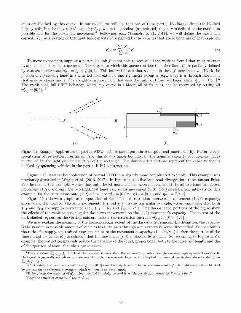
To move to specifics, suppose a particular link j′ is not able to receive all the vehicles from i that want to enterit, and the denied vehicles queue up. The degree to which this queue restricts the other flows f ci,j is partially definedby restriction intervals ηij′,j = [y, z] ⊆ [0, 1]. This interval means that a queue in the i, j′ movement will block theportion of i, j-serving lanes in i with leftmost extent y and rightmost extent z (e.g., if i, j is a through movementthat uses two lanes and i, j′ is a right-turn movement that uses the right of those two lanes, then ηij′,j = [1/2, 1].5The traditional, full FIFO behavior, where any queue in i blocks all of i’s lanes, can be recovered by setting allηij′,j = [0, 1]. 6

(a) (b)

Figure 1: Example application of partial FIFO. (a): A one-input, three-output road junction. (b): Pictorial rep-resentation of restriction intervals on f1,2: this flow is upper-bounded by the nominal capacity of movement (1, 2)multiplied by the lightly-shaded portion of the rectangle. The dark-shaded portions represent the capacity that isblocked by queueing vehicles in the partial FIFO construction.

Figure 1 illustrates the application of partial FIFO in a slightly more complicated example. This example waspreviously discussed in Wright et al. (2016, 2017). In Figure 1(a), a five-lane road diverges into three output links.For the sake of this example, we say that only the leftmost lane can access movement (1, 1), all five lanes can accessmovement (1, 2), and only the two rightmost lanes can access movement (1, 3). So, the restriction intervals for thisexample, for the restrictions onto (1, 2)’s flow, are η1

1,2 = [0, 1/5], η12,2 = [0, 1], and η1

2,3 = [3/5, 1].Figure 1(b) shows a graphical computation of the effects of restriction intervals on movement (1, 2)’s capacity,

given particular flows for the other movements f1,1 and f1,3. In this particular example, we are supposing that bothf1,1 and f1,3 are supply-constrained (i.e., f1,1 = R1 and f1,3 = R3). The dark-shaded portions of the figure showthe effects of the vehicles queueing for these two movements on the (1, 2) movement’s capacity. The extent of thedark-shaded regions on the vertical axis are exactly the restriction intervals η1

j′,2 for j′ ∈ {1, 3}.We now explain the meaning of the horizontal-axis extent of the dark-shaded regions. By definition, the capacity

is the maximum possible amount of vehicles that can pass through a movement in some time period. So, one minusthe ratio of a supply-constrained movement flow to the movement’s capacity (1− fi,j/Fi,j) is then the portion of thetime period for which Fi,j is defined7 that the movement (i, j) is blocked by a queue. So, returning to Figure 1(b)’sexample, the restriction intervals reduce the capacity of the (1, 2), proportional both to the intervals’ length and theof the “portion of time” that their queue exists.

4The constraint∑

c fci,j ≤ Fi,j , that the flow be no more than the maximum possible flow (before any capacity reductions due to

blockages) is generally not given in node model problem statements because it is implied by demand constraint, since by definition∑c β

ci,jS

ci ≤ Fi,j .

5 Continuing this example, we will have ηij,j′ = [0, 1] since the only lane in i that serves movement i, j′ (the right lane) will be blocked

by a queue for the through movement, which will queue on both lanes).6To help keep the meaning of ηi

j′,j clear, we find it helpful to read it as “the restriction interval of j′ onto j for i”7Recall the units of capacity F are veh/time

5

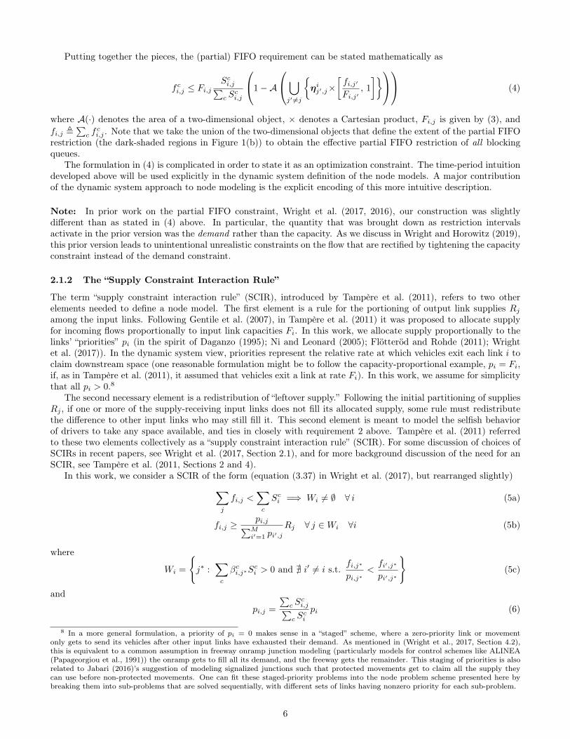
Putting together the pieces, the (partial) FIFO requirement can be stated mathematically as

f ci,j ≤ Fi,jSci,j∑c S

ci,j

1−A

⋃j′ 6=j

{ηij′,j×

[fi,j′

Fi,j′, 1

]} (4)

where A(·) denotes the area of a two-dimensional object, × denotes a Cartesian product, Fi,j is given by (3), andfi,j ,

∑c f

ci,j . Note that we take the union of the two-dimensional objects that define the extent of the partial FIFO

restriction (the dark-shaded regions in Figure 1(b)) to obtain the effective partial FIFO restriction of all blockingqueues.

The formulation in (4) is complicated in order to state it as an optimization constraint. The time-period intuitiondeveloped above will be used explicitly in the dynamic system definition of the node models. A major contributionof the dynamic system approach to node modeling is the explicit encoding of this more intuitive description.

Note: In prior work on the partial FIFO constraint, Wright et al. (2017, 2016), our construction was slightlydifferent than as stated in (4) above. In particular, the quantity that was brought down as restriction intervalsactivate in the prior version was the demand rather than the capacity. As we discuss in Wright and Horowitz (2019),this prior version leads to unintentional unrealistic constraints on the flow that are rectified by tightening the capacityconstraint instead of the demand constraint.

2.1.2 The “Supply Constraint Interaction Rule”

The term “supply constraint interaction rule” (SCIR), introduced by Tampère et al. (2011), refers to two otherelements needed to define a node model. The first element is a rule for the portioning of output link supplies Rjamong the input links. Following Gentile et al. (2007), in Tampère et al. (2011) it was proposed to allocate supplyfor incoming flows proportionally to input link capacities Fi. In this work, we allocate supply proportionally to thelinks’ “priorities” pi (in the spirit of Daganzo (1995); Ni and Leonard (2005); Flötteröd and Rohde (2011); Wrightet al. (2017)). In the dynamic system view, priorities represent the relative rate at which vehicles exit each link i toclaim downstream space (one reasonable formulation might be to follow the capacity-proportional example, pi = Fi,if, as in Tampère et al. (2011), it assumed that vehicles exit a link at rate Fi). In this work, we assume for simplicitythat all pi > 0.8

The second necessary element is a redistribution of “leftover supply.” Following the initial partitioning of suppliesRj , if one or more of the supply-receiving input links does not fill its allocated supply, some rule must redistributethe difference to other input links who may still fill it. This second element is meant to model the selfish behaviorof drivers to take any space available, and ties in closely with requirement 2 above. Tampère et al. (2011) referredto these two elements collectively as a “supply constraint interaction rule” (SCIR). For some discussion of choices ofSCIRs in recent papers, see Wright et al. (2017, Section 2.1), and for more background discussion of the need for anSCIR, see Tampère et al. (2011, Sections 2 and 4).

In this work, we consider a SCIR of the form (equation (3.37) in Wright et al. (2017), but rearranged slightly)∑j

fi,j <∑c

Sci =⇒ Wi 6= ∅ ∀ i (5a)

fi,j ≥pi,j∑Mi′=1 pi′,j

Rj ∀ j ∈Wi ∀i (5b)

where

Wi =

{j∗ :

∑c

βci,j∗Sci > 0 and @ i′ 6= i s.t.

fi,j∗

pi,j∗<fi′,j∗

pi′,j∗

}(5c)

and

pi,j =

∑c S

ci,j∑

c Sci

pi (6)

8 In a more general formulation, a priority of pi = 0 makes sense in a “staged” scheme, where a zero-priority link or movementonly gets to send its vehicles after other input links have exhausted their demand. As mentioned in (Wright et al., 2017, Section 4.2),this is equivalent to a common assumption in freeway onramp junction modeling (particularly models for control schemes like ALINEA(Papageorgiou et al., 1991)) the onramp gets to fill all its demand, and the freeway gets the remainder. This staging of priorities is alsorelated to Jabari (2016)’s suggestion of modeling signalized junctions such that protected movements get to claim all the supply theycan use before non-protected movements. One can fit these staged-priority problems into the node problem scheme presented here bybreaking them into sub-problems that are solved sequentially, with different sets of links having nonzero priority for each sub-problem.

6

is the “oriented priority,” which distributes input links’ priority proportionally to the actual vehicles using thatpriority to claim downstream supply, and fi,j ,

∑c f

ci,j (as before). In the case of capacity-equivalent priorities

pi = Fi, the oriented priority (6) is of course the same as the movement capacity (3).The set Wi denotes all output links that restrict the flow from i.9 The first condition for membership in Wi

(∑c β

ci,j∗S

ci > 0) can be read as “there is some nonzero demand for the movement i, j∗.”

The second condition (@ i′ 6= i s.t. fi,j∗/pi,j∗ < fi′,j∗/pi′,j∗) communicates that there is not some other input link i′that is able to send more (priority-normalized) flow to j∗: that is, that j∗ is either a) restricting to both i and i′ (inwhich case we will have fi,j∗/pi,j∗ = fi′,j∗/pi′,j∗ and j∗ ∈Wi ∩Wi′), or b) that i′’s flow to j∗ was demand-constrained.If the opposite was true (that is, that i′ was able to send more (priority-normalized) flow to j∗ than i), then j∗ wasnot restricting after all (i.e., it was not the link that ran out of supply) and some other output link is what restrictedthe flow from i. More discussion of a physical meaning for the second condition in (5c) will be given later, in Remark2.

Constraint (5a) says that if a link i is not able to fill its demand, then there is at least one output link in Wi thatrestricts i, and that i’s movements claim at least as much as their oriented-priority-proportional allocation of supply.Constraint (5b) captures the reallocation of “leftover” supply, which states that a link i that cannot fulfill all of itsdemand to the links in Wi will continue to send vehicles after links i′ : j /∈ Wi′ have fulfilled their demands to thej ∈Wi.

Remark 1. In (6), we distribute the link priority among the movements proportionate to the demand for eachmovement. Consider the case where the link priority is chosen to be the link capacity, pi = Fi, as we have mentionedas an example, and as suggested by Tampère et al. (2011) (they argued the capacity makes sense as a priority valuebecause vehicles leaving i in a discharging queue will be claiming downstream supply as fast as possible, i.e., at thelink’s capacity). If the capacity is chosen based on a multiple of i’s number of lanes, note that this means that, in(6), each movement will theoretically have available priority proportional to all lanes rather than only the lanes themovement can actually use. This will not be too unrealistic, however, if the demands Si.j are proportional to thenumber of lanes. A more refined SCIR where the oriented priorities pi,j are assigned in a manner aware of both therelative demands between the movements (as in (6)), and the spatial extent of the lane facilities the movements haveavailable (similar to the partial FIFO construction), is an avenue for future work.

2.1.3 Our first-order node model optimization problem

Putting together the pieces, we have

Definition 1 (First-order node model problem).

max

M∑i=1

N∑j=1

C∑c=1

f ci,j

(7a)

subject to:

f ci,j ≥ 0 ∀i, j, c (7b)

f ci,j ≤ Sci,j ∀i, j, c (7c)∑i

∑c

f ci,j ≤ Rj , ∀j (7d)∑i

f ci,j =∑j

f ci,j ∀c (7e)

f ci,j∑c f

ci,j

=βci,jS

ci∑

c βci,jS

ci

∀i, j, c (7f)

(Partial) FIFO and SCIR constraints (in this work, (4) and (5)). (7g)

A solution will have flows that are constrained by at least one of the constraints outlined above. An algorithm tosolve this problem and proof of optimality was given in Wright et al. (2017). Below, we will present a new (simpler)algorithm for the same problem.

9 We defined the set Wi that consisted of the output links restricting i slightly differently in Wright et al. (2017, Definition 3.2)Specifically, there we wrote the second condition as ∃ i′ 6= i s.t. pi′,j∗fi,j∗ ≥ pi,j∗fi′,j∗ . We have inverted the conditional in the presentdefinition so that the definition is still valid for M = 1.

7

2.1.4 Other first-order node model requirements

Note that the list of first-order node requirements presented so far 2.1 (which is the particular node problem ofinterest for the remainder of this work) is not an exhaustive list of all “reasonable” node model requirements. Sincethe statement of the GCNM requirements in Tampère et al. (2011), several authors have proposed extensions ormodifications (as we have in the “partial FIFO” relaxation). Beyond what we have covered here, one of the mostdiscussed are nodal supply constraints. These supply constraints, as their name suggests, describe supply limitationsat the node rather than in one of the output links. They are meant to describe restrictions on traffic that occur dueto interference between flows in the junction (rather than vehicles being blocked in the input link), or the exhaustionof some “shared resource” such as green light time at a signalized intersection. Each movement through the nodemay or may not consume an amount of a node supply proportional to its throughflow.

The node supply constraints in the GCNM framework were originally proposed in Tampère et al. (2011). InCorthout et al. (2012) it was noted that these node supplies may lead to non-unique solutions. Jabari (2016)revisited the node supply constraints (mostly in the context of distribution of green time) to address Corthoutet al. (2012)’s critique of non-uniqueness of solutions and suggested that non-uniqueness can be resolved by properlyaccounting for signal phasing (i.e., which green time allocations are active at the same time).

We do not explicitly include the node supply constraints in the dynamic system node models and resulting solutionalgorithms in this work. The path towards their inclusion in the first- and second-order cases is similar to the partialFIFO construction but notationally cumbersome and somewhat beyond this work’s scope of fusing the GCNM andsecond-order link models.

2.2 Other approaches to road junction modelingIn this section so far, we mostly reviewed node models that pose the node flow problem as an optimization problem(e.g., Tampère et al. (2011); Flötteröd and Rohde (2011); Corthout et al. (2012); Smits et al. (2015); Jabari (2016);Wright et al. (2017) and their references). As mentioned in section 1, this type of problem setup can be interpretedas taking as input the adjacent links’ supply and demand (i.e., their state at the boundary) and producing as outputin- and out-flows (i.e., Neumann boundary conditions) for those links. We will use this framework for the remainderof this work.

Beyond the solving-for-node-flows approach, another class of methods have seen recent development and shouldbe mentioned. As described in Jin (2017), these methods instead resolve the multidimensional Reimann problem bybreaking it into one Riemann problem for each link, then solving each one. Methods of this type tend to explicitly usethe terminology of “Riemann solvers” (e.g., Herty and Rascle (2006); Garavello and Piccoli (2006); Haut and Bastin(2007); Jin (2017)) rather than “node models.” Compared to the node-flow framework, the Riemann-solver frameworkcould be interpreted as setting up and solving a traditional PDE boundary value problem for each link. One work ofparticular interest vis-à-vis the node-flow framework is Jin (2017), which claims to bring these two classes of methodscloser together by incorporating the concepts of supply and demand that the node-flow framework inherited fromthe one-dimensional discretization (Daganzo, 1995).

More related to this work’s concepts, though, are the works of Herty and Rascle (2006); Garavello and Piccoli(2006); Haut and Bastin (2007), which applied this second approach to junctions of roads with second-order dynamics.These “Riemann-solver-framework” methods make a point to not use the the terminology of demand S and supplyR. As we will discuss in more detail in section 4.3, the particular differences of the second-order node flow problemrelative to the first-order problem make the approach (as done in (2.1)) of treating supply and demand as exogenousconstraints not suitable to the second-order case.

The second-order generalization of the node problem, then, needs to take inspiration from the “Riemann-solver-framework” approach of not isolating the node flows from the surrounding links. We will make this statement moreconcrete later.

2.3 Review of first-order node dynamic systemThis section reviews the node dynamic system characterization of node models presented in Wright et al. (2016).This dynamic system is a hybrid system, which means that it contains both continuous and discrete states (alsocalled discrete modes). Here, the continuous states evolve in time according to differential equations, the differentialequations themselves change between discrete states, and the discrete state transitions are activated when conditionson the continuous states are satisfied.

Definition 2 (Generic first-order node hybrid system).

8

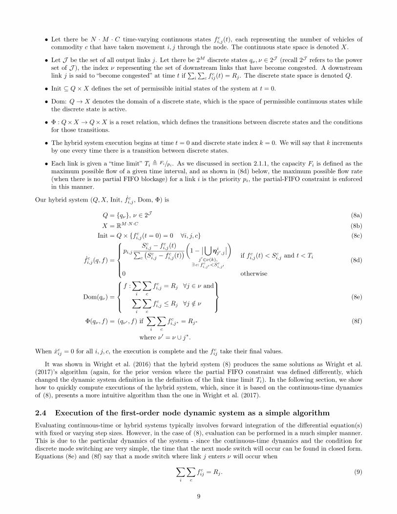
• Let there be N · M · C time-varying continuous states f ci,j(t), each representing the number of vehicles ofcommodity c that have taken movement i, j through the node. The continuous state space is denoted X.

• Let J be the set of all output links j. Let there be 2M discrete states qν , ν ∈ 2J (recall 2J refers to the powerset of J ), the index ν representing the set of downstream links that have become congested. A downstreamlink j is said to “become congested” at time t if

∑i

∑c f

cij(t) = Rj . The discrete state space is denoted Q.

• Init ⊆ Q×X defines the set of permissible initial states of the system at t = 0.

• Dom: Q→ X denotes the domain of a discrete state, which is the space of permissible continuous states whilethe discrete state is active.

• Φ : Q×X → Q×X is a reset relation, which defines the transitions between discrete states and the conditionsfor those transitions.

• The hybrid system execution begins at time t = 0 and discrete state index k = 0. We will say that k incrementsby one every time there is a transition between discrete states.

• Each link is given a “time limit” Ti , Fi/pi. As we discussed in section 2.1.1, the capacity Fi is defined as themaximum possible flow of a given time interval, and as shown in (8d) below, the maximum possible flow rate(when there is no partial FIFO blockage) for a link i is the priority pi, the partial-FIFO constraint is enforcedin this manner.

Our hybrid system (Q,X, Init, f ci,j , Dom, Φ) is

Q = {qν}, ν ∈ 2J (8a)

X = RM ·N ·C (8b)Init = Q× {f ci,j(t = 0) = 0 ∀i, j, c} (8c)

f ci,j(q, f) =

pi,j

Sci,j − f ci,j(t)∑c

(Sci,j − f ci,j(t)

)(1−∣∣⋃j′∈ν(k),

∃ c: fci,j′<S

ci,j′

ηij′,j∣∣)

if f ci,j(t) < Sci,j and t < Ti

0 otherwise

(8d)

Dom(qν) =

f :∑i

∑c

f ci,j = Rj ∀j ∈ ν and∑i

∑c

f ci,j ≤ Rj ∀j /∈ ν

(8e)

Φ(qν , f) = (qν′ , f) if∑i

∑c

f ci,j∗ = Rj∗

where ν′ = ν ∪ j∗.

(8f)

When xcij = 0 for all i, j, c, the execution is complete and the f cij take their final values.

It was shown in Wright et al. (2016) that the hybrid system (8) produces the same solutions as Wright et al.(2017)’s algorithm (again, for the prior version where the partial FIFO constraint was defined differently, whichchanged the dynamic system definition in the definition of the link time limit Ti). In the following section, we showhow to quickly compute executions of the hybrid system, which, since it is based on the continuous-time dynamicsof (8), presents a more intuitive algorithm than the one in Wright et al. (2017).

2.4 Execution of the first-order node dynamic system as a simple algorithmEvaluating continuous-time or hybrid systems typically involves forward integration of the differential equation(s)with fixed or varying step sizes. However, in the case of (8), evaluation can be performed in a much simpler manner.This is due to the particular dynamics of the system - since the continuous-time dynamics and the condition fordiscrete mode switching are very simple, the time that the next mode switch will occur can be found in closed form.Equations (8e) and (8f) say that a mode switch where link j enters ν will occur when∑

i

∑c

f cij = Rj . (9)

9

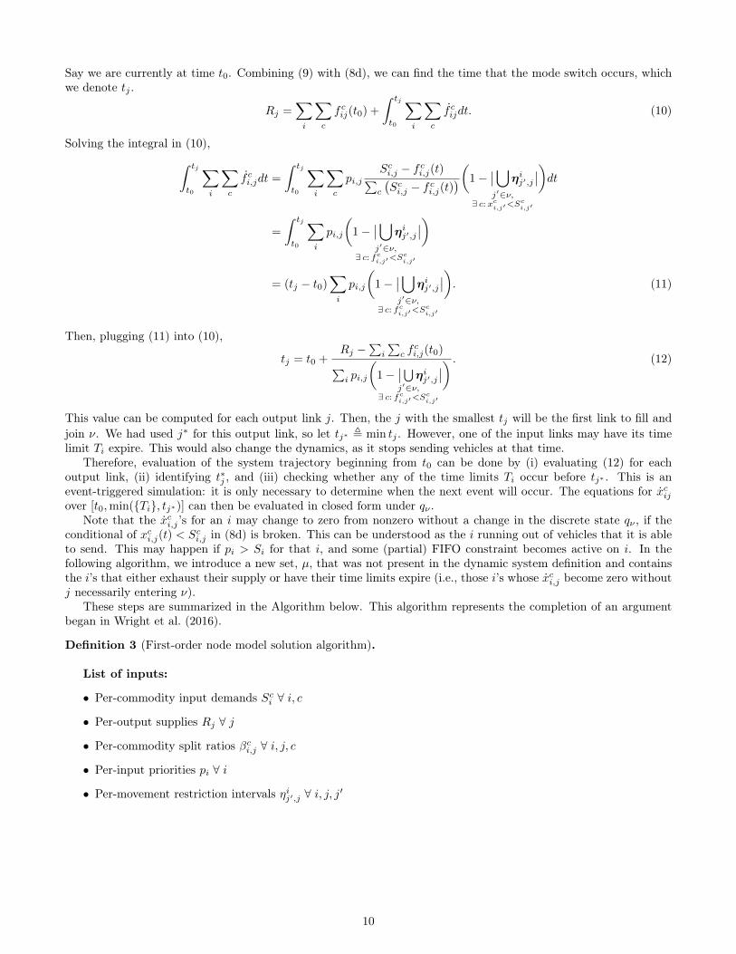
Say we are currently at time t0. Combining (9) with (8d), we can find the time that the mode switch occurs, whichwe denote tj .

Rj =∑i

∑c

f cij(t0) +

∫ tj

t0

∑i

∑c

f cijdt. (10)

Solving the integral in (10),∫ tj

t0

∑i

∑c

f ci,jdt =

∫ tj

t0

∑i

∑c

pi,jSci,j − f ci,j(t)∑c

(Sci,j − f ci,j(t)

)(1−∣∣⋃j′∈ν,

∃ c: xci,j′<S

ci,j′

ηij′,j∣∣)dt

=

∫ tj

t0

∑i

pi,j

(1−

∣∣⋃j′∈ν,

∃ c: fci,j′<S

ci,j′

ηij′,j∣∣)

= (tj − t0)∑i

pi,j

(1−

∣∣⋃j′∈ν,

∃ c: fci,j′<S

ci,j′

ηij′,j∣∣). (11)

Then, plugging (11) into (10),

tj = t0 +Rj −

∑i

∑c f

ci,j(t0)∑

i pi,j

(1−

∣∣⋃j′∈ν,

∃ c: fci,j′<S

ci,j′

ηij′,j∣∣) . (12)

This value can be computed for each output link j. Then, the j with the smallest tj will be the first link to fill andjoin ν. We had used j∗ for this output link, so let tj∗ , min tj . However, one of the input links may have its timelimit Ti expire. This would also change the dynamics, as it stops sending vehicles at that time.

Therefore, evaluation of the system trajectory beginning from t0 can be done by (i) evaluating (12) for eachoutput link, (ii) identifying t∗j , and (iii) checking whether any of the time limits Ti occur before tj∗ . This is anevent-triggered simulation: it is only necessary to determine when the next event will occur. The equations for xcijover [t0,min({Ti}, tj∗)] can then be evaluated in closed form under qν .

Note that the xci,j ’s for an i may change to zero from nonzero without a change in the discrete state qν , if theconditional of xci,j(t) < Sci,j in (8d) is broken. This can be understood as the i running out of vehicles that it is ableto send. This may happen if pi > Si for that i, and some (partial) FIFO constraint becomes active on i. In thefollowing algorithm, we introduce a new set, µ, that was not present in the dynamic system definition and containsthe i’s that either exhaust their supply or have their time limits expire (i.e., those i’s whose xci,j become zero withoutj necessarily entering ν).

These steps are summarized in the Algorithm below. This algorithm represents the completion of an argumentbegan in Wright et al. (2016).

Definition 3 (First-order node model solution algorithm).

List of inputs:

• Per-commodity input demands Sci ∀ i, c

• Per-output supplies Rj ∀ j

• Per-commodity split ratios βci,j ∀ i, j, c

• Per-input priorities pi ∀ i

• Per-movement restriction intervals ηij′,j ∀ i, j, j′

10

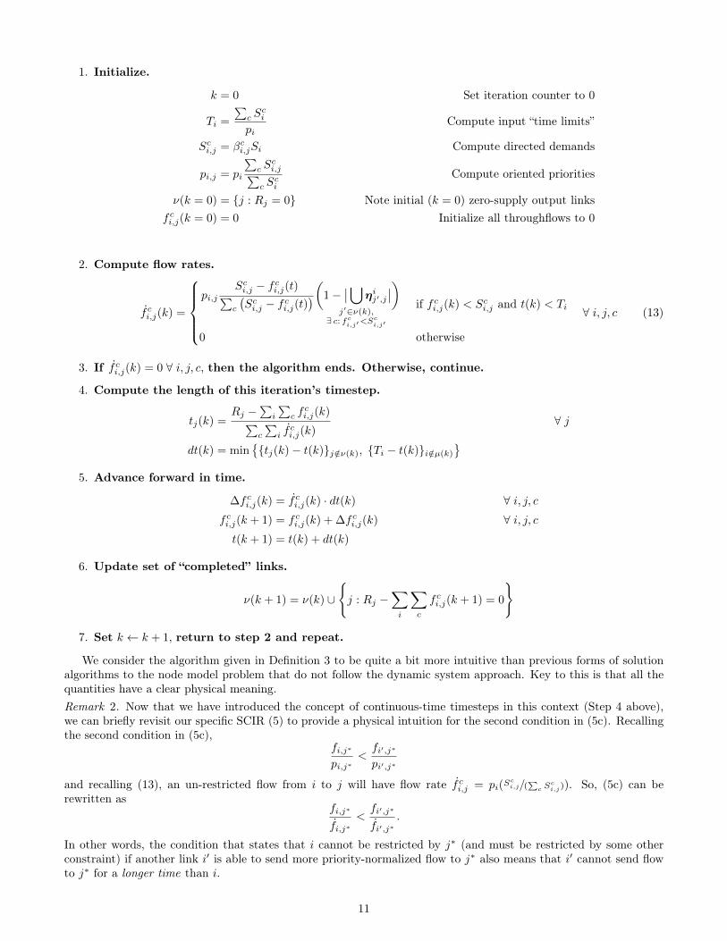
1. Initialize.

k = 0 Set iteration counter to 0

Ti =

∑c S

ci

piCompute input “time limits”

Sci,j = βci,jSi Compute directed demands

pi,j = pi

∑c S

ci,j∑

c Sci

Compute oriented priorities

ν(k = 0) = {j : Rj = 0} Note initial (k = 0) zero-supply output linksf ci,j(k = 0) = 0 Initialize all throughflows to 0

2. Compute flow rates.

f ci,j(k) =

pi,j

Sci,j − f ci,j(t)∑c

(Sci,j − f ci,j(t)

)(1−∣∣⋃j′∈ν(k),

∃ c: fci,j′<S

ci,j′

ηij′,j∣∣)

if f ci,j(k) < Sci,j and t(k) < Ti

0 otherwise

∀ i, j, c (13)

3. If f ci,j(k) = 0 ∀ i, j, c, then the algorithm ends. Otherwise, continue.

4. Compute the length of this iteration’s timestep.

tj(k) =Rj −

∑i

∑c f

ci,j(k)∑

c

∑i f

ci,j(k)

∀ j

dt(k) = min{{tj(k)− t(k)}j /∈ν(k), {Ti − t(k)}i/∈µ(k)

}5. Advance forward in time.

∆f ci,j(k) = f ci,j(k) · dt(k) ∀ i, j, cf ci,j(k + 1) = f ci,j(k) + ∆f ci,j(k) ∀ i, j, ct(k + 1) = t(k) + dt(k)

6. Update set of “completed” links.

ν(k + 1) = ν(k) ∪

{j : Rj −

∑i

∑c

f ci,j(k + 1) = 0

}

7. Set k ← k + 1, return to step 2 and repeat.

We consider the algorithm given in Definition 3 to be quite a bit more intuitive than previous forms of solutionalgorithms to the node model problem that do not follow the dynamic system approach. Key to this is that all thequantities have a clear physical meaning.Remark 2. Now that we have introduced the concept of continuous-time timesteps in this context (Step 4 above),we can briefly revisit our specific SCIR (5) to provide a physical intuition for the second condition in (5c). Recallingthe second condition in (5c),

fi,j∗

pi,j∗<fi′,j∗

pi′,j∗

and recalling (13), an un-restricted flow from i to j will have flow rate f ci,j = pi(Sci,j/(

∑c S

ci,j)). So, (5c) can be

rewritten asfi,j∗

fi,j∗<fi′,j∗

fi′,j∗.

In other words, the condition that states that i cannot be restricted by j∗ (and must be restricted by some otherconstraint) if another link i′ is able to send more priority-normalized flow to j∗ also means that i′ cannot send flowto j∗ for a longer time than i.

11

3 Review of second-order flow modeling

3.1 IntroductionThe formulation of the GSOM seen in (2) has been called the “advective form” (Fan et al., 2017). In this form, theproperty w is advected with the vehicles at speed v. That is, it is constant along trajectories. This form makes thestatement that the property w is a property of vehicles. This understanding is useful because it communicates howoftentimes the forms of w and V (ρ, w) are constructed such that they model some microscopic, per-driver behavior.

For example, it has been shown (Zhang, 2002; Aw et al., 2002) that the original ARZ model can be characterizedas a “coarsening” to a macro-scale of simple car-following models of the form

xn(t) =xn−1(t)− xn(t)

τ(sn(t))

sn(t) = xn−1(t)− xn(t)

(14)

where xn(t), xn(t) and xn(t) are the position, velocity, and acceleration of the nth car, respectively, and τ(sn(t)) is adriver’s response time, which is stated to be a function of their distance from the car ahead of them. This equivalenceis shown by setting the velocity function as V (ρ, w) = Veq(ρ)+(w−Veq(0)), with Veq defined as an equilibrium velocityfunction. The advected property w is thought of as the driver’s distance from equilibrium velocity (Aw et al., 2002;Zhang, 2002; Lebacque et al., 2007b).10

Each individual vehicle can be thought of as having its own w, and the macroscopic w in the PDE form (2b) thenequals the average of the vehicle w’s. To apply a discretization to this PDE formulation, it is useful to consider thetotal property ρw, and rewrite (2) in “conservative form” (Lebacque et al., 2007b; Fan et al., 2017),

∂ρ

∂t+∂(ρv)

∂z= 0

∂(ρw)

∂t+∂(ρwv)

∂z= 0

where v = V (ρ, w).

(15)

We will review the relevant finite-volume discretization using the Godunov scheme of (15) (Lebacque et al., 2007b)in the next section. For a deeper analysis on the physical properties of (15), see, e.g., Lebacque et al. (2007b).

We make one note on constraints imposed on the form of v(ρ, w) in (15). It has been stated (Lebacque et al.,2007b, (19)) that, to apply the Godunov discretization to (15), one is restricted to choices of V (ρ, w) for which thereis a unique ρ for every (v, w), v 6= 0 and a unique w for every (v, ρ), v 6= 0. That is, V (ρ, w) must be invertible inboth its arguments for nonzero values of velocity.

Remark 3. In this work, the only further assumption we make on the form of V (·) is that v = 0 occurs only for aspecific maximum value of density, ρmax, and that at that density, V (ρmax, w) = 0 for any value of w. Further, weassume that the converse is not true: that no value of w exists that induces v = 0 for ρ < ρmax.

3.2 Godunov discretization of the GSOMThe Godunov discretization of the first-order (LWR) model (1), first introduced as the Cell Transmission Model(Daganzo, 1994) is well-known. The Godunov scheme discretizes a conservation law into small finite-volume cells.Each cell has a constant value of the conserved quantity, and inter-cell fluxes are computed by solving Riemannproblems at each boundary. The solution to each Riemann problem is a flux that describes the amount of theconserved quantity that is sent from the upstream cell to the downstream cell. The Godunov scheme is a first-ordermethod, so it is useful for simulating solutions to PDEs with no second- or higher-order derivatives like the LWRformulation. In the CTM, the Godunov flux problem is stated in the form of the demand and supply functions.

Since (15) is also a conservation law with no second- or higher-order derivatives, the Godunov scheme is applicableas well (Lebacque et al., 2007b). However, due to the second PDE for ρw, an intermediate state arises in the Riemannproblem and its solution (Aw and Rascle, 2000; Zhang, 2002; Lebacque et al., 2007a,b). This intermediate state hasnot always had a clear physical meaning, and this lack of clarity likely inhibited the extension of the Godunovdiscretization to the multi-input multi-output node case. In our following outline of the discretized one-input one-output flow problem, we make use of a physical interpretation of the intermediate state due to Fan et al. (2017).

10 Of potential interest to the reader may be the analysis of Aw et al. (2002), where a particular form of τ(·) is shown to be equivalentto a form of (2) with an inhomogeneous (2b): that is, with w allowed to be created or destroyed. We do not consider inhomogeneousforms of (2) in this work.

12

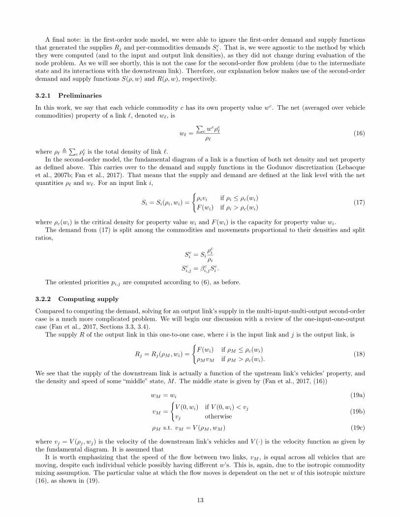
A final note: in the first-order node model, we were able to ignore the first-order demand and supply functionsthat generated the supplies Rj and per-commodities demands Sci . That is, we were agnostic to the method by whichthey were computed (and to the input and output link densities), as they did not change during evaluation of thenode problem. As we will see shortly, this is not the case for the second-order flow problem (due to the intermediatestate and its interactions with the downstream link). Therefore, our explanation below makes use of the second-orderdemand and supply functions S(ρ, w) and R(ρ, w), respectively.

3.2.1 Preliminaries

In this work, we say that each vehicle commodity c has its own property value wc. The net (averaged over vehiclecommodities) property of a link `, denoted w`, is

w` =

∑c w

cρc`ρ`

(16)

where ρ` ,∑c ρ

c` is the total density of link `.

In the second-order model, the fundamental diagram of a link is a function of both net density and net propertyas defined above. This carries over to the demand and supply functions in the Godunov discretization (Lebacqueet al., 2007b; Fan et al., 2017). That means that the supply and demand are defined at the link level with the netquantities ρ` and w`. For an input link i,

Si = Si(ρi, wi) =

{ρivi if ρi ≤ ρc(wi)F (wi) if ρi > ρc(wi)

(17)

where ρc(wi) is the critical density for property value wi and F (wi) is the capacity for property value wi.The demand from (17) is split among the commodities and movements proportional to their densities and split

ratios,

Sci = Siρciρi

Sci,j = βci,jSci .

The oriented priorities pi,j are computed according to (6), as before.

3.2.2 Computing supply

Compared to computing the demand, solving for an output link’s supply in the multi-input-multi-output second-ordercase is a much more complicated problem. We will begin our discussion with a review of the one-input-one-outputcase (Fan et al., 2017, Sections 3.3, 3.4).

The supply R of the output link in this one-to-one case, where i is the input link and j is the output link, is

Rj = Rj(ρM , wi) =

{F (wi) if ρM ≤ ρc(wi)ρMvM if ρM > ρc(wi).

(18)

We see that the supply of the downstream link is actually a function of the upstream link’s vehicles’ property, andthe density and speed of some “middle” state, M . The middle state is given by (Fan et al., 2017, (16))

wM = wi (19a)

vM =

{V (0, wi) if V (0, wi) < vj

vj otherwise(19b)

ρM s.t. vM = V (ρM , wM ) (19c)

where vj = V (ρj , wj) is the velocity of the downstream link’s vehicles and V (·) is the velocity function as given bythe fundamental diagram. It is assumed that

It is worth emphasizing that the speed of the flow between two links, vM , is equal across all vehicles that aremoving, despite each individual vehicle possibly having different w’s. This is, again, due to the isotropic commoditymixing assumption. The particular value at which the flow moves is dependent on the net w of this isotropic mixture(16), as shown in (19).

13

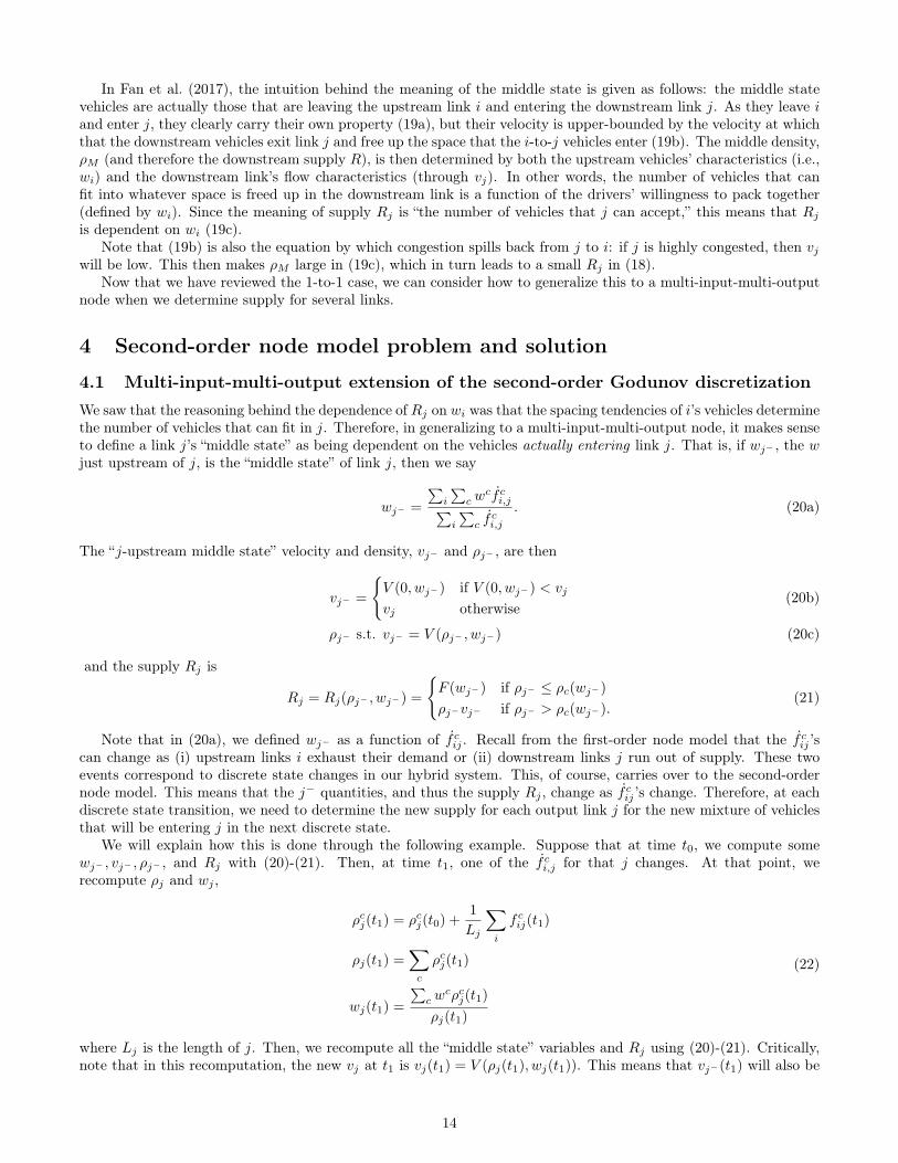
In Fan et al. (2017), the intuition behind the meaning of the middle state is given as follows: the middle statevehicles are actually those that are leaving the upstream link i and entering the downstream link j. As they leave iand enter j, they clearly carry their own property (19a), but their velocity is upper-bounded by the velocity at whichthat the downstream vehicles exit link j and free up the space that the i-to-j vehicles enter (19b). The middle density,ρM (and therefore the downstream supply R), is then determined by both the upstream vehicles’ characteristics (i.e.,wi) and the downstream link’s flow characteristics (through vj). In other words, the number of vehicles that canfit into whatever space is freed up in the downstream link is a function of the drivers’ willingness to pack together(defined by wi). Since the meaning of supply Rj is “the number of vehicles that j can accept,” this means that Rjis dependent on wi (19c).

Note that (19b) is also the equation by which congestion spills back from j to i: if j is highly congested, then vjwill be low. This then makes ρM large in (19c), which in turn leads to a small Rj in (18).

Now that we have reviewed the 1-to-1 case, we can consider how to generalize this to a multi-input-multi-outputnode when we determine supply for several links.

4 Second-order node model problem and solution

4.1 Multi-input-multi-output extension of the second-order Godunov discretizationWe saw that the reasoning behind the dependence of Rj on wi was that the spacing tendencies of i’s vehicles determinethe number of vehicles that can fit in j. Therefore, in generalizing to a multi-input-multi-output node, it makes senseto define a link j’s “middle state” as being dependent on the vehicles actually entering link j. That is, if wj− , the wjust upstream of j, is the “middle state” of link j, then we say

wj− =

∑i

∑c w

cf ci,j∑i

∑c f

ci,j

. (20a)

The “j-upstream middle state” velocity and density, vj− and ρj− , are then

vj− =

{V (0, wj−) if V (0, wj−) < vj

vj otherwise(20b)

ρj− s.t. vj− = V (ρj− , wj−) (20c)

and the supply Rj is

Rj = Rj(ρj− , wj−) =

{F (wj−) if ρj− ≤ ρc(wj−)

ρj−vj− if ρj− > ρc(wj−).(21)

Note that in (20a), we defined wj− as a function of f cij . Recall from the first-order node model that the f cij ’scan change as (i) upstream links i exhaust their demand or (ii) downstream links j run out of supply. These twoevents correspond to discrete state changes in our hybrid system. This, of course, carries over to the second-ordernode model. This means that the j− quantities, and thus the supply Rj , change as f cij ’s change. Therefore, at eachdiscrete state transition, we need to determine the new supply for each output link j for the new mixture of vehiclesthat will be entering j in the next discrete state.

We will explain how this is done through the following example. Suppose that at time t0, we compute somewj− , vj− , ρj− , and Rj with (20)-(21). Then, at time t1, one of the f ci,j for that j changes. At that point, werecompute ρj and wj ,

ρcj(t1) = ρcj(t0) +1

Lj

∑i

f cij(t1)

ρj(t1) =∑c

ρcj(t1)

wj(t1) =

∑c w

cρcj(t1)

ρj(t1)

(22)

where Lj is the length of j. Then, we recompute all the “middle state” variables and Rj using (20)-(21). Critically,note that in this recomputation, the new vj at t1 is vj(t1) = V (ρj(t1), wj(t1)). This means that vj−(t1) will also be

14

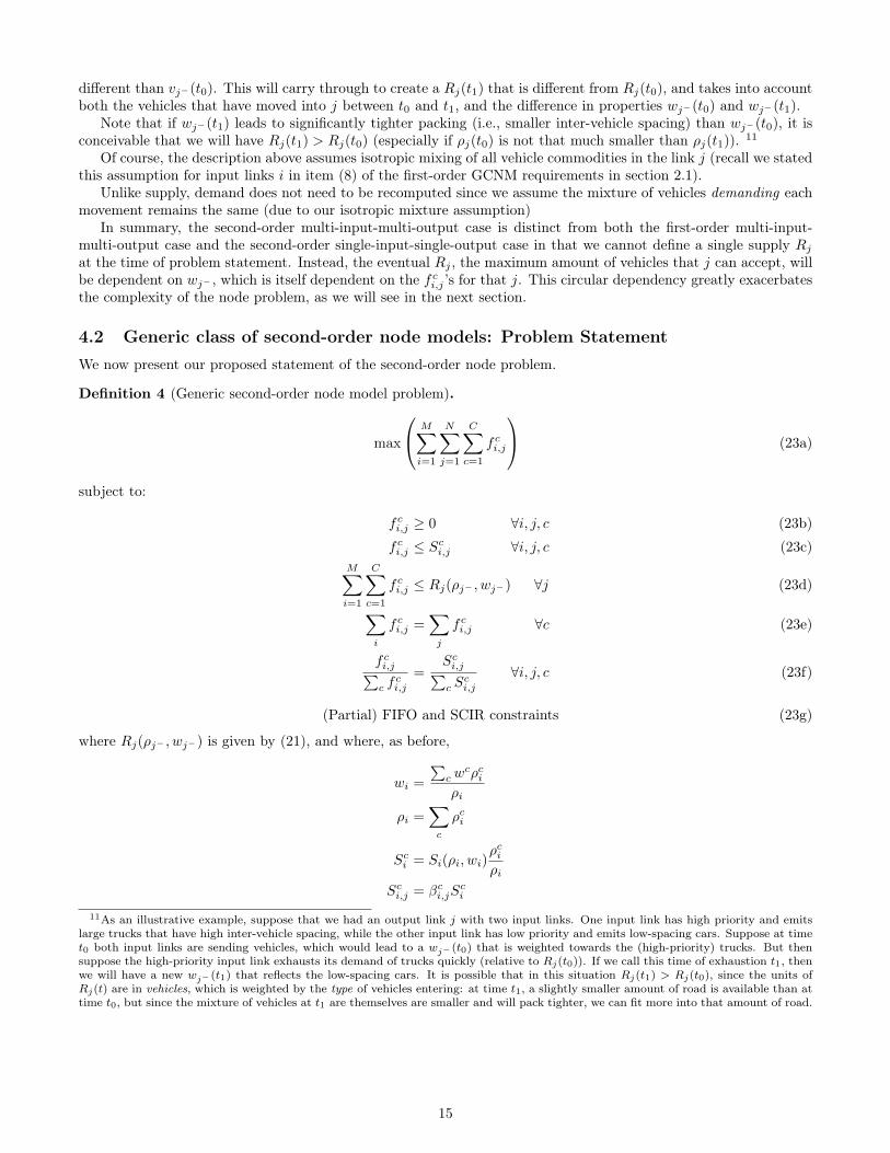
different than vj−(t0). This will carry through to create a Rj(t1) that is different from Rj(t0), and takes into accountboth the vehicles that have moved into j between t0 and t1, and the difference in properties wj−(t0) and wj−(t1).

Note that if wj−(t1) leads to significantly tighter packing (i.e., smaller inter-vehicle spacing) than wj−(t0), it isconceivable that we will have Rj(t1) > Rj(t0) (especially if ρj(t0) is not that much smaller than ρj(t1)). 11

Of course, the description above assumes isotropic mixing of all vehicle commodities in the link j (recall we statedthis assumption for input links i in item (8) of the first-order GCNM requirements in section 2.1).

Unlike supply, demand does not need to be recomputed since we assume the mixture of vehicles demanding eachmovement remains the same (due to our isotropic mixture assumption)

In summary, the second-order multi-input-multi-output case is distinct from both the first-order multi-input-multi-output case and the second-order single-input-single-output case in that we cannot define a single supply Rjat the time of problem statement. Instead, the eventual Rj , the maximum amount of vehicles that j can accept, willbe dependent on wj− , which is itself dependent on the f ci,j ’s for that j. This circular dependency greatly exacerbatesthe complexity of the node problem, as we will see in the next section.

4.2 Generic class of second-order node models: Problem StatementWe now present our proposed statement of the second-order node problem.

Definition 4 (Generic second-order node model problem).

max

M∑i=1

N∑j=1

C∑c=1

f ci,j

(23a)

subject to:

f ci,j ≥ 0 ∀i, j, c (23b)

f ci,j ≤ Sci,j ∀i, j, c (23c)M∑i=1

C∑c=1

f ci,j ≤ Rj(ρj− , wj−) ∀j (23d)∑i

f ci,j =∑j

f ci,j ∀c (23e)

f ci,j∑c f

ci,j

=Sci,j∑c S

ci,j

∀i, j, c (23f)

(Partial) FIFO and SCIR constraints (23g)

where Rj(ρj− , wj−) is given by (21), and where, as before,

wi =

∑c w

cρciρi

ρi =∑c

ρci

Sci = Si(ρi, wi)ρciρi

Sci,j = βci,jSci

11As an illustrative example, suppose that we had an output link j with two input links. One input link has high priority and emitslarge trucks that have high inter-vehicle spacing, while the other input link has low priority and emits low-spacing cars. Suppose at timet0 both input links are sending vehicles, which would lead to a wj− (t0) that is weighted towards the (high-priority) trucks. But thensuppose the high-priority input link exhausts its demand of trucks quickly (relative to Rj(t0)). If we call this time of exhaustion t1, thenwe will have a new wj− (t1) that reflects the low-spacing cars. It is possible that in this situation Rj(t1) > Rj(t0), since the units ofRj(t) are in vehicles, which is weighted by the type of vehicles entering: at time t1, a slightly smaller amount of road is available than attime t0, but since the mixture of vehicles at t1 are themselves are smaller and will pack tighter, we can fit more into that amount of road.

15

and where the “j-upstream middle state” is a modified version of (20) in that (20a) is integrated over time,

wj− =

∑i

∑c w

cf ci,j∑i

∑c f

ci,j

∀j (23h)

vj− =

{V (0, wj−) if V (0, wj−) < vj

vj otherwise∀j (23i)

ρj− s.t. vj− = V (ρj− , wj−) ∀j (23j)

Remark 4. Conservation of w is enforced through (23h).

Remark 5. Examining (23f) and the definition of Sci,j , we see that, again, following the isotropic mixing assumption,all vehicles in a flow (i.j) are equally impeded if the movement’s downstream link j is congested, even if individualcommodities have drastically different w’s. The way that w’s affect the flow (i, j) is through their contribution tothe “j − upstream” state in (23h). That is, in the macroscopic model, we do not model effects of w variability (e.g.,in-movement overtaking) within an (i, j) flow.

The functions Si(ρ, w) and Rj(ρ, w) are the particular demand and supply functions for those links.In section 4.1, we noted that a circular dependency exists between the supplies Rj and the flows f ci,j . The form

that this dependency takes in the problem statement above is in (23d) and (23h)-(23j). Plugging the definitionsof wj− and ρj− into (23d), we see that the f ci,j ’s are constrained by another quantity that is a nonlinear function(through the fundamental diagram) of f ci,j . We conjecture that this makes the optimization problem (23) nonconvexfor general fundamental diagrams. In addition, this construction makes clear that the downstream supplies in thesecond-order multi-input-multi-output cannot be stated a priori. We discuss some implications of this fact in thenext section.

4.3 Generic Class of Second-order Node Models problem: DiscussionIn the first-order case as reviewed in section 2, the node problem is usually stated in terms of supply and demandinstead of the actual conserved quantity ρ. This is done to separate the node and link models from each other: oncethe link model(s) have been used to produce demand and supply, the node model problem is decoupled. In addition,it is possibly more intuitive to think of flows as a function of supplies and demands (which have the same units asflow), rather than as a function of density discontinuities (in other words, we can abstract away the Riemann problemin the first-order case).

However, we have seen that a construction that abstracts away the link states in the node model is not possiblefor the general second-order case. This is because the downstream supplies are dependent on the upstream wi’s ofthe flows that enter each downstream link.12

In our view, this difficulty in applying the extremely-useful “supply-and-demand-based” node problem setup tothe second-order setting has likely hampered efforts towards defining and solving this extension. Compare, forexample, the several papers that have made progress towards the second-order junction problem in a “traditional”PDE, non-Godunov-based approach (e.g., (Herty and Rascle, 2006; Garavello and Piccoli, 2006; Haut and Bastin,2007)), that explicitly do not decouple the junction flow problem from the PDE model on links via the Godunovsupply and demand functions.

In sum, when discussing the node model problem in the second order, one should take care to not think of adownstream link’s “supply” in an unqualified sense. Rather, the downstream link has a supply Rj for each pair(ρj− , wj−) (23d), one of which is compatible with the solution of the optimization problem.

However, our dynamic system construction for the node model solution generalizes to this case rather well. Thisis described next.

4.4 Dynamic system definitionSince we have defined the downstream supplies Rj as depending on the net property of the flows actually enteringlink j (20)–(21), and the final Rj of the node problem solution (23) as depending on the integrated-over-time flowsinto link j (23h), all we have to do to generalize the first-order node model dynamic construction to the second-ordercase is add a recomputation of the downstream supplies Rj whenever we also recompute the xci,j ’s due to a discretemode switch.

12In the case of the one-to-one junction described in section 3.2, we could abstract away the supplies’ dependency on the upstream wi

and find an a priori statement of the downstream Rj , since there was only one upstream wi to influence the supply in (20a)

16

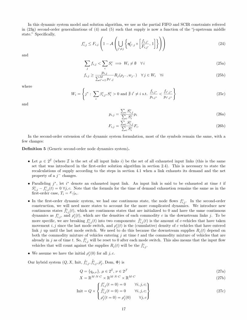
In this dynamic system model and solution algorithm, we use as the partial FIFO and SCIR constraints referredin (23g) second-order generalizations of (4) and (5) such that supply is now a function of the “j-upstream middlestate.” Specifically,

f ci,j ≤ Fi,j

1−A

⋃j′ 6=j

{ηij′,j×

[fi,j′

Fi,j′, 1

]} (24)

and ∑j

fi,j <∑c

Sci =⇒ Wi 6= ∅ ∀ i (25a)

fi,j ≥pi,j∑Mi′=1 pi′,j

Rj(ρj− , wj−) ∀ j ∈Wi ∀i (25b)

where

Wi =

{j∗ :

∑c

βci,j∗Sci > 0 and @ i′ 6= i s.t.

fi,j∗

pi,j∗<fi′,j∗

pi′,j∗

}(25c)

and

pi,j =

∑c S

ci,j∑

c Sci

pi (26a)

Fi,j =

∑c S

ci,j∑

c Sci

Fi. (26b)

In the second-order extension of the dynamic system formulation, most of the symbols remain the same, with afew changes:

Definition 5 (Generic second-order node dynamics system).

• Let µ ∈ 2I (where I is the set of all input links i) be the set of all exhausted input links (this is the sameset that was introduced in the first-order solution algorithm in section 2.4). This is necessary to state therecalculations of supply according to the steps in section 4.1 when a link exhausts its demand and the netproperty of a j− changes.

• Paralleling j∗, let i∗ denote an exhausted input link. An input link is said to be exhausted at time t ifSci,j − f ci,j(t) = 0 ∀j, c. Note that the formula for the time of demand exhaustion remains the same as in thefirst-order case, Ti = Fi/pi.

• In the first-order dynamic system, we had one continuous state, the node flows f ci,j . In the second-orderconstruction, we will need more states to account for the more complicated dynamics. We introduce newcontinuous states f ci,j(t), which are continuous states that are initialized to 0 and have the same continuousdynamics as f ci,j , and ρcj(t), which are the densities of each commodity c in the downstream links j. To bemore specific, we are breaking f ci,j(t) into two components: f ci,j(t) is the amount of c-vehicles that have takenmovement i, j since the last mode switch, and ρcj(t) is the (cumulative) density of c vehicles that have enteredlink j up until the last mode switch. We need to do this because the downstream supplies Rj(t) depend onboth the commodity mixture of vehicles entering j at time t and the commodity mixture of vehicles that arealready in j as of time t. So, f ci,j will be reset to 0 after each mode switch. This also means that the input flowvehicles that will count against the supplies Rj(t) will be the f ci,j .

• We assume we have the initial ρcj(0) for all j, c.

Our hybrid system (Q,X, Init, f ci,j ,˙f ci,j , ρ

cj , Dom, Φ) is

Q = {qµ,ν}, µ ∈ 2I , ν ∈ 2J (27a)

X = RM ·N ·C × RM ·N ·C × RM ·C (27b)

Init = Q×

f ci,j(t = 0) = 0 ∀i, j, c;f ci,j(t = 0) = 0 ∀i, j, c;ρcj(t = 0) = ρcj(0) ∀j, c

(27c)

17

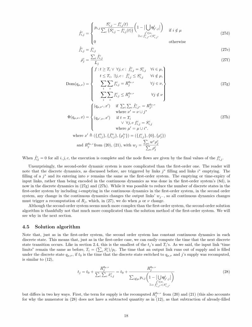
f ci,j =

pi,j

Sci,j − f ci,j(t)∑c

(Sci,j − f ci,j(t)

)(1−∣∣⋃j′∈ν,

∃ c: fci,j′<S

ci,j′

ηij′,j∣∣)

if i /∈ µ

0 otherwise

(27d)

˙f ci,j = f ci,j (27e)

ρcj =

∑i f

ci,j

Lj(27f)

Dom(qµ,ν) =

f : t ≥ Ti ∨ ∀j, c : f ci,j = Sci,j ∀i ∈ µ,t ≤ Ti, ∃j, c : f ci,j ≤ Sci,j ∀i /∈ µ,∑i

∑c

f ci,j = Rqµ,νj ∀j ∈ ν,∑

i

∑c

f ci,j ≤ Rqµ,νj ∀j /∈ ν

(27g)

Φ(qµ,ν , x) =

(qµ,ν′ , x′) if

∑i

∑c f

ci,j∗ = R

qµ,νj∗

where ν′ = ν ∪ j∗

(qµ′,ν , x′) if t = Ti

∨ ∀j, c f ci,j = Sci,jwhere µ′ = µ ∪ i∗.

(27h)

where x′ , ({f ′ci,j}, {f ′ci,j}, {ρ′cj }) = ({f ci,j}, {0}, {ρcj})

and Rqµ,νj from (20), (21), with wj =

∑c w

cρcj∑c ρ

cj

When f cij = 0 for all i, j, c, the execution is complete and the node flows are given by the final values of the f ci,j .

Unsurprisingly, the second-order dynamic system is more complicated than the first-order one. The reader willnote that the discrete dynamics, as discussed before, are triggered by links j∗ filling and links i∗ emptying. Thefilling of a j∗ and its entering into ν remains the same as the first-order system. The emptying or time-expiry ofinput links, rather than being encoded in the continuous dynamics as was done in the first-order system’s (8d), isnow in the discrete dynamics in (27g) and (27h). While it was possible to reduce the number of discrete states in thefirst-order system by including i-emptying in the continuous dynamics in the first-order system, in the second ordersystem, any change in the continuous dynamics changes the output links’ wj− , so all continuous dynamics changesmust trigger a recomputation of Rj , which, in (27), we do when µ or ν change.

Although the second-order system seems much more complex than the first-order system, the second-order solutionalgorithm is thankfully not that much more complicated than the solution method of the first-order system. We willsee why in the next section.

4.5 Solution algorithmNote that, just as in the first-order system, the second order system has constant continuous dynamics in eachdiscrete state. This means that, just as in the first-order case, we can easily compute the time that the next discretestate transition occurs. Like in section 2.4, this is the smallest of the tj ’s and Ti’s. As we said, the input link “timelimits” remain the same as before, Ti = (

∑c S

ci )/pi. The time that an output link runs out of supply and is filled

under the discrete state qµ,ν , if t0 is the time that the discrete state switched to qµ,ν and j’s supply was recomputed,is similar to (12),

tj = t0 +Rqµ,νj∑

i

∑c x

ci,j

= t0 +Rqµ,νj∑

i/∈µ pi,j

(1−

∣∣⋃j′∈ν,

∃ c: fci,j′<S

ci,j′

ηij′,j∣∣) (28)

but differs in two key ways. First, the term for supply is the recomputed Rqµ,νj from (20) and (21) (this also accountsfor why the numerator in (28) does not have a subtracted quantity as in (12), as that subtraction of already-filled

18

supply is accounted for in the recomputed supply). Second is that the denominator is summed over i /∈ µ ratherthan all i, as the set µ is not in the definition of the first-order dynamic system as stated in section 2.3.

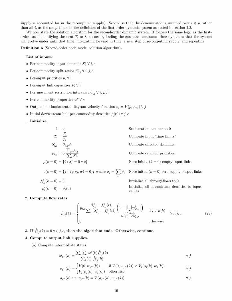
We now state the solution algorithm for the second-order dynamic system. It follows the same logic as the first-order case: identifying the next Ti or tj to occur, finding the constant continuous-time dynamics that the systemwill evolve under until that time, integrating forward in time, a new step of recomputing supply, and repeating.

Definition 6 (Second-order node model solution algorithm).

List of inputs:

• Per-commodity input demands Sci ∀ i, c

• Per-commodity split ratios βci,j ∀ i, j, c

• Per-input priorities pi ∀ i

• Per-input link capacities Fi ∀ i

• Per-movement restriction intervals ηij′,j ∀ i, j, j′

• Per-commodity properties wc ∀ c

• Output link fundamental diagram velocity function vj = V (ρj , wj) ∀ j

• Initial downstream link per-commodity densities ρcj(0) ∀ j, c

1. Initialize.

k = 0 Set iteration counter to 0

Ti =Fipi

Compute input “time limits”

Sci,j = βci,jSi Compute directed demands

pi,j = pi

∑c S

ci,j∑

c Sci

Compute oriented priorities

µ(k = 0) = {i : Sci = 0 ∀ c} Note initial (k = 0) empty input links

ν(k = 0) = {j : Vj(ρj , w) = 0}; where ρj =∑c

ρcj Note initial (k = 0) zero-supply output links

f ci,j(k = 0) = 0 Initialize all throughflows to 0

ρcj(k = 0) = ρcj(0)Initialize all downstream densities to inputvalues

2. Compute flow rates.

f ci,j(k) =

pi,j

Sci,j − f ci,j(t)∑c

(Sci,j − f ci,j(t)

)(1−∣∣⋃j′∈ν(k),

∃ c: fci,j′<S

ci,j′

ηij′,j∣∣)

if i /∈ µ(k)

0 otherwise

∀ i, j, c (29)

3. If f ci,j(k) = 0 ∀ i, j, c, then the algorithm ends. Otherwise, continue.

4. Compute output link supplies.

(a) Compute intermediate states:

wj−(k) =

∑c

∑i w

c(k)f ci,j(k)∑i

∑c f

ci,j(k)

∀ j

vj−(k) =

{V (0, wj−(k)) if V (0, wj−(k)) < Vj(ρj(k), wj(k))

Vj(ρj(k), wj(k)) otherwise∀ j

ρj−(k) s.t. vj−(k) = V (ρj−(k), wj−(k)) ∀ j

19

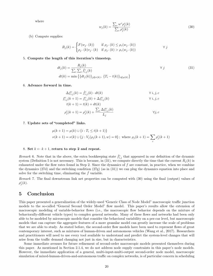
where

wj(k) =

∑c w

cρcj(k)∑c ρ

cj(k)

(30)

(b) Compute supplies:

Rj(k) =

{F (wj−(k)) if ρj−(k) ≤ ρc(wj−(k))

ρj−(k)vj−(k) if ρj−(k) > ρc(wj−(k))∀ j

5. Compute the length of this iteration’s timestep.

dtj(k) =Rj(k)∑

c

∑i f

ci,j(k)

∀ j (31)

dt(k) = min{{dtj(k)}j /∈ν(k), {Ti − t(k)}i/∈µ(k)

}6. Advance forward in time.

∆f ci,j(k) = f ci,j(k) · dt(k) ∀ i, j, cf ci,j(k + 1) = f ci,j(k) + ∆f ci,j(k) ∀ i, j, ct(k + 1) = t(k) + dt(k)

ρcj(k + 1) = ρcj(k) +

∑i ∆f ci,j(k)

Lj∀j, c

7. Update sets of “completed” links.

µ(k + 1) = µ(k) ∪ {i : Ti ≤ t(k + 1)}

ν(k + 1) = ν(k) ∪ {j : Vj(ρj(k + 1), w) = 0} ; where ρj(k + 1) =∑c

ρcj(k + 1)

8. Set k ← k + 1, return to step 2 and repeat.

Remark 6. Note that in the above, the extra bookkeeping state f ci,j that appeared in our definition of the dynamicsystem (Definition 5 is not necessary. This is because, in (31), we compute directly the time that the current Rj(k) isexhausted under the flow rates found in Step 2. Since the dynamics of f are constant, in practice, when we combinethe dynamics (27d) and the switching condition (27g) (as in (31)) we can plug the dynamics equation into place andsolve for the switching time, eliminating the f variable.

Remark 7. The final downstream link net properties can be computed with (30) using the final (output) values ofρcj(k).

5 ConclusionThis paper presented a generalization of the widely-used “Generic Class of Node Model” macroscopic traffic junctionmodels to the so-called “General Second Order Model” flow model. This paper’s results allow the extension ofmacroscopic modeling of variable-behavior flows (i.e., the macroscopic flow behavior depends on the mixture ofbehaviorally-different vehicle types) to complex general networks. Many of these flows and networks had been onlyable to be modeled by microscopic models that consider the behavioral variability on a per-car level, but macroscopicmodels that can capture the aggregate features of a more granular model can greatly increase the scale of problemsthat we are able to study. As stated before, the second-order flow models have been used to represent flows of greatcontemporary interest, such as mixtures of human-driven and autonomous vehicles (Wang et al., 2017). Researchersand practitioners will need to use every tool available to understand and predict the system-level changes that willarise from the traffic demand changing not just in size, but in characteristics.

Some immediate avenues for future refinement of second-order macroscopic models presented themselves duringthis paper. As mentioned in Section 2.1.4, we do not address node supply constraints in this paper’s node models.However, the immediate application of a general, multi-input-multi-output second-order node model, macroscopicsimulation of mixed-human-driven-and-autonomous traffic on complex networks, is of particular concern in scheduling

20

problems involving green light timing. Future work, then, should incorporate the node supply constraints into thegeneral second-order node problem so that they may be used in signal optimization and the still-developing potentialthat connected and automated vehicles bring to traffic control.

We mentioned briefly in Section 3.1 that the ARZ model was originally developed as a spatial coarsening of aparticular simple car-following model (Aw and Rascle, 2000; Zhang, 2002). More sophisticated car-following modelsexist. Some popular ones include the Gipps model (Gipps, 1981), the so-called General Motors family of car-followingmodels (Gazis et al., 1959), and the Intelligent Driver Model (Treiber et al., 2000) and “Improved” Intelligent DriverModel (Shen and Jin, 2012). The Intelligent Driver Model family in particular form the base for many automatedcruise control systems in production vehicles today. That is, the microscopic behavior of many vehicles on the roadare well-understood – either through human-behavioral models or because their behaviors are already (partially)computer-controlled. There is a need to analytically derive second-order fundamental diagrams in the form of spatialdiscretizations of contemporary microscopic models, especially in light of recent analyses (e.g., (Mehr and Horowitz,2019)) that non-controlled deployment of autonomous vehicles can actually worsen traffic network equilibria (i.e.,the familiar Braess/Jevons Paradox, but due to changes in the vehicle fleet rather than changes in the road networkitself). In other words, some of the technological development and deployment already exists for macroscopic mixed-autonomy modeling and control, but some of the theoretical understanding is not yet developed (an uncommonsituation in engineering, indeed).

AcknowledgmentsWe thank our colleagues Alex A. Kurzhanskiy and Gabriel Gomes for their reading and feedback.

ReferencesA. Aw and M. Rascle. Resurrection of "Second Order" Models of Traffic Flow. SIAM Journal on Applied Mathematics,

60(3):916–938, 2000. ISSN 0036-1399. doi: 10.1137/S0036139997332099.

A. Aw, A. Klar, M. Rascle, and T. Materne. Derivation of Continuum Traffic Flow Models from Microscopic Follow-the-Leader Models. SIAM Journal on Applied Mathematics, 63(1):259–278, Jan. 2002. ISSN 0036-1399. doi:10.1137/S0036139900380955.

R. Corthout, G. Flötteröd, F. Viti, and C. M. Tampère. Non-unique flows in macroscopic first-order intersectionmodels. Transportation Research Part B: Methodological, 46(3):343–359, Mar. 2012. ISSN 01912615. doi: 10.1016/j.trb.2011.10.011.

S. Cui, B. Seibold, R. Stern, and D. B. Work. Stabilizing traffic flow via a single autonomous vehicle: Possibilitiesand limitations. In Intelligent Vehicles Symposium (IV), 2017 IEEE, pages 1336–1341. IEEE, 2017. doi: 10.1109/IVS.2017.7995897.

C. F. Daganzo. The cell transmission model: A dynamic representation of highway traffic consistent with the hydro-dynamic theory. Transportation Research Part B: Methodological, 28(4):269–287, 1994. doi: 10.1016/0191-2615(94)90002-7.

C. F. Daganzo. The cell transmission model, Part II: Network traffic. Transportation Research Part B: Methodological,29(2):79–93, Apr. 1995. ISSN 01912615. doi: 10.1016/0191-2615(94)00022-R.

S. Fan, Y. Sun, B. Piccoli, B. Seibold, and D. B. Work. A Collapsed Generalized Aw-Rascle-Zhang Model and ItsModel Accuracy. arXiv preprint arXiv:1702.03624, 2017. URL https://arxiv.org/abs/1702.03624.

G. Flötteröd and J. Rohde. Operational macroscopic modeling of complex urban road intersections. TransportationResearch Part B: Methodological, 45(6):903–922, July 2011. ISSN 01912615. doi: 10.1016/j.trb.2011.04.001.

M. Garavello and B. Piccoli. Traffic Flow on a Road Network Using the Aw–Rascle Model. Communications in PartialDifferential Equations, 31(2):243–275, Jan. 2006. ISSN 0360-5302, 1532-4133. doi: 10.1080/03605300500358053.

D. C. Gazis, R. Herman, and R. B. Potts. Car-Following Theory of Steady-State Traffic Flow. Operations Research,7(4):499–505, 1959. doi: 10.1287/opre.7.4.499.

J. I. Ge and G. Orosz. Dynamics of connected vehicle systems with delayed acceleration feedback. TransportationResearch Part C: Emerging Technologies, 46:46–64, 2014. ISSN 0968-090X. doi: 10.1016/j.trc.2014.04.014.

21

G. Gentile, L. Meschini, and N. Papola. Spillback congestion in dynamic traffic assignment: A macroscopic flowmodel with time-varying bottlenecks. Transportation Research Part B: Methodological, 41(10):1114–1138, 2007.doi: 10.1016/j.trb.2007.04.011.

P. Gipps. A behavioural car-following model for computer simulation. Transportation Research Part B: Methodolog-ical, 15(2):105–111, Apr. 1981. ISSN 01912615. doi: 10.1016/0191-2615(81)90037-0.

F. L. Hall and L. M. Hall. Capacity and speed-flow analysis of the Queen Elizabeth Way in Ontario. TransportationResearch Record, 1287:108–118, 1990. ISSN 0361-1981.

B. Haut and G. Bastin. A second order model of road junctions in fluid models of traffic networks. Networks andHeterogeneous Media, 2(2):227–253, 2007. doi: 10.3934/nhm.2007.2.227.

M. Herty and M. Rascle. Coupling Conditions for a Class of Second-Order Models for Traffic Flow. SIAM Journalon Mathematical Analysis, 38(2):595–616, Jan. 2006. ISSN 0036-1410, 1095-7154. doi: 10.1137/05062617X.

S. E. Jabari. Node modeling for congested urban road networks. Transportation Research Part B: Methodological,91:229–249, Sept. 2016. ISSN 01912615. doi: 10.1016/j.trb.2016.06.001.

W.-L. Jin. A Riemann solver for a system of hyperbolic conservation laws at a general road junction. TransportationResearch Part B: Methodological, 98:21–41, Apr. 2017. ISSN 01912615. doi: 10.1016/j.trb.2016.12.007.

J.-P. Lebacque and M. Khoshyaran. First-order macroscopic traffic flow models: Intersection modeling, networkmodeling. In The 16th International Symposium on Transportation and Traffic Theory (ISTTT), pages 365–386,2005.

J.-P. Lebacque, S. Mammar, and H. Haj-Salem. The Aw–Rascle and Zhang’s model: Vacuum problems, existenceand regularity of the solutions of the Riemann problem. Transportation Research Part B: Methodological, 41(7):710–721, Aug. 2007a. ISSN 01912615. doi: 10.1016/j.trb.2006.11.005.

J.-P. Lebacque, S. Mammar, and H. Haj-Salem. Generic second order traffic flow modelling. In Proceedings of the2007 Symposium on Transportation and Traffic Theory, pages 755–776, 2007b.

M. J. Lighthill and G. B. Whitham. On kinematic waves I. Flood movement in long rivers. Proceedings of theRoyal Society of London. Series A. Mathematical and Physical Sciences, 229(1178):281–316, May 1955a. doi:10.1098/rspa.1955.0088.

M. J. Lighthill and G. B. Whitham. On kinematic waves II. A theory of traffic flow on long crowded roads. Proceedingsof the Royal Society of London. Series A. Mathematical and Physical Sciences, 229(1178):317–345, May 1955b.ISSN 2053-9169. doi: 10.1098/rspa.1955.0089.

N. Mehr and R. Horowitz. How Will the Presence of Autonomous Vehicles Affect the Equilibrium State of TrafficNetworks? arXiv:1901.05168 [cs, math], Jan. 2019. URL http://arxiv.org/abs/1901.05168.

D. Ni and J. D. Leonard. A simplified kinematic wave model at a merge bottleneck. Applied Mathematical Modelling,29(11):1054–1072, Nov. 2005. ISSN 0307904X. doi: 10.1016/j.apm.2005.02.008.

M. Papageorgiou, H. Hadj-Salem, and J. Blosseville. ALINEA: A local feedback control law for on-ramp metering.Transportation Research Record, 1320:58–64, 1991.

P. F. Richards. Shock waves on the highway. Operations Research, 4(1):42–51, 1956. doi: 10.1287/opre.4.1.42.

D. Schrank, B. Eisele, T. Lomax, and J. Bak. 2015 Urban Mobility Scorecard. Technical report, Texas TransportationInstitute, 2015.

J. Shen and X. Jin. Detailed traffic animation for urban road networks. Graphical Models, 74(5):265–282, Sept. 2012.ISSN 15240703. doi: 10.1016/j.gmod.2012.04.002.

E.-S. Smits, M. C. Bliemer, A. J. Pel, and B. van Arem. A family of macroscopic node models. TransportationResearch Part B: Methodological, 74:20–39, Apr. 2015. ISSN 01912615. doi: 10.1016/j.trb.2015.01.002.

R. E. Stern, S. Cui, M. L. Delle Monache, R. Bhadani, M. Bunting, M. Churchill, N. Hamilton, R. Haulcy,H. Pohlmann, F. Wu, B. Piccoli, B. Seibold, J. Sprinkle, and D. B. Work. Dissipation of stop-and-go wavesvia control of autonomous vehicles: Field experiments. Transportation Research Part C: Emerging Technologies,89:205–221, Apr. 2018. ISSN 0968-090X. doi: 10.1016/j.trc.2018.02.005.

22

Y. Sugiyama, M. Fukui, M. Kikuchi, K. Hasebe, A. Nakayama, K. Nishinari, S.-i. Tadaki, and S. Yukawa. Trafficjams without bottlenecks—experimental evidence for the physical mechanism of the formation of a jam. NewJournal of Physics, 10(3):033001, 2008. doi: 10.1088/1367-2630/10/3/033001.

C. M. Tampère, R. Corthout, D. Cattrysse, and L. H. Immers. A generic class of first order node models for dynamicmacroscopic simulation of traffic flows. Transportation Research Part B: Methodological, 45(1):289–309, Jan. 2011.ISSN 01912615. doi: 10.1016/j.trb.2010.06.004.

M. Treiber, A. Hennecke, and D. Helbing. Congested traffic states in empirical observations and microscopic simu-lations. Physical Review E, 62(2):1805–1824, Aug. 2000. ISSN 1063-651X, 1095-3787. doi: 10.1103/PhysRevE.62.1805.

J. Treiterer and J. Myers. The hysteresis phenomenon in traffic flow. In Proceedings of the 6th InternationalSymposium on Transportation and Traffic Theory, volume 6, pages 13–38, Sydney, Australia, Aug. 1974.

R. Wang, Y. Li, and D. B. Work. Comparing traffic state estimators for mixed human and automated trafficflows. Transportation Research Part C: Emerging Technologies, 78:95–110, May 2017. ISSN 0968-090X. doi:10.1016/j.trc.2017.02.011.

G. C. K. Wong and S. C. Wong. A multi-class traffic flow model–an extension of LWR model with heterogeneousdrivers. Transportation Research Part A: Policy and Practice, 36(9):827–841, 2002. doi: 10.1016/S0965-8564(01)00042-8.

M. Wright, R. Horowitz, and A. A. Kurzhanskiy. A dynamic system characterization of road network node models. InProceedings of the 10th IFAC Symposium on Nonlinear Control Systems, volume 49, pages 1054–1059, Monterey,CA, Aug. 2016. doi: 10.1016/j.ifacol.2016.10.307.

M. A. Wright and R. Horowitz. Macro-Scale Lane-Changing and Overtaking Behaviors at Road Junctions:Continuous-Time and Optimization-Problem Formulations. In preparation, 2019.

M. A. Wright, G. Gomes, R. Horowitz, and A. A. Kurzhanskiy. On node models for high-dimensional road networks.Transportation Research Part B: Methodological, 105:212–234, Nov. 2017. ISSN 01912615. doi: 10.1016/j.trb.2017.09.001.

C. Wu, A. Kreidieh, E. Vinitsky, and A. M. Bayen. Emergent Behaviors in Mixed-Autonomy Traffic. In Proceedingsof the 1st Annual Conference on Robot Learning, volume 78 of Proceedings of Machine Learning Research, pages398–407. PMLR, Nov. 2017. URL http://proceedings.mlr.press/v78/wu17a.html.

H. Zhang. A mathematical theory of traffic hysteresis. Transportation Research Part B: Methodological, 33(1):1–23,Feb. 1999. ISSN 01912615. doi: 10.1016/S0191-2615(98)00022-8.

H. Zhang. A non-equilibrium traffic model devoid of gas-like behavior. Transportation Research Part B: Methodolog-ical, 36(3):275–290, Mar. 2002. ISSN 01912615. doi: 10.1016/S0191-2615(00)00050-3.

23