arX

iv:m

ath/

9801

018v

1 [

mat

h.G

T]

6 J

an 1

998

Simple Loops on Surfaces and Their Intersection Numbers

Feng LuoDept. of Math., Rutgers University, New Brunswick, NJ 08903

e-mail: fluo@math.rutgers.edu

Abstract. Given a compact orientable surface Σ, let S(Σ) be the set of isotopyclasses of essential simple loops on Σ. We determine a complete set of relationsfor a function from S(Σ) to Z to be a geometric intersection number function.As a consequence, we obtain explicit equations in RS(Σ) and P (RS(Σ)) definingThurston’s space of measured laminations and Thurston’s compactification of theTeichmuller space. These equations are not only piecewise integral linear but alsosemi-real algebraic.

Table of contents:

§1. Introduction

§2. A Multiplicative Structure on Curve Systems

§3. The One-holed Torus

§4. The Four-holed Sphere

§5. A Reduction Proposition

§6. The Two-holed Tours and the Five-holed Sphere

§7. Proofs of Theorem 1 and the Corollary

§8. Proofs of Results in Section 2 and Some Questions

References

§1. Introduction

Given a compact orientable surface Σ =Σg,r of genus g with r boundary com-ponents, let S = S(Σ) be the set of isotopy classes of essential simple loops onΣ. A function f : S(Σ) → R is called a geometric intersection number function,or simply geometric function if there is a measured lamination m on Σ so thatf(α) is the measure of α in m. Geometric functions were introduced and studiedby W. Thurston in his work on the classification of surface homeomorphisms andthe compactification of the Teichmuller spaces ([FLP], [Th]). The space of all ge-ometric functions under the pointwise convergence topology is homeomorphic toThurston’s space of measured laminations ML(Σ). Thurston showed that ML(Σ)is homeomorphic to a Euclidean space and ML(Σ) has a piecewise integral linearstructure invariant under the action of the mapping class group. The projectiviza-tion of ML(Σ) is Thurston’s boundary of the Teichmuller space. The object of thepaper is to characterize all geometric functions on S(Σ). As a consequence, bothML(Σ) and its projectivization are reconstructed explicitly in terms of an intrinsic(QP 1, PSL(2,Z)) structure on S(Σ).

1

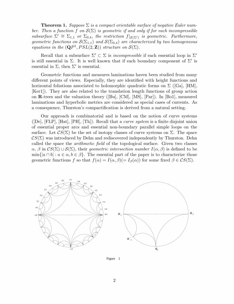
Theorem 1. Suppose Σ is a compact orientable surface of negative Euler num-ber. Then a function f on S(Σ) is geometric if and only if for each incompressiblesubsurface Σ′ ∼= Σ1,1 or Σ0,4, the restriction f |S(Σ′) is geometric. Furthermore,geometric functions on S(Σ1,1) and S(Σ0,4) are characterized by two homogeneousequations in the (QP 1, PSL(2,Z)) structure on S(Σ).

Recall that a subsurface Σ′ ⊂ Σ is incompressible if each essential loop in Σ′

is still essential in Σ. It is well known that if each boundary component of Σ′ isessential in Σ, then Σ′ is essential.

Geometric functions and measures laminations haven been studied from manydifferent points of views. Especially, they are identified with height functions andhorizontal foliations associated to holomorphic quadratic forms on Σ ([Ga], [HM],[Ker1]). They are also related to the translation length functions of group actionon R-trees and the valuation theory ([Bu], [CM], [MS], [Par]). In [Bo1], measuredlaminations and hyperbolic metrics are considered as special cases of currents. Asa consequence, Thurston’s compactification is derived from a natural setting.

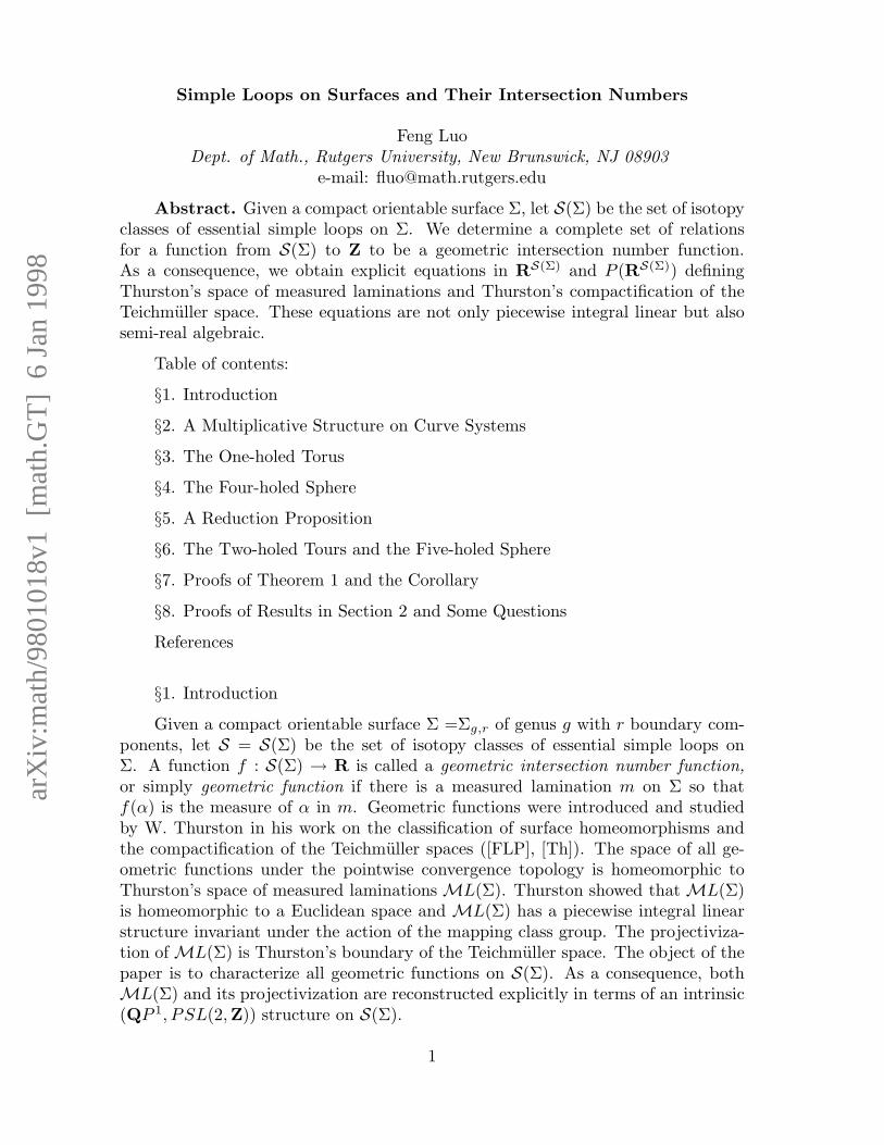
Our approach is combinatorial and is based on the notion of curve systems([De], [FLP], [Hat], [PH], [Th]). Recall that a curve system is a finite disjoint unionof essential proper arcs and essential non-boundary parallel simple loops on thesurface. Let CS(Σ) be the set of isotopy classes of curve systems on Σ. The spaceCS(Σ) was introduced by Dehn and rediscovered independently by Thurston. Dehncalled the space the arithmetic field of the topological surface. Given two classesα, β in CS(Σ) ∪ S(Σ), their geometric intersection number I(α, β) is defined to bemin{|a ∩ b| : a ∈ α, b ∈ β}. The essential part of the paper is to characterize thosegeometric functions f so that f(α) = I(α, β)(= Iβ(α)) for some fixed β ∈ CS(Σ).

1/1

.

-1/1

0/1

1/2

1/3

1/4

2/5

3/5

1/0

3/42/3

4/1

3/1

5/2

3/24/3

2/1

5/3

α

Figure 1

.

3

1α

α2

α 3

2

Given a surface Σ, let S′(Σ) = CS(Σ)∩S(Σ) be the set of isotopy classes ofessential, non-boundary parallel simple loops in Σ. For surfaces Σ = Σ1,0, Σ1,1 and

Σ0,4, it is well known that there exists a bijection π : S′(Σ) → QP 1(= Q) so thatp′q − pq′ = ±1 if and only if I(π−1(p/q), π−1(p′/q′)) = 1 (for Σ1,0, Σ1,1) and 2 (forΣ0,4). See figure 1. We say that three distinct classes α, β, γ in S′(Σ) form anideal triangle if they correspond to the vertices of an ideal triangle in the modularrelation under the map π.

Theorem 2. (a) For surface Σ1,1, a function f : S → Z≥0 is a geometricfunction Iδ with δ ∈CS(Σ) if and only if the following hold.

(1) f(α1) + f(α2) + f(α3) = maxi=1,2,3

(2f(αi), f([∂Σ1,1]))

where (α1, α2, α3) is an ideal triangle, and

(2) f(α3) + f(α′3) = max(2f(α1), 2f(α2), f([∂Σ1,1]))

where (α1, α2, α3) and (α1, α2, α′3) are two distinct ideal triangles.

(3) f([∂Σ1,1]) ∈ 2Z.

(b) For surface Σ0,4 with ∂Σ0,4 = b1 ∪ b2 ∪ b3 ∪ b4, a function f : S → Z≥0 isa geometric function Iδ for some δ ∈ CS(Σ) if and only if for each ideal triangle(α1, α2, α3) so that (αi, bs, br) bounds a Σ0,3 in Σ0,4 the following hold.

(4) Σ3i=1f(αi) = max

1≤i≤3;1≤s≤4(2f(αi), 2f(bs),

4∑

s=1

f(bs), f(αi) + f(bs) + f(br))

(5) f(α3) + f(α′3) = max

1≤i≤2;1≤s≤4(2f(αi), 2f(bs),

4∑

s=1

f(bs), f(αi) + f(bs) + f(br))

where (α1, α2, α3) and (α1, α2, α′3) are two distinct ideal triangles,

(6) f(αi) + f(bs) + f(br) ∈ 2Z.

(c) The characterization of geometric functions f : S(Σ) → R≥0 for Σ = Σ1,1

and Σ0,4 is given by equations (1),(2) (for Σ1,1) and (4), (5) (for Σ0,4).

Theorem 2 is motivated by the tours case. In fact for the torus Σ1,0, a functionon S(Σ1,0) is geometric if and only if it satisfies the triangular equality f(α1) +f(α2) + f(α3) = maxi=1,2,3(2f(αi)) and f(α3) + f(α′

3) = max(2f(α1), 2f(α2)).

The equations (1),(2),(4) and (5) in theorem 2 are obtained as the degenerationsof the trace identities for SL(2,R) matrices. For instance, equations (1), (2) are the

3

degenerations of tr(A)tr(B)tr(AB) = tr2(A) + tr2(B) + tr2(AB) − tr([A, B]) − 2and tr(AB)tr(A−1B) = tr2(A) + tr2(B) − tr([A, B])− 2.

Several properties of the measured laminations spaces are reflected in the equa-tions (1),(2),(4), and (5). For instance, since the equations are piecewise integrallinear so that rational solutions are dense, one obtains Thurston’s result that thespace ML(Σ) has a piecewise integral linear structure and the rational multiplesof the curve systems is a dense subset. On the other hand, the equations are alsosemi-real algebraic. Indeed, the space defined by

∑ki=1 xi = max1≤j≤l(yj) is semi-

real algebraic since it is equivalent to:∏l

j=1(∑k

i=1 xi − yj) = 0, and∑k

i=1 xi ≥ yj ,for all j. This seems to indicate that the space ML(Σ) has a semi-real algebraicstructure. Given a surface Σg,r, Thurston showed that there exists a finite set Fconsisting of 9g + 4r − 9 elements in S(Σ) so that the map τF : ML(Σ) → RF

≥0

sending m to Im|F is an embedding ([FLP]). As a consequence of theorems 1,2, wehave,

Corollary. For surface Σg,r of negative Euler number, there is a finite set Fconsisting of 9g+4r−9 elements in S(Σ) so that the map τF is an embedding whoseimage is a polyhedron defined by finitely many explicit integer coefficient polynomialequations and inequalities.

It is interesting to observe that the approach taken in the paper (also in[Lu1], [Lu3]) follows Grothendieck’s philosophy of the “Teichmuller tower” wherethe “generators” are the surfaces Σ1,1 and Σ0,4 and the “relations” are Σ1,2 andΣ0,5. See [Sch] for more details. From this point of view, it seems clear that the(QP 1, PSL(2,Z)) modular structure is fundamental to the topology and geometryof surfaces and the modular structure plays a role of “local coordinate” on the setS(Σ). Following this line, we may ask the following two questions on the relatedtopics of mapping class groups and SL(2,C) representations.

Question 1. (A presentation of the mapping class group). Suppose Σ is a com-pact oriented surface. Let Mod(Σ) be the mapping class group of Σ consisting ofisotopy classes of orientation preserving homeomorphisms which leaves each bound-ary component invariant. Let G be the group with S(Σ) as the set of generatorsand the following as the set of relations: (R1) xy = yx if I(x, y) = 0; (R2) x = 1if x is a boundary component of Σ; (R3) xy = yz if (x, y, z) forms a positivelyoriented (x → y → z → x is the right hand order in S1) ideal triangle in S(Σ′)where Σ′ ∼= Σ1,1 is incompressible in Σ; (R4) xyz = b1b2b3b4 if (x, y, z) forms apositively oriented ideal triangle in S(Σ′) where Σ′ ∼= Σ0,4 is incompressible in Σwith ∂Σ′ = b1 ∪ b2 ∪ b3 ∪ b4. Is G a presentation of Mod(Σ)?

Note that relation (R3) implies the Artin’s relation (xyx = yxy) and (R4) is thelantern relation which was discovered by Dehn ([De], p333) in 1938 and rediscoveredindependently by Johnson. See [Bi], [De], [Har], [HT], [Li], [Waj] for more details.

Question 2. (Characters of SL(2,C) representations) A function f : S(Σ) → C

is the (restriction of) character of a representation of π1(Σ) into SL(2,C) if andonly if f |S(Σ′) is a character for each incompressible subsurface Σ′ ∼= Σ1,1 or Σ0,4.

4

The description of characters for the surfaces Σ1,1 and Σ0,4 seems to be known.See [CS], [Go], [GoM], [Ho], [Mag] and the references cited therein.

The organization of the paper is as follows. In §2, we establish several basicproperties of the curve systems. In particular, a multiplicative structure on CS(Σ)is introduced. In §3,§4, we prove theorem 2. The proof in §4 is complicated dueto the existence of eight different ideal triangulations of the surface Σ0,4. In §5, weprove a reduction result. This is one of the key steps in the proof of theorem 1. Itreduces the general case to two surfaces: Σ1,2 and Σ0,5. In §6, we prove theorem1 for surfaces Σ1,2 and Σ0,5. The proofs of theorem 1 and the corollary are in §7.The proof of the results in §2 is in §8.

Acknowledgment. I would like to thank F. Bonahon, M. Freedman, X.S. Lin,and Y. Minsky for discussions. The work is supported in part by the NSF.

§2. A Multiplicative Structure on Curve Systems

We work in the piecewise linear category. Surfaces are oriented and connectedand have negative Euler numbers unless specified otherwise. A regular neighborhoodof a submanifold X is denoted by N(X). Regular neighborhoods are assumed tobe small. The isotopy class of a curve system c will be denoted by [c]. Supposef : CS(Σ) → R is a function and c is a curve system. We define f(c) to be f([c]).In particular, I(a, b) = I([a], [b]). Homeomorphic manifolds X , Y are denoted byX ∼= Y . Isotopic submanifolds c, d are denoted by c ∼= d. If m ∈ ML(Σ), Im

denotes the geometric intersection number function with respect to m. A class inCS(Σg,r) is called a Fenchel-Nielsen system (resp. an ideal triangulation ) if it isthe isotopy class of 3g + r − 3 (resp. 6g + 2r − 6) many pairwise non-isotopic non-boundary parallel simple loops (resp. proper arcs). The numbers 3g + r − 3 and6g + 2r − 6 are maximal.

A convention : all surfaces drawn in this paper have the right-hand orientationin the front face.

2.1. A multiplicative structure on CS(Σ)

Suppose a and b are two arcs in Σ intersecting transversely at one point P . Thenthe resolution of a ∪ b at P from a to b is defined as follows. Take any orientationon a and use the orientation on Σ to determine an orientation on b. Then resolvethe intersection according to the orientations. The resolution is independent of thechoice of the orientation on a. See figure 2.

Given two curve systems a, b on Σ with |a ∩ b| = I(a, b), the multiplication abis defined to be the disjoint union of simple loops and arcs obtained by resolvingall intersection points from a to b. It is shown in §8 (lemma 8.1) that ab is again acurve system whose isotopy class depends only on the isotopy classes of a, b. Givenα,β ∈ CS(Σ), we define αβ =[ab] where a ∈ α, b ∈ β so that |a ∩ b| = I(a, b). Thefollowing proposition establishes the basic properties of the multiplication. See §8for a proof.

Let CS0(Σ) be the subset of CS(Σ) consisting of isotopy classes of curve systemswhich contain no arcs.

5

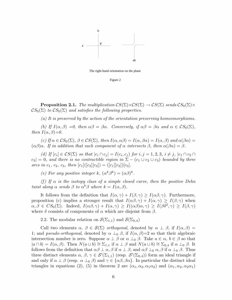
a

b

ab

P

The right-hand orientation on the plane

Figure 2

Proposition 2.1. The multiplication CS(Σ)×CS(Σ) → CS(Σ) sends CS0(Σ)×CS0(Σ) to CS0(Σ) and satisfies the following properties.

(a) It is preserved by the action of the orientation preserving homeomorphisms.

(b) If I(α, β) =0, then αβ = βα. Conversely, if αβ = βα and α ∈ CS0(Σ),then I(α, β)=0.

(c) If α ∈ CS0(Σ), β ∈ CS(Σ), then I(α, αβ) = I(α, βα) = I(α, β) and α(βα) =(αβ)α. If in addition that each component of α intersects β, then α(βα) = β.

(d) If [ci] ∈ CS(Σ) so that |ci ∩ cj | = I(ci, cj) for i, j = 1, 2, 3, i 6= j, |c1 ∩ c2 ∩c3| = 0, and there is no contractible region in Σ − (c1 ∪ c2 ∪ c3) bounded by threearcs in c1, c2, c3, then [c1]([c2][c3]) = ([c1][c2])[c3].

(e) For any positive integer k, (αkβk) = (αβ)k.

(f) If α is the isotopy class of a simple closed curve, then the positive Dehntwist along α sends β to αkβ where k = I(α, β).

It follows from the definition that I(α, γ) + I(β, γ) ≥ I(αβ, γ). Furthermore,proposition (c) implies a stronger result that I(αβ, γ) + I(α, γ) ≥ I(β, γ) whenα, β ∈ CS0(Σ). Indeed, I(αβ, γ) + I(α, γ) ≥ I((αβ)α, γ) ≥ I(βδ2, γ) ≥ I(β, γ)where δ consists of components of α which are disjoint from β.

2.2. The modular relation on S(Σ1,1) and S(Σ0,4)

Call two elements α, β ∈ S(Σ) orthogonal, denoted by α ⊥ β, if I(α, β) =1; and pseudo-orthogonal, denoted by α ⊥0 β, if I(α, β)=2 so that their algebraicintersection number is zero. Suppose α ⊥ β or α ⊥0 β. Take a ∈ α, b ∈ β so that|a ∩ b| = I(α, β). Then N(a ∪ b) ∼= Σ1,1 if α ⊥ β and N(a ∪ b) ∼= Σ0,4 if α ⊥0 β. Itfollows from the definition that αβ ⊥ α, β if α ⊥ β, and αβ ⊥0 α, β if α ⊥0 β. Thusthree distinct elements α, β, γ ∈ S′(Σ1,1) (resp. S′(Σ0,4)) form an ideal triangle ifand only if α ⊥ β (resp. α ⊥0 β) and γ ∈ {αβ, βα}. In particular the distinct idealtriangles in equations (2), (5) in theorem 2 are (α1, α2, α1α2) and (α1, α2, α2α1)

6

where α1 ⊥ α2 or α1 ⊥0 α2 ((α1, α2, α1α2) is positively oriented). If α ⊥ β orα ⊥0 β, we define α−nβ = βαn for n ∈ Z>0. It follows from proposition 2.1(c) thatαn(αmβ) = αn+mβ for n, m ∈ Z.

For Σ = Σ1,1 or Σ0,4, we can find an explicit bijection from S′(Σ) to Q asfollows. Take α, β in S′(Σ) so that α ⊥ β or α ⊥0 β. Then each γ in S′(Σ)can be expressed uniquely as αpβq where q ∈ Z≥0, p ∈ Z and p, q are relatively

prime. Define π(γ) = p/q from S′(Σ) to Q. Then π(γi) = pi/qi, i = 1, 2, satisfyp1q2 − p2q1 = ±1 if and only if γ1 ⊥ γ2 or γ1 ⊥0 γ2.

Given two simple loops a, b, we use a ⊥ b to denote |a ∩ b| = I(a, b) = 1, anduse a ⊥0 b to denote |a ∩ b| = I(a, b) = 2 and [a] ⊥0 [b].

2.3. A gluing lemma

Suppose Σ′ is an incompressible subsurface of Σ. We define the restrictionmap R(= RΣ

Σ′) : CS(Σ) → CS(Σ′) as follows. Given α in CS(Σ), take a ∈ α sothat |a ∩ ∂Σ′| = I(a, ∂Σ′) and a ∩ Σ′ contains no component parallel into ∂Σ′. Wedefine R(α) = [a|Σ′ ](:= α|Σ′). The restriction map is well defined. Furthermore ifX ⊂ Y ⊂ Z are incompressible subsurfaces, then RZ

X = RYXRZ

Y .

Lemma 2.1 (Gluing along a 3-holed sphere) Suppose X and Y are incom-pressible subsurfaces in Σ so that Σ = X ∪ Y and X ∩ Y ∼= Σ0,3. Then for any twoelements αX ∈ CS(X), αY ∈ CS(Y ) with αX |X∩Y = αY |X∩Y , there is a uniqueelement α ∈ CS(Σ) so that α|X = αX and α|Y = αY .

Proof. To show the existence, take a1 ∈ αX and a2 ∈ αY so αX |X∩Y =[a1|X∩Y ], αY |X∩Y = [a2|X∩Y ]. By the assumption, there is a self-homeomorphismh1 of X ∩ Y isotopic to the identity map so that h1(a1|X∩Y ) = a2|X∩Y . Extend h1

to a self-homeomorphism h2 of X isotopic to idX . Define a curve system a on Σ asfollows: a|X = h2(a1), and a|Y = a2. Then we have [a]|X = αX and [a]|Y = αY bydefinition.

To show the uniqueness, suppose β ∈ CS(Σ) so that β|X = αX , and β|Y = αY .Take b ∈ β so that b|X ∈ αX . There is a self-homeomorphism h3 of X isotopic toidX so that h3(b|X) = a|X . By extending h3 to a homeomorphism of Σ isotopicto idΣ, we may assume that b|X = a|X . Now since a|Y ∈ αY and b|X = a|X , weobtain b|Y ∈ αY (due to ∂Y ∩ int(Σ) ⊂ int(X)). Let h4 be a self-homeomorphismof Y sending b|Y to a|Y so that h4

∼= idY and h4|∂Y ∩(∂(X∩Y )) = id. Extend h4 toa homeomorphism h5 of Σ by setting h5(x) = x for x ∈ X − Y . Then h5

∼= id andh5(b) = a. Thus α = β. �

7

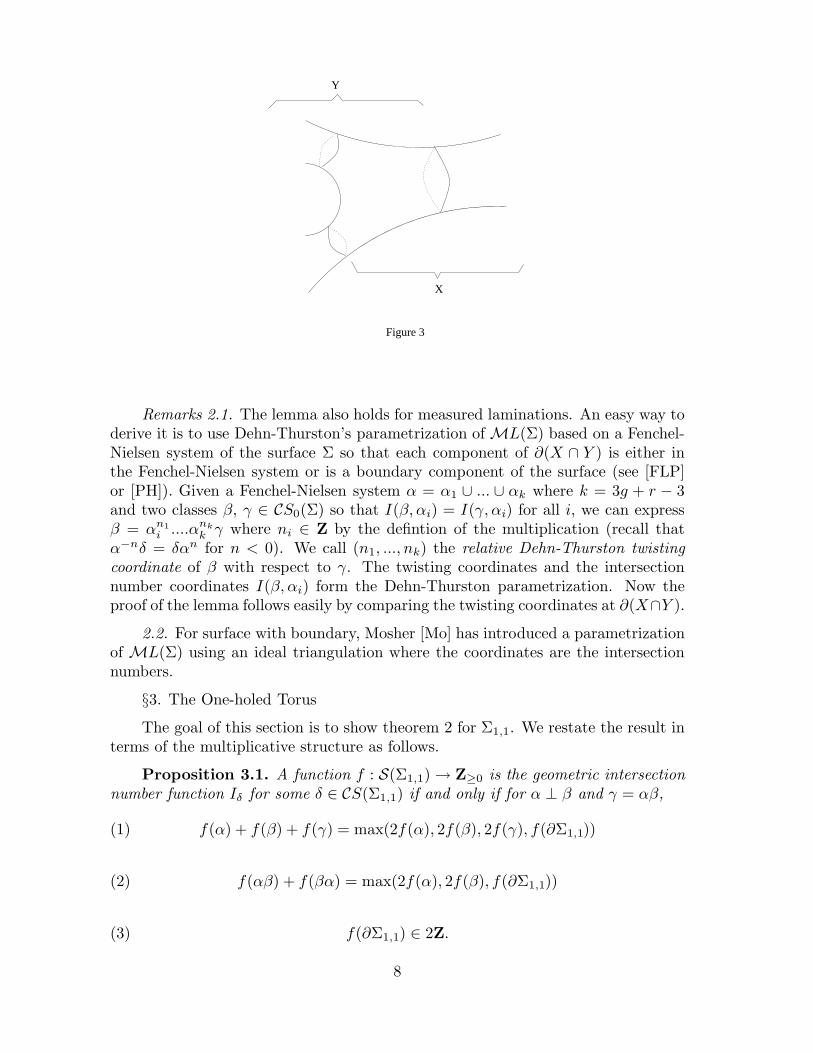
X

Y

Figure 3

Remarks 2.1. The lemma also holds for measured laminations. An easy way toderive it is to use Dehn-Thurston’s parametrization of ML(Σ) based on a Fenchel-Nielsen system of the surface Σ so that each component of ∂(X ∩ Y ) is either inthe Fenchel-Nielsen system or is a boundary component of the surface (see [FLP]or [PH]). Given a Fenchel-Nielsen system α = α1 ∪ ... ∪ αk where k = 3g + r − 3and two classes β, γ ∈ CS0(Σ) so that I(β, αi) = I(γ, αi) for all i, we can expressβ = αn1

i ....αnk

k γ where ni ∈ Z by the defintion of the multiplication (recall thatα−nδ = δαn for n < 0). We call (n1, ..., nk) the relative Dehn-Thurston twistingcoordinate of β with respect to γ. The twisting coordinates and the intersectionnumber coordinates I(β, αi) form the Dehn-Thurston parametrization. Now theproof of the lemma follows easily by comparing the twisting coordinates at ∂(X∩Y ).

2.2. For surface with boundary, Mosher [Mo] has introduced a parametrizationof ML(Σ) using an ideal triangulation where the coordinates are the intersectionnumbers.

§3. The One-holed Torus

The goal of this section is to show theorem 2 for Σ1,1. We restate the result interms of the multiplicative structure as follows.

Proposition 3.1. A function f : S(Σ1,1) → Z≥0 is the geometric intersectionnumber function Iδ for some δ ∈ CS(Σ1,1) if and only if for α ⊥ β and γ = αβ,

(1) f(α) + f(β) + f(γ) = max(2f(α), 2f(β), 2f(γ), f(∂Σ1,1))

(2) f(αβ) + f(βα) = max(2f(α), 2f(β), f(∂Σ1,1))

(3) f(∂Σ1,1) ∈ 2Z.

8

Furthermore, the characterization of geometric functions f : S → R is given byequations (1), (2) above.

Remark. The condition f ≥ 0 in the proposition above is not necessary. Indeed,equation (1) (also equation (4)) implies f ≥ 0. To see this, we note that (1) impliesthat f(α), f(β), f(γ) satisfy the triangular inequalities that sum of two is at leastthe third which in turn shows f ≥ 0.

Proof. To see the necessity, we double the surface Σ1,1 to obtain Σ2,0 =Σ1,1 ∪id∂

Σ1,1. Then each γ ∈ CS(Σ1,1) corresponds to γ ∈ CS(Σ2,0) whose re-striction to both summands Σ1,1 are γ. The curve system γ has no boundary.Let di be a sequence of a hyperbolic metrics on Σ2,0 which pinch to γ, i.e., thereis a sequence λi ∈ R>0 so that limi λildi

(α) = Iγ(α) for all α ∈ S(Σ2,0) whereldi

(α) is the length of the di-geodesic in the class α. Let ti = 2 cosh ldi/2. It is

shown in [FK], [Ke] and [Lu1] that for α ⊥ β in S(Σ1,1) (⊂ S(Σ2,0)), one hasthe following identities: ti(α)ti(β)ti(αβ) = t2i (α) + t2i (β) + t2i (αβ) + ti(∂Σ1,1) − 2and ti(αβ)ti(βα) = t2i (α) + t2i (β) + ti(∂Σ1,1) − 2. Now, for α ∈ S(Σ1,1), we haveIγ(α) = Iγ(α). Let i tend to infinity. The equations for ti degenerate to theequations (1), (2) in the proposition. The equation (3) is evident.

Remark 3.1. To derive equation (1) directly from the trace identity tr(A)tr(B)tr(AB) = tr2(A) + tr2(B) + tr2(AB) − tr([A, B]) − 2 where A, B ∈ SL(2,R),we assume that A, B, AB correspond to three simple closed geodesics forming anideal triangle in S. Then tr(A)tr(B)tr(AB) > 0 and tr([A, B]) < 0 (see [GiM]for instance). In particular, we obtain |tr(A)||tr(B)||tr(AB)| = tr2(A) + tr2(B) +tr2(AB)+ |tr([A, B])| − 2. The degeneration of it becomes f(A)+ f(B)+ f(AB) =max(2f(A), 2f(B), 2f(AB), f([A,B])) which is equation (1).

To show that the conditions are also sufficient, we begin with a function f :S → Z≥0 satisfying equations (1),(2),(3). By the structure of the modular relation,we conclude that f is determined by its values on {α, β, αβ, ∂Σ1,1} for α ⊥ β. Thusit suffices to construct δ ∈ CS(Σ1,1) so that f and Iδ have the same values at thefour-element set above.

We consider two cases: min{f(α) : α ∈ S′(Σ1,1)} = 0, or > 0.

Case 1. There is α ∈ S′(Σ) so that f(α) = 0. If β ⊥ α and γ = αβ, thenf(β) = f(γ). Indeed, by equation (1), f(β) + f(γ) = max(2f(β), 2f(γ), f(∂Σ1,1))≥ max(2f(β), 2f(γ)). Thus f(β) = f(γ). In particular, f(β) ≥ 1

2f(∂Σ1,1). Weconstruct the curve system δ as follows. Let Σ′ = Σ1,1 − int(N(a)) where a ∈ α.Then Σ′ ∼= Σ0,3. Curve systems on Σ0,3 with ∂Σ0,3 = b1∪b2∪b3 are well understood.Namely, S(Σ0,3) = {b1, b2, b3} and each δ ∈ CS(Σ0,3) is uniquely determined byπ(δ) = (Ib1(δ), Ib2(δ), Ib3(δ)). Furthermore, each triple of non-negative integerswhose sum is even is of the form π(δ) and π(δδ′) = π(δ) + π(δ′). Let δ′ ∈ CS(Σ′)(⊂ SC(Σ)) so that I(δ′, ∂Σ1,1) = f(∂Σ1,1) and I(δ′, α) = 0. Let δ = δ′αk in CS(Σ)where k = f(β)− 1

2f(∂Σ1,1). Then Iδ and f have the same values at {α, β, γ, ∂Σ1,1}

by the construction. Thus f = Iδ.

9

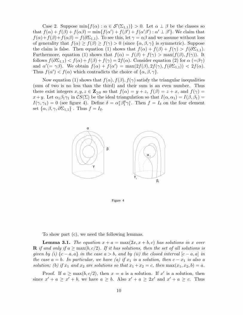
Case 2. Suppose min{f(α) : α ∈ S′(Σ1,1)} > 0. Let α ⊥ β be the classes sothat f(α) + f(β) + f(αβ) = min{f(α′) + f(β′) + f(α′β′) : α′ ⊥ β′}. We claim thatf(α)+f(β)+f(αβ) = f(∂Σ1,1). To see this, let γ = αβ and we assume without lossof generality that f(α) ≥ f(β) ≥ f(γ) > 0 (since {α, β, γ} is symmetric). Supposethe claim is false. Then equation (1) shows that f(α) + f(β) + f(γ) > f(∂Σ1,1).Furthermore, equation (1) shows that f(α) = f(β) + f(γ) > max(f(β), f(γ)). Itfollows f(∂Σ1,1) < f(α)+ f(β) + f(γ) = 2f(α). Consider equation (2) for α (=βγ)and α′(= γβ). We obtain f(α) + f(α′) = max(2f(β), 2f(γ), f(∂Σ1,1)) < 2f(α).Thus f(α′) < f(α) which contradicts the choice of {α, β, γ}.

Now equation (1) shows that f(α), f(β), f(γ) satisfy the triangular inequalities(sum of two is no less than the third) and their sum is an even number. Thusthere exist integers x, y, z ∈ Z≥0 so that f(α) = y + z, f(β) = z + x, and f(γ) =x+ y. Let α1β1γ1 in CS(Σ) be the ideal triangulation so that I(α, α1) = I(β, β1) =I(γ, γ1) = 0 (see figure 4). Define δ = αx

1βy1γz

1 . Then f = Iδ on the four elementset {α, β, γ, ∂Σ1,1} . Thus f = Iδ.

Figure 4

β

γ

α

β

α

γ

1

1

1

To show part (c), we need the following lemmas.

Lemma 3.1. The equation x + a = max(2x, x + b, c) has solutions in x overR if and only if a ≥ max(b, c/2). If it has solutions, then the set of all solutions isgiven by (i) {c − a, a} in the case a > b, and by (ii) the closed interval [c − a, a] inthe case a = b. In particular, we have (a) if x1 is a solution, then c − x1 is also asolution; (b) if x1 and x2 are solutions so that x1 +x2 = c, then max(x1, x2, b) = a.

Proof. If a ≥ max(b, c/2), then x = a is a solution. If x′ is a solution, thensince x′ + a ≥ x′ + b, we have a ≥ b. Also x′ + a ≥ 2x′ and x′ + a ≥ c. Thus

10

a ≥ x′ ≥ c − a. This shows a ≥ c/2, i.e., a ≥ max(b, c/2). If a > b, thenthe equation becomes x + a = max(2x, c) with a ≥ c/2. Thus the solutions are{c− a, a}. If a = b, then one checks easily that all solutions are points in [c− a, a].�

Lemma 3.2. Suppose x1, x2,x3,x4∈Z≥0 so that x1+x2+x3= max(2x1,2x2,2x3,x4). Then there is a function g : S(Σ1,1) → Z satisfying equations (1),(2) and anideal triangle (α1, α2, α3) in S′(Σ1,1) so that g(αi) = xi, i = 1, 2, 3, and g(∂Σ1,1) =x4.

Proof. Take any ideal triangle (α1, α2, α3). We define g on αi and ∂Σ1,1

as required. We now extend g through the neighboring ideal triangles by usingequation (2). Thus, we need to verify that the equation (1) for g on the neighboringideal triangles still holds. Take a neighboring ideal triangle, say (α1, α2, α

′3). Define

g(α′3) = x′

3 where x′3 = max(2x1, 2x2, x4) − x3. We first note that x′

3 ≥ 0 sincexi + xj ≥ xk for {i, j, k} = {1, 2, 3} by the given condition on x′

is. Next, considerx1 + x2 + x3 = max(2x1, 2x2, 2x3, x4) as an equation in x3. Then it is of the formx + x1 + x2 = max(2x, x3 + x′

3). By lemma 3.1(a), x′3 satisfies the equation in x,

i.e., equation (1) holds for g on the neighboring ideal triangles. �

We now show that equations (1), (2) characterize the geometric functions. Evi-dently, any geometric functions satisfies the equations (1), (2). Conversely, supposethat f is a solution to equations (1), (2). Fix an ideal triangle (α1, α2, α3) in S′.Note that the rational solutions of the equation x1+x2+x3 = max(2x1, 2x2, 2x3, x4)are dense in the solutions over R≥0. By lemma 3.2, there is a sequence of functionsgn from S to 2Z≥0 solving equations (1), (2) and a sequence of numbers kn ∈ Q

so that limn kngn(x) = f(x) for x ∈ {α1, α2, α3, ∂Σ}. By equation (2), we havelimn kngn(x) = f(x) for all x ∈ S(Σ). On the other hand, we have gn = Iδn

forsome δn ∈ S(Σ) by the result for curve systems. Thus f = Im where m = limn knδn

∈ ML(Σ) by definition. �

§4. The Four-holed Sphere

The goal of this section is to show theorem 2 for the surface Σ0,4. The basic idealof the proof is the same as in §3. But the proof is considerably longer and morecomplicated due to the existence of eight non-homeomorphic ideal triangulationsof the four-holed sphere. We restate the theorem in terms of the multiplicativestructure below.

Proposition 4.1. For surface Σ0,4 with ∂Σ0,4 = b1 ∪ b2 ∪ b3 ∪ b4, a functionf : S(Σ0,4) → Z≥0 is the geometric intersection number function Iδ for some δ ∈CS(Σ) if and only if for α1 ⊥0 α2 with α3 = α1α2 so that (αi, bs, br) bounds a Σ0,3

in Σ0,4,

(4)3∑

i=1

f(αi) = max1≤i≤3;1≤s≤4

(2f(αi), 2f(bs),4∑

s=1

f(bs), f(αi) + f(bs) + f(br))

11

(5)

f(α1α2) + f(α2α1) = max1≤i≤2;1≤s≤4

(2f(αi), 2f(bs),

4∑

s=1

f(bs), f(αi) + f(bs) + f(br))

(6) f(αi) + f(bs) + f(br) ∈ 2Z

Furthermore, geometric functions on S(Σ0,4) are characterized by the equations(4),(5).

Proof. The necessity of the equations (4),(5) follows from the same argumentas in §3 using the degenerations of the trace relations for geodesic length functions.To be more precise, it is shown in [Lu1] that for any hyperbolic metric d on Σ0,4

with geodesic boundary or cusp ends, then t(α) = 2 cosh ld(α)/2 satisfies:

t(α1)t(α2)t(α3) + 4 =

3∑

i=1

t2(αi) +

4∑

s=1

t2(bs) +

4∏

s=1

t(bs) +1

2

3∑

i=1

4∑

s=1

t(αi)t(bs)t(br)

and

t(α1α2)t(α2α1) =

2∑

i=1

t2(αi) +

4∑

s=1

t2(bs) +

4∏

s=1

t(bs) +1

2

2∑

i=1

4∑

s=1

t(αi)t(bs)t(br) − 4

Now the degenerations of the above two equations are equations (4), (5). Theequation (6) holds for curve systems clearly.

To show that the conditions are also sufficient, we begin with a function f : S →Z≥0 satisfying equations (4),(5),(6). By the structure of the modular relation, weconclude that f is determined by its restriction on {α, β, αβ, b1, ..., b4} for α ⊥0 β.Thus it suffices to construct δ ∈ CS(Σ) so that f and Iδ have the same values onthe seven-element set {α, β, αβ, b1, ..., b4}.

Note that equation (6) implies both∑4

i=1 f(bi) and∑3

i=1 f(αi) are even num-bers.

We shall consider two cases: min{f(α) : α ∈ S′(Σ0,4)} = 0 or > 0.

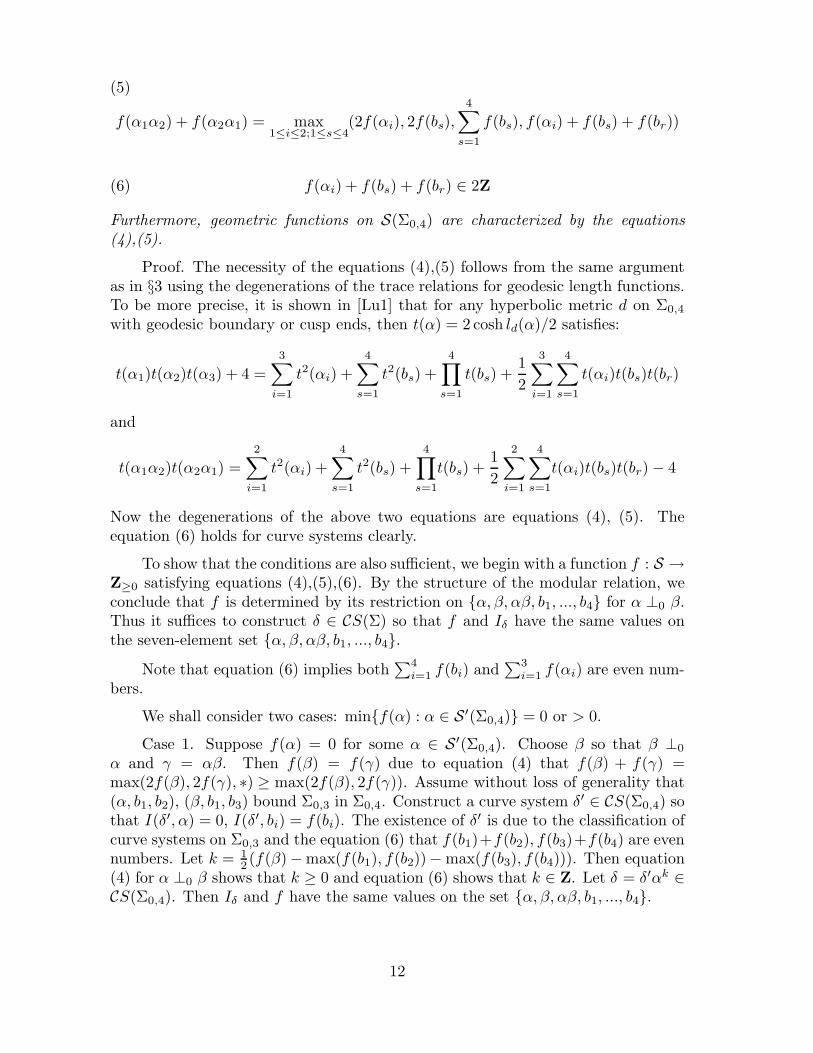
Case 1. Suppose f(α) = 0 for some α ∈ S′(Σ0,4). Choose β so that β ⊥0

α and γ = αβ. Then f(β) = f(γ) due to equation (4) that f(β) + f(γ) =max(2f(β), 2f(γ), ∗) ≥ max(2f(β), 2f(γ)). Assume without loss of generality that(α, b1, b2), (β, b1, b3) bound Σ0,3 in Σ0,4. Construct a curve system δ′ ∈ CS(Σ0,4) sothat I(δ′, α) = 0, I(δ′, bi) = f(bi). The existence of δ′ is due to the classification ofcurve systems on Σ0,3 and the equation (6) that f(b1)+f(b2), f(b3)+f(b4) are evennumbers. Let k = 1

2(f(β)−max(f(b1), f(b2))− max(f(b3), f(b4))). Then equation

(4) for α ⊥0 β shows that k ≥ 0 and equation (6) shows that k ∈ Z. Let δ = δ′αk ∈CS(Σ0,4). Then Iδ and f have the same values on the set {α, β, αβ, b1, ..., b4}.

12

β

α

1

3 4b b

bb2

α

δ

δ

1

3 4b b

bb2

γ

Figure 5

Case 2. Assume f(α) ≥ 1 for all α ∈ S′(Σ0,4). Let {α, β, γ} be an ideal trian-gle in S(Σ) so that f(α) + f(β) + f(γ) achieves the minimal values among all suchtriples. Assume without loss of generality that (α, b1, b2), (β, b1, b3) bound Σ0,3 inΣ0,4 and that f(α) ≥ f(β) ≥ f(γ). We claim that f(α) + f(β) + f(γ) = A whereA = max1≤s≤4(2f(bs), Σ

4s=1f(bs), f(α) + f(b1) + f(b2), f(α) + f(b3) + f(b4), f(β) +

f(b1)+f(b3), f(β)+f(b2)+f(b4), f(γ)+f(b1)+f(b4), f(γ)+f(b2)+f(b3)). Indeed,if otherwise, by equation (4) that f(α)+f(β)+f(γ) = max(2f(α), 2f(β), 2f(γ), A),we obtain f(α) + f(β) + f(γ) > A and f(α) = f(β) + f(γ). In particular,f(α) > f(β), f(γ), and 2f(α) > A. Applying equation (5) to α, α′ where {α, α′} ={βγ, γβ}, we obtain f(α) + f(α′) = max(2f(β), 2f(γ), A′) where A′ ≤ A < 2f(α).Thus f(α) + f(α′) < 2f(α), i.e., f(α′) < f(α). This contradicts the choice of(α, β, γ).

We now construct δ ∈ CS(Σ0,4) so that f and Iδ have the same values on{α, β, γ, b1, ..., b4} under the assumption that f(α)+f(β)+f(γ) = A. For simplicity,we still assume that (α, b1, b2) and (β, b1, b3) bound Σ0,3 but do not assume thatf(α) ≥ f(β) ≥ f(γ).

By symmetry, since f(α)+f(β)+f(γ) = A, it suffices to consider the followingthree subcases: (2.1) f(α) + f(β) + f(γ)= Σ4

s=1f(bs); (2.2) f(α) + f(β) + f(γ)= 2f(b1); and (2.3) f(α) + f(β) + f(γ) = f(α) + f(b1) + f(b2). The correspondingcurve system δ in CS(Σ0,4) will be constructed as follows. First, we construct anideal triangulation τ = τ1...τ6 of Σ0,4. Then the curve system δ is taken to be ofthe form τx1

1 ...τx6

6 , xi ∈ Z≥0.

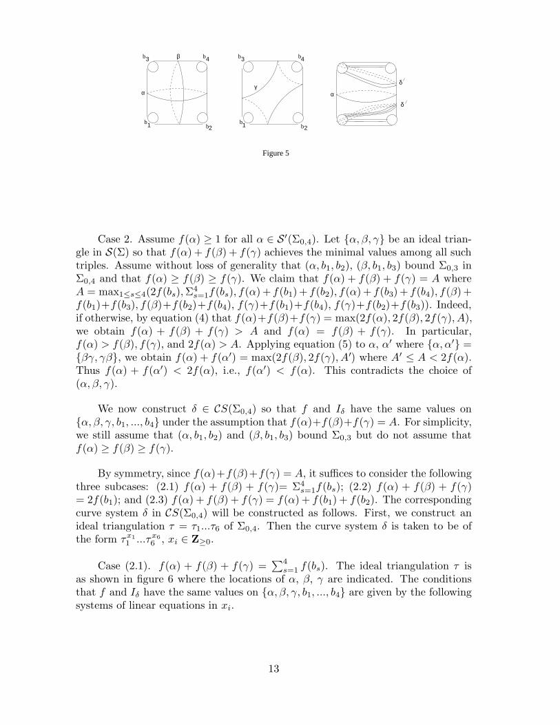
Case (2.1). f(α) + f(β) + f(γ) =∑4

s=1 f(bs). The ideal triangulation τ isas shown in figure 6 where the locations of α, β, γ are indicated. The conditionsthat f and Iδ have the same values on {α, β, γ, b1, ..., b4} are given by the followingsystems of linear equations in xi.

13

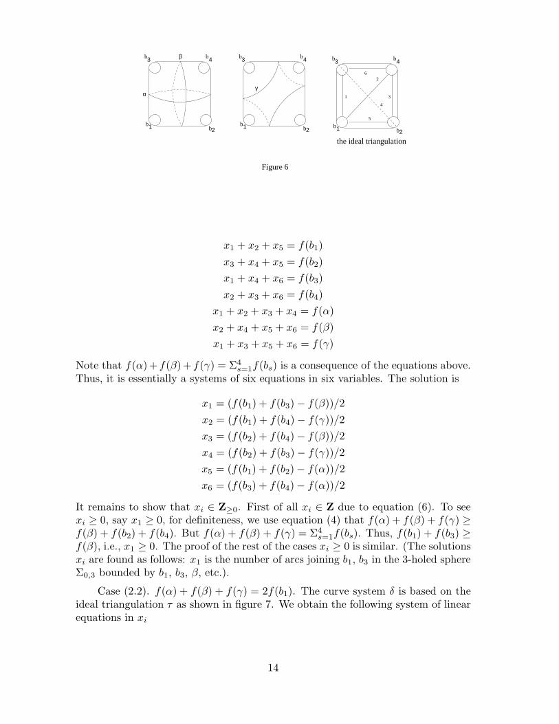
β

α

1

3 4b b

bb2 1

3 4b b

bb2

1

2

3

4

5

6

1

3 4b b

bb2

γ

Figure 6

the ideal triangulation

x1 + x2 + x5 = f(b1)

x3 + x4 + x5 = f(b2)

x1 + x4 + x6 = f(b3)

x2 + x3 + x6 = f(b4)

x1 + x2 + x3 + x4 = f(α)

x2 + x4 + x5 + x6 = f(β)

x1 + x3 + x5 + x6 = f(γ)

Note that f(α)+ f(β)+ f(γ) = Σ4s=1f(bs) is a consequence of the equations above.

Thus, it is essentially a systems of six equations in six variables. The solution is

x1 = (f(b1) + f(b3) − f(β))/2

x2 = (f(b1) + f(b4) − f(γ))/2

x3 = (f(b2) + f(b4) − f(β))/2

x4 = (f(b2) + f(b3) − f(γ))/2

x5 = (f(b1) + f(b2) − f(α))/2

x6 = (f(b3) + f(b4) − f(α))/2

It remains to show that xi ∈ Z≥0. First of all xi ∈ Z due to equation (6). To seexi ≥ 0, say x1 ≥ 0, for definiteness, we use equation (4) that f(α) + f(β) + f(γ) ≥f(β) + f(b2) + f(b4). But f(α) + f(β) + f(γ) = Σ4

s=1f(bs). Thus, f(b1) + f(b3) ≥f(β), i.e., x1 ≥ 0. The proof of the rest of the cases xi ≥ 0 is similar. (The solutionsxi are found as follows: x1 is the number of arcs joining b1, b3 in the 3-holed sphereΣ0,3 bounded by b1, b3, β, etc.).

Case (2.2). f(α) + f(β) + f(γ) = 2f(b1). The curve system δ is based on theideal triangulation τ as shown in figure 7. We obtain the following system of linearequations in xi

14

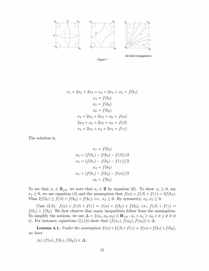
β

α

1

3 4b b

bb2 1

3 4b b

bb2

γ

Figure 7 the ideal triangulation

1

3 4b b

bb2

1

4

2 3

6

5

x1 + 2x2 + 2x3 + x4 + 2x5 + x6 = f(b1)

x4 = f(b2)

x1 = f(b3)

x6 = f(b4)

x1 + 2x2 + 2x3 + x6 = f(α)

2x3 + x4 + 2x5 + x6 = f(β)

x1 + 2x2 + x4 + 2x5 = f(γ)

The solution is,

x1 = f(b3)

x2 = (f(b1) − f(b3) − f(β))/2

x3 = (f(b1) − f(b4) − f(γ))/2

x4 = f(b2)

x5 = (f(b1) − f(b2) − f(α))/2

x6 = f(b4)

To see that xi ∈ Z≥0, we note that xi ∈ Z by equation (6). To show xi ≥ 0, sayx2 ≥ 0, we use equation (4) and the assumption that f(α) + f(β) + f(γ) = 2f(b1).Thus 2f(b1) ≥ f(β) + f(b3) + f(b1), i.e., x2 ≥ 0. By symmetry, x3, x5 ≥ 0.

Case (2.3). f(α) + f(β) + f(γ) = f(α) + f(b1) + f(b2), i.e., f(β) + f(γ) =f(b1) + f(b2). We first observe that many inequalities follow from the assumption.To simplify the notions, we use ∆ = {(a1, a2, a3) ∈ R≥0 : ai + aj ≥ ak, i 6= j 6= k 6=i}. For instance, equations (1),(4) show that (f(α1), f(α2), f(α3)) ∈ ∆.

Lemma 4.1. Under the assumption f(α)+f(β)+f(γ) = f(α)+f(b1)+f(b2),we have

(a) (f(α), f(b1), f(b2)) ∈ ∆;

15

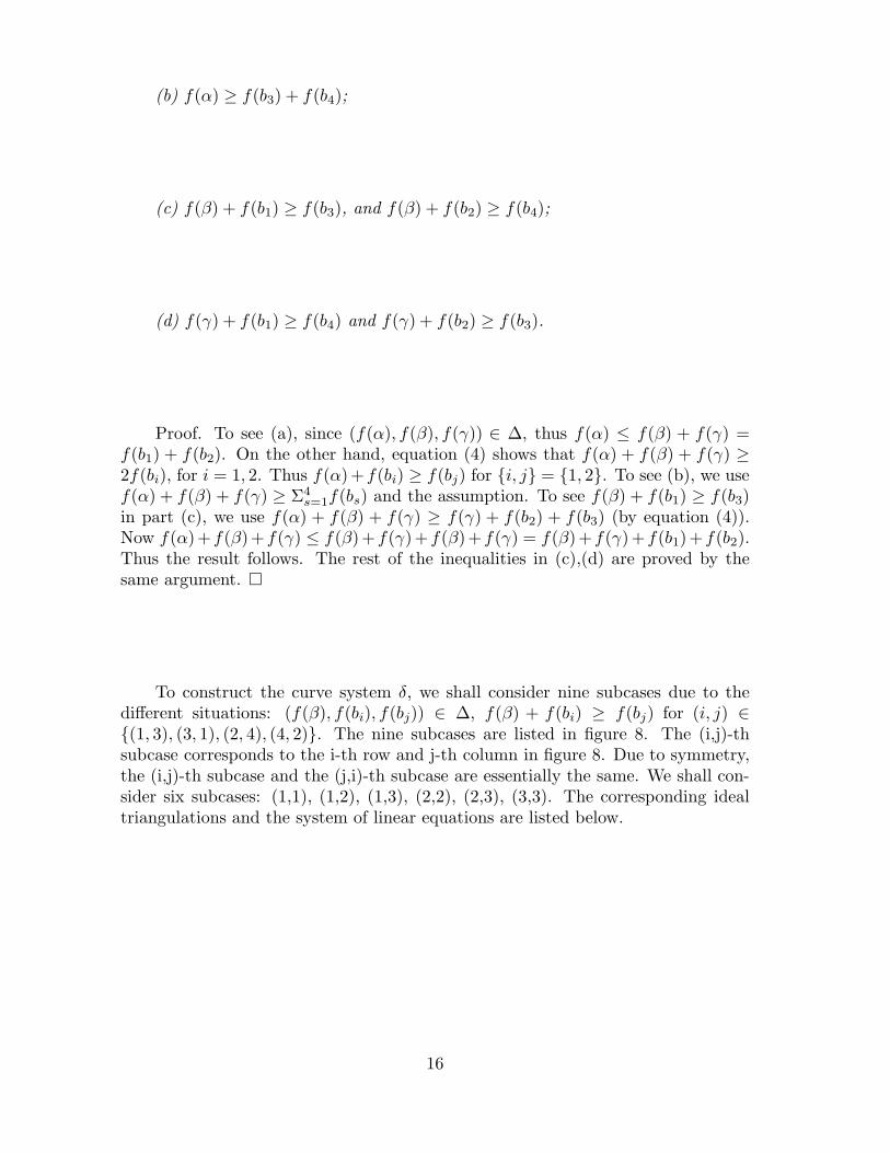
(b) f(α) ≥ f(b3) + f(b4);

(c) f(β) + f(b1) ≥ f(b3), and f(β) + f(b2) ≥ f(b4);

(d) f(γ) + f(b1) ≥ f(b4) and f(γ) + f(b2) ≥ f(b3).

Proof. To see (a), since (f(α), f(β), f(γ)) ∈ ∆, thus f(α) ≤ f(β) + f(γ) =f(b1) + f(b2). On the other hand, equation (4) shows that f(α) + f(β) + f(γ) ≥2f(bi), for i = 1, 2. Thus f(α)+f(bi) ≥ f(bj) for {i, j} = {1, 2}. To see (b), we usef(α) + f(β) + f(γ) ≥ Σ4

s=1f(bs) and the assumption. To see f(β) + f(b1) ≥ f(b3)in part (c), we use f(α) + f(β) + f(γ) ≥ f(γ) + f(b2) + f(b3) (by equation (4)).Now f(α)+f(β)+f(γ) ≤ f(β)+f(γ)+f(β)+f(γ) = f(β)+f(γ)+f(b1)+f(b2).Thus the result follows. The rest of the inequalities in (c),(d) are proved by thesame argument. �

To construct the curve system δ, we shall consider nine subcases due to thedifferent situations: (f(β), f(bi), f(bj)) ∈ ∆, f(β) + f(bi) ≥ f(bj) for (i, j) ∈{(1, 3), (3, 1), (2, 4), (4, 2)}. The nine subcases are listed in figure 8. The (i,j)-thsubcase corresponds to the i-th row and j-th column in figure 8. Due to symmetry,the (i,j)-th subcase and the (j,i)-th subcase are essentially the same. We shall con-sider six subcases: (1,1), (1,2), (1,3), (2,2), (2,3), (3,3). The corresponding idealtriangulations and the system of linear equations are listed below.

16

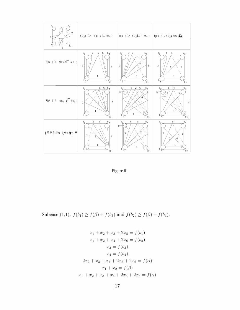
3bf( ) ∋

βf( ) 1bf( ) 3bf( )

3bf( ) βf( )

4bf( )βf( )2bf( ) 2bf( ) 4bf( )

1bf( )

1b

2bβ

1

3 4b b

bb2

∆,

+

+

+ + ∆, , ) α

1

3 4b b

bb2

Figure 8

1

3 4b b

bb2

1

3 4b b

bb2

1

3 4b b

bb2

1

3 4b b

bb2

1

3 4b b

bb2

1

3 4b b

bb2

1

3 4b b

bb2

1

3 4b b

bb2

, )(

1

2

43

5 6

1 1

11

1

1 1

2

2

2

2

22

3

3

33 3

4

4

4

4

4

4

4

5

5

5

55

5 5 5

6

6

6

6 6 6

6

6

3

33

1

2

(

4

2

f( )

f( ) f( ) 4bf( )

∋

β

γf( ) β

βf( )

Subcase (1,1). f(b1) ≥ f(β) + f(b3) and f(b2) ≥ f(β) + f(b4).

x1 + x2 + x3 + 2x5 = f(b1)

x1 + x2 + x4 + 2x6 = f(b2)

x3 = f(b3)

x4 = f(b4)

2x2 + x3 + x4 + 2x5 + 2x6 = f(α)

x1 + x2 = f(β)

x1 + x2 + x3 + x4 + 2x5 + 2x6 = f(γ)

17

The solution is,

x1 = (f(b1) + f(b2) − f(α))/2

x2 = (f(α) + f(β) − f(γ))/2

x3 = f(b3)

x4 = f(b4)

x5 = (f(b1) − f(β) − f(b3))/2

x6 = (f(b2) − f(β) − f(b4))/2

The solutions xi are in Z≥0 by lemma 4.1, equation (6) and the assumption (x5, x6 ≥0).

Subcase (1.2). f(b1) ≥ f(β) + f(b3) and f(β) ≥ f(b2) + f(b4).

x1 + x2 + x3 + x4 + 2x5 + 2x6 = f(b1)

x1 + x2 = f(b2)

x3 = f(b3)

x4 = f(b4)

2x2 + x3 + x4 + 2x5 + 2x6 = f(α)

x1 + x2 + x4 + 2x5 = f(β)

x1 + x2 + x3 + 2x6 = f(γ)

The solution is,

x1 = (f(b1) + f(b2) − f(α))/2

x2 = (f(b2) + f(α) − f(b1))/2

x3 = f(b3)

x4 = f(b4)

x5 = (f(β) − f(b2) − f(b4))/2

x6 = (f(b1) − f(b3) − f(β))/2

The solutions are in Z≥0 by lemma 4, equation (6) and the assumption.

Subcase (1.3). f(b1) ≥ f(β) + f(b3) and (f(β), f(b2), f(b4)) ∈ ∆.

x1 + x3 + 2x4 + x5 + x6 = f(b1)

x1 + x2 + x5 = f(b2)

x3 = f(b3)

x2 + x6 = f(b4)

x2 + x3 + 2x4 + 2x5 + x6 = f(α)

x1 + x5 + x6 = f(β)

x1 + x2 + x3 + 2x4 + x5 = f(γ)

18

The solution is,

x1 = (f(b1) + f(b2) − f(α))/2

x2 = (f(b2) + f(b4) − f(β))/2

x3 = f(b3)

x4 = (f(b1) − f(b3) − f(β))/2

x5 = (f(α) + f(β) − f(b1) − f(b4))/2

x6 = (f(b4) + f(β) − f(b2))/2

By the same argument as in the previous cases, all xi except possibly x5 are inZ≥0. It remains to show that x5 ∈ Z≥0. Indeed, f(α) + f(β) − f(b1) − f(b4) =(f(α)+f(β)+f(γ))−(f(γ)+f(b1)+f(b4)). Thus, by equations (4), (6), x5 ∈ Z≥0.

Subcase (2.2). f(β) ≥ f(b1) + f(b3) and f(β) ≥ f(b2) + f(b4)).

x1 + x2 + x4 + 2x6 = f(b1)

x1 + x2 + x3 + 2x5 = f(b2)

x3 = f(b3)

x4 = f(b4)

2x2 + x3 + x4 + 2x5 + 2x6 = f(α)

x1 + x2 + x3 + x4 + 2x5 + 2x6 = f(β)

x1 + x2 = f(γ)

The solution is

x1 = (f(b1) + f(b2) − f(α))/2

x2 = (f(α) + f(γ)− f(β))/2

x3 = f(b3)

x4 = f(b4)

x5 = (f(β) − f(b1) − f(b3))/2

x6 = (f(β) − f(b2) − f(b4))/2

The solutions xi’s are in Z≥0 by lemma 4.1, equations (4), (6) and the assump-tion.

Subcase (2.3). f(β) ≥ f(b1) + f(b3) and (f(β), f(b2), f(b4)) ∈ ∆.

x1 + x4 + x5 = f(b1)

x1 + x2 + x3 + x4 + 2x6 = f(b2)

x3 = f(b3)

x2 + x5 = f(b4)

x2 + x3 + 2x4 + x5 + 2x6 = f(α)

x1 + x3 + x4 + x5 + 2x6 = f(β)

x1 + x2 + x4 = f(γ)

19

The solution is

x1 = (f(b1) + f(b2) − f(α))/2

x2 = (f(b2) + f(b4) − f(β))/2

x3 = f(b3)

x4 = (f(α) + f(b1) − f(β) − f(b4))/2

x5 = (f(b1) + f(b4) − f(γ))/2

x6 = (f(β) − f(b1) − f(b3))/2

To show that the solutions are in Z≥0, it suffices to show that x4 ∈ Z≥0 (the restof the xi ∈ Z≥0 follows from equations (4),(6), and the assumption). For x4, weexpress x4 as 1

2((f(α) + f(β) + f(γ)) − (f(β) + f(b2) + f(b4)). Thus x4 is in Z≥0

by equations (4) and (6).

Subcase (3.3). Both (f(β), f(b1), f(b3)) and (f(β), f(b2), f(b4)) are in ∆.

The equation is,

x1 + x2 + x3 + x5 = f(b1)

x1 + x4 + x5 + x6 = f(b2)

x3 + x6 = f(b3)

x2 + x4 = f(b4)

x2 + x3 + x4 + 2x5 + x6 = f(α)

x1 + x2 + x5 + x6 = f(β)

x1 + x3 + x4 + x5 = f(γ)

The solution is,

x1 = (f(b1) + f(b2) − f(α))/2

x2 = (f(b4) + f(β) − f(b2))/2

x3 = (f(b1) + f(b3) − f(β))/2

x4 = (f(b2) + f(b4) − f(β))/2

x5 = (f(α) − f(b3) − f(b4))/2

x6 = (f(b3) + f(β) − f(b1))/2

By equations (4), (6), the solutions are in Z≥0.

This ends the proof of the proposition for Iδ. The proof of the characterizationof geometric functions on S(Σ0,4) is the same as in §3. Indeed, first of all, therational solutions of Σ3

i=1xi = max1≤i≤3;1≤j≤4(2xi,2yj, Σ4j=1yj , x1 + y1 + y2,x1 +

y3 +y4, x2 +y1 +y3,x2 +y2 +y4, x3 +y1 +y4,x3 +y2 +y3) are dense in the solutionsover R≥0. Also if we consider f(α1α2) as an unknown in equation (4), it becomes

20

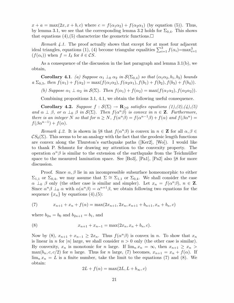
x + a = max(2x, x + b, c) where c = f(α1α2) + f(α2α1) (by equation (5)). Thus,by lemma 3.1, we see that the corresponding lemma 3.2 holds for Σ0,4. This showsthat equations (4),(5) characterize the geometric functions.�

Remark 4.1. The proof actually shows that except for at most four adjacentideal triangles, equations (1), (4) become triangular equalities

∑3i=1 f(αi)=max3

i=1

(f(αi)) when f = Iδ for δ ∈ CS.

As a consequence of the discussion in the last paragraph and lemma 3.1(b), weobtain,

Corollary 4.1. (a) Suppose α1 ⊥0 α2 in S(Σ0,4) so that (α1α2, b1, b2) boundsa Σ0,3, then f(α1) + f(α2) = max(f(α1α2), f(α2α1), f(b1) + f(b2), f(b3) + f(b4)).

(b) Suppose α1 ⊥ α2 in S(Σ). Then f(α1) + f(α2) = max(f(α1α2), f(α2α2)).

Combining propositions 3.1, 4.1, we obtain the following useful consequence.

Corollary 4.2. Suppose f : S(Σ) → R≥0 satisfies equations (1),(2),(4),(5)and α ⊥ β, or α ⊥0 β in S(Σ). Then f(αnβ) is convex in n ∈ Z. Furthermore,there is an integer N so that for n ≥ N , f(αnβ) = f(αn−1β) + f(α) and f(βαn) =f(βαn−1) + f(α).

Remark 4.2. It is shown in §8 that f(αnβ) is convex in n ∈ Z for all α, β ∈CS0(Σ). This seems to be an analogy with the fact that the geodesic length functionsare convex along the Thurston’s earthquake paths ([Ker2], [Wo]). I would liketo thank P. Schmutz for drawing my attention to the convexity property. Theoperation αnβ is similar to the extension of the earthquake from the Teichmullerspace to the measured lamination space. See [Bo3], [Pa1], [Pa2] also §8 for morediscussion.

Proof. Since α, β lie in an incompressible subsurface homeomorphic to eitherΣ1,1 or Σ0,4, we may assume that Σ ∼= Σ1,1 or Σ0,4. We shall consider the caseα ⊥0 β only (the other case is similar and simpler). Let xn = f(αnβ), n ∈ Z.Since αnβ ⊥0 α with α(αnβ) = αn+1β, we obtain following two equations for thesequence {xn} by equations (4),(5):

(7) xn+1 + xn + f(α) = max(2xn+1, 2xn, xn+1 + bn+1, xn + bn, c)

where b2n = b0 and b2n+1 = b1, and

(8) xn+1 + xn−1 = max(2xn, xn + bn, c).

Now by (8), xn+1 + xn−1 ≥ 2xn. Thus f(αnβ) is convex in n. To show that xn

is linear in n for |n| large, we shall consider n > 0 only (the other case is similar).By convexity, xn is monotonic for n large. If limn xn = ∞, then xn+1 ≥ xn >max(bn, c, c/2) for n large. Thus for n large, (7) becomes, xn+1 = xn + f(α). Iflimn xn = L is a finite number, take the limit to the equations (7) and (8). Weobtain:

2L + f(α) = max(2L, L + b∞, c)

21

and2L = max(2L, L + b∞, c)

where b∞ = max(b0, b1). Thus f(α) = 0. By (7), this shows xn = xn+1 for all n,i.e., f(αnβ) = f(αn−1β) + f(α). �

§5. A Reduction Proposition

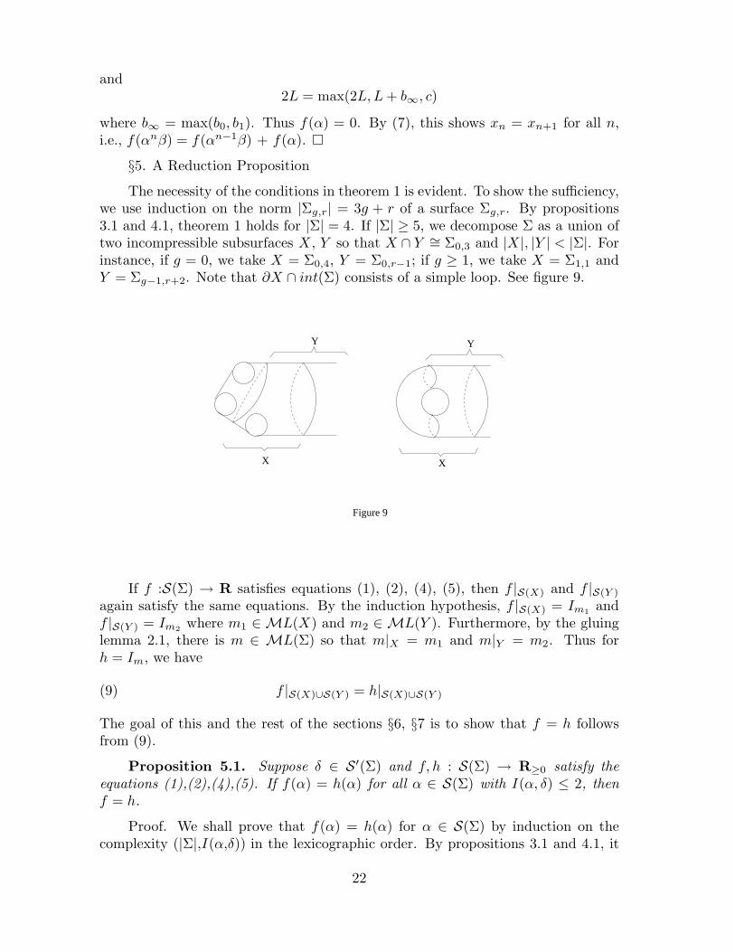
The necessity of the conditions in theorem 1 is evident. To show the sufficiency,we use induction on the norm |Σg,r| = 3g + r of a surface Σg,r. By propositions3.1 and 4.1, theorem 1 holds for |Σ| = 4. If |Σ| ≥ 5, we decompose Σ as a union oftwo incompressible subsurfaces X , Y so that X ∩ Y ∼= Σ0,3 and |X |, |Y | < |Σ|. Forinstance, if g = 0, we take X = Σ0,4, Y = Σ0,r−1; if g ≥ 1, we take X = Σ1,1 andY = Σg−1,r+2. Note that ∂X ∩ int(Σ) consists of a simple loop. See figure 9.

Figure 9

Y

X X

Y

If f :S(Σ) → R satisfies equations (1), (2), (4), (5), then f |S(X) and f |S(Y )

again satisfy the same equations. By the induction hypothesis, f |S(X) = Im1and

f |S(Y ) = Im2where m1 ∈ ML(X) and m2 ∈ ML(Y ). Furthermore, by the gluing

lemma 2.1, there is m ∈ ML(Σ) so that m|X = m1 and m|Y = m2. Thus forh = Im, we have

(9) f |S(X)∪S(Y ) = h|S(X)∪S(Y )

The goal of this and the rest of the sections §6, §7 is to show that f = h followsfrom (9).

Proposition 5.1. Suppose δ ∈ S′(Σ) and f, h : S(Σ) → R≥0 satisfy theequations (1),(2),(4),(5). If f(α) = h(α) for all α ∈ S(Σ) with I(α, δ) ≤ 2, thenf = h.

Proof. We shall prove that f(α) = h(α) for α ∈ S(Σ) by induction on thecomplexity (|Σ|,I(α,δ)) in the lexicographic order. By propositions 3.1 and 4.1, it

22

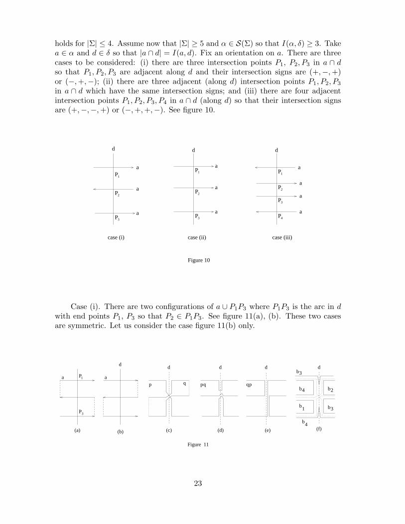
holds for |Σ| ≤ 4. Assume now that |Σ| ≥ 5 and α ∈ S(Σ) so that I(α, δ) ≥ 3. Takea ∈ α and d ∈ δ so that |a ∩ d| = I(a, d). Fix an orientation on a. There are threecases to be considered: (i) there are three intersection points P1, P2, P3 in a ∩ dso that P1, P2, P3 are adjacent along d and their intersection signs are (+,−, +)or (−, +,−); (ii) there are three adjacent (along d) intersection points P1, P2, P3

in a ∩ d which have the same intersection signs; and (iii) there are four adjacentintersection points P1, P2, P3, P4 in a ∩ d (along d) so that their intersection signsare (+,−,−, +) or (−, +, +,−). See figure 10.

P1

P1 P1

P 2P 2P 2

3P 3P

3P

P4

d d d

case (ii)case (i)

a

a

a

a

a

a

a

a

a

a

Figure 10

case (iii)

Case (i). There are two configurations of a ∪ P1P3 where P1P3 is the arc in dwith end points P1, P3 so that P2 ∈ P1P3. See figure 11(a), (b). These two casesare symmetric. Let us consider the case figure 11(b) only.

a

(a)

p q

d

(c)

pq

d

(d)

qp

d

(e)

1

24

4

3d

b

b

b

b

b3

(f)b

Figure 11

a

d

(b)

1P

P3

23

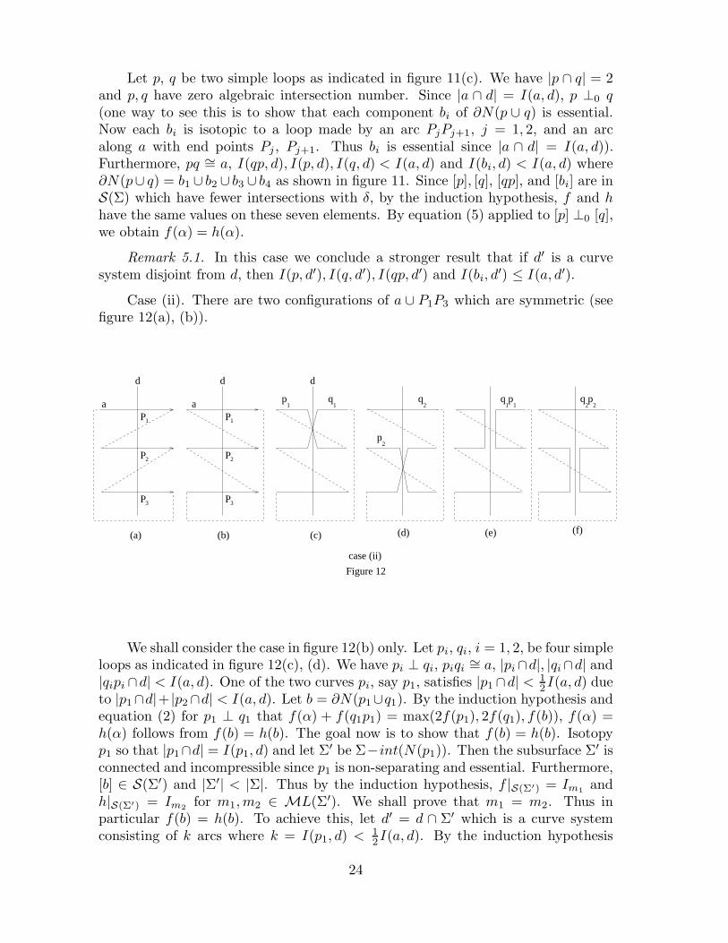
Let p, q be two simple loops as indicated in figure 11(c). We have |p ∩ q| = 2and p, q have zero algebraic intersection number. Since |a ∩ d| = I(a, d), p ⊥0 q(one way to see this is to show that each component bi of ∂N(p ∪ q) is essential.Now each bi is isotopic to a loop made by an arc PjPj+1, j = 1, 2, and an arcalong a with end points Pj , Pj+1. Thus bi is essential since |a ∩ d| = I(a, d)).Furthermore, pq ∼= a, I(qp, d), I(p, d), I(q, d) < I(a, d) and I(bi, d) < I(a, d) where∂N(p∪ q) = b1 ∪ b2 ∪ b3 ∪ b4 as shown in figure 11. Since [p], [q], [qp], and [bi] are inS(Σ) which have fewer intersections with δ, by the induction hypothesis, f and hhave the same values on these seven elements. By equation (5) applied to [p] ⊥0 [q],we obtain f(α) = h(α).

Remark 5.1. In this case we conclude a stronger result that if d′ is a curvesystem disjoint from d, then I(p, d′), I(q, d′), I(qp, d′) and I(bi, d

′) ≤ I(a, d′).

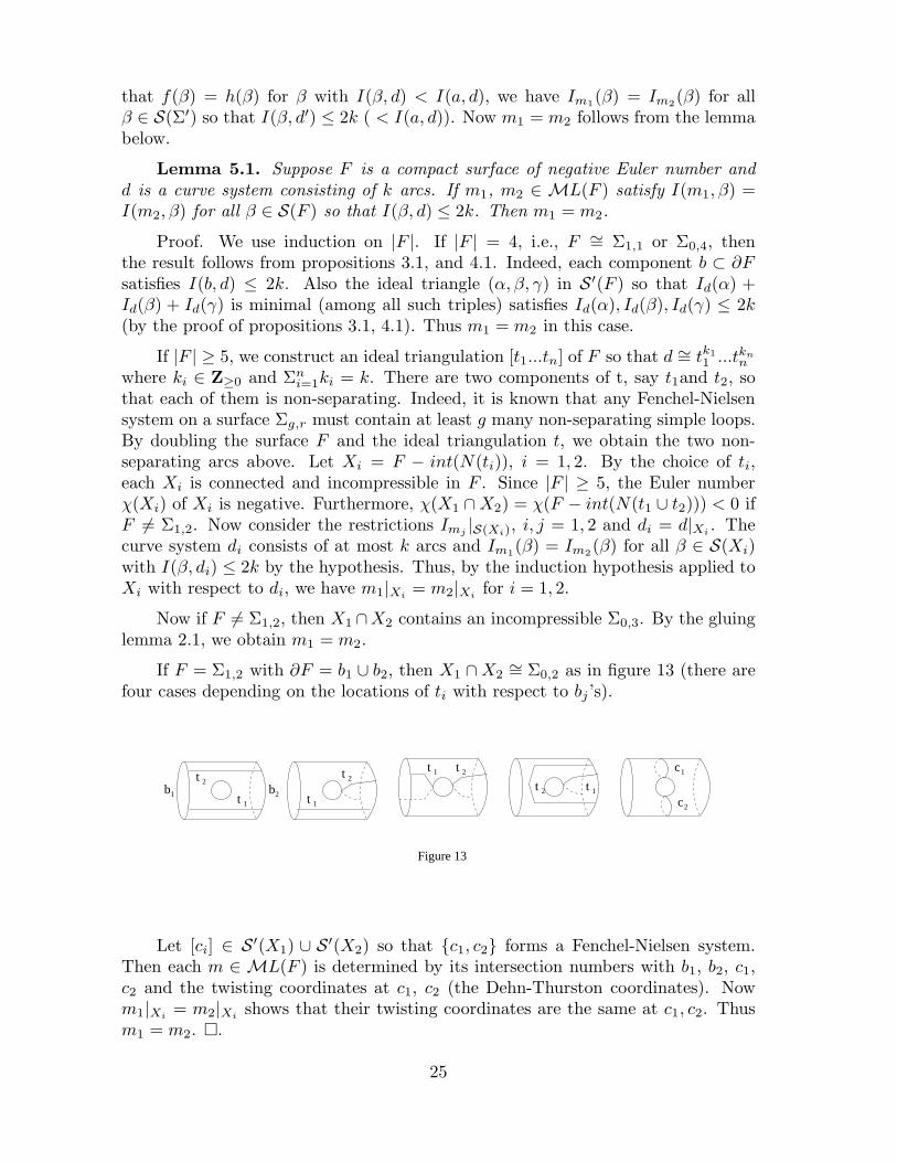
Case (ii). There are two configurations of a ∪ P1P3 which are symmetric (seefigure 12(a), (b)).

P1

P 2

3P

d

a

(a)

P1

P 2

3P

d

a

(b)

1p q

1

d

(c)

q2

p2

(d)

q1 1p q

2p

2

(f)(e)

case (ii)

Figure 12

We shall consider the case in figure 12(b) only. Let pi, qi, i = 1, 2, be four simpleloops as indicated in figure 12(c), (d). We have pi ⊥ qi, piqi

∼= a, |pi∩d|, |qi∩d| and|qipi ∩d| < I(a, d). One of the two curves pi, say p1, satisfies |p1 ∩d| < 1

2I(a, d) dueto |p1∩d|+ |p2∩d| < I(a, d). Let b = ∂N(p1∪q1). By the induction hypothesis andequation (2) for p1 ⊥ q1 that f(α) + f(q1p1) = max(2f(p1), 2f(q1), f(b)), f(α) =h(α) follows from f(b) = h(b). The goal now is to show that f(b) = h(b). Isotopyp1 so that |p1∩d| = I(p1, d) and let Σ′ be Σ−int(N(p1)). Then the subsurface Σ′ isconnected and incompressible since p1 is non-separating and essential. Furthermore,[b] ∈ S(Σ′) and |Σ′| < |Σ|. Thus by the induction hypothesis, f |S(Σ′) = Im1

andh|S(Σ′) = Im2

for m1, m2 ∈ ML(Σ′). We shall prove that m1 = m2. Thus inparticular f(b) = h(b). To achieve this, let d′ = d ∩ Σ′ which is a curve systemconsisting of k arcs where k = I(p1, d) < 1

2I(a, d). By the induction hypothesis

24

that f(β) = h(β) for β with I(β, d) < I(a, d), we have Im1(β) = Im2

(β) for allβ ∈ S(Σ′) so that I(β, d′) ≤ 2k ( < I(a, d)). Now m1 = m2 follows from the lemmabelow.

Lemma 5.1. Suppose F is a compact surface of negative Euler number andd is a curve system consisting of k arcs. If m1, m2 ∈ ML(F ) satisfy I(m1, β) =I(m2, β) for all β ∈ S(F ) so that I(β, d) ≤ 2k. Then m1 = m2.

Proof. We use induction on |F |. If |F | = 4, i.e., F ∼= Σ1,1 or Σ0,4, thenthe result follows from propositions 3.1, and 4.1. Indeed, each component b ⊂ ∂Fsatisfies I(b, d) ≤ 2k. Also the ideal triangle (α, β, γ) in S′(F ) so that Id(α) +Id(β) + Id(γ) is minimal (among all such triples) satisfies Id(α), Id(β), Id(γ) ≤ 2k(by the proof of propositions 3.1, 4.1). Thus m1 = m2 in this case.

If |F | ≥ 5, we construct an ideal triangulation [t1...tn] of F so that d ∼= tk1

1 ...tknn

where ki ∈ Z≥0 and Σni=1ki = k. There are two components of t, say t1and t2, so

that each of them is non-separating. Indeed, it is known that any Fenchel-Nielsensystem on a surface Σg,r must contain at least g many non-separating simple loops.By doubling the surface F and the ideal triangulation t, we obtain the two non-separating arcs above. Let Xi = F − int(N(ti)), i = 1, 2. By the choice of ti,each Xi is connected and incompressible in F . Since |F | ≥ 5, the Euler numberχ(Xi) of Xi is negative. Furthermore, χ(X1 ∩ X2) = χ(F − int(N(t1 ∪ t2))) < 0 ifF 6= Σ1,2. Now consider the restrictions Imj

|S(Xi), i, j = 1, 2 and di = d|Xi. The

curve system di consists of at most k arcs and Im1(β) = Im2

(β) for all β ∈ S(Xi)with I(β, di) ≤ 2k by the hypothesis. Thus, by the induction hypothesis applied toXi with respect to di, we have m1|Xi

= m2|Xifor i = 1, 2.

Now if F 6= Σ1,2, then X1 ∩X2 contains an incompressible Σ0,3. By the gluinglemma 2.1, we obtain m1 = m2.

If F = Σ1,2 with ∂F = b1 ∪ b2, then X1 ∩ X2∼= Σ0,2 as in figure 13 (there are

four cases depending on the locations of ti with respect to bj ’s).

1t

2t

1t

2t1t

2t1t

2t2b1b

c

c

1

2

Figure 13

Let [ci] ∈ S′(X1) ∪ S′(X2) so that {c1, c2} forms a Fenchel-Nielsen system.Then each m ∈ ML(F ) is determined by its intersection numbers with b1, b2, c1,c2 and the twisting coordinates at c1, c2 (the Dehn-Thurston coordinates). Nowm1|Xi

= m2|Xishows that their twisting coordinates are the same at c1, c2. Thus

m1 = m2. �.

25

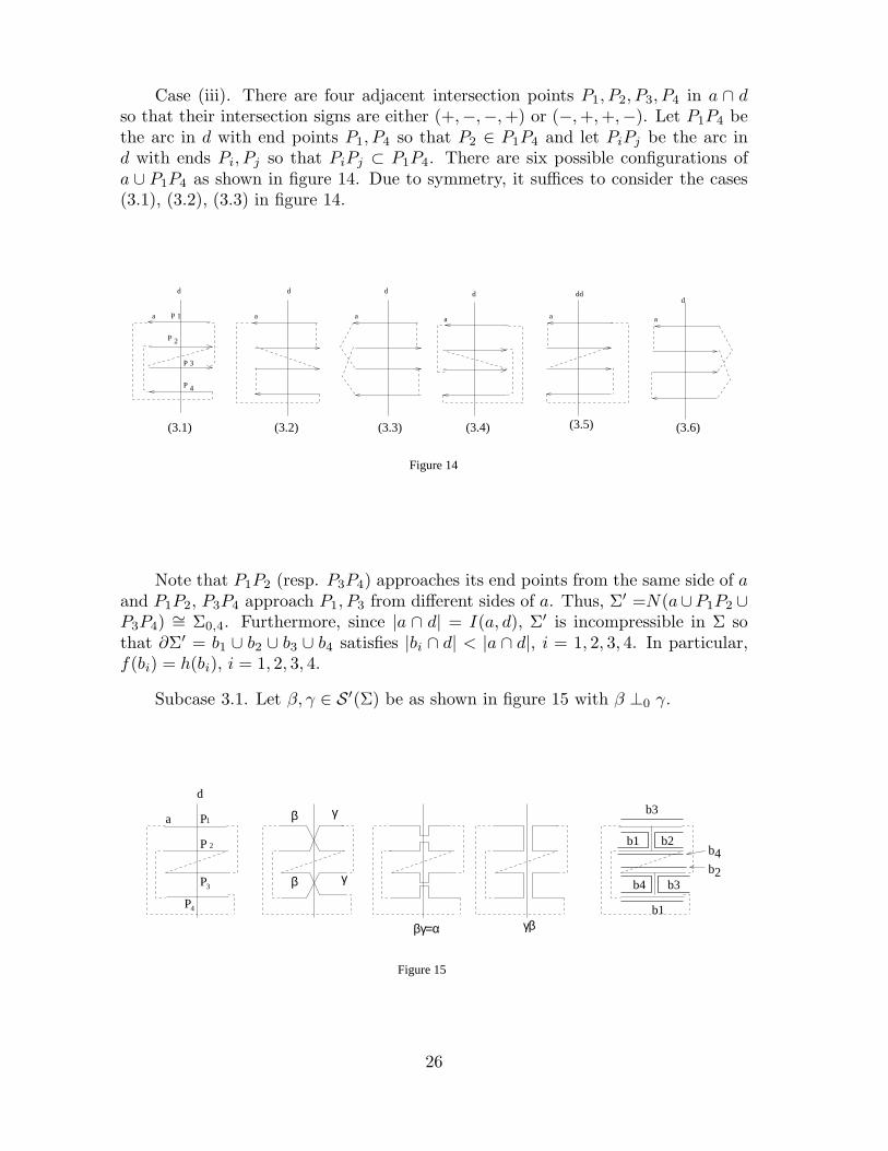
Case (iii). There are four adjacent intersection points P1, P2, P3, P4 in a ∩ dso that their intersection signs are either (+,−,−, +) or (−, +, +,−). Let P1P4 bethe arc in d with end points P1, P4 so that P2 ∈ P1P4 and let PiPj be the arc ind with ends Pi, Pj so that PiPj ⊂ P1P4. There are six possible configurations ofa ∪ P1P4 as shown in figure 14. Due to symmetry, it suffices to consider the cases(3.1), (3.2), (3.3) in figure 14.

Figure 14

d d d d dd

d

a a a a a aP

P

P

1

3

4

(3.1) (3.2) (3.3) (3.5)(3.4) (3.6)

2P

Note that P1P2 (resp. P3P4) approaches its end points from the same side of aand P1P2, P3P4 approach P1, P3 from different sides of a. Thus, Σ′ =N(a∪P1P2 ∪P3P4) ∼= Σ0,4. Furthermore, since |a ∩ d| = I(a, d), Σ′ is incompressible in Σ sothat ∂Σ′ = b1 ∪ b2 ∪ b3 ∪ b4 satisfies |bi ∩ d| < |a ∩ d|, i = 1, 2, 3, 4. In particular,f(bi) = h(bi), i = 1, 2, 3, 4.

Subcase 3.1. Let β, γ ∈ S′(Σ) be as shown in figure 15 with β ⊥0 γ.

β γ

βγ=α γβ

b1 b2

b3b

4b

b24

Figure 15

β γ

1b

b3 d

a P

P

P

P

1

2

3

4

26

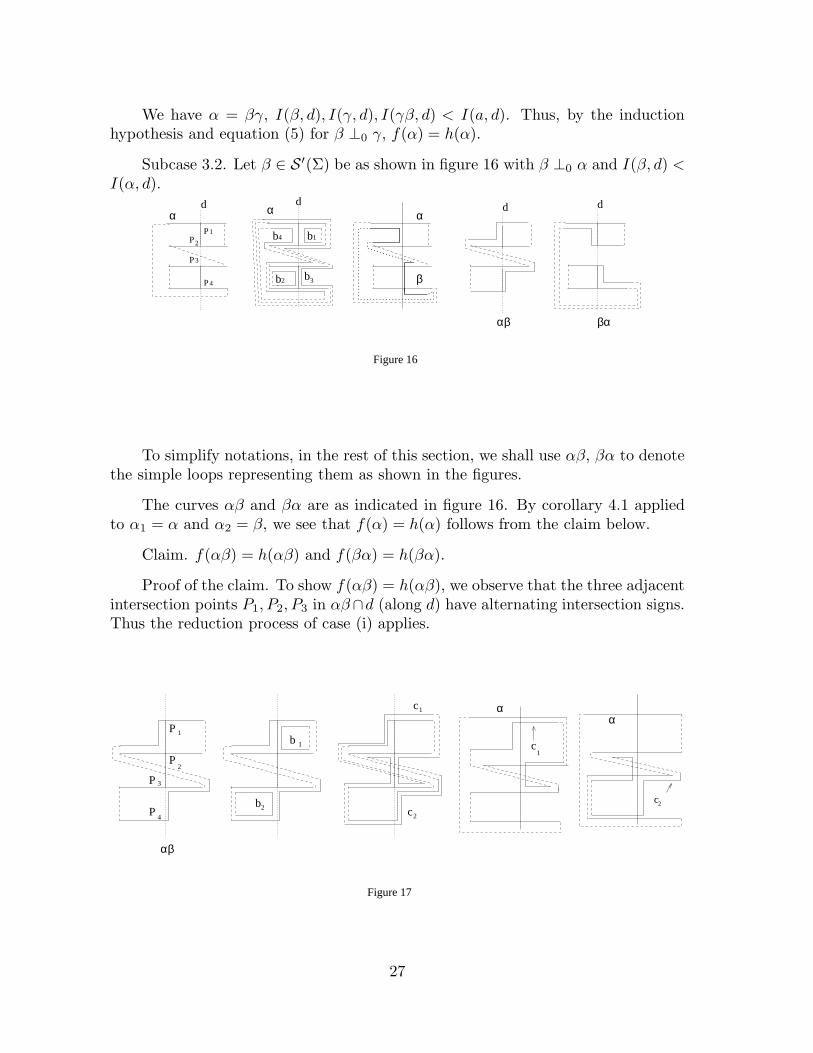
We have α = βγ, I(β, d), I(γ, d), I(γβ, d) < I(a, d). Thus, by the inductionhypothesis and equation (5) for β ⊥0 γ, f(α) = h(α).

Subcase 3.2. Let β ∈ S′(Σ) be as shown in figure 16 with β ⊥0 α and I(β, d) <I(α, d).

d d d

Figure 16

β

α

αβ βα

d

b

b b

b 1

2 3

4

P

3

4

P

P2

P1

αα

To simplify notations, in the rest of this section, we shall use αβ, βα to denotethe simple loops representing them as shown in the figures.

The curves αβ and βα are as indicated in figure 16. By corollary 4.1 appliedto α1 = α and α2 = β, we see that f(α) = h(α) follows from the claim below.

Claim. f(αβ) = h(αβ) and f(βα) = h(βα).

Proof of the claim. To show f(αβ) = h(αβ), we observe that the three adjacentintersection points P1, P2, P3 in αβ∩d (along d) have alternating intersection signs.Thus the reduction process of case (i) applies.

c1

c2

c1

b 1

b2

α

c2

α1P

2P

3P

4P

Figure 17

αβ

27

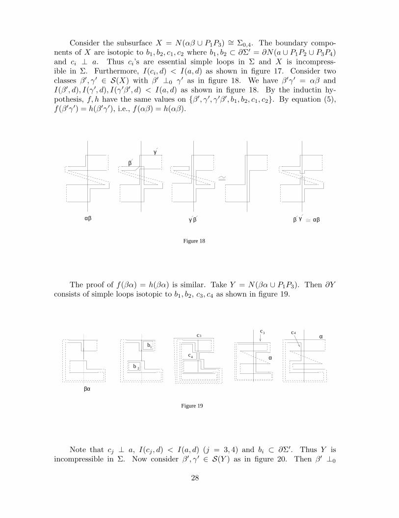
Consider the subsurface X = N(αβ ∪ P1P3) ∼= Σ0,4. The boundary compo-nents of X are isotopic to b1, b2, c1, c2 where b1, b2 ⊂ ∂Σ′ = ∂N(a ∪ P1P2 ∪ P3P4)and ci ⊥ a. Thus ci’s are essential simple loops in Σ and X is incompress-ible in Σ. Furthermore, I(ci, d) < I(a, d) as shown in figure 17. Consider twoclasses β′, γ′ ∈ S(X) with β′ ⊥0 γ′ as in figure 18. We have β′γ′ = αβ andI(β′, d), I(γ′, d), I(γ′β′, d) < I(a, d) as shown in figure 18. By the inductin hy-pothesis, f, h have the same values on {β′, γ′, γ′β′, b1, b2, c1, c2}. By equation (5),f(β′γ′) = h(β′γ′), i.e., f(αβ) = h(αβ).

γ β γβ αβ

γ

β

αβ

Figure 18

The proof of f(βα) = h(βα) is similar. Take Y = N(βα ∪ P1P3). Then ∂Yconsists of simple loops isotopic to b1, b2, c3, c4 as shown in figure 19.

1

2

Figure 19

b

b

c

c

βα

c cα

α

3

4

3 4

Note that cj ⊥ a, I(cj , d) < I(a, d) (j = 3, 4) and bi ⊂ ∂Σ′. Thus Y isincompressible in Σ. Now consider β′, γ′ ∈ S(Y ) as in figure 20. Then β′ ⊥0

28

γ′, β′γ′ = βα, and I(β′, d), I(γ′, d), I(γ′β′, d) < I(a, d). Thus by the inductionhypothesis and equation (5), f(βα) = h(βα).

Figure 20

γ β β γ

β

γ

βα βα

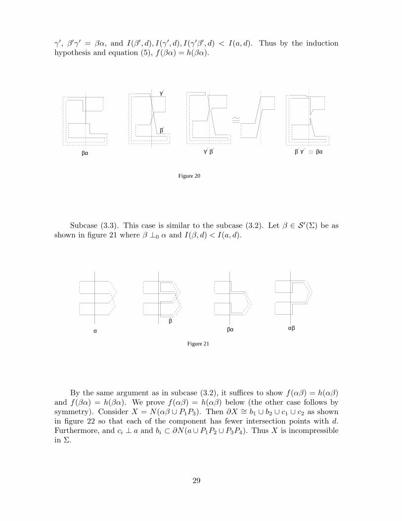
Subcase (3.3). This case is similar to the subcase (3.2). Let β ∈ S′(Σ) be asshown in figure 21 where β ⊥0 α and I(β, d) < I(a, d).

Figure 21

α

ββα αβ

By the same argument as in subcase (3.2), it suffices to show f(αβ) = h(αβ)and f(βα) = h(βα). We prove f(αβ) = h(αβ) below (the other case follows bysymmetry). Consider X = N(αβ ∪ P1P3). Then ∂X ∼= b1 ∪ b2 ∪ c1 ∪ c2 as shownin figure 22 so that each of the component has fewer intersection points with d.Furthermore, and ci ⊥ a and bi ⊂ ∂N(a∪ P1P2 ∪ P3P4). Thus X is incompressiblein Σ.

29

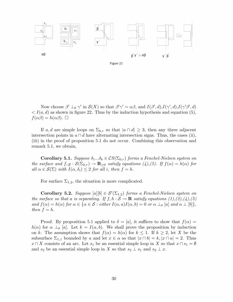
2

β

γ

βγγβ

c

b

b

c

2

11

Figure 22

αβαβ

P

P

1

2P

3

Now choose β′ ⊥0 γ′ in S(X) so that β′γ′ = αβ, and I(β′, d),I(γ′, d),I(γ′β′, d)< I(a, d) as shown in figure 22. Thus by the induction hypothesis and equation (5),f(αβ) = h(αβ). �

If a, d are simple loops on Σ0,r so that |a ∩ d| ≥ 3, then any three adjacentintersection points in a∩ d have alternating intersection signs. Thus, the cases (ii),(iii) in the proof of proposition 5.1 do not occur. Combining this observation andremark 5.1, we obtain,

Corollary 5.1. Suppose δ1...δk ∈ CS(Σ0,r) forms a Fenchel-Nielsen system onthe surface and f, g : S(Σ0,r) → R≥0 satisfy equations (4),(5). If f(α) = h(α) forall α ∈ S(Σ) with I(α, δi) ≤ 2 for all i, then f = h.

For surface Σ1,2, the situation is more complicated.

Corollary 5.2. Suppose [a][b] ∈ S′(Σ1,2) forms a Fenchel-Nielsen system onthe surface so that a is separating. If f, h : S → R satisfy equations (1),(2),(4),(5)and f(α) = h(α) for α ∈ {α ∈ S : either I(α, a)I(α, b) = 0 or α ⊥0 [a] and α ⊥ [b]},then f = h.

Proof. By proposition 5.1 applied to δ = [a], it suffices to show that f(α) =h(α) for α ⊥0 [a]. Let k = I(α, b). We shall prove the proposition by inductionon k. The assumption shows that f(α) = h(α) for k ≤ 1. If k ≥ 2, let X be thesubsurface Σ1,1 bounded by a and let x ∈ α so that |x ∩ b| = k, |x ∩ a| = 2. Thusx∩X consists of an arc. Let s1 be an essential simple loop in X so that x∩ s1 = ∅and s2 be an essential simple loop in X so that s2 ⊥ s1 and s2 ⊥ x.

30

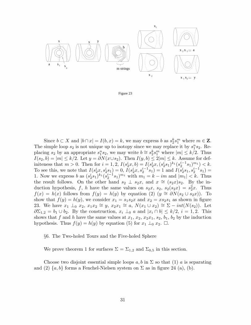
1x

x 2

x 2 x 1

x 1 x2

a s

b

s 12

x x y

m strings

Figure 23

a

y

Since b ⊂ X and |b∩ x| = I(b, x) = k, we may express b as sk2sm

1 where m ∈ Z.The simple loop s2 is not unique up to isotopy since we may replace it by sn

1 s2. Re-placing s2 by an appropriate sn

1s2, we may write b ∼= sk2s

m1 where |m| ≤ k/2. Thus

I(s2, b) = |m| ≤ k/2. Let y = ∂N(x∪s2). Then I(y, b) ≤ 2|m| ≤ k. Assume for def-initeness that m > 0. Then for i = 1, 2, I(si

2x, b) = I(si2x, (si

2s1)k1(si−1

2 s1)m1) < k.

To see this, we note that I(si2x, si

2s1) = 0, I(si2x, si−1

2 s1) = 1 and I(si2s1, s

i−12 s1) =

1. Now we express b as (si2s1)

k1(si−12 s1)

m1 with m1 = k − im and |m1| < k. Thusthe result follows. On the other hand s2 ⊥ s2x, and x ∼= (s2x)s2. By the in-duction hypothesis, f , h have the same values on s2x, s2, s2(s2x) = s2

2x. Thusf(x) = h(x) follows from f(y) = h(y) by equation (2) (y ∼= ∂N(s2 ∪ s2x)). Toshow that f(y) = h(y), we consider x1 = s1s2x and x2 = xs2s1 as shown in figure23. We have x1 ⊥0 x2, x1x2

∼= y, x2x1∼= a, N(x1 ∪ x2) ∼= Σ − int(N(s2)). Let

∂Σ1,2 = b1 ∪ b2. By the construction, xi ⊥0 a and |xi ∩ b| ≤ k/2, i = 1, 2. Thisshows that f and h have the same values at x1, x2, x2x1, s2, b1, b2 by the inductionhypothesis. Thus f(y) = h(y) by equation (5) for x1 ⊥0 x2. �.

§6. The Two-holed Tours and the Five-holed Sphere

We prove theorem 1 for surfaces Σ = Σ1,2 and Σ0,5 in this section.

Choose two disjoint essential simple loops a, b in Σ so that (1) a is separatingand (2) {a, b} forms a Fenchel-Nielsen system on Σ as in figure 24 (a), (b).

31

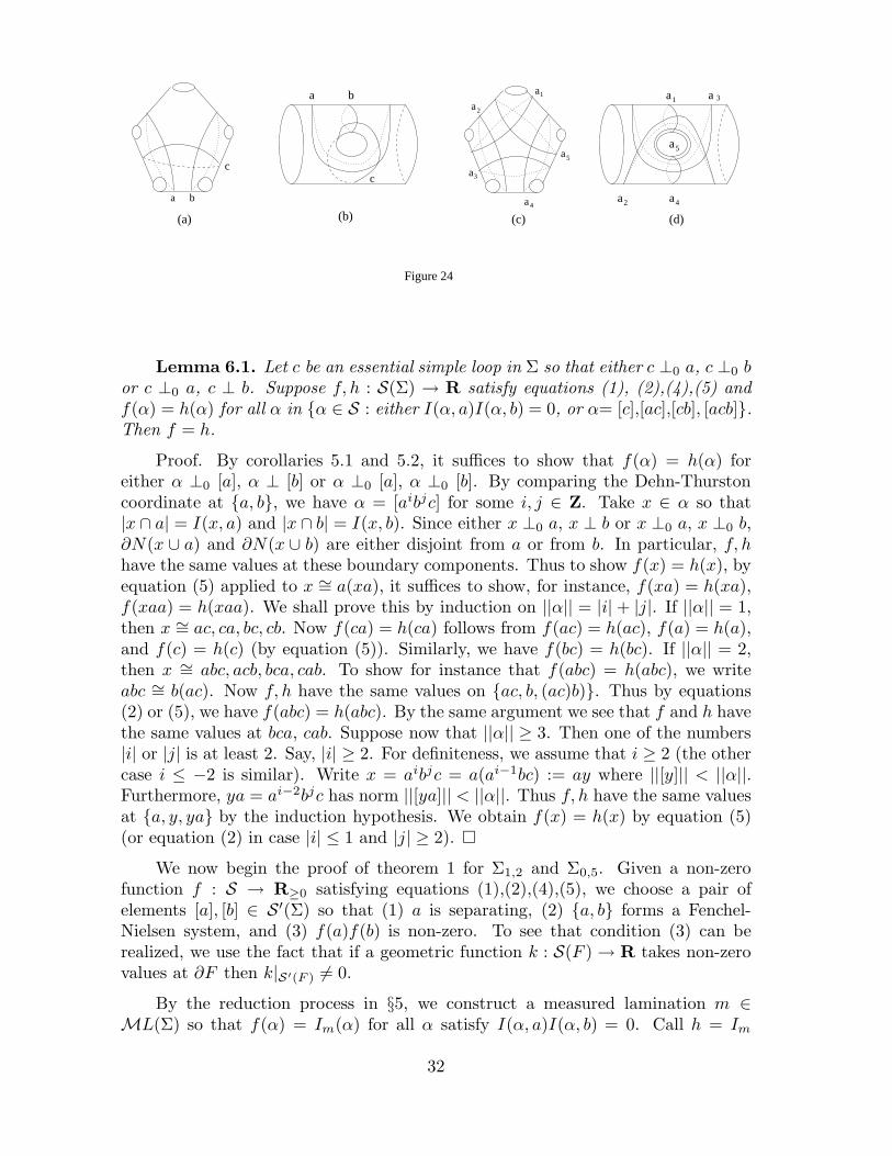
a b

a a

aa1

2

a

4

5

3

a b

a

a

a

a

a

1

2

3

4

5

(a) (b)

Figure 24

(c) (d)

cc

Lemma 6.1. Let c be an essential simple loop in Σ so that either c ⊥0 a, c ⊥0 bor c ⊥0 a, c ⊥ b. Suppose f, h : S(Σ) → R satisfy equations (1), (2),(4),(5) andf(α) = h(α) for all α in {α ∈ S : either I(α, a)I(α, b) = 0, or α= [c],[ac],[cb], [acb]}.Then f = h.

Proof. By corollaries 5.1 and 5.2, it suffices to show that f(α) = h(α) foreither α ⊥0 [a], α ⊥ [b] or α ⊥0 [a], α ⊥0 [b]. By comparing the Dehn-Thurstoncoordinate at {a, b}, we have α = [aibjc] for some i, j ∈ Z. Take x ∈ α so that|x ∩ a| = I(x, a) and |x ∩ b| = I(x, b). Since either x ⊥0 a, x ⊥ b or x ⊥0 a, x ⊥0 b,∂N(x ∪ a) and ∂N(x ∪ b) are either disjoint from a or from b. In particular, f, hhave the same values at these boundary components. Thus to show f(x) = h(x), byequation (5) applied to x ∼= a(xa), it suffices to show, for instance, f(xa) = h(xa),f(xaa) = h(xaa). We shall prove this by induction on ||α|| = |i| + |j|. If ||α|| = 1,then x ∼= ac, ca, bc, cb. Now f(ca) = h(ca) follows from f(ac) = h(ac), f(a) = h(a),and f(c) = h(c) (by equation (5)). Similarly, we have f(bc) = h(bc). If ||α|| = 2,then x ∼= abc, acb, bca, cab. To show for instance that f(abc) = h(abc), we writeabc ∼= b(ac). Now f, h have the same values on {ac, b, (ac)b)}. Thus by equations(2) or (5), we have f(abc) = h(abc). By the same argument we see that f and h havethe same values at bca, cab. Suppose now that ||α|| ≥ 3. Then one of the numbers|i| or |j| is at least 2. Say, |i| ≥ 2. For definiteness, we assume that i ≥ 2 (the othercase i ≤ −2 is similar). Write x = aibjc = a(ai−1bc) := ay where ||[y]|| < ||α||.Furthermore, ya = ai−2bjc has norm ||[ya]|| < ||α||. Thus f, h have the same valuesat {a, y, ya} by the induction hypothesis. We obtain f(x) = h(x) by equation (5)(or equation (2) in case |i| ≤ 1 and |j| ≥ 2). �

We now begin the proof of theorem 1 for Σ1,2 and Σ0,5. Given a non-zerofunction f : S → R≥0 satisfying equations (1),(2),(4),(5), we choose a pair ofelements [a], [b] ∈ S′(Σ) so that (1) a is separating, (2) {a, b} forms a Fenchel-Nielsen system, and (3) f(a)f(b) is non-zero. To see that condition (3) can berealized, we use the fact that if a geometric function k : S(F ) → R takes non-zerovalues at ∂F then k|S′(F ) 6= 0.

By the reduction process in §5, we construct a measured lamination m ∈ML(Σ) so that f(α) = Im(α) for all α satisfy I(α, a)I(α, b) = 0. Call h = Im

32

for simplicity. By lemma 6.1, it suffices to find [c] ∈ S so that c ⊥0 a, c ⊥ b orc ⊥0 b and f, h have the same values at {c, ac, cb, acb}.

We shall consider Σ =Σ1,2 and Σ0,5 separately.

Case 1. Σ = Σ1,2.

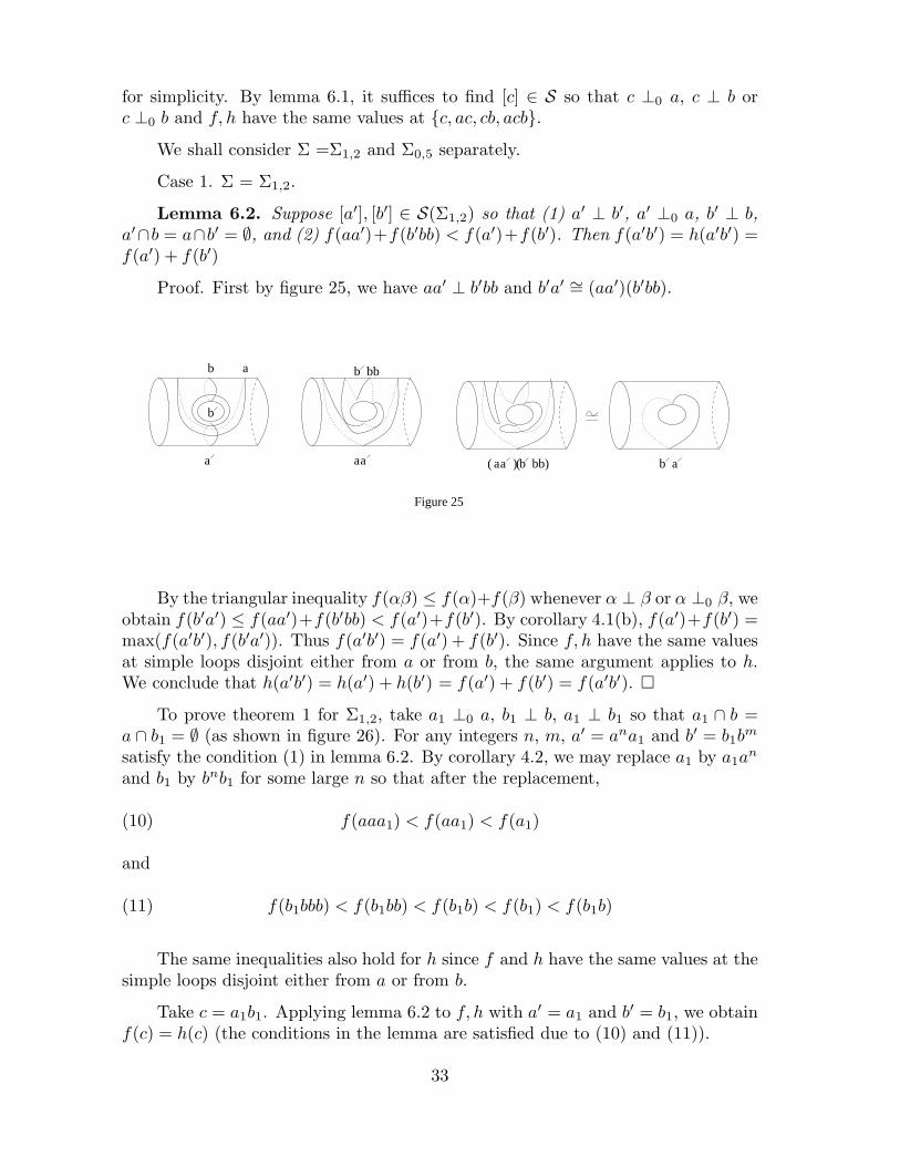
Lemma 6.2. Suppose [a′], [b′] ∈ S(Σ1,2) so that (1) a′ ⊥ b′, a′ ⊥0 a, b′ ⊥ b,a′∩b = a∩b′ = ∅, and (2) f(aa′)+f(b′bb) < f(a′)+f(b′). Then f(a′b′) = h(a′b′) =f(a′) + f(b′)

Proof. First by figure 25, we have aa′ ⊥ b′bb and b′a′ ∼= (aa′)(b′bb).

b

a

b bb

aa b aaa b bb( () )

b a

Figure 25

By the triangular inequality f(αβ) ≤ f(α)+f(β) whenever α ⊥ β or α ⊥0 β, weobtain f(b′a′) ≤ f(aa′)+f(b′bb) < f(a′)+f(b′). By corollary 4.1(b), f(a′)+f(b′) =max(f(a′b′), f(b′a′)). Thus f(a′b′) = f(a′) + f(b′). Since f, h have the same valuesat simple loops disjoint either from a or from b, the same argument applies to h.We conclude that h(a′b′) = h(a′) + h(b′) = f(a′) + f(b′) = f(a′b′). �

To prove theorem 1 for Σ1,2, take a1 ⊥0 a, b1 ⊥ b, a1 ⊥ b1 so that a1 ∩ b =a ∩ b1 = ∅ (as shown in figure 26). For any integers n, m, a′ = ana1 and b′ = b1b

m

satisfy the condition (1) in lemma 6.2. By corollary 4.2, we may replace a1 by a1an

and b1 by bnb1 for some large n so that after the replacement,

(10) f(aaa1) < f(aa1) < f(a1)

and

(11) f(b1bbb) < f(b1bb) < f(b1b) < f(b1) < f(b1b)

The same inequalities also hold for h since f and h have the same values at thesimple loops disjoint either from a or from b.

Take c = a1b1. Applying lemma 6.2 to f, h with a′ = a1 and b′ = b1, we obtainf(c) = h(c) (the conditions in the lemma are satisfied due to (10) and (11)).

33

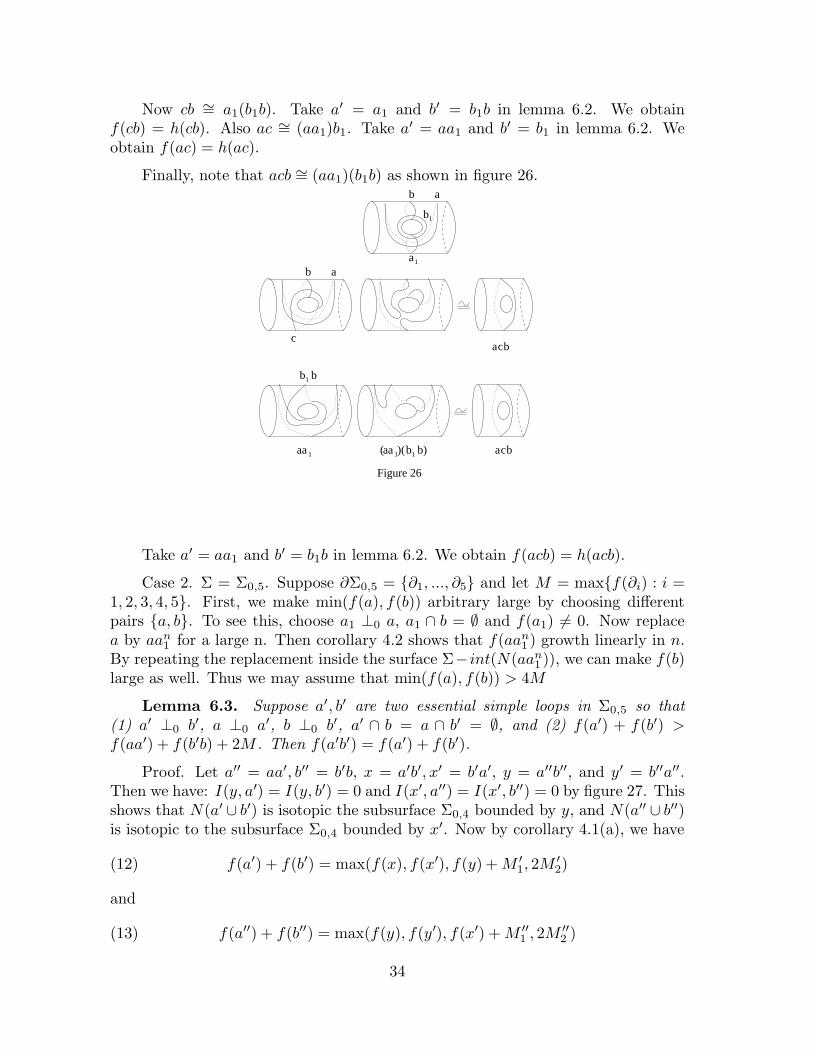
Now cb ∼= a1(b1b). Take a′ = a1 and b′ = b1b in lemma 6.2. We obtainf(cb) = h(cb). Also ac ∼= (aa1)b1. Take a′ = aa1 and b′ = b1 in lemma 6.2. Weobtain f(ac) = h(ac).

Finally, note that acb ∼= (aa1)(b1b) as shown in figure 26.

acb

acb

b b1

aa 1 aa 1 b b1

Figure 26

( )( )

b a

c

b a

b

a1

1

Take a′ = aa1 and b′ = b1b in lemma 6.2. We obtain f(acb) = h(acb).

Case 2. Σ = Σ0,5. Suppose ∂Σ0,5 = {∂1, ..., ∂5} and let M = max{f(∂i) : i =1, 2, 3, 4, 5}. First, we make min(f(a), f(b)) arbitrary large by choosing differentpairs {a, b}. To see this, choose a1 ⊥0 a, a1 ∩ b = ∅ and f(a1) 6= 0. Now replacea by aan

1 for a large n. Then corollary 4.2 shows that f(aan1 ) growth linearly in n.

By repeating the replacement inside the surface Σ− int(N(aan1 )), we can make f(b)

large as well. Thus we may assume that min(f(a), f(b)) > 4M

Lemma 6.3. Suppose a′, b′ are two essential simple loops in Σ0,5 so that(1) a′ ⊥0 b′, a ⊥0 a′, b ⊥0 b′, a′ ∩ b = a ∩ b′ = ∅, and (2) f(a′) + f(b′) >f(aa′) + f(b′b) + 2M . Then f(a′b′) = f(a′) + f(b′).

Proof. Let a′′ = aa′, b′′ = b′b, x = a′b′, x′ = b′a′, y = a′′b′′, and y′ = b′′a′′.Then we have: I(y, a′) = I(y, b′) = 0 and I(x′, a′′) = I(x′, b′′) = 0 by figure 27. Thisshows that N(a′ ∪ b′) is isotopic the subsurface Σ0,4 bounded by y, and N(a′′ ∪ b′′)is isotopic to the subsurface Σ0,4 bounded by x′. Now by corollary 4.1(a), we have

(12) f(a′) + f(b′) = max(f(x), f(x′), f(y) + M ′1, 2M ′

2)

and

(13) f(a′′) + f(b′′) = max(f(y), f(y′), f(x′) + M ′′1 , 2M ′′

2 )

34

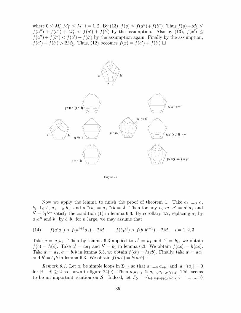
where 0 ≤ M ′i , M

′′i ≤ M , i = 1, 2. By (13), f(y) ≤ f(a′′)+f(b′′). Thus f(y)+M ′

1 ≤f(a′′) + f(b′′) + M ′

1 < f(a′) + f(b′) by the assumption. Also by (13), f(x′) ≤f(a′′) + f(b′′) < f(a′) + f(b′) by the assumption again. Finally by the assumption,f(a′) + f(b′) > 2M ′

2. Thus, (12) becomes f(x) = f(a′) + f(b′) �

a b

a b

b b aa( ))(

aa b b( )( )

b a

a b

b a

aa b b( )( )

b b

aab

Figure 27

a

y

y

yx

a

b

=

=

=

=

=

=

=

x

x

=

Now we apply the lemma to finish the proof of theorem 1. Take a1 ⊥0 a,b1 ⊥0 b, a1 ⊥0 b1, and a ∩ b1 = a1 ∩ b = ∅. Then for any n, m, a′ = ana1 andb′ = b1b

m satisfy the condition (1) in lemma 6.3. By corollary 4.2, replacing a1 bya1a

n and b1 by bnb1 for n large, we may assume that

(14) f(aia1) > f(ai+1a1) + 2M, f(b1bi) > f(b1b

i+1) + 2M, i = 1, 2, 3

Take c = a1b1. Then by lemma 6.3 applied to a′ = a1 and b′ = b1, we obtainf(c) = h(c). Take a′ = aa1 and b′ = b1 in lemma 6.3. We obtain f(ac) = h(ac).Take a′ = a1, b′ = b1b in lemma 6.3, we obtain f(cb) = h(cb). Finally, take a′ = aa1

and b′ = b1b in lemma 6.3. We obtain f(acb) = h(acb). �

Remark 6.1. Let ai be simple loops in Σ0,5 so that ai ⊥0 ai+1 and |ai ∩aj | = 0for |i − j| ≥ 2 as shown in figure 24(c). Then aiai+1

∼= ai+2ai+3ai+4. This seemsto be an important relation on S. Indeed, let F0 = {ai, aiai+1, bi : i = 1, ..., 5}

35

where bi’s are the boundary components. Then the proof of lemma 6.1 shows thatS(Σ0,5) = ∪∞

n=0Fn where Fn+1 = Fn ∪ {α|α = βγ with β ⊥0 γ, β, γ, γβ and thefour components of ∂N(β ∪ γ) are in Fn}. The corresponding curves for Σ1,2 areas shown in figure 24.

§7. Proofs of Theorem 1 and the Corollary

To prove theorem 1 for Σ = Σg,r with |Σ| ≥ 6, we decompose Σ = X ∪ Y asin §5 so that X ∼= Σ1,1 or Σ0,4 and ∂X ∩ int(Σ) is a separating simple loop d. Bythe reduction process in §5, we construct a measured lamination m ∈ ML(Σ) sothat f = Im on the subset S(X) ∪ S(Y ). To show that f = Im, by proposition 5.1for δ = [d], it suffices to show that f(α) = Im(α) for α ⊥0 [d]. Take x ∈ α so that|x∩ d| = 2 and consider the incompressible surface Σ′ = X ∪N(x). Then Σ′ ∼= Σ0,5

or Σ1,2. Let Y ′ = Σ′ ∩ Y . Then Σ′ = X ∪ Y ′ with X ∩ Y ′ = X ∩ Y ∼= Σ0,3. Inparticular Y ′ is incompressible in Σ′. Now consider f |S(Σ′) and Im|S(Σ′). They havethe same values at elements in S(X)∪S(Y ′). Thus by theorem 1 for Σ′ and lemma2.1, we have f |S(Σ′) = Im|S(Σ′). In particular f(α) = Im(α).

To prove the corollary in §1 for surface Σg,r with ∂Σ = b1 ∪ ... ∪ br, we choosea Fenchel-Nielsen system α = α1....αn for Σ where n = 3g + r−3. For each index i,choose βi ∈ S′(Σ) so that I(βi, αj) = 0 for j 6= i and βi ⊥ αi or βi ⊥0 αi. We call theset F = {αi, βi, αiβi, bj : i = 1, ..., n, j = 1, ...r} a Thurston basis of the measuredlamination space. It is shown in [FLP] that the map τF : ML(Σ) → RF

≥0 sending m

to Im|F is an embedding (In [FPL], the set F is taken to be {αi, βi, αiβ2i , bj}. But

the proof works for our case as well). We shall show that the image of τF is a semi-real algebraic polyhedron by induction on |Σ|. By theorem 2, the result holds for|Σ| = 4. Now if |Σ| ≥ 5, we decompose Σ = X∪Y so that (1) 3 < |X |, |Y | < |Σ|, (2)X∩Y ∼= Σ0,3 and (3) the components a1, a2, a3 of ∂(X∩Y ) represent elements, say,α1, α2, α3 in F (α2 may be the same as α3). Let FX = F∩S(X) and FY = F∩S(Y ).There are two possibilities: either α1, α2, α3 are pairwise distinct or α2 = α3 ( 6= α1).In the first case, then FX and FY are Thurston bases for X and Y by condition(3) and the definition. Let τFX

(m) = (x1, ..., xk) and τFY(m) = (y1, ..., yl) so

that xi = Im(αi), yi = Im(αi) for i = 1, 2, 3. By the induction hypothesis, bothimages Imag(τFX

) and Imag(τFY) are semi-real algebraic polyhedrons. Now by

lemma 2.1, each m ∈ ML(Σ) is determined by its restriction on X and Y . ThusImag(τF ) = {(x1, ..., xk; y1, ..., yl) ∈ Imag(τFX

) × Imag(τFY): xi = yi, i = 1, 2, 3}.

Thus the result follows by the induction hypothesis. In the second case that α2 = α3,one of the surfaces X, Y , say, X is Σ1,1. Then FX is a Thurston basis for Xand FY ∪ {[a2], [a3]} is a Thurston basis for Y . Let τFX

(m) = (x1, ..., xk) andτFY

(m) = (y1, ..., yl) so that xi = Im(αi), i = 1, 2, and y1 = Im(α1), y2 = Im([a2]),y3 = Im([a3]). By the same argument as above (using x1 = y1, x2 = y2 = y3), theresult follows.

§8. Proofs of Results in Section 2 and Some Questions

8.1. The Proofs

Lemma 8.1. (a) If a and b are curve systems with |a ∩ b| = I(a, b), then thedisjoint union ab is a curve system.

36

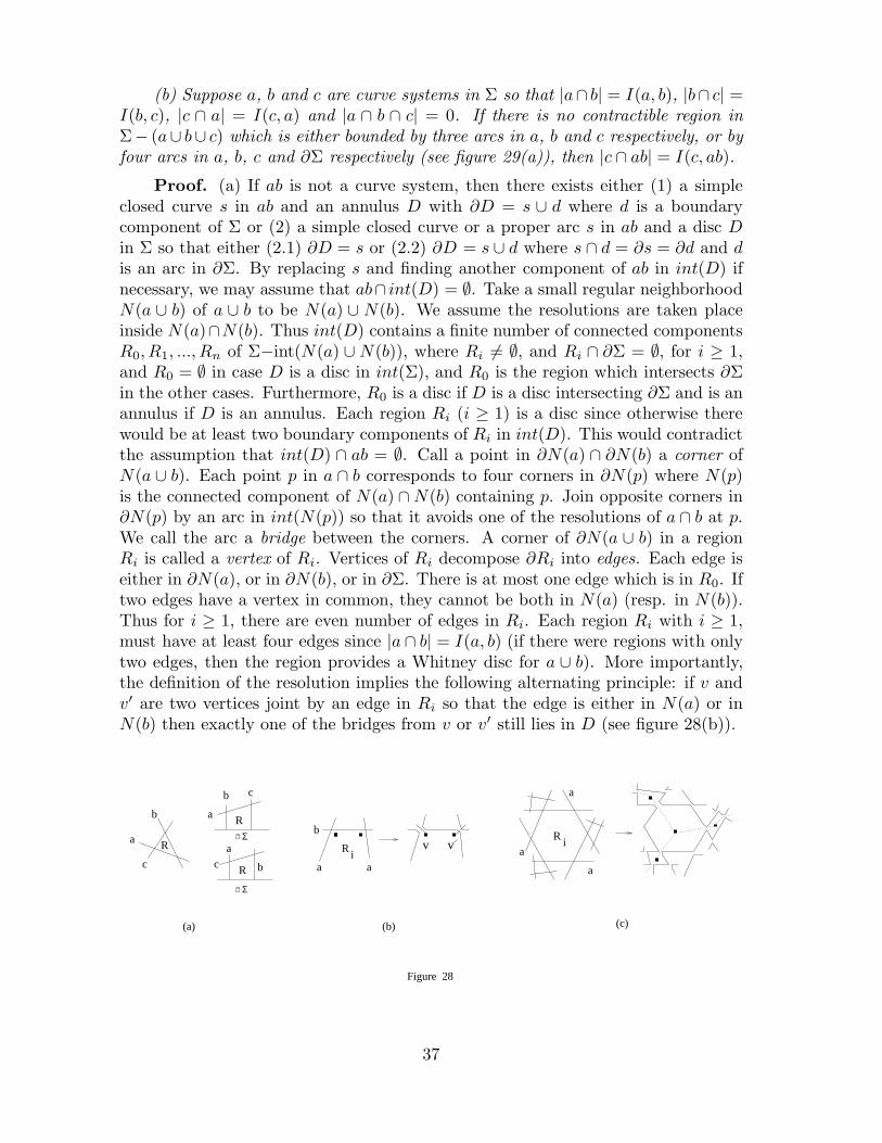
(b) Suppose a, b and c are curve systems in Σ so that |a∩ b| = I(a, b), |b∩ c| =I(b, c), |c ∩ a| = I(c, a) and |a ∩ b ∩ c| = 0. If there is no contractible region inΣ− (a∪ b∪ c) which is either bounded by three arcs in a, b and c respectively, or byfour arcs in a, b, c and ∂Σ respectively (see figure 29(a)), then |c ∩ ab| = I(c, ab).

Proof. (a) If ab is not a curve system, then there exists either (1) a simpleclosed curve s in ab and an annulus D with ∂D = s ∪ d where d is a boundarycomponent of Σ or (2) a simple closed curve or a proper arc s in ab and a disc Din Σ so that either (2.1) ∂D = s or (2.2) ∂D = s ∪ d where s ∩ d = ∂s = ∂d and dis an arc in ∂Σ. By replacing s and finding another component of ab in int(D) ifnecessary, we may assume that ab∩ int(D) = ∅. Take a small regular neighborhoodN(a ∪ b) of a ∪ b to be N(a) ∪ N(b). We assume the resolutions are taken placeinside N(a)∩N(b). Thus int(D) contains a finite number of connected componentsR0, R1, ..., Rn of Σ−int(N(a) ∪ N(b)), where Ri 6= ∅, and Ri ∩ ∂Σ = ∅, for i ≥ 1,and R0 = ∅ in case D is a disc in int(Σ), and R0 is the region which intersects ∂Σin the other cases. Furthermore, R0 is a disc if D is a disc intersecting ∂Σ and is anannulus if D is an annulus. Each region Ri (i ≥ 1) is a disc since otherwise therewould be at least two boundary components of Ri in int(D). This would contradictthe assumption that int(D) ∩ ab = ∅. Call a point in ∂N(a) ∩ ∂N(b) a corner ofN(a ∪ b). Each point p in a ∩ b corresponds to four corners in ∂N(p) where N(p)is the connected component of N(a) ∩ N(b) containing p. Join opposite corners in∂N(p) by an arc in int(N(p)) so that it avoids one of the resolutions of a ∩ b at p.We call the arc a bridge between the corners. A corner of ∂N(a ∪ b) in a regionRi is called a vertex of Ri. Vertices of Ri decompose ∂Ri into edges. Each edge iseither in ∂N(a), or in ∂N(b), or in ∂Σ. There is at most one edge which is in R0. Iftwo edges have a vertex in common, they cannot be both in N(a) (resp. in N(b)).Thus for i ≥ 1, there are even number of edges in Ri. Each region Ri with i ≥ 1,must have at least four edges since |a ∩ b| = I(a, b) (if there were regions with onlytwo edges, then the region provides a Whitney disc for a ∪ b). More importantly,the definition of the resolution implies the following alternating principle: if v andv′ are two vertices joint by an edge in Ri so that the edge is either in N(a) or inN(b) then exactly one of the bridges from v or v′ still lies in D (see figure 28(b)).

Σ

Σ

(a) (b) (c)

a

b

c

a

b c

ca

b

R

R a a

b

R i

R ia

a

a

R

Figure 28

v v

37

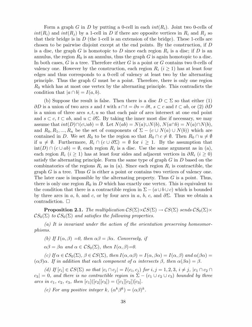
Form a graph G in D by putting a 0-cell in each int(Ri). Joint two 0-cells ofint(Ri) and int(Rj) by a 1-cell in D if there are opposite vertices in Ri and Rj sothat their bridge is in D (the 1-cell is an extension of the bridge). These 1-cells arechosen to be pairwise disjoint except at the end points. By the construction, if Dis a disc, the graph G is homotopic to D since each region Ri is a disc; if D is anannulus, the region R0 is an annulus, thus the graph G is again homotopic to a disc.In both cases, G is a tree. Therefore either G is a point or G contains two 0-cells ofvalency one. However by the construction, each region Ri (i ≥ 1) has at least fouredges and thus corresponds to a 0-cell of valency at least two by the alternatingprinciple. Thus the graph G must be a point. Therefore, there is only one regionR0 which has at most one vertex by the alternating principle. This contradicts thecondition that |a ∩ b| = I(a, b).

(b) Suppose the result is false. Then there is a disc D ⊂ Σ so that either (1)∂D is a union of two arcs s and t with s∩ t = ∂s = ∂t, s ⊂ c and t ⊂ ab, or (2) ∂Dis a union of three arcs s, t, u so that each pair of arcs intersect at one end pointand s ⊂ c, t ⊂ ab, and u ⊂ ∂Σ. By taking the inner most disc if necessary, we mayassume that int(D)∩(c∪ab) = ∅. Let N(ab) = N(a)∪N(b), N(a∩b) = N(a)∩N(b),and R0, R1, ..., Rn be the set of components of Σ − (c ∪ N(a) ∪ N(b)) which arecontained in D. We set R0 to be the region so that R0 ∩ c 6= ∅. Then R0 ∩ u 6= ∅if u 6= ∅. Furthermore, Ri ∩ (c ∪ ∂Σ) = ∅ for i ≥ 1. By the assumption thatint(D) ∩ (c ∪ ab) = ∅, each region Ri is a disc. Use the same argument as in (a),each region Ri (i ≥ 1) has at least four sides and adjacent vertices in ∂Ri (i ≥ 0)satisfy the alternating principle. Form the same type of graph G in D based on thecombinatorics of the regions Ri as in (a). Since each region Ri is contractible, thegraph G is a tree. Thus G is either a point or contains two vertices of valency one.The later case is impossible by the alternating property. Thus G is a point. Thus,there is only one region R0 in D which has exactly one vertex. This is equivalent tothe condition that there is a contractible region in Σ− (a∪ b∪ c) which is boundedby three arcs in a, b, and c, or by four arcs in a, b, c, and ∂Σ. Thus we obtain acontradiction. �

Proposition 2.1. The multiplication CS(Σ)×CS(Σ) → CS(Σ) sends CS0(Σ)×CS0(Σ) to CS0(Σ) and satisfies the following properties.

(a) It is invariant under the action of the orientation preserving homeomor-phisms.

(b) If I(α, β) =0, then αβ = βα. Conversely, if

αβ = βα and α ∈ CS0(Σ), then I(α, β)=0.

(c) If α ∈ CS0(Σ), β ∈ CS(Σ), then I(α, αβ) = I(α, βα) = I(α, β) and α(βα) =(αβ)α. If in addition that each component of α intersects β, then α(βα) = β.

(d) If [ci] ∈ CS(Σ) so that |ci ∩ cj | = I(ci, cj) for i, j = 1, 2, 3, i 6= j, |c1 ∩ c2 ∩c3| = 0, and there is no contractible region in Σ − (c1 ∪ c2 ∪ c3) bounded by threearcs in c1, c2, c3, then [c1]([c2][c3]) = ([c1][c2])[c3].

(e) For any positive integer k, (αkβk) = (αβ)k.

38

(f) If α is the isotopy class of a simple closed curve, then the positive Dehntwist along α sends β to αkβ where k = I(α, β).

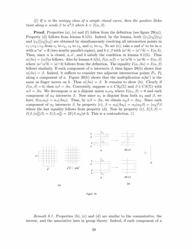
Proof. Properties (a), (e) and (f) follow from the definition (see figure 29(a)).Property (d) follows from lemma 8.1(b). Indeed, by the lemma, both ([c1][c2])[c3]and [c1]([c2][c3]) are obtained by simultaneously resolving all intersection points inc1 ∪ c2 ∪ c3 from c1 to c2, c2 to c3, and c1 to c3. To see (c), take a and a′ to be in αwith a∩a′ = ∅ (two nearby parallel copies), and b ∈ β with |a∩b| = |a′∩b| = I(a, b).Then, since α is closed, a, a′, and b satisfy the condition in lemma 8.1(b). Thusα(βα) = (αβ)α follows. Also by lemma 8.1(b), I(α, αβ) = |a∩a′b| = |a∩b| = I(α, β)where |a∩a′b| = |a∩ b| follows from the definition. The equality I(α, βα) = I(α, β)follows similarly. If each component of α intersects β, then figure 29(b) shows thatα(βα) = β. Indeed, it suffices to consider two adjacent intersection points P1, P2

along a component of a. Figure 29(b) shows that the multiplication a(ba′) is thesame as finger moves on b. Thus α(βα) = β. It remains to show (b). Clearly ifI(α, β) = 0, then αβ = βα. Conversely, suppose α ∈ CS0(Σ) and β ∈ CS(Σ) withαβ = βα. We decompose α as a disjoint union α1α2 where I(α1, β) = 0 and eachcomponent of α2 intersects β. Now since α1 is disjoint from both α2 and β, wehave β(α1α2) = α1(βα2). Thus, by αβ = βα, we obtain α2β = βα2. Since eachcomponent of α2 intersects β, by property (c), β = α2(βα2) = α2(α2β) = (α2)

2βwhere the last equality follows from property (d). Now by property (c), I(β, β) =I(β, (α2

2)β) = I(β, α22) = 2I(β, α2) 6= 0. This is a contradiction. �

a

a

P 2

P 1

b a(b a )

a

a

P 2

P 1

a

a

b a(b a )

a

a

a b5 5 ba 5( )b

a

5

5

b

(a) (b)

Figure 29

Remark 8.1. Properties (b), (c) and (d) are similar to the commutative, theinverse, and the associative laws in group theory. Indeed, if each component of a

39

curve system α ∈ CS0 intersects both β and γ and βα = γα, then (c) implies thatβ = α(βα) = α(γα) = γ.

8.2. Some observations and questions

We begin with a lemma.

Lemma 8.2. Suppose α, β ∈ CS0(Σ), then I(αβ, βα) = 2I(α, β). In particu-lar, we have (a) (αβ)(βα) = β2γ where γ is disjoint from both α and β, and (b)I(δ, αβ) + I(δ, βα) ≥ 2I(δ, β).

Proof. Choose x, x′ ∈ α, y, y′ ∈ β so that |x∩y| = I(x, y) and x′, y′ are parallelcopies of x, y. Then by the definition of the multiplication, there are no bi-gons inxy∪y′x′ and |xy∩y′x′| = 2I(x, y)|. Thus (xy)(y′x′) is a representative of (αβ)(βα).An easy calculation shows that (xy)(y′x′) ∼= y2z where z consists of components ofx disjoint from y. Thus the lemma follows. �

Call the set {αnβ: n ∈ Z} a horocycle in the space CS0(Σ). It follows fromthe lemma 8.2 (b) that Iδ is convex along horocycles. An element α ∈ CS0(Σ) iscalled maximal if the only simple loops or arcs which are disjoint from α are thecomponents of α. By proposition 2.1(c), for any two elements α, β in CS0(Σ), thereis a horocycle containing two maximal elements α′ and β′ so that I(α, α′) = 0 andI(β, β′) = 0. Indeed, the horocycles is of the form α′(β′α′)n. The analogous fact formeasured laminations with respect to the extension of the earthquake was provedby Bonahon [Bo3] and Papadopoulos [Pa1].

We close with two questions. Call a function in n variables x1, ..., xn alge-braically piecewise linear, or simply, APL, if it is obtained from xi’s by finite numberof summations, multiplications over Q, and the absolute value |.| operation.

Question 3. Does the multiplication on CS(Σ) extend to a multiplication onML(Σ) which is APL with respect to the Thurston coordinate τF ?

Question 4. Is the intersection number function on ML(Σ) × ML(Σ) → R

sending (m, m′) to I(m, m′) a APL map with respect to the Thurston coordinates?

See [Bo2], [Bo3], [Pa1], [Pa2], [Re] and the references cited therein for moreinformation on the intersection numbers and the earthquakes in the measured lam-inations space.

Reference

[Bi] Birman, J.S., Braids, links, and mapping class groups. Ann. of Math.Stud., 82, Princeton Univ. Press, Princeton, NJ, 1975

[Bo1] Bonahon, F.: The geometry of Teichmuller space via geodesic currents.Invent. Math. 92 (1988), 139-162.

[Bo2] Bonahon, F.: Bouts des varietes hyperboliques de dimension 3. Ann. ofMath. (2) 124 (1986), no. 1, 71–158.

[Bo3] Bonahon, F.: Earthquakes on Riemann surfaces and on measured geod-esic laminations. Trans. Amer. Math. Soc. 330 (1992), no. 1, 69–95.

40

[Br] Brumfiel, G. W.: The real spectrum compactification of Teichmuller space,Contemp. Math., 74, AMS, (1988), 51-75.

[CM] Culler, M., Morgan, J.: Group actions on R-trees. Proc. London Math.Soc. 55 (1987), no. 3, 571–604.

[CS] Culler, M., Shalen, P.: Varieties of group representations and splittings of3-manifolds. Ann. Math. 117 (1983), 109-146.

[De] Dehn, M.: Papers on group theory and topology. J. Stillwell (eds.).Springer-Verlag, Berlin-New York, 1987.

[FK] Fricke, R., Klein, F.: Vorlesungen uber die Theorie der AutomorphenFunctionen. Teubner, Leipizig, 1897-1912.

[FLP] Fathi, A., Laudenbach, F., Poenaru, V.: Travaux de Thurston sur lessurfaces. Asterisque 66-67, Societe Mathematique de France, 1979.

[Ga] Gardiner, F.: Teichmuller theory and quadratic differentials, John Wiley& Sons, New York, 1987.

[GiM] Gilman, J., Maskit, B.: An algorithm for 2-generator Fuchsian groups.Michigan Math. J. 38 (1991), no. 1, 13-32.

[Go] Goldman, W.: Topological components of spaces of representations. In-vent. Math. 93 (1988) no.3, 557-607.

[GoM] Gonzlez-Acua, F., Montesinos-Amilibia, J.: On the character variety ofgroup representations in SL(2, C) and PSL(2, C). Math. Z. 214 (1993), no. 4,627–652.

[Har] Harer, J.: The second homology group of the mapping class group of anorientable surface. Invent. Math. 72 (1083), 221-239.

[Hat] Hatcher, A.: Measured lamination spaces for surfaces. Topology Appl.30 (1988), 63-88.

[Ho] Horowitz, R.: Characters of free groups represented in the 2-dimensionalspecial linear group. Comm. Pure and App. Math. 25 (1972), 635-649.

[HM] Hubbard, J., Masur, H.: Quadratic differentials and foliations. ActaMath. 142 (1979), no. 3-4, 221–274.

[HT] Hatcher, A. Thurston, W.: A presentation for the mapping class groupof a closed orientable surface. Topology 19 (1980), 221-237.

[Ke] Keen, L.: Intrinsic moduli on Riemann surfaces. Ann. Math. 84 (1966),405-420

[Ker1] Kerckhoff, S.: The asymptotic geometry of Teichmller space. Topology19 (1980), no. 1, 23–41.

[Ker2] Kerckhoff, S.: The Nielsen realization problem. Ann. of Math. 117(1983), no. 2, 235–265.

41

[Li] Lickorish, R.: A representation of oriented combinatorial 3-manifolds. Ann.Math. 72 (1962), 531-540

[Lu1] Luo, F.: Geodesic length functions and Teichmuller spaces, J. Diff.Geom., to appear.

[Lu2] Luo, F.: Geodesic length functions and Teichmuller spaces. ElectronicResearch Announcement, AMS, 2 (1996), no. 1, 34-41.

[Lu3] Luo, F.: Automorphisms of the complex of curves, preprint.

[Mag] Magnus, W.: Rings of Fricke characters and automorphism groups offree groups. Math. Zeit. 170 (1980), 91-103.

[Mo] Mosher, L.: Tiling the projective foliation space of a punctured surface.Trans. Amer. Math. Soc. 306 (1988), 1-70.

[MS] Morgan, J., and Shalen, P.: Valuations, trees, and degenerations of hy-perbolic structures, I. Ann. of Math., 120 (1984), 401-476.

[Pa1] Papadopoulos, A.: On Thurston’s boundary of Teichmuller space and theextension of earthquakes. Topology Appl. 41 (1991), no. 3, 147–177.

[Pa2] Papadopoulos, A.: Geometric intersection functions and Hamiltonianflows on the space of measured foliations on a surface. Pacific J. Math. 124 (1986),no. 2, 375–402.

[Par] Parry, W.: Axioms for translation length functions. Arboreal grouptheory (Berkeley, CA, 1988), 295–330, Math. Sci. Res. Inst. Publ., 19, Springer,New York, 1991.

[PH] Penner, R., Harer, J.: Combinatorics of train tracks. Annals of Mathe-matics Studies, 125. Princeton University Press, Princeton, NJ, 1992.

[Re] Rees, M.: An alternative approach to the ergodic theory of measuredfoliations on surfaces. Ergodic Theory Dynamical Systems 1 (1981), no. 4, 461-488.

[Sc] Schneps, L.: The Grothendieck theory of dessins d’enfants. CambridgeUniversity Press, Cambridge, New York, 1994.

[Th] Thurston, W.: On the geometry and dynamics of diffeomorphisms ofsurfaces. Bul. Amer. Math. Soc. 19 (1988) no 2, 417-438.

[Wa] Wajnryb, B.: A simple presentation for the mapping class group of anorientable surface. Israel J. Math. 45 (1983), 157-174.

[Wo] Wolpert, S.: Geodesic length functions and the Nielsen problem. J. Diff.Geom. 25 (1987), 275-296

42