Resonance phenomena in macroscopic quantum tunneling for an rf SQUID

arX

iv:q

uant

-ph/

0611

255v

1 2

5 N

ov 2

006

Resonance phenomena in Macroscopic Quantum

Tunneling: the small viscosity limit

Yu N Ovchinnikov

L.D. Landau Institute for Theoretical Physics, Academy of Science, Moscow, Russia

S Rombetto ‡Universita degli Studi di Napoli “Federico II”, Naples, Italy

B Ruggiero

Istituto di Cibernetica “E. Caianiello” del CNR, Pozzuoli (Naples), Italy

V Corato

Dipartimento di Ingegneria dell’Informazione, Seconda Universita di Napoli, Naples,

Italy

P Silvestrini

E-mail: [email protected]

Dipartimento di Ingegneria dell’Informazione, Seconda Universita di Napoli, Naples,

Italy

Abstract. We present a new theoretical approach to describe the quantum behavior

of a macroscopic system interacting with an external irradiation field, close to the

resonant condition. Here we consider the extremely underdamped regime for a system

described by a double well potential. The theory includes both: transitions from one

well to the other and relaxation processes. We simulate resonant phenomena in a

rf-SQUID, whose parameters lie in the range typically used in the experiments. The

dependence of the transition probability W on the external drive of the system ϕx shows

three resonance peaks. One peak is connected with the resonant tunneling and the two

others with the resonant pumping. The relative position of the two peaks correlated

to the resonant pumping depends on the pumping frequency ν and on the system

parameters. The preliminary measurements on our devices show a low dissipation

level and assure that they are good candidates in order to realize new experiments on

the resonant phenomena in the presence of an external microwave irradiation of proper

frequency.

PACS numbers: 74.50.+r, 03.65.Yz, 03.67.Lx

‡ also at: Istituto di Cibernetica “E. Caianiello” del CNR, Pozzuoli (Naples), Italy

http://arxiv.org/abs/quant-ph/0611255v1

Resonance phenomena in Macroscopic Quantum Tunneling: the small viscosity limit 2

1. Introduction

Josephson devices are convenient instruments for investigating macroscopic quantum

effects [1]. First experiments focused on incoherent phenomena such as macroscopic

quantum tunneling (MQT) [2, 3, 4, 5] and energy level quantization (ELQ) [6, 7, 8].

Recent experiments have shown a coherent superposition of distinct macroscopic

quantum states in SQUID systems [9, 10, 11] under the action of an external microwave

irradiation. These results have stimulated many researchers to search for new quantum

phenomena at macroscopic level as well as a method to distinguish them from classical

predictions. Moreover quantum effects in SQUID dynamics are interesting because of

possible applications to quantum computing [12], as demonstrated by recent experiments

[10], [11]. Anyway these results need a final confirmation, since some of them have been

reproduced by using a classical model to describe the phenomena [13].

The main problem to observe quantum phenomena at macroscopic level is the interaction

with the environment which produces dissipation of coherent effects into classical

statistical mixture of quantum states. Among a great variety of incoherent effects,

the environment induces a finite width γ of quantum levels [14] and, in this situation,

resonant phenomena can occur only if γ is small compared to the energy difference

between levels, ~γ ≪ ~Ωp, where

Ωp =

√

1

M

(

∂2U

∂ϕ2

)

ϕ=ϕmin

(1)

is the plasma frequency, and ϕmin is the coordinate corresponding to the minimum of

the considered potential well. We have already discussed [15] the behavior of microwave

induced transitions in a rf-SQUID in the moderate underdamped regime, when γ is larger

than the probability of quantum tunneling under the potential barrier, TN , (γ ≫ TN)

[16].

In the present paper we extend the theoretical analysis to the small viscosity limit,

corresponding to γ ≈ TN , referred as the extremely underdamped regime. In this

conditions we can neglect the interwell transitions with respect to the tunneling

transitions. Up to now, this regime has been investigated only for other Josephson

devices [10, 8]. Here we present a new theory specific for the rf-SQUID, characterized

by a double well potential (Fig.1), in order to identify coherent phenomena and to

suggest a way of measuring them.

It’s worth nothing that Averin et al. [17], [18], [19] already reported a theoretical

investigation of resonant quantum phenomena in rf SQUIDs. Nevertheless in that

paper all quantities are postulated and not found from the initial Hamiltonian, while

we don’t not use any fitting parameters, but only external parameter values entering in

the Hamiltonian.

We study the interaction between a macroscopic quantum system (the rf-SQUID) and

an external microwave irradiation, for frequencies close to resonant conditions.

The probability of a transition under the potential barrier decreases exponentially with


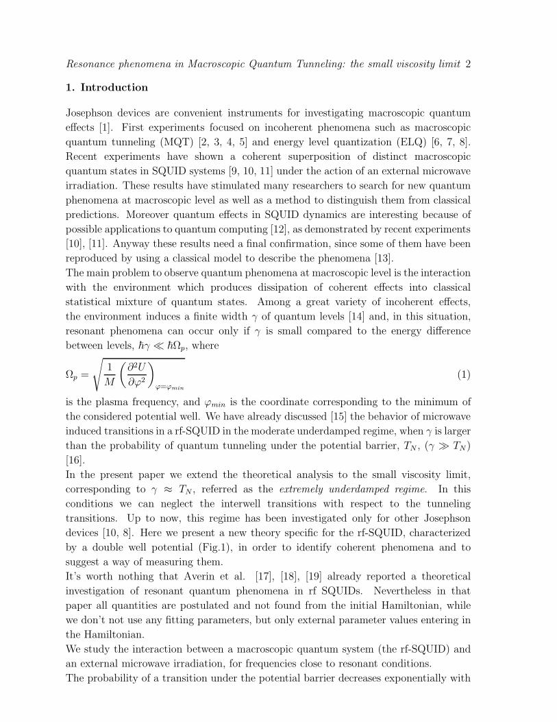
Figure 1. A sketch of an rf-SQUID double-well potential U(ϕ), with two minima

located at ϕmin1

and ϕmin2

. ϕtop is the position of the potential maximum. The

coordinates ϕ1, ϕ2, ϕ3, ϕ4 are the “turning points” of energy Ef1. In the same way

it’s possible to define turning points for energies Ef2, E0, ER, EL. We study the case

EL = E0, that is the ground state in the left potential well.

the decreasing energy of the quantum state. Tunneling occurs from a level close to the

barrier top. In this case, as we’ll show in the following, the transition probability curve

can present three peaks.

A further requirement to observe the quantum tunneling phenomenon is that the number

of levels n is not too large, so that no crowding of levels happens. At the same time we

assume the number of levels in the potential well is large enough, so that the motion

of a particle with energy close to the top of the potential barrier can be considered

quasiclassical. In this limit we use approximations reported in [20].

In the quasiclassical limit, the density of levels close to the barrier top increases, but in

the considered case this effect is not significant, since numerical factors are of the order

of 12π

lnn [20]. Furthermore, near to the barrier top, repulsion of levels is relevant and

hence the equation for the system wave functions should be solved exactly. Finally the

tunneling probability of a particle through the potential barrier depends very strongly

on the particle energy E and on the energy difference between neighboring levels. The

position and the width of each level depends on the external parameters of the system.

A sketch of the double well potential of the rf-SQUID here studied is reported in Fig.1.

Each macroscopic flux state of the rf-SQUID corresponds to the system wave function

confined in one of the two potential wells. By varying the external parameter ϕx it’s

possible to control the energy difference between the levels in different wells.

Out of resonance conditions, the energy levels are localized in each well. When two levels

in different wells are in resonance, a coherent superposition of distinct states occurs and

a gap appears between the energy levels. As a consequence of the coherent quantum

tunneling process, in exact resonant conditions, the two levels have an energy tunnel

splitting ∆, and the wave functions spread over the two wells, generating delocalized


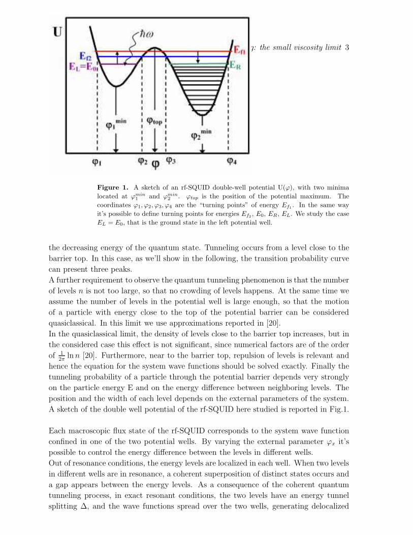
Figure 2. The four essential energy levels considered in this study. All the quantities

are referred to the barrier top. Here Ef1and Ef2

are the energies of the delocalized

levels. E0 is the first level in the left potential well below Ef2and ER is the first level

in the right potential well below Ef2.

states with energies Ef1and Ef2

, as shown in Fig.2. It’s worth noting that the

energy tunnel splitting ∆ corresponds to the tunneling probability TN in exact resonant

conditions and can be experimentally observed only if resonant levels are very close to

the barrier top and in small viscosity limit [9].

Moreover, to study the tunneling process from the upper levels, it’s necessary to populate

them through a pumping process from the ground state of the left well: this requires

the application of a microwave irradiation of proper frequency ν = ω/2π and amplitude

I. Even a small amplitude of external microwave irradiation will cause an essential

change in the population of excited states and will therefore produce a large effect in

the tunneling probability.

We study the rf-SQUID dynamics in these particular conditions and we show some

numerical simulations. For a fixed value of the pumping frequency ν, the transition

probability curve W from one potential well to the other one (as a function of the

external parameter ϕx) can present three maxima: one maximum is connected with

the resonant tunneling and the two others with the resonant pumping toward the two

non-localized levels with energies Ef1, Ef2

.

In the considered phenomenon, friction, that is due to the interaction with the external

environment, has a relevant role since it leads to a finite width γ of levels and destroys

the coherence [21]. In the following sections we will discuss the induced resonance

phenomena by using the density matrix formalism [22].

In particular in section II we discuss the transition probability function in presence of

resonant pumping, in section III we show how to calculate levels position and transition

matrix elements, in section IV we determine the energy spectrum in the vicinity of the

crossing point and ,finally, in section V we show the results of numerical simulations

and first experimental data for the dissipation level for these rf-SQUID based devices.


2. Transition probability function in presence of resonant pumping

In the zero approximation of the system interaction with the thermal bath, the

hamiltonian describing the rf-SQUID in the presence of an external microwave with

amplitude I is

H0 = − ~2

2M

∂2

∂ϕ2+ U0

[

(ϕ− ϕx)2 + βL cosϕ

]

+I~

2ecos(ωt)ϕ (2)

where I has the dimensionality of a current, M is the “mass” of the Josephson junction

defined as

M =

(

~

2e

)2

C (3)

and C is the junction capacitance. Following a common practice[4], the dimensionless

variable ϕx is obtained by referring the magnetic flux to Φ0/2 and normalizing it to

Φ0/2π. In eq.(2) quantities U0 and βL are free parameters of the system and are defined

as

U0 =

[

(

Φ0

2π

)21

L

]

(4)

βL =2πLIc

Φ0(5)

L and Ic are the inductance and the critical current of the rf-SQUID, respectively. The

simplest case is when U0 and βL are constant, while ϕx changes.

Our considerations are valid for any potential U(ϕ). The essential point is that the

potential U(ϕ) has the form given in Fig.1 in the proximity of the points ϕ. All the

parameters ϕx, U0, βL depends on the structure of the considered SQUID.

Here we choose parameters such that, near to the top of the barrier, there are two

close levels Ef1, Ef2

, that can be considered as belonging to both potential wells

simultaneously (delocalized levels) as shown in Fig.1. Moreover it’s worth noting that

the quantity ϕx is proportional to ILΦ0

.

The dissipation is accounted for by an effective resistance Reff in the RSJ model for the

junction [23]. So a bigger Reff implies a better insulation, that means a smaller width

of the levels. Here we consider an rf-SQUID whose Josephson junctions presents a large

value of resistance Reff , so that the condition

Ef1− Ef2

~≫ γ1, γ2 (6)

is satisfied, where γ1, γ2 are the widths of levels Ef1, Ef2

respectively.To describe the resonant tunneling induced by the resonant pumping quantitatively, weuse the following system of equations [14] for the density matrix elements ρj

f

∂ρjf

∂t=

iI2e

cos(ωt)∑

m

(

〈j|ϕ|m〉 exp

[

−i

(

Em − Ej

~

)

t

]

ρmf (7)

−〈m|ϕ|f〉 exp

[

i

(

Em − Ef

~

)

t

]

ρjm

)

+∑

m,n

W j mf n ρm

n − 1

2

∑

m

(

W mjm j + W m f

m f

)

ρjf


Here j, m, f, n are the considered levels, Ej , Em, Ef , En are their energies and t is the

time.

The matrix elements W j mf n entering in eq.(7) are defined in Appendix A and C. They

are nonvanishing provided that

| (Em − Ej) − (En − Ef ) | ≪ ~Ωp (8)

If these conditions are satisfied and if the temperature is low enough, the nonvanishing

terms W j mf n of the transition probability matrix are given by the following equation:

W j mf n =

π

2Reffe2

(

1 + tanhω

2T

)

N(ω) ·[

〈j|e iϕ2 |m〉〈f |e− iϕ

2 |n〉 + 〈j|e− iϕ2 |m〉〈f |e iϕ

2 |n〉]

(9)

where

ω =(Em − Ej + En − Ef)

~(10)

and N (ω) is defined as

N (ω) =ω

πcoth

(

ω

2T

)

(11)

Only the four non-diagonal elements of the density matrix ρ0f1, ρ0

f2, ρf1

0 , ρf2

0 are nonzero,

and they are connected by the expressions

ρf1

0 =(

ρ0f1

)∗ρf2

0 =(

ρ0f2

)∗(12)

In presence of an external pumping also the two diagonal elements ρf1

f1and ρf2

f2are non-

zero.

We suppose that the temperature T is much smaller than the plasma frequency

(kBT ≪ ~Ωp), such that it is of the order of the energy difference kBT ≈ (Ef1−Ef2

).

In the present article we consider T = 50mK. When these hypotheses are satisfied,

from eq.(7) we obtain

∂ρ0f1

∂t= −iI

2ecos(ωt)〈0|ϕ|f1〉e

„

−iEf1

−E0

~t

«

ρ00 +W 0 0

f1 f2ρ0

f2− γ1ρ

0f1

(13)

∂ρ0f2

∂t= −iI

2ecos(ωt)〈0|ϕ|f2〉e

„

−iEf1

−E0

~t

«

ρ00 +W 0 0

f2 f1ρ0

f1− γ2ρ

0f2

(14)

where the widths γ1, γ2 of levels are given by the following expressions

γ1 =1

2

(

W f2 f1

f2 f1+WLf1

L f1+WR f1

R f1

)

(15)

γ2 =1

2

(

W f1 f2

f1 f2+WLf2

L f2+WR f2

R f2

)

The indexes L and R refer to the first energy levels below Ef2in the left and right wells,

respectively. The tunneling transition probability between two states in different wells

decreases very quickly for states below the barrier top, such as e−2πn, where n is the

number of states counted from the barrier top [24]. As a consequence we can neglect

transitions into lower levels in the right potential well.

In order to study this phenomenon, only five energy levels (Ef1, Ef2

, E0, EL, ER) are


essential quantities. E0 is the energy of the ground state in the left potential well, EL

is the first level in the left potential well below Ef2(in the simulations presented here

EL=E0), ER is the first level in the right potential well below Ef2. Energy levels as a

function of the external parameter ϕx, are shown in Fig.2. The pumping frequency ν is

supposed to be close to the frequencies Ef1/~ and Ef2

/~ (referring both to E0/~). In

our simulations EL is also the ground state of the left potential well (it’s the same as

E0), while in the right well there are many more levels, not involved in the described

process.

If these conditions are satisfied, the solutions of eqs.(13), (13) are:

ρ0f1

= Af1e

i

„

ω−Ef1

−E0

~

«

t+Bf1

ei

„

ω−Ef2

−E0

~

«

t(16)

ρ0f2

= Bf2e

i

„

ω−Ef1

−E0

~

«

t+ Af2

ei

„

ω−Ef2

−E0

~

«

t

In eqs.(16) coefficients Af1, Af2

, Bf1, Bf2

are defined as follows

Af1= −

I

4e〈0|ϕ|f1〉

2

4ω −Ef1

− E0

~− iγ1 +

W 0 0f1 f2

W 0 0f2 f1

ω −Ef1

−E0

~− iγ2

3

5

−1

Af2= −

I

4e〈0|ϕ|f2〉

2

4ω −Ef2

− E0

~− iγ2 +

W 0 0f1 f2

W 0 0f2 f1

ω −Ef2

−E0

~− iγ1

3

5

−1

(17)

Bf1= −

iW 0 0f1 f2

Af2

ω −Ef2

−E0

~− iγ1

Bf2= −

iW 0 0f2 f1

Af1

ω −Ef1

−E0

~− iγ2

The diagonal elements ρf1

f1and ρf2

f2of the density matrix can be find by solving the

following equations

∂ρf1

f1

∂t=iI2e

cos(ωt)

[

ρ0f1〈f1|ϕ|0〉e

i

„

Ef1−E0

~

«

t − ρf1

0 〈0|ϕ|f1〉e„

−iEf1

−E0

~t

«]

+W f1 f2

f1 f2ρf2

f2− 2γ1ρ

f1

f1(18)

∂ρf2

f2

∂t=iI2e

cos(ωt)

[

ρ0f2〈f2|ϕ|0〉e

i

„

Ef2−E0

~

«

t − ρf2

0 〈0|ϕ|f2〉e−i

„

Ef2−E0

~

«

t

]

+W f2 f1

f2 f1ρf1

f1− 2γ2ρ

f2

f2(19)

These rate equations completely describe the dynamics of the process. The solutions of

this system are respectively:

ρf1

f1(t) = ρf1

f1+ F1e

i

„

Ef2−Ef1~

«

t+ F∗

1 e−i

„

Ef2−Ef1~

«

t(20)

ρf2

f2(t) = ρf2

f2+ D1e

i

„

Ef2−Ef1~

«

t+ D∗

1e−i

„

Ef2−Ef1~

«

t(21)

The expressions for F1 and D1 are given in Appendix A. By using equations (20) and

(21) inside equations (18) and (19), we obtain the expressions of the quantities ρf1

f1and

ρf2

f2as following:

ρf1

f1=

I2

16e21

γ1γ2 − 14W f2 f1

f2 f1W f1 f2

f1 f2


·[

γ2 | 〈0|ϕ|f1〉 |2γ1 − γ2W

0 0f1 f2

W 0 0f2 f1

[

(

ω − Ef1−E0

~

)2

+ γ22

]−1

(

ω − Ef1−E0

~

)2

+ γ21 +

(W 0 0f1 f2

W 0 0f2 f1

)2+2W 0 0

f1 f2W 0 0

f2 f1

"

„

ω−Ef1

−E0

~

«2

−γ1γ2

#

„

ω−Ef1

−E0

~

«2

+γ22

+1

2W f1 f2

f1 f2| 〈0|ϕ|f2〉 |2

γ2 − γ1W0 0f1 f2

W 0 0f2 f1

[

(

ω − Ef2−E0

~

)2

+ γ21

]−1

(

ω − Ef2−E0

~

)2

+ γ22 +

(W 0 0f1 f2

W 0 0f2 f1

)2+2W 0 0

f1 f2W 0 0

f2 f1

"

„

ω−Ef2

−E0

~

«2

−γ1γ2

#

„

ω−Ef2

−E0

~

«2

+γ21

]

(22)

ρf2

f2=

I2

16e21

γ1γ2 − 14W f2 f1

f2 f1W f1 f2

f1 f2

·[

γ1 | 〈0|ϕ|f2〉 |2γ2 − γ1W

0 0f2 f1

W 0 0f1 f2

[

(

ω − Ef2−E0

~

)2

+ γ21

]−1

(

ω − Ef2−E0

~

)2

+ γ22 +

(W 0 0f1 f2

W 0 0f2 f1

)2+2W 0 0

f1 f2W 0 0

f2 f1

"

„

ω−Ef2

−E0

~

«2

−γ1γ2

#

„

ω−Ef2

−E0

~

«2

+γ21

+1

2W f2 f1

f2 f1| 〈0|ϕ|f1〉 |2

γ1 − γ2W0 0f1 f2

W 0 0f2 f1

[

(

ω − Ef1−E0

~

)2

+ γ22

]−1

(

ω − Ef1−E0

~

)2

+ γ21 +

(W 0 0f1 f2

W 0 0f2 f1

)2+2W 0 0

f1 f2W 0 0

f2 f1

"

„

ω−Ef1

−E0

~

«2

−γ1γ2

#

„

ω−Ef1

−E0

~

«2

+γ22

]

(23)

Finally we can introduce the transition probability W from the left to the right potential

well. W is a function of the external parameter ϕx and computing this quantity is the

main goal of the paper. The transition probability is given by the expression

W = WR f1

R f1ρf1

f1+WR f2

R f2ρf2

f2(24)

where, in the low temperature limit, here considered, from eq.(9) we know that

WR f1

R f1=

2 (Ef1− ER)

Reffe2| 〈R | eiϕ/2 | f1〉 |2 (25)

WR f2

R f2=

2 (Ef2− ER)

Reffe2| 〈R | eiϕ/2 | f2〉 |2 (26)

while the expressions for ρf1

f1and ρf2

f2are given in eqs.(20) and (21) respectively. In the

eqs. (22) and (23), the quantities F1 and D1 determinate the value of the oscillating

part of the tunneling probability W .

It’s worth noting that change of the external parameter ϕx leads to a redistribution of

wave functions relative to energies Ef1, Ef2

between left and right potential wells, so

that transition matrix elements and widths of levels γ1, γ2 are functions of the external

parameter ϕx. To complete our considerations we will find the levels position and the

transition matrix elements as a function of the external parameters, as shown in the


next section.

3. Levels position and transition matrix elements.

As we have seen before, a necessary condition for resolving the splitting is that the

experimental linewidth of states (γ1, γ2) be smaller than ∆ (∆ ≫ ~γ1, ~γ2): it can be

satisfied only for levels near to the barrier top (Fig.1). In Fig.1 ϕ1, ϕ2, ϕ3, ϕ4 are the

“turning points”, that are the solutions of equation

U(ϕ1,2,3,4) = E (27)

where E is the energy value. In Fig.1 the points ϕmin1 , ϕmin

2 are coordinates

corresponding to the minima of potential U(ϕ) and the point ϕtop is the coordinate

corresponding to the maximum of the potential U(ϕ). For energy values E close to the

top of the barrier, the wave function Ψ can be written in the form

Ψ = G−1 · 1

(2M (E − U(ϕ)))1/4sin

π

4+

∫

ϕ1

√

2M (E − U (ϕ))dϕ

in the left potential well

Ψ = A · D− 1−iλ2

((1 + i)(2MU1)1/4(ϕ− ϕtop)) + A∗D− 1+iλ

2

(

(1 − i)(2MU1)1/4(ϕ− ϕtop)

)

near the barrier top(28)

Ψ =B

(2M (E − U(ϕ)))1/4sin

π

4+

ϕ4∫

√

2M (E − U(ϕ))dϕ

in the right potential well

In eqs.(28) Dp is the parabolic cylinder function [25], while quantities A and B are

numerical factors, G is a normalization factor, defined in the following. The other

quantities are defined as

Utop = U(ϕtop) (29)

U1 = −1

2

(

∂2U

∂ϕ2

)

ϕ=ϕtop

(30)

λ =√

2MU1Utop −E

U1(31)

First expression in eqs.(28) is valid in the left potential well, the second one is valid

close to the barrier top, the third one is valid in the right potential well. Coefficients

A, B are defined by imposing boundary conditions for these three expressions. Near to

the top of the potential barrier we use the exact solutions of the Schroedinger equation

for the considered system, whereas in the vicinity of the points ϕ1, ϕ4 we use the well

note method of outgoing in complex plane[26]. The relation between coefficients A and

B can be found by matching coefficients in the right potential well

A =B

23/4(2MU1)1/8exp

πλ

8− iπ

8+iλ

4+iλ

4ln

(

2

λ

)

+ i

ϕ4∫

ϕ3

dϕ√

2M (E − U(ϕ))

(32)

Resonance phenomena in Macroscopic Quantum Tunneling: the small viscosity limit10

By matching boundary conditions in the left potential we obtain two equations. Thefirst one is the exact equation for the position of the levels near the barrier top in thecase of small viscosity limit

cos

ϕ4∫

ϕ3

dϕ√

2M (E − U(ϕ)) −ϕ2∫

ϕ1

dϕ√

2M (E − U(ϕ))

+ (1 + exp(−πλ))1/2 ·

· cos

χ +λ

2+

λ

2ln

(

2

λ

)

+

ϕ4∫

ϕ3

dϕ√

2M (E − U(ϕ)) +

ϕ2∫

ϕ1

dϕ√

2M (E − U(ϕ))

= 0 (33)

In eq.(33) phase shift χ is defined by the expression

Γ

(

1 + iλ

2

)

=

√2πe(−πλ/4)

√1 + e(−πλ)

e(iχ) (34)

where Γ(x) is the Euler gamma function and the phase χ can be presented in the form

χ =λ

2Ψ

(

1

2

)

−∞∑

k=0

(

arctan

(

λ

2k + 1

)

− λ

2k + 1

)

(35)

In eq.(35) ψ(x) is the Euler function and

ψ

(

1

2

)

= −C − 2 ln 2 = −1.96351

The second equation gives the value of the coefficient B as follows

B = exp

(

πλ

2

)[

(1 + exp (−πλ))1/2 sin

χ+λ

2+λ

2ln

(

2

λ

)

+

ϕ2∫

ϕ1

dϕ√

2M (E − U(ϕ)) +

ϕ4∫

ϕ3

dϕ√

2M (E −

− sin

ϕ2∫

ϕ1

dϕ√

2M (E − U(ϕ)) −ϕ4∫

ϕ3

dϕ√

2M (E − U(ϕ))

]

In order to obtain two close levels near to the barrier top (but not too close) the

parameter λ should be λ ≥ 1. In such a case, the normalization factor G can be

approximated as

G2 =~

2

ϕ2∫

ϕ1

dϕ√

2M (E − U(ϕ))+B2

ϕ4∫

ϕ3

dϕ√

2M (E − U(ϕ))

(37)

Since we consider the energy E close to the barrier top, it’s possible to use expressions

with explicit energy dependence (perturbation theory over the quantity (Utop −E) with

separation of the singular terms):∫ ϕ2

ϕ1

dϕ√

2M (E − U(ϕ)) =

∫ ϕtop

ϕ1

dϕ√

2M (Utop − U(ϕ)) − (Utop − E)

√

M

2

∫ ϕtop

ϕ1

dϕ

(

1√

(Utop − U(ϕ))−

− (Utop −E)

√

M

2U1

[

ln

(

8 (ϕtop − ϕ1)√U1

√

Utop −E

)

+1

2

]


∫ ϕ4

ϕ3

dϕ√

2M (E − U(ϕ)) =

∫ ϕ4

ϕtop

dϕ√

2M (Utop − U(ϕ)) − (Utop − E)

√

M

2

∫ ϕ4

ϕtop

dϕ

(

1√

(Utop − U(ϕ))−

(

− (Utop −E)

√

M

2U1

[

ln

(

8 (ϕ4 − ϕtop)√U1

√

Utop −E

)

+1

2

]

In eqs.(38), (39) quantities ϕ1, ϕ4 are defined as

ϕ1 = ϕ1 (E = Utop)

ϕ4 = ϕ4 (E = Utop)

Energies EL, ER of states ΨL, ΨR can be found by using eqs.(33), (38), (39), provided

that ΨL, ΨR are referred to the barrier top. In this case wavefunctions ΨL, ΨR can be

described by using the quasiclassical approximation, so that we find

ΨL =1

GL

sin

(

π4

+ϕ∫

ϕ1

dϕ√

2M (E − U(ϕ))

)

(2M (E − U(ϕ)))1/4(40)

ΨR =1

GR

sin

(

π4

+ϕ4∫

ϕ

dϕ√

2M (E − U(ϕ))

)

(2M (E − U(ϕ)))1/4(41)

where the factors GL and GR are defined as

G2L =

~

2

ϕ2∫

ϕ1

dϕ√

2M (E − U(ϕ))(42)

G2R =

~

2

ϕ4∫

ϕ3

dϕ√

2M (E − U(ϕ))(43)

The wave function Ψ0 of the ground state can be taken in the form

Ψ0 =(2MUmin

1 )1/8

π1/4e

0

@−ϕR

ϕmin1

dϕq

2M(U(ϕ)−U(ϕmin1

))

1

A

(44)

where Umin1,2 = U(ϕmin

1,2 ) and ϕmin1,2 are the coordinates corresponding to the position of

the left and right minimum in the potential U(ϕ)(

∂U

∂ϕ

)

ϕ=ϕmin1,2

= 0

U(ϕ) = U(ϕmin1,2 ) + Umin

1,2 (ϕ− ϕmin1,2 )2 + ...

4. The energy spectrum in the vicinity of the crossing point.

In order to describe the spectrum near to the crossing point we introduce two functions

Φ1 and Φ2, defined as:

Φ1 =

ϕ2∫

ϕ1

dϕ√

2M (E − U(ϕ)) +λ

4

(

1 + ln

(

2

λ

))

=

ϕtop∫

ϕ1

dϕ√

2M (Utop − U(ϕ))


− (Utop −E)

√

M

2

∫ ϕtop

ϕ1

dϕ

1√

Utop − U(ϕ)−

√

ϕtop − ϕ1

(ϕtop − ϕ)(

√

U1 (ϕ− ϕ1))

+ (Utop − E)

√

M

2U1ln

(

21/4

8 (MU1)1/4 (ϕtop − ϕ1)

)

(45)

Φ2 =

∫ ϕ4

ϕ3

dϕ√

2M (E − U(ϕ)) +λ

4

(

1 + ln

(

2

λ

))

=

∫ ϕ4

ϕtop

dϕ√

2M (Utop − U(ϕ))

− (Utop −E)

√

M

2

∫ ϕ4

ϕtop

dϕ

1√

Utop − U(ϕ)−

√

ϕ4 − ϕtop

(ϕ− ϕtop)(

√

U1 (ϕ4 − ϕ))

+ (Utop − E)

√

M

2U1ln

(

21/4

8 (MU1)1/4 (ϕ4 − ϕtop)

)

(46)

Now, we suppose that for some value of the external parameters ϕ0x, U0, βL there is a

point characterized by E0, λ0 = λ (E0) (defined in eq.31) such that

Φ1

(

U0, βL, ϕ0x, E0, λ0

)

+1

2χ (λ0) =

π

2+ πk1 (47)

Φ2

(

U0, βL, ϕ0x, E0, λ0

)

+1

2χ (λ0) =

π

2+ πk2 (48)

where k1, k2 are integer numbers. The equations (46),(47) determine the ”crossing

point”. In fact, we are interested to find the external parameter ϕx such that the two

energy levels Ef1 and Ef2 are close. As a consequence, next to this special point, we

can use Taylor expansion for the functions Φ1 and Φ2 and we can write:

Φ1 +1

2χ =

π

2+ πk1 + α1δϕx + β1δE (49)

Φ2 +1

2χ =

π

2+ πk2 + α2δϕx + β2δE (50)

where

E = E0 + δE, ϕx = ϕ0x + δϕx (51)

and the quantities α1, α2, β1, β2 can be found from eqs.(2), (45). They are given in

Appendix B. From eqs.(33), (49), (50) we obtain the equation to calculate the energy

spectrum for two close levels near to the barrier top

β1β2(δE)2 + α1α2(δϕx)2

+(α1β2 + α2β1)δϕxδE − 1

4e(−πλ) = 0 (52)

The solutions of this equation are two hyperboles

δE = − 1

2β1β2

[

(α1β2 + α2β1)δϕx ±√

(α1β2 − α2β1)2(δϕx)2 + β1β2 exp(−πλ)]

(53)

Note that Eq.53 gives the position of two close levels as function of the external param-

eter ϕx. Two levels can be defined close if δE << ~Ωp (the plasma frequency, defined


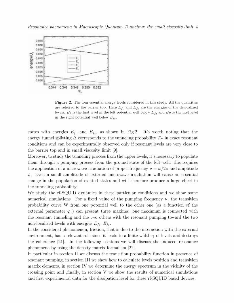
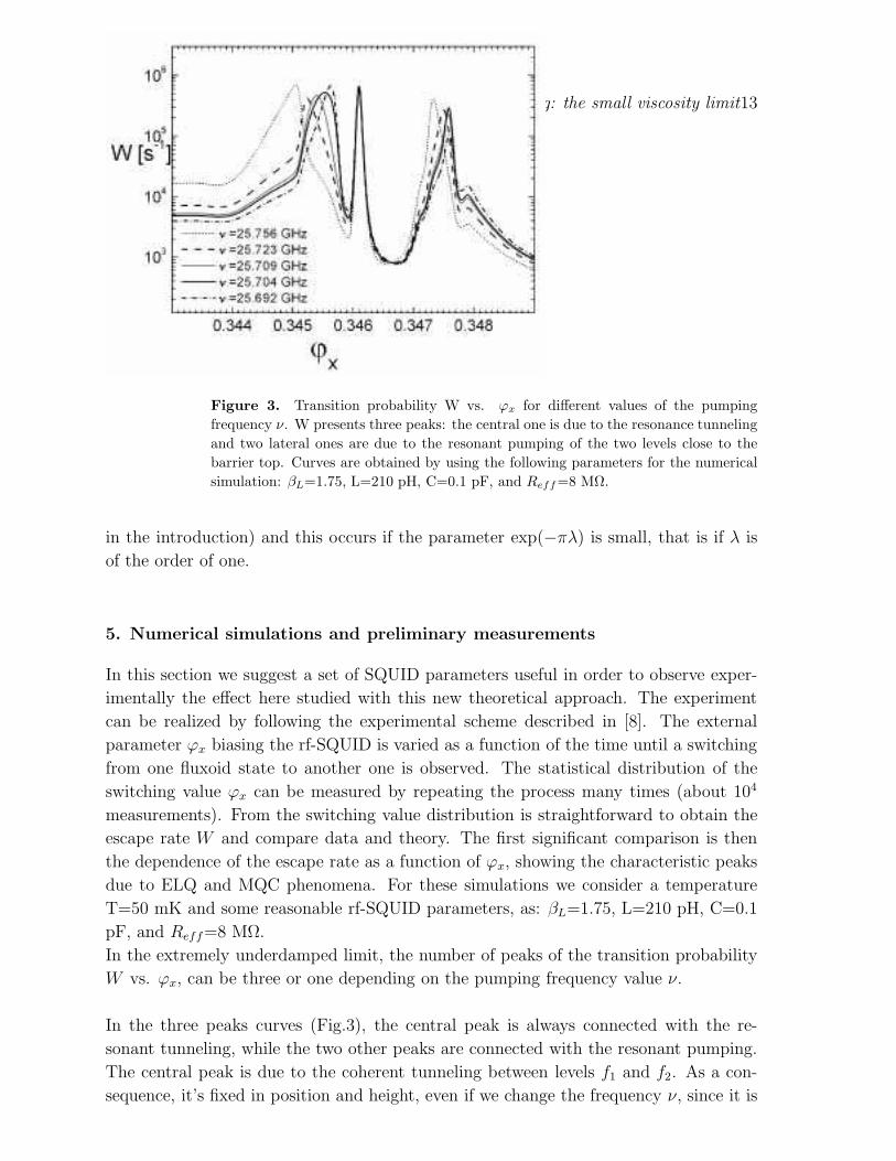
Figure 3. Transition probability W vs. ϕx for different values of the pumping

frequency ν. W presents three peaks: the central one is due to the resonance tunneling

and two lateral ones are due to the resonant pumping of the two levels close to the

barrier top. Curves are obtained by using the following parameters for the numerical

simulation: βL=1.75, L=210 pH, C=0.1 pF, and Reff=8 MΩ.

in the introduction) and this occurs if the parameter exp(−πλ) is small, that is if λ is

of the order of one.

5. Numerical simulations and preliminary measurements

In this section we suggest a set of SQUID parameters useful in order to observe exper-

imentally the effect here studied with this new theoretical approach. The experiment

can be realized by following the experimental scheme described in [8]. The external

parameter ϕx biasing the rf-SQUID is varied as a function of the time until a switching

from one fluxoid state to another one is observed. The statistical distribution of the

switching value ϕx can be measured by repeating the process many times (about 104

measurements). From the switching value distribution is straightforward to obtain the

escape rate W and compare data and theory. The first significant comparison is then

the dependence of the escape rate as a function of ϕx, showing the characteristic peaks

due to ELQ and MQC phenomena. For these simulations we consider a temperature

T=50 mK and some reasonable rf-SQUID parameters, as: βL=1.75, L=210 pH, C=0.1

pF, and Reff=8 MΩ.

In the extremely underdamped limit, the number of peaks of the transition probability

W vs. ϕx, can be three or one depending on the pumping frequency value ν.

In the three peaks curves (Fig.3), the central peak is always connected with the re-

sonant tunneling, while the two other peaks are connected with the resonant pumping.

The central peak is due to the coherent tunneling between levels f1 and f2. As a con-

sequence, it’s fixed in position and height, even if we change the frequency ν, since it is


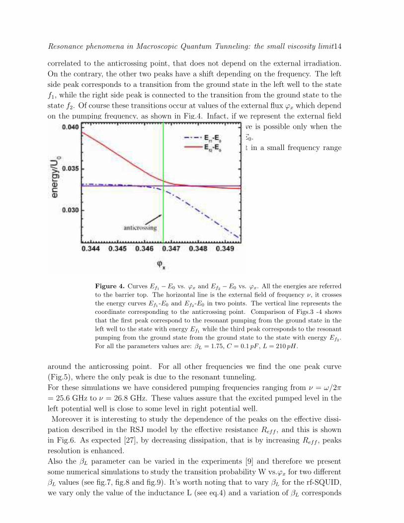
correlated to the anticrossing point, that does not depend on the external irradiation.

On the contrary, the other two peaks have a shift depending on the frequency. The left

side peak corresponds to a transition from the ground state in the left well to the state

f1, while the right side peak is connected to the transition from the ground state to the

state f2. Of course these transitions occur at values of the external flux ϕx which depend

on the pumping frequency, as shown in Fig.4. Infact, if we represent the external field

of frequency ν with a horizontal line, the three peaks curve is possible only when the

frequency crosses both the energy curves Ef1-E0 and Ef2

-E0.

We stress that we can observe the three peaks curve just in a small frequency range

Figure 4. Curves Ef1−E0 vs. ϕx and Ef2

−E0 vs. ϕx. All the energies are referred

to the barrier top. The horizontal line is the external field of frequency ν, it crosses

the energy curves Ef1-E0 and Ef2

-E0 in two points. The vertical line represents the

coordinate corresponding to the anticrossing point. Comparison of Figs.3 -4 shows

that the first peak correspond to the resonant pumping from the ground state in the

left well to the state with energy Ef1while the third peak corresponds to the resonant

pumping from the ground state from the ground state to the state with energy Ef2.

For all the parameters values are: βL = 1.75, C = 0.1 pF , L = 210 pH .

around the anticrossing point. For all other frequencies we find the one peak curve

(Fig.5), where the only peak is due to the resonant tunneling.

For these simulations we have considered pumping frequencies ranging from ν = ω/2π

= 25.6 GHz to ν = 26.8 GHz. These values assure that the excited pumped level in the

left potential well is close to some level in right potential well.

Moreover it is interesting to study the dependence of the peaks on the effective dissi-

pation described in the RSJ model by the effective resistance Reff , and this is shown

in Fig.6. As expected [27], by decreasing dissipation, that is by increasing Reff , peaks

resolution is enhanced.

Also the βL parameter can be varied in the experiments [9] and therefore we present

some numerical simulations to study the transition probability W vs.ϕx for two different

βL values (see fig.7, fig.8 and fig.9). It’s worth noting that to vary βL for the rf-SQUID,

we vary only the value of the inductance L (see eq.4) and a variation of βL corresponds


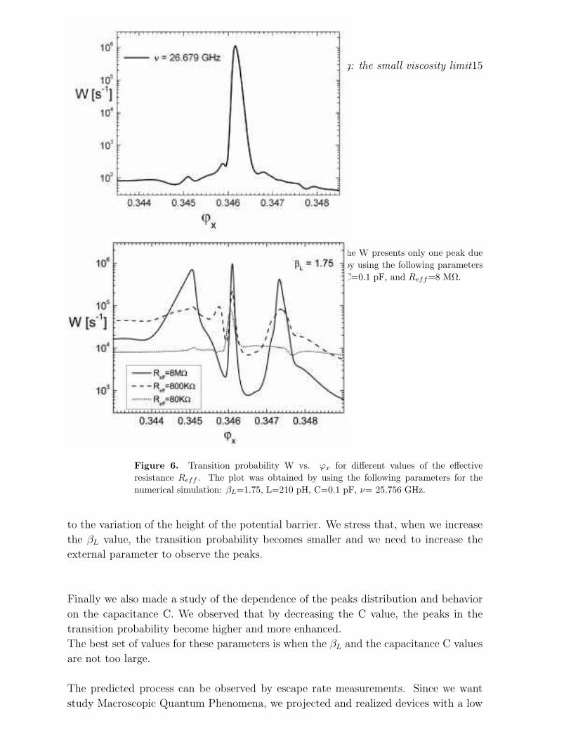
Figure 5. Transition probability W vs. ϕx. Here the W presents only one peak due

to the resonance tunneling. The plot was obtained by using the following parameters

for the numerical simulation: βL=1.75, L=210 pH, C=0.1 pF, and Reff=8 MΩ.

Figure 6. Transition probability W vs. ϕx for different values of the effective

resistance Reff . The plot was obtained by using the following parameters for the

numerical simulation: βL=1.75, L=210 pH, C=0.1 pF, ν= 25.756 GHz.

to the variation of the height of the potential barrier. We stress that, when we increase

the βL value, the transition probability becomes smaller and we need to increase the

external parameter to observe the peaks.

Finally we also made a study of the dependence of the peaks distribution and behavior

on the capacitance C. We observed that by decreasing the C value, the peaks in the

transition probability become higher and more enhanced.

The best set of values for these parameters is when the βL and the capacitance C values

are not too large.

The predicted process can be observed by escape rate measurements. Since we want

study Macroscopic Quantum Phenomena, we projected and realized devices with a low


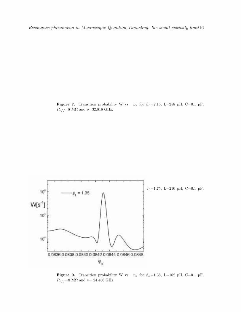
Figure 7. Transition probability W vs. ϕx for βL=2.15, L=258 pH, C=0.1 pF,

Reff=8 MΩ and ν=32.818 GHz.


Reff=8 MΩ and ν= 25.756 GHz.


Reff=8 MΩ and ν= 24.456 GHz.


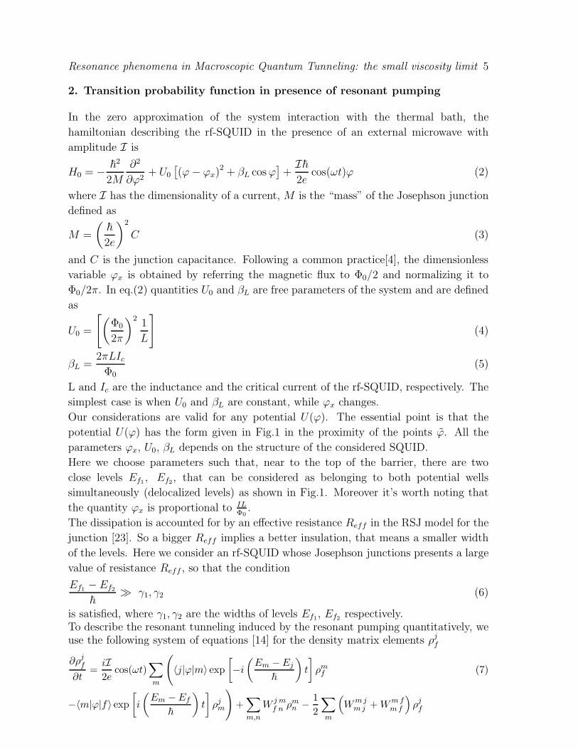
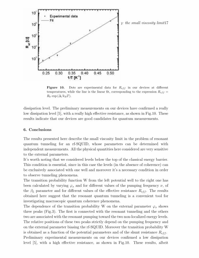
Figure 10. Dots are experimental data for Reff in our devices at different

temperatures, while the line is the linear fit, corresponding to the expression Reff =

R0 exp (∆/kBT ).

dissipation level. The preliminary measurements on our devices have confirmed a really

low dissipation level [5], with a really high effective resistance, as shown in Fig.10. These

results indicate that our devices are good candidates for quantum measurements.

6. Conclusions

The results presented here describe the small viscosity limit in the problem of resonant

quantum tunneling for an rf-SQUID, whose parameters can be determined with

independent measurements. All the physical quantities here considered are very sensitive

to the external parameters.

It’s worth noting that we considered levels below the top of the classical energy barrier.

This condition is essential, since in this case the levels (in the absence of coherence) can

be exclusively associated with one well and moreover it’s a necessary condition in order

to observe tunneling phenomena.

The transition probability function W from the left potential well to the right one has

been calculated by varying ϕx and for different values of the pumping frequency ν, of

the βL parameter and for different values of the effective resistance Reff . The results

obtained here suggest that the resonant quantum tunneling is a convenient tool for

investigating macroscopic quantum coherence phenomena.

The dependence of the transition probability W on the external parameter ϕx shows

three peaks (Fig.3). The first is connected with the resonant tunneling and the others

two are associated with the resonant pumping toward the two non-localized energy levels.

The relative positions of these two peaks strictly depend on the pumping frequency and

on the external parameter biasing the rf-SQUID. Moreover the transition probability W

is obtained as a function of the potential parameters and of the shunt resistance Reff .

Preliminary experimental measurements on our devices confirmed a low dissipation

level [5], with a high effective resistance, as shown in Fig.10. These results, albeit


still unconfirmed by a wider and more accurate experimental campaign, would suggest

potential for interesting observations regarding the resonant phenomena in the presence

of an external microwave irradiation of proper frequency.


Appendix A.

From eqs.(7), (13) we obtain two equations depending on the quantities D1 and F1

F1

[(

Ef2−Ef1

~

)

− 2iγ1

]

+ iW f1 f2

f1 f2D1 =

iI2

16e2·

〈0|ϕ|f1〉〈f2|ϕ|0〉W 0 0f1 f2

(

ω −(

Ef2−E0

~

))2

− γ1γ2 +W 0 0f1 f2

W 0 0f2 f1

+ i(γ1 + γ2)(

ω −

iW f2 f1

f2 f1F1 + D1

[(

Ef2−Ef1

~

)

− 2iγ2

]

=iI2

16e2·

〈0|ϕ|f1〉〈f2|ϕ|0〉W 0 0f2 f1

(

ω −(

Ef1−E0

~

))2

− γ1γ2 +W 0 0f1 f2

W 0 0f2 f1

− i(γ1 + γ2)(

ω −

Solution of equations (A.1) is

F1 =iI2

16e2· 〈0|ϕ|f1〉〈f2|ϕ|0〉(

Ef2−Ef1

~

)2

− 4γ1γ2 − 2i(γ1 + γ2)(

Ef2−Ef1

~

)

+W f1 f2

f1 f2W f2 f1

f2 f1

·

·[

[

Ef2−Ef1

~− 2iγ2

]

W 0 0f1 f2

(

ω − Ef2−E0

~

)2

− γ1γ2 +W 0 0f1 f2

W 0 0f2 f1

+ i(γ1 + γ2)(

ω − Ef2−E0

~

)(A.3)

−iW f1 f2

f1 f2W 0 0

f2 f1

(

ω − Ef1−E0

~

)2

− γ1γ2 +W 0 0f1 f2

W 0 0f2 f1

− i(γ1 + γ2)(

ω − Ef1−E0

~

)

]

D1 =iI2

16e2· 〈0|ϕ|f1〉〈f2|ϕ|0〉(

Ef2−Ef1

~

)2

− 4γ1γ2 − 2i(γ1 + γ2)Ef2

−Ef1

~+W f1 f2

f1 f2W f2 f1

f2 f1

·

[

[

Ef2−Ef1

~− 2iγ1

]

W 0 0f2 f1

(

ω − Ef1−E0

~

)2

− γ1γ2 +W 0 0f1 f2

W 0 0f2 f1

− i(γ1 + γ2)(

ω − Ef1−E0

~

)(A.4)

−iW f2 f1

f2 f1W 0 0

f1 f2

(

ω − Ef2−E0

~

)2

− γ1γ2 +W 0 0f1 f2

W 0 0f2 f1

+ i(γ1 + γ2)(

ω − Ef2−E0

~

)

]

The explicit expression for the transition matrix elements W f1 f2

f1 f2and W 0 0

f1 f2is given

below

W f1 f2

f1 f2=

π

Reffe2

(

1 + tanh

(

Ef2−Ef1

2kBT

))

Ef2− Ef1

πcoth

(

Ef2−Ef1

2kBT

)

|〈f1| expi ϕ2 |f2〉|2(A.5)

W 0 0f1 f2

=π

2Reffe2

(

1 + tanh

(

Ef2− Ef1

4kBT

))

Ef2−Ef1

2πcoth

(

Ef2− Ef1

4kBT

)

·

·[

〈0| expi ϕ2 |0〉〈f1| exp−i ϕ

2 |f2〉 + 〈0| exp−i ϕ2 |0〉〈f1| expi ϕ

2 |f2〉]

(A.6)

W 0 0f2 f1

= exp

(

−Ef2−Ef1

2kBT

)

W 0 0f1 f2

(A.7)


Appendix B.

For the potential, given by eq.(2) we have

ϕtop = ϕx + βL sin(ϕtop)

∂ϕtop

∂ϕx= − 1

βL cos(ϕtop) − 1

∂U

∂ϕx= −U0(ϕ− ϕx)

U1 =U0

2(βL cos(ϕtop) − 1)

∂U1

∂ϕx

=1

2βLU0

sin(ϕtop)


Utop = U0

[

1

2(ϕtop − ϕx)

2 + βL cosϕtop

]

∂Utop

∂ϕx= U0

[

βL sinϕtop − (ϕtop − ϕx)

βL cos(ϕtop) − 1− (ϕtop − ϕx)

]

From equations (29), (32) we obtain all other derivatives that should be found for

calculation of the quantities α1,2, β1,2.

∂λ

∂E= −

√

2M

U1(B.1)

∂λ

∂ϕx

= U0

√

2M

U1

[

1


[

βL sinϕtop

(

1 − Utop − E

4U1

)

− (ϕtop − ϕx)

]

− (ϕtop − ϕx)

]

(B.2)

∂χ

∂λ=

1

2ψ

(

1

2

)

+ λ2

∞∑

k=0

1

(2k + 1)((2k + 1)2 + λ2)(B.3)

Now by using equations (45), (46), (B.1), (B.1) we obtain the value of all coefficients

α1, α2, β1, β2.

β1 =∂Φ1

∂E+

1

2

∂χ

∂λ

∂λ

∂E=

√

M

2

ϕtop∫

ϕ1

dϕ

(

1√

Utop − U(ϕ)−

√

ϕtop − ϕ1

(ϕtop − ϕ)√

U1(ϕ− ϕ1)

)

(B.4)

+

√

M

2U1

ln

(

8(MU1)1/4(ϕtop − ϕ1)

21/4

)

−√

M

2U1

∂χ

∂λ

β2 =∂Φ2

∂E+

1

2

∂χ

∂λ

∂λ

∂E=

√

M

2

ϕ4∫

ϕtop

dϕ

(

1√

Utop − U(ϕ)−

√

ϕ4 − ϕtop

(ϕ− ϕtop)√

U1(ϕ4 − ϕ)

)

(B.5)

+

√

M

2U1ln

(

8(MU1)1/4(ϕ4 − ϕtop)

21/4

)

−√

M

2U1

∂χ

∂λ

α1 =∂Φ1

∂ϕx

+1

2

∂χ

∂λ

∂λ

∂ϕx

= U0

√

M

2

ϕ2∫

ϕ1

dϕϕ− ϕx

√

E − U(ϕ)+

(

1

2

∂χ

∂λ+

1

4ln

(

2

λ

))

U0

√

2M

U1

·(B.6)


·[

1

βL cosϕtop − 1

[

βL sinϕtop

(

1 − Utop − E

4U1

)

− (ϕtop − ϕx)

]

− (ϕtop − ϕx)

]

α2 =∂Φ2

∂ϕx+

1

2

∂χ

∂λ

∂λ

∂ϕx= U0

√

M

2

ϕ4∫

ϕ3

dϕϕ− ϕx

√

E − U(ϕ)+

(

1

2

∂χ

∂λ+

1

4ln

(

2

λ

))

U0

√

2M

U1·(B.7)

·[

1

βL cosϕtop − 1

[

βL sinϕtop

(

1 − Utop − E

4U1

)

− (ϕtop − ϕx)

]

− (ϕtop − ϕx)

]


Appendix C.

Transition matrix elements between states close to the barrier top can be calculated in

quasiclassical approximation if the parameter λ (see eq.(28)) is λ ≥ 1. Consider first

the matrix element 〈L|ζ |f1〉. With the help of eqs.(28), (40), (41) we obtain

〈L|ζ |f1〉 =1

GLGEf1

ϕ2(Ef1)

∫

ϕ1(Ef1)

dϕ

sin

(

π/4 +ϕ∫

ϕ1(EL)

dϕ√

(2M (EL − U(ϕ)))

)

(2M (EL − U(ϕ)))1/4 (2M (Ef1− U(ϕ)))1/4

ζ sin

π/4 +

ϕ∫

ϕ1(Ef1)

dϕ√

(2M (Ef1

that is equal to

〈L|ζ |f1〉 =1

2GLGEf1

∫

dϕ√

(2M (Ef1L − U(ϕ)))ζ cos

(

(Ef1− EL)

∫ ϕ

ϕ1(Ef1L)

Mdϕ√

2M (Ef1L − U(ϕ))

)

(C.2)

To calculate the last integral we can use the time variable t according to the classical

equation of motion

M

2

(

∂ϕ

∂t

)2

= E − U(ϕ) (C.3)

As a consequence, eq.(C.2) becomes

〈L|ζ |f1〉 =1

2MGLGEf1

T1/2∫

0

dtζ cos

(

2π

T1tℓ

)

(C.4)

where T1 is the period of the classical motion in the left potential well with energy E

and ℓ is the number of states between energy levels Ef1and EL plus one. In our case

ℓ = 1. The initial value for ϕ is ϕ(0) = ϕ1.

T1 = 2M

ϕ4∫

ϕ3

dϕ√

(2M (E − U(ϕ)))(C.5)

In the same way we obtain transition the matrix element 〈R|ζ |f1〉.

In eq.(C.1) ϕ1(Ef1) is the first crossing point of the energy level Ef1

in the left well

and ϕ2(Ef1) is the second crossing point of the energy level Ef1

in the left well.

In the same way in eq.(C.2) ϕ1(Ef1L) is the first crossing point of the energy level Ef1L

in the left well, where Ef1L is defined as

Ef1L =Ef1

+ EL

2(C.6)

Consider now the transition matrix element 〈f2| ζ |f1〉. From eq.(28) we find

〈f2| ζ |f1〉 =~

2Gf1Gf2

ϕ2∫

ϕ1

dϕζ

√

(2M (E − U(ϕ)))+Bf1

Bf2

ϕ4∫

ϕ3

dϕζ

√

(2M (E − U(ϕ)))

(C.7)


where ϕ1,2,3,4 are the “turning points” and E here is E =(Ef1

+Ef2)2

.By using eq.(C.3) we reduce the expression (C.7) to the form

〈f2| ζ|f1〉 =~

2MGf1Gf2

T1/2∫

0

dtζ + Bf1Bf2

T2/2∫

0

dtζ

(C.8)

In eq.(C.8) the first integral is taken over the left potential well and the second oneover the right potential well and T1, T2 are the periods of the classical motion in the leftand in the right well respectively.To improve eq.(C.8) we should take into account ortogonality of wavefunctions relativeto the energies Ef1

, Ef2. As result we obtain

〈f2| ζ|f1〉 = ~1 − Bf1

Bf2

2MGf1Gf2

T2

T1 + T2

T1/2∫

0

dtζ − T1

T1 + T2

T2/2∫

0

dtζ

(C.9)

Acknowledgments

The research of one of us (Yu.N.O.) is supported by Cariplo Foundation-Italy, CRDF

USA under Grant No. RP1-2565-MO-03 and the Russian Foundation of Basic Research.

This work has been partially supported by MIUR under Project “Reti di Giunzioni

Josephson per la Computazione e l’Informazione Quantistica-JOSNET”.

References

[1] A. O. Caldeira and A. J. Leggett. Phys. Rev. Lett., 46:211, 1981.

[2] D. B. Schwartz, B. Sen, C. N. Archie, and J. E. Lukens. Phys. Rev. Lett., 55:1547, 1985.

[3] S. Washburn, R. A. Webb, R. F. Voss, and S. M. Faris. Phys. Rev. Lett., 54:2712, 1985.

[4] R. Rouse, S. Han, and J.E. Lukens. Phys.Rev.Lett., 75:1614, 1995.

[5] V. Corato, S.Rombetto, C. Granata, E. Esposito, L. Longobardi, M. Russo, R. Russo, B. Ruggiero,

and P. Silvestrini. Phys. Rev., B70:172502, 2004.

[6] J. M. Martinis, M. H. Devoret, and J. Clarke. Phys. Rev. Lett., 55:1543, 1985.

[7] J. M. Martinis, M. H. Devoret, and J. Clarke. Phys. Rev., 35:4682, 1987.

[8] P. Silvestrini, V. G. Palmieri, B. Ruggiero, and M. Russo. Phys. Rev. Lett., 79:3046, 1997.

[9] J. R. Friedman, V. Patel, W. Chen, S. K. Tolpygo, and J. E.Lukens. Nature (London), 406:43,

2000.

[10] J. B. Majer, F. G. Paauw, A.C. J. ter Haar, C. J. P.M. Harmans, and J. E. Mooij. Phys. Rev.

Lett., 94:090501, 2005.

[11] J. Claudon, F. Balestro, F. W. J. Hekking, and O. Buisson. Phys. Rev. Lett., 93:187003, 2004.

[12] M. H. Devoret and J. M. Martinis. Quantum Entanglement and Information Processing. - Les

Houches Summer School Proceedings 79. Elsevier, San Diego, CA,, 2004.

[13] N. Groenbech-Jensen and M. Cirillo. Phys. Rev., B70:214507, 2004.

[14] A.I.Larkin and Yu.N.Ovchinnikov. J. of Low Temp. Phys., 63:317, 1986.

[15] Yu.N.Ovchinnikov, P.Silvestrini, V.Corato, and S.Rombetto. Phys. Rev., B71:024529, 2005.

[16] Yu.N.Ovchinnikov and A.Schmid. Phys. Rev., B50:6332, 1994.

[17] D. Averin. Solid State Commun., 105:659, 1998.

[18] D. Averin. Phys. of low temp. Phys., 118:781, 2000.

[19] D. V. Averin, J. R. Friedman, and J. E. Lukens. Phys. Rev., B62:11802, 2000.

[20] A.I.Larkin and Yu.N.Ovchinnikov. Sov. Phys. JETP, 64:185, 1986.


[21] A.I.Larkin and Yu.N.Ovchinnikov. Phys. Rev., B50:6332, 1994.

[22] U. Fano. Rev. of Mod. Phys., 29:74, 1957.

[23] A. Barone and G. Paterno. Physics and Applications of the Josephson Effect. Wiley, New York,

1982.

[24] A.I.Larkin and Yu.N.Ovchinnikov. Sov. Phys. JETP, 60:1060, 1984.

[25] I. M. Ryzhik and I. S. Gradstein. Table of Integrals, Series and Products. Academic Press, New

York, 1965.

[26] L. Landau and L. Lifshitz. Quantum Mechanics: non-relativistic theory. Butterworth-Heinemann,

1981.

[27] P. Silvestrini, B. Ruggiero, and Yu.N. Ovchinnikov. Phys. Rev., B54:1246, 1996.

Resonance phenomena in macroscopic quantum tunneling for an rf SQUID

Documents

Transcript of Resonance phenomena in macroscopic quantum tunneling for an rf SQUID