Parameter Estimation of the Macroscopic Fundamental Diagram

Parameter Estimation of the Macroscopic Fundamental Diagram: a

Maximum Likelihood Approach

Rafegh Aghamohammadia, Jorge A. Lavala,∗

aSchool of Civil and Environmental Engineering, Georgia Institute of Technology

Abstract

This paper extends the Stochastic Method of Cuts (SMoC) to approximate of the Macro-scopic Fundamental Diagram (MFD) of urban networks and uses Maximum Likelihood Es-timation (MLE) method to estimate the model parameters based on empirical data from acorridor and 30 cities around the world. For the corridor case, the estimated values are ingood agreement with the measured values of the parameters. For the network datasets, theresults indicate that the method yields satisfactory parameter estimates and graphical fitsfor roughly 50% of the studied networks, where estimations fall within the expected range ofthe parameter values. The satisfactory estimates are mostly for the datasets which (i) covera relatively wider range of densities and (ii) the average flow values at different densitiesare approximately normally distributed similar to the probability density function of theSMoC. The estimated parameter values are compared to the real or expected values andany discrepancies and their potential causes are discussed in depth to identify the challengesin the MFD estimation both analytically and empirically. In particular, we find that themost important issues needing further investigation are: (i) the distribution of loop detec-tors within the links, (ii) the distribution of loop detectors across the network, and (iii) thetreatment of unsignalized intersections and their impact on the block length.

Keywords: Macroscopic Fundamental Diagram, Analytical Approximation, MaximumLikelihood Estimation

1. Introduction1

Urban congestion is an overgrowing issue in many cities all over the globe. Financial,2

economic and environmental costs associated with the congestion have been vastly studied3

and control and management methods have been proposed to improve the level of service4

and mitigate these costs. Significant amount of research effort has been devoted in the past5

decades to develop a better understanding of the nature and dynamics of urban congestion6

and the way it propagates through the urban street network. The idea of an aggregated7

relationship between average density and flow over the network dates back to 1960s (Smeed,8

∗Corresponding authorEmail address: [email protected] (Jorge A. Laval)

Preprint submitted to Elsevier October 20, 2021

Preprints (www.preprints.org) | NOT PEER-REVIEWED | Posted: 21 October 2021

© 2021 by the author(s). Distributed under a Creative Commons CC BY license.

doi:10.20944/preprints202110.0310.v1

http://creativecommons.org/licenses/by/4.0/

https://doi.org/10.20944/preprints202110.0310.v1

1967; Godfrey, 1969). Later, many researchers have elaborated on this idea and proposed1

various models to describe the relationship between the network-wide traffic variables (see2

e.g., Herman and Prigogine, 1979; Mahmassani et al., 1984; Ardekani and Herman, 1987).3

Daganzo (2007) claims that the relationship between the average flow and density is an4

invariant property of the network regardless of the demand and OD patterns. Existence5

of such well-defined relationship was first empirically verified by Geroliminis and Daganzo6

(2008) using the loop detector and taxi GPS data from Yokohama, Japan, which has been7

named the macroscopic fundamental diagram (MFD) by the authors. Since then, many8

researchers have collected network-wide data to investigate the relationship between average9

flow, density and speed across urban networks and have derived the MFD for several cities10

around the world (see e.g., Buisson and Ladier, 2009; Tsubota et al., 2014; Wang et al.,11

2015; Ambuhl et al., 2018; Knoop et al., 2018).12

Nevertheless, deriving the MFD using the empirical data is challenging since (i) the13

required loop detector data is not available in most of the cities, (ii) in the networks with14

available loop detector data, the loop detectors cover only a fraction of streets in the network,15

and (iii) the data coming from various loop detectors is prone to bias and inaccuracy, which16

makes the data cleaning and processing cumbersome. These challenges make it difficult to17

obtain systematic insight into MFD characteristics and the factors impacting its shape.18

To overcome these challenges, some studies have resorted to micro-simulation approaches19

to see how the changes in network topology and control can affect the shape of the MFD20

(see e.g., Ji et al., 2010; Knoop et al., 2014; Gayah et al., 2014). However, these studies are21

mostly carried out on small arbitrary networks since the calibration of the micro-simulation22

models on large-scale networks is a cumbersome task due to their complex and heterogeneous23

nature. Therefore, the micro-simulation approach might not be a feasible option to study24

the impact of network characteristics on the shape of the MFD of real-life networks.25

Analytical approximations can be a useful tool to estimate the MFD without having26

to face the data collection and preparation challenges. Daganzo and Geroliminis (2008)27

introduced the Method of Cuts (MoC) as an analytical approximation method for estimation28

of an upper bound for the MFD of homogeneous corridors using the variational theory (VT;29

Daganzo, 2005a,b). Later, Laval and Castrillon (2015) developed the stochastic method of30

cuts (SMoC) by extending the MoC to heterogeneous corridors by introducing stochasticity31

and using renewal theory. This model is the most detailed analytical MFD estimation model32

to date, incorporating the most number of the influential network topology and control33

characteristics and the variations in their values over time and space.34

Both of the mentioned analytical methods are proposed for estimation of the MFD of35

signalized corridors, while limited discussion have also been presented on their extension for36

network MFD estimation. These extensions come along with a number of assumptions and37

simplifications that make them impractical for estimating the MFD of real-life large-scale38

networks due the inherent heterogeneity of their topological and control characteristics. The39

reasons behind complexity of traffic dynamics in large-scale networks compared to signalized40

corridors includes but is not limited to significantly higher number of links, inclusion of41

streets from different functional classifications and different speed limits, distribution of42

origins and destinations (trip start and end points) all across the network, directionality of43

2

Preprints (www.preprints.org) | NOT PEER-REVIEWED | Posted: 21 October 2021 doi:10.20944/preprints202110.0310.v1


the links, different number of lanes in each link, turning movements at intersections, different1

control strategies at intersections (e.g. pre-timed signals, actuated signals, roundabouts, stop2

and yield signs), etc. Therefore, some considerations have to be made before implementing3

the current methods for estimation of network MFDs.4

The purpose of this study is twofold: (i) first, to extend the SMoC for analytical esti-5

mation of the MFD of large-scale real-life networks and (ii) second, to propose a method6

to estimate the parameters of the stochastic analytical MFD using empirical data for both7

corridors and networks and investigate the impact of different network topology and control8

characteristics on the shape of the MFD. The network-wide dataset studied here is obtained9

from the recently-published loop detector data (LDD) in UTD19 (Loder et al., 2019) for10

40 cities around the world. Toward this end, the rest of this paper is organized as fol-11

lows: section 2 reviews the current literature on the analytical MFD estimation methods,12

section 3 describes the SMoC analytical corridor MFD model, its extension for network13

MFD estimation and lays out the experimental setup for estimating the model parameters,14

section 4 presents the results of application of the proposed parameter estimation method15

on different corridor and network datasets, section 5 discusses the findings, challenges and16

recommendations for future research and finally section 6 presents the concluding remarks.17

2. Background18

The MFD estimation methods in the literature can in general be classified into 3 main19

categories: (i) empirical, (ii) simulation-based and (iii) analytical studies. Although the20

empirical method is the most reliable and accurate way to estimate the MFD, the required21

data is not available for many cities and even when available it is subject to significant22

errors and bias. The exorbitant dependency of empirical approach on the availability and23

accuracy of network-wide data makes it an impractical option for estimation of MFD in24

many cities. While simulation seems to be a promising tool to overcome the dependency of25

empirical approach on data, calibration of detailed micro-simulation models for large-scale26

urban networks is a cumbersome and prohibitive task.27

The aforementioned drawbacks of the empirical and simulation-based MFD estimation28

methods highlight the significance of the analytical approach to determine the network29

MFD using network topology and control characteristics and find out the impact of each30

factor on the shape of the MFD. However, no universal recipe yet exists in the literature31

for analytical approximation of MFD for large-scale networks. The present efforts in the32

literature investigate the analytical estimation of MFD for signalized corridors and there are33

some limited extensions to estimate network-wide MFDs. In this section, we will first present34

the literature on analytical estimation of corridor MFDs and later review the analytical35

methods for estimation of network MFDs.36

2.1. Analytical Corridor MFD Estimation Methods37

Daganzo and Geroliminis (2008) has proposed the Method of Cuts (MoC) as the first38

analytical method for approximation of the MFD of signalized homogeneous corridors imple-39

menting the VT. In this method a set of linear cuts are plotted on the average flow-density40

3



space based on moving observers travelling in the corridor, forming an upper bound for the1

corridor MFD. The average flow-density MFD is defined as the steady-state flow at any2

location, x, as:3

q(k) = minvφ(k) + vk, (MoC) (1)

where q and k are average flow and density, respectively, v is the average speed of the4

moving observer and φ(v) is its maximum passing rate. However, evaluating φ(k) for all cuts5

with different speeds is time-consuming and redundant, therefore, Daganzo and Geroliminis6

(2008) proposes three families of “practical cuts” using stationary, forward-moving and7

backward-moving observers in the corridor. These cuts form an upper bound for the MFD,8

which might not tightly define the MFD.9

Leclercq and Geroliminis (2013) generalizes the concept of practical cuts by including a10

sufficient number of additional cuts representing optimal paths with different mean speeds11

to provide a tighter upper bound for the MFD. Xie et al. (2013) presents two methods for12

estimation of the corridor MFDs with presence of public transport by (i) including buses in13

the method proposed in Leclercq and Geroliminis (2013) and (ii) accounting for buses in the14

time-space diagram according to the kinematic wave theory.15

Nevertheless, the MoC is proposed for homogeneous corridors with equal block lengths16

and signal settings, which makes it complicated to be scaled up for the network MFD17

estimation. Daganzo and Lehe (2016) has extended the concept of the MoC to account18

for inhomogeneities in block length and offset of adjacent traffic signals and formulated the19

method as a linear program.20

To more generally account for the variations in the block length and signal timing set-21

tings, Laval and Castrillon (2015) has extended the MoC to inhomogeneous corridors devel-22

oping the Stochastic Method of Cuts (SMoC). It first defines the stochastic corridor random23

variable, where each inhomogeneous corridor is a realization of this random variable with24

three main independent random variables: block length (`), signal green (g) and red (r)25

times which can vary in time and across different segments of the corridor. In order to sim-26

plify the representation of the problem, it has reformulated the individual link fundamental27

diagram (FD) and network parameters in dimensionless form by measuring time in units of28

critical headway and space in units of jam spacing, assumed the coefficients of variations29

(δ) of the three main parameters are equal and performed a density transformation to have30

symmetric fundamental diagram (FD) and MFD.31

This method results in normally-distributed stochastic cuts, qs(k); therefore, the yielding32

upper-bound MFD found using this model will also be stochastic, whose CDF is formulated33

in the study. The authors found that the shape of the MFD mainly depends on two dimen-34

sionless parameters: (i) mean block length to critical length ratio, λ, and (ii) mean red to35

green signal time ratio, ρ. The SMoC has shown promising results in capturing the shape36

of MFD for corridors with different values of λ, ρ and δ.37

Castrillon and Laval (2018) revisits the MoC to include the impact of buses on the MFD38

of homogeneous corridors. They found that presence of buses has two major impacts: (i)39

“moving bottleneck effect” due to lower speed of buses compared to other vehicles and (ii)40

4



reduction in capacity due to the “short block” effect. Each of these effects result in an1

additional cut in the MoC providing a tighter upper bound for the corridor MFD.2

Recently, Tilg et al. (2020) has compared the performance of MoC and SMoC to the3

empirical MFD obtained using data from the city of Munich, Germany. The empirical data4

is for the northbound direction of an arterial segment of 1.1 km with 5 intersections, where all5

intersections are controlled by actuated traffic signals. Although there are some discrepancies6

between the estimated analytical MFDs and the empirical MFD, which might be due to7

turning movements and other real-life network complexities which are not considered in the8

analytical methods, the results show that the MoC provides a good estimate for the corridor9

capacity and the SMoC delivers a good fit for the free-flow branch of the MFD.10

2.2. Analytical Network MFD Estimation Methods11

Although the analytical MFD estimation methods discussed in the previous section are12

proposed for estimation of corridor MFDs, most studies have discussed the potential exten-13

sion of their method to network MFD estimation and have tested the model on toy networks14

or simplified real-life networks under some assumptions. Daganzo and Geroliminis (2008)15

has tested the MoC on the empirical data from Yokohama and the simulation data for San16

Francisco by decomposing the network into 1-lane links, thereby eliminating lane changing.17

For the Yokohama data, assumptions are made for the link FD and signal setting parame-18

ters. While the MoC results in a good fit for the simulation data for San Francisco assuming19

pre-timed signals with a common cycle, it overestimates the speed and flow for the Yoko-20

hama network, which authors have mentioned can be partly due to the measurement errors21

in the empirical data, heterogeneity of the network and actuated signal settings varying with22

time.23

Geroliminis and Boyacı (2012) introduces a number of extensions and refinements to the24

VT to analytically investigate the effects of different traffic signal offsets and block lengths on25

the homogeneous network MFD. Leclercq and Geroliminis (2013) has extended its method26

to estimate the MFD of a simple network consisting a number of parallel hyperlinks to27

investigate the impacts of different route choice models on the MFD. The results show that28

variation in densities over the network can affect the shape of the MFD.29

Laval and Castrillon (2015) claims that their proposed SMoC can provide a good approx-30

imation for networks as well as corridors if the following conditions are met: (i) the density31

is distributed homogeneously over the network, and (ii) the block lengths and signal green32

and red times are i.i.d. random variables. If these conditions are met, all network paths can33

be considered as realizations of the stochastic corridor random variable and the SMoC will34

provide a good approximation for the network MFD. The approximated analytical MFD for35

the Yokohama network using the assumed network parameters in Daganzo and Geroliminis36

(2008) shows good agreement with the empirical MFD.37

Ambuhl et al. (2018) developed a method to derive a functional form with a physical38

meaning for the upper bound MFD. The proposed model results in a trapezoidal function39

using a smoothing parameter and four physical properties of the network: free-flow speed,40

backward wave speed, jam density and intersection capacity. The authors have fitted the41

model to empirical loop detector data from 4 cities in Europe, which has resulted in viable42

5



estimates for the model parameters. However, this model does not take the block lengths1

into account, which has been shown to have a significant impact on the shape of the MFD2

in most of the other studies.3

3. Experimental Setup4

As discussed earlier, several analytical methods are presented in the literature for the5

MFD estimation. Although the models are mainly proposed for analytical estimation of6

corridor MFDs, there have been limited discussions about extending them to estimate the7

network MFDs. Among the models presented in the literature, the SMoC seems to be the8

most detailed model incorporating the most number of the influential network topology and9

control characteristics taking the spatial and temporal variations in the parameters into10

account. However, this method has not been empirically verified for estimation of network11

MFDs. Here, we will first present the original SMoC model and explore how it can be12

extended to approximate the MFDs of large-scale networks and later a method will be13

presented to estimate the SMoC parameters to fit them to the empirical network MFDs and14

draw insights into the impact of different parameters on the shape of the MFD.15

3.1. Structure of the SMoC16

The stochastic method of cuts (SMoC) proposed by Laval and Castrillon (2015) intro-17

duces an stochastic extension to the MoC by allowing for variations in the network topology18

and control parameters. The variables used in the model are listed in Table 1. This model19

builds on the VT and MoC using cuts based on the same three categories of forward-moving,20

stationary and backward-moving observers. The main addition of the model is its ability21

to capture the spatial variations in block lengths and the spatial and temporal variations in22

signals cycle and phase durations, enabling its application for estimating the MFD where23

Table 1: SMoC model parameters

Link Fundamental Diagram

Q Capacity (veh/h/ln)K Jam Density (veh/km)u Free-flow speed (km/h)w Backward wave speed (km/h)θ Free-flow speed to backward wave speed ratio (dimensionless)

Network Parameters

µ` Mean block length (m)µg Mean signal green time (s)µr Mean signal red time (s)λ Mean block length to critical block length ratio (dimensionless)ρ Mean signal red-to-green ratio (dimensionless)δ Coefficient of variation of network parameters (dimensionless)

6



the signal timing settings are different for different intersections or actuated signal controls1

are in use.2

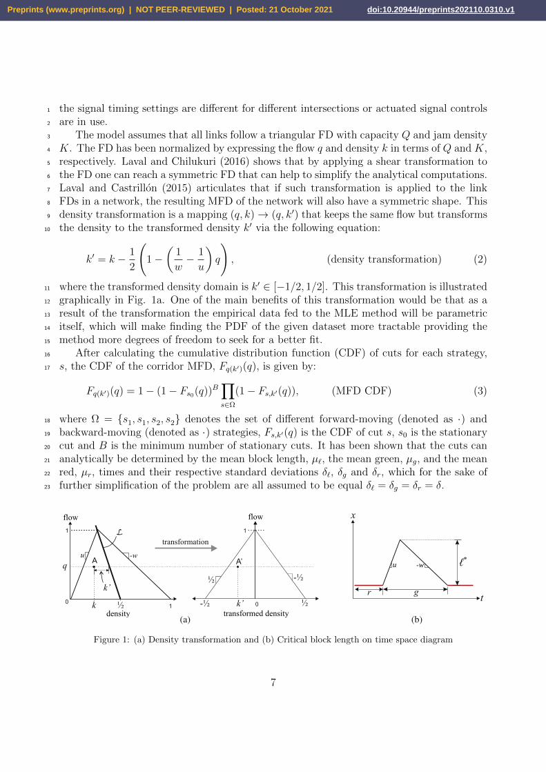
The model assumes that all links follow a triangular FD with capacity Q and jam density3

K. The FD has been normalized by expressing the flow q and density k in terms of Q and K,4

respectively. Laval and Chilukuri (2016) shows that by applying a shear transformation to5

the FD one can reach a symmetric FD that can help to simplify the analytical computations.6

Laval and Castrillon (2015) articulates that if such transformation is applied to the link7

FDs in a network, the resulting MFD of the network will also have a symmetric shape. This8

density transformation is a mapping (q, k)→ (q, k′) that keeps the same flow but transforms9

the density to the transformed density k′ via the following equation:10

k′ = k − 1

2

(1−

(1

w− 1

u

)q

), (density transformation) (2)

where the transformed density domain is k′ ∈ [−1/2, 1/2]. This transformation is illustrated11

graphically in Fig. 1a. One of the main benefits of this transformation would be that as a12

result of the transformation the empirical data fed to the MLE method will be parametric13

itself, which will make finding the PDF of the given dataset more tractable providing the14

method more degrees of freedom to seek for a better fit.15

After calculating the cumulative distribution function (CDF) of cuts for each strategy,16

s, the CDF of the corridor MFD, Fq(k′)(q), is given by:17

Fq(k′)(q) = 1− (1− Fs0(q))B∏s∈Ω

(1− Fs,k′(q)), (MFD CDF) (3)

where Ω = s1, s1, s2, s2 denotes the set of different forward-moving (denoted as ·) and18

backward-moving (denoted as ·) strategies, Fs,k′(q) is the CDF of cut s, s0 is the stationary19

cut and B is the minimum number of stationary cuts. It has been shown that the cuts can20

analytically be determined by the mean block length, µ`, the mean green, µg, and the mean21

red, µr, times and their respective standard deviations δ`, δg and δr, which for the sake of22

further simplification of the problem are all assumed to be equal δ` = δg = δr = δ.23

ℓ*-wu

u -w

flow

density transformed density

flow

(a) (b)

Figure 1: (a) Density transformation and (b) Critical block length on time space diagram

7



The authors further claim that the shape of the MFD is mainly influenced by two di-1

mensionless parameters: (i) the mean block length to critical length ratio λ = µ`µ`∗

, and (ii)2

the mean red to green signal time ratio ρ = µrµg

. The critical block length is the minimum3

block length to avoid the short block effect; see Fig. 1b. As seen in this figure, the critical4

block length can be computed as:5

`∗ = ugkcK

=Q

kcgkcK

=gQ

K, (critical block length) (4)

where kc is the critical density. If the dimensionless forms of flow and density are used in6

the equation above, one will have:7

`∗ = g. (dimensionless critical block length) (5)

Knowing the values of the required parameters for a corridor or network, one can com-8

pute the cut CDFs and eventually determine the corresponding CDF of the MFD. However,9

gathering the data required to find the model parameters is not a straightforward task. In10

many cities the data is not readily available due to the lack of measurement equipment and11

even when it is available, it is prone to different biases and measurement errors. Computing12

the parameters becomes more challenging if the method is applied for network MFD esti-13

mation due to the higher complexity and heterogeneity of the network topology and control14

settings. We will delve into these challenges in more detail later in the paper. Here, we15

will present a method to statistically estimate the parameters by applying the maximum16

likelihood estimation (MLE) method to the empirical corridor and network MFDs based on17

loop detector data (LDD). But before that, we need to check how the original model can be18

extended to approximate the MFDs of large-scale networks.19

3.2. Extension of the SMoC for Network MFD Estimation20

The SMoC has been originally developed for corridor MFD estimation. The authors have21

claimed that the model can be applied for estimation of network MFDs as well. However, the22

model cannot be readily implemented to estimate the network MFDs. Although the model23

can be extended in many different ways to take into account additional network properties24

such as the presence of buses by including additional cuts, here, we want to stick to the25

original model framework and cuts, and only explore whether there would be any need for26

redefinition of any of the model parameters while scaling up from corridors to networks.27

A brief look at Table 1 reveals that link FD and the mean block length parameters can28

be defined and calculated for networks in the same fashion as the corridors. However, this29

is not true for the signal timing parameters and especially for the mean red to green signal30

time ratio, ρ, which is one of the most influential parameters impacting the shape of the31

MFD. In the corridor case, the calculation of ρ is straightforward since at each intersection32

the green and red times for the corridor of interest are known explicitly. However, in the33

network case, there arises confusion in selecting the green and red times for each intersection,34

since there are several approaches with different green and red times. If the signal timing35

data is available for all approaches of all intersection across the network, assuming that most36

signals have only two phases, the sum of green times will almost be equal to the sum of red37

8



times (neglecting the lost times) at the approach, intersection and network level, therefore1

resulting in ρ ≈ 1.2

Nevertheless, in many cities there are intersections with protected left turn phases or3

more than two phases, which will make the mean red time higher than the mean green time4

and ultimately ρ>1. To gain a better understanding of how the presence of traffic signals5

with any general number of phases, ni, impacts the value of ρ, let us first focus on a single6

phase of the intersection. By definition, one can find the mean red to green signal time ratio7

for a phase, ρj, as:8

ρj =rjgj

=

ni∑k=1,k 6=j

gk

gj, (ρj for a single phase, j) (6)

where gj is the average green time for phase j and gk represents the average green time for9

the rest of the phases, k.10

The value of ρ in the model is in fact an indicator of the available intersection capacity.11

Higher ρ values mean that more time is assigned to the red phase compared to the green12

time and less intersection capacity is being utilized, while lower ρ values would mean higher13

utilization of the cycle time and intersection capacity. Therefore, the rational way to compute14

the average ρi for an intersection, i, is to take a weighted average of the values for all phases in15

the signal timing with respect to their respective demand or flow. Without loss of generality,16

one can assume that the signal timing is efficiently programmed to be proportionate to the17

demand values at each phase. Hence, the weight of each phase, wj, can be found as:18

wj =fjni∑j=1

fj

=gjni∑j=1

gj

=gjC, (weighting factor of each phase) (7)

where fj is the demand or flow of each phase j and C is the total cycle time for the19

intersection. Now, the mean red to green time ratio for intersection i, ρi, can be computed20

as:21

ρi =

ni∑j=1

wjρj =

ni∑j=1

gjC×

ni∑k=1,k 6=j

gk

gj=

1

C

ni∑j=1

ni∑k=1k 6=j

gk =(ni − 1)C

C= ni − 1. (8)

Having obtained a simple expression for ρi, the mean red to green signal time ratio for22

the entire network with N intersections can be calculated as:23

ρ =

N∑i=1

ρi

N=

N∑i=1

ni − 1

N=

N∑i=1

ni

N− N

N= n− 1, (ρ of a network) (9)

where n is the average number of signal phases of the intersections in the network. Now24

that we have found how all the model parameters can be determined to approximate the25

network MFDs, we can proceed to estimation of model parameters using empirical data.26

9



3.3. Parameter Estimation Using Maximum Likelihood Estimation Method1

Once the probability distribution of a dataset is known, we can estimate the population2

parameters using the distribution fitting methods such as the method of moments or the3

maximum likelihood estimation (MLE) method. In this study, we will use the MLE due4

to its large-sample or asymptotic properties to estimate the analytical MFD given by the5

SMoC and its parameters for several different cases using their empirical MFDs. The MLE6

estimators become minimum-variance unbiased estimators as the sample size increases and7

have approximate normal distributions and approximate sample variances that can be used8

to generate confidence bounds and hypothesis tests for parameters.9

Let the probability density function (PDF) of the MFD, which can be derived as the10

derivative with respect to q of the CDF given in Eq. (3), be denoted as f(x|Θ). The11

likelihood function for a given dataset X is the joint density of n independent and identically12

distributed (i.i.d.) observations, which is the product of their individual densities:13

L(Θ|X) = f(x1, . . . , xn|Θ) =∏xi∈X

f(xi|Θ), (likelihood function) (10)

where Θ is the unknown parameter vector. Considering that some of the model parameters14

presented in Table 1 are dependent and can be derived using the other parameters, we choose15

Θ = Q,K, θ, µ`, µg, ρ, δ as the independent parameter vector. It is worth noting that the16

likelihood function is a function of the parameters conditioned on the data whereas the joint17

density is a function of the data conditioned on the parameters. In the MLE method, we aim18

to find the parameter values that maximize the likelihood function for the observed data.19

However, for the sake of more convenience in the computations, it is preferred to maximize20

the natural logarithm of the likelihood function, l:21

l(Θ|X) = lnL(Θ|X) = ln∏xi∈X

f(xi|Θ) =∑xi∈X

ln f(xi|Θ). (log-likelihood function) (11)

By maximizing the log-likelihood function, we find the set of parameter estimators Θ for22

each dataset, under which observing the dataset is most probable. Under certain regularity23

conditions, the estimators are known to asymptotically tend to have a multivariate normal24

distribution for large samples:25

Θ ∼ Np(Θ, J−1(Θ)), (multivariate normal distribution of estimators) (12)

where for our model the number of variables is p = 7 and the covariance matrix of param-26

eters, J−1(Θ), is the inverse of the observed Fisher’s information matrix, J(Θ), calculated27

as:28

J(Θ) = −∂2l(Θ)

∂Θ2, (observed information matrix) (13)

where the J−1 is the covariance matrix of the model parameters and its diagonal elements are29

the variance of the parameters. The regularity conditions include: (i) the true parameter30

values must be interior to the parameter space, (ii) the log-likelihood function must be31

thrice differentiable and (iii) the third derivatives must be bounded (Geyer et al., 1994).32

Knowing the distribution of the estimators will enable us to perform hypothesis testings for33

the estimated values.34

10



3.4. Data Sources and Preparation1

The proposed estimation method will first be applied on a empirical MFD dataset for2

a 4-block corridor from Munich provided by Tilg et al. (2020). This dataset is already3

consisted of the average flow versus average density data for the corridor and, thus, does4

not need any further preparation to be used by the proposed method in this study.5

In order to evaluate the method for analytical network MFD and parameter estimation,6

the network-wide loop detector data published in UTD19 (Loder et al., 2019) for 40 cities7

around the world is used. The dataset includes flow, loop detector occupancy and sporadic8

speed measurements for 3 up to 60 minute intervals. We first need to derive the empirical9

MFDs for the networks in the dataset and then apply the proposed estimation method to10

approximate the analytical MFD and estimate the network topology and control parameters.11

However, the provided raw data needs to be cleaned and processed to produce valid empirical12

MFDs, which will be elucidated in the ensuing subsection for the sake of reproducibility of13

the research.14

3.4.1. Network empirical data cleaning and processing15

The UTD19 dataset includes the loop detector measurements, loop detector descriptions16

and link descriptions for 40 urban networks worldwide. We first separate the respective data17

for each network before processing the data further. Our initial evaluation of the dataset18

reveals that the time intervals of the measurements for the city of Paris is 1 hour, which is19

very long for the purpose of finding the MFD. Therefore, we exclude this city from further20

analysis in this study. Furthermore, the data for the 9 cities of Bolton, Birmingham, Gronin-21

gen, Innsbruck, Manchester, Melbourne, Rotterdam, Torino and Utrecht provide partial or22

no occupancy measurements. Hence, these 9 cities are also excluded from further investi-23

gation in this study. For the remaining 30 cities, the following data cleaning steps are applied:2425

• Similar to all other empirical data, the UTD19 dataset includes outliers and faulty val-26

ues. Some of the measurements have already been marked as erroneous in the dataset,27

which are eliminated from the dataset. In addition to the marked measurements, other28

faulty and missing values have been excluded from the dataset based on the following29

criteria:3031

– Negative or nonnumerical flow or occupancy measurements,32

– Occupancy measurements larger than 1,33

– Flow measurements larger than 2500 veh/hr/ln,34

– Flow measurements less than 10 veh/hr/ln for occupancy values between 0.2 and35

0.75,36

– Flow measurements higher than 100 veh/hr/ln for occupancy values larger than37

0.95.38

• After eliminating all the outliers and faulty values, we select only the loop detectors39

with valid data for more than 80% of the time intervals.40

• Moreover, we only keep the intervals which have valid data from more than 80% of41

the loop detectors selected in the previous step.42

11



After cleaning and processing the raw data as explained in the steps above, we obtain1

the average flow versus average occupancy MFDs for 30 cities as shown in Fig. 2. One of2

the most conspicuous issues observed in these empirical MFDs is that the resulting diagrams3

only cover a very limited range of occupancy (density), resulting in a lack of the capacity4

state and the descending congested branch of the MFD for most cases. This deficiency in the5

empirical data might impact the performance of the proposed parameter estimation method6

and its results, which will be discussed further in the next section.7

In order to derive the average flow versus average density MFDs, one should convert the8

occupancy measurements for each individual loop to density values before aggregation, which9

would need further information on the length of each loop detector and the average vehicle10

length for each city to approximate the average field length for each loop detector. However,11

the proposed estimation method in this study is based on the normalized flow and density12

values by the capacity flow and jam density, respectively. Therefore, if a linear relationship13

between the occupancy and density values is assumed, one can regard the occupancy values14

as the normalized density values and there will not be any need to further loop detector and15

average vehicle length data for occupancy to density transformation.16

3.5. Application Considerations17

Our preliminary results indicate that the proposed MLE method might result in unrealis-18

tic estimated values, e.g. negative values for strictly positive model parameters or extremely19

large or small values that do not conform to the expected range of the ground truth val-20

ues, while producing satisfactory graphical fits. In order to prevent the estimation process21

from resulting in such unrealistic results, we can instead solve a constrained MLE (CMLE)22

problem, which allows the method to seek for optimum parameter estimates inside a set23

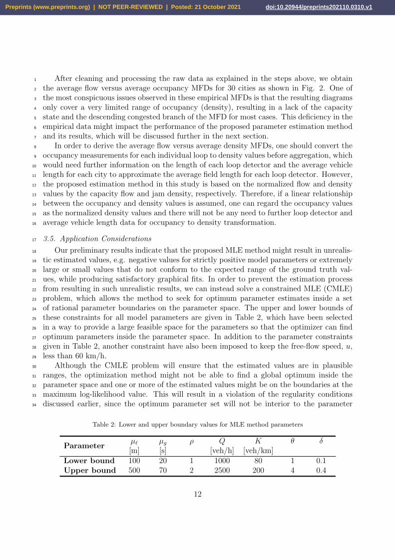
of rational parameter boundaries on the parameter space. The upper and lower bounds of24

these constraints for all model parameters are given in Table 2, which have been selected25

in a way to provide a large feasible space for the parameters so that the optimizer can find26

optimum parameters inside the parameter space. In addition to the parameter constraints27

given in Table 2, another constraint have also been imposed to keep the free-flow speed, u,28

less than 60 km/h.29

Although the CMLE problem will ensure that the estimated values are in plausible30

ranges, the optimization method might not be able to find a global optimum inside the31

parameter space and one or more of the estimated values might be on the boundaries at the32

maximum log-likelihood value. This will result in a violation of the regularity conditions33

discussed earlier, since the optimum parameter set will not be interior to the parameter34

Table 2: Lower and upper boundary values for MLE method parameters

Parameterµ`[m]

µg[s]

ρ.

Q[veh/h]

K[veh/km]

θ.

δ.

Lower bound 100 20 1 1000 80 1 0.1Upper bound 500 70 2 2500 200 4 0.4

12



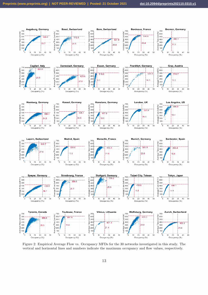
Figure 2: Empirical Average Flow vs. Occupancy MFDs for the 30 networks investigated in this study. Thevertical and horizontal lines and numbers indicate the maximum occupancy and flow values, respectively.

13



space. In such case, the first derivative of the log-likelihood function with respect to the1

parameter on the edge of the parameter space is not necessarily equal to zero, therefore the2

approximate multivariate normal distribution for the parameters will be invalid. Therefore,3

we should be careful about the selection of the boundaries of the parameter space to prevent4

this problem from happening.5

However, as it will be discussed in the next section, hitting the boundaries in the present6

problem might be inevitable due to high number of parameters needed to be estimated, the7

probable errors and biases in the empirical data and the other impacting factors which are8

not considered in the SMoC model such as the presence of buses creating both stationary9

and moving bottlenecks along the network.10

The next section will present the results of application of the proposed method for11

estimation of analytical MFD parameters for both corridors and networks under different12

assumptions.13

4. Results14

In this section, we will estimate the analytical MFD parameters using the proposed15

MLE method for two different sets of empirical MFD data. The first set is the data from a16

corridor and the second set includes empirical MFD datasets for several networks obtained17

from Loder et al. (2019). For the network datasets, the proposed method will be tested18

under two different sets of assumptions.19

Toward this purpose, the MFD CDF for the SMoC model has been coded in Wolfram20

Mathematica R©. Then, the derivative of the CDF with respect to q is computed to find21

the MFD PDF, which has been later used to find the log-likelihood function for any given22

dataset and set of model parameters. A constrained optimization method incorporating23

the constraints given in Table 2 has been utilized to find the optimum parameter value24

maximizing the log likelihood function. Afterwards, the second derivatives of the likelihood25

function are calculated to find the observed information matrix and the variances of the26

model parameters, which will be used in hypothesis testing for the estimated parameter27

values.28

4.1. Corridor MFD Parameter Estimation29

As the original SMoC model was initially proposed for corridor MFD estimation, we first30

intend to test the proposed parameter estimation method on a corridor MFD dataset. Tilg31

et al. (2020) has collected the LDD for a 4-block segment of one direction of an arterial32

with total length of 1.1 km in Munich, Germany for 24 hours. The signal timings for 533

intersections along the segment, which are all actuated, are also collected for the duration34

of study. The authors have assumed the link capacity flow Q = 1690 veh/hr/ln, the jam35

density K = 150 veh/hr and the free-flow speed u = 45 km/hr. The mean green and red36

times are not reported in the paper; however, we have approximated these values by the37

median green and red times, respectively, which are presented in a figure in the study. The38

other required parameter values for the SMoC have been calculated based on the available39

data and the analytical MFD have been derived using these values.40

14



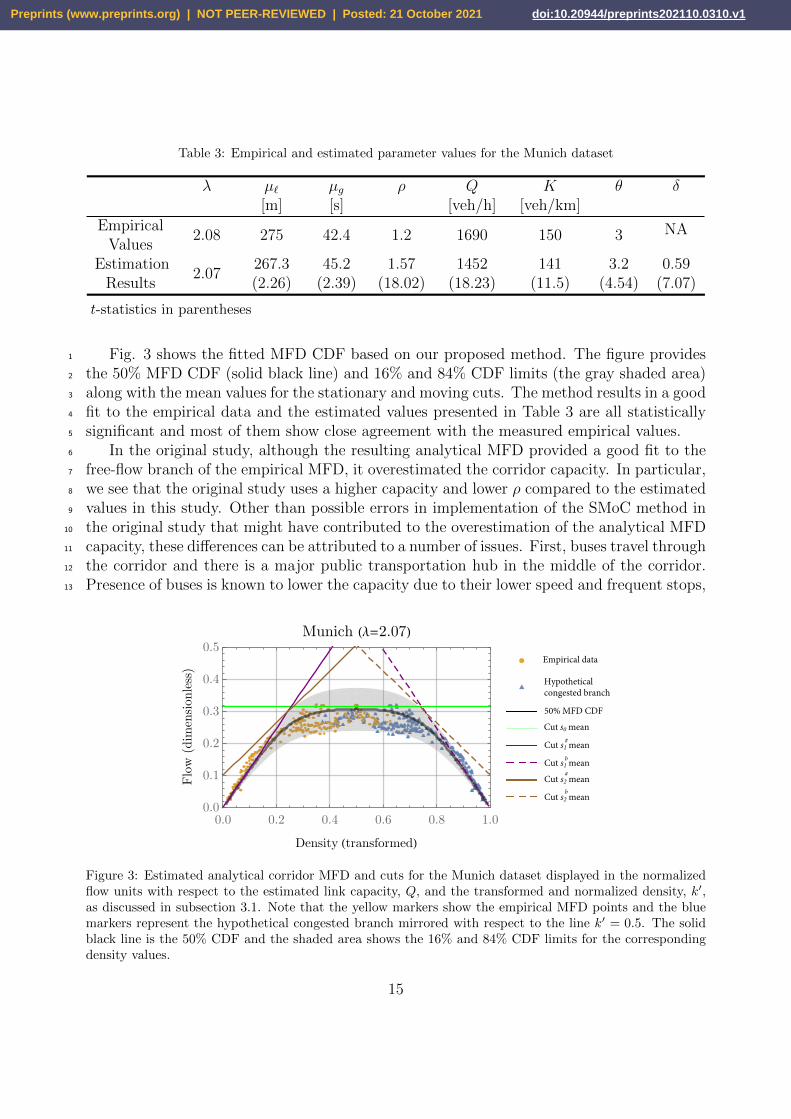
Table 3: Empirical and estimated parameter values for the Munich dataset

λ.

µ`[m]

µg[s]

ρ.

Q[veh/h]

K[veh/km]

θ.

δ.

EmpiricalValues

2.08 275 42.4 1.2 1690 150 3 NA

EstimationResults

2.07267.3(2.26)

45.2(2.39)

1.57(18.02)

1452(18.23)

141(11.5)

3.2(4.54)

0.59(7.07)

t-statistics in parentheses

Fig. 3 shows the fitted MFD CDF based on our proposed method. The figure provides1

the 50% MFD CDF (solid black line) and 16% and 84% CDF limits (the gray shaded area)2

along with the mean values for the stationary and moving cuts. The method results in a good3

fit to the empirical data and the estimated values presented in Table 3 are all statistically4

significant and most of them show close agreement with the measured empirical values.5

In the original study, although the resulting analytical MFD provided a good fit to the6

free-flow branch of the empirical MFD, it overestimated the corridor capacity. In particular,7

we see that the original study uses a higher capacity and lower ρ compared to the estimated8

values in this study. Other than possible errors in implementation of the SMoC method in9

the original study that might have contributed to the overestimation of the analytical MFD10

capacity, these differences can be attributed to a number of issues. First, buses travel through11

the corridor and there is a major public transportation hub in the middle of the corridor.12

Presence of buses is known to lower the capacity due to their lower speed and frequent stops,13

0.0 0.2 0.4 0.6 0.8 1.00.0

0.1

0.2

0.3

0.4

0.5

Flo

w (

dim

ensi

onle

ss)

Munich (λ=2.07)

Density (transformed)

Cut s0 mean

Cut s1 mean

Cut s1 mean

Cut s2 mean

Cut s2 mean

50% MFD CDF

Hypothetical congested branch

Empirical data

#

b

#

b

Figure 3: Estimated analytical corridor MFD and cuts for the Munich dataset displayed in the normalizedflow units with respect to the estimated link capacity, Q, and the transformed and normalized density, k′,as discussed in subsection 3.1. Note that the yellow markers show the empirical MFD points and the bluemarkers represent the hypothetical congested branch mirrored with respect to the line k′ = 0.5. The solidblack line is the 50% CDF and the shaded area shows the 16% and 84% CDF limits for the correspondingdensity values.

15



imposing a moving bottleneck effect. The signals along the corridor prioritize the movement1

of buses causing further delay at the intersections, which is represented by higher ρ values2

in the SMoC.3

Furthermore, there are a few minor unsignalized intersections along the corridor. Al-4

though vehicles on the corridor do not fully stop at these intersections, the turning move-5

ments from and to the intersecting streets may cause the vehicles on the corridor to lower6

their speeds which will eventually result in lower capacity. The large variations in the signal7

green and red times and the fact that we have approximated the empirical value of ρ based on8

the median green and red times instead of their mean values might also have contributed to9

the discrepancy. Taking all into account, we conclude that the SMoC can capture the shape10

of the corridor MFD satisfactorily provided that the parameters are carefully estimated.11

Our proposed method is a step in that direction.12

4.2. Network MFD Parameter Estimation13

After testing the proposed method on empirical corridor and simulation network cases, we14

aim to check the performance of the method to estimate the MFD parameters for empirical15

network data. The data source and cleaning process has been explained earlier in subsection16

3.4. Here, we will present and discuss two sets of estimation results for this network data17

under different assumptions.18

4.2.1. Estimation of all model parameters19

We first assume that we do not have any a posteriori knowledge about the real value20

of any of the model parameters Θ = Q,K, θ, µ`, µg, ρ, δ for the given networks and all of21

these parameters are to be estimated. The cleaned and processed MFD data for 30 cities22

from the UTD19 dataset, shown in Fig. 2, is given to the program coded based on the23

proposed method and the SMoC analytical MFD is fitted to the data from each city and24

the model parameters for each network are estimated.25

Despite the large feasible space provided by the parameter boundaries given in Table 2,26

the estimation method results in boundary values for many datasets. For 16 cities out of27

the total 30 cities at least one estimated parameter value is on the determined boundaries28

while the graphical fits to the empirical data look satisfactory. This issue will result in a29

violation of the MLE regularity conditions and we will not be able to make any statistical30

inference from the estimation results. The issue can be resolved by changing the boundary31

values for the problematic boundaries; however, we refrain from doing so since the imposed32

boundaries are selected to keep the parameter estimates in meaningful ranges and further33

broadening of them would result in unrealistic estimations. Therefore, we deem the results34

from the 16 cities with at least one parameter estimate on the boundaries unsatisfactory35

and direct our further analysis on the results from the 14 cities, where this problem is not36

encountered. The satisfactory results mostly come from the datasets covering a wider range37

of occupancy values or exhibiting downward-bending trends reaching a near capacity state.38

The estimated analytical MFDs and cuts for five cities, in which the method exhibits a39

satisfactory performance, as illustrated in Fig. 4, show that the method results in satisfactory40

fits of the analytical MFD CDF to the empirical data. The estimated parameter values for41

16



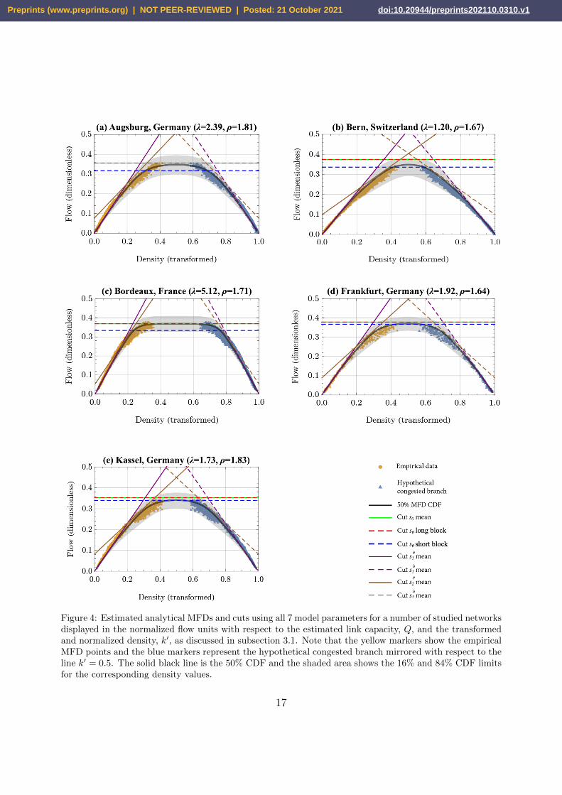
Figure 4: Estimated analytical MFDs and cuts using all 7 model parameters for a number of studied networksdisplayed in the normalized flow units with respect to the estimated link capacity, Q, and the transformedand normalized density, k′, as discussed in subsection 3.1. Note that the yellow markers show the empiricalMFD points and the blue markers represent the hypothetical congested branch mirrored with respect to theline k′ = 0.5. The solid black line is the 50% CDF and the shaded area shows the 16% and 84% CDF limitsfor the corresponding density values.

17



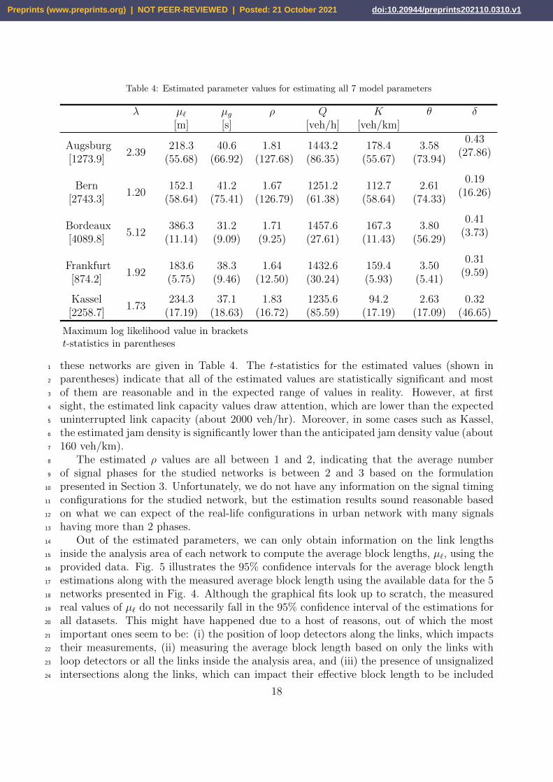
Table 4: Estimated parameter values for estimating all 7 model parameters

λ.

µ`[m]

µg[s]

ρ.

Q[veh/h]

K[veh/km]

θ.

δ.

Augsburg[1273.9]

2.39218.3

(55.68)40.6

(66.92)1.81

(127.68)1443.2(86.35)

178.4(55.67)

3.58(73.94)

0.43(27.86)

Bern[2743.3]

1.20152.1

(58.64)41.2

(75.41)1.67

(126.79)1251.2(61.38)

112.7(58.64)

2.61(74.33)

0.19(16.26)

Bordeaux[4089.8]

5.12386.3

(11.14)31.2

(9.09)1.71

(9.25)1457.6(27.61)

167.3(11.43)

3.80(56.29)

0.41(3.73)

Frankfurt[874.2]

1.92183.6(5.75)

38.3(9.46)

1.64(12.50)

1432.6(30.24)

159.4(5.93)

3.50(5.41)

0.31(9.59)

Kassel[2258.7]

1.73234.3

(17.19)37.1

(18.63)1.83

(16.72)1235.6(85.59)

94.2(17.19)

2.63(17.09)

0.32(46.65)

Maximum log likelihood value in bracketst-statistics in parentheses

these networks are given in Table 4. The t-statistics for the estimated values (shown in1

parentheses) indicate that all of the estimated values are statistically significant and most2

of them are reasonable and in the expected range of values in reality. However, at first3

sight, the estimated link capacity values draw attention, which are lower than the expected4

uninterrupted link capacity (about 2000 veh/hr). Moreover, in some cases such as Kassel,5

the estimated jam density is significantly lower than the anticipated jam density value (about6

160 veh/km).7

The estimated ρ values are all between 1 and 2, indicating that the average number8

of signal phases for the studied networks is between 2 and 3 based on the formulation9

presented in Section 3. Unfortunately, we do not have any information on the signal timing10

configurations for the studied network, but the estimation results sound reasonable based11

on what we can expect of the real-life configurations in urban network with many signals12

having more than 2 phases.13

Out of the estimated parameters, we can only obtain information on the link lengths14

inside the analysis area of each network to compute the average block lengths, µ`, using the15

provided data. Fig. 5 illustrates the 95% confidence intervals for the average block length16

estimations along with the measured average block length using the available data for the 517

networks presented in Fig. 4. Although the graphical fits look up to scratch, the measured18

real values of µ` do not necessarily fall in the 95% confidence interval of the estimations for19

all datasets. This might have happened due to a host of reasons, out of which the most20

important ones seem to be: (i) the position of loop detectors along the links, which impacts21

their measurements, (ii) measuring the average block length based on only the links with22

loop detectors or all the links inside the analysis area, and (iii) the presence of unsignalized23

intersections along the links, which can impact their effective block length to be included24

18



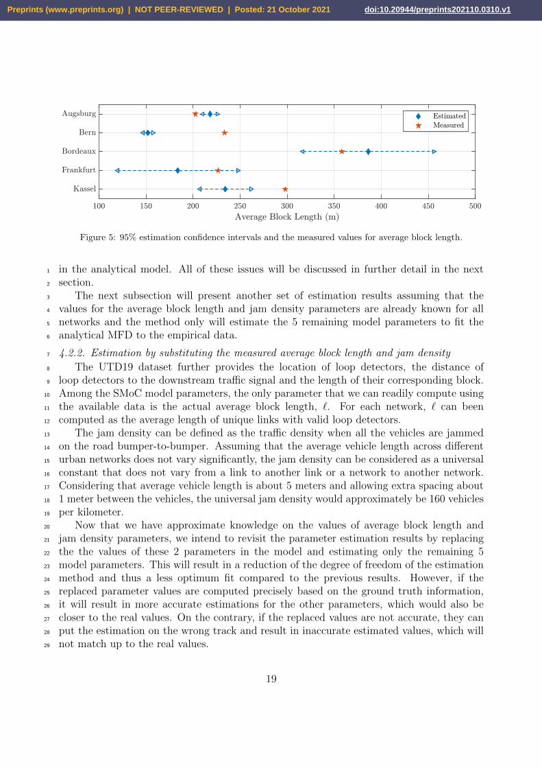
Figure 5: 95% estimation confidence intervals and the measured values for average block length.

in the analytical model. All of these issues will be discussed in further detail in the next1

section.2

The next subsection will present another set of estimation results assuming that the3

values for the average block length and jam density parameters are already known for all4

networks and the method only will estimate the 5 remaining model parameters to fit the5

analytical MFD to the empirical data.6

4.2.2. Estimation by substituting the measured average block length and jam density7

The UTD19 dataset further provides the location of loop detectors, the distance of8

loop detectors to the downstream traffic signal and the length of their corresponding block.9

Among the SMoC model parameters, the only parameter that we can readily compute using10

the available data is the actual average block length, `. For each network, ` can been11

computed as the average length of unique links with valid loop detectors.12

The jam density can be defined as the traffic density when all the vehicles are jammed13

on the road bumper-to-bumper. Assuming that the average vehicle length across different14

urban networks does not vary significantly, the jam density can be considered as a universal15

constant that does not vary from a link to another link or a network to another network.16

Considering that average vehicle length is about 5 meters and allowing extra spacing about17

1 meter between the vehicles, the universal jam density would approximately be 160 vehicles18

per kilometer.19

Now that we have approximate knowledge on the values of average block length and20

jam density parameters, we intend to revisit the parameter estimation results by replacing21

the the values of these 2 parameters in the model and estimating only the remaining 522

model parameters. This will result in a reduction of the degree of freedom of the estimation23

method and thus a less optimum fit compared to the previous results. However, if the24

replaced parameter values are computed precisely based on the ground truth information,25

it will result in more accurate estimations for the other parameters, which would also be26

closer to the real values. On the contrary, if the replaced values are not accurate, they can27

put the estimation on the wrong track and result in inaccurate estimated values, which will28

not match up to the real values.29

19



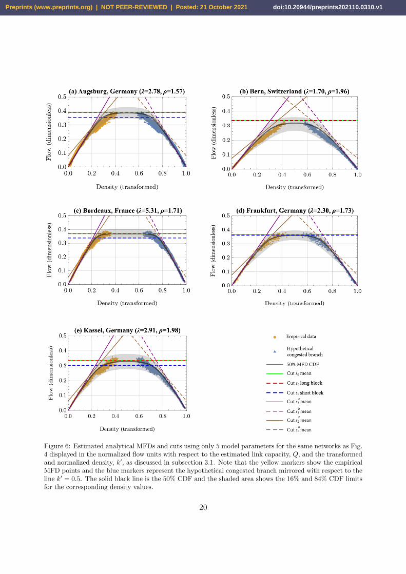
Figure 6: Estimated analytical MFDs and cuts using only 5 model parameters for the same networks as Fig.4 displayed in the normalized flow units with respect to the estimated link capacity, Q, and the transformedand normalized density, k′, as discussed in subsection 3.1. Note that the yellow markers show the empiricalMFD points and the blue markers represent the hypothetical congested branch mirrored with respect to theline k′ = 0.5. The solid black line is the 50% CDF and the shaded area shows the 16% and 84% CDF limitsfor the corresponding density values.

20



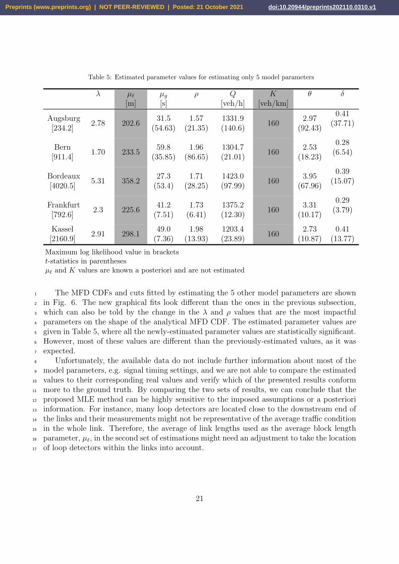
Table 5: Estimated parameter values for estimating only 5 model parameters

λ.

µ`[m]

µg[s]

ρ.

Q[veh/h]

K[veh/km]

θ.

δ.

Augsburg[234.2]

2.78 202.631.5

(54.63)1.57

(21.35)1331.9(140.6)

1602.97

(92.43)

0.41(37.71)

Bern[911.4]

1.70 233.559.8

(35.85)1.96

(86.65)1304.7(21.01)

1602.53

(18.23)

0.28(6.54)

Bordeaux[4020.5]

5.31 358.227.3

(53.4)1.71

(28.25)1423.0(97.99)

1603.95

(67.96)

0.39(15.07)

Frankfurt[792.6]

2.3 225.641.2

(7.51)1.73

(6.41)1375.2(12.30)

1603.31

(10.17)

0.29(3.79)

Kassel[2160.9]

2.91 298.149.0

(7.36)1.98

(13.93)1203.4(23.89)

1602.73

(10.87)0.41

(13.77)

Maximum log likelihood value in bracketst-statistics in parenthesesµ` and K values are known a posteriori and are not estimated

The MFD CDFs and cuts fitted by estimating the 5 other model parameters are shown1

in Fig. 6. The new graphical fits look different than the ones in the previous subsection,2

which can also be told by the change in the λ and ρ values that are the most impactful3

parameters on the shape of the analytical MFD CDF. The estimated parameter values are4

given in Table 5, where all the newly-estimated parameter values are statistically significant.5

However, most of these values are different than the previously-estimated values, as it was6

expected.7

Unfortunately, the available data do not include further information about most of the8

model parameters, e.g. signal timing settings, and we are not able to compare the estimated9

values to their corresponding real values and verify which of the presented results conform10

more to the ground truth. By comparing the two sets of results, we can conclude that the11

proposed MLE method can be highly sensitive to the imposed assumptions or a posteriori12

information. For instance, many loop detectors are located close to the downstream end of13

the links and their measurements might not be representative of the average traffic condition14

in the whole link. Therefore, the average of link lengths used as the average block length15

parameter, µ`, in the second set of estimations might need an adjustment to take the location16

of loop detectors within the links into account.17

21



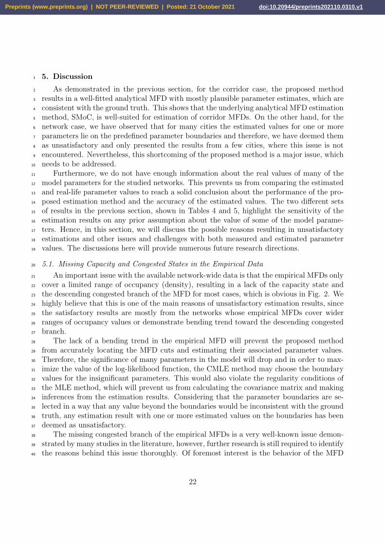
5. Discussion1

As demonstrated in the previous section, for the corridor case, the proposed method2

results in a well-fitted analytical MFD with mostly plausible parameter estimates, which are3

consistent with the ground truth. This shows that the underlying analytical MFD estimation4

method, SMoC, is well-suited for estimation of corridor MFDs. On the other hand, for the5

network case, we have observed that for many cities the estimated values for one or more6

parameters lie on the predefined parameter boundaries and therefore, we have deemed them7

as unsatisfactory and only presented the results from a few cities, where this issue is not8

encountered. Nevertheless, this shortcoming of the proposed method is a major issue, which9

needs to be addressed.10

Furthermore, we do not have enough information about the real values of many of the11

model parameters for the studied networks. This prevents us from comparing the estimated12

and real-life parameter values to reach a solid conclusion about the performance of the pro-13

posed estimation method and the accuracy of the estimated values. The two different sets14

of results in the previous section, shown in Tables 4 and 5, highlight the sensitivity of the15

estimation results on any prior assumption about the value of some of the model parame-16

ters. Hence, in this section, we will discuss the possible reasons resulting in unsatisfactory17

estimations and other issues and challenges with both measured and estimated parameter18

values. The discussions here will provide numerous future research directions.19

5.1. Missing Capacity and Congested States in the Empirical Data20

An important issue with the available network-wide data is that the empirical MFDs only21

cover a limited range of occupancy (density), resulting in a lack of the capacity state and22

the descending congested branch of the MFD for most cases, which is obvious in Fig. 2. We23

highly believe that this is one of the main reasons of unsatisfactory estimation results, since24

the satisfactory results are mostly from the networks whose empirical MFDs cover wider25

ranges of occupancy values or demonstrate bending trend toward the descending congested26

branch.27

The lack of a bending trend in the empirical MFD will prevent the proposed method28

from accurately locating the MFD cuts and estimating their associated parameter values.29

Therefore, the significance of many parameters in the model will drop and in order to max-30

imize the value of the log-likelihood function, the CMLE method may choose the boundary31

values for the insignificant parameters. This would also violate the regularity conditions of32

the MLE method, which will prevent us from calculating the covariance matrix and making33

inferences from the estimation results. Considering that the parameter boundaries are se-34

lected in a way that any value beyond the boundaries would be inconsistent with the ground35

truth, any estimation result with one or more estimated values on the boundaries has been36

deemed as unsatisfactory.37

The missing congested branch of the empirical MFDs is a very well-known issue demon-38

strated by many studies in the literature, however, further research is still required to identify39

the reasons behind this issue thoroughly. Of foremost interest is the behavior of the MFD40

22



at the capacity state and whether the network exhibits a continuous MFD or there is a1

breakdown in average flow values at the capacity state.2

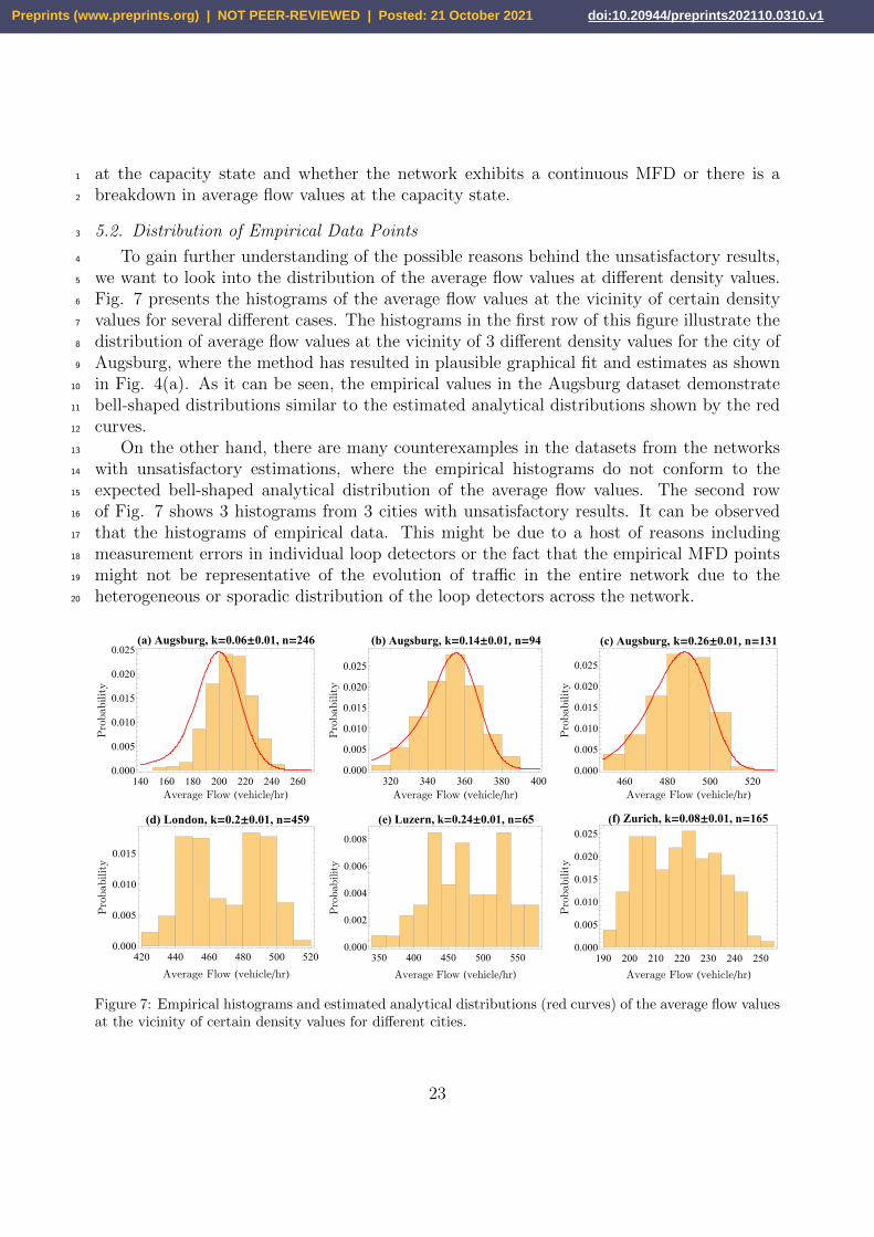
5.2. Distribution of Empirical Data Points3

To gain further understanding of the possible reasons behind the unsatisfactory results,4

we want to look into the distribution of the average flow values at different density values.5

Fig. 7 presents the histograms of the average flow values at the vicinity of certain density6

values for several different cases. The histograms in the first row of this figure illustrate the7

distribution of average flow values at the vicinity of 3 different density values for the city of8

Augsburg, where the method has resulted in plausible graphical fit and estimates as shown9

in Fig. 4(a). As it can be seen, the empirical values in the Augsburg dataset demonstrate10

bell-shaped distributions similar to the estimated analytical distributions shown by the red11

curves.12

On the other hand, there are many counterexamples in the datasets from the networks13

with unsatisfactory estimations, where the empirical histograms do not conform to the14

expected bell-shaped analytical distribution of the average flow values. The second row15

of Fig. 7 shows 3 histograms from 3 cities with unsatisfactory results. It can be observed16

that the histograms of empirical data. This might be due to a host of reasons including17

measurement errors in individual loop detectors or the fact that the empirical MFD points18

might not be representative of the evolution of traffic in the entire network due to the19

heterogeneous or sporadic distribution of the loop detectors across the network.20

140 160 180 200 220 240 2600.000

0.005

0.010

0.015

0.020

0.025

Average Flow (vehicle/hr)

Probability

320 340 360 380 4000.000

0.005

0.010

0.015

0.020

0.025


Probability

0.005

0.010

0.015

0.020

0.025


Probability

0.000460 480 500 520

420 440 460 480 500 5200.000

0.005

0.010

0.015


Probability

350 400 450 500 5500.000

0.002

0.004

0.006

0.008


Probability

190 200 210 220 230 240 2500.000

0.005

0.010

0.015

0.020

0.025


Probability

(a) Augsburg, k=0.06±0.01, n=246 (b) Augsburg, k=0.14±0.01, n=94

(d) London, k=0.2±0.01, n=459 (e) Luzern, k=0.24±0.01, n=65 (f) Zurich, k=0.08±0.01, n=165

(c) Augsburg, k=0.26±0.01, n=131

Figure 7: Empirical histograms and estimated analytical distributions (red curves) of the average flow valuesat the vicinity of certain density values for different cities.

23



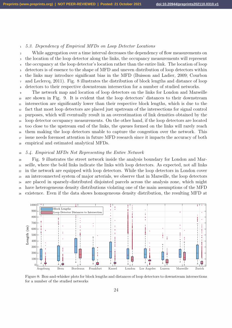
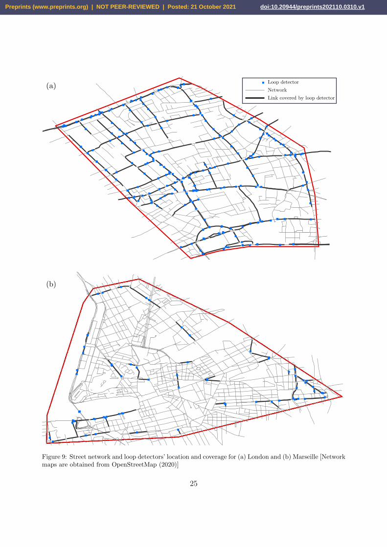
5.3. Dependency of Empirical MFDs on Loop Detector Locations1

While aggregation over a time interval decreases the dependency of flow measurements on2

the location of the loop detector along the links, the occupancy measurements will represent3

the occupancy at the loop detector’s location rather than the entire link. The location of loop4

detectors is of essence to the shape of MFD and uneven distribution of loop detectors within5

the links may introduce significant bias in the MFD (Buisson and Ladier, 2009; Courbon6

and Leclercq, 2011). Fig. 8 illustrates the distribution of block lengths and distance of loop7

detectors to their respective downstream intersection for a number of studied networks.8

The network map and location of loop detectors on the links for London and Marseille9

are shown in Fig. 9. It is evident that the loop detectors’ distances to their downstream10

intersection are significantly lower than their respective block lengths, which is due to the11

fact that most loop detectors are placed just upstream of the intersections for signal control12

purposes, which will eventually result in an overestimation of link densities obtained by the13

loop detector occupancy measurements. On the other hand, if the loop detectors are located14

too close to the upstream end of the links, the queues formed on the links will rarely reach15

them making the loop detectors unable to capture the congestion over the network. This16

issue needs foremost attention in future MFD research since it impacts the accuracy of both17

empirical and estimated analytical MFDs.18

5.4. Empirical MFDs Not Representing the Entire Network19

Fig. 9 illustrates the street network inside the analysis boundary for London and Mar-20

seille, where the bold links indicate the links with loop detectors. As expected, not all links21

in the network are equipped with loop detectors. While the loop detectors in London cover22

an interconnected system of major arterials, we observe that in Marseille, the loop detectors23

are placed in sparsely-distributed disjointed parcels across the analysis zone, which might24

have heterogeneous density distributions violating one of the main assumptions of the MFD25

existence. Even if the data shows homogeneous density distribution, the resulting MFD at26

Figure 8: Box-and-whisker plots for block lengths and distances of loop detectors to downstream intersectionsfor a number of the studied networks

24



"

"

"""

"

"

""

"

"

"

"

"

""

"

"

"

"

""

"

"

""

"

"

"

""

"

"

""

"

"

"

"

""

"

"

"

"

"

""

""

"

"

"

"

"

"

"

"

"

"

""

"

"

"

"

"

"

"

"

"

"

"

"

"

"

"

"

"

"

"

"

"

"

"

"

"

"

"

"

"

"

"

"

"

"

"

"

"

"

"

"

"

""

"

"

"

"

"

"

"

"

"

""

"

"

"

"

"

"

" "

""

"

""

""

"

"

"

""

""

"

"

"

"

" "

"

"

""""

"

"

" ""

""

"

""

"""

"

"

"

"

"

"

"

"

"

"

"

"

"

"

"

""

""

"

"

""

"

"

"

"

"""

"""""

"

"""

"""""" "

""

"

"

""" " ""

"""

"" ""

""""""

"

"""""

"

"""""

""

""""

"""""

"

""""

""""""

"

""""

""

""

"

"

""

""

""

"""

"""

"

"

"""

""""

""" "

"""

"

"

""

"

""""""

"""

"

""""""

"" ""

""

""

"

"

"

"

""""""""

"""

""""

""""""

""

""""

""

""

"""

""""""

"

""

""

"""""""

"""""

""

""

""""

"""

"""

"""""

" """

"

"

""

"" "

""

"""

"

""

"""

""

""

""

"

""

""

"

"""

""

"

""""

""

"""

""

"

""

"""

"

"" "

"

"

"

"

"

""

"

"

"

"

""

"

"

""

"

"

"

"""

"

""

"

"

"

"

""

"

"

"

"

"

""

""

"

"

"

"

"

"

"

"

"

"

""

"

"

"

"

"

"

"

"

"

"

"

"

"

"

"

"

"

"

"

"

"

"

"

"

"

"

"

""

"

""

"

"

"

"

"

"

"

"

"

""

"

"

"

"

"

"

"

"

"

""

"

"

"

"

"

"

" "

""

"""

""

""

"

""

""

""

"

"" "

"

"

""""

"

"

" ""

""

"

""

"""

"

"

"

"

"

"

"

"

"

"

"

"

"

"

"

""

""

"

"

""

"

"

"

"

"""

"""""

"

""""""""" "

""

"

"

""" """"""

"" """""""""

"""" "

""""""

""

""" """""""

"""""""

""" "

""""""

""

"

"

""

" """

"""

"""

"

"

"""""""

""""

"""

""

""

"

""""""

"""

"""""""

"" ""

""""

"

"

"

"

"" """""""

""

""""

""""""

""

""""""

"""""

""""""

"

""

"""""""""

"""""

""

""

"""""""

""""""

""

" """

"

"

""

"" """

"""

"

""

"""

""

""

""

"

""

"""

"""

""

"

""""

""

"""

"""

""

"

"

"

"

"

"

"

" "

"

"

""

""

"

"

"

"

"""

" " "

"

""

"" " "

"

"

""

" ""

"

""

"

"

"

"""

"

"

"

"

"

"

""

"

"""

"

"

""

"

"""

""""

"""""

""

" "

"

"""

""

""

" """

"

"

"

"

"""

"

"" "

"

"""

""

"

"""

"

""""

"

"

"

""

"

""

"""

"

"

""""

"

"

"

""

"

"

""

"

"

"" ""

"

"

""""

""

"

""

"

"

"

"""

""

"

"" "

"

"""

""

"

""

" """

" ""

"

"

"""

"

"

"""

""

" "

" "" "

"

"

""

"

"

"

""

"

"""

""

"

"

""

"""

""

""

"

""

""

"

""

"""

"

"" "

"

"

"

"

"

""

"

"

"

"

""

"

"

""

"

"

"

"""

"

""

"

"

"

"

""

"

"

"

"

"

""

""

"

"

"

"

"

"

"

"

"

"

""

"

"

"

"

"

"

"

"

"

"

"

"

"

"

"

"

"

"

"

"

"

"

"

"

"

"

"

""

"

""

"

"

"

"

"

"

"

"

"

""

"

"

"

"

"

"

"

"

"

""

"

"

"

"

"

"

" "

""

"""

""

""

"

""

""

""

"

"" "

"

"

""""

"

"

" ""

""

"

""

"""

"

"

"

"

"

"

"

"

"

"

"

"

"

"

"

""

""

"

"

""

"

"

"

"

"""

"""""

"

""""""""" "

""

"

"

""" """"""

"" """""""""

"""" "

""""""

""

""" """""""

"""""""

""" "

""""""

""

"

"

""

" """

"""

"""

"

"

"""""""

""""

"""

""

""

"

""""""

"""

"""""""

"" ""

""""

"

"

"

"

"" """""""

""

""""

""""""

""

""""""

"""""

""""""

"

""

"""""""""

"""""

""

""

"""""""

""""""

""

" """

"

"

""

"" """

"""

"

""

"""

""

""

""

"

""

"""

"""

""

"

""""

""

"""

"""

""

"

"

"

"

"

"

"

" "

"

"

""

""

"

"

"

"

"""

" " "

"

""

"" " "

"

"

""

" ""

"

""

"

"

"

"""

"

"

"

"

"

"

""

"

"""

"

"

""

"

"""

""""

"""""

""

" "

"

"""

""

""

" """

"

"

"

"

"""

"

"" "

"

"""

""

"

"""

"

""""

"

"

"

""

"

""

"""

"

"

""""

"

"

"

""

"

"

""

"

"

"" ""

"

"

""""

""

"

""

"

"

"

"""

""

"

"" "

"

"""

""

"

""

" """

" ""

"

"

"""

"

"

"""

""

" "

" "" "

"

"

""

"

"

"

""

"

"""

""

"

"

""

"""

""

""

"

""

"

"

"

" "

""

"""

""

""

"

""

""

""

"

"" "

"

"

""""

"

"

" ""

""

""

"""

"

"

"

"

"

"

"

"

"

"

"

"

"

"

"

""

""

"

"

""

"

"

"

"

""

"

"

"

"

"

"

"

" "

"

"

""

""

"

"

"

"

"""

"" "

"

""

"" ""

"

"

""

" ""

"

""

"

"

"

""

"

"

"

"

"

"

"

""

"

"""

"

"

"

"

"

"""

"""

""""""

""

" "

"

"""

""

""

" """

"

"

"

"

"""

"

"" "

"

"

" "

""

"

"""

"

""

""

"

"

"

""

"

""

"""

"

"

"

""""

"

"

"

""

"

""

"

"

""

""

"

"

""

""

""

"

""

"

"

"

""

"

""

"

"" "

"

""

""

"

"

""

" """

" ""

"

"

"

""

"

"

"

""

""

" "

" "

" "

"

"

"

"

"

"

"

"

""

""

"

""

"

"

""

""

"""

"

"

"

"

"

""

"

"

" Loop detectorNetworkLink covered by loop detector

(a)

(b)

Figure 9: Street network and loop detectors’ location and coverage for (a) London and (b) Marseille [Networkmaps are obtained from OpenStreetMap (2020)]

25



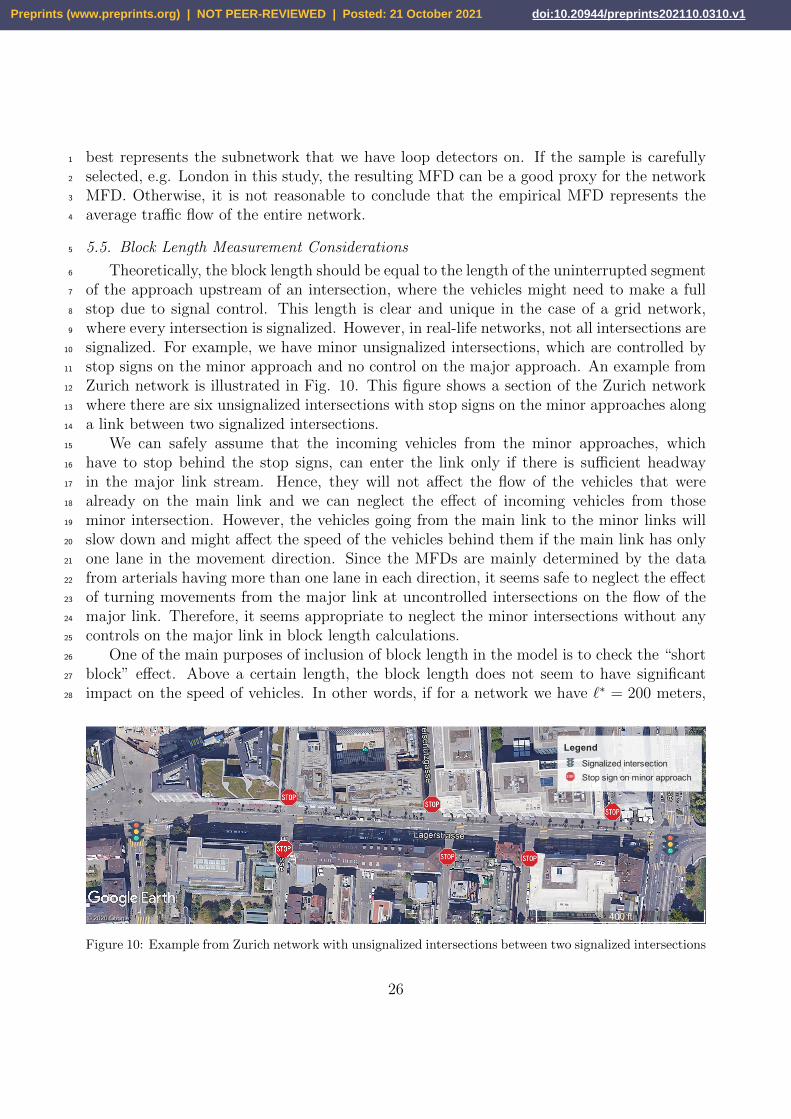
best represents the subnetwork that we have loop detectors on. If the sample is carefully1

selected, e.g. London in this study, the resulting MFD can be a good proxy for the network2

MFD. Otherwise, it is not reasonable to conclude that the empirical MFD represents the3

average traffic flow of the entire network.4

5.5. Block Length Measurement Considerations5

Theoretically, the block length should be equal to the length of the uninterrupted segment6

of the approach upstream of an intersection, where the vehicles might need to make a full7

stop due to signal control. This length is clear and unique in the case of a grid network,8

where every intersection is signalized. However, in real-life networks, not all intersections are9

signalized. For example, we have minor unsignalized intersections, which are controlled by10

stop signs on the minor approach and no control on the major approach. An example from11

Zurich network is illustrated in Fig. 10. This figure shows a section of the Zurich network12

where there are six unsignalized intersections with stop signs on the minor approaches along13

a link between two signalized intersections.14

We can safely assume that the incoming vehicles from the minor approaches, which15

have to stop behind the stop signs, can enter the link only if there is sufficient headway16

in the major link stream. Hence, they will not affect the flow of the vehicles that were17

already on the main link and we can neglect the effect of incoming vehicles from those18

minor intersection. However, the vehicles going from the main link to the minor links will19

slow down and might affect the speed of the vehicles behind them if the main link has only20

one lane in the movement direction. Since the MFDs are mainly determined by the data21

from arterials having more than one lane in each direction, it seems safe to neglect the effect22

of turning movements from the major link at uncontrolled intersections on the flow of the23

major link. Therefore, it seems appropriate to neglect the minor intersections without any24

controls on the major link in block length calculations.25

One of the main purposes of inclusion of block length in the model is to check the “short26

block” effect. Above a certain length, the block length does not seem to have significant27

impact on the speed of vehicles. In other words, if for a network we have `∗ = 200 meters,28

Legend

Signalized intersection

Stop sign on minor approach

400 ft

N

N

© 2020 Google

© 2020 Google

© 2020 Google

Figure 10: Example from Zurich network with unsignalized intersections between two signalized intersections

26



a 300 meters link will not have a different average speed than a 700 meters link, hence1

the extra link length will not have any impact on the average performance of the network2

and the shape of MFD. An upper limit for the block length may be needed to prevent the3

long blocks from skewing the mean block length. The validity of this idea and determining4

case-specific upper limits for the block length needs to be investigated using further link5

performance data.6

5.6. Heterogeneities in Network Topology7

The impacts of heterogeneity in the block lengths on the MFD has already been discussed8

in this section. The urban street networks include links from different functional classes,9

i.e. major and minor arterials, collectors, local streets. In general, the streets from lower10

functional classes have less lanes and lower speed limits and as a result lower operating11

speeds. It should not be expected to observe the same speed as arterials on the local streets.12

Therefore, MFDs cannot include both arterials and local streets, otherwise there will be huge13

variations in the speed and flow measurements, introducing high scatter to the MFD. Based14

on the placement of the loop detectors, we can conclude that the empirical MFDs represent15

the MFD of the grid of arterials inside the network, which are of foremost importance for16

network management and control purposes.17

6. Conclusion18

This paper extends the SMoC to analytical estimation of network MFDs and proposes19

a method to estimate the parameters and shape of analytical MFD using empirical data20

in order to investigate the impact of different network topology and control characteristics21

on the shape of the MFD. The SMoC model has been selected as the base model after an22

exhaustive review of the present analytical MFD estimation models in the literature and the23

MLE method has been implemented to fit the analytical MFD and estimate its parameters24

for several datasets.25

We have found that to extend the SMoC to estimate the analytical network MFDs, we26

need to redefine the mean red to green signal time, ρ, parameter in the original formulation27

as ρ = n− 1, where n is the average number of signal phases for all the intersections in the28

study area. The parameter estimation method imposes constraints on the parameter space29

in order to keep the parameter estimates realistic. The lower and upper boundaries for each30

parameter are selected in a way that any values beyond them would not be attainable in31

real world.32

After testing the proposed MLE method on the empirical data for a corridor, we observe33

that the estimates are very close to the measured values. The parameter estimation method34

is later used to estimate the analytical network MFD parameters for 30 networks using their35

empirical MFDs. While the estimation method yields in statistically significant estimated36

parameter values for many of the studied datasets, there are also many networks where37

at least one parameter estimate is on the imposed boundaries. Such results have been38

considered as unsatisfactory and the possible reasons leading to this issue have been discussed39

in the next section. The satisfactory estimation results are revisited by assuming that the40

27



average block length and jam density values are already known a posteriori. The different1

parameter estimates and analytical MFD shapes indicate that the proposed method can be2

highly sensitive to the input values and any assumptions made throughout the process.3

The observed discrepancies and limitations in the results are discussed in full length in4

section 5. Many of these issues most probably stem from the shortcomings of the underlying5

empirical data. The distribution of the loop detectors within the links is an impactful factor6

considering the fact that the loop detectors measure the occupancy at the point that they7

are located, which might not represent the density of the link if they are placed too close to8

the beginning or end of the link. Furthermore, it is discussed that the empirical MFDs might9

not be a good representative for the network MFD due to the fact that the loop detectors10

do not cover all the links in a network. The computation of block lengths and signal control11

parameters for networks are also discussed in this paper. However, reaching clear methods12

to tackle these issues needs further consideration using additional empirical data, which are13

currently under investigation by the authors.14

Acknowledgements15

We are truly grateful to Lukas Ambuhl, Allister Loder and Monica Menendez for their16

generosity in sharing the data from their study Loder et al. (2019) and helpful discussions17

about the data. This study has received funding from NSF research project # 1562536.18

Ambuhl, L., Loder, A., Bliemer, M.C., Menendez, M., Axhausen, K.W., 2018. A functional form with a phys-19

ical meaning for the macroscopic fundamental diagram. Transportation Research Part B: Methodological20

.21

Ardekani, S., Herman, R., 1987. Urban network-wide traffic variables and their relations. Transportation22

Science 21, 1–16.23

Buisson, C., Ladier, C., 2009. Exploring the impact of homogeneity of traffic measurements on the existence24

of macroscopic fundamental diagrams. Transportation Research Record 2124, 127–136.25

Castrillon, F., Laval, J., 2018. Impact of buses on the macroscopic fundamental diagram of homogeneous26

arterial corridors. Transportmetrica B: Transport Dynamics 6, 286–301.27

Courbon, T., Leclercq, L., 2011. Cross-comparison of macroscopic fundamental diagram estimation methods.28

Procedia-Social and Behavioral Sciences 20, 417–426.29

Daganzo, C.F., 2005a. A variational formulation of kinematic waves: basic theory and complex boundary30

conditions. Transportation Research Part B: Methodological 39, 187–196.31

Daganzo, C.F., 2005b. A variational formulation of kinematic waves: Solution methods. Transportation32

Research Part B: Methodological 39, 934–950.33

Daganzo, C.F., 2007. Urban gridlock: Macroscopic modeling and mitigation approaches. Transportation34

Research Part B: Methodological 41, 49–62.35

Daganzo, C.F., Geroliminis, N., 2008. An analytical approximation for the macroscopic fundamental diagram36

of urban traffic. Transportation Research Part B: Methodological 42, 771–781.37

Daganzo, C.F., Lehe, L.J., 2016. Traffic flow on signalized streets. Transportation Research Part B: Method-38

ological 90, 56–69.39

Gayah, V.V., Gao, X.S., Nagle, A.S., 2014. On the impacts of locally adaptive signal control on urban40

network stability and the macroscopic fundamental diagram. Transportation Research Part B: Method-41

ological 70, 255–268.42

Geroliminis, N., Boyacı, B., 2012. The effect of variability of urban systems characteristics in the network43

capacity. Transportation Research Part B: Methodological 46, 1607–1623.44

Geroliminis, N., Daganzo, C.F., 2008. Existence of urban-scale macroscopic fundamental diagrams: Some45

experimental findings. Transportation Research Part B: Methodological 42, 759–770.46

28



Geyer, C.J., et al., 1994. On the asymptotics of constrained m-estimation. The Annals of Statistics 22,1

1993–2010.2

Godfrey, J., 1969. The mechanism of a road network. Traffic Engineering & Control 8.3

Herman, R., Prigogine, I., 1979. A two-fluid approach to town traffic. Science 204, 148–151.4

Ji, Y., Daamen, W., Hoogendoorn, S., Hoogendoorn-Lanser, S., Qian, X., 2010. Investigating the shape5

of the macroscopic fundamental diagram using simulation data. Transportation Research Record 2161,6

40–48.7

Knoop, V.L., De Jong, D., Hoogendoom, S.P., 2014. Influence of road layout on network fundamental8

diagram. Transportation Research Record 2421, 22–30.9

Knoop, V.L., van Erp, P.B., Leclercq, L., Hoogendoorn, S.P., 2018. Empirical mfds using google traffic10

data, in: 2018 21st International Conference on Intelligent Transportation Systems (ITSC), IEEE. pp.11

3832–3839.12

Laval, J.A., Castrillon, F., 2015. Stochastic approximations for the macroscopic fundamental diagram of13

urban networks. Transportation Research Part B: Methodological 81, 904–916.14

Laval, J.A., Chilukuri, B.R., 2016. Symmetries in the kinematic wave model and a parameter-free represen-15

tation of traffic flow. Transportation Research Part B: Methodological 89, 168 – 177.16

Leclercq, L., Geroliminis, N., 2013. Estimating mfds in simple networks with route choice. Procedia-Social17

and Behavioral Sciences 80, 99–118.18

Loder, A., Ambuhl, L., Menendez, M., Axhausen, K.W., 2019. Understanding traffic capacity of urban19

networks. Scientific reports 9, 1–10.20

Mahmassani, H.S., Williams, J.C., Herman, R., 1984. Investigation of network-level traffic flow relationships:21

some simulation results. Transportation Research Record 971, 121–130.22

OpenStreetMap contributors, 2020. Planet dump retrieved from https://planet.osm.org . https://www.23

openstreetmap.org.24

Smeed, R.J., 1967. The road capacity of city centers. Highway Research Record .25

Tilg, G., Amini, S., Busch, F., 2020. Evaluation of analytical approximation methods for the macroscopic26

fundamental diagram. Transportation Research Part C: Emerging Technologies 114, 1–19.27

Tsubota, T., Bhaskar, A., Edward, C., 2014. Brisbane macroscopic fundamental diagram: Emperical findings28

on network partitioning and incident detection. Trans Res Rec .29

Wang, P.F., Wada, K., Akamatsu, T., Hara, Y., 2015. An empirical analysis of macroscopic fundamental30

diagrams for sendai road networks. Interdisciplinary Information Sciences 21, 49–61.31

Xie, X., Chiabaut, N., Leclercq, L., 2013. Macroscopic fundamental diagram for urban streets and mixed32

traffic: cross comparison of estimation methods. Transportation research record 2390, 1–10.33

29


https://www.openstreetmap.org




Parameter Estimation of the Macroscopic Fundamental Diagram

Documents

Transcript of Parameter Estimation of the Macroscopic Fundamental Diagram