[Frontiers in Bioscience 9, 1082-1099, May 1, 2004]

1082

MACROSCOPIC ELECTROSTATIC MODELS FOR PROTONATION STATES IN PROTEINS

Donald Bashford

Department of Molecular Biotechnology, Hartwell Center, Saint Jude Children’s Research Hospital, Memphis, TN, USA

TABLE OF CONTENTS

1. Abstract2. Introduction3. Macroscopic Electrostatics

3.1. Outer Boundary Conditions3.2. Linear Response and Green Functions

4. Electrolytes and the Linearized Poisson–Boltzmann (LPB) Equation5. Electrostatic Energy and Molecules6. The Finite-Difference Method7. Small-molecule Solvation and p aK

7.1. The Born model of ion solvation7.2. Small molecule p aK

8. Protonation states and p aK in proteins8.1. One-site case8.2. Multiple interacting sites

8.2.1. Tanford–Roxby approximation8.2.2. Reduced Site approximation8.2.3. Monte-Carlo Methods8.2.4. Clustering methods

8.3. Conformational Flexibility9. Open Problems10. References

1. ABSTRACT

The use of macroscopic electrostatic models tocalculate the relative energetics of protonation states andthe pH-titration properties of ionizable groups in proteins isdescribed. These methods treat the protein as anirregularly-shaped low-dielectric object containingembedded atomic charges immersed in a high-dielectric(solvent) medium. The energetics of altering protonationstates then involves the electrostatic work of altering theembedded atomic charges. The governing electrostaticequation is either the Poisson or linearized Poisson–Boltzmann equation, which generally requires numericalsolution. A tutorial approach is taken, the main aim ofwhich is a thorough understanding of the method.

2. INTRODUCTION

The prediction of the pH-titration properties ofionizable sidechains in proteins using macroscopicelectrostatic models has been important for thedevelopment and validation of models of proteinelectrostatics. As these calculations have enjoyed moresuccess, they have also become a useful tool for aquantitative understanding of protein function, particularlywhere internal proton transfers or the maintenance ofunusual protonation states is important for protein function.The focus of this article is the use of models that combinemacroscopic electrostatics with the details of the atomicstructure of proteins. We refer to this class of models by theacronym MEAD, for macroscopic electrostatics with atomic

detail. The quintessential MEAD model (1) depicts theprotein as a region of low dielectric constant with partialatomic charges at the positions of the nuclei, surrounded bya high dielectric medium, the solvent. The boundarybetween the interior, low-dielectric region and the exterior,high-dielectric regions is a surface defined by the atomiccoordinates and radii of the protein. Typically, Connolly’sdefinition of the molecular surface (2) is used, though otherdefinitions (3) are also possible.

Although many papers and several reviews haveappeared reporting the use of such a model to predict pH-titration properties and the relative energetics ofprotonation states in proteins (4,5), they have usually onlydescribed the methods briefly. The significant formal andpractical difficulties that arise in formulating these methodsin detail have either not been discussed, or are mentionedonly in passing. It has been the author’s experience that thislack of a deeper description of the method is often anobstacle for researchers new to the methods who wish to dosuch calculations for themselves. It is therefore the aim ofthis article to bring these details out from the in-house loreof a few research groups, or the internals of specializedsoftware, so that the methods can be more accessible, andtheir pitfalls and possibilities better understood by a wideraudience.

We begin with a brief introduction to themacroscopic Poisson equation for non-uniform dielectric

Electrostatic Models of Protonation

1083

environments, the linearized Poisson–Boltzmann (LPB)theory for electrolytes, and the use of Green functions as away of exploiting the linearity of these equations. Thecalculation of electrostatic energy is discussed in somedetail, with particular attention paid to the problem ofpoint-like charges embedded in a macroscopic media, andneed to cancel out spurious infinite terms in calculations ofenergy differences. The finite-difference method of solvingthe Poisson or LPB equation is discussed next, not so muchto detail the method itself as to point out some issuesparticular to the use of this or other numerical methods toimplement MEAD models. Before describing the applicationof these ideas to protonation states in proteins, we describetheir application to the closely related problem of small-molecule solvation and p aK .

Nearly all of the methods described here areimplemented in the author’s computer program suite,MEAD. (Typewriter typeface distinguishes the programsuite, MEAD, from the model, MEAD). MEAD is available insource-code form through the author’s web site,http://www.scripps.edu/bashford, or by anonymous FTPfrom ftp.scripps.edu, in the directory pub/electrostatics.Modification and redistribution of MEAD is allowed underthe terms of the GNU General Public License (6). Soon,MEAD will be available from a new web site to beestablished at the institution to which the author hasrecently moved, Saint Jude Children’s Research Hospital.Contact Don.Bashford@stjude.org for details.

3. MACROSCOPIC ELECTROSTATICS

In vacuum electrostatic theory, the electric fieldE is determined by Gauss’s law, which, in its differentialform, states that the divergence of the electric field isproportional to the charge density; specifically,

4πρ∇ ⋅ = .E (1)

(In these expressions, and elsewhere in this article, we usethe Gaussian system of units, in which a factor of 4πappears in the Gauss law, but not in the Coulomb law (7).)The further condition that E is curl-free implies that it isthe gradient of a scalar potential. It is conventional todefine the electrostatic potential by φ= −∇E . Substitutionleads to the vacuum Poisson equation,

2 4φ πρ∇ = − . (2)

The macroscopic version of the Gauss law is

4πρ∇ ⋅ = ,D (3)where D is the electric displacement, defined by ε=D E ,where ε is the dielectric constant. Substitution to obtainD in terms of φ leads to,

[ ]( ) ( ) 4 ( )ε φ πρ∇ ⋅ ∇ = − ,r r r (4)

which is the macroscopic version of the Poisson equation.The simple proportionality of D to E involves the

assumption that the polarization of the medium isproportional to the electric field. That is, linear response isassumed.

3.1. Outer Boundary ConditionsEqs. 2 or 4 are not enough to define the potential

uniquely. For example if φ satisfies Eq. 2, then one canadd to it any function φ′ for which 2 0φ′∇ = , and theresulting function will still satisfy the Poisson equation. Inorder to define a unique solution within some region, onemust also specify boundary conditions, relations that φmust satisfy at the boundary of the region. The mostcommon kind are Dirichlet boundary conditions, in whichthe value of the potential on the boundary is specified.Examples are,

( ) 0φ =s (5)( ) ( )fφ = ,s s (6)

where f is a function defined on all surface points, s . Thefirst expression, in which the potential is required to bezero on the boundary is called a homogeneous Dirichletboundary condition. The second is a general Dirichletcondition. It can be shown that for any charge distributionand any Dirichlet boundary condition, there exists one andonly one solution to the Poisson equation.Another type of boundary condition is the von Neumanntype, in which the derivative of the potential in thedirection perpendicular to the boundary is specified allaround the boundary. Again there are both homogenous(the derivative is zero) and more general variants. The vonNeumann conditions only define the potential to within anadditive constant, since adding a constant to φ does notchange its derivative. However, the physical significance ofφ comes only from its derivatives (which determine theelectric field force) or from differences of φ at differentpoints (which determine the work of moving a charge frompoint to point), so adding a constant to φ has no physicalsignificance.

The boundary condition we shall generally beconcerned with here is that φ must go to zero as pointsbecome infinitely far from the charge distribution underconsideration. This is a boundary condition of thehomogenous Dirichlet type.

3.2. Linear Response and Green FunctionsFor a potential determined by the Poisson

equation and a homogenous Dirichlet boundary condition,the manner in which a charge distribution produces anelectric field or potential is linear. This means thatincreasing the charge by some factor increases the field bythat same factor. It is also additive in that the field orpotential produced by the sum of two charge distributionsis equal to the sum of the potentials or fields that would beproduced by the individual charge distributions.Mathematically, these properties arise from the fact that theequations for the potential, Eqs. 2 or 4, are linear andhomogenous in φ and ρ . Linearity in φ (or ρ ) meansthat in all terms in which φ (or ρ ) appears, only linearoperations are applied to it. A linear operation is one that

Electrostatic Models of Protonation

1084

has the property that if it is applied to a linear combinationof operands, the result is an equivalent linear combinationof the results of applying the operator to the individualoperands. That is, if f and g are functions to which alinear operator L can be applied, and a and b areconstants, then

( ) ( ) ( )L af bg a Lf b Lg+ = + . (7)

Differentiation of a function, or multiplication bya constant are examples of linear operators. One can easilyverify that the operations on φ , 2∇ in Eq. 2 or ε∇ ⋅ ∇ inEq. 4, are linear; and the multiplication of ρ by 4π− inboth equations is also linear. Homogeneity in φ and ρmeans that every term is either linear in φ or linear in ρ(but not both: there are no ρφ terms). By exploiting theseproperties, it easily can be shown that if,

1 14ε φ πρ ∇ ⋅ ∇ = − (8)

2 24ε φ πρ ∇ ⋅ ∇ = − (9)

then[ ]1 2 1 2( ) 4 ( )a b a bε φ φ π ρ ρ∇ ⋅ ∇ + = − + . (10)

This is the mathematical statement of the linearand additive character of the potential’s dependence on thecharge.

The linearity of the vacuum Poisson equation (2)arises from fundamental physics. However, the linearity ofthe macroscopic Poisson equation (4) arises because thepolarization of the medium is assumed to be a linearfunction of the electric field. This is an example of linearresponse, and is generally only valid if the fields aresufficiently small.

Systematic explorations of the ways in whichlinearity and additivity can be exploited can be carried outusing Green functions. The Green function associated witha particular Poisson equation and homogenous Dirichletboundary condition is the function whose value ( )g ′,r r isequal to the potential that would be produced at point r ifa unit point charge were placed at the position ′r ,assuming the potential is governed by that particularPoisson equation and boundary condition 1. For example,the green function for the vacuum Poisson equation and theboundary condition, ( ) 0φ →r as →∞r , is the familiarCoulomb formula for a potential due to a unit charge:

1( )g ′, = .′−

r rr r

(11)

For the macroscopic Poisson equation (4) theGreen function depends on the details of the dielectricproperties of the space, as expressed through the function

( )ε r .

For a distribution of point charges: 1q at position,1r , 2q at 2r , etc., the properties of linearity and additivity

mean that the total potential can be expressed in terms ofthe Green function as,

( ) ( )N

i ii

q gφ = , .∑r r r (12)

For a continuous charge distribution ρ ananalogous formula applies:

( ) ( ) ( )V

g dφ ρ ′ ′ ′= , ,∫r r r r r (13)

where V is a volume that contains the charge distribution.The Green function depends only on the dielectricproperties of the space and the boundary conditions aroundthat space, and not on the charges. The potential arisingfrom any charge distribution can be obtained by summationor integration using the Green function.

4. ELECTROLYTES AND THE LINEARIZEDPOISSON–BOLTZMANN (LPB) EQUATION

Let ρ denote the fixed charge distribution, andφ the potential arising from both the fixed and mobilecharges. Let ( ) ( )A Bn n, , ...r r represent the local numberdensity of mobile ion species, A, B, ..., having valence

A BZ Z, , ... . Overall electro-neutrality of the solutionrequires that

0A A B BZ c Z c+ + = ,L (14)

where the c are the average concentrations of the species,expressed as numbers of particles per unit volume. Inregions where φ is negative, the local concentration ofpositive ions should increase, while the concentration ofnegative ions should decrease; and vice versa in regions ofpositive φ . These local changes should follow Boltzmannstatistics, so we expect ( ) exp( ( ) )A An eZ kTφ∝ − /r r , wheree is the proton charge, and k is the Boltzmann constant.In regions far from the fixed charge, φ should becomezero because of the overall electro-neutrality of the solutionand An is expected to revert to its average value Ac . Therelation of An to φ that satisfies these requirements is

( ) exp( ( ) )A A An c eZ kTφ= − /r r . This means that the overallcharge density, including both the fixed and mobiledensities, is

[ ]tot iacc( ) ( ) ( ) exp( ( ) ) exp( ( ) )A A A B B BeZ c eZ kT eZ c eZ kTρ ρ φ φ= + Θ − / + − / + ,r r r r r L

(15)

where iaccΘ is a step function whose value is 1 in ion-accessible regions, and 0 in ion-inaccessible regions, suchas the interior of a macromolecule. To obtain an equationfor φ that accounts for its dependence on both fixed andmobile charges, totρ is substituted for the ρ in themacroscopic Poisson equation, 4:

[ ]iacc4 exp( ) exp( ) 4A A A B B Be Z c eZ kT Z c eZ kTε φ π φ φ πρ∇ ⋅ ∇ + Θ − / + − / + = −L

(16)

This is the Poisson–Boltzmann equation (8).

Electrostatic Models of Protonation

1085

Unlike the Poisson equation, the Poisson–Boltzmann equation is non-linear because of theappearance of φ in the exponential terms. This means thatthe linear superposition properties discussed in Sec. 3.2 donot apply, nor do the energy expressions to be developed inSec. 5. The Poisson–Boltzmann equation is only anapproximation to the effect of mobile ions, because in itsderivation, the effect of hard-sphere repulsion between ionsand the effect of ion–ion correlations have been neglected.

The Poisson–Boltzmann equation, 16, can be linearized byexpanding the exponentials in powers of φ :

21exp( ) 1 ( )2A A AeZ kT eZ kT eZ kTφ φ φ− / = − / + / −L (17)

If terms of order 2( )AeZ kTφ/ and higher are neglected, thePoisson–Boltzmann equation becomes,

2 2iacc4 4A A B B A A B Be Z c Z c Z c e kT Z c e kTε φ π φ φ πρ ∇ ⋅ ∇ + Θ + + − / − / − = − L L

(18)

Because of the electro-neutrality condition (Eq. 14) thezero-order terms, such as A AZ c , sum to zero. The result canbe written as

2( ) ( ) ( ) ( ) ( ) 4 ( )ε φ κ ε φ πρ∇ ⋅ ∇ − = −r r r r r r (19)where

22

iacc8( ) ( )( )

e IkT

πκε

= Θr rr

(20)

2 21 [ ]2 A A B BI Z c Z c= + +L (21)

The last expression is the standard definition ofthe ionic strength in units of ion numbers per volume.Equation 19 is the Linearized Poisson Boltzmann equation(LPB).

We now have an equation for the potential thatincludes electrolyte effects (albeit approximately) and islinear. Therefore, the linear and additive propertiesdiscussed in Sec. 3.2 can be exploited and analyzed interms of Green functions.

The theory outlined here is often referred to asDebye–Hückel theory (9). Its more familiar formulae,which provide a meaning for κ , are obtained in the specialcase where the dielectric constant has the same value εthroughout all space and the mobile ions are free to moveeverywhere. Eq. 19 then becomes,

2 2 4πρφ κ φε

∇ − = − (22)

and its Green function is,exp( )( )g κ

ε′− | − |′, = .

′| − |r rr r

r r(23)

In contrast to the long-ranged Coulombic potential, thepotential in an electrolyte dies off exponentially with acharacteristic length 1κ − , which is inversely proportional tothe square root of the ionic strength. Eq. 23 is often calledthe Debye formula, and 1κ − is called the Debye length.

5. ELECTROSTATIC ENERGY AND MOLECULES

Most applications of the MEAD model tomolecular properties, including the prediction of p aKvalues and protonation states, involve calculation of theelectrostatic work required to assemble some particularcharge distribution within some specified dielectric andelectrolyte environment. Since the charge distributiontypically includes point charges, the resulting electrostaticpotential will include Coulomb singularities: points wherethe potential rises to infinity as one approaches the pointcharge like the limit of 1 r/ as r goes to zero. Whenanalytical solutions for the potential are available, thesesingularities can simply be omitted based on the argumentthat they merely represent the (infinite) work needed tosqueeze a finite amount of charge onto an infinitesimalpoint—a process in which we are not interested. However,in typical applications the potential must be solved for bynumerical methods such as finite differences, which do notgive the potential separated into singular and non-singularparts. Rather, the singularities are mixed into the result asfinite (but large) contributions to the potential whose valueis an artifact of the numerical method. This means that indeveloping methods, one must keep track of singularitiesand arrange a suitable subtraction that removes them. TheGreen function formalism introduced in Sec. 3.2 is wellsuited to this purpose.

In applications to molecules one is ofteninterested in the free energy associated either with movinga molecular charge distribution from one environment toanother (as in the case of solvation of polar molecules), orwith alteration of the charge distribution within some fixedenvironment (as in the case of electron transfer or protontransfer). For either case, a useful starting point is theelectrostatic work of creating a charge distribution in anenvironment of fixed dielectric and electrolyte properties(represented by ( )ε r and 2 ( )κ r ) that is initially empty ofcharge and in which the initial electrostatic potential iszero. This quantity corresponds to a free energy if weregard the charge distribution being built up as amechanical extensive variable (10).The incremental work of adding an increment of chargeδρ is

3( ) ( )V

W dδ φ δρ= ∫ r r r (24)

where φ is the potential due to the charge already present.Assuming that the governing electrostatic equations arelinear (e. g., the Poisson or LPB equations), the dependenceof φ on the density already present can be expressed interms of the Green function for the dielectric and boundaryenvironment, leading to

3 3( ) ( ) ( )V V

W g d dδ ρ δρ′ ′ ′= , .∫ ∫ r r r r r r (25)

The total work W of creating the chargedistribution ρ is found by integrating this expression overthe δρ , from a zero charge distribution to the full chargedistribution. This gives,

Electrostatic Models of Protonation

1086

3 31 ( ) ( ) ( )2 V V

W g d dρ ρ ′ ′ ′= , ,∫ ∫ r r r r r r (26)

which can be understood as the electrostatic interaction ofthe charge distribution ρ with itself, via the interactionkernel provided by the Green function g . Using equation13, this can be written,

31 ( ) ( )2 V

W dρ φ= ,∫ r r r (27)

which means that the work required to create thedistribution ρ can be found by first solving the Poissonequation for the potential due to the distribution, and thenapplying the above formula 2.

In typical applications to molecules, ρ is amolecular charge distribution that is confined to amolecular interior that has some uniform dielectric constant

inε , and is not accessible to the mobile ions of theelectrolyte (i.e., 2 ( ) 0κ =r in the interior). In this case itcan be shown that the Green function always has the form:

in

1( ) ( )rg gε

′ ′, = + , ,′−

r r r rr r

(28)

where it is understood that both r and ′r are confined tothe interior. The first term is the Coulombic green functionand has a 1 r/ singularity; and the second term is thereaction potential term and is smoothly varying and free ofsingularities in the interior region. The reaction potentialarises due to the presence of dielectrics different from inεin the exterior region and from the electrolyte. In the casewhere in 1ε = (a non-polarizable interior) the reaction termis the potential at r due the polarization and mobile ionrearrangement in the external environment that is producedin reaction to a unit charge at ′r . For in 1ε > it is related tothe difference between the exterior polarization and thepolarization that an exterior medium of dielectric inε wouldhave. The electrostatic work expression becomes

3 3 3 3

in inin

1 ( ) ( ) 1 ( ) ( ) ( )2 2 rW d d g d dρ ρ ρ ρ

ε′

′ ′ ′ ′= + , ,′−∫ ∫

r r r r r r r r r rr r

(29)

where the integration volume is confined to the interiorregion.

Typically, the molecular charge distribution isgiven as a set of point charges (such as atomic partialcharges) located at the positions of the atomic nuclei. Topass from the continuous ρ form of the charge distributionto a point-like form, consider a distribution in which foreach atom i , there is an atomic charge iq distributeduniformly in a small sphere of radius iR about the atomicnucleus located at ir . If the sphere radii are very smallcompared to interatomic distances, then to a very goodapproximation the work expression can be integrated toobtain a simple summation over charges and charge pairs:

2

in in

1 1 ( )2 2 2

i jii j r i j

i ij j i iji i j

q qqW q q gRε ε, ≠

+ + ,−∑ ∑ ∑ r r

r r(30)

2

in in

1 ( )2 2

i jii r i

i ij j i ii i j

q qq qR

φε ε, >

= + +−∑ ∑ ∑ r

r r(31)

The first term in Eq. 30 is the Coulombicinteraction of each sphere with itself; the second term is theCoulombic interaction between spheres; and the third is theinteraction of the spheres with themselves and each otherthrough the reaction potential. In Eq. 31, the reaction termis written in terms of the reaction potential using therelation ( ) ( )r j r jj

q gφ = ,∑r r r (see Eq. 12).

As the spheres containing the atomic charge aremade infinitesimally small ( 0iR → ), the approximationsused in Eq. 30 become exact, but the first term, theCoulomb self-energy term, becomes infinite. As mentionedabove, such infinite terms are generally not of interest, soone approach is to simply leave them out. But this can onlybe done if the reaction potential rφ is available in somepractical form. Here we take a more formal approach basedon the observation that one is usually interested incalculating free energy differences, rather than the absolutefree energy of some particular electrostatic arrangements,and in many cases the problematic Coulomb self-energyterms cancel out. For example, calculation of solvationenergies (see Sec. 7) involves a difference of W for twodifferent exterior dielectric environments, while inε and thecharges and their positions remain the same. In that case allbut the reaction-potential terms cancel out. For theelectrostatic energy of a conformational change, thecharges and inε again remain the same, but their positionschange and the shape of the boundary between interior andexterior may change. In this case, both the reaction termand the interatomic Coulomb terms change and contributeto the difference. In general, the Coulombic self-energyterms will cancel for the electrostatic free energy differenceassociated with any process obeying the followingrestrictions:

1. The internal dielectric constant inε does notchange.

2. No charge is moved from the interior region toa region with a different dielectric constant.

3. The the charges iq are not altered.

For most processes of interest the first twoconditions are easily met. The third appears moreproblematic, since protonation and deprotonation involvechanges of the atomic partial charge, but we shall see inthat this can be handled by reference to a model process inwhich the relevant energies are presumed to by known orcalculable by other means.

6. THE FINITE-DIFFERENCE METHOD

The Poisson equation (Eq. 4) or the LPB equation(Eq. 19) are examples of elliptic partial differentialequations, the numerical solution of which is a large branchof applied mathematics whose review is beyond the scope

Electrostatic Models of Protonation

1087

of this article. We shall only deal with one particularmethod that is commonly used to implement MEAD models,the finite-difference method. It is relatively simple, andquite flexible in terms of the dielectric and electrolyteenvironments that can be handled, and it is competitivewith alternative methods in terms of computational cost formany applications to biological molecules. Some accuracyissues have been explored for the specific application of themethod to biomolecules (11,12,13). Rather than describethe method fully or generally, we give the basic ideas, somedetails of how they are applied to the Poisson or LPBequations arising in MEAD models, and some discussion ofhow the problem of infinite Coulomb self energies playsout on the finite-difference grid.

The essential idea is to approximate derivativesas differences between function values sampled at points afinite distance apart. Consider only the x component of thedouble gradient, [ ]ε φ∇ ⋅ ∇ occurring in Eqs. 4 and 19, andlet h be the distance between sampling points:

( )( )

2

2

( )

( )

2

1 ( )( ) ( ) ( )2

( )( )2

1 ( ) ( ) ( )( ) 2

( ) ( ) ( )2

h

h

x y z

x y z

hx y zx x h x

hx y zx

hx y z x h y z x y zh hx y z x y z x h y z

φε φ ε

φε

ε φ φ

ε φ φ

= + , ,

= − , ,

∂ ∂ ∂ + , , ∂ ∂ ∂ ∂− − , ,

∂ + , , + , , − , , − − , , , , − − , ,

r

r

rr r

r

Note that samples of φ and ε are both taken atintervals of h but the ε points are shifted by 2h/ relativeto the φ points. Extending this idea to three dimensionsand replacing functions defined in three-dimensional spaceby values defined on a three-dimensional cubic lattice withspacing h , and lattice indices ijk , the LPB equation(Eq. 19) becomes:

1 1 1 12 2 2 2

1 1 1 12

1i jk i jk i j k i j ki jk i jk i j k i j khφ ε φ ε φ ε φ ε + − + −+ − + −

+ + + (32)

1 12 2

2 31 1 6 4ij k ij k ijk ijk ijk ijkijk ijkij k ij k q hφ ε φ ε φ κ φ πε ε+ −+ −

+ + − − = /

where ijkε is defined as the value of ε averaged over thesix surrounding half-integer grid points, and ijkq is thecharge assigned to the grid point. Requiring this equation tobe satisfied for all ijk (except the outer face points of thegrid) results in a large system of linear equations for thevalues on the φ lattice. The values of φ on the outer facepoints must be supplied as input. This corresponds to theDirichlet boundary conditions required to supplement thePoisson or LPB equations. Perhaps the most straightforwardpractical technique for solving this type of system is thesuccessive over-relaxation (SOR) method, but conjugategradient and multigrid methods are also commonly used.Descriptions of these methods for the non-specialist can befound in references (14) and (15), and more detailedtreatments can be found in (16).

Several points particular to the set-up of finitedifference problems for MEAD models deserve comment.

First, one usually is interested in the Dirichlet boundarycondition 0φ → at infinity, but the finite size of the gridforces one to define φ on the the faces of grid. For thePoisson–Boltzmann equation, setting φ to zero on theboundary can be a satisfactory simulation of the desiredinfinite boundary condition provided there is an electrolyte-filled region spanning several Debye lengths between themolecule under study and the outer faces, since thepotential falls exponentially to zero at such distances (seeEq. 23). Setting the boundary potential to zero in theabsence of electrolyte may be a poor choice, particularlyfor charged molecules, because the true potential falls offonly as 1 r/ . A reasonable approximation in this case is aCoulomb formula with the dielectric constant set to that ofthe exterior region (e. g., the solvent) provided there is asufficiently long span of exterior region between the facesand any part of the molecule under study. At worst, theboundary potential will be off by a dipole term that falls offlike 21 r/ , and the worst errors in the potential will occur faroutside the molecule, whereas one is generally onlyinterested in the potential inside the molecule. In theauthor’s experience, a 15 Å span provides reasonableaccuracy.

These considerations often require the grid tospan a large volume, but since the cost of the calculationsrises rapidly with the number of grid points, this comes intoconflict with the goal of obtaining good accuracy in theunderlying finite-difference approximation for which onewould like to have a grid spacing h that is small comparedto typical interatomic distances. (In the author’s experience

0 25h = . Å gives reasonable accuracy.) For a cubic gridhaving L points along each edge, the memory required tostore the values on the grid obviously rises like 3L . Theprocessor time required for the solution of the finitedifference problem by the SOR method rises at a ratebetween 4L and 5L , Multigrid methods (15) provide muchbetter scaling of processor requirements at the expense ofmore complex code and a modest increase in memoryrequirements, and set-up overhead. A common way aroundthe grid-extent versus grid-spacing trade-off is to exploitthe fact that one is typically only interested in finding thepotential accurately in the interior region of the molecule orsome “interesting” part of a molecule (such as a titratableprotein sidechain). One can therefore make an initialcalculation with an grid of large extent and coarse spacing,followed by calculations on finer grids of smaller extentlying within the coarse grid’s extent and centered on theinteresting region. The boundary conditions for the fine-grid calculations are obtained by interpolation from thecourse grid. This technique is often called focusing (11),and there can be multiple levels of focusing (i.e., finer gridswithin the fine grids, etc.).

Another point particular to MEAD modelsconcerns the ε grid. It would appear to require three timesas much storage as the φ grid since ε must be defined atthe halfway points along the x , y and z directionbetween φ grid points. However, MEAD models typicallyhave large regions of uniform dielectric constant separatedby sharp transitions (e. g., the boundary between the

Electrostatic Models of Protonation

1088

Figure 1. The Coulomb singularity and and its finite-difference counterpart. The result of a finite differencecalculation for the potential in vacuum due to a unit chargeon the origin using a grid spacing, 1 0h = . is shownhistogram style, together with the analytical solution 1 x/ .The finite difference solution has a finite value, 3 18q h≈ . / ,at the location of the charge.

molecular interior and exterior region), with the result thatthe vast majority of the grid points are in regions where thedielectric is uniform between the grid point and its nearestneighbor. For such points, the values of 1

2i jkε + , etc. are allidentical to ijkε and Eq. 32 can be simplified to

2 31 1 1 1 1 12

1 6 4 ( )i jk i jk i j k i j k ij k ij k ijk ijk ijk ijk ijkq hh

φ φ φ φ φ φ φ κ φ π ε + − + − + −

+ + + + + − − = / (33)

This means that ε grid values actually only needbe stored for grid points near the dielectric boundaries.Large savings in processor time are also obtainable sincethe iterative methods need only evaluate an expressionsimilar to Eq. 33 rather than Eq. 32 at most grid points.Exploitation of this can give a speedup factor of order 10.Most general purpose elliptic finite-difference solvers donot exploit this rather special property of the Poissonproblems arising from MEAD models, whereas the packagesspecialized to molecular electrostatics (such asMEAD(17,18) and DelPhi (19)) do exploit it and givemuch better performance.

The Coulomb self-energy problem comes up in anew guise in the finite difference method. The result ofmaking a finite difference calculation for the potential dueto a single charge on a central grid point and a uniformdielectric constant is sketched in Figure 1 along with a plotof the 1 r/ analytical form of the Coulomb potential. Ratherthan rising to infinity as the center is approached, the finitedifference solution takes on a finite value at the centralpoint, and this value is dependent on the grid spacing —specifically, it is inversely proportional to the spacing. Thismeans that if one attempts to use an expression analogousto Eq. 27 using a potential calculated by the finitedifference method and a point charge distribution, the resultwill contain large spurious “grid singularity” contributionsas well as the physically meaningful charge–charge

interactions and reaction field contributions. These spuriouscontributions can be subtracted out in energy differencecalculations of the kind described at the end of Sec. 5, butin addition to the restrictions listed there, the twocalculations must use grids with the same spacing and thecharges must be mapped onto the grids in exactly the sameway. Failure to observe these restrictions can lead tocalculated energy differences several orders of magnitudetoo large. A common second calculation for the subtractionis to simply calculate the finite difference solution for thesame charge distribution in a uniform dielectric of inε . Forthis case, an analytical solution of the finite differenceequations is available, enabling significant computationalsavings (20).

Of course, the finite-difference method is not theonly numerical method for solving the Poisson equation.The 3-D finite-element method also makes use of a mesh ofpoints in three-dimensional space, but the points need notbe regularly spaced. This allows for meshes that arecustomized to shapes of dielectric boundaries and thelocation of charges, finer mesh in regions of more interest,and so on. On the other hand, the algorithms are morecomplex and require more computation per mesh point thanthe finite difference method. Three-dimensional finite-element solvers specialized to molecular electrostaticapplications have been developed (21,22) The Coulombself-energy issue arises in the finite element method muchas it does in the finite-difference method, and similar carewith subtractions must be taken. Another numerical methodis the boundary element method. It is specialized to systemswith regions of uniform dielectric separated by sharpboundaries. The Poisson problem can then be recast into aself-consistency requirement between charges induced onthe dielectric boundary elements and the electric fieldacross the boundary. The Coulomb self energies appear asgenuine singularities rather than finite artifacts of thenumerical method, and they can simply be left out inpractical calculations rather than arranging for them to besubtracted away. In principle of course, the rules at the endof Sec. 5 still apply. The surface element method has beenadapted to molecular applications by several workers(23,24,25) including extension to the LPB equation (26).

7. SMALL-MOLECULE SOLVATION AND p aK

The calculation of the electrostatic component ofthe solvation free energy of polar or charged molecules isclosely related to the problem of calculating the energeticsof protonation states, as well as being an importantapplication of the MEAD model in its own right. Theessential idea, illustrated in Figure 2, is to break the processof bringing a molecule from vacuum to solvent into threehypothetical steps: reduction to zero of the molecule’scharges in vacuum; solvation of the purely non-polarmolecule; and restoration of the original partial charges inthe solvent environment. The overall solvation free energyis then,

sol np v sG G W W∆ = ∆ − + , (34)

Electrostatic Models of Protonation

1089

Figure 2. Thermodynamic cycle relating solvation freeenergy npG∆ to the work of charging in solvent versus

vacuum ( sW versus vW ) and the free energy of solvating asterically equivalent non-polar molecule npG∆ .

where vW and sW are the work of charging in the vacuumand solvent environment, respectively, and npG∆ is the freeenergy of solvation of the hypothetical molecule with allpartial charges set to zero. For some small molecules, the

npG∆ term can be estimated as the solvation energy of asterically equivalent alkane. More often, empiricalformulae relating npG∆ to surface area and/or volume areused (27,28).

In the MEAD model for the work-of-chargingcalculations the solute molecule has an interior of dielectricconstant inε (typically 2 to account for electronicpolarizability), the exterior has a dielectric constant ofeither 1 (for vW ) or 80 (for sW in water), and the boundarybetween the two dielectric regions is the molecular surface,as defined by Connolly (2). The difference calculation thenobeys the rules set out at the end of Sec. 5 (the charges andinterior dielectric calculations are the same in the twocharging processes). From Eq. 31 and the cancellation ofCoulombic terms it follows that

( )1 ( ) ( )2s v i r s i r v i

iW W q φ φ, ,− = − ,∑ r r (35)

where r sφ , and r vφ , are the reaction potentials in solventand vacuum, respectively. If the finite-difference method isused to solve the Poisson equation corresponding to theabove MEAD model, the Coulombic contribution and thereaction-field contribution are both in the φ that isobtained from the grid, and the Coulomb 1 r/ singularitiesat the charge locations ir are replaced by grid-dependentCoulombic artifacts. Provided that the finite-differencesolutions for the potentials in solvent and vacuum, sφ and

rφ , are obtained using grids of the same spacing and thecharges iq are mapped onto them in the same way in bothcalculations, the Coulomb contributions, including the gridartifacts will cancel, and we can use, as the practicalexpression for calculations,

( )1 ( ) ( )2s v i s i v i

iW W q φ φ− = − .∑ r r (36)

This method has been shown to provide goodaccuracy for a wide variety of polar and charged solventsgiven a suitable parameterization of the atomic radii used todefine the dielectric boundary, and the atomic partialcharges (27,28).

A more rigorous approach treats the solutequantum mechanically, and demands self-consistencybetween the electronic structure and the reaction potential.Because electronic polarization is treated explicitly, inεmust be set to unity, and the reaction potential must beincluded in the quantum-mechanical Hamiltonian. Thedependence of the reaction potential on the solute chargedistribution and hence, the electronic structure, gives rise tothe self-consistency requirement. The earliest applicationsof this idea date back to Onsager (29) who used asimplified spherical model. Application to more complexmolecular shapes has been pioneered by Tomasi and co-workers (23,30) who used semi-empirical methods forelectronic structure calculations, and a surface-elementmethod to solve the Poisson equation. Extentions to abinitio quantum mechanics have also been made(31,32,30,33). The terms, polarized continuum model(PCM), or self-consistent reaction field (SCRF), aresometimes used to describe such calculations.

7.1. The Born model of ion solvationIf the geometry of the solute molecule is simply a

sphere with a charge at the center, as in the case of a simpleion, the Poisson equation can be solved analytically.Consider a sphere with dielectric constant inε inside and

exε outside and a charge q at the center. Because ofspherical symmetry, the potential can only be a function ofthe distance r from the sphere center. In the interior andexterior regions the Poisson equation is satisfied by

inin

q ar

φε

= + (37)

exqb cr

φ = + , (38)

where a , b and c are constants to be determined byboundary conditions. Since φ must go to zero as r goes toinfinity, 0c = . At the dielectric boundary, classicalelectrostatics (7) gives the boundary conditions that φ andthe perpendicular component of the electric displacementD Eε⊥ ⊥= , must be continuous. That is,

in ex( ) ( )B BR Rφ φ= (39)

in exin ex

B BR R

d ddr drφ φε ε= , (40)

where BR is the radius of the dielectric sphere. SubstitutingEqs. 37 and 38 (with 0c = ) leads to the solutions:

inin ex in

1 1

B

q qr R

φε ε ε

= + −

(41)

Electrostatic Models of Protonation

1090

Figure 3. Cycle for absolute p aK calculations.

exex

qr

φε

= . (42)

Note that inφ has the expected separation into aCoulombic part (first term) and a reaction part, that in thiscase is simply a constant throughout the interior. ApplyingEq. 35 or 36:

2

ex

112s v

B

qW WR ε

− = − − .

(43)

This formula was first derived by Born using asomewhat different procedure (34).

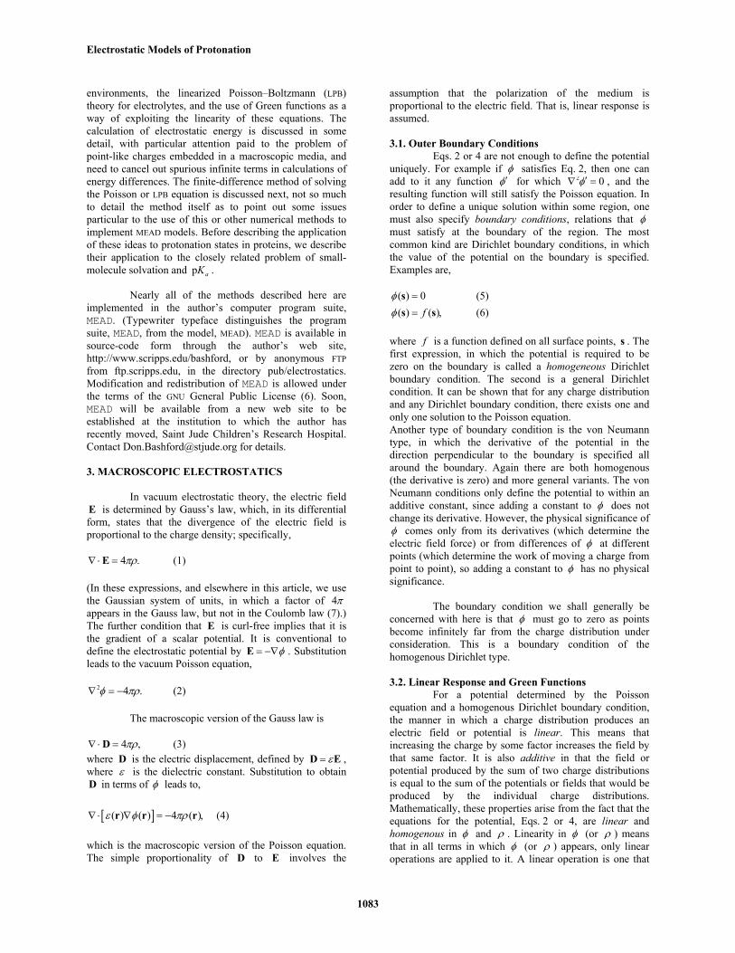
7.2. Small molecule p aKNearly all p aK calculations for ionizable groups

in proteins are made with reference to model compounds ofknown p aK , but for small molecules whose gas-phaseproton affinity can be calculated by quantum chemicalmethods, an absolute p aK calculation is possible.Considering the cycle of Figure 3, one finds,

solv solv solv2 303 p (AH) (A ) (H )a dgRT K G G G G− +. = −∆ − ∆ + ∆ + ∆ . (44)

Here, the free energy of the dissociation reactionin the gas phase dgG∆ is related to the proton affinity bythe entropy of the liberated proton (26 eu) and a smallcorrection ( 0 to 5 eu) for the entropy difference betweenA and AH. The solvation free energies of AH and A can becalculated by the methods of Sec. 7, but the solvG∆ of aproton cannot. An experimental value for solv (H )G +∆would depend on the absolute potential of the standardhydrogen electrode, which itself is only knownapproximately. On this basis, values of solv (H )G +∆ rangingfrom 259.5 to 262.5 kcal/mol have been suggested (35,36).

Lim et al. (35) explored the above approach toabsolute p aK calculation using different charge and radiusparameters. Because the magnitudes of dgG∆ for smallorganic acids and bases range from 200–400 kcal/mol, andthe solvation energies of the charged species are typicallyof order 100 kcal/mol, small percentage errors in theestimation of any of these terms can lead to substantialdeviations from experimental p aK values (one pK unit isequivalent to 1.4 kcal/mol at 300 K). Thus, Lim et al. foundsignificant sensitivity to the choice of charge and radiusparameters and to the details of solute geometry. An SCRFapproach in which the geometry and solute charge is

handled quantum mechanically leaves only atomic radii asempirical parameters, and yields reasonable estimates ofp aK for a number of small organic molecules (31,37). The

SCRF method has also been extended to p aK calculations ofunusual species in protein active sites, such as a watermolecule liganded to a manganese ion in superoxidedismutase (38). In this case, “solvation” means transferfrom vacuum to an in 1ε = cavity within a protein activesite, and the calculation must include the charges anddielectric constant of the remainder of the protein as well asthe surrounding solvent dielectric. Facilities for theclassical electrostatic part of such calculations are providedin the MEAD program suite.

8. PROTONATION STATES AND p aK INPROTEINS

Rather than the more first-principles approachoutlined in Sec. 7.2, calculations of protonation states andp aK values in proteins have generally used an approachbased on model compounds of known p aK , andelectrostatic models to calculate shifts from the modelcompound values. Calculations of this general kind wereintroduced nearly 80 years ago by Linderstrøm-Lang (39)who modeled the protein as a sphere with the charges of theionizable groups spread uniformly over its surface. As itbecome understood that proteins were not fluid globulesbut contained more specific structures, Tanford andKirkwood (40,41) developed a model of protein ionizablesites as point charges uniformly spaced at a short fixeddistance beneath the surface of a sphere. As actual proteinstructures became known, the Tanford–Kirkwood modelwas adjusted to use charge placements derived from theactual structures (42), and empirical corrections fordifferential solvent exposure were introduced (43,44).

The modern MEAD-based models described here(45), which have nearly displaced the sphere-based models,can be thought of as the natural extension of Tanford andKirkwood’s ideas to more detailed and realistic molecularsurface shapes and charge distributions (Figure 4).However, several qualitatively new energy terms areincluded: the Born-like interaction of the ionizing groupwith the polarization that its ionization produces in thesurroundings; and the interaction with non-ionizing groupsin the protein, such as the backbone dipoles. In contrast, theTanford–Kirkwood model only explicitly includes theelectrostatic interactions between ionizing sites; the otherterms, which could not have been explicitly calculatedwithout more atomic detail, were left to be implicitlysubsumed into the model compound p aK .

The fundamental assumptions behind themethods described here are as follows: (1) The free energyof ionization can be divided into an internal part thatincludes bond breaking and other electronic structurechanges and is confined to a relatively small number ofatoms within the ionizing functional group, and an externalpart that includes interactions with the larger surroundings.(2) The internal part is the same for both the ionizing groupin the protein and the corresponding model compound, but

Electrostatic Models of Protonation

1091

Figure 4. MEAD model for p aK calculations for proteins.The charges of the titrating site in protein or modelcompound (black circles in grey region) are changed fromprotonated to deprotonated values. Interactions occur withthe site’s own reaction potential; non-titrating polar groupsin both the protein and model compound (open circles) andother ionizable groups in the protein (black circles in whiteareas).

the external part may differ. (3) Since the steric changes inprotonation/deprotonation are subtle, and similar in boththe protein and model compound the steric contribution tothe difference of the external part can be neglected. (4) Theremaining difference in the external part is purelyelectrostatic. (5) A MEAD model is adequate to describe thiselectrostatic difference. As a practical matter, othersimplifying approximations are often introduced as well,such as neglect of conformational change andsimplification of charge models; but these approximationscan be lifted without changing the basic ideas.

8.1. One-site caseConsider a protein that contains only one

ionizable chemical group, and suppose one wishes tocalculate its p aK given the protein structure and modpK ,the p aK of a small model compound containing that samechemical group. The one-site protein is a usefulhypothetical construct because it removes the complicationof interactions with other groups whose ionization statesare pH dependent. In particular, we will adopt Tanford’sdefinition of the “intrinsic pK ” or intrpK , as the p aK thata site in a protein would have if all other ionizable siteswere held in some reference charge state, typically aneutral-charge state. We also neglect the conformationalflexibility of the protein, except to the extent that it isincluded implicitly in the protein dielectric constant inε .

According to the fundamental assumptions listedabove, the desired intrpK value is the modpK , modified by asuitable difference in electrostatic work of the protonatedversus deprotonated states in the protein versus the modelcompound:

( ) ( ) ( ) ( )

intr modp p2 303

p d p dp p m mW W W W

K KRT

− − −= − ,

.(45)

where the W are the work of creating either the chargedistribution of the protonated or deprotonated state ( ( )p or( )d superscripts) in the protein or the model compound( p or m subscripts). As discussed in Sec. 5, each of thesework terms potentially contains contributions that go toinfinity in the point-charge limit and care must be taken toensure that these cancel in the final calculation. To this end,we begin with Eq. 30, in which the small-sphere energiesthat lead to these infinities is explicit, and we distinguishthe small set of charges Q that differ between theprotonated and deprotonated and deprotonated states (filledcircles in Figure 4) and the remaining charges q (opencircles) that do not. The result is:

2( ) ( ) ( )( ) ( ) ( )

in in

1 ( )2 2

p p pp p pa a b

p a b r p a ba ab b a aba a b

Q Q QW Q Q gRε ε ,

, <

= + + ,−∑ ∑ ∑ r r

r r( )

( )

in

( )p

a p i pa p i r p a i

ai aia i

Q qQ q g

ε,

, ,+ + ,−∑ ∑ r r

r r2

in in

1 ( )2 2

m i jm ip i p j r p i j

i ij j i iji i j

q qqq q g

Rε ε,,

, , ,, <

+ + + , ,−∑ ∑ ∑ r r

r r(46)

where the indices a and b label the titrating-group’scharges, i and j label the non-titrating charges of theprotein (the pq ), and r pg , is the reaction potential term ofthe Green function for the protein (see Eq. 28).

If the analogous expression for ( )dpW is written

down and subtracted from the above, it is immediately seenthat all terms involving interactions between the protein’snon-titrating charges (the qq terms) vanish. Theinteractions between titrating and non-titrating charges canbe conveniently written down in terms of the potential dueto the titrating charges, ( ) ( )p j a p a ja

Q gφ = ,∑r r r , wherepg is the total green function (including the Coulombic

part) for the protein, and superscripts can be added to theQ and pφ to distinguish the ionization states as above.The difference between the two work terms is then,

2 2( ) ( ) ( ) ( ) ( ) ( )( ) ( )

in in2

p d p p d dp d a a a b a b

p pa ab b aa a b

Q Q Q Q Q QW WRε ε, <

− −− = +

−∑ ∑ r r

( ) ( ) ( ) ( )1 1( ) ( )2 2

p p d da b r p a b a b r p a b

ab abQ Q g Q Q g, ,+ , − ,∑ ∑r r r r

( )( ) ( )( ) ( )p dp i p i p i

iq φ φ,+ − .∑ r r (47)

To complete the evaluation of the numerator inEq. 45, an analogous expression for the work of the chargechange in the model compound, ( ) ( )p d

m mW W− must besubtracted from the above expression. This leads to acancellation of all the Coulomb terms involving only the

Electrostatic Models of Protonation

1092

titrating charges (the QQ terms), including the small-sphere energies, so the problem of infinities in the point-charge limit is resolved. The resulting expression is:

( ) ( ) ( ) ( )p d p dp p m mW W W W

− − − =

(48)( ) ( ) ( ) ( )1 ( ) ( )

2p p p p

a b r p a b a b r m a bab ab

Q Q g Q Q g, , , − , ∑ ∑r r r r

( ) ( ) ( ) ( )1 ( ) ( )2

d d d da b r p a b a b r m a b

ab abQ Q g Q Q g, ,

− , − ,

∑ ∑r r r r

( ) ( )( ) ( ) ( ) ( )( ) ( ) ( ) ( )p p p pp i p i p i m k m k m k

i kq qφ φ φ φ, ,+ − − −∑ ∑r r r r

The reaction QQ terms do not cancel, since thereaction part of the Green function is not the same in theprotein as in the model compound. These terms can bewritten in the form a ra

Q φ∑ , where rφ is the reactionpotential, as in Eq. 31. The expressions in the first set ofsquare brackets is then ( ) ( ) ( )( )p p p

a r p r maQ φ φ, ,−∑ , and an

analogous expression using the deprotonated charges isobtained for the second bracketed expression. These arevery similar to Eq. 35 for the solvation case. The differenceis, instead of altering the external dielectric environmentfrom vacuum to solvent, we are altering the dielectricenvironment from that of a protein in solvent to that of themodel compound in solvent. The rules at the end of Sec. 5are satisfied as long is the titrating charges are in a regionof dielectric inε in both cases. Therefore, as in thediscussion of solvation energy (see Eq. 36), we cansubstitute the finite-difference calculated potential due tothe titrating charges for the reaction potentials to obtain apractical expression for calculations.

We have seen that Eq. 48 contains two distinctkinds of terms: the QQ terms leading to expressionssimilar to those for electrostatic solvation energy; and theqφ (or Qq ) terms corresponding to interactions of thetitrating charges with the non-titrating background. It hasbecome conventional to refer to these terms as the Born andand background terms, respectively. The expression for

intrpK is then written:

Born backintr modp p

ln10G GK K

RT∆∆ + ∆∆

= − (49)

where,

( ) ( )titr

( ) ( ) ( ) ( ) ( ) ( )Born

1 ( ) ( ) ( ) ( )2

p p p d d da p a m a a p a m a

aG Q Qφ φ φ φ∆∆ = − − −∑ r r r r (50)

( ) ( )protein model

( ) ( ) ( ) ( )back ( ) ( ) ( ) ( )p d p d

m i p i p i m k m k m ki k

G q qφ φ φ φ, ,∆∆ = − − −∑ ∑r r r r (51)

Note that the same four potentials are needed forboth the Born and background term: the potentialsgenerated by the titrating charges in both their protonatedand deprotonated states in both the protein and the modelcompound. The potential generated by the non-titratingcharges need not be calculated — the non-titrating chargesenter the backG∆∆ expression only as charges that “feel” thepotential, not as charges that generate it.

It should be emphasized that the above is validonly if the titrating charges are the same in the protein andmodel compound and if the interatomic distances betweenthem are the same. Further, if finite-difference or finite-element methods are used, the way that the numerical gridis set up around the titrating charges, and the way that thecharges are distributed over them must be identical. Whencalculations of this kind were first introduced (45) a furtherprecaution was taken along these lines: all the atomiccharges positions and radii of the model compound, even“background” charges were made identical tocorresponding atoms in the protein. In other words, theconceptual model of Figure 4, in which the modelcompound appears to be “cut out” from the protein, wasfollowed strictly. This has the advantage of canceling someof the errors in the finite-difference method that tend to bemore severe for interactions between near atoms, such asbonded pairs within the model compound. But it has thepeculiarity that the calculations use a different modelcompound coordinate sets for each site, even for sites of thesame residue type. Most subsequent calculations of thiskind have followed a similar practice. However, schemesthat include conformational flexibility of both proteinsidechains and model compounds need not have thislimitation (46).

8.2. Multiple interacting sitesIn passing to the full model implied by Figure 4,

we must include the electrostatic interactions between theionizable groups. Strictly speaking, it is no longer possibleto rigorously define the p aK of individual sites, so we shallfirst consider the relative energetics of different protonationstates of the protein, and then the statistics of ensemblesover the possible states. This leads to predictions of thedegree of protonation of each site as a function of pH, andthese pH dependencies can usually (but not always) bereasonably well described by a p aK -like quantity.

By “protonation state” of the protein, we mean aspecification of which sites are protonated and which aredeprotonated. If the protein has N sites, each with twopossible protonation states, there are 2N possibleprotonation states of the protein. Let them be denoted bythe N -element vector, x whose elements ix take caneach take on values representing “protonated” or“deprotonated.” Let 0 be a particular value of this vectorchosen as a reference state, for example, the state with allsites in their neutral state, as in the definition of intrpK .Consider the chemical equilibrium between some state xand the reference state:

M(0) ( )H M( )ν ++ x x (52)

where ( )ν x is the number of protons that would bereleased on going from state x to the reference state. Thefree energy change for going to the right in this reaction atsome fixed pH is,

M M H

[M( )]( pH) ln ( ) (0) ( )( 2 303 pH)[M(0)]

G RT RTµ µ ν µ +∆ , = − = − − − . ,xx x xo o o (53)

Electrostatic Models of Protonation

1093

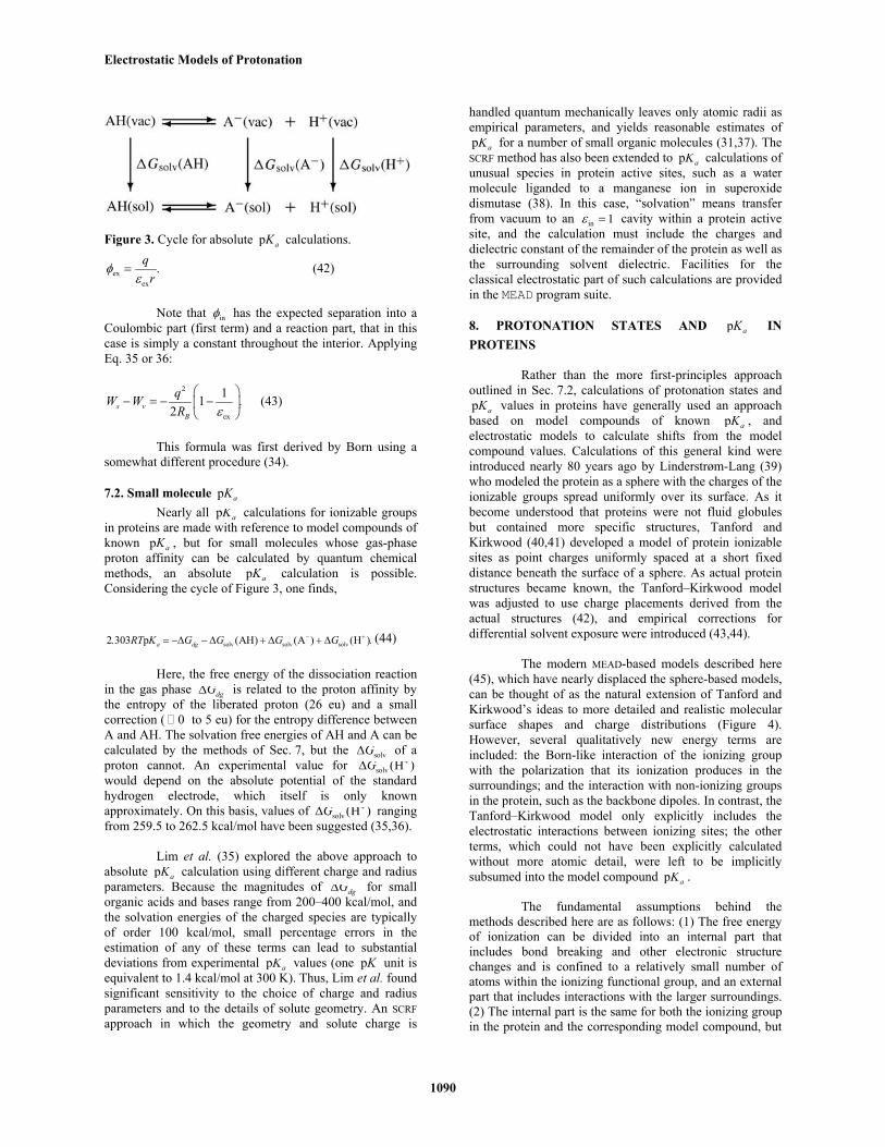
Figure 5. Titration curves of sites in Bacteriorhodopsin,taken from the work of ref. (17).

where the µ o are standard chemical potentials.

Suppose ( )i iP x is the change in the protein’schemical potential for changing site i from its referencestate to state ix , while all other sites remain in thereference state. The expression for chemical potential willthen contain a sum of these iP , but more terms are neededfor the site–site interactions. Since the interactions arepresumed to be governed by linear equations (the Poissonor LPB equations) these terms will be pairwise additive.Therefore,

1( ) (0) ( ) ( )2

N N

M M i i ij i ji ij i j

P x W x xµ µ, ≠

= + + , ,∑ ∑xo o (54)

where ijW is the electrostatic interaction between sites iand j , relative to the reference state. Inserting this intoEq. 53 and writing ( )ν x as a sum over sites, ( )i ii

xν∑ ,gives,

H

1( pH) [ ( ) ( )( 2 303 pH)] ( )2

N

i i i i ij i ji ij i j

G P x x RT W x xν µ +

, ≠

∆ , = − − . + ,∑ ∑x o (55)

Some consideration of the way in which P , ν and intrpKare defined in terms of a reference state leads to the therelation, intrH

( ) ( )( 2 303 p )i i i i iP x x RT Kν µ + ,= − . , so that,

intr1( pH) ( )2 303 (pH p ) ( )2

N

i i i ij i ji ij i j

G x RT K W x xν ,, ≠

∆ , = . − + , .∑ ∑x (56)

The intrinsic p aK values of each site, intrp iK , ,can be calculated by the methods of Sec. 8.1. The

( )ij i jW x x, can be calculated by considering the additionalelectrostatic work to change site i ’s charges from thereference state to ix if site j is in state jx instead of itsreference state. By this definition, ijW is non-zero only ifboth ix and jx are different from their standard states 3. If,for example, the deprotonated states of both i and j arethe standard states, then

site( ) ( ) ( ) ( )(prot prot) [ ( ) ( )]

ip d p d

ij a a j a j aa

W Q Q φ φ

, = − −∑ r r (57)

site( ) ( ) ( ) ( )[ ( ) ( )]

jp d p d

b b i b i bb

Q Q φ φ

= − − ,∑ r r

where ( )piφ is the potential produced by the site i charges

in their protonated state, and so forth, and the sums runover the atoms of the indicated site. Note that the fourdifferent potentials needed here are are already availablefrom the calculations of the intrinsic p aK calculations forthe two sites (Eqs. 49–51). Therefore the construction of afunction that gives the relative energies of all 2N possibleprotein protonation states requires just 4N solutions of thePoisson or LPB equation.

The pH-dependent protonation state free energyfunction, ( pH)G∆ ,x can be used to calculate probabilitiesof protonation states and averages of quantities dependingon protonation state by formulae analogous to the canonicaldistribution of statistical mechanics. For example, thefraction of all protein M that is in state M( )x is

[M( )] exp[ ( pH) ][M] (pH)

G RTZ

−∆ , /= ,

x x (58)

where Z is the normalization constant or partition functiongiven by,

2

(pH) exp[ ( pH) ]N

Z G RT= −∆ , /∑x

x (59)

where the sum runs over all possible protonation states.Perhaps the most common average taken is the the averageprotonation of a particular site:

21(pH) ( )exp[ ( pH) ](pH)

N

i i ix G RTZ

θ ν= −∆ , / .∑x

x (60)

Some illustrative plots of iθ versus pH areshown in Figure 5. In most cases the curves are have anapproximately Henderson–Hasselbalch form, as in Figure5a. One can then define halfpK , a quantity roughlyanalogous to p aK , as the pH at which the plot crosses theprotonation fraction, 0.5. But strong couplings between twosites titrating in overlapping pH ranges can lead to caseswhere halfpK is nearly meaningless; instead the pivotal pHvalues are those that mark changes between no protons oneither site, a single proton shared between the sites, andboth sites protonated (Figure 5b). When three or more sitesstrongly couple, it is even possible to have the

Electrostatic Models of Protonation

1094

counterintuitive result that one site may, within a limited pHrange, increase in protonation as pH increases (17) a situationthat has also been observed experimentally (48). The totalprotonation of all sites, however, must always monotonicallydecrease with increasing pH. Recently some methods ofdisentangling the complexities of multi-site titration curveshave been presented by Onufriev et al. (49) Calculated titrationcurves often have unusual shapes for the active-site groups inproteins, because close proximity and, quite often, a solventshielded environment give rise to strong site–site couplings.Recently, this has been used as a diagnostic to predict thelocation of protein active sites (50).

If there are no more than 12 to 15 sites, averageslike iθ can be evaluated directly from expressions likeEq. 60, but as the number of sites N increases, the cost ofevaluating the sums quickly becomes untenable. For suchsituations, several approximate methods are available.Rather than describe them in detail, we only outline themhere, with citations to papers that provide more thoroughdescriptions.

8.2.1. Tanford–Roxby approximationIt is assumed that each site i interacts not with

particular protonation states of other sites, j but with their(pH dependent) average protonation, jθ (42). Tanford andRoxby’s formulae can be derived from a mean-fieldapproximation in which correlations between theprotonation states of sites are neglected; and it can beshown that this approximation breaks down in cases wherestrongly coupled sites titrate in the same pH range (51).

8.2.2. Reduced Site approximationFor each pH value, a preliminary calculation is

done to determine which sites can be regarded as almostcompletely protonated or almost completely deprotonated.These sites are then regarded as fixed in the protonated ordeprotonated states, respectively, reducing the number ofvariable sites in the calculation (51). This approximation isquite accurate, except in the extreme-pH tails of thetitration curves. However, in typical applications theeffective number of sites is only cut by about half, so thismethod is useful only up to about 30 ionizable groups. Theauthor’s implementation of this method is part of the MEADsuite.

8.2.3. Monte-Carlo MethodsThe application of Monte-Carlo methods to the

multi-site titration problems was introduced by Beroza etal.(52) An initial protonation state is selected, then sites areflipped at random between the protonated and deprotonatedstates, and the flips are accepted or rejected based on thechange in ( pH)G∆ ,x resulting from the flip. A two-siteflipping strategy may be needed to obtain convergence forstrongly coupled sites. The computational cost is apolynomial in N rather than an exponential, so it is usablein practice for systems containing hundreds of sites. Themethod is reasonably accurate if applied correctly, althoughthe titration curves produced are somewhat “noisy.”Beroza’s implementation of the method (52,47) is availableon the Internet (ftp://ftp.scripps.edu/case/beroza)

8.2.4. Clustering methodsVariants of this idea have been introduced by

several authors (53,54,55). The idea is that in calculatingthe protonation of site i , one can use a mean-fieldapproximation for weakly coupled or distant sites, andmore exact expressions for the strongly coupled (or nearby)ones. The version of this idea developed in the author’sgroup is called Iterative Mobile Clustering (IMC) and hasbeen described in detail and tested in a recent paper (55).This method is also applicable to multi-conformationalproblems. A general purpose implementation of IMC isplanned, but not yet written.

Tautomerism of sidechains such as histidine canbe incorporated into the above formalism by allowing the

ix to take on appropriate values, such as “epsilon,” “delta”and “protonated.” In that case, six Poisson or LPB solutionswould be required for each histidine residue so treated.(Calculations incorporating tautomerism in essentially thisway were first done nearly a decade ago (56), but since thetwo-state “protonated/deprotonated” scheme was hard-wired in the software at that time, an equivalent schemeusing extra pseudo-sites was devised. This trick has beendescribed in detail by Baptista et al. (57).) It is alsopossible to incorporate the binding of other ions to specificsites, or oxidation-state changes into the above formalism.This allows one to calculate, for example, the pHdependence of redox potentials in proteins or the workingsof energy transduction proteins in which electron andproton transfer are coupled (58,59,60). Ref. (55) providesan extension of the above formal framework that coversboth tautomerism, binding of other ligands and redoxchanges.

8.3. Conformational FlexibilityThe above methods do not allow for

conformational flexibility, except implicitly through theprotein dielectric constant. But since the dielectric responseof the protein is supposed to be within the linear regime,this implicit flexibility cannot involve much more thanmodest localized fluctuations of dipoles. Significant globalconformational changes, such as unfolding or hinge-bending, go unrepresented. Even changes confined to a fewsidechain degrees of freedom, such as the formation orbreaking of salt bridges, cannot be plausibly subsumed intothe dielectric response, especially insofar as they affect thep aK values of the sidechains themselves. One shouldtherefore expect the method to break down in cases whereconformational changes have a significant influence onp aK .

The prediction of extreme p aK values should betaken as a possible indicator of such a breakdown. Forexample, in the earliest calculations of this kind (45), ap aK of around 20 was calculated for Tyr53 of lysozyme.However, the unfolding of lysozyme is known to becoupled to the ionization of this residue (at pH 12). Thehigh calculated number should be understood as the p aKthat the site would have if the protein could somehow beconstrained to stay near its native conformation at veryhigh pH. On the other hand, some residues do have

Electrostatic Models of Protonation

1095

functionally important large pK shifts that are correctlypredicted by the methods. Examples include bacteriorhodopsin(17) and protein tyrosine phosphatase (61), though in somecases the method over-predicts the magnitude of the shift.

The most desirable solution, in principle, is toinclude conformational flexibility explicitly in thecalculation. However, this raises complex problems. Thefree energy change associated with changingconformational states now becomes part of the problem,and this includes many non-electrostatic factors. Forexample, in the alkaline denaturation example, the p aKbecomes higher to the extent that the forces stabilizing thenative state, such as van der Waals and hydrophobicinteractions, resist the driving force for alkalinedenaturation, which is proportional to the differencebetween the pH and the p aK that the still-protonated siteswould have in the unfolded state. For practical calculationsincluding flexibility, the number of conformers that shouldbe included, and how they should be selected is far fromobvious. For a fairly complete formulation emphasizing theproblem of enumerating the conformational states andconsidering the correlations between distinct flexibleregions of a protein, see Ref. (55). Development ofmethods to include conformational flexibility in titrationcalculations has been a topic of active research using anumber of different approaches (46,47,62-68), and will notbe reviewed in detail here.

However, we will present one easilyimplemented method based on integration over bindingisotherms. It is quite useful for the case of pH-drivenunfolding (69), and it has also been applied to electrontransfer (58). It can be shown (70,71,72) that the pHdependence of the free energy of a conformational changefrom A to B can be expressed as

pH

pH(pH) ( ) 2 302 [ ( ) ( )]pHAB AB B AG G RT Q pH Q pH dpH′ ′ ′∆ − ∆ = . − ,∫

oo

(61)

where the Q are either the total charge or total number ofprotons in the protein bound in state A or B. The integrandscan be calculated by the methods of Sec. 8.2 givenstructural models for conformers A and B. Or, if one of theconformers is the unfolded state, one might assume that itsresidues titrate like independent sites with p aK ’s equal tothe modpK values (69). Having ABG∆ at any one pHallows its value at any other pH to be calculated, in principle.For example, if the pH for acid unfolding (where 0ABG∆ = )is known, then the stability of the protein at neutral pH can becalculated. In effect, the problem of knowing the non-electrostatic contributions to the conformational energetics hasbeen subsumed into the need to know ABG∆ at a particularpH. Titration curves for individual sites (the iθ ) can beobtained in a way that accounts for the conformational changeby weighting the contributions from the A-conformer and theB-conformer in calculations of iθ according to (pH)ABG∆ , ateach pH point.

9. OPEN PROBLEMS

That electrostatic effects are the primary meansby which the protein environment modifies the H + -

titration properties of its ionizable groups is beyonddispute, but one can certainly question whether theapproximations of macroscopic electrostatics arepermissable in the calculation of such effects, and if so,what macroscopic parameters, such as dielectric constantsand boundary definitions, ought to be used. MEAD modelsseem to be on fairly good ground in at least one area: thetreatment of solvent water as a region of high dielectric.Calculations of small molecule solvation energies by themethods of Sec. 7 have been quite successful, given somemodest efforts at parameterization (27,28,36,73).Comparisons between molecular dynamics-basedthermodynamics calculation using an atomisticrepresentation of both solvent and solute, and a MEADmodel of solvation and H-bonding show that the two givevery similar results, at least when the the standard, low-costatomic models of solvent, such as TIP3P are used for smallmolecules whose charges are no more thanmonovalent(74,75).

The depiction of the protein as a macroscopicdielectric medium is another matter. Theories that connectmicroscopic models to a macroscopic dielectric assume anorders-of-magnitude separation between the microscopiclength scale and the size of any region to which a dielectricconstant is assigned. Proteins are in a mesoscopic greyzone, in that the characteristic protein distance (the proteinradius, say) is only a few times greater than the length scaleof the microscopic dipolar elements it contains (e. g.,backbone amides). Furthermore, proteins do not appear tobe particularly uniform within their interior. There has beensome suggestion of addressing the non-uniformity problemby assigning different dielectric constants to different partsof the protein (76), but since these parts must necessarily besmaller than the protein, the microscopic/mesoscopicproblem alluded to above is exacerbated. Some workers(77) have criticized the protein dielectric idea as invalid,particularly when the dipoles whose fluctuations constitutethe dielectric response are also present in the calculations,as in Eq. 51. As an alternative, they advocate an approachthat resembles the standard microscopic moleculardynamics approaches, but enforces linear response andmodifies electrostatic terms according to a scaling factor insuch a way that the resulting model appears quite similar,in effect, to a MEAD model (78).

Recently, a series of papers by Simonson and co-workers have presented some careful analysis of therelationship between microscopic and macroscopicrepresentations of protein electrostatics. They performedmicroscopic calculations of the response of the proteinmedium to the insertion of a charge at various locations inthe protein interior and found that these were well matchedby a macroscopic model with a uniform dielectric constantin the protein region (79). The best value of the dielectricconstant for such a match was in close agreement with thatcalculated using a modified version of Kirkwood–Fröhlichtheory to relate protein dipole fluctuations in a microscopicprotein/water simulation to the protein dielectric constant(80-84). This finding of consistency between various waysof relating microscopic fluctuations and responses to

Electrostatic Models of Protonation

1096

macroscopic dielectric theory provides some support forthe extension of macroscopic ideas to proteins.

Even if the idea of a protein dielectric constant isacceptable, there remains the question of its value. Manyearly workers in the field, following the suggestion ofTanford and co-workers (41,42) used values near 4, whichis consistent with measurements on dry protein powders(85,86). Early molecular mechanics calculations usingKirkwood–Fröhlich theory (80,81) to calculate thedielectric constant from microscopic dipole fluctuationssupported similar values (87,88). More recent calculations,in which increased computing power allows explicitsolvent to be included, seemed at first to suggest highervalues of the protein dielectric constant, such as 20 to 35,but more detailed analysis showed that the large dipolefluctuations were mainly due to the mobility chargedsidechains at the protein surface. If only the more buriedpolar groups are considered, much lower values, such as 2to 6, are calculated (82,83,84,89).

Antosiewicz et al. have taken a more empiricalapproach to the protein dielectric question (90,91). For a setof proteins for which the p aK of a number of sidechainswas known experimentally, they made calculations by themethods of Sec. 8 using various values of inε and foundthat the root mean square error was minimized with

in 20ε . In the present author’s view, the counter-argument is as follows: Most ionizable groups are on theprotein surface where they are well exposed to solvent orcan become so with a sidechain conformational change,and their p aK values are only slightly shifted from those ofmodel compounds. Standard single-conformer MEADmodels tend to overestimate these shifts because the lack ofconformational flexibility eliminates a relaxationmechanism that would allow for more “normal” calculatedtitration properties. Raising inε to high values tends tominimize broad statistical measures of error simply becauseit tends to make calculated shifts smaller. However,important active-site residues are often unusual in that theyhave large p aK shifts, and a computational method thattends to scale down all shifts risks missing these. Indeed,we have computed several large, functionally important,p aK shifts in proteins that could not have been predictedwith a high inε value (17,61,92,93).

Krishtalik et al. (94) have made an interestingproposal to address the potential inconsistency (77) ofexplicit inclusion of peptide dipoles when these samedipoles’ fluctuations are treated implicitly as a dielectricresponse. To state the problem as it relates to p aKcalculations, consider the one-site problem of Sec. 8.1. Theincremental work of adding an incremental charge to thesite is ( )W q V Vδ δ= + ∆o , where Vo is the averageelectrostatic potential at the site due to all other charges,including protein dipoles, prior to any charge at the site,and V∆ is the average change in that potential due to theprotein and solvent dipole’s reorientation in response to thesite’s developing charge. Macroscopic calculations of

BornG∆∆ (Eq. 50) correspond well to the V∆ term, asshown by comparison to microscopic charging calculations

(79). However, it can be argued that for the calculation ofbackG∆∆ , which should correspond to the the Vo term, the

use of a protein dielectric higher than the optical dielectricconstant ( 2 ) constitutes a sort of double countingbecause the coordinates in the calculation already reflectthe orientational polarization of the protein. Thus, it issuggested that a low protein dielectric constant (1–2)should be used for the backG∆∆ term while a higherdielectric constant ( 3≥ ) may be used for BornG∆∆ toreflect the changing orientational polarization as the chargedevelops. This would appear to introduce an inconsistencyof its own — the use of two different dielectric constantsfor one and the same material during the same chargingprocess — but a consistent scheme for implementing thisidea has been devised (95). It requires a detailedmicroscopic model for the whole protein both before andafter the charge change at the site, and is thereforeconsiderably more complicated to implement, particularlyfor a multi-site problem.

Many of the problems and ambiguities outlinedabove can in principle be removed or ameliorated by aproper treatment of conformational flexibility (Sec. 8.3).Although the formalism and the means to overcome somecombinatorial problems have been developed (55), a goodgeneral method to generate the important conformerswithout creating an unmanageably large number of themhas yet to be developed. In this connection, workers in thefield might do well to look at the remarkable progress beingmade in handling the combinatorics of sidechainconformers in the field of protein design (96,97,98).

10. REFERENCES

1. Warwicker, J. & H. C. Watson: Calculation of theelectric potential in the active site cleft due to α -helixdipoles. J Mol Biol 157, 671–679 (1982)2. Connolly, M. L.: Solvent-accessible surfaces of proteinsand nucleic acids. Science 221, 709–713 (1983)3. Richards, F. M.: Areas, volumes, packing and proteinstructure. Ann Rev Biophys Bioeng 6, 151–176 (1977)4. Honig, B. & A. Nicholls: Classical electrostatics inbiology and chemistry. Science 268, 1144–1149 (1995)5. Juffer, A. H.: Theoretical calculations of acid-dissociation constants of proteins. Biochem Cell Biol 76,198–209 (1998)6. GNU general public license, version 2. Published byThe Free Software Foundation, 675 Massachusetts Ave.,Cambridge, MA 02139, USA (1991)7. Jackson, J. D.: Classical Electrodynamics. Wiley andSons, New York, 2 edn. (1975)8. McQuarrie, D. A.: Statistical Mechanics. Harper andRow, New York (1976)9. Debye, P. & E. Hückel: Phys Z 24, 185 (1923)10. Chandler, D.: Introduction to Modern StatisticalMechanics. Oxford, New York (1987)11. Gilson, M. K., K. A. Sharp & B. Honig: Calculatingthe electrostatic potential of molecules in solution: Methodand error assessment. J Comp Chem 9, 327–335 (1987)12. Mohan, V., M. E. Davis, J. A. McCammon & B. M.Pettitt: Continuum model calculations of solvation free

Electrostatic Models of Protonation

1097

energies: Accurate evaluation of electrostatic contributions.J Phys Chem 96, 6428–6431 (1992)13. Beroza, P. & D. R. Fredkin: Calculation of amino acidp aK s in a protein from a continuum electrosatic model:Method and sensititivity analysis. J Comp Chem 17, 1229–1244 (1996)14. Press, W. H., B. P. Flannery, S. A. Teukolsky & W. T.Vetterling: Numerical Recipes. The Art of ScientificComputing. Cambridge University Press, Cambridge(1986)15. Briggs, W. L.: A Multigrid Tutorial. SIAM,Philadelphia (1987)16. Hackbusch, W.: Iterative Solutions of Large SparseSystems of Equations, vol. 95 of Applied MathematicalSciences. Springer, New York (1994)17. Bashford, D. & K. Gerwert: Electrostatic calculationsof the p aK values of ionizable groups inbacteriorhodopsin. J Mol Biol 224, 473–486 (1992)18. Bashford, D.: An object-oriented programming suitefor electrostatic effects in biological molecules. In:Scientific Computing in Object-Oriented ParallelEnvironments, Eds. Ishikawa, Y., R. R. Oldehoeft, J. V. W.Reynders & M. Tholburn, ISCOPE97, Springer, Berlin(1997), vol. 1343 of Lecture Notes in Computer Science,233–24019. Nicholls, A. & B. Honig: A rapid finite differencealgorithm, utilizing successive over-relaxation to solve thePoisson-Boltzmann equation. J Comp Chem 12, 435–445(1991) 20. Luty, B. A., M. E. Davis & J. A. McCammon:Electrostatic energy calculations by a finite-differencemethod: Rapid calculation of charge–solvent interactionenergies. J Comp Chem 6, 768–771 (1992)21. You, T. J. & S. C. Harvey: Finite-element approach tothe electrostatics of macromolecules with arbitrarygeometries. J Comp Chem 14, 484–501 (1993)22. Cortis, C. M., J.-M. Langlois, M. D. Beachy & R. A.Friesner: Quantum mechanical geometry optimization insolution using a finite element continuum electrostaticsmethod. J Chem Phys 105, 5472–5484 (1996)23. Miertus, S., E. Scrocco & J. Tomasi: Electrostaticinteraction of a solute with a continuum: A direct utilizationof ab initio molecular potentials for the prevision of solventeffects. Chem Phys 55, 117–129 (1981)24. Zauhar, R. J. & R. S. Morgan: J Mol Biol 186, 815 (1985)25. Zauhar, R. J. & A. Varnek: A fast and space-efficientboundary element method for computing electrostatic andhydration effects in large molecules. J Comp Chem 17, 864–877 (1996)26. Boschitsch, A. H., M. O. Fenley & H.-X. Zhou: Fastboundary element method for the linear Poisson–Boltzmannequation. J Phys Chem B 106, 2741–2754 (2002)27. Sitkoff, D., K. A. Sharp & B. Honig: Accurate calculationof hydration free energies using macroscopic solvent models. JPhys Chem 98, 1978–1988 (1994)28. Nina, M., D. Beglov & B. Roux: Atomic radii forcontinuum electrostatics calculations based on moleculardynamics free energy simulations. J Phys Chem B 101,5239–5248 (1997)29. Onsager, L.: Electric moments of molecules in liquids.J Amer Chem Soc 58, 1486–1493 (1936)

30. Tomasi, J. & M. Persico: Molecular interactions insolution: An overview of methods based on continuousdistributions of the solvent. Chem Rev 94, 2027–2094(1994)31. Chen, J. L., L. Noodleman, D. A. Case & D. Bashford:Incorporating solvation effects into density functionalelectronic structure calculations. J Phys Chem 98, 11059–11068 (1994)32. Tannor, D. J., B. Marten, R. Murphy, R. A. Friesner,D. Sitkoff, A. Nicholls, M. Ringnalda, W. A. Goddard, III& B. Honig: Accurate first principles calculation ofmolecular charge distributions and solvation energies fromab initio quantum mechanics and continuum dielectrictheory. J Am Chem Soc 116, 11875–11882 (1994)33. Tuñón, I., M. F. Ruiz-López, D. Rinaldi & J. Bertrán:Compuation of hydration free energies using aparameterized continuum model: Study of equilibriumgeometries and reactive processes in water solution. JComp Chem 17, 148–155 (1996)34. Born, M.: Volumes and heats of hydration of ions. ZPhys 1, 45–48 (1920)35. Lim, C., D. Bashford & M. Karplus: Absolute p aKcalculations with continuum dielectric methods. J PhysChem 95, 5610–5620 (1991)36. Gilson, M. K. & B. Honig: Calculation of the totalelectrostatic energy of a macromolecular system: Solvationenergies, binding energies, and conformational analysis.Proteins 4, 7–18 (1988)37. Richardson, W. H., C.-Y. Peng, D. Bashford,L. Noodleman & D. A. Case: Incorporating solvationeffects into density functional theory: Calculation ofabsolute acidities. Int J Quant Chem 61, 207–217 (1997)38. Fisher, C. L., J.-L. Chen, J. Li, D. Bashford &L. Noodleman: Density-functional and electrostaticcalculations for a model of a manganese superoxidedismutase active site in aqueous solution. J Phys Chem100, 13498–13505 (1996)39. Linderstrøm-Lang, K.: On the ionisation of proteins.Comptes-rend Lab Carlsberg 15, 1–29 (1924)40. Tanford, C. & J. G. Kirkwood: Theory of proteintitration curves. I. General equations for impenetrablespheres. J Am Chem Soc 79, 5333–5339 (1957)41. Tanford, C.: Theory of protein titration curves. II.Calculations for simple models at low ionic strength. J AmChem Soc 79, 5340–5347 (1957)42. Tanford, C. & R. Roxby: Interpretation of proteintitration curves. Biochemistry 11, 2192–2198 (1972)43. Shire, S. J., G. I. H. Hanania & F. R. N. Gurd:Electrostatic effects in myoglobin. hydrogen ion equilibriain sperm whale ferrimyoglobin. Biochemistry 13, 2967–2974 (1974)44. Matthew, J. B. & F. R. N. Gurd: Calculation ofelectrostatic interactions in proteins. Meth Enzymol 130,413–436 (1986)45. Bashford, D. & M. Karplus: p aK ’s of ionizable groupsin proteins: Atomic detail from a continuum electrostaticmodel. Biochemistry 29, 10219–10225 (1990)46. You, T. & D. Bashford: Conformation and hydrogenion titration of proteins: A continuum electrostatic modelwith conformational flexibility. Biophys J 69, 1721–1733(1995)

Electrostatic Models of Protonation

1098

47. Beroza, P. & D. A. Case: Including side chainflexibility in continuum electrostatic calculations of proteintitration. J Phys Chem 100, 21056–20163 (1996)48. Sudmeier, J. L. & C. N. Reilley: Nuclear magneticresonance studies of protonation of polyamine andaminocoboxylate compounds in aqueous solution.Analytical Chemistry 36, 1698–1706 (1964)49. Onufriev, A., D. A. Case & G. M. Ullmann: A novelview of pH titration in biomolecules. Biochem 40, 3413–3419 (2001)50. Ondrechen, M. J., J. G. Clifton & D. Ringe:THEMATICS: A simple computational predictor ofenzyme function from structure. Proc Natl Acad Sci USA98, 12473–12478 (2001)51. Bashford, D. & M. Karplus: Multiple-site titrationcurves of proteins: An analysis of exact and approximatemethods for their calculation. J Phys Chem 95, 9556–9561(1991)52. Beroza, P., D. R. Fredkin, M. Y. Okamura & G. Feher:Protonation of interacting residues in a protein by MonteCarlo method: Application to lysozyme and thephotosynthetic reaction center of Rhodobactersphaeroides. Proc Natl Acad Sci USA 88, 5804–5808(1991)53. Gilson, M. K.: Multiple-site titration and molecularmodeling: Two rapid methods for computing energies andforces for ionizable groups in proteins. Proteins 15, 266–282 (1993)54. Yang, A.-S., M. R. Gunner, R. Sampogna, K. Sharp &B. Honig: On the calculations of p aK s in proteins.Proteins 15, 252–265 (1993)55. Spassov, V. Z. & D. Bashford: Multiple-site ligandbinding to flexible macromolecules: Separation of globaland local conformational change and an iterative mobileclustering approach. J Comp Chem 20, 1091–1111 (1999)56. Bashford, D., D. A. Case, C. Dalvit, L. Tennant &P. E. Wright: Electrostatic calculation of side-chain p aKvalues in myoglobin and comparison with NMR data forhistidines. Biochemistry 32, 8045–8056 (1993)57. Baptista, A. M. & C. M. Soares: Some theoretical andcomputational aspects of the inclusion of proton isomerismin the protonation equilibrium of proteins. J Phys Chem B105, 293–309 (2001)58. Beroza, P., D. R. Fredkin, M. Y. Okamura & G. Feher:Electrostatic calculations of amino-acid titration andelectron-transfer, Q(A) − Q(B) → Q(A)Q(B) − , in thereaction-center. Biophys J 68, 2233–2250 (1995)59. Alexov, E. G. & M. R. Gunner: Calculated protein andproton motions coupled to electron transfer from Q A

− to

Q B− in bacterial reaction centers. Biochemistry 38, 8253–

8270 (1999)60. Baptista, A. M., P. J. Martel & C. A. Soares:Simluation of electron-proton coupling with a Monte Carlomethod: Application to cytochrome 3c using continuumelectrostatics. Biophys J 76, 2978–2998 (1999)61. Dillet, V., R. L. Van Etten & D. Bashford:Stabilization of charges and protonation states in the activesite of the protein tyrosine phosphatases: A compuationalstudy. J Phys Chem B 104, 11321–11333 (2000)

62. Ripoll, D. R., Y. N. Vorobjev, A. Liwo, J. A. Vila &H. A. Scheraga: Coupling between folding and ionizationequilibria: Effects of pH on the conformational preferencesof polypeptides. J Mol Biol 264, 770–783 (1996)63. Zhou, H.-X. & M. Vijayakumar: Modeling of proteinconformational fluctuations in p aK predictions. J Mol Biol267, 1002–1011 (1997)64. Baptista, A. M., P. J. Martel & S. B. Petersen:Simulation of protein conformational freedom as a functionof pH: constant-pH molecular dynamics using implicittitration. Proteins 27, 523–44 (1997)65. Luo, R., M. Head, J. Moult & M. K. Gilson: p aKshifts in small molecules and HIV protease: Electrostaticsand conformation. J Am Chem Soc 120, 6138–6146 (1998)66. van Vlijmen, H. W. T., M. Schaefer & M. Karplus:Improving the accuracy of protein p aK calculations:Conformational averaging versus the average structure.Proteins 33, 145–158 (1998)67. Nielsen, J. E. & G. Vriend: Optimizing the hydrogen-bond network in Poisson–Boltzmann equation-based p aKcalculations. Proteins 43, 403–412 (2001)68. Georgescu, R. E., E. G. Alexov & M. R. Gunner:Combining conformational flexibility and continuumelectrostatics for calculating p aK s in proteins. Biophys J83, 1731–1748 (2002)69. Yang, A.-S. & B. Honig: Structural origins of pH andionic strength effects on protein stability. Acid denaturationof sperm whale apomyoglobin. J Mol Biol 237, 602–614(1994)70. Wyman, J.: Linked functions and reciprocal effects inhemoglobin. A second look. Adv Prot Chem 19, 223–286(1964)71. Tanford, C.: Protein denaturation. C. theoreticalmodels for the mechanism of denaturation. Adv ProteinChem 24, 1–95 (1970)72. Schellman, J. A.: Macromolecular binding.Biopolymers 14, 999–1018 (1975)73. Sharp, K. A., A. Jean-Charles & B. H. Honig: A localdielectric constant model for solvation free energies whichaccounts for solute polarizability. J Phys Chem 96, 3822–3828 (1992)74. Jayaram, B., R. Fine, K. Sharp & B. Honig: Freeenergy calculations of ion hydration: An analysis of theBorn model in terms of microscopic simulations. J PhysChem 93, 4320–4327 (1989)75. Ösapay, K., W. S. Young, D. Bashford, C. L. Brooks,III & D. A. Case: Dielectric continuum models forhydration effects on peptide conformational transitions. JPhys Chem 100, 2698–2705 (1996)76. Honig, B., K. Sharp & A.-S. Yang: Macroscopicmodels of aqueous solutions: Biological and chemicalapplications. J Phys Chem 97, 1101–1109 (1993)77. King, G., F. S. Lee & A. Warshel: Microscopicsimulations of macroscopic dielectric constants of solvatedproteins. J Chem Phys 95, 4366–4377 (1991)78. Sham, Y. Y., Z. T. Chu & A. Warshel: Consistentcalculations of p aK ’s of ionizable residues in proteins:Semi-macroscopic and microscopic approaches. J PhysChem B 101, 4458–4472 (1997)

Electrostatic Models of Protonation

1099

79. Simonson, T. & D. Perahia: Microscopic dielectricproperties of cytochrome c from molecular dynamicssimulations in aqueous solution. J Am Chem Soc 117,7987–8000 (1995)80. Kirkwood, J. G.: J Chem Phys 7, 911 (1939) 81. Fröhlich, H.: Theory of Dielectrics. Oxford, 2 edn.(1958)82. Simonson, T. & D. Perahia: Internal and interfacialdielectric properties of cytochrome c from moleculardynamics in aqueous solution. Proc Natl Acad Sci U S A92, 1082–1086 (1995)83. Simonson, T. & C. L. Brooks III: Charge screening andthe dielectric constant of proteins: Insights from moleculardynamics. J Amer Chem Soc 118, 8452–8458 (1996)84. Simonson, T.: Dielectric relaxation in proteins:Microscopic and macroscopic models. Int J Quantum Chem73, 45–57 (1999)85. Bone, S. & R. Pethig: Dielectric studies of the bindingof water to lysozyme. J Mol Biol 157, 571–575 (1982)86. Bone, S. & R. Pethig: Dielectric studies of proteinhydration and hydration-induced flexibility. J Mol Biol181, 323–326 (1985)87. Gilson, M. K. & B. H. Honig: The dielectric constantof a folded protein. Biopolymers 25, 1097–2119 (1986)88. Nakamura, H., T. Sakamoto & A. Wada: A theoreticalstudy of the dielectric constant of protein. ProteinEngineering 2, 177–183 (1988)89. Smith, P. E., R. M. Brunne, A. E. Mark & W. F. vanGunsteren: Dielectric properties of trypsin inhibitor andlysozyme calculated from molecular dynamics simulations.J Phys Chem 97, 2009–2014 (1993)90. Antosiewicz, J., J. A. McCammon & M. K. Gilson:Prediction of pH-dependent properties of proteins. J MolBiol 238, 415–436 (1994)91. Antosiewicz, J. & M. K. Gilson: The determinants ofp aK s in proteins. Biochemistry 35, 7819–7833 (1996)92. Demchuk, E., U. K. Genick, T. T. Woo, G. E. D. &B. Donald: Protonation states and pH titration in thephotocycle of photoactive yellow protein. Biochemistry 39,1100–1113 (2000)93. Spassov, V. Z., H. Luecke, K. Gerwert & D. Bashford:p aK calculations suggest storage of an excess proton in ahydrogen-bonded water network in bacteriorhodopsin. JMol Biol 312, 203–219 (2001)94. Krishtalik, L. I., A. M. Kuznetsov & E. L. Mertz:Electrostatics of proteins: Description in terms of twodielectric constants simultaneausly. Proteins 28, 174–182(1997)95. Simonson, T., G. Archontis & M. Karplus: A Poisson–Boltzmann study of charge insertion in an enzyme activesite: The effect of dielectric relaxation. J Phys Chem B 103,6142–6156 (1999)96. Gordon, D. B. & S. L. Mayo: Radical performanceenhancements for combinatorial optimization algorithmsbased on the dead-end elimination theorem. J Comp Chem19, 1505–1514 (1998)97. Looger, L. L. & H. W. Hellinga: Generalized dead-endelimination algorithms make large-scale protein side-chainstructure prediction tractable: Implications for proteindesign and structural genomics. J Mol Biol 307, 429–445(2001)

98. Desmet, J., J. Spriet & I. Lasters: Fast and accurateside-chain topology and energy refinement (FASTER) as anew method for protein structure optimization. Proteins 48,31–43 (2002)

Footnotes: 1 For those familiar with the formalism of theDirac delta function, g is the solution of the Poissonequation with the charge density, ρ replaced by the three-dimensional Dirac delta function ( )δ ′−r r . 2 The abovederivation is not valid in the case of the non-linear versionof the Poisson–Boltzmann equation. Suitable energyexpressions can be derived, but that is beyond the currentscope of this article. 3 Sometimes the reference state isdefined as having all ionizable group partial charges set tozero. In that case all four ijW may be non-zero. For

example, if the neutral state is dipolar, one ijW is thecharge–charge interactions, two are charge–dipole and oneis dipole–dipole. Although it seems more complicated, sucha scheme has some practical advantages in calculationsincluding sidechain flexibility (47).

Abbreviations: MEAD: macroscopic electrostatics withatomic detail; LPB: linearized Poisson–Boltzmann; SOR:successive over-relaxation; PCM: polarized continuummodel; SCRF: self-consistent reaction field; IMC: iterativemobile clustering.

Key words: Electrostatics, Protonation, Proton transfer,pKa, Review

Send correspondence to: Dr Donald Bashford, Dept.Molecular Biotechnology, Mail stop 312, Hartwell Centerfor Bioinformatics and Biotechnology, Saint JudeChildren’s Research Hospital, 322 N. Lauderdale St.,Memphis, TN 38105-2794, Tel: 901-495-3970, Fax: 901-495-2945, E-mail: Don.Bashford@stjude.org