Hamiltonian formulation and coherent structures in electrostatic turbulence

INSTITUTE OF PHYSICS PUBLISHING PLASMA PHYSICS AND CONTROLLED FUSION

Plasma Phys. Control. Fusion 46 (2004) 1331–1350 PII: S0741-3335(04)79127-7

Hamiltonian formulation and coherent structures inelectrostatic turbulence

F L Waelbroeck, P J Morrison and W Horton

Institute for Fusion Studies, University of Texas, Austin, Texas 78712-0262, USA

Received 14 April 2004Published 12 July 2004Online at stacks.iop.org/PPCF/46/1331doi:10.1088/0741-3335/46/9/001

AbstractA Hamiltonian formulation is constructed for a finite ion Larmor radius fluidmodel describing ion temperature-gradient driven and drift Kelvin–Helmholtzmodes. The Hamiltonian formulation reveals the existence of three invariantsobeying detailed conservation properties, corresponding roughly to generalizedpotential vorticity, internal energy and ion momentum parallel to the magneticfield. These three invariants are added to the energy to form a variationalprinciple that describes coherent structures (CSs), such as monopolar anddipolar vortices or modons. It is suggested that the invariants are responsiblefor the coherence and longevity of CSs and for their robustness during binarycollisions.

(Some figures in this article are in colour only in the electronic version)

1. Introduction

The Hamiltonian formalism constitutes an effective framework for investigating the dynamicsof fluid models [1]. In particular, it provides techniques for finding conserved quantities,obtaining first integrals of the equilibrium equations and constructing variational principlesdescribing the stability of equilibria [1,2] including propagating nonlinear coherent structures(CSs) [3]. It can also be used to guide the derivation of fluid closures by specifying thesubset of higher order terms that need to be retained in order to preserve desired conservationproperties [4]. More recently, the Hamiltonian formalism has been used to derive equationsgoverning the generation of zonal flow and long wavelength CSs under the effect of stochasticforcing by short wavelength modes [5].

A possible objection to the application of the Hamiltonian formalism to models ofturbulent transport is that energy conservation is generally violated in the open systems ofinterest in turbulent transport studies. In slab geometry, for example, energy is generallysupplied to the system through one boundary and removed through the other. Such sourcesand sinks of energy, however, are known and controlled by the modeller and should bedistinguished from unphysical sources arising from faulty dynamical equations. Modelsaiming to describe turbulent dynamics should satisfy energy conservation for closed boundary

0741-3335/04/091331+20$30.00 © 2004 IOP Publishing Ltd Printed in the UK 1331

http://stacks.iop.org/pp/46/1331

1332 F L Waelbroeck et al

conditions in the absence of known volumetric sources and dissipation terms. In particular,energy should be conserved in local interactions such as the collision between two vortices.The purpose of the Hamiltonian formulation is, thus, to shed light on the local properties ofthe dynamics that are independent of the drive.

A particularly appealing feature of the Hamiltonian formalism is that it readily providesthe first integrals of the equations governing the properties of CSs. CS are two-dimensionalsoliton-like waves that usually consist of independent or paired vortex tubes propagating in thedirection perpendicular to both the magnetic field and the equilibrium density gradient [6–15].The paired vortices, called modons, are the simplest solutions that are free of damping by wake-field excitation. Figure 1 illustrates the role of nonlinearity in counteracting wave dispersion bycomparing the evolution of a modon using the linearized and nonlinear dynamical equations.Modons have further been shown to have remarkable resilience, surviving collisions with othermodons when the interaction time is shorter than the eddy turnover time [16–21]. For longerinteraction times, it is common for one of the two modons to be split into independent vortices.The independent vortices experience damping through wake-field radiation, but in general thisdamping is weak and the vortices are quite long-lived [20].

The properties of CS are consistent with the common observation in simulations andexperiments of patterns of flow or density perturbations that enjoy a lifetime substantiallyexceeding the correlation time for the turbulence. Such patterns are thought to play animportant role in turbulent transport [19–23]. In particular, they give rise to intermittencyand non-Gaussian statistics, and they determine the asymptotic behaviour of the turbulentspectra [23]. They appear to be a generic feature in simulations of turbulent transport and havebeen clearly identified in observations of edge turbulence [24–27], where their effect on theerosion of plasma-facing components is a source of concern. In the confinement region, CSare responsible for avalanches and have been observed as radially extended coherent signalsin the electron cyclotron emission [28].

In this paper we present a Hamiltonian formulation of the equations governing thedynamics of the ion temperature gradient (ITG) instability with finite ion Larmor radius(FLR). We use, as a starting point, the model of Kim, Horton and Hamaguchi (henceforthKHH) describing electrostatic turbulence driven by the gradient of the ion temperature in slabgeometry [29]. This model ensures energy conservation by including the divergence of thepolarization drift in the heat equation. The closure scheme introduced by KHH was laterextended by Zeiler et al [30] in their electromagnetic edge turbulence model, and is also usedin the BOUT code developed by Xu et al [31]. We present Hamiltonian formulations for twodifferent versions of the basic ITG model. The first corresponds to a traditional, fully adiabaticresponse for the electrons and the second to a more accurate, parallel adiabatic responsewhere the electron density is insensitive to perturbations that are constant on a flux surface.We find that this second model is Hamiltonian only if the product � = γ τ of the adiabaticindex γ with the ratio τ of ion and electron temperature is taken to be zero. Krommes andKolesnikov [5] have recently proposed an alternative Hamiltonian model based on the two-field version of the gyrofluid equations of Dorland and Hammett [32]. Apart from the differenttreatment of FLR effects, our model differs from theirs in our inclusion of the effects of parallelflow and background drifts.

We derive a complete family of Casimir invariants for our two models and use theseinvariants to construct a variational principle describing the equilibrium and stability ofpropagating CS. Our solution extends previous descriptions of CS for ITG models [11, 14]by retaining both FLR and parallel flow effects. We show that for the parallel adiabatic model,however, the solubility conditions for two-dimensional CSs are violated when the product �

is nonzero.

CSs

inelectrostatic

turbulence1333

31.2

-.1

-31.4

31.2

-.1

-31.4

-31.4 -.1 31.2

Figure 1. Comparison of the evolution of a dipolar structure as predicted by the linearized and the nonlinear equations, showing the coherence of the nonlinearsolution over times long compared to the dispersion time.


This paper is organized as follows. In section 2 we present the KHH model and reviewthe Hamiltonian formalism. In section 3 we construct the Hamiltonian formulation and derivethe conserved quantities for the version of the model that uses the fully adiabatic electronresponse. We next use the conserved quantities to construct a variational principle describingthe steady-state (equilibrium) solutions of the system, and we describe the modon solutionsof these equations. In section 4 we construct a Hamiltonian formulation for the version of themodel that uses the parallel adiabatic electron response. We end by discussing our results insection 5.

2. Formulation

2.1. Fluid model for ITG dynamics

In the electrostatic limit the turbulent dynamics caused by the ITG-driven instability can bedescribed in terms of the four fluid variables n, φ, p and v representing the fluctuations in thedensity, the electrostatic potential, the pressure and the ion velocity parallel to the magneticfield. Following KHH, we normalize these variables to the background density, the electrontemperature, the equilibrium pressure and the cold-ion sound speed cs = √

Te/mi, respectively.The evolution of n, p and v is governed by the ion continuity equation, the adiabatic heatequation and the parallel component of the ion momentum conservation equation:

dn

dt− ∇⊥ · d

dt∇⊥(φ + p) − ∂φ

∂y+ ∇‖v = 0, (1)

d

dt(p − �n) − (K − �)

∂φ

∂y= 0, (2)

dv

dt+ ∇‖(φ + p) = 0, (3)

where � = 53τ , τ = Ti/Te, K = τ(1 + ηi) and

d

dt= ∂

∂t+ vE · ∇,

with vE = z×∇φ. All lengths in the plane perpendicular to the magnetic field are normalizedto ρs = cs/ωci, where ωci is the ion Larmor frequency and all lengths along the magnetic fieldare normalized to the density gradient scale length Ln. The time t is normalized to Ln/cs. Weexpress the gradient in the direction of the magnetic field, ∇‖, in terms of the magnetic fluxψ = x2/2Ls, where Ls is the magnetic shear length, according to

∇‖f = ∂f

∂z+ (z × ∇ψ) · ∇v. (4)

For the sake of clarity we have omitted the dissipation terms from (1)–(3). These termsare essential for a complete description of the turbulent dynamics, but they play no part in theHamiltonian formulation and can easily be restored a posteriori.

The above system of equations must be closed by a constitutive equation describing theresponse of the electron density to electrostatic perturbations. We will consider two models forthe electron response. The first model generalizes the adiabatic model used in KHH, n = φ,so as to ensure Galilean invariance,

n = φ − ux, (5)

CSs in electrostatic turbulence 1335

where u is a constant background velocity in the y-direction. We will refer to this model asthe fully adiabatic model. We will call the second, more realistic model the parallel adiabaticmodel. This second model is defined by

n = φ := φ − φ, (6)

where the over-bar represents the flux-surface average,

φ :=∮ ∮

dy dz

LyLz

φ.

Equation (6) is obtained by observing that the parallel component of the electron momentumequation,

∇‖(n + φ) = 0,

requires that the electron density satisfy the Boltzmann relation only along the field. Thus,

n = φ + f (ψ), (7)

where f (ψ) is an integration constant. One may determine this integration constant from theflux-surface average of the electron continuity equation,

∂t n = −[φ, n] = ∂x(n∂yφ) = 0,

where the second equality follows by integration by parts and the third is a consequence ofequation (7). Thus, n is invariant, and equation (6) follows from the choice n = 0.

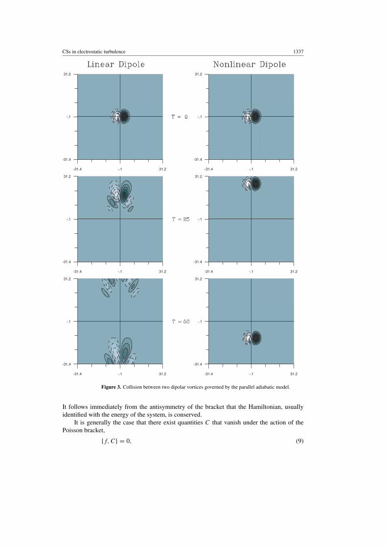
The parallel adiabatic model avoids unphysical fluctuations in the averaged density,fluctuations that are implied by the fully adiabatic model [32]. The two models are illustratedin figures 2 and 3 showing a collision between two dipolar vortices governed by the Hasegawa–Mima equation [33] (fully adiabatic model, figure 2) and a modified version of the Hasegawa–Mima equation using the parallel adiabatic response (figure 3). These figures show that theparallel adiabatic model leads to the generation of zonal flows during the collision. Ouranalysis leads to the conclusion, however, that for finite ITG this model cannot be expressedas a Hamiltonian system (as described in section 2.2) except for vanishing specific heat index,� = 0. The fully adiabatic response model thus has the advantage of being able to addressquestions concerning the effects of �. It is also of historical interest in view of its prevalencein early studies of electrostatic turbulence and its isomorphism with the equivalent barotropicvorticity equation describing Rossby waves [33, 34]. Note that the linear properties of bothmodels are identical. The stability of ITG and Kelvin–Helmholtz eigenmodes in equilibriawith sheared flows is described in [35], and the convective amplification of wavepackets isdescribed in [36].

2.2. The Hamiltonian formalism

The Hamiltonian formulation of fluid models is reviewed in [1]. Here we give only a briefdescription of a method for constructing Hamiltonian formulations.

The primary goal is to find a Hamiltonian H and a Poisson bracket {·, ·} such that theequations of motion can be written in the form

ξ j = {ξ j , H }, (8)

where the dot represents differentiation with respect to time and ξ j represents the suitablychosen dynamical variables indexed by j . The Poisson bracket must be bilinear, antisymmetricand must satisfy the Jacobi identity,

{a, {b, c}} + circular permutations = 0.

1336F

LW

aelbroecketal

31.2

-.1

-31.4

31.2

-.1

-31.4

-31.4 -.1 31.2

Figure 2. Collision between two dipolar vortices governed by the fully adiabatic model.


31.2

-.1

-31.4

-31.4 -.1 31.2

31.2

-.1

-31.4

-31.4 -.1 31.2

31.2

-.1

-31.4

-31.4 -.1 31.2

31.2

-.1

-31.4

-31.4 -.1 31.2

31.2

-.1

-31.4

-31.4 -.1 31.2

31.2

-.1

-31.4

-31.4 -.1 31.2

Figure 3. Collision between two dipolar vortices governed by the parallel adiabatic model.

It follows immediately from the antisymmetry of the bracket that the Hamiltonian, usuallyidentified with the energy of the system, is conserved.

It is generally the case that there exist quantities C that vanish under the action of thePoisson bracket,

{f, C} = 0, (9)


for any choice of f . Such quantities are clearly also conserved. They are called Casimirinvariants, or simply Casimirs. Two well-known examples of Casimirs are the circulationfor an inviscid fluid and the magnetic helicity in magnetohydrodynamics. A complete set ofCasimirs for any given model can be constructed systematically by solving (9).

The Poisson bracket often takes the form of a Lie–Poisson bracket, which in two-dimensional systems can be expressed as

{F, G} = 〈Wij

k ξ k[Fξi , Gξj ]〉, (10)

where the Wij

k are constant coefficients, summation over repeated indices is understood,

〈f 〉 =∫ Lx

0dx

∮dy

∮dz f (x, y, z) (11)

is the volume integral, and

[f, g] = ∂f

∂x

∂g

∂y− ∂g

∂x

∂f

∂y(12)

is called the inner Poisson bracket. Note that the inner bracket acts on fields (functions ofspace and time), whereas the ‘outer’ bracket {·, ·} acts on functionals (functions of fields). Thearguments of the inner bracket are the functional derivatives of F and G defined by

〈ηFξi 〉 := d

dδF [. . . , ξ i + δη, . . .]

∣∣∣∣δ=0

, (13)

where η is an arbitrary function of the spatial coordinates and δ is a real coefficient. Sincethe inner bracket is antisymmetric, W must be symmetric in its upper indices to ensureantisymmetry of the Lie–Poisson bracket. Thiffeault and Morrison [37] have shown thatthe Lie–Poisson bracket defined by (10) satisfies the Jacobi identity when the product

Wij

k W lmi (14)

is symmetric in all three free upper indices. Equivalently, the Lie–Poisson bracket (10) satisfiesthe Jacobi identity when all the matrices W(i) with elements (W i)

j

k commute.Substitution of (10) into the equation of motion and integration by parts results in

ξi = −Wij

k [ξk, Hξj ]. (15)

This suggests a pedestrian, but effective, procedure for finding the Poisson bracket of aHamiltonian model. First, write the two-dimensional version of the equations of motion in aform resembling (15). Identify the coefficients W

ij

k , and verify the Jacobi identity. Second,extend the Poisson bracket to allow for three-dimensional perturbations [38]. We will carryout this procedure in the following sections.

3. Fully adiabatic model

3.1. Conserved energy

We may construct a conserved energy as follows. We begin by multiplying the equations ofmotion by p+φ, p/� and v, respectively, summing the resulting equations, and integrating overall space. Assuming periodic boundary conditions in y and z, there follows after integratingby parts [29]

1

2

d

dt

⟨φ2 + [∇⊥(φ + p)]2 +

p2

�

⟩=

⟨Kp

�

∂φ

∂y

⟩. (16)


We have assumed in (16) that the surface term resulting from the integration by parts vanishes.This is true for either periodic (in x) or impermeable (φ(0) = φ(Lx) = 0) boundary conditions.The volume integral on the right-hand side of (16) represents the work done by the backgroundpressure gradient (K) when a pressure perturbation p is convected across the gradient by theelectric drift vEx = −∂yφ.

In order to eliminate the right-hand side of (16) we multiply the pressure equation by x

and integrate over the volume. We find

d

dt〈x(p − �φ)〉 = −

⟨p

∂φ

∂y

⟩+ Lx(vExp)x=Lx

. (17)

Here the boundary term vanishes for impermeable walls, vEx = 0, at the x = 0, Lx boundaries,but not for periodic boundary conditions. Clearly, if a fluid element is removed from one sideof the simulation volume and reintroduced on the other side where the background pressure ishigher, the energy in the system will change. Since our goal is to investigate the Hamiltonianform and CS of the system, we henceforth adopt impermeable boundary conditions for bothelectrons and ions: ∂yφ = ∂yp = 0. It follows then from (16) and (17) that

E = 1

2

⟨φ2 + [∇⊥(φ + p)]2 +

(p + Kx)2

�− 2Kxφ

⟩(18)

is conserved: E = dE/dt = 0.We may obtain a second conserved quantity by multiplying the vorticity equation by x

and again integrating over all space:

∂

∂t〈xφ〉 = ϒ, (19)

where ϒ is a boundary term that vanishes when ∂x(φ + p) is constant on the x = 0, x = Lx

walls, corresponding to a fixed velocity parallel to the walls. Assuming this boundary conditionto hold, it follows that

A = 2〈xφ〉 (20)

is a conserved quantity. Recalling that φ = n+ux, we see that A is related to the cross-gradientposition of the centre of mass.

3.2. Construction of the Poisson bracket

In order to take advantage of the properties of the Lie–Poisson bracket, described in section 2.2,we specialize at first to the two-dimensional case where ∂/∂z = 0, for which

∇‖v = [ψ, v].

We will see that the generalization to three dimensions is straightforward [38, 14].We begin by noting that the heat transport equation is a simple convection equation,

∂s

∂t= [s, φ], (21)

where

s := p − �φ + [K − (1 − u)�]x (22)

is the linearized change in the entropy per unit mass with respect to a homogeneous referencestate. We use equation (22) to eliminate p in terms of s in the ion continuity equation. We find

∂

∂t= [ , φ] − [∇⊥φ; ∇⊥s] + [ψ, v], (23)


where ψ is the magnetic flux defined above equation (4) and

= ∇2⊥[(1 + �)φ + s] − φ − (1 − u)x

is a generalized potential vorticity. We observe that except for the term

[∇⊥φ; ∇⊥s := [∂xφ, ∂xs] + [∂yφ, ∂ys], (24)

the right-hand side of equation (23) has the form of a sum of inner Poisson brackets actingon the fields ( , s, v). This form is consistent with the general form of the Lie–Poissonbracket (10).

The offending term may be eliminated with a similar term that arises when applying the∇2

⊥ operator to the pressure equation,

∂∇2⊥s

∂t= [∇2

⊥s, φ] + [s, ∇2⊥φ] + 2[∇⊥s; ∇⊥φ] = 0. (25)

There follows∂N

∂t= [N, φ] +

1

2[s, ∇2

⊥φ] + [v, ψ], (26)

where

N = φ − (1 + �)∇2⊥φ − 1

2∇2⊥s + (1 − u)x, (27)

is the density of guiding centres [32].We next turn to the velocity equation. Eliminating the pressure in favour of s leads to

∂v

∂t= [v, φ] − [ψ, (1 + �)φ + s]. (28)

The last term involves a bracket of ψ and φ, neither of which is an independent dynamicalvariable. To remedy this, we change variables to V = v − (1 + �)ψ . The equation for V ,

∂V

∂t= [V, φ] + [s, ψ], (29)

has the desired form.In order to complete the construction of the Lie–Poisson bracket for the dynamical

equations (21), (26) and (29) we rearrange the various terms appearing in these equationsso that each Poisson bracket acts on one of the fields (N, s, V ) and on a functional derivativeof the Hamiltonian, as in equation (15). We expect the Hamiltonian to be given by a linearcombination of the energy E and the conserved quantity A,

H = E + αA,

where α is a coefficient that we must determine. The functional derivatives of the Hamiltonian,denoted by Hξj , are

HN = (1 + �)φ + s + (α − K + �)x, (30)

Hs = N +1

2(1 + �)∇2

⊥φ +s

�, (31)

HV = V + (1 + �)ψ. (32)

We must now rearrange the terms to make each inner Poisson bracket operate on a functionalderivative of H and on one of the dynamical fields (N, s, V ). This task is facilitated by notingthat φ and ∇2

⊥φ can only enter through the functional derivatives HN and Hs , respectively.Eliminating φ from equation (21), we find that we must take α = K − � in order that

equation (21) takes the form

s = [s, HN ]

1 + �, (33)


consistent with equation (10). We next eliminate ∇2⊥φ in favour of Hs in equation (26). We find

N = [N, HN ] + [s, Hs] + [V, HV ]

1 + �. (34)

Lastly, we express equation (29) as

V = [V, HN ] + [s, HV ]

1 + �. (35)

We may now determine the coefficients Wij

k by comparison of equations (33)–(35) withthe general form of the Lie–Poisson bracket given in equation (10). The corresponding Poissonbracket is

{F, G}2 = (1 + �)−1〈N [FN, GN ] + V ([FN, GV ] + [FV , GN ])

+s([FN, Gs] + [Fs, GN ] + [FV , GV ])〉, (36)

where the subscript 2 is included to remind us that this is a two-dimensional bracket since wehave omitted the longitudinal derivatives ∂/∂z in the parallel gradient.

To verify that the above bracket satisfies the Jacobi identity we must show that the threematrices (W i)

j

k , i = 1, 2, 3 commute. Aside from the common (1 + �)−1 factor, thesematrices are

1 0 00 1 00 0 1

,

0 0 0

1 0 00 0 0

,

0 0 0

0 0 11 0 0

. (37)

One easily verifies that they commute.To complete the construction of the Poisson bracket we now extend the bracket to three-

dimensional perturbations. The only change this requires is the replacement of [ψ, ·] by thefull parallel gradient ∇‖ in equations (26) and (28). It is easy to show that this is realized byadding to the two-dimensional bracket the term

{F, G}z =⟨FN

∂GV

∂z− ∂FV

∂zGN

⟩. (38)

The complete three-dimensional bracket is thus

{F, G} = {F, G}2 + {F, G}z, (39)

where the component brackets are given in equations (36) and (38). It is not difficult to verifythat the Jacobi identity survives the addition of the longitudinal terms [38].

3.3. Casimir invariants

Recall that a Casimir invariant is a functional C[N, s, V ] that vanishes when inserted in thePoisson bracket,

{F, C} = 0

for arbitrary F . Using integration by parts and assuming that all the boundary terms vanishwe may write this condition

〈Fξi [Wij

k ξ k, Cξj ]〉 = 0.In order that this is satisfied for any F the coefficients of each of the functional derivatives Fξi

must vanish:

[N, CN ] + [s, Cs] + [V, CV ] = 0, (40)

[s, CN ] = 0, (41)

[V, CN ] + [s, CV ] = 0. (42)


The second of these equations implies that CN = f (s), where f is an arbitrary functionof s. Functional integration yields

C(N, s, V ) = 〈Nf (s) + g(s, V )〉.Substituting this in equation (42), we find

[s, gV − Vf ′(s)] = 0,

or, equivalently,

gV = Vf ′(s) + q(s).

The remaining equation, equation (40), is automatically satisfied. The complete solution is

C(N, s, V ) =⟨c(s) + V q(s) +

V 2

2f ′(s) + Nf (s)

⟩. (43)

We may interpret the above result by choosing alternately each one of the free functionsf , c, q to be a delta function. We obtain, in this way, three families of detailed conservationlaws. For c = δ(s − s), we find that

C(c)(s) :=∮

d�

|∇s| (44)

is conserved, where d� is the element of length along the curve formed by the intersection ofthe surface s = s and the plane z = 0. This shows that the volume inside any tube of constants is conserved, as expected for a field convected by the incompressible electric drift. Takingnext q(s) = δ(s − s), we find that

C(q)(s) :=∮

d�

|∇s|V (45)

is conserved, corresponding to the conservation of parallel ion momentum in each s-tube.Lastly for f = δ(s − s) we find the third family of conserved quantities,

C(f )(s) :=∮

d�

|∇s|N − d

ds

∮d�

|∇s|V2. (46)

This last Casimir generalizes the conservation of potential vorticity given by Ertel’s theorem.It is interesting to compare the Casimirs found above for the KHH model to those given

by Krommes and Kolesnikov (K2) [5] for the gyrofluid model [32]. The gyrofluid model hasthe bracket [5]

{F, G} = 〈N [FN, GN ] + T ([FN, GT ] + [FT , GN ]) + (N + T )[FT , GT ]〉. (47)

It has been pointed out by K2 that symmetry of the (W i)j

k matrices implies that the quantityξ iξ i is a Casimir invariant, which they interpret as the enstrophy:

Z :=⟨N2 + T 2

2

⟩. (48)

For the KHH model, in contrast, the (W i)j

k matrices are asymmetric so that there is no conservedenstrophy. We next show that the enstrophy of K2 is a particular member of a more generalfamily of Casimirs for the gyrofluid equations.

The bracket (47) can be transformed into one where the two fields N and T are decoupled,called a direct product form. This is achieved by a linear change of the dependent variables (ageneral theory of such coordinate changes is presented in [37]). The required transformation is

N = N + γ T , T = N − γ −1T , (49)


where γ := (1 +√

5)/2 is the golden mean. This expression is derived by calculating thecoefficients of a general linear transformation to make the resulting bracket fit the direct productform. Letting F(N, T ) = F (N, T ), there follows the chain rule expressions

FN = FN + FT , FT = γ FN − γ −1FT . (50)

Using these in (47) and inserting the inverse of (49) to replace N and T by the linear expressionsinvolving N and T gives

{F , G} = 〈c1N [FN , GN ] + c2T [FT , GT ]〉, (51)

where c1 = 1 + γ 2 and c2 = 1 + γ −2 are constants that can be scaled out. The bracket (51)has the Casimirs

Ca = 〈a(N)〉, Cb = 〈b(T )〉, (52)

where a and b are arbitrary functions. Thus, in terms of the original variables, the Casimirs are

Ca = 〈a(N + γ T )〉, Cb = 〈b(N − γ −1T )〉. (53)

The Casimir of (48) is clearly a special case, composed of a sum of C(a) and C(b), where thefunctions a and b are quadratic.

3.4. Coherent structures

The calculation and characterization of propagating CS is an important application of theHamiltonian formalism. Such CS may arise as a result of the saturation of a primaryinstability [39], they may be driven by small scale fluctuations [22,40], or they may be formedthrough inverse cascade in two-dimensional turbulence [40]. The standard approach is tolook for solutions of the equations of motion of the form ξ j = ξ j (x, y − ut) where u is thepropagation velocity of the CS. Equivalently, we may transform to a frame moving with theperturbation and look for equilibria by setting the partial time derivatives to zero in the movingframe. For realistic multi-field models, however, the resulting equations can be formidable,especially in the presence of FLR effects.

In Hamiltonian systems, the task of solving the equilibrium equations can be greatlyfacilitated by utilizing the Casimirs. To see this, we use the definition of the Casimir functional,equation (9), to write the equations of motion (8) as

ξ j = {ξ j , F }, (54)

where F = H − C and C is the complete Casimir given in equation (43). It follows that theextrema of the functional F are solutions of the equilibrium equations, {ξ j , F } = 0 (see [1,2]).That is, the set of solutions of δF = 0 or

Fξi = 0, i = 1, 2, 3 (55)

automatically satisfies

ξ j = {ξ j , H } = 0, j = 1, 2, 3. (56)

Comparison of equations (55) and (56) reveals one of the key advantages of the Hamiltonianapproach to equilibrium calculations: since the Poisson bracket is a derivation operator, thevariational principle (55) amounts to a first integral of the equilibrium equations representedby (56). We emphasize that different choices for the Casimir yield different equilibria. Wewill see that there is a correspondence between the choice of Casimir and the choice of profilefunctions for the equilibrium.

We note that the variational functional F can also be used to investigate the stabilityproperties of a given equilibrium [1, 2]. This is based on the observation that since F is


conserved, convexity of F implies that displacements from the equilibrium are bounded [1,2].Examination of F can thus yield sufficient conditions for stability. It is generally the case,however, that the construction of the Casimir functional is restricted in part to two-dimensionalsystems (in magnetized fluids, for example, the construction of the Casimir describing magneticflux conservation depends on the existence of good flux surfaces). Since the most unstableperturbations break the symmetry of the equilibrium, stability investigations using F are oflimited value in three-dimensional systems. An alternative approach that sometimes allows thislimitation to be side-stepped is to restrict the stability analysis to perturbations that preserve theCasimirs, the so-called dynamically accessible perturbations [1]. This approach is related tothe well-known energy principle of magnetohydrodynamics. We will not investigate stabilityhere, and will instead refer the interested reader to [3,41] which discuss the stability of isolatedmodel CSs, and to [42] which shows how instability of a periodic array of convection cells canlead to the generation of zonal flows.

Applying the variational principle given by equation (55) to the problem of finding CSleads to the following three equilibrium equations

FN = (1 + �)φ + s − f (s) = 0, (57)

Fs = (1 − f ′(s))N + 12 (1 + �)∇2

⊥φ − c′(s) − q ′(s)V − 12V 2f ′′(s) = 0, (58)

FV = V + (1 + �)ψ − q(s) − f ′(s)V = 0, (59)

where c(s) = c(s) − s/�. We see that the equilibria are specified by the choice of the threefunctions f (s), c(s) and q(s). This corresponds to the freedom to determine the density,pressure and vorticity profiles of the equilibrium state.

The choice of the three profile functions depends on the problem at hand. In the limitwhere the time scales are long compared to the characteristic time of diffusive relaxation forthe structure of interest, the unknown functions and the profiles they specify are determined bysolving the transport equations. These transport equations can be obtained by expressing thesolubility conditions for the equilibrium equations in the presence of the dissipation terms [43].In the opposite limit of very rapid evolution, in contrast, the unknown functions may be obtainedfrom the condition that the Casimirs must be conserved [44]. A third class of solutionscorresponds to soliton-like structures, called modons [6, 7, 9]. The modon solutions werediscovered by Larichev and Reznik in the context of geophysical fluid dynamics and weresubsequently introduced to plasma physics by Meiss and Horton [9]. They are obtained byseeking CS that correspond to disturbances that are localized in space and are such that therelationship between the vorticity and stream functions inside the convection cells is linear.We will describe these solutions in greater detail after completing the analysis of the generalproblem.

In the general case, we may reduce the equilibrium equations to a single equation for s

by using equations (57) and (59) to eliminate the fields φ and V from equation (58). Therefollows

f ′(f ′ + 1)∇2⊥s +

[(f ′ +

1

2

)(∇⊥s)2 − 1

2

(q + (1 + �)ψ

f ′ + 1

)2]

f ′′

−(f ′ + 1)x − (f ′ + 1)(f + s)

1 + �+ c′ −

(q + (1 + �)ψ

f ′ + 1

)q ′ = 0.

This equation may be simplified by changing variables so as to eliminate the squared gradientterm. To this end we note that

∇2⊥χ(s) = χ ′(s)∇2

⊥s + χ ′′(s)(∇⊥s)2.


We may thus eliminate the square gradient term by replacing s by the field χ determined by

χ ′′

χ ′ = (f ′ + 1/2)f ′′

f ′(f ′ + 1).

Integration yields

χ =∫

ds√

f ′(f ′ + 1), (60)

where the argument of the square root represents the damping decrement for electron driftwaves. The square root is thus well defined whenever the propagation speed of the CS liesoutside the band of frequency where drift waves propagate. If the equation (60) can be solvedfor the field s, this field can be completely eliminated in favour of χ . The resulting equation is

∇2⊥χ = Q(χ, x), (61)

where

Q(χ, x) = −[

1

2

(q + (1 + �)ψ

f ′ + 1

)2

f ′′ + (f ′ + 1)x +(f ′ + 1)(f + s)

1 + �

−c′ +

(q + (1 + �)ψ

f ′ + 1

)q ′

][f ′(f ′ + 1)]−1/2.

In the absence of simplifying assumptions concerning the profiles, analytical solutions of theabove equation can only be obtained in two limits. For structures much smaller than an iongyroradius (∇⊥ � 1), the left-hand side of (61) dominates to lowest order and this results ina linear dependence of χ on x. In this limit the solution reduces to that predicted by lineartheory. In the opposite limit where the CS are much larger than the ion gyroradius (∇⊥ 1),the right-hand side of (61) dominates and all the fields are functions of x to leading order. Thisleads to the long wavelength class of solutions that are identified with zonal flows.

3.5. Modon solutions

Modons constitute a particular family of solutions of equations (57)–(59) corresponding tolocalized disturbances. The assumption of localization allows the profile functions f , c and q

to be almost completely determined. The following description of the modon solutions followsclosely that of Meiss and Horton [9].

In the unperturbed reference state, the fields take the form N = x, φ = ux, s = (K −�)x

and V = νx − (1 + �)ψ(x). Imposing the condition that the modon fields asymptote to theirunperturbed values for x, y → ∞ yields

f (s) =(

1 +1 + �

K − �u

)s, (62)

q(s) = 1 − f ′

K − �νs + (1 + �)�(s)f ′, (63)

c(s) = 1 − f ′

K − �s −

(νs

K − �− (1 + �)�(s)

)q ′(s), (64)

where

�(s) = ψ

(s

K − �

).

Eliminating φ and V yields an equation for s

∇2⊥s − Q(s, x) = 0, (65)


where

Q(s, x) = 1 − u

K − � + (1 − �)u+

(ν(K − �)

[K − � + (1 + �)u]u+

(K − �)2� ′2

u2

)[�(s) − ψ(x)].

(66)

where Q(s, x) is a wave potential. In systems with magnetic shear the wave potential isreversed and induces shear damping. The shear damping results in the decay of the modon.For modons of radius a ω∗/k′

‖cs = ρsLs/Ln, the damping is asymptotically weak and hasbeen calculated perturbatively by Meiss and Horton [9] for cold ions and by Hong et al [14] forITG modes. Here we neglect the effect of the magnetic shear and consider instead the effectof the shear in the parallel velocity (parametrized by ν).

For a constant magnetic field ψ(x) = ψ ′x and ψ ′ is constant. It follows that Q is linearwith respect to s where

Q(s, x) = β2s

and

β2 = 1 − u + νψ ′/uK − � + (1 − �)u

+ψ ′2

u2. (67)

In this case the general solution of (65) is a sum of modified Bessel functions. We selectthe lowest order mode,

s = AK1(βr) cos θ, (68)

where r2 = x2 + y2, cos θ = x/r and β = √−Q. Note that β must be real in order that themodons be localized. We thus recover the familiar result that modons can only propagate atphase velocities such that the linear waves are spatially evanescent.

We next note that some of the surfaces of constant s in the solution of equation (68) do notextend to infinity. In the corresponding region the profile functions need not satisfy (62)–(64)and may in fact be chosen freely, subject to continuity requirements. Taking these profilefunctions to be linear, but with a different slope compared to that in the exterior region,

Qint = −(

1 +γ 2

β2

),

and, demanding continuity of s and ∇s, we obtain the following generalization of the classicmodon solution

s =

AK1(βr) r > a,

CJ1(kr) cos(θ) + ac

(1 +

β2

γ 2

)x r < a,

(69)

where the coefficients are determined by

A = ac

K1(β), C = −

(β

γ

)2ac

J1(γ ).

The constant γ is determined by

K2(β)

βK1(β)= − J2(γ )

γ J1(γ ). (70)

These results differ from those found in cold ion models in the dependence of β on the plasmaparameters and the propagation speed given in equation (67).


4. Parallel adiabatic model

We now consider the Hamiltonian formulation of the KHH model using the parallel adiabaticresponse described by equation (6). The pressure equation for this model takes the form of aconvection equation identical to equation (21), but with s now given by

s = p − �φ + (K − �)x (71)

eliminating p from the quasi-neutrality equation yields

∂

∂t= [ , φ] − [∇⊥φ; ∇⊥(s + �φ)] + [ψ, v], (72)

where

= ∇2⊥((φ + �φ + s) − φ) − x.

The new term �[∇⊥φ; ∇⊥φ] does not suggest the Lie–Poisson form of section 2.2. It iseasy to see that there is no combination of operations acting on the dynamical equations thatwill provide the necessary term without introducing many more inappropriate terms than iteliminates. This suggests that the combination of the KHH model with the parallel adiabaticresponse model is non-Hamiltonian. In order to obtain a Hamiltonian model, we henceforthset � = 0, so that s = p + Kx is the ion pressure fluctuation.

4.1. Hamiltonian formulation for � = 0

For the purpose of modelling transport barriers, it is of interest to generalize the KHH modelby allowing the background density to have an arbitrary profile [40],

n(x, t) = n(x) + φ(x, t).

The equations of motion are then

dφ

dt− ∇⊥ · d

dt∇⊥(φ + s) + [φ, n] + ∇‖v = 0, (73)

ds

dt= 0, (74)

dv

dt+ ∇‖(φ + s) = 0, (75)

where s differs from p by including the spatial variation of the background pressure.We next demonstrate the conservation of energy by multiplying the above equations by

φ + s, φ + n and v, respectively, integrating over space, and summing. There follows

dH

dt= 0,

where

H = 12 〈φ2 + (∇φ + ∇s)2 + 2φs + 2sn + v2〉. (76)

We may eliminate the undesirable [∇φ; ∇s] term from equation (73) by adding half ofthe Laplacian of equation (74) to equation (73) as before. There follows

∂N

∂t= [N, φ] +

1

2[s, ∇2

⊥φ] + [v, ψ], (77)

where

N = n + φ − ∇2⊥φ − 1

2∇2⊥s. (78)


The functional derivatives of H with respect to the new variables are

HN = φ + s, (79)

Hs = N + 12∇2

⊥φ, (80)

HV = V + (1 + �)ψ. (81)

Expressing the arguments in equations (74), (75) and (77) in terms of the above functionalderivatives of H , we find that these equations are Hamiltonian and have the same Lie–Poissonbracket as that given in (36). It follows that the Casimirs will have the same dependenceon the fields N , s and V as those found in section 3.3, although the field N has a differentinterpretation, and in particular a different dependence on φ, in each of the two models.

The Casimirs for the parallel adiabatic response model can be used to simplify theequilibrium equations as demonstrated in the previous section for the model with the fulladiabatic response. The dependence of N on nonlocal information entering through φ = φ−φ,however, causes the conventional methods for solving the equilibrium equations to fail.

4.2. Nonexistence of equilibria for � = 0

In view of the considerable simplification of the equilibrium problem that the Hamiltonianformulation purchases, it is natural to inquire as to the existence and nature of CS in non-Hamiltonian systems. We may investigate this issue by using our result that for the modelwith a parallel adiabatic response, it is necessary to have � = 0 in order that the dynamics beHamiltonian. Assuming the existence of a nontrivial CS solution for � = 0, we attempt tosolve the equilibrium equations perturbatively for � small and positive.

For simplicity we take v = 0 and consider the solutions of the equations obtained bysetting the time derivatives to zero in the equations of motion, equations (21) and (26):

[φ, s] = 0, (82)

[φ, N ] − 12 [s, ∇2φ] − �[∇φ, ∇φ] = 0. (83)

The first of these, equation (82), is easily integrated:

s = f (φ),

where f is an arbitrary function. For equation (83), we look for a solution of the form

φ = φ0 + �φ1, s = s0 + �s1, (84)

where (φ0, s0) is the solution for � = 0 and (φ1, s1) indicate small corrections of order �.Considering first the lowest order terms in equation (83), we find that the reference solution

satisfies

N0 = h(φ0) + 12f ′(φ0)∇2φ0, (85)

where h is an arbitrary function. The first-order equation is

[φ0, N1] + [φ1, N0] − 12 [s0, ∇2φ1] − 1

2 [s1, ∇2φ0] = [∇φ0; ∇φ0].

We note that the operator [φ, ·] = vE · ∇ has the interpretation of the derivative along thestreamlines. Using the lowest order solution, we may regroup all the terms that are expressibleas a derivation along the streamlines,

vE · ∇(

N1 − [f ′(φ0) + 2h′(φ0) + f ′′(φ0)∇2φ0]φ1

2

)= ∂2φ0

∂x2

∂2φ0

∂x∂y.


In order that this equation have a solution it is necessary that the integral of the right-handside along any closed streamline vanish. It is easily seen that this is generally not the case fortwo-dimensional CS. In particular, near an extremum of the potential (corresponding to thecentre of a convection cell) we find

∮d�

|∇φ|∂2x φ0∂xyφ0 =

2π∂2

x φ0∂xyφ0√∂2x φ0∂2

y φ0 − (∂xyφ0)2

x=xmax

.

This vanishes only if the major axes of the streamlines are aligned with the coordinate axes.We conclude that two-dimensional CS generally do not exist for � = 0. We observe that itis the same term, �[∇φ; ∇φ], that is responsible both for the non-Hamiltonian nature of theparallel adiabatic model with � = 0 and for the non-integrability of the equilibrium equations.This suggests that the Hamiltonian property is a necessary condition for the integrability ofthe equilibrium equations. If so, this would imply that non-Hamiltonian models will lead toqualitatively different predictions when used to describe properties that result from CS, suchas intermittency.

5. Discussion

We have constructed a Poisson bracket that provides a Hamiltonian formulation for two modelsof ITG dynamics, the first, with finite adiabatic compression index � and a fully adiabaticelectron response, and the second, with � = 0 and a electron response obeying Boltzmann’slaw only along the field lines. The Hamiltonian formulation shows that both these modelspossess three families of detailed conservation laws in addition to globally conserved quantitiessuch as the energy and centre of mass. They do not, however, conserve enstrophy.

Recalling that the behaviour of soliton solutions of the KdV equation are a consequenceof its complete integrability, we conjecture that the Casimirs play a similar role for CSinteractions in ITG turbulence. Specifically, the infinite set of constraints imposed by Casimirsare responsible for the approximate preservation of modon identity during interactions. Wenote, however, that Casimir conservation is fragile, since Casimirs are subject to mixingsimilar to that which affects the distribution function during Landau damping (note that theconservation of the distribution function in Vlasov dynamics is itself linked to the existenceof a Casimir). Mixing can occur, in particular, as the result of Kelvin–Helmholtz instabilityduring the interaction between two otherwise stable dipole vortices.

We have provided arguments that for non-vanishing specific heat, � = 0, the modelwith an adiabatic electron response along the field lines is non-Hamiltonian. This has twoconsequences with clear physical import. First, the set of conserved quantities is limited tothe energy and the internal energy ptot/n�

tot (here we use the subscript ‘tot’ to denote the sumof the background and perturbed quantities). The laws of detailed conservation of potentialvorticity and parallel momentum no longer apply. Second, there are no coherent convectioncells solutions. One thus expects markedly different behaviour from the non-Hamiltonianmodel. In view of the importance to turbulent dynamics of CS in general and of zonal flowsin particular, we conclude that the Hamiltonian nature of the underlying equations will play adetermining role in turbulent transport.

Acknowledgments

We are grateful to J H Kim for performing the simulations shown in the figures. One of us(FLW) would like to thank Professor S Hamaguchi for helpful conversations, and the Japanese


Society for the Promotion of Science for supporting a visit to Kyoto University where thiswork was started. Another of us (PJM) would like to thank J Krommes for providing us withan early version of the manuscript for [5] and for discussion thereof. This work was supportedby the US DoE under contract No DE-FG03-96ER-54346.

References

[1] Morrison P J 1998 Rev. Mod. Phys. 70 467[2] Holm D D, Marsden J E, Ratiu T and Weinstein A 1985 Phys. Rep. 123 1[3] Nycander J 1992 Phys. Fluids A 4 467[4] Hazeltine R D, Hsu C T and Morrison P J 1987 Phys. Fluids 30 3204[5] Krommes J A and Kolesnikov R A 2004 Phys. Plasmas 11 L29[6] Larichev V D and Reznik G M 1976 Dokl. Akad. Nauk SSSR 231 1077[7] Flierl G R, Larichev V D, McWilliams J C and Reznik G M 1980 Dyn. Atmos. Oceans 5 1[8] Horton W 1990 Phys. Rep. 192 1[9] Meiss J and Horton W 1983 Phys. Plasmas 26 990

[10] Horton W, Liu J, Meiss J D and Sedlak J E 1986 Phys. Fluids 29 1004[11] Shukla P K and Weiland J 1989 Phys. Lett. A 136 59[12] Spatschek K H, Laedke E W, Marquardt C, Musher S and Wenk W 1990 Phys. Rev. Lett. 64 3027[13] Su X N, Horton W and Morrison P J 1991 Phys. Fluids B 3 921[14] Hong B G, Romanelli F and Ottaviani M 1991 Phys. Fluids B 3 615[15] Katou K 1998 Phys. Plasmas 5 381[16] Makino M, Kamimura T and Taniuti T 1981 J. Phys. Soc. Japan 50 980[17] Makino M, Kamimura T and Sato T 1981 J. Phys. Soc. Japan 50 954[18] McWilliams J C and Zabusky N J 1982 Geophys. Astrophys. Dyn. 19 207[19] Horton W 1989 Phys. Fluids B 1 524[20] Crotinger J and Dupree T 1992 Phys. Fluids B 4 2854[21] Fontan C F and Verga A 1995 Phys. Rev. E 52 6717[22] Muhm A, Pukhov A M, Spatschek K H and Tsytovich V 1992 Phys. Fluids B 4 336[23] Kim E J and Diamond P H 2002 Phys. Rev. Lett. 88 225002[24] Benkadda S, de Wit T D, Verga A, Sen A, ASDEX team and Garbet X 1994 Phys. Rev. Lett. 73 3403[25] Wang G, Wang L, Yang X, Feng C, Jiang D and Qi X 1999 Nucl. Fusion 39 263[26] Krasheninnikov S I 2001 Phys. Lett. A 283 368[27] Antar G Y, Devynck P and Fenzi C 2002 Phys. Plasmas 9 1255[28] Politzer P A 2000 Phys. Rev. Lett. 84 1192[29] Kim C B, Horton W and Hamaguchi S 1989 Phys. Fluids B 5 1516[30] Zeiler A, Drake J F and Rogers B 1997 Phys. Plasmas 4 2134[31] Xu X Q, Cohen R H, Rognlien T D and Myra J R 2000 Phys. Plasmas 7 1951[32] Dorland W and Hammett G W 1993 Phys. Fluids 5 812[33] Hasegawa A, MacIennan C and Kodama Y 1979 Phys. Fluids 22 2122[34] Horton W and Hasegawa A 1994 Chaos 4 227[35] Waelbroeck F L, Antonsen T M Jr, Guzdar P N and Hassam A B 1992 Phys. Fluids B 4 2441[36] Waelbroeck F L, Dong J Q, Horton W and Yushmanov P N 1994 Phys. Plasmas 1 3742[37] Thiffeault J L and Morrison P J 2000 Physica D 136 205[38] Morrison P J and Hazeltine R D 1984 Phys. Fluids 27 886[39] Cowley S C, Kulsrud R and Sudan R 1991 Phys. Fluids B 3 1803[40] Botha G J J, Haines M G and Hastie R J 1999 Phys. Plasmas 6 3838[41] Åkerstedt H O, Nycander J and Pavlenko V P 1996 Phys. Plasmas 3 160[42] Drake J F, Finn J M, Guzdar P N, Shapiro V, Shevchenko V, Waelbroeck F L, Hassam A B, Liu C S and Sagdeev R

1992 Phys. Fluids Lett. B 4 488[43] Connor J W, Waelbroeck F L and Wilson H R 2001 Phys. Plasmas 8 2835[44] Waelbroeck F L 1989 Phys. Fluids B 1 2372

Hamiltonian formulation and coherent structures in electrostatic turbulence

Documents

Transcript of Hamiltonian formulation and coherent structures in electrostatic turbulence