arX

iv:1

102.

3474

v2 [

gr-q

c] 1

2 M

ar 2

011

A Hamiltonian Formulation of the BKL Conjecture

Abhay Ashtekar1,∗ Adam Henderson1,† and David Sloan1,2‡

1 Institute for Gravitation and the Cosmos, Physics Department,

Penn State, University Park, PA 16802, U.S.A.2 Institute for Theoretical Physics, Utrecht University, The Netherlands.

The Belinskii, Khalatnikov and Lifshitz conjecture [1] posits that on approach to

a space-like singularity in general relativity the dynamics are well approximated by

‘ignoring spatial derivatives in favor of time derivatives.’ In [2] we examined this

idea from within a Hamiltonian framework and provided a new formulation of the

conjecture in terms of variables well suited to loop quantum gravity. We now present

the details of the analytical part of that investigation. While our motivation came

from quantum considerations, thanks to some of its new features, our formulation

should be useful also for future analytical and numerical investigations within general

relativity.

PACS numbers: 04.20.Dw,04.60.Kz,04.60.Pp,98.80.Qc,04.20.Fy

I. INTRODUCTION

Originally formulated in 1970, the Belinskii-Khalatnikov-Lifshitz (BKL) conjecture statesthat as one approaches a space-like singularity, ‘terms containing time derivatives in Ein-stein’s equations dominate over those containing spatial derivatives’ [1]. This implies thatEinstein’s partial differential equations are well approximated by ordinary differential equa-tions (ODEs), whence the dynamics of general relativity effectively become local and oscil-latory. The time evolution of fields at each spatial point is well approximated by that inhomogeneous cosmologies, classified by Bianchi [3]. The simplest of these are the BianchiI metrics which have no spatial curvature and the Bianchi II metrics which have ‘minimal’spatial curvature. According to the BKL conjecture, the dynamics of each spatial pointfollow the ‘Mixmaster’ behavior —a sequence of Bianchi I solutions bridged by Bianchi IItransitions. Finally, with the significant exception of a scalar field, matter contributionsbecome negligible —to quote Wheeler, “matter doesn’t matter”.

In the beginning, the conjecture seemed to be coordinate dependent and rather implau-sible. However, subsequent analysis by a large number of authors has shown that it can bemade precise and by now there is an impressive body of numerical and analytical evidencein its support [4]. It is fair to say that we are still quite far from a proof of the conjecture inthe full theory. But there has been outstanding progress in simpler models. In particular,Berger, Garfinkle, Moncrief, Isenberg, Weaver and others showed that, in a class of models,as the singularity is approached the solutions to the full Einstein field equations approachthe ‘Velocity Term Dominated’ (VTD) ones obtained by neglecting spatial derivatives [4–8].

∗Electronic address: ashtekar@gravity.psu.edu†Electronic address: adh195@psu.edu‡Electronic address: sloan@gravity.psu.edu

2

Andersson and Rendall [9] showed that for gravity coupled to a massless scalar field or astiff fluid, for every solution to the VTD equations there exists a solution to the full fieldequations that converges to the VTD solution as the singularity is approached, even in the

absence of symmetries. These results were generalized to also include p-form gauge fieldsin [10]. In these VTD models the dynamics are simpler, allowing a precise statement ofthe conjecture that could be proven. In the general case, the strongest evidence to datecomes from numerical evolutions. Berger and Moncrief began a program to analyze genericcosmological singularities [11]. While the initial work focused on symmetry reduced cases[12], more recently Garfinkle [13] has performed numerical evolution of space-times with nosymmetries in which, again, the Mixmaster behavior is apparent. Finally, additional supportfor the conjecture has come from a numerical study of the behavior of test fields near thesingularity of a Schwarzschild black hole [14].

With growing evidence for the BKL conjecture, it is natural to consider its implicationsto quantum gravity. The conjecture predicts a dramatic simplification of general relativitynear space-like singularities, which are precisely the places where quantum gravity effectsare expected to dominate. A promising approach to analyze this issue is provided by loopquantum cosmology (LQC) [15] where there are now several indications that the quantumgravity effects become important only when curvature or matter density are about a percentof the Planck scale. Therefore it is quite possible that, generically, spatial derivatives becomenegligible compared to the time derivatives already when the universe is sufficiently classical.In this case a quantization of the effective theory with ODEs, that descends from techniquesapplicable in the full theory, could provide a reliable qualitative picture of quantum gravityeffects near generic space-like singularities. If, on the other hand, the BKL behavior sets inonly in the Planck regime, this strategy would not be viable. But since there is no reason totrust Einstein’s equations in this regime, then the conjecture would also not have a physicallyinteresting domain of validity.

LQC is the result of application of the principles of loop quantum gravity (LQG) [16–18]to symmetry reduced cosmological models. Initial study of the k=0 Friedmann LemaitreRobertson Walker (FLRW) models revealed that the quantum geometry effects underly-ing LQG provide a natural mechanism for the resolution of the big bang singularity [19].Subsequent more complete analysis led to a detailed understanding of the physics in thePlanck regime and also showed that although these effects are very strong there —capableof replacing the big bang with a quantum bounce— they die extremely rapidly so as to re-cover general relativity as soon as the curvature falls below Planck scale [20]. These resultswere then extended to include spatial curvature in [21] and a cosmological constant in [22].More recent investigations reveal that if matter satisfies a non-dissipative equation of stateP = P (ρ), LQC resolves all strong curvature singularities of the FLRW models, including,e.g., those of the ‘big-rip’ or ‘sudden death’ type [23]. Also, it is now known in LQC thatthe Bianchi I and II and IX singularities are resolved [24–26].

In view of the BKL conjecture, these results, together with further support from the‘hybrid’ quantization of Gowdy models [27], suggest that there may well be a general theoremto the effect that all space-like singularities of the classical theory are naturally resolved inLQG. However, it is difficult to test this idea using the current formulations of the BKLconjecture since these approaches are motivated by the theory of partial differential equationsrather than by Hamiltonian or quantum considerations (See e.g., [28, 29]. In particular, mostapproaches perform a rescaling of their dynamical variables by dividing by the trace of theextrinsic curvature. It is difficult to promote the resulting variables to operators on the LQC

3

Hilbert space. In the analysis presented here, we reformulate the BKL conjecture in a waybetter suited to LQC and explore the resulting system both analytically and numerically.

In LQG one begins with a first order formalism where the basic canonical variables are adensity-weighted triad and a spin-connection [16–18]. In section II we will begin by recallingthis Hamiltonian formulation of general relativity. In section III we rewrite this theory usinga set of variables that are motivated by the BKL conjecture. Rather surprisingly, the coreof this theory can be formulated using (density weighted) fields with only internal indices;space-time tensors never feature! To understand the implications of the BKL conjectureto LQG, we need to express the conjecture using this Hamiltonian framework. This taskis carried out in section IV. We provide a weak and a strong version of the conjecture.The key idea is to say that, as one approaches space-like singularities, the exact systemis well approximated by a truncated system which features only time derivatives. Non-triviality of the formulation lies in the choice of variables and specification of how limitsare taken. Our procedure satisfies a number of stringent requirements. In particular, onecan either first truncate the Hamiltonian and then obtain the equations of motion or firstobtain the full equations of motion and then truncate them; the two procedures commute.In section V we study the truncated Hamiltonian system and explore its dynamics in somedetail. We show that it exhibits all the known features such as the ‘u-map’ and spikes.Thus, the Hamiltonian framework we were led to by LQG considerations successfully captures

the Mixmaster dynamics faithfully. Therefore, in addition to providing a viable point ofdeparture to analyzing the fate of generic space-like singularities in LQG, it should also beuseful in analytical and numerical investigations of the BKL conjecture in classical generalrelativity itself. In section VI we summarize the main results and comment on their relationto those of other works.

The two appendices contain more technical material. Appendix A introduces densitiesin a coordinate-free manner. This notion is important because the basic variables in ourformulation of the BKL conjectures are scalar densities of weight 1. In the main text, forsimplicity we have set the shift and the Lagrange multiplier of the Gauss constraint equalto zero. Appendix B contains the full equations without these restrictions.

II. PRELIMINARIES

We will consider space-times of the form 4M = R× 3M where 3M is a compact, oriented3-dimensional manifold (without boundary).1 We will formulate general relativity in termsof first order variables, the point of departure of LQG [30]. These consist of pairs of fieldsconsisting of a (density weighted) orthonormal triad, Ea

i and its conjugate momentum Kia

which on solutions will correspond to extrinsic curvature. The fundamental poisson bracketis given by

{Eai (x), K

jb (y)} = δji δ

ab δ

3(x− y) (2.1)

Herein, early letters, a, b, c denote spatial indices while i, j, k denote internal indices whichtake values in so(3) —the Lie algebra of SO(3). Tildes are used to capture density weightsof quantities; a tilde above indicates that the quantity transforms as a (tensor) density of

1 The restriction on topology is made primarily to avoid having to specify boundary conditions and having

to keep track of surface terms. There is no conceptual obstruction to removing this restriction (following,

for example, the Hamiltonian framework underlying LQC).

4

weight 1 and a tilde below will denote a (tensor) density of weight −1. The internal indicescan be freely raised and lowered using a fixed kinematical metric qij on so(3). The phase

space spanned by smooth pairs (Eai , K

ia) will be denoted by P.

These phase space variables are related to their Arnowitt, Deser and Misner (ADM) [31]counterparts by

Eai E

bj q

ij = ˜q qab (2.2)

KiaE

bi =

√q K b

a (2.3)

where qab is the metric on the leaf 3M , q its determinant, and Kab the extrinsic curvature of3M . In terms of these variables we perform a 3+1 decomposition of space-time to obtain asHamiltonian a sum of constraints with Lagrange multipliers [30, 32]:

H [E,K] =

∫

3M

−1

2∼N˜S − 1

2NaVa + ΛiG

i . (2.4)

The Lagrange multipliers ∼N , Na, the lapse and shift, are related to the choice of slicing andtime in the standard fashion, and Λi is related to rotations in the internal space. Phase

space functions ˜S, Va, and Gk are the scalar, vector, and Gauss constraints (with densityweights 2, 1, 1 respectively), given by [30, 32]

˜S(E,K) ≡ −˜qR− 2Ea[iE

bj]K

iaK

jb (2.5)

Va(E,K) ≡ 4D[a(Kib] E

bi ) (2.6)

Gk(E,K) ≡ ǫ jki Ea

j Kia (2.7)

Where R is the scalar curvature of the metric qab. The overall sign and numerical factorsin the constraints are chosen so they reduce to the standard ADM constraints upon solvingthe Gauss constraint. R can be written in terms of the triad and its inverse or in terms ofthe triad and the connection Γi

a compatible with the triad, which is defined by

DaEbi + ǫijkΓ

jaE

bk = 0, or Γja = −1

2∼Ebk DaEbi ǫ

ijk . (2.8)

(Note that Da acts only on tensor indices; it treats the internal indices as scalars.) AlthoughΓia is determined entirely by Ea

i for now it is convenient to use all three fields Γia, K

ia and

Eai in our classical analysis: In our formulation of the BKL conjecture Γi

a and Kia will be

the relevant degrees of freedom near the singularity, so it is natural to express the theory interms of them.

The equations of motion are obtained by taking Poisson brackets with the Hamiltonianon the phase space P:

˙Eai = {Ea

i , H [E,K]} (2.9)

Kia = {Ki

a, H [E,K]} . (2.10)

P is the phase space underlying LQG. The basic variables (Aia, E

ai ) used there are obtained

5

by a simple canonical transformation on P [30]:

(Ea

i , Kia

)→

(Ai

a, γ−1Ei

a

)with Ai

a = Γia + γKi

a , (2.11)

γ being the Barbero-Immirzi parameter of LQC. (In classical general relativity, space-timeequations of motion are independent of the value of this real parameter.) For simplicityof presentation we will introduce our formulation of the BKL conjecture using (Ea

i , Kia)

although it will be clear that our framework can be readily recast in terms of (Eai , A

ia).

III. VARIABLES MOTIVATED BY THE BKL CONJECTURE

In order to formulate the BKL conjecture in this system, one needs to specify two things:What kind of derivatives are to dominate as one approaches the singularity and what kindare to become negligible? And, what are the quantities whose derivatives are to be treated asnegligible? In this section we first motivate and introduce a set of variables and a derivativeoperator and then use them to formulate the conjecture. The main idea is as follows. Theaccumulated evidence to date suggests that the spatial metric qab becomes degenerate atthe space-like singularity whence its determinant q vanishes there. (In particular, this isborne out in the numerical simulations of solutions with two commuting Killing fields —theso-called G2 space-times which include Gowdy models [33].) We will focus on the classof singularities where this occurs. In this case one would expect that if we rescaled fieldswhich are ordinarily divergent at the singularity with appropriate powers of q, the rescaledquantities would have well defined limits.

Now, the density weighted triad Eai is obtained by rescaling of the orthonormal triad eai ,

which is divergent at the singularity, by√q. In examples, the factor of

√q not only gives Ea

i

a well defined limit, but the limit in fact vanishes. Therefore, contraction by Eai can serve to

tame fields which would otherwise have been divergent at the singularity. This considerationleads us to construct scalar densities by contracting Ea

i with Kia, and Γi

a. As noted above,since contraction with Ea

i will suppresses the divergence of Kia and Γi

a, the combination isexpected to remain finite at the singularity. Let us then set

P ji := Ea

i Kja − Ea

kKkaδ

ji (3.1)

C ji := Ea

i Γja − Ea

kΓkaδ

ji . (3.2)

These two fields, Pij and Ci

j will turn out to be the relevant variables near the singularityin our BKL framework. In particular, we will show below that the constraints of generalrelativity can be expressed in terms of polynomials of these basic variables and their deriva-tives. Therefore if the basic variables and their derivatives remain finite at the singularity,the constraints will also continue to hold there. Since the Hamiltonian of the theory is alinear combination of these constraints, dynamics of the basic variables will meaningfullyextend to the singularity.

Beyond the possibility of being bounded at the singularity, an important feature of thesevariables is that they have only internal indices which can be freely raised and loweredusing the fixed, kinematic, internal metric qij ; the dynamical metric qab which diverges atsingularities is not needed. Under diffeomorphisms Pi

j and Cij transform as density weighted

scalars on 3M . Because of this feature, statements about their asymptotic properties canbe formulated much more easily than would be possible if they were tensor fields. (For a

6

coordinate free introduction to densities, see Appendix A).To illustrate why these variables are likely to be well defined at the singularity, let us

consider the Bianchi I model. Because of spatial flatness, we can work in an internal gaugein which Ci

j = 0 everywhere. What about Eai and Pi

j? In terms of the commonly usedproper time τ , the metric is given by ds2 = −dτ 2 +

∑i τ

2pidx2i and the singularity occurs at

τ = 0. Since∑

pi = 1, we have q = τ 2 in the Bianchi I chart. In addition, due to the secondconstraint on the exponents,

∑p2i = 1 whence the density weighted triad Ea

i vanishes atthe singularity as τ 1−pi and P j

i is finite there for each i.

We further introduce a derivative operator Di defined by the contraction of Da with Eai :

Di := Eai Da . (3.3)

The expectation is that this contraction will have the effect of suppressing terms containingDi as we approach the singularity. Thus, Di will be the spatial derivatives we were seekingwhich, when acting on certain quantities, will be conjectured to be negligible near thesingularity.2 The variable Pij is related to the momentum P ab(conjugate to the 3-metric)

in the ADM phase space by ˜q P ab = Eai E

bj P

ij. Cij encodes information in the Di spatial

derivatives of the triad Eai :

C ij = −∼Eia ǫ

klj DkEal . (3.4)

Note that, although the Cij depend on spatial derivatives of the triad and are often sub-

dominant to Pij , it turns out that they are not always negligible in the approach to thesingularity. Indeed, this behavior is observed in the truncated system, which is discussedin section IV. It is C ij rather than the triads themselves that will feature directly in ourformulation of the conjecture.

For simplicity of notation, from now on we will drop the tildes. Thus, from now on eachof Ea

i , Cij, Pi

j, Di carries a density weight 1, while the lapse field N carries a density weight−1. The scalar and the vector constraint functions S and Vi (introduce below) carry densityweight 2 while the Gauss constraint Gk carries density weight 1.

By making use of (3.1) and (3.4), functions of (Eai , K

ia) and their covariant derivatives

can be rewritten in terms of (Eai , Ci

j , Pij) and their Di derivatives. The scalar curvature R

for example can be expressed entirely in terms of Cij and its Di derivatives:

qR = −2ǫijkDi(Cjk)− 4C[ij]C[ij] − CijC

ji +1

2C2 (3.5)

Consequently, the constraints can be re-expressed entirely in terms of Cij, Pi

j and their Di

2 This operator is linear and satisfies the Leibnitz rule. It ignores internal indices (since the action of Da

is non-trivial only on tensor indices). However since its action on a function f does not yield the exterior

derivative df , Di is not a connection. If we were to formally treat as a connection, it would have torsion,

which is related to C: D[iDj]f = −T kijDkf where T k

ij = ǫkl[iCl

j] . In what follows, Di often acts on

scalar densities. This action is given explicitly in Appendix A.

7

derivatives (with no direct reference to Eai or even the determinant q of the 3-metric):

S = 2ǫijkDi(Cjk) + 4C[ij]C[ij] + CijC

ji − 1

2C2 + PijP

ji − 1

2P 2 (3.6)

Vi = −2DjPij − 2ǫjklPi

j Ckl − ǫijkCP jk + 2ǫijkPjlCl

k (3.7)

Gk = ǫijkPji . (3.8)

Here we have converted the co-vector index on the vector constraint Va to an internal indexby contracting it with Ea

i . Since the Eai is assumed to be non-degenerate away from the

singularity the constraint Vi defines the same constraint surface as the original vector con-straint introduced in (2.5). Notice here that the constraint can be easily decomposed intothose terms that contain the derivative Di and those that don’t.

The equations of motion for Eai , Ci

j , Pij can be written in a similar form. These can

be obtained using the full Poisson brackets (2.9),(2.10) or by directly computing Poissonbrackets of Pi

j and Cij with the scalar/Hamiltonian constraint. To streamline the second

calculation, let us specify the Poisson brackets between Eai , Ci

j, and Pij:

{Eai (x), Pj

k(y)} =(Ea

j (x)δik − Ea

i (x)δjk)δ(x, y) (3.9)

{Pij(x), Pk

l(y)} =(Pk

j(x)δil − Pi

l(x)δkj)δ(x, y) (3.10)

{∫fijP

ij,∫gklC

kl} =∫ (

fijgkl(Ckjδil + Cjlδik) + ǫjlmδikgklDmfij

)(3.11)

{Eai (x), C

jk(y)} = 0 and {Ci

j(x), Ckl(y)} = 0 , (3.12)

where fij, gij are smooth test scalar fields. The equations of motion obtained by takingPoisson brackets with the scalar constraint are then given by

C ij = − ǫjklDk(N(1

2δilP − P i

l )) +N [2C(ikP

|k|j) + 2C [kj]P ik − PC ij] (3.13)

P ij = ǫjklDk(N(1/2δilC − C il ))− ǫklmDm(NCkl)δ

ij + 2ǫjkmC [ik]Dm(N)

(DiDj −DkDkδij)N +N [−2C(ik)C j

k + CC ij − 2C [kl]C[kl]δij ] (3.14)

andEa

i = −NP ji Ea

j

where we have set the shift to zero to reduce clutter. (For non-zero shift, see AppendixB.) Note that the equation of motion for Ea

i is a simple ODE. Note also that, as was thecase with constraints, the equations of motion for Ci

j and Pij can again be written in terms

of scalar densities and the derivative Di only. This motivates us to ask for an evolutionequation for the derivative operator Di. Since Di ignores internal indices, it suffices toconsider its action just on scalar densities Sn of weight n. We have:

DiSn =n

2[Di(NP )]Sn − NPi

jDjSn . (3.15)

Thus we have cast all the constraint as well as evolution equations as a closed system

involving only Cij, Pi

j , and Di. These equations can then be used as follows. On aninitial slice, we construct (Ci

j , Pij, Di) from a pair (Ea

i , Kia) of canonical variables. Then we

can deal exclusively with the triplet (Cij , Pi

j, Di). The pair (Eai , K

ia) satisfies constraints

if and only if the triplet satisfies (3.6)–(3.8). Given such a triplet, we can evolve it using

8

(3.13),(3.14),(3.15) without having to refer back to the original canonical pair (Eai , K

ia).

These two sets of equations have some interesting unforeseen features. First, as alreadymentioned, the basic triplet (Ci

j, Pij , Di) has only internal indices : our basic fields are

scalars on 3M (with density weight 1). It would be of considerable interest to investigate ifthis fact provides new insights into the dynamics of 3+1 dimensional gravity [35]. Second,these equations do not refer to the triad Ea

i . Suppose we begin at an initial time whereCi

j is derived from an Eai . Then these constraint and evolution equations ensure that

Cij is derivable from a triad at all times. Furthermore, we can easily construct that triad

directly from a solution (Cij , Pi

j) to these equations: first solve (3.13)–(3.15) and then simplyintegrate the ODE

Eai = −NPi

jEaj (3.16)

at the end. Third, the structure of the constraint and evolution equations in terms of(Ci

j, Pij , Di) is remarkably simple since only low order polynomials of these variables are

involved. Finally, thanks to our rescaling by√q, our basic triplet Ci

j , Pij , Di (as well as

Eai ) are expected to have a well behaved limit at the singularity. A close examination of our

equations shows that they allow the triad become to become degenerate during evolution.So, strictly (as in LQG [30, 32]) we have a generalization of Einstein’s equations.

To summarize, we have found variables which remain finite at the singularity in examplesand rewritten Einstein’s equations as a closed system of differential equations in terms ofthem. Therefore, this formulation may be useful for proving global existence and uniquenessresults and rigorous exploration of fields near space-like singularities. Finally, although forsimplicity we have set shift N i and the smearing field Λi equal to zero, the features we justdiscussed hold more generally (see Appendix B).

To conclude, let us examine the action of the vector and the Gauss constraints on ourbasic variables. (The action of the scalar constraint yields the evolution equations whichwe have already discussed.) Since the vector constraint generates a combination of spatialdiffeomorphisms and internal rotations, it is standard to subtract a multiple of the Gaussconstraint to define the diffeomorphism constraint:

V ′i = Vi − 2(Ci

j − C

2δi

j)Gj (3.17)

We can then smear both constraints to obtain

G[Λ] =

∫

3M

ΛkGk and V ′[N ] =

∫

3M

N iV ′i (3.18)

where N i s a scalar with density weight −1 so that Na := N iEai is the standard lapse and,

as before, Λi has density weight zero. The action of G[Λ] on the basic variables is given asusual via Poisson brackets:

{Pij, G[Λ]} = ǫkljΛlPi

k + ǫkliΛlP k

j (3.19)

{Cij, G[Λ]} = ǫkljΛlCi

k + ǫkliΛlCk

j +DiΛj −DkΛkδij (3.20)

{DiSn, G[Λ]} = ǫjkiΛkDjSn (3.21)

In the last equation Sn is any scalar density of weight n. As expected the Gauss constraintgenerates infinitesimal SO(3) transformations with DiSn and Pi

j transforming as tensorsand Ci

j transforming as (the contraction of a triad with) an SO(3) connection.

9

Similarly, the action of the diffeomorphism constraint is given by the Poisson brackets:

{Pij , V ′[N ]} = −2(NkDkPi

j + PijDkN

k + PijǫklmN

kC lm) = −2L ~NPij (3.22)

{Cij , V ′[N ]} = −2(NkDkCi

j + CijDkN

k + CijǫklmN

kC lm) = −2L ~NCij (3.23)

{DiSn, V′[N ]} = −2(N jDj(Disn) + nDj(N

j)DiSn − nǫjklNjCklDiSn) = −2L ~NDiSn

(3.24)

where ~N ≡ Na = Eai Ni. We see that the constraint generates diffeomorphisms as expected

with Pij,Ci

j, and DiSn transforming as scalar densities. Again, note that the infinitesimalchanges generated by each constraint involve only the basic variables Ci

j , Pij , and Di. Thus

there is still a closed system in terms of this set of variables.

IV. THE CONJECTURE

In order to express the BKL conjecture we must make more precise the arena in whichit is to be applied. The ingredients we need are a space-time with a space-like singularity,a notion of ‘spatial’ and ‘temporal’ derivatives, and specification of the system to whichthe conjecture is to be applied. We make use of the framework introduced in the previoussection to provide this arena.

Let us begin with a 4-manifold, 4M admitting a smooth foliation Mt parameterized by atime function, t. We restrict ourselves to a slicing of 4M in which the space-like singularitylies on the limiting leaf. This ensures that we can reasonably discuss an approach to thesingularity as approaching the limiting leaf. The time function t labeling our spatial slices isintertwined with the choice of lapse and shift. We will assume that the lapse N and the shiftN i, each with density weight −1, admit a smooth limit as one approaches the singularity.Since the spatial metric qab(t) becomes degenerate at the singularity, the commonly usedlapse function N :=

√qN (with density weight zero) goes to zero, thus placing the singularity

at t = ∞. (These assumptions are minimal and further constraints on admissible foliationsmay well be needed in a more complete framework.)

Our basic variables will be (Cij , Pi

j), the lapse N , and the shift N i. By time derivatives,we will mean their Lie derivatives along the vector field ta := Nna + Na where na is theunit normal to the foliation Mt. By spatial derivatives we will mean their Di derivatives.Since Di := Ea

i Da, the notion does not depend on coordinates. Rather, it is tied directlyto the physical triads and the covariant derivatives compatible with them. Then, the ideabehind the conjecture is that, as one approaches the singularity, the spatial derivatives

DiCjk, DiPj

k, DiN, DiNj of the basic fields should become negligible compared to the basic

fields themselves because of the√q multiplier in the definition of Ea

i which descends to Di.We now show that an immediate consequence of this assumption is that the antisymmetric

part of Cij is negligible compared to the other basic fields. Let us define ai := ǫijkCjk. Thenby conjecture Di(a

iN) is negligible.3 Since the spatial manifold is assumed to be compact,

3 By their definitions, the internal metric qij and the alternating tensor ǫijk are kinematic, fixed once and

for all, and are annihilated by all derivative operators Da and Di.

10

integrating this negligible quantity and then integrating by parts, one obtains:

∫

3M

Di(Nai) =

∫

3M

Nai DaEai =

∫

3M

N aiai , (4.1)

where we have used the definition of Cij which implies DaEai = ǫijkC

jk. Since the internalmetric and the lapse are positive, we conclude that ai and hence C[ij] are necessarily negligibleunder our assumptions. This fact will be useful throughout our analysis.

Next, note that we have expressed general relativity in the form of a constrained theoryin terms of our basic variables, Ci

j ,Pij, and Di. Our constraints are composed of quadratic

terms in our basic variables and terms of the form DiCjk and DiPj

k. We can therefore spliteach constraint into two parts —terms which contain no derivatives and those which do.Similarly the equations of motion can be split into terms that contain derivatives and thosethat do not. With this background, we can state two versions of our conjecture.

Weak Conjecture : As the singularity is approached the terms containing derivativesin the constraints and equations of motion are negligible in comparison to the polynomialterms. Thus, as the singularity is approached the constraints and equations of motionapproach those found by setting derivative terms to zero.

We define the truncated theory to be the system defined by setting Di-derivative termsto zero,

DiCjk = DiPj

k = DiN = DiNj = C[ij] = 0 , (4.2)

in the equations of motion (3.13)-(3.15) and constraints (3.6)-(3.8). Thus, the weak conjec-ture says that the equations of motion can be well approximated by those of the truncatedtheory in the vicinity of the singularity. Note that this does not imply that the solutions ofthe full equations of motion will approach the solutions to the truncated equations as the sin-gularity is approached. This additional condition is captured in the strong version as follows.

Strong Conjecture: As the singularity is approached the constraints and the equationsof motion approach those of the truncated theory and in addition the solutions to the fullequations are well approximated by solutions to the truncated equations.

With the strong conjecture the solution of the full Einstein equations will asymptote tosolutions of the truncated system defined by (4.2). In the following we will analyze thistruncated system.

Not only are the truncated constraints purely algebraic, but they involve only quadraticcombinations our basic variables:

S(T ) := CijCji − 1

2C2 + PijP

ji − 1

2P 2 (4.3)

V(T )i := −ǫijk CP jk + 2ǫijkP

jlC kl (4.4)

Gk(T ) := ǫijkPji, (4.5)

The truncated Gauss constraint is in fact exact because (3.8) involves no derivative terms,while the scalar and the diffeomorphism constraints are genuinely truncated.

The infinitesimal transformations (3.19) - (3.24) generated by the full constraints contain

11

derivative terms that are now assumed to be negligible in comparison to the polynomialterms. Ignoring the negligible terms leads us to the following transformations on the basicfields:

{Pij, G(Λ)}T = 2ǫkl(jPi)kΛl (4.6)

{Ckl, G(Λ)}T = 2ǫkl(jCi)kΛl (4.7)

{Pij , V (N)}T = 4ǫkl(jPi)kNm (Cm

l − C

2δm

l) (4.8)

{Cij , V (N)}T = 4ǫkl(jCi)kNm (Cm

l − C

2δm

l) (4.9)

{Cij, S(N)}T = −2N (2Ck(iPkj) − PCij) (4.10)

{Pij, S(N)}T = −2N (−2CikCkj + CCij) . (4.11)

The Gauss constraint continues to generate internal rotations, but, whereas in the fulltheory Ci

j transforms as (the contraction of the triad with) a connection, after truncationboth Ci

j and Pij transform as SO(3) tensors. The vector constraint also generates internal

rotations, since the diffeomorphism constraint generates only negligible terms.We arrived at the truncated equations of motion by first obtaining the full equations and

then applying the truncation to them i.e., by setting spatial derivative terms to zero. But wecould also have first truncated the constraints to obtain (4.3)- (4.5) and then computed theirtruncated Poisson brackets with the basic variables. This leads to a consistency check of ourscheme: do the two procedure yield the same ‘truncated equations of motion’ in the end?The answer is in the affirmative. This fact is illustrated by the following ‘commutativitydiagram’:

Full ConstraintTruncation−−−−−−→ Truncated ConstraintyEquation of Motion

yEquation of Motion

Full Equation of MotionTruncation−−−−−−→ Truncated Equation of Motion

Note that the operation of truncation, the final truncated system, and hence the consis-tency requirement mentioned above depends crucially on one’s choice of basic variables andnotions of space and time derivatives. For example, if we had adopted the more ‘obvious’strategy and used triads Ea

i rather than Cij as basic variables, we would have been led to set

Cij to zero in the truncation procedure since Ci

j would then be derived quantities, obtainedby taking the Di derivative of E

ai . This truncation would have led us just to Bianchi I equa-

tions. The resulting BKL conjecture would have been manifestly false. Thus, considerablecare is needed to arrive at variables which satisfy a closed set of equations in a Hamiltonianframework, suggest a natural way to make the heuristic idea of ignoring spatial derivatives infavor of time derivatives precise, lead to the above commuting diagram, and a version of theBKL conjecture that is compatible with the large body of analytical and numerical resultsthat has accumulated so far. It is rather striking that the variables (Ci

j , Pij) automatically

satisfy these rather stringent criteria.

12

V. HAMILTONIAN FORMULATION OF THE TRUNCATED SYSTEM

In this section we will analyze the truncated system in some detail and show that itssolutions reproduce the expected BKL behavior. The section is divided into three parts. Inthe first we regard Ci

j, Pij as fields on the full phase space P, obtain the truncated Poisson

brackets between them and truncated constraints. In the second we solve and gauge fix thevector and the Gauss constraints of the truncated theory. The result is a finite dimensional,reduced phase space with a single constraint which is well suited to serve as a starting pointfor quantization inspired by the BKL conjecture. In the third part we discuss several featuresof solutions to this Hamiltonian theory. In particular, we will find that they exhibit BianchiI phases with Bianchi II transitions.

A. Truncated Poisson brackets

Since the truncated equations of motion can be formulated entirely in terms of Cij, Pi

j,let us truncate the Poisson brackets (3.10), (3.11) we obtained between them by settingthe negligible terms on the right side to zero. Since the full Poisson bracket (3.11) involvessmearing fields fij and gij we first need to specify which terms involving them are to beregarded as negligible. The most natural avenue is to construct to fij and gij only from thebasic fields (Ci

j , Pij, N,Ni, qij , ǫ

ijk) (and their Di derivatives). Then the terms containing Di

derivatives of the smearing fields will also be negligible and hence vanish in the truncation.The resulting truncated Poisson brackets between Ci

j and Pij are then given by:

{Pij(x), Ck

l(y)}T =(Ck

jδil + Cjlδik

)(x) δ(x, y) (5.1)

{Pij(x), Pk

l(y)}T =(Pk

jδil − Pi

lδkj)(x) δ(x, y) (5.2)

{Cij(x), Ck

l(y)}T = 0 . (5.3)

These Poisson brackets suffice to determine the equations of motion because the truncatedHamiltonian constraint (4.3) is algebraic in Ci

j and Pij. They are now ODEs,

Cij = N [2Ck(iPkj) − PCij] and Pij = N [−2CikC

kj + CCij] , (5.4)

so the truncated dynamics at any one spatial point decouple from those at other points.This system has some notable features. First, we have a closed system expressed entirely

in terms of Cij(x) and Pi

j(x) at any fixed point x. Furthermore, the equations of motion(5.4) and constraints (4.3)-(4.5) are at most quadratic in these variables. In the full theory,the triad does not appear explicitly in the equations (3.13) - (3.15) but is implicitly presentthrough Di. Upon truncation, even this implicit dependence disappears. Second, as in thefull theory, one can first solve the equations of motion for Ci

j(x) and Pij(x) and then evolve

the triad at that point at the end by solving an ODE. Third, the truncated scalar constraint(4.3) is symmetric under interchange of Ci

j and Pij and, by adding a multiple of the Gauss

constraint, the vector constraint can be made anti-symmetric under this interchange:

V i(T ) := ǫijkPj

lCkl . (5.5)

However, this symmetry is broken at the level of equations of motion because the truncatedPoisson algebra does not have a simple transformation property under this interchange.

13

Because fields at distinct points decouple, to study the truncated system from the view-point of differential equations, one can simply restrict oneself to a single spatial point.However, this is not directly possible in the Hamiltonian framework because even in thetruncated theory, the Poisson brackets (5.1), (5.2) involve δ(x, y). But one can introduce asubspace Phom of the full phase space P tailored to our truncation. Given a point (Ea

i , Kia)

in P consider the pair (Cij, Pi

j) of density weighted fields it determines. The phase spacepoint will be said to be homogeneous if there exists an internal gauge and a nowhere van-ishing scalar density S−1 of weight −1 such that the (density weight zero) scalar fields(S−1Ci

j , S−1Pij) are constants on 3M (and C[ij] = 0). (Fixing a S1 is equivalent to fixing a

3-form on 3M ; see Appendix A.) Clearly, the truncated dynamics leaves this homogeneous

sub-space Phom of the phase space invariant. More importantly, Phom is invariant under full

dynamics : If the Di-derivatives are initially zero they remain zero under the full equationsof motion. The Hamiltonian dynamics on Phom fully captures the truncated dynamics atany fixed spatial point on 3M .

Remark: Since the triads Eai in the full phase space P have been assumed to be non-

degenerate, they are also non-degenerate in Phom. However, as examples suggest, one wouldexpect them to be become degenerate in the limit to the space-like singularity where, how-ever, Ci

j, Pij would continue to be well behaved (and some of them may even vanish). It

is therefore of some interest to extend the homogeneous subspace by adding ‘limit points’which have this behavior. This construction is not needed in our analysis. However, since itmay be useful in future investigations, we will conclude this subsection with a brief summary.Let us allow the density weighted triads Ea

i to become degenerate such that the subspacesspanned by the non-degenerate directions of vector fields S−1E

ai are integrable. (If this con-

dition is satisfied for one nowhere vanishing scalar density S−1, it is satisfied for all.) Thus,in the degenerate case we obtain preferred 2 or 1 dimensional sub-manifolds on 3M . We canextend the phase space by including such degenerate Ea

i if, in addition, the resulting pair(Ci

j, Pij) is regular, Cij is symmetric and the pair S−1Ci

j , S−1Pij is homogeneous along the

preferred lower dimensional sub-manifolds of 3M . Key questions for the BKL conjecture arethen: i) Does the Hamiltonian flow on P naturally extend to this extension?; and ii) Dogeneric dynamical trajectories flow to it?

B. Reduced Phase Space

Since Cij is symmetric but Pij is not, the homogeneous subspace Phom is not a symplecticsub-manifold of the full phase space P. But it turns out that one can obtain a symplecticmanifold by solving and gauge fixing the truncated vector and the Gauss constraints. It willbe referred to as the reduced phase space, Pred.

The Gauss constraint (4.5) is equivalent to asking that Pij is symmetric and then thevector constraint (4.4) is equivalent to asking that as matrices, Ci

j and Pij should commute.

To gauge fix the Gauss constraint, we first note the transformation properties (4.6) and(4.7) of Pi

j and Cij under the action of the Gauss constraint. It is easy to verify that,

because Pij and Ci

j commute, the requirement that they both be diagonal gauge-fixes theGauss constraint completely. It turns out that the diagonality requirement also fixes thevector constraint. This may seem surprising at first. But note that the combination V ofthe vector and the Gauss constraint of Eq (5.5) again generates internal gauge rotations,where, however the generator Λi is a ‘q-number’, i.e., depends on the phase space variables:Λi = N j(C i

j−Cδij), where Nj is the shift used to smear the vector constraint. The fact that

14

the gauge fixing of the vector constraint does not impose additional requirements on (Cij, Pij)‘cures’ the mismatch in the degrees of freedom in the homogeneous subspace (arising fromthe fact that while Cij is symmetric, P ij is not.).

So far Cij , P j

i are fields on 3M , each carrying density weight 1. Since these fields arehomogeneous, symmetric and diagonal, the reduced phase space is 6 dimensional. It isconvenient to coordinatize it with just six numbers, CI , P

I , with I = 1, 2, 3:

C1 :=

∫

3M

C11; P 1 :=

∫

3M

P11; etc (5.6)

where the integrals are well defined because we have completely fixed the internal gauge, inthat gauge the integrands are all densities of weight 1, and 3M is compact. From now on wewill focus on the description of Pred in terms of CI and P I .

The symplectic structure on Pred is given by the Poisson brackets:4

{P I , P J} = {CI , CJ} = 0 and {P I , CJ} = 2δIJ CJ . (5.7)

The scalar or Hamiltonian constraint

1

2C2 − CIC

I +1

2P 2 − PIP

I = 0 (5.8)

now generates the equations of motion via Poisson brackets:

PI = NCI

(C − 2CI

)(5.9)

CI = −NCI

(P − 2PI

)(5.10)

Here and in what follows we use the summation convention also for the indices I, J and haveset

P = P1 + P2 + P3 and C = C1 + C2 + C3 . (5.11)

As a side remark, we note that CI = 0 is a fixed point of our system for each CI , whence thesign of each CI along any dynamical trajectory is fixed by the initial conditions. Therefore,away from the ‘planes’ CI = 0, we can, if we wish, perform a change of variables to XI =ln |CI |/2 and work with the canonically conjugate pair (XI , PI). However, in what follows,we will continue to work with (CI , P

I).Finally, recall that in the BKL conjecture ‘the only matter that matters’ is a scalar field.

Let us therefore extend our gravitational reduced phase space to include a massless scalarfield φ. Denote the conjugate momentum by π so that {φ, π} = 1. Then on this extended

4 Note that, thanks to the integrals in the definitions of CI and P I , the delta-distributions on the right

hand side of truncated Poisson brackets (5.1) - (5.2) on P have now disappeared. To write the truncated

constraints (4.3), (4.4) in terms of CI , PI , one first fixes a nowhere vanishing scalar density S1 of weight 1

(i.e., a 3-form; see Appendix A). One then multiplies these constraints (S1)−2 to obtain constraints with

density weight zero. Finally, by noting that C1 = (C11S−1)Vo, etc, where Vo is the volume of 3M with

respect (S1), one obtains the equations of motion for CI , PI given below.

15

reduced phase space Pred the Hamiltonian constraint is given by

1

2C2 − CIC

I +1

2P 2 − PIP

I − π2

2= 0 (5.12)

The equations for P and C are still given by (5.9) and (5.10) while those of the scalar field

are simply φ = π and π = 0.

C. Dynamics

The Hamiltonian flow in Pred fully captures the gauge invariant properties of the truncateddynamics of fields at any one fixed spatial point on 3M . Let us therefore focus on thisHamiltonian system. Although the basic constraint and evolution equations on Pred arejust ODEs, they have a rich structure; indeed they incorporate the dynamics of all BianchiType A models. Since the analysis of Bianchi IX is already quite complicated and requiredconsiderable effort [36, 37], we will follow the strategy used in [28] and analyze implicationsof the reduced equations near fixed points.

There are two sets of fixed points of the dynamics, i.e., points at which CI = PI = 0:

1. C1 = C2, C3 = 0, P1 = P2, P3 = 0, and π = 0

2. CI = 0 and PIPI − 1

2P 2 + 1

2π2 = 0 .

The first set of fixed points corresponds essentially to a dimensional reduction of our theory[38] and is therefore highly unstable. To show that our truncation captures the standardfeatures associated with the BKL behavior near singularities, it will suffice to focus on thesecond set which, we will now show, in fact corresponds to the Kasner solutions. One canshow that the solutions to the scalar constraint 2PIP

I −P 2 + π2 = 0 are such that all threePI are positive or all three are negative. Choice of positive signs turns out to be necessaryand sufficient for the singularity to appear at t = +∞ as per our previous conventions.

Let us return for a moment to the homogeneous phase space Phom and set lapse N = S−1,the fiducial scalar density for which S−1Pij is homogeneous, diagonal, with entries PI . Wecan then solve the evolution equation (3.16) for the triad Ea

i (t) in terms of PI . Finally letus set

pI = 1− 2PI

Pand τ = e−Pt/2 . (5.13)

Then the space-time metric computed from Eai (t) is given by

ds2 = −dτ 2 + τ 2p1dx21 + τ 2p2dx2

2 + τ 2p3dx23 (5.14)

so that the singularity lies at τ = 0 (or t = ∞). By definition, the constants pi satisfy

p1 + p2 + p3 = 1 (5.15)

and the Hamiltonian constraint

2PIPI − P 2 + π2 = 0 (5.16)

16

on PI translates to the familiar quadratic Kasner constraint

p21 + p22 + p23 = 1− p2φ where p2φ =2π2

P 2. (5.17)

For each value of pφ < 1, these constraints on the pi define a 1-parameter family of solutions,the intersection of a plane with a 2-sphere. One can check that if p2φ > 1/2 all the pi are

positive while if p2φ < 1/2 solutions exist only if one of the pi is negative. We will now showthat this distinction plays the key role for the stability of the solution.

Let us now move away slightly from a Kasner fixed point (PI , CI) and consider theHamiltonian trajectory through the new point (P ′

I , C′I):

P ′I = PI + δPI , C ′

I = CI + δCI . (5.18)

Then, the evolution equations for the perturbations are of the form

˙(δPI) = O(δP 2) and ˙(δCI) = −NδCI(P − 2PI) +O(δCδP ) (5.19)

For definiteness, let us set I = 1. Then P − 2P1 = p1P and similarly for I = 2, 3. Now Pis positive since all three PI are positive. Therefore, if all pi are positive (i.e. if p2φ > 1/2),

the evolution equation for δCI is of the type ˙(δCI) = (negative definite quantity) × δCI ,whence the perturbation will decay, implying stability. In terms of the canonical variablesdescribing the scalar field, this occurs when the scalar field is large: 4π2 > P 2. This stabilityis in accordance with the Andersson-Rendall results [9] on approach to space-like singularityin presence of a massless scalar field in full general relativity.

0 2 4 6 8 10 12 14 16−0.05

0

0.05

0.1

0.15

0.2

0.25

0.3

t1/4

Eig

enva

lue

C1

C2

C3

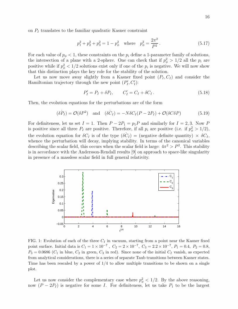
FIG. 1: Evolution of each of the three CI in vacuum, starting from a point near the Kasner fixed

point surface. Initial data is C1 = 1× 10−7 , C2 = 2× 10−7, C3 = 2.2× 10−7, P1 = 0.4, P2 = 0.8,

P3 = 0.0686 (C1 in blue, C2 in green, C3 in red). Since none of the initial CI vanish, as expected

from analytical considerations, there is a series of separate Taub transitions between Kasner states.

Time has been rescaled by a power of 1/4 to allow multiple transitions to be shown on a single

plot.

Let us now consider the complementary case where p2φ < 1/2. By the above reasoning,now (P − 2PI) is negative for some I. For definiteness, let us take P1 to be the largest

17

0 2 4 6 8 10 12 14 160

0.2

0.4

0.6

0.8

1

t1/4

Eig

enva

lue

P1

P2

P3

FIG. 2: Evolution of each of the three PI in vacuum, starting from a point near the Kasner fixed

point surface, with the same initial data as in Fig. 1 (P1 in blue, P2 in green, P3 in red). The

largest eigenvalue, P2, transits first. After this transition, P1 becomes the largest eigenvalue, now

making C1 unstable. In time all three PI tend to zero. In terms of parameters pi used in the Kasner

metric (5.14), the initially expanding direction p2 starts contracting at the end of the transition

and initially contracting p1 starts expanding.

of the PI ’s initially so that (P − 2P1) is negative which implies that C1 will grow and wehave instability. In this case, we cannot use perturbative analysis for the pair C1, P1; itis necessary to keep all order terms in C1 and P1. For simplicity, let us set C2 = C3 = 0initially. Then values of C2, P2, C3, P3 will not change during evolution and equations forC1, P1 simplify,

P1 = −NC21 (5.20)

C1 = −NC1(P2 + P3 − P1) = −NC1Pp1 , (5.21)

which can be solved exactly to obtain

P1(t) = P2 + P3 − 2√P2P3 tanh

(2√

P2P3N(t− to))

C1(t) = ±2√

P2P3 sech(2√P2P3N(t− to)

). (5.22)

These are the Bianchi II solutions written in our variables. Here C1, the unstable variable,rapidly increases and then decays to zero. During that time the P1 transitions between oneKasner solution to another. In the asymptotic limits we have:

P1(−∞) = P2 + P3 + 2√

P2P3 = (√P2 +

√P3)

2

P1(+∞) = P2 + P3 − 2√P2P3 = (

√P2 −

√P3)

2 . (5.23)

(In practice the asymptotic limits are achieved quickly, thanks to the hyperbolic functionsof time.) The result of the transition is that P1, which was originally was the largest of thethree PI , has transitioned to a lower value. By a change of variables to the pi used in (5.14)it is apparent that the eigenvalue corresponding to the negative exponent pi is the one whichhas transitioned, and is positive at the end of the transition. Since the singularity lies at

18

τ = 0, this means that the initially expanding direction now contracts, and one of the twocontracting directions now expands. Indeed, (5.23) is precisely the ‘u-map’ in pi variables.

In this analysis we have made the simplification that initially C2 = C3 = 0. If one startsfrom a generic point in the vicinity of the Kasner fixed point set and still with P1 as thelargest of the three PI initially, there would again be a transition of the type (5.22). Butas P1 decreases, after a finite time either P2 or P3 will now be the largest eigenvalue andmaking the corresponding CI unstable. That pair will then evolve according to (5.22). Thisgeneral scenario was borne out in a large class of simulations of the reduced equations ofmotion. Figs 1 and 2 illustrate this dynamical behavior for generic initial data near theKasner surface. The Taub transitions are easy to see in Fig 2: even though none of the CI

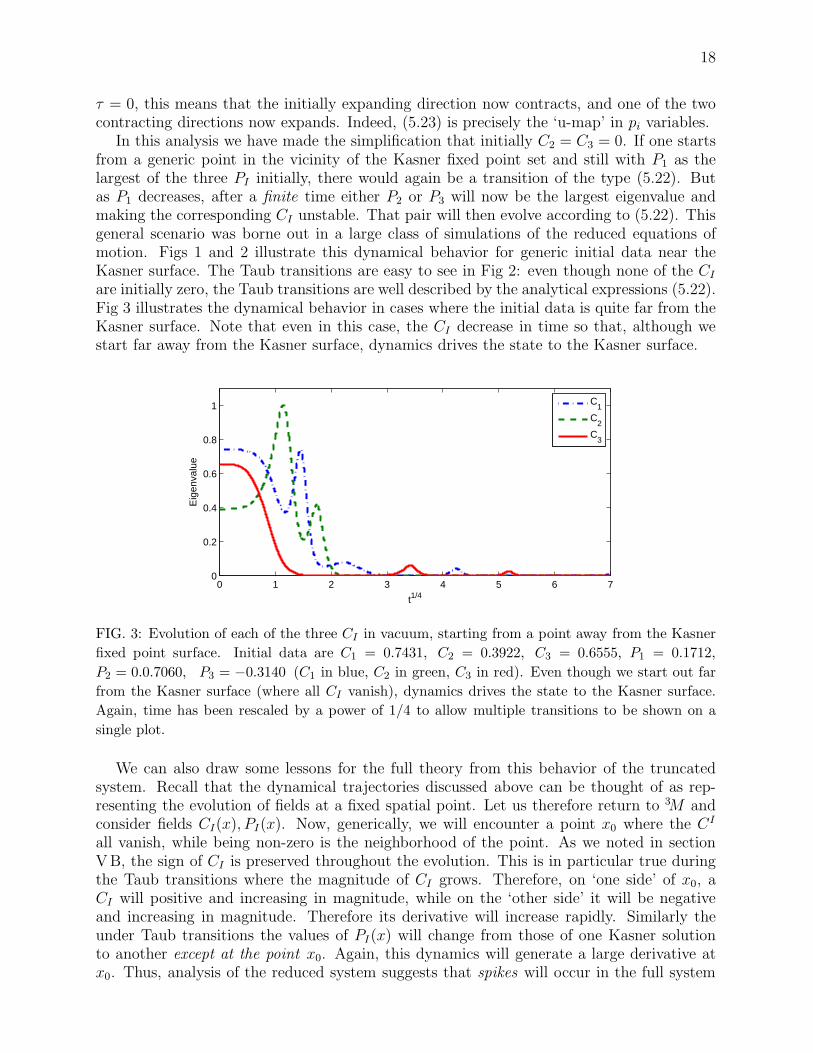
are initially zero, the Taub transitions are well described by the analytical expressions (5.22).Fig 3 illustrates the dynamical behavior in cases where the initial data is quite far from theKasner surface. Note that even in this case, the CI decrease in time so that, although westart far away from the Kasner surface, dynamics drives the state to the Kasner surface.

0 1 2 3 4 5 6 70

0.2

0.4

0.6

0.8

1

t1/4

Eig

enva

lue

C

1

C2

C3

FIG. 3: Evolution of each of the three CI in vacuum, starting from a point away from the Kasner

fixed point surface. Initial data are C1 = 0.7431, C2 = 0.3922, C3 = 0.6555, P1 = 0.1712,

P2 = 0.0.7060, P3 = −0.3140 (C1 in blue, C2 in green, C3 in red). Even though we start out far

from the Kasner surface (where all CI vanish), dynamics drives the state to the Kasner surface.

Again, time has been rescaled by a power of 1/4 to allow multiple transitions to be shown on a

single plot.

We can also draw some lessons for the full theory from this behavior of the truncatedsystem. Recall that the dynamical trajectories discussed above can be thought of as rep-resenting the evolution of fields at a fixed spatial point. Let us therefore return to 3M andconsider fields CI(x), PI(x). Now, generically, we will encounter a point x0 where the CI

all vanish, while being non-zero is the neighborhood of the point. As we noted in sectionVB, the sign of CI is preserved throughout the evolution. This is in particular true duringthe Taub transitions where the magnitude of CI grows. Therefore, on ‘one side’ of x0, aCI will positive and increasing in magnitude, while on the ‘other side’ it will be negativeand increasing in magnitude. Therefore its derivative will increase rapidly. Similarly theunder Taub transitions the values of PI(x) will change from those of one Kasner solutionto another except at the point x0. Again, this dynamics will generate a large derivative atx0. Thus, analysis of the reduced system suggests that spikes will occur in the full system

19

(3.13) - (3.14). As is well known, these spikes were found in numerical simulations and, morerecently, also in analytical treatments [43, 44]. Whenever spikes appear, the key assumptionunderlying BKL truncation is brought to question because the spatial derivatives are largeat the spikes. The key issue for the BKL conjecture —and for the application to quantumgravity we proposed in section I— is whether the time derivatives still dominate generically,as they do in examples.

Let us summarize. Using analytical and numerical methods we showed that there existsa well defined subspace Phom of the full phase space P which exhibits exactly the propertiesexpected in the BKL conjecture. Our procedure to arrive at the reduced system is moredirect than those available in the literature. In [28], for example, elimination of the off-diagonal components and the anti-symmetric parts of Cij involves an additional assumption,beyond ignoring spatial derivatives in favor of time derivatives: these quantities are identifiedas part of the ‘stable subset’ (variables that are expected to decay rapidly as the singularityis approached) and then set to zero to obtain the truncated equations. In our treatment, onthe other hand, the fact that the antisymmetric part of Cij is negligible is directly impliedby the assumption that the Di derivatives are negligible and the constraints imply that thevariables Cij and Pij can be simultaneously diagonalized which, furthermore, completely fixesthe gauge. Thus, our Hamiltonian framework naturally led to a diagonal gauge, enablingus to quickly zero-in on the essential variables and eliminating the need to keep track of thedynamics of extraneous variables involving frame rotations [28, 29]. Finally, the frameworkeasily led us to the Mixmaster behavior —a series of Bianchi I phases interspersed by BianchiII transitions. We recovered the ‘u-map’ for these transitions, and observed the behaviorexpected from the Andersson and Rendall analysis [9] when a scalar field of large enoughmagnitude is introduced.

VI. DISCUSSION

We began with the Hamiltonian formulation of general relativity underlying LQG wherethe basic fields are spatial triads Ea

i with density weight 1, spin connections Γia they deter-

mine, and extrinsic curvatures Kia. Based on examples that have been studied analytically

and numerically, it seems reasonable to expect that the determinant q of the spatial metricqab would vanish and the trace K of the extrinsic curvature would diverge at space-like sin-gularities. (This expectation is in particular borne out in the numerical simulations of G2space-times [33].) One can therefore hope to obtain quantities which remain well-definedat the singularity either by multiplying the natural geometric fields by suitable powers of qor dividing them by suitable powers of K. In the commonly used framework due to Ugglaet al [13, 28, 41], one chooses to divide by K. One first introduces the so-called Hubblenormalized triad K−1eai by rescaling the orthonormal triad eai by K−1, and then constructsa set of Hubble normalized fields by contracting Γa

j and Kaj with K−1eai. These fields are

expected to have regular limit at the space-like singularity. Einstein’s equations expressedin terms of them naturally suggests a truncation and the truncated system successfully de-scribes the expected oscillatory BKL behavior. The resulting form of the BKL conjectureis supported by numerical evolutions of full general relativity carried out by Garfinkle [39].However, because there is no underlying Hamiltonian framework, this approach does noteasily lend itself to non-perturbative quantization. Even if such a framework were to beconstructed, because of the presence of the K−1 factor, it would be difficult to introducequantum operators corresponding to the Hubble rescaled fields.

20

Motivated by quantum considerations, we adopted the complementary strategy of multi-plying geometrical fields by

√q. The LQG Hamiltonian formulation we began with already

features a density weighted triad with exactly the desired property: Eai =

√qeai . Since√

q is expected to vanish at the singularity, one can hope to use Eai in place of the Hubble

normalized K−1eai to construct a new set of fields to formulate the BKL conjecture. Indeed,(modulo trace terms) our basic variables Ci

j and Pij were obtained simply by contacting

the spatial indices of Γaj and Kj

a by Eai . Furthermore, because Ea

i vanishes in the limit,the operator Di := Ea

i Da provided a key tool in the formulation of the BKL conjecture:asymptotically, DiCj

k and DiPjk should become ‘negligible’ relative to Cj

k and Pjk. Now,

in exact general relativity, time derivatives of Cij and Pi

j can be expressed in terms of theirDi derivatives, purely algebraic (and at most quadratic) combinations of Ci

j and Pij, the

lapse N and its Di derivatives (see (3.6)–(3.15)). Therefore, if in the limit the Di derivativesof the basic fields become negligible compared to the fields themselves, we are naturallyled to conclude that time derivatives would dominate the spatial derivatives. This chain ofargument led to our formulation of the BKL conjecture.

This rather simple idea depends on the fact that the structure of Einstein’s equations hasan interesting and unanticipated feature: as we saw in section III, once the triplet Ci

j, Pij , Di

is constructed from the triad Eai and the extrinsic curvature Ki

a on an initial slice, theconstraint and evolution equations can be expressed entirely in terms of the triplet. Given asolution to these equations, the spatial triad Ea

i (and hence the metric qab) can be recoveredat the end simply by solving a total differential equation (3.16). This is a surprising andpotentially deep property of Einstein’s equation. It played essential role in our formulationof the BKL conjecture and could well capture the primary reason behind the BKL behaviorobserved in examples and numerical simulations.

Since our framework is developed systematically from a Hamiltonian theory, its BKLtruncation naturally led to a truncated phase space. The specific truncation used has animportant property: The truncated constraint and evolution equations on the truncatedphase space coincide with the truncation of full equations on the full phase space. Onthe truncated phase space we could solve and gauge-fix the Gauss and vector constraintsto obtain a simple Hamiltonian system (which encompasses all Bianchi type A models).Solutions to this system were explored both analytically and numerically. We showed thatthey exhibit the Bianchi I behavior, the Bianchi II transitions and spikes as in the analysisof symmetry reduced models [45] and numerical investigations of full general relativity [13].Therefore, as explained in section I, an appropriate quantization of the truncated system,e.g., a la loop quantum cosmology, could go a long way toward understanding the fate ofgeneric space-like singularities in quantum gravity.

In sections III, VA and VB, we restricted ourselves to vacuum equations. The additionof a massless scalar field is straightforward and was carried out in the reduced phase spaceframework in section VC. If the energy density in the scalar field is small, one againhas Bianchi II transitions and spikes. However, once the energy density exceeds a criticalvalue, these disappear and the asymptotic dynamics at any spatial point is described justby the Bianchi I model with a scalar field without transitions. Thus, our truncated systemfaithfully captures the main features generally expected from the analysis of Andersson andRendall [9] in full general relativity coupled to a massless scalar field or stiff fluid. Thus,although the initial motivation came from quantum considerations, our formulation of the

BKL conjecture, and the form of the field equations both in the full and truncated versions,

should be useful also in the analytical and numerical investigations of singularities in classical

21

general relativity.

We will conclude with a discussion comparing our approach with that of Uggla, Ellis,Wainwright and Elst (UEWE) ([28]). The Hubble normalized variable used in their formu-lation of field equations are give by

Σij = 3K−1ea(iK|a|j) −K−1eakKkaδij (6.1)

Nij = −3K−1ea(iΓ|a|j) + 3K−1eakΓkaδij (6.2)

Ai = −ǫ jki 3K−1eajΓ

ka (6.3)

∂i = 3K−1eai ∂a . (6.4)

These variables are especially useful because they are scale invariant: they are unchangedunder a constant rescaling of the space-time metric. Because of this property and because ofthe ‘regulating’ factorK−1 in their expressions, it is hoped that in the limit as one approachesthe space-like singularity, these variables will remain finite [41] and their ∂i derivative willbecome negligible.

We began with quite a different motivation and our focus was on constructing a Hamilto-nian framework rather than on differential equations. Since our emphasis was on construct-ing phase space variables that can be readily promoted to well-defined quantum operators,from the start we avoided the use of factors such as 1/K. As a result, our basic variablesCi

j and Pij are not scale invariant. Could we have made a different choice which is also well

suited for quantization and at the same time enjoyed scale invariance? The answer is in thenegative for the following reason. Under constant conformal rescalings gab → λ2gab of thespace-time metric, we have Ea

i → λ2Eai , Γi

a → Γia, and Ki

a → Kia. Now, in the analysis of

approach to singularity, scale invariant quantities are directly useful only if they are spacescalars and it is not possible to construct scale invariant scalars using just sums of productsof these fields, i.e., without introducing fields such asK−1 for which it is difficult to constructquantum operators. Even if one introduces additional non-dynamical fields, such as fiducialframes to construct scalars, for natural choices of these frames, scale invariant componentsof fields such as Ki

a,Γia typically diverge at the singularity. Thus, with our motivation, it

does not seem possible to demand scale invariance of the basic variables that are to featurein the BKL conjecture.

Our viewpoint is that the most important feature of the Hubble normalized variablesis that although the orthonormal triad eai typically diverges as one approaches a space-like singularity, K diverges even faster, making the combination K−1eai go to zero at thesingularity. Furthermore, it goes to zero at a sufficient rate for its contraction with Ki

a, Γia

and ∂a in (6.1) — (6.4) to tame the a priori divergent behavior of these fields. Instead ofdividing the orthonormal triad eai by K which one expects to diverge at the singularity,our strategy was to multiply it by the volume element

√q which, in examples, goes to zero

at the singularity. This difference persists also in the treatment of the lapse. The UEWEframework assumes that the (scalar) lapse N is such that NK admits a limit N while weassume that the density weighted lapse N = (

√q)−1 N admits a well-defined limit at the

singularity. Thus, in both cases, the standard scalar lapse N goes to zero so the singularitylies at t = ∞.

The key scale invariant UEWE variables (Nij ,Σij) —which are expected to be well be-

22

haved at the singularity— are related to our (Cij, Kij) via

Nij = 6P−1C(ij) and Σij = −6P−1 P(ij) + 2δij , or, (6.5)

C(ij) = −K√q

3Nij and P(ij) =

K√q

3(Σij − 2δij) (6.6)

and the two sets of lapse fields are related by:

N = K√q N . (6.7)

If one focuses only on the structure of differential equations near space-like singularities,the two reduced systems would in essence be equivalent if K

√q admits a finite, nowhere

vanishing limit at the singularity. This condition holds for Bianchi I models and also BianchiII which describe the transitions between Bianchi I epochs. In fact in the Bianchi I model,√q K = 1 and our density weighted triad has the same dependence on proper time as the

Hubble normalized triad. Thus, although the motivations, starting points and proceduresused in the two frameworks are quite different, surprisingly, in the end the basic variablesand equations are closely related.

Acknowledgments

We would like to thank Woei-Chet Lim, Alan Rendall, Yuxi Zheng and especially DavidGarfinkle and Claes Uggla for discussions. This work was supported in part by the NSFgrant PHY0854743 and the Eberly and Frymoyer research funds of Penn State.

Appendix A: Densities

Since the basic variables that feature in our formulation of the BKL conjecture are scalarson 3M of density weight 1, in this Appendix we briefly recall a coordinate independentframework for describe densities. The underlying idea is due to Wheeler and the detailedframework was developed by Geroch (see, e.g., [46]). This framework goes hand in hadwith Penrose’s abstract index notation [47, 48]. Because the primary application in thispaper is to our fields Ci

j, Pij on 3M we will focus on scalar densities on 3-manifolds. But

generalization to tensor densities on n-manifolds is straightforward.Fix an oriented 3-manifold 3M and fix a orientation thereon. Denote by E the space

of smooth, positively oriented, no-where vanishing, totally skew tensor fields eabc on 3M .Clearly, given any two elements eabc and e′abc in E , there exists a (strictly) positive functionα such that e′abc = αeabc. This fact will be used repeatedly.

In this paper, a scalar density Sn of weight n is a map from E to the space of (real valued)smooth functions on 3M : e → Sn(e), such that:

Sn(e′) = αn Sn(e) (A1)

Here n can be any real number but in most applications in general relativity it is an integer.(In quantum mechanics, on the other hand, states are (complex-valued) densities of weight1/2 on the configuration space [46].) Since Ci

j, Pij have density weight 1, let us make a

short detour to discuss the case n = 1. Fix any 3-form sabc on3M . It determines a canonical

23

scalar density of weight 1:S1(e) := sabc e

abc . (A2)

Conversely, since S1 is a linear mapping from E to smooth functions, it determines a canonical3-form sabc. Thus, our basic variables could also be taken to be 3-forms C ij

abc, Pijabc on

3M which take values in second rank tensors in the internal space. The standard ADMphase space of general relativity can be similarly coordinatized by positive definite metricsqab and tensor fields P ab

cde which are symmetric in a, b and totally skew in c, d, e [49, 50].Finally note that every metric qab determines a canonical volume 3-form ǫabc which haspositive orientation and satisfies ǫabcǫdef q

adqbeqcf = sgn(q) 3!. Therefore it also determinesa canonical scalar density

√q of weight 1, called the square root of the determinant of qab:√

q(e) := ǫabceabc for all e ∈ E .

This definition can be extended to density weighted tensor fields in an obvious fashion.Note that every 3M carries a natural totally skew tensor density ηabc of weight 1, called theLevi-Civita density:

ηabc(e) = eabc ∀ e ∈ E (A3)

Given any metric qab on3M , the square root of its determinant,

√q, can also be expressed

as√q = ηabc ǫabc.

Finally, given a derivative operator Da on tensor fields on 3M , we can extend its actionon densities Sn of weight 1 in a natural manner. DaSn is a 1-form with the same densityweight n, given by

(DaSn)(e) = Da(Sn(e))− nλa Sn(e) ∀e ∈ E , (A4)

where the first term on the right hand side is just the gradient of the function Sn(e) andthe 1-form λa is given by Dae

bcd = λaebcd. Therefore the action of the derivative operator

Di introduced in the main text is given by:

(DiSn)(e) = Di(Sn(e))− n (Eai λa)Sn(e) ∀e ∈ E . (A5)

Since the derivative operator Da we considered ignores internal indices, this equation givesthe action of Di on Ci

j and Pij by regarding these basic fields simply as scalar densities with

weight 1.

Appendix B: Full Equations of Motion

In the main text we restricted the equations of motion to the case where the shift iszero as is the Lagrange multiplier for the Gauss constraint. In this appendix we give theequations of motion in full generality for both full general relativity and in our reducedsystem. The full equations of motion for C and P are as follows.

C ij = − ǫjklDk(N(1

2δilP − P i

l )) +N [2C(ikP

|k|j) + 2C [kj]P ik − PC ij] (B1)

+NkDkCij + CijDkNk + CijǫklmN

kC lm

+(C ki ǫklj + Ck

jǫkli)(Λl −NmCml +

1

2CN l)

+Di(Λj −NkCkj +1

2NjC)−Dk(Λ

k −N lC kl +

1

2CNk)δij

24

P ij = ǫjklDk(N(1/2δilC − C il ))− ǫklmDm(NCkl)δ

ij + 2ǫjkmC [ik]Dm(N) (B2)

+(DiDj −DkDkδij)N +N [−2C(ik)C j

k + CC ij − 2C [kl]C[kl]δij ]

+NkDkPij + PijDkNk + PijǫklmN

kC lm

+(P ki ǫklj + P k

jǫkli)(Λl −NmCml +

1

2CN l)

In the reduced system the derivative terms are set to zero leading to the following equa-tions of motion for C and P .

Cij = N [2Ck(iPkj) − PCij] + 2ǫkl(iCj)

k(Λl −NmCml +

1

2CN l) (B3)

Pij = N [−2CikCkj + CCij] + 2ǫkl(iPj)

k(Λl −NmCml +

1

2CN l) (B4)

[1] V. A. Belinskii, I. M. Khalatnikov and E. M. Lifshitz, Oscillatory approach to a singular point

in the relativistic cosmology, Adv. Phys. 31, 525-573 (1970)

[2] A. Ashtekar, A. Henderson and D. Sloan, Hamiltonian general relativity and the Belinskii,

Khalatnikov, Lifshitz conjecture, Class. Quant. Grav. 26 052001 (2009)

[3] L. Bianchi, Sugli spazii a tre dimensioni che ammettono un gruppo continuo di movimenti,

Soc. Ital. Sci. Mem. di Mat. 11 267 (1898)

[4] B. Berger, Numerical approaches to space-time singularities, Living Reviews in Relativity 1

(2002)

[5] D. Garfinkle Numerical simulations of generic singuarities, Phys. Rev. Lett. 93 161101 (2004)

[6] B. Berger and V. Moncrief Numerical investigation of cosmological singularities, Phys. Rev.

D48 4676 (1993)

[7] B. Berger, D. Garfinkle, J. Isenberg, V. Moncrief and M. Weaver, The singularity in generic

gravitational collapse is spacelike, local, and oscillatory, Mod. Phys. Lett. A13 1565 (1998)

[8] M. Weaver, J. Isenberg and B. Berger Mixmaster behavior in inhomogeneous cosmological

spacetimes, Phys. Rev. Lett. 80 2984 (1998)

[9] L. Anderson and A. Rendall Quiescent cosmological singularities, Commun. Math. Phys 218

479 (2001)

[10] T. Damour, H. Henneaux, A. Rendall and M. Weaver, Kasner-like behavior for subcritical

Einstein matter systems, Ann. Henri Poincare 3, 1049-1111 (2002)

[11] B. Berger and V. Moncrief, Numerical evidence that the singularity in polarized U(1) sym-

metric cosmologies on T 3 ×R is velocity dominated, Phys. Rev. D 57 7235 (1998)

[12] B. Berger and V. Moncrief, Exact U(1) symmetric cosmologies with local Mixmaster dynamics,

Phys. Rev. D62 023509 (2000)

[13] D. Garfinkle, Numerical simulations of general gravitational singularities, Class. Quant. Grav.

24 295 (2007)

[14] R. Saotome, R. Akhoury and D. Garfinkle, Examining gravitational collapse with test scalar

fields, Class. Quant. Grav. 27 165019 (2010)

[15] M. Bojowald, Loop quantum cosmology, Living Rev. Rel.8:11 (2005);

A. Ashtekar, Loop Quantum cosmology: An overview, Gen. Rel. Grav 41 707-741 (2009)

25

[16] A. Ashtekar and J. Lewandowski, Background independent quantum gravity: A status report,

Class. Quant. Grav. 21 R53-R153 (2004)

[17] C. Rovelli,Quantum Gravity, (Cambridge University Press, Cambridge (2004))

[18] T. Thiemann, Introduction to Modern Canonical Quantum General Relativity, (Cambridge

University Press, Cambridge, (2007))

[19] M. Bojowald, Absence of singularity in loop quantum cosmology, Phys. Rev. Lett. 86, 5227-

5230 (2001)

[20] A. Ashtekar, T. Pawlowski and P. Singh, Quantum nature of the big bang, Phys. Rev. Lett.

96 141301 (2006)

[21] A. Ashtekar, T. Pawlowski, P. Singh and K. Vandersloot, Loop quantum cosmology of k=1

FRW models, Phys. Rev. D75 024035 (2007)

[22] E. Bentivegna and T. Pawlowski, Anti-deSitter universe dynamics in LQC, Phys. Rev. D77,

124025 (2008)

[23] P. Singh Are loop quantum cosmos never singular? Class. Quant. Grav. 26 125005 (2009)

[24] A. Ashtekar and E. Wilson-Ewing Loop quantum cosmology of Bianchi I models, Phys. Rev.

D79 083535 (2009)

[25] A. Ashtekar and E. Wilson-Ewing Loop quantum cosmology of Bianchi type II models Phys.

Rev. D80 123532 (2009)

[26] E. Wilson-Ewing, Loop quantum cosmology of Bianchi type IX models, Phys. Rev. D82

043508 (2010)

[27] G. Mena Marugan and M. Martin-Benito, Hybrid quantum cosmology: Combining loop and

Fock quantizations, Int. J. Mod. Phys. A24 2820 (2009)

[28] C. Uggla, H. van Elst, J. Wainwright and G. Ellis, The past attractor in inhomogeneous

cosmology, Phys. Rev. D 68 103502 (2003)

[29] T. Damour and S. de Buyl, Describing general cosmological singularities in Iwasawa variables,

Phys. Rev. D 77, 043520 (2008)

[30] A. Ashtekar, New variables for classical and quantum gravity, Phys. Rev. Lett. 57, 2244-2247

(1986);

A new Hamiltonian formulation of general relativity, Phys. Rev. D36, 1587-1603 (1987).

[31] R. Arnowitt, S. Deser and C. W. Misner, The dynamics of general relativity, in Gravitation:

An Introduction to Current Research, edited by L. Witten (Wiley, New York (1962))

[32] J.D Romano, Geometrodynamics Vs. Connection Dynamics, Gen. Rel. Grav. 25 759 (1993)

[33] W. Lim (personal communication, July 2008)

[34] J.M. Heinzle, C. Uggla, and N. Rohr, The Cosmological Billiard Attractor, Adv. Theor. Math.

Phys. 13 293 (2009)

[35] G. Barnich and V. Hussain, Geometrical representation of Euclidean general relativity in the

canonical formalism, Class. Quant. Grav. 14 1043 (1997)

[36] H. Ringstrom Curvature blow up in Bianchi VIII and IX vacuum spacetimes, Class. Quantum

Grav. 17 713 (2000)

[37] H. Ringstrom, The Bianchi IX attractor, Annales Henri Poincare 2 405 (2001)

[38] C. Uggla, The Nature of Generic Cosmological Singularity, arXiv:0706.0463

[39] D. Garfinkle, The Nature of gravitational singularities, Int. J. Mod. Phys. D 13 2261 (2004)

[40] M. Heinzle and C. Uggla, A new proof of the Bianchi type IX attractor theorem, Class. Quant.

Grav 26 075015 (2009)

[41] M. Heinzle and C. Uggla, Mixmaster: Fact and belief, Class. Quant. Grav. 26 075016 (2009)

[42] A. Rendall, Global dynamics of the Mixmaster model, Class. Quant. Grav. 14, 2341-2356

26

(1997)

[43] A. Rendall and M. Weaver, Manufacture of Gowdy space-times with spikes, Class. Quant.

Grav.18 2959-2976 (2001)

[44] W. Lim, New Explicit Spike Solution – Non-local Component of the Generalized Mixmaster

Attractor, Class. Quant. Grav. 25 045014 (2008)

[45] W. Lim, L. Andersson, D. Garfinkle and F. Pretorius, Spikes in the Mixmaster regime of G(2)

cosmologies, Phys. Rev. D79 123526 (2009)

[46] R. Geroch, Geometrical Quantum Mechanics, Lecture notes available at

http://www.phy.syr.edu/∼salgado/geroch.notes/geroch-gqm.pdf

[47] R. Penrose, Structure of space-time, in Battlle Rencontres, edited by C. M. DeWitt and J.

Wheeler (Bejamin, New York, (1968))

[48] A. Ashtekar, G. T. Horowitz and A. Magnon, A Generalized tensor calculus and its applica-

tions to physics, Gen. Rel. Grav. 14 411-428 (1982)

[49] A. Ashtekar and R. Geroch, Quantum theory of Gravitation, Rep. Prog. of Phys. 37, 1211-

1256 (1974)

[50] A. Ashtekar and A. Magnon, On the Symplectic structure of general relativity, Commun.

Math. Phys., 86, 55-68 (1982)