Port-Hamiltonian Discretization for Open

Channel Flows

R. Pasumarthy

p.ramkrishna@bits-hyderabad.ac.in

Department of Electrical Engineering,

Birla Institute of Technology and Science Hyderabad, India.

V.R. Ambati∗

v.r.ambati@math.utwente.nl

Numerical Analysis and Computational Mechanics Group,

Department of Applied Mathematics, University of Twente, The Netherlands.

A.J. van der Schaft

a.j.van.der.schaft@rug.nl

Johann Bernoulli Institute for Mathematics and Computer Science,

University of Groningen, The Netherlands.

October 28, 2010

Abstract

A finite-dimensional Port-Hamiltonian formulation for the dynamics of smooth

open channel flows is presented. A numerical scheme based on this formulation

is developed for both the linear and nonlinear shallow water equations. The

scheme is verified against exact solutions and has the advantage of conservation

of mass and energy to the discrete level.

Keywords: Shallow water equations, Port-Hamiltonian, Stokes-Dirac Structure,

Numerical Discretization.

Mathematics Subject Classification: 76B15, 76B75, 93C10, 93C95.

1 Introduction

Port based network modelling of complex lumped parameter physical systems natu-

rally leads to a generalized Hamiltonian formulation of the dynamics. The resulting

∗Corresponding author

1

class of open dynamical systems are called “Port-Hamiltonian” systems [17] which aredefined using a power conserving interconnection structure called Dirac structure, theHamiltonian and dissipative elements. Such a generalized Hamiltonian formulation,called “Port-Hamiltonian” formulation, has been successfully extended to classes ofdistributed parameter systems by introducing an infinite-dimensional Dirac structurebased on Stokes’ Theorem. The key aspect of this formulation is that it allows a non-zero energy flow into the spatial domain through its boundary using Dirac structure,whereas the standard Hamiltonian formulation assumes a zero energy flow throughthe boundary using Poisson structure [12]. The Port-Hamiltonian formulation is alsoeffectively used towards control design by using energy shaping methods. The tech-nique relies on constructing a Lyapunov function by using the energy function of thesystem together with the conserved quantities called Casimirs [14].

The Port-Hamiltonian formulation can be directly applied to model infinite-dimen-sional fluid dynamical systems containing all its physical conservation laws such asmass, momentum and energy (Hamiltonian) [13]. But for practical purposes, it iscrucial to approximate these infinite-dimensional systems by a finite-dimensional sys-tem in such a way that it is again a Port-Hamiltonian system. The finite-dimensionalapproximation should be such that it conserves most of the physical quantities of itsinfinite-dimensional counterpart. The resulting numerical scheme would then accu-rately capture the physics of the fluid dynamical system. To devise such a numericalscheme based on finite dimensional Port-Hamiltonian formulation, we choose a par-ticular example of fluid flows namely open channel flows.

The one-dimensional shallow water equations governing open channel flows arethe depth averaged approximations of the two-dimensional Navier-Stokes equations.They are a direct consequence of the conservation of mass and momentum and obeythe conservation of energy for smooth flows but dissipate energy for non-smoothflows in the form of bores and hydraulic jumps. Many numerical methods exist forthese equations such as finite volume methods [4, 5] and discontinuous Galerkin finiteelement methods [2, 3, 15]. These numerical methods follow mass and momentumlaws of balance, but they may not follow energy balance even in the smooth regionsof a flow. Hence, we propose the use of the framework of Port-Hamiltonian systemswhich follows energy balance law. Such a framework has implications towards themeteorological and oceanographic studies on geophysical flows, where the numericalschemes that conserve the energy are of great importance (for example follow [6, 7,11]).

A new numerical scheme based on a finite-dimensional Port-Hamiltonian formu-lation for the dynamics of shallow open channel water flow is the aim of the presentpaper. A shallow water channel with topography is first modelled as an infinite-dimensional Port-Hamiltonian system defined with respect to a Stokes-Dirac struc-ture. Consequently, the system obeys a power conserving property, which is naturallyequivalent to the energy balance, expressed in terms of power port variables called

2

flows and efforts of the fluid dynamical system. For shallow water system, the flowsare rate of change of water depth and velocity, the efforts are discharge and Bernoulli’sfunction, and the shallow water equations are a direct consequence of the relation be-tween flows and efforts captured by the Stokes-Dirac structure.

To model the shallow water canal as a finite-dimensional Port-Hamiltonian sys-tem, we tessellate the spatial domain with finite elements and approximate the flowvariables with cell averages and effort variables with continuous piecewise linear poly-nomials. Such a choice of different approximation spaces for flows and efforts ensuresthe compatibility of the flow-effort relation in Stokes-Dirac structure which are ordi-nary differential equations. Further, the continuity of efforts ensure the conservationof flow quantities. Consequently, each finite element will be a finite-dimensional Port-Hamiltonian system satisfying a power conserving property per finite element. Wethen enforce a discrete energy balance in the system by summing up the power con-serving relation of all the finite elements. This effectively give rise to an algebraicrelation between the efforts and the corresponding discrete co-energy variables. Thus,the finite-dimensional Port-Hamiltonian system for a shallow water channel consistsof a system of differential-algebraic equations.

The ordinary differential equations arising from the Port-Hamiltonian formulationare further discretized in time using an implicit mid-point time discretization. Thistime discretization is a second-order symplectic method and well-suited for a Hamil-tonian system. After time discretization, the ODE’s are transformed into nonlinearalgebraic equations which are then solved by integrating them in pseudo-time using afive stage Runge-Kutta scheme until a steady state is reached in pseudo-time [2]. Thenumerical scheme is verified against several idealized exact solutions to show that itis first-order accurate and accurately conserves the energy.

2 Infinite Dimensional Port-Hamiltonian Formu-

lation

The Port-Hamiltonian formulation of fluid dynamical systems (Maschke and van derSchaft [10], and Van der Schaft and Maschke [16]) is an extension of the Hamiltonianformulation incorporating non-zero flow through boundaries. Here, we present such aPort-Hamiltonian formulation for open channel or canal water flows in one dimension.

2.1 Shallow water model

The dynamics of flow through an open channel of length L is governed by the shallowwater equations which in one dimension read as

∂th + ∂xQ = 0 and ∂tu+ ∂xB = 0 on [0, L] (1)

3

with h(t, x) the water depth, u(t, x) the depth averaged velocity, Q = hu the flowdischarge, B = u2/2+g(h+b) the Bernoulli function and b(x) the channel bed heightmeasured from a fixed reference level. The shallow water equations (1) are completedtogether with the initial conditions h(0, x) = h0(x) and u(0, x) = u0(x), and inflow,outflow, solid wall or periodic boundary conditions at x = 0 and x = L. The totalhydraulic energy (or Hamiltonian) in the open channel is

H :=

∫ L

0

1

2(h u2 + g (h+ b)2)dx. (2)

2.2 Preliminaries of differential geometry

The Port-Hamiltonian formulation is convenient in a differential geometric framework.Therefore, for one-dimensional problem we introduce the differential zero and oneforms. By definition, zero forms are functions that can be evaluated at any point onthe domain and one forms are objects that can be integrated over any part of thedomain. Now, the following operators relate zero and one forms:

1. Exterior derivative: Consider a zero form or function f(x) ∈ R and a oneform g defined as g := (∂f/∂x)dx which in coordinate-free language is given asg = df , where d(·) is called the exterior derivative transforming zero form toone form.

2. Hodge star operator: Consider a function f(x) ∈ R which by itself is a zeroform and its one form f(x)dx. The Hodge star operator ∗(·) in one dimensionis defined as ∗f(x)dx := f and ∗f := f(x)dx transforming a zero form to a oneform and vice versa.

3. Wedge product: Given a zero form f and one form g, the wedge product f∧gis defined as f ∧ g := fg which is again a one form.

For more general definitions of these operators in n-dimensions, we refer to [1]. Fur-ther, we denote the set of zero forms as W 0(Ω) and the set of one forms as W 1(Ω).

2.3 Stokes Dirac structure

The Port-Hamiltonian formulation is based on the concept of a Dirac structure whichis a geometric object formalizing the power conserving interconnections [17].

Definition 1. Let V be a linear space (possibly infinite-dimensional). There existson V × V ∗ the canonically defined symmetric bilinear form

≪ (f1, e1), (f2, e2) ≫:=< e1 | f2 > + < e2 | f1 > (3)

4

with fi ∈ V, ei ∈ V ∗, i = 1, 2 and <|> denoting the duality product between V and itsdual subspace V ∗. A constant Dirac structure on V is a linear subspace D ⊂ V × V ∗

such thatD = D⊥, (4)

where ⊥ denotes the orthogonal complement with respect to the bilinear form ≪,≫.

Let now (f, e) ∈ D = D⊥. Then as an immediate consequence of (3),

0 =≪ (f, e), (f, e) ≫= 2 < e | f > .

Thus for all (f, e) ∈ D we have < e | f >= 0, expressing power conservation withrespect to the dual power variables f ∈ V and e ∈ V ∗.

To define the Stokes-Dirac structure for the shallow water equations (1), we firstassociate the energy variables water depth h(t, x) and velocity u(t, x), with one formsas (h, u)dx ∈ V 1(Ω); and co-energy variables, Bernoulli function B and discharge Q,with zero forms as (B,Q) ∈ V 0(Ω) in which

V 1(Ω) := W 1(Ω) ×W 1(Ω) and V 0(Ω) := W 0(Ω) ×W 0(Ω) (5)

where, W 0(Ω) and W 1(Ω) is the space of zero and one forms, respectively. Now, therate of energy variables, i.e., fh := −(∂th)dx and fu := −(∂tu)dx, are called flows;and the co-energy variables, i.e., eh := δhH = B and eu := δuH = Q, are calledefforts. Furthermore, the values of the Bernoulli function B and the discharge Qevaluated at the boundaries would also constitute to the flow and effort variables atthe boundary as fb = B|∂Ω ∈ W 0(∂Ω) and eb = −Q|∂Ω ∈ W 0(∂Ω) with W 0(∂Ω) thespace of zero forms on the boundary.

Consider the linear space of flow variables F = V 1(Ω) ×W 0(∂Ω) and effort vari-ables E = V 0(Ω) ×W 0(∂Ω) together with the bilinear form

⟨⟨(

f 1h , f

1u , f

1b , e

1h, e

1u, e

1b

)

,(

f 2h , f

2u , f

2b , e

2h, e

2u, e

2b

)⟩⟩

:=

∫

Ω

(

e1h ∧ f 2h + e2h ∧ f 1

h

+ e1u ∧ f 2u + e2u ∧ f 1

u

)

+

∫

∂Ω

(

e1b ∧ f 2b + e2b ∧ f 1

b

)

, (6)

where fh := −(∂h/∂t) dx, fu := −(∂u/∂t) dx, fb := B|∂Ω, eh := B, eu := Q, eb :=−Q|∂Ω,

(

f ih, f

iu, f

ib

)

∈ F the flows,(

eih, e

iu, e

ib

)

∈ E the efforts and i = 1 or 2. It hasbeen shown in [16] that D ⊂ F × E defined as

D :=

(

f, e)

∈ F × E∣

∣

∣fh = deu, fu = deh, fb = eh|∂Ω, eb = −eu|∂Ω

. (7)

is a Stokes-Dirac structure, i.e., D = D⊥, with respect to the bilinear form⟨⟨

·, ·⟩⟩

defined in (6) and thus defines an infinite-dimensional port-Hamiltonian system. Theflow-effort relation in (7) is a direct consequence of the shallow water equations (1).

5

K1 K2 Kk−1 Kk Kk+1 KN

x1 x2 x3 xj−1 xj xj+1 xj+2 xN xN+1

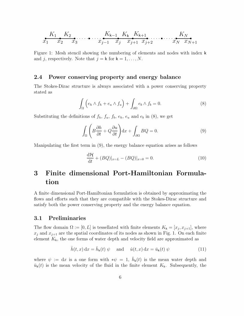
Figure 1: Mesh stencil showing the numbering of elements and nodes with index k

and j, respectively. Note that j = k for k = 1, . . . , N .

2.4 Power conserving property and energy balance

The Stokes-Dirac structure is always associated with a power conserving propertystated as

∫

Ω

(

eh ∧ fh + eu ∧ fu

)

+

∫

∂Ω

eb ∧ fb = 0. (8)

Substituting the definitions of fh, fu, fb, eh, eu and eb in (8), we get

∫

Ω

(

B∂h

∂t+Q

∂u

∂t

)

dx+

∫

∂Ω

BQ = 0. (9)

Manipulating the first term in (9), the energy balance equation arises as follows

dHdt

+ (BQ)|x=L − (BQ)|x=0 = 0. (10)

3 Finite dimensional Port-Hamiltonian Formula-

tion

A finite dimensional Port-Hamiltonian formulation is obtained by approximating theflows and efforts such that they are compatible with the Stokes-Dirac structure andsatisfy both the power conserving property and the energy balance equation.

3.1 Preliminaries

The flow domain Ω := [0, L] is tessellated with finite elements Kk = [xj , xj+1], wherexj and xj+1 are the spatial coordinates of its nodes as shown in Fig. 1. On each finiteelement Kk, the one forms of water depth and velocity field are approximated as

h(t, x) dx = hk(t) ψ and u(t, x) dx = uk(t) ψ (11)

where ψ := dx is a one form with ∗ψ = 1, hk(t) is the mean water depth anduk(t) is the mean velocity of the fluid in the finite element Kk. Subsequently, the

6

approximation of flows are directly given as

fh(t, x) = −∂thk ψ and fu(t, x) = −∂tuk ψ. (12)

As a consequence, the flows are piecewise constant per finite element Kk and discon-tinuous across the nodes in the domain.

To satisfy the energy balance and mass conservation, the efforts eh = B andeu = Q are approximated with linear polynomials per element Kk such that they arecontinuous across each node. The approximation of efforts in each finite element Kk

is therefore given as

eh = B(t, x) = Bj(t)φj(x) + Bj+1(t)φj+1(x) and

eu = Q(t, x) = Qj(t)φj(x) + Qj+1(t)φj+1(x), (13)

where φj(x) := (xj+1 − x)/(xj+1 − xj) and φj+1(x) := (x − xj)/(xj+1 − xj) are

shape functions, Bj(t) and Bj+1(t) are nodal values of the Bernoulli function B, and

Qj(t) and Qj+1(t) are nodal values of the discharge Q. Finally, the approximation ofboundary variables fb and eb on each boundary of the finite element Kk becomes

fb = eh|x=xj,j+1= Bj,j+1(t) and eb = eu|x=xj,j+1

= −Qj,j+1(t) (14)

3.2 Discretization of the Stokes-Dirac structure

The discrete port-Hamiltonian formulation starts by substituting the approximationsof flows (12) and efforts (13) per finite element Kk in the flow-effort relations of theStokes-Dirac structure (7) to get

−∂thkψ = Qj dφj + Qj+1 dφj+1 and − ∂tukψ = Bj dφj + Bj+1 dφj+1. (15)

The choice of approximation of flows with piecewise constants and efforts with piece-wise linear polynomial is made such that the flow-effort relation (15) is non-degenerate.Integrating (15) over the finite element Kk, the evolution of flows in terms of effortsper finite element emerge as

dhk

dt=

1

∆xk

(

Qj − Qj+1

)

andduk

dt=

1

∆xk

(

Bj − Bj+1

)

(16)

with ∆xk = xj+1−xj . The flow and effort approximations together with the boundaryeffort variables (14) automatically satisfy the power conserving property per finiteelement as follows

∫

Kk

(

eh ∧ fh + eu ∧ fu

)

+

∫

∂Kk

eb ∧ fb = − ∆xk

2

(

Bj+1 + Bj

) dhk

dt

−∆xk

2

(

Qj+1 + Qj

) duk

dt−(

Bj+1Qj+1 − BjQj

)

= 0. (17)

7

The power conserving property (17) is deduced by using (12)-(14) in (8) and substi-tuting (16). Having obtained a discretization for the Stokes-Dirac structure, it nowremains to discretize the Hamiltonian and satisfy energy balance.

The Hamiltonian (or energy) is discretized in each finite element Kk as

Hk :=

∫

Kk

(1

2hu2 +

1

2g(h+ b)2dx = ∆xk

(

hk u2k/2 + g h2

k/2 + g hk bk

)

; (18)

where b(x) := bk ∗ψ is the approximated bed height. The co-energy variables of thediscretized Hamiltonian Hk are then defined as

Bk :=δHk

δhk

=(1

2u2

k+ g(hk + bk)

)

∆xk and Qk :=δHk

δuk

= (hkuk)∆xk. (19)

We now enforce the following energy balance

N∑

k=j=1

(dHk

dt+ Bj+1Qj+1 − BjQj

)

= 0 (20)

by relating the efforts and co-energy variables at the interior nodes as

(Bj , Qj) = (αjBk−1 + βjBk, βjQk−1 + αjQk) for j = 2, . . . , N ; (21)

and at the boundary nodes as

(B1, Q1) = (B1, Q0) and (BN+1, QN+1) = (BN , QL) (22)

with αj + βj = 1, αj ∈ R an arbitrary value for any j = 2, . . . , N , Q0 and QL arethe given inflow or outflow discharges at x = 0 and x = L, respectively. For a solidwall boundary, the inflow or outflow discharge is simply set to zero and for periodicboundaries, the boundary efforts are determined by making the two boundary nodesas a single interior node to obtain

B1 = BN+1 = α1B1 + β1BN and Q1 = QN+1 = β1Q1 + α1QN (23)

with α1+β1 = 1 and α1 an arbitrary value. The flow-effort relations (16) together withthe efforts determined in (21)-(23) constitute the Port-Hamiltonian discretization.

Remark 1. To determine the efforts at each node j from the co-energy variablesusing (21), there remains several choices for αj or βj and can be arbitrarily chosen.In all the test cases, we made a simple choice of αj = βj = 1/2.

8

3.3 Discrete conservation properties

Proposition 1. The Port-Hamiltonian discretization (16), (21) and (23) satisfy themass and energy balance as follows

dM

dt+ QN+1 − Q1 = 0 and

dE

dt+ BN+1QN+1 − B1Q1 = 0 (24)

where, M :=∑N

k=1hk∆xk is the total mass and E :=

∑N

k=1Hk the total energy.

Proof. The proof of mass balance is straightforward; evaluating the time derivativeon total mass M using (16):

dM

dt=

N∑

k=1

dhk

dt∆xk =

N∑

k=j=1

(

Qj − Qj+1

)

= −(QN+1 − Q1). (25)

To prove the energy balance, we first evaluate the time derivative on total energyE using (16) to find

dE

dt=

N∑

k=1

dHk

dt=

N∑

k=1

(

Bk

dhk

dt+ Qk

duk

dt

)

∆xk

=

N∑

k=j=1

(

Bk

(

Qj − Qj+1

)

+ Qk

(

Bj − Bj+1

)

)

(26)

Rearranging the summation over elements in (26) into a summation over nodes andsubstituting the efforts determined in (21)-(23), we further find

dE

dt= (B1Q1 + Q1B1) − (BNQN+1 + QN BN+1)

+

N∑

k=j=2

(

(

Bk − Bk−1

)

Qj +(

Qk − Qk−1

)

Bj

)

= (B1Q0 + Q1B1) − (BNQL + QNBN+1) +N∑

k=2

(

BkQk − Bk−1Qk−1

)

= (B1Q0 − BNQL) = (B1Q1 − BN+1QN+1) (27)

for a given inflow or outflow boundary conditions. For periodic and solid wallboundaries, we find that dE/dt = 0. Hence proved.

9

3.4 Time discretization

The Port-Hamiltonian discretization (16) and (21)-(23) takes the following form:

dy

dt= F (y); (28)

with y = (h1, u1, . . . , hN , uN)T the unknown flow variables and F (y) the nonlinearright hand side obtained after substituting efforts (21)-(23) and co-energy variables(19) into RHS of (16). To integrate the ordinary differential equations (28) in time,we employ an implicit mid-point time discretization to get

L(yn,yn−1) := yn − yn−1 − ∆t F(

(yn + yn−1)/2)

= 0, (29)

where L(ynk,yn−1

k) represents the nonlinear algebraic equations. The implicit mid-

point scheme is a second-order symplectic method [8] that is well-suited for Hamil-tonian systems and leads to a stable numerical integration in time. The nonlinearequations (29) are solved by augmenting them with pseudo-time derivative as

∆x · dy

dτ=

−1

∆tL(y,yn−1) (30)

with ∆x = (∆x1,∆x1, . . . ,∆xN ,∆xN )T , ∆t = tn−tn−1 the time step and integratingin pseudo-time using a five-stage Runge-Kutta integration scheme [2] until it reachessteady state in pseudo-time. The five-stage Runge-Kutta scheme is

(1 + αs)ys = y0 + αsλ(ys−1 − L(ys−1,yn−1)); (31)

where s = 1 to 5 are the Runge-Kutta stages, αs = (0.0791451, 0.163551, 0.283663,0.5, 1.0) the Runge-Kutta coefficients, λ = ∆τ/∆t and ∆τ the local pseudo-time

step. The time step ∆t = CFL∆t max(

∆xk/(|uk|+√

ghk))

is chosen globally for all

k = 1, . . . , N , the pseudo-time step ∆τ = CFL∆τ∆xk/(|uk|+√

ghk) is chosen locallyfor each k, and CFL∆t = 1.0 and CFL∆τ = 0.9 are the Courant-Friedrichs-Lewy(CFL) numbers for ∆t and ∆τ , respectively.

4 Numerical Examples

4.1 Burgers equation

On a flat bed, the one dimensional nonlinear shallow water equations take the formof Burgers’ equation ∂tq + q∂xq = 0, when one of its Riemann invariants is taken

10

Table 1: Errors in L2 and L∞ norms for water depth h and velocity u of Burgerssolution at various time levels.

Water depth (h) Velocity (u)Grid L2error order L∞error order L2error order L∞error order

At t = 0.0920 6.3336e-02 – 1.1885e-01 – 6.2561e-02 – 1.1267e-01 –40 3.1625e-02 1.00 5.9098e-02 1.01 3.1214e-02 1.00 5.6714e-02 0.9980 1.5806e-02 1.00 2.9473e-02 1.00 1.5597e-02 1.00 2.8326e-02 1.00160 7.9021e-03 1.00 1.4702e-02 1.00 7.7970e-03 1.00 1.4150e-02 1.00

At t = 0.1820 7.1909e-02 – 1.9581e-01 – 7.1569e-02 – 1.8398e-01 –40 3.5534e-02 1.02 9.8725e-02 0.99 3.5189e-02 1.02 9.6160e-02 0.9480 1.7677e-02 1.01 4.8670e-02 1.02 1.7472e-02 1.01 4.7542e-02 1.02160 8.8255e-03 1.00 2.4119e-02 1.01 8.7184e-03 1.00 2.3531e-02 1.01

At t = 0.2720 9.2282e-02 – 3.1072e-01 – 9.2944e-02 – 2.8366e-01 –40 4.9107e-02 0.91 2.2354e-01 0.48 4.9128e-02 0.92 2.1033e-01 0.4380 2.4568e-02 1.00 1.3433e-01 0.73 2.4451e-02 1.01 1.3040e-01 0.69160 1.2112e-02 1.02 6.9783e-02 0.94 1.2016e-02 1.02 6.9165e-02 0.91

constant as u+ 2√gh = c with q(x, t) = c− 3

√gh. An implicit exact solution is then

constructed as

h(x, t) = (q(x, t) − c)2/(9g) and u(x, t) = (c− 2q(x, t))/3 (32)

with q(x, t) = q0(x′

) and x = x′

+q0(x′

)t, where q(x, 0) = q0(x) is the initial condition.Now for any given initial condition q0(x) with dq0/dx < 0 somewhere, wave breakingoccurs at time tb = −1/min(dq0/dx).

We choose the initial condition as q0(x) = sin(πx) with x ∈ [0, 2], g = 1, c = 3 anduse periodic boundary conditions along x. In our numerical simulation, this smoothinitial condition develops into a discontinuity at time tb = 1/π as in the case of exactsolution, see Fig. 2(a). Fig. 2(b) shows that the total discrete energy is conserved intime demonstrating the advantage of the Port-Hamiltonian based numerical scheme.We then compute the numerical errors in L2 and L∞ norms and the respective ordersof accuracy for water depth h and velocity u at various instants of time on differentmesh sizes, presented in Table 1. The order of accuracy in Table 1 clearly suggeststhat the numerical scheme is first-order accurate.

11

0 0.5 1 1.5 20

0.20.4

0

0.5

1

1.5

2

xt

h

(a)

0 0.05 0.1 0.15 0.2 0.25 0.32.1895

2.1896

2.1897

2.1898

2.1899

t

Dis

cret

e E

nerg

y

(b)

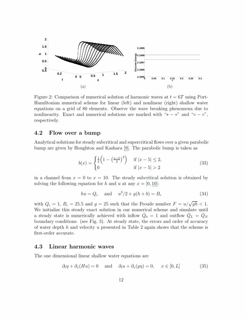
Figure 2: Comparison of numerical solution of harmonic waves at t = 6T using Port-Hamiltonian numerical scheme for linear (left) and nonlinear (right) shallow waterequations on a grid of 80 elements. Observe the wave breaking phenomena due tononlinearity. Exact and numerical solutions are marked with “∗ − ∗” and “ − ”,respectively.

4.2 Flow over a bump

Analytical solutions for steady subcritical and supercritical flows over a given parabolicbump are given by Houghton and Kashara [9]. The parabolic bump is taken as

b(x) =

1

2

(

1 −(

x−5

2

)2)

if |x− 5| ≤ 2,

0 if |x− 5| > 2(33)

in a channel from x = 0 to x = 10. The steady subcritical solution is obtained bysolving the following equation for h and u at any x = [0, 10]:

hu = Qc and u2/2 + g(h+ b) = Bc (34)

with Qc = 1, Bc = 25.5 and g = 25 such that the Froude number F = u/√gh < 1.

We initialize this steady exact solution in our numerical scheme and simulate untila steady state is numerically achieved with inflow Q0 = 1 and outflow QL = QN

boundary conditions. (see Fig. 3). At steady state, the errors and order of accuracyof water depth h and velocity u presented in Table 2 again shows that the scheme isfirst-order accurate.

4.3 Linear harmonic waves

The one dimensional linear shallow water equations are

∂tη + ∂x(Hu) = 0 and ∂tu+ ∂x(gη) = 0, x ∈ [0, L] (35)

12

0 2 4 6 8 100

0.5

1

1.5

x

b, h

+b

(a) Water depth (h)

0 2 4 6 8 100.5

1

1.5

2

2.5

3

x

u

(b) Velocuty (u)

Figure 3: Comparison of numerical solution (“–”) of steady subcritical flow over bumpagainst steady exact solution (“”) on a mesh stencil with 40 elements.

Table 2: Errors in L2 and L∞ norms for water depth h and velocity u of subcriticalflow over bump at steady state.

Water depth (h) Velocity (u)Grid L2error order L∞error order L2error order L∞error order

20 9.5631e-02 – 9.1603e-02 – 2.3890e-01 – 2.0586e-01 –40 4.7945e-02 1.00 4.8336e-02 0.92 1.1895e-01 1.01 1.0469e-01 0.9880 2.3993e-02 1.00 2.4670e-02 0.97 5.9490e-02 1.00 5.1709e-02 1.02160 1.1999e-02 1.00 1.2467e-02 0.98 2.9757e-02 1.00 2.5698e-02 1.01

13

with Hamiltonian H :=∫ L

0(Hu2 + gη2)/2dx. They satisfy a harmonic wave solution,

η(x, t) = A sin(kx+ ωt), and u(x, t) =(−Agk

ω

)

sin(kx+ ωt) (36)

with A the amplitude, k = 2πm/L the wave number, ω the frequency, T = 2π/ωthe time period, L the length of the domain, H the average water depth, ω2 = k2gHthe dispersion relation, m any integer, and periodic boundary conditions. The Port-Hamiltonian scheme for linear shallow water equations is easily derived by treating has η and defining B := gη and Q := Hu.

We first initialized the exact solution (36) in the numerical scheme for linearshallow water equations setting A = 0.01, L = 1, m = 1, g = 1 and H = 1. Linearharmonic waves are then simulated for 50 time periods on grids of size 20, 40, 80and 160 elements with time step ∆t = T/32, T/64, T/128 and T/256, respectively.Subsequently, we display the plots of free surface perturbation η(t, x) at time t = 50Tand the discrete energy w.r.t time in Fig. 4. It is clearly observed that discrete energyis conserved and consequently, there is no dissipation in the amplitude of the waveseven after 50 time periods. However, the numerical scheme displays a dispersion errorin the simulated waves which decreases from coarse to fine grids. Further, to showthat the scheme is first-order accurate, we present numerical errors and orders ofaccuracy in Table. 3 at various time instants.

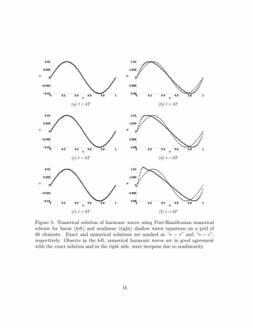
Second, we initialized harmonic waves (36) in the Port-Hamiltonian scheme fornonlinear shallow water equations with h(t, x) := H + η(t, x) and simulated until thesmooth initial linear waves break because of the nonlinearity. To demonstrate theseeffects of nonlinearity, we compare the space-time evolution of harmonic waves usinglinear and nonlinear schemes in Fig. 5.

4.4 Standing waves

The one-dimensional linear shallow water equations (35) also satisfy a standing wavesolution,

η(x, t) = A cos(kx) cos(ωt) and u(x, t) =(Agk

ω

)

sin(kx) sin(ωt) (37)

with solid wall boundary conditions at x = 0 and x = L. Standing wave solution(37) is initialized in the numerical scheme for linear shallow water equations settingA = 0.01, L = 1, m = 1, g = 1 and H = 1. Comparison of the numerical solutionof standing wave against its exact solution after one time period and the discreteenergy conservation in time is shown in Fig. 6(a) and (b). Numerical errors andthe corresponding orders of accuracy tabulated in Table 4 infers that the scheme isfirst-order accurate.

14

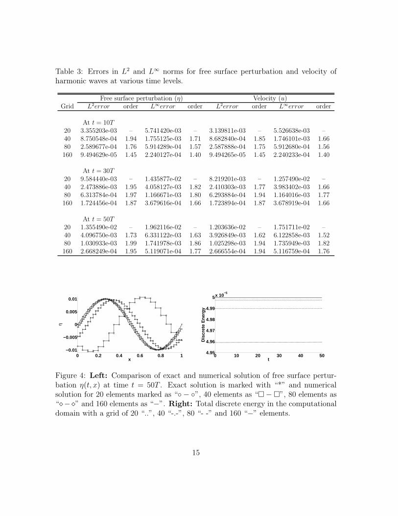
Table 3: Errors in L2 and L∞ norms for free surface perturbation and velocity ofharmonic waves at various time levels.

Free surface perturbation (η) Velocity (u)Grid L2error order L∞error order L2error order L∞error order

At t = 10T20 3.355203e-03 – 5.741420e-03 – 3.139811e-03 – 5.526638e-03 –40 8.750548e-04 1.94 1.755125e-03 1.71 8.682840e-04 1.85 1.746101e-03 1.6680 2.589677e-04 1.76 5.914289e-04 1.57 2.587888e-04 1.75 5.912680e-04 1.56160 9.494629e-05 1.45 2.240127e-04 1.40 9.494265e-05 1.45 2.240233e-04 1.40

At t = 30T20 9.584440e-03 – 1.435877e-02 – 8.219201e-03 – 1.257490e-02 –40 2.473886e-03 1.95 4.058127e-03 1.82 2.410303e-03 1.77 3.983402e-03 1.6680 6.313784e-04 1.97 1.166671e-03 1.80 6.293884e-04 1.94 1.164016e-03 1.77160 1.724456e-04 1.87 3.679616e-04 1.66 1.723894e-04 1.87 3.678919e-04 1.66

At t = 50T20 1.355490e-02 – 1.962116e-02 – 1.203636e-02 – 1.751711e-02 –40 4.096750e-03 1.73 6.331122e-03 1.63 3.926849e-03 1.62 6.122858e-03 1.5280 1.030933e-03 1.99 1.741978e-03 1.86 1.025298e-03 1.94 1.735949e-03 1.82160 2.668249e-04 1.95 5.119071e-04 1.77 2.666554e-04 1.94 5.116759e-04 1.76

0 0.2 0.4 0.6 0.8 1−0.01

−0.005

0

0.005

0.01

x

η

0 10 20 30 40 504.95

4.96

4.97

4.98

4.99

5x 10−5

t

Dis

cret

e E

nerg

y

Figure 4: Left: Comparison of exact and numerical solution of free surface pertur-bation η(t, x) at time t = 50T . Exact solution is marked with “*” and numericalsolution for 20 elements marked as “ − ”, 40 elements as “ − ”, 80 elements as“⋄−⋄” and 160 elements as “−”. Right: Total discrete energy in the computationaldomain with a grid of 20 “..”, 40 “-.-”, 80 “- -” and 160 “−” elements.

15

0 0.2 0.4 0.6 0.8 1−0.01

−0.005

0

0.005

0.01

x

η

(a) t = 4T

0 0.2 0.4 0.6 0.8 10.99

0.995

1

1.005

1.01

x

h

(b) t = 4T

0 0.2 0.4 0.6 0.8 1−0.01

−0.005

0

0.005

0.01

x

η

(c) t = 6T

0 0.2 0.4 0.6 0.8 10.99

0.995

1

1.005

1.01

x

h

(d) t = 6T

0 0.2 0.4 0.6 0.8 1−0.01

−0.005

0

0.005

0.01

x

η

(e) t = 8T

0 0.2 0.4 0.6 0.8 10.99

0.995

1

1.005

1.01

x

h

(f) t = 8T

Figure 5: Numerical solution of harmonic waves using Port-Hamiltonian numericalscheme for linear (left) and nonlinear (right) shallow water equations on a grid of80 elements. Exact and numerical solutions are marked as “∗ − ∗” and “ − ”,respectively. Observe in the left, numerical harmonic waves are in good agreementwith the exact solution and in the right side, wave steepens due to nonlinearity.

16

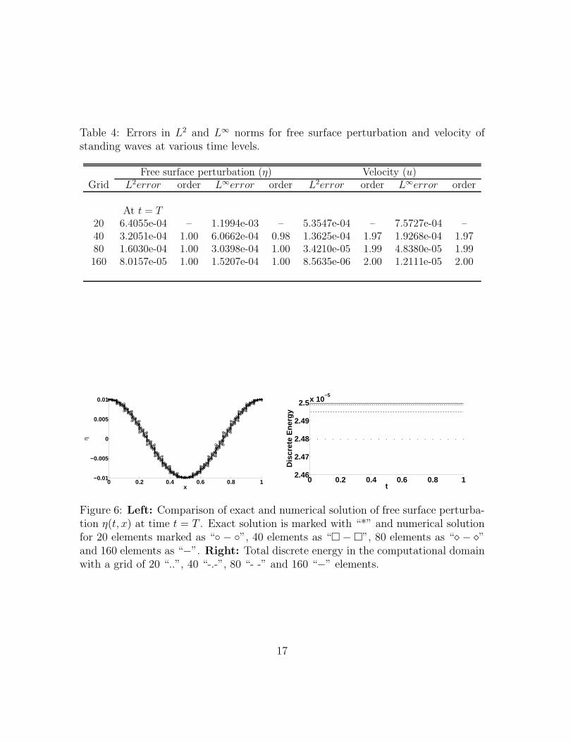
Table 4: Errors in L2 and L∞ norms for free surface perturbation and velocity ofstanding waves at various time levels.

Free surface perturbation (η) Velocity (u)Grid L2error order L∞error order L2error order L∞error order

At t = T20 6.4055e-04 – 1.1994e-03 – 5.3547e-04 – 7.5727e-04 –40 3.2051e-04 1.00 6.0662e-04 0.98 1.3625e-04 1.97 1.9268e-04 1.9780 1.6030e-04 1.00 3.0398e-04 1.00 3.4210e-05 1.99 4.8380e-05 1.99160 8.0157e-05 1.00 1.5207e-04 1.00 8.5635e-06 2.00 1.2111e-05 2.00

0 0.2 0.4 0.6 0.8 1−0.01

−0.005

0

0.005

0.01

x

η

0 0.2 0.4 0.6 0.8 12.46

2.47

2.48

2.49

2.5x 10−5

t

Dis

cret

e E

nerg

y

Figure 6: Left: Comparison of exact and numerical solution of free surface perturba-tion η(t, x) at time t = T . Exact solution is marked with “*” and numerical solutionfor 20 elements marked as “ − ”, 40 elements as “ − ”, 80 elements as “⋄ − ⋄”and 160 elements as “−”. Right: Total discrete energy in the computational domainwith a grid of 20 “..”, 40 “-.-”, 80 “- -” and 160 “−” elements.

17

5 Conclusions

A finite-dimensional Port-Hamiltonian formulation for the nonlinear shallow waterequations denned with respect to a Stokes’ Dirac structure is presented. The keyadvantage of this formulation is that the physical properties of the infinite-dimensionalmodel, such as mass and energy conservation, are directly translated into the finite-dimensional model. Thus, the finite-dimensional model of shallow water equationspreserves discrete mass and energy in time.

It is useful to extend the present formulation to the shallow water equations intwo dimensions and capture its important physical properties such as the conservationof potential vorticity and enstrophy that are of great interest in oceanographic andmeteorological studies. An important aspect of the Port-Hamiltonian formulation isthat it accommodates the flow control design through energy shaping methods. Itremains open to develop such a control design even for these simple open channelflows.

The Port-Hamiltonian based numerical scheme for the shallow water equations isdeveloped and verified against exact solutions. This numerical scheme uses a implicitmid-point time discretization that is symplectic and preserves the discrete energy tosufficient precision in time. The present numerical scheme is first order accurate andonly valid for smooth open channel flows as the underlying governing equations arein the primitive form. For non-smooth flows, the conservative form of shallow waterequations are required as they satisfy the jump conditions at the bores or hydraulicjumps with the correct energy dissipating conditions. This was beyond the scope ofour present work.

Acknowledgements

V.A. thanks Dr. O. Bokhove for giving many useful suggestions on time discretiza-tion. R.P. and V.A. gratefully acknowledge a research grant from Dept. of ElectricalEngineering, University of Melbourne, Australia.

References

[1] R. Abraham, J.E. Marsden, T. Ratiu, Manifolds, Tensor Analysis, and Applica-tions. Springer-Verlag, 1988.

[2] V.R. Ambati, O. Bokhove, Space-time discontinuous Galerkin finite element forshallow water flows, J. Comput. Appl. Math., 204 (2), 452–462, 2007.

[3] V.R. Ambati, O. Bokhove, Space-time discontinuous Galerkin discretization ofrotating shallow water equations, J. Comput. Phys., 225(2), 1233–1261, 2007.

18

[4] E. Audusse, F. Bouchut, M.-O. Bristeau, R. Klein, B. Perthame, A fast andstable well-balanced scheme with hydrostatic reconstruction for shallow waterflows, SIAM J. Sc. Comp., 25(6), 2050–2065, 2004.

[5] E. Audusse, M.-O. Bristeau, A well-balanced positivity preserving second orderscheme for shallow water flows on unstructured meshes, J. Comp. Phys., 206,311–333, 2005.

[6] O. Bokhove, M. Oliver, Parcel Eulerian-Lagrangian fluid dynamics for rotatinggeophysical flows, Proc. Roy. Soc. A. 462, 2575–2592, 2006.

[7] J. Frank, S. Reich, The Hamiltonian particle mesh method for the sphericalshallow water equations. Atmos. Sci. Lett. 5, 89–95, 2004.

[8] E. Hairer, C. Lubich, G. Wanner, Geometric Numerical Integration: Structure-Preserving Algorithms for Ordinary Differential Equations, 2nd Ed., SpringerSeries in Computational Mathematics, Springer-Verlag, Berlin, 2006.

[9] D.D. Houghton and A. Kasahara, Nonlinear shallow fluid flow over an isolatedridge, Commun. Pure Appl. Math., 21, 1–23, 1968.

[10] B.M. Maschke and A.J. van der Schaft, Port controlled Hamiltonian represen-tation of distributed parameter systems, In N.E. Leonard, R. Ortega (Eds.),Proceedings of IFAC workshop on Lagrangian and Hamiltonian methods fornonlinear control, Princeton University, 28–38, 2000.

[11] P.J. Morrison, Hamiltonian description of the ideal fluid, Rev. Mod. Phys., 70,467–521, 1998.

[12] P.J. Olver. Applications of Lie Groups to Differential Equations, 2nd Ed.,Springer, Berlin, 1993.

[13] R.Pasumarthy, A.J van der Schaft. A port-Hamiltonian approach to modelingand interconnections of canal systems. In proceedings: 16th International Sym-posium on Mathematical Theory of Networks and Systems, Kyoto, July 24–28,2006.

[14] H. Rodriguez, A.J. van der Schaft and R. Ortega. On stabilization of nonlineardistributed parameter port-controlled Hamiltonian systems via energy shaping.In Proceedings of the 40th IEEE conference on decision and control, Orlando,FL, December 2001.

[15] P.A. Tassi, O. Bokhove, C.A. Vionnet, Space discontinuous Galerkin method forshallow water flows-kinetic and HLLC flux, and potential vorticity generation,Advances in Water Resources, 30(4), 998–1015, 2007.

19

[16] A.J. van der Schaft and B.M. Maschke, Hamiltonian formulation of distributed-parameter systems with boundary energy flow, Journal of Geometry and Physics,42, 166–194, 2002.

[17] A.J. van der Schaft, L2-Gain and Passivity Techniques in Nonlinear Control,Springer-Verlag, 2000.

20