GÜNTÜRKÜN

Polygon

16

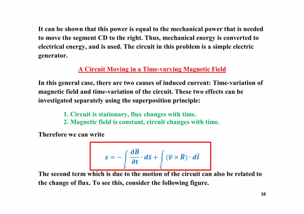
It can be shown that this power is equal to the mechanical power that is needed to move the segment CD to the right. Thus, mechanical energy is converted to electrical energy, and is used. The circuit in this problem is a simple electric generator.

A Circuit Moving in a Time-varying Magnetic Field

In this general case, there are two causes of induced current: Time-variation of magnetic field and time-variation of the circuit. These two effects can be investigated separately using the superposition principle:

1. Circuit is stationary, flux changes with time. 2. Magnetic field is constant, circuit changes with time.

Therefore we can write

휺 = −흏푩흏풕

∙ 풅풔푺

+ (풗 × 푩) ∙ 풅풍̅푪

The second term which is due to the motion of the circuit can also be related to the change of flux. To see this, consider the following figure.

26

훁 × 푬 = −흏푩흏풕

(ퟏ) This is Maxwell's 1st equation. B) Gauss law is valid in time-varying case too.

푫 ∙ 풅풔푺

= 푸 ⇒ 훁 ∙ 푫풅풗푽

= 흆풗풅풗푽

⇒ 훁 ∙ 푫 = 흆풗(ퟐ) This is Maxwell's 3rd equation. C) Conservation of magnetic flux:

푩 ∙ 풅풔푺

= ퟎ ⇒ 훁 ∙ 푩풅풗푽

= ퟎ

⇒ 훁 ∙ 푩 = ퟎ(ퟑ)퐌퐚퐱퐰퐞퐥퐥′퐬ퟒ퐭퐡퐞퐪퐧

27

D) Maxwell’s 2nd Equation

훁 × 푬 = ퟎ which is valid in electrostatics becomes 훁 × 푬 = −흏푩 흏풕 in time-

varying case. It means time-varying magnetic fields create electric field. Starting from here we can deduce directly that, the equation 훁 ×푯 = 푱̅ must also be modified and time derivative of the electric field must be present on the RHS of this equation. Recall the continuity equation which states the conservation of charge:

훁 ∙ 푱̅ = −흏흆풗흏풕

Now if we take the divergence of both sides of the equation 훁 ×푯 = 푱̅, we find

훁 ∙ (훁 × 푯) = 훁 ∙ 푱̅ ⇒ 훁 ∙ 푱̅ ≡ ퟎ

which is not valid for the time-varying case. This situation must be corrected. Now re-write the equation using the correction term 푮 as

훁 × 푯 = 푱̅ + 푮

and take divergence of both sides again. We obtain:

28

훁 ∙ (훁 × 푯) = 훁 ∙ (푱̅ + 푮) ≡ ퟎ

⇒훁 ∙ 푱̅ = −훁 ∙ 푮 = −흏흆풗흏풕

⇒훁 ∙ 푮 =흏흆풗흏풕

=흏흏풕(훁 ∙ 푮) = 훁 ∙

흏푫흏풕

Now, since the two divergences are equal we find:

푮 =흏푫흏풕

In fact, the result would not be affected if vectors with vanishing divergence are added to this term. However, it is verified experimentally that no such term is needed.

훁 × 푯 = 푱̅ +흏푫흏풕

Equation (4) shows that the vector sources of 푯 are 푱̅ and the displacement current given by:

푱̅풅 =흏푫흏풕

29

Thus, even in the case of 푱̅ = ퟎ, if there is a time-varying 푫 field then 푯 will not be zero.

Equation (4) together with Faraday's law explains electromagnetic wave propagation.

Displacement field:

푱̅ ≡ currentdensity(Amp/mퟐ)

Conduction current density: Convection current density: Exists in metals. Created by charge movement.

푱̅ = 흈푬 푱̅ = 흆풗

Now let us investigate 흏푫흏풕

term. Since ∮ 푫 ∙ 풅풔푺 = 푸 (Coul), the unit of 푫 is Coul/m2. Then we can write:

흏푫흏풕

=Coul/mퟐ

sec=Ampmퟐ

30

Hence 흏푫흏풕

term has the unit of current density. This is why this term is called the displacement current.

훁 × 푯 = 푱̅ + 푱̅풅

푱̅풅 is important in the explanation of wave propagation.

Now, let us take surface integral of both sides of the equation 훁 × 푯 = 푱̅ + 흏푫흏풕

.

훁 × 푯 ∙ 풅풔푺

= 푱̅ ∙ 풅풔푺

+흏푫흏풕

∙ 풅풔푺

If we use Stokes' theorem in the first term we find:

푯 ∙ 풅풍̅푪

= 푱̅ ∙ 풅풔푺

+흏푫흏풕

∙ 풅풔푺

= 푰 + 푰풅

Here, I is the real (conduction) current, and Id is the displacement current.

Time variation of 푬, and consequently 푫 behaves like a current effectively.