Models and Solution Techniques for Frequency Assignment Problems: updated
57
DOI: 10.1007/s10288-003-0022-6 4OR 1: 261–317 (2003) Invited survey Models and solution techniques for frequency assignment problems Karen I. Aardal 1 , Stan P.M. van Hoesel 2 , Arie M.C.A. Koster 3 , Carlo Mannino 4 , and Antonio Sassano 4 1 School of Industrial and Systems Engineering, Georgia Institute of Technology, Atlanta, GA 30332-0205, USA 2 Department of Quantitative Economics, Universiteit Maastricht, P.O.Box 616, 6200 MD Maastricht, The Netherlands 3 Konrad-Zuse-Zentrum für Informationstechnik Berlin, Takustraße 7, 14195 Berlin, Germany (e-mail: [email protected]) 4 Dipartimento di Informatica e Sistemistica, Università di Roma “La Sapienza”, Via Buonarroti 12, 00185 Roma, Italy Received: May 2003 / Revised version: September 2003 Abstract. Wireless communication is used in many different situations such as mobile telephony, radio and TV broadcasting, satellite communication, and military operations. In each of these situations a frequency assignment problem arises with application specific characteristics. Researchers have developed different modeling ideas for each of the features of the problem, such as the handling of interference among radio signals, the availability of frequencies, and the optimization criterion. This survey gives an overview of the models and methods that the literature provides on the topic. We present a broad description of the practical settings in which frequency assignment is applied. We also present a classification of the different models and formulations described in the literature, such that the common features of the models are emphasized. The solution methods are divided in two parts. Optimization and lower bounding techniques on the one hand, and heuristic search techniques on the other hand. The literature is classified according to the used methods. Again, we emphasize the common features, used in the different papers. The quality of the solution methods is compared, whenever possible, on publicly available benchmark instances. Key words: Frequency assignment, channel assignment, models, exact methods, heuristics AMS classification: 90-02, 90C35, 05C90 Research carried out with financial support of the project TMR-DONET nr. ERB FMRX-CT98- 0202 of the European Community. Correspondence to: Arie M.C.A. Koster 4OR Quarterly Journal of the Belgian, French and Italian Operations Research Societies © Springer-Verlag 2003
Transcript of Models and Solution Techniques for Frequency Assignment Problems: updated
DOI: 10.1007/s10288-003-0022-6
4OR 1: 261–317 (2003) Invited survey
Models and solution techniquesfor frequency assignment problems�
Karen I. Aardal1, Stan P.M. van Hoesel2, Arie M.C.A. Koster3,Carlo Mannino4, and Antonio Sassano4
1 School of Industrial and Systems Engineering, Georgia Institute of Technology, Atlanta,GA 30332-0205, USA
2 Department of Quantitative Economics, Universiteit Maastricht, P.O.Box 616, 6200 MD Maastricht,The Netherlands
3 Konrad-Zuse-Zentrum für Informationstechnik Berlin, Takustraße 7, 14195 Berlin, Germany(e-mail: [email protected])
4 Dipartimento di Informatica e Sistemistica, Università di Roma “La Sapienza”, Via Buonarroti 12,00185 Roma, Italy
Received: May 2003 / Revised version: September 2003
Abstract. Wireless communication is used in many different situations such asmobile telephony, radio and TV broadcasting, satellite communication, and militaryoperations. In each of these situations a frequency assignment problem arises withapplication specific characteristics. Researchers have developed different modelingideas for each of the features of the problem, such as the handling of interferenceamong radio signals, the availability of frequencies, and the optimization criterion.
This survey gives an overview of the models and methods that the literatureprovides on the topic. We present a broad description of the practical settingsin which frequency assignment is applied. We also present a classification of thedifferent models and formulations described in the literature, such that the commonfeatures of the models are emphasized. The solution methods are divided in twoparts. Optimization and lower bounding techniques on the one hand, and heuristicsearch techniques on the other hand. The literature is classified according to theused methods. Again, we emphasize the common features, used in the differentpapers. The quality of the solution methods is compared, whenever possible, onpublicly available benchmark instances.
Key words: Frequency assignment, channel assignment, models, exact methods,heuristics
AMS classification: 90-02, 90C35, 05C90
� Research carried out with financial support of the project TMR-DONET nr. ERB FMRX-CT98-0202 of the European Community.Correspondence to: Arie M.C.A. Koster
4OR Quarterly Journal of the Belgian, Frenchand Italian Operations Research Societies
© Springer-Verlag 2003
262 K.I. Aardal et al.
1 Introduction
The literature on frequency assignment problems, also called channel assignmentproblems, has grown quickly over the past years. This is mainly due to the fastimplementation of wireless telephone networks (e.g., GSM networks) and satellitecommunication projects. The renewed interest in other applications like TV broad-casting and military communication problems also inspired new research. All theseapplications lead to many different models, and within the models to many differenttypes of instances. Nevertheless, all of them share two common features:
1. A set of wireless communication connections (or a set of antennae) must beassigned frequencies such that data transmission between the two endpointsof each connection (the transceivers) is possible. The frequencies should beselected from a given set that may differ among connections.
2. The frequencies assigned to two connections may incur interference to oneanother, resulting in quality loss of the signal. Two conditions must be fulfilledin order to have interference of two signals:(a) The two frequencies must be close on the Electromagnetic band. Harmonics
may also interfere due to the Doppler effect, but the parts of the Electro-magnetic band that are generally selected prevent this type of interference.
(b) Connections must be geographically close to each other, so that interferingsignals are powerful enough to disturb the quality of a signal.
Frequency assignment problems (FAPs) first appeared in the 1960s (Metzger1970). The development of new wireless services such as the first cellular phonenetworks led to scarcity of usable frequencies in the radio spectrum. Frequencieswere licensed by the government who charged operators for the usage of eachsingle frequency separately. This introduced the need for operators to develop fre-quency plans that not only avoided high interference levels, but also minimized thelicensing costs. It turned out that it was far from obvious to find such a plan. Atthis point, operations research techniques and graph theory were introduced. Met-zger (1970) usually receives the credits for pointing out the opportunities of usingmathematical optimization, especially graph coloring techniques, for this purpose.Until the early 1980s, most contributions on frequency assignment used heuristicsbased on the related graph coloring problem. First lower bounds were derived byGamst and Rave (1982) for the most common problem of that time (cf., Sect. 4).The development of the digital cellular phone standard GSM (General System forMobile Communication) in the late 1980s and 1990s led to a rapidly increasinginterest for frequency assignment (see Eisenblätter 2001 for a discussion of thetypical frequency planning problems in GSM networks). But also projects on otherapplications such as military wireless communication and radio-TV broadcastingcontributed to the literature on frequency assignment in recent years.
This paper is not the first survey on the frequency assignment problem. Hale(1980) presented an overview of the frequency planning problems of that time, witha special focus on modeling the problems. Hale also discussed the relation of the
Frequency assignment problems 263
FAP with graph (vertex) coloring. In particular, the relation of FAPs with the T -coloring problem were introduced by Hale. This led to many new (graph-theoretic)results, in the early 1990s surveyed in Roberts (1991). The survey of Murphey etal. (1999) also concentrates on the results for coloring generalizations that weremotivated by frequency assignment. In Jaumard et al. (1999), a brief description ofseveral exact methods is presented. The survey in Koster (1999, Chapt. 2) served asa starting point of this overview. Finally, Eisenblätter et al. (2002) give an overviewof the evolution of frequency planning from graph coloring and its generalizationsto the models used nowadays, with an emphasis on the GSM practice. The bookby Leese and Hurley (2002) discusses several aspects of spectrum management,and in particular approaches for frequency planning. In this survey, we also restrictourselves to models that are directly motivated from practice, and their solutionmethods.
We only discuss Fixed ChannelAssignment (FCA), i.e., static models where theset of connections remains stable over time. Opposite to FCA, Dynamic ChannelAssignment (DCA) deals with the problem, where the demand for frequencies atan antenna varies over time. Hybrid Channel Assignment (HCA) combines FCAand DCA: a number of frequencies have to be assigned beforehand, but space in thespectrum has to be reserved for the online assignment of frequencies upon request.We refer to Katzela and Naghshineh (1996) for a recent survey on DCA and HCA.
The focus of this manuscript is mainly on the practical relevance of mathemat-ical optimization techniques for frequency assignment. In the next section we willdiscuss the practical settings of the problem in such a way that the common featuresare emphasized. In Sect. 3, we will categorize the models in four standard classes.These categories mainly differ in the objective to be optimized. For each of themodels, the subsequent sections will discuss:
1. structural properties of the models, including bounding techniques based on(combinatorial) relaxations (Sect. 4),
2. exact optimization methods, such as branch-and-cut, branch-and-price, andcombinatorial enumeration (Sect. 4 as well), and
3. heuristic methods, such as local search (including simulated annealing and tabusearch), genetic algorithms, neural networks, constraint programming, and antcolony algorithms. (Sect. 5).
Although we invested much effort in collecting as many papers on the topic aspossible, it is impossible to guarantee completeness. Moreover, new publicationswill reduce the actuality of this survey. Therefore, this survey is accompanied bythe web site FAPweb (2000–2003) (http://fap.zib.de) that contains an overview ofthe results for the available benchmark instances. Moreover, all discussed papersare summarized in a schematic way at this web site. This overview of results andthe digest on frequency assignment literature will be regularly updated. This sitealso serves as a platform for announcing new papers on frequency assignment.
264 K.I. Aardal et al.
2 Practical applications
This section starts with a description of the most important aspects of frequencyassignment, namely the availability of frequencies and the ways of handling inter-ference. Then an overview of situations in which frequency assignment problemsoccur is provided, including application specific characteristics.
2.1 Availability and interference of frequencies
The availability of frequencies from the radio spectrum is regulated by the na-tional governments, and world-wide by the International Telecommunication Union(ITU). Operators of wireless services are licensed to use one or more frequencybands in specific parts of a country. The frequency band [fmin, fmax] available tosome provider of wireless communication is usually partitioned into a set of chan-nels, all with the same bandwidth � of frequencies. For this reason the channels(actually the channels are often called frequencies) are usually numbered from 1 toa given maximum N , where N = (fmax −fmin)/�. The available channels are de-noted by F = {1, . . . , N}. If more than one frequency band is available each bandhas its own set of consecutively numbered channels. For a particular connection orantenna not all channels from F might be available. For instance, if a connection isclose to the border of a country, division rules between the countries involved maylead to a substantial reduction in channel availability.
Therefore, the channels available for a connection or antenna v form a subsetF(v) of F .
Interference of signals is measured by the signal-to-noise ratio, or interferenceratio, at the receiving end of a connection. There, the signal of the transmitting endshould be clearly understandable. The noise comes from other signals broadcastedat interfering frequencies. In general, the level of interference rapidly decreaseswith the distance between the frequencies. The actual signal-to-noise ratio at areceiver depends not only on the choice of frequency, but also on the strength ofthe signal, the direction it is transmitted to, the shape of the environment, and evenweather conditions. It is therefore hard to obtain an accurate prediction of the signal-to-noise ratio at receivers. A first simplification is to ignore the environment andassume an omni-directional antenna. Now, consider two signals, one original andsome other signal transmitted at the same frequency channel. Then the interferenceof the second signal at the receiver of the first signal is computed with the followingformula: P
dγ where P is the power of the interfering transmitter and d its distanceto the disturbed receiver. γ is a fading factor with values between 2 and 4. Itsvalue depends on the frequency used. For instance the 1800 MHz band frequenciesfade faster than the 900 MHz band frequencies both used in GSM networks. Ifthe second signal is transmitted on a frequency at a distance of n ≥ 1 units fromthe original signal, then an additional filtering factor of −15(1 + log2 n) dB istaken into account (see Dunkin and Allen 1997). There may be more than one
Frequency assignment problems 265
source that transmits on the same or a close frequency and thus contributes to thetotal noise experienced at the receiver. The fact that multiple signals may disturbcommunication quality is ignored in most models where only interference betweenpairs of connections or antennae is measured. Notable exceptions are Fischetti etal. (2000), in which constraints are developed to determine the total interferencefrom neighboring connections, and Dunkin et al. (1998), where combinations offrequencies for more than two transmitters are forbidden. We will generally ignoremultiple interference. So it becomes a binary relation: only two connections orantennae are involved.
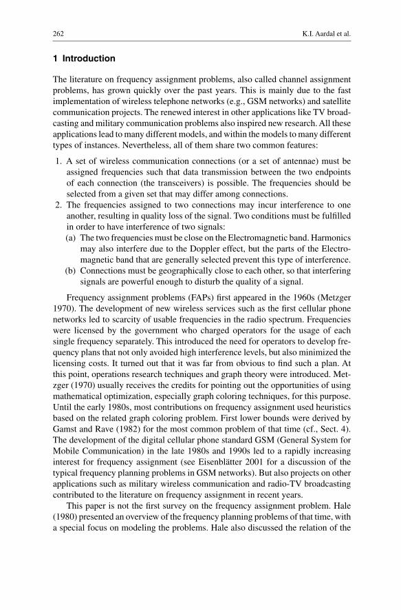
In mobile telephony and radio-TV broadcasting, the receivers are spread withina certain area. The standard approach of determining signal strength at all locationsin the area is the following.
1. A grid of squares of predetermined (small) size, the test points or pixels, isdesigned to overlap the area.
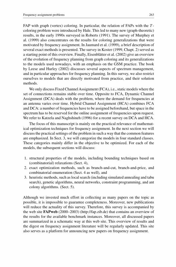
2. For each test point, the levels of the received signals generated by the servingtransmitter, typically the one with the strongest received signal (best server),and by the interfering transmitters are predicted with a wave propagation model.Test points with same best server can be clustered to service areas, resulting inpictures like the one in Fig. 1.
3. For a single transmitter A, and a given interfering transmitter B, the noisegenerated by B in each pixel of the service area of A is aggregated to a singlevalue, which represents the interference of B over A.
The way noise is predicted and aggregated strongly depends on the applicationconsidered. For precise descriptions of wave propagation models used for this task,see Correia (2001).
In the past, more simplified prediction models were used: a standard approachwas to use a grid of hexagons overlapping the area of interest and to consider thetransmitters to be located at the center of each hexagon. The well-known Philadel-phia instances (cf., Sect. 2.2) have this structure (see Fig. 4, p. 269). In the basicmodel for the hexagonal grids, interference of cells is characterized by a co-channelreuse distance d. No interference occurs if and only if the centers of two cells havemutual distance ≥ d . In case the mutual distance is less than d (normalized bythe radius of the cells), it is not allowed to assign the same frequency to bothcells. This pure co-channel case is generalized by replacing the reuse distance d
by a series of non-increasing values d0, . . . , dk and corresponding forbidden setsT 0 ⊆ . . . ⊆ T k . The following relation holds:
Tvw = T j−1 whenever dj ≤ dvw < dj−1, j ∈ {1, . . . , k}where dvw is the distance between the cell centers and Tvw denotes the set of for-bidden differences for frequencies assigned to v and w, i.e., |fv − fw| �∈ Tvw.For the variations of the original Philadelphia instance, the sets T j are taken asT j = {0, . . . , j}. For example, the values d0, . . . , d5 are 2
√3,
√3, 1, 1, 1, 0. So,
266 K.I. Aardal et al.
Fig. 1. Best-server areas in a GSM network. Provided by E-Plus Mobilfunk GmbH
� � � �
� � � � �
� � � � � �
� � � � � � �
� � � � � �
� � � � �
� � � �
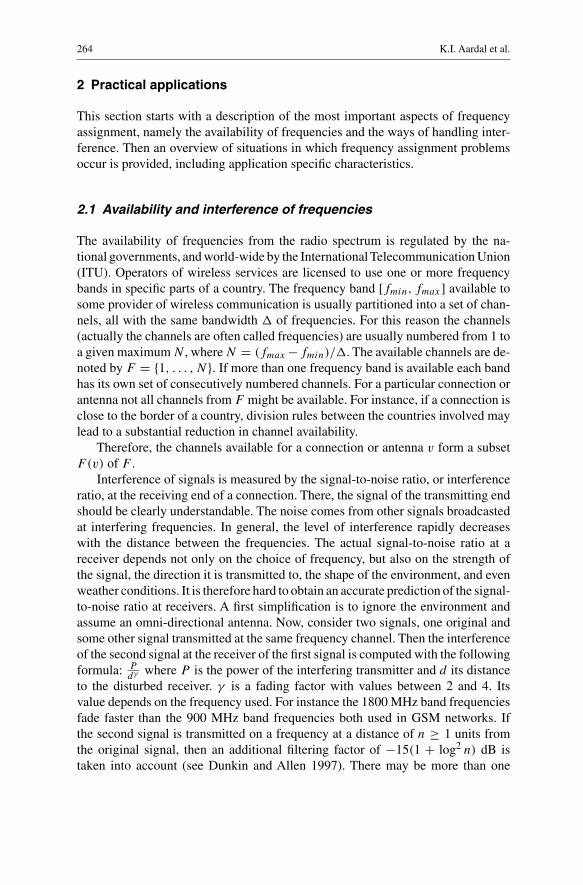
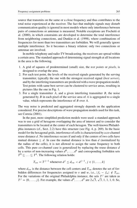
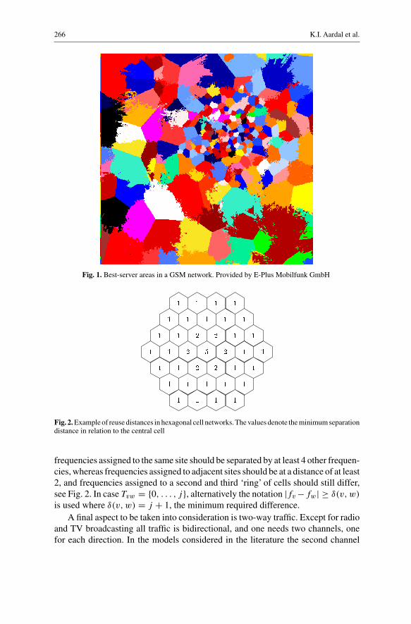
Fig. 2. Example of reuse distances in hexagonal cell networks. The values denote the minimum separationdistance in relation to the central cell
frequencies assigned to the same site should be separated by at least 4 other frequen-cies, whereas frequencies assigned to adjacent sites should be at a distance of at least2, and frequencies assigned to a second and third ‘ring’ of cells should still differ,see Fig. 2. In case Tvw = {0, . . . , j}, alternatively the notation |fv −fw| ≥ δ(v, w)
is used where δ(v, w) = j + 1, the minimum required difference.A final aspect to be taken into consideration is two-way traffic. Except for radio
and TV broadcasting all traffic is bidirectional, and one needs two channels, onefor each direction. In the models considered in the literature the second channel
Frequency assignment problems 267
�
�
� �
�
�
� �
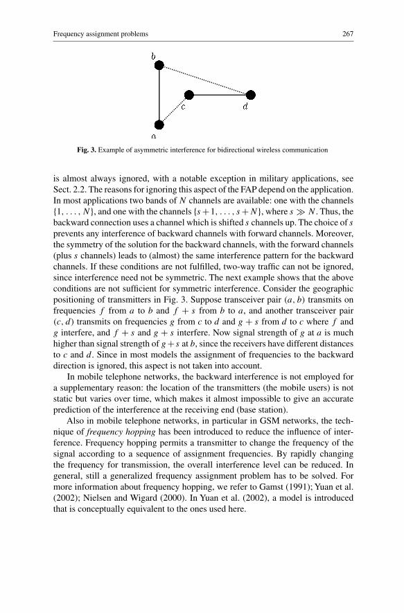
Fig. 3. Example of asymmetric interference for bidirectional wireless communication
is almost always ignored, with a notable exception in military applications, seeSect. 2.2. The reasons for ignoring this aspect of the FAP depend on the application.In most applications two bands of N channels are available: one with the channels{1, . . . , N}, and one with the channels {s +1, . . . , s +N}, where s � N . Thus, thebackward connection uses a channel which is shifted s channels up. The choice of s
prevents any interference of backward channels with forward channels. Moreover,the symmetry of the solution for the backward channels, with the forward channels(plus s channels) leads to (almost) the same interference pattern for the backwardchannels. If these conditions are not fulfilled, two-way traffic can not be ignored,since interference need not be symmetric. The next example shows that the aboveconditions are not sufficient for symmetric interference. Consider the geographicpositioning of transmitters in Fig. 3. Suppose transceiver pair (a, b) transmits onfrequencies f from a to b and f + s from b to a, and another transceiver pair(c, d) transmits on frequencies g from c to d and g + s from d to c where f andg interfere, and f + s and g + s interfere. Now signal strength of g at a is muchhigher than signal strength of g + s at b, since the receivers have different distancesto c and d. Since in most models the assignment of frequencies to the backwarddirection is ignored, this aspect is not taken into account.
In mobile telephone networks, the backward interference is not employed fora supplementary reason: the location of the transmitters (the mobile users) is notstatic but varies over time, which makes it almost impossible to give an accurateprediction of the interference at the receiving end (base station).
Also in mobile telephone networks, in particular in GSM networks, the tech-nique of frequency hopping has been introduced to reduce the influence of inter-ference. Frequency hopping permits a transmitter to change the frequency of thesignal according to a sequence of assignment frequencies. By rapidly changingthe frequency for transmission, the overall interference level can be reduced. Ingeneral, still a generalized frequency assignment problem has to be solved. Formore information about frequency hopping, we refer to Gamst (1991); Yuan et al.(2002); Nielsen and Wigard (2000). In Yuan et al. (2002), a model is introducedthat is conceptually equivalent to the ones used here.
268 K.I. Aardal et al.
2.2 Applications
There are various models and problem instances. The practical setting can varyenormously. This leads not only to different variants of the above model, but alsoto different instance types, see Hale (1980). Some of the settings are given below.
Mobile telephony. In this application one of the endpoints of the connection isa fixed antenna, and the other endpoint is a mobile phone. Each antenna coversa certain area, where it can pick up signals from mobile phones. Each antennacovers a specific region (cell) and can serve several mobile units simultaneously. Inparticular, in TDMA (Time Division Multiple Access) each available frequency canbe used to serve several different mobile units; in addition, multiple frequencies canbe assigned to the same antenna (by the use of multiple transmitter/receiver units,TRXs), so that the number of different mobile units that are served can be verylarge. More antennae are then mounted on a same physical support (site) to cover anumber of adjacent regions. In GSM networks, typically 8 units (channels) can beserved simultaneously using TDMA, by one TRX. Up to 12 TRXs can be installedon an antenna. Note that TRXs using the same antenna have high interferencerestrictions. For more details, we refer to Eisenblätter (2001).
The frequencies assigned to each antenna must satisfy a number of require-ments that depend on (i) availability, especially at country borders; (ii) interferencelevels; (iii) technological requirements; and (iv) size of the area with unacceptableinterference. Four types of constraints can be specified.
Co-cell separation constraint. The frequencies assigned to the same antenna v
must differ by at least δ(v, v) units (typically δ(v, v) = 3).
Co-site separation constraint. If u and v are co-site antennae, then typicallyδ(u, v) = 2.
Interference constraint. Due to interference, additional separations can be requiredbetween pairs of antennae not at the same site. Typically, such pairs u and v shouldhave different frequencies, i.e., δ(u, v) = 1, or frequencies at distance at least 2.
Constraints that forbid two cells to use the same frequency are often calledco-channel constraints. Constraints that forbid frequencies with distance 1, usuallyincluding distance 0, are called adjacent channel constraints.
Hand-over separation constraint. As the mobile unit moves from a cell u to anadjacent one v, control must be switched from u to v (hand-over or hand-off ),which in turn requires that the broadcasting frequencies used by u and v to servethe mobile, differ by at least one unit. Note that the actual situation, in for instanceGSM networks, is more complicated, since the control channels (BCCH) need moreprotection. This is in some countries translated into a desired distance of 2.
There are several sets of instances available from the literature. The most usedsets are the following.
Frequency assignment problems 269
� � � � �
� � � � � �� ��
�� �� �� �� �� ��
�� � ��
a
� �� � � �
�� �� �� �� �� �� ��
�� �� �� �� �� �
�� �� �
b
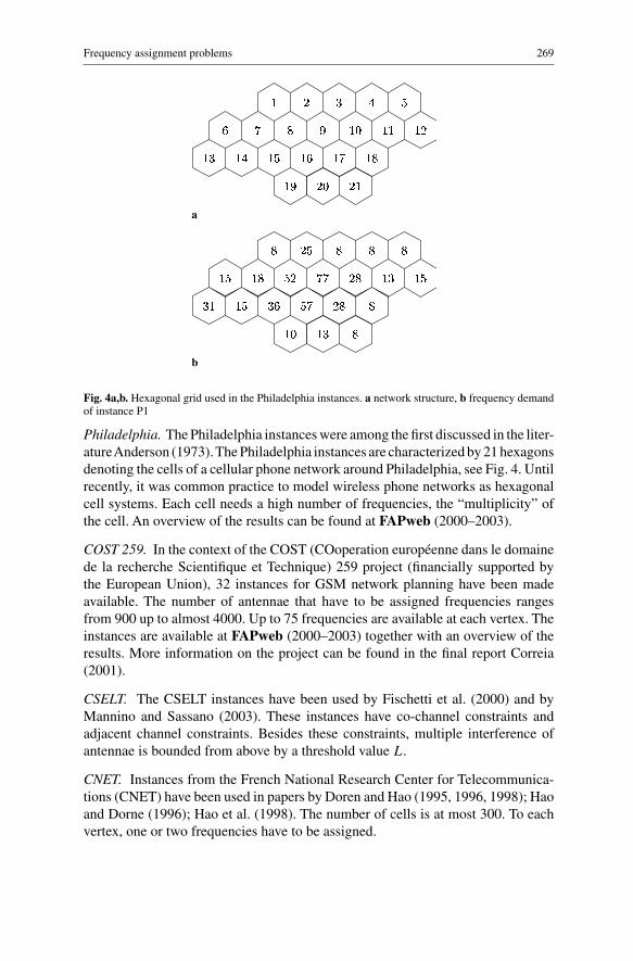
Fig. 4a,b. Hexagonal grid used in the Philadelphia instances. a network structure, b frequency demandof instance P1
Philadelphia. The Philadelphia instances were among the first discussed in the liter-atureAnderson (1973). The Philadelphia instances are characterized by 21 hexagonsdenoting the cells of a cellular phone network around Philadelphia, see Fig. 4. Untilrecently, it was common practice to model wireless phone networks as hexagonalcell systems. Each cell needs a high number of frequencies, the “multiplicity” ofthe cell. An overview of the results can be found at FAPweb (2000–2003).
COST 259. In the context of the COST (COoperation européenne dans le domainede la recherche Scientifique et Technique) 259 project (financially supported bythe European Union), 32 instances for GSM network planning have been madeavailable. The number of antennae that have to be assigned frequencies rangesfrom 900 up to almost 4000. Up to 75 frequencies are available at each vertex. Theinstances are available at FAPweb (2000–2003) together with an overview of theresults. More information on the project can be found in the final report Correia(2001).
CSELT. The CSELT instances have been used by Fischetti et al. (2000) and byMannino and Sassano (2003). These instances have co-channel constraints andadjacent channel constraints. Besides these constraints, multiple interference ofantennae is bounded from above by a threshold value L.
CNET. Instances from the French National Research Center for Telecommunica-tions (CNET) have been used in papers by Doren and Hao (1995, 1996, 1998); Haoand Dorne (1996); Hao et al. (1998). The number of cells is at most 300. To eachvertex, one or two frequencies have to be assigned.
270 K.I. Aardal et al.
CNET 2. Another instance that was also made available by Caminadea (2000) dealswith GSM frequency planning. The instance contains raw data about locations ofantennae and propagation of the signals.
Bell Mobility. Instances provided by Bell Mobility for two Canadian urban areas aremade available at (BellMobility website, 1998). The problems differ in size fromalmost 700 to more than 5000 transmitters. The instances are used by Jaumard etal. (1998, 1999, 2002).
Besides these “realistic” instances, Castelino et al. (1996) discussed 6 computergenerated instances that have constraints with comparatively high frequency dis-tances among neighboring antennae, and are fairly large with respect to the numberof antennae. For every antenna, 50 frequencies are available.
Most of the above mentioned sets of instances consider frequency domains thatdo not depend on the vertices. The domains are usually represented by one or twosets of consecutive integers. Depending on the objective, the size of this set mayvary.
Radio and television. These applications essentially resemble the mobile phoneinstances. The major difference lies in the used frequency distances. Instancesprovided by a major Italian radio broadcasting company were made available at(RADIO website, 1998). Results for these instances are presented by Mannino andSassano (2003).
There is one set of instances available for UHF TV broadcasting in which theconstraints forbid certain differences in frequencies which are not consecutive. Forinstances, frequency distances 1, 2, 5, and 14 are forbidden. The practical cause isthe frequency band itself, which includes higher harmonics of the frequencies.
Military applications. The usage of field phones (or air phones) in the militaryleads to dynamic (in time and place) frequency assignment problems. These prob-lems have the property that each connection consists of two movable phones. Toeach connection we must therefore assign two frequencies at a fixed distance ofeach other, one for each direction of communication. Thus, all frequencies are givenin pairs with this fixed distance between them.
In the context of the EUCLID CALMA (Combinatorial ALgorithms for Mil-itary Applications) project (see CALMA website, 1995), eleven static real-lifeinstances were provided by CELAR (Centre d’ELectronique de l’ARmement,France), whereas a second set of 14 artificial instances was made available bya group at Delft University of Technology. These GRAPH (Generating Radio LinkFrequencyAssignment Problems Heuristically) instances were randomly generatedby van Benthem (1995), and have the same characteristics as the CELAR instances.There are instances in the CALMA project available that vary over the completerange of models as discussed later. A description of the results achieved in theCALMA project can be found in Aardal et al. (2002) or Cabon et al. (1999). Theresults are summarized at FAPweb (2000–2003).
Frequency assignment problems 271
The instances of the ROADEF Challenge 2001 (see ROADEF website, 2000)are also made available by CELAR and can be viewed as a follow-up of the CALMAproject. The frequency assignment problem is extended with polarization con-straints. For every connection, a polarization direction (horizontal or vertical) isto be chosen. The interference depends not only on the assigned frequencies butalso on the choices for polarization.
Satellite communication. In Thuve (1981), a frequency planning problem insatellite communication is discussed. In this application, both the transmitters andreceivers are ground terminals. They communicate with each other with the help ofone or more satellites. Each signal is first transmitted via an uplink to the satelliteand next transmitted by the satellite via a downlink to the receiving terminal. Theuplink and downlink frequency are separated by a fixed distance, much larger thanthe bandwidth, which implies that we only have to assign frequencies to the uplink.A set of consecutive frequencies has to be assigned to every transmitter. To avoidinterference, every frequency may be used only once. Due to the nature of theseconstraints the problem does not really fit in the classification presented in the nextsection.
3 Formulations and classification
The basic frequency assignment problem consists of assignment constraints, inter-ference constraints (usually packing constraints), and an objective. In this section,we first formulate the basic constraints. In the successive subsections we classifythe problem variants, mainly by way of distinct objectives.
The frequency assignment models of Sect. 2 generally have a predefined set offrequencies, denoted by F . For every antenna or connection v, a subset F(v) ⊆ F ofavailable frequencies is specified, from which a subset of m(v) frequencies must beassigned to v. Generally, the multiplicity m(v) is equal to one. Higher multiplicitiesarise in mobile telephony applications, where an antenna represents a cell that maycontain multiple transmission units.
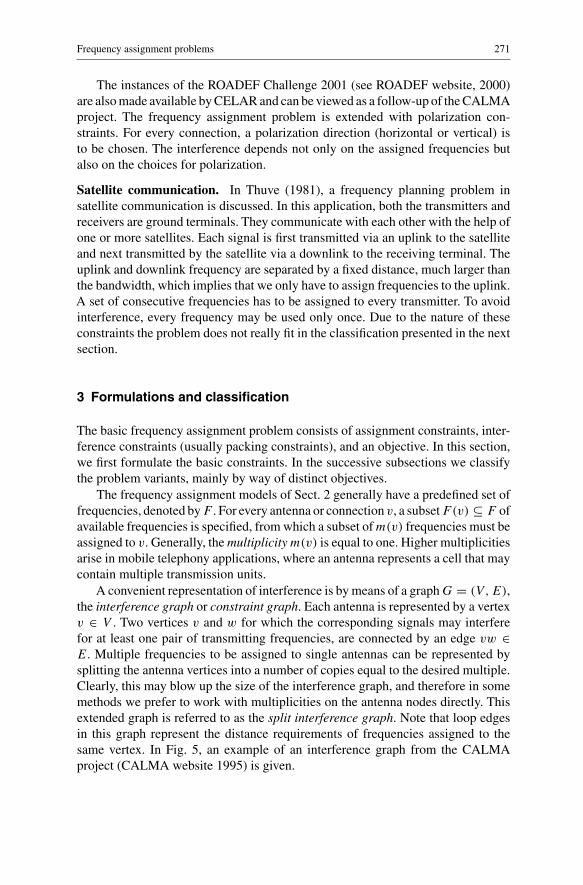
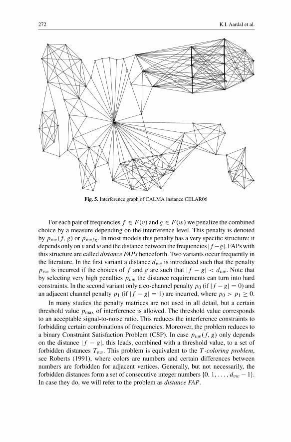
A convenient representation of interference is by means of a graph G = (V , E),the interference graph or constraint graph. Each antenna is represented by a vertexv ∈ V . Two vertices v and w for which the corresponding signals may interferefor at least one pair of transmitting frequencies, are connected by an edge vw ∈E. Multiple frequencies to be assigned to single antennas can be represented bysplitting the antenna vertices into a number of copies equal to the desired multiple.Clearly, this may blow up the size of the interference graph, and therefore in somemethods we prefer to work with multiplicities on the antenna nodes directly. Thisextended graph is referred to as the split interference graph. Note that loop edgesin this graph represent the distance requirements of frequencies assigned to thesame vertex. In Fig. 5, an example of an interference graph from the CALMAproject (CALMA website 1995) is given.
272 K.I. Aardal et al.
Fig. 5. Interference graph of CALMA instance CELAR06
For each pair of frequencies f ∈ F(v) and g ∈ F(w) we penalize the combinedchoice by a measure depending on the interference level. This penalty is denotedby pvw(f, g) or pvwfg . In most models this penalty has a very specific structure: itdepends only onv andw and the distance between the frequencies |f −g|. FAPs withthis structure are called distance FAPs henceforth. Two variants occur frequently inthe literature. In the first variant a distance dvw is introduced such that the penaltypvw is incurred if the choices of f and g are such that |f − g| < dvw. Note thatby selecting very high penalties pvw the distance requirements can turn into hardconstraints. In the second variant only a co-channel penalty p0 (if |f −g| = 0) andan adjacent channel penalty p1 (if |f − g| = 1) are incurred, where p0 > p1 ≥ 0.
In many studies the penalty matrices are not used in all detail, but a certainthreshold value pmax of interference is allowed. The threshold value correspondsto an acceptable signal-to-noise ratio. This reduces the interference constraints toforbidding certain combinations of frequencies. Moreover, the problem reduces toa binary Constraint Satisfaction Problem (CSP). In case pvw(f, g) only dependson the distance |f − g|, this leads, combined with a threshold value, to a set offorbidden distances Tvw. This problem is equivalent to the T -coloring problem,see Roberts (1991), where colors are numbers and certain differences betweennumbers are forbidden for adjacent vertices. Generally, but not necessarily, theforbidden distances form a set of consecutive integer numbers {0, 1, . . . , dvw − 1}.In case they do, we will refer to the problem as distance FAP.

Frequency assignment problems 273
The mathematical programming formulation of the FAP consists of a set ofvariables, constraints, and an objective function. A straightforward choice for thevariables is to use binary variables representing the choice of a frequency for acertain vertex. For every vertex v and available frequency f ∈ F(v) we define:
xvf ={
1 if frequency f ∈ F(v) is assigned to vertex v ∈ V
0 otherwise
These variables have been used by the majority of the researchers. They lead toInteger Linear Programming (ILP) formulations with a large number of variables,that can be solved by Branch-and-Cut methods, for instance. More compact for-mulations are obtained by using variables fv for the choice of frequency for vertexv ∈ V . They lead, however, to nonlinear programs which are hard to solve. More-over, they have the disadvantage that only one frequency can be assigned to avertex. Therefore, we will not consider these formulations. Other formulations andtechniques, such as column generation are discussed at the end of this section.
The requirement that m(v) frequencies have to be assigned to a vertex v ismodelled by the following constraints, the multiplicity constraints:
∑f ∈F(v)
xvf = m(v) ∀v ∈ V (1)
The penalty matrices pvw are often used in combination with a threshold valuepmax. Pairs of frequencies with a penalty exceeding this threshold are forbidden.This is modelled by the following packing constraints:
xvf + xwg ≤ 1 ∀vw ∈ E, f ∈ F(v), g ∈ F(w) :pvw(f, g) > pmax
(2)
When there is no further objective to be optimized, we obtain the so-called feasibilityfrequency assignment problem (F-FAP). Here, we only intend to find a feasiblesolution to the FAP, i.e., a solution satisfying the constraints (1) and (2).
In the sequel we consider a variety of objectives for this model. If no feasiblesolution exists to F-FAP, the next best thing is to assign as many frequencies aspossible. A way to do this cleverly is minimize the probability that a call will beblocked in any of the vertices. Other objectives aim at optimizing operating costsby minimizing the number of frequencies used (until the 1970s), or minimizing thebandwidth used (highest minus lowest frequency).All these models use, besides themultiplicity constraints, packing constraints. In case the penalty matrices are useddirectly, we generally wish to minimize the total penalty incurred. In this model, thepacking constraints are replaced by a version that incorporates penalty for certainchoices of combinations of frequencies.
274 K.I. Aardal et al.
3.1 The maximum serviceand minimum blocking frequency assignment problems
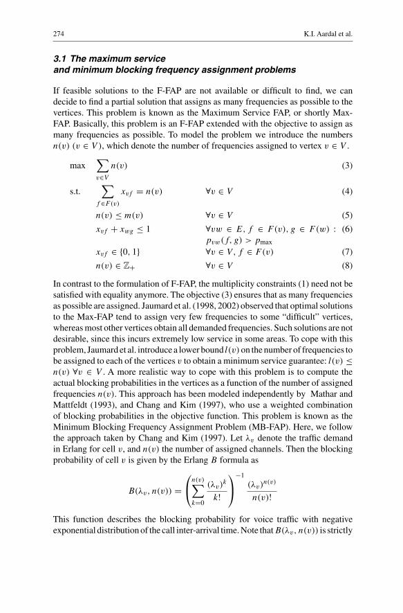
If feasible solutions to the F-FAP are not available or difficult to find, we candecide to find a partial solution that assigns as many frequencies as possible to thevertices. This problem is known as the Maximum Service FAP, or shortly Max-FAP. Basically, this problem is an F-FAP extended with the objective to assign asmany frequencies as possible. To model the problem we introduce the numbersn(v) (v ∈ V ), which denote the number of frequencies assigned to vertex v ∈ V .
max∑v∈V
n(v) (3)
s.t.∑
f ∈F(v)
xvf = n(v) ∀v ∈ V (4)
n(v) ≤ m(v) ∀v ∈ V (5)
xvf + xwg ≤ 1 ∀vw ∈ E, f ∈ F(v), g ∈ F(w) :pvw(f, g) > pmax
(6)
xvf ∈ {0, 1} ∀v ∈ V, f ∈ F(v) (7)
n(v) ∈ Z+ ∀v ∈ V (8)
In contrast to the formulation of F-FAP, the multiplicity constraints (1) need not besatisfied with equality anymore. The objective (3) ensures that as many frequenciesas possible are assigned. Jaumard et al. (1998, 2002) observed that optimal solutionsto the Max-FAP tend to assign very few frequencies to some “difficult” vertices,whereas most other vertices obtain all demanded frequencies. Such solutions are notdesirable, since this incurs extremely low service in some areas. To cope with thisproblem, Jaumard et al. introduce a lower bound l(v)on the number of frequencies tobe assigned to each of the vertices v to obtain a minimum service guarantee: l(v) ≤n(v) ∀v ∈ V . A more realistic way to cope with this problem is to compute theactual blocking probabilities in the vertices as a function of the number of assignedfrequencies n(v). This approach has been modeled independently by Mathar andMattfeldt (1993), and Chang and Kim (1997), who use a weighted combinationof blocking probabilities in the objective function. This problem is known as theMinimum Blocking Frequency Assignment Problem (MB-FAP). Here, we followthe approach taken by Chang and Kim (1997). Let λv denote the traffic demandin Erlang for cell v, and n(v) the number of assigned channels. Then the blockingprobability of cell v is given by the Erlang B formula as
B(λv, n(v)) =
n(v)∑k=0
(λv)k
k!
−1(λv)
n(v)
n(v)!
This function describes the blocking probability for voice traffic with negativeexponential distribution of the call inter-arrival time. Note thatB(λv, n(v)) is strictly
Frequency assignment problems 275
decreasing and convex in n(v). Now, the objective function is a weighted averageof the blocking probabilities of all vertices v, given by
∑v∈V
wvB(λv, n(v)) (9)
with wv = λv/∑
u∈V λu being the traffic weighting factor. In contrast to (3), theobjective function (9) is to be minimized. Note that the objective of Max-FAP canbe viewed as a simplification of this objective: wv = 1, and B(λv, n(v)) is replacedby m(v) − n(v), a linear decreasing function.
Moreover, note that the upper bounds (5) on the number of assigned frequenciesare fairly superficial in this model. Their only relevance may come from practicalconsiderations such as a maximum amount of space to install the transmitters. Ifspace is not an issue, by removing the multiplicity constraints one may obtain evenbetter solutions with respect to the objective (9).
3.2 The minimum order FAP
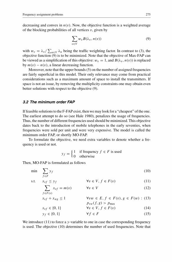
If feasible solutions to the F-FAP exist, then we may look for a “cheapest” of the one.The earliest attempt to do so (see Hale 1980), penalizes the usage of frequencies.Thus, the number of different frequencies used should be minimized. This objectivedates back to the introduction of mobile telephones in the early seventies, whenfrequencies were sold per unit and were very expensive. The model is called theminimum order FAP, or shortly MO-FAP.
To formulate the objective, we need extra variables to denote whether a fre-quency is used or not.
yf ={
1 if frequency f ∈ F is used0 otherwise
Then, MO-FAP is formulated as follows
min∑f ∈F
yf (10)
s.t. xvf ≤ yf ∀v ∈ V, f ∈ F(v) (11)∑f ∈F(v)
xvf = m(v) ∀v ∈ V (12)
xvf + xwg ≤ 1 ∀vw ∈ E, f ∈ F(v), g ∈ F(w) :pvw(f, g) > pmax
(13)
xvf ∈ {0, 1} ∀v ∈ V, f ∈ F(v) (14)
yf ∈ {0, 1} ∀f ∈ F (15)
We introduce (11) to force a y-variable to one in case the corresponding frequencyis used. The objective (10) determines the number of used frequencies. Note that
276 K.I. Aardal et al.
constraints (11) are node packing constraints: using the complement of the y-variables gives xvf + yf ≤ 1. Note that the distance MO-FAP reduces to thestandard vertex coloring problem if all distances are equal to 1, and all vertexdomains are the same set of consecutive integers (see Cozzens and Roberts 1982).
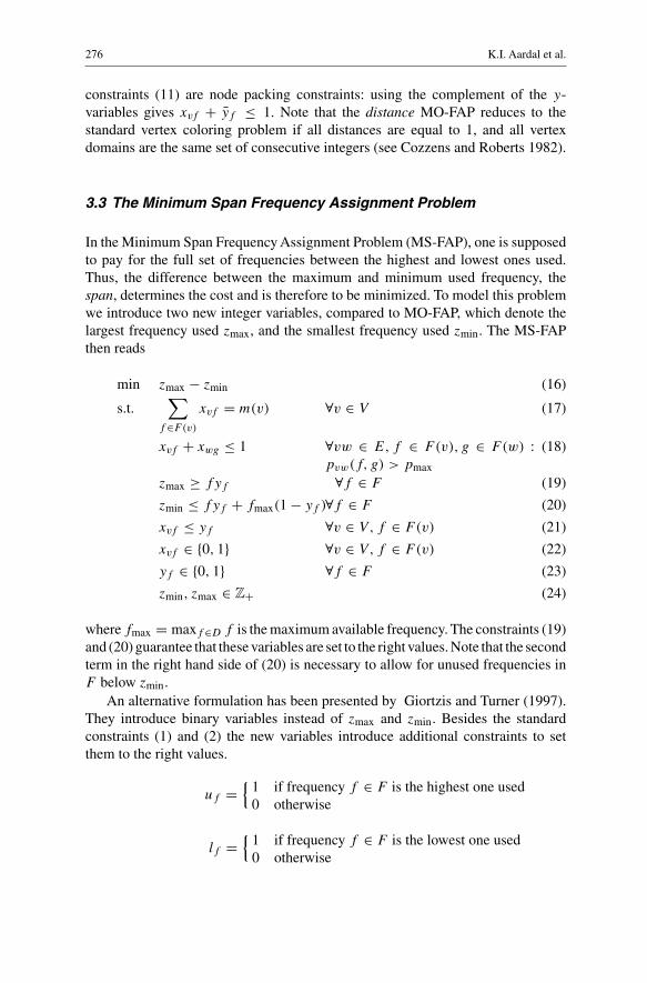
3.3 The Minimum Span Frequency Assignment Problem
In the Minimum Span Frequency Assignment Problem (MS-FAP), one is supposedto pay for the full set of frequencies between the highest and lowest ones used.Thus, the difference between the maximum and minimum used frequency, thespan, determines the cost and is therefore to be minimized. To model this problemwe introduce two new integer variables, compared to MO-FAP, which denote thelargest frequency used zmax, and the smallest frequency used zmin. The MS-FAPthen reads
min zmax − zmin (16)
s.t.∑
f ∈F(v)
xvf = m(v) ∀v ∈ V (17)
xvf + xwg ≤ 1 ∀vw ∈ E, f ∈ F(v), g ∈ F(w) :pvw(f, g) > pmax
(18)
zmax ≥ fyf ∀f ∈ F (19)
zmin ≤ fyf + fmax(1 − yf )∀f ∈ F (20)
xvf ≤ yf ∀v ∈ V, f ∈ F(v) (21)
xvf ∈ {0, 1} ∀v ∈ V, f ∈ F(v) (22)
yf ∈ {0, 1} ∀f ∈ F (23)
zmin, zmax ∈ Z+ (24)
where fmax = maxf ∈D f is the maximum available frequency. The constraints (19)and (20) guarantee that these variables are set to the right values. Note that the secondterm in the right hand side of (20) is necessary to allow for unused frequencies inF below zmin.
An alternative formulation has been presented by Giortzis and Turner (1997).They introduce binary variables instead of zmax and zmin. Besides the standardconstraints (1) and (2) the new variables introduce additional constraints to setthem to the right values.
uf ={
1 if frequency f ∈ F is the highest one used0 otherwise
lf ={
1 if frequency f ∈ F is the lowest one used0 otherwise
Frequency assignment problems 277
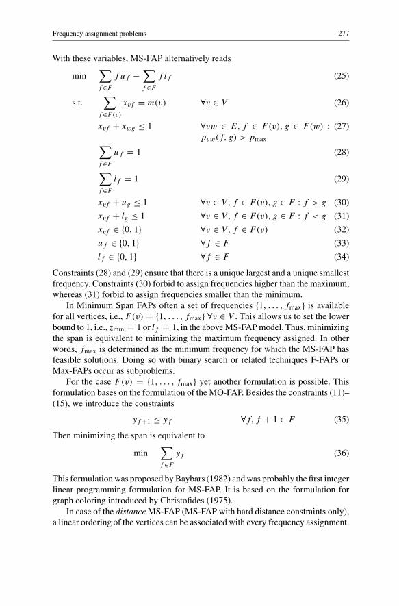
With these variables, MS-FAP alternatively reads
min∑f ∈F
f uf −∑f ∈F
f lf (25)
s.t.∑
f ∈F(v)
xvf = m(v) ∀v ∈ V (26)
xvf + xwg ≤ 1 ∀vw ∈ E, f ∈ F(v), g ∈ F(w) :pvw(f, g) > pmax
(27)
∑f ∈F
uf = 1 (28)
∑f ∈F
lf = 1 (29)
xvf + ug ≤ 1 ∀v ∈ V, f ∈ F(v), g ∈ F : f > g (30)
xvf + lg ≤ 1 ∀v ∈ V, f ∈ F(v), g ∈ F : f < g (31)
xvf ∈ {0, 1} ∀v ∈ V, f ∈ F(v) (32)
uf ∈ {0, 1} ∀f ∈ F (33)
lf ∈ {0, 1} ∀f ∈ F (34)
Constraints (28) and (29) ensure that there is a unique largest and a unique smallestfrequency. Constraints (30) forbid to assign frequencies higher than the maximum,whereas (31) forbid to assign frequencies smaller than the minimum.
In Minimum Span FAPs often a set of frequencies {1, . . . , fmax} is availablefor all vertices, i.e., F(v) = {1, . . . , fmax} ∀v ∈ V . This allows us to set the lowerbound to 1, i.e., zmin = 1 or lf = 1, in the above MS-FAP model. Thus, minimizingthe span is equivalent to minimizing the maximum frequency assigned. In otherwords, fmax is determined as the minimum frequency for which the MS-FAP hasfeasible solutions. Doing so with binary search or related techniques F-FAPs orMax-FAPs occur as subproblems.
For the case F(v) = {1, . . . , fmax} yet another formulation is possible. Thisformulation bases on the formulation of the MO-FAP. Besides the constraints (11)–(15), we introduce the constraints
yf +1 ≤ yf ∀f, f + 1 ∈ F (35)
Then minimizing the span is equivalent to
min∑f ∈F
yf (36)
This formulation was proposed by Baybars (1982) and was probably the first integerlinear programming formulation for MS-FAP. It is based on the formulation forgraph coloring introduced by Christofides (1975).
In case of the distance MS-FAP (MS-FAP with hard distance constraints only),a linear ordering of the vertices can be associated with every frequency assignment.
278 K.I. Aardal et al.
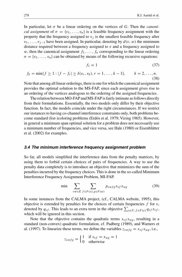
In particular, let σ be a linear ordering on the vertices of G. Then the canoni-cal assignment of σ = {v1, . . . , vn} is a feasible frequency assignment with theproperty that the frequency assigned to vj is the smallest feasible frequency afterv1, . . . , vj−1 have been assigned. In particular, denoting by d(v, w) the minimumdistance required between a frequency assigned to v and a frequency assigned tow, then the canonical assignment f1, . . . , fn corresponding to the linear orderingσ = {v1, . . . , vn} can be obtained by means of the following recursive equations:
f1 = 1 (37)
fk = min{f ≥ 1 : |f − fr | ≥ δ(vr , vk), r = 1, . . . , k − 1}, k = 2, . . . , n.
(38)Note that among all linear orderings, there is one for which the canonical assignmentprovides the optimal solution to the MS-FAP, since each assignment gives rise toan ordering of the vertices analogous to the ordering of the assigned frequencies.
The relation between MO-FAP and MS-FAP is fairly intimate as follows directlyfrom their formulations. Essentially, the two models only differ by their objectivefunction. In fact, the models coincide under the right circumstances. If we restrictour instances to having co-channel interference constraints only, both problems be-come standard (list-)coloring problems (Erdös et al. 1979; Vizing 1965). However,in general a minimum span optimal solution for a problem does not necessarily usea minimum number of frequencies, and vice versa, see Hale (1980) or Eisenblätteret al. (2002) for examples.
3.4 The minimum interference frequency assignment problem
So far, all models simplified the interference data from the penalty matrices, byusing them to forbid certain choices of pairs of frequencies. A way to use thepenalty data completely is to introduce an objective that minimizes the sum of thepenalties incurred by the frequency choices. This is done in the so-called MinimumInterference Frequency Assignment Problem, MI-FAP.
min∑
vw∈E
∑f ∈F(v),g∈F(w)
pvwfgxvf xwg (39)
In some instances from the CALMA project, (cf., CALMA website, 1995), thisobjective is extended by penalties for the choices of certain frequencies f for v,denoted by qvf . This leads to an extra term in the objective
∑v∈V,f ∈F(v) qvf xvf ,
which will be ignored in this section.Note that the objective contains the quadratic terms xvf xwg , resulting in a
standard (non-convex) quadratic formulation, cf. Padberg (1989), and Warners etal. (1997). To linearize these terms, we define the variables zvwfg = xvf xwg , i.e.,
zvwfg ={
1 if xvf = xwg = 10 otherwise
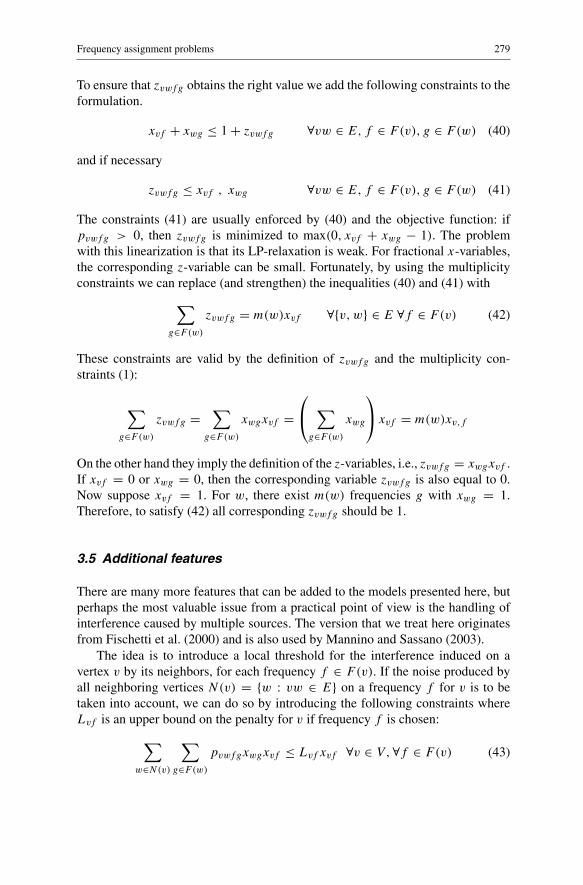
Frequency assignment problems 279
To ensure that zvwfg obtains the right value we add the following constraints to theformulation.
xvf + xwg ≤ 1 + zvwfg ∀vw ∈ E, f ∈ F(v), g ∈ F(w) (40)
and if necessary
zvwfg ≤ xvf , xwg ∀vw ∈ E, f ∈ F(v), g ∈ F(w) (41)
The constraints (41) are usually enforced by (40) and the objective function: ifpvwfg > 0, then zvwfg is minimized to max(0, xvf + xwg − 1). The problemwith this linearization is that its LP-relaxation is weak. For fractional x-variables,the corresponding z-variable can be small. Fortunately, by using the multiplicityconstraints we can replace (and strengthen) the inequalities (40) and (41) with
∑g∈F(w)
zvwfg = m(w)xvf ∀{v, w} ∈ E ∀f ∈ F(v) (42)
These constraints are valid by the definition of zvwfg and the multiplicity con-straints (1):
∑g∈F(w)
zvwfg =∑
g∈F(w)
xwgxvf = ∑
g∈F(w)
xwg
xvf = m(w)xv,f
On the other hand they imply the definition of the z-variables, i.e., zvwfg = xwgxvf .If xvf = 0 or xwg = 0, then the corresponding variable zvwfg is also equal to 0.Now suppose xvf = 1. For w, there exist m(w) frequencies g with xwg = 1.Therefore, to satisfy (42) all corresponding zvwfg should be 1.
3.5 Additional features
There are many more features that can be added to the models presented here, butperhaps the most valuable issue from a practical point of view is the handling ofinterference caused by multiple sources. The version that we treat here originatesfrom Fischetti et al. (2000) and is also used by Mannino and Sassano (2003).
The idea is to introduce a local threshold for the interference induced on avertex v by its neighbors, for each frequency f ∈ F(v). If the noise produced byall neighboring vertices N(v) = {w : vw ∈ E} on a frequency f for v is to betaken into account, we can do so by introducing the following constraints whereLvf is an upper bound on the penalty for v if frequency f is chosen:
∑w∈N(v)
∑g∈F(w)
pvwfgxwgxvf ≤ Lvf xvf ∀v ∈ V, ∀f ∈ F(v) (43)
280 K.I. Aardal et al.
We can linearize this constraint by use of an upper bound on the possible interferencefor any vertex and any frequency, say M .
∑w∈N(v)
∑g∈F(w)
pvwfgxwg ≤ Lvf + M(1 − xvf ) ∀v ∈ V, ∀f ∈ F(v) (44)
Within the CSELT instances of Fischetti et al. (2000) and Mannino and Sassano(2003) only co-channel and adjacent channel interference is penalized. Co-channelinterference is penalized with Ivf , and adjacent channel interference is penalized
withIvf
NFD, where NFD is a reduction factor called the Net Filter Discriminator.
The upper bound on allowable interference, L, is fixed for each vertex frequencypair (v, f ).
∑w∈N(v)
Ivf xwf + Ivf
NFD(xw,f −1 + xw,f +1) ≤ L + M(1 − xvf ) ∀v ∈ V,
∀f ∈ F(v)
(45)
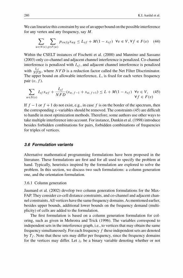
If f − 1 or f + 1 do not exist, e.g., in case f is on the border of the spectrum, thenthe corresponding x-variables should be removed. The constraints (45) are difficultto handle in most optimization methods. Therefore, some authors use other ways totake multiple interference into account. For instance, Dunkin et al. (1998) introducebesides forbidden combinations for pairs, forbidden combinations of frequenciesfor triples of vertices.
3.6 Formulation variants
Alternative mathematical programming formulations have been proposed in theliterature. These formulations are first and for all used to specify the problem athand. Typically, heuristics inspired by the formulation are explored to solve theproblem. In this section, we discuss two such formulations: a column generationone, and the orientation formulation.
3.6.1 Column generation
Jaumard et al. (2002) develop two column generation formulations for the Max-FAP. They consider co-cell distance constraints, and co-channel and adjacent chan-nel constraints.All vertices have the same frequency domains.As mentioned earlier,besides upper bounds, additional lower bounds on the frequency demand (multi-plicity) of cells are added to the formulation.
The first formulation is based on a column generation formulation for col-oring, such as given in Mehrotra and Trick (1996). The variables correspond toindependent sets in the interference graph, i.e., to vertices that may obtain the samefrequency simultaneously. For each frequency f these independent sets are denotedby Tf . Note that these sets may differ per frequency, since the frequency domainsfor the vertices may differ. Let zt be a binary variable denoting whether or not

Frequency assignment problems 281
t ∈ Tf is chosen. To model the constraints and the objective of the Max-FAP withthese variables, we use the relation xvf = ∑
t∈Tf :v∈t zt . To ensure that frequencyf is chosen at most once we add
∑t∈Tf
zt ≤ 1. Note that this formulation canalso be used for the MO- and MS-FAP: for MO-FAP the latter constraints become∑
t∈Tfzt = yf . Jaumard et al. (2002) solve the LP-relaxation of this formulation
with column generation techniques (the pricing problems are weighted indepen-dent set problems), and they describe branching strategies as well as cut generationschemes. The authors use their method as a heuristic.
The second formulation is based on admissible sets of frequencies for separatecells. The variables correspond to sets of frequencies that can be assigned to a certaincell. For each cell v, subsets of F denoted by Tv that satisfy the co-cell constraintsand lower and upper bounds on the multiplicity are given. Another binary variablezt specifies whether or not Tv is chosen. The authors show that the LP-relaxationof the formulation based on these variables is, at best, equal to the value of theLP-relaxation of the previous formulation. On the other hand, the pricing problemsto be solved in a column generation approach are simple constrained shortest pathproblems.
3.6.2 Orientation formulation
Borndörfer et al. (1998b) consider MI-FAPs with co-channel and adjacent channelinterference. They model the interference with penalties on combinations of fre-quencies. Moreover, they forbid combinations of frequencies with penalties abovea certain threshold. Among the feasible assignments they seek one with minimumpenalty. For each vertex in the interference graph they introduce a variable yv thatcorresponds to the frequency number assigned to v. For each pair (v, w) denote theco-channel penalty by pvw and the adjacent-channel penalty by qvw. Now, threemore binary variables are introduced:
zvw ={
1 if |yv − yw| = 00 otherwise
zvw ={
1 if |yv − yw| = 10 otherwise
�vw ={
1 if yv ≥ yw
0 otherwise
The variables �vw determine a partial ordering of the frequencies assigned tothe vertices. With these variables one can model all constraints and the objectivelinearly. The model defined in this way contains much fewer variables, than the for-mulations given in the previous section. The price for this is a weaker formulation.If the �vw are given, the authors show that the problem is solvable in polynomialtime, since the constraint matrix is totally unimodular. This result is used in a two-stage heuristic, where the variables �vw are adjusted iteratively and then a solutionis determined for the new values.
282 K.I. Aardal et al.
4 Methods for optimization and lower bounding
Since all models for FAP share an important part of their structure (assignmentof frequencies and handling of interference), many optimization ideas translateeasily from one model to another. This is specifically true for the most extensivelyused method: tree search. We, therefore, treat this method in a general fashion.We explain the handling of the components of tree search, like branching andsubproblem processing, using the F-FAP as the descriptive generic problem type,or Max-FAP if an objective function is needed.We do this for the two versions of treesearch, one based on the linear programming relaxation of F-FAP, and one basedon combinatorial ideas. Note that these versions latter are used for determininglower bounds on the objective function. The objective function, however, is exactlywhat the models differ in. Therefore, we treat the (combinatorial) lower boundingtechniques separately for each of the models.
The exception to the above is the MI-FAP. Here interference is modeled by usingpenalties. This makes the MI-FAP much harder to solve than the other variants.This is probably the reason behind a relatively rich set of solution methods for theproblem. These methods are therefore treated in a separate subsection.
4.1 F-FAP
In tree search algorithms we distinguish two parts:
1. Construction of the tree. The variable (or function) choice for branching. Theselection of a subproblem from a list L of active subproblems: such as depth-firstsearch, best-first search.
2. The processing of a node (or a subproblem) from the tree. This includes in-stance reduction techniques, and node pruning techniques such as cutting planealgorithms, and combinatorial lower bounding techniques.
The first part of the process structures the tree corresponding to the search algorithm.This part if fairly problem independent. Thus, the ideas used in any of the variantsof the FAP can generally be applied directly to other variants. The second part isconcerned with actually solving (sub)problems. This part partially depends on theproblem at hand, the type of instances, and also on the used technique. The genericideas with respect to instance reduction, cutting planes, and lower bounds are treatedhere. The problem specific ideas are treated separately in later subsections.
The F-FAP that we consider in the sequel is, purely for explanatory reasons,restricted to satisfy the following conditions. The frequency domains are equalfor all vertices, and consist of a consecutive set of integers {1, 2, . . . , fmax},where fmax is a given parameter (F-FAP, Max-FAP, MB-FAP, MO-FAP), or avariable to be minimized (MS-FAP). The interference constraints are of the type|f (v)−f (w)| ≥ δ(v, w), where f (v) and f (w) are frequencies assigned to v andw respectively. These restrictions are the ones that are most frequently encountered
Frequency assignment problems 283
in the literature. So, most techniques are developed for problems with these charac-teristics. Moreover, the ideas described in the sequel often allow for straightforwardgeneralization to other characteristics.
4.1.1 Branching rules
The standard branching rule used in combinatorial optimization is to divide thedomain of a variable into two (or more) disjoint subsets. For binary variables thisrule reduces to setting the variable to either zero or one. In frequency assignment,this implies that a vertex and a frequency have to be chosen. Most branching rules areonly occupied with selecting a vertex. The majority of them is based on the relationbetween FAP and graph coloring (δ(v, w) = 1 for all {v, w} ∈ E) and on ConstraintLogic Programming (CLP).Vertex selection is done either statically or dynamically.A selection mechanism is a static ordering if the ordering is independent of theactual tree search. Such an ordering can be computed at the start. A popular oneis the highest degree first ordering, which orders the vertices according to theirdegree (including multiplicities) in the constraint graph. A related ordering that isapplied frequently is to iteratively select the highest degree vertex, simultaneouslyremoving it from G. This ordering can also be applied backward, selecting andremoving the smallest degree vertices, i.e., smallest degree latest ordering.
The CLP approach of Kolen et al. (1994) and the branch-and-cut approach ofAardal et al. (1996) solve the MO-FAPs from the CALMA project. Both considerthe smallest degree latest ordering as the most successful one. Kolen et al. (1994)also specify the choice of a new frequency as the one with the highest distance to thealready chosen frequencies. Though static, the above orderings all aim at isolatingthe possibly present hard part of an instance. Mannino and Sassano (2003) carrythe idea of selecting the difficult part of the interference graph a little further byidentifying a hard subgraph (called the core in Mannino and Sassano (2003) for theMax-FAP instances of CSELT. After solving the partial problem restricted to thecore they hope that the remainder can be solved without influencing the objectivefunction.
Dynamic orderings depend on the subproblem at hand.A simple example of dy-namic ordering is saturation degree vertex selection. It is attributed to Brélaz (1979)who described the idea for graph coloring problems. During the tree search processthe number of available frequencies for the vertices decreases due to previouslymade choices. Assignment of frequencies to a vertex v generally becomes harderif this number is smaller. Brelaz’ rule therefore selects the vertex with a minimumnumber of frequencies available. Clearly, the multiplicity of v, and the multiplicityof its neighbors, also influences the level of difficulty of assigning frequencies tov. Moreover, the distances play a role. The higher the distances the more combi-nations are forbidden. Giortzis and Turner (1997), who consider the Max-FAP andthe MS-FAP, devised a branching rule that uses the latter two observations. Theydynamically select vertices v for which m(v) ·∑w∈N(v) m(w)δ(v, w) is maximum.Many variants of these ideas are, of course, possible. An overview of many orderingideas can be found in Hurley et al. (1997).
284 K.I. Aardal et al.
The choice of variable on which to branch in LP-based methods is fairly stan-dard. One can take variables that have values closest to 0.5 or closest to 0 or 1. InFischetti et al. (2000) branching is done with three such rules used randomly: 1:variables with value in the interval [0.4, 0.6], where the actual choice is determinedby the largest degree (number of interfering cells) of the corresponding vertex; 2:variables with value smaller than 0.05, where again the actual choice is determinedby the largest number of interfering cells; 3: variables with value closest to 0.5 arechosen. Thus, the standard branching rules for binary variables are mixed randomly.In Aardal et al. (1996) standard LP-based branching is combined with a partial or-dering of the variables: the frequency variables yf are considered first. Strangelyenough, none of the studies on LP-based methods for FAP uses constraints forbranching, although SOS constraints make up a significant part of the formulation.
4.1.2 Subproblem choices
The standard strategies for subproblem selection are depth-first search (DFS) andbest-first search (BFS). In applying DFS one attempts to find good solutions quickly.DFS involves little implementation overhead, since the stored part of the search treeresembles a path.Among others, Giortzis and Turner (1997), and Kolen et al. (1994)use DFS. If a lower bounding method is available, one may select a subproblemwith a small lower bound to be processed first, anticipating better solutions to beavailable, and quicker increase of the overall lower bound. Implementations of BFSare found in Aardal et al. (1996) and Fischetti et al. (2000). Mannino and Sassano(2003) incorporate a backtracking idea from CLP in their tree search, called back-jumping, which attempts moving back multiple levels at once in the search tree,once an inconsistency is found that that can be traced back.
4.1.3 Reduction techniques
Instance reduction techniques attempt to remove frequencies from the domainsof vertices or even complete vertices. The ideas to do so are based on similarideas in CLP (arc-consistency) and coloring. Consider, for instance a vertex v withneighbors N(v). In the process of assigning frequencies to the neighbors of v, acertain number of frequencies from v will be blocked. If the maximum numberof blocked frequencies still leaves enough space (free frequencies) to assign allnecessary frequencies to v, then we can remove v from the constraint graph. Forexample, in the standard instances we consider here, for each vertex w ∈ N(v) afrequency chosen for w can only block 2δ(v, w) − 1 frequencies. Thus, in totalat most
∑w∈N(v) m(w)(2δ(v, w) − 1) frequencies can become unavailable for
usage by v. If the number of remaining available frequencies for v is at leastm(v) · (δ(v, v)−1)+1, we can always select enough frequencies for v. This idea isapplied dynamically to the MO-FAP in Aardal et al. (1996) and Kolen et al. (1994),and to the MS-FAP in Mannino and Sassano (2003).
Frequency assignment problems 285
One way that remains to remove frequencies from domains is by consistencychecking. In its simplest form we check whether, for a particular frequency f ∈F(v), there is a feasible choice of frequencies for the neighbors of v. If not, we canremove f from F(v). This idea is used in Kolen et al. (1994) and Mannino andSassano (2003).
4.1.4 Cutting planes
Techniques using the LP-relaxation of the formulation from F-FAP generallystrengthen the relaxation by using additional constraints, so-called valid inequali-ties. The inequalities that are used are typically derived from the relaxation of FAPobtained by considering the packing constraints (2). These constraints can be illus-trated by a graph H = (W, F ) of the binary variables xvf known as the conflictgraph. For each variable we introduce a node (v, f ). Two nodes (v, f ) and (w, g)
are connected by an edge if at most one of the variables may obtain value 1. Now,consider a clique (a complete subgraph) in H with vertex set S. Then clearly, notwo of the variables of S may have value 1, and therefore
∑(v,f )∈S xvf ≤ 1 is
valid. In general, the most powerful such constraints come from maximal cliques,e.g., cliques that cannot be extended with other vertices. Finding such cliques in H
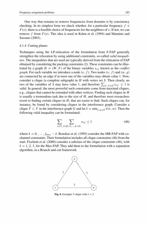
is usually a tremendous task due to the size of H , and therefore most researchersresort to finding certain cliques in H , that are easier to find. Such cliques can, forinstance, be found by considering cliques in the interference graph. Consider aclique V ⊂ V in the interference graph G and let δ = minv,w∈V δ(v, w). Then thefollowing valid inequality can be formulated:
∑v∈S
∑f ∈{k+1,...,k+δ}
xvf ≤ 1 (46)
where k = 0, . . . , fmax − δ. Rouskas et al. (1995) consider the MB-FAP with co-channel constraints. Their formulation includes all clique constraints (46) from thestart. Fischetti et al. (2000) consider a subclass of the clique constraints (46), withδ = 1, 2, 3, for the Max-FAP. They add them to the formulation with a separationalgorithm, in a Branch-and-cut framework.
����
v ����w
����
u
2��
��
��
��
3
��
��
��
��
3
Fig. 6. Example 3-clique with δ = 2
286 K.I. Aardal et al.
Aardal et al. (1996) consider cliques from the conflict graph that can be viewedas lifted versions of (46). Consider, for example, the clique in Fig. 6. This cliqueinduces the following valid inequality (u, v, w are nodes and f, g, h are frequen-cies).
xuf + xug + xuh + xuf + xvg + xvh + xwf + xwg ≤ 1
Finally, in Kazantzakis et al. (1995) the linear programming relaxation of the Max-FAP is tightened by using cuts derived from rounding the objective function duringthe (complete) tree search.
4.2 Max-FAP and MB-FAP
4.2.1 Cutting planes
The Max-FAP of Fischetti et al. (2000) includes multiple interference con-straints (45). These constraints allow for generation of cutting planes based onknapsack covers (see Nemhauser and Wolsey 1988), which are used in their branch-and-cut scheme as well.
4.3 MO-FAP
4.3.1 Instance reduction
The CALMA instances contain nonadjacent pairs of vertices v, w, such that forany neighbor u of v we have δ(uv) ≤ δ(uw). Moreover F(v) ⊆ F(w). Then thechoice made for w is also available for v. Thus, vertices such as v can be removed.Though rare in general, this situation does occur in the CALMA instances.
4.3.2 Valid inequalities
For any clique V in the constraint graph G, the following inequality is valid withrespect to MO-FAP. ∑
v∈S
xvf ≤ yf
These are used in Aardal et al. (1996).
4.3.3 Lower bounds
Clearly, the clique and coloring number of the constraint graph are lower boundsof the MO-FAP. If the domains (available frequencies) differ among the vertices,sometimes a list coloring bound may improve upon such bounds. This occurs insome of the CALMA instances. For an overview of these bounds see Aardal et al.(2002).
Frequency assignment problems 287
4.4 MS-FAP
4.4.1 Valid inequalities
The variables introduced in the model of Giortzis and Turner (1997) for MS-FAPgive rise to special cliques:
∑f ∈F(v):f ≤g
xvf +∑
f ∈F(v):f >g
lf ≤ 1 ∀v ∈ V, g ∈ F(v)
∑f ∈F(v):f ≥g
xvf +∑
f ∈F(v):f <g
uf ≤ 1 ∀v ∈ V, g ∈ F(v)
The use of such cliques has not been reported on, so far.
4.4.2 Lower bounds
The fairly direct relation between MS-FAP and MO-FAP allows some lower bound-ing techniques to be used for both models. This applies for instance to the simplestlower bound: the clique bound. Each subgraph of G induced by W ⊂ V that formsa clique determines a lower bound |W | for MO-FAP and |W | − 1 for MS-FAP.This bound, though applicable to MS-FAP, is especially suitable for MO-FAPs.There are, however, more general and more powerful lower bounds available forMS-FAP. The standard clique bound can be generalized as was first observed byGamst (1986). Let all multiplicities of the vertices be equal to one. If a clique of sizek in the interference graph contains edges with minimum distance d only, then therange of frequencies must be at least (k−1)d +1. Over the years, lower bounds formore and more complex structures have been derived (cf., Murphey et al. (1999)for an overview). Recently, Janssen and Wentzell (2000) showed that many of thesebounds can be derived within a general theoretical framework called tile covers.
The clique bound has been further generalized by Raychaudhuri (1994). Theyconsider a subgraph of the (splitted) interference graph. For an assignment, thevertices can be ordered such that the assigned frequencies form a non-decreasingsequence. If we extend the subgraph to a complete graph by the introduction ofedges with distance zero, this order forms a path with length less than or equal tothe span of the assignment. Hence, the minimum Hamiltonian path in an arbitrarysubgraph (completed by zero-value edges) provides a lower bound on the minimumspan for the MS-FAP defined on that subgraph, and thus, on the minimum span forthe MS-FAP defined on the whole graph. Note that this bound indeed generalizesthe clique bound of Gamst (1986): in a clique of size k with minimum distance d
the shortest Hamiltonian path has length (k − 1)d . Note that the Hamiltonian pathbound can also be shown to be a lower bound by use of the canonical assignment,generated by an optimal solution. The Hamiltonian path bound is obtained by usingthe recursion (38), where we relax the minimization by taking the distance to thelast vertex in the ordering.
Janssen and Kilakos (1999) compute a lower bound of the Hamiltonian pathbound, by considering a limited, but carefully chosen set of subgraphs. For each
288 K.I. Aardal et al.
����
u ����w
����
v
3��
���
1
��
���
1
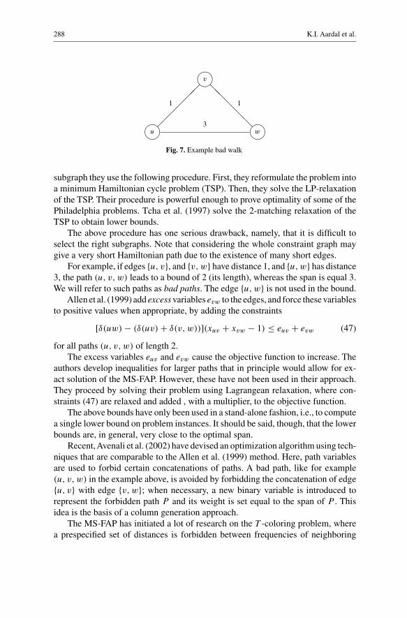
Fig. 7. Example bad walk
subgraph they use the following procedure. First, they reformulate the problem intoa minimum Hamiltonian cycle problem (TSP). Then, they solve the LP-relaxationof the TSP. Their procedure is powerful enough to prove optimality of some of thePhiladelphia problems. Tcha et al. (1997) solve the 2-matching relaxation of theTSP to obtain lower bounds.
The above procedure has one serious drawback, namely, that it is difficult toselect the right subgraphs. Note that considering the whole constraint graph maygive a very short Hamiltonian path due to the existence of many short edges.
For example, if edges {u, v}, and {v, w} have distance 1, and {u, w} has distance3, the path (u, v, w) leads to a bound of 2 (its length), whereas the span is equal 3.We will refer to such paths as bad paths. The edge {u, w} is not used in the bound.
Allen et al. (1999) add excess variables evw to the edges, and force these variablesto positive values when appropriate, by adding the constraints
[δ(uw) − (δ(uv) + δ(v, w))](xuv + xvw − 1) ≤ euv + evw (47)
for all paths (u, v, w) of length 2.The excess variables euv and evw cause the objective function to increase. The
authors develop inequalities for larger paths that in principle would allow for ex-act solution of the MS-FAP. However, these have not been used in their approach.They proceed by solving their problem using Lagrangean relaxation, where con-straints (47) are relaxed and added , with a multiplier, to the objective function.
The above bounds have only been used in a stand-alone fashion, i.e., to computea single lower bound on problem instances. It should be said, though, that the lowerbounds are, in general, very close to the optimal span.
Recent,Avenali et al. (2002) have devised an optimization algorithm using tech-niques that are comparable to the Allen et al. (1999) method. Here, path variablesare used to forbid certain concatenations of paths. A bad path, like for example(u, v, w) in the example above, is avoided by forbidding the concatenation of edge{u, v} with edge {v, w}; when necessary, a new binary variable is introduced torepresent the forbidden path P and its weight is set equal to the span of P . Thisidea is the basis of a column generation approach.
The MS-FAP has initiated a lot of research on the T -coloring problem, wherea prespecified set of distances is forbidden between frequencies of neighboring
Frequency assignment problems 289
vertices. Roberts (1991) develop a theory on lower bounds for special graphs usingT -coloring arguments. An overview of the most important lower bounds is givenin Murphey et al. (1999). These lower bounds, however, are hardly used in practicesince MS-FAP with specific T -coloring type interference constraints are rare.
4.5 The MI-FAP
The MI-FAP model is much more difficult than the previously mentioned variantsof the FAP. This is due to the fact that hard interference constraints are turned intosoft constraints by the use of penalties. This hardness has caused a large diversityin solution methods. For instance, there are only two papers, to our knowledge, thatuse some sort of tree search. Other methods are based on dynamic programming, thestructure of the interference graph, and (in case of lower bounding) combinatorialrelaxations.
The earliest attempt to solve the MI-FAP is from Verfaillie et al. (1996) whodeveloped a procedure called the Russian doll algorithm. This algorithm is perhapsbest described as a backward tree search in combination with lower bounds. Fora certain static ordering of the vertices of the interference graph, say from 1 to n,we consider n iterations. In a backward fashion, in each iteration all assignmentsof vertices {k + 1, . . . , n} are considered. Lower bounds and upper bounds on thepenalties are computed for all subsets {l, . . . , n} (l > k) of vertices, which areused in subsequent iterations. Thus, in the iteration of vertex k we do a completetree search with the vertices {k, . . . , n}, using the produced lower bounds for thesubsets {l, . . . , n} (l > k). Although the paper says little about the choice of theordering of the vertices, it probably uses rules similar to the branching rules ofsubsection 4.1.1, such as “smallest degree last”. The Russian-doll procedure hasbeen used to solve CELAR06 (an instance from CALMA) to optimality.
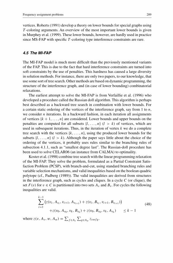
Koster et al. (1998) combine tree search with the linear programming relaxationof the MI-FAP. They solve the problem, formulated as a Partial Constraint Satis-faction Problem (PCSP), with branch-and-cut, using standard branching rules andvariable selection mechanisms, and valid inequalities based on the boolean quadricpolytope (cf., Padberg (1989)). The valid inequalities are derived from structuresin the interference graph, such as cycles and cliques. In a cycle C (or clique), theset F(v) for v ∈ C is partitioned into two sets Av and Bv . For cycles the followinginequalities are valid.
k−1∑i=1
(z(vi, Avi
, vi+1, Avi+1) + z(vi, Bvi, vi+1, Bvi+1)
)
+z(v0, Av0 , vk, Bvk) + z(v0, Bv0 , vk, Avk
) ≤ k − 1
(48)
where z(v, Av, w, Aw) = ∑f ∈Av
∑g∈Aw
zvwfg .

290 K.I. Aardal et al.
Fig. 8. Cycle inequalities
Fig. 9. (γ, k)-clique-cycle inequalities
Figure 8 shows a 3-cycle inequality and a 4-cycle inequality.A line between twodots indicates that the coefficient corresponding to the indicated subsets is equal toone.
For cliques, we take a coefficient 1 ≤ γ ≤ k − 1, where k is the size of theclique, and we get the following (γ, k)-clique inequalities.
γ∑v∈C
x(v, Av) +∑
{v,w}∈E[C]z(v, Bv, w, Bw) ≥ γ k − 1
2γ (γ + 1) (49)
where x(v, Av) = ∑f ∈Av
xvf . See Fig. 9 for examples of 3-clique and 4-inequalities.
The Branch-and-Cut method using these inequalities solves the problem wellfor instances with domain sizes up to 6 frequencies, especially with dominancecriteria and reduction methods incorporated. It has been used as a subroutine (withdomain sizes 2) in a genetic algorithm by Kolen (1999). For larger domain sizesthe method returns fairly poor lower bounds.
In Koster et al. (1999) make use of the structure of the interference graphG = (V , E). They observe that assigning frequencies to a cut-set of G decomposesthe problem into two (or more) independent problems. They generate a sequence
Frequency assignment problems 291
of small cut-sets by using a tree decomposition (see Bodlaender 1997) of the in-terference graph. Note that a small cut-set induces a relatively small number ofassignments to the vertices of the cut-set.
A series of reduction methods were developed to limit the number of assign-ments. These ideas led to the solution of some quite large MI-FAP from the CALMAproject. For some remaining instances Koster et al. (1999) improved the knownlower bounds by introducing a relaxation where the vertex domains are partitionedin a small number of subsets. Each such subset is then treated as a single frequency.By considering a sequence of relaxations, better and better lower bounds couldbe derived for the CALMA instances. The relaxations are solved with the abovedescribed tree decomposition approach. Alternatively, the cutting plane algorithmof Koster et al. (1998) can be applied (see Koster et al. 2001).
4.5.1 Lower bounds for MI-FAP
Lower bounding for MI-FAP has started with the work of Tiourine et al. (1995) whouse a quadratic programming relaxation that can be solved by clever enumeration.Non-trivial bounds are reported on a limited set of CALMA instances, namely thosewhere next to the interference penalties, also single frequency penalties are used tofavor certain frequencies for vertices.
Another lower bound is derived by Eisenblätter (2001) using semidefinite pro-gramming. He studies the semidefinite programming relaxation of the minimumk-partition problem. MI-FAP reduces to a min k-partition problem in case only theco-channel interference is considered. Like the related max cut problem, the mink-partition problem can be modeled as a semidefinite program. The relaxation ofthis semidefinite program can be solved in polynomial time. For GSM networks ofthe COST 259 project (cf., Sect. 2.2), the first lower bounds were computed in thisway.
In Maniezzo and Montemanni (2000), the MI-FAP formulation forms thestarting-point for deriving lower bounds. These bounds are inspired by similarbounds for the quadratic assignment problem. In addition, reduction and domi-nance rules are presented. A tree search algorithm is based on these bounds andrules. The algorithm is tested on the CALMA and Philadelphia instances (taking afixed spectrum) as well as on some graph coloring benchmarks.
In Montemanni et al. (2002b), a refinement of the orientation formulation(cf., Sect. 3.6.2) by Koster (1999) is used. Valid inequalities are derived that boundthe interference in subgraphs from below. A cutting plane algorithm is exploitedon realistic GSM network instances and some Philadelphia instances (by limitingthe spectrum).
292 K.I. Aardal et al.
5 Heuristic methods
Due to the difficulty of the diverse FAPs, the majority of research papers havebeen on heuristic approaches. In this section, we discuss these approaches in theform of an annotated bibliography. This section is organized as follows. We startin Sect. 5.1 with constructive algorithms that build a solution in a greedy manner.In the subsequent subsections we consider local search methods (cf., Sect. 5.2),that start with a given solution and, with iteratively doing small changes (moves),try to find good solutions. Standard local search methods only allow improvingmoves (downhill). To increase the chances for improving solutions also worseningmoves uphill may be allowed. Tabu search (cf., Sect. 5.3) allows worsening movesunder certain conditions (neighborhood restriction with tabu list) and simulatedannealing (cf., Sect. 5.4) allows worsening with a probability that typically dependson the size of the worsening, and generally decreasing in time. Genetic algorithms(cf., Sect. 5.5) start with a whole set of solutions, called generation, and iterativelybuilds new generations by recombination of solutions from the previous generation.Artificial Neural Networks (cf., Sect. 5.6) generate new solutions by emulating thebehavior of a grid of neurons, where each neuron represents a “piece” of solutionand its state is dynamically determined by the states of its neighboring neurons.Ant Colony Optimization (cf., Sect. 5.7) is a meta-heuristic that is inspired by thebehavior of ants.
Finally, the section is closed with application specific heuristics. In Sect. 5.8,heuristics based on mathematical programming formulations are discussed,whereas heuristics based on graph theory and constraint programming are the topicof Sect. 5.9. Throughout the section, we assume that the reader is familiar withthe classical meta-heuristic algorithms mentioned above. Still, in the beginningof each subsection we briefly recall the main components of the described class.The various implementations of a specific scheme mainly differ in the way thesecomponents are handled.
Recently, an interesting discussion on meta-heuristic algorithms has been pre-sented in Hurley and Smith (2002); Smith et al. (2002).
5.1 Greedy algorithms
A greedy algorithm constructs a frequency assignment by iteratively selecting avertex (an antenna), and then assigning a feasible frequency to it. The selectionand assignment follow some rule based on local characteristics that has the aimto optimize the global objective function. An important feature of this (greedy)algorithm is the irrevocable nature of the greedy choice which is performed ateach iteration. Many versions of the greedy algorithm have been proposed in theliterature to solve FAP, often in conjunction with more sophisticated local searchmethods. Several greedy heuristics are described and compared in the early work ofZoellner and Beall (1977). The model is MS-FAP. First, an ordering of the vertices

Frequency assignment problems 293
of the interference graph is performed: then the frequencies are assigned to thevertices following this ordering. In particular, three different orders are considered:
1. highest degree first: the vertices are ordered by non-increasing degree;2. smallest degree last: the vertices are ordered so that the degree of vj in the
graph induced by the set {v1, v2, . . . , vj } is (one of) the smallest;3. random order.
Two types of assignments are compared: frequency exhaustive, which correspondsto the canonical assignment, and uniform where the current vertex is assigned theleast used available and feasible frequency.
Sivarajan et al. (1989) propose a slight modification of the above defined high-est degree first order, taking into account multiple demands and distance require-ments. In particular, the degree of a vertex v ∈ V is defined as the quantity∑
u=1,...,|V | m(v)δ(u, v) − δ(v, v). Frequencies are again assigned by canonicalassignment. Tests were performed on the Philadelphia instances.
Adjakplé and Jaumard (1997) make use of block assignments (cf., Sect. 3)in order to solve distance MI-FAP. At each iteration, the greedy weight of a ver-tex is defined as a function of the unsatisfied demand, of the size of the feasibleblocks, and of the number of forbidden channels (due to several types of interfer-ence constraints). Once a vertex is selected, it is assigned the feasible block whichmaximizes the marginal variation, with respect to the cardinality of the block, ofthe interference level.
Generalized saturation degree. This methodology generalizes the well knownDSATUR procedure for graph coloring (see Brélaz 1979) to FAPs. The basic defini-tion of saturation degree of a vertex v is simply the number of blocked frequencies,i.e., the number of frequencies in the available band which cannot be assignedto v (in consequence of the violation of some hard constraints (2)). At each it-eration, the greedy choice consists of selecting the vertex with largest saturationdegree and assigning to it the smallest non-blocked frequency. This is the schemeadopted in Costa (1993) (where the model is MO-FAP). A slight modification ispresented by Borndörfer et al. (1998a): here the model is MI-FAP; after a vertexv has been selected in the standard way, it is assigned the non-blocked frequencywhich minimizes cost increase. Carlsson and Grindal (1993) reinforce the basicscheme by adding several mechanisms borrowed from constraint programming,such as propagation, lifting, intelligent backtracking, redundancy avoidance anditerative deepening. The model is MI-FAP and frequencies are assigned in blocksrather than singularly. Finally, a Generalized Saturation Degree (GSD) is definedin Valenzuela et al. (1998). If frequency f is blocked for vertex v, then the weightof f is the largest penalty cost pvw(f, g) for all w ∈ V , g assigned to w. The GSDof v is the sum of the weights of its blocked frequencies.
In Zhang amd Yum (1991) the model is MB-FAP. The vertices are clusteredaccording to their geographical distance. In particular, each cluster is compact inthe sense that the average distance between all pairs of vertices in the cluster is
294 K.I. Aardal et al.
minimum. There is only a limited number of such clusters. At each iteration of thealgorithm a new frequency is assigned to a cluster where the cluster is chosen soas to minimize the blocking probability.
Sequential packings
The algorithm presented in Sung and Wong (1997) deals with (distance) MS-FAP.All frequency domains are equal to Z+. Two heuristic procedures are proposed.The first considers only δ(v, w) ≤ 1, for all v, w ∈ V . It finds a family of stablesets S1, . . . , Sq such that each vertex v is contained in exactly m(v) stable sets inthe family. All vertices in stable set Si are assigned frequency i. The stable sets arebuilt in sequence, i.e., the construction of Si+1 begins after Si is completed. Thefirst vertex in the current stable set Si is the one with largest unsatisfied demand.Next, a vertex w which maximizes |N(Si) ∩ N(w)| is selected. Ties are brokenby the weight of the maximum weight clique (where the weights on the verticesare equal to the residual demands) in the set N(Si) ∩ N(w). The authors are ableto prove that for a 3-stripe cellular system (a particular hexagonal network) theassignment produced by their procedure is optimal.
The second heuristic tackles the case where δ(v, w) = 2 for some v, w ∈ V .As in the previous case, it finds a family of stable sets S1, . . . , Sq such that eachvertex v is contained in exactly m(v) stable sets in the family and all vertices instable set Si are assigned frequency i. However, now stable sets are built in pairs,i.e., Si and Si+1 are found simultaneously. The choice of the vertex to add to thecurrent pair of stable sets is made according to criteria analogous to the previouscase.
5.2 Local Search (LS)
Local Search is certainly the most basic improving heuristic developed for combi-natorial problems. We refer here to the classical definition as described, for example,in Papadimitriou and Steiglitz (1982). According to this definition one starts witha given solution and replaces it with a better one (improving solution) selectedfrom a restricted subset of the solution set. If no improving solution exists in therestricted subset, then LS stops. Otherwise, the whole process is iterated with theold solution replaced by the improving one. The restricted solution subset dependson the current solution and is defined as the set of solutions (neighborhood) thatcan be obtained from the current solution by a predefined set of small changes(moves). Observe that a crucial issue in LS, as well as in other neighborhood-basedmethods, is the ability of efficiently optimizing over the neighborhood space. So,on the one hand we would like the neighborhood to be large, so as to increase thechances to find improving solutions, but on the other hand, large neighborhoodscorrespond in general to exponentially increasing search times. In FAP efficiencyis reached by enumerating over small cardinality neighborhoods. Observe that afrequency assignment is a partition of the vertex set, where each class corresponds
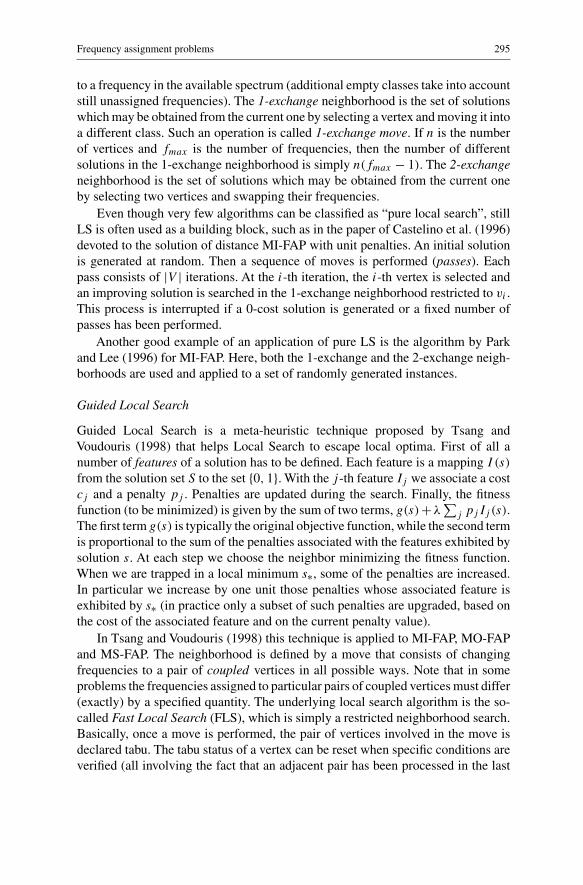
Frequency assignment problems 295
to a frequency in the available spectrum (additional empty classes take into accountstill unassigned frequencies). The 1-exchange neighborhood is the set of solutionswhich may be obtained from the current one by selecting a vertex and moving it intoa different class. Such an operation is called 1-exchange move. If n is the numberof vertices and fmax is the number of frequencies, then the number of differentsolutions in the 1-exchange neighborhood is simply n(fmax − 1). The 2-exchangeneighborhood is the set of solutions which may be obtained from the current oneby selecting two vertices and swapping their frequencies.
Even though very few algorithms can be classified as “pure local search”, stillLS is often used as a building block, such as in the paper of Castelino et al. (1996)devoted to the solution of distance MI-FAP with unit penalties. An initial solutionis generated at random. Then a sequence of moves is performed (passes). Eachpass consists of |V | iterations. At the i-th iteration, the i-th vertex is selected andan improving solution is searched in the 1-exchange neighborhood restricted to vi .This process is interrupted if a 0-cost solution is generated or a fixed number ofpasses has been performed.
Another good example of an application of pure LS is the algorithm by Parkand Lee (1996) for MI-FAP. Here, both the 1-exchange and the 2-exchange neigh-borhoods are used and applied to a set of randomly generated instances.
Guided Local Search
Guided Local Search is a meta-heuristic technique proposed by Tsang andVoudouris (1998) that helps Local Search to escape local optima. First of all anumber of features of a solution has to be defined. Each feature is a mapping I (s)
from the solution set S to the set {0, 1}. With the j -th feature Ij we associate a costcj and a penalty pj . Penalties are updated during the search. Finally, the fitnessfunction (to be minimized) is given by the sum of two terms, g(s)+λ
∑j pj Ij (s).
The first term g(s) is typically the original objective function, while the second termis proportional to the sum of the penalties associated with the features exhibited bysolution s. At each step we choose the neighbor minimizing the fitness function.When we are trapped in a local minimum s∗, some of the penalties are increased.In particular we increase by one unit those penalties whose associated feature isexhibited by s∗ (in practice only a subset of such penalties are upgraded, based onthe cost of the associated feature and on the current penalty value).
In Tsang and Voudouris (1998) this technique is applied to MI-FAP, MO-FAPand MS-FAP. The neighborhood is defined by a move that consists of changingfrequencies to a pair of coupled vertices in all possible ways. Note that in someproblems the frequencies assigned to particular pairs of coupled vertices must differ(exactly) by a specified quantity. The underlying local search algorithm is the so-called Fast Local Search (FLS), which is simply a restricted neighborhood search.Basically, once a move is performed, the pair of vertices involved in the move isdeclared tabu. The tabu status of a vertex can be reset when specific conditions areverified (all involving the fact that an adjacent pair has been processed in the last
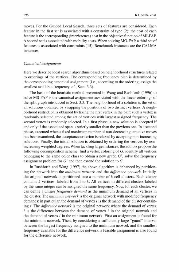
296 K.I. Aardal et al.
move). For the Guided Local Search, three sets of features are considered. Eachfeature in the first set is associated with a constraint of type (2): the cost of eachfeature is the corresponding (interference) cost in the objective function of MI-FAP.A second set is associated with mobility costs. When solving MO-FAP, a third set offeatures is associated with constraints (15). Benchmark instances are the CALMAinstances.
Canonical assignments
Here we describe local search algorithms based on neighborhood structures relatedto orderings of the vertices. The corresponding frequency plan is determined bythe corresponding canonical assignment (i.e., according to the ordering, assign thesmallest available frequency, cf., Sect. 3.3).
The basis of the heuristic method presented in Wang and Rushforth (1996) tosolve MS-FAP is the canonical assignment associated with the linear orderings ofthe split graph introduced in Sect. 3.3. The neighborhood of a solution is the set ofall solutions obtained by swapping the positions of two distinct vertices. A neigh-borhood restriction is obtained by fixing the first vertex in the pair: such a vertex israndomly selected among the set of vertices with largest assigned frequency. Thesecond vertex is randomly selected. In a first phase, a new solution is accepted ifand only if the associated span is strictly smaller than the previous one. In a secondphase, executed when a fixed maximum number of non-decreasing tentative moveshas been examined, the acceptance criterion is relaxed by accepting non-increasingsolutions. Finally, the initial solution is obtained by ordering the vertices by non-increasing weighted degrees. When tackling large instances, the authors propose thefollowing decomposition scheme: find a vertex coloring of G, identify all verticesbelonging to the same color class to obtain a new graph G′, solve the frequencyassignment problem for G′ and then extend the solution to G.
In Rushforth and Wang (1997) the above algorithm is enhanced by partition-ing the network into the minimum network and the difference network. Initially,the original network is partitioned into a number of k-cell-clusters. Each clustercontains k vertices, labeled from 1 to k. All vertices in different clusters labeledby the same integer can be assigned the same frequency. Now, for each cluster, wecan define a cluster frequency demand as the minimum demand of all vertices inthe cluster. The minimum network is the original network with modified frequencydemands: in particular, the demand of vertex i is the demand of the cluster contain-ing i. The difference network is the original network where the demand of vertexi is the difference between the demand of vertex i in the original network andthe demand of vertex i in the minimum network. First an assignment is found forthe minimum network. Then, by considering a sufficiently large “guard” intervalbetween the largest frequency assigned to the minimum network and the smallestfrequency available for the difference network, a feasible assignment is also foundfor the difference network.
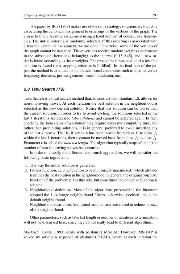
Frequency assignment problems 297
The paper by Box (1978) makes use of the same strategy: solutions are found byassociating the canonical assignment to orderings of the vertices of the graph. Theaim is to find a feasible assignment using a fixed number of consecutive frequen-cies. The initial ordering is randomly selected. If this ordering is associated witha feasible canonical assignment, we are done. Otherwise, some of the vertices ofthe graph cannot be assigned. These vertices receive random weights (incrementsin the subsequent iterations) belonging to the interval [0.15,0.45], and a new or-der is found according to these weights. The procedure is repeated until a feasiblesolution is found (or a stopping criterion is fulfilled). In the final part of the pa-per, the method is extended to handle additional constraints such as distinct vertexfrequency domains, pre-assignments, inter-modulation, etc.
5.3 Tabu Search (TS)
Tabu Search is a local search method that, in contrast with standard LS, allows fornon-improving moves. At each iteration the best solution in the neighborhood isselected as the new current solution. Notice that this solution can be worse thanthe current solution. In order to try to avoid cycling, the solutions selected in thelast k iterations are declared tabu solutions and cannot be selected again. In fact,checking the tabu status of a solution may require excessive computing time. So,rather than prohibiting solutions, it is in general preferred to avoid inverting anyof the last k moves. That is, if vertex v has been moved from class f1 to class f2within the last k iterations, then v cannot be moved back from class f2 to class f1.Parameter k is called the tabu list length. The algorithm typically stops after a fixednumber of non-improving moves has occurred.
In order to classify the different tabu search approaches, we will consider thefollowing basic ingredients:
1. The way the initial solution is generated.2. Fitness function, i.e., the function to be minimized (maximized), which also de-
termines the best solution in the neighborhood. In general the original objectivefunction of the problem plays this role, but sometimes the objective function isadapted.
3. Neighborhood definition. Most of the algorithms presented in the literatureadopted the 1-exchange neighborhood. Unless otherwise specified, this is thedefault neighborhood.
4. Neighborhood restriction. Additional mechanisms introduced to reduce the sizeof the neighborhood.
Other parameters, such as tabu list length or number of iterations to terminationwill not be discussed here, since they do not really lead to different algorithms.
MS-FAP. Costa (1993) deals with (distance) MS-FAP. However, MS-FAP issolved by solving a sequence of (distance) F-FAPs, where at each iteration the
298 K.I. Aardal et al.
size of available band is reduced. The fitness function is the interference cost of thecurrent solution (expressed as the sum of distance violations). The initial solutionis found by generalized DSATUR (see Sect. 5.1). The neighborhood is restrictedby fixing the maximum number of tentative moves. The vertices with largest localviolation, the sum of the terms in the objective function involving v, are chosenfirst. Finally, the test instances are randomly generated.
In Hao and Perrier (1999), the model is MS-FAP, which is solved (as in Costa1993) by solving a sequence of (distance) F-FAPs. The initial solution is generatedby applying standard local search to a random assignment. The fitness function isthe standard objective of MI-FAP. The 1-exchange neighborhood is restricted byrandomly selecting a small subset. Finally, the tabu status of a move depends onhow recent and how often it is preformed. Test instances are 45 randomly generatedmobile telephony instances provided by French CNET. In Hao et al. (1998) theauthors enhance the quality of the algorithm presented in Hao and Perrier (1999) byimplementing the following improvements: 1) an efficient data structure to quicklycompute best moves; 2) the neighborhood is restricted by only considering movesinvolving vertices with positive local violation; 3) co-cell constraints are treatedseparately from other type of interference constraints, i.e., only solutions which arefeasible with respect to co-cell constraints are considered; 4) the algorithm solvesa sequence of problems in order to minimize the span. At each iteration the bestsolution of the previous iteration is used to initialize the tabu-search rather thanproducing a new random solution.
MI-FAP. In Bouju et al. (1995a) the model is distance MI-FAP with two alternativedefinitions of penalties: either unit penalties or penalties proportional to the dis-tance requirement. The initial solution is randomly generated, the fitness functionis the number of violated constraints, the neighborhood restriction is performed byselecting the k vertices with largest local violation, where parameter k is increasedduring the search. Before the tabu search is started, an arc consistency preprocess-ing is performed to reduce the size of the instances, see Sect. 4. A subset of theCALMA data set is adopted to test the algorithm.
In Castelino et al. (1996) the model is distance MI-FAP with unit penalties.The fitness function is the objective of MI-FAP. No restriction is applied to theneighborhood. The tabu state of a move is determined both by how recent a movehas been performed and by the number of times a move has been performed. Testproblems are six artificial instances.
Block assignment is proposed inAdjakplé and Jaumard (1997) to solve distanceMI-FAP, where penalty costs are integers ranging from 0 to a maximum of 10.The initial solution is found by a greedy block assignment, see Sect. 5.1. Thefitness function is the standard objective of MI-FAP. The neighborhood of a blockassignment is defined by means of two different moves. The first move consistsof changing exactly one block assigned to a vertex, replacing it with one or moreavailable blocks (observe that blocks are not equally sized). The neighborhood isrestricted by fixing the maximum number of tentative moves; blocks with largest

Frequency assignment problems 299
local violation are chosen first, where the local violation of a block B with respectto a given solution is the sum of the terms involving B in the fitness function. Inorder to diversify the search, a second type of move is periodically performed.That is, a vertex with largest local violation is selected and all of its frequenciesare reassigned from scratch by a greedy block assignment heuristic. Test instancesare real-life instances provided by the Canadian Bell Mobility (see BellMobilitywebsite 1998).
A more sophisticated definition of move is proposed in the work by Borgne(1994). Frequencies are assigned in blocks and besides the standard move consistingof changing exactly one block assigned to a vertex, Borgne proposes an adaption ofthe so called Kempe Chains Interchange. In terms of graph coloring, a Kempe Chainis simply a connected component of the subgraph induced by two color classes,say C1 and C2 corresponding to colors c1 and c2. A Kempe interchange consistsof interchanging the colors of the vertices in the two color classes, i.e., assigningcolor c2 to the vertices in C1 and color c1 to the vertices in C2. The extension tofrequency assignment with only co-channel constraints is straightforward. The ideais to first select two adjacent vertices u and v that are assigned a same frequency,say f1, and that have strong co-channel interference. Select another frequency f2and suppose that no vertex assigned to f2 is adjacent to u. Then we can assignf1 to all vertices which are assigned to f2 and assign f2 to all vertices which areassigned to f1 but u. In this new assignment, u and v have different frequenciesand no other edge violation is created. This leads to a reduction of the overallinterference cost. This definition of move can be generalized by taking into accountother types of interference constraints such as adjacent channel constraints, andby allowing the interchange of three or more frequencies. Experiments on tworeal-life cellular network problems provided by Ericsson show the effectiveness ofgeneralized Kempe chain interchanges.
Capone and Trubian (1999) solve MI-FAP by minimizing the interference leveldirectly evaluated on the grid of test points introduced in Subsection 2.1 (rather thanon the interference graph). They use the standard neighborhood, i.e., the exchangeof a frequency to a single vertex. However, exploring and evaluating all the solutionsin the standard neighborhood can be too expensive due to the large number of testpoints in an average sized instance. So, once a vertexv is chosen, the neighborhood isrestricted by first evaluating a simplified objective function which makes it possibleto remove some of the frequencies available for v. Ad hoc generated test instanceshave been used to test the algorithm.
Finally, Tabu Search has also been applied to the solution of natural extensionsof FAP, as for example in Smith et al. (2001) where far site constraints, spuriousemission and response constraints, intermodulation product constraints and exclu-sivity constraints are considered.
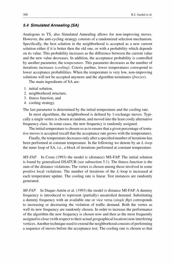
300 K.I. Aardal et al.
5.4 Simulated Annealing (SA)
Analogous to TS, also Simulated Annealing allows for non-improving moves.However, the anti-cycling strategy consists of a randomized selection mechanism.Specifically, the best solution in the neighborhood is accepted as a new currentsolution either if it is better then the old one, or with a probability which dependson its value. This probability increases as the difference between the current valueand the new value decreases. In addition, the acceptance probability is controlledby another parameter, the temperature. This parameter decreases as the number ofiterations increases (cooling). Ceteris paribus, lower temperatures correspond tolower acceptance probabilities. When the temperature is very low, non-improvingsolutions will not be accepted anymore and the algorithm terminates (freezes).
The main ingredients of SA are:
1. initial solution,2. neighborhood structure,3. fitness function, and4. cooling strategy.
The last parameter is determined by the initial temperature and the cooling rate.In most algorithms, the neighborhood is defined by 1-exchange moves. Typi-
cally a single vertex is chosen at random, and moved into the least costly alternativefrequency class. In some cases, the new frequency is randomly assigned.
The initial temperature is chosen so as to ensure that a given percentage of tenta-tive moves is accepted (recall that the acceptance rate grows with the temperature).
Finally, the temperature decreases only after a specified number of iterations hasbeen performed at constant temperature. In the following we denote by an L-loopthe inner loop of SA, i.e., a block of iterations performed at constant temperature.
MS-FAP. In Costa (1993) the model is (distance) MS-FAP. The initial solutionis found by generalized DSATUR (see subsection 5.1). The fitness function is thesum of the distance violations. The vertex is chosen among those involved in somepositive local violations. The number of iterations of the L-loop is increased ateach temperature update. The cooling rate is linear. Test instances are randomlygenerated.
MI-FAP. In Duque-Antón et al. (1993) the model is distance MI-FAP. A dummyfrequency is introduced to represent (partially) unsatisfied demand. Substitutinga dummy frequency with an available one or vice versa (single flip) correspondsto increasing or decreasing the violation of traffic demand. Both the vertex aswell its new frequency are randomly chosen. In order to increase the performanceof the algorithm the new frequency is chosen now and then as the most frequentlyassigned to close (with respect to their actual geographical location) non-interferingvertices.Another technique used to extend the neighborhood consists of performinga sequence of moves before the acceptance test. The cooling rate is chosen so that
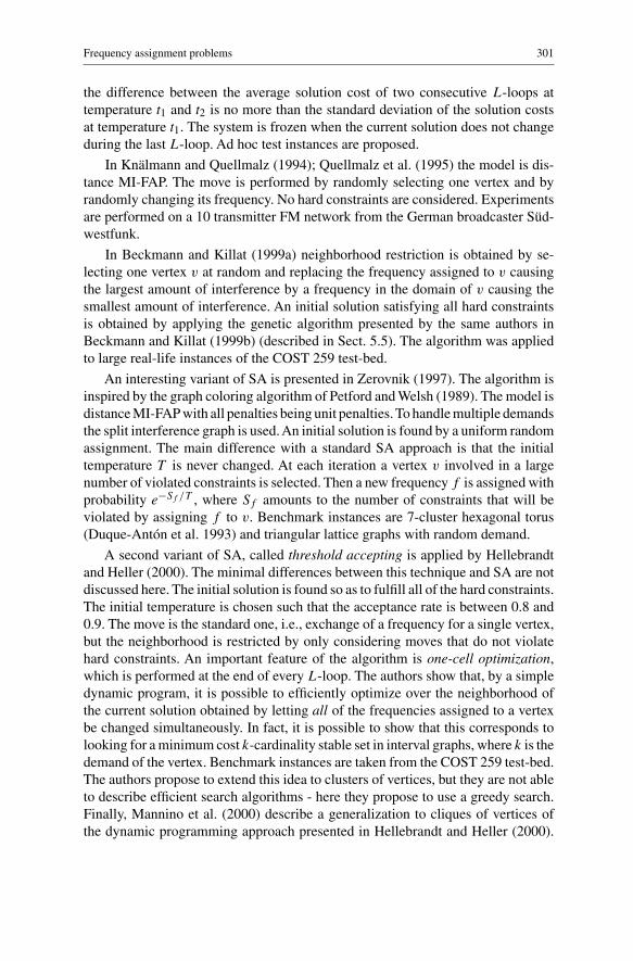
Frequency assignment problems 301
the difference between the average solution cost of two consecutive L-loops attemperature t1 and t2 is no more than the standard deviation of the solution costsat temperature t1. The system is frozen when the current solution does not changeduring the last L-loop. Ad hoc test instances are proposed.
In Knälmann and Quellmalz (1994); Quellmalz et al. (1995) the model is dis-tance MI-FAP. The move is performed by randomly selecting one vertex and byrandomly changing its frequency. No hard constraints are considered. Experimentsare performed on a 10 transmitter FM network from the German broadcaster Süd-westfunk.
In Beckmann and Killat (1999a) neighborhood restriction is obtained by se-lecting one vertex v at random and replacing the frequency assigned to v causingthe largest amount of interference by a frequency in the domain of v causing thesmallest amount of interference. An initial solution satisfying all hard constraintsis obtained by applying the genetic algorithm presented by the same authors inBeckmann and Killat (1999b) (described in Sect. 5.5). The algorithm was appliedto large real-life instances of the COST 259 test-bed.
An interesting variant of SA is presented in Zerovnik (1997). The algorithm isinspired by the graph coloring algorithm of Petford and Welsh (1989). The model isdistance MI-FAP with all penalties being unit penalties. To handle multiple demandsthe split interference graph is used.An initial solution is found by a uniform randomassignment. The main difference with a standard SA approach is that the initialtemperature T is never changed. At each iteration a vertex v involved in a largenumber of violated constraints is selected. Then a new frequency f is assigned withprobability e−Sf /T , where Sf amounts to the number of constraints that will beviolated by assigning f to v. Benchmark instances are 7-cluster hexagonal torus(Duque-Antón et al. 1993) and triangular lattice graphs with random demand.
A second variant of SA, called threshold accepting is applied by Hellebrandtand Heller (2000). The minimal differences between this technique and SA are notdiscussed here. The initial solution is found so as to fulfill all of the hard constraints.The initial temperature is chosen such that the acceptance rate is between 0.8 and0.9. The move is the standard one, i.e., exchange of a frequency for a single vertex,but the neighborhood is restricted by only considering moves that do not violatehard constraints. An important feature of the algorithm is one-cell optimization,which is performed at the end of every L-loop. The authors show that, by a simpledynamic program, it is possible to efficiently optimize over the neighborhood ofthe current solution obtained by letting all of the frequencies assigned to a vertexbe changed simultaneously. In fact, it is possible to show that this corresponds tolooking for a minimum cost k-cardinality stable set in interval graphs, where k is thedemand of the vertex. Benchmark instances are taken from the COST 259 test-bed.The authors propose to extend this idea to clusters of vertices, but they are not ableto describe efficient search algorithms - here they propose to use a greedy search.Finally, Mannino et al. (2000) describe a generalization to cliques of vertices ofthe dynamic programming approach presented in Hellebrandt and Heller (2000).
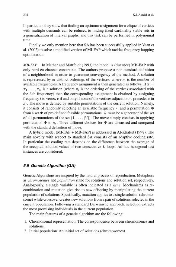
302 K.I. Aardal et al.
In particular, they show that finding an optimum assignment for a clique of verticeswith multiple demands can be reduced to finding fixed cardinality stable sets ina generalization of interval graphs, and this task can be performed in polynomialtime.
Finally we only mention here that SA has been successfully applied in Yuan etal. (2002) to solve a modified version of MI-FAP which tackles frequency hoppingoptimization.
MB-FAP. In Mathar and Mattfeldt (1993) the model is (distance) MB-FAP withonly hard co-channel constraints. The authors propose a non standard definitionof a neighborhood in order to guarantee convergency of the method. A solutionis represented by m distinct orderings of the vertices, where m is the number ofavailable frequencies. A frequency assignment is then generated as follows. If π =π1, . . . , πm is a solution (where πi is the ordering of the vertices associated withthe i-th frequency) then the corresponding assignment is obtained by assigningfrequency i to vertex v if and only if none of the vertices adjacent to v precedes v inπi . The move is defined by suitable permutations of the current solution. Namely,it consists of randomly selecting an available frequency r , and a permutation �
from a set of pre-defined feasible permutations. must be a generator of the setof all permutations of the set {1, . . . , |V |}. The move simply consists in applyingpermutation � to πr . Three different choices for are discussed and comparedwith the standard definition of move.
A hybrid model (MI-FAP + MB-FAP) is addressed in Al-Khaled (1998). Themain novelty with respect to standard SA consists of an adaptive cooling rate.In particular the cooling rate depends on the difference between the average ofthe accepted solution values of two consecutive L-loops. Ad hoc hexagonal testinstances are considered.
5.5 Genetic Algorithm (GA)
Genetic Algorithms are inspired by the natural process of reproduction. Metaphorsas chromosomes and population stand for solutions and solution set, respectively.Analogously, a single variable is often indicated as a gene. Mechanisms as re-combination and mutation give rise to new offspring by manipulating the currentpopulation of solutions. Specifically, mutation applies to a single solution (chromo-some) while crossover creates new solutions from a pair of solutions selected in thecurrent population. Following a standard Darwinistic approach, selection extractsthe most promising individuals in the current population.
The main features of a genetic algorithm are the following:
1. Chromosomal representation. The correspondence between chromosomes andsolutions.
2. Initial population. An initial set of solutions (chromosomes).
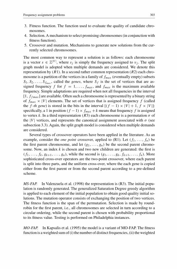
Frequency assignment problems 303
3. Fitness function. The function used to evaluate the quality of candidate chro-mosomes.
4. Selection. A mechanism to select promising chromosomes (in conjunction withfitness function).
5. Crossover and mutation. Mechanisms to generate new solutions from the cur-rently selected chromosomes.
The most common way to represent a solution is as follows: each chromosomeis a vector s ∈ Z
|V |, where sj is simply the frequency assigned to vj . The splitgraph model is adopted when multiple demands are considered. We denote thisrepresentation by (R1). In a second rather common representation (R2) each chro-mosome is a partition of the vertices in a family of fmax (eventually empty) subsetsS1, S2, . . . , Sfmax , called the genes, where Sf is the set of vertices that are as-signed frequency f for f = 1, . . . , fmax , and fmax is the maximum availablefrequency. Simple adaptations are required when not all frequencies in the interval[1, ff max] are available. Often such a chromosome is represented by a binary stringof fmax × |V | elements. The set of vertices that is assigned frequency f (calledthe f -th gene) is stored in the bits in the interval [(f − 1) × |V | + 1, f × |V |]:specifically, a 1 in position (f − 1)×fmax + k means that frequency f is assignedto vertex k. In a third representation (R3) each chromosome is a permutation σ ofthe |V | vertices, and represents the canonical assignment associated with σ (seesubsection 3.3). Again, the split graph model is considered when multiple demandsare considered.
Several types of crossover operators have been applied in the literature. As anexample, consider the one point crossover, applied to (R1). Let (f1, . . . , fn) bethe first parent chromosome, and let (g1, . . . , gn) be the second parent chromo-some. Now, an index k is chosen and two new children are generated: the first is(f1, . . . , fk, gk+1, . . . , gn), while the second is (g1, . . . , gk, fk+1, . . . , fn). Moresophisticated cross-over operators are the two-point crossover, where each parentis split into three parts, and the uniform cross-over, where the each gene is copiedeither from the first parent or from the second parent according to a pre-definedscheme.
MS-FAP. In Valenzuela et al. (1998) the representation is (R3). The initial popu-lation is randomly generated. The generalized Saturation Degree greedy algorithmis applied to each element of the initial population to obtain good quality initial so-lutions. The mutation operator consists of exchanging the position of two vertices.The fitness function is the span of the permutation. Selection is made by round-robin for the first parent, i.e., all chromosomes are selected in turn according to acircular ordering, while the second parent is chosen with probability proportionalto its fitness value. Testing is performed on Philadelphia instances.
MO-FAP. In Kapsalis et al. (1995) the model is a variant of MO-FAP. The fitnessfunction is a weighted sum of (i) the number of distinct frequencies, (ii) the weighted

304 K.I. Aardal et al.
sum of violated constraints (different types of constraints different weights), (iii)mobility costs. Two chromosomal representations are adopted: the first is a simplevariant of (R1), the second is (R2). Besides standard operators, a number of spe-cialized crossover operators were tested. The first one, applied to (R1), consists ofa repeated application of the following steps:
1. Select a constraint (and the corresponding pair of vertices u and v) and checkwhether this constraint is satisfied by any of the two currently selected parents.
2. If it is satisfied, then interchange the frequencies assigned to u and v in the firstparent with those assigned in the second parent.
The second one is a single-point operator applied to (R2): similar to Cromptonet al. (1994) (described above), the genes are interchanged taking care of the hardconstraints. A first mutation operator is applied to (R1) and consists of choosing apair of vertices and interchanging the frequencies assigned to them. Also the sec-ond mutation operator applies to (R1) and consists of choosing a pair of verticeswhose assignment violates a hard constraint, then randomly changing the assignedfrequencies with a new pair of available frequencies which do not violate such con-straint. The last mutation applies to (R2). A set of vertices with the same frequencyare reassigned a commonly available new frequency. Finally, several strategies tostatic and dynamic modification of the fitness function are proposed. Experimentsare performed using the CALMA data set.
In Dorne and Hao (1995) the model is (distance) MO-FAP and the authorsadopt the standard representation (R1). The fitness function is the number of un-satisfied constraints. Mutation in a given chromosome is performed by selectingan infeasible assignment, i.e., a vertex v and a frequency assigned to v violatingone or more constraints, and then replacing this frequency with the best alternative.The selection mechanism extracts one chromosome from the current population byfavoring elements not yet trapped in local optima. The child obtained by applyingthe mutation operator is accepted only if (i) its fitness function is not worse thanthe fitness of the parent or (ii) randomly with a given probability. No crossover isapplied. Test instances are a set of 18 real-life problems from CNET. The algorithmfavorably compares with Constraint Programming and Simulated Annealing.
Dorne and Hao (1996) extend the algorithm presented in Dorne and Hao (1995)to the multi-demand case. Co-cell constraints are used to limit the size of the searchspace by a suitable adaptation of the mutation operator. Again, crossover is notimplemented. The GA algorithm is repeated several times after the generation of anew population. Testing is performed on 10 instances.
Finally, Hao and Dorne (1996) extend the algorithm presented in Dorne andHao (1996) (described above) by applying three different crossovers: single-point,uniform, and conflict based. The last consists of changing only those genes repre-senting frequencies violating one or more constraints.
MI-FAP. In Cuppini (1994) the encoding scheme is (R2), while the fitness functionis the weighted sum of two terms: the first takes into account the global interfer-
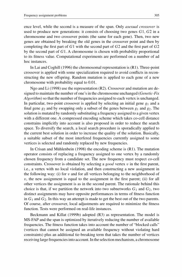
Frequency assignment problems 305
ence level, while the second is a measure of the span. Only asexual crossover isused to produce new generations: it consists of choosing two genes G1, G2 in achromosome and two crossover points (the same for each gene). Then, two newgenes are obtained by breaking the old genes in the crossover point and then bycompleting the first part of G1 with the second part of G2 and the first part of G2by the second part of G1. A chromosome is chosen with probability proportionalto its fitness value. Computational experiments are performed on a number of adhoc instances.
In Lai and Coghill (1996) the chromosomal representation is (R1). Three-pointcrossover is applied with some specialization required to avoid conflicts in recon-structing the new offspring. Random mutation is applied to each gene of a newchromosome with probability equal to 0.01.
Ngo and Li (1998) use the representation (R2). Crossover and mutation are de-signed to maintain the number of one’s in the chromosome unchanged (Genetic-FixAlgorithm) so that the number of frequencies assigned to each vertex is unchanged.In particular, two-point crossover is applied by selecting an initial gene g1 and afinal gene g2 and by swapping only a subset of the genes between g1 and g2. Thesolution is mutated by randomly substituting a frequency assigned to a given vertexwith a different one. A compressed encoding scheme which takes co-cell distanceconstrains implicitly into account is also proposed in order to reduce the searchspace. To diversify the search, a local search procedure is sporadically applied tothe current best solution in order to increase the quality of the solution. Basically,a suitable subset of the most interfered frequencies currently assigned to somevertices is selected and randomly replaced by new frequencies.
In Crisan and Mühlenbein (1998) the encoding scheme is (R1). The mutationoperator consists of replacing a frequency assigned to one vertex by a randomlychosen frequency from a candidate set. The new frequency must respect co-cellconstraints. Crossover is obtained by selecting a good vertex v in the first parent,i.e., a vertex with no local violation, and then constructing a new assignment inthe following way: (i) for v and for all vertices belonging to the neighborhood ofv, the new assignment is equal to the assignment in the first parent; (ii) for allother vertices the assignment is as in the second parent. The rationale behind thischoice is that, if we partition the network into two subnetworks G1 and G2, twodistinct assignments may have opposite performances in terms of fitness functionin G1 and G2. In this way an attempt is made to get the best out of the two parents.Of course, after crossover, local adjustments are required to minimize the fitnessfunction. Tests were performed on real-life instances.
Beckmann and Killat (1999b) adopted (R3) as representation. The model isMS-FAP and the span is optimized by iteratively reducing the number of availablefrequencies. The fitness function takes into account the number of “blocked calls”(vertices that cannot be assigned an available frequency without violating hardconstraints) plus an additional tie-breaking term that takes the number of verticesreceiving large frequencies into account. In the selection mechanism, a chromosome
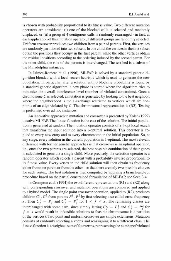
306 K.I. Aardal et al.
is chosen with probability proportional to its fitness value. Two different mutationoperators are considered: (i) one of the blocked calls is selected and randomlydisplaced, or (ii) a group of 4 contiguous calls is randomly rearranged - in fact, ateach application of this mutation operator, 3 different groups are randomly selected.Uniform crossover produces two children from a pair of parents. First, the verticesare randomly partitioned into two subsets. In one child, the vertices in the first subsetobtain the positions they occupy in the first parent, while the other vertices obtainthe residual positions according to the ordering induced by the second parent. Forthe other child, the role of the parents is interchanged. The test bed is a subset ofthe Philadelphia instances.
In Jaimes-Romero et al. (1996), MI-FAP is solved by a standard genetic al-gorithm blended with a local search heuristic which is used to generate the newpopulation. In particular, after a solution with 0 blocking probability is found bya standard genetic algorithm, a new phase is started where the algorithm tries tominimize the overall interference level (number of violated constraints). Once achromosome C is selected, a mutation is generated by looking to the best neighbor,where the neighborhood is the 1-exchange restricted to vertices which are end-points of an edge violated by C. The chromosomal representation is (R2). Testingis performed over ad hoc instances.
An innovative approach to mutation and crossover is presented by Kolen (1999)to solve MI-FAP. The fitness function is the cost of the solution. The initial popula-tion is generated at random. The mutation operator consists of a 1-opt local searchthat transforms the input solution into a 1-optimal solution. This operator is ap-plied to every new entry and to every chromosome in the initial population. So, atany stage, every solution in the current population is 1-optimal. The most relevantdifference with former genetic approaches is that crossover is an optimal operator,i.e., once the two parents are selected, the best possible combination of their genesis calculated to generate a single child. More precisely, the selection operator is arandom operator which selects a parent with a probability inverse proportional toits fitness value. Every vertex in the child solution will then obtain its frequencyeither from one parent or from the other - so that there are only two possible choicesfor each vertex. The best solution is then computed by applying a branch-and-cutprocedure based on the partial constrained formulation of MI-FAP, see Sect. 3.4.
In Crompton et al. (1994) the two different representations (R1) and (R2) alongwith corresponding crossover and mutation operations are compared and appliedto a hybrid model. The single point crossover operation, applied to (R2), produceschildren C1, C2 from parents P 1, P 2 by first selecting a so-called cross frequencyx. Then C1
f = P 1f and C2
f = P 2f for 1 ≤ f ≤ x. The remaining classes are
interchanged with some care, since simply letting C2f = P 1
f and C1f = P 2
f forf > x would result in infeasible solutions (a feasible chromosome is a partitionof the vertices). Two point and uniform crossover are simple extensions. Mutationconsists of randomly selecting a vertex and reassigning it to a different class. Thefitness function is a weighted sum of four terms, representing the number of violated
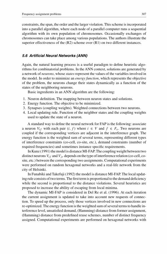
Frequency assignment problems 307
constraints, the span, the order and the larger violation. This scheme is incorporatedinto a parallel algorithm, where each node of a parallel computer runs a sequentialalgorithm with its own population of chromosomes. Occasionally exchanges ofchromosomes can take place among various populations. The authors illustrate thesuperior effectiveness of the (R2) scheme over (R1) on two different instances.
5.6 Artificial Neural Networks (ANN)
Again, the natural learning process is a useful paradigm to define heuristic algo-rithms for combinatorial problems. In the ANN context, solutions are generated bya network of neurons, whose states represent the values of the variables involved inthe model. In order to minimize an energy function, which represents the objectiveof the problem, the neurons change their states dynamically as a function of thestates of the neighboring neurons.
Basic ingredients in an ANN algorithm are the following:
1. Neuron definition. The mapping between neuron states and solutions.2. Energy function. The objective to be minimized.3. Synapses (coupling weights). Weighted connections between two neurons.4. Local updating rule. Function of the neighbor states and the coupling weights
used to update the state of a neuron.
A standard way to define the neural network for FAP is the following: associatea neuron Vif with each pair (i, f ) where i ∈ V and f ∈ Fv . Two neurons arecoupled if the corresponding vertices are adjacent in the interference graph. Theenergy function is the weighted sum of several terms, representing different typesof interference constraints (co-cell, co-site, etc.), demand constraints (number ofrequired frequencies) and sometimes instance specific requirements.
In Kunz (1991) the model is distance MI-FAP. The coupling weight between twodistinct neuronsVif andVjr depends on the type of interference relation (co-cell, co-site, etc.) between the corresponding two assignments. Computational experimentswere performed on random hexagonal networks and a real-life network from thecity of Helsinki.
In Funabiki and Takefuji (1992) the model is distance MI-FAP. The local updat-ing rule consists of two terms. The first term is proportional to the demand deficiencywhile the second is proportional to the distance violations. Several heuristics areproposed to increase the ability of escaping from local minima.
The dynamic MI-FAP is considered in Del Re et al. (1996). At each iterationthe current assignment is updated to take into account new requests of connec-tion. To speed up the process, only those vertices involved in new connections arere-optimized. The energy function is the weighted sum of several terms to handle in-terference level, unsatisfied demand, (Hamming) distance from former assignment,(Hamming) distance from predefined reuse schemes, number of distinct frequencyassigned. Computational experiments are performed on hexagonal networks with

308 K.I. Aardal et al.
non-uniform traffic distribution. A special type of dynamic channel allocation is theborrowing channel assignment (BCA) where one vertex is allowed to borrow fre-quencies from its neighbors.A standardANN algorithm to solve (BCA) is presentedin Sandalidis et al. (1999).
In Kim et al. (1996) the neurons can only assume binary values. The energyfunction takes into account several types of interference constraints and the levelof unsatisfied demand. In particular, the latter term is translated into an additionalinput to each neuron, which forces the assignment of new frequencies to verticeswith unsatisfied demand. Several initialization and updating methods are proposed.Benchmark instances are ad hoc hexagonal networks.
Model MI-FAP is addressed in the connectionist algorithm presented in Boujuet al. (1995b). The algorithm is compared on the CALMA test-bed.
Finally, Smith and Palaniswami (1997) modified the Hopfield network to incor-porate some hill climbing mechanism for escaping from local minima. Experimentswith a self-organizing neural network are also performed (however, the Hopfieldnetwork with hill climbing appears to be the best method). Benchmark instancesare the Philadelphia instances and the Helsinki instances proposed in Kunz (1991).
5.7 Ant Colony and Multi-agent Optimization
Ant Colony Optimization (ACO) is a class of constructive meta-heuristic algorithmsinspired by real ants behavior. We have a fixed number of ants, where each ant can beinterpreted as a sequential greedy algorithm which iteratively generates a solutionby upgrading partial solution moves. A move is controlled by two parameters: theattractiveness which is based on the structure of the problem (costs and constraints);the pheromone trail level which takes into account how many times a given movehas been successful. Pheromone trails are updated when all ants have completedthe construction of their solution, increasing (decreasing) the level for those moveswhich led to good (bad) solutions. A lower bound is required to fix the initial levelof pheromones. Finally, the solution generated by each ant is possibly improved bylocal search.
Maniezzo and Carbonaro (2000) solve MI-FAP by means of ACO. A partialsolution consists of an assignment of frequencies to a subset of the vertices. Inorder to complete a given partial solution, every ant selects a new vertex and anew frequency to be assigned to this vertex at each iteration. This assignment isdefined as a move. The initial lower bound is computed by solving the relaxation ofthe (orientation) formulation proposed in Borndörfer et al. (1998b). The solutionproduced by each ant is locally upgraded by local search. The authors use thissolution to define a partial order on the vertex set (as in the orientation model).The proposed local search algorithm looks for solutions with the same underlyingorder. Benchmark test problems are the CALMA instances and the Philadelphiainstances. A different and simplified version of ant optimization applied to distanceMI-FAP is given by Abril et al. (2000). Here, each ant is assigned to a vertex of

Frequency assignment problems 309
the interference graph (penalties are all equal to 1). At each iteration an ant movesfrom a vertex v to an adjacent one u with largest local violation (or at random).Once there, the ant changes one of the frequencies assigned to u to the best possible(or to a random one). Tests were performed on a set of real-life (Spanish) GSMinstances.
We mention here that ACO has been applied in Montemanni et al. (2002a) tosolve an extension of FAP which incorporates multiple interference.
5.8 Formulation based relaxations
A standard way to solve an optimization problem consists of describing it by meansof a mathematical formulation which in turn may be solved by some standardtechniques. However, for most practical instances such formulations are too largeto be solved to optimality and we must content ourselves with heuristic solutions.A classical heuristic approach consists of removing some “difficult” constraints sothat the residual problem can be handled. Removed constraints can be accountedfor in several ways or simply ignored.
5.8.1 Lagrangian relaxation
In Chang and Kim (1997) the adopted model is MB-FAP, with co-channel andadjacent channel constraints. A family of stable sets (patterns) of the interferencegraph is generated. To simplify the model, frequencies are assigned to patterns,rather than to single vertices. The objective function is linearized by exploiting thefact that the Erlang B formula is piecewise linear. The problem is formulated asa mixed-integer linear program, by means of two types of variables: assignmentvariables (to select patterns and assign a frequency to each selected pattern), andvariables associated with the linearization of the Erlang B formula. The Lagrangianrelaxation is obtained by relaxing all the constraints coupling the two types ofvariables. The residual problem is a maximum weighted stable set problem which issolved by branch-and-bound. The Lagrangian multipliers are updated by a standardsubgradient approach. Test problems are randomly generated.
5.8.2 Orientation formulation
For MI-FAP, the orientation formulation (cf., Sect. 3.6.2) is exploited in the methodproposed by Borndörfer et al. (1998b). The authors show that, under mild assump-tions, the relaxation of the orientation formulation has integral solutions once allvariables of type �uv are fixed either to 0 or 1, i.e., an orientation of the edgeshas been fixed. This observation leads to a two-stage heuristic. In the first stage anorientation � is chosen. In a second stage, a minimum cost assignment is found bysolving the associated linear program. A new partial orientation is then generatedby exploiting information associated to the solution of the relaxation.
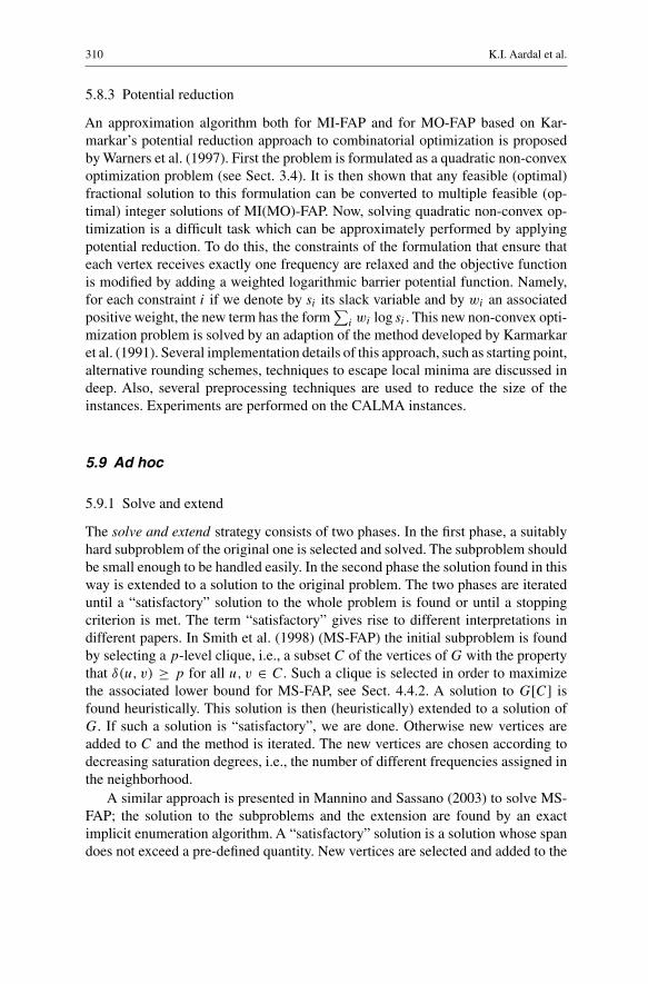
310 K.I. Aardal et al.
5.8.3 Potential reduction
An approximation algorithm both for MI-FAP and for MO-FAP based on Kar-markar’s potential reduction approach to combinatorial optimization is proposedby Warners et al. (1997). First the problem is formulated as a quadratic non-convexoptimization problem (see Sect. 3.4). It is then shown that any feasible (optimal)fractional solution to this formulation can be converted to multiple feasible (op-timal) integer solutions of MI(MO)-FAP. Now, solving quadratic non-convex op-timization is a difficult task which can be approximately performed by applyingpotential reduction. To do this, the constraints of the formulation that ensure thateach vertex receives exactly one frequency are relaxed and the objective functionis modified by adding a weighted logarithmic barrier potential function. Namely,for each constraint i if we denote by si its slack variable and by wi an associatedpositive weight, the new term has the form
∑i wi log si . This new non-convex opti-
mization problem is solved by an adaption of the method developed by Karmarkaret al. (1991). Several implementation details of this approach, such as starting point,alternative rounding schemes, techniques to escape local minima are discussed indeep. Also, several preprocessing techniques are used to reduce the size of theinstances. Experiments are performed on the CALMA instances.
5.9 Ad hoc
5.9.1 Solve and extend
The solve and extend strategy consists of two phases. In the first phase, a suitablyhard subproblem of the original one is selected and solved. The subproblem shouldbe small enough to be handled easily. In the second phase the solution found in thisway is extended to a solution to the original problem. The two phases are iterateduntil a “satisfactory” solution to the whole problem is found or until a stoppingcriterion is met. The term “satisfactory” gives rise to different interpretations indifferent papers. In Smith et al. (1998) (MS-FAP) the initial subproblem is foundby selecting a p-level clique, i.e., a subset C of the vertices of G with the propertythat δ(u, v) ≥ p for all u, v ∈ C. Such a clique is selected in order to maximizethe associated lower bound for MS-FAP, see Sect. 4.4.2. A solution to G[C] isfound heuristically. This solution is then (heuristically) extended to a solution ofG. If such a solution is “satisfactory”, we are done. Otherwise new vertices areadded to C and the method is iterated. The new vertices are chosen according todecreasing saturation degrees, i.e., the number of different frequencies assigned inthe neighborhood.
A similar approach is presented in Mannino and Sassano (2003) to solve MS-FAP; the solution to the subproblems and the extension are found by an exactimplicit enumeration algorithm. A “satisfactory” solution is a solution whose spandoes not exceed a pre-defined quantity. New vertices are selected and added to the
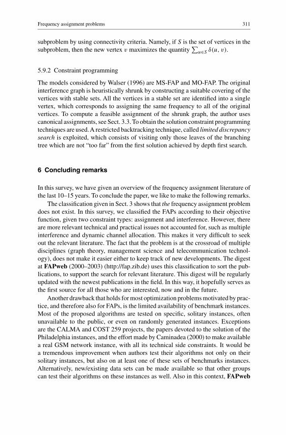
Frequency assignment problems 311
subproblem by using connectivity criteria. Namely, if S is the set of vertices in thesubproblem, then the new vertex v maximizes the quantity
∑u∈S δ(u, v).
5.9.2 Constraint programming
The models considered by Walser (1996) are MS-FAP and MO-FAP. The originalinterference graph is heuristically shrunk by constructing a suitable covering of thevertices with stable sets. All the vertices in a stable set are identified into a singlevertex, which corresponds to assigning the same frequency to all of the originalvertices. To compute a feasible assignment of the shrunk graph, the author usescanonical assignments, see Sect. 3.3. To obtain the solution constraint programmingtechniques are used.A restricted backtracking technique, called limited discrepancysearch is exploited, which consists of visiting only those leaves of the branchingtree which are not “too far” from the first solution achieved by depth first search.
6 Concluding remarks
In this survey, we have given an overview of the frequency assignment literature ofthe last 10–15 years. To conclude the paper, we like to make the following remarks.
The classification given in Sect. 3 shows that the frequency assignment problemdoes not exist. In this survey, we classified the FAPs according to their objectivefunction, given two constraint types: assignment and interference. However, thereare more relevant technical and practical issues not accounted for, such as multipleinterference and dynamic channel allocation. This makes it very difficult to seekout the relevant literature. The fact that the problem is at the crossroad of multipledisciplines (graph theory, management science and telecommunication technol-ogy), does not make it easier either to keep track of new developments. The digestat FAPweb (2000–2003) (http://fap.zib.de) uses this classification to sort the pub-lications, to support the search for relevant literature. This digest will be regularlyupdated with the newest publications in the field. In this way, it hopefully serves asthe first source for all those who are interested, now and in the future.
Another drawback that holds for most optimization problems motivated by prac-tice, and therefore also for FAPs, is the limited availability of benchmark instances.Most of the proposed algorithms are tested on specific, solitary instances, oftenunavailable to the public, or even on randomly generated instances. Exceptionsare the CALMA and COST 259 projects, the papers devoted to the solution of thePhiladelphia instances, and the effort made by Caminadea (2000) to make availablea real GSM network instance, with all its technical side constraints. It would bea tremendous improvement when authors test their algorithms not only on theirsolitary instances, but also on at least one of these sets of benchmarks instances.Alternatively, new/existing data sets can be made available so that other groupscan test their algorithms on these instances as well. Also in this context, FAPweb
312 K.I. Aardal et al.
(2000–2003) likes to serve as an intermediary, and as the place for comparing theresults.
Concerning the methodologies applied to frequency assignment, many of them,especially the proposed heuristics are small variations on standard themes. For thesake of completeness, a brief description of most of these technical papers havebeen reported in the survey. On the other hand, a limited number of original orseminal papers have appeared, and they have been discussed in more detail. Wehope that our categorization of these methods gives insight into their contribution,and helps in positioning future research as well.
All above mentioned reasons for confusing the study of the frequency assign-ment literature, applied to the authors of this survey as well. Over and over again,we discovered relevant (new or old) papers on the topic. Therefore, we do not claimthat this survey gives a complete overview of the literature. We, however, have con-fidence that all important developments in the field have been covered. Althoughwe plan to keep track of future trends in frequency assignment, this intention canonly be realized with the help of all working in the field. Also at this point, FAP-web (2000–2003) plays an important role. By providing information about newpapers and results to FAPweb (2000–2003), the FAP community can be informedextremely fast, and newcomers are always provided with the latest information inthe field.
Looking to the future of frequency assignment, three technological develop-ments are of importance. On the one hand, the major accelerator for the developmentof frequency assignment algorithms, the constitution of GSM and other second gen-eration (2G) networks will come to its end in the near future. The new generationof 3G networks, like the UMTS technology, exploits mainly code division mul-tiplexing (CMDA) instead of frequency division multiplexing. As a consequence,optimization models for CDMA networks have an emphasis other than frequencyassignment. By this frequency assignment will lack some of its importance. On theother hand however, several other new technologies like wireless LANs and ad-hoc networks are rapidly developing and in this context new frequency assignmentproblems pop up. Especially, the dynamic nature and the decentralized structure ofthese networks will (again) effect the view on the frequency assignment problemin the coming years. A third important developing application is in digital terres-trial broadcasting networks. The transition from the current analog technology tothe digital one, forthcoming all over Europe, provides new challenging frequencyassignment problems.
Finally, from the mathematical perspective, there is still enough room for im-provement of the solution and lower bounding techniques for all variants of fre-quency assignment problems. The still practical relevance of, in particular, theminimum interference and minimum blocking FAPs can be an additional motiva-tion to do so. This survey offers the possibility to detect the areas where advancescan be successful. Altogether, we conclude that this survey can not be seen as afinal report on frequency assignment, but as an evaluation of the field.
Frequency assignment problems 313
Acknowledgements. We would like to thank Andreas Eisenblätter for his many helpful comments, bothon the form and the contents of this article.
References
Aardal KI, Hipolito A, van Hoesel CPM, Jansen B (1996) A branch-and-cut algorithm for the frequencyassignment problem. Research Memorandum 96/011, Maastricht University
Aardal KI, Hurkens CAJ, Lenstra JK, Tiourine SR (2002) Algorithms for radio link frequency assign-ment: The CALMA project. Operations Research 50(6): 968–980
Abril J, Comellas F, Cortés A, Ozón J, Vaquer M (2000) A multi-agent system for frequency assignmentin cellular radio networks. IEEE Transactions on Vehicular Technology 49(5): 1558–1565
Adjakplé PM, Jaumard B (1997) Greedy and tabu search heuristics for channel block assignment incellular systems. Technical Report G-97–45, École Polytechnique de Montréal
Al-Khaled FS (1998) Optimal radio channel assignment through the new binary dynamic simulatedannealing algorithm. International Journal of Communication Systems 11: 327–336
Allen SM, Smith DH, Hurley S (1999) Lower bounding techniques for frequency assignment. DiscreteMathematics 197/198: 41–52
Anderson LG (1973) A simulation study of some dynamic channel assignment algorithms in a highcapacity mobile telecommunications system. IEEE Transactions on Communications 21: 1294–1301
AvenaliA, Mannino C, SassanoA (2002) Minimizing the span ofd-walks to compute optimum frequencyassignments. Mathematical Programming 91(2): 357–374. Previously published as techincal report04–00, DIS-Universitá di Roma “La Sapienza”, Rome, Italy
Baybars I (1982) Optimal assignment of broadcasting frequencies. European Journal of OperationsResearch 9: 257–263
Beckmann D, Killat U (1999a) Frequency planning with respect to interference minimization in cellularradio networks. Technical Report TD(99) 032, COST 259, Vienna, Austria
Beckmann D, Killat U (1999b) A new strategy for the application of genetic algorithms to the channel-assignment problem. IEEE Transactions on Vehicular Technology 48(4): 1261–1269
Bell-Mobility website (1998) Frequency assignment benchmarks Canadian urban areas.URL: http://www.crt.umontreal.ca/˜brigitt/telecom/TEST_PROBS/prob1.html
van Benthem HP (1995) GRAPH generating radio link frequency assignment problems heuristically.Master’s thesis, Delft University of Technology
Bodlaender HL (1997) Treewidth: Algorithmic techniques and results. Lecture Notes in ComputerScience 1295: 29–36. Proceedings 22nd International Symposium on Mathematical Foundationsof Computer Science, MFCS’97
Borgne L (1994) Automatic frequency assignment for cellular networks using local search heuristics.Master’s thesis, Uppsala University
Borndörfer R, Eisenblätter A, Grötschel M, Martin A (1998a) Frequency assignment in cellular phonenetworks. Annals of Operations Research 76: 73–93
Borndörfer R, Eisenblätter A, Grötschel M, Martin A (1998b) The orientation model for frequencyassignment problems. Technical Report TR 98-01, Konrad-Zuse-Zentrum für InformationstechnikBerlin
Bouju A, Boyce JF, Dimitropoulos CHD, Vom Scheidt G, Taylor JG (1995) Tabu search for the radiolinks frequency assignment problem. In: Applied Decision Technologies (ADT’95), London
Bouju A, Boyce JF, Dimitropoulos CHD, Vom Scheidt G, Taylor JG, Likas A, Papageorgiou G, Stafy-lopatis A (1995) Intellegent search for the radio links frequency assignment problem. In: Int. Conf.For Digital Signal Processing (DSP’95), Limassol, Cypres
Box F (1978) A heuristic technique for assigning frequencies to mobile radio nets. IEEE Transactionson Vehicular Technology 27: 57–74
Brélaz D (1979) New methods to color the vertices of a graph. Communications of the ACM 22: 251–256Cabon B, De Givry S, Lobjois L, Schiex T, Warners JP (1999) Benchmarks problems: Radio link
frequency assignment. Constraints 4: 79–89CALMA website (1995) EUCLID CALMA project. Publications and instances available at FTP Site:
ftp://ftp.win.tue.nl/pub/techreports/CALMA/Caminada A (2000) CNET France Telecom frequency assignment benchmark.
URL: http://www.cs.cf.ac.uk/User/Steve.Hurley/f_bench.htm
314 K.I. Aardal et al.
Capone A, Trubian M (1999) Channel assignment problem in cellular systems: a new model and a tabusearch algorithm. IEEE Transactions on Vehicular Technology 48(4): 1252–1260
Carlsson M, Grindal M (1993) Automatic frequency assignment for cellular telephones using con-straint satisfaction techniques. In: Proceedings of the Tenth International Conference on LogicProgramming, pp 648–665
Castelino DJ, Hurley S, Stephens NM (1996) A tabu search algorithm for frequency assignment. Annalsof Operations Research 63: 301–319
Chang K-N, Kim S (1997) Channel allocation in cellular radio networks. Computers and OperationsResearch 24(9): 849–860
Christofides N (1975) Graph Theory: An Algorithmic Approach. Academic Press, LondonCorreia LM (ed) (2001) Wireless Flexible Personalized Communications – COST 259: European Co-
operation in Mobile Radio Research. COST Action 259—Final Report. Wiley, New YorkCosta D (1993) On the use of some known methods for t-colourings of graphs. Annals of Operations
Research 41: 343–358Cozzens MB, Roberts FS (1982) T-colorings of graphs and the channel assignment problem. Congressus
Numerantium 35: 191–208Crisan C, Mühlenbein H (1998) The breeder genetic algorithm for frequency assignment. Lecture Notes
in Computer Science 1498: 897–906Crompton W, Hurley S, Stephens NM (1994) A parallel genetic algorithm for frequency assignment
problems. In: Proceedings IMACS/IEEEInt. Symp. on Signal Processing, Robotics and NeuralNetworks, pp 81–84. Lille, France
Cuppini M (1994) A genetic algorithm for channel assignment problems. European Transactions ontelecommunications and related technologies 5: 285–294
Del Re E, Fantacci R, Ronga L (1996) A synamic channel allocaiton technique based on hopfield neuralnetworks. IEEE Transactions on Vehicular Technology 45: 26–32
Dorne R, Hao J-K (1995) An evolutionary approach for frequency assignment in cellular radio networks.In: IEEE Int. Conference on Evolutionary Computing, Perth, Australia
Dorne R, Hao J-K (1996) Constraint handling in evolutionary search: A case study of the frequencyassignment. Lecture Notes in Computer Science 1141: 801–810
Dorne R, Hao J-K (1998) A new genetic local search algorithm for graph coloring. Lecture Notes inComputer Science 1498: 745–754
Dunkin N, Allen SM (1997) Frequency assignment problems: Representations and solutions. TechnicalReport CSD-TR-97–14, Royal Holloway, University of London
Dunkin N, Bater J, Jeavons P, Cohen D (1998) Towards high order constraint representations for thefrequency assignment problem. Technical Report CSD-TR-98-05, Royal Holloway University ofLondon
Duque-Antón M, Kunz D, Rüber B (1993) Channel assignment for cellular radio using simulatedannealing. IEEE Transactions on Vehicular Technology 42: 14–21
EisenblätterA (2001) Frequency Assignment in GSM Networks: Models, Heuristics, and Lower Bounds.PhD thesis, Technische Universität Berlin, Berlin, Germany
EisenblätterA, Grötschel M, KosterAMCA (2002) Frequency assignment and ramifications of coloring.Discussiones Mathematicae Graph Theory 22: 51–88
Erdos P, Rubin AL, Taylor H (1979) Choosability in graphs. Congressus Numerantium 26: 125–157FAP web (2000–2003) A website devoted to frequency assignment.
URL: http://fap.zib.de. Maintained by A. Eisenblätter and A. M. C. A. Koster.Fischetti M, Lepschy C, Minerva G, Romanin-Jacur G, Toto E (2000) Frequency assignment in mobile
radio systems using branch-and-cut techniques. European Journal of Operational Research 123:241–255. Previously published as technical report of the Universita di Padova
Funabiki N, Takefuji Y (1992) A neural network parallel algorithm for channel assignment problemsin cellular radio networks. IEEE Transactions on Vehicular Technology 41: 430–437
Gamst A (1986) Some lower bounds for a class of frequency assignment problems. IEEE Transactionson Vehicular Technology 35: 8–14
Gamst A (1991) Application of graph theoretical methods to GSM radio network planning. In: Pro-ceedings of IEEE International Symposium on Circuits and Systems, vol 2, pp 942–945
Gamst A, Rave W (1982) On frequency assignment in mobile automatic telephone systems. In:Proceedings of GLOBECOM’82. IEEE
GiortzisAI, Turner LF (1997) Application of mathematical programming to the fixed channel assignmentproblem in mobile radio networks. IEE Proceedings – Communications 144: 257–264
Frequency assignment problems 315
Hale WK (1980) Frequency assignment: Theory and applications. Proceedings of the IEEE 68: 1497–1514
Hao J-K, Dorne R (1996) Study of genetic search for the frequency assignment problem. Lecture Notesin Computer Science 1063: 333–344
Hao J-K, Dorne R, Galinier P (1998) Tabu search for frequency assignment in moblie radio networks.Journal of Heuristics 4: 47–62
Hao J-K, Perrier L (1999) Tabu search for the frequency assignment problem in cellular radio networks.Technical Report LGI2P, EMA-EERIE, Parc Scientifique Georges Besse, Nimes, France
Hellebrandt M, Heller H (2000) A new heuristic method for frequency assignment. Technical ReportTD(00) 003, COST 259, Valencia, Spain
Hurley S, Smith DH (2002) Meta-heuristics and channel assignment. In: Leese R, Hurley S (eds)Methods and Algorithms for Radio Channel Assignment, chap 3. Oxford University Press
Hurley S, Smith DH, Thiel SU (1997) FASoft: A system for discrete channel frequency assignment.Radio Science 32: 1921–1939
Jaimes-Romero FJ, Munoz-Rodriguez D, Tekinay S (1996) Channel assignment in cellular systemsusing genetic algorithms. In: Proceedings of the 46th IEEE Vehicular Technology Conference, pp741–745. Atlanta, USA
Janssen J, Kilakos K (1999) An optimal solution to the “Philadelphia” channel assignment problem.IEEE Transactions on Vehicular Technology 48(3): 1012–1014. Previously published as reportCDAM-96–16, London School of Economics
Janssen J, Wentzell T (2000) Lower bounds from tile covers for the channel assignment problem.Technical Report G-2000-09, GERAD, HEC, Montreal, Canada
Jaumard B, Marcotte O, Meyer C (1998) Estimation of the quality of cellular networks using columngeneration techniques. Technical Report G-98-02, Ecole Polytechnique de Montréal
Jaumard B, Marcotte O, Meyer C (1999) Mathematical models and exact methods for channel assign-ment in cellular networks. In: Sansáo B, Soriano P (eds) Telecommunications Network Planning,chap 13, pp 239–255. Kluwer Academic Publishers, Boston
Jaumard B, Marcotte O, Meyer C, Vovor T (2002) Comparison of column generation models forchannel assignment in cellular networks. Discrete Applied Mathematics 118: 299–322. Previouslypublished as technical report of Ecole Polytechnique de Montréal
Kapsalis A, Chardaire P, Rayward-Smith VJ, Smith GD (1995) The radio link frequency assignmentproblem: A case study using genetic algorithms. Lecture Notes on Computer Science 993: 117–131
Karmarkar N, Resende MGC, Ramakrishnan KG (1991) An interior point algorithm to solve computa-tionally difficult set covering problems. Mathematical Programming 52: 597–618
Katzela I, Naghshineh M (1996) Channel assignment schemes for cellular mobile telecommunicationsystems. Personal Communications Magazine 3(3): 10–31
Kazantzakis MG, Demestichas PP, Anagnostou ME (1995) Optimum frequency reuse in mobile tele-phone systems. International Journal of Communications Systems 8: 185–190
Kim J-S, Park S, Dowd P, Nasrabadi N (1996) Cellular radio channel assignment using a modifiedhopfield network. IEEE transactions on vehicular technology 46(4): 957–967
Knälmann A, Quellmalz A (1994) Solving the frequency assignment problem with simulated annealing.IEE conference publication 396: 233–240
Kolen AWJ (1999) A genetic algorithm for frequency assignment. Technical report, Maastricht Uni-versity
Kolen AWJ, van Hoesel CPM, van der Wal R (1994) A constraint satisfaction approach to the radio linkfrequency assignment problem. Technical Report 2.2.2, EUCLID CALMA project
Koster AMCA (1999) Frequency Assignment - Models and Algorithms. PhD thesis, Maastricht Univer-sity
Koster AMCA, van Hoesel CPM, Kolen AWJ (1998) The partial constraint satisfaction problem: Facetsand lifting theorems. Operations Research Letters 23(3–5): 89–97
Koster AMCA, van Hoesel CPM, Kolen AWJ (1999) Solving frequency assignment problems viatree-decomposition. Technical Report RM 99/011, Maastricht University
KosterAMCA, van Hoesel CPM, KolenAWJ (2001) Lower bounds for minimum interference frequencyassignment problems. Ricerca Operativa 30(94–95): 101–116. Previously published as ResearchMemorandum 99/026, Universteit Maastricht; available athttp://www.zib.de/koster/http://www.zib.de/koster
Kunz D (1991) Channel assignment for cellular radio using neural networks. IEEE Transactions onVehicular Technology 40: 188–193
316 K.I. Aardal et al.
Lai WK, Coghill GG (1996) Channel assignment through evolutionary optimization. IEEE Transactionson Vehicular Technology 45: 91–95
Leese R, Hurley S (eds) (2002) Methods and Algorithms for Radio Channel Assignment. Oxford LectureSeries in Mathematics and its Applications. Oxford University Press, Oxford, United Kingdom
Maniezzo V, Carbonaro A (2000) An ants heuristic for the frequency assignment problem. FutureGeneration Computer Systems 16: 927 – 935
Maniezzo V, Montemanni R (2000) An exact algorithm for the min-interference frequency assign-ment problem. Technical Report WP-CO0003, Scienze dell’Informazione, University of Bologna,Cesena, Italy
Mannino C, Oriolo G, Sassano A (2000) Weighted stable set problem in k-thin graphs. Technical Report09–00, Universitá di Roma “La Sapienza”
Mannino C, SassanoA (2003)An enumerative algorithm for the frequency assignment problem. DiscreteApplied Mathematics 129(1): 155–169
Mathar R, Mattfeldt J (1993) Channel assignment in cellular radio networks. IEEE Transactions onVehicular Technology 42: 647–656
Mehrotra A, Trick MA (1996) A column generation approach for graph coloring. INFORMS Journalon Computing 8: 344–354
Metzger BH (1970) Spectrum management technique. Presentation at 38th National ORSA meeting(Detroit, MI)
Montemanni R, Smith DH, Allen SM (2002a) An ANTS algorithm for the minimum-span frequency-assignment problem with multiple interference. IEEE Transactions on Vehicular Technology 15(5):949–953
Montemanni R, Smith DH, Allen SM (2002b) Lower bounds for fixed spectrum frequency assignment.Annals of Operations Research 107(1–4): 237–250
Murphey RA, Pardalos PM, Resende MGC (1999) Frequency assignment problems. In: Du D-Z,Pardalos PM (eds) Handbook of combinatorial optimization, vol Supplement Volume A. KluwerAcademic Publishers
Nemhauser GL, Wolsey LA (1988) Integer and Combinatorial Optimization. Wiley, New YorkNgo CY, Li VOK (1998) Fixed channel assignment in cellular radio networks using a modified genetic
algorithm. IEEE Transactions on Vehicular Technology 47: 163–171Nielsen TT, Wigard J (2000) Performance Enhancements in a Frequency Hopping GSM Network.
Kluwers Academic PublishersPadberg M (1989) The boolean quadric polytope: Some characteristics, facets and relatives. Mathe-
matical Programming 45: 139–172Papadimitriou CH, Steiglitz K (1982) Combinatorial Optimization: Algorithms and Complexity.
Prentice-Hall, New JerseyPark T, Lee CY (1996) Application of the graph coloring algorithm to the frequency assignment problem.
Journal of the Operations Research Society of Japan 39: 258–265Petford A, Welsh D (1989) A randomised 3-colouring algorithm. Discrete Mathematics 74: 253–261Quellmalz A, Knälmann A, Müller B (1995) Efficient frequency assignment with simulated annealing.
IEE conference publication 407(2): 301–304RADIO website (1998) Radio-broadcasting frequency assignment instances. URL:
ftp://ftp.dis.uniroma1.it/PUB/OR/mannino/freq/inst/radio/RaychaudhuriA (1994) Further results on t-coloring and frequency assignment problems. SIAM Journal
on Discrete Mathematics 7(4): 605–613ROADEF website (2000) ROADEF Challenge 2001.
URL: http://www.prism.uvsq.fr/˜vdc/ROADEF/CHALLENGES/2001/Roberts FS (1991) t-colorings of graphs: Recent results and open problems. Discrete Mathematics 93:
229–245Rouskas AN, Kazantzakis MG, Anagnostou ME (1995) Optimal channel assignment in cellular net-
works. International Journal of Communication Systems 8: 359–364Rushforth CK, Wang W (1997) Local search for channel assignment in cellular mobile networks. In:
DIMACS Series in Discrete Mathematics and Theoretical Computer Science, vol 35, pp 89–709.American Mathematical Society
Sandalidis HG, Stavroulakis PP, Rodriguez-Tellez J (1999) Borrowing channel assignment strategiesbased on heuristic techniques for cellular systems. IEEE Transactions on Neural Networks 10:176–181
KN Sivarajan, McEliece RJ, Ketchum JW (1989) Channel assignment in cellular radio. In: Proceedingsof the 39th IEEE Vehicular Technology Conference, pp 846–850
Frequency assignment problems 317
Smith DH, Allen SM, Hurley S (2002) Characteristics of good meta-heuristic algorihtms for the fre-quency assignment problem. Annals of Operations Research 107(1–4): 285–301
Smith DH, Hurley S, Thiel SU (1998) Improving heuristics for the frequency assignment problem.European Journal of Operational Research 107: 76–86
Smith DH, Taplin RK, Hurley S (2001) Frequency assignment with complex co-site constraints. IEEETransaction on Electromagnetic Compatibility 43(2): 210–218
Smith KA, Palaniswami M (1997) Static and dynamic channel assignment using neural networks. IEEEJournal on Selected Areas in Communications 15: 238–249
Sung CW, Wong WS (1997) Sequential packing algorithm for channel assignment under cochannel andadjacent channel interference constraint. IEEE Transactions on Vehicular Technology 46: 676–685
Tcha D, ChungY, Choi T (1997) A new lower bound for the frequency assignment problem. IEEE/ACMTransactions on Networking 5: 34–39
Thuve H (1981) Frequency planning as a set partitioning problem. European Journal of OperationalResearch 6: 29–37
Tiourine SR, Hurkens CAJ, Lenstra JK (1995) An overview of algorithmic approaches to frequency as-signment problems. In: Calma Symposium on Combinatorial Algorithms for Military Applications,pp 53–62
Tsang E, Voudouris C (1998) Solving the radio link frequency assignment problem using guided localsearch. In: NATO Symposium on Radio Length Frequency Assignment. Aalborg, Denmark.http://cswww.essex.ac.uk/CSP/papers.html
Valenzuela C, Hurley S, Smith DH (1998) A permutation based genetic algorithm for minimum spanfrequency assignment. Lecture Notes in Computer Science 1498: 907–916
Verfaillie G, Lemaître M, Schiex T (1996) Russian doll search for solving constraint optimizationproblems. In: Proceedings of the 13th National Conference on Artificial Intelligence (AAAI-96),pp 181–187. Portland, OR, USA
Vizing VG (1965) Critical graphs with given chromatic class (russian). Diskret. Analiz 5: 9–17Walser JP (1996) Feasible cellular frequency assignment using constraint programming abstractions.
In: Proceedings of the Workshop on Constraint Programming Applications (CP96), Cambridge,Massachusetts, USA
Wang W, Rushforth CK (1996) An adaptive local-search algorithm for the channel-assignment problem(CAP). IEEE Transactions on Vehicular Technology 45: 459–466
Warners JP, Terlaky T, Roos C, Jansen B (1997) A potential reduction approach to the frequencyassignment problem. Discrete Applied Mathematics 78: 251–282
Yuan D, Björklund P,Värbrand P (2002) Optimal frequency planning in mobile networks with frequencyhopping. Technical Report LiTH-ITN-R-2002–3, Linköping University, Norrköping, Sweden.submitted to Computers and Operations Research
Zerovnik J (1997) Experiments with a randomized algorithm for a frequency assignment problem.Technical Report 97–27, Ecole Normale Supérieure de Lyon
Zhang M, Yum TP (1991) The nonuniform compact pattern allocation algorithm for cellular mobilesystems. IEEE Transactions on Vehicular Technology 40: 387–391
Zoellner JA, Beall CL (1977) A breakthrough in spectrum conserving frequency assignment technology.IEEE Transactions on Electromagnetic Compatiblity 19: 313–319