WZB Berlin Social Science Center Research Area Markets and Choice Research Unit Market Behavior

Put your Research Area and Unit

Mustafa Oğuz Afacan Inácio Bó Bertan Turhan Assignment Maximization

Discussion Paper

SP II 2018–201 February 2018

Wissenschaftszentrum Berlin für Sozialforschung gGmbH Reichpietschufer 50 10785 Berlin Germany www.wzb.eu

Mustafa Oğuz Afacan, Inácio Bó, Bertan Turhan Assignment Maximization

Affiliation of the authors:

Mustafa Oğuz Afacan Sabancı University, Faculty of Art and Social Sciences

Inácio Bó WZB Berlin Social Science Center Bertan Turhan CIE and Department of Economics, ITAM

Copyright remains with the author(s).

Discussion papers of the WZB serve to disseminate the research results of work in progress prior to publication to encourage the exchange of ideas and academic debate. Inclusion of a paper in the discussion paper series does not constitute publication and should not limit publication in any other venue. The discussion papers published by the WZB represent the views of the respective author(s) and not of the institute as a whole.

Wissenschaftszentrum Berlin für Sozialforschung gGmbH Reichpietschufer 50 10785 Berlin Germany www.wzb.eu

Abstract

Assignment Maximization

by Mustafa Oğuz Afacan, Inácio Bó and Bertan Turhan*

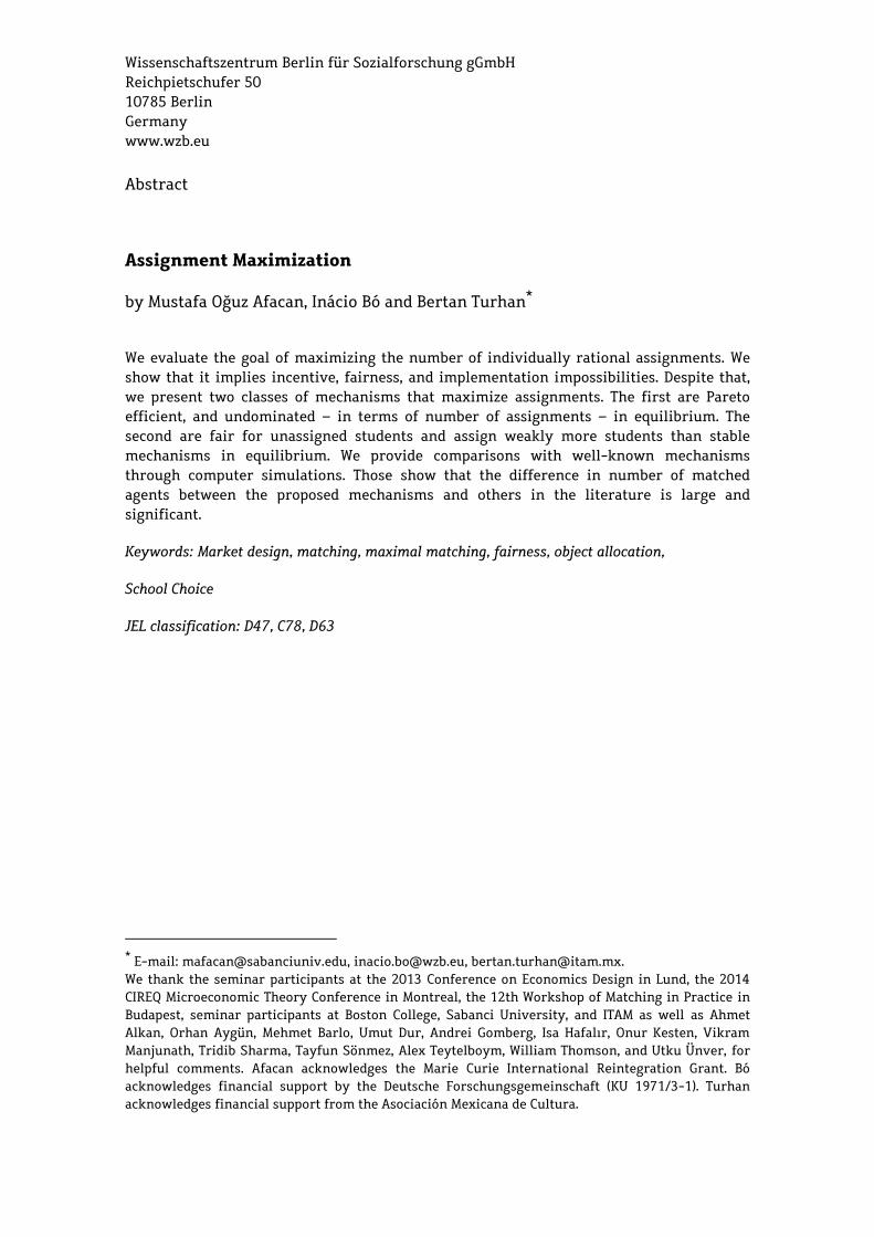
We evaluate the goal of maximizing the number of individually rational assignments. We show that it implies incentive, fairness, and implementation impossibilities. Despite that, we present two classes of mechanisms that maximize assignments. The first are Pareto efficient, and undominated – in terms of number of assignments – in equilibrium. The second are fair for unassigned students and assign weakly more students than stable mechanisms in equilibrium. We provide comparisons with well-known mechanisms through computer simulations. Those show that the difference in number of matched agents between the proposed mechanisms and others in the literature is large and significant.

Keywords: Market design, matching, maximal matching, fairness, object allocation,

School Choice

JEL classification: D47, C78, D63

* E-mail: mafacan@sabanciuniv.edu, inacio.bo@wzb.eu, bertan.turhan@itam.mx. We thank the seminar participants at the 2013 Conference on Economics Design in Lund, the 2014 CIREQ Microeconomic Theory Conference in Montreal, the 12th Workshop of Matching in Practice in Budapest, seminar participants at Boston College, Sabanci University, and ITAM as well as Ahmet Alkan, Orhan Aygün, Mehmet Barlo, Umut Dur, Andrei Gomberg, Isa Hafalır, Onur Kesten, Vikram Manjunath, Tridib Sharma, Tayfun Sönmez, Alex Teytelboym, William Thomson, and Utku Ünver, for helpful comments. Afacan acknowledges the Marie Curie International Reintegration Grant. Bó acknowledges financial support by the Deutsche Forschungsgemeinschaft (KU 1971/3-1). Turhan acknowledges financial support from the Asociación Mexicana de Cultura.

1 Introduction

Maximizing the number of assignments in discrete assignment problems is an impor-tant and natural design objective in many practical domains. One domain where thistakes place is that of school choice. Abdulkadiroglu et al. (2005) describe the change inNew York City’s high schools’ matching program. One of the main problems identifiedwas that the normal process would leave a large proportion of the students unmatched,and would end up assigning them via an administrative process to schools which werenot necessarily among those stated in their preferences. In fact, they show that 30,000out of 100,000 students were assigned in this way in 2002.1 Data from the New Or-leans OneApp, another centralized school choice program, show that an average of20% of the applicants remained unmatched after the main assignment round.(Harriset al., 2015) Having to go through the additional processes used to assign students whoare not matched in the main process can also cause frustration and emotional stress, asshown in the quote below:

“(...)The High School application process is a nerve wrecking nightmare and ex-tremely unfair to single parents, new immigrant families and any other familieswho simply cannot put in the countless hours it takes to attend Open Houses,tours and fairs. We got lucky and our daughter got into a school of her choice, butmy heart goes out to the families who have to go through this process twice.” (TineKindermann) 2

From the perspective of policymakers, leaving students unassigned, even temporarily,may have serious consequences. In 2013, for example, the city of São Paulo (Brazil)was ordered by a state court to pay restitution to 943 parents who had to put theirchildren in temporary private childcare, as a result of remaining unmatched by thecity’s assignment process.3 Maximizing the number of assignments might in fact bethe primary objective of the assignment process, as indicated by the following quotefrom the Frankfurt secondary school district and North Rhine-Westphalia secondaryschool district:

“The organization of the “Frankfurt School Mechanism” is shared between State,city and school. Its primary goal is to give as many applicants as possible one oftheir preferred schools. Each school decides for itself which students to admit...”(Basteck et al., 2015)

1Even after a change in the mechanism, proposed by the authors, the number of students who re-mained unmatched was still about 7,600, requiring additional elicitation of preferences over what aresupposedly undesired schools.

2Source: http://www.nytimes.com/2011/05/08/nyregion/in-applying-for-high-school-some-8th-graders-find-a-maze.html (NYT selected comments, accessed 09/11/2017.)

3Source: http://g1.globo.com/sao-paulo/noticia/2013/05/mae-ganha-direito-de-indenizacao-apos-ficar-sem-vaga-para-o-filho-em-creche.html (in Portuguese, accessed 09/11/2017.)

2

Maximizing the number of organ transplantations is perhaps the most important objec-tive of organ exchange programs, as evidenced by the recent literature on those typesof mechanisms. For both kidney exchange (Roth et al., 2005) and lung exchange (Er-gin et al., 2017), the objective of maximizing the number of matchings (and thereforetransplants), is put first and foremost in the design of their mechanisms.

Another area in which maximizing the number of assignments is relevant and hasraised significant interest on the part of market designers is in the matching of asylumseekers to countries or states. Andersson and Ehlers (2016), for example, propose analgorithm to find maximum mutually acceptable matchings4 which are also stable.Other examples of applications in which matching maximization is relevant includethe matching of babies to nurseries (Sasaki and Ura, 2016) and public housing.

We evaluate the general objective of maximizing the number of matches from amarket design perspective. The objective of maximizing the number of (individuallyrational) matchings has been tackled mostly from its mathematical and algorithmicperspectives. In this paper, we consider the economic problems faced by a policymakerwho wants to produce maximal matchings.

Consider the problem of assigning students to schools.5 The reason why efficiencyand stability (or equivalently, fairness) may conflict with maximizing the number ofmatches is that some schools may be deemed unacceptable to some students. As a re-sult, there may be some Pareto efficient and/or stable matchings that do not maximizeassignments. Consider, for example, the case in which there are two schools (A and B),each with only one seat, and two students (1 and 2). Student 1 only deems A as accept-able, whereas student 2 simply prefers A to B. In this case, student 2 being matched toA and 1 remaining unmatched is a Pareto efficient assignment. Moreover, if student 2has higher priority at school A than student 1, that is also the unique stable assignment.However, student 1 being assigned to A and student 2 to B is a Pareto efficient assign-ment that only matches students to acceptable schools. Therefore, there may typicallybe Pareto efficient and stable mechanisms that can be significantly improved upon interms of the number of assignments.6

In this paper, we set the maximization of the number of assignments as our primarydesign goal. We show that maximizing the number of assignments is incompatiblenot only with fairness, but also with strategy-proofness (Proposition 1), and that nomechanism is maximal in equilibrium (Proposition 6). While these can be interpretedas strong negative results, we present a large set of proposals and analyses.

4A refugee family and a landlord are mutually acceptable if they have a language in common and thenumber of beds offered by the household exceeds the number of beds needed by the refugee family.

5While for the remainder of the text we will frame the problems in terms of school choice, the entireanalysis applies to the more general problem of priority-based object allocation.

6The efficiency cost of stability has been pointed out before in the literature. See Abdulkadiroglu andSönmez (2003) and Kesten (2010).

3

First, we design a family of mechanisms, denoted Efficient Assignment MaximizingMechanisms (EAMs), that are Pareto efficient and maximal in terms of the number of as-signments (Theorem 1). Due to the impossibility above EAMs are not strategy-proof,but we characterize the unique Nash equilibrium outcome, which is Pareto efficient(Proposition 5). Moreover, EAMs are not dominated (in terms of the number of assign-ments) by any other mechanism in equilibrium (Theorem 3).

While assignment maximality and fairness are incompatible, we show that a weakerversion of fairness is compatible. We say that an outcome is fair for unassigned students ifthere is no situation in which an unassigned student justifiably envies the assignmentof some other agent. We define another family of mechanisms, denoted Fair Assign-ment Maximizing mechanisms (FAMs), which maximize the number of assignments andare fair for unassigned students (Theorem 2). Interestingly, a tradeoff between fairnessand efficiency also emerges for this weaker notion of fairness (Proposition 4). More-over, while EAMs are also Pareto efficient in equilibrium, we show that FAMs produceat least the same number of assignments as the problem’s stable matchings in equilib-rium (Proposition 7).

We also provide results regarding how well-known mechanisms compare in termsof the number of assignments made. We show that there is no dominance relationbetween four mechanisms used in practice and the literature (Proposition 2): Gale-Shapley Deferred Acceptance (DA),7 Boston Mechanism (BM), Top-Trading Cycles(TTC), and Serial Dictatorship (SD).

To test the relevance of our theoretical results and see how much EAMs/FAMs im-prove upon well-known mechanisms in terms of number of assignments, we conducta simulation analysis comparing the number of assignments produced by five differ-ent mechanisms – DA, BM, TTC, SD, and EAMs/FAMs. Two facts from the simulationanalysis stand out: (1) the difference between EAMs/FAMs and other mechanisms interms of number of assignments is large and significant, (2) for any choice of parame-ters, the number of matched students in DA, BM, TTC, and SD are very similar. Thesesimulations reinforce the appropriateness of our proposals to the problem presented,by showing that under true preferences the improvements are very significant, andthat the results are at least as good as the alternatives when students behave strategi-cally under EAMs.

The remainder of the paper is organized as follows. In section 2 we introduce themodel, the mechanisms we propose, and its properties. In section 3 we show the equi-librium behavior and outcomes induced by those mechanisms, and in section 4 wepresent the result of computer simulations comparing mechanisms outcomes. Proofsabsent from the main text can be found in the appendix.

7Or any other stable mechanism.

4

2 Model

A school choice problem consists of the following elements:

• A finite set of students I = i1, ..., in,

• a finite set of schools S = s1, ..., sm,

• a strict priority structure for schools = (s)s∈S where s is a linear order overI,

• a capacity vector q = (qs1 , ..., qsm) where qs is the number of available seats atschool s,

• a profile of strict preference of students P = (Pi)i∈I , where Pi is student i’s pref-erence relation over S ∪ ∅ and ∅ denotes the option of being unassigned. Wedenote the set of all possible preferences for a student by P . Let Ri denote theat-least-as-good-as preference relation associated with Pi, that is: sRis

′ ⇔ sPis′

ors = s

′. A school s is acceptable to i if sPi∅, and unacceptable otherwise.

In the rest of the paper, we consider the tuple (I, S,, q) as the commonly knownprimitive of the problem and refer to it as the market. We suppress all those from theproblem notation and simply write P to denote the problem. A matching is a functionµ : I → S ∪ ∅ such that for any s ∈ S, |µ−1(s)| ≤ qs. A student i is assigned under µ

if µ (i) 6= ∅. For any k ∈ I ∪ S, we denote by µk the assignment of k. Let |µ| be the totalnumber of students assigned under µ.

A matching µ is individually rational if, for any student i ∈ I, µiRi∅. A matchingµ is non-wasteful if for any school s such that sPiµi for some student i ∈ I, |µs| = qs. Amatching µ is fair if there is no student-school pair (i, s) such that sPiµi, and for somestudent j ∈ µs, i s j. A matching µ is stable if it is individually rational, non-wasteful,and fair.

In the rest of the paper, we will consider only individually rational matchings.Therefore, whenever we refer to a matching, unless explicitly stated, we refer to anindividually rational matching. LetM be the set of matchings.

A matching µ dominates another matching µ′ if, for any student i ∈ S, µiRiµ′i,

and for some student j, µjPjµ′j. A matching µ is efficient if it is not dominated by

any other matching. Note that efficiency implies both individual rationality and non-wastefulness. We say that a matching µ size-wise dominates another matching µ′ if|µ| > |µ′|. A matching µ is maximal if it is not size-wise dominated.

A mechanism ψ is a systematic way of selecting a matching for every problem, thatis, it is a function from P |I| toM. A mechanism ψ is [stable, efficient, fair, individually

5

rational] if, for any problem P ∈ P |I|, ψ (P) is [stable, efficient, fair, individually ratio-nal]. A Mechanism ψ is strategy-proof if there exist no problem P, and student i witha false preference P′i such that ψi(P′i , P−i)Piψi (P).8

At first sight, the natural objective of a designer would be to find a mechanism thatis fair, maximal, and strategy-proof.

Proposition 1. Regarding maximal mechanisms:(i) No fair mechanism is maximal.(ii) No strategy-proof mechanism is maximal.

Proposition 1 sets the stage for the rest of the paper. Not only there is no strategy-proof mechanism that is maximal, but even without considering incentives, there existsa fundamental incompatibility between fairness and maximality.

Since we will focus on the number of students matched to schools, we also make useof a method for comparing mechanisms with respect to that dimension. A mechanismψ size-wise dominates another mechanism φ if, for any problem P, φ (P) does not size-wise dominate ψ (P), while, for some problem P′, ψ (P′) size-wise dominates φ (P′). Amechanism ψ is maximal if it is not size-wise dominated by any other mechanism.

2.1 A Size-Wise Domination Comparison Among Well-Known Mech-

anisms

Here we compare well-known mechanisms in terms of the number of assigned stu-dents. Namely, we consider the Gale-Shapley deferred acceptance (DA), Top TradingCycles (TTC), Boston (BM), and serial dictatorship (SD) mechanisms. Their definitionsare given in the Appendix.

Proposition 2. There is no size-wise domination between any pair of mechanisms among theDA, TTC, BM, and SD.

As a consequence of the rural hospitals theorem (Roth, 1984), every stable matchingassigns the same number of students to schools, and so we have the following moregeneral result.

Corollary 1.

(i) There is no size-wise domination between any pair of mechanisms among the class ofstable mechanisms, the TTC, the BM, and the SD.

(ii) None of stable, TTC, the BM, and SD mechanisms are maximal.8P−i is the preference profile of all students except student i.

6

The results above take place based on the fact that some students might not rankall of the schools as acceptable. When that is not the case, the only reason for a studentto be unassigned under these mechanisms is that all schools have been filled up, andtherefore they all assign the same number of students.

Remark 1. If every school is acceptable to every student, then DA, TTC, BM, and SDall match the same number of students in any problem, consisting of the total sum ofschools’ capacities.

2.2 A Class of Efficient Maximal Mechanisms

In what follows, we first introduce two concepts which will be critical to the class ofmechanisms in this section.

Definition 1. A matching µ admits an improvement chain at problem P if there aredistinct students and schools i1, ..., in, c1, c2, .., cn+1 such that |µcn+1 | < qcn+1 and forevery k = 1, ..n,

(i) µik = ck,(ii) ck+1Pik ck.

Definition 2. A matching µ admits an improvement cycle in problem P if there aredistinct students and schools i1, ..., in, c1, c2, .., cn, cn+1 such that cn+1 = c1 and forevery k = 1, ..n,

(i) µik = ck,(ii) ck+1Pik ck.

We are now ready to introduce the class of mechanisms. Given a problem P and anenumeration of the students in I (i1, ..in),

Step 0. Let ξ0 =M.Step 1.Substep 1.1. Define the set ξ1 ⊆ ξ0 as follows:

ξ1 =

µ ∈ ξ0 : µi1 6= ∅ If ∃µ ∈ ξ0 such that µi1 6= ∅ξ0 otherwise

In general, for every k ≤ n,Substep 1.k. Define the set ξk ⊆ ξk−1 as follows:

ξk =

µ ∈ ξk−1 : µik 6= ∅ If ∃µ ∈ ξk−1 such that µik 6= ∅ξk−1 otherwise

7

Step 1 ends with the selection of a matching µ ∈ ξn.Step 2.Substep 2.1. If the matching µ does not admit an improving chain or cycle, then

the algorithm ends with the final outcome of µ. Otherwise, pick a chain or cycle, andobtain a new matching by assigning each student in the chosen chain (cycle) to theschool she prefers in the chain (cycle), and move to the next substep.

In general:Substep 2.k. Let µ be the matching obtained in the previous round. If µ does not

admit an improving chain or cycle then the algorithm ends with the final outcome ofµ. Otherwise, pick such a chain or cycle, and obtain a new matching by assigning eachstudent in the chosen chain (cycle) to the school he prefers in the chain (cycle), andmove to the next substep.

As everything is finite and, in every substep of Step 2, students are all weakly bet-ter off with at least one being strictly better off, Step 2 terminates after finitely manysubsteps. The matching obtained in the final round of Step 2 is the outcome of thealgorithm. This algorithm defines a class of mechanisms, each of which is associatedwith different selections of the student ordering, the matching in the end of Step 1,and chains and cycles in the course of Step 2. We refer to this class of mechanisms as“Efficient Assignment Maximizing” (EAM) mechanisms.

The first step of the EAM mechanisms is a “priority mechanism”, introduced byRoth et al. (2005) in the context of the pairwise kidney exchange problem. The authorsshow that this process finds a maximal matching. Though it may seem counterintuitivethat this simple process yields a maximal matching, the intuition behind it is simple.At each step, the set of outcomes is restricted to outcomes that will match the studentbeing considered to an acceptable school. Each one of these may lead to at most oneother student remaining unmatched. Therefore, following the enumeration above andtrying to match each student leads to a maximal matching.

The matching produced, however, may not be efficient. To fix this, the secondstage implements improving chains and cycles. As these chains and cycles are welfare-improving, the second stage preserves the maximality of the first stage outcome whilebenefiting the students. Consequently, every EAM mechanism is maximal and effi-cient.

Theorem 1. Every EAM mechanism is maximal and efficient.

From Proposition 1, fairness and maximality are incompatible. This, along withTheorem 1, implies that no EAM mechanism is fair. However, since maximality aimsto assign as many students as possible, we may be able to satisfy a weaker notion offairness. We say that a matching µ is fair for unassigned students if there is no student-school pair (i, s) where µi = ∅ and i s j for some j ∈ µs. A mechanism ψ is fair for

8

unassigned students if, for any problem P, ψ (P) is fair for unassigned students.

Proposition 3. No EAM mechanism is fair for unassigned students.

Proof. Let I = i, j and S = a, b, each with unit capacity. Let ψ be any EAM mech-anism where the student ordering starts with i. Let the priorities be such that a: j, iand b: i, j. Let us first consider the following preferences: Pi : a, ∅ and Pj : a, ∅.Then, ψi (P) = a and ψj (P) = ∅, violating fairness for unassigned students.

Next, consider any EAM mechanism, say φ, such that the student ordering startswith j. Let us now consider the preferences where Pi : b, ∅ and Pj : b, ∅. Then,φi (P) = ∅ and φj (P) = b, violating fairness for unassigned students.

In the next subsection we show, however, that this weaker notion of fairness is com-patible with assignment maximization, and we provide a mechanism that producesthose outcomes.

2.3 A Class of Maximal and Fair for Unassigned Students Mecha-

nisms

Below is a description of how each mechanism in this class works. Given a problem P,Step 1. Pick an EAM mechanism ψ, and let ψ (P) = µ.Step 2.Substep 2.1. If µ is fair for unassigned students then the algorithm terminates with

the final outcome of µ. Otherwise, pick a student-school pair (i, s) such that sPi∅,µi = ∅, and i s j for some j ∈ µs. Place student i at school s, and let the lowestpriority student in µs be unassigned (note that since µ is maximal, we have |µs| = qs),while keeping everyone else’s assignment the same. Let µ′ be the obtained matching,and move to the next substep.

In general,Substep 2.k. Let µ be the matching obtained in the previous step. If µ is fair for

unassigned students, the algorithm terminates with the outcome µ. Otherwise, picka student-school pair (i, s) such that sPi∅, µi = ∅, and i s j for some j ∈ µs. Placestudent i at school s, and let the lowest priority student in µs be unassigned, whilekeeping everyone else’s assignment the same. Note that as in each substep the numberof assigned students is preserved, µ is maximal. Hence, we have |µs| = qs. Let µ be theobtained matching, and move to the next substep.

As, in every substep, a higher priority student is placed at a school while a lowerpriority one is displaced from the school, and both the students and schools are finite,the algorithm terminates in finitely many rounds. The above procedure defines a classof mechanisms, each of which is associated with different selections of the first stage

9

EAM mechanism as well as the student-school pairs in the course of Step 2. We referto this class of mechanisms as “Fair Assignment Maximizing” (FAM) mechanisms.

The procedure above is similar to the Deferred Acceptance with Arbitrary Input(DAAI) in Blum et al. (1997). Its fundamental difference from our proposal is that inthe second step of a FAM, only unmatched students may fulfill their justified envies,whereas under the DAAI, students who are matched may also fulfill their justifiedenvies. In fact, while outcomes of the DAAI mechanism are always stable, outcomesof a FAM may not be.

Theorem 2. Every FAM mechanism is fair for unassigned students and maximal.

Proof. Let ψ be a FAM mechanism, and µ be the outcome of its first step. As µ is theoutcome of an EAM mechanism, and in Step 2 of ψ, no student is assigned to one of hisunacceptable choices, ψ is individually rational. Because µ is maximal and the numberof assigned students is preserved as |µ| in the course of Step 2, ψ is maximal. More-over, as ψ does not stop until no student-school pair violates fairness for unassignedstudents, ψ is fair for unassigned students as well.

An important downside of the FAM class is the lack of efficiency, in that no FAMmechanism is efficient. However, this is not a problem specific to the FAM class asthere exists a general incompatibility between efficiency and fair for unassigned stu-dents, as shown below.

Proposition 4. No mechanism is efficient and fair for unassigned students.

Proof. Let I = i, j, k and S = a, b, each with unit capacity. Consider the followingpreferences and priorities:

Pi : a, b, ∅; Pj : b, a, ∅; Pk : b, ∅.a: j, i, k; b: i, k, j.Let ψ be an efficient mechanism, and ψ (P) = µ. By the efficiency of µ, exactly one

student is left unassigned.Case 1. Suppose µk = ∅. Then, by efficiency of µ, µi = a and µj = b. However, as

k b j, µ cannot be fair for unassigned students.Case 2. Suppose µj = ∅. Then, by efficiency of µ, µi = a and µk = b. However, as

j a i, µ cannot be fair for unassigned students.Case 3. Suppose µi = ∅. By efficiency of µ, µj = a and µk = b. However, as i b k,

µ cannot be fair for unassigned students.

3 Incentives and Equilibrium Analysis

As shown in Proposition 1, there is no mechanism which is maximal and strategy-proof. Hence, in particular, none of the EAM and FAM mechanisms are strategy-proof.

10

Corollary 2. None of the EAM and FAM mechanisms are strategy-proof.

In this section we show, however, that the mechanisms in the classes EAM andFAM have surprisingly regular properties in terms of equilibrium outcomes. We alsopresent some results comparing equilibrium outcomes between mechanisms. Con-sider the preference reporting game induced by a mechanism ψ. At problem P, a pref-erence submission P′ = (P′i )i∈I is a (Nash) equilibrium of ψ if for every student i,ψi (P′) Riψi(P′′i , P′−i) for any P′′i ∈ P . Let Ω be the set of mechanisms that admit anequilibrium in any problem P ∈ P |I|. In the rest of this section, we consider only themechanisms in Ω.

The first result relates to the equilibria of EAM and FAM mechanisms.

Proposition 5. Every EAM and FAM mechanism is in Ω. Moreover, for any problem, anEAM mechanism has a unique equilibrium outcome that is equivalent to the outcome of theserial dictatorship where the student ordering is the same as that used in that EAM mechanism.

Proposition 5 shows, therefore, that equilibrium outcomes of EAM are not onlyPareto efficient, but will match as many students as a commonly used strategy-proofmechanism.

A mechanism ψ is maximal in equilibrium if, at any problem P and any equilib-rium submission P′ under ψ, ψ (P′) is maximal.

Proposition 6. No mechanism is maximal in equilibrium.

Corollary 3. No EAM and FAM mechanism is maximal in equilibrium.

Our next question is how mechanisms compare, in terms of the number of assign-ments, in equilibrium. For that, we define the concept of size-wise domination inequilibrium.

Definition 3. For a given market (I, S,, q), a mechanism ψ size-wise dominates an-other mechanism φ in equilibrium if, for any problem P and for every equilibria P′, P′′

under ψ and φ, respectively |ψ (P′)| ≥ |φ (P′′)|, and there exists a problem P∗ such thatfor every equilibria P, P under ψ and φ, respectively

∣∣ψ (P)∣∣ > ∣∣φ (P)∣∣.What is needed, therefore, for a mechanism ψ to size-wise dominate mechanism φ

in equilibrium in given a market, is that in every problem ψ assigns at least as manystudents as φ regardless of the equilibrium selection that is made, and that there is atleast one problem in which those differences are strict.

Theorem 3. In any market (I, S,, q), no EAM mechanism is size-wise dominated by anindividually rational mechanism in equilibrium.

11

Notice that the fact that size-wise domination is defined in terms of a given marketmakes Theorem 3 stronger: it is not enough to show that the result is true for a specificmarket. The theorem instead shows that for any set of students, schools, capacitiesand priorities there is no individually rational mechanism that dominates any EAM inequilibrium.

While we do not have a similar result to above for the FAM mechanisms, we areable to compare the number of assigned students under the FAM in equilibrium andthe weakly dominant strategy equilibrium of the DA, which is truth-telling.

Proposition 7. Regarding the FAM mechanisms:

(i) For any problem P and any stable matching for P µ∗, for every equilibrium P′ of a FAMmechanism ψ, |ψ (P′)| ≥ |µ∗|.

(ii) There exist a FAM mechanism ψ, problem P, and an equilibrium profile P′ of ψ at P suchthat |ψ (P′)| > |µ∗∗|, where µ∗∗ is any stable matching for P.

4 Simulations

While we have shown that the EAM family of mechanisms9 dominate any individuallyrational mechanism under true preferences and that they also produce good outcomesin equilibrium, one may wonder whether in practice the magnitude of the difference inthe actual number of students assigned justifies the proposal of a new mechanism. Toprovide an answer to that question, in this section we describe and analyze simulationresults in which we compare the number of students matched under five mechanisms:EAM, DA, BM, TTC, and SD.

The construction of the problems to be simulated follows a method similar to thatapplied in Hafalir et al. (2013). Each problem contains a set of students I = i1, . . . , in,a set of schools S = s1, . . . , sm and their capacities Q = q1, . . . , qm. Studentshave strict preferences

Pi1 , . . . , Pin

over S ∪ ∅ and schools have strict priorities

Ps1 , . . . , Psm over I ∪ ∅. Those ordinal preferences and priorities are derived fromutilities that each student and school have over the other side of the market. Let usfirst consider a student i ∈ I. Her utility from being assigned to school s ∈ S is thefollowing:

Ui (s) =

αΘs + (1− α)Θsi if αΘs + (1− α)Θs

i ≥ λi

−∞ otherwise

9For simplicity, in this section we refer only to EAM mechanisms. Since the number of assignments isthe same under any EAM and FAM mechanism, however, unless explicitly stated, all the results belowhold for both families of mechanisms.

12

The interpretation of the parameters goes as follows. The utility that a student iderives from being assigned to a school s is a combination of a value that is sharedby all students (Θs) and an idiosyncratic value that is unique to a student-school pair(Θs

i ). The value of Θs could therefore be the widespread understanding of the qualityof the school and Θs

i incorporate, for example, the distance of the school to the stu-dent’s house and whether the extra-curricular activities fit the student’s taste. For eachproblem, and for each values of s ∈ S and (s, i) ∈ S× I, Θs and Θs

i are independentlydrawn from the normal distribution with mean zero and variance 1. The value of α,which represents the correlation of preferences between students, is exogenously setin the range [0, 1].

Remark 1 showed that when every student deems every school as acceptable andno student is unacceptable to any school, every mechanism among those being eval-uated assign the same number of students. We therefore allow for students to haveoutside options and for schools to deem some students unacceptable.

Each student i has an outside option which yields utility λi. Therefore, a studentwould only accept being matched to a school if the utility that she derives from thatschool exceeds the value of λi.10 The value of those outside options are also a combi-nation of common and idiosyncratic values:

λi = γΘ + (1− γ)Θi

For each problem and i ∈ I, Θ and Θi are independently drawn from the normaldistribution with a mean of zero and variance 1. The exogenous parameter γ ∈ [0, 1]represents how correlated the value of the outside options are between students.

Schools’ priorities over students follow a similar model. The ordinal priorities ofschool s over the students are derived from utility functions:

Us (i) =

βΘi + (1− β)Θis if βΘi + (1− β)Θi

s ≥ λs

−∞ otherwise

Here once again, for each problem, each value of Θi and Θis is independently drawn

from the normal distribution with a mean of zero and variance 1. The concept of ac-ceptability here, however, is not related to the presence of some “outside option” forthe school. We interpret λs, instead, as an eligibility criterion. In exam schools, forexample, it could be a minimum exam score for admission. For schools which givedistance-based priority it could be a maximal distance requirement, and so on. For

10Although it may seem extreme to define the utility of being matched to any school with value belowλi to be −∞, that choice is inconsequential when we translate those utilities to ordinal preferences. Thatis, for any i, s such that Ui (s) = −∞, it will simply be the case that school s is unacceptable to i: ∅ Pi s.

13

each s ∈ S, λs is drawn independently from the normal distribution with mean λ∗

and variance 1. Therefore, when λ∗ = −∞, no student is unacceptable to any school.Moreover, β ∈ [0, 1] is an exogenous parameter which represents the degree of corre-lation between schools’ priority rankings. Notice that the case in which students maybe unacceptable to schools is not considered in the theoretical analysis, and thereforethose simulations should be taken as an additional experiment on the outcomes ofthose mechanisms under true preferences.

In each simulation performed, we set the values of the parameters (n, m, Q, α, γ, β, λ∗)

and generated 100 problems, each representing different draws for values of the ran-dom variables. More specifically, in all simulations shown below, n = 400, m = 20and every school had capacity q = 20. Every combination of the values of the pa-rameters α, β and γ, in steps of 0.1, were used. In other words, every (α, β, γ) ∈[0, 0.1, 0.2, 0.3, 0.4, 0.5, 0.6, 0.7, 0.8, 0.9, 1]3 was simulated.

For each problem generated, we produced the matching outcome for each of thefive mechanisms : EAM, DA, BM, TTC, and SD, and recorded the number of studentswho remained unassigned.11

4.1 Case 1: No Student is Unacceptable to Any School

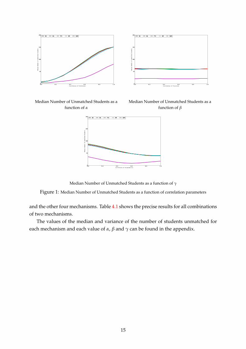
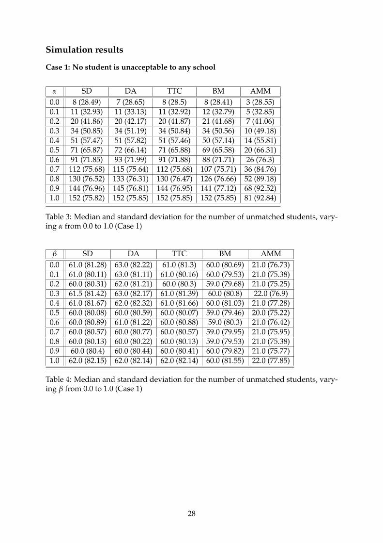
In this case we set the value of λ∗ to be low enough such that no student is deemedunacceptable to any school.12 This is often the case in school choice problems. Figure 1shows the median value of the number of unmatched students across simulations, foreach value of the indicated correlation parameter.13 Two facts clearly stand out. Oneis that the median number of unmatched students, for any choice of fixed parameteramong α, β and γ, is very similar between the DA, BM, TTC, and SD mechanisms.The second is how significant the difference is in the number of unmatched studentsbetween EAM and all the other mechanisms. When combining all the simulationsperformed in case 1, the DA, BM, TTC, and SD mechanisms had a median number ofunmatched students of 60 or 61, while for EAM the value was 21, a reduction of 65%in the number of students unmatched.

In fact, when performing two-sided T-tests testing the null hypotheses that thenumber of unmatched students is the same between any two mechanisms, we are notable to reject the null hypothesis of them being equal at the 0.01 significance level fora wide range of parameters for the DA, BM, TTC, and SD mechanisms. That is not thecase for any value of those parameters for any two-sided comparison between EAM

11For SD, following the principle behind the equilibrium results of EAM, the ordering of students thatwas used was drawn from a uniform distribution, independently of the schools’ priorities.

12More specifically, the value of λ∗ was set to −1.797× 10308, the lowest technically possible.13For the purpose of presentation, the graphs in this section were generated by polynomial fitting of

the simulation results.

14

0.0 0.2 0.4 0.6 0.8 1.0Correlation of Preferences

0

50

100

150

200

Median Number of Unmatched Students

SD DA TTC BM EAM

Median Number of Unmatched Students as afunction of α

0.0 0.2 0.4 0.6 0.8 1.0Correlation of Priorities

0

50

100

150

200

Median Number of Unmatched Students

SD DA TTC BM EAM

Median Number of Unmatched Students as afunction of β

0.0 0.2 0.4 0.6 0.8 1.0Correlation of Acceptability

0

50

100

150

200

Median Number of Unmatched Students

SD DA TTC BM EAM

Median Number of Unmatched Students as a function of γ

Figure 1: Median Number of Unmatched Students as a function of correlation parameters

and the other four mechanisms. Table 4.1 shows the precise results for all combinationsof two mechanisms.

The values of the median and variance of the number of students unmatched foreach mechanism and each value of α, β and γ can be found in the appendix.

15

SD DA TTC BM AMM

SDα

−−−βγ

DAα [0.0, 1.0]

−−−β [0.0, 1.0]γ [0.0, 1.0]

TTCα [0.0, 1.0] [0.0, 1.0]

−−−β [0.0, 1.0] [0.0, 1.0]γ [0.0, 1.0] [0.0, 1.0]

BMα [0.0, 0.6] ∪ [0.9, 1.0] [0.0, 0.5] ∪ [1.0] [0.0, 0.6] ∪ [0.9, 1.0]

−−−β [0.0, 1.0] [0.0, 1.0] [0.0, 1.0]γ [0.2, 1.0] [0.5, 1.0] [0.3, 1.0]

AMMα ∅ ∅ ∅ ∅

−−−β ∅ ∅ ∅ ∅γ ∅ ∅ ∅ ∅

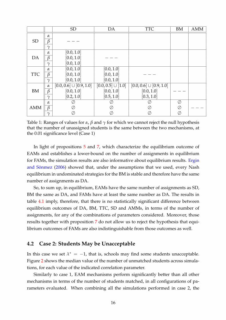
Table 1: Ranges of values for α, β and γ for which we cannot reject the null hypothesisthat the number of unassigned students is the same between the two mechanisms, atthe 0.01 significance level (Case 1)

In light of propositions 5 and 7, which characterize the equilibrium outcome ofEAMs and establishes a lower-bound on the number of assignments in equilibriumfor FAMs, the simulation results are also informative about equilibrium results. Erginand Sönmez (2006) showed that, under the assumptions that we used, every Nashequilibrium in undominated strategies for the BM is stable and therefore have the samenumber of assignments as DA.

So, to sum up, in equilibrium, EAMs have the same number of assignments as SD,BM the same as DA, and FAMs have at least the same number as DA. The results intable 4.1 imply, therefore, that there is no statistically significant difference betweenequilibrium outcomes of DA, BM, TTC, SD and AMMs, in terms of the number ofassignments, for any of the combinations of parameters considered. Moreover, thoseresults together with proposition 7 do not allow us to reject the hypothesis that equi-librium outcomes of FAMs are also indistinguishable from those outcomes as well.

4.2 Case 2: Students May be Unacceptable

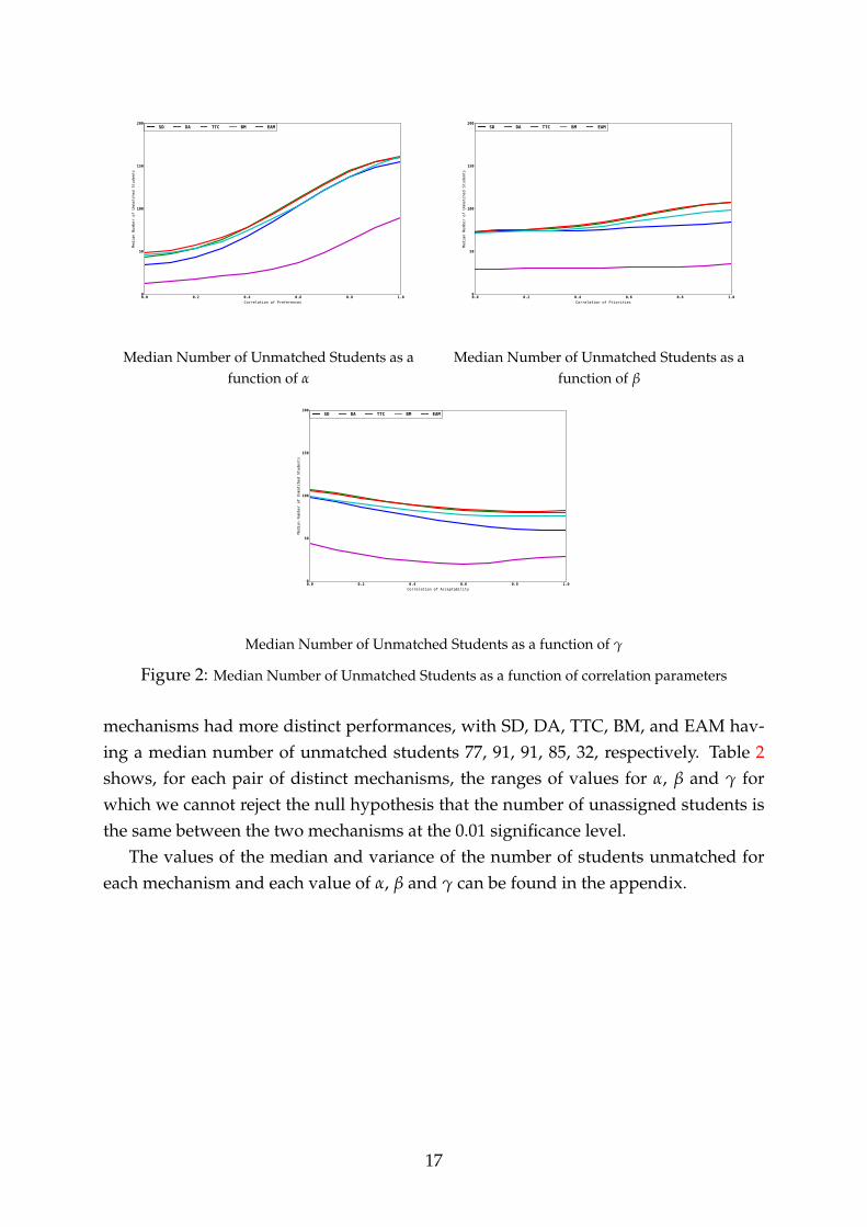
In this case we set λ∗ = −1, that is, schools may find some students unacceptable.Figure 2 shows the median value of the number of unmatched students across simula-tions, for each value of the indicated correlation parameter.

Similarly to case 1, EAM mechanisms perform significantly better than all othermechanisms in terms of the number of students matched, in all configurations of pa-rameters evaluated. When combining all the simulations performed in case 2, the

16

0.0 0.2 0.4 0.6 0.8 1.0Correlation of Preferences

0

50

100

150

200

Median Number of Unmatched Students

SD DA TTC BM EAM

Median Number of Unmatched Students as afunction of α

0.0 0.2 0.4 0.6 0.8 1.0Correlation of Priorities

0

50

100

150

200

Median Number of Unmatched Students

SD DA TTC BM EAM

Median Number of Unmatched Students as afunction of β

0.0 0.2 0.4 0.6 0.8 1.0Correlation of Acceptability

0

50

100

150

200

Median Number of Unmatched Students

SD DA TTC BM EAM

Median Number of Unmatched Students as a function of γ

Figure 2: Median Number of Unmatched Students as a function of correlation parameters

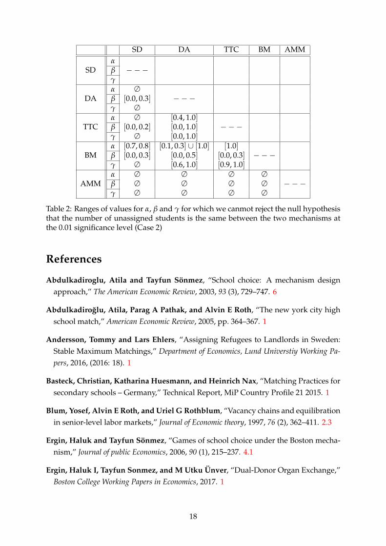
mechanisms had more distinct performances, with SD, DA, TTC, BM, and EAM hav-ing a median number of unmatched students 77, 91, 91, 85, 32, respectively. Table 2shows, for each pair of distinct mechanisms, the ranges of values for α, β and γ forwhich we cannot reject the null hypothesis that the number of unassigned students isthe same between the two mechanisms at the 0.01 significance level.

The values of the median and variance of the number of students unmatched foreach mechanism and each value of α, β and γ can be found in the appendix.

17

SD DA TTC BM AMM

SDα−−−β

γ

DAα ∅

−−−β [0.0, 0.3]γ ∅

TTCα ∅ [0.4, 1.0]

−−−β [0.0, 0.2] [0.0, 1.0]γ ∅ [0.0, 1.0]

BMα [0.7, 0.8] [0.1, 0.3] ∪ [1.0] [1.0]

−−−β [0.0, 0.3] [0.0, 0.5] [0.0, 0.3]γ ∅ [0.6, 1.0] [0.9, 1.0]

AMMα ∅ ∅ ∅ ∅

−−−β ∅ ∅ ∅ ∅γ ∅ ∅ ∅ ∅

Table 2: Ranges of values for α, β and γ for which we canmot reject the null hypothesisthat the number of unassigned students is the same between the two mechanisms atthe 0.01 significance level (Case 2)

References

Abdulkadiroglu, Atila and Tayfun Sönmez, “School choice: A mechanism designapproach,” The American Economic Review, 2003, 93 (3), 729–747. 6

Abdulkadiroglu, Atila, Parag A Pathak, and Alvin E Roth, “The new york city highschool match,” American Economic Review, 2005, pp. 364–367. 1

Andersson, Tommy and Lars Ehlers, “Assigning Refugees to Landlords in Sweden:Stable Maximum Matchings,” Department of Economics, Lund Universtiy Working Pa-pers, 2016, (2016: 18). 1

Basteck, Christian, Katharina Huesmann, and Heinrich Nax, “Matching Practices forsecondary schools – Germany,” Technical Report, MiP Country Profile 21 2015. 1

Blum, Yosef, Alvin E Roth, and Uriel G Rothblum, “Vacancy chains and equilibrationin senior-level labor markets,” Journal of Economic theory, 1997, 76 (2), 362–411. 2.3

Ergin, Haluk and Tayfun Sönmez, “Games of school choice under the Boston mecha-nism,” Journal of public Economics, 2006, 90 (1), 215–237. 4.1

Ergin, Haluk I, Tayfun Sonmez, and M Utku Ünver, “Dual-Donor Organ Exchange,”Boston College Working Papers in Economics, 2017. 1

18

Hafalir, Isa E, M Bumin Yenmez, and Muhammed A Yildirim, “Effective affirmativeaction in school choice,” Theoretical Economics, 2013, 8 (2), 325–363. 4

Harris, Douglas N, Jon Valant, and Betheny Gross, “The New Orleans OneApp,”Education Next, 2015, 15 (4). 1

Kesten, Onur, “School choice with consent,” Quarterly Journal of Economics, 2010, 125(3). 6

Roth, Alvin E., “The Evolution of the Labor Market for Medical Interns and Residents:A Case Study in Game Theory,” Journal of Political Economy, 1984, 92 (6), 991–1016.2.1, 4.2

Roth, Alvin E, Tayfun Sönmez, and M Utku Ünver, “Pairwise kidney exchange,”Journal of Economic theory, 2005, 125 (2), 151–188. 1, 2.2

Sasaki, Yasuo and Masahiro Ura, “Serial dictatorship and unmatch reduction: A prob-lem of Japan’s nursery school choice,” Economics Letters, 2016, 147, 38–41. 1

Appendix

Proofs

Proposition 1

(i). Let ψ be a fair mechanism. Consider a problem where I = i, j and S = a, b,each with unit capacity. Let the preferences and priorities be as follows:

Pi : a, b, ∅; Pj : a, ∅.

a=b= i, j.

The unique maximal matching is µ′ where µ′i = b and µ′j = a. However, µ′ is notfair, showing that no fair mechanism is maximal.

(ii). Assume for a contradiction that ψ is a strategy-proof and maximal mechanism.Consider a problem where I = i, j and S = a, b, each with unit capacity. Let thepriorities be such that a=b: i, j. Consider the problem P where Pi : a, b, ∅ andPj : a, ∅.

As ψ is maximal, ψi (P) = b and ψj (P) = a. Let P′i : a, ∅ and P′ = (P′i , Pj). Dueto the strategy-proofness of ψ, ψi (P′) = ∅ and ψj (P′) = a. The latter is because ψ ismaximal.

Let us now consider P′′j : a, b, ∅ and P′′ = (P′i , P′′j ). As ψ is maximal, ψi (P′′) =

a and ψj (P′′) = b. This, along with the fact that ψj (P′) = a, implies that student

19

j profitably reports false preferences P′j whenever the true preferences are P′′. This,however, contradicts the strategy-proofness of ψ, which finishes the proof.

Proposition 2

Let us consider a problem consisting of I = i, j, k and S = a, b, c, each with unitcapacity. Let the preferences and priorities be as follows:

Pi : a, ∅; Pj : a, b, c, ∅; Pk : b, a, c, ∅.

a: k, j, i; b: i, j, k; c: j, i, k.

In the above problem, the DA and BM produce the same matching, say µ, and it issuch that µi = ∅, µj = a, and µk = b. That is, |µ| = 2. On the other hand, the TTCoutcome, say µ′, is such that µ′i = a, µ′j = c, and µ′k = b. That is, |µ′| = 3. Hence,neither the DA nor the BM dominate the TTC.

Let us now consider I = i, j, k, h and S = a, b, c, d, each with unit capacity. Letthe preferences and priorities be as follows:

Pi : a, b, ∅; Pj : a, ∅; Pk : d, b, c, ∅; Ph : d, ∅.

a: k, j, i; b: i, j, k; c: j, i, k; d: h, i, j, k.

The DA and BM outcomes are the same, say µ, where µi = b, µj = a, µk = c, andµh = d. On the other hand, the TTC outcome, say µ′, is such that µ′i = a, µ′j = ∅,µ′k = b, and µ′h = d. Hence, |µ| > |µ′|, showing that the TTC does not dominate eitherof the DA and the BM.

For the non-existence of a domination relation between the DA and the BM, con-sider I = i, j, k and S = a, b, c, each with unit capacity. Let the preferences andpriorities be as follows:

Pi : a, c, ∅; Pj : b, a, ∅; Pk : b, ∅.

a: k, j, i; b: k, i, j; c: j, i, k.

In the above problem, the DA outcome, say µ, is such that µi = c, µj = a, andµk = b. On the other hand, the BM outcome, say µ′, is such that µ′i = a, µ′j = ∅, andµ′k = b. Hence, |µ| > |µ′|, showing that the BM does not dominate the DA. Next, forthe converse, consider the following preferences and priorities:

Pi : b, a, c, ∅; Pj : a, ∅; Pk : b, ∅.

a: k, i, j; b: k, i, j; c: j, i, k.

20

In the above problem, the DA outcome, say µ, is such that µi = a, µj = ∅, andµk = b. On the other hand, the BM outcome, say µ′, is such that µ′i = c, µ′j = a, andµ′k = b. Hence, |µ| < |µ′|, showing that the DA does not dominate the BM. Thisfinishes the proof.

For the non-existence of a domination relation between the SD and the other mech-anisms, consider I = i, j and S = a, b, each with unit capacity. Let the preferencesand priorities be as follows:

Pi : a, b; Pj : a, ∅.

a: j, i; b: j, i.

Let us consider the SD mechanism where student i comes first in the student order-ing. Then, the SD outcome µ is such that µi = a and µj = ∅. On the other hand, all theDA, TTC, and BM outcomes are the same, say µ′, and it is such that µ′i = b and µ′j = a.Hence, the SD mechanism does not size-wise dominate the DA, TTC, and BM.

Let us now consider the following preferences, with the same priorities as above.

Pi : a, ∅, Pj : a, b, ∅.

At the above problem, the SD outcome µ is such that µi = a and µj = b. All theDA, TTC, and BM outcomes are the same, say µ′, and it is such that µ′i = ∅ and µ′j = a.Hence, none of DA, TTC, and BM size-wise dominate the SD mechanism.

In the above market, the symmetric arguments easily show that there is no size-wisedomination relation between the other SD mechanism where student j comes first, andthe other mechanisms. This finishes the proof.

Theorem 1

We will use the following Lemma:

Lemma. A maximal matching µ is efficient if and only if it does not admit an improving chainor cycle.

Proof. “Only If” Part. Let µ be an efficient matching. If it admits an improving chainor cycle then we can implement it and obtain a new matching. By the definitionsof improving chain and cycle, that matching dominates µ, contradicting our startingsupposition.

“If” Part. Let µ be a maximal matching such that it does not admit an improvingchain or cycle. We want to show that it is efficient. Assume for a contradiction thatthere exists a matching µ′ that dominates µ.

Let W = i ∈ I : µ′iPiµi. By the supposition, W 6= ∅. Note that for any studenti with µi 6= ∅, we have µ′i 6= ∅. This, along with the maximality of µ, implies that|µ′| = |µ|. Hence, for any student i with µi = ∅, µ′i = ∅.

21

Let us enumerate the students in W = i1, .., in and write µ′ik = ck for any k =

1, .., n. If |µck | < qck for some k then the pair ik, ck would constitute an improvingchain, which would yield a contradiction.

Let us suppose that |µck | = qck for any k = 1, .., n. As school c1 does not have excesscapacity at µ, and µ′i1 = c1, we have another student in W, say i2, such that µi2 = c1.Then, consider student i2, and as c2 does not have excess capacity at µ and µ′i2 = c2,we have another student in W, say i3, such that µi3 = c2. If we continue to apply thesame arguments to the other students in W, as W is finite, we would eventually obtainan improving cycle, which yields a contradiction.

We can now proceed to the proof of the theorem. Let ψ be an EAM mechanism, andµ and µ′ be its first stage and final outcome, respectively. As students are not assignedto one of their unacceptable schools in the course of Step 1 of ψ, µ is individually ratio-nal. Moreover, as Step 1 tries to match as many students as possible while preservingindividual rationality, it is immediate to see that µ is maximal.

In Step 2 of ψ, new matchings are obtained by implementing improving chains andcycles (if any). By their definitions, in the course of Step 2, no student receives a worseschool than his assignment µ. This, along with the individual rationality of µ, impliesthat µ′ is maximal. The efficiency of µ′ directly comes from the Lemma above.

Proposition 5

Let ψ be an EAM mechanism. By its definition, the first student in the ordering inStep 0 of the EAM obtains his top choice by reporting it as the only acceptable choice,irrespective of the other students’ preference submissions. By the same reasoning, thesecond student in the ordering can obtain his top choice among the schools with avail-able seats (after the capacity of the first student assignment is decreased by one) byreporting that school as his only acceptable choice, irrespective of the other students’preference submissions. Once we repeat the same arguments for every other student,we not only find an equilibrium of ψ, but also conclude that it is the unique equilibriumoutcome, which coincides with the outcome of serial dictatorship with the ordering asthe same as that in Step 0 of ψ.

Let φ be a FAM mechanism. Let µ be a stable matching at P. Consider the pref-erences submission P′ under which for any student i, the only acceptable school is µi.Any unassigned student at µ reports no school acceptable at P′. It is easy to verify thatφ (P′) = µ.

Next, we claim that P′ is an equilibrium submission under φ. Suppose for a con-tradiction that there exist a student i and P′′i such that φi(P′′i , P′−i)Piφi (P′). For ease ofwriting, let φi(P′′i , P′−i) = s and φi (P′) = s′. As µ is stable, |µs| = qs. This, along withthe definition of P′ and φi(P′′i , P′−i) = s, implies that there exists a student j 6= i such

22

that µj = s and φj(P′′i , P′−i) = ∅. Moreover, from the stability of µ, we also have j s i.These altogether contradict the fairness for unassigned students of φ, showing that P′

is equilibrium of φ.

Proposition 6

Let I = i, j and S = a, b, each with unit capacity. Assume for a contradiction thatψ ∈ Ω such that it is maximal in equilibrium.

Consider the preferences where Pi : a, ∅ and Pj : a, b, ∅. In any equilibrium at P, ψ

places student i and student j at school a and b, respectively.Consider the problem P′ where P′i : a, ∅ and P′j : a, ∅. If there exists an equilibrium

of ψ at P′ under which student j is assigned to school a, then this submission constitutesan equilibrium at P as well. This, however, contradicts ψ being maximal in equilibrium.Hence, under any equilibrium at P′, student i is assigned to school a while student j isunassigned.

Let us now consider the problem P′′ where P′′i : a, b, ∅ and P′′j = P′j : a, ∅. As ψ

is maximal in equilibrium, under any equilibrium at P′′, student i and student j haveto be placed at school b and school a, respectively. Moreover, it is easy to see that anyequilibrium at P′ is also an equilibrium at P′′. Hence, there exists an equilibrium atP′′ under which student i is assigned to school a, and student j is unassigned. This,however, contradicts ψ being maximal in equilibrium, finishing the proof.

Theorem 3

In the proof, we will use the following lemma.

Lemma. Let ψ be an EAM and φ be an individually rational mechanism. In any market(I, S,, q) and problem P, if |ψ (P′)| < |φ (P′′) | where P′ and P′′ are equilibria under ψ andφ, respectively, then there exists a student i such that ψi (P′) Piφi (P′′) Pi∅.

Proof. In a market (I, S,, q) and problem P, let |ψ (P′)| < |φ (P′′) | where P′ andP′′ are equilibria under ψ and φ, respectively. This implies that for some school s,|ψs (P′)| < |φs (P′′)| ≤ qs. Hence, let i ∈ φs (P′′) \ ψs (P′). By the individual rationalityof φ and P′′ being equilibrium under φ, we have sPi∅, where φi (P′′) = s. As theunique equilibrium outcome of ψ coincides with the (truthtelling) outcome of a SDmechanism (Proposition 5), we have ψ (P′) = SD (P). Hence, school s has an excesscapacity under SD (P). Moreover, from above, ψi (P′) = SDi (P) 6= s. Hence, bythe non-wastefulness of SD, i must be matched to a school strictly better than s andtherefore ψi (P′) = SDi (P) Piφi (P′′) Pi∅, which finishes the proof.

Let now (I, S,, q) be a market and ψ be an EAM mechanism. Assume for a con-tradiction that an individually rational mechanism φ size-wise dominates ψ in equilib-

23

rium. This in particular implies that for some problem P, |ψ (P′)| < |φ (P′′) | for everyequilibria P′ and P′′ under ψ and φ, respectively. In what follows, we will fix one suchpair P′, P′′. We prove the result in two steps.

Step 1. By the Lemma above, there exists a student i such that ψi (P′) Piφi (P′′) Pi∅.Let Pi be the preference relation that keeps the relative rankings of the schools the sameas under Pi, while reporting any school that is worse than ψi (P′) as unacceptable. Inother words, Pi truncates Pi below ψi (P′). Let us write P = (Pi, P−i). Recall that theunique equilibrium outcome of ψ always coincides with the truthtelling outcome of aSD mechanism (Proposition 5). Moreover, by the construction of P, SD (P) = SD(P).This in turn implies that ψ (P′) = ψ (P′) for every equilibrium P′ under ψ in problemP.

We next consider problem P. If there exists no student j such that ψj (P′) Pjφj (P′′) Pj∅for some equilibria P′ and P′′ under ψ and φ, respectively, then we move to Step 2.Otherwise, we pick such student j. Note that because of the definition of Pi statesthat any outcome below ψi (P′) is unacceptable for i and φ is individually rational,ψj (P′) Pjφj (P′′) Pj∅ cannot hold for j = i, therefore j 6= i. Then, as the same asabove, let Pj be the preference list that truncates Pj below ψj (P′). Let us write P =

(Pi, Pj, P−i,j). By the same reason as above, ψ (P′) = ψ(

P′)

for any equilibrium P′

under ψ in problem P.We next consider problem P. If there exists no student k such that ψk

(P′)

Pkφk(

P′′)

Pk∅for some equilibria P′ and P′′ under ψ and φ, respectively, then we move to Step2. Otherwise, we pick such a student k. By the same reason as above, student k isdifferent than both i and j. Then, we follow the same arguments above and obtaina new preference profile. In each iteration, we have to consider a different student.But then, since there are finitely many students, this case cannot hold forever. Hence,we eventually obtain a problem, say P, in which there exists no student h such thatψh(P′)Phφh

(P′′)

Ph∅ for some equilibria P′ and P′′ under ψ and φ, respectively, andmove to Step 2. We also have ψ (P′) = ψ(P′) for any equilibrium P′ under ψ in prob-lem P.

Step 2. By the Lemma above, in problem P, we have∣∣ψ (P′)∣∣ ≥ ∣∣φ (P′′)∣∣ for any

equilibria P′ and P′′ under ψ and φ, respectively. If it holds strictly for some equilibria,then we reach a contradiction. Suppose

∣∣ψ(P′)∣∣ = ∣∣φ (P′′)∣∣ for any equilibria P′ and

P′′.We now claim that P′′ is an equilibrium under φ in problem P. Suppose it is

not, and let student k have a profitable deviation, say Pk, from P′′k . This means thatφk(

Pk, P′′−k)

Pkφk(

P′′). But then, by construction above, Pk preserves the relative rank-

ings under Pk. This implies that φk(

Pk, P′′−k)

Pkφk(

P′′), contradicting P′′ being an equi-

librium under φ in problem P.Recall that ψ (P′) = ψ(P′). Hence, this, along with

∣∣ψ(P′)∣∣ = ∣∣φ (P′′)∣∣ and our

24

above finding, implies that in problem P, |ψ (P′)| =∣∣φ (P′′)∣∣ where P′ and P′′ are

equilibria under ψ and φ, respectively. Therefore, we constructed an equilibrium pairfor problem P where ψ matches as many students as φ, contradicting our assumptionthat this does not hold in problem P.

Proposition 7

(i). First, by the Rural Hospital Theorem (Roth, 1984), the number of assignments inany stable matching is the same as that of DA. Let ψ be a FAM mechanism. Assumefor a contradiction that there exist a problem P and an equilibrium profile P′ under ψ

such that |ψ (P′)| < |DA (P) |. For ease of writing, let DA (P) = µ and ψ (P′) = µ′.We now claim that for some student i, µi = s for some school s whereas µ′i = ∅

and, moreover, |µ′s| < qs. To prove this claim, let us define W = i ∈ I : µi = s andµ′i = ∅. By our supposition that |DA (P) | > |ψ (P′)|, we have W 6= ∅. Suppose thatfor each i ∈W with µi = s, |µ′s| = qs. But then this implies that |µ′| ≥ |µ|, contradictingour initial supposition, which finishes the proof of the claim.

Let i ∈ I such that µi = s, µ′i = ∅, and |µ′s| < qs. Now, consider the followingpreferences P′′:

P′′k =

P′k If k 6= is, ∅ If k = i

First, observe that there exists a (individually rational) matching at P′′ that assigns|µ′|+ 1 many students (to see this, keep the assignment of everyone except student ithe same as at µ′, and place student i at school s). Therefore, due to the maximalityof ψ, we have |ψ (P′′)| ≥ |µ′| + 1. If student i is assigned to school s at ψ (P′′) thenthis contradicts P′ being equilibrium under ψ. Hence, ψi (P′′) = ∅. But then, by thedefinition of P′′, ψ (P′′) is individually rational at P′. This, along with the maximality ofψ, implies that |ψ (P′)| ≥ |ψ (P′′)|, contradicting our previous finding that |ψ (P′′)| ≥|ψ (P′)|+ 1, which finishes the proof of the first part.

(ii). Let us consider I = i, j, k, h and S = a, b, c, each with unit capacity. Thepreferences and the priorities are given below.

Pi : a, b, ∅; Pj : c, a, ∅; Pk : c, a, ∅; Ph : c, ∅.

a: k, i, j, h; b: k, h, j, i; c: k, h, i, j.

Let ψ be a FAM mechanism with the student ordering k, j, i, h. Mechanism ψ is suchthat it produces matching µ at P where µi = b, µj = a, µk = c, and µh = ∅. For anyP′i ∈ P with bP′i ∅, let ψ(P′i , P−i) = µ′ where µ′i = b, µ′j = ∅, µ′k = a, and µ′h = c.

25

Moreover, for any P′i ∈ P with ∅P′i b, ψ(P′i , P−i) = µ′′ where µ′′i = ∅, µ′′j = ∅, µ′′k = a,and µ′′h = c. And, for any P′h ∈ P , let ψ(P−h, P′h) = µ.

Note that student j can never get school c under ψ by misreporting because other-wise student h would be unassigned, and he has higher priority at school c. It is im-mediate to see that the above matchings can be obtained in the course of FAM throughparticular selection. All of these show that under ψ, truth-telling is an equilibrium atP, and |ψ (P) | = 3. On the other hand, DA (P) is such that DAi (P) = a, DAk (P) = c,and DAh (P) = DAj (P) = ∅. Hence, |ψ (P) | > |DA (P) |, finishing the proof of thesecond part.

Description of mechanisms

The Deferred Acceptance Mechanism (DA)

Step 1. Each student applies to her favorite acceptable school. Each school tentativelyaccepts the students among its applicants one at a time following its priority order upto its capacity, and rejects the rest.

In general,Step k. Each rejected student in the previous step applies to her next favorite ac-

ceptable school. Each school tentatively accepts the students among its current stepapplicants and the tentatively accepted ones in the previous step one at a time follow-ing its priority order, and rejects the rest.

The algorithm terminates whenever any student is tentatively accepted by a schoolor has all acceptable applications rejected. The tentative assignments in the terminalstep become the final DA assignments.

The Top Trading Cycles Mechanism (TTC)

Step 1. Each student points to her favorite acceptable school. Each school points to thehighest priority student. As both the sets of students and schools are finite, there existsa cycle. Assign each student in a cycle to the school he is pointing to, and decrease thecapacity of each school appearing in a cycle by one.

In general,Step k. Each unassigned student points to her favorite acceptable school with re-

maining capacity. Each school with an empty seat points to the highest priority unas-signed student. As there are finitely many unassigned students and schools with re-maining capacity, there exists a cycle. Assign each student in a cycle to the school heis pointing to, and decrease the remaining capacity of each school appearing in a cycleby one.

26

The algorithm terminates whenever any student is assigned or all of his acceptableschools exhaust their capacities.

Boston Mechanism (BM)

Step 1. Each student applies to her best acceptable school. Each school permanentlyaccepts the students among its applicants one at a time following its priority order upto its capacity, and rejects the rest.

In general,Step k. Each rejected student applies to her next best acceptable school. Each school

with remaining capacity permanently accepts the students among its current step ap-plicants one at a time following its priority order up to its remaining capacity, andrejects the rest.

The algorithm terminates whenever any student is assigned or all of his acceptableschools exhaust their capacities.

Serial Dictatorship (SD)

Step 0. Enumerate the students I = i1, .., in.Step 1. Start with the first student i1, and let him choose his top acceptable school

with an available seat. Decrease the capacity of his assigned school by one while keep-ing the capacity of every other school the same. If there is no acceptable school with anavailable seat, then leave him unassigned.

In general,Step k. Let student ik choose his top acceptable school among those with an avail-

able seat. Decrease the capacity of his assigned school by one while keeping the capac-ity of every other school the same. If there is no acceptable school with an availableseat then leave him unassigned.

The algorithm terminates by the end of Step n. The above description indeed de-fines a class of mechanisms, each member of which is associated with a different enu-meration in Step 0. We call any mechanism in this class serial dictatorship (SD).

27

Simulation results

Case 1: No student is unacceptable to any school

α SD DA TTC BM AMM0.0 8 (28.49) 7 (28.65) 8 (28.5) 8 (28.41) 3 (28.55)0.1 11 (32.93) 11 (33.13) 11 (32.92) 12 (32.79) 5 (32.85)0.2 20 (41.86) 20 (42.17) 20 (41.87) 21 (41.68) 7 (41.06)0.3 34 (50.85) 34 (51.19) 34 (50.84) 34 (50.56) 10 (49.18)0.4 51 (57.47) 51 (57.82) 51 (57.46) 50 (57.14) 14 (55.81)0.5 71 (65.87) 72 (66.14) 71 (65.88) 69 (65.58) 20 (66.31)0.6 91 (71.85) 93 (71.99) 91 (71.88) 88 (71.71) 26 (76.3)0.7 112 (75.68) 115 (75.64) 112 (75.68) 107 (75.71) 36 (84.76)0.8 130 (76.52) 133 (76.31) 130 (76.47) 126 (76.66) 52 (89.18)0.9 144 (76.96) 145 (76.81) 144 (76.95) 141 (77.12) 68 (92.52)1.0 152 (75.82) 152 (75.85) 152 (75.85) 152 (75.85) 81 (92.84)

Table 3: Median and standard deviation for the number of unmatched students, vary-ing α from 0.0 to 1.0 (Case 1)

β SD DA TTC BM AMM0.0 61.0 (81.28) 63.0 (82.22) 61.0 (81.3) 60.0 (80.69) 21.0 (76.73)0.1 61.0 (80.11) 63.0 (81.11) 61.0 (80.16) 60.0 (79.53) 21.0 (75.38)0.2 60.0 (80.31) 62.0 (81.21) 60.0 (80.3) 59.0 (79.68) 21.0 (75.25)0.3 61.5 (81.42) 63.0 (82.17) 61.0 (81.39) 60.0 (80.8) 22.0 (76.9)0.4 61.0 (81.67) 62.0 (82.32) 61.0 (81.66) 60.0 (81.03) 21.0 (77.28)0.5 60.0 (80.08) 60.0 (80.59) 60.0 (80.07) 59.0 (79.46) 20.0 (75.22)0.6 60.0 (80.89) 61.0 (81.22) 60.0 (80.88) 59.0 (80.3) 21.0 (76.42)0.7 60.0 (80.57) 60.0 (80.77) 60.0 (80.57) 59.0 (79.95) 21.0 (75.95)0.8 60.0 (80.13) 60.0 (80.22) 60.0 (80.13) 59.0 (79.53) 21.0 (75.38)0.9 60.0 (80.4) 60.0 (80.44) 60.0 (80.41) 60.0 (79.82) 21.0 (75.77)1.0 62.0 (82.15) 62.0 (82.14) 62.0 (82.14) 60.0 (81.55) 22.0 (77.85)

Table 4: Median and standard deviation for the number of unmatched students, vary-ing β from 0.0 to 1.0 (Case 1)

28

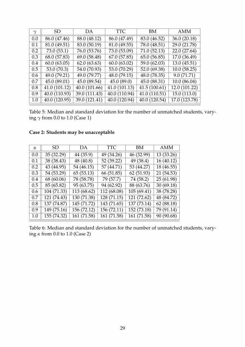
γ SD DA TTC BM AMM0.0 86.0 (47.46) 88.0 (48.12) 86.0 (47.49) 83.0 (46.52) 36.0 (20.18)0.1 81.0 (49.51) 83.0 (50.19) 81.0 (49.55) 78.0 (48.51) 29.0 (21.78)0.2 73.0 (53.1) 76.0 (53.76) 73.0 (53.09) 71.0 (52.13) 22.0 (27.64)0.3 68.0 (57.83) 69.0 (58.48) 67.0 (57.85) 65.0 (56.85) 17.0 (36.49)0.4 60.0 (63.05) 62.0 (63.63) 60.0 (63.02) 59.0 (62.03) 13.0 (45.51)0.5 53.0 (70.3) 54.0 (70.93) 53.0 (70.29) 52.0 (69.38) 10.0 (58.25)0.6 49.0 (79.21) 49.0 (79.77) 48.0 (79.15) 48.0 (78.35) 9.0 (71.71)0.7 45.0 (89.01) 45.0 (89.54) 45.0 (89.0) 45.0 (88.31) 10.0 (86.04)0.8 41.0 (101.12) 40.0 (101.66) 41.0 (101.13) 41.5 (100.61) 12.0 (101.22)0.9 40.0 (110.93) 39.0 (111.43) 40.0 (110.94) 41.0 (110.51) 15.0 (113.0)1.0 40.0 (120.95) 39.0 (121.41) 40.0 (120.94) 40.0 (120.54) 17.0 (123.78)

Table 5: Median and standard deviation for the number of unmatched students, vary-ing γ from 0.0 to 1.0 (Case 1)

Case 2: Students may be unacceptable

α SD DA TTC BM AMM0.0 35 (32.29) 44 (35.9) 49 (34.26) 46 (32.99) 13 (33.26)0.1 38 (38.43) 48 (40.8) 52 (39.22) 49 (38.4) 16 (40.12)0.2 43 (44.95) 54 (46.15) 57 (44.71) 53 (44.27) 18 (46.55)0.3 54 (53.29) 65 (53.13) 66 (51.85) 62 (51.93) 21 (54.53)0.4 68 (60.06) 78 (58.78) 79 (57.7) 74 (58.2) 25 (61.98)0.5 85 (65.82) 95 (63.75) 94 (62.92) 88 (63.76) 30 (69.18)0.6 104 (71.33) 113 (68.62) 112 (68.08) 105 (69.41) 38 (78.28)0.7 121 (74.43) 130 (71.38) 128 (71.15) 121 (72.62) 48 (84.72)0.8 137 (74.87) 145 (71.72) 143 (71.65) 137 (73.14) 62 (88.18)0.9 149 (75.16) 156 (72.12) 156 (72.11) 152 (73.18) 79 (91.14)1.0 155 (74.32) 161 (71.58) 161 (71.58) 161 (71.58) 90 (90.68)

Table 6: Median and standard deviation for the number of unmatched students, vary-ing α from 0.0 to 1.0 (Case 2)

29

β SD DA TTC BM AMM0.0 73 (77.73) 73 (79.29) 73 (77.36) 72 (76.55) 30 (77.02)0.1 75 (77.36) 76 (78.89) 76 (76.89) 74 (76.19) 30 (77.02)0.2 73 (77.85) 75 (78.97) 75 (76.89) 73 (76.47) 30 (77.82)0.3 74 (78.05) 77 (78.58) 78 (76.33) 75 (76.37) 31 (78.26)0.4 75 (75.7) 80 (75.24) 81 (73.1) 77 (73.55) 31 (75.9)0.5 76 (77.95) 83 (75.98) 85 (74.03) 80 (75.04) 31 (78.78)0.6 78 (75.93) 89 (72.36) 90 (70.86) 84 (72.24) 32 (77.14)0.7 79 (75.45) 95 (70.05) 96 (69.09) 89 (70.87) 32 (76.94)0.8 80 (74.65) 100 (67.84) 101 (67.37) 92 (69.41) 32 (76.76)0.9 82 (74.47) 105 (66.57) 105 (66.45) 96 (68.71) 34 (76.87)1.0 84 (74.9) 108 (66.4) 108 (66.4) 99 (68.69) 36 (77.65)

Table 7: Median and standard deviation for the number of unmatched students, vary-ing β from 0.0 to 1.0 (Case 2)

γ SD DA TTC BM AMM0.0 99.0 (42.3) 108.0 (42.4) 106.0 (41.52) 100.0 (40.95) 45.0 (21.06)0.1 93.0 (44.3) 103.0 (44.46) 102.0 (43.42) 95.0 (42.82) 37.0 (24.0)0.2 87.0 (47.8) 98.0 (47.72) 98.0 (46.52) 91.0 (45.91) 31.0 (29.75)0.3 82.0 (52.92) 94.0 (52.47) 93.0 (51.1) 87.0 (50.73) 27.0 (39.01)0.4 76.0 (58.68) 90.0 (58.06) 90.0 (56.53) 84.0 (56.27) 23.0 (49.05)0.5 71.0 (66.66) 85.0 (65.49) 86.0 (63.82) 80.0 (63.78) 21.0 (61.25)0.6 67.0 (75.38) 83.0 (73.8) 84.0 (72.01) 78.0 (72.28) 21.0 (74.42)0.7 65.5 (85.64) 82.0 (83.49) 84.0 (81.64) 77.0 (82.2) 23.0 (88.56)0.8 61.0 (95.31) 80.0 (92.64) 82.0 (90.66) 76.0 (91.56) 23.0 (100.71)0.9 60.0 (107.81) 80.0 (104.5) 82.0 (102.54) 76.0 (103.71) 29.0 (115.26)1.0 60.0 (114.66) 80.0 (111.05) 83.0 (109.05) 76.0 (110.38) 29.0 (122.64)

Table 8: Median and standard deviation for the number of unmatched students, vary-ing γ from 0.0 to 1.0 (Case 2)

30

All discussion papers are downloadable: http://www.wzb.eu/en/publications/discussion-papers/markets-and-choice

Discussion Papers of the Research Area Markets and Choice 2018

Research Unit: Market Behavior

Mustafa Oğuz Afacan, Inácio Bó, Bertan Turhan SP II 2018-201 Assignment maximization

Research Unit: Economics of Change

Kai Barron, Christina Gravert SP II 2018-301 Confidence and career choices: An experiment

Research Professorship: Market Design: Theory and Pragmatics

Daniel Friedman, Sameh Habib, Duncan James, and Sean Crockett SP II 2018-501 Varieties of risk elicitation