Graph-Theoretical Models for Frequency Assignment Problems
129
Graph-Theoretical Models for Frequency Assignment Problems vorgelegt von Diplom-Informatikerin Ewa Malesi´ nska Vom Fachbereich 3 Mathematik der Technischen Universit¨ at Berlin zur Erlangung des akademischen Grades einer Doktorin der Naturwissenschaften genehmigte Dissertation Promotionsausschuß: Vorsitzender: Prof. Dr. Manfred Breger Berichter: Prof. Dr. Rolf H. M¨ ohring Berichterin: Prof. Dr. Dorothea Wagner Tag der wissenschaftlichen Aussprache: 3. M¨ arz 1997 Berlin 1997 D 83
-
Upload
khangminh22 -
Category
Documents
-
view
3 -
download
0
Transcript of Graph-Theoretical Models for Frequency Assignment Problems
Graph-Theoretical Models
for Frequency Assignment Problems
vorgelegt vonDiplom-Informatikerin
Ewa Malesinska
Vom Fachbereich 3 Mathematikder Technischen Universitat Berlin
zur Erlangung des akademischen Grades einerDoktorin der Naturwissenschaften
genehmigte Dissertation
Promotionsausschuß:Vorsitzender: Prof. Dr. Manfred BregerBerichter: Prof. Dr. Rolf H. MohringBerichterin: Prof. Dr. Dorothea Wagner
Tag der wissenschaftlichen Aussprache: 3. Marz 1997
Berlin 1997
D 83

ZUSAMMENFASSUNG
In der vorliegenden Dissertation werden strukturelle und algorithmische Fragen desFrequenzzuweisungsproblems in Mobilfunknetzen untersucht. Fur die Graphentheo-rie ist dieses Problem wegen seiner engen Beziehung zur Graphenfarbung von In-teresse. Das Frequenzzuweisungsproblem umfaßt die Merkmale der T-Farbung, derListenfarbung sowie der Mengenfarbung und gehort dadurch zu den NP-schwerenkombinatorischen Problemen.
Der großte Teil der Arbeit widmet sich den sogenannten hybriden Netzen, in de-nen einige Stationen nach dem statischen und andere nach dem dynamischen Prin-zip funktionieren. Es wird ein graphentheoretisches Modell und zwei Optimierungs-kriterien fur das Frequenzzuweisungsproblem in hybriden Netzen eingefuhrt. DieKomplexitat der Auswertung der beiden Kriterien wird zunachst fur Graphen mit be-schrankter Baumweite sowie fur vollstandige Graphen untersucht und verglichen. Furdie weiteren Untersuchungen wird aus den beiden Kriterien die sogenannte Kanal-Stabilitatszahl, welche das partiellek-Farbungsproblem verallgemeinert, gewahlt. Furdiese Funktion werden in vollstandigen Graphen effiziente Algorithmen fur einigeSpezialfalle entwickelt. Es werden auch die Approximationsmoglichkeiten der Funk-tion untersucht.
Basierend auf den theoretischen Ergebnissen werden heuristische Verfahren furdie Berechnung der Kanal-Stabilitatszahl in allgemeinen Graphen entwickelt. DerVergleich unteren und oberen Schranken zeigt, daß diese Algorithmen auf unserenTestbeispielen, die auf Praxisdaten basieren, eine Genauigkeit von etwa 1 bis zu 6Prozent erreichen.
Mobilfunknetze konnen vereinfachend mit Hilfe von Disk Graphen modelliertwerden. Im letzten Teil der Arbeit untersuchen wir die Eigenschaften von vier Klas-sen von Disk Graphen. Es wird gezeigt, daß in allen diesen Klassen die chromatischeZahl linear in der Cliquenzahl beschrankt ist. Eine lineare Relation wird auch furTeilklassen der Schnittgraphen von Rechtecken gezeigt. Schließlich werden die DiskGraphen mit den planaren Graphen verglichen und es werden verbesserte Algorithmenfur das Cliquenproblem in Unit Disk Graphen sowie fur das Vertex Cover Problem inIntersection Disk Graphen vorgestellt.
i

ABSTRACT
In the present dissertation we investigate structural and algorithmic aspects of the fre-quency assignment problem in mobile telephone networks. This problem is of particu-lar interest for the graph theory because of its close relationship to graph coloring. Thefrequency assignment problem includes the characteristic features of T-coloring, listcoloring, and set coloring, and belongs thereby to NP-hard combinatorial problems.
The main part of this thesis is dedicated to the so-called hybrid networks, withsome stations operating according to the static principle and other stations accordingto the dynamic principle. We develop a graph-theoretical model and introduce twooptimization criteria for the frequency assignment problem in hybrid networks. Thecomputational complexity of evaluating these criteria is first examined for graphs withbounded treewidth and for complete graphs. In the further investigations we concen-trate on the criterion called channel stability number, which generalizesthek-partialcoloring problem. We develop efficient algorithms for some special cases of the chan-nel stability number in complete graphs and study its approximability.
Theoretical complexity results are used in the development of heuristic algorithmsfor the computation of the channel stability number in general graphs. For our testcases based on real world data, the comparison of lower and upper bounds shows thatthe algorithms provide results with a relative error between 1 and 6 percent.
Mobile telephone networks can be in a simplified way modeled using disk graphs.In the last part of the thesis the properties of four classes of disk graphs are examined.We show that the chromatic number of the members of any of these classes is boundedby a linear function of the clique number. A linear relation is also shown for somesubclasses of intersection graphs of rectangles. Finally, we compare disk graphs andplanar graphs and present improved algorithms for the maximum clique problem inunit disk graphs and for the vertex cover problem in intersection disk graphs.
iii

ACKNOWLEDGMENTS
The results presented in this thesis are based on the research that would not bepossi-ble without the help of a number of people. First and foremost, I wish to thank RolfMohring and Dorothea Wagner for inviting me to come to Berlin and join their re-search group. Rolf Mohring was my supervisor and I am particularly grateful for hissupport, guidance and valuable comments, but also for the freedom he has given mein my research.
I learned about the frequency assignment problem, which is the subject of thisthesis, already before coming to Berlin. At the end of my study I worked for sixmonths at T-Mobil with Jurgen Plehn, who introduced me to this beautiful applicationof discrete mathematics. I am sincerely grateful for his constant encouragement andsupport during my research. At this point, I also thank T-Mobil for rendering meaccess to three records of data, which served as a basis of all my computational tests.
Furthermore, I would like to thank Alessandro Panconesi for suggesting the studyof approximation problems and for many fruitful discussions. The presentation ofChapter 2 has profited a lot from his critical but constructive comments as a co-authorof our paper. Thanks are also due to my colleagues in Mainz: Albert Graf, SteffenPiskorz, and Gerhard Weißenfels, for our co-operation in the study of disk graphs.I am also grateful to Jens Gustedt, Matthias Muller-Hannemann, Jorg Rambau, andSergey Tiourine, for their careful reading of the manuscript and the number of valuablecomments. My thanks go to all my colleagues from the group “Discrete Mathematics”at the Berlin University of Technology who provided a friendly working atmosphere.
I did my research as a member of the graduate school “Algorithmic Discrete Math-ematics” supported by the Deutsche Forschungsgemeinschaft (grant GRK 219/ 2-96).Besides its financial support, I acknowledge its contribution in bringing together allBerlin discrete mathematicians.
Finally, let me express my deepest gratitude to my husband Peter Menke-Gluckert for all his love, encouragement, and a lot of patience, especiallyin the lastweeks of writing this thesis.
Ewa Malesinska Berlin, December 1996
v

CONTENTS
Introduction 1
1 Preliminaries 71.1 Generalized Graph Colorings . . . . . . . . . . . . . . . . . . . . . . 7
1.1.1 The Chromatic Binding Function . . . . . . . . . . . . . . . 81.1.2 Set Coloring . . . . . . . . . . . . . . . . . . . . . . . . . . 81.1.3 List Coloring and Precoloring Extension . . . . . . . . . . . . 91.1.4 T-Coloring . . . . . . . . . . . . . . . . . . . . . . . . . . . 101.1.5 Maximum k-Coloring . . . . . . . . . . . . . . . . . . . . . 11
1.2 Fixed Channel Allocation . . . . . . . . . . . . . . . . . . . . . . . . 121.3 Dynamic Channel Allocation . . . . . . . . . . . . . . . . . . . . . . 161.4 Hybrid Channel Allocation . . . . . . . . . . . . . . . . . . . . . . . 18
2 Hybrid Networks – Theoretical Considerations 212.1 Introduction . . . . . . . . . . . . . . . . . . . . . . . . . . . . . . . 212.2 Model of a Hybrid Network . . . . . . . . . . . . . . . . . . . . . . 232.3 Optimization Criteria . . . . . . . . . . . . . . . . . . . . . . . . . . 252.4 Graphs with Bounded Treewidth . . . . . . . . . . . . . . . . . . . . 282.5 Complete Graphs . . . . . . . . . . . . . . . . . . . . . . . . . . . . 32
2.5.1 Channel Stability Number . . . . . . . . . . . . . . . . . . . 342.5.2 Approximation Results . . . . . . . . . . . . . . . . . . . . . 41
3 Hybrid Networks – Computational Results 553.1 Introduction . . . . . . . . . . . . . . . . . . . . . . . . . . . . . . . 553.2 Problem Instances Used for Computational Tests . . . . . . . . . . . 573.3 Graph Partition . . . . . . . . . . . . . . . . . . . . . . . . . . . . . 593.4 Heuristic Algorithms . . . . . . . . . . . . . . . . . . . . . . . . . . 61
3.4.1 Lower Bounds . . . . . . . . . . . . . . . . . . . . . . . . . 613.4.2 Upper Bounds . . . . . . . . . . . . . . . . . . . . . . . . . 72
3.5 Results Using an ILP Formulation . . . . . . . . . . . . . . . . . . . 743.6 Conclusions . . . . . . . . . . . . . . . . . . . . . . . . . . . . . . . 79
vii
viii CONTENTS
4 Chromatic Number of Some Geometric Graphs 814.1 Modeling Cellular Networks as Disk Graphs . . . . . . . . . . . . . . 824.2 Chromatic Number of Disk Graphs . . . . . . . . . . . . . . . . . . . 854.3 Chromatic Number of Rectangle Graphs . . . . . . . . . . . . . . . . 934.4 Conclusions . . . . . . . . . . . . . . . . . . . . . . . . . . . . . . . 96
5 Algorithmic Properties of Disk Graphs 995.1 Introduction . . . . . . . . . . . . . . . . . . . . . . . . . . . . . . . 995.2 Maximum Clique . . . . . . . . . . . . . . . . . . . . . . . . . . . . 1005.3 Vertex Cover . . . . . . . . . . . . . . . . . . . . . . . . . . . . . . 104
Bibliography 109
INTRODUCTION
In the last decades we have been witnessing changes in the telecommunications in-dustry at constantly increasing rate. Equipment and tools that are now used everyday would have been inconceivable 10 or 20 years ago. This rapid development oftelecommunications systems, the invention of wireless networks, and the initiation ofsatellite-based systems have opened new areas for applications of discretemathemat-ics and operations research. Especially in the field of network design, mathematicsis contributing to minimizing costs, ensuring network reliability, and maximizing net-work efficiency.
The subject of this thesis also comes from a relatively new and still rapidly growingbranch of the telecommunication industry, namely mobile telephone networks. Thedesign problems in such networks cover both decisions on the topology and capacityof the wired part of the network as well as on the design of the wireless part. Maincomponents of the wireless part are mobile-service switching centers (MSC)and basestations (BS). The last ones, equipped with transmitters and receivers,are responsiblefor the communication with mobile users, using the frequency spectrum reservedfora particular telephone network.
The design of the wireless part involves several optimization problems, forin-stance, making decisions on the number and locations of base stations and on thenumber of MSC’s. In this thesis we investigate thefrequency assignment problemthat denotes the task of allocating carrier frequencies to the base stations.These car-rier frequencies are sometimes called channels. Thus the problem is also known asthechannel assignment problem. In our study we concentrate on hybrid networks, inwhich frequencies are initially assigned only to a subset of base stations. Weexaminethe specific design problems in such networks, formulate optimization criteria, anddevelop algorithms for their computation.
The second part of our thesis is dedicated to the study of structural and algorithmicproperties of graph instances typical for modeling wireless telephone networks. Themain goal of this part is a theoretical explanation of the fact that thechromatic numberand theclique numberof these graphs hardly differ from each other.
In the contemporary cellular systems,Fixed Channel Allocation(FCA) is the mostpopular strategy for the channel assignment. According to this approach, first, the traf-fic intensity is estimated in order to decide how many channels each base station needsto support the telephone traffic [MR94]. Next, the required number of channels is as-signed to every base station in a way that prevents strong interferences between radio
1
2 INTRODUCTION
signals. For the purpose of this assignment, the network is modeled as a so-calledinterference graph. Vertices in the graph represent base stations, and two nodes areadjacent if the signals transmitted by the corresponding stations could interfere. Now,the channel assignment problem consists in selecting the required number of chan-nels for single graph vertices in such a way that adjacent vertices are assigned disjointsets of channels. Clearly, in the graph model the channel assignment problem closelyresembles the graph coloring. However, in the frequency assignment there is a num-ber of additional restrictions to be satisfied. For technical reasons, two frequenciesfandg assigned to the same station must be separated by one or two carrier frequen-cies. Moreover, some channels may be forbidden for certain stations. This happensparticularly often in border areas, where the frequency spectrum reservedfor mobiletelephone networks has to be divided among the neighboring countries. Actually, thetwo restrictions on frequency assignments can be modeled using some generalizationsof the basic graph coloring problem. Such generalizations are discussed in Chapter1.
In most applications there is one more difference between the channel assignmentproblem and the basic graph coloring problem, namely the objective function. Whencoloring a graph, the aim is to use as few colors as possible. In telephone networks,at least in European civil telecommunications, the number of available frequencies isfixed and saving any of them brings no profit to the network operator. One is ratherinterested in finding an admissible channel assignment using possibly all frequenciesbut ensuring high network quality, i.e., low interference level and low blocking prob-ability at the same time. These objectives are formulated as a cost function to beminimized by the selected channel assignment plan.
Despite some distinctive features, channel assignment and graph coloring remainclosely related. This has been probably first noticed by Metzger [Met70]. However,it was Hale who formalized the frequency assignment problem as a generalizedcol-oring problem. His work [Hal80] motivated Roberts, Cozzens, and many others (seeSection 1.1) to study the T-coloring. The close relationship between coloring and fre-quency assignment is also reflected in our thesis. Several results in Chapters 2 and 3,concerning the channel assignment in hybrid networks, are motivated by the theoryand algorithms for graph coloring. Chapter 4 is in fact completely dedicated to thechromatic number of graph classes defined by intersections of some geometric figuresin the plane.
We have already mentioned that the channel allocation strategies currently in usein all large, i.e. non local, networks follow the static FCA strategy: frequencies areassigned once for all. Reallocation happens rarely, usually every two or three monthsor when the network undertakes restructuring (stations are added, replaced or deleted).This static approach has several shortcomings [ZE93]. For example, such networksare not able to adapt to unpredictable changes in the traffic pattern. No doubt, this willbe improved in the near future and several dynamic allocation strategies have already
3
appeared in the literature (see Section 1.3 for a short overview). Between the currentsituation and the appearance of dynamic networks, however, there will be a transitionphase where networks will behybrid, i.e., they will contain both static and dynamictransmitters. It is this type of networks that we study in the first part of our thesis.A central problem arising in hybrid networks is the following: allocating frequenciesto the static part of the network constraints the available frequency spectrumfor dy-namic stations. Such an assignment might be too restrictive, and it is important to beable to detect whether this is the case. A related and rather important problem is todevise computationally efficient methods allowing to compare different frequency as-signments to the static part of the network, i.e., to decide which of the two assignmentsis the best with respect to the dynamic part.
In this thesis the possibilities and restrictions for the design of such methods arediscussed. We explain why it is not possible to compare unequivocally two frequencyplans and propose two measures for an approximative quality valuation of static fre-quency plans in hybrid networks. Roughly speaking, the first measure is defined asthe maximum number of channel requirements that can be simultaneously satisfiedin the dynamic part of the network. This function generalizes thepartial k-coloringproblem. We call it thechannel stability numberand denote withch(I). The secondfunction counts stations whose requirements can be simultaneously entirely satisfied.First, the complexity of both functions is studied theoretically in order to choosethemore promising approach. This turns out to be the channel stability number. Its prac-tical applicability is later on examined by means of tests based on real world data.
When employing theoretical methods to practical problems one is often confrontedwith intricate and difficult to handle requirements. In such a situation it may be tempt-ing to ignore some specific restrictions or to concentrate on a narrow class of instances.Considering all requirements occurring in practice was of particular importance tous. As a result, the channel stability number generalizes difficult coloring problems,namely list coloring and set coloring as well as special cases of the T-coloring prob-lem. This makes its computation NP-hard even for very simple classes ofgraphs.We know that the results presented in Chapter 2 for graphs with bounded treewidthand for complete graphs are not likely to be directly applied in the design of wirelessnetworks. But we hope that they lead to a better understanding of the complexity ofthe problem, which is important for the development of algorithms for graphs mod-eling real networks. Moreover, some of these algorithms are used as subroutinesinprocedures for general networks presented in Chapter 3.
It is a trivial observation that thechromatic numberof an interference graph yieldsa lower bound on the number of frequencies that are necessary to satisfy channel re-quirements. In fact, if single stations require only one frequency then in practice thechromatic number often coincides with the required number of radio channels. In-terestingly enough, it turns out that the chromatic number of graphs modeling real
4 INTRODUCTION
networks exceeds their clique number only by a small constant. A theoretical expla-nation of that phenomena could help better understand the structure of interferencegraphs.
If for all induced subgraphs of a graphG the chromatic number of the subgraphequals its clique number thenG is calledperfect. Interference graphs are not perfect,sinceC5 — a cycle with 5 vertices — is absolutely eligible in a model of a wirelessnetwork, and this graph is not perfect. The topology of interference graphs, althoughunknown, is not arbitrary. It has been already observed by Hale [Hal80] that graphsmodeling wireless networks can be approximately treated as disk graphs. The reasonfor this is that the supply area of a transmitter usually resembles a disk with the trans-mitter located in its center. Then, simplifying the channel interference,we can assumethat two transmitters could interfere with each other when their supply areas intersect.
This justifies our hope that more insight into the structure of interference graphscan be obtained by the study of intersection graphs defined by geometric figures in theplane. In particular we examine the chromatic number of four classes of disk graphsas well as intersection graphs of rectangles in the plane. A partial explanation for therelatively small chromatic number of interference graphs follows from the propertythat for all classes of disk graphs and some subclasses of rectangle graphs there is aconstantc, such thatχ(G)� c�ω(G).Outline of the thesis
Let us now shortly summarize the contents of the following chapters.Chapter 1 begins with a summary of graph coloring extensions and explains their
relation to the frequency assignment problem. Then, a short survey of the literature onthe Fixed Channel Allocation is given. It is followed by a characterization of the draw-backs of static assignments and the review of different strategies for dynamic channelallocation. The first chapter is closed with a short presentation of some intermediatemethods that combine the static and dynamic approach.
In Chapter 2 we develop a graph-theoretical model and introduce two optimizationcriteria for the frequency assignment problem in hybrid networks. We give polynomialtime algorithms for the computation of these criteria in the case when the dynamic partof the network forms a graph with bounded treewidth. In the practically important caseof complete graphs both functions are NP-hard. However, the second function remainsNP-hard even when some restrictions are disregarded. In the further study of completegraphs we concentrate on the first function. It is called the channel stability numberand generalizes thek-partial coloring problem. Efficient algorithms are developed fortwo special cases, in which not all restrictions are observed. Chapter 2 is closed withan analysis of the approximability of the channel stability number in complete graphs.
In Chapter 3 we examine the possibilities of computing the channel stability num-
5
ber studying several instances based on real world data. At the beginning, we explainhow the test instances have been generated and discuss how the instances can be de-composed into smaller problems. The main part of the chapter is dedicated to thepresentation of a heuristic algorithm providing lower bounds on the channel stabil-ity number. Its performance is analyzed comparing the results with upper boundsobtained by another algorithm. We close the chapter by the presentation of boundsobtained using an integer linear programming formulation.
Chapter 4 is dedicated to the study of the chromatic number of different intersec-tion graphs. At the beginning, we introduce four classes of disk graphs and discuss themutual relations between them. Afterwards, we show new lower and upper bounds onthe function relating the chromatic number to the clique number in disk graphs and insome special cases of rectangle graphs.
In the last Chapter 5 the algorithmic properties of two classes of disk graphs,namely unit disk graphs and intersection disk graphs, are compared with properties ofplanar graphs. Finally, we present improved algorithms for the maximum clique prob-lem in unit disk graphs and for the vertex cover problem in intersection disk graphs.

CHAPTER 1
PRELIMINARIES
1.1 GENERALIZED GRAPH COLORINGS
It is helpful to summarize the most important results on graph colorings in order togive an understanding of the complexity of the frequency assignment problem. Weconsider several generalizations of the graph coloring problem, each capturing anotheraspect of the frequency assignment. Most of these generalizations are more difficultthan the simple vertex coloring in the sense that there are less cases in which thegeneralized problems can be solved in polynomial time.
For completeness, we begin with some basic definitions. For the explanation of allother terms not defined here the reader is referred to [Ber85, Gol80, CLR90, GJ79]. Asan extensive survey on the graph coloring theory we recommend the book by Jensenand Toft [JT95].
All graphs considered in this thesis are finite, undirected, without any loops andmultiple edges. Given a graphG= (V;E), any mappingf : V! IN assigning differentcolors to adjacent vertices is a (proper)vertex coloring. The least number of colors inany such assignment is defined as thechromatic numberof the graphG and is denotedby χ(G). Similarly, anedge coloringcan be defined, but this problem is not consideredin our thesis. Aclique in a graphG = (V;E) is a set of nodesVc � V such that anypair of nodesv;w2Vc is adjacent inG. The order of the largest clique inG is calledtheclique numberand is denoted byω(G). It is commonly known that in every graphG
ω(G)� χ(G)� ∆(G)+1
where∆(G) denotes the maximum vertex degree.Graph coloring belongs to the hardest problems from the point of view of com-
plexity theory. Computing the chromatic number is not only NP-complete [GJ79];there even exists a constantε > 0 such that it is impossible to approximateχ(G) upto a factornε unless P = NP [LY93]. Nevertheless, polynomial time algorithms havebeen developed for coloring many families of graphs. Let us mentionpartial k-treesfor a constantk and several subclasses ofperfectgraphs:bipartite graphs,intervalgraphs,comparabilityandcocomparabilitygraphs — as some important examples.Optimal coloring of an arbitrary perfect graph also belongs to P. However, nopurelycombinatorial algorithm is known in this case.
7
8 PRELIMINARIES
1.1.1 The Chromatic Binding Function
The clique numberω(G) is a lower bound on the chromatic numberχ(G). However,the gap between these two values can be arbitrarily large. Mycielski [Myc55] wasprobably the first one to construct an infinite family of graphsfG1;G2; : : :g such thatω(Gi) = 2 andχ(Gi) = i, for everyi = 1;2; : : : On the other hand,χ(G) = ω(G) for allperfect graphs. These discrepant relations motivated Gyarfas to define theχ-bindingfunction[Gya87]. A functionf is aχ-binding function for a family of graphsG if
χ(G0)� f (ω(G0))holds for all induced subgraphsG0 of G2 G.
Several questions are important in the study ofχ-binding functions. For a fam-ily of graphsG, first, the existence of any binding function must be verified. Aswe have seen, graphs constructed by Mycielski are notχ-bounded. Another inter-esting example is provided by the intersection graphs of boxes (i.e., parallelepipedswith sides parallel to the coordinate axes) in the three-dimensional Euclidean space[Bur65]. For some graphs the best knownχ-binding function is exponential. Thisis the case for circle graphs, for whichχ(G)< 2ω+6 [KK95]. The best known func-tion for two-dimensional box graphs is quadratic. The existence of a linear functionhas been shown only for some subclasses of this family (see Chapter 4). Even ifaχ-binding function is known for a certain class of graphs it usually remains open ifthis function is the smallest possible one.Circular arc graphsmake an exception. Afamily of circular arc graphsGk satisfyingω(Gk) = k andχ(Gk) = �3
2k�
can be foundin the paper by Tucker [Tuc75]. On the other hand, Karapetian [Kar80] proved thatχ(G)� �3
2ω(G)� holds for this class of graphs.The importance of the relation betweenχ(G) andω(G) stems from the fact that
for graphs with smallχ(G)-binding function the vertex coloring problem can usuallybe solved by an approximation algorithm with a good performance ratio. For all diskgraphs discussed in Chapter 4 the derivation of linear binding functions provides con-stant ratio approximation algorithms for their coloring. This is important since diskgraphs can be viewed as idealized graphs modeling radio broadcasting networks.
1.1.2 Set Coloring
A first straightforward generalization of the vertex coloring problem consists of as-signing a set of colors to every vertexv2V. Suchset assignmentproblems have beenformalized by Roberts [Rob79], who was motivated by the mobile radio frequencyassignment problem. In this application it is usually required that each station x isassignedr(x) frequencies, wherer(x) is a small positive integer.
The complexity of computing theset-chromatic number does not differ much fromthe simple vertex coloring. Given a graphG with color requirementsr(v), v2V, let
1.1 GENERALIZED GRAPH COLORINGS 9
us construct the graphG0 from G by the replacement of each vertexv by a cliqueKr(v). The set coloring of the graphG is equivalent to the simple vertex coloring ofG0. If the graphG is perfect, comparability, cocomparability, chordal, or interval,thenG0 belongs to the same class of graphs [Nie95]. For perfect graphs this is thefamous replication lemma by Lovasz [Lov72]. Hence, for all mentioned classes theset coloring problem can be solved in polynomial time.
Roberts [Rob79] considered also set colorings in a more general setting. He de-fined λ-set assignments, i.e., set assignments satisfying conditionsλ. We requiredpreviously that each assigned setS(x) has cardinality at leastr(x). Alternatively, con-ditionsλ can express that eachS(x) has cardinalityn, that it should contain consecu-tive integers, or another requirement. These problems have been further investigatedin [Rob91, BD82, DH88].
1.1.3 List Coloring and Precoloring Extension
In mobile cellular networks the use of some frequencies is often forbidden for severalbase stations. This can be modeled by a list coloring. In such colorings there is alist L(v) associated with every vertexv of G. The question is if there exists a propercoloring of G assigning to every vertexv a color from its own list. Precoloring ex-tension (PrExt, for short) can be viewed as a special case of the list coloring.In thisversion of the problem a vertex subsetW �V is precolored using at mostk differentcolors. We want to know if this precoloring can be extended to a proper k-coloring ofthe whole graphG. The last problem has also its own interpretation in the context offrequency assignment. When new base stations are introduced into the network it isoften required that some of the earlier stations retain their old frequencies.
Very important for the theory of list colorings is the notion of thechoice num-ber of a graphG. It is the smallest numberk such that the graphG can be properlycolored with colors from the listsL(v) provided that eachL(v) has at leastk col-ors. If the choice number of a graphG is not larger thank thenG is a said to bek-choosable. Probably the most famous problem in that context is the 5-choosabilityof planar graphs. It has been conjectured by Vizing in 1975 and remained open un-til Thomassen proved it in a very short and elegant way in 1993 [Tho94]. This wasshortly after Voigt [Voi93] described planar graphs that are not 4-choosable.
For our applications the choice number is of minor importance. We are moreinterested in algorithms examining if a graphG can be properly colored with colorsfrom given listsL(v), v2 V. It turns out that this problem is NP-complete for manyclasses for which the simple vertex coloring can be solved in polynomial or even inlinear time. Actually, many hardness results follow from the NP-completeness ofprecoloring extensions. Let us mention that the latter problem is NP-hard already forplanar bipartite graphs with color boundk= 3 [Kra93] and for interval graphs if colors
10 PRELIMINARIES
are allowed to be used twice in the precoloring [BHT92].We know only two examples of graphs for which precoloring can be efficiently
extended and the list coloring is still NP-complete. Jansen and Scheffler proved thisfor cographs [JS92]. Hujter and Tuza gave a polynomial algorithm for PrExt of splitgraphs [HT93], and we have observed that list coloring of split graphs is NP-complete.
Proposition 1.1 The list coloring problem restricted to split graphs is NP-complete.
Proof. Clearly, the problem is in NP. To prove NP-hardness basically the construc-tion of Jansen and Scheffler for cographs can be used (see Theorem 22 in [JS92]).They reduced the 3SAT problem to the list coloring of a cographG = (V1[V2;E).In their proof G is a complete bipartite graph. VerticesV1 represent boolean vari-ables. The feasible color set for a vertexai 2V1 representing a variablexi is defined asSai = fxi;xig. VerticesV2 represent clauses of a given boolean formula. Given a clauseci = yi;1_yi;2_yi;3, yi; j 2 X = fx1;x1; : : : ;xn;xng, the feasible color set for the corre-sponding vertexbi 2V2 is defined asSbi = fyi;1;yi;2;yi;3g. Then, clearly the graphGhas an admissible list coloring if and only if the given boolean formula is satisfiable. Ifthe subgraph defined on verticesV1 is a clique rather than an independent set then themodified graph is both a cograph and a split graph, and the reduction remains valid.�
List coloring is known to be solvable in polynomial time only for graphs withbounded treewidth [JS92] and for complete graphs (see Chapter 2).
All cited results on the complexity of list colorings manifest the complex nature ofthe frequency assignment problem.
1.1.4 T-Coloring
One more aspect of frequency assignment problems is expressed in the definition of aT-coloring. This variant of the vertex coloring has been introduced by Hale [Hal80].Given a graphGand a setT of nonnegative integers, a T-coloring ofG is an assignmentf : V! IN such that if two verticesv andw are adjacent thenj f (v)� f (w)j 62 T. Halementions the example of UHF-TV transmitters, in which a feasible channel assign-ment should be a T-coloring for a setT = f0;1;2;3;4;5;7;8;14;15g. T-sets charac-teristic for cellular telephone networks are typically intervalsf0; : : : ; rg, r � 2. Hale’scontribution initiated an intensive study of T-colorings. A good overview has beengiven by Roberts in [Rob91].
The efficiency of a T-coloring can be measured using two parameters, the T-chromatic numberχT(G) and the T-span spT(G). χT(G) is the minimum numberof different colors in any T-coloring of a graphG for a given setT. The T-span isthe minimum span of any T-coloringf , where the span is defined as the maximum
1.1 GENERALIZED GRAPH COLORINGS 11j f (v)� f (w)j over all pairsv;w 2 V(G). It can easily be seen thatχT(G) = χ(G).Therefore, the literature on T-colorings concentrates on the study of the T-span.
The complexity of computingspT(G) and finding a T-coloring with the minimumspan depends substantially on the setT. If T has no special structure then com-puting spT(G) is NP-hard already for complete graphs [Gra93, Jan93]. However,many important special cases can be solved efficiently. For example,T is calledr-initial if T = f0;1; : : : ; rg[S, whereS contains no multiple ofr + 1. In that casespT(G) = spT(Kχ(G)) = (r + 1)(χ(G)� 1) [CR82]. For r-initial setsT optimal T-colorings of chordal graphs can be efficiently found by a greedy algorithm applied tothe reverse of a perfect elimination ordering [Ray85].
The T-coloring as defined above does not capture two requirements on a frequencyassignment in cellular networks. In this application two frequenciesf andg assignedto the same station must be separated, i.e.,j f �gj > δ, where typicallyδ = 2. Fre-quencies assigned to interfering stations must satisfy this inequality with δ = 0 orδ = 1, depending on the degree of possible interference. These requirements can onlybe expressed using more than one setT. Such T-colorings with multiple levels ofinterference have already been introduced by Hale [Hal80] and afterwards studied byRaychaudhuri [Ray85], Tesman [Tes89], and some others. A formal definition andsome special cases of multiple setsT are described in Section 2.5.
At last, let us point out that Tesman [Tes89] considered vertex colorings combin-ing the requirements of a T-coloring and a list coloring or of a T-coloring and a setcoloring. This is important for frequency assignment problems, where typically alldescribed restrictions occur simultaneously.
1.1.5 Maximum k-Coloring
The maximum k-colorable subgraph problem can be defined as follows: given a graphG = (V;E) and a positive integerk, find ak-colorable subgraphG(U) of maximumcardinality jU j. Our interest for this problem stems from the fact that thechannelstability number, introduced in the next chapter, generalizes the maximumk-colorablesubgraph problem including the aspects of list-, set-, and T-colorings.
Gavril [Gav87] has shown that a maximumk-colorable subgraph can be found inpolynomial time both in comparability and cocomparability graphs. The same is validfor chordal graphs if the numberk is fixed [GY87]. However, ifk is not fixed thenfinding the maximumk-colorable subgraph is NP-complete even for split graphs (thusalso for chordal graphs) [GY87].
Roberts [Rob79] considered a problem that can be regarded as a generalizationof the maximumk-colorable subgraph problem to the set coloring. He defined theλ-chromatic scoreχλ;N(G) of a set coloring satisfying a set of conditionsλ as∑v2V(G) jS(v)j. Some properties of this parameter as well as further references can
12 PRELIMINARIES
be found in [Ray85].
1.2 FIXED CHANNEL ALLOCATION
Fixed Channel Allocation problem can be described as follows. There is a finite setFof frequencies and a finite set of base stationsV = fv1; : : : ;vng. For each base stationvi , i = 1; : : : ;n, we are given its frequency demandr(i), the set of already assignedfrequenciesA(i), and the set of locally forbidden frequenciesB(i). Furthermore, aninterference probabilityp(v;w) is given for any pairv, w of base stations. Two thresh-old valuesT1 andT2 (whereT1 < T2) are introduced in order to distinguish differentdegrees of interference. If the interference probabilityp(v;w) or p(w;v) is higher thanor equal to the thresholdT2 then no adjacent channels can be assigned to the stationsvandw (adjacent channel constraint). Otherwise, if bothp(v;w) andp(w;v) are smallerthanT2 and at least one of them is higher than or equal toT1 then the sets of channelsassigned tov andw must be disjoint (co-channel constraint). Both adjacent and co-channel constraints can be stored in a symmetriccompatibility matrix C= (ci j ) withnonnegative integer entriesci j . Positive entriesci j > 0 denote the distance that must bepreserved between channels assigned to the stationsvi andv j . This means that positiveentries on the diagonalcii > 0 denote the distance requirements for channels assignedto one stationvi (co-site constraint). In most cellular telephone networkscii = 2 or 3for all base stations. Note that the compatibility matrix can be interpreted as an ad-jacency matrix of theinterference graph(the same as mentioned in the introduction).Nodes of this graph represent base stations and two nodes are adjacent if there is aco-channel constraint imposed on the corresponding stations. Co-site constraints aswell as higher distance requirements for pairs of stations can be expressed as weightson nodes and edges respectively.
The conditions on an admissible frequency assignment can be now formulated asfollows.
Definition 1.1 Let I be an instance of the frequency assignment problem as describedabove. Then a frequency assignment S: V 2F is admissible if and only if:� A(i)� S(i)� F for all i = 1; : : : ;n,� B(i)\S(i) = /0 for all i = 1; : : : ;n,� jS(i)j= r(i) for all i = 1; : : : ;n,� j f � f 0j � ci j for all i ; j = 1; : : : ;n, i 6= j, f 2 S(i), f 0 2 S( j),� j f � f 0j � cii for all i = 1; : : : ;n, f 2 S(i), f 0 2 S(i), f 6= f 0.
1.2 FIXED CHANNEL ALLOCATION 13
At this point we should formally define an objective function in the frequencyassignment problem. Unfortunately, as it is common for many real world problems,there is no unique definition of an objective function. In some earlier applications afrequency assignment minimizing the highest used frequency was defined as optimal.In modern cellular networks the set of frequencies is fixed and saving any of themusually brings no profit. An objective function is instead used to eliminate the sharpthresholds for interference probabilities. Among others, Lanfear [Lan89] and Plehn[Ple94] saw the disadvantages of the strict partition of stations pairs into those thatare allowed to use the same frequencies and those that are forbidden to do so. Moreadequately, stations interfering with moderate probability can be allowedto use thesame channels at the expense of increasing the cost function.
For this purpose a third thresholdT0 < T1 is defined. If for any pairv;w of basestations both valuesp(v;w) andp(w;v) are smaller thanT1 thenv andw are allowed touse the same frequencies. However, if any of these values reachesT0 then we say thatthere is aweakinterference betweenv andw, which cannot be fully neglected. Theassignment of equal frequencies to the pairv, w should then lead to the increase of thecost function.
An appropriate cost function can be certainly defined in many different ways. Togive an example, we cite the definition introduced by Plehn [Ple94]. Given an instanceI and an admissible frequency assignmentS, defineN0(v), for each stationv2V, to bethe set of base stationsw2V weakly interfering withv. An objective function, calledtheprice of interference, is then defined as
pif(I ;S) = ∑v2V1
r(v) ∑w2N0(v)∑ f2S(v)\S(w) p(v;w)∑v2V jN0(v)j :
In the following part of this section we will give a short summary of methods thatcan be applied for solving the fixed frequency assignment problem. In that context, itis worth mentioning the recent CALMA project that was carried out by severalgroupsfrom the Netherlands, France and United Kingdom. The aim of this project was to testthe applicability of different combinatorial algorithms for military applications. Thishas been performed as the case study of the frequency assignment problem [Toe95].The CALMA project provides a valuable comparison of several combinatorial algo-rithms applied to the same instances of the frequency assignment problem. Withinthis project two types of instances were considered, corresponding to the two types ofoptimization functions. In the first type of instances the aim was to minimize the num-ber of used frequencies, whereas the instances of the second type had an interferencecost function. Some instances of the second type included vertices with preassignedfrequencies. A part of preassigned frequencies was allowed to be changed at thepriceof increasing the cost function by a mobility costMi , specified for a preassigned fre-quencyi.
14 PRELIMINARIES
Lower Bounds
Good lower bounds on the number of required frequencies are important to decidehow far from the optimum the results of an assignment procedure are. If we interpretchannel requirements as weights on the nodes in the interference graph then the sizeofthe largest weighted clique yields a lower bound. From the theoretical point of view,the computation of the largest weighted clique is NP-hard. Nonetheless, it turns outinpractice that this bound is not only of good quality but can also be calculated fast. Asan additional advantage, the geographical distribution of heavy cliques allows to spotcritical regions of excessively high channel demands.
The clique bound may turn out to be insufficient if many frequencies are locallyforbidden. In such regions it is advisable to check if the underlying list coloring prob-lem can be solved for all maximal cliques. An algorithm for that is presentedinSection 2.5.1 (see comments to Theorem 2.4).
Another lower bound proposed by Gamst [Gam86] is calculated by the considera-tion of all ν-complete sets, defined as setsV 0 �V in which ci j � ν for all vi;v j 2V 0.The chromatic number can yield an even better lower bound. However, its computa-tion requires global information and is therefore more time-consuming.
Much less is known about lower bounds on the value of the interference function.Few authors have considered this problem at all and as far as we know no useful lowerbounds have been found so far. We mentioned above the CALMA project. Withinthis project one has succeeded to derive good lower bounds on the interference costfunction only in the special case when the cost function combines interference andmobility cost. In the absence of the mobility cost lower bounds were too small to beuseful [HT95].
Algorithms
Already the earliest frequency assignment methods in the end of 70’s have been in-spired by graph coloring procedures. Metzger [Met70] and afterwards Zoellner andBeall [ZB77] tested simplesequential assignment algorithmsusing the largest-firstand the smallest-last vertex order. Frequencies have been assigned in a greedy mannerbased on a fixed vertex order.
At the same time, Box [Box78] suggested an iterative, probabilistic algorithm:several assignments are generated by applying a simple sequential algorithm. Crucialfor his algorithm is the concept of theassignment difficultyof a transmitter. This is areal number associated with a transmitter. It is increased by a random value after eachiteration in which the requirements of this transmitter has not been satisfied. Gamstand Rave [GR82] later suggested to initialize these values according to the smallest-last order. It is remarkable that this simple algorithm has been implementedin the
1.2 FIXED CHANNEL ALLOCATION 15
network planning program GRAND and has been commercially used until recently.
It has been realized long ago that the sequential assignment methods can be im-proved if the fixed vertex order is replaced by a more careful choice of the nextvertex.Hale [Hal81] suggested to use for that purpose thesaturation degreeintroduced byBrelaz [Bre79]. Gamst and Rave [GR82] were probably the first to introduce amorecareful choice of assigned frequencies.
Plehn [Ple94] noticed that the number of assigned frequencies is not an adequatecost function and replaced it by theprice of interference. His sequential assignmentmethod characterizes a very careful selection of vertices and channels. We describethis algorithm in all detail in Chapter 3.
All popular local searchmethods have been already tested for the frequency as-signment problem.Simulated annealing, taboo search, genetic algorithms, andvari-able depth searchbelong to this class of methods. It is very difficult to compare thesealgorithms on the basis of tests performed on different instances and using differentcomputers. To some extent a valuation became possible after the CALMA project.
It turned out during the project that local search methods perform relatively poorif they are not specially tuned for the problem at hand. This has been most distinctlyobserved for genetic algorithms. Original genetic algorithms gave very poor results.However, algorithms specialized for the frequency assignment problem providedthebest solutions for instances with the interference function as the cost function. Posi-tive results gave also an adaptation of the variable depth search method (this methodhas been originally introduced by Kernighan and Lin for graph partitioning problems[KL70]). Most of local search methods have the disadvantage of being more time-consuming than simple sequential assignment methods. This particularly refersto thesimulated annealing.
Recently, some mathematical programming methods have been applied to the fre-quency assignment problem. Aardal et al. [AH+95] report on the results obtainedwithin the CALMA project using abranch-and-cutalgorithm. For instances of thefirst type, in which the number of used frequencies was minimized, the results ob-tained with branch-and-cut were at least as good as solutions obtained by simpleralgorithms. Quite encouraging were also the results obtained for instances with thecost function combining interference and mobility cost. Unfortunately, only verypoorlower bounds could have been found for instances without mobility costs. The lackof good combinatorial lower bounds on the interference function was accompanied byvery weak linear programming relaxations. As a consequence, the gap between lowerbounds and best found admissible solutions was very large.
At last, let us mention an interior pointpotential reductionmethod as anotheralgorithm that has been tested within the CALMA project [WTRJ95]. The resultsobtained by this method were quite promising, considering the short history of themethod. However, it is reported in [WTRJ95] that this method requires a substantial
16 PRELIMINARIES
amount of memory and computational resources.Finally, we note that the above summary of methods used to solve the fixed fre-
quency assignment problem is certainly not complete, since the rapid growth of mobiletelephone networks is being accompanied by a constant development of new algo-rithms for the FCA problem.
1.3 DYNAMIC CHANNEL ALLOCATION
Increasing numbers of users of mobile telephone networks force network providersto use the available radio spectrum as efficiently as possible. The Fixed ChannelAllocation scheme has several shortcomings [ZE93]. Consider for instance a typicalmetropolis like Berlin or New York City; during the day, phone call traffic tends tobe very heavy in the downtown area and light in the suburbs. In the evening thepattern is just reversed. Ideally, a network should be able to adapt to such changes andallocate frequencies dynamically as needed. In the above example the traffic patternis predictable, but in reality this will not be the case; the network should be able toreconfigure dynamically according to (unpredictable) contingencies.
Dynamic Channel Allocation (DCA) strategies can be classified according to theiradaptability to changing traffic, interference and channel reusability conditions. Theprevious example illustrates the need of assignment strategies of the first type.In-terference probability changes due to alternating propagation conditions and varyingtraffic loads in neighboring cells. Computation of a fixed channel plan has to be basedon worst-case interference assumption. This in turn may cause a penalty in capacity,which could be avoided in a dynamic approach.
Radio channels could be even better reused using the following idea. It is legiti-mate to assume that mobiles closer to their base station receive signalsof better qualitythan those more distant and can therefore tolerate a higher interference level. Hence,some channels forbidden in one cell due to adjacent- or co-channel constraints couldbe possibly used by such close mobiles. Algorithms incorporating that idea belong tothe class of reuse-type channel allocation schemes.
Algorithms
As far as we know there is no formal definition of the Dynamic Channel Assign-ment problem. This concept simply denotes the general idea that channels assigned tobase stations can be dynamically reallocated. Different Dynamic Channel Assignmentstrategies share only the assumption that all channels are principally available to everybase station.
The strategies developed for the dynamic allocation can be divided into some ba-sic categories. Most of DCA algorithms follow decentralized management strategies.
1.3 DYNAMIC CHANNEL ALLOCATION 17
Channels are allocated to incoming calls based only on local informations. However,some centralized algorithms, using the global network information, have been alsoproposed. DCA algorithms can be also distinguished by different channel rearrange-ment policies. Some algorithms allow a call in progress to be reassigned to anotherfrequency, whereas other algorithms exclude this possibility. Another important fea-ture of a dynamic allocation scheme is its on-line character. Such procedures assignchannels to base stations only at the moment when a new call arrives. Alternatively, anoff-line DCA algorithm can periodically call an efficient FCA method for momentarychannel requirements.
Let us mention a strategy proposed by Dimitrijevic and Vucetic [DV93] as anexample of a DCA strategy. It can be classified as an on-line algorithm withoutre-arrangements. It is suggested in the article to perform the channel allocation in acentralized way, however, the nature of the algorithm is actually decentralized. At themoment when a new call arrives in the cellc, all channels currently available inc areanalyzed. Then, this channel is chosen that has been already previously blocked inmost neighboring stations. This is a defensive strategy trying to increase the reuseof channels. It is interesting that in an another article just an opposite strategy hasbeen proposed. Chuang and Sollenberger [ChS94] suggest to measure the power ofall channels arriving from other base stations at the corresponding base station. Theweakest channel is chosen for the new connection. It is quite probable that this chan-nel was still available for all neighboring base stations. The advantage of this strategyis that the quality of the chosen signal received at the mobile station is good even ifit is transmitted with small power. And if the power of the chosen channel issmallthen this channel must be excluded from the list of available channels only for a smallnumber of neighboring cells.
On-line centralized algorithms using global information for the assignment ofchannels to single phone calls do not seem to be practical due to unacceptable time re-quirements. Nonetheless, such strategies have been proposed in the literature. Dahl etal. [DJLS94] developed a heuristic that allocates all mobiles to base stations, channelsto the connections between mobiles and base stations, and the power to use for eachconnection. They suggest to call this heuristic every time when the traffic demand orpropagation conditions change.
Performance analysis
Most of the studies of dynamic channel allocation strategies are based on simulation.This hinders an objective comparison of different methods. New methods are usu-ally not tested against best known previous algorithms. This leads to the situationdescribed in the previous paragraph where contrary strategies are suggested fortheDCA problem. Not only the resulting blocking probability but also the computational
18 PRELIMINARIES
costs of various dynamic schemes are difficult to compare. Each scheme requiresdifferent information from base stations and uses this information in different ways.
The number of theoretical studies on the performance of DCA algorithms is rela-tively small. This can be explained by the extreme complexity of the problem. Ray-mond’s work [Ray91] belongs to the few exceptions in which theoretical analysis iscombined with simulations. Raymond derives approximate formulas for the blockingprobability of a DCA strategy calledMarkov allocationand a strategy calledcliquepacking. The last scheme does not yield an admissible channel assignment. However,it provides good lower bounds on the blocking probability of any strategy. It turnsout that the results of the theoretical analysis do not differ much from the simulationresults.
Maximum Packing(MP) belongs to dynamic methods that have been formally ana-lyzed [EM83, Kel85]. According to this method, a new call request is always acceptedwhen there exists a global reassignment of the existing calls so that a free channel isfound for the new coming call. This method is obviously not practically applicable.It has been introduced only for the study of potential advantages of dynamic meth-ods and is treated in the cellular community as a kind of an ideal dynamic allocationalgorithm.
In this context it is interesting to know that in some special situations Fixed Chan-nel Allocation turns out to be more efficient than MP. McEliece and Sivarajan [MS91]gave a simple example of a cellular system defined by a graphG = (V;E), whereV = fa;b;cg andE = fab;bcg. If only two channels are available in this system then,under the assumption of a uniform and heavy traffic, MP tends to support three calls atevery moment — one in each cell. However, if channels allocated by the FCAmethodare used then four calls can be supported on average. These statements are supportedby a probabilistic analysis.
In our opinion it is not disqualifying for dynamic methods to be surpassed bystatic ones under constant traffic conditions. The real potential of dynamic schemes isnamely their ability to adapt automatically to traffic conditions changing in space andtime.
1.4 HYBRID CHANNEL ALLOCATION
We have already discussed the shortcomings of FCA methods. On the other hand mostof the introduced on-line DCA procedures neglect the possibility of global optimiza-tion. This observation has motivated some researchers already long ago to introduceHybrid Channel Assignment (HCA) methods. In contrast to hybrid networks, in whichone part of base stations work according to an FCA strategy and the other part chooseschannels dynamically, in hybrid channel assignment methods the available spectrumis partitioned into two sets. One set of frequencies is assigned by FCA procedures,
1.4 HYBRID CHANNEL ALLOCATION 19
whereas the remaining set is left for dynamic on-line assignments. A single stationcan then simultaneously use both assigned frequencies as well as frequencies that areallocated dynamically. Incoming calls are preferably served by fixed frequencies. Ifnone of them is available then a frequency from the second set is chosen. This simplebut interesting idea has already been studied in [CR73, KG78].
The strict partition of channels into two sets has been given up in hybrid methodswith the borrowing strategy. In this approach an ordered group of channels is initiallyallocated to every base station. The first channels in the list are normally used in thesame cell, whereas the last channels can be temporarily “lent” to other cells. Thismethod has the advantage of the flexible ratio between fixed and borrowed channels.It is a pity that most articles describing the borrowing strategy analyze onlythe verysimplified case of uniform, hexagonal cells [ESG82, JR95].
Recently Janssen et al. [JKM96] described a more sophisticated borrowingstrat-egy called Fixed Preference Allocation, which can be applied to any interferencegraph. According to this strategy an ordered list of all admissible channels isassignedto every cell. Incoming calls are always served by a starting interval of consecutivechannels from these lists. However, the length of the interval changes in the time. Inthat way a single channel may be used by a changing set of base stations. Janssenet al. gave a construction of preference lists based on latin squares that isin somesense optimal. Unfortunately, it is not clear how this method could be generalizedso as to conform to all restrictions typical for practical problems — locally forbiddenchannels, co-site constraints, etc.

CHAPTER 2
HYBRID NETWORKS– THEORETICAL
CONSIDERATIONS
2.1 INTRODUCTION
As we have explained in the introduction, fixed channel allocation will be most prob-ably replaced by dynamic methods in the near future. The current aspiration towardsintelligent systems additionally favors those strategies that permit networks to adjustto different situations that are difficult to predict and to use the radio spectrum moreefficiently.
However, the transition from static to dynamic systems will not be performed atonce in whole networks. There will be a transitional period where networks will behybrid — they will contain two kinds of transmitters: static and dynamic ones. Thishas at least two reasons. Firstly, the introduction of dynamic systems will require notonly the development of a new software, but also the exchange of certain hardwarecomponents of base stations. In Germany mobile networks contain about five thou-sand base stations each, and it is almost certain that the necessary change ofhardwarewill not be carried out at once for all of the transmitters. Secondly, in some parts ofcellular networks DCA strategy may bring no substantial profit. As we explainedinSection 1.3, dynamic methods improve the network performance only if traffic con-ditions are changing in space and time. In areas with relatively stable traffic intensitynetwork operators may decide not to introduce DCA strategy at all.
In this chapter we examine specific design problems encountered in the frequencyassignment problem in hybrid networks. In hybrid networks a channel allocation planis originally computed only for the static stations. This computation must take into ac-count that allocating frequencies to the static part of the network constraints the avail-able frequency spectrum for the dynamic stations. It is important to detect whetherthe remaining lists of admissible frequencies are not too restrictive for the dynamicstations. Moreover, given two different frequency assignments to the static part, wewould like to decide which of them guarantees more flexibility in the dynamic part.
Actually, a similar problem is encountered in some of the current telephone net-works. It often happens that the frequency allocation plan is not computed at once forall stations. Networks are rather divided into regions and the planning process in dif-ferent regions can be carried out in a considerably independent manner. In that case,
21
22 HYBRID NETWORKS – THEORETICAL CONSIDERATIONS
it would be useful to have methods that check if a frequency assignment in one regionis acceptable for neighboring cells in another region.
At the beginning of this chapter, we introduce a graph-theoretical model for hy-brid networks. It is based on the model for the frequency assignment problem in staticnetworks introduced in Section 1.2. In the model for hybrid networks we will distin-guish between the static and the dynamic part of the network and will treat them in adifferent way.
Next, two functions C1 and C2 are proposed as criteria for the choice of the fre-quency assignment in the static part of the network which is more appropriate withrespect to the dynamic part. Given the remaining lists of channels admissiblefor dy-namic stations, we consider the set of feasible channel assignments in the dynamicpart of the network. Function C1 is defined as the maximum number of channels thatcan be simultaneously assigned to the dynamic stations. Function C2 counts dynamicstations whose channel requirements can be in their entirety simultaneously satisfied.
The computation of the two functions is independent from the structure of thestatic part of the network. Therefore, we examine its complexity for differenttypesof graphs modeling the dynamic part. Since channel assignments in the dynamic sub-network have to satisfy similar restrictions as in the static subnetwork both functionsgeneralize difficult coloring problems such as the list coloring problem. Therefore,efficient exact algorithms can exist only for very restricted classes ofgraphs, unless P= NP.
For graphs with a treewidth bounded by a constant a polynomial algorithm is de-veloped for the two functions C1 and C2. However, in the case of complete graphs,which is important for practical applications, the complexity of the two functionsdif-fers considerably. In complete graphs the computation of C2 is NP-hard and it remainsNP-hard even if not all restrictions on admissible channel assignments are observed.Actually, it turns out that in complete graphs C2 generalizes the maximum set packingproblem, which makes it hardly approximable.
Therefore, in our further investigations we concentrate on the study of C1. Fromthat point it is called thechannel stability numberch. This name is motivated by thefact that C1 generalizes the maximumk-coloring problem, which is also known as thek-th stability number problem. We examine the influence which different requirementson admissible channel assignments have on the complexity of computingch in com-plete graphs. Efficient algorithms are given for the case when channel assignmentsdo not need to satisfy the co-site constraints and for the case when all channelsareadmissible for every station. The first of these algorithms will be later used in approx-imation algorithms as well as in algorithms for general networks presented inChapter3. Then, we prove that under all restrictions on admissible channel assignments thecomputation ofch is NP-hard in complete graphs.
We continue with the study of the approximability ofch. These results were ob-
2.2 MODEL OF A HYBRID NETWORK 23
tained in a joint work with Alessandro Panconesi. In general even the problem offinding a single admissible channel assignment in the dynamic subnetwork modeledby a complete graph is NP-hard. Approximation algorithms forch may only existfor instances whose feasibility can be checked in polynomial time. Therefore, weconsider instances withoutminimum channel requirementsfor dynamic stations. Weshow that for such instances the channel stability number can be approximated withina constant factor, but the problem remains MAX SNP-hard.
Finally, we study the complexity of the channel stability number computationwhen the lists of channels admissible for dynamic stations satisfy certain additionalconstraints. It turns out that under certain “sparsity” conditionsch can be more effi-ciently approximated. We also give some “density” conditions which, when satisfied,make the co-site constraints have no influence on admissible channel assignments andthereby makechpolynomially computable.
At last, let us note that the notions of color, channel, and frequency will be usedinterchangeably in this chapter.
2.2 MODEL OF A HYBRID NETWORK
Let us now define the frequency assignment problem in hybrid networks. We keepthe notation used in Section 1.2 for the fixed channel allocation problem. Then, sim-ilarly to the static cellular networks, a hybrid network can be modeled by means ofan interference graphG = (V;E). This graph has now two different types of nodesV =V1[V2, V1\V2 = /0, representing static and dynamic stations respectively. Let usdenote as follows:jVj = n, jV1j = n1, andjV2j = n2. jFj denotes the overall numberof available frequencies. As before, each station may have an associated set of locallyforbidden frequenciesB(v). For each static stations some frequenciesA(v) may bepre-assigned.
It is important to understand that we consider the stage in which the channel allo-cation plan is computed only in the static part of a hybrid network. In the dynamic partthe channel assignment is undertaken at a later time, possibly on-line. Therefore, fixedfrequency demandsr(i) are known only for the static stations. For dynamic stationsv two requirementsmin(v) andmax(v) are given instead. This models the fact thatfor dynamic stations the actual number of frequencies needed can vary unpredictablywithin two values. Although a station, strictly speaking, functions as long as there isone available channel, in practice each station, in order to service its area satisfacto-rily, requires a minimum number of channels. This parameter, denoted asmin(u), isan estimate done by the network managers.
We assume that interference probabilities are given only for pairs of staticstations.It has the following reason. The value of the interference probability depends on thestrength of the signal transmitted by one station and received in the cell of another
24 HYBRID NETWORKS – THEORETICAL CONSIDERATIONS
station. However, it also differs subject to the absolute traffic load aswell as the ratioof the traffic load in this part of a cell, which may suffer from the interference. Sincethese values can be only very roughly estimated for the dynamic part of the network,we cannot expect to have exact information for this part. The same observation isvalid for the current static networks, if their regions are planned independently.Con-sequently, we give up the fine differentiation of the level of interference between twostations if at least one of them is dynamic. Such pairs in our model are simply eitherassumed to interfere or not.
In Section 1.2 three types of channel constraints were introduced. These wereco-channel, adjacent channel, and co-site constraints. In hybrid networks these threetypes of constraints are imposed in the static part of the network. During the compu-tation of the channel allocation plan in the static part interference probabilities are notknown for the dynamic part. Therefore, we do not differentiate channel constraintsfor dynamic stations. We assume only an information about pairs of dynamic stationsthat must use different channels (co-channel constraints), but adjacent channel con-straints are omitted for dynamic stations. Co-site constraints are the same for staticand dynamic station. Namely, two channelsf andg assigned to one station must sat-isfy j f �gj> δ, whereδ usually equals 1 or 2. In our theoretical considerations in thischapter we assume for simplicity thatδ = 1, which means that only adjacent channelscannot be assigned to a single station. However, all our results can be generalized toinclude higher distance requirements except that some approximation factors shouldbe scaled down by a constant factor.
Above considerations can be summarized in the following definition of an instanceof the channel assignment problem in a hybrid network.
Definition 2.1 An instance H of the channel assignment problem in a hybrid networkconsists of the following elements:� an interference graph G= (V1[V2;E),� a set of frequencies F,� a possibly empty set of preassigned frequencies A(v) for all stations v2V1,� a possibly empty set of forbidden frequencies B(v) for all stations v2V1[V2,� frequency requirement r(v) for all static stations v2V1,� minimum and maximum frequency requirement min(v) and max(v) for all dy-
namic stations v2V2,� interference probability p(v;w) for all pairs of static stations v;w2V1,� a forbidden distanceδ between frequencies assigned to one station. �
2.3 OPTIMIZATION CRITERIA 25
An admissible frequency assignmentSin the static part of a hybrid network shouldsatisfy all conditions formulated in Definition 1.1. In that definition we referred to thecompatibility matrixC= (ci j ). The valuesci j , i 6= j, expressing co-channel or adjacentchannel constraints are calculated from the interference probabilities in the same wayas in Section 1.2. Fori = j, cii := δ+1.
Additionally, the assignmentSshould have the following two properties:
1. it should be extendible to satisfy the minimum channel requirementmin(v) inthe dynamic part of the network;
2. informally speaking, it should leave “enough freedom” in the dynamic part sothat different momentary channel requirements can be supported there.
The efficiency of the dynamic part of a network finally depends on the particulardynamic channel allocation procedure. It is beyond the scope of this work to evaluatedifferent dynamic allocation procedures. Therefore, we will formalize the secondproperty in such a way that makes it independent of a particular DCA strategy. Forthe same reason we do not consider the blocking probability in the dynamic part ofthe network as a possible criteria of choice. These value can be only obtained insimulations of the selected DCA algorithm.
2.3 OPTIMIZATION CRITERIA
We are now going to suggest criteria for the choice of a channel assignment in thestatic part of a hybrid network. Let us denote the subgraphGjV1 modeling the staticpart asG1. Similarly GjV2 is denoted asG2. Our aim is to compare two differentchannel assignments inG1 with respect to the “degree of freedom” left forG2. Ac-tually, for this comparison the structure of the graphG1 is irrelevant. We only haveto compare the lists of admissible frequenciesL : V2! 2f1;::: ;jFjg left for the verticesrepresenting dynamic stations. These lists are obtained from the originally admissi-ble listsF nB(v) by the exclusion of the channels allocated to the neighboring staticstations This leads to the following definition of an instance of the dynamic part of ahybrid network, given a frequency assignment in the static part.
Definition 2.2 (Dynamic subnetwork) An instance I of the dynamic subnetwork ofa hybrid network (with a given frequency assignment in the static part) is definedby a quadruple(G2;L;min;max). G2 = (V2;E2) is an interference graph modelingthe dynamic subnetwork, the function L: V2! 2f1;::: ;jFjg denotes the remaining listsof admissible channels, and min(v) and max(v), v 2 V2, denote the minimum andmaximum channel requirements of dynamic stations.
If there is no doubt that the dynamic subnetwork is meant the notationG= (V;E)will be used instead ofG2 = (V2;E2).
26 HYBRID NETWORKS – THEORETICAL CONSIDERATIONS
Now, ideally, we should have a relation�s ordering the lists of admissible chan-nels in the graphG2. If any momentary channel requirementsr : V2! IN could befulfilled by channels from the lists defined byL1 and moreover,L1 �s L2, then thesame possibility would follow forL2.
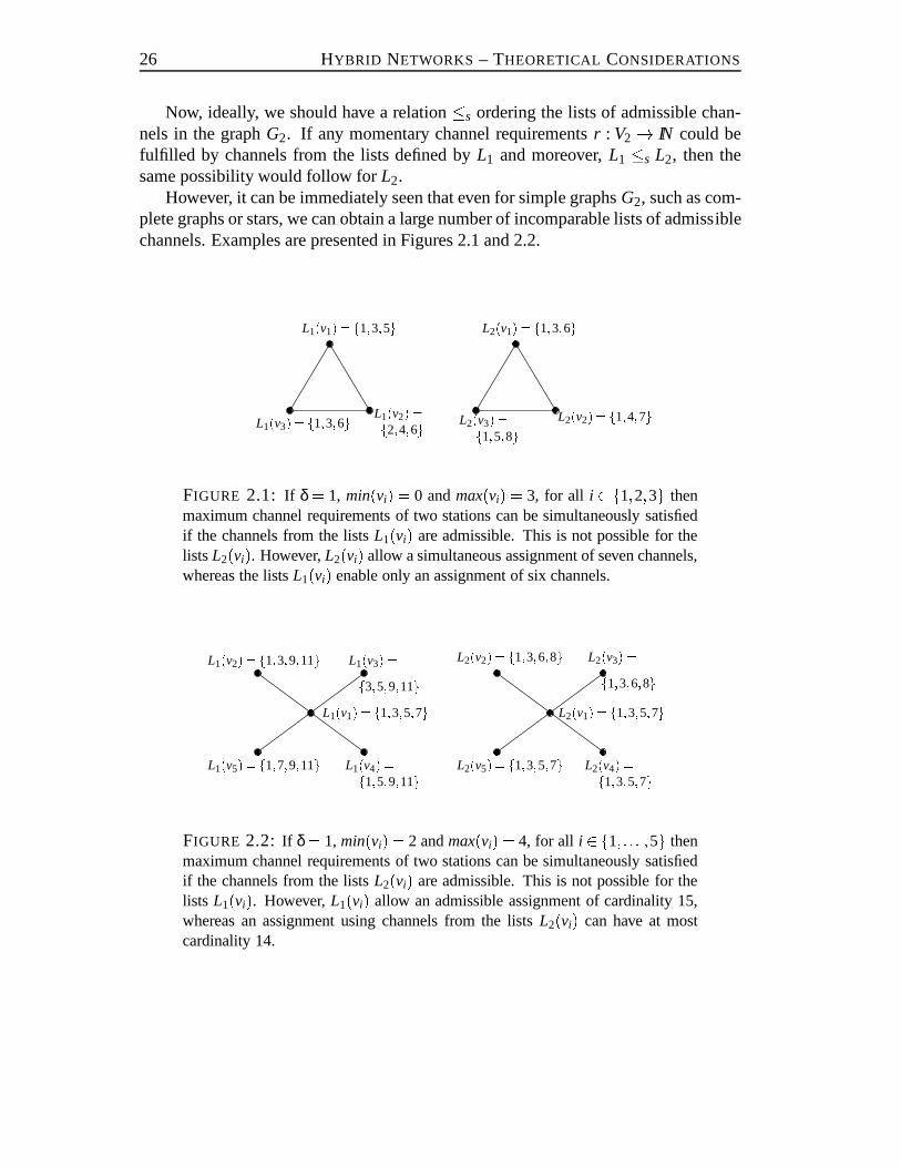
However, it can be immediately seen that even for simple graphsG2, such as com-plete graphs or stars, we can obtain a large number of incomparable lists of admissiblechannels. Examples are presented in Figures 2.1 and 2.2.
����
����
����
����
���� ����f2;4;6g f1;5;8gL1(v1) = f1;3;5g
L1(v3) = f1;3;6g L1(v2) = L2(v1) = f1;3;6gL2(v3) = L2(v2) = f1;4;7g
FIGURE 2.1: If δ = 1, min(vi) = 0 andmax(vi) = 3, for all i 2 f1;2;3g thenmaximum channel requirements of two stations can be simultaneously satisfiedif the channels from the listsL1(vi) are admissible. This is not possible for thelistsL2(vi). However,L2(vi) allow a simultaneous assignment of seven channels,whereas the listsL1(vi) enable only an assignment of six channels.
����
����
����
����
����
������������
������������
������������
������������
������������
������������������������������������������������������������������������������������������������������������������������������������������������������������������������������������
������������������������������������������������������������������������������������������������������������������������������������������������������������������������������������
������������������������������������������������������������������������������������������������������������������������������������������������������������������������������������
������������������������������������������������������������������������������������������������������������������������������������������������������������������������������������
���������������������������������������������������������������������������������������������������������������������������������������������������������������������������������������������
���������������������������������������������������������������������������������������������������������������������������������������������������������������������������������������������
���������������������������������������������������������������������������������������������������������������������������������������������������������������������������������������������
���������������������������������������������������������������������������������������������������������������������������������������������������������������������������������������������
L1(v2) = f1;3;9;11gL1(v5) = f1;7;9;11g
L1(v3) =f3;5;9;11gf1;5;9;11g
f1;3;6;8gf1;3;5;7g
L2(v2) = f1;3;6;8gL2(v1) = f1;3;5;7g
L2(v5) = f1;3;5;7g L2(v4) =L2(v3) =
L1(v4) =L1(v1) = f1;3;5;7gFIGURE 2.2: If δ = 1, min(vi) = 2 andmax(vi) = 4, for all i 2 f1; : : : ;5g thenmaximum channel requirements of two stations can be simultaneously satisfiedif the channels from the listsL2(vi) are admissible. This is not possible for thelists L1(vi). However,L1(vi) allow an admissible assignment of cardinality 15,whereas an assignment using channels from the listsL2(vi) can have at mostcardinality 14.
2.3 OPTIMIZATION CRITERIA 27
These examples illustrate why we should accept an approximated valuation offixed frequency plans. As we have already explained, our intention is to choose a fre-quency plan without simulating the performance of the dynamic part of the network.Our criterion shall exclusively use the definition of an instanceI of the channel as-signment problem in the dynamic part of a hybrid network. In the following we definetwo functions C1 and C2 that seem adequate for that purpose. Given two possibleassignments in the static part of the network, the one resulting in a higher value of thefunction C1 or C2 would be chosen.
Definition 2.3 Given an instance I= (G2 = (V2;E2);L;min;max) of a dynamic sub-network, let us define C1(I) and C2(I) as follows.
C1(I) := maxS2S ∑
u2V2
jS(u)j,C2(I) := max
S2S jfu2V2 : jS(u)j= max(u)gj.S denotes the set of all admissible channel assignments in the dynamic part, that is,each S2 S should satisfy the following conditions:
(a) S(u)� L(u), for all u2V2,
(b) S(u)\S(v) = /0, for all (u;v) 2 E2,
(c) j f �gj> δ, for all u2V2 and f 2 S(u) and g2 S(u), f 6= g, (δ = 1 or 2),
(d) min(u)� jS(u)j �max(u), for all u2V2.
In Section 2.5.1 we will introduce the namechannel stability numberfor the func-tion C1.
One might justifiably ask if the functions C1 and C2 always guarantee the choiceof the best frequency plan. We admit that in some situations the network operator maychoose slightly different criteria. However, we strongly believe that they would notessentially differ from C1 and C2 and therefore the study of the evaluation possibil-ities of these two criteria will give us enough insight to compute other optimizationfunctions.
A suitable function should lead to the choice of the best frequency plan. However,it should be also efficiently computable. The last requirement is truly not simple inview of the computational complexity of generalized graph coloring problems (recallSection 1.1). Actually, the exact value of the functions C1 and C2 can be efficientlycomputed only for restricted graph classes. Both these functions generalize the listcoloring problem, which is NP-complete even for interval graphs. In the next chapterwe will present heuristic algorithms for the computation of C1 for graphs modelingreal world networks. In this chapter we present complexity results for graphs withbounded treewidth and for complete graphs.
28 HYBRID NETWORKS – THEORETICAL CONSIDERATIONS
2.4 GRAPHS WITH BOUNDED TREEWIDTH
To our knowledge, graphs with bounded treewidth constitute the only non-trivial classof graphs for which both C1 and C2 can be exactly evaluated in polynomial time. Wedo not claim that interference graphs modeling real networks have small treewidth.However, the following results can be potentially used to test the efficiency of simplerheuristic algorithms, comparing their results on graphs with small treewidth.
The notions of treewidth and tree-decomposition have been introduced by Robert-son and Seymour.
Definition 2.4 (tree-decomposition)A tree-decomposition of a graph G=(V;E) is apair (T;X ), where T is a tree andX is a system of sets associated with the nodes ofthe tree,X = fXt : Xt �V; t 2V(T)g, such that:
1.S
t2V(T)Xt =V(G),2. for every edge(u;v) 2 E(G), there is a node t2V(T) such thatfu;vg � Xt ,
3. for every pair i; j 2 V(T), if k 2 V(T) lies on the path between i and j thenXi \Xj � Xk.
The width of a tree-decomposition is defined asmaxt2V(T)fjXtj �1g. The treewidthof a graph G is the minimum number w� 0 such that G has a tree decomposition ofwidth w. The treewidth of a graph G is denoted bytw(G).
Graphs with fixed bounded treewidth (i.e., graphs with treewidth not exceedingk, for a constantk) are known for their nice algorithmic properties. Many of theproblems that are generally NP-hard can be solved for these graphs in polynomial oreven linear time using a dynamic programming approach. This is mainly due to thefact that elements of any node of a tree decomposition form a vertex separator in theoriginal graph.
Using a general framework, Courcelle [Cou90] proved that all graph propertiesdefinable inmonadic second-order logic(MS properties) can be decided in linear timefor classes of graphs with fixed bounded treewidth. Arnborg, Lagergren, and Seese[ALS91] generalized these results toextended monadic second-order logicproblems(EMS problems), showing that these problems can be solved in linear, polynomial,orpseudopolynomial time.
Graph coloring can be expressed in the monadic second-order logic only if a con-stant number of colors are used. For any graphG
χ(G)� tw(G)and therefore, coloring graphs with fixed treewidth is a monadic second-order prop-erty. However, list coloring of a graphG may involve more thanχ(G) colors. In
2.4 GRAPHS WITH BOUNDED TREEWIDTH 29
particular, the number of used colors may not be bounded by a constant. For suchinstances the polynomial algorithm of Jansen and Scheffler [JS92] for the list coloringof graphs with bounded treewidth can be used. This algorithm can be extended to thecomputation of C1 and C2 provided that the maximum channel requirements in thedynamic part of the network are bounded by a constant.
In [JS92] a special kind of a tree-decomposition, the so-callednice tree-decomposi-tion, is introduced in order to simplify the algorithm. It is a kind of a regular tree-decomposition(T;X ), whereT is an oriented tree with a rootr, satisfying three addi-tional conditions:� each nodet 2V(T) has at most two children,� if a nodei 2V(T) has two childrenj andk, thenXi = Xj = Xk; in this casei is
called ajoin-node,� if j is the only child ofi in T then there is a vertexv 2 V(G) such that eitherXi = Xj [fvg or Xj = Xi [fvg; in the first casei is called anintroduce-nodeandin the second case aforget-node.
Leaves of a nice tree-decomposition are calledstart-nodes. Notice that any tree-decomposition can be transformed to a nice one in linear time.
The algorithm makes use of the separator property of the nodes ofT. Owing to thisfeature we can afford examining principally all admissible channel assignments in aninstanceI of a dynamic subnetwork defined on a graphG with treewidth bounded bya constant. Obviously, since the number of channel assignments can be exponential,they are not explicitly enumerated. There is no need to do this due to the fact thatany assignment in the subgraph that corresponds to the subtree rooted at a nodew,can be extended to an assignment for the whole graphG, provided that the channelassignment for the vertex setXw is extendible. The following procedure computingC1 and C2 examines the nodes of the treeT in post-order. The partial values of C1and C2 are stored in the two-dimensional arraysC1[�; �] andC2[�; �]. An entry [t;Ht]contains the value of the corresponding function for the subgraph ofG induced by thesubtree ofT rooted at the vertext when the channel assignment for the members oftis defined byHt .
Procedure COMPUTE CRIT
INPUT: GraphG= (V;E) with its tree-decomposition(T;X ) of width k;r - the root ofT;list L(v) and valuesmin(v) andmax(v) for every vertexv2V;for everyv2V, max(v)�M whereM is a constant;
30 HYBRID NETWORKS – THEORETICAL CONSIDERATIONS
beginSUBTREE(T; r);C1 := maxfC1[r;Hr ] over all assignments that are admissible for the elements ofrg;C2 := maxfC2[r;Hr ] over all assignments that are admissible for the elements ofrg;
end
SUBTREE(Tt; t) // Tt is the subtree ofT rooted at the nodetbegin
for all childrend of the nodet do SUBTREE(Td;d);casetype of the nodet of
start-node:generate the lists of all assignmentsHt that are admissible for the set ofstationsXt associated with the nodet;for every generated assignmentHt dobegin
C1[t;Ht ] := the cardinality ofHt;C2[t;Ht ] := the number of stations for which the max. requirement is
satisfied byHt ;end
join-node:// the nodet has two childrend1 andd2
for all feasible channel assignmentHd1stored at the noded1 do
if Hd1is also in the list of assignments stored at the noded2 then
// Hd1is stored as a channel assignment that is extendible
// in the whole subtreeTt
beginC1[t;Hd1
] := C1[d1;Hd1]+ C1[d2;Hd1
]� the cardinality ofHd1;
C2[t;Hd1] := C2[d1;Hd1
]+ C2[d2;Hd1]� the number of stations
in the setXt(= Xd1) for which the max. requirement
is satisfied byHd1;
end
introduce-node:// let d be the only child oft andXt = Xd[fvgfor all channel assignmentsHd stored at the noded do
for all admissible extensionsHt of Hd to the elements ofXt dobegin
C1[t;Ht ] := C1[d;Hd]+ the number of channels allocated tov by Ht ;C2[t;Ht ] := C2[d;Hd] + (1 iff v is allocatedmax(v) channels);
end
forget-node// let d be the only child oft andXt = Xd nfvgreorder the list of the assignments stored at the noded so that assignments
2.4 GRAPHS WITH BOUNDED TREEWIDTH 31
allocating the same channels to the set of stationsXt occur consecutively;Ht := empty channel assignment for the elements ofXt;for all assignments stored atd dobegin
let Hd be the reduction ofHd to Xt ;if Hd 6= Ht thenbegin
Ht := Hd;C1[t;Ht ] := C1[d;Hd];C2[t;Ht ] := C2[d;Hd];
endelsebegin
C1[t;Ht ] := maxfC1[t;Ht ], C1[d;Hd]g;C2[t;Ht ] := maxfC2[t;Ht ], C2[d;Hd]g;
endend
case-endend
SUBTREE(T; r) calculates the sum∑u2V jS(u)j and the set cardinalityjfu2V : jS(u)j= max(u)gj for all admissible channel assignments in the subgraphof G induced by the elements of the subtreeTt . C1 and C2 are equal to the maximumof these values after the call to SUBTREE(T; r).
The complexity of the algorithm can be estimated by the product of the numberof nodes in the nice tree-decomposition, i.e.O(jVj), and the maximum number ofoperations, which have to be executed for one node. In the case of a start-node there
are O�jFj(k+1)�M� channel assignments to be generated, and each of them can be
examined for admissibility in constant timeO((k+1)2M2). Most time-consuming ina join node is the comparison of all admissible channel assignments of its childrennodes. This requiresO(jFj(k+1)�M � (k+ 1) �M) = O(jFj(k+1)�M) time. Since in thecase of introduce- and forget-nodes we can get the same complexity bounds, the wholecomputation of C1 and C2 can be performed inO(jFj(k+1)�MjV2j) time. This leads tothe following theorem.
Theorem 2.1 Let I= (G;L;min;max) be an instance of a dynamic subnetwork. More-over, let the graph G be given with a tree-decomposition of constant width k and letmax(v)�M, for a constant M and for every vertex v2V. Then C1(I) and C2(I) canbe computed in time O(jFj(k+1)�MjV2j).
Note that the above algorithm can be modified in order to compute some otherfunctions evaluating the lists of admissible channels in the dynamic subnetwork, in
32 HYBRID NETWORKS – THEORETICAL CONSIDERATIONS
case the network operator is not satisfied with C1 and C2. Moreover, the complexityof the algorithm does not increase if a tree decomposition of the graphG has to becomputed first, since for graphs with constant treewidth it can be done in linear time(see [Bod93]). However, the situation changes dramatically if there are noconstantbounds for the maximum channel requirements.
In the following we use the notionstar graphto denote a graphK1;n with n+ 1vertices andn edges. It has one vertex withn independent neighbors.
Theorem 2.2 Let I = (G;L;min;max) be an instance of a dynamic subnetwork andlet c be a constant c> 0. Moreover, let the interference graph G be a star graph. Ifmaximum channel requirements can be linear in the number of channelsjFj, then bothdeciding whether C1(I)� c and deciding whether C2(I)� c is NP-complete.
Note that star graphs have treewidth 1.Proof:It can easily be seen that the decision versions of C1 and C2 belong to NP. In or-der to show that the two problems are NP-hard for star graphs we define a polynomialtransformation of the minimum hitting set problem [GJ79] to the problem of com-puting C1 or C2. Let the instance of the minimum hitting set problem be given by acollectionC of subsets of a finite setSand a positive integerk� jSj. The question isif there exists a subsetS0 � Swith jS0j � k such thatS0 contains at least one elementfrom each subset inC . For this instance we define an instanceI = (G;L;min;max) ofa dynamic subnetwork. LetG= (V;E) be a star graph withV = fz;w1; : : : ;wjC jg andE = fzwi j i = 1; : : : ; jC jg. All minimum channel requirements are set to bemin(v) =0. The maximum requirements are defined bymax(z) = jSj � k andmax(wi) = 1,i = 1; : : : ; jC j. The elements of the ground setSare treated as channels in the instanceI . W.l.o.g., let us assume that the distance between any two channels is larger thanδ, i.e., the co-site constraints have no influence on the set of admissible assignments.The lists of channels admissible for a particular station are defined asL(z) = S andL(wi) =Ci , i = 1; : : : ; jC j. Then the collectionC of subsets of the setShas a hitting setof cardinalityk if and only if all maximum channel requirements are satisfiable in theinstanceI , i.e., if and only if C1(I)= jC j+ jSj�k and if and only if C2(I)= jC j+1.�
2.5 COMPLETE GRAPHS
In this section we investigate the complexity of computing C1 and C2 when the un-derlying graph is a complete graphs. The importance of this special case stems fromseveral facts. When allocating frequencies, telephone companies routinely analyze allmaximal cliques of the interference graph. This procedure provides lower bounds onthe number of frequencies required to satisfy given channel requirements. Although
2.5 COMPLETE GRAPHS 33
theoretically this bound can be very far from the real value, it turns out in practice thatthe actual number of required frequencies hardly exceeds the lower bound obtainedfrom cliques. This consideration explains the importance of the clique examinationalso in hybrid networks. A given fixed allocation plan should pass the test of per-forming well on each clique of the dynamic part of the network. Practical observationshow that this is not only a necessary condition, but in a way an “almost” sufficientcondition for the lists of admissible channels to allow flexible channel assignmentinthe dynamic part of the network.
Computing all maximal cliques of the interference graph can be done using a back-tracking algorithm [BK73]. Such computations take the order of minutes even for thelargest existing networks which have as many as 5,000 nodes [Ple95]. The reason forthis is that graphs coming from real systems have the clique number bounded by arather small constant, in the order of 15. The maximum vertex degree is usually intheorder of 50.
The second argument for the study of complete graphs stems from the fact thatgood upper estimates of C1 can be computed from the cliques. In Chapter 3 wediscuss an upper bound obtained by constructing an appropriate clique cover of thegraphG2 modeling the dynamic subnetwork and by summing up the clique bounds.
The presentation in this section starts with the proof of NP-completeness of com-puting C2 for complete graphs even when the co-site constraints are ignored and whenthe maximum channel requirements are no larger than 3. There is even a constantε > 0 such that in complete graphs C2 cannot be approximated up to the rationε, alsowhen the co-site constraints are ignored. This result leaves little chance for an effi-cient approximated evaluation of C2 in interference graphs. Therefore, in our studywe concentrate on C1. We examine its complexity in the case where not all constraintsare imposed simultaneously. Afterwards, we show that the computation of C1 underall constraints is NP-complete for cliques. Several approximation resultsfor C1 arepresented in the last part of this section.
Theorem 2.3 Let I = (Kn;L;min;max) be an instance of a dynamic subnetwork de-fined on a complete graph Kn and let k be a constant k> 0. Then, deciding if C2(I)� kholds is NP-complete even when min(v) = 0 and max(v) � 3 for all v 2V(Kn), andwhen the co-site constraints are ignored.
Proof:Clearly deciding if C2� k for a complete graphKn belongs to NP. It is NP-hard,because the NP-complete maximum set packing problem is a special case. GivenacollectionC = fC1; : : : ;CjC jg of finite sets and a positive integerk� jC j, the problemof the existence of at leastk mutually disjoint sets in the familyC can be transformedto the question if C2(I) � k holds for the following instanceI of a dynamic subnet-work. This instance is defined independently from the numberk. The graph modeling
34 HYBRID NETWORKS – THEORETICAL CONSIDERATIONS
the dynamic subnetwork is defined as a complete graph withjC j vertices. The ele-ments of the sets fromC are treated as channels, and the lists of admissible channelsfor every stationvi; i = 1; : : : ; jC j, are defined asCi . All minimum channel require-ments are set to zero, and the maximum requirement of every stationvi is defined asjCij. Clearly, any channel assignment satisfyingk maximum channel requirements inthe instanceI corresponds to the choice ofk mutually disjoint sets from the familyC .Since the maximum set packing problem remains NP-complete if the cardinality ofall setsCi 2 C is not greater than 3, the analogous property concerning the maximumchannel requirements holds. �
It has been shown in [ADP80] that the computation of a maximum clique can betreated as the special case of the computation of a maximum set packing. It meansthatfor any graphG, a collectionC of sets can be constructed such that there is a 1-1 cor-respondence between cliques in the graphG and sub-collections of mutually disjointsets fromC . Therefore, nonapproximability results for the maximum clique problemcarry over to the maximum set packing. Putting this together with our reduction weobtain the following corollary.
Corollary 2.1 Let I = (Kn;L;min;max) be an instance of a dynamic subnetwork de-fined on a complete graph Kn. Then, there exists a constantε > 0 such that C2(I)cannot be approximated in polynomial time up to a factor nε, unless P = NP, evenwhen min(v) = 0 for all v 2V2 and when the co-site constraints are ignored.
Proof: This result follows directly from the discussed reductions and from the cor-responding nonapproximability result for the clique number of a graph. The prooffor the clique number can be found in the interesting work of Hougardy, Promel andSteger [HPS94].
2.5.1 Channel Stability Number
Theorem 2.3 and Corollary 2.1 show that the computation of C2 is NP-hard andthat the value of C2 cannot be efficiently approximated even in the case of completegraphs. This questions the applicability of C2 in practical applications. Consequently,we restrict from now on our study to the criterion C1. We will refer to this function asthechannel stability numberand denote it withch(I) for a given instanceI . The newname is motivated by the relation to the maximumk-coloring problem, which is alsoknown as thek-th stability number problem.
Recall that given an instanceI of a dynamic subnetwork,ch(I) := C1(I) is themaximum value of∑u2V2
jS(u)j over all admissible channel assignments satisfying theconditions (a)-(d) from Definition 2.3. For simplicity given an admissible assignmentSwe will speak of the sum∑u2V jS(u)j as thevalueof S. Moreover, recall that in our
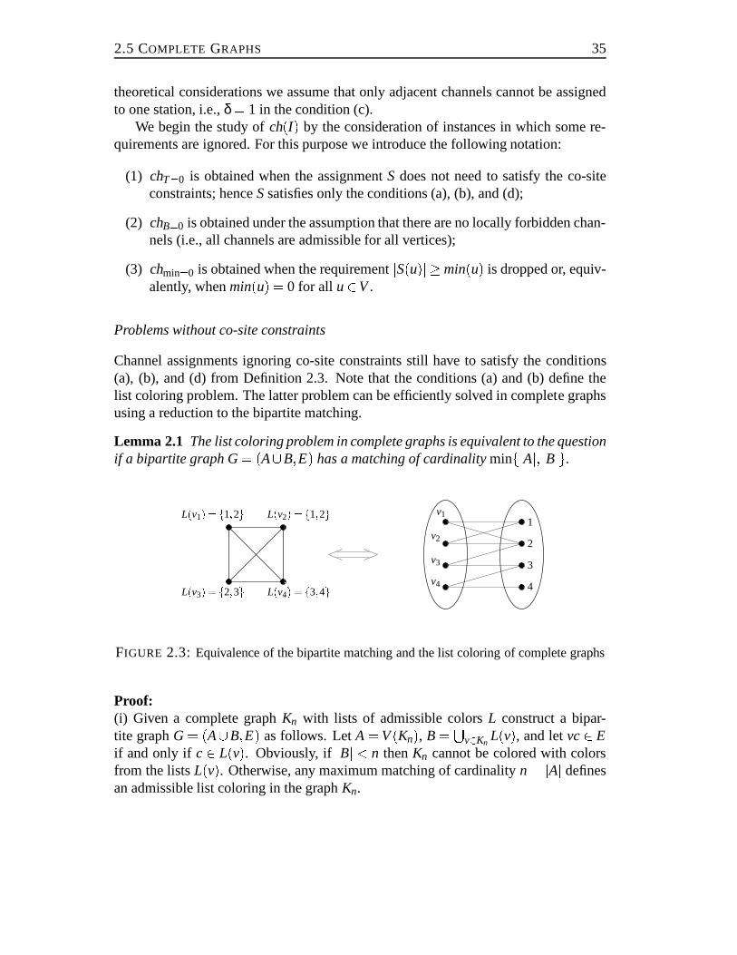
2.5 COMPLETE GRAPHS 35
theoretical considerations we assume that only adjacent channels cannot be assignedto one station, i.e.,δ = 1 in the condition (c).
We begin the study ofch(I) by the consideration of instances in which some re-quirements are ignored. For this purpose we introduce the following notation:
(1) chT=0 is obtained when the assignmentS does not need to satisfy the co-siteconstraints; henceSsatisfies only the conditions (a), (b), and (d);
(2) chB=0 is obtained under the assumption that there are no locally forbidden chan-nels (i.e., all channels are admissible for all vertices);
(3) chmin=0 is obtained when the requirementjS(u)j �min(u) is dropped or, equiv-alently, whenmin(u) = 0 for all u2V.
Problems without co-site constraints
Channel assignments ignoring co-site constraints still have to satisfy the conditions(a), (b), and (d) from Definition 2.3. Note that the conditions (a) and (b) define thelist coloring problem. The latter problem can be efficiently solved in complete graphsusing a reduction to the bipartite matching.
Lemma 2.1 The list coloring problem in complete graphs is equivalent to the questionif a bipartite graph G= (A[B;E) has a matching of cardinalityminfjAj; jBjg.
����������������������������
��������
��������
������������������������������������
��������
����
����
����
����
����
����
����
�������� ����
���� ����
��������������������������������������
����������������������������������������������������������������������������
����������������������������������������������������������������������������
����������������������������������������������������������������������������
����������������������������������������������������������������������������
��������������������������������������
����������������������������������������������������������������������������
����������������������������������������������������������������������������
��������������������������������������
����������������������������������������������������������������������������
����������������������������������������������������������������������������
��������������������������������������
��������������������������������
����������������
������������������������������������������������
��������������������������������������������������������������������������������������������������������
��������������������������������������������������������������������������������������������������������
��������������������������������������������������������������������������������������������������������
��������������������������������������������������������������������������������������������������������
v1
v2
v3
v4
2
3
L(v2) = f1;2gL(v4) = f3;4gL(v3) = f2;3g
L(v1) = f1;2g1
4
FIGURE 2.3: Equivalence of the bipartite matching and the list coloringof complete graphs
Proof:(i) Given a complete graphKn with lists of admissible colorsL construct a bipar-tite graphG= (A[B;E) as follows. LetA= V(Kn), B= Sv2Kn
L(v), and letvc2 Eif and only if c2 L(v). Obviously, if jBj < n thenKn cannot be colored with colorsfrom the listsL(v). Otherwise, any maximum matching of cardinalityn= jAj definesan admissible list coloring in the graphKn.
36 HYBRID NETWORKS – THEORETICAL CONSIDERATIONS
(ii) Given a bipartite graphG= (A[B;E) we can assume w.l.o.g. thatjAj � jBj. Then,let us treat the verticesv2 A as nodes of a complete graphKjAj and verticesw2 B ascolors. Moreover, let us define thatw 2 L(v) if and only if vw2 E. Then, any ad-missible list coloring of the graphKjAj corresponds to a matchingM in G. Since thecoloring comprisesjAj assignments, the cardinality ofM equalsjAj. �
Let us remark that a similar construction has been independently used by Lanfear[Lan89] and by Hujter and Tuza [HT93] for related graph colorings problems.
Lemma 2.1 enables us to reduce the computation ofchT=0 to the maximum car-dinality matching problem in bipartite graphs. The algorithm consists of two phases.First, an admissible assignment satisfying the minimum channel requirementsmin(v)is constructed (provided that one exists), and afterwards this assignment is extendedto satisfy as many requirements as possible. An admissible assignment isconstructedwith the help of an auxiliary bipartite graphH=(A[B;E). The set of verticesA con-tainsmin(v) copies of each original vertex fromKn. The setB comprises one vertexfor every channel occurring in any list of admissible channels. Each vertexvi 2 A,i = 1; : : : ;min(v), corresponding to the original vertexv, is adjacent to the verticesof B representing the channels from the listL(v). By Lemma 2.1,Kn has an admis-sible assignment assigning to each vertexmin(v) colors if and only if the bipartitegraphH has a matching of cardinality∑vmin(v). Now, the procedure of Hopcroft andKarp [HK73] can be applied for the maximum bipartite matching in order to find anadmissible assignment inKn.
In the second phase of the algorithm the auxiliary graphH is further modified tothe graphH 0 — the number of vertex copies in the setA is increased tomax(v), foreachv2V(Kn). The previously computed matching is extended to a maximum match-ing in the bipartite graphH 0. In the procedure of Hopcroft and Karp a matching ofhigher cardinality is found by means of augmenting paths. The set of matched verticesgrows in such a way that any vertex once incident to an edge in the matching remainsmatched during the augmentation. Only the matching edge to which it is incident maychange. This property guarantees that a maximum matching found in the graphH 0still covers in the setA at leastmin(v) copies of each vertexv 2 V(Kn). Therefore,the final matching defines an admissible channel assignment. On the other hand, sinceit is a maximum matching, no more channels can be simultaneously assigned to thevertices ofKn — the cardinality of the matching equalschT=0. Hence, we obtain thenext theorem.
Theorem 2.4 Let I = (Kn;L;min;max) be an instance of a dynamic subnetwork de-fined on a complete graph Kn. Moreover, letjFj denote the overall number of availablechannels and let M be an upper bound on the maximum channel requirement of any
vertex. ThenchT=0(I) can be computed in time O�
MnjFjpMn+ jFj�.
2.5 COMPLETE GRAPHS 37
The time complexity of the algorithm stems from the effort required to compute amaximum matching in a bipartite graph. This can be done in timeO(jEj � jVj 12), andin the bipartite graphsH andH 0, jVj �Mn+ jFj andjEj �MnjFj.
Let us point out that the last algorithm can be very useful in the current cellularnetworks during the analysis of all maximal cliques. As far as we know, currentmethods do not take into consideration locally restricted lists of admissible channels.This modification could possibly improve lower bounds on the number of requiredfrequencies especially in regions with a high concentration of forbidden channels.
Problems without forbidden channels
The following section addresses the complexity ofchB=0 in complete graphs (condi-tions (b) through (d)). These are problems with co-site constraints (condition (c)) thatare considered under the assumption that all channels are admissible for each station.This assumption is not fulfilled in real cases that are of interest for us. Thepurpose ofthis study is rather to compare the influence of the restricted lists of admissible chan-nels on one hand and of the co-site constraints on the other hand on the complexity ofcomputing the channel stability number in complete graphs.
Co-site constraints are very closely related to the T-coloring problem (see Section1.1.4). They can be expressed using the idea of a T-coloring with multiple levels ofinterference.
Definition 2.5 (T-coloring with multiple levels of interference)Let G= (V;G1;G2; : : : ;Gk) be a nested sequence of graphs on the vertex set V , i.e.,
V(Gi) =V; i = 1;2; : : : ;k;and
E(Gk)� E(Gk�1)� : : :� E(G1):Let
T(1)� T(2)� : : :T(k)be sets of nonnegative integers.
Then an assignment h: V! IN is called a T-coloring of G with levels of interfer-ence T(1);T(2); : : : ;T(k) if and only if for all i;1� i� k and for all edges vw2E(Gi),jh(v)�h(w)j =2 T(i).
If all minimum channel requirements coincide with the maximum requirements(min(v) = max(v) for everyv2V) then the computation ofchB=0 can be formulatedas a T-coloring problem with two levels of interference. Let us assume thatan instanceI = (Kn;L;min;max) of a dynamic subnetwork is defined on a complete graphKn.
38 HYBRID NETWORKS – THEORETICAL CONSIDERATIONS
Then consider a nested sequence of graphs(V; G1; G2), whereG1 is a complete graphwith N :=∑v2V(Kn)max(v) vertices andG2 consists ofn disjoint cliques of sizemax(v)for eachv 2 V(Kn). Moreover,T(1) = f0g andT(2) = f0;1g. This special case oftwo levels of interference has been studied by Raychaudhuri ([Ray85]), who provedthe following theorem.
Theorem 2.5 (Raychaudhuri) Let us consider a2-nested sequence of graphs G=(V;G1, G2), where G1 is complete and T(1) = f0g, T(2) = f0;1g. Then, the T-spanspT(G) equals the length of the shortest hamiltonian path in the weighted graph G0with V(G0) =V, E(G0) = E(G1), and with the following weights on edges
l(xy) =( 1 for xy =2 E(G2)2 for xy2 E(G2):
This means thatspT(G) = jVj�1 if and only if G2 has a hamiltonian path. Con-sequently, if the complement of the graphG2 can be arbitrary, then the computationof spT(G) is NP-hard even for these simple 2-nested sequence of graphs. However,an efficient computation ofspT(G) can be still possible ifG2 has a special structure.Tesman ([Tes89] p.46) has shown thatspT(G) can be determined up to the constantadditive factor of 1 whenG2 is a unit interval graph. In our applicationG2 consistsof disjoint cliques, and we will show that in this casespT(G) can be determined inlinear time. Then all maximal channel requirements in the dynamic subnetwork de-fined on a complete graph can be satisfied usingp consecutive channels if and only ifspT(G)< p.
Theorem 2.6 Let G= (V;G1;G2) be a2-nested sequence of graphs, where G1 is acomplete graph on N vertices and G2 consists of n disjoint cliques of size c1; : : : ;cn,∑n
i=1ci = N. Let T(1) = f0g, T(2) = f0;1g, and let cmax= maxi=1;::: ;nci . Then,
spT(G) =8><>: 2N�2 for N = cmax (n= 1) (a)2cmax�2 for cmax+1� N� 2cmax�1 (b)N�1 for N� 2cmax (c):
Proof:Let us construct the weighted graphG0 as described in Theorem 2.5. We determinethe length of the shortest hamiltonian path in this graph.
Part (a). SinceN = cmax, the graphsG1 andG2 are identical and every edge in thecomplete graphG0 has weight 2. Therefore, any permutation of its vertices yields ashortest hamiltonian path of length 2N�2.
Part (b). LetC1 be the maximum clique inG2 of cardinalitycmax. Since the weights onedges in the complete graphG0 satisfy the triangle inequality, the shortest hamiltonian
2.5 COMPLETE GRAPHS 39
path inG0 is at least as long as the shortest hamiltonian path in the subgraphG0jC1.All edges in this subgraph have weight 2, and consequently the shortest hamiltonianpathP in GjC1 has length 2cmax�2. This path can be extended to cover all verticesof G0 as follows. Since the number of unvisited verticesN� cmax is smaller than thenumber of visited verticescmax, the first set of vertices can be visited alternately withthe latter set. In this way some edges inP are replaced by two edges of weight 1, andthe overall weight of the path does not change.
Part (c). Consider the subgraphH of G0 with the same set of verticesV and with theedges of weight 1. IfN � 2cmax then no cliqueCi , i = 1; : : : ;n, contains more thanthe half of the vertices ofG0. Consequently, the minimal vertex degree inH is largeror equal toN=2. Hence, by the theorem of Dirac [D52],H is hamiltonian, and theshortest hamiltonian path inG0 has lengthN�1. �
Theorem 2.6 can be used to test if some fixed channel requirements in a completegraph can be satisfied usingp consecutive channels. This method can be generalizedto computechB=0 for an instanceI of a dynamic subnetwork defined on a completegraph with minimum and maximum channel requirements.
Theorem 2.7 Let I = (Kn;L;min;max) be an instance of a dynamic subnetwork de-fined on a complete graph Kn. Moreover, let F be a set of consecutive channels and letL(v) = F for every v2 Kn. Let N := ∑v2V(Kn)max(v), M := maxv2V(Kn) fmax(v)g,eN := ∑v2V(Kn)min(v), and eM := maxv2V(Kn)fmin(v)g. Then I has an admissiblechannel assignment satisfying the minimum requirements and the co-site constraints(δ = 1) if and only if: jFj � eN and eN� 2 eMor jFj � 2 eM�1 and N < 2 eM:
In that casechB=0(I) has the following value:
chB=0(I) =8>>>>>><>>>>>>:minfjFj;Ng iff N � 2M (a)jFj iff N < 2M andjFj � 2(N�M)+1 (b)minfN; �1
2(jFj+2(N�M)+1)�g iff N < 2M andjFj> 2(N�M)+1 (c)Proof: The existence of an admissible channel assignment can be formulated as aT-coloring problem with 2 levels of interference as in Theorem 2.6. Minimum re-quirements can be satisfied if the number of admissible consecutive channels is higherthan theT-spanspT of the corresponding graph. The conditions on the existence ofan admissible channel assignment follow from Theorem 2.6.
For feasible instances the number of satisfiable requirements can be seen as fol-lows. If N � 2M then the same argumentation as in part (c) of Theorem 2.6 shows
40 HYBRID NETWORKS – THEORETICAL CONSIDERATIONS
that consecutive channels can be assigned to an alternating sequence of vertices un-til all channels are used or all maximum requirements are satisfied. IfN < 2M then2(N�M)+ 1 consecutive channels can be assigned alternately to the vertexv withthe highest channel requirement and to all other vertices. This already provespart (b).If the number of available channels exceeds 2(N�M)+ 1 then every second fromthe remaining channels can be assigned to the vertexv. This leads to the followingformula on the number of satisfiable requirements
2(N�M)+1+ b1=2(jFj�2(N�M)�1)c= b1=2(jFj+2(N�M)+1)c :This proves part (c). �Complexity ofch
Let us summarize the present results on the complexity of computing the channelstability number in complete graphs. It has been shown in Theorem 2.4 thatchT=0can be computed in polynomial time. The evaluation ofchB=0 is even simpler sincethe exact formula from Theorem 2.7 can be evaluated in linear time. However, if bothrestrictions — co-site constraints and lists of admissible colors — are observed, thenthe computation ofch becomes NP-hard for cliques. In the following we prove theeven stronger result that checking the existence of any admissible channel assignmentis NP-hard in complete graphs.
Theorem 2.8 Let I = (G;L;min;max) be an instance of a dynamic subnetwork de-fined on a complete graph G. Then, deciding if the minimum channel requirementscan be satisfied is an NP-complete problem.
Proof:Obviously the problem belongs to NP. In the following we prove that checking thefeasibility of instances withmin(v) = max(v) for everyv 2 V(Kn) is NP-hard. Weuse a polynomial reduction from 3SAT(3) — a satisfiability problem with clauses oflength two or three and with all variables occurring in exactly three clauses, oncenegated and twice positive. For the reduction from 3SAT to 3SAT(3) see [PS82], p.3941.
Given an instanceI of 3SAT(3) with a setX of n variables andm clauses, wedefine an instanceI 0 of a dynamic subnetwork on a complete graphG with 5n+mnodes. The instanceI 0 has the set of channelsC = Si=1:::nfx1;x2;x; xp;xt ;xq;xs;xrg.
1Actually in [PS82] in the resulting boolean formula each variable appears once or twice positiveand once negated; however, the reduction can be easily completed so that variables appear exactly twicepositive and once negated.
2.5 COMPLETE GRAPHS 41
Each set in the sum defines a linear order of consecutive channels. For each variablex we introduce 5 verticespx, qx, rx, sx, andtx with the following lists of admissiblechannels:
L(px) = fx1;xpg,L(qx) = fx2;xqg,L(rx) = fx;xrg,L(sx) = fxs;xrg,L(tx) = fxp;xt ;xq;xsg.For each clause we introduce one clause nodek with a list of admissible channels
representing its literals. The channel requirements of all verticesv2V(Kn) excepttx,x2X, are set tomin(v) = max(v) = 1. For the verticestx we setmin(v) = max(v) = 2.
Now we claim that the instanceI of 3SAT(3) is satisfiable if and only if thecorresponding instanceI 0 of a dynamic subnetwork has an admissible assignmentS : V ! 2f1:::Cg satisfying the requirementsmin(v). Given a satisfiable truth assign-mentτ of I , an admissible channel assignmentS in the graphKn can be constructedas follows. To each clause nodek assign the channel representing a truth literalin the kth clause. Furthermore, if a variablex 2 X is set true inτ then we defineS(px) = fxpg, S(qx) = fxqg, S(rx) = fxg, S(sx) = fxrg, andS(tx) = fxt ;xsg. Other-wise, if x is set false, defineS(px) = fx1g, S(qx) = fx2g, S(rx) = fxrg, S(sx) = fxsg,andS(tx) = fxp;xqg.
To prove the “if” direction we argue as follows. Any admissible channel assign-ment S in Kn uses exactly one channel for each clause vertex. Assume that for avariablex 2 X and for somei; j 2 f1; : : : ;mg we hadS(ki) = fx1g (or fx2g) andS(k j) = fxg. Then, there is only one possible assignment to the verticesrx, sx, andpx (or qx). Namely,S(rx) = fxrg, S(sx) = fxsg, andS(px) = fxpg (or S(qx) = fxqg).However, this implies that only two consecutive colors are still left fortx, and there-fore, its minimum requirement cannot be satisfied. Consequently, in any admissiblechannel assignment for each variablex2 X either onlyx1, x2 or onlyx are assigned toclause vertices. Hence,Sdefines a satisfying truth assignment forI . �2.5.2 Approximation Results
In this section we study the approximability of the channel stability numberch incomplete graphs considering both restricted lists of admissible channels and theco-site constraints. Given that finding any feasible solution under constraints (a) through(d) from Definition 2.3 is an NP-hard task, we are forced to assume additional infor-mation about the input instances in order to find approximated solutions. Therefore,we will consider instances with minimum channel requirements equal zero as well asother instances for which it is known that a feasible channel assignment exists.Re-
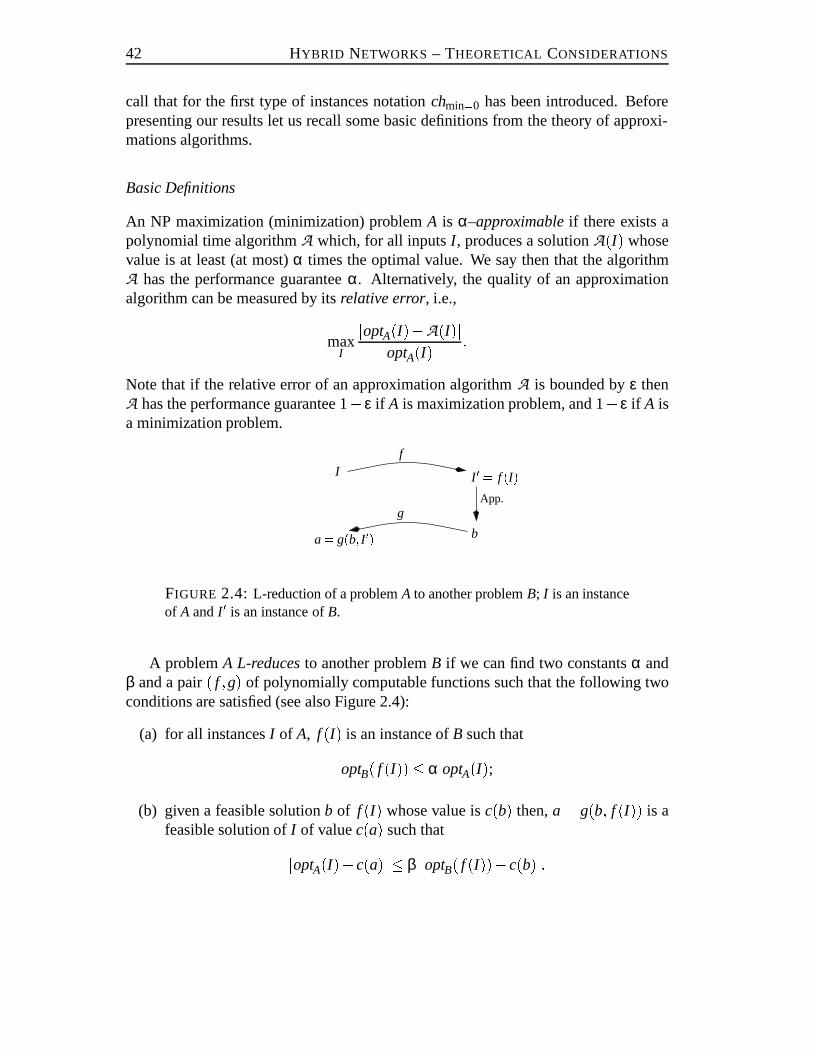
42 HYBRID NETWORKS – THEORETICAL CONSIDERATIONS
call that for the first type of instances notationchmin=0 has been introduced. Beforepresenting our results let us recall some basic definitions from the theory of approxi-mations algorithms.
Basic Definitions
An NP maximization (minimization) problemA is α–approximableif there exists apolynomial time algorithmA which, for all inputsI , produces a solutionA(I) whosevalue is at least (at most)α times the optimal value. We say then that the algorithmA has the performance guaranteeα. Alternatively, the quality of an approximationalgorithm can be measured by itsrelative error, i.e.,
maxI
joptA(I)�A(I)joptA(I) :
Note that if the relative error of an approximation algorithmA is bounded byε thenA has the performance guarantee 1�ε if A is maximization problem, and 1+ε if A isa minimization problem.
f
I 0 = f (I)App.
b
g
I
a= g(b; I 0)FIGURE 2.4: L-reduction of a problemA to another problemB; I is an instanceof A andI 0 is an instance ofB.
A problemA L-reducesto another problemB if we can find two constantsα andβ and a pair( f ;g) of polynomially computable functions such that the following twoconditions are satisfied (see also Figure 2.4):
(a) for all instancesI of A, f (I) is an instance ofB such that
optB( f (I))� α optA(I);(b) given a feasible solutionb of f (I) whose value isc(b) then,a= g(b; f (I)) is a
feasible solution ofI of valuec(a) such thatjoptA(I)�c(a)j � β joptB( f (I))�c(b)j:
2.5 COMPLETE GRAPHS 43
Taken together, these two conditions imply that ifB is approximable with worst caserelative errorε thenA is approximable with the relative errorαβε or, conversely, thatif there exists a limitδ0 such thatA cannot be(1�δ0)–approximated (or(1+δ0)–approximated ifA is a minimization problem) then,B cannot be approximated within1�δ0α�1β�1 (or 1+δ0α�1β�1).
In a seminal paper[PY91], Papadimitriou and Yannakakis introduced a class ofcombinatorial problems called MAX SNP. All problems from this class can be ap-proximated within some fixed ratio but at that time it was not known if they can beapproximated within any degree of accuracy in polynomial time. Papadimitriou andYannakakis shown for the class MAX SNP the existence of many natural completeproblems with respect to L-reductions. Among these is MAX 3SAT-B whose inputis a boolean formulaF(x1; : : : ;xn) in conjunctive normal form such that each clausehas at most three literals and each variable appears at most B times. Theoptimizationgoal of MAX 3SAT-B is to find a truth assignment satisfying the maximum numberof clauses. Recent breakthroughs in the theory of approximation algorithms show thatif a problemA is MAX SNP– hard w.r.t. L-reductions then there exists someδA suchthatA cannot beδA-approximated provided that P6=NP (see [Aro94, BGS93, HPS94]among others).
Approximation algorithms
In this section we show some positive results on the approximability of the channelstability number in complete graphs under the assumptions that guarantee the feasi-bility of an instance. The next theorem shows that if we know that an admissibleassignment exists, thenchcan be approximated non-constructively, i.e., thenumericalvalueof chcan be approximated. Moreover, as soon as we have any explicit admissi-ble assignment it can be always improved in polynomial time to an admissible channelassignment which approximates well.
Theorem 2.9 Let I = (Kn;L;min;max) be an instance of a dynamic subnetwork de-fined on a complete graph Kn. Moreover, letjFj denote the number of admissiblechannels, and let M= maxu2V(Kn)fmax(u)g. If I admits a feasible channel assign-
ment then the valuech(I) can be(1=3)-approximated in time O(MnjFjpMn+ jFj).If additionally one feasible assignment S is known then a(1=3)-approximation T canbe constructed in polynomial time.
Proof. It has been shown in Theorem 2.4 that a feasible assignmentR : V! 2f1;::: ;jFjgattaining the optimum ofchT=0(I) can be computed inO(MnjFjpMn+ jFj) time.We will show that if a feasible assignmentS for ch(I) exists, it can be combined withR to obtain a feasible assignmentT for I of value at leastchT=0(I)=3. Sincech(I)�
44 HYBRID NETWORKS – THEORETICAL CONSIDERATIONS
chT=0(I), if Sexists,ch(I) can be approximated simply by computingchT=0(I)=3. Ifwe do haveS in our hands thenT can be constructed effectively, as follows.
To constructT we first useS. For each vertexu we selectmin(u) channels fromS(u), in any order, and assign it tou. This defines a partial assignment forT that wedenote byT1. Each time a channel is inserted, all possible conflicts are deleted fromR.If c is assigned to vertexu we delete the whole offc�1;c;c+1g\R(u) from R(u),and we also deletec from anyR(v) containing it (v 6= u). In the end, we are left witha set of truncatedR(u) lists, which we denote byR0(u). This ends the first pass of thealgorithm. Now, suppose that� jR0(u)j
2
��max(u)�min(u)for all u. Then, the assignment can be completed by deleting every second channelfrom R0(u) and by adding the remaining channels toT1(u). This defines an assignmentT such that∑u jT(u)j � ∑u jR(u)j=3= chT=0(I)=3.
Otherwise, we must take care of those verticesw such that� jR0(w)j2
�> max(w)�min(w): (2.1)
We show how to take care of them one by one. Pick one suchw. Then,jR0(w)j � � jR0(w)j2
�= max(w)�min(w)+x
for some positive integerx> 0. Sincemax(u)� jR(u)j for all u,
min(w)� (jR(w)j� jR0(w)j)+x=: D(w)+x
The quantityD(w) is precisely the number of channels deleted fromR(w) because ofT1, i.e., there were at leastx insertions inT1(w) which did not cause any deletion fromR(w). If we delete anyx colors fromR0(w) we still maintain the one to three ratio,because each of thesex colorsc caused at most one deletion when it was inserted (inthe case whenc2 R(u), for u 6= w) and is causing now another deletion. Denoting theresulting list byR00(w), we have� jR00(w)j
2
��max(w)�min(w):In this fashion, all violations of type (2.1) can be eliminated. �
If all minimum channel requirements equal zero then an empty assignment is fea-sible. In this case the channel stability number can be approximated as follows.
2.5 COMPLETE GRAPHS 45
Proposition 2.1 Let I = (Kn;L;min;max) be an instance of a dynamic subnetwork.Moreover, letjFj denote the number of admissible frequencies and let max(u)�M forall u2Kn. Then,chmin=0(I) can be (1/2)-approximated in time O(MnjFjpMn+ jFj).Proof.W.l.o.g. assume thatmin(u) = 0 for all u in the instanceI . We first compute anassignmentS : V ! 2f1;::: ;jFjg attaining the optimal value ofchT=0(I) in timeO(MnjFjpMn+ jFj) using the algorithm from Theorem 2.4. Then, we delete ev-ery second element from eachS(u) in order to satisfy the co-site constraints, therebyobtaining a feasible assignmentT. Clearly,
chT=0(I)2
�∑ujT(u)j � chmin=0(I)� chT=0(I): �
Note that the reasoning remains valid when the conditionmin(u) = 0, for all u, isreplaced bymin(u)� 1, for all u.
MAX SNP-hardness
We can now ask ifchmin=0 can be approximated in complete graphs within any degreeof accuracy in polynomial time. The next result shows that this is not the case, unlessP= NP.
Theorem 2.10 Let I = (Kn;L;min;max) be an instance of a dynamic subnetwork de-fined on a complete graph Kn. Then the computation ofchmin=0(I) is MAX SNP-hard.
The proof of Theorem 2.10 combines several steps. The first step is to establishMAX SNP-hardness for a special class of MAX 3SAT that we call MAX 3SAT�. Theseis a slight modification of the MAX 3SAT-B instances which were proved to be MAXSNP-hard by Papadimitriou and Yannakakis [PY91]. The input of MAX 3SAT� is a3SAT formulaF(x;y; : : : ;z) such that:� clauses have length 2 or 3;� each variable occurs in either 4 or 5 or 6 clauses;� clauses of length 2 aresymmetric, that is, they are of the form(x_y) and come
always together with a symmetric clause(x_y);� clauses of length 3 are arbitrary;
46 HYBRID NETWORKS – THEORETICAL CONSIDERATIONS� when a variablex occurs in 4 or 6 clauses these are always of length 2 (andhence symmetric);� when a variable appears in 5 clauses, 4 of these are of length 2 and one is oflength 3.
These instances come from a particular graph construction shown in [PY91]. Thevertices of the graph correspond to variables, and each edge(x;y) corresponds toa constraint(x, y), i.e., a pair of symmetric clauses(x_ y) and (x_ y). In theconstruction of [PY91] the graph has max degree 4 (this reflects on the max numberof occurrences of a variable, namely 8, in the resulting instance of MAX 3SAT-B).For our purposes it is important to lower the max degree to 3 and to have the specialstructure described above.
Lemma 2.2 MAX 3SAT� is MAX SNP-hard.
Proof.The lemma can be established by means of a simple modification of the originalconstruction. We use anL-reduction from MAX 3SAT similar to [PY91]. For eachvariable occurringm times in the 3SAT-formula we construct a graphFm with the fol-lowing properties: (1) it has degree bounded by 3 (in [PY91] it was bounded by 4), (2)it hasO(m) nodes,m of which are ‘distinguished’, and (3) for every partition of thenodes into two sets, the number of edges in the cut is at least min(jS1j; jS2j), whereS1andS2 are the sets of distinguished nodes in the two sides.Fm can be obtained fromm full binary trees with (at least) 1=c leaves. The trees are connected in a slightlydifferent way than in [PY91]. Namely, let us denote the original leaves byL. Weconnect four additional nodesv0, v1, v2, andv3 to eachv2 L using the edges(v;v0),(v;v3), (v0;v1), and(v0;v2). Now, consider a cubicc-expander [Ajt87] on the originalleavesL. For each edge(v;w) of the expander introduce one edge betweenvi andwj
for somei; j 2 f1;2;3g. Altogether, each of the new leavesfv1;v2;v3jv2 Lg shouldbe used exactly once. The distinguished nodes are the roots of the binary trees. Then,Fm satisfies properties(1) and(2). To show that the property 3 is satisfied a similarreasoning to [PY91] can be used. Let us consider a partition of the nodes into twosetsQ1 andQ2. DefineR1 andR2 respectively to be the set of distinguished nodesfor which all theinner nodes of the corresponding binary trees are contained inQ1or Q2 respectively. Let us denote the rest of the distinguished nodes byR3. The cutcontains at leastjR3j edges joining inner nodes of the binary trees. We claim that italso contains min(jR1j; jR2j) edges incident to some leaves.
To see the latter fact, let us denote byQ�1 := Q1\ L and respectively byQ�
2 :=Q2\L. Let us assume, w.l.o.g., thatjQ�
1j � jQ�2j. ThenjQ�
1j � 1c min(jR1j; jR2j) and
in a c-expander on nodesL this set would have at leastc � 1c min(jR1j; jR2j) neighbors
2.5 COMPLETE GRAPHS 47
outside. For each such neighborw we can choose a nodev 2 Q�1 adjacent tow in
the expander. In the graphFm there is a path fromv to w of the formv(v0)viwj(w0)w,i; j 2 f1;2;3g. Notice thatv;v0 2Q1 andw2Q2; hence, at least one of the edges in thepath belongs to the cut. Since for eachw we consider only one path and since pathsstarting in the vertexv may overlap only in the edge(v;v0), which does not belong tothe cut, we can altogether select at least min(jR1j; jR2j) different cut edges from thesepaths. Since none of these cut edges has two inner nodes as its ends, they are differentfrom the firstjR3j edges.
Now jR3j+min(jR1j; jR2j) � min(jS1j; jS2j) andFm satisfies (3). The rest of theconstruction and of the proof is the same as in [PY91]. Each variablex occurringmtimes in the instance of MAX 3SAT is replaced byO(m) new variablesx1;x2; : : : cor-responding to the nodes of the constructed graphFm. For every edge(i; j) of the graphFm two auxiliary clausesxi _ x j andxi _ x j are introduced. Variables correspondingto the distinguished nodes ofFm are used in place ofx in original clauses. It followsby the same argument as in [PY91] that this transformation from MAX 3SAT to MAX
3SAT� is anL-reduction. �We now exhibit an L-reduction from MAX 3SAT� to chmin=0. LetF be an instance
of MAX 3SAT� with a setX of n variables andm clauses. Ifτ is a satisfying assign-ment,F(τ) denotes the number of clauses satisfied by it. As it is customary,opt(F)denotes the optimum value of the MAX 3SAT� instanceF. We note that the definitionof MAX 3SAT� implies thatm� 4n=3. The instanceI of a dynamic subnetwork willbe defined on a complete graphG with 3n+m vertices. The overall set of admissiblechannels is defined as
C= fxi;xi;ax;bx;cx;dx : x2 X; 1� i � 3g:The 6 channelsfxi;xig correspond to the (at most 6) positive and negative occurrencesof the variablex in F . The occurrence in a clause of length 3 is always representedby the channel with lower index 1. Two literals from a pair of symmetric clauses arerepresented by two channels with the same lower index.
For each variablex we introduce three verticestx, px, andqx, which we call thegroup of xand which have lists of admissible channels
L(tx) = fax; x1;bx; x2;x3; x3;x2;cx;x1;dxg;L(px) = fax;dxg;L(qx) = fbx;cxg:
Each setL(tx) is a linear order ofconsecutivechannels, i.e., nearby channels are in-compatible. Then we introduce the requirementsmax(tx) = 5 andmax(px) = max(qx)
48 HYBRID NETWORKS – THEORETICAL CONSIDERATIONS= 1. Intuitively, the task of the group ofx is to ensure that only two channel as-signments, corresponding to the only two possible consistent truth assignments, canreach the maximum requirements. These areS(tx) = fax;bx;x3;x2;x1g, S(px) = fdxg,andS(qx) = fcxg (corresponding to settingx to false) andS(tx) = fx1; x2; x3;cx;dxg,S(px) = faxg, andS(qx) = fbxg (corresponding to settingx to true).
For each clausec we introduce oneclause node Cand associate with it the set ofchannels representing the literals in the clausec. For instance, supposec = (x_ y)and that these are thei-th occurrence ofx and thej-th occurrence ofy. Then,L(C) =fxi; y jg. We also setmax(C) = 1 for all C.
Minimal channel requirements of all vertices inG are defined to be zero. Thisends the construction ofI . Clearly, it can be carried out in polynomial time.
A channel assignmentSfor I is calledcanonicalif, for all variablesx, the channelassignment for the group ofx is one of the two described above.
Any truth assignment ofF induces, in the obvious way, a canonical channel as-signment. Conversely, a canonical channel assignmentSdefines a truth assignmentτS.The difficulty of the proof is to show that, without loss of generality, we can assumethat all channel assignment ofI are canonical.
Lemma 2.3 Any given admissible channel assignment S can be transformed in poly-nomial time into a canonical channel assignment S0 whose value, i.e.∑v jS0(v)j is noless than the value of S.
Once Lemma 2.3 is proven, we are done. To see this, letc denote the value of afeasible channel assignmentS and recall thatchmin=0(I) denotes the optimum valuefor the instanceI . Notice that ifS is canonical its value is of the formc= 7n+k andis essentially an encoding of a satisfying assignmentτS of valueF(τS) = k (τS can becomputed in linear time fromS). By Lemma 2.3 we can assume that, in particular,the optimum channel assignment forI is also canonical and of valuechmin=0(I) =7n+ opt(F). All this implies that the reduction is an L-reduction. Recall that ina MAX 3SAT� instancen� 3m=4� opt(F) (the second inequality can be seen bynoticing that the expected number of clauses of MAX 3SAT� satisfied by a randomtruth assignment is at least 3/4 of the total). Hence, we can satisfy the first requirementof an L-reduction withα = 8:
chmin=0(I) = 7n+opt(F)� 8opt(F):The second requirement holds withβ = 1. If S is an admissible channel assignmentof valuec we can produce in polynomial time a canonical channel assignmentS0 ofvaluec0 � c, by Lemma 2.3. Hence,jchmin=0(I)�cj � jchmin=0(I)�c0j= j7n+opt(F)� (7n+F(τS0))j= jopt(F)�F(τS0)j:
2.5 COMPLETE GRAPHS 49
The rest of the section is devoted to proving Lemma 2.3. This is done using twolemmas, each removing a possible violation of canonicity.
Lemma 2.4 Any channel assignment S for the instance I can be transformed in poly-nomial time into another channel assignment S0 which is no worse and such that:(9x;9i s.t. fxi;xig � S0(tx)):Proof. Such pairs of channels can be iteratively removed fromS. For each variablexwe considerfxi; xig for i = 1;2;3.� (i = 1) If fx1;x1g � S(tx) then neitherax nor dx belong toS(tx). SinceS(px)
can contain at most one ofax anddx, we can trade one of these two inS(tx) foreitherx1 or x1. The value of the modified channel assignment does not change.� (i = 2) If fx2;x2g � S(tx)) then none of the channelsbx, x3, x3, cx is in S(tx).We can now assume that only one of the channelsx1 andx1 belongs toS(tx). Ifx1 =2 S(ti) thenx2 can be replaced inS(tx) by cx andS(qx) can be set tofbxg.Otherwise, ifx1 =2 S(tx) thenx2 can be replaced inS(tx) by bx andS(qx) canbe set tofcxg. Again, the value of the modified channel assignment does notdecrease.� (j=3) This is impossible sincex3
i andx3i are consecutive channels. �
Lemma 2.5 Any channel assignment S for the instance I can be transformed in poly-nomial time into another channel assignment S0 which is no worse and such that:(9x; 9i and two clause-nodes C and D s.t. xi 2 S0(C) andxi 2 S0(D)):Proof. If xi 2 S(C) andxi 2 S(D) thenC andD must form a symmetric pair of clausesC= (xi _y j) andD = (xi _y j) for somey. By Lemma 2.4, we can assume that one ofy j andy j does not belong toS(ty). If y j =2 S(ty) then we can replacey j for fxig in S(C)and symmetrically in the other case. The value of the new channel assignmentS0 is noworse than that ofS. �Proof of Lemma 2.3.By Lemma 2.5, we can assume that no variablex has both pos-itive and negative variable channels (i.e.,xi andxi for somei) assigned to both clausenodes corresponding to a symmetric pair. Hence each variable has at most three chan-nels selected for the clause nodes. Canonicity would be violated only if the channelsappear twice positive and once negative, or vice versa. For instance, we could havex1 2 S(C), x2 2 S(D), andx3 2 S(E), or x1 2 S(C), x2 2 S(D), andx3 2 S(E). Thesingle occurrence is called theminority variable (in our two examples the minority
50 HYBRID NETWORKS – THEORETICAL CONSIDERATIONS
variables are, respectively, ¯x2 andx3). Any such assignment, however, implies that inthe group ofx, consisting of the three verticestx, px, andqx, at most 6 channels canbe allocated overall. (The elementary verification of this claim is left to the reader.)Therefore, we can trade the minority variable in the clause node to get a valueof 7in the group ofx, and the resulting solution will be no worse than the original one.Clearly, the operations of this and the previous lemmas can be carried out in polyno-mial time. �Sparse lists of admissible channels
A possible approach to deal with the computational hardness of the channel stabilitynumber is to look for constraints on the lists of admissible channelsL(u) that, if sat-isfied, would make the function more easily computable. In this section we considera certain “sparsity” condition on the listsL(u) and show that under this condition, abetter approximation ofchmin=0 can be obtained in complete graphs.
Let I be an input instance of the channel stability number problem defined on agraphG and letA be a subset of the vertices ofG; the instanceI restricted to thevertices inA is denoted byIA. By capacity(A)we denote the optimal value of thechannel stability number ofIA without observing minimum and maximum channelrequirements (condition (d) in Definition 2.3). For typographical convenience, we letcapacity(fvg) = capacity(v).
First, we show thatcapacity(A) can be computed in polynomial time for anyA ifG is a complete graph.
Let I be an instance ofcapacitywith vertex setV and lists of admissible channelsLu. Let C = [u2VL(u). We can assume thatC is a chunk of contiguous frequencieswithout holesC= fc;c+1;c+2; : : : ;c+kg. If not, we can just repeat the procedureto be described next for all chunks, without altering the complexity. For any setA�Vof vertices, construct a layered directed graphGA whose vertex set is a subset ofV�Cdefined as
V(GA) = fvc : c2 L(v)gand whose arc set is defined as
E(GA) = f(uc;vd) : d = c+1^u 6= vg:The interpretation of the arc(uc;vd) is that if channelc is assigned to the vertexu
thenc+1 can be assigned tov; the conditionu 6= v ensures that the co-site constraintsare satisfied. The set of verticesfucg, for some fixedc, is called thec-th level.
LetP be a family of vertex-disjoint paths inGA satisfying the following two prop-erties: (a) for every channelc there is at most one vertexvc contained in any of thepaths ofP , and (b) if some path ends at levelc then no path has vertices at levelc+1.
2.5 COMPLETE GRAPHS 51
By the definition ofGA, the familyP corresponds to an assignmentS: A!C of chan-nels to vertices ofA such that the co-site constraints are satisfied andS(u)\S(v) = /0,for all u andv. Conversely, any channel assignment satisfying the co-site constraintsand the conditionS(u)\S(v) = /0, for all u andv, uniquely defines a valid path family.Therefore,
capacity(A) = maxPf∑
P2P jPjg:The familyP maximizing the above expression can be found in timeO(jV(GA)j+jE(GA)j). First, compute the longest path inGA starting from the first level. If the
last level is reached then all channels can be allocated and we are done. Otherwise,suppose the longest path ends at levelc; we skip levelc+1 and compute the longestpath originating from a vertex at levelc+2. We continue in the same way until the lastlevel is reached. This algorithm can be implemented to run in linear time bymeans ofbreadth first or depth first search.
To prove the correctness of this algorithm we argue as follows. First, noticethatthe set of paths in any family satisfying conditions (a) and (b) is totally ordered, whereP1 < P2 if P2 begins at a higher level thanP1 ends. We denote byPi the i-th path ofa family. LetP be the family computed by the algorithm and assume, for the sakeof contradiction, thatQ is another family such that∑P2P jPj< ∑Q2Q jQj. For this toholdQ can comprise no more paths thanP . Moreover, it can be assumed w.l.o.g. thatQ covers the first levelc1 and that if any pathQi 2 Q ends at levelc then the nextpathQi+1 starts at levelc+2. Then, let us compare the corresponding pairsQi andPi of paths from the familiesQ andP . For some indexi, theith pathQi must reach ahigher channel level than the pathPi 2 P . Let i be the smallest such index and letc bethe starting level ofPi . PathQi must start at a lower level and it must contain a vertexvc at levelc. The subpath ofQi starting atvc is a path originating from levelc which islonger thanPi . But this is impossible because the algorithm would have selected thisinstead ofPi .
We now show how the notion of capacity can be used to give better approximationsthan Proposition 2.1 for instances with short lists of admissible channels.
Theorem 2.11 Let I = (Kn;L;min;max) be an instance of a dynamic subnetwork. Ifthere is a constantα� 1 such that for every vertex v
capacity(v)max(v) � α
thencapacity(V)
α� chmin=0(I)� capacity(V):
Proof:We first compute a channel assignmentS: V!C attaining the valuecapacity(V);
52 HYBRID NETWORKS – THEORETICAL CONSIDERATIONS
as described earlier, this can be done in polynomial time. For all verticesu such thatjS(u)j> max(u), simply remove colors in excess arbitrarily, thereby obtaining a feasi-ble assignment forchmin=0. For eachu, jS(u)j�max(u) channels are removed, which,in the worst case, constitutes a(1�1=α) fraction ofS(u). Therefore, the feasible as-signment forchmin=0 is of value at leastcapacity(V)=α� chmin=0(I)=α. �
When α = 1, the above theorem says thatchmin=0 can be computed exactly inpolynomial time, while, whenjL(u)j � 2max(u), for all u, the theorem implies a betterapproximation than Proposition 2.1.
Dense lists of admissible channels
As shown in Theorem 2.4, the channel stability number of complete graphs can beeasily computed when the co-site constraints can be ignored (i.e.,chT=0 is polyno-mially computable), but the problem becomes NP-hard when these constraints haveto be observed. Continuing the line of research from the previous section, we askif this difference disappear when the lists of admissible channels satisfy certain ad-ditional conditions. As a first step in this direction we consider instances defined incomplete graphs and satisfying certain “density” conditions that make the channelstability numberchpolynomially computable.
Theorem 2.12 Let I = (Kn;L;min;max) define a dynamic subnetwork with vertex setV and set of channels C:=Sv2V L(v) such that, for some k< n�1, the following twoproperties are satisfied:
(1) 8A�V; jAj � k+1) jSv2AL(v)j> 4∑v2Amax(v),(2) 8A�V; jAj= k) Sv2AL(v) =C.
Thench(I) = chT=0(I), i.e., the value of an optimal assignment when the co-site con-straints are observed is the same as when they are ignored. Moreover, a feasibleassignment exists if and only if∑v2V min(v)� jCj. In this case
ch(I) = min
(jCj; ∑v2V
max(v)) :Proof. Let S: V !C be a channel assignment satisfying the conditions (a), (b), and(d) but possibly violating the condition (c) from Definition 2.3 (δ = 1). A channelcis free for a vertexv if and only if none of the channels infc�1;c;c+1g belongs toS(v). A channelc is usedby a vertexv if and only if c2 S(v). For a setT of vertices,let free(T) andused(T) denote the set of channels which are free for some vertex ofT and the set of channels used by vertices ofT.
2.5 COMPLETE GRAPHS 53
Let us point out some consequences of properties(1) and(2). The first propertyimplies that, for any setT of no more thank+1 elements,free(T)� used(T)+1. Thisis because the set of channels
Sv2T L(v) can be partitioned intojTj (disjoint) groups
Au � L(u), one for each vertexu 2 T, such that all of them have cardinality at least4max(u) and one of them has cardinality strictly larger.
The second property implies that, for each channelc and any setA of at leastk+2elements, there are at least three verticesui 2 A such thatc2 L(ui), i = 1;2;3.
We now show that conditions (1) and (2) together implych(I) = chT=0(I). First,we compute an optimal assignmentS for chT=0, which can be done in polynomialtime. Then, we modifyS to construct a channel assignmentS0 such that∑u jS0(u)j=∑u jS(u)j and the co-site constraints are satisfied. This is achieved by replacing allchannelsc violating co-site constraints one by one, until none is left. To replace oneviolating channel we proceed as follows. Letc2 S(r) be a channel violating the co-site constraints atr. We start growing a treeTc rooted atr. Letu` denote the last vertexincluded in the tree: initiallyu` = r. If any of the following two stopping conditionsis satisfied we stop growing the tree: (a)c is free foru`, or (b) there is a channeld thatis free foru` and is not used by any vertex inV. If neither (a) nor (b) applies then welook for a vertexv 62 Tc such that there is a channelf 2 S(v) which is free for someu 2 Tc (note that f is not used by any vertex ofTc). That such verticesu, v, and achannelf exist is ensured by condition (1), as long asjTcj< k+2. Then,v is addedto Tc together with the directed arc(u;v) labeledf .
Condition (2) ensures thatTc will never contain more thank+2 vertices, for, assoon asjTcj = k+2, there are at least three vertices inTc which havec in their listsL(�). Sincefc� 1;cg � S(r) or fc;c+ 1g � S(r), channelc must be free at one ofthese three vertices. Hence stopping condition (1) is satisfied.
OnceTc is built, the co-site constraint violation caused byc at r can be eliminatedas follows. Letu` be the last vertex added toTc and consider the directed path fromr to it: P = r � u0;u1; : : : ;u`. Channelc is replaced atu0 with channell1 labeling(u0;u1); then, channell1 is replaced atu1 with the channell2 labeling(u1;u2), andso on until channell` is replaced atu` by the free channel there which satisfied thestopping condition. It is clear that in this fashion, while we eliminate a co-site con-straint violation, the total number of channels assigned remains unchanged. Thereforech(I) = chT=0(I).
We now show that in factch(I) = minfjCj;∑vmax(v)g. Consider the bipartitegraph which hasC on one side and on the other side has∑umax(u) vertices, eachvertexu 2 V having been copiedmax(u) times. We call this thevertex sideof thebipartition. We then connect each copy ofu with all channelsc such thatc 2 L(u).Properties (1) and (2) imply that any subset of the vertex side whose cardinality is lessthanjCj satisfies Hall’s property. Therefore, the graph has a bipartite matching of sizeminfjCj;∑vmax(v)g. The claim follows. �
54 HYBRID NETWORKS – THEORETICAL CONSIDERATIONS
How easy is it to check that conditions (1) and (2) are satisfied? Letkmin be thesmallestk satisfying condition (2). Then,
kmin = maxc2Cjfv : c 62 L(v)gj+1:
Therefore condition (2) can be checked quickly. Ifkmin turns out to be reasonablysmall then condition (1) can be checked exhaustively.
The requirements in Theorem 2.12 are quite restrictive and therefore, it wouldbegood to know if there are some less restrictive conditions on the lists of admissiblechannels under which the co-site constraints have no impact on the channel stabilitynumberch(�). However, the following two examples show that none of the properties1 and 2 alone can be sufficient.
Example 1.Consider a complete graphKn with verticesfv1; : : : ;vng. For the verticesvi , i = 1; : : :n�1 the lists of admissible channels are defined asL(vi) = f1;2; : : : ;n�1g and maximum channel requirements aremax(v) = 1. For the last vertexvn, L(vn) =f1;2; : : : ;n;n+1g andmax(vn) = 2. The minimum channel requirements of all ver-tices equal zero. Thench(I) = n but an optimal solution that does not observe theco-site constraints achieves valuen+1. On the other hand, this instance satisfies thefirst property from Theorem 2.12 for any constantk< bn
4c�1.
Example 2. In this example we also considern+1 channels and a complete graphKn. For the firstn�1 vertices the lists of admissible channels are defined asL(vi) =f1;2; : : : ;n+ 1g andmax(vi) = 1. For the last vertexvn we setL(vn) = f1;2g andmax(vn) = 2. Then, as in the previous example,ch(I) = n, and an optimal solutionthat does not observe the co-site constraints achieves valuen+1. However, the secondproperty from Theorem 2.12 is satisfied for every subset of verticesA, jAj> 2.
CHAPTER 3
HYBRID NETWORKS– COMPUTATIONAL RESULTS
3.1 INTRODUCTION
In the previous chapter we introduced the frequency assignment problem in hybridcellular networks with static and dynamic base stations. We analyzed the specificcharacteristic of this assignment problem. In hybrid networks frequencies are first al-located to the static stations only and it is important to guarantee that through this allo-cation the frequency spectrum available for the dynamic stations is not too tightlycon-strained. Therefore, before accepting a frequency plan for static stations oneshouldanalyze the remaining lists of admissible channels for the dynamic stations.
In Section 2.3 two functions C1 and C2 have been proposed as criteria for thechoice of the frequency allocation plan leaving more flexibility for future channelassignments in the dynamic part of the network. Theoretical analysis has shown es-sential differences in the complexity of the two functions. Therefore, as explained atthe beginning of Section 2.5.1, we have concentrated our study on the first criterioncalling it from then on thechannel stability numberch. For the definition ofch andsome of its special cases we refer to Definition 2.3 and Section 2.5.1. As shown inTheorem 2.8 the channel stability number remains NP-hard even in the special case ofcomplete graphs. However, by Theorem 2.4 it can be computed in polynomial time incomplete graphs when the co-site constraints are ignored, and this result will be usedin the present chapter.
Chapter 2 and in particular Section 2.5 contain a number of theoretical results onthe complexity and approximability ofch. Now, in the present chapter, we examinethe possibilities of computingch, studying several instances based on real world data.Despite the fact that the computation of the channel stability number is NP-complete,it can still be useful for practical applications, if it can be efficientlyapproximated.It is more important to have a good estimation ofch quickly than to learn its exactvalue after a long computation. The time invested in the computation of the channelstability number should be shorter than the computation of a frequency assignmentin the static part. To our knowledge, the latter computation can take approximately 5minutes in networks with 1000 – 2000 base stations. Therefore, in our investigationswe have primarily concentrated on the design of fast heuristics. We describeourresults obtained for several instances based on real world data. All computations have
55
56 HYBRID NETWORKS – COMPUTATIONAL RESULTS
been performed on a SUN4 SPARC 20 station.
T-Mobil — the operator of the German mobile telephone network D1 — has ren-dered us access to three records of interference probabilities in their network. Havingthe data representing a cellular network with static base stations, we have generatedexamples of hybrid networks defining some of the stations as dynamic. The details ofthe generation strategy are described in the next section.
It turns out that the subgraph modeling the dynamic part of the network consistsof several loosely connected components. Therefore, it is profitable to decomposethat subgraph into smaller components before starting the computation of the channelstability number. Different methods merging the results for single components areused in the computation of lower and upper bounds.
In the design of heuristics for the channel stability number we have intensivelyused its close relationship to the fixed frequency assignment problem. Our heuristicyielding lower bounds onch is based on the frequency assignment procedure devel-oped by Plehn [Ple94] (for details see Section 3.4). The lower bound is given by thesum of channel requirements satisfied by the constructed frequency assignment. Se-veral modifications of the algorithm — especially the introduction of local search —turned out to improve its results substantially.
In contrast to the previous chapter, algorithms discussed here have no guaranteedapproximation ratio. In such a situation the performance of an algorithm can onlybe measured comparing its results either with some upper bounds or with the resultsobtained by more accurate though possibly more time-consuming methods. As far asthe first possibility is concerned, we have developed an upper bound procedure, whichextensively uses the algorithm for the computation ofchT=0 in complete graphs (seeTheorem 2.4). Recall thatchT=0 denotes the channel stability number when the co-siteconstraints are ignored. The basic idea of the upper bound computation is to constructan appropriate clique cover of the graph modeling the dynamic part of the networkand to sum up the clique boundschT=0.
In Section 3.5 we present lower and upper bounds on the channel stability numberobtained by an integer linear programming formulation (ILP). After partitioning thegraph modeling the dynamic part of the network, CPLEX Mixed Integer Programmingsolver is called for single components. Lower bounds and in some cases upper boundsobtained by this method are better than the results of the previous heuristics. However,this approach requires substantially more computational time.
To conclude this introduction let us point out that methods developed for the com-putation of the channel stability number can have wider applications. Namely, dueto the close relationship with the fixed channel assignment problem new ideas thatturned out to be successful in the computation ofch may also be useful in planningfrequency assignments in current cellular networks.
3.2 PROBLEM INSTANCESUSED FORCOMPUTATIONAL TESTS 57
3.2 PROBLEM INSTANCES USED FORCOMPUTATIONAL TESTS
Three records of data provided by T-Mobil describe three networks with 3692, 4086and 4404 base stations respectively. The information includes channel requirementr(v) for every stationv and interference probabilityp(v;w) for every pair of stationsvandw. The latter value expresses the probability with which signals of stationw in-terfere with signals transmitted by stationv. This value should be rather treated as anapproximate measure and not as a probability in the strict mathematical sense. More-over, it is not necessarily symmetric. In the data provided by T-Mobil interferenceprobabilities have values between 0 and 1 or the value 1:11. The last value, whichnormally makes no sense as a probability, is intentionally used to denote base stationshaving the same location.
From the given data we first construct an interference graphG= (V;E) modelinga cellular network. Afterwards, some stations are defined as dynamic. As the laststep, frequencies are assigned to the static stations and the resulting lists of forbiddenchannels are computed for the dynamic stations. In that way we obtain an instance ofa dynamic subnetwork, for which the channel stability number will be computed.
The initial construction of interference graphs is done using the rules described inSection 1.2. We define three threshold valuesT0 = 0:01, T1 2 f0:08;0:1;0:14g, andT2 = 1:11. For every instance the threshold valueT1 is fixed suitably. There is an edgebetween two verticesv andw if and only if for the corresponding base stations eitherp(v;w)� T0 or p(w;v)� T0 holds. We distinguish between three types of edges:
(1) if T0�maxfp(v;w); p(w;v)g< T1 then the two stations are allowed to use equalfrequencies but such an assignment contributes to the increase of the cost func-tion;
(2) if T1�maxfp(v;w); p(w;v)g< T2 then the two stations must use different radiochannels;
(3) if maxfp(v;w); p(w;v)g � T2 then any two channels assigned to the stationsvandw must be separated by another radio channel.
In conformity with real requirements we have used lower threshold valuesB0 = 0:01,B1 2 f0:08;0:1g andB2 = 0:25 for one channel per station. This is a channel servingas a so-calledBroadcast Control Channel(BCCH) [Ple95].
As far as the co-site constraints are concerned, it is required that the distancebetween any two channelsf and g assigned to one station is higher than 2, i.e.,j f �gj> 2.
Now, in order to create hybrid networks some stations are defined as dynamic. Ourintention was to generate possibly difficult instances. Therefore, not only the overallnumber of dynamic stations should be high but also the number of these dynamic
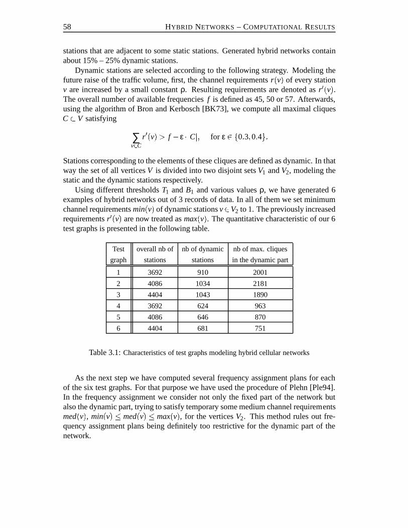
58 HYBRID NETWORKS – COMPUTATIONAL RESULTS
stations that are adjacent to some static stations. Generated hybrid networks containabout 15% – 25% dynamic stations.
Dynamic stations are selected according to the following strategy. Modeling thefuture raise of the traffic volume, first, the channel requirementsr(v) of every stationv are increased by a small constantρ. Resulting requirements are denoted asr 0(v).The overall number of available frequenciesf is defined as 45, 50 or 57. Afterwards,using the algorithm of Bron and Kerbosch [BK73], we compute all maximal cliquesC�V satisfying
∑v2C
r 0(v)> f � ε � jCj; for ε 2 f0:3;0:4g:Stations corresponding to the elements of these cliques are defined as dynamic. In thatway the set of all verticesV is divided into two disjoint setsV1 andV2, modeling thestatic and the dynamic stations respectively.
Using different thresholdsT1 andB1 and various valuesρ, we have generated 6examples of hybrid networks out of 3 records of data. In all of them we set minimumchannel requirementsmin(v) of dynamic stationsv2V2 to 1. The previously increasedrequirementsr 0(v) are now treated asmax(v). The quantitative characteristic of our 6test graphs is presented in the following table.
Test overall nb of nb of dynamic nb of max. cliques
graph stations stations in the dynamic part
1 3692 910 2001
2 4086 1034 2181
3 4404 1043 1890
4 3692 624 963
5 4086 646 870
6 4404 681 751
Table 3.1:Characteristics of test graphs modeling hybrid cellular networks
As the next step we have computed several frequency assignment plans for eachof the six test graphs. For that purpose we have used the procedure of Plehn [Ple94].In the frequency assignment we consider not only the fixed part of the network butalso the dynamic part, trying to satisfy temporary some medium channel requirementsmed(v), min(v) � med(v) � max(v), for the verticesV2. This method rules out fre-quency assignment plans being definitely too restrictive for the dynamic part of thenetwork.
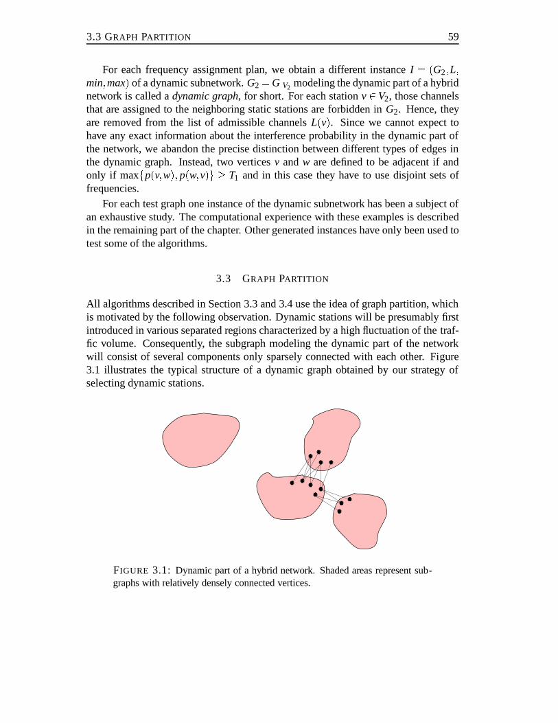
3.3 GRAPH PARTITION 59
For each frequency assignment plan, we obtain a different instanceI = (G2;L;min;max) of a dynamic subnetwork.G2 = GjV2 modeling the dynamic part of a hybridnetwork is called adynamic graph, for short. For each stationv2V2, those channelsthat are assigned to the neighboring static stations are forbidden inG2. Hence, theyare removed from the list of admissible channelsL(v). Since we cannot expect tohave any exact information about the interference probability in the dynamic part ofthe network, we abandon the precise distinction between different types of edges inthe dynamic graph. Instead, two verticesv andw are defined to be adjacent if andonly if maxfp(v;w); p(w;v)g � T1 and in this case they have to use disjoint sets offrequencies.
For each test graph one instance of the dynamic subnetwork has been a subject ofan exhaustive study. The computational experience with these examples is describedin the remaining part of the chapter. Other generated instances have only been used totest some of the algorithms.
3.3 GRAPH PARTITION
All algorithms described in Section 3.3 and 3.4 use the idea of graph partition, whichis motivated by the following observation. Dynamic stations will be presumablyfirstintroduced in various separated regions characterized by a high fluctuation of thetraf-fic volume. Consequently, the subgraph modeling the dynamic part of the networkwill consist of several components only sparsely connected with each other. Figure3.1 illustrates the typical structure of a dynamic graph obtained by our strategy ofselecting dynamic stations.
���� ��������
����������
��������
����
���������������
���������������
����
������������������������������
������������������������������
������������������������������������
������������������������������������
��������������������
��������������������
����������������������������
����������������������������
���������������������������
���������������������������
���������������������������
���������������������������
��������������������������������
��������������������������������������������������������
����������������������������
����
����������������������������
��������������������������������
FIGURE 3.1: Dynamic part of a hybrid network. Shaded areas represent sub-graphs with relatively densely connected vertices.
60 HYBRID NETWORKS – COMPUTATIONAL RESULTS
It seems reasonable to partition such a dynamic graph and then call an algorithmfor the channel stability number separately for each component. The results obtainedfor single components are then put together in an appropriate way so as to obtain re-spectively a lower or an upper bound onch for the whole dynamic graph. We hopedthat the partition of the dynamic graph can substantially reduce the time of the compu-tation and this supposition has been justified by all our tests. The idea of the graph de-composition is particularly important for algorithms using CPLEX MIP solver,since— up to now — this program is not able to cope efficiently at once with a whole in-stance containing more than 600 vertices. Actually, as we will describe inSection 3.5,upper bounds algorithms using CPLEX, often require the partition of the graph intocomponents containing no more than 60 vertices.
The partition of the dynamic graph has been obtained using the following scheme.
Initializationfor all v2V2
create a component containing exclusively this one stationv;
Partition into componentscompute all maximal cliques inG2;for each maximal cliqueC dobegin
max sum[C] = ∑v2C max(v);weight[C] = max sum[C]�chT=0(C); // weight[C] provides a lower bound
// on the number of unsatisfiable// channel requirements inC
if ((weight[C] > 0) and (max sum[C]> freq nb1- clique factor))// the second condition is used to control// the size of cliques taken into account during// the process of component merging
merge all components containing elements ofC into one component;endappend the remaining single vertices to some components;
The decomposition of the dynamic graph is a matter of trade-off between the timecomplexity and the accuracy of the algorithms for the channel stability number. Edgesincident to vertices that are placed in two different components are treated less care-fully than edges joining vertices in one component. However, the time complexityofall algorithms strongly depends on the maximal size of components in the decompo-sition. In order to have a control over this trade-off the parameterclique factor hasbeen introduced.
1freq nbdenotes the overall number of frequencies available in the particular problem instance
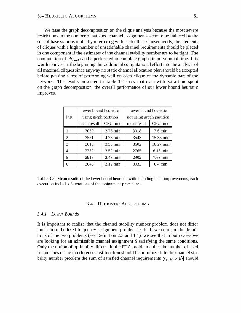
3.4 HEURISTIC ALGORITHMS 61
We base the graph decomposition on the clique analysis because the most severerestrictions in the number of satisfied channel assignments seem to be induced by thesets of base stations mutually interfering with each other. Consequently, theelementsof cliques with a high number of unsatisfiable channel requirements should be placedin one component if the estimates of the channel stability number are to be tight. Thecomputation ofchT=0 can be performed in complete graphs in polynomial time. It isworth to invest at the beginning this additional computational effort into the analysis ofall maximal cliques since anyway no static channel allocation plan should be acceptedbefore passing a test of performing well on each clique of the dynamic part of thenetwork. The results presented in Table 3.2 show that even with extra time spenton the graph decomposition, the overall performance of our lower bound heuristicimproves.
lower bound heuristic lower bound heuristic
Inst. using graph partition not using graph partition
mean result CPU time mean result CPU time
1 3039 2.73 min 3018 7.6 min
2 3571 4.78 min 3543 15.35 min
3 3619 3.58 min 3602 10.27 min
4 2782 2.52 min 2765 6.18 min
5 2915 2.48 min 2902 7.63 min
6 3043 2.12 min 3033 6.4 min
Table 3.2:Mean results of the lower bound heuristic with including local improvements; eachexecution includes 8 iterations of the assignment procedure .
3.4 HEURISTIC ALGORITHMS
3.4.1 Lower Bounds
It is important to realize that the channel stability number problem does not differmuch from the fixed frequency assignment problem itself. If we compare the defini-tions of the two problems (see Definition 2.3 and 1.1), we see that in both cases weare looking for an admissible channel assignmentS satisfying the same conditions.Only the notion of optimality differs. In the FCA problem either the number of usedfrequencies or the interference cost function should be minimized. In the channel sta-bility number problem the sum of satisfied channel requirements∑u2V jS(u)j should
62 HYBRID NETWORKS – COMPUTATIONAL RESULTS
be maximized.Because of that relationship between the two problems we can use the frequency
assignment method developed by Plehn [Ple94] as a heuristic computing lower boundsfor the channel stability number. This method is described below. Afterwards,wedescribe some modifications of the original algorithm that turned out to be useful inour application. At the end of this section we discuss how an admissible frequencyassignments can be improved using a local search method.
The algorithm based on Plehn’s heuristic is successively called for each componentof the partitioned dynamic graph. After finishing the computation for one component,the procedure updates the lists of admissible frequencies of those stations from othercomponents that are adjacent with any of the stations from the current component. Atthe end, the sum of channel requirements satisfied in all components yields a lowerbound on the channel stability number.
Plehn’s algorithm consists of several calls to one assignment procedure. The basicidea of the procedure is to choose iteratively a base stationv and a new channelf for it,as long as there is a station with unsatisfied requirements that still has some admissiblechannels. After each selection the channelf is assigned tov and the sets of channelsadmissible for other stations are updated. At the end of the assignment procedurewe obtain a frequency allocation plan that may leave some channel requirementsun-satisfied. In that case some parameters of unsatisfied base stations are automaticallychanged before the next call to the assignment procedure. After the last call the bestfound frequency allocation plan is output by the algorithm.
The crux of the assignment procedure lies in the careful selection of station–channel pairs. Let us describe the general idea of the selection procedure proposedby Plehn. The exact meaning of single criteria is explained afterwards. The selectionof a base stationv is based on the following criteria:
B1: Smallest ratiorest-capacity(v)=rest-demand(v)B2: Highestvalueof difficulty(v)B3: Largestinterferencesum(v)
The three criteria are applied consecutively. The first criterion is computed for all sta-tions with unsatisfied requirements that still have some admissible channels. It selectsthe set of stations having the smallest ratiorest-capacity(v)=rest-demand(v). For theelements of this set the second criterion is computed, etc. If at the end more than onestation is left the final choice is performed randomly. Afterwards, one frequency isselected out of the set admissible for the chosen station using the following criteria:
F1: Highest category of resultingsatisfiability( f )F2: Smallest change of the cost functionpif
F3: Smallest previous use
3.4 HEURISTIC ALGORITHMS 63
The way of applying these criteria is exactly the same as for the choice of a basestation.
Let us now explain the meaning of the selection criteria.Rest-capacityof a sta-tion v denotes the number of frequencies in its current admissible list that could besimultaneously assigned tov observing the co-site constraints.Rest-demandof v sim-ply denotes the number of still unsatisfied channel requirements of the stationv. Therole of therest-capacity(v)=rest-demand(v) ratio is similar in nature to thesaturationdegree in theDsaturgraph coloring algorithm [Bre79]. The idea is to choose a stationthat is currently in the worst situation.
The valueof difficulty of a base stationv is intended to reflect the difficulty ofsatisfying the channel requirements of this station. It may be initialized forall sta-tions to zero or, alternatively, with values reflecting the smallest–last ordering of thenodes of the dynamic graph (see [MB83]). If a call to the frequency assignment pro-cedure leaves some channel requirements unsatisfied, then thevalueof difficulty ofall unsatisfied base stations is increased by a small random number.
The notion of theinterferencesumis related to the partition of stations interferingwith a given stationv into those strongly interfering, which must not use the samefrequencies asv, and those weakly interfering, which may use equal frequencies at theexpense of the increasing cost function (see Page 13 and 57). If there are any stationsN0(v) of the latter type, then:
interferencesum(v) := ∑w2N0(v) ∑
f2S(v)\S(w) p(v;w):Recall that in the dynamic graph we do not distinguish different degrees of interfer-ence, and therefore the criterion B3 is omitted in our implementation.
The satisfiability( f ) resulting from the assignment of a particular frequency tothe chosen stationv is estimated by slotting the admissible frequencies into threecategories. If after the assignment of the new frequencyf , v has still a positiverest demandand the ratio (rest-capacity(v)=rest-demand(v)) is smaller than 1, thenf falls into the first category. Otherwise, if there is a stationw interfering withv suchthatw has still a positiverest demandand the resulting ratio (rest-capacity(w)=rest-demand(w)) would be smaller than 1, then the frequencyf falls into the second cate-gory. Finally, f belongs to category three if it does not belong to any of the previouscategories.
The cost functionpif , used in the criterion F2, has been already introduced inSection 1.2. Recall that similarly to theinterferencesumthe calculation of thepriceof interference(pif ) makes sense only if there is a distinction between strong andweak interferers. Consequently, F2 is omitted in the heuristic for the channel stabilitynumber.
In the last channel selection criterion F3 we count the number of stations to whicha given frequency has been already assigned. The channel least frequently used is
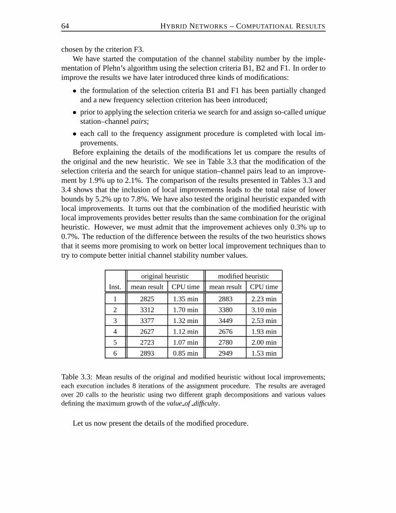
64 HYBRID NETWORKS – COMPUTATIONAL RESULTS
chosen by the criterion F3.We have started the computation of the channel stability number by the imple-
mentation of Plehn’s algorithm using the selection criteria B1, B2 and F1. In order toimprove the results we have later introduced three kinds of modifications:� the formulation of the selection criteria B1 and F1 has been partially changed
and a new frequency selection criterion has been introduced;� prior to applying the selection criteria we search for and assign so-called uniquestation–channelpairs;� each call to the frequency assignment procedure is completed with local im-provements.
Before explaining the details of the modifications let us compare the results ofthe original and the new heuristic. We see in Table 3.3 that the modification of theselection criteria and the search for unique station–channel pairs lead to animprove-ment by 1.9% up to 2.1%. The comparison of the results presented in Tables 3.3 and3.4 shows that the inclusion of local improvements leads to the total raise of lowerbounds by 5.2% up to 7.8%. We have also tested the original heuristic expanded withlocal improvements. It turns out that the combination of the modified heuristic withlocal improvements provides better results than the same combination for the originalheuristic. However, we must admit that the improvement achieves only 0.3% up to0.7%. The reduction of the difference between the results of the two heuristics showsthat it seems more promising to work on better local improvement techniques than totry to compute better initial channel stability number values.
original heuristic modified heuristic
Inst. mean result CPU time mean result CPU time
1 2825 1.35 min 2883 2.23 min
2 3312 1.70 min 3380 3.10 min
3 3377 1.32 min 3449 2.53 min
4 2627 1.12 min 2676 1.93 min
5 2723 1.07 min 2780 2.00 min
6 2893 0.85 min 2949 1.53 min
Table 3.3:Mean results of the original and modified heuristic without local improvements;each execution includes 8 iterations of the assignment procedure. The results are averagedover 20 calls to the heuristic using two different graph decompositions and various valuesdefining the maximum growth of thevalue of difficulty.
Let us now present the details of the modified procedure.
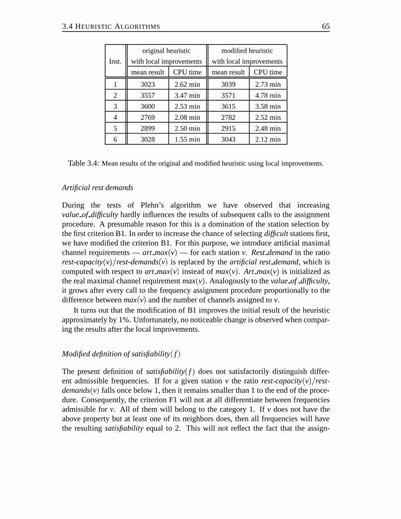
3.4 HEURISTIC ALGORITHMS 65
original heuristic modified heuristic
Inst. with local improvements with local improvements
mean result CPU time mean result CPU time
1 3023 2.62 min 3039 2.73 min
2 3557 3.47 min 3571 4.78 min
3 3600 2.53 min 3615 3.58 min
4 2769 2.08 min 2782 2.52 min
5 2899 2.50 min 2915 2.48 min
6 3028 1.55 min 3043 2.12 min
Table 3.4:Mean results of the original and modified heuristic using local improvements.
Artificial rest demands
During the tests of Plehn’s algorithm we have observed that increasingvalueof difficulty hardly influences the results of subsequent calls to the assignmentprocedure. A presumable reason for this is a domination of the station selection bythe first criterion B1. In order to increase the chance of selectingdifficult stations first,we have modified the criterion B1. For this purpose, we introduce artificial maximalchannel requirements —art max(v) — for each stationv. Restdemandin the ratiorest-capacity(v)=rest-demands(v) is replaced by theartificial rest demand, which iscomputed with respect toart max(v) instead ofmax(v). Art max(v) is initialized asthe real maximal channel requirementmax(v). Analogously to thevalueof difficulty,it grows after every call to the frequency assignment procedure proportionally to thedifference betweenmax(v) and the number of channels assigned tov.
It turns out that the modification of B1 improves the initial result of the heuristicapproximately by 1%. Unfortunately, no noticeable change is observed when compar-ing the results after the local improvements.
Modified definition of satisfiability( f )The present definition ofsatisfiability( f ) does not satisfactorily distinguish differ-ent admissible frequencies. If for a given stationv the ratio rest-capacity(v)=rest-demands(v) falls once below 1, then it remains smaller than 1 to the end of the proce-dure. Consequently, the criterion F1 will not at all differentiate between frequenciesadmissible forv. All of them will belong to the category 1. Ifv does not have theabove property but at least one of its neighbors does, then all frequencies will havethe resultingsatisfiabilityequal to 2. This will not reflect the fact that the assign-
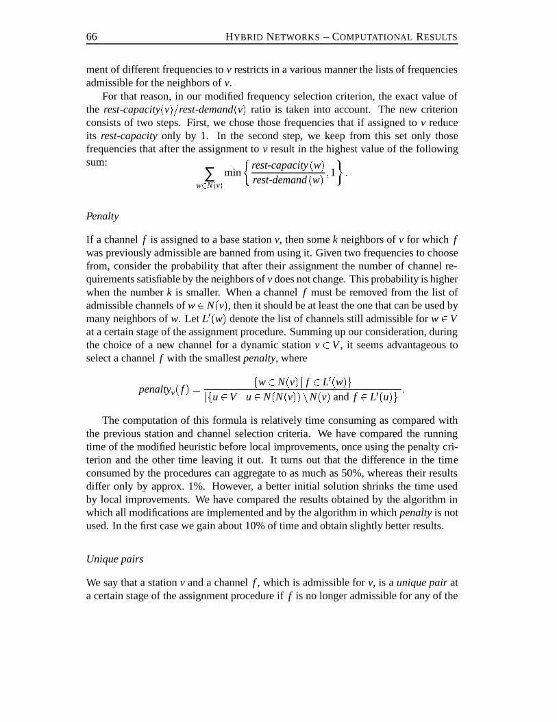
66 HYBRID NETWORKS – COMPUTATIONAL RESULTS
ment of different frequencies tov restricts in a various manner the lists of frequenciesadmissible for the neighbors ofv.
For that reason, in our modified frequency selection criterion, the exact value ofthe rest-capacity(v)=rest-demand(v) ratio is taken into account. The new criterionconsists of two steps. First, we chose those frequencies that if assigned tov reduceits rest-capacityonly by 1. In the second step, we keep from this set only thosefrequencies that after the assignment tov result in the highest value of the followingsum:
∑w2N(v)min
�rest-capacity(w)rest-demand(w) ;1� :
Penalty
If a channelf is assigned to a base stationv, then somek neighbors ofv for which fwas previously admissible are banned from using it. Given two frequencies to choosefrom, consider the probability that after their assignment the number of channel re-quirements satisfiable by the neighbors ofv does not change. This probability is higherwhen the numberk is smaller. When a channelf must be removed from the list ofadmissible channels ofw2N(v), then it should be at least the one that can be used bymany neighbors ofw. Let L0(w) denote the list of channels still admissible forw2Vat a certain stage of the assignment procedure. Summing up our consideration, duringthe choice of a new channel for a dynamic stationv 2 V, it seems advantageous toselect a channelf with the smallestpenalty, where
penaltyv( f ) = jfw2 N(v) j f 2 L0(w)gjjfu2V ju2 N(N(v))nN(v) and f 2 L0(u)gj:The computation of this formula is relatively time consuming as compared with
the previous station and channel selection criteria. We have compared the runningtime of the modified heuristic before local improvements, once using the penalty cri-terion and the other time leaving it out. It turns out that the difference in the timeconsumed by the procedures can aggregate to as much as 50%, whereas their resultsdiffer only by approx. 1%. However, a better initial solution shrinks the time usedby local improvements. We have compared the results obtained by the algorithm inwhich all modifications are implemented and by the algorithm in whichpenaltyis notused. In the first case we gain about 10% of time and obtain slightly better results.
Unique pairs
We say that a stationv and a channelf , which is admissible forv, is aunique pairata certain stage of the assignment procedure iff is no longer admissible for any of the
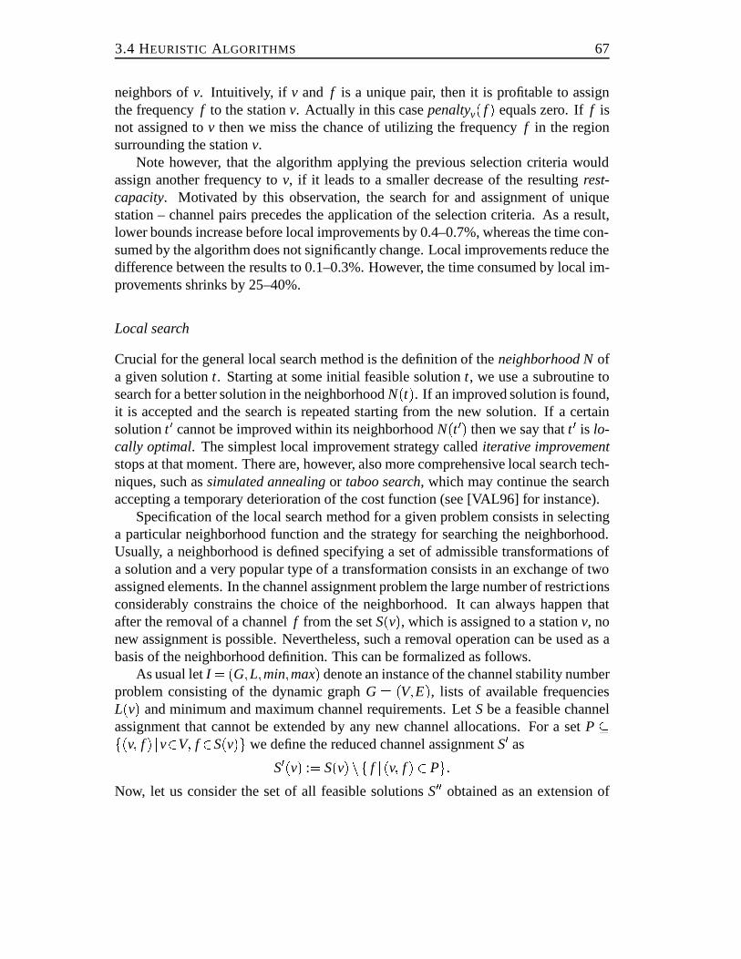
3.4 HEURISTIC ALGORITHMS 67
neighbors ofv. Intuitively, if v and f is a unique pair, then it is profitable to assignthe frequencyf to the stationv. Actually in this casepenaltyv( f ) equals zero. Iff isnot assigned tov then we miss the chance of utilizing the frequencyf in the regionsurrounding the stationv.
Note however, that the algorithm applying the previous selection criteria wouldassign another frequency tov, if it leads to a smaller decrease of the resultingrest-capacity. Motivated by this observation, the search for and assignment of uniquestation – channel pairs precedes the application of the selection criteria.As a result,lower bounds increase before local improvements by 0.4–0.7%, whereas the time con-sumed by the algorithm does not significantly change. Local improvements reduce thedifference between the results to 0.1–0.3%. However, the time consumed by local im-provements shrinks by 25–40%.
Local search
Crucial for the general local search method is the definition of theneighborhood Nofa given solutiont. Starting at some initial feasible solutiont, we use a subroutine tosearch for a better solution in the neighborhoodN(t). If an improved solution is found,it is accepted and the search is repeated starting from the new solution. Ifa certainsolutiont 0 cannot be improved within its neighborhoodN(t 0) then we say thatt 0 is lo-cally optimal. The simplest local improvement strategy callediterative improvementstops at that moment. There are, however, also more comprehensive local search tech-niques, such assimulated annealingor taboo search, which may continue the searchaccepting a temporary deterioration of the cost function (see [VAL96] for instance).
Specification of the local search method for a given problem consists in selectinga particular neighborhood function and the strategy for searching the neighborhood.Usually, a neighborhood is defined specifying a set of admissible transformations ofa solution and a very popular type of a transformation consists in an exchange of twoassigned elements. In the channel assignment problem the large number of restrictionsconsiderably constrains the choice of the neighborhood. It can always happen thatafter the removal of a channelf from the setS(v), which is assigned to a stationv, nonew assignment is possible. Nevertheless, such a removal operation can be used as abasis of the neighborhood definition. This can be formalized as follows.
As usual letI = (G;L;min;max) denote an instance of the channel stability numberproblem consisting of the dynamic graphG = (V;E), lists of available frequenciesL(v) and minimum and maximum channel requirements. LetSbe a feasible channelassignment that cannot be extended by any new channel allocations. For a setP�f(v; f ) jv2V; f 2S(v)g we define the reduced channel assignmentS0 as
S0(v) := S(v)nf f j(v; f ) 2 Pg:Now, let us consider the set of all feasible solutionsS00 obtained as an extension of
68 HYBRID NETWORKS – COMPUTATIONAL RESULTS
S0. This set will be denoted asΠPS. Thefirst neighborhood of the solutionS is then
introduced as the setΠ1
S= [P; jPj=1
ΠPS:
More general, we introduce thek-th neighborhood as the set
ΠkS= [
P; jPj=k
ΠPS:
The highest possible increase in the number of satisfied channel requirements after theremoval of the assignmentsP defines a local improvementimpr(S;P):
impr(S;P) = maxS002ΠP
S
∑v2VjS00(v)j!�∑
v2VjS(v)j:
A solutionS is optimal in itsk-th neighborhood if there is no setP of cardinalityksuch thatimpr(S;P)> 0.
Having specified the notion of a neighborhood we have to examine the computa-tional complexity of checking the local optimality of a solution. The following twopropositions show that this can be done in polynomial time provided thatk is a con-stant. We start with the special case ofk = 1, which is treated separately because ofits simpler proof and a more efficient algorithm. For the sake of convenience we usethe notationimpr(S;(v; f )) if P consists of a single pair(v; f ).Proposition 3.1 Let I = (G;L;min;max), let ∆ be the maximum vertex degree in thegraph G and let S be a feasible and non-extendible channel assignment in G. Then, itcan be examined in time O(jL(v)j+∆2) if
impr(S;(v; f ))> 0;for a given vertex v and a channel f2 S(v).Proof. After the removal of the frequencyf from the setS(v) two kinds of newchannel assignments may be possible:
(1) some new channels may be assigned tov;
(2) the channelf may be assigned to some neighbors ofv.
Let us closer examine these two points. After the removal of the frequencyf ,possibly four frequencies become once again admissible forv. These are the frequen-cies f �2, f �1, f +1, and f +2 that were previously forbidden due to the co-siteconstraints (δ = 2). Which of them exactly become admissible, this depends on other
3.4 HEURISTIC ALGORITHMS 69
frequencies assigned tov and on the frequencies assigned to the neighbors ofw. Notethat due to the co-site constraints, at most two of the four frequencies may be assignedto v. Let us distinguish between the case whenjS(v)j< max(v) andjS(v)j= max(v).In the first case only the above set of four frequencies has to be considered. However,in the second case it could happen that some more frequencies are still admissible forv — they were not previously assigned because the maximum channel requirement ofv was already satisfied. Altogether, in the second case,O(jL(v)j) frequencies shouldbe considered but at most one of them may be assigned tov.
It is important that the channels considered for the stationv are different fromf . Therefore, the search for new assignments can be performed independently forthe stationv and for its neighbors. If as a result of the first search two channels areassigned tov then impr(S;(v; f )) > 0. If only one new channel can be assigned tov then impr(S;(v; f )) > 0 if f can be assigned to at least one neighbor ofv. In theremaining case, when no new channels are assigned tov, it is sufficient to check ifthere are two non-adjacent vertices in the neighborhood ofv that can now use thechannelf . The last search, being most time consuming, can be performed inO(∆2)time.
The total time complexity of the search for new assignments is bounded byO(jL(v)j+∆2). �Let us note that the above proof does not show how to compute the highest pos-
sible improvement ofS. This would involve the computation of a maximum inde-pendent set among all neighborsw of v for which f is now admissible and for whichjS(w)j < max(w). We have only shown how to check in polynomial time whetherafter the withdrawal of the pair(v; f ) any improvement is possible at all. The methodof Proposition 3.1 can be applied for every pair(v; f ), v 2 V and f 2 S(v) in orderto check if a solutionS is optimal in its first neighborhood. A simple implementa-tion of this process has the time complexityO(Mn(jFj+∆2)), whereF denotes theset of frequencies admissible in the whole network andM = maxv2Vfmax(v)g. Thiscomplexity is reasonable for practical purposes.
Proposition 3.2 Let I = (G;L;min;max), let ∆ be the maximum vertex degree in thegraph G and let F be the set of frequencies admissible in the whole network. Then,for a given feasible and non-extendible solution S and a set P= f(vi; fi) j i = 1; : : : ;kgit can be examined in time O((jFj+∆)k+1) if
impr(S;P)> 0;Proof. Similarly as in Proposition 3.1 the withdrawal of pairs(vi; fi), i = 1; : : : ;k canmake two kinds of new assignments possible:
(1) some new channels may be assigned to each of the stationsvi ;
70 HYBRID NETWORKS – COMPUTATIONAL RESULTS
(2) for i = 1; : : : ;k, the channelfi may be assigned to some neighborsw of thestationvi .
The sets of channels considered in point (1) for each stationvi are the same as inProposition 3.1. However, it may happen that more than two channels are assigned toa stationvi , if it is a neighbor of another stationv j , i 6= j, i; j 2 f1; : : : ;kg. Differentlyfrom Proposition 3.1 the sets of channels considered in point (1) and point (2) arepossibly not disjoint. This can happen already fork = 2. Therefore, all stationsvi ,i = 1; : : : ;k, and all their neighborsN(vi) are examined simultaneously. LetS0 denotethe reduced channel assignment
S0(v) := S(v)nf f j(v; f ) 2 Pg:Let S0N(v) denote the set of channels assigned inS0 to the neighbors ofv:
S0N(v) := f f j9w2 N(v); f 2 S0(w)g:We build an auxiliary hypergrapheH = (eV; eF). Its vertices correspond to the possiblenew channel assignments:eV = k[
i=1
�(vi; fi�) j fi
� 2 L(vi)nS0N(vi)and8 f 2 S0(vi) j fi�� f j> 2
[ k[i=1
�(w; fi) jw2 N(vi); fi 2 L(w)nS0N(w) andjS(w)j< max(w)and8 f 2 S0(w) j f � fij> 2
:The edges of the hypergraph define the forbidden combinations of channel assign-ments:eF = ff(u;g);(v;g)g j (u;v) 2 Eg [ ff(u;g1);(u;g2)g j jg1�g2j � 2g[�f(u;g1); : : : ;(u;gl)g j l > max(u)�jS0(u)j :Now, impr(S;P) is positive if the hypergrapheH has an independent set of sizek+1.SincejeVj = O(k � jFj+ k �∆) = O(jFj+∆) the existence of such an independent setcan be checked in timeO((jFj+∆)k+1). �
The method of Proposition 3.2 can be used to examine if a solutionS is optimal inits k-th neighborhood for any constantk. Unfortunately, this method is not very practi-cal even fork= 2. In that case, checking local optimality can takeO(M2n2(jFj+∆)3)time, whereM = maxv2Vfmax(v)g. Therefore, in our program, we have implementedfor the second neighborhood a heuristic search instead of an exhaustive one.
3.4 HEURISTIC ALGORITHMS 71
Our local search procedure follows theiterative improvementstrategy. The searchfor an improved solution is divided into three phases.Phase 1. We perform an exhaustive search for an improvement in the first neigh-borhood. The search is stopped when the first pair(v; f ), v 2 V and f 2 S(v), withimpr(S;(v; f )) > 0 is found. In that case we know that an improvement is possiblebut we continue with the third random phase. We go directly to the third phase also ifimpr(S;(v; f )) = �1 for all pairs(v; f ). Otherwise, letT be a list of pairs(v; f ) withimpr(S;(v; f )) = 0.Phase 2.Using the elements of the setT we search heuristically for an improvementin the second neighborhood. For every element(v; f ) from the setT consider thecorresponding reduced channel assignmentS0. Let us denote this channel assignmentby S0v; f . By definition ofT, S0v; f is extendible exactly by one station–channel pair. Letus denote such an extension byS00v; f . In S00v; f either a new channelf1 is assigned tovor the channelf is assigned to a neighboru2 N(v). For each element(v; f ) 2 T letus denote withNf (v) the neighborhoodN(v) or N(v)nfug respectively. Now, in thesecond phase of local search, setsNf (v), for every(v; f ) 2 T, are searched for twopossible kinds of modifications. First, it is examined if there is a stationw 2 Nf (v)and a channelf2 2 S00v; f (w), such that after the removal off2 from S00v; f (w), f can beassigned tow and f2 can be assigned to some neighbory of w. If this not the case,then we check if after the removal of the frequencyf from S00v; f (y) for some neighbory of w, f can be assigned tow and a new frequencyf2 can be assigned toy.
This search may certainly miss some pairs(v1; f1), (v2; f2) with impr(S;f(v1; f1);(v2; f2)g)> 0. However, it can be implemented in timeO(M2n∆(∆+ jFj)) and findsalready a large number of local improvements.Phase 3.In the third phase of the local search procedure we continue with a randomsearch for an improvement among a setA of candidate pairs. Starting with an initialfeasible and non-extendible solutionS, S is subsequently modified by either removingor introducing some assignments(v; f ). All modifications are stored so as to be able tofind at the end the best intermediate solution. The search for assignments is performedaccording to the following scheme.
1. Initialize the setA of candidate pairs. If in the first phase a pair(v; f ) has beenfound such thatimpr(S;(v; f ))> 0, thenA := f(v; f )g. Otherwise, if in the sec-ond phase an improvement has been found after removing two pairs(v1; f1) and(v2; f2), thenA := f(v2; f2)g. At last, if the deterministic search was unsuccess-ful, initialize A asf(v; f ) j impr(S;(v; f )) = 0g or if this set is empty, choose anyrandom vertex–channel pair.
2. Set the iteration counter to zero.
3. Randomly choose one pair(v; f ) from the set of candidatesA. SetA := Anf(v; f )g. Modify Sremoving the assignment(v; f ).
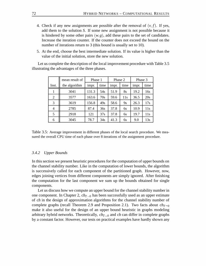
72 HYBRID NETWORKS – COMPUTATIONAL RESULTS
4. Check if any new assignments are possible after the removal of(v; f ). If yes,add them to the solutionS. If some new assignment is not possible because itis hindered by some other pairs(w;g), add these pairs to the set of candidates.Increase the iteration counter. If the counter does not exceed the bound on thenumber of iterations return to 3 (this bound is usually set to 10).
5. At the end, choose the best intermediate solution. If its value is higher than thevalue of the initial solution, store the new solution.
Let us complete the description of the local improvement procedure with Table 3.5illustrating the advantages of the three phases.
mean result of Phase 1 Phase 2 Phase 3
Inst. the algorithm impr. time impr. time impr. time
1 3041 131.3 54s 51.9 8s 19.2 16s
2 3577 163.6 70s 59.6 11s 36.5 20s
3 3619 156.8 49s 58.6 9s 26.3 17s
4 2785 87.4 36s 37.8 6s 10.9 11s
5 2918 121 37s 37.8 6s 19.7 11s
6 3045 78.7 34s 41.3 6s 9.0 13s
Table 3.5:Average improvement in different phases of the local searchprocedure. We mea-sured the overall CPU time of each phase over 8 iterations of the assignment procedure.
3.4.2 Upper Bounds
In this section we present heuristic procedures for the computation of upper bounds onthe channel stability number. Like in the computation of lower bounds, the algorithmis successively called for each component of the partitioned graph. However,now,edges joining vertices from different components are simply ignored. After finishingthe computation for the last component we sum up the bounds obtained for singlecomponents.
Let us discuss how we compute an upper bound for the channel stability number inone component. In Chapter 2,chT=0 has been successfully used as an upper estimateof ch in the design of approximation algorithms for the channel stability number ofcomplete graphs (recall Theorem 2.9 and Proposition 2.1). Two facts aboutchT=0make it also useful for the design of an upper bound heuristic in graphs modelingarbitrary hybrid networks. Theoretically,chT=0 andch can differ in complete graphsby a constant factor. However, our tests on practical examples have hardly shown any
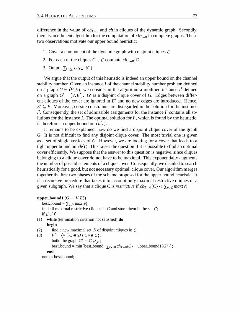
3.4 HEURISTIC ALGORITHMS 73
difference in the value ofchT=0 andch in cliques of the dynamic graph. Secondly,there is an efficient algorithm for the computation ofchT=0 in complete graphs. Thesetwo observations motivate our upper bound heuristic:
1. Cover a component of the dynamic graph with disjoint cliquesC .
2. For each of the cliquesC2 C computechT=0(C).3. Output∑C2C chT=0(C).We argue that the output of this heuristic is indeed an upper bound on the channel
stability number. Given an instanceI of the channel stability number problem definedon a graphG = (V;E), we consider in the algorithm a modified instanceI 0 definedon a graphG0 = (V;E0). G0 is a disjoint clique cover ofG. Edges between differ-ent cliques of the cover are ignored inE0 and no new edges are introduced. Hence,E0 � E. Moreover, co-site constraints are disregarded in the solution for the instanceI 0. Consequently, the set of admissible assignments for the instanceI 0 contains all so-lutions for the instanceI . The optimal solution forI 0, which is found by the heuristic,is therefore an upper bound onch(I).
It remains to be explained, how do we find a disjoint clique cover of the graphG. It is not difficult to find any disjoint clique cover. The most trivial one is givenas a set of single vertices ofG. However, we are looking for a cover that leads to atight upper bound onch(I). This raises the question if it is possible to find an optimalcover efficiently. We suppose that the answer to this question is negative, since cliquesbelonging to a clique cover do not have to be maximal. This exponentially augmentsthe number of possible elements of a clique cover. Consequently, we decided to searchheuristically for a good, but not necessary optimal, clique cover. Our algorithm mergestogether the first two phases of the scheme proposed for the upper bound heuristic. Itis a recursive procedure that takes into account only maximal restrictive cliques of agiven subgraph. We say that a cliqueC is restrictiveif chT=0(C)< ∑v2C max(v).upper bound1 (G= (V;E))
bestbound =∑v2V max(v);find all maximal restrictive cliques inG and store them in the setC ;if C 6= /0
(1) while (termination criterion not satisfied)dobegin
(2) find a new maximal setD of disjoint cliques inC ;(3) V 0 = fvj9C2D s.t. v2Cg;
build the graphG� = GjVnV 0 ;bestbound = minfbestbound,∑C2D chT=0(C)+upperbound1(G�)g;
endoutput bestbound;
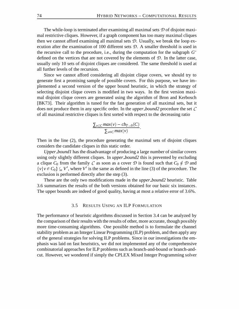
74 HYBRID NETWORKS – COMPUTATIONAL RESULTS
The while-loop is terminated after examining all maximal setsD of disjoint maxi-mal restrictive cliques. However, if a graph component has too many maximal cliquesthen we cannot afford examining all maximal setsD. Usually, we break the loop ex-ecution after the examination of 100 different setsD. A smaller threshold is used inthe recursive call to the procedure, i.e., during the computation for the subgraphG�defined on the vertices that are not covered by the elements ofD. In the latter case,usually only 10 sets of disjoint cliques are considered. The same threshold is used atall further levels of the recursion.
Since we cannot afford considering all disjoint clique covers, we should try togenerate first a promising sample of possible covers. For this purpose, we have im-plemented a second version of the upper bound heuristic, in which the strategy ofselecting disjoint clique covers is modified in two ways. In the first version maxi-mal disjoint clique covers are generated using the algorithm of Bron and Kerbosch[BK73]. Their algorithm is tuned for the fast generation of all maximal sets,but itdoes not produce them in any specific order. In theupper bound2procedure the setCof all maximal restrictive cliques is first sorted with respect to thedecreasing ratio
∑v2C max(v)�chT=0(C)∑v2C max(v) :
Then in the line (2), the procedure generating the maximal sets of disjoint cliquesconsiders the candidate cliques in this static order.
Upper bound1has the disadvantage of producing a large number of similar coversusing only slightly different cliques. Inupper bound2this is prevented by excludinga cliqueC0 from the familyC as soon as a coverD is found such thatC0 =2 D andfvjv2C0g �V 0, whereV 0 is the same as defined in the line (3) of the procedure. Theexclusion is performed directly after the step (3).
These are the only two modifications made in theupperbound2heuristic. Table3.6 summarizes the results of the both versions obtained for our basic six instances.The upper bounds are indeed of good quality, having at most a relative error of 3.6%.
3.5 RESULTS USING AN ILP FORMULATION
The performance of heuristic algorithms discussed in Section 3.4 can be analyzedbythe comparison of their results with the results of other, more accurate, though possiblymore time-consuming algorithms. One possible method is to formulate the channelstability problem as an Integer Linear Programming (ILP) problem, and then apply anyof the general strategies for solving ILP problems. Since in our investigations the em-phasis was laid on fast heuristics, we did not implemented any of the comprehensivecombinatorial approaches for ILP problems such as branch-and-bound or branch-and-cut. However, we wondered if simply the CPLEX Mixed Integer Programming solver
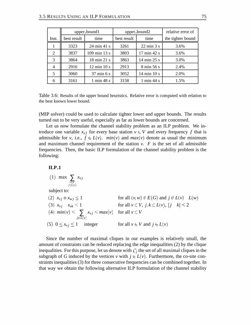
3.5 RESULTS USING AN ILP FORMULATION 75
upperbound1 upperbound2 relative error of
Inst. best result time best result time the tighter bound
1 3323 24 min 41 s 3261 22 min 3 s 3.6%
2 3837 109 min 13 s 3803 17 min 42 s 3.6%
3 3864 18 min 21 s 3863 14 min 25 s 3.0%
4 2916 12 min 10 s 2913 8 min 56 s 2.4%
5 3060 37 min 6 s 3052 14 min 10 s 2.0%
6 3161 1 min 48 s 3158 1 min 44 s 1.5%
Table 3.6:Results of the upper bound heuristics. Relative error is computed with relation tothe best known lower bound.
(MIP solver) could be used to calculate tighter lower and upper bounds. The resultsturned out to be very useful, especially as far as lower bounds are concerned.
Let us now formulate the channel stability problem as an ILP problem. We in-troduce one variablexv f for every base stationv 2 V and every frequencyf that isadmissible forv, i.e., f 2 L(v). min(v) and max(v) denote as usual the minimumand maximum channel requirement of the stationv. F is the set of all admissiblefrequencies. Then, the basic ILP formulation of the channel stability problem is thefollowing:
ILP 1(1) max ∑v2V
j2L(v) xv j
subject to:(2) xv j +xw j � 1 for all (v;w) 2 E(G) and j 2 L(v)\L(w)(3) xv j +xvk� 1 for all v2V; j;k2 L(v); j j�kj � 2(4) min(v)� ∑j2L(v)xv j �max(v) for all v2V(5) 0� xv j � 1 integer for allv2V and j 2 L(v)
Since the number of maximal cliques in our examples is relatively small, theamount of constraints can be reduced replacing the edge inequalities (2) by the cliqueinequalities. For this purpose, let us denote withC j the set of all maximal cliques in thesubgraph ofG induced by the verticesv with j 2 L(v). Furthermore, the co-site con-straints inequalities (3) for three consecutive frequencies can be combined together. Inthat way we obtain the following alternative ILP formulation of the channel stability
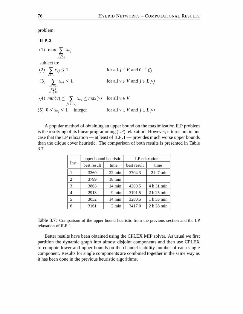
76 HYBRID NETWORKS – COMPUTATIONAL RESULTS
problem:
ILP 2(1) max ∑v2V
j2L(v) xv j
subject to:(2) ∑v2C
xv j � 1 for all j 2 F andC2 C j(3) ∑k2L(v)
k� jk� j�2
xvk� 1 for all v2V and j 2 L(v)(4) min(v)� ∑j2L(v)xv j �max(v) for all v2V(5) 0� xv j � 1 integer for allv2V and j 2 L(v)
A popular method of obtaining an upper bound on the maximization ILP problemis the resolving of its linear programming (LP) relaxation. However, it turnsout in ourcase that the LP relaxation — at least of ILP1 — provides much worse upper boundsthan the clique cover heuristic. The comparison of both results is presented inTable3.7.
upper bound heuristic LP relaxationInst. best result time best result time
1 3260 22 min 3704.3 2 h 7 min
2 3799 18 min
3 3863 14 min 4200.5 4 h 31 min
4 2913 9 min 3191.5 2 h 25 min
5 3052 14 min 3280.5 1 h 53 min
6 3161 2 min 3417.0 2 h 28 min
Table 3.7:Comparison of the upper bound heuristic from the previous section and the LPrelaxation of ILP1.
Better results have been obtained using the CPLEX MIP solver. As usual we firstpartition the dynamic graph into almost disjoint components and then use CPLEXto compute lower and upper bounds on the channel stability number of each singlecomponent. Results for single components are combined together in the same way asit has been done in the previous heuristic algorithms.
3.5 RESULTS USING AN ILP FORMULATION 77
More precisely a lower bound on the channel stability number of the dynamicgraphG can be computed as follows:
partitionG into componentsfGigki=1;for all componentsGi dobegin
formulate the channel stability number problem inGi as ILP2;call CPLEX MIP solver for ILP2, stop when the first integer solution is found;store this solution (channel assignment inGi);update the lists of admissible channels inG j , j > i;
endsum up the channel requirements satisfied in all components;
In Table 3.8 the results obtained using this method are compared with the bestlower bounds found by the heuristic from Section 3.4. The new method providestighter lower bounds for all our examples. However, its time complexity stronglydepends on the structure of the dynamic graph. For graphs with relatively large anddense components, such as in Instance 2, the time consumed by the algorithm becomesunacceptable for practical applications.
An analogous strategy, presented below, has been implemented for the computa-tion of upper bounds:
partitionG into componentsfGigki=1;for all componentsGi dobegin
formulate the channel stability number problem inGi as ILP2;find an optimal solution of the ILP2 using CPLEX MIP solver;
endsum up the channel requirements satisfied in single components;
This strategy turned out to be less successful than the application of the CPLEXMIP solver for the lower bound computation. In our instances, some components of atypical graph decomposition contain 100 nodes or more. An ILP formulation for sucha component has on average 2700 variables and about 10000 constraint inequalities.CPLEX 3.1 was not able to find an optimal solution of such a problem even after 80hours. Therefore, we tried partitioning the graph into smaller components, whichwerenow possibly more densely connected with each other. For some instances, CPLEXonly succeeded in solving the ILP problem for components containing no more than60 vertices. Such a fine partition resulted in upper bounds of worse quality. Thecomparison of results presented in Table 3.8 shows that the new method providedbetter results for three instances. However, this improvement requireda considerableamount of time.
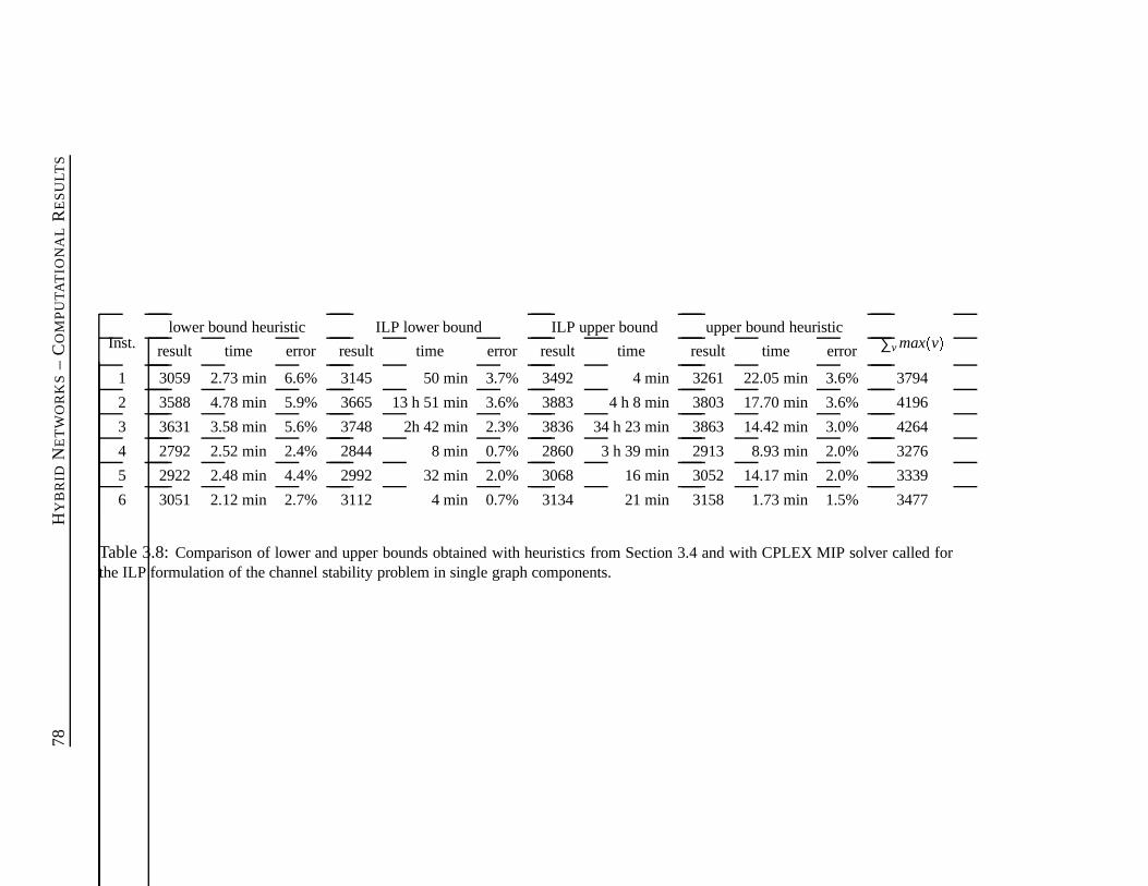
78H
YB
RID
NE
TW
OR
KS
–C
OM
PU
TA
TIO
NA
LR
ES
ULT
S
lower bound heuristic ILP lower bound ILP upper bound upper bound heuristicInst. result time error result time error result time result time error ∑vmax(v)
1 3059 2.73 min 6.6% 3145 50 min 3.7% 3492 4 min 3261 22.05 min 3.6% 3794
2 3588 4.78 min 5.9% 3665 13 h 51 min 3.6% 3883 4 h 8 min 3803 17.70 min 3.6% 4196
3 3631 3.58 min 5.6% 3748 2h 42 min 2.3% 3836 34 h 23 min 3863 14.42 min 3.0% 4264
4 2792 2.52 min 2.4% 2844 8 min 0.7% 2860 3 h 39 min 2913 8.93 min 2.0% 3276
5 2922 2.48 min 4.4% 2992 32 min 2.0% 3068 16 min 3052 14.17 min 2.0% 3339
6 3051 2.12 min 2.7% 3112 4 min 0.7% 3134 21 min 3158 1.73 min 1.5% 3477
Table 3.8:Comparison of lower and upper bounds obtained with heuristics from Section 3.4 and with CPLEX MIP solver called forthe ILP formulation of the channel stability problem in single graph components.
3.6 CONCLUSIONS 79
3.6 CONCLUSIONS
In this chapter we examined the possibilities of computing the channel stability num-ber for several instances based on real world data. Our main aim was the developmentof a fast heuristic efficiently approximating the channel stability number. For ourin-stances the final algorithm finds a channel assignment that is within 2.7–6.6% of theoptimum and its computation takes 2 up to 5 minutes.
The results of this heuristic were compared with the results of an upper boundheuristic and with the results obtained using an ILP formulation. The upper boundheuristic computing a disjoint clique cover of a dynamic graph provides very promis-ing results with a relative error in the range 1.5–3.6%. Additionally, it has the advan-tage of using little memory (less than 1MB).
The time requirements and the quality of the present algorithms using an ILP for-mulation strongly depend on the structure of the dynamic graph. However, very goodlower bounds obtained using this approach show that is worth investing more time inthe implementation of more comprehensive methods for ILP problems, such as branchand bound or branch and cut.

CHAPTER 4
CHROMATIC NUMBER OF SOME GEOMETRICGRAPHS
The chromatic number of an interference graph yields a lower bound on the numberof frequencies needed to satisfy the channel requirements. Actually, since the channelrequirementsr(v) are usually higher than 1 a tighter bound is given by a chromaticnumber of graphG0 that is obtained from the interference graphG by the introductionof cliquesKr(v) in place of single verticesv. G0 can be seen as an interference graph inwhich every transmitter is represented by a single vertex. Interestingly enough, it hasbeen observed in real cellular networks thatχ(G0) often coincides with the requirednumber of radio channels. Moreover, it turns out that the chromatic numberχ(G0)hardly exceeds the clique numberω(G0). Recall however, that in general the differencebetween the chromatic number and the clique number of a graph can be arbitrary high.A theoretical explanation of this interesting phenomena could contribute to a betterunderstanding of the structure of interference graphs.
In general, graphs modeling cellular networks do not belong to any particular classof graphs. They are notperfectsinceC5 — a chordless cycle with 5 vertices — canoccur in a model of a wireless network. In a realistic approximation, interferencegraphs can be seen as intersection graphs of geometric forms in the plane. Each formcorresponds to a region — a cell — in which the signal transmitted by a particularbase station can be received. If two cells overlap then the corresponding base stationsshould use different radio channels in order to prevent interferences. In an unevenarea, e.g. in the mountains, cells can have a very irregular shape. However, in order tograsp the basic structure of the interference graphs, we must make some simplifyingassumptions on the shape of the cells. If the signals that are transmitted by the basestations can equally spread in all directions then the cells have the shape of disks.This could be the case in rural, plain areas. The last observation motivates our studyof different classes ofdisk graphs. This idea goes back to the seminal paper by Haleon theoretical aspects of the frequency assignment problem [Hal80].
We introduce four classes of disk graphs and study the relation between their chro-matic numberχ(G) and the clique numberω(G). We show that for all four classesχ(G)� c �ω(G), for some constantc. In order to understand if similar results can beobtained for intersection graphs of other figures in the plane, we examine the chro-matic number of therectangle intersection graphs. These are intersection graphs ofrectangles in the plane, where all rectangles have edges parallel to the coordinate axes.
81
82 CHROMATIC NUMBER OF SOME GEOMETRIC GRAPHS
For these graphs in general only a quadratic function boundingχ(G) in ω(G) is knownand the existence of a linear function remains an open problem.
Most of the bounds on the chromatic number that are proven in this chapter areobtained using the same basic argument. If a certain class of graphsG is closed undertaking induced subgraphs and if there exists a nondecreasing functionf : IN! IN suchthat for every graphG2G, the minimum vertex degreeδ(G) is smaller thanf (ω(G)),thenχ(G)� f (ω(G)). All considered classes of disk graphs and rectangle graphs areclosed under taking induced subgraphs. The claimed relation betweenχ(G), ω(G),andδ(G) follows from thesmallest-lastgraph coloring algorithm [MB83]. This al-gorithm belongs to the larger family of algorithms that color vertices sequentiallyaccording to a fixed order�. Every sequential algorithm uses at most
col�(G) := 1+ maxv2V(G) jfw2V(G) j vw2 E(G);w� vgj
colors, wherecol�(G) is called thecoloring numberof �. The minimumcol�(G) ofall orders� onV is called thecoloring numberof a graphG(V;E), denotedcol(G).It is attained by thesmallest-last order. The smallest-last order arranges the verticesof a graphG so that every vertexv2 V has the smallest degree among the elementsof Gfw2V(G) jw�vg. Note that if f is nondecreasing then for every induced subgraphG0 of G, f (ω(G0)) � f (ω(G)). Therefore, if for every induced subgraphG0 of G,δ(G0)< f (ω(G0)), thenχ(G)� col(G)� f (ω(G)).
4.1 MODELING CELLULAR NETWORKS ASDISK GRAPHS
In this section we introduce four classes of disk graphs, which can be used as anidealized model of cellular networks. We start with the strongest assumptionthat allbase stations transmit radio channels of the same power and that these signals spreaduniformly in all directions. In this situation signals of all stations can be received indisk-shaped areas. All disks have the same diameter and the interference graph can bemodeled as aunit disk graph.
Definition 4.1 (Unit disk graph) For a set V of points in the plane and a thresholdvalue d> 0 let GU(V;d) be the graph with vertex set V and edges vw2E(GU(V;d)),v 6= w^jvwj � d, wherejvwj denotes the distance between the points v and w. A graphG is called a unit disk graph (UD graph) if and only if G�= GU(V;d) for some suitableset of points V and a threshold value d; we then call(V;d) a UD model of G.
In the above definition adjacent vertices are represented by intersectingdisks. UDgraphs can be equivalently defined using thecontainment modelin which two verticesare adjacent if at least one of the corresponding disks contains the center of another
4.1 MODELING CELLULAR NETWORKS ASDISK GRAPHS 83
disk. This representation is obtained by doubling the diameter of disks from the inter-section model.
Unit disk graphs can be generalized by allowing disks to have different diameters.This corresponds to the fact that different base stations can transmit signalsof differentpower.
Definition 4.2 (Intersection disk graph) Given a set V of points in the plane and adiameter function d: V! IR+ let GI (V;d) be the graph with vertex set V and edgesvw2 E(GI(V;d)), v 6= w^jvwj � 1
2(d(v)+d(w)). A graph G is called an intersec-tion disk graph (ID) iff G�= GI (V;d) for some suitable set of points V and a diameterfunction d; we then call(V;d) an ID model of G.
Graf, Stumpf and Weißenfels [GSW94] proposed to consider also a generalizationof the alternative definition of UD graphs. This leads to the definition ofcontainmentdisk graphs(CD).
Definition 4.3 (Containment disk graph) G is a containment disk graph if and onlyif for some set of points V and a diameter function d: V! IR+, G�= GC(V;d), wherevw2 E(GC(V;d)), v 6= w^jvwj � 1
2 max(d(v);d(w)).Containment disk graphs arise in models for broadcast networks in which two
transmitters are assumed to interfere if and only if the range of one transmitter includesthe location of the other. It will be shown later in this section that in contrast to equal-sized disks, intersection graphs and containment graphs of disks of arbitrary diameterdefine different graph classes.
Graf, Stumpf and Weißenfels [GSW94] also introduced the following most generalclass of disk graphs that we will consider.
Definition 4.4 (Double disk graph) A graph G= (V;E) is called a double disk graph(DD) if it has a DD model(V;d;D) consisting of a set of vertices V and two diameterfunctions d and D, where D(v)� d(v), for every v2V. Two vertices v;w are adjacentif and only if v6= w andjvwj � 1
2 max(d(v)+D(w);D(v)+d(w)).This definition is motivated by the observation that in cellular networks one should
distinguish between the supply area of a transmitter, in which mobile stationscan com-municate with the transmitter, and the larger area to which the signals of the transmitterstill propagate and may interfere with the signals of other transmitters. Two transmit-ters disturb each other if the interference area of one transmitter overlaps the supplyarea of the other transmitter.
In the following we denote the class consisting of all UD graph byUD. The otherclasses are denotedID, CD andDD respectively.
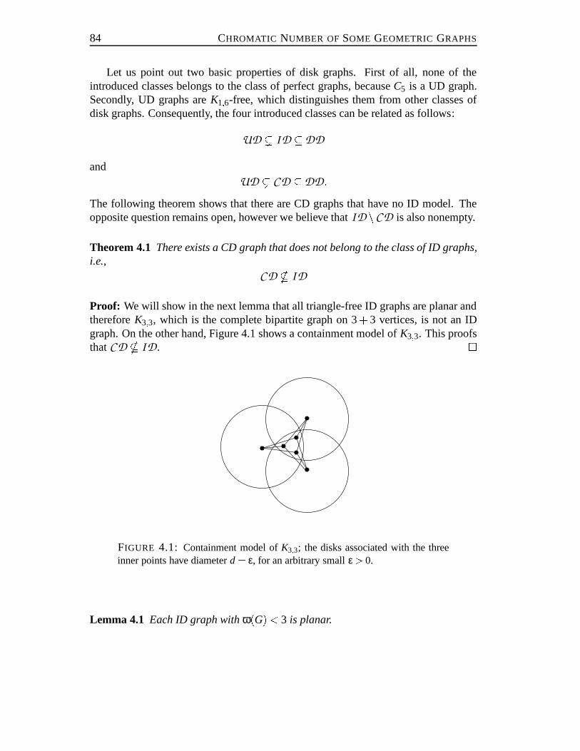
84 CHROMATIC NUMBER OF SOME GEOMETRIC GRAPHS
Let us point out two basic properties of disk graphs. First of all, none of theintroduced classes belongs to the class of perfect graphs, becauseC5 is a UD graph.Secondly, UD graphs areK1;6-free, which distinguishes them from other classes ofdisk graphs. Consequently, the four introduced classes can be related as follows:
UD ( ID �DDand
UD ( CD �DD:The following theorem shows that there are CD graphs that have no ID model. Theopposite question remains open, however we believe thatID nCD is also nonempty.
Theorem 4.1 There exists a CD graph that does not belong to the class of ID graphs,i.e.,
CD * IDProof: We will show in the next lemma that all triangle-free ID graphs are planar andthereforeK3;3, which is the complete bipartite graph on 3+ 3 vertices, is not an IDgraph. On the other hand, Figure 4.1 shows a containment model ofK3;3. This proofsthatCD * ID. �
����
����
����
����
��������
����������������
����������������
������������������������
������������������������
������������������������������������������
������������������������������������������
����������������
����������������
������������������������
������������������������
����������������������������
����������������������������������������������������������������������
������������������������������
�����������������������������������
�����������������������������������
FIGURE 4.1: Containment model ofK3;3; the disks associated with the threeinner points have diameterd = ε, for an arbitrary smallε > 0.
Lemma 4.1 Each ID graph withω(G)< 3 is planar.
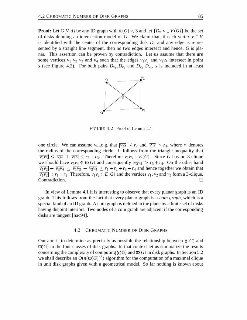
4.2 CHROMATIC NUMBER OF DISK GRAPHS 85
Proof: Let G(V;d) be any ID graph withω(G)< 3 and letfDv;v2V(G)g be the setof disks defining an intersection model ofG. We claim that, if each vertexv 2 Vis identified with the center of the corresponding diskDv and any edge is repre-sented by a straight line segment, then no two edges intersect and hence,G is pla-nar. This assertion can be proven by contradiction. Let us assume that there aresome verticesv1;v2;v3 and v4 such that the edgesv1v3 and v2v4 intersect in points (see Figure 4.2). For both pairsDv1;Dv3 and Dv2;Dv4, s is included in at least
��
����
����
����
������
����
v1v2
s
v4v3
FIGURE 4.2: Proof of Lemma 4.1
one circle. We can assume w.l.o.g. thatjv2sj � r2 and jv3sj � r3, wherer i denotesthe radius of the corresponding circle. It follows from the triangle inequality thatjv2v3j � jv2sj+ jv3sj � r2 + r3. Thereforev2v3 2 E(G). SinceG has no 3-cliquewe should havev3v4 62 E(G) and consequentlyjv3v4j > r3 + r4. On the other handjv1v2j+ jv3v4j � jv1v3j+ jv2v4j � r1+ r2+ r3+ r4 and hence together we obtain thatjv1v2j< r1+ r2. Therefore,v1v22E(G) and the verticesv1, v2 andv3 form a 3-clique.Contradiction. �
In view of Lemma 4.1 it is interesting to observe that every planar graph is anIDgraph. This follows from the fact that every planar graph is acoin graph, which is aspecial kind of an ID graph. A coin graph is defined in the plane by a finite set of diskshaving disjoint interiors. Two nodes of a coin graph are adjacent if the correspondingdisks are tangent [Sac94].
4.2 CHROMATIC NUMBER OF DISK GRAPHS
Our aim is to determine as precisely as possible the relationship betweenχ(G) andω(G) in the four classes of disk graphs. In that context let us summarize the resultsconcerning the complexity of computingχ(G) andω(G) in disk graphs. In Section 5.2we shall describe anO(n(ω(G))3) algorithm for the computation of a maximal cliquein unit disk graphs given with a geometrical model. So far nothing is known about
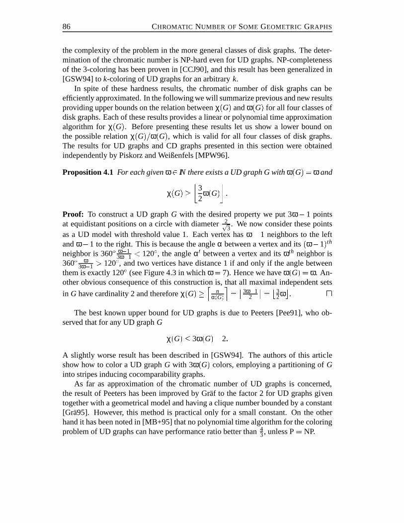
86 CHROMATIC NUMBER OF SOME GEOMETRIC GRAPHS
the complexity of the problem in the more general classes of disk graphs. The deter-mination of the chromatic number is NP-hard even for UD graphs. NP-completenessof the 3-coloring has been proven in [CCJ90], and this result has been generalized in[GSW94] tok-coloring of UD graphs for an arbitraryk.
In spite of these hardness results, the chromatic number of disk graphs can beefficiently approximated. In the following we will summarize previous and new resultsproviding upper bounds on the relation betweenχ(G) andω(G) for all four classes ofdisk graphs. Each of these results provides a linear or polynomial time approximationalgorithm for χ(G). Before presenting these results let us show a lower bound onthe possible relationχ(G)=ω(G), which is valid for all four classes of disk graphs.The results for UD graphs and CD graphs presented in this section were obtainedindependently by Piskorz and Weißenfels [MPW96].
Proposition 4.1 For each givenω2 IN there exists a UD graph G withω(G) = ω and
χ(G)� �32
ω(G)� :Proof: To construct a UD graphG with the desired property we put 3ω� 1 pointsat equidistant positions on a circle with diameter2p
3. We now consider these points
as a UD model with threshold value 1. Each vertex hasω� 1 neighbors to the leftandω�1 to the right. This is because the angleα between a vertex and its(ω�1)thneighbor is 360� ω�1
3ω�1 < 120�, the angleα0 between a vertex and itsωth neighbor is360� ω
3ω�1 > 120�, and two vertices have distance 1 if and only if the angle betweenthem is exactly 120� (see Figure 4.3 in whichω = 7). Hence we haveω(G) = ω. An-other obvious consequence of this construction is, that all maximal independent sets
in G have cardinality 2 and thereforeχ(G)� l nα(G)m= �3ω�1
2
�= �32ω�. �
The best known upper bound for UD graphs is due to Peeters [Pee91], who ob-served that for any UD graphG
χ(G)� 3ω(G)�2:A slightly worse result has been described in [GSW94]. The authors of this articleshow how to color a UD graphG with 3ω(G) colors, employing a partitioning ofGinto stripes inducing cocomparability graphs.
As far as approximation of the chromatic number of UD graphs is concerned,the result of Peeters has been improved by Graf to the factor 2 for UD graphs giventogether with a geometrical model and having a clique number bounded by a constant[Gra95]. However, this method is practical only for a small constant. Onthe otherhand it has been noted in [MB+95] that no polynomial time algorithm for the coloringproblem of UD graphs can have performance ratio better than4
3, unless P= NP.
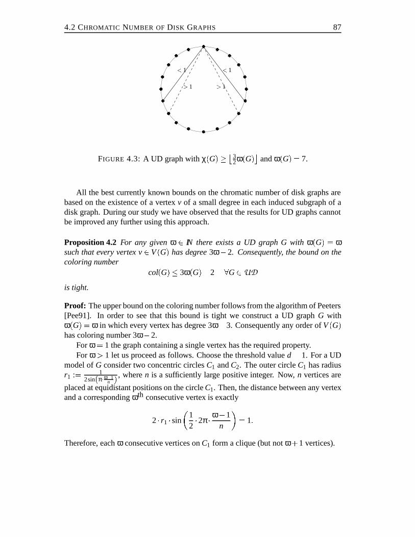
4.2 CHROMATIC NUMBER OF DISK GRAPHS 87
����
����
��������
����
����
����
����
������
��������
����
��������
����
����
������
����
��������
�����������������������������������������������������������������������������������������������������������������������������������������������������������������������������������������������������������������������������
�����������������������������������������������������������������������������������������������������������������������������������������������������������������������������������������������������������������������������
�����������������������������������������������������������������������������������������������������������������������������������������������������������������������������������������������������������������������������
�����������������������������������������������������������������������������������������������������������������������������������������������������������������������������������������������������������������������������
���������������������������������������������������������������������������������������������������������������������������������������������������������������������������������������������������������������������������������
���������������������������������������������������������������������������������������������������������������������������������������������������������������������������������������������������������������������������������
���������������������������������������������������������������������������������������������������������������������������������������������������������������������������������������������������������������������������������
��������������������������������������������������������������������������������������������������������������������������������������������������������������������������������������������������������������������������������� < 1< 1 > 1> 1
FIGURE 4.3: A UD graph withχ(G)� �32ω(G)� andω(G) = 7.
All the best currently known bounds on the chromatic number of disk graphs arebased on the existence of a vertexv of a small degree in each induced subgraph of adisk graph. During our study we have observed that the results for UD graphs cannotbe improved any further using this approach.
Proposition 4.2 For any givenω 2 IN there exists a UD graph G withω(G) = ωsuch that every vertex v2 V(G) has degree3ω�2. Consequently, the bound on thecoloring number
col(G)� 3ω(G)�2 8G2UDis tight.
Proof: The upper bound on the coloring number follows from the algorithm of Peeters[Pee91]. In order to see that this bound is tight we construct a UD graphG withω(G) = ω in which every vertex has degree 3ω�3. Consequently any order ofV(G)has coloring number 3ω�2.
Forω = 1 the graph containing a single vertex has the required property.For ω > 1 let us proceed as follows. Choose the threshold valued = 1. For a UD
model ofG consider two concentric circlesC1 andC2. The outer circleC1 has radiusr1 := 1
2sin(π�ω�1n ) , wheren is a sufficiently large positive integer. Now,n vertices are
placed at equidistant positions on the circleC1. Then, the distance between any vertexand a correspondingωth consecutive vertex is exactly
2� r1 �sin
�12�2π � ω�1
n
�= 1:Therefore, eachω consecutive vertices onC1 form a clique (but notω+1 vertices).
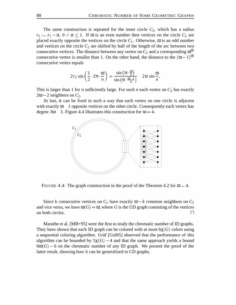
88 CHROMATIC NUMBER OF SOME GEOMETRIC GRAPHS
The same construction is repeated for the inner circleC2, which has a radiusr2 := r1�α, 0< α � 1. If ω is an even number then vertices on the circleC2 areplaced exactly opposite the vertices on the circleC1. Otherwise,ω is an odd numberand vertices on the circleC2 are shifted by half of the length of the arc between twoconsecutive vertices. The distance between any vertex onC2 and a correspondingωth
consecutive vertex is smaller than 1. On the other hand, the distance to the(ω+1)thconsecutive vertex equals
2r2 sin
�12�2π � ω
n
�= sin�π � ω
n
�sin�π � ω�1
n
��2α sinωn:
This is larger than 1 forn sufficiently large. For suchn each vertex onC2 has exactly2ω�2 neighbors onC2.
At last, α can be fixed in such a way that each vertex on one circle is adjacentwith exactlyω�1 opposite vertices on the other circle. Consequently each vertex hasdegree 3ω�3. Figure 4.4 illustrates this construction forω = 4.
����
����
����
����
����
����
����
������
������
������
������
������
������
������
C1
C2
FIGURE 4.4: The graph construction in the proof of the Theorem 4.2 forω = 4.
Sincek consecutive vertices onC1 have exactlyω� k common neighbors onC2and vice versa, we haveω(G) = ω, whereG is the UD graph consisting of the verticeson both circles. �
Marathe et al. [MB+95] were the first to study the chromatic number of ID graphs.They have shown that each ID graph can be colored with at most 6χ(G) colors usinga sequential coloring algorithm. Graf [Gra95] observed that the performance ofthisalgorithm can be bounded by 5χ(G)�4 and that the same approach yields a bound6ω(G)� 6 on the chromatic number of any ID graph. We present the proof of thelatter result, showing how it can be generalized to CD graphs.
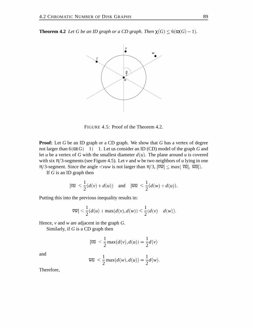
4.2 CHROMATIC NUMBER OF DISK GRAPHS 89
Theorem 4.2 Let G be an ID graph or a CD graph. Thenχ(G)� 6(ω(G)�1).����
����
����
����
������������������������
������������������������
t
vw
π3
u
FIGURE 4.5: Proof of the Theorem 4.2.
Proof: Let G be an ID graph or a CD graph. We show thatG has a vertex of degreenot larger than 6(ω(G)�1)�1. Let us consider an ID (CD) model of the graphG andlet u be a vertex ofG with the smallest diameterd(u). The plane aroundu is coveredwith six π=3-segments (see Figure 4.5). Letv andw be two neighbors ofu lying in oneπ=3-segment. Since the anglevuw is not larger thanπ=3, jvwj �max(jvuj; jwuj).
If G is an ID graph thenjvuj � 12(d(v)+d(u)) and jwuj � 1
2(d(w)+d(u)):
Putting this into the previous inequality results in:jvwj � 12(d(u)+max(d(v);d(w))� 1
2(d(v)+d(w)):
Hence,v andw are adjacent in the graphG.Similarly, if G is a CD graph thenjvuj � 1
2max(d(v);d(u)) = 1
2d(v)
and jwuj � 12
max(d(w);d(u)) = 12
d(w):Therefore,
90 CHROMATIC NUMBER OF SOME GEOMETRIC GRAPHSjvwj �max(jvuj; jwuj)� 12
max(d(v);d(w));which means thatv andw are adjacent.
Since any two neighbors ofu contained in one segment are adjacent,jN(u)j �6(ω(G)� 1). This bound can improved to 6(ω(G)� 1)� 1 observing that the seg-ments can be always constructed in such a way that at least one vertext 6= u lies onthe border of two segments. �
For double disk graphs no constant bound on the ratioχ(G)=ω(G) was previouslyknown. Graf, Stumpf and Weißenfels have shown in [GSW94] that any DD graph
can be colored in polynomial time using(K + 1)ω(G) colors, whereK := l 2D0p3d0
m,
D0 := 12(maxvd(v)+maxvD(v)) andd0 := 1
2(minvd(v)+minvD(v)). This yields agood upper bound on the chromatic number provided that the difference in the size ofvarious disks is not large. For instance, ifD0
d0<p3 thenχ(G)� 3ω(G).
The next theorem shows that the ratio betweenχ(G) andω(G) is bounded by aconstant irrespectively of the size of particular disks.
Theorem 4.3 For any DD graph G
χ(G)� 33(ω(G)�1)�2:Proof: Recall that any induced subgraph of a DD graph is a DD graph itself. Hence,the assertion can be proven showing that any DD graphG has a vertex of degree notlarger than 33(ω(G)�1)�3. Consider a DD model(V;d;D) of a graphG with theclique numberω� 2. Letv be a vertex with the smallest outer diameterD(v) =: D.
For an appropriate constant 0< a< 12, we partition the neighborhoodN(v) of the
vertexv into three subsets:
N1(v) - the neighbors represented by points contained in the outer disk ofv,
N2(v) - the neighbors represented by points lying outside the outer disk ofv but notmore thanaD away from this disk,
N3(v) - the remaining neighbors.
The idea is now to show that each part of the neighborhoodNi(v), i 2 f1;2;3g, can bepartitioned into a constant number of sectors, such that all neighbors contained in onesector form a clique.
We first consider the neighborhoodN1(v). Since the outer disk of any vertexu1 2V(G) has the diameterD(u1) � D, and the distance between any two verticesu1;u2contained in aπ=3-segments of the outer disk associated withv is smaller thanD
2 , u1andu2 are adjacent. Hence,jN1(v)j � 6(ω(G)�1).
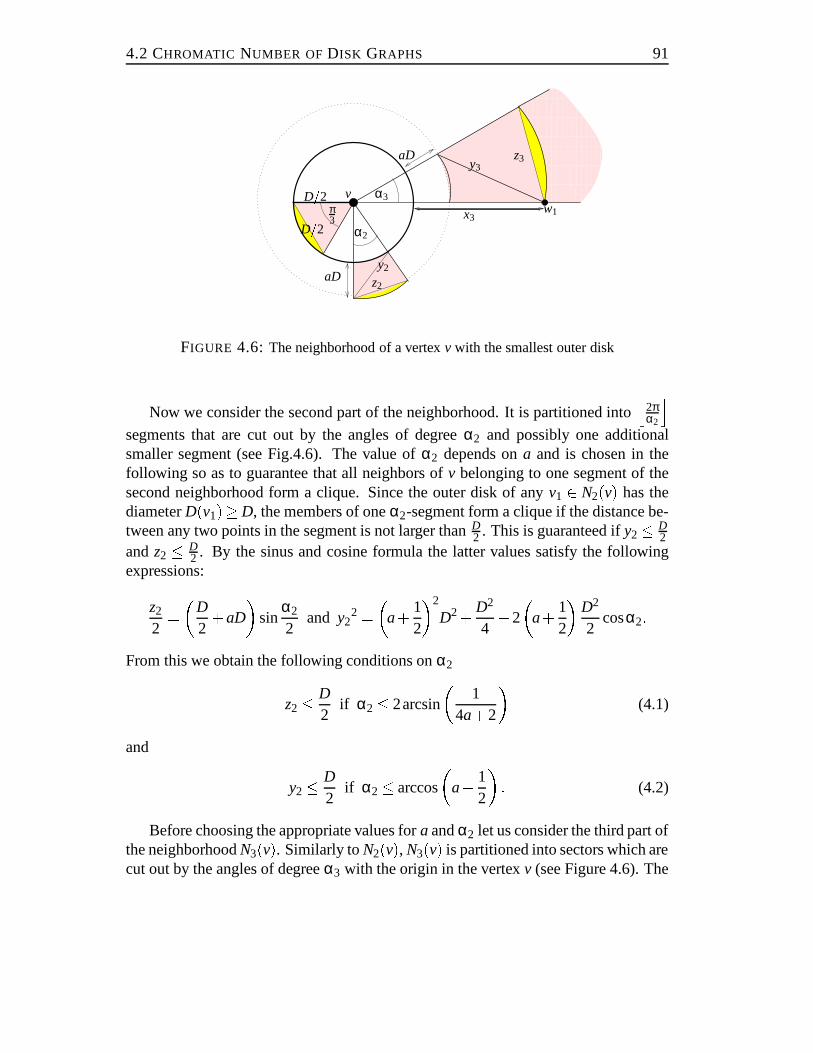
4.2 CHROMATIC NUMBER OF DISK GRAPHS 91
���������������������������������������������������������������������������������������������������������������������������������������������������������������������������������������������������
���������������������������������������������������������������������������������������������������������������������������������������������������������������������������������������������������
�������������������������������������������������������������������������������������������������������������������������������������������������������������������������
�������������������������������������������������������������������������������������������������������������������������������������������������������������������������
D=2
D=2
vπ3
α2
z2
y2aD
α3
aD
x3
y3z3
w1
FIGURE 4.6: The neighborhood of a vertexv with the smallest outer disk
Now we consider the second part of the neighborhood. It is partitioned intoj
2πα2
ksegments that are cut out by the angles of degreeα2 and possibly one additionalsmaller segment (see Fig.4.6). The value ofα2 depends ona and is chosen in thefollowing so as to guarantee that all neighbors ofv belonging to one segment of thesecond neighborhood form a clique. Since the outer disk of anyv1 2 N2(v) has thediameterD(v1)�D, the members of oneα2-segment form a clique if the distance be-tween any two points in the segment is not larger thanD
2 . This is guaranteed ify2� D2
andz2 � D2 . By the sinus and cosine formula the latter values satisfy the following
expressions:
z2
2= �D
2+aD
�sin
α2
2and y2
2 = �a+ 12
�2
D2+ D2
4�2
�a+ 1
2
�D2
2cosα2:
From this we obtain the following conditions onα2
z2� D2
if α2� 2arcsin
�1
4a+2
�(4.1)
and
y2� D2
if α2� arccos
�a+ 1
2
� : (4.2)
Before choosing the appropriate values fora andα2 let us consider the third part ofthe neighborhoodN3(v). Similarly toN2(v), N3(v) is partitioned into sectors which arecut out by the angles of degreeα3 with the origin in the vertexv (see Figure 4.6). The
92 CHROMATIC NUMBER OF SOME GEOMETRIC GRAPHS
value ofα3 will be chosen so as to guarantee that any two neighbors ofv belongingto one sector are adjacent. This is achieved if for allw1 2 N3(v), the outer disk ofw1 covers all the verticesw2 2 N3(v) for which jw2vj � jw1vj. This requirement isfulfilled whenz3 � x3 andy3 � x3 (becausex3 � D(w1)). Employing once more thesinus and cosine formula we obtain that
z3
2= �D
2+x3
�sin
α3
2
and
y32 = �D
2+x3
�2+�D2+aD
�2�2
�D2+x3
��D2+aD
�cosα3:
From this we obtain that
z3� x3 if sinα3
2� 1
2� D
4x3+2D
and
y3� x3 if cosα3� 11+2a
+ a(a+1)D(1+2a)x3+ �12 +a
�D:
Observing thatx3 > aD the above conditions can be strengthened to the followingconditions onα3:
α3� 2arcsin
�12� D
4aD+2D
�(4.3)
and
α3� arccos
1
1+2a+ a(a+1)(1+2a)a+ �1
2 +a�! : (4.4)
We now choose the values fora, α2 andα3 so as to satisfy the conditions 4.1 – 4.4
and to keepl
2πα2
m+ l2πα3
mpossibly small. Settinga = 1
4, α2 = 330 andα3 = 230 we
obtain thatjN(v)j � �l2πα1
m+l2πα2
m+l2πα3
m�(ω(G)�1)� (6+11+16)(ω(G)�1) =33(ω(G)� 1). This can be improved to 33(ω(G)� 1)� 3 observing that each partof the neighborhood can be divided into sectors in such a way that one neighbor ofvbelongs to two sectors. �
4.3 CHROMATIC NUMBER OF RECTANGLE GRAPHS 93
4.3 CHROMATIC NUMBER OF RECTANGLE GRAPHS
In this section we continue the study of the chromatic number of intersection graphs ofsome other regular figures in the plane. We examine intersection graphs of rectanglesin the plane, where all rectangles have edges parallel to the coordinate axes.Rectangleintersection graphs — or for short rectangle graphs — have been studied long beforethe disk graphs. They build a very natural generalization of the well known classof interval graphs. Besides the 2-dimensional case, one considers also intersectiongraphs of boxes, i.e. generalized rectangles, with sides parallel to the coordinate axisin thek-dimensional space. Let us note that a lot of attention has been devoted to thestudy of theboxicityof a graphG. This parameter is defined as the smallest numberk such thatG has the representation as an intersection graph of boxes in dimensionk ([Rob69], [Yan82]). A previously open problem of the complexity of recognizinggraphs with boxicity 2, i.e. rectangle graphs, has been proven to be NP-complete byKratochvil [Kra94].
As far as the computation ofω(G) andχ(G) in rectangle graphs is concerned, thecomplexity of these problems resembles the case of UD graphs. Given a geometricmodel of a rectangle graphG its clique numberω(G) can be computed inO(nlogn)time [Lee83] but the computation of its chromatic numberχ(G) is NP-hard [LL84].
Already Asplund and Grunbaum have studied the relationship betweenχ(G) andω(G) in rectangle graphs. They proved in [AG60] that the chromatic number oftriangle-free rectangle graphs is at most 6 and that this bound is tight. For arbitraryω(G), they showed thatχ(G) < 4(ω(G))2. The latter bound has been improved byBurling [Bur65] who proved thatχ(G) � 2(ω(G))2�ω(G) in rectangle graphs. In-terestingly enough, Burling also constructed a family of 3-dimensional triangle-freeboxes having an arbitrarily high chromatic number.
It is still open if the ratio betweenχ(G) andω(G) is bounded by a constant inrectangle graphs. In the present work we have succeeded in showing a constant boundin two special cases. The first result shows a linear relation betweenχ(G) andω(G)in rectangle graphs in which either the ratio between the width or the ratio betweenthe height of different rectangles is bounded by a constant. The second result proves alinear relation for rectangle graphs in which the ratio between the width andthe heightof every single rectangle is bounded by a constant. Before presenting these results, letus show a lower bound on theχ-binding function of rectangle graphs.
Proposition 4.3 For each givenω 2 IN there exists a rectangle graph G withω(G) =ω and
χ(G)� �4ω�13
� :Proof: Consider the graphGω presented in Figure 4.7. It is build according to a similarprinciple as the UD graph from Proposition 4.1. It has 4ω�1 vertices represented as
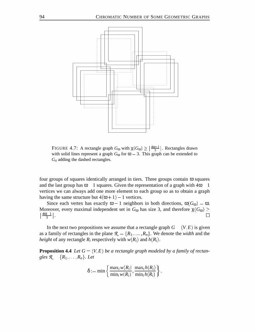
94 CHROMATIC NUMBER OF SOME GEOMETRIC GRAPHS
FIGURE 4.7: A rectangle graphGω with χ(Gω) � �4ω�1
3
�. Rectangles drawn
with solid lines represent a graphGω for ω = 3. This graph can be extended toG4 adding the dashed rectangles.
four groups of squares identically arranged in tiers. Three groups containω squaresand the last group hasω�1 squares. Given the representation of a graph with 4ω�1vertices we can always add one more element to each group so as to obtain a graphhaving the same structure but 4(ω+1)�1 vertices.
Since each vertex has exactlyω� 1 neighbors in both directions,ω(Gω) = ω.Moreover, every maximal independent set inGω has size 3, and thereforeχ(Gω) ��4ω�1
3
�. �
In the next two propositions we assume that a rectangle graphG= (V;E) is givenas a family of rectangles in the planeR = fR1; : : : ;Rng. We denote thewidthand theheightof any rectangleRi respectively withw(Ri) andh(Ri).Proposition 4.4 Let G= (V;E) be a rectangle graph modeled by a family of rectan-glesR = fR1; : : : ;Rng. Let
δ := min
�maxi w(Ri)mini w(Ri) ; maxi h(Ri)
mini h(Ri)� :
4.3 CHROMATIC NUMBER OF RECTANGLE GRAPHS 95
Then the chromatic number of G is at most
χ(G)� 3(blogδc+1)ω(G):Proof: W.l.o.g. we can assume thatδ = maxi h(Ri)
mini h(Ri) . For simplicity let us denotemaxi h(Ri) with Maxh and mini h(Ri) with Minh. The set of rectanglesR is partitionedinto k := blogδc+1 groups, where the groupR j , 1� j � k, contains all rectanglesRi
with the heighth(Ri), Maxh2 j < h(Ri)� Maxh
2 j�1 . Each subgraphG j induced by the groupR j can be colored using 3ω(G j) colors. This can be seen as follows.
Let us partition the plane horizontal lines into stripes of the heightMaxh2 j . The
lines are chosen so as not to contain any rectangle edge. Each rectangle from thegroupR j is now associated with the stripe that contains its bottom edge. RectanglesR j are colored in groups corresponding to the allocation to the stripes. Note that norectangle overlaps more than three stripes, and therefore the same set of colors canbe used for every fourth stripe. On the other hand, rectangles associated withonestripe build an interval graph — the adequate representation can be always seen on theupper boundary of the stripe. This boundary is reached by all associated rectanglesbecause their height exceeds the height of one stripe. Since interval graphs are perfectrectangles associated with one stripe can be colored using at mostω(G j) colors andfor the whole graphG j not more than 3ω(G j) colors are needed.
Summing up over 1� j � k we obtain that
χ(G)� 3� k
∑j=1
ω(G j)� 3(blogδc+1)ω(G): �Proposition 4.5 Let G= (V;E) be a rectangle graph represented by a family of rect-anglesR = fR1; : : : ;Rng, such that
c2� w(Ri)h(Ri) � c1; for every1� i � n:
Then, the chromatic number of G is at most
χ(G)� 2
��c1
c2
�+1
� (ω(G)�1)+1:Proof: We will show that every rectangle graph contains a vertexv of degreedeg(v)�2�l
c1c2
m+1�(ω(G)�1). Since the class of rectangle graphs is closed under taking

96 CHROMATIC NUMBER OF SOME GEOMETRIC GRAPHS
induced subgraphs, the bound on the minimum degree yields the claimed bound onthe chromatic number.
Let us consider the vertexvi represented by a lowest rectangleRi . It holds forevery rectangleRj 2 R that
h(Rj)� h(Ri) and w(Rj)� c2h(Rj)� c2h(Ri)� c2
c1w(Ri):
Every neighbor ofvi must intersect one of the edges ofRi . Let us first analyze theneighbors ofRi intersecting its lower edgel i. Starting from the left corner we parti-
tion this edge intol
c1c2
msegments. The first
jc1c2
ksegments have widthc2
c1w(Ri) and a
possible one additional segment is shorter. All neighbors ofRi intersecting with theirleft vertical edge the same segment ofl i , must intersect each other. Therefore, theirnumber is bounded byω(G)�1. Some neighbors ofRi may intersectl i only with theirright vertical edge. They also build a clique, since all of them contain the left-handlower corner ofRi . Altogether, the number of neighbors ofRi intersecting its lower
edgel i is bounded by�l
c1c2
m+1�(ω(G)� 1). By symmetry, the same is valid for
the neighbors intersecting the upper edge ofRi . Since every rectangle intersecting avertical edge ofRi must also intersect one of its horizontal edges, the overall number
of vi is bounded by 2�l
c1c2
m+1�(ω(G)�1). �4.4 CONCLUSIONS
In this chapter we have studied the chromatic number of graphs obtained from inter-sections of some geometric figures in the plane. We have restricted our attention tovery regular figures, namely disks and rectangles. For each of these families, there isa function f such thatχ(G)� f (ω(G)), for every graphG. It is a linear function forall classes of disk graphs and a quadratic function for the rectangle graphs. In thatcontext two important problems still remain open. The first one is the existence of alinearχ-binding function for rectangle graphs and the second problem is the determi-nation of an exact value of theχ-binding function for UD graphs. Moreover, in viewof the study of interference graphs, it would be interesting to characterize a possiblylarge class of intersection graphs, for which the chromatic number is linearlyboundedin the clique number.
A complete understanding of the relation betweenχ(G) andω(G) in interferencegraphs, requires the study of more irregular figures. It is an important and still openquestion, if all intersection graphs in the plane have aχ-binding function. Consideringintersection graphs of convex polygons, it seems that the complexity of the problemsubstantially depends on the number of lines limiting the admissible directions of thepolygon edges. For the case when this number is bounded by a constant, the existence
4.4 CONCLUSIONS 97
of an exponentialχ-binding function has been proven by Burling [Bur65]. However,if the number of directions is not fixed then the existence of anyχ-binding function isstill not known even for intersection graphs of straight-line segments.

CHAPTER 5
ALGORITHMIC PROPERTIES OFDISK GRAPHS
5.1 INTRODUCTION
The structure of interference graphs modeling cellular networks most closely resem-bles intersection graphs of disks in the plane. In Chapter 4, four classes of disk graphswere introduced, each modeling cellular networks with different degree of accuracy.Two of these classes — unit disk graphs and intersection disk graphs — are the subjectof the study in the present chapter. So far, we have only examined the approximabil-ity of the chromatic numberχ(G) and its relation to the clique numberω(G) in theintroduced classes of disk graphs. The aim of that study has been a theoretical ex-planation of an empirical observation that the chromatic number of graphs modelingreal cellular networks hardly exceeds their clique number. For a deeper understand-ing of the structure and properties of interference graphs we now turn our attention tothe complexity of computing other basic graph parameters such asmaximum clique,maximum independent set, minimum vertex cover, andminimum domination set. Anadditional motivation is given by practical applications of some of these parameters.For instance, a dominating set problem in UD graphs with a containment model canbe used to model the emergency sender problem. In this problem one is looking for aminimum subset of a set of transmitters, which can transmit to all remaining stations[TSRB71].
Clark, Colbourn and Johnson [CCJ90] considered the complexity of several stan-dard graph theoretical problems on UD graphs, including coloring and the other fourproblems mentioned above. They showed that all these problems except the maxi-mum clique problem remain NP-hard when restricted to UD graphs. For the maxi-mum clique problem they developed anO(n4:5) algorithm for UD graphs given with ageometric representation. In Section 5.2 we present an improved version of this algo-rithm having the worst case complexityO(nω3), whereω denotes the clique numberω(G).
Clark, Colbourn and Johnson were the first to observe a certain similarity betweenUD graphs and planar graphs. Note that there are some UD graphs likeK5 that arenot planar as well as some planar graphs likeK1;6 that are not UD graphs. However,the complexity of all graph problems mentioned above is the same in both classes.This analogy is confirmed by the results on the approximation of some NP-hard graph
99
100 ALGORITHMIC PROPERTIES OFDISK GRAPHS
parameters. In both cases of the UD graphs and the planar graphs, the chromaticnumberχ(G) can be approximated within a certain constant ratio, but no polynomialtime approximation algorithm for the coloring problem can have a performance ratiobetter than4
3 in any of the two classes, unless P = NP. Baker [Bak83] constructedpolynomial time approximation schemes (PTAS) for the maximum independent set,minimum vertex cover and minimum dominating set problem in planar graphs. Forall these problems in UD graphs Marathe et al. [MB+95] constructed constant ratioapproximation algorithms. Few years later, they generalized the results of Baker byconstructing PTAS for the three problems in UD graphs [HM+94].
These results show an apparent similarity between the complexity of solving prob-lems in UD graphs and planar graphs. However, there is one important problem havingdifferent complexity in the two classes, namely therecognition problem. It is decid-able in linear time if a graph is planar [HT74], but the recognition of UD graphs isNP-complete [BK93].
A similar relationship cannot be confirmed for planar graphs and intersection diskgraphs, which contain the class of planar graphs. For ID graphs the complexity of themaximum clique problem remains unknown. We have already mentioned in Section4.2 that the chromatic number of ID graphs can be approximated within the ratio 5.Marathe et al. constructed a polynomial time5
3-approximation algorithm for the mini-mum vertex cover and a 5-approximation algorithm for the maximum independent setproblem in ID graphs [MB+95]. In Section 5.3 we show that the ratio for the min-imum vertex cover can be improved to32 both for the unweighted as well as for theweighted case. However, no polynomial time approximation scheme is yet known forID graphs.
The complexity of the basic graph problems in UD, ID and planar graphs is sum-marized in Table 5.1.
In the remaining part of this chapter we present our improved algorithms for theclique problem in UD graphs and the vertex cover problem in ID graphs.
5.2 MAXIMUM CLIQUE
We sketch the idea of the algorithm developed by Clark, Colbourn and Johnson thatfinds a maximum clique in any UD graph inO(n4:5) time [CCJ90]. Afterwards, wepresent an improved version of this algorithm having the time complexityO(nω3).
In the following, letC(v; r) denote the closed circle centered at the pointv andhaving the radiusr. Recall thatjvwj denotes the distance between two pointsv andw.Then, letRvw denote the intersection of two closed disks of radiusjvwj, one centered atv and one centered atw, i.e.,Rvw=C(v; jvwj)\C(w; jvwj). Furthermore, ifG= (V;E)is a UD graph given with a UD model(V;d), thenHvw denotes the set of verticescontained inRvw.
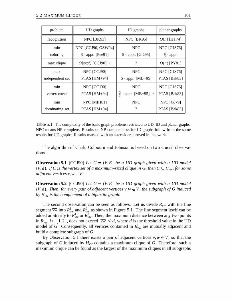
5.2 MAXIMUM CLIQUE 101
problem UD graphs ID graphs planar graphs
recognition NPC [BK93] NPC [BK95] O(n) [HT74]
min NPC [CCJ90, GSW94] NPC NPC [GJS76]
coloring 3 - appr. [Pee91] 5 - appr. [Gra95] 43 - appr.
max clique O(nω3) [CCJ90],� ? O(n) [PY81]
max NPC [CCJ90] NPC NPC [GJS76]
independent set PTAS [HM+94] 5 - appr. [MB+95] PTAS [Bak83]
min NPC [CCJ90] NPC NPC [GJS76]
vertex cover PTAS [HM+94] 32 - appr. [MB+95],� PTAS [Bak83]
min NPC [MIH81] NPC NPC [GJ79]
dominating set PTAS [HM+94] ? PTAS [Bak83]
Table 5.1:The complexity of the basic graph problems restricted to UD,ID and planar graphs.NPC means NP-complete. Results on NP-completeness for ID graphs follow from the sameresults for UD graphs. Results marked with an asterisk are proved in this work.
The algorithm of Clark, Colbourn and Johnson is based on two crucial observa-tions.
Observation 5.1 [CCJ90] Let G= (V;E) be a UD graph given with a UD model(V;d). If C is the vertex set of a maximum–sized clique in G, then C� Hvw, for someadjacent vertices v;w2V.
Observation 5.2 [CCJ90] Let G= (V;E) be a UD graph given with a UD model(V;d). Then, for every pair of adjacent vertices v;w2V, the subgraph of G inducedby Hvw is the complement of a bipartite graph.
The second observation can be seen as follows. Let us divideRvw with the linesegmentvw into R1
vw andR2vw as shown in Figure 5.1. The line segment itself can be
added arbitrarily toR1vw or R2
vw. Then, the maximum distance between any two pointsin Ri
vw, i 2 f1;2g, does not exceedjvwj � d, whered is the threshold value in the UDmodel ofG. Consequently, all vertices contained inRi
vw are mutually adjacent andbuild a complete subgraph ofG.
By Observation 5.1 there exists a pair of adjacent vertices ˜v; w 2 V, so that thesubgraph ofG induced byHvw contains a maximum clique ofG. Therefore, such amaximum clique can be found as the largest of the maximum cliques in all subgraphs
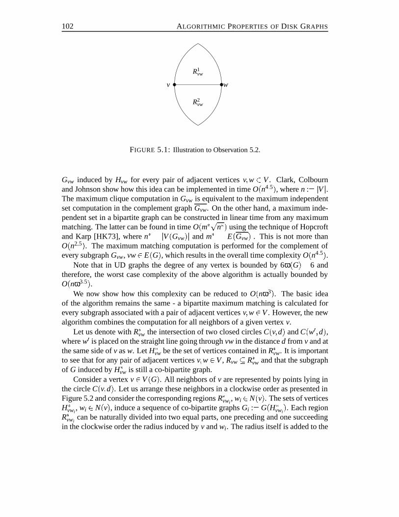
102 ALGORITHMIC PROPERTIES OFDISK GRAPHS
��������
R1vw
v w
R2vw
FIGURE 5.1: Illustration to Observation 5.2.
Gvw induced byHvw for every pair of adjacent verticesv;w 2 V. Clark, Colbournand Johnson show how this idea can be implemented in timeO(n4:5), wheren := jVj.The maximum clique computation inGvw is equivalent to the maximum independentset computation in the complement graphGvw. On the other hand, a maximum inde-pendent set in a bipartite graph can be constructed in linear time from any maximummatching. The latter can be found in timeO(m�pn�) using the technique of Hopcroftand Karp [HK73], wheren� = jV(Gvw)j andm� = jE(Gvw)j. This is not more thanO(n2:5). The maximum matching computation is performed for the complement ofevery subgraphGvw, vw2E(G), which results in the overall time complexityO(n4:5).
Note that in UD graphs the degree of any vertex is bounded by 6ω(G)� 6 andtherefore, the worst case complexity of the above algorithm is actually bounded byO(nω3:5).
We now show how this complexity can be reduced toO(nω3). The basic ideaof the algorithm remains the same - a bipartite maximum matching is calculated forevery subgraph associated with a pair of adjacent verticesv;w2V. However, the newalgorithm combines the computation for all neighbors of a given vertexv.
Let us denote withR�vw the intersection of two closed circlesC(v;d) andC(w0;d),wherew0 is placed on the straight line going throughvw in the distanced from v and atthe same side ofv asw. Let H�
vw be the set of vertices contained inR�vw. It is importantto see that for any pair of adjacent verticesv;w2V, Rvw� R�vw and that the subgraphof G induced byH�
vw is still a co-bipartite graph.Consider a vertexv2V(G). All neighbors ofv are represented by points lying in
the circleC(v;d). Let us arrange these neighbors in a clockwise order as presented inFigure 5.2 and consider the corresponding regionsR�vwi
, wi 2N(v). The sets of verticesH�
vwi, wi 2 N(v), induce a sequence of co-bipartite graphsGi := G(H�
vwi). Each region
R�vwican be naturally divided into two equal parts, one preceding and one succeeding
in the clockwise order the radius induced byv andwi . The radius itself is added to the
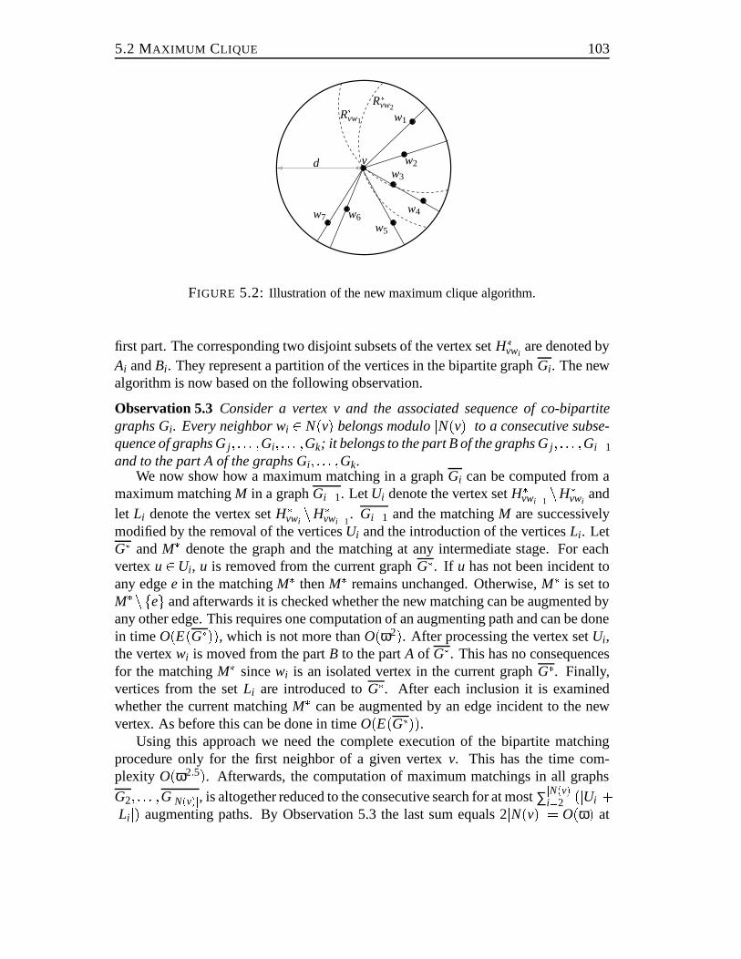
5.2 MAXIMUM CLIQUE 103
����
����
����
����
����
����
����
�����������������������������������������������������������
���������������������������������������������������������������������������������������������������������
������������������������������������������������������������������������������������������������������������������������
����������������������������������������������������������������������������������������������������
����������������������������������������������������������������������������������������������������
����������������������������������������������������������������������������������������������������
����������������������������������������������������������������������������������������������������
������������������������������������������������������������������������������������������������������������
������������������������������������������������������������������������������������������������������������w2
w1
w7
d
R�vw1
R�vw2
w6w5
w4
w3
v
FIGURE 5.2: Illustration of the new maximum clique algorithm.
first part. The corresponding two disjoint subsets of the vertex setH�vwi
are denoted byAi andBi . They represent a partition of the vertices in the bipartite graphGi . The newalgorithm is now based on the following observation.
Observation 5.3 Consider a vertex v and the associated sequence of co-bipartitegraphs Gi . Every neighbor wi 2 N(v) belongs modulojN(v)j to a consecutive subse-quence of graphs Gj ; : : : ;Gi; : : : ;Gk; it belongs to the part B of the graphs Gj ; : : : ;Gi�1and to the part A of the graphs Gi; : : : ;Gk.
We now show how a maximum matching in a graphGi can be computed from amaximum matchingM in a graphGi�1. LetUi denote the vertex setH�
vwi�1nH�
vwiand
let Li denote the vertex setH�vwinH�
vwi�1. Gi�1 and the matchingM are successively
modified by the removal of the verticesUi and the introduction of the verticesLi . LetG� andM� denote the graph and the matching at any intermediate stage. For eachvertexu2Ui , u is removed from the current graphG�. If u has not been incident toany edgee in the matchingM� thenM� remains unchanged. Otherwise,M� is set toM� nfeg and afterwards it is checked whether the new matching can be augmented byany other edge. This requires one computation of an augmenting path and can be donein time O(E(G�)), which is not more thanO(ω2). After processing the vertex setUi,the vertexwi is moved from the partB to the partA of G�. This has no consequencesfor the matchingM� sincewi is an isolated vertex in the current graphG�. Finally,vertices from the setLi are introduced toG�. After each inclusion it is examinedwhether the current matchingM� can be augmented by an edge incident to the newvertex. As before this can be done in timeO(E(G�)).
Using this approach we need the complete execution of the bipartite matchingprocedure only for the first neighbor of a given vertexv. This has the time com-plexity O(ω2:5). Afterwards, the computation of maximum matchings in all graphs
G2; : : : ;GjN(v)j, is altogether reduced to the consecutive search for at most∑jN(v)ji=2 (jUij+jLij) augmenting paths. By Observation 5.3 the last sum equals 2jN(v)j = O(ω) at
104 ALGORITHMIC PROPERTIES OFDISK GRAPHS
most. Therefore, the search for maximum matchings in all graphsG1; : : : ;GjN(v)j re-quires altogetherO(ω2:5+ω �ω2) = O(ω3) time.
The same approach is now applied to the neighbors of every vertexv2V. In totalwe obtain anO(nω3) algorithm for the maximum clique computation in UD graphs.This proves the following theorem.
Theorem 5.1 Given a UD graph G with a UD model, a maximum clique in G can befound in O(nω3) time.
5.3 VERTEX COVER
Marathe et al. constructed a polynomial time53-approximation algorithm for the un-
weighted vertex cover problem in intersection disk graphs [MB+95]. In this sectionwe generalize this result to the weighted vertex problem and improve the performanceratio from 5
3 to 32 both in the unweighted and weighted case.
Let us recall that in theminimum weighted vertex problem(WVC) we are given agraphG= (V;E) and a weightw(v)� 0 for each vertexv2V, and we wish to selecta subset of verticesS� V such that for each edge(u;v) 2 E at least one ofu andvis in S, and so as to minimize the total weight ofS, w(S) := ∑v2Sw(v). The specialcase with weightsw(v) = 1, for everyv2V, is called the (unweighted) vertex coverproblem (VC).
The vertex cover problem is MAX SNP-hard even in the unweighted case [PY91].A simple linear time 2-approximation algorithm for the unweighted case is being at-tributed to Gavril [GJ79]. For the weighted case an elegant linear time 2-approximationalgorithm was developed by Bar-Yehuda and Even [BE81]. It is remarkable that af-ter a long time it is still unknown if there is aρ-approximation algorithm for the VCproblem, for any constantρ < 2.
The situation is different for planar graphs. The VC problem remains NP-completewhen restricted to planar graphs. However, as we have already mentioned, there is apolynomial time approximation scheme for the vertex cover problem in planar graphs[Bak83]. In our investigation we use a method developed by Bar-Yehuda and Even[BE85], which yields a3
2-approximation algorithm for planar graphs. This methodhas been previously used by Marathe et al. for the unweighted vertex cover problemin UD graphs. Their result was generalized by Halldorsson to allK1;6-free graphs[Hal95].
For the presentation of the general idea of the algorithm by Bar-Yehuda and Even[BE85] we need the definition of the Nemhauser-Trotter decomposition (NT decom-position).
Theorem 5.2 [NT75, Hoc83]Given an undirected graph G= (V;E) and a weightw(v) � 0, for each vertex v2 V, the set of vertices V can be partitioned into three
5.3 VERTEX COVER 105
disjoint subsets P, Q and R so that:
1. There exists an optimum cover VC�(G) for G such that P�VC�.2. For every vertex v2 R, N(v)� P.
3. Every cover in G has at least weight w(P)+ 12w(Q).
Moreover, the sets P, Q and R can be found in polynomial time. �Let us remark that the problem of constructing an NT decomposition can be trans-
formed to a minimum cut problem, as described in [Hoc83]. The latter problem issolvable inO(n3) time (see [MKM78] for instance).
The general scheme of the algorithm proposed by Bar-Yehuda and Even is as fol-lows:
VC-Algorithm
1. Eliminate all triangles from the graphG= (V;E) by removing a vertex setV1�V. As we will see below, weights of some vertices are possibly changed duringthis process. Denote the modified vertex weights withw0.
2. Compute the NT decomposition of the graphG(V nV1) with weightsw0. Let P,Q andRdenote the resulting vertex sets.
3. Color the subgraphG(Q) with k colors. LetSdenote the heaviest color class.
4. OutputV1[P[QnS.
The vertex setV1 in the first phase of the algorithm is found by the followingprocedure
V 0 V; V1 /0;while G(V 0) contains trianglesdobegin
for a setS�V 0 inducingK3 in G(V 0) computeδ := minfw(u) ju2 Sg;for all u2 Sdo
w(u) w(u)�δ;V1 =V1[fujw(u) = 0g;V 0 =V 0 nfujw(u) = 0g;
end
106 ALGORITHMIC PROPERTIES OFDISK GRAPHS
Hochbaum has shown that a vertex cover approximation algorithm that executesonly the second and the third phase of the VC-algorithm and then outputsP[QnShas the performance ratio 2� 2
k [Hoc83]. By Local-Ratio Theoremproved by Bar-Yehuda and Even [BE85] the performance ratio of the complete VC-algorithm is atmost maxfr4;R2;3(G;w0)g. In this expressionr4 denotes the ratio between the num-ber of vertices in a triangle and the size of its optimum unweighted vertex cover, andhence equals32. R2;3(G;w0) denotes the performance ratio of the algorithm executingonly the second and the third phase.
This performance analysis of the VC-algorithm leads to the following observation:
Observation 5.4 The VC-algorithm has a performance ratioδ < 2 for every class ofgraphs in which all triangle-free graphs are k-colorable, for a constant k. For k> 4the algorithm has a guaranteed performance ratioδ = 2� 2
k and for k� 4, δ = 32.
In the unweighted case we can simplify the first phase of the VC-algorithm. In thatcase all vertices inducing triangles can be chosen to the setV1 and this does not changethe guaranteed performance ratio. Such a version of the VC-algorithm Marathe et al.[MB+95] used to prove the53-approximation ratio for the unweighted vertex cover inID graphs.
In Chapter 4 we have shown that all triangle-free ID graphs are planar (Lemma4.1). Note that triangle-free planar graphs can be 4-colored in linear time. For com-pleteness we present the proof of this fact.
Lemma 5.1 Every planar graph G withω(G)� 2 can be colored in linear time using4 colors.
Proof: Recall that by Euler formula, for every planar graphG= (V;E) with n verticesandm edges every embedding ofG in the plane hasf faces, wheren�m+ f = 2.Since in our caseG has no triangle, every face is bounded by at least four edges andtherefore 4f � 2m. Putting this into the Euler formula we obtain:
n�m+ m2� 2
m� 2n�4
∑v2V
deg(v)� 4n�8:Therefore, each subgraph ofG has at least one vertex of degree not larger than 3 andG is 4-colorable in linear time using the smallest-last algorithm. �
Now, by Lemma 4.1, Lemma 5.1 and Observation 5.4 we obtain the improvedapproximation ratio for the VC problem in ID graphs.
5.3 VERTEX COVER 107
Theorem 5.3 Let G= (V;E) be an intersection disk graph. The VC-algorithm findsin polynomial time a vertex cover of G whose weight is at most3
2 times the optimum.
Note that the 3-colorability of triangle-free planar graphs cannot be used to im-prove the ratio of the algorithm due to the remaining factor3
2 in the first phase of thealgorithm.

BIBLIOGRAPHY
[AH+95] K.I. Aardal, A. Hipolito, C.P.M. van Hoesel, B. Jansen, C. Roos,T. Terlaky. A Branch-and-cut algorithm for the frequency assignmentproblem. EUCLID CALMA T-2.2.1 A. Avalailable via WWW fromftp://ftp.win.tue.nl/pub/techreports/CALMA/T221A.ps.gz
[Ajt87] M. Ajtai. Recursive construction for 3-regular expanders.Proc. 28th IEEESymp. on Foundations of Computer Science(1987), 295–304.
[ALS91] S. Arnborg, J. Lagergren, D. Seese. Easy problems for tree-decomposablegraphs.Journal of Algorithms 12(1991), 308–340.
[Aro94] S. Arora. Probabilistic checking of proofs and the hardness of approxima-tion problems. Ph.D. Thesis, U.C. Berkeley, 1994. Available via anony-mous ftp as Princeton TR94–476.
[AG60] E. Asplund, B. Grunbaum. On a coloring problem.Math. Scand. 8(1960),181–188.
[ADP80] G. Ausiello, A. D’Atri, M. Protasi. Structure preserving reductions amongconvex optimization problems.Journal of Computer and System Science21 (1980), 136–153.
[Bak83] B.S. Baker. Approximation algorithms for NP-complete problems on pla-nar graphs.Proc. 24th IEEE Symposium on Foundations of Computer Sci-ence(1983), 265–273. (Journal version inJ. ACM 41(1994), 153–180.)
[BE81] R. Bar-Yehuda, S. Even. A linear time approximation algorithm for theweighted vertex cover problem.Journal of Algorithms 2(1981). 198–203.
[BE85] R. Bar-Yehuda, S. Even. A local-ratio theorem for approximating theweighted vertex cover problem.Annals of Discrete Mathematics 25(1985), 27–46.
[BGS93] M. Bellare, O. Goldreich, M. Sudan. Free bits, PCPs and non-approximability – towards tight results. Technical Report ECCC TR95-24,Revised version, September 1995. Extended abstract inProc. 25th ACMSymp. on Theory of Computing(1993), 113–131.
109
110 BIBLIOGRAPHY
[Ber85] C. Berge. Graphs.North-Holland Math. Library 6, Part 1, Elsevier Sci-ence Publishers(1985).
[BHT92] M. Biro, M. Hujter, Zs. Tuza. Precoloring extensions. I. Intervalgraphs.Discrete Math. 100(1992), 267–279.
[Bod93] H. Bodlaender. A linear time algorithm for finding tree-decomposition ofsmall treewidth.Proc. of the 25th Annual ACM Symp. on Theory of Comp.(1993), 226–234.
[Box78] F. Box. A heuristic technique for assigning frequencies to mobile radionets.IEEE Transactions on Vehicular Technology VT-27(1978), 57–64.
[Bre79] D. Brelaz. New methods to color the vertices of a graph.Communicationsof the ACM 22(1979), 251–256.
[BK93] H. Breu, D. Kirkpatrick. Unit disk graph recognition is NP-hard. TechnicalReport 93-27, Dept. of Computer Science, University of British Columbia,August, 1993.
[BK95] H. Breu, D. Kirkpatrick. On the complexity of recognizing intersectionand touching graphs of disks.Proc. Graph Drawing’95, Lect. Notes Com-put. Sci. 1027 (1995), 88–98.
[BD82] R.C. Brigham, R.D. Dutton. Generalized k-tuple colorings of cycles andother graphs.Journal of Comb. Theory, (B) 32(1982), 90–94.
[BK73] C. Bron, J. Kerbosch. Finding all cliques of an undirected graph.Commu-nications of the ACM 16(1973), 575–577.
[Bur65] J.P. Burling.On coloring problem of families of prototypes. Ph.D. Thesis,University of Colorado, 1965.
[ChS94] J. Chuang, N. Sollenberger. Performance of Autonomous Dynamic Chan-nel Assignment and Power Control for TDMA/FDMA Wireless Access.IEEE 44th Vehicular Technology Conference(1994), 794–798.
[CCJ90] B. Clark, J. Colbourn, D. Johnson. Unit disk graphs.Discrete Mathematics86 (1990), 165–177.
[CLR90] T.H. Cormen, C.E. Leiserson, R.L.Rivest.Introduction to Algorithms. TheMIT Press, Cambridge, McGraw Hill, 1990.
[Cou90] B. Courcelle. Recognizability and second-order definability for sets of fi-nite graphs.Information and Comput. 85(1990) 12–75.
BIBLIOGRAPHY 111
[CR73] D.C. Cox, D.O. Reudink. Increasing channel occupancy in large-scale mo-bile radio systems: dynamic channel reassignment.IEEE Transactions onVehicular Technology VT-22(1973), 218–222.
[CR82] M.B. Cozzens, F.S. Roberts. T-colorings of graphs and the channel assign-ment problem.Congressus Numerantium 35(1982), 191–208.
[DH88] D. de Werra, A. Hertz. Consecutive Colorings of Graphs.Zeitschrift Oper.Res. 32(1988), 1–8.
[DJLS94] G. Dahl, K. Jornsten, G. Løvnes, S. Svaet. Graph optimization problemsin connection with the management of mobile communication systems.Telecommunications Systems 3(1994), 319–340.
[DV93] D. Dimitrijevic, J. Vucetic. Design and Performance Analysis of the Al-gorithms for Channel Allocation in Cellular Networks.IEEE Transactionson Vehicular Technology 42(1993), 526–534.
[D52] G.A. Dirac. Some theorems on abstract graphs.Proc. Lond. Math. Soc. 2(1952), 69–81.
[ESG82] S.M. Elnoubi, R. Singh, S.C. Gupta. A new frequency channel assignmentalgorithm in high capacity mobile communication systems.IEEE Trans-actions on Vehicular Technology VT-31(1982), 125–131.
[EM83] D.E. Everitt, N.W. Macfadyen. Analysis of multicellular mobile radiotele-phone systems with loss.British Telecom. Technology Journal 1(1983),37–45.
[Gam86] A. Gamst. Some Lower Bounds for a Class of Frequency AssignmentProblems.IEEE Transactions on Vehicular Technology 35(1986), 8–14.
[GR82] A. Gamst, W. Rave. On frequency assignment in mobile automatic tele-phone systems.GLOBECOM’82, IEEE Global Telecom. Conference 1(1982), 309–315.
[GJS76] M.R. Garey, D.S. Johnson, L. Stockmeyer. Some simplified NP-completegraph problems.Theoretical Computer Science 1(1976), 237–267.
[GJ79] M.R. Garey, D.S. Johnson.Computers and Intractability. A Guide to theTheory of NP-Completeness. W.H. Freeman, New York, 1979.
[Gav87] F. Gavril. Algorithms for maximum k-colorings and k-coverings of transi-tive graphs.Networks 17(1987), 465–470.
112 BIBLIOGRAPHY
[Gol80] M.C. Golumbic.Algorithmic Graph Theory and Perfect Graphs. Aca-demic Press, 1980.
[Gra93] A. Graf. Complete difference sets and T-colorings of complete graphs.Musikinformatik und Medientechnik Bericht 7/93. Johannes Gutenberg-Universitat Mainz (1993).
[Gra95] A. Graf. Coloring and recognizing special graph classes. Musikinformatikund Medientechnik Bericht 20/95. Johannes Gutenberg-Universitat Mainz(1995).
[GSW94] A. Graf, M. Stumpf, G. Weißenfels. On coloring unit disk graphs.Musikinformatik und Medientechnik Bericht 17/94. Johannes Gutenberg-Universitat Mainz (1994).
[Gya87] A. Gyarfas. Problems from the world surrounding perfect graphs.Zas-tosowania Matematyki 19(1987), 413–441.
[Hal95] M. Halldorsson. Approximating discrete collections via local improve-ments.Proc. 6th ACM-SIAM Symp. on Discrete Algorithms(1995), 160–169.
[Hal80] W.K. Hale. Frequency Assignment: Theory and Applications.Proc. IEEE68 (1980), 1497–1514.
[Hal81] W.K. Hale. New Spectrum Management Tools.IEEE International Sym-posium on Electromagnetic Compatibility, Boulder, Colorado (1981), 47–53.
[Hoc83] D.S. Hochbaum. Efficient bounds for the stable set, vertex cover and setpacking problems.Discrete Applied Mathematics 6(1983), 243–254.
[HK73] J.E. Hopcroft, R.M. Karp. Ann5=2 algorithm for maximum matchings inbipartite graphs.SIAM J. Comput. 2(1973), 225–231.
[HT74] J.E. Hopcroft, R.E. Tarjan. Efficient planarity testing.J. ACM 21(1974),549–568.
[HPS94] S. Hougardy, H.J. Promel, A. Steger. Probabilistically checkable proofsand their consequences for approximation algorithms.Discrete Math. 136(1994), 175–223.
[HT93] M. Hujter, Zs. Tuza. Precoloring extension. II. Graph classes realted tobipartite graphs.Acta Math. Univ. Comenianae, 62(1993), 1–11.
BIBLIOGRAPHY 113
[HM+94] H.B. Hunt III, M.V. Marathe, V. Radhakrishnan, S.S. Ravi,D.J. Rosenkrantz, R.E. Stearns. A unified approach to approxima-tion schemes for NP- and PSPACE-hard problems for geometric graphs.Proc. 2nd Annual European Symposium on Algorithms (ESA’94), Lect.Notes Comput. Sci. 855, 424–435.
[HT95] C.A.J. Hurkens, S.R. Tiourine. Upper and lower bounding techniquesfor frequency assignment problems. Memorandum COSOR 95-34, Eind-hoven University of Technology. Submitted.
[JS92] K. Jansen, P. Scheffler. Generalized coloring for tree-like graphs.Proc.18th Workshop on Graph-Theoretic Concepts in Computer Science(WG’92), Lect. Notes Comput. Sci. 657 (1993), 50–59.
[Jan93] K. Jansen. A rainbow about T-colorings for complete graphs.Proc. 19thWorkshop on Graph-Theoretic Concepts in Computer Science (WG’93)(1993), Lect. Notes Comput. Sci. 790, 189–199.
[JKM96] J. Janssen, K. Kilakos, O. Marcotte. Fixed preference channel allocationfor cellular telephone systems.CDAM Research and Report Series, Lon-don School of Economics and Political Science 1996.
[JT95] T. Jensen, B. Toft.Graph Coloring Problems. John Wiley & Sons, Inc.,1995.
[JR95] H. Jiang, S.S. Rappaport. A channel borrowing scheme for TDMA cellu-lar communication systems.IEEE 45th Vehicular Technology Conference(1995), 97–101.
[KG78] T.J. Kahwa, N.D. Georganas. A hybrid channel assignment schemein large-scale cellular-structured mobile communication systems.IEEETransactions on Communications COM-26(1978), 432–438.
[Kar80] I.A. Karapetian. On coloring circular arc graphs (in Russian).Dokl. Akad.Nauk Armjan. SSR 5(1980), 306–311.
[Kel85] F.P. Kelly. Stochastis Models of Computer Communication Systems.Jour-nal of Royal Statist. Society 47(1985), 379–395.
[KL70] B. W. Kernighan, S. Lin. An efficient heuristic procedure for partitioninggraphs.The Bell System Technical Journal 49(1970), 291–307.
[KK95] A. Kostochka, J. Kratochvil. Covering and coloring polygon-circle graphs.Manuscript.
114 BIBLIOGRAPHY
[Kra93] J. Kratochvil. Precoloring extension with fixed color bound.Acta Math.Univ. Comenianae, New Ser. 62(1993), 139–153.
[Kra94] J. Kratochvil. A special planar satisfiability problem and a consequenceofits NP-completeness.Discrete Applied Mathematics 52(1994), 233–252.
[Lan89] T.A. Lanfear. Graph theory and radio frequency assignment.Allied RadioFrequency Agency, Brussels, 1989.
[Lee83] D.T. Lee. Maximum clique problem of rectangle graphs. InAdvancesin Computing Research Vol. 1, ed. by F.P. Preparata, JAI PRESS INC.,Greenwich, Connecticut (1983), 91–107.
[LL84] D.T. Lee, J.Y-T. Leung. On the 2-dimensional channel assignment prob-lem. IEEE Transactions on Computers C-33(1984), 2–6.
[Lov72] L. Lovasz. A characterization of perfect graphs.J. Graph Theory (B) 13(1972), 95–98.
[LY93] C. Lund, M. Yannakakis. On the hardness of approximating minimizationproblems.Proc. 25th Annual ACM Symp. on the Theory of Computing(1993), 286–293.
[MR94] J. MacLellan, Ch. Rose. Resource Allocation for Wireless Networks.IEEE 44th Vehicular Technology Conference(1994), 804–808.
[M95] E. Malesinska. An optimization method for the channel assignment inmixed environments.Proc. 1st ACM Int. Conf. on Mobile Computing andNetworking(1995), 210–217.
[MP96] E. Malesinska, A. Panconesi. On the Hardness of Allocating Frequenciesfor Hybrid Networks. to appear inProc. of 22nd Workshop on Graph-Theoretic Concepts in Computer Science (WG’96), Lect. Notes Comput.Sci.
[MPW96] E. Malesinska, S. Piskorz, G. Weißenfels. On the chromatic numberofdisk graphs. Musikinformatik und Medientechnik Bericht 26/96. JohannesGutenberg-Universitat Mainz (1996).
[MKM78] V.M. Malhorta, M.P. Kumar, S.N. Maheshwari. AnO(jVj3) algorithm forfinding maximum flows in networks.Inf. Proc. Letters 7(1978), 277–78.
[MB+95] M.V. Marathe, H. Breu, H.B. Hunt III, S.S. Ravi, D.J. Rosenkrantz. Simpleheuristics for unit disk graphs.Networks 25(1995), 59–68.
BIBLIOGRAPHY 115
[MIH81] S. Masuyama, T. Ibaraki, T. Hasegawa. The computational complexity oftheM-center problems in the plane.Trans. IECE Japan E64(1981), 57–64.
[MB83] D.W. Matula, L.L. Beck. Smallest-last ordering and clustering and graphcoloring algorithms.Journal of the ACM 30(1983), 417–427.
[MS91] R.J. McEliece, K.N. Sivarajan. Asymptotic performance of fixed and dy-namic channel assignment in cellular radio.Proc. of the IEEE Int. Sympo-sium on Information Theory, ISIT-91, Budapest 1991, p. 154.
[Met70] B.H. Metzger. Spectrum Management Technique.38th National ORSAMeeting, Detroit, Fall 1970.
[Myc55] J. Mycielski. Sur le coloriage des graphs.Colloq. Math. 3(1955), 161–162.
[NT75] G.L. Nemhauser, L.E. Trotter. Vertex packings: structural propertiesandalgorithms.Mathematical Programming 8(1975), 232–248.
[Nie95] T. Niessen. Optimal Channel Allocation for Several Types of Cellular Ra-dio Networks (1995).Manuscript.
[PS82] Ch.H. Papadimitriou, K. Steiglitz.Combinatorial Optimization: Algo-rithms and Complexity. Prentice-Hall, Inc. Englewood Cliffs, New Jersey1982.
[PY81] Ch.H. Papadimitriou, M. Yannakakis. The clique problem for planargraphs.Information Processing Letters 13(1981), 131–133.
[PY91] Ch.H. Papadimitriou, M. Yannakakis. Optimization, Approximation, andComplexity Classes.Journal of Computer and System Sciences 43(1991),425–440.
[Pee91] R. Peeters. On coloringj-unit sphere graphs. FEW 512, Department ofEconomics, Tilburg University, NL, 1991.
[Ple94] J. Plehn. Applied frequency assignment.IEEE 44th Vehicular TechnologyConference(1994), 853–857.
[Ple95] J. Plehn. Private communication.
[Ray85] A. Raychaudhuri.Intersection assignments, T-coloring, and powers ofgraphs. Ph.D. Thesis, Dept. of Mathematics, Rutgers University, NewBrunswick, NJ, 1985.

116 BIBLIOGRAPHY
[Ray91] P.-A. Raymond. Performance analysis of cellular networks.IEEE Trans-actions on Communications 39(1991), 1787–1793.
[Rob69] F.S. Roberts. On the boxicity and cubicity of a graph. inRecent Progressin Combinatoricsed. by W.T. Tutte, Academic Press, New York (1969),301–310.
[Rob79] F.S. Roberts. On the mobile radio frequency assignment problem and thetraffic light phasing problem.Annals New York Acad. Sci. 319(1979),466–483.
[Rob91] F.S. Roberts. From garbage to rainbows: generalizations of graph col-orings and their applications. InGraphs Theory, Combinatorics, andApplications, ed. by Y. Alavi, G. Chartrand, O.R. Oellermann andA.J. Schwenk, (1991) vol. 2, 1031–1052.
[Rob91] F.S. Roberts. T-colorings of graphs: recent results and open problems.Discrete Math. 93(1991), 229–245.
[Sac94] H. Sachs. Coin graphs, polyhedra, and conformal mapping.Discrete Math.134(1994), 133–138.
[Tes89] B.A. Tesman.T-Colorings, List T-Colorings, and Set T-Colorings ofGraphs.Ph.D. Thesis, Dept. of Mathematics, Rutgers University, NewBrunswick, NJ, 1989.
[Tho94] C. Thomassen. Every planar graph is 5-choosable.Journal of Comb. The-ory (B) 62(1994), 180–181.
[Toe95] A. Toet, ed. Proceedings of the CALMA Symposium on CombinatorialAlgorithms for Military Applications. Scheveningen, 1995.
[TSRB71] C. Toregas, R. Swain, C. Revelle, L. Bergeman. The location of emergencyservice facilities.Operations Research 19(1971), 1363–1373.
[Tuc75] A. Tucker. Coloring a family of circular arcs.SIAM Journal Appl. Math. 3(1975), 493–502.
[VAL96] R.J.M. Vaessens, E.H.L. Aarts, J.K. Lenstra. Job shop scheduling by localsearch.Manuscript.
[Voi93] M. Voigt. List colourings of planar graphs.Discrete Math. 120(1993),215–219.
BIBLIOGRAPHY 117
[WTRJ95] J.P. Warners, T. Terlaky, C. Roos, B. Jansen. A Potential Reduction Ap-proach to the Frequency Assignment Problem. DUT-TWI report no. 95-98, Delft University of Technology (1995). Submitted toDiscrete AppliedMath..
[Yan82] M. Yannakakis. The complexity of the partial order dimension problem.SIAM J. Algebraic Discrete Methods 3(1982), 351–358.
[GY87] M. Yannakakis, F. Gavril. The maximum k-colorable subgraph problemfor chordal graphs.Information Processing Letters 24(1987), 133–137.
[ZE93] J. Zander, H. Eriksson. Asymptotic Bounds on the Performance of a Classof Dynamic Channel Assignment Algorithms.Wireless communications:future directions, ed. by J.M. Holtzman, D.J. Goodman, Kluwer Ac. Publ.(1993), 259–274.
[ZB77] J.A. Zoellner, C.L. Beall. A breakthrough in spectrum conserving fre-quency assignment technology.IEEE Transactions on ElectromagneticCompatibility EMC-19(1977), 313–319.

CURRICULUM V ITAE
EWA MALESINSKA
geboren am 15. Januar 1970 in Warschau, Polen
1976–1983 Grundschule in Warschau
1983–1987 Dobiszewski–Gymnasium in Warschau
Juni 1987 Abitur
1987–1990 Mathematik- und Informatikstudium an der Technischen UniversitatWarschau
1990–1994 Informatikstudium mit Nebenfach Mathematik an der UniversitatBonn
SS 1991 Informatikstudium an der Universitat Kopenhagen
April 1993 Master of Science, Technische Universitat Warschau
Marz 1994 Diplom in Informatik, Universitat Bonn
1994–1996 Promotionsstipendiatin im Graduiertenkolleg “Algorithmische Dis-krete Mathematik” an der Technischen Universitat Berlin
119