OPTIMAL CONTROL APPLICATIONS 8~ METHODS, VOL. 17,341 -355 (1996)

AN EXTENDED PENALTY FUNCTION APPROACH TO THE NUMERICAL SOLUTION OF CONSTRAINED OPTIMAL

CONTROL PROBLEMS

BRIAN C. FABIEN Department of Mechanical Engineering, FU-10, University of Washington, Seattle. WA 98195, U.S.A.

SUMMARY

This paper presents the extended penalty function method for solving constrained optimal control problems. Here, equality and inequality constraints on the state and control variables are considered. Using the extended penalty function method, the original constrained optimal control problem is transformed into a sequence of optimal control problems without inequality constraints. This is accomplished by adding to the cost functional a penalty term that takes on large values when the inequality constraints are violated and small values when the constraints are satisfied. Also presented is a continuation method for solving the sequence of differential-algebraic boundary value problems arising from the transformed optimal control problems. The effectiveness of the approach is demonstrated via examples.

KEY WORDS constrained optimal control; penalty function; boundary value problem; differential -algebraic equations

1. INTRODUCTION

Optimal control problems with state and control variable inequality constraints are among the most difficult problems to solve numerically. The available numerical approaches can be divided into direct and indirect methods. In the direct method the state and control variables are paramemzed using a piecewise polynomial approximation or global expansion. Inserting these approximations into the cost functional, dynamic equations, constraints and boundary conditions results in a finite-dimensional parameter optimization problem.

Bock and Plitt’ use a direct method such that the state and control variables are parametrized as piecewise constants. Von Stryk and Bulirsch’ treat the state variables as piecewise cubic and the control variables as piecewise linear. Vlassenbroeck3 approximates both the state and control variables using Chebyshev polynomial expansions.

In the direct method, inequality constraints are handled in a straightforward manner, since these constraints simply appear as inequality constraints on the parametrized variables. Thus any parameter optimization procedure that can accommodate inequality constraints is a candidate for solving the parameter optimization problem resulting from the direct method.

The main advantage of the direct method is that approximate optimal solutions can be achieved starting from a very poor initial guess. On the other hand, the main disadvantage of the direct method is that the resultant parameter optimization problem has a large number of

CCC 0143-2087/96/050341- 15 0 1996 by John Wiley & Sons, Ltd.

Received I 1 May 1994 Revised 22 March 1996

342 B. C. FABIEN

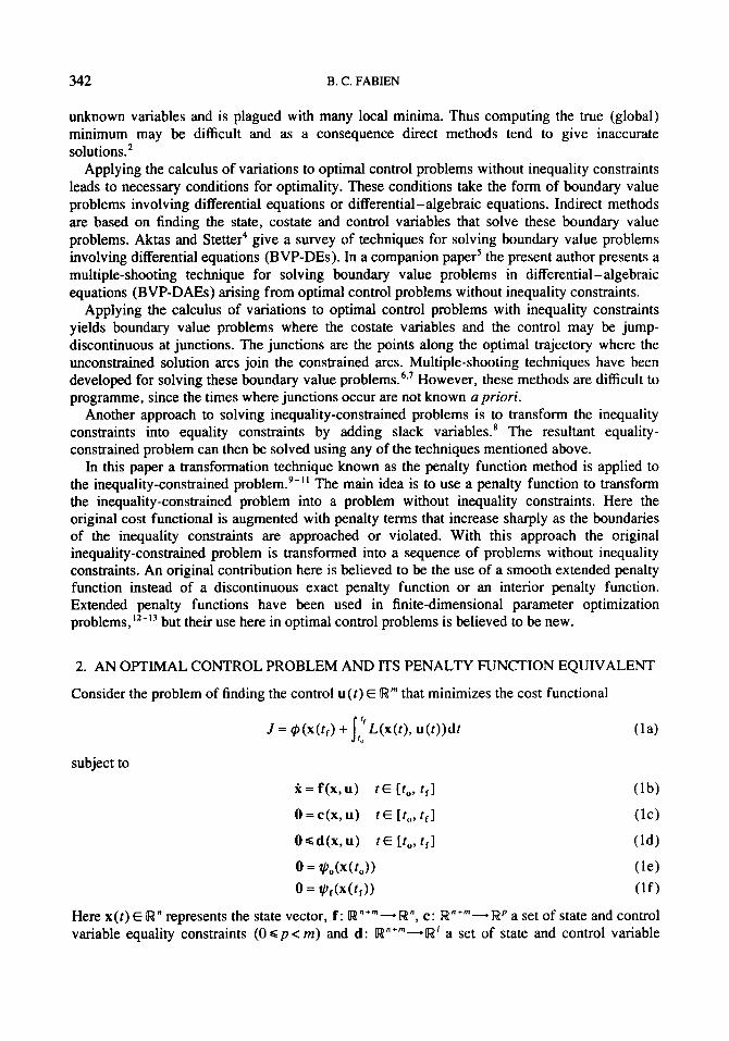
unknown variables and is plagued with many local minima. Thus computing the true (global) minimum may be difficult and as a consequence direct methods tend to give inaccurate solutions.'

Applying the calculus of variations to optimal control problems without inequality constraints leads to necessary conditions for optimality. These conditions take the form of boundary value problems involving differential equations or differential-algebraic equations. Indirect methods are based on finding the state, costate and control variables that solve these boundary value problems. Aktas and Stetter4 give a survey of techniques for solving boundary value problems involving differential equations (BVP-DEs). In a companion paper' the present author presents a multiple-shooting technique for solving boundary value problems in differential-algebraic equations (BVP-DAEs) arising from optimal control problems without inequality constraints.

Applying the calculus of variations to optimal control problems with inequality constraints yields boundary value problems where the costate variables and the control may be jump- discontinuous at junctions. The junctions are the points along the optimal trajectory where the unconstrained solution arcs join the constrained arcs. Multiple-shooting techniques have been developed for solving these boundary value problem^.^" However, these methods are difficult to programme, since the times where junctions occur are not known u priori.

Another approach to solving inequality-constrained problems is to transform the inequality constraints into equality constraints by adding slack variables.* The resultant equality- constrained problem can then be solved using any of the techniques mentioned above.

In this paper a transformation technique known as the penalty function method is applied to the inequality-constrained problem.g-" The main idea is to use a penalty function to transform the inequality-constrained problem into a problem without inequality constraints. Here the original cost functional is augmented with penalty terms that increase sharply as the boundaries of the inequality constraints are approached or violated. With this approach the original inequality-constrained problem is transformed into a sequence of problems without inequality constraints. An original contribution here is believed to be the use of a smooth extended penalty function instead of a discontinuous exact penalty function or an interior penalty function. Extended penalty functions have been used in finite-dimensional parameter optimization

but their use here in optimal control problems is believed to be new.

2. AN OPTIMAL CONTROL PROBLEM AND ITS PENALTY FUNCTION EQUIVALENT

Consider the problem of finding the control u (t) E Iw that minimizes the cost functional

J = $(x(rf) + I "L(x(t), u(t))dt ( la) 1"

subject to

Here x ( r ) E R" represents the state vector, f : Rn+m-Rn, c: Iw"+'"-Iwp a set of state and control variable equality constraints (0 " p c rn) and d: Rn+m-+Iw' a set of state and control variable

EXTENDED PENALTY FUNCTION APPROACH 343

inequality constraints (0 d I). The equality constraints are such that rank(dc/du) = p. rl0: [ w " - [ w q ~ and qf: R"--.[wqf denote initial and terminal state manifolds respectively, with 0 s 4,s n and 0 G q f s n. In equation (la) the cost functional consists of the scalar terminal weighting function f and the scalar function L. The initial time t, and the final time t , are both fixed. It is assumed that all the functions are sufficiently smooth and that the problem (1) has a unique solution.

To obtain a numerical solution to this problem, the penalty function method is used to transform the inequality-constrained problem into a problem without inequality constraints. An optimal control problem that is equivalent to (1) but without the inequality constraints is as follows: find the control u (t) E R that minimizes the cost functional

subject to

x = f(x, u) t E [to, f f ] (2b ) 0 = c(x, u) t E [ to, t f ] (2c ) 0 = r lo(x( t0 ) ) (2d) 0 = r l f ( X ( f , ) ) (2e)

where p k > p n + , > O and limb- p t = O . In equation (2a) D,, i = 1, ..., f, denote the penalty function terms that are added to the original cost functional (la). In general these penalty function terms are small if the constraints (Id) are satisfied and large if the constraints are violated. If the inequality constraints are violated, then the cost functional is dominated by the penalty term. Therefore the optimization problem will tend to minimize the penalty term and thus the amount of constraint violation. On the other hand, if the constraints are satisfied, then the penalty term remains small makes no significant contribution to the cost functional (2a). As the penalty parameter pk approaches zero, the influence of the penalty term D, on the cost functional (2a) becomes smaller and smaller. It is shown by Russell" that for the penalty function used here the sequence of solutions to (2) converges to the solution of (1) in the limit as pk-O.

The penalty functions D, are usually classified as (a) exterior penalty functions, (b) interior penalty functions or (c) extended penalty functions." Figure 1 shows qualitatively the behaviour of each of these penalty functions. Here the feasible region is defined as the domain of all trajectories that satisfy the inequality constraint (Id). The infeasible region is defined as the domain of all trajectories that violate the inequality constraint.

A popular exterior penalty function is the quadratic loss function defined as D, = (min(0, d,) / pn)', where d, denotes the ith component of the vector d(x, u) in (Id). This penalty function is zero if the ith constraint is satisfied and non-zero otherwise. A disadvantage in using this penalty function is that at the constraint boundary d, = O the first-order derivatives of the penalty function are discontinuous. Also, when solving problems that have bang-bang optimal control solutions, this penalty function yields a BVP-DAE that is not index one.

To illustrate this, consider a problem (2) that has an inequality constraint d with c(x, u) = 0, and u appearing linearly in f(x,u) and L(x,u). The inequality constraint is given by d = (1 - u)( 1 + u) 2 0. Now, using the exterior penalty function, construct the Hamiltonian H = L(x, u) + I:_, D,(x, u) + I ' f (x , u). Then the first-order necessary conditions for optimality lead to a BVP-DAE that is not index one, since 1 a z H / ~ u 2 1 = 0 for any feasible trajectory. This makes numerical solution via the multiple-shooting technique described by Fabien' very difficult.

344 B. C. FABIEN

&or Penalty Function

Feasible Region (d, >= 0)

Figure 1. Penalty functions

To circumvent the difficulties caused by the exterior penalty function, an interior penalty function can be used. The interior penalty function shown in Figure 1 is the inverse barrier function given by Di= l / d p This function is defined only for di>O and is infinite on the constraint boundary d j = 0. Another popular interior penalty function is the logarithmic barrier function given by Di = log(d,). These penalty functions have continuous derivatives at the constraint boundary and lead to BVP-DAEs that are index one for all feasible trajectories and p k arbitrarily close to zero. This can be seen by using the example cited in the previous paragraph and noting that I a’H/du’ I # 0 for any feasible trajectory.

A disadvantage of this interior penalty function is that it is not defined for infeasible trajectories. Thus the numerical solution procedure used must be such that all intermediate solutions satisfy the inequality constraints. Unfortunately, this is often difficult to accomplish in practice.

To retain the favourable properties of the interior penalty function and allow infeasible trajectories to be considered, an extended penalty function is employed. A quadratic extended penalty function is given by

This extended penalty function is quite different from the standard interior penalty function used by Lasdon et al. I ’ Figure 1 clearly illustrates the difference between the interior penalty function and the extended penalty function. By using (3 as a transition point, the penalty function (3) extends the range where the interior penalty function is defined into a region of d d 0. The fact that D j in equation (3) extends into the infeasible region of (Id) is very important, since it allows trajectories that do not satisfy these constraints (i.e. (Id)) to be treated at intermediate steps of the optimization process. As the penalty parameter pk approaches zero, the extended penalty function becomes equivalent to the inverse barrier function.

Note that the first and second derivatives of the extended penalty function Di are continuous at the transition point. Extended penalty functions that have third-order continuity at the transition point are available. I’ However, second-order continuity is sufficient for the numerical procedure developed below.

EXTENDED PENALTY FUNCTION APPROACH 345

3. A MULTIPLE-SHOOTING-CONTINUATION SOLUTION

From the discussion in Section 2 it is clear that the solution to (1) is obtained by solving a sequence of problems (2) with progressively smaller values of pk The first-order necessary conditions for the problem (2) to be optimal are stated in terms of the Hamilt~nian'~.'~

I

H(X, U, a ,p ;pk) =L(x, U) + p k I ~ i ( p t , X, U) + aTm, U) +pTc(x, U) i- 1

as

x = HT, = f(x, u), t E [to, r,]

0 = HT, r E [to, tf]

0 =H: = C(X, u), t E [ ro , tf]

0 = q O ( x ( t 0 ) )

A.=-H,T, t E [to,tf]

where L E R " , p E W , voER; and pfE Rq' are Lagrange multipliers. Note that in (4) HTx = (aH/ax)T, etc.

The BVP-DAE (4) can be written in a more compact form by defining

y = [ ;] E !laZn, z = [ ;] E Rm+p

to get

0 = r ( Y ( t o ) , Y ( t f ) ) (5c) Note that the 2n +qo+ qt equations (4e)-(4h) provide the 2n equations in (5c) by

eliminating the qo + qr equations involving the Lagrange multipliers vo and wr. Furthermore, the explicit dependence of the BVP-DAE on the penalty parameter pL is emphasized.

346 B. C. FABIEN

A multiple-shooting-continuation method is used to solve ( 5 ) as pk-O and hence obtain the solution to (1). The multiple-shooting method for solving (5) for a given ph is similar to that outlined in Reference 5. The time span [ to , t f ] is divided into M intervals such that to = to c t I < < t, = t f . In each interval let y(t; s:, s:; pk) , x(t; s;, s,z; p k ) denote the solution to the relaxed initial value DAE

Y = h(y, z; Pk) , tE (ti, f i + l ) (6a)

o = g ( y , z ; P , ) - y i , tE(t i , t , , l ) (6b 1

y(ti)=s,Y, S ( t , ) = S : , i = o , 1 ,..., M - 1 (6c 1

y i = g(sr, s,z) =constant

with s,! and s,z being the solutions to the BVP-DAE (5) at the nodes t,, i = 0, 1,2, .. ., M. To ensure that SJ and s; are solutions to the BVP-DAE ( 5 ) , the following conditions must be satisfied:

(i) continuity of the solution s' at the nodes, i.e.

y ( t i + l ; s ~ , S ~ ; ~ ~ ) - S ) ; + , = O , i =o ,1 ,2 ,..., M - 1

(ii) satisfaction of the algebraic equations at the nodes, i.e.

g ( s r , s : ; p , ) = O , i = O , 1 , 2 ,..., M (iii) satisfaction of the boundary conditions, i.e.

r(s& sL) = 0

These three conditions lead to a system of (2n + m + p ) ( M + 1) non-linear equations in (2n + m + p ) ( M + 1) unknowns s and the parameter pk. These equations are written as

= 0, S = (7 )

For a given p k the solution to the non-linear system (7) yields the solution to the problem (4) at the nodes ti. i = 1.2, .. ., M. In the limit as pk-0 the solution to these non-linear equations gives the solution to the inequality-constrained optimal control problem (1).

3.1. A continuation procedure

This subsection presents a continuation algorithm for solving problem (7) for a sequence of pk approaching zero. The basic idea behind the continuation method is as follows. Given the system of non-linear equations q(s; p k ) = 0 and solutions ( & I ; p k - ] ) , (sk-'; p k T 2 ) , etc., use these previous solutions to compute an approximation of the solution at pk. Then with the

EXTENDED PENALTY FUNCTION APPROACH 341

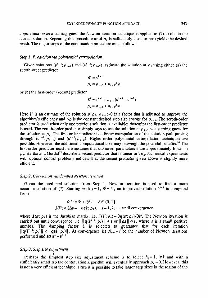
approximation as a starting guess the Newton iteration technique is applied to (7) to obtain the correct solution. Repeating this procedure until p,: is sufficiently close to zero yields the desired result. The major steps of the continuation procedure are as follows.

Step I . Prediction via polynomial extrapolation

Given solutions zeroth-order predictor

pk-1) and ( s k - ' ; Pk-z), estimate the solution at pk using either (a) the

g k Z S k - l

Pk=Pk-I+ hk-lAp

or (b) the first-order (secant) predictor

g k = s k - l 4- hk-I(Sk-' - S k - 2 )

Pk=Pk-l+hk- lAp

Here g k is an estimate of the solution at pn, h k - l > 0 is a factor that is adjusted to improve the algorithm's efficiency and Ap is the constant desired step size change for P , : - ~ . The zeroth-order predictor is used when only one previous solution is available; thereafter the first-order predictor is used. The zeroth-order predictor simply says to use the solution at p k - l as a starting guess for the solution at Pk. The first-order predictor is a linear extrapolation of the solution path passing through (s"-'; p n - and (s"'; pk-& Higher-order polynomial extrapolation techniques are possible. However, the additional computational cost may outweigh the potential benefits. I6 The first-order predictor used here assumes that unknown parameters s are approximately linear in p,:. Haftka and GurdalI3 describe a secant predictor that is linear in d p n . Numerical experiments with optimal control problems indicate that the secant predictor given above is slightly more efficient.

Step 2 . Correction via damped Newton iteration

Given the predicted solution from Step 1, Newton iteration is used to find a more accurate solution of (7). Starting with j = 1, s" = 1', an improved solution S'" is computed from

S I + I = I S + AS, < E (0,1]

J (GI; p k ) h = -q (SJ; p k ) , j = 1,2, . . . , until convergence

where J(SJ; p k ) is the Jacobian matrix, i.e. J(S'; P I ) = aq(sJ; p,)/aSJ. The Newton iteration is carried out until convergence, i.e. (1 q(S'+I; pk) ( 1 C E or 1 1 As 1 1 d E , where E is a small positive number. The damping factor is selected to guarantee that for each iteration (1 q(S1+' ; p k ) ( 1 < ( 1 q(SJ; pk) ( 1 . At convergence let N,,, = j be the number of Newton iterations performed and set sA = 5'+'.

Step 3 . Step size adjustment

Perhaps the simplest step size adjustment scheme is to select h k = 1, Vk and with a sufficiently small Ap the continuation algorithm will eventually approach pk = 0. However, this is not a very efficient technique, since it is possible to take larger step sizes in the region of the

+

348 B. C. FABIEN

solution path where the first-order predictor provides good estimates of the true solution. An effective method for changing the step size is to select the new scale factor, used in the prediction step, as

nCW h,i, = Q hk-1 d h,,

where hmin and h,, are the minimum and maximum allowable values for the scale factor respectively. N , is the optimum number of Newton iterations that should be performed during the Step 2. Therefore, if N,, c Nqlr then the scale factor is increased and a larger step size is taken during the next prediction step. Intuitively this makes sense, since N,, c Nopf implies that the predicted solution is very close to the true solution and thus the linear approximation is a good estimate of the solution path curvature in the neighbourhood of ( s k , p k ) . On the other hand, if N,, < N,, then the predicted solution is far away from the true solution; therefore the scale factor is reduced and a smaller step size is taken during the next prediction phase.

This continuation procedure is carried out until I f (p, ) - I(pk-1) I < & or I pa I c E , where & is a small positive number. The continuation method outlined above is by no means the only possible approach to solving (7).

The major computational effort is required in performing the Newton iteration during the correction step of the continuation algorithm. A detailed discussion on the computation and solution of the non-linear system (7) is given in Reference 5.

4. EXAMPLES

Example I . A state variable inequality constraint problem’4

Consider the problem of finding the control u E R that minimizes the functional

1 1 J = - / 3 0 u2dt

subject to

R, =x2

x2 = u

Or0.1 -XI XI (0) = 0 X2(O) = 1 x,(l) = o XZ(1) = -1

This problem finds the energy-optimal control for a second-order system that has a constraint on the upper bound for the state variable x I . In terms of equation (2) this problem can be written as t ,=O, r t = l , $ = O , c=O, d=0.1-x1, L = 0 - 5 u z , ~0=[xl(0)rx2(O)-l]T,

EXTENDED PENALTY FUNCTION APPROACH 349

qr = [x, (l) , x,(l) + 1IT. The first-order necessary conditions for optimality (4) yield

1, = x2 x2= u

I , = - P P x I,= -1, 0 = 1 , + u

X,(O) =o x2(0) = 1 x,( l ) = 0 xz(l) = -1

1/(0.1 - d z u

3/a2 - 2(0.1 - x , ) / u ~ , d < u

u = 4 p k

Figure 2 shows the results obtained using the continuation method described above to solve this problem. The starting guess is shown by the dotted line and the converged solution is shown by full solid line. The initial guess is obtained by solving the optimal control problem without the inequality constraint. Note that this starting guess violates the inequality constraints. The standard interior penalty function will not be able to solve this problem using this starting guess. However, using the extended penalty function, a solution is obtained quite easily. For this problem, six continuation steps were performed starting with po = 10, Ap = 0.1, M = 10, N, = 4 and E = 1.0 x Clearly the converged solution satisfies the desired constraints and is in good agreement with the analytical solution given in Reference 14.

Example 2. A stirred-tank chemical reactor”

Consider the problem of finding the control ZI E R that minimizes the functional 0.78

0 J = I [x;(t) + x : ( t ) ] d t

subject to

il = -2(x, + 0.25) + (x2 + O.5)exp - - (xl + 0.25)~ ( x::;)

xz = -0.5 - x2 - (x2 + 0.5) exp - ( x::;)

OG (1 - u)(l + u )

X, (0) = 0.05 x,(O) = 0

XI (0.78) = 0 xZ(0.78) = 0

350

-0.2

-0.4

-0.6

-0.6

- I

B. C. FABIEN

- - - -

I 1 I

25

2 0 -

15

10

5 -

0

-5

-10

-15

-20

-25

I I I I

- -

- - - - - -

I 1 I 1

Figure 2. Continued

EXTENDED PENALTY FUNCTION APPROACH

0 2

0 15

0 1

A1

0.05

0 ’

-0.05

35 1

I 1 1 I I I I

- ...

- ’.. -

.’... ................. ...

-

I I 1 I I I I

tlme

‘r I I I I

-7 ‘ I I I 1

0 0.2 0.4 0.6 0.8 I timc

Figure 2. State variable inequality constraints

This problem seeks the bounded optimal control for a stirred-tank chemical reactor. The state variable x , denotes the deviation from the steady state temperature, the state variable x2 the deviation from the steady state concentration and the control u the effect of coolant flow on the chemical reaction. Using the penalty function approach to remove the inequality constraint on the control variable, this problem is written in terms of equation (2) with ro = 0, r , = 0.78, C$ = 0,

The first-order necessary conditions for optimality (4) yield c = O . d = (1 - u ) ( l + u), L = $ + $ , qo= [ ~ I ( O ) - 0 * 0 5 , x z ( O ) ] ~ , q f = [~l(0.78),~,(0-78)]~.

i , = - 2 ( x , + 0.25) + ( x 2 + 0-5)exp - - ( x I + 0-25)u ( x::;) i 2 - - -0.5 - x , - ( x , + 0.5)exp

A1 = - 2 ~ 1 + 211 - A ~ ( x , + 0.5)

+I,u + &(x2 + 0.5) ( ( 50 )exp(”) X I + 2)* X I + 2

352 B. C. FABIEN

1, = -2x, - I, exp ( - 25x1) + I , [ 1 + exp ( - ""I)]

x1+2 XI + 2

O=p,D,- IZI(XI +0.25) 0=~1(0)-0.05 0 = x,(O)

0 = X I (0.78) 0 = ~ ~ ( 0 . 7 8 )

2 4 1 - u ) ( l + u)12

6u /a2 - 4u(l - u)(l + u)/u'

d s a d < U, u = l /p t

Du=[

This problem is solved with 100 equally spaced nodes, po= 10, A p =0.1, N,,,=4, and E = 1.0 x Results for the state, costate and control variables are shown in Figure 3. The starting guess is shown by the dotted line and the converged solution is shown by the full line. Here the initial guess is obtained by solving the optimal control problem without the inequality constraint, L = $+ $+ 0.1 u2, qr = 0. and all other terms as given above. The optimal solution

timc

0.01 1 I 1 I I I 1

-

I? -0.03 -

-0.06 - -0.07 1 1 I I I I I

0 0.1 0.2 0.3 0 4 0 5 0.6 0.7 0.8 time

Figure 3. Continued

EXTENDED PENALTY FUNCTION APPROACH

1.2

1

0.8

0.6

0.4

353

- I 1

*.

- '._

I I I 1 I

- -

0.2

0.15

0.1

Ai

0.05

1 I I I I I I

- '..

- *..

-

U

2

1.5

1

0.5

0

-0.5

-1 0 0.1 0.2 0.3 0.4 0.5 0.6 0.7 0.8

time

Figure 3. Stirred-tank chemical reactor

354 B. C. FABlEN

is obtained after 70 continuation steps with the minimum value of the cost function J = 040200, compared with J = 040220 given by Kirk.”

It is interesting to note that the numerical solution to this problem indicates that the optimal trajectory possess a singular arc in the interval f E [0.43,0-71]. To see this, let H* = ATf + L denote the Hamiltonian for the problem without the extended penalty function. Note that H* is linear in the control u( t ) . Thus the necessary conditions for optimality indicate that H* is a minimum if u ( t ) = 1 when s ( t ) = - [x , ( t )+0.25]AI(t)<0 and if u ( t ) = -1 when s ( t ) > O . If s ( r ) = 0, for some finite time interval the Hamiltonian does not provide any information on the optimal value of the control variable. The trajectory along such a time interval is called a singular arc and s ( t ) is called the switching fun~ t i0n . l~ If the switching function does not vanish, then a bang-bang optimal control is obtained. However, the switching function does vanish in the interval t E [0.43,0.71], indicating a singular arc. Along the singular arc the optimal control input obtained here is quite different from the solution given by Kirk. Is

5. DISCUSSION

In general, using the penalty function method to solve constrained optimal control problems leads to BVP-DAEs. Owing to the structure of the penalty terms, the algebraic equations are difficult to eliminate; thus the BVP-DAEs must be solved directly (see Example 2). Employing the extended penalty function method, the sequence of BVP-DAE arising from the problem (2) can be solved using the technique presented in Reference 5. Unlike the exterior penalty function, the extended penalty function (3) leads to BVP-DAEs that are index one. Also, the extended penalty function allows infeasible trajectories in the solution procedure; such trajectories cannot be considered with the interior penalty function.

The algorithm presented in this paper uses a multiple shooting technique where the grid points in the interval [to, t,] are fixed. For constrained optimal control problems the precise location of the junctions between the unconstrained and constrained arcs is of interest. In general these junctions will fall between the specified grid points. However, the examples presented here demonstrate that fixed grid points can be used to accurately solve constrained optimal control problems. In fact, the algorithm has been shown to give good estimates of the location of the junctions as well as accurate optimal state and control trajectories. Future work will involve developing a technique to adaptively space the grid points for precise determination of the junctions.“’

ACKNOWLEDGEMENTS

The support of this research through a grant from the National Science Foundation (MSS- 9350467) is hereby acknowledged. The author would also like to thank the reviewers for their careful reading of the manuscript and their helpful suggestions.

REFERENCES

1. Bock, H. G. and K. J . Plitt, ‘A multiple shooting algorithm for direct solution of optimal control processes’, Proc.

2. von Stryk, 0. and R. Bulirsch, ‘Direct and indirect methods for trajectory optimization’, Ann. Oper. Res., 37,

3. Vlassenbroeck, J . , ‘A Chebychev polynomial method for optimal control with state constraints’, Autornnfica, 24,

4. Aktas, Z. and H. J. Stetter. ‘A classification and survey of numerical methods for boundary value problems in

9th IFAC World Congr., Budapest, 1984, pp. 1603- 1608.

357-373 (1992).

499-506 (1998).

ordinary differential equations’, Int. j . numer. methods eng. , 11, 771 -796 (1977).

EXTENDED PENALTY FUNCTION APPROACH 355

5. Fabien, B. C., ‘Numerical solution of boundary-value problems in differential algebraic equations arising from

6. Maurer, H. and W. Gillessen, ‘Application of multiple shooting to the numerical solution of optimal control

7. Maurer, H., ‘Numerical solution of singular control problems using multiple shooting techniques’, J. Opfirn.

8. Jacobson, D. H. and M. M. Lele, ‘A transformation technique for optimal control problems with a state variable

9. Okamura, K., ‘Some mathematical theory of the penalty method for solving optimum control problems’, J. SIAM

10. Russell, D. L.. ‘Penalty functions and bounded phase coordinate control’, J . SIAM Control. Ser. A. 2, 409-422

1 1 . Lasdon, L. S., A. D. Waren and R. K. Rice, ‘An interior penalty method for inequality constrained optimal control

12. Haftka, R. T. and J. H. Starnes, ‘Applications of a quadratic extended penalty function to structural optimization’.

13. Haftka, R. T. and Z. Gurdal, Elemenfs of Sfrucfural Opfimizarion, Kluwer, Boston, MA, 1992. 14. Bryson, A. E. and Y.-C. Ho, Applied OprimaI Control, Hemisphere, New York, 1975. 15. Kirk, D. E., Optimal Conrrol Theory. Prentice-Hall, Englewood Cliffs, NJ, 1970. 16. Seydel, R., From Equilibrium to Chaos, Elsevier, New York, 1988.

optimal control’, Proc. Am. Confrol Conf., Vol. 3, 1995,2069-2070,2075-2076.

problems with bounded state variables’, Compufing, 15, 105- 126 (1975).

Theory Appl., 18,235-257 (1976).

inequality constraint’, IEEE Trans. Aufomatic Confrol, AC-14,457-464 (1969).

Control, Ser. A, 2.317-331 (1965).

(1965).

problems’, IEEE Trans. Auromaric Confrol, AC-12, 388-395 (1967).

AIAAJ. , 14,718-724 (1976).