Pre-emptive Resource-Constrained Multimode Project ...
54
Journal of Industrial Engineering and Management JIEM, 2016 – 9(3): 732-785 – Online ISSN: 2013-0953 – Print ISSN: 2013-8423 http://dx.doi.org/10.3926/jiem.1522 Pre-emptive Resource-Constrained Multimode Project Scheduling Using Genetic Algorithm: A Dynamic Forward Approach Aidin Delgoshaei , Mohd Khairol Mohd Ariffin , B.T. Hang Tuah Baharudin University Putra Malaysia (Malaysia) [email protected] , [email protected] , [email protected] Received: May 2015 Accepted: July 2016 Abstract: Purpose: The issue resource over-allocating is a big concern for project engineers in the process of scheduling project activities. Resource over-allocating drawback is frequently seen after scheduling of a project in practice which causes a schedule to be useless. Modifying an over-allocated schedule is very complicated and needs a lot of efforts and time. In this paper, a new and fast tracking method is proposed to schedule large scale projects which can help project engineers to schedule the project rapidly and with more confidence. Design/methodology/approach: In this article, a forward approach for maximizing net present value (NPV) in multi-mode resource constrained project scheduling problem while assuming discounted positive cash flows (MRCPSP-DCF) is proposed. The progress payment method is used and all resources are considered as pre-emptible. The proposed approach maximizes NPV using unscheduled resources through resource calendar in forward mode. For this purpose, a Genetic Algorithm is applied to solve. Findings: The findings show that the proposed method is an effective way to maximize NPV in MRCPSP-DCF problems while activity splitting is allowed. The proposed algorithm is very fast and can schedule experimental cases with 1000 variables and 100 resources in few seconds. The results are then compared with branch and bound method and simulated annealing algorithm and it is found the proposed genetic algorithm can provide results with better quality. Then algorithm is then applied for scheduling a hospital in practice. -732-
-
Upload
khangminh22 -
Category
Documents
-
view
2 -
download
0
Transcript of Pre-emptive Resource-Constrained Multimode Project ...

Journal of Industrial Engineering and ManagementJIEM, 2016 – 9(3): 732-785 – Online ISSN: 2013-0953 – Print ISSN: 2013-8423
http://dx.doi.org/10.3926/jiem.1522
Pre-emptive Resource-Constrained Multimode Project Scheduling
Using Genetic Algorithm: A Dynamic Forward Approach
Aidin Delgoshaei , Mohd Khairol Mohd Ariffin , B.T. Hang Tuah Baharudin
University Putra Malaysia (Malaysia)
[email protected], [email protected], [email protected]
Received: May 2015Accepted: July 2016
Abstract:
Purpose: The issue resource over-allocating is a big concern for project engineers in the process
of scheduling project activities. Resource over-allocating drawback is frequently seen after
scheduling of a project in practice which causes a schedule to be useless. Modifying an
over-allocated schedule is very complicated and needs a lot of efforts and time. In this paper, a
new and fast tracking method is proposed to schedule large scale projects which can help project
engineers to schedule the project rapidly and with more confidence.
Design/methodology/approach: In this article, a forward approach for maximizing net
present value (NPV) in multi-mode resource constrained project scheduling problem while
assuming discounted positive cash flows (MRCPSP-DCF) is proposed. The progress payment
method is used and all resources are considered as pre-emptible. The proposed approach
maximizes NPV using unscheduled resources through resource calendar in forward mode. For
this purpose, a Genetic Algorithm is applied to solve.
Findings: The findings show that the proposed method is an effective way to maximize NPV in
MRCPSP-DCF problems while activity splitting is allowed. The proposed algorithm is very fast
and can schedule experimental cases with 1000 variables and 100 resources in few seconds. The
results are then compared with branch and bound method and simulated annealing algorithm and
it is found the proposed genetic algorithm can provide results with better quality. Then algorithm
is then applied for scheduling a hospital in practice.
-732-

Journal of Industrial Engineering and Management – http://dx.doi.org/10.3926/jiem.1522
Originality/value: The method can be used alone or as a macro in Microsoft Office Project®
Software to schedule MRCPSP-DCF problems or to modify resource over-allocated activities
after scheduling a project. This can help project engineers to schedule project activities rapidly
with more accuracy in practice.
Keywords: multimode project scheduling, genetic algorithm, pre-emptive resource-constrained,
discounted cash flows
1. Introduction
Classic Resource-constrained project scheduling problem (RCPSP), which is dealt with scheduling the
project activities considering time and resource constraints, is generalized for minimizing completion time
(or makespan) of the project Kelley (1963). Normally, in RCPSP, activities are scheduled considering two
main types of constraints:
• The executive priority relations between activities which are expressed by a relation matrix
• The availability resources level for executing activities
Multi-mode resource constraint project scheduling problems (MRCPSP) are distinctive resource-
constraint problems where each activity can be carried out via different modes (regarding to technologies
or material). As consequence, the execution period (activity duration), resource requirement level and
even the cash flow may be vary form a mode to another. Kolisch and Drexl (1997) proved that the
MPRCPSP problem is a NP-hard problem.
Traditionally, classic RCPSP models were developed for minimizing makespan (Talbot, 1982). But, during
last 2 decades, scientists have developed more RCPSP problems considering varied objectives. Mainly,
authors developed RCPSP while 4 main optimization objectives are taken into consideration:
1.1. Makespan (Cmax) minimization
Minimizing makespan where an attempt is done to minimize the total elapsed time among time horizon
of a project. In this manner, a time dependent cost structure for minimizing completion time by using
extra resources which cause faster execution of activities was developed by Achuthan and Hardjawidjaja
(2001). Effects of the serial and parallel scheduling schemes while using multi- and single-project
approaches were analysed later (Lova & Tormos, 2001). It was found that using parallel scheduling
-733-

Journal of Industrial Engineering and Management – http://dx.doi.org/10.3926/jiem.1522
schemes and multi-project approach provide a base for managers to minimize mean project delay or
multi-project duration increasing. Alcaraz and Maroto (2001) developed a GA for solving single mode
RSPCP. They showed that GA can efficiently solve RCPSPs in an acceptable computation time. In the
same year, GA was also employed by Hartmann (2001) for minimizing Cmax in MRCPSP and then using a
local search extension motor for the proposed GA, results were more improved. Kim, Yun, Yoon, Gen
and Yamazaki (2005) proposed a hybrid of GA with fuzzy logic controller (FLC-HGA) to solve the
resource-constrained multiple project scheduling problem (RC-MPSP). The proposed approach worked
based on using genetic operators with fuzzy logic controller (FLC) through initializing the revised serial
method with precedence and resources constraints. Using fuzzy concepts in minimizing Cmax was carried
out by Ke and Liu (2010) in a fuzzy-based GA. Delgoshaei, Ariffin, Baharudin and Leman (2015)
proposed a backward method for minimizing makespan in the resource constrained project scheduling
problem. For this purpose they used a hybrid greedy and genetic algorithm. The novelty of their research
is using remained resources through the calendar of the project to minimize the completion time of the
project.
1.2. Optimizing Robustness of Solutions
For this purpose normally a trade-off between quality-robustness and solution-robustness in RCPSP will
be determined while safety times in project scheduling were taken into consideration (Van de Vonder,
Demeulemeester, Herroelen & Leus, 2005). Afterward, Van de Vonder, Demeulemeester, Herroelen and
Leus (2006) focused on resource constraint impacts in determining trade-off values between
quality-robustness and solution-robustness in RCPSP. Lee and Lei (2001) presented 2 versions of
resource-constraint multi project scheduling problem were developed in a way that in first version, the
activity durations are considered fixed but in second one, a project duration function is used to decrease
the amount of resource allocating. Afterward, an attempt has been done for minimizing Cmax, as well as
maximizing solution robustness by increasing float time maximization (Abbasi, Shadrokh & Arkat, 2006).
A two-stage algorithm for robust RCPSP was used while minimize Cmax, of the project as an acceptance
threshold for second stage was carried out and then, in next stage, a set of 12 alternative robust predictive
indicators was employed to maximize robustness of the project (Chtourou & Haouari, 2008).
RCPSPs can be considered as a NP-hard problem while more than one none-renewable resource is
taken into account (Kolisch, 1996). There are also some other parameters of project complexity that
should be noticed as other managerial factors (Castejón-Limas, Ordieres-Meré, González-Marcos &
González-Castro, 2011). Traditionally, many problems were solved using branch-and-bound algorithm
(Sprecher, 2000), but heuristics and metaheuristics were then found as good ways of solving RCPSCPs.
-734-

Journal of Industrial Engineering and Management – http://dx.doi.org/10.3926/jiem.1522
Multi-mode resource constraint project scheduling problems (MRCPSP) are distinctive
resource-constraint problems where each activity can be carried out via different modes (regarding to
technologies or material etc.). As consequence, the execution period (activity duration), resource
requirement level and even the cash flow may be vary form a mode to another. The MPRCPSP problem
was initially developed for minimizing the project makespan and was proved to be a NP-hard problem
(Kolisch & Drexl, 1997). Węglarz, Józefowska, Mika and Waligóra (2011) provided a wide research on
literature of the multimode project scheduling. One of the most important issues in MRCPSP studies is
financial issues which can be considered in two ways of positive or negative cash flows. Positive cash
flows are supposed to earn as scheduled milestones. Despite, negative cash flows are referred to those
expenses which must be spent for making positive cash flows (as human resource salary, equipment and
machinery purchasing and maintenance costs, raw material providing etc.). In such models, cash flow can
be influenced by activity due date, duration, resource requirements and also payment method which will
effect on activity execution mode as well. GA was then used for solving a multi-criteria project portfolio
selection problem when project interactions (in terms of multiple selection criteria) and preference
information (in terms of the criteria importance) were considered (Yu, Wang, Wen & Lai, 2012).
Kolisch and Drexl (1997) found that MRCPSP is NP-hard if more than one resource is considered. To
come up with such problem, many heuristics and metaheuristics approaches are applied so far. Yan,
Jinsong, Xiaofeng and Ye (2009) applied some heuristics to solve project scheduling problem in order to
provide a quick response structure while encountering with maritime disasters. Laslo (2010) presented an
integrated method using simulation for resource planning and scheduling to minimize scheduling
dependent expenses. Kim et al. (2005) proposed a hybrid GA and fuzzy logic controller (FLC-HGA) to
solve the resource-constrained multiple project scheduling problem (RC-MPSP). Their objectives were
minimizing total project time and total tardiness penalty. Ke and Liu (2010) used hybrid fuzzy set and GA
to minimize total cost with completion time limits (see also Hartmann & Briskorn, 2010). Jarboui,
Damak, Siarry and Rebai (2008) used particle swarm optimization (PSO) to show the effectiveness of
PSO for solving MRCPSPs.
1.3. Maximizing Profit of the Project
Maximizing profit of projects is considered as an important objective in financial studies of scheduling
problems. Profit of the project can be considered with many different styles. In some studies profit is
expressed as net present value of the project. The idea of maximizing NPV was first proposed by
(Russell, 1970). The proposed model was nonlinear without taking limitations of resources. They assumed
activity on art (AOA) to present network charts. Elmaghraby and Herroelen (1990) proposed an
optimal-finder algorithm which includes resource constraints for maximizing NPV. Sung and Lim (1994)
-735-
Journal of Industrial Engineering and Management – http://dx.doi.org/10.3926/jiem.1522
proposed a two stage heuristic to maximize NPV of a RCPSP. They found that while difference between
the due date and the minimum duration increases, the NPV gets more improved.
One of the most important issues in maximizing NPV is considering positive or negative cash flows
during scheduling process. Positive cash flows are supposed to earn as scheduled milestones. Despite,
negative cash flows are referred to those expenses which must be spent for making positive cash flows (as
human resource salary, equipment and machinery purchase and maintenance costs and raw material
providing). In such models, cash flow can be influenced by activity due date, duration, resource
requirements and also payment method which will effect on determining activity execution mode as well.
Etgar, Shtub and LeBlanc (1997) showed that resources beyond time limit can have significant effect on
makespan of project Meanwhile, De Reyck (1998) offered an algorithm based on which both positive and
negative cash flows had been considered. A lower and upper bound were considered for each activities
where coupled with limited resources. Icmeli, Erenguc and Zappe (1993) discussed that adding resources
limitations caused turning model into a non-poly nominal model which cannot be solved easily by
optimizing algorithms. Then, they considered discounted rate in the proposed a model a way that more
cash flows will be earned in case of completing an activity in shorter period (RCPSPDC). Afterward,
many researchers tried their utmost effort with the aim of solving the problem of maximizing NPV while
discount rate is taken into consideration. Baroum and Patterson (1999) solved a RCPSPDC model with
50 variables where only positive cash flows were considered. Afterward, Icmeli and Erenguc (1994) used
Tabu search (TS) algorithm in solving RCPSPDC problem. They set penalty for activities later than the
due date. Yang, Talbot and Patterson (1993) developed statistical programming for solving RCPSPDC
problems while positive cash flows were taken into consideration. Moreover, Zhu and Padman (1999)
used TS for solving RCPSPDC problems. Mika, Waligóra and Węglarz (2005) presented a model with
the aim of maximizing NPV of project with taking discounted rate and also both renewable and
non-renewable resources. They used hybrid of SA and TS to solve the problems. During last decade,
considering preemptive resource in scheduling problems have been more developed due to their impacts
on making major delays through project lifecycle as well. Delgoshaei, Al-Mudhafar and Ariffin (2016)
developed a new branch and bound based scheduling method for modifying resource over-allocated
schedules. Laslo (2010) proposed a method for minimizing total cost of executing project activities.
Delgoshaei, Ariffin, Baharudin and Leman (2014) used SA for maximizing NPV of the MRCPSPDC
while discounted cash flows is taken into consideration. For this purpose a backward method is used to
use remained resources through the resource calendar of a schedule.
During last decade, considering preemptive resource in scheduling problems have been more developed
due to their impacts on making major delays through project lifecycle as well. Demeulemeester and
Herroelen (1996) presented an optimal solution for RCPSP while they considered preemptive resources
-736-

Journal of Industrial Engineering and Management – http://dx.doi.org/10.3926/jiem.1522
in their model. Buddhakulsomsiri and Kim (2006) discussed that considering pre-emption resources is
vital while studying makespan of the project. Damay, Quilliot and Sanlaville (2007) applied linear
programming algorithms for preemptive RCPSP studies while Ballestín, Valls and Quintanilla (2008)
proposed heuristic for solving preemptive RCPSP. Seifi and Tavakkoli-Moghaddam (2008) evaluated four
payment methods during maximizing NPV and minimizing holding cost of completed activities in a
MRCPSP. Vanhoucke and Debels (2008) focused on impacts of variable activity durations under a fixed
work content, possibility of allowing activity pre-emption and use of fast tracking in decreasing project
makespan. Van Peteghem and Vanhoucke (2010) used GA to minimize makespan of MRCPSP while
they considered preemptive resources which allow activity splitting through their research.
To the best knowledge of authors, the idea maximizing profit of manufacturing projects in MRCPSPs
while activity split is allowed and preemptive resources are taken into consideration, is less developed. To
overcome such shortcoming, a multi-mode resource constrained scheduling problem with positive cash
flows (MRCPSP-PCF) is developed. Then impact of activity split on preventing resource over-allocation
is examined. In this regard, a forward method is proposed which works based on positive cash flow and
activity id priority rules to overcome the resource over-allocations that usually happen by scheduling
resource constraint project. The reminder for rest of the research is summarized as: research
methodology including mathematical model is presented in section 2. In continue the proposed solving
algorithm is illustrated in section 3. Section 4 presented a number of experiments where the performance
of the proposed method is explained in detail and to examine the performance of the proposed method
in practice, a case study is solved and results are compared with the results of Microsoft Office Project
(MSP) 2010.
2. Materials and Methods
In this section, we present the proposed mathematical scheduling model with the aim of NPV in the
condition of resource constraint. The model considers multi-mode of execution for each activity. Our aim
is to survey how allocation of pre-emptive resources can change the activity scheduling and what is their
impact to the net present value.
As summary we can mention the advantages of the proposed model as follows: Considering pre-emptive
resources in maximizing net present value of project, considering multi-mode execution activities,
considering activity splitting ability with respect of the predecessors, using useless amount of remained
resources. Main constraints are the resource capacity, fixed time of the planning, only positive cash flow is
considered, exact occurrence of all activities, and exact duration of each activity mode and exact cash flow
for each activity mode.
-737-

Journal of Industrial Engineering and Management – http://dx.doi.org/10.3926/jiem.1522
2.1. Problem Definitions
In order to classify models easily, in this section we define problems with a unique code as below:
n\m\k\th\it\g\p (1)
In this classification, n presents number of Activities, m is number of activity mode, k is number of
resource types, th is time horizon of the project, it is number of time iterations of the program, g is
number of generations is each time iterations during time horizon, p indicates population size.
2.2. Assumptions
The properties of the developed model are shown as:
1. Model is presented in Activity on Node (AON) structure.
2. PP (Progress Payment) is selected as the payment model. Noted that in progress payment
method, the contractor receives the project payments from the client at regular time intervals until
the project is completed Ulusoy, Sivrikaya-Şerifoğlu and Şahin (2001).
3. Resources are considered preemptive.
4. Activities are allowed to be split through the planning horizon.
5. The preemptive resources have limited capacities.
6. In this study, positive cash flows are considered as weight factor of each activity.
7. Activities can be executed in different modes. While a mode selected to an activity, the same
mode must be used during executing of the activity.
8. Activities are allowed to move only in their free-float time.
9. All improving movements will carry out in forward mode.
2.3. Subscript
Subscripts used in the model are considered as follows:
i = number of activities which is a 1 × n matrix ([1 .. N]1×n)
k = number of resource types which is a 1 × m matrix ([1 .. K]1×k)
t = available time horizon for production (t = 1, 2 … T)
m = number of modes of performance ([1 .. M]1×m)
-738-

Journal of Industrial Engineering and Management – http://dx.doi.org/10.3926/jiem.1522
2.4. Parameters
The list of parameters and notations is as follows:
Resource_Capacity: illustrates available resource in sub periods:
(2)
As result, number of in-process activities that queued ina waiting list to be served by a preemptive
resource can be expressed using below formula:
(3)
Activity_time: shows duration of each activity considering different execution modes.
(4)
Activity_sequence matrix is used in mathematical programming to show precedence relations between
activities.
(5)
CF(i,m) = positive cash flow of activity i while it performs in mode m
r(i,k) = usage amount of resource type k for activity I
R(k) = available level of resource type k
D(i,m) = duration of activity i while it performs in mode m
TH = time horizon of the projects
α = discounted rate
2.5. Decision Variables
(6)
ESi = Early start of activity i
EFi = Early finish of activity i
-739-

Journal of Industrial Engineering and Management – http://dx.doi.org/10.3926/jiem.1522
2.6. Mathematical Model
As mentioned in the previous parts, studying an MRCPSP problem is the major objective of this paper.
We supposed to have n activities on an AON network. Hence, Mathematical model is now written as
follows:
(7)
S.T:
(8)
(9)
(10)
(11)
(12)
(13)
(14)
(15)
(16)
(17)
In the proposed model, maximizing profit of a multi-mode project by considering renewable resources is
considered as the main objective. The objective function is written in a way that it can easily calculate
NPV of the project in every time slots using the progress payment method. For example, suppose an
activity (let’s say A) is supposed to be scheduled. Figure 1 shows 3 different conditions of scheduling an
-740-

Journal of Industrial Engineering and Management – http://dx.doi.org/10.3926/jiem.1522
activity while α is considered 0.05. As seen while the activity is scheduled earlier, more NPV is achieved
than those conditions that it is scheduled later or being split for any reason.
Figure 1. Calculating NPV in 3 execution alternatives of an activity
First constraint in this model is defined for determining early start of activities, which guarantees the solving
algorithm to stay feasible during searching process. Using the term mint=1:TH({t.(y(i,m,t) – (y(i,m,t – 1))| y(i,m,t – 1) = 0
helps identifying the real early start of activities when they are taken apart by the solving algorithm to
avoid encountering with resource over-allocation. The reason of using split ability for some activities will
be explained in section 3.4. It is important to know that using standard definition of early start of
activities (which is ESi ≥ ESj + dj if j is predecessor of i ) is not appropriate for MRCPSPs while activity
splitting is allowed since it causes wrong calculation. To explain more, suppose it is decided to calculate
ES for activity D with and without activity splitting permission (Figure 2).
Figure 2. Comparing different styles of calculating ES with and without activity splitting (left to right)
In the left Gantt of Figure 2, while splitting is not allowed, ESD can be calculated correctly by using the
mentioned formula (ESD = ESC + DC). But, as seen, calculating early start of activity D while activity
splitting is allowed (right figure) is not 13 anymore since activity C is split two times in days 10 and 13 and
cannot be finished earlier than the end of day 14. Consequently, activity D cannot be started sooner than
-741-

Journal of Industrial Engineering and Management – http://dx.doi.org/10.3926/jiem.1522
the day 15. Therefore, to prevent such error, a new formula is developed for calculating ES of each
activity:
(18)
Second constraint ensures that activity will not be started before the early finish of its predecessors.
Similar to the logic used for calculating early start of activities while activity splitting is allowed, early
standard finish formula (EFi = ESi + di) cannot be used here as there might be some none working days
that happens by the solving algorithm to avoid resource over-allocating. Therefor a formula is developed
for calculating the early finish of an activity which is able to consider the idle times among the lifecycle of
an activity:
(19)
The third constraint is developed to set a logic starting day for any project. The fourth set of constraints is
used for those activities which are related to each other by finish to start (FS) relation. In this model the
FS precedence is converted to the following mode to be applicable to employ in the model:
(20)
Since the model is considered a real time model which must be finished before a due date, the eighth
constraint is set for ensuring that the early finish of the last activity will not exceeded than the due date.
Due to considering splitting ability, the solving algorithm must be able to divide an activity to the smallest
period slots (1 day) to schedule them throughout the calendar of the project to avoid resource
over-allocation. It may cause passing the initial duration of activities in dynamic process of scheduling. To
avoid this mistake, the ninth set of constraints are set which guarantee that the number of working days
for each activity will not exceeded than the original duration of an activity (considering its execution
mode). The tenth sets of constraints are set to keep a selected execution mode of an activity throughout
its execution period. The eleventh sets of constraints are to avoid over-allocating the resources in every
single period slot throughout the project. The last two sets of constraints are logic constraints which show
the domain of the variables.
-742-

Journal of Industrial Engineering and Management – http://dx.doi.org/10.3926/jiem.1522
3. An Iterative Genetic Algorithm Procedure
In this section a new forward method is proposed for scheduling activities through planning horizon
while maximum amount of available resources are restricted and activity splitting is allowed.
Elmaghraby and Herroelen (1990) have dealt with the demonstration of NP-hard in its RCPSP models.
Zhou and Askin (1998) also reported that Resource-constrained project scheduling problems with cash
flows (RCPSPCF) are complex and combinatorial optimization problems and should be solved by
heuristics. As mentioned in above, if MRCPSP issues enjoy more than one resource, they will be
considered strongly as part of NP-hard issues. Since nonlinear with exponential status is considered as
target function of our desired model and with due observance to this fact that some of constraints enjoy
nonlinear status like constraints of the first group, we can come to this conclusion that the proposed
model is NP-hard.
There is also another reason for considering the mentioned model as NP-hard that is due to the
number of the basic solutions that increases extremely while we increase the number of the variables.
For example consider a simple model with 10 variables and 3 resources with 75 constraints that
includes C = 85! / (10! 75!) = 3,129,162,672,636 solutions as basic feasible and basic infeasible
solutions together. Therefore, if the number of the variables increases extremely, optimal solution
algorithms obviously cannot able to find the Optimum Basic solution.
Consequently since MRCPSP are dynamic in their natures, it seems necessary to use self-improve
algorithms such as Genetic Algorithms (GA), Simulated Annealing (SA) and Neural Networks as the
problem cannot be solved by optimal solution algorithms. As mentioned during last two decades, genetic
algorithm has been widely used to solve MRCPSP. Therefore, the research group decided to develop an
efficient GA in this article to determine net present value of the project while resources are considered as
pre-emptive .
In general, the main steps of our GA procedure are:
Step 1) Create the initial population.
Step 2) Compute the fitness value of each individual in the population.
Step 3) Select a set of individuals to undergo genetic operators.
Step 4) Evaluate the individuals created by the genetic operators.
Step 5) Apply a replacement strategy to form the new generation.
Step 6) If the stopping criteria are met then stop, otherwise go to Step 3.
-743-

Journal of Industrial Engineering and Management – http://dx.doi.org/10.3926/jiem.1522
The main concept of the proposed GA method is inspired from Delgoshaei et al. (2015) as their research
is similar to this research in terms of scheduling constraint resource activities. The following flowchart
shows the mechanism of the proposed method (Figure 3):
Figure 3. Structure of the proposed GA to solve CMS model
The procedure starts by finding an initial feasible solution to the problem from an upper bound for
each activity that meet the feasible priorities to each activity but not necessarily the maximum objective
function value (or a set of activities that can make full scheduling). In this step we do not pay attention
to the time horizon of the project. The upper bound for the cycle can be found from the below
equation:
(21)
3.1. Population Size and Number of Generations
Generally metaheuristic algorithms quickly respond to small size or relaxed resource RCPSPs but while
large scale problems are taken into account choosing appropriate population size for such algorithms
plays essential rule to solve experiments. For this purpose a GA coding operator is developed which
suggests the suitable, but not necessarily the best, population size according to the equation below:
(22)
Equatión. (10) consists on the largest frequency of the resource demands. The genetic algorithm
maintains a collection (population) of solutions in each generation until the end of the searching process.
-744-

Journal of Industrial Engineering and Management – http://dx.doi.org/10.3926/jiem.1522
Considering the complexity of experiments, number of generations is considered 20, 50 and 100
generations for small, medium and large scale experiments respectively.
3.2. String Representation
The technique of GA requires a string representation scheme (chromosomes). The encoding of solutions
in the proposed procedure is of type ‘one-to-one’ which means that each solution is represented exactly
by one chromosome and the decoding of each chromosome results in exactly one solution for the
problem. The chromosome is a string of length N where each element represents a Genetic operator of
paired data of an activity priority based on activity priority list and machine position to which the
corresponding task is assigned.
Figure 4 shows the solution string which is based on product sequencing:
(23)
Figure 4. An example of a chromosome and the corresponding balancing solution
3.3. Selection Operator and Fitness Functions
The selection operator is applied to select parent chromosomes from the population. A Monte Carlo
selection technique is applied. Individual's selection procedure operates as follows:
• Possible feasible function operator: The GA procedure works to find a feasible solution, that is, a
solution with S operators. The procedure is restarted with an upper cycle time to bind the
operator movement over feasible solutions.
• Possible length-string function operator: Since it was included a constraint that excludes solutions with
more than one operator, all solutions in the search space will have the same number of operators.
-745-

Journal of Industrial Engineering and Management – http://dx.doi.org/10.3926/jiem.1522
The fitness Function operator is considered as the objective function of the proposed mathematical
model which is represented in Equation 3.
3.4. Crossover Operator
The genetic algorithm maintains a collection or population of solutions for each activity set throughout
the search.
The main genetic operator is the crossover, which has the role to combine pieces of information from
different individuals in the population. Two parents (P1 and P2) are chosen from the tournament list and
a crossover point (cp), from Priority matrix is selected.
The selection method is based on two rules respectively:
• Weight Rule: the gen will choose according to maximum weighted factor, here is cash flow, among
parents' genes.
• Remained path: In this step if resource becomes over allocated, operator will find the much less
important scheduled paths to make a split in the activities.
• Resource availability: if resource becomes over allocated, algorithm will find the next good gene
(next activity) for allocation.
Note that split usually happens in more than one way network in a network diagram or when activity
relations are start to start. If none of above happens, the mentioned place will leave blank. The proposed
procedure, respecting to activity priorities, consists on scheduling more valuable activities sooner which
cause gaining maximum net present value of the project, and filling the remained resources by other
activities or even by replacing more weighted activities with current activities. GA will choose according
to Weight Rule, Remained path and Resource availability sequentially, which determines the best activity string
scheduling among the set of available tasks. In the other words, through child's chromosome string
creation each of genes in string would be selected based on the maximum weighted factor among its
parent's gens in their string. In this method, GA will support the idea of maximizing the net present
value. In addition, if the place don’t have enough resource to allocate, GA will find search through the
before scheduled paths to find out whether there is any worth less path to make a delay on this path. In
this manner GA utilizes the past information by simultaneously operating on a population of solutions.
Figure 5 typically shows how algorithm chooses next machine to minimize the total cost of the project:
-746-

Journal of Industrial Engineering and Management – http://dx.doi.org/10.3926/jiem.1522
Figure 5. Sample of Crossover Operator’s Function
This heuristic also checks if the task to be assigned is over allocated to the machine capacity. In this
manner the task will wait on the queue of the allocated machine or will allocate to another same type
machine.
In this way, the suggested GA can quickly locate high performance regions in each step in extremely large
and complex search spaces of product sequences in order to maximize total NPV of the project.
3.5. Mutation Operator
The mutation operator is used to rearrange the structure of a chromosome which helps escaping from
local optimum traps. In this Article, the swap mutation is used, which is selecting two chromosomes
randomly and swapping their contents. The probability of mutation of a gene is based on statistical
function and is a low probability in its nature as below:
(24)
Which P1, P2 are chromosomes of random parent 1 and 2 and P' is new solution. The mutation rate is
considered 0.1 as found in many researches in literature. This equation evaluated the objective function of
the new population member. If the objective function of the new population is worse than its parents,
there is still a small chance to consider it for further processing. Such idea helps escaping from local
optimum traps.
-747-

Journal of Industrial Engineering and Management – http://dx.doi.org/10.3926/jiem.1522
3.6. Stopping Criterion
The program is terminated when at least one of these conditions happen:
1. The maximum number of generations is reached.
2. Activities are scheduled in a way that there are no remain resources during time horizon which
means there is no improvement in current solutions.
3. Time Horizon of the project finishes.
It is important to consider the steady conditions of designed algorithm as it is dynamic in its nature. For
example, if two activities, which scheduled simultaneously and over allocated through their scheduled
period, were bonded by a common successor, the program would never meet steady condition since it
got stock into a loop:
(25)
*ES=early start; **LF=late finish; ***D=Duration
Figure 6. A graphical sample of unsteady condition of MRCSP
The Figure 6 shows that under mentioned condition, activity A and B will over allocate during the
scheduling. This means that MRCSP system will stay in unsteady state or may come into transient state
but it may never pass it.
-748-

Journal of Industrial Engineering and Management – http://dx.doi.org/10.3926/jiem.1522
4. Results and Discussion
To examine and verify the impact of pre-emptive resources to net present value of a resource-constraint
scheduling problem, 3 problems (in small, medium and large scales) will be illustrated in detail at first.
Then a number of large scale experiments will be solved to examine the effectiveness of the proposed
method. The problems will be solved using MATLAB R2011® which is installed on a Core i7 laptop that
is supported by 8 Mb RAM. Each problem is allowed the maximum time based on upper bound
introduced in Equation 15. Noted that the proposed model is Np-hard that cannot be solved within
reasonable time optimally. Thus, we consider a feasible interval for the optimal objective function value
(OFV). At such a point, the user may choose to interrupt the solver and go with the current best solution
in the interest of saving on additional computation time.
4.1. Experiment 1 (Medium Scale)
In this experiment, 15 activities are considered. Number of modes are 4 and number of the limited
resources are 3. The network diagram of the project is shown by Figure 7. Using Figure 7, a binary matrix
is drawn which can be entered to the Matlab program (Table 1). Other projects information including
resource usage, priorities between activities and resource availability level are presented in Table 3
(example 7).
Figure 7. Network Diagram for experiment number 1
-749-

Journal of Industrial Engineering and Management – http://dx.doi.org/10.3926/jiem.1522
ID 1 2 3 4 5 6 7 8 9 10 11 12 13 14 15
1 0 0 0 0 0 0 0 0 0 0 0 0 0 0 0
2 1 0 0 0 0 0 0 0 0 0 0 0 0 0 0
3 1 0 0 0 0 0 0 0 0 0 0 0 0 0 0
4 1 0 0 0 0 0 0 0 0 0 0 0 0 0 0
5 0 1 0 0 0 0 0 0 0 0 0 0 0 0 0
6 0 1 0 0 0 0 0 0 0 0 0 0 0 0 0
7 0 0 1 0 0 0 0 0 0 0 0 0 0 0 0
8 0 0 1 0 0 0 0 0 0 0 0 0 0 0 0
9 0 0 0 1 1 0 0 0 0 0 0 0 0 0 0
10 0 0 0 1 0 0 0 0 0 0 0 0 0 0 0
11 0 0 0 0 0 1 1 0 0 0 0 0 0 0 0
12 0 0 0 0 0 0 1 1 0 0 0 0 0 0 0
13 0 0 0 0 0 0 0 0 1 1 0 0 0 0 0
14 0 0 0 0 0 0 0 0 0 0 1 1 0 0 0
15 0 0 0 0 0 0 0 0 0 0 0 0 1 1 0
Table 1. Priority Matirx for experiment number 1
This experiment is also solved in two modes of relaxed and limited resource constraints. Figure 8 and 9
show the proposed Gantt charts for relaxed and limited resource modes respectively. The calculated
upper bound for this experiment is 90 working days. In this experiment also the limited resources cause
the makespan of the project to be extended from 36 working days in the first mode to 42 working days in
the second mode. The Gantt chart in Figure 8 shows that activities 7 and 10 are taken apart by the
algorithm to increase the resource usage.
Figure 8. Gantt chart of the 4th experiment relaxed resource constraints
-750-

Journal of Industrial Engineering and Management – http://dx.doi.org/10.3926/jiem.1522
Figure 9. Gantt chart of the 4th experiment after using the proposed method
The cumulative resource usages throughout the project calendar for each of the resources are shown in
Figures 10 to 15. As seen for each of the resources, the slope of resource usage graphs after using the
proposed forward method is smoothed (Figures 11, 13 and 15). The S-curve of the graphs shows that the
schedule is safe to be used.
Figure 10. Cumulative resource usage for resource 1
of experiment 1 (relaxed resource constraint)
Figure 11. Cumulative resource usage for resource 1
of experiment 1 (after using forward method)
-751-

Journal of Industrial Engineering and Management – http://dx.doi.org/10.3926/jiem.1522
Figure 12. Cumulative resource usage for resource 2
of experiment 1 (relaxed resource constraint)
Figure 13. Cumulative resource usage for resource 2
of experiment 1 (after using forward method)
Figure 14. Cumulative resource usage for resource 3
of experiment 1 (relaxed resource constraint)
Figure 15. Cumulative resource usage for resource 3
of experiment 1 (after using forward method)
The resource usage through the resource calendar is shown by Figures 16 to 21. The days 13, 20, 21 and
22 are reported as over-allocated working days where the number of available resources is insufficient to
complete the activities that are scheduled in these days (Figure 16, 18 and 20). In order to modify the
over-allocating in this case, the algorithm decided to take apart activity number 7 and 10 (as shown by
Figure 9) for the mentioned days. Consequently, the activity 7 is split in day 13 and activity 10 is split in
days 20, 21 and 22. It is observed that in this experiment after using the forward method, none of the
working days are reported over-allocated (Figures 17, 19 and 21).
-752-

Journal of Industrial Engineering and Management – http://dx.doi.org/10.3926/jiem.1522
Figure 16. Daily usage of resource 1 throughout the calendar
of the project (before using the method)-Experiment 1
Figure 17. Daily usage of resource 1 throughout the calendar
of the project (before using the method)-Experiment 1
Figure 18. Daily usage of resource 2 throughout the calendar
of the project (before using the method)-Experiment 1
Figure 19. Daily usage of resource 2 throughout the calendar
of the project (before using the method)-Experiment 1
Figure 20. Daily usage of resource 3 throughout the calendar
of the project (before using the method)-Experiment 1
Figure 21. Daily usage of resource 3 throughout the calendar
of the project (before using the method)-Experiment 1
-753-
Journal of Industrial Engineering and Management – http://dx.doi.org/10.3926/jiem.1522
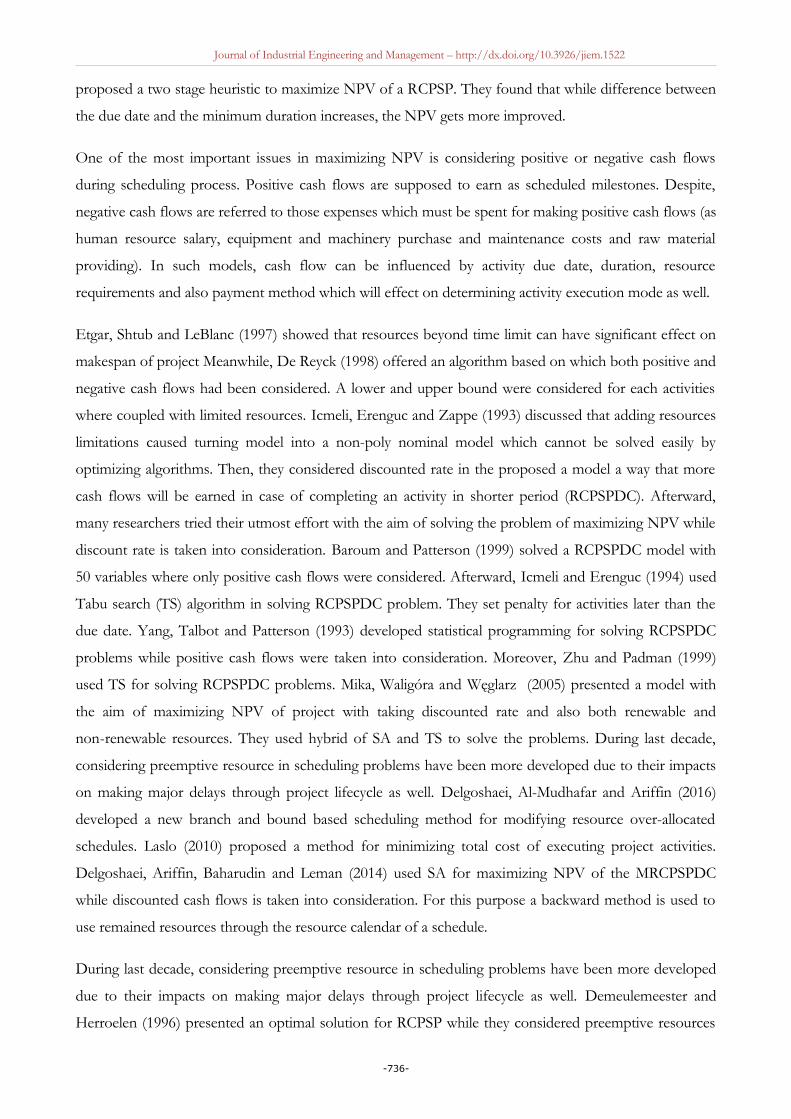
4.2. Experiment 2 (Large Scale)
In this experiment, 30 activities are considered. Number of modes is 4 and number of the limited
resources is 2. The network of this experiment is shown by Figure 22. Similar to the previous experiment,
rest of the required data are presented by Table 3.
Figure 22. Network diagram for experiment number 2
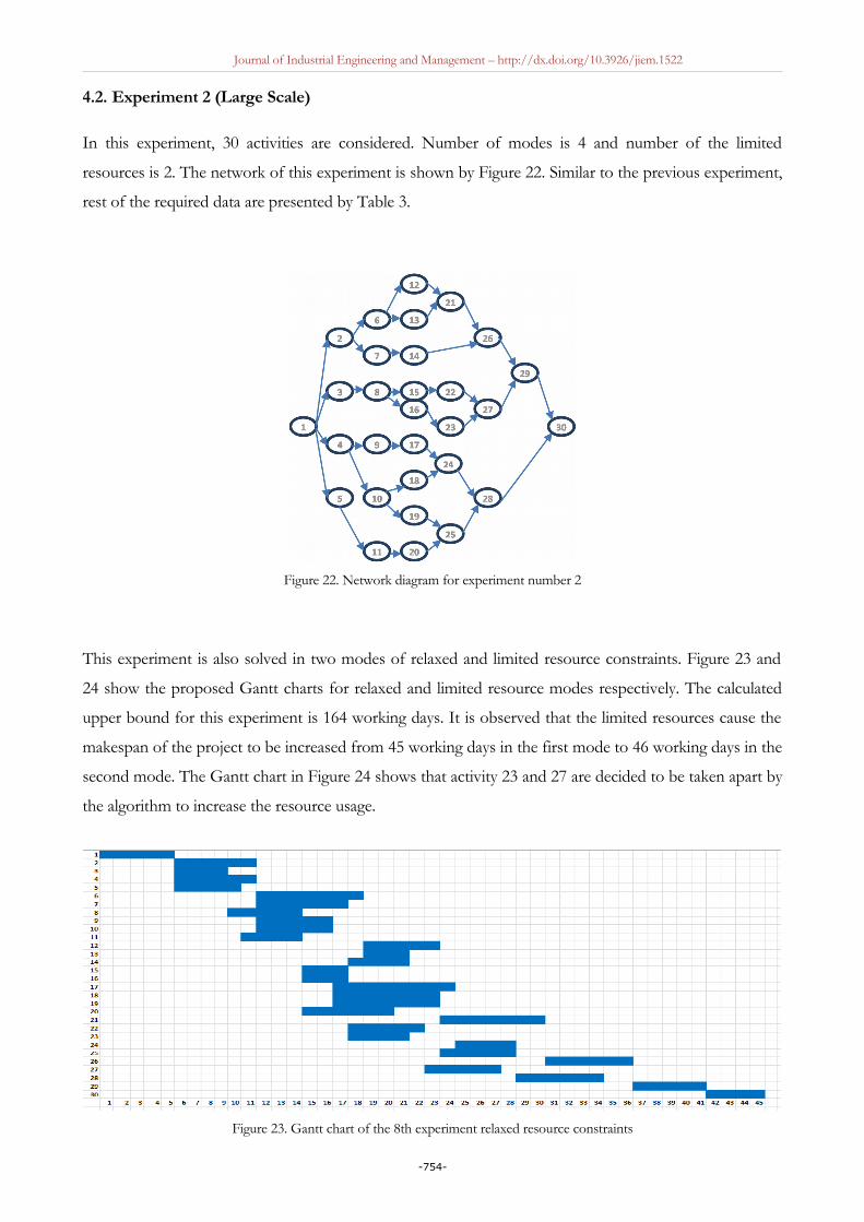
This experiment is also solved in two modes of relaxed and limited resource constraints. Figure 23 and
24 show the proposed Gantt charts for relaxed and limited resource modes respectively. The calculated
upper bound for this experiment is 164 working days. It is observed that the limited resources cause the
makespan of the project to be increased from 45 working days in the first mode to 46 working days in the
second mode. The Gantt chart in Figure 24 shows that activity 23 and 27 are decided to be taken apart by
the algorithm to increase the resource usage.
Figure 23. Gantt chart of the 8th experiment relaxed resource constraints
-754-

Journal of Industrial Engineering and Management – http://dx.doi.org/10.3926/jiem.1522
Figure 24. Gantt chart of the 8th experiment after using the proposed method
The cumulative resource usages throughout the project calendar for each of the resources are shown in
Figures 25 to 28. As seen for each of the resources, the slope of resource usage graphs after using the
proposed forward method is smoothed (Figures 26 and 28). The S-curve of the graphs shows that the
schedule is safe to be used.
Figure 25. Cumulative resource usage for resource 1
of experiment 2 (relaxed resource constraint)
Figure 26. Cumulative resource usage for resource 1
of experiment 2 (after using forward method)
-755-

Journal of Industrial Engineering and Management – http://dx.doi.org/10.3926/jiem.1522
Figure 27. Cumulative resource usage for resource 2
of experiment 2 (relaxed resource constraint)
Figure 28. Cumulative resource usage for resource 2
of experiment 2 (after using forward method)
The resource usage through the resource calendar is shown by Figures 29 to 32. The days 17, 18, 19, 20
and 21 are reported as over-allocated working days where the number of available resources is
insufficient to complete the activities that are scheduled in these days (Figures 29 and 31). In order to
modify the over-allocation in this case, the algorithm decided to take apart activities number 23 and 27
(as shown by Figure 24) for the mentioned days. Consequently, the activity 23 is split in days 19 and 20
and activity 27 is taken apart in days 31 to 36. Similar to other experiments, in this experiment after
using the forward method, none of the working days are reported over-allocated (Figures 30 and 32).
Figure 29. Daily usage of resource 1 throughout the calendar
of the project (before using the method)-Experiment 2
Figure 30. Daily usage of resource 1 throughout the calendar
of the project (before using the method)-Experiment 2
-756-

Journal of Industrial Engineering and Management – http://dx.doi.org/10.3926/jiem.1522
Figure 31. Daily usage of resource 2 throughout the calendar
of the project (before using the method)-Experiment 2
Figure 32. Daily usage of resource 2 throughout the calendar
of the project (before using the method)-Experiment 2
4.3. Experiment 3 (Large Scale)
The last experiment is a large scale MRCPSP which contains 50 activities, 4 executing modes and 5
preemptive resources. The network diagram is shown by Figure 33. Rest of the information is shown by
Table 4.
Figure 33. Network diagram of experiment number 3
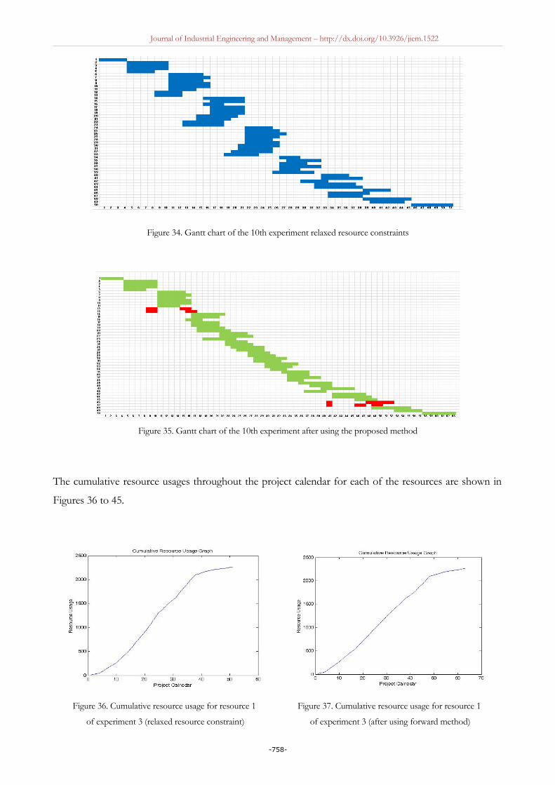
This experiment is also solved in two modes of relaxed and limited resource constraints. Figure 34 and 35
show the proposed Gantt charts for relaxed and limited resource modes respectively. The calculated
upper bound for this experiment is 78 working days. It is observed that the limited resources cause the
makespan of the project to be increased from 51 working days in the first mode to 63 working days in the
second mode. The Gantt chart in Figure 35 shows that activity 12, 13, 46 and 47 are taken apart by the
algorithm to increase the resource usage.
-757-
Journal of Industrial Engineering and Management – http://dx.doi.org/10.3926/jiem.1522
Figure 34. Gantt chart of the 10th experiment relaxed resource constraints
Figure 35. Gantt chart of the 10th experiment after using the proposed method
The cumulative resource usages throughout the project calendar for each of the resources are shown in
Figures 36 to 45.
Figure 36. Cumulative resource usage for resource 1
of experiment 3 (relaxed resource constraint)
Figure 37. Cumulative resource usage for resource 1
of experiment 3 (after using forward method)
-758-

Journal of Industrial Engineering and Management – http://dx.doi.org/10.3926/jiem.1522
Figure 38. Cumulative resource usage for resource 1
of experiment 3 (relaxed resource constraint)
Figure 39. Cumulative resource usage for resource 1
of experiment 3 (after using forward method)
Figure 40. Cumulative resource usage for resource 1
of experiment 3 (relaxed resource constraint)
Figure 41. Cumulative resource usage for resource 1
of experiment 3 (after using forward method)
Figure 42. Cumulative resource usage for resource 1
of experiment 3 (relaxed resource constraint)
Figure 43. Cumulative resource usage for resource 1
of experiment 3 (after using forward method)
-759-

Journal of Industrial Engineering and Management – http://dx.doi.org/10.3926/jiem.1522
Figure 44. Cumulative resource usage for resource 1
of experiment 3 (relaxed resource constraint)
Figure 45. Cumulative resource usage for resource 1
of experiment 3 (after using forward method)
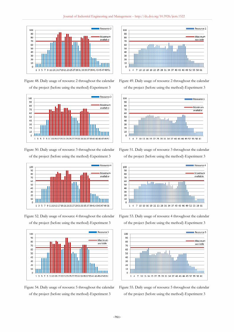
The resource usage through the resource calendar is shown by Figures 46 to 55. The days 10 to 38 are
mostly reported as over-allocated working days where the number of available resources is insufficient
to complete the activities that are scheduled in these days (Figures 46, 48, 50, 52 and 54). In order to
modify the over-allocating in this case, the algorithm decided to take apart activity number 46 and 47
(as shown by Figure 35) for the mentioned days. Consequently, the activity 46 is split in days 42 to 47
and activity 47 is split in days 42 to 45 and again in day 48. Similar to other experiments, in this
experiment after using the forward method, none of the working days are reported over-allocated
(Figures 47, 49, 51, 53 and 55).
Figure 46. Daily usage of resource 1 throughout the calendar
of the project (before using the method)-Experiment 3
Figure 47. Daily usage of resource 1 throughout the calendar
of the project (before using the method)-Experiment 3
-760-
Journal of Industrial Engineering and Management – http://dx.doi.org/10.3926/jiem.1522
Figure 48. Daily usage of resource 2 throughout the calendar
of the project (before using the method)-Experiment 3
Figure 49. Daily usage of resource 2 throughout the calendar
of the project (before using the method)-Experiment 3
Figure 50. Daily usage of resource 3 throughout the calendar
of the project (before using the method)-Experiment 3
Figure 51. Daily usage of resource 3 throughout the calendar
of the project (before using the method)-Experiment 3
Figure 52. Daily usage of resource 4 throughout the calendar
of the project (before using the method)-Experiment 3
Figure 53. Daily usage of resource 4 throughout the calendar
of the project (before using the method)-Experiment 3
Figure 54. Daily usage of resource 5 throughout the calendar
of the project (before using the method)-Experiment 3
Figure 55. Daily usage of resource 5 throughout the calendar
of the project (before using the method)-Experiment 3
-761-

Journal of Industrial Engineering and Management – http://dx.doi.org/10.3926/jiem.1522
4.4. Solving Experiments Gathered from the Literature
To examine the proposed approach, 10 series of small, medium and large scale examples are designed and
solved with 5, 6, 13, 15, 18, 20, 25, 30, 40, 50, 100, 200 and 500 variables. For evaluating the efficiency of
proposed model each example is solved under two conditions where all the criteria are considered the
same but resource availability. The results, then, checked with results of forward serial programming
method (Table 2).
No. Activity Resource Mode ResourcesCapacity Makespan GA
(OFV)SA
(OFV)
Branchand
Bound(OFV)
%GapCPU time
(perseconds)
Maximumsplit
activities
1 5 3 2 [60 100 300] 16 539.4 539.4 539.4 0.00% 0.357 0
2 5 3 2 [6 10 30] 19 538.7 538.7 538.7 0.00% 0.338 1
3 6 2 2 [130 100] 17 753.7 753.7 753.7 0.00% 0.212 0
4 6 2 2 [13 10] 19 751.3 751.3 751.3 0.00% 0.2109 1
5 13 2 2 [220 300] 30 2014.2 2014.2 2014.2 0.00% 0.218 0
6 13 2 2 [22 30] 32 2013.1 2013.1 2013.1 0.00% 0.217 5
7 15 3 4 [200 200 220] 36 2574.0 2574.0 2574.0 0.00% 0.336 0
8 15 3 4 [20 20 22] 41 2572.3 2572.3 2572.3 0.00% 0.34 1
9 18 3 3 [24 24 28] 27 2998.3 2998.3 2998.3 0.00% 0.334 0
10 18 3 3 [24 24 28] 36 2995.8 2995.8 2995.8 0.00% 0.335 1
11 20 3 4 [220 280 300] 35 3226.0 3232.0 3226.0 0.19% 0.33 0
12 20 3 4 [22 28 30] 42 3223.0 3223.0 3223.0 0.00% 0.334 2
13 25 2 3 [320 200] 52 4004.3 4031.0 4004.3 0.66% 0.178 0
14 25 2 3 [32 20] 52 4003.1 4016.0 4003.1 0.32% 0.221 3
15 30 2 4 [450 400] 45 5021.8 5021.8 5021.8 0.00% 0.222 0
16 30 2 4 [45 40] 45 5019.9 5019.9 5019.9 0.05% 0.226 2
17 40 4 3 [450 400 350] 57 6082.6 6086.4 6082.6 0.06% 0.352 0
18 40 4 3 [45 40 35] 68 6078.8 6082.1 6078.8 0.05% 0.354 6
19 50 5 4 [550 700 600 620650] 47 8457.3 8458.7 8457.3 0.02% 0.594 0
20 50 5 4 [55 70 60 62 65] 57 8450.7 8450.7 8450.7 0.04% 0.612 6
21 100 10 4R=[120 130 45 8964 78 124 220 135
90]190 1580.7 1584.2 1580.7 0.22% 2.266 0
22 100 10 4 R=[45 40 45 50 6445 64 45 65 45]
204 1692.5 1692.5 1692.5 0.09% 2.866 23
23 200 20 3
R=[140 160 140220 160 150 110120 150 130 140160 140 220 160150 110 120 150
130]
239 29625 29658 29625 0.11% 3.278 0
-762-
Journal of Industrial Engineering and Management – http://dx.doi.org/10.3926/jiem.1522
No. Activity Resource Mode ResourcesCapacity Makespan GA
(OFV)SA
(OFV)
Branchand
Bound(OFV)
%GapCPU time
(perseconds)
Maximumsplit
activities
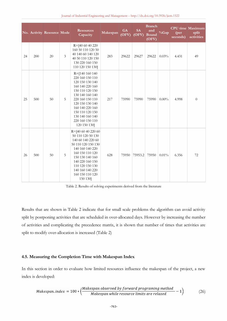
24 200 20 3
R=[40 60 40 220160 50 110 120 5040 140 60 140 12040 50 110 120 150130 220 160 150110 120 150 130]
283 29622 29627 29622 0.03% 4.431 49
25 500 50 5
R=[140 160 140220 160 150 110120 150 130 140160 140 220 160150 110 120 150130 140 160 140220 160 150 110120 150 130 140160 140 220 160150 110 120 150130 140 160 140220 160 150 110
120 150 130]
217 75990 75990 75990 0.00% 4.998 0
26 500 50 5
R=[40 60 40 220 6050 110 120 50 130140 60 140 220 6050 110 120 150 130
140 160 140 220160 150 110 120150 130 140 160140 220 160 150110 120 150 130140 160 140 220160 150 110 120
150 130]
628 75950 75953.2 75950 0.01% 6.356 72
Table 2. Results of solving experiments derived from the literature
Results that are shown in Table 2 indicate that for small scale problems the algorithm can avoid activity
split by postponing activities that are scheduled in over-allocated days. However by increasing the number
of activities and complicating the precedence matrix, it is shown that number of times that activities are
split to modify over-allocation is increased (Table 2)
4.5. Measuring the Completion Time with Makespan Index
In this section in order to evaluate how limited resources influence the makespan of the project, a new
index is developed:
(26)
-763-

Journal of Industrial Engineering and Management – http://dx.doi.org/10.3926/jiem.1522
Figure 56 shows the results of calculating Equation 15 for the experiments.
Figure 56. Makespan index graph for the solved experiments
No.Number ofActivities
Number ofResources
Number ofexecution
modesResource level
Method
M.S.I%U.B
Normalscheduling
Frowardprogramming
method
1 5 3 2 [6, 10, 30] 23 20 23 15.00
2 6 2 2 [13, 10] 31 19 21 10.53
3 13 2 2 [22, 30] 78 28 35 25.00
4 15 3 4 [20, 20, 22] 90 36 42 16.67
5 18 3 3 [24, 24, 28] 93 32 36 12.50
6 20 3 4 [22, 28, 30] 112 33 40 21.21
7 25 2 3 [32, 20] 136 55 60 9.09
8 30 2 4 [45, 40] 164 45 46 2.22
9 40 3 3 [45, 40, 35] 205 60 70 16.67
10 50 5 4 [55, 70, 60, 62, 65] 275 51 63 23.53
Table 3. Results gained after scheduling experiments
-764-

Journal of Industrial Engineering and Management – http://dx.doi.org/10.3926/jiem.1522
The results in Table 3 shows that although proposed method can avoid over-allocating of activities, but at
the same time limited resources can cause delay in makespan in a value between 2.22% and 25%.
Figure 57. Comparing the makespan in normal scheduling and forward serial programming for the solved experiments
Figure 57 shows that in all the studied case the observed makespan are smaller than UB. UB is considered
as upper limit for the makespan of a project and any value larger than this can thus be considered as an
infeasible solution.
No. 1 2 3 4 5 6 7 8 9 10
Over allocated days(Normal Scheduling)
[3, 3, 0] [4, 0] [5, 0] [7, 8, 7] [6, 5, 2] [12, 7, 6] [4, 11] [5, 5] [7, 13, 24] [22, 15, 21, 22, 17]
Over-allocated days(Forward programming
method)[0, 0, 0] [0, 0] [0, 0] [0, 0, 0] [0, 0, 0] [0, 0, 0] [0, 0] [0, 0] [0, 0, 0] [0, 0, 0, 0, 0]
Table 4. Over-allocated days in normal and modified schedules observed before and after using the method
Table 4 compares the number of over-allocated days of each of the resources through its calendar before
and after using the method. The results show that in none of the studied cases the over-allocation is
observed (Figure 58).
-765-

Journal of Industrial Engineering and Management – http://dx.doi.org/10.3926/jiem.1522
Figure 58. Comparing number of over allocated days for the solved experiments
Results also indicate that by increasing the discounted rate and the number of activities (dimension of the
problem) the angle of slope of the NPV is increased (Figure 59).
Figure 59. Comparing the effects of alpha rate and number of activities in increasing NPV
-766-

Journal of Industrial Engineering and Management – http://dx.doi.org/10.3926/jiem.1522
5. Verification the Proposed Method
In this section the proposed scheduling method is applied for 2 case studies. The first case study is
constructing a hospital. The list of activities is shown by Table 5:
ID Activity Duration ID Activity Duration1 Shop Preparedness and Mobilization 7 30 Installing Gas Supply System 22 Foundation 21 31 Installing Cable Trunk 53 Structure 40 32 Install Cable Tray 54 Flooring 10 33 Cabling 75 Trench 2 34 Installing Lightning Cables 56 Wall Erection 12 35 Installing Lightning Lamps 27 Roofing 5 36 Installing of Electrical Panels 78 Window Frames 3 37 Cable Connecting for Electrical Panel 29 Door Frames 3 38 Installing of Plugs & Sockets 210 Fire Box Frames 1 39 Connect Cables and Pipes of Chillers 111 Installing False Ceiling Structure 10 40 Installing CCTVs 212 Roof Insulation 2 41 Installing Nurse Call System 213 Installing False Ceiling 10 42 Installing Paging System 214 Rain Water Piping 3 43 Windows 315 Install Piping Tray 4 44 Wooden Doors 216 Water Piping 5 45 Plastering 717 Return Piping 5 46 Tilling 218 Drainage Piping 5 47 Operating Rooms Tilling 219 Floor Drains 1 48 Installing Ceramics 420 Installing Supports for Ducts 10 49 Painting 421 Installing Ducts 7 50 Installing Wooden Works 222 Installing Coverage for Ducts 7 51 Installing Radiology Door 123 FCU(Duct) 6 52 Locker Room Preparation 224 FCU (Cold, Hot and Return Water Piping) 3 53 Installing Hospital Beds 125 FCU (Drainage Piping) 4 54 Sliding Door 226 FCU (Machine) 2 55 Installing Surgical Beds 127 FCU (Grille) 2 56 Area 3028 Structure of Chillers 2 57 Building Facades 3029 Install Chillers 4 58 Testing And Site Delivery 2
Table 5. List of Activities for Constructing a Hospital
-767-

Journal of Industrial Engineering and Management – http://dx.doi.org/10.3926/jiem.1522
The Table 6 shows the precedence network between activities:
1 2 3 4 5 6 7 8 9 10 11 12 13 14 15 16 17 18 19 20 21 22 23 24 25 26 27 28 29 30 31 32 33 34 35 36 37 38 39 40 41 42 43 44 45 46 47 48 49 50 51 52 53 54 55 56 57 58
1
2 FS
3 FS
4 FS
5SS+1
6FS+1
7 FS
8 FS
9 FS
10 FS
11 FS
12 FS FS FS
13 FS FS FS FS FS FS FS
14 FS
15 FS FS
16 FS
17 FS FS
18 FS
19 FS
20 FS FS
21 FS
22SS+1
23 FS
24 FS
25 SS
26 FS
27 FS
28 FS
29 FS
30 FS
31 FS FS
32 FS
33 FS
34 FS FS
35 FS FS
36 FS
37 FS FS
38 FS
39 FS FS
40 FS
41 FS
42 FS
43 FS
44 FS
45 FS FS FS FS FS
46 FS FS
47 FS FS
48 FS FS
49 FS FS
50 FS
51 FS
52 FS
53 FS
54 FS
55 FS FS FS
56 FS
57 FS
58 FS FS FS FS FS FS FS FS
Table 6. The Activity Precedence Matrix
-768-

Journal of Industrial Engineering and Management – http://dx.doi.org/10.3926/jiem.1522
And finally Table 7 shows the resource usage of activities:
ActivityID
1 2 3 4 5 6 7 8 9 10 11 12 13 14 15
CivilWorker
MechanicalWorker
ElectricalWorker
Pipeman
ElectricalTechnician
MechanicalTechnician
CivilTechnician Welder Painter Carpenter Blacksmith
CivilEngineer
MechanicalEngineer
ElectricalEngineer Mason
1 1 1 1 1 1 1 1 1 1
2 5 1 1
3 5 1 1
4 4 1 1
5 1 1
6 5 1 1 1
7 4 1 1 1
8 2 1
9 2 1
10 2 1
11 4 1 2 1 1
12 1 1 1
13 4 1 2 1 1
14 2 2 1 1
15 4 2 1 2 1
16 4 2 1 1
17 4 2 1 1
18 2 1 1 1
19 2 1
20 4 1 1
21 4 1 1
22 2 1
23 2 1 1
24 4 1 1
25 1 1 1
26 2 1 1
27 1 1
28 1 1 1 1
29 2 1 1
30 2 1 1
31 4 1 1 1
32 4 1 1 1
33 2 1 1
34 2 1 1
35 2 1 1
36 2 1 1
37 2 1 1
38 2 1 1
39 2 1 1
40 2 1 1
41 2 1 1
42 2 1 1
43 2 1 1
44 2 1 2 1
45 4 1 1 2
46 4 1 1 2
47 2 1 1 1
48 4 1 1 2
49 1 2 1
50 2 1 2 1
51 2 1 1 1
52 2 1 1
53 2 1 1
54 2 1 1
55 2 1 1
56 2 1 1 1
57 4 1 1 1
58 1 1 1 1 1 1
Table 7. Resource Usage of Activities
-769-

Journal of Industrial Engineering and Management – http://dx.doi.org/10.3926/jiem.1522
And finally Table 8 shows the maximum available resource:
Resource CivilWorker
MechanicalWorker
ElectricalWorker
Pipeman
ElectricalTechnician
MechanicalTechnician
CivilTechnician
Welder Painter Carpenter Blacksmith CivilEngineer
MechanicalEngineer
ElectricalEngineer
Mason
MaximumLevel 800% 800% 800% 200% 200% 200% 200% 200% 200% 100% 200% 100% 100% 100% 200%
Table 8. Maximum Available Resource
In the first step we schedule the problem using Microsoft Office Project® 2010 (MSP 2010). As expected
the project is unacceptable since most of the resources are over-allocated (Figure 60).
Figure 60. Resource sheet of MSP 2010
The Gantt chart of the resource over allocated schedule is shown by Figure 61 and 62:
-770-

Journal of Industrial Engineering and Management – http://dx.doi.org/10.3926/jiem.1522
Figure 61. Gantt Chart of MSP 2010 for case study (Continued)
Figure 62. Gantt Chart of MSP 2010 for case study
In continue the case study is solved by the proposed solving algorithm while all resources constraint are
considered relaxed. The same results are completely in accordance with the results gained by the MSP
2010 (Figure 63):
Figure 63. Results of solving the case study by the proposed method while Resource constraints are relaxed
-771-

Journal of Industrial Engineering and Management – http://dx.doi.org/10.3926/jiem.1522
In continue the proposed algorithm is used to modify the over-allocated schedule. The results show that
the modified schedule is not suffered by any over allocated resource so it is trustable and can be used for
constructing phase.
Table 9 compares the information of the activities before and after using the proposed method.
MSP 2010 Classic Branch and Bound Proposed Algorithm
Number of Activities 58 58 58
Number of Resources 15 15 15
Number of over allocated resources 10 10 0
Number of Split Times 0 0 5
Makespan 146 146 204
NPV – 77564$ 77560$
Table 9. Comparing results of scheduling the hospital unig MSP, Classic Branch and Bound and the proposed algorithm
Figures 64 and 65 show the Gantt chart of the modified scheduled that is achieved by the proposed
solving method.
Figure 64. The modified Gantt chart for the Hospital (Continued)
-772-

Journal of Industrial Engineering and Management – http://dx.doi.org/10.3926/jiem.1522
Figure 65. The modified Gantt chart for the Hospital
Results show that the proposed algorithm can successfully modified the over-allocated resources in a
reasonable computing time.
6. Conclusion
Scheduling multi-mode resource constraint project scheduling problems while preemptive resources are
exists are a big concern in project management. In this research the over-allocated project schedules with
preemptive resources are rescheduled using genetic algorithm. By presenting a dynamic forward
approach, an appropriate and logical solution is boosted and it is observed that the proposed method can
modify over-allocated MRCPSPs schedules by taking apart less important activities and keeping more
important activities. It is also found that using the proposed procedure has caused noticeable rise in
remaining resources usage during life the project implementation. Further expansion of the research by
considering negative cash flows is suggested.
Acknowledgements: The authors would like to thank Dr. Mohammad Gholami (Post-doctoral fellow;
University of Calgary-Abb.CA) for his positive comments during the writing of this manuscript.
-773-

Journal of Industrial Engineering and Management – http://dx.doi.org/10.3926/jiem.1522
References
Abbasi, B., Shadrokh, S., & Arkat, J. (2006). Bi-objective resource-constrained project scheduling with
robustness and makespan criteria. Applied Mathematics and Computation, 180(1), 146-152.
http://dx.doi.org/10.1016/j.amc.2005.11.160
Achuthan, N., & Hardjawidjaja, A. (2001). Project scheduling under time dependent costs–A branch and
bound algorithm. Annals of Operations Research, 108(1-4), 55-74. http://dx.doi.org/10.1023/A:1016046625583
Alcaraz, J., & Maroto, C. (2001). A robust genetic algorithm for resource allocation in project scheduling.
Annals of Operations Research, 102(1-4), 83-109. http://dx.doi.org/10.1023/A:1010949931021
Ballestín, F., Valls, V., & Quintanilla, S. (2008). Pre-emption in resource-constrained project scheduling.
European Journal of Operational Research, 189(3), 1136-1152. http://dx.doi.org/10.1016/j.ejor.2006.07.052
Baroum, S.M., & Patterson, J.H. (1999). An exact solution procedure for maximizing the net present
value of cash flows in a network. Project Scheduling (pp. 107-134). Springer. http://dx.doi.org/10.1007/978-1-
4615-5533-9_5
Buddhakulsomsiri, J., & Kim, D.S. (2006). Properties of multi-mode resource-constrained project
scheduling problems with resource vacations and activity splitting. European Journal of Operational Research,
175(1), 279-295. http://dx.doi.org/10.1016/j.ejor.2005.04.030
Castejón-Limas, M., Ordieres-Meré, J., González-Marcos, A., & González-Castro, V. (2011). Effort
estimates through project complexity. Annals of Operations Research, 186(1), 395-406.
http://dx.doi.org/10.1007/s10479-010-0776-0
Chtourou, H., & Haouari, M. (2008). A two-stage-priority-rule-based algorithm for robust
resource-constrained project scheduling. Computers & industrial engineering, 55(1), 183-194.
http://dx.doi.org/10.1016/j.cie.2007.11.017
Damay, J., Quilliot, A., & Sanlaville, E. (2007). Linear programming based algorithms for preemptive and
non-preemptive RCPSP. European Journal of Operational Research, 182(3), 1012-1022.
http://dx.doi.org/10.1016/j.ejor.2006.09.052
De Reyck, B. (1998). A branch-and-bound procedure for the resource-constrained project scheduling
problem with generalized precedence relations. European Journal of Operational Research, 111(1), 152-174.
http://dx.doi.org/10.1016/S0377-2217(97)00305-6
-774-

Journal of Industrial Engineering and Management – http://dx.doi.org/10.3926/jiem.1522
Delgoshaei, A., Al-Mudhafar, A., & Ariffin, M.K.A. (2016). Developing a new method for modifying
over-allocated multi-mode resource constraint schedules in the presence of preemptive resources.
Decision Science Letters, 5(4), 499-518. http://dx.doi.org/10.5267/j.dsl.2016.5.002
Delgoshaei, A., Ariffin, M.K., Baharudin, B.H.T.B., & Leman, Z. (2014). A Backward Approach for
Maximizing Net Present Value of Multi-mode Pre-emptive Resource-Constrained Project Scheduling
Problem with Discounted Cash Flows Using Simulated Annealing Algorithm. International Journal of
Industrial Engineering and Management, 5(3), 151-158.
Delgoshaei, A., Ariffin, M.K.M., Baharudin, B.H.T.B., & Leman, Z. (2015). Minimizing makespan of a
resource-constrained scheduling problem: A hybrid greedy and genetic algorithms. Resource. International
Journal of Industrial Engineering Computations, 6(4), 503-520. http://dx.doi.org/10.5267/j.ijiec.2015.5.002
Demeulemeester, E.L., & Herroelen, W.S. (1996). An efficient optimal solution procedure for the
preemptive resource-constrained project scheduling problem. European Journal of Operational Research,
90(2), 334-348. http://dx.doi.org/10.1016/0377-2217(95)00358-4
Elmaghraby, S.E., & Herroelen, W.S. (1990). The scheduling of activities to maximize the net present
value of projects. European Journal of Operational Research, 49(1), 35-49. http://dx.doi.org/10.1016/0377-
2217(90)90118-U
Etgar, R., Shtub, A., & LeBlanc, L.J. (1997). Scheduling projects to maximize net present value—the case
of time-dependent, contingent cash flows. European Journal of Operational Research, 96(1), 90-96.
http://dx.doi.org/10.1016/0377-2217(95)00382-7
Hartmann, S. (2001). Project scheduling with multiple modes: a genetic algorithm. Annals of Operations
Research, 102(1-4), 111-135. http://dx.doi.org/10.1023/A:1010902015091
Hartmann, S., & Briskorn, D. (2010). A survey of variants and extensions of the resource-constrained
project scheduling problem. European Journal of Operational Research, 207(1), 1-14.
http://dx.doi.org/10.1016/j.ejor.2009.11.005
Icmeli, O., & Erenguc, S. S. (1994). A tabu search procedure for the resource constrained project
scheduling problem with discounted cash flows. Computers & operations research, 21(8), 841-853.
http://dx.doi.org/10.1016/0305-0548(94)90014-0
Icmeli, O., Erenguc, S.S., & Zappe, C.J. (1993). Project scheduling problems: a survey. International Journal
of Operations & Production Management, 13(11), 80-91. http://dx.doi.org/10.1108/01443579310046454
-775-

Journal of Industrial Engineering and Management – http://dx.doi.org/10.3926/jiem.1522
Jarboui, B., Damak, N., Siarry, P., & Rebai, A. (2008). A combinatorial particle swarm optimization for
solving multi-mode resource-constrained project scheduling problems. Applied Mathematics and
Computation, 195(1), 299-308. http://dx.doi.org/10.1016/j.amc.2007.04.096
Ke, H., & Liu, B. (2010). Fuzzy project scheduling problem and its hybrid intelligent algorithm. Applied
Mathematical Modelling, 34(2), 301-308.
Kelley, J.E. (1963). The critical-path method: Resources planning and scheduling. Industrial scheduling, 13,
347-365.
Kim, K., Yun, Y., Yoon, J., Gen, M., & Yamazaki, G. (2005). Hybrid genetic algorithm with adaptive
abilities for resource-constrained multiple project scheduling. Computers in industry, 56(2), 143-160.
http://dx.doi.org/10.1016/j.compind.2004.06.006
Kolisch, R. (1996). Serial and parallel resource-constrained project scheduling methods revisited: Theory
and computation. European Journal of Operational Research, 90(2), 320-333. http://dx.doi.org/10.1016/0377-
2217(95)00357-6
Kolisch, R., & Drexl, A. (1997). Local search for nonpreemptive multi-mode resource-constrained project
scheduling. IIE transactions, 29(11), 987-999. http://dx.doi.org/10.1080/07408179708966417
Laslo, Z. (2010). Project portfolio management: An integrated method for resource planning and
scheduling to minimize planning/scheduling-dependent expenses. International Journal of Project
Management, 28(6), 609-618. http://dx.doi.org/10.1016/j.ijproman.2009.10.001
Lee, & Lei, L. (2001). Multiple-project scheduling with controllable project duration and hard resource
constraint: some solvable cases. Annals of Operations Research, 102(1-4), 287-307.
http://dx.doi.org/10.1023/A:1010918518726
Lova, A., & Tormos, P. (2001). Analysis of scheduling schemes and heuristic rules performance in
resource-constrained multiproject scheduling. Annals of Operations Research, 102(1-4), 263-286.
http://dx.doi.org/10.1023/A:1010966401888
Mika, M., Waligóra, G., & Węglarz, J. (2005). Simulated annealing and tabu search for multi-mode
resource-constrained project scheduling with positive discounted cash flows and different payment
models. European Journal of Operational Research, 164(3), 639-668. http://dx.doi.org/10.1016/j.ejor.2003.10.053
Russell, A. (1970). Cash flows in networks. Management Science, 16(5), 357-373.
http://dx.doi.org/10.1287/mnsc.16.5.357
-776-

Journal of Industrial Engineering and Management – http://dx.doi.org/10.3926/jiem.1522
Seifi, M., & Tavakkoli-Moghaddam, R. (2008). A new bi-objective model for a multi-mode resource-
constrained project scheduling problem with discounted cash flows and four payment models. Int. J. of
Engineering, Transaction A: Basic, 21(4), 347-360.
Sprecher, A. (2000). Scheduling resource-constrained projects competitively at modest memory
requirements. Management Science, 46(5), 710-723. http://dx.doi.org/10.1287/mnsc.46.5.710.12044
Sung, C., & Lim, S. (1994). A project activity scheduling problem with net present value measure.
International Journal of Production Economics, 37(2), 177-187. http://dx.doi.org/10.1016/0925-5273(94)90169-4
Talbot, F.B. (1982). Resource-constrained project scheduling with time-resource tradeoffs: The
nonpreemptive case. Management Science, 28(10), 1197-1210. http://dx.doi.org/10.1287/mnsc.28.10.1197
Ulusoy, G., Sivrikaya-Şerifoğlu, F., & Şahin, Ş. (2001). Four payment models for the multi-mode resource
constrained project scheduling problem with discounted cash flows. Annals of Operations Research,
102(1-4), 237-261. http://dx.doi.org/10.1023/A:1010914417817
Van de Vonder, S., Demeulemeester, E., Herroelen, W., & Leus, R. (2005). The use of buffers in project
management: The trade-off between stability and makespan. International Journal of Production Economics,
97(2), 227-240. http://dx.doi.org/10.1016/j.ijpe.2004.08.004
Van de Vonder, S., Demeulemeester, E., Herroelen, W., & Leus, R. (2006). The trade-off between
stability and makespan in resource-constrained project scheduling. International Journal of Production
Research, 44(2), 215-236. http://dx.doi.org/10.1080/00207540500140914
Van Peteghem, V., & Vanhoucke, M. (2010). A genetic algorithm for the preemptive and non-preemptive
multi-mode resource-constrained project scheduling problem. European Journal of Operational Research,
201(2), 409-418. http://dx.doi.org/10.1016/j.ejor.2009.03.034
Vanhoucke, M., & Debels, D. (2008). The impact of various activity assumptions on the lead time and
resource utilization of resource-constrained projects. Computers & industrial engineering, 54(1), 140-154.
http://dx.doi.org/10.1016/j.cie.2007.07.001
Węglarz, J., Józefowska, J., Mika, M., & Waligóra, G. (2011). Project scheduling with finite or infinite
number of activity processing modes–A survey. European Journal of Operational Research, 208(3), 177-205.
http://dx.doi.org/10.1016/j.ejor.2010.03.037
Yan, L., Jinsong, B., Xiaofeng, H., & Ye, J. (2009). A heuristic project scheduling approach for quick
response to maritime disaster rescue. International Journal of Project Management, 27(6), 620-628.
http://dx.doi.org/10.1016/j.ijproman.2008.10.001
-777-

Journal of Industrial Engineering and Management – http://dx.doi.org/10.3926/jiem.1522
Yang, Talbot, F.B., & Patterson, J.H. (1993). Scheduling a project to maximize its net present value: an
integer programming approach. European Journal of Operational Research, 64(2), 188-198.
http://dx.doi.org/10.1016/0377-2217(93)90176-N
Yu, Wang, S., Wen, F., & Lai, K.K. (2012). Genetic algorithm-based multi-criteria project portfolio
selection. Annals of Operations Research, 197(1), 71-86. http://dx.doi.org/10.1007/s10479-010-0819-6
Zhou, M., & Askin, R.G. (1998). Formation of general GT cells: an operation-based approach. Computers
& industrial engineering, 34(1), 147-157. http://dx.doi.org/10.1016/S0360-8352(97)00157-5
Zhu, D., & Padman, R. (1999). A metaheuristic scheduling procedure for resource‐constrained projects
with cash flows. Naval Research Logistics (NRL), 46(8), 912-927. http://dx.doi.org/10.1002/(SICI)1520-
6750(199912)46:8<912::AID-NAV3>3.0.CO;2-C
Appendix
Precedence Matrix for Experiments number 1 and 2 in Table 3
1 2 3 4 5
1 - - - - -
2 FS(1)+2 - - - -
3 SS(1) FS(2) - - -
4 - FS(2) SS(3)+1 - -
5 - - - SF(4) -
Precedence Matrix for Experiments number 3 and 4 in Table 3
1 2 3 4 5 6
1
2 FS(1)
3 FS(1)+2
4 SF(3)
5 FS(3)+1
6 FS(4)+2 FF(5)
-778-

Journal of Industrial Engineering and Management – http://dx.doi.org/10.3926/jiem.1522
Precedence Matrix for Experiments number 5 and 6 in Table 3
1 2 3 4 5 6 7 8 9 10 11 12 13
1
2 FS(1)+1
3 FS(1)
4 FS(1)
5 SS(2)+1
6 FS(2)+1
7 FF(3)+1
8 FS(4)+1
9 FS(4)+1
10 FS(5) FS(6)
11 SS(7)+1
12 FS(8)+1 FS(9)+1
13 FS(10) FS(11) FS(12)
Precedence Matrix for Experiments number 7 and 8 in Table 3
1 2 3 4 5 6 7 8 9 10 11 12 13 14 15
1
2 FS(1)
3 FS(1)+1
4 FS(1)
5 FS(2)+1
6 FS(2)+1
7 FS(3)
8 FF(3)+1
9 FS(4)+2 FS(5)
10 SS(4)+1
11 FS(6)+1 FS(7)
12 FS(7)+1 SS(8)+1
13 FF(9)+1 FF(10)
14 SS(11) FS(12)+1
15 FS(13) FS(14)+1
-779-

Journal of Industrial Engineering and Management – http://dx.doi.org/10.3926/jiem.1522
Precedence Matrix for Experiments number 9 and 10 in Table 3
1 2 3 4 5 6 7 8 9 10 11 12 13 14 15 16 17 18
1
2 FS(1)
3 FS(1)+1
4 FS(2)+2
5 FS(2)
6 SS(3)+1
7 FS(3)
8 FF(4)+1
9 FS(5)
10 FS(6)+1
11 SF(7)
12 FS(8)+1
13 FF(8)
14 SS(9)
15 SS(10)
16 FS(11)+2
17 SF(11)+1
18 FS(12)+2 SS(13)+1 FS(14)+1 FS(15)+1 FS(16)+1 FS(17)+1
Precedence Matrix for Experiments number 11 and 12 in Table 3
1 2 3 4 5 6 7 8 9 10 11 12 13 14 15 16 17 18 19 20
1
2 FS(1)
3 FS(1)
4 FS(1)
5 FS(2)
6 FS(2)
7 SS(3)
8 FF(4)
9 FS(4)
10 FS(5)
11 SS(6)
12 FS(6)
13 FS(7)
14 SS(8)+2
15 SF(9)+3
16 FS(9)+2
17 FS(10)+2 FS(11)+1
18 SS(12)+3 FS(13)+1
19 FS(14)+4 FS(15)+1 FF(16)+3
20 FS(17)+2 FS(18)+1 FS(19)+1
-780-

Journal of Industrial Engineering and Management – http://dx.doi.org/10.3926/jiem.1522
Precedence Matrix for Experiments number 13 and 14 in Table 3
1 2 3 4 5 6 7 8 9 10 11 12 13 14 15 16 17 18 19 20 21 22 23 24 25
1
2 FS(1)
3 FS(1)
4 FS(2)+1
5 SS(2)
6 FS(3)+1
7 SF(3)+1
8 FS(3)
9 SS(4)+1
10 FF(5)+2
11 FS(6)
12 FS(7)
13 SS(8)+1
14 FS(9) FS(10)
15 FS(11) FS(12) FS(13)+1
16 FS(14) FS(15)+1
17 SS(16)+1
18 FS(16)
19 FF(17)+1
20 FS(18)
21 SF(18)+1
22 FS(19)+1
23 FS(20)
24 FS(21)
25 FS(22) FS(23) FS(24)
-781-

Journal of Industrial Engineering and Management – http://dx.doi.org/10.3926/jiem.1522
Precedence Matrix for Experiments number 15 and 16 in Table 3
1 2 3 4 5 6 7 8 9 10 11 12 13 14 15 16 17 18 19 20 21 22 23 24 25 26 27 28 29 30
1
2 FS(1)
3 FS(1)
4 FS(1)
5 FS(1)+1
6 FS(2)
7 FS(2)+1
8 SS(3)
9 FS(4)+1
10 FF(4)
11 FS(5)+1
12 SF(6)+1
13 FS(6)
14 SS(7)+1
15 FF(8)
16 FS(8)+1
17 FS(9)
18 SS(10)+1
19 FS(10)
20 SS(11)+1
21 FS(12)
FS(13)+2
22 FF(15)+1
23 SF(16)+2
24 SS(17)
FS(18)+3
25 FS(19)
FS(20)
26 FS(14)
FS(21)
27 FS(22)
FS(23)
28 SS(24)
FS(25)+1
29 FS(26)
FS(27)
30 FS(28)
FS(29)
-782-
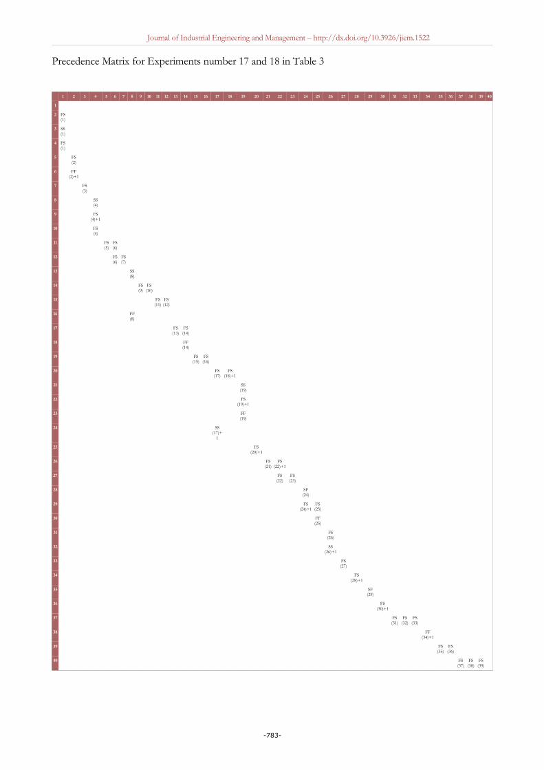
Journal of Industrial Engineering and Management – http://dx.doi.org/10.3926/jiem.1522
Precedence Matrix for Experiments number 17 and 18 in Table 3
1 2 3 4 5 6 7 8 9 10 11 12 13 14 15 16 17 18 19 20 21 22 23 24 25 26 27 28 29 30 31 32 33 34 35 36 37 38 39 40
1
2 FS(1)
3 SS(1)
4 FS(1)
5 FS(2)
6 FF(2)+1
7 FS(3)
8 SS(4)
9 FS(4)+1
10 FS(4)
11 FS(5)
FS(6)
12 FS(6)
FS(7)
13 SS(8)
14 FS(9)
FS(10)
15 FS(11)
FS(12)
16 FF(8)
17 FS(13)
FS(14)
18 FF(14)
19 FS(15)
FS(16)
20 FS(17)
FS(18)+1
21 SS(19)
22 FS(19)+1
23 FF(19)
24 SS(17)+
1
25 FS(20)+1
26 FS(21)
FS(22)+1
27 FS(22)
FS(23)
28 SF(24)
29 FS(24)+1
FS(25)
30 FF(25)
31 FS(26)
32 SS(26)+1
33 FS(27)
34 FS(28)+1
35 SF(29)
36 FS(30)+1
37 FS(31)
FS(32)
FS(33)
38 FF(34)+1
39 FS(35)
FS(36)
40 FS(37)
FS(38)
FS(39)
-783-

Journal of Industrial Engineering and Management – http://dx.doi.org/10.3926/jiem.1522
Precedence Matrix for Experiments number 19 and 20 in Table 3
1 2 3 4 5 6 7 8 9 10 11 12 13 14 15 16 17 18 19 20 21 22 23 24 25 26 27 28 29 30 31 32 33 34 35 36 37 38 39 40 41 42 43 44 45 46 47 48 49 50
1
2 FS(1)
3 FS(1)
4 FS(1)
5 SS(1)
6 FS(2)
7 FS(2)
8 FF(2)+1
9 FS(3)
10 SS(3)+1
11 SF(4)
12 FS(5)+1
13 SS(5)
14 FF(6)
15 FS(6)+1
FS(7)
16 SS(8)+1
17 SS(9)
18 FS(10)+1
19 FS(10)
20 FS(11)+1
21 SS(11)
22 FS(12)
23 FS(13)
24 FS(14)
25 SS(14)+1
26 FS(15)
FS(16)+1
27 SF(17)
28 FS(18)+1
29 FS(19)
30 FS(20)+1
31 SS(20)+1
32 FS(21)
FS(22)
33 SS(23)+1
34 FS(24)
FS(25)
35 FS(26)+1
FS(27)
36 FF(27)+1
37 FS(28)
FS(29)+1
38 FS(30)
FS(31)
39 FS(32)
FS(33)
40 FS(34)
FS(35)
41 FS(36)
FS(37)
42 FS(38)+1
43 SS(39)
44 FS(39)
45 FS(40)
FS(41)
46 FF(42)
47 FS(42)
48 FS(43)
FS(44)
49 FS(46)
FS(47)
50 FS(45)
FS(48)
FS(49)
-784-

Journal of Industrial Engineering and Management – http://dx.doi.org/10.3926/jiem.1522
In order to receive precedence matrices for experiments with 100, 200, 500 and 1000 activities, please
send an email to the corresponding author.
Journal of Industrial Engineering and Management, 2016 (www.jiem.org)
Article's contents are provided on an Attribution-Non Commercial 3.0 Creative commons license. Readers are allowed to copy,
distribute and communicate article's contents, provided the author's and Journal of Industrial Engineering and Management's
names are included. It must not be used for commercial purposes. To see the complete license contents, please visit
http://creativecommons.org/licenses/by-nc/3.0/.
-785-