Groupwise Constrained Reconstruction for Subspace Clustering

Ruijiang Li† rjli@fudan.edu.cnBin Li‡ bin.li-1@uts.edu.auKe Zhang† k_zhang@fudan.edu.cnCheng Jin† jc@fudan.edu.cnXiangyang Xue† xyxue@fudan.edu.cn† School of Computer Science, Fudan University, Shanghai, 200433, China‡ QCIS Centre, FEIT, University of Technology, Sydney, NSW 2007, Australia

AbstractReconstruction based subspace clusteringmethods compute a self reconstruction ma-trix over the samples and use it for spectralclustering to obtain the final clustering result.Their success largely relies on the assumptionthat the underlying subspaces are indepen-dent, which, however, does not always holdin the applications with increasing numberof subspaces. In this paper, we propose anovel reconstruction based subspace cluster-ing model without making the subspace inde-pendence assumption. In our model, certainproperties of the reconstruction matrix areexplicitly characterized using the latent clus-ter indicators, and the affinity matrix used forspectral clustering can be directly built fromthe posterior of the latent cluster indicatorsinstead of the reconstruction matrix. Exper-imental results on both synthetic and real-world datasets show that the proposed modelcan outperform the state-of-the-art methods.

1. Introduction

Subspace clustering aims to group the given samplesinto clusters according to the criterion that samples inthe same cluster are drawn from the same linear sub-space. In the last decade, a number of subspace clus-tering methods have been proposed with successful ap-plications in the areas including motion segmentation(Kanatani, 2001; Vidal & Hartley, 2004; Elhamifar &Vidal, 2009), image clustering under different illumi-nations (Ho et al., 2003), etc. Generally speaking, ex-isting approaches to subspace clustering can be classi-fied into the following categories: matrix factorization

Appearing in Proceedings of the 29 th International Confer-ence on Machine Learning, Edinburgh, Scotland, UK, 2012.Copyright 2012 by the author(s)/owner(s).

based, algebraic based, statistically modelling, and re-construction based, among which the reconstructionbased approach has been proved most effective andhas drawn much attention recently (Elhamifar & Vi-dal, 2009; Liu et al., 2010; Wang et al., 2011). In thispaper, we focus on the reconstruction based approach.

The objective of the reconstruction based subspaceclustering is to approximate the dataset X ∈ RD×N(N is the number of samples andD denotes the sampledimensionality) with the reconstruction XW , whereW ∈ RN×N is the reconstruction matrix which can befurther used to build the affinity matrix |W |+

∣∣W>∣∣

for spectral clustering. The intuition behind the re-construction is to make the value of wij small or evenvanish if samples xi and xj are not in the same sub-space, such that the subspaces/clusters can be easilyidentified by the subsequent spectral clustering.

All the existing reconstruction based methods comewith proofs claiming that the desired W could be ob-tained under the subspace independence assumption,i.e., the underlying subspaces S1,S2, · · · ,SK are lin-early independent, or mathematically,

dim(

K∑k=1

⊕Sk) =

K∑k=1

dim(Sk) (1)

Unfortunately, this assumption will be violated if thereexist bases shared among the subspaces. For example,given three orthogonal bases, b1, b2, b3, and two sub-spaces, S1 = b1 ⊕ b2 and S2 = b3 ⊕ b2 (b2 is shared inS1 and S2), the l.h.s. of Eq.(1) is 3, which is smallerthan the r.h.s. being 4. In real-world scenarios, thesubspace independence assumption does not alwayshold. For example, in human face clustering, as thenumber of clusters (persons) increases, the r.h.s. ofEq.(1) will exceed the l.h.s., which is upper boundedby the dimensionality of “human faces”, so the sub-space independence assumption will be violated even-tually. Figure 1 illustrates this phenomenon based onthe Extended Yale Database B (Georghiades et al.,

Groupwise Constrained Reconstruction for Subspace Clustering

5 10 15 20 25 30 350

50

100

150

200

250

Number of Subspaces (Persons)

l.h.s.r.h.s.difference

Figure 1. Evaluation of Eq.(1) on the Extended YaleDatabase B. The dimensionality is computed as the mini-mal number of principle components keeping 95% energy.Obviously, as the number of subspaces increases (x-axis),the r.h.s. of Eq.(1) grows linearly, while the l.h.s. is ap-proaching a value upper bounded by the dimensionality ofthe combined space.

2001). Once the subspace independence assumption isviolated, there is no guarantee that the existing recon-struction based methods are able to obtain the desiredW . In practice, we observe that the subspace indepen-dence assumption is critical to the success of the exist-ing reconstruction based methods. Once the subspaceindependence assumption is violated, the performanceof these existing reconstruction based methods becomefar from decent, even though the dimensionality of theunderlying subspaces is low (shown in Section 4.1.1).

To tackle the subspace clustering problem, we pro-pose a Groupwise Constrained Reconstruction (GCR)model, with the advantage that GCR no longer relieson the subspace independence assumption. In GCR,the sample cluster indicators are introduced as latentvariables, conditioned on which the Slab-and-Spike-like priors are used as groupwise constraints to sup-press the magnitude of certain entries in W . Thanksto these constraints, the requirement of the subspaceindependence assumption is no longer needed to ob-tain the desired W . Our method significantly differsfrom the existing methods in that, the reconstructionin GCR incorporates the information that “the samplescan be grouped into clusters”; whereas in the existingmethods, this information is ignored and the recon-struction depends solely on the data.

Another advantage of GCR is that, the affinity matrixneeded for spectral clustering can be built from thecluster indicators rather than W . In our model, thereconstruction matrixW can be analytically marginal-ized out. We first use Gibbs Sampler to collect sam-ples from the posterior of the cluster indicators, thenuse the collected samples to build the “probabilisticaffinity matrix”, which is finally input to the spectralclustering algorithm to obtain the final clustering re-sult. Compared with |W | +

∣∣W>∣∣, which is used as

the affinity matrix in the existing methods, the proba-bilistic affinity matrix built from the cluster indicatorsis more sophisticated, because it is naturally positive,symmetric and of clear interpretation. The experimen-tal results on synthetic dataset, motion segmentationdataset and human face dataset show that GCR canoutperform the state-of-the-art.

2. Background

In this section, we give a brief introduction to the pre-vious works on subspace clustering.

2.1. Non-Reconstruction Based

Matrix factorization based methods Costeira &Kanade (1998); Kanatani (2001) approximate the datamatrix with the product of two matrices, one contain-ing the bases and the other containing the factors. Thefinal clustering result is obtained by exploiting the fac-tor matrix. These methods are not robust to noise andoutliers and will fail if the subspaces are dependent.

The algebraic based General Principle ComponentAnalysis (GPCA) (Vidal et al., 2005) fits the sampleswith a polynomial, with the gradient of a point or-thogonal to the subspace containing it. This approachmakes fewer assumptions on the subspaces, and thesuccess is guaranteed when certain conditions are met.The major problem of the algebraic based approach isthat the computational complexity is high (exponen-tial to the number of subspaces and their dimensions),which restricts its application scenarios. In (Rao et al.,2010), Robust Algebraic Segmentation (RAS) is pro-posed to handle the data with outliers, but the com-plexity issue still remains.

Statistical models assume that the samples in eachsubspace are drawn from a certain distribution suchas Gaussian, and take different objectives to find theoptimal clustering result. For example, Mixture ofProbabilistic PCA (Tipping & Bishop, 1999) uses theExpectation Maximization (EM) algorithm to find themaximum likelihood over all the samples, k-subspacesmethod (Ho et al., 2003) alternates between assign-ing the cluster to each sample and updating the sub-spaces, Random Sample Consensus (RANSAC) (Fis-chler & Bolles, 1981) keeps looking for the samples inthe same subspace until the number of samples in thesubspace is sufficient, then continues searching anothersubspace after removing these samples. AgglomerativeLossy Compression (ALC) (Ma et al., 2007) searchesthe latent subspaces by minimizing an objective con-taining certain information criteria with an agglomer-ative strategy.

Groupwise Constrained Reconstruction for Subspace Clustering

2.2. Reconstruction Based

Reconstruction based methods usually consist of thefollowing two steps: 1) Find a reconstruction for allthe samples, in the form that each sample is approxi-mated by the weighted sum of the other samples in thedataset. The optimization problem in Eq.(2) is solvedto get the reconstruction weight matrix W .

minW

`(X −XW ) + ωΩ(W ) (2)

s.t. wii = 0

where the term l(·) : RD×N 7→ R measures the er-ror made by approximating xi with its reconstruction∑j 6=i wjixj , the term Ω(·) : RN×N 7→ R is used for

regularization, and ω is a tradeoff parameter. 2) Applyspectral clustering algorithm to get the final cluster-ing result from the reconstruction weightsW . Usually,|W |+ |W |> is treated as the affinity matrix input tothe spectral clustering methods.

The methods of this class distinguish from each otherin employing different regularization terms, i.e., Ω(W )in Eq.(2). In Sparse Subspace Clustering (SSC) (El-hamifar & Vidal, 2009), the authors propose to usethe l1 norm ‖W ‖1 to enforce the sparseness in W , inthe hope that the sparse coding process could shrinkwji to zero if xi and xj are not in the same subspace.In Low-Rank Representation (LRR) (Liu et al., 2010),nuclear norm ‖W ‖∗ is used to encourage W to havea low rank structure1, and l2,1 norm is used as the`(·) term in Eq.(2) to make the method more robustto outliers. In SSQP (Wang et al., 2011), the authorschoose Ω(W ) =

∥∥W>W∥∥1, meanwhile force W to

be non-negative. As a consequence, the optimizationproblem in Eq.(2) turns out to be a quadratic pro-gramming problem, for which the projected gradientdescend method can be used to find a solution.

3. Groupwise ConstrainedReconstruction Model

Consider a clustering task in which we want to groupN samples, denoted by X = [x1,x2, · · · ,xN ] ∈RD×N , intoK clusters, where N is the number of sam-ples, D is the sample dimensionality, and xi ∈ RD de-notes the i-th sample. Let z = [z1; z2; · · · ; zN ] be thecluster indicator vector, where zi ∈ 1, 2, · · · ,K indi-cates that sample xi is drawn from the zi-th cluster.The goal of subspace clustering is to find the clusterindicators z, such that for each k ∈ 1, 2, · · · ,K, thesamples in the k-th cluster, i.e., xi|zi = kNi=1, re-side in the same linear space. This objective is quite

1Nuclear norm ‖W ‖∗is defined to be the sum of singularvalues of matrix W .

different from the objective of traditional clusteringmethods, in which the variance of inter-cluster samplesare minimized, such as K-means; or the “difference” ofclusters are maximized, such as Discriminative Clus-tering (Ye et al., 2007).

3.1. Model

Following the idea of the reconstruction based ap-proach to subspace clustering, the Groupwise Con-strained Reconstruction (GCR) model uses p(X|W )in Eq.(3) to quantify the reconstruction,

p(X|W ,σ) =

N∏i=1

N (xi|∑j 6=i

wjixj , σ2i ) (3)

where N (·|µ,Σ) denotes the Gaussian distributionwith mean µ and variance Σ, wji is the element at thej-th row, i-th column of matrixW ∈ RN×N , σ2

i > 0 isa random variable measuring the reconstruction errorfor the i-th sample, and σ = [σ1;σ2; · · · ;σN ] ∈ RN .We place an inverse Gamma prior on all the σi’s:

p(σ2i ) = IG(σ2

i |ν

2,νλ

2) (4)

where IG denotes the inverse Gamma distribution, andν > 0 and λ > 0 are given hyperparameters.

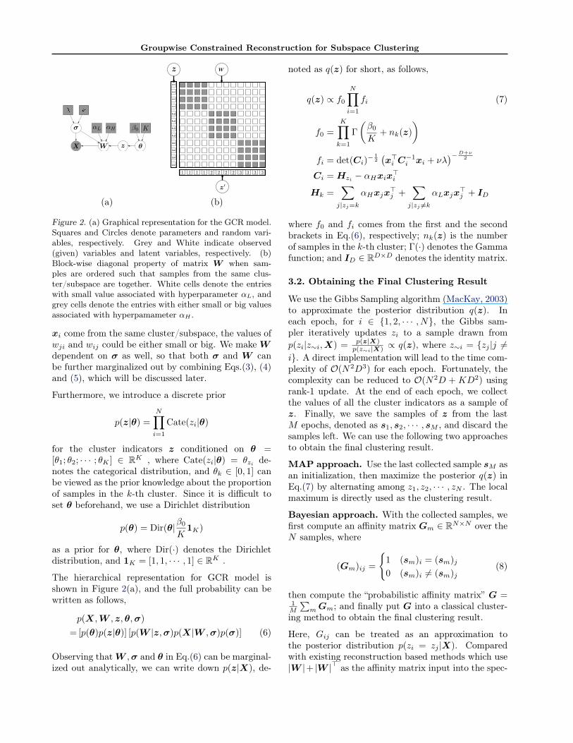
What makes the GCR model different is that, GCRexplicitly requires every sample to be reconstructedmainly by the samples in the same cluster. In otherwords, the magnitudes of weights for the samples indifferent clusters should be small. Intuitively, Wshould be nearly block-wise diagonal if the samplesare rearranged in a proper order (see Figure 2(b) foran illustration). To enforce such property of W , wetreat the cluster indicators z as latent random vari-ables, and introduce a prior for W conditioned on zand σ as follows,

p(W |z,σ) =

N∏i=1

N∏j=1

N (wji|0, σ2i αji) (5)

αji = αij =

αL zj 6= zi

αH zj = zi

where αH > αL ≥ 0 are hyperparameters and αLαH

issmall. This prior is quite similar to the Slab and Spikeprior used for variable selection (George & Mcculloch,1997), with αH corresponding to the slab and αL cor-responding to the spike. As the effects of Eq.(5), togenerate W given the latent cluster indicators, if xiand xj are not in the same cluster/subspace, wji andwij are restricted to be small or close to the mean value0 of the corresponding Gaussian distribution; if xj and

Groupwise Constrained Reconstruction for Subspace Clustering

(a) (b)

Figure 2. (a) Graphical representation for the GCR model.Squares and Circles denote parameters and random vari-ables, respectively. Grey and White indicate observed(given) variables and latent variables, respectively. (b)Block-wise diagonal property of matrix W when sam-ples are ordered such that samples from the same clus-ter/subspace are together. White cells denote the entrieswith small value associated with hyperparameter αL, andgrey cells denote the entries with either small or big valuesassociated with hyperpamameter αH .

xi come from the same cluster/subspace, the values ofwji and wij could be either small or big. We makeWdependent on σ as well, so that both σ and W canbe further marginalized out by combining Eqs.(3), (4)and (5), which will be discussed later.

Furthermore, we introduce a discrete prior

p(z|θ) =

N∏i=1

Cate(zi|θ)

for the cluster indicators z conditioned on θ =[θ1; θ2; · · · ; θK ] ∈ RK , where Cate(zi|θ) = θzi de-notes the categorical distribution, and θk ∈ [0, 1] canbe viewed as the prior knowledge about the proportionof samples in the k-th cluster. Since it is difficult toset θ beforehand, we use a Dirichlet distribution

p(θ) = Dir(θ|β0K

1K)

as a prior for θ, where Dir(·) denotes the Dirichletdistribution, and 1K = [1, 1, · · · , 1] ∈ RK .

The hierarchical representation for GCR model isshown in Figure 2(a), and the full probability can bewritten as follows,

p(X,W , z,θ,σ)

= [p(θ)p(z|θ)] [p(W |z,σ)p(X|W ,σ)p(σ)] (6)

Observing thatW ,σ and θ in Eq.(6) can be marginal-ized out analytically, we can write down p(z|X), de-

noted as q(z) for short, as follows,

q(z) ∝ f0N∏i=1

fi (7)

f0 =

K∏k=1

Γ

(β0K

+ nk(z)

)fi = det(Ci)

− 12

(x>i C

−1i xi + νλ

)−D+ν2

Ci = Hzi − αHxix>iHk =

∑j|zj=k

αHxjx>j +

∑j|zj 6=k

αLxjx>j + ID

where f0 and fi comes from the first and the secondbrackets in Eq.(6), respectively; nk(z) is the numberof samples in the k-th cluster; Γ(·) denotes the Gammafunction; and ID ∈ RD×D denotes the identity matrix.

3.2. Obtaining the Final Clustering Result

We use the Gibbs Sampling algorithm (MacKay, 2003)to approximate the posterior distribution q(z). Ineach epoch, for i ∈ 1, 2, · · · , N, the Gibbs sam-pler iteratively updates zi to a sample drawn fromp(zi|z∼i,X) = p(z|X)

p(z∼i|X) ∝ q(z), where z∼i = zj |j 6=i. A direct implementation will lead to the time com-plexity of O(N2D3) for each epoch. Fortunately, thecomplexity can be reduced to O(N2D + KD2) usingrank-1 update. At the end of each epoch, we collectthe values of all the cluster indicators as a sample ofz. Finally, we save the samples of z from the lastM epochs, denoted as s1, s2, · · · , sM , and discard thesamples left. We can use the following two approachesto obtain the final clustering result.

MAP approach. Use the last collected sample sM asan initialization, then maximize the posterior q(z) inEq.(7) by alternating among z1, z2, · · · , zN . The localmaximum is directly used as the clustering result.

Bayesian approach. With the collected samples, wefirst compute an affinity matrix Gm ∈ RN×N over theN samples, where

(Gm)ij =

1 (sm)i = (sm)j

0 (sm)i 6= (sm)j(8)

then compute the “probabilistic affinity matrix” G =1M

∑mGm; and finally put G into a classical cluster-

ing method to obtain the final clustering result.

Here, Gij can be treated as an approximation tothe posterior distribution p(zi = zj |X). Comparedwith existing reconstruction based methods which use|W |+ |W |> as the affinity matrix input into the spec-

Groupwise Constrained Reconstruction for Subspace Clustering

tral clustering algorithm, our probabilistic affinity ma-trix G is more sophisticated since Gij can be clearlyinterpreted as the the possibility that sample i and jshare the same cluster label. What is more, our affinitymatrixG is naturally positive and symmetric, whereas|W |+ |W |> is somehow like an ad-hoc way to “force”W to be an affinity matrix.

3.3. When K → +∞

From Eq.(8) we see that, to obtain the probabilisticaffinity matrix G, it is not mandatory to set K to bethe exact number of subspaces. In fact, the proba-bilistic affinity matrix can be obtained with any pos-itive integer K. Particularly, we are interested in theGCR model when K goes to positive infinity, in whichcase, the number of non-empty clusters remains a fi-nite number (at most N when each sample forms itsown cluster). This strategy is in analogy with the In-finite Gaussian Mixture Model with Dirichlet Process(Rasmussen, 1999). For this reason, we refer to theGCR model with K → +∞ as GCR-DP. As the limitof GCR, the posterior of z for GCR-DP is

q(z) ∝ f0N∏i=1

fi, f0 = βK−10

K∏k=1

Γ(nk(z)) (9)

where fi remains the same as in Eq.(7), and K is thenumber of non-empty clusters 2. The Gibbs samplingprocedure is similar to that of the original GCR, andthe difference is described as follows. Suppose for nowthere are K ′ non-empty clusters, to update zi, besidescomputing K ′ values for the non-empty clusters byplugging zi ← 1, 2, , · · · , K into the r.h.s. of Eq.(9),we need to compute an extra value for a new emptycluster by plugging K ← K ′ + 1 and zi = K ′ + 1 intoEq.(9). Then the Categorical sampler picks a clusterindicator for zi according to these K ′ + 1 values. Ifthe indicator for the new cluster (K ′+ 1) is picked, wecreate a new empty cluster and put the i-th sampleinto it. The variables for the empty clusters can beremoved to save the computational resource.

In the case of K → ∞, Eq.(6) shows that there ex-ists a trade-off among the reconstruction quality, priorfor the cluster indicators and p(W |z,σ). p(W |z,σ)prefers more clusters, in which case more spikes inEq.(5) could be introduced into the model, resulting inhigh p.d.f. of p(W |z,σ). On the contrary, the Dirich-let process prior favors fewer number of clusters. In thepremise of good reconstruction quality (p(X|W ,σ) ishigh), the competition between the Dirichlet process

2To use Eq.(9), z should be reorganized so that the firstK clusters are non-empty.

prior p(z) and p(W |z,σ) provides a way to circum-vent the trivial solutions to the model (all the samplesin one cluster or each sample in it’s own cluster).

Due to the allowance to create more clusters, the out-liers, which cannot be well reconstructed by the inliers,have the chance to “stand alone”. As a result, the in-fluence of the outliers can be reduced.

3.4. Hyperparameters

β0: Throughout our experiment, β0 for the Dirichletdistribution is always set to 1.

λ and ν: From Eq.(4) we see that λ and ν control thereconstruction quality. According to the property ofthe inverse Gamma distribution, we have E(σ−1i ) = 1

λ

and Var(σ−1i ) = 2λ2ν . Thus, it is reasonable to set λ

to a smaller number if the dataset are less noisy, andset ν to a smaller number if the variance of the recon-struction quality for different samples is higher (e.g.,the dataset has more outliers). In our experiments,these two parameters are tuned for different datasets.

αH and αL: According to Eq.(5), σ2i αH and σ2

i αL di-rectly influence the magnitude of wji. Since E(σ−1i ) =1λ , we can use λαH and λαL to control the mag-nitude of wji intuitively. After integrating out σ,we can rewrite the prior for W as p(W |z) =∏Ni=1

∏Nj=1 T (wji|ν, 0, λαji), where T (·|u, v, w) de-

notes the student t distribution with degree of freedomu, mean v and variance w. Therefore, it is natural touse the mean value of the t distribution to control themagnitude of W . In practice, we find that λαH = 0.1and αH

αL= 10000 yield good performance.

4. Experimental Results

In this section, we compare our methods with the otherthree reconstruction based subspace clustering meth-ods: LRR (Liu et al., 2010), SSC (Elhamifar & Vidal,2009) and SSQP (Wang et al., 2011). In our eval-uation, the quality of clustering is measured by ac-curacy, which is computed as the maximum percent-age of match between the clustering result and theground truth. For GCR, the MAP estimation is di-rectly used as the final clustering result; for GCR-DP,we first compute the probabilistic affinity matrix ac-cording to Eq.(8), then use NCut (Shi & Malik, 2000)to get the final clustering result. For MCMC, we treatG(0) =

∣∣∣(X>X + δI)−1∣∣∣ ∈ RN×N as the affinity ma-

trix, and the result of spectral clustering is used as theinitialization3. This can be understood by switching

3δ is a jitter value making the matrix invertible.

Groupwise Constrained Reconstruction for Subspace Clustering

the rule between sample (N) and dimension (D), insuch a way that G0 becomes the precision matrix overN samples, and

∣∣∣G(0)ij

∣∣∣ measures the dependency be-tween the i-th and the j-th samples conditioned on theother samples. We set the number of epochs for theGibbs sampler to 500, and use the last 100 samplesto construct the probabilistic affinity matrix. We findthat under such settings, our methods runs faster thanSSC and SSQP empirically.

4.1. Synthetic Datasets

We use synthetic datasets to investigate how these re-construction based methods perform when the sub-space independence assumption mentioned in Section1 is violated. The synthetic data containing K sub-spaces are generated as follows: 1) Generate a ma-trix B ∈ R2×50, each column of which is drawn froma Gaussian distribution N (·|0, I2). 2) For the k-thcluster containing nk samples, generate y1 ∈ Rnk ,the elements of which are drawn independently fromthe uniform distribution defined on [−1, 1]. Afterthat, generate y2 = tan 16k

17Ky1 (avoiding tan π2 ). Fi-

nally, generate the nk samples in the k-th cluster as[y1,y2]B ∈ RnK×50. All the experiments here are re-peated for 5 times.

4.1.1. Violation of Subspace IndependenceAssumption

For K = 2, 3, · · · , 8, we generate 7 datasets accordingto the steps listed above. For these synthetic datasets,the l.h.s. of Eq.(1) is 2, and the r.h.s. of Eq.(1) is K.Thus, the degree of the violation of the subspace in-dependence assumption increases as K increases. Theresults are reported in Figure 3(a).

As we can see, LRR and SSC perform well when thesubspace independence assumption holds (K = 2) oris slightly violated (K = 3). However, their perfor-mance decreases significantly as the violation degreeincreases, even though their parameters are tuned fordifferent K. In contrast, GCR and GCR-DP are ableto retain high performance even though the violationdegree keeps increasing.

In the case of K = 8, we compare the affinity matricesproduced by these reconstruction based methods, asshown in Figure 4. Obviously, the affinity matrix pro-duced by GCR-DP has stronger discrimination poweron the clusters than those of the others. The affinitymatrix produced by SSQP looks promising. However,a deep investigation shows that in the matrix the sumof many rows are zero, making the clustering perfor-mance less satisfactory.

2 3 4 5 6 7 80.4

0.5

0.6

0.7

0.8

0.9

1

1.1

Number of Clusters

Acc

urac

y

LRRSSCSSQPGCR−DPGCR

0 0.05 0.1 0.15 0.2 0.25 0.3 0.35 0.40.4

0.5

0.6

0.7

0.8

0.9

1

Propotion of Outliers

Acc

urac

y

LRRSSCSSQPGCR−DPGCR

(a) (b)

Figure 3. Comparison on the Synthetic Datasets. (a) Ac-curacy on the synthetic dataset when subspace indepen-dence assumption is violated. (b) Accuracy on the syn-thetic dataset with increasing portion of noisy samples.

4.1.2. Increasing Portion of Noisy Samples

Consider the case when there exist samples deviatingfrom the exact positions in the subspaces. Followingthe previous listed steps, we generate a dataset con-taining 2 subspaces, each of which contains 50 samples.We add Gaussian noises N (·|0, 3) to 0%, 5%, · · · , 40%of the samples, respectively. The results on the 9datasets are reported in Figure 3(b).

The results show that our methods and LRR are ableto maintain high accuracy even though high portionof the samples deviate from their ideal position. Thesuccess of LRR is due to the l2,1 norm used for the lossterm in Eq.(2), while the success of GCR and GCR-DPmay be due to the model in which each sample has itsown parameter σi to measure the reconstruction error.SSC performs less better, and its performance remainsacceptable when the noise level is low.

4.2. Hopkins 155 Dataset

We evaluate our models on the Hopkins 155 motiondataset. This dataset consists of 155 sequences, eachof which contains the coordinates of about 39 − 550points tracked from 2 or 3 motions. The task is togroup the points into clusters according to their mo-tions for each sequence. Since the coordinates of thepoints from a single motion lie in an affine subspacewith the dimensionality at most 4 (Elhamifar & Vidal,2009), we project the coordinates in each sequence into4r dimensions with PCA, where r is the number of mo-tions in the sequence, then append 1 as the last dimen-sion of each sample. The results are reported in Table1. This dataset contains a small number of latent sub-spaces, and the results of the compared methods haveno significant difference.

4.3. MSRC Dataset

In the MSRC dataset, 591 images are provided withmanually labeled image segmentation results (each re-

Groupwise Constrained Reconstruction for Subspace Clustering

100 200 300 400

50

100

150

200

250

300

350

400 0

0.2

0.4

0.6

0.8

1

100 200 300 400

50

100

150

200

250

300

350

400

0.01

0.02

0.03

0.04

0.05

0.06

0.07

0.08

0.09

100 200 300 400

50

100

150

200

250

300

350

400 0

0.05

0.1

0.15

0.2

0.25

0.3

100 200 300 400

50

100

150

200

250

300

350

400 0

0.05

0.1

0.15

0.2

GLR_DP LRR SSC SSQP

Figure 4. The affinity matrices produced by reconstruction based methods. The samples are ordered so that samples fromthe same cluster are adjacent.

Table 1. Accuracy on the Hopkins 155 DatasetMethod Mean Median MinLRR .9504 .9948 .5820SSC .9729 1 .5766SSQP .9536 1 .5450

GCR-DP .9764 1 .5532GCR .9608 .9970 .5833

Table 2. Accuracy on the MSRC Dataset with 459 ImagesMethod Mean Median MinLRR .6625 .6500 .3514SSC .6548 .6400 .3673SSQP .6550 .6374 .3784

GCR-DP .6651 .6667 .3587GCR .7046 .6964 .3838

gion is given a label, and there are totally 23 labels).Following (Cheng et al., 2011), for each image, wegroup the superpixels, which are small patches in anover-segmented result, with subspace clustering meth-ods. The groundtruth (cluster label) for a superpixelis given as the label of region it belongs to.

In our experiment, 100 superpixels are extracted foreach image with the method described in (Mori et al.,2004), and each superpixel is represented with theRGB Color Histogram feature of dimensionality 768.We discard all the superpixels with label “background”,and then discard the images containing only one label.Finally, we get 459 images. For each image, the av-erage number of superpixels is 91.3, and the numberof clusters ranges from 2 to 6. We use PCA to reducethe dimensionality to 20 in order to keep 95% energy.The results are show in Table 2.

Clearly, our methods outperform the other three onthis dataset. GCR also performs better than GCR-DPbecause it utilizes the information about the numberof latent subspaces during the reconstruction step.

3 4 5 6 7 8 90.4

0.5

0.6

0.7

0.8

0.9

1

Number of Subspaces (Persons)A

ccur

acy

LRRSSCSSQPGCR−DPGCR

Figure 5. Results On Extended YaleB Dataset with In-creasing Number of Subspaces.

4.4. Human Face Dataset

We also evaluate our method on the Extended YaleDatabase B (Georghiades et al., 2001). This databasecontains 2414 cropped frontal human face images from38 subjects under different illuminations, and groupingthese images can be treated as a subspace clusteringproblem, because it is shown in (Ho et al., 2003) thatthe images for a fixed face under different illuminationscan be approximately modeled with low dimensionalsubspace. To evaluate the performance of all thesemethods, we form 7 tasks, each of which contains theimages from randomly picked 3, 4, · · · , 9 subjects,respectively. We resize the images to 42×48, then usePCA to reduce the dimensionality of the raw featuresto 30. We repeat the experiment for 5 times and showthe results in Figure 5.

The performance of GCR and GCR-DP are betterthan the other three methods. In particular, with thenumber of subspaces increasing, the difference betweenthe l.h.s. and r.h.s. of Eq.(1) increases (see Figure1). Consequently, the performance of LRR, SSC andSSQP, which rely on the subspace independence as-sumption to build the affinity matrix, degrades quickly.On the contrary, GCR and GCR-DP utilize the infor-mation that “the samples can be grouped into sub-spaces”, thus they are less influenced by the violationof subspace independence assumption.

Groupwise Constrained Reconstruction for Subspace Clustering

5. Conclusion and Discussion

We propose the Groupwise Constrained Reconstruc-tion (GCR) models for subspace clustering in this pa-per. Compared with other reconstruction based meth-ods, our models no longer rely on the subspace in-dependence assumption, which usually gets violatedin the applications in which the number of subspaceskeeps increasing. On the synthetic datasets, we showthat existing reconstruction based methods suffer fromthe violation of the subspace independence assump-tion, while the affinity matrix produced by our model,which is built from the posterior of the latent clusterindicators, is more sophisticated and of stronger dis-crimination power on discovering the latent clusters.On the three real-world datasets, our methods showpromising results.

Besides the subspace clustering problem, the idea ofgroupwise constraints can be further applied to otherproblems involving graph construction. For example,in semi-supervised learning (SSL), the constraints canbe modified such that a sample is only allowed to be re-constructed by its neighbors in the Euclidean space. Inthis way, the cluster assumption and manifold assump-tion, which are two fundamental SSL assumptions, canbe neatly unified within our framework. For dimensionreduction methods such as LLE (Roweis & Saul, 2000),it is also interesting to design new models to use theposterior of the reconstruction matrix for embedding,such that the local and global structure of the datacould be preserved simultaneously.

Acknowledgements

We thank the anonymous reviewers for valuable com-ments. This work was partially supported by 973 Pro-gram (2010CB327906), Shanghai Leading AcademicDiscipline Project (B114), Doctoral Fund of Ministryof Education of China (20100071120033), and Shang-hai Municipal R&D Foundation (08dz1500109). BinLi thanks UTS Early Career Researcher Grants.

ReferencesCheng, B., Liu, G., Wang, J., Huang, Z., and Yan, S.

Multi-task low-rank affinity pursuit for image segmen-tation. In ICCV, pp. 2439–2446, 2011.

Costeira, J. P. and Kanade, T. A multibody factorizationmethod for independently moving objects. InternationalJournal of Computer Vision, 29(3):159–179, 1998.

Elhamifar, E. and Vidal, R. Sparse subspace clustering. InCVPR, pp. 2790–2797, 2009.

Fischler, M. A. and Bolles, R. C. Random sample consen-sus: A paradigm for model fitting with applications to

image analysis and automated cartography. Commun.ACM, 24(6):381–395, 1981.

George, E. I. and Mcculloch, R. E. Approaches for bayesianvariable selection. Statistica Sinica, pp. 339–374, 1997.

Georghiades, A. S., Belhumeur, P. N., and Kriegman, D. J.From few to many: Illumination cone models for facerecognition under variable lighting and pose. IEEETrans. Pattern Anal. Mach. Intell., 23(6):643–660, 2001.

Ho, J., Yang, M-H, Lim, J., Lee, K-C, and Kriegman, D. J.Clustering appearances of objects under varying illumi-nation conditions. In CVPR (1), pp. 11–18, 2003.

Kanatani, K. Motion segmentation by subspace separationand model selection. In ICCV, pp. 586–591, 2001.

Liu, G., Lin, Z., and Yu, Y. Robust subspace segmentationby low-rank representation. In ICML, pp. 663–670, 2010.

Ma, Y., Derksen, H., Hong, W., and Wright, J. Segmenta-tion of multivariate mixed data via lossy data coding andcompression. IEEE Trans. Pattern Anal. Mach. Intell.,29(9):1546–1562, 2007.

MacKay, D. J. C. Information theory, inference, and learn-ing algorithms. Cambridge University Press, 2003. ISBN978-0-521-64298-9.

Mori, G., Ren, X., Efros, A. A., and Malik, J. Recoveringhuman body configurations: Combining segmentationand recognition. In CVPR (2), pp. 326–333, 2004.

Rao, S., Yang, A. Y., Sastry, S., and Ma, Y. Robust alge-braic segmentation of mixed rigid-body and planar mo-tions from two views. International Journal of ComputerVision, 88(3):425–446, 2010.

Rasmussen, C. E. The infinite gaussian mixture model. InNIPS, pp. 554–560, 1999.

Roweis, S. T. and Saul, L. K. Nonlinear dimensionality re-duction by locally linear embedding. Science, 290(5500):2323–2326, 2000.

Shi, J. and Malik, J. Normalized cuts and image segmen-tation. IEEE Trans. Pattern Anal. Mach. Intell., 22(8):888–905, 2000.

Tipping, M. E. and Bishop, C. M. Mixtures of probabilisticprincipal component analyzers. Neural computation, 11(2):443–482, 1999.

Vidal, R. and Hartley, R. I. Motion segmentation withmissing data using powerfactorization and gpca. InCVPR (2), pp. 310–316, 2004.

Vidal, R., Ma, Yi, and Sastry, S. Generalized principalcomponent analysis (gpca). IEEE Trans. Pattern Anal.Mach. Intell., 27(12):1945–1959, 2005.

Wang, S., Yuan, X., Yao, T., Yan, S., and Shen, J. Efficientsubspace segmentation via quadratic programming. InAAAI, 2011.

Ye, J., Zhao, Z., and Wu, M. Discriminative k-means forclustering. In NIPS, 2007.