VIDEO TRANSMISSION OVER CONSTRAINEDBANDWIDTHCHANNELSGirish MahantaA thesisinThe DepartmentofComputer SciencePresented in Partial Fulfillment of the RequirementsFor the Degree of Master of Computer ScienceConcordia UniversityMontr�eal, Qu�ebec, CanadaOctober 1997c Girish Mahanta, 1997

Concordia UniversitySchool of Graduate StudiesThis is to certify that the thesis preparedBy: Girish MahantaEntitled: Video Transmission over Constrained BandwidthChannelsand submitted in partial ful�llment of the requirements for the degree ofMaster of Computer Sciencecomplies with the regulations of this University and meets the accepted standardswith respect to originality and quality.Signed by the �nal examining commitee: ChairDr.Lata Narayanan ExaminerDr.J. William Atwood ExaminerDr.Ferhat Khendek SupervisorDr.Manas SaksenaApproved Dr.Hon F. Li, Graduate Program Director19 Dr.Nabil Esmail, DeanFaculty of Engineering and Computer Science

AbstractVideo Transmission over Constrained BandwidthChannelsGirish MahantaMultimedia applications are often considered adaptive in the sense that their be-haviour can be adapted to the available resources. One way to achieve this is throughselective dropping of media frames. Di�erent media types have di�erent tolerance toloss, for example, humans are more sensitive to loss of continuity in audio as comparedto video. It is, therefore, attractive to develop best e�ort services targeted for a par-ticular media type (e.g., video). Such a service should provide graceful performancedegradation as resources become scarce by exploiting the particular characteristics ofthe media type.In this thesis, we consider providing a best e�ort service targeted for video trans-mission, by multiplexing multiple video streams over a reserved bandwidth networkchannel. The emerging services architecture in ATM networks as well as the Internetprovide the capability to reserve resources such as bandwidth, and to use them toprovide higher level services. We use simulation to consider the e�ect of di�erentscheduling and bu�er management policies on the performance when the bandwidthis scarce and losses are inevitable. By using e�ective frame rate as a performance mea-sure, we show that FIFO scheduling is unable to ensure fairness in terms of equitableperformance degradation of the multiplexed streams. Our simulations reveal thatexplicit bandwidth allocation is required, and that this bandwidth allocation mustbe (1) targeted to ensure that the performance of each of the multiplexed streamsdegrades equitably, and (2) must be dynamically changed to take advantage of thetime varying characteristics of video data.iii

AcknowledgmentsI am indebted to my supervisor Dr.Manas Saksena, for his guidance and constantsupport all through the course of this work. His patience and understanding werehelpful in the completion of this thesis. I acknowledge with thanks the �nancialsupport I received through Dr.Saksena.I extend my thanks to Dr.J.W.Atwood, Dr.F.Khendek for being on the examiningcommittee and Dr.L.Narayanan for chairing the defence.I would like to express my gratitude for my parents and sisters, for their love anda�ection.I wish to thank the �ne group of systems analysts for their timely solutions duringthe cource of my Master's programme.Thanks to Mr.Shawn D., Ms.Arbinder K. Pal and Ms.Jaya N. for their help duringproof reading of the thesis.I am grateful to Mr.Krishnamurthy W., Mrs.Savitha G.C. and Mr.Prakash S. forcontinually urging me to complete the thesis. I thank Mr.Narayan S., Mrs.SavitaD.C., Ms.Sunita H.K., Mr.Veeresh K.M. and Mr.Surya Prakash N. for being in touchall the time and never missing me out on anything. Also, my thanks to Mr.MaheshB., Mr.Venkateshwara Rao A., Mr.Vijay K. and Mr. Seetharaman S. for making mystay in Montreal, a pleasant one.iv

ContentsList of Figures ixList of Tables xi1 Introduction 21.1 Video Transmission : : : : : : : : : : : : : : : : : : : : : : : : : : : : 31.2 Related Work : : : : : : : : : : : : : : : : : : : : : : : : : : : : : : : 51.2.1 Optimal Video Transmission : : : : : : : : : : : : : : : : : : : 61.2.2 Filters for Rate Control : : : : : : : : : : : : : : : : : : : : : 61.2.3 Feedback Based Rate Control : : : : : : : : : : : : : : : : : : 71.2.4 An Application Level Video Gateway : : : : : : : : : : : : : : 91.3 Contributions : : : : : : : : : : : : : : : : : : : : : : : : : : : : : : : 92 Video 112.1 Digital Video Preliminaries : : : : : : : : : : : : : : : : : : : : : : : : 112.1.1 Resolution : : : : : : : : : : : : : : : : : : : : : : : : : : : : : 122.1.2 Colour Spaces : : : : : : : : : : : : : : : : : : : : : : : : : : : 122.2 Video Compression : : : : : : : : : : : : : : : : : : : : : : : : : : : : 132.2.1 Classi�cation : : : : : : : : : : : : : : : : : : : : : : : : : : : 142.2.2 Some Techniques : : : : : : : : : : : : : : : : : : : : : : : : : 152.3 Video Compression Standards : : : : : : : : : : : : : : : : : : : : : : 182.3.1 The Joint Pictures Expert Group : : : : : : : : : : : : : : : : 192.3.2 CCITT Expert Group on Visual Telephony : : : : : : : : : : : 192.3.3 CMTT/2 Activities : : : : : : : : : : : : : : : : : : : : : : : : 202.4 Motion Pictures Expert Group : : : : : : : : : : : : : : : : : : : : : : 202.4.1 Bitstream Details : : : : : : : : : : : : : : : : : : : : : : : : : 21v

2.4.2 MPEG-1 Compression Algorithm : : : : : : : : : : : : : : : : 232.4.3 MPEG-2 and MPEG-4 : : : : : : : : : : : : : : : : : : : : : : 273 Networks 283.1 Networking Requirements for Multimedia Applications : : : : : : : : 283.2 The Asynchronous Transfer Mode : : : : : : : : : : : : : : : : : : : : 313.2.1 Basic Principles : : : : : : : : : : : : : : : : : : : : : : : : : : 323.2.2 ATM Protocol Reference Model : : : : : : : : : : : : : : : : : 323.2.3 Tra�c Contract : : : : : : : : : : : : : : : : : : : : : : : : : : 363.2.4 Tra�c Management : : : : : : : : : : : : : : : : : : : : : : : : 373.2.5 Tra�c Management Related Algorithm : : : : : : : : : : : : : 393.3 Internet : : : : : : : : : : : : : : : : : : : : : : : : : : : : : : : : : : 393.3.1 Integrated Services : : : : : : : : : : : : : : : : : : : : : : : : 413.3.2 Real-Time Transport Protocol : : : : : : : : : : : : : : : : : : 443.3.3 Resource Reservation Protocol : : : : : : : : : : : : : : : : : : 473.4 Packet Scheduling : : : : : : : : : : : : : : : : : : : : : : : : : : : : : 513.4.1 Scheduling Best E�ort Connections : : : : : : : : : : : : : : : 513.4.2 Scheduling Guaranteed Service Connections : : : : : : : : : : 523.5 ATM and Internet : : : : : : : : : : : : : : : : : : : : : : : : : : : : 533.5.1 TCP/IP Over ATM : : : : : : : : : : : : : : : : : : : : : : : : 533.5.2 IP over ATM Encapsulation : : : : : : : : : : : : : : : : : : : 543.5.3 IP over ATM Address Resolution : : : : : : : : : : : : : : : : 553.6 Discussion : : : : : : : : : : : : : : : : : : : : : : : : : : : : : : : : : 564 Problem Statement 594.1 The Model : : : : : : : : : : : : : : : : : : : : : : : : : : : : : : : : : 594.2 Video Sequences Characterization : : : : : : : : : : : : : : : : : : : : 604.3 Simulation Environment : : : : : : : : : : : : : : : : : : : : : : : : : 614.3.1 The ns simulator : : : : : : : : : : : : : : : : : : : : : : : : : 614.3.2 Simulation Set-up : : : : : : : : : : : : : : : : : : : : : : : : : 674.3.3 Assumptions : : : : : : : : : : : : : : : : : : : : : : : : : : : : 674.3.4 Frame Arrival Process : : : : : : : : : : : : : : : : : : : : : : 684.4 Results Generation : : : : : : : : : : : : : : : : : : : : : : : : : : : : 684.4.1 Statistics Collection : : : : : : : : : : : : : : : : : : : : : : : : 69vi

4.4.2 Performance Measures : : : : : : : : : : : : : : : : : : : : : : 694.5 E�ect of Bandwidth Variation on Performance : : : : : : : : : : : : : 715 Shared Bandwidth and Shared Bu�ers 785.1 Overview of Experiments : : : : : : : : : : : : : : : : : : : : : : : : : 785.2 Results : : : : : : : : : : : : : : : : : : : : : : : : : : : : : : : : : : : 805.2.1 Synchronized Start : : : : : : : : : : : : : : : : : : : : : : : : 805.2.2 Frame Arrival Desynchronization : : : : : : : : : : : : : : : : 805.3 Summary : : : : : : : : : : : : : : : : : : : : : : : : : : : : : : : : : 845.4 Additional Observations : : : : : : : : : : : : : : : : : : : : : : : : : 845.4.1 Frame Size E�ect : : : : : : : : : : : : : : : : : : : : : : : : : 865.4.2 Bu�er Size E�ect : : : : : : : : : : : : : : : : : : : : : : : : : 866 Static Bu�er Partition 896.1 Bu�er Partitioning : : : : : : : : : : : : : : : : : : : : : : : : : : : : 896.2 Overview of Experiments : : : : : : : : : : : : : : : : : : : : : : : : : 916.3 Results : : : : : : : : : : : : : : : : : : : : : : : : : : : : : : : : : : : 916.3.1 Synchronized Start : : : : : : : : : : : : : : : : : : : : : : : : 916.3.2 Frame Arrival Desynchronization : : : : : : : : : : : : : : : : 946.4 Summary : : : : : : : : : : : : : : : : : : : : : : : : : : : : : : : : : 957 Static Bandwidth Partition 977.1 Bandwidth Partitioning : : : : : : : : : : : : : : : : : : : : : : : : : 977.2 Overview of Experiments : : : : : : : : : : : : : : : : : : : : : : : : : 987.3 Results : : : : : : : : : : : : : : : : : : : : : : : : : : : : : : : : : : : 1017.3.1 Frame Arrival Desynchronization : : : : : : : : : : : : : : : : 1017.4 Summary : : : : : : : : : : : : : : : : : : : : : : : : : : : : : : : : : 1028 Dynamic Bandwidth Partition 1048.1 Dynamic Bandwidth Partitioning Scheme : : : : : : : : : : : : : : : : 1048.2 Overview of Experiments : : : : : : : : : : : : : : : : : : : : : : : : : 1098.3 Results : : : : : : : : : : : : : : : : : : : : : : : : : : : : : : : : : : : 1108.3.1 Frame Arrival Desynchronization : : : : : : : : : : : : : : : : 1108.4 Summary : : : : : : : : : : : : : : : : : : : : : : : : : : : : : : : : : 111vii

9 Conclusions 1129.1 Limitations and Directions for Future Work : : : : : : : : : : : : : : 113A Dynamic Bandwidth Partition Plots 115A.1 Case: 100% Average Bandwidth : : : : : : : : : : : : : : : : : : : : : 115A.2 Case: 90% Average Bandwidth : : : : : : : : : : : : : : : : : : : : : : 115A.3 Case: 70% Average Bandwidth : : : : : : : : : : : : : : : : : : : : : : 115A.4 Case: 60% Average Bandwidth : : : : : : : : : : : : : : : : : : : : : : 123Bibliography 127

viii

List of Figures1 Dependency Among the I, P and B Frames : : : : : : : : : : : : : : : 242 ATM Protocol Reference Model : : : : : : : : : : : : : : : : : : : : : 333 UNI (left) and NNI (right) ATM Cell Format : : : : : : : : : : : : : 354 Generic Cell Rate Algorithm : : : : : : : : : : : : : : : : : : : : : : : 405 Reservation Attributes and Styles : : : : : : : : : : : : : : : : : : : : 496 Network Model : : : : : : : : : : : : : : : : : : : : : : : : : : : : : : 607 Frame Size Distribution of bla Sequence : : : : : : : : : : : : : : : : 628 Frame Size Distribution of boo Sequence : : : : : : : : : : : : : : : : 629 Frame Size Distribution of can Sequence : : : : : : : : : : : : : : : : 6310 Frame Size Distribution of jet Sequence : : : : : : : : : : : : : : : : 6311 Frame Size Distribution of mov Sequence : : : : : : : : : : : : : : : : 6412 Frame Size Distribution of tha Sequence : : : : : : : : : : : : : : : : 6413 Frame Size Distribution of suk Sequence : : : : : : : : : : : : : : : : 6514 Frame Size Distribution of sum Sequence : : : : : : : : : : : : : : : : 6515 Frame Size Distribution of foo Sequence : : : : : : : : : : : : : : : : 6616 Frame Size Distribution of boe Sequence : : : : : : : : : : : : : : : : 6617 Two Regions of Simulation : : : : : : : : : : : : : : : : : : : : : : : : 6918 EFR of bla Sequence over Sample Bandwidth Points : : : : : : : : : 7219 EFR of boo Sequence over Sample Bandwidth Points : : : : : : : : : 7220 EFR of can Sequence over Sample Bandwidth Points : : : : : : : : : 7321 EFR of jet Sequence over Sample Bandwidth Points : : : : : : : : : 7322 EFR of mov Sequence over Sample Bandwidth Points : : : : : : : : : 7423 EFR of tha Sequence over Sample Bandwidth Points : : : : : : : : : 7424 EFR of suk Sequence over Sample Bandwidth Points : : : : : : : : : 7525 EFR of sum Sequence over Sample Bandwidth Points : : : : : : : : : 7526 EFR of foo Sequence over Sample Bandwidth Points : : : : : : : : : 76ix

27 EFR of boe Sequence over Sample Bandwidth Points : : : : : : : : : 7628 Dynamically Partitioned Bandwidth for bla and boo Sequences : : : 10729 Dynamically Partitioned Bandwidth for can and jet Sequences : : : 10730 Dynamically Partitioned Bandwidth for mov and tha Sequences : : : 10831 Dynamically Partitioned Bandwidth for suk and sum Sequences : : : 10832 Dynamically Partitioned Bandwidth for foo and boe Sequences : : : 10933 Dynamically Partitioned Bandwidth for bla and boo Sequences : : : 11634 Dynamically Partitioned Bandwidth for can and jet Sequences : : : 11635 Dynamically Partitioned Bandwidth for mov and tha Sequences : : : 11736 Dynamically Partitioned Bandwidth for suk and sum Sequences : : : 11737 Dynamically Partitioned Bandwidth for foo and boe Sequences : : : 11838 Dynamically Partitioned Bandwidth for bla and boo Sequences : : : 11839 Dynamically Partitioned Bandwidth for can and jet Sequences : : : 11940 Dynamically Partitioned Bandwidth for mov and tha Sequences : : : 11941 Dynamically Partitioned Bandwidth for suk and sum Sequences : : : 12042 Dynamically Partitioned Bandwidth for foo and boe Sequences : : : 12043 Dynamically Partitioned Bandwidth for bla and boo Sequences : : : 12144 Dynamically Partitioned Bandwidth for can and jet Sequences : : : 12145 Dynamically Partitioned Bandwidth for mov and tha Sequences : : : 12246 Dynamically Partitioned Bandwidth for suk and sum Sequences : : : 12247 Dynamically Partitioned Bandwidth for foo and boe Sequences : : : 12348 Dynamically Partitioned Bandwidth for bla and boo Sequences : : : 12449 Dynamically Partitioned Bandwidth for can and jet Sequences : : : 12450 Dynamically Partitioned Bandwidth for mov and tha Sequences : : : 12551 Dynamically Partitioned Bandwidth for suk and sum Sequences : : : 12552 Dynamically Partitioned Bandwidth for foo and boe Sequences : : : 126x

List of Tables1 Coding and Compression Techniques: A Classi�cation : : : : : : : : : 152 Six Layers of MPEG-1 Video and Their Functions : : : : : : : : : : : 233 Mapping of Internet Integrated Service Classes to ATM Service Classes. 444 Frame Size Characteristics (in ATM cells) for Ten Video Streams : : 615 Con�guration Parameters for E�ect of Bandwidth Variation : : : : : 716 SD-of-EFR for Ten Video Streams Used in Simulations : : : : : : : : 777 Con�guration Parameters for Shared Bandwidth and Shared Bu�ers : 798 Mapping for Order1 (left), Order2 (middle) and Order3 (right) : : : : 799 EFR of Synchronized Start for Shared Bandwidth and Shared Bu�ers 8110 SD-of-EFR of Synchronized Start for Shared Bandwidth and SharedBu�ers : : : : : : : : : : : : : : : : : : : : : : : : : : : : : : : : : : : 8211 EFR of Desynchronized Frame Arrivals for Shared Bandwidth andShared Bu�ers : : : : : : : : : : : : : : : : : : : : : : : : : : : : : : : 8312 SD-of-EFR of Desynchronized Frame Arrivals for Shared Bandwidthand Shared Bu�ers : : : : : : : : : : : : : : : : : : : : : : : : : : : : 8513 Con�guration Parameters for Frame Size E�ect : : : : : : : : : : : : 8614 Frame Size E�ect on Fairness for tha and sum : : : : : : : : : : : : : 8715 Frame Size E�ect on Fairness for bla and foo : : : : : : : : : : : : : 8716 Bu�er Size E�ect on EFR (top) and SD-of-EFR (bottom) : : : : : : 8817 EFR (top) and SD-of-EFR (bottom) for Equally Partitioned LargeBu�ers : : : : : : : : : : : : : : : : : : : : : : : : : : : : : : : : : : : 9018 EFR of Synchronized Start for Statically Partitioned Bu�ers : : : : : 9219 SD-of-EFR of Synchronized Start for Statically Partitioned Bu�ers : 9320 EFR of Desynchronized Frame Arrivals for Statically Partitioned Bu�ers 9421 SD-of-EFR of Desynchronized Frame Arrivals for Statically PartitionedBu�ers : : : : : : : : : : : : : : : : : : : : : : : : : : : : : : : : : : : 95xi

22 Static Bandwidth Split for 5.884272 Mbps (left) and 5.230464 Mbps(right) : : : : : : : : : : : : : : : : : : : : : : : : : : : : : : : : : : : 10023 Static Bandwidth Split for 4.576656 Mbps (left) and 3.922848 Mbps(right) : : : : : : : : : : : : : : : : : : : : : : : : : : : : : : : : : : : 10024 Con�guration Parameter for Statically Partitioned Bandwidth : : : : 10125 EFR of Desynchronized Frame Arrivals for Static Bandwidth PartitionMechanisms: Scheme 1 (top) and Scheme 2 (bottom) : : : : : : : : : 10226 SD-of-EFR of Desynchronized Frame Arrivals for Static BandwidthPartition Mechanisms: Scheme 1 (top) and Scheme 2 (bottom) : : : : 10327 EFR (top) and SD-of-EFR (bottom) of Desynchronized Frame Arrivalsfor Dynamically Split Bandwidth : : : : : : : : : : : : : : : : : : : : 110

xii

Contents

1

Chapter 1IntroductionRecent technological advancements in broadband communications, computers, andmedia peripherals have led to the emergence of a new paradigm of computing inwhich continuous media (e.g., video and audio) is treated in much the same wayas discrete media (data). This paradigm shift is re ected in distributed multime-dia applications such as virtual reality, media-on-demand, video conferencing, tele-marketing, tele-medicine, etc., that seek to revolutionize the computing world. Itis commonly accepted that these applications will use a single integrated network tocarry a wide variety of data (video, audio, images, text, etc.) with processing supportat end systems (i.e., host computers) connected to a variety of multimedia peripherals(speakers, microphones, television monitors, camera, etc.).In a typical distributed multimedia application, data is generated at a sourcecomputer, transported over the communications network, and �nally processed andpresented at the destination computer. The successful use of multimedia applicationsrequires that multimedia data is presented with high perceptual quality to the user.The perceptual quality of a multimedia presentation depends on maintaining thetemporal relationships between media items. Such relationships include, for instance,displaying video frames one every 30 ms or so, maintaining \lip-synch" between audioand video, etc. Furthermore, live multimedia applications also require that the end-to-end latency in presenting the data is small (typically less than 200 ms). Thetimeliness requirements are soft, in the sense that small deviations do not a�ectperceptual quality. On the other hand, consistent large deviations from the desiredtemporal behaviour is unacceptable and renders the presentation useless.Most multimedia applications, unlike traditional data, can tolerate some data loss2

without resulting in the transmitted data being completely futile. On the contrary,traditional data require an error-free transmission. In addition, multimedia appli-cations can exhibit graceful degradation in performance under controlled losses byproducing reasonable quality outputs at the receiver end. Also, multimedia appli-cations are adaptable to such an extent that they can experience some variation inservice without a�ecting the quality. Such a behaviour can be seen in the case of amovie where the video segment can lag the audio segment up to 40 ms without beingnoticed by the user.A major challenge in the development of next generation computer networks andsystems is the incorporation of resource management policies that cater to the speci�cneeds of distributed multimedia applications. Clearly, this requires a network too�er services beyond the \best-e�ort" services o�ered in today's Internet. Recentdevelopments in computer networking research suggest a convergence towards a two-pronged approach to this problem.� At the lower layer, the computer network provides generic services using whichan application can reserve resources, and expect some quality of service guar-antees provided it conforms to a tra�c contract. For example, an applicationmay request a Constant Bit Rate (CBR) service that guarantees a bandwidthB to it. The network on its part commits that all packets will be sent un-less the bandwidth usage at any time instant is greater than to the negotiatedbandwidth B.� Using such generic services provided by the computer network, the higher levelservices tailored to a particular media type such as video or a particular appli-cation such as video presentation, determines how to use the resources availableto provide the quality of service desired by the application.1.1 Video TransmissionIn this thesis, we address video transmission as part of higher level services that canbe used in many applications. Video data in the uncompressed form requires highbandwidth for transmission and thus calls for compression. The di�erent amountsof compression achieved produces frames of uneven sizes and thus results in timevarying data rates. Furthermore, video can su�er from small amounts of loss without3

substantially degrading the quality. In case of a major short-fall in a resource suchas bandwidth, the video can exhibit graceful degradation by employing frame leveldrops. The time varying nature of video data prompts an idea wherein a bandwidthreservation can be shared for transmission of multiple video streams so that moree�ective use of link capacity is possible. We thus choose to study the transmission ofmultiple video streams over a reserved bandwidth.Networks providing resource reservation facilities consist of objects such as sources,sinks and routers, which employ bu�ers to manage dynamic data rates of media suchas video. Due to time varying data rate, the required bandwidth typically di�ers fromthat of reserved bandwidth by a small quantity. If such a variation results in higherdemand for bandwidth, then it is o�set by storing the excess data in bu�ers and thusbridging the gap between asking and reserved bandwidths. Data in the bu�ers isgoverned by a scheduling discipline, which decides on what data to send and whento send it. The number of bu�ers employed is determined such that the delay due toqueueing is within real-time requirements. Hence, the extent to which bu�ers can beemployed is limited by the permissible delay.There has been considerable research towards exploring the transmission of mul-tiple video streams to determine the bandwidth and bu�er requirements for zero loss.The bandwidth in this case is the average data rates of all streams being transmitted.On the other hand, we �nd relatively less work in case of inadequate bandwidth.The problems will be acute, in case a vital resource such as bandwidth is short ofrequired quantum. Existing networks can result in insu�cient bandwidth for videoapplications, which are on the higher end of resource requirements. As a consequenceof insu�cient bandwidth, data loss is certain due to over- ow of permissible bu�erspace. Such drops are regulated by bu�er management policies which decide whenthe data are to be dropped. Data drops so in icted lead to random information lossand thereby adversely a�ect quality of video. A possible solution for this problemis to eliminate random losses. This has resulted in proposing frame level drops. Ifa particular video frame consisting of many packets is found to incur random losses,then instead of sending an incomplete frame, it is better to drop the entire frame.Drops are forced this way to prevent bandwidth from being consumed by incompletevideo frames. Such drops will help increase the number of intact frames sent resultingin improved visual quality. Thus, we have selected constrained bandwidth channelsfor our study. 4

We attempt to control the loss of video data in order to ensure graceful degradationin the performance under reduced bandwidth conditions. The losses so experiencedcannot be expressed in terms of percentage of packet losses as can be done withtraditional data, since video data is subjective in nature. Thus, we need measurescapable of capturing the visual quality for a single stream. In order to accomplishthis, we employ a measure called E�ective Frame Rate. This metric can be used toloosely quantify the loss in quality due to frame drops against the original stream. Weopt for frame level drops to limit the scope of the thesis, though slice or macroblocklevel drops would have resulted in better performance. Furthermore, we focus oursolutions to obtain a low variation of E�ective Frame Rate so that the uctuationsin quality are not too high.As far as the performance of multiple video streams is concerned, we want to ensurefairness among sequences. This is achieved by maximizing the minimum qualityamong all streams leading to best possible quality video at the sink.1.2 Related WorkIn this section, we brie y describe the related work connected with video transmis-sion under insu�cient bandwidth. Typically from such a transmission we expect thebest possible quality video at the receiver end. The video data somehow has to becontrolled to meet the desired quality. Research in this direction shows two maincategories. The �rst category concerns dropping video data. For this purpose videodata components which are readily available (which do not need processing) are em-ployed. Examples of such components include slices and frames. The second categoryfocuses on minimizing the bandwidth requirement of video streams by manipulatingone of the video generation parameters at the encoder. One such example is thequantizer value which can be used to e�ectively bring down the data rate. We reviewsome projects covering both these approaches. In addition, we also note the appli-cation of video gateways to exclusively manage video streams in the current networkenvironments. 5

1.2.1 Optimal Video TransmissionThe work by [KMS95] is driven by the need to address video transmission of a sin-gle stream over insu�cient reserved bandwidth link. The authors address optimaltransmission of prioritised data that is a characteristic of MPEG video sequences andthus is of interest to us. Their goal is to maximize the visual quality of video at thesink. The model proposed by them uses the frame size as weight. Their algorithmsappear in two versions: the �rst version assumes that the exact channel bandwidth isknown, while the second version assumes that the bandwidth is uniformly distributedin an interval of known endpoints. The premise of their algorithms is to minimizethe expected maximum gap due to unplayable or dropped frames. The algorithmsgiven by them are less suitable for real-time applications like video conferencing, asthe frames need to be reassembled for playing in addition to the regular decodingdelay.1.2.2 Filters for Rate ControlAnother related work at Lancaster [YMGH96] deals with transmission of a singlevideo stream under limited link capacity. It aims at implementing a dynamic qualityof service control led architecture capable of optimizing a variety of requirementsevident amongst the large group of simultaneous users. This work takes into accountthe heterogeneity in terms of hardware, software and network protocols among others.The authors propose �lters, which employ certain heuristics to reduce bandwidthrequirements with controlled loss of quality. The �lters-governed data rate controlemployed in this work is of relevance to our work. The following are the six types of�lters developed by them:� Codec �lter. This is used to compress or decompress a bitstream, usually bytranscoding between two compression standards. Implementation of this �ltermay or may not need full decompression and recompression depending on thestandard used.� Frame-Dropping Filter. This �lter drops frames thereby considerably re-ducing the data rate. In case of MPEG video, this �lter has the knowledge ofthe type of frame and uses this knowledge while dropping according to their6

importance. For instance, in an IPB video sequence of MPEG, �rst B, next Pand �nally I frames would be selected for dropping.� Frequency Filter. These �lters operate on the semi-uncompressed data in thefrequency domain. An example of these �lter's input is the DCT-coe�cients.This category includes facilities to remove: (i) higher frequencyDCT-coe�cients,(ii) chrominance part, and (iii) all the colour information, from a stream.� Mixing Filter. This �lter is used to mix streams together, re ecting themultiplexer operation. The mixing can be performed at two levels, (i) at theframe level and (ii) at the slice level. Slice level mixing incurs more processingas incompatible slices need to be matched with the help of padding.� Re-Quantization Filter. This �lter operates on the DCT-coe�cients to de-quantize them. These de-quantized coe�cients are re-quantized with a higherquantization step. This process leads to substantial reduction in data require-ment at the cost of quality.� Slicing Filter. This �lter is used to increase the number of slices in a frame.The main idea is to provide protection against data loss by not propagating thee�ect of some data loss beyond the particular slice. However, the addition ofevery slice involves an overhead of 38 to 45 bits, in terms of new slice headerlength.As mentioned in the introductory section, we notice data rates being modi�ed invarying quantities at di�erent levels starting from frames to DCT coe�cients. Theprevious work by [YMGH96] provided an optimal solution, while in this case we ob-serve rate reduction to bridge heterogeneity gaps among various network components.A common aspect between this and our work is the drop entity, which is a frame.1.2.3 Feedback Based Rate ControlIn this paper, the authors [KM96] employ a feedback mechanism to monitor thedata rates of multiple video streams in distributed ATM networks. In this case thenetwork elements such as switches, routers and others inform the sources generatingvideo data of their changing situations so that sources can adapt the data rate withthe help of the encoder. The feedback is in the form of a single bit in the cell header7

called Explicit Forward Congestion Noti�cation (EFCN), for the source to adapt itsdata rate.This paper presents two methods designed for bursty sources, which are modi�edfor video data, and a new technique. Among the two schemes designed for burstysources, the �rst by Ramakrishnan and Jain sets the single bit when the averagequeue length of the switch is greater than or equal to a particular threshold. Thisscheme is modi�ed using the assumption that the congestion bit is set based on thequeue occupancy value at the instant of cell transmission.The second scheme by Mitra and Seery, adapts the windows or data rates byimplicit feedback (derived frommeasured round trip delay) or explicit feedback (aboutqueue occupancy). The switches periodically send queue occupancy information tothe sources directly, with the bit set according to the instantaneous queue occupancylevel. Window sizes are then set to re ect the network conditions. Kanakia andMishra modify this method such that after setting the bit the cells are forwarded tothe receiver rather than the source to suit EFCN.The third scheme developed by the authors uses the single bit to convey moreaccurate information about the queue occupancy. Their premise is that the receiveris capable of capturing more information about the slowly varying quantities suchas queue levels and this can be passed on to the source. One way this scheme canbe implemented is by employing multiple thresholds to depict various levels of queueoccupancy.The results show that the feed-back schemes work well for all the three schemeswith minor di�erences. But, these conclusions are accompanied by unfair services tothe users. To address the fairness issue, the authors have proposed a scheme whichallows the sources to adjust their bit rates so that the quality of the compressedbit-stream matches the target image quality.This work is similar to ours from the point of view of the fairness issue and ingeneral improving the quality of video. The main di�erence is that we address thefairness issue with the help of few scheduling techniques, while in this case we noticefeedback being employed resulting in the transmission of additional data in the reversepath of video transmission. 8

1.2.4 An Application Level Video GatewayAt present multicast transmission across the Internet assumes that a �xed averagebandwidth is available over the entire network. This restricts the users having higherbandwidth links from achieving a better quality. The authors [AM95] address thisproblem by proposing an architecture for video transmission, wherein a single trans-mission can be decomposed into multiple sessions with di�erent bandwidth require-ments using an application level gateway. Their video gateway manipulates the dataand control information of the video sequences to establish a single logical conferencefrom pairs of sessions. It employs transcoding and rate-control to e�ect bandwidthadaptation. They present an algorithm to transcode Motion-JPEG to H.261 in real-time. The Real-time Transport Protocol (RTP) is embedded into the video gatewaythereby allowing it to interoperate with current video tools.We are interested in this work as it addresses data rate adaptation throughtranscoding and rate control. Among these, transcoding incorporating RTP is aspecial feature compared to our work. On the other hand, rate control enforced overa transcoded stream with frame drops is similar to our work. A notable feature ofthis video gateway is the mechanism it provides to dedicatedly handle video withthe help of advanced protocols like RTP and RSVP, where RSVP can be used toreserve resources along the path of transmission. The solution to our problem couldbe implemented on top of a video gateway such as this one.1.3 ContributionsIn this thesis, we have explored a few simple mechanisms to manage bandwidth andbu�ers, when multiple video streams share a bandwidth reservation. Our design spaceconsists of: (i) whether the bu�ers should be shared or partitioned and (ii) whetherthe bandwidth should be shared and managed using a FIFO scheduler, or partitioned(perhaps dynamically) and controlled using a scheduler employing some GeneralizedProcessor Scheduling mechanism [PG93].Our results suggest that in order to ensure fairness among di�erent streams, it isnecessary to partition both bu�ers and bandwidth. A second outcome of our tests isthat the speci�c manner in which bu�ers are partitioned is not so important, as longas some minimum bu�ering is available. Finally, our results indicate that bandwidth9

partitioning should be dynamic to exploit the time varying characteristics of videosequences. Also, such a partition should be driven by \quality" requirements.

10

Chapter 2VideoVideo has become one of the main constituents in the emerging multimedia andtelecommunication applications. This has attracted much attention leading to a spurin research directed towards integrating video into the world of computers. In thischapter, we address the various issues connected with digital video. We begin withfundamental aspects of video in the digital form. We then show the need for compres-sion and present relevant compression techniques. Finally, we detail video standardsdeveloped for the computer domain.2.1 Digital Video PreliminariesRecent advances in technology are paving the way to integrate video, computer andtelecommunication industries together on a single platform called \Multimedia". Inorder to integrate video into the multimedia platform, the video signal needs to bescalable, platform independent, robust, and error resilient. In addition, it also needsto facilitate interactivity and editing. Analog video signal unfortunately fails to meetthese requirements, thus, making it unsuitable for such multimedia platforms [AB95].Hence, switching to digital not only answers these problems, but also opens up a wholenew range of sophisticated digital video processing techniques, which can improve thequality of video.Video is a sequence of time varying images, which convey visual information.Conversion of video from analog to digital format starts with the process of sampling.The basic unit of sampling is called a pixel. The sampling process yields a set of11

parameters essential to represent a digital video signal in terms of pixels per line,number of lines per frame, resolution, aspect ratio and �nally frame rate. In additionto these, images in video sequences are characterized by colour spaces or chrominanceand luminance. In the following subsections, we provide an overview of these aspects.2.1.1 ResolutionResolution speci�es the matrix of pixels that constitutes the image size, also referredto as spatial resolution [SN95]. The process of sampling in fact establishes the resolu-tion of an image. Sampling in the horizontal direction de�nes the horizontal resolutionof the picture. In contrast, sampling in the vertical direction yields the vertical res-olution, indicated by the number of lines. On the other hand, temporal samplingdetermines the frame rate of the video sequence, quoted as frames per second (fps).Aspect ratio is de�ned as the ratio of horizontal to vertical resolution of the image.2.1.2 Colour SpacesVideo images in addition to the resolution are de�ned by the way colour informationis stored [AB95]. A gray-scale picture has only one colour component: luminance.Since brightness is a complicated item to quantify, luminance was de�ned [Poy97].For example, in an image with 8 bits/pixel scale, higher range values in this scaleindicate lighter gray colour. Thus, a value 0 represents the colour black and 255represents the colour white.In order to capture the chrominance part of colour video images, three componentsare required. These components can be denoted by the most popular colour space asRGB. In this colour space, the R, G and B represent the amount of red, green andblue respectively. True-colour pictures use 8-bits for each component and thus yield24 bits/pixel. Another known colour space is the YUV. The Y component representsthe luminance, while the two chrominance components U and V determine the actualcolour. The following expressions specify the way the RGB colour space is convertedto YUV space: Y = 0:3R + 0:59G + 0:11BU = 0:493(B � Y )V = 0:877(R � Y )12

The human eye is known to be more sensitive to luminance components than tocolour components [AB95]. This observation is used to separate both the luminanceand chrominance parts so that the luminance component can be captured in a higherresolution than the chrominance component. Additional details on this issue can befound in [SN95].2.2 Video CompressionMultimedia systems include media such as images, audio, video and graphics in ad-dition to the traditional data types. Among the new media in picture, images haveconsiderably higher storage requirements than text while audio and video need stillhigher data storage. The data rates required for transfer of continuous media are alsosigni�cant as illustrated by the following examples [SN95]:� For text, employing 2 bytes/character of 8� 8 pixels for a screen of size 640 �480 results in: Characters per screen = 640�4808�8 = 4800Storage required per screen = 4800 � 2bytes = 9600bytesStorage required per screen ' 9:4kbytes� An uncompressed audio signal of telephone quality, sampled at 8 kHz and quan-tized with 8 bits per sample would lead to:Storage required per second = 64�1024 bps8 bits=byte � 1 sec1024 bytes=kbyteStorage required per second ' 8 kbytes� A video sequence of 25 fps, with luminance and chrominance encoded in 3 bytesand for a frame size of 640�480 pixels requires:Data rate = 640 � 480 � 25 � 3 bytes=sec = 23040000 bytes=secStorage required for a 2 hour movie =23040000 bytes=sec� 60 sec=min� 60 min=hour � 2 hour = 165:89 GbytesThese examples provide the requirements of secondary storage devices. In thecase of processing uncompressed video, the requirements increase astronomically. In13

addition, the transmission rates required are very high: 184.32 Mbps in the aboveexample. Adding to the problem of data storage and data rate is the problem ofrelatively slow storage devices, which cannot play the multimedia data in real-time.Thus, the use of an appropriate compression technique can considerably reduce thedata requirements. In the next section, we deal with various compression techniquesavailable.2.2.1 Classi�cationVideo compression aims at lowering the total number of parameters required to rep-resent the video, while maintaining perceptually good quality. These parameters arethen coded either for storage or for transmission over the communication networks.The compression revolves around the di�erent redundancies present in the video signal{ spatial, temporal and psychovisual. Spatial redundancy occurs as the neighbouringpixels in each frame are related, exhibiting some degree of correlation. The pixels inconsecutive frames are also correlated, leading to substantial temporal redundancy.In addition, the human visual system does not treat all the visual information withequal sensitivity, thereby leading to psychovisual redundancy. For example, the eyeperceives changes to a greater extent in the luminance factor than the chrominancefactor. Various compression techniques have been developed over the years takingadvantage of these redundancies.The compression techniques used in the multimedia systems can be grouped intoentropy or lossless, source or lossy and hybrid techniques. Table 1 shows the dif-ferent categories and their examples. Entropy encoding is a term used to describecompression algorithms that increase the energy or the information density in a mes-sage [AB95]. The input to be compressed is considered to be a simple digital sequenceand the semantics of the data is ignored. This technique is used for media regardlessof their speci�c characteristics. Entropy encoding is also called lossless as the decom-pression process regenerates the data completely. Run length encoding is an exampleof entropy coding which is used for text, images, and video or audio coding pro-cesses. Entropy encoding techniques exploit the spatial redundancy in compressingthe media. For example, suppose a number occurs subsequently four times. Insteadof sending the number 4 times, entropy encoding �rst sends the number and then itscount. 14

Prediction

Delta Modulation

DPCM

MPEG

H.261

DVI, RTV, PLV

JPEG

Subband Coding

Layered Coding Bit Position

Subsampling

DCT

FFTTransformation

Entropy Encoding

Source Encoding

Runlength Encoding

Huffman Encoding

Arithmetic Encoding

Hybrid Encoding

Vector QuantizationTable 1: Coding and Compression Techniques: A Classi�cationSource encoding represents the compression techniques which compress sampleddata by taking the semantics of the data into account. Source encoding techniquesare lossy, since the original and encoded data stream are not identical though similar.The di�erent source encoding techniques make use of the characteristics of a speci�cmedium. Such characteristics can include temporal and psychovisual redundanciesmentioned in the last section. For example, a content prediction technique can makeuse of spatial redundancies as in the case of still images [AB95].Hybrid compression techniques are a combination of entropy and source encodingtechniques. These combine well known algorithms and transformation techniques thatcan be applied to multimedia systems [Ste93]. For example, each hybrid technique inTable 1 uses entropy encoding in the form of run length encoding and/or a statisticalcompression.Video sequences need to be compressed aggressively to reduce the data storage andbandwidth requirements. Typically, the extent of video compression to be employedis determined by the trade-o� between the cost to be paid and the expected quality.2.2.2 Some TechniquesUncompressed video, as discussed in the beginning of this section, requires high band-width for transmission purposes and large storage spaces for storing. The obvious15

solution is to bring down the asking rate of video. For this purpose, it is essential tohave good compression techniques. In the following paragraphs, we present a briefdescription of some commonly used compression techniques [AB95], [11193].1. DCT Transformation. A transformation useful in image compression is theDiscrete Cosine Transform (DCT). This transformation converts an n�n block of ele-ments into another block of n�n coe�cients representing the two-dimensional uniquespatial frequencies. The DCT function is reversible by using an Inverse DiscreteCosine Transform (IDCT) function.The �rst coe�cient in location (0,0) of the block represents the zero vertical andzero horizontal frequency and is called the DC coe�cient. This is equal to the averagevalue of the original elements. The other coe�cients represent one or more nonzerohorizontal or nonzero vertical spatial frequencies and are called AC coe�cients.The DCT and IDCT could be lossless, if the DCT encoded data are stored withperfect accuracy. In practice, however, the coe�cients are stored as integers whichcan introduce small di�erences with the original data after the IDCT decoding.2. Scalar and Vector Quantization. Quantization represents a range of valuesby a single value in the range. For example, converting a real number to the nearestinteger is a form of quantization.Scalar quantization is used to reduce the number of bits that are needed to storean integer. This can be achieved by dividing the integer by a quantization factor androunding it to the nearest integer before it is stored. To retrieve the integer again, thequantized integer is multiplied by the quantization factor. This step is not lossless asthe density of the domain of the integer is reduced by the quantization factor.Vector quantization makes use of codebooks in combination with a matrix of vec-tors to represent an image. Instead of referring to elements directly, elements are ref-erenced via the codebook. To transmit an image, only the references to the codebook(the vectors) have to be sent. Numerous vector quantization methods are available.3. Entropy Coding: Hu�man, Arithmetic and LZW Techniques. An en-tropy or lossless algorithm encodes the data based on their statistical characteristics.Hu�man algorithms assign shorter bit-patterns to characters in the message thatoccur more frequently and longer bit patterns to characters that occur less often.16

The table which is used to �nd the frequency of occurrence of a character is calledthe Hu�man-table. This table is determined before encoding is done by analyzingthe statistics of the data to be encoded. For data with the same statistical charac-teristics the Hu�man Table is incorporated into the decoder; otherwise, it has to betransmitted.A better version of the basic Hu�man algorithm is adaptive Hu�man coding.This method outputs a bit-pattern for each character of the message, based on theoccurrence of this character within the previously encoded characters; a characterthat occurred more frequently in the past has a smaller bit-pattern. The Hu�man-table is built on the y at both the encoder and the decoder and hence need not betransmitted.Arithmetic coding performs better than the (adaptive) Hu�man coding. Thismethod assigns a fractional number of bits per code, instead of a �xed number of bitsas in Hu�man-coding. The result of an arithmetic coded message is a number between0 and 1. This number is multiplied by the number of characters in the message. Theinteger part is used for decoding the next character and the fraction for decoding therest of the message.Lempel-Ziv-Welch (LZW) is a technique developed by Terry Welch. The bestknown implementation of LZW are the UNIX \compress" utility and CompuServe'sGraphic Interchange Format (GIF). LZW is based on the the LZ77 and LZ78, whichare dictionary based algorithms; they build up a dictionary of previously used stringsof characters. The output consists of characters or references to the dictionary. Acombination of a reference with a character generates a new reference in the dictionary.LZW is an improvement over LZ78. LZW uses a table of entries with an index�eld and a substitution-string �eld. This dictionary is preloaded with every possiblesymbol in the alphabet and thus, any symbol can be found with a reference. Theencoder searches in the dictionary for the largest possible reference to the string atthe input. This reference plus the �rst symbol of the input stream after the referenceis stored in the output stream.4. Fractal Compression. Fractal compression is one of the latest lossy imagecompression techniques. Fractals are images that recursively contain themselves.They are de�ned by a number of translations that include rescales, rotations anddimensional ips. The idea behind fractal compression is to automatically �nd a17

fractal that resembles the image that must be compressed. A major advantage ofthis technique is the ability to decompress to any given resolution. This techniqueis unattractive for real-time image compression due to higher search time to �nd thetransformations which can best represent a particular image.5. Wavelet Compression. Wavelet transformation is a relatively new and promis-ing development in the area of lossy image compression. An important characteristicof this transformation is that, if it is applied on a time-domain signal, it results in arepresentation that is localized in the time domain as well as in the frequency domain.The wavelet transformation converts a sample of 2J values into 2J�1 approximatewavelet transform coe�cients and 2J�1 detail wavelet transform coe�cients. Thistransformation can be repeated over the generated approximation wavelet transformcoe�cients a number of times, until the minimumnumber of two approximate wavelettransform coe�cients and 2J � 2 detailed transform coe�cients remain. The numberof transformations is called the number of levels of the wavelet transformation. Thewavelet transformation is inversive. Thus, by applying the inverse wavelet transformequal to the number of levels, the original sample can be recomputed.2.3 Video Compression StandardsThe development of digital video compression techniques has made many telecom-munication applications feasible. These include teleconferencing and video telephony.Standardizing video compression techniques was necessary to bring down the cost ofthe codecs and to resolve the problem of interoperability of equipments from di�erentvendors. The development of the MPEG standard derived technical input from ear-lier standardizing bodies like JPEG for still images and the CCITT1 group on visualtelephony. It is thus essential to know the developments of these standardizationbodies before presenting the MPEG standard. Hence, in the following subsections wepresent three MPEG related standards.1CCITT is the International Committee on Telegraph and Telephones.18

2.3.1 The Joint Pictures Expert GroupJoint Pictures Expert Group (JPEG) played a considerable role in the beginning ofthe MPEG as both were in the same working group of the ISO [Ste93]. In JPEG,the picture is divided into blocks of 8�8 pixels for encoding. Each block is trans-formed into another block of 8�8 using the DCT function to obtain 64 unique two-dimensional spatial frequency coe�cients. Next, the coe�cients are quantized usingan 8�8 quantization table. In this step, each coe�cient is divided by its correspond-ing quantizational value with the result rounded to the nearest integer. The �nal stepinvolves entropy encoding consisting of a mixture of the variable-length encoder andthe Hu�man or arithmetic encoder.Despite the fact that the JPEG focussed exclusively on still image compression, thedistinction between still and moving image is thin; a video sequence can be thoughtof as a sequence of still images to be coded individually, but displayed sequentiallyat video rate. It is to be noted that in this case \the sequence of still images" fails totake into account the interframe redundancy present in the video sequences. Hence,in order to exploit the temporal redundancy which could bring down the storageand bandwidth requirements considerably, extending the ISO committee to movingpictures was a natural step.2.3.2 CCITT Expert Group on Visual TelephonyThe high growth oriented nature of the video compression area was triggered byapplications such as teleconferencing and video-telephony [Gal91]. The de�nition andplanned deployment of ISDN was the motivation for the development of compressiontechniques at the rate of p�64 kbps, where p takes values from 1 to 30. The visualtelephony group produced the recommendation H.261: \Video Codec for AudiovisualServices at p�64 kbits". The focus of H.261 is the real-time encoding-decoding system,which exhibits less than 150 ms delay.H.261 has two modes of coding: intraframe and interframe [AB95]. The intraframeencoding is similar to JPEG, where each block of 8�8 pixels is DCT transformed. Thequantization of DC-coe�cients di�ers from that of AC-coe�cients. In the last step,the AC and DC parameters are entropically encoded to produce a variable lengthword. In interframe mode, each 8�8 block is also DCT transformed and systemquantized, but the result is �rst sent to the motion-compensator and then to the19

entropy encoder. The motion-compensator is used for comparing the macroblock ofthe current frame with blocks of the previously sent frame. If the di�erence is below apredetermined threshold, no data are sent for this block. Otherwise, the di�erence isDCT transformed and linearly quantized. In the �nal step, a variable length streamis obtained from the entropy encoder.The MPEG committee on pursual of the CCITT expert group's work concludedthat relaxing the constraint on very low delay and focusing on extremely low bit ratescan lead to a solution with increased visual quality in the range of 1 to 1.5 Mbps.Thus, the decks were cleared for the development of MPEG-1.2.3.3 CMTT/2 ActivitiesThe use of digital video compression for video-conferencing and video-telephony alsoopens up the issue of its use in broadcasting compressed television signals [Gal91].The transmission channels for such an application are either the high level digi-tal hierarchy-H21 (34 Mbps) and H22 (45 Mbps) or digital satellite channels. TheCMTT/22 addressed the compression of television signals at 34 and 45 Mbps. Thefocus of this work was to produce quality codecs. While the technology used mighthave some commonalities with MPEG, the problem and target bandwidth are verydi�erent.2.4 Motion Pictures Expert GroupAmidst the largely uncorrelated independent initiatives described in the previoussection, the Motion Pictures Expert Group (MPEG) was established. The two mainchallenges addressed were: �rst, to �nd a mechanism to convince the di�erent in-dustries that there was a technology advantage in going digital, together with thesame solution and second, to de�ne a single \syntax" capable of representing theaudiovisual information in such a way that the common syntax could be the commonplatform enabling interoperability between applications.The MPEG-1, part of the ISO-IEC/JCT1/SC2/WK11, was entrusted with thedevelopment of an audio-visual standard [Gal91], [Chi95], [Fur94]. The premise of2CMTT is a joint commission of the CCITT and the CCIR { the International ConsultativeCommittee on Broadcasting. 20

MPEG-1 is that the video signal and associated audio can be compressed to a bitrate of 1.5 Mbps. This could well be the starting point where the video can be aform of computer data type. The MPEG-1 is the �rst standard of the MPEG-Groupand consists of three parts: MPEG-1-Video, MPEG-1-Audio and MPEG-1-Systems.MPEG-1-Video addresses the compression of digital video at about 1.5 Mbps. MPEG-1-Audio addresses the compression of digital audio signal at the rates of 64, 128 and192 kbps per channel. MPEG-1-System addresses the issue of synchronization andmultiplexing of multiple compressed audio and video bit streams. Since the thrust ofour work is video, we focus on the MPEG-1-Video in the rest of this section.2.4.1 Bitstream DetailsThe syntax for the MPEG-1-Video sequence can be speci�ed in the BNF notation asfollows [LCY94]:hsequencei ::= hsequence headerihgroup of picturesif[hsequence headeri]hgroup of picturesighsequence end codeihgroup of picturesi ::= hgroup headerihpictureifhpictureighpicturei ::= hpicture headerihsliceifhsliceighslicei ::= hslice headerihmacroblockifhmacroblockigwhere the curly brackets fg delimit an expression that is repeated zero or moretimes.The sequence header contains control information needed to decode the MPEG-1video sequence [11193]. It starts with a unique sequence header code. The horizontaland vertical sizes determine the size of the picture. The picture rate �eld gives theframe display rate and there are 8 di�erent rates to choose from, in the set of f23.976,24, 35, 19.97, 30, 50, 59.94, 60g fps. The additional �elds include: pel aspect ratio,VBV bu�er size, extension data, user data and other ags.The pictures are united into groups to facilitate random access. The time codeincluded in the Group of Picture header facilitates decoding at intermediate points.Each picture has a header which contains, among other items, the temporal ref-erence and the picture type. The temporal reference is used to de�ne the order in21

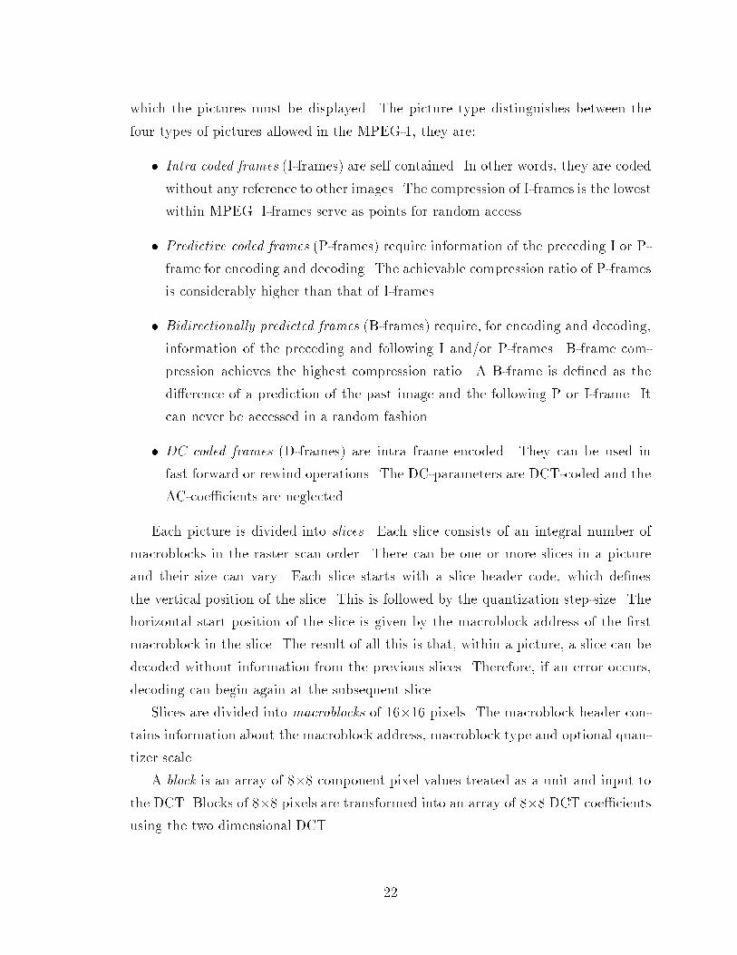
which the pictures must be displayed. The picture type distinguishes between thefour types of pictures allowed in the MPEG-1, they are:� Intra coded frames (I-frames) are self contained. In other words, they are codedwithout any reference to other images. The compression of I-frames is the lowestwithin MPEG. I-frames serve as points for random access.� Predictive coded frames (P-frames) require information of the preceding I or P-frame for encoding and decoding. The achievable compression ratio of P-framesis considerably higher than that of I-frames.� Bidirectionally predicted frames (B-frames) require, for encoding and decoding,information of the preceding and following I and/or P-frames. B-frame com-pression achieves the highest compression ratio. A B-frame is de�ned as thedi�erence of a prediction of the past image and the following P or I-frame. Itcan never be accessed in a random fashion.� DC coded frames (D-frames) are intra frame encoded. They can be used infast forward or rewind operations. The DC-parameters are DCT-coded and theAC-coe�cients are neglected.Each picture is divided into slices. Each slice consists of an integral number ofmacroblocks in the raster scan order. There can be one or more slices in a pictureand their size can vary. Each slice starts with a slice header code, which de�nesthe vertical position of the slice. This is followed by the quantization step-size. Thehorizontal start position of the slice is given by the macroblock address of the �rstmacroblock in the slice. The result of all this is that, within a picture, a slice can bedecoded without information from the previous slices. Therefore, if an error occurs,decoding can begin again at the subsequent slice.Slices are divided into macroblocks of 16�16 pixels. The macroblock header con-tains information about the macroblock address, macroblock type and optional quan-tizer scale.A block is an array of 8�8 component pixel values treated as a unit and input tothe DCT. Blocks of 8�8 pixels are transformed into an array of 8�8 DCT coe�cientsusing the two dimensional DCT. 22

Group of Pictures Layer:

Picture Layer:

Slice Layer:

Macroblock Layer:

Block Layer:

( Random Access Unit : Video Coding )

( Primary Coding Unit )

( Resynchronization Unit )

( Motion Compensation Unit )

( DCT Unit )

( Random Access Unit: Context )Sequence Layer:Table 2: Six Layers of MPEG-1 Video and Their FunctionsEach of the above six layers supports a de�nite function, which can be either asignal processing function (DCT or motion compensation) or a logical function (resyn-chronization or random access point). The layers and their functions are summarizedin Table 2 [Gal91].2.4.2 MPEG-1 Compression AlgorithmThe main aspect which stands out between a still image compression technique likeJPEG and a moving picture compression technique like MPEG, is interframe coding.This aspect stems out, since the quality requirements demand a very high compressionnot achievable with intraframe coding alone. On the other hand, the random accessrequirement is best met with intraframe coding. Addressing all these aspects requiresa delicate balance between intraframe and interframe coding, and between recursiveand non recursive temporal redundancy reduction. This challenge is answered by theMPEG-Group by using two interframe coding techniques: predictive and interpolative.The MPEG-1 video compression algorithm relies on two basic techniques: blockbased motion compensation for reduction of the temporal redundancy and transformbased (DCT) compression for the reduction of the spatial redundancy [Gal91], [11193].Motion compensation techniques are applied with predictors that are both casual(pure predictive coding) and non-casual (interpolative coding). The remaining signal(prediction error) is further compressed with spatial redundancy reduction (DCT).The information relative to motion is based on 16�16 pixel blocks and is transmittedtogether with the spatial information. The motion information is compressed usingvariable-length codes to achieve maximum e�ciency.23

I B B B P B B B I

Bidirectional Prediction

Forward Prediction

Figure 1: Dependency Among the I, P and B FramesTemporal Redundancy Reduction. The three types of frames: I, P and B ad-dress the dual need of random access points and signi�cant reduction in bit-rate. Incase of P and B frames, which are coded with respect to a reference frame, motioncompensation is used to improve the coding e�ciency. The relationship between thethree types of frames is illustrated in Figure 1.The organization of the pictures in a sequence depends on the application speci�cparameters such as random accessibility and coding delay.Motion Compensation. Motion-compensated prediction is the most widely usedtemporal redundancy reduction mechanism. Motion-compensated prediction assumesthat \locally" the current picture can be modelled as a translation of the picture atsome previous time. Locally means that the displacement need not be the sameeverywhere in the picture. In this process, motion information is a crucial part torecover the picture.Motion-compensated interpolation, also called the bidirectional prediction, is thekey feature of MPEG. In the temporal dimension, Motion-compensated interpolationis a multi-resolution technique: a sub-signal with low temporal resolution (typically1/2 or 1/3 the frame rate) is coded and the full resolution signal is obtained byinterpolation of the low-resolution signal and addition of a correction term. Thesignal to be reconstructed by interpolation is obtained by adding a correction termto a combination of a past and a future reference.Motion Representation: Macroblock. The choice of 16�16 pixels blocks formotion compensation is a result of the tradeo� between the coding gain provided bythe motion information and the cost associated with coding the motion information.24

These motion compensation blocks are calledmacroblocks. In the case of a bidirection-ally predicted picture, each 16�16 macroblock can be of type intra, forward-predicted,backward-predicted or average. The motion information consists of one vector eachfor forward-predicted macroblocks and backward-predicted macroblocks, and two forbidirectionally predicted macroblocks. The motion information associated with each16�16 block is coded di�erentially with respect to the motion information present inthe adjacent block. The range of the di�erential motion vector can be selected on apicture-by-picture basis to match the spatial resolution, the temporal resolution andthe nature of the motion in a particular sequence. The di�erential motion informationis further coded by means of a variable-length code to provide greater e�ciency bytaking advantage of the strong spatial correlation of the motion vector �eld.Motion Estimation. Motion estimation covers a set of techniques used to extractthe motion information from a video sequence. The MPEG syntax speci�es how torepresent the motion information: one or two motion vectors per 16�16 sub-block ofthe picture depending on the type of motion compensation used. The MPEG draftdoes not specify how such vectors are to be computed. However, block-matchingtechniques are the likely choices as the motion representation is block-based. In ablock-matching technique, the motion vector is obtained byminimizing a cost functionthat measures the mismatch between a block and each predictor candidate.Spatial Redundancy Reduction. Both still-image and the prediction error sig-nal have a very high spatial redundancy. There are many redundancy reductiontechniques usable to this e�ect, but due to the block based nature of the motioncompensation process, block based techniques are preferred. In this context, trans-form coding and vector quantization techniques are two likely candidates. Transformcoding techniques with combination of visually weighted scalar quantization and runlength coding have been preferred because the DCT provides a de�nite number ofadvantages and has a relatively straight forward implementation.Discrete Cosine Transform. The DCT has inputs in the range [-255, 255] andoutput signals in the range [-2048, 2048], providing enough accuracy even for the�nest quantizer. In order to control the e�ect of rounding errors when di�erentimplementations of the inverse transforms are in use, the accuracy of the inverse25

transform is determined according to the CCITT H.261 standard speci�cation.Quantization. Quantization of the DCT coe�cients is a key operation, becausethe combination of quantization and run length coding contributes to most of thecompression. It is also through quantization that the encoder can match its outputto a given bit rate. Additionally, the adaptive quantization is the key to achievingvisual quality. As the MPEG has both intra coded and di�erentially coded pictures, itcombines features of both the JPEG and H.261 standards to achieve a set of accuratequantization tools to deal with the DCT-coe�cients. In the following paragraphs, wepresent di�erent forms of quantizations employed in video compression.1. Visually Weighted Quantization. Subjective perception of quantization er-ror varies with the frequency thus, it is advantageous to use coarser quantizers forthe higher frequencies. The exact quantization matrix depends on many externalparameters such as the characteristics of the intended display, the viewing distanceand the amount of noise in the source. Hence, it is possible to design a particularquantization matrix for an application or an individual sequence which can be storedas context along with the compressed video.2. Quantization of Intra versus Non-intra Blocks. The signal from intracoded blocks is quantized di�erently from the signal that results from prediction orinterpolation. Intra coded blocks contain energy in all frequencies and are very likelyto produce \blocking e�ects" if too coarsely quantized. On the other hand, predictionerror-type blocks contain predominantly high frequencies and can be subjected tomuch coarser quantization.3. Modi�ed Quantizers. The human visual system does not perceive all spatialinformation alike and some blocks need to be coded more accurately than others. Thisis particularly true of blocks that correspond to very smooth gradients where a veryslight inaccuracy could be perceived as a visible block boundary (blocking e�ect).Such inequality between blocks can be dealt with by modifying the quantizer stepsize on a block-by-block basis if the image content makes it necessary. Furthermore,this mechanism can also be used to provide a very smooth adaption to a particularbit rate. 26

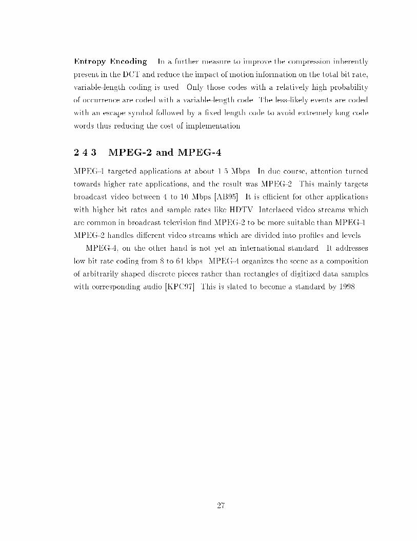
Entropy Encoding. In a further measure to improve the compression inherentlypresent in the DCT and reduce the impact of motion information on the total bit rate,variable-length coding is used. Only those codes with a relatively high probabilityof occurrence are coded with a variable-length code. The less-likely events are codedwith an escape symbol followed by a �xed length code to avoid extremely long codewords thus reducing the cost of implementation.2.4.3 MPEG-2 and MPEG-4MPEG-1 targeted applications at about 1.5 Mbps. In due course, attention turnedtowards higher rate applications, and the result was MPEG-2. This mainly targetsbroadcast video between 4 to 10 Mbps [AB95]. It is e�cient for other applicationswith higher bit rates and sample rates like HDTV. Interlaced video streams whichare common in broadcast television �nd MPEG-2 to be more suitable than MPEG-1.MPEG-2 handles di�erent video streams which are divided into pro�les and levels.MPEG-4, on the other hand is not yet an international standard. It addresseslow bit rate coding from 8 to 64 kbps. MPEG-4 organizes the scene as a compositionof arbitrarily shaped discrete pieces rather than rectangles of digitized data sampleswith corresponding audio [KPC97]. This is slated to become a standard by 1998.

27

Chapter 3NetworksCommunication networks o�er a variety of services ranging from the basic telephoneservice to current multimedia based integrated services. These services show dis-tinctly di�erent characteristics in terms of the scope of users and applications, andthe integration of di�erent applications and media. Thus, this chapter �rst capturesthe network requirements of the emerging multimedia applications. We then presentthe Asynchronous Transfer Mode networking technology, which supports real-timemultimedia tra�c. As majority of the tra�c ows through the Internet, we nextdescribe how the Internet supports multimedia applications in association with ad-vanced protocols. Since our work concerns link and associated bu�er sharing, wefurther look at di�erent ways of tra�c scheduling. We then present how ATM cansupport TCP/IP as most networks connected to the Internet run TCP/IP. Finally,we discuss how quality of service can be met for video, the medium we are studying.3.1 Networking Requirements for Multimedia Ap-plicationsMultimedia communication imposes many requirements on the network used. Ingeneral, these requirements are determined based on the respective application. Me-dia, such as video, are characterized by large frame sizes, calling for much higherresources than traditional media such as text. The di�erent media in multimediaapplications such as audio and video are bounded by processing time. Such boundsimpose stringent constraints on the delay applications can tolerate. Delays beyond28

the expected levels can render a segment of data useless, as in the case of a video clipwhere the associated audio has to be played at a particular time instant. Multimediaapplications demand measures against data corruption or data loss or both. If dataare missing or corrupt, there need to be mechanisms to recover from such impair-ment. Furthermore, it is natural for multimedia applications to employ more thantwo media to convey the information. Thus, it becomes necessary to maintain theirrelationship with respect to time. All these features become necessary to maintain thequality at the receiver's end. In the following paragraphs, we present details aboutthe requirements of multimedia on network technologies [Kar95], [Dav92].Bandwidth. Among the di�erent media, transmission of compressed video requiresone of the highest data rates, and accordingly, network experts predicted that the re-quested rate of such media would drive the bandwidth requirements in the 1990s[Stu95]. In order to reduce the transmission bandwidth and storage requirements,video is compressed in today's applications. We look at three video standards:MPEG, DVI and H.261. These standards require about 1.5 Mbps for MPEG-1, 4Mbps and above for MPEG-2, 1.2 to 1.8 Mbps for DVI and 0.064 to 2 Mbps forH.261. Practical experience recommends a total of 1.4 Mbps for audio and videofor DVI and MPEG-1 [Stu95]. The proposed bandwidth provides good video qualityand supports commercial audiovisual equipment. Additionally, it can be transmittedover the T1 leased lines of capacity 1.54 Mbps [Bat92]. Apart from this bandwidthcapacity, the highly asymmetric nature of the tra�c requires attention in dealing withbandwidth management.Transmission Delay. The delay restrictions of multimedia applications are morestringent than those of traditional data tra�c. In order to show the di�erence inmagnitude (but not actual values), consider the example of traditional tra�c, whichconsists of a �le transfer and video. The �le transfer can have a maximum end-to-enddelay of 1 sec, while video can have 0.25 sec [HSS90]. Consider another example, voicecommunication via satellite with round-trip transmission time of around 0.6 secondmakes it very di�cult for partners to hold a normal conversation. In this case, anend-to-end delay of 0.3 second is desired. Practical experience suggests an end-to-enddelay of 150 ms for interactive video applications [Stu95].Based on the delay characteristic, tra�c can fall into one of the three categories29

[SN95]. First, the asynchronous transmission mode directs communication with norestrictions on time. Second, the synchronous transmission mode de�nes a boundedtransmission delay for each message. Third, the isochronous transmission mode de-�nes a constant transmission delay for each message.Audio and video fall into the isochronous category. Isochrony does not have to bemaintained across the entire path from source to sink, only at the information's �naldestination. Thus, isochrony can be recovered by a play-out bu�er at the sink. Thecost to be paid for this is the additional delay due to the play-out bu�er [Stu95]. Forpractical purposes, synchronous tra�c with su�ciently low delay bound can fake anisochronous stream between source and sink. Therefore, the delay variance or jitter isnot considered as a separate item. To meet CCITT requirements, the maximumdelaybound is assumed to be 150 ms. We can break this into at least four components:1. source compression and packetization delay,2. transmission delay,3. end-system queueing and play-out (synchronization) delay,4. sink decompression, depacketization and output delay.Reliability. Existing communications systems strive to provide end-to-end reliabil-ity by using checksum and sequence numbering for error control and some form ofnegative or missing positive acknowledgement with packet retransmission handshakefor error recovery [SN95]. The system performance will be very bad if checksummingis not performed either in hardware or at the media access layer or link layer, asit consumes more time thereby reducing the performance [Kes97]. Error correctionthrough retransmission due to a negative acknowledgement is not appropriate fortime critical data as the retransmitted data would normally arrive late.A possible remedy for the con icting goals of reliability and low delay is to useForward Error Correction (FEC) techniques. FEC takes a set of input symbols rep-resenting data and adds redundancy to produce a di�erent and larger set of outputsymbols. It is advantageous to employ FEC technique as the receiver can recoverfrom a packet loss without retransmission. For time bound data like audio and video,the retransmission delay, which at the minimum can be of the range of one round triptime, is not favourable. As a result, FEC schemes are suitable for real-time tra�c,30

especially for links with long propagation delays. There are disadvantages with FEC[Kes97]. First, the load from a source may increase due to error correction. As packetlosses increase with load, FEC may tend to cause more losses, degrading overall per-formance. Second, FEC is not e�ective when the packet losses are bursty, a casesimilar to that of high-speed networks. Finally, FEC leads to an increase in end-to-end transmission time, as the receiver has to wait for the entire FEC block beforeprocessing the packets in the block. On the other hand, if the data from a streamis spaced well enough not to be a�ected by bursty losses and their error correctionoverhead is small then FEC may perform well.Synchronization. An important feature of multimedia systems is integrated mediaprocessing. The need for integration arises because of the inherent dependenciesamong the information coded in media objects. Though the word synchronizationrefers to time, in multimedia it is often used to re ect content, spatial, and temporalrelationships between media objects [SN95]. For instance, when audio, video, andother data streams come from di�erent sources via di�erent routers, there is a needfor mechanisms to synchronize these di�erent streams at the destination in order toachieve the equivalent of lip synchronization. Synchronization can be achieved usinga combination of time-stamping and play-out bu�ers [Stu95].3.2 The Asynchronous Transfer ModeIn an e�ort to provide real-time transport capability for emerging multimedia applica-tions, networks with high bandwidth and low latency are required. For an applicationaiming to transmit large amounts of data in real-time, new network architectures andprotocols need to be designed. Furthermore, such architectures and protocols mustsupport the di�erent media types in an e�cient and cost e�ective way. Thus, thedevelopment of the Asynchronous Transfer Mode (ATM) was initiated. In 1988,CCITT (now ITU) designated ATM, a cell based switching technology, as the trans-mission mode for the future broadband ISDN services [For95], [Sat96], [SJ95], [Vet95],[Ste95]. At the same time the ATM Forum, driven by more than 700 members, in-cluding almost all major providers of data and communication equipment, focused onthe de�nition of the private ATM networks for the local and wide area environments.ATM networks are designed for high bandwidth, scalability and manageability.31

ATM uses statistical multiplexing to provide bandwidth on demand, where the clientsnegotiate bandwidth allocation rather than the choice being made by the network.ATM is potentially capable of supporting all classes of tra�c (audio, video and tra-ditional), in one transmission and switching fabric technology. It promises to providegreater integration of capabilities and services, and increased and more exible accessto the network.3.2.1 Basic PrinciplesATM networks carry all tra�c on a stream of �xed-size packets called cells, eachcomprised of 5 bytes of header information and a 48-byte information �eld, whichis often referred to as payload. The cell size was chosen to be �xed to enable quickswitching and multiplexing. ATM is connection-oriented technology. In ATM net-works, each connection is called a virtual circuit or virtual channel (VC), because italso allows the capacity of each link to be shared by connections using that link ona demand basis rather than by �xed allocations. The connections allow the networkto guarantee the quality of service (QoS) by limiting the number of VCs, where QoSdetermines the end-to-end network performance through parameters mentioned laterin subsection 3.2.3. Typically a user declares key service requirements at the time ofconnection setup. In addition, they declare the tra�c parameters and may agree tocontrol these parameters dynamically as demanded by the network.3.2.2 ATM Protocol Reference ModelThe ATM protocol reference model is based on standards developed by the ITU.Communication from the higher layers is adapted to the lower ATM de�ned layers,which in turn pass the information onto the physical layer for transmission over aselected medium. The protocol reference model consists of three layers: the ATMadaptation layer, the ATM layer, and the Physical layer as given in Figure 2. Thereference model contains three planes; a user plane to transport user information, acontrol plane mainly composed of signalling information and a management plane tomaintain the network and to perform operational functions. In the rest of this sectionwe present the three layers in detail. 32

Control Plane User Plane

Higher Layers Higher Layers

ATM Adaptation Layer

ATM Layer

Physical Layer

Management Plane

LayerManagement

Plane ManagementFigure 2: ATM Protocol Reference Model1. The ATM Adaptation Layer (AAL). The AAL interfaces the higher layerprotocols to the ATM layers. It relays ATM cells both from the upper layers tothe ATM layer and vice versa. When relaying information received from the higherlayers to the ATM layer, the AAL segments the data into ATM cells. When relayinginformation received from the ATM layers to the higher layers, the AAL must take thecells and reassemble the payloads into a format the higher layers can understand. Thisis called segmentation and reassembly. To support di�erent types of tra�c or service,four types of AALs were initially proposed [Vet95]. In the recent ATM Forum Tra�cManagement Speci�cation Version 4.0, �ve service categories are speci�ed. Whileeach of the AALs is optimized for a particular type of tra�c, there is no stipulationin the standard that AALs designated for one service cannot be used for another. Inthe following paragraphs we present details of di�erent service classes [Sat96].Constant Bit Rate service (CBR). AAL1 supports a connection-oriented service inwhich the bit rate is constant. Examples of such applications include 64 kbps voice,�xed rate uncompressed video and leased line for private data networks. Under CBR,the network application establishes a CBR connection and negotiates the parametercalled Peak Cell Rate (PCR), the maximum data rate the connection will supportwithout losing data.Variable Bit Rate service (VBR). AAL2 supports a connection oriented service inwhich the bit rate is variable but requires a bounded delay for delivery. Examples forthis service include compressed packetized voice and video.33

Real-Time VBR service (RT-VBR). This category is meant for real-time applica-tions requiring tightly constrained delay and jitter as in the case of live video andaudio. In addition to PCR, RT-VBR is characterized by Sustained Cell Rate (SCR),the average throughput rate the application is permitted and the Maximum BurstSize (MBS), the maximumnumber of back-to-back cells that can be sent at the PCR.For this category, the sources are expected to transmit at a rate which varies withtime or, in other words, the sources can be described as bursty.Non-Real-Time VBR service (NRT-VBR). This category is intended for non-real-time applications which have bursty tra�c characteristics. This category is charac-terized in terms of PCR, SCR and MBS, but no delay bounds are associated with thisservice category. For the cells transmitted in this category, the application expects alow cell loss. In addition, this category may support statistical multiplexing.Available Bit Rate service (ABR). This service category permits the parametersrepresenting ATM layer transfer characteristics, which include PCR and MinimumCell Rate (MCR), to change subsequent to connection establishment. A ow controlmechanism is used to control the source rate. Feedback is provided to the sourcethrough the control cells called resource management cells. It is expected that anend-system that adapts its tra�c in accordance with the feedback will receive lowcell loss and get a fair share of the bandwidth. Furthermore, ABR service does notneed to bind the delay or the delay variation experienced by a connection.Unspeci�ed Bit Rate (UBR). This class is intended for non-real-time applicationsthat do not need tightly bound delay and jitter. Examples for this category includetraditional computer communication applications such as �le transfer and e-mail.The UBR service does not specify bit-rate and quality of service guarantees. Theonly assurance is that UBR will make its best e�ort to deliver cells. There is no ow-control. Thus, the cells are subject to drops once the bu�ers are full.2. The ATM Layer. The ATM layer provides an interface between the AAL andthe physical layer. The ATM layer is responsible for [SN95], [For95]:� relaying cells from the AAL to the physical layer for transmission and from thephysical layer to the AAL for use at the end system;� translation of the cell identi�er and management functions;34

GFC

VCI PTI

1

2

3

4

5

53

PTI

1

2

3

4

5

53

VPI

HEC HEC

VCI

CLPCLP

VCI

VPI

VCI

VCIVPI

VCI

VPI

Payload PayloadFigure 3: UNI (left) and NNI (right) ATM Cell Format� multiplexing and demultiplexing of cells of di�erent connections into a singlecell stream;� cell header insertion, which includes explicit forward congestion and payloadindicators;� implementation of a generic ow control mechanism at the user-network inter-face;� monitoring the transmission rate and enforcing the tra�c contract.The ATM layer's functionality is de�ned by the �elds in the ATM cell header.The format of the header for ATM cells has two di�erent forms; one for use at theuser-to-network interface (UNI) and the other for internal use by the network, thenetwork-to-network interface (NNI).As shown at the beginning of Figure 3, four bits are allocated to Generic FlowControl (GFC), which is used by the UNI to control the amount of tra�c enteringthe network. This allows the UNI to limit the amount of data entering the networkduring periods of congestion. At the NNI these four bits are assigned to the Virtualpath Identi�er (VPI).The VPI and the Virtual Channel Identi�er (VCI) together form the routing �eld,which associates each cell with a particular channel or circuit. The VCI is a singlechannel identi�er; the VPI allows grouping of VCs with di�erent VCIs and allows thegroup to be switched together as an entity.The Payload Type Indicator (PTI) �eld is used to distinguish between user cellsand control cells. This allows control and signalling data to be transmitted on adi�erent sub-channel from user data. 35

The Cell Loss Priority (CLP) provides the network with selective discard capa-bility. This bit can be set by the user to indicate lower priority cells that could bediscarded by the network during periods of congestion. For example, voice data maybe able to su�er lost cells without the need for retransmission, whereas text datacannot tolerate such losses. The CLP can also be used by the network to indicatecells that exceed the negotiated rate limit of the user; a process called tagging.The Head Error Check (HEC) �eld is used to reduce errors in the header thatcause a misrouting of the cell for one user into another user's data stream. This �eldcontains the result of an 8-bit CRC checking on the ATM header.3. The Physical Layer. The physical layer encodes and decodes the data into suit-able electrical/optical waveforms for transmission and reception on the communicationmedium used. In addition, the physical layer also provides cell delineation functions,HEC generation and processing, performance monitoring and payload matching ofthe di�erent formats used at this layer.The physical layer can transfer ATM cells from one user to another in two ways.At the UNI, ATM cells may be carried in an externally framed synchronous structureor in a cell-based asynchronous transmission structure. The SONET (SynchronousOptical NETwork), a synchronous transmission structure, is often used for framingand synchronization at the physical layer.3.2.3 Tra�c ContractThe ATM network, in order to deliver guaranteed service on demand, employs manytra�c management mechanisms. At the same time, the utilization of available net-work resources has to be maximized. The �rst step in this process is the speci�cationof the tra�c contract. A user requesting a connection with the ATM network has todeclare the characteristics of the connection in terms of the tra�c contract parame-ters. We enumerate the set of tra�c contract parameters along with their de�nitionsbelow [SJ95]:1. Peak Cell Rate is de�ned as the static amount of bandwidth that is continuouslyavailable or the maximum instantaneous rate at which the user will transmit.2. Sustained Cell Rate is de�ned as the average rate as measured over a long timeinterval. 36

3. Cell Loss Ratio is de�ned as the percentage of cells lost in the network due toerror or congestion and not delivered to the destination.4. Cell Transfer Delay is de�ned as the delay experienced by a cell between networkentry and exit points. This includes the propagation delay, queueing delay atvarious intermediate switches and service times at queueing points.5. Cell Delay Variation is de�ned as the variance of cell transfer delay. Highvariation implies larger bu�ering for delay sensitive tra�c such as voice andvideo.6. Burst Tolerance (BT) is de�ned as the maximum burst size (MBS) that canbe sent at the PCR. This is the bucket size parameter for the leaky bucketalgorithm employed to control the tra�c entering the network. BT and MBSare related as follows [SJ95]:BT = (MBS � 1)� 1SCR � 1PCR�7. Minimum Cell Rate is de�ned as the minimum cell rate desired by the user.3.2.4 Tra�c ManagementThe ATM tra�c management speci�cation de�nes a set of tra�c and congestioncontrol functions to monitor the network. These functions are intended to react tonetwork congestion in order to minimize its intensity, spread and duration. They areas follows [Sat96]:� Connection Admission Control is the set of actions taken by the network duringconnection establishment to determine whether the connection can be acceptedor rejected.� Usage Parameter Control is the set of actions taken by the network to monitorand control tra�c. Its main purpose is to protect the resources from violationsof the negotiated tra�c contract, which can a�ect the QoS of other alreadyestablished connections.� Selective Cell Discard is an optional function. A network under congestion canselectively discard cells which meet either of the following conditions:37

1. cells that belong to a non-compliant ATM connection, where a non-compliantconnection is de�ned as the one whose cells do not conform with the tra�ccontract;2. cells that have the CLP bit in the cell header set to 1.� Tra�c Shaping is a mechanism that alters the characteristics of a stream ofcells on a connection to achieve better network e�ciency while meeting the QoSobjectives or to ensure conformance at a subsequent interface.� Explicit Forward Congestion Indication (EFCI) is also an optional function. Anetwork element in an impending congested state or a congested state may setan EFCI in the cell header so that this �eld can be examined by the destinationend-system to take some corrective action.� Resource Management uses Virtual Paths, which are an important componentin tra�c control and resource management in ATM networks. Virtual Pathconnections can be used in conjunction with tra�c control to:1. simplify call admission control;2. implement a form of priority control by segregating groups of virtual con-nections according to service category;3. e�ciently distribute messages for the operation of tra�c control schemes;4. aggregate user-to-user services such that the UPC can be applied to thetra�c aggregate.� Frame Discard is based on the premise that, in case a network needs to discardcells, it is more e�ective to discard at the frame level rather than at the cell level[RRV93]. The frame referred in this case is the AAL protocol data unit. Thenetwork detects frame boundaries by checking the payload type �eld in the cellheader. This mechanism can help avoid congestion and increase the performanceby preventing partial data from consuming bandwidth [Sat96]. For example, inthe case of video, instead of sending only a few packets belonging to a framerendering the frame incomplete, it is better not to send such incomplete frameswhich may eventually be dropped. 38

� ABR Flow Control needs the transmitting stations on an ATM network toincrease or decrease their transmission rates according to the network's availablebandwidth, reducing congestion and cell loss. Transmitting stations collectbandwidth information by generating resource management cells. The resourcemanagement cell collects bandwidth information along its way to its destinationnode, which returns bandwidth data to its transmitting source so that thesubsequent transmissions can be optimized.3.2.5 Tra�c Management Related AlgorithmThe Generic Cell Rate Algorithm (GCRA), also called the leaky bucket, is used tode�ne conformance in accordance with the tra�c contract. The Usage ParameterControl function may implement the GCRA, or one or more equivalent algorithms,to enforce conformance. Although tra�c conformance is de�ned in terms of GCRA,the network is not required to use this algorithm for UPC. The continuous state leakybucket [For95], a version of GCRA, is de�ned by the ow chart in Figure 4.3.3 InternetThe Internet is a loose collection of networks organized into multi-level hierarchiesusing a wide variety of interconnection technologies. It is often referred to as a networkof networks. The majority of tra�c on the Internet consists of applications that areinsensitive to the performance they receive from the network. For example, considera �le transfer application. The best possible scenario is in�nite bandwidth and zeroend-to-end delay. However, this application works �ne as the available bandwidthdecreases and delay increases. Such applications are termed elastic, as they can adaptto changing situations. These applications are called best e�ort service applications.But, presently there are applications which need a bound on the end-to-end delay.For example, an audio application carrying voice as a 64 kbps requires the round tripdelay to be around 150 ms [Kes97]. Applications like this, which need a guaranteefrom the network on the performance, are called guaranteed service applications. Forguaranteed delay bound applications, any packets that arrive at the sink beyond theprescribed delay will be discarded thereby degrading the performance.The emerging multimedia applications have a di�erent requirement to achieve39

NO

YES

NO

YES

Xn = X - ( ta(k) - LCT )

Xn = 0

Non

Conforming

Cell

X = Xn + I

LCT = ta(k)

Conforming Cell

Xn Auxilary Variable

At the time of arrival ta of the first cell

of the connection, X = 0 and LCT = ta(k)

X Value of the Leaky Bucket Counter

Arrival of Cell k at Time ta(k)

I Increment

L Limit

LCT Last Compliance Time

Xn > L

Xn < 0

Figure 4: Generic Cell Rate Algorithm40

desired performance and, at the same time, have di�erent data characteristics. Theseare time critical applications, which are less elastic and less tolerant of delay variation.If such applications were to be run on the current Internet framework of best e�ortservice, they will be subjected to excessive delay and, in turn, a large number ofpacket drops. In addition, these applications do not adapt to congestion and thisleaves less bandwidth for other adaptable applications. It is thus necessary to extendthe current Internet model to support the newer applications [She95]. The IETF'sInternet Services Group is working on providing an enhanced model.3.3.1 Integrated ServicesAs any other network, the goal of Extended Internet is to maximize performance.Extended Internet has to support applications that do not �t into the best e�ort cat-egory. In order to support such applications, there must be a mechanism to meet theperformance requirements of the emerging applications. These requirements can bemet by providing multiple service classes instead of the prevailing best e�ort serviceclass. The new set of service classes should re ect the concerned application's require-ments. It is also essential to support any application in the prescribed multi-serviceclass. Thus, instead of a network implicitly choosing the service class for a particu-lar application it would be better for it to be explicitly speci�ed by the application.Additionally, admission control is another feature that needs to be supported by thenetwork. Such a mechanism would allow the network to reject incoming requests topreserve the performance levels of applications already being serviced. Also, this willprovide a way for the applications to specify their requirements, based on which, thenetwork can either accept or reject a request.In order to meet the above objectives, the Integrated Services (IS) model wasproposed. This model supports both real-time and non-real-time applications. Theunderlying assumptions of IS model are [BCS94]:� resources must be explicitlymanaged in order to meet application requirements;� the service guarantees for a real-time service cannot be achieved without reser-vations;� in spite of an application's ability to adapt, the end-to-end delay must bebounded; 41

� to secure statistical gain, it is desirable to use the Internet as an infrastructurefor both real-time and non-real-time applications.Quality of Service. Real-time applications based on their reaction to delay arecategorized into two classes. First, applications that are intolerant to delay will havegood performance only if they get a perfect upper-bound on the delay [Dav92]. Sec-ond, applications that do not require a perfect upper-bound on delay can adjust tovariations in delay and are called adaptive applications. Based on these applications,two real-time service classes are de�ned: guaranteed service and controlled load ser-vice. The guaranteed service provides an upper bound on delay that is perfectlyreliable, while the controlled load service provides one that is fair but not perfect.The elastic applications always wait for the data to arrive. The main feature ofthese applications is that they typically use the arriving data immediately, ratherthan bu�er it for later use. In case of delay, they always choose to wait for the datarather than proceed without it. An appropriate model for elastic applications is theexisting best e�ort service class in the Internet.Classes of Service. Based on the QoS requirement as quoted in the last paragraph,two real-time service classes, the guaranteed and the controlled load class, in additionto the best e�ort class can be introduced. The Tspec, which de�nes the data ow andRspec, which de�nes the desired QoS, belong to the RSVP and are used to specifythe service class completely. A separate subsection later describes RSVP.The guaranteed service class provides �rm end-to-end delay guarantees. This classprovides both delay and bandwidth guarantees. A ow is described using a tokenbucket, a variation of the leaky bucket presented in the section on ATM. The Tspechere consists of a token bucket (r,b), a peak rate (p), a minimum policed unit (m)and a maximum datagram size (M). The token bucket has a depth b and a data rater. The minimum policed unit (m) implies that any datagram of size less than m willbe counted as being of size m. The Rspec is de�ned using a rate R and a slack termS in microseconds. The slack term quanti�es the di�erence between the desired delayand that obtained by using a reservation rate R. Policing can be done in two ways.The �rst, simple policing, refers to comparing the arriving tra�c against a Tspec.The second, reshaping, refers to the reconstruction of a tra�c's shape to conform tothe Tspec [SPG97]. 42

The controlled load service is an enhanced quality of service to support applicationsrequiring better performance than the best e�ort service. Service for this class isdescribed by using only Tspec. As the network does not provide any quantitativeguarantee, Rspec is not required. The parameters are the same as the guaranteedservice class. For a time period T, the burst should not exceed rT + b. Otherwise,the packets violating this are considered as non-conforming [Wor97].The best e�ort service class supports applications that do not have any deadlines.Examples of such applications include telnet and ftp. These applications are bestsuited for operation under the \best e�ort" service class and hence this class is main-tained in the same state as it is in the current Internet model. This class has noTspec or Rspec as there is no guarantee of any sort by the network.Support for Service Classes. Once the service classes are in place, the questionis, how can these classes be requested? By virtue of the multiple service classes, onecan select a class suitable for the application. At the same time, all the networkelements along the path of the ow such as routers must be informed of the ow andthe parameters. Such a requirement can be realized by using RSVP. It is useful witha variety of QoS control services and deals with their setup mechanism. On the otherhand, the Real Time Transport (RTP) protocol can be used to enforce end-to-enddelay, which is a prime requirement for real-time applications. In addition, RTP canalso monitor the QoS along with the delay. The next subsection deals with RTPseparately.Integrated Services over ATM. IP of the TCP/IP is interoperable today withdi�erent link layers such as ATM and Ethernet. Of the two, the ATM has multipleclasses of service and also supports QoS functionalities. These characteristics help tosupport Internet Integrated Services over ATM. For this purpose, we need to look atmapping service classes and supporting RSVP over ATM.The three service classes of IP service model can be mapped to �ve classes of ATMservice model [GB97], as given in Table 3.The most appropriate ATM service class for the corresponding IP service class isshown in italics. RT-VBR is best suited for guaranteed service as it can utilize theunused portion of other applications and can support more bursty sources. NRT-VBR is good for controlled load service since bandwidth and bu�ers can be allocated.43

UBR,

CBR,

IP Service Class ATM Service Class

Guaranteed Service

Controlled Load Service

Best-Effort Service

NRT-VBR

Any ATM Class

or ABR

CBR or RT-VBRTable 3: Mapping of Internet Integrated Service Classes to ATM Service Classes.UBR is a natural choice for best e�ort service.The RSVP messages used to set up ow reservations must follow the same IPpath throughout the network. The main issue in supporting RSVP over ATM is thecertainty of the timing of the setup of a virtual circuit for a speci�c QoS correspondingto RSVP. Other details are being discussed.3.3.2 Real-Time Transport ProtocolIn an inter-network, for playback of audio and video, TCP may be appropriate.However, for real-time delivery of audio and video, TCP and other reliable transportprotocols are inappropriate due to the following reasons [Sch95]:� TCP cannot support multicast.� Even for unicast, reliable transmission is inappropriate for delay-sensitive datasuch as real-time audio and video. By the time the sender knows that thereceiver has missed a packet and retransmitted it, a period of one round-triptime would have elapsed. In case of the TCP fast retransmit algorithm, threeadditional packetization intervals beyond the round-trip are needed.� The TCP congestion control mechanisms decrease the congestion window whenpacket losses are detected (slow start). Audio and video have natural rates thatcannot be suddenly decreased without starving the receiver.Thus, there is a need for real-time protocols. In the following paragraphs we describethe Real-Time Transport Protocol (RTP) and its constituents.RTP has been designed within the IETF [Sch95]. RTP provides end-to-end deliv-ery services for data with real-time characteristics such as interactive audio and video.44

The services provided include play-load type identi�cation, sequence numbering, timestamping and delivery monitoring. Applications typically run RTP on top of UDP tomake use of its multiplexing and checksum services; both protocols contribute partsof the transport protocol functionality. RTP supports data transfer to multiple des-tinations using multicast distribution if provided by the underlying network. RTPitself does not provide any mechanism to ensure timely delivery or provide other QoSguarantees, but relies on lower level services to do so. It does not guarantee deliveryor prevent out-of-order delivery, nor does it assume that the underlying network isreliable and delivers packets in sequence. RTP does not address resource reservation.The sequence numbers included in RTP allow the receiver to reconstruct thesender's packet sequence or determine the proper location of a packet. RTP consistsof two parts: a data part, to carry data that has real-time properties and a controlpart, to monitor the QoS and to convey information about the participants in an on-going session. RTP is a protocol framework, which can be integrated into applicationsrather than implemented as a separate layer.Among the many use scenarios, the RTP level Translators and Mixers are notable[SCFJ96], [Sch95]. Suppose, in the case of a video conference, some participantshave high-speed links while others have lower bandwidth links. Rather than sendinglow-bandwidth, low-quality video to all participants, or having each well connectedparticipant generate both high and low bandwidth video, it may be preferable toinstall a video mixer at the low-bandwidth area. This mixer resynchronizes the in-coming video packets to reconstruct the constant spacing generated by the sender,mixes these reconstructed video streams into a single stream, translates the video en-coding into one of lower bandwidth and forwards the lower-bandwidth packet streamacross the low-speed link.Some of the intended participants in the video conference may be connected withhigh bandwidth links but might not be directly reachable via IP multicast. Forexample they might be behind an application-level �rewall that will not let any IPpackets pass. For these sites, mixing may not be necessary. In such cases another typeof RTP-relay called a translator may be used. Two translators are installed, one oneither side of the �rewall, with the outside one funnelling all multicast packets receivedthrough a secure connection to the translator inside the �rewall. The translator insidethe �rewall sends them again as multicast packets to a multicast group restricted tothe site's internal network. 45

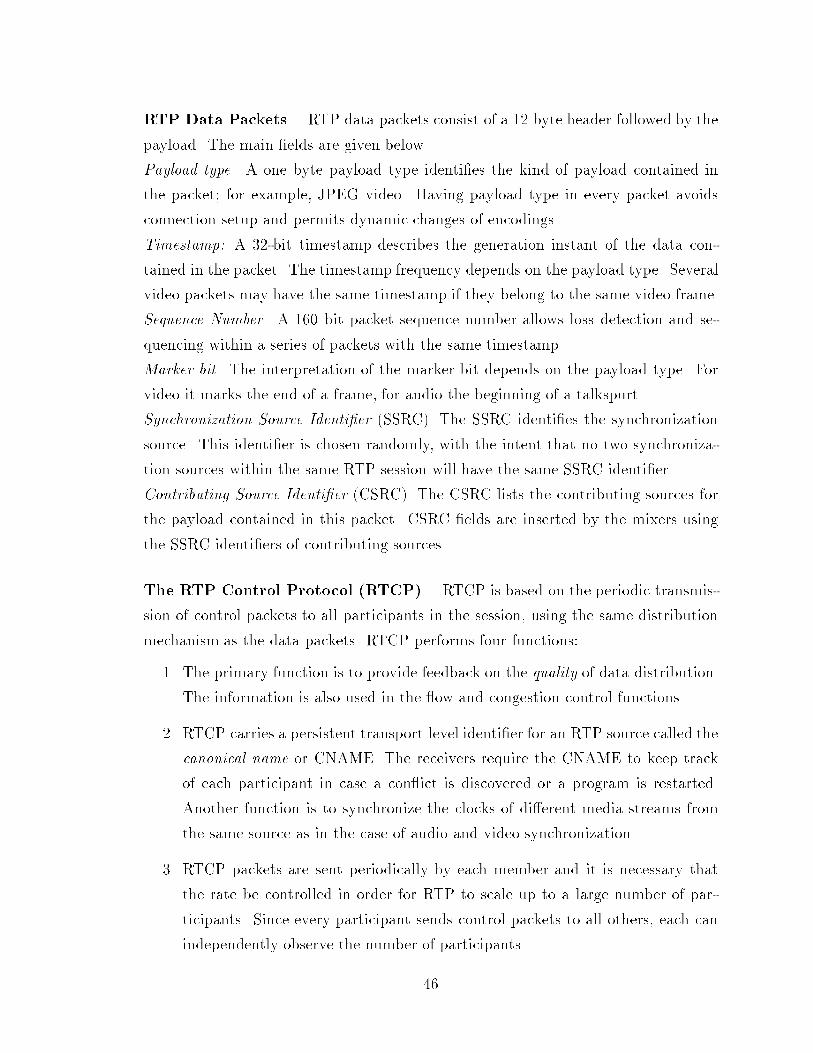
RTP Data Packets. RTP data packets consist of a 12 byte header followed by thepayload. The main �elds are given below.Payload type. A one byte payload type identi�es the kind of payload contained inthe packet; for example, JPEG video. Having payload type in every packet avoidsconnection setup and permits dynamic changes of encodings.Timestamp: A 32-bit timestamp describes the generation instant of the data con-tained in the packet. The timestamp frequency depends on the payload type. Severalvideo packets may have the same timestamp if they belong to the same video frame.Sequence Number. A 160 bit packet sequence number allows loss detection and se-quencing within a series of packets with the same timestamp.Marker bit. The interpretation of the marker bit depends on the payload type. Forvideo it marks the end of a frame, for audio the beginning of a talkspurt.Synchronization Source Identi�er (SSRC). The SSRC identi�es the synchronizationsource. This identi�er is chosen randomly, with the intent that no two synchroniza-tion sources within the same RTP session will have the same SSRC identi�er.Contributing Source Identi�er (CSRC). The CSRC lists the contributing sources forthe payload contained in this packet. CSRC �elds are inserted by the mixers usingthe SSRC identi�ers of contributing sources.The RTP Control Protocol (RTCP). RTCP is based on the periodic transmis-sion of control packets to all participants in the session, using the same distributionmechanism as the data packets. RTCP performs four functions:1. The primary function is to provide feedback on the quality of data distribution.The information is also used in the ow and congestion control functions.2. RTCP carries a persistent transport level identi�er for an RTP source called thecanonical name or CNAME. The receivers require the CNAME to keep trackof each participant in case a con ict is discovered or a program is restarted.Another function is to synchronize the clocks of di�erent media streams fromthe same source as in the case of audio and video synchronization.3. RTCP packets are sent periodically by each member and it is necessary thatthe rate be controlled in order for RTP to scale up to a large number of par-ticipants. Since every participant sends control packets to all others, each canindependently observe the number of participants.46

4. An optional function is to convey minimal session control information; for ex-ample participant identi�cation to be displayed in the user interface. This ismore likely to be useful in cases where the members join and leave withoutmembership control. Though RTP serves as a convenient channel to reach allparticipants, it is not expected to support all communication requirements ofan application.In RFC 1889 [SCFJ96] several RTCP packet types have been de�ned to carry avariety of control information:� SR. Sender report, for transmission and reception statistics from participantsthat are active senders.� RR.Receiver report, for reception statistics from participants that are not activesenders.� SDES. Source description items, including CNAME.� BYE. Indicates end of participation.� APP. Application speci�c functions.3.3.3 Resource Reservation ProtocolThe Internet in its present form o�ers a very simple service model, which can be bestdescribed as point-to-point best e�ort service. The best e�ort service has workedwell for the traditional tra�c consisting of electronic mail, �le transfers, etc. Theemerging real-time tra�c is comprised of applications which include remote video andmultimedia conferencing among others. The Internet's primitive service model failsto address two main requirements of these new applications [ZDE+93]. First, manyapplications are very responsive to the quality of service o�ered by the underlyingnetworks to their data. A network, to o�er adequate QoS, has to go farther than thebest e�ort service model and permit tra�c streams to reserve resources. Second, theemerging new applications are not solely point-to-point. They are often multipoint-to-multipoint. Such applications include interactive multimedia conferencing, whereeach one of the participants sends and receives data.Given the Internet's lack of support for the newer applications, there is a spurin research activity aimed at developing new architectures. Resource reservation is47

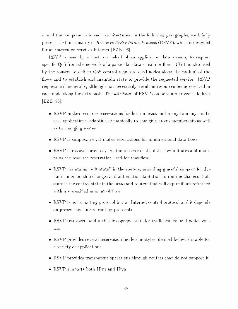
one of the components in such architectures. In the following paragraphs, we brie ypresent the functionality of Resource ReSerVation Protocol (RSVP), which is designedfor an integrated services Internet [BZB+96].RSVP is used by a host, on behalf of an application data stream, to requestspeci�c QoS from the network of a particular data stream or ow. RSVP is also usedby the routers to deliver QoS control requests to all nodes along the path(s) of the ows and to establish and maintain state to provide the requested service. RSVPrequests will generally, although not necessarily, result in resources being reserved ineach node along the data path. The attributes of RSVP can be summarized as follows[BZB+96]:� RSVP makes resource reservations for both unicast and many-to-many multi-cast applications, adapting dynamically to changing group membership as wellas to changing routes.� RSVP is simplex, i.e., it makes reservations for unidirectional data ows.� RSVP is receiver-oriented, i.e., the receiver of the data ow initiates and main-tains the resource reservation used for that ow.� RSVP maintains \soft state" in the routers, providing graceful support for dy-namic membership changes and automatic adaptation to routing changes. Softstate is the control state in the hosts and routers that will expire if not refreshedwithin a speci�ed amount of time.� RSVP is not a routing protocol but an Internet control protocol and it dependson present and future routing protocols.� RSVP transports and maintains opaque state for tra�c control and policy con-trol.� RSVP provides several reservation models or styles, de�ned below, suitable fora variety of applications.� RSVP provides transparent operations through routers that do not support it.� RSVP supports both IPv4 and IPv6.48

Distinct SharedSender Selection

Fixed-Filter Style

(None Defined) Wildcard-Filter (WF) Style

Shared-Explicit (SE) StyleExplicit

Wildcard

ReservationFigure 5: Reservation Attributes and StylesReservation Model. An elementary RSVP request consists of a owspec and a�lter spec. Together, they are a ow descriptor. The owspec speci�es a desiredQoS. The �lter spec, together with a session speci�cation, de�nes the set of datapackets { the ow { to receive the QoS de�ned by the owspec. The owspec isused to set parameters in the node's packet scheduler, while the �lter spec is used toset parameters in the packet classi�er. Both packet classi�er and packet schedulerare tra�c control functions in the primary data packet forwarding path. The packetclassi�er selects a service class for each packet in accordance with the reservation statesetup by RSVP. While the packet scheduler implements QoS for each ow, it usesone of the service models de�ned by the Integrated Service Working Group [BZB+96].The owspec in a reservation request will generally include a service class and twosets of numeric parameters; an Rspec (R for reserve) that de�nes the desired QoSand Tspec (T for tra�c) that describes the data ow [BZB+96].Reservation Styles. A reservation request includes a set of options that are col-lectively called the reservation style, shown in Figure 5.One reservation option concerns the treatment of reservation for di�erent senderswithin the same session: establish a distinct reservation for each upstream sender, ormake a single reservation that is shared among all packets of selected senders.Another reservation option controls the selection of senders; it may be an explicitlist of all selected senders or a wildcard that implicitly selects all the senders to thesession. In an explicit sender selection reservation, each �lter spec must match exactlyone sender, while in a wildcard sender selection no �lter spec is needed.RSVP Message Types. There are two fundamental RSVP message types : Resvand Path [BZB+96]. 49

Resv. Each Receiver host sends reservation request (Resv) message upstreamtowards the sender(s). These messages create and maintain reservation state in eachnode along the path(s). Resv messages must �nally be delivered to the sender hoststhemselves, so that the hosts can set up appropriate tra�c control parameters for the�rst hop. At each intermediate node two general actions are taken on request:1. Make a reservation. The request is passed to admission control and policycontrol. If either test fails, the reservation is rejected and RSVP returns anerror message to the appropriate receiver(s). If both succeed, the node uses the owspec to set up the packet scheduler for the desired QoS and the �lter spec toset the packet classi�er to determine the QoS class for each of the data packets.2. Forward the request upstream. The reservation request is propagated upstreamtoward the appropriate senders. The set of sender hosts to which a given reser-vation request is propagated is called the \scope" of that request.Path. Each RSVP sender host transmits Path messages downstream along theunicast or multicast routes provided by the routing protocol(s) along the paths ofthe data. These path messages store path state, which contains at least the unicastIP address of the previous hop node, in the node along the way. The additionalinformation in Path messages and their uses are:1. Sender template. A Path message is required to carry a sender template, whichdescribes the format of packets that the sender will originate. This template isin the form of the �lter spec that would be used to select this sender's packetfrom others in the same session on the same link.2. Sender Tspec. APath message is required to carry a Sender Tspec, which de�nesthe characteristics of the data ow that the sender will generate. This spec isused by tra�c control to prevent over-reservation, and perhaps unnecessaryadmission control failures.3. Adspec. A Path message may carry a package of One Pass With Advertisement(OPWA) advertising information, known as an Adspec. An Adspec received ina Path message is passed to the local tra�c control, which returns an updatedAdspec. The updated version is then forwarded in path messages sent down-stream. The result is that the Adspec at the receiver end may be used to gatherinformation that may be used to predict the end-to-end QoS.50

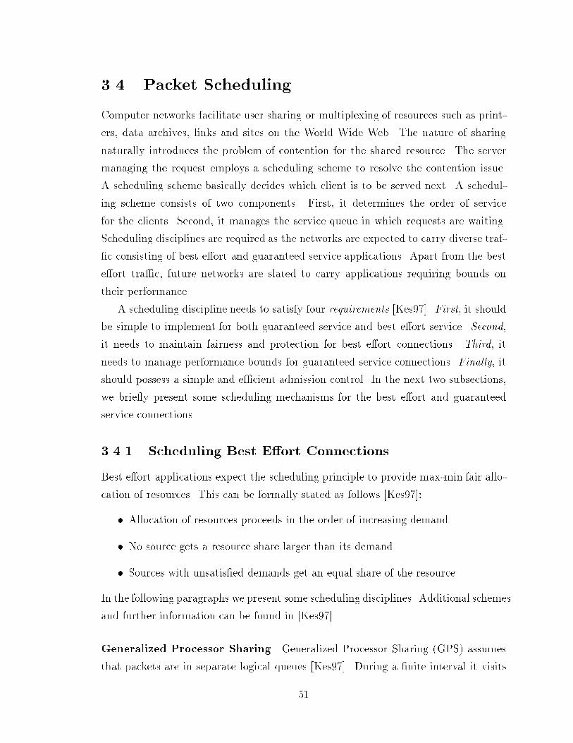
3.4 Packet SchedulingComputer networks facilitate user sharing or multiplexing of resources such as print-ers, data archives, links and sites on the World Wide Web. The nature of sharingnaturally introduces the problem of contention for the shared resource. The servermanaging the request employs a scheduling scheme to resolve the contention issue.A scheduling scheme basically decides which client is to be served next. A schedul-ing scheme consists of two components. First, it determines the order of servicefor the clients. Second, it manages the service queue in which requests are waiting.Scheduling disciplines are required as the networks are expected to carry diverse traf-�c consisting of best e�ort and guaranteed service applications. Apart from the beste�ort tra�c, future networks are slated to carry applications requiring bounds ontheir performance.A scheduling discipline needs to satisfy four requirements [Kes97]. First, it shouldbe simple to implement for both guaranteed service and best e�ort service. Second,it needs to maintain fairness and protection for best e�ort connections. Third, itneeds to manage performance bounds for guaranteed service connections. Finally, itshould possess a simple and e�cient admission control. In the next two subsections,we brie y present some scheduling mechanisms for the best e�ort and guaranteedservice connections.3.4.1 Scheduling Best E�ort ConnectionsBest e�ort applications expect the scheduling principle to provide max-min fair allo-cation of resources. This can be formally stated as follows [Kes97]:� Allocation of resources proceeds in the order of increasing demand.� No source gets a resource share larger than its demand.� Sources with unsatis�ed demands get an equal share of the resource.In the following paragraphs we present some scheduling disciplines. Additional schemesand further information can be found in [Kes97].Generalized Processor Sharing Generalized Processor Sharing (GPS) assumesthat packets are in separate logical queues [Kes97]. During a �nite interval it visits51

each non-empty queue and serves an in�nitesimally small amount of data from eachqueue. The idea is to visit every logical queue at least once in the �nite interval.Weights can be associated with connections, which will allow each connection toreceive service proportional to its weight whenever its queue is not empty. In case ofan empty queue the scheduler skips to the next non-empty queue. It is claimed thatthis will result in a max-min fair share of the bandwidth allocation.Weighted Round Robin Weighted Round Robin (WRR) is the simplest emula-tion of the GPS scheme. The main di�erence is that instead of serving an in�nitesi-mally small amount of data, WRR serves a packet from each non-empty queue. WRRemulates GPS reasonably well when both the weights and packet sizes are same. Con-nections with di�erent weights are served in proportion to their weights. This schemeis used for best e�ort tra�c.Weighted Fair Queueing Weighted Fair Queueing (WFQ) along with packet-by-packet generalized processor sharing approximates the GPS scheme. These twoschemes do not make the \in�nitesimally small amount of data" assumption and withvariable packet sizes do not need to know the mean packet size of the connection inadvance. The idea behind WFQ is to determine the time a packet would completeservice if it were to be served with a GPS server and then serve packets in the orderof these �nishing times.3.4.2 Scheduling Guaranteed Service ConnectionsWFQ presented in the previous subsection can be used both for best e�ort and guar-anteed service connections. In order to provide performance guarantees, a bound onthe worst case end-to-end delay is determined. The next two paragraphs contain twonotable mechanisms [Kes97].Virtual Clocks. A virtual clock scheduler is an independent scheme. The packetsare stamped with a tag, which determines the serving order. The tag allocates thevirtual transmission time [SN95]. One distinguishing feature is that the tag values donot emulate the GPS discipline as in the case of WFQ. The virtual clock scheduleremulates time division multiplexing in a similar way that a fair queueing scheduler52

emulates GPS. Both the virtual clock scheduler andWFQ provide similar performancewhen all connections are backlogged. But, when two connections are backlogged, thevirtual clock scheduler does not provide a fair performance.Rate Controlled Scheduler. Rate Controlled Scheduler (RCS) schemes can pro-vide bounds on the connection bandwidth and delay. RCS consists of two components;a regulator and a scheduler. The regulator houses the incoming packets, which de-termines the eligibility of a packet with the help of one of many algorithms. Uponeligibility, the packet is sent to the scheduler which arbitrates among eligible pack-ets. The ow of packets can be controlled by the regulator operating under someconstraints, such as the arrival of the packets to the scheduler at a rate smaller thanthat of the peak rate. On the other hand, the scheduler can emulate many disciplinesby issuing directions to the regulator such as the restriction of the number of eligiblepackets that arrive from the regulator. Thus, with a proper choice of regulator andscheduler, a variety of performance bounds can be achieved.3.5 ATM and InternetIn the current Internet framework, the majority of constituent networks run TCP/IP.In order to use the existing Internet frame-work in the future, it is essential that boththe ATM and Internet technologies interoperate. We detail an e�ort in this directionled by the IETF's IP over the ATM working Group, in the following subsections.3.5.1 TCP/IP Over ATMTransmission Control Protocol/Internet Protocol (TCP/IP) is widely used in thenetworking world [CCGP95]. TCP/IP places emphasis on inter-networking using aconnectionless model. In TCP/IP, the IP layer is responsible for moving packets fromone node to another, while TCP is responsible for verifying the correct delivery of datafrom client to server. TCP/IP performs well on traditional services like �le transfer,remote login and e-mail. TCP/IP, in its basic form, is not suitable for real-timeapplications for the following reasons:1. IP packets are based on the datagram model and are not suitable for real-timetra�c. 53

2. Routing of IP packets via a connectionless model may lead to out of orderdelivery. Also, media synchronization is an accompanying problem.3. Since the delivery is best e�ort only, there is no support for QoS.Currently, the Internet is growing at an extremely fast pace. Within the Internet,a large number of networks run TCP/IP. Thus, a natural question is whether ornot the TCP/IP can run over ATM? The answer is positive and, as a result, theIETF initiated the IP over ATM Working Group to develop standards for routingand forwarding IP packets over ATM subnetworks. IP over ATM project issues arelisted below [CCGP95]:1. The encapsulation and transmission of IP network or link layer packets acrossan ATM Adaptation Layer 5 connection.2. The provision of a mechanism for the resolution of IP addresses to their corre-sponding ATM addresses. This is known as the Classical IP over ATM protocoland solves the problem of IP unicast tra�c over ATM. The multicast part usesResource ReSerVation Protocol and the Internet Integrated Services model.3. The expansion of the Classical IP over ATM model to include the emergingNext Hop Resolution Protocol, described later in this section.4. The integration of multimedia services into IP, which will also allow connectivityto ATM networks.3.5.2 IP over ATM EncapsulationTransporting IP packets within the ATM cells needs a standard governing encapsu-lation. Such encapsulation allows for the multiplexing of multiple packet types at thenetwork layer on the same connection. This results in connection resource conser-vation and reduces the connection setup time. The multiplexing �eld allows a nodethat receives a network layer packet across an ATM connection to know what typeof packet has been received and to know about the application by which it must bereceived. The methods identifying this type of information are [CCGP95]:1. Virtual Channel multiplexing carries only one protocol across the ATM connec-tion with the type of protocol identi�ed at the connection setup time.54

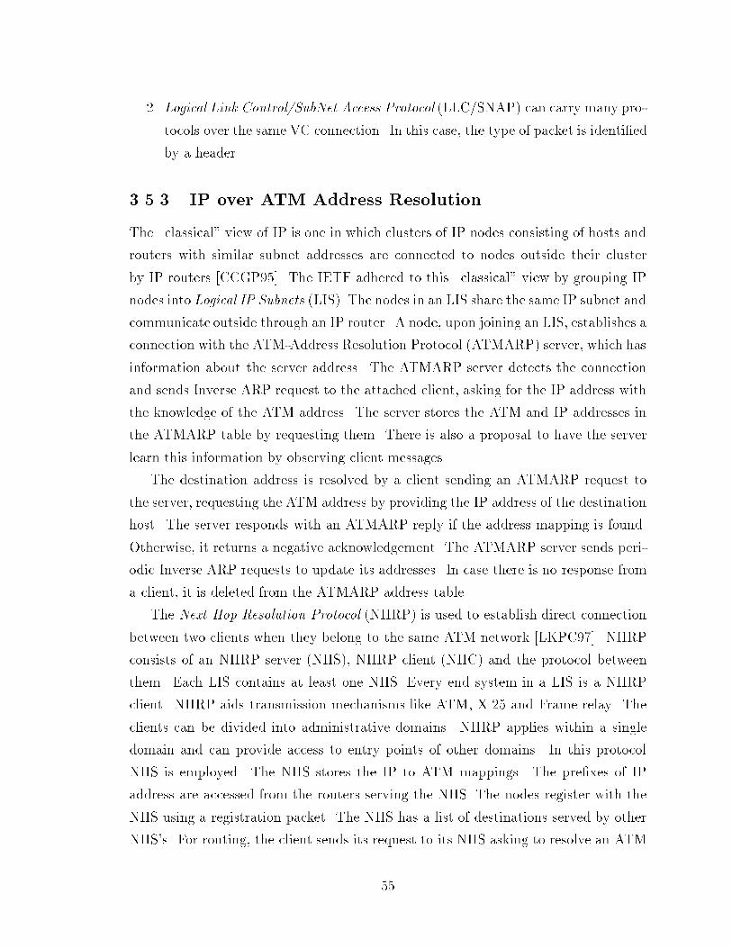
2. Logical Link Control/SubNet Access Protocol (LLC/SNAP) can carry many pro-tocols over the same VC connection. In this case, the type of packet is identi�edby a header.3.5.3 IP over ATM Address ResolutionThe \classical" view of IP is one in which clusters of IP nodes consisting of hosts androuters with similar subnet addresses are connected to nodes outside their clusterby IP routers [CCGP95]. The IETF adhered to this \classical" view by grouping IPnodes into Logical IP Subnets (LIS). The nodes in an LIS share the same IP subnet andcommunicate outside through an IP router. A node, upon joining an LIS, establishes aconnection with the ATM-Address Resolution Protocol (ATMARP) server, which hasinformation about the server address. The ATMARP server detects the connectionand sends Inverse ARP request to the attached client, asking for the IP address withthe knowledge of the ATM address. The server stores the ATM and IP addresses inthe ATMARP table by requesting them. There is also a proposal to have the serverlearn this information by observing client messages.The destination address is resolved by a client sending an ATMARP request tothe server, requesting the ATM address by providing the IP address of the destinationhost. The server responds with an ATMARP reply if the address mapping is found.Otherwise, it returns a negative acknowledgement. The ATMARP server sends peri-odic Inverse ARP requests to update its addresses. In case there is no response froma client, it is deleted from the ATMARP address table.The Next Hop Resolution Protocol (NHRP) is used to establish direct connectionbetween two clients when they belong to the same ATM network [LKPC97]. NHRPconsists of an NHRP server (NHS), NHRP client (NHC) and the protocol betweenthem. Each LIS contains at least one NHS. Every end system in a LIS is a NHRPclient. NHRP aids transmission mechanisms like ATM, X.25 and Frame relay. Theclients can be divided into administrative domains. NHRP applies within a singledomain and can provide access to entry points of other domains. In this protocolNHS is employed. The NHS stores the IP to ATM mappings. The pre�xes of IPaddress are accessed from the routers serving the NHS. The nodes register with theNHS using a registration packet. The NHS has a list of destinations served by otherNHS's. For routing, the client sends its request to its NHS asking to resolve an ATM55

address. If the address is being served by the NHS it returns the mapping. Otherwiseit forwards the request to another NHS. The reply is sent along the reverse route.Any further requests are responded to without forwarding the request. The NHRPis likely to be used on routers for frame relay and X.25.The future work on IP over ATM domain includes support for multicast of IPpackets over ATM and multiprotocol encapsulation over AAL5.3.6 DiscussionReal-time applications exhibit stringent timing conditions, which are crucial to achieveintended performance levels. The medium of our focus, video, is accompanied by thedynamic nature of frame sizes along with critical timing requirements. Owing to thelarge frame sizes, video is handled almost completely in a compressed form. It is thevarying levels of compression that give rise to the dynamic nature in frame sizes. Thisis evident in case of I, P and B frames of MPEG sequences where, at times, the sizeof an I frame can be easily 10 times that of a B frame. The timing constraints arisebecause of the need to maintain continuity in playing frames. Otherwise, the artifactsbecome noticeable, and thus would lead to degraded performance. For example, anMPEG sequence operating at 30 fps needs a frame to be played every 33 ms. Thoughthe eye can tolerate a delay of 40 ms, any delay beyond that would impair the qual-ity [SN95]. In order to meet such requirements, we need mechanisms to guaranteerequired performance levels before embarking with the actual transmission. ATM isone such technology, which o�ers the QoS mechanism.Much of the future success of ATM is attributed to ATM's ability to interoperatewith IP. But, there are two major di�erences between ATM and Internet. First, ATMis connection-oriented, wherein the two parties establish a connection before trans-mission. On the other hand, IP is connection-less wherein each packet is forwardedby routers independently on a hop-by-hop basis. This can be solved in two ways. Onepossibility is to establish a new connection on demand. However, this is not viable incase of small amounts of data transfer due to the high cost of setting up and tearingdown the connection. The other option is to forward the data through precon�guredconnection(s). This scheme may not be the optimal path and the amount of datacould overwhelm the connection. The second major di�erence is that of ATM's QoS56

facility and IP's best e�ort service. This is being solved by extending the Internet asexplained in the Integrated Internet section.Networks o�ering QoS need packet scheduling schemes, which can help sustainthe promised QoS. The work by [SL97] proposes such a scheme wherein the authorsenhance the GPS schemeby addressing its shortcomings. In GPS, service rate receivedby a session is proportional to the backlogged sessions in the system. If another sessionbecomes active, the service rate of a session may change abruptly. This could resultin increased delay for consecutive packets. The authors propose a new scheme whichalleviates this problem called Slow-Start GPS. In this method, when a new sessionbecomes active, instead of giving its share of bandwidth immediately, it is allocatedgradually from 0 to �nal value. In this way the \older" sessions do not experience asudden drop in service rates.In another work, the authors [APKR95] experiment with the tra�c control mech-anism of ATM; namely the Usage Parameter Control (UPC) aided by leaky buckets.In this mechanism, the authors demonstrate the control functions for a connectionde�ned by PCR and SCR. They further illustrate controlling the PCR of a video con-nection by using the PCR's of the connection and the source in addition to Cell DelayVariation (CDV) tolerance. It is observed that whenever the actual PCR exceeds con-tracted PCR, any change in CDV tolerance has little e�ect on the Cell Discard Ratio.Once the CDV tolerance is larger than the the inverse of contracted PCR, the UPCdiscards exactly that excess amount of tra�c. In case the actual PCR is below thecontracted PCR, only cell clumping will cause cell discards. Given such a scenariowherein losses occur, new mechanisms are required so that the quality of video canbe maximized at receiver end.Some mechanisms can be proposed, which can help maximize the visual quality.For example, priority can be established for video frame drops under constrainedbandwidth conditions. As mentioned earlier, MPEG contains 3 types of frames ofvarying importance. Such information can be used to drop the frames in decreasingorder of importance; �rst B, then P and �nally I. This could lead to a considerable gaininstead of loosing all I frames which would seriously damage the set of P and B framesdependent on them. In order to recover from packet losses, error correction techniqueslike FEC are used. FEC is preferred since the traditional techniques would contributedelay which the real-time applications cannot tolerate. FEC is supported by ATM inAAL1. However, FEC comes with a trade o� [Yas96]. It facilitates recovery of lost57

information at the cost of additional bandwidth required for transmission of correctioninformation. Due to the issues involved, FEC is till a topic of discussion.

58

Chapter 4Problem StatementWe consider the transmission of multiple video streams, such that a bandwidth reser-vation is shared between them. We are interested in a case when the bandwidthavailable is not su�cient to ensure zero-loss transmission, i.e., the bandwidth is lessthan the sum of average bandwidths of the participating video streams. In this en-vironment, we wish to investigate the e�ect of bandwidth and bu�er managementpolicies on the quality of video streams received at the destination.Accordingly, in this chapter, we detail our approach towards addressing this prob-lem. We �rst present the model employed in our study. We then provide informationabout the video sequences used in our simulations. Then, we cover the simulationenvironment and next, we discuss the statistics-gathering process and highlight theperformance measures. In the last section, we present the e�ect of bandwidth varia-tion on the performance of each sequence.4.1 The ModelOur model consists of a video gateway serving a link of �xed bandwidth. The videogateway has a �nite number of bu�ers, small enough to ignore the delay due toqueueing. We have multiple sources generating video data in the form of frames.Each frame of video-data is characterized by its size. The data arriving at the gate-way is subjected to the Frame Admission Control (FAC) before being bu�ered fortransmission as in Figure 6. The FAC implements the bu�er management policyat the frame level. FAC operates with frames instead of the conventional packets59

...

Buffers

Constrained

BandwidthSinksServer

Link

SourcesCells

Video Gateway

FramesAdmission

Control

Frame

Frames

Dropped FramesFigure 6: Network Modelas we deal with frame-drops. The bu�er size is quanti�ed in terms of ATM cells.Frames in the queue of bu�ers are forwarded in the form of ATM cells on the out-going link. The constrained bandwidth of the outgoing link re ects the negotiatedreserved bandwidth with the network.The FAC is the key component in our model, and determines the quality of videotransmitted. Any frame that is not dropped at the FAC is considered to be receivedat the sink.4.2 Video Sequences CharacterizationWe call a set of video frames a video sequence or a video stream. For the experiments,we use MPEG-1 sequences consisting of only I-frames obtained from the Internet.Initially, we determine the frame sizes in bytes by parsing video sequences. Werepeat video sequences in order to obtain su�cient frames for the entire simulationlength. We then convert each frame size in terms of ATM cell's payload of 48 bytes.The resulting frame sizes in ATM cells are used as input data for the experiments.We characterize video sequences with the following: minimum frame size, maximumframe size, average frame size and standard deviation of frame sizes. Table 4 liststhe characteristics of video sequences employed in the simulations.We present the frame size characteristics of ten sequences employed in our simu-lations in Figures 7 through 16. These video streams re ect di�erent informationcontent. Sequences bla, jet and can have fast motion pictures. Among these three,bla has a large number of scene changes. Streams foo and sum are live recordingsof a football match and sumo wrestling respectively. These two streams also showfast motion between consecutive pictures. In contrast, tha and suk cover low activity60

Streams Maximum Minimum Average Std. Deviationbla 35.9 15.9 26.9 151.4boo 68.4 27.2 43.2 568.7can 69.5 28.4 48.4 269.2jet 74.1 15.1 46.7 824.5mov 61.5 55.1 58.8 77.8tha 34.9 6.5 23.4 293.4suk 60.6 33.8 42.0 296.1sum 126.5 30.4 85.1 1276.5foo 116.2 7.6 92.7 1517.3boe 75.3 20.6 41.7 507.8Table 4: Frame Size Characteristics (in ATM cells) for Ten Video Streamsimages of a total solar eclipse and a parked aircraft respectively. The last three videoclips named boo, boe and mov are captured with a moving camera showing di�erentlevels of activity between the pictures. With a collection of these sequences, we intendto capture a wide range of content and frame size variation. As the graphs of framesize characteristics illustrate, every sequence shows a di�erent spread in terms of theirframe size characteristics.4.3 Simulation EnvironmentIn this section we �rst present details of the simulator used. We then list the assump-tions under which our experiments are conducted, followed by the set of con�gurationparameters.4.3.1 The ns simulatorWe enhance the ns version 1 simulation tool [MF95] developed by the Network Re-search Group at the Lawrence Berkeley National Laboratory for our experiments.ns is easily con�gurable and has a programmed event-driven simulation engine. Anetwork topology is realized in ns by using three primitive building blocks: nodes,links and agents. Nodes act as containers for agents, the active objects that drive thesimulation. Sources and sinks are de�ned with the help of nodes and are connected61

0

200

400

600

800

1000

1200

1400

1600

1800

0 200 400 600 800 1000 1200 1400 1600 1800 2000

Fram

e Si

zes

(byt

es)

Frame Numbers

blaAverage

MaximumMinimum

Std. DeviationFigure 7: Frame Size Distribution of bla Sequence500

1000

1500

2000

2500

3000

3500

0 200 400 600 800 1000 1200 1400 1600 1800 2000

Fram

e Si

zes

(byt

es)

Frame Numbers

booAverage

MaximumMinimum

Std. DeviationFigure 8: Frame Size Distribution of boo Sequence62

0

500

1000

1500

2000

2500

3000

3500

0 200 400 600 800 1000 1200 1400 1600 1800 2000

Fram

e Si

zes

(byt

es)

Frame Numbers

canAverage

MaximumMinimum

Std. DeviationFigure 9: Frame Size Distribution of can Sequence500

1000

1500

2000

2500

3000

3500

4000

0 200 400 600 800 1000 1200 1400 1600 1800 2000

Fram

e Si

zes

(byt

es)

Frame Numbers

jetAverage

MaximumMinimum

Std. DeviationFigure 10: Frame Size Distribution of jet Sequence63

0

500

1000

1500

2000

2500

3000

0 200 400 600 800 1000 1200 1400 1600 1800 2000

Fram

e Si

zes

(byt

es)

Frame Numbers

movAverage

MaximumMinimum

Std. DeviationFigure 11: Frame Size Distribution of mov Sequence200

400

600

800

1000

1200

1400

1600

1800

0 200 400 600 800 1000 1200 1400 1600 1800 2000

Fram

e Si

zes

(byt

es)

Frame Numbers

thaAverage

MaximumMinimum

Std. Deviation

Figure 12: Frame Size Distribution of tha Sequence64

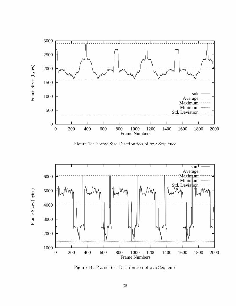
0

500

1000

1500

2000

2500

3000

0 200 400 600 800 1000 1200 1400 1600 1800 2000

Fram

e Si

zes

(byt

es)

Frame Numbers

sukAverage

MaximumMinimum

Std. DeviationFigure 13: Frame Size Distribution of suk Sequence1000

2000

3000

4000

5000

6000

0 200 400 600 800 1000 1200 1400 1600 1800 2000

Fram

e Si

zes

(byt

es)

Frame Numbers

sumAverage

MaximumMinimum

Std. Deviation

Figure 14: Frame Size Distribution of sum Sequence65

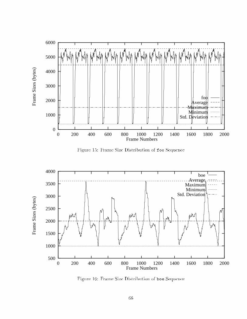
0

1000

2000

3000

4000

5000

6000

0 200 400 600 800 1000 1200 1400 1600 1800 2000

Fram

e Si

zes

(byt

es)

Frame Numbers

fooAverage

MaximumMinimum

Std. DeviationFigure 15: Frame Size Distribution of foo Sequence500

1000

1500

2000

2500

3000

3500

4000

0 200 400 600 800 1000 1200 1400 1600 1800 2000

Fram

e Si

zes

(byt

es)

Frame Numbers

boeAverage

MaximumMinimum

Std. Deviation

Figure 16: Frame Size Distribution of boe Sequence66

using the link command. The ns simulation description language is an extension ofthe Tool Command Language, (Tcl) [Ous94]. A simulation is de�ned by a Tcl pro-gram. We have upgraded this simulator to support video tra�c. For this purpose,we have introduced video speci�c sources and sinks, along with necessary changes toimplement FAC.4.3.2 Simulation Set-upSources generate frames, based on the natural frame rate, which is �xed in our sim-ulations at 30 fps. Frames arriving at the gateway are �rst checked by the FAC. Itdecides whether the frame is admissible or not. If the frame is admissible, the frame issent to the queue, otherwise it is dropped. At the sink, we record the arrival status offrames and further process them through perl scripts [WCS96] to generate the outputinformation.The link capacity re ects a value in the constrained bandwidth region. For thispurpose, we employ reduced values of the sum of average bandwidths of all the tensequences, called Average Bandwidth. We determine the Average Bandwidth basedon the Average Rate of ten sequences. The Average Rate for a particular sequence iscomputed as:Average Rate (bps) = Frame Rate (fps) � Average Frame Size (bits)The Average Bandwidth is obtained as:Average Bandwidth (bps) = 10Xseq=1 Average Rateseq (bps)4.3.3 AssumptionsThe assumptions employed in our simulations are as follows:� The video frame sizes are known apriori. This assumption is used in computingthe bandwidth values as explained in the previous section.� There is no delay due to the frame admission part of FAC.� Frame rate is �xed at 30 fps. The arrival times of the frames may vary if theframe arrivals are desynchronized. 67

� All packets (ATM cells) belonging to a particular frame will be available at theirrespective arrival time at the queue.4.3.4 Frame Arrival ProcessThe basic form of frame arrivals in our simulation environment, is guided by synchro-nized arrivals. In this process, all the sources start at the same time and generateframes with an interval equivalent to a frame period (also called inter-arrival period).We de�ne a frame period as the inverse of a Frame Rate. As a result of this process, allframes corresponding to the ten sources arrive at the same time at the gateway, thusleading to a highly synchronized arrival pattern. In other words, such arrivals con-tribute to frame clumping at the queue. This leads to a serious contention for bu�erspace. In this situation, frames belonging to the �rst few sequences are almost alwaysaccepted into the queue, while the sequences at the end experience losses. Thus, it isnecessary to alter the arrival pattern to break the high degree of synchrony.We desynchronize every frame arrival in order to break the high degree of syn-chronization. We call such an arrival pattern desynchronized frame arrival. This typeof arrival process re ects the real-world network environments wherein the artifactslead to variations in transmission time. We a�ect desynchronization of frame arrivalsby adding some randomness to arrival times. Thus, in our simulations the range overwhich the frame arrivals can vary is chosen to be equivalent to the frame period. As aresult of this interval, two consecutive frames can arrive either with a gap of twice theinter-arrival time (66 ms) or back-to-back. The inter-arrival time is used in specifyingthe randomness interval for obvious reasons, as it is the smallest identi�able unit invideo transmission.4.4 Results GenerationWe �rst describe the statistics gathering process and conclude with a description ofperformance measures in this section. 68

Statistics GatheringRegion

0.0Time : Seconds80.020.0

Transient Region Figure 17: Two Regions of Simulation4.4.1 Statistics CollectionWe employ a simulation length of 80.0 seconds. The sources generate video data forthe entire simulation length. This time can be split into two regions as in Figure17. We name the two regions as: transient region and statistics gathering region.Since our aim is to capture the drop occurrences, we ignore the events during the�rst 20.0 seconds, which includes the time taken for the queue to �ll up leading todrops. This can be illustrated in the following example. In an experiment employingshared bu�ers and shared bandwidth under synchronized frame arrivals, the �rstframe drop for 90% bandwidth case, occurs at time 5.17725 seconds; while, in thesame experiment for 60% bandwidth case, we observe the �rst frame drop at 1.52919seconds. On the other hand, experiments involving static bandwidth partition incurthe �rst drop at around 18.0 seconds. Thus, we use statistics from the interval 20.0to 80.0 seconds for generating the results. The statistics gathering length of 60.0seconds is �xed for all experiments in this thesis. The results are quanti�ed using themetrics de�ned in the next subsection.4.4.2 Performance MeasuresTraditionally, packets have been used in quantifying performance as they are thefundamental transmission units. But video data di�ers from this notion. A videoframe typically consists of many packets. These packets together represent a picturecomplete with all the information. If packets belonging to a particular frame are lost,it will lead to an incomplete picture { a�ecting the quality. Thus, it is necessaryto measure the performance of video streams in terms of frames, which can looselycorrelate to qualitative performance.We employ a measure called E�ective Frame Rate (EFR). EFR can be de�ned as69

the rate of successfully sent frames. It is measured over a one second quantum. Inquantifying the performance of a run of a sequence, we use the average of EFRs overthe Simulation Length (SL); where, the SL corresponds to the statistics gatheringregion of 60 seconds. The Average EFR is computed as:Average EFR = PSLtime=1 EFRtimeSLFurthermore, in order to observe the extent of variation in fairness in an experiment,we employ Fairness Index (FI). Suppose, if EFR1, EFR2, : : : , EFRN represent Av-erage EFRs for N sequences, then the FI is obtained by the standard deviation of allthe Average EFRs as:V ariance of Average EFRs = �N�PNseq=1 EFR2seq���PNseq=1 EFRseq�2N �(N�1)Standard Deviation of Average EFRs (FI) = pV ariance of Average EFRsApart from the fairness measure given by EFR, it is also necessary to know howthe quality uctuates within a sequence over time. Since the frame losses may notbe uniform, we observe di�erent EFRs over time. It is thus necessary to capture thevariation in EFRs over the transmission time. This will enable us to know the extentof variation in quality when compared to the original sequence, which has a perfectframe rate of 30 fps. Thus, the variation of quality within a lossy sequence can bestated in terms of the deviation of EFR. Such a variation can occur in many ways.For example, if every other frame is sent, then we have a at EFR curve with thedeviation being zero. While in another case, if we have low EFRs in some intervalsand high EFRs in some others, we have a uctuating curve for EFR. We thus computethe standard deviation of EFR as:V ariance of EFR = (SL�PSLi=1 EFR2i )�(PSLi=1 EFRi)2SL �(SL�1)Standard Deviation of EFR = pV ariance of EFRWe call the Average EFR for a run as simply \EFR" while specifying fairness inthe following chapters. The deviation within a sequence represented by the StandardDeviation (SD) of EFR is denoted as \SD-of-EFR".70

Video average Bu�er Size forName bandwidth (ab) Zero Loss at abbla 0.34344 1476boo 0.55968 1035can 0.62328 406jet 0.59784 2695mov 0.75048 915tha 0.30528 1565suk 0.54696 1080sum 1.09392 3732foo 1.18296 4652boe 0.53424 2886Table 5: Con�guration Parameters for E�ect of Bandwidth Variation4.5 E�ect of Bandwidth Variation on PerformanceIn this section, we present the e�ect of bandwidth variation on performance of eachvideo sequence. For this purpose, we run each sequence independently with linkcapacity varied in steps of 5% over the entire range of average bandwidth of the re-spective sequences. The bu�er size is �xed such that there is no loss for 100% ofaverage bandwidth. Table 5 lists average bandwidth of each sequence and corre-sponding bu�er size for the experiment. The frame arrivals are desynchronized, tore ect a realistic environment.The performance in terms of EFR of each sequence is captured in Figures 18through 27. We observe that the EFR decreases uniformly with the decrease inbandwidth, accompanied by negligible variations. Thus, the graphs exhibit almostlinear plots, resulting in near monotonous drop in performance over the entire band-width region.We capture the standard deviation of EFR of all the ten sequences in Table 6.The uctuation is quite noticeable in some sequences as in case of jet, tha, sum andfoo. Such a behaviour is attributed to the frame sizes consistently deviating awayfrom their average frame size for long durations. On the contrary, sequences which uctuate close to the average frame size result in low deviations of EFR. Examplesof such sequences include bla, can and mov.71

0

5

10

15

20

25

30

0 0.05 0.1 0.15 0.2 0.25 0.3 0.35

EFR

(fp

s)

Bandwidth (Mbps)Figure 18: EFR of bla Sequence over Sample Bandwidth Points0

5

10

15

20

25

30

0 0.1 0.2 0.3 0.4 0.5 0.6

EFR

(fp

s)

Bandwidth (Mbps)Figure 19: EFR of boo Sequence over Sample Bandwidth Points72

0

5

10

15

20

25

30

0 0.1 0.2 0.3 0.4 0.5 0.6 0.7

EFR

(fp

s)

Bandwidth (Mbps)Figure 20: EFR of can Sequence over Sample Bandwidth Points0

5

10

15

20

25

30

0 0.1 0.2 0.3 0.4 0.5 0.6

EFR

(fp

s)

Bandwidth (Mbps)Figure 21: EFR of jet Sequence over Sample Bandwidth Points73

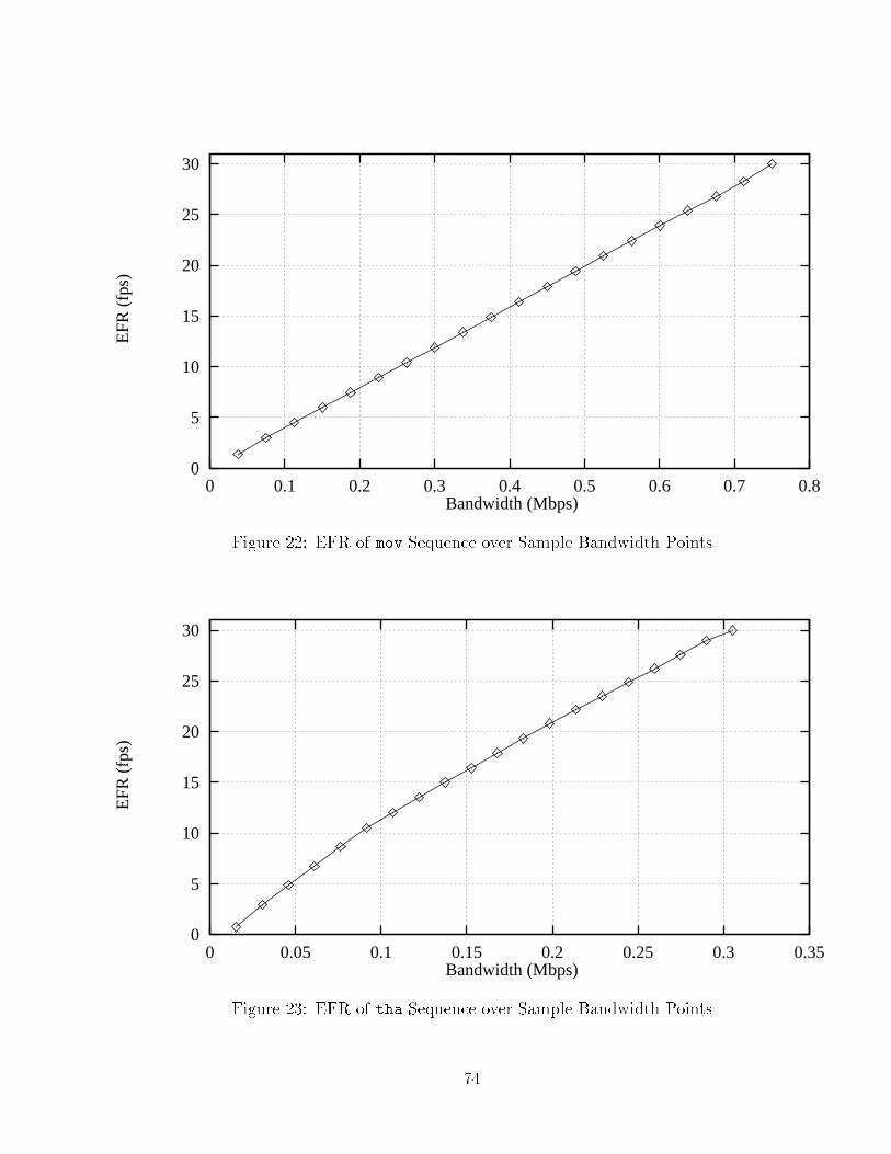
0

5

10

15

20

25

30

0 0.1 0.2 0.3 0.4 0.5 0.6 0.7 0.8

EFR

(fp

s)

Bandwidth (Mbps)Figure 22: EFR of mov Sequence over Sample Bandwidth Points0

5

10

15

20

25

30

0 0.05 0.1 0.15 0.2 0.25 0.3 0.35

EFR

(fp

s)

Bandwidth (Mbps)Figure 23: EFR of tha Sequence over Sample Bandwidth Points74

0

5

10

15

20

25

30

0 0.1 0.2 0.3 0.4 0.5 0.6

EFR

(fp

s)

Bandwidth (Mbps)Figure 24: EFR of suk Sequence over Sample Bandwidth Points0

5

10

15

20

25

30

0 0.2 0.4 0.6 0.8 1 1.2

EFR

(fp

s)

Bandwidth (Mbps)Figure 25: EFR of sum Sequence over Sample Bandwidth Points75

0

5

10

15

20

25

30

0 0.2 0.4 0.6 0.8 1 1.2

EFR

(fp

s)

Bandwidth (Mbps)Figure 26: EFR of foo Sequence over Sample Bandwidth Points0

5

10

15

20

25

30

0 0.1 0.2 0.3 0.4 0.5 0.6

EFR

(fp

s)

Bandwidth (Mbps)Figure 27: EFR of boe Sequence over Sample Bandwidth Points76

Video SequencesBandwidth bla boo can jet mov tha suk sum foo boe100% 0.00 0.00 0.00 0.00 0.00 0.00 0.00 0.00 0.00 0.0095% 2.26 2.1 1.36 1.63 0.52 1.81 1.68 1.92 1.93 2.5290% 1.54 3.8 1.3 7.12 0.47 5.53 1.99 6.52 5.33 3.7885% 1.31 3.33 1.23 7.29 0.53 5.79 1.74 5.96 5.45 3.3280% 1.23 3.02 0.99 7.2 0.45 6.10 1.56 5.45 5.47 3.1375% 1.1 2.61 0.86 6.41 0.5 6.28 1.37 4.77 5.57 3.1670% 1.42 2.25 0.81 5.55 0.39 6.63 1.19 4.09 5.58 2.965% 1.62 1.9 0.68 4.94 0.5 6.07 0.99 3.4 6.04 2.7460% 1.66 1.53 0.78 4.05 0.26 4.96 0.94 2.93 5.8 2.4155% 1.56 1.2 0.52 3.25 0.5 3.9 0.8 2.4 5.9 2.0750% 1.34 1.15 0.44 2.47 0.0 2.98 0.9 1.83 5.18 1.5845% 0.86 0.8 0.5 1.3 0.63 1.32 0.75 1.21 2.42 0.8540% 2.43 2.81 1.67 2.68 0.56 2.84 3.02 3.14 2.64 3.5835% 2.49 3.81 1.75 3.49 0.56 3.35 3.13 4.09 3.37 3.9530% 2.37 4.23 1.77 4.22 0.6 3.77 2.99 4.78 3.89 4.525% 2.18 4.55 1.7 4.93 0.5 4.39 2.8 5.39 4.21 4.7920% 2.08 5.03 1.72 5.34 0.62 4.83 2.6 6.02 4.67 4.6915% 1.99 4.86 1.63 5.88 0.5 5.1 2.44 6.27 5.05 4.6210% 1.86 4.5 1.49 6.37 0.5 5.25 2.32 6.37 5.23 4.425% 1.67 4.17 1.36 6.74 0.5 5.45 2.12 6.54 5.38 4.05Table 6: SD-of-EFR for Ten Video Streams Used in Simulations77

Chapter 5Shared Bandwidth and SharedBu�ersOur �rst set of experiments employ FCFS scheduling such that the bandwidth iscompletely shared between the competing streams. The bu�ers are also shared. Whena new frame arrives at the gateway, the FAC checks for available space in the bu�erpool and if space is available, the frame is queued in a single FIFO queue. If not, theframe is dropped. The enqueued frames are served in a FCFS manner. We start withFCFS scheduling due to its simplicity and least cost of implementation. We presentadditional experiments to show the e�ect of large frame sizes and varying bu�er sizeson performance.5.1 Overview of ExperimentsWe split the experiments into two categories: synchronized start and desynchronizedframe arrivals. We distinguish between the two forms of arrivals by the desynchro-nization parameter. We achieve this by associating a value of 0 ms for synchronizedarrivals and a non zero value representing the interval for desynchronized frame ar-rivals, which is 66 ms in our case, as described in Chapter 4.The con�guration parameters are given in Table 7. Bu�er size is selected suchthat there are no losses for 100% of Average Bandwidth, which is the sum of averagebandwidths of all ten streams. We gather statistics over a period of 60 seconds, asoutlined in Chapter 4. The link capacity is varied in steps of 10% in the range [100%,78

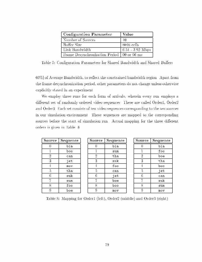
Con�guration Parameter ValueNumber of Sources 10Bu�er Size 8046 cellsLink Bandwidth 6.54 - 3.92 MbpsFrame Desynchronization Period 00 or 66 msTable 7: Con�guration Parameters for Shared Bandwidth and Shared Bu�ers60%] of Average Bandwidth, to re ect the constrained bandwidth region. Apart fromthe frame desynchronization period, other parameters do not change unless otherwiseexplicitly stated in an experiment.We employ three runs for each form of arrivals, wherein every run employs adi�erent set of randomly ordered video sequences. These are called Order1, Order2and Order3. Each set consists of ten video sequences corresponding to the ten sourcesin our simulation environment. These sequences are mapped to the correspondingsources before the start of simulation run. Actual mapping for the three di�erentorders is given in Table 8.Source Sequence0 bla1 boo2 can3 jet4 mov5 tha6 suk7 sum8 foo9 boeSource Sequence0 bla1 sum2 tha3 suk4 foo5 can6 jet7 boe8 boo9 mov

Source Sequence0 bla1 foo2 boe3 tha4 boo5 jet6 can7 suk8 sum9 movTable 8: Mapping for Order1 (left), Order2 (middle) and Order3 (right)79

5.2 ResultsIn this section, we present experiments to capture the e�ect of sharing both bandwidthand bu�ers under synchronized and desynchronized frame arrivals.5.2.1 Synchronized StartIn synchronized arrivals, all the ten participating sequences start at the same time. Asa result, frames corresponding to the ten sequences arrive at their respective arrivaltimes, based on the frame rate of 30 fps. We deactivate desynchronization parameterwith a value of 0 ms in this experiment.The EFR depicted in Table 9 for the ten sequences exhibits typical FCFS be-haviour. A prime observation is that, sequences in the beginning of an order almostalways succeed in sending their frames, while the sequences at the rear end su�er fromlosses. As expected, the number of sequences experiencing losses increase as band-width is reduced to lower levels. For instance, in orders 1 and 3, for 90% bandwidthcase, only two sequences su�ered losses, whereas in 60% case four or more sequencesincurred drops.Another prime observation appears in the form of high unfairness in loss distri-bution. For example, in Order1, for 60% bandwidth, the EFR range achieved is 30.0to 2.7 fps. This is re ected by the higher values of Fairness Index (FI).The variation of EFRs is presented in Table 10. The SD-of-EFR shows no distinctpatterns for the three orders. Drop occurrences in the sequences uctuate very widely.This can be illustrated as follows: in Order2, for 80% bandwidth, the sequence boohas a SD of 9.42; while, it is 3.77 for 60% bandwidth. A still worse case in Order2 isthe mov sequence where the SD jumps from 0.18 to 10.5, for 60% to 90% bandwidth.This behaviour coupled with the unfairness results in a high degree of adverse e�ecton visual quality. As sources successful in sending all their frames will result in perfectquality, the others incurring losses yield poor quality.5.2.2 Frame Arrival DesynchronizationDesynchronization of frame arrivals is implemented by randomly varying the framearrival times over the desynchronization period. In this experiment we activate desyn-chronization parameter with a value of 66 ms. As a result, two consecutive frames80

Order1 Video Sequences FIBandwidth bla boo can jet mov tha suk sum foo boe100% 30.0 30.0 30.0 30.0 30.0 30.0 30.0 30.0 30.0 30.0 0.090% 30.0 30.0 30.0 30.0 30.0 30.0 30.0 30.0 19.3 20.9 4.1980% 30.0 30.0 30.0 30.0 30.0 30.0 30.0 28.0 8.5 15.9 7.6370% 30.0 30.0 30.0 30.0 30.0 30.0 30.0 17.0 3.9 16.9 9.1260% 30.0 30.0 30.0 30.0 30.0 30.0 26.7 4.0 2.7 9.3 11.8Order2 Video Sequences FIBandwidth bla sum tha suk foo can jet boe boo mov100% 30.0 30.0 30.0 30.0 30.0 30.0 30.0 30.0 30.0 30.0 0.090% 30.0 30.0 30.0 30.0 30.0 30.0 30.0 29.1 22.1 11.0 6.2180% 30.0 30.0 30.0 30.0 30.0 30.0 27.2 20.9 10.9 2.4 9.8670% 30.0 30.0 30.0 30.0 30.0 27.2 16.3 10.3 4.8 0.4 11.860% 30.0 30.0 30.0 30.0 27.1 17.4 8.2 5.4 2.7 0.0 12.7Order3 Video Sequences FIBandwidth bla foo boe tha boo jet can suk sum mov100% 30.0 30.0 30.0 30.0 30.0 30.0 30.0 30.0 30.0 30.0 0.090% 30.0 30.0 30.0 30.0 30.0 30.0 30.0 30.0 22.3 18.0 4.2880% 30.0 30.0 30.0 30.0 30.0 30.0 30.0 29.7 10.1 9.8 8.4470% 30.0 30.0 30.0 30.0 30.0 30.0 28.2 18.2 2.3 2.1 11.660% 30.0 30.0 30.0 30.0 30.0 27.3 14.0 7.7 0.5 0.5 12.9Table 9: EFR of Synchronized Start for Shared Bandwidth and Shared Bu�ers81

Order1 Video SequencesBandwidth bla boo can jet mov tha suk sum foo boe100 % 0.00 0.00 0.00 0.00 0.00 0.00 0.00 0.00 0.00 0.0090 % 0.00 0.00 0.00 0.00 0.00 0.00 0.00 0.00 8.60 5.4580 % 0.00 0.00 0.00 0.00 0.00 0.00 0.00 3.44 8.22 5.7370 % 0.00 0.00 0.00 0.00 0.00 0.00 0.00 8.78 5.62 5.5460 % 0.00 0.00 0.00 0.00 0.00 0.00 5.29 6.63 5.15 7.76Order2 Video SequencesBandwidth bla sum tha suk foo can jet boe boo mov100 % 0.00 0.00 0.00 0.00 0.00 0.00 0.00 0.00 0.00 0.0090 % 0.00 0.00 0.00 0.00 0.00 0.00 0.00 1.99 8.05 10.580 % 0.00 0.00 0.00 0.00 0.00 0.00 5.39 7.76 9.42 5.3270 % 0.00 0.00 0.00 0.00 0.00 5.59 10.0 8.29 5.61 1.5360 % 0.00 0.00 0.00 0.00 4.82 10.2 8.17 4.84 3.77 0.18Order3 Video SequencesBandwidth bla foo boe tha boo jet can suk sum mov100 % 0.00 0.00 0.00 0.00 0.00 0.00 0.00 0.00 0.00 0.0090 % 0.00 0.00 0.00 0.00 0.00 0.00 0.00 0.00 7.87 7.6780 % 0.00 0.00 0.00 0.00 0.00 0.00 0.00 0.73 9.36 7.4970 % 0.00 0.00 0.00 0.00 0.00 0.00 3.25 7.23 5.00 3.6460 % 0.00 0.00 0.00 0.00 0.00 4.86 7.77 6.23 1.62 1.47Table 10: SD-of-EFR of Synchronized Start for Shared Bandwidth and Shared Bu�ers82

Order1 Video Sequences FIBandwidth bla boo can jet mov tha suk sum foo boe100% 30.0 30.0 30.0 30.0 30.0 30.0 30.0 30.0 30.0 30.0 0.090% 29.5 28.3 28.5 28.4 27.9 29.4 28.9 25.2 25.0 28.7 1.5980% 28.6 26.8 26.9 26.6 25.8 29.2 27.5 21.2 19.1 27.3 3.2270% 27.9 25.4 25.0 24.6 22.7 28.3 25.8 16.9 14.0 26.1 4.6660% 27.2 23.2 22.5 22.3 19.5 28.0 24.2 12.7 10.0 24.2 5.84Order2 Video Sequences FIBandwidth bla sum tha suk foo can jet boe boo mov100% 30.0 30.0 30.0 30.0 30.0 30.0 30.0 30.0 30.0 30.0 0.090% 29.4 25.0 29.6 28.9 25.0 28.6 28.3 28.8 28.7 27.8 1.6680% 28.8 20.8 29.1 27.4 19.1 27.0 26.5 27.5 27.1 25.9 3.3170% 28.3 16.9 28.6 26.0 14.0 24.6 24.9 25.7 25.1 23.2 4.7160% 27.7 12.7 27.7 23.9 10.0 22.6 21.9 23.9 23.6 19.9 5.83Order3 Video Sequences FIBandwidth bla foo boe tha boo jet can suk sum mov100% 30.0 30.0 30.0 30.0 30.0 30.0 30.0 30.0 30.0 30.0 0.090% 29.6 24.2 29.0 29.8 28.8 28.3 28.5 28.8 25.6 28.0 1.7880% 28.9 18.6 27.5 29.2 27.4 26.9 26.7 27.2 21.5 25.7 3.3470% 28.3 13.9 26.1 28.3 25.5 24.3 24.4 25.6 17.3 23.3 4.6360% 27.2 9.6 23.9 28.0 23.4 22.2 22.1 23.8 13.3 20.3 5.78Table 11: EFR of Desynchronized Frame Arrivals for Shared Bandwidth and SharedBu�ersmay arrive with a maximum gap of roughly twice the inter-arrival time. On the otherhand, frames can arrive with a much shorter gap.Frame level desynchronization shows considerable improvement over the synchro-nized arrivals as shown in Table 11. We observe that higher bandwidth values in theconstrained region show better results. For example, in Order1 for 90% bandwidthcase, the range of EFRs achieved is 29.5 to 25.0 fps. Similar trend continues for theother two orders. On the other hand, as the bandwidth drops toward 60% mark, theunevenness in EFR becomes quite visible. For instance, the best and worst EFRs of60% bandwidth case, for orders 1, 2 and 3 are: 28.0 and 10.0 fps; 27.7 and 10.0 fps;28.0 and 9.6 fps respectively. Such a variation in fairness captured by the FI showsconsiderable improvement over that of synchronized arrivals.We notice that tha achieves the highest individual EFR in all the three orders,83

which has the least average frame size. On the contrary, foo records the lowestEFR, which has the second highest average frame size in the set of ten sequences andhighest deviation of frame sizes. We also notice that foo and sum achieve the lowestEFR in all the three orders when compared to other sequences. We �nd from theframe size characteristics that these two streams have larger frame sizes among allthe sequences.The variation in EFR depicted in Table 12, also exhibits major improvementscompared to the synchronized start, where the SD-of-EFR was around 10 in fewinstances. Low SD-of-EFR is achieved by sequences that are statistically less variant.Examples of such sequences include bla and tha in all the three orders. On thecontrary, sequences which are statistically more variant exhibit higher variation. Forinstance, sum in all the three orders. As in the case of fairness, desynchronized arrivalslead to considerable improvements in the outcome compared to synchronized arrivals.5.3 SummaryWe present the highlights of sharing both bandwidth and bu�ers below:� In terms of fairness, synchronized arrivals case fares poorly whereas frame leveldesynchronization leads to considerable improvement. However, the fairness isnot very good especially when bandwidth is more constrained. In addition, se-quences with large frames are unfairly treated when compared to other streams.� In terms of variation within a sequence, synchronized start exhibits higher val-ues. The situation improves towards a better note in frame level desynchroniza-tion. But, there is still potential for further improvement.5.4 Additional ObservationsIn this section, we include additional experiments to illustrate the e�ect of FCFSscheduling technique on sequences with large frame sizes and the in uence of bu�ersize variations on performance. 84

Order1 Video SequencesBandwidth bla boo can jet mov tha suk sum foo boe100 % 0.00 0.00 0.00 0.00 0.00 0.00 0.00 0.00 0.00 0.0090 % 0.72 1.61 1.41 1.66 1.78 0.95 1.21 3.55 3.37 1.3880 % 1.14 2.24 1.80 2.43 2.29 0.95 1.72 5.00 3.94 1.5370 % 1.38 2.87 2.46 3.13 2.27 1.39 2.61 5.70 4.63 2.4960 % 1.61 3.88 2.81 4.12 2.59 1.90 2.46 6.62 5.02 3.22Order2 Video SequencesBandwidth bla sum tha suk foo can jet boe boo mov100 % 0.00 0.00 0.00 0.00 0.00 0.00 0.00 0.00 0.00 0.0090 % 0.89 3.76 0.57 1.26 3.28 1.19 1.81 1.44 1.21 1.7280 % 1.15 4.83 0.96 1.72 4.29 1.30 2.75 1.76 2.24 2.0570 % 1.39 5.91 1.22 2.06 4.62 1.93 3.33 2.43 2.46 2.2160 % 1.65 6.39 1.61 2.66 5.86 2.78 4.21 3.09 3.40 2.94Order3 Video SequencesBandwidth bla foo boe tha boo jet can suk sum mov100 % 0.00 0.00 0.00 0.00 0.00 0.00 0.00 0.00 0.00 0.0090 % 0.76 3.83 1.14 0.51 1.49 1.84 1.51 1.33 3.37 1.4880 % 1.07 4.18 1.73 0.85 1.83 2.48 1.80 2.07 4.82 2.1970 % 1.39 4.97 2.39 1.38 2.93 3.81 1.75 2.20 5.36 2.4760 % 1.72 5.79 3.33 1.48 3.59 4.05 2.61 2.17 6.22 2.71Table 12: SD-of-EFR of Desynchronized Frame Arrivals for Shared Bandwidth andShared Bu�ers85

Con�guration Parameter Pair1 Pair2Bu�er Size 4600 cells 5772 cellsLink Bandwidth 1.4 - 0.84 Mbps 1.53 - 0.92 MbpsTable 13: Con�guration Parameters for Frame Size E�ect5.4.1 Frame Size E�ectPrevious experiment shows unfair treatment for streams with large frame sizes. Inorder to validate this e�ect, the current test is conducted. The idea behind the presentexperiment is to determinewhether the streamwith larger frame sizes always performslower than other streams. For this purpose, we have selected two pairs of sequencesbased on their frame size characteristics. Each pair consists of two sequences, onewith smaller frame sizes and another with larger frame sizes. The two pairs are (tha,sum) (Pair1) and (bla, foo) (Pair2). Among these sequences, sum and foo are largerones, while tha and bla are the smaller ones.Most of the con�guration parameters are modi�ed as only two sequences are usedin this experiment. The variable parameters are listed in Table 13 which includesbandwidth and bu�er size for the two pairs of sequences considered. Bandwidth isthe sum of the average bandwidth of two streams. The bu�er size is set such thatthere are no losses for either sequences at their combined average bandwidth.We conducted two runs for each pair, wherein the position of sequences was in-terchanged in each run. The outcome is presented in Tables 14 and 15. The smallersequences tha and bla achieve a higher EFR in both the positions for all the band-width points. On the other hand, the larger sequences sum and foo su�er considerablelosses. For instance, tha achieves an EFR of 28.9 fps, while sum records around 17.1fps for 60% bandwidth case. This, indicates that FIFO o�ers unfair treatment tosequences with larger frame sizes.5.4.2 Bu�er Size E�ectIn this section, we consider the e�ect of bu�er size on the performance measures.We conducted several experiments to determine the e�ect of variations in bu�er sizeover the performance of ten sequences. Here, we present one such instance of an86

Video SequencesBandwidth tha sum100 % 30.0 30.090 % 29.8 27.480 % 29.5 24.470 % 29.3 21.460 % 28.6 17.9 Video SequencesBandwidth sum tha100 % 30.0 30.090 % 27.4 29.780 % 24.4 29.470 % 21.4 29.360 % 17.1 29.0Table 14: Frame Size E�ect on Fairness for tha and sumVideo SequencesBandwidth bla foo100 % 30.0 30.090 % 29.7 26.380 % 29.2 23.070 % 29.1 19.660 % 28.6 16.4 Video SequencesBandwidth foo bla100 % 28.6 29.290 % 24.7 28.580 % 21.4 28.070 % 18.2 27.860 % 15.0 27.1Table 15: Frame Size E�ect on Fairness for bla and fooexperiment for Order1. The con�guration parameters are similar to the ones employedin desynchronized frame arrivals case in the previous section. Notable changes are:the bandwidth which is �xed at 90% of Average Bandwidth (5.88 Mbps) and thebu�er size which is varied in steps of 100, starting from 8046 cells till 8446 cells.Table 16 depicts the EFR and its variation. The �rst column lists the bu�er sizesinstead of bandwidth. The EFR values indicate no variations. We observe similaroutcome in terms of SD-of-EFR. Thus, we conclude that bu�er size has no e�ect onperformance, when the link capacity and associated bu�ers are shared.87

Order1 Video SequencesBu�er Size bla boo can jet mov tha suk sum foo boe8046 29.5 28.3 28.5 28.4 27.9 29.4 28.9 25.2 25.0 28.78146 29.5 28.3 28.5 28.4 27.9 29.4 28.9 25.2 25.0 28.78246 29.5 28.3 28.5 28.4 27.9 29.4 28.9 25.2 25.0 28.78346 29.5 28.3 28.5 28.4 27.9 29.4 28.9 25.2 25.0 28.78446 29.5 28.3 28.5 28.4 27.9 29.4 28.9 25.2 25.0 28.7Order1 Video SequencesBu�er Size bla boo can jet mov tha suk sum foo boe8046 0.72 1.61 1.41 1.66 1.78 0.95 1.21 3.55 3.37 1.388146 0.72 1.61 1.41 1.66 1.78 0.95 1.21 3.55 3.37 1.388246 0.72 1.61 1.41 1.66 1.78 0.95 1.21 3.55 3.37 1.388346 0.72 1.61 1.41 1.66 1.78 0.95 1.21 3.55 3.37 1.388446 0.72 1.61 1.41 1.66 1.78 0.95 1.21 3.55 3.37 1.38Table 16: Bu�er Size E�ect on EFR (top) and SD-of-EFR (bottom)88

Chapter 6Static Bu�er PartitionShared bandwidth and bu�ers resulted in high unfairness, wherein some streamsexperienced large drops. We also noticed higher deviations in quality within thesequences. In order to improve the performance, we need to provide an \equal"opportunity for each stream to get their frames through the FAC. Such a requirementpoints at partitioning the resources. Thus, the idea is to split the bu�ers once forthe entire duration of transmission. We anticipate a better spread of drops across thestreams, with such a partition which could lead to an improved visual quality videoat the sink.In the current set of experiments, we employ FCFS scheduling technique so thatthe link capacity is shared among the participating streams. On the other hand,bu�ers are partitioned and thereby each sequence has an independent pool of bu�ersdedicated to it. Upon arrival of a new frame, the FAC tests for the availability ofsu�cient bu�ers in the independent FIFO bu�er space and if found, the frame isqueued. Otherwise, it is dropped. The enqueued frames are served in an FCFS basis.We use FCFS scheduler because of its simple implementation and least cost.6.1 Bu�er PartitioningWe consider partitioning the available bu�ers equally among the ten sequences. Forpartitioning, we use the bu�er size employed in Chapter 5. A shared bu�er size of8050 cells was su�cient to send all ten sequences without any loss at 100% of AverageBandwidth. Equally partitioning the bu�er space of 8050 cells results in 805 cells per89

Order1 Video SequencesBandwidth bla boo can jet mov tha suk sum foo boe100% 30.0 30.0 30.0 30.0 30.0 30.0 30.0 29.5 29.4 30.090% 30.0 29.9 30.0 29.8 29.9 30.0 30.0 23.9 21.9 29.980% 30.0 28.6 29.1 27.6 25.9 30.0 29.6 19.8 16.5 29.270% 30.0 26.4 25.0 24.4 20.8 30.0 28.0 16.5 13.9 27.160% 29.9 23.2 20.6 21.2 16.7 29.9 23.9 13.4 12.0 23.7Order1 Video SequencesBandwidth bla boo can jet mov tha suk sum foo boe100 % 0.00 0.00 0.00 0.00 0.00 0.00 0.00 1.27 1.26 0.0090 % 0.00 0.28 0.00 0.56 0.29 0.00 0.00 4.73 3.35 0.1880 % 0.00 1.83 1.22 2.77 1.44 0.00 0.80 6.27 4.08 1.6670 % 0.00 3.44 1.99 4.01 1.31 0.00 2.63 6.12 4.72 3.1860 % 0.40 4.89 1.90 5.47 1.18 0.29 3.07 5.19 4.96 4.20Table 17: EFR (top) and SD-of-EFR (bottom) for Equally Partitioned Large Bu�erssource. Applying this value we conduct the �rst experiment. In order to determinethe e�ect of such a partition, in the next experiment we reduce the bu�er size foreach sequence by half to 403 cells. Apart from these independent bu�er sizes, othercon�guration parameters are identical to the ones declared in the previous Chapter.We employ desynchronized frame arrivals to re ect a realistic environment.The results of small and large bu�ers for equal split show similar behaviour. Boththese cases show negligible variations in terms of fairness. A similar trend is observedin the case of deviation within a sequence aspect. We present EFR and its deviation inTable 17. In order to determine the e�ect of unequal partitioning, we conducted otherexperiments. The results of these experiments are not presented here as its bu�eroperating region is not in our domain1. Deriving from these tests we found that tillall the sources get a fair number of bu�ers, the performance does not deteriorate. Inother words, the split bu�ers should not di�er from one another in large magnitudes.Based on these observations we opt for equal bu�er split of larger quantity.1We do not consider the issue of constrained bu�er space in this thesis.90

6.2 Overview of ExperimentsWe conduct experiments under synchronized and desynchronized frame arrivals, dis-tinguished by the desynchronization parameter. We maintain the bandwidth as ashared resource. On the other hand, bu�er usage receives a change in the form ofstatic partitioning where, each stream has an independent bu�er space of 805 cells.For each form of frame arrivals, we make use of the three orders described in the lastChapter.6.3 ResultsIn this section, we describe experiments to examine the e�ect of sharing link band-width with equally partitioned bu�ers as outlined in the previous section.6.3.1 Synchronized StartIn the synchronized arrival case, frames corresponding to the ten sources arriveroughly at their respective arrival times which are spaced apart by an inter-arrivaltime of 33 ms. We employ the parameters mentioned in the overview section with avalue of 0 ms for frame desynchronization parameter.The synchronized start shows a sizable improvement in performance over similarexperiment in Chapter 5. The frame drops, as expected are better spread out andare depicted in Table 18. A key observation is that, every sequence in a di�erentposition, according to the three orders performs in an identical manner with negli-gible di�erence. As regards fairness, though we notice improvements compared tothe synchronized arrival case of shared bandwidth and shared bu�ers, there is stillconsiderable disparity. For instance, in Order2, 60% bandwidth case results in anEFR range of 29.9 to 12.0 fps. The variation in fairness is still high. Thus, there is apotential for further improvement in performance.Variation within a sequence also shows a downward trend, as can be seen in Table19. Sequences with high resource demands su�er from large variations. Examples ofsuch a behaviour include foo, jet and sum. In fact, these sequences are at the higherend of frame size deviation among the ten sequences.91

Order1 Video Sequences FIBandwidth bla boo can jet mov tha suk sum foo boe100% 30.0 30.0 30.0 30.0 30.0 30.0 30.0 29.6 29.4 30.0 0.2290% 30.0 30.0 30.0 29.9 30.0 30.0 30.0 23.9 21.8 29.9 3.0480% 30.0 28.8 29.4 27.9 26.1 30.0 29.6 19.7 16.3 29.1 4.7970% 30.0 26.7 25.5 24.5 20.8 30.0 28.1 16.4 13.7 26.9 5.5860% 29.9 23.5 20.8 21.3 16.8 29.9 23.8 13.3 12.0 23.5 6.1Order2 Video Sequences FIBandwidth bla sum tha suk foo can jet boe boo mov100% 30.0 29.6 30.0 30.0 29.4 30.0 30.0 30.0 30.0 30.0 0.2290% 30.0 24.1 30.0 30.0 21.8 30.0 29.8 29.9 29.8 29.9 2.9980% 30.0 20.2 30.0 29.7 16.7 29.2 27.6 29.1 28.5 25.4 4.670% 30.0 16.8 30.0 28.2 14.0 25.2 24.3 27.1 26.3 20.4 5.4860% 29.9 13.6 29.9 24.2 12.0 20.6 21.2 23.6 23.1 16.5 6.09Order3 Video Sequences FIBandwidth bla foo boe tha boo jet can suk sum mov100% 30.0 29.6 30.0 30.0 30.0 30.0 30.0 30.0 29.4 30.0 0.2290% 30.0 22.3 29.9 30.0 29.9 29.9 30.0 30.0 23.5 29.9 2.9980% 30.0 16.9 29.3 30.0 28.7 27.7 29.2 29.6 19.6 25.5 4.6770% 30.0 14.2 27.4 30.0 26.6 24.4 25.0 28.0 16.3 20.4 5.5360% 29.9 12.2 24.0 29.9 23.3 21.3 20.5 23.8 13.2 16.5 6.12Table 18: EFR of Synchronized Start for Statically Partitioned Bu�ers92

Order1 Video SequencesBandwidth bla boo can jet mov tha suk sum foo boe100 % 0.00 0.00 0.00 0.00 0.00 0.00 0.00 1.20 1.45 0.0090 % 0.00 0.00 0.00 0.26 0.00 0.00 0.00 4.62 3.50 0.1880 % 0.00 1.93 0.93 2.56 1.56 0.00 0.82 6.27 4.10 1.7370 % 0.00 3.22 2.10 3.88 1.59 0.00 2.62 6.16 4.65 3.3360 % 0.22 4.81 1.96 5.39 1.13 0.29 3.07 5.27 5.15 4.20Order2 Video SequencesBandwidth bla sum tha suk foo can jet boe boo mov100 % 0.00 1.07 0.00 0.00 1.27 0.00 0.00 0.00 0.00 0.0090 % 0.00 4.56 0.00 0.00 3.53 0.00 0.55 0.18 0.37 0.3380 % 0.00 6.13 0.00 0.65 4.04 1.08 2.67 1.67 1.88 1.6470 % 0.00 6.21 0.00 2.57 4.70 2.03 3.91 3.30 3.47 1.6560 % 0.18 5.37 0.26 3.15 5.05 1.85 5.39 4.15 4.92 1.03Order3 Video SequencesBandwidth bla foo boe tha boo jet can suk sum mov100 % 0.00 0.86 0.00 0.00 0.00 0.00 0.00 0.00 1.47 0.0090 % 0.00 3.41 0.18 0.00 0.18 0.38 0.00 0.00 4.88 0.3380 % 0.00 4.08 1.56 0.00 1.95 2.69 1.12 0.80 6.32 1.6070 % 0.00 4.67 3.06 0.00 3.39 3.90 2.05 2.67 6.16 1.7460 % 0.22 4.95 4.30 0.26 4.66 5.40 2.05 3.04 5.20 0.96Table 19: SD-of-EFR of Synchronized Start for Statically Partitioned Bu�ers93

6.3.2 Frame Arrival DesynchronizationIn this experiment, we examine the e�ect of desynchronized frame arrivals with stat-ically split bu�ers and shared bandwidth, on performance. We employ the same setof parameters that were used in the previous experiment with frame level desynchro-nization activated.Order1 Video Sequences FIBandwidth bla boo can jet mov tha suk sum foo boe100% 30.0 30.0 30.0 30.0 30.0 30.0 30.0 29.5 29.4 30.0 0.2390% 30.0 29.9 30.0 29.8 29.9 30.0 30.0 23.9 21.9 29.9 3.0180% 30.0 28.6 29.1 27.6 25.9 30.0 29.6 19.8 16.5 29.2 4.770% 30.0 26.4 25.0 24.4 20.8 30.0 28.0 16.5 13.9 27.1 5.560% 29.9 23.2 20.6 21.2 16.7 29.9 23.9 13.4 12.0 23.7 6.1Order2 Video Sequences FIBandwidth bla sum tha suk foo can jet boe boo mov100% 30.0 29.5 30.0 30.0 29.4 30.0 30.0 30.0 30.0 30.0 0.2390% 30.0 23.8 30.0 30.0 21.9 30.0 29.9 29.9 29.9 29.9 3.0380% 30.0 19.8 30.0 29.6 16.6 29.1 27.6 29.2 28.6 25.9 4.6870% 30.0 16.5 30.0 28.1 13.9 25.1 24.4 27.1 26.4 20.7 5.5260% 29.9 13.4 29.9 23.8 12.1 20.6 21.3 23.7 23.2 16.7 6.07Order3 Video Sequences FIBandwidth bla foo boe tha boo jet can suk sum mov100% 30.0 29.4 30.0 30.0 30.0 30.0 30.0 30.0 29.5 30.0 0.2390% 30.0 21.9 29.9 30.0 29.9 29.8 30.0 30.0 23.9 29.9 3.0180% 30.0 16.5 29.2 30.0 28.6 27.6 29.2 29.6 19.8 25.9 4.7170% 30.0 13.9 27.2 30.0 26.4 24.4 25.0 28.0 16.5 20.7 5.5260% 29.9 12.0 23.7 29.9 23.2 21.3 20.6 23.9 13.4 16.7 6.1Table 20: EFR of Desynchronized Frame Arrivals for Statically Partitioned Bu�ersThe outcome of fairness listed in Table 20 shows no major changes from that ofsynchronized arrivals. Partitioned bu�ers mask the e�ect of desynchronized framearrivals that was observed in case of shared bandwidth and shared bu�ers. Since thebu�er spaces are independent, the randomized arrivals do not a�ect the performance.In contrast, the same scheme had shown considerable improvement in case of sharedbandwidth and shared bu�ers, where there was contention among the sources for theshared bu�er space. 94

The spread of frame arrivals does not show any distinct change in the deviationwithin a sequence aspect, as in Table 21. The arrival pattern of frames into theindependent bu�ers does not change either the fairness or variation within a sequence,except for negligible di�erences.Order1 Video SequencesBandwidth bla boo can jet mov tha suk sum foo boe100 % 0.00 0.00 0.00 0.00 0.00 0.00 0.00 1.27 1.26 0.0090 % 0.00 0.28 0.00 0.56 0.29 0.00 0.00 4.73 3.35 0.1880 % 0.00 1.83 1.22 2.77 1.44 0.00 0.80 6.27 4.08 1.6670 % 0.00 3.44 1.99 4.01 1.31 0.00 2.63 6.12 4.72 3.1860 % 0.40 4.89 1.90 5.47 1.18 0.29 3.07 5.19 4.96 4.20Order2 Video SequencesBandwidth bla sum tha suk foo can jet boe boo mov100 % 0.00 1.19 0.00 0.00 1.26 0.00 0.00 0.00 0.00 0.0090 % 0.00 4.70 0.00 0.00 3.43 0.00 0.40 0.18 0.22 0.1880 % 0.00 6.23 0.00 0.85 4.09 1.12 2.62 1.69 1.74 1.5870 % 0.00 6.13 0.00 2.65 4.65 2.15 3.99 3.24 3.47 1.6960 % 0.40 5.39 0.29 3.00 5.14 1.95 5.44 4.22 4.81 1.22Order3 Video SequencesBandwidth bla foo boe tha boo jet can suk sum mov100 % 0.00 1.29 0.00 0.00 0.00 0.00 0.00 0.00 1.12 0.0090 % 0.00 3.37 0.18 0.00 0.25 0.49 0.00 0.00 4.68 0.2280 % 0.00 3.96 1.68 0.00 1.80 2.77 1.14 0.88 6.25 1.4670 % 0.00 4.69 3.24 0.00 3.38 4.04 1.99 2.71 6.15 1.1560 % 0.40 5.04 4.22 0.26 4.79 5.44 1.67 3.17 5.18 1.35Table 21: SD-of-EFR of Desynchronized Frame Arrivals for Statically PartitionedBu�ers6.4 SummaryWe notice that the performance does not di�er much between desynchronized arrivalsand synchronized arrivals in case of statically split bu�ers and shared bandwidth.Below we list our observations highlighting the e�ect of partitioned bu�ers on thetwo objectives. 95

� While split bu�ers provide appreciable improvement in terms of fairness undersynchronized arrivals, the large uctuations observed in case of shared link andshared bu�ers under the same arrival pattern is considerably reduced. Desyn-chronized arrivals do not result in any notable performance change. In-spite ofthe improvement achieved, there is still a possibility of further enhancing theperformance.� Variation within a sequence is in uenced by the independent bu�er spaces asobserved in the case of synchronized arrivals. In comparison with the desyn-chronized frame arrival based shared link and shared bu�ers experiment, theresults show minor di�erence.� Much of the improvement observed in case of synchronized arrivals is attributedto the partitioned bu�ers, as the desynchronized arrivals yield no signi�cantchange in performance.

96

Chapter 7Static Bandwidth PartitionIn the last Chapter, we noticed a fair amount of improvement in performance whenthe bu�er space was split among the clients. Though bu�er partition helps improvethe performance, it is not su�cient. We encounter undesirable e�ects due to sharedbandwidth which leads to interference among the streams. At the same time, theoutcome implies that the performance improves under independent resource alloca-tion. Thus, in this Chapter, we investigate whether bandwidth partitioning can leadto an improved fairness. Based on this idea, we propose to split bandwidth as eachstream would be independent, eliminating any interference from others.The current set of experiments employs an approximation of Generalized ProcessorSharing scheduling technique such that both bandwidth and bu�ers are partitionedstatically among the streams. When a new frame arrives at the gateway, the FACchecks for the availability of adequate bu�ers in the independent queue, if found,the frame is appended to the queue. If not, the frame is dropped. The enqueuedvideo frames are served in a weighted fair share manner, an approximation of theGeneralized Processor Sharing scheme.7.1 Bandwidth PartitioningWe propose to split the bandwidth in two di�erent ways. In the �rst scheme, we par-tition the available bandwidth proportional to the average bandwidth of each sequence(Scheme 1). In the second scheme, we partition the available bandwidth based on theapriori determined target EFR (Scheme 2).97

Bandwidth allocation based on Scheme 1 guarantees that every sequence gets aweighted share under the prevailing resource crunch and is simple to implement. Onthe other hand, the second possibility involves determining a common EFR for allsequences, for which the sum of corresponding bandwidths is equivalent to availablebandwidth.In Chapter 4, when each sequence was run independently over the entire rangeof their respective average bandwidth, we noticed that the EFR achieved decreasedalmost linearly with decrease in bandwidth. Such a behaviour serves as the motivatingfactor for Scheme 2. The output EFR values of this experiment are employed asthe preprocessed data which in fact forms the input matrix. Using the matrix, thealgorithm interpolates to �nd the split for a sequence. This is a two step process: inthe �rst step, a region is found among sample points where the currently tried targetEFR is located. In the next step, corresponding required bandwidth is found withfew simple mathematical operations. The target partition is obtained when the sumof individual splits does not exceed the available bandwidth.This scheme provides a better bandwidth split for a particular sequence comparedto Scheme 1 by directly addressing the desired goal, but it is expensive as moreinformation is required. We present the complete process for Scheme 2 in Algorithm1. We list sample bandwidth partitions obtained from both the schemes in Tables 22and 23. A notable feature of these bandwidth partition schemes is the variation inallocation of link capacity to each sequence. For instance, the sequence sum is alloted0.984528 Mbps in Scheme 1 whereas it is 0.961303 Mbps in Scheme2.7.2 Overview of ExperimentsExperiments in the previous two sets are split into two categories: synchronizedarrivals and desynchronized frame arrivals. In the current set of experiments, as bothbandwidth and bu�er space are independent for each sequence, we do not observeany substantial change in performance between the synchronized and desynchronizedframe arrivals. Thus, we choose the desynchronized frame arrival case to re ect arealistic environment. Furthermore, due to separate bu�er and bandwidth space, thepositional e�ect of a sequence in an order becomes insigni�cant. Hence, instead ofthree orders, we have chosen only one order in the form of Order1.98

Algorithm 1: Static Bandwidth Partition Based on Predetermined EFR.Inputs. The Available Bandwidth for n sequences.For each sequence:The array BW[ ] containing sample (SP) bandwidth values.The array EFR[ ] containing EFR achieved for BW[ ] elements.Outputs. The partitioned bandwidths in the array PartBW[ ].begin algorithmTarget EFR = 30.0; Total bandwidth = 0; Terminate = FALSE; Step size = 0.1;while (not Terminate)for (seq = 0 to n-1) dofound = FALSEfor (points = 0 to (SP - 1 or not found)) doif (EFR[points] < Target EFR and not found) doposition = pointsfound = TRUEendifendformin EFR = EFR[position]max EFR = EFR[position - 1]min bandwidth = BW[position]max bandwidth = BW[position - 1]bandwidth interval = max bandwidth - min bandwidthEFR interval = max EFR - min EFREFR di�erence = Target EFR - min EFRBW di�erence = (bandwidth interval / EFR interval) � EFR di�erenceInterpolated bandwidth = min bandwidth + BW di�erenceTotal bandwidth = Total bandwidth + Interpolated bandwidthPartBW[seq] = Total bandwidthendforif (Total bandwidth > Available Bandwidth)then Target EFR = Target EFR - Step sizeelse Terminate = TRUEend whilef split any residual bandwidth among the sequences gif (sum of PartBW < Available Bandwidth) dofor (seq = 0 to n-1) doPartBw[seq] = (PartBw[seq] / sum of PartBW) � Available Bandwidthendforendifreturn PartBW[ ]end algorithm 99

Video Bandwidth BandwidthName Split for Split forScheme 1 Scheme 2bla 0.309096 0.315775boo 0.503712 0.496357can 0.560952 0.562591jet 0.538056 0.539628mov 0.675432 0.690759tha 0.274752 0.272387suk 0.492264 0.484854sum 0.984528 0.961303foo 1.064664 1.078399boe 0.480816 0.482220Video Bandwidth BandwidthName Split for Split forScheme 1 Scheme 2bla 0.274752 0.284323boo 0.447744 0.438264can 0.498624 0.507260jet 0.478272 0.473949mov 0.600384 0.621299tha 0.244224 0.242235suk 0.437568 0.437805sum 0.875136 0.840303foo 0.946368 0.957402boe 0.427392 0.427624Table 22: Static Bandwidth Split for 5.884272 Mbps (left) and 5.230464 Mbps (right)Video Bandwidth BandwidthName Split for Split forScheme 1 Scheme 2bla 0.240408 0.253025boo 0.391776 0.385875can 0.436296 0.449100jet 0.418488 0.405601mov 0.525336 0.552905tha 0.213696 0.211338suk 0.382872 0.390059sum 0.765744 0.713824foo 0.828072 0.837078boe 0.373968 0.377850Video Bandwidth BandwidthName Split for Split forScheme 1 Scheme 2bla 0.206064 0.221021boo 0.335808 0.335809can 0.373968 0.391832jet 0.358704 0.336563mov 0.450288 0.482972tha 0.183168 0.182116suk 0.328176 0.340442sum 0.656352 0.594601foo 0.709776 0.709779boe 0.320544 0.327712Table 23: Static Bandwidth Split for 4.576656 Mbps (left) and 3.922848 Mbps (right)100

Order1 bla boo can jet mov tha suk sum foo boeBu�er Size 1476 1035 406 2695 915 1565 1080 3732 4652 2886Table 24: Con�guration Parameter for Statically Partitioned BandwidthWe maintain independent bu�ers for each source as in the case of last set ofexperiments. The independent bu�er sizes for all ten streams are reproduced fromChapter 4 in Table 24. The bandwidth is partitioned according to the two schemes.Such a partition is realized in practice using the Weighted Fair Queueing, while inour simulations we separately run each sequence for a particular bandwidth capacityand bu�er value. Thus, we have ten runs for a particular bandwidth value. Boththese forms approximate the Generalized Processor Scheduling technique. We employthe partitioned bandwidth values presented in Tables 22 and 23 for the currentexperiment.7.3 ResultsWe present results for the two bandwidth partition schemes with independent bu�ersunder desynchronized frame arrivals in this section.7.3.1 Frame Arrival DesynchronizationWe conducted experiments with the partitioned bandwidths for schemes 1 and 2. Thefairness values are depicted in Table 25.The results of both these mechanisms show remarkable improvements when com-pared to the previous two sets of experiments. In the �rst two sets, we observedlarge di�erences in fairness among the ten sequences. For instance, in the �rst set weobserved a di�erence of around 10 fps between the highest and lowest EFR recordedfor 80% bandwidth; in the second set, wherein bu�er space was partitioned we ob-served a similar behaviour with minor uctuations. In this set, as each sequence iscompletely independent we observe a high EFR di�erence of around 3 fps in case of60% bandwidth for scheme 1. In terms of variation in fairness, we notice that thereis a substantial reduction. The FI is less than 1.0 for all the bandwidth points in theconstrained region. 101

Order1 Video Sequences FIBandwidth bla boo can jet mov tha suk sum foo boe100% 30.0 30.0 30.0 30.0 30.0 30.0 30.0 30.0 30.0 30.0 0.0390% 26.8 27.7 27.3 27.3 26.8 27.6 27.8 27.9 27.1 27.4 0.3980% 23.9 25.2 24.3 24.9 23.9 24.8 24.7 25.5 24.5 24.7 0.5170% 20.9 22.3 21.4 22.5 20.9 22.2 21.6 23.1 21.8 21.8 0.760% 17.9 19.2 18.3 20.1 17.9 19.3 18.5 20.7 19.2 18.8 0.91Order1 Video Sequences FIBandwidth bla boo can jet mov tha suk sum foo boe100% 30.0 30.0 30.0 29.1 30.0 30.0 30.0 30.0 29.8 28.5 0.5390% 27.4 27.4 27.4 27.4 27.5 27.4 27.4 27.4 27.4 27.4 0.0380% 24.7 24.7 24.8 24.7 24.7 24.7 24.7 24.7 24.7 24.7 0.0370% 22.0 22.0 21.9 22.0 22.0 22.0 22.0 22.0 22.1 22.0 0.0560% 19.2 19.2 19.2 19.3 19.2 19.2 19.2 19.2 19.2 19.2 0.03Table 25: EFR of Desynchronized Frame Arrivals for Static Bandwidth PartitionMechanisms: Scheme 1 (top) and Scheme 2 (bottom)Scheme 2 achieves the best results in comparison with the three sets discussed sofar. The results show near identical EFRs for all sequences and for all bandwidthvalues in the constrained region. The di�erence is a negligible 0.1 fps in the 90% to60% constrained bandwidth region. This results in a negligible FI.On variation within a sequence aspect, the results in Table 26 show negligibledi�erence between the two partition schemes. With regard to the previous two setswe observe only minor di�erences. In e�ect, the variation within a sequence stillshows large variations. This behaviour is not unexpected, as bandwidth is �xed forthe entire duration. Such an allocation would result in all frames being sent in someintervals, while in some others it may not. We thus note that, there is still a possibilityto further improve the deviations within a stream.7.4 SummaryWe have presented the partitioned bandwidth as well as the partitioned bu�ers casere ecting the advantage of Scheme 2 over Scheme 1. Such an outcome leads to signif-icant gains in terms of fairness, with large variations in deviation within a sequence.The fairness achieved is the best of the three sets. On the other hand, the deviation102

Order1 Video SequencesBandwidth bla boo can jet mov tha suk sum foo boe100 % 0.00 0.00 0.00 0.31 0.00 0.00 0.00 0.00 0.00 0.0090 % 2.43 2.81 1.67 2.73 0.56 2.84 3.02 3.14 2.64 3.5880 % 2.37 4.23 1.77 4.24 0.60 3.77 2.99 4.78 3.89 4.5070 % 2.08 5.03 1.72 5.28 0.62 4.83 2.60 6.02 4.67 4.6960 % 1.86 4.50 1.49 6.37 0.50 5.25 2.32 6.37 5.23 4.42Order1 Video SequencesBandwidth bla boo can jet mov tha suk sum foo boe100 % 0.00 0.00 0.00 1.22 0.00 0.00 0.00 0.00 0.50 2.7990 % 2.32 3.00 1.63 2.66 0.65 2.91 3.18 3.61 2.50 3.5280 % 2.46 4.38 1.73 4.27 0.63 3.81 2.98 5.18 3.86 4.5270 % 2.13 5.05 1.70 5.55 0.43 4.90 2.67 6.27 4.53 4.7360 % 2.00 4.50 1.64 6.64 0.56 5.23 2.34 6.53 5.23 4.49Table 26: SD-of-EFR of Desynchronized Frame Arrivals for Static Bandwidth Parti-tion Mechanisms: Scheme 1 (top) and Scheme 2 (bottom)within a sequence results indicates further need for improvement. We summarize theobservations in the following:� In terms of fairness, the outcome is remarkable and surpasses the previous twosets.� In terms of Variation within a sequence, we observe large variations which dif-fer from the previous set with minor di�erence. Thus, there is potential forimprovement in this aspect.� The current set of experiments is characterized by complete elimination of inter-ference among the sequences due to shared link or shared bu�er space therebyresulting in a signi�cant improvement in fairness.103

Chapter 8Dynamic Bandwidth PartitionIn the previous Chapter, static partitioning of the bandwidth produced signi�cantgains in fairness. At the same time, large deviations within a sequence still persisted.We obtained such an undesirable outcome because of the variations in frames sent dueto static bandwidth allocation. On the contrary, we noticed that reduced interferenceproduces improved performance in connection with fairness. In this Chapter, weexamine whether time varying partitioning of bandwidth can improve the deviationsin a sequence.In the current set of experiments, we employ dynamically partitioned bandwidthsuch that the bandwidth is shared among the competing streams based on their needover speci�c time intervals. In our case, such an interval is �xed at one second. Onthe contrary, bu�ers are statically partitioned. The gateway accepts a new frame ifthere is su�cient space in the independent queue, otherwise, the frame is dropped.The enqueued frames are forwarded onto the link based on the bandwidth, whichchanges for every second.8.1 Dynamic Bandwidth Partitioning SchemeWe present a scheme wherein, the bandwidth is dynamically partitioned over onesecond quanta. In e�ecting such a partition, we take into account the prevailingrequirements of the sequence to achieve the target quality. We obtain partitionedbandwidth for every second, when the sum of bandwidth requirement for all sequencesis less than the available bandwidth. 104

In the previous set, we observed high deviations as frames dropped varied overtime owing to �xed bandwidth. We address such an e�ect by distributing the band-width for each one second quantum by taking into account the prevailing needs ofeach sequence, to attain a common target EFR for all streams. In e�ecting parti-tioning this way, we exercise greater control over the manner bandwidth is allocated.The dynamic partition algorithm is similar to Scheme 2-algorithm presented in theprevious Chapter. The only di�erence is that partitioning is e�ected every secondrather than once for the entire duration of transmission. We present the requiredsteps in Algorithm 2.We derive preprocessed data for the algorithm, based on the behaviour of nearlinear drop in EFR with decrease in bandwidth, mentioned in the previous Chapter.The data are obtained in terms of the EFR achieved per second for sample bandwidthpoints spread over the entire average bandwidth range of each sequence. These data,in fact, form the region within which the algorithm interpolates to �nd the splitfor all sequences during the one second quanta. Such a split is governed by thetarget EFR under consideration, which ranges from a peak of 30 fps and lower. Theprocess of determining best bandwidth match for the target EFR is identical to thatof Algorithm 1. The target partition for each second is obtained when the sum ofindividual splits does not exceed the available bandwidth.The dynamic bandwidth partition scheme provides a better bandwidth split whencompared to static split schemes by directly considering the desired goal. But, itis expensive as it needs more information (per second EFR values for a bandwidthpoint) than the second scheme of static bandwidth partition (single EFR value for abandwidth point).In order to illustrate the operation of the dynamic bandwidth partition algorithm,we present bandwidth split for 80% of Average Bandwidth case in graphs 28 through32. The plots depict bandwidth variations of sequences over one second quanta, whichvaries among the highest and the lowest bandwidth requirement. For instance, inTable 28, the sequence boo has a maximum bandwidth of approximately 0.55 Mbpson few occasions, while it shows di�erent needs in course of the transmission time{ requiring well below 0.35 Mbps in some instances. For the same sequence, staticbandwidth allocation policy would have allocated 0.494 Mbps under Scheme 2 for theentire duration of the transmission and this illustrates the main advantage of dynamic105

Algorithm 2: Predetermined EFR Based Dynamic Bandwidth Partition.Inputs. The Available Bandwidth for n sequences.For each sequence:The array BW[ ], with sample (SP) bandwidth values.The array EFR[ ], with each row containing EFR achieved for BW[ ]elements over one second quanta.Outputs. The array DBW[ ] with dynamically split bandwidths for one second quanta.begin algorithmfor (time = 0 to total time) doTarget EFR = 30.0; Terminate = FALSE; Step size = 0.1;while (not Terminate)for (seq = 0 to n-1) dofound = FALSE; Total bandwidth = 0for (points = 0 to (SP - 1 or not found)) doif (EFR[points] < Target EFR and not found) doposition = points fpoints modi�ed to access respective time and EFRgfound = TRUEendifendformin EFR = EFR[position]; max EFR = EFR[position - 1]min bandwidth = BW[position]; max bandwidth = BW[position - 1]bandwidth interval = max bandwidth - min bandwidthEFR interval = max EFR - min EFREFR di�erence = Target EFR - min EFRBW di�erence = (bandwidth interval / EFR interval) � EFR di�erenceInterpolated bandwidth = min bandwidth + BW di�erenceTotal bandwidth = Total bandwidth + �nal bandwidthDBW[seq] = Total bandwidthendforif (Total bandwidth > Available Bandwidth)then Target EFR = Target EFR - Step sizeelse Terminate = TRUEend whilef distributes any residual bandwidth among all sequences gif (sum of DBW[ ] < Available Bandwidth) dofor (seq = 0 to n-1) doDBW[seq] = (DBW[seq] / sum of DBW[ ]) � Available Bandwidthendforendifreturn DBW[ ]end forend algorithm 106

0.2

0.25

0.3

0.35

0.4

0.45

0.5

0.55

0.6

0 10 20 30 40 50 60

Ban

dwid

th (

Mbp

s)

TIME (Seconds)

blaboo

Figure 28: Dynamically Partitioned Bandwidth for bla and boo Sequences0.15

0.2

0.25

0.3

0.35

0.4

0.45

0.5

0.55

0.6

0.65

0.7

0 10 20 30 40 50 60

Ban

dwid

th (

Mbp

s)

TIME (Seconds)

canjet

Figure 29: Dynamically Partitioned Bandwidth for can and jet Sequences107

0

0.1

0.2

0.3

0.4

0.5

0.6

0.7

0.8

0 10 20 30 40 50 60

Ban

dwid

th (

Mbp

s)

TIME (Seconds)

movtha

Figure 30: Dynamically Partitioned Bandwidth for mov and tha Sequences0.3

0.4

0.5

0.6

0.7

0.8

0.9

1

1.1

1.2

0 10 20 30 40 50 60

Ban

dwid

th (

Mbp

s)

TIME (Seconds)

suksum

Figure 31: Dynamically Partitioned Bandwidth for suk and sum Sequences108

0.1

0.2

0.3

0.4

0.5

0.6

0.7

0.8

0.9

1

1.1

1.2

0 10 20 30 40 50 60

Ban

dwid

th (

Mbp

s)

TIME (Seconds)

fooboe

Figure 32: Dynamically Partitioned Bandwidth for foo and boe Sequencesbandwidth partition algorithm. The plots for other constrained bandwidth points areincluded in the appendix.8.2 Overview of ExperimentsAs in the previous set of experiments, we do not notice any major change in perfor-mance between synchronized arrivals and desynchronized frame arrivals. Thus, weopt for desynchronized frame arrivals to re ect a realistic environment. Also, theposition of a stream in an order does not matter as in the previous set and hence wechoose Order1 for our experiments.The bu�ers are statically partitioned and we employ the same independent bu�ersizes that were used in the previous set. The bandwidth, on the other hand, is parti-tioned dynamically. In practice, this can be realized using Weighted Fair Queueing,but instead of a single bandwidth value for the entire transmission, the schedulerhas to change link capacity every second. In our simulations, we run each sequenceseparately. The dynamic bandwidth values are supplied as input to the simulator.109

Order1 Video Sequences FIBandwidth bla boo can jet mov tha suk sum foo boe100% 30.0 29.8 30.0 28.6 30.0 28.6 30.0 27.8 29.5 29.7 0.7890% 28.6 27.5 29.2 26.2 29.8 26.0 28.5 25.8 27.2 27.3 1.3880% 25.6 24.4 25.9 23.6 26.0 23.6 25.6 24.2 24.3 24.4 0.9370% 22.1 21.5 22.2 21.1 22.2 21.2 22.2 21.6 21.2 21.7 0.4560% 18.8 18.7 18.9 18.4 18.8 18.5 18.8 18.6 18.2 18.7 0.22Order1 Video SequencesBandwidth bla boo can jet mov tha suk sum foo boe100 % 0.00 0.56 0.00 2.47 0.00 2.25 0.00 2.31 0.91 0.8790 % 1.82 2.86 1.21 3.70 0.57 3.31 2.39 3.38 2.18 3.1080 % 1.76 2.81 2.08 4.22 2.02 3.44 2.39 3.60 2.88 2.6170 % 1.75 2.03 1.91 3.89 1.89 2.91 1.87 2.63 2.69 1.9460 % 1.63 1.64 1.68 3.16 1.74 2.08 1.66 1.77 2.65 1.55Table 27: EFR (top) and SD-of-EFR (bottom) of Desynchronized Frame Arrivals forDynamically Split Bandwidth8.3 ResultsThe experiments in this section are characterized by the dynamically partitionedbandwidth values when compared to previous set of experiments.8.3.1 Frame Arrival DesynchronizationWe deliberately employ the same constrained bandwidth region as in the previoussets to enable us to compare the performance. We present the fairness results inTable 27. The EFRs are in the expected range with minor di�erences. The fairnessobtained is comparable to that of the third set wherein both bandwidth and bu�erswere statically split. The FI is less than 1.0 except 90% bandwidth case, whichis similar to that of Scheme 1 of the statically partitioned bandwidth. Prominentstreams which exhibit variations in fairness include jet, tha, sum and foo. Such abehaviour is attributed to the frame size characteristics, which consistently deviateaway from their average frame sizes for long durations.The outcome of deviation within a sequence shows signi�cant improvements ascan be seen in Table 27. In the previous set, we encountered high variation within110

a sequence. Such a behaviour included large disparity among sequences and also ahigh individual value. For instance, in the last set for Scheme 2, sum had a highSD-of-EFR of 6.53 whereas it is 3.6 in the current set. Among other sequences, weobserve similar improvement in case of jet.Another key improvement is seen in terms of deviation of a particular sequenceover constrained region. For example, sum had a di�erence of 2.92 between the lowestand highest SD in the second scheme of the previous set, while it is 1.83 in thisexperiment. We observe similar trend in other sequences.8.4 SummaryWe observed signi�cant gains in fairness when bandwidth was split in the third set.Such a gain in fairness was accompanied with a high deviation in each sequence.The current set of experiments address this issue yielding major improvements, withminor variations in fairness. Thus, dynamic partitioning answers the two objectiveswe set out in the problem statement. Below we capture the signi�cance of dynamicbandwidth partition algorithm.� The fairness achieved is comparable with that of statically partitioned band-width case, but with minor di�erence.� The deviation within a sequence improves signi�cantly, answering the mainthrust of current set of experiments. With dynamic bandwidth allocation, thelosses are further localized to one-second intervals, thus aiding the deviationaspect.� Results of the current set meet the objectives we outlined in the problem state-ment, by maximizing the minimum fairness and achieving low deviation withina sequence.111

Chapter 9ConclusionsDistributed multimedia applications are fast occupying the bandwidth on networks,which were designed to carry ordinary data. Until recently, computer networks andprotocols have evolved to ensure reliable data delivery, but make virtually no assur-ance to an application in terms of expected throughput and delay. On the contrary,multimedia applications impose stringent demands in terms of bandwidth, delay andsynchronization, including reliability.In order to meet the speci�c needs of multimedia applications, recent develop-ments in networking suggest resource reservation. Such a reservation can be providedprimarily for bandwidth, but also, perhaps for bu�ers. Networks o�er di�erent ser-vices based on these reservations. Examples of such services include, CBR, VBR,ABR, etc., or Controlled Load.The di�erent media constituting multimedia applications have di�erent perfor-mance requirements. Human visual system tests have established that video, with atolerance level of 40 ms, is more tolerant to loss than audio. A video stream typi-cally has time varying bandwidth requirements. Therefore, it is attractive to use alow-level network service, such as CBR to carry multiple video streams at the sametime. Statistical multiplexing of multiple streams would result in lower cumulativebandwidth and bu�ering requirements to deliver the same quality.We notice that much work has been done on video transmission and multiplex-ing of multiple streams. However, most such work has focused on near zero losstransmission.In this thesis, we focus on the case where the bandwidth is limited. That is,consider the case when N streams are transmitted over a link of bandwidth B, such112

that the cumulative bandwidth requirements (average) of all streams is higher than B.In this case, losses are inevitable. In such an environment, the challenge is to designqueueing policies to achieve maximal, but fair, performance for all video streams.As video data is subjective in nature, we employ E�ective Frame Rate (EFR) as aperformance measure. The EFR varies over time. Therefore, the objective is to ensurethat at any time the EFR of all streams is similar and that there is no bandwidthlost.We conducted four sets of experiments with di�erent policies of managing thequeue and bandwidth. The aim was to see what kind of queueing and bandwidthmanagement policies are needed to achieve the desired objectives. In the �rst set, weuse FIFO queueing policy for shared bu�ers with shared bandwidth. In the second set,we employ FIFO queueing policy for partitioned bu�ers along with shared bandwidth.In the third set, we use WFQ policy by way of partitioned bu�ers, and in addition,split bandwidth. In the last set, we retain the partitioned bu�ers and the bandwidthwas split dynamically.Our results indicated that, explicit bandwidth management is required to ensuregood and fair performance for all streams. That is, simple FIFO scheduling is notenough to ensure fair quality to the competing streams even when the bu�ers are par-titioned. Overall, the best performance was achieved when bandwidth was allocatedto the di�erent streams to achieve a maximal quality level for all streams, and whenthis allocation was dynamically tuned to match the time varying characteristics ofthe video sequences.9.1 Limitations and Directions for Future WorkIn our work, we have assumed many things: (1) stored video, (2) all video sequenceshad the same nominal frame rate (30fps), (3) all video frames were independent frames(no temporal dependency), (4) complete knowledge of video characteristics known inadvance, and (5) overheads are not accounted for. Also, the drop entity in our case {frame { is too coarse a granularity for drops. Instead, low level video components suchas, slice and macroblock level drops, utilizing Forward Error Correction techniqueswould be more bene�cial. Nevertheless, we expect that the key result of this thesis,i.e., bandwidth must be explicitly allocated (in a time varying manner) to achieve113

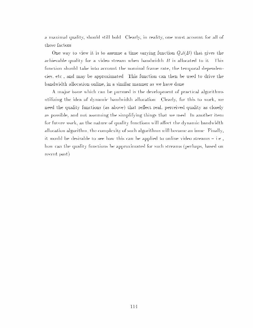
a maximal quality, should still hold. Clearly, in reality, one must account for all ofthese factors.One way to view it is to assume a time varying function Q t(B) that gives theachievable quality for a video stream when bandwidth B is allocated to it. Thisfunction should take into account the nominal frame rate, the temporal dependen-cies, etc., and may be approximated. This function can then be used to drive thebandwidth allocation online, in a similar manner as we have done.A major issue which can be pursued is the development of practical algorithmsutilizing the idea of dynamic bandwidth allocation. Clearly, for this to work, weneed the quality functions (as above) that re ect real, perceived quality as closelyas possible, and not assuming the simplifying things that we used. In another itemfor future work, as the nature of quality functions will a�ect the dynamic bandwidthallocation algorithm, the complexity of such algorithms will become an issue. Finally,it would be desirable to see how this can be applied to online video streams { i.e.,how can the quality functions be approximated for such streams (perhaps, based onrecent past).

114

Appendix ADynamic Bandwidth PartitionPlotsAs mentioned in Chapter 8, in this appendix, we include plots for four sample pointsin the constrained bandwidth region, which are split according to the dynamic band-width partition algorithm (Algorithm 2). In these plots, we notice similar split patternacross di�erent sample bandwidth points for a particular sequence.A.1 Case: 100% Average BandwidthIn this section, we present the dynamically split bandwidth graphs for 100% of AverageBandwidth in Figures 33 through 37.A.2 Case: 90% Average BandwidthIn this section, we include the dynamically split bandwidth graphs for 90% of AverageBandwidth in Figures 38 through 42.A.3 Case: 70% Average BandwidthIn this section, we present the dynamically split bandwidth graphs for 70% of AverageBandwidth in Figures 43 through 47. 115

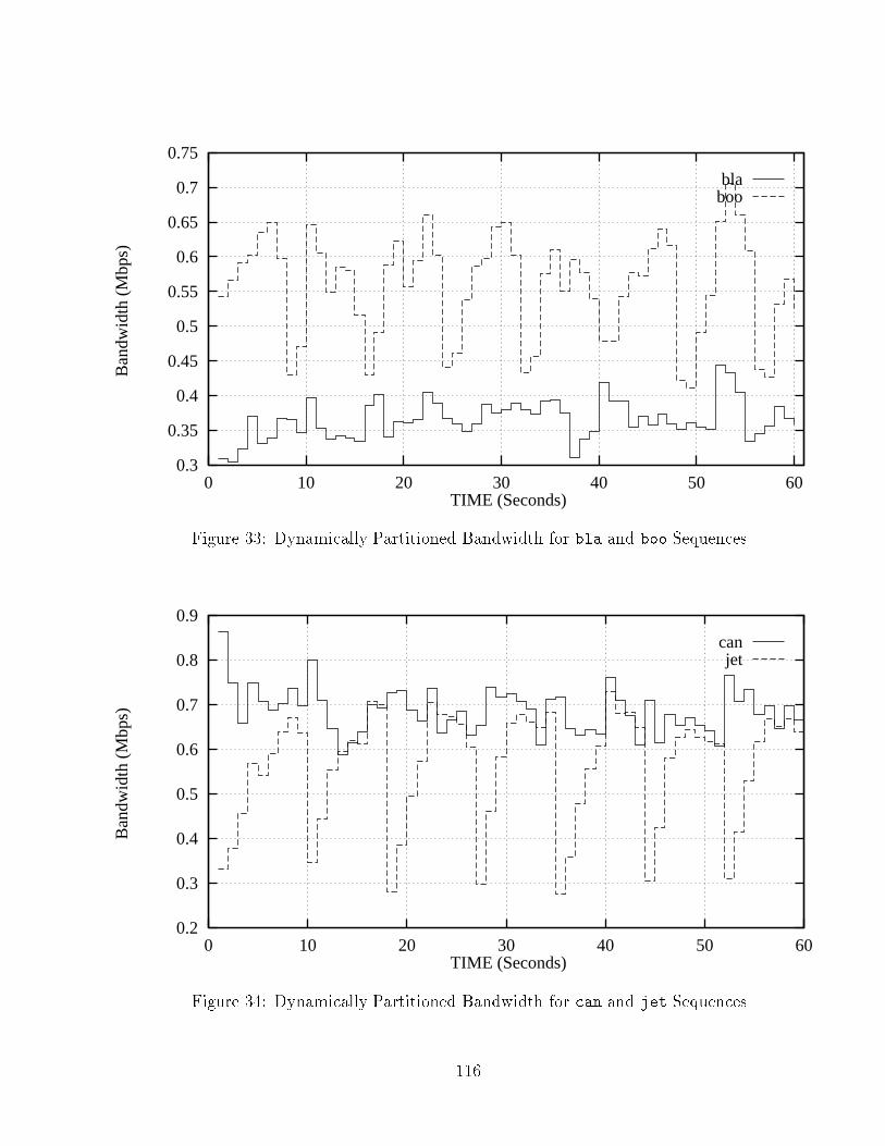
0.3

0.35

0.4

0.45

0.5

0.55

0.6

0.65

0.7

0.75

0 10 20 30 40 50 60

Ban

dwid

th (

Mbp

s)

TIME (Seconds)

blaboo

Figure 33: Dynamically Partitioned Bandwidth for bla and boo Sequences0.2

0.3

0.4

0.5

0.6

0.7

0.8

0.9

0 10 20 30 40 50 60

Ban

dwid

th (

Mbp

s)

TIME (Seconds)

canjet

Figure 34: Dynamically Partitioned Bandwidth for can and jet Sequences116

0.1

0.2

0.3

0.4

0.5

0.6

0.7

0.8

0.9

1

0 10 20 30 40 50 60

Ban

dwid

th (

Mbp

s)

TIME (Seconds)

movtha

Figure 35: Dynamically Partitioned Bandwidth for mov and tha Sequences0.5

0.6

0.7

0.8

0.9

1

1.1

1.2

1.3

1.4

0 10 20 30 40 50 60

Ban

dwid

th (

Mbp

s)

TIME (Seconds)

suksum

Figure 36: Dynamically Partitioned Bandwidth for suk and sum Sequences117

0.2

0.4

0.6

0.8

1

1.2

1.4

0 10 20 30 40 50 60

Ban

dwid

th (

Mbp

s)

TIME (Seconds)

fooboe

Figure 37: Dynamically Partitioned Bandwidth for foo and boe Sequences0.25

0.3

0.35

0.4

0.45

0.5

0.55

0.6

0.65

0 10 20 30 40 50 60

Ban

dwid

th (

Mbp

s)

TIME (Seconds)

blaboo

Figure 38: Dynamically Partitioned Bandwidth for bla and boo Sequences118

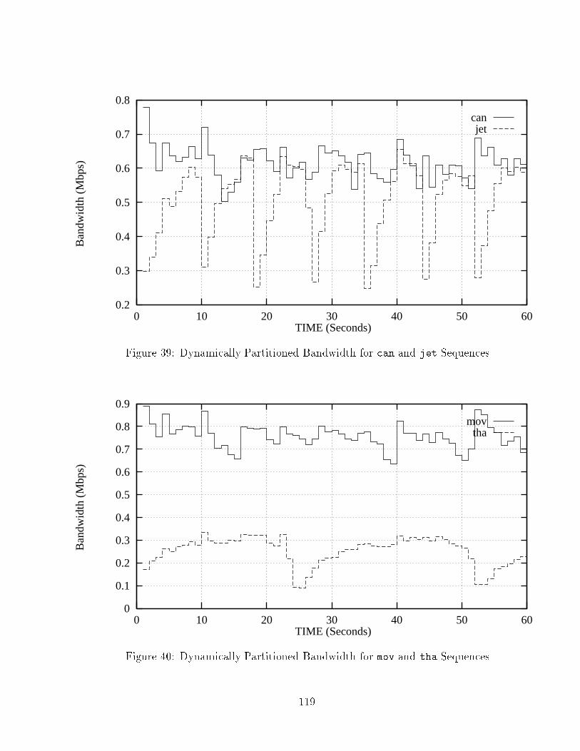
0.2

0.3

0.4

0.5

0.6

0.7

0.8

0 10 20 30 40 50 60

Ban

dwid

th (

Mbp

s)

TIME (Seconds)

canjet

Figure 39: Dynamically Partitioned Bandwidth for can and jet Sequences0

0.1

0.2

0.3

0.4

0.5

0.6

0.7

0.8

0.9

0 10 20 30 40 50 60

Ban

dwid

th (

Mbp

s)

TIME (Seconds)

movtha

Figure 40: Dynamically Partitioned Bandwidth for mov and tha Sequences119

0.4

0.5

0.6

0.7

0.8

0.9

1

1.1

1.2

1.3

0 10 20 30 40 50 60

Ban

dwid

th (

Mbp

s)

TIME (Seconds)

suksum

Figure 41: Dynamically Partitioned Bandwidth for suk and sum Sequences0.2

0.4

0.6

0.8

1

1.2

1.4

0 10 20 30 40 50 60

Ban

dwid

th (

Mbp

s)

TIME (Seconds)

fooboe

Figure 42: Dynamically Partitioned Bandwidth for foo and boe Sequences120

0.15

0.2

0.25

0.3

0.35

0.4

0.45

0.5

0.55

0 10 20 30 40 50 60

Ban

dwid

th (

Mbp

s)

TIME (Seconds)

blaboo

Figure 43: Dynamically Partitioned Bandwidth for bla and boo Sequences0.15

0.2

0.25

0.3

0.35

0.4

0.45

0.5

0.55

0.6

0.65

0 10 20 30 40 50 60

Ban

dwid

th (

Mbp

s)

TIME (Seconds)

canjet

Figure 44: Dynamically Partitioned Bandwidth for can and jet Sequences121

0

0.1

0.2

0.3

0.4

0.5

0.6

0.7

0.8

0 10 20 30 40 50 60

Ban

dwid

th (

Mbp

s)

TIME (Seconds)

movtha

Figure 45: Dynamically Partitioned Bandwidth for mov and tha Sequences0.3

0.4

0.5

0.6

0.7

0.8

0.9

1

1.1

0 10 20 30 40 50 60

Ban

dwid

th (

Mbp

s)

TIME (Seconds)

suksum

Figure 46: Dynamically Partitioned Bandwidth for suk and sum Sequences122

0.1

0.2

0.3

0.4

0.5

0.6

0.7

0.8

0.9

1

1.1

0 10 20 30 40 50 60

Ban

dwid

th (

Mbp

s)

TIME (Seconds)

fooboe

Figure 47: Dynamically Partitioned Bandwidth for foo and boe SequencesA.4 Case: 60% Average BandwidthIn this section, we include the dynamically split bandwidth graphs for 60% of AverageBandwidth in Figures 48 through 52.123

0.15

0.2

0.25

0.3

0.35

0.4

0.45

0.5

0 10 20 30 40 50 60

Ban

dwid

th (

Mbp

s)

TIME (Seconds)

blaboo

Figure 48: Dynamically Partitioned Bandwidth for bla and boo Sequences0.1

0.15

0.2

0.25

0.3

0.35

0.4

0.45

0.5

0.55

0 10 20 30 40 50 60

Ban

dwid

th (

Mbp

s)

TIME (Seconds)

canjet

Figure 49: Dynamically Partitioned Bandwidth for can and jet Sequences124

0

0.1

0.2

0.3

0.4

0.5

0.6

0 10 20 30 40 50 60

Ban

dwid

th (

Mbp

s)

TIME (Seconds)

movtha

Figure 50: Dynamically Partitioned Bandwidth for mov and tha Sequences0.2

0.3

0.4

0.5

0.6

0.7

0.8

0.9

1

0 10 20 30 40 50 60

Ban

dwid

th (

Mbp

s)

TIME (Seconds)

suksum

Figure 51: Dynamically Partitioned Bandwidth for suk and sum Sequences125

0.1

0.2

0.3

0.4

0.5

0.6

0.7

0.8

0.9

1

0 10 20 30 40 50 60

Ban

dwid

th (

Mbp

s)

TIME (Seconds)

fooboe

Figure 52: Dynamically Partitioned Bandwidth for foo and boe Sequences126

Bibliography[11193] ISO/IEC 11172. MPEG Standard, 1993. International Organization forStandardization's Document on Digital Video and Associated Audio.[AB95] Roalt Aalmoes and Peter Bosch. Overview of Still-picture and VideoCompression Standards, Dec 1995. Technical Report No. 95-3, PegasusProject, University of Cambridge.[AM95] Elan Amir and Steven McCanne. An Application Level Video Gateway.In Proceedings of ACM Multimedia, San Francisco, USA, Nov 1995.[APKR95] Egil Aarstad, Harald Pettersen, John Kroeze, and Thomas Renger. Ex-periments on Usage Parameter Control and Connection Admission Con-trol in the EXPLOIT Testbed. In Workshop on ATM Hot Topics onTra�c and Performance, Settimo Milanese, Italy, 1995.[Bat92] Regis J. Bates. Introduction to T1/T3 Networking. Artech House, Boston,1992.[BCS94] Bob Braden, David Clark, and Scott Shenker. Integrated Services in theInternet Architecture: an Overview, Jun 1994. Request For Comments:1633.[BZB+96] Bob Braden, Lixia Zhang, Steve Berson, Shai Herzog, and Sugih Jamin.Resource ReSerVation Protocol - Version 1 Functional Speci�cation, Oct1996. Internet Draft.[CCGP95] James Cummiskey, Harlan Carvey, Steve Graves, and Dave Petit. IPOver ATM Overview and Tutorial, Dec 1995. Naval Postgraduate School,Working Group's Document.127

[Chi95] Leonardo Chiariglione. The Development of an Integrated AudiovisualCoding Standard: MPEG. In Proceedings of the IEEE, pages 151{157,Feb 1995.[Dav92] David D. Clark and Scott Shenker and Lixia Zhang. Supporting Real-Time Applications in an Integrated Services Packet Network: Architec-ture and Mechanisms. In Proceedings of SIGCOMM, pages 14{26, ACM,USA, 1992.[For95] ATM Forum. ATM User-Network Interface Speci�cation - Ver-sion 3.1, Jun 1995. Online Document. Available at: http://cell-relay.indiana.edu/cell-relay/docs/atmforum/ps.html.[Fur94] Borko Furht. Multimedia Systems: An Overview. IEEE Multimedia,pages 47{59, Spring 1994.[Gal91] Dider Le Gall. MPEG: A Video Compression Standard for MultimediaApplications. Communications of the ACM, 34, No. 4:47{58, April 1991.[GB97] Mark W. Garret and Marty Borden. Interoperation of Controlled-LoadService and Guaranteed Service with ATM, Jul 1997. Internet Draft.[HSS90] Dietmar B. Hehmann, Michael G. Salmony, and Heinrich J. Stuttgen.Transport Services for Multimedia Applications on Broadband Networks.Computer Communications, 13, No. 4:197{203, May 1990.[Kar95] Gunnar Karlson. Asynchronous Transfer of Video. SICS Research ReportR95:14, Swedish Institute of Computer Science, 1995.[Kes97] Srinivasan Keshav. An Engineering Approach to Computer Networking.ATM Networks, the Internet and the Telephone Network. Addision Wes-ley, USA, 1997.[KM96] Hemant Kanakia and Partho P. Mishra. Packet Video Transport in ATMNetworks with Single-bit Feedback. Multimedia Systems, 1996:4:370{380,1996. 128

[KMS95] Dexter Kozen, Yaron Minsky, and Brian Smith. E�cient Algorithms forOptimal Video Transmission. Technical Report, Cornell University, May1995.[KPC97] Rob Koenen, Fernando Pereirs, and Leonardo Chiariglione. MPEG-4Context and Objectives. In Image Communication Journal, Special Issueon MPEG-4, Torino , Italy, 1997.[LCY94] Simon S. Lam, Simon Chow, and David K. Y. Yau. An Algorithm forLossless Smoothing of MPEG Video. In Proceedings of ACM SIGCOMM,London, U.K., 1994.[LKPC97] James V. Luciani, Dave Katz, David Piscitello, and Bruce Cole. NBMANext Hop Resolution Protocol (NHRP), Sep 1997. Internet Draft.[MF95] Steven McCanne and Sally Floyd. Man Page for the ns SimulatorVersion 1, Jul 1995. Online Document. Available at: http://www-nrg.ee.lbl.gov/ns/man.html.[Ous94] John K. Ousterhout. Tcl and the Tk Toolkit. Addison-Wesley, USA, 1994.[PG93] Abhay K. Parekh and Robert G. Gallager. A Generalized Processor Shar-ing Approach to Flow Control in Integerated Services Network: The Sin-gle Node Case. IEEE/ACM Transactions on Networking, Jun 1993.[Poy97] Charles Poynton. Poynton's Color FAQ, Feb 1997. Online Document.Available at: http://www.inforamp.net/ poynton/Poynotn-color.html.[RRV93] Srinivas Ramanathan, P. Venkat Rangan, and Harrick M. Vin. Frame-Induced Packet Discarding: An E�cient Strategy for Video Networking.In 4th International Workshop on Network and Operating Systems Sup-port for Digital Audio and Video, Lancaster, U.K., Nov 1993.[Sat96] Shirish S. Sathaye. ATM Forum, Tra�c Management Speci�cation v4.0,April 1996. Ballot Version of the Speci�cation by Fore Systems Inc.[SCFJ96] Henning Schulzarine, Stephen Casner, Ron Frederick, and Van Jacob-son. RTP: A Transport Protocol for Real-Time Applications, Jan 1996.Request For Comments: 1889.129

[Sch95] Henning Schulzrine. Internet Services: From Electronic Mail to Real-Time Multimedia. In Kommunikation in Verteilten Systemen, pages 21{34. Springler-Verlag, Germany, Feb 1995.[She95] Scott Shenker. Fundamental Design Issues for the Future Internet, Sept1995. Internet Draft.[SJ95] Kai-Yeung Siu and Raj Jain. A Brief Overview of ATM: Protocol Layers,LAN Emulation, and Tra�c Management. Computer CommunicationReview, ACM SIGCOMM, pages 6{20, April 1995.[SL97] Anastasios Stamoulis and Jorg Liebeherr. S2GPS: Slow-Start GeneralizedProcessor Sharing. Technical Report No. CS-97-03, University of Virginia,Feb 1997.[SN95] Ralf Steinmetz and Klara Nahrstedt. Multimedia: Computing, Commu-nications and Applications. Prentice Hall, USA, 1995.[SPG97] Scott Shenker, Craig Patridge, and Roch Guerin. Speci�cation of Guar-anteed Quality of Service, Feb 1997. Internet Draft.[Ste93] Ralf Steinmetz. Compression Techniques in Multimedia Systems: A Sur-vey, 1993. Technical Report:43.9307, IBM Networking Center, Germany.[Ste95] James P. Sterbenz. Protocols for High Speed Networks: Life after ATM?In Protocols for High Speed Networks IV, pages 3{18. Chapman and Hall,London, 1995.[Stu95] Heinrich J. Stuttgen. Network Evolution and Multimedia Communica-tion. IEEE Multimedia, pages 42{59, Fall 1995.[Vet95] Ronald J. Vetter. ATM Concepts, Architecture and Protocols. Commu-nications of the ACM, 38, No. 2:30{44, Feb 1995.[WCS96] Larry Wall, Tom Christiansen, and Randal L. Schwartz. ProgrammingPerl. O'Reilly & Associates, Inc., USA, 1996.[Wor97] John Worclawski. Speci�cation of the Controlled-Load Network ElementService, May 1997. Internet Draft.130

[Yas96] Yasser Rasheed and Alberto Leon-Garcia. AAL 1 with FEC for the Trans-port of CBR MPEG2 Video over ATM Networks. In IEEE Infocom,volume 2, pages 529{536, 1996.[YMGH96] Nicholas Yeadon, Andreas Mauthe, Francisco Garcia, and David Hutchi-son. QoS Filters: Addressing the Heterogeneity Gap. In Proceedings ofInteractive Multimedia Systems and Services, Berlin, 1996.[ZDE+93] Lixia Zhang, Steve Deering, Deborah Estrin, Scott Shenker, and DanielZappala. RSVP: A New Resource ReSerVation Protocol. IEEE Network,Sep 1993.

131