Linköping Studies in Science and Technology. Dissertations, No. 1348

Norrköping 2010

Available-Bandwidth Estimation in Packet-Switched Communication Networks

Erik Bergfeldt

Available-Bandwidth Estimation in Packet-Switched Communication Networks

Erik Bergfeldt Linköping Studies in Science and Technology. Dissertations, No. 1348 Copyright © 2010 Erik Bergfeldt ISBN 978-91-7393-292-9 ISSN 0345-7524 Printed by LiU-Tryck, Linköping, Sweden, 2010

Abstract This thesis presents novel methods that are able to perform real-time estima-tion of the available bandwidth of a network path. In networks such as the Internet, knowledge of bandwidth characteristics is of great significance in, e.g., network monitoring, admission control, and audio/video streaming. The term bandwidth describes the amount of information a network can deliver per unit of time. For network end users, it is only feasible to obtain bandwidth properties of a path by actively probing the network with probe packets, and to perform estimation based on received measurements. In this thesis, two active-probing based methods for real-time available-bandwidth estimation are presented and evaluated. The first method, BART (Bandwidth Available in Real-Time), uses Kalman filtering for the analysis of received probe packets. BART is examined ana-lytically and through experiments which are carried out in wired and wire-less laboratory networks as well as over the Internet and commercial mobile broadband networks. The opportunity of tuning the Kalman filter and en-hancing the performance by introducing change detection are investigated in more detail. Generally, the results show accurate estimation with only modest computational efforts and minor injections of probe packets. However, it is possible to identify weaknesses of BART, and a summary of these as well as general problems and challenges in the field of available-bandwidth estimation are laid out in the thesis. The second method, E-MAP (Expectation-Maximization Active Probing), is designed to overcome some of these issues. E-MAP modifies the active-probing scheme of BART and utilizes the expectation-maximization algorithm before filtering is used to generate a bandwidth estimate. Overall, this thesis shows that in many cases it is achievable to obtain effi-cient and reliable real-time estimation of available bandwidth by using light-weight analysis techniques and negligible probe-traffic overhead. Hence, this opens up exciting new possibilities for a range of applications and services in communication networks.

Populärvetenskaplig sammanfattning Avhandlingen fokuserar på att skatta tillgänglig bandbredd i nätverk. Band-bredd beskriver den mängd information som är möjlig att överföra per tids-enhet mellan två enheter anslutna till ett nätverk, exempelvis Internet. Kännedom om rådande bandbreddssituation är önskvärd i många sam-manhang. En nätverksoperatör är ofta intresserad av att övervaka vad som sker i ett nätverk och om det finns tillräckligt med bandbredd. En användare upplever att kommunikationen fungerar mer tillfredsställande om datorn förmår utvinna kunskap om nätverkets tillgängliga bandbredd. För om in-formation sänds ut i en takt som nätverket inte mäktar med, då är risken överhängande att den går förlorad och inte når avsedd mottagare. I avhandlingen presenteras två originella skattningsmetoder som är kapab-la att skatta tillgänglig bandbredd för en uppkoppling i realtid. Detta är möj-ligt genom att först dela in informationen i flera paket som skickas enligt ett utvalt mönster, och därefter studera huruvida mönsterförändringar är obser-verbara när utseendet hos utsänd och mottagen paketsekvens jämförs. Den första metoden BART (Bandwidth Available in Real-Time) översätter mönsterförändringar till en skattning av tillgänglig bandbredd med hjälp av Kalman-filtrering. I avhandlingen framgår det hur filtret kan justeras och hur det är möjligt att inkludera förändringsdetektering för att förbättra BART:s prestanda. BART har dock brister, vilket motiverar utvecklingen av den andra metoden E-MAP (Expectation-Maximization Active Probing). E-MAP har potentialen att övervinna några av BART:s svagheter genom att utsända paket följer ett annorlunda mönster samt att filtreringen föregås av en lämp-lig algoritm som tidigare ej nyttjats för skattning av tillgänglig bandbredd. Avhandlingen visar att korta paketsekvenser och blygsamma beräknings-resurser är tillräckligt för att skattningarna av den tillgängliga bandbredden skall överensstämma med verkligheten. Denna insikt skapar goda förutsätt-ningar för att utveckla helt nya tjänster i framtidens nätverk.

Acknowledgements First and foremost, I wish to express my deepest appreciation to my supervi-sors. I am grateful to Prof. Johan M Karlsson at Linköping University for his encouragement and guidance, and for giving me the time, faith, and creative freedom to explore my own research interests. I am thankful to Dr. Svante Ekelin at Ericsson Research for introducing me to the field of bandwidth measurements, and for always being on hand to offer advice and support. I gratefully acknowledge and I am very thankful to Ericsson in Katrine-holm and Ericsson Research in Stockholm for the encouraging support and for allowing me to take part in stimulating and attractive research projects. I am greatly indebted to all my colleagues at Linköping University and Ericsson Research, as well as other co-workers who I have collaborated with in various projects, for inspiring discussions and for contributing to an enjoy-able working environment. I am thankful to the division of Mobile Networking and Computing at Luleå University of Technology for welcoming me to Skellefteå, and for pro-viding me with the opportunity to carry out useful experiments during my visit. Sist men inte minst vill jag utrycka en oändlig tacksamhet till mina nära och kära, för all den stöttning och omtanke som ni visat och den glädje som ni spridit under alla år. Er betydelse för mina prestationer och mitt välbefinnan-de är av en dignitet som jag ej förmår formulera i ord. ♥ 1 Erik Bergfeldt Norrköping, October 2010 This work has been funded by Ericsson in Katrineholm and partly supported by the graduate school in Personal Computing and Communication (PCC++).

Table of Contents INTRODUCTION......................................................................................................1

1 BACKGROUND........................................................................................................ 1 2 DATA TRANSMISSION IN PACKET-SWITCHED NETWORKS................................... 3 3 AVAILABLE-BANDWIDTH MEASUREMENTS.......................................................... 7 4 KALMAN FILTERING............................................................................................ 11 5 OVERVIEW OF THESIS STRUCTURE....................................................................... 12 6 CONTRIBUTIONS................................................................................................... 19 7 LIST OF PUBLICATIONS......................................................................................... 21 REFERENCES............................................................................................................. 23

PART I ACTIVE PROBING AND KALMAN-FILTER BASED AVAILABLE-BANDWIDTH ESTIMATION..................................................... 27

ABSTRACT................................................................................................................ 27 1 INTRODUCTION.................................................................................................... 28

1.1 Overview..................................................................................................... 28 1.2 Related Work.............................................................................................. 29

2 MEASURING AVAILABLE BANDWIDTH............................................................... 31 2.1 Definition of Available Bandwidth......................................................... 31 2.2 The Network Model...................................................................................32

3 FILTER-BASED BANDWIDTH ESTIMATION........................................................... 36 3.1 Filter-Based Estimation............................................................................. 36 3.2 The BART Method..................................................................................... 38 3.3 Stability versus Agility.............................................................................. 41 3.4 Change Detection....................................................................................... 46

4 DISCUSSION AND CONCLUSIONS......................................................................... 49 REFERENCES............................................................................................................. 50

PART II FILTER TUNING FOR ENHANCED AVAILABLE-BANDWIDTH TRACKING......................................................... 53

ABSTRACT................................................................................................................ 53

1 INTRODUCTION.................................................................................................... 54 1.1 Overview..................................................................................................... 54 1.2 Related Work.............................................................................................. 55

2 FILTER-BASED BANDWIDTH ESTIMATION........................................................... 55 2.1 Filter-Based Estimation............................................................................. 55 2.2 The BART Filter Method for Available-Bandwidth Estimation..........58 2.2.1 The Process-Noise Covariance....................................................... 59 2.2.2 The Measurement-Noise Covariance............................................ 60 2.2.3 Tuning BART.................................................................................... 62

3 EXPERIMENTS....................................................................................................... 63 4 RESULTS................................................................................................................ 66 5 DISCUSSION AND CONCLUSIONS......................................................................... 75 REFERENCES............................................................................................................. 77

PART III CHANGE DETECTION FOR FILTER-BASED AVAILABLE-BANDWIDTH ESTIMATION..................................................... 81

ABSTRACT................................................................................................................ 81 1 INTRODUCTION.................................................................................................... 82

1.1 Overview..................................................................................................... 82 1.2 Related Work.............................................................................................. 83

2 BACKGROUND...................................................................................................... 84 2.1 Filter Methods.............................................................................................84 2.2 The BART Method..................................................................................... 86

3 PROBLEM - STABILITY VERSUS AGILITY............................................................... 87 4 METHOD............................................................................................................... 89

4.1 Change Detection....................................................................................... 89 4.2 The CUSUM Test........................................................................................90 4.3 The GLR Test.............................................................................................. 91

5 EXPERIMENTS....................................................................................................... 94 5.1 Experiment Setup....................................................................................... 95 5.2 BART with the CUSUM Test.................................................................... 97 5.2.1 Test Statistics and Design Parameters...........................................97 5.2.2 Available-Bandwidth Estimation.................................................. 99 5.3 BART with the GLR Test......................................................................... 103 5.3.1 Test Statistics and Design Parameters.........................................103 5.3.2 Available-Bandwidth Estimation................................................ 109

6 DISCUSSION AND CONCLUSIONS....................................................................... 113 REFERENCES........................................................................................................... 114

PART IV REAL-TIME AVAILABLE-BANDWIDTH MEASUREMENTS OVER MOBILE CONNECTIONS................................. 117

ABSTRACT.............................................................................................................. 117 1 INTRODUCTION.................................................................................................. 118

1.1 Overview................................................................................................... 118 1.2 Related Work............................................................................................ 119

2 AVAILABLE BANDWIDTH................................................................................... 120 2.1 Definition of Available Bandwidth....................................................... 120 2.2 Characteristics of Bottleneck Links........................................................120

3 HSDPA EXPERIMENTS...................................................................................... 122 3.1 Experiment Setup..................................................................................... 122 3.2 Available-Bandwidth Measurements................................................... 126 3.3 Discussion................................................................................................. 131

4 CDMA2000 1XEV-DO EXPERIMENTS.............................................................. 133 4.1 Experiment Setup..................................................................................... 133 4.2 Inter-Packet Time Separation................................................................. 134 4.3 Discussion................................................................................................. 136

5 IEEE 802.11 EXPERIMENTS................................................................................ 138 5.1 Experiment Setup..................................................................................... 138 5.2 Available-Bandwidth Measurements................................................... 139 5.3 Discussion................................................................................................. 141

6 CONCLUSIONS.................................................................................................... 141 REFERENCES........................................................................................................... 142

PART V AVAILABLE-BANDWIDTH ESTIMATION: CHALLENGES AND RESEARCH DIRECTIONS.......................................... 145

ABSTRACT.............................................................................................................. 145 1 INTRODUCTION.................................................................................................. 146

1.1 Overview................................................................................................... 146 1.2 Related Work............................................................................................ 147

2 AVAILABLE-BANDWIDTH MEASUREMENTS...................................................... 148 2.1 Available Bandwidth............................................................................... 148 2.2 Difficulties in Measuring Available Bandwidth.................................. 149 2.2.1 Definition and Variability of Bandwidth.................................... 149 2.2.2 Probe-Traffic Intensities................................................................ 154 2.2.3 Time Stamping and Queuing Principles.................................... 160

3 THE E-MAP METHOD....................................................................................... 161 3.1 The Measurement Model........................................................................ 162

3.2 The Expectation-Maximization Algorithm.......................................... 163 3.3 E-MAP with Kalman Filtering............................................................... 165

4 SIMULATIONS..................................................................................................... 166 4.1 Simulation Setup...................................................................................... 166 4.2 Results........................................................................................................ 167

5 DISCUSSION AND CONCLUSIONS....................................................................... 171 REFERENCES........................................................................................................... 172

1

Introduction This thesis deals with measurements of network-performance characteristics in packet-switched communication networks. More specifically, the challenge of estimating available bandwidth along a network path is addressed. Avail-able-bandwidth information is of great interest to both operators and users of communication networks in order to, e.g., monitor the network utilization and optimize the performance of applications (such as file transferring and multimedia streaming). Two methods for accomplishing bandwidth estima-tion in real-time are presented and evaluated, as well as several discussions and studies covering configuration possibilities, feasible enhancements, gen-eral definitions and measurement issues. In this introduction, the structure and some common properties of packet-switched networks are briefly described. As many people of today employ the world-wide Internet, the explanation is frequently associated to this glob-al packet-switched network with the aim of facilitating the understanding of general concepts such as networks and data transmission. Furthermore, the interpretation of available bandwidth is explained in some detail as well as the idea of using filter-based estimation. All together, this will hopefully pro-vide the reader with an initial comprehension regarding data communica-tions, a motivation of why network measurements are important, and the most fundamental components of the novel available-bandwidth measure-ment methods BART (Bandwidth Available in Real-Time) and E-MAP (Ex-pectation-Maximization Active Probing), which are discussed and examined in the thesis. 1 Background Today, the most well-known communication network is the Internet [1], which is a very large network of networks where millions of interconnected computer networks make it feasible to cover a great geographical area and

Introduction

2

enable people from all over the world to access and use popular services like the World Wide Web (WWW), e-mail, and file sharing. Although the Internet is much more than applications and services, the majority of the users are not aware of the complex infrastructure and the underlying fundamental tech-nologies that make the basis of the network. Due to the large number of interconnections of smaller networks (e.g., this could be private, public, academic, government, and business networks), it is achievable to transfer information between an enormous amount of com-puters on the Internet. A fundamental principle of the Internet architecture is that all networks should be autonomous, which means that each network is under separate administrative control and decisions are decentralized. The reason for this is to make the Internet more robust, such that if a particular network does not work properly, the overall performance of the Internet should not be affected. All these smaller networks building up the Internet are often owned and independently maintained by commercial operators. Due to business reasons, these operators seldom cooperate, except that they have mutual agreements that make it feasible for information to flow through an operator’s network, although the source and the destination are connected to other networks. It is reasonable to assume that the network operators have enough knowl-edge of their own networks to ensure decent performance and bandwidth capacity. However, ordinary Internet users typically do not have any or very limited information regarding the conditions of the utilized networks; to the majority, the Internet is only a black box that conveys data back and forth be-tween connected computers. The employment of the Internet would probably be more efficient if users and their applications could receive information about the state and the behavior of the used networks. This is also in line with the end-to-end principle that was suggested for the Internet architecture [2], which means that endpoints in the network should have knowledge of how and when traffic is flowing, whereas nodes inside the network should have limited functionality and only forwarding data from one link to another. This would imply that the intelligence of the Internet is found at the endpoints, as opposed to traditional telecommunication networks [3]. Today, the endpoints of the Internet are normally not supplied with net-work-state information and, consequently, they need to obtain this by them-selves in case it is desired. One approach is to perform measurements, al-though this is difficult without actively probing the networks with data pack-ets (also known as probe packets). Active probing is accomplished by trans-mitting flows of packets from one endpoint to another and thereafter, by

Introduction

3

comparing the characteristics of the transmitted and received traffic flows, draw conclusions regarding end-to-end properties of the used network path [4]. It should be noted that active end-to-end measurements do not automati-cally yield information regarding the characteristics of each particular link along the used path; in fact, there is no guarantee that probe packets utilize the same path between two endpoints, which makes it hard to ensure that consecutive measurements affect the same links. Nevertheless, it is often pos-sible to extract information which at least corresponds to one link between the sender and receiver, although it may be complicated to identify the loca-tion of this particular link. Moreover, even if active probing can describe the state of a network and discover changes, it is in most cases difficult to explain the reason for being in a specific state or describing why changes occur. In this thesis, active probing is used to measure end-to-end available-bandwidth characteristics in real-time, which generally can be defined as the amount of unutilized capacity of a network path. This is an important net-work property, which is dependent on both link capacities and other traffic flows affecting the network links between the probe sender and probe re-ceiver. The measurement procedure is non-trivial, but it is shown how real-time estimation is achievable by, e.g., applying filter-based analysis of re-ceived probe traffic. 2 Data Transmission in Packet-Switched Networks This section describes the fundamental network components that are of spe-cific interest for available-bandwidth measurements. Although the following discussion is frequently related to the Internet, the reasoning generally holds for other packet-switched communication networks as well. The networks building up the Internet consist of different types of nodes; among these, hosts and routers are explained in some detail. The hosts are typically ordinary computers that can be found in offices or in people’s home environment, these are sometimes also used as servers for WWW and e-mail services etc. In fact, any portable computing device that has the ability of connecting to the Internet and transmitting data can be considered as a host, e.g. mobile phones. Different hosts connect to each other via communication links. It may only be one single link, but mostly the path between two hosts consists of several links and it is also possible to have multiple paths, which requires devices that can choose between different links; these devices are

Introduction

4

known as routers. Routers are generally based on specific hardware and software which are customized to the task of forwarding traffic between links as efficiently as possible. Figure 1 illustrates the interconnection of different networks. The hosts and routers are connected by wired or wireless links.

Figure 1. An overview of interconnected networks. Networks commonly consist of several network nodes, such as hosts and routers. Network nodes connect to each other via wired or wireless links. A communication link is the physical media used for transferring informa-tion between two nodes. For example, this could be cables, optical fibers or the air in case of wireless communications. With respect to the properties of network interfaces that attach nodes to communication links, each link con-nection corresponds to a maximum capacity that limits the intensity at which it is possible to transfer information. In digital communications, the capacity is often defined as the number of bits that can be transmitted during the time interval of one second. A bit is the smallest amount of digital data, a binary digit represented by either 0 or 1. Due to this, the maximum capacity of network links is often re-ferred to as the maximum bandwidth capacity described in the unit bits per second (bit/s). By dividing a given amount of data with this capacity value, one receives the time it takes to push the bits through the interface of the

Introduction

5

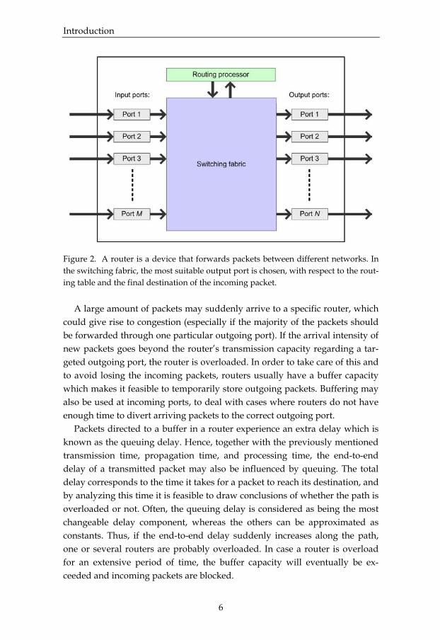
network node; this also corresponds to what is known as the transmission time. The bandwidth capacity of the individual links of the Internet differs a lot. In the backbone of the Internet (also known as the core network), link capaci-ties of several Gbit/s or higher are common, whereas lower capacities are expected toward the endpoints of the network. In the access networks, where end hosts connect to the Internet, it is normal to have capacities in the range of Mbit/s. It may also be that the endpoint capacity is different with respect to uplink and downlink connections to the access network, e.g. this is the case for the ADSL (Asymmetric Digital Subscriber Line) technique [5]. Uplink connections transfer information from the end hosts whereas downlink con-nections are used for transferring information to the end host. Two other properties that characterize a communication link are the prop-agation time and the probability of bit error. The propagation time is propor-tional to the distance of the link. The probability of error is highly dependent on the communication channel, e.g. in a wireless environment the error rate is expected to be quite large while corrupted bits are fairly uncommon in wired networks. In packet-switched networks, such as the Internet, the information is transmitted in packets. Packets can be of different size and transmitted ac-cording to various patterns. When applying active probing, the idea is to transmit sequences of probe packets and study how these packets are affected by the utilized network path. The links along the path will influence the pat-tern of the packet sequences with respect to link capacity and reliability, but it is also expected that other traffic flows may interfere with the probe packets. One prominent effect on the probe packets can be understood by considering the functionality of a router in more detail [6]. A router typically connects to several links; this is accomplished through the incoming and outgoing ports of the router, see Figure 2. These ports are connected to a switching fabric, which is a combination of hardware and software that moves data from an input port to an output port. The main task of the router is to forward traffic, and it is necessary that this is performed efficiently to avoid congestion. In order for routers to forward packets onto appropriate links, they make use of routing tables where it is specified which link to use for a specific packet in order to reach the destination. It is important that these tables are continuously updated with valid information to avoid incorrect decisions. The time needed for routers to search through the tables and to find the re-quired information is often referred to as the processing time.

Introduction

6

Figure 2. A router is a device that forwards packets between different networks. In the switching fabric, the most suitable output port is chosen, with respect to the rout-ing table and the final destination of the incoming packet. A large amount of packets may suddenly arrive to a specific router, which could give rise to congestion (especially if the majority of the packets should be forwarded through one particular outgoing port). If the arrival intensity of new packets goes beyond the router’s transmission capacity regarding a tar-geted outgoing port, the router is overloaded. In order to take care of this and to avoid losing the incoming packets, routers usually have a buffer capacity which makes it feasible to temporarily store outgoing packets. Buffering may also be used at incoming ports, to deal with cases where routers do not have enough time to divert arriving packets to the correct outgoing port. Packets directed to a buffer in a router experience an extra delay which is known as the queuing delay. Hence, together with the previously mentioned transmission time, propagation time, and processing time, the end-to-end delay of a transmitted packet may also be influenced by queuing. The total delay corresponds to the time it takes for a packet to reach its destination, and by analyzing this time it is feasible to draw conclusions of whether the path is overloaded or not. Often, the queuing delay is considered as being the most changeable delay component, whereas the others can be approximated as constants. Thus, if the end-to-end delay suddenly increases along the path, one or several routers are probably overloaded. In case a router is overload for an extensive period of time, the buffer capacity will eventually be ex-ceeded and incoming packets are blocked.

Introduction

7

There are often several opportunities for a router to choose how packets in a buffer should be removed. The most common option in the Internet is to dequeue packets in the same order as they arrive, i.e. according to the first-come first-served principle. However, it is generally achievable to configure a router such that a more sophisticated dequeuing algorithm is used; it may for example be possible to prioritize capacity for certain traffic types, which could be of advantage for real-time applications where extensive delays are devastating. As a conclusion, traffic flows in communication networks typically interact with each other in routers. The outcome of this interaction, which can be measured by the end hosts of the networks, is dependent on aspects like the traffic intensity, link capacity, and router performance. By transmitting probe traffic and analyzing how the probes are affected along a network path, it is feasible for active-measurement methods to extract end-to-end characteristics and, e.g., generate estimates of the available bandwidth. 3 Available-Bandwidth Measurements The available bandwidth is the end-to-end property that is of particular inter-est in this thesis. A fairly intuitive interpretation of this characteristic may be obtained by considering the previously described bandwidth capacity of a communication link. The traffic intensity on a link is limited to the maximum bandwidth capacity, even though a network node which connects to the link has the potential of generating data with a higher intensity. When data is transmitted according to the maximum intensity, the packets on the link will be transferred back-to-back, which means that there is no time gap between the packets. On the other hand, if the transmission intensity is lower than the link capacity, a certain amount of the bandwidth is unutilized, and it is feasi-ble to observe an empty space between the packets. This unutilized band-width can be defined as the available bandwidth. Often, a communication link is shared by traffic flows originated from dif-ferent users and applications. All these flows contribute to the total cross traf-fic along the link, which is equal to or less than the maximum bandwidth ca-pacity. For a network path, which typically consists of several links, each in-dividual link corresponds to a certain capacity and has a specific cross-traffic mixture; both properties may be different and individual for each link. This implies that the unutilized capacity of each link of a path may be different and, from an end-to-end perspective, the available bandwidth corresponds to

Introduction

8

the minimum unutilized capacity among all links of the path [4]; the link with the smallest amount of available bandwidth is referred to as the bottleneck link (or the tight link). However, one should observe that the bottleneck link does not necessarily correspond to the link with the lowest maximum band-width capacity (also known as the narrow link). In Figure 3, the relation between available bandwidth, cross-traffic load, and link-bandwidth capacity is illustrated. It is obvious that available band-width may vary with time, which often relates to the bursty properties of network traffic. The reason is that most applications do not deliver packets with a constant time separation; instead, the transmission of data typically corresponds to short and high-intensity bursts that appear rather irregularly with periods of no transmission in between.

Figure 3. The available bandwidth of a network link is dependent on the maximum bandwidth capacity of the link and the aggregated cross traffic. The level of burstiness of data is greatly dependent on the definition of traffic intensity and bandwidth. Normally, a chosen time resolution (or aver-aging time scale) is used for describing the utilization of a link [4]. The reason is that, in reality, a link can only be either fully utilized or idle, although in many cases it is inconvenient to explain data traffic in terms of these two conditions. Instead, the traffic load along a link is commonly related to some time resolution that corresponds to a sliding window, which is used for aver-aging the amount of cross traffic utilizing the link during a given time inter-val. With respect to this, traffic that is considered as bursty according to a high time resolution has most likely smoother characteristics if a lower time resolution is considered.

Introduction

9

The fluctuation of cross traffic, which also affects the characteristics of the available bandwidth, is not only dependent on the used time resolution; the cross-traffic aggregation level is also of great impact. The implications of these two properties are further studied in the thesis. In Figure 3 the maximum bandwidth capacity is constant although this is not necessarily the case in reality. Especially, the link capacity is likely to vary in wireless networks due to the fluctuating nature of radio channels and, of course, this also affects the properties of the available bandwidth. Actively probing the end-to-end available bandwidth can be useful in sev-eral contexts. For example, in real-time applications such as streaming of au-dio and video, it is of great importance that packets arrive to the destination in time. These streaming applications often have the option to regulate the amount of traffic to transmit by choosing the codec (coder/decoder) scheme appropriately. One type of codec may render high-quality audio and video, but the drawback is the large amount of data that needs to be transmitted. Another codec choice delivers less data, but the quality of the streaming con-tent is likely to be worse. If streaming applications could be continuously provided with available-bandwidth information, they should be able to au-tomatically adapt the traffic intensity and the used codec with respect to the present bandwidth utilization. Hence, high-quality audio and video would be chosen if there is a large amount of unused capacity, whereas lower quality is appropriate to eliminate streaming interruption in case of the bottleneck link being almost congested. Bandwidth measurements could also be employed to verify that Internet service providers supply the bandwidth capacity that customers pay for. When a customer arrives at an agreement with an operator regarding Internet access, the terms and conditions are often specified in a service level agree-ment, which may include a guaranteed bandwidth capacity. As a user, it is hard to verify this capacity, but one possibility is to apply tools for available-bandwidth measurements. A third application could be to measure available bandwidth before down-loading large data files from the Internet. It is fairly common that particular files are available for download at different servers located at various places around the world. Users usually have the opportunity to choose which server to use, and measurements of the available bandwidth may guide them to servers and network paths that are able to provide rapid data transfer. Of course, the above examples can be supplemented by numerous other cases where available-bandwidth measurements would be of great advan-tage.

Introduction

10

Although it would be useful to receive available-bandwidth indications, it is a great challenge to perform active probing appropriately, which is neces-sary in order to obtain the relevant end-to-end characteristics. For example, intrusive probing may decrease the performance and stability of measured networks, and consequently it is important to minimize the amount of in-jected probe traffic. In case of extensive high-intensity probing, severe conges-tion may occur in the networks which results in significant delays and in the worst case also packet losses. Another issue, in e.g. the Internet, is the large amount of traffic which employs the Transmission Control Protocol (TCP) [1]. These flows are adaptive in terms of transmission intensity, and network overload due to probing will yield a decrease in TCP traffic intensity, since TCP flows back off in case they experience congestion. Hence, aggressive ac-tive probing is unacceptable as it decreases the performance of other applica-tions, and thus also the satisfaction of network users. It is very important to take this into consideration when designing and utilizing active-probing tools. From another point of view, it is also important to take into account the requirements of applications and users that are expected to apply the meas-urement tools. In some cases, it is urgent to obtain estimates of available bandwidth in real-time, whereas a delayed estimate is acceptable in other sit-uations. Other issues could be the reliability of the estimates, how often to perform measurements, the most suitable definition of bandwidth with re-spect to time resolution etc. To summarize, it would certainly be of advantage for network end hosts to have the ability of performing measurements of the end-to-end available bandwidth. However, it is a non-trivial task to obtain this information, and if active probing is used several aspects need to be considered. It is difficult to perform measurements that are network friendly but still live up to the de-mands of different applications; this also emphasis the challenge of designing appropriate tools, since the optimal configuration generally varies with re-spect to the utilization of the measurements. Often, it is necessary to com-promise between, e.g., the quality and the time it takes to receive an estimate. Throughout the years, several available-bandwidth measurement tools with various qualities and characteristics have been developed, see e.g. [7-12]. Comparisons between different tools have been made in simulation and mea-surement studies such as [12-14]. However, these methods are typically not able to generate accurate available-bandwidth estimates in real-time, and this motivates the work of this thesis.

Introduction

11

For a general introduction to the field of end-to-end bandwidth measure-ments, including definitions of relevant metrics and descriptions of some measurement techniques and tools, see the review article [4]. 4 Kalman Filtering The available-bandwidth measurement methods BART and E-MAP (which are presented in this thesis) use active probing together with filtering for es-timating available bandwidth. A filter is a recursive data-processing algo-rithm, which is suitable for state estimation of noisy dynamic systems [15]. Normally, the state corresponds to one or several variables describing some important system properties. In filter applications, these variables are in gen-eral not directly measurable, which makes the estimation rather troublesome. However, as long as the filter has access to some measurements of the system, and given that it is possible to describe how these measurements depend on the system state, the variables can be estimated. In BART and E-MAP, the aim is to estimate the available bandwidth in a network and, consequently, with respect to the above mentioned filtering terminology, the network corre-sponds to the measured system whereas the available bandwidth relates to the system state. The measurements which are used in the filtering are ob-tained by active probing. In addition to the model that describes the correlation between the system state and the measurements, a filter is also making use of a model that ex-plains the expected evolution of the system state. Regarding both these mod-els, one has to account for uncertainty when performing the filtering; poor precision of the measurements and unexpected variations of the true system state are issues that increase the uncertainty and make the estimation more challenging. The uncertainty is often referred to as noise, and filters typically make use of descriptions of the noise characteristics when performing the filter calculations. If it is achievable to find a linear dependence of the evolution of the system state as well as between the measurements and the system state, and if the noises affecting the models are white and Gaussian distributed, the Kalman filter is the optimal estimator (with respect to virtually any statistical criterion that makes sense) [16]. This filter is also known to perform very well for sys-tems where the specific properties of linearity and noises are slightly broken. Kalman filtering has been used in a wide range of applications since the filter was presented by R. E. Kalman in 1960 [17]. Some people even consider

Introduction

12

the Kalman filter as one of the greatest innovations in the history of statistical estimation theory, since it has been the foundation of numerous advances in modern technology, with respect to control and prediction of dynamic sys-tems. It has been successfully used in, e.g., aircraft control, manufacturing processes, and now also for available-bandwidth measurements as shown in this thesis. One reason for the great performance of Kalman filtering is the approach in which supplied information is utilized. It does not matter how accurate or unreliable the filter input is, the Kalman filter always uses all provided in-formation with the aim of receiving the overall best estimate of the system state. This is accomplished with respect to the knowledge of aspects like the dynamics of the system, statistical descriptions of the noises, and initial con-ditions. The Kalman-filter algorithm can be described by two alternating phases. In the first phase, which is known as the prediction phase, the Kalman filter predicts the most likely state estimate for the occasion when the next meas-urement of the system is obtained, given the model of how the system evolves and the previous state estimate. The second phase, which is known as the correction phase, is applied once the filter has access to a new measure-ment. It uses this measurement to compute what is known as the filter resid-ual, which is the difference between the received measurement and the filter’s prediction of this measurement. Then, the Kalman gain is utilized to correct the predicted state estimate with respect to the filter residual. It can be shown that the Kalman gain is applied in a manner that minimizes the estimated error covariance [15], which can be seen as a measure of the estimated accu-racy of the system-state estimate. The Kalman filter consists of several parameters that describe the behavior of the filter. The ability of tracking the system state is typically of great inter-est, and this is further investigated in the thesis. Also, the feature of assisting filter-based tools with change detection is considered; this makes it feasible to automatically adjust filter parameters such that fast adaptation is achievable in case of sudden changes in the system state, although the basic filter con-figuration yields slow and stable tracking [18-24]. 5 Overview of Thesis Structure The contributions of the present thesis mainly relate to inventions and evalua-tions of methods for determining the end-to-end available bandwidth in

Introduction

13

packet-switched communication networks. These contributions are divided into five parts (Part I – Part V) which are presented in the form of stand-alone reports (sections, equations, figures, tables, references etc. are numbered sep-arately in each part). All parts are based on either combinations of studies or selected segments of studies that previously have been published or submit-ted for publication (see Section 7 for details). Due to this organization, it is feasible to focus on one or several topics that are covered in the thesis by only studying the corresponding part or parts (i.e., it is not necessary to read the complete thesis or to read the parts in sequence). However, this also implies that there is a bit of redundancy across the thesis since it is necessary to re-peat the most fundamental concepts when introducing each part. The content of the five parts is briefly described below (a summary of the main contribu-tions are also listed in Section 6). Conventional approaches for available-bandwidth estimation use active probing in order to momentarily cause congestion along the network path of interest, and as long as the amount of injected probe packets is small, buffer queues in the network nodes are able to hold packets during the time of con-gestion such that no packet loss is caused. The congestion yields an increase of the end-to-end path delay and this information is used to generate an esti-mate of the available bandwidth. However, previously developed methods for estimating available band-width either do not produce real-time estimates, or sufficiently accurate esti-mates, or both. Also, a large number of these methods tend to require signifi-cant resources when it comes to data processing and memory requirements. Therefore, the main objective of the work conducted in this thesis has been to develop the foundation for a reliable and efficient available-bandwidth mea-surement method which is able to overcome these weaknesses, and by simu-lations and experiments evaluate the applicability of the method in various networks and traffic scenarios. Firstly, a thorough study of the light-weight available-bandwidth method BART (which is developed for real-time estimation and light-weight with re-spect to processing and memory requirements) was made in order to care-fully identify advantages and disadvantages as well as how tunable parame-ters affect the performance of the method. In order to obtain a brief overview of BART and a rough idea of what is further studied in this thesis, see Figure 4 which shows a simplified illustration of the BART method. Figure 4 depicts a basic block diagram of the BART method. The probe-traffic transmitter node sends sequences of probe-packet pairs through a net-work path to the receiving node. The probe-traffic receiver extracts time-

Introduction

14

stamp information and the used probe-traffic intensity from the probe pack-ets. With respect to the time stamps, a strain-calculation unit computes the inter-packet separation strain of each pair of probe packets in the received probe sequence as well as the average inter-packet separation strain (the measured strain reflects the available bandwidth, which BART tries to esti-mate). The strain calculator forwards the average inter-packet separation strain to a Kalman filter, which enables real-time estimation of the available band-width. It is also feasible to provide the filter with a quality measure of this average strain value by, e.g., considering the strain distribution when taking into account the measured strain of each probe pair in the received probe se-quence.

Figure 4. A simplified block diagram of BART, which is developed for real-time es-timation of end-to-end available bandwidth in packet-switched communication net-works. In order to perform the Kalman-filter computations [15], the filter requires a measurement model and a system-evolution model. In BART, the meas-urement model varies with regard to the used probe-traffic intensity, which typically differs between transmitted probe-traffic sequences. Due to this, the BART method makes use of a measurement-model generator that produces a suitable measurement model in response to the used probe-traffic intensity,

Introduction

15

which is extracted from the probe packets in the probe receiver. The model which explains the expected evolution of the system state between two con-secutive measurements is static and does not change during the measure-ments. The two blocks in Figure 4 that provide the Kalman filter with the meas-urement model and system-evolution model also generate accuracy measures of these models. These measures correspond to filter parameters which are known as the covariance of the measurement noise and process noise, respec-tively, and their values greatly affect the system-state tracking characteristics of the Kalman filter. After the Kalman filter has performed its calculations, the filter output is fed into an available-bandwidth calculator which updates the available-bandwidth estimate based on the values from the Kalman filter. This updated available-bandwidth estimate is the output of the BART method. As shown in Figure 4, the available-bandwidth calculator also provides the available-bandwidth estimate to a congestion-judger block. The purpose of the congestion judger is to make an approximation of whether the used probe-traffic intensity is high enough to overload the bottleneck link of the network path, since this is required in order to obtain a useable output from the strain calculator. In BART, the congestion judger makes the assumption that it is likely that congestion has occurred if the used probe-traffic intensity is higher than the most current estimate of the available bandwidth (although this does not necessarily have to be the case in reality). If the used probe-traffic intensity is lower, the strain calculator does not provide the Kalman filter with the required inter-packet separation strain value and, thus, the bandwidth estimate will not be updated. To fully understand the BART algorithm and to get a complete view of all input and output values as well as configurable parameters, the reader is re-ferred to Part I in the thesis, which thoroughly explains and illustrates basic concepts and features of BART. Since the above description only serves as a short introduction to the method, several details are omitted. Regarding BART, this thesis mainly focuses on the evaluation of the me-thod; the performance has been examined by both simulations and experi-ments in networks with various characteristics. Especially, the possibility of tuning BART for desired tracking properties by adjusting the configurable process-noise covariance has been of specific interest. This study is presented in Part II. However, there is typically not one given set of BART parameters that is preferable in all possible cases. The desired behavior of the method may vary

Introduction

16

and, therefore, also the optimal setting of parameters such as the process-noise covariance. In some cases, the estimation performance would be heavily enhanced if the parameters (and hence also the BART characteristics) could be adjusted on the fly while performing bandwidth measurements, e.g. due to sudden changes of traffic flows and link capacities along the measured network path. Actually, this is achievable through the use of change-detection techniques, which is another major contribution of this thesis.

Figure 5. A simplified block diagram of a change detector which could be used with the BART method for enhanced available-bandwidth estimation. Before BART was equipped with a change detector for enhanced band-width estimation, no available-bandwidth measurement method had the pos-sibility to deal with irregular and abruptly changing network-path character-istics in an efficient way. In fact, no one had previously presented the idea of using change-detection techniques for available-bandwidth estimation. Change detection makes it feasible to significantly improve the perform-ance of filter-based tools that experience sudden changes in the system state. A change detector can automatically discover when the received measure-ments of the system state face a systematic deviation from the system state which is predicted by the used filter. See Figure 5 for a simplified illustration of a change detector that may be used with the BART method.

Introduction

17

The change detector can indicate when the system-state estimating filter seems to be out of track by combining and analyzing the difference between system-state measurements and filter predictions of the system state. With respect to different change-detection techniques, this may be performed in various ways but generally an alarm indication is generated when, e.g., the deviation between the measurements and predictions is above some thresh-old value. The action in case of a change-detection alarm may differ depend-ing on the used change detector, but one suitable approach is to make ad-justments that relates to the used system-evolution model, as indicated in Figure 5. For example, by momentarily providing the Kalman filter in BART with a larger process-noise covariance (which means that the prediction of the system state according to the system-evolution model is assumed to be less accurate) when the change detector believes that a system-state change has occurred, BART is able to quickly adapt to the new circumstances by giv-ing more weight than usual to the system-state measurement when updating the Kalman-filter estimate of the system state. In Part III, this is described in more detail and it is also shown that BART is able to achieve good estimation performance in case of both abrupt changes and slowly changing available-bandwidth characteristics when a change de-tector is attached to the Kalman filter. The change-detection evaluation is per-formed with two different change detectors, the simple Cumulative Sum (CUSUM) test [18, 24] and the more complex Generalized Likelihood Ratio (GLR) test [21, 24]. Part IV presents the first investigation where active-probing based tools are used for available-bandwidth measurements over the air interface of mo-bile broadband networks [25-28]. The performance of BART and two other measurement methods are studied, and the main conclusion is that it may be difficult to carry out reliable measurements with active-probing tools in gen-eral, since the mobile networks seem to treat transmitted packets differently compared to what is typically the case in wired networks. However, it is sug-gested how this can be handled. This part also includes available-bandwidth measurements over an IEEE 802.11 wireless local area network [29]. With regard to Part I – Part IV, BART is generally seen to produce useful and reliable available-bandwidth estimates under all conceivable circum-stances with respect to both network topologies and traffic scenarios. How-ever, it is feasible to identify weaknesses with the BART implementation which have been used in this thesis. These particular issues as well as a num-ber of other aspects that could deteriorate the performance of available-bandwidth measurements in general are discussed in Part V.

Introduction

18

In addition, Part V also presents a novel available-bandwidth method E-MAP (Expectation-Maximization Active Probing), which overcomes some of the disadvantages of BART. See Figure 6 for a simplified block-diagram illus-tration of E-MAP.

Figure 6. A simplified block diagram of E-MAP, which overcomes some of the weaknesses of the BART method when performing real-time available-bandwidth estimation. E-MAP is able to deal with situations that prevent BART from updating the available-bandwidth estimate, due to the use of too low probe-traffic in-tensities which forces BART to discard received probe-packet sequences (re-call the purpose of using the congestion judger in Figure 4). Furthermore, E-MAP has the potential of preventing overestimation of the available band-width in case too high probe-traffic intensities are used, which may be a prob-lem for the BART method. For details, see Part V. E-MAP reduces the risk of making inappropriate choices of probe-traffic intensities by covering a wide range of intensities within each sample of the measured network path, instead of a fixed intensity for each probe-packet sequence which is the case for BART. With respect to Figure 6, the probe receiver extracts time-stamp informa-tion from the probe traffic, as in BART. A strain calculator makes use of this information and calculates the inter-packet separation strain of each probe-

Introduction

19

packet pair in the probe sequence. An implementation of the expectation-maximization algorithm [30] then utilizes these strain samples to identify and estimate parameters of straight lines; the BART method also estimates pa-rameters of a straight line since these parameters reflect the available band-width according to the used measurement model, although BART does not make use of the expectation-maximization algorithm. This is accomplished by an iterative process where information is sent back and forth between a line-assigning unit, a maximum-likelihood estimator, and a convergence-determining unit which decides when to stop the iteration process. The maximum-likelihood estimate of the line which is supposed to de-scribe the available bandwidth is then fed into a Kalman filter which is able to further improve the estimate of the line parameters. As in BART, filter tuning can be used for obtaining different tracking characteristics of E-MAP, e.g. by adjusting the process-noise covariance which describes the accuracy of the used system-evolution model. Finally, the Kalman-filter output is delivered to the available-bandwidth calculator which generates an available-bandwidth estimate. The E-MAP algorithm is more carefully described in Part V, which also includes some simulation results when the method is used for available-bandwidth estimation in a wired and wireless network scenario. 6 Contributions The following list summarizes the main contributions made by this thesis: • Part I: Active Probing and Kalman-Filter Based Available-Bandwidth Estimation

o A detailed and careful description of the BART method, which uses

active probing and Kalman filtering for real-time estimation of end-to-end available bandwidth in packet-switched communication networks.

o Explanations and illustrations describing tuning possibilities of

Kalman-filter parameters which make it feasible to track available bandwidth with respect to different bandwidth definitions as well as various network and traffic characteristics.

Introduction

20

o An introduction to the novel idea of using change-detection tech-niques to achieve accurate available-bandwidth estimation in net-works with irregular characteristics.

• Part II: Filter Tuning for Enhanced Available-Bandwidth Tracking

o A thorough evaluation of the BART performance when available-

bandwidth measurements are carried out in a physical network with carefully controlled cross-traffic characteristics.

o A compilation of guiding principles for how to tune the process-noise covariance parameter in BART with regard to bandwidth va-riability, which depends on aspects such as used time resolution for describing bandwidth and fluctuation properties of cross traffic and link capacities.

o A demonstration of the challenge of creating reliable and applicable

estimates of the measurement-noise covariance parameter which, in combination with the process-noise covariance, determines the Kalman-filter tracking ability.

• Part III: Change Detection for Filter-Based Available-Bandwidth Estimation

o A detailed description of the innovation of using change detection for enhanced available-bandwidth estimation in packet-switched communication networks.

o A careful report on how the BART method may use change-

detection techniques such as the CUSUM test and GLR test as well as how test statistics and selection of design parameters influence the credibility and usefulness of change detectors.

o Numerous BART experiments in a physical network where the

available bandwidth is subject to irregular characteristics and the CUSUM test as well as the GLR test are evaluated for detection and compensation of sudden bandwidth changes.

Introduction

21

• Part IV: Real-Time Available-Bandwidth Measurements over Mobile Connections

o The first study where the performance of active-probing based available-bandwidth measurement tools is investigated over paths including the air interface of mobile broadband networks.

o The identification of packet-processing effects that may reduce the applicability of active-probing tools; however, a suggested solution to this problem is also provided.

o An introduction to the novel idea of using the inter-packet separa-

tion of received probe traffic for network-topology analysis and identification of mobile broadband networks.

• Part V: Available-Bandwidth Estimation: Challenges and Research Directions

o The identification of general available-bandwidth estimation diffi-

culties and challenges, which motivate further research within the area.

o The identification of BART weaknesses, which relate to active-

probing configurations that force the method to discard received probe sequences or overestimate the available bandwidth.

o The innovation and evaluation of the real-time available-

bandwidth estimation method E-MAP, which makes use of the novel idea of applying the expectation-maximization algorithm to overcome some of the weaknesses of the BART method.

7 List of Publications This thesis is related to and partly based on the author’s material and experi-ence from a number of studies that are already published or submitted, see below for details (the publications relate to the different parts of the thesis according to the Roman numerals in brackets):

Introduction

22

• Journal Articles:

o E. Bergfeldt, S. Ekelin, and J. M. Karlsson, “Real-time bandwidth measurements over mobile connections,” Submitted to European Transactions on Telecommunications, 2010. [IV]

o E. Bergfeldt, S. Ekelin, and J. M. Karlsson, “Real-time available-

bandwidth estimation using filtering and change detection,” Com-puter Networks, vol. 53, 2009. [I, II, III]

• Peer-Reviewed Conference and Workshop Papers:

o E. Bergfeldt, S. Ekelin, and J. M. Karlsson, “A performance study of bandwidth measurement tools over mobile connections,” in Proc. IEEE Vehicular Technology Conference, 2009. [IV]

o E. Bergfeldt, S. Ekelin, and J. M. Karlsson, “Bandwidth estimation

over a high-speed downlink shared channel in UMTS,” in Proc. Nordic Conference on Radio Science and Communications, 2008. [IV]

o E. Bergfeldt, “Real-time estimation of available bandwidth using

the expectation-maximization algorithm,” in Proc. Swedish National Computer Networking Workshop, 2008. [V]

o E. Hartikainen, S. Ekelin, and J. M. Karlsson, “Change detection

and estimation for network-measurement applications,” in Proc. ACM Workshop on Performance Monitoring and Measurement of Het-erogeneous Wireless and Wired Networks, 2007. [III]

o E. Hartikainen and S. Ekelin, “Enhanced network-state estimation

using change detection,” in Proc. IEEE Conference on Local Computer Networks, 2006. [III]

o E. Hartikainen and S. Ekelin, “Tuning the temporal characteristics of a Kalman-filter method for end-to-end bandwidth estimation,” in Proc. IEEE/IFIP Workshop on End-to-End Monitoring Techniques and Services, 2006. [II]

Introduction

23

o S. Ekelin et al., “Real-time measurement of end-to-end available bandwidth using Kalman filtering,” in Proc. IEEE/IFIP Network Op-erations and Management Symposium, 2006. [I]

o E. Hartikainen, S. Ekelin, and J. M. Karlsson, “Adjustment of the

BART Kalman filter to improve real-time estimation of end-to-end available bandwidth,” in Proc. Swedish National Computer Network-ing Workshop, 2005. [II, III]

• Thesis:

o E. Hartikainen, “Filter-based bandwidth estimation for communi-

cation networks,” Licentiate Thesis, Linköping Studies in Science and Technology, Linköping University, 2006. [I, II, III]

• Patent Applications:

o E. Bergfeldt et al., “Available end to end bandwidth estimation in

packet-switched communication networks,” International Patent Application Number PCT/IB2009/000576, 2009. [V]

o E. Hartikainen and S. Ekelin, “Data transfer path evaluation using

filtering and change detection,” International Patent Application Number PCT/IB2006/001538, 2006. [III]

References [1] A. Leon-Garcia and I. Widjaja, Communication Networks: Fundamental

Concepts and Key Architectures. The McGraw-Hill Companies, Inc., 2004. [2] J. H. Saltzer, D. P. Reed, and D. D. Clark, “End-to-end arguments in sys-

tem design,” ACM Transactions on Computer Systems, vol. 2, 1984. [3] D. S. Isenberg, “The dawn of the stupid network,” ACM netWorker, vol.

2, 1998. [4] R. Prasad, M. Murray, C. Dovrolis, and K. Claffy, “Bandwidth estima-

tion: metrics, measurement techniques, and tools,” IEEE Network, vol. 17, 2003.

[5] D. Miller, Data Communications and Networks. The McGraw-Hill Compa-nies, Inc., 2006.

Introduction

24

[6] B. A. Forouzan, Data Communications and Networking. The McGraw-Hill Companies, Inc., 2004.

[7] M. Jain and C. Dovrolis, “End-to-end available bandwidth: measure-ment methodology, dynamics, and relation with TCP throughput,” IEEE/ACM Transactions on Networking, vol. 11, 2003.

[8] V. Ribeiro, R. Riedi, R. Baraniuk, J. Navratil, and L. Cottrell, “pathChirp: efficient available bandwidth estimation for network paths,” in Proc. Passive and Active Measurement Workshop, 2003.

[9] B. Melander, M. Björkman, and P. Gunningberg, “A new end-to-end probing and analysis method for estimating bandwidth bottlenecks,” in Proc. IEEE GLOBECOM’00, 2000.

[10] N. Hu and P. Steenkiste, “Evaluation and characterization of available bandwidth probing techniques,” IEEE JSAC Internet and WWW Meas-urement, Mapping, and Modeling, vol. 21, 2003.

[11] V. Ribeiro, M. Coates, R. Riedi, S. Sarvotham, B. Hendricks, and R. Ba-raniuk, “Multifractal cross-traffic estimation,” in Proc. ITC Specialist Se-minar on IP Traffic Measurement, Modeling and Management, 2000.

[12] J. Strauss, D. Katabi, and F. Kaashoek, “A measurement study of avail-able bandwidth estimation tools,” in Proc. ACM SIGCOMM Internet Measurement Conference, 2003.

[13] A. Shriram and J. Kaur, “Empirical evaluation of techniques for measur-ing available bandwidth,” in Proc. IEEE INFOCOM, 2007.

[14] A. Shriram, M. Murray, Y. Hyun, N. Brownlee, A. Broido, M. Fo-menkov, and K. Claffy, “Comparison of public end-to-end bandwidth estimation tools on high-speed links,” in Proc. Passive and Active Meas-urement Workshop, 2005.

[15] G. Bishop and G. Welch, “An introduction to the Kalman filter,” SIG-GRAPH, Course 8, 2001.

[16] P. S. Maybeck, Stochastic Models, Estimation, and Control. Academic Press, Inc., 1979.

[17] R. E. Kalman, “A new approach to linear filtering and prediction prob-lems,” Transactions of the ASME-Journal of Basic Engineering, 1960.

[18] E. S. Page, “Continuous inspection schemes,” Biometrika, vol. 41, 1954. [19] U. Appel and A. V. Brandt, “Adaptive sequential segmentation of

piecewise stationary time series,” Information Sciences, vol. 29, 1983. [20] M. Basseville and A. Benveniste, “Design and comparative study of

some sequential jump detection algorithms for digital signals,” IEEE Transactions on Acoustics, Speech, and Signal Processing, vol. 31, 1983.

Introduction

25

[21] A. S. Willsky and H. L. Jones, “A generalized likelihood ratio approach to the detection and estimation of jumps in linear systems,” IEEE Trans-actions on Automatic Control, vol. 21, 1976.

[22] F. Gustafsson, “The marginalized likelihood ratio test for detecting ab-rupt changes,” IEEE Transactions on Automatic Control, vol. 41, 1996.

[23] F. Gustafsson, “A comparative study on change detection for some au-tomotive applications,” in Proc. European Control Conference, 1997.

[24] F. Gustafsson, Adaptive Filtering and Change Detection. John Wiley & Sons, Ltd, 2000.

[25] E. Dahlman, S. Parkvall, J. Sköld, and P. Beming, 3G Evolution: HSPA and LTE for Mobile Broadband. Academic Press, 2007.

[26] H. Holma and A. Toskala, HSDPA/HSUPA for UMTS: High Speed Radio Access for Mobile Communications. John Wiley & Sons, 2006.

[27] P. Bender, P. Black, M. Grob, R. Padovani, N. Sindhushyana, and S. Vi-terbi, “CDMA/HDR: a bandwidth efficient high speed wireless data service for nomadic users,” IEEE Communications Magazine, 2000.

[28] J. Wang and T.-S. Ng, Advances in 3G Enhanced Technologies for Wireless Communications. Artech House, 2002.

[29] B. O’Hara and A. Petrick, The IEEE 802.11 Handbook: A Designer’s Com-panion. IEEE Press, 1999.

[30] A. P. Dempster, N. M. Laird, and D. B. Rubin, “Maximum likelihood from incomplete data via the EM algorithm,” Journal of the Royal Statisti-cal Society, vol. 39, 1977.

26

27

Part I Active Probing and Kalman-Filter Based Available-Bandwidth Estimation Abstract This part of the thesis presents the basic concepts of the filter-based method BART (Bandwidth Available in Real-Time) for real-time estimation of end-to-end available bandwidth in packet-switched communication networks. BART relies on self-induced congestion, and repeatedly samples the available bandwidth of the network path with sequences of probe-packet pairs. The method is light-weight with respect to computation and memory require-ments, and performs well when only a small amount of probe traffic is in-jected. BART uses Kalman filtering, which enables real-time estimation. It maintains a current estimate which is incrementally improved with each new measurement of the inter-packet time separation in a sequence of probe-packet pairs. BART allows tuning for specific needs, and it is feasible to ob-tain high-quality performance under various conditions by suitable configu-ration of the Kalman-filter parameters and by employing a change-detection technique.

Part I

28

1 Introduction 1.1 Overview The capability of measuring available bandwidth is useful in several contexts, including service level agreement verification, network monitoring and serv-er selection. This can be achieved by applying either passive or active meas-urement tools. Passive monitoring of available bandwidth of an end-to-end network path would in principle be possible if one could access information regarding the present link load and capacity from all the network nodes in the path, since these quantities describe the available bandwidth. However, in practice this is typically not the case, and estimation of end-to-end available bandwidth is usually accomplished by active probing. By injecting probe traffic into the network, and then analyzing how the probes are affected by link capacities and other traffic along the measured network path, the available bandwidth can be estimated. This kind of active measurement only requires access to the sender and receiver hosts. The active-probing method BART (Bandwidth Available in Real-Time) uses Kalman filtering for real-time estimation of available bandwidth. By measuring in real-time, it is feasible to obtain instant indications of the avail-able bandwidth which, e.g., can be used in congestion control and for adapta-tion of transmission intensity in real-time applications (such as streaming of audio and video). In the measurement model of BART, the convenient measure inter-packet separation strain of consecutive probe packets is used (see Section 2 for de-tails). When there is no congestion, this strain is zero on average. When the total load at the bottleneck link of the network path (i.e. the link with the min-imum unused capacity) starts to become larger than the bottleneck-link ca-pacity, the strain becomes proportional to the overload. Some of the features of BART are: it produces an estimate quickly; stability can be traded for agility; no communication is required from the receiver of the probe packets to the sender; and there are few parameters that need man-ual adjustment. In addition, an implementation of the BART method only requires about a dozen floating-point multiplications and divisions for the filtering computa-tions, and the memory requirements are minimal as only the previous esti-mate and the new measurement are needed to calculate the new estimate.

Part I

29

In the forthcoming sections, the concept of active-probing based available-bandwidth measurements is described as well as the theory of Kalman filter-ing and how it can be applied for available-bandwidth estimation. That is, the fundamentals of the BART method. 1.2 Related Work A number of papers have appeared in recent years in the field of available-bandwidth measurements. For example, Jain and Dovrolis have developed Pathload [1], and Melander et al. TOPP [2]. Both use probe-packet trains sent at various intensities, and attempt to estimate the point of congestion, i.e. the probe intensity where the delay starts increasing. TOPP fits data to a straight line in order to arrive at an estimate, whereas Pathload looks for an increasing trend in the one-way delay, and performs a binary search to successively find shorter and shorter intervals containing the available-bandwidth estimate. Both these methods require a substantial time for measurement and analysis before producing an estimate, and are not suitable for real-time tracking of available bandwidth. Ribeiro et al. have developed pathChirp [3] for measuring available band-width. pathChirp uses probe trains with internally varying inter-packet sepa-rations, in order to scan a range of probe intensities with each train. By ana-lyzing the internal delay signature of each such “chirp”, an estimate of the available bandwidth is produced. Estimates are smoothed by averaging over a sliding window interval. Pathload [1], TOPP [2], and pathChirp [3], as well as several other tools such as PTR [4] and BART (which is further discussed) are all based on varia-tions of what is known as the probe rate model (PRM). The prominent charac-teristic of PRM is that it relies on self-induced congestion. If probe packets are sent at intensities lower than the available bandwidth, the received probe-traffic intensity at the probe-packet receiver is expected to match the used transmission intensity at the sender. If probe packets are sent at intensities higher than the available bandwidth, congestion occurs at the bottleneck link and the probe packets will be delayed; this increases the inter-packet time separation, which is observable at the probe receiver. By transmitting probe packets at various intensities, it is feasible to measure the available band-width by identifying the point of congestion, i.e. the probe intensity where the time separation starts to increase.

Part I

30

Tools like IGI [4], Spruce [5], and Delphi [6] are based on the probe gap model (PGM). PGM estimates the amount of cross traffic at the bottleneck link by exploiting the information in time-gap variations between consecutive probe packets. The available bandwidth is estimated by subtracting the measured cross traffic from the bottleneck-link capacity. In practice, PRM based tools are most likely more useful than PGM tools, since the latter require knowledge of the bottleneck-link capacity in order to deliver reliable estimates. In addition, PGM tools also assume that the bottle-neck link is the same as the narrow link (i.e. the link with the minimum ca-pacity), which not necessarily is the case in reality. Several comparisons of available-bandwidth measurement tools have been made in various simulation and measurement studies, e.g. [5, 7, 8]. Kalman filtering has previously been applied in the context of some other types of traffic measurements, but not to the estimation of available band-width. In an early paper [9], Keshav discussed using a Kalman filter for the esti-mation of “bottleneck service rate” for endpoint flow control purposes, and concluded that this would not be practical. However, the analysis rested on the assumption that queuing service in network nodes is based on stateful flow-based round-robin instead of stateless first-come first-served, whereas typically the latter holds in the packet-switched networks of today. In [10] and [11], Kim and Noble as well as Jacobsson et al. used Kalman filtering for round-trip time estimation with regard to network capacity. However, their definition of bandwidth differs from the one used in the BART method and from that of numerous other bandwidth-measurement tools, such as [1-6, 12]. Similarly to TOPP, the BART method uses the fact that the inter-packet separation strain is approximately proportional to the overload. This means that there is more information to be gained from each data point than merely whether or not the value indicates overload. In TOPP, a measurement phase where trains of various intensities are sent is followed by an analysis phase, where linear regression is performed in or-der to estimate the parameters of the straight line. A shortcoming of this me-thod is that it requires a long time before arriving at an available-bandwidth estimate, which then is already “old” when obtained. The novelty of BART is the technique for applying Kalman filtering, main-taining and continuously updating the available-bandwidth estimate for each new sampling. This leads to a simple, fast, and easy-to-implement method,

Part I

31

which is able to perform accurate real-time estimation of the end-to-end available bandwidth. The content of the following sections is mainly based on [13]. 2 Measuring Available Bandwidth The measurement of the time-varying available bandwidth over a network path poses more of a challenge compared to several other traffic-dependent network-path properties, which can be measured directly (such as packet de-lay and packet-loss probability). Without access to relevant statistics from all the network nodes along the path (these required figures are typically not available, as the path often crosses administrative network domain borders, and transit network provid-ers are not compelled to share this information), there is probably no other way to measure available bandwidth than by active probing. 2.1 Definition of Available Bandwidth Each link j in a network path has a certain throughput capacity C-j, i.e. the amount of bits successfully transmitted over the link per unit time. For wired links, it may be reasonable to define C as the data rate, i.e. the maximum number of bits that can be transmitted per unit time over the link (which is determined by the network interfaces in the nodes at each end of the link). The reason is that the bit-error probability is typically very low over wired links and, consequently, the throughput more or less corresponds to the data rate. For wireless links the throughput capacity is seldom equal to the data rate, due to fluctuating radio-channel conditions. Hence, it is more appropri-ate to regard C as the momentary throughput capacity. For wired links, the throughput capacity typically does not change, whe-reas the opposite holds for wireless links. The link load, or cross traffic, X-j = X-j(t, Δ) is, however, expected to vary for all kinds of links over time. Here, Δ symbolizes an arbitrary time resolution at which the traffic fluctuations are described. So, the cross-traffic intensity is defined by

[ ]ttYX jj ,1 Δ−Δ

= (1)

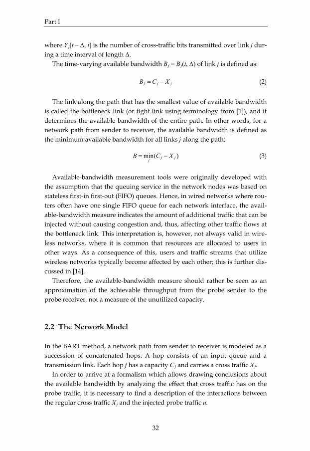
Part I

32

where Y-j[t – Δ, t] is the number of cross-traffic bits transmitted over link j dur-ing a time interval of length Δ. The time-varying available bandwidth B-j = B-j(t, Δ) of link j is defined as: jjj XCB −= (2) The link along the path that has the smallest value of available bandwidth is called the bottleneck link (or tight link using terminology from [1]), and it determines the available bandwidth of the entire path. In other words, for a network path from sender to receiver, the available bandwidth is defined as the minimum available bandwidth for all links j along the path: )(min jj

jXCB −= (3)

Available-bandwidth measurement tools were originally developed with the assumption that the queuing service in the network nodes was based on stateless first-in first-out (FIFO) queues. Hence, in wired networks where rou-ters often have one single FIFO queue for each network interface, the avail-able-bandwidth measure indicates the amount of additional traffic that can be injected without causing congestion and, thus, affecting other traffic flows at the bottleneck link. This interpretation is, however, not always valid in wire-less networks, where it is common that resources are allocated to users in other ways. As a consequence of this, users and traffic streams that utilize wireless networks typically become affected by each other; this is further dis-cussed in [14]. Therefore, the available-bandwidth measure should rather be seen as an approximation of the achievable throughput from the probe sender to the probe receiver, not a measure of the unutilized capacity. 2.2 The Network Model In the BART method, a network path from sender to receiver is modeled as a succession of concatenated hops. A hop consists of an input queue and a transmission link. Each hop j has a capacity C-j and carries a cross traffic X-j. In order to arrive at a formalism which allows drawing conclusions about the available bandwidth by analyzing the effect that cross traffic has on the probe traffic, it is necessary to find a description of the interactions between the regular cross traffic X-j and the injected probe traffic u.

Part I

33

For a first rough idea, consider a fluid model of traffic flows and temporar-ily disregard the discrete nature of packet traffic. First, consider a single hop with capacity C and cross traffic X. The available link bandwidth is then C – X. Now, assume that the link is also subject to probe traffic demand at an inten-sity u. If u ≤ C – X there is no congestion, and the received probe-traffic inten-sity r exiting the link is the same as the demanded probe intensity u. How-ever, in the case u > C – X the link is overloaded. Given that there is no priori-tization in the router, so that all traffic is served on a first-come first-served basis, this means that the cross traffic and the probe traffic each receive their proportionate share of the capacity C. In the overload situation, the received probe-traffic intensity can be de-scribed as:

CXu

ur+

= (4)

By rearranging, it is feasible to see that the ratio of demanded to received probe-traffic intensity is a first-order polynomial in u:

CXu

Cru += 1 (5)

Hence,

. )(1)(1

⎪⎩

⎪⎨⎧

−>+

−≤= XCu

CXu

C

XCu

ru (6)

Thus, by varying u and trying to identify the point where u / r starts to devi-ate from unity, it is feasible to estimate the available bandwidth of the link. This is essentially the network model proposed for the TOPP method [2]. By repeating this argument for several concatenated links, it was shown in [2] that the available bandwidth of the entire path from sender to receiver can be estimated by studying the ratio of offered probe intensity at the sender to received probe intensity at the receiver, and determining the point where this ratio starts deviating from unity. This value of u is the estimate of the avail-able bandwidth B of the entire path. Now, considering the discrete packet-oriented nature of network traffic, it is necessary to adapt the reasoning above to take into account the fact that the traffic is not a continuous flow, instead composed of discrete packets.

Part I

34

With respect to the generic multiple-hop model presented in [15] and the notation therein, consider a sequence of packet pairs where the two packets in pair i arrive at a hop at times 1iτ and 2iτ , and depart (i.e. arrive at the next hop) at times *

1iτ and .*2iτ It is not the absolute arrival times that are of interest,

but rather the inter-arrival times of the packets in pair i: 12 iiit ττ −= (7) *

1*2

*iiit ττ −= (8)

In [15], the focus is on the difference between these quantities, the delay vari-ation .*

iii tt −=δ In the BART method it is instead the dimensionless quantity inter-packet strain εi which is of interest:

i

ii t

t*

1 =+ ε (9)

The strain can be expressed in terms of the delay variation as:

i

ii t

δε = (10)

The correlation between this strain and the network model (6) can be un-derstood by considering the probe-traffic intensities u and r at the time reso-lution of inter-packet time-separation level. With a packet size s, the de-manded traffic intensity becomes itsu /= and the received traffic intensity

./ *itsr = With respect to (9), the ratio of demanded to received probe-traffic

intensity can be expressed as:

ii

i

i

i

tt

tsts

ru ε+=== 1

// *

* (11)

The deviation of u / r from unity is equivalent to the deviation of the strain ε from zero, see Figure 1. No strain means no congestion. It should be noted that when going beyond the fluid model and taking packet-level interactions in router queues into account, the system measure-ment model curve is expected to deviate somewhat from the form in Figure 1 [16]. However, one can still expect the asymptotic behavior to be the sloping straight line, which is the main point of interest.

Part I

35

0

Probe-traffic intensity (u)

Inte

r-pac

ket s

train

( ε)

Available bandwidth

Figure 1. The asymptotic relation between available bandwidth, probe intensity and expectation value of inter-packet strain. In the BART model, observing the inter-packet strain over the path makes it feasible to estimate the available bandwidth at the bottleneck link, and con-sequently the available bandwidth of the entire path. It is assumed that for the average inter-packet strain of consecutive packet pairs in a probe se-quence of a given intensity u, any systematic deviation from zero is domi-nated by the characteristics of the cross traffic at the bottleneck link and the bottleneck-link capacity. Input data for the BART estimation algorithm is generated by sending se-quences of N probe-packet pairs with the same internal traffic intensity u. By increasing N, the statistical precision in the measurements is improved. For each new sample, i.e. new sequence, the intensity u is randomized. Each probe packet is time stamped on sending and on reception. The re-ceiver calculates the inter-packet strain εi for each probe pair ., ... ,1 Ni = When the whole sequence has been received, the average inter-packet strain ε is computed from εi ), ... ,1( Ni = and thereafter used in the Kalman filtering.

Part I

36

3 Filter-Based Bandwidth Estimation 3.1 Filter-Based Estimation In a filter-based approach, the state of a system is estimated from repeated measurements of some quantity dependent on the system state. This requires models of how the system state evolves from one measurement occasion to the next, and also how the measured quantity depends on the system state. The system equations can be expressed as 11)( −− += kkk wxfx (12) kkk vxhz += )( (13) where x is the state of the system, z is the measured quantity, w is the process noise and v is the measurement noise. The functions f and h represent the sys-tem-evolution model and the measurement model, respectively. The sub-script refers to discrete time. According to (12), the system is not influenced by a control input. A con-trol input in the filter formalism is only needed if it is known that the system is affected in a particular way that yields changes to the system state. For ex-ample, BART injects probe packets which could potentially be seen as a con-trol input, but as long as the probe overhead is small and only overloads the bottleneck link momentarily, one could take the view that this input has neg-ligible impact on the underlying system (that is on the overall behavior of other traffic flows as well as the bottleneck-link capacity, which correspond to the system state in BART). For this reason, it is feasible to still obtain reliable available-bandwidth estimates although the control input is excluded. A filter is a procedure which takes a previous estimate 1ˆ −kx and a new measurement zk as input, and calculates a new estimate kx̂ of the system state. A compelling property of filters is that they are capable of producing esti-mates in real-time, i.e. tracking the system state. For each new measurement, the previous estimate is updated. If the functions f and h are linear, and if both the process noise and the measurement noise are Gaussian and uncorrelated, there is an optimal filter, namely the Kalman filter [17]. Experience has shown that Kalman filters often work very well, even when these conditions are not strictly met. In the linear case the system equations (12) and (13) can be expressed using matrices:

Part I

37

11 −− += kkk wAxx (14) kkkk vxHz += (15) From the previous estimate and the new measurement, the Kalman filter eq-uations allow estimation of the system state x and the error covariance matrix P as kkkkkkkkk KxxHzKxx γ+=−+= −−− ˆ)ˆ(ˆˆ (16) −−= kkkk PHKIP )( (17) where 1ˆˆ −

− = kk xAx (18) QAAPP T

kk += −−

1 (19) and .)( 11 −−−−− =+= k

Tkk

Tkkk

Tkkk VHPRHPHHPK (20)

For further details, see [17]. Kalman filtering can be understood as an iterative process where each step consists of two phases of calculation. First, there is a prediction phase, where the previous estimate evolves one discrete time step according to the system model (18). Then, there is a correction phase, where the new measurement is taken into account (16). One also computes the updated error covariance ma-trix Pk of the state estimate (17). The difference −− kkk xHz ˆ in (16) is known as the residual or innovation γk, which is essential in the correction phase. The residual reflects the deviation of the actual measurement from what is predicted according to the measure-ment model and the evolved state estimate. The Kalman gain Kk, given by (20) and appearing in (16) and (17), can be interpreted as the relative weight given to the new measurement as opposed to the pure expected evolution of the previous estimate. As can be seen from (19) and (20), the Kalman gain increases as either Q increases or R decreases. These required inputs to the Kalman filter are the covariances of the process noise w and measurement noise v, respectively. An intuitive understanding of

Part I

38

the importance of these quantities may be acquired by the following argu-ments: • Large variations of the noise in the system model (large Q) imply that the

prediction according to the system model is likely to be less accurate, and the new measurement should be weighted heavier.

• Large variations in the measurement noise (large R) imply that the new measurement is likely to be less accurate, and the prediction according to the system model should be weighted heavier.

3.2 The BART Method The BART method for available-bandwidth estimation makes use of active probing and Kalman filtering. Updated estimates of the system state are pro-duced based on probe-packet measurements. Each measurement consists of sending a sequence of pairs of packets, which are time stamped on sending and arrival. The measured quantity z corresponds to the average relative in-crease in packet-pair time separation, also referred to as the inter-packet sepa-ration strain ε. The expectation value of ε is zero when the probing intensity u is less than the available bandwidth B, and grows in proportion to the over-load when the probing intensity is larger:

⎩⎨⎧

>+=−≤

=)( )()(0

BuuBuBu

βααε (21)

It should be noted that the Kalman filter is rather robust, and good results are often produced even when the ideal conditions are slightly broken [17]. Thus, even if a real system displays characteristics which deviate somewhat from the piecewise linear system curve (see (21) and Figure 1), the resulting available-bandwidth estimate is not automatically invalidated. Since the model (21) is piecewise linear, the break point at u = B prevents a direct application of a Kalman filter. In order to circumvent this, the filter is only applied to measurements for which Bu ˆ> where B̂ is the current esti-mate of the available bandwidth, which is known. The state of the system is represented by a vector containing the two un-known parameters of the sloping straight line in the overload region:

Part I

39

⎥⎦

⎤⎢⎣

⎡=

βα

x (22)

According to (21), ε is measured and u is chosen whereas α and β are typically unknown. The measurement zk of the strain ε at discrete time k may be denoted as kkkk vxHz += (23) where [ ].1kk uH = (24) The evolution of the system state is defined as 11 −− += kkk wxx (25) which means that the Kalman filter formalism may be applied with A = I (the identity matrix). In order to use dimensionless quantities in the BART filtering, u is normal-ized with respect to the chosen maximum probe intensity umax. When the filter estimates the system-state variables α and β, an estimate of the available bandwidth B is immediately obtained, which corresponds to the break point in the piecewise linear curve in Figure 1. In addition, simultane-ously also an estimate of the bottleneck-link capacity C is obtained, as this corresponds to the inverse of the slope α (see (6), (11), and (21)). The BART algorithm can be described as follows: 1. The receiver initializes the state vector estimate x̂ as well as the available-

bandwidth estimate B̂ and the error covariance matrix P of .x̂ Since P0 = 0 indicates that the initial state estimate 0x̂ is correct, it is recommended to choose P0 ≠ 0.

2. The sender generates a sequence of probe-packet pairs with probe-traffic intensity u, for instance drawn from a selected probability distribution. The value of the probe-packet intensity is carried in each packet.

3. For each received probe sequence, the receiver recovers u. If Bu ˆ≤ no up-dating is performed and the cycle repeats from step 2. If Bu ˆ> the receiver computes the average strain ε, which corresponds to z using the filter no-tation (13).

Part I

40

4. The receiver inputs the strain measurement to the Kalman filter, and also provides the filter with an estimate of the process-noise covariance Q and the measurement-noise covariance R. The filter then updates the estimates of the state vector x̂ and the matrix P.

5. The receiver uses the updated x̂ to compute a new u-axis crossing, pro-ducing a new available-bandwidth estimate .B̂ The cycle repeats from step 2.

An important issue when applying Kalman filtering is to find suitable es-timates of the process-noise covariance Q and the measurement-noise covari-ance R. These parameters highly influence the tracking ability of the filter, since they affect the Kalman gain K which decides the contribution by a new measurement when updating the system-state estimate. It should be noted, however, that it is only the relative magnitude of Q and R that is critical, and scaling of the covariances does not affect the performance of the filter [18]. In BART, the measurement-noise covariance R is a scalar that could be seen as a description of the precision of the strain measurement. It should be pos-sible to estimate this parameter based on the received packet pairs in a probe sequence, however, this is not further discussed in this introduction to the method. Q describes the intrinsic fluctuations in the system, and is in the BART ap-plication related to the volatility of the cross traffic and the bottleneck-link capacity. This cannot be assumed to be known a priori, but can be treated as an adjustable parameter. This enables tuning of the BART estimation charac-teristics. Larger values result in low stability but high agility of the filter, since the Kalman-filter equations give greater weight to the recent measurement relative to the previous estimate. Conversely, smaller values result in higher stability in presence of spurious measurement errors, but with a slower step response. In (25), the process noise is defined as the change of the system state be-tween two consecutive measurements. Hence,

⎥⎦

⎤⎢⎣

⎡ΔΔ

=Δ=βα

xw (26)

and the process-noise covariance matrix

.)(),(

),()(2221

1211⎥⎦

⎤⎢⎣

⎡ΔΔΔ

ΔΔΔ=⎥

⎦

⎤⎢⎣

⎡=

ββαβαα

VCCV

QQQQ

Q (27)

Part I

41

Since the state vector x in BART is two-dimensional, the covariance Q of the process noise w is by definition a symmetric 2×2 matrix with three scalar parameters, i.e. Q12 = Q21. Consequently, there are three degrees of freedom available for tuning. The allowed ranges of the elements in Q are given by the inequalities Q11 ≥ 0, Q22 ≥ 0, and .2211122211 QQQQQ ≤≤− These bounds are simply due to the properties of variances and covariances of stochastic variables [19]. 3.3 Stability versus Agility The available bandwidth usually varies over time and one can expect that the true system state differs between two BART measurements. The magnitude of the difference can, however, be everything from hardly noticeable to very large, where the former typically is the case in a slowly changing or station-ary scenario while the latter may occur in case of, e.g., low cross-traffic aggre-gation or due to sudden changes that greatly affect the system.

0 2 4 6 8 10 12 14 16 18 20

0

0.2

0.4

0.6

0.8

1

1.2

1.4

1.6

1.8

2

Probe-traffic intensity (u) [Mbit/s]

Inte

r-pac

ket s

train

( ε)

Strain measurementSystem state (average)

Figure 2. Calculated strain measurements from a BART experiment performed in a laboratory network with controlled cross traffic. Figure 2 illustrates strain measurements ε for a BART experiment with fair-ly high cross-traffic variability. The dashed line corresponds to the expecta-

Part I

42

tion value of the true system state, mapped into the piecewise linear meas-urement model. As can be seen, the strain measurements are scattered and cover a considerable area. Hence, the sloping straight line will move around quite frequently if BART is supposed to fully adapt its state estimate with respect to new measurements. When discussing stability versus agility of the BART method, the challenge is to decide how much a new measurement should contribute to the updated state estimate in the Kalman-filter correction phase. This is determined by the Kalman gain K, which in turn is affected by the noise covariances Q and R.

0 2 4 6 8 10 12 14 16 18 20

0

Probe-traffic intensity (u) [Mbit/s]

Inte

r-pac

ket s

train

( ε)

New strain measurementPrevious state estimateUpdated state estimate (K small)Updated state estimate (K large)

Figure 3. Illustration of how the Kalman gain K affects the tracking ability of BART when a new system-state estimate is produced based on the previous state estimate and the new measurement. Figure 3 illustrates the expected behavior of BART when creating a new estimate. The solid sloping straight line corresponds to the previous state es-timate, which yields an available-bandwidth estimate of 8 Mbit/s. In the cor-rection phase, the filter takes the new measurement into account, represented by the circle. The Kalman gain decides how the previous state estimate and the new measurement should be combined. If the Kalman gain is relatively small, BART is expected to weight the previous estimate heavier than the new measurement when updating the system-state estimate. This is illustrated by the dashed sloping straight line, which gives an updated available-bandwidth

Part I

43

estimate of 7 Mbit/s. The opposite holds for a relatively large Kalman gain, which gives more weight to the new measurement. In this case, the new esti-mate is expected to end up close to the measurement, which is illustrated by the dotted sloping straight line indicating an updated available-bandwidth estimate of 3 Mbit/s. The example in Figure 3 is purely constructed for illustrating the impact of the Kalman gain K and the ratio of the noise covariances Q and R. Intention-ally, the slope of the lines is constant whereas the intersection of the horizon-tal axis changes due to the Kalman gain and the location of the strain meas-urement. This is not necessarily the case in reality; recall that the slope of the straight line in the BART measurement model refers to the inverse of the bot-tleneck-link capacity, which may vary with time.

0 200 400 600 800 1000 1200 1400 1600 1800 20000

1

2

3

4

5

6

7

8

9

10

Time [s]

Ava

ilabl

e ba

ndw

idth

[Mbi

t/s]

Available bandwidthBART estimate (Q large)BART estimate (Q small)

Figure 4. Illustration of the BART performance when the Kalman filter is provided with two different configurations of the process-noise covariance Q, which affect the Kalman gain K and the tracking ability of BART. Having the knowledge of how the Kalman gain affects the performance of BART, the challenge is to find a ratio of Q and R that suits the measurement application. In Figure 4, BART is estimating the available bandwidth based on the strain measurements in Figure 2. In this example, the refinement pos-sibility of providing the Kalman filter with a precision measurement R of the inter-packet separation strain ε has not been utilized. Instead, this filter pa-

Part I

44

rameter was set to R = 1 for all measurements (i.e. from the filter’s perspective all strain measurements were considered to be of equal quality and treated accordingly) and the Kalman gain is regulated by adjustments of the process-noise covariance Q. The solid curve corresponds to the true available band-width, which is defined according to the chosen time resolution Δ, see (1) and (3); the actual value of Δ can be disregarded at this point. The dotted curve depicts the BART estimation when Q is relatively large, which corresponds to a large Kalman gain that gives much weight to the strain measurements. The dashed curve in Figure 4 shows the BART performance when a relatively small Q is used; BART believes more in previous estimates than new strain measurements. Both Q configurations used in Figure 4 seem to be unsuitable if BART should follow the true available bandwidth defined by the solid curve. The dotted curve gives too much weight to strain measurements, which makes BART agile but also sensitive to measurement noise; however, this behavior may be convenient in case of rapid fluctuations in the system state. The BART configuration corresponding to the dashed curve yields stable estimates that are insensitive to measurement noise, which is suitable when estimating a slowly changing or stationary system state; the disadvantage is the slow re-sponse to changes. In order to tune BART such that its estimate follows the variability of the true available bandwidth, Q should be chosen to something in between the two rather extreme configurations used in Figure 4. The most appropriate choice of Q typically varies with respect to different measurement applications and traffic scenarios. Aspects affecting the optimal selection of this parameter are, e.g., the variability of the bottleneck-link ca-pacity, the cross-traffic aggregation, the used time resolution for which the cross-traffic is defined, and the sampling frequency of BART (i.e. how often BART is probing the network path). The two latter may be user or application specified, whereas the variability of the bottleneck-link capacity and the cross-traffic aggregation level typically are difficult to predict since these cha-racteristic are usually not known beforehand. So far, the trade-off between stability and agility has been discussed with the aim of finding a suitable but static Q configuration. However, when deal-ing with dynamic systems, changes may suddenly occur that significantly influence the characteristics of the system-state variability. In such cases, it would be desired to adjust the tracking ability in real-time, since static con-figurations of statistical measurement tools typically cannot optimally deal with both slowly changing conditions and rapid fluctuations. A tool config-ured for stability will suffer in case of rapid changes in the system state, due

Part I

45

to slow adaptation. A tool with agile properties delivers fluctuating estimates in a steady-state situation, due to the measurement noise. It is reasonable to believe that many applications would benefit from tools which have the ability to deliver reliable estimates under various conditions.

0 200 400 600 800 1000 1200 1400 1600 1800 20000

1

2

3

4

5

6

7

8

9

10

Time [s]

Ava

ilabl

e ba

ndw

idth

[Mbi

t/s]

Available bandwidthBART estimate (Q large)BART estimate (Q small)

Figure 5. BART estimation of the available bandwidth using two configurations of Q for different tracking ability, for a scenario with abrupt changes in the available bandwidth. As an illustration, consider Figure 5 where BART is estimating the unuti-lized capacity of a network path (the cross-traffic intensity is configured ac-cording to a step function while the bottleneck-link capacity is constant). Again, the measurement noise covariance R = 1 and the Kalman gain is regu-lated by Q. The dotted curve corresponds to a high-agility configuration. It is obvious that BART easily follows the abrupt changes in the available band-width, whereas the precision of the estimates leaves a great deal to be de-sired, due to amplification of the measurement noise. The dashed curve cor-responds to an opposite configuration of high stability. Here, one can see that BART is insensitive to the measurement noise and delivers stable and reliable estimates in the interval from 0 to 750 seconds. However, the configuration does not allow for fast adaptation, which is obvious when considering the estimates after 750 seconds, where BART is very slow in adapting to the new system state.

Part I

46

Streaming of real-time data over a network path is an application which would probably benefit from a tool such as BART. Since congestion and packet loss are detrimental to real-time data, it would be beneficial if the sender could regulate the transmission intensity with respect to the prevail-ing network conditions; for example by changing codec in case of audio or video streaming. A BART configuration corresponding to the dashed curve in Figure 5 would probably be suitable when estimating the available band-width over a network path given slowly changing network characteristics. However, in case of abrupt changes, as in Figure 5, it is desirable that the es-timates follow the variations such that a streaming application using BART has the possibility of adjusting the transmission intensity in case it is needed. A static BART configuration tuned for agility is undesirable, since it con-stantly would trigger adjustment of the streaming codec due to exaggerated fluctuations in the available-bandwidth estimates. Nevertheless, it would be useful to transiently apply a configuration corresponding to the dotted curve in Figure 5, in order to rapidly follow abrupt changes in the network condi-tions. Although the BART configurations used in Figure 5 could be seen as two rather extreme choices (it is of course possible to choose Q such that the esti-mates become something in between the two estimation curves in Figure 5), there is a clear trade-off between having stable but slowly adapting estimates and agile but noise-sensitive estimation properties. For a more detailed discussion regarding the Kalman gain and the noise covariances, as well as the possibility of tuning BART for enhanced tracking performance, see [13, 20]. 3.4 Change Detection There are solutions to the problem described in Section 3.3, regarding abrupt changes in the system state which make it hard to maintain a good estimation performance given a static filter configuration. In the area of system identifi-cation using filter-based estimation methods, these solutions are often re-ferred to as adaptive control and change detection (also known as fault detec-tion). There are a number of existing filter-based methods available for detecting abrupt changes in dynamic systems, e.g. [21-25]. A comparative study on sev-eral change-detection techniques for automotive applications has been pre-

Part I

47

sented in [26]. In the field of computer networking, change detection has been used in [11] for estimation of round-trip time for use in congestion control. These methods for change detection can, in general, be divided into three classes: methods using one filter, where a whiteness test is applied to the filter residuals; methods using two filters, where a slow filter configured for stabil-ity runs in parallel with a fast filter configured for agility; methods using mul-tiple filters, where each filter configuration is matched to a particular assump-tion regarding the abrupt change. For more information about these tech-niques and change detection in general, see [27]. There is a trade-off in complexity versus performance when comparing different change-detection techniques; generally, the more complex algo-rithm, the better result is obtained [26]. The computational complexity is often proportional to the number of filters required by the algorithm. A simple and intuitive technique is known as the Cumulative Sum (CUSUM) test [21, 27], which only uses one filter in order to make decisions regarding the hypothe-ses of change or no change in the system. This can be compared to, e.g., the full Generalized Likelihood Ratio (GLR) test [24, 27], where the number of required filters (and thus also the complexity) grows linearly with time. When using change detection, it is normally assumed that abrupt changes occur infrequently. With respect to this, it is sound to implement a filter (e.g. a Kalman filter) with regard to a basic model based on the assumption of no abrupt changes, and to design a secondary system that monitors the residuals of the filter to determine if a change has occurred or not. A change detector can essentially be attached to the end of any existing filter that does not ac-count for sudden changes; the type of filter is of less importance, it is the re-siduals of the filter that matter. The characteristics of filter residuals can be examined for indications of the filter’s state estimation being off track. A filter residual γk is defined as the difference between the measured quantity at time k and the prediction of this using the a priori estimate of the system state at time k. In the Kalman filter, the residual is used in the correction phase (16). Figure 6 illustrates the filter residual in BART. Assuming a system-state estimate which indicates an available bandwidth of 7 Mbit/s (represented by the sloping straight line), and given that the next measurement of the system state is carried out by transmitting a sequence of probe packets at u = 9 Mbit/s, it is feasible to predict the new strain measurement ε with respect to the used measurement model H (24) and the current state estimate. In Figure 6, this prediction of the measurement is depicted as a square which overlaps the sloping straight line at u = 9 Mbit/s. In an ideal situation where the meas-

Part I

48

urement model is perfect, the predicted estimate of the system state equals the true system state, and the new measurement does not contain any meas-urement noise, the filter residual γ would be zero. However, in practice this is typically not the case. In Figure 6, the new strain measurement is larger than the expected value according to the prediction of the filter, which yields a positive filter residual (it is also feasible to obtain negative filter residuals) according to (16).

0 2 4 6 8 10 12 14 16 18 20

0

Probe-traffic intensity (u) [Mbit/s]

Inte

r-pac

ket s

train

( ε)

New strain measurementState estimatePredicted strain measurement

Residual γ

Figure 6. Illustration of the filter residual γ in the BART method. The residual γk re-flects the deviation of the strain measurement εk from what is predicted according to the measurement model and the evolved state estimate at time k. An important property of filter residuals is that, under certain model as-sumptions, they resemble white noise before a change occurs. This character-istic is often useful in change detection. In an ideal system, the residuals would be zero before a change and non-zero after a change. However, due to measurement noise and process noise, which are unavoidable in statistical methods, this is not the case in reality and the residuals cannot be predicted beforehand. Nevertheless, conclusions may be drawn from the statistical be-havior of the residuals. Assuming that there is no change in the system state, and given that the used model is correct, the residuals can be interpreted as independent sto-chastic variables with zero mean and a certain variance, which characterize

Part I

49

white noise. After a change in the system state, the distribution of the residu-als also changes. The challenge in statistical change detection is to design a hypothesis test allowing to distinguish between random and systematic de-viation of the residuals. Regarding BART and change detection, experiments have been performed with both the CUSUM test and the GLR test, see [13, 28] and [29] for details. 4 Discussion and Conclusions The BART method, which uses active probing and Kalman filtering for real-time estimation of the end-to-end available bandwidth, has been presented. It is demonstrated that Kalman filtering is applicable to the problem of measur-ing available bandwidth, despite a strong nonlinearity in the system meas-urement model. Furthermore, the required computational efforts and costs in terms of extra traffic load on the network from the probe packets are low compared to numerous other bandwidth-measurement tools. The method has considerable potential for tuning the estimation according to specific needs, e.g. by configuring the process-noise covariance matrix Q appropriately which affects the Kalman gain K and the tracking ability of BART. The optimal choice of this filter parameter (which is an input to the BART estimation algorithm) is dependent on the variability of the true avail-able bandwidth, which in turn depends on the cross-traffic aggregation, the characteristics of the bottleneck-link capacity, and the time resolution Δ that is used for describing bandwidth. The problem of accurately estimating the available bandwidth in networks with irregular characteristics has also been addressed. For statistical estima-tion methods, there is generally a clear trade-off between noise insensitive estimates and the ability of fast adaptation to sudden changes. However, a virtue of filter-based methods is the possibility to enhance the performance by combining them with change detection. This makes it feasible to overcome the trade-off, and enable stable estimation in case of a slowly varying system state and quick adaptation in case of abrupt changes.

Part I

50

References [1] M. Jain and C. Dovrolis, “End-to-end available bandwidth: measure-

ment methodology, dynamics, and relation with TCP throughput,” IEEE/ACM Transactions on Networking, vol. 11, 2003.

[2] B. Melander, M. Björkman, and P. Gunningberg, “A new end-to-end probing and analysis method for estimating bandwidth bottlenecks,” in Proc. IEEE GLOBECOM’00, 2000.

[3] V. Ribeiro, R. Riedi, R. Baraniuk, J. Navratil, and L. Cottrell, “pathChirp: efficient available bandwidth estimation for network paths,” in Proc. Passive and Active Measurement Workshop, 2003.

[4] N. Hu and P. Steenkiste, “Evaluation and characterization of available bandwidth probing techniques,” IEEE JSAC Internet and WWW Meas-urement, Mapping, and Modeling, vol. 21, 2003.

[5] J. Strauss, D. Katabi, and F. Kaashoek, “A measurement study of avail-able bandwidth estimation tools,” in Proc. ACM SIGCOMM Internet Measurement Conference, 2003.

[6] V. Ribeiro, M. Coates, R. Riedi, S. Sarvotham, B. Hendricks, and R. Ba-raniuk, “Multifractal cross-traffic estimation,” in Proc. ITC Specialist Se-minar on IP Traffic Measurement, Modeling and Management, 2000.

[7] A. Shriram and J. Kaur, “Empirical evaluation of techniques for measur-ing available bandwidth,” in Proc. IEEE INFOCOM, 2007.

[8] A. Shriram, M. Murray, Y. Hyun, N. Brownlee, A. Broido, M. Fo-menkov, and K. Claffy, “Comparison of public end-to-end bandwidth estimation tools on high-speed links,” in Proc. Passive and Active Meas-urement Workshop, 2005.

[9] S. Keshav, “A control-theoretic approach to flow control,” ACM SIG-COMM Computer Communication Review, vol. 21, 1991.

[10] M. Kim and B. Noble, “Mobile network estimation,” in Proc. ACM Con-ference on Mobile Computing and Networking, 2001.

[11] K. Jacobsson, N. Möller, K.-H. Johansson, and H. Hjalmarsson, “Some modeling and estimation issues in control of heterogeneous networks,” in Proc. 16th International Symposium on Mathematical Theory of Networks and Systems, 2004.

[12] R. S. Prasad, M. Murray, C. Dovrolis, and K. Claffy, “Bandwidth estima-tion: metrics, measurement techniques, and tools,” IEEE Network, vol. 17, 2003.

Part I

51

[13] E. Bergfeldt, S. Ekelin, and J. M. Karlsson, “Real-time available-bandwidth estimation using filtering and change detection,” Computer Networks, vol. 53, 2009.

[14] E. Bergfeldt, S. Ekelin, and J. M. Karlsson, “Real-time bandwidth meas-urements over mobile connections,” Submitted to European Transactions on Telecommunications, 2010.

[15] A. Pásztor and D. Veitch, “The packet size dependence of packet-pair like methods,” in Proc. 10th International Workshop on Quality of Service (IWQoS), 2002.

[16] X. Liu, K. Ravindran, and D. Loguinov, “Multi-hop probing asymptotics in available bandwidth estimation: stochastic analysis,” in Proc. Internet Measurement Conference (IMC), 2005.

[17] G. Welch and G. Bishop, “An introduction to the Kalman filter,” SIG-GRAPH, Course 8, 2001.

[18] F. Gustafsson, “Slip-based tire-road friction estimation,” Automatica, vol. 33, 1997.

[19] G. James, Advanced Modern Engineering Mathematics. Addison-Wesley, 1999.

[20] E. Hartikainen and S. Ekelin, “Tuning the temporal characteristics of a Kalman-filter method for end-to-end bandwidth estimation,” in Proc. 4th IEEE/IFIP Workshop on End-to-End Monitoring Techniques and Services, 2006.

[21] E. S. Page, “Continuous inspection schemes,” Biometrika, vol. 41, 1954. [22] U. Appel and A. V. Brandt, “Adaptive sequential segmentation of

piecewise stationary time series,” Information Sciences, vol. 29, 1983. [23] M. Basseville and A. Benveniste, “Design and comparative study of

some sequential jump detection algorithms for digital signals,” IEEE Transactions on Acoustics, Speech, and Signal Processing, vol. 31, 1983.

[24] A. S. Willsky and H. L. Jones, “A generalized likelihood ratio approach to the detection and estimation of jumps in linear systems,” IEEE Trans-actions on Automatic Control, vol. 21, 1976.

[25] F. Gustafsson, “The marginalized likelihood ratio test for detecting ab-rupt changes,” IEEE Transactions on Automatic Control, vol. 41, 1996.

[26] F. Gustafsson, “A comparative study on change detection for some au-tomotive applications,” in Proc. European Control Conference, 1997.

[27] F. Gustafsson, Adaptive Filtering and Change Detection. John Wiley & Sons, Ltd, 2000.

Part I

52

[28] E. Hartikainen and S. Ekelin, “Enhanced network-state estimation using change detection,” in Proc. 31st IEEE Conference on Local Computer Net-works, 2006.

[29] E. Hartikainen, S. Ekelin, and J. M. Karlsson, “Change detection and es-timation for network-measurement applications,” in Proc. 2nd ACM Workshop on Performance Monitoring and Measurement of Heterogeneous Wireless and Wired Networks, 2007.

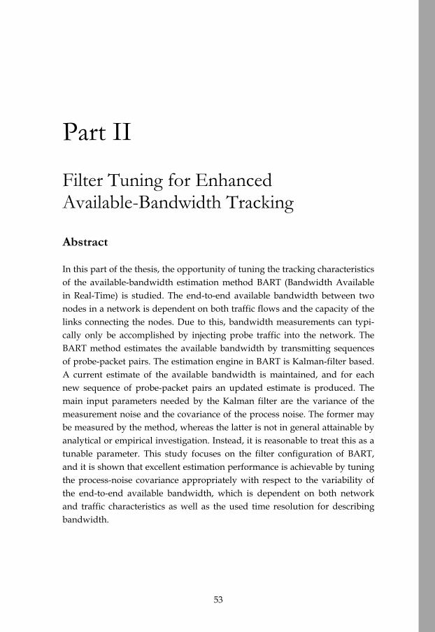
53

Part II Filter Tuning for Enhanced Available-Bandwidth Tracking Abstract In this part of the thesis, the opportunity of tuning the tracking characteristics of the available-bandwidth estimation method BART (Bandwidth Available in Real-Time) is studied. The end-to-end available bandwidth between two nodes in a network is dependent on both traffic flows and the capacity of the links connecting the nodes. Due to this, bandwidth measurements can typi-cally only be accomplished by injecting probe traffic into the network. The BART method estimates the available bandwidth by transmitting sequences of probe-packet pairs. The estimation engine in BART is Kalman-filter based. A current estimate of the available bandwidth is maintained, and for each new sequence of probe-packet pairs an updated estimate is produced. The main input parameters needed by the Kalman filter are the variance of the measurement noise and the covariance of the process noise. The former may be measured by the method, whereas the latter is not in general attainable by analytical or empirical investigation. Instead, it is reasonable to treat this as a tunable parameter. This study focuses on the filter configuration of BART, and it is shown that excellent estimation performance is achievable by tuning the process-noise covariance appropriately with respect to the variability of the end-to-end available bandwidth, which is dependent on both network and traffic characteristics as well as the used time resolution for describing bandwidth.

Part II

54

1 Introduction 1.1 Overview The capability of estimating end-to-end available bandwidth is useful in sev-eral contexts, including service level agreement verification, network moni-toring and server selection. Estimation of bandwidth in real-time, with per-sample update, opens up for many applications, including adaptation based directly on available bandwidth (rather than measures such as loss or delay) in, e.g., congestion control and streaming of audio and video. Estimation methods based on a filtering approach possess this compelling feature of producing an updated estimate for each new sampling of the sys-tem properties. For instance, if one has been able to successfully apply a filter method to the problem of estimating available bandwidth, it is feasible to track the bandwidth on a time-unit basis by measuring the network path of interest once every time unit, since each measurement gives rise to an up-dated estimate of the currently available bandwidth. The BART (Bandwidth Available in Real-Time) method has been developed for this particular pur-pose, where sequences of probe-packet measurements and Kalman filtering are used for producing estimates of the end-to-end available bandwidth [1]. In the forthcoming sections, the possibility of tuning BART to track the available bandwidth for a variety of different cross-traffic aggregation levels and time resolutions (or averaging time scales) Δ [2] is investigated. There is no canonical time resolution at which to define available bandwidth. The re-levant time resolution may be different for various applications. The time resolution of bandwidth tracking offered by BART is related to two adjustable properties. The obvious one is the inter-probing time. By prob-ing more frequently, it is reasonable to expect an improved tracking perform-ance with respect to being able to follow bandwidth variations within short time intervals; however, the trade-off is the larger amount of probe traffic af-fecting the network. The more subtle adjustable property is the process-noise covariance Q, one of the crucial Kalman-filter parameters. This is a 2×2 matrix in the BART formalism which, in combination with the variance of the meas-urement noise R, affects the Kalman gain K that determines the tracking char-acteristics of the filter. For details regarding Kalman filtering, see [3]. In the present study, it is explored how the elements of Q could be chosen so as to optimize the available-bandwidth tracking performance of BART with respect to properties of different network technologies, traffic character-istics, and choices of time resolution Δ for describing bandwidth. A specific

Part II

55

variability measure, which captures the effect of both time resolution and traffic aggregation, is introduced and applied. Also, the possibility of estimat-ing the variance of the measurement noise R is briefly discussed. 1.2 Related Work A frequently used definition of the time-varying available bandwidth of a link is B = C – X bit/s, where C is the capacity of the link and X corresponds to the cross traffic (or link load) which affects the link. For a network path from sender to receiver, the end-to-end available bandwidth is defined as the min-imum available bandwidth of all links along the path. For example, see [1, 2] for details. This definition of available bandwidth is used by BART and numerous other bandwidth estimation methods which have been proposed throughout the years, e.g. [4-11]. Some of these methods have been compared for per-formance in studies such as [12, 13]. In a seminal paper on packet-pair techniques [14], Keshav discussed using a Kalman filter for the estimation of “bottleneck service rate” for end-point flow control purposes, and concluded that this would not be practical. How-ever, his analysis rested on the assumption that queuing service in network nodes is based on stateful flow-based round-robin instead of stateless first-come first-served (FCFS), whereas typically the latter holds in today’s Inter-net. This study demonstrates that Kalman filtering is applicable to the problem of estimating available bandwidth based on observations of the time separa-tion between packet pairs. In addition, it is shown that appropriate configura-tion of the Kalman filter enables excellent estimation performance even though the available-bandwidth variability may vary significantly for differ-ent network and traffic scenarios. The content of the following sections is mainly based on [1, 15]. 2 Filter-Based Bandwidth Estimation 2.1 Filter-Based Estimation In a filter-based approach, the state of a system is estimated from repeated measurements of some quantity dependent on the system state, given models

Part II

56

of how the system state evolves from one measurement occasion to the next, and how the measured quantity depends on the system state. Both these de-pendencies include a random noise term; the process noise and the measure-ment noise, respectively. The system equations become1 11)( −− += kkk wxfx (1) kkk vxhz += )( (2) where x is the state of the system, z is the measurement, w is the process noise and v is the measurement noise. The functions f and h represent the system-evolution model and the measurement model, respectively. The subscripts refer to discrete time. A filter is a procedure which takes a previous estimate of the system state

1ˆ −kx and a new measurement zk as input, and calculates a new estimate kx̂ of the system state. A compelling property of filters is that they are capable of producing estimates in real-time, i.e. tracking the system state. For each new measurement, the previous estimate is updated. A key point of this study is how the relative weights of the previous esti-mate and the new measurement in the filtering process influence the tracking characteristics of the method. This is further discussed below. If the functions f and h are linear, and if both the process noise and the measurement noise are Gaussian and uncorrelated, there is an optimal filter, namely the Kalman filter [3]. Experience has shown that Kalman filters often work very well, even when these conditions are not strictly met. Another im-portant advantage with Kalman filters is that, unless the dimension of the system is very large, they are computationally light-weight with minimal re-quirements on the memory. In this linear case the system equations can be expressed using matrices: 11 −− += kkk wAxx (3) kkkk vxHz += (4) The Kalman filter equations allowing calculation of the new estimate from the previous estimate and the new measurement are (for details, see [3]): 1 This can be formulated more generally, when the system is also influenced by a control input. Since this is not needed in BART, this additional degree of freedom is not used.

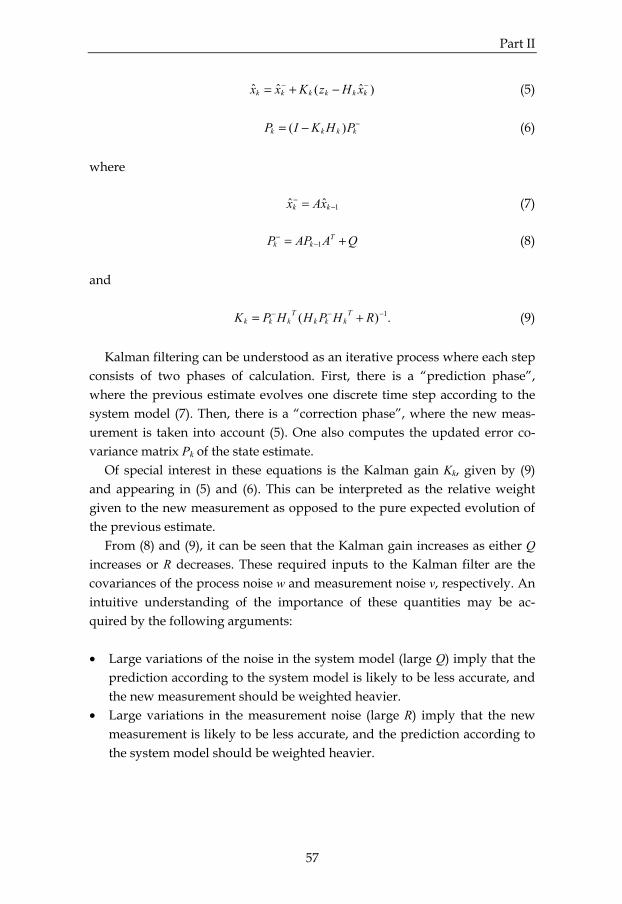
Part II

57

)ˆ(ˆˆ −− −+= kkkkkk xHzKxx (5) −−= kkkk PHKIP )( (6) where 1ˆˆ −

− = kk xAx (7) QAAPP T

kk += −−

1 (8) and .)( 1−−− += RHPHHPK T

kkkT

kkk (9) Kalman filtering can be understood as an iterative process where each step consists of two phases of calculation. First, there is a “prediction phase”, where the previous estimate evolves one discrete time step according to the system model (7). Then, there is a “correction phase”, where the new meas-urement is taken into account (5). One also computes the updated error co-variance matrix Pk of the state estimate. Of special interest in these equations is the Kalman gain Kk, given by (9) and appearing in (5) and (6). This can be interpreted as the relative weight given to the new measurement as opposed to the pure expected evolution of the previous estimate. From (8) and (9), it can be seen that the Kalman gain increases as either Q increases or R decreases. These required inputs to the Kalman filter are the covariances of the process noise w and measurement noise v, respectively. An intuitive understanding of the importance of these quantities may be ac-quired by the following arguments: • Large variations of the noise in the system model (large Q) imply that the

prediction according to the system model is likely to be less accurate, and the new measurement should be weighted heavier.

• Large variations in the measurement noise (large R) imply that the new measurement is likely to be less accurate, and the prediction according to the system model should be weighted heavier.

Part II

58

2.2 The BART Filter Method for Available-Bandwidth Estimation The BART method for available-bandwidth estimation makes use of active-probing measurements and Kalman filtering to produce updated estimates of the available bandwidth over a network path [1]. The measurements consist of sending sequences of probe packets at randomized probing intensities. The probe packets are time-stamped on sending and on arrival, and the BART receiver calculates the average relative increase ε in packet-pair time separa-tion. From a simple FCFS network model [11], it is seen that the expectation value of ε is zero when the probing intensity u is less than the available bandwidth B, and grows in proportion to the overload when the probing in-tensity is larger:

⎩⎨⎧

>+=−≤

=)( )()(0

BuuBuBu

βααε (10)

In order to use dimensionless quantities in the BART filtering, u is normal-ized with respect to the maximum probe intensity umax. It should be noted that the Kalman filter method is very “forgiving”, and good results are often produced even when the ideal conditions are slightly broken. So, even if a real system displays characteristics which deviate somewhat from this piecewise linear system curve (10), the resulting avail-able-bandwidth estimate is not automatically invalidated. All variables in this model are dynamical, i.e. may vary in time, so they depend on the subscript (which is sometimes suppressed in this exposition). This model allows for application of a Kalman filter, when the state of the system is represented by a vector containing the two parameters of the slop-ing straight line:

⎥⎦

⎤⎢⎣

⎡=

βα

x (11)

The measurement zk of the strain at discrete time k may be written as,

kkkk vxHz += (12)

where

[ ].1kk uH = (13)

Part II

59

The evolution of the system state is defined as

11 −− += kkk wxx (14)

which means that the Kalman filter formalism may be applied with A = I (the identity matrix). The Kalman equations in BART become computationally very simple, and only a few floating-point operations are needed at each iteration. When the filter estimates the system-state variables α and β, an estimate of the available bandwidth B is immediately obtained, since these quantities are related by

.0 =+ βα B (15) 2.2.1 The Process-Noise Covariance The state vector x in BART is two-dimensional, so the covariance Q of the process noise w is a 2×2 matrix. In (14), the process noise is defined as the change of the system state be-tween two consecutive measurements (which is due to the change in cross traffic and/or bottleneck-link capacity).

⎥⎦

⎤⎢⎣

⎡ΔΔ

=Δ=βα

xw (16)

so

.)(),(

),()(2221

1211⎥⎦

⎤⎢⎣

⎡ΔΔΔ

ΔΔΔ=⎥

⎦

⎤⎢⎣

⎡=

ββαβαα

VCCV

QQQQ

Q (17)

Since Q is a symmetric matrix (i.e. Q12 = Q21) there are three degrees of freedom available for tuning. The allowed ranges are given by the inequali-ties Q11 ≥ 0, Q22 ≥ 0, and .2211122211 QQQQQ ≤≤− These bounds are simply due to the properties of variances and covariances of stochastic variables [16]. When configuring BART for bandwidth estimation in wired networks, it is reasonable to expect that Q11 should be chosen rather small, since this element reflects expected variations of α, and α is correlated to the bottleneck-link ca-pacity C (α is the inverse of the bottleneck-link capacity, see [1] for details)

Part II

60

which typically is constant in wired networks. Instead, available-bandwidth fluctuations are more likely due to cross-traffic variations at the bottleneck link, which affect the β parameter. Consequently, for measurements in wired networks, Q22 is the significant element when tuning the characteristics of BART. However, since the capacity C of a wireless link is highly dependent on the radio-channel conditions, which may be subject to extensive fluctuations on a short time scale, a suitable Q configuration is most likely different when using BART for measurements over wireless bottleneck links. In this case, Q11 should instead be rather large in order to allow for rapid variations of α, whe-reas Q22 is still supposed to reflect the properties of cross traffic. In case of no interaction between probe traffic and cross traffic at the bottleneck link, it is appropriate to choose Q22 to a very small value and expect β to be close to -1. The reason is that if no cross traffic is affecting the bottleneck link of the net-work path, the end-to-end available bandwidth is simply limited by the ca-pacity C of the bottleneck link, i.e. B = C. With respect to this and since α cor-responds to the inverse of C, it can be seen from (15) that β = -1. However, since it may be hard to know beforehand whether cross traffic exists along the measured network path, it is reasonable to assume that β may deviate from -1 and therefore choosing Q22 > 0 (similarly, Q11 > 0 is an appropriate choice for wired networks, since the bottleneck-link capacity could be subject to varia-tions). For example, this Q configuration strategy was used and turned out to be a suitable choice in [17], where BART was evaluated over a mobile broad-band connection based on UMTS (Universal Mobile Telecommunications Sys-tem) with HSDPA (High-Speed Downlink Packet Access) functionality [18, 19]. Q12 represents the covariance of the difference in the system-state variables. With respect to numerous BART experiments, the choice of Q12 seems to be of less importance (compared to Q11 and Q22) for the overall BART performance as long as it stays within its theoretical bounds [15]. However, according to the above discussion regarding properties of wired and wireless links it is often appropriate to choose Q12 = 0, since this denotes independent variations of α and β, which is reasonable if α or β is expected to be stable. 2.2.2 The Measurement-Noise Covariance Because the input measurement z in the BART Kalman filtering corresponds to the average inter-packet separation strain ε which is a scalar, the measure-

Part II

61

ment-noise covariance R is also a scalar and thus represents the variance of the measurement noise v. R is of great importance since it, in combination with the process-noise co-variance Q, determines the Kalman gain K and thus the tracking ability of the Kalman filter. In BART, R could be seen as an estimator for the precision of the strain measurement ε. However, to guarantee an appropriate BART per-formance, the computation of R is not straightforward. In some studies, e.g. [20, 21], BART has been shown to perform reasonable when R has been calculated as the variance of the average inter-packet strain ε, considering all probe-packet pairs in a probe sequence. This yields a rather large R value when the variability of the inter-packet strain among the packet pairs is high, which means that the measurement ε is likely to be less accurate and the prediction should be weighted heavier than the new measurement in the Kalman filtering; vice versa if the deviation of the inter-packet strains is small within a probe sequence.

0 50 100 150 200 2500

1

2

3

4

5

6

7

8

9

10

Time [s]

Ava

ilabl

e ba

ndw

idth

[Mbi

t/s]

Available bandwidthBART estimate

Figure 1. The BART performance when R is computed as the variance of the average inter-packet strain ε. The abrupt increases of the BART estimate occur when the probe traffic does not interact with the cross traffic. However, this approach has its drawbacks. For example, if the cross traffic along a network path has bursty characteristics it becomes more likely that transmitted probe sequences miss the cross-traffic packets. In case of no inter-

Part II

62

action between the cross traffic and the probe traffic, the variance of ε be-comes very small. Hence, this yields a large Kalman gain in the Kalman filter-ing, and the updated available-bandwidth estimate of BART will almost en-tirely be based on the measurement ε, which in this case indicates an empty bottleneck link. This is illustrated in Figure 1, where the BART estimate sud-denly increases due to no interaction between the probe traffic and the cross traffic. In Figure 1, BART is obviously overestimating the available bandwidth and the main reason for this is the applied R computation in combination with bursty cross traffic. The abrupt increases of the BART estimate are due to very small values of R (causing large values of K according to (9)), which are obtained when the strain of the packet pairs is equal or almost equal within a probe sequence. This may happen in case the probe traffic does not interact with the cross traffic. The reason for the slow recovery is related to the used Q configuration. A larger Q would cause BART to adapt to the true available bandwidth more quickly for measurements where probe packets become affected by the cross traffic. For details regarding the experiment setup and used BART configura-tion, see [21]. Instead of considering R as an indicator of the precision of the measure-ment ε, an alternative approach is to set this filter parameter to a fixed value, e.g. R = 1 for all measurements. From the filter’s perspective, this means that all strain measurements ε are considered to be of equal quality and treated accordingly. Hence, the possibility of providing the Kalman filter with a pre-cision measure of ε is discarded, but on the other hand abrupt changes as in Figure 1 are avoided and it becomes easier to control the BART tracking char-acteristics since the Kalman gain is only affected by changes of the Q configu-ration. This strategy, which has been successfully used in several BART ex-periments (see e.g. [1, 22, 23]) is also applied in this study. 2.2.3 Tuning BART Besides the process-noise covariance Q and the variance of the measurement noise R, the BART estimation method comprises several other tunable com-ponents which may affect the performance, e.g.: • The probe-packet size • The number of probe-packet pairs in each sequence

Part II

63

• The organization of the probe pairs, i.e. separated or as a train • The inter-measurement time separation • The probability distribution for the probing intensity In this study, the tracking ability of BART with respect to tuning of the process-noise covariance matrix Q is of specific interest. All the other compo-nents are fixed, although some of them have been evaluated in [21]. There is plenty of opportunity to further increase the performance. However, the qua-litative dependence of the tracking characteristics on Q which is presented is likely to remain even when more evolved choices of other components are made. 3 Experiments In order to evaluate the estimation performance of BART for a large number of different Q configurations, experiments were carried out in phases with different cross-traffic aggregation and time resolution Δ for describing band-width.

Figure 2. An illustration of the testbed used for the experiments. First, two traffic cases of different cross-traffic aggregation level (around 10 or 100 active traffic streams) were studied in a lab network with two Extreme Summit routers, see Figure 2 for the experiment setup. In each traffic case, the true cross traffic was recorded using the standard tool tcpdump, while the probe-traffic receiver host recorded the series of measurements zk for k = 1…2000 (i.e. once every second for 2000 seconds). See below for details of the cross-traffic configuration and BART probing setup. Then, the true available bandwidth Bk for k = 1…2000 was calculated by subtracting the recorded cross-traffic intensity from the bottleneck-link capacity (which was known due to the setup). The cross-traffic intensity was obtained by averaging the

Part II

64

content of the cross-traffic traces, using a sliding window with eight different time resolutions Δ (1, 2, 4, 8, 16, 32, 64, and 128 seconds). Finally, the Kalman filter was fed the series of measurements zk and produced the series of esti-mates kB̂ for k = 1…2000. The filter analysis was done for a large number of different Q configurations. The cross-traffic generator emulates a scenario of approximately 10 or 100 simultaneously active traffic streams, which transmit UDP packets with sizes according to Table 1. These packet sizes refer to IP datagrams in bytes, and the distribution roughly corresponds to observations from Sprint2. New con-nections arrive according to a Poisson process (mean value dependent on ex-pected number of active traffic streams) and remain active according to a Pa-reto distribution (shape parameter = 1.5, mean value = 1.0 second). The cross-traffic generator (which is the Ericsson proprietary tool IPTrafGen) is config-ured such that all active connections utilize (on average) an equal and prede-termined amount of the bandwidth capacity. The cross-traffic packets are transmitted with inter-arrival times following a Pareto distribution (shape parameter = 1.9, whereas the location parameter is dependent on the expected cross-traffic intensity). The distribution parameters were chosen such that in both cases the expected value of the overall cross-traffic intensity was 5 Mbit/s.

Table 1. Distribution of synthetic cross traffic packet sizes.

Packet Size: Percentage: 40 B 30.23 % 52 B 18.75 % 576 B 10.10 % 1420 B 15.15 % 1500 B 25.77 %

BART was configured to transmit sequences of pairs of 1500-byte probe packets, organized as trains of 17 packets (16 pairs). It has been investigated in [21] that the accuracy of BART increases with increasing probe-packet size and probe-train length. However, for these measurements the probe-packet size is limited by the Ethernet maximum transmission unit (i.e. 1500 bytes), and to avoid causing excessive probe-traffic overhead, the train length was limited to 17 probe packet as this gives reasonable accuracy. The traffic inten-sity for each probe train was randomly chosen using a uniform distribution from 1 Mbit/s to 20 Mbit/s. The inter-departure time between two consecu-

2 https://ipmon.sprintlabs.com/packstat/packetoverview.php (October 2010)

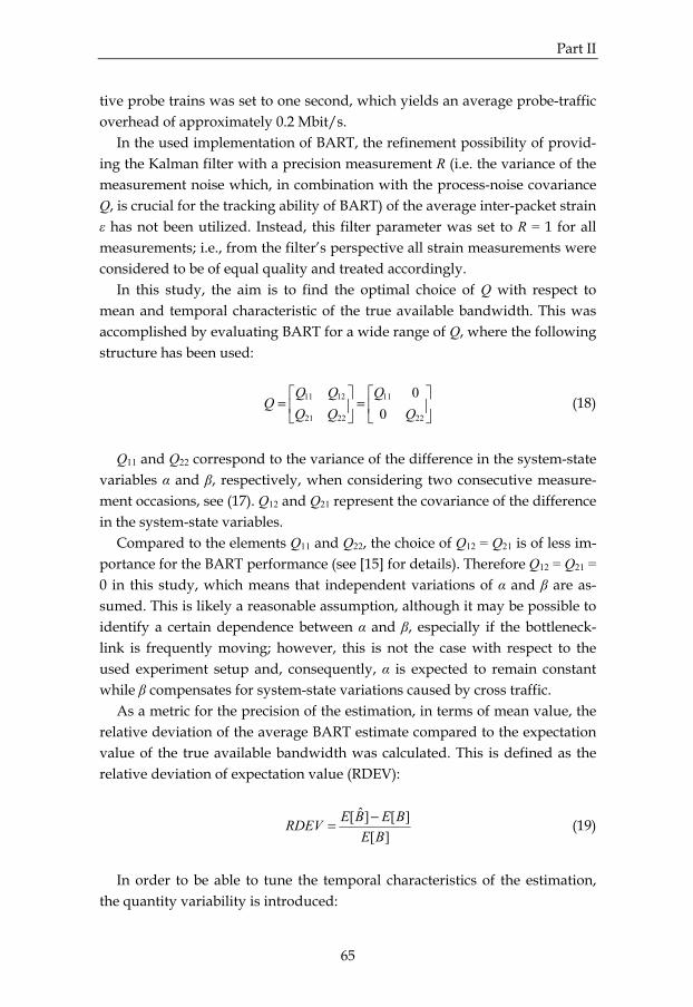
Part II

65

tive probe trains was set to one second, which yields an average probe-traffic overhead of approximately 0.2 Mbit/s. In the used implementation of BART, the refinement possibility of provid-ing the Kalman filter with a precision measurement R (i.e. the variance of the measurement noise which, in combination with the process-noise covariance Q, is crucial for the tracking ability of BART) of the average inter-packet strain ε has not been utilized. Instead, this filter parameter was set to R = 1 for all measurements; i.e., from the filter’s perspective all strain measurements were considered to be of equal quality and treated accordingly. In this study, the aim is to find the optimal choice of Q with respect to mean and temporal characteristic of the true available bandwidth. This was accomplished by evaluating BART for a wide range of Q, where the following structure has been used:

⎥⎦

⎤⎢⎣

⎡=⎥

⎦

⎤⎢⎣

⎡=

22

11

2221

1211

00

QQ

QQQQ

Q (18)

Q11 and Q22 correspond to the variance of the difference in the system-state variables α and β, respectively, when considering two consecutive measure-ment occasions, see (17). Q12 and Q21 represent the covariance of the difference in the system-state variables. Compared to the elements Q11 and Q22, the choice of Q12 = Q21 is of less im-portance for the BART performance (see [15] for details). Therefore Q12 = Q21 = 0 in this study, which means that independent variations of α and β are as-sumed. This is likely a reasonable assumption, although it may be possible to identify a certain dependence between α and β, especially if the bottleneck-link is frequently moving; however, this is not the case with respect to the used experiment setup and, consequently, α is expected to remain constant while β compensates for system-state variations caused by cross traffic. As a metric for the precision of the estimation, in terms of mean value, the relative deviation of the average BART estimate compared to the expectation value of the true available bandwidth was calculated. This is defined as the relative deviation of expectation value (RDEV):

][

][]ˆ[BE

BEBERDEV −= (19)

In order to be able to tune the temporal characteristics of the estimation, the quantity variability is introduced:

Part II

66

{ } { },..., 2312 BBBBVBVyVariabilit k −−=Δ= (20) The variability is defined as the standard deviation of the set of consecutive differences of bandwidth values. For each time resolution Δ, the variability of the available bandwidth is calculated and thereafter compared to the variabil-ity of the BART estimate. The definition of the variability is partly chosen with respect to Q. If the available bandwidth B varies, so does the system-state variables α and β. The variability is based on the variance of the differences ΔB of consecutive band-width measurements (20); the diagonal elements of Q describe the estimated variance of the differences Δα and Δβ (17). Hence, if the variability of the true available bandwidth is known, the BART estimate should be able to repro-duce this characteristic given a suitable Q (since Q relates to the characteristic of the system-state estimate and consequently also the estimate of the avail-able bandwidth). 4 Results Regarding the RDEV precision of the BART estimation, it soon became ap-parent that there is not much to be gained by tuning Q; nor was it possible to identify a clear correlation of the Q configuration and the resulting RDEV. This is illustrated in Figure 3 and Figure 4, where the RDEV in percent is plot-ted against Q22 for three different values of Q11 and for two aggregation levels of the cross traffic. The RDEV observations are in line with previous BART experiments, i.e. the Q configuration mainly affects the fluctuation of the estimate whereas the average typically remains fairly constant. The appearance of the curves in Figure 3 and Figure 4 is essentially inde-pendent of the time resolutions Δ that are considered in this study. This is reasonable, since Δ corresponds to the length of the averaging sliding win-dow that is used for defining the available bandwidth B, of which the average is used for the RDEV calculation. When it is shown that appropriate first-order characteristics of the estima-tion can be achieved, i.e. appropriate precision as measured by the RDEV, a natural next step is to go on to study the feasibility of reproducing higher-order characteristics, such as the temporal structure. This is measured accord-ing to the variability definition (20).

Part II

67

10-6 10-5 10-4 10-3 10-2 10-1 100-10

-8

-6

-4

-2

0

2

4

6

8

10

Q22

RD

EV

[%]

Q11 = 10-1

Q11 = 10-3

Q11 = 10-5

Figure 3. RDEV in percent for the traffic case with the mean of 10 active traffic streams, when varying Q11 and Q22 (Q12 = Q21 = 0).

10-6 10-5 10-4 10-3 10-2 10-1 100-10

-8

-6

-4

-2

0

2

4

6

8

10

Q22

RD

EV

[%]

Q11 = 10-1

Q11 = 10-3

Q11 = 10-5

Figure 4. RDEV in percent for the traffic case with the mean of 100 active traffic streams, when varying Q11 and Q22 (Q12 = Q21 = 0).

Part II

68

For each time resolution Δ = 1, 2, 4, 8, 16, 32, 64, and 128 seconds, the re-gion 10-6 ≤ Q11 ≤ 1 and 10-6 ≤ Q22 ≤ 1 were systematically scanned, using loga-rithmically spaced grid points in both dimensions. Some of the results regard-ing the variability as a function of Q11 and Q22 are shown in Figure 5 and Fig-ure 6. Figure 5 depicts the variability of the available bandwidth versus Q22 for the traffic case corresponding to approximately 10 traffic streams. The hori-zontal lines show the variability of the true available bandwidth at four dif-ferent time resolutions. The true bandwidth does not depend on the estima-tion parameters (this explains the horizontal lines), however, the variability is dependent on the time resolution Δ. For a more fine-grained time resolution, the variability is higher. The other curves show the variability of the BART estimate as a function of Q22 for three different Q11. Provided Q11 is chosen low enough, it can be seen that it is possible to choose Q22 such that the vari-ability of the estimate matches the true variability of the available bandwidth for a wide range of desired time resolutions Δ. This means that it is feasible to tune the method to reproduce the temporal characteristics of the true avail-able bandwidth, by appropriately choosing Q22.

10-6 10-5 10-4 10-3 10-2 10-1 10010-4

10-3

10-2

10-1

100

Q22

Var

iabi

lity

(nor

mal

ized

)

Q11=10-1

Q11=10-3

Q11=10-5

Δ = 2Δ = 8Δ = 32Δ = 128

Figure 5. Variability for the traffic case with approximately 10 active traffic streams, when varying Q11 and Q22 (Q12 = Q21 = 0).

Part II

69

10-6 10-5 10-4 10-3 10-2 10-1 10010-4

10-3

10-2

10-1

100

Q22

Var

iabi

lity

(nor

mal

ized

)

Q11=10-1

Q11=10-3

Q11=10-5

Δ = 2Δ = 8Δ = 32Δ = 128

Figure 6. Variability for the traffic case with approximately 100 active traffic streams, when varying Q11 and Q22 (Q12 = Q21 = 0). Figure 6 shows the same as Figure 5, but for the traffic case corresponding to around 100 traffic streams. When comparing Figure 6 to Figure 5, with re-spect to a particular time resolution Δ, it can be seen that the variability of the available bandwidth is lower, which is sound due to the properties of higher cross-traffic aggregation. Considering Figure 5 and Figure 6, Q11 = 10-5 turns out to be a suitable choice, since this makes it possible to restrict the tuning to Q22 and still obtain a variability of the BART estimate that equals the true available bandwidth for a variety of time resolutions and cross-traffic aggregation levels; this is due to the fact that the bottleneck-link capacity C is constant during these ex-periments, if C varies the optimal Q11 would likely be larger. For this reason, Q11 = 10-5 for the remainder of this investigation. From now on, the analysis concerns the correlation between Q22 and the available-bandwidth variability. Figure 7 depicts the optimum Q22 versus the time resolution Δ, with respect to variability. A power-law behavior can be observed, but with clearly differ-ent proportionality constants for the different aggregation levels. In Figure 8, the variability of the true available bandwidth is plotted versus the time resolution Δ. Again, a power-law behavior can be observed, but with clearly different proportionality constants for the different aggregation levels.

Part II

70

100 101 10210-6

10-5

10-4

10-3

10-2

10-1

100

Time resolution [s]

Q22

~10 traffic streams~100 traffic streams

Figure 7. Optimum Q22 versus time resolution with respect to available-bandwidth variability, for different cross-traffic aggregation levels (Q11 = 10-5, Q12 = 0).

100 101 10210-4

10-3

10-2

10-1

Var

iabi

lity

(nor

mal

ized

)

Time resolution [s]

~10 traffic streams~100 traffic streams

Figure 8. Variability of the true available bandwidth versus time resolution for dif-ferent cross-traffic aggregation levels.

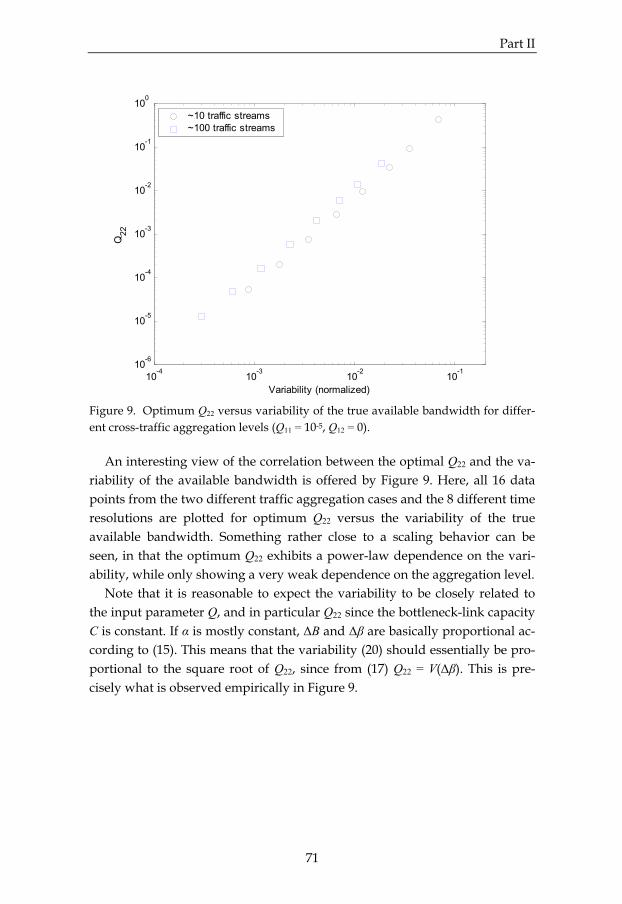
Part II

71

10-4 10-3 10-2 10-110-6

10-5

10-4

10-3

10-2

10-1

100

Variability (normalized)

Q22

~10 traffic streams~100 traffic streams

Figure 9. Optimum Q22 versus variability of the true available bandwidth for differ-ent cross-traffic aggregation levels (Q11 = 10-5, Q12 = 0). An interesting view of the correlation between the optimal Q22 and the va-riability of the available bandwidth is offered by Figure 9. Here, all 16 data points from the two different traffic aggregation cases and the 8 different time resolutions are plotted for optimum Q22 versus the variability of the true available bandwidth. Something rather close to a scaling behavior can be seen, in that the optimum Q22 exhibits a power-law dependence on the vari-ability, while only showing a very weak dependence on the aggregation level. Note that it is reasonable to expect the variability to be closely related to the input parameter Q, and in particular Q22 since the bottleneck-link capacity C is constant. If α is mostly constant, ΔB and Δβ are basically proportional ac-cording to (15). This means that the variability (20) should essentially be pro-portional to the square root of Q22, since from (17) Q22 = V(Δβ). This is pre-cisely what is observed empirically in Figure 9.

Part II

72

0 200 400 600 800 1000 1200 1400 1600 1800 20000

1

2

3

4

5

6

7

8

9

10

Time [s]

Ava

ilabl

e ba

ndw

idth

[Mbi

t/s]

(a)

Available bandwidthBART estimate

850 900 950 1000 1050 1100 11500

1

2

3

4

5

6

7

8

9

10

Time [s]

Ava

ilabl

e ba

ndw

idth

[Mbi

t/s]

(b)

Available bandwidthBART estimate

Figure 10. (a) The BART estimate and the true available bandwidth for the low cross-traffic aggregation case where Δ = 4 seconds. (b) Enlargement of an interval of 300 seconds.

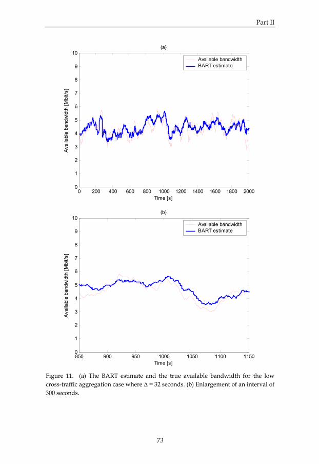
Part II

73

0 200 400 600 800 1000 1200 1400 1600 1800 20000

1

2

3

4

5

6

7

8

9

10

Time [s]

Ava

ilabl

e ba

ndw

idth

[Mbi

t/s]

(a)

Available bandwidthBART estimate

850 900 950 1000 1050 1100 11500

1

2

3

4

5

6

7

8

9

10

Time [s]

Ava

ilabl

e ba

ndw

idth

[Mbi

t/s]

(b)

Available bandwidthBART estimate

Figure 11. (a) The BART estimate and the true available bandwidth for the low cross-traffic aggregation case where Δ = 32 seconds. (b) Enlargement of an interval of 300 seconds.

Part II

74

0 200 400 600 800 1000 1200 1400 1600 1800 20000

1

2

3

4

5

6

7

8

9

10

Time [s]

Ava

ilabl

e ba

ndw

idth

[Mbi

t/s]

(a)

Available bandwidthBART estimate

850 900 950 1000 1050 1100 11500

1

2

3

4

5

6

7

8

9

10

Time [s]

Ava

ilabl

e ba

ndw

idth

[Mbi

t/s]

(b)

Available bandwidthBART estimate

Figure 12. (a) The BART estimate and the true available bandwidth for the high cross-traffic aggregation case where Δ = 32 seconds. (b) Enlargement of an interval of 300 seconds.

Part II

75

In Figure 10 and Figure 11, the resulting BART tracking of the available bandwidth in the case of around 10 traffic streams can be compared to the true available bandwidth for the time resolutions Δ = 4 seconds and Δ = 32 seconds, respectively. Note that the true available bandwidth is exactly the same in both figures; it is only averaged over different time resolutions. The only difference in the BART configuration for the two cases (Δ = 4 seconds and Δ = 32 seconds) is that Q22 has been set to the optimal value for each time resolution, with respect to the variability. In Figure 12, the same time resolu-tion is used as in Figure 11 (Δ = 32 seconds) whereas the cross-traffic aggrega-tion is changed from approximately 10 to 100 traffic streams. This causes a lower variability of the available bandwidth and consequently a smaller val-ue for the optimal Q22. 5 Discussion and Conclusions The purpose of this study is to examine how the BART method may be con-figured with respect to tracking ability. In the performed experiments, the case of a continuously alternating system state has been considered, where available-bandwidth variations are dependent on cross-traffic aggregation and the used time resolution Δ for describing bandwidth. The tuning possi-bilities of BART have been limited to one filter parameter, namely the proc-ess-noise covariance Q which is a 2×2 matrix. With regard to the performed measurements where the bottleneck-link capacity was constant but the cross traffic was varying, it turned out that it is feasible to limit the tuning of the BART tracking properties to one particular element in Q, given a specific and static configuration of the other elements. The optimal choice of this filter parameter was seen to be dependent on both the cross-traffic aggregation and the time resolution Δ. The precision of the BART estimation in terms of mean value and variabil-ity was compared to the true available bandwidth for several traffic configu-rations and choices of Δ. In particular, the Q elements Q11 and Q22 were con-sidered in the BART performance analysis. Tuning of Q12 = Q21 has also been examined, but this choice seems to be of less importance for the overall BART performance and from a theoretical point of view it is often reasonable to choose Q12 = Q21 = 0 since this means independent variations of the BART sys-tem-state variables, which generally is a sound assumption. From the experiments it could be seen that the choice of Q mainly influ-ences the variability of BART, whereas the average value of the estimates is

Part II

76

less affected. Hence, if it is only necessary to obtain appropriate first-order characteristics of the BART estimation, the cross-traffic properties and time resolution as well as the choice of Q11 and Q22 are rather insignificant. How-ever, this is not the case when accurate real-time tracking of the available bandwidth is desired for various network topologies and traffic scenarios. A specific variability measure was suggested and used, in order to be able to describe bandwidth fluctuations and to examine the feasibility to tune BART such that the characteristics of generated available-bandwidth esti-mates agree with the true available bandwidth. With respect to the configuration of the experiments and the used variabil-ity measure, it turned out that as long as Q11 is small enough, Q22 is the crucial element when tuning Q. The recommendation is to assign Q11 to a constant and small value (Q11 = 10-5 was chosen in this study). Setting Q11 exactly equal to zero does not work well. The behavior of the filter would be too dependent on the choice of the initial system-state estimate and error covariance matrix (see the Kalman-filter equations). Also, the filter would probably perform poorly in case of a change in the bottleneck-link capacity. Consequently, it is better to allow for some uncertainty by choosing a small nonzero value for Q11. Provided Q11 is given a small value, it is possible to obtain a large range of variabilities of the BART estimate by simply tuning Q22. The optimal Q22 de-creases as the variability of the true available bandwidth decreases (i.e. Q22 decreases with increasing time resolution Δ and cross-traffic aggregation). Also, from Figure 9, it appears that, when fitted to a power-law behavior, the optimal Q22 roughly scales with the variability, with an exponent of 2 (which is reasonable with regard to the definition of Q and the chosen variability measure). Overall, the experimental results are consistent with what might be ex-pected: • Q11 should be small (cf. the discussion in Section 2.2.1). • For rapid response to new measurements, which is needed for tracking at

high variability, Q22 should be large. For a more stable tracking, suitable for low variability, Q22 should be small (cf. the argument in the end of Sec-tion 2.1).

In conclusion, it has been shown that it is feasible to tune the BART filter-based estimation method for enhanced tracking performance at desired avail-able-bandwidth variability, by choosing the input parameter Q appropriately.

Part II

77

However, it should be noted that it is reasonable to expect that the above rec-ommendations regarding Q11 and Q22 could be different in case of network and traffic scenarios that clearly differ from the chosen experiments in this study. For example, given a network path where available-bandwidth fluc-tuations mainly occur due to a frequently changing bottleneck-link capacity, which typically could be the case for a wireless link, the configuration of Q11 and Q22 should likely be the other way around (i.e. when adjusting the BART tracking characteristics, Q11 is the important parameter whereas Q22 should be assigned a small and constant value). References [1] E. Bergfeldt, S. Ekelin, and J. M. Karlsson, “Real-time available-

bandwidth estimation using filtering and change detection,” Computer Networks, vol. 53, 2009.

[2] R. S. Prasad, M. Murray, C. Dovrolis, and K. Claffy, “Bandwidth estima-tion: metrics, measurement techniques, and tools,” IEEE Network, vol. 17, 2003.

[3] G. Welch and G. Bishop, “An introduction to the Kalman filter,” SIG-GRAPH, Course 8, 2001.

[4] J. Navratil and R. L. Cottrell, “Abwe: a practical approach to available bandwidth estimation,” in Proc. Passive and Active Measurement Work-shop, 2003.

[5] R. Carter and M. Crovella, “Measuring bottleneck link speed in packet-switched networks,” Technical Report BU-CS-96-006, Boston University, 1996.

[6] N. Hu and P. Steenkiste, “Evaluation and characterization of available bandwidth probing techniques,” IEEE JSAC Internet and WWW Meas-urement, Mapping, and Modeling, vol. 21, 2003.

[7] V. Ribeiro, R. Riedi, R. Baraniuk, J. Navratil, and L. Cottrell, “pathChirp: efficient available bandwidth estimation for network paths,” in Proc. Passive and Active Measurement Workshop, 2003.

[8] G. Jin, G. Yang, B. R. Crowley, and D. A. Agarwal, “Network characteri-zation service (NCS),” Lawrence Berkley National Lab Report 47892, 2001.

[9] M. Jain and C. Dovrolis, “Pathload: a measurement tool for end-to-end available bandwidth,” in Proc. Passive and Active Measurement Workshop, 2002.

Part II

78

[10] J. Strauss, D. Katabi, and F. Kaashoek, “A measurement study of avail-able bandwidth estimation tools,” in Proc. ACM SIGCOMM Internet Measurement Conference, 2003.

[11] B. Melander, M. Björkman, and P. Gunningberg, “A new end-to-end probing and analysis method for estimating bandwidth bottlenecks,” in Proc. IEEE GLOBECOM’00, 2000.

[12] F. Montesino-Pouzols, “Comparative analysis of active bandwidth esti-mation tools,” in Proc. Passive and Active Measurement Workshop, 2004.

[13] A. Shriram, M. Murray, Y. Hyun, N. Brownlee, A. Broido, M. Fo-menkov, K. Claffy, “Comparison of public end-to-end bandwidth esti-mation tools on high-speed links,” in Proc. Passive and Active Measure-ment Workshop, 2005.

[14] S. Keshav, “A control-theoretic approach to flow control,” ACM SIG-COMM Computer Communication Review, vol. 21, 1991.

[15] E. Hartikainen and S. Ekelin, “Tuning the temporal characteristics of a Kalman-filter method for end-to-end bandwidth estimation,” in Proc. 4th IEEE/IFIP Workshop on End-to-End Monitoring Techniques and Services, 2006.

[16] G. James, Advanced Modern Engineering Mathematics. Addison-Wesley, 1999.

[17] E. Bergfeldt, S. Ekelin, and J. M. Karlsson, “Bandwidth estimation over a high-speed downlink shared channel in UMTS,” in Proc. Nordic Confer-ence on Radio Science and Communications, 2008.

[18] E. Dahlman, S. Parkvall, J. Sköld, and P. Beming, 3G Evolution: HSPA and LTE for Mobile Broadband. Academic Press, 2007.

[19] H. Holma and A. Toskala, HSDPA/HSUPA for UMTS: High Speed Radio Access for Mobile Communications. John Wiley & Sons, 2006.

[20] E. Hartikainen, S. Ekelin, and J. M. Karlsson, “Adjustment of the BART Kalman filter to improve real-time estimation of end-to-end available bandwidth,” in Proc. Swedish National Computer Networking Workshop, 2005.

[21] S. Ekelin, M. Nilsson, E. Hartikainen, A. Johnsson, J.-E. Mångs, B. Me-lander, M. Björkman, “Real-time measurement of end-to-end available bandwidth using Kalman filtering,” in Proc. IEEE/IFIP Network Opera-tions and Management Symposium, 2006.

[22] E. Hartikainen and S. Ekelin, “Enhanced network-state estimation using change detection,” in Proc. 31st IEEE Conference on Local Computer Net-works, 2006.

Part II

79

[23] E. Hartikainen, S. Ekelin, and J. M. Karlsson, “Change detection and es-timation for network-measurement applications,” in Proc. 2nd ACM Workshop on Performance Monitoring and Measurement of Heterogeneous Wireless and Wired Networks, 2007.

80

81

Part III Change Detection for Filter-Based Available-Bandwidth Estimation Abstract This part of the thesis presents the concept of change detection for filter-based network-state estimation. This can be of benefit in various contexts, e.g. in network management and adaptive streaming applications. In particular, it is shown that the performance of available-bandwidth estimation can be signifi-cantly enhanced by employing change detection in conjunction with a filter-based estimator. The use of filtering makes it feasible to track the communica-tion network state and to estimate selected properties in real-time. In addi-tion, filter-based methods may be combined with change detection in order to overcome the trade-off regarding stable estimation versus speed of adapta-tion to change. This part discusses filtering and change detection in general, and presents the novel approach of combining the filter-based available-bandwidth estimator BART with two different change-detection techniques, the light-weight Cumulative Sum (CUSUM) test and the more complex Gen-eralized Likelihood Ratio (GLR) test.

Part III

82

1 Introduction 1.1 Overview In recent years, there has been a strong interest in the field of network meas-urements. The use of communication networks, as well as their misuse, be-come increasingly more complex, which motivates the development of tools for providing network operators and applications with comprehensive in-formation regarding fault diagnosis, performance tuning, network monitor-ing etc. In order to achieve and maintain good network performance, decisions and actions need to be based upon accurate and reliable information, prefera-bly obtained in real-time. However, the performance of tools used for this purpose typically is configuration-dependent. It would be desirable if the tools could be reconfigured automatically in response to sudden changes of the network state. One interesting area within network measurements is bandwidth monitor-ing. There exist several tools for estimating the end-to-end available band-width along network paths, which can be useful for surveillance and adapta-tion of network-traffic flows with regard to the unutilized capacity. However, due to the dynamic and time dependent characteristics of network traffic, it is a challenge to always deliver high-quality estimates, as the network state can be subject to both fast and slow variations of different magnitudes. As a possible way of accomplishing continuous available-bandwidth moni-toring of a path in packet-switched communication networks, a filter-based approach BART (Bandwidth Available in Real-Time) has been suggested [1]. BART uses active probing and Kalman filtering in order to maintain and up-date an estimate of the current available bandwidth. Using BART with a static configuration limits the range of system-state variability where estimation performance is accurate, just as for many other statistical estimation tools. In addition, it is generally hard to know the true state variability beforehand and there is often no guarantee that it will remain constant. In many cases, the state variability can be assumed to be fairly con-stant and low for most of the time. However, transiently and unpredictably the variability becomes larger when there is a change of the system state, such as a sudden increase or decrease of the available bandwidth. The weakness of a static configuration often manifests as either fluctuating estimates when the system state is rather stable or as slow adaptation in case of abrupt system-state changes, depending on the choice of fixed estimator tuning.

Part III

83

In order to obtain filter-based tools featuring both fast adaptation to changes and stable estimation in the normal case of slowly changing or sta-tionary system state, change detection may be used. A change-detection tech-nique has the ability of testing the hypothesis that a change has occurred ver-sus the null hypothesis that a change has not occurred in the system state. Hence, it is appropriate to tune the filter for stability by default, and adjust for agile adaptation only when the change-detection test indicates a change. Sudden link failures causing re-routing, rapidly changing characteristics of wireless links, and various types of network attacks are examples of events that could abruptly influence the available-bandwidth situation, and proba-bly also other network properties. As will be shown in the forthcoming sec-tions, the performance of BART can be significantly improved in such situa-tions, when assisted by a change detector. Although the reasoning is exemplified with available-bandwidth experi-ments, it is reasonable to believe that filter-based estimation and change de-tection could be useful for many other applications within computer net-working, especially when reliable and accurate real-time estimation is re-quired. 1.2 Related Work Besides BART [1], several other alternatives exist for measuring the available bandwidth in packet-switched networks, e.g. [2-9]. These tools are not filter based, and the majority do not have the capability of providing real-time es-timates. Regarding change detection for filter-based tools, a number of techniques have been proposed, e.g. [10-14]. A comparative study on change-detection techniques for automotive applications has been presented in [15]. In computer networking, change detection together with a filter-based es-timator has been used in [16] for estimation of round-trip time for use in con-gestion control. This study focuses on the problem of accurately estimating the available bandwidth in networks with irregular characteristics. It is shown that the novel approach of combining a filter-based available-bandwidth estimator with change detection enables accurate real-time estimation although the bandwidth can be subject to both fast and slow fluctuations. The content of the following sections is mainly based on [17, 18].

Part III

84

2 Background 2.1 Filter Methods In a filter-based approach, the state of a system is estimated from repeated measurements of some quantity dependent on the system state. This requires models of how the system state evolves from one measurement occasion to the next, and of how the measured quantity depends on the system state. The system equations can be expressed as 11)( −− += kkk wxfx (1) kkk vxhz += )( (2) where x is the state of the system, z is the measured quantity, w is the process noise and v is the measurement noise. The functions f and h represent the sys-tem-evolution model and the measurement model, respectively. The sub-scripts refer to discrete time. A filter is a procedure which takes a previous estimate 1ˆ −kx and a new measurement zk as input, and calculates a new estimate .ˆkx A compelling property of filters is that they are capable of producing estimates in real-time, i.e. tracking the system state. For each new measurement, the previous esti-mate is updated. If the functions f and h are linear, and if both the process noise and the measurement noise are Gaussian and uncorrelated, there is an optimal filter, namely the Kalman filter [19]. In this linear case the system equations (1) and (2) can be expressed using matrices: 11 −− += kkk wAxx (3) kkkk vxHz += (4) From the previous estimate and the new measurement, the Kalman filter eq-uations allow estimation of the system state x and the error covariance matrix P as: kkkkkkkkk KxxHzKxx γ+=−+= −−− ˆ)ˆ(ˆˆ (5) −−= kkkk PHKIP )( (6)

Part III

85

where 1ˆˆ −

− = kk xAx (7) QAAPP T

kk += −−

1 (8) and .)( 11 −−−−− =+= k

Tkk

Tkkk

Tkkk VHPRHPHHPK (9)

For details, see [19]. Kalman filtering can be understood as an iterative process where each step consists of two phases of calculation. First, there is a prediction phase, where the previous estimate evolves one discrete time step according to the system model (7). Then, there is a correction phase, where the new measurement is taken into account (5); one also computes the updated error covariance matrix Pk of the state estimate (6). The difference −− kkk xHz ˆ in (5) is known as the residual (or innovation) γk, which is essential in the correction phase. The residual reflects the deviation of the actual measurement from what is predicted according to the measure-ment model and the evolved state estimate. The Kalman gain Kk, given by (9) and appearing in (5) and (6), can be in-terpreted as the relative weight given to the new measurement as opposed to the pure expected evolution of the previous estimate. As can be seen from (8) and (9), the Kalman gain increases as either Q increases or R decreases; these required inputs to the Kalman filter are the covariances of the process noise w and measurement noise v, respectively. An intuitive understanding of the importance of these quantities may be acquired by the following arguments: • Large variations of the noise in the system model (large Q) imply that the

prediction according to the system model is likely to be less accurate, and the new measurement should be weighted heavier.

• Large variations in the measurement noise (large R) imply that the new measurement is likely to be less accurate, and the prediction according to the system model should be weighted heavier.

Part III

86

2.2 The BART Method The BART method for available-bandwidth estimation [1] makes use of active probing and Kalman filtering. Updated estimates are produced based on probe-packet measurements, which are performed at randomized probe-traffic intensities in order to improve the statistical estimation properties. Each measurement is carried out by transmitting a sequence of pairs of pack-ets, which are time-stamped on departure and on arrival. The average relative increase from sender to receiver in the packet-pair time separation is used as the measured quantity z, also referred to as the inter-packet separation strain ε. In a simple fluid-traffic, first-come-first-served network model [9], the ex-pectation value of ε is zero when the probing intensity u is less than the avail-able bandwidth B, and grows in proportion to the overload when the probing intensity is larger (this is described by a sloping straight line with the parame-ters α and β):

⎩⎨⎧

>≤

+=−=

)()(

)( 0

BuBu

uBu βααε (10)

For details regarding the definition of available bandwidth, see [1, 20].

0

Probe-traffic intensity (u)

Inte

r-pac

ket s

train

( ε)

Available bandwidth

Figure 1. Based on measurements of the inter-packet separation strain and the inten-sity of the probe traffic, it is feasible to estimate the available bandwidth.

Part III

87

It should be noted that the Kalman filter is rather robust, and good results are often produced even when the ideal conditions are slightly broken [19]. So, even if a real system displays characteristics which deviate somewhat from the piecewise linear system curve (see (10) and Figure 1), the resulting available-bandwidth estimate is not automatically invalidated. The model (10) allows for application of a Kalman filter in the overload region, when the state of the system is represented by a vector containing the two parameters of the sloping straight line:

⎥⎦

⎤⎢⎣

⎡=

βα

x (11)

This makes it feasible to express the measurement zk ≡ εk of the strain at dis-crete time k as kkkk vxHz += (12) where ].1[ kk uH = (13) In the BART method, the evolution of the system state is defined as 11 −− += kkk wxx (14) which means that the Kalman filter formalism may be applied with A = I (the identity matrix). When the filter estimates the system-state variables α and β an estimate of the available bandwidth B, which corresponds to the break point in the piecewise linear curve in Figure 1, is immediately obtained. For more details regarding the BART method, see [1]. 3 Problem – Stability versus Agility When dealing with dynamic systems, a static configuration of statistical mea-surement tools typically cannot optimally deal with both slowly changing conditions and rapid fluctuations. A tool configured for stability will suffer in case of sudden changes in the system state, due to slow adaptation. A tool

Part III

88

with agile properties delivers fluctuating estimates in a steady-state situation, due to the measurement noise. As an illustration, consider Figure 2 where the available-bandwidth meas-urement tool BART estimates the unutilized capacity of a network path. The dotted curve corresponds to a high-agility configuration. This is accom-plished by choosing a large process-noise covariance Q. It is obvious that BART easily follows the sudden changes in the available bandwidth (which occur after 750 and 1250 seconds, respectively), whereas the precision of the estimates leaves a great deal to be desired due to amplification of the meas-urement noise. The dashed curve corresponds to an opposite configuration aimed for high stability. Here, it can be seen that BART is insensitive to the measurement noise and delivers stable and reliable estimates in the interval from 0 to 750 seconds. However, the configuration does not allow for fast ad-aptation, which is obvious when considering the estimates after 750 seconds where BART is very slow in adapting to the new system state.

0 200 400 600 800 1000 1200 1400 1600 1800 20000

1

2

3

4

5

6

7

8

9

10

Time [s]

Ava

ilabl

e ba

ndw

idth

[Mbi

t/s]

Available bandwidthBART estimate (agility)BART estimate (stability)

Figure 2. BART estimation of the available bandwidth using two configurations of Q, for different tracking ability. The available bandwidth changes abruptly after 750 and 1250 seconds. The BART configurations used in Figure 2 can be seen as two rather ex-treme choices (it is of course possible to choose Q such that the estimates be-come something in between the two curves). The figure is mainly to illustrate

Part III

89

the trade-off between having stable but slowly adapting estimates and agile but noise-sensitive estimation properties. 4 Method There are solutions to the problem described in Section 3. In the area of sys-tem identification using filter-based estimation methods, these solutions are often referred to as adaptive control and change detection (also known as fault detection). In the following subsections, change detection will be introduced and ex-emplified by two different algorithms. In Section 5, it is explained how these algorithms can be integrated with BART, for estimating available bandwidth. 4.1 Change Detection There is a number of existing filter-based methods available for detecting ab-rupt changes in dynamic systems, e.g. [10-14]. These methods can, in general, be divided into three classes: methods using one filter, where a whiteness test is applied to observed filter residuals γ; methods using two filters, where a slow filter configured for stability runs in parallel with a fast filter configured for agility; methods using multiple filters, where each filter configuration is matched to a particular assumption regarding the abrupt change. For more information regarding these techniques and change detection in general, see [21]. There is a trade-off in complexity versus performance when comparing different change-detection techniques; generally, the more complex algo-rithm, the better result is obtained [15]. The computational complexity is often proportional to the number of filters required by the algorithm. A simple and intuitive technique is known as the Cumulative Sum (CUSUM) test [10, 21], which only uses one filter in order to make decisions regarding the hypothe-ses of change or no change in the system. This can be compared to, e.g., the full Generalized Likelihood Ratio (GLR) test [13, 21], where the number of required filters (and thus also the complexity) grows linearly with time. When using change detection, it is normally assumed that abrupt changes occur infrequently. Hence, it is sound to implement a filter (e.g. a Kalman filter) with respect to a basic model based on the assumption of no abrupt changes, and to design a secondary system that monitors the residuals of the

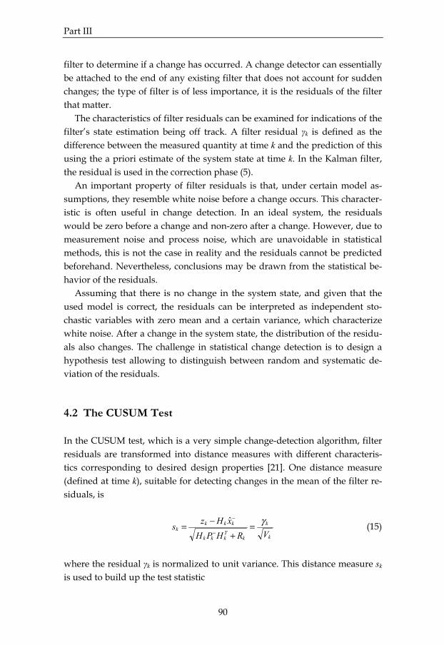
Part III

90

filter to determine if a change has occurred. A change detector can essentially be attached to the end of any existing filter that does not account for sudden changes; the type of filter is of less importance, it is the residuals of the filter that matter. The characteristics of filter residuals can be examined for indications of the filter’s state estimation being off track. A filter residual γk is defined as the difference between the measured quantity at time k and the prediction of this using the a priori estimate of the system state at time k. In the Kalman filter, the residual is used in the correction phase (5). An important property of filter residuals is that, under certain model as-sumptions, they resemble white noise before a change occurs. This character-istic is often useful in change detection. In an ideal system, the residuals would be zero before a change and non-zero after a change. However, due to measurement noise and process noise, which are unavoidable in statistical methods, this is not the case in reality and the residuals cannot be predicted beforehand. Nevertheless, conclusions may be drawn from the statistical be-havior of the residuals. Assuming that there is no change in the system state, and given that the used model is correct, the residuals can be interpreted as independent sto-chastic variables with zero mean and a certain variance, which characterize white noise. After a change in the system state, the distribution of the residu-als also changes. The challenge in statistical change detection is to design a hypothesis test allowing to distinguish between random and systematic de-viation of the residuals. 4.2 The CUSUM Test In the CUSUM test, which is a very simple change-detection algorithm, filter residuals are transformed into distance measures with different characteris-tics corresponding to desired design properties [21]. One distance measure (defined at time k), suitable for detecting changes in the mean of the filter re-siduals, is

k

k

kTkkk

kkkk

VRHPHxHzs γ=+

−=−

−ˆ (15)

where the residual γk is normalized to unit variance. This distance measure sk is used to build up the test statistic

Part III

91

)0 ,max( 1 υ−+= − kkk sgg (16) which is used to decide whether the residuals are reflecting a positive trend (i.e. the predictions of the filter are systematically underestimating the meas-ured quantity). The design parameter υ is used to allow for a slowly varying system state; υ is also referred to as the drift parameter. Once the value of the test statistic g exceeds the design threshold h, the CUSUM test supplies the filter with an alarm indication, such that an appro-priate action can be performed with respect to the change. The parameters h and υ are further discussed in Section 5.2. Figure 3 illustrates the basic structure of the CUSUM test.

Figure 3. A filter based on the assumption of no abrupt change may be comple-mented by the CUSUM test which monitors the residuals of the filter in order to de-termine whether a change has occurred or not. A suitable filter action when receiving a change-detection alarm is to mo-mentarily increase the process-noise covariance Q. By doing this, the filter gain becomes larger and the received measurements will be given more weight (as compared to the expected evolution of the previous estimate) when the system-state estimate is updated and, consequently, the filter im-proves the response to variations in the system. 4.3 The GLR Test As for the CUSUM test, the GLR change-detection technique makes use of filter residuals in order to build up a predefined test statistic which is recalcu-lated for each new filter iteration, and if the test statistic exceeds a specified threshold h the GLR test generates an alarm. However, unlike the majority of the available change detectors, the GLR test also estimates both the time and magnitude of the change causing the alarm; this information can be useful in order to achieve fast and smooth adaptation, but also for analyzing the reason of a particular change.

Part III

92

In order to calculate the test statistic, the GLR test makes use of a bank of parallel filters where each filter is matched to a certain assumption regarding the change time, see Figure 4. The GLR detector is a test of the hypothesis of no change against the hy-pothesis that a change of magnitude η occurred at time θ. Based on the ob-tained residuals γ, the likelihoods of these hypotheses are used in a likeli-hood-ratio test, which is a multiple test where different change hypotheses are pairwise compared to the no-change hypothesis. The hypotheses may be denoted as H0 and H1(θ,η), which represent the hypothesis of no change and the hypothesis that a change of magnitude η occurred at time θ, respectively. In the likelihood-ratio test, the change time and the magnitude of the change are replaced by their maximum likelihood estimates, since the true θ and η are typically unknown.

Figure 4. A filter based on the assumption of no abrupt change may be comple-mented by the GLR test which monitors the residuals of the filter in order to deter-mine whether a change has occurred or not. The log-likelihood ratio compared to the threshold h at time k can be ex-pressed as

)|,...,(

)ˆ,ˆ,|,...,(log2)ˆ,(01

11

HpHpkl

k

kkkk γγ

ηηθθγγθ ==⋅= (17)

Part III

93

where p denotes the probability density function and kθ̂ and kη̂ are the max-imum likelihood estimates of θ and η under the hypothesis H1, i.e.: )~,~,|,...,(maxarg

)~,~()ˆ,ˆ( 11 ηηθθγγ

ηθηθ === Hp kkk (18)

Despite the complexity of the GLR test, the maximum test statistic (17) may be obtained in a pleasant and recursive manner as ),(),(),(),(maxarg)ˆ,( 1 θθθθ

θθ kdkCkdkl

kkl T

k−=

≤= (19)

where ),1(),(),( 1 θγθθ −+= − kdVkGkd kk

T (20) ),1(),(),(),( 1 θθθθ −+= − kCkGVkGkC k

T (21) and )],1()1,(),([),( θθθ −−−= kFkkAkAHkG k (22) . ),1()1,(),(),( θθθ −−+= kFkkAkGKkF k (23) The above equations are computed for all considered change times θ < k. In addition, the following calculations are made for θ = k: kk

Tk VHkkd γ1),( −= (24)

kk

Tk HVHkkC 1),( −= (25)

kk HKkkF =),( (26) Regarding the above variables, l(k,θ) is the test statistic at time k given the assumption that a change occurred at time θ. d(k,θ) is a linear combination of the residuals from time θ to k. C(k,θ) is known as the change-information ma-trix, and its inverse corresponds to the error covariance of the maximum like-lihood estimate of the true change η. G(k,θ) describes the effect on the residual at time k given a sudden change η at time θ. F(k,θ) is used to explain how a

Part III

94

change η at time θ influences the system-state estimate at time k. A is the state transition matrix, where A(k,θ) = A(k-1)·A(k-2)·…·A(θ). Regarding the other variables, the reader is referred to the previous description of the Kalman fil-ter in Section 2. The maximum test statistic (19) is compared to the threshold h in order to determine whether a change has taken place or not. If the test statistic exceeds the threshold, the most likely magnitude of the change is estimated as: )ˆ,()ˆ,(ˆ 1

kkk kdkC θθη −= (27) When the GLR test deems that a change has occurred, the system-state es-timating filter may be adjusted using at least three different approaches. One can transiently increase the process-noise covariance Q (as suggested for the CUSUM test), which in turn increases the error covariance P and, conse-quently, the filter becomes more agile. Another possibility is to use the GLR change estimates of θ and η to provide instant compensation to the filter’s state estimate. However, especially the GLR estimate of η may be rather inac-curate. A third approach is to combine these two, thereby reducing the de-pendence on the potentially inaccurate GLR estimate. The instant compensation of the system state can be achieved by updating x̂ as [13]: kkk

oldk

newk kFkAxx ηθθ ˆ)]ˆ,()ˆ,([ˆˆ −+= (28)

The corresponding error covariance of the state estimate may be updated as:

)]ˆ,()ˆ,()[ˆ,(

)]ˆ,()ˆ,([1

kkk

kkold

knew

k

kFkAkC

kFkAPP

θθθθθ

−⋅

⋅−+=−

(29)

For more details regarding the GLR detector, see [13, 21]. 5 Experiments In order to evaluate the performance of BART when applying change detec-tion, several experiments have been performed in a controlled laboratory network. Additional measurements have also been carried out over an Inter-net path, but these are not presented in this study, see [1, 17] for details.

Part III

95

5.1 Experiment Setup In the laboratory network, a testbed consisting of two Extreme Summit rou-ters has been used, see Figure 5. Several traffic cases have been considered, including different cross-traffic aggregation levels, statistical distributions of the inter-packet arrival times, and magnitude of changes. However, for the scope of this study and for clarity, the illustrations of the results are limited to one particular cross-traffic case. General conclusions drawn from this sce-nario are applicable to all other cases that have been under consideration. The chosen cross-traffic case emulates a scenario with approximately 100 simultaneously active traffic streams, which transmit UDP packets1 with in-ter-arrival times following a Pareto distribution (shape parameter = 1.9). New connections arrive according to a Poisson process and remain active accord-ing to a Pareto distribution (shape parameter = 1.5, mean = 1.0 second). The cross-traffic generator (which is the Ericsson proprietary tool IPTrafGen) is configured such that all active connections utilize (on average) an equal and predetermined amount of the bandwidth capacity.

Figure 5. An illustration of the testbed setup used in the evaluation of BART with change detection. In order to construct abrupt changes in the available bandwidth, a second instance of the same cross-traffic scenario suddenly affects the monitored path for a duration of 500 seconds. This additional traffic flow has statistical properties as described above, except that the traffic intensity for each stream is somewhat higher in order to make the change in the system state more evi-dent. By abruptly adding 100 new traffic streams along the path, the available bandwidth will instantaneously decrease. A similar effect could occur in a

1 The distribution of the cross-traffic packet sizes roughly corresponds to observations from Sprint: https://ipmon.sprintlabs.com/packstat/packetoverview.php (October 2010)

Part III

96

real network in case of, e.g., a computer-network attack or a nearby link fail-ure (causing re-routing of the traffic). The true cross traffic was recorded using the standard tool tcpdump, while the probe-traffic receiver host recorded the series of strain measurements zk. Based upon the recorded cross traffic, the true available bandwidth could be calculated by subtracting the cross-traffic intensity from the bottleneck-link capacity (which was known due to the setup). The cross-traffic intensity was obtained by averaging the content of the cross-traffic traces, using a sliding window with averaging time scale Δ = 4 seconds. The true available band-width for this traffic case is depicted in Figure 2. For all experiments in this study, BART has been configured to transmit sequences of 1500-byte probe packets, organized as trains of 17 packets (16 pairs). The traffic intensity for each probe train was randomly chosen using a uniform distribution from 1 Mbit/s to 20 Mbit/s. The inter-departure time between two consecutive probe trains was set to one second, which yields an average probe-traffic overhead of 0.2 Mbit/s. In the used implementation of BART, the refinement possibility of provid-ing the Kalman filter with a precision measurement R of the strain ε has not been used. Instead, this filter input parameter was set to R = 1 for all meas-urements, i.e. from the filter’s perspective all strain measurements were con-sidered to be of equal quality and treated accordingly. Regarding the process-noise covariance parameter Q, which is crucial for the tracking ability of BART, the following simple form has been used:

⎥⎦

⎤⎢⎣

⎡=⋅=⎥

⎦

⎤⎢⎣

⎡=

λλ

λ0

02221

1211 IQQQQ

Q (30)

It should be noted that Q, which is a symmetric matrix, has three degrees of freedom and Q11 and Q22 do not necessarily have to be equal; however, since rather accurate estimation can be achieved without exploiting the full potential of Q, there is no compelling reason for the purposes of the present study to increase the complexity by tuning each element separately. For a more detailed discussion regarding Q in BART, see [1, 22]. In the performed experiments, the used Q differs depending on desired characteristics of the BART estimation. Unless a change has been detected λ = 10-5. In case a change-detection alarm is generated, BART is momentarily provided with another Q configuration, denoted as Qalarm. In Section 5.2 and 5.3 it is specified how λ is chosen when Qalarm is used.

Part III

97

5.2 BART with the CUSUM Test 5.2.1 Test Statistics and Design Parameters BART has been implemented and evaluated with the CUSUM change-detection technique. Since the residual of the Kalman filter can be both posi-tive and negative, it is recommended to use a two-sided CUSUM test. Hence, at time k, the positive and negative test statistics are computed as )0 ,max( 1 υ−+= − k

posk

posk sgg (31)

and )0 ,min( 1 υ++= − k

negk

negk sgg (32)

where g0 = 0. For each discrete time step, the test statistics are re-calculated and com-pared to the chosen design threshold h. If the threshold is exceeded, the CU-SUM test is re-initialized (by setting the test statistics to zero) and an alarm indication is sent to the Kalman filter, which is responsible to react appropri-ately to compensate for the change. The other design parameter υ, the drift, can be seen as an indicator for what is expected to be random deviations between the measurements and the predictions. If the distance measure (15) is smaller than the drift parameter υ, the observed residual will be interpreted as a normal statistical fluctuation and, consequently, not contribute to a larger test statistic. The choice of design parameters h and υ affect the performance of the change detector, especially in terms of the false alarm rate (FAR) and the mean time to detection (MTD). It should be noted that h and υ do not necessarily have to be equal for the positive and the negative CUSUM test. However, for the purpose of this study there is no compelling reason for allowing them to differ (i.e., hpos, hneg, υpos, υneg could be different, but in this investigation hpos = hneg and υpos = υneg). When running BART (configured for stability) without change detection, the estimates in case of abrupt changes can appear as illustrated by the dashed curve in Figure 2. It is obvious that BART is not responding promptly when rapid changes occur in the system, due to its configuration for stability. When running BART (configured for stability) with CUSUM for the sce-nario in Figure 2, and the design threshold h = ∞ (i.e., no alarm will ever oc-

Part III

98

cur), the positive and negative test statistics behave as in Figure 6, using dif-ferent settings of the drift parameter υ.

0 200 400 600 800 1000 1200 1400 1600 1800 2000

-100

-50

0

50

100

Test

sta

tistic

Time [s]

Positive: υ = 0.025Negative: υ = 0.025Positive: υ = 0.05Negative: υ = 0.05Positive: υ = 0.1Negative: υ = 0.1Positive: υ = 0.2Negative: υ = 0.2

Figure 6. The CUSUM test statistic (both positive and negative) for different υ when BART (configured for stability) is exposed to abrupt changes in the system, accord-ing to Figure 2. It is clear that the positive test statistic (solid curves) starts to increase after 750 seconds, due to the sudden drop in the available bandwidth. The test sta-tistic behaves differently with respect to the chosen drift parameter υ; larger υ requires larger residuals in order to increase the test statistic. After 1250 sec-onds, the system returns to its previous state and, consequently, the positive test statistic decreases due to the lack of positive contributions from the dis-tance-measure computation (15). Instead, the filter residuals are facing a negative trend (since the BART estimate is below the true available band-width in Figure 2), which can be seen in Figure 6 by studying the negative test statistic (dashed curves). Furthermore, with regard to the used drift parameter υ, a threshold value of e.g. h = 50 is probably an inconvenient choice, since the CUSUM test would not even alarm for the case when υ = 0.2, and for the other cases, the time to detection would be very large. By decreasing h, the performance is expected to improve in terms of shorter time to detection, although going too low

Part III

99

would cause false alarms; e.g. h = 2 would result in a false alarm after ap-proximately 200 seconds, when using υ = 0.025. The CUSUM design parameters should be chosen with respect to the de-sired FAR and MTD, which could be different for various applications. One alternative is to apply the autotuning approach presented in [23], which pre-dicts suitable parameter values given a specified FAR and a data set of test statistics. 5.2.2 Available-Bandwidth Estimation In Figure 7, the trade-off between false alarms and time to detection is illus-trated when BART is estimating available bandwidth supported by the CU-SUM test. As mentioned previously, choosing a low threshold value h in the CUSUM detector guarantees fast detection in case of a change in the system, although one has to be aware of the greater risk of false alarms. If false alarms are unacceptable, it is recommended to choose a rather high value of h; more test statistic is needed before exceeding the threshold, which also implies that one has to accept slower detection.

0 200 400 600 800 1000 1200 1400 1600 1800 20000

1

2

3

4

5

6

7

8

9

10

Time [s]

Ava

ilabl

e ba

ndw

idth

[Mbi

t/s]

Available bandwidthBART estimate (h low)BART estimate (h high)

Figure 7. BART using the CUSUM test with two different threshold values h = 0.75 and h = 50, in order to exemplify the trade-off between false alarms and time to de-tection (λ = 1 for one iteration in case of CUSUM alarm).

Part III

100

Figure 7 shows the effect of different design choices when two rather ex-treme threshold values h are used (υ = 0.05 for both cases). The thick solid curve illustrates an experiment where a low threshold value is applied, h = 0.75. During this measurement interval of 2000 seconds, a total of 50 alarms are issued from the CUSUM test, although only two are justified (i.e. corre-sponding to actual steps in the available bandwidth). Consequently, the con-figured stability property of BART is somewhat overridden, since the change detector frequently triggers BART to transiently switch to Qalarm with agile properties (λ = 1 in (30)). The advantage of this low threshold is the rapid re-sponse once the actual changes occur in the system; hence, the time to detec-tion is very low. The dashed curve depicts the opposite situation, when a relatively large threshold value is used, h = 50. In this case, only two alarms are indicated during the 2000 second interval, and they are both due to the actual step changes taking place after 750 and 1250 seconds, respectively. The disadvan-tage of having a large threshold is clearly the time to detection, which is ap-proximately 150 seconds. Note, however, that BART starts to react by itself earlier and adapts to the change in available bandwidth. For the remainder of this study, the CUSUM test has been applied with h = 3 and υ = 0.05, since this seemed to be a decent design choice with respect to the analysis of the test-statistic curves depicted in Figure 6. When the CUSUM test issues an alarm, it is interesting to investigate which Q matrix should be chosen in order to provide BART with enough agil-ity such that the adaptation to the new state is successful. For the evaluation in Figure 8, the only parameter that differs between the four subfigures (a) – (d) is the momentarily used (one single filter iteration) process-noise covari-ance Qalarm. The diagonal elements of Q are related to the tracking ability of the corre-sponding state variables (in BART, Q11 affects the tracking of α and, likewise, Q22 influences the estimation of β). Figure 8 (a) shows the performance of BART with the CUSUM test when Qalarm is assigned the value of 10-3 on the diagonal, i.e., λ = 10-3 in (30). Although the Kalman filter becomes more agile, it is obviously not enough to quickly track the new system state. By increas-ing Qalarm (see (b) and (c), where λ = 10-1 and λ = 101, respectively) the agility of the filter increases and the adaptation is much quicker. Increasing Qalarm even more, see (d) where λ = 103, BART can be seen as overreacting in case of alarm, although the system-state estimate rapidly adjusts to the new circum-stances.

Part III

101

0 500 1000 1500 20000

2

4

6

8

10

Time [s]

Ava

ilabl

e ba

ndw

idth

[Mbi

t/s]

(a)

Available bandwidthBART estimate

0 500 1000 1500 20000

2

4

6

8

10

Time [s]

Ava

ilabl

e ba

ndw

idth

[Mbi

t/s]

(b)

0 500 1000 1500 20000

2

4

6

8

10

Time [s]

Ava

ilabl

e ba

ndw

idth

[Mbi

t/s]

(c)

0 500 1000 1500 20000

2

4

6

8

10

Time [s]

Ava

ilabl

e ba

ndw

idth

[Mbi

t/s]

(d)

Figure 8. BART (configured for stability, λ = 10-5) supported by the CUSUM test. In presence of change-detection alarm, a different λ is momentarily used in (a) – (d). In case of alarm: (a) λ = 10-3, (b) λ = 10-1, (c) λ = 101, and (d) λ = 103. In Figure 9, the estimation of the system state variables (α and β) of BART are shown for the same four cases as in Figure 8. The estimates of α and β are crucial in order to deliver reliable available-bandwidth estimation. In the traffic scenario considered in this study, the abrupt changes in the available bandwidth occur due to changes in the cross-traffic intensity, as ap-proximately 100 additional traffic streams suddenly appear/disappear along the network path. Since the bottleneck-link capacity remains constant, the value of the state variable α is expected to remain constant throughout the measurements (α describes the slope in Figure 1, which in the network model is equal to the inverse of the bottleneck-link capacity). The state variable β is, however, expected to change when the cross-traffic changes. In Figure 9 (a) – (d), the estimation and adaptation of the state variables α and β are studied as the abrupt changes occur in the system state according to Figure 8. In Figure 9 (a), BART was provided with a fairly weak agility injec-tion in case of a change-detection alarm, λ = 10-3 for one filter iteration. Al-though the estimates of α and β are provided with equal opportunities for changing their values (Q11 = Q22 = λ in (30)), the α estimate basically keeps its value, whereas the estimate of β slowly adapts to the new circumstances. The

Part III

102

reason for this slow adaptation is the low value of λ. When increasing λ, as in subfigures (b) – (d), a much more distinct and determined adaptation of the state variables can be observed.

0 500 1000 1500 2000-2

-1

0

1

2

3

4

Time [s]

Est

imat

e of

α a

nd β

(nor

mal

ized

)

(a)

α estimateβ estimate

0 500 1000 1500 2000-2

-1

0

1

2

3

4

Time [s]

Est

imat

e of

α a

nd β

(nor

mal

ized

)

(b)

0 500 1000 1500 2000-2

-1

0

1

2

3

4

Time [s]

Est

imat

e of

α a

nd β

(nor

mal

ized

)

(c)

0 500 1000 1500 2000-2

-1

0

1

2

3

4

Time [s]

Est

imat

e of

α a

nd β

(nor

mal

ized

)

(d)

Figure 9. The estimation of the state variables α and β when BART (configured for stability, λ = 10-5) is used with the CUSUM test. In presence of change-detection alarm, a different λ is momentarily used in (a) – (d). In case of alarm: (a) λ = 10-3, (b) λ = 10-1, (c) λ = 101, and (d) λ = 103. Consequently, one way to achieve fast and successful adaptation in case of a change-detection alarm is to select a suitable configuration of Qalarm, which momentarily increases the Kalman gain. Another approach, which makes the choice of Qalarm less sensitive, is to vary the duration for which Qalarm remains active in the Kalman filtering; it does not necessarily have to be for only one filter iteration. Recall from Figure 8 (b) that λ = 10-1 for one filter iteration appears to be too weak in order to accomplish a successful adaptation at once, which could be seen clearly at 1250 seconds. In Figure 10, the experiment from Figure 8 (b) is repeated, but now with Qalarm active for 15 consecutive filter iterations (in-stead of only one) in case of alarm. As can be seen, repeated injections of a Q with agile properties make it easier for the filter to adapt to the new system state. However, an issue when using this approach could be that applying Qalarm for too many filter iterations may cause unnecessary fluctuations of the

Part III

103

estimates, although that potential problem is not apparent in this particular case.

0 200 400 600 800 1000 1200 1400 1600 1800 20000

1

2

3

4

5

6

7

8

9

10

Time [s]

Ava

ilabl

e ba

ndw

idth

[Mbi

t/s]

Available bandwidthBART estimate

Figure 10. BART (configured for stability, λ = 10-5) supported by the CUSUM test. In presence of change-detection alarm, λ = 10-1 for 15 consecutive filter iterations. 5.3 BART with the GLR Test 5.3.1 Test Statistics and Design Parameters For the GLR experiments in this study, the test statistic is computed accord-ing to the recursive algorithm described previously, see (19)-(26). For each discrete time step, the test statistic is recalculated for the matched filters. The maximum test statistic is compared to the chosen threshold h, and if the thre-shold is exceeded an alarm indication is sent to the Kalman filter and the GLR test is reinitialized; i.e. the states of the matched filters are set to zero, which enables the GLR test to detect several consecutive state changes and to avoid successive false alarms. Together with the alarm, the Kalman filter is supplied with the information needed for the compensation described in (28) and (29). When running BART (configured for stability) with the GLR test for the traffic case in Figure 2, the first abrupt change in the available bandwidth oc-curs after 750 seconds. Hence, it is expected that the likelihood of the hy-

Part III

104

pothesis H1 (where θ = 750) becomes larger than H0 (the hypothesis of no change) as k ≥ 750. This is illustrated in Figure 11, which also shows the test statistic of two other matched filters in the GLR filter bank. The GLR test is designed with the threshold h = ∞, i.e. no alarm will ever occur which makes it feasible to study the long-term behavior of the test statistic.

600 700 800 900 1000 1100 12000

1000

2000

3000

4000

5000

6000

7000

8000

Time [s]

Test

sta

tistic

θ = 600θ = 750θ = 900

Figure 11. The GLR test statistic l(k,θ) for three different θ when BART (configured for stability) is exposed to an abrupt change in the system state, according to Figure 2. It is clear that the test statistic l(k,750) starts to increase after 750 seconds; when k < 750 the matched filter is not activated and l(k,750) is zero. As k ≥ 750, the matched filter is continuously provided with positive residuals that indi-cates the event of a change. The likelihood of the change hypothesis increases as k increases, and this is reflected in the magnitude of the test statistic. As a comparison to l(k,750), the test statistic for θ = 600 and θ = 900 are also depicted. If Figure 11 is enlarged, it can be seen that the test statistic l(k,600) fluctuates just above zero for 600 ≤ k < 750 but it is not until k ≥ 750 that l(k,600) clearly grows due to the large residuals. The test statistic for θ = 900 is not computed until k ≥ 900. When k ≥ 900, the matched filter for θ = 900 im-mediately recognizes that the system-state estimate of the BART Kalman filter is off track and the test statistic increases.

Part III

105

The matched filters corresponding to θ = 600 and 900 are both able to clearly identify that a change has occurred, although it actually happened at θ = 750. However, due to the signature of the residuals, the change time θ = 750 appears to be more likely than θ = 600 and 900 for all k ≥ 750; this is realized by the GLR test through comparison of the test-statistic magnitude, see Fig-ure 11. Although the differences in test statistic may be small when comparing the output of the matched filters for θ values close to the true change time, the GLR test typically is rather successful in identifying the correct change time. Due to this, it is seldom necessary to perform numerous filter iterations and to build up a very large test statistic before generating an alarm. This enables a GLR test design with a fairly low threshold value h. As for the CUSUM test, the performance of the GLR test is greatly affected by the threshold h, especially in terms of false alarms and time to detection. A high threshold gives a low false alarm rate although it increases the time to detect a change, since additional filter iterations are required to obtain the required test statistic; vice versa regarding a low threshold. For example, ac-cording to Figure 11, h = 1 would cause false alarms since l(k,600) happens to be larger than 1 in the interval 600 ≤ k < 750 (not observable without enlarging the figure) and the time to detect the abrupt change would be more than 100 seconds if h = 2000. Another design aspect of the GLR test which should be considered is the size of the filter bank. In Figure 11, the full GLR test has been used, which means that the bank of matched filters grows linearly with time and test sta-tistic needs to be computed for all θ = 1,…,k. The increasing number of matched filters in the GLR filter bank is inconvenient in terms of complexity, and for sustained monitoring applications it is necessary due to finite mem-ory and processing resources to limit the number of matched filters. Given a design with a bank of M matched filters, the search for change times is typi-cally constrained to the interval k – M < θ ≤ k, which still provides adequate detection performance as long as M is chosen large enough. If M is chosen too small, the risk of receiving a poor estimate of the change magnitude η is in-creased. In Figure 12 and Figure 13, the estimate ),(ˆ θη k is plotted for θ = 600, 750, and 900, which relates to the test-statistic curves in Figure 11. When using BART with the GLR test, η contains two elements which describe the change of the system-state variables α and β, respectively. Figure 12 (a) shows ).600,(ˆ kη The matched filter is activated after 600 sec-onds without any knowledge of previous residuals. This leads to an initial

Part III

106

estimate of η that is very unreliable and transiently indicates irrelevant val-ues. As additional residuals are provided, the matched filter becomes more certain regarding the present system state, and as long as no change is ob-served the elements of )600,(ˆ kη are fluctuating rather close to zero. Once k ≥ 750, the change has occurred and the estimate of η converges to values that roughly corresponds to the true change (α keeps it previous state since the bottleneck-link capacity remains constant whereas β is increased with around 0.55 due to the higher cross-traffic intensity). In Figure 12 (b) the estimate of η is shown for θ = 900. For this case, the true change has already occurred when the matched filter is activated. Again, the initial transient can be observed before the change is recognized and conver-gence is obtained.

600 800 1000 1200-1.5

-1

-0.5

0

0.5

1

1.5

Time [s]

Max

imum

like

lihoo

d es

timat

e of

η (n

orm

aliz

ed)

(a)

600 800 1000 1200-1.5

-1

-0.5

0

0.5

1

1.5

Time [s]

Max

imum

likel

ihoo

d es

timat

e of

η (n

orm

aliz

ed)

(b)

η-estimate regarding αη-estimate regarding β

η-estimate regarding αη-estimate regarding β

Figure 12. The estimate of η corresponding to the GLR test statistic l(k,θ) for (a) θ = 600 and (b) θ = 900 when BART (configured for stability) is exposed to an abrupt change in the system state. The curves in Figure 13 relate to the hypothesis that a change occurred af-ter θ = 750 seconds (which in fact is true). Figure 13 (a) shows the maximum likelihood estimate of the change magnitude η. After some filter iterations, the estimate of η is quite close to the true change. From this figure and with re-spect to the reliability of the η estimate, one could claim that there is no obvi-ous need for waiting more than 50 seconds before generating a change-

Part III

107

detection alarm; the quality of η̂ will hardly be improved by providing the matched filter with more residuals. The above argument is also supported considering Figure 13 (b) which il-lustrates the error covariance of the estimate of η, i.e. C -1(k,750). The effect of a change on the residual is expected to decrease with time as the Kalman filter slowly adapts to the new state. That is, the magnitude of the residuals be-comes smaller for every filter iteration, which increases the impact of process noise and measurement noise on the residual credibility. Hence, less informa-tion about the change is provided as k increases and after an initial period only minor improvements of the η estimate can be expected; this is described by the change-information matrix C (21). From Figure 13 (b) a rather high er-ror covariance can initially be observed at around 750 seconds, although it quickly decreases and after approximately 50 seconds the change estimate will not improve significantly. Actually, the elements of the error covariance matrix eventually reach a limit which is dependent on noise characteristics.

600 800 1000 1200-1.5

-1

-0.5

0

0.5

1

1.5

Time [s]

Max

imum

like

lihoo

d es

timat

e of

η (n

orm

aliz

ed)

(a)

600 800 1000 1200-15

-10

-5

0

5

10

15

Time [s]

C-1

(nor

mal

ized

)

(b)

C11-1

C22-1

C12-1 = C21

-1

η-estimate regarding αη-estimate regarding β

Figure 13. (a) The estimate of η corresponding to the GLR test statistic l(k,θ) for θ = 750. (b) The error covariance C -1(k,θ) of the estimate of η for θ = 750. However, it may be hard to predict the number of needed residuals be-forehand in order to guarantee a decent estimate of the change magnitude. Sometimes it is easy for the GLR test to estimate the characteristics of a change, but it could also be the other way around. The curves in Figure 14

Part III

108

correspond to something like a worst case scenario. The maximum likelihood estimate of the matched filter for θ = 1250 is depicted, which corresponds to the true change time for the second abrupt change shown in Figure 2. For this particular case, it takes around 300 seconds before the GLR test starts to con-verge towards the true change magnitude. In addition, the convergence is very slow, since the GLR test assumes that less change information is carried in residuals obtained long time after the expected change time θ; as can be seen in the figure, the η estimate at 2000 seconds is still quite far from the true values zero and -0.55, respectively. Hence, in order to end up with a decent estimate of the change magnitude, the GLR test would require numerous re-siduals and a very large filter bank M.

1000 1100 1200 1300 1400 1500 1600 1700 1800 1900 2000-1

-0.5

0

0.5

Time [s]

Max

imum

like

lihoo

d es

timat

e of

η (n

orm

aliz

ed)

η-estimate regarding αη-estimate regarding β

Figure 14. The estimate of η corresponding to the GLR test statistic l(k,1250) when BART (configured for stability) is exposed to an abrupt change in the system state. Consequently, if the GLR test generates alarm indications too rapidly when changes arise, the risk for poor estimation of η is obvious (see Figure 13 and especially Figure 14). In order to improve the probability of convergence regarding η̂ the threshold h may be increased. This would require larger test statistic which typically is obtained if the matched filter corresponding to the correct time change θ is provided with additional residuals from the Kalman filter, see Figure 11. However, this will increase the time to detection and it also requires that the filter bank is large enough. If the design parameter M is

Part III

109

too small, the matched filter corresponding to the correct change time may be discarded before its test statistic reaches the threshold h, and the actual change would not be identified. Another issue is the correlation of the change magnitude and the growth of the test statistic. According to Figure 11, the slope of the curves would be smaller if the magnitude of the system-state change is less distinct; the reason is that smaller changes yield smaller residu-als and the GLR test becomes less certain which is reflected in the test statistic (this is also the case for the CUSUM test). Hence, for a given design of the GLR test, the performance may vary with respect to the characteristics of the changes. 5.3.2 Available-Bandwidth Estimation In Figure 15, BART (configured for stability) is estimating the available bandwidth for the same traffic scenario as in Section 5.2.2. For the four sub-figures (a) – (d) in Figure 15, the GLR test is applied with the threshold h = 20 and filter-bank size M = 20, 40, 60, and 80, respectively. The system-state compensation (28), which makes use of the GLR estimate of the change η, is applied in BART in case the GLR test identifies a change. For this analysis, no compensation of P is used, neither is Q increased. The time to detection of the two abrupt changes in Figure 15 is fair for all choices of M, although the used system-state compensation is poor, especially for small M; this is due to a weak GLR estimate of the change magnitude η. Figure 15 (a) shows that the GLR test easily recognizes the available-bandwidth change at 750 and 1250 seconds, respectively. However, the sys-tem-state compensation is exaggerated at 750 seconds and underestimated at 1250 seconds. After the first compensation, the GLR test is able to realize that the Kalman filter is still off track, and another alarm is issued. This enables further adjustment although it takes approximately 150 seconds until the BART estimate is tracking the true system state fairly accurately. Regarding the compensation of the second step change, BART is underestimating the available bandwidth after 1250 seconds, due to the poor estimate of η and the inability of the change detector to issue another alarm; further compensation would be obtained if h was lower or if M was larger. By comparing the available-bandwidth estimation in subfigure (a) to the three cases (b) – (d) where M is larger, it can be concluded that the system-state compensation (and thus also the performance of BART) improves as M increases. This is in line with the discussion in Section 5.3.1 regarding Figure

Part III

110

13 and Figure 14. As M increases, each matched filter in the GLR test may base the likelihood of its change hypothesis upon additional residual infor-mation, given that h is large enough such that early detections do not inter-rupt the computation of the test statistic. This will most likely yield more reli-able estimation of the change magnitude η, and an adequate compensation is achievable. In particular, a large M is assumed to be useful if the BART estimate is slightly incorrect, which results in residuals of moderate magnitude. Consid-ering Figure 15 (a) after the detection of the abrupt change at 1250 seconds, the underestimation of BART does not generate residuals large enough with-in 20 filter iterations to build up the required test statistic for indicating the need of additional system-state compensation. However, by increasing the filter bank to M = 80, as in Figure 15 (d), the gain in performance is evident. In this case, a number of change-detection alarms are issued which mostly imply minor corrections of the system-state estimate, and BART almost fully adapts to the abrupt changes, solely due to the GLR estimate of η.

0 500 1000 1500 20000

2

4

6

8

10(a)

Time [s]

Ava

ilabl

e ba

ndw

idth

[Mbi

t/s]

0 500 1000 1500 20000

2

4

6

8

10(b)

Time [s]

Ava

ilabl

e ba

ndw

idth

[Mbi

t/s]

0 500 1000 1500 20000

2

4

6

8

10(c)

Time [s]

Ava

ilabl

e ba

ndw

idth

[Mbi

t/s]

0 500 1000 1500 20000

2

4

6

8

10(d)

Time [s]

Ava

ilabl

e ba

ndw

idth

[Mbi

t/s]

Available bandwidthBART estimate

Figure 15. BART (configured for stability, λ = 10-5) supported by the GLR test. In case of a change-detection alarm, system-state compensation (28) is utilized based on the GLR estimate of η. Applied size of the GLR filter bank: (a) M = 20, (b) M = 40, (c) M = 60, (d) M = 80.

Part III

111

If BART is completely astray with respect to the true system state, e.g. when a change has occurred but before it has been detected, it cannot be tak-en for granted that simply increasing M gives an improved compensation of the system-state estimate. The reason is that large residuals may yield test statistic that exceeds the threshold h within a few iterations, and the estimate of η may thus be unreliable independently of M. This is the reason for the weak initial compensation to the abrupt changes in Figure 15. To overcome this, the threshold h may be increased or the possible change times could be constrained to k – M < θ ≤ k – N (where 0 < N < M). This would force the matched filters to take extra residuals into account when calculating the like-lihood of a change and improved accuracy of the η estimate is expected; how-ever, this also increases the time to detection, which in some applications may be unacceptable.

0 500 1000 1500 20000

2

4

6

8

10(a)

Time [s]

Ava

ilabl

e ba

ndw

idth

[Mbi

t/s]

0 500 1000 1500 20000

2

4

6

8

10(b)

Time [s]

Ava

ilabl

e ba

ndw

idth

[Mbi

t/s]

0 500 1000 1500 20000

2

4

6

8

10(c)

Time [s]

Ava

ilabl

e ba

ndw

idth

[Mbi

t/s]

0 500 1000 1500 20000

2

4

6

8

10(d)

Time [s]

Ava

ilabl

e ba

ndw

idth

[Mbi

t/s]

Available bandwidthBART estimate

Figure 16. BART (configured for stability, λ = 10-5) supported by the GLR test. Action in case of a change-detection alarm: (a) system-state compensation according to (28), (b) compensation of both the system-state estimate (28) and the error covariance (29), (c) system-state compensation (28) complemented by Qalarm where λ = 101, (d) only momentarily adjustment of Q (Qalarm is used with λ = 101). A final note regarding M: one should be aware of the greater risk of false alarms if M is large and the matched filters are provided with residual meas-urements for an extended period of time. Even if the residuals are small, the

Part III

112

GLR test may generate an alarm as the test statistic often grows as more re-siduals are taken into account. However, the consequences of these false alarms do not necessarily have to decrease the performance of BART. Alarms due to a large M generally result in fairly reliable estimates of η with decent system-state compensation. Hence, this should not be of great disadvantage as the estimate of η is likely to be close to zero for false alarms, and thus the state compensation is essentially negligible. This may be exemplified by Fig-ure 15 (d), where a total of 14 alarms are generated during the experiment. For instance, two of these alarms occur after approximately 200 and 300 sec-onds, respectively; both can be interpreted as false alarms, since there is no obvious need for adjusting the system-state estimate. However, the compen-sation (28) due to these events is not even noticeable for the first alarm, but causes a minor available-bandwidth overestimation for the second case. Considering Figure 15 and the used threshold h = 20, one could claim that a filter bank of size M = 20 is too small in order for the GLR test to work prop-erly in conjunction with BART. However, it is important to remember that for this investigation BART is only provided with the system-state compensation (28) in case of a change-detection alarm. As proposed in Section 4.3, it is also feasible to make use of (29) and to tune the process-noise covariance Q. In Figure 16, four subfigures illustrate the BART estimate when the GLR test is used with h = 20 and M = 20. In Figure 16 (a), the action in case of alarm is merely the system-state compensation, as in Figure 15. In (b), the system-state compensation is complemented by the proposed adjustment of the error covariance P in (29), which increases the Kalman gain. This improves the ad-aptation of the first change, but the behavior at the second change needs some explanation. For this particular case, a change-detection alarm is generated at around 1250 seconds but the system-state compensation is poor due to an inaccurate η estimate; this explains the absence of an evident step change in the BART estimate. However, since (29) is applied the alarm results in an in-crease of the Kalman gain and the Kalman filter improves its adaptation abil-ity and starts tracking the new system state faster than if change detection had not been used. This results in smaller residuals, and although the matched filters of the GLR test starts to realize that BART is still off track, the test statistic never exceeds the threshold a second time, and further compen-sation does not occur. As an alternative to adjusting P according to (29), a lar-ger Kalman gain can be obtained by tuning Q as in the CUSUM test. This yields the performance depicted in Figure 16 (c), where the system-state com-pensation is used in conjunction with a transient and predefined Q adjust-ment in the event of an alarm (Qalarm is used with λ = 101). Regarding Figure 16

Part III

113

(d), the filter action due to a change-detection alarm is only the transient ad-justment of Q (λ = 101 for one filter iteration). From Figure 15 and Figure 16, it can be concluded that immediate compen-sation of the system-state estimate and its error covariance should be used with some caution. The precision of the change estimate η̂ may be weak, and it appears advisable to also apply a transiently larger Q. This ensures a higher filter agility in case of a change, and the Kalman filter is provided with the opportunity to track the change itself and, obviously, it is achievable to obtain accurate BART estimation although a relatively small filter bank is used in the GLR detector, see Figure 16 (c) – (d). However, a minor disadvantage of automatically increasing the Kalman gain as soon as the GLR test indicates a change relates to the previous discus-sion of harmless false alarms when M is large and the η estimate is based upon numerous residual measurements. In Figure 15 (d), where system-state compensation is applied and M is relatively large, unobserved false alarms occur due to reliable η estimates that are close to zero. But, if all change-detection alarms would imply a larger Kalman gain, one can expect a behav-ior where the state estimate of BART transiently becomes unstable for every alarm. Hence, false alarms in the GLR test may become an issue, even if the estimate of the change magnitude is close to zero. 6 Discussion and Conclusions In this study, the problem of accurately estimating communication network properties in systems with irregular characteristics has been addressed. For statistical estimation methods, there is a clear trade-off between noise insensi-tivity and the ability of fast adaptation to sudden changes. A major virtue of filter-based methods is the ability to enhance perform-ance by combining them with a change-detection technique. Hence, a solution to the problem above is to utilize filter-based estimation tools assisted with change detection. This enables accurate estimation in case of abrupt changes, at the cost of higher complexity. Two change-detection techniques, the simple CUSUM test and the more complex GLR test, were implemented and evaluated together with the avail-able-bandwidth estimation tool BART in a laboratory network. Design properties of the CUSUM and GLR algorithms have been discussed as well as how the performance, in terms of probability of false alarms and

Part III

114

time to detection, is affected with respect to different choices of adjustable parameters. Furthermore, attention has been paid to possible and suitable actions when the used filter-based tool receives alarm indications from the change detector. The focus has been on filter-gain adjustments, but also instant system-state compensation which is an option when utilizing the GLR test. It was shown that when using both the CUSUM and GLR test, a convenient action is to momentarily increase the process-noise covariance parameter in the BART Kalman filter when an available-bandwidth change is detected; this increases the filter gain which makes BART more responsive to changes. In addition, it was observed that the reliability of the instant system-state compensation clearly correlates to the chosen complexity of the GLR test; this is related to the number of matched filters in the GLR test, which is configurable. Overall, it is reasonable to believe that filter-based estimation with change detection is a promising approach for various applications in communication networks. Specifically for bandwidth measurements, this study concludes that significant enhancement of the estimation performance can be achieved by integrating a change-detection technique with BART, in case the network state is subject to abrupt changes. References [1] E. Bergfeldt, S. Ekelin, and J. M. Karlsson, “Real-time available-

bandwidth estimation using filtering and change detection,” Computer Networks, vol. 53, 2009.

[2] V. Ribeiro, R. Riedi, R. Baraniuk, J. Navratil, and L. Cottrell, “pathChirp: efficient available bandwidth estimation for network paths,” in Proc. Passive and Active Measurement Workshop, 2003.

[3] M. Jain and C. Dovrolis, “End-to-end available bandwidth: measure-ment methodology, dynamics, and relation with TCP throughput,” IEEE/ACM Transactions on Networking, vol. 11, 2003.

[4] J. Navratil and R. L. Cottrell, “Abwe: a practical approach to available bandwidth estimation,” in Proc. Passive and Active Measurement Work-shop, 2003.

[5] R. Carter and M. Crovella, “Measuring bottleneck link speed in packet-switched networks,” Technical Report BU-CS-96-006, Boston University, 1996.

Part III

115

[6] N. Hu and P. Steenkiste, “Evaluation and characterization of available bandwidth probing techniques,” IEEE JSAC Internet and WWW Meas-urement, Mapping, and Modeling, vol. 21, 2003.

[7] G. Jin, G. Yang, B. R. Crowley, and D. A. Agarwal, “Network characteri-zation service (NCS),” Lawrence Berkley National Lab Report 47892, 2001.

[8] J. Strauss, D. Katabi, and F. Kaashoek, “A measurement study of avail-able bandwidth estimation tools,” in Proc. ACM SIGCOMM Internet Measurement Conference, 2003.

[9] B. Melander, M. Björkman, and P. Gunningberg, “A new end-to-end probing and analysis method for estimating bandwidth bottlenecks,” in Proc. IEEE GLOBECOM’00, 2000.

[10] E. S. Page, “Continuous inspection schemes,” Biometrika, vol. 41, 1954. [11] U. Appel and A. V. Brandt, “Adaptive sequential segmentation of

piecewise stationary time series,” Information Sciences, vol. 29, 1983. [12] M. Basseville and A. Benveniste, “Design and comparative study of

some sequential jump detection algorithms for digital signals,” IEEE Transactions on Acoustics, Speech, and Signal Processing, vol. 31, 1983.

[13] A. S. Willsky and H. L. Jones, “A generalized likelihood ratio approach to the detection and estimation of jumps in linear systems,” IEEE Trans-actions on Automatic Control, vol. 21, 1976.

[14] F. Gustafsson, “The marginalized likelihood ratio test for detecting ab-rupt changes,” IEEE Transactions on Automatic Control, vol. 41, 1996.

[15] F. Gustafsson, “A comparative study on change detection for some au-tomotive applications,” in Proc. European Control Conference, 1997.

[16] K. Jacobsson, N. Möller, K.-H. Johansson, and H. Hjalmarsson, “Some modeling and estimation issues in control of heterogeneous networks,” in Proc. 16th International Symposium on Mathematical Theory of Networks and Systems, 2004.

[17] E. Hartikainen and S. Ekelin, “Enhanced network-state estimation using change detection,” in Proc. 31st IEEE Conference on Local Computer Net-works, 2006.

[18] E. Hartikainen, S. Ekelin, and J. M. Karlsson, “Change detection and es-timation for network-measurement applications,” in Proc. 2nd ACM Workshop on Performance Monitoring and Measurement of Heterogeneous Wireless and Wired Networks, 2007.

[19] G. Welch and G. Bishop, “An introduction to the Kalman filter,” SIG-GRAPH, Course 8, 2001.

Part III

116

[20] R. S. Prasad, M. Murray, C. Dovrolis, and K. Claffy, “Bandwidth estima-tion: metrics, measurement techniques, and tools,” IEEE Network, vol. 17, 2003.

[21] F. Gustafsson, Adaptive Filtering and Change Detection. John Wiley & Sons, Ltd, 2000.

[22] E. Hartikainen and S. Ekelin, “Tuning the temporal characteristics of a Kalman-filter method for end-to-end bandwidth estimation,” in Proc. 4th IEEE/IFIP Workshop on End-to-End Monitoring Techniques and Services, 2006.

[23] F. Gustafsson and J. Palmqvist, “Change detection design for low false alarm rates,” in Proc. IFAC SAFEPROCESS’97, 1997.

117

Part IV Real-Time Available-Bandwidth Measurements over Mobile Connections Abstract This part of the thesis presents the first study that investigates the characteris-tics of received probe packets and the reliability of bandwidth estimates when actively measuring the available bandwidth over radio interfaces in mobile communication networks. This knowledge is very useful in various contexts, e.g. in network management and adaptive streaming applications. Band-width-measuring tools have so far primarily been designed for and evaluated in wired networks. However, such tools should also be examined in wireless networks, since the use of radio channels is rapidly increasing. The properties of wired and wireless links differ substantially, which affect the performance of the tools. In this study, active-probing experiments have been made over a high-speed downlink shared channel, which is used for High-Speed Down-link Packet Access (HSDPA) in the mobile communication technology UMTS, and over a forward traffic channel in CDMA2000 1xEV-DO. Both experiments were performed over commercial networks. They show that one cannot al-ways expect uniform per packet processing over the radio interface in mobile networks, which is expected by many active-probing tools. This reduces the reliability of the available-bandwidth estimates; however, a suggested solu-tion to this problem is provided. Finally, the mobile-network measurements are compared to experiments performed in an IEEE 802.11 wireless local area network, where the radio interface does not create the same packet-processing behavior. This part also discusses the possibility of using the probe traffic for the purpose of identifying the communication technology at the bottleneck link of the network path, assumed this is a wireless broadband

Part IV

118

link, by mapping specifications of standardized communication technologies to observed probe-traffic characteristics. 1 Introduction 1.1 Overview In recent years, several active measurement tools have been developed for end-to-end estimation of the unused traffic capacity along packet-switched communication paths, i.e. the available bandwidth [1-8]. These tools can be useful in several contexts, including audio/video streaming, admission con-trol, service level agreement verification, intelligent routing, and network monitoring. The measurements are carried out by actively probing the network path of interest. Active probing implies transmission of sequences of packets, known as probe packets, which are expected to be affected in the same way as ordi-nary packet streams in the chosen path. These probe packets are time stamped at the sending and reception point, and by analyzing the observed effects of link capacities and other network traffic (also known as cross traffic) on the probe packets, it is feasible to estimate the available bandwidth. So far, the measurement tools have mainly been designed for and evalu-ated in wired networks. Due to the increased capacity in new mobile and wireless technologies, the use of wireless Internet access has increased dra-matically, and this trend is likely to continue. Consequently, if active-probing tools are to be used henceforth in the Internet, it is essential that their per-formance and reliability are examined over wireless links as well, since wired and wireless links usually have different performance characteristics. This study investigates the applicability of actively probing the available bandwidth over a high-speed downlink shared channel, which is used for High-Speed Downlink Packet Access (HSDPA) in UMTS (Universal Mobile Telecommunications System) [9, 10], and over a forward (downlink) traffic channel in CDMA2000 1xEV-DO Rev. A (Code Division Multiple Access 2000, one-carrier EVolution-Data Optimized, Revision A), which is based on the High Data Rate (HDR) proposal and also known as IS-856 [11, 12]; hereaf-ter, this communication system is referred to as 1xEV-DO. The HSDPA and 1xEV-DO experiments are compared to measurements performed in an IEEE 802.11b wireless local area network [13].

Part IV

119

The data-rate capability of HSDPA and 1xEV-DO is comparable to a digital subscriber line (DSL) modem and, hence, a mobile broadband connection based on these radio technologies is an attractive alternative for Internet ac-cess, especially when mobility is desirable or no DSL or other fixed line is available. 1.2 Related Work Several available-bandwidth measurement tools have been developed throughout the years. For example, Pathload [1], pathChirp [2], BART [3], TOPP [4], and PTR [5] are all based on variations of the probe rate model (PRM). PRM relies on self-induced congestion. If probe packets are sent at intensities lower than the available bandwidth, the arrival intensity at the probe-packet receiver is ex-pected to match the used transmission intensity at the sender. If probe pack-ets are sent at intensities higher than the available bandwidth, congestion oc-curs at the bottleneck link and the probe packets will be delayed; this in-creases the inter-packet time separation, which is observable at the probe re-ceiver. By transmitting probe packets at various intensities, it is feasible to measure the available bandwidth by identifying the point of congestion, i.e. the probe intensity where the time separation starts to increase. Tools like IGI [5], Spruce [6], and Delphi [7] are based on the probe gap model (PGM). PGM estimates the amount of cross traffic at the bottleneck link by exploiting the information in time-gap variations between consecutive probe packets. The available bandwidth is estimated by subtracting the measured cross traffic from the bottleneck-link capacity. In practice, PRM based tools tend to be more useful than PGM tools, since the latter require knowledge of the bottleneck-link capacity in order to deliver reliable estimates. In addition, PGM tools also assume that the bottleneck link (i.e. the link with the minimum unused capacity) is the same as the narrow link (i.e. the link with the minimum total capacity), which not necessarily is the case in reality. Several comparisons of available-bandwidth measurement tools have been made in various simulation and measurement studies, e.g. [6, 14, 15]. How-ever, none of these investigate the applicability of measuring over radio chan-nels.

Part IV

120

Some work has been done regarding available-bandwidth measurements in wireless local area networks, see e.g. [16, 17], but nobody has previously considered mobile broadband networks. Regarding the performance of HSDPA and 1xEV-DO networks, quality of service (QoS) studies in real networks have been carried out in [18] and [19], respectively. These studies consider QoS parameters such as throughput and delay. The present study reports on the first investigation where the performance of active-probing based available-bandwidth measurement tools is investi-gated over the radio interface in mobile broadband networks. The content of the following sections is mainly based on [20, 21]. 2 Available Bandwidth 2.1 Definition of Available Bandwidth In a network path, each link j has a certain capacity C-j, which is the highest possible throughput capacity. The cross traffic, or link load, for each link j is denoted X-j. The cross traffic X is likely to vary on short time scales. The avail-able bandwidth of link j is defined as B-j = C-j – X-j bits/second. For a network path from sender to receiver, the available bandwidth is de-fined as the minimum available bandwidth of all links j along the path, i.e. B = min (C-j – X-j) for all j. This link, with the minimum value, is known as the bottleneck link (or tight link using terminology from [1]) of the end-to-end network path. For further details, see the review article [8]. 2.2 Characteristics of Bottleneck Links The end-to-end available bandwidth is dependent on the capacity C of the bottleneck link. However, the definition of capacity is not always obvious. Sometimes, the capacity C is thought of as the maximum number of bits that can be transmitted per unit time over the link (i.e. the data rate), which is determined by the network interfaces in the nodes on each end of the link. But, the capacity C should rather be defined as the maximum throughput; i.e. the amount of bits which is successfully transmitted over the link per unit time.

Part IV

121

The definition of C as the data rate of the bottleneck link may be reasonable if wired networks are considered, since the bit-error probability is typically very low over wired links. Hence, in case of active probing, the time separa-tion between received probe packets is strongly correlated to the present cross traffic and the data rate (which equals the throughput in case of no transmission error) of the bottleneck link. For wireless links the throughput capacity is seldom equal to the data rate, due to fluctuating radio-channel conditions. The bit-error probability can be significant for a poor radio channel, and this may trigger retransmissions at the data-link layer and cause strong channel coding, which imply that the throughput decreases and the time separation between transmitted probe packets increases. In addition, for some wireless technologies such as HSDPA and 1xEV-DO, adaptive modulation with respect to the present radio-channel quality is also used. This modifies the data rate and thus also the throughput and inter-packet time separation [9-12]. Consequently, it is rather the throughput capacity than the data-rate capac-ity of the bottleneck link which, together with the cross traffic, determines the available bandwidth, and in contrast to wired links the throughput may fluc-tuate extensively for wireless links. Another issue is related to the allocation of resources (which is correlated to the obtained capacity) at the bottleneck link. The majority of the available-bandwidth measurement tools were origi-nally developed with the assumption that the queuing service in the network nodes was based on stateless first-in first-out (FIFO) queues. With respect to this, the available bandwidth corresponds to the unused capacity at the bot-tleneck link, which describes the amount of additional traffic that could be injected until congestion occurs; i.e., other users and traffic flows would not be affected by additional traffic as long as the intensity is equal to or below the measured available bandwidth. This interpretation is not always valid in wireless networks. For wide-area wireless networks, it is common that allocation of radio re-sources among connected users depends on factors such as signal strengths, characteristics of transmitted traffic, activities of other users etc. Thus, the queuing scheme typically becomes more complex than the simple FIFO prin-ciple, and the assigned capacity for a particular user may be subject to rapid variations. As a consequence, users in wide-area wireless networks typically become affected by each other in a different way compared to wired networks. As an

Part IV

122

example, even if all resources are utilized for a particular wireless channel (i.e. there is no unused capacity), a new user may still obtain a significant fraction of the overall capacity if, for instance, the signal strength of the radio channel for the new user is excellent compared to other users. Furthermore, if this new user measures the available bandwidth with existing tools, it is like-ly that estimates will indicate a large portion of unused capacity, which may encourage activation of a high-intensity traffic flow, although the other users were initially using all the capacity. This would not happen if the traffic from all users shared one single FIFO queue, which often is the case for links in wired networks. Hence, due to the more complex resource scheduling in wire-area wireless technologies, which often tries to maximize the overall throughput but at the same time be reasonably fair in the sense that all users should be given access to the channel, the available-bandwidth measurements should not be seen as a measure of the amount of additional traffic that can be injected until conges-tion occurs. The available-bandwidth measure should rather only be seen as an approximation of the achievable throughput from the probe sender to the probe receiver. 3 HSDPA Experiments 3.1 Experiment Setup The network setup for the HSDPA experiments is shown in Figure 1. The probe traffic was transmitted from a sender at Linköping University, Sweden, which connects to the Internet through the Swedish University Net-work (SUNET), to a probe receiver in a laboratory network at Ericsson Re-search in Stockholm, Sweden. Besides the probe receiver, the laboratory net-work was equipped with a Cisco 2821 router, a cross-traffic sink, and an Ericsson W25 fixed wireless terminal (FWT). The FWT was connected to a UMTS/HSDPA commercial mobile network and operated as a gateway to the Internet. A cross-traffic generator was also connected to the Internet, generating cross traffic in the downlink of the mobile connection. The Internet access link of the probe-traffic transmitter and cross-traffic generator as well as all links in the laboratory network have a capacity of at least 100 Mbit/s.

Part IV

123

The FWT was connected to the mobile operator Hi3G Access AB via a wireless UMTS/HSDPA connection. According to the operator, the HSDPA link could provide up to 7.2 Mbit/s in this area. The HSDPA capability of the FWT corresponds to the user equipment (UE) category 7/8, i.e. a maximum achievable transmission intensity of 7.2 Mbit/s [9, 10]. Note that the probe traffic and the cross traffic from the Internet represent two different traffic flows, but they are routed through the same UE; i.e. the FWT has only one SIM card and, hence, corresponds to one single user in the mobile network.

Figure 1. Overview of the used network topology for the HSDPA experiments. The throughput of the network path was measured, both before and im-mediately after the available-bandwidth measurements. This was accom-plished by activating the traffic generator Iperf1 at the cross-traffic genera-tor, which was configured to send a constant bit rate (CBR) traffic stream of 20 Mbit/s to the cross-traffic sink. This high cross-traffic intensity was chosen in order to ensure an overloaded bottleneck link. The standard tool tcpdump was used to record the received traffic in the laboratory network. Based on the recorded traffic traces, throughput samples were obtained by averaging the content of the traces using a sliding window with an averaging time scale

1 http://sourceforge.net/projects/iperf (October 2010)

Part IV

124

of one second. With regard to more than 20,000 throughput samples, the av-erage throughput at the IP layer was found to be 6 Mbit/s. If it is assumed that the HSDPA link is the bottleneck of the network path, the average throughput of 6 Mbit/s can be seen as an approximation of the capacity of the HSDPA link. This is likely a reasonable assumption, although one cannot be completely sure unless it is feasible to obtain information about the capacity and available bandwidth of all intermediate routers between the end hosts (this information was not available in this study). Figure 2 shows the distribution of all measured throughput samples. With respect to the chosen time resolution of one second (this was a rather arbi-trary choice, the distribution may have a somewhat different shape if a larger or smaller time resolution is considered), it can be seen that the deviation around the average throughput is rather small. Also, the throughput is very high with regard to the maximum theoretical throughput of 7.2 Mbit/s at the physical layer.

5 5.2 5.4 5.6 5.8 6 6.2 6.4 6.6 6.8 70

500

1000

1500

2000

2500

3000

3500

Throughput [Mbit/s]

# of

sam

ples

Figure 2. The distribution of more than 20,000 throughput samples. The throughput corresponds to the IP layer and the mean value is 6 Mbit/s. One explanation for the rather sharp throughput distribution, as well as the relatively high throughput, could be that the FWT was stationary during the experiments, and the signal quality of the radio channel was excellent ac-cording to the signal-strength indicator on the FWT. Thus, since the FWT con-

Part IV

125

tinuously informs the base station of the mobile network about the downlink-channel conditions, a data-rate efficient modulation technique in combination with a relatively weak channel coding have likely been used to provide high capacity over the radio channel. Since it was not possible to have knowledge of the true available band-width during the experiments, the mean value of the throughput samples (i.e. 6 Mbit/s) was used as an approximation of the true available bandwidth from the probe sender to the probe receiver when no cross traffic was acti-vated. Although the characteristics of a network path are typically not static (especially not in a wireless and mobile environment), this is likely a reason-able choice since the throughput deviations from 6 Mbit/s are fairly small, as seen in Figure 2. With respect to this value, a tentative reference value for the true available bandwidth when cross traffic is injected may be obtained. This is accom-plished by subtracting the cross-traffic intensity from 6 Mbit/s. Since this time-varying reference value is subject to unknown uncertainties, it is hard to be conclusive regarding the performance of the measurement tools. However, at least some general conclusions may be drawn, such as whether the tools react appropriately when the cross-traffic generator is activated. In the experiments, the performance of the bandwidth-estimation tools Pathload [1], pathChirp [2] and BART [3] was examined. The cross traffic was generated by Iperf, which was configured to transmit a UDP traffic stream using IP datagrams of 1500 bytes. In several studies, Pathload has shown relatively accurate available-bandwidth estimates in various scenarios. This makes it interesting to explore the capability of Pathload in this study. pathChirp is another estimation tool that has shown a good performance record. In addition, this tool has interesting real-time properties and the probe-traffic overhead for each estimate is relatively low compared to a lot of other tools. The majority of the developed available-bandwidth estimation tools require quite some time for both probing and analysis before delivering an estimate; this is often undesirable, especially for real-time monitoring and measurements over wireless links due to the fluctuating nature of radio channels. With regard to earlier studies, Pathload and pathChirp are thoroughly eva-luated in, e.g., [14] and [15]. Like pathChirp, BART also has the feature of estimating available band-width in real-time. The performance of BART has previously been studied in several papers, see e.g. [3].

Part IV

126

3.2 Available-Bandwidth Measurements The measurement tool Pathload was downloaded from the authors’ web site2. Although Pathload has been shown to perform well in various investigations, it was found that its applicability is limited in measurements over radio channels, in particular when rapid variations of the available bandwidth are present. This is due to the fact that Pathload needs a fair amount of time for probing and analysis before producing an estimate. In the experiments in this study, around 40-60 seconds were required to arrive at an estimate of moder-ate precision, and the accuracy of the estimates dropped quickly when the probing phase was limited to shorter time intervals. Accordingly, pathChirp and BART were found to be more useful when it comes to measurements over radio channels, due to their real-time estimation properties. With respect to this, no Pathload results are presented since the estimates of this tool were not able to track the available-bandwidth changes within the desirable time limits for real-time applications. Regarding pathChirp, the most recent code available from the pathChirp website3 was used with the default parameter settings. For the measurements reported in this study, the average load of probe traffic was 0.3 Mbit/s. For the BART measurements, an implementation with change detection was used and configured according to the description in [22]. The BART es-timates shown in this study are based on a probe-traffic load of 0.2 Mbit/s. Several different experiments have been performed, and each one has been executed several times. See the subsections (a-c) below for the three selected traffic cases.

a) Case 1: CBR Cross Traffic In this scenario, no cross traffic was activated during the first part of the ex-periment. The bottleneck link is most likely the HSDPA link and the true available bandwidth is therefore approximated to 6 Mbit/s according to the discussion above. After 50 seconds, the cross-traffic generator sends CBR traffic where the 1500-byte packets have a constant time separation corresponding to a traffic intensity of 4 Mbit/s. Thus, the true available bandwidth is expected to be in the region of 2 Mbit/s.

2 http://www.pathrate.org (October 2010) 3 http://www.spin.rice.edu/Software/pathChirp (October 2010)

Part IV

127

0 10 20 30 40 50 60 70 80 90 1000

1

2

3

4

5

6

7

8

9

10

Time [s]

Ava

ilabl

e ba

ndw

idth

[Mbi

t/s]

Available bandwidthpathChirp estimate

Figure 3. Available-bandwidth estimation by pathChirp. Cross traffic is activated after around 50 seconds.

0 10 20 30 40 50 60 70 80 90 1000

1

2

3

4

5

6

7

8

9

10

Time [s]

Ava

ilabl

e ba

ndw

idth

[Mbi

t/s]

Available bandwidthBART estimate

Figure 4. Available-bandwidth estimation by BART. Cross traffic is activated after around 50 seconds.

Part IV

128

In Figure 3 the estimation performance of pathChirp is illustrated. In gen-eral, pathChirp underestimates the true available bandwidth when no cross traffic is activated. When cross traffic affects the bottleneck link, pathChirp systematically overestimates the available bandwidth. The performance of BART is depicted in Figure 4. Like pathChirp, BART underestimates the available bandwidth during the first 50 seconds. How-ever, when the available bandwidth drops due to cross traffic, BART reacts to the change fairly quickly and adapts to the new bottleneck-link characteris-tics. The cause for the overestimation of pathChirp when cross traffic is present is not clear. However, a possible description of the underestimation for both tools when no cross traffic is activated is discussed below. Due to the limited reliability of the pathChirp estimates (especially in case of activated cross traffic), the following sections are delimited to measure-ment results of the BART method, since BART at least delivers accurate esti-mates for some of the traffic scenarios that have been under consideration.

b) Case 2: Bursty Cross Traffic An interesting observation was made when the cross traffic over the HSDPA link was transmitted in bursts, instead of CBR traffic (i.e. constant time sepa-ration between the packets). A phenomenon in available-bandwidth estimation in case of highly bursty cross traffic is that the estimates may be the same as when no cross traffic is present. This is due to the fact that the probe traffic can “miss” the cross-traffic bursts; if no interaction occurs between the probe traffic and the cross traffic, the measurement tools do not register the presence of any cross traffic. This is a general problem for active-probing tools. A possible solution could be to probe the network path more frequently, or to increase the dura-tion of each probe sequence in order to increase the probability of cross-traffic interaction. However, this leads to an increase of probe traffic in the network, which in general is undesired. When bursty cross traffic was present on the HSDPA link in this study, the available-bandwidth estimate was seen to increase compared to the case when no cross traffic was present. This was unexpected in the light of the discussion above. The estimate was expected to either decrease, in case the probe traffic interacted with the cross traffic, or to stay unchanged if the probe traffic arrived at the bottleneck link between the cross-traffic bursts. In Figure 5, BART estimates the available bandwidth when bursty cross traffic is activated after around 40 seconds.

Part IV

129

For this scenario the traffic from the cross-traffic generator was reshaped and scheduled such that bursts were sent just before and not at the same time as the sequences of probe traffic. The cross-traffic intensity corresponded to 4 Mbit/s with respect to a time resolution of one second; however, within each burst, the packets were approximately sent back-to-back which momentarily constitutes a much higher cross-traffic intensity.

0 10 20 30 40 50 60 70 80 90 1000

1

2

3

4

5

6

7

8

9

10

Time [s]

Ava

ilabl

e ba

ndw

idth

[Mbi

t/s]

Available bandwidthBART estimate

Figure 5. Available-bandwidth estimation by BART. Bursty cross traffic is activated after around 40 seconds. As can be seen in Figure 5, the BART estimate is around 5 Mbit/s in case of no cross traffic. This is in accordance with Figure 4. But, when bursty cross traffic appears, the BART estimate slowly increases until the change detector in BART concludes that a bandwidth change has occurred, which causes the rapid adaptation. The time to detection is fairly long compared to the case depicted in Figure 4, but this is due to the change magnitude in combination with a suboptimal change-detection configuration (however, this is of subor-dinate importance for this discussion regarding effects of HSDPA), see [22] for more details. Consequently, the injection of bursty cross traffic yields BART estimates that are close to the average throughput which was obtained when Iperf measured the network path as described in Section 3.1. But when the cross

Part IV

130

traffic is turned off, the estimates become too low with respect to the ap-proximated reference value of 6 Mbit/s. In the absence of detailed knowledge about the actual implementation and configuration of the mobile network in the experiments, the interpretation is that the estimation performance in Figure 5 is related to packet processing and resource management in the nodes of the mobile network. This assumption is also reasonable when studying the inter-packet separa-tion of the received probe packets more carefully. See below for details.

c) Case 3: Initial Probe Packets Discarded The results from the previous HSDPA experiments make it interesting to study the received probe sequences in more detail, in order to find more in-formation about the unexpected BART results in case of no cross traffic and bursty cross traffic.

0 5 10 15 20 25 30 35 40 45 500

1

2

3

4

5

6

7

8

9

10

Time [s]

Ava

ilabl

e ba

ndw

idth

[Mbi

t/s]

No packets discarded1 packet discarded2 packets discarded3 packets discarded

Figure 6. Available-bandwidth estimation by BART in case of no cross traffic over the HSDPA link. The different curves show that the estimates increase as initial packets of the received probe sequences are discarded. When comparing the time separation between the packets in the received probe sequences, the first packets in each sequence typically seem to have a larger time separation than the remaining packets. With respect to this obser-vation, it is natural to expect that the available-bandwidth estimates will in-crease if the first packets of the probe sequences are discarded at the receiver,

Part IV

131

since large time separations indicate low available bandwidth. In Figure 6 this behavior could be observed. In Figure 6, the BART estimate is shown for a time interval of 50 seconds when no cross traffic is sent over the HSDPA link. The lowest curve corre-sponds to using all (i.e. 17) probe packets in the probe sequences in the BART analysis, and the other curves show the results when disregarding the first one, two or three probe packets in the beginning of each probe sequence. It can be seen that in the first case the estimate is close to 5 Mbit/s, which is in accordance to Figure 4 and Figure 5, as should be expected. However, when the first three probe packets of each probe sequence are discarded at the probe receiver, the estimate of BART is close to the approximated reference value (i.e. 6 Mbit/s) of the true available bandwidth. 3.3 Discussion The unexpected observation that when using standard estimation tools the available-bandwidth estimate increases when bursty cross traffic is injected, and that systematic underestimation occurs when no cross traffic is present, can be understood when considering the properties of HSDPA. According to details which are well explained in [9, 10], the intensity of the received probe packets at the FWT is dependent on the transmitting capabil-ity of the base station of the mobile network, the receiving capability of the FWT, the quality of the radio channel, and the number of UEs that demand radio resources in the same cell at the same time. Typically, the scheduler in the base station takes the current downlink traf-fic situation and buffer status into account for each active HSDPA user when determining which UE to serve, and the transmission intensity is adjusted to match the present radio conditions. The adaptation of the transmission inten-sity can be accomplished by adjusting the modulation scheme, the transport-block size, and the channelization-code resources appropriately. This is done for each transmission time interval, which is of length 2 ms in HSDPA [9, 10]. The actual criteria to use to control the transmission intensity in HSDPA are implementation specific and not defined in the standard. However, the mobile operators typically make choices that yield as high throughput as pos-sible given the instantaneous radio conditions and the current source-traffic situation. Hence, in case that no traffic is sent over the HSDPA link, it is reasonable that the first packets that arrive to the mobile network are sent with a lower

Part IV

132

transmission intensity compared to the subsequent packets in a given traffic flow. For example, after a period of no traffic to a particular UE, the corre-sponding buffer is naturally empty and the scheduler in the base station typi-cally requires a certain period of time to both set up the high-speed radio channel (the connection may have been released after a certain time of inac-tivity) and to observe the characteristics of the incoming traffic. This means that the radio-resource allocation can change during the transmission of a sequence of probe packets. For the case of no cross traffic, it is conceivable that the first packets of each probe sequence are received at the probe receiver with a larger time separa-tion compared to the subsequent packets, transmitted when more radio re-sources have been provided. This could explain the underestimation of the available bandwidth when all received probe packets are used for the calcula-tion of the estimate, but when the first packets of the probe sequences are dis-carded the estimate increases and approaches the true value (see Figure 6). When CBR cross traffic is sent to the FWT over the HSDPA link as in Fig-ure 4, the cross-traffic packets arrive frequently enough to keep the wireless connection up between the probe sequences, and therefore the initial probe packets do not experience the extra delay as in the case of no cross traffic. This explains the available-bandwidth estimate of 6 – 4 = 2 Mbit/s when 4 Mbit/s of CBR cross traffic is transmitted (and not 5 – 4 = 1 Mbit/s, which could be expected if the estimate of 5 Mbit/s in case of no cross traffic would be correct). This is reasonable since the capacity of the HSDPA link is ap-proximated as 6 Mbit/s with respect to the Iperf throughput measurements. Further, when a burst of cross traffic arrives at the HSDPA link just before the probe sequences as in Figure 5, the time interval with no traffic to the FWT is probably large enough in order for the mobile network to release ra-dio resources (in this study, the cross-traffic bursts and the probe traffic are sent at intervals of approximately one second). Hence, when the first cross-traffic packets arrive to the mobile network, the scheduler may not immedi-ately provide maximum resources since the buffer is empty (i.e. the scheduler behaves similarly to the case of only probe traffic and no cross-traffic trans-mission). Consequently, the larger time separation which was observed between the initial probe packets at the receiver in case of no cross traffic (as discussed above) is now likely affecting the initial packets of the cross-traffic bursts. The probe packets which become buffered after the cross traffic are instead sent back-to-back over the radio channel when maximum resources are already allocated to the FWT HSDPA link. Thus, this yields a more uniform packet

Part IV

133

processing among the probe packets, and the initial probe packets are not treated differently compared to the remaining ones. This explains why BART, in the case bursty cross traffic arrives before the probe traffic, delivers esti-mates that are close to the maximum capacity of the HSDPA link, as meas-ured by Iperf. The discussion above provides a reasonable explanation for the unex-pected estimates in case of no cross traffic and bursty cross traffic. However, due to the lack of detailed knowledge of the configuration of the mobile net-work, other explanations cannot be excluded. Traffic shaping in the nodes of the mobile network and flow control mechanisms in the radio access network may perhaps also influence the inter-packet time separation within the probe sequences. Initial delays and warm-up phases have also been observed in other mo-bile networks. Although the effects at the receiver are not obviously in line with the HSDPA observations in this study, interesting results can be found in [23] where the user-perceived throughput in GPRS and UMTS systems is investigated. For more details regarding the HSDPA technology and performance, see [9, 10, 18, 24, 25]. 4 CDMA2000 1xEV-DO Experiments In order to investigate whether similar inter-packet time separation phenom-ena occur in other mobile broadband networks than HSDPA, experiments were also performed in a commercial CDMA2000 1xEV-DO Rev. A network. 4.1 Experiment Setup The network setup for the 1xEV-DO experiments is shown in Figure 7. As for the HSDPA experiments, the probe traffic was transmitted from a sender at Linköping University, Sweden. The probe receiver was located at Luleå University of Technology in Skellefteå, Sweden. The 1xEV-DO mobile network was operated by Nordisk Mobiltelefon AB, which utilizes the 450 MHz frequency band for wireless communication. Ac-cording to the operator, the maximum downlink capacity was 3.1 Mbit/s. The probe-packet receiver was connected to a D-50 USB modem, which was provided by the mobile operator.

Part IV

134

For this investigation, no cross traffic was used. The ability to produce es-timates that follow rapid bandwidth variations has already been studied in several BART experiments (see e.g. [3]), and the focus of this study is instead to examine the inter-packet time separation pattern of received probe packets.

Figure 7. Overview of the network topology used for the CDMA2000 1xEV-DO ex-periments. It is assumed that the wireless link of the 1xEV-DO network is the bottle-neck link of the network path. This is typically the case, although one cannot be completely sure unless it is feasible to obtain information about the avail-able bandwidth of all intermediate links between the end hosts (this informa-tion was not available in this study). As for the HSDPA experiments, the mobile node did not move during the experiments, and the signal quality of the radio channel was excellent accord-ing to the signal-strength indicator. For the BART measurements, one probe train of 17 probe packets of 1500 bytes was sent each second (which corresponds to a probe-traffic load of 0.2 Mbit/s), as in the HSDPA study. 4.2 Inter-Packet Time Separation Similar observations as were made when probing the HSDPA link were also evident in the 1xEV-DO experiments. The time separation of the initial probe packets was generally larger compared to the last packets at the probe re-ceiver. See Figure 8, which shows the received inter-packet time separation of the probe packets for a randomly chosen series of four probe sequences, when BART measures the available bandwidth.

Part IV

135

In Figure 8, each subfigure corresponds to a particular probe sequence. In this study, a probe sequence consists of a probe train of 17 packets. This means that one BART measurement corresponds to 16 probe-packet pairs. From Figure 8 it is evident that the packet processing is not uniform within the probe sequences. Also, it is obvious that the characteristics of the larger initial inter-packet time separation may vary when comparing different mea-surements. In subfigure (a), only the first probe pair seems to have a time separation which is notably larger than the remaining probe pairs. In subfigure (b), the time separation of the three first probe pairs differs from the others, and the time separation also decreases within these probe pairs. This observation also holds for subfigure (c), although for this case only two probe pairs deviate from the others. Regarding subfigure (d), the time separation of the first probe packets is fairly constant for five subsequent probe pairs and not as large as for the initial probe pairs in subfigures (a)-(c).

5 10 150

0.05

0.1

0.15

0.2

Inte

r-pac

ket t

ime

sepe

ratio

n [s

]

(a)

5 10 150

0.05

0.1

0.15

0.2(b)

5 10 150

0.05

0.1

0.15

0.2

Probe pair

(c)

5 10 150

0.05

0.1

0.15

0.2(d)

Figure 8. The inter-packet time separation of four consecutive BART measurements (subfigures (a)-(d)). Each probe sequence consists of a probe train of 17 packets, i.e. 16 probe pairs.

Part IV

136

4.3 Discussion As seen in Figure 8, it is clear that the packet processing is not uniform. The reason for this could be related to resource allocation and initial delays, as discussed in Section 3.3 regarding HSDPA. For example, in [26] it is stated that users connected to 1xEV-DO networks may have to release radio resources if they do not send or receive data for a certain period of time. When users release radio resources, they enter the dormant state, and the transitioning from the dormant state to active state (which occurs when users have new data to send or receive) involves a setup delay. The dormancy timer which determines when to release radio resources seem to be implementation specific and not standardized; the choice implies a trade-off between the number of connected users and the user-perceived de-lay. Another possible reason, as described in [12], could be that in case the pre-diction of the present radio-channel conditions is poor, the mobile nodes in the 1xEV-DO networks may be quite conservative when requesting the transmission intensity to be used for the downlink communication, in order to ensure low packet error rate. In general, mobile nodes which continuously receive data typically have a more reliable estimate of the radio channel than terminals which have been idle. Hence, since the BART probe sequences are separated by approximately one second, this could also explain why initial probe packets are received with a lower intensity (i.e. larger time separation) than subsequent packets. However, as also stated in [12], manufacturers and perhaps also mobile operators may include their own efficient algorithms regarding channel pre-diction and selection of transmission intensity etc., and thus it is difficult to point out the actual reason for the observed initial inter-packet separation. The larger time separation of initial probe packets at the probe receiver may pose a challenge for active-probing tools in general. For the case of avail-able-bandwidth estimation, it is likely that the increased inter-packet separa-tion of the initial packets causes underestimation; however, the actual magni-tude of the underestimation depends on the probing scheme and algorithm for producing the estimates. The underestimation could of course be avoided by discarding initial packets at the receiver, as demonstrated in the HSDPA experiments (see Figure 6), but this is not straightforward since it is not obvi-ous beforehand how many packets are affected by the initial delay. For ex-ample, see Figure 8 where the inter-packet separation increase is different and affects a varying number of probe packets for each of the four measurements.

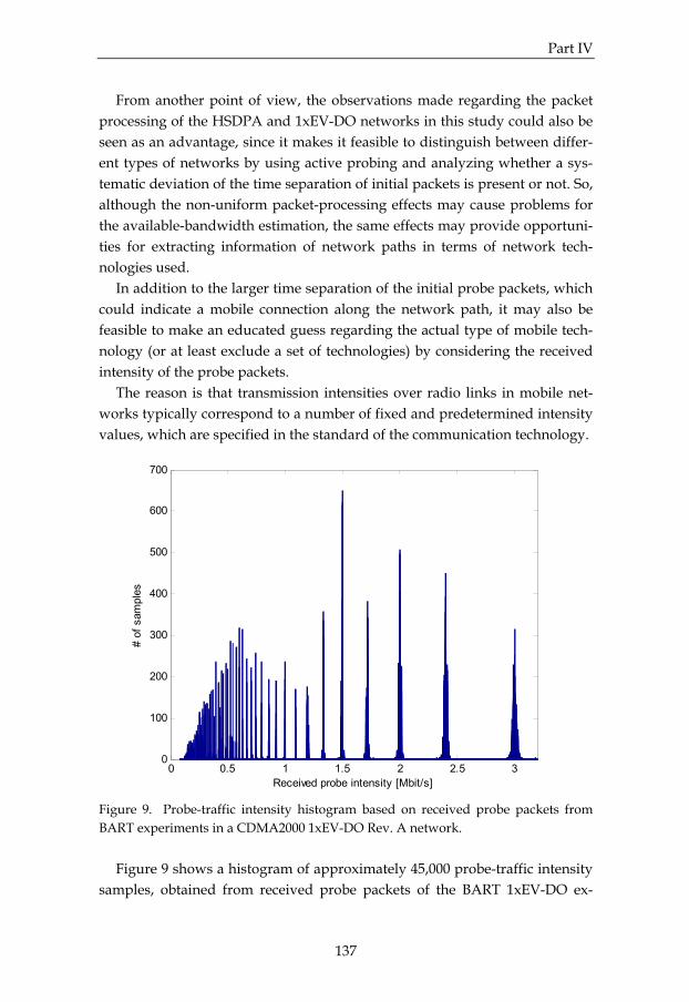
Part IV

137

From another point of view, the observations made regarding the packet processing of the HSDPA and 1xEV-DO networks in this study could also be seen as an advantage, since it makes it feasible to distinguish between differ-ent types of networks by using active probing and analyzing whether a sys-tematic deviation of the time separation of initial packets is present or not. So, although the non-uniform packet-processing effects may cause problems for the available-bandwidth estimation, the same effects may provide opportuni-ties for extracting information of network paths in terms of network tech-nologies used. In addition to the larger time separation of the initial probe packets, which could indicate a mobile connection along the network path, it may also be feasible to make an educated guess regarding the actual type of mobile tech-nology (or at least exclude a set of technologies) by considering the received intensity of the probe packets. The reason is that transmission intensities over radio links in mobile net-works typically correspond to a number of fixed and predetermined intensity values, which are specified in the standard of the communication technology.

0 0.5 1 1.5 2 2.5 30

100

200

300

400

500

600

700

Received probe intensity [Mbit/s]

# of

sam

ples

Figure 9. Probe-traffic intensity histogram based on received probe packets from BART experiments in a CDMA2000 1xEV-DO Rev. A network. Figure 9 shows a histogram of approximately 45,000 probe-traffic intensity samples, obtained from received probe packets of the BART 1xEV-DO ex-

Part IV

138

periments. As can be seen, the majority of the received intensities of the BART probe packets are gathered around a number of specific intensity values. For example, from right to left, it is clear that a large number of the probe packets are received with an intensity around, 3.0 Mbit/s, 2.4 Mbit/s, 2.0 Mbit/s, 1.7 Mbit/s etc. When comparing these received intensities to the range of nomi-nal transmission intensities of the forward traffic channel in 1xEV-DO [27] there is a clear correlation although the majority of the observed probe inten-sities are slightly below the nominal transmission intensities in the 1xEV-DO specification. A reasonable explanation is that the intensities in the specifica-tion correspond to the physical layer, whereas the received probe intensities from the BART experiments correspond to the IP layer. However, Figure 9 also contains a few intensity peaks which clearly differ from the transmission intensities in [27]. For example, there is no obvious ex-planation for the observed peak around 2.0 Mbit/s with respect to the 1xEV-DO specification; this is also the case for a few other peaks, e.g. around 1.3 Mbit/s. This could perhaps be an effect of the error-control scheme in 1xEV-DO, i.e. the hybrid automatic repeat request (HARQ) technique [12]. The HARQ scheme uses incremental redundancy which allows transmissions of packets to be terminated earlier than expected with respect to the predicted radio-channel conditions. This yields an additional set of truncated packets which correspond to intensities that do not agree with the specification. 5 IEEE 802.11 Experiments Active-probing measurements in a wireless laboratory network were per-formed in order to examine if the observed packet-processing effects in the mobile experiments also could be identified in less complex wireless-network technologies such as wireless local area networks (WLANs) based on the IEEE 802.11 standard. 5.1 Experiment Setup The network setup for the WLAN experiments is shown in Figure 10. In contrast to the previous experiments performed in commercial mobile networks, this investigation was carried out in a controlled laboratory net-work. This means that it was feasible to have knowledge of all traffic that was sent and received as well as the number of connected nodes. During the ex-

Part IV

139

periments, no other nodes than the probe sender and probe receiver were connected to the network. The BART sender was directly attached to the wireless access point, which was a D-Link wireless router (DI-524UP) configured according to the default factory settings. The probe-traffic receiver was a laptop computer equipped with an Intel PRO/Wireless LAN 2100 3B Mini PCI Adapter (which supports the IEEE standard 802.11b) in order to connect to the wireless network. As for the previous studies, the network nodes did not move during the experiments, the signal strength was excellent, and no cross traffic was used. This yields conditions which improve the chances of only being affected by the characteristics of the WLAN technology when transmitting probe packets (however, disturbances, if any, from nearby equipment which uses the same frequencies as IEEE 802.11b cannot be excluded).

Figure 10. Overview of the network topology used for the IEEE 802.11b experi-ments. With respect to the IEEE 802.11b specification regarding the maximum transmission intensity, it was concluded that the wireless link was the bottle-neck link along the path since the wired link between the probe-traffic trans-mitter and the wireless router had a capacity of 100 Mbit/s. The BART probing was configured as in the other experiments reported in this study, i.e. every second a probe train of 17 probe packets of 1500 bytes was sent from the probe-traffic transmitter. 5.2 Available-Bandwidth Measurements In Figure 11, the BART performance is shown for four different cases where initial probe packets are removed compared to when no probe packets are removed. The dashed curve is identical for the four subfigures in Figure 11, and it represents the BART estimate when no probe packets are discarded before the BART analysis. This curve acts as a reference for the four cases (solid curves in subfigures (a)-(d)) where initial probe packets are discarded at the probe receiver, in order to examine whether the available-bandwidth estimate

Part IV

140

systematically increases due to large initial inter-packet time separations, as was the case in Figure 6. The solid curve in subfigure (a) depicts the BART estimate when the two first probe packets in each probe sequence are discarded at the probe receiver. This yields an estimate which is slightly below the reference curve. In subfigure (b), the first four probe packets are removed at the BART re-ceiver for each probe sequence, and this also causes a lower estimate than if all received probe packets are used. For subfigure (c), when the six first probe packets are discarded, the BART estimate starts to vary somewhat around the reference curve, and this fluctu-ating behavior is even more evident in subfigure (d) when the eight initial packets in each probe sequence are removed before the BART analysis; for this latter case, the BART estimate also overestimates with regard to the case when no packets are discarded.

0 10 20 30 40 500

5

10

Ava

ilabl

e ba

ndw

idth

[Mbi

t/s]

(a)

BART referenceBART estimate

0 10 20 30 40 500

5

10(b)

0 10 20 30 40 500

5

10

Time [s]

(c)

0 10 20 30 40 500

5

10(d)

Figure 11. Available-bandwidth estimation by BART in case of no cross traffic over the IEEE 802.11b link. The dashed reference curve in all subfigures is the BART esti-mate when no probe packets are discarded. (a) BART estimate when 2 probe packets discarded. (b) BART estimate when 4 probe packets discarded. (c) BART estimate when 6 probe packets discarded. (d) BART estimate when 8 probe packets dis-carded.

Part IV

141

5.3 Discussion From the WLAN study, it was not feasible to make similar observations as from the studies of the HSDPA and 1xEV-DO networks. There is no indication that the initial packets are subject to larger inter-packet separation than subsequent packets, which is confirmed by the results in Figure 11. There is no systematic deviation when considering the four sub-figures; one can observe BART estimates below, above, and almost on top of the reference curve. One conclusion that can be drawn from Figure 11 is that the fluctuations of the BART estimates increase with the number of discarded probe packets. However, this is not surprising since less probe packets in the BART analysis imply a lower statistical precision of the average inter-packet separation strain of consecutive probe packets, which is the fundamental input measure when producing available-bandwidth estimates in BART; see [3] for a de-tailed description of the BART algorithm. 6 Conclusions This study has examined the applicability of using active-probing tools for estimating the available bandwidth over wide-area mobile communication networks. In the experiments performed, probe traffic was routed over the wireless link of a commercial UMTS network with HSDPA functionality as well as a CDMA2000 1xEV-DO network. For the purpose of comparing ob-servations from the mobile-network experiments with wireless local area networks, measurements were also carried out in an IEEE 802.11 laboratory network. Tools such as Pathload, which do not feature real-time estimation charac-teristics, have drawbacks when measuring over wireless links. The character-istics of radio channels often imply rapid variations of the available band-width. Consequently, if measurement tools need a long time for producing an estimate, there is a significant risk that once the estimate is obtained it does not reflect the present bandwidth situation. Hence, it is more appropriate to use tools with real-time estimation proper-ties such as pathChirp and BART. It was observed, however, that in order to maintain good estimation accuracy, such tools, primarily designed for wired networks, may require some modification when measuring over mobile broadband links.

Part IV

142

Several interesting conclusions related to the observed packet-processing phenomena in this study can be drawn. Some interesting packet-processing effects seem to appear due to the char-acteristics of HSDPA and 1xEV-DO networks. This may pose challenges for active-probing tools, especially if they only transmit short packet sequences for each measurement. It was observed that this caused both pathChirp and BART to underestimate the available bandwidth. The reason for this bias is probably due to issues as initial delays and warm-up phases related to re-source allocation and/or transmission-intensity control in the mobile net-works. However, it was also shown how this can be handled by removing initial probe packets, and how packet-processing properties as well as trans-mission intensities of mobile networks may be used as signatures for distin-guishing between network technologies. The phenomenon that initial packets in packet sequences may be treated differently is not present for all wireless links, which was observed from the IEEE 802.11 experiments. This could be due to the fact that IEEE 802.11 net-works are less complex than wide-area mobile networks when it comes to efficient resource-allocation techniques and control mechanisms for transmis-sion-intensity selection. This study was limited to scenarios where mainly the effects of the net-work technology used influenced the available bandwidth. Since the end nodes of the wireless link did not move and the signal strength of the radio channel was high for all experiments, the results were not subject to effects which could have caused rapid variations of the throughput. Regarding future work, it would be interesting to extend this study by considering more complex scenarios. In real networks, it is however rather difficult to investigate and compare the performance of measurement tools for the case of, for example, fast-fading radio channels, since it is hard to ob-tain reliable measures of the true available bandwidth over short time inter-vals. A simulation study may therefore be more appropriate for examining these scenarios. References [1] M. Jain and C. Dovrolis, “End-to-end available bandwidth: measure-

ment methodology, dynamics, and relation with TCP throughput,” IEEE/ACM Transactions on Networking, vol. 11, 2003.

Part IV

143

[2] V. Ribeiro, R. Riedi, R. Baraniuk, J. Navratil, and L. Cottrell, “pathChirp: efficient available bandwidth estimation for network paths,” in Proc. Passive and Active Measurement Workshop, 2003.

[3] E. Bergfeldt, S. Ekelin, and J. M. Karlsson, “Real-time available-bandwidth estimation using filtering and change detection,” Computer Networks, vol. 53, 2009.

[4] B. Melander, M. Björkman, and P. Gunningberg, “A new end-to-end probing and analysis method for estimating bandwidth bottlenecks,” in Proc. IEEE GLOBECOM’00, 2000.

[5] N. Hu and P. Steenkiste, “Evaluation and characterization of available bandwidth probing techniques,” IEEE JSAC Internet and WWW Meas-urement, Mapping, and Modeling, vol. 21, 2003.

[6] J. Strauss, D. Katabi, and F. Kaashoek, “A measurement study of avail-able bandwidth estimation tools,” in Proc. ACM SIGCOMM Internet Measurement Conference, 2003.

[7] V. Ribeiro, M. Coates, R. Riedi, S. Sarvotham, B. Hendricks, and R. Ba-raniuk, “Multifractal cross-traffic estimation,” in Proc. ITC Specialist Se-minar on IP Traffic Measurement, Modeling and Management, 2000.

[8] R. S. Prasad, M. Murray, C. Dovrolis, and K. Claffy, “Bandwidth estima-tion: metrics, measurement techniques, and tools,” IEEE Network, vol. 17, 2003.

[9] E. Dahlman, S. Parkvall, J. Sköld, and P. Beming, 3G Evolution: HSPA and LTE for Mobile Broadband. Academic Press, 2007.

[10] H. Holma and A. Toskala, HSDPA/HSUPA for UMTS: High Speed Radio Access for Mobile Communications. John Wiley & Sons, 2006.

[11] P. Bender, P. Black, M. Grob, R. Padovani, N. Sindhushyana, and S. Vi-terbi, “CDMA/HDR: a bandwidth efficient high speed wireless data service for nomadic users,” IEEE Communications Magazine, 2000.

[12] J. Wang and T.-S. Ng, Advances in 3G Enhanced Technologies for Wireless Communications. Artech House, 2002.

[13] B. O’Hara and A. Petrick, The IEEE 802.11 Handbook: A Designer’s Com-panion. IEEE Press, 1999.

[14] A. Shriram and J. Kaur, “Empirical evaluation of techniques for measur-ing available bandwidth,” in Proc. IEEE INFOCOM, 2007.

[15] A. Shriram, M. Murray, Y. Hyun, N. Brownlee, A. Broido, M. Fo-menkov, and K. Claffy, “Comparison of public end-to-end bandwidth estimation tools on high-speed links,” in Proc. Passive and Active Meas-urement Workshop, 2005.

Part IV

144

[16] S. H. Shah, K. Chen, and K. Nahrstedt, “Available bandwidth estimation in IEEE 802.11-based wireless networks,” in Proc. ISMA Workshop on Bandwidth Estimation (BEst), 2003.

[17] M. A. Alzate, J.-C. Pagán, N. M. Peña, and M. A. Labrador, “End-to-end bandwidth and available bandwidth estimation in multi-hop IEEE 802.11b ad hoc networks,” in Proc. Conference on Information Sciences and Systems (CISS), 2008.

[18] M. Jurvansuu, J. Prokkola, M. Hanski, and P. Perälä, “HSDPA perform-ance in live networks,” in Proc. IEEE International Conference on Commu-nications (ICC), 2007.

[19] Y. Lee, “Measured TCP performance in CDMA 1xEV-DO Network,” in Proc. Passive and Active Measurement Conference, 2006.

[20] E. Bergfeldt, S. Ekelin, and J. M. Karlsson, “Real-time bandwidth measurements over mobile connections,” Submitted to European Transactions on Telecommunications, 2010.

[21] E. Bergfeldt, S. Ekelin, and J. M. Karlsson, “A performance study of bandwidth measurement tools over mobile connections,” in Proc. IEEE 69th Vehicular Technology Conference, 2009.

[22] E. Hartikainen and S. Ekelin, “Enhanced network-state estimation using change detection,” in Proc. 31st IEEE Conference on Local Computer Net-works, 2006.

[23] M. Fiedler, L. Isaksson, and S. Chevul, “Measurements and analysis of application-perceived throughput via mobile links,” in Proc. Performance Modeling and Evaluation of Heterogeneous Networks (HET-NETs), 2005.

[24] M. Necker and A. Weber, “Parameter Selection for HSDPA Iub flow control,” in Proc. IEEE Wireless Communication Systems (ISWCS), 2005.

[25] P. J. A. Gutiérrez, “Packet scheduling and quality of service in HSDPA,” Ph.D. dissertation, Aalborg University, Denmark, 2003.

[26] C. Y. Huang, Q. Bi, A. Gandhi, R. Brown, and D. Cui, “Forward and re-verse link capacity for 1xEV-DO: third generation wireless high-speed data systems,” in Proc. IEEE Global Telecommunications Conference, 2002.

[27] 3rd Generation Partnership Project 2 (3GPP2), “cdma2000 high rate packet data air interface specification,” 3GPP2 C.S0024-A version 3.0, 2006.

145

Part V Available-Bandwidth Estimation: Challenges and Research Directions Abstract This part of the thesis discusses general challenges as well as weaknesses of current methods and tools within the field of end-to-end available-bandwidth estimation. In recent years, numerous tools have been developed for measur-ing available bandwidth. Generally, these tools have limitations which reduce the overall reliability, although they may have performed reasonably in some evaluation studies where specific network and traffic scenarios have been considered. A number of these shortcomings are further discussed and illus-trated in this part. A new method, E-MAP (Expectation-Maximization Active Probing), for probing and analyzing the end-to-end available bandwidth is also presented. E-MAP overcomes some of the weaknesses of other band-width-measurement tools. The majority of the previously developed tools rely on self-induced congestion; this implies injection of probe traffic at inten-sities high enough to momentarily overload the bottleneck link of the net-work path. However, if the used probe-traffic intensity is too low or too high, it is not feasible to produce reliable available-bandwidth estimates. It is diffi-cult to determine the optimal choice of probe-traffic intensity beforehand, but unlike many other bandwidth-measurement tools the E-MAP strategy re-duces the risk of making inappropriate choices by covering a wide range of intensities in each measurement. Most likely, this approach generates probe traffic that contains both useful and useless information at the probe receiver, but the expectation-maximization algorithm in E-MAP is able to automati-cally identify the probe packets that point out the true available bandwidth; these are further used in the available-bandwidth analysis whereas the other

Part V

146

may be discarded. E-MAP also has the potential of taking care of measure-ments affected by multiple bottleneck links along the network path, which is a common problem for several bandwidth-measurement tools. 1 Introduction 1.1 Overview The capability of measuring the end-to-end available bandwidth is important and useful in several contexts. For example, network operators may apply available-bandwidth estimation tools in order to monitor their networks, and to identify congested as well as unutilized network links. Internet users could measure the bandwidth in order to verify that network operators provide at least the bandwidth capacity stated in the service level agreement. Further-more, the performance of various applications (especially real-time applica-tions, such as streaming of audio and video) would likely benefit from tools that can provide information about the prevailing network conditions; for instance, congestion and packet loss which are detrimental for real-time ap-plications may be avoided if the sender could regulate the transmission inten-sity with respect to the current available bandwidth. By utilizing active measurement tools, it is feasible to estimate the end-to-end available bandwidth along a network path. Active measurements imply injection of probe traffic into the network. By analyzing the observed effects of link capacities and cross traffic on the probe traffic, conclusions can be drawn regarding the available bandwidth. This kind of measurement tech-nique only requires access to the probe sender and the probe receiver. However, although the capability and the reliability of developed band-width-measurement tools have improved throughout the years, a number of difficulties and ambiguities are still associated with accurate available-bandwidth estimation. For example, it is reasonable to raise questions such as how to define bandwidth, how to configure measurement tools for optimum performance, how are bandwidth measurements affected by hardware limita-tions of network nodes and multiple bottleneck links along the network path etc. All of these issues are addressed and further discussed in the forthcoming sections. A novel active-probing method, E-MAP (Expectation-Maximization Active Probing), for measuring available bandwidth is also presented. The main con-tribution of E-MAP is the use of the expectation-maximization (EM) algo-

Part V

147

rithm for real-time estimation of the end-to-end available bandwidth. By measuring in real-time it is possible to obtain instant indications of the avail-able bandwidth, which is suitable for congestion control and adaptation of the transmission intensity in real-time applications etc. E-MAP overcomes a number of problems that may affect the efficiency and reliability of other bandwidth-measurement tools. Some of its features can be summarized as: it produces an estimate quickly; it measures the network path with chirps, i.e. probe-packet trains covering a wide range of probe intensities in each measurement; no communication is required from the probe-packet receiver to the probe-packet sender; probe packets sent at too low or too high intensities are automatically identified and discarded; the method is usable in case of multiple congested links; a filter can be applied for enhanced per-formance. E-MAP has been evaluated in the network simulator ns-21, where the si-mulations have covered both wired and wireless network scenarios. Some of these results are presented in this study. 1.2 Related Work In recent years, several available-bandwidth measurement tools have been presented. For example, Pathload [1], pathChirp [2], PTR [3], TOPP [4], and BART [5] are all based on variations of the probe rate model (PRM). PRM relies on self-induced congestion. If probe packets are sent at intensities lower than the available bandwidth, the arrival intensity at the probe-packet receiver is ex-pected to match the used transmission intensity at the sender. If the probe-packet intensity is higher than the available bandwidth, congestion occurs at the bottleneck link and the probe packets will be delayed; this increases the inter-packet time separation, which is observable at the probe receiver. By transmitting probe packets at various intensities, it is feasible to measure the available bandwidth by identifying the point of congestion, i.e. the probe-traffic intensity where the time separation starts to increase. Tools like Spruce [6], IGI [3], and Delphi [7] are based on the probe gap model (PGM). PGM estimates the amount of cross traffic at the bottleneck link by exploiting the information in time-gap variations between consecutive

1 http://www.isi.edu/nsnam/ns/ (October 2010)

Part V

148

probe packets. The available bandwidth is estimated by subtracting the measured cross traffic from the bottleneck-link capacity. In practice, PRM based tools tend to be more useful than PGM tools, since the latter require knowledge of the bottleneck-link capacity in order to deliver reliable estimates. In addition, PGM tools also assume that the bottleneck link (i.e. the link with the minimum unused capacity) is the same as the narrow link (i.e. the link with the minimum capacity), which not necessarily is the case in reality. E-MAP belongs to the family of PRM tools, and its measurement approach can be seen as a mixture of the advantages of pathChirp, TOPP, and BART. The EM algorithm in E-MAP makes it is feasible to use an active-probing technique similar to pathChirp, a line-fitting approach as in TOPP for gener-ating a bandwidth estimate, and filtering for enhanced tracking performance which is used in the BART method. Previous work has highlighted some general difficulties associated with available-bandwidth measurements, see e.g. [8-10]. However, these papers do not address all the issues that are covered in the present study. The content of the following sections is mainly based on [5, 11]. 2 Available-Bandwidth Measurements 2.1 Available Bandwidth In a network path, each link j has a certain capacity C-j. This is the highest possible throughput capacity over the link. C is typically constant in wired networks whereas the opposite holds for wireless links. The cross traffic, or link load, for each link j is denoted X-j. X is likely to vary on short time scales. The time-varying available bandwidth of link j is defined as B-j = C-j – X-j. The link with the minimum available bandwidth is called the bottleneck link, and this link determines the available bandwidth of the entire path. Hence, the end-to-end available bandwidth is defined as: )(min jj

jXCB −= (1)

Part V

149

2.2 Difficulties in Measuring Available Bandwidth In general, several difficulties exist when estimating the end-to-end available bandwidth along packet-switched network paths. It is a great challenge to develop measurement tools that are able to deal with all of these issues. If the bandwidth is measured in network and traffic scenarios which have characteristics that are not accounted for in the design of the used measurement tool, it is not reasonable to expect useful and reli-able estimates of the available bandwidth. This also holds if users and appli-cations, which may use available-bandwidth measurements for various pur-poses, are not aware of how to configure the tools appropriately. The optimal configuration typically varies with respect to the utilization of the measure-ments as well as the network and cross-traffic properties (which are not al-ways known beforehand) and, consequently, it is not straightforward how to set adjustable parameters. An unsuitable configuration will likely deliver low quality bandwidth estimates. In the following subsections, a number of aspects that should be taken into account when developing and using active-measurement tools for available-bandwidth estimation are discussed and illustrated. 2.2.1 Definition and Variability of Bandwidth A fundamental challenge when measuring available bandwidth is to deter-mine how bandwidth should be defined. In practice, a link in a packet-switched communication network could either be fully utilized or idle. How-ever, it is often inconvenient to explain the utilized bandwidth in terms of these two conditions. Instead, the traffic load on a link is commonly related to a chosen time resolution (or averaging time scale) Δ [12] that corresponds to a sliding window, which is used for averaging the amount of traffic utilizing the link during a given time interval. With respect to this, the characteristics of the true available bandwidth may be quite different for a particular traffic case, if two different time resolu-tions Δ are used for describing bandwidth. Hence, if it is unclear how the bandwidth is defined and since the definition may vary, it is a great challenge to develop measurement tools that are able to accurately track the available bandwidth.

Part V

150

0 50 100 150 200 250 3000

1

2

3

4

5

6

7

8

9

10

Time [s]

Ava

ilabl

e ba

ndw

idth

[Mbi

t/s]

Available bandwidthBART estimate

Figure 1. The BART estimate and the true available bandwidth for a traffic case where the bandwidth is defined according to a time resolution of Δ = 4 seconds.

0 50 100 150 200 250 3000

1

2

3

4

5

6

7

8

9

10

Time [s]

Ava

ilabl

e ba

ndw

idth

[Mbi

t/s]

Available bandwidthBART estimate

Figure 2. The BART estimate and the true available bandwidth for a traffic case where the bandwidth is defined according to a time resolution of Δ = 32 seconds.

Part V

151

For example, see Figure 1 and Figure 2 which show the true available bandwidth and estimate of the BART method [5] for exactly the same net-work and traffic scenario; it is only the filter configuration of BART and the used time resolution Δ for describing bandwidth that differ. According to the curves in Figure 1 and Figure 2, it is obvious that the BART method would perform poorly in case the used configuration of BART yields estimates corresponding to the thick solid curve in Figure 1 and the true available bandwidth is defined with respect to a time resolution of Δ = 32 seconds as is the case in Figure 2, and vice versa. Generally, it can be seen as a great advantage that measurement tools can be configured according to specific needs, but in order to make use of this benefit it is necessary that users and applications that utilize these tools are aware of how tunable parameters should be adjusted in order to not obtain misleading results. Unfortunately, this configuration may be rather compli-cated, especially since different tools often have different design parameters which could interact and influence the bandwidth estimate in various ways. For example, it is common that changes of configurable parameters of available-bandwidth measurement tools affect the variability of the generated estimates, which ideally should agree with the variability of the true available bandwidth; compare Figure 1 and Figure 2, where BART is configured for high variability and low variability, respectively. But, the variability of the true available bandwidth is typically hard to predict, since this property de-pends on several aspects such as the characteristics of the bottleneck-link ca-pacity and the cross-traffic aggregation level, which are usually not known; i.e. the bandwidth variability does not only depend on the used time resolu-tion Δ for describing bandwidth. For details regarding how the BART method can be configured with re-spect to variability, as well as more information about the performed meas-urements shown in Figure 1 and Figure 2, see [5, 13]. The problem of finding a suitable configuration of the measurement tools becomes even more complex when taking into account that the magnitude and the frequency of the true available-bandwidth fluctuations can vary con-siderably during the measurements. Typically, the measurement tools cannot have a static configuration and still perform optimally in case of both slowly and rapidly changing conditions. In general, a tool configured for stability (which is suitable given low bandwidth variability) will suffer in case of sudden changes in the system, due to slow adaptation. A tool with agile properties (which is suitable in case of high bandwidth variability) delivers fluctuating estimates in a steady-state

Part V

152

situation, due to measurement noise. For example, see Figure 3 where BART is used with two different configurations aimed for following a slowly and rapidly changing available bandwidth, respectively.

0 200 400 600 800 1000 1200 1400 1600 1800 20000

1

2

3

4

5

6

7

8

9

10

Time [s]

Ava

ilabl

e ba

ndw

idth

[Mbi

t/s]

Available bandwidthBART estimate (agile)BART estimate (stable)

Figure 3. BART estimating the available bandwidth using two configurations for different tracking ability, for a scenario with abrupt changes in the available band-width. In Figure 3, the dotted curve corresponds to a high-agility configuration. It is obvious that BART easily follows the abrupt changes in the available bandwidth, whereas the precision of the estimates leaves a great deal to be desired, due to amplification of the measurement noise. The dashed curve corresponds to an opposite configuration of high stability, which means that BART is insensitive to the measurement noise and delivers stable and reliable estimates in the interval from 0 to 750 seconds. However, the configuration does not allow for fast adaptation, which is obvious when considering the estimates after 750 seconds, where BART is very slow in adapting to the new system state. Although the BART configurations used in Figure 3 could be seen as two rather extreme choices (it is possible to choose a parameter setting such that the estimates become something in between the two BART curves in Figure 3), there is a clear trade-off between having stable but slowly adapting esti-mates and agile but noise-sensitive estimation properties.

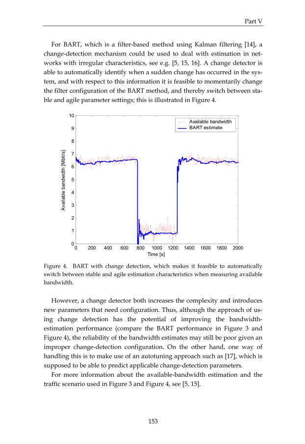
Part V

153

For BART, which is a filter-based method using Kalman filtering [14], a change-detection mechanism could be used to deal with estimation in net-works with irregular characteristics, see e.g. [5, 15, 16]. A change detector is able to automatically identify when a sudden change has occurred in the sys-tem, and with respect to this information it is feasible to momentarily change the filter configuration of the BART method, and thereby switch between sta-ble and agile parameter settings; this is illustrated in Figure 4.

0 200 400 600 800 1000 1200 1400 1600 1800 20000

1

2

3

4

5

6

7

8

9

10

Time [s]

Ava

ilabl

e ba

ndw

idth

[Mbi

t/s]

Available bandwidthBART estimate

Figure 4. BART with change detection, which makes it feasible to automatically switch between stable and agile estimation characteristics when measuring available bandwidth. However, a change detector both increases the complexity and introduces new parameters that need configuration. Thus, although the approach of us-ing change detection has the potential of improving the bandwidth-estimation performance (compare the BART performance in Figure 3 and Figure 4), the reliability of the bandwidth estimates may still be poor given an improper change-detection configuration. On the other hand, one way of handling this is to make use of an autotuning approach such as [17], which is supposed to be able to predict applicable change-detection parameters. For more information about the available-bandwidth estimation and the traffic scenario used in Figure 3 and Figure 4, see [5, 15].

Part V

154

Although all of these examples are illustrated by available-bandwidth es-timates generated by the BART method, it is reasonable to assume that con-figuration is a general issue for bandwidth-measurement tools; especially when it is desired to track the available bandwidth at different time resolu-tions Δ, and when the measured network path has irregular characteristics which suddenly cause abrupt bandwidth changes. According to the above discussion, a tool such as BART has the ability to cope with these situations although an appropriate configuration of adjustable parameters is required, which is not always straightforward. However, numerous measurement tools do not even have the capability of, e.g., estimating in real-time and with re-gard to different bandwidth definitions, which of course limits the applicabil-ity of these tools. 2.2.2 Probe-Traffic Intensities There is a clear trade-off regarding the reliability of the estimation and the amount of injected probe traffic. Excessive levels of probe traffic is normally undesired in the networks, and one should strive for developing accurate tools that also keep the probe-traffic load low. Today, the amount of transmit-ted probe traffic varies considerably when comparing different measurement tools. This is also related to the ability of performing real-time estimation, which varies a lot with respect to different methods. Existing available-bandwidth estimation methods are typically associated to either the probe rate model (PRM) or the probe gap model (PGM). Meth-ods based on PRM (which generally are more useful than PGM based meth-ods, see Section 1.2) inject probe traffic at different intensities and the probe receiver observes and analyzes the relation between the used probe-traffic intensity at the sender and the observed probe-traffic intensity at the receiver. If probe packets are transmitted with an intensity which is lower than the available bandwidth, the received intensity at the probe receiver is expected to match the used intensity at the sender. If probe packets are transmitted with an intensity which is higher than the available bandwidth, congestion occurs at the bottleneck link and the probe packets will be delayed. In [4] it has been shown that this phenomenon can be modeled as a piecewise linear curve, see Figure 5. By transmitting probe packets at various intensities, it is feasible to meas-ure the available bandwidth by identifying the point of congestion, i.e. the probe-traffic intensity where the time separation between probe packets starts

Part V

155

to increase. However, the time it takes to find the available bandwidth by continuously varying the probe-traffic intensity may be notable, and this is the reason why tools such as Pathload [1] and TOPP [4] are unsuitable for real-time tracking of available bandwidth; both these methods require a sub-stantial time for measurement and analysis before producing an estimate.

0

Probe-traffic intensity

Con

gest

ion

mea

sure

Available bandwidth

Figure 5. The asymptotic relation between available bandwidth, probe-traffic inten-sity and congestion measure. If the used probe-traffic intensity is too low with respect to the available bandwidth (i.e. the probe traffic in combination with cross traffic do not over-load the bottleneck link of the network path), it is not feasible to produce a reliable estimate of the unused capacity based on the received probe packets; one can only conclude that the available bandwidth is larger than the used probe intensity. Hence, it is undesirable to utilize probe intensities lower than the available bandwidth, since this decreases the performance, especially for tools that are used for real-time estimation. For example, Figure 6 illustrates the perform-ance of BART with change detection when the used probe-traffic intensity occasionally is too low; in this experiment, BART is used over an Internet path and rapid available-bandwidth changes occur due to manual activation and deactivation of cross traffic, see [5] for details.

Part V

156

0 200 400 600 800 1000 1200 1400 16000

10

20

30

40

50

60

70

80

Time [s]

Ava

ilabl

e ba

ndw

idth

[Mbi

t/s]

Available bandwidthBART estimate

Figure 6. BART with change detection is estimating the available bandwidth over an Internet path when sudden cross-traffic changes occur in the network. In Figure 6, it is obvious that BART does not immediately react to the available-bandwidth decrease after approximately 450 seconds. The explana-tion for this behavior could be found by considering an aspect of the used BART implementation in combination with the utilized probe-traffic intensi-ties. Measurements performed with probe-traffic intensities below the current estimate of the available bandwidth are discarded (this is in accordance with the BART algorithm described in [5]), because these measurements are most likely to the left of the break point in Figure 5. Since in the experiment corre-sponding to Figure 6, the probe-traffic intensities are randomly and uni-formly chosen in the interval from 10 Mbit/s to 100 Mbit/s, more than every other measurement is expected to be unutilized when the current estimate of the available bandwidth is around 60 Mbit/s, which is the case around 450 seconds. With regard to this reasoning, it is sound that the change-detection delay is shorter for the third change around 1350 seconds, and even shorter for the first abrupt change after 300 seconds, as a larger fraction of the trans-mitted probe packets are taken into account when the estimate of the avail-able bandwidth is low.

Part V

157

Consequently, a measurement tool such as BART, which is developed for real-time estimation, suffers from the fact that it is necessary to vary the prob-ing intensity; these variations are needed since the aim of BART is to accu-rately estimating the parameters of the sloping straight line in Figure 5, see [5] for details. However, this weakness could easily be taken care of by including feedback from the probe receiver to the sender; in BART, the option to not have feedback communication could be seen as a feature of the method (for several other available-bandwidth measurement tools feedback is required). Thus, the BART receiver could constantly inform the sender about the current estimate of the available bandwidth, and the sender would be able to adapt the range of probing intensities such that the probability of receiving useful bandwidth measurements is increased. This would most likely improve the required time to detect the changes in Figure 6. The discussion above only describes how too low probe-traffic intensities may deteriorate the estimation performance of available-bandwidth meas-urement tools. However, too high probe-traffic intensities are also undesired. For example, by increasing the probe intensity at the sender, the probability of overloading more than one node along the network path increases.

0 10 20 30 40 50 60 70 80 90 1000

1

2

3

4

5

6

7

8

9

10

Time [s]

Ava

ilabl

e ba

ndw

idth

[Mbi

t/s]

Available bandwidthBART estimate

Figure 7. Available-bandwidth estimation by BART. After around 50 seconds, cross traffic is activated which creates a new bottleneck along the network path and probe packets sent at intensities above 5 Mbit/s become affected by two bottleneck links.

Part V

158

Again, the performance of the BART method is used as an example. See Figure 7, where BART partially uses too high probe-traffic intensities causing multiple bottlenecks (for details regarding the experiment setup, see [18]). During the first part of this experiment, the probe traffic only overloads one link along the network path and BART indicates that the available bandwidth is around 5 Mbit/s. But, after around 50 seconds, additional cross traffic is injected in the network, which yields an end-to-end available bandwidth of 2 Mbit/s. This new cross traffic does not affect the link which corresponds to the bot-tleneck during the initial phase of the experiment. Instead, the cross traffic puts extra load on another link which means that the bottleneck moves along the network path, since the end-to-end available-bandwidth decreases due to the injected cross traffic. With respect to the used network topology, the new bottleneck link is located closer to the probe receiver, compared to the posi-tion of the bottleneck during the first 50 seconds. As a consequence of this, the BART probe traffic will be affected by two bottlenecks when using probe intensities above 5 Mbit/s, and this causes the evident overestimation of the available bandwidth after 50 seconds. The reason why BART overestimates the available bandwidth after around 50 seconds in Figure 7 relates to the used measurement model. BART uses the simple piece-wise linear model that was introduced in [4], see Figure 5. With respect to a suitable congestion measure (BART uses the inter-packet separa-tion strain of consecutive probe packets [5]) which is expected to increase li-nearly with regard to the probe-traffic overload, the available bandwidth (i.e. the break point of the piece-wise linear curve) can be calculated by first esti-mating the parameters of the sloping straight line. However, in case of multiple bottleneck links, the congestion measure does not grow linearly. Instead, there will be a new break point for each new bot-tleneck link. It is still feasible to obtain a correct estimate of the first break point given that congestion measures for probe-traffic intensities above the following break points are discarded. But this is not taken into consideration in the used BART implementation and, hence, a bias appears when BART estimates the available bandwidth in case of multiple bottleneck links. This is further illustrated in Figure 8. Figure 8 (a) describes the relationship between the probe-traffic intensity and the congestion measure in case of a single bottleneck link with an avail-able bandwidth of 5 Mbit/s, i.e. approximately the BART estimate in Figure 7 before the additional cross traffic creates a new bottleneck. Figure 8 (b) shows the behavior of the congestion measure if there is only one bottleneck link

Part V

159

with 2 Mbit/s of available bandwidth. For both these subfigures, the conges-tion measure grows linearly for probe-traffic intensities larger than the avail-able bandwidth.

0 2 4 6

0

(a)

Con

gest

ion

mea

sure

0 2 4 6

0

(b)

0 2 4 6

0

(c)

Probe-traffic intensity [Mbit/s]0 2 4 6

0

(d)

Figure 8. An illustration of the relationship between the probe-traffic intensity and the BART congestion measure. The first break point corresponds to the available bandwidth. (a) One bottleneck link with available bandwidth 5 Mbit/s. (b) One bot-tleneck link with available bandwidth 2 Mbit/s. (c) Two bottleneck links with avail-able bandwidth 2 Mbit/s and 5 Mbit/s, respectively. (d) An approximation of the BART estimate of the sloping straight line based on congestion measures according to (c). For Figure 8 (c), there are break points at both 2 Mbit/s and 5 Mbit/s. Hence, if the probe-traffic intensity is lower than 2 Mbit/s, no congestion oc-curs. If the probe sender transmits traffic in the interval from 2 – 5 Mbit/s, only one link is overloaded along the network path. For intensities larger than 5 Mbit/s, congestion occurs at two links and the congestion measure grows faster. The true available bandwidth according to Figure 8 (c) is 2 Mbit/s, i.e. the position of the first break point. If BART would not send probe traffic at in-tensities larger than 5 Mbit/s, the available-bandwidth estimates would be close to 2 Mbit/s. But when also probe intensities causing congestion at mul-tiple links are taken into account in the probe-traffic analysis of BART, the

Part V

160

estimate of the sloping straight line may appear as in Figure 8 (d); i.e. a com-bination of the two sloping straight lines in Figure 8 (c). In Figure 8 (d), it can be seen that the position of the first break point is overestimated with respect to Figure 8 (c). The available-bandwidth estimate is in the region of 3-4 Mbit/s instead of 2 Mbit/s. This is also the case in Fig-ure 7 after around 50 seconds. The impact of multiple bottleneck links along network paths is trouble-some for several available-bandwidth measurement tools. For example, re-garding pathChirp which also has real-time estimation properties, this has already been concluded in several studies, see e.g. [19]. For BART, one approach to avoid multiple bottleneck links and the overes-timation as illustrated in Figure 7 is, again, to include feedback from the probe receiver to the probe sender, and thereby limit and adapt the probing intensity to the region of interest (which corresponds to the current estimate of the available bandwidth). 2.2.3 Time Stamping and Queuing Principles In addition to the discussion above regarding challenges of how to define and track bandwidth as well as how to select suitable probe-traffic intensities when using active measurement tools, the quality and the interpretation of the bandwidth estimates may also be dependent on issues such as the clock resolution of operating systems, the properties of network interfaces, and the used queuing scheme in routers. The time resolution and the accuracy of the time stamping at the probe sender and receiver can be critical, since numerous active-probing tools only base their available-bandwidth estimates on the time separation of the probe packets. Also, as the transmission intensities of both wired and wireless links increase, the time intervals between packets typically decrease and, thus, the probing tools become even more sensitive to time-resolution errors. This is also related to effects like offloading and interrupt coalescence, which the network interfaces of the nodes may utilize in order to improve packet proc-essing in high-speed networks, and which may add or subtract to the send and receive packet time stamps. Even if the packet processing becomes more efficient, it implies that one cannot assume to have uniform per packet proc-essing, which is expected by many probing tools; this also makes it more dif-ficult to use active probing over radio interfaces in mobile networks, where the packet processing is dependent on resource-allocation schemes and con-

Part V

161

trol mechanisms for transmission-intensity selection [18, 20]. It should be noted, however, that a filter-based tool such as BART can be expected to deal with these problems more gracefully than other methods, since packet timing errors are explicitly catered for by the statistical measurement noise in the underlying filter model; see [5] for details. Another problem relates to how the interpretation of the available-bandwidth estimate may differ depending on the used mechanisms for man-aging queues in the routers along the network path. Available-bandwidth measurement tools were originally developed with the assumption that the queuing service in the network nodes was based on stateless first-in first-out (FIFO) queues. Hence, in wired networks where routers (in most cases) have one single FIFO queue for each network interface, the available-bandwidth estimate indicates the amount of additional traffic that can be injected with-out causing congestion and, thus, affecting other traffic flows at the bottle-neck link. However, this interpretation is not always valid in wireless and mobile networks, where it is common that resources are allocated to users in other ways. The queuing scheme is often based on weighted fair queuing or other more sophisticated algorithms which, e.g., utilize a separate FIFO queue for each traffic flow. Due to this, it is not feasible to measure the unutilized ca-pacity by active probing. The available-bandwidth estimate should rather only be seen as an approximation of the achievable throughput from the probe sender to the probe receiver. For more details regarding some of these as well as other active-measurement difficulties in packet-switched networks, see [8-10, 18, 20]. 3 The E-MAP Method The E-MAP (Expectation-Maximization Active Probing) method for estimat-ing end-to-end available bandwidth combines properties from pathChirp [2], TOPP [4], and BART [5]. The aim is to make use of the advantages of these three tools, and by that having a new and improved real-time estimation me-thod which also has the ability to take care of some of the issues discussed in Section 2.2. Especially, E-MAP uses a wide range of probe-traffic intensities in each measurement (i.e. a probing scheme similar to pathChirp), which decrease the risk of receiving inapplicable measurements due to probing at intensities below the available bandwidth. E-MAP also has the potential of dealing with

Part V

162

multiple bottleneck links along the network path, by utilizing a multiple-line fitting approach for identifying the available bandwidth (as is the case for the TOPP method). Finally, the E-MAP performance can easily be enhanced by applying a filter (e.g. a Kalman filter as in the BART method) and thereby having the possibility to adjust the method for desired characteristics, such as tuning between stable and agile estimation properties. 3.1 The Measurement Model Similar to the BART method, E-MAP uses the relative inter-packet separation strain ε as the measured quantity of the bottleneck-link characteristics [5]; ε is calculated by comparing the inter-packet time separation of the probe traffic at the sender and receiver. The expectation value of ε is zero when the prob-ing intensity u is less than the available bandwidth B, and grows in propor-tion to the overload when the probing intensity is larger [4], i.e. when the probe packets momentarily cause congestion at the bottleneck link. Hence, the strain ε can be expressed as

⎩⎨⎧

>+=−≤

=)( )()(0

BuuBuBu

βααε (2)

where α and β are the parameters of the sloping straight line l2 in Figure 9 and the available bandwidth corresponds to the breakpoint of l1 and l2. By varying the probe-packet intensity u at the probe sender and identifying the point where ε starts to deviate from zero at the receiver, it is feasible to estimate the available bandwidth of the bottleneck link and, thus, of the entire end-to-end path. The breakpoint B can be determined by estimating the parameters of l2. This is the used approach in E-MAP, TOPP, and BART. The measurement model (2) is based on a fluid-flow model of the traffic along the measured path. Hence, it should be noted that when going beyond the fluid model and taking packet-level interactions in router queues into ac-count, the measured strain ε is expected to deviate somewhat from the form in Figure 9 [21]. However, it is reasonable to believe that the asymptotic be-havior remains. Furthermore, the measurement model assumes that congestion only occurs in one link along the network path; the number of breakpoints in Figure 9 corresponds to the number of congestion points. Due to this, several meas-

Part V

163

urement tools may deliver erroneous estimates in case of multiple congested links. However, the E-MAP method should be able to handle this situation, with regard to the properties of the used EM algorithm.

0

Probe-traffic intensity (u)

Inte

r-pac

ket s

train

( ε)

Available bandwidth

l 1

l 2

Figure 9. The asymptotic relation between available bandwidth, probe-traffic inten-sity and inter-packet strain. 3.2 The Expectation-Maximization Algorithm The expectation-maximization (EM) algorithm has been applied in a wide range of estimation problems in statistics. It is used for finding maximum-likelihood estimates from incomplete data (which can be seen as a set of ob-servations). In E-MAP, the EM algorithm is used for parameter estimation of straight lines. Hence, the description of the algorithm is limited to this par-ticular case; for more details and a general description of the theory and ap-plicability of the EM algorithm, see [22]. By transmitting probe packets as a probe train with internally varying in-ter-packet time separations (also known as a “chirp” of probe packets), strain measurements ε appear along both the horizontal line l1 and the sloping straight line l2 in Figure 9, since numerous traffic intensities are used within one probe chirp. However, in order to estimate the available bandwidth B the parameters of l2 are of specific interest, and by utilizing the EM algorithm it is

Part V

164

feasible to estimate l2 by identifying the strain measurements that belong to this line. The EM algorithm is iterative and consists of two steps, the E-step and the M-step. In the E-step, the algorithm believes that it has knowledge of the true parameters of the lines l1 and l2 in order to assign the strain measurements εi (i = 1, 2, …, N-1, where N is the number of probe packets in a chirp) to the line that fits best. In the M-step, the algorithm assumes that it knows whether the strain measurements εi belong to l1 or l2, and based on this assumption the estimated parameters of the lines can be updated. Initially, random parameter values can be used to model l1 and l2. One approach to decide if the strain measurements belong to l1 or l2 in the E-step is to calculate the two residuals r1 and r2:

iiuir εβα −+= 111

ˆˆ)( (3)

iiuir εβα −+= 222ˆˆ)( (4)

Here )ˆ ,ˆ( 11 βα and )ˆ ,ˆ( 22 βα denote the estimated parameters of l1 and l2, re-spectively. ui is the probe intensity, which is different for each strain meas-urement εi. The residuals correspond to the difference between the measured strains and the prediction of these measurements according to the current estimates of l1 and l2. Given the residuals, the weights w1 and w2 can be calculated as:

)(/)()(/)(

)(/)(

1 22

22

21

21

21

21

)(iiriir

iir

eeeiw

σσ

σ

−−

−

+= (5)

)(/)()(/)(

)(/)(

2 22

22

21

21

22

22

)(iiriir

iir

eeeiw

σσ

σ

−−

−

+= (6)

w1 and w2 actually correspond to probabilities. w1(i) is the probability that strain measurement εi belongs to l1 and w2(i) is the probability that εi belongs to l2; consequently, the sum of w1(i) and w2(i) is one. With respect to (5) and (6), the residuals are modeled as normally distributed random variables with zero mean and variance σ2. The parameter σ corresponds to the expected noise level in the strain measurements, which can be used as a tuning pa-rameter in E-MAP to enhance the performance.

Part V

165

In the M-step the calculated weights are used to update the estimated pa-rameters of l1 and l2. This can be done by solving two weighted least square equations with respect to )ˆ ,ˆ( 11 βα and )ˆ ,ˆ( 22 βα :

⎥⎥⎦

⎤

⎢⎢⎣

⎡=⎥

⎦

⎤⎢⎣

⎡⋅⎥⎥⎦

⎤

⎢⎢⎣

⎡

⋅ ∑∑

∑∑∑∑

i i

i ii

ii i

i ii i

iwuiw

iwuiwuiwuiw

εε

βα

)()(

ˆˆ

1)()()()(

1

1

1

1

11

12

1 (7)

⎥⎥⎦

⎤

⎢⎢⎣

⎡=⎥

⎦

⎤⎢⎣

⎡⋅⎥⎥⎦

⎤

⎢⎢⎣

⎡

⋅ ∑∑

∑∑∑∑

i i

i ii

ii i

i ii i

iwuiw

iwuiwuiwuiw

εε

βα

)()(

ˆˆ

1)()()()(

2

2

2

2

22

22

2 (8)

The above equations (3) – (8) assume that the measurement model only has one breakpoint, see Figure 9. In case a probe chirp includes high probe inten-sities that cause congestion at two links along the path, a second breakpoint is expected. This can be taken care of by introducing a third line l3 in the EM algorithm, although E-MAP is still mainly interested in the parameters of l2, since l2 points out the first breakpoint which equals the available bandwidth of the network path. This reasoning holds for multiple congested links. 3.3 E-MAP with Kalman Filtering Similar to the BART method, E-MAP can apply a Kalman filter for enhanced tracking performance of the available bandwidth. In BART, a sequence of probe-packet pairs, typically organized as a probe train, is transmitted for each estimate. The used probe intensity is randomly chosen but constant for all the packets within a probe sequence. The average inter-packet separation strain ε of all packet pairs in a measurement sequence is used as the input to the Kalman filter; the output of the filter is the estimate of the sloping straight line l2 [5]. E-MAP does not calculate the average strain of all probe pairs within a chirp. Instead, it directly estimates the parameters of l2 by using information from the received probe packets in combination with the EM-based multiple-line fitting approach. Due to this, the input to the E-MAP Kalman filter is a vector containing the final EM estimates of α2 and β2, and the Kalman-filter output is a filtered, and hopefully enhanced, estimate of l2. Since both the input and output of the E-MAP Kalman filter describe the sloping straight line l2 which corresponds to the system state that is estimated in the Kalman filter, some of the Kalman-filter parameters used in E-MAP

Part V

166

have a slightly different structure compared to BART. With respect to the Kalman-filter notation used in [5] and [14], the input measurement z is a two dimensional vector in E-MAP, compared to a scalar strain measurement in BART. As a consequence of this and because z is the EM estimate of l2 in E-MAP (which means that the input measurement z to the Kalman filter directly reflects the system state x, such that no mapping is needed between z and x), the measurement model H equals a 2×2 identity matrix instead of the 1×2 vec-tor H = [u 1] which is used in the BART method. The Kalman gain K is a 2×2 and not a 2×1 matrix. Finally, the measurement-noise covariance R which de-scribes the precision of the measurement z is a 2×2 matrix, in contrast to a sca-lar as is the case for BART. 4 Simulations 4.1 Simulation Setup An implementation of E-MAP has been evaluated through simulations in the network simulator ns-2. This study presents results from three different sce-narios. First, the EM algorithm in E-MAP is examined when the bottleneck of the network path is a wired link with capacity C = 10 Mbit/s and no cross traffic is activated, i.e. X = 0 bit/s. This simple case makes it easy to illustrate the fundamental strategy of E-MAP, since the measured strains appear along straight lines as in Figure 9; more complex and realistic scenarios result in strain measurements that deviate from the ideal linear curves, due to cross-traffic interaction and/or variations of the bottleneck-link capacity. The second scenario is an extension of the first case and illustrates the E-MAP performance when cross traffic continuously affects the bottleneck link. The cross traffic is described as an aggregation of 100 traffic sources, where each single cross-traffic source transmits packets with various sizes and inter-departure times following a Pareto distribution. The traffic sources are con-figured such that the average cross-traffic intensity of the aggregated traffic stream is X = 5 Mbit/s. Finally, E-MAP is investigated when the available bandwidth is subject to extensive fluctuations. For this case, the bottleneck link is a wireless link, where the radio channel is simulated as a Rayleigh-fading channel. More spe-

Part V

167

cifically, the ns-2 simulator is used with EURANE2 (Enhance UMTS Radio Ac-cess Network Extensions for ns-2), and the bottleneck is simulated as a high-speed downlink shared channel (HS-DSCH), which is used for HSDPA in the third generation mobile communication system UMTS [23, 24]. Regarding the E-MAP configuration, a new chirp is transmitted every sec-ond. One chirp consists of 17 probe packets (i.e. 16 probe pairs) where each packet is 1500 bytes. The probe-traffic intensities within a chirp are uniformly distributed in the interval 1 ≤ u ≤ 20 Mbit/s and 0.3 ≤ u ≤ 3 Mbit/s for the wired and wireless case, respectively, and the intensity increases gradually for each probe pair (i.e. u1 < u2 < … < u16). A comprehensive analysis regarding the optimal Kalman-filter configura-tion in E-MAP is yet to be performed. The chosen filter configurations for the simulations in this study are rather arbitrary, and the performance can most likely be improved by tuning the filter parameters more carefully. 4.2 Results Figure 10 illustrates the EM algorithm, and shows the behavior of E-MAP for the simple case of a wired bottleneck link with C = 10 Mbit/s and no cross traffic. The subfigures (a) – (d) illustrate the initialization of l1 and l2 as well as the output of the EM algorithm after 2, 4, and 8 E-step and M-step iterations. The strain measurements correspond to one probe chirp; i.e. 16 measure-ments are obtained from one chirp, since 17 consecutive packets in a chirp constitute 16 probe pairs. Figure 10 (a) depicts the initial estimates of the two lines in the measure-ment model, i.e. l1 and l2 according to Figure 9. Subfigures (b) – (d) show the updated estimates of l1 and l2 after 2, 4, and 8 iterations of the EM algorithm. Although the initial estimates of l1 and l2 are rather poor, the algorithm even-tually converges to maximum likelihood estimates that completely coincide with the strain measurements. Since l2 finally crosses the horizontal axis at u = 10 Mbit/s, this becomes the available-bandwidth estimate of the EM algo-rithm in E-MAP, which also equals the true available bandwidth B; in gen-eral, the bandwidth estimate may be improved if the estimated parameters of l2 is fed into a Kalman filter, although this is obviously not needed in this sim-ple scenario.

2 http://www.ti-wmc.nl/eurane/ (October 2010)

Part V

168

Since l1 is expected to be rather horizontal and l2 to have a positive slope and a negative intersection value (with respect to the vertical axis in the measurement model), it is of course feasible to make an initial guess of l1 and l2 that is more reasonable than Figure 10 (a). However, this is not of great im-portance for the overall performance of the method, even though it may speed up the convergence of the parameter estimation.

0 5 10 15 20-0.5

0

0.5

1

1.5

Int

er-p

acke

t stra

in ( ε

)

(a)

0 5 10 15 20-0.5

0

0.5

1

1.5(b)

0 5 10 15 20-0.5

0

0.5

1

1.5(c)

0 5 10 15 20-0.5

0

0.5

1

1.5

Probe-traffic intensity (u) [Mbit/s]

(d)

MeasurementLine 1Line 2

Figure 10. By measuring the inter-packet separation strain of the probe packets, E-MAP is able to estimate the parameters of the sloping straight line and thus also the available bandwidth. (a) shows the initial estimates of the two lines in the measure-ment model, whereas (b) – (d) illustrate the updated estimates after 2, 4, and 8 itera-tions of the EM algorithm. Figure 11 shows the weights w1 and w2 that correspond to the four EM it-erations in Figure 10. In Figure 11 (a) it can be seen that the EM algorithm is initially uncertain whether the strain measurements εi belong to l1 or l2. The algorithm believes that measurements ε3 – ε5 belong to l1 and ε13 to l2, since the weights regarding these measurements are equal to one. For the other meas-urements the weight is 0.5 with respect to both l1 and l2, which is due to large residuals r1 and r2, see (3) and (4). As the EM algorithm updates its estimates of l1 and l2, it becomes clear whether the strain measurements belong to l1 or l2. Considering Figure 11 (d), the algorithm has converged and indicates that ε1 – ε7 correspond to l1 and ε9 –

Part V

169

ε16 to l2. The reason why both w1(8) and w2(8) are close to 0.5 is that both l1 and l2 more or less overlap with ε8, see Figure 10 (d).

0 5 10 150

0.5

1

(a)

0 5 10 150

0.5

1

0 5 10 150

0.5

1

(b)

0 5 10 150

0.5

1

0 5 10 150

0.5

1

(c)

0 5 10 150

0.5

1

0 5 10 150

0.5

1

W

eigh

t (w

1 and

w2)

(d)

0 5 10 150

0.5

1

Strain measurement εi (i = 1, 2, ... , 16)

Figure 11. The weights w1 (dashed stems) and w2 (solid stems) are calculated in the E-step of the EM algorithm. (a) shows the weights after the first E-step computation; these weights are based on the initial estimates of l1 and l2. (b) – (d) illustrate the cal-culated weights after 2, 4, and 8 iterations of the EM algorithm. In Figure 12 and Figure 13, E-MAP is evaluated in more realistic scenarios, which typically implies that the strain measurements deviate from the straight lines in Figure 9. Figure 12 corresponds to the case where the bottle-neck link is a wired link with capacity C = 10 Mbit/s and the probe chirps interact with a Pareto distributed cross traffic at the bottleneck link. The thin solid curve corresponds to the true available bandwidth, which is obtained by subtracting the cross-traffic intensity from the bottleneck-link capacity. The cross traffic is calculated by averaging the content of cross-traffic traces using a time resolution Δ = 1 second. The thick solid curve depicts the performance of E-MAP when the output of the EM algorithm is forwarded to a Kalman filter. The Kalman filter gener-ates an updated estimate of the available bandwidth by combining the EM estimate of l2 with the predicted Kalman-filter estimate of l2. The weight given to the EM estimate of l2 is defined with respect to the expected noise varia-

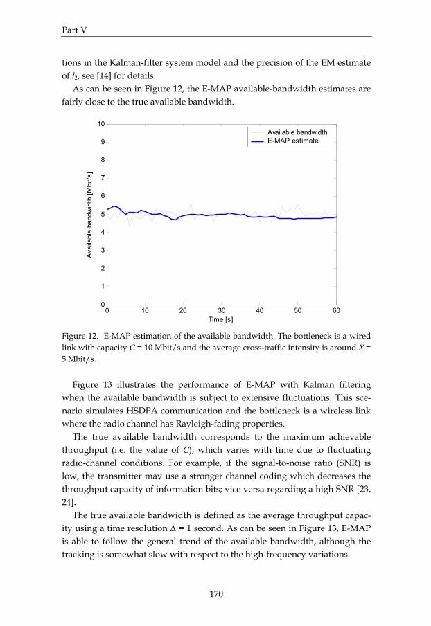
Part V

170

tions in the Kalman-filter system model and the precision of the EM estimate of l2, see [14] for details. As can be seen in Figure 12, the E-MAP available-bandwidth estimates are fairly close to the true available bandwidth.

0 10 20 30 40 50 600

1

2

3

4

5

6

7

8

9

10

Time [s]

Ava

ilabl

e ba

ndw

idth

[Mbi

t/s]

Available bandwidthE-MAP estimate

Figure 12. E-MAP estimation of the available bandwidth. The bottleneck is a wired link with capacity C = 10 Mbit/s and the average cross-traffic intensity is around X = 5 Mbit/s. Figure 13 illustrates the performance of E-MAP with Kalman filtering when the available bandwidth is subject to extensive fluctuations. This sce-nario simulates HSDPA communication and the bottleneck is a wireless link where the radio channel has Rayleigh-fading properties. The true available bandwidth corresponds to the maximum achievable throughput (i.e. the value of C), which varies with time due to fluctuating radio-channel conditions. For example, if the signal-to-noise ratio (SNR) is low, the transmitter may use a stronger channel coding which decreases the throughput capacity of information bits; vice versa regarding a high SNR [23, 24]. The true available bandwidth is defined as the average throughput capac-ity using a time resolution Δ = 1 second. As can be seen in Figure 13, E-MAP is able to follow the general trend of the available bandwidth, although the tracking is somewhat slow with respect to the high-frequency variations.

Part V

171

However, if it is desired that E-MAP should react more rapidly, this can be taken care of by adjusting the configuration of the used Kalman filter, as dis-cussed in Section 2.2.1.

0 20 40 60 80 100 1200

0.5

1

1.5

Time [s]

Ava

ilabl

e ba

ndw

idth

[Mbi

t/s]

Available bandwidthE-MAP estimate

Figure 13. E-MAP estimation of the available bandwidth. The bottleneck is a wire-less link and its capacity C varies with respect to the properties of a simulated Ray-leigh-fading radio channel. No cross traffic is activated. 5 Discussion and Conclusions This study has presented a number of general problems and challenges in the area of end-to-end available-bandwidth estimation. The discussion highlights several fundamental issues that should be taken into consideration when de-veloping and utilizing bandwidth-estimation tools. The BART method for available-bandwidth estimation has been used for illustrating the effect of using unsuitable configurations of adjustable parameters, or by performing bandwidth estimation in networks which have characteristics that are not accounted for in the measurement approach. With respect to BART, this study also includes suggestions of how some of these weaknesses can be handled. As an attempt to improve the efficiency and reliability when performing available-bandwidth measurements, a new method E-MAP has been devel-

Part V

172

oped. E-MAP, which is able to deal with some of the difficulties that are dis-cussed in this study, combines useful properties of other measurement tools. However, the main novelty is the utilization of the expectation-maximization algorithm for bandwidth estimation. In this investigation, E-MAP has been evaluated through simulations and the results indicate that the method is able to deliver reasonable estimates in both wired and wireless environments. However, in order to identify and understand all the advantages and disadvantages of E-MAP, it is necessary to perform a more thorough analysis where numerous aspects are considered. The estimation performance of E-MAP should also be compared to other bandwidth-measurement tools in various network topologies and traffic sce-narios. References [1] M. Jain and C. Dovrolis, “End-to-end available bandwidth: measure-

ment methodology, dynamics, and relation with TCP throughput,” IEEE/ACM Transactions on Networking, vol. 11, 2003.

[2] V. Ribeiro, R. Riedi, R. Baraniuk, J. Navratil, and L. Cottrell, “pathChirp: efficient available bandwidth estimation for network paths,” in Proc. Passive and Active Measurement Workshop, 2003.

[3] N. Hu and P. Steenkiste, “Evaluation and characterization of available bandwidth probing techniques,” IEEE JSAC Internet and WWW Meas-urement, Mapping, and Modeling, vol. 21, 2003.

[4] B. Melander, M. Björkman, and P. Gunningberg, “A new end-to-end probing and analysis method for estimating bandwidth bottlenecks,” in Proc. IEEE GLOBECOM’00, 2000.

[5] E. Bergfeldt, S. Ekelin, and J. M. Karlsson, “Real-time available-bandwidth estimation using filtering and change detection,” Computer Networks, vol. 53, 2009.

[6] J. Strauss, D. Katabi, and F. Kaashoek, “A measurement study of avail-able bandwidth estimation tools,” in Proc. ACM SIGCOMM Internet Measurement Conference, 2003.

[7] V. Ribeiro, M. Coates, R. Riedi, S. Sarvotham, B. Hendricks, and R. Ba-raniuk, “Multifractal cross-traffic estimation,” in Proc. ITC Specialist Se-minar on IP Traffic Measurement, Modeling and Management, 2000.

Part V

173

[8] R. Prasad, M. Jain, and C. Dovrolis, “Effects of interrupt coalescence on network measurements,” in Proc. Passive and Active Measurement Work-shop, 2004.

[9] H. Zhou, Y. Wang, X. Wang, and X. Huai, “Difficulties in estimating available bandwidth,” in Proc. IEEE International Conference on Communi-cations (ICC), 2006.

[10] T. Tsugawa, C. L. T. Man, G. Hasegawa, and M. Murata, “Inline band-width measurements: implementation difficulties and their solutions,” in Proc. IEEE/IFIP Workshop on End-to-End Monitoring Techniques and Ser-vices, 2007.

[11] E. Bergfeldt, “Real-time estimation of available bandwidth using the expectation-maximization algorithm,” in Proc. 5th Swedish National Com-puter Networking Workshop (SNCNW), 2008.

[12] R. S. Prasad, M. Murray, C. Dovrolis, and K. Claffy, “Bandwidth estima-tion: metrics, measurement techniques, and tools,” IEEE Network, vol. 17, 2003.

[13] E. Hartikainen and S. Ekelin, “Tuning the temporal characteristics of a Kalman-filter method for end-to-end bandwidth estimation,” in Proc. 4th IEEE/IFIP Workshop on End-to-End Monitoring Techniques and Services, 2006.

[14] G. Welch and G. Bishop, “An introduction to the Kalman filter,” SIG-GRAPH, Course 8, 2001.

[15] E. Hartikainen and S. Ekelin, “Enhanced network-state estimation using change detection,” in Proc. 31st IEEE Conference on Local Computer Net-works, 2006.

[16] E. Hartikainen, S. Ekelin, and J. M. Karlsson, “Change detection and es-timation for network-measurement applications,” in Proc. 2nd ACM Workshop on Performance Monitoring and Measurement of Heterogeneous Wireless and Wired Networks, 2007.

[17] F. Gustafsson and J. Palmqvist, “Change detection design for low false alarm rates,” in Proc. IFAC SAFEPROCESS’97, 1997.

[18] E. Bergfeldt, S. Ekelin, and J. M. Karlsson, “A performance study of bandwidth measurement tools over mobile connections,” in Proc. IEEE 69th Vehicular Technology Conference, 2009.

[19] A. Shriram and J. Kaur, “Empirical evaluation of techniques for measur-ing available bandwidth,” in Proc. IEEE INFOCOM, 2007.

[20] E. Bergfeldt, S. Ekelin, and J. M. Karlsson, “Real-time bandwidth meas-urements over mobile connections,” Submitted to European Transactions on Telecommunications, 2010.

Part V

174

[21] X. Liu, K. Ravindran, and D. Loguinov, “Multi-hop probing asymptotics in available bandwidth estimation: stochastic analysis,” in Proc. Internet Measurement Conference (IMC), 2005.

[22] A. P. Dempster, N. M. Laird, and D. B. Rubin, “Maximum likelihood from incomplete data via the EM algorithm,” Journal of the Royal Statisti-cal Society, vol. 39, 1977.

[23] E. Dahlman, S. Parkvall, J. Sköld, and P. Beming, 3G Evolution: HSPA and LTE for Mobile Broadband. Academic Press, 2007.

[24] H. Holma and A. Toskala, HSDPA/HSUPA for UMTS: High Speed Radio Access for Mobile Communications. John Wiley & Sons, 2006.