AdaptiveControlAllocation forConstrainedSystems ?

Seyed Shahabaldin Tohidi a, Yildiray Yildiz a, Ilya Kolmanovsky b

aMechanical Engineering Department, Bilkent University, Ankara, 06800, Turkey

bDepartment of Aerospace Engineering, University of Michigan, Ann Arbor, MI 48109, USA

Abstract

This paper proposes an adaptive control allocation approach for uncertain over-actuated systems with actuator saturation. Theproposed control allocation method does not require uncertainty estimation or persistency of excitation. Actuator constraintsare respected by employing the projection algorithm. The stability analysis is provided for two different cases: when idealadaptive parameters are inside and when they are outside of the projection boundary which is chosen consistently with theactuator saturation limits. Simulation results for the Aerodata Model in Research Environment (ADMIRE), which is used as anexample of an over-actuated aircraft system with actuator saturation, demonstrate the effectiveness of the proposed method.

Key words: Control allocation; Uncertain systems; Actuator saturation.

1 Introduction

Control allocation is the process of distributing controlsignals among redundant actuators which is employed inmany engineering domains such as aerial vehicles [1,4,13,29,35–37,50,53,54], marine vehicles [8,20,25,33,39], au-tomobiles [12,46], robots [42], and power systems [5,34].In particular, in aircraft and spacecraft applications, theflight control law determines forces and moments whilecontrol actuator settings are determined through con-trol allocation. Control allocation improves fault tolera-bility and modularity of the overall control system whilepermitting to exploit actuator redundancy for improvedmaneuverability.

Control allocation methods can be categorized into thefollowing three categories: Pseudo-inverse-based meth-ods, optimization based methods and dynamic controlallocation. Given a mapping between a control input v

? This work was supported by the Scientific and Technologi-cal Research Council of Turkey under grant number 118E202,and by Turkish Academy of Sciences the Young ScientistAward Program. The material in this paper was partiallypresented at American Control Conference (ACC), Boston,MA, 2016, World Congress of the International Federationof Automatic Control (IFAC), Toulouse, France, 2017, andIEEE Conference on Control Technology and Applications(CCTA), Copenhagen, Denmark, 2018.

Email addresses: shahabaldin@bilkent.edu.tr (SeyedShahabaldin Tohidi), yyildiz@bilkent.edu.tr (YildirayYildiz), ilya@umich.edu (Ilya Kolmanovsky).

and the actuator input vector u defined as Bu = v,in pseudo inverse based control allocation [2, 14, 15, 47],the control input is distributed to the individual actu-ators by the pseudo inverse mapping, i.e., u = B+v,which is the minimum 2-norm solution among infinitelymany control allocation solutions. Such a method canbe extended to account for actuator saturation [6, 14,15, 26, 41, 47, 51]. In optimization based control alloca-tion [7, 21, 23,32,55,56], control allocation is performedby minimizing the cost function ||Bu−v||+J0, where J0

represents a secondary objective such as minimizing ac-tuator deflections. For a recent optimization based com-putationally efficient control allocation example see [52].In dynamic control allocation [17, 18, 45, 48, 49, 57], thecontrol signals are distributed among actuators using aset of rules dictated by differential equations. A surveyof control allocation methods can be found in [24].

Control allocation is an appealing approach also for thedesign of active fault-tolerant control systems [3, 13, 16,40, 58]. For instance, it is used in [46] to improve thesteering performance in faulty automotive vehicles. Inanother study [33], control allocation distributes propul-sive forces of an autonomous underwater vehicle amongredundant thrusters so that faults are accommodated.In [35], experimental results of employing control allo-cation for quadrotor helicopter are reported. In severalapplications, fault detection and isolation methods areemployed in parallel with control allocation [13]. In [2],a sliding mode controller is coupled with a pseudo in-verse based control allocation to obtain a fault tolerantcontroller wherein faults are assumed to be estimated.

Preprint submitted to Automatica 25 August 2020

Similarly in [40], it is assumed that there exists a faultdetection and isolation scheme which is able to estimateand identify stuck-in-place, hard-over, loss of effective-ness and floating actuator faults. In [10], an unknown in-put observer is applied to identify actuator and effectorfaults. A family of unknown input observers is proposedin [11] to detect and isolate faults in systems with re-dundant actuators. In [47] and [7], faults are estimatedadaptively using recursive least squares, and an onlinedither generation method is proposed to guarantee thepersistence of excitation.

In this paper we consider the following problem: Allocatea control input vector v among redundant constrainedactuators in the presence of actuator effectiveness un-certainty. To solve this problem, two subproblems needto be addressed:

(i) Actuator uncertainty: Determine u such thatBΛu + d = v, where Λ represents uncertainty and drepresents an unknown bounded disturbance. In thispaper, we address this problem by proposing an adap-tive control allocation method which does not needuncertainty estimation unlike prior approaches.

(ii) Actuator constraints: Determine u such thatBΛu + d = v, where the elements of the actuator sig-nal vector, u, are constrained. One approach to preventactuators from getting saturated is to determine a setfor the control input vector elements, vi, i = 1, ..., r,and confine them to this set [9, 30, 44]. However, whenan adaptive approach is utilized to solve (i), restrictingcontrol signals in an attainable set may not preventactuator saturation. Hence, in addition to restrictingcontrol signals to an attainable set, an element-wisenon-symmetric projection algorithm is employed in thispaper to constrain adaptive parameters.

Other adaptive approaches to control allocation havebeen described in [45] and [17]. As compared to thesereferences, the approach in this paper eliminates theneed for uncertainty estimation and persistence of ex-citation assumption. Furthermore, in the proposed ap-proach, a closed loop reference model [19] is employed toachieve fast convergence without inducing undesired os-cillations. Apart from these contributions, we also showthat it is possible to employ the projection algorithm [28]in a stable manner even if the ideal adaptive parametersare not inside the projection boundaries. To the best ofour knowledge, such a result is not available in the priorliterature.

Preliminary results were reported in our conference pa-pers [48], [49] and [50]. This paper contains additionaldetails and proofs not reported in earlier publicationsand provides a procedure to account for the actuatorsaturation in a way that facilitates the design and inte-gration of the controller.

This paper is organized as follows. Section 2 introducesnotations and preliminary results. Section 3 presents the

uncertain over-actuated plant dynamics and the pro-posed model reference adaptive control allocation ap-proach with a closed loop reference model. A discussionof actuator saturation and its effects on the control lim-its together with the projection algorithm are given inSection 4. The ADMIRE model is used in Section 5 todemonstrate the effectiveness of the proposed approachin the simulation environment. Finally, a summary isgiven in Section 6.

2 Notations and preliminaries

In this section, we collect several definitions and ba-sic results which are exploited in the following sections.Throughout this paper, ||.|| refers to the Euclidean normfor vectors and induced 2-norm for matrices, and ||.||Frefers to the Frobenius norm. λmin(.), λmax(.) and λi(.)refer to the minimum, maximum and ith eigenvalue of amatrix, respectively. Also, rowi(.) and columni(.) referto the ith row and column of a matrix, respectively, andvec(.) : Rr×m → Rrm puts the elements of a matrix ina column vector. Ir is an identity matrix of dimensionr × r and tr(.) refers to the trace operation.

The element-wise projection Proj(θvi,j , Yi,j , f) : R×R×F → R is defined as

Proj(θvi,j , Yi,j , f) (1)

≡

Yi,j − Yi,jf(θvi,j ) if f(θvi,j ) > 0 & Yi,j(df

dθvi,j) > 0

Yi,j otherwise,

where f(.) ∈ F(R → R) is a convex and continuouslydifferentiable (C1) function defined as

f(θvi,j ) =(θvi,j − θmini,j − ζi,j)(θvi,j − θmaxi,j + ζi,j)

(θmaxi,j − θmini,j − ζi,j)ζi,j, (2)

and where ζi,j is the projection tolerance of the (i, j)th

element of θv that should be chosen as 0 < ζi,j <0.5(θmaxi,j − θmini,j ). θmaxi,j and θmini,j are the up-

per and lower bound of the (i, j)th element of θv. Thesebounds also form the projection set, Ωproj = θv : θvi,j ∈[θmini,j , θmaxi,j ]. A useful subset of Ωproj is defined

as Ωproj = θv : θvi,j ∈ [θmini,j + ζi,j , θmaxi,j − ζi,j ].For θv ∈ Ωproj and θ∗v ∈ Ωproj, the following inequalityholds [28]:

tr((θTv − θ∗vT )(−Y + Proj(θv, Y, f))) ≤ 0, (3)

where θv ∈ Ωproj ⊂ Rr×m, Y ∈ Rr×m.

3 Control Allocation Problem

The closed loop system studied in this paper is presentedin Fig. 1. The plant dynamics are given by

x(t) = Ax(t) +Bu(Λu(t) + du(t)), (4)

2

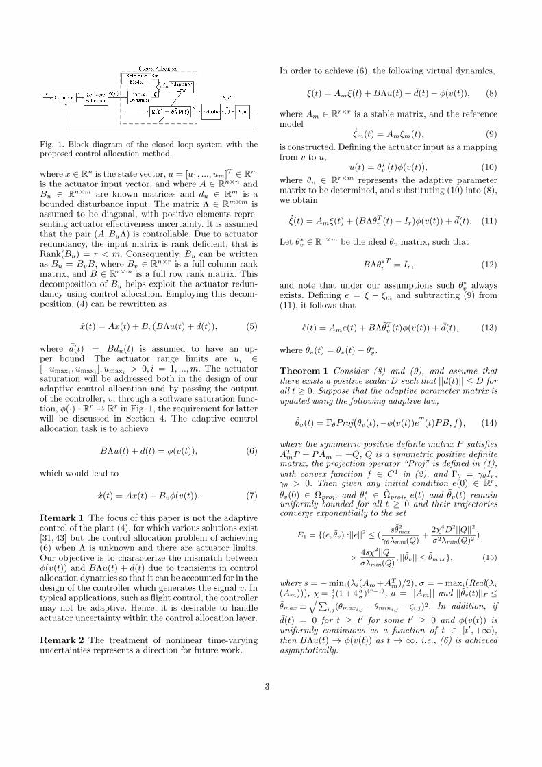
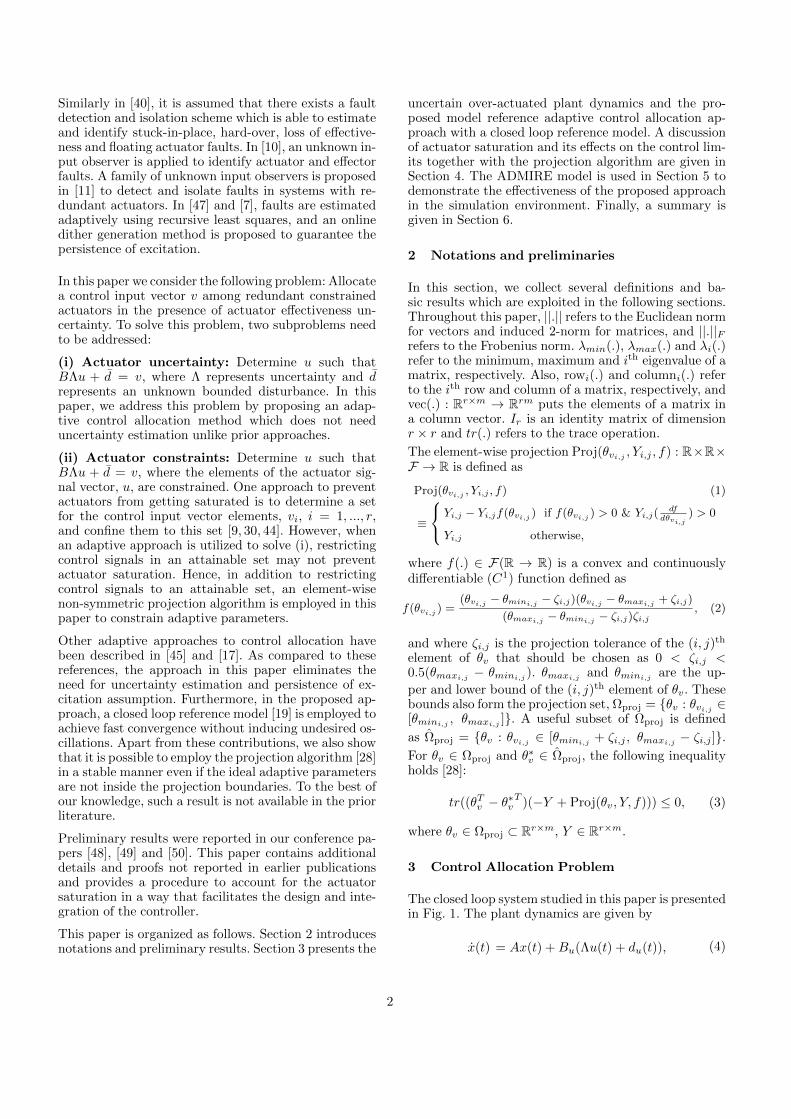
Fig. 1. Block diagram of the closed loop system with theproposed control allocation method.

where x ∈ Rn is the state vector, u = [u1, ..., um]T ∈ Rmis the actuator input vector, and where A ∈ Rn×n andBu ∈ Rn×m are known matrices and du ∈ Rm is abounded disturbance input. The matrix Λ ∈ Rm×m isassumed to be diagonal, with positive elements repre-senting actuator effectiveness uncertainty. It is assumedthat the pair (A,BuΛ) is controllable. Due to actuatorredundancy, the input matrix is rank deficient, that isRank(Bu) = r < m. Consequently, Bu can be writtenas Bu = BvB, where Bv ∈ Rn×r is a full column rankmatrix, and B ∈ Rr×m is a full row rank matrix. Thisdecomposition of Bu helps exploit the actuator redun-dancy using control allocation. Employing this decom-position, (4) can be rewritten as

x(t) = Ax(t) +Bv(BΛu(t) + d(t)), (5)

where d(t) = Bdu(t) is assumed to have an up-per bound. The actuator range limits are ui ∈[−umaxi , umaxi ], umaxi > 0, i = 1, ...,m. The actuatorsaturation will be addressed both in the design of ouradaptive control allocation and by passing the outputof the controller, v, through a software saturation func-tion, φ(·) : Rr → Rr in Fig. 1, the requirement for latterwill be discussed in Section 4. The adaptive controlallocation task is to achieve

BΛu(t) + d(t) = φ(v(t)), (6)

which would lead to

x(t) = Ax(t) +Bvφ(v(t)). (7)

Remark 1 The focus of this paper is not the adaptivecontrol of the plant (4), for which various solutions exist[31, 43] but the control allocation problem of achieving(6) when Λ is unknown and there are actuator limits.Our objective is to characterize the mismatch betweenφ(v(t)) and BΛu(t) + d(t) due to transients in controlallocation dynamics so that it can be accounted for in thedesign of the controller which generates the signal v. Intypical applications, such as flight control, the controllermay not be adaptive. Hence, it is desirable to handleactuator uncertainty within the control allocation layer.

Remark 2 The treatment of nonlinear time-varyinguncertainties represents a direction for future work.

In order to achieve (6), the following virtual dynamics,

ξ(t) = Amξ(t) +BΛu(t) + d(t)− φ(v(t)), (8)

where Am ∈ Rr×r is a stable matrix, and the referencemodel

ξm(t) = Amξm(t), (9)

is constructed. Defining the actuator input as a mappingfrom v to u,

u(t) = θTv (t)φ(v(t)), (10)

where θv ∈ Rr×m represents the adaptive parametermatrix to be determined, and substituting (10) into (8),we obtain

ξ(t) = Amξ(t) + (BΛθTv (t)− Ir)φ(v(t)) + d(t). (11)

Let θ∗v ∈ Rr×m be the ideal θv matrix, such that

BΛθ∗vT = Ir, (12)

and note that under our assumptions such θ∗v alwaysexists. Defining e = ξ − ξm and subtracting (9) from(11), it follows that

e(t) = Ame(t) +BΛθTv (t)φ(v(t)) + d(t), (13)

where θv(t) = θv(t)− θ∗v .

Theorem 1 Consider (8) and (9), and assume thatthere exists a positive scalar D such that ||d(t)|| ≤ D forall t ≥ 0. Suppose that the adaptive parameter matrix isupdated using the following adaptive law,

θv(t) = ΓθProj(θv(t),−φ(v(t))eT (t)PB, f

), (14)

where the symmetric positive definite matrix P satisfiesATmP + PAm = −Q, Q is a symmetric positive definitematrix, the projection operator “Proj” is defined in (1),with convex function f ∈ C1 in (2), and Γθ = γθIr,γθ > 0. Then given any initial condition e(0) ∈ Rr,θv(0) ∈ Ωproj, and θ∗v ∈ Ωproj, e(t) and θv(t) remainuniformly bounded for all t ≥ 0 and their trajectoriesconverge exponentially to the set

E1 = (e, θv) :||e||2 ≤ (sθ2

max

γθλmin(Q)+

2χ4D2||Q||2

σ2λmin(Q)2)

× 4sχ2||Q||σλmin(Q)

, ||θv|| ≤ θmax, (15)

where s = −mini(λi(Am+ATm)/2), σ = −maxi(Real(λi(Am))), χ = 3

2(1 + 4 a

σ)(r−1), a = ||Am|| and ||θv(t)||F ≤

θmax ≡√∑

i,j(θmaxi,j − θmini,j − ζi,j)2. In addition, if

d(t) = 0 for t ≥ t′ for some t′ ≥ 0 and φ(v(t)) isuniformly continuous as a function of t ∈ [t′,+∞),then BΛu(t) → φ(v(t)) as t → ∞, i.e., (6) is achievedasymptotically.

3

PROOF. See Appendix A. 2

Theorem 1 implies that θv and e are bounded. Consider-ing that φ(v) is bounded, (10) implies that u is bounded.Since Am is Hurwitz, the variable ξ, whose dynamics isgiven in (8), is also bounded. Therefore, all the signalsin the adaptive control allocation system are bounded.

Remark 3 To realize (8), the signal BΛu + d, is re-quired. In motion control applications, this signal cor-responds to the net forces and moments (see [22], forexample, for an aerospace application), that can be ob-tained via an inertial measurement unit (IMU). Exam-ples of measuring/estimating this signal, without intro-ducing delay or noise amplification, and employing it inreal applications can be found in [27,38].

Remark 4 A sufficient but not necessary condition forthe uniform continuity of φ(v(t)) is that its time rateof change is bounded, which can be ensured, e.g., byextending the software saturation function to include therate limiting. (see Fig. 1).

Remark 5 The proposed control allocation methoduses the signal φ(v(t)), which is the output of the soft-ware saturation. The saturation limits are determinedbased on the attainable set for v, the details of whichare given in Section 4. The control allocator then deter-mines the actuator signals, ui, i = 1, 2, ...,m, that do notsaturate the actuators. Note that putting a bound onv using soft saturation does not necessarily imply thatthe actuators will not be saturated by ui. To preventactuator saturation, the boundaries of the projectionoperator in (14) must be selected carefully, as furtherdetailed in Section 4.

Remark 6 In the case the assumption d(t) = 0, fort ≥ t′ for some t′ ≥ 0 is not made, a bound similarto E1 can be derived for the control allocation error,BΛu+ d−φ(v). However, note that even though only aboundedness result can be given for the control alloca-tion error, the tracking error for the overall closed loopsystem can still be forced to converge to zero by an ap-propriately designed controller (see Remark 11).

Remark 7 θ∗v ∈ Rr×m is the ideal parameter matrixthat should satisfy (12). Since Λ is unknown, θ∗v is alsounknown. However, although the diagonal matrix Λ isunknown, its elements are in the interval (0, 1]. Thus,using (12), the set Ω∗ that contains all possible valuesof θ∗v can be defined.

Conventionally, it is assumed that the projection bound-aries, θmini,j and θmaxi,j , are chosen such that θ∗v ∈ Ω∗ ⊂Ωproj ⊂ Ωproj. However, such a choice may not be con-sistent with the actuator limits as further discussed inSection 4.

Remark 8 Let θ∗v ∈ Ω∗, Ω∗ 6⊂ Ωproj and consider theprojection algorithm (1) with convex function (2). Then,

θmax, defined in Theorem 1, should be redefined as

θMAX ≡ (16)√∑i,j

(max(|θ∗maxi,j − θmini,j − ζi,j |, |θ∗mini,j

− θmaxi,j + ζi,j |))2.

We note that to differentiate two different cases (theideal parameter θ∗v being inside or outside the projectionbounds), the maximum value of adaptive parameter de-

viation from its ideal value is designated by θmax for theformer and θMAX for the latter case. Below, we provide alemma and a theorem, regarding the stability of the con-trol allocation for the latter case, i.e. when θ∗v /∈ Ωproj.

Lemma 1 For θ∗v /∈ Ωproj, θvi,j ∈ Rr×m, Y ∈ Rr×mwith r ≤ m and the projection algorithm (1)-(2), thefollowing inequality holds:

tr((θTv −θ∗vT )(−Y +Proj(θv, Y ))) ≤

√rθMAX ||Y ||. (17)

PROOF. See Appendix B. 2

Theorem 2 Consider (8), (9), (10), and (14). Assumethat there exist positive scalars M and D such that||φ(v(t))|| ≤ M and ||d(t)|| ≤ D for all t ≥ 0. Then,for any initial condition e(0) ∈ Rr, θv(0) ∈ Ωproj, and

θ∗v /∈ Ωproj, e(t) and θv(t) are uniformly bounded for allt ≥ 0 and their trajectories converge exponentially to theclosed and bounded set

E1 = (e, θv) : ||θv|| ≤ θMAX , ||e||2 ≤ (sθ2

MAX

γθλmin(Q)

+4χ4||Q||2(D2 + rθ2

MAX||B||2M2)

σ2λmin(Q)2)

4sχ2||Q||σλmin(Q)

, (18)

where s = −mini(λi(Am+ATm)/2), σ = −maxi(Real(λi

(Am))), χ =3

2(1 + 4

a

σ)(r−1), a = ||Am|| and θMAX is

defined in (16).

PROOF. See Appendix C. 2

To obtain fast convergence without introducing exces-sive oscillations, (9) is modified to obtain the followingclosed loop reference model [19].

ξm(t) = Amξm(t)− L(ξ(t)− ξm(t)), (19)

where Am ∈ Rr×r is Hurwitz, L = −`Ir, ` > 0. DefiningAm = Am + L, and subtracting (19) from (11), we get

e(t) = Ame(t) +BΛθTv (t)φ(v(t)) + d(t). (20)

We assume that the matrix Am is Hurwitz through anappropriate selection of L.

4

Theorem 3 Consider (8), the reference model (19), theactuator signal (10), and the adaptive law

θv(t) = ΓθProj(θv(t),−φ(v(t))e(t)T PB, f), (21)

where the symmetric positive definite matrix P satisfiesATmP + P Am = −Q, Q is a symmetric positive definitematrix, Γ−1

θ = (1/γθ)Ir, γθ > 0 and the projection isdefined by (1) and (2). Assume that there exist positivescalars M and D such that ||φ(v(t))|| ≤M and ||d(t)|| ≤D for all t ≥ 0. Then, for any initial condition e(0) ∈ Rr,and θv(0) ∈ Ωproj, e(t) and θ(t) are uniformly boundedfor all t ≥ 0 and their trajectories converge exponentiallyto a closed and bounded set

E2 =(e, θv) : ||e||2 ≤ ((s+ `)θ2

max

γθλmin(Q)+

2χ4D2||Q||2

σ2λmin(Q)2)

× 4(s+ `)χ2||Q||σλmin(Q)

, ||θv|| ≤ θmax,

if θ∗vi,j ∈ Ωproj, or to closed and bounded set

E2 = (e, θv) : ||θv|| ≤ θMAX , ||e||2 ≤ ((s+ `)θ2

MAX

γθλmin(Q)

+4χ4||Q||2(D2 + rθ2

MAX||B||2M2)

σ2λmin(Q)2)4(s+ `)χ2||Q||σλmin(Q)

,

if θ∗vi,j /∈ Ωproj, where σ = −maxi(Real(λi(Am))), s =

−mini(λi(Am + ATm)/2), a = ||Am|| and χ = 32 (1 +

4 aσ )(r−1).

PROOF. The proof procedure is similar to the one forTheorem 1 and 2, and is omitted for brevity. 2

4 Determination of the projection set

In the previous section, the control allocator was de-signed based on the projection operator. In this section,the determination of the projection set, Ωproj, which de-fines the bounds on adaptive control parameters, is de-tailed. The projection set is determined to satisfy tworequirements: 1) The actuator command signals, ui, i =1, ...,m, should not saturate the actuators and 2) a spe-cific condition (to be introduced shortly) which is nec-essary for the controller and control allocation integra-tion, should be satisfied. The design procedure to achievethese goals is composed of three main steps. First, anattainable set for control signal vector v is found forΛ = Im, which is used to determine the software sat-uration function φ(.). Secondly, a compact set for theadaptive parameter θv is calculated, to satisfy −umax ≤θTv φ(v) ≤ umax. Thirdly, the projection set that satisfiesthe specific requirement necessary for the controller andcontrol allocation integration is determined.

Step 1: Realizable values of control signals are found.

The actuator constraints are known: u(t) ∈ Ωu, whereΩu = [u1, ..., um]T : −umaxi ≤ ui ≤ umaxi , i =1, ...,m, umaxi > 0, i = 1, ...,m. Using Ωu, the set Ωv,defining all realizable values of the control input v, canbe obtained as Ωv = v : v = Bu, u ∈ Ωu, B

†v ∈ Ωu,where (.)† refers to the pseudo inverse of a non-squarematrix. Furthermore, there exist Mi, i = 1, ..., r, suchthat Ωv ≡ v : vi ∈ [−Mi,Mi], i = 1, ..., r ⊂ Ωv. The

set Ωv can be used to define the constraints which areenforced using a software saturation function, whoseoutput is φ(v(t)). See Fig. 1 and Remark 5.

Step 2: The boundaries for the adaptive parameters toensure that the actuator signal vector u does not saturatethe actuators are calculated.

A subset of the attainable set for the control signals, Ωv,was obtained in Step 1. The actuator limits are known.With this information, the set Ωθ = θv : −umax ≤θTv φ(v) ≤ umax, φ(v) ∈ Ωv can be obtained. Let θ∗I =B† which corresponds to an adaptive parameter value inthe absence of uncertainty, i.e., Λ = I. Since φ(v) ∈ Ωv ⊂Ωv, we have B†φ(v) = θ∗I

Tφ(v) ∈ Ωu, for all φ(v) ∈ Ωv.Therefore, θ∗I ∈ Ωθ, which is required to subsequentlysolve the optimization problem (25) (see Remark 9).

Step 3: A subset of Ωθ, which satisfies a necessary con-dition for a stabilizing controller, is obtained. This sub-set of Ωθ also determines the ultimate projection bound-aries, and is denoted by Ωproj.

The plant dynamics (5), can be rewritten, by using (10),

(12) and defining θv = θv − θ∗v , as

x = Ax+Bv(BΛu+ d) = Ax+Bv(BΛθTv φ(v) + d)

= Ax+Bv(I +BΛθTv )φ(v) +Bvd, (22)

where φ(v) ∈ Ωv and d is a bounded disturbance. Notethat the projection algorithm guarantees that the actu-ators do not saturate, and the closed loop system doesnot see any residual disturbance due to saturation of theactuators. Defining ∆B(t) ≡ BΛθTv (t), and substitutingin (22), it follows that

x(t) = Ax(t) +Bv(φ(v(t)) + d(t)), (23)

where d(t) = ∆B(t)φ(v(t)) + d(t) ∈ Rr.

To be able to design a stabilizing controller, which willproduce the control input v, one must make sure thateach element of the disturbance vector d = [d1, ..., dr]

T

in (23), is smaller in absolute value than the upper boundof the corresponding element of the saturated controlinput, φ(v), that is |di| < Mi, i = 1, ..., r. Since di =rowi(∆B)v+di, i = 1, ..., r, where di is the ith element ofd, satisfying the following condition ensures that |di| <Mi, i = 1, ..., r:

Mi − ||rowi(∆B)||Mmax > |di|, i = 1, ..., r, (24)

5

where Mmax = maxiMi. A necessary conditionfor satisfying the inequality (24) is ||rowi(∆B)|| =

||rowi(BΛθTv )|| < Mi/Mmax for all i = 1, ..., r. (Suf-ficient conditions required to satisfy (24) is discussedlater in Remark 10). Thus, the elements of the matrixθv should be properly bounded in order to satisfy thenecessary condition ||rowi(BΛθTv )|| < Mi/Mmax for all

i = 1, ..., r, and for all Λ ∈ ΩΛ, where ΩΛ ⊂ ΩΛ, and ΩΛ

is the set of all m×m diagonal matrices with elementsin (0, 1]. Thus ΩΛ has diagonal elements λi ∈ (γ, 1],where γ is precisely defined later in Theorem 4.

SinceBΛθTv = BΛ(θTv −θ∗vT ) = BΛθTv −Ir, the solution,

R, of the optimization problem,

R2 = minθv

(vec(θv − θ∗I )T vec(θv − θ∗I )

)(25)

s.t.∥∥∥rowi(BΛθTv − Ir)

∥∥∥2

=M2i

M2max

− ε, i = 1, ..., r,

Λ ∈ ΩΛ, θv ∈ Ωθ,

which is solved offline, is the minimum distance from thevec(θ∗I ) to the boundary of the set

Ψ = θv : ||rowi(BΛθTv − Ir)||2 ≤M2i

M2max

− ε,

Λ ∈ ΩΛ, θv ∈ Ωθ, i = 1, ..., r, (26)

where ε is a small positive constant used to have a closedset, since typical numerical optimizers optimize only overa closed set. It is noted that the corresponding θmaxi,jand θmini,j are not unique, and different boundaries canbe found by defining different cost functions in (25).With the calculated θmaxi,j and θmini,j , the projectionset is obtained as,

Ωproj = θv : θi,j ∈ [θmini,j , θmaxi,j ]. (27)

Remark 9 For all elements of ΩΛ, the optimizationproblem (25) finds the largest neighborhood of θ∗I in Ωθthat satisfies ||rowi(∆B)|| < Mi/Mmax, i = 1, ..., r. Thisneighborhood is an n-sphere, with the center at vec(θ∗I )and with the radius R.

To show that the optimization problem (25) is feasible, itshould be proven that the set E always includes vec(θ∗I ).

Theorem 4 The set Υ = vec(θv) : ||rowi(BΛθTv −Ir)||2 ≤ M2

i

M2max− ε,Λ ∈ ΩΛ ⊂ ΩΛ, i = 1, ..., r∩ vec(θ∗I ) 6=

∅ when λmin(Λ) ≥ γ ≡ maxi(1 −√γMi/γBi), where

γBi ≡ ||rowi(B)||||BT (BBT )−1|| and γMi≡ M2

i

M2max− ε.

PROOF. See Appendix D. 2

Based on the definition of γBi , γMi and γ given in The-

orem 4, ΩΛ is defined as

ΩΛ = Λ : Λ ∈ Dm×m, diagi(Λ) ∈ (γ, 1], i = 1, ...,m,(28)

where D denotes the set of real diagonal matrices, anddiagi(.) : Rm×m → R provides the ith diagonal elementof square matrices.

Remark 10 Using ΩΛ, defined in (28), and Ωproj,defined in (27), the upper bound on ||rowi(∆B)|| =

||rowi(BΛθTv )|| can be found, which we denote as ρi,i = 1, ..., r. Therefore, recalling that Mi is defined asthe upper bound on the absolute value of ith controlsignal vi, and considering (24), |di| should be smallerthan Mi − ρiMmax, i.e. |di| < Mi − ρiMmax. Notethat ρi <

Mi

Mmaxis guaranteed by the solution of (25).

Therefore, the condition |di| < Mi is satisfied.

Remark 11 A step by step procedure for the controlallocation design is provided in Appendix E. Note thatin the presence of the control allocator, the system dy-namics takes the form of (23). The controller, which willproduce the control signal v, needs to be designed inthe presence of the saturation nonlinearity representedby φ(.) and the bounded disturbance d. Tracking con-trollers for (23) can be designed using, for instance, themethods presented in [9]. See also [48, 49] which illus-trate the process of integrating an initial version of ourcontrol allocation scheme and a controller. We omit de-tails for lack of space.

5 SIMULATION RESULTS

The Aerodata Model in Research Environment (AD-MIRE), which represents the dynamics of an over-actuated aircraft model, is used to demonstrate theeffectiveness of the adaptive control allocation in thepresence of uncertainty and actuator constraints. Thelinearized ADMIRE model [23] is given below:

x = Ax+Buu = Ax+Bvv,

v = Bu, Bu = BvB, Bv = [03×2 I3×3]T , (29)

where x = [α β p q r]T with α, β, p, q and r denote the an-gle of attack, sideslip angle, roll rate, pitch rate and yawrate, respectively. The vector u = [uc ure ule ur]

T rep-resents the control surface deflections of canard wings,right and left elevons and the rudder. The position lim-its of the control surfaces are given as uc ∈ [−55, 25] ×π

180rad, ure, ule, ur ∈ [−30, 30]× π180rad and the actu-

ators have first-order dynamics and a time constant of0.05 s. The state and control matrices are given in [23].To represent actuator loss of effectiveness and distur-bance, a diagonal matrix Λ and a vector du, respectively,are augmented to the model (29) as

x = Ax+BuΛu+Budu = Ax+Bvv +Bvd (30)

v = BΛu, d = Bdu, Bu = BvB, Bv = [03×2 I3×3]T .

In the simulations, the disturbance d is a sinusoidalfunction with amplitude 0.1 and frequency 1 rad/s

6

0 5 10 15 200

0.1

0.2

0.3

0 5 10 15 20

-0.05

0

0.05

0 5 10 15 200

0.2

0.4

0 5 10 15 200

0.1

0.2

0.3

0 5 10 15 20

0

0.05

0.1

0 5 10 15 20

Time(s)

-0.5

0

0.5

0 5 10 15 20

-1

0

1

0 5 10 15 20

-1

0

1

0 5 10 15 20

-0.2

0

0.2

0 5 10 15 20-1

-0.5

0

0.5

0 5 10 15 20

-0.5

0

0.5

0 5 10 15 20

Time(s)

-0.5

0

0.5

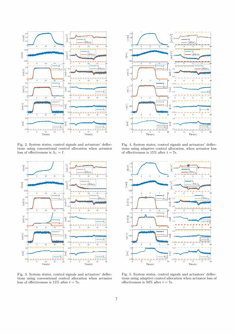
Fig. 2. System states, control signals and actuators’ deflec-tions using conventional control allocation when actuatorloss of effectiveness is Λ1 = I.

0 5 10 15 200

0.5

1

0 5 10 15 20

-0.05

0

0.05

0 5 10 15 200

0.2

0.4

0 5 10 15 200

0.5

1

0 5 10 15 20

0

0.05

0.1

0 5 10 15 20

Time(s)

-0.5

0

0.5

0 5 10 15 20

-1

0

1

0 5 10 15 20

-1

0

1

0 5 10 15 20

-0.2

0

0.2

0 5 10 15 20-1

-0.5

0

0.5

0 5 10 15 20

-0.5

0

0.5

0 5 10 15 20

Time(s)

-0.5

0

0.5

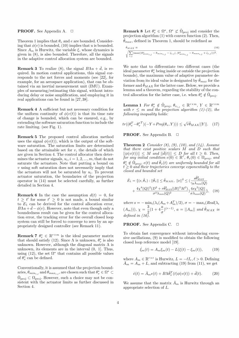
Fig. 3. System states, control signals and actuators’ deflec-tions using conventional control allocation when actuatorloss of effectiveness is 15% after t = 7s.

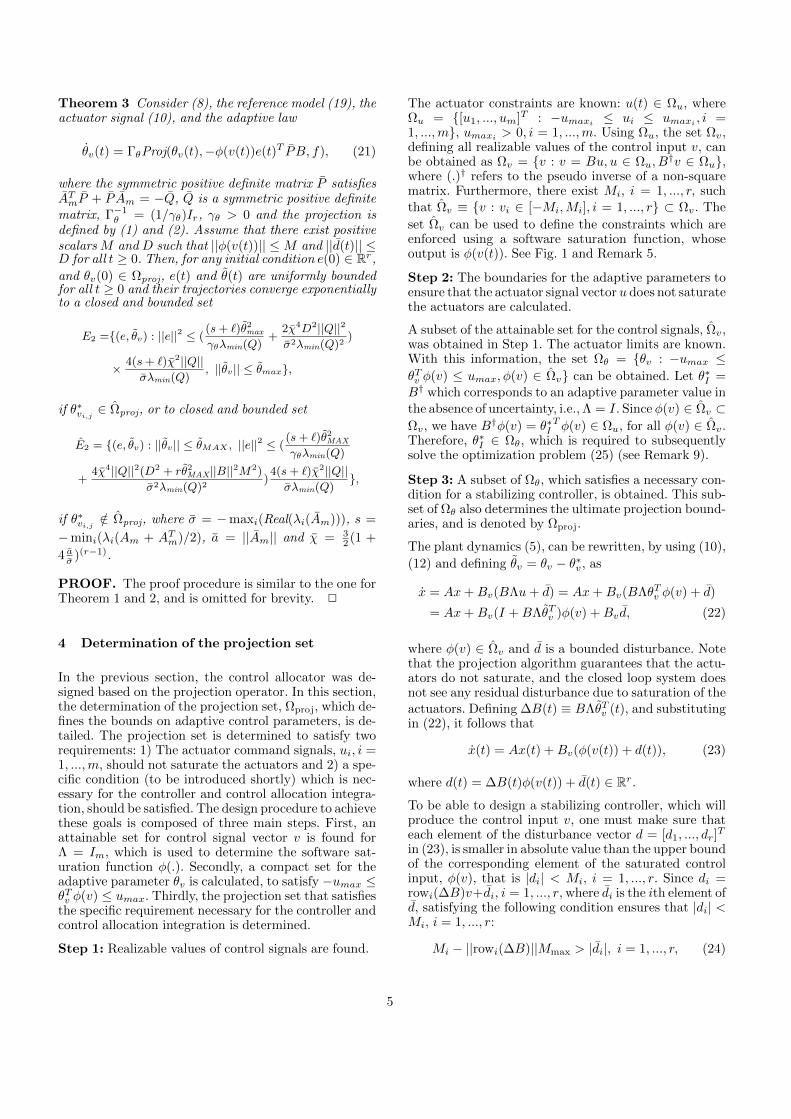
Fig. 4. System states, control signals and actuators’ deflec-tions using adaptive control allocation, when actuator lossof effectiveness is 15% after t = 7s.

Fig. 5. System states, control signals and actuators’ deflec-tions using adaptive control allocation when actuator loss ofeffectiveness is 50% after t = 7s.

7

while zero-mean white Gaussian noise with standarddeviation σp,q,r = 0.0017 rad/s for the angular ratesand σα,β = 0.0044 rad for angles represent the mea-surement noise [38]. For all of the simulations a slidingmode controller is used to create the control signal v.The simulation results for a conventional pseudo in-verse based control allocation are reported in Fig. 2 forthe case without actuator loss of effectiveness, that is,Λ1 = I. With the actuator loss of effectiveness modeledas changing the diagonal elements of Λ from 1 to 0.85at t = 7s, the simulation results for the conventionalcontrol allocation are given in Fig. 3. It is seen that 15%loss of effectiveness in all actuators at t = 7 s causesinstability. The proposed adaptive control allocation in-troduced in Section 3 is used in the simulations. UsingSteps 1-3 in Section 4, the values of M1 = 1.4, M2 = 1.4and M3 = 0.3 are obtained and Ωproj, which determinesthe maximum and minimum of each element of theadaptive parameter matrix is computed correspondingto θv1,1 ∈ [−0.0129, 0.0129], θv1,2 ∈ [0.0307, 0.5225],θv1,3 ∈ [−0.1357, 0.1371], θv1,4 ∈ [−0.212, 0], θv2,1 ∈[−0.3149,−0.1113], θv2,2 ∈ [−0.217,−0.1416], θv2,3 ∈[−0.0241, 0.2363], θv2,4 ∈ [−0.4162,−0.01], θv3,1 ∈[0.1587, 0.1977], θv3,2 ∈ [0.0673, 0.0675], θv3,3 ∈[−0.001, 0.001], θv3,4 ∈ [−1.2755,−0.7641]. We use aclosed loop reference model with l = 4 and Am selectedas Am = diag([−0.2,−0.1,−0.1]). Figure 4 shows thesimulation results for the system with adaptive con-trol allocation and 15% actuator loss of effectiveness att = 7s. It is seen that the first two states, α and β, arebounded, and the other states (p, q and r) follow thereference inputs (pref , qref and rref ) after the intro-duction of 15% actuator loss of effectiveness at t = 7sec. Also, it is seen that the elements of (BΛu)i fori = 1, 2, 3, converge to the control signal elements vi fori = 1, 2, 3. Finally, as seen from Figures 2, 3, and 4, theexistence of noise does not affect the adaptive controlallocation performance compared to the non-adaptivefixed control allocation. Another scenario is considerednext, where a the diagonal elements of Λ change from1 to 0.5 at t = 7s. It is seen in Fig. 5 that the systemremains stable even after the introduction of the 50%loss of effectiveness.

6 SUMMARY

An adaptive control allocation for uncertain over-actuated systems with actuator saturation is proposedin this paper. The method needs neither uncertaintyidentification nor persistence of excitation assumption.Simulation results with the ADMIRE model show theeffectiveness of the proposed method.

A Proof of Theorem 1

Consider a Lyapunov function candidate,

V = eTPe+ tr(θTv Γ−1θ θvΛ). (A.1)

The time derivative of (A.1) along the trajectories of(13)-(14) can be calculated as

V = −eTQe+ 2eTPBΛθTv v + 2tr(θTv Γ−1θ

˙θvΛ) + 2eTP d.

(A.2)

Using the property of the trace operation and the adap-tive law (14), (A.2) can be written as

V = −eTQe+ 2eTP d

+2tr(θTv (veTPB + Proj(θv,−veTPB, f))Λ).(A.3)

If d(t) = 0 for t ≥ 0 (without loss of generality), it can

be shown, by using (3), that V ≤ 0 and therefore e(t)

and θv(t) are bounded. Since e ∈ L2 and e ∈ L∞, e(t)converges to zero as t→∞ [43]. Since θv, e and φ(v) are

bounded, θv is also bounded by (14). In addition, since e,

θv and v are bounded, e is also bounded by (13). There-

fore, e and θv are uniformly continuous functions. If v isalso uniformly continuous, then e is uniformly continu-ous by (13) since the multiplication of bounded and uni-formly continuous functions are uniformly continuous.Then, according to Barbalat’s lemma, e(t) converges tozero as t→∞. Since both e and e converges to zero, by(13) BΛθvv(t) converges to zero, and hence using (10)and (12), it can be shown that (6) is achieved asymp-totically. When d 6= 0, it can be shown that all the tra-jectories converge to a compact set E1. To find E1, wefirst introduce two properties of P [19] derived from theLyapunov equation ATmP + PAm = −Q as

||P || ≤ χ2||Q||/σ, (A.4)

λmin(P ) ≥ λmin(Q)/2s. (A.5)

Using (A.1), it follows that

V ≤ ||e||2||P ||+ tr(θTv Γ−1θ θvΛ) = ||e||2||P ||

+ (1/γθ)tr(θTv θvΛ) ≤ ||e||2||P ||+ (1/γθ)θ

2max, (A.6)

Since θ∗v ∈ Ωproj, using (A.3) and (3), we have V ≤−λmin(Q)||e||2 + 2||e||||P d||. By using Young’s inequal-

ity, it follows that V ≤ − 12λmin(Q)||e||2 + 2||P ||2D2/

λmin(Q). Thus, using this inequality and (A.6), we have

V (t) ≤ −λmin(Q)V

2||P ||+λmin(Q)θ2

max

2γθ||P ||+

2||P ||2D2

λmin(Q)

≤ −ω1V + ω2, (A.7)

where ω1 = σλmin(Q)2χ2||Q|| and ω2 = s

γθθ2

max + 2χ4D2||Q||2σ2λmin(Q) . By

using the Gronwall inequality, (A.7) can be rewritten as

V (t) ≤(V (0)− ω2

ω1

)e−ω1t +

ω2

ω1. (A.8)

8

Using e(t)TPe(t) ≤ V (t) ≤(V (0)− ω2

ω1

)e−ω1t + ω2

ω1and

taking the limits of the leftmost and rightmost sides ast goes to infinity, we have

lim supt→∞

e(t)TPe(t) ≤ (sθ2

max

γθ+

2χ4D2||Q||2

σ2λmin(Q))

2χ2||Q||σλmin(Q)

.

(A.9)By using the inequality λmin(P )||e||2 ≤ eTPe ≤λmax(P )||e||2 and (A.5), we have λmin(Q)

2s ||e||2 ≤λmin(P )||e||2 ≤ eTPe. Thus, from (A.9) we have,

lim supt→∞

||e(t)||2 ≤ (sθ2

max

γθλmin(Q)+

2χ4D2||Q||2

σ2λmin(Q)

2

)4sχ2||Q||σλmin(Q)

.

Therefore, for the initial conditions e(0) and θv(0) ∈Ωproj, e(t) and θv(t) are uniformly bounded for all t ≥ 0and system trajectories converge to the following com-pact set E1 given by (15).

B Proof of Lemma 1

For both cases in projection algorithm (1), we have

tr((θTv − θ∗vT

)(−Y + Proj(θv, Y, f)))

=

m∑j=1

r∑i=1

(θvi,j − θ∗vi,j )

(− Yi,j + Proj(θvi,j , Yi,j , f)

)≤

m∑j=1

r∑i=1

|(θvi,j − θ∗vi,j )Yi,jf(θvi,j )| ≤

m∑j=1

r∑i=1

|θi,jYi,j |

= tr(|θTv ||Y |) ≤ ||θv||F ||Y ||F ≤√rθMAX ||Y ||,

where we used the property, ||Y ||F ≤√min(r,m)||Y ||,

and |θTv | and |Y | which are the matrices of absolute val-

ues of the elements of θTv and Y , respectively.

C Proof of Theorem 2

By using (A.1), (A.3), (17) with Y = −veTPB, andYoung’s inequality, we have

V ≤ −1

2||e||2 + 4||P ||2D2 + 4rθ2

MAX ||P ||2||B||2M2.

(C.1)

Also, instead of (A.6), we have V||P || −

θ2MAX

γθ||P || ≤ ||e||2.

Using this inequality, (A.4), (A.5) and (C.1), we obtain

V ≤ −λmin(Q)V

2||P || +λmin(Q)θ2

MAX

2γθ||P ||+

4||P ||2D2

λmin(Q)(C.2)

+4rθ2

MAX||P ||2||B||2M2

λmin(Q)≤ −ω1V + ω2,

where ω1 = λmin(Q)σ2χ2||Q|| and ω2 =

sθ2MAX

γθ+ 4χ

4D2||Q||2σ2λmin(Q) +

4rθ2MAXχ

4||B||2M2||Q||2σ2λmin(Q) . Following the same procedure as

for E1, E1 is obtained and is given by (18).

D Proof of Theorem 4

To prove the non-emptiness of Υ, we should show that

||rowi(BΛθ∗IT − Ir)||2 ≤ M2

i

M2max− ε. Using (26) and the

definition of θ∗IT = BT (BBT )−1, we have,

||rowi(BΛθ∗IT − Ir)||2 = ||rowi(BΛBT (BBT )−1 − Ir)||2

= ||rowi(BΛBT (BBT )−1 −BBT (BBT )−1)||2

≤ ||rowi(B(Λ− Im))||2||BT (BBT )−1||2

≤ (λmax(Λ− Im))2||rowi(B)||2||BT (BBT )−1||2

= (λmin(Λ)− 1)2||rowi(B)||2||BT (BBT )−1||2. (D.1)

Therefore, in order to show that ||rowi(BΛθ∗IT−Ir)||2 ≤

M2i

M2max− ε, for all i = 1, ..., r, we should satisfy

(λmin(Λ)− 1)2||rowi(B)||2||BT (BBT )−1||2 ≤ M2i

M2max

− ε

⇒ −√γMi/γBi ≤ λmin(Λ)− 1 ≤

√γMi/γBi , i = 1, ..., r,

where γBi ≡ ||rowi(B)||||BT (BBT )−1|| and γMi =M2i

M2max− ε for all i = 1, ..., r. Since the maximum value

for the diagonal elements of Λ is one, the only conditionthat should be satisfied is that 1−

√γMi/γBi ≤ λmin(Λ)

for i = 1, ..., r or γ ≡ maxi(1−√γMi/γBi) ≤ λmin(Λ).

E Design procedure

The following procedure can be followed to compute theparameters of our control allocation scheme:

Step 1- Use Step 1 in Section 4, to determine Mi, i =1, ..., r, thus, Ωv is obtained.

Step 2- Calculate Ωθ using Step 2 in Section 4.

Step 3- Using Theorem 4, calculate γ ≡ maxi(1 −√γMi

/γBi), where Mmax = maxiMi, γMi≡ M2

i

M2max− ε

for a small positive ε, and γBi ≡ ||rowi(B)||||BT (BBT )−1||.

Step 4- Using γ, obtain ΩΛ in (28).

Step 5- Solve the optimization problem (25), whichleads to obtaining the Ωproj, which is defined in Section4, step 3. This allows the implementation of (10).

References

[1] D. M. Acosta, Y. Yildiz, R. W. Craun, S. D. Beard, M. W.Leonard, G. H. Hardy, and M. Weinstein. Piloted evaluationof a control allocation technique to recover from pilot-inducedoscillations. Journal of Aircraft, 52(1):130–140, 2014.

[2] H. Alwi and C. Edwards. Fault tolerant control usingsliding modes with on-line control allocation. Automatica,44(7):1859–1866, 2008.

[3] A. Argha, S. W. Su, and B. G. Celler. Control allocation-based fault tolerant control. Automatica, 103:408–417, 2019.

9

[4] M. Bodson. Evaluation of optimization methods for controlallocation. Journal of Guidance, Control, and Dynamics,25(4):703–711, 2002.

[5] A. Bouarfa, M. Bodson, and M. Fadel. A fast active-balancingmethod for the 3-phase multilevel flying capacitor inverterderived from control allocation theory. IFAC-PapersOnLine,50(1):2113–2118, 2017.

[6] J. M. Buffington and D. F. Enns. Lyapunov stability analysisof daisy chain control allocation. Journal of Guidance,Control, and Dynamics, 19(6):1226–1230, 1996.

[7] A. Casavola and E. Garone. Fault-tolerant adaptive controlallocation schemes for overactuated systems. InternationalJournal of Robust and Nonlinear Control, 20(17):1958–1980,2010.

[8] M. Chen, S. S. Ge, B. V. E. How, and Y. S. Choo. Robustadaptive position mooring control for marine vessels. IEEETransactions on Control Systems Technology, 21(2):395–409,2013.

[9] M. L. Corradini, A. Cristofaro, and G. Orlando. Robuststabilization of multi input plants with saturating actuators.IEEE Transactions on Automatic Control, 55(2):419–425,2010.

[10] A. Cristofaro and T. A. Johansen. Fault tolerant controlallocation using unknown input observers. Automatica,50(7):1891–1897, 2014.

[11] A. Cristofaro, M. M. Polycarpou, and T. A. Johansen.Fault diagnosis and fault-tolerant control allocation for aclass of nonlinear systems with redundant inputs. In IEEEConference on Decision and Control, pages 5117–5123, 2015.

[12] M. Demirci and M. Gokasan. Adaptive optimal controlallocation using lagrangian neural networks for stabilitycontrol of a 4ws–4wd electric vehicle. Transactions ofthe Institute of Measurement and Control, 35(8):1139–1151,2013.

[13] G. J. Ducard. Fault-tolerant flight control and guidancesystems: Practical methods for small unmanned aerialvehicles. Springer Science & Business Media, 2009.

[14] W. Durham, K. A. Bordignon, and R. Beck. Aircraft Controlallocation. Springer Science & Business Media, 2009.

[15] W. C. Durham. Constrained control allocation. Journal ofGuidance, control, and Dynamics, 16(4):717–725, 1993.

[16] C. Edwards, T. Lombaerts, H. Smaili, et al. Fault tolerantflight control. Lecture Notes in Control and InformationSciences, 399:1–560, 2010.

[17] G. P. Falconı and F. Holzapfel. Adaptive fault tolerant controlallocation for a hexacopter system. In American ControlConference (ACC), 2016, pages 6760–6766. IEEE, 2016.

[18] S. Galeani and M. Sassano. Data-driven dynamic controlallocation for uncertain redundant plants. In IEEEConference on Decision and Control, pages 5494–5499, 2018.

[19] T. E. Gibson, Z. Qu, A. M. Annaswamy, and E. Lavretsky.Adaptive output feedback based on closed-loop referencemodels. IEEE Transactions on Automatic Control,60(10):2728–2733, 2015.

[20] W. Gierusz and M. Tomera. Logic thrust allocation appliedto multivariable control of the training ship. ControlEngineering Practice, 14(5):511–524, 2006.

[21] O. Harkegard. Efficient active set algorithms for solvingconstrained least squares problems in aircraft controlallocation. In IEEE Conference on Decision and Control,volume 2, pages 1295–1300, 2002.

[22] O. Harkegard. Backstepping and control allocation withapplications to flight control. PhD thesis, Linkopingsuniversitet, 2003.

[23] O. Harkegard andS. T. Glad. Resolving actuator redundancy-optimal controlvs. control allocation. Automatica, 41(1):137–144, 2005.

[24] T. A. Johansen and T. I. Fossen. Control allocation—asurvey. Automatica, 49(5):1087–1103, 2013.

[25] T. A. Johansen, T. P. Fuglseth, P. Tøndel, and T. I.Fossen. Optimal constrained control allocation in marinesurface vessels with rudders. Control Engineering Practice,16(4):457–464, 2008.

[26] M. Kirchengast, M. Steinberger, and M. Horn. Inputmatrix factorizations for constrained control allocation. IEEETransactions on Automatic Control, 63(4):1163–1170, 2018.

[27] A. Kutay, J. Culp, J. Muse, D. Brzozowski, A. Glezer, andA. Calise. A closed-loop flight control experiment using activeflow control actuators. In 45th AIAA Aerospace SciencesMeeting and Exhibit, page 114, 2007.

[28] E. Lavretsky and T. E. Gibson. Projection operator inadaptive systems. arXiv preprint arXiv:1112.4232, 2011.

[29] F. Liao, K.-Y. Lum, J. Wang, and M. Benosman. Adaptivecontrol allocation for non-linear systems with internaldynamics. IET control theory & applications, 4(6):909–922,2010.

[30] M. Naderi, A. K. Sedigh, and T. A. Johansen. Guaranteedfeasible control allocation using model predictive control.Control Theory and Technology, 17(3):252–264, 2019.

[31] K. S. Narendra and A. M. Annaswamy. Stable adaptivesystems. Courier Corporation, 2012.

[32] J. A. Petersen and M. Bodson. Constrained quadraticprogramming techniques for control allocation. IEEETransactions on Control Systems Technology, 14(1):91–98,2006.

[33] T. K. Podder and N. Sarkar. Fault-tolerant control of anautonomous underwater vehicle under thruster redundancy.Robotics and Autonomous Systems, 34(1):39–52, 2001.

[34] M. E. Raoufat, K. Tomsovic, and S. M. Djouadi. Dynamiccontrol allocation for damping of inter-area oscillations. IEEETransactions on Power Systems, 32(6):4894–4903, 2017.

[35] I. Sadeghzadeh, A. Chamseddine, Y. Zhang, and D. Theilliol.Control allocation and re-allocation for a modified quadrotorhelicopter against actuator faults. IFAC ProceedingsVolumes, 45(20):247–252, 2012.

[36] Q. Shen, D. Wang, S. Zhu, and E. K. Poh. Inertia-free fault-tolerant spacecraft attitude tracking using control allocation.Automatica, 62:114–121, 2015.

[37] Q. Shen, D. Wang, S. Zhu, and E. K. Poh. Robust controlallocation for spacecraft attitude tracking under actuatorfaults. IEEE Transactions on Control Systems Technology,25(3):1068–1075, 2017.

[38] S. Sieberling, Q. Chu, and J. Mulder. Robust flight controlusing incremental nonlinear dynamic inversion and angularacceleration prediction. Journal of guidance, control, anddynamics, 33(6):1732–1742, 2010.

[39] A. J. Sørensen. A survey of dynamic positioning controlsystems. Annual reviews in control, 35(1):123–136, 2011.

[40] M. E. N. Sørensen, S. Hansen, M. Breivik, and M. Blanke.Performance comparison of controllers with fault-dependentcontrol allocation for uavs. Journal of Intelligent & RoboticSystems, 87(1):187–207, 2017.

10

[41] J. Stephan and W. Fichter. Fast exact redistributedpseudoinverse method for linear actuation systems. IEEETransactions on Control Systems Technology, (99):1–8, 2017.

[42] H. D. Taghirad and Y. B. Bedoustani. An analytic-iterativeredundancy resolution scheme for cable-driven redundantparallel manipulators. IEEE Transactions on Robotics,27(6):1137–1143, 2011.

[43] G. Tao. Adaptive control design and analysis, volume 37.John Wiley & Sons, 2003.

[44] S. Tarbouriech, G. Garcia, J. M. G. da Silva Jr, andI. Queinnec. Stability and stabilization of linear systems withsaturating actuators. Springer Science & Business Media,2011.

[45] J. Tjønnas and T. A. Johansen. Adaptive control allocation.Automatica, 44(11):2754–2765, 2008.

[46] J. Tjønnas and T. A. Johansen. Stabilization of automotivevehicles using active steering and adaptive brake controlallocation. IEEE Transactions on Control SystemsTechnology, 18(3):545–558, 2010.

[47] S. S. Tohidi, A. Khaki Sedigh, and D. Buzorgnia. Faulttolerant control design using adaptive control allocationbased on the pseudo inverse along the null space.International Journal of Robust and Nonlinear Control,26(16):3541–3557, 2016.

[48] S. S. Tohidi, Y. Yildiz, and I. Kolmanovsky. Fault tolerantcontrol for over-actuated systems: An adaptive correctionapproach. In American Control Conference, 2016, pages2530–2535, 2016.

[49] S. S. Tohidi, Y. Yildiz, and I. Kolmanovsky. Adaptivecontrol allocation for over-actuated systems with actuatorsaturation. volume 50, pages 5492–5497. Elsevier, 2017.

[50] S. S. Tohidi, Y. Yildiz, and I. Kolmanovsky. Pilot inducedoscillation mitigation for unmanned aircraft systems: Anadaptive control allocation approach. In IEEE Conference onControl Technology and Applications, pages 343–348, 2018.

[51] J. Virnig and D. Bodden. Multivariable control allocationand control law conditioning when control effectors limit. InGuidance, Navigation, and Control Conference, page 3609,1994.

[52] Y. Yang and Z. Gao. A new method for control allocationof aircraft flight control system. IEEE Transactions onAutomatic Control, 65(4):1413–1428, 2020.

[53] Y. Yildiz and I. Kolmanovsky. Implementation of capio forcomposite adaptive control of cross-coupled unstable aircraft.In Infotech@ Aerospace 2011, page 1460. 2011.

[54] Y. Yildiz and I. Kolmanovsky. Stability properties and cross-coupling performance of the control allocation scheme capio.Journal of Guidance, Control, and Dynamics, 34(4):1190–1196, 2011.

[55] Y. Yildiz and I. V. Kolmanovsky. A control allocationtechnique to recover from pilot-induced oscillations (capio)due to actuator rate limiting. In American ControlConference, pages 516–523, 2010.

[56] Y. Yildiz, I. V. Kolmanovsky, and D. Acosta. A controlallocation system for automatic detection and compensationof phase shift due to actuator rate limiting. In AmericanControl Conference, pages 444–449, 2011.

[57] L. Zaccarian. Dynamic allocation for input redundant controlsystems. Automatica, 45(6):1431–1438, 2009.

[58] Y. Zhang and J. Jiang. Bibliographical review onreconfigurable fault-tolerant control systems. Annual reviewsin control, 32(2):229–252, 2008.

11