Hohmann Transfer via Constrained Optimization

Li Xie∗

State Key Laboratory of Alternate Electrical Power System with Renewable Energy SourcesNorth China Electric Power University, Beijing 102206, P.R. China

Yiqun Zhang† and Junyan Xu‡

Beijing Institute of Electronic Systems Engineering, Beijing 100854, P.R. China

In the first part of this paper, inspired by the geometric method of Jean-Pierre Marec, we

consider the two-impulse Hohmann transfer problem between two coplanar circular orbits

as a constrained nonlinear programming problem. By using the Kuhn-Tucker theorem, we

analytically prove the global optimality of the Hohmann transfer. Two sets of feasible solutions

are found, one of which corresponding to theHohmann transfer is the global minimum, and the

other is a local minimum. In the second part, we formulate the Hohmann transfer problem as

two-point and multi-point boundary-value problems by using the calculus of variations. With

the help of the Matlab solver bvp4c, two numerical examples are solved successfully, which

verifies that the Hohmann transfer is indeed the solution of these boundary-value problems.

Via static and dynamic constrained optimization, the solution to the orbit transfer problem

proposed by W. Hohmann ninety-two years ago and its global optimality are re-discovered.

I. Introduction

In 1925, Dr. Hohmann, a civil engineer published his seminal book [1] in which he first described the well-known

optimal orbit transfer between two circular coplanar space orbits by numerical examples, and this transfer is now

generally called the Hohmann transfer. Hohmann claimed that the minimum-fuel impulsive transfer orbit is an elliptic

orbit tangent to both the initial and final circular orbits. However a mathematical proof to its optimality was not

addressed until 1960s. The first proof targeted to the global optimality was presented by Barrar [2] in 1963, where the

Whittaker theorem in classical analytical dynamics was introduced and the components of the velocity at any point on

an elliptic orbit, perpendicular to its radius vector and the axis of the conic respectively, were used to be coordinates

in a plane; see also Prussing and Conway’s book [3, eq. (3.13)] in detail. Before that, Ting in [4] obtained the local

optimality of the Hohmann transfer. By using a variational method, Lawden investigated the optimal control problem

of a spacecraft in an inverse square law field, and invented the prime vector methodology [5]. According to different

thrusts, the trajectory of a spacecraft is divided into the arcs of three types: (1) null thrust arc; (2) maximum thrust arc;∗Professor, School of Control and Computer Engineering; the correspondence author, lixie@ncepu.edu.cn†Senior Research Scientist, yiqunzhang@hotmail.com‡Associate Research Scientist, junyan_Xu@sina.cn

arX

iv:1

712.

0151

2v1

[cs

.SY

] 5

Dec

201

7

(3) intermediate arc. If we approximate the maximum thrust by an impulse thrust, then the orbit transfer problem can

be studied by the the prime vector theory and the Hohmann transfer is a special case, which can also be seen in the

second part of this paper. Lawden derived all necessary conditions that the primer vector must satisfy. A systemic

design instruction can be found in [6].

In 2009, Pontani in [7] reviewed the literature concerning the optimality of the Hohmann transfer during 1960s

and 1990s, for example [8–14]. Among of them, Moyer verified the techniques devised respectively by Breakwell

and Constensou via variational methods for general space orbit transfers. The dynamical equations involved were

established for orbital elements. Battin and Marec used a Lagrange multiplier method and a geometric method in light of

a hodograph plane, respectively. It is Marec’s method that enlightens us to consider the Hohmann transfer in a different

way. Based on Green’s theorem, Hazelrigg established the global optimal impulsive transfers. Palmore provided an

elemental proof with the help of the gradient of the characteristic velocity, and Prussing simplified Palmore’s method by

utilizing the partial derivatives of the characteristic velocity, and a similar argument also appeared in [15] which was

summarized in the book [16]; see more work of Prussing in [3, Chapter 6]. Yuan and Matsushima carefully made use of

two lower bounds of velocity changes for orbit transfers and showed that the Hohmann transfer is optimal both in total

velocity change and each velocity change.

Recently, Gurfil and Seidelmann in their new book [17, Chapter 15] consider the effects of the Earth’s oblateness J2

on the Hohmann transfer. Then the velocity of a circular orbit is calculated by

v =

√√√µ

r

(1 +

3J2r2eq

2r2

)

By using Lagrange multipliers, the optimal impulsive transfer is derived. This transfer is referred as to the extended

Hohmann transfer which degenerates to the standard Hohmann transfer as J2 = 0. Avendaño et al. in [18] present a pure

algebraic approach to the minimum-cost multi-impulse orbit-transfer problem. By using Lagrange multipliers, as a

particular example, the optimality of the Hohmann transfer is also provided by this algebraic approach. These authors

are all devoted to proving the global optimality of the Hohmann transfer.

In the first part of this paper, we present a different method to prove the global optimality of the Hohmann transfer.

Inspired by the geometric method of Marec in [10, pp. 21-32], we transform the Hohmann transfer problem into a

constrained nonlinear programming problem, and then by using the results in nonlinear programming such as the

well-known Kuhn-Tucker theorem, we analytically prove the global optimality of the Hohmann transfer. Here by the

global optimality, we mean that the Hohmann transfer is optimum among all possible two-impulse coplanar transfers.

Two sets of feasible solutions are found, one of which corresponding to the Hohmann transfer is the global minimum,

and the other is a local minimum. In the second part of the paper, we consider the Hohmann transfer problem as

dynamic optimization problems. By using variational method, we first present all necessary conditions for two-point and

2

multi-point boundary-value problems related to such dynamic optimization problems, and we then solve two numerical

examples with the help of Matlab solver bvp4c, which verifies that the Hohmann transfer is indeed the solution of these

constrained dynamic optimization problems. By formulating the Hohmann transfer problem as constrained optimization

problems, the solution to the orbit transfer problem proposed by W. Hohmann 92 years ago and its global optimality are

re-discovered.

II. The optimality of the Hohmann TransferThe Hohmann transfer is a two-impulse orbital transfer from one circular orbit to another; for the background see,

e.g., [3, 10, 19, 20]. We use the same notation as Marec in [10, pp. 21-32]. Let O0 denote the initial circular orbit

of a spacecraft, and the radius and the velocity of the initial circular orbit are r0 and V0 respectively. Let O f denote

the final circular orbit, and its radius and velocity are rf and Vf respectively. For simplicity, let rf be greater than r0.

We use boldface to denote vectors. The center of these two coplanar circular orbits is at the origin of the Cartesian

inertia reference coordinate system. Suppose all transfer orbits are coplanar to O0. Hence we need only to consider the

x − y plane of the reference coordinate system. Assume that the spacecraft is initially located at the point (r0, 0) of the

initial circular orbit. At the initial time t0, the first velocity impulse vector ∆V0 is applied, and its components in the

direction of the radius and the direction perpendicular to the radius are ∆X0,∆Y0 respectively. Similarly, at the final time

t f , the second velocity impulse ∆V f occurs, and its components are ∆Xf ,∆Yf . Hence at the time t+0 just after t0, the

components of the velocity of the spacecraft are (∆X0,V0 + ∆Y0). Then in order to enter the final circular orbit, the

components of the velocity of the spacecraft must be (−∆Xf ,Vf − ∆Yf ) at the time t−f just before t f .

During the period from t+0 to t−f , the spacecraft is on a transfer orbit (conic) and the angular momentum and the

energy (per unit mass) are conserved, hence we have

h = r0(V0 + ∆Y0) = rf (Vf − ∆Yf )

E = 12

[(V0 + ∆Y0)2 + ∆X2

0]− µ

r0=

12

[(Vf − ∆Yf )2 + ∆X2

f

]− µ

rf(1)

Notice that for a circular orbit, its radius and velocity satisfy V =õ

r, µ is gravitational constant. It follow from (1)

that we can express ∆X0,∆Y0 in terms of ∆Xf ,∆Yf and vice versa. In order to simplify equations, at first, using the

initial orbit radius and velocity as reference values, we define new variables:

rf =rfr0, v f =

Vf

V0, y0 =

∆Y0V0

, x0 =∆X0V0

, y f =∆Yf

V0, x f =

∆Xf

V0(2)

3

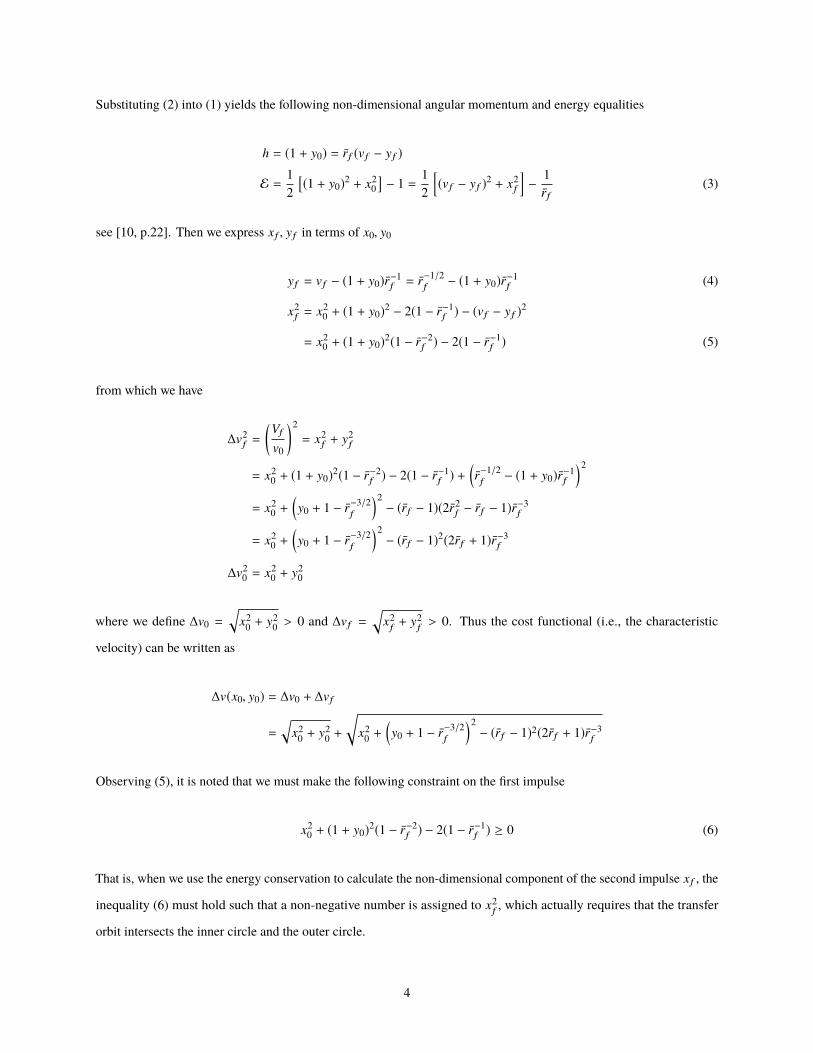
Substituting (2) into (1) yields the following non-dimensional angular momentum and energy equalities

h = (1 + y0) = rf (v f − y f )

E = 12

[(1 + y0)2 + x2

0]− 1 =

12

[(v f − y f )2 + x2

f

]− 1

rf(3)

see [10, p.22]. Then we express x f , y f in terms of x0, y0

y f = v f − (1 + y0)r−1f = r−1/2

f− (1 + y0)r−1

f (4)

x2f = x2

0 + (1 + y0)2 − 2(1 − r−1f ) − (v f − y f )2

= x20 + (1 + y0)2(1 − r−2

f ) − 2(1 − r−1f ) (5)

from which we have

∆v2f =

(Vf

v0

)2= x2

f + y2f

= x20 + (1 + y0)2(1 − r−2

f ) − 2(1 − r−1f ) +

(r−1/2f− (1 + y0)r−1

f

)2

= x20 +

(y0 + 1 − r−3/2

f

)2− (rf − 1)(2r2

f − rf − 1)r−3f

= x20 +

(y0 + 1 − r−3/2

f

)2− (rf − 1)2(2rf + 1)r−3

f

∆v20 = x2

0 + y20

where we define ∆v0 =√

x20 + y2

0 > 0 and ∆v f =√

x2f+ y2

f> 0. Thus the cost functional (i.e., the characteristic

velocity) can be written as

∆v(x0, y0) = ∆v0 + ∆v f

=

√x2

0 + y20 +

√x2

0 +(y0 + 1 − r−3/2

f

)2− (rf − 1)2(2rf + 1)r−3

f

Observing (5), it is noted that we must make the following constraint on the first impulse

x20 + (1 + y0)2(1 − r−2

f ) − 2(1 − r−1f ) ≥ 0 (6)

That is, when we use the energy conservation to calculate the non-dimensional component of the second impulse x f , the

inequality (6) must hold such that a non-negative number is assigned to x2f , which actually requires that the transfer

orbit intersects the inner circle and the outer circle.

4

The above background can be found in [10, Section 2.2] which is specified here. Marec used the independent

variables x0, y0 as coordinates in a hodograph plan and in geometric language, an elegant and simple proof was given

to show the optimality of the Hohmann transfer. Marec’s geometric method enlightens us to consider the Hohmann

transfer in a different way. Then the global optimality of the Hohmann transfer analytically appears.

We now formulate the Hohmann transfer problem as a nonlinear programming problem subject to the inequality

constraint (6) in which x0 and y0 are independent variables.

Theorem II.1 The classical Hohmann transfer is the solution of the following constrained optimization problem

minx0,y0∆v(x0, y0) (7)

s.t. x20 + (1 + y0)2(1 − r−2

f ) − 2(1 − r−1f ) ≥ 0

Also this solution is the global minimum.

Proof. We say that the Hohmann transfer is the solution to the above optimization problem if the pair (x0, y0)

corresponding to the Hohmann transfer is feasible to (7). As usual, we use Lagrange multiplier method and define the

Lagrangian function as follows

F(x0, y0) = ∆v(x0, y0) + λ(−x2

0 − (1 + y0)2(1 − r−2f ) + 2(1 − r−1

f ))

(8)

In view of the Kuhn-Tucker theorem, a local optimum of ∆v(x0, y0) must satisfy the following necessary conditions

∂F∂x0=

x0∆v0+

x0∆v f− 2λx0 = 0 (9)

∂F∂y0=

y0∆v0+

y0 + 1 − r−3/2f

∆v f− 2λ(1 + y0)(1 − r−2

f ) = 0 (10)

λ(−x2

0 − (1 + y0)2(1 − r−2f ) + 2(1 − r−1

f ))= 0 (11)

− x20 − (1 + y0)2(1 − r−2

f ) + 2(1 − r−1f ) ≤ 0 (12)

λ ≥ 0 (13)

Notice that we have assumed that ∆v0,∆v f > 0. In order to find a feasible solution, we divide the proof of the first part

of this theorem into two cases.

(i) If λ = 0, then due to the equations (9) and (10), we have x0 = 0 and

y0∆v0+

y0 + 1 − r−3/2f

∆v f= 0 (14)

5

respectively. We claim that the equality (14) does not hold because the equality x0 = 0 implies that

y0∆v0=

y0

|y0 |= ±1

which contradicts

1 <y0 + 1 − r−3/2

f

∆v f=

y0 + 1 − r−3/2f√(

y0 + 1 − r−3/2f

)2− (rf − 1)2(2rf + 1)r−3

f

, ory0 + 1 − r−3/2

f

∆v f< −1

Therefore the equation (14) has no solution under the assumption λ = 0.

(ii) We now consider the case λ > 0. Then the equation (11) yields

−x20 − (1 + y0)2(1 − r−2

f ) + 2(1 − r−1f ) = 0 (15)

which together with (5) leads to x2f = 0. Thus

∆v f =√

x2f+ y2

f=

√y2f=

��y f �� (16)

and also

x20 = −(1 + y0)2(1 − r−2

f ) + 2(1 − r−1f ) (17)

Then we obtain ∆v20 as follows

∆v20 = x2

0 + y20 = r−2

f (1 + y0)2 − (1 + 2y0) + 2(1 − r−1f )

=(r−1f (1 + y0) − rf

)2+ 2(1 + y0) − r2

f − (1 + 2y0) + 2(1 − r−1f )

=(r−1f (1 + y0) − rf

)2+ 3 − r2

f − 2r−1f (18)

Thanks to (9)

x0∆v0+

x0∆v f− 2λx0 = 0 (19)

We now show that x0 = 0 by contradiction. If x0 , 0, then the equality (19) implies that

2λ =1∆v0+

1∆v f

(20)

6

Substituting (20) into (10) gives

y0∆v0+

y0 + 1 − r−3/2f

∆v f= (1 + y0)(1 − r−2

f )(

1∆v0+

1∆v f

)Arranging the above equation and using (4) and (16), we get

y0 − (1 + y0)(1 − r−2f )

∆v0=

r−3/2f− (y0 + 1)r−2

f

∆v f=

r−1/2f− (y0 + 1)r−1

f

∆v fr−1f =

y f��y f �� r−1f

where y f , 0 since we have assumed v f > 0 and just concluded x f = 0. By further rearranging the above equation, we

have

r−1f (1 + y0) − rf

∆v0=

y f��y f �� =

1, if y f > 0

−1, if y f < 0(21)

It is noted that (18) gives a strict inequality

∆v20 =

(r−1f (1 + y0) − rf

)2+ 3 − r2

f − 2r−1f <

(r−1f (1 + y0) − rf

)2(22)

where the function 3 − r2f − 2r−1

f < 0 since it is decreasing with respect to rf and rf > 1. Hence (21) contradicts to

(22) and does not hold, which implies that the assumption λ > 0 and the equality x0 , 0 do not hold simultaneously.

Therefore λ > 0 leads to x f = 0 and x0 = 0.

Summarizing the two cases above, we now conclude that a feasible solution to (7) must have λ∗ > 0, x∗f = 0 and

x∗0 = 0. Then the corresponding normal component y0 can be solved from (15)

y∗0 =

√2rf

1 + rf− 1, y∗0 = −

√2rf

1 + rf− 1 (23)

Substituting them into (4) and (10) yields

y∗f = r−1/2f

(1 −

√2

1 + rf

), λ∗ =

12(1 + y∗0)(1 − r−2

f)©­«1 +

y∗0 + 1 − r−3/2f

y∗f

ª®¬ > 0

y∗f = r−1/2f

(1 +

√2

1 + rf

), λ∗ =

12(1 + y∗0)(1 − r−2

f)©­«1 +

y∗0 + 1 − r−3/2f

y∗f

ª®¬ > 0 (24)

One can see that there exist two sets of feasible solutions, one of which (x∗0, y∗0) is corresponding to the Hohmann

transfer, and its the Lagrange multiplier is λ∗.

7

We are now in a position to show that the Hohmann transfer is the global minimum. We first show that (x∗0, y∗0) is a

strict local minimum. Theorem 3.11 in [21] gives a second order sufficient condition for a strict local minimum. To

apply it, we need to calculate the Hessian matrix of the Lagrangian function F defined by (8) at (x∗0, y∗0)

∇2F(x∗0, y∗0, λ∗) =

©­­­­­«∂2F∂x2

0

∂2F∂x0∂y0

∂2F∂y0∂x0

∂2F∂y2

0

ª®®®®®¬(x∗0,y∗0 )(25)

After a straightforward calculation, by the equations (9) and (10) and using the fact x∗0 = 0, we have

∂2F∂x0∂y0

(x∗0, y∗0) =

∂2F∂y0∂x0

(x∗0, y∗0) = 0

and also

∂2F∂x2

0(x∗0, y

∗0) =

1y∗0+

1y∗f

− 2λ∗ =1 + r−1

f (1 + y∗0)y∗0(1 + y∗0)(1 + r−1

f)> 0 (26)

∂2F∂y2

0(x∗0, y

∗0) =

−b((y∗0 + a)2 − b

)3/2 − 2λ∗(1 − r−2f ) < 0 (27)

where a = 1 − r−3/2f

, b = (rf − 1)2(2rf + 1)r−3f> 0. Then one can see that the Hessian matrix is an indefinite matrix.

Thus we cannot use the positive definiteness of the Hessian matrix, that is,

zT∇2F(x∗0, y∗0, λ∗)z > 0, ∀z , 0

as a sufficient condition to justify the local minimum of (x∗0, y∗0) as usual. Fortunately, Theorem 3.11 in [21] tells us that

for the case λ∗ > 0, that is, the inequality constraint is active, when we use the positive definiteness of the Hessian

matrix to justify the local minimum, we need only to consider the positive definiteness of the first block of the Hessian

matrix with the non-zero vector z , 0 defined by

z ∈ Z(x∗0, y∗0) = {z : zT∇g(x∗0, y

∗0) = 0} (28)

where g(x0, y0) is the constraint function

g(x0, y0) = −x20 − (1 + y0)2(1 − r−2

f ) + 2(1 − r−1f )

8

With this kind of z, if zT∇2F(x∗0, y∗0, λ∗)z > 0, then (x∗0, y

∗0) is a strict local minimum. Specifically, the vector z defined

by the set (28) satisfies

zT∇g(x∗0, y∗0) =

[z1 z2

] −2x0

−2(1 + y0)(1 − r−2f )

(x∗0,y∗0 )= 0 (29)

Notice that x∗0 = 0,−2(1 + y∗0)(1 − r−2f ) , 0. Hence (29) implies that the components z1 , 0 and z2 = 0. Obviously it

follows from (26) that

[z1 0

]∇2F(x∗0, y

∗0, λ∗)

z1

0

= z1∂2F∂x2

0(x∗0, y

∗0)z1 > 0 (30)

Therefore in light of Theorem 3.11 in [21, p.48], we can conclude that (x∗0, y∗0) is a strict local minimum. The same

argument can be used to show that (x∗0, y∗0) is also a strict local minimum in view of (30). Meanwhile a straightforward

calculation gives

∆v(x∗0, y∗0) < ∆v(x

∗0, y∗0)

Hence the pair (x∗0, y∗0) is a global minimum, and further it is the global minimum due to the uniqueness; see [22, p.194]

for the definition of a global minimum. This completes the proof of the theorem.

III. The Hohmann transfer as dynamic optimization problemsIn this section, the orbit transfer problem is formulated as two optimal control problems of a spacecraft in an inverse

square law field, driven by velocity impulses, with boundary and interior point constraints. The calculus of variations is

used to solve the resulting two-point and multi-point boundary-value problems (BCs).

A. Problem formulation

Consider the motion of a spacecraft in the inverse square gravitational field, and the state equation is

Ûr = v

Ûv = − µr3 r (31)

where r(t) is the spacecraft position vector and v(t) is its velocity vector. The state vector consists of r(t) and v(t). We

use (31) to describe the state of the transfer orbit, which defines a conic under consideration; see, e.g., [19, Chapter 2].

Problem III.1 Given the initial position and velocity vectors of a spacecraft on the initial circular orbit, r(t0), v(t0).

9

The terminal time t1 is not specified. Let t+0 signify just after t0 and t−1 signify just before t1.∗ During the period from t+0

to t−1 , the state evolves over time according to the equation (31). To guarantee at the time t+1 , the spacecraft enters the

finite circular orbit, we impose the following equality constraints on the finial state

gr1(r(t+1 )) =��r(t+1 )�� − rf = 0

gv1(v(t+1 )) =��v(t+1 )�� − v f = 0

g2(r(t+1 ), v(t+1 )) = r(t+1 ) · v(t

+1 ) = 0 (32)

where v f is the orbit velocity of the final circular orbit v f =õ/rf . Suppose that there are velocity impulses at time

instants t0 and t1

v(t+i ) = v(t−i ) + ∆vi, i = 0, 1 (33)

where v(t−0 ) = v(t0). The position vector r(t) is continuous at these instants. The optimal control problem is to design

∆vi that minimize the cost functional

J = |∆v0 | + |∆v1 | (34)

subject to the constraints (32).

In control theory, such an optimal control problem is called impulse control problems in which there are state or

control jumps. Historically an optimal problem with the cost functional (34) is also referred to as the minimum-fuel

problem. By Problem III.1,† the orbit transfer problem has been formulated as a dynamic optimization problem instead

of a static one considered in Section II. The advantage of this formulation is that the coplanar assumption of the transfer

orbit to the initial orbit is removed, but the computation complexity follows.

In the next problem we consider the orbit transfer problem as a dynamic optimization problem with interior point

constraints.

Problem III.2 Consider a similar situation as in Problem III.1. Let tHT be the Hohmann transfer time. Instead of the

unspecified terminal time, here the terminal time instant t f > tHT is given and the time instant t1 now is an unspecified

interior time instant. The conditions (32) become a set of interior boundary conditions. The optimal control problem is

to design ∆vi that minimize the cost functional (34) subject to the interior boundary conditions (32).∗In mathematical language, t+0 represents the limit of t0 approached from the right side and t−1 represents the limit of t1 approached from the left

side.† A Matlab script for the Hohmann transfer was given as a numerical example in the free version of a Matlab-based software GPOPS by an direct

method. The constrained (32) was also used to describe the terminal conditions. We here use the variational method (i.e., indirect method) to optimalcontrol problems

10

B. Two-point boundary conditions for Problem III.1

Problem III.1 is a constrained optimization problem subject to static and dynamic constraints. We use Lagrange

multipliers to convert it into an unconstrained one. Define the augmented cost functional

J : = |∆v0 | + |∆v1 |

+ qTr1

[r(t+0 ) − r(t0)

]+ qT

r2[r(t+1 ) − r(t−1 )

]+ qT

v1[v(t+0 ) − v(t0) − ∆v0

]+ qT

v2[v(t+1 ) − v(t−1 ) − ∆v1

]+ γr1gr1(r(t+1 )) + γv1gv1(v(t+1 )) + γ2gr2(r(t+1 ), v(t

+1 ))

+

∫ t−1

t+0

pTr (v − Ûr) + pT

v

(− µ

r3 r − Ûv)

dt

where Lagrange multipliers pr, pv are also called costate vectors; in particular, Lawden [5] termed −pv the primer

vector. Introducing Hamiltonian function

H(r, v, p) := pTr v − pT

v

µ

r3 r, p =[pr pv

]T(35)

By taking into account of all perturbations, the first variation of the augmented cost functional is

δ J =∆vT0|∆v0 |

δv0 +∆vT1|∆v1 |

δv1

+ qTr1

[dr(t+0 ) − dr(t−0 )

]+ qT

r2[dr(t+1 ) − dr(t−1 )

]+ qT

v1[dv(t+0 ) − dv(t−0 ) − δv0

]+ qT

v2[dv(t+1 ) − dv(t−1 ) − δv1

]+ drT(t+1 )

∂gr1(r(t+1 ))∂r(t+1 )

���∗γr1 + dvT(t+1 )

∂gv1(v(t+1 ))∂v(t+1 )

���∗γv1

+ drT(t+1 )∂g2(r(t+1 ), v(t

+1 ))

∂r(t+1 )

���∗γ2 + dvT(t+1 )

∂g2(r(t+1 ), v(t+1 ))

∂v(t+1 )

���∗γ2

(∗) +(H∗ − pT

r Ûr − pTv Ûv

) ���t−∗1

δt1

(∗∗) + pTr (t+0 )δr(t

+0 ) − pT

r (t−∗1 )δr(t−∗1 ) + pT

v (t+0 )δv(t+0 ) − pT

v (t−∗1 )δv(t−∗1 )

+

∫ t−∗1

t+0

[(∂H(r, v, p)

∂r+ Ûpr (t)

)T∗δr +

(∂H(r, v, p)

∂v+ Ûpv(t)

)T∗δv

]dt (36)

where we use d(·) to denote the difference between the varied path and the optimal path taking into account the

differential change in a time instant (i.e., differential in x), for example,

dv(t+1 ) = v(t+1 ) − v∗(t+∗1 )

11

and δ(·) is the variation, for example, δv(t∗1) is the variation of v as an independent variable at t∗1 . Notice that

dr(t−0 ) = 0, dv(t−0 ) = 0 since t0 is fixed. The parts of δ J in (36) marked with asterisks are respectively due to the linear

term of

∫ t−∗1 +δt1

t−∗1

(H(r, v, p) − pT

r Ûr − pTv Ûv

)dt

and the first term in the right-hand side of the following equation

∫ t−∗1

t+0

pTr δÛrdt = pT

r δr��t−∗1t+0−

∫ t−∗1

t+0

ÛpTr δrdt

obtained by integrating by parts. In order to derive boundary conditions, we next use the following relation

dv(t−1 ) = δv(t−∗1 ) + Ûv(t

−∗1 )δt1 (37)

see [23, Section 3.5] and [20, Section 3.3].

In view of the necessary condition δ J = 0 and the fundamental lemma, we have the costate equations

Ûpr (t) = −∂H(r, v, p)

∂r, Ûpv(t) = −

∂H(r, v, p)∂v

(38)

Based on the definition of the Hamiltonian function in (35), the costate equation (38) can be rewritten as

Ûpr =∂

∂r

( µr3 r

)pv = −

µ

r3 (3r2 rrT − I3×3)pv, Ûpv = −pr (39)

where I3×3 is the 3 × 3 identity matrix.

Using (37) and regrouping terms in (36) yields the following terms or equalities for ∆v1,∆v2, dv

(∆v0

|∆v0 |− qv1

)T∆v0(

∆v1

|∆v1 |− qv2

)T∆v1

qTv1dv(t+0 ) + pT

v (t+0 )δv(t+0 ) =

(qTv1 + pT

v (t+0 ))

dv(t+0 )

−qTv2dv(t−1 ) − pT

v (t−1 )(δv(t−∗1 ) + Ûv(t

−∗1 )δt1

)= −

(qTv2 + pT

v (t−1 ))

dv(t−1 )(qTv2 + γv1

∂gv1(v(t+1 ))∂vT(t+1 )

���∗+ γ2

∂g2(r(t+1 ), v(t+1 ))

∂vT(t+1 )

���∗

)dv(t+1 ) (40)

As usual, in order to assure δ J = 0, we choose Lagrange multipliers to make the coefficients of ∆v0, ∆v1, dv(t+0 ), dv(t−1 ),

12

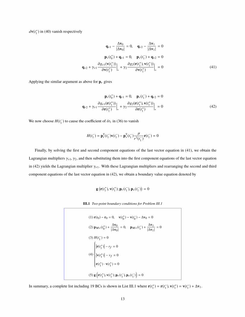
dv(t+1 ) in (40) vanish respectively

qv1 −∆v0

|∆v0 |= 0, qv2 −

∆v1

|∆v1 |= 0

pv(t+0 ) + qv1 = 0, pv(t−1 ) + qv2 = 0

qv2 + γv1∂gv1(v(t+1 ))∂v(t+1 )

���∗+ γ2

∂g2(r(t+1 ), v(t+1 ))

∂v(t+1 )

���∗= 0 (41)

Applying the similar argument as above for pr gives

pr (t+0 ) + qr1 = 0, pr (t−1 ) + qr2 = 0

qr2 + γr1∂gr1(r(t+1 ))∂r(t+1 )

���∗+ γ2

∂g2(r(t+1 ), v(t+1 ))

∂r(t+1 )

���∗= 0 (42)

We now choose H(t−1 ) to cause the coefficient of δt1 in (36) to vanish

H(t−1 ) = pTr (t−1 )v(t

−1 ) − pT

v (t−1 )µ

r3(t−1 )r(t−1 ) = 0

Finally, by solving the first and second component equations of the last vector equation in (41), we obtain the

Lagrangian multipliers γv1, γ2, and then substituting them into the first component equations of the last vector equation

in (42) yields the Lagrangian multiplier γr1. With these Lagrangian multipliers and rearranging the second and third

component equations of the last vector equation in (42), we obtain a boundary value equation denoted by

g(r(t+1 ), v(t

+1 ); pr (t−1 ), pv(t−1 )

)= 0

III.1 Two-point boundary conditions for Problem III.1

(1) r(t0) − r0 = 0, v(t+0 ) − v(t−0 ) − ∆v0 = 0

(2) pMv(t+0 ) +∆v0|∆v0 |

= 0, pMv(t−1 ) +∆v1|∆v1 |

= 0

(3) H(t−1 ) = 0

(4)

��r(t+1 )�� − rf = 0��v(t+1 )�� − v f = 0

r(t+1 ) · v(t+1 ) = 0

(5) g(r(t+1 ), v(t

+1 ); pr (t−1 ), pv(t

−1 )

)= 0

In summary, a complete list including 19 BCs is shown in List III.1 where r(t+1 ) = r(t−1 ), v(t+1 ) = v(t−1 ) + ∆v1.

13

C. Multi-point boundary conditions for Problem III.2

Define the augmented cost functional

J : = |∆v0 | + |∆v1 |

+ qTr1

[r(t+0 ) − r(t0)

]+ qT

r2[r(t+1 ) − r(t−1 )

]+ qT

v1[v(t+0 ) − v(t0) − ∆v0

]+ qT

v2[v(t+1 ) − v(t−1 ) − ∆v1

]+ γr1gr1(r(t+1 )) + γv1gv1(v(t+1 )) + γ2gr2(r(t+1 ), v(t

+1 ))

+

∫ t−1

t+0

pTr (v − Ûr) + pT

v

(− µ

r3 r − Ûv)

dt +∫ t f

t+1

pTr (v − Ûr) + pT

v

(− µ

r3 r − Ûv)

dt

We introduce the Hamiltonian functions for two time sub-intervals [t+0 , t−1 ] ∪ [t

+1 , t f ]

Hi(r, v, pi) := pTriv − pT

vi

µ

r3 r, pi =

[pri pvi

]T, i = 1, 2 (43)

A tedious and similar argument as used in Problem III.1 can be applied to Problem III.2 to derive the costate

equations and boundary conditions. The two-phase costate equations are given by

Ûpri(t) = −∂Hi(r, v, pi)

∂r, Ûpvi(t) = −

∂Hi(r, v, pi)∂v

, i = 1, 2

A complete list for boundary conditions is given in List III.2.

III.2 31 boundary conditions for Problem III.2

(1)

r(t0) − r0 = 0, v(t−0 ) − v(t+0 ) − ∆v0 = 0

r(t−1 ) − r(t+1 ) = 0, v(t−1 ) − v(t+1 ) − ∆v1 = 0

(2)

pv1(t+0 ) +

∆v0|∆v0 |

= 0, pv1(t−1 ) +∆v1|∆v1 |

= 0

pv2(t f ) = 0, pr2(t f ) = 0

(3) H1(t−1 ) − H2(t+1 ) = 0 or − pTr1(t−1 )∆v1 = 0

(4)

��r(t+1 )�� − rf = 0��v(t+1 )�� − v f = 0

r(t+1 ) · v(t+1 ) = 0

(5) g(r(t+1 ), v(t

+1 ); pr1(t−1 ), pr1(t+1 ), pv1(t−1 ), pv1(t+1 )

)= 0

14

IV. Numerical Examples

−6 −4 −2 0 2 4 6

x 107

−4

−3

−2

−1

0

1

2

3

4

x 107

rx m

rym

0 0.2 0.4 0.6 0.8 1 1.2 1.4 1.6 1.8 2

x 104

0.75

0.8

0.85

0.9

0.95

1The magnitude of the primer vector

t second

Fig. 1 The Hohmann transfer and the magnitude of the primer vector

In order to use Matlab solver bvp4c or bvp5c to solve two-point and multi-point boundary value problems with

unspecified switching time instants in Section III, two time changes must be introduced. For the time change, we refer

to, e.g., [20, Appendix A] and [24, Section 3] for details. The solver bvp4c or bvp5c accepts boundary value problems

with unknown parameters; see [25] and [26].

Example IV.1 This example in [10, p.25] is used to illustrate that the Hohmann transfer is the solution to Problem

III.1. The altitude of the initial circular orbit is 300km, and the desired final orbit is geostationary, that is, its radius is

42164km. By the formulas of the Hohmann transfer, the magnitudes of two velocity impulses are given by

∆v1 = 2.425726280326563e + 03, ∆v2 = 1.466822833675619e + 03 m/s (44)

Setting the tolerance of bvp4c equal to 1e-6, we have the solution to the minimum-fuel problem III.1 with an unspecified

terminal time given by bvp4c

dv1 = 1.0e+03*[0.000000000000804; 2.425726280326426; 0]

dv2 = 1.0e+03*[0.000000000000209; -1.466822833675464; 0]

Compared with (44), the accuracy of the numerical solution is found to be satisfactory since only the last three digits of

fifteen digits after decimal place are different. It is desirable to speed up the computational convergence by scaling

the state variables though bvp4c already has a scale procedure. The computation time is about 180 seconds on Intel

Core i5 (2.4 GHz, 2 GB). Figure 1 shows the Hohmann transfer and the magnitude of the primer vector. The solution

15

provided by bvp4c depends upon initial values. Figure 2 shows the transfer orbit and the magnitude of the primer vector

corresponding to the local minimum given by (24) in the proof of Theorem II.1.

−6 −4 −2 0 2 4 6

x 107

−4

−3

−2

−1

0

1

2

3

4

x 107

rx m

rym

0 0.2 0.4 0.6 0.8 1 1.2 1.4 1.6 1.8 2

x 104

0.4

0.5

0.6

0.7

0.8

0.9

1The magnitude of the primer vector

t second

Fig. 2 The orbit transfer and the magnitude of the primer vector for the local minimum

−1 −0.8 −0.6 −0.4 −0.2 0 0.2 0.4 0.6 0.8 1

x 107

−8

−6

−4

−2

0

2

4

6

8x 10

6

rx m

rym

0 500 1000 1500 2000 2500 3000

0

0.2

0.4

0.6

0.8

1

The magnitude of the primer vector

t second

Fig. 3 The Hohmann transfer and the magnitude of the primer vector

Example IV.2 Consider the Hohmann transfer as the multi-point boundary value problem (Problem III.2). The altitudes

of the initial and final circular orbits are 200km and 400km respectively. By the formulas of the Hohmann transfer, the

magnitudes of two velocity impulses are given by

∆v1 = 58.064987253967857, ∆v2 = 57.631827424189602 (45)

16

The Hohmann transfer time tHT = 2.715594949192177e + 03 seconds, hence we choose the terminal time t f = 2800

seconds. The constants, the initial values of the unknown parameters, and the solver and its tolerance are specified in

Table 1.

Table 1 Constants and initial values

Constants Gravitational constant µ = 3.986e + 14 Earth’s radius Re = 6378145

The initial values of the stater0 m v0 m/s

6578145 0 0 0 7.7843e+03 0

The initial values of the costatepv pr

-0.0012 0 0 0 -0.9 0

The initial values of the velocity impulses∆v1 ∆v2

0 102 0 0 102 0

The initial value of the scaled time 0.9

Solver bvp4c Tolerance=1e-7

By trial and error, this example is successfully solved by using bvp4c. We obtain the following solution message

The solution was obtained on a mesh of 11505 points.

The maximum residual is 4.887e-08.

There were 2.2369e+06 calls to the ODE function.

There were 1442 calls to the BC function.

Elapsed time is 406.320776 seconds.

The first velocity impulse vector dv1 = [0.000000000000001, 58.064987253970472, 0]

The second velocity impulse vector dv2 = [0.000000000000924, -57.631827424187151, 0]

The scaled instant of the second velocity impulse 0.969855338997211

The time instant of the second velocity impulse 2.715594949192190e+03

The maximal error of boundary conditions 4.263256e-13

Figure 3 shows the Hohmann transfer and the magnitude of the primer vector. The magnitude of the velocity and the

velocity vector on the vx − vy plane are shown in Figure 4, where the symbol + corresponds to the time instant at which

the velocity impulse occurs.

We now assume the initial values of the velocity impulses

dv10=[0, 45, 0], dv20=[0, -60, 0]

17

0 500 1000 1500 2000 2500

7650

7700

7750

7800

7850

The magnitude of the velocity vector

time second

−8000 −7000 −6000 −5000 −4000 −3000 −2000 −1000 0 1000−8000

−6000

−4000

−2000

0

2000

4000

6000

8000The velocity vector

vx m/s

vy m

/s

Fig. 4 The magnitude of the velocity and the velocity vector on the vx − vy plane

In stead of bvp4c, we use the other solver bvp5c. Setting Tolerance=1e-6, the solution corresponding to the local

minimum is found.

The solution was obtained on a mesh of 2859 points.

The maximum error is 5.291e-14.

There were 809723 calls to the ODE function.

There were 1382 calls to the BC function.

Elapsed time is 190.920474 seconds.

The first velocity impulse vector dv1 = 1.0e+4*[0.000000000000001, -1.562657038966310, 0]

The second velocity impulse vector dv2 = 1.0e+4*[0.000000000000011, -1.527946697280544, 0]

The scaled instant of the second velocity impulse 0.969855338997205

The time instant of the second velocity impulse 2.715594949192175e+03

The maximal error of boundary conditions 4.403455e-10

Figure 5 shows the orbit transfer and the magnitude of the primer vector corresponding to the local minimum, where the

spacecraft starts from the initial point on the initial orbit, moves clockwise along the transfer orbit until the second pulse

point, and then travels counterclockwise along the final circle orbit until the terminal point marked with the symbol ×.

V. ConclusionIn this paper, by a static constrained optimization, we study the global optimality of the Hohmann transfer using a

nonlinear programming method. Specifically, an inequality presented by Marec in [10, pp. 21-32] is used to define

an inequality constraint, then we formulate the Hohmann transfer problem as a constrained nonlinear programming

18

−1 −0.8 −0.6 −0.4 −0.2 0 0.2 0.4 0.6 0.8 1

x 107

−8

−6

−4

−2

0

2

4

6

8x 10

6

rx m

rym

0 500 1000 1500 2000 2500 3000

0

0.2

0.4

0.6

0.8

1

The magnitude of the primer vector

t second

Fig. 5 The orbit transfer and the magnitude of the primer vector corresponding to the local minimum

problem. A natural application of the well-known results in nonlinear programming such as the Kuhn-Tucker theorem

clearly shows the the global optimality of the Hohmann transfer. In the second part of the paper, we introduce two

optimal control problems with two-point and multi-point boundary value constraints respectively. With the help of

Matlab solver bvp4c, the Hohmann transfer is solved successfully.

AcknowledgmentsThe first author is supported by the National Natural Science Foundation of China (no. 61374084).

References[1] Hohmann, W., The Attainability of Heavenly Bodies (1925), NASA Technical Translation F-44, 1960.

[2] Barrar, R. B., “An Analytic Proof that the Hohmann-Type Transfer is the True Minimum Two-Impulse Transfer,” Astronautica

Acta, Vol. 9, No. 1, 1963, pp. 1–11.

[3] Prussing, J. E., and Conway, B. A., Orbital Mechanics, 1st ed., Oxford University Press, 1993.

[4] Ting, L., “Optimum Orbital Transfer by Impulses,” ARS Journal, Vol. 30, 1960, pp. 1013–1018.

[5] Lawden, D. F., Optimal Trajectories for Space Navigation, Butter Worths, London, 1963.

[6] Prussing, J. E., “Primer Vector Theory and Applications,” Spacecraft Trajectory Optimization, edited by B. A. Conway,

Cambridge, 2010, Chap. 2, pp. 16–36.

[7] Pontani, M., “Simple Method to Determine Globally Optimal Orbital Transfers,” Journal of Guidance, Control, and Dynamics,

Vol. 32, No. 3, 2009, pp. 899–914.

19

[8] Moyer, H. G., “Minimum Impulse Coplanar Circle-Ellipse Transfer,” AIAA Journal, Vol. 3, No. 4, 1965, pp. 723–726.

[9] Battin, R. H., An Introduction to the Mathematics and Methods of Astrodynamics, AIAA Education Series, AIAA, New York,

1987.

[10] Marec, J.-P., Optimal Space Trajectories, Elsevier, New York, 1979.

[11] Hazelrigg, G. A., “Globally Optimal Impulsive Transfers via Green’s Theorem,” Journal of Guidance, Control, and Dynamics,

Vol. 7, No. 4, 1984, pp. 462–470.

[12] Palmore, J. I., “An Elementary Proof the Optimality of Hohmann Transfers,” Journal of Guidance, Control, and Dynamics,

Vol. 7, No. 5, 1984, pp. 629–630.

[13] Prussing, J. E., “Simple Proof the Global Optimality of the Hohmann Transfer,” Journal of Guidance, Control, and Dynamics,

Vol. 15, No. 4, 1992, pp. 1037–1038.

[14] Yuan, F., and Matsushima, K., “Strong Hohmann Transfer Theorem,” Journal of Guidance, Control, and Dynamics, Vol. 18,

No. 2, 1995, pp. 371–373.

[15] Vertregt, M., “Interplanetary orbits,” Journal of the British Interplanetary Society, Vol. 16, 1958, pp. 326–354.

[16] Cornelisse, J. W., Schöyer, H. F. R., and Walker, K. F., Rocket Propulsion and Spaceflight Dynamics, Pitman, London, 1979.

[17] Gurfil, P., and Seidelmann, P. K., Celestial Mechanics and Astrodynamics Theory and Practice, Springer, 2016.

[18] Avendaño, M., Martín-Molina, V., Martín-Morales, J., and Ortigas-Galindo, J., “Algebraic Approach to the Minimum-Cost

Multi-Impulse Orbit-Transfer Problem,” Journal of Guidance, Control, and Dynamics, Vol. 39, No. 8, 2016, pp. 1734–1743.

[19] Curtis, H. D., Orbital Mechanics for Engineering Students, 3rd ed., Elsevier Ltd., 2014.

[20] James M. Longuski, J. J. G., and Prussing, J. E., Optimal Control with Aerospace Applications, Springer, 2014.

[21] Avriel, M., Nonlinear Programming: Analysis and Methods, an unabridged republication of the edition published by

Prentice-Hall in 1976 ed., Dover Publications Inc., 2003.

[22] Bertsekas, D., Nonlinear Programming, 2nd ed., Athena Scientific, 1999.

[23] Bryson Jr., A. E., and Ho, Y.-C., Applied Optimal Control, Hemisphere Publishing Corp., London, 1975.

[24] Zefran, M., Desai, J. P., and Kumar, V., “Continuous Motion Plans for Robotic Systems with Changing Dynamic Behavior,”

The second Int. Workshop on Algorithmic Fundations of Robotics, Toulouse, France, 1996.

[25] Shampine, L., Gladwell, I., and Thompson, S., Solving ODEs with Matlab, Cambridge University Press, 2003.

[26] Kierzenka, J., “Studies in the numerical solution of ordinary differential equations,” Ph.D. thesis, Department of Mathematics,

Southern Methodist University, Dallas, TX., 1998.

20