1

Promises of Conic Relaxation for Contingency-Constrained

Optimal Power Flow Problem

Ramtin Madani, Morteza Ashraphijuo and Javad Lavaei

Abstract—This paper is concerned with the security-constrained optimal power flow (SCOPF) problem, where eachcontingency corresponds to the outage of an arbitrary number oflines and generators. The problem is studied by means of a convexrelaxation, named semidefinite program (SDP). The existenceof a rank-1 SDP solution guarantees the recovery of a globalsolution of SCOPF. We prove that the rank of the SDP solutionis upper bounded by the treewidth of the power network plusone, which is perceived to be small in practice. We then proposea decomposition method to reduce the computational complexityof the relaxation. In the case where the relaxation is not exact,we develop a graph-theoretic convex program to identify theproblematic lines of the network and incorporate the loss overthose lines into the objective as a penalization (regularization)term, leading to a penalized SDP problem. We perform severalsimulations on large-scale benchmark systems and verify that theglobal minima are at most 1% away from the feasible solutionsobtained from the proposed penalized relaxation.

I. INTRODUCTION

The classical optimal power flow (OPF) problem aims

to find a steady-state operating point of a power system

that minimizes a desirable cost function, e.g. power loss or

generation cost, and satisfies network and physical constraints

on loads, powers, voltages and line flows [1]. The OPF

problem is not only non-convex but also NP-hard, due to its

possible reduction to the (0,1)-quadratic optimization. Started

by the work [2] in 1962, many of the existing optimization

techniques have been studied for the OPF problem, leading

to algorithms based on linear programming, Newton Raphson,

quadratic programming, nonlinear programming, Lagrange re-

laxation, interior point method, artificial intelligence, artificial

neural network, fuzzy logic, genetic algorithm, evolutionary

programming and particle swarm optimization [3]. Due to the

non-convexity of OPF, these algorithms are not robust, lack

performance guarantees, and may not find a global optimum.

Followed by the idea proposed in [4] and by exploiting the

physical properties of transmission lines, it has been argued

in the series of work [5], [6], [7], [8], [9], [10], [11], [12] that

the classical OPF problem corresponding to a practical power

system may be convexified and solved efficiently through a

semidefinite programming (SDP) relaxation. In particular, the

paper [13] shows that the SDP relaxation is exact in two cases

under certain technical assumptions: (i) for acyclic networks,

(ii) for cyclic networks after relaxing the angle constraints.

However, the SDP relaxation is not always exact for a general

mesh network [14], [15], [16], [17]. This issue has been

discussed extensively in the literature and several test cases

The authors are with the Electrical Engineering Department, Columbia

University (email: madani@ee.columbia.edu, ashraphijuo@ee.columbia.eduand lavaei@ee.columbia.edu). This work was supported by NSF CAREER

Award 1351279, NSF EECS Award 1406865, and ONR YIP Award.

have been contrived that witness the failure of SDP relaxation

in obtaining a global optimal solution of the OPF problem

[15], [18]. To ameliorate the issue, we have recently shown in

[19] that: (i) the exactness of the SDP relaxation depends on

the formulation of the line capacity constraints, and (ii) the

penalization of total reactive loss may enable the recovery of

a near-global solution (i.e., a solution that is measurably close

to a global minimum) for modest-sized systems (as verified in

over 7000 simulations).

The major drawback of representing the optimal power flow

problem as a semidefinite program is the requirement of defin-

ing a square matrix variable, which makes the number of scaler

variables of the problem quadratic with respect to the number

of network buses. This may yield a very high-dimensional SDP

problem for a real-world network. To address this issue, the

papers [20], [21], [22] have leveraged the sparsity of power

networks in order to break down the large-scale semidefinite

constraint into small-sized constraints. Similarly, the papers

[23], [24] and [25] have exploited the general technique

proposed in [26], [27] to reduce the complexity of the SDP

relaxation of the OPF problem. The simulations performed in

those papers suggest that the SDP relaxation would fail to

work properly for large-scale systems [22].

Although OPF is a fundamental problem studied extensively

in the literature for power systems, a real-world power flow

optimization is based on a set of coupled OPFs with a variety

of constraints and variables. The latter problem is named

security-constrained OPF (SCOPF) [28], [29]. The SCOPF

problem is important in practice, since independent system

operators tend to design an operating point that satisfies the de-

mand and network constraints not only under normal operation

but also under pre-specified contingencies such as line outages.

Depending on the network characteristics, one may adopt

preventive or corrective approaches for the SCOPF problem. In

the preventive formulation of SCOPF, the under-design state of

each generator (e.g., production level) is considered identical

for the pre- and post-contingency scenarios. This reflects the

fact that mechanical facilities may not be able to respond to the

changes in the network fast. In the corrective approach, limited

changes in certain control parameters are permitted after the

network experiences a fault. SCOPF is more challenging than

the conventional OPF problem for two reasons. First, the

size of the optimization could be prohibitive, depending on

the number of contingencies. Second, SCOPF is obtained by

coupling a group of non-convex OPF problems associated with

different contingencies and therefore its non-convexity would

be much higher than an individual OPF problem. The purpose

of this work is to propose an efficient computational method

that can be applied to not only OPF but also SCOPF.

In this paper, we study the SCOPF problem—as a general

2

version of OPF—through a convex relaxation. First, we pro-

pose an SDP relaxation for this problem. The existence of

a rank-1 SDP solution guarantees the recovery of a global

solution of SCOPF. We prove that the relaxation has a matrix

solution whose rank is at most the treewidth of the pre-

contingency network plus one. The treewidth of real-world

networks is perceived to be small due to their (almost)

planarity and sparsity [30]. For example, the treewidth of

the graph corresponding to a peak hour setup of a Polish

system with over 3000 buses is less than 25. Second, we

reduce the computational complexity of the SDP problem

using a tree decomposition method to arrive at a decomposed

SDP relaxation with a set of small-sized SDP matrices as

opposed to a full-scale SDP matrix. We show that the full-

scale SDP relaxation has a solution whose rank is upper

bounded by the ranks of the small-sized matrices of the

decomposed SDP relaxation. By working on the ranks of

these small matrices, we propose a technique to identify the

problematic lines of the network for each contingency that

may contribute to the inexactness of the SDP relaxation for

SCOPF. This diagnosis method may enable us to develop a

heuristic method, named penalized SDP relaxation, to find a

near-global solution of the problem by penalizing the loss over

the problematic lines for each contingency. Note that a certain

line may be problematic with respect to one contingency and

not problematic with respect to another contingency. It is

suggested to define the penalty term as a summation of all

loss functions for problematic lines under each contingency.

Note that a uniform penalty—consisting of losses over all lines

for all contingencies—also work for all test systems studied

in this paper, but the resulting SDP solution would have a

lower global optimality guarantee compared to the case where

the loss over only problematic lines is penalized. We test our

method on several benchmark systems with as high as 3000

buses and find a solution with a global optimality guarantee

of at least 99% for each case.

Notations: R, C, and Hn denote the sets of real numbers,

complex numbers, and n×n Hermitian matrices, respectively.

The m by n rectangular identity matrix whose (i, j) entry

is equal to the Kronecker delta δij is denoted by Im×n.

The notations Re{W}, Im{W}, and rank{W} denote the

real part, imaginary part, and rank of a scalar/matrix W,

respectively. The notation W � 0 means that W is Hermitian

and positive semidefinite. The notation ]x denotes the angle

of a complex number x. The notation “i” is reserved for

the imaginary unit. The superscripts (·)∗ and (·)T represent

the conjugate transpose and transpose operators, respectively.

Given a matrix W, its (l, m) entry is denoted as Wlm .

The subscript (·)opt is used to show the optimal value of an

optimization parameter. Given a matrix M, its Moore Penrose

pseudoinverse is denoted as M+. Given a simple graph H, its

vertex and edge sets are denoted by VH and EH, respectively.

Given two sets S1 and S2, the notation S1\S2 denotes the set

of all elements of S1 that do not exist in S2. Given a scalar

m and a real-valued set S, define S + m as a set obtained by

adding m to every element of S. Given a Hermitian matrix M

and two sets of natural numbers S1 and S2, define M{S1,S2}

Fig. 1: A minimal tree decomposition for a ladder

as a submatrix of M obtained through two operations: (i)

removing all rows of M whose indices do not belong to S1,

and (ii) removing all columns of M whose indices do not

belong to S2. For instance, M {{1, 2}, {2, 3}} is a 2×2 matrix

with the entries M12, M13, M22, M23.

II. PROBLEM FORMULATION

Consider a power network with the set of buses N :={1, 2, ..., n} and the set of flow lines L ⊆ N×N . With no loss

of generality, each line (l, m) ∈ L of the network is modeled

as a series admittance ylm. Suppose that a known constant-

power load with the complex value SDk= PDk

+ QDki

is connected to bus k ∈ N , where PDk, QDk

∈ R. Given

a nonnegative integer c, consider a set of c contingencies,

where each contingency corresponds to an arbitrary number of

pre-specified line/generator outages. In this work, we model

a line outage by removing the line from the base case and

model a generator outage by enforcing its output to be zero.

Define C := {0, 1, . . . , c} as the set of all pre- and post-

contingencies, where the base case is treated as contingency 0.

Define L(0) = L, and L(r) as the set of lines of the network

under contingency r ∈ {1, 2, ..., c}.

Consider a contingency scenario r ∈ C. Assume that a

generator is connected to each bus k ∈ N , whose unknown

complex output is denoted as S(r)Gk

= P(r)Gk

+Q(r)Gk

i. Let f(r)k (·)

be a convex function representing the generation cost for

generator k in the contingency case r ∈ C. The unknown

complex voltage at bus k ∈ N is denoted as V(r)

k . Further-

more, define S(r)lm = P

(r)lm + Q

(r)lm i as the unknown complex

power transferred from bus l ∈ N to the rest of the network

through the line (l, m) ∈ L(r). Define:

P(r)G ,

[

P(r)G1

, . . . , P(r)Gn

]T, Q

(r)G ,

[

Q(r)G1

, . . . , Q(r)Gn

]T,

PD ,[

PD1 , . . . , PDn

]T, QD ,

[

QD1 , . . . , QDn

]T,

V(r) ,[

V(r)1 , . . . , V (r)

n

]T.

Given the known vectors PD and QD, SCOPF minimizes

the generation cost over the unknown parameters V(r), P(r)G

and Q(r)G for r = 0, 1, ..., c subject to the power balance

equations at all buses and certain network constraints. SCOPF

is formalized below.

SCOPF problem: Minimize∑

r∈C

∑

k∈N

f(r)k

(

P(r)Gk

)

(1)

over the variables P(0)G , P

(1)G , . . . ,P

(c)G ∈ Rn, Q

(0)G , Q

(1)G ,

. . . , Q(c)G ∈ Rn and V(0), V(1), . . . ,V(c) ∈ Cn, subject to

3

1

2

3

5

4

7

8

9

6

11

14

13 12

10 6,12,13

1,2,5

2,4,5

2,3,4

4,5,9

6,9,13

4,7,9 7,8

5,6,9

9,13,14

6,9,11 9,10,11

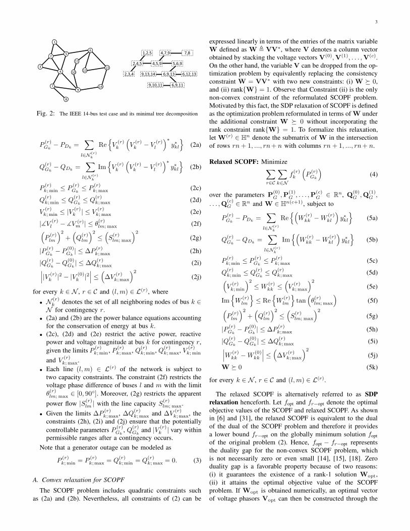
Fig. 2: The IEEE 14-bus test case and its minimal tree decomposition

P(r)Gk

− PDk=

∑

l∈N(r)

k

Re{

V(r)

k

(

V(r)k − V

(r)l

)∗

y∗kl

}

(2a)

Q(r)Gk

− QDk=

∑

l∈N(r)k

Im{

V(r)

k

(

V(r)k − V

(r)l

)∗

y∗kl

}

(2b)

P(r)k;min ≤ P

(r)Gk

≤ P(r)k;max (2c)

Q(r)k;min ≤ Q

(r)Gk

≤ Q(r)k;max (2d)

V(r)

k; min ≤ |V (r)k | ≤ V

(r)k; max (2e)

|]V(r)l − ]V (r)

m | ≤ θ(r)lm; max (2f)

(

P(r)lm

)2

+(

Q(r)lm

)2

≤(

S(r)lm; max

)2

(2g)

|P (r)Gk

− P(0)Gk

| ≤ ∆P(r)k;max (2h)

|Q(r)Gk

− Q(0)Gk

| ≤ ∆Q(r)k;max (2i)

∣

∣

∣|V (r)

k |2 − |V (0)k |2

∣

∣

∣≤

(

∆V(r)k;max

)2

(2j)

for every k ∈ N , r ∈ C and (l, m) ∈ L(r), where

• N (r)k denotes the set of all neighboring nodes of bus k ∈

N for contingency r.

• (2a) and (2b) are the power balance equations accounting

for the conservation of energy at bus k.

• (2c), (2d) and (2e) restrict the active power, reactive

power and voltage magnitude at bus k for contingency r,

given the limits P(r)k;min , P

(r)k;max, Q

(r)k;min, Q

(r)k; max, V

(r)k; min

and V(r)k; max.

• Each line (l, m) ∈ L(r) of the network is subject to

two capacity constraints. The constraint (2f) restricts the

voltage phase difference of buses l and m with the limit

θ(r)lm; max ∈ [0, 90◦]. Moreover, (2g) restricts the apparent

power flow |S(r)lm | with the line capacity S

(r)lm; max.

• Given the limits ∆P(r)k;max, ∆Q

(r)k;max and ∆V

(r)k;max, the

constraints (2h), (2i) and (2j) ensure that the potentially

controllable parameters P(r)Gk

, Q(r)Gk

and |V (r)k | vary within

permissible ranges after a contingency occurs.

Note that a generator outage can be modeled as

P(r)k; min = P

(r)k;max = Q

(r)k;min = Q

(r)k; max = 0. (3)

A. Convex relaxation for SCOPF

The SCOPF problem includes quadratic constraints such

as (2a) and (2b). Nevertheless, all constraints of (2) can be

expressed linearly in terms of the entries of the matrix variable

W defined as W , VV∗, where V denotes a column vector

obtained by stacking the voltage vectors V(0), V(1), . . . ,V(c).

On the other hand, the variable V can be dropped from the op-

timization problem by equivalently replacing the consistency

constraint W = VV∗ with two new constraints: (i) W � 0,

and (ii) rank{W} = 1. Observe that Constraint (ii) is the only

non-convex constraint of the reformulated SCOPF problem.

Motivated by this fact, the SDP relaxation of SCOPF is defined

as the optimization problem reformulated in terms of W under

the additional constraint W � 0 without incorporating the

rank constraint rank{W} = 1. To formalize this relaxation,

let W(r) ∈ Hn denote the submatrix of W in the intersection

of rows rn + 1, ..., rn+ n with columns rn + 1, ..., rn+ n.

Relaxed SCOPF: Minimize∑

r∈C

∑

k∈N

f(r)k

(

P(r)Gk

)

(4)

over the parameters P(0)G , P

(1)G , . . . ,P

(c)G ∈ Rn, Q

(0)G , Q

(1)G ,

. . . , Q(c)G ∈ Rn and W ∈ Hn(c+1), subject to

P(r)Gk

− PDk=

∑

l∈N(r)k

Re{(

W(r)kk − W

(r)kl

)

y∗kl

}

(5a)

Q(r)Gk

− QDk=

∑

l∈N(r)k

Im{(

W(r)kk − W

(r)kl

)

y∗kl

}

(5b)

P(r)k;min ≤ P

(r)Gk

≤ P(r)k; max (5c)

Q(r)k;min ≤ Q

(r)Gk

≤ Q(r)k;max (5d)

(

V(r)k;min

)2

≤ W(r)kk ≤

(

V(r)

k; max

)2

(5e)

Im{

W(r)lm

}

≤ Re{

W(r)lm

}

tan(

θ(r)lm; max

)

(5f)

(

P(r)lm

)2

+(

Q(r)lm

)2

≤(

S(r)lm; max

)2

(5g)

|P (r)Gk

− P(0)Gk

| ≤ ∆P(r)k;max (5h)

|Q(r)Gk

− Q(0)Gk

| ≤ ∆Q(r)k;max (5i)

∣

∣

∣W

(r)kk − W

(0)kk

∣

∣

∣≤

(

∆V(r)k;max

)2

(5j)

W � 0 (5k)

for every k ∈ N , r ∈ C and (l, m) ∈ L(r).

The relaxed SCOPF is alternatively referred to as SDP

relaxation henceforth. Let fopt and fr−opt denote the optimal

objective values of the SCOPF and relaxed SCOPF. As shown

in [6] and [31], the relaxed SCOPF is equivalent to the dual

of the dual of the SCOPF problem and therefore it provides

a lower bound fr−opt on the globally minimum solution fopt

of the original problem (2). Hence, fopt − fr−opt represents

the duality gap for the non-convex SCOPF problem, which

is not necessarily zero or even small [14], [15], [18]. Zero

duality gap is a favorable property because of two reasons:

(i) it guarantees the existence of a rank-1 solution Wopt,

(ii) it attains the optimal objective value of the SCOPF

problem. If Wopt is obtained numerically, an optimal vector

of voltage phasors Vopt can then be constructed through the

4

decomposition Wopt = VoptV∗opt. It has been shown in [31]

that whenever the duality gap of the classical OPF problem

is zero for a specific power network, the SCOPF problem

also possesses zero duality gap, leading to the presence of a

rank-1 solution for the relaxed SCOPF. As investigated in [32]

and [13], the duality gap for the OPF problem (without any

contingency scenarios) is highly correlated with the topology

of the network. In addition, the gap heavily depends on the

mathematical formulation of the line capacity constraints [19].

Since a power network has a sparse graph in general, the

relaxed SCOPF problem may have infinitely many solutions.

As an extreme case, the duality gap could be zero and yet there

exist a set of rank-1 and higher-rank solutions for the relaxed

problem. To alleviate this issue, the paper [6] suggests adding

a small resistance (10−5 per unit) to every ideal transformer

with zero resistance.

Using a graph-theoretic approach combined with the SDP

relaxation, we aim to study three problems:

• Since the dimension of the matrix variable W is pro-

hibitive for a large-scale network, how can the computa-

tional complexity of the relaxed SCOPF be reduced?

• What is the rank of an optimal solution Wopt of the

relaxed SCOPF and how does it relate to the topology

of the power grid?

• If the rank of Wopt is not 1, how can a near-global solu-

tion be recovered for the non-convex SCOPF problem?

III. LOW-RANK SDP SOLUTIONS

In this section, the objective is twofold. First, the compu-

tational complexity of the relaxed SCOPF will be reduced.

Second, the rank of its lowest-rank solution will be studied.

A. Reduction of computational complexity

Definition 1 (Treewidth). Given a graph H = (VH, EH), a

tree T is called a tree decomposition of H if it satisfies the

following properties:

1) Every node of T corresponds to and is identified by a

subset of VH.

2) Every vertex of H is a member of at least one node of

T .

3) Tk is a connected graph for every k ∈ VH, where Tk

denotes the subgraph of T induced by all nodes of Tcontaining the vertex k of H.

4) If (i, j) ∈ EH, then the subgraphs Ti and Tj have at least

one node in common.

Each node of T is a bag (collection) of vertices of H and

hence it is referred to as bag. The width of T is the cardinality

of its biggest bag minus one. The treewidth of H is the

minimum width over all possible tree decompositions of Hand is denoted by tw(H).

Note that the treewidth of a tree is equal to 1. Figure 1

shows a graph H with 6 vertices named a, b, c, d, e, f , together

with its minimal tree decomposition T . Every node of T is

a set containing three members of VH. The width of this

decomposition is therefore equal to 2. The graph of the IEEE

14-bus system and its minimal tree decomposition are depicted

in Figure 2. As shown in Table I, the treewidth of IEEE

systems and various setups of Polish systems with as high

as 3000 buses is at most 24. This empirical evidence signifies

that real-world power grids may have a small treewidth, which

is leveraged in this work to solve the SCOPF problem.

Definition 2 (Sparsity graph). The sparsity graph of the

relaxed SCOPF problem is defined as a graph with n(c + 1)vertices such that (i, j) is an edge of the graph whenever

i 6= j, i, j ∈ {1, 2, ..., n(c+ 1)} and Wij appears in either of

the constraints (5a) and (5b) with a nonzero coefficient.

Consider a tree decomposition of the power network in

the pre-contingency case and denote its bags (nodes) as

J (0)1 ,J (0)

2 , ...,J (0)p ⊆ N .

Theorem 1. The following statements hold:

i) The sparsity graph of the relaxed SCOPF problem has a

tree decomposition with p(c + 1) bags given by the set:{

J (0)m + nr

∣

∣

∣

∣

m = 1, ..., p and r = 0, ..., c

}

(6)

ii) The optimal objective value of the relaxed SCOPF prob-

lem does not change if its constraint W � 0 is replaced

by

W{

J (0)m + nr,J (0)

m + nr}

� 0 (7)

or equivalently

W(r){

J (0)m ,J (0)

m

}

� 0 (8)

for every r ∈ C and m ∈ {1, . . . , p}.

Proof. The proof of Part (i) follows from the fact that the

sparsity graph of the relaxed SCOPF problem is composed

of c +1 disconnected components, each corresponding to one

of the contingencies 0, 1, 2..., c. This is due to the fact that

the constraints of the SCOPF problem can all be described in

terms of only those entries of W that appear in one of the

submatrices W(0), ...,W(c). Part (ii) is a direct consequence

of Part (i) and the chordal theorem in [33].

Define decomposed relaxed SCOPF as a convex op-

timization obtained from the relaxed SCOPF by replacing

W � 0 with the constraints W(r){

J (0)m ,J (0)

m

}

� 0 for

every r ∈ C and m ∈ {1, . . . , p}. Theorem 1 reduces the

computational cost of the SDP relaxation dramatically for a

large-scale system with a relatively small treewidth. Note that

many entries of the matrix variable W may not appear in the

objective or constraints of the decomposed relaxed SCOPF,

and those redundant entries can be eliminated. For example,

the relaxed OPF for a Polish system has about 9,000,000 scalar

variables, while the decomposed relaxed OPF has only about

100,000 parameters. As will be illustrated later, this enables

us to solve a large-scale problem efficiently.

B. Existence of low-rank solutions

Let Wref ∈ Hn(c+1) denote an arbitrary solution of the

relaxed SCOPF or decomposed relaxed SCOPF. Note that if

Wref corresponds to the decomposed problem, its redundant

entries may not have been found by the numerical algorithm

5

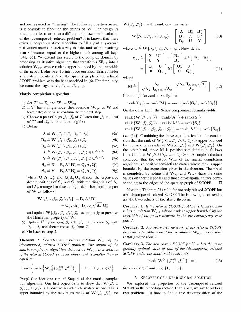
and are regarded as “missing”. The following question arises:

is it possible to fine-tune the entries of Wref or design its

missing entries to arrive at a different, but lower rank, solution

of the (decomposed) relaxed problem? It is known that there

exists a polynomial-time algorithm to fill a partially-known

real-valued matrix in such a way that the rank of the resulting

matrix becomes equal to the highest rank among all bags

[34], [35]. We extend this result to the complex domain by

proposing an iterative algorithm that transforms Wref into a

solution Wopt whose rank is upper bounded by the treewidth

of the network plus one. To introduce our algorithm, consider

a tree decomposition TC of the sparsity graph of the relaxed

SCOPF problem with the bags specified in (6). For simplicity,

we name the bags as J1,J2, ...,Jp(c+1).

Matrix completion algorithm:

1) Set T ′ := TC and W := Wref .

2) If T ′ has a single node, then consider Wopt as W and

terminate; otherwise continue to the next step.

3) Choose a pair of bags Jx,Jy of T ′ such that Jx is a leaf

of T ′ and Jy is its unique neighbor.

4) Define

A , W{Jx ∩ Jy,Jx ∩ Jy} (9a)

Bx , W{Jx \ Jy,Jx ∩ Jy} (9b)

By , W{Jy \ Jx,Jx ∩ Jy} (9c)

X , W{Jx \ Jy,Jx \ Jy} ∈ Cdx×dx (9d)

Y , W{Jy \ Jx,Jy \ Jx} ∈ Cdy×dy (9e)

Sx , X− BxA+B∗

x = QxΛxQ∗x (9f)

Sy , Y −ByA+B∗

y = QyΛyQ∗y (9g)

where QxΛxQ∗x and QyΛyQ

∗y denote the eigenvalue

decompositions of Sx and Sy with the diagonals of Λx

and Λy arranged in descending order. Then, update a part

of W as follows:

W{Jy \ Jx,Jx \ Jy} := ByA+B∗

x

+ Qy

√

Λy Idy×dx

√

Λx Q∗x

and update W{Jx\Jy,Jy \Jx} accordingly to preserve

the Hermitian property of W.

5) Update T ′ by merging Jx into Jy , i.e., replace Jy with

Jx ∪ Jy and then remove Jx from T ′.

6) Go back to step 2.

Theorem 2. Consider an arbitrary solution Wref of the

(decomposed) relaxed SCOPF problem. The output of the

matrix completion algorithm, denoted as Wopt, is a solution

of the relaxed SCOPF problem whose rank is smaller than or

equal to:

max

{

rank{

W(r)ref {J (0)

m ,J (0)m }

}

∣

∣

∣

∣

1 ≤ m ≤ p, r ∈ C}

.

Proof. Consider one run of Step 4 of the matrix comple-

tion algorithm. Our first objective is to show that W{Jx ∪Jy,Jx ∪ Jy} is a positive semidefinite matrix whose rank is

upper bounded by the maximum ranks of W{Jx,Jx} and

W{Jy,Jy}. To this end, one can write:

W{Jx ∪ Jy,Jx ∪ Jy} =

A B∗x B∗

y

Bx X U∗

By U Y

(10)

where U , W{Jy \ Jx,Jx \ Jy}. Now, define

Sxy ,

[

X U∗

U Y

]

−[

Bx

By

]

A+[

B∗x B∗

y

]

=

[

Qx 0

0 Qy

]

M

[

Q∗x 0

0 Q∗y

]

(11)

where

M ,

[

Λx

√Λx Idx×dy

√

Λy√

Λy Idy×dx

√Λx Λy

]

(12)

It is straightforward to verify that

rank{Sxy} = rank{M} = max{rank{Sx}, rank{Sy}}On the other hand, the Schur complement formula yields:

rank {W{Jx,Jx}} = rank{A+} + rank{Sx}rank {W{Jy,Jy}} = rank{A+} + rank{Sy}rank {W{Jx ∪ Jy,Jx ∪ Jy}} = rank{A+} + rank{Sxy}

(see [36]). Combining the above equations leads to the conclu-

sion that the rank of W{Jx ∪Jy,Jx ∪Jy} is upper bounded

by the maximum ranks of W{Jx,Jx} and W{Jy,Jy}. On

the other hand, since M is positive semidefinite, it follows

from (11) that W{Jx∪Jy,Jx∪Jy} � 0. A simple induction

concludes that the output Wopt of the matrix completion

algorithm is a positive semidefinite matrix whose rank is upper

bounded by the expression given in the theorem. The proof

is completed by noting that Wopt and Wref share the same

values on their diagonals and those off-diagonal entries corre-

sponding to the edges of the sparsity graph of SCOPF.

Note that Theorem 2 is valid for not only relaxed SCOPF but

also decomposed relaxed SCOPF. The following three results

are the by-products of the above theorem.

Corollary 1. If the relaxed SCOPF problem is feasible, then

it has a solution Wopt whose rank is upper bounded by the

treewidth of the power network in the pre-contingency case

plus 1.

Corollary 2. For every tree network, if the relaxed SCOPF

problem is feasible, then it has a solution Wopt whose rank

is not greater than 2.

Corollary 3. The non-convex SCOPF problem has the same

globally optimal value as that of the (decomposed) relaxed

SCOPF under the additional constraints

rank{W(r){J (0)m ,J (0)

m }} = 1 (13)

for every r ∈ C and m ∈ {1, . . . , p}.

IV. RECOVERY OF A NEAR-GLOBAL SOLUTION

We explored the properties of the decomposed relaxed

SCOPF in the preceding section. In this part, we aim to address

two problems: (i) how to find a tree decomposition of the

6

power network in order to be able to formulate the decom-

posed problem, (ii) how to recover a near-global solution of

the SCOPF problem through an SDP relaxation.

A. Tree decomposition algorithm

Although the problem of finding the treewidth of an arbi-

trary graph is known to be NP-hard, there are many efficient

algorithms in the literature that provide lower and upper

bounds on treewidth [37], [38]. In what follows, we describe

an effective algorithm for finding a tree decomposition that

is used in all of the simulations offered in the next section.

This algorithm combines the greedy degree and greedy fill-

in algorithms presented in [37] in order to obtain a tree

decomposition for a graph with a low maximum clique order.

Consider a graph H = (VH, EH) together with an arbitrary

vertex u of this graph. δH(u) denotes the degree of u ∈ VH.

The fill-in of u is defined as the number of edges whose

addition to the subgraph formed by the neighbors of u makes

the resulting subgraph a clique (complete subgraph). This

number is denoted by φH(u). The vertex u is called simplicial

if φH(u) = 0 (i.e., if the neighbors of u are all connected to

one another).

Greedy decomposition algorithm:

1) Consider α as an arbitrary constant and define H′ = H.

Initialize T as a graph with no nodes.

2) If H′ has a single vertex, then consider T as a graph with

the single node VH and terminate; otherwise continue.

3) Choose a vertex u in H′ according to the following rules:

• If H′ has a simplicial node, then set u as that vertex.

• Otherwise, set u as a (not necessarily unique) vertex

of H′ that minimizes the function φH′(u) + α ×δH′ (u).

4) Define U as the set of all neighboring vertices of u in H′.

Add the bag U ∪ {u} to T , and then update the graph

H′ by first connecting all vertices in U to each other and

then removing u. Jump to Step 2.

Based on [37], it is straightforward to show that a set of

edges can be added to the nodes of T to make it a tree

decomposition for H. Since the decomposed relaxed SCOPF

only needs the bags of T , it is unnecessary to find the edges

of the tree decomposition.

B. Penalization method

Consider the (decomposed) relaxed SCOPF. Since the map-

ping from W to the generating active power levels P(r)Gk

’s

is not bijective, there often exists a space of optimal ma-

trix solutions with disparate ranks. Under such circumstance,

commonly-used numerical algorithms would normally find the

highest-rank SDP solution, although there may exist a hidden

rank-1 solution. To address this issue in the context of OPF, we

proposed in [19] to penalize the total reactive power generation∑

k∈NQGk

in the objective function of the SDP relaxation.

This penalty term aims to guide the numerical algorithm by

speculating that the right operating point would yield a small

reactive loss.

To flourish the above penalization technique, consider the

case where the (decomposed) relaxed SCOPF has no rank-1

solution. Suppose that it is possible to design a convex function

g(W(0), ...,W(c)) such that the SDP relaxation admits a rank-

1 solution whenever the objective of the relaxed SCOPF is

replaced by this function. Then, penalizing the objective of

the relaxed SCOPF with ε× g(·) may lead to an approximate

rank-1 SDP solution and subsequently a near-global SCOPF

solution, for an appropriate choice of the penalty coefficient ε.

Therefore, the main challenge is to seek a penalization

function g(·). The recent literature of compressed sensing

suggests a penalty term consisting of a weighted sum of

the diagonal entries of W [39]. However, this idea fails

to work for SCOPF since all feasible solutions of the SDP

relaxation have similar diagonal values due to a tight voltage

control in practice. We propose a different penalty function

in this paper. Consider a positive semidefinite matrix X with

constant (fixed) diagonal entries X11, . . . , Xnn and variable

off-diagonal entries. If we maximize a weighted sum of the

off-diagonal entries of X with positive weights, then the (l, m)entry of the optimal solution would be Xlm =

√XllXmm

for all l, m ∈ {1, . . . , n}, in which case X becomes rank-1.

Motivated by this fact, we employ the idea of elevating the

off-diagonal entries of W to obtain a low-rank solution. For

a lossless network, any decrease in the total reactive power

generation increases the weighted sum of the real parts of the

off-diagonal entries of W. Likewise, the penalization of the

apparent power loss over the series impedance of the lines

of the network (without incorporating the shunt capacitors)

plays a similar role for a lossy network. More precisely, the

penalization of the loss

L(r)lm ,

∣

∣

∣S

(r)lm + S

(r)ml

∣

∣

∣

=∣

∣

∣V

(r)l

(

V(r)

l − V (r)m

)∗

+ V (r)m

(

V (r)m − V

(r)l

)∗∣∣

∣|y∗lm|

=∣

∣

∣W

(r)ll + W (r)

mm − W(r)lm − W

(r)ml

∣

∣

∣|y∗lm| (14)

associated with the line (l, m) for contingency r enforces the

increase of the off-diagonal entries W(r)lm and W

(r)ml (relative to

those of W(r)ll and W

(r)mm). Therefore, this penalty term aims

for a low-rank solution.

Penalized SDP relaxation: This optimization is obtained from

the (decomposed) relaxed SCOPF problem by replacing its

objective function with∑

k∈Nr∈C

f(r)k

(

P(r)Gk

)

+ εb

∑

k∈Nr∈C

Q(r)Gk

+ εl

∑

(r,l,m)∈Lprob

L(r)lm (15)

for given nonnegative numbers εb, εl and a set of triples

Lprob ⊆{

(r, l, m) | r ∈ C, (l, m) ∈ L(r)}

, where L(r)lm repre-

sents the apparent power loss over the series impedance of the

line (l, m) for contingency r.

Let Wopt and Wε denote arbitrary solutions of the SDP

and penalized SDP relaxations, respectively. Assume that

Wopt does not have rank 1, whereas Wε has rank 1. By

decomposing Wε as VεV∗ε , a feasible solution Vε of the

SCOPF can be obtained. In addition, the optimal value fopt of

7

the SCOPF problem is lower bounded by the optimal value

fr-opt of the SDP relaxation and upper bounded by fε, where

fε is defined as the total generation cost associated with the

operating point Vε. Define global optimality guarantee as

100− fε − fr-opt

fε

× 100. (16)

This number shows the closeness of the feasible solution Vε to

the unknown globally optimal solution in terms of their costs

(in percentage). For example, if the global optimality guarantee

is 99%, then the cost associated with the global solution of

SCOPF is at most 1% better than the cost corresponding to

the obtained feasible point. In summary, if the penalized SDP

relaxation has a rank-1 solution, then a feasible solution of

SCOPF together with a global optimality guarantee can be

computed.

The success of the penalized SDP relaxation is in part

related to the choice of Lprob. Sometimes, a good choice

is to consider this set as the collection of all lines of the

system in pre- and post-contingency cases. In what follows,

we propose an effective heuristic method for designing Lprob.

Consider a bag Ji of the tree decomposition TC together with

a matrix W. Ji is called a problematic bag associated with

W if W{Ji,Ji} does not have rank 1. Any line of the

pre- or post-contingency network corresponding to an off-

diagonal entry of W{Ji,Ji} is called a problematic line

associated with W. It follows from Theorem 2 and Corollary 3

that the SDP relaxation is exact if there is no problematic

bags/lines associated with the solution of the decomposed

relaxed SCOPF.

Problematic line selection algorithm: Consider the penalized

SDP relaxation with εl = 0. Using a bisection method,

find a value for εb such that the number of problematic

lines associated with the penalized SDP solution is small

(minimum). A candidate for Lprob is the set of resulting

problematic lines.

Assume that the penalized SDP relaxation results in a rank-

1 solution or a low-rank matrix solution with a dominant

nonzero eigenvalue. The next algorithm can be used to find

an approximate feasible solution of SCOPF.

Recovery algorithm: Given a low-rank solution Wopt of the

penalized SDP relaxation, we obtain an approximate solution

for the SCOPF by recovering V(r) according to the following

procedure for every r ∈ C:

1) Set the voltage magnitude V(r)

k equal to the square root

of the (k, k) entry of W(r)opt for k = 1, ..., n.

2) Find the phases of the entries of V(r) through a convex

program by minimizing∑

(l,m)∈L(r)

∣

∣

∣](Wopt)

(r)lm − ]V

(r)l + ]V(r)

m

∣

∣

∣(17)

over the variable ]V(r) ∈ [−π, π]n and subject to

]V(r)1 = 0.

Note that the above recovery algorithm retrieves a glob-

ally optimal solution of the SCOPF problem in the case

where rank{Wopt} = 1. Under that circumstance, we have

](Wopt)(r)lm − ]V

(r)l + ]V

(r)m = 0. If the rank of Wopt is

not 1 but this matrix has a dominant nonzero eigenvalue, the

above recovery method aims to find a vector V for which the

corresponding line angle differences are as closely as possible

to those suggested by the matrix Wopt.

V. SIMULATIONS RESULTS

In what follows, we offer several simulations for OPF and

SCOPF problems. We have written a custom OPF Solver to

perform these simulations [40], which is based on CVX and

SDPT3.

For all of the cases that will be studied in this section, the

penalized SDP has a rank-1 solution with εb = 0, a roughly

chosen εl, and

Lprob ={

(r, l, m) | r ∈ C, (l, m) ∈ L(r)}

. (18)

This means that the proposed method works at the first try with

roughly chosen parameters, leading to a near-optimal solution.

Figures 3 and 4 demonstrate for multiple systems that the

near-optimal cost changes slowly by the increase of εl, which

points to the high degree of freedom in choosing εl. However,

a careful choice of problematic lines and the regularization

parameters εb and εl using a bisection approach would lead

to a better near-global solution. This will be elaborated in the

rest of this section.

3-bus system: Consider the 3-bus system presented in [14].

The SDP relaxation may not result in a rank-1 solution for

this system if a certain line is under stress (i.e. the capacity

constraint of the line is binding at optimality). To address this

issue, we use the penalized SDP relaxation with the objective

function (15), where the parameter εb is set to zero and the line

under stress is chosen for penalization. The resulting optimal

cost is reported in Figure 3(a) for different values of εl . It can

be seen that there exists a relatively large interval for εl that

makes the penalized SDP relaxation posses a rank-1 solution

with a fixed cost. This cost overlaps with the globally optimal

cost of the OPF problem. Hence, our method is able to bridge

the duality gap reported in [14].

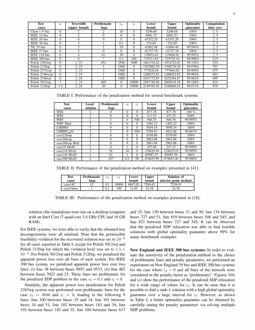
IEEE and Polish systems: As our second example, we eval-

uate the penalization method for the OPF problem performed

over benchmark systems. The results are reported in Table I.

For each system, the following numbers are reported:

• Treewidth: exact treewidth or an upper bound on the

treewidth (shown as “≤”) of the pre-contingency network

• Problematic bags: number of problematic bags for the

SDP relaxation with εb = εl = 0• Lower bound: lower bound on the globally minimum cost

of OPF, corresponding to the cost of the SDP relaxation

• Upper Bound: upper bound on the globally optimal cost

of OPF, corresponding to the solution recovered from the

penalized SDP problem

• Optimality guarantee: global optimality guarantee (in

percentage)

• Computation time: the total computation time (in sec-

onds) including those consumed towards tree decom-

position, solving the SDP relaxation, and recovering a

8

Test α Treewidth Problematic εb εl Lower Upper Optimality Computation

cases (upper bound) bags bound bound guarantee time (sec)

Chow’s 9 bus 0 2 2 10 0 5296.68 5296.68 100% ≤ 5

IEEE 14 bus 0 2 0 0 0 8081.53 8081.53 100% ≤ 5

IEEE 24 bus 0 4 0 0 0 63352.20 63352.20 100% ≤ 5

IEEE 30 bus 0 3 1 0.1 0 576.89 576.89 100% ≤ 5

NE 39 bus 0 3 1 10 0 41862.08 41864.40 99.994% ≤ 5

IEEE 57 bus 0 5 0 0 0 41737.78 41737.78 100% ≤ 5

IEEE 118 bus 0 4 61 10 0 129654.61 129660.81 99.995% ≤ 5

IEEE 300 bus 0 6 7 0.1 100 719711.63 719725.10 99.998% 13.9

Polish 2383wp 0 ≤ 23 651 3500 3000 1861510.42 1874322.65 99.316% 529

Polish 2736sp 0 ≤ 23 1 1500 0 1307882.29 1308270.20 99.970% 701

Polish 2737sop 0 ≤ 23 3 1000 0 777626.26 777664.02 99.995% 675

Polish 2746wop 0 ≤ 23 1 1000 0 1208273.91 1208453.93 99.985% 801

Polish 2746wp 0 ≤ 24 1 1000 0 1631772.83 1632384.87 99.962% 699

Polish 3012wp 1 ≤ 24 605 0 10000 2587740.98 2608918.45 99.188% 814

Polish 3120sp -1.5 ≤ 24 20 0 10000 2140765.92 2160800.42 99.073% 910

TABLE I: Performance of the penalization method for several benchmark systems.

Test Local Problematic εb εl Lower Upper Optimality

cases minima bags bound bound guarantee

WB2 2 0 0 0 877.78 877.78 100 %

WB3 2 0 0 0 417.25 417.25 100%

WB5 2 3 0 500 946.53 946.58 99.995%

WB5 Mod 3 0 0 0 1482.22 1482.22 100%

LMBM3 5 0 0 0 5694.54 5694.54 100%

LMBM3 50 2 2 0 500 5789.91 5823.86 99.807%

case22loop 2 0 0 0 4538.80 4538.80 100%

case30loop 2 0 0 0 2863.06 2863.06 100%

case30loop Mod 3 0 0 0 2861.88 2861.88 100%

case39 Mod4 3 4 1 0 557.08 557.15 99.999%

case118 Mod1 3 36 10 0 129624.98 129625.19 99.999%

case118 Mod2 2 42 1 0 85987.27 85987.59 100%

case300 Mod2 2 107 0.5 50 474625.99 474643.46 99.996%

TABLE II: Performance of the penalization method on examples presented in [41].

Test Problematic εb εl Lower Upper Solution of

cases bags bound bound interior point method

case14C 12 0.1 10000 6897.02 7289.62 7238.93

case34tree 1 0.1 100 14.49 24.38 24.38

TABLE III: Performance of the penalization method on examples presented in [18].

solution (the simulations were run on a desktop computer

with an Intel Core i7 quad-core 3.4 GHz CPU and 16 GB

RAM).

For IEEE systems, we were able to verify that the obtained tree

decompositions were all minimal. Note that the permissible

feasibility violation for the recovered solution was set to 10−6

for all cases reported in Table I, except for Polish 3012wp and

Polish 3120sp for which the violation level was set to 1.5 ×10−5. For Polish 3012wp and Polish 3120sp, we penalized the

apparent power loss over all lines of each system. For IEEE

300 bus system, we penalized apparent power loss over two

lines: (i) line 38 between buses 9053 and 9533, (ii) line 402

between buses 7023 and 23. These lines are problematic for

the penalized SDP problem in the case εb = 0.1 and εl = 0.

Similarly, the apparent power loss penalization for Polish

2383wp system was performed over problematic lines for the

case εb = 3500 and εl = 0, leading to the following 9

lines: line 100 between buses 35 and 34, line 101 between

buses 34 and 51, line 102 between buses 183 and 34, line

103 between buses 183 and 35, line 104 between buses 617

and 35, line 130 between buses 51 and 50, line 134 between

buses 727 and 51, line 819 between buses 546 and 545, and

line 821 between buses 727 and 545. It can be observed

that the penalized SDP relaxation was able to find feasible

solutions with global optimality guarantee above 99% for

many benchmark examples.

New England and IEEE 300 bus systems: In order to eval-

uate the sensitivity of the penalization method to the choice

of problematic lines and penalty parameters, we performed an

experiment on New England 39 bus and IEEE 300 bus systems

for the case where εb = 0 and all lines of the network were

considered in the penalty factor as “problematic”. Figures 3(b)

and (c) show the performance of the penalized SDP relaxation

for a wide range of values for εl. It can be seen that it is

possible to find a rank-1 solution with a high global optimality

guarantee over a large interval for εl . However, as shown

in Table I, a better optimality guarantee can be obtained by

carefully tuning the penalty parameters via solving multiple

SDP problems.

9

Modified systems 1: We also tested the SDP relaxation

method over some of the examples presented in [41]. The

results are tabulated in Table II, together with the minimum

number of local solutions for each system. For case WB5, line

5 (between buses 4 and 5) was chosen for apparent power loss

penalization. Interestingly, the penalization of a different line

in the objective function would result in the recovery of a local

minimum as opposed to a global solution. For the modified

IEEE 300 bus system, the apparent power loss penalization

was performed over 116 problematic lines of the network.

For LMBM3 50, all lines of the networks were considered

as problematic.

Modified systems 2: Two OPF test cases have been recently

proposed in [18], for which the semidefinite relaxation is

inexact. The penalization algorithm proposed here can find a

rank-1 solution for each of these cases, as reported in Table III.

The test system “case34tree” is of particular interest due to its

tree topology. We obtained a rank-1 solution by penalizing the

only problematic line of this network.

New England system with contingency constraints: Con-

sider the New England test system under 10 contingency

scenarios, each representing the outage of one line as described

in Table IV. Suppose that the objective function of the SCOPF

problem only includes the power generation cost for the

base case. The corrective active power production for each

generator in case of contingency is set to be within 2 MWaway from the base case production level. We solve the

penalized SDP relaxation by setting εb to zero and minimizing

the apparent power loss over all lines of the network. The

result is depicted in Figure 4(a) for different values of the

coefficient εl . It can be seen that a near-global solution for

the SCOPF problem is associated with the cost 45141.70. This

SCOPF cost is 7% higher than the optimal cost of the OPF

problem with no contingency.

Contingency Line Initial Terminalnumber number node node

1 1 1 2

2 2 1 39

3 3 2 3

4 4 2 25

5 6 3 4

6 7 3 18

7 15 7 8

8 20 10 32

9 40 25 26

10 45 28 29

TABLE IV: List of contingencies for New England test system.

IEEE 300 bus system with contingency constraints: Con-

sider the 300 bus system with one contingency scenario asso-

ciated with the simultaneous outage of three highly congested

lines of the base OPF. These lines are listed in Table V.

The corrective active power production for each generator in

case of contingency is set to be within 1 MW away from

the base case production level. We intend to minimize the

pre-contingency power generation cost while being secure

in the post-contingency scenario. As before, we solve the

penalized SDP relaxation by setting εb to zero and minimizing

the apparent power loss over all lines of the network. The

result is depicted in Figure 4(b). It can be seen that a near-

global solution for the SCOPF problem is associated with the

cost 740493.80, which is 3% different from that of the OPF

problem.

Contingency Line Initial Terminalnumber number node node

1

266 19 231

388 234 236400 7130 130

TABLE V: List of lines outages of the contingency scenario consideredfor IEEE 300 bus system.

VI. CONCLUSIONS

This paper studies the security-constrained optimal power

flow (SCOPF) problem by means of a semidefinite program-

ming (SDP) relaxation. The existence of a rank-1 solution

guarantees that this convex program will find a globally

optimal solution of the SCOPF problem. First, we prove that

the SDP relaxation has a solution whose rank is at most equal

to the treewidth of the power network plus one, which is

expected to be very small for real-world systems. Second, we

propose a decomposition method to reduce the computational

complexity of the SDP relaxation. In the case where the SDP

relaxation fails to work, we develop a graph-theoretic method

to identify the problematic lines of the network that make

SCOPF difficult to solve. By penalizing the loss over those

lines in the SDP relaxation, we develop a rank-enforcing

SDP relaxation. We test our relaxation method on several

benchmark examples and demonstrate its ability in finding

feasible solutions with the property that the global minima

are at most 1% away from the obtained solutions.

REFERENCES

[1] J. A. Momoh, Electric Power System Applications of Optimization. NewYork: Markel Dekker, 2001.

[2] J. Carpentier, “Contribution to the economic dispatch problem,” Bull.

Soc. Francoise Elect., vol. 3, no. 8, pp. 431–447, 1962.[3] K. Pandya and S. Joshi, “A survey of optimal power flow methods,” J.

Theoretic. Appl. Inf. Technol., vol. 4, no. 5, pp. 450–458, 2008.[4] X. Bai, H. Wei, K. Fujisawa, and Y. Wang, “Semidefinite programming

for optimal power flow problems,” Int. J. Elect. Power Energy Syst.,

vol. 30, no. 6–7, pp. 383–392, 2008.[5] J. Lavaei and S. H. Low, “Relationship between power loss and network

topology in power systems,” in Proc. IEEE 49th Conf. Decision Control,

Dec. 2010, pp. 4004–4011.[6] J. Lavaei and S. Low, “Zero duality gap in optimal power flow problem,”

IEEE Trans. Power Syst., vol. 27, no. 1, pp. 92–107, Feb. 2012.

[7] S. Sojoudi and J. Lavaei, “Exactness of semidefinite relaxations fornonlinear optimization problems with underlying graph structure,” SIAM

J. Optimiz., vol. 24, no. 4, pp. 1746–1778, Jul. 2014.[8] J. Lavaei, B. Zhang, and D. Tse, “Geometry of power flows in tree

networks,” in in Proc. IEEE Power & Energy Society General Meeting,

Jul. 2012, pp. 22–27.[9] S. Low, “Convex relaxation of optimal power flow part I: Formulations

and equivalence,” IEEE Trans. Power Syst., vol. 1, no. 1, pp. 15–27,

Mar. 2014.[10] S. Low, “Convex relaxation of optimal power flow part II: Exactness,”

IEEE Trans. Power Syst., vol. 1, no. 2, pp. 177–189, Jun. 2014.

[11] B. Zhang and D. Tse, “Geometry of injection regions of power net-works,” IEEE Trans. Power Syst., vol. 28, no. 2, pp. 788–797, May.2013.

[12] S. Bose, D. F. Gayme, S. Low, and M. K. Chandy, “Optimal powerflow over tree networks,” in Proc. 49th Annual Allerton Conf., 2011,

pp. 1342–1348.

10

Rank 1

Rank 2

Parameterl

Op

tim

al c

ost

fε

(a)

Rank 1

Parameterl

Opti

mal

co

st f

ε

(b)

Rank 1

Parameterl

Opti

mal

co

st f

ε

(c)

Fig. 3: (a) The 3-bus system presented in [14]; (b) New England system; (c) IEEE 300 bus system.

Rank 1

Parameterl

Opti

mal

cost

fε

(a)

Rank 1

Opti

mal

cost

fε

Parameterl

(b)

Fig. 4: (a) Contingency analysis of New England system; (b) contingency analysis of IEEE 300 bus system.

[13] S. Sojoudi and J. Lavaei, “Physics of power networks makes hardoptimization problems easy to solve,” IEEE Power & Energy SocietyGeneral Meeting, 2012.

[14] B. Lesieutre, D. Molzahn, A. Borden, and C. L. DeMarco, “Examiningthe limits of the application of semidefinite programming to power flowproblems,” in Proc. Allerton Conf., 2011.

[15] W. Bukhsh, A. Grothey, K. McKinnon, and P. Trodden, “Local solutions

of the optimal power flow problem,” IEEE Trans. Power Syst., vol. 28,no. 4, pp. 4780–4788, Nov. 2013.

[16] A. Gopalakrishnan, A. U. Raghunathan, D. Nikovski, and L. T. Biegler,

“Global optimization of optimal power flow using a branch & boundalgorithm,” in Proc. Allerton Conf., 2011.

[17] D. T. Phan, “Lagrangian duality and branch-and-bound algorithms for

optimal power flow,” Oper. Res., vol. 60, no. 2, pp. 275–285, Mar./Apr.2012.

[18] R. Louca, P. Seiler, and E. Bitar, “Nondegeneracy and inexactness ofsemidefinite relaxations of optimal power flow,” submitted for publica-

tion. [Online]. Available: http://arxiv.org/abs/1411.4663.

[19] R. Madani, S. Sojoudi, and J. Lavaei, “Convex relaxation for optimalpower flow problem: Mesh networks,” IEEE Trans. Power Syst., vol. 30,

no. 1, pp. 199–211, Jan. 2015.

[20] A. Lam, B. Zhang, and D. Tse, “Distributed algorithms for optimalpower flow problem,” in Proc. IEEE Conf. Decision and Control, 2012.

[21] B. Zhang, A. Lam, A. Dominguez-Garcia, and D. Tse, “An optimal and

distributed method for voltage regulation in power distribution systems,”IEEE Trans. Power App. Syst., to be published. [Online]. Available:http://arxiv.org/abs/1204.5226.

[22] D. K. Molzahn, J. T. Holzer, B. C. Lesieutre, and C. L. DeMarco,“Implementation of a large-scale optimal power flow solver based onsemidefinite programming,” IEEE Trans. Power Syst., vol. 28, no. 4, pp.

3987–3998, Nov. 2013.

[23] M. S. Andersen, A. Hansson, and L. Vandenberghe, “Reduced-complexity semidefinite relaxations of optimal power flow problems,”

IEEE Trans. Power Syst., vol. 29, no. 4, pp. 1855–1863, Jul 2014.

[24] R. Jabr, “Exploiting sparsity in SDP relaxations of the OPF problem,”IEEE Trans. Power Syst., vol. 27, no. 2, pp. 1138–1139, May. 2012.

[25] D. K. Molzahn and I. A. Hiskens, “Sparsity-exploiting moment-based

relaxations of the optimal power flow problem,” IEEE Trans. Power

App. Syst., to be published. [Online]. Available: http://arxiv.org/abs/1404.5071v2.

[26] M. Fukuda, M. Kojima, K. Murota, and K. Nakata, “Exploiting sparsity

in semidefinite programming via matrix completion I: General frame-work,” SIAM J. Optimiz., vol. 11, no. 3, pp. 647–674, 2001.

[27] K. Nakata, K. Fujisawa, M. Fukuda, M. Kojima, and K. Murota,“Exploiting sparsity in semidefinite programming via matrix completion

II: Implementation and numerical results,” Math. Program., vol. 95,no. 2, pp. 303–327, 2003.

[28] F. Capitanescu, M. Glavic, D. Ernst, and L. Wehenkel, “Contingency

filtering techniques for preventive security-constrained optimal powerflow,” IEEE Trans. Power Syst., vol. 22, no. 4, pp. 1690–1697, Nov.2007.

[29] A. J. Wood and B. F. Wollenberg, Power generation, operation, andcontrol, 2nd ed., New York: Wiley, 1996.

[30] F. V. Fomin and D. M. Thilikos, “New upper bounds on the decompos-ability of planar graphs,” J. Graph Theory, vol. 51, no. 1, pp. 53–81,

2006.

[31] J. Lavaei, “Zero duality gap for classical OPF problem convexifiesfundamental nonlinear power problems,” in Proc. Amer. Control Conf.,

June 2011, pp. 4566–4573.

[32] L. Gan, N. Li, U. Topcu, and S. Low, “On the exactness of convexrelaxation for optimal power flow in tree networks,” in Proc. 51st IEEE

Conf. Decision and Control, Dec. 2012.

[33] R. Grone, C. R. Johnson, E. M. Sa, and H. Wolkowicz, “Positivedefinite completions of partial Hermitian matrices,” Linear AlgebraAppl., vol. 58, pp. 109–124, 1984.

[34] M. Laurent, “Polynomial instances of the positive semidefinite andEuclidean distance matrix completion problems,” SIAM J. Matrix Aanl.A., vol. 22, no. 3, pp. 874–894, 2001.

[35] M. Laurent and A. Varvitsiotis, “A new graph parameter related to

bounded rank positive semidefinite matrix completions,” Math. Pro-gram., vol. 145, no. 1-2, pp. 291–325, 2014.

[36] D. Carlson, E. Haynsworth, and T. Markham, “A generalization of the

Schur complement by means of the moore-penrose inverse,” SIAM J.Appl. Math., vol. 26, no. 1, pp. 169–175, Jan. 1974.

[37] H. L. Bodlaender and A. M. Koster, “Treewidth computations I. upper

bounds,” Inform. Comput., vol. 208, no. 3, pp. 259–275, 2010.

11

[38] H. L. Bodlaender and A. M. Koster, “Treewidth computations II. lower

bounds,” Inform. Comput., vol. 209, no. 7, pp. 1103–1119, 2011.[39] B. Recht, M. Fazel, and P. A. Parrilo, “Guaranteed minimum rank

solutions to linear matrix equations via nuclear norm minimization,”

SIAM Rev., vol. 52, pp. 471–501, 2010.[40] R. Madani, M. Ashraphijuo, and J. Lavaei. (2014, Jul.) SDP Solver of

Optimal Power Flow. [Online]. Available: http://www.ee.columbia.edu/∼lavaei/Software.html

[41] W. A. Bukhsh. (2012, Feb.) Test Case Archive of Optimal PowerFlow (OPF) Problems with Local Optima. [Online]. Available:

http://www.maths.ed.ac.uk/OptEnergy/LocalOpt

Ramtin Madani received the B.Sc. and M.Sc. de-

grees in electrical engineering from Sharif Univer-sity of Technology, Tehran, Iran, in 2010 and 2012,

respectively. He is currently working towards thePh.D. degree in the Department of Electrical Engi-neering, Columbia University, New York, NY, USA.

His current research interests include optimizationover graphs, optimal power networks & smart grids,distributed control and nonlinear optimization. He

has worked in many areas of optimization theory,communications, and signal processing.

Morteza Ashraphijuo received the B.Sc. degree

in electrical engineering from Sharif University ofTechnology, Tehran, Iran, in 2015. He is currentlyworking towards the Ph.D. degree in the Department

of Electrical Engineering, Columbia University, NewYork, NY. He has won Silver Medal in the 2010

International Mathematical Olympiad. His researchinterests lie in the general areas of non-linear op-timization with applications in power systems and

control theory.

Javad Lavaei is an Assistant Professor in the

Department of Electrical Engineering at ColumbiaUniversity. He obtained his Ph.D. degree in Com-puting and Mathematical Sciences from California

Institute of Technology in 2011 and held a one-yearpostdoc position jointly with Electrical Engineeringand Precourt Institute for Energy at Stanford Uni-

versity. He is recipient of the Milton and FrancisClauser Doctoral Prize for the best university-wide

Ph.D. thesis. His research interests include non-linear optimization, distributed computation, power

systems, and control theory. Javad Lavaei is a senior member of IEEE

and has won multiple awards, including NSF CAREER Award, Office ofNaval Research Young Investigator Award, Google Faculty Research Award,the Canadian Governor General’s Gold Medal, Northeastern Association of

Graduate Schools Master’s Thesis Award, and Silver Medal in the 1999International Mathematical Olympiad. For his computation work on energysystems, he was chosen by Resnick Sustainability Institute as one of the

5 innovators in the area of sustainability worldwide in 2014. Javad Lavaeiis an associate editor for IEEE Transactions on Smart Grid and serves onthe conference editorial board for both IEEE Control Systems Society and

European Control Association.