HAL Id: tel-02303045https://tel.archives-ouvertes.fr/tel-02303045

Submitted on 2 Oct 2019

HAL is a multi-disciplinary open accessarchive for the deposit and dissemination of sci-entific research documents, whether they are pub-lished or not. The documents may come fromteaching and research institutions in France orabroad, or from public or private research centers.

L’archive ouverte pluridisciplinaire HAL, estdestinée au dépôt et à la diffusion de documentsscientifiques de niveau recherche, publiés ou non,émanant des établissements d’enseignement et derecherche français ou étrangers, des laboratoirespublics ou privés.

Chance constrained problem and its applicationsShen Peng

To cite this version:Shen Peng. Chance constrained problem and its applications. Optimization and Control [math.OC].Université Paris Saclay (COmUE); Xi’an Jiaotong University, 2019. English. NNT : 2019SACLS153.tel-02303045

Thes

ede

doct

orat

NN

T:2

019S

AC

LS15

3

Optimisation stochastique aveccontraintes en probabilites et applications

These de doctorat de Xi’an Jiaotong University et de l’Universite Paris-Saclaypreparee a l’Universite Paris-Sud

Ecole doctorale n580 Sciences et Technologies de l’Information et de laCommunication (STIC)

Specialite de doctorat : Informatique

These presentee et soutenue a Orsay, le 17 juin 2019, par

M. Shen PENG

Composition du Jury :

M. Alexandre CAMINADAProfesseur, Universite de Nice President, Rapporteur

M. Mounir HADDOUProfesseur, INSA Rennes Rapporteur

M. Yacine CHITOURProfesseur, CentraleSupelec Examinateur

Mme Janny LEUNGProfesseure, Chinese University of Hong Kong (Shenzhen) Examinatrice

Mme Francesca MAGGIONIProfesseure, University of Bergamo Examinatrice

M. Vikas Vikram SINGHProfesseur assistant, Indian Institute of Technology Delhi Examinateur

M. Abdel LISSERProfesseur, Universite Paris-Sud Directeur de these

M. Zhiping CHENProfesseur, Xi’an Jiaotong University Co-directeur de these

Chance Constrained Problem and Its

Applications

A dissertation submitted to

Universite Paris Sud

in fulfillment of the requirements

for the Ph.D. degree in

Computer Science

By

Shen PENG

Supervisor: Prof. Abdel LISSER

Co-supervisor: Prof. Zhiping CHEN

June 2019

Acknowledgements

First of all, I would like to thank my supervisors, Prof. Abdel Lisser and Prof.Zhiping Chen, who illuminate my way to the science.

Prof. Zhiping Chen is my supervisor in Xi’an Jiaotong University. Thanksto his consistent support and encouragement, I can navigate many obstacles inpursuing the Ph.D degree. He has spent a lot of time and efforts on my studyand research. He not only taught me scientific knowledge but also sharing a lotof experience on life and research. I have earned a lot from him both on how tobe a researcher and how to research.

Prof. Abdel Lisser is my supervisor in Universite Paris Sud. Thanks to hisopen-door policy, I can always discuss any problem with him and obtain thenutritious suggestions. He is not just an supervior to my research, a mentor fromwhom I learnt, but also a friend. I feel extremely lucky and want to sincerely saythank you from the bottom of my heart.

My special thanks then go to Dr. Jia Liu of Xi’an Jiaotong University andDr. Vikas Vikram Singh of Indian Institute of Technology Delhi for their positivediscussion and helpful advice on my research work.

I also would like to give my gratitude to all of my friends and colleagues both inChina and France from whom I have benefited enormously. Particularly, I thankHehuan Shi who helped me solving a lot of registration problems in France. Ithank Dr. Jihong Yu, Dr. Rongrong Zhang, Dr. Ruqi Huang, Dr. Chuan Xu,Zhoudan Lyu and Xingchao Cui for sharing a lot of great moments in Paris. Ialso thank Dr. Zongxin Li, Liyuan Wang, Xinkai Zhuang, Zhe Yan, Jie Jiang,Fei Yu, He Hu, Yu Mei, Wei Wang, Xin Wei, Rui Xie, Zhujia Xu, Ming Jin andTianyao Chen for sharing many wonderful time with me and making my life richand colorful.

Last but not least, I would like to devote the most deep gratitude to eachmember of my family: my parents, my parents-in-law and my wife for theirunconditional love, support and encouragement. Especially, I want to expressthe most special gratitude to my wife Yingping Li. Thanks for being at my sidefor all these years.

I

II

Resume

L’incertitude est une propriete naturelle des systemes complexes. Les parametresde certains modeles peuvent etre imprecis ; la presence de perturbations aleatoiresest une source majeure d’incertitude pouvant avoir un impact important sur lesperformances du systeme. L’optimisation sous contraintes en probabilites est uneapproche naturelle et largement utilisee pour fournir des decisions robustes dansdes conditions d’incertitude. Dans cette these, nous etudierons systematiquementles problemes d’optimisation avec contraintes en probabilites dans les cas suivants:

En tant que base des problemes stochastiques, nous passons d’abord en revueles principaux resultats de recherche relatifs aux contraintes en probabilites selontrois perspectives: les problemes lies a la convexite en presence de contraintesprobabilistes, les reformulations et les approximations de ces contraintes, et lescontraintes en probabilites dans le cadre de l’optimisation distributionnellementrobuste.

Pour les problemes d’optimisation geometriques stochastiques, nous etudionsles programmes avec contraintes en probabilites geometriques rectangulaires joint-es. A l’aide d’hypotheses d’independance des variables aleatoires elliptiquementdistribuees, nous deduisons une reformulation des programmes a contraintes geom-etriques rectangulaires jointes. Comme la reformulation n’est pas convexe, nousproposons de nouvelles approximations convexes basees sur la transformation desvariables ainsi que des methodes d’approximation lineaire par morceaux. Nosresultats numeriques montrent que nos approximations sont asymptotiquementserrees.

Lorsque les distributions de probabilite ne sont pas connues a l’avance ou quela reformulation des contraintes probabilistes est difficile a obtenir, des bornesobtenues a partir des contraintes en probabilites peuvent etre tres utiles. Parconsequent, nous developpons quatre bornes superieures pour les contraintesprobabilistes individuelles, et jointes dont les vecteur-lignes de la matrice des con-traintes sont independantes. Sur la base de l’inegalite unilaterale de Chebyshev,de l’inegalite de Chernoff, de l’inegalite de Bernstein et de l’inegalite de Hoeffding,nous proposons des approximations deterministes des contraintes probabilistes.En outre, quelques conditions suffisantes dans lesquelles les approximations sus-mentionnees sont convexes et solvables de maniere efficace sont deduites. Pourreduire davantage la complexite des calculs, nous reformulons les approxima-tions sous forme de problemes d’optimisation convexes solvables bases sur desapproximations lineaires et tangentielles par morceaux. Enfin, des experiencesnumeriques sont menees afin de montrer la qualite des approximations determinis-

III

tes etudiees sur des donnees generees aleatoirement.Dans certains systemes complexes, la distribution des parametres aleatoires

n’est que partiellement connue. Pour traiter les incertitudes complexes en ter-mes de distribution et de donnees d’echantillonnage, nous proposons un ensem-ble d’incertitude base sur des donnees obtenues a partir de distributions mixtes.L’ensemble d’incertitude base sur les distributions mixtes est construit dans laperspective d’estimer simultanement des moments d’ordre superieur. Ensuite,a partir de cet ensemble d’incertitude, nous proposons une reformulation duprobleme robuste avec contraintes en probabilites en utilisant des donnees issuesd’echantillonnage. Comme la reformulation n’est pas un programme convexe,nous proposons des approximations nouvelles et convexes serrees basees sur lamethode d’approximation lineaire par morceaux sous certaines conditions. Pourle cas general, nous proposons une approximation DC pour deriver une bornesuperieure et une approximation convexe relaxee pour deriver une borne inferieurepour la valeur de la solution optimale du probleme initial. Nous etablissonsegalement le fondement theorique de ces approximations. Enfin, des experiencesnumeriques sont effectuees pour montrer que les approximations proposees sontpratiques et efficaces.

Nous considerons enfin un jeu stochastique a n joueurs non-cooperatif. Lorsquel’ensemble de strategies de chaque joueur contient un ensemble de contrainteslineaires stochastiques, nous modelisons les contraintes lineaires stochastiques dechaque joueur sous la forme de contraintes en probabilite jointes. Pour chaquejoueur, nous supposons que les vecteurs lignes de la matrice definissant les con-traintes stochastiques sont independants les unes des autres. Ensuite, nous for-mulons les contraintes en probabilite dont les variables aleatoires sont soit nor-malement distribuees, soit elliptiquement distribuees, soit encore definies dans lecadre de l’optimisation distributionnellement robuste. Sous certaines conditions,nous montrons l’existence d’un equilibre de Nash pour ces jeux stochastiques.

IV

Abstract

Uncertainty is a natural property of complex systems. Imprecise model parame-ters and random disturbances are major sources of uncertainties which may havea severe impact on the performance of the system. The target of optimizationunder uncertainty is to provide profitable and reliable decisions for systems withsuch uncertainties. Ensuring reliability means satisfying specific constraints ofsuch systems. An appropriate treatment of inequality constraints of a systeminfluenced by uncertain variables is required for the formulation of optimizationproblems under uncertainty. Therefore, chance constrained optimization is a nat-ural and widely used approaches for this purpose. Moreover, the topics aroundthe theory and applications of chance constrained problems are interesting andattractive.

Chance constrained problems have been developed for more than four decades.However, there are still some important issues requiring non-trivial efforts tosolve. In view of this, we will systematically investigate chance constrained prob-lems from the following perspectives.

(1) As the basis for chance constrained problems, we first review some main re-search results about chance constraints in three perspectives: convexity of chanceconstraints, reformulations and approximations for chance constraints and distri-butionally robust chance constraints. Since convexity is fundamental for chanceconstrained problems, we introduce some basic mathematical definitions and the-ories about the convexity of large classes of chance constrained problems. Then,we state some tractable convex reformulations and approximations for chanceconstrained problems. For distributionally robust optimization, we illustrate mo-ments based uncertainty set, and distance based uncertainty set and show theirapplications in distributionally robust chance constrained problems, respectively.

(2) For stochastic geometric programs, we first review a research work aboutjoint chance constrained geometric programs with normal distribution and in-dependent assumptions. As an extension, when the stochastic geometric pro-gram has rectangular constraints, we formulate it as a joint rectangular geometricchance constrained program. With elliptically distributed and pairwise indepen-dent assumptions for stochastic parameters, we derive a reformulation of the jointrectangular geometric chance constrained programs. As the reformulation is notconvex, we propose new convex approximations based on the variable transfor-mation together with piecewise linear approximation methods. Our numericalresults show that our approximations are asymptotically tight.

(3) When the probability distributions are not known in advance or the refor-mulation for chance constraints is hard to obtain, bounds on chance constraints

V

can be very useful. Therefore, we develop four upper bounds for individual andjoint chance constraints with independent matrix vector rows. Based on the one-side Chebyshev inequality, Chernoff inequality, Bernstein inequality and Hoeffd-ing inequality, we propose deterministic approximations for chance constraints.In addition, various sufficient conditions under which the aforementioned ap-proximations are convex and tractable are derived. Therefore, to reduce furthercomputational complexity, we reformulate the approximations as tractable con-vex optimization problems based on piecewise linear and tangent approximations.Finally, based on randomly generated data, numerical experiments are discussedin order to identify the tight deterministic approximations.

(4) In some complex systems, the distribution of the random parameters isonly known partially. To deal with the complex uncertainties in terms of the dis-tribution and sample data, we propose a data-driven mixture distribution baseduncertainty set. The data-driven mixture distribution based uncertainty set isconstructed from the perspective of simultaneously estimating higher order mo-ments. Then, with the mixture distribution based uncertainty set, we derivea reformulation of the data-driven robust chance constrained problem. As thereformulation is not a convex program, we propose new and tight convex ap-proximations based on the piecewise linear approximation method under certainconditions. For the general case, we propose a DC approximation to derive anupper bound and a relaxed convex approximation to derive a lower bound for theoptimal value of the original problem, respectively. We also establish the theo-retical foundation for these approximations. Finally, simulation experiments arecarried out to show that the proposed approximations are practical and efficient.

(5) We consider a stochastic n-player non-cooperative game. When the strat-egy set of each player contains a set of stochastic linear constraints, we modelthe stochastic linear constraints of each player as a joint chance constraint. Foreach player, we assume that the row vectors of the matrix defining the stochasticconstraints are pairwise independent. Then, we formulate the chance constraintswith the viewpoints of normal distribution, elliptical distribution and distribu-tionally robustness, respectively. Under certain conditions, we show the existenceof a Nash equilibrium for the stochastic game.

VI

Contents

1 Introduction 11.1 Convexity . . . . . . . . . . . . . . . . . . . . . . . . . . . . . . . 21.2 Reformulations and approximations for Chance Constraints . . . . 31.3 Distributionally Robust Chance Constrained Problems . . . . . . 41.4 Contribution and Outline of the Dissertation . . . . . . . . . . . . 7

2 Chance Constraints 92.1 α-concave measures and convexity of chance constraints . . . . . . 92.2 Reformulations and approximations for chance constraints . . . . 14

2.2.1 Individual chance constraints . . . . . . . . . . . . . . . . 142.2.2 Normally distributed joint linear chance constraints . . . . 162.2.3 Integer programming approaches for joint linear chance con-

straints . . . . . . . . . . . . . . . . . . . . . . . . . . . . 172.2.4 Convex approximations for chance constraints . . . . . . . 182.2.5 Sample average approximations for chance constraints . . . 19

2.3 Distributionally robust chance constraints . . . . . . . . . . . . . 202.3.1 Distributionally robust individual chance constraints with

known mean and covariance . . . . . . . . . . . . . . . . . 202.3.2 Distributionally robust joint chance constraints with known

mean and covariance . . . . . . . . . . . . . . . . . . . . . 212.3.3 Distributionally robust joint chance constraints with uncer-

tain mean and covariance . . . . . . . . . . . . . . . . . . 222.3.4 Distributionally robust chance constrained problem based

on φ-divergence . . . . . . . . . . . . . . . . . . . . . . . . 252.3.5 Distributionally robust chance constrained problem based

on Wasserstein distance . . . . . . . . . . . . . . . . . . . 272.4 Conclusion . . . . . . . . . . . . . . . . . . . . . . . . . . . . . . . 29

3 Geometric Chance Constrained Programs 313.1 Stochastic geometric optimization with joint chance constraints . 31

3.1.1 Introduction . . . . . . . . . . . . . . . . . . . . . . . . . . 313.1.2 Stochastic geometric optimization under Gaussian distri-

bution . . . . . . . . . . . . . . . . . . . . . . . . . . . . . 323.1.3 Numerical experiments . . . . . . . . . . . . . . . . . . . . 37

3.2 Joint rectangular geometric chance constrained programs . . . . . 383.2.1 Introduction . . . . . . . . . . . . . . . . . . . . . . . . . . 393.2.2 Elliptically distributed stochastic geometric problems . . . 40

VII

3.2.3 Convex approximations of constraints (3.35) and (3.36) . . 433.2.4 Numerical experiments . . . . . . . . . . . . . . . . . . . . 50

3.3 Conclusion . . . . . . . . . . . . . . . . . . . . . . . . . . . . . . . 55

4 Bounds for Chance Constrained Problems 574.1 Introduction . . . . . . . . . . . . . . . . . . . . . . . . . . . . . . 574.2 Chebyshev and Chernoff Bounds . . . . . . . . . . . . . . . . . . . 58

4.2.1 Chebychev bounds . . . . . . . . . . . . . . . . . . . . . . 584.2.2 Chernoff bounds . . . . . . . . . . . . . . . . . . . . . . . 61

4.3 Bernstein and Hoeffding Bounds . . . . . . . . . . . . . . . . . . . 654.3.1 Bernstein bounds . . . . . . . . . . . . . . . . . . . . . . . 654.3.2 Hoeffding bounds . . . . . . . . . . . . . . . . . . . . . . . 66

4.4 Computational Results . . . . . . . . . . . . . . . . . . . . . . . . 684.5 Conclusion . . . . . . . . . . . . . . . . . . . . . . . . . . . . . . . 72

5 Data-Driven Robust Chance Constrained Problems: A MixtureModel Approach 755.1 Mixture Distribution Based Uncertainty Set . . . . . . . . . . . . 75

5.1.1 Data-Driven Confidence Region for Moments . . . . . . . . 775.1.2 Data-Driven Confidence Region for Mixture Weights . . . 81

5.2 Data-Driven Robust Chance Constrained Problems . . . . . . . . 825.2.1 Reformulation of Problem (P) . . . . . . . . . . . . . . . . 825.2.2 Convex Approximation . . . . . . . . . . . . . . . . . . . . 845.2.3 DC reformulation . . . . . . . . . . . . . . . . . . . . . . . 89

5.3 Numerical Results . . . . . . . . . . . . . . . . . . . . . . . . . . . 955.3.1 Convex approximation . . . . . . . . . . . . . . . . . . . . 955.3.2 DC approximation . . . . . . . . . . . . . . . . . . . . . . 97

5.4 Conclusion . . . . . . . . . . . . . . . . . . . . . . . . . . . . . . . 98

6 Chance Constrained Stochastic Game Theory 996.1 The model . . . . . . . . . . . . . . . . . . . . . . . . . . . . . . . 996.2 Existence of Nash equilibrium with normal distribution . . . . . . 1006.3 Existence of Nash equilibrium with elliptical distribution . . . . . 1076.4 Existence of Nash equilibrium for distributionally robust model . 111

6.4.1 φ-divergence uncertainty set . . . . . . . . . . . . . . . . . 1126.4.2 Moments based uncertainty set I . . . . . . . . . . . . . . 1146.4.3 Moments based uncertainty set II . . . . . . . . . . . . . . 1166.4.4 Moments based uncertainty set III . . . . . . . . . . . . . 117

6.5 Conclusion . . . . . . . . . . . . . . . . . . . . . . . . . . . . . . . 119

7 Conclusions and Prospects 1217.1 Conclusions . . . . . . . . . . . . . . . . . . . . . . . . . . . . . . 1217.2 Prospects . . . . . . . . . . . . . . . . . . . . . . . . . . . . . . . 122

Bibliography 125

VIII

Chapter 1

Introduction

Consider the following constrained optimization problem:

minx

g (x)

s.t. c1(x, ξ) ≤ 0, · · · , cd(x, ξ) ≤ 0,x ∈X,

(1.1)

where X ∈ Rm is a deterministic set, x ∈ X is the decision vector, ξ isa k-dimensional parameter vector, g (x) : Rn → R and ci (x, ξ) : Rn+k →R, i = 1, · · · , d, are real value functions. Furthermore, we assume that g (x)and ci (x, ξ) , i = 1, · · · , d are convex in x and X is a compact and convex set.Then, problem (1.1) is a constrained convex optimization problem. This kind ofproblem has broad applications in communications and networks, product design,system control, statistics, and finance, and it can be solved efficiently.

However, in many practical problems, the parameter ξ of problem (1.1) mightbe uncertain. If we ignore the uncertainty, such as using the expectation of ξ,the obtained optimal solution might be infeasible with high probability.

To take the uncertainty into consideration, we can formulate the problem asa chance constrained optimization problem:

minx

g (x)

s.t. PF c1(x, ξ) ≤ 0, · · · , cd(x, ξ) ≤ 0 ≥ ε,x ∈X,

(1.2)

where ξ is a random vector defined on some probability space (Ω,F ,P), F is thejoint probability distribution function of the random vector ξ and ε ∈ (0, 1) is thetolerance probability, say, 0.95 or 0.99. Therefore, the solution to problem (1.2)is guaranteed to be a feasible solution to the original problem (1.1) with a proba-bility at least ε. Problem (1.2) is called a joint chance constrained problem, andthe chance constraint is called a joint chance constraint. When d = 1, problem(1.2) is called an individual chance constrained problem because it requires onlya single constraint to be satisfied with probability ε.

Chance (probabilistic) constrained optimization problems were firstly pro-posed by Charnes et al.[17] and Miller and Wagner [75]. In the paper of Charneset al. [17], chance constraints are imposed individually on each constraint involv-

1

ing random variables. The paper by Miller and Wagner [75] takes the chanceconstraint jointly on the stochastic constraints but handles only independentrandom variables appearing on the right hand sides of the stochastic constraints.Prekopa [87] initiated the research on this topic, where the chance constraint istaken jointly for the stochastic constraints and the random variables involved arestochastically dependent, in general. Applications of probabilistic constraints aresubstantial in engineering and finance. For an overview on the theory, solutionand applications of chance constrained optimization problems, one can refer tothe monographs [13], [89] and [96].

1.1 Convexity

A fundamental issue for chance constrained problems is the convexity of chanceconstraints, which is widely considered as a considerable difficulty. Both fromtheoretical and computational perspectives, it was recognized that chance con-strained problems are hard to treat. Van de Panne and Popp [79] proposed asolution method for a linear chance constrained problem with one-row normallydistributed constraint, transformed to a nonlinear convex constraint. Kataoka[59] studied an individual chance constrained problem with random right-handside following a normal distribution.

Apart from the above simple problems, chance constrained problems oftenlead to a non-convex feasible solution set. Various conditions and techniques weredeveloped to handle this issue. Miller and Wagner [75] considered a joint chanceconstrained model with independent random right-hand side. The convexity oftheir problem is ensured when the probability distribution possesses a propertyof decreasing reversed hazard function. Jagannathan [56] extended this result tothe dependent case, and also considered a linear joint chance constrained problemwith normally distributed independent rows.

Prekopa [88] made an essential step by proving the convexity of the feasi-ble solution set of linear chance constrained problems with dependent randomright-hand sides in the chance constraint when the probability distribution islogarithmically concave. This kind of distributions include normal, Wishart andDirichlet distributions. Borell [9] and Brascamp and Lieb [11] generalized loga-rithmical concavity to a concept called r-concave measures. A generalized defini-tion of r-concave function on set, which is also suitable for discrete distributions,was proposed by Dentcheva et al. [28]. Concretely, Calafiore and El Ghaoui [15]reformulated an individual chance constraint as a second order cone constraintby using a similar notion of Q-radial distribution.

Despite this progress, the problem of convexity remains to be a big challengefor chance constrained problems, especially for joint chance constrained prob-lems. However, there are still some extensions about the convexity. Prekopa etal. [90] asserted that a joint linear chance constrained problem is convex if therows are independently normally distributed and the covariances matrices of therows are constant multiples of each other. Henrion [49] gave a completely struc-tural description of the feasible solution set defined by individual linear chanceconstraints, which can be seen as a more promising direction. Following this

2

direction, by using the r-concavity and introducing a notion of r-decreasing func-tion, Henrion and Strugarek [50] further proved the convexity of joint chanceconstraints with independent random variables separated from decision vectors.For the dependent case with random right-hand side, Henrion and Strugarek [51]and Ackooij [1] extended the result by using the theory of copulas, respectively,while Houda [54] considered the dependent case by using a variation to the mixingcoefficient. In addition, handling the dependence of the random vectors by copu-las, Cheng et al. [23] proposed a mixed integer linear reformulation and providean efficient semidefinite relaxation of 0–1 quadratic programs with joint prob-abilistic constraints. Lagoa et al. [62] proved the convexity when the randomvector have a log-concave symmetric distribution. Recently, Lubin et al. [66]showed the convexity of two-sided chance constrained program when ξ followsnormal (or log-concave) distribution.

1.2 Reformulations and approximations for Chance

Constraints

Generally, the probability associated with chance constraints is difficult to com-pute due to the multiple integrals. For this reason, many equivalent reformula-tions for chance constraints or their approximations have been proposed. Whenthe random vector ξ in individual linear chance constraints follows normal dis-tribution, elliptical distribution or radial distribution, the chance constraint inthe individual linear chance constrained problem can be reformulated as a sec-ond order conic programming (SOCP) constraint ([15, 49, 56, 88]). For the jointlinear chance constrained problem with normally distributed coefficients and in-dependent matrix rows, Cheng and Lisser [24] proposed SOCP approximationsby using piecewise linear and piecewise tangent approximations. And for the jointchance constrained geometric programming problem with independent normallydistributed parameters, Liu et al [65] derived asymptotically tight geometric pro-gramming approximations based on variable transformation and piecewise linearapproximations. Using Archimedean copula, Cheng et al. [22] considered ellipti-cally distributed joint linear chance constraints with dependent rows and derivedSOCP approximation schemes. Luedtke and Ahmed [68] constructed a mixed in-teger linear programming reformulation for joint linear chance constrained prob-lems when the random vector has finite support.

In order to solve chance constrained problems efficiently, we need both theconvexity of the corresponding feasible set and efficient computability of the con-sidered probability [76]. This combination is rare, and very few are the cases inwhich a chance constraint can be processed efficiently (see [28, 62, 91]). When-ever this is the case, tractable approximations of chance constraints can be veryuseful in practice.

A computationally tractable approximation of chance constrained problemsis given by the scenario approach, based on Monte Carlo sampling techniques.With this kind of techniques, one can recur to approximate solutions based onconstraint sampling. And the constraint consists in taking into account only

3

a finite set of constraints, chosen at random among the possible continuum ofconstraint instances of the uncertainty. The attractive feature of this methodis to provide explicit bounds on the measure of the original constraints that arepossibly violated by the randomized solution. The properties of the solutions pro-vided by this approach, called scenario approach, have been studied in [12, 16, 40],where it has been shown that most of the constraints of the original problem aresatisfied provided that the number of samples is sufficiently large. The constraintsampling method has been extensively studied within the chance constraint ap-proach through different directions by [36] and [78]. More concretely, Nemirovskiand Shapiro [77] solved joint linear chance constrained problems through sce-nario approximation and studied the conditions under which the solution of theapproximation problem is feasible for the original problem with high probability.By using the sample approximation method, Luedtke and Ahmed [67] derivedthe minimal sample size and the probability requirement such that a solutionof the approximate problem is feasible for the original joint chance constrainedproblem. Based on Monte Carlo sampling techniques, Hong, Yang and Zhang[53] proposed a difference of convex (DC) functions approximation for the jointnonlinear chance constrained problem, and solved it by a sequence of convexapproximations.

Besides the scenario approximation approach, Ben-Tal and Nemirovski [6]proposed a conservative convex approximation, which includes the quadratic ap-proximation for individual linear chance constraints. Nemirovski and Shapiro [76]provided the CVaR approximation and Bernstein approximation for individualchance constraints.

An alternative to the above approximated approaches consists in providingbounds based on using deterministic analytical approximations of chance con-straints. For the case of individual chance constraint, the bounds are mainlybased on extensions of Chebyshev inequality together with the first two moments[8, 52, 85]. For joint chance constraints, deterministic equivalent approximationshave been widely studied in [23, 24, 25, 65, 99].

In the literature, several bounding techniques have been proposed for two-stage and multistage stochastic programs with expectation (see for instance [8,84]). This class of problems brings computational complexity which increasesexponentially with the size of the scenario tree, representing a discretization ofthe underlying random process. Even if a large discrete tree model is constructed,the problem might be untractable due to the curse of dimensionality. In thissituation, easy-to-compute bounds have been proposed in the literature (see forinstance [2, 37, 70, 71, 72]) by solving small size problems.

1.3 Distributionally Robust Chance Constrained

Problems

In many practical situations, one can only obtain the partial information aboutthe probability distribution of ξ. If we replace the real distribution by an esti-mated one, the obtained optimal solution may be infeasible in practice with high

4

probability [108]. For this reason, the distributionally robust chance constrainedproblems are proposed in [15, 36, 108].

minx

g (x)

s.t. infF∈D

PF c1(x, ξ) ≤ 0, · · · , cd(x, ξ) ≤ 0 ≥ ε,

x ∈X,

(1.3)

where D is an uncertainty set of the joint probability distribution F .

Early uncertainty sets of distribution are based on exact moments informationof the random parameter. With this kind of uncertainty sets, El Ghaoui et al. [35],Popescu [86] and Chen et al. [18] studied the distributionally robust counterpartsof many risk measures and expected value functions. Calafiore and El Ghaoui[15] reformulated a distributionally robust individual linear chance constrainedproblem as a SOCP problem with known mean and covariance. Zymler et al.[108]approximated the distributionally robust joint chance constrained problem as atractable semidefinite programming (SDP) problem, and the authors prove thatthe proposed SDP is a reformulation when the chance constraint is individual.Li et al. [63] studied a single chance constraint with known first and secondmoments and unimodality of the distributions.

Considering the uncertainties in terms of the distribution and of the first twoorder moments, Delage and Ye [27] introduced the uncertainty set characterizedby an elliptical constraint and a linear matrix inequality. Based on that, theytransformed expected utility problems into optimization problems with linear ma-trix inequality constraints. Cheng et al.[21] established a distributionlly robustchance constrained knapsack problem where the first order moment is fixed andthe second order moment in the uncertainty set is contained in an elliptical set.Yang and Xu [103] showed that the distributionally robust chance constrainedoptimization is tractable if the uncertainty set is characterized by its mean andvariance in a given set, and the constraint function is concave with respect to thedecision variables and quasi-convex with respect to the uncertain parameters. Inaddition, Zhang et al. [104] developed a SOCP reformulation for a distributionalfamily subject to an elliptical constraint and a linear matrix inequality. More-over, Xie and Ahmed [102] showed that a distributionally robust joint chanceconstrained optimization problem is convex when the uncertainty set is specifiedby convex moment constraints.

Except for the above two kinds of uncertainty sets, Hanasusanto et al. [48]studied distributionally robust chance constraints where the distribution of un-certain parameters belongs to an uncertainty set characterized by the mean, thesupport and the dispersion information instead of the second order moment.

It is well known that the distributions of financial security returns are oftenskewed with high leptokurtic ([29]). This suggests to consider higher moments(especially skewness and kurtosis) in some realistic models. A tractable way totake higher order moments into consideration is to adopt the mixture distributionframework. Simply speaking, a mixture distribution is a convex combination ofsome component distributions. In this aspect, Hanasusanto et al.[46] considered arisk-averse newsvendor model where the demand distribution is supposed to be a

5

mixture distribution with known weights and unknown component distributions.Zhu and Fukushima [107] considered a robust portfolio selection problem withthe finite normal mixture distribution, where the unknown mixture weights arerestricted in linear or elliptical uncertainty sets.

However, for quite a few complex decision making problems under uncertainty,the precise knowledge about the necessary partial information is rarely availablein reality. Hence, a strategy based on erroneous inputs might be infeasible orexhibit poor performance when implemented. To deal with such complex decisionproblems, a new framework called ’data-driven’ robust optimization is proposed.This new scheme directly uses the observations of random variables as the inputsto the mathematical programming model and is now receiving particular attentionin operations research community.

Basically, there are two kinds of data-driven approaches for distributionallyrobust optimizations. The first one estimates the parameters in an uncertainty setthrough statistical methods. For example, from the parametric estimation per-spective, Delage and Ye [27] showed that the uncertainty set characterizing theuncertainties of first and second order moments can be estimated through statisti-cal confidence regions, which can be calculated directly from the data. Bertsimaset al. [7] proposed a systematic scheme for estimating uncertainty sets from databy using statistical hypothesis tests. And they proved that robust optimizationproblems over each of their uncertainty sets are generally tractable. However, asfar as we know, the tractable data-driven uncertainty sets can only characterizethe first and the second moments. From the non-parametric perspective, Zhuet al.[106] showed that the data-driven uncertainty sets of mixture distributionweights can be estimated through Bayesian learning. Recently, Gupta [43] pro-posed a near-optimal Bayesian uncertainty set, which is smaller than uncertaintysets based on statistical confidence regions.

The second kind of data-driven approaches directly characterizes the uncer-tainty of a distribution through a probabilistic distance, and thus forms a newtype of data-driven uncertainty sets. One of the most frequently used data-drivenuncertainty sets is characterized by the distance function based on probabilitydensity, such as φ-divergence and Wasserstein distance. By utilizing sophisti-cated probabilistic measures, Ben-Tal et al.[4] proposed a class of data-drivenuncertainty sets based on φ-divergences. Hu and Hong [55] studied distribu-tionally robust individual chance constrained optimization problems where theuncertainty set of the probability distribution is defined by the Kullback-Leiblerdivergence, which is a special case of φ-divergences, the authors showed that thedistributionally robust chance-constrained problem can be reformulated as thechance constrained problem with an adjusted confidence level. Jiang and Guan[57] considered a family of density-based uncertainty sets based on φ-divergenceand proved that a distributionally robust joint linear chance constraint is equiv-alent to a chance constraint with a perturbed risk level. Recently, Esfahani andKuhn [38] and Zhao and Guan [105] showed that under certain conditions, thedistributionally robust expected utility optimization problem with Wassersteindistance is tractable. On the other hand, Hanasusanto et al. [47] showed thatthe distributionally robust joint linear chance constrained program with the un-certainty set characterized by Wasserstein distance is strongly NP-hard.

6

1.4 Contribution and Outline of the Disserta-

tion

Motivated by the literature review, we conduct a systematic research in thisdissertation on chance constrained problem and its applications. The main workof this dissertation is stated as following:

(1) First of all, as the basic knowledge of chance constrained problems, wereview some standard work about chance constraints in Chapter 2. We firstlystate some mathematical theories about convexity of large classes of chance con-strained problems. Then, we review some standard research results about convexreformulations and solvable approximations for chance constraints. These resultsare fundamental for solving chance constrained problems. At last, we introducemoments based uncertainty set and distance based uncertainty set, which areimportant and popular uncertainty sets in research about distributionally robustchance constrained problems.

(2) Chance constrained geometric programs play an important role in manypractical problems. Therefore, as a first step, we first review the recent resultsabout geometric programs with joint chance constraints, where the stochasticparameters are normally distributed and independent of each other. To extendthis work, we discuss joint rectangular geometric chance constrained programsunder elliptical distribution with independent components. With standard vari-able transformation, a convex reformulation of rectangular geometric chance con-strained programs can be derived. As for the quantile function of elliptical dis-tribution in the reformulation, we propose convex approximations with piecewiselinear approximation method, which are asymptotically tight approximations.This result is discussed in Chapter 3.

(3) As equivalent reformulations of chance constrained problems are hard toobtained in most cases, finding bounds of chance constraints is a tractable and fea-sible approach for solving chance constrained problems. From this viewpoint, wedevelop bounds for individual and joint chance constrained problems with inde-pendent matrix vector rows. The deterministic bounds of chance constraints arebased on the one-side Chebyshev inequality, Chernoff inequality, Bernstein andHoeffding inequalities, respectively. Under various sufficient conditions related tothe confidence parameter value, we show that the aforementioned approximationsare convex and tractable. To obtain the approximations by applying probabilityinequalities, Chebyshev inequality requires the knowledge of the first and secondmoments of the random variables while Bernstein and Hoeffding ones require theirmean and their support. On the contrary, Chernoff inequality requires only themoment generating function of the random variables. In order to reduce furtherthe computational complexity of the problem, we propose approximations basedon piecewise linear and tangent. This work is illustrated precisely in Chapter 4.

(4) For data-driven robust optimization problems, to catch the fat-tailness,skewness and high leptokurticness properties of the random variables, we con-struct a data-driven mixture distribution based uncertainty set, which can char-acterize higher order moments information from data. Such a data-driven un-certainty set can more efficiently match non-Guassian characters of real random

7

variables. Then, with the data-driven mixture distribution based uncertainty set,we study a distributionally robust individual linear chance constrained problem.Under certain conditions of parameters, the distributionally robust chance con-strained problem can be reformulated as a convex programming problem. As theconvex equivalent reformulation contains a quantile function, we further proposetwo approximations leading to tight upper and lower bounds. Moreover, undermuch weaker conditions, the distributionally robust chance constrained problemcan be reformulated as a DC programming problem. In this case, we proposea sequence convex approximation method to find a tight upper bound, and userelaxed convex approximation method to find a lower bound. This work is shownin Chapter 5.

(5) As an application of chance constrained problems, we consider an n-playernon-cooperative game with stochastic strategy sets, which is constructed by a setof stochastic linear constraints. For each player, the stochastic linear constraintis formulated as a joint chance constraint. In addition, we further assume thateach random vector of the matrix defining stochastic linear constraints is pairwiseindependent. Under certain conditions, we propose new convex reformulationsfor the joint chance constraints, following normally, elliptically distributed anddistributionally robust framework, respectively. We show that there exists a Nashequilibrium of such a chance constrained game if the payoff function of each playersatisfies certain assumptions. This part of work is stated in Chapter 6.

In Chapter 7, we conclude the main work of this dissertation and develop adiscussion on open issues and questions and future work.

8

Chapter 2

Chance Constraints

In this chapter, we summarize some standard work about chance constraints.We first introduce some mathematical theories which can be used to prove theconvexity of large classes of chance constrained problems. Then, we state someconvex reformulations and approximations for chance constraints which lead tochance constrained problems tractable. Finally, we discuss distributionally robustchance constrained problems with moments based uncertainty set and distancebased uncertainty set.

2.1 α-concave measures and convexity of chance

constraints

Logconcave measure was introduced by Prekopa [88] in the stochastic program-ming framework but they became widely used also in statistics, convex geometry,mathematical analysis, economics, etc.

Definition 2.1. A function f(z) ≥ 0, z ∈ Rn, is said to be logarithmically concave(logconcave), if for any z1, z2 and 0 < λ < 1 we have the inequality

f(λz1 + (1− λ)z2) ≥ [f(z1)]λ [f(z2)](1−λ) . (2.1)

If f(z) > 0 for z ∈ Rn, then this means that log f(z) is a convex function in Rn.

Definition 2.2. A probability measure defined on the Borel sets of Rn is said tobe logarithmically concave (logconcave) if for any convex subsets of Rn: A,B and0 < λ < 1 we have the inequality

P(λA+ (1− λ)B) ≥ [P(A)]λ [P(B)](1−λ) , (2.2)

where λA+ (1− λ)B = z = λx+ (1− λ)y|x ∈ A, y ∈ B.

Theorem 2.1. If the probability measure P is absolutely continuous with respectto Lebesgue measure and is generated by a logconcave probability density functionthen the measure P is logconcave.

In [88], Prekopa also proved the following simple consequences of Theorem2.1.

9

Theorem 2.2. If P is a logconcave probability distribution and A ∈ Rn is aconvex set, then P(A+ x), x ∈ Rn, is a logconcave function.

Theorem 2.3. If ξ ∈ Rn is a random variable, whose probability distributionis logconcave, then the probability distribution function F (x) = P(ξ ≤ x) is alogconcave function in Rn.

Theorem 2.4. If n = 1 in Theorem 2.3 then also 1 − F (x) = P(ξ > x) is alogconcave function in R1.

With these fundamental theorems, some convexity results of chance con-straints can be derived. Consider the following minimization problems:

min f(x)

s.t. Pg1(x) ≥ β1, · · · , gm(x) ≥ βm ≥ ε, (2.3)

where β1, · · · , βm are random variables, ε ∈ (0, 1) is a prescribed probability andg1(x), · · · , gm(x) are convex functions in the whole space Rn.

With Theorem 2.1-Theorem 2.4, Prekopa proved that the function h(x) =Pg1(x) ≥ β1, · · · , gm(x) ≥ βm is logarithmic concave in the whole space Rn. Bytaking the logarithm of both sides of the constraint (2.3), we can obtain a convexproblem.

As generalizations of logconcave measures, Borell [9] and Brascamp and Lieb[11] introduced the α-concave measure.

Definition 2.3. A nonnegative function f(x) defined on a convex set Ω ⊂ Rn issaid to be α-concave, where α ∈ [−∞,+∞], if for all x, y ∈ Ω and all λ ∈ [0, 1]the following inequality holds true:

f(λx+ (1− λ)y) ≥ mα(f(x), f(y), λ),

where mα : R+ × R+ × [0, 1]→ R is defined as follows:

mα(a, b, λ) = 0 if ab = 0,

and if a > 0, b > 0, 0 ≤ λ ≤ 1, then

mα(a, b, λ) =

aλb1−λ if α = 0,maxa, b if α =∞,mina, b if α = −∞,(λaα + (1− λ)bα)1/α otherwise.

In the case of α = 0, the function f is called logarithmically concave or log-concave because ln f(·) is a concave function. In the case of α = 1, the functionf is simply concave. In the case of α = −∞, the function f is quasi-concave.

By the definition of the α-concave function, we have the following theorems.

Theorem 2.5. Let f be a concave function defined on a convex set C ⊂ Rs andg : R → R be a nonnegative nondecreasing α-concave function, α ∈ [−∞,∞].Then the function g f is α-concave.

10

Theorem 2.6. If the functions fi : Rn → R+, i = 1, · · · ,m, are αi-concave andαi are such that

∑mi=1 α

−1i > 0, then the function g : Rnm → R+, defined as

g(x) =∏m

i=1 fi(xi) is γ-concave with γ =(∑m

i=1 α−1i

)−1.

We point out that for two Borel measurable sets A,B in Rs, the Minkowskisum A+B = x+ y : x ∈ A, y ∈ B is Lebesgue measurable in Rs.

Definition 2.4. A probability measure P defined on the Lebesgue measurablesubsets of a convex set Ω ⊂ Rs is said to be α-concave if for any Borel measurablesets A,B ⊂ Ω and for all λ ∈ [0, 1], we have the inequality

P(λA+ (1− λ)B) ≥ mα(P(A),P(B), λ),

where λA+ (1− λ)B = λx+ (1− λ)y : x ∈ A, y ∈ B.

Then, as shown [96], we have the following theorems about convexity of chanceconstraints.

Theorem 2.7. Let the functions gi : Rn → Rs, i = 1, · · · ,m, be quasi-concave.If Z ∈ Rs is a random vector that has an α-concave probability distribution, thenthe function

G(x) = Pgi(x, Z) ≥ 0, i = 1, · · · ,m

is α-concave on the set

D = x ∈ Rn : ∃z ∈ Rs such that gi(x, z) ≥ 0, i = 1, · · · ,m.

As a consequence, we obtain convexity statements for sets described by prob-abilistic constraints.

Theorem 2.8. Assume that the functions gi(·, ·), i = 1, · · · ,m, are quasi-concavejointly in both arguments and that Z ∈ Rs is a random vector that has an α-concave probability distribution. Then the following set is convex and closed:

X0 = x ∈ Rn : Pgi(x, Z) ≥ 0, i = 1, · · · ,m ≥ ε .

We consider the case of a separable mapping g when the random quantitiesappear only on the right-hand side of the inequalities.

Theorem 2.9. Let the mapping g : Rn → Rm be such that each componentgi is a concave function. Furthermore, assume that the random vector Z hasindependent components and the one-dimensional marginal distribution functionsFZi , i = 1, · · · ,m, are αi-concave. Furthermore, let

∑ki=1 α

−1i > 0. Then the set

X0 = x ∈ Rn : Pg(x) ≥ Z ≥ ε

is convex.

For elliptical distributions, Henrion [49] gave a convexity result of the feasiblesolution set defined by individual linear chance constraints.

A multivariate distribution is said to be elliptical if its characteristic functionφ(t) is of the form φ(t) = eit

Tµψ(tTΣt

)for a specified µ, positive-definite matrix

11

Σ, and the characteristic generator function ψ. For an s-dimensional randomvector ξ, we denote ξ ∼ Ellip (µ,Σ;φ) if ξ has an elliptical distribution.

When the density functions exist, they have the following structure:

f (x) =c√

det Σg(√

(x− µ)TΣ−1(x− µ)), (2.4)

where function g : R+ → R++ is the so-called radial density, x is an n-dimensionalrandom vector with median vector µ (which is also the mean vector if exists),Σ is a positive definite matrix which is proportional to the covariance matrix ifexists, and c > 0 is a normalization factor ensuring that f integrates to one.

Law Characteristic generator Radial densitynormal exp

−1

2t

exp−1

2t2

t ∗ (1 + 1νt2)−(n+ν)/2

Cauchy exp−√t

(1 + t2)−(n+1)/2

Laplace(1 + 1

2t)−1

exp−√

2|t|

logistic 2π√t

eπ√t−e−π

√t

e−t2

(1+e−t2 )2

Table 2.1: Table of selected elliptical distributions.

Remark 2.1. Table 2.1 provides a short selection of prominent multivariate el-liptical distributions, together with their characteristic generators and radial den-sities. Note that Cauchy distribution is a special case of the t distribution withν = 1.

Consider the following linear chance constraint sets

Mαp := x ∈ Rn|P(〈q(x), ξ〉 ≤ p) ≥ ε

Here, ξ is an s-dimensional random vector defined on a probability space (Ω,F ,P)and q : Rn → Rs is a mapping from the space of decision vectors to the space ofrealizations of the random vector. p ∈ R, ε ∈ (0, 1).

In the following, the norm induced by a positive definite matrix C is ‖x‖C =√〈x,Cx〉. Moreover, for a one-dimensional distribution function F , we define

its ε-quantile as F−1(ε) = inft|F (t) ≥ ε. Among many properties of ellipticaldistributions, we notice that the class of elliptical distributions is closed underaffine transformation. Then, we have the following lemma (Proposition 2.1 in[49]).

Lemma 2.1 ([49]). Let q be an arbitrary mapping and let ξ have an ellipticallysymmetric distribution with parameters Σ, µ, where Σ is positive definite. Denoteby ψ its characteristic generator. Then,

Mpε :=

x ∈ Rn|〈µ, q(x)〉+ Ψ(−1)(ε)‖q(x)‖Σ ≤ p

where Ψ is one-dimensional distribution function induced by the characteristicfunction φ(t) = ψ(t2).

12

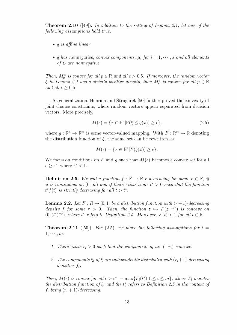
Theorem 2.10 ([49]). In addition to the setting of Lemma 2.1, let one of thefollowing assumptions hold true.

• q is affine linear

• q has nonnegative, convex components, µi for i = 1, · · · , s and all elementsof Σ are nonnegative.

Then, Mαp is convex for all p ∈ R and all ε > 0.5. If moreover, the random vector

ξ in Lemma 2.1 has a strictly positive density, then Mpε is convex for all p ∈ R

and all ε ≥ 0.5.

As generalization, Henrion and Strugarek [50] further proved the convexity ofjoint chance constraints, where random vectors appear separated from decisionvectors. More precisely,

M(ε) = x ∈ Rn|P(ξ ≤ q(x)) ≥ ε , (2.5)

where g : Rn → Rm is some vector-valued mapping. With F : Rm → R denotingthe distribution function of ξ, the same set can be rewritten as

M(ε) = x ∈ Rn|F (q(x)) ≥ ε .

We focus on conditions on F and g such that M(ε) becomes a convex set for allε ≥ ε∗, where ε∗ < 1.

Definition 2.5. We call a function f : R → R r-decreasing for some r ∈ R, ifit is continuous on (0,∞) and if there exists some t∗ > 0 such that the functiontrf(t) is strictly decreasing for all t > t∗.

Lemma 2.2. Let F : R→ [0, 1] be a distribution function with (r+1)-decreasingdensity f for some r > 0. Then, the function z 7→ F (z−1/r) is concave on(0, (t∗)−r), where t∗ refers to Definition 2.5. Moreover, F (t) < 1 for all t ∈ R.

Theorem 2.11 ([50]). For (2.5), we make the following assumptions for i =1, · · · ,m:

1. There exists ri > 0 such that the components gi are (−ri)-concave.

2. The components ξi of ξ are independently distributed with (ri+1)-decreasingdensities fi.

Then, M(ε) is convex for all ε > ε∗ := maxFi(t∗i )|1 ≤ i ≤ m, where Fi denotesthe distribution function of ξi and the t∗i refers to Definition 2.5 in the context offi being (ri + 1)-decreasing.

13

2.2 Reformulations and approximations for chance

constraints

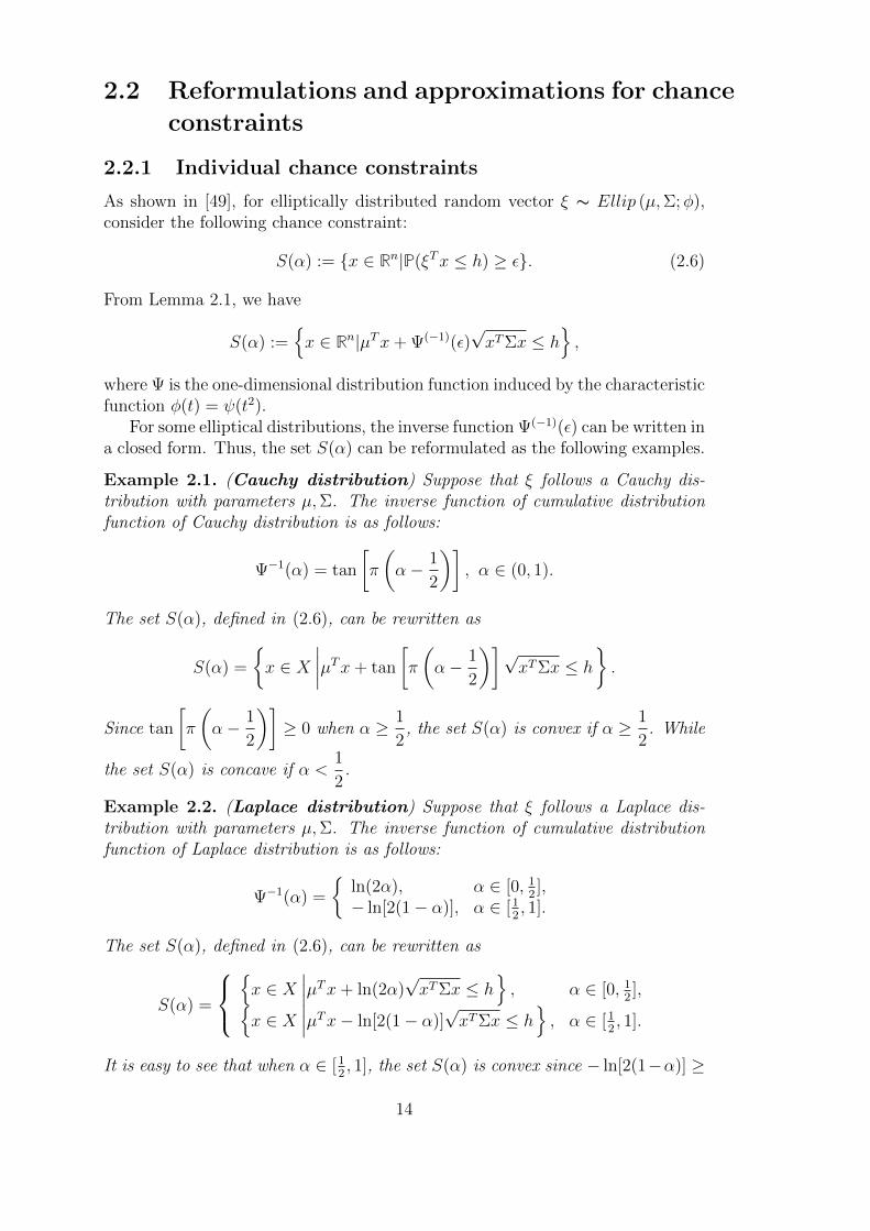
2.2.1 Individual chance constraints

As shown in [49], for elliptically distributed random vector ξ ∼ Ellip (µ,Σ;φ),consider the following chance constraint:

S(α) := x ∈ Rn|P(ξTx ≤ h) ≥ ε. (2.6)

From Lemma 2.1, we have

S(α) :=x ∈ Rn|µTx+ Ψ(−1)(ε)

√xTΣx ≤ h

,

where Ψ is the one-dimensional distribution function induced by the characteristicfunction φ(t) = ψ(t2).

For some elliptical distributions, the inverse function Ψ(−1)(ε) can be written ina closed form. Thus, the set S(α) can be reformulated as the following examples.

Example 2.1. (Cauchy distribution) Suppose that ξ follows a Cauchy dis-tribution with parameters µ,Σ. The inverse function of cumulative distributionfunction of Cauchy distribution is as follows:

Ψ−1(α) = tan

[π

(α− 1

2

)], α ∈ (0, 1).

The set S(α), defined in (2.6), can be rewritten as

S(α) =

x ∈ X

∣∣∣∣µTx+ tan

[π

(α− 1

2

)]√xTΣx ≤ h

.

Since tan

[π

(α− 1

2

)]≥ 0 when α ≥ 1

2, the set S(α) is convex if α ≥ 1

2. While

the set S(α) is concave if α <1

2.

Example 2.2. (Laplace distribution) Suppose that ξ follows a Laplace dis-tribution with parameters µ,Σ. The inverse function of cumulative distributionfunction of Laplace distribution is as follows:

Ψ−1(α) =

ln(2α), α ∈ [0, 1

2],

− ln[2(1− α)], α ∈ [12, 1].

The set S(α), defined in (2.6), can be rewritten as

S(α) =

x ∈ X

∣∣∣µTx+ ln(2α)√xTΣx ≤ h

, α ∈ [0, 1

2],

x ∈ X∣∣∣µTx− ln[2(1− α)]

√xTΣx ≤ h

, α ∈ [1

2, 1].

It is easy to see that when α ∈ [12, 1], the set S(α) is convex since − ln[2(1−α)] ≥

14

0. Otherwise, the set S(α) is concave.

Example 2.3. (Logistic distribution) Suppose that ξ follows a Logistic dis-tribution with parameters µ,Σ. The inverse function of cumulative distributionfunction of Logistic distribution is as follows:

Ψ−1(α) = ln

(α

1− α

), α ∈ (0, 1).

The set S(α), defined in (2.6), can be rewritten as

S(α) =

x ∈ X

∣∣∣∣µTx+ ln

(α

1− α

)√xTΣx ≤ h

.

Since ln

(α

1− α

)≥ 0 when α ≥ 1

2, the set S(α) is convex if α ≥ 1

2. While the

set S(α) is concave if α < 12.

Besides elliptical distributions, Calafiore and El Ghaoui [15] reformulated in-dividual chance constraints under Q-radial distribution.

Definition 2.6. A random vector d ∈ Rn has a Q-radial distribution with definingfunction g(·) if d−Ed = Qω where Q ∈ Rn×ν, ν ≤ n, is a fixed, full-rank matrixand ω ∈ Rν is a random vector with probability density fω that depends only onthe norm of ω; i.e., fω(ω) = g(‖ω‖). The function g(·) that defines the radialshape of the distribution is named the defining function of d.

The family of Q-radial distributions includes all probability densities whoselevel sets are ellipsoids with shape matrix Q 0 and may have any radial behav-ior. Another notable example is the uniform density over an ellipsoidal set.

Theorem 2.12 ([15]). For any α ∈ [0.5, 1), the chance constraint

PξTx ≤ 0 ≥ ε,

where ξ has a Q-radial distribution with defining function g(·) and covariance Γ,is equivalent to the convex second-order cone constraint

κα,r√xTΓx+ ξTx < 0, (2.7)

where κε,r = vΨ−1(α), with v :=(Vν´∞

0rν+1g(r)dr

)−1/2, Vν denotes the volume

of the Euclidean ball of unit radius in Rν, Ψ the cumulative probability functionof density f(ξ) = Sν−1

´∞0g(√ρ2 + ξ2)ρν−2dρ, Sn denotes the surface measure of

the Euclidean ball of unit radius in Rn.

In the case where ξ follows a normal distribution with mean µ and covarianceΓ, which is Q-radial with v = 1, Q = Γf , Γ = ΓfΓ

Tf , the function g(r) is

g(r) =1

(2π)1/2e−

r2

2 .

15

Therefore, for ε ∈ (0, 0.5], the parameter κε,r is given by κε,r = Ψ−1G (1− ε), where

ΨG is the standard normal cumulative distribution function. Hence, (2.7) can berewritten as

Ψ−1G (α)

√xTΓx+ ξTx < 0,

which is convex.

2.2.2 Normally distributed joint linear chance constraints

For joint chance constrained problems, Cheng and Lisser [24] considered the fol-lowing normally distributed linear program with joint chance constraint:

minx

cTx

s.t. PTx ≤ D ≥ ε,x ∈X,

(2.8)

whereX ⊂ Rn+ is polyhedron, c ∈ Rn, D = (D1, · · · , DK) ∈ RK , ε is a prespecifiedconfidence parameter, T = [T1, · · · , TK ]T is a K×n random matrix, where Tk, k =1, · · · , K, is a normally distributed random vector in Rn with mean vector µk =(µk1, · · · , µkn)T and covariance matrix Σk. Moreover, the multivariate normallydistributed vectors Tk, k = 1, · · · , K, are independent.

Then, a deterministic reformulation of (2.8) can be derived as follows:

minx

cTx

s.t. µTkx+ F−1(εyk)‖Σ1/2k x‖ ≤ Dk, k = 1, · · · , K∑K

k=1 yk = 1, yk ≥ 0x ∈X

(2.9)

Because of the nonelementary function F−1(εyk), two piecewise linear approx-imations are applied to F−1(εyk).Piecewise tangent approximation of F−1(εz)

The authors of [24] use the linear tangents asz + bs, s = 1, · · · , S, betweenz1, z2, · · · , zS ∈ (0, 1] to form a piecewise linear function

l(z) = maxs=1,··· ,S

asz + bs ,

whereas = (F−1)′(εzs)εzs ln ε, bi = F−1(εz)− aszs.

Then, (2.9) can be approximated by the following second order cone program-ming:

minx

cTx

s.t. µTkx+ ‖Σ1/2k zk‖ ≤ Dk, k = 1, · · · , K

zk ≥ asxi + bsyki, s = 0, 1, · · · , S, i = 1, · · · , n∑Kk=1 yki = xi, yki ≥ 0, i = 1, · · · , n

x ∈X,

(2.10)

where a0 = 0, b0 = 0. Additionally, the optimal value of problem (2.10) is a lower

16

bound of problem (2.9).

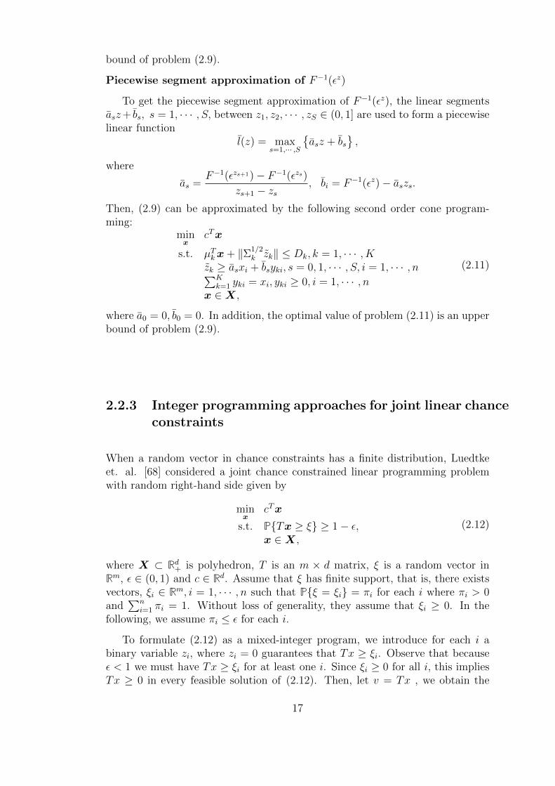
Piecewise segment approximation of F−1(εz)

To get the piecewise segment approximation of F−1(εz), the linear segmentsasz+ bs, s = 1, · · · , S, between z1, z2, · · · , zS ∈ (0, 1] are used to form a piecewiselinear function

l(z) = maxs=1,··· ,S

asz + bs

,

where

as =F−1(εzs+1)− F−1(εzs)

zs+1 − zs, bi = F−1(εz)− aszs.

Then, (2.9) can be approximated by the following second order cone program-ming:

minx

cTx

s.t. µTkx+ ‖Σ1/2k zk‖ ≤ Dk, k = 1, · · · , K

zk ≥ asxi + bsyki, s = 0, 1, · · · , S, i = 1, · · · , n∑Kk=1 yki = xi, yki ≥ 0, i = 1, · · · , n

x ∈X,

(2.11)

where a0 = 0, b0 = 0. In addition, the optimal value of problem (2.11) is an upperbound of problem (2.9).

2.2.3 Integer programming approaches for joint linear chanceconstraints

When a random vector in chance constraints has a finite distribution, Luedtkeet. al. [68] considered a joint chance constrained linear programming problemwith random right-hand side given by

minx

cTx

s.t. PTx ≥ ξ ≥ 1− ε,x ∈X,

(2.12)

where X ⊂ Rd+ is polyhedron, T is an m × d matrix, ξ is a random vector inRm, ε ∈ (0, 1) and c ∈ Rd. Assume that ξ has finite support, that is, there existsvectors, ξi ∈ Rm, i = 1, · · · , n such that Pξ = ξi = πi for each i where πi > 0and

∑ni=1 πi = 1. Without loss of generality, they assume that ξi ≥ 0. In the

following, we assume πi ≤ ε for each i.

To formulate (2.12) as a mixed-integer program, we introduce for each i abinary variable zi, where zi = 0 guarantees that Tx ≥ ξi. Observe that becauseε < 1 we must have Tx ≥ ξi for at least one i. Since ξi ≥ 0 for all i, this impliesTx ≥ 0 in every feasible solution of (2.12). Then, let v = Tx , we obtain the

17

MIP formulation of (2.12):

minx

cTx

s.t. x ∈X, Tx− v = 0v + ξizi ≥ ξi, i = 1, · · · , n∑n

i=1 πizi ≤ εz ∈ 0, 1n

(2.13)

The assumption of finite distribution may seem restrictive. However, if thepossible values for ξ are generated through Monte Carlo sampling from a generaldistribution, the resulting problem can be viewed as an approximation of a prob-lem with general distribution. There is theoretical and empirical evidence whichdemonstrates that such a sample approximation can indeed be used to approx-imately solve problems with continuous distribution. A standard result will beintroduced in subsection 2.2.5.

2.2.4 Convex approximations for chance constraints

An alternative to the above approaches consists in providing tractable convexapproximations for chance constraints. Nemirovski and Shapiro [76] studied thefollowing optimization problem:

minx∈X

f(x) subject to PF (x, ξ) ≤ 0 ≥ 1− ε. (2.14)

Here ξ is a random vector with probability distribution P supported on a setΞ ⊂ Rd, X ⊂ Rn is a nonempty convex set, ε ∈ (0, 1), f : Rn → R is a real valuedconvex function, F = (f1, · · · , fm) : Rn × Ξ→ Rm, and P(A) denotes probabilityof an event A.

The chance constraint of problem (2.14) is equivalent to the constraint

p(x) := PF (x, ξ) > 0 ≤ ε.

Let 1A denotes the indicator function of a set A, i.e., 1A(z) = 1 if z ∈ A and1A(z) = 0 if z /∈ A.

Let ψ : R → R be a nonnegative valued, nondecreasing, convex functionsatisfying the following property:

ψ(z) > ψ(0) = 1 for any z > 0.

We refer to function f(z) which satisfies the above properties as a (one-dimensional)generating function. It follows from the property that for t > 0 and random vari-able Z,

E[ψ(tZ)] ≥ E[1[0,+∞)(tZ)] = PtZ ≥ 0 = PZ ≥ 0.

By taking Z = F (x, ξ) and changing t to t−1, we have

p(x) ≤ E[ψ(t−1F (x, ξ))] (2.15)

18

for all x and t > 0. Let

Ψ(x, t) = tE[ψ(t−1F (x, ξ))].

Then, we have

inft>0

[Ψ(x, t)− tε] ≤ 0 implies p(x) ≤ ε

Therefore, we obtain, under the assumption that X, f(·) and F (·, ξ) are convex,that

minx∈X

f(x) subject to inft>0

[Ψ(x, t)− tε] ≤ 0 (2.16)

gives a convex conservative approximation of the chance constrained problem(2.14).

Since ψ(0) = 1 and ψ(·) is convex and nonnegative, we conclude that ψ(z) ≥max1 + az, 0 for all z, so that the upper bounds (2.15) can be only improvedwhen replacing ψ(z) with the function ψ(z) := max1 + az, 0, which is also agenerating function. But the bounds produced by the latter function are, up toscaling z ← z/a, the same as those produced by the function

ψ∗(z) := [1 + z]+, (2.17)

where [a]+ := maxa, 0. That is, from the point of view of the most accurateapproximation, the best choice of the generating function ψ is the piecewise linearfunction ψ∗ defined in (2.17). For the generating function ψ∗ defined in (2.17),the approximate constraint in problem (2.16) takes the form

inft>0

[E[[F (x, ξ) + t]+

]− tε

]≤ 0. (2.18)

Replacing in the left-hand side inft>0

with inft

, we clearly do not affect the validity

of the relation; thus, we can equivalently rewrite (2.18) as

inft∈R

[E[−tε+ [F (x, ξ) + t]+

]]≤ 0.

In that form, the constraint is related to the definition of conditional value atrisk (CVaR) Then, the constraint

CVaR1−ε[F (x, ξ)] ≤ 0.

defines a convex conservative approximation of the chance constraint in problem(2.14).

2.2.5 Sample average approximations for chance constraints

Besides the above approaches for chance constraints, the sample average approx-imation (SAA) method is also a computationally tractable approximation forchance constrained problems.

19

In [96], the authors considered a chance constrained problem of the form

minx∈X

f(x) s.t. p(x) ≤ ε, (2.19)

where X ⊂ Rn is a closed set, f : Rn → R is a continuous function, ε ∈ (0, 1)is a given tolerance level, and p(x) = PC(x, ξ) > 0. We assume that ξ is arandom vector, whose probability distribution P is supported on set Ξ ∈ Rd, andthe function C : Rn → R is a Caratheodory function.

For the sake of simplicity, we assume that the objective function f(x) is givenexplicitly and only the chance constraints should be approximated. We can writethe probability p(x) with the expectation form,

p(x) = E[1(0,∞)(C(x, ξ))],

and estimate this probability by the corresponding SAA function

p(x) =1

N

N∑j=1

1(0,∞)

(C(x, ξj)

).

Consequently we can write the corresponding SAA problem as

minx∈X

f(x) s.t. pN(x) ≤ ε. (2.20)

Denote ϑ∗ and S the optimal value and the optimal solution set of problem(2.19), respectively, and ϑN and SN the optimal value and the optimal solution setof problem (2.20), respectively Then, we have the following consistency propertiesof the optimal value ϑN and the set SN of optimal solutions of the SAA problem(2.20).

Theorem 2.13 ([96]). Suppose that X is a compact set, the function f(x) iscontinuous, C(x, ξ) is a Caratheodory function, the samples are iid, and the fol-lowing condition holds: (a) there exists an optimal solution x to the true problemsuch that for any δ > 0, there exists an x ∈ X with ‖x − x‖ ≤ δ and p(x) < ε.

Then ϑN → ϑ∗ and D(SN , S

)→ 0 w.p.1 as N →∞.

2.3 Distributionally robust chance constraints

Since in many practical situations, one can only obtain the partial informationabout probability distributions. Replacing the real distribution by an estimatedone, we may obtain an infeasible solution in practice with high probability. There-fore, the distributionally robust chance constrained approaches are proposed.

2.3.1 Distributionally robust individual chance constraintswith known mean and covariance

With given mean and covariance, Calafiore and El Ghaoui [15] studied a distri-butionally robust individual chance constrained problem where the family P of

20

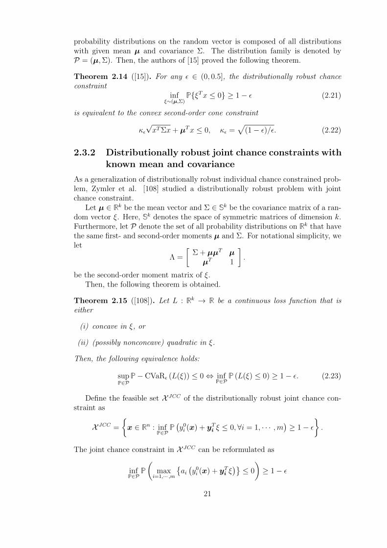
probability distributions on the random vector is composed of all distributionswith given mean µ and covariance Σ. The distribution family is denoted byP = (µ,Σ). Then, the authors of [15] proved the following theorem.

Theorem 2.14 ([15]). For any ε ∈ (0, 0.5], the distributionally robust chanceconstraint

infξ∼(µ,Σ)

PξTx ≤ 0 ≥ 1− ε (2.21)

is equivalent to the convex second-order cone constraint

κε√xTΣx+ µTx ≤ 0, κε =

√(1− ε)/ε. (2.22)

2.3.2 Distributionally robust joint chance constraints withknown mean and covariance

As a generalization of distributionally robust individual chance constrained prob-lem, Zymler et al. [108] studied a distributionally robust problem with jointchance constraint.

Let µ ∈ Rk be the mean vector and Σ ∈ Sk be the covariance matrix of a ran-dom vector ξ. Here, Sk denotes the space of symmetric matrices of dimension k.Furthermore, let P denote the set of all probability distributions on Rk that havethe same first- and second-order moments µ and Σ. For notational simplicity, welet

Λ =

[Σ + µµT µµT 1

].

be the second-order moment matrix of ξ.Then, the following theorem is obtained.

Theorem 2.15 ([108]). Let L : Rk → R be a continuous loss function that iseither

(i) concave in ξ, or

(ii) (possibly nonconcave) quadratic in ξ.

Then, the following equivalence holds:

supP∈P

P− CVaRε (L(ξ)) ≤ 0⇔ infP∈P

P (L(ξ) ≤ 0) ≥ 1− ε. (2.23)

Define the feasible set X JCC of the distributionally robust joint chance con-straint as

X JCC =

x ∈ Rn : inf

P∈PP(y0i (x) + yTi ξ ≤ 0,∀i = 1, · · · ,m

)≥ 1− ε

.

The joint chance constraint in X JCC can be reformulated as

infP∈P

P

(max

i=1,··· ,m

ai(y0i (x) + yTi ξ

)≤ 0

)≥ 1− ε

21

for any vector of strictly positive scaling parameters a ∈ A = a ∈ Rm : a > 0.Thus, for any a ∈ A, the requirement

x ∈ ZJCC(a) =

x ∈ Rn : sup

P∈PCVaRα

(max

i=1,··· ,m

ai(y0i (x) + yTi ξ

))≤ 0

implies x ∈ X JCC .

Then, it can be shown that ZJCC(a) provide a convex approximation for X JCC

with an exact tractable representation in terms of linear matrix inequalities.

Theorem 2.16 ([108]). For any fixed x ∈ Rn and a ∈ A, we have

ZJCC(a) =

x ∈ Rn :

∃(β,M) ∈ R× Sk+1,β + 1

ε〈Λ,M〉 ≤ 0,M 0,

M −[

0 12aiyi(x)

12aiy

Ti (x) aiy

0i (x)− β

] 0,∀i = 1, · · · ,m

.

2.3.3 Distributionally robust joint chance constraints withuncertain mean and covariance

In practice, the models’ parameters, such as mean and covariance, themselves areunknown and can only be estimated from data. For this case, distributionally ro-bust optimization problem with uncertain mean and covariance was first proposedand studied by Delage and Ye [27], and was also investigated for distributionallyrobust chance constrained problem by Cheng et al. [21].

In [21], the authors’ interest lies in solving a distributionally robust knapsackproblem with chance constraint:

(DRSKP ) maxx

infF∈D

EF [u(xT Rx)]

s.t. infF∈D

PF(wTj x ≤ dj ∀j ∈ 1, 2, · · · ,M

)≥ 1− ε, (2.24)

xi ∈ 0, 1 ∀i ∈ 1, 2, · · · , n, (2.25)

where u(·) is some concave utility function that captures risk aversion with respectto the total achieved reward. x is a vector of binary values indicating whethereach item is included in the knapsack. R ∈ Rn×n is a random matrix whose(i, j)th term describes the linear contribution to reward of holding both items iand j. wj ∈ Rn is a random vector of attributes whose total amount must satisfysome capacity constraint dj.

Distributionally robust one-dimensional knapsack problem

In this case, we have M = 1. To ensure that the approximation model obtainedcan be solved efficiently, a few assumptions are made.

Definition 2.7. Let ξ be a random vector in Rm on which R and w depend

22

linearly:

R =n∑i=1

ARξi, w = Awξ.

Assumption 2.1. The utility function u(·) is piecewise linear, increasing andconcave. In other words, it can be represented in the form

u(y) = mink∈1,2,··· ,K

aky + bk,

where a ∈ RK and a ≥ 0.

Assumption 2.2. The distributional uncertainty set accounts for informationabout the convex support §, mean µ in the strict interior of §, and an upperbound Σ 0 on the covariance matrix of the random vector ξ:

D (§, µ,Σ) =

F∣∣∣∣∣∣∣P (ξ ∈ §) = 1

EF [ξ] = µ

EF[(ξ − µ)(ξ − µ)T

] Σ

.

Theorem 2.17 ([21]). Under Assumptions 2.1 and 2.2, M = 1 and given that thesupport of F is ellipsoidal, § =

ξ|(ξ − ξ0)TΘ(ξ − ξ0) ≤ 1

, problem (DRSKP )

reduces to the following problem

maxx,t,q,Q,v,s,t,q,Q,s

t− µTq −(Σ + µµT

)•Q

s.t.

[Q q+akv

2qT+akv

T

2bk − t

] −sk

[Θ −Θξ0

−ξT0 Θ ξT0 Θξ0 − 1

]∀k,

vj = ARj • (xxT ) ∀j ∈ 1, 2, · · · ,m,t+ 2µT q + (Σ + µµT ) • Q ≤ εs1,[Q qqT t

] −s2

[Θ −Θξ0

−ξT0 Θ ξT0 Θξ0 − 1

],[

Q q −AwTx

(q −AwTx)T t+ 2d− s1

] −s3

[Θ −Θξ0

−ξT0 Θ ξT0 Θξ0 − 1

],

Q 0, Q 0, s ≥ 0, s ≥ 0,

xi ∈ 0, 1 ∀i ∈ 1, 2, · · · , n.

Alternatively, if the support of F is polyhedral, i.e., § = ξ|Cξ ≤ c with C ∈Rp×m and c ∈ Rp, then problem (DRSKP ) reduces to

maxx,t,q,Q,v,s,t,q,Qλ1,λ2,··· ,λK+2

t− µTq −(Σ + µµT

)•Q

s.t.

[Q q+akv+CTλk

2qT+akv

T+λTkC

2bk − t− cTλk

] 0 ∀k ∈ 1, 2, · · · , K,

23

vj = ARj • (xxT ) ∀j ∈ 1, 2, · · · ,m,t+ 2µT q + (Σ + µµT ) • Q ≤ s,[

Q q + 12CTλK+1

qT + 12λTK+1C t− cTλK+1

] 0,[

Q q −AwTx+ 12CTλK+2

(q −AwTx)T + 12λTK+2C t+ 2d− s− cTλK+2

] 0,

Q 0, Q 0, s ≥ 0, λk ≥ 0,∀k ∈ 1, 2, · · · , K + 2,xi ∈ 0, 1 ∀i ∈ 1, 2, · · · , n,

where λk ∈ Rp for all k are the dual variables associated with the linear inequal-ities Cξ ≤ c for each infinite set of constraints. Finally, if the support of F isunbounded (i.e., § = Rm), then problem (DRSKP ) reduces to

maxx,t,q,Q,v,s,z,τ

t− µTq −(Σ + µµT

)•Q

s.t.

[Q q+akv

2qT+akv

T

2bk − t

] 0 ∀k = 1, 2, · · · , K,

vj = ARj • (xxT ) ∀j ∈ 1, 2, · · · ,m,Q 0, τk ≥ 0 ∀k = 1, 2, · · · , K,[

0 Σ1/2zzTΣ1/2 0

]√

ε

1− ε(µTz − d)I,

z = AwTx,

xi ∈ 0, 1 ∀i ∈ 1, 2, · · · , n.

Distributionally robust multidimensional knapsack problem

In this case, we consider problem (DRSKP ) with M > 1, where F now describesthe joint distribution of all types of “weights” of all items, wjMj=1 ∼ F , and Dnow describes a set of such joint distributions.

Definition 2.8. Without loss of generality, for all j = 1, · · · ,M , let ξj be arandom vector in Rm on which the wj depend linearly and let R depend linearlyon ξjMj=1:

R =M∑j=1

m∑i=1

ARji(ξj)i, wj = A

wjj ξj, j = 1, · · · ,M.

Assumption 2.3. The distributional uncertainty set accounts for informationabout the mean µj, and an upper bound Σj on the covariance matrix of the randomvector ξj, for each j = 1, · · · ,M :

D (µj,Σj) =

Fj

∣∣∣∣∣EFj [ξj] = µj

EFj[(ξj − µj)(ξj − µj)T

] Σj

.

24

Furthermore, the random vectors ξi and ξj are independent when i 6= j. Notethat the support of Fj is unbounded, i.e., § = Rm.

Theorem 2.18 ([21]). Under Assumptions 2.2 and 2.3, the following problem isa conservative approximation of problem (DRSKP ):

maxx,t,q,Q,v,y

t− µTq −(Σ + µµT

)•Q

s.t.

[Q q+akv

2qT+akv

T

2bk − t

] 0 ∀k = 1, 2, · · · , K,

v(j−1)M+i = ARji • (xxT ) ∀j ∈ 1, 2, · · · ,M∀i ∈ 1, 2, · · · ,m,Q 0,

µTj Awjx+

√pyj

1− pyj‖Σ1/2

j AwjTx‖2 ≤ d2,

M∑j=1

yj = 1, yj ≥ 0,

xi ∈ 0, 1 ∀i ∈ 1, 2, · · · , n,

where p = 1− ε, q,v ∈ RmM , and Q ∈ RmM×mM , and with

µ :=

µ1

µ2...µM

and Σ =

Σ1 0m,m 0m,m · · · 0m,m

0m,m Σ2 0m,m · · · 0m,m0m,m 0m,m Σ3 · · · 0m,m

......

.... . .

...0m,m 0m,m 0m,m · · · ΣM

.

Furthermore, this approximation is exact when u(·) is linear, i.e. the attitude isrisk neutral.

2.3.4 Distributionally robust chance constrained problembased on φ-divergence

An alternative to moments based uncertainty set of probability distributions isthe distance based uncertainty set. Jiang and Guan [57] applied φ-divergence toconstruct the uncertainty set of probability distributions. Then, they consideredthe following distributionally robust chance constrained problem:

minx

ψ(x)

s.t. infP∈Dφ

PC(x, ξ) ≥ 1− ε,

x ∈X,

(2.26)

where ψ : Rn → R represents a convex function, X ⊂ Rn represents a tractablebounded convex set, ξ ∈ RK is a random vector defined on a probability space(Ω,F ,P), ε ∈ (0, 1). Dφ is the uncertainty set based on φ-divergence, which is

25

defined as follows:

Dφ = P ∈M+ : Dφ(f ||f0) ≤ d, f = dP/dξ.

Here, M+ represents the set of all probability distributions and the divergencetolerance d can be chosen by the decision makers to represent their risk-aversionlevel or can be obtained from statistical inference. Dφ(f ||f0) is the φ-divergencedefined as

Dφ(f ||f0) =

ˆΩ

φ

(f(ξ)

f0(ξ)

)f0(ξ)dξ,

where f and f0 denote the true density function and its estimate respectively,and φ : R→ R is a convex function on R+ such that

1. φ(1) = 0,

2. 0φ(x/0) :=

x limp→+∞ φ(p)/p if x > 0,0 if x = 0,

3. φ(x) = +∞ for x < 0.

Definition 2.9. Let φ : R → R be a convex function such that φ(1) = 0 andφ(x) = +∞ for x < 0. Define m(φ∗) := supm ∈ R : φ∗ is a finite constant on(−∞,m] and m(φ∗) := infm ∈ R : φ∗(m) = +∞.

Theorem 2.19 ([57]). Let P0 represent the probability distribution defined by f0.Then the

infP∈Dφ

PC(x, ξ) ≥ 1− ε (2.27)

is equivalent toP0C(x, ξ) ≥ 1− ε′+, (2.28)

where

ε′ = 1− infz>0,z0+πz<lφ,

m(φ∗)≤z0+z≤m(φ∗)

φ∗(z0 + z)− z0 − εz + d

φ∗(z0 + z)− φ∗(z0)

,

ε+ = maxε, 0 for ε ∈ R, φ∗ is the conjugate function of φ, lφ = limx→+∞ φ(x)/x,and

π =

−∞ if Leb[f0 = 0] = 0,0 if Leb[f0 = 0] > 0 and Leb[f0 = 0] \ C(x, ξ) = 0,1 otherwise,

Leb· represents the Lebesgue measure and [f0 = 0] := ξ ∈ Ω : f0(ξ) = 0.

By applying different φ-divergences in Theorem 2.19, the following propositioncan be obtained.

Proposition 2.1 ([57]). 1. Suppose that Dφ is constructed by using the χ di-vergence of order 2 with φ(x) = (x− 1)2 and ε < 1/2. Then

ε′ = ε−√d2 + 4dε(1− ε)− (1− 2ε)d

2d+ 2,

26

2. Suppose that Dφ is constructed by using the variation distance with φ(x) =|x− 1|. Then

ε′ = ε− d

2,

3. Suppose that Dφ is constructed by using the KL divergence with φ(x) =x log x− x+ 1. Then

ε′ = 1− infx∈(0,1)

e−dx1−ε − 1

x− 1

.

2.3.5 Distributionally robust chance constrained problembased on Wasserstein distance

Besides φ-divergence based uncertainty set, Wasserstein distance based uncer-tainty set is another popular distance based uncertainty set. Wasserstein distanceis a natural way of comparing two distributions when one is obtained from theother by perturbations.

The type-1 Wasserstein distance dW (P1,P2) between two distributions P1 andP2 on RK , equipped with a general norm ‖ · ‖, is defined as the minimal trans-portation cost of redistributing mass from P1 to P2 in terms that the cost ofmoving a Dirac point mass from ξ1 to ξ2 is ‖ξ1 − ξ2‖. Mathematically,

dW (P1,P2) = infP∈(P1,P2)

EP[‖ξ1 − ξ2‖],

where ξ1 ∼ P1, ξ2 ∼ P2, and (P1,P2) represents the set of all distributions onRK × RK with marginals P1 and P2. The Wasserstein ambiguity set F (θ) is thendefined as a ball of radius θ ≥ 0 with respect to the Wasserstein distance, centeredat a prescribed reference distribution P:

F(θ) = P ∈ P(RK)|dW (P, P) ≤ θ.

If only a finite training dataset ξii∈[N ] is available, a natural choice for P is the

empirical distribution P = 1N

∑Ni=1 δξi , which represents the uniform distribution

on the training samples.

Assume that P is the empirical distribution as above, Chen et al. [19] studydistributionally robust chance constrained programs of the form

(DRCCW ) minx∈X

cTx

s.t. P[ξ ∈ S(x)] ≥ 1− ε ∀P ∈ F(θ),

where the goal is to find a decision x from within a compact polyhedron X ∈RL that minimizes a linear cost function cTx and ensures that the exogenousrandom vector ξ falls within a decision-dependent safety set S(x) ⊂ RK withhigh probability 1− ε under every distribution P ∈ F(θ).

27

Theorem 2.20 ([19]). The chance constrained program (DRCCW ) is equivalentto

mins,t,x

cTx

s.t. εNt− eTs ≥ θN

dist(ξi, S(x)) ≥ t− si ∀i ∈ [N ]

s ≥ 0, x ∈ X ,

where 0 and e respectively correspond to the zero vector and the vector of allones, [N ] = 1, 2, · · · , N represents the set of all integers up to N , dist(ξi, S(x))denotes the distance of ξi to the set S(x), and S(x) denotes the closed complementof S(x).

With Theorem 2.20, the following corollaries can be obtained.

Corollary 2.1 ([19]). Given A ∈ RL×K ,a ∈ RL, b ∈ RK , b ∈ R. Assume thatATx 6= b for all x ∈ X . For the safety set S(x) = ξ ∈ RK |(Aξ + a)Tx ≤bTξ + b, problem (DRCCW ) is equivalent to the mixed integer conic program

minq,s,t,x

cTx

s.t. εNt− eTs ≥ θN‖b−ATx‖∗(b−ATx)T ξi + b− aTx+Mqi ≥ t− si ∀i ∈ [N ]

M(1− qi) ≥ t− si ∀i ∈ [N ]

q ∈ 0, 1N , s ≥ 0, x ∈ X ,

where ‖ · ‖∗ denotes the dual norm of a general norm ‖ · ‖ and M is a suitablylarge (but finite) positive constant.

Corollary 2.2 ([19]). Given am ∈ RL, bm ∈ RK , bm ∈ R,m ∈ [M ]. For thesafety set S(x) = ξ ∈ RK |aTmx < bTmξ + bm ∀m ∈ [M ], where b 6= 0 for allm ∈ [M ], the chance constrained problem (DRCCW ) is equivalent to the mixedinteger conic program

minp,q,s,t,x

cTx

s.t. εNt− eTs ≥ θN

pi +Mqi ≥ t− si ∀i ∈ [N ]

M(1− qi) ≥ t− si ∀i ∈ [N ]

bTmξi + bm − aTmx‖bm‖∗

≥ pi ∀m ∈ [M ], ∀i ∈ [N ]

q ∈ 0, 1N , s ≥ 0, x ∈ X ,

where M is a suitably large (but finite) positive constant.

28

2.4 Conclusion

In this chapter, we introduce some standard results of chance constrained prob-lems covering convexity, reformulation/approximation approaches for chance con-straints and distributionally robust chance constraints. These results have impor-tant influences on development of chance constrained problems. As this kind ofproblems are widely applied in many practical areas, such as finance, energy prob-lems, water resources, telecommunication, production and inventory, the theoryand application of chance constrained problems are still important issues whichattract a lot of attentions from different researchers.

29

30

Chapter 3

Geometric Chance ConstrainedPrograms

In this chapter, we first review a work of Liu et al. [65] about geometric programswith joint chance constraints, where the stochastic parameters are normally dis-tributed and independent of each other. Then, we extend the work in [65] anddiscuss joint rectangular geometric chance constrained programs with ellipticaldistribution.

3.1 Stochastic geometric optimization with joint

chance constraints

In this section, we review the work of Liu et al. [65] about geometric programswith joint chance constraints. When the stochastic parameters are normallydistributed and independent of each other, the problem is approximated by usingpiecewise linear functions, and the approximation problem is transformed into aconvex geometric program. The authors proved that this approximation methodprovides a lower bound and designed an algorithm under the sequential convexoptimization scheme to find an upper bound. Finally, numerical tests are carriedout with a stochastic shape optimization problem.

3.1.1 Introduction

Geometric programming is an important topic in operations research where theobjective function and the constraints of the corresponding optimization prob-lems have a special form. Geometric optimization has been studied for severaldecades, it was introduced by Duffin et al. in the late 1960s [30]. Applicationsof geometric programming can be found in several surveys papers, namely Boydset al. [10], Ecker [33] and Peterson [83]. A numerous practical problems can beformulated as geometric programs, e.g., electrical circuit design problems [10], in-formation theory [26], queue proportional scheduling in fading broadcast channels[95], mechanical engineering problems [101], economic and managerial problems[69], nonlinear network problems [60]. A geometric program can be formulated

31

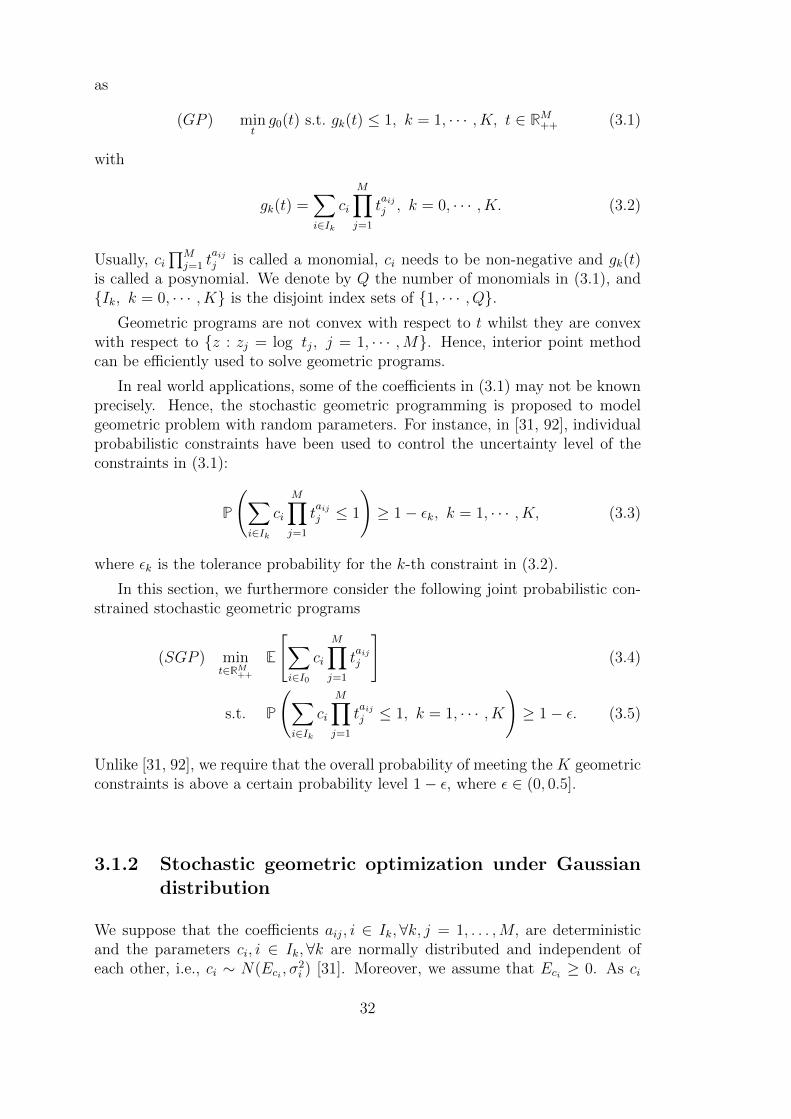
as

(GP ) mintg0(t) s.t. gk(t) ≤ 1, k = 1, · · · , K, t ∈ RM++ (3.1)

with

gk(t) =∑i∈Ik

ci

M∏j=1

taijj , k = 0, · · · , K. (3.2)

Usually, ci∏M

j=1 taijj is called a monomial, ci needs to be non-negative and gk(t)

is called a posynomial. We denote by Q the number of monomials in (3.1), andIk, k = 0, · · · , K is the disjoint index sets of 1, · · · , Q.

Geometric programs are not convex with respect to t whilst they are convexwith respect to z : zj = log tj, j = 1, · · · ,M. Hence, interior point methodcan be efficiently used to solve geometric programs.

In real world applications, some of the coefficients in (3.1) may not be knownprecisely. Hence, the stochastic geometric programming is proposed to modelgeometric problem with random parameters. For instance, in [31, 92], individualprobabilistic constraints have been used to control the uncertainty level of theconstraints in (3.1):

P

(∑i∈Ik

ci

M∏j=1

taijj ≤ 1

)≥ 1− εk, k = 1, · · · , K, (3.3)

where εk is the tolerance probability for the k-th constraint in (3.2).

In this section, we furthermore consider the following joint probabilistic con-strained stochastic geometric programs

(SGP ) mint∈RM++

E

[∑i∈I0

ci

M∏j=1

taijj

](3.4)

s.t. P

(∑i∈Ik

ci

M∏j=1

taijj ≤ 1, k = 1, · · · , K

)≥ 1− ε. (3.5)

Unlike [31, 92], we require that the overall probability of meeting the K geometricconstraints is above a certain probability level 1− ε, where ε ∈ (0, 0.5].

3.1.2 Stochastic geometric optimization under Gaussiandistribution

We suppose that the coefficients aij, i ∈ Ik,∀k, j = 1, . . . ,M, are deterministicand the parameters ci, i ∈ Ik,∀k are normally distributed and independent ofeach other, i.e., ci ∼ N(Eci , σ

2i ) [31]. Moreover, we assume that Eci ≥ 0. As ci

32

are independent of each other, constraint (3.5) is equivalent to

K∏k=1

P

(∑i∈Ik

ci

M∏j=1

taijj ≤ 1

)≥ 1− ε. (3.6)

By introducing auxiliary variables yk ∈ R+, k = 1, · · · , K, (3.6) can be equiva-lently transformed into

P(∑

i∈Ik ci∏M

j=1 taijj ≤ 1) ≥ yk, k = 1, · · · , K, (3.7)

and

K∏k=1

yk ≥ 1− ε, 1 ≥ yk ≥ 0, k = 1, · · · , K. (3.8)

It is easy to see that for independent normally distributed ci ∼ N(Eci , σ2i )

[31], constraint (3.7) is equivalent to

∑i∈Ik Eci

M∏j=1

taijj + Φ−1(yk)

√∑i∈Ik σ

2i

M∏j=1

t2aijj ≤ 1, k = 1, · · · , K. (3.9)

Here, Φ−1(yk) is the quantile of the standard normal distribution N(0, 1). How-ever, biconvex inequalities (3.9) are still very hard to solve within an optimizationproblem [41].

Standard variable transformation

The standard variable transformation rj = log(tj), j = 1, · · · ,M and xk =log(yk), k = 1, · · · , K applied to (3.8) and (3.9) leads to the following constraints:

∑i∈Ik

Eci exp

M∑j=1

aijrj

+

√√√√∑i∈Ik

σ2i exp

M∑j=1

(2aijrj + log(Φ−1(exk)2))

≤ 1, k = 1, · · · , K, (3.10)

K∑k=1

xk ≥ log(1− ε), xk ≤ 0, k = 1, · · · , K. (3.11)

Φ−1(·) is also called the probit function and can be expressed in terms of theinverse error function:

Φ−1(yk) =√

2 erf−1(2yk − 1), yk ∈ (0, 1).

The inverse error function is a nonelementary function which can be repre-sented by the Maclaurin series:

erf−1(z) =∞∑p=0

λp2p+ 1

(√π

2z

)2p+1

,

33

where λ0 = 1 and λp =∑p−1

i=0λiλp−1−i

(i+1)(2i+1)> 0, p = 1, 2, · · · . Thus, we know that

Φ−1(yk) is convex for 1 > yk ≥ 0.5, and concave for 0 > yk ≤ 0.5. Moreover,Φ−1(yk) is always monotonic increasing.

Under constraint (3.11), we have 0.5 ≤ 1 − ε ≤ yk = exk < 1. Hence, wecan only focus on the right tail part of Φ−1(exk). This means the feasible setconstrained by both (3.10) and (3.11) is convex. However, as Φ−1(·) is nonele-mentary, we still need to approximate it for practical use. Unlike the approxi-mation method in [21], we approximate log(Φ−1(exk)2) rather than Φ−1(yk) by apiecewise linear function.

Approximation of log(Φ−1(exk)2)

We choose S different linear functions:

Fs(xk) = dsxk + bs, s = 1, · · · , S,

such that

Fs(xk) ≤ log(Φ−1(exk)2), ∀xk ∈ [log(1− ε), 0), s = 1, · · · , S. (3.12)

log(Φ−1(exk)2) is then approximated by a piecewise linear function

F (xk) = maxs=1,··· ,S

Fs(xk). (3.13)

Constraints (3.12) and (3.13) guarantee that F (xk) provides a lower bound oflog(Φ−1(exk)2).

For a practical use, we can choose the tangent lines of log(Φ−1(exk)2) at dif-ferent points in [log(1− ε), 0), say ξ1, ξ2, · · · , ξS. Then, we have

ds =2eξs(Φ−1)(1)(eξs)

Φ−1(eξs)(3.14)

and

bs = −dsξs + log(Φ−1(eξs)2), s = 1, · · · , S. (3.15)

Remark 3.1. By changing the variables into yk, we can see that the piecewiselinear approximation of log(Φ−1(exk)2) with respect to xk is equivalent to the piece-

wise power function approximation maxs=1,··· ,S

ebs2 y

ds2k for Φ−1(yk).

Convex geometric approximation

After obtaining the piecewise linear approximation of log(Φ−1(exk)2), we can re-place log(Φ−1(exk)2) by F (xk) in (3.13).

Theorem 3.1. Using the piecewise linear function F (xk), we have the followingconvex approximation of the stochastic geometric program with a joint probabilistic

34

constraint (SGP ):

(SGPA) minr∈RM ,x∈RK

∑i∈I0

Eci exp

M∑j=1

aijrj

(3.16)

∑i∈Ik

Eci exp

M∑j=1

aijrj

+

√√√√∑i∈Ik

σ2i exp

M∑j=1

(2aijrj + dsxk + bs)

≤ 1, s = 1, · · · , S, k = 1, · · · , K, (3.17)

K∑k=1

xk ≥ log(1− ε), xk ≤ 0, k = 1, · · · , K. (3.18)

The optimal value of the approximation problem (3.16)-(3.18) is a lower boundof problem (GP ). Moreover, when S goes to infinity, (SGPA) is a reformulationof problem (SGP ).

We call this approximation a piecewise linear approximation. As problem(SGPA) is convex, it can be solved efficiently by interior point methods.

Proof. From (3.7) and (3.8), we know that 0 ≤ yk ≤ 1. Moreover, we havefrom (3.8) that for any k, yk ≥

∏Kk=1 yk ≥ 1 − ε ≥ 0.5 and hence xk ≥ log(1 −

ε) ≥ log(0.5). Then, from the convexity of log(Φ−1(exk)2) with respect to xk in[log(1− ε), 0), we have

log(Φ−1(exk)2) ≥ dsxk + bs, ∀xk ∈ [log(1− ε), 0), s = 1, · · · , S. (3.19)

where ds and bs are defined in (3.14) and (3.15). As yk = exk , (3.19) is equivalentto

Φ−1(yk) ≥ ebs2 y

ds2k , ∀yk ∈ [1− ε, 1), s = 1, · · · , S. (3.20)

Furthermore, constraint (3.17) is equivalent to

∑i∈Ik

Eci

M∏j=1

taijj +

(max

s=1,··· ,Sebs2 y

ds2k

)√√√√∑i∈Ik

σ2i

M∏j=1

t2aijj ≤ 1, k = 1, · · · , K. (3.21)

As ebs2 y

ds2k ≤ Φ−1(yk), ∀s, any feasible solution for (3.9) is feasible for (3.17)

or (3.21). From the equivalence between (3.5) and (3.9) under the Guassiandistribution assumption, the optimal solution of (SGP ) is feasible for (SGPA).This means that the approximation problem (SGPA) provides a lower bound forthe original problem (SGP ).

Moreover, the S tangent functions in (3.19) are chosen differently and forxk ∈ ξ1, · · · , ξS, log(Φ−1(exk)2) = dsxk + bs. Hence, when S goes to infinity,inequality (3.19) becomes tight. Furthermore, from the biconvexity of (3.9) and(3.21), we know the distance between the sets constrained by (3.9) and (3.21) issmall enough when S goes to infinity. As the objective functions of (SGP ) and

35

(SGPA) are the same, i.e., (SGPA) is a reformulation of (SGP ) when S goes toinfinity.

Sequential convex approximation

In order to come up with an upper bound of the joint probabilistic constrainedproblem (SGP ), which is equivalent to minimize (3.4) subject to the constraints(3.8) and (3.9), we use the popular sequential convex approximation. The basicidea of the sequential convex approximation consists in decomposing the originalproblem into subproblems where a subset of variables is fixed alternatively. Forour problem, we first fix y = yn and update t by solving

(SQ1) mint∈RM++

∑i∈I0

Eci

M∏j=1

taijj (3.22)

s.t.∑i∈Ik

Eci

M∏j=1

taijj + Φ−1(ynk )

√√√√∑i∈Ik

σ2i

M∏j=1

t2aijj ≤ 1, k = 1, · · · , K (3.23)

and then fix t = tn and update y by solving

(SQ2) miny∈RK+

K∑k=1

φk yk (3.24)

s.t. yk ≤ Φ

1−∑

i∈Ik Eci∏M

j=1(tnj )aij√∑i∈Ik σ

2i

∏Mj=1(tnj )2aij

, k = 1, · · · , K. (3.25)

K∏k=1

yk ≥ 1− ε, yk ≥ 0, k = 1, · · · , K. (3.26)

Here, φk is a chosen searching direction. The sequential approximation is givenby the following algorithm:

Algorithm 1 Sequential convex approximation

Initialization:Choose an initial point y0 of y feasible for (3.8). Set n = 0.

Iteration:while n ≥ 1 and ||yn−1 − yn|| is small enough do• Solve problem (SQ1); let tn, θn and vn denote an optimal solution of t, anoptimal solution of the Lagrangian dual variable θ and the optimal value,respectively.

• Solve problem (SQ2) with φk = θnk · (Φ−1)′(ynk )√∑

i∈Ik σ2i

∏Mj=1(tnj )2aij ; let

y denote an optimal solution.• yn+1 ← yn + τ(y − yn), n← n+ 1. Here, τ ∈ (0, 1) is the step length.

end whileOutput: tn, vn

36

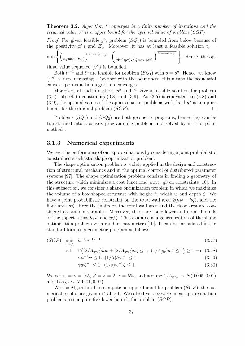
Theorem 3.2. Algorithm 1 converges in a finite number of iterations and thereturned value vn is a upper bound for the optimal value of problem (SGP ).

Proof. For given feasible yn, problem (SQ1) is bounded from below because ofthe positivity of t and Ec. Moreover, it has at least a feasible solution tj =

min

(1

2QmaxiEci

) 1M maxiai,j ,

(1

2Φ−1(yn)√Qmaxiσ2

i

) 1M maxiai,j

. Hence, the op-

timal value sequence vn is bounded.Both tn−1 and tn are feasible for problem (SQ1) with y = yn. Hence, we know

vn is non-increasing. Together with the boundness, this means the sequentialconvex approximation algorithm converges.

Moreover, at each iteration, yn and tn give a feasible solution for problem(3.4) subject to constraints (3.8) and (3.9). As (3.5) is equivalent to (3.8) and(3.9), the optimal values of the approximation problems with fixed yn is an upperbound for the original problem (SGP ).

Problems (SQ1) and (SQ2) are both geometric programs, hence they can betransformed into a convex programming problem, and solved by interior pointmethods.

3.1.3 Numerical experiments

We test the performance of our approximations by considering a joint probabilisticconstrained stochastic shape optimization problem.

The shape optimization problem is widely applied in the design and construc-tion of structural mechanics and in the optimal control of distributed parametersystems [97]. The shape optimization problem consists in finding a geometry ofthe structure which minimizes a cost functional w.r.t. given constraints [10]. Inthis subsection, we consider a shape optimization problem in which we maximizethe volume of a box-shaped structure with height h, width w and depth ζ. Wehave a joint probabilistic constraint on the total wall area 2(hw + hζ), and thefloor area wζ. Here the limits on the total wall area and the floor area are con-sidered as random variables. Moreover, there are some lower and upper boundson the aspect ratios h/w and w/ζ. This example is a generalization of the shapeoptimization problem with random parameters [10]. It can be formulated in thestandard form of a geometric program as follows:

(SCP ) minh,w,ζ

h−1w−1ζ−1 (3.27)

s.t. P((2/Awall)hw + (2/Awall)hζ ≤ 1, (1/Aflr)wζ ≤ 1

)≥ 1− ε, (3.28)

αh−1w ≤ 1, (1/β)hw−1 ≤ 1, (3.29)

γwζ−1 ≤ 1, (1/δ)w−1ζ ≤ 1. (3.30)

We set α = γ = 0.5, β = δ = 2, ε = 5%, and assume 1/Awall ∼ N(0.005, 0.01)and 1/Aflr ∼ N(0.01, 0.01).

We use Algorithm 1 to compute an upper bound for problem (SCP ), the nu-merical results are given in Table 1. We solve five piecewise linear approximationproblems to compute five lower bounds for problem (SCP ).

37

The first column in Table 1 gives the number of segments S used in the piece-wise linear approximation for solving (SGPA). The second and third columnsgive the number of variables and the number of constraints of the five problems,respectively. Notice that the number of variables is composed by the number ofdecision variables and the slack variables. Similarly, the number of constraintsconcerns both the original constraints and the added constraints. The forth andthe fifth columns give the lower bounds and the CPU time for the five approxi-mation problems, respectively. Algorithm 1 converges within 7 outer iterations,the corresponding upper bound and the CPU time are given by columns 6 and7 respectively. We use Sedumi solver from CVX package [42] to solve the ap-proximation problems with Matlab R2012b, on a PC with a 2.6 Ghz Intel Corei7-5600U CPU and 12.0 GB RAM. For better illustration, we compute gaps ofthe piecewise linear approximation bounds, which are the percentage differencesbetween these lower bounds and the upper bound, and show them in the lastcolumn.

Table 3.1: Computational results of piecewise linear approximations and Algo-rithm 1.

S Var. Num. Con. Num. Lower bound CPU(s) Upper bound CPU(s) Gap(%)

1 133 60 0.232 0.5955 0.256 5.5274 9.655

2 184 91 0.234 0.6272 0.256 5.5274 8.789

5 283 153 0.241 0.9480 0.256 5.5274 6.044

10 513 273 0.252 1.3554 0.256 5.5274 1.713

20 973 513 0.256 1.9986 0.256 5.5274 0

From Table 3.1, we can see that as the number of segments S increases, thegap of the corresponding piecewise linear approximation becomes smaller. Whenthe number of segments is equal to 20, the gap is tight.

Although the problem size is increasing with the number of segments, the CPUtime does not increase proportionally. This means our approximation approachestogether with an increasing number of segments keeps a good structure of theproblem to be solved.

3.2 Joint rectangular geometric chance constrained

programs

In this section, we extend the results in section 3.1 to joint rectangular geometricchance constrained programs. When the stochastic parameters are ellipticallydistributed and pairwise independent, we present a reformulation of the jointrectangular geometric chance constrained programs. As the reformulation is notconvex, we propose new convex approximations based on the variable transfor-mation together with piecewise linear approximation method. Numerical resultsshow that our approximations are tight.

38

3.2.1 Introduction

A rectangular geometric program can be formulated as

(GP ) mint∈RM++

g0(t)

s.t. αk ≤ gk(t) ≤ βk, k = 1, . . . , K,

where αk, βk ∈ R, k = 1, . . . , K and

gk(t) =

Ik∑i=1

cki

M∏j=1

takijj , k = 0, . . . , K. (3.31)

Usually, cki∏M

j=1 takijj is called a monomial where cki , i = 1, . . . , Ik, k = 0, . . . , K,

are nonnegative and gk(t), k = 0, . . . , K, are called posynomials.

We require that 0 < αk < βk, k = 1, . . . , K. When αk ≤ 0, k = 1, . . . , K, therectangular geometric program is equivalent to the geometric program discussedin [30, 83, 10].

Both geometric programs and rectangular geometric programs are not convexwith respect to [t1, t2, . . . , tM ]>. However, geometric programs are convex withrespect to [log(t1), log(t2), . . . , log(tM)]>. Hence, interior point methods can beused to efficiently solve geometric programs. To the best of our knowledge, thereis no variable transformation method to derive a convex equivalent reformulationfor a rectangular geometric program.

Stochastic geometric programming is used to model geometric problems whensome of the parameters are not known precisely. Stochastic geometric programswith individual chance constraints are discussed in [31] and [92] where the authorsshowed that an individual chance constraint is equivalent to several determinis-tic constraints involving posynomials and common additional slack variables. Intheir work, the parameters akij,∀k, i, j, are deterministic and cki ,∀k, i, are uncor-related normally distributed random variables. When akij ∈ 0, 1,∀k, i, j and∑

j akij = 1, ∀k, i, stochastic geometric programs are equivalent to stochastic lin-

ear programs.

In the rest of this chapter, we consider the following joint rectangular geomet-ric chance constrained programming problem

(SGP ) mint∈RM++

E

[I0∑i=1

c0i

M∏j=1

ta0ij

j

](3.32)

s.t. P

(αk ≤

Ik∑i=1

cki

M∏j=1

takijj ≤ βk, k = 1, . . . , K

)≥ 1− ε.(3.33)

Here 1 − ε is a prespecified probability with ε < 0.5, akij, k = 0, 1, . . . , K,i = 1, . . . , Ik, j = 1, . . . ,M , are given parameters and cki , k = 0, 1, . . . , K,i = 1, . . . , Ik, are random parameters with non-negative mean values.

39

3.2.2 Elliptically distributed stochastic geometric prob-lems

In this section, we consider the joint rectangular geometric chance constrainedprograms under the elliptical distribution assumption.

Assumption 3.1. ck = [ck1, ck2, . . . , c

kIk

] follows a multivariate elliptical distribu-tion EllipIk(µ

k,Γk, ϕk) with a mean vector (location parameter) µk = [µk1, µk2, . . . , µ

kIk

]> ≥0, and a scale matrix Γk. The element in the ith row and the pth column of Γk

is σki,p, i, p = 1, . . . , Ik, k = 0, 1, . . . , K. We require that µki > 0, i = 1, . . . , Ik,and σki,p ≥ 0, i, p = 1, . . . , Ik, k = 0, 1, . . . , K. Moreover, we assume that ck,k = 1, . . . , K are pairwise independent.

Definition 3.1. A L-dimensional random vector ξ follows an elliptical distribu-tion EllipL(µ,Γ, ϕ) if its characteristic function is given by Eeiz

>ξ = eiz>µϕ(z>Γz)

where ϕ is the characteristic generator function, µ is the location parameter, andΓ is the scale matrix.

Elliptical distributions include normal distribution with ϕ(t) = exp−12t,

student’s t distribution with ϕ(t) varying with its degree of freedom [61], Cauchydistribution with ϕ(t) = exp−

√t, Laplace distribution with ϕ(t) = (1 + 1

2t)−1,

and logistic distribution with ϕ(t) = 2π√t

eπ√t−e−π

√t. The mean value of an elliptical

distribution EllipL(µ,Γ, ϕ) is µ, and its covariance matrix is E(r2)rank(Γ)

Γ, where r is

the random radius [39].

Proposition 3.1 (Embrechts et al., 2005). If a L-dimensional random vectorξ follows an elliptical distribution EllipL(µ,Γ, ϕ), then for any (N × L)-matrixA and any N-vector b, Aξ + b follows an N-dimensional elliptical distributionEllipN(Aµ+ b, AΓA>, ϕ).

Moreover, we have some restrictions on ε as follows.

Assumption 3.2. We assume that

*φ′ϕk

(Φ−1ϕk

(1−ε))φϕk (Φ−1

ϕk(1−ε))Φ

−1ϕk

(1− ε) < −1, k = 1, . . . , K,

* (Φ−1ϕk

(1− ε))2σki,p − µki µkp > 0, i, p = 1, . . . , Ik, k = 1, . . . , K,

* 2σki,p

(1− φ′ϕk

(Φ−1ϕk

(z))

φϕk (Φ−1ϕk

(z))Φ−1ϕk

(z)

)((Φ−1

ϕk(z))2σki,p − µki µkp

)− (2σki,pΦ

−1ϕk

(z))2 ≥ 0,

for z ∈ [1− ε, 1], i, p = 1, . . . , Ik, k = 1, . . . , K.

Here, Φϕ(·) is the distribution function of an univariate standard elliptical dis-tribution Ellip1(0, 1, ϕ). We assume that the elliptical distribution Ellip1(0, 1, ϕ)associated with ϕ has a density function φϕ(·), and Φϕ(·) is continuous and in-creasing. We denote that, Φ−1

ϕ (·) is the inverse function of Φϕ(·), i.e., the quantileof the standard elliptical distribution. We assume Φ−1

ϕ (·) to be continuous andφϕ(·) is positive a.s., and denote the first order derivative of φϕ(·) by φ′ϕ(·).

For some distributions in elliptical distribution group, such as a normal dis-tribution, Assumption 3.2 has some simpler equivalent formulation.

40

Proposition 3.2. For an univariate standard normal distribution N(0, 1), ε ≤1− Φϕk(1) implies

φ′ϕk(Φ−1ϕk

(1−ε))φϕk (Φ−1

ϕk(1−ε))Φ

−1ϕk

(1− ε) < −1.

Proof. We denote Φ−1ϕk

(1− ε) by ς for short. The left hand side of the conclusion

can be rewritten as ςφ′ϕk

(ς)

φϕk (ς). We have

ςφ′ϕk(ς)

φϕk(ς)= ς

1√2πe−

ς2

2 (−ς)1√2πe−

ς2

2

= −ς2.

Moreover, ε ≤ 1− Φϕk(1) implies ς ≥ 1, which furthermore implies ςφ′ϕk

(ς)

φϕk (ς)<

−1.

Theorem 3.3. Given Assumption 3.1, the joint rectangular geometric chanceconstrained programs (SGP ) can be equivalently reformulated as

(SGPr)

mint∈RM++

I0∑i=1

µ0i

M∏j=1

ta0ij

j (3.34)

s.t. Φ−1ϕk

(z+k )

√√√√ Ik∑i=1

Ik∑p=1

σki,p

M∏j=1

takij+a

kpj

j −Ik∑i=1

µki

M∏j=1

takijj ≤ −αk,

k = 1, . . . , K, (3.35)

Φ−1ϕk

(z−k )

√√√√ Ik∑i=1

Ik∑p=1

σki,p

M∏j=1

takij+a

kpj

j +

Ik∑i=1

µki

M∏j=1

takijj ≤ βk,

k = 1, . . . , K, (3.36)

z+k + z−k − 1 ≥ yk, 0 ≤ z+

k , z−k ≤ 1, k = 1, . . . , K, (3.37)

K∏k=1

yk ≥ 1− ε, 0 ≤ yk ≤ 1, k = 1, . . . , K. (3.38)

Proof. As cki are pairwise independent, constraint (3.33) is equivalent to

K∏k=1

P

(αk ≤

Ik∑i=1

cki

M∏j=1

takijj ≤ βk

)≥ 1− ε. (3.39)

By introducing auxiliary variables yk ∈ R+, k = 1, . . . , K, (3.39) can be equiva-lently written as

P

(αk ≤

Ik∑i=1

cki

M∏j=1

takijj ≤ βk

)≥ yk, k = 1, . . . , K, (3.40)

41

and

K∏k=1

yk ≥ 1− ε, 0 ≤ yk ≤ 1, k = 1, . . . , K. (3.41)

(3.40) is also equivalent to

P

(Ik∑i=1

cki

M∏j=1

takijj ≥ αk

)+ P

(Ik∑i=1

cki

M∏j=1

takijj ≤ βk

)− 1 ≥ yk, k = 1, . . . , K.

(3.42)

Let z+k , z

−k ∈ R+, k = 1, . . . , K, be two additional auxiliary variables. Constraint

(3.42) can be equivalently expressed by

P

(Ik∑i=1

cki

M∏j=1

takijj ≥ αk

)≥ z+

k , k = 1, . . . , K, (3.43)

P

(Ik∑i=1

cki

M∏j=1

takijj ≤ βk

)≥ z−k , k = 1, . . . , K, (3.44)

z+k + z−k − 1 ≥ yk, 0 ≤ z+

k , z−k ≤ 1, k = 1, . . . , K. (3.45)

From Proposition 3.1, we know that∑Ik

i=1 cki

∏Mj=1 t

akijj follows an elliptical

distribution Ellip1(∑Ik

i=1 µki

∏Mj=1 t

akijj ,∑Ik

i=1

∑Ikp=1 σ

ki,p

∏Mj=1 t

akij+akpj

j , ϕk). By using

the quantile function Φ−1ϕk

(z+k ), we can equivalently rewrite constraint (3.43) as

−Ik∑i=1

µki

M∏j=1

takijj + Φ−1

ϕk(z+k )

√√√√ Ik∑i=1

Ik∑p=1

σki,p

M∏j=1

takij+a

kpj

j ≤ −αk, k = 1, . . . , K,

and rewrite constraint (3.44) as

Ik∑i=1

µki

M∏j=1

takijj + Φ−1

ϕk(z−k )

√√√√ Ik∑i=1

Ik∑p=1

σki,p

M∏j=1

takij+a

kpj

j ≤ βk, k = 1, . . . , K.

This gives the equivalent reformulation of the joint chance constrained problem.As ck ∼ EllipIk(µ

k,Γk, ϕk), its expected value is µk. Hence, from the additivityproperty of the expectation operator, we can get the equivalent reformulation ofthe objective function.

In (SGPr), both constraints (3.35) and (3.36) are nonconvex constraints. Inthe next section, we propose inner and outer convex approximations of the feasiblesolution set.

42

3.2.3 Convex approximations of constraints (3.35) and (3.36)

Convex approximations of constraint (3.35)

We first denote

wk =

[M∏j=1

tak1jj , . . . ,

M∏j=1

takIkjj

]∈ RIk , k = 1, . . . , K.

Constraint (3.35) can be reformulated as

−(µk)>wk + Φ−1ϕk

(z+k )√

(wk)>Γkwk ≤ −αk, k = 1, . . . , K. (3.46)

As we assume that ε ≤ 0.5 and ck follows a symmetric distribution, it is easyto see that (µk)>wk − αk ≥ 0. Hence, (3.46) is equivalent to

(Φ−1ϕk

(z+k ))2((wk)>Γkw

k) ≤ ((µk)>wk − αk)2, k = 1, . . . , K,

which can be reformulated as

(wk)>((Φ−1

ϕk(z+k ))2Γk − µk(µk)>

)wk + 2αk(µ

k)>wk ≤ α2k, k = 1, . . . , K. (3.47)

As wk =

[∏Mj=1 t

ak1jj , . . . ,

∏Mj=1 t

akIkjj

], k = 1, . . . , K, constraint (3.47) is equiv-

alent to

2αk

Ik∑i=1

µki

M∏j=1

takijj +

Ik∑i=1

Ik∑p=1

((Φ−1ϕk

(z+k ))2σki,p − µki µkp)

M∏j=1

takij+a

kpj

j ≤ α2k,

k = 1, ...K. (3.48)

From (3.37) and (3.38), we know that z+k ≥ 1− ε ≥ 0.5. Moreover, we know

from Assumption 3.2 that

(Φ−1ϕk

(z+k ))2σki,p − µki µkp ≥ (Φ−1

ϕk(1− ε))2σki,p − µki µkp > 0,

for all z+k ∈ [1−ε, 1), i, p = 1, . . . , Ik, k = 1, . . . , K. Hence, given Assumption 3.2,

we can apply the standard variable transformation rj = log(tj), j = 1, . . . ,M , to(3.48). Therefore, we have an equivalent formulation of (3.48)

2αk

Ik∑i=1

µki exp

M∑j=1

akijrj

+

Ik∑i=1

Ik∑p=1

exp

M∑j=1

(akijrj + akpjrj)

+ log((Φ−1ϕk

(z+k ))2σki,p − µki µkp)

≤ α2

k, k = 1, . . . , K. (3.49)

Proposition 3.3. Given Assumption 3.2, fi,p,k(z+k ) = log((Φ−1

ϕk(z+k ))2σki,p−µki µkp)

is monotone increasing and convex for z+k ∈ [1 − ε, 1), i, p = 1, . . . , Ik, k =

1, . . . , K.

43

Proof. From the continuity and monotonicity of Φϕk(·) and the positiveness ofφϕk(·), we know Φϕk(·) is strictly monotone a.s.. Hence, from the formula forthe derivative of the inverse function, we have that Φ−1

ϕk(z) is differential and its

derivative is 1ddx

Φϕk (x)= 1

φϕk (x), where x = Φ−1

ϕk(z). Furthermore, we have that

fi,p,k(z+k ) is differential and its first and second order derivatives are

f ′i,p,k(z+k ) =

dfi,p,k(z+k )

dz+k

=σki,p((Φ

−1ϕk

(z+k ))2)′

(Φ−1ϕk (z+

k ))2σki,p − µki µkp=

2σki,pΦ−1ϕk

(z+k )(Φ−1

ϕk(z+k ))′

(Φ−1ϕk (z+

k ))2σki,p − µki µkp

=2σki,pΦ

−1ϕk

(z+k )

φϕk(Φ−1

ϕk (z+k ))((Φ−1

ϕk (z+k ))2σki,p − µki µkp)

,

f ′′i,p,k(z+k ) =

d2fi,p,k(z+k )

d(z+k )2

=2σki,p(Φ

−1ϕk

(z+k ))′

(φϕk(Φ−1

ϕk (z+k )))((Φ−1

ϕk (z+k ))2σki,p − µki µkp)

−2σki,pΦ

−1ϕk

(z+k )(φϕk

(Φ−1ϕk

(z+k ))((Φ−1

ϕk(z+k ))2σki,p − µki µkp))′

(φϕk(Φ−1

ϕk (z+k )))2((Φ−1

ϕk (z+k ))2σki,p − µki µkp)2

=

2σki,p

(1−

φ′ϕk(Φ−1

ϕk(z+k ))

φϕk(Φ−1

ϕk(z+k ))

Φ−1ϕk

(z+k )

)((Φ−1

ϕk(z+k ))2σki,p − µki µkp

)−(2σki,pΦ

−1ϕk

(z+k ))2

(φϕk(Φ−1

ϕk (z+k )))2((Φ−1

ϕk (z+k ))2σki,p − µki µkp)2

.

From Assumption 3.2, we know thatdfi,p,k(z+

k )

dz+k

≥ 0 and fi,p,k(z+k ) is monotone

increasing for z+k ∈ [1 − ε, 1), i, p = 1, . . . , Ik, k = 1, . . . , K. From Assumption

3.2, we know thatd2fi,p,k(z+

k )

d(z+k )2 ≥ 0 and fi,p,k(z

+k ) is convex for z+

k ∈ [1 − ε, 1),

i, p = 1, . . . , Ik, k = 1, . . . , K.

Thanks to the convexity and the monotonicity of fi,p,k(z+k ), we use the piece-

wise linear approximation method to find a lower approximation of fi,p,k(z+k ) [65].

Then, we propose a piecewise linear approximation method to find an lower ap-proximation of fi,p,k(z

+k ).

We choose S different linear functions:

FLs,i,p,k(z

+k ) = ds,i,p,kz

+k + bs,i,p,k, s = 1, . . . , S,

which are the tangent segments of fi,p,k(z+k ) at given points in [1 − ε, 1), e.g.,

ξ1, ξ2, . . . , ξS. Here, we choose ξS = 1 − δ, where δ is a very small positive realnumber. We have

ds,i,p,k = f ′i,p,k(ξs)

and

bs,i,p,k = fi,p,k(ξs)− f ′i,p,k(ξs)ξs, s = 1, . . . , S.

Then, we use the piecewise linear function

FLi,p,k(z

+k ) = max

s=1,...,SFLs,i,p,k(z

+k )

to approximate fi,p,k(z+k ).

44

Proposition 3.4. Given Assumption 3.2, FLi,p,k(z

+k ) ≤ fi,p,k(z

+k ), ∀z+

k ∈ [1−ε, 1).

Proof. The proof can be drawn from the convexity of fi,p,k(z+k ) shown in Propo-

sition 3.3.

We use the piecewise linear function FLi,p,k(z

+k ) to replace log((Φ−1

ϕk(z+k ))2σki,p−

µki µkp) in (3.49). Hence, we have the following convex approximation of constraint

(3.35):

2αk

Ik∑i=1

µki exp

M∑j=1

akijrj

+

Ik∑i=1

Ik∑p=1

exp

M∑j=1

(akijrj + akpjrj)

+ ωLi,p,k

≤ α2

k, k = 1, . . . , K,

ds,i,p,kz+k + bs,i,p,k ≤ ωLi,p,k, s = 1, . . . , S, i, p = 1, . . . , Ik, k = 1, . . . , K.

(3.50)

As log((Φ−1ϕk

(z+k ))2σki,p − µki µkp) is convex, (3.50), together with (3.36)-(3.38), pro-

vides an outer approximation of the feasible set of (SGP ).To get an upper approximation of the function fi,p,k(z

+k ), we sort 1−ε, ξ1, ξ2, . . .,

ξS in the increasing order and denote the sorted array by ξ1, ξ2, . . . , ξS+1. Thesegments

FUs,i,p,k(z

+k ) = ds,i,p,kz

+k + bs,i,p,k, s = 1, . . . , S,

form a piecewise linear function

FUi,p,k(z

+k ) = max

s=1,...,SFUs,i,p,k(z

+k ).

Here,

ds,i,p,k =fi,p,k(ξs+1)− fi,p,k(ξs)

ξs+1 − ξs

and

bs,i,p,k = −ds,i,p,kξs + fi,p,k(ξs), s = 1, . . . , S.

Using the piecewise linear function FUi,p,k(z

+k ) leads to the following convex

approximation of constraint (3.35):

2αk

Ik∑i=1

µki exp

M∑j=1

akijrj

+

Ik∑i=1

Ik∑p=1

exp

M∑j=1

(akijrj + akpjrj)

+ ωUi,p,k

≤ α2

k, k = 1, . . . , K,

ds,i,p,kz+k + bs,i,p,k ≤ ωUi,p,k, s = 1, . . . , S, i, p = 1, . . . , Ik, k = 1, . . . , K.

(3.51)

As log((Φ−1ϕk

(z+k ))2σki,p − µki µkp) is convex, (3.51), together with (3.36)-(3.38), pro-

45

vides an inner approximation of the feasible set of (SGP ).

Convex approximation of constraint (3.36)

In constraint (3.36), the terms

√∑Iki=1

∑Ikp=1 σ

ki,p

∏Mj=1 t

akij+akpj

j and∑Ik

i=1 µki

∏Mj=1 t

akijj

are convex with respect to rj = log(tj), j = 1, . . . ,M .

From [50], we know that Φ−1ϕk

(z−k ) is convex with respect to z−k on [1 − ε, 1),if φϕk is 0-decreasing with some threshold t∗(0) > 0, and ε < 1 − Φϕk(t

∗(0)).The definition of r-decreasing and t∗(0) can be found in [50]. Hence, given someconditions, constraint (3.36) is a biconvex constraint on [1 − ε, 1). One can usethe sequential convex approach to solve this problem. However, Φ−1

ϕk(z−k ) cannot

be expressed explicitly, it is still not easy to compute the optimal z−k with fixedtj. In this section, we use the piecewise linear approximation method proposedin [65], and its modified approximation method to find tight lower and upperbounds of (3.36).

We first make the standard variable transformation rj = log(tj), j = 1, . . . ,Mto (3.36) in order to get an equivalent formulation of (3.36)√√√√ Ik∑

i=1

Ik∑p=1

exp

M∑j=1

(akijrj + akpjrj) + 2 log(Φ−1ϕk

(z−k )) + log(σki,p)

+

Ik∑i=1

µki exp

M∑j=1

akijrj

≤ βk, k = 1, . . . , K. (3.52)

Lemma 3.1. Given Assumption 3.2, log(Φ−1ϕk

(z−k )) is monotone increasing andconvex on [1− ε, 1).

Proof. The first order and second order derivatives of log(Φ−1ϕk

(z−k )) are

d(log(Φ−1ϕk

(z−k )))

dz−k=

1

Φ−1ϕk

(z−k )φϕk(Φ−1ϕk

(z−k )),

and

d2(log(Φ−1ϕk

(z−k )))

d(z−k )2= −

1 + Φ−1ϕk

(z−k )φ′ϕk

(Φ−1ϕk

(z−k ))

φϕk (Φ−1ϕk

(z−k ))

(Φ−1ϕk

(z−k )φϕk(Φ−1ϕk

(z−k )))2.

From Assumption 3.2, we know that

1 + Φ−1ϕk

(1− ε)φ′ϕk(Φ

−1ϕk

(1− ε))φϕk(Φ

−1ϕk

(1− ε))< 0.

As 1+Φ−1ϕk

(z−k )φ′ϕk

(Φ−1ϕk

(z−k ))

φϕk (Φ−1ϕk

(z−k ))is monotone decreasing with respect to z−k in [1− ε, 1),

we can find that the second order derivative of log(Φ−1ϕk

(z−k )) is larger than orequal to zero on z−k ∈ [1 − ε, 1), which implies the convexity of log(Φ−1

ϕk(z−k )) on

[1− ε, 1), k = 1, . . . , K.

46

From the convexity and monotonicity, we can use the piecewise linear ap-proximation methods introduced in the last section to find tight piecewise linearapproximations for log(Φ−1

ϕk(z−k )). We choose S different linear functions:

GLs,k(z

−k ) = ls,kz

−k + qs,k, s = 1, . . . , S,

which are the tangent segments of log(Φ−1ϕk

(z−k )) at ξ1, ξ2, . . . , ξS, respectively. Wehave

ls,k =1

φϕk(Φ−1ϕk

(ξs))Φ−1ϕk

(z−k )

and

qs,k = log(Φ−1ϕk

(ξs))− ξsφϕk(Φ

−1ϕk

(ξs))Φ−1ϕk

(z−k ), s = 1, . . . , S.

Then, we use the piecewise linear function

GLk (z−k ) = max

s=1,...,SGLs,k(z

−k )

to approximate log(Φ−1ϕk

(z−k )), and derive the following convex approximation of(3.52):

Ik∑i=1

µki exp

M∑j=1

akijrj

+

√√√√ Ik∑i=1

Ik∑p=1

exp

M∑j=1

(akijrj + akpjrj) + 2ωLk + log(σki,p)

≤ βk, k = 1, . . . , K,

ls,kz−k + qs,k ≤ ωLk , s = 1, . . . , S, k = 1, . . . , K.

(3.53)As log(Φ−1

ϕk(z−k )) is convex, (3.53) together with (3.35), (3.37)-(3.38) provides an

outer approximation of the feasible set of (SGP ).

Moreover, we use the segments

GUs,k(z

−k ) = ls,kz

−k + qs,k, s = 1, . . . , S,

between ξ1, ξ2, . . . , ξS+1 to form a piecewise linear function

GUk (z−k ) = max

s=1,...,SGUs,k(z

−k ).

Here,

ls,k =log(Φ−1

ϕk(ξs+1))− log(Φ−1

ϕk(ξs))

ξs+1 − ξs,

and

qs,k = −ls,kξs + log(Φ−1ϕk

(ξs)), s = 1, . . . , S.

47

Using the piecewise linear function GUk (z−k ) to replace log(Φ−1

ϕk(z−k )) in (3.52)

gives the following convex approximation of the constraint (3.52):

Ik∑i=1

µki exp

M∑j=1

akijrj

+

√√√√ Ik∑i=1

Ik∑p=1

exp

M∑j=1

(akijrj + akpjrj) + 2ωUk + log(σki,p)

≤ βk, k = 1, . . . , K,

ls,kz−k + qs,k ≤ ωUk , s = 1, . . . , S, k = 1, . . . , K.

(3.54)As log(Φ−1

ϕk(z−k )) is convex, (3.54) provides an inner approximation.

Main result

Theorem 3.4. Given Assumptions 3.1 and 3.2, we have the following convexapproximations for the joint rectangular geometric chance constrained programs(SGP ):

(SGPL) minr,z+,z−,x,ωL,ωL

I0∑i=1

µ0i exp

M∑j=1

a0ijrj

s.t. ds,i,p,kz

+k + bs,i,p,k ≤ ωi,p,k, s = 1, . . . , S,

i, p = 1, . . . , Ik, k = 1, . . . , K,

2αk

Ik∑i=1

µki exp

M∑j=1

akijrj

+

Ik∑i=1

Ik∑p=1

exp

M∑j=1

(akijrj + akpjrj)

+ωLi,p,k

≤ α2

k, k = 1, . . . , K,√√√√ Ik∑i=1

Ik∑p=1

exp

M∑j=1

(akijrj + akpjrj) + 2ωLk + log(σki,p)

+

Ik∑i=1

µki exp

M∑j=1

akijrj

≤ βk, k = 1, . . . , K,

ls,kz−k + qs,k ≤ ωLk , s = 1, . . . , S, k = 1, . . . , K,

z+k + z−k − 1 ≥ exk , 0 ≤ z+

k , z−k ≤ 1, k = 1, . . . , K,

K∑k=1

xk ≥ log(1− ε), xk ≤ 0, k = 1, . . . , K.

(SGPU) minr,z+,z−,x,ωU ,ωU

I0∑i=1

µ0i exp

M∑j=1

a0ijrj

s.t. ds,i,p,kz+k + bs,i,p,k ≤ ωUi,p,k, s = 1, . . . , S,

i, p = 1, . . . , Ik, k = 1, . . . , K,

48

2αk

Ik∑i=1

µki exp

M∑j=1

akijrj

+

Ik∑i=1

Ik∑p=1

exp

M∑j=1

(akijrj + akpjrj)

+ωUi,p,k

≤ α2

k, k = 1, . . . , K,√√√√ Ik∑i=1

Ik∑p=1

exp

M∑j=1

(akijrj + akpjrj) + 2ωUk + log(σki,p)

+

Ik∑i=1

µki exp

M∑j=1

akijrj

≤ βk, k = 1, . . . , K,

ls,kz−k + qs,k ≤ ωUk , s = 1, . . . , S, k = 1, . . . , K,

z+k + z−k − 1 ≥ exk , 0 ≤ z+

k , z−k ≤ 1, k = 1, . . . , K,

K∑k=1

xk ≥ log(1− ε), xk ≤ 0, k = 1, . . . , K.

The optimal value of the approximation problem (SGPL) is a lower boundof problem (SGP ). The optimal value of the approximation problem (SGPU) isan upper bound of problem (SGP ). Moreover, if the feasible set of (SGP ) isnonempty, both (SGPL) and (SGPU) are reformulations of (SGP ) when S goesto infinity, .

Proof. (SGPL) is obtained from the reformulation (SGPr) of (SGP ) and thetwo outer approximations (3.50) and (3.53). Besides, we transform the variabley into xk = log(yk), k = 1, . . . , K. The outer approximations guarantee thatthe feasible region of (SGPL) contains the feasible region of (SGP ). Hence theoptimal value of (SGPL) is a lower bound of problem (SGP ).

Meanwhile, (SGPI) is obtained from the reformulation (SGPr) of (SGP ),the two inner approximations (3.51) and (3.54) and the variable transformationxk = log(yk), k = 1, . . . , K. The inner approximations guarantee that the feasibleregion of (SGPU) is contained in the feasible region of (SGP ). Hence the optimalvalue of (SGPU) is an upper bound of problem (SGP ).

Finally, when S goes to infinity, GL(z−k ) uniformly converges to log(Φ−1ϕk

(z−k ))for z−k ∈ [1 − ε, 1) due to the convexity of the two terms given in Assumption3.2 and the property of the piece-wise linear approximation. Hence, the lefthand side term of (3.53) converges to the left hand side term of (3.52) uniformly.Given Assumption 3.2, left hand side terms of both (3.52) and (3.53) are convex.Moreover, both feasible sets are closed and the feasible set constrained by (3.52)are nonempty. Hence, the convex feasible set constrained by (3.53) converges tothe convex feasible set constrained by (3.52) when S is large enough. Similarly,when S goes to infinity, GU(z−k ) uniformly converges to log(Φ−1

ϕk(z−k )) for z−k ∈

[1− ε, 1), and the feasible set constrained by (3.54) converges to the feasible setconstrained by (3.52). Moreover, both FL(z+

k ) and FU(z+k ) uniformly converge

to log((Φ−1ϕk

(z+k ))2σki,p−µki µkp). From the convexity of the feasible sets constrained

by (3.49), (3.50) and (3.51), we know the feasible sets constrained by (3.50) andby (3.51) both converge to the feasible set constrained by (3.49). By taking the

49

intersection of the feasible sets constrained by (3.50) and by (3.53), we can findthat the distance between the feasible sets of (SGPL) and (SGP ) converges tozero when S goes to infinity. Similarly, by taking the intersection of the feasiblesets constrained by (3.51) and by (3.54), we can find that the distance betweenthe feasible sets of (SGPU) and (SGP ) converges to zero when S goes to infinity.This means both (SGPL) and (SGPU) are reformulations of (SGP ) when S goesto infinity.

Both (SGPL) and (SGPU) are convex programming problems. Interior pointmethods can be used to solve them efficiently.

3.2.4 Numerical experiments

We test the performances of our approximation methods by considering the fol-lowing stochastic rectangular shape optimization problem with a joint chanceconstraints:

minx1,...,xm

m∏i=1

x−1i

s.t. P

[αwall ≤

m−1∑j=1

(m− 1

Ajx1

m∏i=2,i 6=j

xi) ≤ βwall, αflr ≤1

Aflr

m∏j=2

xj ≤ βflr

]≥ 1− ε,

xix−1j ≤ γi,j, ∀i 6= j.

Here, 1/Aflr and 1/Aj, j = 1, . . . ,m− 1, are considered as random variables.We assume 1/Afl to be independent of 1/Aj, j = 1, . . . ,m− 1. This example isa generalization of the shape optimization problem with random parameters in[65]. In all following experiments, we set γi,j = 2, ∀i 6= j, αwall = 1, βwall = 2,αflr = 1, βflr = 2 and ε = 5%.

In order to test the tightness of the piecewise linear approximation, we firstconsider three different examples in the elliptical distribution group.

Example 3.1. We set m = 10. We let 1/Aflr follow a normal distributionN(0.02, 0.02), and the random vector [1/A1, 1/A2, . . . , 1/Am−1] follow a (m− 1)-dimensional normal distribution, such that E[1/Aj] = 0.01, j = 1, . . . ,m − 1,and cov[1/Ai, 1/Aj] = 0.01, i, j = 1, . . . ,m − 1. Moreover, 1/Aj and 1/Aflr areindependent, j = 1, . . . ,m− 1.

Example 3.2. We set m = 15. We let 1/Aflr follow a logistic distributionwith location parameter 0.02 and scale parameter 0.078, i.e., E[1/Aflr] = 0.02and Var[1/Aflr] = 0.02. We let [1/A1, 1/A2, . . . , 1/Am−1] follow a (m − 1)-dimensional logistic distribution, such that E[1/Aj] = 0.01, j = 1, . . . ,m − 1,and cov[1/Ai, 1/Aj] = 0.01, i, j = 1, . . . ,m − 1. Moreover, 1/Aj and 1/Aflr areindependent, j = 1, . . . ,m− 1.

Example 3.3. We set m = 20. We let 1/Aflr follow a Student’s t distribution,with location parameter 0.02, scale parameter 0.02 and degree of freedom 4. We

50

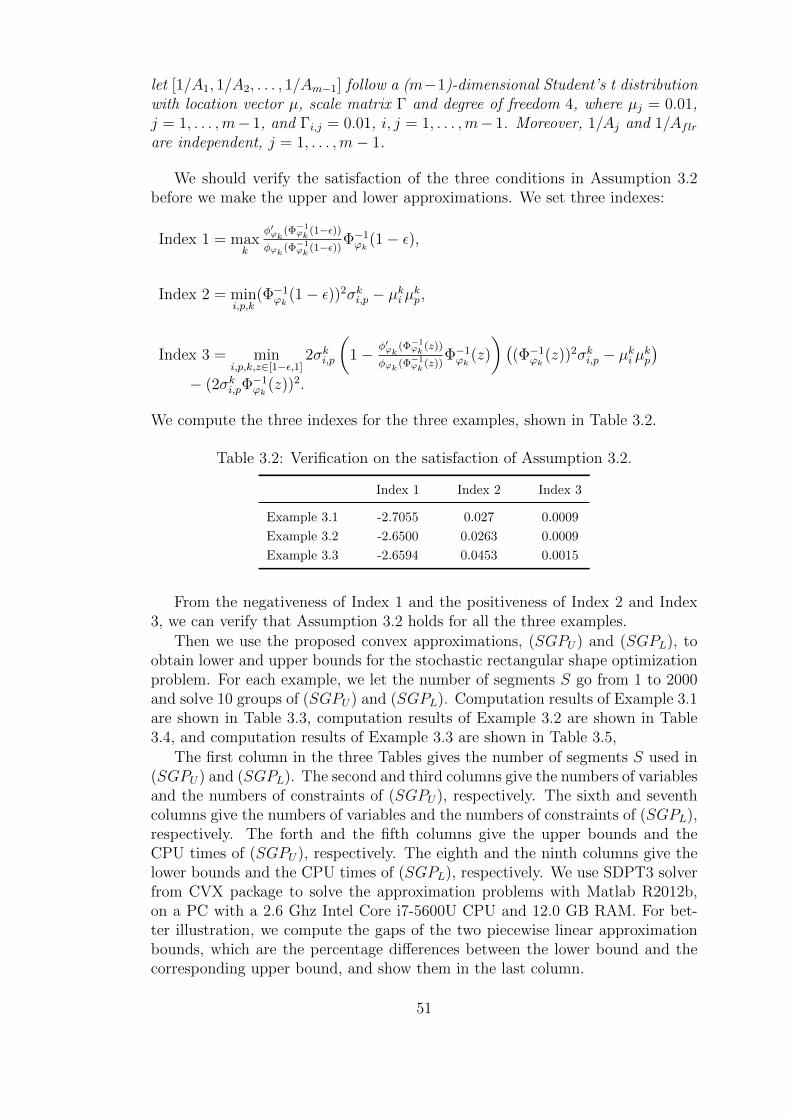
let [1/A1, 1/A2, . . . , 1/Am−1] follow a (m−1)-dimensional Student’s t distributionwith location vector µ, scale matrix Γ and degree of freedom 4, where µj = 0.01,j = 1, . . . ,m− 1, and Γi,j = 0.01, i, j = 1, . . . ,m− 1. Moreover, 1/Aj and 1/Aflrare independent, j = 1, . . . ,m− 1.

We should verify the satisfaction of the three conditions in Assumption 3.2before we make the upper and lower approximations. We set three indexes:

Index 1 = maxk

φ′ϕk(Φ−1ϕk

(1−ε))φϕk (Φ−1

ϕk(1−ε))Φ

−1ϕk

(1− ε),

Index 2 = mini,p,k

(Φ−1ϕk

(1− ε))2σki,p − µki µkp,

Index 3 = mini,p,k,z∈[1−ε,1]

2σki,p

(1− φ′ϕk

(Φ−1ϕk

(z))

φϕk (Φ−1ϕk

(z))Φ−1ϕk

(z)

)((Φ−1

ϕk(z))2σki,p − µki µkp

)− (2σki,pΦ

−1ϕk

(z))2.

We compute the three indexes for the three examples, shown in Table 3.2.

Table 3.2: Verification on the satisfaction of Assumption 3.2.

Index 1 Index 2 Index 3

Example 3.1 -2.7055 0.027 0.0009

Example 3.2 -2.6500 0.0263 0.0009

Example 3.3 -2.6594 0.0453 0.0015

From the negativeness of Index 1 and the positiveness of Index 2 and Index3, we can verify that Assumption 3.2 holds for all the three examples.

Then we use the proposed convex approximations, (SGPU) and (SGPL), toobtain lower and upper bounds for the stochastic rectangular shape optimizationproblem. For each example, we let the number of segments S go from 1 to 2000and solve 10 groups of (SGPU) and (SGPL). Computation results of Example 3.1are shown in Table 3.3, computation results of Example 3.2 are shown in Table3.4, and computation results of Example 3.3 are shown in Table 3.5,

The first column in the three Tables gives the number of segments S used in(SGPU) and (SGPL). The second and third columns give the numbers of variablesand the numbers of constraints of (SGPU), respectively. The sixth and seventhcolumns give the numbers of variables and the numbers of constraints of (SGPL),respectively. The forth and the fifth columns give the upper bounds and theCPU times of (SGPU), respectively. The eighth and the ninth columns give thelower bounds and the CPU times of (SGPL), respectively. We use SDPT3 solverfrom CVX package to solve the approximation problems with Matlab R2012b,on a PC with a 2.6 Ghz Intel Core i7-5600U CPU and 12.0 GB RAM. For bet-ter illustration, we compute the gaps of the two piecewise linear approximationbounds, which are the percentage differences between the lower bound and thecorresponding upper bound, and show them in the last column.

51

Table 3.3: Computational results of approximations for normal distribution inExample 3.1.

S Var. Con. UB CPU(s) Var. Con. LB CPU(s) Gap(%)

1 681 216 8.1507 13.3390 681 216 6.6180 10.6090 23.1583

2 685 216 8.1368 13.8255 685 216 7.4902 10.7009 8.6325

5 697 216 8.1311 14.7254 697 216 8.0253 13.4361 1.3186

10 717 216 8.1311 15.5340 717 216 8.1116 14.6222 0.2403

20 757 216 8.1303 15.7734 757 216 8.1279 14.9508 0.0300

100 1077 216 8.1303 17.9095 1077 216 8.1303 17.8283 0.0000

200 1477 216 8.1303 18.0155 1477 216 8.1303 18.3668 0.0000

500 2677 216 8.1303 20.4507 2677 216 8.1303 20.2324 0.0000

1000 4677 216 8.1303 24.5032 4677 216 8.1303 24.3255 0.0000

2000 8677 216 8.1303 33.3699 8677 216 8.1303 33.8009 0.0000

Table 3.4: Computational results of approximations for Logistic distribution inExample 3.2.

S Var. Con. UB CPU(s) Var. Con. LB CPU(s) Gap(%)

1 1526 466 20.3036 27.0223 1526 466 17.0253 25.1127 19.2557

2 1530 466 19.8479 32.8251 1530 466 18.7557 25.9661 5.8232

5 1542 466 19.6918 35.1827 1542 466 19.5681 32.7463 0.6320

10 1562 466 19.6740 36.5728 1562 466 19.6583 35.3287 0.0800

20 1602 466 19.6701 39.4038 1602 466 19.6681 42.9635 0.0100

100 1922 466 19.6701 39.2123 1922 466 19.6701 41.7810 0.0000

200 2322 466 19.6701 39.2405 2322 466 19.6701 40.4707 0.0000

500 3522 466 19.6701 41.2078 3522 466 19.6701 40.4667 0.0000

1000 5522 466 19.6701 46.4123 5522 466 19.6701 46.5576 0.0000

2000 9522 466 19.6701 54.0321 9522 466 19.6701 53.9358 0.0000

Table 3.5: Computational results of approximations for Student’s t distributionin Example 3.3.

S Var. Con. UB CPU(s) Var. Con. LB CPU(s) Gap(%)

1 2721 816 57.2656 73.8665 2721 816 43.3974 51.5729 31.9562

2 2725 816 49.5113 74.7218 2725 816 46.5860 57.3962 6.2793

5 2737 816 47.4843 91.6425 2737 816 47.2853 79.1193 0.4209

10 2757 816 47.3326 80.6797 2757 816 47.2853 82.1539 0.1001

20 2797 816 47.3042 94.3056 2797 816 47.2853 85.8753 0.0400

100 3117 816 47.2901 87.8563 3117 816 47.2901 91.1235 0.0000

200 3517 816 47.2901 86.2648 3517 816 47.2901 84.5257 0.0000

500 4717 816 47.2901 89.6698 4717 816 47.2901 87.5018 0.0000

1000 6717 816 47.2901 95.3347 6717 816 47.2901 92.2044 0.0000

2000 10717 816 47.2901 106.3244 10717 816 47.2901 104.3638 0.0000

52

From the three tables, we can see that as the number of segments S increases,the gap of the corresponding piecewise linear approximation bounds for the prob-lem becomes smaller. For all the three examples, the gap is tight when the numberof segments is equal to or larger than 100. Notice that the CPU time does notincrease proportionally with the increase of S. When S = 2000, the CPU time isless than twice of the CPU time when S = 2.

We further study the effect on the approximation precision and CPU time ofmean value, increasing variance and m.

We use Example 3.1 as the basic setting. We set E[1/Aflr] = µflr, E[1/Aj] =µA, j = 1, . . . ,m − 1, and let them vary from 0.02 to 0.2 and from 0.01 to 0.1,respectively. All other parameters are fixed at the same values as Example 3.1.We should verify the satisfaction of the conditions in Assumption 3.2. Like whatwe do in Table 3.2, we compute three indexes for each group of the distributionswith different mean values, and show them in Table 3.6. From the table, wecan easily see that Assumption 3.2 holds for all the groups of distributions withdifferent mean values.

Table 3.6: Verification on the satisfaction of Assumption 3.2 with increasing meanvalue.

µA 0.01 0.02 0.03 0.04 0.05 0.06 0.07 0.08 0.09 0.1

µflr 0.02 0.04 0.06 0.08 0.1 0.12 0.14 0.16 0.18 0.2

Index 1 -2.7055 -2.7055 -2.7055 -2.7055 -2.7055 -2.7055 -2.7055 -2.7055 -2.7055 -2.7055

Index 2 0.0270 0.0267 0.0262 0.0255 0.0246 0.0235 0.0222 0.0207 0.0190 0.0171

Index 3 0.0009 0.0009 0.0009 0.0008 0.0007 0.0007 0.0006 0.0004 0.0003 0.0002

Then we use the proposed convex approximations, (SGPU) and (SGPL), toobtain lower and upper bounds for the stochastic rectangular shape optimizationproblem. We set the number of segments S to be 200. Computation results,including sizes of programming problems, lower/upper bounds and CPU times,and bound gaps, are shown in Table 3.7. From Table 3.7, we can obverse thatupper bound and lower bound are tight under all the settings with different meanvalues. The CPU times are almost the same when we let the mean values vary.

Table 3.7: Computational results with increasing mean value.

µA µflr Var. Con. UB CPU(s) Var. Con. LB CPU(s) Gap(%)

0.01 0.02 1477 216 8.1303 18.3817 1477 216 8.1303 19.5148 0

0.02 0.04 1477 216 8.6504 18.7815 1477 216 8.6504 19.2838 0

0.03 0.06 1477 216 9.1724 21.7914 1477 216 9.1724 22.3960 0

0.04 0.08 1477 216 9.6978 22.3719 1477 216 9.6978 22.5001 0

0.05 0.1 1477 216 10.3026 18.5951 1477 216 10.3026 21.5380 0

0.06 0.12 1477 216 11.9317 18.6117 1477 216 11.9317 22.3053 0

0.07 0.14 1477 216 13.9698 18.1727 1477 216 13.9698 21.3361 0

0.08 0.16 1477 216 16.1110 18.1408 1477 216 16.1110 21.4588 0

0.09 0.18 1477 216 18.3055 18.3133 1477 216 18.3055 21.5131 0

0.1 0.2 1477 216 20.5385 18.2731 1477 216 20.5385 18.7971 0

Nextly, we let the variance and covariance vary. In detail, we use Example3.1 as the basic setting, set Var[1/Aflr] = σ2

flr, Cov[1/Ai, 1/Aj] = σ2A, i, j =

1, . . . ,m − 1, and let σ2flr and σ2

A vary from 0.02 to 0.2 and from 0.01 to 0.1,

53

respectively. We verify the satisfaction of the conditions in Assumption 3.2 bycomputing the three indexes shown in Table 3.8. Then we set S = 200 anduse (SGPU) and (SGPL), to obtain lower and upper bounds for the stochasticrectangular shape optimization problem. Computation results, including sizes ofprogramming problems, lower/upper bounds and CPU times, and bound gaps, areshown in Table 3.9. From Table 3.9, we can obverse that upper bound and lowerbound are tight under all the settings with different variances and covariances.The CPU times are almost the same when we let variances and covariances vary.

Table 3.8: Verification on the satisfaction of Assumption 3.2 with increasingvariance.

σ2A 0.01 0.02 0.03 0.04 0.05 0.06 0.07 0.08 0.09 0.1

σ2flr 0.02 0.04 0.06 0.08 0.1 0.12 0.14 0.16 0.18 0.2

Index 1 -2.7055 -2.7055 -2.7055 -2.7055 -2.7055 -2.7055 -2.7055 -2.7055 -2.7055 -2.7055

Index 2 0.0270 0.054 0.0811 0.1081 0.1352 0.1622 0.1893 0.2163 0.2434 0.2705

Index 3 0.0009 0.0037 0.0083 0.0147 0.023 0.0332 0.0452 0.0590 0.0747 0.0922

Table 3.9: Computational results with increasing variance.

σ2A σ2

flr Var. Con. UB CPU(s) Var. Con. LB CPU(s) Gap(%)

0.01 0.02 1477 216 8.1303 18.4132 1477 216 8.1303 19.2847 0

0.02 0.04 1477 216 11.7271 18.8420 1477 216 11.7271 19.8981 0

0.03 0.06 1477 216 14.5661 18.7148 1477 216 14.5661 19.2016 0

0.04 0.08 1477 216 17.0083 18.6797 1477 216 17.0083 19.3238 0

0.05 0.1 1477 216 19.2036 18.5938 1477 216 19.2036 22.4753 0

0.06 0.12 1477 216 21.2424 18.7255 1477 216 21.2424 22.0337 0

0.07 0.14 1477 216 23.1872 18.1202 1477 216 23.1872 21.7534 0

0.08 0.16 1477 216 25.0757 18.5851 1477 216 25.0757 21.698 0

0.09 0.18 1477 216 26.9343 18.5935 1477 216 26.9343 18.8600 0

0.1 0.2 1477 216 28.7719 18.3161 1477 216 28.7719 19.0957 0

Table 3.10: Computational results for increasing m.

m Var. Con. UB CPU(s) Var. Con. LB CPU(s) Gap(%)

3 880 32 1.4430 4.5124 880 32 1.4430 5.9128 0

5 982 66 1.6864 7.4550 982 66 1.6864 7.9741 0

7 1138 114 3.5648 10.7008 1138 114 3.5648 11.1916 0

10 1477 216 8.1303 19.1872 1477 216 8.1303 20.4025 0

20 3517 816 36.4121 86.0015 3517 816 36.4121 95.0357 0

Finally, we test the effect of m. In detail, we use Example 3.1 with differentm. For each group, we let 1/Aflr follow a normal distribution N(0.02, 0.02), andthe random vector [1/A1, 1/A2, . . . , 1/Am−1] follow a (m−1)-dimensional normaldistribution, with E[1/Aj] = 0.01, j = 1, . . . ,m− 1, and Cov[1/Ai, 1/Aj] = 0.01,i, j = 1, . . . ,m − 1. As the parameters of each component are set the same, thesatisfaction of the conditions in Assumption 3.2 can be observed from Example3.1. Then we set S = 200 and use (SGPU) and (SGPL), to obtain lower and upperbounds for the stochastic rectangular shape optimization problem. Computationresults, including sizes of programming problems, lower/upper bounds and CPU

54

times, and bound gaps, are shown in Table 3.10. From Table 3.10, we can againobverse that the upper bound and the lower bound are both tight for all theexamples with different sizes. However, the CPU time increases faster than alinear way with respect to m. It increases even faster when m is larger.

3.3 Conclusion

In this chapter, we first review a work of Liu et al. [65] about geometric programswith joint chance constraints. As an extension, we then discuss joint rectangulargeometric chance constrained programs. We propose tight convex approximationsfor them under elliptical distributions and some conditions on the parameters.

This chapter corresponds to a paper submitted to Engineering and Optimiza-tion.

55

56

Chapter 4

Bounds for Chance ConstrainedProblems

In this chapter, we develop four upper bounds for individual and joint chance con-straints with independent matrix vector rows. The deterministic approximationsof the probability constraints are based on the one-side Chebyshev inequality,Chernoff inequality, Bernstein in-equality and Hoeffding inequality, respectively.Various sufficient conditions under which the aforementioned approximations areconvex and tractable are derived. Therefore, we approximate the chance con-strained problems as tractable convex optimization problems based on piecewiselinear and tangent approximations allowing to reduce further the computationalcomplexity. Finally, numerical results on randomly generated data are discussedallowing to identify the tight deterministic approximations.

4.1 Introduction

In this chapter, we consider the following chance constrained linear program:

minx

cTx

s.t. P Ξx ≤ H ≥ α,

x ∈ X, (4.1)

where H = (h1, . . . , hK) ∈ RK , Ξ = [ξ1, . . . , ξK ]T is a K × n random matrix,where ξk, k = 1, . . . , K is a random vector in Rn. P is a probability measure, xis a decision vector, set X ⊆ Rn+, c ∈ Rn and 0 < α < 1 a prespecified confidenceparameter.

An individual chance constrained problem can be written as

minx

cTx

s.t. PξTx ≤ h

≥ α,

x ∈ X. (4.2)

57

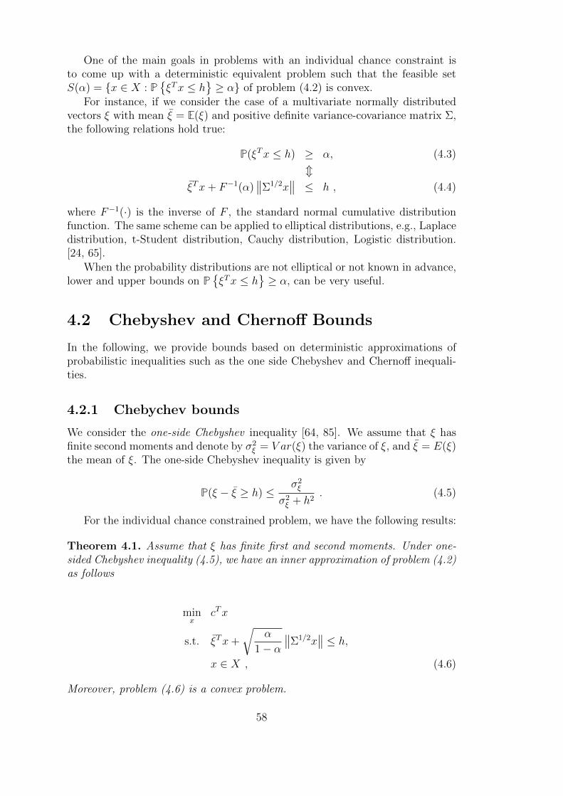
One of the main goals in problems with an individual chance constraint isto come up with a deterministic equivalent problem such that the feasible setS(α) = x ∈ X : P

ξTx ≤ h

≥ α of problem (4.2) is convex.

For instance, if we consider the case of a multivariate normally distributedvectors ξ with mean ξ = E(ξ) and positive definite variance-covariance matrix Σ,the following relations hold true:

P(ξTx ≤ h) ≥ α, (4.3)

mξTx+ F−1(α)

∥∥Σ1/2x∥∥ ≤ h , (4.4)

where F−1(·) is the inverse of F , the standard normal cumulative distributionfunction. The same scheme can be applied to elliptical distributions, e.g., Laplacedistribution, t-Student distribution, Cauchy distribution, Logistic distribution.[24, 65].

When the probability distributions are not elliptical or not known in advance,lower and upper bounds on P

ξTx ≤ h

≥ α, can be very useful.

4.2 Chebyshev and Chernoff Bounds

In the following, we provide bounds based on deterministic approximations ofprobabilistic inequalities such as the one side Chebyshev and Chernoff inequali-ties.

4.2.1 Chebychev bounds

We consider the one-side Chebyshev inequality [64, 85]. We assume that ξ hasfinite second moments and denote by σ2

ξ = V ar(ξ) the variance of ξ, and ξ = E(ξ)the mean of ξ. The one-side Chebyshev inequality is given by

P(ξ − ξ ≥ h) ≤σ2ξ

σ2ξ + h2

. (4.5)

For the individual chance constrained problem, we have the following results:

Theorem 4.1. Assume that ξ has finite first and second moments. Under one-sided Chebyshev inequality (4.5), we have an inner approximation of problem (4.2)as follows

minx

cTx

s.t. ξTx+

√α

1− α∥∥Σ1/2x

∥∥ ≤ h,

x ∈ X , (4.6)

Moreover, problem (4.6) is a convex problem.

58

Proof. First, we note that

P(ξTx ≤ h

)≥ α, (4.7)

mP(ξTx > h

)≤ 1− α, (4.8)

mP(ξTx− ξTx > h− ξTx

)≤ 1− α . (4.9)

Then, we apply (4.5) to (4.9):

P(ξTx− ξTx > h− ξTx

)≤ P

(ξTx− ξTx ≥ h− ξTx

)≤

σ2ξ

σ2ξ + (h− ξTx)2

,

(4.10)

where σ2ξ = xTΣx with variance-covariance matrix Σ. If

σ2ξ

σ2ξ+(h−ξT x)2 ≤ 1−α, then

(4.7) will be satisfied. Therefore,

xTΣx

xTΣx+ (h− ξTx)2≤ 1− α,⇐⇒ α

1− αxTΣx ≤ (h− ξTx)2,

which is equivalent to √α

1− α∥∥Σ1/2x

∥∥ ≤ h− ξTx. (4.11)

In the following, we extend our results to the case of independent joint chanceconstraints.

Remark 4.1. For the sake of clarity, we replace the constraints x ∈ X by x ∈ Rn+for the joint chance constraints case in the remainder of this chapter. Noticethat additional constraints could be considered if their logarithm transformationpreserves the convexity. See [82] for examples preserving the convexity.

If we assume that ξk, k = 1, . . . , K are multivariate normally distributed inde-pendent row vectors with mean vector µk = (µk1, . . . , µkn), and covariance matrixΣk, we can derive a deterministic reformulation of problem (4.1). P Ξx ≤ H ≥α is equivalent to

K∏k=1

PξTk x ≤ hk

≥ α =

K∏k=1

αyk , (4.12)

with∑K

k=1 yk = 1, yk ≥ 0, k = 1, . . . , K and y = (y1, · · · , yK)T .

We provide now an upper bound to problem (4.1) based on the one-side Cheby-shev inequality. We assume that ξk, k = 1, . . . , K, has finite second moments.Let Σk denote the covariance matrix of ξk and ξk = E(ξk) denote its mean, wehave

59

Theorem 4.2. Based on one-side Chebyshev inequality, an upper bound for prob-lem (4.1) can be obtained by solving the following deterministic equivalent problem

minx,y

cTx

s.t. ξTk x+

√αyk

1− αyk∥∥∥Σ

1/2k x

∥∥∥ ≤ hk, k = 1, . . . , K,

K∑k=1

yk = 1, yk ≥ 0, k = 1, . . . , K, x ∈ X . (4.13)

Proof. From the reformulation (4.12) and the proof of Theorem 4.1, we can im-mediately obtain the conclusion.

Assumption 4.1. X = Rn+ ∩ L, L is selected such that Z = z ∈ Rn : zj =ln(xj), j = 1 · · · , n, x ∈ L is convex.

Problem (4.13) is not convex but biconvex ([41]) because of the first group ofconstraints. To come-up with a tractable convex reformulation, with Assumption4.1, we use the following logarithmic transformation z = lnx.

In this case, problem (4.13) can be reformulated as follows

minz,y

cT ez

s.t. ξTk ez +

∥∥∥∥Σ1/2k e

ln(√

αyk

1−αyk

)·en+z

∥∥∥∥ ≤ hk k = 1, . . . , K,

K∑k=1

yk = 1, yk ≥ 0, k = 1, . . . , K, z ∈ Z, (4.14)

where en is an n× 1 vector of onesWe now prove that problem (4.14) is convex for all α ∈ [0, 1].

Lemma 4.1. Given sets X, Y, Z where X, Y are convex. Let f : X → Y be aconvex function, g : Y → Z be a nonincreasing concave function. Then, we haveg f : X → Z is a concave function.

Proof. Since f is convex, we have that for λ ∈ [0, 1] and x1, x2 ∈ X, f(λx1 +(1− λ)x2) ≤ λf(x1) + (1− λ)f(x2). Therefore, as g : Y → Z be a nonincreasingconcave function, we have

g f(λx1 + (1−λ)x2) ≥ g(λf(x1) + (1−λ)f(x2)) ≥ λg f(x1) + (1−λ)g f(x2).

This conclude this lemma.

Assumption 4.2. For each k = 1, . . . , K, all the components of ξk and Σk arenon-negative.

Theorem 4.3. If Assumption 4.2 holds, then problem (4.14) is convex for allα ∈ [0, 1].

60

Proof. To show the convexity of problem (4.14), we firstly need to show the

convexity of ln(√

αyk1−αyk

). As ln

(√αyk

1−αyk

)= 1

2(yk lnα− ln (1− αyk)), we can

deduce the convexity of function ln(√

αyk1−αyk

)if ln (1− αyk) is concave.

Since log (1− p) is decreasing and concave with respect to p and αyk is convexwith respect to yk. we have that ln (1− αyk) is concave with respect to yk asshown by Lemma 4.1.

Since the norm is a convex function and it is also a nondecreasing function

on nonnegative space, the composition function

∥∥∥∥Σ1/2k e

ln(√

αyk

1−αyk

)+z

∥∥∥∥ is a convex

function. The term ξTk ez is a convex function because ξk ≥ 0. Hence, the problem

(4.14) is convex for all α ∈ [0, 1].

4.2.2 Chernoff bounds

We consider now the Chernoff bound :

P(ξ ≥ h) ≤ E(etξ)

eth, (4.15)

where E(etξ) is the moment generating function of the random variable ξ andt > 0. ξ is the mean of ξ and σ2 = V ar(ξ) is the variance.

First, we proof the convexity of E(etξT x).

Lemma 4.2. For any t > 0, E(etξT x) is a convex function with respect to x.

Proof. Since etξT x is convex with respect to x ∈ X, we have that for λ ∈ [0, 1]

and x1, x2 ∈ X, etξT (λx1+(1−λ)x2) ≤ λetξ

T x1 + (1− λ)etξT x2 . Therefore,

E(etξT (λx1+(1−λ)x2)) ≤ E(λetξ

T x1 + (1− λ)etξT x2) = λE(etξ

T x1) + (1− λ)E(etξT x2).

Theorem 4.4. If ξ follows a normal distribution with mean vector ξ and variance-covariance matrix Σ, under Chernoff bound, problem (4.2) can be formulated asfollows

minx

cTx

s.t. ξTx+

√2 ln

1

(1− α)

∥∥Σ1/2x∥∥ ≤ h,

x ∈ X (4.16)

Moreover, problem (4.16) is a convex problem.

Proof. First, we have from (4.8)

P(ξTx ≤ h) ≥ α⇐⇒ P(ξTx ≥ h) ≤ 1− α.

61

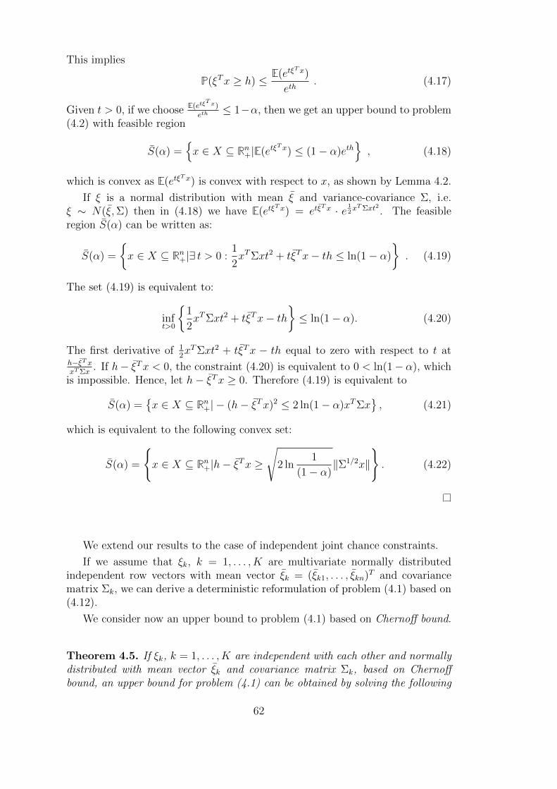
This implies

P(ξTx ≥ h) ≤ E(etξT x)

eth. (4.17)

Given t > 0, if we choose E(etξT x)

eth≤ 1−α, then we get an upper bound to problem

(4.2) with feasible region

S(α) =x ∈ X ⊆ Rn+|E(etξ

T x) ≤ (1− α)eth, (4.18)

which is convex as E(etξT x) is convex with respect to x, as shown by Lemma 4.2.

If ξ is a normal distribution with mean ξ and variance-covariance Σ, i.e.ξ ∼ N(ξ,Σ) then in (4.18) we have E(etξ

T x) = etξT x · e 1

2xTΣxt2 . The feasible

region S(α) can be written as:

S(α) =

x ∈ X ⊆ Rn+|∃ t > 0 :

1

2xTΣxt2 + tξTx− th ≤ ln(1− α)

. (4.19)

The set (4.19) is equivalent to:

inft>0

1

2xTΣxt2 + tξTx− th

≤ ln(1− α). (4.20)

The first derivative of 12xTΣxt2 + tξTx − th equal to zero with respect to t at

h−ξT xxTΣx

. If h− ξTx < 0, the constraint (4.20) is equivalent to 0 < ln(1− α), whichis impossible. Hence, let h− ξTx ≥ 0. Therefore (4.19) is equivalent to

S(α) =x ∈ X ⊆ Rn+| − (h− ξTx)2 ≤ 2 ln(1− α)xTΣx

, (4.21)

which is equivalent to the following convex set:

S(α) =

x ∈ X ⊆ Rn+|h− ξTx ≥

√2 ln

1

(1− α)‖Σ1/2x‖

. (4.22)

We extend our results to the case of independent joint chance constraints.

If we assume that ξk, k = 1, . . . , K are multivariate normally distributedindependent row vectors with mean vector ξk = (ξk1, . . . , ξkn)T and covariancematrix Σk, we can derive a deterministic reformulation of problem (4.1) based on(4.12).

We consider now an upper bound to problem (4.1) based on Chernoff bound.

Theorem 4.5. If ξk, k = 1, . . . , K are independent with each other and normallydistributed with mean vector ξk and covariance matrix Σk, based on Chernoffbound, an upper bound for problem (4.1) can be obtained by solving the following

62

problem

minz,y

cTx

s.t. ξTk x+

√2 ln

(1

1− αyk

)‖Σ1/2

k x‖ ≤ hk, k = 1, . . . , K,

K∑k=1

yk = 1, yk ≥ 0, k = 1, . . . , K, x ∈ X . (4.23)

Proof. First, we note that

P(ξTk x ≤ hk) ≥ αyk ⇐⇒ P(ξTk x ≥ hk) ≤ 1− αyk .

Chernoff bound leads to

P(ξTk x ≥ hk) ≤E(etξ

Tk x)

ethk, k = 1, . . . , K, (4.24)

with t > 0. An upper bound to problem (4.1) is then obtained by solving thefollowing problem with t > 0:

minz,y

cTx

s.t. E(etξTk x) ≤ (1− αyk)ethk , k = 1, . . . , K,

K∑k=1

yk = 1, yk ≥ 0, k = 1, . . . , K, x ∈ X .

(4.25)

However, if the probability distributions of ξk, k = 1, . . . , K are not known,the main difficulty of the model (4.25) is given by the computation of E(etξ

Tk x).

On the other hand, if we assume ξk, k = 1, . . . , K are normal distributions withmean ξk and variance-covariance Σk, i.e. ξk ∼ N(ξk,Σk), then we have that

E(etξTk x) = etξ

Tk x · e 1

2xTΣkxt

2, k = 1, . . . , K. Consequently problem (4.25) can be

written as

minz,y

cTx

s.t. 12xTΣkxt

2 + tξTk x− thk ≤ ln(1− αyk), k = 1, . . . , K,K∑k=1

yk = 1, yk ≥ 0, k = 1, . . . , K, x ∈ X .

(4.26)

Similarly to the individual chance constraint case, we have:

minz,y

cTx

s.t. hk − ξTk x ≥√

2 ln(

11−αyk

)‖Σ1/2

k x‖, k = 1, . . . , K,K∑k=1

yk = 1, yk ≥ 0, k = 1, . . . , K, x ∈ X .

63

Similarly, problem (4.23) is not a convex optimization problem. Therefore,with Assumption 4.1, we apply the transformation z = lnx and get:

minz,y

cT ez

s.t. ξTk ez +

∥∥∥∥∥Σ1/2k e

ln

(√2 ln(

11−αyk

))+z

∥∥∥∥∥ ≤ hk k = 1, . . . , K ,

K∑k=1

yk = 1, yk ≥ 0, k = 1, . . . , K, z ∈ Z , (4.27)

Moreover, if ξk ≥ 0, k = 1, 2, · · · , K, and the function ln(√

2 ln( 11−αyk )

)is

convex, then problem (4.27) is convex. The following lemma shows the convexity

of ln(√

2 ln( 11−αyk )

).

Lemma 4.3. If α ≥ 1 − e−1 ≈ 0.6321, then ln(√

2 ln( 11−αyk )

)is convex with

respect to yk.

Proof. By the convexity theorem of composite function, we only need to prove

the convexity of ln(√

2 ln( 11−p)

)with respect to p, since the convexity of compos-

ite function ln(√

2 ln( 11−αyk )

)is implied when ln

(√2 ln( 1

1−p))

is nondecreasing

and convex. As ln(√

2 ln( 11−p)

)is monotone, we need to show the convexity of

ln(√

2 ln( 11−p)

). We can notice that ln

(√2 ln( 1

1−p))

=1

2ln(

2 ln( 11−p)

). There-

fore, we only need to focus on the convexity of ln(

2 ln( 11−p)

).

The second order derivative of ln(

2 ln( 11−p)

)can be written as

−[(1− p)−2 (ln(1− p))−1 + (1− p)−2 (ln(1− p))−2] ,

= −(1− p)−2 (ln(1− p))−2 (ln(1− p) + 1) .

Then, ln(

2 ln( 11−p)

)is convex if and only if

ln(1− p) + 1 ≤ 0.

Therefore, we have p ≥ 1− e−1.

As αyk is convex with respect to yk and αyk ≥ α for any 0 ≤ yk ≤ 1, if

α ≥ 1− e−1, then the function ln√

2 ln( 11−αyk ) is convex.

Therefore, when c ≥ 0, α ≥ 1− e−1, ξk ≥ 0, k = 1, 2, · · · , K, problem (4.27)is convex.

64

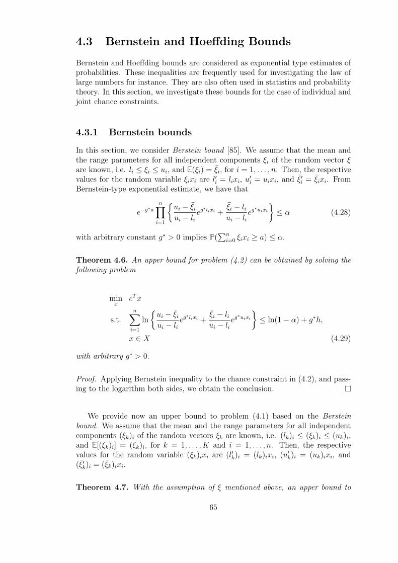
4.3 Bernstein and Hoeffding Bounds

Bernstein and Hoeffding bounds are considered as exponential type estimates ofprobabilities. These inequalities are frequently used for investigating the law oflarge numbers for instance. They are also often used in statistics and probabilitytheory. In this section, we investigate these bounds for the case of individual andjoint chance constraints.

4.3.1 Bernstein bounds

In this section, we consider Berstein bound [85]. We assume that the mean andthe range parameters for all independent components ξi of the random vector ξare known, i.e. li ≤ ξi ≤ ui, and E(ξi) = ξi, for i = 1, . . . , n. Then, the respectivevalues for the random variable ξixi are l′i = lixi, u

′i = uixi, and ξ′i = ξixi. From

Bernstein-type exponential estimate, we have that

e−g∗a

n∏i=1

ui − ξiui − li

eg∗lixi +

ξi − liui − li

eg∗uixi

≤ α (4.28)

with arbitrary constant g∗ > 0 implies P(∑n

i=0 ξixi ≥ a) ≤ α.

Theorem 4.6. An upper bound for problem (4.2) can be obtained by solving thefollowing problem

minx

cTx

s.t.n∑i=1

ln

ui − ξiui − li

eg∗lixi +

ξi − liui − li

eg∗uixi

≤ ln(1− α) + g∗h,

x ∈ X (4.29)

with arbitrary g∗ > 0.

Proof. Applying Bernstein inequality to the chance constraint in (4.2), and pass-ing to the logarithm both sides, we obtain the conclusion.

We provide now an upper bound to problem (4.1) based on the Bersteinbound. We assume that the mean and the range parameters for all independentcomponents (ξk)i of the random vectors ξk are known, i.e. (lk)i ≤ (ξk)i ≤ (uk)i,and E[(ξk)i] = (ξk)i, for k = 1, . . . , K and i = 1, . . . , n. Then, the respectivevalues for the random variable (ξk)ixi are (l′k)i = (lk)ixi, (u′k)i = (uk)ixi, and(ξ′k)i = (ξk)ixi.

Theorem 4.7. With the assumption of ξ mentioned above, an upper bound to

65

problem (4.2) can be obtained by solving the following problem

minx,y

cTx

s.t.n∑i=1

ln

(uk)i − (ξk)i(uk)i − (lk)i

eg∗k(lk)ixi +

(ξk)i − (lk)i(uk)i − (lk)i

eg∗i (uk)ixi

≤ g∗khk +

ln(1− αyk), k = 1, . . . , K,K∑k=1

yk = 1, yk ≥ 0, k = 1, . . . , K, x ∈ X . (4.30)

with arbitrary g∗ > 0.

Proof. According to Berstein-type exponential estimate, we have

e−g∗kak

n∏i=1

(uk)i − (ξk)i(uk)i − (lk)i

eg∗k(lk)ixi +

(ξk)i − (lk)i(uk)i − (lk)i

eg∗k(uk)ixi

≤ αyk , k = 1, . . . , K ,

(4.31)with arbitrary g∗k > 0 which implies P(

∑ni=0(ξk)ixi ≥ ak) ≤ αyk , k = 1, . . . , K.

We note that

P(ξTk x ≤ hk

)≥ αyk , k = 1, . . . , K, (4.32)

m

P

(n∑i=1

(ξk)ixi ≥ hk

)≤ 1− αyk , k = 1, . . . , K. (4.33)

Constraints (4.33) can be approximated by

n∑i=1

ln

(uk)i − (ξk)i(uk)i − (lk)i

eg∗k(lk)ixi +

(ξk)i − (lk)i(uk)i − (lk)i

eg∗k(uk)ixi

≤ ln(1− αyk) + g∗khk

(4.34)for any g∗k > 0, k = 1, . . . , K.

From Proposition 4.1 in [85] and the concavity of function ln(1−αyk), problem(4.30) is convex.

4.3.2 Hoeffding bounds

We consider now an approximation based on Hoeffding inequality ([85]):

P(ξT enn− ξT en

n≥ h) ≤ e

−2n2h2∑ni=1

(ui−li)2 , (4.35)

with the range parameters for all independent components ξi of the random vectorξ, i.e. li ≤ ξi ≤ ui, for i = 1, . . . , n, ξ = E(ξ) and en ∈ Rn is a vector with allelements equal to 1.

66

Theorem 4.8. With the assumption of ξ mentioned above, an upper bound forproblem (4.2) can be obtained by solving the following convex programming prob-lem

minx

cTx

s.t. ξTx+

√2

2

√− ln(1− α)‖Mx‖ ≤ h,

x ∈ X

(4.36)

where M = diag(u− l), u = (u1, . . . , un)T , l = (l1, . . . , ln)n.

Proof. We note that

P(ξTx ≤ h

)≥ α, (4.37)

mP(ξTx− ξTx ≥ h− ξTx

)≤ 1− α . (4.38)

Then, we apply (4.35) to (4.38) and get:

P(ξTx− ξTx ≥ h− ξTx

)≤ e

−2(h−ξT x)2∑ni=1

(ui−li)2x2i . (4.39)

If

e−2(h−ξT x)2∑ni=1

(ui−li)2x2i ≤ 1− α , (4.40)

then (4.37) will be satisfied. Logarithmic transformation of (4.40) leads to

−2(h− ξTx)2∑ni=1(ui − li)2x2

i

≤ ln(1− α) , (4.41)

which can be written as

h− ξTx ≥√

2

2

√− ln(1− α)‖Mx‖, (4.42)

where M = diag(u− l) and then (4.42) is a convex inequality.

Theorem 4.9. Assume that the mean and the range parameters for all indepen-dent components (ξk)i of the random vectors ξk are known, i.e. (lk)i ≤ (ξk)i ≤(uk)i, for k = 1, . . . , K and i = 1, . . . , n. An approximation of problem (4.1)based on Hoeffding’s inequality can be given by

minx,y

cTx

s.t. ξTk x+

√2

2

√ln(

11−αyk

)‖Mkx‖ ≤ hk, k = 1, . . . , K,∑K

k=1 yk = 1, yk ≥ 0, k = 1, . . . , K, x ∈ X,

(4.43)

where Mk = diag(uk − lk), uk = ((uk)1, . . . , (uk)n)T , lk = ((lk)1, . . . , (lk)n)T , k =1, . . . , K.

67

Proof. With almost the same proof method of Theorem 4.8, the conclusion canbe obtained.

Additionally, with Assumption 4.1, an equivalent upper bound for problem(4.1) based on Hoeffding inequality can be obtained by applying the followingtransformation z = lnx:

minz,y

cT ez

s.t. ξTk ez +

1

2‖Mke

ln

(√2 ln(

11−αyk

))+z‖ ≤ hk, k = 1, . . . , K,∑K

k=1 yk = 1, yk ≥ 0, k = 1, . . . , K, z ∈ Z.

(4.44)

From Lemma 4.3, function ln(√

2 ln( 11−αyk )

)is convex, when α ≥ 1 − e−1.

Hence, if c ≥ 0, α ≥ 1− e−1, problem (4.44) is convex.

4.4 Computational Results

Although the problems which give upper bounds obtained by Chebyshev inequal-ity, Chernoff inequality, Bernstein inequality and Hoeffding inequality, respec-tively, for problem (4.1) are convex under some conditions, they are still hard to

solve directly by current tools because of the following terms: ln(√

αyk1−αyk

)and

ln(√

2 ln( 11−αyk )

).

In the following, we denote these functions by Υ(yk). We propose piecewiselinear approximations for Υ(yk) based on tangent and segment approximations.

Tangent approximation

We choose S different linear functions:

ls(yk) = asyk + bs, s = 1, . . . , S,

such thatls(yk) ≤ Υ(yk), ∀yk ∈ [ρ, 1), k = 1, . . . , K.

Here ρ ≥ 0 is a constant such that Υ(yk) is convex on [ρ, 1). Then, Υ(yk) can beapproximated by the following piecewise linear function

l(yk) = maxs=1,...,S

ls(yk),

which provides a lower approximation for Υ(yk).

In order to achieve the expected precision, we set ls(yk) as the tangent line ofΥ(yk) at S points τ1, . . . , τS with τs ∈ [ρ, 1), s = 1, . . . , S. Then, we have

as =dΥ(yk)

dyk

∣∣∣∣yk=τs

, bs = Υ(τs)− asτs.

68

Thanks to these piecewise linear approximations for Υ(yk), we have the fol-lowing results:

Theorem 4.10. Under the aforementioned convexity conditions, if we replace inproblems (4.14), (4.27), (4.44) Υ(yk) by l(yk), we obtain their convex approxima-tions. The optimum values of the approximation problems are lower bounds forproblems (4.14), (4.27), (4.44), respectively. Moreover, the approximation prob-lems become an equivalent reformulation of problems (4.14), (4.27), (4.44) whenS goes to infinity.

Proof. As the approximation problems are obtained by relaxing some constraintsin problems (4.14), (4.27), (4.44), it is easy to see that the optimal values ofthe approximation problems are lower bounds for problems (4.14), (4.27), (4.44),respectively.

We know under convexity conditions for problems (4.14), (4.27), (4.44), Υ(yk)is convex for each problem. As the S tangent functions are selected differently,when S goes to infinity, the constraints in the approximation problems are equiv-alent to the constraints in problems (4.14), (4.27), (4.44), respectively. As theoriginal problems and the corresponding approximation problems are all convexprograms, the approximation problems become an equivalent reformulation ofproblems (4.14), (4.27), (4.44), respectively, when S goes to infinity.

Segment approximation

In order to come up with conservative bounds for the optimum values of problems(4.14), (4.27), (4.44), we use the linear segments asyk + bs, s = 1, . . . , S, betweenτ1, τ2, . . . , τS+1 ∈ [ρ, 1) to construct a piecewise linear function

l(yk) = maxs=1,...,S

asyk + bs

, (4.45)

where

as =Υ(τs+1)−Υ(τs)

τs+1 − τs, bs = Υ(τs)− asτs, s = 1, . . . , S.

Using the piecewise linear function l(yk) to replace Υ(yk) in problems (4.14),(4.27), (4.44), gives the corresponding approximation problems.

Similar to Theorem 4.10, we can derive the following result for the linearapproximation:

Theorem 4.11. Under the aforementioned convexity conditions, if we replace inproblems (4.14), (4.27), (4.44) Υ(yk) by l(yk), we obtain the convex approxima-tions of these problems. The optimum values of the approximation problems arean upper bound for problems (4.14), (4.27), (4.44), respectively. Moreover, theapproximation problems become an equivalent reformulation of problems (4.14),(4.27), (4.44), respectively, when S goes to infinity.

The proof of this theorem follows the same pattern as the proof of Theorem4.10.

69

Numerical experiments

The four bounds have been implemented and compared under Matlab environ-ment using CVX software, a modeling system for constructing and solving convexprograms. We run the bounds for 100 instances randomly generated with the fol-lowing characteristics: in the individual chance constraint (4.2) we set n = 10,h = 0.5, α = 0.95, the constraint x ∈ X ∈ Rn+ is given by

∑ni=1 xi = 1, c is a

random vector from a uniform distribution in the interval [0, 1]n, ξT is uniformlygenerated in the interval [0, 10]n and σ2

ξ is uniformly generated in the interval[0, 1]n×n. In the following, we assume that the random variable ξ is distributedaccording to a normal distribution with mean ξ and variance σ2

ξ generated asdescribed above. This will allow us to make a fair comparison of the bounds withthe exact SOCP reformulation. For joint chance constrained problem(4.1), weset n = 10, K = 5 and hi = 0.5, i = 1, · · · , K. The other parameters are thesame as those in the individual case.

As upper and lower bounds for random vector ξ are needed in Bernstein andHoeffding bounds, 5000 samples following a normal distribution with mean ξ andvariance σ2

ξ described above are generated. And the maximal value of these 5000samples is selected as upper bound while the minimal value is selected as lowerbound

Numerical results for the individual chance constraint case are reported inFigure 4.1: Figure 4.1(a) shows a comparison of the objective function values ofthe four bounds (Chebyshev, Chernoff, Bernstein and Hoeffding) with the exactSOCP reformulation for 100 different randomly generated instances, while Fig-ure 4.1(b) shows the corresponding box-and-whisker plots where the extrema ofthe box represents the 1/4 and 3/4 quartiles, the band inside the box is the me-dian and the whiskers the minimum and maximum obtained from 100 randomlygenerated instances.

0 10 20 30 40 50 60 70 80 90 100

instances

0

0.05

0.1

0.15

0.2

0.25

0.3

0.35

0.4

optim

al valu

es

socp vs bound

(a)

SOCP Bernstein Chebyshev Chernoff Hoeffding

instances

0

0.05

0.1

0.15

0.2

0.25

0.3

0.35

op

tim

al va

lue

s

SOCP vs bounds

(b)

Figure 4.1: (a) Comparison of SOCP versus bounds for individual chance con-straint. (b) box-and-whisker plots from the same 100 randomly generated in-stances of (a).

The average CPU times and gaps for different bounds and SOCP are shownin Table 4.1 in second and third rows, respectively. Results from Figure 4.1 and

70

Table 4.1 show that the best upper bound is obtained by Chernoff inequality,followed by Bernstein which in all the instances outperfoms one-side Chebyshevand Hoeffding ones. The worst bound is in all the cases obtained by Hoeffdingapproximation. Notice that the CPU times for Chebyshev, Chernoff, Bernstein,Hoeffding and SOCP are relatively comparable. The reason for the good perfor-mance of Chernoff bound compared to the others, could be due to the explicitassumption that the moment generating function of the random variable ξ fol-lows a normal distribution, information not taken into account in all the otherapproaches. Very good is the performance of the Bernstein bound, consideringthat only the mean and the range of the random variable are known.

Table 4.1: Average results over 100 instances of different bounds and SOCP forindividual chance constrained problem.

Bound Chebyshev Chernoff Bernstein Hoeffding SOCP

CPU time(s) 0.9815 0.9727 1.2761 1.0850 0.9932

Gap (%) 7.55 1.58 2.8 13.64 -

Numerical results for the joint chance constraints case are reported in Figure4.2: Figure 4.2(a) shows a comparison of the objective function values of the fourbounds (Chebyshev, Chernoff, Bernstein and Hoeffding) with the SOCP refor-mulation for 100 different randomly generated instances, where SOCP, Hoeffdingand Chernoff are obtained both with tangent and segment approximations withS = 50. Figure 4.2(b) shows the corresponding box-and-whisker plots where theextrema of the box represents the 1/4 and 3/4 quartiles, the band inside the boxis the median and the whiskers the minimum and maximum obtained from 100randomly generated instances.

0 10 20 30 40 50 60 70 80 90 100

instances

0.1

0.15

0.2

0.25

0.3

0.35

0.4

0.45

0.5

0.55

0.6

Op

tim

al va

lue

Optimal value socp vs Bounds

socpTangent

socpSegment

HoeffdingTangent

HoeffdingSegment

ChernoffTangent

ChernoffSegment

Chebyshev

Bernstein

(a)

SOCP_S SOCP_T Bernstein Chebyshev Chernoff_S Chernoff_T Hoeffding_S Hoeffding_T

Instances

0.2

0.25

0.3

0.35

0.4

0.45

0.5

0.55

0.6

0.65

Op

tim

al V

alu

es

Optimal value SOCP vs Bounds

(b)

Figure 4.2: (a) Comparison of SOCP versus bounds for the joint chance con-strained problem. (b) Box-and-whisker plots from the same 100 randomly gener-ated instances of (a).

Table 4.2 shows the average CPU time (second row) for different bounds andSOCP and the average gap (third row) between different bounds and SOCP for

71

the joint chance constraints case. Results from Figure 4.2 and Table 4.2 showthat Chebyshev bound always provide the worst bound, while there are not muchdifferences among other bounds. As in the individual chance constraint case,the best bound is the Chernoff one followed by the Bernstein’s bound. Noticethat the CPU times for Chebyshev, Chernoff, Bernstein, Hoeffding and SOCPare relatively comparable.

Table 4.2: Average results of different bounds and SOCP for the joint chanceconstrained problem.

Bound Chebyshev Chernoff Bernstein Hoeffding SOCP

CPU time(s) 2.9932 2.8255 3.2030 2.2845 2.2551

Gap (%) 12.30 3.69 3.91 4.01 -

Notice that in the upper bound problems obtained by Chernoff and Hoeffd-ing inequalities for problem (1), we use tangent and segment approximations,

as described above, to approximate the complex terms: ln(√

2 ln(

11−αyk

))and

ln

(√2 ln

(1

1−yk

)), respectively.

A sensitivity analysis of the segment and tangent approximations on the num-ber of segments S = 3, 10, 20, 50 is reported in Figure 4.3 with correspondingbox-and-whisker plots in Figure 4, for 100 instances randomly generated. Resultsshow that when S = 50, there’s almost no gap between the results obtained bytangent and segment approximations, respectively. And for each S, Chernoff in-equality and Hoeffding inequality always provide an upper bound for the resultobtained by SOCP.

4.5 Conclusion

In this chapter, we propose deterministic approximations for individual and jointchance constraints with independent matrix vector rows. The bounds are basedon classical inequalities from probability theory such as the one-side Chebyshevinequality, Bernstein inequality, Chernoff inequality and Hoeffding inequality andallow to reformulate the problem in in a tractable convex way. Approximationsbased on piecewise linear and tangent are also provided in case of Chernoff andHoeffding inequalities allowing to reduce the computational complexity of theproblem. Finally numerical results on randomly generated data are provided al-lowing to identify that the Chernoff bound provides the tighter deterministic ap-proximation while the Chebyshev bound, requiring the knowledge of the first andsecond moments, is very loose both for individual and joint chance constrainedproblems. Remarkable is also the performance of Bernstein’s bound, consideringthat only the mean and the range of the random variables are assumed to beknown. In terms of CPU times all the considered bounds are relatively compa-rable.

This chapter correrponds to the reference [81].

72

0 10 20 30 40 50 60 70 80 90 100

instances

0

0.1

0.2

0.3

0.4

0.5

0.6

0.7

Optim

al valu

e

Optimal value socp vs Bounds with S=3

socpTangent

socpSegment

HoeffdingTangent

HoeffdingSegment

ChernoffTangent

ChernoffSegment

(a)

0 10 20 30 40 50 60 70 80 90 100

instances

0.1

0.15

0.2

0.25

0.3

0.35

0.4

0.45

0.5

0.55

0.6

Optim

al valu

e

Optimal value socp vs Bounds with S=10

socpTangent

socpSegment

HoeffdingTangent

HoeffdingSegment

ChernoffTangent

ChernoffSegment

(b)

0 10 20 30 40 50 60 70 80 90 100

instances

0.15

0.2

0.25

0.3

0.35

0.4

0.45

0.5

0.55

Optim

al valu

e

Optimal value socp vs Bounds with S=20

socpTangent

socpSegment

HoeffdingTangent

HoeffdingSegment

ChernoffTangent

ChernoffSegment

(c)

0 10 20 30 40 50 60 70 80 90 100

instances

0.15

0.2

0.25

0.3

0.35

0.4

0.45

0.5

0.55

Optim

al valu

e

Optimal value socp vs Bounds with S=50

socpTangent

socpSegment

HoeffdingTangent

HoeffdingSegment

ChernoffTangent

ChernoffSegment

(d)

Figure 4.3: Comparison of SOCP versus bounds for the joint chance constrainedproblem with different values of S for segment and tangent approximations.

73

SOCP_S SOCP_T Chernoff_S Chernoff_T Hoeffding_S Hoeffding_T

Instances

0.1

0.2

0.3

0.4

0.5

0.6

0.7

Op

tim

al V

alu

es

Optimal value SOCP vs Bounds with S=3

(a)

SOCP_S SOCP_T Chernoff_S Chernoff_T Hoeffding_S Hoeffding_T

Instances

0.15

0.2

0.25

0.3

0.35

0.4

0.45

0.5

0.55

0.6

Optim

al V

alu

es

Optimal value SOCP vs Bounds with S=10

(b)

SOCP_S SOCP_T Chernoff_S Chernoff_T Hoeffding_S Hoeffding_T

Instances

0.2

0.25

0.3

0.35

0.4

0.45

0.5

0.55

0.6

Optim

al V

alu

es

Optimal value SOCP vs Bounds with S=20

(c)

SOCP_S SOCP_T Chernoff_S Chernoff_T Hoeffding_S Hoeffding_T

Instances

0.2

0.25

0.3

0.35

0.4

0.45

0.5

0.55

0.6

Optim

al V

alu

es

Optimal value SOCP vs Bounds with S=50

(d)

Figure 4.4: Box-and-whisker plots corresponding to Figure 4.3 for different valuesof S = 3, 10, 20, 50 with segment and tangent approximations.

74

Chapter 5

Data-Driven Robust ChanceConstrained Problems: AMixture Model Approach

This chapter discusses the mixture distribution based data-driven robust chanceconstrained problem. We construct a data-driven mixture distribution baseduncertainty set from the perspective of simultaneously estimating higher ordermoments. Then, we derive a reformulation of the data-driven robust chance con-strained problem. As the reformulation is not a convex programming, we proposenew and tight convex approximations based on the piecewise linear approxima-tion method under certain conditions. For the general case, we propose a DCapproximation to derive an upper bound and a relaxed convex approximationto derive a lower bound for the optimal value of the original problem, respec-tively. We establish the theoretical foundation for these approximations. Finally,the results of simulation experiments show that the proposed approximations arepractical and efficient.

5.1 Mixture Distribution Based Uncertainty Set

As a preparation for our later construction of the data-driven robust chanceconstrained problem, we first define the uncertainty set under the mixture distri-bution framework, and then consider the moments estimation from sample datato determine the parameters of the data-driven uncertainty set.

We assume that the n-dimensional random vector ξ has a continuous proba-bility density function. For notational clarity, we use f to denote the distributionof ξ and f(·) to denote the probability density function of ξ.

To ensure a reliable estimation of the real distribution, we assume that ξfollows a finite normal mixture distribution. This means that f(·) can be explicitlydefined by

f(·) =M∑m=1

wmfm(·), (5.1)

here fm(·) is the probability density function of the m-th component. In this

75

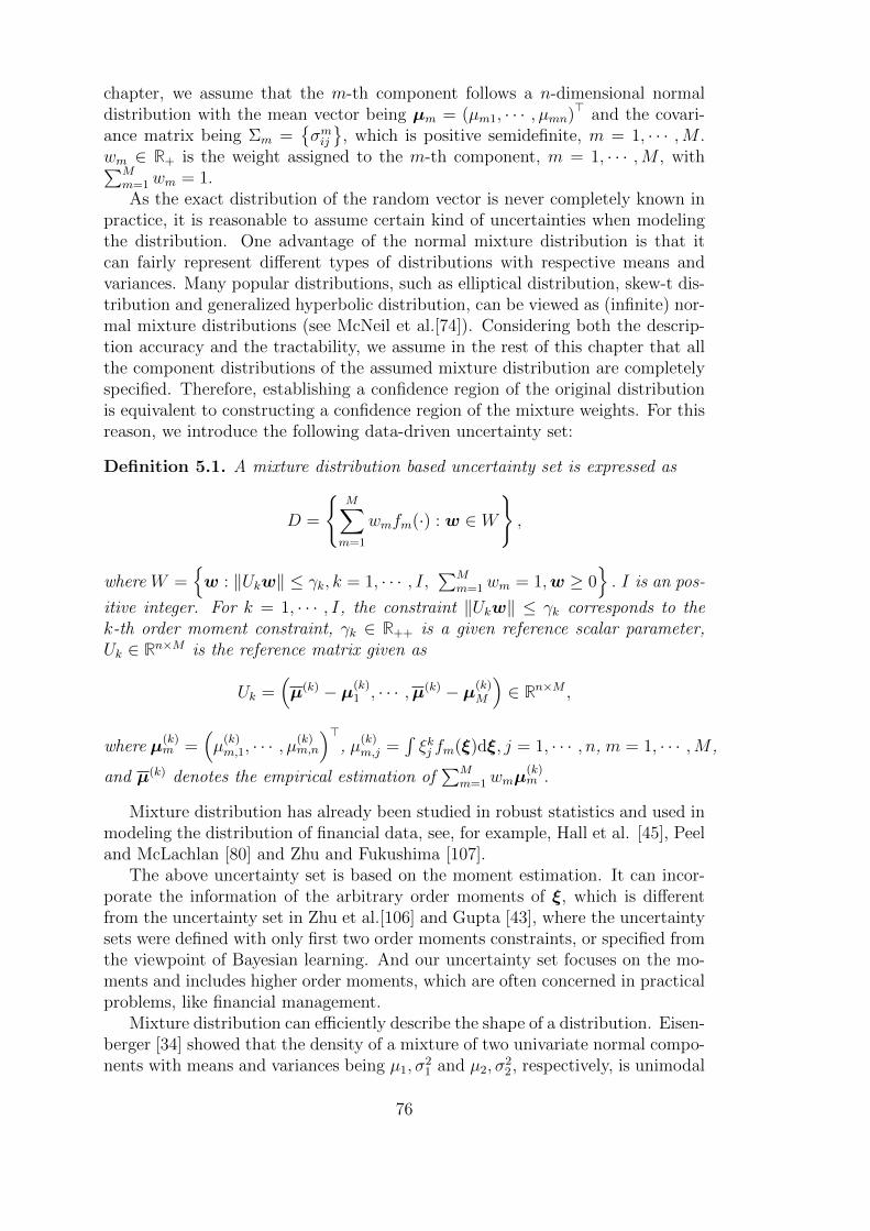
chapter, we assume that the m-th component follows a n-dimensional normaldistribution with the mean vector being µm = (µm1, · · · , µmn)> and the covari-ance matrix being Σm =

σmij

, which is positive semidefinite, m = 1, · · · ,M .wm ∈ R+ is the weight assigned to the m-th component, m = 1, · · · ,M , with∑M

m=1wm = 1.As the exact distribution of the random vector is never completely known in

practice, it is reasonable to assume certain kind of uncertainties when modelingthe distribution. One advantage of the normal mixture distribution is that itcan fairly represent different types of distributions with respective means andvariances. Many popular distributions, such as elliptical distribution, skew-t dis-tribution and generalized hyperbolic distribution, can be viewed as (infinite) nor-mal mixture distributions (see McNeil et al.[74]). Considering both the descrip-tion accuracy and the tractability, we assume in the rest of this chapter that allthe component distributions of the assumed mixture distribution are completelyspecified. Therefore, establishing a confidence region of the original distributionis equivalent to constructing a confidence region of the mixture weights. For thisreason, we introduce the following data-driven uncertainty set:

Definition 5.1. A mixture distribution based uncertainty set is expressed as

D =

M∑m=1

wmfm(·) : w ∈ W

,

where W =w : ‖Ukw‖ ≤ γk, k = 1, · · · , I,

∑Mm=1wm = 1,w ≥ 0

. I is an pos-

itive integer. For k = 1, · · · , I, the constraint ‖Ukw‖ ≤ γk corresponds to thek-th order moment constraint, γk ∈ R++ is a given reference scalar parameter,Uk ∈ Rn×M is the reference matrix given as

Uk =(µ(k) − µ(k)

1 , · · · ,µ(k) − µ(k)M

)∈ Rn×M ,

where µ(k)m =

(µ

(k)m,1, · · · , µ

(k)m,n

)>, µ

(k)m,j =

´ξkj fm(ξ)dξ, j = 1, · · · , n, m = 1, · · · ,M ,

and µ(k) denotes the empirical estimation of∑M

m=1 wmµ(k)m .

Mixture distribution has already been studied in robust statistics and used inmodeling the distribution of financial data, see, for example, Hall et al. [45], Peeland McLachlan [80] and Zhu and Fukushima [107].

The above uncertainty set is based on the moment estimation. It can incor-porate the information of the arbitrary order moments of ξ, which is differentfrom the uncertainty set in Zhu et al.[106] and Gupta [43], where the uncertaintysets were defined with only first two order moments constraints, or specified fromthe viewpoint of Bayesian learning. And our uncertainty set focuses on the mo-ments and includes higher order moments, which are often concerned in practicalproblems, like financial management.

Mixture distribution can efficiently describe the shape of a distribution. Eisen-berger [34] showed that the density of a mixture of two univariate normal compo-nents with means and variances being µ1, σ

21 and µ2, σ

22, respectively, is unimodal

76

if (µ1 − µ2)2 <27σ2

1σ22

4(σ21+σ2

2). For the case that (µ1 − µ2)2 >

27σ21σ

22

4(σ21+σ2

2), there exist

values of the weights for which the density function is bimodal. For the unimodalcase, first two order moments can describe the location and dispersion, while thedensity shape can be described through concepts like skewness and kurtosis [93].For the multimodal case, a probability distribution can be characterized by itsenough moments [73]. Then, the multimodality can be described efficiently withenough moments. For the above reasons, we use the mixture distribution withuncertain weights to construct the uncertainty set and use moments to estimatethe size of uncertainty set. Our approach is a complementary to the existinguncertainty sets which focus on the unimodal case [63].

We will show that the parameters Uk, γk, k = 1, · · · , I, of the uncertainty set Dcan be determined by a set of independently observed samples from the underlyingdistribution of ξ, and the confidence region defined by Uk, γk, k = 1, · · · , I, isassured with high probability to contain the first four componentwise momentsof ξ.

5.1.1 Data-Driven Confidence Region for Moments

In order to get the confidence region for moments of ξ, we use a measurablefunction π(ξ) to denote a vector valued or matrix valued mapping of ξ, whilethe norm ‖ · ‖ with respect to π(ξ) is the Euclidean norm when π(ξ) is vectorvalued, and is the Frobenius norm when π(ξ) is matrix valued. Suppose that wehave a sample set S of ξ with N observations ξ(l), l = 1, · · · , N . Then we denoteπS = 1

N

∑Nl=1 π(ξ(l)).

To derive the basic conclusion of this subsection, we utilize an inequalityknown as the “independent bounded differences inequality”, which is estabilshedby McDiarmid in [44].

Lemma 5.1. Let X = (X1, · · · , Xn) be a family of independent random variableswith Xk taking values in a set Ak for each k, 1 ≤ k ≤ n. Suppose that thereal-valued function Γ defined on

∏nk=1 Ak satisfies

|Γ(x)− Γ(x′)| ≤ ck, k = 1, · · · , n,

whenever the vectors x and x′ differ only in the k-th coordinate. Then for anyτ ≥ 0,

PΓ(X)− E[Γ(X)] ≥ τ ≤ exp

(−2τ 2∑nk=1 c

2k

).

With this lemma, we have the following theorem for chosen ε ∈ ]0, 1[ .

Theorem 5.1. Let S be a sample set with N observations which are generatedindependently at random according to the distribution of ξ whose density functionis defined by (5.1), and suppose that there exists an R <∞ such that P‖π(ξ)‖ ≤R ≥ 1− ε. Then with probability at least 1−∆, we have

‖πS − Eξ[π(ξ)]‖ ≤ 1√N

(2ρM +R

√2 ln

1− ε∆− ε

), (5.2)

77

where ε < ∆ < 1, ρ2M = max

m=1,··· ,M

´‖π(ξ)‖2fm(ξ)dξ

and ρM ≥ 0.

Proof. Let g(S) = ‖πS−Eξ[π(ξ)]‖ denote the measure of the estimation accuracybased on the sample S.

By Lemma 2.3.1 in [100], we have

ES[g(S)] = ES[‖πS − Eξ[π(ξ)]‖] ≤ 2Er,S[‖ 1

N

N∑l=1

rlπ(ξ(l))‖],

where r = (r1, · · · , rN)> and rl, l = 1, · · · , N , are Rademacher variables whichhave 50% chance of being +1 or −1 and are independent of S. It is then knownfrom the Jensen’s inequality that

Er,S[‖ 1

N

N∑l=1

rlπ(ξ(l))‖] =1

NEr,S[‖

N∑l=1

rlπ(ξ(l))‖]

=1

NEr,S

⟨ N∑

l=1

rlπ(ξ(l)),N∑l=1

rlπ(ξ(l))

⟩1/2

≤ 1

N

Er,S

N∑l,l=1

rlrl

⟨π(ξ(l)), π(ξ(l))

⟩1/2

,

where 〈·, ·〉 denotes the inner product with respect to π(ξ). When π(ξ) is a vec-

tor,⟨π(ξ(l)), π(ξ(l))

⟩=(π(ξ(l))

)>π(ξ(l)). Otherwise, 〈·, ·〉 denotes the Frobenius

inner product. Thus, by utilizing the fact that rlrl, l 6= l, takes the two possiblevalues +1,−1 with equal probabilities, we haveEr,S

N∑l,l=1

rlrl

⟨π(ξ(l)), π(ξ(l))

⟩1/2

=

(ES

[N∑l=1

‖π(ξ(l))‖2

])1/2

.

Therefore,

ES[g(S)] ≤ 2

N

(ES

[N∑l=1

‖π(ξ(l))‖2

])1/2

=2

N

(NEξ

[‖π(ξ)‖2

])1/2=

2√N

(Eξ[‖π(ξ)‖2

])1/2,

Eξ[‖π(ξ)‖2

]=

ˆ M∑m=1

‖π(ξ)‖2wifm(ξ)dξ

=M∑m=1

wm

ˆ‖π(ξ)‖2fm(ξ)dξ =

M∑m=1

wmρ2m.

78

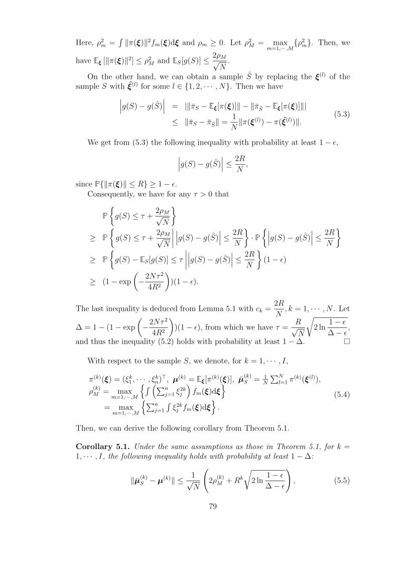
Here, ρ2m =

´‖π(ξ)‖2fm(ξ)dξ and ρm ≥ 0. Let ρ2

M = maxm=1,··· ,M

ρ2m. Then, we

have Eξ [‖π(ξ)‖2] ≤ ρ2M and ES[g(S)] ≤ 2ρM√

N.

On the other hand, we can obtain a sample S by replacing the ξ(l) of thesample S with ξ(l) for some l ∈ 1, 2, · · · , N. Then we have∣∣∣g(S)− g(S)

∣∣∣ = |‖πS − Eξ[π(ξ)]‖ − ‖πS − Eξ[π(ξ)]‖|

≤ ‖πS − πS‖ =1

N‖π(ξ(l))− π(ξ(l))‖.

(5.3)

We get from (5.3) the following inequality with probability at least 1− ε,∣∣∣g(S)− g(S)∣∣∣ ≤ 2R

N,

since P‖π(ξ)‖ ≤ R ≥ 1− ε.Consequently, we have for any τ > 0 that

P

g(S) ≤ τ +

2ρM√N

≥ P

g(S) ≤ τ +

2ρM√N

∣∣∣∣ ∣∣∣g(S)− g(S)∣∣∣ ≤ 2R

N

· P∣∣∣g(S)− g(S)

∣∣∣ ≤ 2R

N

≥ P

g(S)− ES[g(S)] ≤ τ

∣∣∣∣∣∣∣g(S)− g(S)∣∣∣ ≤ 2R

N

(1− ε)

≥ (1− exp

(−2Nτ 2

4R2

))(1− ε).

The last inequality is deduced from Lemma 5.1 with ck =2R

N, k = 1, · · · , N . Let

∆ = 1− (1− exp

(−2Nτ 2

4R2

))(1− ε), from which we have τ =

R√N

√2 ln

1− ε∆− ε

,

and thus the inequality (5.2) holds with probability at least 1−∆.

With respect to the sample S, we denote, for k = 1, · · · , I,

π(k)(ξ) = (ξk1 , · · · , ξkn)>, µ(k) = Eξ[π(k)(ξ)], µ(k)S = 1

N

∑Nl=1 π

(k)(ξ(l)),

ρ(k)M = max

m=1,··· ,M

´ (∑nj=1 ξ

2kj

)fm(ξ)dξ

= max

m=1,··· ,M

∑nj=1

´ξ2kj fm(ξ)dξ

.

(5.4)

Then, we can derive the following corollary from Theorem 5.1.

Corollary 5.1. Under the same assumptions as those in Theorem 5.1, for k =1, · · · , I, the following inequality holds with probability at least 1−∆:

‖µ(k)S − µ

(k)‖ ≤ 1√N

(2ρ

(k)M +Rk

√2 ln

1− ε∆− ε

), (5.5)

79

where ρ(k)M , 1 ≤ k ≤ I, are defined in (5.4) and ∆ is the same as that in Theorem

5.1.

Proof. For k = 1, · · · , I, consider the mapping π : ξ 7→ π(k)(ξ). Then we have

‖π(ξ)‖ =

√√√√ n∑m=1

ξ2km ≤

√√√√( n∑m=1

ξ2m

)k

= (‖ξ‖)k.

Therefore, by applying Theorem 5.1 to the mapping π, the inequality (5.5) followssince P‖π(ξ)‖ ≤ Rk ≥ P‖ξ‖ ≤ R ≥ 1− ε.

The determination of parameters ρ(k)M , 1 ≤ k ≤ I, in Theorem 5.1 amounts

to calculating´ξ2kj fm(ξ)dξ, j = 1, · · · , n, m = 1, · · · ,M, which are actually the

2k-th order origin moments of the j-th random variable whose density function isfm(·). For m = 1, · · · ,M , as fm(·) is the density function of a given n-dimensionalnormal distribution with the mean vector being µm and the covariance matrixbeing Σm,

´ξ2kj fm(ξ)dξ, j = 1, · · · , n, can be easily computed with the help of

the moment generation function of normal distribution.

All the above derivations assume that one can pre-specify a ball which containsthe support with probability at least 1− ε. To make the results more tractable,we need to estimate the radius R from the samples. Concretely, we have thefollowing conclusion.

Corollary 5.2. Let S be an N sample set, with observations ξ(l), l = 1, · · · , N ,generated independently at random according to the distribution of ξ whose densityfunction is defined by (5.1), and the support of ξ is contained in a ball with

probability at least 1− ε. Let µ(k)S = 1

N

∑Nl=1 π

(k)(ξ(l)) and

R = max‖ξ(l)‖, l = 1, · · · , N

be a sample-based estimation for the radius R of the ball. If

N ≥ 2

εln

1

∆+ 2n+

2n

εln

2

ε,

then with probability at least (1−∆)2, the inequality (5.5) holds with R replacedwith R.

Proof. Consider the following optimization problem:

minRR s.t. P‖ξ‖ ≤ R ≥ 1− ε.

We use the scenario approach to bound the above chance constraint such thatit holds with probability 1 −∆. Specifically, the scenario approach replaces thechance constraint with the following deterministic constraints:

‖ξ(l)‖ ≤ R, l = 1, · · · , N. (5.6)

80

This means that we have R = max‖ξ(l)‖, l = 1, · · · , N

to be the optimum

value under constraints (5.6). We know from Corollary 1 in [14] that, if N ≥2

εln

1

∆+ 2n +

2n

εln

2

ε, the original chance constraint will hold with probability

no smaller than 1−∆, or more formally,

P

P‖ξ‖ ≤ R ≥ 1− ε≥ 1−∆.

Here, the inner probability is with respect to ξ, while the outer probability iswith respect to R, since R is also random due to the randomness of the sampleS from a statistical point of view.

Given that the event A0: P‖ξ‖ ≤ R ≥ 1 − ε occurs, we conclude fromCorollary 5.1 that with probability at least 1 − ∆, the inequality (5.5) holds.The probability of the event E that constraint (5.5) holds is necessarily at least(1−∆)2:

PE ≥ PE |A0PA0 ≥ (1−∆) (1−∆) = (1−∆)2,

which completes the proof.

5.1.2 Data-Driven Confidence Region for Mixture Weights

With the above results, we can concretely specify the uncertainty set D in Defini-

tion 5.1 by using historical samples. To this end, we denote µ(k)m =

(µ

(k)m,1, · · · , µ

(k)m,n

)>,

here µ(k)m,j =

´ξkj fm(ξ)dξ, j = 1, · · · , n, m = 1, · · · ,M , and denote the empirical

estimation of µ(k) by µ(k), k = 1, · · · , I.As ξ follows the mixture distribution whose density function is defined by

(5.1), we have µ(k) =∑M

m=1wmµ(k)m , and the support of ξ can be contained in a

ball with any specified probability 1 − ε. Therefore, by applying Corollary 5.2,we have

‖µ(k) −M∑m=1

wmµ(k)m ‖ ≤ γk, k = 1, · · · , I, (5.7)

hold with probability at least (1−∆)2. Here

γk =1√N

(2ρ

(k)M +R

k

√2 ln

1− ε∆− ε

), k = 1, · · · , I. (5.8)

To derive a proper presentation for the uncertainty set, we now show thatthe confidence region for mixture weights can be described as the intersection ofsome ellipsoidal sets. Concretely, for k = 1, · · · , I, we have

‖µ(k)−M∑m=1

wmµ(k)m ‖ ≤ γk ⇔

∥∥∥∥∥M∑m=1

wm(µ(k) − µ(k)

m

)∥∥∥∥∥ ≤ γk ⇔ ‖Ukw‖ ≤ γk, (5.9)

whereUk =

(µ(k) − µ(k)

1 , · · · ,µ(k) − µ(k)M

)∈ Rn×M . (5.10)

81

By now, we have obtained an easily implemented representation for the mix-ture distribution based uncertainty set D given in Definition 5.1, with γk andUk, k = 1, · · · , I, being defined in (5.8) and (5.10), respectively.

From (5.8) and the first inequality in (5.9), we see that when N increases, thedistance between the estimated moments and true moments becomes smaller.This means that the estimated moments become more accurate and the uncer-tainty set D becomes smaller when N increases, which is consistent with intuition.Moreover, as N increases, the estimated values of moments tend to their true val-ues. All these observations tell us that when N becomes large, the true valuesof weights w are contained in the uncertainty set, which implies the feasibility ofour obtained uncertainty set.

5.2 Data-Driven Robust Chance Constrained Prob-

lems

With the data-driven uncertainty set specified in Definition 5.1, we now considerthe correspondingly data-driven robust chance constrained problem:

(P) minz

g (z) , s.t. inff∈D

Pfξ>z ≤ d

≥ 1− α, z ∈ Z,

where ξ ∈ Rn is a random vector defined on some probability space (Ω,F ,P),Z ⊆ Rn is a deterministic closed and convex set, g (z) : Rn → R is a continuousfunction, d ∈ R is a constant. f is the joint probability distribution functionof ξ. D, defined in Definition 5.1, is an uncertainty set of the joint probabilitydistribution f and α ∈]0, 1[ is the tolerance probability, say, 0.01 or 0.05.

5.2.1 Reformulation of Problem (P)

As ξ follows a mixture distribution f in the uncertainty set D, we have that

Pfξ>z ≤ d

=

ˆξ>z≤d

M∑m=1

wifm(ξ)dξ =M∑m=1

wm

ˆξ>z≤d

fm(ξ)dξ = p(z)>w,

where p(z) = (p1(z), · · · , pM(z))>, pm(z) =´ξ>z≤d fm(ξ)dξ. Therefore,

inff∈D

Pfξ>z ≤ d

= infw∈W

p(z)>w. (5.11)

To derive the reformulation of problem (P), we need the following assumption.

Assumption 5.1. Assume that for any z ∈ Z, the Slater’s conditions hold forproblem (5.11).

According to the definition of W , we have from the duality theory in [5] that

82

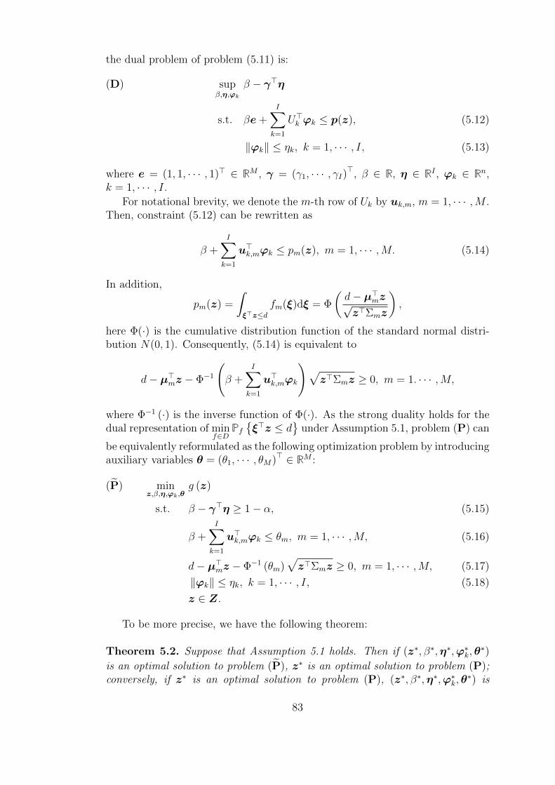
the dual problem of problem (5.11) is:

(D) supβ,η,ϕk

β − γ>η

s.t. βe+I∑

k=1

U>k ϕk ≤ p(z), (5.12)

‖ϕk‖ ≤ ηk, k = 1, · · · , I, (5.13)

where e = (1, 1, · · · , 1)> ∈ RM , γ = (γ1, · · · , γI)>, β ∈ R, η ∈ RI , ϕk ∈ Rn,k = 1, · · · , I.

For notational brevity, we denote the m-th row of Uk by uk,m, m = 1, · · · ,M .Then, constraint (5.12) can be rewritten as

β +I∑

k=1

u>k,mϕk ≤ pm(z), m = 1, · · · ,M. (5.14)

In addition,

pm(z) =

ˆξ>z≤d

fm(ξ)dξ = Φ

(d− µ>mz√z>Σmz

),

here Φ(·) is the cumulative distribution function of the standard normal distri-bution N(0, 1). Consequently, (5.14) is equivalent to

d− µ>mz − Φ−1

(β +

I∑k=1

u>k,mϕk

)√z>Σmz ≥ 0, m = 1. · · · ,M,

where Φ−1 (·) is the inverse function of Φ(·). As the strong duality holds for thedual representation of min

f∈DPfξ>z ≤ d

under Assumption 5.1, problem (P) can

be equivalently reformulated as the following optimization problem by introducingauxiliary variables θ = (θ1, · · · , θM)> ∈ RM :

(P) minz,β,η,ϕk,θ

g (z)

s.t. β − γ>η ≥ 1− α, (5.15)

β +I∑

k=1

u>k,mϕk ≤ θm, m = 1, · · · ,M, (5.16)

d− µ>mz − Φ−1 (θm)√z>Σmz ≥ 0, m = 1, · · · ,M, (5.17)

‖ϕk‖ ≤ ηk, k = 1, · · · , I, (5.18)

z ∈ Z.

To be more precise, we have the following theorem:

Theorem 5.2. Suppose that Assumption 5.1 holds. Then if (z∗, β∗,η∗,ϕ∗k,θ∗)

is an optimal solution to problem (P), z∗ is an optimal solution to problem (P);conversely, if z∗ is an optimal solution to problem (P), (z∗, β∗,η∗,ϕ∗k,θ

∗) is

83

an optimal solution to problem (P), here (β∗,η∗,ϕ∗k) is an optimal solution to

problem (D) and θ∗ = Φ

(d−µ>mz√z>Σmz

).

Proof. Let (z∗, β∗,η∗,ϕ∗k,θ∗) be an optimal solution to problem (P). By the

weak duality theorem, we have

inff∈D

Pfξ>z ≤ d

= infw∈W

p(z)>w ≥ β∗ − γ>η∗ ≥ 1− α,

where the last inequality follows from (5.15). This implies that z∗ is feasible forproblem (P). In the following, we prove that it is also optimal to problem (P).

Suppose that, on the contrary, z∗ is not optimal to problem (P), i.e., there ex-ists an optimal solution z∗ such that g (z∗) < g (z∗). Let (β∗, η∗, ϕk

∗) be the cor-

responding optimal solution to problem (D) and θ∗ = p(z∗) = Φ

(d−µ>mz∗√(z∗)>Σmz∗

).

From Assumption 5.1 and the strong conic duality theory in [5], we have

β∗ − γ>η∗ = infw∈W

p(z∗)>w ≥ 1− α.

This and other constraints in problems (P) and (D) mean that (z∗, β∗, η∗, ϕk∗,

θ∗) is feasible for problem (P). This contradicts the fact that (z∗, β∗,η∗,ϕ∗k,θ∗)

is an optimal solution to problem (P) since g (z∗) < g (z∗). Therefore, z∗ is anoptimal solution to problem (P).

On the other hand, let z∗ be an optimal solution to problem (P), (β∗,η∗,ϕ∗k)

be an optimal solution to problem (D) and θ∗ = Φ

(d−µ>mz√z>Σmz

). Then, (z∗, β∗,

η∗,ϕ∗k,θ∗) must constitute an optimal solution to problem (P). Otherwise, there

would exist an optimal solution (z∗, β∗, η∗, ϕk∗, θ∗) to problem (P) such that

g (z∗) < g (z∗). And we know from the first part of the proof that z∗ must be anoptimal solution to problem (P), which contradicts the fact that z∗ is an optimalsolution to problem (P) since g (z∗) < g (z∗).

Problem (P) is a non-convex programming problem due to the third group ofconstraints (5.17). We will derive its convex approximations in subsection 5.2.2 ,and its DC programming approximations in subsection 5.2.3.

5.2.2 Convex Approximation

In this part, we will show that, under certain conditions, problem (P) can bereformulated as a convex programming problem. Liu et al [65] proposed tightconvex approximations to a kind of joint geometric chance constrained problems.We extend their method and propose tight convex approximations to problem(P) under some conditions. To this end, we need the following assumption:

Assumption 5.2. Denote et = (et1 , · · · , etn)>

for t = (t1, · · · , tn)>. Assumethat

1) α ≤ 1− Φ(1),

84

2) the function h(t) = g (et) is convex with respect to t,

3) µmj ≥ 0, σmjl ≥ 0, j = 1, · · · , n, l = 1, · · · , n, m = 1, · · · ,M ,

4) Z = Rn+ ∩ L, L is selected such that L = z ∈ Rn : zj = log(zj), j =1 · · · , n,z ∈ L is closed and convex.

To illustrate the possible selections of L, we consider the following two exam-ples.

Example 5.1. Let L =z ∈ Rn++ : c>z ≤ h

, here c = (c1, · · · , cn)> ∈ Rn+ and

h ∈ R+ are constants. Then, L =z ∈ Rn :

∑nj=1 cje

zj ≤ h

is a closed and

convex set.

Example 5.2. Define L =z ∈ Rn++ : f(z) ≤ h

, here f : Rn++ → R is a non-

decreasing convex function and h ∈ R is a constant. Then, L = z ∈ Rn :f(ez) ≤ h

is a closed and convex set. Here ez = (ez1 , · · · , ezn).

Then, we have the following lemma.

Lemma 5.2. Constraints (5.15), (5.16) and (5.18) imply that

(a) if α ≤ 12, Φ−1(θm) ≥ 0, m = 1, · · · ,M ,

(b) if α ≤ 1 − Φ(1), the function log (Φ−1(θm)) is convex with respect to θm,m = 1, · · · ,M .

Proof. (a) Firstly, we determine the range of θm, m = 1, · · · ,M . We have from(5.15) and (5.16) that

1− α + γ>η +I∑

k=1

u>k,mϕk ≤ θm, m = 1, · · · ,M.

Hence,

Lm := minη,ϕk

1− α + γ>η +∑I

k=1 u>k,mϕk

s.t. ‖ϕk‖ ≤ ηk, k = 1, · · · , I,(5.19)

is smaller than or equal to θm, m = 1, · · · ,M . Problem (5.19) can bedecomposed into I subproblems, and correspondingly Lm =

∑Ik=1 Lm,k,

where

Lm,k = minηk,ϕk

γkηk + u>k,mϕk

s.t. ‖ϕk‖ ≤ ηk.(5.20)

Since γk > 0, k = 1, · · · , I, it is easy to deduce that Lm,k = 0, and Lm =1 − α. Hence, θm ≥ 1 − α, m = 1, · · · ,M . Therefore, if α ≤ 1

2, we have

Φ−1(θm) ≥ Φ−1(1− α) ≥ 0, m = 1, · · · ,M.

85

(b) The second order derivative function of log (Φ−1(θm)) is − φ(y)+yφ′(y)

(yφ(y))2φ(y), where

y = Φ−1(θm), φ(·) is the probability density function of the standard normaldistribution N(0, 1) and φ′(·) is its first order derivate.

− φ(y)+yφ′(y)

(yφ(y))2φ(y)≥ 0 if and only if log (Φ−1(θm)) is convex. Moreover, we have

that

−φ (y) + yφ′ (y)

(yφ(y))2 φ (y)≥ 0⇔ φ (y) + yφ′ (y) ≤ 0

⇔ 1√2πe−

y2

2 + y 1√2πe−

y2

2 (−y) ≤ 0

⇔ 1− y2 ≤ 0⇔ θm ≥ Φ(1) or θm ≤ Φ(−1).

As θm ≥ 1 − α,m = 1, · · · ,M , we can conclude that if α ≤ 1 − Φ(1), thefunction log (Φ−1(θm)) is convex with respect to θm, m = 1, · · · ,M .

From Lemma 5.2, we have that Φ−1(θm) ≥ 0 holds for α ≤ 12. Hence, the

inequality constraint (5.17) can be rewritten as

d− µ>mz −

√√√√ n∑j=1

n∑l=1

σmjl zjzl (Φ−1(θm))2 ≥ 0, m = 1, · · · ,M. (5.21)

By introducing tm = log(zm),m = 1, · · · ,M , we have that (5.21) is equivalent to√√√√ n∑j=1

n∑l=1

σmjl etj+tl+2 log(Φ−1(θm)) +

n∑j=1

µmjetj − d ≤ 0, m = 1, · · · ,M.

By now, problem (P) can be reformulated as

(PC) mint,β,η,ϕk,θ

g(et)

s.t.

√√√√ n∑j=1

n∑l=1

σmjl etj+tl+2 log(Φ−1(θm))

+n∑j=1

µmjetj − d ≤ 0, m = 1, · · · ,M,

(5.15), (5.16), (5.18), t ∈ L.

From Lemma 5.2, we have that log (Φ−1(θm)) is convex with respect to θm,m =1, · · · ,M , when α ≤ 1−Φ(1). From Assumption 5.2, we have that α ≤ 1−Φ(1)and µmj ≥ 0, σmjl ≥ 0, j = 1, · · · , n, l = 1, · · · , n, m = 1, · · · ,M . Hence,√∑n

j=1

∑nl=1 σ

mjl e

tj+tl+2 log(Φ−1(θm)) is convex with respect to (t, θm) under As-

sumption 5.2. This means that, under Assumption 5.2, problem (PC) is a convexprogramming problem.

However, it is still difficult to directly solve problem (PC) because of thenonelementary function log (Φ−1(θm)). We thus propose two piecewise linear

86

approximations to log (Φ−1(θm)), and then derive two approximations to problem(PC), which provide lower and upper bounds to the optimum value of problem(PC), respectively.

Lower Approximation

We choose K different linear functions:

li(θm) = aiθm + bi, i = 1, · · · , K,

such that

li(θm) ≤ log(Φ−1(θm)

), ∀θm ∈ [1− α, 1[ , i = 1, · · · , K.

Then log (Φ−1(θm)) can be approximated by the following piecewise linear func-tion

l(θm) = maxi=1,··· ,K

li(θm),

which provides a lower approximation to log (Φ−1(θm)).In order to achieve a satisfactory accuracy, we set li(θm) as the tangent line

of log (Φ−1(θm)) at K points τ1, · · · , τK with τi ∈ [1−α, 1[ , i = 1, · · · , K. Then,we have

ai =(Φ−1(τi)φ

(Φ−1(τi)

))−1, bi = log

(Φ−1(τi)

)− aiτi.

Remark 5.1. In general, we can choose the K tangent points uniformly dis-tributed in the interval [1− α, 1[ .

To demonstrate the reasonability of the above piecewise linear approxima-tion to log (Φ−1(θm)), we first introduce some notations. For sets A,B ⊂ Rn, letdist(x,A) = infx′∈A ‖x− x′‖, and D(A,B) = supx∈A dist(x,B) denote the devia-tion of the set A from the set B (see Shapiro et al. [96]). We denote the feasiblesolution set, the optimal solution set and the optimal value to problem (PC) by

Z, O and v, respectively. Then for the above piecewise linear approximation tolog (Φ−1(θm)), we have the following theorem.

Theorem 5.3. Under Assumption 5.2, replacing log (Φ−1(θm)) in problem (PC)by l(θm) generates the following convex approximation to problem (PC):

(PCL ) min

t,β,η,ϕk,θg(et)

s.t.

√√√√ n∑j=1

n∑l=1

σmjl etj+tl+2(aiθm+bi)

+n∑j=1

µmjetj − d ≤ 0, m = 1, · · · ,M, i = 1, · · · , K,

(5.15), (5.16), (5.18), t ∈ L.

The optimum value of problem (PCL ) is a lower bound to that of problem (P).

What’s more, we have Z = limK→∞

ZLK, lim

K→∞D(OL

K , O) = 0 and v = limK→∞

vLK, here

87

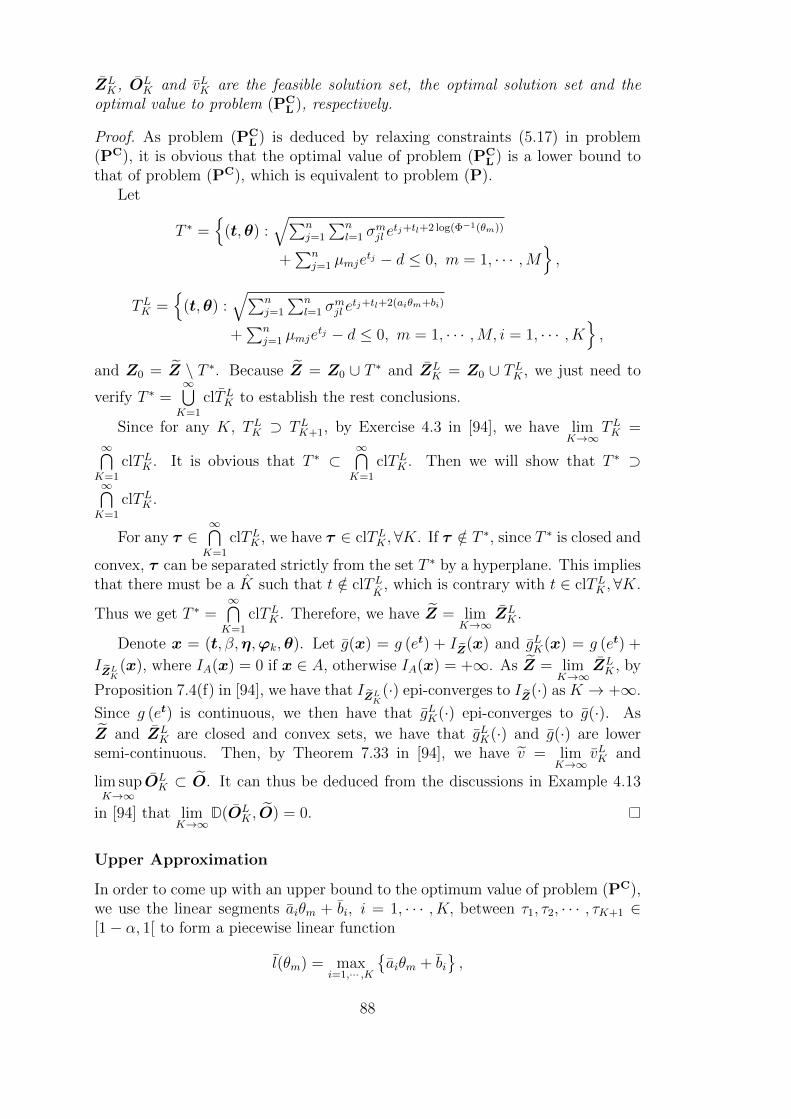
ZLK, OL

K and vLK are the feasible solution set, the optimal solution set and theoptimal value to problem (PC

L ), respectively.

Proof. As problem (PCL ) is deduced by relaxing constraints (5.17) in problem

(PC), it is obvious that the optimal value of problem (PCL ) is a lower bound to

that of problem (PC), which is equivalent to problem (P).Let

T ∗ =

(t,θ) :√∑n

j=1

∑nl=1 σ

mjl e

tj+tl+2 log(Φ−1(θm))

+∑n

j=1 µmjetj − d ≤ 0, m = 1, · · · ,M

,

TLK =

(t,θ) :√∑n

j=1

∑nl=1 σ

mjl e

tj+tl+2(aiθm+bi)

+∑n

j=1 µmjetj − d ≤ 0, m = 1, · · · ,M, i = 1, · · · , K

,

and Z0 = Z \ T ∗. Because Z = Z0 ∪ T ∗ and ZLK = Z0 ∪ TLK , we just need to

verify T ∗ =∞⋃K=1

clTLK to establish the rest conclusions.

Since for any K, TLK ⊃ TLK+1, by Exercise 4.3 in [94], we have limK→∞

TLK =∞⋂K=1

clTLK . It is obvious that T ∗ ⊂∞⋂K=1

clTLK . Then we will show that T ∗ ⊃∞⋂K=1

clTLK .

For any τ ∈∞⋂K=1

clTLK , we have τ ∈ clTLK ,∀K. If τ /∈ T ∗, since T ∗ is closed and

convex, τ can be separated strictly from the set T ∗ by a hyperplane. This impliesthat there must be a K such that t /∈ clTL

K, which is contrary with t ∈ clTLK ,∀K.

Thus we get T ∗ =∞⋂K=1

clTLK . Therefore, we have Z = limK→∞

ZLK .

Denote x = (t, β,η,ϕk,θ). Let g(x) = g (et) + IZ(x) and gLK(x) = g (et) +

IZLK(x), where IA(x) = 0 if x ∈ A, otherwise IA(x) = +∞. As Z = lim

K→∞ZLK , by

Proposition 7.4(f) in [94], we have that IZLK(·) epi-converges to IZ(·) as K → +∞.

Since g (et) is continuous, we then have that gLK(·) epi-converges to g(·). As

Z and ZLK are closed and convex sets, we have that gLK(·) and g(·) are lower

semi-continuous. Then, by Theorem 7.33 in [94], we have v = limK→∞

vLK and

lim supK→∞

OLK ⊂ O. It can thus be deduced from the discussions in Example 4.13

in [94] that limK→∞

D(OLK , O) = 0.

Upper Approximation

In order to come up with an upper bound to the optimum value of problem (PC),we use the linear segments aiθm + bi, i = 1, · · · , K, between τ1, τ2, · · · , τK+1 ∈[1− α, 1[ to form a piecewise linear function

l(θm) = maxi=1,··· ,K

aiθm + bi

,

88

where

ai =log (Φ−1(τi+1))− log (Φ−1(τi))

τi+1 − τi, bi = log (Φ−1(τi))− aiτi, i = 1, · · · , K.

Using the piecewise linear function l(θm) to replace log (Φ−1(θm)) in problem(PC) gives the following approximation problem:

(PCU) min

t,β,η,ϕk,θg(et)

s.t.

√√√√ n∑j=1

n∑l=1

σmjl etj+tl+2(aiθm+bi)

+n∑j=1

µmjetj − d ≤ 0, m = 1, · · · ,M, i = 1, · · · , K,

(5.15), (5.16), (5.18), t ∈ L.

Similar to the proof of Theorem 5.3, we can establish the following conclusion:

Theorem 5.4. Under Assumption 5.2, problem (PCU) is a conic programming

and the optimum value of problem (PCU) is an upper bound to that of problem

(P). What’s more, we have Z = limK→∞

ZUK, lim

K→∞D(OU

K , O) = 0 and v = limK→∞

vUK,

here ZUK, OU

K and vUK are the feasible solution set, the optimal solution set andthe optimal value to problem (PC

U), respectively.

5.2.3 DC reformulation

Assumption 5.2 might not always hold in practice. Therefore, in this subsection,we assume g (z) is convex and bounded from below on the feasible solution set of

problem (P) instead of Assumption 5.2, and then demonstrate that problem (P)is still solvable, since it can be equivalently represented as a DC programming.

Let pm = Φ−1 (θm) and introduce auxiliary variables σm,m = 1, · · · ,M , prob-

lem (P) can be rewritten as

(PDC) minz,β,η,ϕ,p,σ

g(z)

s.t. β − γ>η ≥ 1− α, (5.22)

β +I∑

k=1

u>k,mϕk ≤ Φ (pm) , m = 1, · · · ,M, (5.23)

‖ϕk‖ ≤ ηk, k = 1, · · · , I, (5.24)

pmσm ≤ d− µ>mz, m = 1, · · · ,M, (5.25)∥∥∥Σ12mz∥∥∥ ≤ σm, m = 1, · · · ,M, (5.26)

z ∈ Z,

here σ = (σ1, · · · , σM)>. In problem (PDC), the constraints (5.25) can be rewrit-

89

ten as1

2(pm + σm)2 − 1

2

(p2m + σ2

m

)≤ d− µ>mz, m = 1, · · · ,M,

which are DC constraints. Meanwhile, the function Φ (pm) in (5.23) can also bewritten as a DC function, which means the inequality constraints (5.23) are alsoDC constraints. Therefore, problem (PDC) is essentially a DC programming.

We know from Lemma 5.2 that pm = Φ−1 (θm) ≥ 0 when α < 12. This implies

that the second group of constraints (5.23) become convex constraints, since thefunction Φ(·) is concave on positive axis. Thus the number of the DC constraintsin problem (PDC) is reduced. On the other hand, we always have α < 1

2in

practice. Hence, we only consider problem (PDC) with α < 0.5 in the rest of thischapter. Similar to that in subsection 5.2.2, we approximate Φ (pm) by a lowerpiecewise linear function.

Upper bound

From Lemma 5.2, we have that Φ (pm) is concave when α < 0.5. Therefore, we

can obtain an upper bound approximation of problem (P) by replacing Φ (pm)with its lower piecewise linear function.

Concretely, we construct a piecewise linear function through K ≥ 2 differentpoints τ1 = Φ−1 (1− α) , τ2, · · · , τK which are arranged in an ascending order,as follows:

l(pm) = mini=1,··· ,K

aipm + bi

, (5.27)

where

ai =

Φ(τi+1)−Φ(τi)

τi+1−τi , 1 ≤ i < K

0, i = K; bi = Φ(τi)− aiτi.

By replacing Φ(pm) with l(pm) in problem (PDC), we get the following DCupper bound approximation:

(PDCU ) min

z,β,η,ϕ,p,σg(z)

s.t. β − γ>η ≥ 1− α,β +

∑Ik=1 u

>k,mϕk ≤ aipm + bi, m = 1, · · · ,M, i = 1, · · · , K,

‖ϕk‖ ≤ ηk, k = 1, · · · , I,12

(pm + σm)2 − 12

(p2m + σ2

m) ≤ d− µ>mz, m = 1, · · · ,M,∥∥∥Σ12mz∥∥∥ ≤ σm, m = 1, · · · ,M,

z ∈ Z.

We denote the feasible solution sets of problem (PDC) and problem (PDCU )

by ZDC and ZK , respectively. Let ODC and vDC be the optimal solution set andthe optimal value of problem (PDC), OK and vK be the optimal solution set andoptimal value of problem (PDC

U ), respectively. Then, similar with Theorem 5.4,we have the following theorem.

Theorem 5.5. The optimal value of problem (PDCU ) is an upper bound for the op-

timal value of problem (P). What’s more, we have ZDC = limK→∞

ZK, limK→∞

D(OK , ODC

)=

90

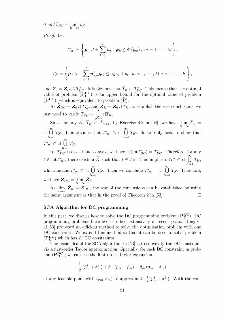
0 and vDC = limK→∞

vK.

Proof. Let

T ∗DC =

p : β +

I∑k=1

u>k,mϕk ≤ Φ (pm) , m = 1, · · · ,M

,

TK =

p : β +

I∑k=1

u>k,mϕk ≤ aipm + bi, m = 1, · · · ,M, i = 1, · · · , K

,

and Z0 = ZDC \T ∗DC . It is obvious that TK ⊂ T ∗DC . This means that the optimalvalue of problem (PDC

U ) is an upper bound for the optimal value of problem

(PDC), which is equivalent to problem (P).

As ZDC = Z0 ∪ T ∗DC and ZK = Z0 ∪ TK , to establish the rest conclusions, we

just need to verify T ∗DC =∞⋃K=1

clTK .

Since for any K, TK ⊂ TK+1, by Exercise 4.3 in [94], we have limK→∞

TK =

cl∞⋃K=1

TK . It is obvious that T ∗DC ⊃ cl∞⋃K=1

TK . So we only need to show that

T ∗DC ⊂ cl∞⋃K=1

TK .

As T ∗DC is closed and convex, we have cl (intT ∗DC) = T ∗DC . Therefore, for any

t ∈ intT ∗DC , there exists a K such that t ∈ TK . This implies intT ∗ ⊂ cl∞⋃K=1

TK ,

which means T ∗DC ⊂ cl∞⋃K=1

TK . Then we conclude T ∗DC = cl∞⋃K=1

TK . Therefore,

we have ZDC = limK→∞

ZK .

As limK→∞

ZK = ZDC , the rest of the conclusions can be established by using

the same argument as that in the proof of Theorem 2 in [53].

SCA Algorithm for DC programming

In this part, we discuss how to solve the DC programming problem (PDCU ). DC

programming problems have been studied extensively in recent years. Hong etal.[53] proposed an efficient method to solve the optimization problem with oneDC constraint. We extend this method so that it can be used to solve problem(PDC

U ) which has K DC constraints.The basic idea of the SCA algorithm in [53] is to convexify the DC constraint

via a first-order Taylor approximation. Specially, for each DC constraint in prob-lem (PDC

U ), we can use the first-order Taylor expansion

1

2

(p2m + σ2

m

)+ pm (pm − pm) + σm (σm − σm)

at any feasible point with (pm, σm) to approximate 12

(p2m + σ2

m). With the con-

91

vexity of the function 12

(p2m + σ2

m), we have

1

2

(p2m + σ2

m

)≥ 1

2

(p2m + σ2

m

)+ pm (pm − pm) + σm (σm − σm) ,

and the original constraint is replaced by

1

2(pm + σm)2 − 1

2

(p2m + σ2

m

)− pm (pm − pm)− σm (σm − σm) ≤ d− µ>mz.

Let CP((p, σ)) denote the following optimization problem:

minz,β,η,ϕk,p,σ

g(z)

s.t. β − γ>η ≥ 1− α,β +

∑Ik=1 u

>k,mϕk ≤ aipm + bi, m = 1, · · · ,M, i = 1, · · · , K,

‖ϕk‖ ≤ ηk, k = 1, · · · , I,12

(pm + σm)2 − pm (pm − pm)− σm (σm − σm)≤ d− µ>mz + 1

2(p2m + σ2

m) , m = 1, · · · ,M,∥∥∥Σ12mz∥∥∥ ≤ σm, m = 1, · · · ,M,

z ∈ Z.

Here, p = (p1, · · · , pM)> and σ = (σ1, · · · , σM)>. And the feasible set to problem(PDC

U ) is denoted by Z(p,σ). Then for any feasible point with (p, σ) of problem(PDC

U ), problem CP((p, σ)) is a convex conservative approximation to problem(PDC

U ). Therefore, we can repeat solving problem CP((p, σ)) at the newly ob-tained solution, which leads to the following algorithm.

Algorithm 2 SCA method for solving problem (PDCU )

Step 1. Choose an initial feasible point with (p0,σ0), set j = 0.

Step 2. Solve problem CP((pj,σj)) and obtain (pj+1,σj+1).

Step 3. Stop if the optimal solution of problem CP((pj,σj)) is a KKT point ofproblem (PDC

U ). Otherwise, let j = j + 1 and go to Step 2.

Algorithm 2 is easy to implement since we only need to solve at each iterationthe convex optimization problem CP((pj,σj)), which is actually a SOCP andcan thus be solved in polynomial time.

We say the Slater’s condition holds at the feasible point with (p, σ) if theinterior of the feasible solution set of problem CP((p, σ)) is nonempty. TheSlater’s condition is one of the most commonly used constraint qualifications forconvex optimization. Then we have the following theorem.

Theorem 5.6. Suppose that zj, βj,ηj,ϕjk,pj,σj is a sequence of solutionsgenerated by 2. Then

(a) zj, βj,ηj,ϕjk,pj,σj is contained in the feasible solution set of problem(PDC

U ) and g (zj) is a convergent non-increasing sequence.

92

(b) If a cluster point of zj, βj,ηj,ϕjk,pj,σj satisfies the Slater’s condition,the cluster point is a KKT point of problem (PDC

U ), whose correspondingobjective function value also provides an upper bound for the optimal valueof problem (P).

Proof. (a) For any j ≥ 0, zj+1, βj+1,ηj+1,ϕj+1k ,pj+1,σj+1 is an optimal solu-

tion to problem CP((pj,σj)). Then, it is also a feasible solution to problem(PDC

U ), since the feasible solution set of problem CP((pj,σj)) is a subsetof the feasible solution set of problem (PDC

U ).

As zj+1, βj+1,ηj+1,ϕj+1k ,pj+1,σj+1 is an optimal solution to problem

CP((pj,σj)) and zj, βj,ηj,ϕjk,pj,σj is a feasible solution to problemCP((pj,σj)), we have g (zj+1) ≤ g (zj). This shows that g (zj) is non-increasing. Because the continuous function g (z) is bounded from belowon the feasible solution set, g (zj) is thus bounded from below, whichimplies that g (zj) is a convergent non-increasing sequence.

(b) Let

gm1 :=1

2(pm + σm)2 + µ>mz − d

and

gm2 :=1

2

(p2m + σ2

m

),

for m = 1, · · · ,M , and we denote the mappings g1 =(g1

1, · · · , gM1)>

and

g2 =(g1

2, · · · , gM2)>

. Then, the DC constraints in problem (PDCU ) can be

rewritten asg1 − g2 ≤ 0.

With this representation, we can then use the same argument as that inthe proof of Property 3 in [53] to prove the conclusion (b), which is thusomitted.

The property (a) in 5.6 shows that we always search for better solutions inthe feasible region, which is similar to the framework of classical interior-pointmethods. It also shows that we make improvement at each iteration and thesequence of objective function values converges to a certain value. The secondproperty (b) ensures that all accumulation points of the sequence of solutionsgenerated are KKT points of problem (PDC

U ). If problem (PDCU ) has a unique

KKT point or has only one KKT point that is better than the initial solution, 2guarantees to converge to a global optimal solution of problem (PDC

U ).

Lower bound

In order to evaluate how conservative the solution of the above upper boundapproximation is when it is compared to the true solution of problem (P), weneed a procedure that could provide a lower bound for the optimal value ofproblem (P). For this purpose, we apply the tangent approximation technique

93

where the function Φ(pm) is approximated by its upper bound tangent piecewiselinear function.

From Lemma 5.2, we have that Φ (pm) is concave when α < 12. We select K

different tangent functions:

li(pm) = aipm + bi, i = 1, · · · , K,

withai = φ (τi) , bi = Φ(τi)− aiτi,

where τ1, · · · , τK are K points with τi ∈ [Φ−1 (1− α) ,∞), 1 ≤ i ≤ K. Therefore,we have

l(pm) = mini=1,··· ,K

li(pm) ≥ Φ (pm) , ∀pm ∈ [Φ−1 (1− α) ,∞).

With the above tangent piecewise linear approximation l(pm) of Φ (pm), weobtain the following lower bound approximation of problem (PC).

(PDCL0

) minz,β,η,ϕ,p,σ

g(z)

s.t. β − γ>η ≥ 1− α,β +

∑Ik=1 u

>k,mϕk ≤ aipm + bi, m = 1, · · · ,M, i = 1, · · · , K,

‖ϕk‖ ≤ ηk, k = 1, · · · , I,pmσm ≤ d− µ>mz, m = 1, · · · ,M,∥∥∥Σ

12mz∥∥∥ ≤ σm, m = 1, · · · ,M,

z ∈ Z.

By approximating the biconvex term pmσm with Cheng and Lisser’s methodin [24], we have the following conclusion.

Theorem 5.7. Replacing Φ (pm) in problem (PC) by l(pm), we get the followingconvex approximation of problem (PDC):

(PDCL ) min

z,β,η,ϕ,p,σg(z)

s.t. β − γ>η ≥ 1− α,β +

∑Ik=1 u

>k,mϕk ≤ aipm + bi, m = 1, · · · ,M, i = 1, · · · , K,

‖ϕk‖ ≤ ηk, k = 1, · · · , I,ym ≤ d− µ>mz, m = 1, · · · ,M,∥∥∥Σ

12mz∥∥∥ ≤ σm, m = 1, · · · ,M,

Φ−1 (1− α)σm ≤ ym, m = 1, · · · ,M,κmpm ≤ ym, m = 1, · · · ,M,z ∈ Z,

where κm = minz∈Z

∥∥∥Σ12mz∥∥∥. Then, the optimal value of problem (PDC

L ) is a lower

bound to that of problem (P).

94

Proof. Let

T ∗ =

p : β +

I∑k=1

u>k,mϕk ≤ Φ (pm) , m = 1, · · · ,M

,

and

TS =

p : β +

I∑k=1

u>k,mϕk ≤ aipm + bi, m = 1, · · · ,M, i = 1, · · · , K

.

It is obvious that T ∗ ⊂ TS.In addition, for m = 1, · · · ,M , we replace pmσm by ym. As pm ≥ Φ−1 (1− α),

the constraint ym = pmσm can be relaxed by Φ−1 (1− α)σm ≤ ym and κipm ≤ ym,

where κm = minz∈Z

∥∥∥Σ12mz∥∥∥. Therefore, the optimal value of problem (PDC

L ) is a

lower bound to that of problem (P).

5.3 Numerical Results

In this section, we apply the proposed data-driven robust chance constrainedoptimization problem (P) to two practical problems. The data is generated ran-domly. We use the CVX package to solve all the approximation problems in thissection with Matlab R2015a, on a Laptop with a 2.60 GHz Intel Core m5-4300MCPU and 4.0 GB RAM.

5.3.1 Convex approximation

In this subsection, we test the performance of our convex approximations by con-sidering a data-driven robust production problem with the Cobb-Douglas utility.

Cobb-Douglas utility function delicately captures the practical characteristicsof different multi-factor input-output contexts besides production. Here, we gen-eralize the model in [32] by maximizing the Cobb-Douglas utility with chanceconstraints. Suppose that there are n goods, and the random price of good j isξj, j = 1, · · · , n. Suppose the distribution of ξ = (ξ1, · · · , ξn) is contained in theuncertainty set D where M = 3 and I = 4. Let z = (z1, · · · , zn) ≥ 0 denotethe quantities of n goods purchased in the market. Then, the agent solves thefollowing optimization problem

(PP) minz

∏nj=1 z

−rjj

s.t. minf∈D

Pfξ>z ≤ W

≥ 1− α,

z ≥ 0,

where n = 10, α = 0.1, rj = 0.1, j = 1, · · · , 10, W = 10000. The problem(PP) can be approximated by piecewise linear approximation problems (PC

L ) and(PC

U), respectively, to find the lower bound and upper bound to its optimal value,respectively.

95

To generate the necessary data, we adopt the following framework in [106] todetermine the parameters of the component distributions f1(·), f2(·) and f3(·) inthe uncertainty set D:

ymk = amk + bikymbase + emk , m = 1, · · · 3, k = 1, · · · , 10,

where ymk represents the random realization of the kth component of the randomvector, corresponding to the mth component distribution fm(·); amk and bmk areconstants which are randomly selected in [0, 1] and [1, 1.5], respectively; ybase =(y1

base, y2base, y

3base)

> denotes the base random vector, which is normally distributedwith the mean vector being E (ybase) = (5, 10, 15) and the covariance matrix beingCov (ybase) = diag(0.2, 0.4, 0.6); and emk is a normally distributed residual termwith zero mean and the variance randomly selected in [0, 2 × 10−2], which isindependent of ybase.

In this simulation, 5000 samples are randomly generated according to themixture distribution with the mixture weight vector being w = (0.3, 0.4, 0.3).With the generated data and the parameters of the component distributionsf1(·), f2(·) and f3(·), and setting ε = 0.02 and ∆ = 0.03, we can determine thevalues of parameters Uk, γk, k = 1, 2, 3, 4, in the uncertainty set D given in 5.1.Under 5.2, the problem (PP) is actually a convex programming problem, whichcan be approximated by problem (PC

L ) to find a lower bound to its optimal valueand by problem (PC

U) to find an upper bound to its optimal value, respectively.By setting K to 3,5,10, and 20, respectively, we solve problem (PC

L ) andproblem (PC

U) four times and find four groups of respective lower bounds andupper bounds. The results are presented in Table 1. The first column in 5.1 givesthe value of K. The second and third columns give the lower bound and thecorresponding CPU time in seconds to solve problem (PC

L ). The forth and fifthcolumns give the upper bound and the CPU time in seconds to solve problem(PC

U). For better illustration, we compute the relative difference between thelower bound and the respective upper bound, which is shown in the last columnof 5.1.

Table 5.1: Computational results of convex reformulation problems.

K lower bound time(s) upper bound time(s) Gap(%)

3 0.01262726 4.1763 0.01388198 3.6563 9.04

5 0.01291510 6.4696 0.01359047 6.5156 4.97

10 0.01310726 8.0135 0.01326751 8.7344 1.21

20 0.01314893 11.7500 0.01314893 12.5469 0 (< 10−8)

From Table 5.1, we can see that as K increases, the difference between thelower bound and corresponding upper bound monotonically decreases. Whenthe number of tangent points is 20, these bounds become tight. Meanwhile, thesolution times in the third and fifth columns tell us that our convex approximationproblems can be solved within a few seconds. These results demonstrate that,with a suitable size of linear approximations, our convex approximations canprovide a very good approximate solution quickly.

96

5.3.2 DC approximation

In this subsection, we examine the performance of our DC approximation byconsidering a data-driven robust portfolio selection problem under the safety-firstprinciple.

Suppose there are n risky securities and one riskless security in the stockmarket. The random loss of the jth stock is ξj, 1 ≤ j ≤ n, and the proportion

of the wealth invested in the jth asset is zj, 1 ≤ j ≤ n. Let ξ = (ξ1, · · · , ξn)>,

z = (z1, · · · , zn)>. Therefore, the loss of the portfolio z can be determined as ξ>z.In addition, we assume that the distribution of ξ is contained in the uncertaintyset D with M = 3. Then the data-driven robust portfolio selection model underthe safety-first principle can be established as follows:

(PS) minz,RL

RL

s.t. minf∈D

Pfξ>z ≤ RL

≥ 1− α,

e>nz ≤ 1, z ≥ 0.

where n = 10, α = 0.1, en denotes the 10−dimensional vector with all ones.

The data generation procedure is almost the same as that in 5.3.1. Theonly difference is that the mean vector and covariance matrix of ybase are set asE (ybase) = (−1,−1.5,−2) and Cov (ybase) = diag(0.02, 0.04, 0.06), respectively.Similarly, 1000 samples are randomly generated, and we can then obtain thevalues of parameters Uk, γk, k = 1, 2, 3, 4. It is obvious that Assumption 5.2 doesnot hold for problem (PS). Therefore, we solve problems (PDC

U ) and (PDCL ) to

find an upper bound and a lower bound for the optimal value of problem (PS).

For the piecewise linear approximations, we set the number of points K to3, 5, 10, 15, 20, 30, 40, 60, 80 respectively, and denote the corresponding point setsasK3, K5, K10, K15, K20, K30, K40, K60, K80 which satisfyK3 ⊂K5 ⊂K10 ⊂K15 ⊂K20 ⊂K30 ⊂K40 ⊂K60 ⊂K80.

The first column in Table 5.2 gives the value of K. The second and thirdcolumns give the lower bound and the CPU time in seconds. The forth andfifth columns provide the upper bound and the CPU time in seconds. For betterillustration, we compute the percentage difference between the lower bound andthe corresponding upper bound, which are shown in the last column of Table 5.2.

We can see from Table 5.2 that our DC algorithms can find lower and up-per bounds quickly. What’s more important, as K increases, the gap betweenthe lower bound and corresponding upper bound becomes smaller and smaller.When the number of tangent points reaches 80, the gap is very small and doesn’tdecrease significantly. Hence, the respective bounds provide a very good approx-imation to the optimal return value of (PS).

All the above results demonstrate the practicality and efficiency of the al-gorithms proposed in this chapter for the solution of data-driven robust chanceconstrained problems.

97

Table 5.2: Computational results of DC reformulation problems.

K lower bound time(s) upper bound time(s) Gap(%)

3 -0.822313 0.4212 -0.608109 3.2136 35.22

5 -0.822312 0.5460 -0.613951 3.3400 33.94

10 -0.822311 0.5928 -0.631720 3.6052 30.17

15 -0.822311 0.7020 -0.655087 3.7768 25.53

20 -0.822310 0.7176 -0.708550 3.9484 16.06

30 -0.822310 0.9204 -0.780821 5.9256 5.31

40 -0.822309 1.2012 -0.822271 7.8222 0.0046

60 -0.822309 1.6068 -0.822276 11.6689 0.0040

80 -0.822309 1.7004 -0.822276 13.1197 0.0040

5.4 Conclusion

In this chapter, we discuss a data-driven robust chance constrained problem.Starting from the available data, we construct a mixture distribution based un-certainty set of the ambiguous underlying distribution. And the uncertainty settakes the first four moments into consideration simultaneously. In addition to therobustness, the mixture distribution employed in our model enable us to refor-mulate the chance constraint. Moreover, we propose tight convex approximationsfor the problem under some conditions on the parameters for the uncertainty set.And we propose a tight DC approximation for the upper approximation and arelaxed convex approximation for the lower approximation in the general case.Finally, simulation experiments are carried out to illustrate the practicality andefficiency of our approach.

This chapter correrponds to the reference [20].

98

Chapter 6

Chance Constrained StochasticGame Theory

In this chapter, we consider an n-player non-cooperative game with continuousstrategy sets. The strategy set of each player contains a set of stochastic lin-ear constraints. We model the stochastic linear constraints of each player as ajoint chance constraint. We assume that the row vectors of a matrix definingthe stochastic constraints of each player are pairwise independent. We modelthe stochastic constraints with normal distribution, elliptical distribution anddistributionally robustness, respectively. Under certain conditions we show theexistence of a Nash equilibrium for this game.

6.1 The model

We consider an n-player non-cooperative game. Let I = 1, 2, · · · , n be the setof players. A generic element of the set I is denoted by i. The payoffs of playeri is defined by a function ui : Rm1

++ × Rm2++ × · · · × Rmn++ → R, where Rmi++ (Rmi+ )

denotes the positive (non-negative) orthant of Rmi . The set X i ⊂ Rmi++ denotesthe set of all strategies of player i. We assume X i to be a convex and compactset. The product set X =

∏i∈I X

i denotes the set of all strategy profiles. Wedenote the set of all vectors of strategies of all the players except player i byX−i =

∏nj=1;j 6=iX

j. The generic elements of X i, X−i, and X are denoted by xi,

x−i, and x respectively. We define (yi, x−i) to be a strategy profile where playeri chooses a strategy yi and each player j ∈ I, j 6= i, chooses a strategy xj. Weconsider the case where the strategies of player i are further constrained by thefollowing stochastic linear constraints

Aixi ≤ bi, (6.1)

where Ai = [Ai1, Ai2, · · · , AiKi ]

T is a Ki × mi random matrix, and bi ∈ RKi ; Tdenotes the transposition. For each k = 1, 2, · · · , Ki, A

ik is the kth row of Ai.

We consider the case where the constraints of player i given by (6.1) are jointlysatisfied with at least a given probability level. Let αi be a given probability levelof player i. We formulate the stochastic linear constraints (6.1) as a joint chance

99

constraint given byPFiAixi ≤ bi

≥ αi, (6.2)

where P is a probability measure, Fi is the distribution of Ai. Therefore, for anαi ∈ [0, 1], the feasible strategy set of player i is defined by

Siαi =xi ∈ X i | PFi

Aixi ≤ bi

≥ αi

, i ∈ I.

We assume that the set Siαi is non-empty, and the probability distribution of therandom matrix Ai and the probability level vector (αi)i∈I are known to all theplayers. Then, the above chance-constrained game is a non-cooperative gamewith complete information. A strategy profile x∗ is said to be a Nash equilibriumof a chance-constrained game if and only if for each i ∈ I

ui(xi∗, x−i∗) ≥ ui(x

i, x−i∗), ∀ xi ∈ Siαi .

Assumption 6.1. For each player i, i ∈ I, the following conditions hold.

1. The payoff function ui(·, x−i) is a concave function of xi for every x−i ∈X−i.

2. The payoff function ui(·) is a continuous function of x.

Such game theoretic situations arise in a renewable energy markets based onwind turbine and solar panels with n-players. Each player aims at maximizinghis payoff subject to technical, operational and budget constraints. Both energytechnologies are highly concerned by uncertainties. For the wind turbine case,the constraints are related to tensile strength, tip deflection rate, blade naturalfrequency, turbulence, turbine size. For the solar energy, the constraints arerelated to generation sites, storage and inter-regional power transmission, thesize of the panels. Such constraints could be modeled as chance constraints andconsidered either as individual chance constraints or joint chance constraints.And it is well known that joint chance constraints are highly reliable comparedto individual ones

6.2 Existence of Nash equilibrium with normal

distribution

We consider the case where for each i ∈ I, the row vector Aik, k = 1, 2, · · · , Ki,follows a multivariate normal distribution with mean µik = (µik1, µ

ik2, · · · , µikmi)

and a covariance matrix Σik, i.e., Aik ∼ N (µik,Σ

ik). We assume Σi

k to be a positivedefinite matrix. Moreover, the row vectors are also independent. In this case wehave the following results.

Lemma 6.1. For each i ∈ I, let the row vector Aik ∼ N (µik,Σik) with posi-

tive definite covariance matrix Σik, k = 1, 2, · · · , Ki. Moreover, the row vec-

tors of Ai, i ∈ I, are independent. Then, Siαi, i ∈ I, is a convex set when

100

αi > F(max

√3, vi

), where F (·) is the one-dimensional standard normal dis-

tribution function,

vi = maxk=1,2,··· ,Ki

4λi,kmax

(λi,kmin

)− 32 ∥∥µik∥∥ ,

and λi,kmax, λi,kmin refer to the largest and smallest eigenvalues of Σik; ‖·‖ denotes the

Euclidean norm.

Proof. The proof follows from Theorem 5.1 of [50].

Remark 6.1. If the value of vi is smaller than√

3, Siαi is a convex set when

αi > F (√

3) ≈ 0.958.

Lemma 6.2. For each i ∈ I, let the row vector Aik ∼ N (µik,Σik) with positive

definite covariance matrix Σik, k = 1, 2, · · · , Ki. Moreover, the row vectors of Ai,

i ∈ I, are independent. Then, Siαi, i ∈ I, is a compact set provided

αi > mink=1,2,··· ,Ki

F(∥∥(Σi

k)−1/2µik

∥∥) .Proof. The proof directly follows from Theorem 2.3 of [49].

For each i ∈ I, the set of best response strategies of player i for a fixed strategyprofile x−i of other players is given by

Bαii (x−i) =xi ∈ Siαi | ui(x

i, x−i) ≥ ui(xi, x−i), ∀ xi ∈ Siαi

.

Denote, Sα =∏

i∈I Siαi

, where α = (α1, α2, · · · , αn)T . Let P(Sα) be the powerset of Sα. Then, for an α ∈ [0, 1]n, define a set-valued map

Gα : Sα → P(Sα)

such thatGα(x) =

∏i∈I

Bαii (x−i).

A point x is said to be a fixed point of Gα(·) if x ∈ Gα(x). It is clear that a fixedpoint of Gα(·) is a Nash equilibrium of a chance-constrained game.

Theorem 6.1. Consider an n-player non-cooperative game where the payoff func-tion of player i, i ∈ I, satisfies the Assumption 6.1. The stochastic linear con-straints of player i are jointly satisfied with at least a given probability αi ∈ [0, 1].For each i ∈ I, let the row vector Aik ∼ N (µik,Σ

ik) with positive definite co-

variance matrix Σik, k = 1, 2, · · · , Ki. Moreover, the row vectors of Ai, i ∈ I,

are independent. Then, there exists a Nash equilibrium for a chance-constrainedgame for all α ∈ (α1, 1]× (α2, 1]× · · · × (αn, 1], where for each i ∈ I

αi = maxαi, αi,

and

αi = F(

max√

3, vi

), where vi = max

k=1,2,··· ,Ki4λkmax

(λkmin

)− 32∥∥µik∥∥ ,

101

αi = mink=1,2,··· ,Ki

F(∥∥(Σi

k)−1/2µik

∥∥) .Proof. Fix α ∈ (α1, 1] × (α2, 1] × · · · × (αn, 1]. To show the existence of a Nashequilibrium for a chance-constrained game, it is enough to show that Gα(·) hasa fixed point. We show that Gα(·) satisfies all the conditions of Kakutani fixedpoint theorem [58] as given below:

(i) Sα is a non-empty, convex, and compact subset of a finite dimensionalEuclidean space.

(ii) Gα(x) is a non-empty and convex set for all x ∈ Sα.

(iii) The graph of set-valued map Gα(·), defined by (x, y) | y ∈ Gα(x), is aclosed subset of Sα × Sα: if (xn, xn) → (x, x) with xn ∈ Gα(xn) for all n,then x ∈ Gα(x).

Sα is a non-empty set because for each i ∈ I, Siαi is a non-empty set. Theconvexity of Sα follows from Lemma 6.1 and the compactness of Sα follows fromLemma 6.2. To show the condition (ii), it is enough to show that Bαii (x−i) is anon-empty and convex set for all i ∈ I. The set Bαii (x−i) in non-empty becauseui(·, x−i) is a continuous function of xi and Siαi is a compact set. The set Bαii (x−i)is convex because ui(·, x−i) is a concave function of xi. Since, the payoff functionui(·), i ∈ I, is a continuous function of x, then the closed graph condition can beproved using the similar arguments given in the proof of Theorem 3.2. [98] (seealso Theorem 4.4 of [3]).

From Theorem 6.3, a Nash equilibrium for a chance-constrained game existsfor sufficiently large values for αi, i ∈ I. Therefore, in most of the cases we do nothave an answer for the existence of a Nash equilibrium for a chance-constrainedgame defined in Section 6.1. In order to answer this question we first propose anew reformulation for (6.2).

Under independent and normally distributed assumption on matrix Ai, wehave the following equivalent deterministic reformulation for the joint chance-constraint (6.2)

Qiαi

=

(µik)

Txi + F−1(αziki

)∥∥∥(Σik

)1/2xi∥∥∥ ≤ bik, ∀ k = 1, 2, · · · , Ki, (i)

Ki∑k=1

zik = 1, (ii)

zik ≥ 0, ∀ k = 1, 2, · · · , Ki, (iii)

where F−1(·) is a quantile function for a standard normal distribution [24]. For

an αi ∈ [0.5, 1], the set Qiαi

is a bi-convex set as it is a convex set in xi(

resp.

(zik)Kik=1

)for a fixed (zik)

Kik=1

(resp. xi

).

We propose a new convex reformulation of the set Qiαi

. Let αi ∈ [0.5, 1], i ∈ I.

For 0 ≤ zik ≤ 1, F−1(αziki

)≥ 0 for all αi ≥ 0.5. Therefore, the constraint (i) of

102

the set Qiαi

can be written as(µik)Txi +

∥∥∥(Σik

)1/2(F−1

(αziki

)xi)∥∥∥ ≤ bik, ∀ k = 1, 2, . . . , Ki. (6.3)

We use a change of variables technique under logarithmic transformation [65].The logarithmic transformation is well defined because X i ⊂ Rmi++. We transformthe vector xi ∈ X i into a vector yi ∈ Rmi , where yij = log xij, j = 1, 2, . . . ,mi.Then, constraint (6.16) can be written as

(µik)T ey

i

+

∥∥∥∥∥(Σik

)1/2e

logF−1

(αziki

)1mi+y

i

∥∥∥∥∥ ≤ bik, ∀ k = 1, 2, . . . , Ki,

where 1mi is anmi×1 vector of ones, and eyi

=(ey

i1 , · · · , eyimi

)Tand e

logF−1

(αziki

)1mi+y

i

=(e

logF−1

(αziki

)+yi1

, · · · , elogF−1

(αziki

)+yimi

)T

. Therefore, we have the following de-

terministic reformulation for (6.2)

Qiαi

=

(µik)T ey

i

+

∥∥∥∥∥(Σik

)1/2e

logF−1

(αziki

)1mi+y

i

∥∥∥∥∥ ≤ bik,

∀ k = 1, 2, . . . , Ki, (i)

Ki∑k=1

zik = 1 (ii)

zik ≥ 0, ∀ k = 1, 2, . . . , Ki. (iii)

Let Y i be an image of X i under logarithmic function. Since, the logarithmicfunction is continuous and X i is a compact set, Y i is also a compact set. Broadlyspeaking, the convexity may not be preserved under logarithmic transformation.In this section, we consider the sets X i for which the sets Y i remain convex.We give hereafter few examples of convex sets X i which are invariant underlogarithmic transformation.

Example 6.1. Consider a set

X i =

xi ∈ Rmi++ | cTxi ≤ h

,

where c = (c1, · · · , cmi)T ∈ Rmi+ and h ∈ R+ are all constant. Then,

Y i =

yi ∈ Rmi |

mi∑j=1

cjeyij ≤ h

,

is a convex set.

103

Example 6.2. Consider a set

X i =

xi ∈ Rmi++ |

mi−1∑j=1

xij ≤ ximi

.

Then, Y i can be reformulated as

Y i =

yi ∈ Rmi |

mi−1∑j=1

eyij−yimi ≤ 1

,

which is also a convex set.

Example 6.3. Consider a set

X i =

xi ∈ Rmi++ |

mi∑j=1

(xij)2 ≤ h

,

where h ∈ R++ is a constant. Then,

Y i =

yi ∈ Rmi |

mi∑j=1

e2yij ≤ h

,

is a convex set.

Example 6.4. Consider a set

X i =

xi ∈ Rmi++ | f(xi) ≤ h

,

where f : Rmi++ → R++ is a log-convex and non-decreasing function of xi, andh ∈ R++ is a constant. Then,

Y i =

yi ∈ Rmi | f(ey

i

) ≤ h

,

is a convex set.

The reformulation of feasible strategy set Siαi of player i, i ∈ I, is given by

Siαi =

(yi, zi) ∈ Y i × RKi | (yi, zi) ∈ Qiαi

.

Assumption 6.2. For each player i, i ∈ I, ui(·, x−i) is a non-increasing functionfor every x−i ∈ X−i.

Assumption 6.3. For each i ∈ I and k = 1, 2, . . . , Ki, all the components of Σik

and µik are non-negative.

104

Under Assumption 6.3, we show that the set Siαi is convex. It is enough

to show that constraint (i) of Qiαi

is convex. We present Lemma 6.3 on thecomposition of convex functions. It is used to prove Lemma 6.4 which is the keyto prove the convexity of the sets Siαi , i ∈ I.

Lemma 6.3. Let Γ1,Γ2 ⊆ R and Γ1,Γ2 are convex sets. Suppose f1 : Γ1 → Γ2 isa convex function on Γ1, and f2 : Γ2 → R is a non-decreasing and convex functionon Γ2. Then, the composition function f2 f1 is a convex function on Γ1.

Proof. Consider any two points x1, x2 ∈ Γ1 and λ ∈ [0, 1]. Since, f1 is a convexfunction on Γ1, we have

f1(λx1 + (1− λ)x2) ≤ λf1(x1) + (1− λ)f1(x2).

Using the non-decreasing and convexity properties of f2 on Γ2, we have

(f2 f1)(λx1 + (1− λ)x2) ≤ λ(f2 f1)(x1) + (1− λ)(f2 f1)(x2).

Hence, f2 f1 is a convex function on Γ1.

Lemma 6.4. For each i ∈ I and k = 1, 2, . . . , Ki, logF−1(αziki

)is a convex

function of zik on [0, 1] for all αi ∈ [F (1), 1] where F (1) ≈ 0.84.

Proof. Let g1 : [0, 1] → [F (1), 1] such that g1(zik) = αziki , and g2 : [F (1), 1] → R

such that g2(p) = logF−1(p) be two functions. Then, the function composition

(g2 g1)(zik) = logF−1(αziki

). From Lemma 6.3, logF−1

(αziki

)is a convex func-

tion of zik if g1(·) is a convex function and g2(·) is convex and non-decreasingfunction on their respective domains.

Since, 0 ≤ zik ≤ 1 and F (1) ≤ αi ≤ 1, then αziki ≥ αi. Therefore, the function

g1(·) is well defined and it is also a convex function of zik. The function g2(·) isa non-decreasing function because the quantile function F−1(·) as well as log(·)are non-decreasing functions. The only thing remains to show is that logF−1 (p)is a convex function. It is enough to show that the second order derivative oflogF−1 (p) is non-negative. The second order derivative of logF−1 (p) can bewritten as

−ψ(y) + yψ′(y)

(yψ(y))2ψ(y).

where y = F−1(p), and ψ(·) is the probability density function of a standardnormal distribution, and ψ′(·) is the first order derivate of ψ(·). We have

ψ(y) + yψ′(y) =1√2πe−

y2

2 (1− y)(1 + y) ≤ 0,

because 1 + y = 1 + F−1(p) ≥ 0 and 1 − y = 1 − F−1(p) ≤ 0 for all p ∈[F (1), 1]. Hence, the second order derivative of logF−1 (p) is non-negative for all

p ∈ [F (1), 1]. Therefore, logF−1(αziki

)is a convex function of zik on [0, 1] for all

αi ∈ [F (1), 1].

105

Lemma 6.5. For each i ∈ I, let the convex set X i be such that Y i is a convexset. Let Assumption 6.3 hold. Then, the set Siαi, i ∈ I, is a convex set for allαi ∈ [F (1), 1].

Proof. Fix i ∈ I and αi ∈ [F (1), 1]. Then,

((Σi

k)1/2e

logF−1

(αziki

)1mi+y

i

)is an

mi×1 vector. Each component of the vector is a non-negative linear combinationof the convex functions. Hence, it is a vector of non-negative convex functions.The Euclidean norm is a convex function and it is also a non-decreasing function ineach argument when the arguments are non-negative. Therefore, the composition

function

∥∥∥∥∥(Σik)

1/2e

logF−1

(αziki

)1mi+y

i

∥∥∥∥∥ is a convex function. The term (µik)T ey

iis

a convex function because µik ≥ 0. Hence, the constraints

(µik)T ey

i

+

∥∥∥∥∥(Σik

)1/2e

logF−1

(αziki

)1mi+y

i

∥∥∥∥∥ ≤ bik, ∀ k = 1, 2, · · · , Ki,

are convex. It is easy to see that the other constraints of Siαi are convex. Hence,

Siαi is a convex set.

Theorem 6.2. Consider an n-player non-cooperative game where the payoff func-tion of player i, i ∈ I, satisfies the Assumptions 6.1 and 6.2 . The stochasticlinear constraints of each player are jointly satisfied with at least a given proba-bility αi ∈ [0, 1]. For each i ∈ I, let the row vector Aik ∼ N (µik,Σ

ik) where mean

vector µik and positive definite covariance matrix Σik, k = 1, 2, · · · , Ki, satisfies

Assumption 6.3. Moreover, the row vectors of Ai, i ∈ I, are independent. Then,there exists a Nash equilibrium of a chance-constrained game for all α ∈ [F (1), 1]n.

Proof. Let α ∈ [F (1), 1]n. For each i ∈ I, define a composition function Ci =−ui di, where di : Rm1 × Rm2 × · · · × Rmn → Rm1

++ × Rm2++ × · · · × Rmn++, such that

di(y1, y2, · · · , yn

)=(ey

1

, ey2

, · · · , eyn).

Then, define a best response set for player i for a fixed y−i ∈ Y −i

Bαii (y−i) =

(yi, zi) ∈ Siαi | Ci(yi, y−i) ≤ Ci(y

i, y−i), ∀ (yi, zi) ∈ Siαi.

Denote Sα =∏

i∈I Siαi

. Then, define a set-valued map

Gα : Sα → P(Sα)

such thatGα(y, z) =

∏i∈I

Bαii (y−i).

It follows from Lemma 6.5 that Sα is a convex set. It is also a closed and boundedset. Both the functions ui(·) and di(·) are continuous functions. Therefore, the

106

composition function Ci(·) is also a continuous function. Since, Siαi is a compact

set, then the best response set Bαii (y−i) is non-empty. The function di(·) is aconvex function and −ui(·, x−i) is a convex and non-decreasing function of xi.Then, the composition function Ci(·, y−i) is a convex function of yi which, in

turn, implies that the best response set Bαii (y−i) is a convex set. Hence, Gα(y, z)is a non-empty and convex set for each (y, z). The closed graph condition for

Gα(·) follows from the continuity of the functions Ci(·), i ∈ I. Therefore, fromKakutani fixed point theorem there exists a fixed point (y∗, z∗) for the set-valued

map Gα(·). Then, for each i ∈ I

Ci(yi∗, y−i∗) ≤ Ci(y

i, y−i∗), ∀ (yi, zi) ∈ Siαi .

Under the hypothesis of theorem, Siαi is a reformulation of Siαi , where xi = eyi.

This impliesui(x

i∗, x−i∗) ≥ ui(xi, x−i∗), ∀ xi ∈ Siαi .

Hence, x∗ is a Nash equilibrium of a chance-constrained game for all α ∈ [F (1), 1]n.

6.3 Existence of Nash equilibrium with ellipti-

cal distribution

In this section, we will prove the existence of Nash equilibrium with ellipticaldistribution. The definition of elliptical distribution is shown in subsection 2.1and density function is given by (2.4).

Then, we assume that the row vector Aik, k = 1, 2, · · · , Ki all follow someelliptical distributions, that is, Aik ∼ Ellip (µik,Σ

ik;φ

ik) , k = 1. · · · , K, where φik

is the characteristic function as defined in subsection 2.1. Moreover, Aikr andAiks are independent of each other when kr 6= ks. In this case, with the help ofTheorem 3 in [22], we can reformulated the joint chance-constraint (6.2) as

Qiαi

=

(i) (µik)

Txi +(F ik

)−1(αziki

)||(Σik

)1/2xi|| ≤ bik, ∀ k = 1, 2, · · · , Ki

(ii)

Ki∑k=1

zik = 1

(iii) zik ≥ 0, ∀ k = 1, 2, · · · , Ki,(6.4)

where F ik is one-dimensional distribution function induced by the characteristic

function φik(t) = ϕik(t2), ϕik is the characteristic generator function.

The reformulation of feasible strategy set Siαi of player i, i ∈ I, is given by

Siαi =

(xi, zi) ∈ X i × RKi+ | (xi, zi) ∈ Qiαi

.

Denote Sα =∏

i∈I Siαi

.

To prove the convexity of set Siαi , we introduce the following definition.

107

Definition 6.1. ([50]) A function f : R → R is called r−decreasing for somer ∈ R with threshold t∗(r) > 0 if it is continuous on (0,+∞) and the functiont 7→ trf(t) is strictly decreasing for all t > t∗(r).

The following proposition shows the thresholds of some elliptical distributions.

Proposition 6.1. ([22]) The following one-dimensional elliptical distributionshave r−decreasing densities for some r:

1. normal distribution, for r > 0 with the threshold t∗(r) = 12

(µ+

√µ2 + 4rσ2

);

2. Student’s t distribution with ν degrees of freedom, for 0 < r < ν + 1 withthe threshold t∗(r) =

√rν

ν+1−r ;

3. Laplace distribution, for all r > 0 with the threshold t∗(r) = rσ√2.

With the definition of threshold, we have the following theorem about theconvexity of Siαi :

Theorem 6.3. For each i ∈ I, Siαi is a convex set when

1. the densities associated with F ik are (rik + 1)−decreasing with thresholds

tik∗(rik + 1) > 0 for some rik > 1, or at least 2−dereasing if µik = 0;

2. the probability level αi satisfies

αi > maxk

F ik

(max

tik∗(rik + 1),

rik+1

rik−1

(λkmin

)− 12 ‖µik‖

), µik 6= 0

F ik

(tik∗(2)), µik = 0

Proof. The proof follows derectly from [22].

Similar with the case of normal distribution, we have the following theoremabout the existence of Nash equilibrium with elliptical distribution. And theproof is exactly the same with the proof of Theorem 6.3.

Theorem 6.4. Consider an n-player non-cooperative game where the payoff func-tion of player i, i ∈ I, satisfies the Assumption 6.1. The stochastic linearconstraints of each player are jointly satisfied with at least a given probabilityαi ∈ [0, 1]. Let the row vector Aik ∼ Ellip (µik,Σ

ik;φ

ik) , k = 1. · · · , Ki, of random

matrix Ai. Moreover, Aikr and Aiks are independent of each other when kr 6= ks.Then, there always exists a Nash equilibrium for a chance-constrained game forall α ∈ (α1, 1]× (α2, 1]× · · · × (αn, 1], where for each i ∈ I

αi = maxk

F ik

(max

tik∗(rik + 1),

rik+1

rik−1

(λkmin

)− 12 ‖µik‖

), µik 6= 0,

F ik

(tik∗(2)), µik = 0.

(6.5)

From Theorem 6.4, a Nash equilibrium for a chance-constrained game existsfor very high values for αi, i ∈ I. This is because the reformulation Si(αi) ofthe joint chance constraint (6.2) is not a convex set. Therefore, for most of thecases we do not have an answer for the existence of a Nash equilibrium for a

108

chance-constrained game. In order to answer this question we propose a newreformulation for (6.2).

From the constraints (i) in (6.4), we can find that the feasible strategy setSi(αi) is nonconvex in general. In the following, we will consider a convex refor-mulation of set Si(αi).

When α ≥ 0.5, we have (F ik)−1(αziki

)≥ 0 where 0 ≤ zk ≤ 1. Therefore, the

first group constraints in (6.4) can be reformulated as

(µik)Tx+ ||

(Σik

) 12

((F ik

)−1(αziki

)xi)|| ≤ bik, ∀ k = 1, 2, · · · , K (6.6)

We transform the vector xi ∈ X i into a vector yi ∈ Rmi , where yij = lnxij,j = 1, 2, . . . ,mi. Then, constraint (6.6) can be written as

(µik)T ey

i

+

∥∥∥∥∥(Σik

)1/2e

log (F ik)−1(αziki

)·1mi+y

i

∥∥∥∥∥ ≤ bik, ∀ k = 1, 2, . . . , Ki,

where 1mi is an mi × 1 vector of ones, and eyi

=(ey

i1 , · · · , eyimi

)Tand

elog (F ik)

−1(αziki

)·1mi+y

i

=

(e

log (F ik)−1(αziki

)+yi1

, · · · , elog (F ik)

−1(αziki

)+yimi

)T

.

Therefore, we have the following deterministic reformulation for (6.4)

Qiαi

=

(i) (µik)T ey

i

+

∥∥∥∥∥(Σik

)1/2e

log (F ik)−1(αziki

)1mi+y

i

∥∥∥∥∥ ≤ bik, ∀ k = 1, 2, . . . , Ki,

(ii)

Ki∑k=1

zik = 1

(iii) zik ≥ 0, ∀ k = 1, 2, . . . , Ki.(6.7)

Let Y i =yi ∈ Rmi | yij = lnxij, x

i = (xi1, · · · , ximi)T , xi ∈ X i

. The set Y i

is an image of X i under logarithmic function. Since, the logarithmic function iscontinuous and X i is a compact, Y i is also compact set. The reformulation offeasible strategy set Siαi of player i, i ∈ I, is given by

Siαi =

(yi, zi) ∈ Y i × RKi | (yi, zi) ∈ Qiαi

.

Assumption 6.4. For each i ∈ I and k = 1, 2, . . . , Ki, all the components of Σik

and µik are non-negative.

Under Assumption 6.4, we show that the set Siαi is convex. It is enough to

show that the constraint (i) of Qiαi

is convex.

109

Lemma 6.6. log (F ik)−1

(αzki ) is convex, if αi satisifies

rik

((F ik

)−1(αzki )

)+(F ik

)−1(αzki ) · (rik)′

((F ik

)−1(αzki )

)≤ 0, ∀0 ≤ zk ≤ 1 (6.8)

where rik is the radial density corresponding to F ik, (rik)

′ is the first order derivativefunction of rik, k = 1, · · · , K.

Proof. As αzki is a convex function, with Lemma 6.3 and the monotonicity of

function log (F ik)−1

, we only need to show the convexity of log (F ik)−1

, which isequivalent with

−ψik(y) + y(ψik)

′(y)

(yψik(y))2ψik(y)≥ 0.

where y = (F ik)−1

(p), ψik(·) is the probability density function corresponding to

F ik, (ψik)

′(·) is the derivate of ψik(·). Then, log (F ik)

(−1)(p) is convex if and only if

ψik(y) + y(ψik)′(y) ≤ 0. Therefore, we have

rik

((F ik

)−1(αzki )

)+(F ik

)−1(αzki ) · (rik)′

((F ik

)−1(αzki )

)≤ 0.

Since αzki is convex, if (6.8) is satisfied, we have log (F ik)−1

(αzki ) is convex.

Example 6.5. (Normal distribution) For normal distribution, the radial den-sity function can be expressed as rik(z) = exp

−1

2z2

. Then inequality (6.8) canbe written as αzki ≥ F i

k(1), ∀0 ≤ zk ≤ 1 . Since αzki ≥ αi, ∀0 ≤ zk ≤ 1 , then

from Lemma 6.6, we have when αi ≥ F ik(1), log (F i

k)−1

(αzki ) is convex.

Example 6.6. (t distribution) For t distribution with degree ν, the radial den-

sity function can be expressed as g(z) =(1 + 1

νz2)−(1+ν)/2

. Then inequality (6.8)can be written as αzki ≥ F i

k(1), ∀0 ≤ zk ≤ 1 . Then from Lemma 6.6 we have

when αi ≥ F ik(1), log (F i

k)−1

(αzki ) is convex.

Example 6.7. (Cauchy distribution) For Cauchy distribution, the radial den-sity function can be expressed as g(z) = (1 + z2)

−1. TThen inequality (6.8) can

be written as αzki ≥ F ik(1), ∀0 ≤ zk ≤ 1 . Then from Lemma 6.6 we have when

αi ≥ F ik(1), log (F i

k)−1

(αzki ) is convex.

Example 6.8. (Laplace distribution) For Laplace distribution, the radial den-

sity function can be expressed as g(z) = e−√

2|z|. Then inequality (6.8) can be

written as αzki ≥ F ik(√

22

), ∀0 ≤ zk ≤ 1 . Then from Lemma 6.6 we have when

αi ≥ F ik(√

22

), log (F ik)−1

(αzki ) is convex.

With Lemma 6.6, we can deduce the following lemma:

Lemma 6.7. For each i ∈ I, let the convex set X i ⊂ Rmi+ be such that Y i is a

convex set. Let Assumption 6.4 holds. Then, the set Siαi, i ∈ I, is a convex setfor all αi satisifying the conditions in Lemma 6.6.

110

Proof. Fix i ∈ I and αi satisfies the conditions in Lemma 6.6. Then,((Σik

)1/2e

log (F ik)−1(αziki

)·1mi+y

i

)

is an mi × 1 vector. Each component of the vector is a linear combination of theconvex functions where the coefficients are nonnegative. The norm is a convexfunction and it is also a nondecreasing function when the arguments are nonneg-

ative. Therefore, The composition function

∥∥∥∥∥(Σik)

1/2e

log (F ik)−1(αziki

)·1mi+y

i

∥∥∥∥∥ is a

convex function. The term (µik)T ey

iis a convex function because µik ≥ 0. Hence,

the constraints

(µik)T ey

i

+

∥∥∥∥∥(Σik

)1/2e

log (F ik)−1(αziki

)·1mi+y

i

∥∥∥∥∥ ≤ bik, ∀ k = 1, 2, · · · , Ki,

are convex. It is easy to see that the other constraints of Siαi are convex. There-

fore, Siαi is a convex set.

Hence, similar with Theorem 6.2, we have the following theorem about theexistence of Nash equilibrium for elliptically distributed case.

Theorem 6.5. Consider an n-player non-cooperative game where the payoff func-tion of player i, i ∈ I, satisfies the Assumption 6.1. The stochastic linearconstraints of each player are jointly satisfied with at least a given probabilityαi ∈ [0, 1]. Let the row vector Aik ∼ Ellip (µik,Σ

ik;φ

ik) , k = 1. · · · , Ki, of random

matrix Ai with the mean vector µik and the covariance matrix Σik which satisfy

Assumption 6.4. Moreover, Aikr and Aiks are independent of each other whenkr 6= ks. Then, there always exists a Nash equilibrium for a chance-constrainedgame for all αi satisfying the conditions in Lemma 6.6.

6.4 Existence of Nash equilibrium for distribu-

tionally robust model

As mentioned in section 6.1, we formulate the stochastic linear constraints (6.1)as a joint chance constraint given by (6.2):

PFiAixi ≤ bi

≥ αi.

However, in practical, the assumption of full knowledge of the distribution Fi failsIn this case, we take the uncertainty of Fi into consideration. The only knowledgewe have is that Fi is in some uncertainty set Di. Therefore, the stochastic linearconstraints (6.1) can be formualted as

infFi∈Di

PFiAixi ≤ bi

≥ αi, (6.9)

111

Therefore, for an αi ∈ [0, 1], the feasible set of player i, i ∈ I, is defined by

Siαi =

xi ∈ X i | inf

Fi∈DiPFiAixi ≤ bi

≥ αi

. (6.10)

For each i ∈ I, we assume Siαi to be a nonempty set, and the uncertainty set Di

and the probability level vector (αi)i∈I are known to all the players. Then, abovechance-constrained game is a non-cooperative game.

In the following, we consider four kinds of popular uncertainty sets: φ-divergenceuncertainty set and three moment based uncertainty sets. With these four uncer-tainty sets of distribution of Ai, we will show the existence of Nash equilibriumof the non-cooperative game.

6.4.1 φ-divergence uncertainty set

In this subsection, we consider the case that the uncertainty sets Di, ı ∈ I are alldefined as

Di =fi|Dϕ

(fi||f 0

i

)≤ εi

, (6.11)

where

Dϕ

(fi||f 0

i

)=

ˆΩ

ϕ

(fi(ξ)

f 0i (ξ)

)f 0i (ξ)dξ,

f 0i denotes the estimated density function of Ai. Furthermore, the corresponding

estimated distribution of row vector Aik, k = 1, 2, · · · , Ki, is a multivariate normaldistribution with mean µik = (µik1, µ

ik2, · · · , µikmi) and a covariance matrix Σi

k. Aikr

and Aiks are independent of each other when kr 6= ks. Moreover, ϕ : R → R is aconvex function on R+ such that

1. ϕ(1) = 0,

2. 0ϕ(x/0) :=

p limp→+∞ ϕ(p)/p if x > 0,0 if x = 0,

3. ϕ(x) = +∞ for x < 0.

By using Theorem 1 in Jiang and Guan [57], we have

Theorem 6.6. For player i, with the uncertainty set (6.11), the constraint (6.9)is equivalent to

Pf0i

Aixi ≤ bi

≥ α′i, (6.12)

where

α′i0 = infz > 0, z0 + παiz < lϕ,

m(ϕ∗) ≤ z0 + z ≤ m(ϕ∗)

ϕ∗(z0 + z)− z0 − (1− αi)z + εi

ϕ∗(z0 + z)− ϕ(z0)

,

α′i = minα′i0, 1 for α′i0 ∈ R, ϕ∗ is the conjugate function of ϕ, lϕ = limx→+∞ ϕ(x)/x,m(ϕ∗) = supm ∈ R : ϕ∗ is a finite constant on (−∞,m] and m(ϕ∗) = infm ∈

112

R : ϕ∗ = +∞, and

παi =

−∞ if Leb[f0 = 0] = 0,0 if Leb[f0 = 0] > 0 and Leb[f0 = 0][Aixi ≤ bi] = 0,1 otherwise,

Leb· represents the Lebesgue measure and [f0 = 0] := ξ ∈ Ω : f0(ξ) = 0.

From the Proposition 2-4 in Jiang and Guan [57], we have the following propo-sition.

Proposition 6.2. 1. Suppose that Dϕ is constructed by using the χ divergenceof order 2 with ϕ(x) = (x− 1)2 and αi ≥ 1/2. Then

α′i = αi +

√ε2i + 4εiαi(1− αi)− (2αi − 1)εi

2εi + 2,

2. Suppose that Dϕ is constructed by using the variation distance with ϕ(x) =|x− 1|. Then

α′i = αi +εi2,

3. Suppose that Dϕ is constructed by using the KL divergence with ϕ(x) =x log x− x+ 1. Then

α′i = infx∈(0,1)

e−εixαi − 1

x− 1

.

With Theorem 6.6, we can rewrite the set Siαi as

Siαi =xi ∈ X i | Pf0

i

Aixi ≤ bi

≥ α′i

, (6.13)

where α′i is defined in Theorem 6.6. As the estimated distribution of row vectorAik is a multivariate normal distribution, the existence of Nash equilibrium canbe derived directly from the case of normal distribution in section 6.2.

Theorem 6.7. Consider an n-player non-cooperative game where the payoff func-tion of player i, i ∈ I, satisfies the Assumptions 6.1 and 6.2 . The stochastic lin-ear constraints of each player are jointly satisfied with at least a given probabilityαi ∈ [0, 1] and uncertainty set Di defined as (6.11). For each i ∈ I, mean vectorµik and positive definite covariance matrix Σi

k, k = 1, 2, · · · , Ki, satisfies Assump-tion 6.3. Moreover, the row vectors of Ai, i ∈ I, are independent. Then, thereexists a Nash equilibrium of a chance-constrained game for all α′ ∈ [F (1), 1]n,where α′ = (α′1, · · · , α′n) and α′i, i = 1, · · · , n, are defined in Theorem 6.6.

113

6.4.2 Moments based uncertainty set I

In this section, we consider the case that the uncertainty sets Di, i ∈ I are alldefined as

Di =

Fi∣∣∣∣∣∣

E[Aik] = µik, k = 1, · · · , Ki

E[(Aik − µik)(Aik − µik)T ] = Σik, k = 1, · · · , Ki

Aik and Aij are independent when k 6= j

(6.14)

In this case, from [15], we have the following deterministic reformulation fordistributionally robust joint chance-constraint (6.9)

QiDi

(αi) =

(i) (µik)Txi +

√√√√ αziki

1− αziki

∥∥∥(Σik

)1/2xi∥∥∥ ≤ bik, ∀ k = 1, 2, · · · , Ki

(ii)

Ki∑k=1

zik = 1

(iii) zik ≥ 0, ∀ k = 1, 2, · · · , Ki.(6.15)

The reformulation of feasible strategy set Si(αi) of player i, i ∈ I, is given by

Siαi =

(xi, zi) ∈ X i × RKi+ | (xi, zi) ∈ QiDi

(αi).

Denote Sα =∏

i∈I Siαi

.

To propose a convex reformulation of joint chance-constraint (6.9), we startwith the deterministic reformulation (6.15). Therefore, the constraint (i) of (6.15)can be written as

(µik)Txi +

∥∥∥∥∥∥(Σik

)1/2

√√√√ α

ziki

1− αziki

· xi∥∥∥∥∥∥ ≤ bik, ∀ k = 1, 2, . . . , Ki. (6.16)

We use a change of variables technique under logarithmic transformation. Thelogarithmic transformation is well defined because X i ⊂ Rmi+ . We transform thevector xi ∈ X i into a vector yi ∈ Rmi , where yij = lnxij, j = 1, 2, . . . ,mi. Then,constraint (6.16) can be written as

(µik)T ey

i

+

∥∥∥∥∥(Σik

)1/2e

12

(zik logαi−log

(1−α

ziki

))·1mi+y

i

∥∥∥∥∥ ≤ bik, ∀ k = 1, 2, . . . , Ki,

where 1mi is an mi × 1 vector of ones, eyi

=(ey

i1 , · · · , eyimi

)Tand

e12

(zik logαi−log

(1−α

ziki

))·1mi+y

i

=

(e

12

(zik logαi−log

(1−α

ziki

))+yi1

, · · · , e12

(zik logαi−log

(1−α

ziki

))+yimi

)T

.

114

Therefore, we have the following deterministic reformulation for (6.9)

QiDi

(αi) =

(i) (µik)T ey

i

+

∥∥∥∥∥(Σik

)1/2e

12

(zik logαi−log

(1−α

ziki

))·1mi+y

i

∥∥∥∥∥ ≤ bik,

(ii)

Ki∑k=1

zik = 1

(iii) zik ≥ 0, ∀ k = 1, 2, . . . , Ki.

(6.17)

Let Y i =yi ∈ Rmi | yij = lnxij, x

i = (xi1, · · · , ximi)T , xi ∈ X i

. The set

Y i is an image of X i under logarithmic function. Since, the logarithmic functionis continuous and X i is a compact, Y i is also compact set. The convexity neednot to be preserved under logarithmic transformation. We consider the set X i

for which the set Y i remains convex. Such sets indeed exists.The reformulation of feasible strategy set Siαi of player i, i ∈ I, is given by

Siαi =

(yi, zi) ∈ Y i × RKi | (yi, zi) ∈ QiDi

(αi).

Assumption 6.5. For each i ∈ I and k = 1, 2, . . . , Ki, all the components of Σik

and µik are non-negative.

Under Assumption 6.5, we show that the set Siαi is convex. It is enough to

show that the constraint (i) of QiDi

(αi) is convex.

Lemma 6.8. Let f : X → Y be a nonincreasing concave function, g : Z → X bea convex function. Then we have that f(g) : Z → Y is a concave function.

Proof. To show that f(g) is a concave function, it is enough to show that thesecond order derivative of f(g) is nonpositve. The second order derivative of f(g)can be written as

f ′′(g)(g′)2 + f ′(g)g′′.

Since f is nonincreasing and concave, g is convex, we have f ′′(g) ≤ 0, f ′(g) ≤ 0and g′′ ≥ 0. Therefore, f ′′(g)(g′)2 +f ′(g)g′′ ≤ 0, which means f(g) is concave.

With Lemma 6.8, we can deduce the following lemma:

Lemma 6.9. For each i ∈ I, let the convex set X i ⊂ Rmi+ be such that Y i is a

convex set. Let Assumption 6.5 holds. Then, the set Siαi, i ∈ I, is a convex setfor all αi ∈ [0, 1] .

Proof. Fix i ∈ I. Then,

((Σi

k)1/2e

12

(zik logαi−log

(1−α

ziki

))·1mi+y

i

)is an mi × 1

vector. Since log (1− p) is decreasing and concave with respect to p and αziki is

convex with respect to zik, from Lemma 6.8, we have that log(

1− αziki

)is concave

with respect to zik. Each component of the vector is a linear combination of theconvex functions where the coefficients are nonnegative. The norm is a convex

115

function and it is also a nondecreasing function when the arguments are nonnega-

tive. Therefore, The composition function

∥∥∥∥∥(Σik)

1/2e

12

(zik logαi−log

(1−α

ziki

))·1mi+y

i

∥∥∥∥∥is a convex function. The term (µik)

T eyi

is a convex function because µik ≥ 0.Hence, the constraints

(µik)T ey

i

+

∥∥∥∥∥(Σik

)1/2e

12

(zik logαi−log

(1−α

ziki

))·1mi+y

i

∥∥∥∥∥ ≤ bik, ∀ k = 1, 2, · · · , Ki,

are convex. It is easy to see that the other constraints of Si(αi) are convex.

Therefore, Siαi is a convex set.

Then, with the same proof statement of Theorem 6.2, we get the followingtheorem about existence of Nash equilibnum:

Theorem 6.8. Consider an n-player non-cooperative game where the payoff func-tion of player i, i ∈ I, satisfies the Assumptions 6.1 and 6.2. The stochastic lin-ear constraints of each player are jointly satisfied with at least a given probabilityαi ∈ [0, 1] and uncertainty set Di defined as (6.14). The mean vectors µik andthe covariance matrixes Σi

k in (6.14) satisfy Assumption 6.5. Then, there alwaysexists a Nash equilibrium for a chance-constrained game for all α ∈ [0, 1]n.

6.4.3 Moments based uncertainty set II

In this section, we consider the case that the uncertainty sets Di, i ∈ I are alldefined as

Di =

Fi∣∣∣∣∣∣

E[Aik] = µik, k = 1, · · · , Ki

E[(Aik − µik)(Aik − µik)T ] Σik, k = 1, · · · , Ki

Aik and Aij are independent when k 6= j

(6.18)

In this case, from [21], we have the following deterministic reformulation fordistributionally robust joint chance-constraint (6.9)

QiDi

(αi) =

(i) (µik)Txi +

√√√√ αziki

1− αziki

∥∥∥(Σik

)1/2xi∥∥∥ ≤ bik, ∀ k = 1, 2, · · · , Ki

(ii)

Ki∑k=1

zik = 1

(iii) zik ≥ 0, ∀ k = 1, 2, · · · , Ki.(6.19)

The reformulation of feasible strategy set Siαi of player i, i ∈ I, is given by

Siαi =

(xi, zi) ∈ X i × RKi+ | (xi, zi) ∈ QiDi

(αi).

116

Denote Sα =∏

i∈I Siαi

, which is same with the case in subsection 6.4.2. Then, theexistence of Nash equilibrium is exactly same with the case in subsection 6.4.2.

Theorem 6.9. Consider an n-player non-cooperative game where the payoff func-tion of player i, i ∈ I, satisfies the Assumptions 6.1 and 6.2. The stochastic lin-ear constraints of each player are jointly satisfied with at least a given probabilityαi ∈ [0, 1] and uncertainty set Di defined as (6.20). The mean vectors µik andthe covariance matrixes Σi

k in (6.14) satisfy Assumption 6.5. Then, there alwaysexists a Nash equilibrium for a chance-constrained game for all α ∈ [0, 1]n.

6.4.4 Moments based uncertainty set III

In this section, we consider the case that the uncertainty sets Di, i ∈ I are alldefined as

Di =

Fi∣∣∣∣∣∣

(E[Aik]− µik)>

(Σik)−1

(E[Aik]− µik) ≤ γik1, k = 1, · · · , Ki

E[(Aik − µik)(Aik − µik)T ] γik2Σik, k = 1, · · · , Ki

Aik and Aij are independent when k 6= j

(6.20)

By applying the Corollary 4 in Yang and Xu [103], we have the following de-terministic reformulation for distributionally robust joint chance-constraint (6.9)

QiDi

(αi) =

(i) k2 ·⟨Qik,Σ

ik

⟩+

αziki

1− αziki

· rik + (µik)Txi

+√k1

∥∥∥(Σik

)1/2xi∥∥∥ ≤ bik, ∀ k = 1, 2, · · · , Ki

(ii)

(Qik −xi

2

−xi

2

>rik

) 0,

(iii)

Ki∑k=1

zik = 1

(iv) zik ≥ 0, ∀ k = 1, 2, · · · , Ki.

(6.21)

The reformulation of feasible strategy set Siαi of player i, i ∈ I, is given by

Siαi =

(xi, zi, ri, Qi) ∈ X i × RKi+ × RKi+ × SKi+ | (xi, zi, ri, Qi) ∈ QiDi

(αi).

Here, S+ denote the set of semidefinite matrixes. Denote Sα =∏

i∈I Siαi

.

To propose a convex reformulation of joint chance-constraint (6.9), we startwith the deterministic reformulation (6.21). Therefore, because of the nonnega-

117

tivity of rik, the constraints (i) and (ii) of (6.21) can be written as

(i) k2 ·⟨Qik,Σ

ik

⟩+

αziki

1− αziki

+ (µik)Tχik

+√k1

∥∥∥(Σik

)1/2χik

∥∥∥ ≤ bik(rik)−1

, ∀ k = 1, 2, · · · , Ki

(ii)

(Qik −χi

2

−χi

2

>1

) 0,

(iii) rikχik = xi.

(6.22)

We use a change of variables technique under logarithmic transformation. Thelogarithmic transformation is well defined because X i ⊂ Rmi+ . We transform thevector xi ∈ X i into a vector yi ∈ Rmi , where yij = lnxij, j = 1, 2, . . . ,mi. And

rik = eγik , χik = eβ

ik , where k = 1, 2, · · · , Ki. Therefore, we have the following

deterministic reformulation for (6.9)

QiDi

(αi) =

(i) k2 ·⟨Qik,Σ

ik

⟩+

αziki

1− αziki

+ (µik)T eβ

ik

+√k1

∥∥∥(Σik

)1/2eβ

ik

∥∥∥ ≤ bike−γik , ∀ k = 1, 2, · · · , Ki

(ii)

Qik − eβ

ik

2

− eβik

2

>1

0,

(iii) γik + βik = yi

(iv)

Ki∑k=1

zik = 1

(v) zik ≥ 0, ∀ k = 1, 2, · · · , Ki.

(6.23)

Let Y i =yi ∈ Rmi | yij = lnxij, x

i = (xi1, · · · , ximi)T , xi ∈ X i

, The

reformulation of feasible strategy set Siαi of player i, i ∈ I, is given by

Siαi =

(yi, zi, γi, βi, Qi) ∈ Y i×RKi+ ×RKi×RKi×SKi+ | (yi, zi, γi, βi, Qi) ∈ QiDi

(αi).

Assumption 6.6. For each i ∈ I and k = 1, 2, . . . , Ki, bik are negative.

Since p1−p is a convex and increasing function on [0, 1) and α

ziki is convex for

∀α ∈ [0, 1], from Lemma 6.3, we have that functionαziki

1−αziki

is convex with respect

to zik for ∀α ∈ [0, 1]. Hence, with Assumptions 6.2, 6.5 and 6.6, we have every

constraints in QiDi

(αi) are convex. Hence, the set Siαi , i ∈ I, is a convex set forall αi ∈ [0, 1].

Then, with the exactly the same proof of Theorem 6.2, we get the followingtheorem about existence of Nash equilibnum:

118

Theorem 6.10. Consider an n-player non-cooperative game where the payofffunction of player i, i ∈ I, satisfies the Assumptions 6.1 and 6.2. The stochas-tic linear constraints of each player are jointly satisfied with at least a givenprobability αi ∈ [0, 1] and uncertainty set Di defined as (6.11). The mean vec-tors µik and the covariance matrixes Σi

k in (6.11) satisfy Assumption 6.5. Andbik satisfy Assumption 6.6. Then, there always exists a Nash equilibrium for achance-constrained game for all α ∈ [0, 1]n.

6.5 Conclusion

In this chapter, we modeled an n-player non-cooperative game with continu-ous strategy sets containing stochastic linear constraints by chance constrainedproblem. And the row vectors in chance constraints of each player are pairwiseindependent. We considered the existence of Nash equilibrium for the chanceconstrained stochastic game in three cases: normal distribution, elliptical distri-bution and distributionally robustness, respectively. Under certain conditions weshowed the existence of Nash equilibrium for this stochastic game in all abovethree cases, respectively.

The work about stochastic games with normal distribution correrponds to thereference [82].

119

120

Chapter 7

Conclusions and Prospects

7.1 Conclusions

Chance constrained problem was first introduced in 1959 [17]. Since then thetheory and applications of chance constrained problem have been developed. Upto now, there are still some important issues about chance constrained problemsunsolved. Therefore, the topics around the theory and applications of chanceconstrained problem are still attractive. Based on the above statements, thisdissertation has been dedicated to addressing the chance constrained problemsand their applications. And the following research results were obtained:

(1) In Chapter 3, we reviewed the work about geometric programs with jointchance constraints, where the stochastic parameters are normally distributed andindependent of each other. As an extension, we considered a joint rectangulargeometric chance constrained programs under elliptical distribution with inde-pendent components. By using the standard variable transformation, we deriveda convex reformulation of rectangular geometric chance constrained programs. Asthere was a quantile function of elliptical distribution in the reformulation whichis nonelementary, we proposed new tight convex approximations based on thevariable transformation together with piecewise linear approximation method.

(2) In Chapter 4, we developed upper bounds for linear individual and jointchance constrained problems with independent matrix vector rows. The uncer-tainty was considered in the coefficient matrix. The deterministic approximationsof probability inequalities were based on the one-side Chebyshev inequality, Cher-noff inequality, Bernstein and Hoeffding inequalities. We derived various sufficientconditions related to the confidence parameter value under which the aforemen-tioned approximations are convex and tractable. The approximations could becomputed under different assumptions: more specifically Chebyshev inequalityrequires the knowledge of the first and second moments of the random variableswhile Bernstein and Hoeffding ones, their mean and support. On the contrary,Chernoff inequality required only the moment generating function of the randomvariables. Approximations based on piecewise linear and tangent were also pro-vided in order to reduce further the computational complexity of the problem.Finally, numerical results on randomly generated data were discussed.

(3) In Chapter 5, we considered a mixture distribution based data-driven un-

121

certainty set which can characterize higher order moments information. When wecan only estimate the proposed uncertainty set from data, we proposed a date-driven approach, which is based on confidence region for higher order moments.Such a data-driven uncertainty set can more efficiently match non-Guassian char-acters of real random variables. Then, we used the proposed data-driven mixturedistribution based uncertainty set in a distributionally robust individual linearchance constrained problem. We showed that, under certain conditions of param-eters, the distributionally robust chance constrained problem can be reformulatedas a convex programming problem, with the data-driven mixture distributionbased uncertainty set. As the convex equivalent reformulation contains a quan-tile function, we further proposed two approximations leading to tight upper andlower bounds. Moreover, under much weaker conditions, we showed that, thedistributionally robust chance constrained problem can be reformulated as a DCprogramming problem. We proposed a sequence convex approximation methodto find a tight upper bound, and used relax convex approximation method to finda lower bound.

(4) In Chapter 6, we considered an n-player non-cooperative game with contin-uous strategy sets. We investigated the case where the strategy sets are stochas-tic in nature. We assumed that the strategy set of each player contains a set ofstochastic linear constraints. We formulated the stochastic linear constraints ofeach player as a joint chance constraint. We assumed that the row vectors ofthe matrix defining stochastic linear constraints are independent and each rowvector follows a multivariate normal distribution. Under certain conditions, weproposed a new convex reformulation for the joint chance constraints in this case.We showed that there always exists a Nash equilibrium of such a chance con-strained game if the payoff function of each player satisfies certain assumptions.

7.2 Prospects

In this dissertation, we discuss some research fields about chance constrainedproblems, including chance constrained stochastic games, bounds for chance con-straints, joint rectangular geometric chance constrained programs and data-drivenchance constrained problems. However, there are still some open issues and futureworks about chance constrained problems worth studying:

(1) In Chapter 3, we reformulated a joint rectangular geometric chance con-strained programs under elliptical distribution with independent components andcertain conditions about parameters. Therefore, finding tight convex approxima-tions with weaker conditions or under other distributions, such as the generalizedhyperbolic distributions, are still open questions for joint rectangular geometricchance constrained programs.

(2) In Chapter 4, we developed upper bounds for linear individual and jointchance constrained problems with independent matrix vector rows. Then, propos-ing a bound for joint chance constrained problem with dependent matrix vectorrows is an interesting issue. What’s more, another future work will be devoted onthe application of the bounds addressed in Chapter 4 to more general stochasticoptimization problems with chance constraints.

122

(3) In Chapter 5, we focused on a data-driven robust chance constrainedproblem. The proposed approaches in Chapter 5 just focus on the individuallinear chance constraints. Therefore, application for practical problems of ourapproaches is limited. Different approaches for joint nonlinear chance constrainedproblems still have not been proposed. A further research topic is how to applyour approaches to data-driven robust joint nonlinear chance constrained prob-lems.

(4) In Chapter 6, we discuss the existence of Nash equilibrium with certainconditions under elliptical distribution and distributionally robust framework.How to characterize the Nash equilibria under elliptical distribution and distri-butionally robust framework still needs to be solved. In addition, proving Nashequilibrium with weaker conditions or under different distributions, such as gen-eralized mixture distributions, is also an open question.

123

124

Bibliography

[1] van Ackooij, W.: Eventual convexity of chance constrained feasible sets.Optimization 64(5), 1263–1284 (2015). DOI 10.1080/02331934.2013.855211

[2] Bakir, I., Boland, N., Dandurand, B., Erera, A.: Scenario set partition dualbounds for multistage stochastic programming: A hierarchy of bounds anda partition sampling approach. http://www.optimization-online.org/

DB_FILE/2016/01/5311.pdf (2016)

[3] Basar, T., Olsder, G.J.: Dynamic non-cooperative game theory, 2nd edn.SIAM, Philadelphia, PA (1999)

[4] Ben-Tal, A., den Hertog, D., De Waegenaere, A., Melenberg, B., Ren-nen, G.: Robust solutions of optimization problems affected by uncer-tain probabilities. Management Science 59, 341–357 (2013). DOI10.1287/mnsc.1120.1641

[5] Ben-Tal, A., El Ghaoui, L., Nemirovski, A.: Robust Optimization. Prince-ton University Press (2009)

[6] Ben-Tal, A., Nemirovski, A.: Robust solutions of linear programming prob-lems contaminated with uncertain data. Mathematical Programming 88,411–424 (2000). DOI 10.1007/PL00011380

[7] Bertsimas, D., Gupta, V., Kallus, N.: Data-driven robust optimiza-tion. Mathematical Programming pp. 1–58 (2017). DOI 10.1007/s10107-017-1125-8

[8] Birge, J.R., Louveaux, F.: Introduction to Stochastic Programming.Springer, New York, NY (2011)

[9] Borell, C.: Convex set functions ind-space. Periodica Mathematica Hun-garica 6(2), 111–136 (1975). DOI 10.1007/BF02018814

[10] Boyd, S., Kim, S.J., Vandenberghe, L., Hassibi, A.: A tutorial on geometricprogramming. Optimization and Engineering 8(1), 67–127 (2007)

[11] Brascamp, H.J., Lieb, E.H.: On extensions of the brunn-minkowski andprekopa-leindler theorems, including inequalities for log concave functions,and with an application to the diffusion equation. Journal of FunctionalAnalysis 22(4), 366–389 (1976). DOI 10.1016/0022-1236(76)90004-5

125

[12] Calafiore, G., Campi, M.: Uncertain convex programs: randomized so-lutions and confidence levels. Mathematical Programming 102(1), 25–46(2005). DOI 10.1007/s10107-003-0499-y

[13] Calafiore, G., Dabbene, F.: Probabilistic and Randomized Methods forDesign under Uncertainty. Springer London (2006)

[14] Calafiore, G.C., Campi, M.C.: The scenario approach to robust controldesign. IEEE Transactions on Automatic Control 51, 742–753 (2006). DOI10.1109/TAC.2006.875041

[15] Calafiore, G.C., El Ghaoui, L.: On distributionally robust chance-constrained linear programs. Journal of Optimization Theory and Applica-tions 130, 1–22 (2006). DOI 10.1007/s10957-006-9084-x

[16] Campi, M., Garatti, S.: The exact feasibility of randomized solutions ofuncertain convex programs. SIAM Journal on Optimization 19(3), 1211–1230 (2008). DOI 10.1137/07069821X

[17] Charnes, A., Cooper, W.W.: Chance-constrained programming. Manage-ment Science 6, 73–79 (1959). DOI 10.1287/mnsc.6.1.73

[18] Chen, L., He, S., Zhang, S.: Tight bounds for some risk measures, withapplications to robust portfolio selection. Operations Research 59, 847–865(2011). DOI 10.1287/opre.1110.0950

[19] Chen, Z., Kuhn, D., Wiesemann, W.: Data-driven chance constrained pro-grams over Wasserstein balls. http://www.optimization-online.org/

DB_HTML/2018/06/6671.html (2018)

[20] Chen, Z., Peng, S., Liu, J.: Data-driven robust chance constrained prob-lems: A mixture model approach. Journal of Optimization Theory andApplications 179, 1065–1085 (2018). DOI 10.1007/s10957-018-1376-4

[21] Cheng, J., Delage, E., Lisser, A.: Distributionally robust stochastic knap-sack problem. SIAM Journal on Optimization 24, 1485–1506 (2014). DOI10.1137/130915315

[22] Cheng, J., Houda, M., Lisser, A.: Second-order cone programming approachfor elliptically distributed joint probabilistic constraints with dependentrows. http://www.optimization-online.org/DB_FILE/2014/05/4363.

pdf (2014)

[23] Cheng, J., Houda, M., Lisser, A.: Chance constrained 0–1 quadratic pro-grams using copulas. Optimization Letters 9(7), 1283–1295 (2015). DOI10.1007/s11590-015-0854-y

[24] Cheng, J., Lisser, A.: A second-order cone programming approach for linearprograms with joint probabilistic constraints. Operations Research Letters40(5), 325–328 (2012). DOI 10.1016/j.orl.2012.06.008

126

[25] Cheng, J., Lisser, A.: A completely positive representation of 0–1 linearprograms with joint probabilistic constraints. Operations Research Letters41(6), 597–601 (2013). DOI 10.1016/j.orl.2013.08.008

[26] Chiang, M., Boyd, S.: Geometric programming duals of channel capacityand rate distortion. IEEE Transactions on Information Theory 50(2), 245–258 (2004).

[27] Delage, E., Ye, Y.: Distributionally robust optimization under momentuncertainty with application to data-driven problems. Operations Research58, 595–612 (2010). DOI 10.1287/opre.1090.0741

[28] Dentcheva, D., Prekopa, A., Ruszczynski, A.: Concavity and efficient pointsof discrete distributions in probabilistic programming. Mathematical Pro-gramming 89, 55–77 (2000). DOI 10.1007/PL00011393

[29] Duffie, D., Pan, J.: An overview of value at risk. The Journal of Derivatives4, 7–49 (1997). DOI 10.3905/jod.1997.407971

[30] Duffin, R.J., Peterson, E.L., Zener, C.: Geometric programming: theoryand application. Wiley, New York, United States (1967)

[31] Dupacova, J.: Stochastic geometric programming: Approaches and applica-tions. In: Conference on Mathematical Methods in Economics, pp. 163–169.Kostelec nad Cernymi Lesy (2009)

[32] Eaves, B.C.: Finite solution of pure trade markets with cobb-douglas utili-ties. Economic Equilibrium: Model Formulation and Solution 23, 226–239(1985). DOI 10.1007/BFb0121035

[33] Ecker, J.: Geometric programming: methods, computations and applica-tions. SIAM Review 22, 338–362 (1980).

[34] Eisenberger, I.: Genesis of bimodal distributions. Technometrics 6(4), 357–363 (1964)

[35] El Ghaoui, L., Oks, M., Oustry, F.: Worst-case value-at-risk and robustportfolio optimization: A conic programming approach. Operations Re-search 51, 543–556 (2003). DOI 10.1287/opre.51.4.543.16101

[36] Erdogan, E., Iyengar, G.: Ambiguous chance constrained problems androbust optimization. Mathematical Programming 107, 37–61 (2006). DOI10.1007/s10107-005-0678-0

[37] Escudero, L.F., Garın, A., Merino, M., Perez, G.: The value of the stochas-tic solution in multistage problems. TOP 15(1), 48–64 (2007). DOI10.1007/s11750-007-0005-4

[38] Esfahani, P.M., Kuhn, D.: Data-driven distributionally robust optimiza-tion using the Wasserstein metric: Performance guarantees and tractablereformulations (2016)

127

[39] Fang, K.T., Kotz, S., Ng, K.W.: Symmetric Multivariate and Related Dis-tributions. Chapman and Hall, London (1990)

[40] de Farias, D.P., Van Roy, B.: On constraint sampling in the linear program-ming approach to approximate dynamic programming. Mathematics ofOperations Research 29(3), 462–478 (2004). DOI 10.1287/moor.1040.0094

[41] Gorski, J., Pfeuffer, F., Klamroth, K.: Biconvex sets and optimization withbiconvex functions: a survey and extensions. Mathematical Methods ofOperations Research 66(3), 373–407 (2007)

[42] Grant, M., Boyd, S., Ye, Y.: CVX: Matlab software for disciplined convexprogramming (2008).

[43] Gupta, V.: Near-optimal ambiguity sets for distributionally robust op-timization. http://www.optimization-online.org/DB_FILE/2015/07/

4983.pdf (2015)

[44] Habib, M., McDiarmid, C., Ramirez-Alfonsin, J., Reed, B.: ProbabilisticMethods for Algorithmic Discrete Mathematics. Springer, Berlin (1998)

[45] Hall, J.A., Brorsen, W., Irwin, S.H.: The distribution of futures prices:A test of the stable paretian and mixture of normals hypotheses. TheJournal of Financial and Quantitative Analysis 24, 105–116 (1989). DOI10.2307/2330751

[46] Hanasusanto, G.A., Kuhn, D., Wallace, S.W., Zymler, S.: Distribution-ally robust multi-item newsvendor problems with multimodal demanddistributions. Mathematical Programming 152, 1–32 (2015). DOI10.1007/s10107-014-0776-y

[47] Hanasusanto, G.A., Roitch, V., Kuhn, D., Wiesemann, W.: A distribu-tionally robust perspective on uncertainty quantification and chance con-strained programming. Mathematical Programming 151, 35–62 (2015).DOI 10.1007/s10107-015-0896-z

[48] Hanasusanto, G.A., Roitch, V., Kuhn, D., Wiesemann, W.: Ambiguousjoint chance constraints under mean and dispersion information. http:

//www.optimization-online.org/DB_FILE/2015/11/5199.pdf (2016)

[49] Henrion, R.: Structural properties of linear probabilistic constraints. Opti-mization 56, 425–440 (2007). DOI 10.1080/02331930701421046

[50] Henrion, R., Strugarek, C.: Convexity of chance constraints with indepen-dent random variables. Computational Optimization and Applications 41,263–276 (2008). DOI 10.1007/s10589-007-9105-1

[51] Henrion, R., Strugarek, C.: Convexity of chance constraints with depen-dent random variables: The use of copulae. In: M. Bertocchi, G. Con-sigli, M.A.H. Dempster (eds.) Stochastic Optimization Methods in Fi-nance and Energy: New Financial Products and Energy Market Strate-

128

gies, pp. 427–439. Springer New York, New York, NY (2011). DOI10.1007/978-1-4419-9586-5 17

[52] Hoeffding, W.: Probability inequalities for sums of bounded random vari-ables. Journal of the American Statistical Association 58(301), 13–30(1963). DOI 10.1080/01621459.1963.10500830

[53] Hong, L.J., Yang, Y., Zhang, L.: Sequential convex approximations tojoint chance constrained programs: A monte carlo approach. OperationsResearch 59, 617–630 (2011). DOI 10.1287/opre.1100.0910

[54] Houda, M.: Weak structural dependence in chance-constrained program-ming. In: Proceedings of the 26th International Conference on Mathemat-ical Methods in Economics, pp. 198–203. Technical University of Liberec,Faculty of Economics, Liberec (2008)

[55] Hu, Z., Hong, L.J.: Kullback-Leibler divergence constrained distribution-ally robust optimization. http://www.optimization-online.org/DB_

FILE/2012/11/3677.pdf (2012)

[56] Jagannathan, R.: Chance-constrained programming with joint constraints.Operations Research 22, 358–372 (1974). DOI 10.1287/opre.22.2.358

[57] Jiang, R., Guan, Y.: Data-driven chance constrained stochastic pro-gram. Mathematical Programming 158, 291–327 (2016). DOI 10.1007/s10107-015-0929-7

[58] Kakutani, S.: A generalization of Brouwer’s fixed point theorem. DukeMathematical Journal 8(3), 457–459 (1941)

[59] Kataoka, S.: A stochastic programming model. Econometrica 31, 181–196(1963). DOI 10.2307/1910956

[60] Kim, S.J., Boyd, S.P., Yun, S., Patil, D.D., Horowitz, M.A.: A heuristicfor optimizing stochastic activity networks with applications to statisticaldigital circuit sizing. Optimization and Engineering 8(4), 397–430 (2007)

[61] Kotz, S., Nadarajah, S.: Multivariate T-Distributions and Their Applica-tions. Cambridge University Press, Cambridge (2004)

[62] Lagoa, C.M., Li, X., Sznaier, M.: Probabilistically constrained linear pro-grams and risk-adjusted controller design. SIAM Journal on Optimization15, 938–951 (2005). DOI 10.1137/S1052623403430099

[63] Li, B., Jiang, R., Mathieu, J.L.: Ambiguous risk constraints with momentand unimodality information. http://www.optimization-online.org/

DB_FILE/2016/09/5635.pdf (2016)

[64] Lin, Z., Bai, Z.: Probability Inequalities. Science Press Beijing andSpringer-Verlag, Berlin Heidelberg (2010)

129

[65] Liu, J., Lisser, A., Chen, Z.: Stochastic geometric optimization with jointprobabilistic constraints. Operations Research Letters 44, 687–691 (2016).DOI 10.1016/j.orl.2016.08.002

[66] Lubin, M., Bienstock, D., Vielma, J.P.: Two-sided linear chance constraintsand extensions (2015)

[67] Luedtke, J., Ahmed, S.: A sample approximation approach for optimizationwith probabilistic constraints. SIAM Journal on Optimization 19, 674–699(2008). DOI 10.1137/070702928

[68] Luedtke, J., Ahmed, S., Nemhauser, G.L.: An integer programming ap-proach for linear programs with probabilistic constraints. MathematicalProgramming 122, 247–272 (2010). DOI 10.1007/s10107-008-0247-4

[69] Luptacik, M.: Geometric programming: Method and applications. ORSpektrum 2(3), 129–143 (1981)

[70] Maggioni, F., Allevi, E., Bertocchi, M.: Bounds in multistage linearstochastic programming. Journal of Optimization Theory and Applications163(1), 200–229 (2014). DOI 10.1007/s10957-013-0450-1

[71] Maggioni, F., Allevi, E., Bertocchi, M.: Monotonic bounds in multistagemixed-integer stochastic programming. Computational Management Sci-ence 13(3), 423–457 (2016). DOI 10.1007/s10287-016-0254-5

[72] Maggioni, F., Pflug, G.: Bounds and approximations for multistage stochas-tic programs. SIAM Journal on Optimization 26(1), 831–855 (2016). DOI10.1137/140971889

[73] Mccauley, J.L.: Dynamics of Markets: The New Financial Economics.Cambridge University Press, New York (2009)

[74] McNeil, A.J., Frey, R., Embrechts, P.: Quantitative Risk Management:Concepts, Techniques and Tools. Princeton University Press, New Jersey(2005)

[75] Miller, B.L., Wagner, H.M.: Chance constrained programming with jointconstraints. Operations Research 13, 930–945 (1965). DOI 10.1287/opre.13.6.930

[76] Nemirovski, A., Shapiro, A.: Convex approximations of chance constrainedprograms. SIAM Journal on Optimization 17, 969–996 (2006). DOI 10.1137/050622328

[77] Nemirovski, A., Shapiro, A.: Scenario approximations of chance con-straints. Probabilistic and Randomized Methods for Design under Uncer-tainty pp. 3–47 (2006). DOI 10.1007/1-84628-095-8 1

130

[78] Pagnoncelli, B.K., Ahmed, S., Shapiro, A.: Sample average approximationmethod for chance constrained programming: Theory and applications.Journal of Optimization Theory and Applications 142(2), 399–416 (2009).DOI 10.1007/s10957-009-9523-6

[79] van de Panne, C., Popp, W.: Minimum-cost cattle feed under probabilisticprotein constraints. Management Science 9(3), 405–430 (1963). DOI 10.1287/mnsc.9.3.405

[80] Peel, D., McLachlan, G.J.: Robust mixture modeling using the t distri-bution. Statistics and Computing 10, 339–348 (2000). DOI 10.1023/A:1008981510081

[81] Peng, S., Lisser, A., Maggioni, F.: Bounds for probabilistic constrainedproblems. http://www.optimization-online.org/DB_FILE/2018/10/

6884.pdf(2018)

[82] Peng, S., Singh, V.V., Lisser, A.: General sum games with joint chanceconstraints. Operations Research Letters 46(5), 482 – 486 (2018)

[83] Peterson, E.L.: Geometric programming. SIAM Review 18(1), 1–51 (1976)

[84] Pflug, G.C., Pichler, A.: Multistage Stochastic Optimization. SpringerInternational Publishing (2014)

[85] Pinter, J.: Deterministic approximations of probability inequalities. Math-ematical Methods of Operations-Research 33(4), 219–239 (1989). DOI10.1007/BF01423332

[86] Popescu, I.: Robust mean-covariance solutions for stochastic optimization.Operations Research 55, 98–112 (2007). DOI 10.1287/opre.1060.0353

[87] Prekopa, A.: On probabilistic constrained programming. In: H.W. Kuhn(ed.) Proceedings of the Princeton Symposium on Mathematical Program-ming, pp. 113–138. Princeton University Press, Princeton, NJ (1970)

[88] Prekopa, A.: Logarithmic concave measures with application to stochasticprogramming. Acta Scientiarum Mathematicarum 32, 301–316 (1971)

[89] Prekopa, A.: Stochastic Programming. Springer Netherlands (1995)

[90] Prekopa, A., Yoda, K., Subasi, M.M.: Uniform quasi-concavity in proba-bilistic constrained stochastic programming. Operations Research Letters39(3), 188–192 (2011). DOI 10.1016/j.orl.2011.03.007

[91] Prekopa, A., Vizvari, B., Badics, T.: Programming under probabilisticconstraint with discrete random variable. In: F. Giannessi, S. Komlosi,T. Rapcsak (eds.) New Trends in Mathematical Programming: Homageto Steven Vajda, pp. 235–255. Springer US, Boston, MA (1998). DOI10.1007/978-1-4757-2878-1 18

131

[92] Rao, S.S.: Engineering Optimization: Theory and Practice, 3 edn. Wiley(2009)

[93] Ray, S., Lindsay, B.G.: The topography of multivariate normal mixtures.The Annals of Statistics 33(5), 2042–2065 (2005)

[94] Rockafellar, R.T., Wets, R.J.B.: Variational Analysis. Springer-Verlag,Berlin Heidelberg (1998)

[95] Seong, K., Narasimhan, R., Cioffi, J.M.: Queue proportional schedulingvia geometric programming in fading broadcast channels. IEEE Journal onSelected Areas in Communications 24(8), 1593–1602 (2006).

[96] Shapiro, A., Dentcheva, D., Ruszczynski, A.: Lectures on Stochastic Pro-gramming: Modeling and Theory. SIAM, Philadelphia (2009)

[97] Sokolowski, J., Zolesio, J.P.: Introduction to Shape Optimization. Springer,Berlin Heidelberg (1992).

[98] Singh, V.V., Jouini, O., Lisser, A.: Existence of Nash equilibrium forchance-constrained games. Operations Research Letters 44, 640–644 (2016)

[99] Szantai, T.: Evaluation of a special multivariate gamma distribution func-tion. In: A. Prekopa, R.J.B. Wets (eds.) Stochastic Programming 84 PartI, pp. 1–16. Springer, Berlin, Heidelberg (1986). DOI 10.1007/BFb0121111

[100] van der Vaart, A.W., Wellner, J.A.: Weak Convergence and EmpiricalProcesses: With Applications to Statistics, 2th edn. Springer, New York(1996)

[101] Wiebking, R.D.: Optimal engineering design under uncertainty by geomet-ric programming. Management Science 23(6), 644–651 (1977)

[102] Xie, W., Ahmed, S.: On deterministic reformulations of distribution-ally robust joint chance constrained optimization problems. http://www.

optimization-online.org/DB_FILE/2016/09/5639.pdf (2017)

[103] Yang, W., Xu, H.: Distributionally robust chance constraints for non-linearuncertainties. Mathematical Programming 155, 231–265 (2016). DOI10.1007/s10107-014-0842-5

[104] Zhang, Y., Jiang, R., Shen, S.: Distributionally robust chance-constrainedbin packing (2016)

[105] Zhao, C., Guan, Y.: Data-driven risk-averse stochastic optimization withWasserstein metric. http://www.optimization-online.org/DB_FILE/

2015/05/4902.pdf (2015)

[106] Zhu, S., Fan, M., Li, D.: Portfolio management with robustness in bothprediction and decision: A mixture model based learning approach. Journalof Economic Dynamics and Control 48, 1–25 (2014). DOI 10.1016/j.jedc.2014.08.015

132

[107] Zhu, S., Fukushima, M.: Worst-case conditional value-at-risk with applica-tion to robust portfolio management. Operations Research 57, 1155–1168(2009). DOI 10.1287/opre.1080.0684

[108] Zymler, S., Kuhn, D., Rustem, B.: Distributionally robust joint chance con-straints with second-order moment information. Mathematical Program-ming 137, 167–198 (2013). DOI 10.1007/s10107-011-0494-7

133

Titre : Optimisation stochastique avec contraintes en probabilites et applications

Mots cles : Contraintes en probabilites, Programmation convexe, Distributionnellement robuste, Distributionsmixtes, Theorie des jeux stochastiques

Resume : L’incertitude est une propriete naturelledes systemes complexes. Les parametres de certainsmodeles peuvent etre imprecis ; la presence de per-turbations aleatoires est une source majeure d’incerti-tude pouvant avoir un impact important sur les perfor-mances du systeme. L’optimisation sous contraintesen probabilites est une approche naturelle et large-ment utilisee pour fournir des decisions robustes dansdes conditions d’incertitude. Dans cette these, nousetudierons systematiquement les problemes d’optimi-sation avec contraintes en probabilites dans les cassuivants :En tant que base des problemes stochastiques, nouspassons d’abord en revue les principaux resultatsde recherche relatifs aux contraintes en probabi-lites selon trois perspectives: les problemes lies ala convexite en presence de contraintes probabi-listes, les reformulations et les approximations de cescontraintes, et les contraintes en probabilites dans lecadre de l’optimisation distributionnellement robuste.Pour les problemes d’optimisation geometriques sto-chastiques, nous etudions les programmes aveccontraintes en probabilites geometriques rectangu-laires jointes. A l’aide d’hypotheses d’independancedes variables aleatoires elliptiquement distribuees,nous deduisons une reformulation des programmesa contraintes geometriques rectangulaires jointes.Comme la reformulation n’est pas convexe, nousproposons de nouvelles approximations convexesbasees sur la transformation des variables ainsi quedes methodes d’approximation lineaire par morceaux.Nos resultats numeriques montrent que nos approxi-mations sont asymptotiquement serrees.Lorsque les distributions de probabilite ne sont pasconnues a l’avance ou que la reformulation descontraintes probabilistes est difficile a obtenir, desbornes obtenues a partir des contraintes en pro-babilites peuvent etre tres utiles. Par consequent,nous developpons quatre bornes superieures pourles contraintes probabilistes individuelles, et jointesdont les vecteur-lignes de la matrice des contraintessont independantes. Sur la base de l’inegalite uni-laterale de Chebyshev, de l’inegalite de Chernoff, del’inegalite de Bernstein et de l’inegalite de Hoeffding,nous proposons des approximations deterministesdes contraintes probabilistes. En outre, quelquesconditions suffisantes dans lesquelles les approxima-tions susmentionnees sont convexes et solvables demaniere efficace sont deduites. Pour reduire davan-

tage la complexite des calculs, nous reformulons lesapproximations sous forme de problemes d’optimisa-tion convexes solvables bases sur des approximationslineaires et tangentielles par morceaux. Enfin, desexperiences numeriques sont menees afin de montrerla qualite des approximations deterministes etudieessur des donnees generees aleatoirement.Dans certains systemes complexes, la distribu-tion des parametres aleatoires n’est que partiel-lement connue. Pour traiter les incertitudes com-plexes en termes de distribution et de donneesd’echantillonnage, nous proposons un ensemble d’in-certitude base sur des donnees obtenues a par-tir de distributions mixtes. L’ensemble d’incertitudebase sur les distributions mixtes est construit dansla perspective d’estimer simultanement des momentsd’ordre superieur. Ensuite, a partir de cet ensembled’incertitude, nous proposons une reformulation duprobleme robuste avec contraintes en probabilitesen utilisant des donnees issues d’echantillonnage.Comme la reformulation n’est pas un programmeconvexe, nous proposons des approximations nou-velles et convexes serrees basees sur la methoded’approximation lineaire par morceaux sous certainesconditions. Pour le cas general, nous proposons uneapproximation DC pour deriver une borne superieureet une approximation convexe relaxee pour deriverune borne inferieure pour la valeur de la solution opti-male du probleme initial. Nous etablissons egalementle fondement theorique de ces approximations. En-fin, des experiences numeriques sont effectuees pourmontrer que les approximations proposees sont pra-tiques et efficaces.Nous considerons enfin un jeu stochastique an joueurs non-cooperatif. Lorsque l’ensemble destrategies de chaque joueur contient un ensemble decontraintes lineaires stochastiques, nous modelisonsles contraintes lineaires stochastiques de chaquejoueur sous la forme de contraintes en probabilitejointes. Pour chaque joueur, nous supposons queles vecteurs lignes de la matrice definissant lescontraintes stochastiques sont independants les unesdes autres. Ensuite, nous formulons les contraintes enprobabilite dont les variables aleatoires sont soit nor-malement distribuees, soit elliptiquement distribuees,soit encore definies dans le cadre de l’optimisationdistributionnellement robuste. Sous certaines condi-tions, nous montrons l’existence d’un equilibre deNash pour ces jeux stochastiques.

Universite Paris-SaclayEspace Technologique / Immeuble DiscoveryRoute de l’Orme aux Merisiers RD 128 / 91190 Saint-Aubin, France

Title : Chance constrained problem and its applications

Keywords : Chance constraints, Convex programming, Distributionally robust, Mixture distribution, Stochasticgame theory

Abstract : Chance constrained optimization is a natu-ral and widely used approaches to provide profitableand reliable decisions under uncertainty. And the to-pics around the theory and applications of chanceconstrained problems are interesting and attractive.However, there are still some important issues re-quiring non-trivial efforts to solve. In view of this,we will systematically investigate chance constrainedproblems from the following perspectives.As the basis for chance constrained problems, wefirst review some main research results about chanceconstraints in three perspectives: convexity of chanceconstraints, reformulations and approximations forchance constraints and distributionally robust chanceconstraints.For stochastic geometric programs, we formu-late consider a joint rectangular geometric chanceconstrained program. With elliptically distributed andpairwise independent assumptions for stochastic pa-rameters, we derive a reformulation of the joint rec-tangular geometric chance constrained programs. Asthe reformulation is not convex, we propose newconvex approximations based on the variable trans-formation together with piecewise linear approxima-tion methods. Our numerical results show that our ap-proximations are asymptotically tight.When the probability distributions are not known in ad-vance or the reformulation for chance constraints ishard to obtain, bounds on chance constraints can bevery useful. Therefore, we develop four upper boundsfor individual and joint chance constraints with in-dependent matrix vector rows. Based on the one-side Chebyshev inequality, Chernoff inequality, Bern-stein inequality and Hoeffding inequality, we proposedeterministic approximations for chance constraints.In addition, various sufficient conditions under whichthe aforementioned approximations are convex andtractable are derived. To reduce further computatio-nal complexity, we reformulate the approximations as

tractable convex optimization problems based on pie-cewise linear and tangent approximations. Finally, ba-sed on randomly generated data, numerical experi-ments are discussed in order to identify the tight de-terministic approximations.In some complex systems, the distribution of the ran-dom parameters is only known partially. To deal withthe complex uncertainties in terms of the distributionand sample data, we propose a data-driven mixturedistribution based uncertainty set. The data-drivenmixture distribution based uncertainty set is construc-ted from the perspective of simultaneously estimatinghigher order moments. Then, with the mixture distribu-tion based uncertainty set, we derive a reformulationof the data-driven robust chance constrained problem.As the reformulation is not a convex program, we pro-pose new and tight convex approximations based onthe piecewise linear approximation method under cer-tain conditions. For the general case, we propose aDC approximation to derive an upper bound and a re-laxed convex approximation to derive a lower boundfor the optimal value of the original problem, respec-tively. We also establish the theoretical foundation forthese approximations. Finally, simulation experimentsare carried out to show that the proposed approxima-tions are practical and efficient.We consider a stochastic n-player non-cooperativegame. When the strategy set of each player containsa set of stochastic linear constraints, we model thestochastic linear constraints of each player as a jointchance constraint. For each player, we assume thatthe row vectors of the matrix defining the stochasticconstraints are pairwise independent. Then, we for-mulate the chance constraints with the viewpoints ofnormal distribution, elliptical distribution and distribu-tionally robustness, respectively. Under certain condi-tions, we show the existence of a Nash equilibrium forthe stochastic game.

Universite Paris-SaclayEspace Technologique / Immeuble DiscoveryRoute de l’Orme aux Merisiers RD 128 / 91190 Saint-Aubin, France