Compensating for the loss of a chance

Rafael Stern∗1 and Joseph Kadane†1

1Department of Statistics, Carnegie Mellon University

March 21, 2015

Abstract

Civil liability for a lost chance applies to cases in which a tortious action changes the probabilities

of the outcomes that can be obtained by the victim. A central point in the application of this

type of liability is the valuation of damages. Despite the practical importance of the valuation of

lost chances, the legal restrictions that guide it have rarely been discussed explicitly. In order to

discuss these restrictions, we propose an abstract description of a lost chance case in which there

are multiple possible outcomes and the victim can make a choice that affects these outcomes. Given

this description, we propose six conceptual questions to guide the valuation of lost chances. We

discuss alternative answers to these questions and present the formulas that derive from them. More

specifically, we show that the main formulas that have been proposed for medical misdiagnosis cases

are particular instances of the alternatives we discuss.

Keywords: lost-chance valuation, subjective expected utility theory, counterfactual outcomes,

medical misdiagnosis, lost-chance doctrine.

1 Current valuation of lost chances

Civil liability for a lost chance applies to cases in which a tortious action changes the probabilities of

the outcomes that can be obtained by the victim1. The element of chance is responsible for differences

∗rafaelst@stat.cmu.edu†kadane@stat.cmu.edu1Specifically, King (1998)[p.495] argues that “the loss-of-a-chance doctrine should operate when the following criteria are

present: (1) the defendant tortiously failed to satisfy a duty owed to the victim to protect or preserve the victim’s prospects

1

between typical tort cases and lost chance cases. For example, in a typical tort case one proves that,

if not for the tortious action, a better outcome certainly would have occurred. By contrast, in a

lost-chance case, one proves that, if not for the tortious action, there would be a higher probability of

a given desirable outcome. This different type of proof has been applied to varying degrees in Brazil

(Silva, 2013), England (Smith, 1999), France (Viney and Jourdain, 1998)[p. 74], Italy (Miceli, 2013),

Portugal (Ferreira, 2013) and the USA (Fischer, 2001; Koch, 2009).

A central point in the application of civil liability for a lost chance is the valuation of damages

(King, 1981). The most commonly used method of valuation is that of proportional damage. This

method applies to situations in which, had the tortious action not occurred, the victim would obtain

either their current outcome or a better outcome with, respectively, probabilities 1− p0 and p0. Also,

the tortious action reduces the probability of a better outcome from p0 to 0. For example, this

situation is found when a lawyer negligently misses a deadline for an appeal. According to the rule

of proportional damage, if the difference between the values of the better and the current outcome is

∆v, then the value of the lost chance is p0 ·∆v.

The hypothetical situation described in the rule of proportional damage is often not found in

practice. For example, suppose that a patient consults a physician about an infection in his leg.

Also, the physician negligently misdiagnoses the infection and reduces the patient’s probability of not

having his leg amputated from p0 to p1 (0 < p1 < p0). Since the patient might not have his leg

amputated despite the tortious action, this situation is different from the one discussed in the rule of

proportional damage.

The valuation of damages in the patient’s case is more controversial than in the type of case

described by the rule of proportional damage. Noah (2005) identifies that at least three formulas have

been used to value the lost chance in similar situations2: (p0 − p1) · ∆v, p0−p1p0· ∆v and p0−p1

1−p1 · ∆v.

In particular, Noah identifies that each of the formulas was used by one of the judges who decided

Herskovits v. Group Health Coop. (1998).

The difference between the above formulas isn’t merely a technical detail. For example, if a leg

for some favorable outcome; (2) either (a) the duty owed to the victim was based on a special relationship, undertaking, orother basis sufficient to support a preexisting duty to protect the victim’s likelihood of a more favorable outcome, or (b) theonly question was how to reflect the presence of a preexisting condition in calculating the damages for a materialized injurythat the defendant is proven to have probably actively, tortiously caused; (3) the defendant’s tortious conduct reduced thelikelihood that the victim would have otherwise achieved a more favorable outcome; and (4) the defendant’s tortious conductwas the reason it was not feasible to determine precisely whether or not the more favorable outcome would have materializedbur for the tortious conduct”.

2Noah (2005) presents the cases Herskovits v. Group Health Coop. (1998), Fulton v. Pontiac Gen. Hosp. (2002) andFalcon v. Memorial Hosp. (1990). Also, Rhee (2013) discusses the same formulas and their application in Matsuyama v.Birnbaum (2008) and McKellips v. Saint Francis Hosp., Inc. (1987).

2

amputation caused a patient a damage of $100, 000 and a medical misdiagnosis reduced the probability

of avoiding the amputation from 95% to 90%, then the formulas would prescribe compensations

of approximately $5,000, $5,250 and $50,000. The tenfold increase from the lowest to the highest

compensation value indicates that the formulas (p0−p1)·∆v and p0−p11−p1 ·∆v should require substantially

different justifications. Nevertheless, these justifications and the legal restrictions that guide them

have rarely been discussed explicitly. As a result, it is hard to anticipate what compensation will be

awarded in a lost chance case.

The lack of an explicit understanding of the legal restrictions that guide the valuation of lost

chances also makes it hard to generalize the traditional formulas to more complex situations. For

example, how would the formula’s change if the victim had more than two possible outcomes? How

would the formulas change if the victim had an active role and could make a choice that would influence

his outcome? Both of these considerations are relevant in Matos v. BF Utilidades Domesticas Ltda.

(2005), a Brazilian case in which the victim participated in a game show. The participant could decide

whether to address the question that was posed, and if she decided to answer, her answer may or may

not have been correct. Therefore, there were three possible outcomes.

Here, we discuss the legal restrictions that apply to the valuation of lost chances. We start from an

abstract case description that is sufficiently general to encompass Matos v. BF Utilidades Domesticas

Ltda. (2005). Next, we use this description to present conceptual questions that we believe are relevant

to value a lost chance. By exploring alternative answers to these questions, we find justifications for

each of the compensation formulas that have been used in medical misdiagnosis cases; each of these

formulas is shown to be equivalent to combinations of qualitative answers to the conceptual questions.

We also show how these qualitative answers can be used to adapt the formulas presented in medical

misdiagnosis to more general situations. The rules for compensation obtained in these situations

resemble the “expected-value approach” that is described in King (1981)[p.1384].

Our approach to valuation is based on obtaining indemnification, that is, undoing the damage that

was caused by the tortious action. There exist valid reasons why a compensation valuation should

provide more than indemnity. For example, compensation can be used to deter or punish tortious

actions. Also, indemnity disregards the risk and costs of taking a case to court. One might argue

that these factors should be included in the compensation. Nevertheless, we study compensation

valuations that strictly provide indemnity. We take this approach because we believe that, in order

to determine compensation, the decision-maker can start from indemnity and then increase this value

to obtain other goals.

3

In order to discuss indemnity, one must be able to value situations in which outcomes are un-

certain. We perform these valuations using Subjective Expected Utility Theory (SEUT) (Lindley,

1971). SEUT expresses the value of situations with uncertain outcomes in terms of the value and the

probability of each outcome. In the next Section, we discuss the elements that we require in order to

apply SEUT to lost chance cases.

Afterwards, we discuss the valuation of lost chances that have many possible outcomes. In this

setting, there are several possible translations of indemnity into the SEUT model. The choice between

these translations raise three conceptual questions. First, how much factual information about the

victim’s outcome should be used to calculate compensation? Second, how should this information be

used to determine the outcome had the tortious action not occurred? Third, how should the word

“indemnity” be interpreted in the context of SEUT? By combining different answers to these questions,

we obtain several possible compensation valuations. We illustrate these compensation valuations with

abstract examples. In particular, we apply the compensation valuations to medical malpractice cases

and contrast the result with the formulas discussed in Noah (2005).

Finally, we generalize the above abstract description and consider a case such that the victim could

make choices that would affect his outcome. This type of case raises three new conceptual questions:

At the time he made his choice, had the tortious action not occurred, how much information would the

victim have available? In the previous scenario, how would the victim use the available information

in order to make a choice? If the victim makes a wrongful choice, how is his compensation affected

by his choice? The main effect of these questions is to establish which party is responsible for the

loss derived from the victim making an ill advised choice after the tortious action occurs. We discuss

possible presumptions on the victim’s choice-making and relate these presumptions to compensation

valuation. We illustrate the compensation valuations that we obtain with an application to Matos v.

BF Utilidades Domesticas Ltda. (2005).

2 The elements of lost chance valuation

In this Section we discuss the elements that we require to value a lost chance. Specifically, we assume

that all the elements that are presented in Description 1 have been established in Court.

Description 1. The trier of fact determines that, first, the tortfeasor committed a tortious action

and, second, among all legally relevant possibilities in a set O, an outcome “o” occurred. This is the

factual scenario. Furthermore, in the counterfactual scenario, had the tortious action not occurred,

4

the outcomes in O would occur with different probabilities. The trier of fact assigns a value V (o) ∈ R

to each outcome o ∈ O, assigns for each value v ∈ R the amount of money M(v) ∈ R that has value v

and decides on what information, K, about the factual outcome can be used to calculate compensation.

The symbol O stands for the set of all the relevant outcomes that the victim may experience. An

outcome in O may occur in the factual scenario, in the counterfactual scenario or in both. These

outcomes must be mutually exclusive and exhaustive. That is, one and only one of the outcomes can

occur in each scenario. For example, in some medical malpractice cases the victim either dies or doesn’t

die. In this example, O = victim dies, victim doesn’t die. Requiring the outcomes to be mutually

exclusive isn’t a strong restriction. For example, if one considers that there are two relevant outcomes

that can both occur, A and B, one can construct O by taking the combinations of occurrences that

involve A and B, that is, O = A and B,A and not B, not A and B, not A and not B. By contrast,

the requirement that the list be exhaustive often requires careful consideration. Although a list can be

made exhaustive by adding an extra outcome that stands for all possibilities that previously weren’t

in the list, this move usually isn’t useful. The new outcome usually is abstract and hard to value.

For example, the outcome “victim doesn’t die” is harder to value than multiple outcomes of the type

“victim survives for t years with quality of life q”. Since SEUT requires a value for each outcome, the

latter more concrete outcomes are preferable over the abstract former ones.

We also specified that O should contain only outcomes that are legally relevant for the case under

consideration. This requirement indicates that O reflects a legal construction that isn’t necessarily

equivalent to a scientific account of the possible outcomes. For example, Jansen (1999) presents an

hypothetical case in which a person is robbed before going to a casino. Even though the victim

would probably lose the robbed money in the casino, this is not legally relevant. In this case, the

legally relevant outcome is that the victim was robbed of a given amount of money. Since this loss is a

recoverable harm, it limits further questions about what might have happened to the money. Although

this hypothetical case involves no uncertainty, similar considerations can occur in lost chance cases.

For example, consider a medical malpractice followed by the death of a victim who had a high risk

of committing suicide. Similarly to the robbery case, if the lost chance of survival is a recoverable

damage, then it can limit the considerations of whether the victim would have committed suicide.

Besides determining O, in Description 1 the trier of fact also specifies a value, V , for each outcome.

Since the value of each outcome varies from person to person, it is necessary to state whose valuation

is represented by V . For an example of a lost chance case that illustrates the impact of valuating

5

outcomes from different perspectives, we refer the reader to Aumann (2003). In the discussion of

this example, Michael Keren argues that the valuation perspective should fit the intended effect of

compensation: “If punishment is ‘retribution’, then the yardstick should be the effect on the victim;

if ‘deterrent’, then it should be the effect on the perpetrator” (Aumann, 2003)[p.237]. Since we focus

on finding a compensation that indemnifies the victim, V should be evaluated from the victim’s

perspective. For each possible outcome, o, the trier of fact provides a value for o, V (o), by considering

himself in the victim’s place.

The calculations we perform in this paper require V to be an utility function. Qualitatively, the

higher the value of V (o), the more o is desirable. In this sense, V (o) resembles a monetary valuation

of o. The main difference between monetary value and utility is that, while the same increase in

money can bring different values3, the same increase in utility always brings the same gain. To the

best of our knowledge, this distinction usually isn’t made apparent in legal decisions. Most decisions

use monetary values as a basis for calculating compensation. By using this methodology, one cannot

incorporate a common phenomenon such as the tendency to avoid risks and, therefore, compensation

values won’t necessarily provide indemnification.

Although V isn’t a monetary valuation, the compensation value determined by the court must be

expressed in terms of money. Given this constraint, our calculations also require the trier of fact to

establish, for each value v ∈ R, the amount of money that the trier of fact believes would bring an

increase in value of v to the victim. This element is presented in Description 1 by the function M(v).

One can inspect the difference between V (o) and M(v) by contrasting the way in which each is used

to determine compensation. Initially, V (o) is used to determine the value of the lost chance in terms

of the value of each possible outcome. For example, if the victim loses the chance to avoid pain and

suffering, then V (o) represents the victim’s preferences over his emotional and physiological responses

in each outcome in O. The judge determines the value of the lost chance in terms of the value of each

outcome. Only at a later stage would M(v) be used to determine a monetary compensation in terms

of the value of the lost chance.

The next element in Description 1 is the trier of fact’s representation of uncertainty through

3For example, Bernoulli (1954)[pp.24] argues that “. . . the determination of the value of an item must not be based onits price, but rather on the utility it yields. The price of the item is dependent only on the thing itself and is equal foreveryone; the utility, however, is dependent on the particular circumstances of the person making the estimate”. In order toillustrate this difference, Bernoulli presents a gamble in which a person earns either a large sum or money with probability0.5 or nothing. Prospective buyers of this gamble would be willing to pay different prices according to their aversion to risk.Although the price to participate in this gamble might be the same for all prospective buyers, their utilities for the gambleare different.

6

probabilities. These probabilities reflect the trier of fact’s uncertainty at a moment before the tortious

action occurred. The probability model for Description 1 can be presented using an influence diagram4

such as in Figure 1. The random quantities O0 and O1 stand for the outcomes that occur in the factual

and counterfactual scenarios. Similarly, V0 and V1 stand for the values attributed to the outcome in

the counterfactual and factual scenarios; V0 = V (O0) and V1 = V (O1). Finally, F stands for the

factors that connect the outcomes in each scenario. The marginal probabilities associated to O0 and

O1 are often presented by expert witnesses in Court. Example 1 uses a typical medical malpractice

case to illustrate the model in Figure 1. For more uses of probability models in lost chance cases, we

refer the reader to Miller (2005); Pan and Gastwirth (2013).

O0

Foo // O1

V0 V1

Figure 1: Influence diagram for Description 1.

Example 1 (typical medical malpractice case). The victim can obtain either a bad outcome, ob, or

a good outcome, og. The difference in value between these outcomes is ∆v = V (og)− V (ob) > 0. By

performing an act of medical malpractice, the physician reduces the probability of the good outcome

from P (O0 = og) = p0 to P (O1 = og) = p1. It is commonly established that, if the bad outcome were

to occur had there been no medical misdiagnosis, then it would also occur in the event of the medical

misdiagnosis. This relationship between each scenario is expressed through the influence of F on O0

and on O1. For example, one can model this relation by assuming F ∼ Uniform(0, 1), O0 = og if and

only if F < p0 and O1 = og if and only if F < p1.

The connection between the factual and counterfactual scenarios in Example 1 is based on the

assumption that appropriate diagnosis would never worsen the outcome obtained in the factual sce-

nario. Evidence doesn’t always corroborate this assumption. Examples 2 and 3 present two similar

situations that stress the importance of F , the connection between the factual and the counterfactual

scenarios.

Example 2. The tortfeasor has two boxes that have red and blue balls. The relative frequencies of

balls in boxes 1 and 2 are, respectively, p0 and p1 blue balls and 1− p0 and 1− p1 red balls, p1 < p0.

4Formally, the influence diagram presents a twin-network model (Balke and Pearl, 1994).

7

The tortfeasor had the obligation to randomly select a ball from box 1. The tortfeasor would then have

to reward the victim according to the color of the ball that was drawn using the following scheme:

V(red)=vr, V(blue)= vb, vb − vr = ∆v > 0. Nevertheless, the tortfeasor secretly draws a ball from box

2, the ball that is drawn is red and the tortfeasor pays vr to the victim. There is evidence that a draw

from box 1 would be independent from a draw from box 2.

Example 3. The tortfeasor had the same obligation as in Example 2. Nevertheless, in this case, before

a ball is drawn, the tortfeasor secretly paints red some of the blue balls in box 1. As a consequence,

box 1’s new relative frequencies were p1 blue balls and 1 − p1 red balls. Next, the tortfeasor removes

a ball from box 1, the ball that is drawn is red and the tortfeasor pays vr to the victim.

From a perspective based on evidence, the connection between the factual and counterfactual sce-

narios is different in Examples 2 and 3. In Example 2, since the draws from each box are independent,

the knowledge that a red ball was drawn from box 2 brings no information about which ball would

have been drawn from box 1. Consequently, a blue draw in the factual scenario can occur jointly

with a red draw in the counterfactual scenario. By contrast, in Example 3 the factual outcome brings

information about the counterfactual outcome. No ball in box 1 was painted blue and, consequently,

upon observing a blue ball, one knows for sure that a blue ball also would have been drawn in the

counterfactual scenario.

Despite the aforementioned difference between Examples 2 and 3, another line of inquiry approx-

imates these scenarios. In both of them, the obligation of drawing a ball from a box with a relative

frequency of p0 blue balls was replaced by a draw from a box with a relative frequency of p1 blue balls.

Furthermore, even in Example 2 one can associate the blue ball in the factual scenario to the blue

ball in the counterfactual scenario. This type of inquiry questions whether there is any reason to com-

pensate the victim differently in these examples. In other words, similarly to the legal construction

of causality, the relation between the factual and counterfactual scenarios can be a legal construction

that diverges from the scientific perspective. For example, one might adopt the connection that brings

the outcomes in the factual scenario the closest to the outcomes in the counterfactual scenario. In

Example 2, this type of reasoning is a possible justification for approximating a blue ball drawn from

box 1 and a blue ball drawn from box 2, although evidence shows these draws are independent. In the

next Section we discuss in more detail the differences in compensation that arise by adopting different

connections between the factual and counterfactual scenarios.

The last element of compensation presented in Description 1 is K, the information about the

8

factual outcome that can be used to determine compensation5. Given the uncertainty that exists in

lost chance cases, the trier of fact might have more information about the factual outcome at the

time of litigation than the tortfeasor had available at the time of the tortious action. Due to this

asymmetry, during litigation the trier of fact might be certain about a given factual outcome that

was very unlikely and couldn’t reasonably be expected at the time the tortious action occurred. This

type of situation leads Fisher and Romaine (1990) to question whether the trier of fact can use the

full extent of the available factual information in order to determine compensation. The choice of K

allows one to take this type of consideration into account and restrict the use of factual information.

If two outcomes differ only in respect to inadmissible factual information according to K, then their

respective compensations should be equal.

Although Description 1 assumes that the factual outcome is known at the time of trial, a change

on K can be used to extend Description 1 to cases in which only partial information about the factual

outcome is known at that time. In such cases, K is determined both by the legal restrictions and

the evidence that is available6. We believe that such an extension is of practical importance in some

cases. For example, consider a medical misdiagnosis case such that the victim has an increased risk

of suffering many different symptoms throughout the rest of his life. Since law suits are expensive, it

is usually unreasonable to expect that the victim will file more than a single law suit. Also, in case

the victim files a single law suit, then in case the extension to Description 1 isn’t available, the victim

won’t be compensated for the symptoms that occur after the law suit is resolved. Therefore, in these

cases, Description 1 would be a practical limitation to the victim’s right to be fully compensated.

The anticipation of future damages that we suggest by extending Description 1 avoids this practical

limitation by allowing the victim to be fully compensated in a single law suit7.

In the next Section we use the above elements to discuss the valuation of lost chances with many

possible outcomes. We discuss several interpretations of how compensation should be determined.

These interpretations are answers to conceptual questions such as: How much factual information can

be used in order to determine compensation? For each set of interpretations, we obtain a compen-

5Formally, the random variables F ,O0,O1,V0 and V1 are defined in a probability space (Ω,F ,P). We use the symbolK to denote a sub-σ-field of F . In order to define this sub-σ-field, the σ notation is often useful. For each F0 ⊂ F , wedenote by σ(F0) the smallest σ-field that contains F0. Similarly, for every F-measurable random variable, Z, we defineσ(Z) = σ(Z−1[(a,∞)] : a ∈ R).

6Formally, consider that Ot1 represents the outcomes that are known at the time of the trial and that O1 represent all thelegally relevant outcomes that the victim will experience. In cases such that not every factual outcome is known at the timeof trial, K ⊂ σ(Ot1) ⊂ σ(O1).

7Here, we disagree with the statement that “where the defendant’s tortious conduct created a risk of future consequences,the operation of the loss-of-a-chance doctrine should be suspended until the harmful effects actually materialize” (King,1998)[p.496].

9

sation valuation in terms of the elements described in this Section. We contrast these compensation

valuations by applying them to cases such as the medical malpractice case described in Example 1.

For this example, we also contrast the compensation valuations to the formulas for compensation

discussed in Noah (2005).

3 Valuation of lost chances with many possible outcomes

In order to derive the compensation in Description 1, we first translate legal restrictions on compensa-

tion into the model described in the previous Section. The legal restrictions we discuss in this Section

are varying answers to the following conceptual questions:

1. How much information about the factual outcome should be used to determine compensation?

2. Is the connection between the factual scenario and the counterfactual scenario a matter of

evidence or law?

3. How should the expression “undo the damage” be interpreted in the context of lost chances?

Once the above questions are discussed, we use the probability model and the legal restrictions on

compensation to obtain rules for valuating lost chances.

In order to translate legal restrictions on compensation into the probabilistic model described in

Section 2, we first translate the word compensation. This translation is presented in Definition 1.

Definition 1 (compensation valuation). A compensation valuation, X, is a function of the factual

outcome that determines the value of the compensation that should be awarded. The compensation

valuation is non-negative, since the legal decision cannot fine the victim. Also, the compensation

valuation can use only the information allowed by K8. We use the letter X to denote the set of all

compensation valuations. The amount of money awarded to the victim is that amount which increases

the victim’s value by X9.

The first legal restriction we discuss regards to how much information about the factual outcome

can be used in order to determine compensation. This restriction is translated into the model in

Section 2 as a determination of K. On the one hand, one can argue that the use of factual information

increases the uncertainty about the compensation value and, therefore, can make the tortfeasor owe

values that are much higher than the one he would expect to owe at the moment he committed the

8Formally, K ⊂ σ(O1) and X is a non-negative K-measurable random variable.9Formally, the victim should be awarded M(V1 +X)−M(V1).

10

tortious action. On the other hand, one can also argue that the use of factual information allows the

victim to be compensated proportionally to the damage he effectively suffered. In the following, we

present three possible restrictions that allow varying uses of factual information.

Restriction 1 (L-FI). Low Factual Information. No information about the factual outcome can be

used10. That is, the victim receives the same compensation no matter what factual outcome occurred.

Restriction L-FI is the most extreme restriction among the possible uses of factual information.

Since no factual information is used to determine compensation, at the moment of the occurrence of

the tortious action the tortfeasor can determine exactly what compensation he will be required to

pay in the future. Although Restriction L-FI is defended in the case discussed in Fisher and Romaine

(1990), it has rarely been observed in lost chance cases. For example, consider the typical case of

medical malpractice in Example 1. Restriction L-FI determines that the compensation is always the

same, no matter if the bad outcome occurs or not. On the contrary, the most common approach is

to allow compensation only when the bad outcome occurs.

Other Restrictions compensate only the victims that obtain outcomes that are worse than the

one they were expected to obtain in the counterfactual scenario. For example, in Example 1, only

the victims that obtained the bad outcome would be compensated. This separation between factual

outcomes is found in Definition 2.

Definition 2 (Selective compensation groups). We denote by O− and O+, the sets of outcomes that

are, respectively, more and less valuable than the corresponding expected outcome in the counterfactual

scenario11.

Restrictions M-FI and H-FI present opposite extremes on the use of factual information that allows

the groups in Definition 2 to be compensated differently.

Restriction 2 (M-FI). Medium Factual Information. The only information about the factual outcome

that can be used is whether it is more or less valuable than the corresponding expected counterfactual

outcome12. That is, while performing compensation valuation, one can use only the factual information

of whether the outcome lies in O− or O+. The compensation valuation must be the same for every

outcome in O− and also for every outcome in O+.

10Formally, K = σ(∅).11Formally, O− = o ∈ O : E[V0|O1] < E[V1|O1] and O+ = O −O−.12Formally, K = σ(O+).

11

Restriction 3 (H-FI). High Factual Information. All the available information about the factual

outcome can be used in the compensation valuation13. That is, every factual outcome can lead to a

different compensation (although not necessarily).

While, Restriction M-FI uses the minimum factual information that is necessary so that outcomes

in O− and in O+ obtain different compensations, Restriction H-FI allows one to use the complete

factual information in order to determine the compensation. Hence, at the moment in which the

tortious action occurs and considering all other factors fixed, Restrictions from L-FI to H-FI grad-

ually increase both the uncertainty (at the time of the event) and the precision (at the time of the

adjudication) of the future compensation.

Besides the use of factual information, Section 2 also doesn’t completely specify what should be

the connection between the factual and the counterfactual scenarios. Although we didn’t find any

previous discussion of this matter, we believe Restrictions E-C, LD-C and I-C provide reasonable ways

to determine this connection.

Restriction 4 (E-C). Evidence Connection. The connection between the scenarios in Description 1

should be determined by evidence.

Restriction 5 (LD-C). Least Divergence Connection. The connection between the scenarios in De-

scription 1 should be determined by law and should be chosen as the one that brings least divergence14

between the values obtained by the victim in each scenario15.

Restriction 6 (I-C). Independence Connection. The connection between the scenarios in Description

1 should be determined by law and should be chosen as the one that makes the scenarios independent16.

Examples 2 and 3 can be used to contrast Restrictions E-C, LD-C and I-C. If one constructs

the connection between scenarios based on evidence, then compensation in these two examples can

13Formally, K = σ(O1).14Several restrictions in this Section use words such as “divergence”, “closeness” and “distance”. Here, and throughout,

we use expected squared difference (euclidean distance) as a measure of distance between random quantities.15Formally, let P denote the set of all the joint distributions for (F,O0, O1) that satisfy the conditions specified in De-

scription 1 and in Figure 1. The joint distribution for (F,O0, O1) should be taken according to the solution to

arg minP∈P

EP[(V0 − V1)2].

Finding the minimum of the above equation is known as the Monge-Kantorovich mass transfer problem (Kantorovich, 1960).16Formally, σ(F ) = ∅,Ω. That is, the probability model in Figure 1 can be simplified to the following figure:

O0

O1

V0 V1

12

be different. Evidentially, while in Example 2 a blue ball draw in the factual scenario brings no

information about the counterfactual draw, in Example 3 it brings certainty about this draw . As

possible alternatives, Restrictions LD-C and I-C treat Examples 2 and 3 equivalently. In Example 2,

Restriction LD-C compares a blue draw from box 1 to a blue draw from box 2. That is, Restriction

LD-C generates a certain correspondence in both examples between a blue factual draw and a blue

counterfactual draw. On the contrary, in Example 3, Restriction I-C ignores the connection given by

evidence between the factual and counterfactual scenarios. In summary, Restriction E-C distinguishes

the compensation in Examples 2 and 3. Restriction I-C models both examples as Restriction E-C

models Example 2, while Restriction LD-C models both as Restriction E-C models Example 3.

The last conceptual question raised in the beginning in this Section was about the legal interpre-

tation of indemnity in lost chance cases. One idea associated to indemnity is that it should “undo”

the damage caused to the victim. Another idea that is associated to indemnity is that the factual

scenario with compensation should have the same value as the counterfactual scenario without com-

pensation. Restrictions CC-I and FM-I stress the difference between these concepts in the context of

the compensation for a lost chance.

Restriction 7 (CC-I). Closest to Counterfactual Indemnity. The compensation valuation should be

the function in Definition 1 that brings the victim the closest to the counterfactual scenario17.

Theorem 1. Assume that there exists a compensation valuation, X, such that E[(V0− (V1 +X))2] <

∞ and that E[|V0 − V1|] < ∞. There exists a unique18 compensation valuation, X∗, that satisfies

Restriction CC-I and

X∗ = max(0, E[V0 − V1|K])

The proof of Theorem 1 is in the Appendix.

Restriction 8 (FM-I). Fixed Mean Indemnity. Before the tortious actions occurs, the victim should

be indifferent between a situation in which the tortious action doesn’t occur and a situation in which

it occurs and the victim receives compensation. The compensation valuation should be the function in

Definition 1 that satisfies the above restriction and that brings the victim the closest to the counter-

factual scenario19.

17Formally, X = arg minX∈XE[((V0 − V1)−X)2].18Formally, we say that there exists a unique random variable that satisfies a restriction if, for every random variables X

and Y that satisfy the restriction, P (X = Y ) = 1.19Formally, X = arg minX∈X :E[X]=E[V0−V1] or X=0E[((V0 − V1)−X)2].

13

Theorem 2. Assume that there exists a compensation valuation, X, such that E[(V0− (V1 +X))2] <

∞, E[X] = E[V0 − V1] and that E[|V0 − V1|] < ∞. There exists a unique compensation valuation,

X∗, that satisfies Restriction FM-I. If E[V0 − V1] ≤ 0, then X∗ = 0. If E[V0 − V1] > 0, then there

exists a unique λ∗ ∈ R+ that satisfies the equation E[max(0, E[V0 − V1|K] − λ∗)] = E[V0 − V1] and

X∗ = max(0, E[V0 − V1|K]− λ∗).

The proof of Theorem 2 is also in the Appendix.

Restrictions CC-I and FM-I lead to different compensations only when it is possible to obtain

an outcome in the factual scenario with a larger value than the corresponding expected value in the

counterfactual scenario. In case such an outcome occurred, a naive interpretation of “undoing” the

tortious action would involve fining the victim. Restrictions CC-I and FM-I deal with the impossibility

of this naive interpretation of “undo”. Whenever the expected counterfactual outcome is better

than the factual outcome, Restriction CC-I compensates the victim to bring him to the expected

counterfactual outcome. In order obtain this effect, Restriction CC-I makes, at the time of the tortious

action, the factual scenario with compensation to be preferable to the victim than the counterfactual

scenario. Restriction FM-I, however, establishes that the factual scenario with compensation should

have the same expected value as the counterfactual scenario. Hence, in order for some factual outcomes

to be better than the corresponding expected counterfactual values, other factual outcomes (with

compensation) must be worse. We use Example 4 to illustrate the difference between Restrictions

CC-I and FM-I.

Example 4. In the counterfactual scenario one out of 5 prizes would be awarded to the victim with

equal probability. Let O = a1, a2, a3, a4, a5 stand for the possible awards and V (a1) = 5, V (a2) =

30, V (a3) = 35, V (a4) = 70, V (a5) = 110. Evidence establishes that the tortfeasor tampered with the

probabilities of the awards in such a way that there is a deterministic relation between the factual and

counterfactual scenarios that is given by Table 1.

Variable OutcomesO0 a1 a2 a3 a4 a5

O1 (Restriction E-C) a3 a3 a2 a1 a4

O1 (Restriction LD-C) a1 a2 a3 a4 a3

Table 1: Possible outcomes in the counterfactual scenario (O0) followed by their corresponding outcomesin the factual scenario (O1).

If Restrictions H-FI and E-C are used, then there exists a difference between Restrictions CC-I

and FM-I in Example 4. This difference occurs since the outcome a3 in the factual scenario has

14

Restrictions Compensation ValuationL-FI and (CC-I or FM-I) X = max(0, E[V0 − V1])

M-FI and CC-I X = O+ · E[V0 − V1|O+]

M-FI and FM-I X = O+ · max(0,E[V0−V1])P (O+)

H-FI and CC-I X = max(0, E[V0 − V1|O1])

H-FI and FM-I X = max(0, E[V0 − V1|O1]− λ∗)

Table 2: Compensation valuations obtained by combining different legal restrictions

a larger value than the corresponding expected value in the counterfactual scenario. Hence, if the

outcome in the factual scenario is a3, the victim obtains no compensation. Also, if a1 occurs in the

factual scenario, then one knows that a4 would have happened in the counterfactual scenario. Hence,

Restriction CC-I would award the victim V (a4) − V (a1) = 70 − 5 = 65. However, Restriction FM-I

would provide a smaller compensation value in order to balance out the fact that, when a3 occurs, the

victim obtains an outcome that is better than the expected counterfactual value. In order to obtain

this effect, Restriction FM-I would award the victim a value of 50 when a1 occurs in the factual

scenario.

Table 2 summarizes the compensation valuations obtained by combining different legal restrictions.

Restrictions E-C, LD-C and I-C don’t appear in the first row since they are implicitly taken into

account by the formulas that are derived. In combination with either Restriction CC-I or FM-I,

Restriction M-FI provides a larger compensation to outcomes in O+ than Restriction L-FI. This

occurs because Restriction M-FI allows the decision-maker not to compensate the victims that obtain

a factual outcome better than the counterfactual outcome. As a consequence, the decision-maker can

increase the compensation in the counterfactual outcomes in which the victim was disadvantaged by

the tort. Similarly, by allowing complete information about the factual outcome, Restriction H-FI

allows compensation to be the closer than Restrictions L-FI and M-FI to the trier of fact’s current

evaluation of damages. Finally, no matter whether Restrictions L-FI, M-FI or H-FI are used, the

compensation valuation obtained with Restriction CC-I is always at least as high as the one obtained

with Restriction FM-I.

Despite the fact that the compensation valuations in Table 2 might seem unfamiliar, they can be

compared to two of the formulas20 presented in Noah (2005) for medical malpractice cases (Example

20Noah (2005) indicates that the formula p0−p1p0

∆v has also been used to calculate compensation. None of the compensation

valuations we obtain in Table 2 reduces to this formula in Example 1. As an intuitive argument against the formula p0−p1p0

∆v,

observe that it doesn’t reduce to p0∆v when p1 = 0. Instead, Noah (2005) observes that, in this situation, p0−p1p0∆v reduces

to ∆v. The author argues that this formula is unreasonable by pointing out that, if the chance of a better outcome were

15

Factual OutcomeRestrictions ob/red og/blue

L-FI and (E-C or LD-C or I-C) and (CC-I or FM-I) (p0 − p1)∆v (p0 − p1)∆v(M-FI or H-FI) and (E-C or LD-C) and (CC-I or FM-I) p0−p1

1−p1 ∆v 0

(M-FI or H-FI) and I-C and CC-I p0∆v 0

(M-FI or H-FI) and I-C and FM-I p0−p11−p1 ∆v 0

Table 3: Compensation valuation obtained in Examples 1 and 3 for each possible outcome when thetortious action occurs and given different combinations of Restrictions.

1). Table 3 summarizes the compensation valuations for each possible combination of restrictions and

outcome. From this Table one finds that, in medical malpractice cases, both the formulas (p0−p1)∆v

and p0−p11−p1 ∆v can be justified according to the choice of Restrictions one uses. If Restrictions E-

C or LD-C are used, then, while (p0 − p1)∆v is justified when no factual information can be used

to determine the compensation, p0−p11−p1 ∆v is obtained when this information can be used and one

doesn’t compensate the good outcomes. Notwithstanding the justification for both formulas, we find

no justification for using the formula (p0 − p1)∆v while compensating only the victims that obtain

the bad outcome. Also, the formula obtained by combining Restrictions I-C and CC-I with the use

of factual information is p0∆v and resembles the rule of proportional damage. In this case, the

compensation is always the same no matter what is the reduction, p0 − p1, in the probability of

obtaining og, because Restriction I-C models the factual and counterfactual scenarios as independent.

Although the compensation in Example 1 is the same whether one applies Restriction E-C or

LD-C, the pattern isn’t general. Examples 2 and 3 explore the difference between these restrictions.

Example 3 is analogous to Example 1 and, therefore, leads to the same compensation valuations as

in Table 3. However, in Example 2, Restriction E-C generates the same model as Restriction I-C

and, therefore, differs from Restriction LD-C. Table 4 contrasts the compensation valuations obtained

by applying different combinations of Restrictions in Example 2. If one uses Restriction LD-C, then

Examples 3 and 2 share the same probabilistic model and compensations are equal. On the other hand,

under Restriction E-C or I-C, the counterfactual and factual outcomes are independent in Example 2.

Consequently, under either of these restrictions the expected value of the counterfactual outcome that

corresponds to a factual red ball is higher than under Restriction LD-C. Hence, if the decision-maker

allows the use of factual information to determine compensation and applies Restriction CC-I, he

obtains a higher compensation valuation with Restrictions E-C or I-C than with Restriction LD-C.

reduced from 2% to 0%, then the formula would prescribe the victim to receive the total difference between the values of thegood and bad outcomes (instead of 2% of this value, as prescribed by proportional damage).

16

Factual OutcomeRestrictions red blue

L-FI and (E-C or LD-C or I-C) and (CC-I or FM-I) (p0 − p1)∆v (p0 − p1)∆v(M-FI or H-FI) and (E-C or I-C) and CC-I p0∆v 0

(M-FI or H-FI) and E-C and FM-I p0−p11−p1 ∆v 0

(M-FI or H-FI) and LD-C and (CC-I or FM-I) p0−p11−p1 ∆v 0

Table 4: Compensation valuation obtained in Example 2 for each possible outcome when the tortiousaction occurs and given different combinations of Restrictions.

The differences between the combinations of Restrictions are further heightened when there are

many possible outcomes, such as in Example 4. Table 5 presents the compensation valuations obtained

in this example for each possible combination of Restrictions. In general, one can observe that the

variability of compensations increases when the use of factual information increases from Restriction

L-FI to H-FI. Also, for any fixed combination of use of factual information and connection between

factual and counterfactual scenarios, the compensation under Restriction CC-I is always at least as

high as under Restriction FM-I. Finally, while Restriction E-C compares the factual and counterfactual

scenarios based on evidence, Restrictions LD-C and I-C use a connection defined by law. Restriction

LD-C focuses on the fact that the only difference between the possible outcomes in O0 and O1 (Table

1) is that O1 substitutes a5 by an extra possible occurrence of a3. As a consequence, when factual

information is allowed in combination with Restriction LD-C, the victim is compensated only when

a3 is observed. Restriction I-C compares the factual value of each observed outcome with the average

counterfactual value of 50. The wide variety of compensation valuations that are found, by applying

different combinations of Restrictions to Example 4, highlights the importance of the conceptual

questions formulated at the beginning of this Section.

Next, we discuss the valuation of lost chances in which the victim can make a choice that affects

his outcome. The main question in this type of situation is how to model what the victim would have

chosen in the counterfactual scenario. We consider this question while building upon the results in

this section.

4 Valuation of lost chances with choices

Consider that, in the lost chance description, the victim is able to make a choice that affects his

outcome. For example, under appropriate medical diagnosis, a victim might be able to choose among

different treatments for his condition. Each choice influences the victim’s final outcome in different

17

Factual OutcomeRestrictions a1 a2 a3 a4

L-FI and (E-C or LD-C or I-C) and (CC-I or FM-I) 15 15 15 15M-FI and E-C and CC-I 36.6 36.6 0 36.6M-FI and E-C and FM-I 25 25 0 25H-FI and E-C and CC-I 65 5 0 40H-FI and E-C and FM-I 50 0 0 25

(M-FI or H-FI) and LD-C and (CC-I or FM-I) 0 0 37.5 0M-FI and I-C and CC-I 23.7 23.7 23.7 0M-FI and I-C and FM-I 18.7 18.7 18.7 0H-FI and I-C and CC-I 45 20 15 0H-FI and I-C and FM-I 40 15 10 0

Table 5: Compensation valuation obtained in Example 4 when the tortious action occurs and given differentcombinations of Restrictions.

ways. Description 2 provides an abstraction of this type of situation.

Description 2. The trier of fact determines that, in the following order, the tortfeasor committed a

tortious action, the victim made a choice, c, among a set of choices C, and among all relevant possibil-

ities in a set R, a result, r, occurred. This is the factual scenario. Furthermore, in the counterfactual

scenario, had the tortious action not occurred, the choices in C and the results in R would occur with

different probabilities. The trier of fact also assigns a value from the victim’s perspective, V (c, r) ∈ R,

and a value from the tortfeasor’s perspective, V ∗(c, r) ∈ R, to each combination of choice c ∈ C and

result r ∈ R, assigns for each value v ∈ R the amount of money M(v) and M∗(v) that has value v

for, respectively, the victim and tortfeasor and decides on what information, K, about the result can

be used to calculate compensation. Finally, the judge decides that it was the victim’s duty to make a

choice in a set D ⊂ C.

From the perspective of the trier of fact, the choices in C and the results in R are similar with

respect to their uncertainty. Usually, the trier of fact can’t know for sure what the counterfactual

choice or result would be. Given this uncertainty, we assume that the trier of fact assigns probabilities

to both the victim’s choices and the results. From this perspective, the model in Section 2 is applicable

to Description 2, using a space of outcomes that includes both the victim’s choice and the result21.

This model is illustrated in Figure 2a. In this Figure, the relevant outcomes are separated into two

types of variables: while C0 and C1 represent, respectively, the counterfactual and factual choices of

the victim, R0 and R1 represent, respectively, the counterfactual and factual results. One obtains

Figure 1 by calling O0 = (C0, R0) and O1 = (C1, R1). The arrows that connect to V0 and V1 indicate

21Formally, for each o ∈ O, o = (c, r), where c ∈ C and r ∈ R.

18

that the valuation of the victim’s counterfactual and factual situations can depend on both the victim’s

choice and the final outcome, that is, V0 = V (C0, R0) and V1 = V (C1, R1).

C0

F

~~

oo // C1

R0

R1

V0 V1,

(a) no restrictions.

C0

FCoo // C1

R0

FRoo // R1

V0 V1

(b) FR doesn’t directly influence FC .

Figure 2: Influence diagrams for Description 2.

Despite the formal similarity between choices and outcomes, the separation in Figure 2 is important

due to a practical matter. It is often hard for either party to argue about what the victim would have

done had the tortious action not occurred. Therefore, one can expect that the probabilities on F and

C0 will often depend on legal presumptions and on which party has the burden of proof regarding these

variables. Also, some of the choices available to the victim might be wrongful actions. This criterion

wasn’t used to classify the outcomes in Section 3. In this Section, we discuss presumptions and

consequences that are applicable to the counterfactual choices. Similarly to Section 3, our analysis

of the probability model used by the trier of fact relies on the answers given to three conceptual

questions:

• At the time the victim made his choice, had the tortious action not occurred, how much infor-

mation about the result would the victim have available?

• Had the tortious action not occurred, how would the victim use the available information about

the result in order to make a choice?

• The victim’s choices are classified by whether they are wrongful or not. How does this classifi-

cation affect the valuation of lost chances?

The importance of the first question can be understood by contrasting the probability models in

Figures 2a and 2b. In Figure 2a there is a single connection between the factual and counterfactual

scenario. That is, the underlying variables that connect the factual and counterfactual choices are the

same as the ones that connect the factual and counterfactual results. The sharing of the underlying

variables allows the hypothesis that, at the time the victim made his choice, he had more information

19

about the underlying variables that affect the result than that which was presented as evidence to

the trier of fact. By contrast, in Figure 2b, the connection between the counterfactual and factual

situations, F , is separated into two variables: FC and FR. While FC is the connection between factual

and counterfactual choices, FR is the connection between the results. The lack of an arrow connecting

FR to FC assumes that the underlying variables that connect the counterfactual and factual results

don’t directly influence the ones that connect the counterfactual and factual choices. Therefore, as

opposed to Figure 2a, Figure 2b assumes that, at the time the victim made his decision, he didn’t

have access to the underlying variables that connect the factual and counterfactual results. Example

5 illustrates the difference between Figures 2a and 2b.

Example 5. Consider that the individuals of a population can be classified in types 1 and 2. If an

individual is of type 1, then treatment 1 is more effective than treatment 2 to cure a given disease, D.

Similarly, if an individual is of type 2, then treatment 2 is more effective than treatment 1 to cure D.

On average, both treatments are equally effective to cure an individual of an unknown type. In order

to find a person’s type, one must perform an exam that takes a large amount of time.

In an emergency situation, a physician is responsible for treating a patient infected by D. Although

the physician had the legal obligation of consulting with the patient about which treatment to apply,

negligently and unaware of the victim’s type, he applied treatment 1 without communicating with the

victim.

If either the model in Figure 2a or 2b were applied to Example 5, then the patient’s type would

be an underlying variable that affects the result. If the model in Figure 2a is used, then the patient’s

type could also affect the patient’s decision regarding what treatment to use. On the contrary, the

model in Figure 2b doesn’t allow this underlying variable to affect both choice and result. Figure 2b

allows two scenarios. In the first scenario, the patient isn’t able to prove that, at the time he made

his choice, he was aware of his type. Therefore, the model assumes that the patient couldn’t act as

if his type were known. In the second scenario, the patient is able to prove that he was aware of his

type. In this case, the trier of fact should model the victim’s type as a known fact, instead of as an

underlying variable.

By restricting the use of the underlying variables by the victim, the probability model in Figure

2b limits the way in which evidence about the factual choice and result influences the respective

counterfactuals. Given that the factual choice is known, the factual result brings no information

about the counterfactual choice. In this sense, the factual result influences the counterfactual choice

20

only by bringing information about the factual choice. This limitation can be justified on the grounds

that, if the victim had access to information about the underlying variables at the time he made his

choice, then it would be the victim’s burden to prove this information existed. The above presumption

is described in Restriction 9.

Restriction 9 (VK). Victim’s Knowledge. The victim should be presumed to know at each time only

the facts that were proven in court to be known by victim at that time22.

Besides the question of how much information was available to the victim, the trier of fact should

also evaluate how the victim would use this information in order to make a choice. One position is

that, in the lack of evidence, the judge should presume that the victim would make the best valued

choice. Since the victim could lawfully choose any of the options, it is usually unreasonable to assume

he would choose an undervalued option. Restriction 10 presents a method for obtaining the presumed

choice.

Restriction 10 (IT-CP). Iuris Tantum Choice Presumption. In the lack of evidence about how

a party would have made a choice in Description 2, the judge should assume that the party would

certainly select the choice that is obtained following the steps23:

1. The judge should consider an hypothetical situation in which the judge knows the same informa-

tion as the party at the time the party made his choice.

2. In the hypothetical situation, the judge picks the dutiful choice that would maximize the expected

value obtained by the party according to the probability model assessed by the trier of facts.

One can also defend that the choice obtained by Restriction 10 should always be presumed, no

matter what evidence is available about the counterfactual choice. From this perspective, indem-

nification should be rewarded according to the value of the choice itself, and not according to how

the victim would have used the choice. In favor of this argument, consider the example in Jansen

(1999) in which a person is robbed before going to a casino. The expected loss of money in the casino

shouldn’t be taken into account while calculating indemnification. By analogy, the possible uses of the

lost choice shouldn’t be taken into account while calculating indemnification. The value of a choice

is usually taken to be the highest expected value obtainable over all possible options. Restriction 11

presents this position.

22Formally, the joint distribution for (C0, C1, FC , R0, R1, FR) should follow the conditional independencies in Figure 2b.23Formally, let c∗0 = arg minc∈D E[V0|C0 = c]. Presume P (C0 = c∗0) = 1.

21

Restriction 11 (II-CP). Iuris et de Iure Choice Presumption. No matter what evidence is pre-

sented, the counterfactual choice in Description 2 should always be presumed to be the option obtained

according to the steps outlined in Restriction 10.

Although Restrictions 10 and 11 present the same presumption about the counterfactual choice of

the victim, the restrictions differ with respect to the force of this presumption. Restriction 10 presents

a relative presumption, which may be rebutted by evidence. By contrast, Restriction 11 presents an

absolute presumption, which cannot be rebutted by evidence.

The last conceptual question we consider is about how the valuation of damages is affected by

the victim’s duty in Description 2. Often, the victim might have the duty to take reasonable care to

mitigate the damage caused by the tortfeasor. For example, consider a case in which a tenant vacates

a rented building before the end of his lease. The landlord has the duty to mitigate the damage by

trying to rent the building to a new tenant. In this type of case, the victim’s breach of duty is a

tortious action and, therefore, we can imagine a new hypothetical case in which the roles of victim

and tortfeasor are exchanged. We say that the tortfeasor and victim in Description 2 are, respectively,

the dual victim and the dual tortfeasor in Description 3.

Description 3. The trier of fact determines that the dual tortfeasor had a duty to make a decision in a

set D ⊂ C, but the dual tortfeasor neglected his duty and chose c /∈ D. Among all relevant possibilities

in a set R, a result, r, occurred. This is the factual scenario. Furthermore, in the counterfactual

scenario, had the dual tortfeasor performed his duty and chosen c ∈ D, the results in R would occur

with different probabilities. The trier of fact also assigns a value from the dual victim’s perspective,

V ∗(c, r) ∈ R to each combination of choice c ∈ C and result r ∈ R, assigns for each value v ∈ R the

monetary value M(v) ∈ R that has value v to the dual victim and decides on what information, K,

about the result can be used to calculate compensation.

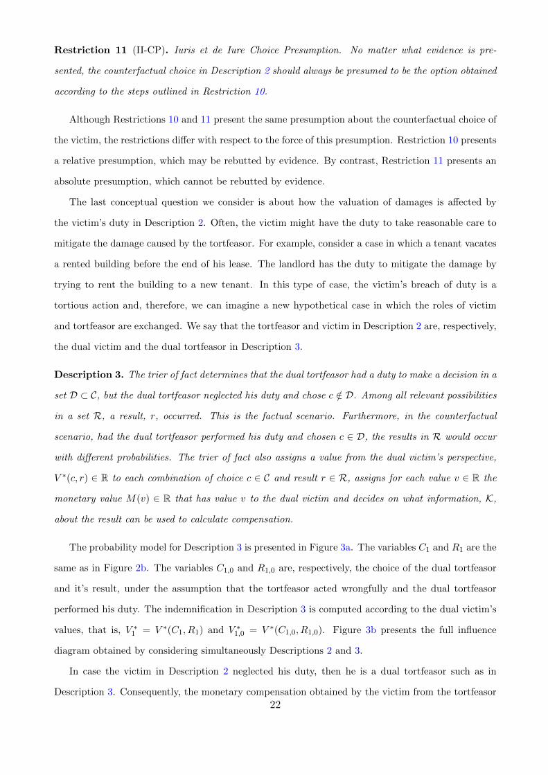
The probability model for Description 3 is presented in Figure 3a. The variables C1 and R1 are the

same as in Figure 2b. The variables C1,0 and R1,0 are, respectively, the choice of the dual tortfeasor

and it’s result, under the assumption that the tortfeasor acted wrongfully and the dual tortfeasor

performed his duty. The indemnification in Description 3 is computed according to the dual victim’s

values, that is, V ∗1 = V ∗(C1, R1) and V ∗1,0 = V ∗(C1,0, R1,0). Figure 3b presents the full influence

diagram obtained by considering simultaneously Descriptions 2 and 3.

In case the victim in Description 2 neglected his duty, then he is a dual tortfeasor such as in

Description 3. Consequently, the monetary compensation obtained by the victim from the tortfeasor

22

in the lost chance case in Description 2 should be reduced by the monetary amount that the victim

owes to the tortfeasor in the lost chance case in Description 3. This understanding conforms to the

practice of reducing the compensation of a victim who doesn’t take reasonable precautions to mitigate

damages. Restriction 12 presents this position.

C1,0

F ∗Coo // C1

R1,0

F ∗Roo // R1

V ∗1,0 V ∗1

(a) Influence diagram for Description 3.

C0

FCoo // C1

F ∗Coo // C1,0

R0

FRoo // R1

~~

F ∗Roo // R1,0

V0 V1 V ∗1 V ∗1,0

(b) Influence diagram for Descriptions 2 and3.

Figure 3: Influence diagrams related to Description 3.

Restriction 12. In case the victim in Description 2 neglects his duty, then his compensation monetary

value should be subtracted by the compensation monetary value due to the tortfeasor because of this

breach in duty24.

By combining the restrictions in Sections 3 and 4, one obtains compensation policies for lost chance

cases with choices. In Section 5 we apply these compensation policies to a lost chance case in which

the victim had the right to a choice, Matos v. BF Utilidades Domesticas Ltda. (2005).

5 An application of the valuation of lost chances with

choices

An important precedent in the application of the Lost Chance Doctrine in Brazil is Matos v. BF

Utilidades Domesticas Ltda. (2005), known as the “Millionaire Show” case. Similar to its American

version, the “Millionaire Show” was a Brazilian television show in which in each round a guest could

answer a multiple choice question. If the guest’s answer was correct, her cumulative prize would

increase and she would pass to the next round. If the guest’s answer was incorrect she would be

24Formally, let X0 and X1,0 be, respectively, the compensations obtained in Figures 2b and in 3a. The monetary valueawarded to the victim should be max(0,M(V1 +X0)−M(V1)−M∗(V ∗1 +X1,0) +M∗(V ∗1 )). For example, if the judge adoptsRestriction CC-I, then the monetary value awarded to the victim should be max(0,max(0,M(E[V0|K]) −M(E[V1|K])) −max(0,M(E[V ∗1,0|K])−M(E[V ∗1 |K]))).

23

awarded a fraction of her cumulative prize and her participation in the show would end. Finally,

if the guest decided not to answer, she would get the full extent of her cumulative prize and her

participation would end.

The guest in 06/15/2000, Matos, got to the last round of the show. Her cumulative prize was

R$500, 000. The last multiple choice question which was presented to her had four options. The

question asked the proportion of Brazil’s territory that the country’s Constitution reserves to na-

tives: 22%, 2%, 4% or 10%? Had Matos answered correctly, she would get R$1, 000, 000. Had she

answered incorrectly, she would get R$300. She decided not to answer and keep the cumulative prize

of R$500,000.

Nevertheless, it was later found out that, although the plaintiff had registered one of the alternative

answers as correct, none of them were actually correct. The Brazilian Constitution doesn’t directly

specify a percentage of Brazil’s territory reserved to natives, but specifies that natives have the right

over the land that they had traditionally occupied25. Based on this error, Matos filed a lawsuit against

the producers of the show. Her case reached the Superior Court of Justice, the highest appellate

court in Brazil for non-constitutional matters. It was the first case the Court decided using the Lost

Chance Doctrine. Although the Court ruled that Matos wasn’t able to prove that she would get the

R$1, 000, 000 prize if faced with a proper question, it also decided that Matos had been wrongfully

deprived of her right to answer a properly formulated question and that the producers of the show were

liable for this damage. The Court stated that the “mathematical probability” of correctly answering

a multiple choice question with four options was 25% and, therefore, Matos should be compensated

with 25% of the difference between the total prize and the R$500,000 that she had already received.

Next, we compare the Court’s valuation with the method we propose in Sections 3 and 4.

We start by exposing the elements of Description 2 that are present in Matos v. BF Utilidades

Domesticas Ltda. (2005). The first element in Description 2 is the set of choices that the victim could

choose from, C. After the multiple choice question was presented to Matos, she could choose between

two options: either to answer or not to answer the question. That is, C = answer,not answer. The

next element in Description 2 is the set of possible results of the victim’s choice, R. In case Matos

chose to answer, she would receive either R$1, 000, 000 or R$300. In case Matos chose not to answer,

then she would certainly receive R$500, 000. Therefore, the set of all relevant results that could follow

from Matos’s choice was R = R$300, R$500, 000, R$1, 000, 00025Brasil (1988) specifies: “art. 231. sao reconhecidos aos ındios sua organizacao social, costumes, lınguas, crencas e

tradicoes, e os direitos originarios sobre as terras que tradicionalmente ocupam, competindo a Uniao demarca-las, protegere fazer respeitar todos os seus bens”.

24

Given the previous two elements, we proceed to the relevant probabilities for Matos v. BF Util-

idades Domesticas Ltda. (2005). No matter if the tortious action occurred or not, Matos would

certainly receive $500, 000 in case she chose not to answer26. By contrast, in case Matos had answered

the question, then two outcomes could occur. In the factual scenario, the alternative that had been

marked as correct by the plaintiff was actually incorrect. In this case, Matos’s best hope to obtain

the answer marked as correct was to randomly guess with equal probability one of the alternatives27.

In the counterfactual scenario, one should consider a question such that the answer marked as correct

was also a correct answer to the question that was asked. In this case, Matos would have been able

to rely on her knowledge in order to find the correct answer.

In this respect, we disagree with the Court’s decision. Matos’s probability of correctly answering a

properly designed question should depend, at least, on Matos’s skill and the difficulty of the question.

Probability theory does not specify that the “mathematical probability” of correctly answering to a

multiple choice question with four alternatives is 0.25. On the contrary, this probability should be

judged according to the evidence that was available. For example, the alternatives that were presented

to Matos (22%, 2%, 4% and 10%) were qualitatively different. In a properly formulated question,

qualitative differences can be used to rule out some of the alternatives (is it reasonable to expect more

than a fifth of Brazil’s territory to be reserved to natives?). Using this method and then guessing,

Matos would improve her probability from 25%. Furthermore, Matos had shown skill by correctly

answering all questions that had previously been asked in the show. This evidence also gives reason to

believe that Matos would probably be able to choose the correct alternative with a greater probability

than if she were to randomly guess one of the alternatives with equal probability.

By contrast, the defendant claimed that the questions’ difficulties progressed as the contestant

got closer to the final prize. For example, among the first questions that were asked to previous

contestants, there was “what fruit is dried to obtain dried plums? 1) plum, 2) grape, 3) peach,

4) melon”. By contrast, the defendant presented evidence that, until that date, no contestant had

successfully answered the last question in the show. Therefore, the defendant argued that the high

probability obtained by considering Matos’s record of successful answers should be balanced by the

higher difficulty of the last question.

A possible alternative to the Court’s evaluation of the probability was to subjectively balance the

evidence presented by the victim and the defendant. In the following, we aim for a general analysis

26Formally, P (R0 = $500, 000|C0 = answer) = P (R1 = $500, 000|C1 = not answer) = 1.27Formally, P (R1 = R$1, 000, 000|C1 = answer) = 0.25.

25

of Matos’s probability of success. We refer to the probability that Matos would choose the correct

alternative of a properly formulated question by P (R0 = R$1, 000, 000|C0 = answer) and describe the

consequences of all possible choices for this probability on the valuation of the lost chance.

The next elements in Description 2 are the victim’s utility for each outcome, V , and the amount

of money that is necessary to increase the victim’s utility by v, M(v). In principle, V could depend

on both the choice, c, and the result, r. Nevertheless, Matos claimed a lost chance over only the

monetary gain. For example, Matos didn’t claim a loss over the excitement of answering a properly

formulated question. Therefore, we assume that the value of each outcome is a function of the money

that is obtained in that outcome. Using this simplification, V returns a valuation of money and M

returns the amount of money that corresponds to a given value. That is, M is a function of V 28 and,

therefore, it is sufficient to specify V alone.

In Matos v. BF Utilidades Domesticas Ltda. (2005), the Court didn’t directly specify the victim’s

utility for each outcome. Instead, the Court directly assigned that the compensation should be 25%

of a difference between monetary amounts. By using this rule, the Court implicitly assumed the

identity between amount of money and value. One consequence of this assumption is that the victim

would value equally the options of receiving R$500,000 with certainty and receiving R$1,000,000 with

probability 50% and nothing otherwise. It might be unreasonable to believe a person has this type of

preference. For example, it would be a common answer to prefer the certain R$500,000 to the risky

R$1,000,000, a phenomenon known as risk aversion.

Risk aversion is such a commonly observed phenomenon that we consider the effect of other

valuations of money on the compensation. We value money with a class of functions29, presented in

Kadane (2011), that has a parameter that permits adjustment to the amount of risk aversion of the

victim. The trier of fact’s judgment on this parameter could be informed, for example, by the fact

that Matos decided to answer all the questions before the last one. Based on the questions’ difficulties

and Matos’s skill, the trier of fact would be able to set a bound for Matos’s risk aversion.

The last element of Description 2 defines the set of choices the victim had the duty to choose from,

D. That is, we evaluate whether Matos took appropriate measures to mitigate her damages. This

element wasn’t discussed by either the parties or the Court. Since Matos chose the safe option and

avoided answering the improperly formulated question that was asked to her, we believe her factual

28Formally, we assume that V is a monotone increasing function and that M(v) = V −1(v).29Formally, V (m) = 1−m1−θ

θ−1 , for 0 ≤ θ ≤ 1. In case θ = 0, utility is linear and there is no risk aversion. Risk aversionincreases with θ and one obtains V (m) = log(m) as θ goes to 1.

26

No risk aversion(θ=0)

P(R0=R$1,000,000|C0= answer)

Com

pens

atio

n (in

mill

ions

of R

$)

0.5

0.00

0.25

0.50

High risk aversion(θ=1)

P(R0=R$1,000,000|C0= answer)

0.915

0.00

0.25

0.50

Figure 4: Compensation that should be awarded in Matos v. BF Utilidades Domesticas Ltda. (2005) as afunction of Matos’s probability of correctly answering the question.

choice was dutiful30.

Given the previously defined elements, the Restrictions in Sections 3 and 4 completely specify the

lost chance valuation. In Matos’s case, the factual result was a certain consequence of her chance. As

a consequence, all the combinations of the different types of Restrictions provide the same valuation.

Figure 4 illustrates the compensation that should be awarded to Matos under the two extreme

cases of risk aversion. The left graph represents the case in which Matos has no risk aversion. In

this case, Matos would need at least a probability of 500,000−3001,000,000−300 (approximately 50%) of correctly

answering the question in order to obtain some compensation. Intuitively, if this probability were

lower than 500,000−3001,000,000−300 , then, in the counterfactual scenario, not answering would be the best choice

for Matos. After the probability of 500,000−3001,000,000−300 is attained, Matos’s compensation increases linearly

until it reaches R$500, 000 when her probability of correctly answering is 1. The right graph represents

the case in which Matos has a proportion of risk aversion of 1. In this case, Matos would need at least

a probability of log(500,000)−log(300)log(1,000,000)−log(300) (approximately 91.5%) to be compensated. This value is higher

than in the previous case because, under risk aversion, Matos would take the risky chance of answering

the question only if she were extremely confident that she would answer correctly. Similarly to the

previous graph, compensation increases with Matos’s probability of success and reaches R$500, 000

when this probability is 1.

Figure 5 illustrates the variation of Matos’s compensation in terms of her risk aversion and proba-

bility of correctly answering the question. While the white coloring indicates points such that Matos

30Formally, D ⊂ answer.27

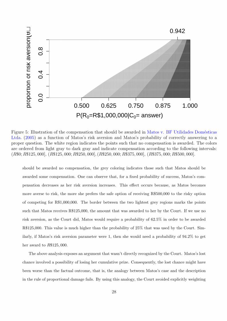
0.0

0.4

0.8

P(R0=R$1,000,000|C0= answer)

prop

ortio

n of

ris

k av

ersi

on(θ

)

0.500 0.625 0.750 0.875 1.000

0.942

Figure 5: Illustration of the compensation that should be awarded in Matos v. BF Utilidades DomesticasLtda. (2005) as a function of Matos’s risk aversion and Matos’s probability of correctly answering to aproper question. The white region indicates the points such that no compensation is awarded. The colorsare ordered from light gray to dark gray and indicate compensation according to the following intervals:(R$0;R$125, 000], (R$125, 000;R$250, 000], (R$250, 000;R$375, 000], (R$375, 000;R$500, 000].

should be awarded no compensation, the grey coloring indicates those such that Matos should be

awarded some compensation. One can observe that, for a fixed probability of success, Matos’s com-

pensation decreases as her risk aversion increases. This effect occurs because, as Matos becomes

more averse to risk, the more she prefers the safe option of receiving R$500,000 to the risky option

of competing for R$1,000,000. The border between the two lightest grey regions marks the points

such that Matos receives R$125,000, the amount that was awarded to her by the Court. If we use no

risk aversion, as the Court did, Matos would require a probability of 62.5% in order to be awarded

R$125,000. This value is much higher than the probability of 25% that was used by the Court. Sim-

ilarly, if Matos’s risk aversion parameter were 1, then she would need a probability of 94.2% to get

her award to R$125, 000.

The above analysis exposes an argument that wasn’t directly recognized by the Court. Matos’s lost

chance involved a possibility of losing her cumulative prize. Consequently, the lost chance might have

been worse than the factual outcome, that is, the analogy between Matos’s case and the description

in the rule of proportional damage fails. By using this analogy, the Court avoided explicitly weighting

28

the importance of elements such as the rules of the television show, Matos’s skill, Matos’s aversion to

risk and the question’s difficulty. These elements are key figures in our analysis and could change the

compensation to any value between R$0 and R$500, 000.

6 Conclusion

What legal restrictions inform the valuation of lost chances? Despite the practical importance of this

question, it has seldom been discussed explicitly. On the contrary, the discussion around the valuation

of lost chances has mostly revolved around the formula prescribed by the rule of proportional damage.

The above focus on a single formula is dangerous for at least two reasons. The first reason is

that the formula applies only to a very specific type of case. Furthermore, when slight variations of

this specific case (such as medical misdiagnosis) are considered, the different formulas that have been

proposed can yield widely different valuations. Without a justification for choosing a given formula,

the compensation value that is obtained is arbitrary. The second reason is that the formulas that have

been discussed require the trier of fact to specify only one or two probabilities and a single monetary

value. As a consequence, they induce the trier of fact to disregard elements that don’t easily fall into

these categories. For example, in Matos v. BF Utilidades Domesticas Ltda. (2005), the Court ignored

relevant questions such as Matos’s skill, the difficulty of the questions, Matos’s risk aversion and the

different possible outcomes of the lost chance.

Based on the above considerations, we propose a discussion of the legal restrictions that guide the

valuation of lost chances. We frame this discussion in terms of six conceptual questions.

The first three questions can be applied to every lost chance case: How much information about the

factual outcome can be used in the valuation of lost chances? How does the law connect the scenario

that was observed to the scenario that would have occurred but for the tortious action? What is

the meaning of indemnification for a lost chance? Despite the qualitative nature of these questions,

we show that the answers that are given to them completely specify compensation valuation in a

description that is more general than the one required for the application of the rule of proportional

damage.

We explore alternative combinations of answers to the above questions using two types of examples.

As a first example, we use the typical case of medical misdiagnosis. In this case, we show in Table

3 that the main formulas that have been proposed in the literature can be obtained from specific

answers. Consequently, the differences between these qualitative answers can be used to understand

29

the proposed formulas and make justified choices between them. A second example, consists of

a though experiment that involves a lost chance with 5 possible outcomes. As a summary, Table 5

shows that different combinations of answers to the conceptual questions can lead to radically different

compensation valuations. Some of these compensations disagree completely even with respect to

what outcomes should be compensated. This disagreement illustrates the necessity of discussing the

conceptual questions that were raised.

The other three conceptual questions we present apply to cases in which the victim had the right

to a choice that could affect the probabilities of his possible outcomes: At the time the victim made

his choice, how much information did he have available? How would the victim use this information

to make a choice? Is a victim’s compensation affected by a wrongful choice? Since it is hard to predict

the behavior of a human, both of the parties might fail to answer the first two questions. In this case,

we discuss possible legal presumptions.

We use the six conceptual questions to study Matos v. BF Utilidades Domesticas Ltda. (2005).

Despite this case being Brazil’s Supreme Court of Justice’s first application of the lost chance doctrine,

in this case the victim had multiple possible outcomes and also had the right to make a choice. The

conceptual questions we propose raise relevant elements for compensation that weren’t explicitly

considered by the Court’s decision.

Acknowledgement

The authors are grateful for the insightful discussions with Celso Campilongo, Andre Katsurada,

Caroline Mitchell, Marcelo Nunes, Carlos Pereira, Ted Permigiani, Fernando Rozenblit, Julio Stern

and Julio Trecenti.

References

Aumann, R. J. (2003), ‘Risk aversion in the Talmud’, Economic Theory 21(2-3), 233–239.

Balke, A. and Pearl, J. (1994), Counterfactual probabilities: Computational methods, bounds and

applications, in ‘Proceedings of the Tenth international conference on Uncertainty in artificial

intelligence’, Morgan Kaufmann Publishers Inc., pp. 46–54.

30

Bernoulli, D. (1954), ‘Exposition of a new theory on the measurement of risk’, Econometrica: Journal

of the Econometric Society pp. 23–36.

Brasil (1988), Constituicao Federal de 1988, Senado Federal.

Falcon v. Memorial Hosp., 436 Mich. 443 (1990).

Ferreira, R. C. (2013), ‘The Loss of Chance in Civil Law countries: A Comparative and Critical

Analysis’, Maastricht journal of European and comparative law 20(1), 56–74.

Fischer, D. A. (2001), ‘Tort Recovery for Loss of a Chance’, Wake Forest L. Rev. 36, 605.

Fisher, F. M. and Romaine, R. C. (1990), ‘Janis Joplin’s yearbook and the theory of damages’, Journal

of Accounting, Auditing & Finance 5(1), 145–157.

Fulton v. Pontiac Gen. Hosp., 655 N.W.2d 569 (Mich. Ct. App. 2002).

Herskovits v. Group Health Coop., 99 Wn.2d 609, 664 P.2d 474 (Wash. 1998).

Jansen, N. (1999), ‘The idea of a lost chance’, Oxford Journal of Legal Studies 19(2), 271–296.

Kadane, J. B. (2011), ‘Partial-Kelly strategies and expected utility: Small-edge asymptotics’, Decision

Analysis 8(1), 4–9.

Kantorovich, L. V. (1960), ‘Mathematical methods of organizing and planning production’, Manage-

ment Science 6(4), 366–422.

King, Jr., J. H. (1981), ‘Causation, valuation, and chance in personal injury torts involving preexisting

conditions and future consequences’, Yale law journal pp. 1353–1397.

King, Jr., J. H. (1998), ‘”Reduction of Likelihood” Reformulation and Other Retrofitting of the

Loss-of-a-Chance Doctrine’, U. Mem. L. Rev. 28, 492–1279.

Koch, S. R. (2009), ‘Whose Loss is It Anyway-Effects of the Lost-Chance Doctrine on Civil Litigation

and Medical Malpractice Insurance’, NCL Rev. 88, 595.

Lindley, D. (1971), Making Decisions, Wiley.

Matos v. BF Utilidades Domesticas Ltda., REsp 788459 BA 2005/0172410-9 (2005).

Matsuyama v. Birnbaum, 890 N.E.2d 819 (Mass. 2008).

31

McKellips v. Saint Francis Hosp., Inc., 741 P.2d 467 (Okla. 1987).

Miceli, C. M. (2013), Il danno da perdita di chance, PhD thesis.

Miller, C. (2005), ‘Gregg v. scott: loss of chance revisited’, Law, Probability and Risk 4(4), 227–235.

Noah, L. (2005), ‘An Inventory of Mathematical Blunders in Applying the Loss-of-a-Chance Doctrine’,

Rev. Litig. 24, 369.

Pan, Q. and Gastwirth, J. L. (2013), ‘The appropriateness of survival analysis for determining lost

pay in discrimination cases: application of the “lost chance” doctrine to alexander v. milwaukee’,

Law, Probability and Risk 12(1), 13–35.

Rhee, R. J. (2013), ‘Loss of chance, probabilistic cause, and damage calculations: The error in mat-

suyama v. birnbaum and the majority rule of damages in many jurisdictions more generally’, Suffolk

University Law Review Online 1, 39–46.

Silva, R. P. (2013), Responsabilidade Civil pela Perda de uma Chance, 3rd edn, Atlas.

Smith, B. (1999), ‘Loss of a Chance’, Victoria U. Wellington L. Rev. 29, p. 225–252.

Viney, G. and Jourdain, P. (1998), Traite de droit civil: Les conditions de la responsabilite civile,

L.G.D.J.

Appendix

Definition 3. In the following proofs, we use:

1. R(X) = E[(V0 − (V1 +X))2].

2. ∆VK = E[V0 − V1|K].

Lemma 1. If E[|V0 − V1|] <∞, then for every X,X∗ ∈ X such that R(X) <∞ and R(X∗) <∞,

R(X)−R(X∗) = E[(X −∆VK)2]− E[(X∗ −∆VK)2]

32

Proof. For every X ∈ X ,

R(X) = E[E[((V0 − V1)−X)2|K]]

= E[((V0 − V1)−∆VK)2] + E[(∆VK −X)2] since E[|V0 − V1|] <∞, E[∆VK] = E[V0 − V1]

and X and ∆VK are K-measurable

Hence,

R(X)−R(X∗) = E[(∆VK −X)2]− E[(∆VK −X∗)2]

Proof of Theorem 1. Let X∗1 = max(0,∆VK). For every X ∈ X ,

R(X)−R(X∗1 ) = E[(∆VK −X)2]− E[(∆VK −X∗1 )2] Lemma 1

= E[((∆VK −X)2 − (∆VK −X∗1 )2) · O+] + E[(X2 − 2∆VKX) · O−] X∗1 · O− = 0

≥ E[((∆VK −X)2 − (∆VK −X∗1 )2) · O+] + E[(X − 0)2 · O−] ∆VK · O− ≤ 0, X ≥ 0

= E[(∆VK −X)2 · O+] + E[(X − 0)2 · O−] X∗1 · O+ = ∆VK · O+

= E[(X −X∗1 )2]

Hence, if P (X 6= X∗1 ) > 0, R(X) > R(X∗1 ).

Lemma 2. If E[|V0 − V1|] <∞ and E[V0 − V1] > 0, then there exists a unique λ∗ ∈ R such that

E[max(0,∆VK − λ∗)] = E[V0 − V1]

Proof. Let f(λ) = E[max(0,∆VK − λ)]. Observe that f is a decreasing function and that, for every

ε > 0 and λ ∈ R, |f(λ+ ε)− f(λ)| ≤ ε. Hence, f is a continuous function. Furthermore,

f(0) = E[max(0,∆VK)] ≥ E[∆VK] = E[V0 − V1]

and, since E[|V0 − V1|] <∞, E[|∆VK|] <∞ and

limλ→∞

f(λ) ≤ limλ→∞

∫ ∞λ

xdF∆VK(x) = 0

33

Since f is continuous, f(0) ≥ E[V0 − V1] and limλ→∞ f(λ) = 0 conclude from the intermediate value

theorem that there exists a λ∗ such that f(λ∗) = E[V0 − V1]. Since f is decreasing, conclude that λ∗

is the only λ ∈ R such that f(λ) = E[V0 − V1].

Lemma 3. Let λ ∈ R, X+2 = max(0,∆VK − λ) and X−2 = min(0,∆VK − λ). For every X ∈ X ,

V ar[X −∆VK] = V ar[X −X+2 ]− 2Cov[X,X−2 ] + 2Cov[X+

2 , X−2 ] + V ar[X−2 ]

Proof.

V ar[X −∆VK] = V ar[X − (∆VK − λ)]

= V ar[X]− 2Cov[X,∆VK − λ] + V ar[VK − λ]

= V ar[X]− 2Cov[X,X+2 +X−2 ] + V ar[X+

2 +X−2 ]

= V ar[X]− 2Cov[X,X+2 ]− 2Cov[X,X−2 ] + V ar[X+

2 ] + V ar[X−2 ] + 2Cov[X+2 , X

−2 ]

= V ar[X −X+2 ]− 2Cov[X,X−2 ] + 2Cov[X+

2 , X−2 ] + V ar[X−2 ]

Proof of Theorem 2. Let X1 = X ∈ X : E[X] = E[V0 − V1] or X = 0. If X ∈ X , then X ≥ 0.

Therefore, if E[V0−V1] ≤ 0, X1 = X = 0 and arg minX∈X1R(X) = 0. Next, consider that E[V0−

V1] > 0. It follows from Lemma 2 that there exists a unique λ∗ ∈ R such that E[max(0,∆VK−λ∗)] =

E[V0−V1]. Let X+2 be defined as max(0,∆VK−λ∗). It remains to show that arg minX∈X1 R(X) = X+

2 .

For every X ∈ X1,

R(X)−R(X+2 ) = E[(∆VK −X)2]− E[(∆VK −X+

2 )2] Lemma 1

= V ar[∆VK −X]− V ar[∆VK −X+2 ] E[X] = E[X+

2 ]

= V ar[X −X+2 ]− 2Cov[X,X−2 ] + 2Cov[X+

2 , X−2 ] Lemma 3

= V ar[X −X+2 ]− 2(E[X ·X−2 ]− E[X+

2 ·X−2 ]) E[X] = E[X+

2 ]

= V ar[X −X+2 ]− 2E[X ·X−2 ] X+

2 ·X−2 = 0

≥ V ar[X −X+2 ] X ·X−2 ≤ 0

34

Also,

R(0)−R(X+2 ) = E[∆V 2

K]− E[(∆VK −X+2 )2] Lemma 1

= E[(X+2 +X−2 )2]− E[(X−2 )2]

= E[(X+2 )2] X+

2 ·X−2 = 0

= E[X+2 ]2 + V ar[X+

2 ]

> E[∆VK]2 > 0 E[∆VK] = E[V0 − V1] > 0,

E[X+2 ] > E[∆VK]

Hence, if E[V0 − V1] > 0, then for every X ∈ X1 such that P (X 6= X+2 ) > 0, R(X) > R(X+

2 ).

35