Physically constrained maximum likelihood mode filtering

Physically constrained maximum likelihood mode filteringJoseph C. Papp,a� James C. Preisig, and Andrey K. MorozovWoods Hole Oceanographic Institution, MS 44, Woods Hole, Massachusetts 02543

�Received 28 September 2009; revised 24 January 2010; accepted 27 January 2010�

Mode filtering is most commonly implemented using the sampled mode shapes or pseudoinversealgorithms. Buck et al. �J. Acoust. Soc. Am. 103, 1813–1824 �1998�� placed these techniques in thecontext of a broader maximum a posteriori �MAP� framework. However, the MAP algorithmrequires that the signal and noise statistics be known a priori. Adaptive array processing algorithmsare candidates for improving performance without the need for a priori signal and noise statistics.A variant of the physically constrained, maximum likelihood �PCML� algorithm �A. L. Kraay andA. B. Baggeroer, IEEE Trans. Signal Process. 55, 4048–4063 �2007�� is developed for modefiltering that achieves the same performance as the MAP mode filter yet does not need a prioriknowledge of the signal and noise statistics. The central innovation of this adaptive mode filter isthat the received signal’s sample covariance matrix, as estimated by the algorithm, is constrained tobe that which can be physically realized given a modal propagation model and an appropriate noisemodel. Shallow water simulation results are presented showing the benefit of using the PCMLmethod in adaptive mode filtering. © 2010 Acoustical Society of America.�DOI: 10.1121/1.3327799�

PACS number�s�: 43.60.Mn �EJS� Pages: 2385–2391

I. INTRODUCTION

Buck et al.1 presented a unified framework for modefiltering using a model of the underwater environment con-taining propagating modes plus noise. Nonadaptive linearmode filters such as the sampled mode shapes and pseudo-inverse filters were analyzed and the MAP filter was pre-sented to make use of signal and noise statistics and showeda significant performance improvement. However, the statis-tics are required to be known a priori. This paper proposesan adaptive mode filter based on the minimum power distor-tionless response �MPDR� beamformer that uses pressurefield statistics estimated from the data. However, in a non-stationary environment there are often an insufficient numberof snapshots available to accurately estimate the required sta-tistics. Kraay2 presented a physically constrained, maximumlikelihood �PCML� method for using knowledge of the spa-tial environment to estimate the statistics using fewer snap-shots. This paper adapts the PCML method to the underwatermode estimation problem using adaptive mode filters basedon the MPDR and MAP frameworks.

The remaining sections of the introduction introduce thesignal and noise model used in this paper and describe sev-eral established mode filtering techniques—the sampledmode shapes, pseudoinverse, diagonally weighted pseudoin-verse, reduced rank pseudoinverse, and maximum a poste-riori �MAP� mode filters. Section II describes the MPDRmode filter and a diagonal weighting technique to address thesnapshot deficiency problem. Section III outlines the PCMLalgorithm developed by Kraay for a spatial beamformer. Sec-tion IV describes the adaptation of the PCML algorithm forthe mode estimation problem. Lastly, Sec. V presents the

a�Author to whom correspondence should be addressed. Electronic mail:
[email protected]
J. Acoust. Soc. Am. 127 �4�, April 2010 0001-4966/2010/127�4

performance of the various mode filters in a shallow watersimulation and Sec. VI summarizes the main conclusions ofthis paper.

A. Modes as basis functions

Modes are physically motivated, orthogonal basis func-tions for the vertical sound field. They are derived from so-lutions to the wave equation and are dependent on frequencyand environmental conditions, such as water depth, tempera-ture, salinity, and bottom properties.3 Equation �1� shows thepressure field as a sum of modes, where p�z , f� is the com-plex acoustic pressure at frequency f and depth z, dm is themode coefficient of the mth mode, and �m�z , f� is the mthmode shape as a function of depth and frequency,

p�z, f� = �m

dm�f��m�z, f� . �1�

B. Signal and noise model used

Equation �2� shows the signal model used to representthe sound pressure field,

�p�z1�]

p�zN�� = ��1�z1� ¯ �M�z1�

] � ]

�1�zN� ¯ �M�zN�� d1

]

dM� + �n�z1�

]

n�zN�� , �2�

where n�z� is the noise received by the sensor at depth z. Thefunctional dependence of all quantities on frequency hasbeen dropped for notational convenience. In this paper, themode shapes, �, are assumed known a priori and the goal isto estimate the complex mode coefficients d given measure-ments of the pressure field p. Written in vector notation, the
above equation becomes
© 2010 Acoustical Society of America 2385�/2385/7/$25.00

p = �d + n , �3�

where � is the matrix of sampled mode shapes at a particularfrequency

� = ��1�z1� ¯ �M�z1�] � ]

�1�zN� ¯ �M�zN�� , �4�

and d is a vector of complex-valued mode amplitudes and isassumed to be zero mean. A spatially white �SW� noisemodel is used in this paper. The SW noise model assumes thenoise is complex valued and zero mean, with the noise ateach hydrophone uncorrelated with noise at all of the otherhydrophones. Assuming that the noise has save variance ateach sensor, the covariance matrix for this type of noise is

Rn = �2I . �5�

Often noise is contained in the propagating modes as well,and this type of noise is described by the Kuperman–Ingenitomodel.4 The goal of mode filtering, however, is to simplyestimate the coefficients of the received energy in each modeand not to distinguish between signal and noise contained inthe modes. Determining what part of the mode amplitude isfrom signal and what part is from noise is an applicationspecific problem. Therefore, only spatially white noise willbe considered in this paper.

C. Established mode filtering techniques

This section outlines several established mode filteringtechniques. Mode filters estimate the complex-valued ampli-tude of a particular mode at a particular frequency given themeasured vertical pressure field and knowledge of the modeshapes. Further information about the mode filtering tech-niques can be found in Ref. 1. Equation �6� expresses theestimated mode amplitudes as a function of the vertical pres-sure field and a linear mode filter, H.

d̂ = Hp . �6�

The remaining part of this subsection lists several choices forH that can be used in estimating the mode amplitudes.

�a� Sampled mode shape �SMS� mode filter.

HSMS = ��1�z1� ¯ �1�zN�] � ]

�M�z1� ¯ �M�zN�� = �H. �7�

�b� Pseudoinverse �PI� mode filter.

HPI = ��H��−1�H. �8�

�c� Diagonal weighting on pseudoinverse mode filter.

HDW = ��H� + �I�−1�H, �9�

where � is real valued and greater than zero.
�d� Reduced rank pseudoinverse mode filter. Let the singular
2386 J. Acoust. Soc. Am., Vol. 127, No. 4, April 2010

value decomposition of � be

� = USVT, �10�

where S is a diagonal matrix consisting of the singular valuesof �, and U and V are orthogonal matrices representing theeigenvectors of ��T and �T�, respectively. The reducedrank pseudoinverse mode filter can be written as

HRR = �+ = VS+UT, �11�

where S+ is the pseudoinverse of the diagonal matrix S,where the inverses of diagonal elements less than somethreshold �1/100 of the maximum diagonal value for thispaper� are set to zero.5

�e� MAP mode filter.

HMAP = �Rd−1 + �HRn

−1��−1�HRn−1, �12�

where Rd is the covariance matrix of the mode coefficientsand Rn is the noise covariance matrix. This assumes that themode amplitude coefficients and noise are jointly Gaussianrandom variables and that the mode amplitude coefficientsare independent of the noise.

II. MINIMUM POWER DISTORTIONLESS RESPONSEMODE FILTER

The MPDR mode filter minimizes the filter outputpower subject to the constraint that the desired mode ispassed with a gain equal to 1. It is based on the MPDRbeamformer used in spatial array processing, with a substi-tution of the mode shape vector in place of the spatial steer-ing vector.6–8 The goal is to minimize contributions frominterfering signals and noise while preserving the signalpropagating in the desired mode. Let the received verticalpressure field be p and the desired mode be n. wn is theweight vector that filters for mode n, with the output of themode filter being wn

Hp. The MPDR filter is defined by thefollowing constrained optimization problem:

wn = arg minwn

E��wnHp�2�

= arg minwn

wnHRpwn such that wn

H�n = 1. �13�

The solution is given by9,10

wn =Rp

−1�n

�nHRp

−1�n

, �14�

where Rp is the covariance matrix of the vertical pressurefield at a particular frequency. In practice, Rp is not known apriori and must be estimated from the received data. Thesample covariance matrix is one option for estimating Rp,but it requires a large number of snapshots to accuratelyestimate the matrix. The linear mode filter H that estimatesall the modes together is formed by combining the weights
for each mode:
Papp et al.: Physically constrained mode filtering

HMPDR = �w1

H

w2H

]

wMH� . �15�

The sample covariance matrix, R̂data, defined as

R̂data =1

L�

l=1,. . .,LXl��Xl��H �16�

is often used as the estimate of Rp, where Xl�� is the arraysnapshot vector at frequency �.6 This matrix is the uncon-strained maximum likelihood estimate of the covariance

matrix.11 R̂data is a good approximation of the true matrixonly when a large number of snapshots are used. An inad-equate number of snapshots results in poor adaptive algo-rithm performance.6,12

A diagonal weighting technique may be used on thesample covariance matrix to compensate for an inadequatenumber of snapshots and improve filter performance, similarto the diagonally weighted PI filter.6,13 When the weighting

factor, �, increases by a large amount, R̂DW becomes propor-tional to the identity matrix and the diagonally weightedMPDR filter becomes the same as the SMS filter.

R̂DW = R̂data + �I . �17�

III. PCML METHOD

This section describes a physically constrained, maxi-mum likelihood method for estimating the spatial covariancematrix used in adaptive filters. This method was proposed byKraay in 2003.2 The goal of the PCML method is to improveadaptive array processing methods under snapshot-deficientconditions. The algorithm determines the maximum likeli-hood estimate of the spatial covariance matrix subject toknown physical constraints. The physical constraints comefrom our knowledge that the received signal is composed ofa propagating component plus spatially white sensor noise.As a result of the physical constraints, fewer snapshots arerequired to obtain an accurate estimate of the spatial covari-ance matrix.

A. PCML covariance matrix estimate

The signal snapshots are modeled as series of indepen-dent, identically distributed �i.i.d.� zero-mean complexGaussian random vectors �CGRVs�. The joint probabilitydensity function of L such snapshots is14

p�Xl, . . . ,XL� = l=1,. . .,L

1

�N�R�e−Xl

HR−1Xl, �18�

where R is the covariance matrix of those snapshots and N isthe number of elements in each vector X. The ML estimate
of this covariance matrix given the received snapshots is
J. Acoust. Soc. Am., Vol. 127, No. 4, April 2010

R̂ML = arg maxR

p�X1, . . . ,XL�

= arg maxR

l=1. . .L

1

�N�R�e−Xl

HR−1Xl

= arg maxR

�−NL�R�−Le−�l=1. . .L−XlHR−1Xl

= arg maxR

− log�R� −1

L�

l=1,. . .,LTr�Xl

HR−1Xl�

= arg maxR

− log�R� − Tr 1

L�

l=1,. . .,LR−1XlXl

H�= arg max

R− log�R� − Tr�R−1R̂data� , �19�

where L�R , R̂data�=−log�R�−Tr�R−1R̂data� is the log-likelihood function. There is no closed form solution for theR that maximizes this log-likelihood function when thephysical constraint of Eq. �20� is imposed. It is, however,possible to use derivatives of the likelihood function in aniterative approach to finding the constrained ML estimate.Kraay2 derived this method for a spatial beamformer. Thecovariance matrix is separated into its propagating compo-nent plus spatially white sensor noise,

�R�ij = �2�ij +1

�2��3��k�

P��,k��v�k��i�vH�k�� jdk ,

�20�

where �v�k��n=e−jkTpn is the nth element of the array mani-fold vector, pn is the location of the nth array element, k isthe spatial wavenumber vector, and P�� ,k� is the frequencywavenumber power spectrum. ��k� is the region of supportof the wavenumber field imposed by the wave equation, k =2� /=� /c.

B. Iteration structure

The PCML algorithm iterates between estimating Rgiven current estimates of P�� ,k� and �2 and using the gra-dient of the likelihood function with respect to P�� ,k� and

�2 to update P̂m�� ,k� and �̂m2 , where the subscript m denotes

the estimate of the quantity at the mth iteration. The structureis shown in Fig. 1 and is discussed in detail in Secs. III C and

FIG. 1. Iteration used in the PCML algorithm to find the constrained maxi-mum likelihood spatial covariance matrix estimate.

III E.

Papp et al.: Physically constrained mode filtering 2387

C. Initialization

The PCML algorithm initializes its estimate of the cova-

riance matrix with the sample covariance matrix, R̂0= R̂data.The initial frequency wavenumber spectral estimate, P�� ,k�,is estimated using the MPDR estimator,8

P̂0��,kn� = wMPDRH �kn�R̂datawMPDR�kn�

=1

vH�kn�R̂data−1 v�kn�

. �21�

The white noise power estimate is initialized as one-tenth the

average diagonal value of R̂data since it is physically re-stricted to lie between zero and the smallest diagonal value

of R̂data.

�̂02 =

1

10NTr�R̂data� . �22�

D. Covariance matrix update

The first iterative step is to obtain a new estimate of thecovariance matrix. This is done by inverse Fourier trans-forming the frequency wavenumber spectrum with respect tothe wavenumber vector k.

�R̂m�ij = �F−1�P̂m−1��,k� + �̂m−12 ��i,j = �̂m−1

2 �ij

+1

�2��3��k�

P̂m−1��,k�e−jkT�pi−pj�dk , �23�

where P̂m−1�� ,k� is the estimate of the power at frequency �coming from the direction specified by k at iteration m−1.

Since P̂m can only be calculated at discrete points, a covari-ance matrix taper is used to smooth the estimates of propa-gating energy around the discrete spatial plane wave

samples. Each sample, P̂m−1�� ,k�, is approximated as aweighted, shifted window in k-space,

P̂m−1��,k� = �n

�P̂m−1��,kn�W�k − kn�� , �24�

where kn is the nth sample of k at which the frequencywavenumber spectrum is calculated. The integral in Eq. �23�then becomes a summation,

�R̂m�ij = �̂m−12 �ij + �

n

P̂m−1��,kn�e−jknT�pi−pj��Wij , �25�

where Wij is the inverse Fourier transform of the covariancematrix taper.15,16 The taper primarily used by Kraay was auniform window given by13

W�u� = W�ux,uy�

= �1 for �ux� �u/2 and �uy� �u/20 otherwise,

��26�


where u is the wavenumber vector, normalized by 2� /, and�u is the wavenumber grid spacing. The inverse Fouriertransform of this window is

Wi,j =� W�u�e+j�2�/�uT�pi−pj�du

= �u sinc2�

�u

2�pi,x − pj,x��u sinc

�2�

�u

2�pi,y − pj,y�� . �27�

E. Power spectrum and noise power updates

The power spectral density estimates of the power ineach mode are updated using the gradient of the likelihoodfunction �Eq. �19�� with respect to the power estimates.

The gradient with respect to the power at a given wave-number is given by

�L�R̂m,R̂data�

� P̂m��,kn�= − vH�kn�R̂m

−1v�kn�

+ vH�kn�R̂m−1R̂dataR̂m

−1v�kn� �28�

and the gradient with respect to the white noise power isgiven by

�L�R̂m,R̂data��̂m

2 = Tr��R̂m−1R̂data − I�R̂m

−1� . �29�

The second order gradient can be used to verify that a maxi-mum of the likelihood function is reached and not a mini-mum. The multiplicative update proposed by Kraay providesa convenient mapping between the gradients of the likeli-hood function and a multiplicative scaling factor. The updateis chosen such that when the gradient of the likelihood func-tion is zero, the power estimates remain unchanged. Thescale factor increases monotonically for a positive gradient

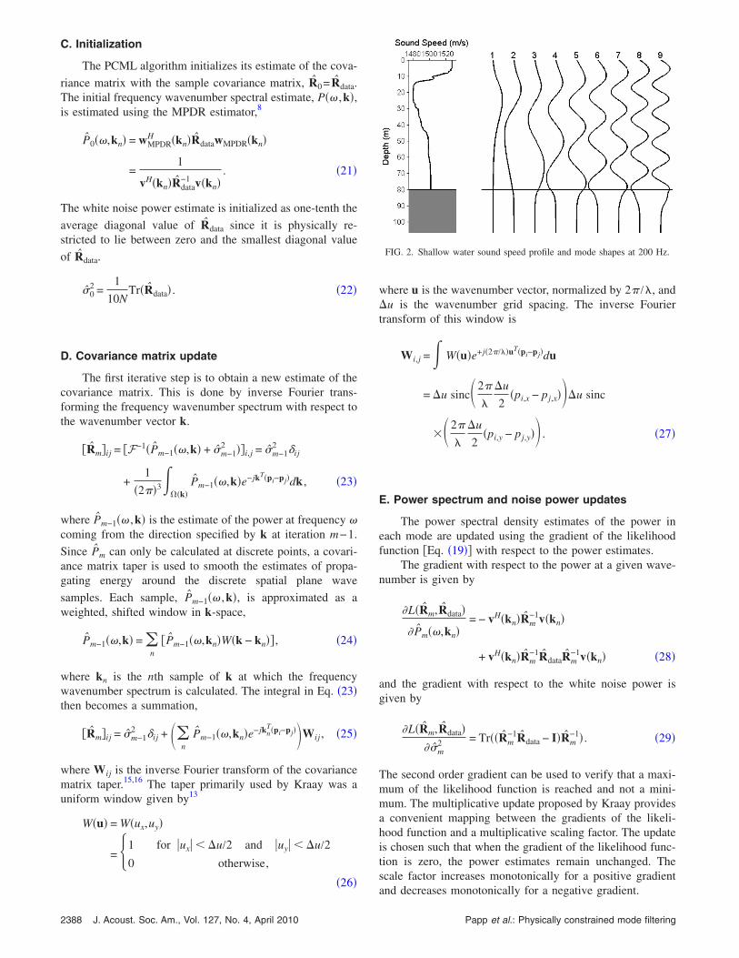
FIG. 2. Shallow water sound speed profile and mode shapes at 200 Hz.

and decreases monotonically for a negative gradient.


P̂m��,kn� =� P̂m−1��,kn�� A − 1

e�/2 − 1�earctan� �L/��P̂m−1��,kn�� − 1� + 1�,

�L

� P̂m−1

� 0

P̂m−1��,kn�� B − 1

e−�/2 − 1�earctan��L/��P̂m−1��,kn�� − 1� + 1� otherwise, � �30�

where A and B are the scale’s upper and lower limits, and and � are parameters that control how quickly the algorithmsteps as a function of the gradient. For the white noise powerupdate, Kraay used an additive form since it offered betterstability in her environment.

�̂m2 = �̂m−1

2 + 10−4 �L��̂m−1

2 �� 2L��̂m−1

2 �2� . �31�

The PCML algorithm iterates for a number of iterations untilthe covariance matrix estimate has converged to its mostlikely value. The PCML frequency wavenumber spectrum

estimates are the values of P̂m�� ,k� at the final iteration ofthe algorithm. The likelihood function can be calculated ateach iteration to provide an indication of whether the algo-rithm has converged, and a stopping condition can be formedbased on this. Kraay chose to run the algorithm for 50 itera-tions.

IV. PCML ALGORITHM APPLIED TO MODES

This section describes the application of Kraay’s PCMLalgorithm to the problem of estimating complex-valuedmode amplitudes. For the underwater environment model ofEq. �1�, the covariance matrix of the acoustic pressure fieldcan be decomposed into a propagating modal componentplus spatially white sensor noise. In this case, there are adiscrete number of propagating modes to sum instead of aninfinite number of spatial plane waves to integrate over, sono covariance matrix taper is necessary. Thus Eqs. �23� and�25� become

R̂ = �̂2I + �n=1,. . .,M

P̂��,�n��n�nH. �32�

The second change is that instead of steering the beamformerto a spatial direction, it is steered to a particular mode. Thearray steering vector, v�k�, becomes

v�kn� = �n. �33�

With these modifications, the PCML algorithm developed byKraay can be applied to determine the maximum likelihoodestimate of the covariance matrix given the physical con-straint. With each iteration, the PCML algorithm generatesan estimate of the power in each mode and the power of thespatially white noise. These estimates are used to generate anestimate of the covariance matrix using Eq. �32�. Once thePCML algorithm has converged, the PCML-MPDR filteruses the estimate of the covariance matrix at the final itera-tion of the PCML algorithm in the MPDR filter, Eqs. �14�and �15�. The PCML-MAP filter implements a MAP modefilter using the estimates of the signal and noise statistics
from the final iteration of the PCML algorithm. That is, the

filter assumes that the mode amplitude coefficients are un-correlated, and the noise is spatially white and calculates

Rd = �P̂��,�1�2 0 ¯ 0

0 P̂��,�2�2� ]

] ] � 0

0 . . . 0 P̂��,�M�2� �34�

and

Rn = �̂2I �35�

in Eq. �12�, using P̂ and �̂2 from the final PCML iteration.

V. PERFORMANCE AND ANALYSIS

A. Simulation setup

This section describes the setup of the shallow watersimulation. The mode coefficient vector, d, is modeled as azero-mean complex Gaussian random vector. The noise ismodeled as spatially white. The real and imaginary parts of dand n are i.i.d. and Gaussian, and therefore their covariancematrices are real valued.14 The simulation is similar to theone described by Buck et al.1 for a shallow water environ-ment. The simulated environment had typical shallow watersound speed profile and bottom properties and was 80 mdeep. Figure 2 shows the sound speed profile and the corre-sponding mode shapes at a frequency of 200 Hz.

A vertical array of 20 equally spaced hydrophones wasused. The location of the bottom hydrophone was fixed at 79m depth and the depth of the top hydrophone was variedfrom the water surface to a depth of 40 m �half the watercolumn�. This gradually reduced the fraction of the watercolumn that was spanned by the array. For each aperture, 500trials were run using independent realizations of the modecoefficients and noise vector. Linear mode filters were ap-plied to the simulated pressure field to obtain an estimate ofthe mode amplitudes. The error criteria are the sample mean

squared errors, d̂−d 2, between the estimate of the complexmode amplitudes and their actual values over the 500 trials.The total mode energy is included in the plots for referenceand represents the error that would result from estimatingeach mode to have zero amplitude. The mode coefficients, d,were assumed to be an i.i.d., zero-mean, CGRV. Exceptwhere stated otherwise, 25 snapshots were used to initializethe sample covariance matrix for the PCML algorithms and
for the MPDR filter.

B. Simulation results

Figure 3 shows the performance of the MPDR filter us-ing the sample covariance matrix as the number of snapshotsis varied. As was discussed in Sec. II, thousands of snapshotsare required for the covariance matrix to converge to its finalvalue. When sufficient snapshots are used, the MPDR filter’sperformance matches that of the MAP filter for a full span-ning array, but is a few dB worse than the MAP filter whenthe array span is reduced.

Figure 4 shows the effect of changing the loading pa-rameter on the diagonally weighted PI filter. With only smallamounts of weighting, the filter still suffers from sensitivityto white noise as the span of the array is reduced. With largeamounts of weighting, the filter performs poorly, as the am-plitude of the mode estimates approaches zero. Only whenthe correct weighting is applied is the filter able to performthe same as the MAP filter.

FIG. 3. Comparison of the performance of the MPDR mode filters as thenumber of snapshots used in the sample covariance matrix is varied. TheSMS and MAP filter performances and the total mode energy are includedfor reference.

FIG. 4. Comparison of the performance of the diagonally weighted PI filteras the weighting factor is varied. The SMS and MAP filter performances and
the total mode energy are included for reference.

Figure 5 shows the effect of changing the loading pa-rameter on the diagonally weighted MPDR filter. The filterconverges on the SMS filter as the weighting is increased;however, it is unable to perform better than SMS.

Figure 6 shows the simulation results for the PCML-MAP, PCML-MPDR, and reduced rank PI filters. With only25 snapshots, the PCML-MPDR filter is able to do as well asthe unconstrained MPDR filter using 10 000 snapshots. Fur-thermore, the PCML-MAP filter performs as well as theMAP filter that has full knowledge of the signal and noisestatistics. The sawtooth pattern in the reduced rank PI filter isa result of the changing number of singular values used inthe pseudoinversion as the condition number of � changes.As the condition number worsens, singular values aredropped one at a time resulting in the observed pattern.

FIG. 5. Comparison of the performance of the diagonally weighted MPDRfilter as the weighting factor is varied, using 25 snapshots to generate thesample covariance matrix in the MPDR filters. The SMS and MAP filterperformances and the total mode energy are included for reference. With adiagonal weighting of 100, the MPDR curve falls on top of the SMS curve.

FIG. 6. Comparison of the performance of the PCML-MAP, PCML-MPDR,PI, and reduced rank PI filters. The SMS and MAP filter performances andthe total mode energy are included for reference. The PCML algorithms
were initialized with 25 data snapshots.

VI. CONCLUSIONS

The MPDR filter using the sample covariance matrixrequires a large number of snapshots in order to estimate thereceived signal covariance matrix, Rp, with accuracy suffi-cient for the algorithm to yield satisfactory results. Whilediagonal loading of the sample covariance matrix can com-pensate for an insufficient number of snapshots, the perfor-mance of the diagonally loaded PI and MPDR algorithms issensitive to the choice of the loading parameter. This sensi-tivity is undesirable in real world applications.

The PCML algorithm uses physical constraints to esti-mate Rp and the second order statistics of the mode ampli-tudes and noise. When the resulting Rp is then used in aMPDR mode filter, it is found that the snapshot requirementcan be reduced by over two orders of magnitude withoutsacrificing the resulting algorithm performance. Furthermore,using the same number of snapshots as used for the PCML-MPDR algorithm, the estimated second order signal andnoise statistics can be used in the MAP mode filter andachieve the same performance as the MAP mode filter thathas a priori knowledge of these statistics.

ACKNOWLEDGMENTS

This paper is based on a thesis submitted in partial ful-fillment of the requirements of the degree of Master of Sci-ence in the Department of Electrical Engineering and Com-puter Science at the Massachusetts Institute of Technologyand Woods Hole Oceanographic Institution in September,2009. This work was supported by the Office of Naval Re-search through ONR Grant Nos. N00014-05-10085 andN00014-06-10788 and through the WHOI Academic Pro-grams Office.


1J. R. Buck, J. C. Preisig, and K. E. Wage, “A unified framework for modefiltering and the maximum a posteriori mode filter,” J. Acoust. Soc. Am.103, 1813–1824 �1998�.

2A. L. Kraay, “Physically constrained maximum-likelihood method forsnapshot-deficient adaptive array processing,” Master Thesis, Massachu-setts Institute of Technology, Cambridge, MA �2003�.

3F. B. Jensen, W. A. Kuperman, M. B. Porter, and H. Schmidt, Computa-tional Ocean Acoustics �Springer-Verlag, New York, 2000�.

4W. A. Kuperman and F. Ingenito, “Spatial correlation of surface generatednoise in a stratified ocean,” J. Acoust. Soc. Am. 67, 1988–1996 �1980�.

5G. Strang, Linear Algebra and Its Applications, 4th ed. �ThompsonBrooks/Cole, Belmont, CA, 2006�.

6H. L. VanTrees, Optimum Array �Wiley-Interscience, New York, 2002�,Part IV.

7B. D. Vanveen and K. Buckley, “Beamforming: A versatile approach tospatial filtering,” IEEE ASSP Magazine �1988�.

8J. Capon, “High-resolution frequency-wavenumber spectrum analysis,”Proc. IEEE 57, 1408–1418 �1969�.

9O. L. Frost, “An algorithm for linearly constrained adaptive array process-ing,” Proc. IEEE 60, 926–935 �1972�.

10D. H. Brandwood, “A complex gradient operator and its application inadaptive array theory,” IEE Proc. F, Commun. Radar Signal Process. 130,11–16 �1983�.

11J. R. Guerci, Space-Time Adaptive Processing for Radar �Artech House,Inc., Norwood, MA, 2003�.

12A. B. Baggeroer and H. Cox, “Passive sonar limits upon nulling multiplemoving ships with large aperture arrays,” Conference Record of the 33rdAsilomar Conference on Signals, Systems, Computers �1999�, Vol. 1, pp.103–108.

13A. L. Kraay and A. B. Baggeroer, “A physically constrained maximum-likelihood method for snapshot-deficient adaptive array processing,” IEEETrans. Signal Process. 55, 4048–4063 �2007�.

14D. Tse and P. Viswanath, Fundamentals of Wireless Communication �Cam-bridge University Press, New York, 2005�.

15J. R. Guerci, “Theory and application of covariance matrix tapers forrobust adaptive beamforming,” IEEE Trans. Signal Process. 47, 977–985�1999�.

16F. J. Harris, “On the use of windows for harmonic analysis with the dis-crete Fourier transform,” Proc. IEEE 66, 51–83 �1978�.


Physically constrained maximum likelihood mode filtering

Documents

Transcript of Physically constrained maximum likelihood mode filtering