a Fast Physically Interpretable Tensor Graphical Model - arXiv

SG-PALM: a Fast Physically Interpretable Tensor Graphical Model

Yu Wang 1 Alfred Hero 1

AbstractWe propose a new graphical model inference pro-cedure, called SG-PALM, for learning conditionaldependency structure of high-dimensional tensor-variate data. Unlike most other tensor graphicalmodels the proposed model is interpretable andcomputationally scalable to high dimension. Phys-ical interpretability follows from the Sylvestergenerative (SG) model on which SG-PALM isbased: the model is exact for any observationprocess that is a solution of a partial differen-tial equation of Poisson type. Scalability followsfrom the fast proximal alternating linearized min-imization (PALM) procedure that SG-PALM usesduring training. We establish that SG-PALM con-verges linearly (i.e., geometric convergence rate)to a global optimum of its objective function. Wedemonstrate the scalability and accuracy of SG-PALM for an important but challenging climateprediction problem: spatio-temporal forecastingof solar flares from multimodal imaging data.

1. IntroductionHigh-dimensional tensor-variate data arise in computer vi-sion (video data containing multiple frames of color images),neuroscience (EEG measurements taken from different sen-sors over time under various experimental conditions), andrecommending system (user preferences over time). Dueto the non-homogeneous nature of these data, second-orderinformation that encodes (conditional) dependency structurewithin the data is of interest. Assuming the data are drawnfrom a tensor normal distribution, a straightforward way toestimate this structure is to vectorize the tensor and estimatethe underlying Gaussian graphical model associated withthe vector. However, such an approach ignores the tensorstructure and requires estimating a rather high dimensionalprecision matrix, often with insufficient sample size. Forinstance, in the aforementioned EEG application the sample

1University of Michigan, Ann Arbor, Michigan, USA. Corre-spondence to: Yu Wang <[email protected]>.

Proceedings of the 38 th International Conference on MachineLearning, PMLR 139, 2021. Copyright 2021 by the author(s).

size is one if we aim to estimate the dependency structureacross different sensors, time and experimental conditionsfor a single subject. To address such sample complexitychallenges, sparsity is often imposed on the covariance Σ orthe inverse covariance Ω, e.g., by using a sparse Kroneckerproduct (KP) or Kronecker sum (KS) decomposition of Σor Ω. The earliest and most popular form of sparse struc-tured precision matrix estimation approaches represent Ω,equivalently Σ, as the KP of smaller precision/covariancematrices (Allen & Tibshirani, 2010; Leng & Tang, 2012; Yin& Li, 2012; Tsiligkaridis et al., 2013; Zhou, 2014; Lyu et al.,2019). The KP structure induces a generative representationfor the tensor-variate data via a separable covariance/inversecovariance model. Alternatively, Kalaitzis et al. (2013);Greenewald et al. (2019) proposed to model inverse co-variance matrices using a KS representation. Rudelson &Zhou (2017); Park et al. (2017) proposed KS-structured co-variance model which corresponds to an errors-in-variablesmodel. The KS (inverse) covariance structure correspondsto the Cartesian product of graphs (Kalaitzis et al., 2013;Greenewald et al., 2019), which leads to more parsimoniousrepresentations of (conditional) dependency than the KP.However, unlike the KP model, KS lacks an interpretablegenerative representation for the data. Recently, Wang et al.(2020) proposed a new class of structured graphical mod-els, called the Sylvester graphical models, for tensor-variatedata. The resulting inverse covariance matrix has the KSstructure in its square-root factors. This square-root KSstructure is hinted in the paper to have a connection withcertain physical processes, but no illustration is provided.

A common challenge for structured tensor graphical modelsis the efficient estimation of the underlying (conditional)dependency structures. KP-structured models are gener-ally estimated via extension of GLasso (Friedman et al.,2008) that iteratively minimize the `1-penalized negativelikelihood function for the matrix-normal data with KP co-variance. This procedure was shown to converge to somelocal optimum of the penalized likelihood function (Yin &Li, 2012; Tsiligkaridis et al., 2013). Similarly, Kalaitzis et al.(2013) further extended GLasso to the KS-structured casefor 2-way tensor data. Greenewald et al. (2019) extendedthis to multiway tensors, exploiting the linearity of the spaceof KS-structured matrices and developing a projected prox-imal gradient algorithm for KS-structured inverse covari-

arX

iv:2

105.

1227

1v1

[st

at.M

L]

26

May

202

1


ance matrix estimation, which achieves linear convergence(i.e., geometric convergence rate) to the global optimum.In Wang et al. (2020), the Sylvester-structured graphicalmodel is estimated via a nodewise regression approach in-spired by algorithms for estimating a class of vector-variategraphical models (Meinshausen et al., 2006; Khare et al.,2015). However, no theoretical convergence result for thealgorithm was established nor did they study the computa-tional efficiency of the algorithm.

In the modern era of big data, both computational and statis-tical learning accuracy are required of algorithms. Further-more, when the objective is to learn representations for phys-ical processes, interpretablility is crucial. In this paper, webridge this “Statistical-to-Computational-to-Interpretablegap” for Sylvester graphical models. We develop a sim-ple yet powerful first-order optimization method, based onthe Proximal Alternating Linearized Minimization (PALM)algorithm, for recovering the conditional dependency struc-ture of such models. Moreover, we provide the link betweenthe Sylvester graphical models and physical processes obey-ing differential equations and illustrate the link with a real-data example. The following are our principal contributions:

1. A fast algorithm that efficiently recovers the generat-ing factors of a representation for high-dimensionalmultiway data, significantly improving on Wang et al.(2020).

2. A comprehensive convergence analysis showing lin-ear convergence of the objective function to its globaloptimum and providing insights for choices of hyper-parameters.

3. A novel application of the algorithm to an importantmulti-modal solar flare prediction problem from solarmagnetic field sequences. For such problems, SG-PALM is physically interpretable in terms of the partialdifferential equations governing solar activities pro-posed by heliophysicists.

2. Background and Notation2.1. Notations

In this paper, scalar, vector and matrix quantities aredenoted by lowercase letters, boldface lowercase lettersand boldface capital letters, respectively. For a matrixA = (Ai,j) ∈ Rd×d, we denote ‖A‖2, ‖A‖F as itsspectral and Frobenius norm, respectively. We define‖A‖1,off :=

∑i 6=j |Ai,j | as its off-diagonal `1 norm. For

tensor algebra, we adopt the notations used by Kolda &Bader (2009). A K-th order tensor is denoted by boldfaceEuler script letters, e.g, X ∈ Rd1×···×dK . The (i1, . . . , iK)-th element of X is denoted by X i1,...,iK , and thevectorization of X is the d-dimensional vector vec(X ) :=

(X 1,1,...,1,X 2,1,...,1, . . . ,X d1,1,...,1, . . . ,X d1,d2,...,dk)T

with d =∏Kk=1 dk. A fiber is the higher order analogue of

the row and column of matrices. It is obtained by fixingall but one of the indices of the tensor. Matricization,also known as unfolding, is the process of transforminga tensor into a matrix. The mode-k matricization ofa tensor X , denoted by X (k), arranges the mode-kfibers to be the columns of the resulting matrix. Thek-mode product of a tensor X ∈ Rd1×···×dK and amatrix A ∈ RJ×dk , denoted as X ×k A, is of sized1×· · ·×dk−1×J×dk+1× . . . dK . Its entry is defined as(X ×k A)i1,...,ik−1,j,ik+1,...,iK :=

∑dkik=1 X i1,...,iKAj,ik .

For a list of matrices AkKk=1 with Ak ∈ Rdk×dk , wedefine X × A1, . . . ,AK := X ×1 A1 ×2 · · · ×K AK .Lastly, we define the K-way Kronecker product as⊗K

k=1 Ak = A1 ⊗ · · · ⊗ AK , and the equivalentnotation for the Kronecker sum as

⊕Kk=1 Ak =

A1 ⊕ · · · ⊕ AK =∑Kk=1 I[dk+1:K ] ⊗ Ak ⊗ I[d1:k−1],

where I[dk:`] = Idk ⊗ · · · ⊗ Id` . For the case of K = 2,A1 ⊕A2 = Id2 ⊗A1 + A2 ⊗ Id1 .

2.2. Tensor Graphical Models

A random tensor X ∈ Rd1×···×dK follows the tensor nor-mal distribution with zero mean when vec(X ) follows anormal distribution with mean 0 ∈ Rd and precision ma-trix Ω := Ω(Ψ1, . . . ,ΨK), where d =

∏Kk=1 dk. Here,

Ω(Ψ1, . . . ,ΨK) is parameterized by Ψk ∈ Rdk×dk viaeither Kronecker product, Kronecker sum, or the Sylvesterstructure, and the corresponding negative log-likelihoodfunction (assuming N independent observations X i, i =1, . . . , N )

−N2

log |Ω|+ N

2tr(SΩ), (1)

where Ω =⊗K

k=1 Ψk,⊕K

k=1 Ψk, or(⊕K

k=1 Ψk

)2

forKP, KS, and Sylvester models, respectively; and S =1N

∑Ni=1 vec(X i) vec(X i)T . To encourage sparsity, penal-

ized negative log-likelihood function is proposed

−N2

log |Ω|+ N

2tr(SΩ) +

K∑k=1

Pλk(Ψk),

where Pλk(·) is a penalty function indexed by the tuning pa-rameter λk and is applied elementwise to the off-diagonal el-ements of Ψk. Popular choices for Pλk(·) include the lassopenalty (Tibshirani, 1996), the adaptive lasso penalty (Zou,2006), the SCAD penalty (Fan & Li, 2001), and the MCPpenalty (Zhang et al., 2010).

2.3. The Sylvester Generating Equation

Wang et al. (2020) proposed a Sylvester graphical modelthat uses the Sylvester tensor equation to define a generative


process for the underlying multivariate tensor data. TheSylvester tensor equation has been studied in the context offinite-difference discretization of high-dimensional ellipticalpartial differential equations (Grasedyck, 2004; Kressner &Tobler, 2010). Any solution X to such a PDE must have the(discretized) form:

K∑k=1

X ×k Ψk = T ⇐⇒( K⊕k=1

Ψk

)vec(X ) = vec(T ).

(2)where T is the driving source on the domain, and

⊕Kk=1 Ψk

is a Kronecker sum of Ψk’s representing the discretizeddifferential operators for the PDE, e.g., Laplacian, Euler-Lagrange operators, and associated coefficients. These op-erators are often sparse and structured.

For example, consider a physical process characterized as afunction u that satisfies:

Du = f in Ω, u(Γ) = 0, Γ = ∂Ω.

where f is a driving process, e.g., a Wiener process (whiteGaussian noise); D is a differential operator, e.g, Laplacian,Euler-Lagrange; Ω is the domain; and Γ is the boundaryof Ω. After discretization, this is equivalent to (ignoringdiscretization error) the matrix equation

Du = f .

Here, D is a sparse matrix since D is an infinitesimal op-erator. Additionally, D admits Kronecker structure as amixture of Kronecker sums and Kronecker products.

The matrix D reduces to a Kronecker sum when D involvesno mixed derivatives. For instance, consider the Poissonequation in 2D, where u(x, y) on [0, 1]2 satisfies the ellipti-cal PDE

Du = (∂2x + ∂2

y)u = f.

The Poisson equation governs many physical processes,e.g., electromagnetic induction, heat transfer, convection,etc. A simple Euler discretization yields U = (u(i, j))i,j ,where u(i, j) satisfies the local equation (up to a constantdiscretization scale factor)

4u(i, j) = u(i+ 1, j) + u(i− 1, j) + u(i, j + 1)

+ u(i, j − 1)− f(i, j).

Defining u = vec(U) and A (a tridiagonal matrix)

A =

−1 2 −1

. . . . . . . . .. . . . . . . . .

−1 2 −1

,then (A⊕A)u = f , which is the Sylvester equation (K =2).

For the Poisson example, if the source f is a white noiserandom variable, i.e., its covariance matrix is proportionalto the identity matrix, then the inverse covariance matrixof u has sparse square-root factors, since Cov−1(u) =(A⊕A)(A⊕A)T . Other physical processes that are gener-ated from differential equations will also have sparse inversecovariance matrices, as a result of the sparsity of generaldiscretized differential operators. Note that similar con-nections between continuous state physical processes andsparse “discretized” statistical models have been establishedby Lindgren et al. (2011), who elucidated a link betweenGaussian fields and Gaussian Markov Random Fields viastochastic partial differential equations.

The Sylvester generative (SG) model (2) leads to a tensor-valued random variable X with a precision matrix Ω =(⊕K

k=1 Ψk

)2

, given that T is white Gaussian. TheSylvester generating factors Ψk’s can be obtained via min-imization of the penalized negative log-pseudolikelihood

Lλ(Ψ) =− N

2log |(

K⊕k=1

diag(Ψk))2|

+N

2tr(S · (

K⊕k=1

Ψk)2) +

K∑k=1

λk‖Ψk‖1,off.

(3)This differs from the true penalized Gaussian negative log-likelihood in the exclusion of off-diagonals of Ψk’s in thelog-determinant term. (3) is motivated and derived directlyusing the Sylvester equation defined in (2), from the per-spective of solving a sparse linear system. This maximumpseudolikelihood estimation procedure has been applied tovector-variate Gaussian graphical models (see Khare et al.(2015) and references therein). Detailed derivations andfurther discussions are provided in Appendix A.

3. The SG-PALM AlgorithmEstimation of the generating parameters Ψk’s of the SGmodel is challenging since the sparsity penalty applies tothe square root factors of the precision matrix, which leadsto a highly coupled likelihood function. Wang et al. (2020)proposed an estimation procedure called SyGlasso, that re-covers only the off-diagonal elements of each Sylvesterfactor. This is a deficiency in many applications where thefactor-wise variances are desired. Moreover, the conver-gence rate of the cyclic coordinate-wise algorithm used inSyGlasso is unknown and the computational complexityof the algorithm is higher than other sparse Glasso-typeprocedures. To overcome these deficiencies, we propose aproximal alternating linearized minimization method thatis more flexible and versatile, called SG-PALM, for find-ing the minimizer of (3). SG-PALM is designed to exploit


structures of the coupled objective function and yields si-multaneous estimates for both off-diagonal and diagonalentries.

The PALM algorithm was originally proposed to solve non-convex optimization problems with separable structures,such as those arising in nonnegative matrix factorization (Xu& Yin, 2013; Bolte et al., 2014). Its efficacy in solving con-vex problems has also been established, for example, inregularized linear regression problems (Shefi & Teboulle,2016), it was proposed as an attractive alternative to iter-ative soft-thresholding algorithms (ISTA). The SG-PALMprocedure is summarized in Algorithm 1.

For clarity of notation we write

Lλ(Ψ1, . . . ,ΨK) = H(Ψ1, . . . ,ΨK) +

K∑k=1

Gk(Ψk),

(4)where H : Rd1×d1 × · · · × RdK×dK → R represents thelog-determinant plus trace terms in (3) and Gk : Rdk×dk →(−∞,+∞] represents the penalty term in (3) for each axisk = 1, . . . ,K. For notational simplicity we use Ψ (i.e.,omitting the subscript) to denote the set ΨkKk=1 or the K-tuple (Ψ1, . . . ,ΨK) whenever there is no risk of confusion.The gradient of the smooth function H with respect to Ψk,∇kH(Ψ), is given by

diag(

tr[(diag((Ψk)ii) +⊕j 6=k

diag(Ψj))−1]dki=1

)+ SkΨk + ΨkSk + 2

∑j 6=k

Sj,k.(5)

Here, the first “diag” maps a dk-vector to a dk × dk diag-onal matrix, the second one maps a scalar (i.e., (Ψk)ii) toa (∏j 6=k dj) × (

∏j 6=k dj) diagonal matrix with the same

elements, and the third operator maps a symmetric matrix toa matrix containing only its diagonal elements. In addition,we define:

Sk =1

N

N∑i=1

X i(k)(X

i(k))

T ,

Sj,k =1

N

N∑i=1

Vij,k(Vi

j,k)T ,

Vij,k = X i

(k)

(Id1:j−1

⊗Ψj ⊗ Idj:K

)T, j 6= k.

(6)

A key ingredient of the PALM algorithm is a proximal opera-tor associated with the non-smooth part of the objective, i.e.,Gk’s. In general, the proximal operator of a proper, lowersemi-continuous convex function f from a Hilbert spaceHto the extended reals (−∞,+∞] is defined by (Parikh &Boyd, 2014)

proxf (v) = argminx∈H

f(x) +1

2‖x− v‖22

for any v ∈ H. The proximal operator well-defined asthe expression on the right-hand side above has a uniqueminimizer for any function in this class. For `1-regularizedcases, the proximal operator for the function Gk is given by

proxλkGk(Ψk) = diag(Ψk)+soft(Ψk−diag(Ψk), λk), (7)

where the soft-thresholding operator softλ(x) =sign(x) max(|x| − λ, 0) has been applied element-wise. For popular choices of non-convex Gk, the proximaloperators are derived in Appendix D.

Algorithm 1 SG-PALM

Input: Data tensor X , mode-k Gram matrix Sk, regulariz-ing parameter λk, backtracking constant c ∈ (0, 1), initialstep size η0, initial iterate Ψk for each k = 1, . . . ,K.while not converged do

for k = 1, . . . ,K doLine search:Let ηtk be the largest element of cjηtk,0j=1,... suchthat condition (8) is satisfied.Update:Ψt+1k ← proxGk

ηtkλk

(Ψtk − ηtk∇kH(Ψt+1

i<k,Ψti≥k)

).

end forUpdate initial step size: Compute Barzilai-Borweinstep size ηt+1

0 = mink ηt+1k,0 , where ηt+1

k,0 is computedvia (9).

end whileOutput: Final iterates ΨkKk=1.

3.1. Choice of Step Size

In the absence of a good estimate of the blockwise Lipchitzconstant, the step size of each iteration of SG-PALM ischosen using backtracking line search, which, at iteration t,starts with an initial step size ηt0 and reduces the size with aconstant factor c ∈ (0, 1) until the new iterate satisfies thesufficient descent condition:

H(Ψt+1i≤k,Ψ

ti>k) ≤ Qηt(Ψt+1

i≤k,Ψti>k; Ψt+1

i<k,Ψti≥k). (8)

Here,

Qη(Ψi<k,Ψk,Ψi>k; Ψi<k,Ψ′k,Ψi>k)

= H(Ψi<k,Ψk,Ψi>k)

+ tr(

(Ψ′k −Ψk)T∇kH(Ψi<k,Ψk,Ψi>k))

+1

2η‖Ψ′k −Ψk‖2F .

The sufficient descent condition is satisfied with any 1η =

Mk and Mk ≥ Lk, for any function that has a block-wiseLipschitz gradient with constant Lk for k = 1, . . . ,K. In


other words, so long as the function H has block-wise gra-dient that is Lipschitz continuous with some block Lipschitzconstant Lk > 0 for each k, then at each iteration t, we canalways find an ηt such that the inequality in (8) is satisfied.Indeed, we proved in Lemma C.1 in the Appendix that Hhas the desired properties. Additionally, in the proof ofTheorem 4.2 we also showed that the step size found at eachiteration t satisfies 1

η0k≤ Lk ≤ 1

ηtk≤ cLk.

In terms of the initialization, a safe step size (i.e., very smallηt0) often leads to slower convergence. Thus, we use themore aggressive Barzilai-Borwein (BB) step (Barzilai &Borwein, 1988) to set a starting ηt0 at each iteration (seeAppendix B for justifications of the BB method). In ourcase, for each k, the step size is given by

ηtk,0 =‖Ψt+1

k −Ψtk‖2F

tr(A), (9)

where

A = (Ψt+1k −Ψt

k)T×(∇kH(Ψt+1

i≤k,Ψti>k)−∇kH(Ψt+1

i<k,Ψti≥k)).

3.2. Computational Complexity

After pre-computing Sk, the most significant computa-tion for each iteration in the SG-PALM algorithm is thesparse matrix-matrix multiplications SkΨk and Sj,k inthe gradient calculation. In terms of computational com-plexity, if sk is the number of non-zeros per column inΨk, then the former and latter can be computed usingO(skd

2k) and O(N

∑j 6=k sjd

2j ) operations, respectively.

Thus, each iteration of SG-PALM can be computed us-ingO

(∑Kk=1(skd

2k+N

∑j 6=k sjd

2j ))

floating point opera-tions, which is significantly lower than competing methods.

For instance, other popular algorithms for tensor-variategraphical models, such as the TG-ISTA presented in Gree-newald et al. (2019) and the Tlasso proposed in Lyu et al.(2019) both require inversion of dk × dk matrices, which isnon-parallelizable and requires O(d3

k) operations for eachk. In particular, TeraLasso’s TG-ISTA algorithm requiresO(Kd +

∑Kk=1 d

3k

)operations. The TG-ISTA algorithm

requires matrix inversions that cannot easily exploit thesparsity of Ψk’s. In the sample-starved ultra-sparse setting(N d and sk dk), the O(N

∑j 6=k sjd

2j ) terms in

SG-PALM are comparable to O(Kd) in TG-ISTA, mak-ing it more appealing. The cyclic coordinate-wise methodproposed in (Wang et al., 2020) does not allow for paral-lelization since it requires cycling through entries of eachΨk in specified order. In contrast, SG-PALM can be im-plemented in parallel to distribute the sparse matrix-matrixmultiplications because at no step do the algorithms requirestoring all dense matrices on a single machine.

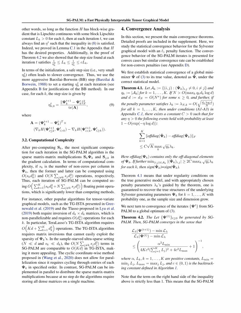
4. Convergence AnalysisIn this section, we present the main convergence theorems.Detailed proofs are included in the supplement. Here, westudy the statistical convergence behavior for the Sylvestergraphical model with an `1 penalty function. The conver-gence behavior of the SG-PALM iterates is presented forconvex cases but similar convergence rate can be establishedfor non-convex penalties (see Appendix D).

We first establish statistical convergence of a global mini-mizer Ψ of (3) to its true value, denoted as Ψ, under thecorrect statistical model.

Theorem 4.1. LetAk := (i, j) : (Ψk)i,j 6= 0, i 6= j andqk := |Ak| for k = 1, . . . ,K. If N > O(maxk qkdk log d)and d := dN = O(Nκ) for some κ ≥ 0, and further, if

the penalty parameter satisfies λk := λN,k = O(√

dk log dN )

for all k = 1, . . . ,K, then under conditions (A1-A3) inAppendix C.1, there exists a constant C > 0 such that forany η > 0 the following events hold with probability at least1−O(exp(−η log d)):

K∑k=1

‖offdiag(Ψk)− offdiag(Ψk)‖F

≤ C√K max

k

√qkλk.

Here offdiag(Ψk) contains only the off-diagonal elementsof Ψk. If further min(i,j)∈Ak |(Ψk)i,j | ≥ 2C maxk

√qkλk

for each k, then sign(Ψk)=sign(Ψk).

Theorem 4.1 means that under regularity conditions onthe true generative model, and with appropriately chosenpenalty parameters λk’s guided by the theorem, one isguaranteed to recover the true structures of the underlyingSylvester generating parameters Ψk for k = 1, . . . ,K withprobability one, as the sample size and dimension grow.

We next turn to convergence of the iterates Ψt from SG-PALM to a global optimum of (3).

Theorem 4.2. The Let Ψ(t)t≥0 be generated by SG-PALM. Then, SG-PALM converges in the sense that

Lλ(Ψ(t+1))−minLλLλ(Ψ(t))−minLλ

≤

(α2Lmin

4Kc2(∑Kj=1 Lj)

2 + 4c2Lmax

+ 1

)−1

,

where α, Lk, k = 1, . . . ,K are positive constants, Lmin =minj Lj , Lmax = maxj Lj , and c ∈ (0, 1) is the backtrack-ing constant defined in Algorithm 1.

Note that the term on the right hand side of the inequalityabove is strictly less than 1. This means that the SG-PALM


algorithm converges linearly, which is a strong results for anon-strongly convex objective (i.e., Lλ). Although similarconvergence behaviors of the PALM-type algorithms havebeen studied for other problems (Xu & Yin, 2013; Bolteet al., 2014), such as nonnegative matrix/tensor factoriza-tion, the analysis of this paper works for non-strongly blockmulti-convex objectives, leveraging more recent analyses ofmulti-block PALM and a class of functions satisfying the theKurdyka - Łojasiewicz (KL) property (defined in Section Cof the Appendix). To the best of our knowledge, for first-order optimization methods, our rate is faster than any otherGaussian graphical models having non-strongly convex ob-jectives (see Khare et al. (2015); Oh et al. (2014) and refer-ences therein) and comparable with those having strongly-convex objectives (see, for example, Guillot et al. (2012);Dalal & Rajaratnam (2017); Greenewald et al. (2019)).

5. ExperimentsExperiments in this section were performed in a sys-tem with 8-core Intel Xeon CPU E5-2687W v23.40GHz equipped with 64GB RAM. Both SG-PALM andSyGlasso were implemented in Julia v1.5 (https://github.com/ywa136/sg-palm). For real dataanalyses, we used the Tlasso package implementa-tion in R (Sun et al., 2016) and the TeraLasso im-plementation in MATLAB (https://github.com/kgreenewald/teralasso).

5.1. Synthetic Data

We first validate the convergence theorems discussed in theprevious section via simulation studies. Synthetic datasetswere generated from true sparse Sylvester factors ΨkKk=1

where K = 2, 3 and dk = 16, 32, 64, 128 for all k.Instances of the random matrices used here have uniformlyrandom sparsity patterns with edge densities (i.e., the pro-portion of non-zero entries) ranging from 0.1%− 30% onaverage over all Ψk’s. For each d and edge density combi-nation, random samples of size N = 10, 100, 1000 weretested. For comparison, the initial iterates, convergencecriteria were matched between SyGlasso and SG-PALM.Highlights of the results in run times are summarized inTable 1.

Convergence behavior of SG-PALM is shown in Figure 1(a) for the datasets with dk = 32, N = 10, 100, and edgedensities roughly around 5% and 20%, respectively. Geo-metric convergence rate of the function value gaps underTheorem 4.2 can be verified from the plot. Note an accel-eration in the convergence rate (i.e., a steeper slope) nearthe optimum, which is suggested by the “localness” of theKL property of the objective function close to its globaloptimum. Further for the same datasets, in Figure 1 (b), SG-PALM graph recovery performances is illustrated, where

Table 1. Run time comparisons (in seconds with N/As indicatingthose exceeding 24 hour) between SyGlasso and SG-PALM onsynthetic datasets with different dimensions, sample sizes, anddensities of the generating Sylvester factors. Note that the proposedSG-PALM has average speed-up ratios ranging from 1.5 to 10 overSyGlasso.

d N NZ% SyGlasso SG-PALMiter sec iter sec

1282

101 1.20 17 138.5 46 5.824.0 20 169.3 48 6.2

102 1.30 21 211.3 50 12.627.0 30 303.6 47 21.9

103 1.30 21 2045.8 50 80.125.0 47 4782.7 51 373.1

163

101 0.11 9 4.6 11 4.54.10 9 5.1 32 5.1

102 0.21 8 8.8 11 5.42.60 8 10.8 35 7.2

103 0.26 8 82.4 12 14.33.40 10 99.2 37 33.5

323

101 0.13 10 191.2 19 7.37.50 17 304.8 42 10.2

102 0.46 9 222.4 24 28.97.00 17 395.2 41 48.5

103 0.10 9 1764.8 22 226.46.90 19 3789.4 41 473.9

643

101 0.65 10 583.7 42 91.314.5 22 952.2 47 119.0

102 0.62 9 6683.7 41 713.914.4 21 15607.2 48 1450.9

103 0.85 N/A 39 6984.414.0 N/A 48 12968.7

the Matthew’s Correlation Coefficients (MCC) is plottedagainst run time. Here, MCC is defined by

MCC =TP× TN− FP× FN√

(TP + FP)(TP + FN)(TN + FP)(TN + FN),

where TP is the number of true positives, TN the numberof true negatives, FP the number of false positives, and FNthe number of false negatives of the estimated edges (i.e.,non-zero elements of Ψk’s). An MCC of 1 represents aperfect prediction, 0 no better than random prediction and−1 indicates total disagreement between prediction and ob-servation. The results validate the statistical accuracy underTheorem 4.1. It also shows that SG-PALM outperformsSyGlasso (indicated by blue/red solid dots) within the sametime budget.

https://github.com/ywa136/sg-palm

https://github.com/ywa136/sg-palm

https://github.com/kgreenewald/teralasso

https://github.com/kgreenewald/teralasso


(a) Cost gap vs. Iteration (b) MCC vs. Run time

Figure 1. Convergence of SG-PALM algorithm under datasets with varying sample sizes (solid and dashed) generated via matrices withdifferent sparsity (red and blue). The function value gaps on log-scale (left) verifies the geometric convergence rate in all cases and theMCC over time (right) demonstrates the algorithm’s accuracy and efficiency. Note that the SG-PALM reached almost perfect recoveries(i.e., MCC of 1) within 20 seconds in all cases. In comparison, SyGlasso (big solid dots with line-range) was only able to achieve at lowerMCCs for lower sample-size cases within 30 seconds.

5.2. Solar Flare Imaging Data

A solar flare occurs when magnetic energy that has built upin the solar atmosphere is suddenly released. Such eventsstrongly influence space weather near the Earth. Therefore,reliable predictions of these flaring events are of great inter-est. Recent work (Chen et al., 2019; Jiao et al., 2019; Sunet al., 2019) has shown the promise of machine learningmethods for early forecasting of these events using imagingdata from the solar atmosphere. In this work, we illustratethe viability of the SG-PALM algorithm for solar flare pre-diction using data acquired by multiple instruments: theSolar Dynamics Observatory (SDO)/Helioseismic and Mag-netic Imager (HMI) and SDO/Atmospheric Imaging Assem-bly (AIA). It is evident that these data contain informationabout the physical processes that govern solar activities (seeAppendix E for detailed data descriptions).

The data samples are summarized in d1 × d2 × d3 × d4

tensors with q = d1 · d2 · d3 = 50 · 100 · 7 = 35000and p = d4 = 13. The first two modes represent the im-ages’ heights and widths, the third mode represents theHMI/AIA components/channels, and the last mode repre-sents the length of the temporal window. Previous stud-ies (Chen et al., 2019; Jiao et al., 2019) found that the timeseries of solar images from the SDO/HMI data provideuseful information for distinguishing strong solar flares ofM/X class from weak flares of A/B class roughly 24 to 12hours prior to the flare event. Thus, in this study we usea 13-hour temporal window recorded with 1-hour cadence,prior to the occurrence of a solar flare. The task is to pre-dict the pth frame using the frames in each of the p − 1previous hours (i.e., one hour ahead prediction). Each ob-

servation is a video with full dimension d = pq, and each p-dimensional observation vector is formed by concatenatingthe p time-consecutive q-dimensional vectors (vectorizationof the matrices representing pixels of the multichannel im-ages) without overlapping the time segments. The trainingset contains two types (B- and MX-class flares) of active re-gions producing flares. Each is distinguished by the flaringintensities, and there are a total of 186 B flares and 48 MXflares. Forward linear predictors were constructed usingestimated precision matrices in a multi-output least squaresregression setting. Specifically, we constructed the linearpredictor of a frame from the p− 1 previous frames in thesame video:

yt = −Ω−12,2Ω2,1yt−1:t−(p−1), (10)

where yt−1:t−(p−1) ∈ R(p−1)q is the stacked set of pixelvalues from the previous p− 1 time instances and Ω2,1 ∈Rq×(p−1)q and Ω2,2 ∈ Rq×q are submatrices of the pq×pqestimated precision matrix:

Ω =

(Ω1,1 Ω1,2

Ω2,1 Ω2,2

).

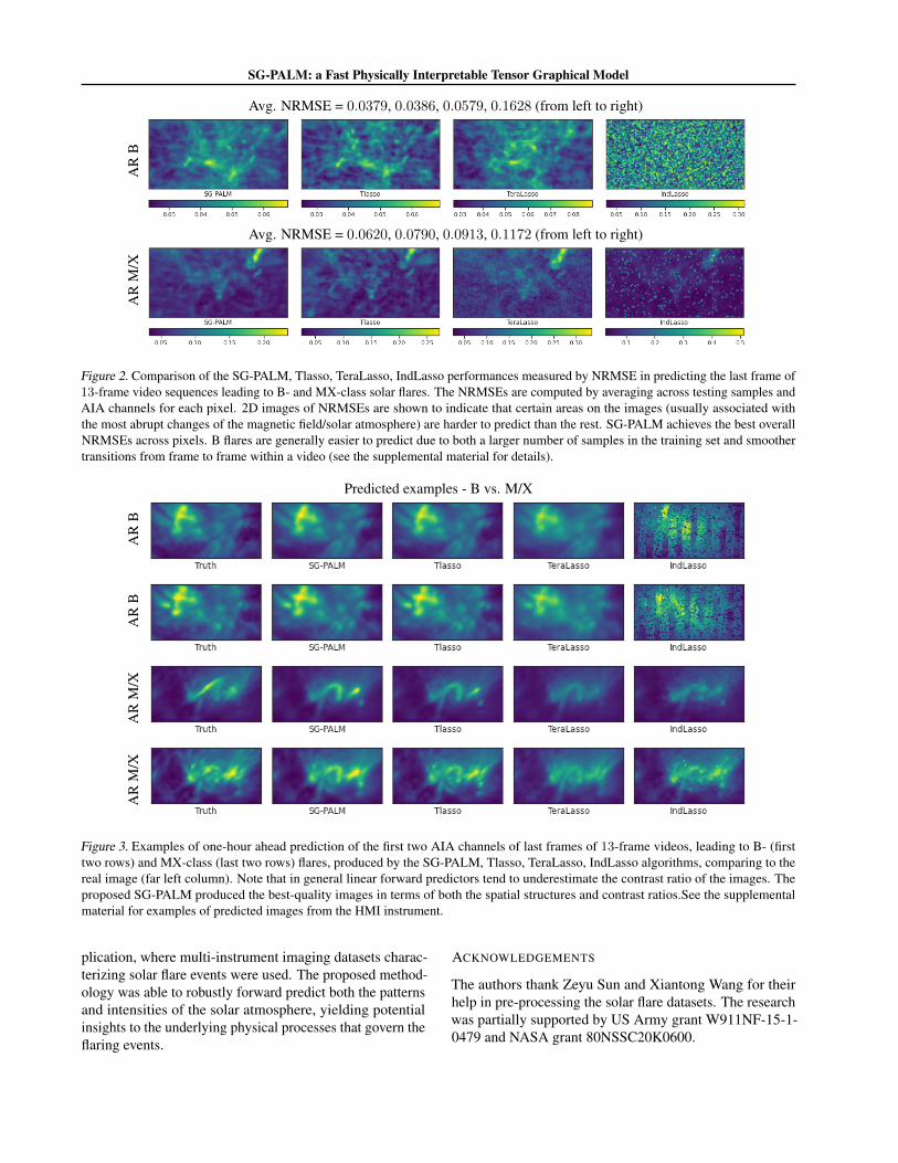
The predictors were tested on the data containing flares ob-served from different active regions than those in trainingset, so that the predictor has never “seen” the frames thatit attempts to predict, corresponding to 117 observationsof which 93 are B-class flares and 24 are MX-class flares.Figure 2 shows the root mean squared error normalizedby the difference between maximum and minimum pixels(NRMSE) over the testing samples, for the forecasts basedon the SG-PALM estimator, TeraLasso estimator (Gree-newald et al., 2019), Tlasso estimator (Lyu et al., 2019),


and IndLasso estimator. Here, the TeraLasso and the Tlassoare estimation algorithms for a KS and a KP tensor pre-cision matrix model, respectively; the IndLasso denotesan estimator obtained by applying independent and sep-arate `1-penalized regressions to each pixel in yt. TheSG-PALM estimator was implemented using a regulariza-

tion parameter λN = C1

√min(dk) log(d)

N for all k with theconstant C1 chosen by optimizing the prediction NRMSEon the training set over a range of λ values parameterizedby C1. The TeraLasso estimator and the Tlasso estima-tor were implemented using λN,k = C2

√log(d)

N∏i6=k di

and

λN,k = C3

√log(dk)Nd for k = 1, 2, 3, respectively, with

C2, C3 optimized in a similar manner. Each sparse regres-sion in the IndLasso estimator was implemented and tunedindependently with regularization parameters chosen froma grid via cross-validation.

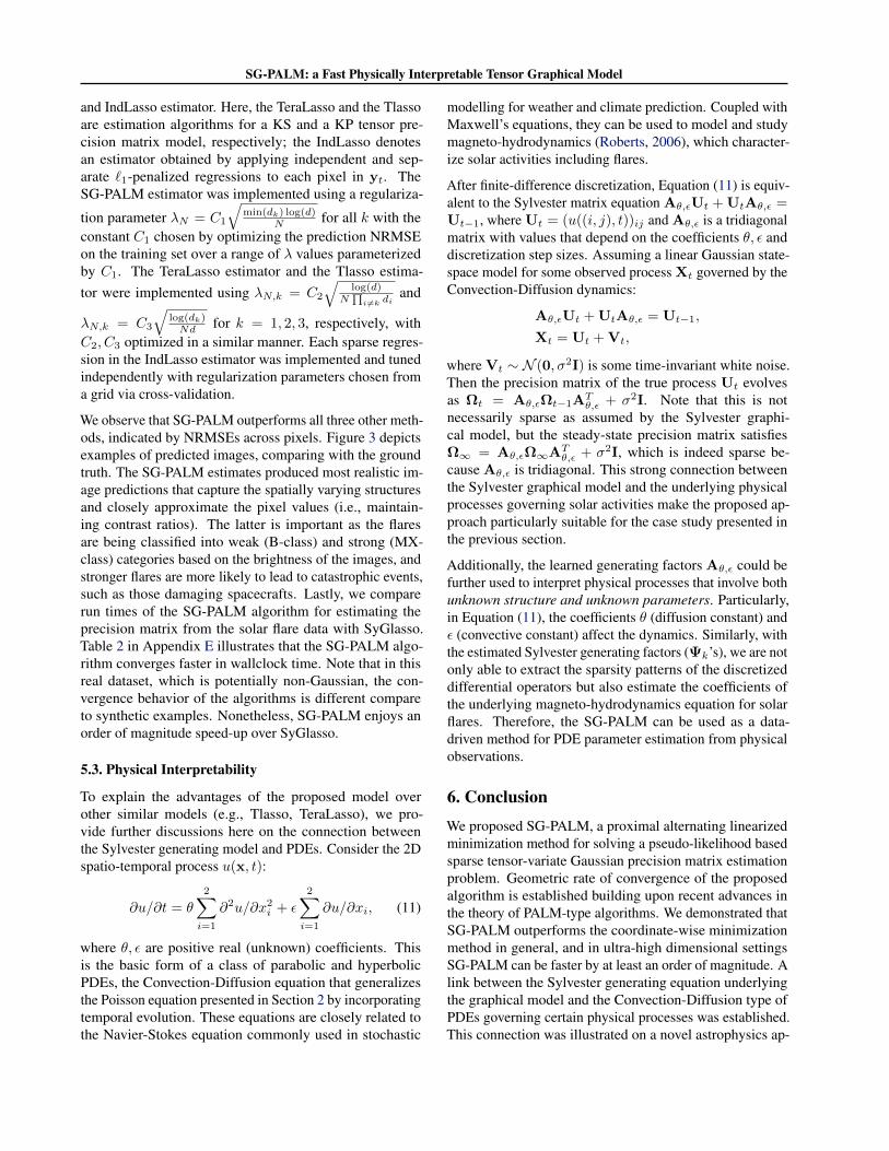
We observe that SG-PALM outperforms all three other meth-ods, indicated by NRMSEs across pixels. Figure 3 depictsexamples of predicted images, comparing with the groundtruth. The SG-PALM estimates produced most realistic im-age predictions that capture the spatially varying structuresand closely approximate the pixel values (i.e., maintain-ing contrast ratios). The latter is important as the flaresare being classified into weak (B-class) and strong (MX-class) categories based on the brightness of the images, andstronger flares are more likely to lead to catastrophic events,such as those damaging spacecrafts. Lastly, we comparerun times of the SG-PALM algorithm for estimating theprecision matrix from the solar flare data with SyGlasso.Table 2 in Appendix E illustrates that the SG-PALM algo-rithm converges faster in wallclock time. Note that in thisreal dataset, which is potentially non-Gaussian, the con-vergence behavior of the algorithms is different compareto synthetic examples. Nonetheless, SG-PALM enjoys anorder of magnitude speed-up over SyGlasso.

5.3. Physical Interpretability

To explain the advantages of the proposed model overother similar models (e.g., Tlasso, TeraLasso), we pro-vide further discussions here on the connection betweenthe Sylvester generating model and PDEs. Consider the 2Dspatio-temporal process u(x, t):

∂u/∂t = θ

2∑i=1

∂2u/∂x2i + ε

2∑i=1

∂u/∂xi, (11)

where θ, ε are positive real (unknown) coefficients. Thisis the basic form of a class of parabolic and hyperbolicPDEs, the Convection-Diffusion equation that generalizesthe Poisson equation presented in Section 2 by incorporatingtemporal evolution. These equations are closely related tothe Navier-Stokes equation commonly used in stochastic

modelling for weather and climate prediction. Coupled withMaxwell’s equations, they can be used to model and studymagneto-hydrodynamics (Roberts, 2006), which character-ize solar activities including flares.

After finite-difference discretization, Equation (11) is equiv-alent to the Sylvester matrix equation Aθ,εUt + UtAθ,ε =Ut−1, where Ut = (u((i, j), t))ij and Aθ,ε is a tridiagonalmatrix with values that depend on the coefficients θ, ε anddiscretization step sizes. Assuming a linear Gaussian state-space model for some observed process Xt governed by theConvection-Diffusion dynamics:

Aθ,εUt + UtAθ,ε = Ut−1,

Xt = Ut + Vt,

where Vt ∼ N (0, σ2I) is some time-invariant white noise.Then the precision matrix of the true process Ut evolvesas Ωt = Aθ,εΩt−1A

Tθ,ε + σ2I. Note that this is not

necessarily sparse as assumed by the Sylvester graphi-cal model, but the steady-state precision matrix satisfiesΩ∞ = Aθ,εΩ∞AT

θ,ε + σ2I, which is indeed sparse be-cause Aθ,ε is tridiagonal. This strong connection betweenthe Sylvester graphical model and the underlying physicalprocesses governing solar activities make the proposed ap-proach particularly suitable for the case study presented inthe previous section.

Additionally, the learned generating factors Aθ,ε could befurther used to interpret physical processes that involve bothunknown structure and unknown parameters. Particularly,in Equation (11), the coefficients θ (diffusion constant) andε (convective constant) affect the dynamics. Similarly, withthe estimated Sylvester generating factors (Ψk’s), we are notonly able to extract the sparsity patterns of the discretizeddifferential operators but also estimate the coefficients ofthe underlying magneto-hydrodynamics equation for solarflares. Therefore, the SG-PALM can be used as a data-driven method for PDE parameter estimation from physicalobservations.

6. ConclusionWe proposed SG-PALM, a proximal alternating linearizedminimization method for solving a pseudo-likelihood basedsparse tensor-variate Gaussian precision matrix estimationproblem. Geometric rate of convergence of the proposedalgorithm is established building upon recent advances inthe theory of PALM-type algorithms. We demonstrated thatSG-PALM outperforms the coordinate-wise minimizationmethod in general, and in ultra-high dimensional settingsSG-PALM can be faster by at least an order of magnitude. Alink between the Sylvester generating equation underlyingthe graphical model and the Convection-Diffusion type ofPDEs governing certain physical processes was established.This connection was illustrated on a novel astrophysics ap-


Avg. NRMSE = 0.0379, 0.0386, 0.0579, 0.1628 (from left to right)

AR

B

Avg. NRMSE = 0.0620, 0.0790, 0.0913, 0.1172 (from left to right)

AR

M/X

Figure 2. Comparison of the SG-PALM, Tlasso, TeraLasso, IndLasso performances measured by NRMSE in predicting the last frame of13-frame video sequences leading to B- and MX-class solar flares. The NRMSEs are computed by averaging across testing samples andAIA channels for each pixel. 2D images of NRMSEs are shown to indicate that certain areas on the images (usually associated withthe most abrupt changes of the magnetic field/solar atmosphere) are harder to predict than the rest. SG-PALM achieves the best overallNRMSEs across pixels. B flares are generally easier to predict due to both a larger number of samples in the training set and smoothertransitions from frame to frame within a video (see the supplemental material for details).

Predicted examples - B vs. M/X

AR

BA

RB

AR

M/X

AR

M/X

Figure 3. Examples of one-hour ahead prediction of the first two AIA channels of last frames of 13-frame videos, leading to B- (firsttwo rows) and MX-class (last two rows) flares, produced by the SG-PALM, Tlasso, TeraLasso, IndLasso algorithms, comparing to thereal image (far left column). Note that in general linear forward predictors tend to underestimate the contrast ratio of the images. Theproposed SG-PALM produced the best-quality images in terms of both the spatial structures and contrast ratios.See the supplementalmaterial for examples of predicted images from the HMI instrument.

plication, where multi-instrument imaging datasets charac-terizing solar flare events were used. The proposed method-ology was able to robustly forward predict both the patternsand intensities of the solar atmosphere, yielding potentialinsights to the underlying physical processes that govern theflaring events.

ACKNOWLEDGEMENTS

The authors thank Zeyu Sun and Xiantong Wang for theirhelp in pre-processing the solar flare datasets. The researchwas partially supported by US Army grant W911NF-15-1-0479 and NASA grant 80NSSC20K0600.


ReferencesAllen, G. I. and Tibshirani, R. Transposable regularized

covariance models with an application to missing dataimputation. The Annals of Applied Statistics, 4(2):764,2010.

Attouch, H. and Bolte, J. On the convergence of the proxi-mal algorithm for nonsmooth functions involving analyticfeatures. Mathematical Programming, 116(1-2):5–16,2009.

Barzilai, J. and Borwein, J. M. Two-point step size gradientmethods. IMA journal of numerical analysis, 8(1):141–148, 1988.

Besag, J. Efficiency of pseudolikelihood estimation forsimple gaussian fields. Biometrika, pp. 616–618, 1977.

Bolte, J., Sabach, S., and Teboulle, M. Proximal alternatinglinearized minimization for nonconvex and nonsmoothproblems. Mathematical Programming, 146(1-2):459–494, 2014.

Chen, Y., Manchester, W. B., Hero, A. O., Toth, G., DuFu-mier, B., Zhou, T., Wang, X., Zhu, H., Sun, Z., and Gom-bosi, T. I. Identifying solar flare precursors using timeseries of sdo/hmi images and sharp parameters. SpaceWeather, 17(10):1404–1426, 2019.

Dai, Y.-H. and Liao, L.-Z. R-linear convergence of theBarzilai and Borwein gradient method. IMA Journal ofNumerical Analysis, 22(1):1–10, 2002.

Dalal, O. and Rajaratnam, B. Sparse gaussian graph-ical model estimation via alternating minimization.Biometrika, 104(2):379–395, 2017.

Fan, J. and Li, R. Variable selection via nonconcave pe-nalized likelihood and its oracle properties. Journal ofthe American statistical Association, 96(456):1348–1360,2001.

Fletcher, R. On the Barzilai-Borwein method. In Optimiza-tion and control with applications, pp. 235–256. Springer,2005.

Friedman, J., Hastie, T., and Tibshirani, R. Sparse inversecovariance estimation with the graphical lasso. Biostatis-tics, 9(3):432–441, 2008.

Galvez, R., Fouhey, D. F., Jin, M., Szenicer, A., Munoz-Jaramillo, A., Cheung, M. C., Wright, P. J., Bobra, M. G.,Liu, Y., Mason, J., et al. A machine-learning data set pre-pared from the nasa solar dynamics observatory mission.The Astrophysical Journal Supplement Series, 242(1):7,2019.

Grasedyck, L. Existence and computation of low kronecker-rank approximations for large linear systems of tensorproduct structure. Computing, 72(3-4):247–265, 2004.

Greenewald, K., Zhou, S., and Hero III, A. Tensor graphicallasso (teralasso). Journal of the Royal Statistical Society:Series B (Statistical Methodology), 81(5):901–931, 2019.

Guillot, D., Rajaratnam, B., Rolfs, B. T., Maleki, A.,and Wong, I. Iterative thresholding algorithm forsparse inverse covariance estimation. arXiv preprintarXiv:1211.2532, 2012.

Jiao, Z., Sun, H., Wang, X., Manchester, W., Hero, A., Chen,Y., et al. Solar flare intensity prediction with machinelearning models. arXiv preprint arXiv:1912.06120, 2019.

Kalaitzis, A., Lafferty, J., Lawrence, N. D., and Zhou, S.The bigraphical lasso. In International Conference onMachine Learning, pp. 1229–1237, 2013.

Karimi, H., Nutini, J., and Schmidt, M. Linear conver-gence of gradient and proximal-gradient methods underthe polyak-łojasiewicz condition. In Joint European Con-ference on Machine Learning and Knowledge Discoveryin Databases, pp. 795–811. Springer, 2016.

Khare, K., Oh, S.-Y., and Rajaratnam, B. A convex pseudo-likelihood framework for high dimensional partial corre-lation estimation with convergence guarantees. Journal ofthe Royal Statistical Society: Series B: Statistical Method-ology, pp. 803–825, 2015.

Kolda, T. G. and Bader, B. W. Tensor decompositions andapplications. SIAM review, 51(3):455–500, 2009.

Kressner, D. and Tobler, C. Krylov subspace methods for lin-ear systems with tensor product structure. SIAM journalon matrix analysis and applications, 31(4):1688–1714,2010.

Leng, C. and Tang, C. Y. Sparse matrix graphical models.Journal of the American Statistical Association, 107(499):1187–1200, 2012.

Li, G. and Pong, T. K. Calculus of the exponent of kurdyka–łojasiewicz inequality and its applications to linear con-vergence of first-order methods. Foundations of computa-tional mathematics, 18(5):1199–1232, 2018.

Lindgren, F., Rue, H., and Lindstrom, J. An explicit link be-tween gaussian fields and gaussian markov random fields:the stochastic partial differential equation approach. Jour-nal of the Royal Statistical Society: Series B (StatisticalMethodology), 73(4):423–498, 2011.

Lourenco, B. F. and Takeda, A. Generalized subdifferen-tials of spectral functions over euclidean jordan algebras.arXiv preprint arXiv:1902.05270, 2019.


Lyu, X., Sun, W. W., Wang, Z., Liu, H., Yang, J., and Cheng,G. Tensor graphical model: Non-convex optimizationand statistical inference. IEEE transactions on patternanalysis and machine intelligence, 2019.

Meinshausen, N., Buhlmann, P., et al. High-dimensionalgraphs and variable selection with the lasso. Annals ofstatistics, 34(3):1436–1462, 2006.

Oh, S., Dalal, O., Khare, K., and Rajaratnam, B. Opti-mization methods for sparse pseudo-likelihood graphicalmodel selection. In Advances in Neural Information Pro-cessing Systems, pp. 667–675, 2014.

Parikh, N. and Boyd, S. Proximal algorithms. Foundationsand Trends in optimization, 1(3):127–239, 2014.

Park, S., Shedden, K., and Zhou, S. Non-separable co-variance models for spatio-temporal data, with appli-cations to neural encoding analysis. arXiv preprintarXiv:1705.05265, 2017.

Raydan, M. On the Barzilai and Borwein choice ofsteplength for the gradient method. IMA Journal of Nu-merical Analysis, 13(3):321–326, 1993.

Raydan, M. The Barzilai and Borwein gradient methodfor the large scale unconstrained minimization problem.SIAM Journal on Optimization, 7(1):26–33, 1997.

Roberts, B. Slow magnetohydrodynamic waves in the so-lar atmosphere. Philosophical Transactions of the RoyalSociety A: Mathematical, Physical and Engineering Sci-ences, 364(1839):447–460, 2006.

Rudelson, M. and Zhou, S. Errors-in-variables models withdependent measurements. Electronic Journal of Statistics,11(1):1699–1797, 2017.

Shefi, R. and Teboulle, M. On the rate of convergence of theproximal alternating linearized minimization algorithmfor convex problems. EURO Journal on ComputationalOptimization, 4(1):27–46, 2016.

Sun, H., Manchester, W., Jiao, Z., Wang, X., and Chen, Y.Interpreting lstm prediction on solar flare eruption withtime-series clustering. arXiv preprint arXiv:1912.12360,2019.

Sun, W. W., Wang, Z., Lyu, X., Liu, H., and Cheng,G. Tlasso: Non-Convex Optimization and Statisti-cal Inference for Sparse Tensor Graphical Models,2016. URL https://CRAN.R-project.org/package=Tlasso. R package version 1.0.1.

Tibshirani, R. Regression shrinkage and selection via thelasso. Journal of the Royal Statistical Society: Series B(Methodological), 58(1):267–288, 1996.

Tsiligkaridis, T., Hero III, A. O., and Zhou, S. On conver-gence of kronecker graphical lasso algorithms. IEEEtransactions on signal processing, 61(7):1743–1755,2013.

Varin, C., Reid, N., and Firth, D. An overview of compositelikelihood methods. Statistica Sinica, pp. 5–42, 2011.

Wang, Y. and Ma, S. Projected Barzilai-Borwein methodfor large-scale nonnegative image restoration. InverseProblems in Science and Engineering, 15(6):559–583,2007.

Wang, Y., Jang, B., and Hero, A. The sylvester graphi-cal lasso (syglasso). In The 23rd International Confer-ence on Artificial Intelligence and Statistics (AISTATS),pp. 1943–1953, 2020. URL http://proceedings.mlr.press/v108/wang20d.html.

Wen, Z., Yin, W., Goldfarb, D., and Zhang, Y. A fastalgorithm for sparse reconstruction based on shrinkage,subspace optimization, and continuation. SIAM Journalon Scientific Computing, 32(4):1832–1857, 2010.

Wright, S. J., Nowak, R. D., and Figueiredo, M. A. Sparsereconstruction by separable approximation. IEEE Trans-actions on signal processing, 57(7):2479–2493, 2009.

Xu, Y. and Yin, W. A block coordinate descent method forregularized multiconvex optimization with applicationsto nonnegative tensor factorization and completion. SIAMJournal on imaging sciences, 6(3):1758–1789, 2013.

Yin, J. and Li, H. Model selection and estimation in thematrix normal graphical model. Journal of multivariateanalysis, 107:119–140, 2012.

Zhang, C.-H. et al. Nearly unbiased variable selection underminimax concave penalty. The Annals of statistics, 38(2):894–942, 2010.

Zhang, H. New analysis of linear convergence of gradient-type methods via unifying error bound conditions. Math-ematical Programming, 180(1):371–416, 2020.

Zhou, S. GEMINI: Graph estimation with matrix variatenormal instances. The Annals of Statistics, 42(2):532–562, 2014.

Zou, H. The adaptive lasso and its oracle properties. Journalof the American statistical association, 101(476):1418–1429, 2006.

https://CRAN.R-project.org/package=Tlasso

https://CRAN.R-project.org/package=Tlasso

http://proceedings.mlr.press/v108/wang20d.html

http://proceedings.mlr.press/v108/wang20d.html


AppendixSection A provides detailed derivation of the log-pseudolikelihood function.

Section B provides justifications for the Barzilai-Borwein step sizes implemented in Algorithm 1.

Section C provides detailed proofs of Theorems 4.1 and 4.2.

Section D discusses extensions of Algorithm 1 and its convergence properties to non-convex cases.

Section E provides additional details of the solar flare experiments.

A. Derivation of the Log-PseudolikelihoodBy rewriting the Sylvester tensor equation defined in (2) element-wise, we first observe that(

K∑k=1

(Ψk)ik,ik

)X i[1:K]

= −K∑k=1

∑jk 6=ik

(Ψk)ik,jkX i[1:k],jk,i[k+1:K]+ T i[1:K]

.

(12)

Note that the left-hand side of (12) involves only the summation of the diagonals of the Ψk’s and the right-hand side iscomposed of columns of Ψk’s that exclude the diagonal terms. Equation (12) can be interpreted as an autogregressive modelrelating the (i1, . . . , iK)-th element of the data tensor (scaled by the sum of diagonals) to other elements in the fibers of thedata tensor. The columns of Ψk’s act as regression coefficients. The formulation in (12) naturally leads to a pseudolikelihood-based estimation procedure (Besag, 1977) for estimating Ω (see also Khare et al. (2015) for how this procedure applied tovector-variate Gaussian graphical model estimation). It is known that inference using pseudo-likelihood is consistent andenjoys the same

√N convergence rate as the MLE in general (Varin et al., 2011). This procedure can also be more robust to

model misspecification (e.g., non-Gaussianity) in the sense that it assumes only that the sub-models/conditional distributions(i.e., X i|X−i) are Gaussian. Therefore, in practice, even if the data is not Gaussian, the Maximum PseudolikelihoodEstimation procedure is able to perform reasonably well. Wang et al. (2020) also studied a different model misspecificationscenario where the Kronecker product/sum and Sylvester structures are mismatched for SyGlasso.

From (12) we can define the sparse least-squares estimators for Ψk’s as the solution of the following convex optimizationproblem:

minΨk∈Rdk×dkk=1,...K

−N∑

i1,...,iK

logWi[1:K]

+1

2

∑i1,...,iK

‖(I) + (II)‖22 +K∑k=1

Pλk(Ψk).

where Pλk(·) is a penalty function indexed by the tuning parameter λk and

(I) = Wi[1:K]X i[1:K]

(II) =

K∑k=1

∑jk 6=ik

(Ψk)ik,jkX i[1:k],jk,i[k+1:K],

with Wi[1:K]:=∑Kk=1(Ψk)ik,ik .

The optimization problem above can be put into the following matrix form:

minΨk∈Rdk×dkk=1,...K

− N

2log |(diag(Ψ1)⊕ · · · ⊕ diag(ΨK))2|

+N

2tr(S(Ψ1 ⊕ · · · ⊕ΨK)2) +

K∑k=1

Pλk(Ψk)


where S ∈ Rd×d is the sample covariance matrix, i.e., S = 1N

∑Ni=1 vec(X i) vec(X i)T . Note that this is equivalent to

the negative log-pseudolikelihood function that approximates the `1-penalized Gaussian negative log-likelihood in thelog-determinant term by including only the Kronecker sum of the diagonal matrices instead of the Kronecker sum of the fullmatrices.

B. The Barzilai-Borwein Step SizeThe BB method has been proven to be very successful in solving nonlinear optimization problems. In this section weoutline the key ideas behind the BB method, which is motivated by quasi-Newton methods. Suppose we want to solve theunconstrained minimization problem

minxf(x),

where f is differentiable. A typical iteration of quasi-Newton methods for solving this problem is

xt+1 = xt −B−1t ∇f(xt),

where Bt is an approximation of the Hessian matrix of f at the current iterate xt. Here, Bt must satisfy the so-called secantequation: Btst = yt, where st = xt − xt−1 and yt = ∇f(xt) −∇f(xt−1) for t ≥ 1. It is noted that in to get B−1

t oneneeds to solve a linear system, which may be computationally expensive when Bt is large and dense.

One way to alleviate this burden is to use the BB method, which replaces Bt by a scalar matrix (1/ηt)I. However, it is hardto choose a scalar ηt such that the secant equation holds with Bt = (1/ηt)I. Instead, one can find ηt such that the residualof the secant equation, i.e., ‖(1/ηt)st − yt‖22, is minimized, which leads to the following choice of ηt:

ηt =‖st‖22sTt yt

.

Therefore, a typical iteration of the BB method for solving the original problem is

xt+1 = xt − ηt∇f(xt),

where ηt is computed via the previous formula.

For convergence analysis, generalizations and variants of the BB method, we refer the interested readers to Raydan (1993;1997); Dai & Liao (2002); Fletcher (2005) and references therein. BB method has been successfully applied for solvingproblems arising from emerging applications, such as compressed sensing (Wright et al., 2009), sparse reconstruction (Wenet al., 2010) and image processing (Wang & Ma, 2007).

C. Proofs of TheoremsC.1. Proof of Theorem 4.1

We first state the regularity conditions needed for establishing convergence of the SG-PALM estimators ΨkKk=1 to theirtrue value ΨkKk=1.

(A1 - Subgaussianity) The data X 1, . . . ,XN are i.i.d subgaussian random tensors, that is, vec(X i) ∼ x, where x is asubgaussian random vector in Rd, i.e., there exist a constant c > 0, such that for every a ∈ Rd, EeaT x ≤ ecaT Σa, and thereexist ρj > 0 such that Eetx

2j ≤ +∞ whenever |t| < ρj , for 1 ≤ j ≤ d.

(A2 - Bounded eigenvalues) There exist constants 0 < Λmin ≤ Λmax < ∞, such that the minimum and maximumeigenvalues of Ω are bounded with λmin(Ω) = (

∑Kk=1 λmax(Ψk))−2 ≥ Λmin and λmax(Ω) = (

∑Kk=1 λmin(Ψk))−2 ≤

Λmax.

(A3 - Incoherence condition) There exists a constant δ < 1 such that for k = 1, . . . ,K and all (i, j) ∈ Ak

|L′′

ij,Ak(Ψ)[L′′

Ak,Ak(Ψ)]−1sign(ΨAk,Ak)| ≤ δ,

where for each k and 1 ≤ i < j ≤ dk, 1 ≤ k < l ≤ dk,

L′′

ij,kl(Ψ) := EΨ

(∂2L(Ψ)

∂(Ψk)i,j∂(Ψk)k,l|Ψ=Ψ

),


and

L(Ψ) = −N2

log |(K⊕k=1

diag(Ψk))2|+ N

2tr(S · (

K⊕k=1

Ψk)2).

Given assumptions (A1-A3), the theorem follows from Theorem 3.3 in Wang et al. (2020).

C.2. Proof of Theorem 4.2

We next turn to convergence of the iterates Ψt from SG-PALM to a global optimum of (3). The proof leverages recentresults in the convergence of alternating minimization algorithms for non-strongly convex objective (Bolte et al., 2014;Karimi et al., 2016; Li & Pong, 2018; Zhang, 2020). We outline the proof strategy:

1. We establish Lipschitz continuity of the blockwise gradient∇kH(Ψ) for k = 1, . . . ,K.

2. We show that the objective function Lλ satisfies the Kurdyka - Łojasiewicz (KL) property. Further, it has a KL exponentof 1

2 (defined later in the proofs).

3. The KL property (with exponent 12 ) is equivalent to a generalized Error Bound (EB) condition, which enables us to

establish linear iterative convergence of the objective function (3) to its global optimum.

Definition C.1 (Subdifferentials). Let f : Rd → (−∞,+∞] be a proper and lower semicontinuous function. Its domain isdefined by

domf := x ∈ Rd : f(x) < +∞.If we further assume that f is convex, then the subdifferential of f at x ∈ domf can be defined by

∂f(x) := v ∈ Rd : f(z) ≥ f(x)+ < v, z − x >,∀z ∈ Rd.

The elements of ∂f(x) are called subgradients of f at x.

Denote the domain of ∂f by dom∂f := x ∈ Rd : ∂f(x) 6= ∅. Then, if f is proper, semicontinuous, convex, andx ∈ domf , then ∂f(x) is a nonempty closed convex set. In this case, we denote by ∂0f(x) the unique least-norm elementof ∂f(x) for x ∈ dom∂f , along with ‖∂0f(x)‖ = +∞ for x /∈ dom∂f . Points whose subdifferential contains 0 are criticalpoints, denoted by critf . For convex f , critf = argmin f .Definition C.2 (KL property). Let Γc2 stands for the class of functions φ : [0, c2]→ R+ for c2 > 0 with the properties:

i. φ is continuous on [0, c2];

ii. φ is smooth concave on (0, c2);

iii. φ(0) = 0, φ′(s) > 0,∀s ∈ (0, c2).

Further, for x ∈ Rd and any nonempty Q ⊂ Rd, define the distance function d(x,Q) := infy∈Q ‖x− y‖. Then, a functionf is said to have the Kurdyka - Łojasiewicz (KL) property at point x0, if there exist c1 > 0, a neighborhood B of x0, andφ ∈ Γc2 such that for all

x ∈ B(x0, c1) ∩ x : f(x0) < f(x) < f(x0) + c2,the following inequality holds

φ′(f(x)− f(x0)

)dist(0, ∂f(x)) ≥ 1.

If f satisfies the KL property at each point of dom∂f then f is called a KL function.

We first present two lemmas that characterize key properties of the loss function.Lemma C.1 (Blockwise Lipschitzness). The function H is convex and continuously differentiable on an open set containingdomG and its gradient, is block-wise Lipschitz continuous with block Lipschitz constant Lk > 0 for each k, namely for allk = 1, . . . ,K and all Ψk,Ψ

′k ∈ Rdk×dk

‖∇kH(Ψi<k,Ψk,Ψi>k)−∇kH(Ψi<k,Ψ′k,Ψi>k)‖

≤ Lk‖Ψk −Ψ′k‖,


where∇kH denotes the gradient of H with respect to Ψk with all remaining Ψi, i 6= k fixed. Further, the function Gk foreach k = 1, . . . ,K is a proper lower semicontinuous (lsc) convex function.

Proof. For simplicity of notation, in this and the following proofs we use Ψ (i.e., omitting the subscript) to denote the setΨkKk=1 or the K-tuple (Ψ1, . . . ,ΨK) whenever there is no confusion. Recall the blockwise gradient of the smooth partof the objective function H with respect to Ψk, for each k = 1, . . . ,K, is given by

∇kH(Ψ) = diag([

tr(diag((Ψk))ii +⊕j 6=k

diag(Ψj))−1 i = 1 : dk

])+ SkΨk + ΨkSk + 2

∑j 6=k

Sj,k.

Then for Ψk,Ψ′k,

‖SkΨk + ΨkSk + 2∑j 6=k

Sj,k − (SkΨ′k + Ψ′kSk + 2

∑j 6=k

Sj,k)‖

= ‖SkΨk + ΨkSk − SkΨ′k −Ψ′kSk‖

≤ 2‖Sk‖‖Ψk −Ψ′k‖.

To prove Lipschitzness of the remaining parts, we consider the case of K = 2 for simplicity of notations. The argumentseasily carry over cases of K > 2. In this case, denote A = (aij) := Ψ1 and B = (bkl) := Ψ2. Let f(A) :=∂∂A log | diag(A⊕B)|, then

f(A)− f(A′) = diag([ m2∑

i=1

(ajj + bii)−1 −

m2∑i=1

(a′jj + bii)−1 j = 1, . . . ,m1

])and

‖f(A)− f(A′)‖F =

(m1∑j=1

( m2∑i=1

(ajj + bii)−1 −

m2∑i=1

(a′jj + bii)−1)2)1/2

≤

(m1∑j=1

m2

m2∑i=1

((ajj + bii)

−1 − (a′jj + bii)−1)2)1/2

=(m2

m1∑j=1

m2∑i=1

(c−1ji − (c′ji)

−1)2)1/2

=(m2

m1∑j=1

m2∑i=1

(c′ji)−2(c′ji − cji)2c−2

ji

)1/2

=(m2

m1∑j=1

(ajj − a′jj)2m2∑i=1

(c′jicji)−2)1/2

≤(Cm2

m1∑j=1

m2∑i=1

(c′jicji)−2)1/2

‖A−A′‖F ,

where the first inequality is due to Cauchy-Schwartz inequality; the third line is due to cji := ajj + bii; and in the lastinequality we upper-bound each (ajj − a′jj)2 by its maximum over all j, which is absorbed in a constant C. Note that thefirst term in the last line above is finite as long as the summations of the diagonal elements of the factors A and B are finite,which is implied if the precision matrix Ω defined by the Sylvester generating equation as (A⊕B)2 has finite diagonalelements. This follows from Theorem 3.1 of Oh et al. (2014), who proved that if a symmetric matrix Ω satisfying Ω ∈ C0,where

C0 =

Ω|Lλ(Ω) ≤ Lλ(Ω(0)) = M,

and Ω(0) is an arbitrary initial point with a finite function value Lλ(Ω(0)) := M , the diagonal elements of Ω are boundedabove and below by constants which depend only on M , the regularization parameter λ, and the sample covariance matrix


S. Therefore, we have‖f(A)− f(A′)‖F ≤ C‖A−A′‖F

for some constant C ∈ (0,+∞). Similarly, we can establish such an inequality for B, proving that the first term in ∇kH isLipschitz continuous.

As a consequence of Lemma C.1, the gradient of H , defined by ∇H = (∇1H, . . . ,∇KH) is Lipschitz continuous onbounded subsets B1×· · ·×BK of Rd1×d1×· · ·×RdK×dK with some constant L > 0, such that for all (Ψk,Ψ

′k) ∈ Bk×Bk,

‖(∇1H(Ψ1,Ψi>1)−∇1H(Ψ′1,Ψ′i>1), . . . ,

∇KH(Ψ′i<K ,Ψ′K)−∇KH(Ψ′i<K ,Ψ

′K))‖

≤ L‖(Ψ1 −Ψ′1, . . . ,ΨK −Ψ′K)‖,

and we have L ≤∑Kk=1 Lk.

Lemma C.2 (KL property of Lλ). The objective function Lλ(Ψ) defined in (3) satisfies the KL property. Further, φ in thiscase can be chosen to have the form φ(s) = αs1/2, where α is some positive real number. Functions satisfying the KLproperty with this particular choice of φ is said to have a KL exponent of 1

2 .

Proof. This can be established in a few steps:

1. It can be shown that the function (of X) tr(SX2) + ‖X‖1,off satisfies the KL property with exponent 12 (Karimi et al.,

2016). We then apply the calculus rules of the KL exponent (compositions and separable summations) studied in Li &Pong (2018) to prove that tr(S(

⊕j Ψj)

2) and∑j ‖Ψj‖1,off are also KL functions with exponent 1

2 .

2. The − log det(⊕

j diag(Ψj))

term can be shown to be KL with exponent 12 using a transfer principle studied

in Lourenco & Takeda (2019).

3. Finally, using the calculus rules of KL exponent one more time, we combine the first two results and establish that Lλhas KL exponent of 1

2 .

Karimi et al. (2016) proved that the following function, parameterized by some symmetric matrix X, satisfies the KLproperty with KL exponent 1

2 :tr(SX2) + ‖X‖1,off = ‖AX‖2F + ‖X‖1,off

for S = AAT , even when A is not of full rank.

We apply the calculus rules of the KL exponent studied in Li & Pong (2018) to prove that tr(S(⊕

j Ψj)2) and

∑j ‖Ψj‖1,off

are KL functions with exponent 12 . Particularly, we observe that tr

(S(⊕

j Ψj)2)

is the composition of functions X →tr(SX) and (X1, . . . ,XK)→

⊕j Xj ; and

∑j ‖Ψj‖1,off is a separable block summation of functions Xj → ‖Xj‖1,off.

Thus, by Theorem 3.2. (exponent for composition of KL functions) in Li & Pong (2018), since the Kronecker sumoperation is linear and hence continuously differentiable, the trace function is KL with exponent 1

2 , and the mapping(X1, . . . ,XK)→

⊕j Xj is clearly one to one, the function tr(S(

⊕j Ψj)

2) has the KL exponent of 12 . By Theorem 3.3.

(exponent for block separable sums of KL functions) in Li & Pong (2018), since the function ‖ · ‖1,off is proper, closed,continuous on its domain, and is KL with exponent 1

2 , the function ‖Xj‖1,off is KL with an exponent of 12 .

It remains to prove that− log det(⊕

j diag(Ψj))

is also a KL function with an exponent of 12 . By Theorem 30 in Lourenco

& Takeda (2019), if we have f : Rr → R a symmetric function and F : E → R the corresponding spectral function, thefollowings hold

(i). F satisfies the KL property at X iff f satisfies the KL property at λ(X), i.e., the eigenvalues of X.

(ii). F satisfies the KL property with exponent α iff f satisfies the KL property with exponent α at λ(X).


Here, take f(λ(X)) := −∑ri=1 log(λi(X)), and F (X) := − log det(X) the corresponding spectral function. Then, the

function f is symmetric since its value is invariant to permutations of its arguments, and it is a strictly convex function in itsdomain, so it satisfies the KL property with an exponent of 1

2 . Therefore, F satisfies the KL property with the same KLexponent of 1

2 . Now, we apply the calculus rules for KL functions again. As both the Kronecker sum and the diag operators

are linear, we conclude that − log det(⊕

j diag(Ψj))

is a KL function with an exponent of 12 .

Overall, we have that the negative log-pseudolikelihood function L(Ψ) satisfies the KL property with an exponent of 12 .

Now we are ready to prove Theorem 4.2. We follow Zhang (2020) and divide the proof into three steps.

Step 1. We obtain a sufficient decrease property for the loss function L in terms of the squared distance of two successiveiterates:

L(Ψ(t))− L(Ψ(t+1)) ≥ Lmin

2‖Ψ(t) −Ψ(t+1)‖2. (13)

Here and below, Ψ(t+1) := (Ψ(t+1)1 , . . . ,Ψ

(t+1)K ) and Lmin := mink Lk. First note that at iteration t, the line search

condition is satisfied for step size 1

η(t)k

≥ Lk, where Lk is the Lipschitz constant for ∇kH . Further, it follows that for

SG-PALM with backtracking one has for every t ≥ 0 and each k = 1, . . . ,K,

1

η(0)k

≤ 1

η(t)k

≤ cLk,

where c > 0 is the backtracking constant.

Then by Lemma 3.1 in Shefi & Teboulle (2016), we get

L(Ψ(t))− L(Ψ(t+1)) ≥ 1

2η(t+1)min

‖Ψ(t) −Ψ(t+1)‖2

≥ Lmin

2‖Ψ(t) −Ψ(t+1)‖2

for η(t)min := mink η

(t)k .

Step 2. By Lemma C.2, L satisfies the KL property with an exponent of 12 . Then from Definition C.2, this suggests that at

x = Ψt+1 and f(x0) = minL‖∂0L(Ψt+1)‖ ≥ α

√L(Ψt+1)−minL, (14)

where α > 0 is a fixed constant defined in Lemma C.2. This property is equivalent to the error bound condition, (∂0L, α,Ω)-(res-obj-EB), defined in Definition 5 in Zhang (2020), for Ω ⊂ dom∂L. This is strictly weaker than strong convexity (seeSection 4 in Zhang (2020)).

At iteration t+ 1, there exists ξ(t+1)k ∈ ∂Gk(Ψ

(t+1)k ) satisfying the optimality condition:

∇kH(Ψ(t+1)i<k ,Ψ

(t)i≥k) +

1

η(t+1)k

(Ψ(t+1)k −Ψ

(t)k ) + ξ

(t+1)k = 0.

Let ξ(t+1) := (ξ(t+1)1 , . . . , ξ

(t+1)K ). Then,

∇H(Ψ(t+1)) + ξ(t+1) ∈ ∂L(Ψ(t+1))

and hence the error bound condition becomes

L(Ψ(t+1))−minL ≤ ‖∂0L(Ψ(t+1))‖2

α2≤ ‖∇H(Ψ(t+1)) + ξ(t+1)‖2

α2.


It follows that

‖∇H(Ψ(t+1)) + ξ(t+1)‖2 =

K∑k=1

‖∇kH(Ψ(t+1))−∇kH(Ψ(t+1)i<k ,Ψ

(t)i≥k)− 1

η(t+1)k

(Ψ(t+1)k −Ψ

(t)k )‖2

≤K∑k=1

2‖∇kH(Ψ(t+1))−∇kH(Ψ(t+1)i<k ,Ψ

(t)i≥k)‖2 +

K∑k=1

2

(η(t+1)k )2

‖Ψ(t+1)k −Ψ

(t)k ‖

2

≤K∑k=1

2‖∇H(Ψ(t+1))−∇H(Ψ(t+1)i<k ,Ψ

(t)i≥k)‖2 +

K∑k=1

2

(η(t+1)k )2

‖Ψ(t+1)k −Ψ

(t)k ‖

2

≤K∑k=1

2( K∑j=1

1

η(t+1)j

)2

‖Ψ(t+1)i≥k −Ψ

(t)i≥k‖

2 +

K∑k=1

2

(η(t+1)k )2

‖Ψ(t+1)k −Ψ

(t)k ‖

2

≤

(2Kc2

( K∑j=1

Lj

)2

+ 2c2Lmax

)‖Ψ(t+1) −Ψ(t)‖2.

Therefore, we get

L(Ψ(t+1))−minL ≤

(2Kc2

(∑Kj=1 Lj

)2

+ 2c2Lmax

)α2

‖Ψ(t+1) −Ψ(t)‖2. (15)

Step 3. Combining (13) and (15), we have

L(Ψ(t))−minL =(L(Ψ(t))− L(Ψ(t+1))

)+(L(Ψ(t+1))−minL

)≥ Lmin

2‖Ψ(t) −Ψ(t+1)‖2 +

(L(Ψ(t+1))−minL

)≥

(α2Lmin

4Kc2(∑Kj=1 Lj)

2 + 4c2Lmax

+ 1

)(L(Ψ(t+1))−minL

).

This completes the proof.

D. SG-PALM with Non-Convex RegularizersThe estimation algorithm for non-convex regularizer is largely the same as Algorithm 1, except with an additional termadded to the gradient term. Specifically, the updates are of the form

Ψ(t+1)k = prox‖·‖1,off

ηtkλk

(Ψtk − ηtk∇kH(Ψt+1

i<k,Ψti≥k)

),

where

H(Ψ) = H(Ψ) +

K∑k=1

∑i 6=j

(gλk([Ψk]i,j)− λk|[Ψk]i,j |

).

Here, the formulation covers a range of non-convex regularizations. Particularly, the SCAD penalty (Fan & Li, 2001) withparameter a > 2 is given by

gλ(t) =

λ|t|, if |t| < λ

− t2−2aλ|t|+λ2

2(a−1) , if λ < |t| < aλ(a+1)λ2

2 , if aλ < |t|,which is linear for small |t|, constant for large |t|, and a transition between the two regimes for moderate |t|.

The MCP penalty (Zhang et al., 2010) with parameter a > 0 is given by

gλ(t) = sign(t)λ

∫ |t|0

(1− z

aλ

)+dz,


which gives a smoother transition between the approximately linear region and the constant region (t > aλ) as defined inSCAD.

The updates can also be written as

Ψ(t+1)k = prox‖·‖1,off

ηtkλk

(Ψtk − ηtk∇k

(H(Ψt+1

i<k,Ψti≥k) +Q′λk(Ψk)

)),

where q′λ(t) := ddt (gλ(t) − λ|t|) for t 6= 0 and q′λ(0) = 0 and Q′λ denotes q′λ applied elementwise to a matrix argument.

These updates can be inserted into the framework of Algorithm 1. The details are summarized in Algorithm 2.

Algorithm 2 SG-PALM with non-convex regularizer

Input: Data tensor X , mode-k Gram matrix Sk, regularizing parameter λk, backtracking constant c ∈ (0, 1), initial stepsize η0, initial iterate Ψk for each k = 1, . . . ,K.while not converged do

for k = 1, . . . ,K doLine search: Let ηtk be the largest element of cjηtk,0j=1,... such that condition (8) is satisfied for Ψt+1

k =

prox‖·‖1,off

ηtkλk

(Ψtk − ηtk∇k

(H(Ψt+1


)).

Update: Ψt+1k ←− prox‖·‖1,off

ηtkλk

(Ψtk − ηtk∇k

(H(Ψt+1


)).

end forNext initial step size: Compute Barzilai-Borwein step size ηt+1

0 = mink ηt+1k,0 , where ηt+1

k,0 is computed via (9).end while

Output: Final iterates ΨkKk=1.

D.1. Convergence Property

Consider a sequence of iterate xtt∈N generated by a generic PALM algorithm for minimizing some objective function f .Specifically, assume

(H1) inf f > −∞.

(H2) The restriction of the function to its domain is a continuous function.

(H3) The function satisfies the KL property.

Then, as in Theorem 2 of Attouch & Bolte (2009), if this objective function satisfying (H1), (H2), (H3) in addition satisfiesthe KL property with

φ(s) = αs1−θ,

where α > 0 and θ ∈ (0, 1]. Then, for x∗ some critical point of f , the following estimations hold

(i). If θ = 0 then the sequence of iterates converges to x∗ in a finite number of steps.

(ii). If θ ∈ (0, 12 ] then there exist ω > 0 and τ ∈ [0, 1) such that ‖xt − x∗‖ ≤ ωτ t.

(iii). If θ ∈ ( 12 , 1) then there exist ω > 0 such that ‖xt − x∗‖ ≤ ωt−

1−θ1θ−1 .

In the case of SG-PALM with non-convex regularizations, so long as the non-convex L satisfies the KL property with anexponent in (0, 1

2 ], the algorithm remains linearly convergent (to a critical point). We argue that this is true for SG-PALMwith MCP or SCAD penalty. Li & Pong (2018) showed that penalized least square problems with such penalty functionssatisfy the KL property with an exponent of 1

2 . The proof strategy for the convex case can be easily adopted, incorporatingthe KL results for MCP and SCAD in Li & Pong (2018), to show that the new L still has KL exponent of 1

2 . Therefore,SG-PALM with MCP or SCAD penalty converges linearly in the sense outlined above.


E. Additional Details of the Solar Flare ExperimentsE.1. HMI and AIA Data

The Solar Dynamics Observatory (SDO)/Helioseismic and Magnetic Imager (HMI) data characterize solar variabilityincluding the Sun’s interior and the various components of magnetic activity; the SDO/Atmospheric Imaging Assembly(AIA) data contain a set of measurements of the solar atmosphere spectrum at various wavelengths. In general, HMIproduces data that is particularly useful in determining the mechanisms of solar variability and how the physical processesinside the Sun that are related to surface magnetic field and activity. AIA contains structural information about solar flares,and the the high AIA pixel values are correlated with the flaring intensities. We are interested in examining if combination ofmultiple instruments enhances our understanding of the solar flares, comparing to the case of single instrument. Both HMIand AIA produce multi-band (or multi-channel) images, for this experiment we use all three channels of the HMI imagesand 9.4, 13.1, 17.1, 19.3 nm wavelength channels of the AIA images. For a detailed descriptions of the instruments andall channels of the images, see https://en.wikipedia.org/wiki/Solar_Dynamics_Observatory and thereferences therein. Furthermore, for training and testing involved in this study, we used the data described in (Galvez et al.,2019), which are further pre-processed HMI and AIA imaging data for machine learning methods.

E.2. Classification of Solar Flares/Active Regions (AR)

The classification system for solar flares uses the letters A, B, C, M or X, according to the peak flux in watts per squaremetre (W/m2) of X-rays with wavelengths 100 to 800 picometres (1 to 8 angstroms), as measured at the Earth by the GOESspacecraft (https://en.wikipedia.org/wiki/Solar_flare#Classification). Here, A usually refers toa “quite” region, which means that the peak flux of that region is not high enough to be classified as a real flare; B usuallyrefers a “weak” region, where the flare is not strong enough to have impact on spacecrafts, earth, etc; and M or X refers to a“strong” region that is the most detrimental. Differentiating between a weak and a strong flare/region ahead of time is afundamental task in space physics and has recently attracted attentions from the machine learning community (Chen et al.,2019; Jiao et al., 2019; Sun et al., 2019). In our study, we also focus on B and M/X flares and attempt to predict the videosthat lead to either one of these two types of flares.

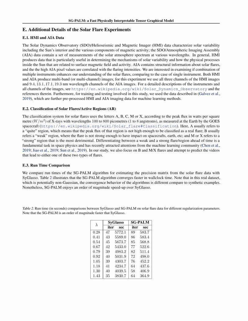
E.3. Run Time Comparison

We compare run times of the SG-PALM algorithm for estimating the precision matrix from the solar flare data withSyGlasso. Table 2 illustrates that the SG-PALM algorithm converges faster in wallclock time. Note that in this real dataset,which is potentially non-Gaussian, the convergence behavior of the algorithms is different compare to synthetic examples.Nonetheless, SG-PALM enjoys an order of magnitude speed-up over SyGlasso.

Table 2. Run time (in seconds) comparisons between SyGlasso and SG-PALM on solar flare data for different regularization parameters.Note that the SG-PALM is an order of magnitude faster that SyGlasso.

λSyGlasso SG-PALMiter sec iter sec

0.28 47 5772.1 89 583.70.41 43 5589.0 86 583.40.54 45 5673.7 85 568.80.67 42 5433.0 77 522.60.79 39 4983.2 82 511.40.92 40 5031.9 72 498.01.05 39 4303.7 76 452.21.18 41 4234.7 64 437.61.30 40 4039.5 58 406.91.43 35 3830.7 64 364.9

https://en.wikipedia.org/wiki/Solar_Dynamics_Observatory

https://en.wikipedia.org/wiki/Solar_flare#Classification


E.4. Examples of Predicted Magnetogram Images

Figure 4 depicts examples of the predicted HMI channels by SG-PALM. We observe that the proposed method was ableto reasonably capture various components of the magnetic field and activity. Note that the spatial behaviors of the HMIcomponents are quite different from those of AIA channels, that is, the structures tend to be less smooth and continuous(e.g., separated holes and bright spots) in HMI.

E.5. Multi-instrument vs. Single Instrument Prediction

To illustrate the advantages of multi-instrument analysis, we compare the NRMSEs between an AIA-only (i.e., last fourchannels of the dataset) and an HMI&AIA (i.e., all seven channels of the dataset) study in predicting the last frames of13-frame AIA videos, for each flare class, respectively, using the proposed SG-PALM. The results are depicted in Figure 5,where the average, standard deviation, and range of the NRMSEs across pixels are also shown for each error image. Byleveraging the cross-instrument correlation structure, there is a 0.5%− 1% drop in the averaged error rates and a 2%− 4%drop in the range of the errors.

E.6. Illustration of the Difficulty of Predictions for Two Flares Classes

We demonstrate the difficulty of forward predictions of video frames. Figure 6 depicts two different channels of multipleframes from two videos leading to MX-class solar flares. Note that the current frame is the 13th frame in the sequence thatwe are trying to predict. We observe that the prediction task is particularly difficult if there is a sudden transition of either thebrightness or spatial structure of the frames near the end of the video. These sudden transitions are more frequent for MXflares than for B flares. In addition, as MX flares are generally considered as rare events (i.e., less frequent than B flares), itis harder for SG-PALM or related methods to learn a common correlation structures from training data.

On the other hand, typical image sequences leading to B flares exhibit much smoother transitions from frame to frame. Asshown in Figure 7, the SG-PALM was able to produce remarkably good predictions of the current frames.

E.7. Illustration of the Estimated Sylvester Generating Factors

Figure 8 illustrates the patterns of the estimated Sylvester generating factors (Ψk’s) for each flare class. Here, the videosfrom both classes appear to form Markov Random Fields, that is, each pixel only depends on its close neighbors in spaceand time given all other pixels. This is demonstrated by observing that the temporal or each of the spatial generating factor,which can be interpreted as conditional dependence graph for the corresponding mode, has its energies concentrate aroundthe diagonal and decay as the nodes move far apart (in space or time).

The spatial patterns are similar for different flares. Although the exact spatial patterns are different from one frame toanother, they always have their energies being concentrated at certain region (i.e., the brightest spot) that is usually close tothe center of the images. This is due to the way how these images were curated and pre-processed before analysis. On theother hand, the temporal structures are quite different. Specifically, B flares tend to have longer range dependencies, as theframes leading to these types flares are smooth, which is consistent with results from the previous section.


Predicted HMI examples - B vs. M/X

AR

BA

RB

AR

BA

RM

/XA

RM

/XA

RM

/X

Figure 4. Examples of one-hour ahead prediction of the first three channels (HMI components) of ending frames of 13-frame videos,leading to B- (first three rows) and MX-class (last three rows) flares, produced by the SG-PALM, comparing to the real image (leftcolumn). Similarly to AIA predictions, linear forward predictors tend to underestimate the contrast ratio of the images. Nonetheless, theSG-PALM algorithm was able to both capture the spatial structures and intensities of the underlying magnetic fields. Note that the HMIimages tend to be harder to predict, as indicated by the increased number and decreased degree of smoothness of features in the images,signifying the underlying magnetic activity on the solar surface.


AIA Avg. NRMSE = 0.0379 (with HMI channels) AIA Avg. NRMSE = 0.0479 (without HMI channels)

AR

B

AIA Avg. NRMSE = 0.0620 (with HMI channels) AIA Avg. NRMSE = 0.0674 (without HMI channels)

AR

MX

Figure 5. Comparison of the SG-PALM performance measured by NRMSE in predicting the AIA channels (i.e., last four channels)of the ending frame of 13-frame videos leading to B- and MX-class solar flares, by using all HMI&AIA channels (left column) andAIA-only channels (right column). The NRMSEs are computed by averaging across both testing samples and channels for each pixel.Note that there are improvements in both the averaged errors rates and the uncertainty in those errors (i.e., range of the errors) by includingmulti-instrument image channels.

Predicted examples - M/X

Figure 6. Examples of frames at various timestamps of videos preceding the predictions of the last frames (last column) that lead to MXflares. Here, the first two rows correspond to the same video as the last two rows in Figure 3. Note that the prediction tasks are difficult inthese two extreme cases, where there are dramatic changes from the 12th to the current (13th) frames.


Predicted examples - B

Figure 7. Examples of frames at various timestamps of videos preceding the predictions of the last frames (last column) that lead to Bflares. Here, the first two rows correspond to the same video as the first two rows in Figure 3. Note that the prediction tasks are easier thanthose illustrated in Figure 6, since the transitions near the end of the videos are much smoother.

(a) Estimated precision matrices - B flares (b) Estimated precision matrices - M/X flares

Figure 8. Estimated spatial and two (longitude and latitude) temporal Sylvester generating factors for B and MX solar flares, along withtheir off-diagonal sparsity patterns (second row in each subplot). Both classes exhibit autoregressive dependence structures (across time orspace). Note the significant difference in the temporal components, where the B flares exhibit longer range dependency. This is consistentwith the smooth transition property of the corresponding videos as illustrated previously.

a Fast Physically Interpretable Tensor Graphical Model - arXiv

Documents

Transcript of a Fast Physically Interpretable Tensor Graphical Model - arXiv