Physically-Based Image Reconstruction
162
Physically-Based Image Reconstruction Dissertation zur Erlangung des Grades des Doktors der Ingenieurwissenschaften der Naturwissenschaftlich-Technischen Fakultäten der Universität des Saarlandes vorgelegt von Nico Persch Saarbrücken, 2016 Mathematische Bildverarbeitungsgruppe Fakultät für Mathematik und Informatik, Universität des Saarlandes, 66041 Saarbrücken
-
Upload
khangminh22 -
Category
Documents
-
view
0 -
download
0
Transcript of Physically-Based Image Reconstruction

Physically-Based Image Reconstruction
Dissertation zur Erlangung des Grades desDoktors der Ingenieurwissenschaften der
Naturwissenschaftlich-Technischen Fakultäten derUniversität des Saarlandes
vorgelegt von
Nico Persch
Saarbrücken, 2016
Mathematische BildverarbeitungsgruppeFakultät für Mathematik und Informatik,
Universität des Saarlandes, 66041 Saarbrücken

Tag des Kolloquiumsxx.xx.2016
DekanProf. Dr. Markus Bläser
PrüfungsausschussName (Vorsitzender)Prof. Dr. Joachim Weickert (1. Gutachter)Universität des Saarlandes, DeutschlandProf. Dr. Martin Welk (2. Gutachter)Universität Hall/Tyrol, ÖsterreichName (akademischer Mitarbeiter)

CopyrightCopyright c© by Nico Persch 2016. All rights reserved. No part of this workmay be reproduced or transmitted in any form or by any means, electronic ormechanical, including photography, recording, or any information storage orretrieval system, without permission in writing from the author. An explicitpermission is given to Saarland University to reproduce up to 100 copies ofthis work and to publish it online. The author confirms that the electronicversion is equal to the printed version. It is currently available at http://www.mia.uni-saarland.de/persch/phd-thesis.pdf.

iv
KurzzusammenfassungDie Rekonstruktion gestörter oder verlorengegangener Daten ist eine derwesentlichen Herausforderungen der Bildverarbeitung und des Maschinen-sehens. In dieser Arbeit konzentrieren wir uns auf den physikalischen Bild-gebungsprozess und nähern ihn mittels sogenannter Vorwärtsoperatoren an.Wir betrachten die Umkehrung dieser mathematisch stichhaltigen Formulie-rungen als das Ziel von Rekonstruktion. Wir gehen diese Aufgabe mit Varia-tionsverfahren an, wobei wir unsere Methoden auf die spezifischen physikali-schen Grenzen und Schwächen der verschiedenen Bildgebungsverfahren aus-richten. Der erste Teil dieser Arbeit betrifft die Bildverarbeitung. Wir stelleneine weiterentwickelte Rekonstruktionsmethode für 3-D Konfokal und STED(stimulated emission depletion) Mikroskopiebilder vor. Hierzu vereinigen wirBildentrauschung, Entfaltung und anisotropes Einfüllen. Der zweite Teil be-trifft maschinelles Sehen: Wir stellen eine neue Depth-from-Defocus Methodevor und entwerfen einen neuen Vorwärtsoperator, der wichtige physikalischeEigenschaften wahrt. Unser Operator passt gut in ein variationelles Gerüst.Zudem zeigen wir die Vorteile etlicher weitergehender Konzepte, wie einegemeinsame Depth-from-Defocus- und Entrauschungsmethode, sowie Robu-stifizierungsstrategien. Außerdem zeigen wir die Vorteile des multiplikativenEuler-Lagrange Formalismus gegenüber dem additiven. Synthetische und rea-le Experimente in den Hauptkapiteln bestätigen die Anwendbarkeit und dasVermögen unserer Methoden.
v
Short AbstractThe reconstruction of perturbed or lost data is one of the fundamental chal-lenges in image processing and computer vision. In this work, we focus onthe physical imaging process and approximate it in terms of so-called for-ward operators. We consider the inversion of these mathematically soundformulations to be the goal of reconstruction. We approach this task withvariational techniques where we tailor our methods to the specific physicallimitations and weaknesses of different imaging processes. The first partof this work is related to image processing. We propose an advanced recon-struction method for 3-D confocal and stimulated emission depletion (STED)microscopy imagery. To this end, we unify image denoising, deconvolutionand anisotropic inpainting. The second part is related to computer vision:We propose a novel depth-from-defocus method and design a novel forwardoperator that preserves important physical properties. Our operator fits wellinto a variational framework. Moreover, we illustrate the benefits of a numberof advanced concepts such as a joint depth-from-defocus and denoising ap-proach as well as robustification strategies. Besides, we show the advantagesof the multiplicative Euler-Lagrange formalism compared to the additive one.Synthetic and real-world experiments within the main chapters confirm theapplicability and the performance of our methods.

vi
ZusammenfassungDie Rekonstruktion gestörter oder verlorengegangener Information ist eineder wesentlichen Herausforderungen der Bildverarbeitung und des Maschi-nensehens. Der Bildgebungsprozess, der die 3-D Welt in ein 2-D Bild proji-ziert, ist ein gutes Beispiel für solch einen Informationsverlust. In dieser Ar-beit entwickeln wir Modelle physikalischer Bildgebungsprozesse mittels ma-thematisch stichhaltiger Formulierungen – sogenannter Vorwärtsoperatoren.Solch ein Operator beschreibt formell, wie die echte Welt in ein Bild abgebil-det wird. Dementsprechend präsentieren wir in dieser Dissertation verschie-dene Verwirklichungen von Vorwärtsoperatoren und besprechen ihre Vor-und Nachteile. In dieser Arbeit verstehen wir unter dem Begriff der Rekon-struktion die Umkehrung des Vorwärtsoperators. Wir zeigen, wie man dieseAufgabe mit Variationsmodellen angeht und erklären, wie unsere Methodenauf die spezifischen physikalischen Grenzen und Schwächen der betrachtetenBildgebungsverfahren ausgerichtet werden können. In diesem Zusammenhangmachen wir deutlich, auf welche Art und Weise der physikalische Prozess derDiffusion eine wichtige Rolle spielt. Wir wenden unsere Rekonstruktionsideenin zwei verschiedenen Bereichen an: Im Rahmen der Bildverarbeitung stellenwir eine weiterentwickelte Rekonstruktionsmethode vor, die speziell für 3-DKonfokal- und STED (stimulated emission depletion) Mikroskopie maßge-schneidert ist. Unsere Methode vereinigt Bildentrauschung, Entfaltung undInterpolation in einem gemeinsamen Ansatz. Dies ermöglicht uns, die spezi-ellen Schwächen dieser Mikroskope zu bewältigen: Defokussierte Unschär-fe, Poisson Rauschen und geringe axiale Auflösung. Demzufolge schlagenwir die Kombination von (i) Richardson-Lucy Entfaltung, welche besondersgeeignet ist bezüglich des Rauschmodells, (ii) Bild-Restaurierung und (iii)anisotropem Einfüllen, welches speziell für die Verbesserung von länglichenZellstrukturen konstruiert ist, in einem einzigen Modell vor. Im Rahmendes Maschinensehens schlagen wir eine neue Depth-from-Defocus Variati-onsmethode vor. Wir besprechen verschiedene Bildentstehungsmodelle undentwerfen einen Vorwärtsoperator, der wichtige physikalische Eigenschaftenwahrt. Unser neuer Vorwärtsoperator kommt dem Dünne-Linsen Kamera-Modell nahe und passt gut in ein variationelles Gerüst. Zudem zeigen wir dieVorteile etlicher weitergehender Konzepte: Verwenden der vollen Informati-on eines Mehrkanal-Signals, eine gemeinsame Depth-from-Defocus und Ent-rauschungsmethode sowie Robustifizierungs-Strategien. All diese Konzepteermöglichen es uns, die Rekonstruktionsqualität zu verbessern. Ein weitererwichtiger Beitrag dieser Dissertation ist die Veranschaulichung der Vorteiledes multiplikativen Euler-Lagrange Formalismus in Hinblick auf die Minimie-rung der vorkommenden Variationsfunktionale. Dieser ist der gebräuchlichen

vii
additiven Variante in zweierlei Hinsicht überlegen: Erstens erlaubt er uns, dieLösung auf den plausiblen positiven Bereich zu begrenzen. Zweitens ermög-licht er uns, ein semi-impliziteres Gradientenverfahren zu entwickeln, welcheseinen höheren Stabilitätsbereich aufweist. Synthetische und reale Experimen-te in den Hauptkapiteln bestätigen die Anwendbarkeit und das Vermögenunserer Methoden.

viii
AbstractThe reconstruction of perturbed or lost information is one of the funda-mental challenges in image processing and computer vision. The imagingprocess that projects the 3-D real world into a 2-D image is a good examplefor such a loss of information. In this work, we develop models of physicalimaging processes in terms of mathematically sound formulations – so-calledforward operators. Such an operator describes formally how the real worldis mapped to an image. Thus, we present different realisations of forwardoperators in this dissertation and discuss their advantages and shortcomings.In this work, we understand reconstruction as the inversion of the forwardoperator. We show how to approach this task with variational models, andwe explain how to tailor our methods to the specific physical limitations andweaknesses of the considered imaging processes. In that respect, we makeobvious in which sense the physical process of diffusion plays an importantrole. We apply our reconstruction ideas in two different fields: In the contextof image processing, we propose an advanced reconstruction method thatis specifically tailored towards 3-D confocal and stimulated emission deple-tion (STED) microscopy. Our method unifies image denoising, deconvolutionand interpolation in one joint approach. This allows us to handle the typ-ical weaknesses of these microscopes: Out-of-focus blur, Poisson noise, andlow axial resolution. Hence, we propose the combination of (i) Richardson-Lucy deconvolution which is especially suited for this noise model, (ii) im-age restoration, and (iii) anisotropic inpainting which is designed especiallyfor the enhancement of elongated cell structures, in one single scheme. Inthe context of computer vision, we propose a novel variational depth-from-defocus method. We discuss different image formation models and designa forward operator that preserves important physical properties. Our novelforward operator approximates the thin lens camera model and fits well intoa variational framework. Moreover, we illustrate the benefit of a number ofadvanced concepts: using the full information of a multi-channel signal, ajoint depth-from-defocus and denoising approach, as well as robustificationstrategies. All these concepts allow us to improve the reconstruction results.Another important contribution of this dissertation is the demonstration ofthe advantages of the multiplicative Euler-Lagrange formalism regarding theminimisation of the occurring variational functionals. It is superior over thecommon additive one in two aspects: First, it allows us to constrain thesolution to the plausible positive range. Second, it allows us to develop amore semi-implicit gradient descent scheme which exhibits a higher stabilityrange. Synthetic and real-world experiments in the main chapters confirmthe applicability and the performance of our methods.

ix
AcknowledgementsFirst of all, I would like to express my gratitude to Prof. Dr. JoachimWeickertgiving me this PhD position in the Mathematical Image Analysis (MIA)group, for offering me this interesting field of research, and for being mysupervisor. Furthermore, I want to thank Prof. Dr. Martin Welk for thewillingness and effort involved in acting as the external reviewer of my thesis.
My thanks are addressed to the German Federal Ministry for Educationand Research (BMBF) who funded the first part of my work through theproject ‘Intracellular Transport of Nanoparticles: 3D Imaging and StochasticModelling’. The second part of my research has been funded by the DeutscheForschungsgemeinschaft (DFG) through a Gottfried Wilhelm Leibniz Prizefor Prof. Dr. Joachim Weickert and the Cluster of Excellence MultimodalComputing and Interaction. I would also like to express my sincere thanksto them.
It is a very important desire for me to express my very deep gratitude tomy friends Oliver Demetz, David Hafner, Sebastian Hoffmann, ChristopherSchroers, and Simon Setzer for the friendship, the support, and the scientificdiscussions. Besides that, I also want to extend my thanks for the sparetime, the sporting activities and the lark together. I want to thank MrsEllen Wintringer for her help concerning organisational stuff, the friendlyconfabs and for regularly putting my dirty cup into the dishwasher.
Moreover, I would like to thank Prof. Dr. Andrés Bruhn, Prof. Dr. Mar-tin Welk, and Prof. Dr. Michael Breuss for their great support and helpfulguidance. I thank my current and former colleagues of the MIA group: SvenGrewenig, Pascal Gwosdek, Kai Uwe Hagenburg, Markus Mainberger, Pas-cal Peter, Martin Schmidt, and Laurent Hoeltgen for the fruitful discussionsand the very friendly atmosphere. Further thanks are addressed to our ac-tual system administrator Peter Franke as well as his predecessor MarcusHargarter.
For having the understanding that I did not have much time to spend withher, and for the moments together, I thank my girlfriend Janine Schweitzer.
Finally, I want to thank my parents Anne and Karl-Heinz. They alwaysmotivated and supported me, making it possible for me to go this way. In-deed, thank you for all the things you have done for me.


Contents
1 Introduction 11.1 Common Challenges in Image Reconstruction . . . . . . . . . 21.2 Scope of this Thesis . . . . . . . . . . . . . . . . . . . . . . . . 71.3 Our Contributions . . . . . . . . . . . . . . . . . . . . . . . . 81.4 Our Methodology . . . . . . . . . . . . . . . . . . . . . . . . . 9
1.4.1 Forward Operator . . . . . . . . . . . . . . . . . . . . . 91.4.2 Variational Methods . . . . . . . . . . . . . . . . . . . 101.4.3 Multiplicative Euler-Lagrange Formalism . . . . . . . . 11
1.5 Organisation of this Thesis . . . . . . . . . . . . . . . . . . . . 12
2 Basic Concepts 152.1 Diffusion . . . . . . . . . . . . . . . . . . . . . . . . . . . . . . 16
2.1.1 Isotropic Diffusion . . . . . . . . . . . . . . . . . . . . 182.1.2 Anisotropic Diffusion . . . . . . . . . . . . . . . . . . . 232.1.3 Discretisation . . . . . . . . . . . . . . . . . . . . . . . 25
2.2 Image Restoration . . . . . . . . . . . . . . . . . . . . . . . . 272.2.1 Variational Model . . . . . . . . . . . . . . . . . . . . . 272.2.2 Classical Euler-Lagrange Formalism . . . . . . . . . . . 28
2.3 PDE-Based Inpainting . . . . . . . . . . . . . . . . . . . . . . 312.4 Joint Inpainting and Restoration . . . . . . . . . . . . . . . . 322.5 Deconvolution . . . . . . . . . . . . . . . . . . . . . . . . . . . 34
2.5.1 Convolution Theorem and Wiener Deconvolution . . . 342.5.2 Richardson-Lucy Deconvolution . . . . . . . . . . . . . 362.5.3 Variational Deconvolution . . . . . . . . . . . . . . . . 38
3 Cell Reconstruction 413.1 Image Acquisition . . . . . . . . . . . . . . . . . . . . . . . . . 43
3.1.1 Confocal Laser Scanning Microscope (CLSM) . . . . . 433.1.2 Stimulated Emission and Depletion (STED) Microscopy 463.1.3 Physical Estimation of the Point-Spread Function (PSF) 47
3.2 Simultaneous Interpolation and Deconvolution . . . . . . . . . 48
xi

xii CONTENTS
3.2.1 Forward Operator . . . . . . . . . . . . . . . . . . . . . 493.2.2 Towards a Physically Justified Data Term . . . . . . . 503.2.3 Multiplicative Euler-Lagrange Formalism . . . . . . . . 533.2.4 Robust Regularised Richardson-Lucy Deconvolution . 593.2.5 Joint Variational Approach . . . . . . . . . . . . . . . 60
3.3 Fibre Enhancement with Anisotropic Regularisation . . . . . . 633.4 Efficient and Stabilised Iteration Scheme . . . . . . . . . . . . 653.5 Space Discretisation . . . . . . . . . . . . . . . . . . . . . . . 683.6 Experiments . . . . . . . . . . . . . . . . . . . . . . . . . . . . 733.7 Summary . . . . . . . . . . . . . . . . . . . . . . . . . . . . . 82
4 Depth-from-Defocus 854.1 Image Formation Models . . . . . . . . . . . . . . . . . . . . . 89
4.1.1 Pinhole Camera Model . . . . . . . . . . . . . . . . . . 904.1.2 Thin Lens Model . . . . . . . . . . . . . . . . . . . . . 914.1.3 Spatially Variant Point-Spread Function . . . . . . . . 924.1.4 Approximation of the PSF . . . . . . . . . . . . . . . . 934.1.5 Our Modification . . . . . . . . . . . . . . . . . . . . . 95
4.2 Variational Formulation . . . . . . . . . . . . . . . . . . . . . 974.2.1 Variational Model . . . . . . . . . . . . . . . . . . . . . 984.2.2 Minimisation . . . . . . . . . . . . . . . . . . . . . . . 1004.2.3 Multi-Channel Images . . . . . . . . . . . . . . . . . . 1054.2.4 Robustification . . . . . . . . . . . . . . . . . . . . . . 107
4.3 Joint Denoising and Depth-from-Defocus . . . . . . . . . . . . 1084.4 Discretisation and Implementation . . . . . . . . . . . . . . . 1104.5 Experiments . . . . . . . . . . . . . . . . . . . . . . . . . . . . 113
4.5.1 Error Measures . . . . . . . . . . . . . . . . . . . . . . 1144.5.2 Synthetic Data . . . . . . . . . . . . . . . . . . . . . . 1164.5.3 Real-World Data . . . . . . . . . . . . . . . . . . . . . 122
4.6 Summary . . . . . . . . . . . . . . . . . . . . . . . . . . . . . 123
5 Summary and Outlook 1255.1 Summary . . . . . . . . . . . . . . . . . . . . . . . . . . . . . 1255.2 Conclusions and Future Work . . . . . . . . . . . . . . . . . . 127

Chapter 1
Introduction
The pursuit of improving imaging techniques has always been a competitionagainst or with physics. Already in the Middle Ages, the Arabian scientistIbn al-Haytham, also known as Alhazen, analysed the magnifying propertyof spherical glasses – lenses [Twyman, 1988; King, 2011]. His studies ‘Book ofOptics’ about vision, the physical phenomena of reflection and refraction areconsidered to be significant contributions in the field of early optics and tohave inspired the development of future imaging techniques. About 600 yearsafter Alhazen, Francesco Maria Grimaldi observed deviations from the raymodel in the propagation of light [Hall, 1990]. The wave characteristic of lightbegan to attract attention. Representatives of this wave theory include PierreAngo [1682], Robert Hooke [1665] and Ignace-Gaston Pardies, see e.g. [Hall,1990] and [Dijksterhuis, 2006]. The assumption of a wave-like character oflight was later corroborated by Christiaan Huygens [1690] [Ziggelaar, 1980].Eventually, Albert Einstein [1905] postulated the theory that light consistsof energy quanta, so-called photons.
Once the principles of geometric optics were understood, one recognisedthat correct arrangements of several lenses allowed for the development ofnew optical instruments such as the telescope and the microscope. However,due to the wave character of light, the maximum resolution was consideredfor a long time to be physically limited by the diffraction limit as describedby Ernst Abbe [1873]. Nowadays, about thousand years after the studies ofAlhazen, we have knowledge about electromagnetism and quantum physics.Exploiting these theories has allowed for the development of scientific in-struments such as electron microscopes [Knoll and Ruska, 1932] and scan-ning tunnelling microscopes (STM) [Binnig and Rohrer, 1983]. Moreover,the work of Stefan Hell has revealed a way to bypass the diffraction limiteven working with visible light [Hell and Wichmann, 1994]. Although, theachievable resolution of all these techniques and the quality of acquired data
1

2 CHAPTER 1. INTRODUCTION
has become very impressive, one is now confronted with perturbations andweaknesses arising, for instance, from aberration of electromagnetic lenses[Goldstein et al., 2012], physical properties of the tip of the STM [Dongmoet al., 1996] or quantum phenomena such as shot or Poisson noise [Pawley,2006; Conn, 2012].
So, in every age, researchers have been confronted with technological andphysical limits and have developed clever concepts in order to increase theperformance of state-of-the-art imaging devices. However, even if techno-logical limits are pushed further and further, and some physical limits werebypassed, new ones were revealed. Hence, it seems that imaging techniqueswill never become perfect, which implies that perturbations will always bepresent in the acquired data. The different kind of degradations involvedthereby depend strongly on the individual image acquisition technique. Forinstance, the degradations that appear in ultra-sound imaging are completelydifferent from those appearing in methods working with visible light, otherelectromagnetic waves, or particles such as electrons. But even only amonglight microscopy based methods, one is confronted with different perturba-tions depending on the exact type of microscope and observed specimen.Thus, no matter how much effort is spent on the development of an imageacquisition method, the captured information does not completely coincidewith the real world.
However, another way to improve the quality of acquired data is post-processing: Image restoration and enhancement methods may help whereacquisition methods reach their limits. Hence, these strategies, which are asold as image processing itself, are still an current topic. The ongoing goal isto further increase the gain of exploitable information and to bring it closerto the real world.
In addition to that, especially with regard to computer vision, anotherobjective addresses the interpretation of the acquired data. Here, the aim isto analyse and interpret the captured scene based on one or several imagesautomatically. This covers aspects such as automatic segmentation, the re-construction of depth information and the recognition and interpretation ofindividual patterns, structures and objects.
1.1 Common Challenges in ImageReconstruction
Image processing and computer vision are typically confronted with certainclasses of degradations and limitations. Depending on the individual image

1.1. COMMON CHALLENGES IN IMAGE RECONSTRUCTION 3
Figure 1.1: Comparison of artificially created Gaussian distributed noise andPoisson distributed noise. (a) Top: Gaussian noise (µ = 0) with increasingstandard deviation σnoise from left to right. (b) Bottom: Poisson noise withdecreasing number photons per intensity value from left to right.
acquisition technique and capturing settings, often the captured informationnot only suffers from a single type of perturbation but from a combinationof several types. To formulate deteriorations mathematically, we interpretan n-dimensional grey value image as a continuous function f : Ωn → R,where Ωn ⊂ Rn denotes the image domain. Furthermore, we denote byx = (x1, . . . , xn)T ∈ Ωn a location in the image domain. In the following, wediscuss common degradations and limitations.
Noise. The phenomenon of noise constitutes a random change of signalvalues that might only be modelled stochastically. Most typical reasons fornoise have a physical or chemical origin and usually occur directly in thephoto sensor during image acquisition or in electronic circuits during signalprocessing. In this dissertation, we focus on two different kinds of noise:additive white Gaussian noise and Poisson noise. Figure 1.1 compares thedegradation by artificially created Gaussian and Poisson distributed noiserespectively.
Gaussian distributed noise mainly arises by signal amplification or withinthe image sensor and is, e.g. based on the thermal movement of charge car-riers [Van Etten, 2006; Bovik, 2009]. Additive white Gaussian noise can bemodelled as
f(x) = g(x) + η(x) , x ∈ Ωn , (1.1)

4 CHAPTER 1. INTRODUCTION
Figure 1.2: Hidden or lost signal information. (a) Left: Corrupted image.(b) Right: Mask indicating region D where information is known (white)and where information is missing (black).
where g : Ωn → R+ denotes the original undisturbed signal, f : Ωn → Rthe observed one and η the noise function. The noise function η follows aGaussian distribution, i.e.
p(s) = 1σnoise
√2π
exp(−(s− µ)2
2σ2noise
)(1.2)
with mean µ and standard deviation σnoise (see e.g. [Bovik, 2009]). WhileGaussian noise is independent of the underlying intensity values, shot orPoisson noise does depend on them [Rangayyan, 2004]. Hence, it can gener-ally be described by
f(x) = η(g(x)) , x ∈ Ωn . (1.3)
This type of noise is based on the particle nature of light and charge car-riers. Thus, it occurs particularly in low light intensity imagery [Rangayyan,2004]. For this reason, we take a closer look at Poisson noise in Section 3.2.2.
Typical denoising approaches are based on eliminating high frequencies,e.g. with the help of smoothing low-pass filters. This strategy is based on thefact that noise usually acts as a high frequency perturbation and it is basedon the assumption that the original undisturbed image is piecewise smooth,i.e. it contains more low frequency components.
Partially missing information. Here, the information is only availableon a subset D ⊂ Ωn of the whole image domain Ωn. In the remaining partsΩn\D, it is missing. We assume that D and Ωn are known and that Dat least partially surrounds Ωn\D. If this is not the case, we would endup in an extrapolation task at the boundaries of Ωn. Such a degradationis illustrated in Figure 1.2 and might originate from defects in the imagesensor, hidden image information (due to overlapping objects, text characters

1.1. COMMON CHALLENGES IN IMAGE RECONSTRUCTION 5
Figure 1.3: Image convolution. From left to right: (a) Input image (512×512pixels). (b) Blurred with a 2-D Gaussian with σ = 3.0 (inserted in the upperleft corner). (c) Ditto with σ = 6.0. (d) σ = 9.0.
or overpaintings) or dropouts in a transmission.We will approach this problem in Section 2.3 with the help of suitable
inpainting or interpolation strategies.
Blur. This phenomenon describes a blending or an averaging of neighbour-ing information. Common types of blur are out-of-focus and motion blur.Out-of-focus blur occurs if the light rays of an object point are not bundledto a single image point by the lens system. In contrast, motion blur occursif the camera moves relative to the object during exposure time. Furtherreasons for a blurred acquisition can be atmospheric turbulences as well asimperfections of optical systems and diffraction phenomena. In this disserta-tion, we consider out-of-focus blur. Since blur constitutes a weighted averageover some neighbourhood, the image formation can be modelled as
f(x) = (H ~ g) :=∫RnH(x,y) · g(y) dy , (1.4)
where the spatially variant point-spread function (PSF) H : Rn × Rn →R0+ describes the weighting. If the blur does not change between differentlocations, i.e. if it is spatially invariant, it can be expressed with the help ofthe mathematical convolution operation:
f(x) = (h ∗ g)(x) :=∫Rnh(x− y) · g(y) dy , (1.5)
where h : Rn → R0+ denotes a spatially invariant PSF. In the discrete setting,summation replaces integration. Figure 1.3 shows the effect of convolutionwith different 2-D Gaussian kernels with µ = 0, i.e.:
h(x) = Kσ(x) := 12πσ2 · e
−−x2
1−x22
2σ2 . (1.6)

6 CHAPTER 1. INTRODUCTION
Figure 1.4: Loss of depth information. (a) Left: 3-D scene to be captured.(b) Right: 2-D image recorded by a pinhole camera placed on top of thescene.
To reconstruct the original sharp information, the blurring must be in-verted. Such deblurring or deconvolution (if the PSF is spatially invariant)techniques are typically based on a (stabilised) inversion of the convolutionoperator as, e.g. proposed by Wiener [1949], variational methods as, e.g. de-scribed by Osher and Rudin [1994], Marquina and Osher [1999], Chan andWong [1998], and You and Kaveh [1996a], or Bayesian-based schemes assuggested independently of each other by Richardson [1972] and Lucy [1974].
Loss of depth information. This constitutes more a physical limitationthan some kind of degradation and is – as its name implies – inherentlycoupled with 2-D photography. Generally, 2-D photography can be seen as aprojective mapping of the 3-D world onto a 2-D image plane. This projectionmaps all world points lying on the same optical ray to the same point on thesensor. Due to the fact that such a projective mapping acts independently ofthe object distance to the camera, information about depth is lost. Hence,regarding Figure 1.4(b) one can only have at most an intuition of the depthprofile of the scene shown in Figure 1.4(a). This intuition is based on theenormous past experiences of the human visual system. A reconstruction of3-D information – also called depth-map or topography – based upon the dataof the 2-D image 1.4(b) is not straightforwardly possible.
The reconstruction of depth information from a single 2-D image consti-tutes a very challenging task. The research on shape-from-shading methodshas addressed this problem for more than 30 years. As the name implies,here the shading of objects is taken as a cue for the depth reconstruction[Horn and Brooks, 1989; Zhang et al., 1999; Vogel et al., 2009]. However thesevere model assumptions limit the practical use of such approaches. Köseret al. [2011] propose a method that is applicable for the special case that theimaged scene contains symmetric structures. If at least two images varying intheir perspective exist, one typically uses stereo methods [Alvarez et al., 2002;

1.2. SCOPE OF THIS THESIS 7
Slesareva et al., 2005] where the work of Marr and Poggio [1976] marks oneof the first approaches in this field of research. A quite different approach,namely, depth-from-defocus uses the amount of out-of-focus blur as a cue toreconstruct the depth. This idea is discussed in Chapter 4.
1.2 Scope of this Thesis
In this dissertation, our intention is to provide insights into the developmentof advanced reconstruction frameworks by means of incorporating essentialphysical properties. The aim is a specific tailoring of the reconstructionmethods towards the individual systematic peculiarities and limitations ofa considered imaging process. Confronted with conjunctions of the above-mentioned degradations and limitations, we illustrate the way of posing thereconstruction issue as the inversion of the associated imaging model. Obvi-ously, the reconstruction performance depends fundamentally on the abilityto approximate the physical imaging process. For this purpose, a large partof this work is devoted to exactly this task. Each main chapter starts with ananalysis of the respective image acquisition technique, investigates reasonsfor degradations and limitations, and tries to formulate the imaging processmathematically. To this end, we use the notion of forward operators which inturn brings us to the question of what one should be aware of when modellingthem.
The considered reconstruction tasks constitute ill-posed problems. Al-ready with a small change in the input data, one may end up in a completelydifferent reconstruction result. Further, the solution may be not unique. Forthis reason, the second main contribution of this thesis is an adequate andstable inversion strategy. Here, we focus on variational methods [Gelfand andFomin, 2000; Aubert and Kornprobst, 2006]. They determine the solutions asa minimiser of the discrepancy between the forward process and the captureddata. The ill-posedness can be counteracted by following established regu-larisation schemes and by restricting the solution to only plausible values.However, not every forward operator is well suited for variational methods.Therefore, one main issue is finding a compromise between a good imitationof the physical imaging process and the feasibility of its inversion. The factthat not each detail of the image acquisition can be incorporated in turnraises the demand of advanced variational concepts such as robustificationideas.

8 CHAPTER 1. INTRODUCTION
1.3 Our ContributionsIn this work, we suggest two novel reconstruction approaches: In Chapter3 we propose an advanced method for the joint treatment of typical per-turbations arising during 3-D cell recordings in confocal laser scanning mi-croscopy (CLSM) [Minsky, 1988] and stimulated emission depletion (STED)microscopy [Hell and Wichmann, 1994]. These microscopy techniques typi-cally suffer from Poisson noise, blur and a relative low axial resolution. Thischapter is based on our journal publication [Persch et al., 2013] which inturns extends the conference publication of Elhayek et al. [2011]. Besidesrevisiting and discussing the ideas of the latter paper in a very detailed way,we extend this model in three aspects: First, we replace the isotropic reg-ularisation and inpainting term of Elhayek et al. [2011] by an anisotropicoperator. We explain how to exploit the physical process of diffusion in or-der to reach a smoothing behaviour that is tailored especially towards theelongated structures of the cell filament. For this purpose, we replace thescalar-valued diffusivity by a tensor-valued quantity, the so-called diffusiontensor. In this way, we are able to steer the diffusion process along the singlefibres of the cell filament. Besides regularisation and inpainting, this strat-egy improves the handling of an incomplete fluorescence labelling. Second,a novel semi-implicit numerical scheme is proposed. It is more robust and– for the isotropic case – at the same time faster compared to its predeces-sor [Elhayek et al., 2011]. More precisely, our scheme allows larger amountsof regularisation and reaches a significantly faster convergence behaviour.Third, we perform extensive numerical experiments by evaluating our ap-proach on real-world CLSM as well as STED images. A comparison withcompeting methods in the literature validates the suitability of our modifi-cations.
Chapter 4 is based on our conference publication [Persch et al., 2014],as well as our submitted technical report [Persch et al., 2015]. Here, weaddress the depth-from-defocus problem and propose a novel approach thatincorporates important physical properties. For many existing methods, amain challenge constitutes the reconstruction of strong depth changes. Whilea common remedy is given by imposing local equifocal assumptions – localpatches of constant depth – we go a quite different way. Our idea is basedon the modelling of a novel forward operator. It simulates the depth-of-fieldlike the thin lens model very accurately. This is realised by additionally pre-serving a maximum-minimum principle w.r.t. the unknown image intensities.Moreover, we show how to embed this operator in a variational frameworkand derive its minimality conditions. For this purpose, we advocate the useof the multiplicative Euler-Lagrange formalism. This way, the solution can

1.4. OUR METHODOLOGY 9
be constrained to the physically plausible range and the ill-posedness of theproblem can be mitigated. Furthermore, it allows us to follow a more stableand more efficient semi-implicit, gradient descent strategy similar to that pre-sented in Chapter 3. Besides that, we explain how to handle multi-channelfocal stacks, analyse the impact of robustification and propose a novel jointvariational denoising and depth-from-defocus approach. We illustrate theachieved improvements by synthetic and real-world experiments. In thatcontext, we also make abundantly clear the difference between depth-from-defocus and standard 3-D deconvolution.
1.4 Our Methodology
1.4.1 Forward OperatorAs we interpret reconstruction as the inversion of the imaging process, wefirst need to formulate the image formation along with its degradations math-ematically. This is exactly the task of the forward operator F . It serves asan approximative mathematically sound formulation in order to describe thephysical image formation process. Given the original undisturbed informa-tion (of an object to be captured) as argument, the outcome of the forwardoperator should resemble the result of the real imaging system. However, inour case it is only half the story because the second main requirement is thatthe forward operator has to be easily invertible. More precisely, it should beapplicable within a variational framework. Therefore, the main issue in de-signing a suitable forward operator is finding a compromise between physicalaccuracy and computational feasibility. This leads us to a discussion aboutphysical properties as well as specific imaging characteristics that should beincorporated or could be neglected, and others that must be guaranteed.Such investigations form the basis within each of our reconstruction frame-works and have to be done individually:
A forward operator that reasonably approximates the image formationprocess of CLSM and STED microscopy has to respect Poisson distributednoise and 3-D blur. A proper simplification of this is the assumption of spa-tially invariant blur. In this case, blurring can then be described by means ofmathematical convolution of the sharp information with a 3-D point-spreadfunction (PSF). The PSF describes the redistribution of a point light sourceand can be estimated physically within a separate processing step.
Regarding the depth-from-defocus problem, a suitable forward operatorhas to simulate the local out-of-focus blur based on the local depth infor-mation. Here, the energy distribution at strong depth changes constitutes a

10 CHAPTER 1. INTRODUCTION
severe challenge.
1.4.2 Variational MethodsOnce we have understood the physical imaging process and found a wayto formulate it reasonably by a mathematical forward operator F , we needa suitable strategy to go the inverse direction. More precisely, we wantto estimate the arguments to be applied to F approximating the captureddata. As already mentioned, in contrast to the forward direction, however,such inverse problems are typically ill-posed and require a more elaboratetechnique. Variational methods offer an elegant way for exactly such tasks[Bertero et al., 1988; Gelfand and Fomin, 2000; Aubert and Kornprobst,2006] and have found their way into a broad area of image processing andcomputer vision applications such as image restoration [Whittaker, 1923;Tikhonov, 1963; Rudin et al., 1992], optical flow [Horn and Schunck, 1981;Brox et al., 2004], image segmentation [Mumford and Shah, 1989; Ambrosioand Tortorelli, 1992; Morel and Solimini, 1994; Chan and Vese, 2001], anddeconvolution techniques [Marquina and Osher, 1999; Chan and Wong, 1998;You and Kaveh, 1996a]. The principles of variational methods consist in de-termining the solution as a minimiser of an appropriate energy formulation.It is also possible to couple different problems in one joint functional. Bysophisticated regularisation techniques, variational methods are able to han-dle the problem of ill-posedness. Moreover, we can modify the regularisationstrategy such that a desired smoothing behaviour can be achieved.
To explain the principle of variational methods, let us now consider ageneral energy functional E of the form
E(u1, . . . , up) = ED(f, u1, . . . , up,F)︸ ︷︷ ︸data term
+ α · ES(u1, . . . , up)︸ ︷︷ ︸smoothness term
. (1.7)
This functional is composed of two terms as well as a parameter α thatbalances both. The first term ED is the so-called data term. It penalises thediscrepancy between the captured data f and its approximation provided bythe forward operator F . The aim is to find the p functions (u1, . . . , up) of Fsuch that the discrepancy attains its minimum. Within the data term, weconsider only the part of the forward operation that acts deterministically.The remaining stochastic part as well as perturbations that are not regardedby the forward operator, e.g. calibration or detector problems are treated asnoise. In order to cope with such noise, several discrepancy measures andpenalisation strategies for the data term are proposed in the literature. Whilequadratic penalisation is especially suited for Gaussian distributed noise,

1.4. OUR METHODOLOGY 11
Csiszár’s information divergence (I -divergence) [Csiszár, 1991] is suitablefor Poisson noise [Steidl and Teuber, 2010; Welk, 2015]. Besides, robust dataterms as already proposed in [Zervakis et al., 1995; Bar et al., 2005; Bruhnet al., 2005; Welk, 2010, 2015] tackle small deviations in the imaging model[Huber, 2004]. These deviations may be originated by the above-mentionednoise, i.e. complex degradations that cannot be simulated exactly by theforward operator.
Considering the data term on its own, the minimiser may be not unique.To handle this problem, the smoothness term denoted by ES demands (piece-wise) smoothness of the solution as a second constraint. This is usuallyenforced by penalising first or higher order derivatives of the unknown. Inthis way, variational methods profit from a filling in effect caused by reg-ularisation at locations where no (in the case of inpainting) or not enoughinformation is available.
In order to find a suitable minimiser of such a variational functional andby that a solution of the corresponding inverse problem, let us now introducethe multiplicative Euler-Lagrange formalism.
1.4.3 Multiplicative Euler-Lagrange FormalismIn the last section, we have discussed the variational principles using a generalenergy functional (see Equation 1.7). To obtain a suitable minimiser of such afunctional, the additive Euler-Lagrange formalism constitutes a very populartechnique and is usually the first choice. Less known than this classicalapproach is its multiplicative counterpart, which presents itself as a verypromising alternative especially for our work.
Both, additive and multiplicative Euler-Lagrange variants require thatthe minimising functions fulfil the associated Euler-Lagrange equations whosedemand is a vanishing variational gradient [Gelfand and Fomin, 2000]. Toderive the variational gradient, the classical approach considers an additiveperturbation of the functional with a test function. Here, the sought min-imiser is not constrained to any specific range. Instead, in the multiplicativeformalism, the perturbation is done multiplicatively. It behaves like a sub-stitution with an exponential function and thus it constraints the solutionto the positive range [Welk, 2010, 2015]. Furthermore, the associated Euler-Lagrange equations are eventually supplemented by a multiplication with theunknown function. Therefore, in searching for a suitable minimiser, we canpursue more semi-implicit gradient descent schemes offering both higher sta-bility and efficiency. Moreover, it enables us to interpret the Richardson-Lucy(RL) deconvolution method [Richardson, 1972; Lucy, 1974] as an iterative

12 CHAPTER 1. INTRODUCTION
minimisation scheme for a specific functional. This allows us to combine theadvantages of the variational calculus with those of RL deconvolution. Byits adaptation to Poisson statistics, RL deconvolution is especially suited forlow intensity imagery such as CLSM and STED microscopy.
1.5 Organisation of this ThesisThis thesis is organised as follows: In Chapter 2, we revisit some estab-lished basic reconstruction methods. The first part of this chapter startswith recapitulating the ideas behind image diffusion filtering in Section 2.1.We consider the physical process of diffusion and explain its powerfulnessfor image denoising. Isotropic as well as anisotropic diffusion filters are dis-cussed and compared. We illustrate their continuous modelling as well as theway to their discrete counterparts. After that, we revisit variational imagerestoration and the classical additive Euler-Lagrange formalism in Section2.2. The resulting partial differential equation (PDE) brings us to the ap-proach of PDE-based inpainting in Section 2.3. Combining both challengesin one variational functional is the topic of Section 2.4, where we considerthe idea of joint inpainting and restoration. The second part of this chap-ter is devoted to deconvolution methods and their comparison. To make thereader familiar with such methods, we briefly present the idea behind inversefiltering as well as the Wiener filter [Wiener, 1949] in Section 2.5.1. To thisend, we also make a brief excursion to the Fourier domain (see e.g. [Gas-quet et al., 1998; Bracewell, 1999]). After that, we describe the idea of thestatistics-based Richardson-Lucy (RL) deconvolution method [Richardson,1972; Lucy, 1974] in Section 2.5.2. How variational methods can be used forimage deconvolution is the topic of Section 2.5.3.
Chapter 3 addresses our novel cell reconstruction approach. We startby giving some insights about confocal laser scanning microscopy (CLSM)in Section 3.1.1 and stimulated emission depletion microscopy (STED) inSection 3.1.2. Besides explaining the functional principles, we discuss theirphysical limitations as well as resulting typical perturbations. Since blurconstitutes one of the main problems, in Section 3.1.3 we describe how thePSF of an optical system can be estimated. In Section 3.2.1 we design asuitable forward operator simulating such 3-D low light intensity techniquesand show the way to a statistically justified data term in Section 3.2.2. Themathematical concepts behind the multiplicative Euler-Lagrange formalismare shown in Section 3.2.3. They also allow us to give the relation betweenRL deconvolution and Csiszár’s information divergence. Section 3.2.4 revisits

1.5. ORGANISATION OF THIS THESIS 13
the idea of Welk [2010] supplementing RL deconvolution to a robust andregularised approach. Its extension to a joint inpainting and deconvolutionapproach presented by Elhayek et al. [2011] is discussed in Section 3.2.5.After that, we present our fibre enhancement approach in Section 3.3 andpropose a novel, fast, and stabilised iteration scheme in the following Section3.4. This chapter is completed by discretising our models and performingevaluations on real-world microscopy data sets.
In Chapter 4, we turn to the field of computer vision, and present anovel variational depth-from-defocus approach. For this purpose, we discusssome appropriate image formation models in Section 4.1 and show the wayfrom the thin lens camera model to our novel normalised forward operator asits suitable approximation. After that, we address our variational inversionstrategies in Section 4.2. There, we model a suitable functional and derivethe associated variational derivatives w.r.t. both variants, additive and mul-tiplicative Euler-Lagrange formalism. In Section 4.2.3 we supplement ourmodel with the multi-channel case and propose a robust variant in the fol-lowing Section 4.2.4. To handle noisy focal-stacks, Section 4.3 presents ajoint denoising and depth-from-defocus approach. We discretise the devel-oped concepts in Section 4.4 and give experimental comparisons using realand synthetic data in Section 4.5.

14 CHAPTER 1. INTRODUCTION

Chapter 2
Basic Concepts
In this chapter, we want to revisit some established image processing tech-niques that counteract typical degradations such as noise and blur as well aspartial loss of information (cf. Section 1.1). Our intention is to familiarisethe reader with these reliable concepts as they form the foundations for eachof our proposed reconstruction frameworks.
Denoising while preserving important signal features such as image edgesis one of the main challenges in signal processing. To this end, we first revisitdiffusion filtering. Inspired by the physical process of diffusion [Fourier, 1822;Graham, 1829; Fick, 1855; Carslaw and Jaeger, 1959; Cussler, 1997], we il-lustrate its adaptation to an edge preserving smoothing filter [Fritsch, 1992;Perona and Malik, 1987; Weickert, 1997]. Furthermore, in order to incorpo-rate even directional information that will be necessary in view of our cellreconstruction approach of Chapter 3, we explain the idea behind anisotropicdiffusion filtering [Weickert, 1996, 1998]. Apart from the continuous mod-elling of those techniques, we also consider their discrete formulations. Onthe one hand, this represents a necessary step before the application of theseideas to digital images. On the other hand, a discrete formulation of theproblem allows one to consult numerical methods [Morton and Mayers, 2005;Evans et al., 1999; Mitchell and Griffiths, 1980] which in turn are necessaryto solve even more challenging PDEs occurring in later chapters.
To obtain more insights into variational methods, we proceed with thebasic ideas behind variational image restoration [Bertero et al., 1988; De-moment, 1989; Rudin et al., 1992; Schnörr, 1994; Charbonnier et al., 1994]and show how to formulate the denoising and restoration tasks within a suit-able energy functional. The problem then becomes the search for a suitableminimiser to which end we derive the corresponding Euler-Lagrange (EL)equation. In this chapter, we only consider classical additive EL formalism[Gelfand and Fomin, 2000] because our focus here is to introduce the basic
15

16 CHAPTER 2. BASIC CONCEPTS
concept.Apart from image denoising, the estimation of missing information is a
second elementary issue. This not only includes the reconstruction of lostinformation due to, e.g. transmission gaps or defects of the sensor, in thediscrete setting, this also comprises the task of interpolation, i.e. increasingthe resolution. Due to physical limitations, in three-dimensional optical mi-croscopy, the axial resolution (z-direction) is always below the lateral one (xand y direction). With image interpolation and inpainting strategy, one isable to remove this discrepancy [Lehmann et al., 1999]. To this end, we firstconsider the strategy of PDE-based inpainting [Masnou and Morel, 1998;Bertalmío et al., 2000; Chan and Shen, 2001; Galić et al., 2005; Roussos andMaragos, 2007]. Next, in order to also handle noisy data, we revisit jointinpainting and image restoration approaches. Such approaches are proposedby Chan and Shen [2002] or by Weickert and Welk [2006] in the context oftensor-valued images.
We complete this chapter by revisiting several sophisticated deconvolu-tion techniques. Therefore, we also briefly explain the convolution theoremwhere we make a brief excursion to the Fourier spectrum [Gasquet et al.,1998; Bracewell, 1999]. On the one hand, this will be necessary to under-stand inverse filtering and Wiener filtering [Wiener, 1949]. On the otherhand, following the convolution theorem ameliorates the runtime as we aredealing with large spatially invariant blurring kernels in our frameworks.After that, we illustrate the idea behind the iterative deconvolution tech-nique of Richardson [1972] and Lucy [1974]. The last section of this chapteris devoted to variational deconvolution [Osher and Rudin, 1994; Marquinaand Osher, 1999] and a direct comparison of the proposed deconvolutionstrategies.
2.1 Diffusion
Diffusion is a natural, mass-preserving physical process that equilibrates spa-tial changes in concentrations such as particles in a fluid or in a gas. To for-mulate this process mathematically, let us consider an n-dimensional closedsystem Ωn ⊂ Rn where u : Ωn × R0,+→R0,+ describes the concentration ateach location x := (x1, . . . , xn)> ∈ Ωn at evolution time t ∈ R0,+. If theconcentration is not constant in space, a flux j ∈ Rn that is proportional tothe negative concentration gradient to equilibrate spatial variations occurs(Fick’s law) [Fick, 1855]:
j = −D ·∇u . (2.1)

2.1. DIFFUSION 17
Table 2.1: Mathematical notations and definitions for 2-D and 3-D imagedata sets.
Symbol 2-D 3-DΩ Ω2 ⊂ R2 Ω3 ⊂ R3
u u : Ω2 × R0,+ → R0,+ u : Ω3 × R0,+ → R0,+
j (j1, j2)> (j1, j2, j3)>
D D ∈ R2×2 D ∈ R3×3
∇ ∇2 · := (∂x1·, ∂x2·)> ∇3 · := (∂x1·, ∂x2·, ∂x3·)>
div div(j) := ∂x1j1 + ∂x2j2 div(j) := ∂x1j1 + ∂x2j2 + ∂x3j3
∆ ∆2 · := ∂x1x1 ·+∂x2x2· ∆3 · := ∂x1x1 ·+∂x2x2 ·+∂x3x3·
Here ∇ := (∂x1 , . . . , ∂xn)> denotes the n-dimensional gradient operator and∂xi the partial derivative w.r.t. the i-th dimension. The diffusion tensor Dcan be seen as a descriptor of the mobility of particles and depends on a lot ofdifferent factors such as the temperature or the medium within the diffusionprocess occurs (see e.g. [Cussler, 1997]). In the anisotropic case, where themobility of particles may vary for different directions,D is a positive definitesymmetric matrix of size n × n. In the isotropic case where no directionaldependency exists j and ∇u are parallel and D turns into scalar-valueddiffusivity, usually denoted by g.
Due to the fact that mass is preserved, one has to follow the continuityequation. The temporal change in concentration ∂tu thus can be formulatedby the partial differential equation (PDE)
∂tu = div(D ·∇u) , (2.2)
which is the so-called diffusion or heat equation [Fick, 1855; Cussler, 1997;Weickert, 1998]. To utilise the physical process of diffusion for image pro-cessing, one regards images as smooth (differentiable) functions f : Ωn→R+given on an image domain Ωn. The diffusion process (Equation (2.2)) canthen be transferred to image processing by interpreting grey values f(x) asconcentration values with the initial setting u(x, 0) := f(x). Since we aremainly dealing with 2-D and 3-D data sets in this thesis, Table 2.1 providesan overview of the mathematical notations.
Nowadays, diffusion filtering is a very popular method in image process-ing and computer vision. It can be found in a broad spectrum of applica-tions such as the well-known edge preserving isotropic denoising approach of

18 CHAPTER 2. BASIC CONCEPTS
Figure 2.1: Image denoising with homogenous diffusion. (2.3). From left toright: (a) Input image (Gaussian noise, σnoise = 45). (b) After a diffusiontime of t = 4.5. (c) Diffusion time t = 18. (d) Diffusion time t = 40.5.
Perona and Malik [1987], in image inpainting as well as image compressionmethods [Galić et al., 2005; Mainberger and Weickert, 2009; Galić et al., 2008;Hoffmann et al., 2013]. Additionally, it provides the foundation to under-stand and classify most of the advanced variational regularisation techniques[Scherzer and Weickert, 2000].
The diffusion process, and thus its smoothing behaviour, strongly dependson the diffusion tensor. It can describe an isotropic or anisotropic process,it can be variant or invariant w.r.t. the location and/or the evolution time.By adapting the diffusion tensor to the local image structure, one can createedge preserving and edge enhancing effects. In the forthcoming sections, weare going to briefly discuss different diffusion techniques and we are going toanalyse their smoothing properties.
2.1.1 Isotropic Diffusion
Homogeneous Diffusion. Strictly speaking, homogeneous diffusion com-prises diffusion processes having a spatially invariant diffusion tensor suchthat its entries do not change between different locations. Most often, how-ever, one interprets this designation as the simplest case wherein the dif-fusion tensor reduces to the identity matrix D := I (equal to g = 1 dueto its isotropy). If we talk about homogeneous diffusion, we follow the lastinterpretation and refer to
∂tu = ∆u , (2.3)
where ∆u := div(I ·∇u) = ∑ni=1 ∂xi∂xiu denotes the Laplacian of u [Iijima,
1959]. To obtain the solution of the PDE above, one possibility is to exploitthe equivalence between homogeneous diffusion and Gaussian convolution[Cannon, 1984; Gonzalez-Velasco, 1996]. Accordingly, if f denotes the initial

2.1. DIFFUSION 19
image, the intensity distribution at evolving time t > 0 can be calculated by
u(x, t) = (K√2t ∗ f)(x) , (2.4)
where Kσ denotes a Gaussian (for the 2-D case cf. Equation (1.6)) with zeromean and standard deviation σ. The only parameter in this diffusion modelis the evolution time t and the standard deviation σ, respectively. Figure 2.1demonstrates the behaviour of homogeneous diffusion for different evolutiontimes t applied to a noisy input image. The noise is Gaussian distributedwith σnoise = 45. While the equivalence with Gaussian convolution holds forhomogeneous diffusion, we need more advanced strategies to even solve morechallenging PDEs. Moreover, until now, our formulation has been done in acontinuous setting, but digitial images only provide sampled discrete data.For these reasons, let us investigate in later sections how such PDEs can besolved numerically.
Inhomogeneous Diffusion. Due to a spatially constant diffusivity, homo-geneous diffusion can not take into account any local structural information.This results in a uniform blur over the whole image domain, and thus besidesa denoising effect, in blurred and dislocated edges. For the human visual sys-tem, however, edges are one of the most significant image features. They arevery important for our perception and make it easy for us to separate andidentify different objects. For this reason, we are interested in filters pro-viding good denoising capabilities but at the same time preserving edges:The idea behind inhomogeneous diffusion is to locally control the strengthof the diffusion process by adapting its diffusivity g to the underlying imagestructure. The gradient magnitude of the image usually serves a suitable in-dicator of the local structure and can be taken either from the initial imagef , so-called linear inhomogeneous diffusion, as proposed by Fritsch [1992],or the evolving image u as proposed by Perona and Malik [1987] (nonlinearinhomogeneous diffusion). In this thesis, we only regard the nonlinear casewhich leads to a more sophisticated approach offering better edge localisa-tions. Making the diffusivity dependent on the gradient magnitude of theevolving image, the diffusion process can be formulated as
∂tu = div(g(|∇u|2) ·∇u) , (2.5)
where the differentiable diffusivity function g(s2) > 0 decreases with increas-ing s and should be close to 0 for s→ ∞ in order to damp the diffusionprocess near image discontinuities. While for Perona-Malik [Perona and Ma-lik, 1987], Charbonnier [Charbonnier et al., 1997], and Weickert diffusivities

20 CHAPTER 2. BASIC CONCEPTS
[Weickert, 1998] additionally holds that g(0) = 1, total variation (TV) diffu-sivity [Rudin et al., 1992] becomes unbounded, or in the case of regularisedTV [Feng and Prohl, 2002] bounded by 1/ε with some small stabilising ε > 0.Besides that, the Perona-Malik and Weickert diffusivities are designed in away that they do not only offer an edge preserving, but also an edge enhanc-ing effect, which is controllable by the so-called contrast parameter λ.
If strong noise is involved as well as to avoid staircasing artefacts, one of-ten takes the gradient magnitude of a presmoothed version uσ of the evolvingimage u. This way, Equation (2.5) turns to
∂tu = div(g(|∇uσ|2) ·∇u) , (2.6)
where uσ := Kσ ∗ u. One can show that such a presmoothing step turns theill-posed problem of Perona-Malik diffusion to a well-posed one, referred asregularised Perona-Malik diffusion.
Discretisation. To apply isotropic diffusion to digital 2-D images sampledon a rectangular regular grid of N := Nx1 ×Nx2 pixels, let uki,j approximateu at pixel (i, j) and evolving time t = k · τ . Here, τ denotes the time step-size. If we further assume a cell size of h2 := (hx1 , hx2)>, and follow a finitedifferences scheme [Mitchell and Griffiths, 1980; Morton and Mayers, 2005],we can approximate Equation (2.6) in each pixel by
uk+1i,j − uki,j
τ=(gi+1,j + gi,j
2 ·uki+1,j + uki,j
h2x1
− gi,j + gi−1,j
2 ·uki,j + uki−1,j
h2x1
)
+(gi,j+1 + gi,j
2 ·uki,j+1 + uki,j
h2x2
− gi,j + gi,j−1
2 ·uki,j + uki,j−1
h2x2
),
(2.7)
where gi,j approximates g at pixel (i, j) in a so-called lagged diffusivity manner(Kačanov-method) [Fučik et al., 1973; Chan and Mulet, 1999; Vogel, 2002],i.e. g is applied to u at the old iteration step k:
gi,j := g(∣∣∣[∇uσ]ki,j
∣∣∣2) . (2.8)
The notation [∇uσ]ki,j = ([∂x1uσ]ki,j , [∂x2uσ]ki,j)> describes the approximationof the 2-D gradient operator. The first order derivatives can be obtained

2.1. DIFFUSION 21
with the help of central differences:
[∂x1u]ki,j :=uki+1,j − uki−1,j
2hx1
,
[∂x2u]ki,j :=uki,j+1 − uki,j−1
2hx2
. (2.9)
Since there is no information available outside the image domain Ω, wefollow homogeneous Neumann boundary conditions by mirroring the imageat its boundaries ∂Ω.
To formulate Equation (2.7) in a more compact way, we now change froma double-index notation to a single-index one (e.g. row-major ordering) andrearrange discrete 2-D signals ui,j in vectors u ∈ RN . Further, let us definethe symmetric matrix A(uk) ∈ RN×N by its entries
an,m :=
gn+gm2h2x`
(m ∈ Nx`(n)) ,
−2∑`=1
∑m∈Nx` (n)
gn+gm2h2x`
(m = n) ,
0 (else) ,
(2.10)
where Nx`(n) denotes the neighbouring pixels in the `-th direction of pixeln. Then, Equation (2.7) can be expressed with the help of a matrix-vectormultiplication
uk+1 − uk
τ= A(uk)uk . (2.11)
Solving for uk+1 results in an explicit iteration scheme
uk+1 = (I + τ ·A(uk)) uk , (2.12)
with u0 = f . Setting the diffusivity function gi,j := 1, of course, resultsin a discretisation scheme for homogeneous diffusion. While this explicitapproach can be implemented in a straightforward way, it suffers from thestability condition [Weickert, 1998]
τ <1
maxn|an,n|
, (2.13)
and thus requires a relatively large number of iterations. Such a restrictioncan be circumvented by going a slightly different way. It is based on consid-ering the factor u in the right-hand side of Equation (2.11) not at the old

22 CHAPTER 2. BASIC CONCEPTS
Figure 2.2: Image denoising by nonlinear isotropic diffusion using Charbon-nier diffusivity [Charbonnier et al., 1997] in Equation (2.17). From left toright: (a) Input image. (b) Output with σ = 0.4, t = 18 and λ = 1. (c)Ditto with λ = 2. (d) Ditto with t = 40.5 and λ = 2.
time step k but at the new one k + 1:
uk+1 − uk
τ= A(uk)uk+1 . (2.14)
Eventually, solving for uk+1 leads to
uk+1 = (I − τ ·A(uk))−1 uk . (2.15)
This so-called semi-implicit iteration scheme no longer suffers from thestability condition (2.13) [Weickert, 1998]. However, it requires to solve alinear system of equations in each iteration.
In later sections of this thesis, we demonstrate how we can take benefitfrom such semi-implicit ideas as they may help us to also solve very unstablePDEs.
Multi-Channel Images. Now, let us explain how to extend isotropic dif-fusion filtering for its application to multi-channel images (e.g. colour im-ages). So, let f = (fc)c∈C be an image with channel index set C (e.g. RGB).For homogeneous diffusion there is no need to couple different channels, sincethe diffusivity is constant and no information exchange between differentchannels is necessary. Hence, if we denote by u = (uc)c∈C the evolving im-age, the homogeneous diffusion process can be performed channel-wise:
∂tuc = ∆uc , ∀c ∈ C ,u(x, 0) = f(x) . (2.16)
In contrast, inhomogeneous diffusion needs an indicator that combinesthe structural information of all channels. This can be provided by taking

2.1. DIFFUSION 23
the sum over the squared gradient magnitude of each channel as proposedby Gerig et al. [1992]. Using it as an argument for the diffusivity function g,the diffusion equation reads
∂tuc = div(g(∑c∈C|∇uσ,c|2
)·∇uc
)∀c ∈ C . (2.17)
Figure 2.2 shows the behaviour of nonlinear isotropic diffusion with Char-bonnier diffusivity [Charbonnier et al., 1997].
2.1.2 Anisotropic DiffusionIn the last section, we have discussed the idea of isotropic inhomogeneousdiffusion filtering. By adapting the scalar-valued diffusivity to the under-lying (evolving) image structure, the diffusivity of the diffusion process islocally regulated such that blurring proceeds within flat regions but is at-tenuated at image discontinuities. Although it provides in this way an edgepreserving denoising filter, it suffers from the limitation to not incorporateany directional information. Reducing the diffusivity in all directions equallyat discontinuities may preserve image edges, but it may also preserve noise atthose locations. Further, particularly regarding our cell reconstruction prob-lem of Chapter 3, we need a regularisation technique that can be steeredalong coherent elongated image structures. For this purpose, let us nowbriefly discuss the nonlinear anisotropic diffusion scheme of Weickert [1998]for the two-dimensional case. Instead of a scalar-valued diffusivity, here, asymmetric, positive definite diffusion tensor D ∈ R2×2 modulates the flux.While it is sufficient to use an edge detector such as the gradient magnitudein the isotropic case, for the anisotropic case, directional information aboutthe underlying image structure is also required. This can be achieved byanalysing the structure tensor J ∈ R2×2 of Förstner and Gülch [1987], whichis a symmetric, positive semi-definite matrix. For a multi-channel imageu = (uc)c∈C, we follow Di Zenzo [1986] and Weickert [1999a] and considerthe joint structure tensor
Jρ(uσ) :=∑c∈CKρ ∗
(∇uσ,c ·∇u>σ,c
), (2.18)
where the two involved convolution operations act differently: While the in-ner one uσ := Kσ ∗ u offers robustness w.r.t. noise, the outer convolution(that is applied to all entries of the tensor) averages the directional infor-mation over some neighbourhood whose size is described by the standard

24 CHAPTER 2. BASIC CONCEPTS
Figure 2.3: Comparison of isotropic (2.17) versus anisotropic diffusion (2.21).The white rectangle in the top images indicates the origin of the zoom-inshown in the bottom image. From left to right: (a) Column 1: Inputimage (b) Column 2: Isotropic with σ = 0.4, t = 40.5 and λ = 2. (c)Column 3: Anisotropc with σ = 0.4, λ = 2, ρ = 1.0, t = 24. (d) Column4: ρ = 4.0.
deviation ρ. Eventually, an eigenvalue decomposition of the structure tensor
Jρ(uσ) =(v1 v2
)(µ1 00 µ2
)(v>1v>2
)(2.19)
reveals the averaged (w.r.t. the integration scale ρ) direction v1 of the highestcontrast and v2 (v1⊥v2) of the lowest contrast. Accordingly, the respectiveeigenvalue µ1 and µ2 describes the contrast in the corresponding direction.Adopting the eigenvectors but penalising each of the eigenvalues in a separateway
D(Jρ(uσ)) :=(v1 v2
)(g1(µ1) 00 g2(µ2)
)(v>1v>2
), (2.20)
the diffusion tensor can be seen as a function of the structure tensor. Fi-nally, we obtain an anisotropic diffusion equation by replacing the diffusivityfunction in Equation (2.6) by the diffusion tensor above:
∂tu = div(D(Jρ(uσ)) ·∇u) . (2.21)
Such an anisotropic diffusion process now allows us to perform a differentsmoothing w.r.t. the directions v1 and v2. For example, choosing g1(s2) :=

2.1. DIFFUSION 25
Table 2.2: Discretisation scheme to approximate Equation (2.23).
∂x1(a ∂x1u)≈ [∂x1(a ∂x1u)]i,j=(ai+1,j+ai,j
2ui+1,j−ui,j
h2x1
− ai,j+ai−1,j2
ui,j−ui−1,jh2x1
)∂x1(b ∂x2u)≈ [∂x1(b ∂x2u)]i,j=
(bi+1,j
ui+1,j+1−ui+1,j−14hx1hx2
− bi−1,jui−1,j+1−ui−1,j−1
4hx1hx2
)∂x2(b ∂x1u)≈ [∂x2(b ∂x1u)]i,j=
(bi,j+1
ui+1,j+1−ui−1,j+14hx1hx2
− bi,j−1ui+1,j−1−ui−1,j−1
4hx1hx2
)∂x2(c ∂x2u)≈ [∂x2(c ∂x2u)]i,j=
(ci+1,j+ci,j
2ui+1,j−ui,j
h2x2
− ci,j+ci,j−12
ui,j−ui,j−1h2x2
)
1/√
1 + s2/λ2 and g2(s2) := 1 results in edge preserving Charbonnier penal-isation [Charbonnier et al., 1997] along the direction of the highest contrast,i.e. across edges, combined with homogeneous diffusion along the direction ofthe lowest contrast, i.e. along coherent structures, respectively. In Figure 2.3,we compare the smoothing behaviour of isotropic and anisotropic diffusion.
2.1.3 DiscretisationIn the meantime, several approaches for a suitable discretisation scheme ofthe anisotropic diffusion model exist in the literature [Weickert, 1998, 1999b;Cottet and El Ayyadi, 1998; Weickert et al., 2013]. In that respect, one of themain challenges is the preservation of scale-space properties of the continuousanisotropic diffusion model even in the discrete setting. However, in this basicchapter we want to show only the basic principles of anisotropic diffusion.Hence, let us consider the standard discretisation of Weickert [1999b]. Thus,assuming a diffusion tensor D of the form
D =(a bb c
), (2.22)
the right-hand side of Equation (2.21) turns to
div(a ∂x1u+ b ∂x2ub ∂x1u+ c ∂x2u
)= ∂x1(a ∂x1u)+∂x1(b ∂x2u)+∂x2(b ∂x1u)+∂x2(c ∂x2u) ,
(2.23)where each of the summands can be approximated by means of central dif-ferences (cf. Table 2.2). Even though the dependency of the diffusion tensoron uσ is not denoted in the equation above, one should keep in mind thatthe entries ofD depend on the evolving image. Due to the mixed derivatives

26 CHAPTER 2. BASIC CONCEPTS
and the involved diagonal neighbours, we refrain from an explicit formula-tion of the entries of the matrix A and make use of a stencil notation (greyannotations indicates the pixel indices).
− bi−1,j+bi,j+14hx1hx2
ci,j+1+ci,j2h2x2
bi+1,j+bi,j+14hx1hx2
ai−1,j+ai,j2h2x1
−(ai−1,j+2ai,j+ai+1,j
2h2x1
+ ci,j−1+2ci,j+ci,j+12h2x2
) ai+1,j+ai,j2h2x1
j ↑ bi−1,j+bi,j−14hx1hx2
ci,j−1+ci,j2h2x2
− bi+1,j+bi,j−14hx1hx2
i→

2.2. IMAGE RESTORATION 27
Figure 2.4: Variational image restoration (cf. Equation (2.24)). From left toright: (a) Input image. (b) With Whittaker-Tikhonov penaliser [Whittaker,1923; Tikhonov, 1963] (α = 30). (c) With Charbonnier penaliser (λ = 2,α = 20) [Charbonnier et al., 1997]. (d) Ditto (α = 30).
2.2 Image RestorationIn Section 1.4.2 we have already briefly introduced the principles of varia-tional methods. As already mentioned, they pose the respective reconstruc-tion problem as the minimisation of a suitable energy functional. While wehave considered a general expression so far, let us now become more concreteand illustrate how such a technique can be used for image denoising. Fur-thermore, let us explain the concept of the classical additive Euler-Lagrangeformalism in order to find a suitable minimiser of the considered functional.
2.2.1 Variational ModelAccording to the noise model of Equation (1.1), let us assume that f : Ωn →R describes a noisy version of the original undisturbed signal g. Then, we areinterested in a denoised signal u that approximates g. This approximationshould at least fulfil two requirements. On the one hand, it should, of course,resemble the input data as exactly as possible. On the other hand, as noiseusually acts as a high-frequency perturbation, the approximation should be(piecewise) smooth. Accordingly, an energy functional requiring these twoaspects to its minimiser u can be modelled as
E(u) :=∫
Ωn(u− f)2 dx︸ ︷︷ ︸data term
+ α ·∫
ΩnΨ(|∇u|2) dx︸ ︷︷ ︸
smoothness term
, (2.24)
where α weights between accuracy and smoothness, ∇ := (∂x1 , . . . , ∂xn)> de-notes the gradient operator, and Ψ : R0,+ → R+ is a positive increasing func-tion. The data term enforces the required similarity between u and f (thisimplies a forward operator that is just the identity operator). It is known that

28 CHAPTER 2. BASIC CONCEPTS
a quadratic penaliser r1,f (u) := (u−f)2 (acting in a least square sense) of de-viations is especially appropriate w.r.t. additive white Gaussian noise [Steidland Teuber, 2010; Welk, 2015]. In the smoothness term, depending on therespective choice of Ψ, different smoothing behaviours can be achieved. Typ-ical choices are Whittaker-Tikhonov penaliser Ψ(s2) := s2 [Whittaker, 1923;Tikhonov, 1963], Charbonnier penaliser Ψ(s2) := 2λ2
√1 + s2/λ2 [Charbon-
nier et al., 1997] or total variation (TV) [Rudin et al., 1992] regularisationΨ(s2) := |s|.
To find a suitable minimiser of such a functional, let us explain the clas-sical additive Euler-Lagrange formalism in the next section.
2.2.2 Classical Euler-Lagrange Formalism
After we have modelled a variational energy functional, we need a way to finda suitable minimiser. As we can see, for the n-dimensional case, Equation(2.24) is of the form
E(u) =∫
ΩnF (x1, . . . , xn, u, ux1 , . . . , uxn) dx , (2.25)
where uxi describes the first order partial derivative of u w.r.t. the i-th direc-tion. From variational calculus, one knows that a minimiser necessarily hasto fulfil the Euler-Lagrange equation
δE
δu= 0 , (2.26)
as well as the corresponding boundary conditions [Gelfand and Fomin, 2000].To derive the variational gradient (or functional derivative) δE
δu, one com-
monly follows the additive Euler-Lagrange formalism. It requires that
⟨δE
δu, v⟩
!= ∂
∂εE(u+ ε v)
∣∣∣∣ε=0
, ∀v ∈ Rn → R , (2.27)
where 〈a(x), b(x)〉 =∫a(x) · b(x) dx denotes the standard inner product.
The right-hand side of Equation (2.27) can be interpreted as a directionalderivative in the direction of a differentiable perturbation function v. Inthe classical Euler-Lagrange formalism, this perturbation acts additively and

2.2. IMAGE RESTORATION 29
yields for the functional (2.25)
∂
∂εE(u+ε v)
∣∣∣∣ε=0
= ∂
∂ε
∫ΩnF (x1, . . . , xn, u+εv, ux1+ εvx1 , . . . , uxn+ εvxn) dx
∣∣∣∣∣ε=0
∗=∫
Ωn
(Fu(x1, . . . , xn, u+εv, ux1+ εvx1 , . . . , uxn+ εvxn) · v
+n∑i=1
Fuxi (x1, . . . , xn, u+εv, ux1+ εvx1 , . . . , uxn+ εvxn) · vxi)dx∣∣∣∣∣ε=0
=∫
Ωn
(Fu(x1, . . . , xn, u, ux1 , . . . , uxn) · v
+n∑i=1
Fuxi (x1, . . . , xn, u, ux1 , . . . , uxn) · vxi)dx
=∫
Ωn
(Fu · v +
n∑i=1
Fuxi · vxi)dx . (2.28)
The second row (*) is obtained according to the chain rule. For a betterreadability, we do not write the arguments from the last row on. If we furtherdefine the vector F∇u := (Fux1
, . . . , Fuxn )>, we can write the equation aboveas:
∂
∂εE(u+ε v)
∣∣∣∣ε=0
=∫
Ωn
(Fu · v + F>∇u ∇v
)dx . (2.29)
By applying integration by parts for the higher dimensional case to the secondsummand, we can now reformulate Equation (2.27) to⟨
δE
δu, v⟩
!=∫
ΩnFu · v dx−
∫Ωndiv (F∇u) · v dx
+∫∂Ωn
(η>F∇u
)· v dx ∀v ∈ Rn → R ,
=∫
Ωn(Fu − div (F∇u)) · v dx
+∫∂Ωn
(η>F∇u
)· v dx , ∀v ∈ Rn → R , (2.30)

30 CHAPTER 2. BASIC CONCEPTS
where ∂Ωn denotes the image boundary with its unit normal vector η.Since this requirement has to be fulfilled for all perturbation functions v ∈Rn → R, it has to hold also for those v that vanish at ∂Ωn, i.e. v(x) = 0 forx ∈ ∂Ωn which in turn leads us to the variational gradient⟨
δE
δu, v⟩
!=∫
Ωn(Fu − div (F∇u)) · v dx , ∀v ∈ Rn → R ,
⇐⇒ δE
δu= Fu − div ( F∇u ) . (2.31)
Not imposing the restriction above to the set of perturbation functions i.e.also allowing v that do not vanish at ∂Ωn, and embedding the variationalgradient of Equation (2.31) as the first argument of the scalar product (2.30),we obtain⟨
Fu − div (F∇u) , v⟩
!=∫
Ωn(Fu − div (F∇u)) · v dx
+∫∂Ωn
(η>F∇u
)· v dx , ∀v ∈ Rn → R
⇐⇒ 0 !=∫∂Ωn
(η>F∇u
)· v dx , ∀v ∈ Rn → R , (2.32)
which leads us to the natural boundary conditions
η>F∇u!= 0 . (2.33)
Let us now come back to our variational image restoration approach (cf.Equation (2.24)). Following Equation (2.31), eventually, the necessary Euler-Lagrange condition reads
(u− f)︸ ︷︷ ︸similarity
− α · div(Ψ′(|∇u|2) ·∇u
)︸ ︷︷ ︸
smoothness
!= 0 (2.34)
with boundary conditions (cf. Equation (2.33))
η>∇u!= 0 , (2.35)
which can be realised, e.g. by mirroring the image at its boundaries. Aswe can see, while the data term results in a similarity expression in the

2.3. PDE-BASED INPAINTING 31
Figure 2.5: Inpainting. From left to right: (a) Input image. (b) inpaintingmask. (c) PDE-based inpainting (2.36) with Whittaker-Tikhonov penaliser[Tikhonov, 1963; Whittaker, 1923]. (d) Ground truth.
associated Euler-Lagrange equation, regularisation finds its analogue in aterm that resembles an isotropic diffusion process as described in Equation(2.6). The relation between regularisation and diffusion is investigated indetail by Scherzer and Weickert [2000]. This connection not only allows us tomodify the smoothing behaviour of variational methods in the same flexibleway as in diffusion filtering, it also enables us to follow similar numericalstrategies.
In Figure 2.4, we compare the results of variational image restoration withdifferent regularisation strategies. As we can see, Whittaker-Tikhonov [Whit-taker, 1923; Tikhonov, 1963] regularisation resembles homogeneous diffusioni.e. noise is removed but edges become blurred. With Charbonnier penalisa-tion [Charbonnier et al., 1997] edge information can be preserved.
Let us now explain the way from variational image restoration to a PDEor diffusion-based inpainting approach. After that we will also show howto derive a joint inpainting and restoration approach [Chan and Shen, 2002;Weickert and Welk, 2006].
2.3 PDE-Based InpaintingIn the previous sections, we have explained the principles of diffusion filter-ing and variational image restoration. Both techniques utilise a smoothingprocess in order to denoise an image. The strength of smoothness can besteered by the diffusion time t and parameter α respectively. This is moti-vated by the assumption that neighbouring values of the undisturbed imagebelong together, i.e. their intensities should not vary strongly. This aspectshould not only be considered for denoising given data, it may also help to

32 CHAPTER 2. BASIC CONCEPTS
estimate missing information. However, instead of weighting globally be-tween similarity and smoothness one distinguishes two cases: (i) in regionswhere information is known, one solely demands similarity while refrainingfrom any smoothness, (ii) in regions where no data is available, one proceedsvice versa and requires smoothness without any similarity constraints [Galićet al., 2005; Weickert and Welk, 2006]. This can be realised by modifyingEquation (2.34) to
χD · (u− f)︸ ︷︷ ︸similarity
− (1− χD) · div(Ψ′(|∇u|2) ·∇u
)︸ ︷︷ ︸
filling-in
!= 0 (2.36)
whereas the boundary conditions remain unchanged. By χD := χD(x) wedenote the characteristic or confidence function
χD(x) :=
1 for x ∈ D ,
0 for x ∈ Ωn\D .(2.37)
Here D ⊂ Ωn denotes the region where the information is known and Ωn\Dthe region where no information is available. Hence, χD switches betweenconfidence and smoothness depending on whether information is availableor not. Figure 2.5 provides a small impression of the quality of PDE-basedinpainting. The characteristic function χD is given by Figure 2.5(b). There,black indicates regions where information is missing, i.e. χD = 0 and whitewhere it is known, i.e. χD = 1.
However, please note that plugging the characteristic function directlyinto the partial differential equation (PDE) is different to that of embeddingit into the functional (2.24). This is due to the fact that χD can not be treatedas a constant within the divergence operator while deriving the minimalitycondition. Moreover, please keep in mind that such inpainting approachesimply the correctness of the known data, i.e. no degradations such as noiseshould be present. Otherwise, in case that we also have to denoise the giveninformation, we refer to the next section.
Due to its considerable capabilities, in the meantime, PDE-based inpaint-ing has found its way into image compression [Galić et al., 2005]. There, onlya small number of clever selected pixels are necessary to reconstruct the com-plete original image with high accuracy.
2.4 Joint Inpainting and RestorationIn the last section, we have illustrated the idea behind PDE-based inpaint-ing. This technique is a valuable tool to fill-in missing information while

2.4. JOINT INPAINTING AND RESTORATION 33
Figure 2.6: Joint inpainting and restoration (2.39). From left to right: (a)Input image with mask from Figure 2.5(b). (b) With Whittaker-Tikhonovpenaliser (α = 20) [Whittaker, 1923; Tikhonov, 1963]. (c)With Charbonnierpenaliser (λ = 2, α = 20) [Charbonnier et al., 1997]. (d) Ditto (λ = 3,α = 25).
given image information is preserved. However, this preservation only makessense, of course, if the given data is correct. Otherwise, we not only have apreservation of corrupted data but also a filling-in of it. On the other hand,with variational image restoration we have shown a method for denoisingand restoring perturbed data.
In this section, we now want to illustrate the combination of both ideas.One strategy for this purpose is presented by Weickert and Welk [2006]. Theypropose the use of a confidence function in Equation (2.36) being between 0and 1 in order to perform also regularisation of the known data. A variationalstrategy is suggested by Chan and Shen [2002]. There, similarity enforcedby the data term is only required on the subset D where information is givenwhile regularisation is performed over the whole n-dimensional image domainΩn including the known and the missing regions. This can be formulated as
E(u) :=∫D
(u− f)2 dx+ α ·∫
ΩnΨ(|∇u|2) dx . (2.38)
With the help of the characteristic function χD (cf. Equation (2.37)), bothintegrals can be summarised to one:
E(u) :=∫
Ωn
(χD · (u− f)2 + α ·Ψ(|∇u|2)
)dx . (2.39)
Following classical Euler-Lagrange formalism, the scheme of (2.31) even-tually leads us to the minimality condition:
χD · (u− f)︸ ︷︷ ︸similarity
− α · div(Ψ′(|∇u|2) ·∇u
)︸ ︷︷ ︸
smoothness
!= 0 . (2.40)

34 CHAPTER 2. BASIC CONCEPTS
Note that the characteristic function is not applied to the smoothness term,such that no derivatives of it are needed in the minimisation step.
Figure 2.6 compares joint inpainting and restoration approaches with dif-ferent regularisation strategies. As we can see, using Whittaker-Tikhonov[Whittaker, 1923; Tikhonov, 1963] regularisation already provides sufficientinpainting and denoising performance. Also in this setting, edges can bepreserved by applying Charbonnier diffusivity [Charbonnier et al., 1997].
2.5 DeconvolutionThis section is devoted to reconstructing information that suffers from ablurred acquisition. This means, we want to invert the imaging model (1.4) inthe spatially variant case or (1.5) in the spatially invariant one. Such methods– referred to as deblurring or deconvolution – belong to the fundamental tasksin image processing.
The task of deblurring or deconvolution is severely ill-posed not offeringa unique solution. If not only the sharp image but, at the same time, thepoint-spread function (PSF), which describes the blur, has to be estimated,the problem will become considerably harder. Such methods are called blinddeconvolution techniques and among others considered by Ayers and Dainty[1988]; Fish et al. [1995]; Chan and Wong [1998]; You and Kaveh [1996b,a].In contrast to that, non-blind deconvolution methods assume the blurringkernel either to be known or to be estimated in a preprocessing step. In thisdissertation, only non-blind deconvolution methods are relevant.
Postulating a spatially invariant blurring process, this section briefly ex-plains the convolution theorem and, based on this, revisits inverse filteringas well as Wiener deconvolution [Wiener, 1949] as two linear deconvolutionmodels. After that, we discuss the iterative Richardson-Lucy (RL) decon-volution model [Richardson, 1972; Lucy, 1974] that also allows a spatiallyvariant blurring kernel. This nonlinear technique is based on Bayes’ theoremof conditional probabilities and presumes only positive intensities. Besidesthat, we illustrate the idea behind variational deconvolution as proposed bye.g. Osher and Rudin [1994] and Marquina and Osher [1999].
2.5.1 Convolution Theorem and Wiener Deconvolu-tion
If the PSF can be assumed to be spatially invariant, the process of a noise-free blurring can be described by f = h ∗ g (cf. Equation (1.5)). However,especially in case of a large support of the PSF, computing the convolution

2.5. DECONVOLUTION 35
Figure 2.7: Wiener deconvolution (2.45). From left to right: (a) Input imageand PSF (σ = 3.0). (b) Wiener deconvolution with K = 0.1. (c) Ditto withK = 0.01. (d) Ditto with K = 0.001.
operation in a straightforward way may be very expensive. As a remedy, oneconsiders the components not in the spatial domain but in the Fourier orfrequency domain. The Fourier transformation of a 1-D signal ν reads
ν(ξ) :=∫ ∞−∞
ν(x) e−i2πξxdx , (2.41)
where ξ describes the frequency and i is the imaginary unit (see e.g. [Gasquetet al., 1998; Bracewell, 1999]). Its inverse is defined by
ν(x) :=∫ ∞−∞
ν(ξ) ei2πξxdξ . (2.42)
To transfer a higher dimensional signal, one exploits the separability ofthis transformation. Further, in the discrete setting, the fast Fourier trans-form (FFT), that is based on a divide-and-conquer strategy, allows to re-duce the complexity from O(N2) of the discrete Fourier transform (DFT)to O(N log(N)), where N denotes the signal length. However, the FFTrequires N to be a power-of-two.
Following the convolution theorem, the expensive convolution operationin the spatial domain becomes a cheap multiplication
f = h · g (2.43)
in the Fourier domain, where f , h, g denote the signals f, h, g respectivelygiven in the Fourier space (see e.g. [Gasquet et al., 1998; Bracewell, 1999]).Besides a more efficient computation, this formulation enables us to solvedirectly for the unknown g by g = f/h. However, this deconvolution method,known as inverse filtering, diverges for h → 0. Hence, as a remedy one canconsider the stabilised variant

36 CHAPTER 2. BASIC CONCEPTS
u =
f
hif |h| > ε ,
0 else ,(2.44)
where u constitutes an approximation of the unknown sharp image g. Sincethis scheme is still sensitive w.r.t. noise, Wiener [1949] proposed the so-calledWiener deconvolution method
u = 1h
|h|2
|h|2 +K· f , (2.45)
whereK acts as a stability parameter. This deconvolution technique aimsat minimising the mean squared error (MSE) (cf. Section 4.5.1) between uand f . Thus, it is especially suited in the presence of additive Gaussian noise.The influence of the parameter K is demonstrated in Figure 2.7.
2.5.2 Richardson-Lucy DeconvolutionA quite different deconvolution strategy has been proposed independently byRichardson [1972] and Lucy [1974]. To illustrate the basic idea of Richardson[1972], we assume an imaging model with space-variant blur according toEquation (1.4). We denote by f the observed discrete 1-D signal, by g theoriginal undisturbed one, and by H the spatially variant PSF. Instead ofbeing interpreted as grey values, intensities of a signal may be interpretedas frequency values of an event. This means that one can estimate theprobability P (fi) that an event occurs in f at position i by
P (fi) = fiF, (2.46)
where F := ∑i fi denotes the total number of events of f . Further, following
the law of total probability, it holds that:
P (fi) =∑`
P (fi ∩ g`) =∑`
P (fi|g`) · P (g`) , (2.47)
where P (g`) is the probability that an event occurs in g at position ` and theconditional probability P (fi|g`) defines the probability of an event in signalf at position i given an event in g at position `. Analogously, we have
P (gi) =∑`
P (gi ∩ f`) =∑`
P (gi|f`) · P (f`) . (2.48)

2.5. DECONVOLUTION 37
Figure 2.8: Richardson-Lucy (RL) deconvolution (2.52). From left to right:(a) Input image and PSF (σ = 3.0). (b) Result after 1 RL deconvolutioniteration. (c) After 30 iterations. (d) After 100 iterations.
With the help of Bayes’ theorem
P (gi|f`) = P (f`|gi) · P (gi)P (f`)
= P (f`|gi) · P (gi)∑j P (f`|gj) · P (gj)
(2.49)
one can reformulate Equation (2.48) to
P (gi) =∑`
P (f`|gi) · P (gi)∑j P (f`|gj) · P (gj)
· P (f`) . (2.50)
The conditional probability P (f`|gi) can be described by the PSF itself.Hence, we can replace P (f`|gi) by H`,i. Additionally assuming energy preser-vation, i.e. P (gi) = gi/G with G = F , brings us to
gi = gi ·∑`
Hi,` · f`∑j Hi,j · gj
. (2.51)
Introducing a fixed point iteration over k and making use of the ~ operatoryields
uk+1 = uk ·(H∗ ~
f
H ~ uk
), (2.52)
where H∗ is the adjoint of H, i.e. H∗i,` := H`,i. Initialised with the observedimage, Richardson-Lucy deconvolution produces successively sharpened im-ages uk as approximations of g. Even though g constitutes a fixed point ofthis iteration scheme if no noise is involved in the imaging model, the con-vergence has only be shown empirically, so far. Moreover, if the observedimage suffers from other kinds of strong noise, this scheme tends to diverge.This is because the degree of sharpening only depends on the number of it-erations in the absence of any additional regularisation. How to extend RL

38 CHAPTER 2. BASIC CONCEPTS
Figure 2.9: Variational deconvolution (2.53). From left to right: (a) Inputimage and PSF (σ = 3.0). (b) With Whittaker-Tikhonov regularisation(α = 0.2) [Whittaker, 1923; Tikhonov, 1963]. (c) ditto (α = 0.5). (d) WithCharbonnier Regularisation (λ = 1.0, α = 0.2) [Charbonnier et al., 1997].
deconvolution to a stabilised and regularised version will be the subject oflater sections. Further, we are going to illustrate its justification in terms ofPoisson statistics. Due to this, RL deconvolution is a very popular deblurringtechnique for low intensity imagery such as astronomical image acquisitionimaging or confocal microscopy [Bratsolis and Sigelle, 2001; Dey et al., 2006;Prato et al., 2012; Bertero et al., 2009]. Figure 2.8 illustrates the sharpeningprocess of RL deconvolution.
2.5.3 Variational Deconvolution
In Section 2.2, the reconstruction of information by means of variationalmethods has been discussed. There, enforced by the data term, the searchedu should resemble the acquired signal. For the task of deconvolution, one goesa slightly different way. This time, u should not resemble the observed signal,what of course would end in a blurred estimate. Instead, one is interested in areconstruction that only convolved with the PSF approximates the observedimage. The PSF is assumed to be known. That is, we want to minimisethe distance between f and H ~ u. Deviations between both are commonlypenalised in a quadratic way. Since deconvolution constitutes an ill-posedproblem and noise is still a severe issue, one follows established regularisationstrategies. Osher and Rudin [1994] and Marquina and Osher [1999] propose asimultaneous deconvolution and denoising approach. A corresponding energycan be formulated as
E(u) :=∫
Ωn(H ~ u− f)2 dx︸ ︷︷ ︸
data term
+ α ·∫
ΩnΨ(|∇u|2) dx︸ ︷︷ ︸
smoothness term
. (2.53)

2.5. DECONVOLUTION 39
Applying additive Euler-Lagrange formalism (cf. Equation (2.31)), we obtainthe minimality condition:
H∗ ~ (H ~ u− f)− α · div(Ψ′(|∇u|2) ·∇u
) != 0 , (2.54)
where H∗ denotes the adjoint of H, i.e. H∗(x,y) := H(y,x). The boundaryconditions remain unchained as given in Equation (2.35).
Figure 2.9 shows the results of variational deconvolution with differentregularisation strategies. As we can see, due to its homogeneous smoothingbehaviour Whittaker-Tikhonov regularisation [Whittaker, 1923; Tikhonov,1963] works against the deblurring process. Instead performing Charbonnierregularisation [Charbonnier et al., 1997] results in a very sharp reconstruc-tion. Besides denoising, regularisation is motivated by declining oscillationswhich are typical artefacts for deconvolution methods. This is demonstratedin Figure 2.10: Standard deconvolution techniques such as Wiener decon-volution [Wiener, 1949] and Richardson-Lucy deconvolution [Lucy, 1974;Richardson, 1972] suffer from oscillation artefacts (cf. Figure 2.10(a),(b) and(c)). These artefacts are successfully damped in Figure 2.10(d), where theresult of variational deconvolution with Charbonnier regularisation [Char-bonnier et al., 1997] is shown.

40 CHAPTER 2. BASIC CONCEPTS
Figure 2.10: Direct comparison of the proposed deconvolution methods(2.52). The white rectangle in the top image indicates the origin of the zoom-in shown in the bottom image. From left to right: (a) Column 1: Wiener de-convolution (K = 0.01) [Wiener, 1949]. (b) Column 2: Ditto (K = 0.001).(c) Column 3: RL deconvolution after 100 iterations. (d) Column 4:Variational deconvolution with Charbonnier regularisation (λ = 3, α = 25).

Chapter 3
Cell Reconstruction
This chapter is devoted to the enhancement of 3-D cell images recordedwith confocal laser scanning [Minsky, 1988] or stimulated emission depletion(STED) [Hell and Wichmann, 1994] microscopy. Such challenging imagesplay an important role in our cooperation within the Nano-Cell InteractionGroup. There physicists, biologists, and computer scientists work togetherand analyse the harmfulness of nano-particles and nano-technology. Nan-otechnology means the manipulation of matter on a scale between 1 and 100nanometres. Since this technology allows the design of novel materials withcompletely new properties (e.g. dirt- and smell-resistant), it has found itsway into modern life in the past years and is well on track to become om-nipresent [The Royal Society & The Royal Academy of Engineering, 2004;BMBF, 2010]. In the meantime, one can find nanotechnology in some modernsun-blockers, toothpaste, washing powder, cosmetics, and even food. How-ever, due to their direct contact with the human body and very small size,nano-scale particles might penetrate cell membranes and embed themselvesinto the cells of our bodies and organs. Consequently, the obvious ques-tion about the harmfulness of such a technology arises and researchers havestarted observing the cell filament network [Maynard, 2006; Lewinski et al.,2008; Krug and Wick, 2011]. If abnormal changes can be detected, this mightserve as an indicator of such inflammatory effects (see e.g. [Weber, 2010]).Adequate imaging tools for such investigations are CLSM and STED micro-scopes. Both allow the imaging of living material and STED additionallyoffers a very high lateral resolution. However, one has to be aware that thesetechniques have several systematic drawbacks. For this reason, we will nowfirst perform a detailed analysis of these image acquisition techniques andtheir individual drawbacks. After that, the aim of this chapter is the devel-opment of an enhancement method that is tailored to exactly these inherentweaknesses.
41

42 CHAPTER 3. CELL RECONSTRUCTION
This chapter is based on our journal publication [Persch et al., 2013],which extends the conference publication of Elhayek et al. [2011] in severalaspects.
Related work. Before presenting our strategies, first, let us discuss somerelated approaches. In the context of deconvolution, van Cittert is regardedas one of the first researches in this field with his more than 80 years old work[Cittert, 1931]. Later, Wiener [1949] popularises the discipline with his sem-inal deconvolution method (cf. Section 2.5.1). Since then, deconvolution hasbeen the topic of numerous publications. Among those, the Bayesian-basediterative Richardson-Lucy (RL) deconvolution scheme [Richardson, 1972;Lucy, 1974] (cf. Section 2.5.2) and the maximum likelihood-based equivalentproposed by Shepp and Vardi [1982], respectively, are closely related to ourapproach. To avoid typical over- and undershoots, Bratsolis and Sigelle [2001]propose a regularised RL deconvolution approach where regularisation takesplace as a convex combination directly within the iterative scheme. Green[1990] and Panin et al. [1998] propose reconstruction approaches for single-photon emission computerised tomography imagery suffering under Poissonnoise by means of expectation-maximisation (EM) algorithms. Dey et al.[2004, 2006] derive a variational model for the RL scheme and supplementit with an additional total variation (TV) [Rudin et al., 1992] regularisationterm. They further compare it with a Whittaker-Tikhonov [Whittaker, 1923;Tikhonov, 1963] regularisation term in [Dey et al., 2004]. Using alternat-ing split Bregman techniques, Figueiredo and Bioucas-Dias [2009] considera discrete TV regularised Csiszár’s [Csiszár, 1991] (or Kullback-Leibler) di-vergence term. In [Setzer et al., 2010], this approach is supplemented byembedding an explicit non-negativity constraint into the functional to beminimised. Sawatzky et al. [2008, 2009], Sawatzky and Burger [2010], andBrune et al. [2011] consider primal-dual algorithms to solve regularised EMor RL deconvolution models. The work of Zanella et al. [2013] focuses onthe computational efficiency of RL-based deconvolution techniques. Theysuggest a scaled-gradient-projection method as well as a graphics processingunit (GPU) implementation.
A wavelet-regularised RL approach is proposed by Starck and Murtagh[1994] in the context of astronomical imaging. In the context of 3-D confocalmicroscopy imaging, De Monvel et al. [2001] present a combination of RLdeconvolution and wavelet denoising. Also regarding this type of imaging,Vonesch and Unser [2007] propose a wavelet-regularised approach, however,in conjunction with a quadratic similarity term.
Earlier variational non-blind deconvolution models with TV regularisa-

3.1. IMAGE ACQUISITION 43
specimen
focal planelight source
aperture
aperture
lens
Bsensor
dichroic mirror
A
Figure 3.1: Schematic view of a confocal microscope (CM): The aperaturein front of the light source allows a point-wise illumination of the focal re-gion. With a second aperture in front of the sensor, only in-focus informationreaches the sensor. A dichroic mirror allows to separate excitation and emit-ted light using the fluorescence technique.
tion date back to the work by Marquina and Osher [1999], which also fits intothe more general model of Osher and Rudin [1994]. Furthermore, blind de-convolution models with simultaneous regularisation are proposed by Chanand Wong [1998] and You and Kaveh [1999]. The anisotropic diffusion con-cepts of Weickert [1998] are introduced to deconvolution by Welk et al. [2005].In the recent works of Ben Hadj et al. [2013, 2014], blind deconvolution meth-ods accounting for Possion noise and spatial varying PSF are proposed.
In the context of image interpolation and inpainting [Bertalmío et al.,2000; Galić et al., 2005], a joint model of 2-D image restoration and inpaintingis proposed by Chan and Shen [2002] and Weickert and Welk [2006]. In[Chan et al., 2005] inpainting and blind deconvolution are combined in onejoint model.
3.1 Image Acquisition
3.1.1 Confocal Laser Scanning Microscope (CLSM)Figure 3.1 provides a schematic view of the confocal microscopy technique.Its functional principle was developed in 1955 and patented in 1957 by Min-sky [Minsky, 1988]. Although working with visible light, so that confocalmicroscopes can be classified into the group of optical or so-called light mi-croscopes, their acquisition strongly differs from that of standard microscopesknown from biology lectures in school. Based on the so-called wide-field tech-

44 CHAPTER 3. CELL RECONSTRUCTION
nique, conventional microscopy illuminates and captures a translucent spec-imen at once. However when using a lens system, only points lying withinthe focal plane can be mapped sharply to the image plane (sensor). Regionsin front or behind this plane are mapped in a blurred way (cf. the thin lensmodel of Section 4.1.2). Consequently, a captured 2-D image constitutes asuperposition of the sharp information of the focal plane with intensities ofthe blurred background. In contrast to that, confocal microscopy performsa point-wise illumination as well as a point-wise acquisition by blocking out-of-focus information [Pawley, 2006; Semwogerere and Weeks, 2008]. This isachieved with the help of two apertures (pinholes). Together with the opticalsystem, an aperture in front of the light source bundles a light beam to thefocus point of the lens system. By this quite locally restricted illumination,only that part of the translucent specimen which is located near the focusis illuminated brightly. Regarding Figure 3.1, such a situation is given inPoint A. However due to the fact that some out-of-focus light may survive,the remaining parts (e.g. Point B) may also receive some weak light and,thus, are not completely dark. As a remedy, a second aperture is placed infront of the imaging sensor. Only light coming from the in-focus region ofthe lens system can pass this second aperture and arrive at the sensor. Thisis illustrated by the green beam. Scattered light arriving from out-of-focusareas (blue beam) is blocked. In this way, a very thin optical sectioning canbe reached such that only a small region around the focal plane is imaged[Semwogerere and Weeks, 2008; Smith, 2008]. Sampling of the probe can beaccomplished, e.g. by moving the specimen (stage-scanning) or by guidingthe beams via small moving mirrors (beam-scanning). Eventually, the finalimage is composed. This way, a confocal microscope is capable of compos-ing a 3-D stack of slices, each showing its actual focal plane. The fact thatthe aperture in front of the sensor and the illuminated point are confocal toeach other explains the origin of the microscope’s name. Nowadays, confocallaser scanning microscopy (CLSM or LSCM) (see e.g. [Pawley, 2006; Smith,2008]) constitutes a further stage of this technique. There, the point illumi-nation is accomplished by a laser. It provides a higher intensity than otherlight sources which becomes especially important when CLSM is combinedwith the fluorescence technique [Lichtman and Conchello, 2005; Pawley, 2006;Semwogerere and Weeks, 2008]. This method uses fluorophores to label thesub-cellular structure of the cell one is interested in. By adjusting the laserbeam to the specific wavelength of the fluorophores, their electrons becomeexcited and reach a higher energetic quantum state. After a short time, theelectrons return back to the ground state while emitting photons of lowerenergy (longer wavelength) than the excitation light (see e.g. [Lichtman andConchello, 2005]). This process is known as spontaneous relaxation. Using

3.1. IMAGE ACQUISITION 45
Figure 3.2: (a) Left: Volumetric visualisation of the filament network ofa cell, recorded with a 3-D confocal laser scanning microscope (CLSM). (b)Right: Scaled 3-D point-spread function (PSF). For the visualisation weused imagevis3d software package (http://www.imagevis3d.org).
a dichroic mirror, excitation and fluorescence light can be separated. Thisway, only light coming from the structure of interest finally arrives in thedetector.CLSM provides a higher (especially axial) resolution than conventional op-tical microscopes. By incorporating the fluorescence technique, high con-trast images offering better separability of adjacent structures can be ac-quired. Moreover, while other microscopy techniques such as electron mi-croscopy [Knoll and Ruska, 1932] or scanning tunnelling microscopy [Binnigand Rohrer, 1983] already reached much higher resolutions, CLSM offers theessential advantage of being applicable on living materials.
However, due to the two apertures, only a few photons finally arrive atthe detector. This low light intensity naturally leads to Poisson distributednoise [Pawley, 2006; Semwogerere and Weeks, 2008]. By increasing the sizeof the pinholes, it is possible to reduce the noise level at the expense of moreblur. As a consequence, there exists a natural trade-off between the noiseand blur level. Moreover, 3-D records of CLSM suffer from a relatively lowaxial resolution which constitutes a typical problem for light microscopes[Abbe, 1873; Murphy and Davidson, 2012]. A volumetric visualisation of anexemplary 3-D CLSM image together with the estimated PSF is depicted inFigure 3.2. How an associated PSF can be estimated is the subject of Section3.1.3

46 CHAPTER 3. CELL RECONSTRUCTION
excitation
aperture
sensor
depletion
specimen
B A -
=
CLSMSTED
Figure 3.3: Schematic view of a STED microscope: With the help of a de-pletion beam, already excited fluorophores can be switched off. The effectivearea of excitation is given as the difference between the excitation and de-pletion spot. While in CLSM point A and B are excited at the same time, inSTED only Point A can remain excited while B can be turned off (and viceversa).
3.1.2 Stimulated Emission and Depletion (STED) Mi-croscopy
Although the CLSM principle already reaches a higher resolution than con-ventional light microscopes, the beam to excite the fluorophores cannot befocussed arbitrarily sharply. The physical restriction for this lies in the wavenature of light [Hooke, 1665; Ango, 1682; Huygens, 1690]. By that, the size ofboth the illumination spot and the acquisition point is bounded from belowby the diffraction law, which is described by the Abbe-limit [Abbe, 1873]. Itlimits the physical resolution of CLSM to approximately half the used wave-length, i.e. approx 200 nm. Features of the specimen which are located closerto each other than 200 nm appear as a single light spot and are no longerdistinguishable.
Eventually, by presenting the STED microscopy, Hell and Wichmann[1994] found a way to bypass the diffraction limit: Besides spontaneous re-laxation, fluorophores can also be pushed back to a lower energetic quan-tum state by stimulated depletion. This means, exposing already excitedfluorophores to light having a sufficient intensity and a specific wavelength,immediately leads to their de-excitation (depletion). The wavelength of thedepletion beam has to be close to that of the fluorescence light. At the sametime, photons having the same direction, polarisation, and wavelength asthe incident de-excitation light are emitted (see e.g. [Farahani et al., 2010]).Hence, by using a second (red-shifted) depletion beam, which is doughnut-

3.1. IMAGE ACQUISITION 47
shaped, already excited molecules can be switched off again. This way, thearea emitting photons can be made much smaller. Since the wavelength ofthe de-excitation light can be tuned to differ slightly to that of the fluores-cence light, one can separate both. Consequently, a specific isolation of theregion of interest is possible. Regarding Figure 3.3, in CLSM, the adjacentPoints A and B lying within the excitation spot (dotted circle) are excited tofluoresce. However, due to diffraction phenomena, they arrive as one blurredspot at the sensor and are thus not separable. Instead, in the STED case,Point B is switched off by stimulated depletion. Therefore, only light emittedby Point A arrives at the sensor. Knowing the position of both beams, theorigin of the received light is very well localised. This way, STED is able todecline the diffraction barrier of Abbe [1873] to a lower one that is formulatedby Westphal and Hell [2005]. As a result, nowadays, a lateral resolution ofa few nanometres can be reached. However, it is clear that incorporating adepletion beam that goes parallel to the optical axis cannot help to increasethe resolution in that direction. Moreover, by de-exciting fluorophores, theoverall intensity further shrinks. This in turn brings us back to the compro-mise between blur and noise. Additionally, due to the high intensity of thedepletion beam, fluorophores may lose their ability to fluoresce permanently(so-called photobleaching, see e.g. [Bradshaw and Stahl, 2015]).
3.1.3 Physical Estimation of the Point-Spread Func-tion (PSF)
The point-spread function (PSF) delivers a measure for the blurriness of theacquired signal. This constitutes essential information required within ourreconstruction task. Since only non-blind deconvolution techniques are con-sidered in this dissertation, we need a way to estimate the PSF of the micro-scope within a separate preprocessing step. This estimation can be performedeither completely theoretically or practically with the help of physical mea-surements. While in the theoretical case, the estimation is done solely on thebasis of the configurations of the microscope, the physical estimation experi-mentally measures the redistribution of bead shaped light sources within themicroscope [Müller, 2006]. Since, here, the light passes the same optical sys-tem as during the specimen acquisition, one usually obtains a more realisticPSF. This motivates us to follow the physical way and to analyse 3-D record-ings of some small fluorescence beads. Here, one has to pay attention thatthe recordings of the beads should be chronologically very close to those ofthe specimen and to avoid any changes of the camera configurations. Instead,the estimation would not reflect the PSF of the original acquisition process.

48 CHAPTER 3. CELL RECONSTRUCTION
Moreover, captured bead aggregates should be rejected. Eventually, to ex-tract a PSF, we apply Huygens2 software package. Besides a few parametersof the device, Huygens requires the diameter of fluorescence beads. Then,Huygens searches the image for suitable beads. Although one recording canconsist of several beads, they should be not too close to each other, and notbe located at image boundaries. These records are aligned and averaged toobtain a better noise ratio and attenuate outliers. The connection betweena fluorescence bead θ and its appearance θ can be described by
θ = h ∗ θ , (3.1)
where h denotes the searched PSF. Hence, the PSF can be estimated via de-convolution of θ and θ. To this end, Huygens models theoretically the shapeof θ based on the device’s settings and the given bead diameter.
Besides showing how to determine the PSF of a device, this section il-lustrates that our reconstruction framework has to cope with a more or lessaccurate estimation of the PSF. Further, the PSF is regarded to be spa-tially invariant which, for instance, ignores diffraction phenomena within thetranslucent specimen. This motivates the incorporation of robustness ideasinto our variational model (see Section 3.2.4).
3.2 Simultaneous Interpolation and Decon-volution
Now that we have understood the physical imaging process of confocal andSTED microscopes, let us consider the three main systematic weaknesses ofthese microscopy techniques: First, we are confronted with image materialwhose axial resolution (z-direction) is significantly lower than its lateral one(x- and y-direction) [Abbe, 1873; Murphy and Davidson, 2012]. Second, theacquired data is perturbed by strong Poisson distributed noise [Pawley, 2006].As already mentioned, reasons for that are the low intensity light emittedby fluorescence dyes, the two apertures, and the de-excitation technique ofSTED. Third, the raw acquired data suffers from out-of-focus blur which canbe described by the PSF (as discussed in the previous section) [Müller, 2006].
To counteract degradations such as noise, blur, and partial loss of informa-tion, some established methods have already been revisited in the previouschapter. So, let Ω3 ⊂ R3 denotes the whole three-dimensional image do-main, where the image shall be reconstructed and D ⊂ Ω3 the region where
2Scientific Volume Imaging b.v., Huygens Software, http://www.svi.nl
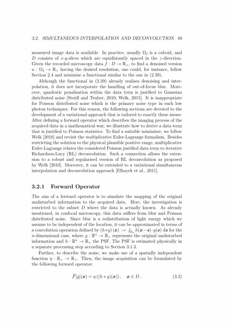
3.2. SIMULTANEOUS INTERPOLATION AND DECONVOLUTION 49
measured image data is available. In practice, usually Ω3 is a cuboid, andD consists of x-y-slices which are equidistantly spaced in the z-direction.Given the recorded microscopy data f : D → R+, to find a denoised versionu : Ω3 → R+ having the desired resolution, one could, for instance, followSection 2.4 and minimise a functional similar to the one in (2.39).
Although the functional in (2.39) already realises denoising and inter-polation, it does not incorporate the handling of out-of-focus blur. More-over, quadratic penalisation within the data term is justified to Gaussiandistributed noise [Steidl and Teuber, 2010; Welk, 2015]. It is inappropriatefor Poisson distributed noise which is the primary noise type in such lowphoton techniques. For this reason, the following sections are devoted to thedevelopment of a variational approach that is tailored to exactly these issues:After defining a forward operator which describes the imaging process of theacquired data in a mathematical way, we illustrate how to derive a data termthat is justified to Poisson statistics. To find a suitable minimiser, we followWelk [2010] and revisit the multiplicative Euler-Lagrange formalism. Besidesrestricting the solution to the physical plausible positive range, multiplicativeEuler-Lagrange relates the considered Poisson justified data term to iterativeRichardson-Lucy (RL) deconvolution. Such a connection allows the exten-sion to a robust and regularised version of RL deconvolution as proposedby Welk [2010]. Moreover, it can be extended to a variational simultaneousinterpolation and deconvolution approach [Elhayek et al., 2011].
3.2.1 Forward Operator
The aim of a forward operator is to simulate the mapping of the originalundisturbed information to the acquired data. Here, the investigation isrestricted to the subset D where the data is actually known. As alreadymentioned, in confocal microscopy, this data suffers from blur and Poissondistributed noise. Since blur is a redistribution of light energy which weassume to be independent of the location, it can be approximated in terms ofa convolution operation defined by (h∗g) (x) :=
∫Ωn h(x−s) ·g(s) ds for the
n-dimensional case, where g : Rn → R+ represents the original undisturbedinformation and h : Rn → R+ the PSF. The PSF is estimated physically ina separate processing step according to Section 3.1.3.
Further, to describe the noise, we make use of a spatially independentfunction η : R+ → R+. Then, the image acquisition can be formulated bythe following forward operator:
F [g](x) = η ((h ∗ g)(x)) , x ∈ D . (3.2)

50 CHAPTER 3. CELL RECONSTRUCTION
As we can see, the forward operator not only consists of a determinis-tic convolution operation but also of a noise function which acts stochasti-cally. Hence, particularly with respect to our reconstruction task, the ques-tion arises how to incorporate such a stochastic part. One strategy is tocompletely refrain from its modelling within the forward process. Instead,one chooses an adequate penalisation strategy within the data term. Thismeans one exploits a suitable discrepancy measurement between the givenand sought data. Thus, while the forward operator reduces to just a convo-lution operation
F [g](x) = (h ∗ g)(x), x ∈ D , (3.3)
the task turns into the modelling of a data term tailored especially towardsPoisson distributed noise.
3.2.2 Towards a Physically Justified Data TermIn confocal microscopy mainly two types of noise appear: On the one hand,caused by the imaging sensor and by the signal amplification, additive whiteGaussian noise appears which is independent of the light intensity. On theother hand, the dominant type of noise in this setting is Poisson noise. Thisis due to the fact that the probability of k ∈ N photon impacts at the sensorcomplies with the Poisson distribution [Bovik, 2009]
Pλ(X = k) = λk
k! e−λ , (3.4)
where e is the exponential function and λ ∈ R+ is both the mean and thevariance of the distribution. Since the mean can be seen as a long-timeaverage of the acquisition, it corresponds to a capture where no noise isinvolved. Therefore, expecting a blurred acquisition according to Equation(3.3), one can set λ = F [g] = h ∗ g. Moreover, the probability of k photonimpacts at a specific location xi of the sensor is regarded to be independentof the q impacts at a different location xj. Therefore, the joint probabilityof both events can be calculated by
Pλ(X = k and Y = q) = Pλ(X = k) · Pλ(Y = q) , (3.5)
where the random variablesX and Y count the photon impacts at location xiand xj, respectively. Hence, according to Shepp and Vardi [1982], Bratsolisand Sigelle [2001], Dey et al. [2006] and Le et al. [2007], under the assumptionthat the photon impacts follow a Poisson distribution and all points x ∈ D

3.2. SIMULTANEOUS INTERPOLATION AND DECONVOLUTION 51
are independent, the probability p(f |g) of acquiring image f , given that thetrue object is g, reads
p(f |g) =∏x∈D
((F [g](x))f(x)
f(x)! e−F [g](x))
. (3.6)
Then, an estimate u of the original undisturbed signal g that leads to thegiven observation f can be found by following a maximum-likelihood ap-proach. This means that one searches an u that maximises the probability pw.r.t. a fixed f :
u = argmaxu
( ∏x∈D
((F [u](x))f(x)
f(x)! e−F [u](x)))
. (3.7)
However, searching for a maximiser of such a probability equals the searchfor a minimiser of its negative. Thus, the problem can be reformulated to
u = argminu
(−∏x∈D
((F [u](x))f(x)
f(x)! e−F [u](x)))
. (3.8)
Further, by taking the logarithm, multiplications become summations andintegration, respectively. This way, the problem can be interpreted as theminimisation of the variational functional
ED(f, u,F) :=∫D
(−lnF [u]f
f ! − ln(e−F [u]
))dx
=∫D
(F [u] + ln (f !)− f · ln(F [u])
)dx . (3.9)
Based on the fact that any constant additive change of a functional doesnot affect its minimiser, the term ln(f !) can be left out as done by Deyet al. [2004, 2006] or be replaced by ln(f f )− f . The last in turn reveals theequivalence of (3.9) to
ERL(f, u,F) :=∫D
(F [u]− f − f · ln
(F [u]f
))︸ ︷︷ ︸
=r2,f (F [u])
dx , (3.10)
which is known as Csiszár’s information divergence (I -divergence) [Csiszár,1991]. Due to its justification to Poisson statistics, Csiszár’s I -divergence

52 CHAPTER 3. CELL RECONSTRUCTION
Figure 3.4: Comparison of different discrepancy measures (x-axis: s andy-axis: value of penalisation function). From left to right: (a) Quadraticpenaliser r1,f (s). (b) Robust penaliser Φ(r1,f (s)) with Φ(r) := 2
√r. (c)
Asymmetric penaliser r2,f (s). (d) Robust asymmetric penaliser Φ(r2,f (s)).
is especially suitable for low-intensity imagery, and, among others, used in[Panin et al., 1998; Anconelli et al., 2005; Sawatzky et al., 2009; Dey et al.,2006; Welk, 2010]. As we can see, instead of penalising the discrepancybetween two measures F and f quadratically, i.e. via a penalty functionr1,f (F) := (F−f)2 as it is done in Section 2.2.1 or 2.5.3, Csiszár considers anasymmetric penaliser r2,f (F) := (F−f−f ln(F/f)). A direct comparison ofdifferent penalisers is given in Figure 3.4. Although, r2,f (F) is strictly convexin F for F , f > 0 and attains its minimum for F = f , it is obvious that aminimiser u of the functional (3.10) is not unique: Assume that u minimisesthe functional in (3.10), then any ξ that vanishes under convolution withh, i.e. h ∗ ξ = 0 induces an additional minimiser u := u + ξ with the sameminimal energy. This is because the forward operator would produce thesame result in both cases:
F [u] = h ∗ u = h ∗ (u+ ξ) = h ∗ u+ h ∗ ξ = h ∗ u+ 0 = h ∗ u = F [u] .
Now that we have found a Poisson justified deconvolution functional ordata term (since there is no regularisation involved), we need a strategy toestimate a suitable minimiser. Without the task of inpainting, i.e. D :=Ωn and assuming an imaging model of F [u] := h ∗ u, different approachesalready exist: Snyder et al. [1992] consider Equation (3.10) within a discretesetting. They show that the iterative Richardson-Lucy scheme constitutesa fixed point iteration converging to a minimiser of Csiszár’s informationdivergence. Dey et al. [2004] derive the variational gradient of an equivalentof (3.10) for the 2-D (Ω2 ⊂ R2) and 3-D case (Ω3 ⊂ R3) according to anadditive perturbation. Subsequently, the resulting Euler-Lagrange equationis solved iteratively in a multiplicative way which in turn corresponds to RLdeconvolution. In other words, if F [u] := h ∗ u and D := Ωn, Csiszár’s I -divergence (3.10) provides a variational interpretation of RL deconvolution.

3.2. SIMULTANEOUS INTERPOLATION AND DECONVOLUTION 53
This fact has been exploited among others by Welk [2010] and allows theenhancement of RL deconvolution by established variational robustificationand regularisation ideas. While such ideas are the subject of later sections,we first follow [Welk, 2010, 2015; Elhayek et al., 2011] and illustrate therelation between Csiszár’s I -divergence and RL deconvolution. To this end,a minimiser of Equation (3.10) is estimated according to the Euler-Lagrange(EL) formalism. However, instead of classical additive EL, this time, weconsider its multiplicative counterpart.
3.2.3 Multiplicative Euler-Lagrange FormalismTo derive the variational gradient of a considered energy functional, the clas-sical Euler-Lagrange formalism [Gelfand and Fomin, 2000], which is basedon an additive perturbation, provides a very common procedure (cf. Section2.2.2). However, deconvolution states a severely ill-posed problem with anon-unique minimiser. To reduce the problem of ill-posedness, a commonremedy is given by imposing additional inequality constraints. This way, thesolution can be restricted to only physically plausible values. Regarding theimaging process, we know that the number of photons arriving at the imagesensor is larger than zero. Hence, the intensity values have to be positive.While the classical additive Euler-Lagrange formalism does not impose anyconstraints on the estimation, in this section, we now follow multiplicativeEuler-Lagrange formalism as one way to retain the positivity of the solution[Welk, 2010, 2015]. Compared to the classical Euler-Lagrange formalism,here, the additive perturbation is replaced by a multiplicative one. Moreprecisely, within the multiplicative formalism, the variational gradient δ∗E
δuof
a functional E is derived by requiring⟨δ∗E
δu, v⟩
!= ∂
∂εE(u · (1 + ε v))
∣∣∣∣ε=0
, ∀v ∈ Rn → R , (3.11)
where v, again, denotes any differentiable perturbation function and 〈·, ·〉 thestandard inner product. Assuming a general functional (2.25) and proceedinganalogously to the additive case, the right-hand side expands to
∂
∂εE(u · (1 + ε v)
∣∣∣∣ε=0
= ∂
∂ε
∫ΩnF (x1, . . . , xn, u(1+εv), (u(1+εv))x1 , . . . , (u(1+εv))xn) dx
∣∣∣∣∣ε=0

54 CHAPTER 3. CELL RECONSTRUCTION
∗= ∂
∂ε
(∫
ΩnF (x1, . . . , xn, u(1+εv), ux1+εux1v+εuvx1 , . . . , uxn+εuxnv+εuvxn) dx
)∣∣∣∣∣ε=0
∗∗=∫
Ωn
(Fu(x1, . . . , xn, u(1+εv), ux1+εux1v+εuvx1 , . . . , uxn+εuxnv+εuvxn) · vu
+n∑i=1
(Fuxi (x1, . . . , xn, u(1+εv), ux1+εux1v+εuvx1 , . . . , uxn+εuxnv+εuvxn)
· (uxiv + vxiu)))
dx∣∣∣∣∣ε=0
(3.12)
Since both, the searched function u, as well as the perturbation function v,depend on x, we follow the product rule in (*). The chain rule is applied at(**). Now, by setting ε = 0, we proceed with
∂
∂εE(u · (1 + ε v)
∣∣∣∣ε=0
=∫
Ωn
(Fu(x1, . . . , xn, u, ux1 , . . . , uxn) · vu
+n∑i=1
Fuxi (x1, . . . , xn, u, ux1 , . . . , uxn) · (uxiv + vxiu))dx
∗∗∗=∫
Ωn
(Fu · v +
n∑i=1
Fuxi · (uv)x1
)dx , (3.13)
where we follow the product rule and omit the arguments in (***). By usingour notation F∇u := (Fux1
, . . . , Fuxn )>, we obtain
∂
∂εE(u · (1 + ε v)
∣∣∣∣ε=0
=∫
Ωn
(Fu · v + F>∇u∇(uv)
)dx , (3.14)
such that Equation (3.11) becomes (by following integration by parts analo-gously to (2.30))
⟨δ∗E
δu, v⟩
!=∫
Ωn(Fu − div (F∇u)) · uv dx
+∫∂Ωn
(η>F∇u
)· uv dx , ∀v ∈ Rn → R . (3.15)

3.2. SIMULTANEOUS INTERPOLATION AND DECONVOLUTION 55
Here, the image boundary is again described by ∂Ωn where η defines itsunit normal vector. Continuing analogously to Equation (2.31) and (2.32),we first consider the subset of perturbation functions where v(x) = 0 forx ∈ ∂Ωn and obtain
⟨δ∗E
δu, v⟩
!=∫
Ωn(Fu − div (F∇u)) · uv dx , ∀v ∈ Rn → R ,
⇐⇒ δ∗E
δu= (Fu − div (F∇u)) · u . (3.16)
If we plug this variational gradient into Equation (3.15), we arrive at theboundary conditions:⟨
(Fu − div (F∇u)) · u, v⟩
!=∫
Ωn(Fu − div (F∇u)) · uv dx
+∫∂Ωn
(η>F∇u
)· uv dx , ∀v ∈ Rn → R ,
⇐⇒ 0 !=∫∂Ωn
(η>F∇u
)· uv dx , ∀v ∈ Rn → R ,
⇐⇒ 0 != η>F∇u · u . (3.17)
Compared to the classical additive Euler-Lagrange formalism, its mul-tiplicative variant now differs through a multiplication with the unknownfunction for both the variational gradient, i.e. δ∗E
δu= δE
δu· u and the boundary
conditions.Welk [2010, 2015] illustrates in two different ways why the multiplicative
Euler-Lagrange formalism restricts the solution to positive values: On theone hand, one can observe that the multiplicative functional gradient δ∗E
δu
occurs within the additive formalism if one replaces the Euclidean metricdu by a hyperbolic one, i.e. du/u. Thus, one effectively moves unwantedvalues to infinite distance. On the other hand, it can also be shown thatthe multiplicative Euler-Lagrange formalism corresponds to the reparametri-sation u = exp(w). Such a reparametrisation concerning deconvolution ina discrete setting is proposed by Nagy and Strakoš [2000]. Welk and Nagy[2007] demonstrate the advantages of such a reparametrisation in the contextof variational deconvolution: While commonly Gibbs phenomena – which arecharacteristic artefacts for deconvolution – are counteracted by regularisa-tion, Welk and Nagy [2007] illustrate that these artefacts are mitigated intheir reparametrised approach. As a consequence, the need for regularisation

56 CHAPTER 3. CELL RECONSTRUCTION
may be reduced. This implies a possible higher accuracy within such a con-strained model. Besides the positivity of scalar values, such a technique isalso suggested if the preservation of positive definiteness w.r.t. tensor-valuedimages is relevant.
From Csiszár’s I -divergence to RL Deconvolution
With Csiszár’s information divergence [Csiszár, 1991], we have found a vari-ational functional that is especially tailored towards Poisson statistics and,therefore, to the considered imagery. With multiplicative Euler-Lagrange for-malism, we have a strategy to restrict the solution to the plausible positiverange. In this section, we now combine both ideas: Assuming a forward pro-cess of F [u] := h∗u, we derive the Euler-Lagrange equation of the functionalin (3.10) by following the multiplicative formalism. Here, we ignore for themoment the problem of a low axial resolution and assume that acquired infor-mation is complete, i.e. we set D := Ωn. According to Welk [2010, 2015] andElhayek et al. [2011] besides deriving the associated Euler-Lagrange equation,we illustrate the way from the multiplicative-based minimality condition tothe iterative Richardson-Lucy deconvolution scheme. So, let us derive the as-sociated variational gradient δ∗E
δuby requiring the equality in Equation (3.11).
For the functional (3.10), the right-hand side of (3.11) expands to
∂
∂εERL(f, u · (1 + εv),F)
∣∣∣∣ε=0
= ∂
∂ε
∫Ωn
(F [u · (1 + εv)]− f − f ln
(F [u · (1 + εv)]
f
))dx
∣∣∣∣∣ε=0
= ∂
∂ε
∫Ωn
(h ∗ (u · (1 + εv))− f − f ln
(h ∗ (u(1 + εv))
f
))dx
∣∣∣∣∣ε=0
= ∂
∂ε
∫Ωn
(h ∗ u+ ε h ∗ (uv)− f − f ln
(h ∗ u+ ε h ∗ (uv)
f
))dx
∣∣∣∣∣ε=0
=∫
Ωn
(h ∗ (uv)−
(f
h ∗ u+ ε h ∗ (uv)
)· (h ∗ (uv))
)dx
∣∣∣∣∣ε=0

3.2. SIMULTANEOUS INTERPOLATION AND DECONVOLUTION 57
=∫
Ωn
((1− f
h ∗ u+ ε h ∗ (uv)
)· (h ∗ (uv))
)dx
∣∣∣∣∣ε=0
=∫
Ωn
((1− f
h ∗ u
)· (h ∗ (uv))
)dx . (3.18)
By applying the definition of convolution, we can proceed with
d
dεERL(f, u · (1 + εv),F)
∣∣∣∣∣ε=0
=∫
Ωn
((1− f
h ∗ u
)(x) ·
∫Ωn
(h(x− s) u(s) v(s)
)ds)
dx
=∫
Ωn
∫Ωn
((1− f
h ∗ u
)(x) · h(x− s) u(s) v(s)
)ds dx
=∫
Ωn
∫Ωn
(h∗(s− x) ·
(1− f
h ∗ u
)(x) · u(s) v(s)
)ds dx , (3.19)
where h∗(x) := h(−x). Now, if we change the order of integration as follows
d
dεERL(f, u · (1 + εv),F)
∣∣∣∣ε=0
=∫
Ωn
(∫Ωn
(h∗(s− x) ·
(1− f
h ∗ u
)(x) dx
)· u(s)v(s)
)ds , (3.20)
one can in turn make use of the convolution notation. This leads us to
d
dεERL(f, u · (1 + εv),F)
∣∣∣∣∣ε=0
=∫
Ωn
((h∗ ∗
(1− f
h ∗ u
))(s) · u(s)v(s)
)ds .
(3.21)Embedding this result into the requirement in (3.11), and substituting theintegration variable s by x brings us to
⟨δ∗E
δu, v⟩
!=∫
Ωn
((h∗ ∗
(1− f
h ∗ u
))(x) · u(x)v(x)
)dx , ∀v ∈ Rn → R .
(3.22)

58 CHAPTER 3. CELL RECONSTRUCTION
Following the definition of the scalar product immediately reveals the func-tional derivative
δ∗E
δu=(h∗ ∗
(1− f
h ∗ u
))· u . (3.23)
If the support of the PSF h exceeds the image boundaries, we imposemirrored boundary conditions on u.
According to the minimality condition (2.26), a minimiser of (3.10) hasto fulfil a vanishing variational gradient, i.e.
δ∗E
δu= 0
⇐⇒(h∗ ∗
(1− f
h ∗ u
))· u = 0
⇐⇒(h∗ ∗ 1− h∗ ∗ f
h ∗ u
)· u = 0 . (3.24)
Since one additionally assumes energy preservation, i.e. h∗ ∗ 1 = 1 where 1 isthe constant function 1, we obtain(
1− h∗ ∗ f
h ∗ u
)· u = 0
⇐⇒ u−(h∗ ∗ f
h ∗ u
)· u = 0 . (3.25)
Eventually, introducing a fixed point iteration in k yields the well knownRichardson-Lucy (RL) deconvolution algorithm [Lucy, 1974; Richardson, 1972]of Section 2.5.2:
uk+1 =(h∗ ∗ f
h ∗ uk
)· uk . (3.26)
As already mentioned, initialised with the observed image, i.e. u0 :=f , this scheme produces successively sharpened images uk. Further, in theabsence of noise, i.e. f = h ∗ g, one fixed point of this scheme is given by g.This can be shown as follows: Assume g be given as an intermediate solutionat iteration step k, i.e. uk = g, then any further step
uk+1 =(h∗ ∗ f
h ∗ g
)· g =
(h∗ ∗ f
f
)· g = (h∗ ∗ 1) · g = g .

3.2. SIMULTANEOUS INTERPOLATION AND DECONVOLUTION 59
would not change anything so that uk+1 = uk = g which is the definition ofa fixed point. However, in practice if noise is present, the scheme has to bestopped after a certain number of iterations since it is known to diverge fork → ∞. The fact that noise can be tackled by limiting the total numberof iterations can be interpreted as some kind of regularisation [Welk, 2010].However, this, of course, would not only suppress noise, but it would alsoinhibit the sharpening process. For this reason, one is interested in an explicit(edge preserving) regularisation.
3.2.4 Robust Regularised Richardson-Lucy Deconvo-lution
In the last section, we inspected the relation between the iterative Richardson-Lucy deconvolution technique and the variational Csiszár’s information di-vergence (for D = Ωn, F [u] := h ∗ u) by means of the multiplicative Euler-Lagrange formalism. Besides illustrating the tailoring of RL deconvolutiontowards Poisson statistics, this variational interpretation gives direct accessto established regularisation and robustification ideas. Hence, the goal ofthis section is to combine the ideas from Section 2.2 and 2.5.3 with the vari-ational RL interpretation from the last section. Analogously to Dey et al.[2004, 2006], Sawatzky et al. [2009]; Sawatzky and Burger [2010], Welk [2010,2015], and Elhayek et al. [2011], we thus extend the energy functional ERL
(3.10) with an explicit regularisation term ES to:
ERRL (u) := ERL(f, u,F)︸ ︷︷ ︸RL-deconvolution
+ α · ES(u)︸ ︷︷ ︸smoothness
, (3.27)
where we choseES(u) :=
∫D
Ψ(|∇u|2) dx , (3.28)
where ∇ is the n-dimensional gradient operator.As we can see, the variational interpretation ERL of RL deconvolution
represents the data term ED. As a result, instead of limiting the total numberof iterations, now the amount of smoothness can be steered by the parameterα. This offers a better balance between deblurring and regularisation. Thisway, we can counteract the problem of non-uniqueness, noise, as well as theoccurrence of ringing artefacts, without stopping the sharpening process.
According to Equation (3.16) and (3.23), under the assumption that theforward operator is defined by F [u] := h ∗ u, the associated minimalitycondition [Welk, 2010; Elhayek et al., 2011; Welk, 2015] of this supplemented
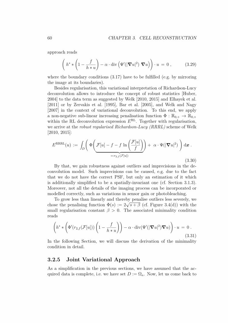
60 CHAPTER 3. CELL RECONSTRUCTION
approach reads(h∗ ∗
(1− f
h ∗ u
)− α · div
(Ψ′(|∇u|2) ∇u
))· u = 0 , (3.29)
where the boundary conditions (3.17) have to be fulfilled (e.g. by mirroringthe image at its boundaries).
Besides regularisation, this variational interpretation of Richardson-Lucydeconvolution allows to introduce the concept of robust statistics [Huber,2004] to the data term as suggested by Welk [2010, 2015] and Elhayek et al.[2011] or by Zervakis et al. [1995], Bar et al. [2005], and Welk and Nagy[2007] in the context of variational deconvolution. To this end, we applya non-negative sub-linear increasing penalisation function Φ : R0,+ → R0,+within the RL deconvolution expression ERL. Together with regularisation,we arrive at the robust regularised Richardson-Lucy (RRRL) scheme of Welk[2010, 2015]:
ERRRL(u) :=∫D
(Φ(F [u]− f − f ln
(F [u]f
)︸ ︷︷ ︸
=:r2,f (F [u])
)+ α ·Ψ(|∇u|2)
)dx .
(3.30)By that, we gain robustness against outliers and imprecisions in the de-
convolution model. Such imprecisions can be caused, e.g. due to the factthat we do not have the correct PSF, but only an estimation of it whichis additionally simplified to be a spatially-invariant one (cf. Section 3.1.3).Moreover, not all the details of the imaging process can be incorporated ormodelled correctly, such as variations in sensor gain or photobleaching.
To grow less than linearly and thereby penalise outliers less severely, wechose the penalising function Φ(s) := 2
√s+ β (cf. Figure 3.4(d)) with the
small regularisation constant β > 0. The associated minimality conditionreads(
h∗ ∗(
Φ′(r2,f (F [u]))(
1− f
h ∗ u
))− α · div(Ψ′(|∇u|2)∇u)
)· u = 0 .
(3.31)In the following Section, we will discuss the derivation of the minimalitycondition in detail.
3.2.5 Joint Variational ApproachAs a simplification in the previous sections, we have assumed that the ac-quired data is complete, i.e. we have set D := Ωn. Now, let us come back to

3.2. SIMULTANEOUS INTERPOLATION AND DECONVOLUTION 61
slice
PSF
Figure 3.5: Support of the PSF overlaps missing slices to be inpainted (lightgrey). Consequently, the blurring process carries partially missing informa-tion to acquired slices (solid black).
the additional problem of a low axial resolution. Hence, assuming that thedata is only given at a subset D ⊂ Ωn, we want to reconstruct the informa-tion on the whole image domain Ωn. To solve both tasks of deconvolutionand interpolation, clearly we could apply the methods for inpainting fromSection 2.3 and deconvolution from Section 3.2.4 sequentially. However, asChan et al. [2005] point out, such a naive solution is disadvantageous: In-terpolation followed by deconvolution propagates blurred information intomissing regions. By reversing the order of application, the support of thePSF overlaps with the unknown areas. Moreover, as illustrated in Figure3.5, the acquired data contains information about the signal in the domainto be inpainted due to the convolution that is part of the image acquisitionprocess.
This motivates a joint variational solution as advocated by Chan et al.[2005] in the context of blind deconvolution, and by Elhayek et al. [2011] inthe context of RRRL deconvolution. The latter proposes the following energyfunctional for simultaneous interpolation and RRRL deconvolution (IRRRL):
EIRRRL(u) :=∫DΦ(F [u]− f − f ln
(F [u]f
)︸ ︷︷ ︸
=:r2,f (F [u])
)dx+ α
∫Ωn
(Ψ(|∇u|2)
)dx .
(3.32)By restricting the data term (or deconvolution term) to only the acquired
subset D but at the same time demanding smoothness over the whole imagedomain Ωn, the functional (3.32) performs simultaneous interpolation anddeconvolution.
Since, compared to the functional in (3.27), nothing is changed w.r.t. theregularisation term ES, let us for the moment focus on the data term EIRRRL
Dof EIRRRL. To derive the variational gradient of EIRRRL
D , we proceed analo-

62 CHAPTER 3. CELL RECONSTRUCTION
gously to (3.18) et seqq. and obtain:
∂
∂εEIRRRL
D (f, u · (1 + εv),F)∣∣∣∣ε=0
= ∂
∂ε
∫D
Φ(r2,f (F [u(1 + εv)])
)dx
∣∣∣∣∣ε=0
= ∂
∂ε
∫D
Φ(h ∗ (u · (1 + εv))− f − f ln
(h ∗ (u(1 + εv))
f
))dx
∣∣∣∣∣ε=0
=∫DΦ′(r2,f (F [u(1 + εv)])
)·((
1− f
h ∗ u+ ε h ∗ (uv)
)· (h ∗ (uv))
)dx
∣∣∣∣∣ε=0
=∫D
Φ′(r2,f (F [u])
)·((
1− f
h ∗ u
)· (h ∗ (uv))
)dx . (3.33)
At this point, one has to take care that now the convolution domain (which isgiven by Ωn) in the forward operator F differs from the integration domainD.Using the definition of convolution and the abbreviation Φ′ := Φ′ (r2,f (F [u])),we thus have
d
dεEIRRRL
D (f, u · (1 + εv),F)∣∣∣∣∣ε=0
=∫D
(Φ′(x) ·
(1− f
h ∗ u
)(x) ·
∫Ωn
(h(x− s) u(s) v(s)
)ds)
dx (3.34)
However, with the help of the characteristic function χD, defined in Equation(2.37), both integration domains can be harmonised as follows:
d
dεEIRRRL
D (f, u · (1 + εv),F)∣∣∣∣∣ε=0
=∫
Ωn
(χD(x) · Φ′(x) ·
(1− f
h ∗ u
)(x) ·
∫Ωn
(h(x− s) u(s) v(s)
)ds)
dx
=∫
Ωn
(∫Ωn
(h∗(s− x)·
(χD(x)·Φ′(x)
(1− f
h ∗ u
)(x) dx
))u(s)v(s)
)ds

3.3. FIBRE ENHANCEMENT WITH ANISOTROPIC REGULARISATION63
=∫
Ωn
(h∗ ∗
(χD ·Φ′ ·
(1− f
h ∗ u
))(s) · u(s)v(s)
)ds . (3.35)
Hence, the corresponding minimality condition for the functional (3.32) reads[Elhayek et al., 2011](h∗ ∗
(χD · Φ′(r2,f (F [u])) ·
(1− f
u ∗ h
))− α · div(Ψ′(|∇u|2)∇u)
)· u = 0 .
(3.36)Similarly to Equation (2.39) the characteristic function χD is used to
impose the fidelity condition F [u] := h ∗u ≈ f only at those locations wheredata is available. In the minimisation process, information is transferredfrom D to Ω \D by both the enforced smoothness in the regularisation termand the convolution operations in the data term. A coupling of neighboursthus not only exists by regularisation but also within the data term.
Even though this model already achieves an interpolation compatible withthe blur model, it does not respect the directional information of the under-lying cell structure. Hence, let us discuss in the next section, how to turnthe smoothing behaviour induced by regularisation into a fibre enhancementtechnique with the help of anisotropic diffusion (cf. Section 2.1.2).
3.3 Fibre Enhancement with AnisotropicRegularisation
In this section, we want to illustrate how we can exploit the physical processof anisotropic diffusion in order to enhance 3-D images capturing the filamentnetwork of cells. In previous sections, we have already discussed variationalrestoration and deconvolution models, which utilise the concept of regular-isation in some sense. The need of regularisation has been argued by theproblem of non-uniqueness, noise, and ringing artefacts. Moreover, regular-isation has been extended to achieve an inpainting approach. As alreadymentioned in Section 2.2.2, mathematically, such variational regularisationterms, which penalise the derivative of the unknown, cause a divergence ex-pression of type
div(
Ψ′(|∇u|2) ∇u)
(3.37)
in the associated minimality conditions. Such expressions are known to leadto scalar-valued (isotropic) diffusion [Perona and Malik, 1987]. However, theaim of this study is the enhancement and reconstruction of tube-like patternssuch as the microtubules, which are part of the intracellular structure of cells.

64 CHAPTER 3. CELL RECONSTRUCTION
For this particular application, the isotropic behaviour of the latter class ofprocesses is not well suited.
In the context of image denoising and smoothing, we have revisited thephysical phenomena of diffusion in Section 2.1. Besides isotropic diffusion, wehave also recapitulated the idea behind anisotropic diffusion [Weickert, 1998]in Section 2.1.2. By incorporating directional information of the underlyingimage structure, anisotropic diffusion allows one to steer the flux and therebythe smoothing process along such elongated structures. This aspect makesanisotropic diffusion in particular attractive for our cell enhancement task.
Hence, let us now exchange the isotropic smoothing behaviour by ananisotropic one. To this end, we proceed as in Section 2.1.2, and replace thescalar-valued diffusivity Ψ′ ∈ R+ in Equation (3.37) by a diffusion tensor D.This leads to the right-hand side of Equation (2.21):
div(D(Jρ(uσ)) ·∇u
). (3.38)
In this way, our strategy is related to the work of Welk et al. [2005] in thecontext of deblurring and to Galić et al. [2008] in the context of inpaintingand compression, respectively. To gather local directional information, weagain choose the structure tensor J of Förstner and Gülch [1987]. Sincewe are dealing with 3-D microscopy data sets, D as well as J are 3 × 3tensor fields. Moreover, we assume that the recorded data only consist ofone channel. In this setting, the structure tensor is given by
Jρ(∇uσ) :=Kρ ∗
uσx1
uσx2
uσx3
uσx1
uσx2
uσx3
>
=Kρ ∗
uσ2x1 uσx1uσx2 uσx1uσx3
uσx1uσx2 uσ2x2 uσx2uσx3
uσx1uσx3 uσx2uσx3 uσ2x3
. (3.39)
Since the directional information of the underlying image structure is con-tained in the eigenvectors and eigenvalues of this symmetric, positive semi-definite tensor, we consider the eigendecompositon
Jρ(∇uσ) = (v1|v2|v3)
µ1µ2
µ3
v>1v>2v>3
, (3.40)
where v1,v2,v3 are orthonormal eigenvectors.

3.4. EFFICIENT AND STABILISED ITERATION SCHEME 65
Now, the essential idea is that the image intensity does not vary muchalong a cell fibre. Hence, we are searching for the direction of lowest contrast,which is given by the eigenvector v3 corresponding to the smallest eigenvalueµ3. In order to enhance such elongated approximately one-dimensional cellstructures in 3-D space, we demand smoothness only in the direction of thelowest contrast, i.e. along v3. This smoothing process should also be ableto close small gaps caused by, e.g. an imperfect labelling with the fluores-cence dyes. On the other hand, the reconstruction should be sharp so thatthe single fibres are clearly differentiable against their background. Thus,smoothing perpendicular to v3, i.e. along v1 and v2 respectively should bepenalised in dependence to the respective contrast described by µ1 and µ2.To achieve such a directionally dependent smoothing behaviour, we assemblethe diffusion tensor as follows
D(Jρ(∇uσ)) := (v1|v2|v3)
Ψ′(µ1)Ψ′(µ2)
1
v>1v>2v>3
, (3.41)
where we apply the Charbonnier diffusivity [Charbonnier et al., 1997], i.e.Ψ′(s2) = 1/
√1 + s2/λ2 to the two largest eigenvalues µ1 and µ2. The third
eigenvalue is strictly set to 1 in order to perform homogeneous diffusionalong the eigenvector v3, i.e. along the fibres. As reasoned above, this choiceis suitable to enhance the tube-like structures of microtubules. Eventually,replacing the diffusivity in Equation (3.36) by this anisotropic term, we ob-tain
u ·
h∗ ∗ (χD · Φ′(rf (F [u]))(
1− f
u ∗ h
))
− α · div (D(Jρ(∇uσ)) ∇u) = 0 . (3.42)
We call this interpolating robust and (an)isotropic regularised Richardson-Lucy (IRARRL) method. How to solve such a PDE efficiently, as well as itsapplication to discrete digital images, is the central topic of the followingsections.
3.4 Efficient and Stabilised Iteration SchemeThis section is devoted to the task of solving Equation (3.42) by means ofan efficient and stabilised gradient descent scheme. We want to illustrate

66 CHAPTER 3. CELL RECONSTRUCTION
that a clever evaluation of the unknown w.r.t. the old and the new time stepmay drastically improve the performance of the overall method. Generally,computing a solution of isotropic regularised RL (or equivalent models) is anon-trivial task and different strategies for this exist in the literature [Green,1990; Panin et al., 1998; Sawatzky et al., 2008; Dey et al., 2004; Sawatzkyet al., 2009; Bertero et al., 2009; Sawatzky and Burger, 2010; Setzer et al.,2010; Welk, 2010].
Dey et al. [2004, 2006] propose for their related isotropic approach withoutany inpainting or robustification strategy the fixed point scheme
uk+1 −(h∗ ∗ f
h ∗ uk
)· uk − α div
(Ψ′(|∇uk|2)∇uk
)· uk+1 = 0 , (3.43)
where the second term, as well as the divergence term, are evaluated com-pletely at the old time step k. Only the first term and the factor behind thedivergence term are evaluated at the new time step k+1. Eventually, solvingfor uk+1 yields
uk+1 = uk
1− α div (Ψ′(|∇uk|2)∇uk) ·(h∗ ∗ f
h ∗ uk
). (3.44)
However, as we can see, the divergence term has moved into the denomina-tor. This, in turn, leads to the risk of evaluating to negative values or evendivisions by zero. To prevent such a scenario, Dey et al. [2004, 2006] suggestthe restriction of regularisation by allowing only small values for α. Sucha restriction has already been proposed by Green [1990] and Panin et al.[1998], where an expectation-maximisation (EM) algorithm is performed. Inorder to avoid such a restriction of the regularisation parameter, Welk [2010]proposes a different strategy. He refrains from strictly multiplying the diver-gence term in Equation (3.31) with uk+1. Instead, the multiplication is madeconditionally, depending on the sign of the divergence term: If the divergenceterm has a negative sign, it is multiplied with uk+1 from the new time step.Otherwise, the old one uk is chosen. This can be formulated as(h∗ ∗ Φ′kD
)uk+1−
(h∗ ∗
(Φ′kD ·
f
h ∗ uk
))uk−α div
(Ψ′(|∇uk|2)∇uk
)uk+ν = 0 .
(3.45)Here, we use the abbreviation Φ′kD := χD ·Φ′(rf (F [uk])) and set ν := 1, if thedivergence term is negative, and ν := 0 else. Solving for uk+1 leads to theiteration scheme
uk+1 =h∗ ∗
(Φ′kD · f
h∗uk)
+ α [div(Ψ′(|∇uk|2) ∇uk
)]+
h∗ ∗ Φ′kD − α [div (Ψ′(|∇uk|2) ∇uk)]−· uk , (3.46)

3.4. EFFICIENT AND STABILISED ITERATION SCHEME 67
where we adopt the notation [z]± := 12(z ± |z|) from Welk [2010].
Although this case distinction ensures the non-negativity of the overallscheme, our experiments in Section 3.6 (cf. Figure 3.8) show that it stillbehaves unsatisfactory when high levels of regularisation are used.
This motivates us to a novel fixed point iteration with better stabilityproperties: Instead of evaluating the divergence expression completely at theold time step, we propose a semi-implicit realisation. This means, within thedivergence term, we propose to apply the diffusivity function (and diffusiontensor respectively) to uk, i.e. at the old time step. However, the gradient∇u is taken from the new time step k + 1. At the end, the diffusion termis multiplied with uk. The other terms are untouched and the remainingnonlinear parts are still solved by the lagged diffusivity or Kačanov-method[Fučik et al., 1973; Chan and Mulet, 1999; Vogel, 2002], i.e. at the old iterationstep k. Applying this novel fixed point strategy to Equation (3.42), the moregeneral anisotropic model can be written as
(h∗ ∗Φ′kD) uk+1−(h∗∗
(Φ′kD
f
h ∗ uk
))uk−α div
(D(Jρ(∇ukσ)) ∇uk+1
)uk= 0 .
(3.47)This scheme already reaches a higher stability w.r.t. large amount of regular-isation. However, in each iteration, three convolution operations have to beperformed. Since each convolution is computationally expensive, one shouldtry to minimise their occurrence. To this end, we propose to replace thefactor uk in the first subtrahend by uk+1, leading to
(h∗∗Φ′kD) uk+1−(h∗∗
(Φ′kD
f
h ∗ uk
))uk+1−α div
(D(Jρ(∇ukσ)) ∇uk+1
)uk= 0 ,
(3.48)where the distributivity property of convolution, i.e. h∗f+h∗g = h∗(f+g),allows us to reformulate it as
(h∗ ∗
(Φ′kD ·
(1− f
h ∗ uk
)))uk+1 − α div
(D(Jρ(∇ukσ)) ∇uk+1
)uk = 0 .
(3.49)On the one hand, as we can see, this strategy reduces the number of necessaryconvolutions per iteration by one. On the other hand, our scheme becomeseven more semi-implicit.
The actual solution of the latter equation is carried out using the steepestdescent method (see e.g. [Luenberger and Yinyu, 2015]), to which end we

68 CHAPTER 3. CELL RECONSTRUCTION
introduce the relaxation parameter τ :
−(h∗ ∗
(Φ′kD ·
(1− f
h ∗ uk
)))uk+1 + α div(D(Jρ(∇ukσ)) ∇uk+1) uk
= uk+1 − uk
τ. (3.50)
To apply this fixed point iteration to 3-D digital images, we discuss inSection 3.5 how this scheme above can be discretised.
A Semi-implicit Relaxation Scheme for RL Deconvolution
Of course, the latter semi-implicit iteration scheme can also be transferredto the original Richardson-Lucy deconvolution approach just by omittinginterpolation and setting Φ(s) = s, α = 0. Hence, we proceed analogouslyto Section 3.4, and consider the fixed point iteration (3.49) for Φ′kD = 1 andα = 0. This way, Equation (3.49) comes down to(
h∗ ∗(
1− f
h ∗ uk
))· uk+1 = 0 . (3.51)
After that, we apply again the steepest descent method with relaxation pa-rameter τ . This leads us to
−(h∗ ∗
(1− f
h ∗ uk
))· uk+1 = uk+1 − uk
τ, (3.52)
which is a semi-implicit version of the scheme of Holmes and Liu [1991].Finally, we solve for uk+1 and obtain
uk+1 =(
1 + τ
(1− h∗ ∗ f
h ∗ uk
))−1
· uk . (3.53)
As for the standard RL scheme (3.26), if noise is negligible, i.e. f = h ∗ g,the undisturbed signal g is a fixed point of the latter scheme.
3.5 Space DiscretisationIn this section, we want to discretise the IRARRL deconvolution schemefrom Equation (3.50). To this end, according to the discretisation scheme inSection 2.1.1, we assume a 3-D cell image to be sampled on a regular grid of

3.5. SPACE DISCRETISATION 69
size Nx1 ×Nx2 ×Nx3 =: N with sampling distances (hx1 , hx2 , hx3)> =: h3 inhorizontal-, vertical- and depth-direction, respectively. Further, we denote byuki,j,` the approximation of u at voxel (i, j, `) at evolving time t = k ·τ . Hence,a discrete version of Equation (3.50) has to fulfil the following equation ineach voxel (i, j, `) ∈ 1, . . . , Nx1 × 1, . . . , Nx2 × 1, . . . , Nx3:
−[h∗ ∗
(Φ′kD ·
(1− f
h ∗ uk
))]i,j,`︸ ︷︷ ︸
D1
·uk+1i,j,`
+ α · [div(D(Jρ(∇ukσ))∇uk+1)]i,j,`︸ ︷︷ ︸A(uk)uk+1
·uki,j,`︸ ︷︷ ︸D2
=uk+1i,j,` − uki,j,`
τ. (3.54)
At this point, let us again change to a single-index notation (e.g. row-majorordering) and arrange 3-D signals u : R3 → R in vectors u ∈ RN . Then,the diffusion term can be expressed in terms of the matrix-vector multipli-cation A(uk)uk+1. This reminds us of the semi-implicit diffusion scheme ofEquation (2.14). For the discretisation of the anisotropic diffusion process,we use a 3-D extension3 of the scheme presented by Weickert et al. [2013].While, in the isotropic case, A has a straightforward structure and can be de-scribed, e.g. by (2.10), the anisotropic case is much more complex. Thereforeit is not shown explicitly here. Further, in order to formulate the point-wisemultiplications in Equation (3.54), we introduce the N×N diagonal matrices
D1 := diag(−[h∗ ∗
(Φ′kD ·
(1− f
h ∗ uk
))]1, . . . ,
. . . ,−[h∗ ∗
(Φ′kD ·
(1− f
h ∗ uk
))]N
)(3.55)
andD2 := diag
(uk1, . . . , u
kN
), (3.56)
where the two convolution operations are realised by exploiting the convo-lution theorem (cf. Section 2.5.1) [Gasquet et al., 1998; Bracewell, 1999].However, to reduce wraparound errors and to obtain a power-of-two imagesize as required for the application of the fast Fourier transformation (FFT),we first mirror the image at the boundary according to Figure 3.6.
3Special thanks go to Prof. Dr. Joachim Weickert and Prof. Dr. Martin Welk for pro-viding their implementation.

70 CHAPTER 3. CELL RECONSTRUCTION
1 2 3 4 5 6 7 7 6 5 6 5 4 3 2 1 1 2 3 ...... 4 3 2 1 4
Figure 3.6: Boundary treatment to reduce wraparound errors, By mirroringthe image depending on the size of the PSF support, we obtain a power-of-two image size. The remaining voxels are set as the mirror of the periodicimage extension.
Eventually, Equation (3.54) can be written in the following vector-valuedscheme:
(D1(uk) + α ·D2(uk) ·A(uk)
)· uk+1 = uk+1 − uk
τ. (3.57)
This leads us to a system of equations Bx = b to be solved in every iterationstep: (
I − τ(D1(uk) + α ·D2(uk) ·A(uk)))
︸ ︷︷ ︸B
·uk+1︸ ︷︷ ︸x
= uk︸︷︷︸b
. (3.58)
Please note that due to the multiplication with diagonal matrices, the result-ing system matrix B is not symmetric.
Let us now illustrate how to solve this system of equations with the help ofthe Jacobi relaxation or weighted Jacobi method [Morton and Mayers, 2005].
The Jacobi Relaxation Method
In every iteration k of the presented approach, the system of equations in(3.58) has to be solved. To this end, let us split the system matrix B = D−Tinto a diagonal component D that is easily invertible and a remaining off-diagonal part T by
D = I − τ ·(D1(uk) + α ·D2(uk) ·Adiag(uk)
),
T = τ · α ·D2(uk) ·Arest(uk) ,(3.59)
whereAdiag andArest denotes the diagonal and off-diagonal part ofA respec-tively. Then, following the Jacobi relaxation method [Morton and Mayers,

3.5. SPACE DISCRETISATION 71
2005] with parameter ω > 0 and iteration index m, the solution vector x canbe iteratively determined by
xm+1 = (1− ω)xm + ωD−1(T xm + b) . (3.60)
In detail, we compute the solution uk+1 = (uk+11 , . . . , uk+1
N )> for the discreteversion of our IRARRL deconvolution scheme in every gradient descent stepk via iterating the following scheme over m:
uk+1,m+1p = (1− ω) · uk+1,m
p
+ ω ·
1 + τ · α ·N∑q=1q 6=p
akpq · uk+1,mq
· ukp1 + τ
[h∗ ∗ (Φ′kD · (1− fh∗uk
)) ]p
− α · ukp · akpp
, p = 1 . . . N ,
(3.61)
where akpq denotes an entry of the discretised diffusion matrix A(uk). Ini-tialised with the observed image f , i.e. u0,0 := f , after a fixed number ofinner iterations, the outer iteration process is updated and the inner onestarts again. This is continued until a certain stopping criterion is satisfied.In our work, we have considered the relative L2-norm of the residuum of thesystem of equations.
Regarding the latter equation, we can recognise that during the inner iter-ation, the coupling of neighbours is accomplished only by regularisation. Thisis because the diffusion term is considered semi-implicitly. In contrast, D1(cf. Equation (3.54)) is evaluated in a lagged diffusivity manner (Kačanov-method) [Fučik et al., 1973; Chan and Mulet, 1999; Vogel, 2002], i.e. con-sidered completely at the old outer iteration step. Therefore, the couplingperformed by the data term comes only into play when the outer iteration isupdated, i.e. during the gradient descent process.
Now, it remains to prove that if xm contains only physical plausible pos-itive entries, the same holds for xm+1. To this end, let us first consider thefactor D−1 in Equation (3.60). Negative entries in this diagonal matrix canappear for large τ , since D1 can have entries of arbitrary sign. Hence, wederive the following bound on τ :
∀ p ∈ 1, . . . , N : Dp,p > 0⇔ [I − τ (D1 + α ·D2 ·Adiag)]p,p > 0
⇔ [−D1 − α ·D2 ·Adiag]p,p > −1τ
(3.62)

72 CHAPTER 3. CELL RECONSTRUCTION
The latter inequality must hold for all α > 0, and since −α ·D2 ·Adiag > 0,we obtain:
minp
[−D1 − α ·D2 ·Adiag]p,p > minp
[−D1]p,p > −1τ. (3.63)
At this point we distinguish two cases: If minp[−D1]p,p ≥ 0, the conditionis fulfilled for all τ > 0 anyway. Otherwise, the theoretical step-size of thegradient descent is restricted by the inequality
τ <−1
minp
[−D1
]p,p
, (3.64)
or expressed with the values of D1:
τ <−1
minp
[h∗ ∗
(Φ′kD ·
(1− f
h∗uk))]
p
. (3.65)
Please note that this bound is necessary to ensure the positivity of the solu-tion.
Next, let us discuss the remaining component of Equation (3.60) thatmight become negative: Since the matrix T contains the off-diagonal en-tries of the discrete anisotropic diffusion operator A, the positivity of theterm T xm + b cannot be guaranteed. Thus, we have to ensure for allp ∈ 1, . . . , N
(1− ω)[xm]p > −ω[D−1(T xm + b)
]p. (3.66)
The latter inequality is only critical for voxels, where the right-hand side ispositive. Hence, the following bound on the relaxation parameter can beestablished:
ω < minp
[xm]p[xm]p −min
[D−1(T xm + b)
]p, 0
, (3.67)
or with the components of the matrices
ω < minp
uk+1,mp
uk+1,mp −min
1+τ ·α·N∑q=1q 6=p
akpq ·uk+1,mq
·ukp1+τ
([h∗∗(Φ′kD ·(1− f
h∗uk ))]p
−α·ukp ·akpp
) , 0
. (3.68)

3.6. EXPERIMENTS 73
Note that in the isotropic case, the positivity of the off-diagonals of A isguaranteed anyway, so no relaxation is necessary (ω = 1). Furthermore, thelatter bound is derived for arbitrarily negative entries in A. In practice, wecan safely set ω in [0.9, 1.0] without observing any experimental problems inpractice.
Now, let us briefly come back to the semi-implicit relaxation scheme forRL deconvolution. To show that the equivalence for Φ′kD = 1, and α = 0also holds in the discrete case, we plug these values into the iteration scheme(3.61) and obtain:
uk+1p =
ukp
1 + τ
[h∗ ∗ (1− fh∗uk
)]p
, p = 1 . . . N . (3.69)
Here, we can refrain from the Jacobi method since the off-diagonal part ofthe system matrix B vanishes by setting α := 0. As we can see, the itera-tion scheme above constitutes a discretised version of Equation (3.53). Thederived condition for τ (Equation (3.64)) for preserving the positivity carriesover as well. This accelerated Richardson-Lucy scheme has not been testedextensively, but first experiments demonstrate that half as many iterationsare needed compared to standard Richardson-Lucy deconvolution.
3.6 ExperimentsIn this section, we demonstrate the performance of our reconstruction ap-proach on a 3-D confocal laser scanning microscopy (CLSM) image as wellas on a stimulated emission depletion (STED) microscopy image of cells.These data sets are provided by the Nano-Cell Interaction group of the Leib-niz Institute for New Materials (INM) in Saarbrücken. As illustrated inSection 3.1.1 and 3.1.2, respectively, these data sets comprise degradationssuch as blur, Poisson noise and a relatively low axial resolution. To estimatethe individual point-spread function (PSF) of each record, we proceed as ex-plained in Section 3.1.3. For this purpose, to each cell image, a second 3-Drecord showing some small fluorescence beads has been provided. The imageof the 3-D confocal microscope has a resolution of 1024 × 1024 × 50 voxelswith a grid size of (62/62/126) nm. A corresponding PSF is estimated ata grid size of (25/25/126) nm. Since the PSF must have the same grid sizeas the reconstruction, we have to resample it accordingly: For doubling thedepth (axial) resolution and leaving the grid in x and y direction unaltered,

74 CHAPTER 3. CELL RECONSTRUCTION
Figure 3.7: Slice 13 of the 3-D CLSM image (grey values rescaled to [0, 255]).(a) Top left: Slice of the complete volume of size 1024 × 1024 × 50. Thewhite rectangle indicates the origin of the first zoom-in. (b) Top right: Sliceof the volume segment (376 × 244 × 24) of (a). Again, the white rectanglesshow the position of the second level magnifications. (c) Bottom left:Central slice of the estimated PSF (24× 24× 33). Its scale fits to the secondmagnification level. (d) Bottom centre and (e) right: Two second-levelmagnifications.
we need (62/62/63) nm. For this reason, the given PSF must be subsampledin the lateral direction and supersampled in axial direction. Since the PSFis a smooth function, we found simple linear interpolation to be sufficient forthis task.
Although all our experiments are performed in 3-D, we depict distinctive2-D slices of the processed volumes for the sake of a better recognisability.Figure 3.7 shows one such slice of the original CLSM image, along withtwo levels of magnification. For the rest of this section, we will discuss ourresults on the basis of these magnifications, since the fine-scale details arebetter comparable on high magnification levels.
Our first experiment addresses the stability of the semi-implicit scheme

3.6. EXPERIMENTS 75
(3.50) for the interesting case of relatively large α. For a direct comparison,we restrict our method to isotropic regularisation in this experiment. Inthe isotropic setting, typical choices for α are in the interval [0.001, 0.05].Figure 3.8 compares our scheme (3.50) against the one of Elhayek et al. [2011]and Welk [2010] (see Equation (3.46)) respectively. While the numericalscheme of the latter method becomes unstable and exhibits chequerboard-like artefacts with increasing α, our semi-implicit scheme remains stable evenfor very high regularisation weights.
Before we demonstrate the performance of our anisotropic fibre enhancingapproach, let us first illustrate the behaviour of the anisotropic smoothingstrategy with regard to an underlying cell filament network. To this end, inour next experiment we superimpose a 2-D image slice with a visualisationof the main estimated smoothing orientations in Figure 3.9. This visualisa-tion is computed by projecting the 3-D eigenvector of the structure tensorcorresponding to the smallest eigenvalue into the 2-D slice. One can seethat the anisotropic strategy yields good estimates for the sought smoothingdirections and seems to be particularly applicable for such a task.
The third experiment compares our anisotropic fibre enhancement ap-proach (3.50) with the original Richardson-Lucy method (2.52) [Richardson,1972; Lucy, 1974]), as well as the isotropic (TV) regularisation strategy (3.46)of Elhayek et al. [2011]. To assess the interpolation quality of these tech-niques, we show in Figure 3.10 an in-between slice of the data set. Thereare a number of equivalences between wavelet-based approaches and tech-niques using variational principles or partial differential equations (such asTV approaches) [Steidl et al., 2004; Welk et al., 2008]. Since one can expecta similar quality as with the TV-like approach of Elhayek et al. [2011], wedo not explicitly compare with wavelet-based methods here.
For the special case of Richardson-Lucy (RL) deconvolution [Richardson,1972; Lucy, 1974], we have to fill in the missing slice by linear interpolationin advance. RL deconvolution results in very sharp contrasts after 200 iter-ations. However, due to absence of any regularisation, the main drawbackof the RL algorithm is its sensitivity to noise and the deconvolution typi-cal creation of over- and undershoots, i.e. oscillation artefacts [Bratsolis andSigelle, 2001]. As a consequence, the deconvolved images have sharp con-trasts, but the fibre structures are inhomogeneous and rough, particularly infibre crossings. The regularisation component in the methods of Dey et al.[2004, 2006] and Elhayek et al. [2011] suppresses these over- and undershoots.With increasing degree of regularisation, the fibres become more and moresmooth and homogeneous. However, at the same time, the radii of single fi-bres grow and fine structured details melt together, which is shown in Figure

76 CHAPTER 3. CELL RECONSTRUCTION
Figure 3.8: Numerical stability with respect to large amount of isotropic(TV) regularisation (rescaled to [0, 255]). From Top to Bottom (a) Row 1:Result of the method of Welk [2010] and Elhayek et al. [2011] respectively,α = 0.1, 11 iterations. (b) Row 2: Semi-implicit approach with isotropicregularisation, α = 0.1, 11 iterations. (c) Row 3: Same with 900 iterationsand α = 0.1. (d) Row 4: With 900 iterations and α = 0.5.

3.6. EXPERIMENTS 77
Figure 3.9: Orientations of the eigenvectors corresponding to the smallesteigenvalues of the structure tensor (3.40) projected into the actual slice.
3.10(b),(c) and Figure 3.11(b),(c), respectively. It partially results in smallover-segmentation of the fibres. The benefit of our anisotropic regularisationbecomes obvious by considering Figure 3.10(d) and Figure 3.11(d), respec-tively. As we can see, we obtain smoothness only along the fibres but sharpedges against the background.
Let us now come to the STED data set. The original record has a resolu-tion of 1057 × 1059 × 65, acquired with a sampling distance of (40/40/168)nm. The corresponding beads for the PSF estimation are recorded with asampling distance of (40/40/84) nm, which is already the required grid sizefor doubling the z-resolution. In Figure 3.12, we illustrate the suitability ofour IRARRL scheme for STED images. Moreover, we compare the robustdata term against its non-robust variant. One can recognise that the robustdata term results in a slightly more sharpened structure.
In the final experiment, we analyse the runtime of our scheme (3.50)and compare it against the numerical interpolation scheme of Elhayek et al.[2011]. To have a fair comparison, we compute an approximate steady stateusing 10,000 iterations of the scheme of Elhayek et al. [2011]. To reducethe experimentation time, we restrict our computations to a region of size105 × 89 × 47. In Figure 3.13 we show the input region along with the

78 CHAPTER 3. CELL RECONSTRUCTION
Figure 3.10: Reconstructed slice between slices 13 and 14 of the CLSM cellimage (rescaled to [0, 255]). Zoom-ins of the white rectangle are shown inFig. 3.11. From top to bottom (a) Row 1: RL deconvolution (200 iterations)with preceding linear interpolation. (b) Row 2: Isotropic (TV) method ofElhayek et al. [2011], α = 0.0006. (c) Row 3: Ditto, α = 0.002. (d) Row4: Our anisotropic method (3.42), α = 0.0004, ρ = 1.5, σ = 0.6, λ = 0.1.

3.6. EXPERIMENTS 79
Figure 3.11: From left to right (a) Column 1: Zoom-in of Figure 3.10(a):RL deconvolution. (b) Column 2: Zoom-in of Fig. 3.10(b): Isotropic (TV)method, α = 0.0006. (c) Column 3: Zoom-in of Fig. 3.10(c): Ditto withα = 0.002. (d) Column 4: Zoom-in of Fig. 3.10(d): Our anisotropicmethod.
approximate solution. Next, we once more run the scheme of Elhayek et al.[2011] as well as our scheme (with a diffusion tensor that realises the sameisotropic behaviour) and plot the average difference per voxel between theactual iterate and the approximate solution in Figure 3.14. One can clearlysee the superior convergence rate of our method. Furthermore, we measurethe time until the average difference per voxel drops below 0.1 and summarisethese computation times in Table 3.1. All runtime experiments are performedwith a C implementation on an Intel Xeon Processor W3565 (8M Cache,3.20 GHz, 4.80 GT/s Intel) CPU with 24 GB RAM using a single-threadedimplementation. The upper bound for the relaxation parameter τ = 1.5 isdetermined experimentally. This speed-up can be explained by two facts: Onthe one hand, the novel semi-implicit scheme only performs two instead ofthree convolutions per iteration, which leads to a speed-up factor of 1.5. Onthe other hand, the number of required iterations is decreased by a factor of2.2.

80 CHAPTER 3. CELL RECONSTRUCTION
Original Elhayek, et al. α=0.0004 Elhayek, et al. α=0.001STED Image without Robustification without Robustification
RL, 250 iterations Elhayek, et al. α=0.0004 Elhayek, et al. α=0.001
Ours, α=0.0002, σ = 0.6 Ours, α=0.0002, σ = 1.5
Figure 3.12: Reconstruction of cell fibres recorded with a STED microscope.Cut-outs (87×111 px) of an interpolated slice (Images are rescaled to [0, 255]).In reading order: (a) Original input slice. (b) Method of Elhayek et al.[2011], (TV) regularisaton α = 0.0004, without robustification. (c) Ditto,α = 0.001. (d) RL deconvolution (250 iterations). (e) Result of Elhayeket al. [2011], α = 0.0004. (f) Ditto, α = 0.001. (g) Our anisotropic scheme(3.42), α = 0.0002, ρ = 2.0, σ = 0.6, λ = 0.1. (h) Ditto, σ = 1.5.

3.6. EXPERIMENTS 81
Figure 3.13: (a) Left: Original input CLSM region (rescaled to [0, 255]).(b) Right: Result after 10,000 iterations using the scheme of Elhayek et al.[2011] with α = 0.001.
0.1
0.2
0.5
1
9
0 1000 2000 3000 4000 5000 6000
Diffe
rence
Iterations
Elhayek et al. 2011Semi-Implicit: τ=1.5
Figure 3.14: Average L1 difference between the approximate solution andthe iterated signal. Note the logarithmic scaling of the y-axis. Dottedline: Elhayek et al. [2011]. Solid line: Our semi-implicit iteration scheme,τ = 1.5.

82 CHAPTER 3. CELL RECONSTRUCTION
Table 3.1: Computation times of the approach of Elhayek et al. [2011] andour novel semi-implicit scheme (3.50).
Method Iterations Time speed up factorElhayek et al. [2011] 6276 9827 s 1Semi-implicit τ = 1.5 2879 2982 s 3.3
3.7 SummaryIn the beginning of this thesis, we revisited some established methods forimage restoration. In this chapter, we have shown how to combine and ex-tend these concepts in order to reach a tailoring towards the specific physicalcharacteristics of modern low photon light microscope imagery. We haveillustrated the development of a PDE-based method aiming especially atthe restoration and enhancement of 3-D cell images recorded by CLSM andSTED microscopes. To this end, we started with a detailed discussion ofthese microscopy techniques and their functional principles. Moreover, wehave revealed their physical limitations and typical weaknesses: blur, Poissonnoise and low axial resolution. To provide access to non-blind deconvolutiontechniques, we employed an estimation of the PSF of the participating op-tical system based on physical measurements. Concerning deblurring underPoisson distributed noise, we have shown that Richardson-Lucy deconvolu-tion (RL) [Richardson, 1972; Lucy, 1974] is well suited for this task. Byfollowing the multiplicative Euler-Lagrange formalism, we have illustratedthe connection between RL deconvolution and Csiszár’s information diver-gence [Csiszár, 1991]. With this variational representation, we have shownthe way to the robust and regularised RL approach of Welk [2010] and itsextension to inpainting [Elhayek et al., 2011]. Eventually, we exploited thephysical process of anisotropic diffusion [Weickert, 1998]. To this end, wereplaced the scalar-valued diffusivity by a diffusion tensor. In this way, thesmoothing behaviour is aligned to the tube-like structure of the cell fibresand the reconstruction quality is increased.
Compared to the work by Elhayek et al. [2011] and Dey et al. [2004, 2006],our novel proposed semi-implicit iteration scheme provides higher stabilityw.r.t. large regularisation weights. Besides that, we achieved a higher effi-ciency than Elhayek et al. [2011], because first, our novel scheme needs lessiterations and second, it saves one out of three convolutions in each iterationstep.
This chapter illustrates the way of tailoring a reconstruction framework

3.7. SUMMARY 83
towards the specific physical characteristics and weaknesses of a consideredimage acquisition technique. Additionally, this chapter shows once morehow one can get inspired by physical phenomena appearing in nature (hereanisotropic diffusion) and how to adjust it according to specific requirements.Moreover, it demonstrates the benefits of an integrated view and the handlingof all degradations simultaneously. By an adequate numerical algorithm, wecombine stability and efficiency.

84 CHAPTER 3. CELL RECONSTRUCTION

Chapter 4
Depth-from-Defocus
In this chapter, we address the so-called depth-from-defocus problem. Ourgoal is to exploit the physical properties of an optical system, which appearto be a weakness or limitation at first glance. More precisely, depth-from-defocus methods are based on the fact that a lens can only focus points at acertain distance. This distance is given by the focal plane. Points displacedfrom it are imaged in a blurred way whereas the amount of blur increases asthe offset becomes larger. Although, strictly speaking, all points not lyingwithin the focal plane are projected blurred, they still appear sharp, if theyare within a certain distance range around the focal plane. This distanceinterval is called depth-of-field (DOF) [Träger, 2007; Wayne, 2013]. Theposition of the focal plane as well as the width of the depth-of-field dependon the individual optical properties of the camera. For instance, opticalsystems having a small focal ratio (also called f-number or relative aperture)– meaning the ratio of the focal length of the lens to the aperture diameter, seee.g. [Barsky et al., 2003] – suffer from a very limited depth-of-field [Langford,2000; Stroebel, 1999; Wayne, 2013]. Such a situation is present in close-upand macro photography [Davies, 2012]. To imitate an acquisition as it wouldbe done by such a limited DOF imagery, computer graphics methods simulatethe local blur on the basis of the local depth information. This is called depth-of-field simulation and is usually applied in order to increase the realism ofartificially created images [Pharr and Humphreys, 2004; Barsky and Kosloff,2008].
In principle, depth-from-defocus is the inverse operation to the depth-of-field simulation. This means its goal is to reconstruct the depth mapby means of estimating the local amount of out-of-focus blur. As a by-product, one is also able to compute the completely sharp image as it wouldbe recorded by a camera having an infinite depth-of-field. However, regardinga single image, one can neither estimate the amount of blur nor distinguish
85

86 CHAPTER 4. DEPTH-FROM-DEFOCUS
between out-of-focus blur and a blurred texture. Therefore, several imagesof the same static scene but varying focal settings are required. Then eachof these images, usually arranged in a so-called focal stack, varies locally intheir amount of out-of-focus blur (cf. Figure 4.1).
While the forward problem of simulating the depth-of-field effect alwayshas a unique solution, depth-from-defocus is an ill-posed inverse problem: Forinstance, blurring a homogeneous region creates a focal stack whose imagesdo not differ in the amount of blur. Thus, it is not possible to reconstruct aunique depth map. As in previous chapters, in order to handle such an ill-posed problem, we make use of variational methods and regularisation. Thisallows to extract a solution as the minimiser of some energy functional thatinvolves an additional smoothness assumption [Bertero et al., 1988; Gelfandand Fomin, 2000; Aubert and Kornprobst, 2006]. Hence, the task turns intothe design of a suitable variational functional to which end we first have tofind an adequate forward operator. To keep the numerical complexity rea-sonable, many variational models for the depth-from-defocus problem involveonly a relatively small set of simplified assumptions in their forward model,e.g. requiring local equifocality, i.e. a locally constant depth [Rajagopalan andChaudhuri, 1997; Favaro and Soatto, 2000; Favaro et al., 2003a; Lin et al.,2015]. As a consequence, their solutions reflect the physical reality only toa very limited extent in the general case. Approaches that do not rely onany equifocal assumption at all can also violate important physical principlessuch as a maximum-minimum principle for the intensity values. For that pur-pose, the goal of Section 4.1 is to find a forward operator that approximatesthe depth-of-field effect. By refraining from any equifocal assumption, ouroperator comes closer to the physical reality. An additional requirement isthat the forward operator should fit well into a variational framework. InSection 4.2 we then formulate our variational framework which enables us toinvert this imaging model. In Section 4.2.2 we illustrate how to find a suit-able minimiser of it. We further show how to handle multi-channel imagesin Section 4.2.3 and how to gain benefit from a robustification in Section4.2.4. In Section 4.3 we present our novel denoising and depth-from-defocusapproach in order to handle focal stacks suffering from severe noise. Howto discretise the presented models is the topic of Section 4.4 and the follow-ing Section 4.5 demonstrates the performance of the different approaches onsynthetic and real-world experiments.
This chapter is based on our conference publication [Persch et al., 2014]and its follow-up technical report [Persch et al., 2015] which has been submit-ted to the journal ‘Image and Vision Computing’ and is still under review.

87
Figure 4.1: Focal stack. Each slice captures the same static scene, but differsin its focal settings. The gradual transition from sharp to blurred regionswithin each image corresponds to the depth profile.
Related Work. Generally, depth estimation based on differently focusedimages can be separated into two approaches: While depth-from-defocusmethods also incorporate out-of-focus information, depth-from-focus meth-ods estimate the depth by means of in-focus information only. To this end,a local sharpness criterion [Pertuz et al., 2013] such as the local variance ofintensities [Sugimoto and Ichioka, 1985] is applied. Locally, the slice withmaximal sharpness is assumed to be in focus and to match the depth. Bosh-tayeva et al. [2015] analyse different sharpness measures and combine themwith anisotropic smoothing strategies.
Since the estimation of depth is usually combined with the recovery of thesharp pinhole image, image fusion methods can also be seen as related. Suchmethods fuse several defocused images to one sharp image. A simultaneousmulti-focus image fusion and denoising approach is proposed by Ludusan andLavialle [2012].
Inferring the depth based on the amount of out-of-focus blur goes back toPentland [1987] as one of the pioneers in the field of depth-from-defocus. Inhis work, the blurriness of sharp edges or patches in different recordings servesfor the depth estimation. To also incorporate diffraction effects, he discussesthe use of a Gaussian instead of a pinhole as a suitable point-spread function(PSF). However, Pentland [1987] assumes one image to be in focus acting asa reference. This restriction is resolved in the work of Subbarao [1988]. Hecontinues his work by suggesting a depth-from-defocus approach [Subbaraoand Surya, 1994] using a convolution/deconvolution transform in the spatialdomain and investigating its noise sensitivity [Subbarao and Tyan, 1997].
Rajagopalan and Chaudhuri [1997] approach the depth-from-defocus prob-lem by means of a space-frequency representation technique based on theWigner distribution and the complex spectrogram. Furthermore spatial reg-ularisation of the local blur parameter is imposed.
The approach of Bailey et al. [2014] consists of two main steps. First, the

88 CHAPTER 4. DEPTH-FROM-DEFOCUS
level of blurriness is determined using the method of Hu and de Haan [2007].Next, to estimate the depth, the relation between blurriness, position of thefocal plane and depth is exploited.
Making use of the equivalence of Gaussian blurring and linear homo-geneous diffusion in the context of depth-from-defocus is proposed by Nam-boodiri and Chaudhuri [2004]. Since this implicates a constant depth, imagesare partitioned into equifocal patches. In [Favaro et al., 2008; Namboodiriand Chaudhuri, 2007; Namboodiri et al., 2008; Wei et al., 2009] the ideais extended to nonlinear isotropic diffusion that allows spatial changes ofthe diffusivity corresponding to the depth profile. Favaro et al. [2003b] andHong et al. [2009] extend this diffusion strategy by also involving directionalinformation via anisotropic diffusion.
Markov random fields can also be employed to handle the depth-from-defocus problem [Chaudhuri and Rajagopalan, 1999; Bhasin and Chaudhuri,2001; Namboodiri et al., 2008]. Among those approaches, Bhasin and Chaud-huri [2001] investigate how the PSF has to be iteratively corrected at strongdepth changes, where partial occlusions occur. However, their work is limitedto only two focal planes (two defocussed images).
Favaro [2010] and Wu et al. [2014] suggest to estimate the relative spread,i.e. the discrepancy in the standard deviations or width between the PSFs oftwo images in order to infer the depth values. This way, the computation ofthe sharp pinhole image can be avoided. While in the work of Favaro [2010]a nonlocal-means regularisation w.r.t. the depth map is proposed, Wu et al.[2014] considers geometric constraints to the relative spread.
Also restricting themselves to only two images, Ben-Ari and Raveh [2011]address the performance of depth-from-defocus. They suggest the use offast explicit diffusion (FED) [Grewenig et al., 2010], as well as a graphicsprocessing unit GPU implementation. Lin et al. [2015] propose a depth-from-defocus approach working with video pairs.
Most depth-from-defocus methods are restricted to imaging models basedon geometric optics describing light propagation via straight lines. In therecent work of Wei et al. [2014] and Wei and Wu [2015], respectively, thisrestriction is removed by incorporating also Fresnel diffraction.
Modelling the image formation (forward operator), embedding it intoa suitable energy functional, and posing depth-from-defocus as a variationalminimisation problem, is most closely related to our work [Favaro and Soatto,2000; Jin and Favaro, 2002; Aguet et al., 2008]. As a suitable discrepancymeasure between the given data and the forward operator, the first twoapproaches suggest Csiszár’s information divergence [Csiszár, 1991]. Aguetet al. [2008] penalise deviations from the model assumption in a quadraticway. Favaro and Soatto [2000] assumes a locally equifocal surface, which

4.1. IMAGE FORMATION MODELS 89
implies a shift-invariant PSF. Instead, Jin and Favaro [2002] refrain fromsuch a restriction and embed a shift-variant PSF in their model.
Interpreting a shift-invariant PSF as a 2-D function and a shift-variant asa 4-D one, the approach of Aguet et al. [2008] can be seen as a compromisebetween both. They propose the use of a 3-D PSF whose slices are 2-D nor-malised Gaussians with varying standard deviation. Each slice represents theblur level according to a specific depth value. On the one hand, this strategyreduces the complexity by incorporating knowledge about the depth depen-dence on the PSF. On the other hand, especially at strong depth changes,it may result in a convolution operation with a non-normalised kernel. As aconsequence, an essential physical property, namely the maximum-minimumprinciple w.r.t. the image intensities may be violated which leads to a wrongmodel assumption.
4.1 Image Formation ModelsIn this section, we want to approach the depth-from-defocus problem bymeans of inverting an approximation of the physical imaging process. Hence,as a first step, we have to find a forward operator that describes the imag-ing process reasonably well. Given the depth information of the scene anda completely sharp image, the sought forward operator should generate aresult as it would be produced by a camera with a limited depth-of-field. Inliterature, in particular in the field of computer graphics, several suggestionsalready exist [Barsky and Kosloff, 2008]. The most famous model is thethin lens camera model which is often used in the context of raytracing tosimulate the depth-of-field effect [Pharr and Humphreys, 2004; Cook et al.,1984]. There, the sharp information is given by the object texture. However,even though these approaches already produce very realistic results, theirinversion in the sense of depth-from-defocus, is not possible or at least verydifficult. Consequently, we have to develop a novel forward operator with abetter trade-off between being invertible and simulating a real camera well.
To understand the relation between depth and out-of-focus blur, let usbriefly discuss the pinhole camera model and the thin lens camera modelin this section. While the first one produces completely sharp images with-out suffering from any depth-of-field effect, the second is a physical modelto simulate such depth dependent out-of-focus blur [Pharr and Humphreys,2004; Shirley and Morley, 2008]. Differences in their results allow to infer theamount of out-of-focus blur and thus the value of depth. Hence, the mainidea is to relate both models. To this end, we express the thin lens cam-era model first by means of a spatially variant PSF applied to the pinhole

90 CHAPTER 4. DEPTH-FROM-DEFOCUS
pinholeimage plane
Figure 4.2: Pinhole camera model.
image. Next, we follow Aguet et al. [2008], and approximate the spatiallyvariant PSF by a three-dimensional but spatially invariant one. Assuminglocal equifocal patches, i.e. patches that are parallel to the lens, such an ap-proach may already yield good approximations. However, in case of strongdepth changes, it leads to a convolution with a non-normalised kernel. Con-sequently, it violates the maximum-minimum principle of the intensity valuesat those places. Therefore, its use within a depth reconstruction frameworkis not advisable and motivates us to develop a novel forward operator whichincorporates a normalisation function.
4.1.1 Pinhole Camera ModelThe pinhole camera model (cf. Figure 4.2) is the standard imaging model.It refrains from any lenses and consists only of a very small pinhole and animage plane (or screen) [Pharr and Humphreys, 2004; Shirley and Morley,2008]. The pinhole is placed in the optical centre `0 := (0, 0, 0)> and has adistance v ∈ R+ to the image plane. The functional principles of the pinholeimaging model are based only on geometrical optics. This means, it describesthe propagation of light only via rays, i.e. as linear subsets of R3. In thisway, it completely ignores the wave character of light so that no diffractionphenomena come into play. For the sake of notational convenience, let usparametrise a ray by two points a, b ∈ R3 it passes through. Hence, we canfully describe a ray by
r(a, b) := y ∈ R3 | y = (1− λ) · a+ λ · b, λ ∈ R. (4.1)
The set of all rays is denoted by R. If x := (x1, x2)> denotes the locationwithin the image domain Ω2 ⊂ R2, then for each point x := (x1, x2,−v)>on the image plane, there exists exactly one optical ray r(x, `0) ∈ R goingthrough the pinhole. Let d : Ω2 → R+ denote the depth map of a surfaceS ⊂ R3, which we assume to be opaque. Then the resulting pinhole operator

4.1. IMAGE FORMATION MODELS 91
image plane
focal plane
Figure 4.3: Thin lens camera model.
FP can be expressed as
FP[φ, d](x) := φ(Zd(x, `0
)), (4.2)
where, φ : S → R+ denotes the intensity value of a surface point andZd(x, `0) yields the first (i.e. closest) intersection point of the ray r(x, `0)with the surface S. Since there exists at most one optical ray per image pointhitting the surface, the object will be imaged completely sharp. Thus, noout-of-focus blur arises in this image formation model, and the depth-of-fieldis infinite.
4.1.2 Thin Lens ModelFigure 4.3 shows the thin lens camera model, which is a classical modelto simulate the depth-of-field effect physically. In this model, instead of apinhole, an infinitely thin (circular) lens with focal length f is placed in theoptical centre `0. Lens and image plane are parallel and have a distance vto each other. As already mentioned in the beginning of this chapter, a lenscan only focus points to the image plane that lie within the focal plane. Toobtain the distance fp of focal plane to the lens one can follow the thin lensequation (see e.g. [Born and Wolf, 1970]):
1fp
= 1f− 1v. (4.3)
Intersecting the pinhole ray r(x, `0) with the focal plane yields for eachimage point x its corresponding point x within the focal plane. As the nameof the ray already implies, this mapping exactly corresponds to the one ofthe pinhole camera model.
The more interesting case, of course, involves points that lie outside ofthe focal plane. They spread their intensity to a circle of confusion onto

92 CHAPTER 4. DEPTH-FROM-DEFOCUS
the image plane [Horn, 1968; Subbarao, 1988; Barsky et al., 2003; Pharr andHumphreys, 2004]. In other words, if the object is not lying in the focal plane,the intensity of several surface points may blend into one single image pointcausing blurred information. These surface points lie within the intersectionarea of the bundle of lens rays with the surface. For an image point x, thisbundle can be described using x and all points on the lens. Following Pharrand Humphreys [2004], one can formulate this imaging process via the thinlens operator
FL[φ, d](x) := 1|A|
∫Aφ(Zd(`, x
))d` , (4.4)
where |A| denotes the area of the lens. For the limiting case that |A| → 0,only the pinhole ray r(x, `0) survives which again leads to the pinhole cameramodel with no out-of-focus blur.
The thin lens camera model also complies with geometric optics and canthus be simulated in a straightforward way using raytracing techniques [Cooket al., 1984]. However, since a large amount of blur requires processing a hugenumber of rays per pixel, raytracing is computationally very expensive. Fur-thermore, it is not well suited for our variational inversion strategy. Hence,the goal of the following sections is the development of a forward operatorthat approximates the thin lens camera model, but can additionally be em-bedded into a variational framework. As a first step in that direction, letus express the thin lens camera model with the help of a spatially variantpoint-spread function (PSF) and the completely sharp pinhole image.
4.1.3 Spatially Variant Point-Spread FunctionIn the thin lens camera model, the sharp information is given by the intensityvalues of the surface. However, we already know that in the pinhole cameramodel each surface point is represented by exactly one image point becausethere exists a sharp one-to-one mapping. Hence, instead of integrating overthe lens, we can integrate over the sharp pinhole image u in order to expressthe thin lens camera model. To this end, though, one has to weight eachpinhole image point correctly. This can be realised with the help of a spatiallyvariant PSF Hd : Ω2×Ω2 → R0+ that depends on the depth profile d. In thecontext of computer graphics, such a postprocessing depth-of-field approachhas been proposed by Potmesil and Chakravarty [1981]. Accordingly, insteadof pursuing the intersection of light rays, we can express the imaging processas
FH[u, d](x) :=∫
Ω2Hd(x,y) u(y) dy , (4.5)

4.1. IMAGE FORMATION MODELS 93
where x describes the location within the 2-D image plane.One important property of the thin lens camera model is its preservation
of a maximum-minimum principle w.r.t. φ. This means that the intensityvalue of an image point lies between the minimum and maximum intensityvalue of any underlying surface point:
φmin ≤ FL[φ, d](x) ≤ φmax , ∀x ∈ Ω2 . (4.6)
Consequently, in order to imitate the thin lens camera model, the used spa-tially variant PSF Hd has to preserve this property w.r.t. the intensity valuesof the sharp pinhole image u. Therefore, we have to guarantee that the PSFis normalised for each image point x:∫
Ω2Hd(x,y) dy = 1 , ∀x ∈ Ω2 . (4.7)
As this imaging model constitutes a weighted average of the sharp imageintensities, the main issue turns into the computation of the weights of thePSF Hd. A straightforward solution for that would be the use of raytracingtechniques and to apply the thin lens camera model. However, this is ex-actly what we want to avoid. Thus, we have to find a more efficient way toapproximate the weights of the PSF Hd.
4.1.4 Approximation of the PSFIn this section, we want to approximate the weights of the PSF in orderto avoid the need of expensive raytracing techniques. To this end, let ustake a closer look at the intensity distribution within the thin lens cameramodel. From Horn [1968] and Subbarao [1988] we know that the intensityemitted by a non-occluded surface point lying outside of the focal plane is(uniformly) spread to a circle – assuming a circular lens – of confusion onthe image plane. The size of this circle of confusion depends on the distanced of the surface point to the lens. Since we know from previous sections thatsurface intensities can be represented by grey values of the pinhole image,the weights of the PSF in Equation (4.5) have to represent the intensitydistribution caused by such circle of confusion.
For simplification, let us for the moment assume that the surface is equifo-cal. This means that it is aligned parallel to the lens so that the depth d isconstant. Then the circle of confusion do not change for any surface pointand one has to distinguish only two cases: (i) surface points whose circleof confusion overlaps the actual image point are weighted by the reciprocalof the circle area (assuming a uniform intensity distribution). (ii) surface

94 CHAPTER 4. DEPTH-FROM-DEFOCUS
image plane surface
focal plane
PSF
Figure 4.4: Left: Circles of confusion for different surface points appearingon the image plane. Right: 3-D PSF composed of 2-D normalised Gaussians.
points whose circle of confusion does not reach the actual image point areweighted by zero. This equifocal assumption, moreover, allows the simplifi-cation of Equation (4.5) to a convolution operation [Horn, 1968]. The spa-tially variant PSF Hd thus can be replaced by a spatially invariant kernelhd : Ω2 ⊂ R2 → R0+. The case distinction above can be realised with thehelp of a 2-D pillbox PSF whose radius is related to the constant depth.
However, in the general case of a non-constant depth map, the radiuschanges with the depth of each surface point. Thus, to estimate the intensityof an image point x, Aguet et al. [2008] weight each neighbouring pointu(y) corresponding to its circle of confusion, where a point having a largecircle of confusion will get a small weight and vice versa. To achieve this,they introduce a 3-D spatially invariant PSF h : Ω3 ⊂ R3 → R0+ as anapproximation of spatially variant Hd:
FU[u, d](x, z) :=∫
Ω2h(x− y, z − d(y))︸ ︷︷ ︸
≈Hd(x,y)
u(y) dy , (4.8)
where z represents a given focal plane. In this model, the weight not onlydepends on the distance of two points, but also on the actual depth value ofthe neighbouring points.
Until now, we have assumed that an out-of-focus point spreads its inten-sity uniformly to a circle of confusion. This results in PSF that is pillbox-shaped. However, to additionally take into account the wave character oflight, Aguet et al. [2008] choose a 2-D Gaussian PSF instead of a pillbox one.This has been already proposed by Pentland [1987]. The standard deviationof the Gaussian replaces the radius of the pillbox. The approach of Aguetet al. [2008] can be illustrated as in Figure 4.4: First, the 2-D function hd islifted to a 3-D one h, composed of 2-D normalised Gaussians. The standard

4.1. IMAGE FORMATION MODELS 95
deviation of each Gaussian increases with increasing distance to the focalplane. Next, one cuts a slice out of this 3-D PSF h corresponding to thedepth. This slice serves as a local approximation of Hd for a specific imagepoint x. With the help of this 3-D PSF, a second interpretation of the equa-tion above is also possible: For this, we assume that the sharp pinhole imageu lies in a dark volume g : Ω3 → R corresponding to the depth profile. Itcan be defined as
g(x, z) := u(x) · δ(z − d(x)) with δ(x) :=
1 if x = 0 ,0 else .
(4.9)
Then Equation (4.8) is just a standard 3-D convolution of g with the PSF h:
(g ∗ h)(x, z) :=∫
Ω3g(y, z′) · h(x− y, z − z′) dy dz′
=∫
Ω3u(y) · δ(z′ − d(y)) · h(x− y, z − z′) dy dz′ . (4.10)
Here, the integrand vanishes everywhere except for z′ = d(y). Thus, theequation above can be simplified to
(g ∗ h)(x, z) =∫
Ω2u(y) · h(x− y, z − d(y)) dy , (4.11)
where the integration domain has changed from Ω3 to Ω2. This illustratesthat the forward operator of Aguet et al. [2008] performs a spatially invariant3-D convolution.
Although the forward operator in (4.8) uses a 3-D PSF which is composedof 2-D normalised Gaussians, one has to keep in mind that the slice to be cutout – as local approximation ofHd – is not necessarily normalised. This wouldviolate the requirement in Equation (4.7). Therefore, in the next section, wesuggest a novel forward operator that counters exactly this problem.
4.1.5 Our ModificationIn the last section, we have illustrated how to approximate locally the weightsof Hd by following Aguet et al. [2008]. The idea is to compose a 3-D PSFof 2-D Gaussians varying in their standard deviation and taking a slice outof it corresponding to the depth profile. Assuming the equifocal case, thisslice is just a 2-D normalised Gaussian of a certain standard deviation again.Accordingly, the requirement in Equation (4.7) is fulfilled, the maximum-minimum principle is automatically guaranteed, and the imaging model is

96 CHAPTER 4. DEPTH-FROM-DEFOCUS
surface
Approximation of
surface
Approximation of
Figure 4.5: Unnormalised kernel. In the presence of strong depth changes,the local approximation of Hd by Aguet et al. [2008] is composed of differentGaussians (blue and red). (a) Top row: Overshoot: While the blue part isnearly a complete Gaussian, with the second (red) part an integration weightof 1 is exceeded. (b) Bottom row: Undershoot: The local composed PSFconsists only of a part of a normalised Gaussian (red) and a second (blue)Gaussian already reaching negligible values. The resulting integration weightbecomes smaller than 1.
approximated. However, the formulation above becomes problematic if par-tial occlusions occur, which is expected to happen due to depth changes.In this case, the slice is a composition of weights of several Gaussians withdifferent standard deviations. As a direct consequence the normalisation can-not be guaranteed anymore. The forward operator then effectively performsspatially invariant 2-D integration with an unnormalised kernel as a local ap-proximation of Hd (see Figure 4.5). Hence, the requirement in Equation (4.7)is not fulfilled. This leads to a violation of the maximum-minimum principlew.r.t. the image intensities (4.6) and thus to a violation of the imaging model.
To avoid this, the idea is to consider the local approximation of Hd andto use it as a normalisation function. That way, our novel forward operatorreads
FN[u, d](x, z) := FU[u, d](x, z)∫Ω2h(x− x′, z − d(x′)) dx′ . (4.12)
This forward operator guarantees the requirement in Equation (4.7) per defi-nition and consequently preserves the maximum-minimum principle of Equa-tion (4.6).
Although this normalisation function may look like a small modification

4.2. VARIATIONAL FORMULATION 97
at first glance, it can have a large impact on the simulation quality of thedepth-of-field effect. To demonstrate this, we compare different forward op-erators in Figure 4.6. As one can see, the result of the forward operator ofAguet et al. [2008] shown in Figure 4.6(c) is very close to simple 3-D convolu-tion (cf. Equation (4.10)) given in Figure 4.6(b). Differences are caused dueto the discretisation required when embedding the pinhole image into thediscrete 3-D volume according to Equation (4.9). Since both forward modelsperform convolutions with an unnormalised kernel h on strong depth changes,they produce bright overshoots followed by dark shadows. This behaviouris illustrated in Figure 4.5. In Figure 4.5(a) the slice taken out of the PSFconsists of nearly a complete Gaussian caused by the blue surface and largepart of a second Gaussian caused by the red surface. Hence, the integrationweight of the slice exceeds 1 which leads to overshoots. In Figure 4.5(b) theslice only consists of approximately three-quarter of a Gaussian caused bythe red surface. The rest is set to 0. Thus, the integration weight is lowerthan 1 which results in undershoots. Indeed, regarding Figure 4.6(c) and4.6(b) respectively these local violations of the maximum-minimum principleon strong depth changes are violations of the model assumption and produceresults that are not photorealistic. In contrast, comparing Figure 4.6(d)and (e) demonstrates that our normalised approach comes very close to thephysically well-founded thin lens camera model, and allows to create realisticdepth-of-field effects.
However, we have to keep in mind that the proposed normalisation isnot a constant but a function depending on the position and on the depthprofile of the scene. This make the model and the mathematical equationsmore complicated. Hence, the topic of the next sections is the embedding ofour novel forward operator into a variational framework and how to find asuitable minimiser of it.
4.2 Variational Formulation
In the last section, we have proposed a novel forward operator that approxi-mates the thin lens camera model simulating the depth-of-field effect. Now,as the next step of our reconstruction framework, we illustrate how to invertthis novel forward operator within a variational framework. Given a stackof blurred images, we want to jointly estimate the depth map and the sharppinhole image.

98 CHAPTER 4. DEPTH-FROM-DEFOCUS
a b c d e
Figure 4.6: Left box: (a) Top: Synthetic 3-D test model. (a) Middle:Sharp image obtained with a pinhole camera renderer. (a) Bottom: Cor-responding grey-valued coded depth map (the brighter the larger the depthvalue). Right box: Comparison of different forward operators. From topto bottom: Increasing focal plane distance. (b) Standard spatially invariant3-D convolution (4.10). (c) Forward operator of Aguet et al. [2008] withoutnormalisation preservation. (d) Our normalised forward operator (4.12). (e)Thin lens camera model (4.4) realised by raytracing technique.
4.2.1 Variational Model
As already mentioned, our depth-from-defocus framework needs a set of 2-Dimages capturing the same static scene but varying in their focal settings.Thus, let us assume such a set being arranged as a 3-D focal stack s : Ω3 →R+ where Ω3 ⊂ R3 denotes the stack volume. In contrast to the last chapter,our forward operator is now applied to two arguments instead of one, namelythe depth map d : Ω2 → R+ of the scene and the sharp image u : Ω2 → R+as it would be recorded by a pinhole camera. Moreover, in this chapterwe do not assume the input data to be acquired by a low intensity imageacquisition technique such as CLSM or STED microscopy. Hence, it is nolonger necessary to assume Poisson distributed noise. Thus, we can refrainfrom Csiszár’s information divergence [Csiszár, 1991]. Instead, we demandsimilarity between the recorded focal stack and our forward operator FN

4.2. VARIATIONAL FORMULATION 99
applied to u and d by considering the residual error
r[u, d](x, z) = s(x, z)−FN[u, d](x, z) . (4.13)
Then, we follow the most common choice in variational calculus and penalisethe residual error in a quadratic way (least-squares sense). This is especiallysuitable if Gaussian distributed noise is involved and leads us to the dataterm
ED(s, u, d,FN) :=∫
Ω3
(r[u, d]
)2dx dz . (4.14)
Please note here that given a depth map and a completely sharp imageas arguments, FN produces only one 2-D image of a certain focal plane z.Only by integrating over z, we enforce similarity to each of the given slicesof the focal stack. Exactly like FU, our forward operator FN from Equation(4.12) is linear in u but nonlinear in d, and the data term is convex in u butnonconvex in d.
A minimiser of the data term alone is not unique. On the one hand,this is due to the involved convolution operation as explained in the previouschapter (cf. Equation (3.11)). On the other hand, regarding a homogeneousregion where u is constant, it is not possible to infer any amount of blur.Accordingly, in such regions, the depth d cannot be determined. To avoidsuch ambiguities and to cope with the problem of ill-posedness, we supple-ment our variational approach by a regularisation term ES [Bertero et al.,1988; Gelfand and Fomin, 2000; Aubert and Kornprobst, 2006]. Since wewant to reconstruct a completely sharp image u, here, we restrict the (piece-wise) smoothness assumption to the sought depth map and refrain from anysmoothness on u. This leads to the functional
E(u, d) = ED(s, u, d,FN) + α · ES(d) . (4.15)
Although the integration domain of the data term is Ω3, the depth mapconstitutes a 2-D signal. This implies an integration over Ω2. Hence, we canachieve a penalisation of large gradient magnitudes of the depth profile byemploying the smoothness term
ES(d) :=∫
Ω2Ψ(|∇d|2) dx . (4.16)
As usual, Ψ : R → R+ denotes a positive increasing function. Our experi-ments in Section 4.5 are obtained with the Whittaker-Tikhonov [Tikhonov,1963; Whittaker, 1923] penaliser Ψ(x2) = x2.

100 CHAPTER 4. DEPTH-FROM-DEFOCUS
4.2.2 MinimisationEuler-Lagrange Equations
In previous chapters, we have already illustrated the way of finding a min-imiser of a variational energy by means of the Euler-Lagrange formalism.No matter whether we follow the additive or multiplicative Euler-Lagrangeformalism, a minimiser has to fulfil the Euler-Lagrange equation. So far,however, the considered approaches only depend on one unknown leadingto one Euler-Lagrange equation. In this chapter, we now want to estimatejointly the depth map d along with the sharp pinhole image u. Hence, ourvariational framework depends on two unknown functions and we have toconsider the two Euler-Lagrange equations
δE
δu= 0 and δE
δd= 0 . (4.17)
To derive the variational gradient δEδu
w.r.t. the sharp pinhole image u aswell as the variational gradient δE
δdw.r.t. the depth map d, we can again
follow classical additive Euler-Lagrange formalism [Gelfand and Fomin, 2000](cf. Section 2.2.2). Since the novelties take place only within the data termED, we can leave out the smoothness term ES for a moment. Regardingthe variational gradient δE
δuno smoothness assumption is affected anyway.
Hence, let us consider an additive perturbation with a test function v in EDaccording to Equation (2.27), first w.r.t. u:
∂
∂εED(s, u+ εv, d,FN)
∣∣∣∣ε=0
= ∂
∂ε
∫Ω3
(s(x, z)−FN[u+ εv, d](x, z)
)2dx dz
∣∣∣∣ε=0
= ∂
∂ε
∫Ω3
(s(x, z)−
∫Ω2
(u+ εv)(y) · h(x− y, z − d(y))∫Ω2h(x− x, z − d(x)) dx dy
)2
dx dz
∣∣∣∣∣∣ε=0
= −2∫
Ω3
(s(x, z)− ∫Ω2
(u+ εv)(y) · h(x− y, z − d(y))∫Ω2h(x− x, z − d(x)) dx dy
)
·∫
Ω2
v(x) · h(x− x, z − d(x))∫Ω2h(x− x, z − d(x)) dx dx
dx dz
∣∣∣∣∣∣ε=0
(4.18)

4.2. VARIATIONAL FORMULATION 101
If we now set ε = 0 and change the order of integration, we proceed with
∂
∂εED(s, u+ εv, d,FN)
∣∣∣∣ε=0
= −2∫
Ω2
∫Ω3
s(x, z)−∫
Ω2u(y) · h(x−y,z−d(y))∫
Ω2h(x−x,z−d(x)) dx dy∫
Ω2h(x− x, z − d(x)) dx
· h(x− x, z − d(x)) dx dz · v(x) dx . (4.19)
The variational gradient w.r.t. u can then be obtained via the requirementof Equation (2.27). Moreover, we use the notation of the adjoint of h, i.e.h∗(x, z) = h(−x,−z) and obtain:
δED
δu= −2
∫Ω3
s(x, z)−∫
Ω2u(y) · h(x−y,z−d(y))∫
Ω2h(x−x,z−d(x)) dx dy∫
Ω2h(x− x, z − d(x)) dx
· h∗(x− x, d(x)− z)dx dz . (4.20)
Let us now introduce the abbreviation N(x, z) :=∫
Ω2h(x− x, z − d(x)) dx
that corresponds to the normalisation function, i.e. the denominator in Equa-tion (4.12). Then, we can shorten the equation above to
δED
δu= −2
∫Ω3
(N−1(x, z) · r[u, d](x, z) ·h∗(x−x, d(x)− z)
)dx dz , (4.21)
where r[u, d] denotes the residual error defined in Equation (4.13). Theremaining integration constitutes a three-dimensional convolution. Accord-ingly, we can make use of the convolution operator ∗ and thereby express thevariational gradient w.r.t. to the sharp pinhole image u as
δE
δu(x) = −2
((N−1 · r[u, d]
)∗h∗
)(x, d(x)) , (4.22)
where x has been substituted by x, in the last step. Further, we have replacedED by E since no regularisation on u is involved in this model.
Let us now derive the functional derivative w.r.t. the depth map d. Tothis end, we again additively perturb within the data term, but this time the

102 CHAPTER 4. DEPTH-FROM-DEFOCUS
perturbation is applied to the third argument of ED:
∂
∂εED(s, u, d+ εv,FN)
∣∣∣∣ε=0
= ∂
∂ε
∫Ω3
(s(x, z)−FN[u, d+ εv](x, z)
)2dx dz
∣∣∣∣ε=0
(4.23)
= ∂
∂ε
∫Ω3
(s(x, z)−
∫Ω2
u(y) · h(x− y, z − (d+ εv)(y))∫Ω2h(x− x, z − (d+ εv)(x)) dx dy
)2
dx dz∣∣∣∣∣ε=0
.
Since ε is placed in the nominator as well as in the denominator, we have tofollow the quotient rule. This is aggravated by the fact that it is also placedwithin the argument of the PSF h. Consequently, we additionally have toconsider the chain rule. In doing so, we obtain:
∂
∂εED(s, u, d+ εv,FN)
∣∣∣∣ε=0
= −2∫
Ω3
(s(x, z)−
∫Ω2u(y) h(x− y, z − (d+ εv)(y))∫
Ω2h(x− x, z − (d+ εv)(x)) dx dy
)·
∫Ω2
1(∫Ω2h(x− x, z − (d+ εv)(x)) dx
)2 ·
(−hz(x− x, z − (d+ εv)(x)) · v(x) ·
∫Ω2h(x− x, z − (d+ εv)(x)) dx
+ h(x− x, z − (d+ εv)(x)) ·∫
Ω2hz(x− x, z − (d+ εv)(x)) v(x) dx
)
· u(x) dxdx dz
∣∣∣∣∣ε=0
.
(4.24)
Here hz denotes the partial derivative of h in z-direction. If we set ε = 0 and

4.2. VARIATIONAL FORMULATION 103
use the introduced abbreviations, we proceed with:
= −2∫
Ω3
r[u, d](x, z)N(x, z)2 ·
∫Ω2u(x) ·
(−hz(x− x, z − d(x)) · v(x) ·N(x, z)
+ h(x− x, z − d(x)) ·∫
Ω2hz(x− x, z − d(x)) v(x) dx
)dxdx dz
= −2∫
Ω3
r[u, d](x, z)N(x, z)2 ·
∫Ω2−u(x) · hz(x− x, z − d(x)) · v(x) ·N(x, z) dx
+∫∫
Ω2u(x) · h(x− x, z − d(x)) · hz(x− x, z − d(x)) v(x) dx dx
dx dz
= −2∫
Ω3
r[u, d](x, z)N(x, z) ·
∫Ω2−u(x) · hz(x− x, z − d(x)) · v(x) dx
+∫
Ω2
∫Ω2u(x) h(x− x, z − d(x)) dx
N(x, z) · hz(x− x, z − d(x)) · v(x) dxdx dz .
The fraction in the last row just describes our forward operator FN. More-over, we can harmonise the variables of integration. This yields
∂
∂εED(s, u, d+ εv,FN)
∣∣∣∣ε=0
= −2∫
Ω3
r[u, d](x, z)N(x, z) ·
∫Ω2−u(x) hz(x− x, z − d(x)) · v(x) dx
+∫
Ω2FN[u, d](x, z)· hz(x− x, z − d(x)) · v(x) dx
dx dz
∗= 2∫
Ω2
∫Ω3
r[u, d](x, z)N(x, z) ·
(u(x)−FN[u, d](x, z))· hz(x− x, z − d(x))
dx dz · v(x) dx ,

104 CHAPTER 4. DEPTH-FROM-DEFOCUS
where we have changed the order of integration in (*). At this point, wefollow once more the requirement in Equation (2.27) giving the variationalgradient
δED
δd(x) = 2·
∫Ω3
r[u, d](x, z)N(x, z) ·
(u(x)−FN[u, d](x, z))· hz(x− x, z − d(x))
dx dz
= 2 ·∫
Ω3
r[u, d](x, z)N(x, z) ·h∗z(x− x, d(x)− z) dx dz · u(x)
− 2 ·∫
Ω3
r[u, d](x, z)N(x, z) FN[u, d](x, z) · h∗z(x− x, d(x)− z) dx dz . (4.25)
As one can see, we can now simplify things by using the convolution operator.If we further incorporate regularisation to the depth map, the functionalderivative w.r.t. d can be written as
δE
δd(x) = 2
(r[u, d]N
∗ h∗z)
(x, d(x)) · u−((r[u, d]N
· FN[u, d])∗ h∗z
)(x, d(x))
− α · div(
Ψ′(|∇d|2) ∇d) .
(4.26)
Since Ψ′d > 0, the natural boundary condition reads n>∇d = 0, where n> isthe outer normal vector at the image boundary.
Enforcing Positivity
In Section 3.2.3 we have discussed the multiplicative Euler-Lagrange (EL)formalism. Its usage has been motivated by the obvious assumption that thenumber of arriving photons at the imaging sensor is larger than zero. Due tothe positivity preservation property of the multiplicative EL formalism, thesolution is restricted to the plausible positive range, and the ill-posedness ofthe incorporated deconvolution part can be mitigated [Welk, 2010; Welk andNagy, 2007]. Regarding our depth-from-defocus approach, we are in a verysimilar situation. We also have to handle a deconvolution part here and theaccompanying ill-posedness. However, we can still assume that the acquired

4.2. VARIATIONAL FORMULATION 105
intensities are in the positive range. Besides that, the considered surface islying in front of the lens which also implies a positive range concerning thedepth values. Hence, it should make sense to derive the variational gradientsvia this multiplicative formalism. For this purpose, we can exploit the factthat a variational gradient of the multiplicative formalism can be obtainedby the classical functional derivative multiplied with the unknown function(cf. Section 3.2.3). Accordingly, in this multiplicative setting, the functionalderivative w.r.t. the pinhole image reads
δ∗E
δu(x) = −2u
((N−1 · r[u, d]
)∗h∗
)(x, d(x)) , (4.27)
and the one w.r.t. the depth d is given by
δ∗E
δd(x) = 2d
(r[u, d]N
∗ h∗z)
(x, d(x)) · u−((r[u, d]N
· FN[u, d])∗ h∗z
)(x, d(x))
− α · div(
Ψ′(|∇d|2) ∇d) .
(4.28)
The boundary condition remains the same as in the additive formalism.
4.2.3 Multi-Channel ImagesUntil now, our depth-from-defocus approach has been restricted to single-channel images. This has been done to simplify things in illustrating themain ideas and strategies such as the derivation of the functional derivatives.In this section, we now explain how to extend our method to the more generalmulti-channel case. To this end, let us assume the refraction index of thelens to be independent of the wavelength of the light. Consequently, the lenstreats all channels equally. This results in a uniform, channel-invariant PSF.Additionally, the focal length and therewith the distance of the focal planedoes not change between different channels. To approximate the depth-of-field effect given a depth map and a sharp pinhole image with channelindex set C, we thus can apply our forward operator FN channel-wise in astraightforward way (cf. Figure 4.7).
To solve the inverse problem, Aguet et al. [2008] propose to convert amulti-channel image into a single-channel one before performing their frame-work. To obtain a multi-channel texture, only within the last processingstep, after the depth estimation is completed, the texture is reconstructed

106 CHAPTER 4. DEPTH-FROM-DEFOCUS
Figure 4.7: Multi-channel focal stack. Simulating the depth-of-field effectby applying our novel forward operator channel-wise to an RGB pinholeimage. 5 out of 20 slices. (a) Top: Result of a thin lens camera renderer.(b) Bottom: Our result.
by considering all channels. Although this also constitutes a way to recon-struct a sharp multi-channel image, the applied grey scale conversion entailsa loss of information. Here, we want to prevent this loss and improve thereconstruction quality by incorporating the information of all channels of therecorded focal stack s = (sc)c∈C. To this end, we consider the residual error
rc(u, d) = sc −FN[uc, d] , ∀c ∈ C . (4.29)
To determine the sharp multi-channel image u = (uc)c∈C along with thedepth map d, we follow Welk and Nagy [2007] in the context of variationaldeconvolution of multi-channel images. Accordingly, we sum up the squaredresidual errors over all channels c ∈ C within the data term
ED2(s,u>, d,FN) :=∫
Ω3R(u, d) dx dz , (4.30)
where we use the abbreviation
R(u, d) :=∑c∈C
(rc(u, d)
)2. (4.31)
Since we estimate a joint depth map for all channels, it remains a one channelsignal, and there is no change required in the smoothness term.

4.2. VARIATIONAL FORMULATION 107
4.2.4 Robustification
In the last chapter, we have already benefited from robustification strate-gies. Hence, it is a straightforward idea to also improve the results of ourdepth-from-defocus approach in this way. For this purpose, let us now havea closer look at the data term. It measures the distance between the forwardoperation and the given data. Although a quadratic penalisation of devia-tions is especially suited in the presence of Gaussian distributed noise, it maypenalise outliers or deviations of the model assumptions from the recordedstack too severely. As already discussed in the last chapter, the response ofan optical system to a point light source depends on a lot of different fac-tors such as optical imperfections of the lenses or diffraction phenomena. Inour cell reconstruction framework, the PSF has been estimated by means ofphysical measurements. Hence, at least partially, the response of the usedoptical system has been incorporated into our reconstruction framework. In-stead, in this chapter, the forward process and thereby the employed PSF isderived completely theoretically. Choosing a pillbox or Gaussian kernel canthus only be a rough approximation of the true PSF. For this reason, therobustification strategy of Zervakis et al. [1995], Bar et al. [2005], and Welk[2010] that we followed already in the last chapter, should even more showits potential for improvements in our depth-from-defocus approach. Hence,let us replace the quadratic data term above by a robust one:
ED3(s,u>, d,FN) :=∫
Ω3Φ(R(u, d)) dx dz , (4.32)
with the non-negative, subquadratic penaliser function Φ : R+ → R+ in orderto give large outliers less influence. More precisely, we apply the regularisedL1-norm Φ(x2) =
√x2 + ε (cf. Figure 3.4(b)) with some small stabilisation
ε > 0 to avoid singularities at 0.
Regarding the more general multi-channel case, an associated minimiser(u, d) has now to fulfil the set of Euler-Lagrange equations δ∗E
δuc= 0,∀c ∈ C
as well as δ∗Eδd
= 0. If we further incorporate the proposed robustificationand follow multiplicative EL formalism, we obtain for each channel
δ∗E
δuc(x) = −2 uc·
((Φ′ · rc
)∗h∗
)(x, d(x)) (4.33)
w.r.t. u and

108 CHAPTER 4. DEPTH-FROM-DEFOCUS
δ∗E
δd(x) = 2d ·
∑c∈C
(((Φ′ · rc
)∗h∗z
)(x, d(x)) · uc
−((
Φ′ · rc · FN[uc, d])∗ h∗z
)(x, d(x))
)− α · div
(Ψ′(|∇d|2) ∇d
)(4.34)
w.r.t. d where we have introduced the abbreviations Φ′ := Φ′(R(u, d)) andrc := N−1 · rc. For the channel-wise residuum rc (4.29) we omit the argu-ments for a better readability. Note that setting Φ′ := 1 comes down to theminimality conditions of the multi-channel approach without robustification.
4.3 Joint Denoising and Depth-from-DefocusUntil now, we have assumed that our recorded focal stack is free from anykind of noise. The only perturbation involved was blur, which can be ex-ploited to estimate the depth. Therefore, and since the ill-posedness of theproblem has been counteracted by imposing smoothness on d, there has beenno need to postulate any smoothness assumption on the sought pinhole im-age u. Moreover, smoothness of u, of course, would counteract the deblurringprocess and we want to recover a sharp pinhole image. However, especiallyin the context of microscopy at low light intensity or due to signal processingin general, the recorded stacks can contain noise. Then, it can be benefi-cial to demand (piecewise) smoothness of the reconstructed sharp image. Ofcourse considering denoising and depth-from-defocus as two separate tasksoffers a straightforward strategy. Techniques for image denoising have al-ready been discussed in the Chapter 2 of this dissertation: In Section 2.1,we have revisited diffusion-based image filtering. Besides that, variationalimage restoration has been recapitulated in Section 2.2. Both methods allowto denoise each 2-D image w : Ω2 → R+ of a focal stack before perform-ing a standard depth-from-defocus method. For the multi-channel case, letw = (wc)c∈C denotes the input slice of a noisy focal stack. Then the filteredslice w can be determined, for instance, as minimiser of
E(w>) =∫
Ω2
∑c∈C
(wc − wc
)2dx+ γ ES2(w>) . (4.35)
Here the smoothness term ES2 is applied to the evolving image w and γbalances between smoothness and accuracy.

4.3. JOINT DENOISING AND DEPTH-FROM-DEFOCUS 109
Figure 4.8: Focal stack disturbed by artificial Gaussian noise with standarddeviation σnoise = 30 and mean 0.
However, a more promising idea is to couple these tasks into one jointmodel instead of treating them separately. As already mentioned in Section2.5.3, in the context of deblurring noisy data, in [Osher and Rudin, 1994;Marquina and Osher, 1999] a simultaneous approach is recommended. Ad-ditionally, Figure 2.10 demonstrates that regularisation allows to suppressthe occurrence of oscillation artefacts in deconvolution approaches. Sinceour depth-from-defocus approach also contains a deconvolution part, it ispromising to follow these ideas. Moreover, in our approach, we treat theunknown depth as a parameter of the blur kernel. Therefore blind deconvo-lution approaches such as the one by Chan and Wong [1998] can also be seenas related. An extension to a joint restoration and blind deconvolution modelwas presented by You and Kaveh [1996b,a]. Following these approaches, weextend our method to
E(u>, d) = ED(s,u>, d,FN) + α ES(d) + β ES2(u>) , (4.36)
where a second regularisation term
ES2(u) =∫
Ω2Ψu(|∇u|2) dx , (4.37)
is applied to the evolving sharp pinhole image u. Here α, β ≥ 0 balance thetwo regularisation terms against the data term where |∇u|2 := ∑
c∈C |∇uc|2.The functions Ψ (see Equation (4.16)) and Ψu allow different smoothingbehaviours for each regularisation.
Since the second regularisation term only depends on the sharp pinholeimage u, the functional derivative w.r.t. d remains the same as in Equation(4.34). The variational gradient w.r.t. uc changes to
δ∗E
δuc(x) = −2 uc ·
(((Φ′ · rc
)∗h∗
)(x, d(x)) + β · div
(Ψ′u ∇uc
)), (4.38)

110 CHAPTER 4. DEPTH-FROM-DEFOCUS
where the abbreviation Ψ′u := Ψ′u(|∇u|2) is used. Since also Ψ′u > 0 theboundary conditions read
n>∇uc = 0 , ∀c ∈ C and n>∇d = 0 . (4.39)
Please note that in case of very low intensity levels where Poisson dis-tributed noise becomes relevant, one should think about coming back toCsiszár’s information divergence [Csiszár, 1991]. Then our forward operatorFN should be considered within the data term (3.10) or its robust variant.While Csiszár’s I -divergence is regarded, e.g. by Favaro and Soatto [2000]and Jin and Favaro [2002], we are not employing it in our work.
4.4 Discretisation and ImplementationIn the previous sections, we have proposed a novel variational depth-from-defocus approach and suggested further ideas for its improvement. Besidesthat, we have presented a joint denoising and depth-from-defocus approach.So far, however, only continuous ideas have been formulated. In this section,we now show how to transfer them into the discrete setting. On the onehand, this is required for the application of these ideas to digital images. Onthe other hand, we can thereby again follow iterative methods to solve thepresented PDEs.
Regarding the last point, we once more profit from applying the multi-plicative Euler-Lagrange formalism. In addition to constraining the solutionto the plausible positive range, it also allows an iteration strategy that isin accordance with our fast and stabilised iteration scheme of our cell re-construction framework (cf. Section 3.4). Accordingly, concerning the mul-tiplicative functional derivative from Equation (4.38) w.r.t. u = (uc)c∈C, wesuggest the following gradient descent scheme:
uk+1c − ukcτ
= 2 uk+1c
((Φ′k ·rkc
)∗h∗
)(x, d)+2β ·div
(Ψ′ku ·∇uk+1
c
)·ukc , (4.40)
for all c ∈ C, where τ is the relaxation parameter, and k denotes the iterationlevel. Furthermore, we have used the abbreviations Φ′k := Φ′(R(uk, d))and Ψ′ku := Ψ′u(|∇uk|2) evaluated in a lagged diffusivity manner (Kačanov-method) [Fučik et al., 1973; Chan and Mulet, 1999; Vogel, 2002]. Exactly likethe gradient descent scheme of Equation (3.50), the unknown that appearsas factor in the similarity expression (the first summand), is evaluated atthe new time step k+ 1, while the smoothness expression, i.e. last summand

4.4. DISCRETISATION AND IMPLEMENTATION 111
of (4.40) is evaluated in a semi-implicit fashion. Proceeding analogously inestimating the depth map d, we obtain
dk+1 − dk
τ= −2
∑c∈C
(((Φ′k · rkc
)∗h∗z
)(x, dk) · uc
−((
Φ′k · rkc · FN[uc, dk])∗ h∗z
)(x, dk)
)· dk+1
+ 2α · div(
Ψ′k ·∇dk+1)· dk . (4.41)
Here, we abbreviate Ψ′k := Ψ′(|∇dk|2) and Φ′k := Φ′(R(u, dk)). Using thestandard additive Euler-Lagrange formalism requires to adapt the relaxationparameter in each iteration step. For this purpose, the computation of a suit-able step-size has to be done by time-expensive algorithms such as the back-tracking line-search method (see e.g. [Nocedal and Wright, 2006]). Since thesuggested semi-implicit scheme above gives a higher stability range w.r.t. therelaxation parameter τ , the step-size can be chosen fixed in advance. There-fore, we can refrain from such computationally expensive algorithms.
To apply the presented method on a focal stack consisting of Nz digitalimages, each sampled on a rectangular regular grid of size Nx1 ×Nx2 =: N ,we replace continuous functions by their discrete approximations. Hence, ineach pixel (i, j) ∈ 1, ..., Nx1 × 1, ..., Nx2, we have to fulfil
uk+1c,i,j − ukc,i,j
τ= 2
[((Φ′k · rkc
)∗h∗
)]i,j,di,j︸ ︷︷ ︸
D1
· uk+1c,i,j +2β ·
[div
(Ψ′ku ∇uk+1
c
)]i,j︸ ︷︷ ︸
A(uk)uk+1
·ukc,i,j︸ ︷︷ ︸D2
(4.42)w.r.t. the sharp pinhole image u = (uc)c∈C. For the 3-D convolution denotedby the operator ∗, we again exploit the convolution theorem (cf. Section 2.5.1)[Gasquet et al., 1998; Bracewell, 1999]. If we refrain from regularisation ofthe sharp pinhole image, i.e. β = 0, Equation (4.40) can be solved directlyby
uk+1c,i,j =
ukc,i,j
1− τ[((
Φ′k · rkc)∗h∗
)]i,j,di,j
. (4.43)
Otherwise, we have to solve a linear system of equations to which end weagain switch to a single-index notation. Accordingly, let us describe 2-Dmulti-channel images u : R2 → R|C|+ by vectors u ∈ RNC and the point-wise

112 CHAPTER 4. DEPTH-FROM-DEFOCUS
multiplications with the help of the diagonal matrices
D1 := diag(
2[((
Φ′k · rkc)∗h∗
)]1, . . . , 2
[((Φ′k · rkc
)∗h∗
)]NC
), (4.44)
and D2 := diag(uk1, . . . , u
kNc
), where NC := N · |C|. The discrete regulari-
sation term is again accomplished by A(uk)uk+1. The diffusion matrix Acan be defined according to Equation (2.10) where the diffusivity function gis represented by Ψ′. With that, the equation above can be written in thesame form as in (3.58):
(I − τ(D1(u)k + 2β ·D2(uk) ·A(uk)))︸ ︷︷ ︸B
·uk+1︸ ︷︷ ︸x
= uk︸︷︷︸b
. (4.45)
Since we only employ isotropic regularisation in this chapter, we choose theJacobi algorithm [Morton and Mayers, 2005] with iteration index m to solvethis system of equations. In this way, we obtain for p = 1 . . . NC :
uk+1,m+1p =
1 + 2τ · β · ∑∈
x1,x2
∑q∈N`(p)
Ψ′kup+Ψ′kuq2h2`· uk+1,m
q
· ukp1− 2τ
[((Φ′k · rkc)∗h∗)]p
+ β · ukp ·∑∈
x1,x2
∑q∈N`(p)
Ψ′kup+Ψ′kuq2h2`
.
(4.46)Concerning the estimation of the depth map d, we proceed analogously.
To formulate a system of equations like (4.45), we setD2 := diag(dk1, . . . , d
kN
),
exchange β by α, and set
D1 := diag− 2
∑c∈C
([(Φ′k · rkc
)∗h∗z
]1· u1−
[(Φ′k · rkc · FN[uc, dk]
)∗h∗z
]1
), . . .
. . . ,−2∑c∈C
([(Φ′k · rkc
)∗h∗z
]N· uN −
[(Φ′k · rkc · FN[uc, dk]
)∗ h∗z
]N
) .
(4.47)

4.5. EXPERIMENTS 113
This leads us to
dk+1,m+1p =
1 + 2τ · α ·∑`∈
x1,x2
∑q∈N`(p)
Ψ′kp + Ψ′kq2h2
`
· dk+1,mq
· dkp·
1 + 2τ∑c∈C
([(Φ′k · rkc
)∗h∗z
]1· u1 −
[(Φ′k · rkc · FN[uc, dk]
)∗ h∗z
]1
)
− α · dkp∑`∈
x1,x2
∑q∈N`(p)
Ψ′kp + Ψ′kq2h2
`
−1
. (4.48)
Since both systems of equations depend on each other, we perform an al-ternating minimisation strategy [Luenberger and Yinyu, 2015]. While solvingthe first problem (e.g. the estimation of the sharp image u), the second one(e.g. the estimation of the depth d) remains fixed. After a fixed numberof gradient descent steps, the roles are exchanged. Such a strategy is verycommon, for example in blind deconvolution problems [Chan and Wong,1998], where both the sharp image and the blur kernel have to be estimated.To handle the problem of nonconvexity, we apply a coarse-to-fine strategywhere the solution of the coarser level provides the initialisation for the nextfiner one [Bornemann and Deuflhard, 1996]. This strategy cannot removethe nonconvexity but at least allows a stable and repeatable solution of thesystem.
To guarantee the positivity of our solution under the condition that theresult of the previous iteration step is positive, we have to restrict the re-laxation parameter τ . An upper bound can be found by plugging-in thecorresponding D1 (in dependency whether we estimate d or u) into the for-mula (3.64).
4.5 ExperimentsNow that we have discussed different strategies for depth-from-defocus meth-ods and have illustrated how to discretise them as well as how to solve theassociated PDE, in this section, let us compare the performance of thesetechniques. To this end, we first consider experiments on synthetic datawhich also allows a quantitative comparison. To substantiate the practicalapplicability of our methods, we perform further experiments on real-worlddata.

114 CHAPTER 4. DEPTH-FROM-DEFOCUS
a b c
d e f
g
h
Figure 4.9: Comparison of different reconstruction methods. Left box:In reading order (a) Variance Method (VM) with a subsequent Gaussiansmoothing step (patch-size = 6, σ = 4.0). (b) Without normalisation FU,initialised with constant depth (α = 45). (c) ditto, initialisation providedby the variance method. (d) Our normalised approach FN, initialised withconstant depth (α = 150). (e) ditto initialisation provided by the variancemethod. (f) Ground truth of the depth profile. Right box: (g) Top:Estimated pinhole image. (h) Bottom: Ground truth of the pinhole image.
4.5.1 Error MeasuresBefore starting with synthetic experiments, let us first explain the appliederror measures to assess the achieved reconstruction quality. In this work,we consider the mean squared error (MSE) as well as the structure similarityerror (SSIM) of Wang et al. [2004].
Mean Squared Error. Regarding two discrete signals u ∈ RN and f ∈RN , each having a signal length N , the mean squared error (MSE) is givenby the averaged squared differences in sample values between u and f :
MSE(u,f) := 1N
N∑i=1
(ui − fi)2 . (4.49)
The MSE can be straightforwardly implemented and it is one of the mostcommon error measure to judge the signal quality w.r.t. a reference signal.However, with regard to image processing, it does not incorporate any charac-teristics of the human visual system. Therefore, reconstructed signals havingthe same MSE may provide completely different visual quality.

4.5. EXPERIMENTS 115
Table 4.1: Error measurements. To compare the estimated pinhole imageas well as the depth map against their ground truth, we consider the meansquared error (MSE) and the mean structural similarity (MSSIM) [Wanget al., 2004] as similarity metrics. We show the error of the pure variancemethod (VM) as well as the one with an additional post-smoothing step withvariance σ. Further, the operator FU [Aguet et al., 2008] and our normalisedimaging model FN is considered. The latter two are initialised once with aconstant depth and once with an estimation of the VM.
Method VM FU Oursσ = 0 σ = 4 const. VM const. VM
Depth MSE 2.83 1.10 21.66 2.26 0.77 0.58MSSIM 0.98 0.93 0.94 0.99 1.00 1.00
Image MSE 48.33 46.38 124.52 52.17 49.09 45.17MSSIM 0.87 0.87 0.67 0.87 0.90 0.92
Structure Similarity Error. As its name already implies, with the struc-ture similarity error (SSIM), Wang et al. [2004] judge the local structuralsimilarity between two discrete signals u ∈ RN and f ∈ RN with respectto the human visual system. To this end, they compose the SSIM of threecomponents:
SSIM(u,f) :=(
2µuµf + C1
µ2u + µ2
f + C1︸ ︷︷ ︸`(u,f)
)α·(
2σuσf + C2
σ2u + σ2
f + C2︸ ︷︷ ︸c(u,f)
)β·(σuf + C3
σuσf + C3︸ ︷︷ ︸s(u,f)
)γ,
(4.50)where µu, µf denote the mean intensities, σu,σf the standard deviations, andσuf the cross-covariance for signals u and f respectively within a certainpatch. The constants are defined by C1 := (K1 · L)2, C2 := (K2 · L)2, andC3 := C2/2, where L denotes the dynamic range of the images, i.e. 255 inour case and K1, K2 is suggested to be 0.01 and 0.03 respectively.
In this way, `(u,f) acts as a comparison of u and f w.r.t. the lumi-nance, c(u,f) w.r.t. the contrast, and s(u,f) as a structure comparison.The weighting parameters α, β, γ are usually set to 1.
The range of SSIM lies between −1 and 1 where the latter one is onlyobtained if and only if both signal are identical. To obtain a single error value

116 CHAPTER 4. DEPTH-FROM-DEFOCUS
Figure 4.10: Equifocal case: Highly textured plane parallel to the lens. 5 outof 9 images of a focal stack rendered by a thin lens camera renderer. Thethird image is in focus.
for two images, one considers the mean structure similarity error (MSSIM):
MSSIM(u, f) := 1N
N∑i=1
SSIM(ui,fi) . (4.51)
where ui,fi denote the i-th patches within u and f respectively.
4.5.2 Synthetic DataIn Section 4.1.4, Equation (4.10) illustrates the equivalence of the forwardoperator of Aguet et al. [2008] to standard 3-D convolution. The only require-ment is that the sharp pinhole image is placed in a dark volume correspondingto the depth profile as defined in Equation (4.9). This aspect has also beenconfirmed by our comparison of different forward operators in Figure 4.6. Aswe have seen, both forward models do not preserve the maximum-minimumprinciple w.r.t. the intensities of the pinhole image at strong depth changes.Nevertheless, the natural question arises whether a 3-D deconvolution can beused to recover the sharp pinhole image from a recorded focal stack. Hence,our first experiment is devoted to exactly this question. To this end, wegenerate a focal stack with the help of a thin lens camera renderer with thefollowing parameters: lens diameter D = 2.69 cm, lens distance to imageplane v = 35 mm. The distance of the focal plane to the lens varies equidis-tantly from fp = 3 cm to fp = 11 cm. In this way, we produce 9 imagesof size 250 × 250 in total, 5 of them are shown in Figure 4.10. For this ex-periment, a very simple 3-D model which consists only of a highly texturedequifocal plane at distance d(x) = 7 cm is entirely sufficient. We deblur thegenerated focal stack with variational deconvolution from Section 2.5.3. Tothis end, we consider Equation (2.53) for the three-dimensional case wherethe 3-D PSF is given by h. Figure 4.11(a) demonstrates that variational 3-Ddeconvolution is not able to reconstruct the sharp slice in a reasonable way.

4.5. EXPERIMENTS 117
Figure 4.11: Variational 3-D deconvolution applied to the focal stack ofFigure 4.10. The slice corresponding to the true depth d(x) = 7 cm withincreasing gradient descent steps (from left to right) is shown. (a) Top:Without further assumptions. (b) Middle: Additionally all slices not cor-responding to the depth profile are set to zero. (c) Bottom: Our method.
This is because the standard 3-D deconvolution does not incorporate thefact that the focal stack has to originate from a dark volume with only asingle sharp slice according to a depth profile. However, if we incorporatedepth information, e.g. by setting all values to zero that do not correspondto the actual depth in each iteration, we obtain the result in Figure 4.11(b).Of course this is not a practical solution since it requires knowledge of thecorrect depth. Since such an approach is not useful even in this simplescenario, we do not consider the standard 3-D deconvolution any further.Figure 4.11(c) shows the result of our method from Section 4.2.1. Here, wehave used a coarse-to-fine approach (unidirectional multigrid [Bornemannand Deuflhard, 1996]) where the coarsest grid is initialised with a constantdepth d(x) = 3 cm and constant texture intensity u0 = 1.
Our second experiment addresses the direct comparison of our noveldepth-from-defocus approach against the variance method (VM) as well asthe approach of Aguet et al. [2008]. The variance method belongs to depth-from-focus approaches. First, for each slice of the focal stack, the VM com-putes the local variances of the intensities in a patch-based manner. Next,

118 CHAPTER 4. DEPTH-FROM-DEFOCUS
Figure 4.12: Visual comparison. (a) Left: Single channel approach. (b)Middle: Incorporating all channels of an RGB focal stack. (c) Right:Ground truth.
locally, the slice with the highest variance is assumed to represent the in-focus slice and thus to describe the relative depth value. In this way, weinvestigate the impact of our normalisation strategy and compare both ap-proaches against a depth-from-focus method. For this experiment, we usea 3-D model that is a bit more complex than in our first experiment. Itis shown in Figure 4.6(a). We render this scene with the thin lens camerarenderer where the camera is placed perpendicular above the model. The op-tical settings remain the same as in the first experiment and the focal planemoves equidistantly from fp = 3 cm to fp = 7 cm to render a focal stack of20 images. In this experiment, we restrict ourselves to the one-channel casesince we only want to demonstrate the impact of normalisation here. Figure4.6(e) shows 3 different slices of the created focal stack. The local variationof blur between each slice is clearly recognisable.
Besides that, Figure 4.9 also provides the reconstruction results of thedifferent approaches. The result of the variance method is shown in Figure4.9(a). As we can see, the reconstruction of the depth suffers from twoundesired hills in front of and behind the hemisphere. That is because theVM misinterprets the blur circle of the hemisphere as a higher local sharpnessthan the flat contrast of the textured floor which corresponds to the actualslice being in focus.
The consequence of ignoring normalisation can be clearly seen in Figure4.9(b) and (c). Applying the forward operator FU to a depth map producessevere over- and undershoots at strong depth changes. This is a direct con-

4.5. EXPERIMENTS 119
Figure 4.13: (a) Left: Without robustification. (b) Middle: With robus-tification. (c) Right: Ground truth.
sequence of ignoring the requirement in (4.7) that leads to the discussedviolation of the imaging model. This in turn implies that keeping strongdepth changes in the inverse operation would increase the residual error dras-tically at those locations since such over- and undershoots do not occur innatural recordings. Thus, when minimising the residual error with FU asforward operator, strong changes of the depth are avoided and smooth onesare preferred. This can be seen as an unwanted regularisation of the depthreconstruction implied by the forward operator. Furthermore, comparingFigure 4.9(b) and (c), one observes that the result is strongly affected bythe initialisation. While in the first one a constant depth map is used, thesecond one was initialised with the result of the variance method. Due to thestrong regularisation implied by FU , initialising with a constant depth, themethod is not able to converge to a reasonable solution. In contrast to that,
Figure 4.14: (a) Left: Without robustification. (a) Right: With robusti-fication.

120 CHAPTER 4. DEPTH-FROM-DEFOCUS
Figure 4.15: (a) Left: Sequential approach. (b) Middle: Joint approach.(c) Right: Ground truth.
our forward operator FN approximates the thin lens camera model very well.With its incorporated normalisation function, the requirement in (4.7) is lo-cally preserved leading to a guarantee of the maximum-minimum principle.Thus, our forward operator comes much closer to the physical imaging pro-cess, especially at strong depth changes. Consequently, it is better suitablefor variational depth-from-defocus approaches. Embedded into a variationalframework, our forward operation improves the estimation of the unknowndepth as well as the sharp pinhole image substantially. Indeed, as we cansee in the Figures 4.9(d) and (e), the hemisphere as well as the strong depthchange at the wall are well reconstructed and no smoothing effect implied bythe forward operator exists. Besides that, our reconstruction does not sufferfrom misinterpretations like the one of the variances method. Also regardingthe reconstruction of the sharp pinhole image shown in Figure 4.9(g), ourresults match the ground truth more closely. This can also be seen quanti-tatively in Table 4.1. Moreover, the initialisation of our approach does notaffect the solution severely.
With the third synthetic experiment we investigate the benefit of incor-porating all channels given a multi-channel focal stack. To this end, we applyour algorithm with data term ED2 (cf. Equation 4.30) to an RGB version ofthe focal stack from the last experiment (see Figure 4.7(a)). In Figure 4.12we compare the multi-channel to the single channel approach. As one canrecognise, incorporating the information of all channels not only leads to amore appealing and more accurate estimation of the sharp pinhole image,

4.5. EXPERIMENTS 121
Figure 4.16: Focal stack of a house fly eye (grey scaled). This focal stack wasprovided by the Biomedical Imaging Group EPFL, Lausanne, Switzerland.(a) Left box: 3 of 21 images of the focal stack. (b) Right box: Recoveredpinhole image and depth profile (α = 25).
but also the reconstruction of the depth map improved. The quantitativecomparison given in Table 4.2 confirms this visual impression.
In our cell enhancement framework from Chapter 3, the reconstructionquality could be clearly improved by robustification strategies that penalisestrong deviations from the model assumption less severely. Hence, the nat-ural question comes up if such a strategy also improves the performance ofour depth-from-defocus approach. Therefore, the fourth experiment com-pares the results using a quadratic data term ED2 against the robust dataterm ED3 (cf. Equation (4.32)). In Figure 4.13 both results are shown. Thedata term ED3 gives a higher reconstruction quality, especially at the strongdepth change at the wall (cf. Figure 4.14). In Table 4.2 the results withdifferent data terms are summarised. We see that both modifications (colourand robustification) lead to better depth estimates. In this experiment, theparameters are tuned w.r.t the depth reconstruction. For all approaches, thequality of the pinhole image is visually similar. If the main focus lies on thequality of the pinhole image, the parameters can be adapted to this end.
With the last experiment on synthetic data, we want to demonstratethe potential of our novel joint denoising and depth-from-defocus approach.Therefore, we first add artificially created Gaussian noise with zero meanand standard deviation σnoise = 30 (cf. Figure 4.8) according to Equation(1.1) to the focal stack of the second experiment. As a baseline for compar-ison, we consider a sequential framework where each slice of the focal stackis denoised by image restoration according to Equation (4.35) in advancebefore performing depth-from-defocus. The comparisons in Figure 4.15 andTable 4.3 show that our novel joint approach outperforms the sequential onequalitatively and quantitatively.

122 CHAPTER 4. DEPTH-FROM-DEFOCUS
Table 4.2: Quantitative comparison: Colour and robustification. Again meansquared error (MSE) and the mean structural similarity (MSSIM) [Wanget al., 2004] are used. We consider the benefit of incorporating all imagechannels as well as the influence of a robustification. We use the sharp greyscale pinhole image as ground truth. Therefore, we convert the reconstructedsharp colour image to grey scale before measuring the MSE and MSSIM.
Method Grey value Colour Colour + RobustED ED2 (α = 780) ED3 (α = 60)
Depth MSE 0.58 0.23 0.18MSSIM 0.9973 0.9985 0.9986
Image MSE 45.17 33.73 39.79MSSIM 0.9175 0.9301 0.9167
4.5.3 Real-World Data
In the last section, we have demonstrated that all of the devised conceptsare well suited for the depth-from-defocus task and each one clearly improvesthe reconstruction results. However, we have restricted our considerationsonly on synthetic data, so far. While such experiments offer the advantageof having a ground truth and therewith offer the possibility to judge theresults quantitatively, it is also important to consider the results on focalstacks captured by a real optical system. Besides demonstrating the practicalapplicability of the method, this shows the ability to handle characteristicsof the imaging process that are not incorporated in the model assumption.Here, especially the impact of a real PSF against an estimated one comesinto play.
To this end, we consider in our next experiment a real-world focal stackshowing a house fly eye. This stack consists of 21 slices where 3 of them areshown in Figure 4.16(a). For this experiment, our approach uses a coarse-to-fine strategy [Bornemann and Deuflhard, 1996]. On the coarsest grid themethod is initialised with the variance method. Figure 4.16(b) shows theestimated sharp pinhole image along with the recovered depth map of thescene. The determined pinhole image is reconstructed well and the depth-of-field appears infinite: the small hairs in the front as well as the compoundeye are entirely sharp. The level of detail can also be seen in the depthmap. Also here small structures such as hairs are clearly recognisable. Forthe depth map a grey value coding is used: the brighter the grey value, the

4.6. SUMMARY 123
Table 4.3: Quantitative comparison of sequential and joint approach. Tohave a better comparison against previous experiments, we again convertthe reconstructed colour results to grey scale before measuring the MSE andMSSIM.
Method Seq. (α = 500, γ = 20) Joint (α = 350, β = 2.0)Depth MSE 0.52 0.32
MSSIM 0.9971 0.9976Image MSE 110.54 103.18
MSSIM 0.7421 0.7649
Figure 4.17: Focal stack of a coffee bean. This stack was provided by theComputer Graphics Group, MPI for Informatics, Saarbrücken, Germany.(a) Left box: 3 of 22 images of the focal stack. (b) Right box: Estimatedpinhole image and reconstructed depth map (α = 20).
larger the depth.For the second real-world experiment, we apply our robust approach to an
RGB focal stack capturing a coffee bean. The focal stack consists of 22 frameswhere 3 of them are depicted in Figure 4.17(a). Also for this experiment,a coarse-to-fine strategy is used. This time, the challenge is made slightlymore difficult: We refrain from the variance method as initialisation on thecoarsest grid, but use a constant depth value instead. The results are shownin Figure 4.17(b).
4.6 SummaryIn this chapter, we have illustrated how to exploit the physical effect of alimited depth-of-field to infer jointly the depth map of the scene along withthe sharp image. To this end, we first made a detailed investigation of dif-ferent imaging processes. Next, we showed how to model a suitable forwardoperator and demonstrated the improvement of existing approaches by in-

124 CHAPTER 4. DEPTH-FROM-DEFOCUS
corporating essential physical characteristics such as the maximum-minimumprinciple. To accomplish the ill-posed inversion, we advocate variationalmethods. Our experiments show that our novel forward operator achievesa depth-of-field simulation very close to that of the thin lens camera modelconstituting a physical model to describe such an effect.
Besides an improved forward operator, we have demonstrated that thebenefits of respecting physical constraints generally carries over to a sig-nificantly better reconstruction quality in the depth-from-defocus problem,especially at strong depth changes. In the context of modelling, we showedonce more that robustification can be a fruitful strategy to limit the influ-ence of remaining imperfections in the model assumptions. Moreover, wemade full usage of the colour information and proposed a joint denoising anddepth-from-defocus approach.
In finding a suitable minimiser, as in the previous chapter, we have advo-cated to replace the traditional Euler-Lagrange formalism by a multiplicativevariant. Besides the plausible positivity preservation, this allowed us to fol-low a more efficient semi-implicit iteration strategy.
This chapter illustrate the advantages of a physically refined modellingin combination with appropriate mathematics. Again, the superiority of ajoint handling of different reconstruction task in contrast to a separate onehas been demonstrated successfully.
Chapter 5
Summary and Outlook
5.1 SummaryIn this dissertation, we have pursued the strategy of interpreting reconstruc-tion as the inversion of the physical imaging processes. To this end, weshowed the way from a detailed analysis of the image acquisition techniqueto the modelling of a suitable forward operator. Such a forward operatorserves as a mathematically sound formulation of the physical imaging pro-cess and should allow a reasonably accurate simulation. While in general,the forward process is well-posed, its inversion confronts us with an ill-posedproblem. For this purpose, we have made use of variational methods. Theaim was the combination of an adequate forward operator with a suitablefunctional where we focused the tailoring to the peculiarities and deficienciesof the considered image acquisition technique and the exploitation of physicalprinciples. To clarify our ideas, we considered two concrete examples. Whilethe first one lies in the area of image processing, the second one falls into thescope of computer vision.
In the first part of this dissertation, we developed a reconstruction frame-work aiming at the enhancement of 3-D cell images recorded with confo-cal laser scanning (CLSM) and stimulated emission depletion (STED) mi-croscopy techniques. While such microscopes provide a very high spatial res-olution – and in the case of STED a resolution beyond the diffraction limit– they have to cope with very low light intensities. Therefore, the record-ings suffer from blur and Poisson distributed noise. Besides that, as theybelong to the class of optical 3-D microscopes, the captured images provideonly a relatively low axial resolution. Moreover, working with fluorescencedyes, the region of interest may suffer from a defect labelling. To handleall these issues, we presented a joint model that counteracts these prob-
125

126 CHAPTER 5. SUMMARY AND OUTLOOK
lems simultaneously: By choosing an adequate forward operator in combina-tion with Csiszár’s information divergence [Csiszár, 1991], we incorporatedRichardson-Lucy [Richardson, 1972; Lucy, 1974] deconvolution as an appro-priate deblurring technique under Poisson distributed noise. Ill-posedness ofdeconvolution and remaining imperfections in the model assumptions, as wellas in the estimation of the point-spread functions, has led us to the robustand regularised variant of RL deconvolution [Welk, 2010]. The relatively lowz-resolution has been counteracted by extending the regularisation domainaccording to the approach of Elhayek et al. [2011]. Also with respect toa defect labelling, we incorporated anisotropic diffusion. To this end, theisotropic divergence term has been replaced by an anisotropic one which isalso well suited for inpainting. Moreover, its anisotropy has been designedin such a way that it enhances the filament structures of cells. As result, ouranisotropic model yields a higher reconstruction quality than its isotropicpredecessor from Elhayek et al. [2011].
In the second part of this dissertation, we presented a novel variationaldepth-from-defocus approach. There, a detailed discussion of different for-ward operators describing depth-of-field simulations brought us to the ne-cessity of incorporating specific physical principles. We demonstrated thatignoring principles such as the maximum-minimum principle w.r.t. the in-tensity values not only results in a wrong model assumption in the forwarddirection but may also erroneously implicitly regularise the estimation pro-cess of the depth values. The result was an insufficient reconstruction es-pecially at strong depth changes. To handle this problem, we advocated anovel forward operator. It incorporates a normalisation function and therebyinherently guarantees the maximum-minimum principle. Our novel forwardoperator provides a simulation very close to that of the thin lens cameramodel and is designed in such a way that it fits well into a variational frame-work. In that context, we illustrated the benefit of robustification ideas andthe full integration of colour information. All these ideas successively ame-liorated the reconstruction quality. As a further contribution, regarding thehandling of noisy focal stacks, we supplemented our method to a novel jointvariational depth-from-defocus and denoising approach.
Besides addressing modelling aspects in this dissertation, we also consideradequate variational minimisation strategies. With the help of the multiplica-tive Euler-Lagrange formalism we explained the tailoring of Richardson-Lucydeconvolution [Richardson, 1972; Lucy, 1974] to Poisson statistics and its re-lation to Csiszár’s information divergence [Csiszár, 1991]. Besides that, incontrast to the well-known classical additive formalism, the multiplicativevariant constrains the solution to the positive range. This is reasonable,

5.2. CONCLUSIONS AND FUTURE WORK 127
since both the number of arriving photons at an imaging sensor and thevalues of the depth map are positive. Moreover, it allowed us to developmore efficient gradient descent schemes also offering better stability. Thiswas realised by using explicit and implicit terms in a more powerful way.
5.2 Conclusions and Future WorkThis thesis advocates the incorporation of physical principles into the taskof reconstruction. The more such laws are respected, the better the resultingquality could potentially be. However, accurate physics most often comes atthe cost of computational expense. To date, it is just not feasible to invertany physically exact forward operator. Hence, this thesis balances theseopposite requirements and presents two approaches that at the same timeincorporate more physics and are efficiently solvable. Eventually, the attainedreconstruction performance could only be realised through the harmony ofappropriate physics and established mathematical concepts.
Obviously, one goal of future work should be the development of evenmore realistic forward operators. On the one hand, this means the incorpo-ration of additional physical principles and physical refinements of the con-sidered model assumptions, respectively. For instance, an important problemthat has not been solved to date are partial occlusions. While our normalisa-tion and robustification efforts limit their influence, an explicit incorporationof occlusion handling into the operator might perform much better. On theother hand, generally, the big challenge will be to manage the proper min-imisation of such models. In order to make significant progress, however, anovel strategy in that respect will be indispensable.
A further example concerns the estimation of the point-spread function(PSF). Until now, as discussed, e.g. in our cell reconstruction approach, ourframework depends on an external estimation of the PSF. Here, it can be ad-vantageous to involve this estimation process directly into our framework. Inthat respect, we also believe that a joint semi-blind approach that optimisesthe PSF based on bead measurements, should be advantageous and furtherimprove the results.

128 CHAPTER 5. SUMMARY AND OUTLOOK

Own Publications
Persch, N., Elhayek, A., Welk, M., Bruhn, A., Grewenig, S., Böse, K.,Kraegeloh, A., and Weickert, J. (2013). Enhancing 3-D cell structuresin confocal and STED microscopy: a joint model for interpolation, deblur-ring and anisotropic smoothing. Measurement Science and Technology,24(12):125703.
Persch, N., Schroers, C., Setzer, S., andWeickert, J. (2014). Introducing morephysics into variational depth-from-defocus. In Jiang, X., Hornegger, J.,and Koch, R., editors, Pattern Recognition, volume 8753 of Lecture Notesin Computer Science, pages 15–27. Springer, Berlin.
Persch, N., Schroers, C., Setzer, S., and Weickert, J. (2015). Physicallyinspired depth-from-defocus. Technical Report 355, Department of Math-ematics, Saarland University, Saarbrücken, Germany. Submitted to Imageand Vision Computing Journal on Feb. 3, 2015.
129

130 OWN PUBLICATIONS

Bibliography
Abbe, E. (1873). Beiträge zur Theorie des Mikroskops und der Mikroskopis-chen Wahrnehmung. Archiv für mikroskopische Anatomie, Bd. 9:413–468.(Cited on pages 1, 45, 46, 47, and 48)
Aguet, F., Van De Ville, D., and Unser, M. (2008). Model–based 2.5-Ddeconvolution for extended depth of field in brightfield microscopy. IEEETransactions on Image Processing, 17(7):1144–1153. (Cited on pages 88,89, 90, 94, 95, 96, 97, 98, 105, 115, 116, and 117)
Alvarez, L., Deriche, R., Sánchez, J., and Weickert, J. (2002). Dense disparitymap estimation respecting image derivatives: A PDE and scale-space basedapproach. Journal of Visual Communication and Image Representation,13(1/2):3–21. (Cited on page 6)
Ambrosio, L. and Tortorelli, V. (1992). Approximation of functionals de-pending on jumps by elliptic functionals via Γ-convergence. Bolletino dellaUnione Matematica Italiana, 7:105–123. (Cited on page 10)
Anconelli, B., Bertero, M., Boccacci, P., Carbillet, M., and Lanteri, H.(2005). Restoration of interferometric images - III. Efficient Richardson-Lucy methods for LINC-NIRVANA data reduction. Astronomy & Astro-physics, 430(2):731–738. (Cited on page 52)
Ango, P. (1682). L’ optique. Chez Estienne Michallet. (Cited on pages 1and 46)
Aubert, G. and Kornprobst, P. (2006). Mathematical Problems in ImageProcessing: Partial Differential Equations and the Calculus of Variations,volume 147 of Applied Mathematical Sciences. Springer, New York, secondedition. (Cited on pages 7, 10, 86, and 99)
Ayers, G. and Dainty, J. C. (1988). Iterative blind deconvolution methodand its applications. Optics letters, 13(7):547–549. (Cited on page 34)
131

132 BIBLIOGRAPHY
Bailey, S. W., Echevarria, J. I., Bodenheimer, B., and Gutierrez, D. (2014).Fast depth from defocus from focal stacks. The Visual Computer, 31:1–12.(Cited on pages 87 and 88)
Bar, L., Sochen, N., and Kiryati, N. (2005). Image deblurring in the presenceof salt-and-pepper noise. In Kimmel, R., Sochen, N., and Weickert, J.,editors, Scale Space and PDE Methods in Computer Vision, volume 3459of Lecture Notes in Computer Science, pages 107–118. Springer, Berlin.(Cited on pages 11, 60, and 107)
Barsky, B. A., Horn, D. R., Klein, S. A., Pang, J. A., and Yu, M. (2003).Camera models and optical systems used in computer graphics: Part I,object-based techniques. In Kumar, V., Gavrilova, M., Tan, C. J. K.,and L’ Ecuyer, P., editors, Computational Science and Its Applications -ICCSA 2003, volume 2669 of Lecture Notes in Computer Science, pages246–255. Springer, Berlin. (Cited on pages 85 and 92)
Barsky, B. A. and Kosloff, T. J. (2008). Algorithms for rendering depth offield effects in computer graphics. In Proc. WSEAS International Confer-ence on Computers, pages 999–1010, Heraklion, Greece. World Scientificand Engineering Academy and Society. (Cited on pages 85 and 89)
Ben-Ari, R. and Raveh, G. (2011). Variational depth from defocus in real-time. In IEEE International Conference on Computer Vision (ICCV)Workshops, pages 522–529, Barcelona, Spain. IEEE. (Cited on page 88)
Ben Hadj, S., Blanc-Féraud, L., and Aubert, G. (2014). Space variant blindimage restoration. SIAM Journal on Imaging Sciences, 7(4):2196–2225.(Cited on page 43)
Ben Hadj, S., Blanc-Féraud, L., Aubert, G., and Engler, G. (2013). Blindrestoration of confocal microscopy images in presence of a depth-variantblur and Poisson noise. In IEEE International Conference on Acous-tics, Speech and Signal Processing (ICASSP), pages 915–919, Vancouver,Canada. IEEE. (Cited on page 43)
Bertalmío, M., Sapiro, G., Caselles, V., and Ballester, C. (2000). Image in-painting. In Proc. SIGGRAPH, pages 417–424, New Orleans, USA. ACM.(Cited on pages 16 and 43)
Bertero, M., Boccacci, P., Desiderà, G., and Vicidomini, G. (2009). Imagedeblurring with Poisson data: from cells to galaxies. Inverse Problems,25(12):123006. (Cited on pages 38 and 66)

BIBLIOGRAPHY 133
Bertero, M., Poggio, T. A., and Torre, V. (1988). Ill-posed problems in earlyvision. Proceedings of the IEEE, 76(8):869–889. (Cited on pages 10, 15,86, 99, and 7)
Bhasin, S. and Chaudhuri, S. (2001). Depth from defocus in presence of par-tial self occlusion. In Proc. IEEE International Conference on ComputerVision, volume 1, pages 488–493, Vancouver. (Cited on page 88)
Binnig, G. and Rohrer, H. (1983). Scanning tunneling microscopy. Surfacescience, 126(1):236–244. (Cited on pages 1 and 45)
BMBF (2010). Nano-initiative action plan. German Federal Ministry ofEducation and Research. (Cited on page 41)
Born, M. and Wolf, E. (1970). Principles of Optics: Electromagnetic Theoryof Propagation, Interference and Diffraction of Light. Pergamon Press,Oxford, 4th edition. (Cited on page 91)
Bornemann, F. and Deuflhard, P. (1996). The cascadic multigrid methodfor elliptic problems. Numerische Mathematik, 75:135–152. (Cited onpages 113, 117, and 122)
Boshtayeva, M., Hafner, D., and Weickert, J. (2015). A focus fusionframework with anisotropic depth map smoothing. Pattern Recognition,48(11):3310 – 3323. (Cited on page 87)
Bovik, A. (2009). The Essential Guide to Image Processing. Elsevier Science,Philadelphia. (Cited on pages 3, 4, and 50)
Bracewell, R. N. (1999). The Fourier Transform and its Applications.McGraw-Hill, New York. (Cited on pages 12, 16, 35, 69, and 111)
Bradshaw, R. and Stahl, P. (2015). Encyclopedia of Cell Biology. ElsevierScience, Philadelphia. (Cited on page 47)
Bratsolis, E. and Sigelle, M. (2001). A spatial regularization method pre-serving local photometry for Richardson-Lucy restoration. Astronomy &Astrophysics, 375(3):1120–1128. (Cited on pages 38, 42, 50, and 75)
Brox, T., Bruhn, A., Papenberg, N., and Weickert, J. (2004). High accuracyoptical flow estimation based on a theory for warping. In Pajdla, T. andMatas, J., editors, Computer Vision – ECCV 2004, volume 3024 of Lec-ture Notes in Computer Science, pages 25–36. Springer, Berlin. (Cited onpage 10)

134 BIBLIOGRAPHY
Bruhn, A., Weickert, J., and Schnörr, C. (2005). Lucas/Kanade meetsHorn/Schunck: Combining local and global optic flow methods. Inter-national Journal of Computer Vision, 61(3):211–231. (Cited on page 11)
Brune, C., Sawatzky, A., and Burger, M. (2011). Primal and dual Bregmanmethods with application to optical nanoscopy. International Journal ofComputer Vision, 92(2):211–229. (Cited on page 42)
Cannon, J. (1984). The One-Dimensional Heat Equation. Encyclopedia ofMathematics and its Applications. Cambridge University Press. (Cited onpage 18)
Carslaw, H. S. and Jaeger, J. C. (1959). Conduction of Heat in Solids. OxfordUniversity Press, Oxford, second edition. (Cited on page 15)
Chan, T. F. and Mulet, P. (1999). On the convergence of the lagged diffusivityfixed point method in total variation image restoration. SIAM Journal onNumerical Analysis, 36(2):354–367. (Cited on pages 20, 67, 71, and 110)
Chan, T. F. and Shen, J. (2001). Non-texture inpainting by curvature-drivendiffusions (CDD). Journal of Visual Communication and Image Represen-tation, 12(4):436–449. (Cited on page 16)
Chan, T. F. and Shen, J. (2002). Mathematical models for local nontextureinpaintings. SIAM Journal on Applied Mathematics, 62:1019–1043. (Citedon pages 16, 31, 33, and 43)
Chan, T. F. and Vese, L. A. (2001). Active contours without edges. IEEETransactions on Image Processing, 10(2):266–277. (Cited on page 10)
Chan, T. F. and Wong, C. K. (1998). Total variation blind deconvolution.IEEE Transactions on Image Processing, 7:370–375. (Cited on pages 6,10, 34, 43, 109, and 113)
Chan, T. F., Yip, A. M., and Park, F. E. (2005). Simultaneous total vari-ation image inpainting and blind deconvolution. International Journal ofImaging Systems and Technology, 15:92–102. (Cited on pages 43 and 61)
Charbonnier, P., Blanc-Féraud, L., Aubert, G., and Barlaud, M. (1994).Two deterministic half-quadratic regularization algorithms for computedimaging. In Proc. IEEE International Conference on Image Processing,volume 2, pages 168–172. (Cited on page 15)

BIBLIOGRAPHY 135
Charbonnier, P., Blanc-Féraud, L., Aubert, G., and Barlaud, M. (1997).Deterministic edge–preserving regularization in computed imaging. IEEETransactions on Image Processing, 6(2):298–311. (Cited on pages 19, 22,23, 25, 27, 28, 31, 33, 34, 38, 39, 65, and 40)
Chaudhuri, S. and Rajagopalan, A. (1999). Depth From Defocus: A RealAperture Imaging Approach. Springer, Berlin. (Cited on page 88)
Cittert, P. H. (1931). Zum Einfluß der Spaltbreite auf die Inten-sitätsverteilung in Spektrallinien. II. Zeitschrift für Physik, 69:298–308.(Cited on page 42)
Conn, P. (2012). Imaging and Spectroscopic Analysis of Living Cells: Opticaland Spectroscopic Techniques. Academic Press. Elsevier/Academic Press.(Cited on page 2)
Cook, R. L., Porter, T., and Carpenter, L. (1984). Distributed ray tracing.In Computer Graphics, SIGGRAPH, pages 137–145, Minneapolis. ACM.(Cited on pages 89 and 92)
Cottet, G.-H. and El Ayyadi, M. (1998). A Volterra type model for imageprocessing. IEEE Transactions on Image Processing, 7(3):292–303. (Citedon page 25)
Csiszár, I. (1991). Why least squares and maximum entropy? An axiomaticapproach to inference for linear inverse problems. Annals of Statistics,19(4):2032–2066. (Cited on pages 11, 42, 51, 56, 82, 88, 98, 110, 126, 10,and 99)
Cussler, E. (1997). Diffusion: Mass Transfer in Fluid Systems. CambridgeSeries in Chemical Engineering. Cambridge University Press. (Cited onpages 15 and 17)
Davies, A. (2012). Close-Up and Macro Photography. The Focus On Series.Taylor & Francis, Oxford. (Cited on page 85)
De Monvel, J. B., Le Calvez, S., and Ulfendahl, M. (2001). Image restorationfor confocal microscopy: improving the limits of deconvolution, with ap-plication to the visualization of the mammalian hearing organ. BiophysicalJournal, 80(5):2455–2470. (Cited on page 42)
Demoment, G. (1989). Image reconstruction and restoration: Overviewof common estimation structures and problems. IEEE Transactions onAcoustics, Speech, and Signal Processing, 37(12):2024–2036. (Cited onpage 15)

136 BIBLIOGRAPHY
Dey, N., Blanc-Féraud, L., Zimmer, C., Kam, Z., Roux, P., Olivo-Marin, J.,and Zerubia, J. (2006). Richardson-Lucy algorithm with total variationregularization for 3D confocal microscope deconvolution. Microscopy Re-search Technique, 69:260–266. (Cited on pages 38, 42, 50, 51, 52, 59, 66,75, and 82)
Dey, N., Blanc-Féraud, L., Zimmer, C., Roux, P., Kam, Z., Olivo-Marin, J.,and Zerubia, J. (2004). 3D microscopy deconvolution using Richardson-Lucy algorithm with total variation regularization. Research Report RR-5272, INRIA, Paris. (Cited on pages 42, 51, 52, 59, 66, 75, and 82)
Di Zenzo, S. (1986). A note on the gradient of a multi-image. ComputerVision, Graphics and Image Processing, 33:116–125. (Cited on page 23)
Dijksterhuis, F. J. (2006). Lenses and waves: Christiaan Huygens andthe mathematical science of optics in the seventeenth century, volume 9.Springer, Berlin. (Cited on pages 1 and 46)
Dongmo, S., Troyon, M., Vautrot, P., Delain, E., and Bonnet, N. (1996).Blind restoration method of scanning tunneling and atomic force mi-croscopy images. Journal of Vacuum Science & Technology B, 14(2):1552–1556. (Cited on page 2)
Einstein, A. (1905). Über einen die Erzeugung und Verwandlung des Lichtesbetreffenden heuristischen Gesichtspunkt. Annalen der Physik, 322(6):132–148. (Cited on page 1)
Elhayek, A., Welk, M., and Weickert, J. (2011). Simultaneous interpolationand deconvolution model for the 3-D reconstruction of cell images. InMester, R. and Felsberg, M., editors, Pattern Recognition, volume 6835of Lecture Notes in Computer Science, pages 316–325. Springer, Berlin.(Cited on pages 8, 13, 42, 49, 53, 56, 59, 60, 61, 63, 75, 76, 77, 78, 79, 80,81, 82, and 126)
Evans, G., Blackledge, J., and Yardley, P. (1999). Numerical Methods forPartial Differential Equations. Springer, Berlin. (Cited on page 15)
Farahani, J. N., Schibler, M. J., and Bentolila, L. A. (2010). Stimulated emis-sion depletion (STED) microscopy: from theory to practice. In Méndez-Vilas, A. and Díaz, J., editors, Microscopy: Science, Technology, Appli-cations and Education, volume 2, pages 1539–1547. Formatex ResearchCenter, Badajoz, Spain. (Cited on page 46)

BIBLIOGRAPHY 137
Favaro, P. (2010). Recovering thin structures via nonlocal-means regulariza-tion with application to depth from defocus. In Proc. IEEE Conferenceon Computer Vision and Pattern Recognition, pages 1133–1140, San Fran-cisco. (Cited on page 88)
Favaro, P., Mennucci, A., and Soatto, S. (2003a). Observing shape fromdefocused images. International Journal of Computer Vision, 52(1):25–43.(Cited on page 86)
Favaro, P., Osher, S., Soatto, S., and Vese, L. (2003b). 3D shape fromanisotropic diffusion. In Proc. IEEE Conference on Computer Vision andPattern Recognition (CVPR), pages 179–186, Madison, USA. (Cited onpage 88)
Favaro, P. and Soatto, S. (2000). Shape and radiance estimation from theinformation divergence of blurred images. In Vernon, D., editor, ComputerVision – ECCV 2000, volume 1842 of Lecture Notes in Computer Science,pages 755–768. Springer, Berlin. (Cited on pages 86, 88, 110, and 89)
Favaro, P., Soatto, S., Burger, M., and Osher, S. (2008). Shape from de-focus via diffusion. IEEE Transactions on Pattern Analysis and MachineIntelligence, 30(3):518–531. (Cited on page 88)
Feng, X. and Prohl, A. (2002). Analysis of total variation flow and its finiteelement approximations. ESAIM: Mathematical Models and Methods inthe Applied Sciences, 37(3):533–556. (Cited on page 20)
Fick, A. (1855). Über Diffusion. Annalen der Physik, 170(1):59–86. (Citedon pages 15, 16, and 17)
Figueiredo, M. A. and Bioucas-Dias, J. M. (2009). Deconvolution of Poisso-nian images using variable splitting and augmented Lagrangian optimiza-tion. In IEEE/SP 15th Workshop on Statistical Signal Processing, pages733–736, Cardiff. (Cited on page 42)
Fish, D. A., Brinicombe, A. M., Pike, E. R., and Walker, J. G. (1995). Blinddeconvolution by means of the Richardson-Lucy algorithm. Journal of theOptical Society of America A, 12(1):58–65. (Cited on page 34)
Förstner, W. and Gülch, E. (1987). A fast operator for detection and pre-cise location of distinct points, corners and centres of circular features.In Proc. ISPRS Intercommission Conference on Fast Processing of Pho-togrammetric Data, pages 281–305, Interlaken, Switzerland. (Cited onpages 23 and 64)

138 BIBLIOGRAPHY
Fourier, J. (1822). Théorie analytique de la chaleur, par M. Fourier. ChezFirmin Didot, père et fils. (Cited on page 15)
Fritsch, D. S. (1992). A medial description of greyscale image structureby gradient-limited diffusion. In Robb, R. A., editor, Visualization inBiomedical Computing ’92, volume 1808 of Proceedings of SPIE, pages105–117. SPIE Press, Bellingham. (Cited on pages 15 and 19)
Fučik, S., Kratochvil, A., and Nečas, J. (1973). Kačanov–Galerkin method.Commentationes Mathematicae Universitatis Carolinae, 14(4):651–659.(Cited on pages 20, 67, 71, and 110)
Galić, I., Weickert, J., Welk, M., Bruhn, A., Belyaev, A., and Seidel, H.-P.(2005). Towards PDE-based image compression. In Paragios, N., Faugeras,O., Chan, T., and Schnörr, C., editors, Variational, Geometric and Level-Set Methods in Computer Vision, volume 3752 of Lecture Notes in Com-puter Science, pages 37–48. Springer, Berlin. (Cited on pages 16, 18, 32,and 43)
Galić, I., Weickert, J., Welk, M., Bruhn, A., Belyaev, A., and Seidel, H.-P.(2008). Image compression with anisotropic diffusion. Journal of Mathe-matical Imaging and Vision, 31(2–3):255–269. (Cited on pages 18 and 64)
Gasquet, C., Ryan, R., and Witomski, P. (1998). Fourier Analysis and Ap-plications: Filtering, Numerical Computation, Wavelets. Texts in AppliedMathematics. Springer, New York. (Cited on pages 12, 16, 35, 69, and 111)
Gelfand, I. M. and Fomin, S. V. (2000). Calculus of Variations. Dover, NewYork. (Cited on pages 7, 10, 11, 15, 28, 53, 86, 99, and 100)
Gerig, G., Kübler, O., Kikinis, R., and Jolesz, F. A. (1992). Nonlinearanisotropic filtering of MRI data. IEEE Transactions on Medical Imaging,11:221–232. (Cited on page 23)
Goldstein, J., Newbury, D., Echlin, P., Joy, D., Romig, A., Lyman, C.,Fiori, C., and Lifshin, E. (2012). Scanning Electron Microscopy and X-RayMicroanalysis: A Text for Biologists, Materials Scientists, and Geologists.Springer, New York. (Cited on page 2)
Gonzalez-Velasco, E. (1996). Fourier Analysis and Boundary Value Problems.Elsevier Science. (Cited on page 18)
Graham, T. (1829). A short account of experimental researches on the dif-fusion of gases through each other, and their separation by mechanical

BIBLIOGRAPHY 139
means. Quarterly Journal of Science, Literature and Art, 27:74–83. (Citedon page 15)
Green, P. J. (1990). Bayesian reconstructions from emission tomography datausing a modified em algorithm. IEEE Transactions on Medical Imaging,9(1):84–93. (Cited on pages 42 and 66)
Grewenig, S., Weickert, J., and Bruhn, A. (2010). From box filtering to fastexplicit diffusion. In Goesele, M., Roth, S., Kuijper, A., Schiele, B., andSchindler, K., editors, Pattern Recognition, volume 6376 of Lecture Notesin Computer Science, pages 533–542. Springer, Berlin. (Cited on page 88)
Hall, A. R. (1990). Beyond the fringe: Diffraction as seen by Grimaldi, Fabri,Hooke and Newton. Notes and Records of the Royal Society of London,44(1):13–23. (Cited on pages 1 and 46)
Hell, S. W. and Wichmann, J. (1994). Breaking the diffraction resolutionlimit by stimulated emission: stimulated-emission-depletion fluorescencemicroscopy. Optics Letters, 19(11):780–782. (Cited on pages 1, 8, 41,and 46)
Hoffmann, S., Mainberger, M., Weickert, J., and Puhl, M. (2013). Compres-sion of depth maps with segment-based homogeneous diffusion. In Kui-jper, A., Bredies, K., Pock, T., and Bischof, H., editors, Scale-Space andVariational Methods in Computer Vision, volume 7893 of Lecture Notes inComputer Science, pages 319–330. Springer, Berlin. (Cited on page 18)
Holmes, T. J. and Liu, Y.-H. (1991). Acceleration of maximum–likelihoodimage restoration for fluorescence microscopy and other noncoherent im-agery. Journal of the Optical Society of America A, 8(6):893–907. (Citedon page 68)
Hong, L., Yu, J., Hong, C., and Sui, W. (2009). Depth estimation fromdefocus images based on oriented heat–flows. In Proc. IEEE InternationalConference on Machine Vision, pages 212–215, Dubai, UAE. (Cited onpage 88)
Hooke, R. (1665). Micrographia: or Some physiological descriptions of minutebodies made by magnifying glasses with observations and inquiries there-upon. Royal Society, J. Martyn and J. Allestry, London. (Cited on pages 1and 46)
Horn, B. (1968). Focusing. MIT Artificial Intelligence Laboratory, Memo no.160. (Cited on pages 92, 93, and 94)

140 BIBLIOGRAPHY
Horn, B. and Brooks, M. J., editors (1989). Shape from Shading. MIT Press,Cambridge, MA, USA. (Cited on page 6)
Horn, B. and Schunck, B. (1981). Determining optical flow. Artificial Intel-ligence, 17:185–203. (Cited on page 10)
Hu, H. and de Haan, G. (2007). Adaptive image restoration based on lo-cal robust blur estimation. In Blanc-Talon, J., Philips, W., Popescu, D.,and Scheunders, P., editors, Advanced Concepts for Intelligent Vision Sys-tems, volume 4678 of Lecture Notes in Computer Science, pages 461–472.Springer, Berlin. (Cited on page 88)
Huber, P. J. (2004). Robust Statistics, volume 1. Wiley, Chichester. (Citedon pages 11 and 60)
Huygens, C. (1690). Traité de la lumière: où sont expliquées les causes de cequi luy arrive dans la reflexion, & dans la refraction, et particulièrementdans l’étrange refraction du Cristal d’Islande. Pierre Vander Aa. (Citedon pages 1 and 46)
Iijima, T. (1959). Basic theory of pattern observation. In Papers of TechnicalGroup on Automata and Automatic Control. IECE, Japan. In Japanese.(Cited on page 18)
Jin, H. and Favaro, P. (2002). A variational approach to shape from defocus.In Heyden, A., Sparr, G., Nielsen, M., and Johansen, P., editors, ComputerVision – ECCV 2002, volume 2351 of Lecture Notes in Computer Science,pages 18–30. Springer, Berlin. (Cited on pages 88, 89, and 110)
King, H. C. (2011). The history of the telescope. Dover Publications, NewYork. (Cited on page 1)
Knoll, M. and Ruska, E. (1932). Das Elektronenmikroskop. Zeitschrift fürPhysik, 78(5-6):318–339. (Cited on pages 1 and 45)
Köser, K., Zach, C., and Pollefeys, M. (2011). Dense 3D reconstruction ofsymmetric scenes from a single image. In Pattern Recognition, volume 6835of Lecture Notes in Computer Science, pages 266–275. Springer, Berlin.(Cited on page 6)
Krug, H. F. and Wick, P. (2011). Nanotoxicology: An interdisciplinarychallenge. Angewandte Chemie International Edition, 50(6):1260–1278.(Cited on page 41)

BIBLIOGRAPHY 141
Langford, M. (2000). Basic Photography. Taylor & Francis, Oxford. (Citedon page 85)
Le, T., Chartrand, R., and Asaki, T. J. (2007). A variational approach toreconstructing images corrupted by Poisson noise. Journal of MathematicalImaging and Vision, 27(3):257–263. (Cited on page 50)
Lehmann, T., Gönner, C., and Spitzer, K. (1999). Survey: Interpolationmethods in medical image processing. IEEE Transactions on MedicalImaging, 18(11):1049–1075. (Cited on page 16)
Lewinski, N., Colvin, V., and Drezek, R. (2008). Cytotoxicity of nanoparti-cles. Small, 4(1):26–49. (Cited on page 41)
Lichtman, J. W. and Conchello, J. A. (2005). Fluorescence microscopy. Na-ture Methods, 2:910–919. (Cited on page 44)
Lin, X., Suo, J., and Dai, Q. (2015). Extracting depth and radiance froma defocused video pair. IEEE Transactions on Circuits and Systems forVideo Technology, 25(4):557–569. (Cited on pages 86 and 88)
Lucy, L. B. (1974). An iterative technique for rectification of observed dis-tributions. The Astronomical Journal, 79(6):745–765. (Cited on pages 6,11, 12, 16, 34, 36, 39, 42, 58, 75, 82, and 126)
Ludusan, C. and Lavialle, O. (2012). Multifocus image fusion and denoising:A variational approach. Pattern Recognition Letters, 33(10):1388 – 1396.(Cited on page 87)
Luenberger, D. and Yinyu, Y. (2015). Linear and Nonlinear Programming.Springer, New York, 4rd edition. (Cited on pages 67 and 113)
Mainberger, M. and Weickert, J. (2009). Edge-based image compressionwith homogeneous diffusion. In Jiang, X. and Petkov, N., editors, Com-puter Analysis of Images and Patterns, volume 5702 of Lecture Notes inComputer Science, pages 476–483. Springer, Berlin. (Cited on page 18)
Marquina, A. and Osher, S. (1999). A new time dependent model based onlevel set motion for nonlinear deblurring and noise removal. In Nielsen, M.,Johansen, P., Olsen, O. F., and Weickert, J., editors, Scale-Space Theoriesin Computer Vision, volume 1682 of Lecture Notes in Computer Science,pages 429–434. Springer, Berlin. (Cited on pages 6, 10, 16, 34, 38, 43, 109,and 42)

142 BIBLIOGRAPHY
Marr, D. and Poggio, T. (1976). Cooperative computation of stereo disparity.Science, 194(4262):283–287. (Cited on pages 7 and 6)
Masnou, S. and Morel, J.-M. (1998). Level lines based disocclusion. InProc. IEEE International Conference on Image Processing, volume 3,pages 259–263, Chicago. (Cited on page 16)
Maynard, A. (2006). Nanotechnology: A research strategy for addressingrisk. Woodrow Wilson International Center for Scholars, PEN, 3. (Citedon page 41)
Minsky, M. (1988). Memoir on inventing the confocal scanning microscope.Scanning, 10:128–138. (Cited on pages 8, 41, and 43)
Mitchell, A. R. and Griffiths, D. F. (1980). The Finite Difference Methodin Partial Differential Equations. Wiley, Chichester. (Cited on pages 15and 20)
Morel, J.-M. and Solimini, S. (1994). Variational Methods in Image Segmen-tation. Birkhäuser, Basel. (Cited on page 10)
Morton, K. W. and Mayers, L. M. (2005). Numerical Solution of Partial Dif-ferential Equations. Cambridge University Press, Cambridge, UK, secondedition. (Cited on pages 15, 20, 70, and 112)
Müller, M. (2006). Introduction to Confocal Fluorescence Microscopy. Tuto-rial Text Series. SPIE Press, Bellingham. (Cited on pages 47 and 48)
Mumford, D. and Shah, J. (1989). Optimal approximation of piecewisesmooth functions and associated variational problems. Communicationson Pure and Applied Mathematics, 42:577–685. (Cited on page 10)
Murphy, D. and Davidson, M. (2012). Fundamentals of Light Microscopyand Electronic Imaging. Wiley, New York. (Cited on pages 45 and 48)
Nagy, J. G. and Strakoš, Z. (2000). Enforcing nonnegativity in image recon-struction algorithms. In Wilson, D. C., Tagare, H. D., Bookstein, F. L.,Preteux, F. J., and Dougherty, E. R., editors, Mathematical Modeling, Es-timation, and Imaging, volume 4121, pages 182–190, San Diego. (Cited onpage 55)
Namboodiri, V. P. and Chaudhuri, S. (2004). Use of linear diffusion in depthestimation based on defocus cue. In Proc. Indian Conference on ComputerVision, Graphics and Image Processing, pages 133–138, Kolkata. AlliedPublishers. (Cited on page 88)

BIBLIOGRAPHY 143
Namboodiri, V. P. and Chaudhuri, S. (2007). On defocus, diffusion anddepth estimation. Pattern Recognition Letters, 28(3):311–319. (Cited onpage 88)
Namboodiri, V. P., Chaudhuri, S., and Hadap, S. (2008). Regularized depthfrom defocus. In Proc. IEEE International Conference on Image Process-ing, pages 1520–1523, San Diego, USA. (Cited on page 88)
Nocedal, J. and Wright, S. J. (2006). Numerical Optimization. SpringerSeries in Operations Research and Financial Engineering. Springer, Berlin.(Cited on page 111)
Osher, S. and Rudin, L. (1994). Total variation based image restoration withfree local constraints. In Proc. IEEE International Conference on ImageProcessing, volume 3, pages 31–35, Austin, Texas. (Cited on pages 6, 16,34, 38, 43, 109, and 42)
Panin, V., Zeng, G., and Gullberg, G. (1998). Total variation regulatedEM algorithm. In Nuclear Science Symposium, 1998. Conference Record,volume 3, pages 1562–1566. IEEE. (Cited on pages 42, 52, and 66)
Pawley, J. B., editor (2006). Handbook of Biological Confocal Microscopy.Springer, Berlin, 3rd edition. (Cited on pages 2, 44, 45, and 48)
Pentland, A. P. (1987). A new sense for depth of field. IEEE Transactionson Pattern Analysis and Machine Intelligence, 9(4):523–531. (Cited onpages 87 and 94)
Perona, P. and Malik, J. (1987). Scale space and edge detection usinganisotropic diffusion. In Proc. Computer Society Workshop on ComputerVision, pages 16–22. IEEE Computer Society Press. (Cited on pages 15,18, 19, and 63)
Pertuz, S., Puig, D., and García, M. A. (2013). Analysis of focus measureoperators for shape-from-focus. Pattern Recognition, 46:1415–1432. (Citedon page 87)
Pharr, M. and Humphreys, G. (2004). Physically Based Rendering: FromTheory to Implementation. Morgan Kaufmann, San Francisco. (Cited onpages 85, 89, 90, and 92)
Potmesil, M. and Chakravarty, I. (1981). A lens and aperture camera modelfor synthetic image generation. In Computer Graphics, SIGGRAPH, pages297–305, Dallas. ACM. (Cited on page 92)

144 BIBLIOGRAPHY
Prato, M., R., R. C., Zanni, L., Boccacci, P., and Bertero, M. (2012). Efficientdeconvolution methods for astronomical imaging: algorithms and IDL–GPU codes. Astronomy & Astrophysics, 539:A133. (Cited on page 38)
Rajagopalan, A. and Chaudhuri, S. (1997). A variational approach to re-covering depth from defocused images. IEEE Transactions on PatternAnalysis and Machine Intelligence, 19(10):1158–1164. (Cited on pages 86and 87)
Rangayyan, R. (2004). Biomedical Image Analysis. Biomedical Engineering.CRC Press, Boca Raton, USA. (Cited on page 4)
Richardson, W. H. (1972). Bayesian-based iterative method of image restora-tion. Journal of the Optical Society of America, 62:55–59. (Cited onpages 6, 11, 12, 16, 34, 36, 39, 42, 58, 75, 82, and 126)
Roussos, A. and Maragos, P. (2007). Vector-valued image interpolation byan anisotropic diffusion-projection PDE. In Sgallari, F., Murli, F., andParagios, N., editors, Scale Space and Variational Methods in ComputerVision, volume 4485 of Lecture Notes in Computer Science, pages 104–115.Springer, Berlin. (Cited on page 16)
Rudin, L. I., Osher, S., and Fatemi, E. (1992). Nonlinear total variation basednoise removal algorithms. Physica D, 60:259–268. (Cited on pages 10, 15,20, 28, and 42)
Sawatzky, A., Brune, C., Mueller, J., and Burger, M. (2009). Total varia-tion processing of images with Poisson statistics. In Jiang, X. and Petkov,N., editors, Proceedings of the 13th International Conference on ComputerAnalysis of Images and Patterns, volume 5702 of Lecture Notes in Com-puter Science, pages 533–540. Springer, Berlin. (Cited on pages 42, 52, 59,and 66)
Sawatzky, A., Brune, C., Wubbeling, F., Kosters, T., Schafers, K., andBurger, M. (2008). Accurate EM-TV algorithm in PET with low SNR.In Nuclear Science Symposium Conference Record, NSS, pages 5133–5137.(Cited on pages 42 and 66)
Sawatzky, A. and Burger, M. (2010). Edge–preserving regularization for thedeconvolution of biological images in nanoscopy. In T. E. Simos, G. P.and Tsitouras, C., editors, Proc. International Conference of NumericalAnalysis and Applied Mathematics, volume 1281 of Conference Proceedings,pages 1983–1986. (Cited on pages 42, 59, and 66)

BIBLIOGRAPHY 145
Scherzer, O. and Weickert, J. (2000). Relations between regularization anddiffusion filtering. Journal of Mathematical Imaging and Vision, 12(1):43–63. (Cited on pages 18 and 31)
Schnörr, C. (1994). Unique reconstruction of piecewise smooth images byminimizing strictly convex non-quadratic functionals. Journal of Mathe-matical Imaging and Vision, 4:189–198. (Cited on page 15)
Semwogerere, D. and Weeks, E. R. (2008). Confocal microscopy. In Wnek,G. and Bowlin, G., editors, Encyclopedia of Biomaterials and BiomedicalEngineering, volume 2, pages 705–714. Informa Healthcare, London. (Citedon pages 44 and 45)
Setzer, S., Steidl, G., and Teuber, T. (2010). Deblurring Poissonian imagesby split Bregman techniques. Journal of Visual Communication and ImageRepresentation, 21(3):193–199. (Cited on pages 42 and 66)
Shepp, L. A. and Vardi, Y. (1982). Maximum likelihood reconstruction foremission tomography. IEEE Transactions on Medical Imaging, 1(2):113–122. (Cited on pages 42 and 50)
Shirley, P. and Morley, R. (2008). Realistic Ray Tracing, Second Edition.Taylor & Francis, Oxford. (Cited on pages 89 and 90)
Slesareva, N., Bruhn, A., and Weickert, J. (2005). Optic flow goes stereo: Avariational method for estimating discontinuity-preserving dense disparitymaps. In Kropatsch, W., Sablatnig, R., and Hanbury, A., editors, PatternRecognition, volume 3663 of Lecture Notes in Computer Science, pages33–40. Springer, Berlin. (Cited on pages 7 and 6)
Smith, C. L. (2008). Basic Confocal Microscopy, pages 14.11.1–14.11.18.Wiley, Chichester. (Cited on page 44)
Snyder, D., Schulz, T. J., and O’Sullivan, J. A. (1992). Deblurring subjectto nonnegativity constraints. IEEE Transactions on Image Processing,40(5):1143–1150. (Cited on page 52)
Starck, J.-L. and Murtagh, F. (1994). Image restoration with noise suppres-sion using the wavelet transform. Astronomy and Astrophysics, 288:342–348. (Cited on page 42)
Steidl, G. and Teuber, T. (2010). Removing multiplicative noise by Douglas-Rachford splitting methods. Journal of Mathematical Imaging and Vision,36(2):168–184. (Cited on pages 11, 28, 49, and 10)

146 BIBLIOGRAPHY
Steidl, G., Weickert, J., Brox, T., Mrázek, P., and Welk, M. (2004). Onthe equivalence of soft wavelet shrinkage, total variation diffusion, totalvariation regularization, and SIDEs. SIAM Journal on Numerical Analysis,42(2):686–713. (Cited on page 75)
Stroebel, L. (1999). View Camera Technique. Taylor & Francis, Oxford.(Cited on page 85)
Subbarao, M. (1988). Parallel depth recovery by changing camera parame-ters. In Proc. IEEE International Conference on Computer Vision, pages149–155, Washington, USA. (Cited on pages 87, 92, and 93)
Subbarao, M. and Surya, G. (1994). Depth from defocus: A spatial domainapproach. International Journal of Computer Vision, 13:271–294. (Citedon page 87)
Subbarao, M. and Tyan, J.-K. (1997). Noise sensitivity analysis of depth-from-defocus by a spatial-domain approach. In Proceedings of SPIE 3174,pages 174–187, San Diego, USA. (Cited on page 87)
Sugimoto, S. A. and Ichioka, Y. (1985). Digital composition of images withincreased depth of focus considering depth information. Applied Optics,24(14):2076–2080. (Cited on page 87)
The Royal Society & The Royal Academy of Engineering (2004). Nanoscienceand nanotechnologies: opportunities and uncertainties. (Cited on page 41)
Tikhonov, A. N. (1963). Solution of incorrectly formulated problems and theregularization method. Soviet Mathematics Doklady, 4:1035–1038. (Citedon pages 10, 27, 28, 31, 33, 34, 38, 39, 42, and 99)
Träger, F. (2007). Springer Handbook of Lasers and Optics. Springer, NewYork. (Cited on page 85)
Twyman, F. (1988). Prism and Lens Making: A Textbook for Optical Glass-workers. CRC Press, Boca Raton, USA. (Cited on page 1)
Van Etten, W. (2006). Introduction to Random Signals and Noise. Wiley,Chichester. (Cited on page 3)
Vogel, C. R. (2002). Computational Methods for Inverse Problems. SIAM,Philadelphia. (Cited on pages 20, 67, 71, and 110)

BIBLIOGRAPHY 147
Vogel, O., Leichtweis, T., Breuß, M., andWeickert, J. (2009). Fast shape fromshading for Phong-type surfaces. In Tai, X.-C., Mørken, K., Lysaker, M.,and Lie, K.-A., editors, Scale Space and Variational Methods in ComputerVision, volume 5567 of Lecture Notes in Computer Science, pages 733–744.Springer, Berlin. (Cited on page 6)
Vonesch, C. and Unser, M. (2007). A fast iterative thresholding algorithm forwavelet-regularized deconvolution. In Optical Engineering + Applications,volume 6701, pages 1–5, San Diego, CA. (Cited on page 42)
Wang, Z., Bovik, A., Sheikh, H., and Simoncelli, E. (2004). Image quality as-sessment: from error visibility to structural similarity. IEEE Transactionson Image Processing, 13(4):600–612. (Cited on pages 114, 115, and 122)
Wayne, R. (2013). Light and Video Microscopy. Elsevier Science, Philadel-phia. (Cited on page 85)
Weber, I. (2010). Analyse und Modellierung von Fluktuationen intrazel-lulärer Filamente. Diploma thesis, Department of Theoretical Physics,Saarland University, Saarbrücken. (Cited on page 41)
Wei, Y., Dong, Z., and Wu, C. (2009). Global depth from defocus with fixedcamera parameters. In Proc. IEEE International Conference on Mecha-tronics and Automation, pages 1887–1892, Changchun, China. (Cited onpage 88)
Wei, Y. and Wu, C. (2015). Fast depth reconstruction with a defocus modelon micro scale. In IEEE International Conference on Cyber Technology inAutomation, Control, and Intelligent Systems (CYBER), pages 947–952.IEEE. (Cited on page 88)
Wei, Y., Wu, C., and Dong, Z. (2014). Nanoscale depth reconstruction fromdefocus: within an optical diffraction model. Optics express, 22(21):25481–25493. (Cited on page 88)
Weickert, J. (1996). Theoretical foundations of anisotropic diffusion in imageprocessing. Computing Supplement, 11:221–236. (Cited on page 15)
Weickert, J. (1997). A review of nonlinear diffusion filtering. In ter HaarRomeny, B., Florack, L., Koenderink, J., and Viergever, M., editors, Scale-Space Theory in Computer Vision, volume 1252 of Lecture Notes in Com-puter Science, pages 3–28. Springer, Berlin. (Cited on page 15)

148 BIBLIOGRAPHY
Weickert, J. (1998). Anisotropic Diffusion in Image Processing. Teubner,Stuttgart. (Cited on pages 15, 17, 20, 21, 22, 23, 25, 43, 64, and 82)
Weickert, J. (1999a). Coherence-enhancing diffusion of colour images. Imageand Vision Computing, 17(3–4):199–210. (Cited on page 23)
Weickert, J. (1999b). Nonlinear diffusion filtering. In Jähne, B., Hauß-ecker, H., and Geißler, P., editors, Handbook on Computer Vision andApplications, Vol. 2: Signal Processing and Pattern Recognition, pages423–450. Academic Press, San Diego. (Cited on page 25)
Weickert, J. and Welk, M. (2006). Tensor field interpolation with PDEs.In Weickert, J. and Hagen, H., editors, Visualization and Processing ofTensor Fields, pages 315–325. Springer, Berlin. (Cited on pages 16, 31,32, 33, and 43)
Weickert, J., Welk, M., and Wickert, M. (2013). L2-stable nonstandard finitedifferences for anisotropic diffusion. In Kuijper, A., Bredies, K., Pock, T.,and Bischof, H., editors, Scale-Space and Variational Methods in ComputerVision, volume 7893 of Lecture Notes in Computer Science, pages 380–391.Springer, Berlin. (Cited on pages 25 and 69)
Welk, M. (2010). Robust variational approaches to positivity-constrainedimage deconvolution. Technical Report 261, Department of Mathematics,Saarland University, Saarbrücken, Germany. (Cited on pages 11, 13, 49,52, 53, 55, 56, 59, 60, 66, 67, 75, 76, 82, 104, 107, 126, and 12)
Welk, M. (2015). A robust variational model for positive image deconvolu-tion. Signal, Image and Video Processing, pages 1–10. (Cited on pages 11,28, 49, 53, 55, 56, 59, 60, and 10)
Welk, M. and Nagy, J. (2007). Variational deconvolution of multi–channelimages with inequality constraints. In Martí, J., Benedí, J., Mendonça,A., and Serrat, J., editors, Pattern Recognition and Image Analysis, vol-ume 4477 of Lecture Notes in Computer Science, pages 386–393. Springer,Berlin. (Cited on pages 55, 60, 104, and 106)
Welk, M., Steidl, G., and Weickert, J. (2008). Locally analytic schemes: Alink between diffusion filtering and wavelet shrinkage. Applied and Com-putational Harmonic Analysis, 24:195–224. (Cited on page 75)
Welk, M., Theis, D., Brox, T., and Weickert, J. (2005). PDE–based de-convolution with forward–backward diffusivities and diffusion tensors. InKimmel, R., Sochen, N., and Weickert, J., editors, Scale Space and PDE

BIBLIOGRAPHY 149
Methods in Computer Vision, volume 3459 of Lecture Notes in ComputerScience, pages 585–597. Springer, Berlin. (Cited on pages 43 and 64)
Westphal, V. and Hell, S. (2005). Nanoscale resolution in the focal plane ofan optical microscope. Physical Review Letters, 94(14):571–579. (Cited onpage 47)
Whittaker, E. T. (1923). A new method of graduation. Proceedings of theEdinburgh Mathematical Society, 41:65–75. (Cited on pages 10, 27, 28, 31,33, 34, 38, 39, 42, and 99)
Wiener, N. (1949). Extrapolation, Interpolation, and Smoothing of StationaryTime Series. MIT Press, Cambridge. (Cited on pages 6, 12, 16, 34, 36,39, 40, and 42)
Wu, Q., Wang, K., and Zuo, W. (2014). Depth from defocus based on geo-metric constraints. Journal of Computers, 9(1):44–51. (Cited on page 88)
You, Y.-L. and Kaveh, M. (1996a). Anisotropic blind image restoration.In Proc. IEEE International Conference on Image Processing, volume 2,pages 461–464, Lausanne, Switzerland. (Cited on pages 6, 10, 34, and 109)
You, Y.-L. and Kaveh, M. (1996b). A regularization approach to joint bluridentification and image restoration. IEEE Transactions on Image Pro-cessing, 5(3):416–428. (Cited on pages 34 and 109)
You, Y.-L. and Kaveh, M. (1999). Blind image restoration by anisotropic reg-ularization. IEEE Transactions on Image Processing, 8(3):396–407. (Citedon page 43)
Zanella, R., Zanghirati, G., Cavicchioli, R., Zanni, L., Boccacci, P., Bertero,M., and Vicidomini, G. (2013). Towards real-time image deconvolution:application to confocal and STED microscopy. Scientific reports, 3. (Citedon page 42)
Zervakis, M., Katsaggelos, A., and Kwon, T. (1995). A class of robust en-tropic functionals for image restoration. IEEE Transactions on ImageProcessing, 4(6):752–773. (Cited on pages 11, 60, and 107)
Zhang, R., Tsai, P.-S., Cryer, J. E., and Shah, M. (1999). Shape-from-shading: a survey. IEEE Transactions on Pattern Analysis and MachineIntelligence, 21(8):690–706. (Cited on page 6)

150 BIBLIOGRAPHY
Ziggelaar, A. (1980). How did the wave theory of light take shape in themind of Christiaan Huygens? Annals of Science, 37(2):179–187. (Citedon page 1)