High Quality Image Reconstruction from RAW and JPEG ...
8
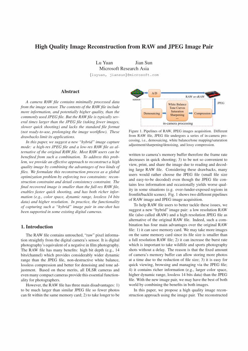
High Quality Image Reconstruction from RAW and JPEG Image Pair Lu Yuan Jian Sun Microsoft Research Asia {luyuan, jiansun}@microsoft.com Abstract A camera RAW file contains minimally processed data from the image sensor. The contents of the RAW file include more information, and potentially higher quality, than the commonly used JPEG file. But the RAW file is typically sev- eral times larger than the JPEG file (taking fewer images, slower quick shooting) and lacks the standard file format (not ready-to-use, prolonging the image workflow). These drawbacks limit its applications. In this paper, we suggest a new “hybrid” image capture mode: a high-res JPEG file and a low-res RAW file as al- ternative of the original RAW file. Most RAW users can be benefited from such a combination. To address this prob- lem, we provide an effective approach to reconstruct a high quality image by combining the advantages of two kinds of files. We formulate this reconstruction process as a global optimization problem by enforcing two constraints: recon- struction constraint and detail consistency constraint. The final recovered image is smaller than the full-res RAW file, enables faster quick shooting, and has both richer infor- mation (e.g., color space, dynamic range, lossless 14 bits data) and higher resolution. In practice, the functionality of capturing such a “hybrid” image pair in one-shot has been supported in some existing digital cameras. 1. Introduction The RAW file contains untouched, “raw” pixel informa- tion straightly from the digital camera’s sensor. It is digital photography’s equivalent of a negative in film photography. The RAW file has many benefits: high bit depth (e.g., 14 bits/channel) which provides considerably wider dynamic range than the JPEG file, non-destructive white balance, lossless compression and better for denoising and tone ad- justment. Based on these merits, all DLSR cameras and even many compact cameras provide this essential function- ality for photographers. However, the RAW file has three main disadvantages: 1) to be much larger than similar JPEG file so fewer photos can fit within the same memory card; 2) to take longer to be A/D Demosaicing sensor White Balance Tone Curves Saturation Sharpening … Compression RAW or sRAW JPEG in-camera processing Figure 1. Pipelines of RAW, JPEG images acquisition. Different from RAW file, JPEG file undergoes a series of in-camera pro- cessing, i.e., demosaicing, white balance/tone mapping/saturation adjustment/sharpening/denoising, and lossy compression. written to camera’s memory buffer therefore the frame rate decreases in quick shooting; 3) to be not so convenient to view, print, and share the image due to reading and decod- ing large RAW file. Considering these drawbacks, many users would rather choose the JPEG file (small file size and easy-to-be decoded) even though the JPEG file con- tains less information and occasionally yields worse qual- ity in some situations (e.g. over-/under-exposed regions in frontlit/backlit scenes). Fig. 1 shows two different pipelines of RAW image and JPEG image acquisition. To help RAW file users to better tackle these issues, we suggest a new “hybrid” image pair: a low resolution RAW file (also called sRAW) and a high resolution JPEG file as alternative of the original RAW file. Indeed, such a com- bination has four main advantages over the original RAW file: 1) it can save memory card. We may take more images on the same memory card since its file size is smaller than a full resolution RAW file; 2) it can increase the burst rate which is important to take wildlife and sports photography shots without a delay. The reason is that the fixed amount of camera’s memory buffer can allow storing more photos at a time due to the reduction of file size; 3) it is easy for quick viewing, browsing and managing via the JPEG file; 4) it contains richer information (e.g., larger color space, higher dynamic range, lossless 14 bits data) than the JPEG file. With the new image pair, we may have the best of both world by combining the benefits in both images. In this paper, we propose a high quality image recon- struction approach using the image pair. The reconstructed
-
Upload
khangminh22 -
Category
Documents
-
view
0 -
download
0
Transcript of High Quality Image Reconstruction from RAW and JPEG ...
High Quality Image Reconstruction from RAW and JPEG Image Pair
Lu Yuan Jian Sun
Microsoft Research Asia
luyuan, [email protected]
Abstract
A camera RAW file contains minimally processed data
from the image sensor. The contents of the RAW file include
more information, and potentially higher quality, than the
commonly used JPEG file. But the RAW file is typically sev-
eral times larger than the JPEG file (taking fewer images,
slower quick shooting) and lacks the standard file format
(not ready-to-use, prolonging the image workflow). These
drawbacks limit its applications.
In this paper, we suggest a new “hybrid” image capture
mode: a high-res JPEG file and a low-res RAW file as al-
ternative of the original RAW file. Most RAW users can be
benefited from such a combination. To address this prob-
lem, we provide an effective approach to reconstruct a high
quality image by combining the advantages of two kinds of
files. We formulate this reconstruction process as a global
optimization problem by enforcing two constraints: recon-
struction constraint and detail consistency constraint. The
final recovered image is smaller than the full-res RAW file,
enables faster quick shooting, and has both richer infor-
mation (e.g., color space, dynamic range, lossless 14 bits
data) and higher resolution. In practice, the functionality
of capturing such a “hybrid” image pair in one-shot has
been supported in some existing digital cameras.
1. Introduction
The RAW file contains untouched, “raw” pixel informa-
tion straightly from the digital camera’s sensor. It is digital
photography’s equivalent of a negative in film photography.
The RAW file has many benefits: high bit depth (e.g., 14
bits/channel) which provides considerably wider dynamic
range than the JPEG file, non-destructive white balance,
lossless compression and better for denoising and tone ad-
justment. Based on these merits, all DLSR cameras and
even many compact cameras provide this essential function-
ality for photographers.
However, the RAW file has three main disadvantages: 1)
to be much larger than similar JPEG file so fewer photos
can fit within the same memory card; 2) to take longer to be
A/D
Demosaicing
sensor
White Balance Tone Curves
Saturation Sharpening
…
Compression
RAW or sRAW
JPEG
in-camera processing
Figure 1. Pipelines of RAW, JPEG images acquisition. Different
from RAW file, JPEG file undergoes a series of in-camera pro-
cessing, i.e., demosaicing, white balance/tone mapping/saturation
adjustment/sharpening/denoising, and lossy compression.
written to camera’s memory buffer therefore the frame rate
decreases in quick shooting; 3) to be not so convenient to
view, print, and share the image due to reading and decod-
ing large RAW file. Considering these drawbacks, many
users would rather choose the JPEG file (small file size
and easy-to-be decoded) even though the JPEG file con-
tains less information and occasionally yields worse qual-
ity in some situations (e.g. over-/under-exposed regions in
frontlit/backlit scenes). Fig. 1 shows two different pipelines
of RAW image and JPEG image acquisition.
To help RAW file users to better tackle these issues, we
suggest a new “hybrid” image pair: a low resolution RAW
file (also called sRAW) and a high resolution JPEG file as
alternative of the original RAW file. Indeed, such a com-
bination has four main advantages over the original RAW
file: 1) it can save memory card. We may take more images
on the same memory card since its file size is smaller than
a full resolution RAW file; 2) it can increase the burst rate
which is important to take wildlife and sports photography
shots without a delay. The reason is that the fixed amount
of camera’s memory buffer can allow storing more photos
at a time due to the reduction of file size; 3) it is easy for
quick viewing, browsing and managing via the JPEG file;
4) it contains richer information (e.g., larger color space,
higher dynamic range, lossless 14 bits data) than the JPEG
file. With the new image pair, we may have the best of both
world by combining the benefits in both images.
In this paper, we propose a high quality image recon-
struction approach using the image pair. The reconstructed

low-res RAW
detail constraint
R l
high-res JPEG J h
16-bit TIFF
R h reconstruction constraint
final result
16-bit mapped image R
~ h
RAW convertor
locally tone mapping
optimization
Figure 2. System overview.
image has higher spatial resolution than the input RAW im-
age and wider dynamic range than the input JPEG image.
Specifically, we formulate this reconstruction problem as
a guided image super-resolution problem: we increase the
spatial resolution of the RAW image under the guidance of
the high resolution JPEG image. We exploit two kinds of
constraints: reconstruction constraint and detail consistency
constraint. The former constraint requires the downsampled
version of the reconstructed image should approach the in-
put low resolution RAW image. The latter constraint en-
forces the consistence between the recovered image and the
input JPEG image at the detail layer. The final image is ob-
tained by minimizing a quadratic function which enforces
two constraints.
The camera manufactures also noticed the problem in the
original RAW file and added a new functionality in recent
DSLR cameras like Canon’s 7D, 5D mark II, and 1Ds Mark
III: the user can simultaneously capture a RAW file and a
JEPG file with different resolution. These two images are
exactly from the same sensor but with different downsam-
pling and processing. Since the “hybrid” images can be cap-
tured by one-shot in camera, our image acquisition is quite
practical to help any photographers - no special require-
ments on device, no limitations on the capturing method,
and no restrictions on scene.
2. Related Work
Two categories of work are most related to ours: im-
age super-resolution and inverse tone mapping. Single
image super-resolution is an extensively studied problem.
Representative work include interpolation-based methods
(e.g. [11, 26]), edge-based methods (e.g. [2, 6, 24]), and
example-based methods (e.g. [8, 9, 16, 25]). These single
image super-resolution methods mainly sharpen the image
edges and enhance the details. Only limited amount of high
frequency structures or details can be “invented”. Multi-
frame super-resolution methods (e.g. [4, 5, 12]) use a set of
low-resolution images from the same scene to recover the
lost high frequency details. These approaches require ac-
curate image registration at the sub-pixel level and are nu-
merically limited only to small increases in resolution [15].
To reduce color aberration in single image super-resolution,
the work [17] performs color assignment in chroma chan-
nels guided by the super-resolution luminance channel.
Another related work “inverse tone mapping” aims to ex-
pand dynamic range of the input image. Many work are pro-
posed to tackle this ill-posed problem (e.g. [7, 22, 27]) and
some representative techniques are evaluated in [18]. Most
of existing inverse tone mapping algorithms (e.g. [22]) ad-
just the global tone response curve. However, the results by
global mapping may have amplified quantization artifacts
and incorrect local colors. In [23], a locally linear oper-
ator is proposed to Hdr2Ldr mapping, which can outper-
form global operators. In our work, we want to perform
“inverse” tone mapping on the JPEG image. In some situa-
tions, a global operator or even a local linear operator is not
very suitable for our problem. We further propose a locally
piecewise-linear tone mapping for better quality.
Recently, several challenging vision problems were at-
tacked by using multiple images of the same scene, such as
HDR imaging (e.g. [3, 19]), denoising [14, 20], and deblur-
ring [29] using blurred/noisy image pair. In this paper, we
use the low-res RAW image and high-res JPEG image pair
to solve a reconstruction problem for both spatial resolution
and dynamic range. Usually, these techniques require more
than one shot, which may largely reduce their applicability,
especially for dynamic scenes.
3. Framework Overview
The pipeline of our approach is summarized in Fig. 2.
Given a low-res RAW 1 Rl and a high-res JPEG Jh, the
reconstruction of the high-res RAW Rh can be formulated
by minimizing the following objective function:
Rh∗ = argminRh
E(Rh;Rl, Jh)
= argminRhEr(R
h;Rl) + λEd(Rh;Rl, Jh).(1)
The first term Er(Rh;Rl) enforces the reconstruction con-
straint. Similar to previous super-resolution work, the re-
construction constraint enforces that the down-sampled ver-
sion of high-res RAW should be close to the input low-res
1In principle, we should use the true RAW file in the processing. How-
ever, it is difficult to access original RAW data without the specified RAW
codec since both RAW file format and in-camera demosaicing algorithm
are secret in various types of camera. To make a general solution to all
camera, we consider a 16-bit/channel TIFF image (TIFF is known as a
standard file format) generated from RAW convertor (the conversion pro-
cess ensures no information loss) as our “RAW image” in this paper.
RAW. The second term Ed(Rh;Rl, Jh) enforces the detail
consistency constraint. It means that the local structures of
high-res RAW should be consistent with those of high-res
JPEG. Since the input JPEG and RAW have different color
ranges, we cannot directly copy the high-res JPEG details
to the low-res RAW. Instead, we need firstly to “inversely”
map JPEG values from a narrow color range to a wide color
range. To achieve a better inverse tone mapping, we pro-
pose a locally piecewise linear mapping operator. Then we
extract the detail layer from the mapped image and integrate
it to our objective function. In the next section, we will first
describe how to obtain high-res details from JPEG.
4. High-resolution Details Reconstruction
Detail reconstruction includes: infer local tone mapping
models from a low-res RAW and a downscaled JPEG, up-
sample coefficients to map the high-res JPEG to a high-bit
color space, and extract details from the mapped image.
4.1. Locally Piecewise Linear Tone Mapping
Since the JPEG file may undergo complicated non-linear
and non-local in-camera processing (shown in Fig. 1), a
global tone mapping curve or a locally linear curve are of-
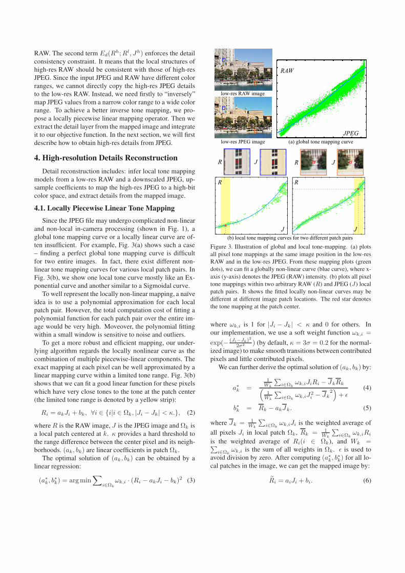
ten insufficient. For example, Fig. 3(a) shows such a case
– finding a perfect global tone mapping curve is difficult
for two entire images. In fact, there exist different non-
linear tone mapping curves for various local patch pairs. In
Fig. 3(b), we show one local tone curve mostly like an Ex-
ponential curve and another similar to a Sigmoidal curve.
To well represent the locally non-linear mapping, a naıve
idea is to use a polynomial approximation for each local
patch pair. However, the total computation cost of fitting a
polynomial function for each patch pair over the entire im-
age would be very high. Moveover, the polynomial fitting
within a small window is sensitive to noise and outliers.
To get a more robust and efficient mapping, our under-
lying algorithm regards the locally nonlinear curve as the
combination of multiple piecewise-linear components. The
exact mapping at each pixel can be well approximated by a
linear mapping curve within a limited tone range. Fig. 3(b)
shows that we can fit a good linear function for these pixels
which have very close tones to the tone at the patch center
(the limited tone range is denoted by a yellow strip):
Ri = akJi + bk, ∀i ∈ i|i ∈ Ωk, |Ji − Jk| < κ., (2)
where R is the RAW image, J is the JPEG image and Ωk is
a local patch centered at k. κ provides a hard threshold to
the range difference between the center pixel and its neigh-
borhoods. (ak, bk) are linear coefficients in patch Ωk.
The optimal solution of (ak, bk) can be obtained by a
linear regression:
(a∗k, b∗k) = argmin
∑i∈Ωk
ωk,i · (Ri − akJi − bk)2 (3)
R J
low-res RAW image
R J
low-res JPEG image
R R
RAW
JJ
JPEG
(b) local tone mapping curves for two different patch pairs
(a) global tone mapping curve
Figure 3. Illustration of global and local tone-mapping. (a) plots
all pixel tone mappings at the same image position in the low-res
RAW and in the low-res JPEG. From these mapping plots (green
dots), we can fit a globally non-linear curve (blue curve), where x-
axis (y-axis) denotes the JPEG (RAW) intensity. (b) plots all pixel
tone mappings within two arbitrary RAW (R) and JPEG (J) local
patch pairs. It shows the fitted locally non-linear curves may be
different at different image patch locations. The red star denotes
the tone mapping at the patch center.
where ωk,i is 1 for |Ji − Jk| < κ and 0 for others. In
our implementation, we use a soft weight function ωk,i =
exp(− (Ji−Jk)2
2σ2 ) (by default, κ = 3σ = 0.2 for the normal-
ized image) to make smooth transitions between contributed
pixels and little contributed pixels.
We can further derive the optimal solution of (ak, bk) by:
a∗k =1
Wk
∑i∈Ωk
ωk,iJiRi − JkRk(1
Wk
∑i∈Ωk
ωk,iJ2i − Jk
2)+ ǫ
(4)
b∗k = Rk − akJk. (5)
where Jk = 1Wk
∑i∈Ωk
ωk,iJi is the weighted average of
all pixels Ji in local patch Ωk, Rk = 1Wk
∑i∈Ωk
ωk,iRi
is the weighted average of Ri(i ∈ Ωk), and Wk =∑i∈Ωk
ωk,i is the sum of all weights in Ωk. ǫ is used to
avoid division by zero. After computing (a∗k, b∗k) for all lo-
cal patches in the image, we can get the mapped image by:
Ri = aiJi + bi. (6)
(a) (b)
(c) (d)
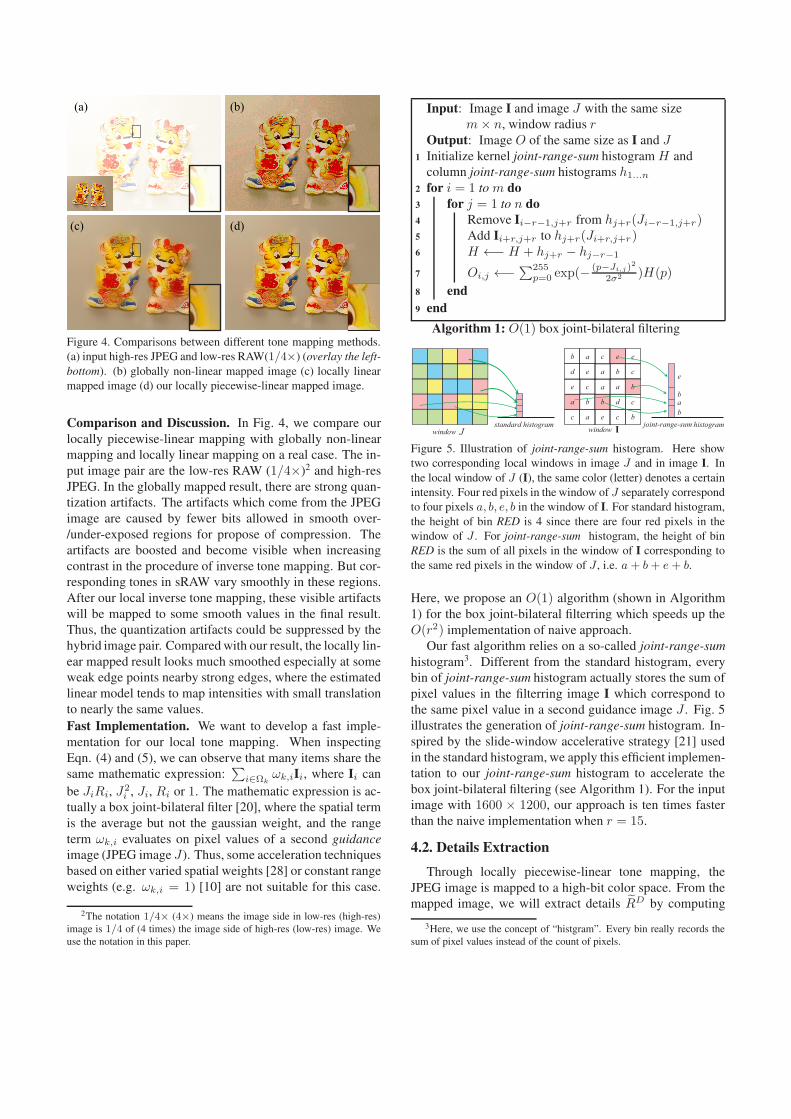
Figure 4. Comparisons between different tone mapping methods.
(a) input high-res JPEG and low-res RAW(1/4×) (overlay the left-
bottom). (b) globally non-linear mapped image (c) locally linear
mapped image (d) our locally piecewise-linear mapped image.
Comparison and Discussion. In Fig. 4, we compare our
locally piecewise-linear mapping with globally non-linear
mapping and locally linear mapping on a real case. The in-
put image pair are the low-res RAW (1/4×)2 and high-res
JPEG. In the globally mapped result, there are strong quan-
tization artifacts. The artifacts which come from the JPEG
image are caused by fewer bits allowed in smooth over-
/under-exposed regions for propose of compression. The
artifacts are boosted and become visible when increasing
contrast in the procedure of inverse tone mapping. But cor-
responding tones in sRAW vary smoothly in these regions.
After our local inverse tone mapping, these visible artifacts
will be mapped to some smooth values in the final result.
Thus, the quantization artifacts could be suppressed by the
hybrid image pair. Compared with our result, the locally lin-
ear mapped result looks much smoothed especially at some
weak edge points nearby strong edges, where the estimated
linear model tends to map intensities with small translation
to nearly the same values.
Fast Implementation. We want to develop a fast imple-
mentation for our local tone mapping. When inspecting
Eqn. (4) and (5), we can observe that many items share the
same mathematic expression:∑
i∈Ωkωk,iIi, where Ii can
be JiRi, J2i , Ji, Ri or 1. The mathematic expression is ac-
tually a box joint-bilateral filter [20], where the spatial term
is the average but not the gaussian weight, and the range
term ωk,i evaluates on pixel values of a second guidance
image (JPEG image J). Thus, some acceleration techniques
based on either varied spatial weights [28] or constant range
weights (e.g. ωk,i = 1) [10] are not suitable for this case.
2The notation 1/4× (4×) means the image side in low-res (high-res)
image is 1/4 of (4 times) the image side of high-res (low-res) image. We
use the notation in this paper.
Input: Image I and image J with the same size
m× n, window radius rOutput: Image O of the same size as I and J
1 Initialize kernel joint-range-sum histogram H and
column joint-range-sum histograms h1...n
2 for i = 1 to m do
3 for j = 1 to n do
4 Remove Ii−r−1,j+r from hj+r(Ji−r−1,j+r)5 Add Ii+r,j+r to hj+r(Ji+r,j+r)6 H ←− H + hj+r − hj−r−1
7 Oi,j ←−∑255
p=0 exp(−(p−Ji,j)
2
2σ2 )H(p)
8 end
9 end
Algorithm 1: O(1) box joint-bilateral filtering
b a c e e
d e a b c
e c a a b
a b b d c
c a e c b
e
b
ba
window Jstandard histogram joint-range-sum histogram
window I
Figure 5. Illustration of joint-range-sum histogram. Here show
two corresponding local windows in image J and in image I. In
the local window of J (I), the same color (letter) denotes a certain
intensity. Four red pixels in the window of J separately correspond
to four pixels a, b, e, b in the window of I. For standard histogram,
the height of bin RED is 4 since there are four red pixels in the
window of J . For joint-range-sum histogram, the height of bin
RED is the sum of all pixels in the window of I corresponding to
the same red pixels in the window of J , i.e. a+ b+ e+ b.
Here, we propose an O(1) algorithm (shown in Algorithm
1) for the box joint-bilateral filterring which speeds up the
O(r2) implementation of naive approach.
Our fast algorithm relies on a so-called joint-range-sum
histogram3. Different from the standard histogram, every
bin of joint-range-sum histogram actually stores the sum of
pixel values in the filterring image I which correspond to
the same pixel value in a second guidance image J . Fig. 5
illustrates the generation of joint-range-sum histogram. In-
spired by the slide-window accelerative strategy [21] used
in the standard histogram, we apply this efficient implemen-
tation to our joint-range-sum histogram to accelerate the
box joint-bilateral filtering (see Algorithm 1). For the input
image with 1600 × 1200, our approach is ten times faster
than the naive implementation when r = 15.
4.2. Details Extraction
Through locally piecewise-linear tone mapping, the
JPEG image is mapped to a high-bit color space. From the
mapped image, we will extract details RD by computing
3Here, we use the concept of “histgram”. Every bin really records the
sum of pixel values instead of the count of pixels.
the ratio between a high-res radiance map Rh and a low-res
radiance map Rl: RD = Rh
Rl↑+ǫ, where ǫ = 0.01 is used to
avoid division by zero, and ↑ is an upsampling operator.
The low-res radiance map Rl can be estimated by the in-
put low-res RAW image and the scaled JPEG image, which
is achieved by scaling the input JPEG image down to the
same resolution of the input RAW image. For these image
pair, we first estimate the locally piecewise-linear coeffi-
cients at each pixel using Eqn. 4 and 5. Then the radiance
map Rl is obtained by locally linear mapping the scaled
JPEG image pixel-by-pixel using Eqn. 6.
If we have the inferred mapping coefficients with the
same resolution to the input JPEG image, the high-res ra-
diance map Rh can be estimated by simply mapping the
high-res JPEG image pixel-by-pixel via Eqn. 6. But now,
we can only estimate the exact mapping coefficients from
the low-res RAW and the scaled JPEG image. We need to
up-sample the inferred coefficients for mapping. To achieve
a high quality up-scaled coefficients, we use joint-bilateral
upsampling [13] under the guidance of the input high-res
JPEG image. Here, we can efficiently compute the guided
upsampling by the accelerated box joint-bilateral filtering
(see Algorithm 1).
5. Image Reconstruction using Image Pair
The reconstruction constraint in Eqn. 1 measures the dif-
ference between the input low-res RAW image Rl and the
down-scaled version of high-res RAW image Rh:
Er
(Rh;Rl
)=
∥∥Rl −(Rh ⊗ G
)↓∥∥2 (7)
where⊗ is the convolution operator and G is a gaussian fil-
ter. Here, we assume the blurring process in down-scaling
of JPEG and RAW images is the same, thus G can be in-
ferred by argminG
∥∥J l − (Jh ⊗G) ↓∥∥2.
The detail consistency constraint in Eqn. 1 requires that
details of the final image Rh should be close to those of the
mapped image Rh, i.e. RD = [RD]β , where RD = Rh
Rl↑+ǫ.
β controls the extent of detail strength (by default, β = 1.6).
Larger β will make the final image look much sharper.
Then, the detail consistency constraint can be expressed as:
Ed
(Rh;Rl, Jh
)=
∥∥∥Rh −Rl ↑ ×(RD)β∥∥∥2
(8)
Since the objective function (in Eqn. 1) is a quadratic
form, we can obtain the global minimum by solving a linear
system. The solution can be further efficiently computed
using the following FFT-based implementation:
F(Rh)∗ = argminRh∥∥F(Rl ↑)−F(Rh)⊙F(G))
∥∥2+
λ∥∥∥F(Rh)−F(Rl ↑)⊙F
((RD)
β)∥∥∥
2
(j) (k)(e) (f) (g) (h) (i)
(a) (b)
(c) (d)
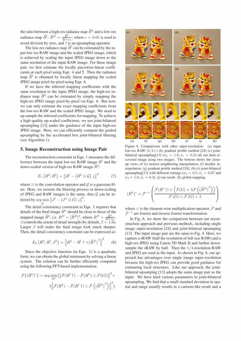
Figure 6. Comparisons with other super-resolution. (a) input
low-res RAW (1/4×) (b) gradient profile method [24] (c) joint-
bilateral upsampling[13] (σd = 1.0, σs = 0.2) (d) our final re-
covered image using two images. The bottom shows the close-
up views of (e) nearest neighboring interpolation, (f) bicubic in-
terpolation, (g) gradient profile method [24], (h)-(i) joint-bilateral
upsampling[13] with different settings (σd = 0.5, σs = 0.07 and
σd = 1.0, σs = 0.2), (j) our result. (k) global mapping.
(Rh)∗ = F−1
F(Rl ↑)⊙
(F(G) + λF
((RD)
β))
F (G)⊙ F (G) + λ
where⊙ is the element-wise multiplication operator,F and
F−1 are fourier and inverse fourier transformation.
In Fig. 6, we show the comparison between our recon-
struction approach and previous methods, including single
image super-resolution [24] and joint-bilateral upsamping
[13]. The input image pair are the same to Fig. 4. Here, we
capture a sRAW (half the resolution of full size RAW) and a
high-res JPEG using Canon 5D Mark II and further down-
sample the sRAW by half. Then the 1/4-resolution RAW
and JPEG are used as the input. As shown in Fig. 6, our ap-
proach has advantages over single image super-resolution
because the high-res JPEG can provide good guidance for
estimating local structures. Like our approach, the joint-
bilateral upsamping [13] adopts the same image pair as the
input. We have tried various parameters in joint-bilateral
upsampling. We find that a small standard deviation in spa-
tial and range usually results in a cartoon-like result and a
(a) (b)
(c) (d)
(e)
(f)
(g)
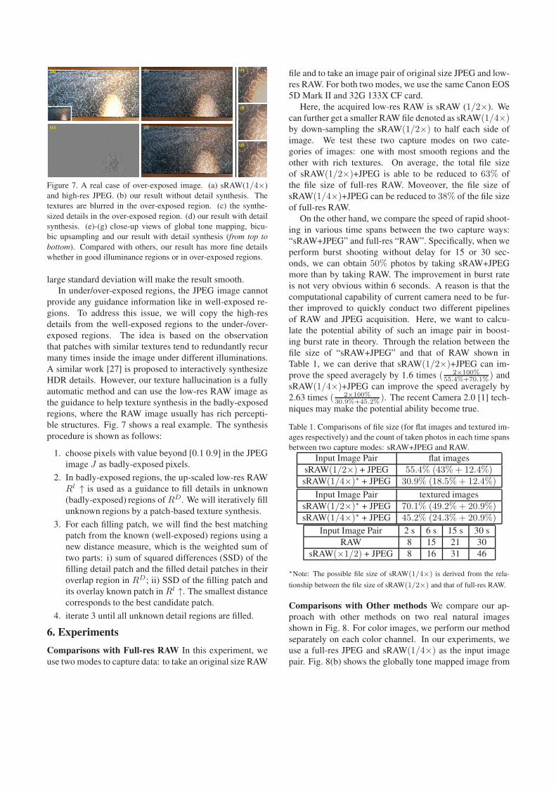
Figure 7. A real case of over-exposed image. (a) sRAW(1/4×)
and high-res JPEG. (b) our result without detail synthesis. The
textures are blurred in the over-exposed region. (c) the synthe-
sized details in the over-exposed region. (d) our result with detail
synthesis. (e)-(g) close-up views of global tone mapping, bicu-
bic upsampling and our result with detail synthesis (from top to
bottom). Compared with others, our result has more fine details
whether in good illuminance regions or in over-exposed regions.
large standard deviation will make the result smooth.
In under/over-exposed regions, the JPEG image cannot
provide any guidance information like in well-exposed re-
gions. To address this issue, we will copy the high-res
details from the well-exposed regions to the under-/over-
exposed regions. The idea is based on the observation
that patches with similar textures tend to redundantly recur
many times inside the image under different illuminations.
A similar work [27] is proposed to interactively synthesize
HDR details. However, our texture hallucination is a fully
automatic method and can use the low-res RAW image as
the guidance to help texture synthesis in the badly-exposed
regions, where the RAW image usually has rich percepti-
ble structures. Fig. 7 shows a real example. The synthesis
procedure is shown as follows:
1. choose pixels with value beyond [0.1 0.9] in the JPEG
image J as badly-exposed pixels.
2. In badly-exposed regions, the up-scaled low-res RAW
Rl ↑ is used as a guidance to fill details in unknown
(badly-exposed) regions of RD. We will iteratively fill
unknown regions by a patch-based texture synthesis.
3. For each filling patch, we will find the best matching
patch from the known (well-exposed) regions using a
new distance measure, which is the weighted sum of
two parts: i) sum of squared differences (SSD) of the
filling detail patch and the filled detail patches in their
overlap region in RD; ii) SSD of the filling patch and
its overlay known patch in Rl ↑. The smallest distance
corresponds to the best candidate patch.
4. iterate 3 until all unknown detail regions are filled.
6. Experiments
Comparisons with Full-res RAW In this experiment, we
use two modes to capture data: to take an original size RAW
file and to take an image pair of original size JPEG and low-
res RAW. For both two modes, we use the same Canon EOS
5D Mark II and 32G 133X CF card.
Here, the acquired low-res RAW is sRAW (1/2×). We
can further get a smaller RAW file denoted as sRAW(1/4×)by down-sampling the sRAW(1/2×) to half each side of
image. We test these two capture modes on two cate-
gories of images: one with most smooth regions and the
other with rich textures. On average, the total file size
of sRAW(1/2×)+JPEG is able to be reduced to 63% of
the file size of full-res RAW. Moveover, the file size of
sRAW(1/4×)+JPEG can be reduced to 38% of the file size
of full-res RAW.
On the other hand, we compare the speed of rapid shoot-
ing in various time spans between the two capture ways:
“sRAW+JPEG” and full-res “RAW”. Specifically, when we
perform burst shooting without delay for 15 or 30 sec-
onds, we can obtain 50% photos by taking sRAW+JPEG
more than by taking RAW. The improvement in burst rate
is not very obvious within 6 seconds. A reason is that the
computational capability of current camera need to be fur-
ther improved to quickly conduct two different pipelines
of RAW and JPEG acquisition. Here, we want to calcu-
late the potential ability of such an image pair in boost-
ing burst rate in theory. Through the relation between the
file size of “sRAW+JPEG” and that of RAW shown in
Table 1, we can derive that sRAW(1/2×)+JPEG can im-
prove the speed averagely by 1.6 times ( 2×100%55.4%+70.1%) and
sRAW(1/4×)+JPEG can improve the speed averagely by
2.63 times ( 2×100%30.9%+45.2%). The recent Camera 2.0 [1] tech-
niques may make the potential ability become true.
Table 1. Comparisons of file size (for flat images and textured im-
ages respectively) and the count of taken photos in each time spans
between two capture modes: sRAW+JPEG and RAW.
Input Image Pair flat images
sRAW(1/2×) + JPEG 55.4% (43%+ 12.4%)sRAW(1/4×)∗ + JPEG 30.9% (18.5%+ 12.4%)
Input Image Pair textured images
sRAW(1/2×)∗ + JPEG 70.1% (49.2%+ 20.9%)sRAW(1/4×)∗ + JPEG 45.2% (24.3%+ 20.9%)
Input Image Pair 2 s 6 s 15 s 30 s
RAW 8 15 21 30
sRAW(×1/2) + JPEG 8 16 31 46
∗Note: The possible file size of sRAW(1/4×) is derived from the rela-
tionship between the file size of sRAW(1/2×) and that of full-res RAW.
Comparisons with Other methods We compare our ap-
proach with other methods on two real natural images
shown in Fig. 8. For color images, we perform our method
separately on each color channel. In our experiments, we
use a full-res JPEG and sRAW(1/4×) as the input image
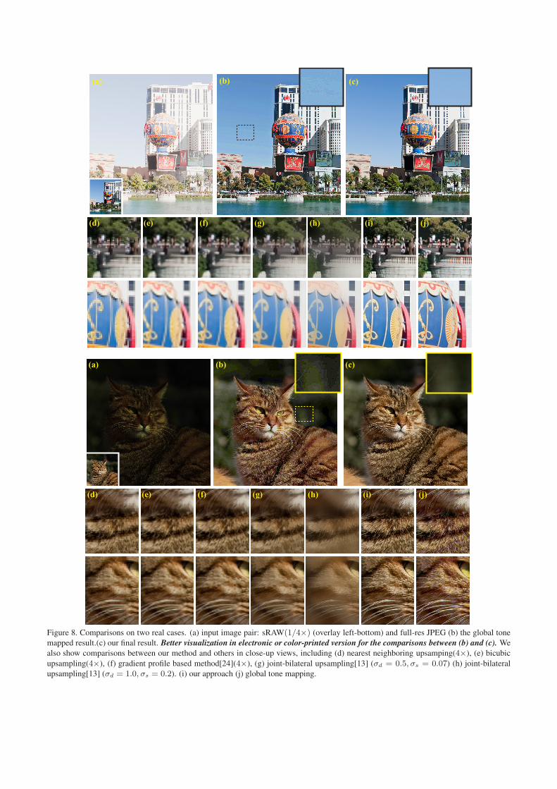
pair. Fig. 8(b) shows the globally tone mapped image from
the input JPEG image. The mapped result looks not so good
as ours especially on the smooth regions, where we can no-
tice many quantization artifacts. We further show the com-
parison in close-up views (overlay top-right patches).
We also compare our approach with other image super-
resolution methods, including nearest neighboring upscal-
ing, bicubic upscaling, gradient-profile based method[24],
and joint-bilateral upsampling[13]. Using an image pair,
our approach is able to recover many high-res details that
can not be seen in single image super-resolution results, for
instance, the fur of cat in Fig. 8. Similar to our approach,
joint-bilateral upsampling[13] can also use a high-res image
as a guidance map to help interpolation. But we tried the
best parameters and cannot achieve comparable results to
ours. The joint-bilateral upsampling result is either cartoon-
like (in Fig. 8(g)) or smoothed (in Fig. 8(h)). We further
show more comparisons, quantitative evaluation in the Sup-
plementary materials. Our approachs take advantage over
other methods in PSNR (41.4 dB vs 24.8 dB against global
tone mapping, 41.4 dB vs 27.8 dB against joint-bilateral up-
sampling). However, a limitation may occur when there are
too large areas saturated in the JPEG image and no similar
visible structures used to synthesize those missing details.
7. Conclusions
In this paper, we have presented a high-quality image re-
construction approach using a RAW and JPEG image pair.
The reconstruction is formulated by enforcing two con-
straints from the input pair. Our solution is practical and
applicable to the existing commercial digital SLR cameras.
Acknowledgments We thank the anonymous reviewers for
helping us to improve this paper, and appreciate Yin Li for
his help in discussion.
References
[1] A. Adams, E.-V. E. Talvala, S. H. Park, D. E. Jacobs,
B. Ajdin, N. Gelfand, J. Dolson, D. Vaquero, J. Baek,
M. Tico, H. P. Lensch, W. Matusik, K. Pulli, M. Horowitz,
and M. Levoy. The frankencamera: An experimental plat-
form for computational photography. Proc. of SIGGRAPH,
29:1–12, 2010.
[2] S. Y. Dai, M. Han, W. Xu, Y.Wu, and Y. H. Gong. Soft
edge smoothness prior for alpha channel super resolution. In
CVPR, 2007.
[3] P. E. Debevec and J. Malik. Recovering high dynamic range
radiance maps from photographs. In SIGGRAPH, 1997.
[4] M. Elad and A. Feuer. Super-resolution reconstruction of
image sequences. IEEE Trans. on PAMI, v.21 n.9:817–834,
1999.
[5] S. Farsiu, D. Robinson, M. Elad, and P. Milanfar. Fast and
robust multi-frame super-resolution. IEEE Trans. on Image
Processing, 13:1327–1344, 2003.
[6] R. Fattal. Image upsampling via imposed edge statistics.
ACM Trans. on Graphics, 26(3):95:1–8, 2007.
[7] B. Francesco, L. Patrick, D. Kurt, and C. Alan. Inverse tone
mapping. In GRAPHITE, 2006.
[8] W. T. Freeman, E. Pasztor, and O. Carmichael. Learning
low-level vision. IJCV, 40(1):25–47, 2000.
[9] D. Glasner, S. Bagon, and M. Irani. Super-resolution from a
single image. In ICCV, 2009.
[10] K. He, J. Sun, and X. Tang. Guided image filtering. In ECCV,
2010.
[11] H. S. Hou and H. C. Andrews. Cubic splines for image inter-
polation and digital filtering. IEEE Trans. on SP, 26(6):508–
517, 1978.
[12] M. Irani and S. Peleg. Improving resolution by image regis-
tration. In CVGIP: Graphical Models and Image Processing,
1991.
[13] J. Kopf, M. Cohen, D. Lischinski, and M. Uyttendaele. Joint
bilateral upsampling. SIGGRAPH, 26(3), 2007.
[14] D. Krishnan and R. Fergus. Dark flash photography. ACM
Trans. on Graphics, 28:1–8, 2009.
[15] Z. C. Lin and H. Y. Shum. Fundamental limits of
reconstruction-based super-resolution algorithms under local
translation. IEEE Trans. on PAMI, 26(1):83–97, 2004.
[16] C. Liu, H. Y. Shum, and W. T. Freeman. Face hallucination:
Theory and practice. International Journal of Computer Vi-
sion, 75(1):115–134, 2007.
[17] S. Liu, M. S. Brown, S. J. Kim, and Y.-W. Tai. Colorization
for single image super resolution. In ECCV, 2010.
[18] B. Masia, S. Agustin, R. Fleming, O. Sorkine, and D. Gutier-
rez. Evaluation of reverse tone mapping through varying ex-
posure conditions. ACM Trans. on Graphics, 28:160, 2009.
[19] T. Mertens, J. Kautz, and F. V. Reeth. Exposure fusion. In
PCCGA, 2007.
[20] G. Petschnigg, R. Szeliski, M. Agrawala, M. Cohen,
H. Hoppe, and K. Toyama. Digital photography with flash
and no-flash image pairs. ACM Trans. on Graphics, 23:664–
672, 2004.
[21] F. Porikli. Constant time o(1) bilateral filtering. In CVPR,
2008.
[22] A. Rempel, M. Trentacoste, H. Seetzen, H. Young, W. Hei-
drich, L. Whitehead, and G. Ward. Ldr2hdr: On-the-fly re-
verse tone mapping of legacy video and photographs. Proc.
ACM SIGGRAPH, page 39, 2007.
[23] Q. Shan, J. Jia, and M. S. Brown. Globally optimized linear
windowed tone-mapping. IEEE TVCG, 2009.
[24] J. Sun, J. Sun, Z. Xu, and H. Y. Shum. Image super-
resolution using gradient profile prior. In CVPR, 2008.
[25] J. Sun, N. N. Zheng, H. Tao, and H. Y. Shum. Image hallu-
cination with primal sketch priors. In CVPR, 2003.
[26] P. Thevenaz, T. Blu, and M. Unser. Image Interpolation and
Resampling. Academic Press, San Diego, USA, 2000.
[27] L. Wang, L.-Y. Wei, K. Zhou, B. Guo, and H.-Y. Shum. High
dynamic range image hallucination. In Eurographics Sympo-
sium on Rendering, 2007.
[28] W. Wells. Efficient synthesis of gaussian filters by cascaded
uniform filters. IEEE Trans. on PAMI, 8:234–239, 1986.
[29] L. Yuan, J. Sun, L. Quan, and H.-Y. Shum. Image deblurring
with blurred/noisy image pairs. ACM Trans. on Graphics,
26:1–10, 2007.
(a) (b) (c)
(d) (e) (f) (g) (h) (i) (j)
(a) (b) (c)
(d) (e) (f) (g) (h) (i) (j)
Figure 8. Comparisons on two real cases. (a) input image pair: sRAW(1/4×) (overlay left-bottom) and full-res JPEG (b) the global tone
mapped result.(c) our final result. Better visualization in electronic or color-printed version for the comparisons between (b) and (c). We
also show comparisons between our method and others in close-up views, including (d) nearest neighboring upsamping(4×), (e) bicubic
upsampling(4×), (f) gradient profile based method[24](4×), (g) joint-bilateral upsampling[13] (σd = 0.5, σs = 0.07) (h) joint-bilateral
upsampling[13] (σd = 1.0, σs = 0.2). (i) our approach (j) global tone mapping.