Statistical detection of JPEG traces in digital images in ...

IEEE TRANSACTIONS ON INFORMATION FORENSICS AND SECURITY, VOL. XX, NO. XX, XXX XXXX 1

Statistical detection of JPEG tracesin digital images in uncompressed formatsCecilia Pasquini, Giulia Boato, Member, IEEE, and Fernando Perez-Gonzalez, Fellow, IEEE

Abstract—Intrinsic statistical properties of natural uncom-pressed images are used in image forensics for detecting tracesof previous processing operations. In this paper, we proposenovel forensic detectors of JPEG compression traces in imagesstored in uncompressed formats, based on a theoretical analysisof Benford–Fourier coefficients computed on the 8×8 block-DCTdomain. In fact, the distribution of such coefficients is derivedtheoretically both under the hypotheses of no compression andprevious compression with a certain quality factor, allowing forthe computation of the respective likelihood functions. Then, twoclassification tests based on different statistics are proposed, bothrelying on a discriminative threshold that can be determinedwithout the need of any training phase. The statistical analysisis based on the only assumptions of Generalized Gaussiandistribution of DCT coefficients and independence among DCTfrequencies, thus resulting in robust detectors applying to anyuncompressed image. In fact, experiments on different datasetsshow that the proposed models are suitable for images of differentsizes and source cameras, thus overcoming dataset-dependencyissues that typically affect state-of-art techniques.

Index Terms—Benford–Fourier coefficients, Benford’s law, im-age forensics, JPEG compression.

I. INTRODUCTION

IN the last decade, the field of digital image forensics hasundergone a constant expansion, drawing a growing atten-

tion of the research community. In fact, the increasing need ofauthentication techniques for digital images without a prioriinformation (like the presence of a watermark) has broughtresearchers to develop a number of forensic approaches de-signed to work passively and facing different forensic issues,like forgery detection, source identification, and computergenerated versus natural content discrimination [1] [2] [3].One of the most widely investigated problems is the detectionof previous operations and the estimation of the processinghistory, which might reveal the non-pristine condition of thesubject image and allow for the localization of forged areas.Given the wide variety of potential processing operations andthe corresponding statistical traces, a high number of forensictechniques have been designed, often tailored to specific tracesand experimental settings. Several valuable solutions have

C. Pasquini was with the Department of Information Engineering andComputer Science, University of Trento, Trento 38123, Italy. She is now withthe Institute fur Informatik, Universitat Innsbruck, Innsbruck 6020, Austria,and also with the Department of Information Systems, University of Munster,Munster 48149, Germany (e-mail: [email protected]).

G. Boato is with the Department of Information Engineering and Com-puter Science, University of Trento, Trento 38123, Italy (e-mail: [email protected]).

F. Perez-Gonzalez is with the Department of Signal Theory and Communi-cations, University of Vigo, Vigo 36310, Spain (e-mail: [email protected]).

Manuscript received xxx xx, xxxx; revised xxx xx, xxxx.

been proposed for different forensic problems, yielding goodperformance both in synthetic and more realistic forensicscenarios. However, a common issue to many methods is thefact that a solid theoretic framework describing the statisticalbehavior of the quantities involved is not available. Thus,although they achieve excellent results in certain experimentalsettings, the absence of a generalized model might result innon-controllable performance when the test setting is modifiedsince the parameters of the methods change as well. Thisgenerally happens, for instance, when a certain approachimplies the need of machine learning techniques: althoughthey represent extremely useful tools, they usually requireextensive training phases and suffer from typical automaticlearning issues (as overfitting or dataset-dependency), whichmight have a strong impact on the applicability of multimediaforensic techniques in different settings. This is especiallytrue when data depicting sensitive content are analyzed andforensic analysis reliability is an essential requirement, as itcommonly happens in real-world cases [4] and even more sowhen they involve courts of law.

In this paper, we tackle from a theoretical perspective theproblem of detecting the traces of a previous JPEG com-pression in images that are stored in uncompressed formats.Such issue appears when the forensic analysis is performedon images supposedly taken by a device set to provideuncompressed images (like professional or semi-professionalcameras) or, in general, in every situation where the subjectimage is supposed to be never compressed, and the presenceof JPEG compression traces would suggest that the image hasbeen taken from a different camera or it has been alreadyprocessed by someone. Indeed, although the JPEG standardrepresents the most used format for digital images, the needfor analyzing uncompressed formats arises, for instance, whenprofessional photographic images are involved, for which it isgetting a common practice to provide the original raw imageand employ it in the forensic analysis [5].

In this framework, the proposed method relies on thetheoretical analysis of the Benford–Fourier (BF) coefficients[6] computed from the DCT coefficients of the image, forwhich a statistical model is derived both under the hypothesesof no previous compression (i.e., the image is pristine) andprevious compression with a certain quantization table (i.e., theimage has been JPEG compressed). This allows us to definea hypothesis testing framework where the null hypothesisis the pristine condition of the image, and the alternativehypothesis is represented by a previous compression. Thework [7] contains a preliminary and partial version of themethodology, which is here extended to the case multiple


DCT frequencies and encompasses also a novel model for thealternative hypotheses. This results in two novel tests based ondifferent statistical schemes, namely the λ-test and the logL0-test, with the aim of discriminating images that have neverbeen compressed from images previously compressed.

An interesting peculiarity of the proposed methods is thatthe statistical description of the BF coefficients, derived ana-lytically, explicitly depends on the number of DCT coefficientsconsidered, i.e., it is related to the size of the subject image.Moreover, all the statistical parameters involved in the modelare estimated directly from the data without relying on anypredetermined dataset. This results in two size-adaptive JPEGcompression detectors, which do not require any trainingphase. Experimental results on several datasets and JPEGcompression parameters show the benefits of this approachwith respect to state-of-the-art methods.The paper is structured as follows: in Section II, the literatureon the detection of JPEG traces in uncompressed formatimages is revisited; the BF coefficients are introduced inSection III; the novel statistical analysis of such coefficients ispresented in Section IV and in Section V the proposed detec-tion algorithm is described; the experimental tests performedare reported in Section VI, while conclusions are presented inSection VII.

II. RELATED WORK

The detection of JPEG compression traces in digital imagesthat are stored in uncompressed formats is a known problemin multimedia forensic research. In principle, a previous com-pression could be identified by exhaustively recompressing thetest image with all the possible quality factors and lookingfor the minimal distance between the test image and the re-compressed versions. However, such an approach is extremelytime consuming for bigger images and highly dependent on theimage content, leading to poor detection rates. As a matter offact, researchers have developed several alternative techniques,each of them relying on different statistics and presenting prosand cons.

One of the first approaches was proposed in [8]: there,the blocking artifacts left by a JPEG compression in thepixel domain are exploited, and a detector based on inter-and intra-block pixel differences is designed. Such valuesare combined in a final statistic K, expressing the strengthof blocking artifacts, and images presenting a value of Khigher than a certain threshold are classified as compressed.In the same paper, a procedure based on ML estimation ofthe used quantization table is proposed. An improved versionis presented in [9], where the joint detection of both thequantization table and the used color space transformation isachieved.

As the quantization of the 8 × 8-block DCT coefficientsrepresents the core of the JPEG compression procedure andleaves characteristic footprints, several methods for JPEGimages focus on the analysis of the DCT coefficients forextracting information regarding the compression history. In[10], the distribution of DCT coefficients after quantizationand reprojection on the pixel domain is studied: in particular,

the authors observe how the DCT coefficients behave differ-ently around 0 when the image is pristine or previously com-pressed. Such different behaviors are captured in a 1D feature,discriminating between original and compressed images; in thelatter case, a simple procedure is proposed for estimating thequantization steps. A similar rationale is exploited in [11],where the authors suggest to use the variance of the forwardquantization noise (error in quantizing the DCT coefficients)as discriminative threshold. On the other hand, the workpresented in [12] studies the first order statistics of the factorsof the AC DCT coefficients, i.e., the set of numbers that divideevenly the coefficients: after the quantization the histogramof the factor set is altered, showing sharper peaks. Thus, themaximum difference between adjacent bins is considered asdiscriminative threshold.

Such methods are characterized by a low complexity andgood performance, also in case of small images; on the otherhand, the used statistics present a quite different behaviourwhen varying the size and source camera of the image andtherefore the performance is strongly dependent on the initialset of images used for determining the threshold.

Another statistic that has been explored in image forensicsis the distribution of the First Significant Digits (FSD) ofthe DCT coefficients. Indeed, when the DCT coefficients arequantized, their FSDs change together with their distribution.In particular, for uncompressed images we have that theFSDs follow a logarithmic distribution, known as Benford’slaw, which is perturbed when a quantization occurs. Drivenby this observation, the authors in [13] proposed a JPEGcompression detector based on an SVM classifier which usesas features the empirical frequencies of the nine FSDs on allthe DCT coefficients in the image. The method achieves goodresults on the considered dataset and requires a relatively lowcomputational complexity; however, it does not provide anestimate of the quality factor or quantization table used, sinceno theoretical model for the FSD distribution is available, andthe results are strongly dependent on the dataset.

Recently, a first approach based of Benford–Fourier coeffi-cients has been proposed in [6] and a preliminary version ofthis work is available in [7]; both of them will be describedin detail in the next sections.

III. BENFORD–FOURIER COEFFICIENTS

In this work, we exploit Benford–Fourier coefficients tocharacterize uncompressed images and identify potential pre-vious processing operations, in particular JPEG compression.Such coefficients have been originally introduced in [14] andhave a precise mathematical meaning which makes themextremely suitable for the considered forensic problem.

For the sake of clarity, in the following we will indicate uni-variate real or complex random variables with capital letters,whose realizations will be represented by the correspondinglower case letters. Moreover, we will denote the real andimaginary parts of a complex number a as <(a) and =(a),respectively.

Then, let X be a random variable representing the non-zero DCT coefficients and fX its probability density function;


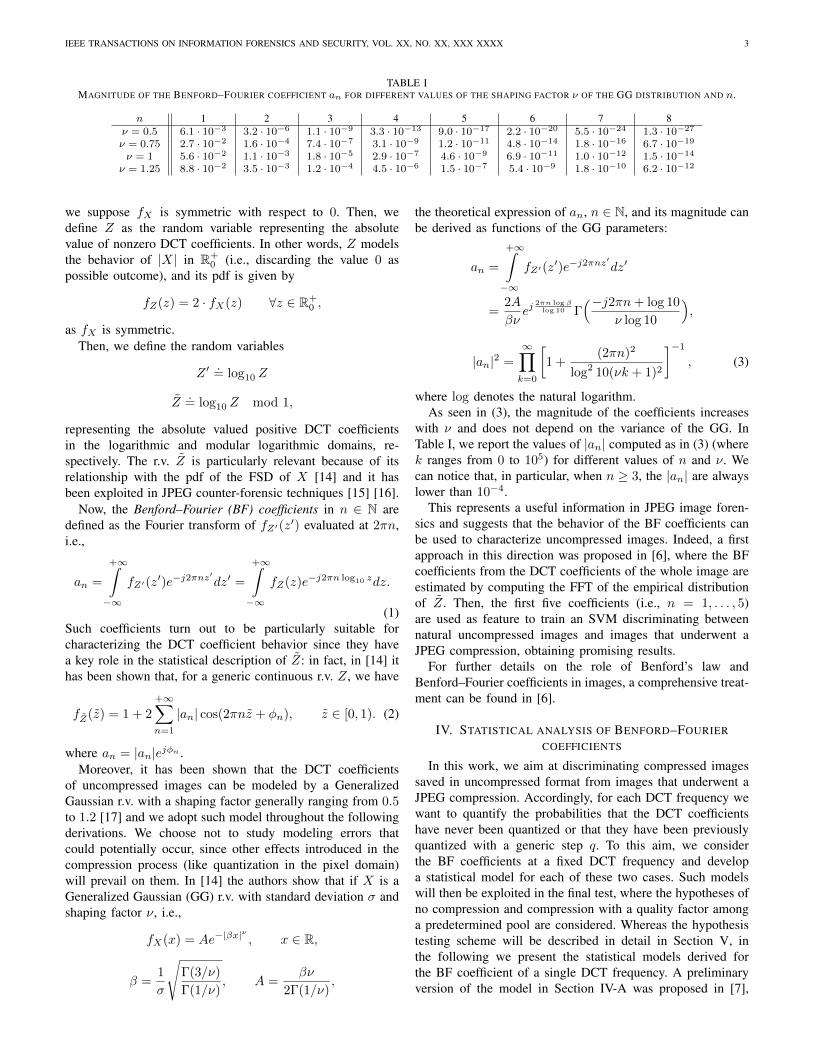
TABLE IMAGNITUDE OF THE BENFORD–FOURIER COEFFICIENT an FOR DIFFERENT VALUES OF THE SHAPING FACTOR ν OF THE GG DISTRIBUTION AND n.

n 1 2 3 4 5 6 7 8ν = 0.5 6.1 · 10−3 3.2 · 10−6 1.1 · 10−9 3.3 · 10−13 9.0 · 10−17 2.2 · 10−20 5.5 · 10−24 1.3 · 10−27

ν = 0.75 2.7 · 10−2 1.6 · 10−4 7.4 · 10−7 3.1 · 10−9 1.2 · 10−11 4.8 · 10−14 1.8 · 10−16 6.7 · 10−19

ν = 1 5.6 · 10−2 1.1 · 10−3 1.8 · 10−5 2.9 · 10−7 4.6 · 10−9 6.9 · 10−11 1.0 · 10−12 1.5 · 10−14

ν = 1.25 8.8 · 10−2 3.5 · 10−3 1.2 · 10−4 4.5 · 10−6 1.5 · 10−7 5.4 · 10−9 1.8 · 10−10 6.2 · 10−12

we suppose fX is symmetric with respect to 0. Then, wedefine Z as the random variable representing the absolutevalue of nonzero DCT coefficients. In other words, Z modelsthe behavior of |X| in R+

0 (i.e., discarding the value 0 aspossible outcome), and its pdf is given by

fZ(z) = 2 · fX(z) ∀z ∈ R+0 ,

as fX is symmetric.Then, we define the random variables

Z ′.= log10 Z

Z.= log10 Z mod 1,

representing the absolute valued positive DCT coefficientsin the logarithmic and modular logarithmic domains, re-spectively. The r.v. Z is particularly relevant because of itsrelationship with the pdf of the FSD of X [14] and it hasbeen exploited in JPEG counter-forensic techniques [15] [16].

Now, the Benford–Fourier (BF) coefficients in n ∈ N aredefined as the Fourier transform of fZ′(z′) evaluated at 2πn,i.e.,

an =

+∞∫−∞

fZ′(z′)e−j2πnz′dz′ =

+∞∫−∞

fZ(z)e−j2πn log10 zdz.

(1)Such coefficients turn out to be particularly suitable forcharacterizing the DCT coefficient behavior since they havea key role in the statistical description of Z: in fact, in [14] ithas been shown that, for a generic continuous r.v. Z, we have

fZ(z) = 1 + 2

+∞∑n=1

|an| cos(2πnz + φn), z ∈ [0, 1). (2)

where an = |an|ejφn .Moreover, it has been shown that the DCT coefficients

of uncompressed images can be modeled by a GeneralizedGaussian r.v. with a shaping factor generally ranging from 0.5to 1.2 [17] and we adopt such model throughout the followingderivations. We choose not to study modeling errors thatcould potentially occur, since other effects introduced in thecompression process (like quantization in the pixel domain)will prevail on them. In [14] the authors show that if X is aGeneralized Gaussian (GG) r.v. with standard deviation σ andshaping factor ν, i.e.,

fX(x) = Ae−|βx|ν

, x ∈ R,

β =1

σ

√Γ(3/ν)

Γ(1/ν), A =

βν

2Γ(1/ν),

the theoretical expression of an, n ∈ N, and its magnitude canbe derived as functions of the GG parameters:

an =

+∞∫−∞

fZ′(z′)e−j2πnz′dz′

=2A

βνej

2πn log βlog 10 Γ

(−j2πn+ log 10

ν log 10

),

|an|2 =

∞∏k=0

[1 +

(2πn)2

log2 10(νk + 1)2

]−1, (3)

where log denotes the natural logarithm.As seen in (3), the magnitude of the coefficients increases

with ν and does not depend on the variance of the GG. InTable I, we report the values of |an| computed as in (3) (wherek ranges from 0 to 105) for different values of n and ν. Wecan notice that, in particular, when n ≥ 3, the |an| are alwayslower than 10−4.

This represents a useful information in JPEG image foren-sics and suggests that the behavior of the BF coefficients canbe used to characterize uncompressed images. Indeed, a firstapproach in this direction was proposed in [6], where the BFcoefficients from the DCT coefficients of the whole image areestimated by computing the FFT of the empirical distributionof Z. Then, the first five coefficients (i.e., n = 1, . . . , 5)are used as feature to train an SVM discriminating betweennatural uncompressed images and images that underwent aJPEG compression, obtaining promising results.

For further details on the role of Benford’s law andBenford–Fourier coefficients in images, a comprehensive treat-ment can be found in [6].

IV. STATISTICAL ANALYSIS OF BENFORD–FOURIERCOEFFICIENTS

In this work, we aim at discriminating compressed imagessaved in uncompressed format from images that underwent aJPEG compression. Accordingly, for each DCT frequency wewant to quantify the probabilities that the DCT coefficientshave never been quantized or that they have been previouslyquantized with a generic step q. To this aim, we considerthe BF coefficients at a fixed DCT frequency and developa statistical model for each of these two cases. Such modelswill then be exploited in the final test, where the hypotheses ofno compression and compression with a quality factor amonga predetermined pool are considered. Whereas the hypothesistesting scheme will be described in detail in Section V, inthe following we present the statistical models derived forthe BF coefficient of a single DCT frequency. A preliminaryversion of the model in Section IV-A was proposed in [7],


while Section IV-B contains a novel analysis of the quantizedDCT coefficients.

A. Uncompressed image model

In order to use BF coefficients for analyzing an image, weneed a numerical procedure to estimate them given the subjectimage.

By looking at (1), we can notice that an is the expectedvalue of the complex random variable gn(Z) = e−j2πn log10 Z ,whose values lie on the unit circle1. Thus, as it is usually donein statistics, we can obtain an estimate of an = E{gn(Z)} byconsidering the sample mean of gn(Z) provided by the DCTcoefficients of the image through the different 8 × 8 blocks.Thus, if we denote as zm the value of the DCT coefficient atthe chosen frequency in the m-th block, we can consider asestimator of an the expression

an.=

M∑m=1

e−j2πn log10 zm

M, m = 1, . . . ,M, (4)

where M is the total number of 8× 8 blocks in the image.In other words, we can see an as realization of the r.v.

An.=

M∑m=1

e−j2πn log10 Zm

M, m = 1, . . . ,M, (5)

where Zm is the r.v. representing the DCT coefficient at thechosen frequency in the m-th block.

Although the sample mean is a minimum variance unbiasedestimator of the expected value (i.e., E{An} = an), we shouldtake into account the fact that the actual accuracy of an in theestimation of an depends on the size of the considered sample.For this reason, we are interested in studying the distributionof An as a function of the number of samples M .

To this end, we can observe that An is a sum of M inde-pendent and identically distributed random variables gn(Zm).Then, by applying the Central Limit Theorem (CLT) to thereal and imaginary parts of An, we have that their distributionis asymptotically Gaussian with expected values <(an) and=(an), respectively [18]. In other words,

An ≈ an +W0,

where W0 is a zero-mean complex normal random variable.A necessary and sufficient condition for W0 to be circularly

symmetric (i.e., with real and imaginary parts independent andidentically distributed [18]) is that E{W 2

0 } = 0. Starting fromthe definition of An, it is easy to prove that

E{W 20 } ≈ E{(An − an)2} =

1

M(a2n − a2n). (6)

Hence, |E{W 20 }| ≤ (|a2n| + |a2n|)/M and, by looking at

Table I, we can conclude that the value of (6) will be veryclose to 0 (for instance, when ν = 1 and n = 3 its orderof magnitude is 10−11). Therefore, An is approximately acircular bivariate normal r.v. with non-zero mean.

1It is worth noticing that BF coefficients are defined for integers n ∈ N butsuch definition could be easily extended to the entire real line by replacing2πn with a real value ω, and the following analysis would hold identicallyalso in this more general case.

It is well known that the r.v. R .= |An| approximately

follows a Rice distribution with mean parameter |an| and scaleparameter s, where s is the standard deviation of both its realand imaginary parts [19]. Similarly as before, we can nowobtain s2 by exploiting the fact that for a Rice distribution

s2 =E{|An|2} − |an|2

2=

1

2M(1− |an|2).

As we observed, |an| is lower than 10−4 when n ≥ 3 andwe can reasonably assume |an| ≈ 0, thus considering thespecial case of Rice distribution with mean parameter 0, i.e.,the Rayleigh distribution with scale parameter s = 1/

√2M .

According to this, we can define p(an|NQ) (NQ means“never quantized”) as the probability density function ofobtaining a BF coefficient an under the hypothesis of noprevious quantization and compute it as follows:

p(an|NQ) = 2M |an|e−M |an|2

, (7)

where the expression on the right is the Rayleigh pdf withs = 1/

√2M . By considering its properties, we have that |an|

is in any case an overestimate of |an| = 0, where its mean isgiven by 1√

M·√π2 (the expected accuracy increases linearly

with√M ) and its variance is given by 1

M · 4−π4 (the expectedaccuracy variance decreases linearly with M ).

An example of the model is showed in Fig. 1.

B. Compressed image model

When computing the DCT from an image stored in un-compressed format that was previously compressed, the DCTcoefficients at a certain frequency have a distribution like inFig. 2a. The error affecting the histogram is due to the quan-tization in the pixel domain after the block-DCT quantizationand the rounding/truncation errors in the DCT computation,and has been modeled in the literature as a Gaussian r.v. [20].

We propose here an alternative statistical description whoseaccuracy has been assessed by extensive numerical tests. Wecan restrict our analysis to a single quantization interval andconsider the DCT coefficients contained within it. Without anyloss of generality, we consider the interval Iq

.= [q− q/2, q+

q/2[ (q is the quantization step) and we denote with Zq the r.v.representing the DCT coefficients falling in Iq . Then, we canapproximate its distribution with a Laplacian truncated outsidethe quantization interval, as in Fig. 2b. Then, the pdf of Zq isgiven by

fZq (z) =L(z; q, σ)

Nσ,q· 1Iq (z), (8)

where L(·; q, σ) is a Laplacian pdf with mean q and standarddeviation σ (which is unknown and needs to be estimated),Nσ,q is the integral of L(z; q, σ) over Iq (so that expression(8) is a pdf), and 1I(·) is the indicator function of Iq

1Iq (z).=

{1 z ∈ Iq0 z /∈ Iq.

Starting from this hypothesis, we can define an,q as theBenford-Fourier coefficients of Zq , and derive their theoretical


Image size 64x64, M=64

Image size 256x256, M=1024

Image size 1024x1024, M=16384

0 0.1 0.2 0.3 0.4 0.50

10

20

30

40

50

60

70

80

0 0.1 0.2 0.3 0.4 0.50

1

2

3

4

5

6

7

8

0 0.05 0.1 0.15 0.20

20

40

60

80

100

120

140

0 0.05 0.1 0.150

5

10

15

20

25

30

0 0.01 0.02 0.030

20

40

60

80

100

120

0 0.01 0.02 0.030

20

40

60

80

100

120

×10-30 2 4 6 80

10

20

30

40

50

60

70

80

90

×10-30 2 4 6 80

50

100

150

200

250

300

350

400

450Image size 4096x4096, M=262144

-10 -5 0 5 100

0.05

0.1

0.15

0.2

0.25

0.3

0.35

0.4

Generalized Gaussian pdf,

=1

BF coefficient computation

�2 = 7.1 · 10�3

�2 = 6.3 · 10�3

�2 = 5.0 · 10�3

�2 = 2.1 · 10�3

⌫

×10-30 2 4 6 80

10

20

30

40

50

60

70

80

90

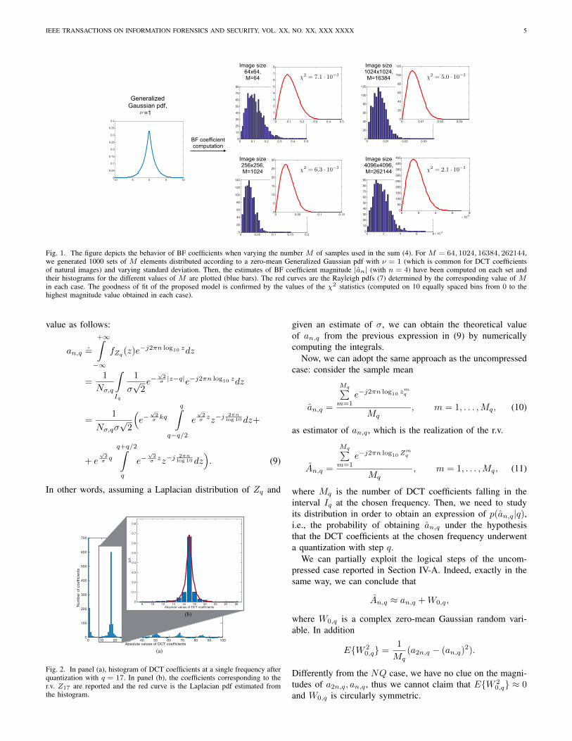
Fig. 1. The figure depicts the behavior of BF coefficients when varying the number M of samples used in the sum (4). For M = 64, 1024, 16384, 262144,we generated 1000 sets of M elements distributed according to a zero-mean Generalized Gaussian pdf with ν = 1 (which is common for DCT coefficientsof natural images) and varying standard deviation. Then, the estimates of BF coefficient magnitude |an| (with n = 4) have been computed on each set andtheir histograms for the different values of M are plotted (blue bars). The red curves are the Rayleigh pdfs (7) determined by the corresponding value of Min each case. The goodness of fit of the proposed model is confirmed by the values of the χ2 statistics (computed on 10 equally spaced bins from 0 to thehighest magnitude value obtained in each case).

value as follows:

an,q.=

+∞∫−∞

fZq (z)e−j2πn log10 zdz

=1

Nσ,q

∫Iq

1

σ√

2e−

√2σ |z−q|e−j2πn log10 zdz

=1

Nσ,qσ√

2

(e−

√2σ kq

q∫q−q/2

e√

2σ zz−j

2πnlog 10 dz+

+ e√

2σ q

q+q/2∫q

e−√

2σ zz−j

2πnlog 10 dz

). (9)

In other words, assuming a Laplacian distribution of Zq and

Absolute values of DCT coefficients0 10 20 30 40 50 60 70 80 90 100

Num

ber o

f coe

ffici

ents

0

100

200

300

400

500

600

700

Absolute values of DCT coefficients8 10 12 14 16 18 20 22 24 26

pdf

0

0.1

0.2

0.3

0.4

0.5

0.6

0.7

0.8

(a)

(b)

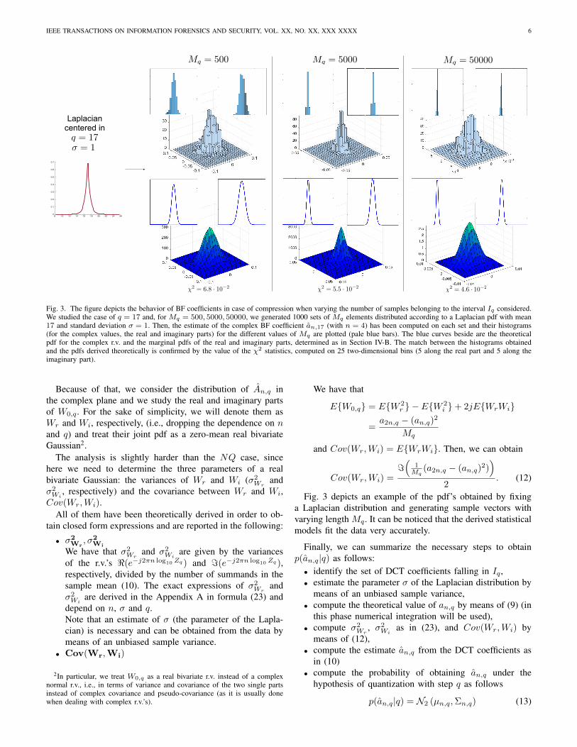
Fig. 2. In panel (a), histogram of DCT coefficients at a single frequency afterquantization with q = 17. In panel (b), the coefficients corresponding to ther.v. Z17 are reported and the red curve is the Laplacian pdf estimated fromthe histogram.

given an estimate of σ, we can obtain the theoretical valueof an,q from the previous expression in (9) by numericallycomputing the integrals.

Now, we can adopt the same approach as the uncompressedcase: consider the sample mean

an,q =

Mq∑m=1

e−j2πn log10 zmq

Mq, m = 1, . . . ,Mq, (10)

as estimator of an,q , which is the realization of the r.v.

An,q =

Mq∑m=1

e−j2πn log10 Zmq

Mq, m = 1, . . . ,Mq, (11)

where Mq is the number of DCT coefficients falling in theinterval Iq at the chosen frequency. Then, we need to studyits distribution in order to obtain an expression of p(an,q|q),i.e., the probability of obtaining an,q under the hypothesisthat the DCT coefficients at the chosen frequency underwenta quantization with step q.

We can partially exploit the logical steps of the uncom-pressed case reported in Section IV-A. Indeed, exactly in thesame way, we can conclude that

An,q ≈ an,q +W0,q,

where W0,q is a complex zero-mean Gaussian random vari-able. In addition

E{W 20,q} =

1

Mq(a2n,q − (an,q)

2).

Differently from the NQ case, we have no clue on the magni-tudes of a2n,q, an,q , thus we cannot claim that E{W 2

0,q} ≈ 0and W0,q is circularly symmetric.


8 10 12 14 16 18 20 22 24 260

0.1

0.2

0.3

0.4

0.5

0.6

0.7

Laplacian centered in

�2 = 6.8 · 10�2

Mq = 500

�2 = 5.5 · 10�2

Mq = 5000

�2 = 4.6 · 10�2

Mq = 50000

q = 17� = 1

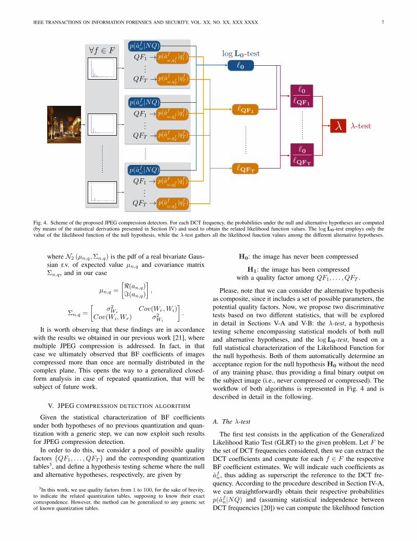
Fig. 3. The figure depicts the behavior of BF coefficients in case of compression when varying the number of samples belonging to the interval Iq considered.We studied the case of q = 17 and, for Mq = 500, 5000, 50000, we generated 1000 sets of Mq elements distributed according to a Laplacian pdf with mean17 and standard deviation σ = 1. Then, the estimate of the complex BF coefficient an,17 (with n = 4) has been computed on each set and their histograms(for the complex values, the real and imaginary parts) for the different values of Mq are plotted (pale blue bars). The blue curves beside are the theoreticalpdf for the complex r.v. and the marginal pdfs of the real and imaginary parts, determined as in Section IV-B. The match between the histograms obtainedand the pdfs derived theoretically is confirmed by the value of the χ2 statistics, computed on 25 two-dimensional bins (5 along the real part and 5 along theimaginary part).

Because of that, we consider the distribution of An,q inthe complex plane and we study the real and imaginary partsof W0,q . For the sake of simplicity, we will denote them asWr and Wi, respectively, (i.e., dropping the dependence on nand q) and treat their joint pdf as a zero-mean real bivariateGaussian2.

The analysis is slightly harder than the NQ case, sincehere we need to determine the three parameters of a realbivariate Gaussian: the variances of Wr and Wi (σ2

Wrand

σ2Wi

, respectively) and the covariance between Wr and Wi,Cov(Wr,Wi).

All of them have been theoretically derived in order to ob-tain closed form expressions and are reported in the following:

• σ2Wr

, σ2Wi

We have that σ2Wr

and σ2Wi

are given by the variancesof the r.v.’s <(e−j2πn log10 Zq ) and =(e−j2πn log10 Zq ),respectively, divided by the number of summands in thesample mean (10). The exact expressions of σ2

Wrand

σ2Wi

are derived in the Appendix A in formula (23) anddepend on n, σ and q.Note that an estimate of σ (the parameter of the Lapla-cian) is necessary and can be obtained from the data bymeans of an unbiased sample variance.

• Cov(Wr,Wi)

2In particular, we treat W0,q as a real bivariate r.v. instead of a complexnormal r.v., i.e., in terms of variance and covariance of the two single partsinstead of complex covariance and pseudo-covariance (as it is usually donewhen dealing with complex r.v.’s).

We have that

E{W0,q} = E{W 2r } − E{W 2

i }+ 2jE{WrWi}

=a2n,q − (an,q)

2

Mq

and Cov(Wr,Wi) = E{WrWi}. Then, we can obtain

Cov(Wr,Wi) ==(

1Mq

(a2n,q − (an,q)2))

2. (12)

Fig. 3 depicts an example of the pdf’s obtained by fixinga Laplacian distribution and generating sample vectors withvarying length Mq . It can be noticed that the derived statisticalmodels fit the data very accurately.

Finally, we can summarize the necessary steps to obtainp(an,q|q) as follows:• identify the set of DCT coefficients falling in Iq ,• estimate the parameter σ of the Laplacian distribution by

means of an unbiased sample variance,• compute the theoretical value of an,q by means of (9) (in

this phase numerical integration will be used),• compute σ2

Wr, σ2

Wias in (23), and Cov(Wr,Wi) by

means of (12),• compute the estimate an,q from the DCT coefficients as

in (10)• compute the probability of obtaining an,q under the

hypothesis of quantization with step q as follows

p(an,q|q) = N2 (µn,q,Σn,q) (13)


QF1 !...

QFT !

0 50 100 1500

500

1000

1500

2000

2500

0 50 100 1500

200

400

600

800

1000

1200

1400

1600

1800

0 50 100 1500

200

400

600

800

1000

1200

QF1 !...

QFT !

QF1 !...

QFT !

�

8f 2 F

`0

`0`QF1

`0`QFT

`QFT

p(af

!,qf1

|qf1 )

p(af

!,qfT

|qfT )

p(af

!,qf1

|qf1 )

p(af

!,qfT

|qfT )

p(af

!,qf1

|qf1 )

p(af

!,qfT

|qfT )

�-test

p(af!|NQ)

p(af!|NQ)

p(af!|NQ)

log L0-test

`QF1

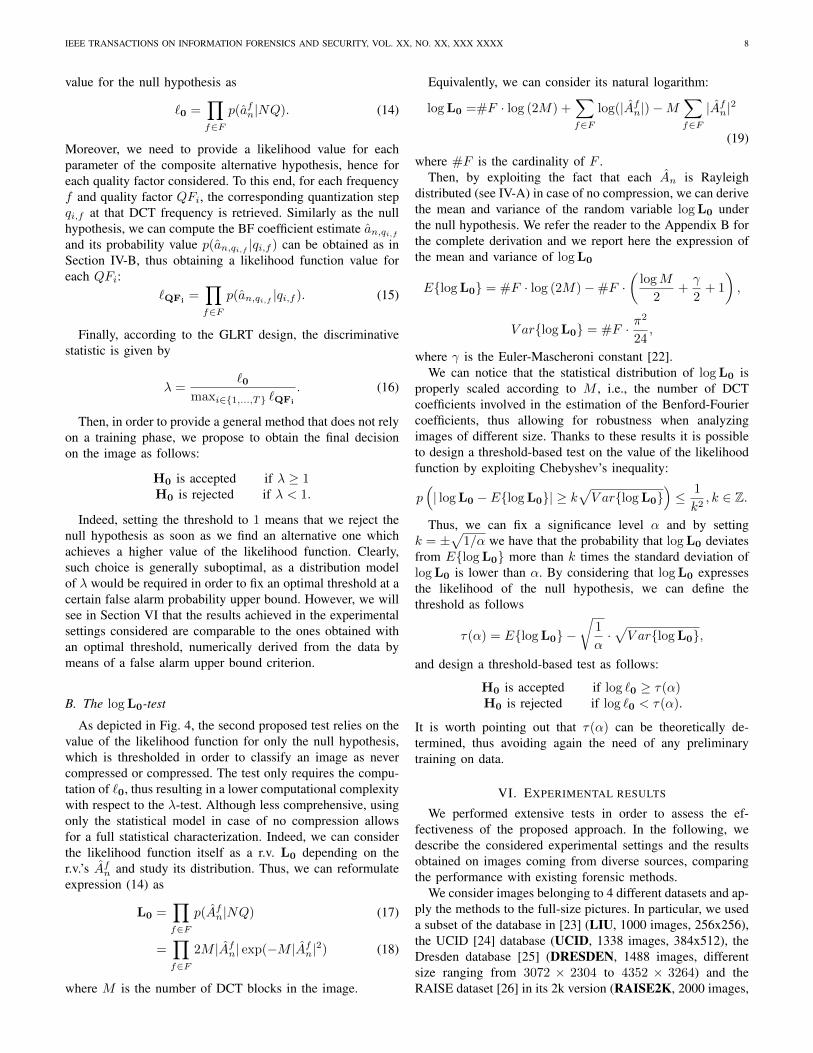
Fig. 4. Scheme of the proposed JPEG compression detectors. For each DCT frequency, the probabilities under the null and alternative hypotheses are computed(by means of the statistical derivations presented in Section IV) and used to obtain the related likelihood function values. The logL0-test employs only thevalue of the likelihood function of the null hypothesis, while the λ-test gathers all the likelihood function values among the different alternative hypotheses.

where N2 (µn,q,Σn,q) is the pdf of a real bivariate Gaus-sian r.v. of expected value µn,q and covariance matrixΣn,q , and in our case

µn,q =

[<(an,q)=(an,q)

],

Σn,q =

[σ2Wr

Cov(Wr,Wi)Cov(Wi,Wr) σ2

Wi

].

It is worth observing that these findings are in accordancewith the results we obtained in our previous work [21], wheremultiple JPEG compression is addressed. In fact, in thatcase we ultimately observed that BF coefficients of imagescompressed more than once are normally distributed in thecomplex plane. This opens the way to a generalized closed-form analysis in case of repeated quantization, that will besubject of future work.

V. JPEG COMPRESSION DETECTION ALGORITHM

Given the statistical characterization of BF coefficientsunder both hypotheses of no previous quantization and quan-tization with a generic step, we can now exploit such resultsfor JPEG compression detection.

In order to do this, we consider a pool of possible qualityfactors {QF1, . . . , QFT } and the corresponding quantizationtables3, and define a hypothesis testing scheme where the nulland alternative hypotheses, respectively, are given by

3In this work, we use quality factors from 1 to 100, for the sake of brevity,to indicate the related quantization tables, supposing to know their exactcorrespondence. However, the method can be generalized to any generic setof known quantization tables.

H0: the image has never been compressed

H1: the image has been compressedwith a quality factor among QF1, . . . , QFT .

Please, note that we can consider the alternative hypothesisas composite, since it includes a set of possible parameters, thepotential quality factors. Now, we propose two discriminativetests based on two different statistics, that will be exploredin detail in Sections V-A and V-B: the λ-test, a hypothesistesting scheme encompassing statistical models of both nulland alternative hypotheses, and the logL0-test, based on afull statistical characterization of the Likelihood Function forthe null hypothesis. Both of them automatically determine anacceptance region for the null hypothesis H0 without the needof any training phase, thus providing a final binary output onthe subject image (i.e., never compressed or compressed). Theworkflow of both algorithms is represented in Fig. 4 and isdescribed in detail in the following.

A. The λ-test

The first test consists in the application of the GeneralizedLikelihood Ratio Test (GLRT) to the given problem. Let F bethe set of DCT frequencies considered, then we can extract theDCT coefficients and compute for each f ∈ F the respectiveBF coefficient estimates. We will indicate such coefficients asafn, thus adding as superscript the reference to the DCT fre-quency. According to the procedure described in Section IV-A,we can straightforwardly obtain their respective probabilitiesp(afn|NQ) and (assuming statistical independence betweenDCT frequencies [20]) we can compute the likelihood function


value for the null hypothesis as

`0 =∏f∈F

p(afn|NQ). (14)

Moreover, we need to provide a likelihood value for eachparameter of the composite alternative hypothesis, hence foreach quality factor considered. To this end, for each frequencyf and quality factor QFi, the corresponding quantization stepqi,f at that DCT frequency is retrieved. Similarly as the nullhypothesis, we can compute the BF coefficient estimate an,qi,fand its probability value p(an,qi,f |qi,f ) can be obtained as inSection IV-B, thus obtaining a likelihood function value foreach QFi:

`QFi=∏f∈F

p(an,qi,f |qi,f ). (15)

Finally, according to the GLRT design, the discriminativestatistic is given by

λ =`0

maxi∈{1,...,T} `QFi

. (16)

Then, in order to provide a general method that does not relyon a training phase, we propose to obtain the final decisionon the image as follows:

H0 is accepted if λ ≥ 1H0 is rejected if λ < 1.

Indeed, setting the threshold to 1 means that we reject thenull hypothesis as soon as we find an alternative one whichachieves a higher value of the likelihood function. Clearly,such choice is generally suboptimal, as a distribution modelof λ would be required in order to fix an optimal threshold at acertain false alarm probability upper bound. However, we willsee in Section VI that the results achieved in the experimentalsettings considered are comparable to the ones obtained withan optimal threshold, numerically derived from the data bymeans of a false alarm upper bound criterion.

B. The logL0-test

As depicted in Fig. 4, the second proposed test relies on thevalue of the likelihood function for only the null hypothesis,which is thresholded in order to classify an image as nevercompressed or compressed. The test only requires the compu-tation of `0, thus resulting in a lower computational complexitywith respect to the λ-test. Although less comprehensive, usingonly the statistical model in case of no compression allowsfor a full statistical characterization. Indeed, we can considerthe likelihood function itself as a r.v. L0 depending on ther.v.’s Afn and study its distribution. Thus, we can reformulateexpression (14) as

L0 =∏f∈F

p(Afn|NQ) (17)

=∏f∈F

2M |Afn| exp(−M |Afn|2) (18)

where M is the number of DCT blocks in the image.

Equivalently, we can consider its natural logarithm:

logL0 =#F · log (2M) +∑f∈F

log(|Afn|)−M∑f∈F|Afn|2

(19)

where #F is the cardinality of F .Then, by exploiting the fact that each An is Rayleigh

distributed (see IV-A) in case of no compression, we can derivethe mean and variance of the random variable logL0 underthe null hypothesis. We refer the reader to the Appendix B forthe complete derivation and we report here the expression ofthe mean and variance of logL0

E{logL0} = #F · log (2M)−#F ·(

logM

2+γ

2+ 1

),

V ar{logL0} = #F · π2

24,

where γ is the Euler-Mascheroni constant [22].We can notice that the statistical distribution of logL0 is

properly scaled according to M , i.e., the number of DCTcoefficients involved in the estimation of the Benford-Fouriercoefficients, thus allowing for robustness when analyzingimages of different size. Thanks to these results it is possibleto design a threshold-based test on the value of the likelihoodfunction by exploiting Chebyshev’s inequality:

p(| logL0 − E{logL0}| ≥ k

√V ar{logL0}

)≤ 1

k2, k ∈ Z.

Thus, we can fix a significance level α and by settingk = ±

√1/α we have that the probability that logL0 deviates

from E{logL0} more than k times the standard deviation oflogL0 is lower than α. By considering that logL0 expressesthe likelihood of the null hypothesis, we can define thethreshold as follows

τ(α) = E{logL0} −√

1

α·√V ar{logL0},

and design a threshold-based test as follows:

H0 is accepted if log `0 ≥ τ(α)H0 is rejected if log `0 < τ(α).

It is worth pointing out that τ(α) can be theoretically de-termined, thus avoiding again the need of any preliminarytraining on data.

VI. EXPERIMENTAL RESULTS

We performed extensive tests in order to assess the ef-fectiveness of the proposed approach. In the following, wedescribe the considered experimental settings and the resultsobtained on images coming from diverse sources, comparingthe performance with existing forensic methods.

We consider images belonging to 4 different datasets and ap-ply the methods to the full-size pictures. In particular, we useda subset of the database in [23] (LIU, 1000 images, 256x256),the UCID [24] database (UCID, 1338 images, 384x512), theDresden database [25] (DRESDEN, 1488 images, differentsize ranging from 3072 × 2304 to 4352 × 3264) and theRAISE dataset [26] in its 2k version (RAISE2K, 2000 images,


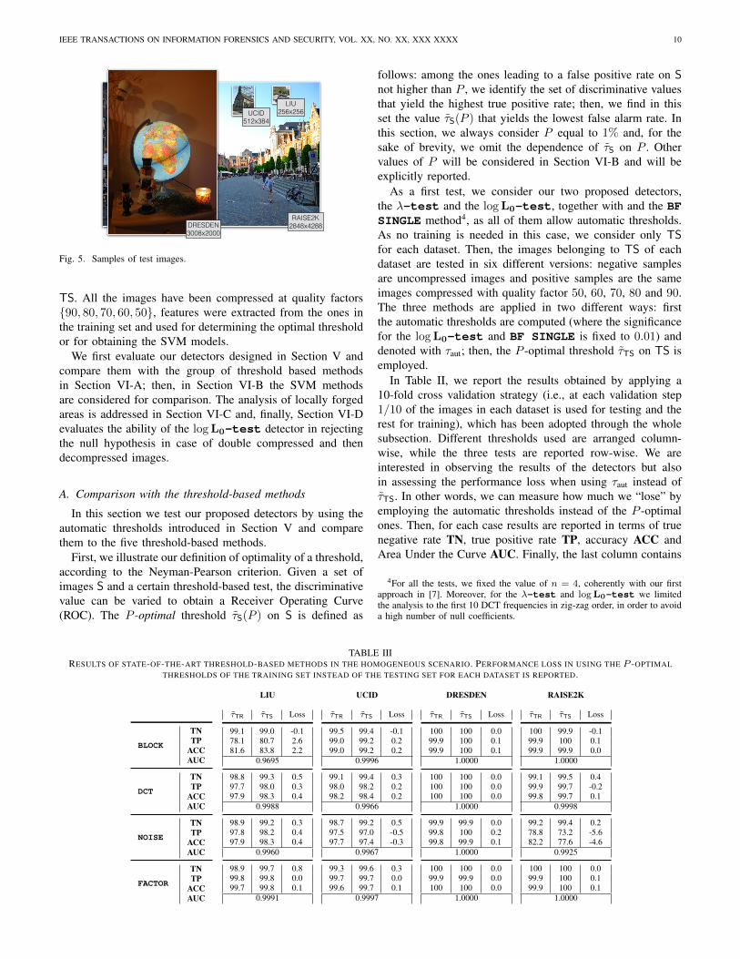
different sizes ranging from 3008 × 2000 to 4928 × 3264).The different datasets and their size proportions are visuallyrepresented in Fig. 5.

Other seven state-of-the-art methods have been consideredfor comparisons, that can be grouped into two categories:the threshold-based techniques proposed in [7], [8], [10],[11] and [12] (denoted in the following as BF SINGLE,BLOCK, DCT, NOISE and FACTOR, respectively) and theSVM-based techniques proposed in [6] and [13] (denoted in

the following as BF FFT and FSD, respectively). They havebeen briefly described in Section II and all of them (except forBF SINGLE whose threshold is determined as in [7]) requiresome preliminary training phase, whose goal is to determinethe discriminative threshold to be adopted for the threshold-based group and the SVM model for the SVM-based group.Therefore, each dataset was randomly divided into two parts,one for training and another one for testing. Thus, for each ofthe four datasets we have a training set TR and a training set

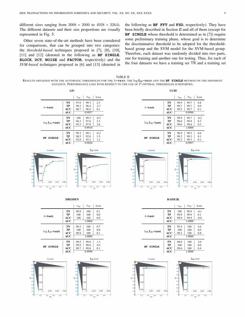
TABLE IIRESULTS OBTAINED WITH THE AUTOMATIC THRESHOLDS FOR THE λ-TEST , THE logL0-TEST AND THE BF SINGLE METHOD ON THE DIFFERENT

DATASETS. PERFORMANCE LOSS WITH RESPECT TO THE USE OF P -OPTIMAL THRESHOLDS IS REPORTED.

LIU

τaut τTS Loss

λ-test

TN 97.0 99.3 2.3TP 99.3 96.4 -2.7

ACC 96.7 96.9 0.1AUC 0.9957

logL0-test

TN 100 99.5 -0.5TP 94.3 97.6 3.3

ACC 95.3 97.9 2.6AUC 0.9918

BF SINGLE

TN 99.3 99.1 -0.2TP 90.5 92.0 1.5

ACC 92.0 93.2 1.2AUC 0.9826

FP0 0.2 0.4 0.6 0.8 1

TP

0

0.1

0.2

0.3

0.4

0.5

0.6

0.7

0.8

0.9

1

FP0 0.2 0.4 0.6 0.8 1

TP

0

0.1

0.2

0.3

0.4

0.5

0.6

0.7

0.8

0.9

1�-test L0-test

0 0.02 0.04 0.06FP

0.94

0.96

0.98

1

TP

0 0.02 0.04 0.06FP

0.94

0.96

0.98

1

TP

UCID

τaut τTS Loss

λ-test

TN 98.9 99.7 0.8TP 99.7 99.7 0.0

ACC 99.5 99.7 0.1AUC 0.9990

logL0-test

TN 99.9 99.7 -0.2TP 99.6 99.9 0.3

ACC 99.6 99.8 0.2AUC 1.0000

BF SINGLE

TN 98.9 99.5 0.6TP 99.2 99.3 0.1

ACC 99.2 99.3 0.1AUC 0.9997

FP0 0.2 0.4 0.6 0.8 1

TP

0

0.1

0.2

0.3

0.4

0.5

0.6

0.7

0.8

0.9

1

FP0 0.2 0.4 0.6 0.8 1

TP

0

0.1

0.2

0.3

0.4

0.5

0.6

0.7

0.8

0.9

1�-test L0-test

0 0.02 0.04 0.06FP

0.94

0.96

0.98

1

TP

0 0.02 0.04 0.06FP

0.94

0.96

0.98

1

TP

DRESDEN

τaut τTS Loss

λ-test

TN 99.9 100 0.1TP 100 100 0.0

ACC 100 100 0.0AUC 1.0000

logL0-test

TN 99.3 100 0.7TP 100 100 0.0

ACC 99.9 100 0.1AUC 1.0000

BF SINGLE

TN 98.5 99.8 1.3TP 99.9 99.8 -0.1

ACC 99.7 99.8 0.1AUC 0.9998

FP0 0.2 0.4 0.6 0.8 1

TP

0

0.1

0.2

0.3

0.4

0.5

0.6

0.7

0.8

0.9

1

FP0 0.2 0.4 0.6 0.8 1

TP

0

0.1

0.2

0.3

0.4

0.5

0.6

0.7

0.8

0.9

1�-test L0-test

0 0.02 0.04 0.06FP

0.94

0.96

0.98

1

TP

0 0.02 0.04 0.06FP

0.94

0.96

0.98

1

TP

RAISE2K

τaut τTS Loss

λ-test

TN 100 99.9 -0.1TP 99.8 99.9 0.1

ACC 99.9 99.9 -0.0AUC 1.0000

logL0-test

TN 95.4 100 4.6TP 100 100 0.0

ACC 99.2 100 0.8AUC 1.0000

BF SINGLE

TN 98.0 100 2.0TP 100 100 0.0

ACC 99.6 100 0.4AUC 1.0000

FP0 0.2 0.4 0.6 0.8 1

TP

0

0.1

0.2

0.3

0.4

0.5

0.6

0.7

0.8

0.9

1

FP0 0.2 0.4 0.6 0.8 1

TP

0

0.1

0.2

0.3

0.4

0.5

0.6

0.7

0.8

0.9

1�-test L0-test

0 0.02 0.04 0.06FP

0.94

0.96

0.98

1

TP

0 0.02 0.04 0.06FP

0.94

0.96

0.98

1

TP


RAISE2K 2848x4288DRESDEN

3008x2000

UCID 512x384

LIU 256x256

Fig. 5. Samples of test images.

TS. All the images have been compressed at quality factors{90, 80, 70, 60, 50}, features were extracted from the ones inthe training set and used for determining the optimal thresholdor for obtaining the SVM models.

We first evaluate our detectors designed in Section V andcompare them with the group of threshold based methodsin Section VI-A; then, in Section VI-B the SVM methodsare considered for comparison. The analysis of locally forgedareas is addressed in Section VI-C and, finally, Section VI-Devaluates the ability of the logL0-test detector in rejectingthe null hypothesis in case of double compressed and thendecompressed images.

A. Comparison with the threshold-based methods

In this section we test our proposed detectors by using theautomatic thresholds introduced in Section V and comparethem to the five threshold-based methods.

First, we illustrate our definition of optimality of a threshold,according to the Neyman-Pearson criterion. Given a set ofimages S and a certain threshold-based test, the discriminativevalue can be varied to obtain a Receiver Operating Curve(ROC). The P -optimal threshold τS(P ) on S is defined as

follows: among the ones leading to a false positive rate on Snot higher than P , we identify the set of discriminative valuesthat yield the highest true positive rate; then, we find in thisset the value τS(P ) that yields the lowest false alarm rate. Inthis section, we always consider P equal to 1% and, for thesake of brevity, we omit the dependence of τS on P . Othervalues of P will be considered in Section VI-B and will beexplicitly reported.

As a first test, we consider our two proposed detectors,the λ-test and the logL0-test, together with and the BFSINGLE method4, as all of them allow automatic thresholds.As no training is needed in this case, we consider only TSfor each dataset. Then, the images belonging to TS of eachdataset are tested in six different versions: negative samplesare uncompressed images and positive samples are the sameimages compressed with quality factor 50, 60, 70, 80 and 90.The three methods are applied in two different ways: firstthe automatic thresholds are computed (where the significancefor the logL0-test and BF SINGLE is fixed to 0.01) anddenoted with τaut; then, the P -optimal threshold τTS on TS isemployed.

In Table II, we report the results obtained by applying a10-fold cross validation strategy (i.e., at each validation step1/10 of the images in each dataset is used for testing and therest for training), which has been adopted through the wholesubsection. Different thresholds used are arranged column-wise, while the three tests are reported row-wise. We areinterested in observing the results of the detectors but alsoin assessing the performance loss when using τaut instead ofτTS. In other words, we can measure how much we “lose” byemploying the automatic thresholds instead of the P -optimalones. Then, for each case results are reported in terms of truenegative rate TN, true positive rate TP, accuracy ACC andArea Under the Curve AUC. Finally, the last column contains

4For all the tests, we fixed the value of n = 4, coherently with our firstapproach in [7]. Moreover, for the λ-test and logL0-test we limitedthe analysis to the first 10 DCT frequencies in zig-zag order, in order to avoida high number of null coefficients.

TABLE IIIRESULTS OF STATE-OF-THE-ART THRESHOLD-BASED METHODS IN THE HOMOGENEOUS SCENARIO. PERFORMANCE LOSS IN USING THE P -OPTIMAL

THRESHOLDS OF THE TRAINING SET INSTEAD OF THE TESTING SET FOR EACH DATASET IS REPORTED.

BLOCK

TNTP

ACCAUC

DCT

TNTP

ACCAUC

NOISE

TNTP

ACCAUC

FACTOR

TNTP

ACCAUC

LIU

τTR τTS Loss

99.1 99.0 -0.178.1 80.7 2.681.6 83.8 2.2

0.9695

98.8 99.3 0.597.7 98.0 0.397.9 98.3 0.4

0.9988

98.9 99.2 0.397.8 98.2 0.497.9 98.3 0.4

0.9960

98.9 99.7 0.899.8 99.8 0.099.7 99.8 0.1

0.9991

UCID

τTR τTS Loss

99.5 99.4 -0.199.0 99.2 0.299.0 99.2 0.2

0.9996

99.1 99.4 0.398.0 98.2 0.298.2 98.4 0.2

0.9966

98.7 99.2 0.597.5 97.0 -0.597.7 97.4 -0.3

0.9967

99.3 99.6 0.399.7 99.7 0.099.6 99.7 0.1

0.9997

DRESDEN

τTR τTS Loss

100 100 0.099.9 100 0.199.9 100 0.1

1.0000

100 100 0.0100 100 0.0100 100 0.0

1.0000

99.9 99.9 0.099.8 100 0.299.8 99.9 0.1

1.0000

100 100 0.099.9 99.9 0.0100 100 0.0

1.0000

RAISE2K

τTR τTS Loss

100 99.9 -0.199.9 100 0.199.9 99.9 0.0

1.0000

99.1 99.5 0.499.9 99.7 -0.299.8 99.7 0.1

0.9998

99.2 99.4 0.278.8 73.2 -5.682.2 77.6 -4.6

0.9925

100 100 0.099.9 100 0.199.9 100 0.1

1.0000


the performance loss between the two thresholds. Thus, ifTN(τTS) and TN(τaut) are the true negative rates obtained withτTS and τaut, respectively, the loss is computed as

TN(τTS)− TN(τaut),

where a positive (negative) loss means a performance decrease(increase). The same holds for TP and ACC.

It is worth noticing that the true negative rate TN is thecomplementary of the false positive rate (i.e., the minimumvalue for optimal thresholds is at least 99.0%) and it isused equivalently for uniformly defining the performanceloss; moreover, the positive samples are more numerous thannegative samples, thus, the accuracy value is more influencedby the TP rather than the TN value. In Table II, we alsoplot below each dataset the ROC curve of the two proposeddetectors for one TR− TS partition, in order to highlight thedisplacement between results obtained with τTS (orange circle)and τaut (yellow circle).

We can notice that both detectors yield good accuracies

values in any case and outperform BF SINGLE, which isbased on a single Benford-Fourier coefficient. Moreover, theperformance loss is generally limited, in the sense that eitherthe TP and the TN rates are not significantly compromised.In particular, it is interesting to notice that the automaticthreshold for the logL0-test, determined with the falsealarm probability upper bound fixed to 0.01, indeed yields afalse positive rate below 1% in every case, with the exceptionof the RAISE2K dataset where the false positive rate raiseto 4.3%. By selecting the outlier images from this databaseand exploring their statistics, we have noticed that DCTcoefficients in uncompressed images (that are supposed to beGG distributed) usually present some anomalies, which causedeviations with respect to the models predicted in Section IV-Aand disappear when the image is decimated by a factor 2 ineach dimension. We conjecture such phenomenon is due tospecific capture settings (all outlier images have been takenwith the same camera) coupled with the high resolution, whichpotentially increases the correlation among image blocks.

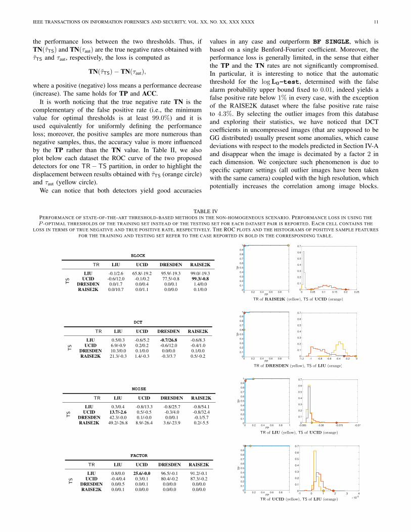
TABLE IVPERFORMANCE OF STATE-OF-THE-ART THRESHOLD-BASED METHODS IN THE NON-HOMOGENEOUS SCENARIO. PERFORMANCE LOSS IN USING THEP -OPTIMAL THRESHOLDS OF THE TRAINING SET INSTEAD OF THE TESTING SET FOR EACH DATASET PAIR IS REPORTED. EACH CELL CONTAINS THE

LOSS IN TERMS OF TRUE NEGATIVE AND TRUE POSITIVE RATE, RESPECTIVELY. THE ROC PLOTS AND THE HISTOGRAMS OF POSITIVE SAMPLE FEATURESFOR THE TRAINING AND TESTING SET REFER TO THE CASE REPORTED IN BOLD IN THE CORRESPONDING TABLE.

BLOCK

TR LIU UCID DRESDEN RAISE2K

TS

LIU -0.1/2.6 65.8/-19.2 95.9/-19.3 99.0/-19.3UCID -0.6/12.0 -0.1/0.2 77.5/-0.8 99.3/-0.8

DRESDEN 0.0/1.7 0.0/0.4 0.0/0.1 1.4/0.0RAISE2K 0.0/10.7 0.0/1.1 0.0/0.0 0.1/0.0

FP0 0.2 0.4 0.6 0.8 1

TP

00.10.20.30.40.50.60.70.80.91

0 0.05 0.1 0.15 0.2 0.250

0.1

0.2

0.3

0.4

0.5

0.6

0.7

TR of RAISE2K (yellow), TS of UCID (orange)

DCT


TS

LIU 0.5/0.3 -0.6/5.2 -0.7/26.8 -0.6/8.3UCID 6.9/-0.9 0.2/0.2 -0.6/12.0 -0.4/1.0

DRESDEN 10.3/0.0 0.1/0.0 0.0/0.0 0.1/0.0RAISE2K 21.3/-0.3 1.4/-0.3 -0.3/3.7 0.5/-0.2

FP0 0.2 0.4 0.6 0.8 1

TP

00.10.20.30.40.50.60.70.80.91

-1.2 -1 -0.8 -0.6 -0.4 -0.2 00

0.1

0.2

0.3

0.4

0.5

0.6

0.7

TR of DRESDEN (yellow), TS of LIU (orange)

NOISE


TS

LIU 0.3/0.4 -0.8/13.3 -0.8/25.7 -0.8/54.1UCID 13.7/-2.6 0.5/-0.5 -0.3/4.0 -0.8/32.4

DRESDEN 42.3/-0.0 0.1/-0.0 0.0/0.1 -0.1/5.7RAISE2K 49.2/-26.8 8.9/-26.4 3.6/-23.9 0.2/-5.5

FP0 0.2 0.4 0.6 0.8 1

TP

00.10.20.30.40.50.60.70.80.91

-0.085 -0.08 -0.075 -0.070

0.1

0.2

0.3

0.4

0.5

0.6

0.7

TR of LIU (yellow), TS of UCID (orange)

FACTOR


TS

LIU 0.8/0.0 25.6/-0.0 96.5/-0.1 91.2/-0.1UCID -0.4/0.4 0.3/0.1 80.4/-0.2 87.3/-0.2

DRESDEN 0.0/0.5 0.0/0.1 0.0/0.0 0.0/0.0RAISE2K 0.0/0.1 0.0/0.0 0.0/0.0 0.0/0.0

FP0 0.2 0.4 0.6 0.8 1

TP

00.10.20.30.40.50.60.70.80.91

-1 0 1 2 3 4#10-3

0

0.1

0.2

0.3

0.4

0.5

0.6

0.7

TR of UCID (yellow), TS of LIU (orange)


Further investigation on these anomalies will be subject offuture work.

With the same spirit, we perform a similar test for the4 state-of-the-art threshold-based methods. Since no explicitmodels for the statistics they use are available, in order tofind a reference threshold, we used the training sets TR of thedatasets. Thus, for every method and dataset we first determinenumerically by exhaustive search the threshold τTR that is P -optimal on TR, and then we apply such threshold on TS. Wereport the loss performance loss with respect to the specificτTS, so that results refer to the very same set of images ofTable II.

We first consider an experimental setting where both TR andTS come from the same dataset. For instance, threshold τTRobtained from TR of UCID is tested on TS of UCID. For thesecond experimental setting, the image set TR from a differentdataset is used to obtain the reference threshold τTR which istested on TS from a different dataset. We will indicate thesesettings as the homogeneous and non-homogeneous scenarios,respectively.Results for the homogeneous scenario are reported in Table III.In this case the threshold-based methods provide results thatare comparable and in some cases superior to our detectors.

However, when moving to the non-homogeneous scenariowe observe that the performance of the threshold-based detec-tors is no longer reliable. In Table IV, we report the results forall the training/testing dataset combinations for each threshold-based method. Different training sets are arranged column-wise, while testing sets are placed row-wise. Due to spaceconstraints, each cell contains only two values, correspondingto the loss in terms of TN and TP, respectively. Although insome cases thresholds are relatively robust, we can notice thatthe performance often drops in one of these two indicators.

In order to explore the causes of such underperformance,in one selected case for each dataset (corresponding to boldnumbers in the table) we also plot the ROC curve on the testing

set for one TR − TS partition. The performance obtainedwith τTS and τTR is marked with orange and yellow circles,respectively. Moreover, for the same cases we report thenormalized histogram of the statistic values of the specificmethod5 for negative samples (uncompressed images) fromTS (orange line) and TR (yellow line). The correspondingoptimal thresholds τTS (orange circle) and τTR (yellow circle)are also plotted. We can observe that the two histogramsin the selected cases are substantially different and hardlypredictable, thus causing the optimal thresholds to be far apartfrom each other. Then, although the statistics used are actuallydiscriminative (τTS yields very good results on TS), the choiceof the threshold when dealing with diverse data still representsa significant issue for threshold-based approaches. On the otherhand, the λ-test and logL0-test come with an automaticthresholds according to the images tested and, thanks to therobust and adaptive models, they achieve the stable resultsacross the different datasets reported in Table II. In otherwords, as long as the data follow the GG assumption, asnatural images do, there is no dataset-dependency.

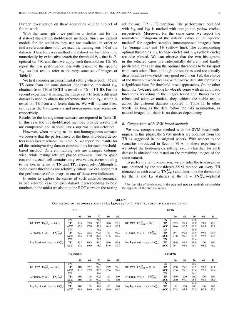
B. Comparison with SVM-based methods

We now compare our method with the SVM-based tech-niques. In this phase, the SVM models are obtained from theTR as suggested in the original papers. With respect to thescenarios introduced in Section VI-A, in these experimentswe adopt the homogenous setting, i.e., a classifier for eachdataset is obtained and tested on the remaining images of thesame dataset.

To perform a fair comparison, we consider the true negativerate obtained by the considered SVM method on every TR(denoted in each case as TNTR

SVM) and determine the thresholdsfor the λ and L0 statistics as the (1 − TNTR

SVM)-optimal

5For the sake of consistency, in the DCT and NOISE methods we considerthe opposite of the statistic values.

TABLE VCOMPARISON OF THE λ-TEST AND THE logL0-TEST TO [6] WITH TRUE NEGATIVE RATE MATCHING.

LIU

90 80 70 60 50

BF FFT, TNTRSVM = 74.8

TN 74.2TP 99.4 99.8 96.6 98.8 98.2

ACC 86.8 87.0 85.4 86.5 86.2

λ-test, τTR(1− TNTRSVM)

TN 75.2TP 97.2 98.8 99.4 100 99.2

ACC 86.2 87.0 87.3 87.6 87.2

logL0-test, τTR(1− TNTRSVM)

TN 78.2TP 96.0 99.8 99.6 99.6 99.8

ACC 87.1 89.0 88.9 88.9 89.0

UCID

90 80 70 60 50


TN 93.6TP 99.5 99.1 98.0 99.0 98.2

ACC 96.6 96.3 95.8 96.3 95.9


TN 96.0TP 99.7 99.7 99.9 99.9 99.9

ACC 97.8 97.8 97.9 97.9 97.9


TN 92.4TP 99.9 99.9 99.9 100 100

ACC 96.1 96.1 96.1 96.2 96.2

DRESDEN

90 80 70 60 50


TN 96.0TP 100 99.7 97.3 99.9 99.8

ACC 98.0 97.9 96.6 97.6 97.9


TN 100TP 100 100 99.7 100 100

ACC 100 100 99.9 100 100


TN 99.9TP 100 100 100 100 100

ACC 99.9 99.9 99.9 99.9 99.9

RAISE2K

90 80 70 60 50


TN 95.3TP 99.8 99.8 99.5 98.9 99.6

ACC 97.6 97.6 97.4 97.1 97.4


TN 96.1TP 99.9 100 100 100 100

ACC 98.0 98.0 98.0 98.0 98.0


TN 94.6TP 100 100 100 100 100

ACC 97.3 97.3 97.3 97.3 97.3


TABLE VICOMPARISON OF THE λ-TEST AND THE logL0-TEST TO [13] WITH TRUE NEGATIVE RATE MATCHING.

LIU

90 80 70 60 50

FSD, TNTRSVM = 92.8

TN 92.6TP 87.4 97.8 94.8 87.8 82.8

ACC 90.0 95.2 93.7 90.2 87.7


TN 92.6TP 87.6 98.6 98.6 99.4 99.0

ACC 90.1 95.6 95.6 96.0 95.8


TN 94.0TP 93.8 99.8 99.4 99.6 99.8

ACC 93.0 96.9 96.7 96.8 96.9

UCID

90 80 70 60 50

FSD, TNTRSVM = 97.6

TN 97.5TP 96.4 99.1 98.6 96.4 95.5

ACC 96.9 98.3 98.0 96.9 96.5


TN 98.8TP 99.4 99.6 99.9 99.9 99.9

ACC 99.1 99.2 99.3 99. 99.3


TN 99.5TP 99.9 99.9 99.9 99.7 100

ACC 99.6 99.7 99.7 99.6 99.8

DRESDEN

90 80 70 60 50

FSD, TNTRSVM = 99.7

TN 97.5TP 98.4 100 98.5 91.1 89.1

ACC 97.9 98.7 98.0 94.3 93.3


TN 100.0TP 100 100 99.7 100 100

ACC 100 100 99.9 100 100


TN 99.9TP 100 100 100 100 100

ACC 99.9 99.9 99.9 99.9 99.9

RAISE2K

90 80 70 60 50

FSD, TNTRSVM = 93.8

TN 99.2TP 86.3 96.8 98.5 94.4 91.4

ACC 92.8 98.0 98.9 96.8 95.3


TN 99.9TP 99.9 99.9 100 100 100

ACC 99.8 99.9 99.9 99.9 99.9


TN 100TP 99.9 99.8 100 100 100

ACC 99.9 99.9 100 100 100

threshold on TR, according to the definition given in SectionVI-A. In other words, we allow the false positive rate of ourmethod to be at most equal to the one obtained by the SVM-based method on the same TR. We indicate such thresholdas τTR(1− TNTR

SVM), in accordance with the previous section.The SVM classifiers and thresholds obtained are then appliedto the corresponding TS.

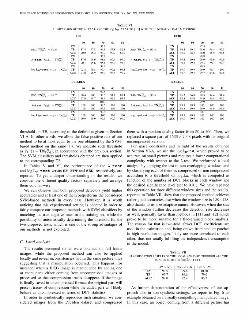
In Tables V and VI, the performance of the λ-testand logL0-test versus BF FFT and FSD, respectively, arereported. To get a deeper understanding of the results, weconsider the different quality factors separately and arrangethem column-wise.

We can observe that both proposed detectors yield higheraccuracies and at least one of them outperforms the consideredSVM-based methods in every case. However, it is worthnoticing that this experimental setting is adopted in order tofairly compare our proposed methods with SVM classifiers bymatching the true negative rates in the training set, while thepossibility of automatically determining the threshold for thetwo proposed tests, which is one of the strong advantages ofour methods, is not exploited.

C. Local analysis

The results presented so far were obtained on full frameimages, while the proposed method can also be appliedlocally and reveal inconsistencies within the same picture, thussuggesting that a manipulation occurred. This happens, forinstance, when a JPEG image is manipulated by adding oneor more parts either coming from uncompressed images orprocessed so that compression traces disappear. If the imageis finally saved in uncompressed format, the original part willpresent traces of compression while the added part will likelybehave as uncompressed in terms of DCT statistics.

In order to synthetically reproduce such situation, we con-sidered images from the Dresden dataset and compressed

them with a random quality factor from 50 to 100. Then, wereplaced a square part of 1536× 2048 pixels with its originaluncompressed version.

For space constraints and in light of the results obtainedin Section VI-A, we use the logL0-test, which proved to beaccurate on small pictures and requires a lower computationalcomplexity with respect to the λ-test. We performed a localanalysis by applying the test to non-overlapping windows andby classifying each of them as compressed or non compressedaccording to a threshold on logL0, which is computed asfunction of the number of DCT blocks in each window andthe desired significance level (set to 0.01). We have repeatedthis operation for three different window sizes and the results,reported in Table VII, show that the proposed method achievesrather good accuracies also when the window size is 128×128,also thanks to its size-adaptive nature. However, when the sizeof the window further decreases the detection rate decreasesas well, generally faster than methods in [11] and [12] whichprove to be more suitable for a fine-grained block analysis.The reason for that is two-fold: fewer DCT coefficients areused in the estimation and, being drawn from smaller patchesin high resolution images, likely are more correlated to eachother, thus not totally fulfilling the independence assumptionin the model.

TABLE VIICLASSIFICATION RESULTS OF THE LOCAL ANALYSIS THROUGH ALL THE

IMAGES WITH THE logL0-TEST .

512× 512 256× 256 128× 128TN 99.5 99.8 100.0TP 95.7 89.6 79.0

ACC 97.0 92.9 85.7

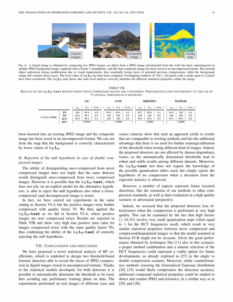
As further demonstration of the effectiveness of our ap-proach also in non-synthetic settings, we report in Fig. 6 anexample obtained on a visually compelling manipulated image.In this case, an object coming from a different picture has


Original images

Composite image

20 40 60 80 100 120 140 160 180

20

40

60

80

100

120

140

-250

-200

-150

-100

-50

0

20 40 60 80 100 120 140 160 180

20

40

60

80

100

120

140

-250

-200

-150

-100

-50

0

maplog L0

Fig. 6. A forged image is obtained by composing two JPEG images: an object from a JPEG image (downloaded from the web) has been superimposed onanother JPEG background image (captured with a Nexus 5 smartphone), and the final composite image has been saved in an uncompressed format. The insertedobject underwent strong modifications due to visual requirements, thus essentially losing traces of potential previous compressions, while the backgroundimage still contains those traces. The local value of logL0 has then been computed. Overlapping windows of 120×120 pixels with a stride equal to 2 pixelshave been considered. The logL0 map shows that such local analysis correctly identifies the different statistical properties within the image.

TABLE VIIIRESULTS OF THE logL0-TEST METHOD WHEN TWICE COMPRESSED IMAGES ARE CONSIDERED. PERFORMANCE LOSS WITH RESPECT TO THE USE OF

P -OPTIMAL THRESHOLDS IS REPORTED.

logL0-test

TNTP

ACCAUC

LIU

τaut τTS Loss

100 99.4 -0.698.6 99.1 0.598.8 99.2 0.4

0.9965

UCID

τaut τTS Loss

99.9 99.9 0.0100 100 0.0100 100 0.0

1.0000

DRESDEN

τaut τTS Loss

99.7 99.8 0.1100 100 0.099.9 99.9 0.0

1.0000

RAISE2K

τaut τTS Loss

94.9 100 4.6100 100 0.099.1 99.9 0.8

1.0000

been inserted into an existing JPEG image and the compositeimage has been saved in an uncompressed format. We can seefrom the map that the background is correctly characterizedby lower values of logL0.

D. Rejection of the null hypothesis in case of double com-pressed images

The ability of distinguishing once-compressed from nevercompressed images does not imply that the same detectorwould distinguish once-compressed from twice compressedimages. However, it is possible that the logL0-test, whichdoes not rely on an explicit model for the alternative hypoth-esis, is able to reject the null hypothesis also when a twice-compressed (and decompressed) image is tested.

In fact, we have carried out experiments in the samesetting as Section VI-A but the positive images were furthercompressed with quality factor 70. We then applied thelogL0-test as we did in Section VI-A, where positiveimages are now compressed twice. Results are reported inTable VIII and show very high true positive rates (also forimages compressed twice with the same quality factor 70),thus confirming the ability of the logL0-test of correctlyrejecting the null hypothesis.

VII. CONCLUSIONS AND DISCUSSION

We have proposed a novel statistical analysis of BF co-efficients, which is exploited to design two threshold-basedforensic detectors able to reveal the traces of JPEG compres-sion in digital images stored in uncompressed formats. Thanksto the statistical models developed, for both detectors it ispossible to automatically determine the threshold to be used,thus avoiding any preliminary training phase on data. Theexperiments performed on real images of different sizes and

source cameras show that such an approach yields to resultsthat are comparable to existing methods and has the additionaladvantage that there is no need for further training/calibrationof the threshold when testing different kind of images. Indeed,the proposed detectors are not affected by dataset-dependencyissues, as the automatically determined thresholds lead torobust and stable results among different datasets. Moreover,the logL0-test test does not require the knowledge ofthe possible quantization tables used, but simply rejects thehypothesis of no compression when a deviation from theexpected statistics is observed.

However, a number of aspects represent future researchdirections, like the extension of our methods to other com-pression standards, as well as their evaluation in a high qualityscenario or adversarial perspective.

Indeed, we assessed that the proposed detectors lose ef-fectiveness when the compression is performed at very highquality. This can be explained by the fact that high factors(≥ 94/95) involve very small quantization steps (often equalto 1 for the DCT frequencies used), which result in verysimilar statistical properties between never compressed andcompressed/dequantized images so that the model assumed inSection IV-B might not be accurate. Given the good perfor-mance obtained by techniques like [11] also in this scenario,a proper method combination and a smarter selection of theDCT frequencies could represent a viable option for futuredevelopments, as already explored in [27] in the single vsdouble compression scenario. Moreover, while counterforen-sics methods restoring the Generalized Gaussian distribution[28] [15] would likely compromise the detection accuracy,additional compound statistical properties could be studied todetect and counter JPEG anti-forensics, in a similar way as in[29] and [30].


Finally, the encouraging results obtained in Section VI-D,as well as in the work [21], confirm the effectiveness of BFcoefficients in characterizing DCT coefficients. This suggeststhat future work should be devoted to the analysis of morecomplex scenarios involving multiple JPEG compression andother processing operations [31], [32].

ACKNOWLEDGEMENT

We would like to thank Dr. Bin Li and Dr. Janquiang Yangfor kindly providing us with the code of their methods in [11]and [12], respectively.

APPENDIX ADERIVATION OF σ2

Wr,i

In order to obtain the variance of Wr,i, we need to considerthe pdf of Zq and study the real and imaginary parts of the r.v.e−j2πn log10 Zq , i.e., the r.v.’s C .

= cos(2πn log10 Zq) and S .=

− sin(2πn log10 Zq), respectively. For the sake of simplicity,in the following analysis we drop the subscript q of Z. Forderiving the pdf of C, the following r.v. transformations needto be applied

Zlog10−→ Z ′

·2πn−→ Z ′′cos−→ C

and the same happens for S by applying − sin(·) as lasttransformation.

Since they are monotonic, the first two transformations canbe treated with the formula

fY (y) = fX(h−1(y))·∣∣∣∣ ∂∂yh−1(y)

∣∣∣∣ , Y = h(X), X ∼ fX(x)

and we obtain

fZ′′(z′′) = L(10z′′2πn ) · 10

z′′2πn · log 10

2πn.

The third transformation is not monotonic and a generaliza-tion of formula (A) should be used [33]:

fY (y) =∑

{x|h(x)=y}

fX(x)∣∣ ∂∂xh(x)

∣∣ (20)

So, if we define IZ′′ = [2πn log10(q− q/2), 2πn log10(q+q/2)[, we have that

fC(c) =∑

{z′′|cos(z′′)=c}∩IZ′′

fZ′′(z′′)| − sin z′′|

=∑Dc

e−√

2σ |10

z′′2πn−q|10

z′′2πn log 10

σ√

2Nσ,q2πn

1√1− c2

where

Dc = {z′′| cos(z′′) = c} ∩ IZ′′

= ∪i∈Z{2πi+ t, 2π(i+ 1)− t} ∩ IZ′′ ,

t.= arccos(c).

By definition, the variance of C is given by

σ2C =

1∫−1

c2fC(c)dc− µ2C (21)

=

1∫−1

c2∑

z′′∈Dc

e−√

2σ|10

z′′2πn−q|10

z′′2πn

σ√2Nσ,q2πn

log 10√1− c2

dc−<(an,q)2.

(22)

The variance σ2S of S is obtained similarly by replacing c

with s in the first integral and recalling that µS = =(an,q).Finally, in order to get the variance of the real and imaginaryparts of W0,q = An,q − an,q we should consider that it is ashift (i.e., has the same variance) of An,q , the sample mean ofe−j2πn log10 Zq computed from Mq samples. By applying theCentral Limit Theorem on real and imaginary parts, we have:

σ2Wr

=σ2C

Mq, σ2

Wi=

σ2S

Mq. (23)

APPENDIX BMEAN AND VARIANCE OF logL0

We can reformulate expression (19) as follows

logL0 = #F · log (2M) +∑f∈F

log |Afn|︸︷︷︸Lf

−M |Afn|2︸︷︷︸Bf

︸︷︷︸

Sf

(24)

The r.v.’s |afn| are i.i.d. (assuming independency among DCTfrequencies) and they follow a Rayleigh distribution with scaleparameter σ = 1/

√2M . Starting from this we can study Lf ,

Bf and Sf .• Each Lf is a log-Rayleigh random variable. According

to [34], we have that

E{Lf} = − logM

2− γ

2, V ar{Lf} =

π2

24,

where γ is the Euler-Mascheroni constant.• Each Bf is a squared Rayleigh r.v. multiplied by a con-

stant term −M . It can be shown (via r.v. transformation)that a squared Rayleigh r.v. with scale parameter σ hasan exponential distribution with rate parameter 1/2σ2 (inour case M ). By scaling with a factor −M , we have that

E{Bf} = −1, V ar{Bf} = 1.

• Each Sf ’s is sum of two r.v., hence we have that

E{Sf} = E{Lf}+ E{Bf} = − logM

2− γ

2− 1,

V ar{Sf} =V ar{Lf}+V ar{Bf}+2Cov{Lf , Bf}=π2

24as the value of the covariance has been derived by meansof symbolic computation and is equal to −1/2.

• Finally, logL0 is a sum of the iid r.v.’s Sf plus a constantterm #F · log (2M). Then, we have that

E{logL0} = #F · log (2M)−#F ·(

logM

2+γ

2+ 1

),

V ar{logL0} = #F · π2

24.


REFERENCES

[1] H. Sencar and N. Memon, Eds., Digital Image Forensics - There is moreto a picture than meets the eye. Springer, 2013.

[2] A. Rocha, W. Scheirer, T.Boult, and S. Goldenstein, “Vision of the un-seen: current trends and challenges in digital image and video forensics,”ACM Computing Surveys, vol. 43, no. 4, 2011.

[3] M. Stamm, M. Wu, and K. Liu, “Information forensics: an overview ofthe first decade,” IEEE Access, pp. 167–200, 2013.

[4] I. Steadman. (2013, May) “Fake” World Press Photo isn’tfake, is lesson in need for forensic restraint. [Online]. Avail-able: http://www.wired.co.uk/news/archive/2013-05/16/photo-faking-controversy

[5] G. Scoblete. (2015, June) How World Press Photo catches image ma-nipulators. [Online]. Available: http://www.pdnonline.com/news/How-World-Press-Photo-Catches-Image-Manipulators-13819.shtml

[6] F. Perez-Gonzalez, T. Quach, S. J. Miller, C. Abdallah, and G. Heileman,“Application of Benford’s law to images,” S. J. Miller, A. Berger andT. Hill (Eds), The Theory and Applications of Benford’s law, PrincetonUniversity Press, 2015.

[7] C. Pasquini, F. Perez-Gonzalez, and G. Boato, “A Benford-Fourier JPEGcompression detector,” in Proc. of IEEE ICIP, 2014, pp. 5322–5326.

[8] Z. Fan and R. D. Queiroz, “Identification of bitmap compression history:JPEG detection and quantizer estimation,” IEEE Transactions on ImageProcessing, vol. 12, n. 2, pp. 230–235, 2003.

[9] R. Neelamani, R. D. Queiroz, Z. Fan, S. Dash, and R. Baraniuk, “JPEGcompression history estimation for color images,” IEEE Transactions onImage Processing, vol. 15, n. 2, pp. 1363–1378, 2006.

[10] W. Luo, J. Huang, and G. Qiu, “JPEG error analysis and its applicationsto digital image forensics,” IEEE Transactions on Information Forensicsand Security, vol. 5, no. 3, pp. 480–491, 2010.

[11] B. Li, T.-T. Ng, X. Li, S. Tan, and J. Huang, “Revealing the trace of high-quality JPEG compression through quantization noise analysis,” IEEETransactions on Information Forensics and Security, vol. 10, no. 3, pp.558–573, 2015.

[12] J. Yang, G. Zhu, J. Huang, and X. Zhao, “Estimating JPEG compressionhistory of bitmaps based on factor histogram,” Digital Signal Processing,no. 41, pp. 90–97, 2015.

[13] D. Fu, Y. Shi, and W. Su, “A generalized Benford’s law for JPEGcoefficients and its applications in image forensics,” in SPIE Conferenceon Security, Steganography, and Watermarking of Multimedia Contents,vol. 6505, 2007.

[14] F. Perez-Gonzalez, G. Heileman, and C. Abdallah, “Benford’s law inimage processing,” in Proc. of IEEE ICIP, 2007, pp. 405–408.

[15] C. Pasquini and G. Boato, “JPEG compression anti-forensics based onfirst significant digit distribution,” in Proc. of IEEE MMSP, 2013, pp.500–505.

[16] P. Comesana-Alfaro and F. Perez-Gonzalez, “The optimal attack tohistogram-based forensic detectors is simple(x),” in Proc. of IEEE WIFS,2014, pp. 1730–1735.

[17] T. Birney and T. Fischer, “On the modeling of DCT and subband imagedata for compression,” IEEE Transactions on Image Processing, vol. 4,no. 2, pp. 186–193, 1995.

[18] J. Barry, E. Lee, and D. Messerschmitt, “Digital communication,”Springer, 2004.

[19] S. Rice, “Mathematical analysis of random noise,” Bell System TechnicalJournal, vol. 24, pp. 46–156, 1945.

[20] T. Bianchi and A. Piva, “Image forgery localization via block-grainedanalysis of JPEG artifacts,” IEEE Transactions on Information Forensicsand Security, vol. 7, n. 3, pp. 1003–1017, 2012.

[21] C. Pasquini, G. Boato, and F. Perez-Gonzalez, “Multiple JPEG com-pression detection by means of Benford-Fourier coefficients,” in Proc.of IEEE WIFS, 2014, pp. 113–118.

[22] J. Havil, Gamma: exploring Euler’s constant, ser. Princeton ScienceLibrary. Princeton University Press, 2009.

[23] Q. Liu, “Detection of misaligned cropping and recompression with thesame quantization matrix and relevant forgery,” in ACM Workshop onMultimedia Forensics and Intelligence, 2011, pp. 25–30.

[24] G. Schaefer and M. Stich, “UCID - An uncompressed colour imagedatabase,” in SPIE Storage and Retrieval Methods and Applications toMultimedia, vol. 5307, 2004.

[25] T. Gloe and R. Boehme, “The Dresden image database for benchmarkingdigital image forensics,” in ACM Symposium on Applied Computing,vol. 2, 2010, pp. 1585–1591.

[26] D.-T. Dang-Nguyen, C. Pasquini, V. Conotter, and G. Boato, “RAISE- a raw images dataset for digital image forensics,” in Proc. of ACMMMSys, 2015, pp. 219–224.

[27] C. Pasquini, P. Schottle, R. Bohme, G. Boato, and F. Perez-Gonzalez,“Forensics of high quality and nearly identical JPEG image recompres-sion,” in ACM Information Hiding & Multimedia Security (IH&MMSec),2016, pp. 11–21.

[28] M. Stamm and K. J. Ray Liu, “Anti-forensics of digital image compres-sion,” IEEE Transactions on Information Forensics and Security, vol. 6,no. 3, pp. 1050–1065, 2011.

[29] M. Kirchner and S. Chakraborty, “A second look at first significant digithistogram restoration,” in Proc. of IEEE WIFS, 2015, pp. 1–6.

[30] A. De Rosa, M. Fontani, M. Massai, A. Piva, and M. Barni, “Second-order statistics analysis to cope with contrast enhancement counter-forensics,” IEEE Signal Processing Letters, vol. 22, no. 8, pp. 1132–1136, 2015.

[31] T. Bianchi and A. Piva, “Reverse engineering of double JPEG compres-sion in the presence of image resizing,” in Proc. of IEEE WIFS, 2012,pp. 127–132.

[32] Q. Liu, “An approach to detecting JPEG down-recompression and seamcarving forgery under recompression anti-forensics,” Pattern Recogni-tion, vol. 65, pp. 35–46, 2016.

[33] H. Kobayashi, B. Mark, and W. Turin, Probability, Random Processesand Statistical Analysis. Cambridge University Press, 1991.

[34] B. Rivet, L. Girin, and C. Jutten, “Log-Rayleigh distribution: a simpleand efficient statistical representation of log-spectral coefficients,” IEEETransactions on Audio, Speech, and Language Processing, vol. 15, no. 3,2007.

Cecilia Pasquini is a Post-Doctoral Researcher atthe Privacy and Security Lab with the UniversitatInnsbruck, Austria, and University of Munster, Ger-many. She received the Ph.D. degree from the Uni-versity of Trento, Italy, in 2016. She has been aVisiting Scholar with the University of Vigo, Spain,in 2013. Her research interests include multimediaforensics and anti-forensics, multimedia analysis andverification.

Giulia Boato is an Assistant Professor with the De-partment of Information Engineering and ComputerScience, University of Trento, Italy, where she hasbeen coordinating the Multimedia Signal Processingand Understanding Lab from 2008 to 2011. She wason the project staff of many projects (FP7 FET-IPLIVINGKNOWLEDGE, FP7 IP GLOCAL, FP7 CAETERNALS, and ICT-COST 3D-ConTourNet). Shehas co-authored 85 papers in international confer-ences and journals. Her research interests includeimage and signal processing, with particular atten-

tion to multimedia data protection, data hiding and digital forensics but alsointelligent multidimensional data management and analysis.

Fernando Perez-Gonzalez (M’90–SM’09–F’16) isa Professor with the School of TelecommunicationEngineering, University of Vigo, Spain, and alsoa Research Professor in information science andtechnology with the University of New Mexico,USA. From 2007 to 2010, he was Program Managerof the Spanish National Research and DevelopmentPlan on Electronic and Communication Technolo-gies, Ministry of Science and Innovation. From 2007to 2014, he was the Executive Director of the Gali-cian Research and Development Center in Advanced

Telecommunications. He has co-authored over 60 papers in internationaljournals, 160 conference papers and several international patents. His researchinterests include the areas of digital communications, adaptive algorithms,privacy enhancing technologies, and information forensics and security.

Statistical detection of JPEG traces in digital images in ...

Documents

Transcript of Statistical detection of JPEG traces in digital images in ...