IMAGE RECONSTRUCTION IN HIGH-RESOLUTION PET
195
-
Upload
khangminh22 -
Category
Documents
-
view
1 -
download
0
Transcript of IMAGE RECONSTRUCTION IN HIGH-RESOLUTION PET

IMAGE RECONSTRUCTION IN HIGH-RESOLUTION PET:
GPU-ACCELERATED STRATEGIES FOR IMPROVING IMAGE QUALITY
AND ACCURACY
A DISSERTATION
SUBMITTED TO THE DEPARTMENT OF ELECTRICAL ENGINEERING
AND THE COMMITTEE ON GRADUATE STUDIES
OF STANFORD UNIVERSITY
IN PARTIAL FULFILLMENT OF THE REQUIREMENTS
FOR THE DEGREE OF
DOCTOR OF PHILOSOPHY
Guillem Pratx
December 2009

http://creativecommons.org/licenses/by-nc/3.0/us/
This dissertation is online at: http://purl.stanford.edu/vz692jm2943
© 2010 by Guillem Pratx. All Rights Reserved.
Re-distributed by Stanford University under license with the author.
This work is licensed under a Creative Commons Attribution-Noncommercial 3.0 United States License.
ii

I certify that I have read this dissertation and that, in my opinion, it is fully adequatein scope and quality as a dissertation for the degree of Doctor of Philosophy.
Craig Levin, Primary Adviser
I certify that I have read this dissertation and that, in my opinion, it is fully adequatein scope and quality as a dissertation for the degree of Doctor of Philosophy.
Patrick Hanrahan
I certify that I have read this dissertation and that, in my opinion, it is fully adequatein scope and quality as a dissertation for the degree of Doctor of Philosophy.
John Pauly
Approved for the Stanford University Committee on Graduate Studies.
Patricia J. Gumport, Vice Provost Graduate Education
This signature page was generated electronically upon submission of this dissertation in electronic format. An original signed hard copy of the signature page is on file inUniversity Archives.
iii

Abstract
Molecular imaging can interrogate subtle molecular disease signatures non-invasively in liv-
ing subjects. Positron emission tomography (PET), one particular molecular imaging modal-
ity, is able to sense molecular signals deep within tissue. Although PET is well suited for
imaging signals associated with cancerous lesions in humans, it is still unable to resolve
very small (<2 mm) structures. Improving the spatial resolution of PET is an active area
of research driven by many potential applications. However, the new generation of high-
resolution PET systems raise new challenges for image reconstruction.
In this dissertation, several strategies and algorithms are proposed to enable accurate
and practical image reconstruction for high-resolution PET. Reconstruction is performed di-
rectly from the list-mode data via maximum-likelihood estimation. A shift-varying model of
the imaging process is incorporated in the reconstruction. For fast reconstruction, the calcu-
lations are implemented using highly-parallel graphics processing units (GPU). A Bayesian
sequence reconstruction algorithm is also used to position the annihilation photons that
deposit energy in multiple detection elements.
We show that the reconstruction provides near-uniform spatial resolution throughout the
eld-of-view, enhanced trade-o between noise and contrast, and better image quantitative
accuracy. Furthermore, thanks to the computing power of graphics hardware, reconstruction
times are practical for clinical applications.
iv

Acknowledgement
This work would not have been possible without the support of my coworkers, and the help
and love from my friends, family and wife.
In particular, I am very grateful to my dissertation adviser Craig Levin, a passionate
teacher never reluctant to share his knowledge. I thank him for his availability and his
dedication to help me achieve my goals. Also, I was lucky to share the lab with a band
of great people: Alex, Angela, Arne, Eric, Frances, Frezghi, Garry, Hao, Jing-Yu, Jinjiang,
Paul, Peter, Virginia, and Yi. I am grateful to you all for these intense discussions from
which I learned so much, for the help I received conducting experiments, for reviewing my
dissertation, for the basketball games, and for sometimes watching over my cats during the
holidays.
I also gratefully acknowledge the institutional support that I have received while working
on this project. In particular, I thank the Bio-X program for their generous graduate
fellowship program, that has allowed me to perform research in the best conditions possible.
I also thank the NVIDIA Corporation for providing funds and state-of-the-art equipment
for my research. This work would also not have been possible without support from the
National Institutes of Health.
Last, I want to give special thanks to my familyJean-Max, Marie-Paule, Thomas, and
Annewhose permanent support has helped me so much. These lines would be incomplete
without a word for my dear wife Lindsey, for her love, patience, and support over the years.
v
Contents
Abstract iv
Acknowledgement v
1 Introduction 1
1.1 Molecular Imaging . . . . . . . . . . . . . . . . . . . . . . . . . . . . . . . . . 1
1.2 Principles of PET . . . . . . . . . . . . . . . . . . . . . . . . . . . . . . . . . . 3
1.3 High-Resolution PET Systems . . . . . . . . . . . . . . . . . . . . . . . . . . 6
1.3.1 Overview . . . . . . . . . . . . . . . . . . . . . . . . . . . . . . . . . . 6
1.3.2 Pre-Clinical PET System . . . . . . . . . . . . . . . . . . . . . . . . . 7
1.3.3 Breast Cancer PET System . . . . . . . . . . . . . . . . . . . . . . . . 8
1.4 Image Reconstruction Challenges . . . . . . . . . . . . . . . . . . . . . . . . . 9
1.4.1 Image Reconstruction Complexity . . . . . . . . . . . . . . . . . . . . 9
1.4.2 Shift-Varying System Response . . . . . . . . . . . . . . . . . . . . . . 11
1.4.3 Multiple-Interaction Photon Events . . . . . . . . . . . . . . . . . . . 13
1.5 Overview of this Work . . . . . . . . . . . . . . . . . . . . . . . . . . . . . . . 14
2 Imaging Model for High-Resolution PET 16
2.1 Principles and Theory . . . . . . . . . . . . . . . . . . . . . . . . . . . . . . . 16
2.1.1 Physics of PET . . . . . . . . . . . . . . . . . . . . . . . . . . . . . . . 16
2.1.1.1 Photon Emission . . . . . . . . . . . . . . . . . . . . . . . . . 16
2.1.1.2 Photon Detection . . . . . . . . . . . . . . . . . . . . . . . . 17
2.1.1.3 Photon Transport . . . . . . . . . . . . . . . . . . . . . . . . 19
2.1.1.4 Mathematical Model . . . . . . . . . . . . . . . . . . . . . . . 20
2.1.2 Spatially Variant and Invariant Models for Discrete Image Represen-
tations . . . . . . . . . . . . . . . . . . . . . . . . . . . . . . . . . . . 22
2.2 Analytical Calculation of the Coincident Detector Response Function . . . . 24
vi

2.3 Approximation for Small Crystals . . . . . . . . . . . . . . . . . . . . . . . . . 27
2.3.1 Fast Calculation of Intrinsic Detector Response Function . . . . . . . . 27
2.3.2 Analytical Scaled Convolution . . . . . . . . . . . . . . . . . . . . . . . 30
2.4 Results . . . . . . . . . . . . . . . . . . . . . . . . . . . . . . . . . . . . . . . . 31
2.5 Summary and Discussion . . . . . . . . . . . . . . . . . . . . . . . . . . . . . . 34
3 Maximum-Likelihood Image Reconstruction 36
3.1 Background . . . . . . . . . . . . . . . . . . . . . . . . . . . . . . . . . . . . . 36
3.1.1 Analytical Methods . . . . . . . . . . . . . . . . . . . . . . . . . . . . 36
3.1.2 Statistical Methods . . . . . . . . . . . . . . . . . . . . . . . . . . . . . 37
3.1.2.1 Maximum Likelihood . . . . . . . . . . . . . . . . . . . . . . 38
3.1.2.2 Maximum A Posteriori . . . . . . . . . . . . . . . . . . . . . 38
3.1.2.3 Other Objective Functions . . . . . . . . . . . . . . . . . . . 39
3.1.3 Existing Optimization Methods . . . . . . . . . . . . . . . . . . . . . . 39
3.1.3.1 Expectation-Maximization for ML reconstruction . . . . . . 39
3.1.3.2 Ordered-Subset Expectation-Maximization for ML reconstruc-
tion . . . . . . . . . . . . . . . . . . . . . . . . . . . . . . . . 40
3.1.3.3 List-Mode Processing . . . . . . . . . . . . . . . . . . . . . . 41
3.1.3.4 Gradient Ascent for ML reconstruction . . . . . . . . . . . . 42
3.1.3.5 Conjugate Gradient for WLS Reconstruction . . . . . . . . . 43
3.1.3.6 Conjugate Gradient for ML Reconstruction . . . . . . . . . . 46
3.2 Novel ML Conjugation of Search Directions . . . . . . . . . . . . . . . . . . . 46
3.2.1 Conjugation in ML-CG . . . . . . . . . . . . . . . . . . . . . . . . . . 47
3.2.2 Explicit Conjugation of Search Directions . . . . . . . . . . . . . . . . 48
3.2.3 Results . . . . . . . . . . . . . . . . . . . . . . . . . . . . . . . . . . . 49
3.2.4 Discussion . . . . . . . . . . . . . . . . . . . . . . . . . . . . . . . . . . 50
3.3 Novel ML Reconstruction via Truncated Newton's Method . . . . . . . . . . 53
3.3.1 Dual Problem . . . . . . . . . . . . . . . . . . . . . . . . . . . . . . . . 53
3.3.2 KarushKuhnTucker Conditions . . . . . . . . . . . . . . . . . . . . . 54
3.3.3 Newton Step for a Relaxed Problem . . . . . . . . . . . . . . . . . . . 55
3.3.4 Preconditioning . . . . . . . . . . . . . . . . . . . . . . . . . . . . . . . 57
3.3.5 Results . . . . . . . . . . . . . . . . . . . . . . . . . . . . . . . . . . . 57
3.4 Discussion . . . . . . . . . . . . . . . . . . . . . . . . . . . . . . . . . . . . . . 58
vii
4 Fast Shift-Varying Line Projection using Graphics Hardware 61
4.1 Background . . . . . . . . . . . . . . . . . . . . . . . . . . . . . . . . . . . . . 61
4.1.1 The Graphics Processing Unit . . . . . . . . . . . . . . . . . . . . . . . 61
4.1.2 Iterative Reconstruction on the GPU . . . . . . . . . . . . . . . . . . . 64
4.2 Theory . . . . . . . . . . . . . . . . . . . . . . . . . . . . . . . . . . . . . . . . 65
4.2.1 System Response Kernel . . . . . . . . . . . . . . . . . . . . . . . . . . 65
4.2.2 GPU Implementation . . . . . . . . . . . . . . . . . . . . . . . . . . . 66
4.2.2.1 Data Representation . . . . . . . . . . . . . . . . . . . . . . . 66
4.2.2.2 Line Projection Stages . . . . . . . . . . . . . . . . . . . . . . 67
4.2.2.3 Voxel Identication in Line Forward Projection . . . . . . . 67
4.2.2.4 Voxel Identication in Line Backprojection . . . . . . . . . . 70
4.2.2.5 Kernel Evaluation . . . . . . . . . . . . . . . . . . . . . . . . 71
4.2.2.6 Vector Data Update . . . . . . . . . . . . . . . . . . . . . . . 72
4.3 Discussion . . . . . . . . . . . . . . . . . . . . . . . . . . . . . . . . . . . . . . 73
5 Applications of GPU-Based Line Projections 75
5.1 Overview . . . . . . . . . . . . . . . . . . . . . . . . . . . . . . . . . . . . . . 75
5.2 List-Mode OSEM with Shift-Invariant Projections . . . . . . . . . . . . . . . 75
5.2.1 Shift-Invariant System Response Kernel . . . . . . . . . . . . . . . . . 75
5.2.2 Methods . . . . . . . . . . . . . . . . . . . . . . . . . . . . . . . . . . . 76
5.2.2.1 Simulation Data . . . . . . . . . . . . . . . . . . . . . . . . . 76
5.2.2.2 Validation: Experimental Pre-Clinical Data . . . . . . . . . . 78
5.2.3 Results . . . . . . . . . . . . . . . . . . . . . . . . . . . . . . . . . . . 79
5.2.4 Discussion . . . . . . . . . . . . . . . . . . . . . . . . . . . . . . . . . . 83
5.3 List-mode OSEM with Shift-Varying Projections . . . . . . . . . . . . . . . . 85
5.3.1 Methods . . . . . . . . . . . . . . . . . . . . . . . . . . . . . . . . . . . 85
5.3.1.1 Implementation . . . . . . . . . . . . . . . . . . . . . . . . . 85
5.3.1.2 Evaluation . . . . . . . . . . . . . . . . . . . . . . . . . . . . 86
5.3.2 Results . . . . . . . . . . . . . . . . . . . . . . . . . . . . . . . . . . . 87
5.3.2.1 Resolution . . . . . . . . . . . . . . . . . . . . . . . . . . . . 87
5.3.2.2 Contrast . . . . . . . . . . . . . . . . . . . . . . . . . . . . . 88
5.3.2.3 Reconstruction Time . . . . . . . . . . . . . . . . . . . . . . . 90
5.3.3 Discussion . . . . . . . . . . . . . . . . . . . . . . . . . . . . . . . . . . 92
5.4 Time-of-ight PET Reconstruction . . . . . . . . . . . . . . . . . . . . . . . . 93
5.4.1 Background . . . . . . . . . . . . . . . . . . . . . . . . . . . . . . . . . 93
5.4.2 Methods . . . . . . . . . . . . . . . . . . . . . . . . . . . . . . . . . . . 95
viii
5.4.2.1 System Description . . . . . . . . . . . . . . . . . . . . . . . 95
5.4.2.2 Implementation on the GPU . . . . . . . . . . . . . . . . . . 95
5.4.2.3 Phantom Experiment . . . . . . . . . . . . . . . . . . . . . . 96
5.4.3 Results . . . . . . . . . . . . . . . . . . . . . . . . . . . . . . . . . . . 98
5.4.3.1 Contrast vs. Noise . . . . . . . . . . . . . . . . . . . . . . . . 98
5.4.3.2 Processing Time . . . . . . . . . . . . . . . . . . . . . . . . . 99
5.4.4 Discussion . . . . . . . . . . . . . . . . . . . . . . . . . . . . . . . . . . 101
5.5 Summary . . . . . . . . . . . . . . . . . . . . . . . . . . . . . . . . . . . . . . 101
6 Bayesian Reconstruction of Photon Interaction Sequences 103
6.1 Background . . . . . . . . . . . . . . . . . . . . . . . . . . . . . . . . . . . . . 103
6.1.1 Motivation . . . . . . . . . . . . . . . . . . . . . . . . . . . . . . . . . 103
6.1.2 Methods to Position Multiple Interaction Photon Events . . . . . . . . 104
6.1.2.1 Initial Interaction Selection. . . . . . . . . . . . . . . . . . . . 104
6.1.2.2 Unconstrained Positioning. . . . . . . . . . . . . . . . . . . . 104
6.1.2.3 Full Sequence Reconstruction. . . . . . . . . . . . . . . . . . 105
6.2 Theory . . . . . . . . . . . . . . . . . . . . . . . . . . . . . . . . . . . . . . . . 105
6.2.1 Maximum-Likelihood . . . . . . . . . . . . . . . . . . . . . . . . . . . . 106
6.2.2 Maximum A Posteriori . . . . . . . . . . . . . . . . . . . . . . . . . . . 109
6.3 Evaluation Methodology . . . . . . . . . . . . . . . . . . . . . . . . . . . . . . 112
6.3.1 Simulation of a CZT PET System . . . . . . . . . . . . . . . . . . . . 112
6.3.2 Positioning Algorithms and Figures of Merit Used . . . . . . . . . . . 113
6.4 Results . . . . . . . . . . . . . . . . . . . . . . . . . . . . . . . . . . . . . . . . 116
6.4.1 Recovery Rate . . . . . . . . . . . . . . . . . . . . . . . . . . . . . . . 116
6.4.2 Point-Spread Function . . . . . . . . . . . . . . . . . . . . . . . . . . . 118
6.4.3 Reconstructed Contrast . . . . . . . . . . . . . . . . . . . . . . . . . . 118
6.4.4 Reconstructed Sphere Resolution . . . . . . . . . . . . . . . . . . . . . 121
6.5 Discussion . . . . . . . . . . . . . . . . . . . . . . . . . . . . . . . . . . . . . . 124
6.5.1 Performance of Proposed Scheme . . . . . . . . . . . . . . . . . . . . . 124
6.5.2 Limitations . . . . . . . . . . . . . . . . . . . . . . . . . . . . . . . . . 126
6.5.3 Possible Extensions . . . . . . . . . . . . . . . . . . . . . . . . . . . . . 127
6.6 Summary . . . . . . . . . . . . . . . . . . . . . . . . . . . . . . . . . . . . . . 128
7 Concluding Remarks, Future Directions 129
ix

A GPU Line Projections 131
A.1 Data Representation . . . . . . . . . . . . . . . . . . . . . . . . . . . . . . . . 131
A.1.1 Images . . . . . . . . . . . . . . . . . . . . . . . . . . . . . . . . . . . 131
A.1.2 List-Mode Data . . . . . . . . . . . . . . . . . . . . . . . . . . . . . . 131
A.2 Line Forward Projection . . . . . . . . . . . . . . . . . . . . . . . . . . . . . 133
A.3 Line Backprojection . . . . . . . . . . . . . . . . . . . . . . . . . . . . . . . . 134
B File Formats 145
B.1 List Mode and Histogram Mode . . . . . . . . . . . . . . . . . . . . . . . . . . 145
B.2 Image Files . . . . . . . . . . . . . . . . . . . . . . . . . . . . . . . . . . . . . 146
B.3 Colormap Files . . . . . . . . . . . . . . . . . . . . . . . . . . . . . . . . . . . 146
C User Manual 147
C.1 Command Line Options . . . . . . . . . . . . . . . . . . . . . . . . . . . . . . 147
C.2 Conguration File . . . . . . . . . . . . . . . . . . . . . . . . . . . . . . . . . 147
C.3 Interactive-Mode Commands . . . . . . . . . . . . . . . . . . . . . . . . . . . 148
D Gamma Camera Acquisition Software 150
D.1 Background . . . . . . . . . . . . . . . . . . . . . . . . . . . . . . . . . . . . . 150
D.2 Hardware . . . . . . . . . . . . . . . . . . . . . . . . . . . . . . . . . . . . . . 151
D.3 Software . . . . . . . . . . . . . . . . . . . . . . . . . . . . . . . . . . . . . . . 151
D.3.1 Initialization . . . . . . . . . . . . . . . . . . . . . . . . . . . . . . . . 152
D.3.2 Flood Acquisition . . . . . . . . . . . . . . . . . . . . . . . . . . . . . . 152
D.3.3 Automatic Peak Finding . . . . . . . . . . . . . . . . . . . . . . . . . . 153
D.3.4 Peak Manual Adjustment . . . . . . . . . . . . . . . . . . . . . . . . . 154
D.3.5 Automatic Peak Sorting . . . . . . . . . . . . . . . . . . . . . . . . . . 154
D.3.6 Crystal Segmentation and Energy Gating . . . . . . . . . . . . . . . . 154
D.3.7 Camera Performance Analysis . . . . . . . . . . . . . . . . . . . . . . . 157
D.3.8 Real-Time Imaging . . . . . . . . . . . . . . . . . . . . . . . . . . . . . 157
D.3.8.1 Accumulation Mode . . . . . . . . . . . . . . . . . . . . . . . 157
D.3.8.2 Dynamic Mode . . . . . . . . . . . . . . . . . . . . . . . . . . 157
D.4 User's Commands . . . . . . . . . . . . . . . . . . . . . . . . . . . . . . . . . . 159
E Analysis of Reconstructed Sphere Size 160
F Glossary of Terms 163
x

Bibliography 166
xi

List of Tables
3.1 Example of histogram-mode and list-mode datasets . . . . . . . . . . . . . . 42
5.1 Reconstruction time for GPU and CPU . . . . . . . . . . . . . . . . . . . . . 83
5.2 Reconstruction time on GPU with and without shift-varying model . . . . . . 91
5.3 Processing time for list-mode TOF reconstruction . . . . . . . . . . . . . . . . 100
6.1 Recovery rate for MAP and MPD positioning for four datasets . . . . . . . . 117
6.2 Recovery rate as a function of the number of interactions . . . . . . . . . . . . 117
6.3 Recovery rate as a function of system parameters . . . . . . . . . . . . . . . . 117
6.4 Recovery rate for MAP for stochastic and deterministic objectives . . . . . . . 117
C.1 Command-line options . . . . . . . . . . . . . . . . . . . . . . . . . . . . . . . 148
C.2 Interactive shortcuts . . . . . . . . . . . . . . . . . . . . . . . . . . . . . . . . 149
xii

List of Figures
1.1 Basic principles of PET imaging . . . . . . . . . . . . . . . . . . . . . . . . . 5
1.2 High-resolution small-animal PET scanner based on CZT detectors . . . . . . 7
1.3 High-resolution PET camera for breast cancer . . . . . . . . . . . . . . . . . . 8
1.4 Trend in the number of LORs for PET systems . . . . . . . . . . . . . . . . . 10
1.5 Depiction of parallax error in ring-shaped PET systems. . . . . . . . . . . . 11
1.6 Depiction and eect of spatially-varying spatial resolution in a box-shaped
system. . . . . . . . . . . . . . . . . . . . . . . . . . . . . . . . . . . . . . . . 12
1.7 Comparison of resolution at the center at the center of a ring and a box-shaped
PET system . . . . . . . . . . . . . . . . . . . . . . . . . . . . . . . . . . . . 12
1.8 Example of mispositioning caused by multiple-interaction photon event . . . . 14
2.1 Depiction of positron emission and positron range . . . . . . . . . . . . . . . 17
2.2 Intrinsic detector response function . . . . . . . . . . . . . . . . . . . . . . . 18
2.3 The three types of coincidences in PET . . . . . . . . . . . . . . . . . . . . . 21
2.4 Depiction of the system matrix . . . . . . . . . . . . . . . . . . . . . . . . . . 23
2.5 Geometry used for calculating the CDRF . . . . . . . . . . . . . . . . . . . . 25
2.6 2-D vs 3-D system response kernels . . . . . . . . . . . . . . . . . . . . . . . . 26
2.7 Representation of the detection length and the attenuation length . . . . . . 28
2.8 Comparison of the intrinsic detector response function for a small CZT crystal
and a larger LSO crystal . . . . . . . . . . . . . . . . . . . . . . . . . . . . . . 29
2.9 Decomposition of the coincidence detector response function into the sum of
nine elementary functions . . . . . . . . . . . . . . . . . . . . . . . . . . . . . 32
2.10 Coincidence detector response function for three lines-of-response . . . . . . . 33
2.11 Comparison for a section of the CDRF for a normal LOR, calculated by a full
Monte-Carlo simulation and by the SC+SA approximate method. (a) Section
at the center of the LOR. (b) Section 25 mm from the LOR center. . . . . . 34
xiii

3.1 Reconstructed images for ML-CG with PolakRibière and with the new for-
mulation . . . . . . . . . . . . . . . . . . . . . . . . . . . . . . . . . . . . . . . 50
3.2 Rate of convergence for ML-CG reconstruction with PolakRibière and with
ML conjugation of search directions . . . . . . . . . . . . . . . . . . . . . . . 51
3.3 Example of calculated values for β using ML conjugation of search direction 51
3.4 Histogram of the diagonal coecient of Λ . . . . . . . . . . . . . . . . . . . . 52
3.5 Initial log-likelihood gradient and initial Newton search direction for the re-
construction of a noise-free and a noisy Shepp-Logan phantom with Newton's
method . . . . . . . . . . . . . . . . . . . . . . . . . . . . . . . . . . . . . . . 56
3.6 Reconstructed Shepp-Logan phantom using the truncated Newton's method . 58
3.7 Convergence rate for reconstruction with the truncated Newton's method . . 59
4.1 Trend in the computational performance for CPUs and GPUs . . . . . . . . . 62
4.2 The graphics pipeline . . . . . . . . . . . . . . . . . . . . . . . . . . . . . . . . 63
4.3 Example of a parametrization of the system response kernel. . . . . . . . . . . 65
4.4 Depiction of line forward projection on the GPU . . . . . . . . . . . . . . . . 69
4.5 Depiction of line backprojection on the GPU . . . . . . . . . . . . . . . . . . 71
5.1 Rod phantom and sphere phantom . . . . . . . . . . . . . . . . . . . . . . . . 76
5.2 Photos of hot/cold phantom and GE Vista eXplore DR . . . . . . . . . . . . 78
5.3 Reconstructed rod phantom on GPU and CPU . . . . . . . . . . . . . . . . . 79
5.4 Prole through reconstructed rod phantom . . . . . . . . . . . . . . . . . . . 79
5.5 Contrastnoise trade-o for rod phantom . . . . . . . . . . . . . . . . . . . . . 80
5.6 Reconstructed sphere phantom with GPU and CPU . . . . . . . . . . . . . . 81
5.7 Prole through reconstructed sphere phantom . . . . . . . . . . . . . . . . . . 81
5.8 Average error between GPU and CPU reconstructions . . . . . . . . . . . . . 81
5.9 Reconstruction of the hot rod phantom . . . . . . . . . . . . . . . . . . . . . . 82
5.10 Reconstruction of the cold rod phantom . . . . . . . . . . . . . . . . . . . . . 82
5.11 Architecture of the calculation of the coincidence detector response function
on the GPU . . . . . . . . . . . . . . . . . . . . . . . . . . . . . . . . . . . . . 85
5.12 Depiction of phantoms used for measuring the eect of shift-varying resolution
models . . . . . . . . . . . . . . . . . . . . . . . . . . . . . . . . . . . . . . . . 87
5.13 Reconstructed sphere phantom with and without shift-varying model . . . . . 88
5.14 Reconstructed sphere size in sphere phantom with and without shift-varying
model . . . . . . . . . . . . . . . . . . . . . . . . . . . . . . . . . . . . . . . . 89
5.15 Reconstructed contrast phantom, with and without shift-varying model . . . . 90
xiv

5.16 Noisecontrast trade-o with and without shift-varying model . . . . . . . . . 91
5.17 Principles of time-of-ight PET . . . . . . . . . . . . . . . . . . . . . . . . . . 94
5.18 TOF kernel . . . . . . . . . . . . . . . . . . . . . . . . . . . . . . . . . . . . . 95
5.19 Cylindrical phantom used for time-of-ight PET measurements . . . . . . . . 96
5.20 GPU list-mode reconstructed images with and without TOF information . . . 98
5.21 Inuence of voxel size on TOF reconstructed images . . . . . . . . . . . . . . 99
5.22 Noisecontrast trade-o curves for TOF and non-TOF reconstructions . . . . 100
6.1 Position quantization in CZT cross-strip modules . . . . . . . . . . . . . . . . 106
6.2 Eect of detection element size on sequence reconstruction . . . . . . . . . . . 109
6.3 Linear Compton scatter attenuation coecient for CZT . . . . . . . . . . . . 111
6.4 Phantoms used in the quantitative evaluation of the positioning methods . . . 114
6.5 Success rate in positioning the rst interaction with MAP as a function of
the parameter β (6.19). . . . . . . . . . . . . . . . . . . . . . . . . . . . . . . 115
6.6 Point-spread functions (1-D) for four positioning methods . . . . . . . . . . . 119
6.7 Point-spread function (2-D) for three beams angles . . . . . . . . . . . . . . . 120
6.8 Reconstructed contrast phantom for four positioning methods . . . . . . . . . 120
6.9 Noisecontrast trade-o curve for four positioning methods . . . . . . . . . . 122
6.10 Reconstructed sphere phantom for four positioning methods . . . . . . . . . . 123
6.11 Sphere size for reconstructed sphere phantom for four positioning methods . . 125
A.2 List-mode storage on the GPU . . . . . . . . . . . . . . . . . . . . . . . . . . 132
A.1 Image storage on the GPU . . . . . . . . . . . . . . . . . . . . . . . . . . . . . 132
A.3 Schematic of the forward projection of a LOR. . . . . . . . . . . . . . . . . . 133
D.1 Photos of the gamma camera prototype . . . . . . . . . . . . . . . . . . . . . 151
D.2 State schematics for the gamma camera software . . . . . . . . . . . . . . . . 152
D.3 Example of ood histogram and individual channel histogram . . . . . . . . . 153
D.4 Peak nder and sorting . . . . . . . . . . . . . . . . . . . . . . . . . . . . . . . 154
D.5 Crystal segmentation map, per-crystal energy resolution, and examples of
energy spectrums . . . . . . . . . . . . . . . . . . . . . . . . . . . . . . . . . . 155
D.6 Per-crystal photopeak and eciency factor . . . . . . . . . . . . . . . . . . . . 156
D.7 Example of real-time imaging for a SLN biopsy . . . . . . . . . . . . . . . . . 158
E.1 Impact of blurring on reconstructed sphere size . . . . . . . . . . . . . . . . . 161
E.2 FWHM size of blurred sphere as a function of the blurring kernel FWHM . . 162
xv

xvi

Chapter 1
Introduction
1.1 Molecular Imaging
When researchers began studying living organisms and disease at the molecular level, they
needed more powerful instruments to allow them to quantify these molecular processes
in vivo. Although microscopes and other in-vitro instruments could be used to analyze
molecular markers in small tissue samples, the information gained by performing such studies
was limited. Hence, a new eld of instrumentation emerged, called molecular imaging [1,
2]. In molecular imaging, medical imaging techniques are used to visualize and quantify
subtle molecular processes in living subjects. While conventional medical imaging can reveal
the details of the anatomy, molecular imaging can estimate how a given molecular probe
distributes in the body. As a result, researchers can now visualize the molecular signals
associated with disease without perturbing the biological system. The insights resulting from
these studies have led to new ways of detecting and treating diseases. Molecular imaging was
pioneered by one particular imaging modality called positron emission tomography (PET).
PET is now commonly used for imaging cancer [3, 4], the heart [5] and the brain [6].
Because resolving very small (≤ 2 mm) structures with PET is still problematic, improving
the spatial resolution of PET systems is an active area of research. Unfortunately, high-
resolution PET raises new challenges for image reconstruction.
Molecular imaging studies require a molecular probe and a medical imaging instrument.
Imaging endogenous molecules directly would be ideal; however, it is dicult because most
molecules of interest do not naturally produce physical signals that could be detected by
an instrument. Therefore, molecular probes (or tracers) are engineered ex vivo and injected
into the subject. These probes are composed of a biological marker that determines how
the probe interacts with its host, and a label that signals the location of the probe. The
1

2 CHAPTER 1. INTRODUCTION
biological marker is designed to answer a specic question, such as Which cells express a
specic receptor? or Which cells actively transport a specic molecule?
Molecular imaging techniques are already widely used to diagnose diseases early and
improve treatment. For example, certain molecular targets can indicate the onset of cancer
before any anatomical changes are detectable. For example, when cancer is diagnosed in
stage I, more treatment options are available and the ve-year patient survival rate is greater
than 90% [7]. With conventional anatomical imaging techniques, such as X-ray computed
tomography (CT), cancer can be detected only when tumors have grown larger than 1 cm in
diameter and contain 109 cells [8]. Furthermore, molecular imaging can be used to monitor
treatment for disease in the clinic to eciently determine whether a patient is responding
to a particular therapy, or whether alternative drugs or treatments are needed.
Molecular imaging is also a powerful tool for discovering novel treatments that target
cancer [8, 9], Alzheimer's disease [10], etc. The development of new drugs is expensive
and time-consuming, and clinical trials require many patients. Molecular imaging has the
potential to accelerate drug discovery and reduce development costs. Imaging studies can
be performed on animal models of human disease using a wide range of molecular imaging
techniques. New targets for drugs can be discovered by imaging biomarkers specic to
disease. In clinical trials, the ecacy of the new drugs can be evaluated more quickly using
therapy endpoints based on imaging biomarkers rather than histological analysis of tumor
biopsy samples.
Besides PET, molecular imaging encompasses four major imaging modalities. Each
modality uses a specic mechanism for signaling where the molecular probes are and conse-
quently oers a dierent trade-o in term of cost, spatial resolution, biological signal sensi-
tivity, signal penetration depth, and clinical applicability. These four modalities operate as
follows:
• Radionuclide imaging uses radioactive elements to label molecular probes. This
well-established modality is well suited for imaging molecular signals deep within tis-
sue. In addition, the molecular probes can be made very small because the signal
transmitter consists of a single atom. Within this modality, PET is the most sensi-
tive molecular imaging instrument for whole body imaging, as probes can be detected
in concentrations as low as 10-12 mol/L. Besides PET, gamma camera and single-
photon emission computed tomography (SPECT) can image molecular probe built from
gamma-emitting isotopes.
• Optical imaging uses light as a signaling mechanism [11]. Light has several advan-
tages: it is harmless to the patient and relatively inexpensive to produce and to detect.

1.2. PRINCIPLES OF PET 3
However, light does not penetrate deep within tissue, which limits the clinical applica-
bility of optical techniques. Light can be produced by uorescent probes (which need
to be excited by an external light source), bioluminescent probes (which produce light
through a chemical reaction), or other nano-sized probes such as quantum dots.
• Magnetic resonance imaging (MRI) uses strong magnetic elds to align the mag-
netic moment of protons. Following a short radio-frequency pulse, these protons lose
their alignment and produce radio-frequency signals. MRI is conventionally used for
imaging anatomical structures; however, MRI-specic molecular probes have been de-
veloped, so MRI can now also be used for imaging molecular processes. MRI has high
spatial resolution and new probe discoveries can be readily translated into clinical ap-
plications. However, it remains an expensive tool and the sensitivity of MRI-specic
molecular probes is still limited.
• Ultrasonography uses pressure pulses to image anatomical structures. This inex-
pensive modality is widely used in many medical applications. Thanks to a special
micro-bubbles contrast agent, ultrasonography is now starting to be used for molecular
imaging.
1.2 Principles of PET
PET is a molecular imaging technique that uses positron emission as a signaling mechanism.
In PET, the molecular probe contains a radioactive atom that can decay by emitting a
positron. A PET probe interacts with a living subject in the same way as a chemically
identical molecule made of stable isotopes. This property allows PET to track molecules
without aecting their behavior. Several positron-emitting isotopes have a half-life suitable
for PET imaging: 11C, 15O, 13N, 18F, 64Cu, 82Rb, and 124I.
One of the most successful PET probes has been 2-[18F]uoro-2-deoxy-D-glucose (FDG)
[5, 6, 12]. FDG consists of a modied molecule of glucose in which a radioactive uorine
atom (18F) substitutes for a hydroxyl group (OH). Radioactive uorine is synthesized in
a cyclotron [13]. After intravenous injection into the patient, FDG is transported from the
blood stream into the cells by glucose transporters (Glut-1 in particular). In the cell, FDG
is phosphorylated by a group of enzymes called hexokinases [14]. The additional phosphate
group prevents phosphorylated FDG from leaving the cell, resulting in FDG accumulation
in cells where glucose is transported and utilized. Hence, FDG concentration is a good
surrogate for the local rate at which the cells use glucose. Unlike glucose, FDG is cleared

4 CHAPTER 1. INTRODUCTION
out of the blood by the kidneys [15]. This results in high contrast between the signal (the
FDG trapped in cells) and the background (the FDG not trapped in cells). Cancerous cells
have abnormally high metabolism and require a lot of energy (in the form of glucose) to
sustain accelerated division. Therefore, in principle, cancerous lesions appear brighter than
normal tissue on PET scans.
The signal of a PET probe is transmitted by a pair of annihilation photons. When the
probe radioactive label decays, it emits a positron which annihilates with an electron within
tens of microns to a few millimeters of the decay location. The annihilation results in the
simultaneous production of two anticollinear (i.e. back-to-back) 511 keV1 photons, called
annihilation photons.
Annihilation photons are detected using radiation detectors that surround the subject.
These photons have high energy and are therefore very penetrating. This is an advantage
for imaging because they can easily escape from the subject in which they are produced,
hence PET can image molecular probes deep within tissue. However, for the same rea-
son, annihilation photons are hard to stop and detect. To stop annihilation photons, PET
radiation detectors must be made from special materials that are dense and have a high
atomic number. Annihilation photons have a higher chance of interacting with such heavy
materials.
Most PET radiation detectors comprise a scintillation crystalwhich converts the an-
nihilation photon into lightand a photodetector. Some common scintillation crystals are
Lu2(SiO4)O:Ce, Gd2(SiO4)O:Ce and Bi4(GeO4)3 (abbreviated LSO, GSO and BGO, re-
spectively). These crystals are cut in small, discrete elements and glued together to form
2-D arrays (Figure 1.1). They are then coupled through a light guide to a sensitive pho-
todectector, typically a photomultiplier tube (PMT). In most PET systems, one PMT can
read out multiple crystals and the light generated from one crystal can spread to multiple
PMTs (Figure 1.1). This form of multiplexing allows for fewer PMTs than crystal elements,
and fewer electronic readout channels are required. For this reason, such PET detectors are
called block detectors.
PET detectors can measure where, when and how annihilation photons interact with
them. Each time an annihilation photon is stopped by a PET detector, the system records
the time, location and energy of that interaction. The detection of an interaction with
an energy close to 511 keV is referred as a single event. Because annihilation photons are
produced in pairs, one can assume that two single events recorded roughly simultaneously
1By denition, one electron-volt (1 eV = 1.6 × 10⁻¹⁹ J) is the amount of kinetic energy gained by anelectron when it accelerates through an electrostatic potential dierence of one volt.

1.2. PRINCIPLES OF PET 5
Figure 1.1: Basic principles of PET imaging. The radioactive molecular probe, injectedin the subject, forms a spatial distribution which correlates with a biological parameter ofinterest. The signal is produced by the decay of the radioactive label, which leads to theproduction two anticollinear 511 keV photons (red line). The photons are detected by acombination of scintillation crystals (yellow) and photomultiplier tube (PMT). When theelectronics records two photons in near coincidence, a coincidence event is generated for thecorresponding line-of-response and stored in a computer for image reconstruction.
are the result of a single positron emission. Therefore, PET electronics pair up single events
by comparing their timestamp to extract coincidence events.
Coincidence events are reconstructed to estimate the location of positron emissions.
When two annihilation photons are detected roughly simultaneously, it can be inferred that
a positron was emitted in the proximity of the line that connects the two detectors involved,
called the line-of-response (LOR, shown by a red line in Figure 1.1). A typical whole-body
PET collects several hundred million coincidence events. From these coincidence events,
the spatial distribution of the PET probe is recovered by applying image reconstruction
algorithms. Image reconstruction uses advanced statistical or analytical methods to produce
the tomographic images, from which radiologists make their diagnosis.
How small a structure a PET system can visualize is quantied by its spatial resolution.
The spatial resolution of PET systems is mainly determined by the size of the scintillation
crystal elements. However, a sucient number of coincidence events must also be acquired,
which is determined by the acquisition time, probe activity and the photon detection e-

6 CHAPTER 1. INTRODUCTION
ciency. Although in current whole-body PET the spatial resolution (5383 mm3) is sucient
for many clinical applications, improvements in this domain are needed to further enhance
disease imaging.
1.3 High-Resolution PET Systems
High-resolution PET systems have been designed to visualize molecular signals in more
detail. Imaging breast cancer or small research animals is a particularly active area of
research.
1.3.1 Overview
Conventional PET systems are designed for imaging a wide range of targets in humans.
Their bore is large to accommodate a variety of patient sizes, provide enough room for
patients comfort and avoid spatial resolution variations throughout the eld-of-view (FOV).
Therefore, these systems are not optimized to image small subjects, such as small research
animals.
Because of limited spatial resolution, clinical PET systems can detect cancerous tumors
that contains more than 108 cells [4]. Improving the spatial resolution of PET can reduce
the number of cancerous cells required to produce a detectable signal, hence helping early
detection and staging. Higher resolution can also new enable applications, such as studying
protein-protein interactions in signal transduction pathways or investigating the interaction
of two populations of cells over time, such as cells of the immune system and tumor cells.
The rst requirement for higher resolution in PET is to decrease the crystal size. How-
ever, the system must also have high photon detection eciency to capture a large fraction
of the annihilation photons. For small objects, such as research animals or specic organs,
it is feasible to design a PET system with a small bore. The coincidence photon detection
eciency can be very high for such a system because of the increase in solid angle coverage.
Because they require small bore, high-resolution PET systems are rarely based on the
conventional block detector design used in whole-body clinical PET. Some use semiconductor
material that can directly sense the high-energy photons instead of scintillation crystals
[16]. In other designs, the bulky PMTs are replaced by thin photodiodes [17, 18]. Optical
bers have also been used to transport the light from the tightly packed crystal arrays to
multichannel PMTs placed away from the bore [19,20]. High-resolution PET systems many
several application, but the most signicant ones are imaging small animals and breast
cancer.

1.3. HIGH-RESOLUTION PET SYSTEMS 7
1.3.2 Pre-Clinical PET System
Mice and rats are widely used in biomedical research as surrogates for human disease. Small
rodents have been used to develop models for human diseases [21,22]. To study these diseases
in living animals, PET systems dedicated for imaging small animals have been designed, built
and even commercialized [19, 20, 2330]. Such systems oer new opportunities to perform
longitudinal studies of molecular markers in living animal subjects. Molecular imaging can
reduce the duration and cost of biomedical studies since the animal does not need to be
sacriced to obtain the tracer bio-distribution. In addition, the study can be repeated at
multiple time-points. Last, the animal can serve as its own control in experiments designed
to evaluate the ecacy of a treatment.
Imaging small animals with PET requires that small structures can be resolved. A mouse
brain is on average 2,700 times smaller (in volume) than a human brain. Therefore, small-
animal PET requires spatial resolution better than 0.63 mm3 to image a mouse with a level
of detail equivalent to imaging a human subject with a standard PET system.
Figure 1.2: High-resolution small-animal
PET scanner based on CZT detector slabs
with cross-strip electrodes, with 8 × 8 × 8cm3 useful FOV.
A small-animal PET system (Figure 1.2)
is under development using detectors based
on a semiconductor material called Cadmium
Zinc Telluride (CZT) [16]. Unlike scintil-
lation crystals, semiconductor detectors di-
rectly produce electronic charges when they
are hit by annihilation photons. In these de-
tectors, a strong electric eld is established
across the crystal by applying a relatively
large potential dierence (a few hundreds
volts) on the two electrodes (anode and cath-
ode) on either face of a monolithic crystal
slab. When an incoming annihilation photon
interacts with the atoms in the semiconduc-
tor crystal, electron-hole pairs are created and
drift toward opposite faces where they are de-
tected by readout electronics. The motion of
the charge induces signals on the respective
electrodes. These signals are used to extract spatial, energy, and temporal information [16].
CZT detectors have high energy and spatial resolution [31]. A detector module in devel-
opment [16] uses a set of parallel, very thin rectangular strips for the anode and an orthogonal

8 CHAPTER 1. INTRODUCTION
set for the cathode. The x − y coordinate of the interaction (as dened in Figure 1.2) is
determined by the intersection of the strips on either side of the crystal slab that record a
signal above threshold. The pitch with which the electrodes are deposited determines the
intrinsic spatial resolution in that direction. The z coordinate along the direction orthogonal
to the electrode plane is determined using either the ratio of the cathode to anode signal
pulse heights, or the arrival time dierence. In this direction, the intrinsic resolution is below
1 mm full-width half-maximum (FWHM). The eective detection elements are 1×5×1 mm3
(in the coordinate system of Figure 1.2). In this cross-strip electrode design, the signals are
multiplexed, thereby reducing the number of electronic channels required. In addition, the
3-D coordinates of the energy deposition for individual photon interactions can be measured.
In the small-animal PET based on CZT detector modules (Figure 1.2), 40× 40× 5 mm3
slabs of CZT are arranged edge-on with respect to the incoming annihilation photons to
form an 8× 8× 8 cm3 FOV [32]. The system has high photon detection eciency (18% of
the positrons emitted at the center of the FOV produce coincident events) and high spatial
resolution (1× 1× 1 mm3).
1.3.3 Breast Cancer PET System
Figure 1.3: High-resolution PET camera for
breast cancer, with adjustable panel separa-
tion.
Breast cancer is the most common type of
cancer for women. When detected early,
new treatments can greatly improve patient
survival rate. Breast cancer management
currently involves whole-body PET imag-
ing. Post treatment, whole-body PET is
used to monitor how cancer responds to
therapy or its possible recurrence. Because
whole-body PET systems have spatial reso-
lution greater than 53 mm3, they cannot vi-
sualize small cancerous lesions. It is particu-
larly important to detect and visualize duc-
tal carcinoma in situ (DCIS), a non-invasive
condition that can lead to invasive ductal carcinoma (IDC), an aggressive form of breast
cancer. In this disease, abnormal cells multiply and form a growth within a milk duct.
High resolution PET can be a powerful tool in the management of breast cancer. Stan-
dard x-ray mammography can visualize the micro-calcications associated with DCIS. How-
ever, 2530% of x-ray mammography studies produce inconclusive results, therefore, there

1.4. IMAGE RECONSTRUCTION CHALLENGES 9
is a need for more sensitive cancer detection. In addition, many breast-conserving lumpec-
tomies require multiple surgeries when the extent of the disease is underestimated, due to
the presence of residual cancerous cells on the outer surface of the tissue specimen (positive
margins). A breast-dedicated PET system might be able to assess the presence of cancer in
inconclusive mammography studies. In addition, such a system can quantify the margins of
the disease and guide tumor biopsy and resection with more accuracy. Furthermore, it can
be used to monitor local breast cancer recurrence with high sensitivity.
Several high-resolution PET systems specic to breast cancer are being developed [33
36]. Most designs place the detectors close to the breast to improve photon detection sensi-
tivity. In one possible geometry, the PET detectors are arranged in two opposing panels in
a way similar to x-ray mammography. The breast might be slightly compressed for higher
image quality. Alternatively, the panels can be retracted to allow for rotation. Another
possible geometry arranges the detector in a ring that fully encircles the breast.
1.4 Image Reconstruction Challenges
Reconstructing images from high-resolution PET systems present a number of challenges
that stem from the small crystal size and unique detector geometries.
1.4.1 Image Reconstruction Complexity
Over the years, the number of LORs in PET systems has increased by orders of magnitude
(Figure 1.4 and [37]). This trend has been driven by smaller detector crystals, more accurate
3-D photon positioning, larger solid angle coverage and 3-D acquisition. These advances
have boosted the spatial resolution and the photon detection eciency of PET systems.
However, they have made the task of reconstructing images from the collected data more
dicult. The demand in computation and memory storage for high-resolution PET has
exploded, outpacing the advances in memory capacity and processor performance [38].
By accounting for the stochastic nature of the imaging process, statistical image recon-
struction methods [39,40] oer a better trade-o between noise and resolution in comparison
to other methods, such as ltered backprojection [41]. These methods incorporate an accu-
rate imaging model represented by the system matrix, which maps the image voxels to the
LORs. The system matrix is gigantic for high-resolution 3-D PET systems with billions of
LORs. As a consequence, statistical methods are computation and memory intensive.
The issues arising from the size of the system matrix have been addressed by various
methods. The system matrix can be factored into the product of smaller components that

10 CHAPTER 1. INTRODUCTION
are stored in memory [42]. Some implementations also compute parts (such as solid angle)
of this factorization on-the-y, which saves memory but increases the processor workload.
The system matrix can also be compressed using symmetries and near-symmetries [43], and
extracted only when needed to limit the memory prole. However, all of these methods
degrade the accuracy of the reconstruction because they involve approximating the system
matrix.
Figure 1.4: Trend in the number of LORs for
PET systems (adapted from [37] with permis-
sion).
Another approach to reduce the com-
plexity of the reconstruction consists in re-
binning the 3-D projections into a stack of
2-D sinograms that can be reconstructed
independently using a 2-D reconstruction
method. Fourier rebinning (FORE), com-
bined with a 2-D iterative reconstruction
method [44], is an order of magnitude
faster than a direct 3-D reconstruction
method. Furthermore, it produces images
that are not signicantly degraded com-
pared to 3-D OSEM for whole-body clinical
scanners [45]. However, for high-resolution
pre-clinical PET systems, the average num-
ber of counts recorded per LOR is low (i.e.
the data is sparse). As a consequence, the measured projections do not reect the ideal line
integral and the potential for resolution recovery is lost with this approach [42].
A better way to deal with the high dimensionality of the measurements is to perform
the reconstruction in list-mode. List-mode is an ecient format to process sparse data
sets, such as dynamic or low count studies. In this format, the LOR index and other
physical quantities (e.g. time, energy, TOF, depth-of-interaction, or incident photon angle)
are stored sequentially in a long list as the scanner records the events. Reconstruction can
be performed directly from the raw list-mode data using on-the-y calculations, which is
particularly appealing for dealing with the parameter complexity as well as sparseness of
the measured data.
Iterative image reconstruction is computationally intensive, whether the data is in list-
mode, histogram-mode or sinogram format. Graphics processing units (GPU) have been used
with success as a practical way of accelerating the reconstruction of sinograms. Yet, these
GPU-based techniques are not directly applicable to list-mode or histogram-mode datasets.
1.4. IMAGE RECONSTRUCTION CHALLENGES 11
The main challenge in implementing list-mode reconstruction on the GPU is that, unlike
sinograms, the list-mode elements are not arranged in any regular pattern. In addition,
the projection operations must be line driven, which means that the processing must be
performed on individual list-mode elements. Therefore, a new technique is required to allow
GPUs to process individual list-mode elements, described by arbitrary endpoint locations.
1.4.2 Shift-Varying System Response
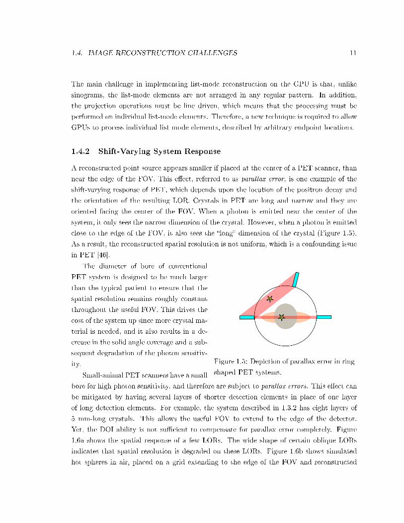
A reconstructed point source appears smaller if placed at the center of a PET scanner, than
near the edge of the FOV. This eect, referred to as parallax error, is one example of the
shift-varying response of PET, which depends upon the location of the positron decay and
the orientation of the resulting LOR. Crystals in PET are long and narrow and they are
oriented facing the center of the FOV. When a photon is emitted near the center of the
system, it only sees the narrow dimension of the crystal. However, when a photon is emitted
close to the edge of the FOV, it also sees the long dimension of the crystal (Figure 1.5).
As a result, the reconstructed spatial resolution is not uniform, which is a confounding issue
in PET [46].
Figure 1.5: Depiction of parallax error in ring-
shaped PET systems.
The diameter of bore of conventional
PET system is designed to be much larger
than the typical patient to ensure that the
spatial resolution remains roughly constant
throughout the useful FOV. This drives the
cost of the system up since more crystal ma-
terial is needed, and it also results in a de-
crease in the solid angle coverage and a sub-
sequent degradation of the photon sensitiv-
ity.
Small-animal PET scanners have a small
bore for high photon sensitivity, and therefore are subject to parallax errors. This eect can
be mitigated by having several layers of shorter detection elements in place of one layer
of long detection elements. For example, the system described in 1.3.2 has eight layers of
5 mm-long crystals. This allows the useful FOV to extend to the edge of the detector.
Yet, the DOI ability is not sucient to compensate for parallax error completely. Figure
1.6a shows the spatial response of a few LORs. The wide shape of certain oblique LORs
indicates that spatial resolution is degraded on these LORs. Figure 1.6b shows simulated
hot spheres in air, placed on a grid extending to the edge of the FOV and reconstructed

12 CHAPTER 1. INTRODUCTION
(a) (b)
Figure 1.6: (a) Depiction of the spatially-varying response of ve LORs. Horizontal andvertical LORS only cover the small dimension of the crystal (1 mm) and therefore providethe highest spatial resolution. In contrast, oblique LORs suer from signicant parallaxerrors due to the 5:1 crystal aspect ratio. (b) A simulated PET acquisition of spheres lledwith activity (diameters 1, 1.25, 1.5, and 1.75 mm) were placed in four quadrants in thesystem central axial plane.
0.5
1
1.5
2
30
210
60
240
90
270
120
300
150
330
180 0
Box (5 mm DOI)
Box (1 mm DOI)
Ring (no DOI)
Figure 1.7: Polar plot of the coin-cident detector response (full-widthhalf-maximum, mm) as a function ofLOR angle, at the center of the FOV,for three CZT systems with 1 × 1mm2 crystal pitch. Two of the sys-tems (blue and black) are arranged ina box geometry (see Figure 1.2) with5 and 1 mm depth-of-interaction lay-ers (DOI). The third system (red) isbuilt in a ring geometry, with no DOIcapability.

1.4. IMAGE RECONSTRUCTION CHALLENGES 13
with an iterative method. The spheres closer to the detectors suer from substantial spatial
resolution degradations. In a box-shaped geometry with 5 mm DOI, parallax errors are not
limited to the edge of the FOV. Figure 1.7 shows that at the center of the FOV, the spatial
resolution (measured as the FWHM of the coincident detector response) can vary from 0.5 to
1.6 mm, depending on the LOR angle. The issue of shift-varying system response is critical
to obtaining high quality images with good spatial resolution. Hence, several approaches
can be implemented to provide uniform reconstructed spatial resolution.
The incorporation of an accurate model of the spatially-variant response of PET has been
shown to help reduce quantitative errors [42,43,47,48] and improve resolution uniformity by
deconvolving the system blurring. Yet, including the contribution of voxels that are o of
the LOR axis increases the number of voxels processed by an order of magnitude. Accurate
reconstruction with a detailed resolution model is computationally demanding and typically
requires large computer clusters. Therefore, a new approach is needed to perform list-mode
reconstruction with shift-varying kernels within practical processing times.
1.4.3 Multiple-Interaction Photon Events
High-resolution PET requires detector modules comprising small detection elements. In
these detectors, Compton scatter and other physical eects cause the annihilation photon to
deposit energy in multiple interaction locations in the detectors. These multiple-interaction
photon events (MIPEs) can produce misidentication of the LOR (as shown in Figure 1.8),
which in turn causes contrast, quantitative accuracy, and spatial resolution loss. For the
CZT system presented in 1.3.2 (1 × 1 × 5 mm3 eective detection elements), 93.8% of
the recorded coincidences involve at least one MIPE. These events must be used in the
reconstruction to maintain high photon eciency. Unless MIPEs are positioned accurately
to the location of the initial interaction, the potential performance of high-resolution PET
will not be achieved.
In a MIPE, the initial interaction denes the correct LOR for the coincidence event.
Subsequent interactions are not aligned with the true LOR because Compton scatter deviates
the annihilation photon from its straight trajectory. Reconstructing the complete sequence
of interactions of each photon provides a reliable way to select the initial interaction [49].
This procedure ensures that all the subsequent interactions are consistent with the choice
of the initial interaction.

14 CHAPTER 1. INTRODUCTION
Figure 1.8: Example of coinci-dent event recorded by a PETsystem based on CZT cross-strip electrodes modules (Sec-tion 1.3.2). The solid red linerepresents the annihilation pho-ton trajectory. In this exam-ple, a coincident pair consists ofa pure photoelectric event (left)and a multiple-interaction pho-ton events (MIPE, right). Mis-positioning of the MIPE resultsin misidentication of the LOR(dotted line).
1.5 Overview of this Work
This work presents a set of novel approaches adapted for high-resolution PET image recon-
struction. The methods are implemented and evaluated for the CZT-based small-animal
PET system presented in 1.3.2. These methods are suitable for a number of other high-
resolution PET systems, including those dedicated to breast cancer (1.3.3). To some extent,
for standard clinical PET systems (Section 5.4).
The methods are organized in four chapters. Chapter 2 provides some background on
mathematical models of the data collection process in PET. A new way of calculating the
response of the imaging system with very low memory overhead is presented. Owing to
the small size of the crystals, the intrinsic detector response function can be linearized,
which lead to a fast analytical expression for the coincident aperture function. The new
formulation is evaluated against Monte-Carlo simulations.
Chapter 3 contains background information on statistical image reconstruction algo-
rithms for PET. A novel formulation of the conjugate gradient algorithm, specic to the
ML objective, is proposed and evaluated. Newton's method is also investigated for PET
reconstruction.
Chapter 4 details a new implementation of fast, shift-varying line projections using
graphics hardware. Fully 3-D, list-mode OSEM was developed based on this method on a
graphics processing unit (GPU). The iterative reconstruction algorithm was evaluated both
on simulated and real PET datasets.
Chapter 5 presents two applications of GPU-based line projection. The rst applica-
tion uses the GPU framework to calculate the coecients of the system coincident detector

1.5. OVERVIEW OF THIS WORK 15
response function on-the-y, and incorporates an accurate model of the data acquisition
process within list-mode iterative reconstruction. The second application uses the GPU for
image reconstruction on an existing clinical PET system that has time-of-ight (TOF) capa-
bilities. The TOF information is incorporated within the list-mode iterative reconstruction.
Chapter 6 proposes a new statistical algorithm for positioning photons in small crystal
detectors. The algorithm uses robust Bayesian estimation for reconstructing the full in-
teraction track of the annihilation photon in the detectors. An evaluation of the method,
implemented on the GPU, is performed for a high-resolution PET system made of CZT
detectors.

Chapter 2
Imaging Model for High-Resolution
PET
2.1 Principles and Theory
The measurements in PET involve complex physical processes. An accurate model of the
data collection process is important, not only to better understand the system's performance,
but also to improve the quality and accuracy of the image reconstruction.
2.1.1 Physics of PET
A PET dataset is produced by counting how many coincident photon pairs have been de-
tected for every possible pair of detection elements. We call a line-of-response (LOR) a line
that connects a pair of detectors elements (Figure 1.1). In order to describe the imaging
process, the photon emission, transport and detection must be modeled.
2.1.1.1 Photon Emission
Positrons are emitted with a range of initial kinetic energies, the maximum amount of which
depends on the radionuclide. For example, the maximum kinetic energy of the positron
emitted by an 18F atom is 0.64 MeV. The positron can only annihilate with an electron
once it has given up most of its kinetic energy through inelastic collisions with atoms and
molecules. As a result, the positron-electron annihilation does not occur at the location of
the positron emission (Figure 2.1a). This fundamental blurring eect limits the resolution
of PET. For example, the positron range of 18F in water is 0.10 mm FWHM and 1.03 mm
FWTM, one of the lowest among all positron emitters [50]. The distribution of the positron
16

2.1. PRINCIPLES AND THEORY 17
(a) (b)
Figure 2.1: (a) A radioactive 18F atom decays by emitting a positron with some initialamount of kinetic energy. The positron propagates through matter, loosing its kinetic energythrough Coulombic interactions until it annihilates with an electron and produce two roughlyanti-colinear 511 keV photons. (b) Spatial distribution of the positron annihilations forpositrons emitted at the origin (from [50]).
annihilation locations is isotropic and well modeled by a cusp-like response function for
homogeneous materials (Figure 2.1b). The distribution of the positron annihilations in a
homogeneous material is obtained by convolving the tracer spatial distribution with the
response function. Modeling of positron range in inhomogeneous material is more complex
because the width of the blurring kernel depends on the density and eective Z of the
material.
In addition to the positron range, the two annihilation photons are not always emitted in
exactly opposite directions. Due to uctuations in residual positron and electron momenta,
conservation of momentum implies that the summed momentum of the annihilation photons
is also not zero, leading to photon acolinearity. The angle between the two photons is
approximated by a Gaussian distribution with mean 180 degree and FWHM 0.23 degree [51].
The contribution of photon acolinearity to spatial resolution depends on the separation D
between the two detectors hit and is approximated by 0.0022 × D [50]. For small-animal
PET systems with small bore diameter, the contribution of photon acolinearity to the spatial
resolution is often neglected. For example, for a bore diameter of 80 mm, the resolution
blurring due to photon acolinearity is less 0.2 mm FWHM.
2.1.1.2 Photon Detection
One factor that impacts the spatial resolution is the detector geometry. Unlike other physical
processes, the detector geometry is determined by design and can be optimized for a specic
goal. The resolution of a radiation detector is quantied by its intrinsic detector response

18 CHAPTER 2. IMAGING MODEL
Figure 2.2: Intrinsic detector response function gθ(X) (red) for a crystal array without (left :normal photon; middle: oblique photon) and with DOI positioning capabilities (right). Thescintillation array with DOI capabilities results in a narrower IDRF, hence better spatialresolution.
function (IDRF). The IDRF describes the response of a single detector to a ux of photons.
For a needle beam of 511 keV photons, aimed at a detector with an angle θ and oset X,
the number of photons detected per second in the detector is given by I0gθ(X), where I0 is
the intensity of the beam (in photons per second) and gθ(X) is the IDRF (see Figure 2.2).
The photons detected in PET have high energy (511 keV). Therefore, standard PET
systems use long and narrow crystals to produce both high photon detection eciency and
high spatial resolution. For this design to work, however, the crystals must always present
the narrow face to the incoming photons. This requires that crystals be arranged in a ring
geometry, far from the subject. Yet, small-animal PET systems place the detectors close
to the animal, therefore the photons emitted near the edge of the FOV are more likely to
be enter the detectors obliquely. In the CZT system described in 1.3.2, the box geometry
further complicates the situation since photons can hit the detector obliquely, regardless
where they were emitted.
Parallax errors resulting from oblique photons can be mitigated by measuring the 3-D
coordinate of the interaction (or depth of interaction DOI). This can be achieved by
segmenting the crystal array in the depth dimension (Figure 2.2, right) [16,17], or by other
schemes, such as reading out a continuous scintillation crystal element from both sides [52].
Formulating the response of the detector in terms of the IDRF neglects an important
component of the spatial resolution. A 511 keV photon can either interact with detector
material by undergoing photoelectric conversion or Compton scatter. In photoelectric con-
version, the total energy of the photon is transferred to a bound electron and the photon
disappears. In Compton scatter, the photon interacts with an unbound or loosely bound
electron. Due to conservation of momentum, the photon cannot transfer all of its energy.
The photon instead transfers a portion of its energy to the recoil electron, and is deected

2.1. PRINCIPLES AND THEORY 19
from its initial trajectory. The scattered photon might then either escape from the system or
interact further with the detectors, leaving behind her a track of interactions. The average
number of interactions depends on the photon initial energy, the detector material and the
size of the detection elements.
In the standard PET detector, the scintillation crystal array is coupled to one or more
light detectors. Because one photon detector typically reads out multiple scintillation crys-
tals, the light signals aremultiplexed. Charge can also be multiplexed in the position-sensitive
photo-detector or in the associated readout circuit. This results in a few (typically four)
readout channels. Such detectors estimate the photon interaction coordinates for each event
by determining the weighted mean of the readout signals. Therefore, individual interaction
coordinates and their deposited energies cannot be determined in the standard PET detec-
tor [16]. For these systems, Compton scatter in the detectors is a blurring factor that cannot
be corrected with signal processing algorithms.
Some more recent PET system designs allow readout of multiple interactions [17, 23,
37, 53]. In the CZT cross-strip electrode design (1.3.2), the 3-D coordinates and energy
deposition for every interaction can be recorded. All these systems are able to distinguish the
photons that deposit their energy in a single detection element from those which deposit their
energy in multiple detection elements. For systems where high resolution is a requirement,
these latter photons can be discarded or included provided that appropriate identication
methods exist (such as the method presented in Chapter 6).
2.1.1.3 Photon Transport
Another complication is the possibility of scatter and absorption of the photon before it
reaches the detector. Even though the photon energy is high (511 keV), some photons
interact in the subject. As a consequence, photons can be absorbed or scattered by the tissue.
Photon absorption always decrease the number of coincidence events measured along a given
LOR. Photon scatter can either increase or decrease the correct number of coincidence events
measured along an LOR because photons might scatter out of the LOR, or into the LOR
(Figure 2.3, middle). The measurement of the photon energy can help reject tissue scattered
events. When the energy of an interaction is measured to be much lower than 511 keV, it
can be inferred that the photon either scattered in tissue, or deposited only a fraction of its
total energy in the detection element. The nite energy resolution of the detector limits how
accurately scattered events can be identied. For a clinical 3-D PET acquisition, 4060% of
all the recorded coincidences include scattered events [54].
Photon attenuation includes both the eects of photon absorption and photons scattering

20 CHAPTER 2. IMAGING MODEL
out of the LOR. In PET, the attenuation is constant along the LOR because the total
distance traveled by the two annihilation photons does not depend on the location where
these photons were emitted. Therefore, the photon attenuation factor for LOR i is modeled
as
ωi = exp−∫LOR
µ(r)dr
(2.1)
where µ(r) is the spatial distribution of the total attenuation coecient at 511 keV.
Tissue scattered events increase the number of coincidence events detected along a given
LOR. The contribution of these events is denoted yr in (2.3). Modeling analytically the
dependence of the scatter distribution on the tracer spatial distribution is dicult. Accurate
scatter distributions can be obtained by Monte-Carlo methods [54]. When an approximate
distribution is acceptable, faster methods such as the single scatter simulation [55] have been
shown to yield reasonably accurate results .
2.1.1.4 Mathematical Model
Mathematically, a PET dataset consists of a non-negative integer vector m ∈ NP , which
represents the number of coincidence events recorded for all P LORs in the system. PET
imaging is a stochastic process due to the limited number of discrete events recorded. There-
fore, a PET dataset is not well modeled by a deterministic quantity. Two scans of the same
object can dier quite substantially. Instead, a random vector Y is used to describe the
stochastic distribution of the measurements. The components Yi (i = 1 . . . P is the LOR
index) are independent and follow a Poisson distribution with mean yi
Yi ∼ Poisson(yi). (2.2)
A sample measurement mi is a realization of Yi. The measurements m are often referred to
as projections because they are roughly equal to the integral of the tracer spatial distribution
along the LOR, also known as the Radon transform [56].
The expected number of coincidence events y on each LOR as a function of the tracer
spatial distribution is well described by a linear model, provided that the amount of activity
in the FOV is not too high. At high count rate, pulse pile-up and dead-time lead to saturated
output. For lower activity levels, the expected measurements recorded by the scanner depend
linearly on the internal tracer distribution. The process of data collection is naturally
represented by a discrete-continuous model that relates the discrete vector of measurements
to the continuous tracer spatial distribution [57]. The volumetric tracer distribution is well
described by a 3-D function f(r) of the spatial variable r. The most general formulation

2.1. PRINCIPLES AND THEORY 21
Figure 2.3: The three types of coincidences in PET. (left) true coincidence; (middle) tissuescattered coincidence; and (right) random coincidence. The black dashed line represents theincorrect LOR recorded by the system in the case of the scattered and random coincidences.
of the imaging process is based on a spatially-varying response. The contribution from a
point of unit strength located at r to a LOR i is represented by a kernel hi(r), called the
coincidence detector response function (CDRF). Hence, the expected measurement yi on
LOR i can be expressed as
yi = ηiωi
∫Ωf(r)hi(r)dr + ysi + yri (2.3)
where Ω is the support of the tracer spatial distribution. The additive terms ysi and yriaccount for tissue scattered and random coincidences (see Figure 2.3). Both terms depend
upon the tracer distribution f(r) and various models have been proposed to express this
dependency [55, 58]. The multiplicative factors ηi and ωi model respectively the eect of
small variations in detector eciency and photon attenuation by the subject along the
LOR. The detector eciency ηi is calibrated by performing a normalization scan [59, 60].
The photon attenuation ωi is measured either by performing a special transmission scan of
the patient using an external positron emitter, or using a previous scan from an anatomical
imaging modality such as X-ray CT [61].
The spatial response of PET systems is determined by a number of factors. The physical
processes involved in the photon production and detection aect the spatial resolution.
Physical processes involved in photon transport (tissue scatter and photon attenuation)
rather impact the contrast of the reconstructed images.
22 CHAPTER 2. IMAGING MODEL
2.1.2 Spatially Variant and Invariant Models for Discrete Image Repre-
sentations
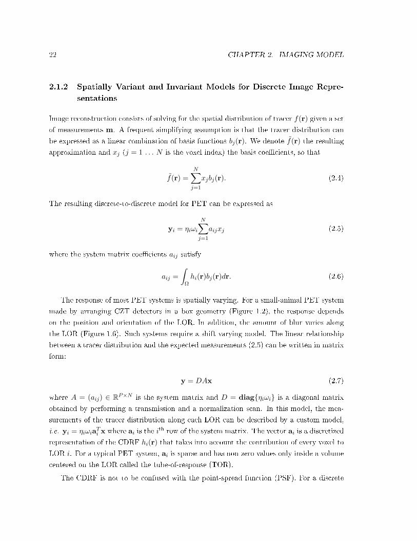
Image reconstruction consists of solving for the spatial distribution of tracer f(r) given a setof measurements m. A frequent simplifying assumption is that the tracer distribution can
be expressed as a linear combination of basis functions bj(r). We denote f(r) the resultingapproximation and xj (j = 1 . . . N is the voxel index) the basis coecients, so that
f(r) =N∑j=1
xjbj(r). (2.4)
The resulting discrete-to-discrete model for PET can be expressed as
yi = ηiωi
N∑j=1
aijxj (2.5)
where the system matrix coecients aij satisfy
aij =∫
Ωhi(r)bj(r)dr. (2.6)
The response of most PET systems is spatially varying. For a small-animal PET system
made by arranging CZT detectors in a box geometry (Figure 1.2), the response depends
on the position and orientation of the LOR. In addition, the amount of blur varies along
the LOR (Figure 1.6). Such systems require a shift-varying model. The linear relationship
between a tracer distribution and the expected measurements (2.5) can be written in matrix
form:
y = DAx (2.7)
where A = (aij) ∈ RP×N is the system matrix and D = diagηiωi is a diagonal matrix
obtained by performing a transmission and a normalization scan. In this model, the mea-
surements of the tracer distribution along each LOR can be described by a custom model,
i.e. yi = ηiωiaTi x where ai is the ith row of the system matrix. The vector ai is a discretized
representation of the CDRF hi(r) that takes into account the contribution of every voxel to
LOR i. For a typical PET system, ai is sparse and has non-zero values only inside a volume
centered on the LOR called the tube-of-response (TOR).
The CDRF is not to be confused with the point-spread function (PSF). For a discrete
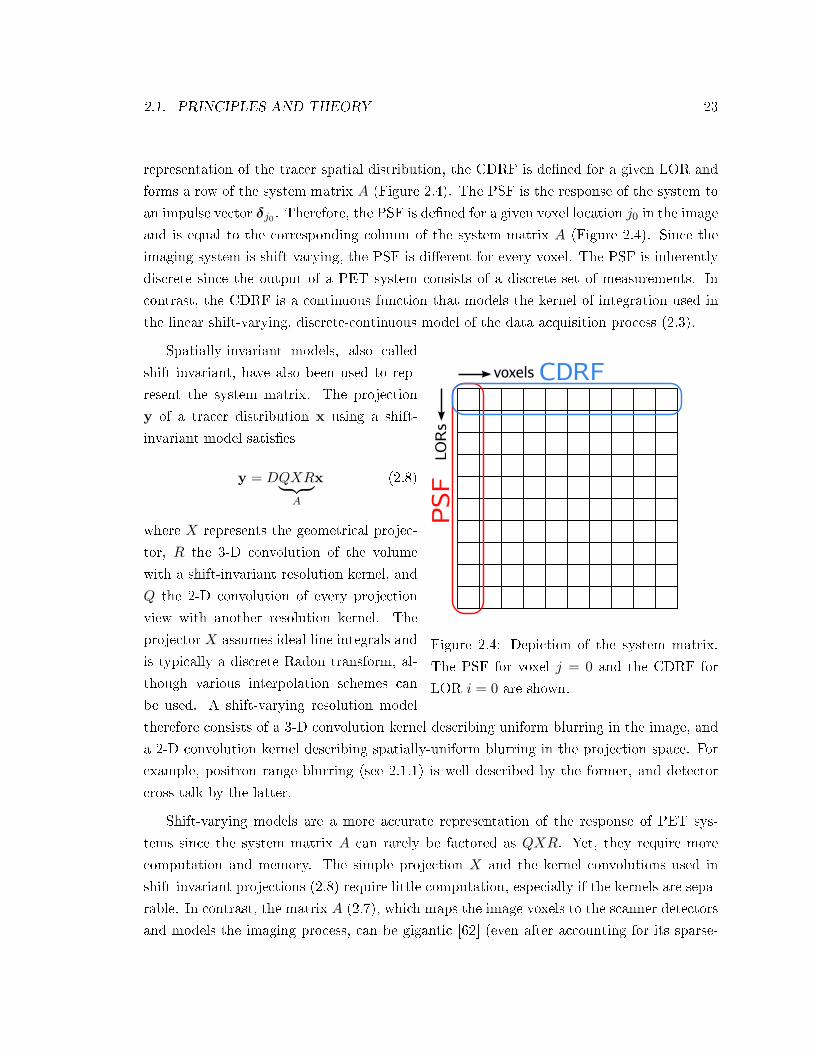
2.1. PRINCIPLES AND THEORY 23
representation of the tracer spatial distribution, the CDRF is dened for a given LOR and
forms a row of the system matrix A (Figure 2.4). The PSF is the response of the system to
an impulse vector δj0 . Therefore, the PSF is dened for a given voxel location j0 in the image
and is equal to the corresponding column of the system matrix A (Figure 2.4). Since the
imaging system is shift-varying, the PSF is dierent for every voxel. The PSF is inherently
discrete since the output of a PET system consists of a discrete set of measurements. In
contrast, the CDRF is a continuous function that models the kernel of integration used in
the linear shift-varying, discrete-continuous model of the data acquisition process (2.3).
Figure 2.4: Depiction of the system matrix.
The PSF for voxel j = 0 and the CDRF for
LOR i = 0 are shown.
Spatially-invariant models, also called
shift-invariant, have also been used to rep-
resent the system matrix. The projection
y of a tracer distribution x using a shift-
invariant model satises
y = DQXR︸ ︷︷ ︸A
x (2.8)
where X represents the geometrical projec-
tor, R the 3-D convolution of the volume
with a shift-invariant resolution kernel, and
Q the 2-D convolution of every projection
view with another resolution kernel. The
projector X assumes ideal line integrals and
is typically a discrete Radon transform, al-
though various interpolation schemes can
be used. A shift-varying resolution model
therefore consists of a 3-D convolution kernel describing uniform blurring in the image, and
a 2-D convolution kernel describing spatially-uniform blurring in the projection space. For
example, positron range blurring (see 2.1.1) is well described by the former, and detector
cross-talk by the latter.
Shift-varying models are a more accurate representation of the response of PET sys-
tems since the system matrix A can rarely be factored as QXR. Yet, they require more
computation and memory. The simple projection X and the kernel convolutions used in
shift-invariant projections (2.8) require little computation, especially if the kernels are sepa-
rable. In contrast, the matrix A (2.7), which maps the image voxels to the scanner detectors
and models the imaging process, can be gigantic [62] (even after accounting for its sparse-
24 CHAPTER 2. IMAGING MODEL
ness).
2.2 Analytical Calculation of the Coincident Detector Response
Function
The response of a PET system can be either measured, simulated or calculated analytically.
In the rst case, a point-source (made of a long-lived positron emitting isotope sealed in a
small capsule) is stepped by a robotic arm through the scanner FOV [48]. The PSF of the
system is measured by acquiring a long scan for every point-source position. This process
requires several weeks of acquisition as well as large memory storage. Regularization is
sometimes performed to obtain a smooth PSF from fewer events or point source locations.
Measuring the PSF is labor-intensive. As a result, Monte-Carlo simulations are often
performed instead [43, 63]. The geometry of the system, consisting of the position and size
of all the detection elements, is entered in the Monte-Carlo program. Billions of positrons
are randomly generated throughout the FOV. The resulting photons are tracked using ray-
tracing techniques and physical process simulations. When photons deposit energy in a
detection element, an event is created and recorded. These events undergo further processing
to replicate the generation and processing of a real PET signal. The PSF at a given location
is available by compounding all the events that originated from positrons emitted in the
proximity of that location.
The third class of methods uses analytical models to compute the PSF [47,64]. The spa-
tial resolution in PET is the product of multiple factors (see 2.1.1), and therefore there does
not exist a perfect analytical model that includes everything. Analytical models attempt to
capture the dominant eects. For the box-shaped PET system studied in this work, we have
assumed that the geometrical response of the detectors dominates over all the other blurring
processes. The justication for this is as follows: First, positron range is an image-based
factor that can be factored out of the system matrix. Then, owing to the small diameter
of the bore (80 mm), photon acolinearity is a small blurring eect (∼0.2 mm) [50]. Last,
the resolution-degrading eect of MIPEs will be removed before reconstruction by a special
approach detailed in Chapter 6. In contrast, the detector response blurring is on the order
of W cos θ + T sin θ, where W stands for the crystal width (1 mm for the system studied)
and T for the thickness of the crystal (5 mm) and θ is the photon incidence angle [65].
An accurate framework for calculating the CDRF was developed in the early days of
PET [6668] in order to design better systems without requiring computationally expensive
Monte-Carlo simulations. The key nding of the method is that the CDRF can be computed
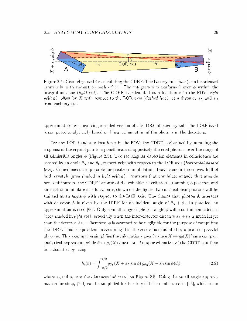
2.2. ANALYTICAL CDRF CALCULATION 25
Figure 2.5: Geometry used for calculating the CDRF. The two crystals (blue) can be orientedarbitrarily with respect to each other. The integration is performed over φ within theintegration cone (light red). The CDRF is calculated at a location r in the FOV (lightyellow), oset by X with respect to the LOR axis (dashed line), at a distance sA and sBfrom each crystal.
approximately by convolving a scaled version of the IDRF of each crystal. The IDRF itself
is computed analytically based on linear attenuation of the photons in the detectors.
For any LOR i and any location r in the FOV, the CDRF is obtained by summing the
response of the crystal pair to a pencil beam of oppositely-directed photons over the range of
all admissible angles φ (Figure 2.5). Two rectangular detection elements in coincidence are
rotated by an angle θA and θB, respectively, with respect to the LOR axis (horizontal dashed
line). Coincidences are possible for positron annihilations that occur in the convex hull of
both crystals (area shaded in light yellow). Positrons that annihilate outside that area do
not contribute to the CDRF because of the coincidence criterion. Assuming a positron and
an electron annihilate at a location r, shown on the gure, two anti-colinear photons will be
emitted at an angle φ with respect to the LOR axis. The chance that photon A interacts
with detector A is given by the IDRF for an incident angle of θA + φ. In practice, an
approximation is used [66]. Only a small range of photon angle φ will result in coincidences
(area shaded in light red), especially when the inter-detector distance sA +sB is much larger
than the detector size. Therefore, φ is assumed to be negligible for the purpose of computing
the IDRF. This is equivalent to assuming that the crystal is irradiated by a beam of parallel
photons. This assumption simplies the calculations greatly sinceX 7→ gθ(X) has a compactanalytical expression, while θ 7→ gθ(X) does not. An approximation of the CDRF can then
be calculated by using
hi(r) =∫ π/2
−π/2gθA(X + sA sinφ) gθB(X − sB sinφ)dφ (2.9)
where sAand sB are the distances indicated on Figure 2.5. Using the small angle approxi-
mation for sinφ, (2.9) can be simplied further to yield the model used in [66], which is an

26 CHAPTER 2. IMAGING MODEL
Out-of-planeincident angle
In-planeincident angle
Ring difference
(a) (b)
Figure 2.6: (a) In-plane and out-of-plane components of the resolution model. (b) Variationof the axial blurring as a function of ring dierence (blue: data, red : linear t). Theblur (FWHM) was measured for the box-shaped CZT PET system, at the center of LORswith zero in-plane angle and varying out-of-plane angle. In the box-shaped system, a ringdierence of 80 mm corresponds to an out-of-plane angle of 45 deg.
analytical scaled convolution:
hi(r) =∫ J
IgθA(x) gθB((1 + ε)X − εx)
dx
sA(2.10)
where x = X + sAφ is the new integration variable, [I, J ] the integration domain and
ε = sB/sA is the ratio of the distances to each detector.
The model based on the analytical scaled convolution only depends on the in-plane
dimensions (Figure 2.6a), i.e. it assumes that both crystals lie in the same axial plane. This
works well for a 2-D PET system in which lead or tungsten septa restrict the acquisition
to in-plane LORs. However, modern PET systems use fully 3-D acquisition to improve the
photon sensitivity. For these systems, coincidences can be acquired between two crystals
located within dierent rings. Therefore, a complete model takes into consideration the ring
dierence. This requires modeling the IDRF as a 2-D function, and calculating the CDRF
though a double convolution (over the in-plane and out-of-plane angles).
This additional parameter would entail a considerable increase in computation, not nec-
essarily justied by image quality gains. In an eort to make modeling practical for image
reconstruction, the 2-D model neglects how the spatial resolution varies with the ring dif-
ference. Blur in the axial direction is modeled by a shift-invariant Gaussian kernel. This is
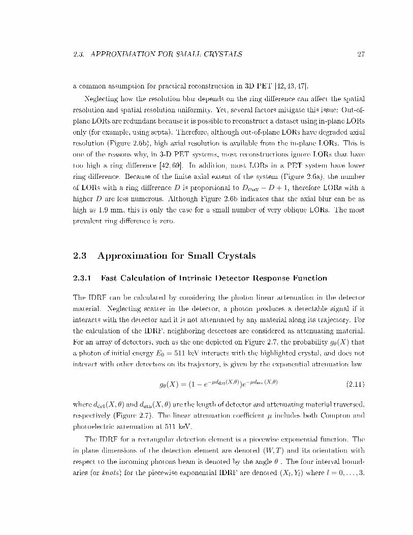
2.3. APPROXIMATION FOR SMALL CRYSTALS 27
a common assumption for practical reconstruction in 3D PET [42,43,47].
Neglecting how the resolution blur depends on the ring dierence can aect the spatial
resolution and spatial resolution uniformity. Yet, several factors mitigate this issue: Out-of-
plane LORs are redundant because it is possible to reconstruct a dataset using in-plane LORs
only (for example, using septa). Therefore, although out-of-plane LORs have degraded axial
resolution (Figure 2.6b), high axial resolution is available from the in-plane LORs. This is
one of the reasons why, in 3-D PET systems, most reconstructions ignore LORs that have
too high a ring dierence [42, 69]. In addition, most LORs in a PET system have lower
ring dierence. Because of the nite axial extent of the system (Figure 2.6a), the number
of LORs with a ring dierence D is proportional to Dmax −D + 1, therefore LORs with a
higher D are less numerous. Although Figure 2.6b indicates that the axial blur can be as
high as 1.9 mm, this is only the case for a small number of very oblique LORs. The most
prevalent ring dierence is zero.
2.3 Approximation for Small Crystals
2.3.1 Fast Calculation of Intrinsic Detector Response Function
The IDRF can be calculated by considering the photon linear attenuation in the detector
material. Neglecting scatter in the detector, a photon produces a detectable signal if it
interacts with the detector and it is not attenuated by any material along its trajectory. For
the calculation of the IDRF, neighboring detectors are considered as attenuating material.
For an array of detectors, such as the one depicted on Figure 2.7, the probability gθ(X) thata photon of initial energy E0 = 511 keV interacts with the highlighted crystal, and does not
interact with other detectors on its trajectory, is given by the exponential attenuation law
gθ(X) = (1− e−µddet(X,θ))e−µdatn(X,θ) (2.11)
where ddet(X, θ) and datn(X, θ) are the length of detector and attenuating material traversed,respectively (Figure 2.7). The linear attenuation coecient µ includes both Compton and
photoelectric attenuation at 511 keV.
The IDRF for a rectangular detection element is a piecewise exponential function. The
in-plane dimensions of the detection element are denoted (W,T ) and its orientation with
respect to the incoming photons beam is denoted by the angle θ . The four interval bound-
aries (or knots) for the piecewise exponential IDRF are denoted (Xl, Yl) where l = 0, . . . , 3.

28 CHAPTER 2. IMAGING MODEL
Figure 2.7: Representation of the detec-tion length (ddet(X, θ)) and the attenu-ation length (datn(X, θ)) as a functionof the oset X and the incident angle θfor a linear crystal array. The two func-tions are piecewise linear and can can beevaluated with minimal computation.
The knots X coordinate can be computed following
Xi = (±W ) cos(θ) + (±T ) sin(θ). (2.12)
Let us assume that the knots are sorted X0 < X1 < X2 < X3. The knots are located
symmetrical around zero: X0 = −X3 and X1 = −X2 (Figure 2.7).
The detection element photon detection eciency depends upon the thickness of both
the detection element of interest and the attenuating material traversed by the beam. The
thickness ddet(X, θ) of the detection element of interest traversed by the photon beam is
zero outside the outer knots X0 and X3. Between X0 and X1, ddet(X, θ) increases linearly.It is then constant between X1 and X2, and it decrease linearly down to zero between X2
and X3 (Figure 2.7). The peak thickness of the crystal is obtained using maxX
ddet(X, θ) =
min 2Lcos θ ,
2Hsin θ.
In a standard crystal array, neighboring crystals will cause attenuation of the photon
beam. Mechanical structures required to hold the crystals together, support readout elec-
tronics, or provide heat dissipation in the detectors can also provide some attenuation. In
the following derivation, mechanical structures are neglected and the crystal array is as-
sumed to be innitely long. Under these assumptions, there is no attenuation for the two
knots that correspond to the front of the crystal (X0 and X1 for the beams depicted in
Figure 2.7). The attenuation length datn(X, θ) then increases linearly until its peak value,
which is attained either at X0 or X3, depending on the incident angle θ (Figure 2.7). The
peak attenuation length is maxX
datn(X, θ) = 2Lcos θ .
Following the calculation of the detection and attenuation length, the IDRF is computed
using the linear attenuation coecient µ in the material (2.11).
Figure 2.8 compares the IDRF for the 1× 5× 1 mm3 CZT detection element used in the

2.3. APPROXIMATION FOR SMALL CRYSTALS 29
Figure 2.8: Comparison of the IDRF for a 1 × 5 × 1 mm2 CZT crystal and a 4 × 20 × 4mm2 LSO crystal. Two dierent incident angles are shown. The IDRF is shown with (red)and without (black) attenuation from surrounding detectors. For the small CZT crystal, theIDRF is well approximated by a piecewise linear function.
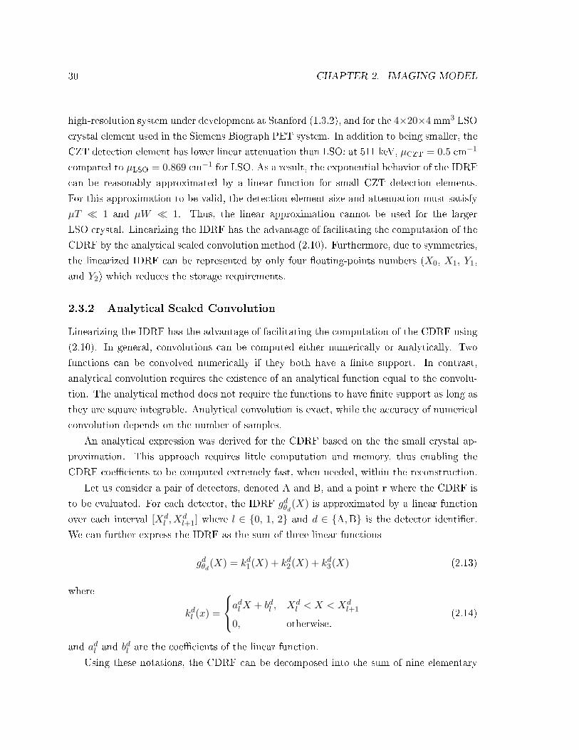
30 CHAPTER 2. IMAGING MODEL
high-resolution system under development at Stanford (1.3.2), and for the 4×20×4 mm3 LSO
crystal element used in the Siemens Biograph PET system. In addition to being smaller, the
CZT detection element has lower linear attenuation than LSO: at 511 keV, µCZT = 0.5 cm−1
compared to µLSO = 0.869 cm−1 for LSO. As a result, the exponential behavior of the IDRF
can be reasonably approximated by a linear function for small CZT detection elements.
For this approximation to be valid, the detection element size and attenuation must satisfy
µT 1 and µW 1. Thus, the linear approximation cannot be used for the larger
LSO crystal. Linearizing the IDRF has the advantage of facilitating the computation of the
CDRF by the analytical scaled convolution method (2.10). Furthermore, due to symmetries,
the linearized IDRF can be represented by only four oating-points numbers (X0, X1, Y1,
and Y2) which reduces the storage requirements.
2.3.2 Analytical Scaled Convolution
Linearizing the IDRF has the advantage of facilitating the computation of the CDRF using
(2.10). In general, convolutions can be computed either numerically or analytically. Two
functions can be convolved numerically if they both have a nite support. In contrast,
analytical convolution requires the existence of an analytical function equal to the convolu-
tion. The analytical method does not require the functions to have nite support as long as
they are square integrable. Analytical convolution is exact, while the accuracy of numerical
convolution depends on the number of samples.
An analytical expression was derived for the CDRF based on the the small crystal ap-
proximation. This approach requires little computation and memory, thus enabling the
CDRF coecients to be computed extremely fast, when needed, within the reconstruction.
Let us consider a pair of detectors, denoted A and B, and a point r where the CDRF is
to be evaluated. For each detector, the IDRF gdθd(X) is approximated by a linear function
over each interval [Xdl , X
dl+1] where l ∈ 0, 1, 2 and d ∈ A,B is the detector identier.
We can further express the IDRF as the sum of three linear functions
gdθd(X) = kd1(X) + kd2(X) + kd3(X) (2.13)
where
kdl (x) =
adlX + bdl , Xdl < X < Xd
l+1
0, otherwise.(2.14)
and adl and bdl are the coecients of the linear function.
Using these notations, the CDRF can be decomposed into the sum of nine elementary
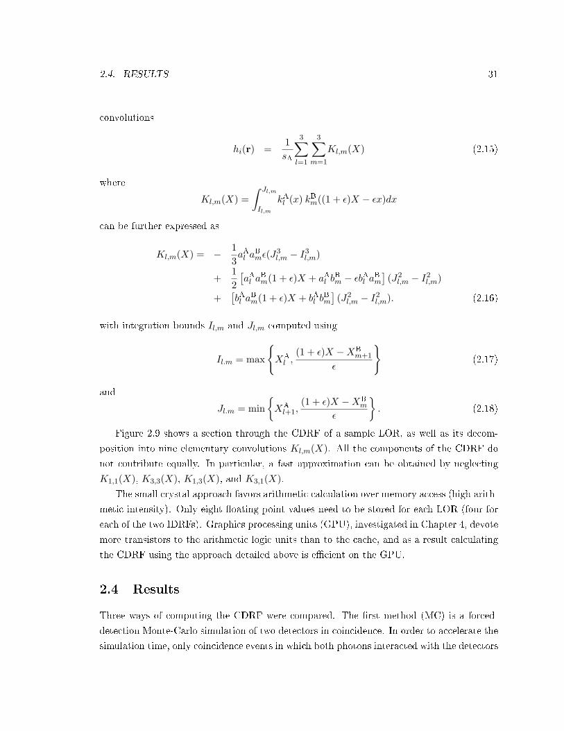
2.4. RESULTS 31
convolutions
hi(r) =1sA
3∑l=1
3∑m=1
Kl,m(X) (2.15)
where
Kl,m(X) =∫ Jl,m
Il,m
kAl (x) kBm((1 + ε)X − εx)dx
can be further expressed as
Kl,m(X) = − 13aAl a
Bmε(J
3l,m − I3
l,m)
+12[aAl a
Bm(1 + ε)X + aAl b
Bm − εbAl aBm
](J2l,m − I2
l,m)
+[bAl a
Bm(1 + ε)X + bAl b
Bm
](J2l,m − I2
l,m). (2.16)
with integration bounds Il,m and Jl,m computed using
Il.m = max
XAl ,
(1 + ε)X −XBm+1
ε
(2.17)
and
Jl.m = minXAl+1,
(1 + ε)X −XBm
ε
. (2.18)
Figure 2.9 shows a section through the CDRF of a sample LOR, as well as its decom-
position into nine elementary convolutions Kl,m(X). All the components of the CDRF do
not contribute equally. In particular, a fast approximation can be obtained by neglecting
K1,1(X), K3,3(X), K1,3(X), and K3,1(X).The small crystal approach favors arithmetic calculation over memory access (high arith-
metic intensity). Only eight oating point values need to be stored for each LOR (four for
each of the two IDRFs). Graphics processing units (GPU), investigated in Chapter 4, devote
more transistors to the arithmetic logic units than to the cache, and as a result calculating
the CDRF using the approach detailed above is ecient on the GPU.
2.4 Results
Three ways of computing the CDRF were compared. The rst method (MC) is a forced-
detection Monte-Carlo simulation of two detectors in coincidence. In order to accelerate the
simulation time, only coincidence events in which both photons interacted with the detectors

32 CHAPTER 2. IMAGING MODEL
were simulated. For that purpose, the location of each interaction within the detector was
randomly generated using a uniform distribution. Each randomly generated coincidence
event was weighed by its probability of occurrence, computed based on the photon linear
attenuation. An estimate the CDRF was obtained by combining many simulated coincidence
events according to their respective probability weights. The second method (SA) sampled
the accurate IDRFs using 200 samples and produced a numerical convolution according to
the small angle approximation (2.10). The third method (SC+SA) used both the small
angle and the small crystal (SC) approximations to calculate the CDRF analytically (2.15).
−3 −2 −1 0 1 2 30
1
2x 10
−4
X (mm)
CA
F
SC+SA approximation
Decomposition
Figure 2.9: Decomposition of the CDRF
(black) into the sum of nine functions (red)
that are calculated analytically using (2.16).
For a LOR normal to the detector (Fig-
ure 2.10, rst row), the detector response is
a trapezoid except at the center where it is
a triangle. The three methods for comput-
ing the CDRF are in good agreement. The
Monte-Carlo approach is indeed more noisy
since it relies on the simulation of a limited
number of discrete events. Normal LORs
provide the highest resolution in the system
since they are not subject to parallax error.
For these LORs, the FWHM of the CDRF
at the center is equal to half of the detector
size (0.5 mm).
In the standard ring geometry, the resolution is optimal at the center of the system
because all the LORs that pass through that point are normal to the detectors. In a box-
shaped geometry, there is no such sweet spot. Hence, LORs with degraded resolution
traverse the center of the system. As an example, for a 45 deg angle LOR (Figure 2.10,
second row), the blurring kernel FWHM is equal to 1.8 mm at the LOR center, more than
three times the value for a normal LOR. For a 45 deg LOR, both the SA and the SC+SA
approximations provide accurate CDRF models compared to the Monte-Carlo method. Due
to crystal penetration, the coincident response is asymmetric.
For a very oblique LOR (Figure 2.10, third row), the LOR forms a 9 deg angle with
the leftmost detector and a 81 deg angle with the rightmost one. As a result, the LOR has
fairly good spatial resolution in the proximity of the leftmost detector (prole A), but the
resolution degrades quickly when approaching the rightmost detector (proles B and C). In
addition, the quality of both analytical models is inferior for short and very oblique LORs.
For such LORs, the SA approximation deviates from the true distribution because the angle

2.4. RESULTS 33
Figure 2.10: CDRF for three LORs. (top row) Normal LOR connecting two 1×5 mm2 CZTdetectors, shown on a linear intensity scale (inset). The proles through the CDRF at threelocations (center, one quarter, one eighth) are shown (A, B and C, respectively) for threemethods: Monte-Carlo simulation, small-angle approximation (SA) and a combination ofthe SA and the small-crystal (SC+SA) approximation. (middle row) CDRF for a 45 degoblique LOR going through the center of the FOV. Both detectors are oriented vertically.(bottom row) CDRF for an oblique LOR. The leftmost detector is oriented horizontally andforms a 9 deg angle with the LOR. The rightmost detector is oriented vertically and thereforeforms an 81 deg angle with the LOR.
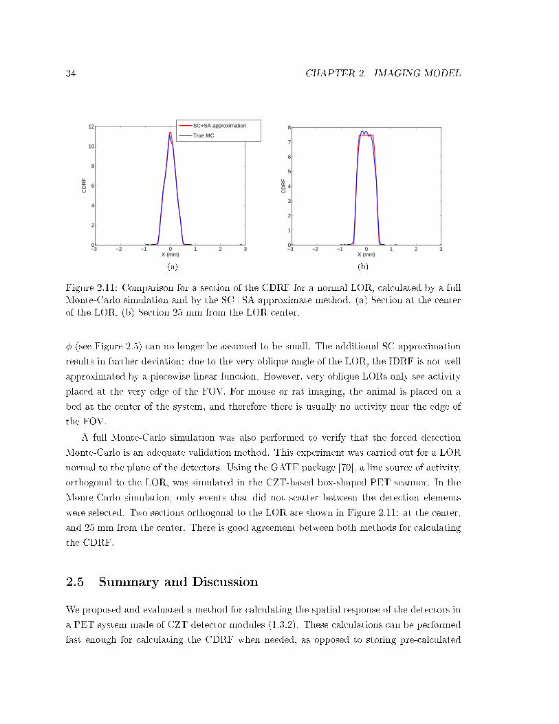
34 CHAPTER 2. IMAGING MODEL
−3 −2 −1 0 1 2 30
2
4
6
8
10
12
X (mm)
CD
RF
SC+SA approximation
True MC
(a)
−3 −2 −1 0 1 2 30
1
2
3
4
5
6
7
8
X (mm)
CD
RF
(b)
Figure 2.11: Comparison for a section of the CDRF for a normal LOR, calculated by a fullMonte-Carlo simulation and by the SC+SA approximate method. (a) Section at the centerof the LOR. (b) Section 25 mm from the LOR center.
φ (see Figure 2.5) can no longer be assumed to be small. The additional SC approximation
results in further deviation: due to the very oblique angle of the LOR, the IDRF is not well
approximated by a piecewise linear function. However, very oblique LORs only see activity
placed at the very edge of the FOV. For mouse or rat imaging, the animal is placed on a
bed at the center of the system, and therefore there is usually no activity near the edge of
the FOV.
A full Monte-Carlo simulation was also performed to verify that the forced detection
Monte-Carlo is an adequate validation method. This experiment was carried out for a LOR
normal to the plane of the detectors. Using the GATE package [70], a line source of activity,
orthogonal to the LOR, was simulated in the CZT-based box-shaped PET scanner. In the
Monte-Carlo simulation, only events that did not scatter between the detection elements
were selected. Two sections orthogonal to the LOR are shown in Figure 2.11: at the center,
and 25 mm from the center. There is good agreement between both methods for calculating
the CDRF.
2.5 Summary and Discussion
We proposed and evaluated a method for calculating the spatial response of the detectors in
a PET system made of CZT detector modules (1.3.2). These calculations can be performed
fast enough for calculating the CDRF when needed, as opposed to storing pre-calculated
2.5. SUMMARY AND DISCUSSION 35
values in a huge look-up table. This approach runs eciently on GPUs since large amounts
of computations are done for every memory access.
The model we presented can provide an accurate representation of the geometrical com-
ponent of the detector response for most of the LORs. It does not include eects such
as inter-crystal scatter, photon acolinearity, or positron range. Inter-crystal scatter in the
CZT-based system is addressed using a sequence reconstruction approach (Chapter 6). The
remaining blurring eects are small compared to the geometrical detector response. In
Section 5.3, we show that incorporating a model based only on the geometrical detector
response corrects for most of the parallax blurring and improves the global accuracy of the
reconstruction.

Chapter 3
Maximum-Likelihood Image
Reconstruction
3.1 Background
The goal of a PET scan is to non-invasively estimate the distribution of a radio-labeled
molecular tracer accumulating in the patient organs. The tracer distribution is not directly
available, but it can be inferred from the millions of oppositely-directed annihilation photon
pairs collected by the scanner, using a process known as image reconstruction.
Image reconstruction consists in solving the inverse problem associated with the data
collection process in PET (detailed in Section 2.1). That is, given a set of PET measure-
ments, how to produce an estimate of the tracer distribution consistent with the imaging
model, and prior information.
This section presents existing image reconstruction methods. Sections 3.1.3.6 and 3.3
present two novel image reconstruction methods.
3.1.1 Analytical Methods
Early image reconstruction methods were based on a simplied model for the data collection
process in PET. These methods assume that the projection value for each LOR is equal
to the integral of the tracer distribution along an innitely thin line connecting the two
detectors. For a 2-D PET acquisition, this is equivalent to assuming that the measurements
are produced by the Radon transform [56]. The tracer distribution can then be recovered
from the measurements by using an analytical inverse method called ltered backprojection
[41].
36

3.1. BACKGROUND 37
In addition to trans-axial sinograms, 3-D datasets contain oblique LORs. In the ab-
sence of noise, these LORs are redundant because the trans-axial sinograms contains all the
information necessary to reconstruct the exact tracer distribution. However, with limited
counting statistics, using oblique LORs improves the photon sensitivity and SNR. If pro-
jection data is acquired for all angles (θ and φ), then the tracer distribution can also be
reconstructed analytically. However, in practice PET systems have nite axial coverage;
therefore, very oblique LORs cannot be acquired. Several approaches have been devised
to reconstruct images from 3-D sinograms, even when some angles are missing. The Orlov
suciency condition [71, 72] determines which spatial sampling patterns provide sucient
information to reconstruct the images analytically. Several other reconstruction approaches
are based on this condition [73, 74]. Alternatively, missing projections can be estimated by
reprojecting an image reconstructed using the set of 2-D transaxial sinograms only [75]. The
resulting complete 3-D dataset can then be reconstructed using 3-D FBP.
Because most of these 3-D analytical methods are computationally demanding, 3-D
datasets are sometimes reconstructed using rebinning techniques. Briey, rebinning consists
in converting a 3-D sinogram into a stack of 2-D transaxial sinograms. These 2-D transaxial
sinograms are similar to those obtained in the conventional 2-D PET scan, however they
are less noisy because they include the complete set of 3-D measurements. Thus, rebinning
decomposes the 3-D reconstruction problem into a set of independent 2-D reconstructions.
Approximate methods were rst proposed, such as single slice rebinning [76] and multi-
slice rebinning [77]. Later, exact rebinning techniques were discovered, such as Fourier
rebinning [44].
In summary, analytical reconstruction methods are fast and relatively simple to analyze.
Yet, they cannot account for either the statistical nature of the measurements, or model the
physical complexity of the data collection process. Statistical methods provide a framework
in which the nature of the noise is taken into consideration. In addition, these methods
are iterative, and can therefore incorporate complex arbitrary models of the data collec-
tion process. These two features can improve reconstructed image quality and quantitative
accuracy.
3.1.2 Statistical Methods
Statistical methods formulate the image reconstruction problem using statistical estimation
techniques such as maximum likelihood (ML) or maximum a posteriori (MAP). They use
optimization to nd the image that maximizes a merit function (also known as the objective
function) and satises a set of constraints. In particular, the image solution is faithful to the

38 CHAPTER 3. ML RECONSTRUCTION
measurements without being too sensitive to the noise, and has other desired characteristics
such as non-negativity and smoothness.
3.1.2.1 Maximum Likelihood
The log-likelihood objective is commonly used to evaluate the agreement of an image can-
didate with the PET measurements [40]. Using the statistical model described in (2.2), the
likelihood of y given m is dened as
pm(y) = P (Y = m|y) =P∏i=1
ymii e−yi
mi!.
The log-likelihood is a concave function of y and it can be expressed as
log pm(y) =P∑i=1
−yi +mi log(yi)− log(mi!).
The image x that satises the ML criterion is a solution to the convex optimization problem
maximize fm(y) =P∑i=1
−yi +mi log(yi)
subject to Ax− y = 0x ≥ 0
(3.1)
where the variables are x ∈ RN and y ∈ RP , and the data is m ∈ RP . The condition y ≥ 0is implicit in the objective function. The system matrix A ∈ RP×N
+ is large but sparse (see
2.1.2).
3.1.2.2 Maximum A Posteriori
Typical ML reconstructions exhibit a high level of noise due to ill-conditioning. Some form
of regularization is required to produce images useful for clinical diagnostics. Two of the
most frequent procedures are early termination of the optimization iterations and post-
reconstruction smoothing [78].
Regularization can also be achieved by using a suitable penalty function within the objec-
tive function. The problem can be formulated within a Bayesian framework by introducing a
statistical prior distribution for the object being imaged [42]. Typically, these priors assume
that the object is a smooth random eld. The distribution of PET tracers is locally smooth,

3.1. BACKGROUND 39
except at organ boundaries where it can vary abruptly. The Gibbs distribution, based on
a Markov random eld, provides a good model for the local image properties [42]. It is
also computationally attractive because the local nature of the model results in an ecient
update strategy. The Gibbs prior results in an additive penalty term to the log-likelihood.
The simplest version of the Gibbs prior is a Gauss-Markov random eld and has a quadratic
form. More complex priors can be designed to allow for abrupt changes at organ boundaries,
using anatomical priors derived from a coregistered X-ray CT scan [79].
3.1.2.3 Other Objective Functions
Other objectives have been proposed for PET image reconstruction. Because a Poisson dis-
tribution can be approximated by a normal distribution, the least-square (LS) and weighted
least-square (WLS) objectives are potential alternatives to the Poisson log-likelihood [80].
For quadratic objectives, the gradient is a linear function of the image estimate, and therefore
conjugate gradient optimization methods can be readily applied [80].
3.1.3 Existing Optimization Methods
3.1.3.1 Expectation-Maximization for ML reconstruction
The expectation-maximization (EM) algorithm is a method for nding the ML estimate.
It introduces a set of complete, unobserved variables that relate the projections to the
image. The method alternates between performing an expectation step, which computes
the expectation of the log likelihood with respect to the current estimate of the distribution
for the unobserved variables, and a maximization step, which solves for the parameters that
maximize the expected log likelihood.
The EM algorithm has been successfully applied to PET reconstruction based on the
inhomogeneous Poisson process (3.1) [40]. The procedure results in the following update
strategy
xn+1j =
xnjNj
P∑i=1
pijmi
N∑b=1
pibxnb
(3.2)
where xnj is the volume estimate after iteration n. The voxels are indexed by j = 1, ..., J .The system response coecients pij model the probability that a positron emitted from
voxel j will generate two annihilation photons detected along the LOR i. The sensitivity

40 CHAPTER 3. ML RECONSTRUCTION
image
Nj =P∑i=1
ηiωipij (3.3)
takes into account the non-uniform density of LORs throughout the volumetric image and
the change in sensitivity ηiωi along LOR i caused by tissue attenuation and geometrical
and intrinsic detection eciency variations. This computation requires the time-consuming
backprojection of all LORs, unless variance reduction techniques are used [81].
The measurements in PET include random and tissue scattered coincidences (as de-
scribed by the mathematical model (2.3) in 2.1.1.4). When an estimate of these background
events is available for every LOR, it can be included in the calculation of the expected
projections by adding these corrections to the forward projection (in the denominator of
(3.2)).
Including the corrections within the reconstruction model is more accurate than subtract-
ing these corrections prior to reconstruction. The latter method alters the Poisson nature
of the measurements, and can also result in negative measurement values. Furthermore, the
subtraction method is not applicable to list-mode processing (see 3.1.3.3).
The EM algorithm involves two main operations. The forward projection computes the
expected number of events measured in each LOR and can be formulated as the matrix-vector
multiplication x → Ax. The backprojection is the transpose operation, i.e. y → ATy. In
a standard implementation of the EM algorithm, the image estimate is initialized with a
uniform image. For each iteration, the forward projection is calculated for the current image
estimate. The ratio of the measured to the estimated projection is then backprojected.
Finally, a multiplicative update is performed on the image.
One of the benets of the EM algorithm is that the multiplicative update naturally
enforces the non-negativity constraint (3.1). Other optimization methods must be adapted
to account for the non-negativity constraint, for example, by using a bent line search [80] or
an active set [82].
3.1.3.2 Ordered-Subset Expectation-Maximization for ML reconstruction
It was found that the convergence of the EM algorithm could be accelerated by order-of-
magnitudes by partitioning the data into subsets. The ordered-subset expectation-maximization
(OSEM) algorithm was designed based on this principle [39]. OSEM has established itself
as the standard iterative image reconstruction method in nuclear medicine.
Each subset in OSEM consists of a limited number of projection views. Each update
is performed using the data from a single subset. That way, each update requires far less

3.1. BACKGROUND 41
computation than if the full data was used. The subsets are processed sequentially, and one
iteration of OSEM is completed once all the subsets have been used. The OSEM algorithm
can be formulated as
xn,lj =xn,l−1j
Nj
∑i∈Sl
pijmi
N∑b=1
pibxn,l−1b
(3.4)
where the projections are partitioned into subsets Sl and l = 1, ..., L is the subset index.
The image estimate at the end of the nth iteration is xn+1,1 = xn,L+1.
The OSEM algorithm accelerates the EM algorithm by a factor roughly equal to the
number of subsets. However, the acceleration is limited because as the number of subsets
increases, the variance of the reconstructed image increases too. In addition, the OSEM
algorithm is subject to limit cycles and does not converge. As a result, OSEM is best suited
for providing early image iterates using a small number of subsets (32 is a popular choice).
3.1.3.3 List-Mode Processing
In list-mode, the processing method used in this work, the LOR index and other physical
quantities (e.g. time, energy, TOF, depth-of-interaction, etc.) are stored sequentially in a
long list as the scanner records the events. The problem of reconstructing directly from the
list-mode data lends itself to a maximum-likelihood formulation based on the EM algorithm.
Despite its computational burden, this processing method is popular [38,62,8387] because
it is an ecient format to process sparse data sets, such as dynamic, time-of-ight, or high-
resolution studies. It has additional benets, namely: (1) all the original information can
be stored for each event; (2) natural complete subsets can be formed by splitting the events
chronologically; (3) the symmetries of the system are preserved; (4) image reconstruction
can be started as soon as the acquisition begins; (5) events can be positioned continuously
in space and time; and (6) data can be converted to any other format. Table 3.1 shows an
sample dataset with four counts represented both in histogram-mode and list-mode.
The OSEM algorithm can be adapted for list-mode data. In list-mode, the vector m
of measurements for every LOR is not readily available (although it could be obtained
by parsing the list-mode). Therefore, the standard OSEM update strategy (3.4) is not
applicable. Instead, each event is processed (forward and back- projections) individually.
The OSEM subsets are formed according to the arrival time of the events. The resulting

42 CHAPTER 3. ML RECONSTRUCTION
Crystal ID 1 2 3 41 0 1 02 2 13 04
(a)
Event ID Crystal 1 Crystal 2
1 3 12 2 33 2 44 3 2
(b)
Table 3.1: Sample PET dataset with four counts and six LORs stored in (a) histogram formand (b) list-mode.
list-mode OSEM algorithm can be formulated as follow
xn,lj =xn,l−1j
Nj
L∑k=1
pikj1
N∑b=1
pikbxn,l−1b
(3.5)
where L denotes the number of list-mode events recorded and ik is the LOR index for the
kth list-mode event. Unlike the subsets Sl in (3.4), an index might be repeated if multiple
events are measured on the corresponding LOR (see Table 3.1). Likewise, the vector of
measurements m is replaced by 1 in the update equation. The method is ecient for sparse
datasets because empty LOR bins are neither stored nor processed.
3.1.3.4 Gradient Ascent for ML reconstruction
Gradient ascent is a common convex optimization method that can be used to solve (3.1) [88].
For each iteration, the search direction dn is computed from the log-likelihood gradient
dn = ∇fm(xn) (3.6)
= AT(mi
Ax− 1). (3.7)
Next, a 1-D line search is performed along the search direction dn to nd the step size that
maximizes the log-likelihood
αn = argmaxα
fm(xn + αdn). (3.8)

3.1. BACKGROUND 43
The line search is performed using an iterative method, such as Newton-Raphson or the
Amijo rule [82] . Last, an additive update is performed
xn+1 = xn + αndn. (3.9)
Unlike the EM algorithm, gradient ascent is not applicable to list-mode data because the
line search requires the knowledge of the measurement vector m. The EM algorithm itself
can also be formulated as a scaled gradient ascent method with a constant step size [80].
The EM update rule can be equivalently written as
xm+1j = xmj +
xmjNj∇fm(y). (3.10)
3.1.3.5 Conjugate Gradient for WLS Reconstruction
This section reviews the rationale for using the conjugate gradients (CG) algorithm for
quadratic objective functions such as WLS [89, 90]. The WLS estimate x∗wls is the solution
to the quadratic problem with equality constraints
maximize fm(y) = −12
P∑i=1
(yi −mi√
mi
)2
subject to Ax = y.
(3.11)
The gradient of the WLS objective with respect to x is given by
gn = ∇xfm(yn) (3.12)
= ATM−1 (m− yn) (3.13)
where yn = Axn and M = diag(m).
CG is the iterative method of choice to optimize a quadratic objective. This ascent
method alternates the computation of a search direction and a step size, producing a se-
quence of estimates xn. The CG search direction dn combines the gradient of the objective
function fm and the previous search direction
dn = gn + βndn−1. (3.14)
where βn denes the relative weight of each term. Several formulations exist for βn. In this

44 CHAPTER 3. ML RECONSTRUCTION
work, we have used the PolakRibière formulation [91]:
βn =(∇fm(xn)−∇fm(xn−1))T∇fm(xn)
∇fm(xn−1)T∇fm(xn−1). (3.15)
In CG, the image update is performed additively as in (3.9) and a line search determines
the step size αn (in a way similar to the gradient ascent method see 3.1.3.4). After the
line search procedure (3.8), the gradient gn+1 is orthogonal to the search direction dn
dTngn+1 = 0. (3.16)
The image residual is dened as the dierence between the current image estimate and the
optimal WLS solution
en+1 = xn+1 − x∗wls. (3.17)
The optimal solution x∗wls of (3.11) satises ∇xfm(Ax∗wls) = 0. Using this property, the
gradient can be expressed as a linear function of the residual
gn = −ATM−1Aen. (3.18)
From (3.16), the search direction and the image residual satisfy a conjugation relationship
dTnCen+1 = 0 (3.19)
where C = ATM−1A is the conjugation matrix. Following (3.9) and (3.17), the residual
en+1 can be reformulated as
en+1 = xi+1 +n∑
j=i+1
αjdj︸ ︷︷ ︸xn+1
−x∗wls (3.20)
= ei+1 +n∑
j=i+1
αjdj (3.21)

3.1. BACKGROUND 45
for i < n. As a result,
dTi Cen+1 = dTi Cei+1︸ ︷︷ ︸0
+n∑
j=i+1
αjdTi Cdj (3.22)
=n∑
j=i+1
αjdTi Cdj . (3.23)
The key to WLS-CG is to use Gram-Schmidt orthogonalization procedure to construct
a basis of conjugate search directions (di) that satisfy
dTi Cdj = 0, i 6= j. (3.24)
For such a basis of conjugate directions, (3.23) implies that the residual is conjugate to all
the past search directions
eTnCdi = 0, i < n. (3.25)
In other words, n − 1 components of en are zero in the C-orthogonal basis dened by
(di). As n increases, the image residuals en are constrained to a subspace of decreasing
dimension. In other words, the nth update does not undo the work achieved during the
previous steps. The exact value of the residual en is never known during the optimization,
yet afterN+1 iterations it is exactly zero (at least in theory). Moreover, it has been observed
that small residuals can be obtained even after a number of iterations much smaller than
N . Convergence is particularly fast when the eigenvalues of the conjugation matrix C are
clustered [92].
For WLS-CG, conjugate search directions can be interpreted as being orthogonal when
projected and normalized by the measured standard deviation of each sinogram bin(M−1/2Adi
)⊥(M−1/2Adj
). (3.26)
The PolakRibière formulation builds recursively such a basis of conjugate search direc-
tions (3.24). The new search direction dn is chosen in the subspace spanned by the gradient
gn and all the past search directions:
dn = gn +n−1∑j=1
βn,jdj . (3.27)

46 CHAPTER 3. ML RECONSTRUCTION
The coecients βn must be such that dn satises (3.24), which yields
gTnCdi + βn,idTi Cdi = 0 (3.28)
for i < n. The n− 1 equations are uncoupled and can be solved independently, which yields
the PolakRibière formulation (3.15).
3.1.3.6 Conjugate Gradient for ML Reconstruction
The ML objective (3.1) is non-quadratic, therefore the results derived in 3.1.3.5 do not apply.
In particular, (3.18) is not valid for the ML gradient. Yet, the CG update mechanisms have
been applied with some success to the non-quadratic ML objective [80, 82, 93, 94]. The
ML-CG reconstruction method involves calculating a search direction based on the gradient
of the ML objective (3.7) and the PolakRibière formulation (3.15). An additive update,
including a line search for the step size, are then performed.
In ML-CG, most of the properties of WLS-CG no longer hold. For example, the search
directions are not exactly conjugate because the objective is not quadratic. However, empir-
ical evidence suggests that the ML-CG algorithm performs better than the simpler gradient
ascent method presented in 3.1.3.4 [93]. One reason often cited for this result is that ML-CG
exploits the local quadraticity of the ML objective. Fast convergence can be expected when
the Hessian matrix varies slowly between iterations. Near the optimal value, the objective is
well approximated by a quadratic function, and as a result ML-CG is ecient. However, in
the early iterations, CG takes large steps and the Hessian matrix can change substantially
between iterations. Hence, the search directions are not conjugate and the image residual
en does not get constrained to a subspace of the full image volume.
In the next section, an alternate formulation of CG that preserves the conjugation of
the search directions is derived for the ML objective. This new formulation substitutes the
conjugation relationship (3.19) by an approximate conjugation relationship specic to the
ML objective.
3.2 Novel ML Conjugation of Search Directions
The ML estimate x∗ml solves the convex problem described in (3.1). Although the log-
likelihood objective pm(y) is non-quadratic, it has been observed that (3.1) could be opti-
mized eciently using CG with the PolakRibière formulation (see 3.1.3.6).
A new CG method, specic to the ML objective, was investigated [95]. Inspiration was

3.2. NOVEL ML CONJUGATION OF SEARCH DIRECTIONS 47
drawn from the WLS case to derive a new approximate conjugation relationship specic to
the ML criterion, and to design a method to form search directions consistent with that
relationship. This new formulation outperforms applying the conventional PolakRibière
formulation directly to the non-quadratic ML objective.
3.2.1 Conjugation in ML-CG
The image residual is dened as
en = xn − x∗ml (3.29)
where x∗ml satises ∇xfm(Ax∗ml) = 0.
The gradient of the ML objective with respect to x is given by
hn = ∇xfm(yn) (3.30)
= ATY −1n (m− yn) (3.31)
where yn = Axn and Yn = diag(yn). For the ML gradient hn, the dierence between
the measured and estimated projection (mi − yi) is scaled by the inverse of the estimated
variance yn, while in the WLS gradient gn, this dierence is scaled by the inverse of the
measured variance m.
The ML gradient can be expressed as a function of the residual:
hn = −ATY −1n ΛAen (3.32)
where Λ = diag(m/Ax∗ml). This expression depends upon the unknown optimal solution to
the ML problem, therefore Λ is approximated by the identity matrix. This approximation
is equivalent to Ax∗ml = m. It should be noted that if this relationship is true, then indeed
x∗ml is the ML optimal solution. Alternatively, (3.33) can be written using an additive error
term ε:
hn = −ATY −1n Aen + ε (3.33)
where ε = ATY −1n (Ax∗ml −m). Here again, ε can be assumed to be negligible.
An approximate relationship can then be established between the gradient and the image
residual, independently of the optimal solution:
hn ≈ −ATY −1n Aen. (3.34)

48 CHAPTER 3. ML RECONSTRUCTION
The gradient is orthogonal to the search direction when αn is computed by a line search
dTnhn+1 = 0. (3.35)
Following (3.34), a new conjugation relationship can be formulated for ML
dTnBn+1en+1 ≈ 0 (3.36)
where Bn+1 = −ATY −1n+1A. Unlike in the WLS case, the conjugation matrix Bn+1 varies
with the iterations. Nevertheless, this conjugation relationship can be exploited to constrain
the residual.
Similarly to (3.23), the image residual en satises
dTi Bi+1en+1 ≈n∑
j=i+1
αjdTj Bi+1di (3.37)
for i = 1 . . . n − 1. We therefore explored a method that recursively builds a sequence of
search directions such that
dTj Bi+1di = 0, i < j. (3.38)
For such a sequence of search directions, the image residuals en are constrained to a subspace
of decreasing dimension as the image estimate xn approach the optimal solution
dTi Bi+1en+1 ≈ 0, i < n. (3.39)
The basis of search directions conjugated in the ML sense (3.38) can be interpreted as
follows. The projected search directions Adi and Adj (i < j), scaled by the estimate of the
variance at the ith iteration, are orthogonal:
Y−1/2i+1 Adi ⊥ Y −1/2
i+1 Adj . (3.40)
3.2.2 Explicit Conjugation of Search Directions
An algorithm similar to Gram-Schmidt orthogonalization procedure is employed to produce a
basis of search directions that satisfy (3.38). The search direction dn is formed by combining
linearly the gradient hn and all the past search directions
dn = hn +n−1∑j=1
βn,jdj . (3.41)

3.2. NOVEL ML CONJUGATION OF SEARCH DIRECTIONS 49
Applying conditions (3.38) yields a system of n−1 linear equations with n−1 variables βn,j
hTnBi+1di +n−1∑j=1
βn,jdTj Bi+1di = 0 (3.42)
for i = 1 . . . n − 1. Unlike for the WLS objective, the equations are coupled. They can be
equivalently represented in matrix notation
H(n)βn = cn, (3.43)
where βn = (βn,1, . . . , βn,n−1), cn is the vector dened as
cn,i = −hTnBi+1di (3.44)
and H(n) is a lower-triangular matrix
H(n)ij = dTj Bi+1di. (3.45)
The matrix H(n) can be constructed recursively since H(n+1)ij = H
(n)ij for i, j ≤ n− 1.
A truncated formulation can also be implemented by assuming βn,j = 0 for j ≤ n − 2.In that case, the non-zero component can be formulated as
βtruncn,n−1 = − hTnBndn−1
dTn−1Bndn−1. (3.46)
3.2.3 Results
A 2-D 128 × 128 Shepp Logan phantom with a positive-valued surrounding background
was simulated. No cold region was present in the phantom to circumvent the issue of the
non-negativity constraint which exists for all additive update methods. A noise-free dataset
was obtained by computing 192 parallel-beam projection views. A noisy dataset was also
produced by generating a realization of a Poisson random vector parameterized by the noise-
free projections, resulting in 35 million counts.
Reconstructions were performed for both datasets (Figure 3.1). We compared ML-
CG with the PolakRibière formulation (3.1.3.6) against the new formulation (3.42). The
truncated formulation (3.46) was also investigated. The log-likelihood residual, dened as
| log pm − log p∗|, where log p∗ is the value of the objective function at optimality, was the
main gure of merit of this study. The value of the objective at optimality was computed

50 CHAPTER 3. ML RECONSTRUCTION
(a) (b) (c) (d)
Figure 3.1: The noise-free and noisy reconstructed images are shown for 500 iterations ofPolakRibière ((a) and (c)) and 500 iterations of the new ML-specic formulation ((b) and(d)).
by running 10,000 iterations of ML-CG with PolakRibière.
Figure 3.3 shows typical values for βn,j for n = 30. We have observed that, independently
of the iteration number, the last coecient (here, β30,29) is always far greater than the others.
Yet, accounting for all the search directions improves the convergence of ML-CG both for
noise-free and noisy datasets. The log-likelihood residual converges to zero faster for the new
formulation . For the noisy dataset, it reaches the equivalent of 50 PolakRibière iterations
in 39 iterations (1.3 times faster), and the equivalent of 2,000 PolakRibière iterations in
451 iterations (4.4 times faster) (Figure 3.2).
The new formulation can be truncated as shown in (3.46). The resulting formulation
converges to the ML solution at the same rate as Polak-Ribière. Furthermore, both for-
mulations yield similar values (average dierence smaller than 0.3%) for β for all iterations
(Figure 3.3).
The assumption (in 3.2.1) that Λ ≈ IP (or, equivalently, Ax∗ml ≈m) was experimentally
studied. Figure 3.4 is a histogram of the diagonal coecients of Λ, computed from the
estimate of x∗ml obtained by running 10,000 iterations of PolakRibière ML-CG for the
dataset with noise. The histogram is centered on 1, with a full-width half-maximum of 0.04.
3.2.4 Discussion
For quadratic objectives, such as WLS, accounting for the last search direction alone is
sucient to form a basis of conjugated search directions. For a non-quadratic objective,
such as ML, all the past search directions must be combined when forming a new search
direction to ensure conjugation. In the new, ML-specic formulation, the last search di-
rection is typically more heavily weighted than older ones. However, accounting for all the
search directions improves the convergence rate. If older search directions are truncated,

3.2. NOVEL ML CONJUGATION OF SEARCH DIRECTIONS 51
(a) (b)
Figure 3.2: Progress of reconstruction, measured by | log pm − log p∗|, where p∗ is the log-likelihood optimal value found by running 10,000 iterations of Polak-Ribière ML-CG. Theprogress of our new formulation for ML-CG is shown with and without truncation of thesearch directions. Two datasets were reconstructed: (a) a noise-free dataset and (b) a datasetwith Poisson noise based on 35 million counts. For the noise-free case, the log-likelihood ofthe new formulation exceeded the result of 10,000 iterations with PolakRibière after only485 iterations; therefore, the residual could not be plot past iteration 485.
(a) (b)
Figure 3.3: (a) Typical coecients for βn,i for n = 30 and i = 1 . . . 29. The last searchdirection dn−1 is weighted more heavily than older ones for computing the new searchdirection dn, but older search directions also contribute to the nal search direction. Whenthe contribution of these older search directions is ignored, the new formulation 3.46 iswithin 0.3% of PolakRibière 3.15, as shown (b) by plotting β for both formulations for 20iterations of ML-CG.

52 CHAPTER 3. ML RECONSTRUCTION
the convergence rate reverts back to that of standard PolakRibière.
Figure 3.4: Histogram of the diagonal coe-
cients of Λ = diag(m/Ax∗ml). In the deriva-
tion of the ML conjugation relationship, Λ is
assumed to be the identity matrix.
The CG method based on the Polak
Ribière formulation is surprisingly ecient
for the non-quadratic ML objective. Fur-
thermore, it can be shown (by doing a full
search on β) that no other formulation con-
verges faster. The reason is that Polak
Ribière applied to the ML objective is equiv-
alent to truncating the optimal ML formu-
lation, which uses all the past search direc-
tions.
For the new method, only a small
amount of additional computation is re-
quired (evaluation of dot products). The
total complexity remains dominated by the
cost of the back- and forward projections. The main drawback of the optimal ML formu-
lation is that it requires that all the past search directions be stored in memory, which is
impractical for large image volumes. How to reduce the memory footprint while keeping the
desirable properties of the new formulation needs to be researched further.
The images produced by ML iterative reconstruction become increasingly noisy as the
sequence of estimates reaches optimality. The noise can obscure the main features of the
images. Thus, most clinical protocols terminate the iterations early, before the convergence
is reached. This indeed limits the attractiveness of the reconstruction methods described
in this section. When an early ML iterate is sought, the method of choice is the ordered-
subsets expectation-maximization (OSEM) algorithm. OSEM can produce images suitable
for clinical use in as little as two iterations [96], but it does not converge to the ML solution
[97]. Alternatively, a fully converged reconstruction can be performed, and in such case
a smoothing lter must be applied to the ML estimate, or a smoothing penalty must be
incorporated in the objective. The CG algorithm and the novel methods described in this
section are suitable for fully converged reconstruction approaches.
The CG algorithm can be modied to incorporate a preconditioning matrix [90]. Pre-
conditioned CG (PCG), with the right choice of matrix, converges faster than regular CG
to the optimal solution [82, 94]. Conventional preconditioners attempt to approximate the
inverse of the Hessian matrix. In PET, the EM preconditioner [80] has also been shown to
improve convergence and provide a non-linear smoothing eect, similar to that obtained by

3.3. NOVEL ML RECONSTRUCTION VIA TRUNCATED NEWTON'S METHOD 53
running the EM algorithm. The optimal ML formulation for CG can be readily extended to
include preconditioning.
The current ML problem formulation (3.1) does not incorporate a non-negativity con-
straint for the voxels. The non-negativity of the estimated projections is however implicitly
enforced by the logarithmic term in the ML objective. Largely negative voxel values are
therefore prevented, because they would induce negative projection values. In the absence
of a non-negativity constraint, voxels can take slightly negative values. It is very challenging
to incorporate non-negativity constraints in CG while preserving the fast convergence [80].
In the early iterations, during which the cold voxels are identied, CG is not faster than a
simple gradient ascent method. A suboptimal ML estimate might be found by truncating
the negative voxels at the end of the reconstruction (projection onto convex sets). Such
truncation cannot be performed within the iterations because it would destroy the deli-
cate sequence of conjugate directions. A logarithmic barrier can also be used to enforce
non-negativity. Positive bias in cold regions might result, but the advantage of the barrier
method is that the conjugation of the search directions in CG is preserved. The positive
bias can be mitigated by reducing the weight of the log barrier, but this negatively aects
the conditioning of the objective.
3.3 Novel ML Reconstruction via Truncated Newton's Method
3.3.1 Dual Problem
A dual problem can be formulated for ML reconstruction. The Lagrangian associated with
problem (3.1) is
L(x,y,λ,ν) = λTθ + νT (y −Ax) +P∑i=1
−ρi +mi log(ρi) (3.47)
= (ν − 1)Tρ + (λ−ATν)Tx +P∑i=1
yi log(ρi) (3.48)
where ν ∈ RP is the dual vector for the linear equality constraint, and λ ∈ RN is the dual
vector for the non-negativity constraint. The Lagrange dual function g(λ,ν) is dened as
54 CHAPTER 3. ML RECONSTRUCTION
the supremum over the primal variables of the Lagrangian:
g(λ,ν) = supx∈RP ,y∈RN
L(x,y,λ,ν). (3.49)
The dual function is equal to ∞ unless ATν = λ and ν ≤ 1. In that case, the supremum is
attained for yi = mi/(1− νi), and the value of the dual function is
g(λ,ν) =P∑i=1
mi log(mi)−mi −mi log(1− νi). (3.50)
The dual function leads to the formulation of the dual problem, where the constant terms
in the objective have been dropped:
maximizeP∑i=1
mi log(1− νi)
subject to ATν = λ
λ ≥ 0.
(3.51)
The optimal primal variable y∗, and the optimal dual variable ν∗ are orthogonal. This
follows from y∗Tν∗ = x∗TATν∗ = x∗Tλ∗, which is zero due to complementarity slackness.
Using the relationship between primal and dual variables,
y∗Tν∗ = y∗T (1− my∗
) = 1T (y∗ −m) = 0. (3.52)
The ML estimate therefore has the interesting property that 1Ty∗ = 1Tm, i.e. the total
number of counts estimated is equal to the total number of counts measured. This condition
can provide a necessary stopping criterion for the reconstruction.
Solving the dual problem (3.51) is not as practical as solving the primal problem (3.1)
since x∗ can only be recovered from ν∗ by computing A−1(
m1−ν∗
), which is expensive or
inaccurate if CG is used.
3.3.2 KarushKuhnTucker Conditions
The primal variables x∗ and y∗ are optimal for (3.1) if and only if there are ν∗ ∈ Rm and
λ∗ ∈ Rn such that[0
∇f(y∗)
]+
[−AT
I
]ν∗ +
[I
0
]λ∗ = 0, Ax∗ = y∗, x∗ ≥ 0, λ∗ ≥ 0. (3.53)

3.3. NOVEL ML RECONSTRUCTION VIA TRUNCATED NEWTON'S METHOD 55
The KKT conditions can be more conveniently formulated as
ATν∗ = λ∗, ∇f(y∗) = −ν∗, Ax∗ = y∗, x∗ ≥ 0, λ∗ ≥ 0. (3.54)
In particular, we have x∗TAT∇f( y∗) = 0, or equivalently x∗T∇Xf(Ax∗) = 0.
3.3.3 Newton Step for a Relaxed Problem
The inequality constraints can be handled by using a log barrier. However, for simplicity,
we relax the original problem (3.1) by dropping the constraints x ≥ 0. The coecients of Aare non-negative, and the objective constrains Ax to be positive. As a result, large negative
values of x are penalized. If needed, we can project x onto RN+ and perform a few additional
iterations.
The Newton step can be obtained by solving for the minimum under constraints of the
quadratic approximation of f around (x,y).
minimize f(y + v) = f(y) +∇f(y)Tv + 12vT∇2f(y)v
subject to A(x + u)− y − v = 0.(3.55)
where u and v are the Newton steps for x and y, respectively. Using Ax = y, the optimal
variables for the quadratic problem satisfy 0 0 AT
0 −∇2f(y) −ImA −Im 0
u
v
w
=
0∇f(y)
0
(3.56)
where w is the associated optimal dual variable. The gradient and the diagonal Hessian are,
respectively,
(∇f(y))i =mi − yiyi
,(∇2f(y)
)ii
= −mi
y2i
. (3.57)
The variables u and w can be eliminated, which yield the more compact equation for the
Newton step ∆xnt
AT∇2f(y)A∆xnt = −AT∇f(y). (3.58)
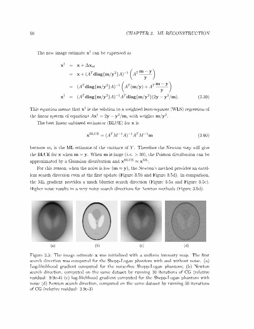
56 CHAPTER 3. ML RECONSTRUCTION
The new image estimate x† can be expressed as
x† = x + ∆xnt
= x + (ATdiagm/y2A)−1
(AT
m− yy
)= (ATdiagm/y2A)−1
(AT (m/y) +AT
m− yy
)x† = (ATdiagm/y2A)−1ATdiagm/y2(2y − y2/m). (3.59)
This equation means that x† is the solution to a weighted least-squares (WLS) regression of
the linear system of equations Ax† = 2y − y2/m, with weights m/y2.
The best linear unbiased estimator (BLUE) for x is
xBLUE = (ATM−1A)−1ATM−1m (3.60)
because mi is the ML estimate of the variance of Y . Therefore the Newton step will give
the BLUE for x when m = y. When m is large (i.e. > 30), the Poisson distribution can be
approximated by a Gaussian distribution and xBLUE ≈ xML.
For this reason, when the noise is low (m ≈ y), the Newton's method provides an excel-
lent search direction even at the rst update (Figure 3.5b and Figure 3.5d). In comparison,
the ML gradient provides a much blurrier search direction (Figure 3.5a and Figure 3.5c).
Higher noise results in a very noisy search directions for Newton methods (Figure 3.5d).
(a) (b) (c) (d)
Figure 3.5: The image estimate x was initialized with a uniform intensity map. The rstsearch direction was computed for the Shepp-Logan phantom with and without noise. (a)Log-likelihood gradient computed for the noise-free Shepp-Logan phantom; (b) Newtonsearch direction, computed on the same dataset by running 30 iterations of CG (relativeresidual: 9.9e-4) (c) log-likelihood gradient computed for the Shepp-Logan phantom withnoise (d) Newton search direction, computed on the same dataset by running 50 iterationsof CG (relative residual: 3.9e-3)

3.3. NOVEL ML RECONSTRUCTION VIA TRUNCATED NEWTON'S METHOD 57
3.3.4 Preconditioning
A diagonal preconditioner Mdiag can be designed by using the diagonal coecients of the
Hessian matrix:
Mdiagii = eTi A
T∇2f(y)Aei. (3.61)
The diagonal preconditioner Mdiag depends upon the current estimate y, and therefore
must be recomputed at every iteration. Because H = AT∇2f(y)A is factored and not
stored in memory, the computation of Mdiag is costly (order PN2) compared to one CG
iteration (order PN). Therefore this diagonal preconditioner is impractical. We will instead
investigate a constant preconditionerM cons that is computed once before the reconstruction
M consii = eTi A
TM−1Aei, (3.62)
where mi/y2i is approximated by 1/mi. At optimality, yi ≈ mi.
3.3.5 Results
To evaluate the method, we used the Shepp-Logan 2D phantom with 128×128 pixels (Figure3.6). 128 projections, each with 192 samples, were used to generate a noise-free projection
dataset. The projections were corrupted by Poisson noise to simulate limited statistics. The
noise level (35 million counts in a single slice) is consistent a clinical PET scan. The matrix
A, which models the line projection, was chosen to be the product of two operators: a simple
line projector where the contribution of one voxel to one projection bin is one if the line
intersects the voxel and zero otherwise, and a shift-invariant Gaussian kernel that models
limited spatial resolution.
The projection data were reconstructed with a gradient ascent method (3.1.3.4), ML-CG
(3.1.3.6) and truncated Newton. 3, 5, 10, 25 and 50 iterations of CG were run to compute
the Newton direction, with and without preconditioning. The previous search direction was
used as an initial value. All methods used the same constant preconditioner. A line search
was performed using bisection.
An order-of-magnitude improvement in the convergence rate can be seen between gra-
dient ascent and non-linear conjugate gradient (Figure 3.7). Newton's method using a low
number of iterations (3, 5 and 10) provides a better search direction than ML-CG, however
the improvement does not compensate for the increased computational cost. In addition, the
method jams and fails to converge. Jamming occurs when a xed number of CG iterations
does not yield a Newton step that has a lower relative residual than the value it is initialized

58 CHAPTER 3. ML RECONSTRUCTION
(a) (b) (c) (d)
Figure 3.6: (a) Shepp-Logan phantom, 128 × 128 voxels, with Poisson noise equivalent to35 million counts recorded. Reconstructed image for (b) 4 iterations of truncated Newtonwith 50 sub-iterations of linear CG, (c) 200 iterations of non-linear conjugate gradient and(d) 200 iterations of gradient ascent.
with.
For CG higher iteration numbers (25 and 50), Newton's method with preconditioning
converges almost at the same rate as ML-CG. Four iterations of Newton's method are com-
parable to 200 iterations of ML-CG, however, the two methods have the same computational
cost.
The use of the constant preconditioner (3.62) improved the convergence rate for all
algorithms (dashed line versus solid line in Figure 3.7). A variable preconditioner computed
at each iteration would further improve the convergence.
3.4 Discussion
Solving problem (3.1) can be approached in many dierent ways. OSEM has become the
preferred method for obtaining an estimate quickly before convergence is reached. In this
chapter, other methods that use more elaborate search directions and step sizes were inves-
tigated.
In Section 3.2, we presented a new way to form search directions in ML-CG by enforcing
explicit conjugation relationships derived from the expression of the log-likelihood in PET.
This new ML conjugation relationship accounts for the non-quadraticity of the objective
function. It thus requires that all the past search directions be used when forming a new
conjugated search direction.
The new formulation converges faster to the ML objective: it takes 22% fewer iterations
to reach the equivalent of 50 PolakRibière iterations, and 77% less iterations to reach the
equivalent of 2,000 PolakRibière iterations. To reduce the memory burden, truncating all

3.4. DISCUSSION 59
0 50 100 150 20010
−1
100
101
102
103
104
105
Equivalent gradient computations
|log(
p m)−
p*|
TNT, 3 CG it.TNT, 5 CG it.TNT, 10 CG it.TNT, 25 CG it.TNT, 50 CG it.Non−linear PCGGradient ascent
Figure 3.7: Progress of reconstruction, measured by | log pm − p∗|, where p∗ is the log-likelihood optimal value found by running 2,000 iterations of ML-CG. For truncated Newton(TNT), the inner CG loop ran 3, 5, 10, 25 and 50 iterations. Computation is evaluated interms of the number of operations required to evaluate the gradient (i.e. two matrix-vectormultiplications by A and AT respectively). We compared reconstruction with (dashed lines)and without (solid lines) preconditioners. The preconditioner used was M cons (3.62).
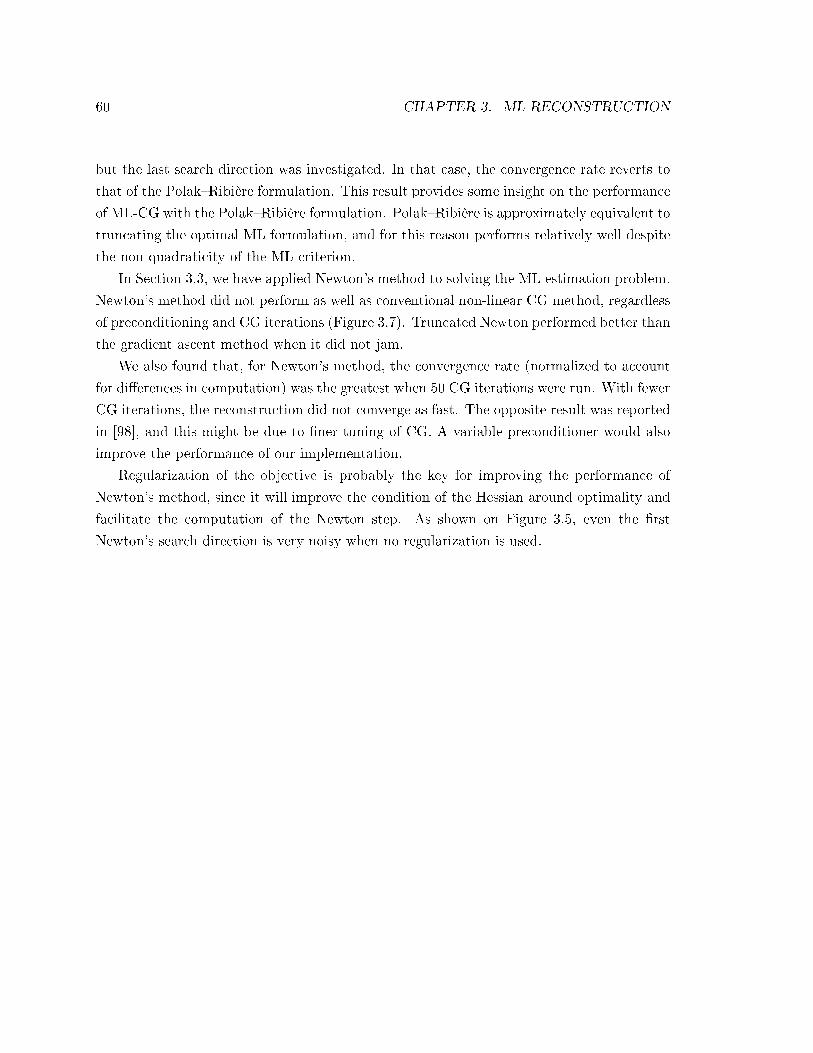
60 CHAPTER 3. ML RECONSTRUCTION
but the last search direction was investigated. In that case, the convergence rate reverts to
that of the PolakRibière formulation. This result provides some insight on the performance
of ML-CG with the PolakRibière formulation. PolakRibière is approximately equivalent to
truncating the optimal ML formulation, and for this reason performs relatively well despite
the non-quadraticity of the ML criterion.
In Section 3.3, we have applied Newton's method to solving the ML estimation problem.
Newton's method did not perform as well as conventional non-linear CG method, regardless
of preconditioning and CG iterations (Figure 3.7). Truncated Newton performed better than
the gradient ascent method when it did not jam.
We also found that, for Newton's method, the convergence rate (normalized to account
for dierences in computation) was the greatest when 50 CG iterations were run. With fewer
CG iterations, the reconstruction did not converge as fast. The opposite result was reported
in [98], and this might be due to ner tuning of CG. A variable preconditioner would also
improve the performance of our implementation.
Regularization of the objective is probably the key for improving the performance of
Newton's method, since it will improve the condition of the Hessian around optimality and
facilitate the computation of the Newton step. As shown on Figure 3.5, even the rst
Newton's search direction is very noisy when no regularization is used.

Chapter 4
Fast Shift-Varying Line Projection
using Graphics Hardware
4.1 Background
Most of the computation time in ML image reconstruction is spent in the line projection
operations. In addition, list-mode schemes require that LORs be processed individually, in
arbitrary order. We investigated practical ways to implement and accelerate these operations
using programmable graphics hardware, namely the graphics processing unit (GPU) [99].
This chapter describes how graphics concepts can be mapped onto the GPU. A more
detailed presentation is available in Appendix A. A glossary of GPU terms can be found in
Appendix F.
4.1.1 The Graphics Processing Unit
Primarily designed to deliver high-denition graphics for video games in real-time, GPUs
are now increasingly being used as cost-eective high-performance co-processors for scientic
computing [100]. GPUs are characterized by massively parallel processing, fast clock-rate,
high-bandwidth memory access, and hardwired mathematical functions. These character-
istics make them particularly well suited for on-the-y schemes with high computational
intensity.
As shown on Figure 4.1, over the last ve years, GPUs' peak performance P has increased
at a faster rate than CPU's: PGPU ≈ P 1.4CPU. While Moore's law hypothesises that the
density of transistors on a chips doubles every two years, the peak compute performance of
GPU GPUs are single-instruction multiple-data (SIMD) processors but multi-core CPUs are
61

62 CHAPTER 4. GPU LINE PROJECTION
2002 2003 2004 2005 2006 2007 2008 2009 2010
101
102
103
GF
LOP
S
Year
CPU
GPU
A
B
C
D
E F
GH I J
A
B
C
DE
F
G
Figure 4.1: Trend in the computational performance P for CPUs and GPUs over ve years,measured in billion single-precision oating-point operation per second (GFLOPS). GPUs:NVIDIA GeForce FX 5800 (A), FX 5950 Ultra (B), 6800 Ultra (C), 7800 GTX (D), QuadroFX 4500 (E), GeForce 7900 GTX (F), 8800 GTX (G), and Tesla C1060 (H); CPUs: Athlon64 3200+ (A), Pentium IV 560 (B), Pentium D 960 (C), 950 (D), Athlon 64 X2 5000+ (E),Core 2 Duo E6700 (F), Core 2 Quad Q6600 (G), Athlon 64 FX-74 (H), Core 2 Quad QX6700(I) and Intel Core i7 965 XE (J).

4.1. BACKGROUND 63
Figure 4.2: The graphics pipeline. The boxes shaded in light red correspond to stages of thepipeline that can be programmed by the user.
multiple-instruction multiple-data (MIMD). MIMD leads to more complex integrated circuit
designs because multiple instruction decode blocks as well as special logic are required to
avoid data read/write hazards. SIMD also dedicates less area to the data cache and more
to the arithmetic logic units. As a result, the number of parallel SIMD processing units has
been growing faster than has the number of MIMD's. It therefore appears likely that GPUs
will continue to be increasingly useful for medical image reconstruction, especially as the
performance gap with CPUs widens.
Computations can be executed on the GPU either using graphics APIs, such as OpenGL
or DirectX, or specic APIs such as CUDA. This work used OpenGL to interface with the
GPU, hence we will present briey the graphic pipeline (Figure 4.2).
The role of the GPU in a 3-D graphical application (such as a video game) is to perform
the calculations necessary to render complex 3-D scenes in a short amount of time. The
3-D scene is created by the application using polygons (triangle, quadrangles, etc.). Using
OpenGL, these polygons are streamed to the GPU, along with instructions on how to render
the scene (position of the camera, lighting, textures, etc.). The programmer does not need
to know about the specics of the GPU because OpenGL is a standard API that interfaces
directly with the GPU driver. Two stages in the GPU are fully programmable: the vertex

64 CHAPTER 4. GPU LINE PROJECTION
and the fragment shaders (in light red on Figure 4.2).
The vertex shaders can perform, in parallel, a programmable sequence of instructions
on each individual vertex that passes through the pipeline. In computer graphics, the ver-
tex shader is used to perform the projection of the polygons on the plane of the display
and to calculate per-vertex properties, such as surface normals or texture mapping coor-
dinates. Properties dened for each vertex are bilinearly interpolated within the polygon.
The vertices are then assembled, and the triangles rastered into fragments (i.e. all the data
necessary to generate a pixel in the frame buer).
The fragment shaders' role is to perform programmable computation in parallel on all the
fragments. In computer graphics, they are used to calculate the nal color of the voxel based
on texture and lighting information. General-purpose computation (i.e. non-graphical) can
also be performed in this stage since the output of the fragment shader can be read out from
directly the frame-buer. Each fragment is then combined with the frame-buer according
to predened raster operation (additive blending, etc.).
4.1.2 Iterative Reconstruction on the GPU
Image reconstruction on GPUs has been the focus of previous research. Texture mapping on
non-programmable graphics hardware was rst proposed in 1994 [101] as a way to accelerate
cone-beam FBP for x-ray computed tomography. The same technique was later applied to
port sinogram-based OSEM to a consumer-grade graphics architecture [102]. More accurate
methods were developed once the GPU became programmable and handled oating-point
textures. The general approach was rst described for processing sinograms using FBP
and EM [103], and the ordered subset convex reconstruction algorithm [104]. Attenuation
correction and the incorporation of a point spread function were also addressed for SPECT
[105]. A real-time GPU-based reconstruction framework was developed for X-ray CT [106].
These methods [101106] have been successful because the GPU is ecient at applying
the ane transformation that maps a slice through the volumetric image to any sinogram
projection view, and vice-versa.
Until now, there have not been any work on executing list-mode iterative reconstruction
on GPUs. The main challenge in implementing list-mode OSEM on the GPU is that the
list-mode LORs are not arranged in any regular pattern like sinogram LORs. The mapping
between the list-mode data and the volumetric image is not ane, and as a result texture
mapping cannot be used in this context. The projection operations must be line driven,
which means that the back- and forward projections must be performed on a per LOR
basis. This constraint motivates the design and investigation of a novel GPU technique

4.2. THEORY 65
Figure 4.3: Example of a parametrization ofthe system response kernel. Two detectionelements in coincidence are shown, as wellas the projection Lij of a sample voxel Vjonto the axis of LOR i.
to back- and forward project individual LORs described by arbitrary endpoint locations,
even when a shift-varying kernel is used to model the response of the system [107]. No
existing GPU projection technique has addressed the specic issues of list-mode processing.
These issues also arise when data is processed in histogram-mode, in which case a weight,
representing the measured projection, is passed to the GPU with each LOR [49]. Even
sinogram-based reconstruction can be performed in this new LOR-driven framework by
describing each sinogram bin by its value and the two LOR endpoint locations; however this
approach would be less ecient than the GPU texture mapping technique cited above. We
also propose a novel framework to dene arbitrary, shift-varying system response kernels
that are evaluated on-the-y by parallel units within the GPU. This feature is important to
correct for the various resolution blurring factors in emission tomography.
The implementation on the GPU of list-mode 3D-OSEM with shift-varying kernels is
challenging because the graphics pipeline architecture does not run eciently unless the two
main components (line back- and forward projections) are reformulated. This reformulation
involves handling line backprojection using the GPU rasterizer and decomposing line forward
projection into smaller elementary operations that run eciently in parallel on the GPU. We
proved, both mathematically and experimentally, that the reformulated operations replicate
the correct line back- and forward projections [107].
4.2 Theory
4.2.1 System Response Kernel
The spatial resolution in PET is degraded by physical processes associated with photon
emission, transport and detection. These resolution blurring factors can be modeled in
the system matrix. This provides resolution recovery through deconvolution on condition
that the model is accurate enough, the SNR is high enough and the number of iterations
is sucient. Several experiments have shown that incorporating a model of the system
response can improve the performance of the reconstruction for certain tasks [42,43,48,79].
In the GPU line-projection technique we have developed, we generalize the notion of

66 CHAPTER 4. GPU LINE PROJECTION
system matrix by modeling the system response using kernels. Kernels are non-negative
real-valued functions that model the contribution of each voxel to each LOR as a function
of multiple variables. These variables include the indices of the current LOR and voxel,
which allow any system matrix to be represented with a kernel. Kernels can be described
more generally by selecting another choice of parametrization, such as the center Vj of voxel
j, the projection Lij of Vj on LOR i, the distance dij between the center of voxel j and
LOR i, the distances between Lij and each of the two detectors δ(1)ij and δ(2)
ij , the orientation
ui and length li of LOR i, the time-of-ight τi, and the photon depth-of-interaction for
each detector z(1)i and z(2)
i (Figure 4.3). Kernels are smooth approximations of the system
matrix, independent of the voxel size. They model the system response in a compact way
by exploiting the geometrical redundancies in the system.
The kernel is evaluated at all voxels that contribute signicantly to LOR i. We call the
set of such voxels the tube-of-response (TOR), further dened by a cylindrical volume:
Ti = j : dij ≤ η (4.1)
where η is a user-dened constant which sets an upper bound on the distance dij between
voxel j and LOR i. While system matrices are implemented by look-up tables, kernels allow
for a mix of memory look-ups and on-the-y computations and lead to a higher computa-
tional intensity (dened as the ratio of arithmetic logic unit to memory usage). Kernels can
also be evaluated at each voxel independently, in the GPU parallel processing units.
4.2.2 GPU Implementation
In order to use the GPU pipeline eciently, we reformulated the projections to enhance
parallelism and match the pipeline architecture.
4.2.2.1 Data Representation
GPU memory is organized in textures, which in computer graphics are used to store color
images. A 2-D color texture forms an array of 32-bit oating-point quadruples, that can be
accessed randomly by GPU shaders. We stored the volumetric images used for reconstruction
in such textures by tiling the stack of slices in 2-D (A.1.1). The list-mode projection data,
consisting of LOR endpoints and the projection value, were stored in another 2-D texture
using the four color channels. We used the OpenGL frame-buer object (FBO) extension
to enable shaders to write directly to texture [108].
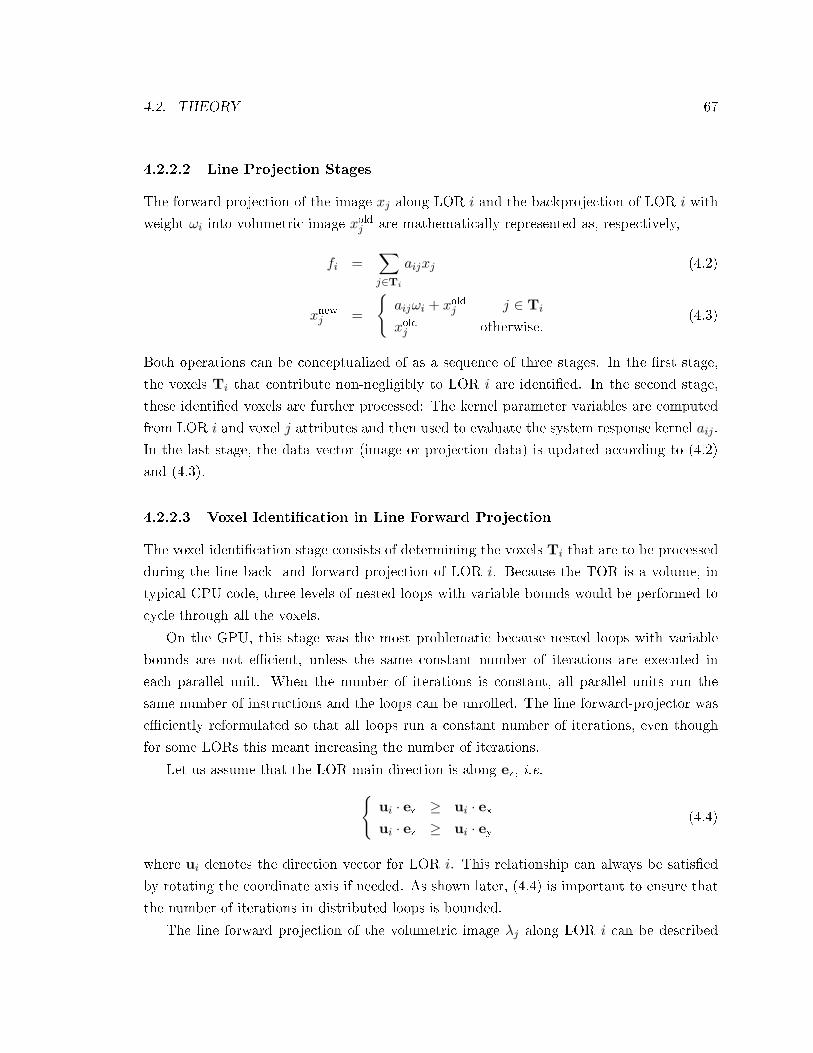
4.2. THEORY 67
4.2.2.2 Line Projection Stages
The forward projection of the image xj along LOR i and the backprojection of LOR i with
weight ωi into volumetric image xoldj are mathematically represented as, respectively,
fi =∑j∈Ti
aijxj (4.2)
xnewj =
aijωi + xoldj j ∈ Ti
xoldj otherwise.(4.3)
Both operations can be conceptualized of as a sequence of three stages. In the rst stage,
the voxels Ti that contribute non-negligibly to LOR i are identied. In the second stage,
these identied voxels are further processed: The kernel parameter variables are computed
from LOR i and voxel j attributes and then used to evaluate the system response kernel aij .
In the last stage, the data vector (image or projection data) is updated according to (4.2)
and (4.3).
4.2.2.3 Voxel Identication in Line Forward Projection
The voxel identication stage consists of determining the voxels Ti that are to be processed
during the line back- and forward projection of LOR i. Because the TOR is a volume, in
typical CPU code, three levels of nested loops with variable bounds would be performed to
cycle through all the voxels.
On the GPU, this stage was the most problematic because nested loops with variable
bounds are not ecient, unless the same constant number of iterations are executed in
each parallel unit. When the number of iterations is constant, all parallel units run the
same number of instructions and the loops can be unrolled. The line forward-projector was
eciently reformulated so that all loops run a constant number of iterations, even though
for some LORs this meant increasing the number of iterations.
Let us assume that the LOR main direction is along ez, i.e.ui · ez ≥ ui · exui · ez ≥ ui · ey
(4.4)
where ui denotes the direction vector for LOR i. This relationship can always be satised
by rotating the coordinate axis if needed. As shown later, (4.4) is important to ensure that
the number of iterations in distributed loops is bounded.
The line forward projection of the volumetric image λj along LOR i can be described
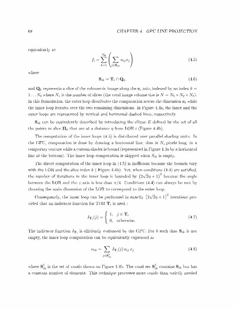
68 CHAPTER 4. GPU LINE PROJECTION
equivalently as
fi =Nz∑k=1
∑j∈Sik
aijxj
(4.5)
where
Sik = Ti ∩Qk. (4.6)
and Qk represents a slice of the volumetric image along the ez axis, indexed by an index k =1 . . . Nz where Nz is the number of slices (the total image volume size is N = Nx×Ny×Nz).
In this formulation, the outer loop distributes the computation across the dimension ez while
the inner loop iterates over the two remaining dimensions. In Figure 4.4a, the inner and the
outer loops are represented by vertical and horizontal dashed lines, respectively.
Sik can be equivalently described by introducing the ellipse E dened by the set of all
the points in slice Πk that are at a distance η from LOR i (Figure 4.4b).
The computation of the inner loops (4.5) is distributed over parallel shading units. In
the GPU, computation is done by drawing a horizontal line, that is Nz-pixels long, in a
temporary texture while a custom shader is bound (represented in Figure 4.4a by a horizontal
line at the bottom). The inner loop computation is skipped when Sik is empty.
The direct computation of the inner loop in (4.5) is inecient because the bounds vary
with the LOR and the slice index k ( Figure 4.4b). Yet, when conditions (4.4) are satised,
the number of iterations in the inner loop is bounded by(2√
2η + 1)2
because the angle
between the LOR and the z axis is less than π/4. Conditions (4.4) can always be met by
choosing the main dimension of the LOR to correspond to the outer loop.
Consequently, the inner loop can be performed in exactly⌈2√
2η + 1⌉2
iterations pro-
vided that an indicator function for TOR Ti is used :
ITi(j) =
1, j ∈ Ti
0, otherwise.(4.7)
The indicator function ITi is eciently evaluated by the GPU. For k such that Sik is not
empty, the inner loop computation can be equivalently expressed as
αik =∑j∈S†ik
ITi(j) aij xj (4.8)
where S†ik is the set of voxels shown on Figure 4.4b. The voxel set S†ik contains Sik but has
a constant number of elements. This technique processes more voxels than strictly needed

4.2. THEORY 69
(a)
(b)
Figure 4.4: (a) In the line forward projection, voxels that contribute to LOR i are identiedby performing an outer and an inner loop. The former iterates over the main dimension forthe LOR ( as dened in (4.4) here ez), while the latter iterates over the two remainingdimensions (only ey is shown on the gure). The computation of the inner loops is performedsimultaneously in parallel shaders within the GPU. To make computation ecient, the innerloop bounds are increased so that the number of iterations is constant. In a second pass,the outer loop sum is computed by a second shader (bottom).(b) Voxel j ∈ Sik (represented in dark gray) if and only if its center (V x
j , Vyj ) is inside ellipse
E (4.6). The size and shape of Sik vary with i and k, which prevents ecient GPU loopsover this set. However, Sik is a subset of S†ik (light+dark gray), whose size is constant. Thus,loops on S†ik run eciently on the GPU.

70 CHAPTER 4. GPU LINE PROJECTION
but keeps the bounds of the inner loop constant.
The translation of this technique in OpenGL/Cg terms is the following: horizontal lines
(shown on the bottom of Figure 4.4a) are drawn into a temporary 2-D buer while a 1-D
texture is applied onto these lines by mapping the horizontal line endpoints to the original
LOR endpoints. The 1-D mapping generates texture look-up coordinates (shown as white
dots in Figure 4.4a). Textures are ltered on-the-y by custom shaders which performed
the inner loop computation described in (4.8). This method generates the αik values and
stores them in a temporary 2-D texture. In a second pass, a shader calculates the sum over
k (4.1 on page 73).
4.2.2.4 Voxel Identication in Line Backprojection
A dierent technique was used to identify the voxels in the line backprojection. The GPU
rasterizer was used to identify which voxels belong to the TOR and distribute the evaluation
of the system response kernel.
The GPU rasterizer can convert a 2-D vectorial polygon Γ into a 2-D pixel image xj .
In computer graphics, 2-D polygons come from the projection of 3-D vectorial primitives
onto the plane of the display. Pixel j is rastered if its center (V xj , V
yj ) belongs to polygon Γ
(Figure 4.5). We call
RΓ =j : (V x
j , Vyj ) ∈ Γ
(4.9)
the set of such voxels. A pixel shader Φ can be inserted in the graphics pipeline to compute
the pixel value xj (i.e. color). This yields the raster equation
xj =
Φ(j), j ∈ RΓ
0, otherwise.(4.10)
GPUs can only raster 2-D vectorial objects, which hinders a straightforward implementa-
tion of 3-D line backprojection. Yet, it is possible to circumvent this obstacle by performing
the line backprojection slice by slice. Color is used to encode the slice index and process
four slices simultaneously. For each slice k and LOR i, a polygon Γ is generated and then
rastered into the set of voxels RΓ (4.9). The best choice for Γ is the smallest rectangle that
covers the ellipse E (Figure 4.5). In that case, RΓ contains Sik and all the voxels in Ti are
processed. RΓ can be larger than Sik, so an indicator function is necessary (4.7).
In OpenGL, rectangles are drawn into a 2-D texture while vertex and pixel shaders
are bound, respectively, to dene Γ's coordinates and to evaluate the value of the system
response kernel at each pixel location. The result of the kernel evaluation, aij , is then
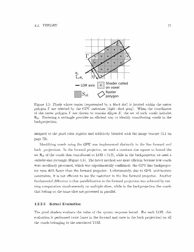
4.2. THEORY 71
Figure 4.5: Pixels whose center (represented by a black dot) is located within the rasterpolygon Γ are selected by the GPU rasterizer (light+dark gray). When the coordinatesof the raster polygon Γ are chosen to contain ellipse E, the set of such voxels includesSik. Rastering a rectangle provides an ecient way to identify contributing voxels in thebackprojection.
assigned to the pixel color register and additively blended with the image texture (4.1 on
page 73).
Identifying voxels using the GPU was implemented distinctly in the line forward and
back- projections. In the forward projector, we used a constant-size square to bound the
set Sik of the voxels that contributed to LOR i (4.2), while in the backprojector we used a
variable-size rectangle (Figure 4.5). The latter method was more ecient because less voxels
were needlessly processed, which was experimentally conrmed: the GPU line backprojec-
tor runs 40% faster than the forward projector. Unfortunately, due to GPU architecture
constraints, it is not ecient to use the rasterizer in the line forward projector. Another
fundamental dierence is that parallelization in the forward projection was achieved by run-
ning computation simultaneously on multiple slices, while in the backprojection the voxels
that belong to the same slice are processed in parallel.
4.2.2.5 Kernel Evaluation
The pixel shaders evaluate the value of the system response kernel. For each LOR, this
evaluation is performed twice (once in the forward and once in the back projection) on all
the voxels belonging to the associated TOR.

72 CHAPTER 4. GPU LINE PROJECTION
First, the kernel parameters are calculated using LOR and voxel attributes. LOR at-
tributes are dened in the vertex shader and passed to the pixel shader. The voxel attributes
are read from the Cg WPOS register.
For a xed-width Gaussian system response kernel, the only parameter needed is the
distance dij between LOR i and voxel j. This distance can be computed by forming the
orthogonal projection of the voxel center Vj onto the LOR dened by a point Pi and a
direction vector ui, i.e.
dij =∥∥∥−−→PiVj − (
−−→PiVj · ui) ui
∥∥∥2. (4.11)
This computation is fast because hardwired GPU functions for dot product and norm are
used.
Following the calculation of the parameter variables, the kernel value aij for LOR i and
voxel j is evaluated. The kernel evaluation can use texture look-ups and arithmetic functions
such as exponentials, powers and linear interpolation. Texture look-ups are useful, for
example, to read out the coecients of splines functions, which represent one parameter of
the system response kernel. The kernel value is only computed when needed. This approach
allows for implementation of arbitrary shift-varying kernels. The high-level shading language
Cg [109] provides an important library of mathematical functions that are applicable to both
scalar and vectorial oating-point registers.
4.2.2.6 Vector Data Update
The last stage of the projection consists of updating the data vector (either a volumetric
image or a set of list-mode projections).
For the line forward projector, the partial sums αik (4.5) are summed (outer loop):
fi =Nz∑k=1
αik. (4.12)
The resulting values fi are then inverted and written back to the projection data texture in
preparation of the line backprojection.
In the line backprojector, the pixel shader called by the rasterizer directly writes to
the correct voxel location. Additive blending was enabled to add the shader output to
the previous voxel value (4.10). Additive blending is performed in dedicated 32-bit oating-
point units. The last step in OSEM consists of multiplying the update image by the previous
volumetric image and dividing it by the sensitivity map (3.5). This is done by running the
volumetric image through a pixel shader.

4.3. DISCUSSION 73
Algorithm 4.1 Simplied schematics for one sub-iteration of list-mode 3D-OSEM on the GPU.
(OGL) indicates an OpenGL call, (VS) and (PS) denote programs running in the vertex and the
pixel shader, respectively.
Load list-mode events in video memory (OGL)
Line forward projection:
For each event
Choose outer loop dimension (VS)
Compute number of slices traversed (VS)
Draw a horizontal line (outer loop) (OGL)
For each pixel in the horizontal line
Inner loop through a slice (PS)
Evaluate kernel (PS)
Read image value (PS)
Accumulate (PS)
Sum horizontal line voxels (PS)
Update projection value (PS)
Line backprojection:
For each slice
For each event
Raster rectangle (OGL)
Compute rectangle coordinates (VS)
For each voxel in rectangle
Evaluate kernel (PS)
Blend additively with image (OGL)
Update image estimate multiplicatively (PS)
Divide by normalization map (PS)
4.1 summarizes the steps involved in the back- and forward projection of a group of
LORs. A more detailed overview, including shader code, can be found in Appendix A.
4.3 Discussion
GPUs and CPUs both aim at executing the workload as fast as possible but they use dier-
ent strategies to achieve that goal. CPUs excel at executing one long thread of computation,
while GPUs are ecient at running thousands of independent threads. Therefore, it is nec-
essary to adopt dierent reconstruction strategies on each platform. For example, Siddon's
algorithm [110] is well suited to CPU but not GPU architectures because it requires voxels to
be processed sequentially, in long threads of computation. In kernel projection techniques,
the system matrix is evaluated at each voxel independently, so the computation can be bro-

74 CHAPTER 4. GPU LINE PROJECTION
ken down into many small threads. Besides, kernel projection techniques produce better
images because Siddon's algorithm is based on the perfect line integral model which does
not include the contribution of voxels that are o of the LOR axis.
The CUDA library [111] is another interface to the compute engine of the GPU. CUDA
has several advantages, including greater ease of development, shared memory, and scattered
reads. However, CUDA does not provide access to the rastering engine, which is a critical
component of the line backprojection approach we have developed.
The GPU line projection technique presented in this chapter in used to implement three
dierent applications that are presented in the next chapter. An evaluation of the accuracy
of the projection is also presented.

Chapter 5
Applications of GPU-Based Line
Projections
5.1 Overview
Line projections are essential building blocks in tomographic image reconstruction. In this
chapter, we present three applications of GPU-based line projections for list-mode recon-
struction.
Three reconstruction algorithms were implemented. The rst algorithm was imple-
mented for the CZT high-resolution PET system and used a simple shift-invariant projection
kernel and served to validate the accuracy of the GPU-based line projections (Section 5.2).
The second algorithm, implemented on the same system, was based on an accurate detector
response model that was calculated on-the-y on the GPU (Section 5.3). The third algo-
rithm algorithm was implemented for a clinical system with time-of-ight (TOF) capabilities
(Section 5.4).
Owing to the sparseness of the data, list-mode OSEM (3.1.3.3) was chosen for all three
applications. The techniques we have described in Chapter 4 are particularly suitable for
list-mode because the line projections need to be performed individually on the GPU.
5.2 List-Mode OSEM with Shift-Invariant Projections
5.2.1 Shift-Invariant System Response Kernel
The results presented in this section are based on a shift-invariant Gaussian kernel centered
on the LOR axis. The full-width half-maximum (FWHM) was chosen to match the average
75

76 CHAPTER 5. APPLICATIONS
system-resolution blurring. The kernel K is parametrized by the distance dij between the
center of voxel j and LOR i
K(dij) = exp
(−d2ij
2σ2
)(5.1)
and we have aij = K(dij). This kernel is not the perfect representation of the system
response, but it is sucient to demonstrate the GPU line-projection technique. The next
section will demonstrate the use of the GPU line projection with more advanced, shift-
varying projection kernels.
5.2.2 Methods
5.2.2.1 Simulation Data
This work used data provided by a simulated small-animal PET system design based on
cross-strip 3-D CZT detectors described in 1.3.2.
(a) (b)
Figure 5.1: (a) Rod phantom used for contrast recovery comparison. (b) Sphere phantomused for resolution evaluation.
The Monte-Carlo package GATE [70] was used to simulate the acquisition of two phan-
toms. To keep the simulation as realistic as possible, the output from the GATE hits le
was used to position each photon event. Due to the low photo-fraction of the CZT material,
incoming photon events often interact multiple times in the detectors (Chapter 6). Such
photon events were positioned at the estimated location of the rst interaction and binned
to the nearest 1×5×1 mm3 bin. Consistent with measurements [16], we modeled the energy
resolution by adding Gaussian noise with FWHM 3%×√
511/E, where E is the energy of
the single interaction in keV.
A phantom comprising two large concentric rods (1 cm and 4 cm diameter) of activity
(Figure 5.1a) was simulated to assess the quantitative contrast recovery of the GPU-based

5.2. LIST-MODE OSEM WITH SHIFT-INVARIANT PROJECTIONS 77
reconstruction independent of the system resolution. Two regions of interest (ROI 1 and
ROI 2) were dened in the 1 cm and the 4 cm radius rods as shown in Figure 5.1. The
activity in each rod were set up to create a 10:1 activity concentration ratio between ROI 1
and ROI 2. The contrast C was measured on reconstructed images as a function of iteration
as
C =xROI 1 − xROI 2
xROI 2(5.2)
where xROI 1 and xROI 2 are the average image intensities over each ROI. Spatial variance
σ2ROI 2 in ROI 2 was also computed to approximate image noise N . Our gure of merit for
noise in the images is
N = σROI 2/xROI 2. (5.3)
Photons that scattered in the object as well as random coincidences were not included in
the reconstruction to obtain the reconstructed contrast in an ideal case.
The phantom data were reconstructed using list-mode 3D-OSEM on a CPU and a GPU
architecture. On the CPU, we used an in-house C++ reconstruction package [112] that was
modied to support arbitrary system response kernels. On the GPU, we used the novel
technique described in Section 4.2. For both platforms, the FWHM (= 2.35σ in (5.1)) of the
xed-width Gaussian kernel was chosen to be 1 mm, a value roughly equal to the detector
pitch. The computation of the sensitivity image Nj followed the same procedure for both
reconstructions.
A high-resolution sphere phantom (Figure 5.1b) was simulated to look at the eects of
the GPU reconstruction on image resolution. The phantom was composed of four quadrants
of spheres, all in one central plane, placed in air. The spheres were 1, 1.25, 1.5 and 1.75 mm
in diameter. Their centers were placed twice their diameter apart. Twenty million counts
were acquired. The activity was placed all the way up to the edge of the 8 × 8 × 8 cm3
system FOV.
Finally, to provide a global measure of the deviation between images produced using
GPU and CPU list-mode 3D-OSEM, we measured the average relative deviation
ε =1N
N∑j=1
∣∣∣xcpuj − xgpuj
∣∣∣xcpuj
(5.4)
at dierent sub-iterations for both phantoms.
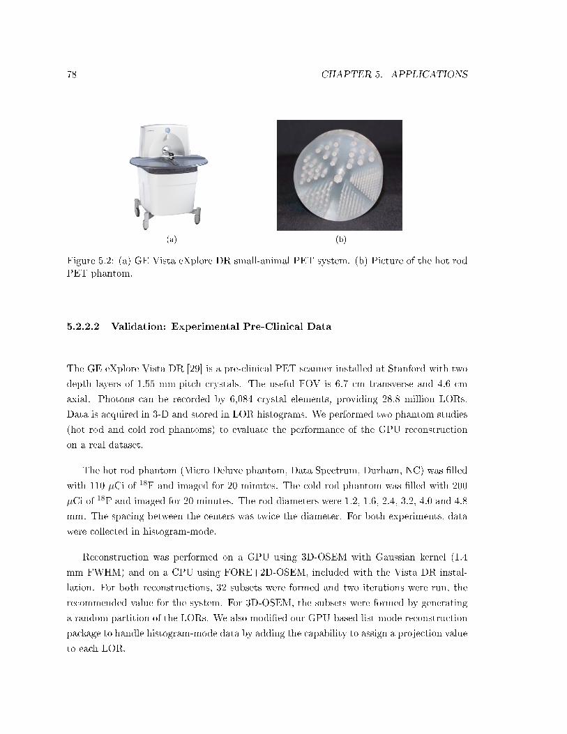
78 CHAPTER 5. APPLICATIONS
(a) (b)
Figure 5.2: (a) GE Vista eXplore DR small-animal PET system. (b) Picture of the hot rodPET phantom.
5.2.2.2 Validation: Experimental Pre-Clinical Data
The GE eXplore Vista DR [29] is a pre-clinical PET scanner installed at Stanford with two
depth layers of 1.55 mm-pitch crystals. The useful FOV is 6.7 cm transverse and 4.6 cm
axial. Photons can be recorded by 6,084 crystal elements, providing 28.8 million LORs.
Data is acquired in 3-D and stored in LOR histograms. We performed two phantom studies
(hot rod and cold rod phantoms) to evaluate the performance of the GPU reconstruction
on a real dataset.
The hot rod phantom (Micro Deluxe phantom, Data Spectrum, Durham, NC) was lled
with 110 µCi of 18F and imaged for 20 minutes. The cold rod phantom was lled with 200
µCi of 18F and imaged for 20 minutes. The rod diameters were 1.2, 1.6, 2.4, 3.2, 4.0 and 4.8
mm. The spacing between the centers was twice the diameter. For both experiments, data
were collected in histogram-mode.
Reconstruction was performed on a GPU using 3D-OSEM with Gaussian kernel (1.4
mm FWHM) and on a CPU using FORE+2D-OSEM, included with the Vista DR instal-
lation. For both reconstructions, 32 subsets were formed and two iterations were run, the
recommended value for the system. For 3D-OSEM, the subsets were formed by generating
a random partition of the LORs. We also modied our GPU-based list-mode reconstruction
package to handle histogram-mode data by adding the capability to assign a projection value
to each LOR.

5.2. LIST-MODE OSEM WITH SHIFT-INVARIANT PROJECTIONS 79
(a)
(b)
Figure 5.3: Reconstruction of the rodphantom using list-mode 3D-OSEMon (a) the GPU and (b) the CPU.
0 20 40 60 80 100 120 140 1600
2
4
6
8
10
Voxel index
Rec
onst
ruct
ed v
oxel
val
ue
CPUGPU
Figure 5.4: Horizontal prole through the centerof both images (Figure 5.3).
5.2.3 Results
No signicant dierence was observed between the images generated using list-mode 3D-
OSEM on the GPU and the CPU for the simulated rod contrast phantom (Figure 5.3). This
was further conrmed by a horizontal prole through the center of both images (Figure
5.4). The contrastnoise trade-o at dierent sub-iterations was neither aected by the
mathematical reformulation of line projections nor by the use of the GPU as a reconstruction
platform (Figure 5.5). The contrast, measured between ROI 1 and ROI 2, converged to 9.426
for the GPU and 9.428 for the CPU. Noise was virtually identical on both reconstruction
(0.28440 vs 0.28435 RMS).
Inspection of the sphere phantom images revealed no signicant dierence between the
two implementations (Figure 5.6). Neither did the prole through one row of 1.75 mm
spheres. The reconstructed sphere size was evaluated by tting a sum of Gaussians to 1-D
proles through the center of the 1.75 mm spheres. The sphere size on images reconstructed
with 3D-OSEM on both GPU and CPU is 1.36±0.32 mm. The dierence in the reconstructedsphere size between the GPU and CPU implementations was on the order of 10−5 mm.
The global dierence between images reconstructed using the GPU and the CPU was

80 CHAPTER 5. APPLICATIONS
Figure 5.5: Contrastnoise trade-o at dierent sub-iterations for the rod phantom (Figure5.3). Contrast is evaluated between ROI 1 and ROI 2 (Figure 5.1). Noise is approximatedby the spatial standard deviation in ROI 1.
quantitatively evaluated by measuring the average relative deviation (5.4). The overall
deviation ε between the two implementations was below 0.25% at 20 iterations for both
phantom. It was lower for the rod phantom than for the sphere phantom (Figure 5.8).
The GPU reconstruction package was benchmarked against an existing standard recon-
struction package on high-resolution datasets acquired on the Vista DR. A comparison of
GPU histogram-mode 3D-OSEM against CPU FORE+2D-OSEM for the hot rod (Figure
5.9) and the cold rod (Figure 5.10) shows visual dierences. All of the nineteen 1.6 mm rods
were resolved when 3D-OSEM was used, compared to only ten with FORE+2D-OSEM. The
improvement is due to the limited potential of FORE for resolution recovery [42, 43], not
the dierence in processing between GPU and CPU.
The processing time for each reconstruction method was measured (Table 5.1). CPU-
based 3D-OSEM was benchmarked on an Intel Core 2 Duo E6600 (2.4GHz) CPU. The
GPU used for the same task was the NVIDIA GeForce 8800GT GPU. The image size was
160 × 160 × 160 voxels for the simulated datasets and 175 × 175 × 60 voxels for Vista DR
datasets. The measured time includes Fourier rebinning for FORE+2D-OSEM. A 1 mm-
FWHM Gaussian kernel with a TOR cut-o of η = 1 mm was used for 3D-OSEM in the rst
experiment. In the second one, we chose a 1.1 mm-FWHM kernel with a TOR η = 0.8 mm
cut-o. Reconstruction time is provided for one million LORs processed (back- and forward

5.2. LIST-MODE OSEM WITH SHIFT-INVARIANT PROJECTIONS 81
(a)
(b)
Figure 5.6: Sphere phantom in air re-constructed with 20 iterations of list-mode 3D-OSEM on (a) the GPU and(b) the CPU, using Gaussian kernelwith 1 mm-FWHM.
10 20 30 40 50 60 70 800
2
4
6
8
10
Voxel index
Rec
onst
ruct
ed v
oxel
val
ue
CPUGPU
Figure 5.7: Horizontal prole through the 1.75 mmspheres for both reconstructions.(Figure 5.6).
Figure 5.8: Average relative deviation between the GPU and the CPU versions of list-mode3D-OSEM for the rod phantom and the sphere phantom.

82 CHAPTER 5. APPLICATIONS
(a) (b)
Figure 5.9: Micro Deluxe hot rod phantom, acquired on the Vista DR system and recon-structed with (a) histogram-mode 3D-OSEM with 1.4 mm-FWHM Gaussian kernel on theGPU and (b) using FORE+2D-OSEM provided with the system. A single slice is shown.The rod diameters are 1.2, 1.6, 2.4, 3.2, 4.0 and 4.8 mm. Spacing is twice the diameter.
(a) (b)
Figure 5.10: Micro Deluxe cold rod phantom, acquired on the Vista DR system and recon-structed with histogram-mode 3D-OSEM with (a) 1.4 mm-FWHM Gaussian kernel on theGPU and also (b) using the FORE+2D-OSEM provided with the Vista DR system. A singleslice is shown. The rod diameters are 1.2, 1.6, 2.4, 3.2, 4.0 and 4.8 mm. Spacing betweencenters is twice the diameter.
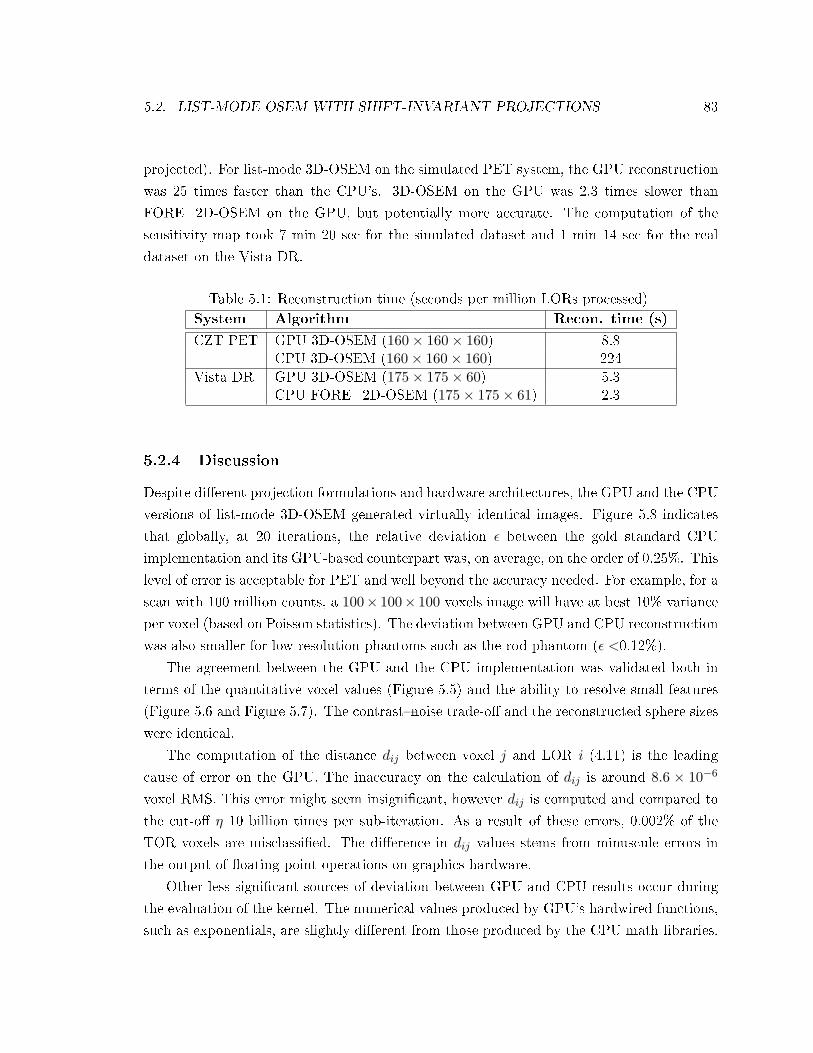
5.2. LIST-MODE OSEM WITH SHIFT-INVARIANT PROJECTIONS 83
projected). For list-mode 3D-OSEM on the simulated PET system, the GPU reconstruction
was 25 times faster than the CPU's. 3D-OSEM on the GPU was 2.3 times slower than
FORE+2D-OSEM on the GPU, but potentially more accurate. The computation of the
sensitivity map took 7 min 20 sec for the simulated dataset and 1 min 14 sec for the real
dataset on the Vista DR.
Table 5.1: Reconstruction time (seconds per million LORs processed)System Algorithm Recon. time (s)
CZT PET GPU 3D-OSEM (160× 160× 160) 8.8CPU 3D-OSEM (160× 160× 160) 224
Vista DR GPU 3D-OSEM (175× 175× 60) 5.3CPU FORE+2D-OSEM (175× 175× 61) 2.3
5.2.4 Discussion
Despite dierent projection formulations and hardware architectures, the GPU and the CPU
versions of list-mode 3D-OSEM generated virtually identical images. Figure 5.8 indicates
that globally, at 20 iterations, the relative deviation ε between the gold standard CPU
implementation and its GPU-based counterpart was, on average, on the order of 0.25%. This
level of error is acceptable for PET and well beyond the accuracy needed. For example, for a
scan with 100 million counts, a 100× 100× 100 voxels image will have at best 10% variance
per voxel (based on Poisson statistics). The deviation between GPU and CPU reconstruction
was also smaller for low-resolution phantoms such as the rod phantom (ε <0.12%).
The agreement between the GPU and the CPU implementation was validated both in
terms of the quantitative voxel values (Figure 5.5) and the ability to resolve small features
(Figure 5.6 and Figure 5.7). The contrastnoise trade-o and the reconstructed sphere sizes
were identical.
The computation of the distance dij between voxel j and LOR i (4.11) is the leading
cause of error on the GPU. The inaccuracy on the calculation of dij is around 8.6 × 10⁻⁶
voxel RMS. This error might seem insignicant, however dij is computed and compared to
the cut-o η 10 billion times per sub-iteration. As a result of these errors, 0.002% of the
TOR voxels are misclassied. The dierence in dij values stems from minuscule errors in
the output of oating-point operations on graphics hardware.
Other less signicant sources of deviation between GPU and CPU results occur during
the evaluation of the kernel. The numerical values produced by GPU's hardwired functions,
such as exponentials, are slightly dierent from those produced by the CPU math libraries.

84 CHAPTER 5. APPLICATIONS
The Vista DR study shows that the GPU reconstruction performs well with data mea-
sured on an existing high-resolution PET system. We compared GPU 3D-OSEM with a
Gaussian kernel to the standard reconstruction algorithm installed on this system, FORE+2D-
OSEM, in order to show that the GPU reconstruction produces acceptable results. The qual-
ity of the images meets our expectations and matches or exceeds that of FORE+2D-OSEM
reconstruction.
As mentioned in Table Table 5.1, FORE+2D-OSEM on a CPU is 2.3 times faster than
3D-OSEM on the GPU, but potentially not as accurate because FORE uses several approx-
imations to rebin the 28.8 million LORs into 1.4 million eective 2-D LORs (sixty-one 2-D
sinograms with 175 spatial locations and 128 angles [29]). While FORE+2D-OSEM trades
image quality for reconstruction speed, the GPU implementation does not pay a signicant
penalty for the acceleration.
It is also worth noting that the processing time for FORE+2D-OSEM per million eective
LORs is 47.3 sec, which is 9 times than that for GPU 3D-OSEM. In addition, the rebinned
2-D LORs involve a smaller number of voxels because they are shorter than 3-D LORs and
they do not incorporate a broad system kernel. The TORs that were used in Table Table 5.1
for 3D-OSEM involved on average 10 times more voxels than the LORs used for 2D-OSEM,
the volumetric image size being equal. Thus, 3D-OSEM would run around 10 times faster
if a narrow (i.e. η small) TOR was used.
A few other qualitative comments can be made. Concerning the hot rod phantom (Figure
5.9), all of the 1.6 mm rods are clearly resolved for the GPU-based reconstruction with
Gaussian kernel. In contrast, some the 1.6 mm rods at the edge of the FOV are not resolved
on the FORE+2D-OSEM image. The background noise is also lower by 27% for the 3-
D reconstruction. For the cold rod phantom (Figure 5.10), we observed that 3D-OSEM
provided greater uniformity throughout the FOV as well as higher contrast.
The 1.6 mm diameter rods are more dicult to resolve in the cold rod phantom than
in the hot rod phantom. This is due to several factors. In the hot rod phantom, the signal
(dened as the reconstructed activity in the hot rods) has lower noise than the surrounding
background. The situation is reversed for the cold rod phantom where the signal is consti-
tuted by the cold rods. In addition, random and scatter events (uncorrected in this study)
tend to obscure the cold regions of the phantom. Positive reconstruction bias, which occurs
in cold regions in PET, has a similar eect. Because spatial resolution is not the limitation
in a cold rod phantom, the dierence between 2-D and 3-D reconstruction is more subtle
for the cold rod phantom than for the hot rod phantom.
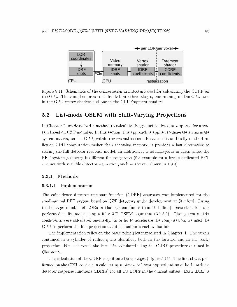
5.3. LIST-MODE OSEM WITH SHIFT-VARYING PROJECTIONS 85
Figure 5.11: Schematics of the computation architecture used for calculating the CDRF onthe GPU. The complete process is divided into three stages, one running on the CPU, onein the GPU vertex shaders and one in the GPU fragment shaders.
5.3 List-mode OSEM with Shift-Varying Projections
In Chapter 2, we described a method to calculate the geometric detector response for a sys-
tem based on CZT modules. In this section, this approach is applied to generate an accurate
system matrix, on the GPU, within the reconstruction. Because this on-the-y method re-
lies on GPU computation rather than accessing memory, it provides a fast alternative to
storing the full detector response model. In addition, it is advantageous in cases where the
PET system geometry is dierent for every scan (for example for a breast-dedicated PET
scanner with variable detector separation, such as the one shown in 1.3.3).
5.3.1 Methods
5.3.1.1 Implementation
The coincidence detector response function (CDRF) approach was implemented for the
small-animal PET system based on CZT detectors under development at Stanford. Owing
to the large number of LORs in that system (more than 10 billion), reconstruction was
performed in list-mode using a fully 3-D OSEM algorithm (3.1.3.3). The system matrix
coecients were calculated on-the-y. In order to accelerate the computation, we used the
GPU to perform the line projections and the online kernel evaluation.
The implementation relies on the basic principles introduced in Chapter 4. The voxels
contained in a cylinder of radius η are identied, both in the forward and in the back-
projection. For each voxel, the kernel is calculated using the CDRF procedure outlined in
Chapter 2.
The calculation of the CDRF is split into three stages (Figure 5.11). The rst stage, per-
formed on the CPU, consists in calculating a piecewise linear approximation of both intrinsic
detector response functions (IDRFs) for all the LORs in the current subset. Each IDRF is

86 CHAPTER 5. APPLICATIONS
stored using only four oating-point coecients: X0, X1, Y1 and Y2. These coecients are
transferred to a 2-D texture in the GPU video memory.
In the second stage, which takes place in the GPU parallel vertex shaders, the coecients
adl and bdl are calculated for every LOR. They are then streamed to the fragment shaders.
In the third stage, the GPU fragment shaders compute the kernel value for every voxel
within the tube-of-response following (2.15).
5.3.1.2 Evaluation
The Monte-Carlo package GRAY [113] was used to simulate the acquisition of two phantoms
with the CZT-based PET system. To keep the simulation as realistic as possible, the output
from GRAY was used to position each photon event. Due to the low photo-fraction of
the CZT material, incoming photon events often interact multiple times in the detectors
(Chapter 6). Such photon events were positioned at the estimated location of the rst
interaction and binned to the nearest 1×5×1 mm3 bin. Consistent with measurements [16],
we modeled the energy resolution by adding Gaussian noise with FWHM 3% ×√
511/E,where E is the energy of the single interaction in keV.
The high-resolution sphere phantom (Figure 5.12a) was used to research the eects
of accurate system modeling on image resolution. The phantom was composed of four
quadrants of spheres in air, all in the central axial plane, placed all the way to the edge of
the 8× 8× 8 cm3 transaxial FOV. The spheres were 1, 1.25, 1.5, and 1.75 mm in diameter.
Their centers were placed twice their diameters apart. The phantom had a total of 800 µCi
and ve seconds of acquisition were simulated, yielding 27.2 million coincident events.
Two reconstructions were performed on the GPU using list-mode 3D-OSEM, with 10 sub-
sets. The rst reconstruction used a shift-invariant 1 mm-FWHM Gaussian kernel, and the
second one a shift-varying model based on the analytical CDRF. The reconstructed sphere
FWHM was measured by tting a Gaussian mixture with oset to 1-D proles through the
reconstructed image. Since the ML estimate is non-linear, the reconstructed sphere FWHM
should be analyzed with care and should not be interpreted in terms of modulation transfer
function. It should also be noted that reconstructed sphere FWHM is not expected to be
equal to the true sphere diameter (see Appendix E for more details). The 1 mm spheres
were also too small relative to the voxel size for a reliable measure of their FWHM.
The contrast phantom (Figure 5.12b) was also used to assess the quantitative contrast
recovery. The phantom was composed of a 2.5 cm-radius, 6 cm-long cylinder, lled with a
warm solution of activity, in which ve hot spheres were placed. The spheres were centered
on the central axial plane and their diameters were 1, 1.5, 2, 4, and 8 mm. The activity

5.3. LIST-MODE OSEM WITH SHIFT-VARYING PROJECTIONS 87
(a) (b)
Figure 5.12: Depiction of phantoms used for measuring the eect of shift-varying resolutionmodels. (b) A contrast phantom, consisting of a 2.5 cm-radius, 6 cm long cylinder lledwith a warm solution of activity, in which were placed ve hot spheres of diameters 1, 1.5, 2,4, and 8 mm. The ratio of the activity concentration in the hot spheres to that in the warmbackground cylinder was 10. (c) A hot sphere resolution phantom, consisting of four spherepatterns, all in the same central plane. The spheres extended to the edge of the 8 × 8 × 8cm3 FOV and their diameters were 1, 1.25, 1.5, and 1.75 mm. The spacing between thespheres' centers was twice their diameter.
was ten times more concentrated in the hot spheres than in the warm background. The
phantom had a total of 800 µCi and ve seconds of acquisition were simulated, yielding
14.6 million coincident events. Reconstruction was performed in list-mode with two subsets
and attenuation correction. The contrast was measured in the reconstructed image as a
function of iteration number (5.2). The mean reconstructed activity was measured in the hot
spheres using spherical regions-of-interest (ROIs). The background activity was evaluated by
averaging the reconstructed intensity in two cylindrical ROIs placed o of the central axial
plane. The noise was approximated by the spatial standard deviation in the background
ROI, normalized by the mean background intensity (5.3).
5.3.2 Results
The impact of using a resolution model based on the CDRF in the reconstruction was
evaluated both in term of contrast recovery and spatial resolution.
5.3.2.1 Resolution
Figure 5.13 shows the high-resolution sphere phantom reconstructed with a shift-invariant
Gaussian kernel and a shift-varying model. The image reconstructed with a shift-invariant
model has non-uniform resolution due to parallax errors (dened in 1). Radial blurring is
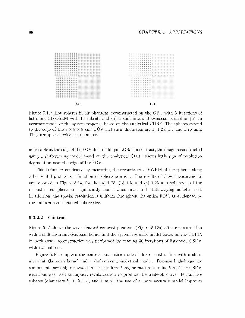
88 CHAPTER 5. APPLICATIONS
(a) (b)
Figure 5.13: Hot spheres in air phantom, reconstructed on the GPU with 5 iterations oflist-mode 3D-OSEM with 10 subsets and (a) a shift-invariant Gaussian kernel or (b) anaccurate model of the system response based on the analytical CDRF. The spheres extendto the edge of the 8 × 8 × 8 cm3 FOV and their diameters are 1, 1.25, 1.5 and 1.75 mm.They are spaced twice the diameter.
noticeable at the edge of the FOV due to oblique LORs. In contrast, the image reconstructed
using a shift-varying model based on the analytical CDRF shows little sign of resolution
degradation near the edge of the FOV.
This is further conrmed by measuring the reconstructed FWHM of the spheres along
a horizontal prole as a function of sphere position. The results of these measurements
are reported in Figure 5.14, for the (a) 1.75, (b) 1.5, and (c) 1.25 mm spheres. All the
reconstructed spheres are signicantly smaller when an accurate shift-varying model is used.
In addition, the spatial resolution is uniform throughout the entire FOV, as evidenced by
the uniform reconstructed sphere size.
5.3.2.2 Contrast
Figure 5.15 shows the reconstructed contrast phantom (Figure 5.12a) after reconstruction
with a shift-invariant Gaussian kernel and the system response model based on the CDRF.
In both cases, reconstruction was performed by running 50 iterations of list-mode OSEM
with two subsets.
Figure 5.16 compares the contrast vs. noise trade-o for reconstruction with a shift-
invariant Gaussian kernel and a shift-varying analytical model. Because high-frequency
components are only recovered in the late iterations, premature termination of the OSEM
iterations was used as implicit regularization to produce the trade-o curve. For all ve
spheres (diameters 8, 4, 2, 1.5, and 1 mm), the use of a more accurate model improves
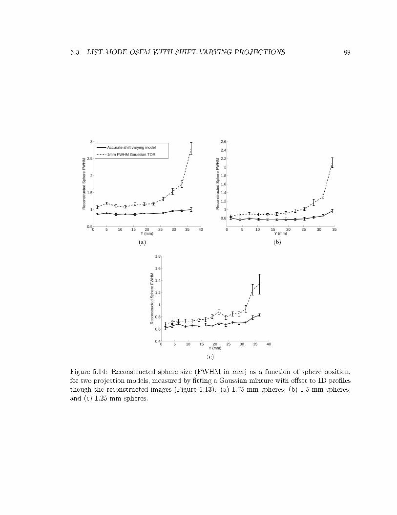
5.3. LIST-MODE OSEM WITH SHIFT-VARYING PROJECTIONS 89
0 5 10 15 20 25 30 35 400.5
1
1.5
2
2.5
3
Y (mm)
Rec
onst
ruct
ed S
pher
e F
WH
M
Accurate shift varying model
1mm FWHM Gaussian TOR
(a)
0 5 10 15 20 25 30 35
0.8
1
1.2
1.4
1.6
1.8
2
2.2
2.4
2.6
Y (mm)
Rec
onst
ruct
ed S
pher
e F
WH
M
(b)
0 5 10 15 20 25 30 35 400.4
0.6
0.8
1
1.2
1.4
1.6
1.8
Y (mm)
Rec
onst
ruct
ed S
pher
e F
WH
M
(c)
Figure 5.14: Reconstructed sphere size (FWHM in mm) as a function of sphere position,for two projection models, measured by tting a Gaussian mixture with oset to 1D prolesthough the reconstructed images (Figure 5.13). (a) 1.75 mm spheres; (b) 1.5 mm spheres;and (c) 1.25 mm spheres.

90 CHAPTER 5. APPLICATIONS
(a) (b)
Figure 5.15: Contrast phantom, reconstructed with 50 iterations of list-mode 3D-OSEMwith two subsets, using (a) a shift-invariant Gaussian kernel and (b) a shift-varying modelbased on the CDRF. The phantom was composed of a 2.5 cm-radius, water-lled cylinder,in which were placed ve hot spheres. The activity was ten times more concentrated in thespheres than in the background. The sphere diameters were 1, 1.5, 2, 4 and 8 mm.
the trade-o between contrast and noise. More specically, at any given iteration number,
the CR is higher and the noise is lower (except for the 1 mm sphere) for the shift-varying
reconstruction. For the 8 mm sphere, close to full contrast recovery is observed (CR of
95.7% at convergence). In addition, the background variability is lower for the shift-varying
reconstruction.
5.3.2.3 Reconstruction Time
The reconstruction time was measured for the simple Gaussian shift-invariant and accurate
shift-varying model in Table 5.2. Both measurements were made for the hot sphere phan-
tom dataset, using a GeForce 285 GTX (NVIDIA). The image size was 160 × 160 × 160.Consistently with Section 5.2, the Gaussian kernel width was 1 mm, much narrower than
the average width of the shift-varying kernel based on the CDRF. Hence, the TOR cut-o
parameter η was set to 3.5 voxels for the Gaussian projections, and to 5.5 voxels for the
shift-varying projections. More specically, η = 3.5 voxels means that the diameter of the
TOR is more than eight times the standard deviation of the Gaussian kernel. Likewise, for
the shift-varying kernel, η = 5.5 voxels results in a TOR diameter of 5.5 mm, larger than
the maximum CDRF kernel width of 5.1 mm (=√
52 + 12). As a result, the reconstruction
with accurate, shift-varying model was ten times slower than the simpler method based on
the shift-invariant Gaussian kernel.
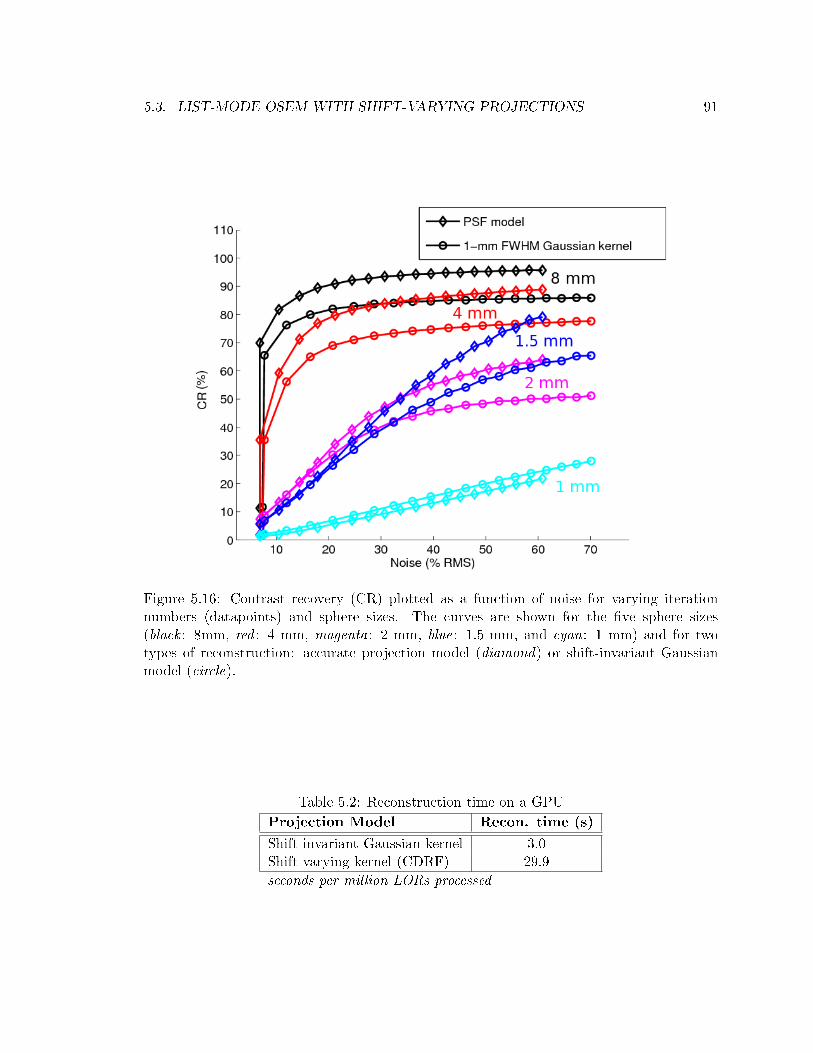
5.3. LIST-MODE OSEM WITH SHIFT-VARYING PROJECTIONS 91
Figure 5.16: Contrast recovery (CR) plotted as a function of noise for varying iterationnumbers (datapoints) and sphere sizes. The curves are shown for the ve sphere sizes(black : 8mm, red : 4 mm, magenta: 2 mm, blue: 1.5 mm, and cyan: 1 mm) and for twotypes of reconstruction: accurate projection model (diamond) or shift-invariant Gaussianmodel (circle).
Table 5.2: Reconstruction time on a GPUProjection Model Recon. time (s)
Shift-invariant Gaussian kernel 3.0Shift-varying kernel (CDRF) 29.9seconds per million LORs processed

92 CHAPTER 5. APPLICATIONS
It should be noted that the results reported in Table 5.2 for the shift-invariant kernel
are better than those reported in Table 5.1 in Section 5.2, since the value reported in this
section was obtained on a newer computer equipped with a more powerful GPU.
5.3.3 Discussion
The benets of using a more accurate, shift-varying model are clear and have already been
demonstrated elsewhere [42, 43, 47, 64, 68, 114]. For the CZT system we are developing, we
have shown that a system response model based solely on the detector response brings four
main improvements. First, the reconstructed spatial resolution is more uniform across the
FOV (Figure 5.13 and Figure 5.14). By incorporating accurate shift-varying information in
the system matrix, the spatially-variant blur present in the projections does not propagate
to the reconstructed image. Secondly, because the reconstructed spheres are smaller for the
shift-varying model, it suggests that the spatial resolution is globally higher (Figure 5.14)
and hence being recovered. Thirdly, the reconstructed images are more quantitative and
accurate because the physical processes involved are better modeled. Fourthly, the noise is
lower because using a more accurate system matrix in the reconstruction reduces the amount
of inconsistency between the dierent projections.
Figure 5.16 illustrates three of these properties. Higher resolution results in lower partial
volume eect and contributes to higher contrast recovery. The noise is also systematically
lower at a xed contrast, and at a xed iteration number. For the 8 mm diameter sphere,
which is large enough not to be aected by partial volume eect, the CR is 95.8% for the
shift-varying model vs. 85.9% for the shift-invariant Gaussian projection. This suggests
that the shift-varying reconstruction is more quantitative and accurate, a property observed
elsewhere [47,48].
For small object, spatial blurring causes a loss of contrast also known as partial volume
eect (PVE). Due to PVE, small spheres have a lower CR than larger spheres. This property
can be observed on Figure 5.16, except for two spheres: the 1.5 mm-diameter has CR higher
than the 2 mm one. This eect might be a consequence of the spatially varying nature
of the system response. Because the system is not cylindrical, the spatial resolution can
be dierent at dierent sphere locations. Therefore, the amount of PVE for each sphere
depends upon its position.
The total reconstruction time is ten times higher when the shift-varying model is used
(Table 5.2). This is due to two factors: an increase in the number of voxels processed, and
an increase in the computation required to evaluate the shift-varying kernel. For the shift-
invariant Gaussian kernel, 7 × 7 voxels are processed within each slice through the TOR,

5.4. TIME-OF-FLIGHT PET RECONSTRUCTION 93
twice fewer than for the wider kernels based on the CDRF (11 × 11 voxels per slice). In
addition, each voxel requires the evaluation of nine dierent kernel functions that are added
together ((2.15)).
The system response model can be implemented in many dierent ways. In this thesis,
we have chosen not to store any information but rather to compute the coecients of the
system matrix every time they are needed. As a consequence, this approach is useful when
the PET geometry needs to be adjusted between scans to the patient morphology. It is also
a scalable technique which uses a constant amount of computing resources, independent of
the number of LOR in the system.
A shift-varying model can also be stored in memory, however there exists a trade-o
between the accuracy of the representation and the amount of memory used. Our approach,
based on linearizing the IDRF, is accurate for the majority of the LORs (Figure 2.10) and
uses little memory. In addition, the computation of the kernel on the GPU is partially
hidden by the latency of reading the voxel values from memory.
5.4 Time-of-ight PET Reconstruction
5.4.1 Background
In PET, when two photons are detected in near coincidence, it can be inferred that the
positron annihilated somewhere near the LOR that connects the two detectors (see Figure
1.1 in Chapter 1). When the time dierence between tow single events falls within a pre-
determined time window, the two events are said to be in coincidence. Due to the nite
speed of light, two photons emitted simultaneously by positron annihilation do not reach
the detectors at the same time. For example, for a 60 cm FOV, the time dierence between
the two photons caused by travel time can be as large as 2 ns.
The timing uncertainty in existing clinical PET systems can be as good as 585 ps1 [115],
which makes it possible to estimate the photon time-of-ight (TOF) dierence, and to some
extent the rough location of the positron annihilation along the LOR. This information can
be used in image reconstruction to improve the image quality and quantitative accuracy. A
new generation of PET scanners have been designed and commercialized according to this
principle [115]. For the same scan duration, these systems have higher signal-to-noise ratio
(SNR) than similar systems that do not use the TOF information, and, as a result, provide
improved lesion detectability. Alternately, the scan time can be decreased while providing
the same image quality as non-TOF PET systems.
1One picosecond (ps) is equal to 10−12 seconds.
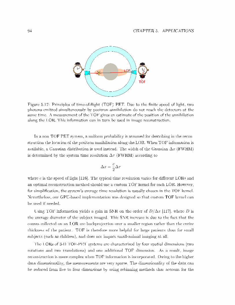
94 CHAPTER 5. APPLICATIONS
Figure 5.17: Principles of time-of-ight (TOF) PET. Due to the nite speed of light, twophotons emitted simultaneously by positron annihilation do not reach the detectors at thesame time. A measurement of the TOF gives an estimate of the position of the annihilationalong the LOR. This information can in turn be used in image reconstruction.
In a non-TOF PET system, a uniform probability is assumed for describing in the recon-
struction the location of the positron annihilation along the LOR. When TOF information is
available, a Gaussian distribution is used instead. The width of the Gaussian ∆x (FWHM)
is determined by the system time resolution ∆τ (FWHM) according to
∆x =c
2∆τ
where c is the speed of light [116]. The typical time resolution varies for dierent LORs and
an optimal reconstruction method should use a custom TOF kernel for each LOR. However,
for simplication, the system's average time resolution is usually chosen in the TOF kernel.
Nevertheless, our GPU-based implementation was designed so that custom TOF kernel can
be used if needed.
Using TOF information yields a gain in SNR on the order of D/∆x [117], where D is
the average diameter of the subject imaged. This SNR increase is due to the fact that the
counts collected on an LOR are backprojection over a smaller region rather than the entire
thickness of the patient. TOF is therefore more helpful for large patients than for small
subjects (such as children), and does not impact small-animal imaging at all.
The LORs of 3-D TOF-PET systems are characterized by four spatial dimensions (two
rotations and two translations) and one additional TOF dimension. As a result, image
reconstruction is more complex when TOF information is incorporated. Owing to the higher
data dimensionality, the measurements are very sparse. The dimensionality of the data can
be reduced from ve to four dimensions by using rebinning methods that account for the

5.4. TIME-OF-FLIGHT PET RECONSTRUCTION 95
(a) (b)
Figure 5.18: (a) Depiction of a Gaussian TOF kernel. (b) Parametrization of the TOF andprojection kernels.
TOF information [118]. However, such methods are approximate. The best image quality
is obtained when the images are directly reconstructed from the raw data. Fortunately,
ML reconstruction can be performed directly from list-mode (3.1.3.3), which is an ecient
format to store unprocessed PET data with TOF information.
In this section, we demonstrate that reconstruction of TOF-PET data can be performed
on a GPU in list-mode. The basic framework introduced in Chapter 4 is applied.
5.4.2 Methods
5.4.2.1 System Description
The Gemini TF (Philips Medical Systems, Highland Heights, OH) is the rst commercial
PET system capable of exploiting TOF information. The system comprises 28 modules,
each consisting of a 23×44 array of 4×4×22 mm3 LYSO crystals. The individual modules
are arranged in multiple 90 cm-diameter rings. The useful transverse and axial FOVs are
57.6 and 18.0 cm, respectively. The system timing resolution for the data shown in this
section was 785 ps (FWHM), however the timing resolution can be as good as 585 ps (for a
point source) [115]. The timing resolution can be aected by factors such as the count rate
and the detector temperature.
5.4.2.2 Implementation on the GPU
The GPU implementation of list-mode reconstruction with TOF information diers slightly
from non-TOF reconstruction. The projections are performed according to the approach
previously described in Chapter 4, with the exception that the TOF kernel was combined
with the projection kernel.

96 CHAPTER 5. APPLICATIONS
Figure 5.19: Cylindrical phan-tom used for time-of-ight PETmeasurements. The phantomis composed of six 10 mm diam-eter spheres, placed in a singleaxial plane 4.2 cm away fromthe central plane. The activ-ity is six times more concen-trated in the spheres than inthe cylinder.
Within projection operations, the TOF kernel, modeled as a Gaussian with standard
deviation σ, was truncated at ±3σ. Therefore, the LOR endpoints were reassigned to
C± 3σui, where C is the TOF kernel center, and ui is the direction of LOR i (Figure 5.18).
With this transformation, the transfer of the TOF kernel center C and width σ to the GPU
can be avoided, which reduces the amount of memory required on the GPU.
Within both the forward and the back-projection, the TOF kernel parameters were
computed in the vertex shaders. The TOF kernel center and width were recovered by
computing respectively the center and the distance between the two endpoints. Hence, the
only data required on the GPU are the coordinates of the transformed LOR endpoints.
The Gaussian projection kernel Kp (5.2.1) and the Gaussian TOF kernel Ktof were
combined, resulting in a singe 2-D Gaussian kernel parametrized both by the TOF and the
distance from the voxel center to the LOR
aij = Kp(dij) Ktof(dtofij )
where the distances dij and dtofij are the distances between Vj and Lij , and Lij and C,
respectively (as indicated on Figure 5.18).
The projection Lij of the voxel center Vj onto LOR i is computed on the GPU for each
voxel. Next, the distances dij and dtofij are computed and the Gaussian kernel is evaluated.
5.4.2.3 Phantom Experiment
PET measurements using the Gemini TF system were performed at the University of Penn-
sylvania using a 35 cm diameter cylindrical phantom (Figure 5.19). Six 10 mm diameter
spheres were placed in the phantom in a single axial plane 4.2 cm away from the central
plane. Within the plane, the spheres were arranged on a 8 cm-radius circle. The spheres
and the cylinder were lled with a solution of radioactive 18F. The activity was six times
5.4. TIME-OF-FLIGHT PET RECONSTRUCTION 97
more concentrated in the spheres than in the cylinder. The total activity was 6.4 mCi,
corresponding to a background activity concentration of 0.16 µCi/cc. The total scan time
was 5 min.
The images were reconstructed using 15 iterations of list-mode OSEM, with and without
TOF information. Twenty subsets were used for each iteration. The GPU-based image
reconstruction was compared against a CPU-based reconstruction performed at the Univer-
sity of Pennsylvania [119]. While the GPU used a radially-symmetric Gaussian kernel in
the projection and cubic voxels in the image representation (4.2.2), the CPU reconstruction
modeled the tracer spatial distribution as a sparse collection of Kaiser-Bessel (KB) blob
basis functions [120], and the projections as ideal line integrals. The Gaussian kernel and
the KB blobs are similar approaches: both use a kernel parametrized by the distance be-
tween the LOR axis and the center of the voxel. The dierences between the two approaches
include the kernel used, the kernel spacing, and in the fact that the Gaussian kernel directly
reconstructs image voxels, while the KB blob image must be converted to voxels for display.
The goal of this study is not to compare two image representations, but rather to inves-
tigate the feasibility of performing reconstruction of TOF PET data on a GPU in list-mode.
Therefore, the objective is to show that the improvement achieved by using TOF informa-
tion is consistent across both computing platforms. A comparison of the image quality on
GPU and CPU was presented in Section 5.2.
On the GPU, voxel sizes of 2× 2× 2, 4× 4× 4 and 8× 8× 8 mm3 were investigated. A
4 mm-FWHM Gaussian kernel was used in the projections. A post-reconstruction Gaussian
lter was also applied. The width of the lter was chosen to obtain image quality comparable
with the CPU implementation. A lter width of 2.1 mm FWHM was found to yield the
closest results. On the CPU, the blobs were arranged in a 8 mm body centered cubic (BCC)
grid. In theory, 8 mm blob spacing is comparable to 4 mm voxels [120].
Both reconstructions were normalized using the same blank and transmission scans.
The blank scan was performed by rotating a positron emitting source around the gantry.
A transmission scan of the phantom was acquired on the Gemini TF system using X-ray
CT to obtain a map of the photon attenuation coecients. In the standard manner, the
attenuation values were subsequently rescaled for 511 keV photons [61]. An estimate of
the random coincidences was also produced by measuring delayed coincidence events within
the emission scan. The random coincidences estimate was smoothed using Casey's method
[58] to improve the SNR. A TOF scatter estimate was generated using the single-scatter
simulation method [121]. The ratio of the normalization over the transmission scan were
incorporated in the sensitivity map (3.1.3.1) as a multiplicative factor (3.3). The randoms

98 CHAPTER 5. APPLICATIONS
Figure 5.20: Phantom images reconstructed with GPU-based and CPU-based implementa-tions, with and without TOF information. The voxels are 2× 2× 2 mm2.
and TOF scatter estimates were corrected for normalization and attenuation, and were then
used as additive terms in the forward projection, as described previously in (2.3).
The contrast recovery (CR), dened as the contrast as a percentage of the original ac-
tivity concentration ratio, was assessed in the reconstructed images. The sphere signal was
computed by averaging the voxel intensity in spherical ROIs for the six spheres. The back-
ground signal was evaluated similarly for six ROIs in a background slice axially opposite
to the sphere plane. The noise was approximated by the spatial variability (RMS) within
the background ROIs (5.3). The CR and noise were averaged over the six spheres present
in the phantom.
5.4.3 Results
5.4.3.1 Contrast vs. Noise
Figure 5.20 shows 2 mm-thick slices taken from the volume reconstructed with and without
TOF information, on the GPU (voxel representation) and the CPU platform (blobs repre-
sentation). All the images are shown for 15 iterations of list-mode OSEM with 20 subsets.
For all images, the pixel size is 2 × 2 mm2. In particular, the blob-based images were also
converted to 2 mm voxels for display.

5.4. TIME-OF-FLIGHT PET RECONSTRUCTION 99
Figure 5.21: Phantom images reconstructed using TOF information on the GPU with vary-ing voxel size.
The image sampling rate impacts the reconstructed image quality, as well as the process-
ing time. Figure 5.21 shows the same TOF dataset reconstructed on the GPU with three
dierent square voxel sizes: 2, 4 and 8 mm. While the 2 and 4 mm voxels result in similar
image quality, 8 mm voxels do not provide sucient sampling and result in a loss of spatial
resolution.
Figure 5.22 displays the trade-o between the contrast and the noise at dierent itera-
tions for the GPU and CPU implementations, with and without TOF information. The use
of TOF information within the reconstruction (black and red curves) results in an increase of
the CR compared to non-TOF reconstruction (blue and purple curves), while the noise level
is comparable. While for the non-TOF dataset, GPU and CPU reconstructions resulted in
comparable behavior, the reconstruction of the TOF dataset presented some disagreement
between CPU and GPU implementations. These dierences are unavoidable since the two
implementations have some key dierences that are described in the next section. However,
the contrast vs. noise trade-o curves show that the improvement achieved by using TOF
information is consistent across GPU and CPU platforms.
5.4.3.2 Processing Time
The processing time for the GPU reconstruction are summarized in Table 5.3. The values
are quoted for one pass through one million events, not including the calculation of the
sensitivity map and the scatter and randoms estimates. Two graphics card were used: a
GeForce 9800 GX2 and a GeForce 285 GTX.
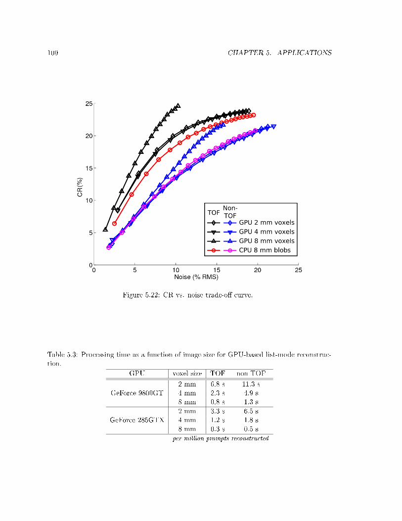
100 CHAPTER 5. APPLICATIONS
Figure 5.22: CR vs. noise trade-o curve.
Table 5.3: Processing time as a function of image size for GPU-based list-mode reconstruc-tion.
GPU voxel size TOF non-TOF
2 mm 6.8 s 11.3 sGeForce 9800GT 4 mm 2.3 s 4.9 s
8 mm 0.8 s 1.3 s2 mm 3.3 s 6.5 s
GeForce 285GTX 4 mm 1.2 s 1.8 s8 mm 0.3 s 0.5 s
per million prompts reconstructed

5.5. SUMMARY 101
5.4.4 Discussion
Section 5.2 and Section 5.3 showed that GPUs could be employed for non-TOF list-mode
reconstruction. Furthermore, the GPU implementation was shown to produce images that
were not signicantly dierent from those produced with an equivalent CPU implemen-
tation. In this section, we demonstrate that GPUs can be used for list-mode TOF-PET
reconstruction.
Figure 5.22 showed some discrepancies between the GPU and CPU reconstructions.
These dierences are unlikely to be caused by dierences in image representation alone. For
the TOF reconstruction, the single scatter simulation estimate was stored using coarser TOF
bins on the GPU to make processing practical. Furthermore, the subsets were organized
chronologically within the GPU implementation while a geometrical ordering was applied for
the CPU implementation. Further dierences might exist between the two implementations
since the goal of this study was not to compare both implementations, but to verify the
feasibility of implementing list-mode TOF PET reconstruction on the GPU.
Three factors determine the speed of the reconstruction: the number of variables in
the image representation (voxels or blobs), the size of the projection footprint (how many
variables are accessed for each line projection), and the amount of computation involved in
the evaluation of the projection kernel. The rst two factors determine the number of voxels
(or blobs) processed, hence the amount of memory that must be accessed for each event
processed. The amount of computation required is a combination of all three factors. As an
example, the GPU reconstruction with a Gaussian projection kernel involves a large number
of small voxels in the image, a relatively large number of voxels per LOR (i.e. the TOR)
and a medium amount of computation. Therefore, adjusting a single parameter (such as in
Table 5.3) characterizes only partially the performance of the method.
Hence, a comparison between the computing performance of two methods that use dier-
ent representations of the image and have dierent projection footprints is dicult. There-
fore, further investigation would be required to better characterize the benets of each
approach.
5.5 Summary
Three applications have been implemented based on the GPU-based line projection frame-
work introduced in Chapter 4. List-mode iterative reconstruction was performed on the
GPU for a high-resolution PET system with billions of LORs. The GPU framework allows

102 CHAPTER 5. APPLICATIONS
for a broad range of projection kernels, hence both a simple shift-invariant and a more com-
plex shift-varying model were studied. The latter model resulted in signicant image quality
and accuracy improvements, however the computation time increased tenfold. These two
examples show the exibility of the framework.
In addition, the framework was also chosen to implement list-mode reconstruction for
TOF PET. We showed the feasibility of the approach. Further work is required to match
the projection models of both GPU and CPU implementations and establish a comparison
of processing time with commercially-available software.

Chapter 6
Bayesian Reconstruction of Photon
Interaction Sequences
6.1 Background
6.1.1 Motivation
Cadmium Zinc Telluride (CZT) is a semiconductor material that can be used for building
radiation detectors. As a low Z material, its photo-fraction is low compared to other scin-
tillation crystals [16]. To preserve high photon detection eciency, the geometry of our
system (described in 1.3.2) is designed such that 511 keV photons traverse a minimum of 4
cm-thick material. Still, a large fraction of all the photons undergoes Compton scatter in
the detectors (see Figure 1.8). Because the eective detection elements are small (1× 5× 1mm3), the scattered photons usually escape into adjacent elements. On average, a 511 keV
photon deposits its energy in 2.2 detection elements.
To exploit the full potential of CZT detector modules, one major challenge needs to be
overcome. The image reconstruction must be able to use coincident events in which at least
one annihilation photon deposits its energy (511 keV) across multiple detection elements.
For the PET system described in 1.3.2, 93.8% of all the recorded coincident events for which
the summed energy is near 511 keV comprise at least one such multiple-interaction photon
event (MIPE). When MIPEs are used, high coincident photon sensitivity can be reached:
17 % for 800 µCi at the center of the eld of view (FOV) [32], a 16-fold increase compared
to using only events that deposit all their energy in a single detection element. However,
the ability to correctly position these events strongly determines the quality and accuracy
of the images obtained from a CZT-based PET system [49]. Determining the crystal of
103

104 CHAPTER 6. BAYESIAN SEQUENCE RECONSTRUCTION
entrance for MIPEs is ambiguous (see Figure 1.8). Hence, these events are at risk of being
erroneously assigned to the incorrect line-of-response (LOR), which in turn degrades spatial
resolution and image contrast [122,123].
6.1.2 Methods to Position Multiple Interaction Photon Events
Unlike standard PET detectors (2.1.1.2), the CZT cross-strip electrode design presented
in 1.3.2 can record the 3-D coordinates and energy deposition of individual interactions
for MIPEs. The system is able to distinguish the photons that deposit their energy in a
single detection element from those which deposit their energy in multiple detection elements
through multiple interactions. Positioning schemes have been devised to attribute a position
to MIPEs. These schemes can be broadly divided into three categories:
6.1.2.1 Initial Interaction Selection.
The MIPE position is selected from the nite set of all detected interactions. This class
of methods exploits some form of correlation between the order of the interactions and
properties of their energy and position. Techniques previously investigated include choosing
the interaction with largest / second largest signal [124,125], the smallest depth of interac-
tion [125], or the minimum distance to the other coincident photon [49]. For sequences of
more than two interactions, the order of subsequent interactions is not recovered with those
methods. Several techniques have been developed specically for positioning photons that
deposit energy in exactly two detectors. One method is based exclusively on the energies,
which for 511 keV photons is equivalent to assuming that the initial interaction is the most
energetic [126]. When one of the annihilation photon in a coincident pair scatters once, both
possible LORs can be used in the image reconstruction [127].
6.1.2.2 Unconstrained Positioning.
The positioning problem can be relaxed by allowing the position of MIPEs to be assigned to
any location within the detection volume. For example, the energy-weighted mean scheme
[124] combines the interaction locations linearly using the energy as weight. This is the only
positioning method available for conventional PET systems based on four-channel block
detectors. Because block detectors use a high degree of light and electronic multiplexing,
they cannot position individual interactions within a MIPE.

6.2. THEORY 105
6.1.2.3 Full Sequence Reconstruction.
The crystal of entry for MIPEs can also be estimated by reconstructing the complete se-
quence of interactions. A number of metrics have been investigated in order to penalize
sequences that violate the kinematics of Compton scatter. These techniques are based on
testing the consistency of redundant information. For example, the cosine of the scatter
angle can be computed using the Compton formula, provided that the order of the sequence
of interactions and the annihilation photon energy are known. This quantity can also be
computed directly from the interaction locations. The sum of the square of the dierences
of the scatter angle cosines [128,129] can be used as a metric to assess the kinematic validity
of a given sequence. This scheme can be rened by weighting the summands by the posi-
tional and energy measurement uncertainties. The weighted sum of the absolute dierence
between the scatter angle computed from trigonometry and from Compton kinematics is
another option for forming objective [130] .
The validity of an ordered sequence of interactions can also be measured based on physical
considerations, such as the probability that the annihilation photon follows a particular
trajectory realization. The Klein-Nishina dierential cross-section [131] is one component of
the trajectory probability [127]. Other components, such as the photoelectric cross section,
also contribute to the trajectory probability and can be included.
The sequence of interactions can also be reconstructed backwards [132]. Instead of
performing a full search over the combinatorial space of all the sequences, the method
recovers the complete sequence of interactions sequentially by rst identifying the photo-
electric interaction, whose energy is assumed to be independent of the track properties, and
then retracing the interaction track backwards.
6.2 Theory
We investigated a new sequence reconstruction technique which optimizes agreement with
the measurements while also accounting for the a priori probability of the photon trajectory
[49]. Bayesian estimation provides a natural framework to combine these two goals. The
likelihood component can deal with the consistency of the measurements, while a prior
probability distribution can describe the total trajectory cross-section. The product of
the likelihood with the prior distribution yields the maximum a posteriori (MAP) rule.
Using a statistical framework has the advantage that measurement noise can be explicitly
characterized and its eects accounted for.
One issue often reported with interaction sequence reconstruction methods is that the

106 CHAPTER 6. BAYESIAN SEQUENCE RECONSTRUCTION
Figure 6.1: The true interaction position riof the energy deposition is quantized to thenearest intersection of the electrodes (di).The quantization error is qi = ri−di. Elec-tronic signals are read out from the an-odes and cathodes involved. Eective de-tection elements are represented by dottedrectangles.
exact location of each interaction within the detection element is uncertain. It is then as-
sumed that the interactions occur at the center of the detection elements, which induces
errors in the calculation of the objective. To mitigate this problem, we consider a stochastic
Bayesian estimation approach. For every possible sequence ordering, the objective is aver-
aged over many possible interaction paths where the interaction locations are sampled from
3D uniform distributions over the corresponding detection elements.
Although the general formalism for interaction sequence determination derived in this
work applies in principle to any detector, we focus on its application to the CZT cross-strip
module module described in 1.3.2.
6.2.1 Maximum-Likelihood
The ML criterion is used to seek the sequence of interactions that has the greatest statistical
consistency with the observations. For an event comprising N interactions, N ! hypothesesare tested. Each hypothesis describes a possible sequence of N interactions. The ML
procedure evaluates the likelihood of all the hypotheses and selects the one that has the
greatest likelihood.
Due to the pixelated nature of the detector, the interaction position is quantized to
the center of the nearest detection element. The exact position ri of interaction i can be
expressed as the sum of the detection element center di and the position quantization error
qi, also referred to as sub-voxel position (Figure 6.1):
ri = di + qi. (6.1)
Let PN denote the set of all the permutations with N elements. PN is a nite set of
cardinality N !. We use s = (s1, . . . , sN ) to refer to a particular element of PN . For example,s = (3, 1, 2) is an element of P3. The set of all the possible sequences of N interactions can
be mathematically represented by PN .

6.2. THEORY 107
The recorded energy deposition locations are numbered j = 1, . . . , N , which is related to
i, the true interaction number, by a permutation s ∈ PN . The mapping of index j to the ith
interaction is arbitrary and thus does not represent the true order of the interactions. The
measurement Ej of the energy deposited at the jth location rj in the detector is subject to
zero-mean Gaussian noise ni, with variance Σ2i ,
Ej = εi + ni, ni ∼ N (0,Σi), j = si (6.2)
where εi denotes the true energy deposition for the ith interaction.
The key in formulating a ML objective is that it is possible to compute the energy
deposited during a Compton scatter interaction analytically. Given any permutation s ∈ PNin the order of the interactions, ei(s) is the hypothetical value of the photon energy betweenthe ith and the (i+ 1)th interactions, computed from Compton kinematics.
Furthermore, events whose summed interaction energy is not in the energy window are
discarded, since these might have been deected by scatter in the tissue. Therefore, it can
be assumed that the last interaction in the sequence is a photoelectric interaction.
The hypothetical energy deposited by the ith interaction is denoted εi(s). Conservationof energy implies
ei(s) = ei+1(s) + εi(s). (6.3)
The rst hypothetical energy deposition can be computed based on the Compton formula
ε1(s) = e0 −e0
1 + e0mec2
(1− cos θ1), cos θ1 =
< rs1 − p | rs2 − rs1 >||rs1 − p|| · ||rs2 − rs1 ||
, (6.4)
where me denotes the mass of the electron and c the speed of light in vacuum. In this
expression, it is assumed that the energy e0 of the incoming photon and the position p of
the other coincident photon in the pair are known. For PET, the incoming energy e0 is set to
511 keV. When the other coincident pair also involves multiple interactions, p is estimated
roughly, for example, by computing the center of mass. The error in estimating p with such
a method is on the order of the distance among interactions within the same cluster, which
is in general much smaller than the distance between interaction clusters.
In a similar fashion, for i ≤ N−1, εi(s) can be evaluated recursively for any permutations:
εi(s) = ei−1 −ei−1
1 + ei−1
mec2(1− cos θi)
, cos θi =< rsi − rsi−1 | rsi+1 − rsi >
||rsi − rsi−1 || · ||rsi+1 − rsi ||. (6.5)
For i = N , the energy of the annihilation photon is fully deposited through photoelectric

108 CHAPTER 6. BAYESIAN SEQUENCE RECONSTRUCTION
interaction. Therefore the last energy deposition is
εN (s) = eN−1(s). (6.6)
The correct sequence ssol satises εi(ssol) = εi for all i. However, only a noisy measure-
ment Ei of εi is known (5.3); therefore the sequence ssol which maximizes the likelihood that
εi(ssol) = ESsoli
is chosen instead. Assuming the positions qi are known, the likelihood Lq
is then our objective function and can be expressed as
Lq(s) = P (Es1 = ε1(s), . . . , EsN = εN (s) | s) (6.7)
=N∏i=1
1√
2πΣi
exp(−(Eσi − εi(s))2/2 Σ2
i
), (6.8)
because ni is a Gaussian-distributed random variable with variance Σ2i . The hypothetical
energy depositions εi(s) are computed using (6.4), (6.5) and (6.6). The variance Σ2i is a
function of the energy deposition εi. A model of the energy resolution of the detector is
used and a hypothetical variance Σ2i is computed using the hypothetical energy deposition
εi(s). In the evaluation of this method, we used Σ2i = Σ2
elec + Σ2det(εi). This expression is
the quadrature sum of white electronics noise Σ2elec, and detector specic noise. We assumed
6 keV FWHM for Σelec and used a linear model for the detector noise as a function of the
energy. The linear coecient was adjusted to t the energy resolution for 511 keV photons.
In most of this chapter, the energy resolution was assumed to be 2.5% at 511 keV, but other
energy resolutions were also investigated (Table 6.3).
In practice, the sub-voxel positions qi are unknown. In order to compute the objective,
they can be substituted by their expected value E(qi). For a uniform distribution, E(qi) = 0,therefore the interaction locations are assumed to be at the detection element center di.
Because the scatter angle θi is sensitive to the precise location of the interactions, signicant
errors in the objective can result from position uncertainty (Figure 6.2).
Stochastic optimization can deal with this uncertainty in the problem parameters by
seeking an optimal solution to the expectation of the objective function (which is modeled
as a function of random variables). The objective expectation can be computed via Monte-
Carlo integration by sampling the parameters distribution. This framework was applied to
sequence reconstruction by assuming that the sub-voxel interaction locations q are uniformly
distributed within each detection element. The expectation over q of the likelihood function

6.2. THEORY 109
Figure 6.2: Eect of detection element size: an interaction has occurred in each of the twodetection elements, delineated by dashed rectangles. The sub-voxel position q1 and q2 ofeach interaction is unknown. If the interactions are assumed to occur at the center of thedetection element, one obtains the average trajectory (dotted line). If sub-voxel samplingis used instead, q1 and q2 are generated randomly within the detection elements and theobjective is averaged over many possible trajectories, two of which are shown (solid red line).The scatter angle θ is subject to large variations depending on the position of the interactionwithin each detection element.
was calculated using Monte-Carlo integration
L(σ) = E(Lq(s)) (6.9)
and maximized over the nite set of all possible sequence ordering.
A GeForce 9800 GX2 (NVIDIA) graphics processing unit (GPU) and the CUDA li-
brary [111] were used to accelerate the calculation of the expected value by Monte-Carlo
integration. Processing each MIPE involved computing the likelihood objective over 16 384realizations. A Mersenne-Twister random number generator was executed on the GPU to
randomly sub-sample the detection elements using a uniform distribution. The computation
was decomposed into 32 blocks of 128 threads, resulting in a total of 4 096 threads each pro-
cessing four realizations. The number of realizations was chosen to maximize performance,
and can be reduced for faster processing. The 16 384 objective values were subsequently
averaged on the CPU.
6.2.2 Maximum A Posteriori
The quality of the estimation can be enhanced by incorporating prior knowledge into the
objective. This particularly helps when the measurements are noisy and unreliable. To
estimate the order of the interactions in a MIPE, a prior probability distribution is obtained

110 CHAPTER 6. BAYESIAN SEQUENCE RECONSTRUCTION
by computing the total cross-section for all N ! trajectories. This cross-section is based on
the physics of γ-ray transport. Before the energy measurements are made, the relative a
priori distribution of the sequence of interactions can be inferred based on the Klein-Nishina
dierential cross-section for Compton scatter [131] and the photoelectric absorption cross-
section.
The prior probability distribution Pprior(s) comprises three components: the probabilityPprop(s) that the annihilation photon travels the distance linking two successive interactionswithout interacting with matter; the probability Pcomp(s) that the photon Compton scattersN − 1 times, with angle θi, each interaction being localized within a small control volume
δVi centered on ri; and the probability Pphot(s) that the photon is absorbed by photoelectriceect within a small control volume δVN centered on rN .
The rst component Pprop(s) can be expressed as
Pprop(s) =N−1∏i=1
exp(−µtot(ei)× ||rsi+1 − rsi ||) (6.10)
where µtot is the linear photon attenuation coecient in the detector material [133], which
is a function of ei, the energy of the photon after interaction i, is computed from Compton
kinematics using (6.4) and (6.5).
The second component Pcomp(s) can be obtained from the Compton scatter cross-section
Pcomp(s) =N−1∏i=1
µc(ei)µkn(ei)
∫ 2π
φ=0
dσkn
dθi, (6.11)
where ∫ 2π
φ=0
dσkn
dθi=
∫ 2π
φ=0
dσkn
dΩi
dΩi
dθi(6.12)
=∫ 2π
0
dσkn
dΩisin θidφ (6.13)
= 2π sin θidσkn
dΩi(6.14)
is the dierential Compton cross-section per unit of angle, which can be computed using the
Klein-Nishina formula [131]:
dσkn
dΩi∝
(ei+1
ei−(ei+1
ei
)2
sin2 θi +(ei+1
ei
)3). (6.15)

6.2. THEORY 111
0 100 200 300 400 5000
0.01
0.02
0.03
0.04
0.05
0.06
0.07
0.08
0.09
0.1
Energy (keV)
Line
ar a
ttenu
atio
n co
effic
ient
(m
m−
1 )
Klein−NishinaXCOM database
Figure 6.3: Linear Compton scat-ter attenuation coecient as a func-tion of photon energy for CZT. Un-like the XCOM photon cross-sectiondatabase [133], the Klein-Nishina for-mula [131] does not accurately pre-dict the Compton cross section forlow (≤ 100 keV) energies.
However, the Klein-Nishina model assumes the electron is free and at rest. As a result, σknis not accurate for low photon energy. For this reason, (6.11) was rescaled by the ratio of
the Compton scatter attenuation coecient µc(ei) obtained from published databases [133]
and that obtained by integrating the Klein-Nishina scatter cross-section over all angles:
µkn(ei) =∫ 2π
φ=0
∫ π
θ=0dσkn. (6.16)
Figure 6.3 compares both attenuation coecients as a function of photon energy for CZT.
The third component can be calculated using a model of the probability of photoelectric
interaction, for an incoming photon energy eN−1. This prior probability is computed for an
arbitrarily small control volume δVN , and is proportional to
Pphot(s) = µphot(eN−1). (6.17)
The resulting prior distribution is the product of the three components:
Pprior(s) = Pprop(s)× Pcomp(s)× Pphot(s). (6.18)
The MAP objective is then formed by multiplying the likelihood objective with the a priori
probability distribution
PMAP(s) = Lq(s)(1−β) × Pprior(s)β, (6.19)
where β is a parameter weighing the the prior probability and the likelihood. The ML
estimate is obtained when β is zero.

112 CHAPTER 6. BAYESIAN SEQUENCE RECONSTRUCTION
Algorithm 6.1 Simplied schematics of the MAP positioning scheme.
For each event:
Form the set of all permutations with N elements
For each permutation:
Generate 16 384 realizations of the positions in the detection elements
For each realization
Compute the hypothetical energy depositions
Compute the hypothetical energy variance
Compute the hypothetical scatter angles
Evaluate the likelihood
Compute the prior probability
Evaluate the MAP objective
Average the MAP objective
Select the permutation with maximum objective value
Position MIPE at the location of estimated initial interaction
A description of the steps involved in the positioning algorithm is provided in 6.1.
6.3 Evaluation Methodology
6.3.1 Simulation of a CZT PET System
We used GRAY, a fast Monte-Carlo package developed in our group [113], to simulate a
PET system based on CZT cross-strip electrode modules (1.3.2). The photoelectric eect
and Compton scattering are the only physical processes included in GRAY. GRAY uses
published databases [133] for computing the interaction cross-sections. The Compton scatter
angle is generated according to the Klein-Nishina formula [131]. Accurate time, energy and
position values of individual interactions in the detector material are stored in list-mode.
After the simulation, the position of each event was processed to account for the the
limited spatial resolution of the system. Within one module, the spatial coordinates were
binned to a grid of 1×5×1 mm3 eective detection elements. On the rare occasion when two
interactions occurred in the same detection element, they were merged and their energies
summed. The energy of each individual interaction was blurred by additive Gaussian noise
with variance Σ2i = 1/2.352 × ((6 keV)2 + (2.2% × εi)2). The order of the interactions was
also randomly permuted, i.e. j = si where s is a random permutation in PN . A lower
energy detection threshold of 10 keV was applied. The time stamp was blurred using an 8
ns FWHM Gaussian noise source [134]. Consistent with maximizing NEC for rat and mouse
phantoms [32], an 8 ns time window was applied for coincidence gating.

6.3. EVALUATION METHODOLOGY 113
6.3.2 Positioning Algorithms and Figures of Merit Used
For evaluation, the performance of four MIPE positioning schemes was compared:
1. Initial Interaction (II): The interaction with the smallest non-blurred time stamp was
selected. This ideal positioning scheme provides the best possibly achievable perfor-
mance for any positioning algorithm. Due to time resolution limitations, it is only
available for Monte-Carlo simulations.
2. Maximum A Posteriori (MAP): The full sequence was reconstructed using the methods
described in sections 6.2.1 and 6.2.2. The event was positioned at the location of the
estimated rst interaction.
3. Energy-Weighted Mean (EWM): The event was positioned at the energy-weighted
mean position of the interactions. This scheme is the only one available for con-
ventional PET block detectors, because they cannot position individual interactions
within a MIPE.
4. Minimum Pair Distance (MPD): First, both coincident events are roughly positioned
(for example, using energy EWM). Then, the interaction closest to the rough location
of the other coincident photon event is selected. This scheme is based on the preference
of 511 keV photons to forward scatter, at small angles. Unlike in MAP, the energy
measurements are not used.
Positioning only single-interaction photoelectric events has not been considered because,
for the system considered in this study, those only represent a small fraction (6.2%) of all
coincidence photon events.
To identify the initial interaction with MAP, the full sequence of interactions is recon-
structed. Unlike MPD where the search space grows linearly with N, the search space in
MAP grows super-exponentially. In particular, for N ≥ 5 the size of the combinatorial
search space (N !) is greater than 60. Therefore, the MPD scheme was used instead of MAP
for identifying the initial interaction for N ≥ 5. In addition, for N large, the energy depo-
sitions in that event are small which means most Compton scatter interactions have small
angle. Hence, the MPD method can recover the rst interaction with high probability when
N ≥ 5.The simplest measure of the quality of the positioning is the recovery rate, dened as the
fraction of all the processed single-photon events for which the rst interaction is correctly
identied. This gure of merit is not applicable for unconstrained positioning methods such
as EWM. The recovery rate was evaluated in a variety of situations: for β varying between

114 CHAPTER 6. BAYESIAN SEQUENCE RECONSTRUCTION
(a) (b) (c)
Figure 6.4: Depiction of phantoms used in the quantitative evaluation of the positioningmethods. (a) Three beams, with incident angles 0, 30 and 60 deg., were simulated. (b)A contrast phantom, consisting of a 2.5 cm-radius, 6 cm long cylinder lled with a warmsolution of activity, in which were placed ve hot spheres of diameters 1, 1.5, 2, 4, and 8 mm.The ratio of the activity concentration in the hot spheres to that in the warm backgroundcylinder was 10. (c) A hot sphere resolution phantom, consisting of four sphere patterns, allin the same central plane. The spheres extended to the edge of the 8× 8× 8 cm3 FOV andtheir diameters were 1, 1.25, 1.5, and 1.75 mm. The spacing between the spheres' centerswas twice their diameter.
zero and one (dened in (6.19)); for stochastic and deterministic objectives; for MIPEs with
number of interactions varying between one and six; and for varying energy resolution (0, 3
and 12% FWHM at 511 keV) and spatial resolution (1× 1× 1 and 1× 5× 1 mm3 detection
elements).
The collimated, single-photon, 1-D point-spread function (PSF) was measured for three
incident angles (0, 30 and 60 deg) and for all four positioning methods (II, MAP, MPD,
and EWM). An innitely thin needle beam of 511 keV photons was simulated in GRAY
and aimed at the center of a detection element in the middle of the panel (Figure 6.4).
The events were positioned and their transverse coordinate (along ey) histogrammed. The
axial coordinate (along ez) was also histogrammed for the normal (0 deg) beam. In order
to assess the extent of back-scatter, and investigate depth-dependent eects, 2-D PSFs were
also generated by histogramming the estimated event positions along both ex and ey.
A contrast phantom (Figure 6.4) was simulated to assess the quantitative contrast re-
covery. The phantom was composed of a 2.5 cm-radius, 6 cm-long cylinder, lled with a
warm solution of activity, in which were placed ve hot spheres. The spheres were centered
on the central axial plane and their diameters were 1, 1.5, 2, 4, and 8 mm. The ratio of
the activity concentration in the hot spheres to that in the warm background cylinder was
10. The phantom had a total of 800 µCi and ve seconds of acquisition time was simulated,

6.4. RESULTS 115
0 0.2 0.4 0.6 0.8 174
76
78
80
82
84
86
β
Rec
over
y R
ate
(%)
Figure 6.5: Success rate in positioning therst interaction with MAP as a functionof the parameter β (6.19).
yielding 14.6 million coincident events. List-mode 3D-OSEM, with 10 million events per
subset, was used for the reconstruction [107]. Attenuation correction was implemented by
calculating analytically the absorption of 511 keV photons through a cylinder of water of
known dimensions. The contrast was measured in the reconstructed image as a function
of iteration number. The mean reconstructed activity was measured in the hot spheres
using spherical 3-D regions of interest (ROIs). The background activity was evaluated by
averaging the reconstructed intensity in two cylindrical ROIs placed o of the central axial
plane. The noise was approximated by the spatial standard deviation in the background
ROI, normalized by the mean background intensity (as dened previously in (5.3)). The
peak value of the contrast-to-noise ratio (CNR) was computed over all the iterations.
A high-resolution sphere phantom (Figure 6.4) was also simulated to research the eects
of the positioning algorithm on image resolution. The phantom comprised four quadrants of
spheres in air, all in the central axial plane, placed all the way to the edge of the 8×8×8 cm3
system FOV. The spheres were 1, 1.25, 1.5, and 1.75 mm in diameter. Their centers were
placed twice their diameters apart. The phantom had a total of 800 µCi and ve seconds of
acquisition time was simulated, yielding 27.2 million coincident events. The reconstructed
FWHM sphere size was measured by tting a sum of Gaussians with oset to 1-D intensity
proles through the reconstructed image. Note that the 1 mm spheres were too small relative
to the reconstruction voxel size for a reliable measurement of their FWHM size.

116 CHAPTER 6. BAYESIAN SEQUENCE RECONSTRUCTION
6.4 Results
6.4.1 Recovery Rate
The recovery rate is the fraction (%) of all the processed single-photon events for which
the rst interaction is correctly identied. All recovery rates were evaluated based on at
least 10 million events, and are subject to statistical measurement error below 0.02%. Some
positioning methods, such as EWM, do not identify the rst interaction, but rather estimate
the position directly. The recovery rate is undened for such methods.
For the MAP positioning scheme, the recovery rate is shown as a function of β, for β
varying between zero and one (Figure 6.5). For the contrast phantom, the highest recovery
rate (85.2%) is obtained for β = 0.85. The use of prior information increases the quality
of the estimation: for β = 0 (no prior), the rst interaction is correctly identied only in
83.5% of the single photons. The worst performance is reached for β = 1, when only the
prior probability is optimized. Yet, in this case, the recovery rate (74.3%) is still larger than
for MPD (69.9 %).
The recovery rate varies with the photon angle of incidence (Table 6.1). MAP is most
challenged by large photon incident angles (such as 60 deg), where the photon is more likely
to interact with multiple panels in the box-shaped PET system. The MPD scheme performs
best for photons impinging normally on the detector. For a realistic set-up (such as the
contrast phantom, in which the activity extends across the entire axial FOV) the number
of mispositioned events with MAP is a factor of two lower compared to MPD: 30.6% versus
14.8%.
The recovery rate also depends upon the number of times the annihilation photon in-
teracts with the detector (Table 6.2). MAP's ability to nd the initial interaction is not
substantially degraded by an increasing number of interactions. The second column of Ta-
ble 6.2 shows that MIPEs with two interactions are the most challenging to sequence for
both methods in terms of accuracy. In addition to identifying the initial interaction, MAP
also has the ability to recover the full sequence of interactions, which is useful in certain
applications [135,136] (Table 6.2, third row).
The specications of the detector technology, including the energy resolution and intrinsic
spatial resolution, aect the performance of the MAP scheme (Table 6.3). For MAP, higher
detector spatial and energy resolution increases the fraction of MIPEs that are correctly
positioned. Also, the recovery rate is less sensitive to the energy resolution than to the
detection element size.
The estimation procedure uses stochastic optimization via sub-voxel sampling to account

6.4. RESULTS 117
Table 6.1: Recovery rate (%) for MAP and MPD positioning, measured on four simulateddatasets.
Positioning Beam Beam Beam Contrastmethods 0 deg. 30 deg. 60 deg. Phantom
MAP (1st interaction) 84.3 86.2 83.6 85.2MDP (1st interaction) 76.6 71.9 70.2 69.4
Table 6.2: Recovery rate (%) for MAP and MPD positioning, as a function of the numberof interactions. CS: Compton scatter. PE: photoelectric.Positioning PE 1 CS 2 CS 3 CS 4 CS 5 CS Globalmethods Only +PE +PE +PE +PE +PE
MAP (1st interaction) 100 76.7 85.0 84.8 85.2∗
MDP (1st interaction) 100 52.1 64.1 75.6 82.4 86.4 69.4MAP(Full sequence) 100 76.7 78.3 67.0 77.6†∗ For N ≥ 5, the rst interaction is estimated using MPD because the large size of thecombinatorial search space (≥ 60) makes the identication of the correct sequencecomputationally impractical.† Computed only based on events with N ≤ 4 interactions.
Table 6.3: Recovery rate (%) for MAP and MPD positioning, as a function of the detectionelement size and energy resolution.
Positioning 1× 1× 1 mm3 1× 5× 1 mm3
methods 0.5%† 2.5%† 12%† 0.5%† 2.5%† 12%†
MAP (1st interaction) 90.0 89.6 88.1 85.5 85.2 84.5MDP (1st interaction) 69.4∗ 69.4∗∗ The MPD scheme does not use energy information.† FWHM at 511 keV.
Table 6.4: Recovery rate (%) for MAP using stochastic and deterministic objectives. CS:Compton scatter. PE: photoelectric.
Interaction PE 1 CS 2 CS 3 CS Globalposition Only +PE +PE +PE
Sub-voxel sampling 100 76.7 85.0 84.8 85.2Voxel center 100 68.2 75.9 72.5 78.8
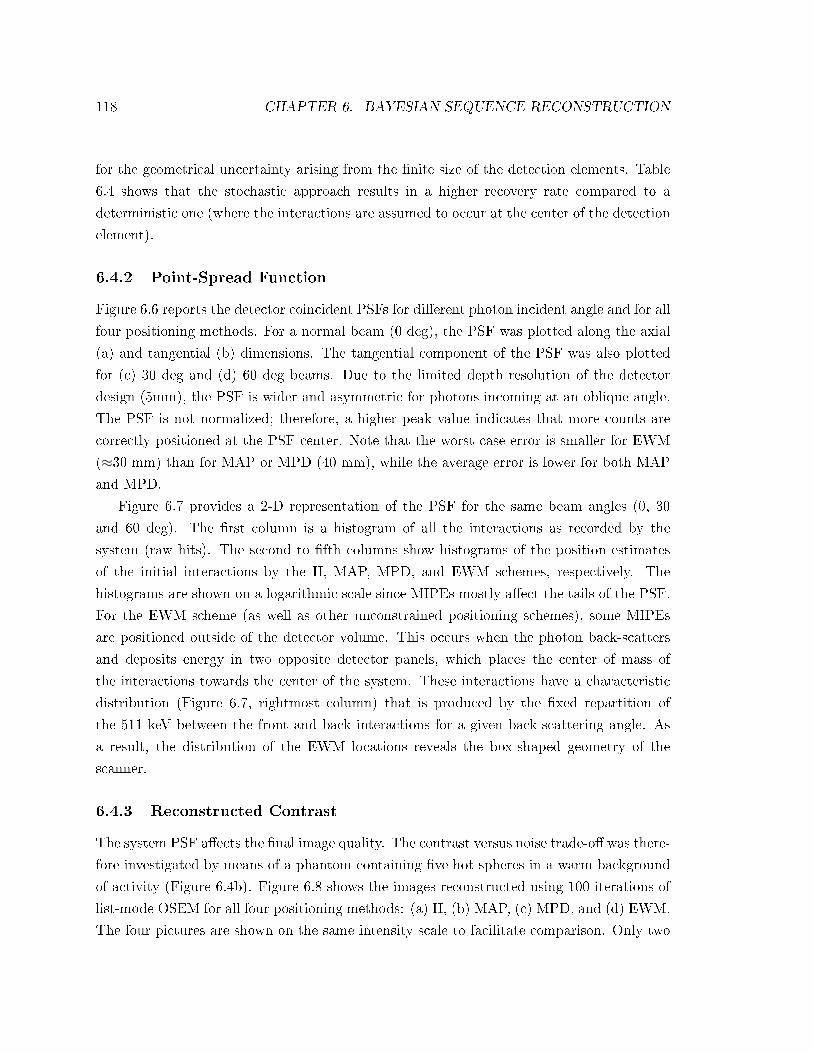
118 CHAPTER 6. BAYESIAN SEQUENCE RECONSTRUCTION
for the geometrical uncertainty arising from the nite size of the detection elements. Table
6.4 shows that the stochastic approach results in a higher recovery rate compared to a
deterministic one (where the interactions are assumed to occur at the center of the detection
element).
6.4.2 Point-Spread Function
Figure 6.6 reports the detector coincident PSFs for dierent photon incident angle and for all
four positioning methods. For a normal beam (0 deg), the PSF was plotted along the axial
(a) and tangential (b) dimensions. The tangential component of the PSF was also plotted
for (c) 30 deg and (d) 60 deg beams. Due to the limited depth resolution of the detector
design (5mm), the PSF is wider and asymmetric for photons incoming at an oblique angle.
The PSF is not normalized; therefore, a higher peak value indicates that more counts are
correctly positioned at the PSF center. Note that the worst case error is smaller for EWM
(≈30 mm) than for MAP or MPD (40 mm), while the average error is lower for both MAP
and MPD.
Figure 6.7 provides a 2-D representation of the PSF for the same beam angles (0, 30
and 60 deg). The rst column is a histogram of all the interactions as recorded by the
system (raw hits). The second to fth columns show histograms of the position estimates
of the initial interactions by the II, MAP, MPD, and EWM schemes, respectively. The
histograms are shown on a logarithmic scale since MIPEs mostly aect the tails of the PSF.
For the EWM scheme (as well as other unconstrained positioning schemes), some MIPEs
are positioned outside of the detector volume. This occurs when the photon back-scatters
and deposits energy in two opposite detector panels, which places the center of mass of
the interactions towards the center of the system. These interactions have a characteristic
distribution (Figure 6.7, rightmost column) that is produced by the xed repartition of
the 511 keV between the front and back interactions for a given back-scattering angle. As
a result, the distribution of the EWM locations reveals the box-shaped geometry of the
scanner.
6.4.3 Reconstructed Contrast
The system PSF aects the nal image quality. The contrast versus noise trade-o was there-
fore investigated by means of a phantom containing ve hot spheres in a warm background
of activity (Figure 6.4b). Figure 6.8 shows the images reconstructed using 100 iterations of
list-mode OSEM for all four positioning methods: (a) II, (b) MAP, (c) MPD, and (d) EWM.
The four pictures are shown on the same intensity scale to facilitate comparison. Only two
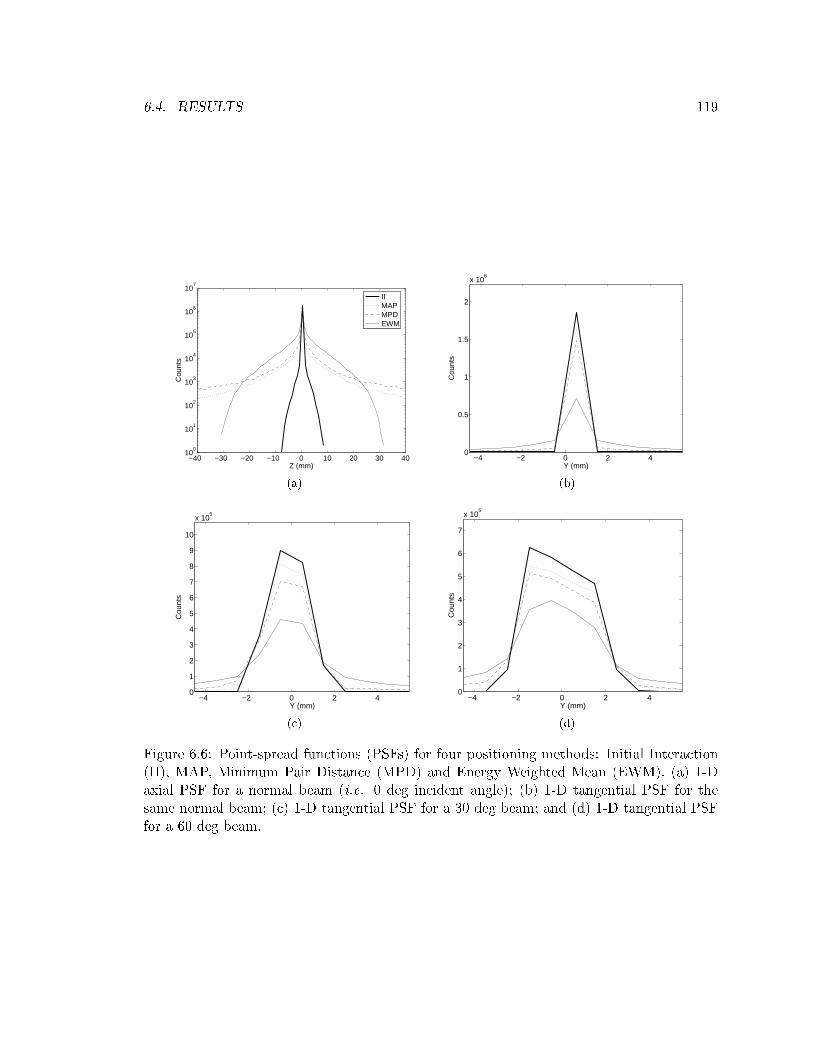
6.4. RESULTS 119
−40 −30 −20 −10 0 10 20 30 4010
0
101
102
103
104
105
106
107
Z (mm)
Cou
nts
IIMAPMPDEWM
(a)
−4 −2 0 2 40
0.5
1
1.5
2
x 106
Y (mm)
Cou
nts
(b)
−4 −2 0 2 40
1
2
3
4
5
6
7
8
9
10
x 105
Y (mm)
Cou
nts
(c)
−4 −2 0 2 40
1
2
3
4
5
6
7
x 105
Y (mm)
Cou
nts
(d)
Figure 6.6: Point-spread functions (PSFs) for four positioning methods: Initial Interaction(II), MAP, Minimum Pair Distance (MPD) and Energy Weighted Mean (EWM). (a) 1-Daxial PSF for a normal beam (i.e. 0 deg incident angle); (b) 1-D tangential PSF for thesame normal beam; (c) 1-D tangential PSF for a 30 deg beam; and (d) 1-D tangential PSFfor a 60 deg beam.

120 CHAPTER 6. BAYESIAN SEQUENCE RECONSTRUCTION
Figure 6.7: Point-spread function (2-D, log scale) for three beam angles (top: 0 deg, middle:30 deg, bottom: 60 deg). In the rst column, the histogram of all the interactions recorded bythe system is shown. The second to fth columns show histograms of the position estimateof the initial interaction by the II, MAP, MPD and EWM positioning schemes, respectively.
(a) (b) (c) (d)
Figure 6.8: Image slice through the contrast phantom, reconstructed with 100 sub-iterationsof list-mode 3-D OSEM. Ten million events were included in each subset. The phantomcomprised a 2.5 cm-radius, water-lled cylinder, in which were placed ve hot spheres. Theratio of the activity concentration in the spheres to that in the background was 10. Thesphere diameters were 1, 1.5, 2, 4 and 8 mm. Four positioning schemes were used: (a) II,(b) MAP, (c) MPD, and (d) EWM. No post-processing was performed. The images aredisplayed using the same intensity scale.

6.4. RESULTS 121
spheres can be resolved for EWM, for the other positioning schemes however all but the
smallest spheres are resolved.
Figure 6.9 shows the contrast versus noise in the reconstructed images for the ve spheres
(diameter 18 mm). A total of 100 list-mode 3D-OSEM sub-iterations are displayed. The
non-monotonic behavior of the noise is caused by the structural artifacts present in the early
image iterations.
Unlike the contrast recovery, the noise is not aected by mispositioning as evidenced by
Figure 6.9. Independently of the positioning method, the contrast is degraded by small-
angle tissue scatter, random coincidences (randoms rate is 10.6% for the contrast phantom
simulation), partial volume eect and inaccurate system matrix. For these reasons, it never
reaches its true value (10:1), even for the ideal II positioning scheme which provides the
highest contrast recovery (8.6 to 1). For the largest sphere, the contrast is 10% higher for
MAP (7.5 to 1) than for the MPD scheme (6.8 to 1). The contrast dierence is even greater
for the smaller spheres: for the 2 mm sphere, the contrast is 24% higher for MAP than
for MPD. It should also be noted that the contrast of the smallest spheres (1 and 1.5 mm)
did not converge within a hundred iterations; however, the monotonically increasing noise
prevents iterating further if the image is to maintain a reasonable signal-to-noise ratio.
The EWM method demonstrates the worst performance for the contrast recovery task.
The contrast is degraded to the extent that the small spheres (≤ 2 mm) cannot be resolved.
The contrast of the largest sphere is 46% lower to that achieved with MAP.
The CNR provides a rough estimate of the detectability of hot lesions in a background.
Lesions with CNR greater than 4 (shown as a dotted line in 6.9f) are generally detectable,
even though observer experience and object shape can also aect the detectability [137]. Ac-
cording to this criterion, the 1 mm sphere can be detected only when the ideal II positioning
scheme is used for the chosen reconstruction voxel size, while the 1.5 and 2 mm spheres are
not detectable when EWM is used. The peak CNR is systematically higher for MAP than
for MPD.
6.4.4 Reconstructed Sphere Resolution
The hot spheres resolution phantom (Figure 6.4c) was used to evaluate how the spatial
resolution is aected by positioning accuracy when iterative 3D-OSEM reconstruction is
used. Figure 6.10 shows the reconstructed images at 50 iterations for the four positioning
methods (II, MAP, MPD and EWM). The spheres are best resolved by the ideal II scheme.
MAP and MPD appear to perform similarly, but EWM shows substantial degradation of
the spatial resolution.
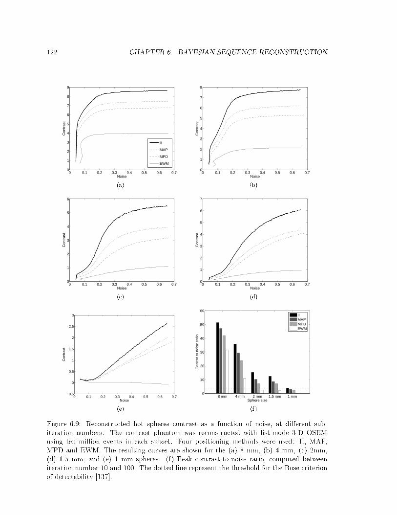
122 CHAPTER 6. BAYESIAN SEQUENCE RECONSTRUCTION
0 0.1 0.2 0.3 0.4 0.5 0.6 0.70
1
2
3
4
5
6
7
8
9
Noise
Con
tras
t
II
MAP
MPD
EWM
(a)
0 0.1 0.2 0.3 0.4 0.5 0.6 0.70
1
2
3
4
5
6
7
8
Noise
Con
tras
t
(b)
0 0.1 0.2 0.3 0.4 0.5 0.6 0.70
1
2
3
4
5
6
Noise
Con
tras
t
(c)
0 0.1 0.2 0.3 0.4 0.5 0.6 0.70
1
2
3
4
5
6
7
Noise
Con
tras
t
(d)
0 0.1 0.2 0.3 0.4 0.5 0.6 0.7−0.5
0
0.5
1
1.5
2
2.5
3
Noise
Con
tras
t
(e)
8 mm 4 mm 2 mm 1.5 mm 1 mm0
10
20
30
40
50
60
Sphere size
Con
trat
to n
oise
rat
io
IIMAPMPDEWM
(f)
Figure 6.9: Reconstructed hot spheres contrast as a function of noise, at dierent sub-iteration numbers. The contrast phantom was reconstructed with list-mode 3-D OSEMusing ten million events in each subset. Four positioning methods were used: II, MAP,MPD and EWM. The resulting curves are shown for the (a) 8 mm, (b) 4 mm, (c) 2mm,(d) 1.5 mm, and (e) 1 mm spheres. (f) Peak contrast-to-noise ratio, computed betweeniteration number 10 and 100. The dotted line represent the threshold for the Rose criterionof detectability [137].
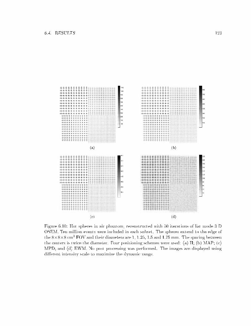
6.4. RESULTS 123
(a) (b)
(c) (d)
Figure 6.10: Hot spheres in air phantom, reconstructed with 50 iterations of list-mode 3-DOSEM. Ten million events were included in each subset. The spheres extend to the edge ofthe 8×8×8 cm3 FOV and their diameters are 1, 1.25, 1.5 and 1.75 mm. The spacing betweenthe centers is twice the diameter. Four positioning schemes were used: (a) II; (b) MAP; (c)MPD; and (d) EWM. No post-processing was performed. The images are displayed usingdierent intensity scale to maximize the dynamic range.

124 CHAPTER 6. BAYESIAN SEQUENCE RECONSTRUCTION
Further investigation was performed by measuring the reconstructed FWHM size of the
spheres. The results of these measurements are reported in Figure 6.11, for the (a) 1.75,
(b) 1.5, and (c) 1.25 mm spheres. Since the ML estimate is non-linear, the reconstructed
sphere FWHM size should be analyzed with care and should not be interpreted in terms of
modulation transfer function. The FWHM size is, however, an interesting gure of merit to
study since it denes the ability of the algorithm to distinguish small lesions that are close
to each other. It should also be noted that reconstructed sphere FWHM size is not expected
to be equal to the true sphere diameter (see Appendix E for more details).
Due to parallax blurring and despite 5 mm depth resolution, the reconstructed FWHM
sphere size is degraded for spheres near the edge of the FOV. The ideal II scheme provides
the best reconstructed FWHM size value, followed by MAP and MPD. Due to fewer mispo-
sitioned events, the reconstructed 1.75 mm diameter spheres were, on average, 5.6% smaller
for MAP than for MPD. As demonstrated in Figure 6.10d, EWM adds a substantial amount
of blur to the reconstructed images. The prole through the 1.75 mm diameter spheres (Fig-
ure 6.11d) shows that, besides the FWHM, the contrast of the spheres is aected by the
positioning accuracy as well.
6.5 Discussion
6.5.1 Performance of Proposed Scheme
When MAP is used, two times fewer events are mispositioned compared to MPD, a simpler
algorithm. As a result, the PSF has lower tails and higher peak value (Figure 6.6) because
more events are positioned to the correct LOR. MAP is also less likely to misposition events
in which the photon undergoes back-scatter (Figure 6.7). This directly aects the recon-
structed image quality. The contrast is higher for MAP positioning than for MPD (Figure
6.9), because mispositioning causes contrast loss because events that originate from the hot
lesion are positioned in the background. The peak CNR is greater for MAP than for MPD
and EWM, which implies that hot lesions have a better chance of being detected in a clin-
ical setting. In addition, MAP provides better quantitative accuracy in the sense that the
reconstructed contrast is a better estimate of the actual tracer concentration ratio. Images
reconstructed using the MAP positioning scheme also show higher spatial resolution (Figure
6.11), which facilitate the detection of smaller hot structures.
The full sequence of interactions can also be reconstructed by optimizing the prior distri-
bution alone (i.e. β = 1 in MAP). Like MPD, this approach has the advantage that energy
measurements are not needed. Furthermore, MAP with β = 1 outperforms MPD by 4.4%

6.5. DISCUSSION 125
0 5 10 15 20 25 30 35 401
1.5
2
2.5
3
3.5
Y (mm)
Rec
onst
ruct
ed S
pher
e F
WH
M
II
MAP
MPD
EWM
(a)
0 5 10 15 20 25 30 350.8
1
1.2
1.4
1.6
1.8
2
2.2
2.4
2.6
2.8
Y (mm)
Rec
onst
ruct
ed S
pher
e F
WH
M
(b)
0 5 10 15 20 25 30 35 40
0.8
1
1.2
1.4
1.6
1.8
2
2.2
Y (mm)
Rec
onst
ruct
ed S
pher
e F
WH
M
(c)
40 45 50 55 60 650
0.5
1
1.5
2
2.5
3
3.5
4
4.5
X (mm)
Rec
onst
ruct
ed v
oxel
val
ue
(d)
Figure 6.11: Reconstructed FWHM sphere size (mm) as a function of sphere position for thefour positioning methods, measured by tting a Gaussian mixture with oset to 1D prolesthough the reconstructed volume. (a) 1.75 mm spheres; (b) 1.5 mm spheres; and (c) 1.25mm spheres. (d) A prole through the 1.75 mm spheres is shown for the four positioningmethods.
126 CHAPTER 6. BAYESIAN SEQUENCE RECONSTRUCTION
(Figure 6.5).
Both the number of energy measurements and the size of the search space used for
recovering just the rst interaction are equal to N , the number of interactions. Therefore,
the accuracy performance of the MAP scheme is maintained even as N increases (Table 6.2,
rst row). When attempting to recover the full sequence, however, the size of the search
space increases super-exponentially with N , hence the recovery rate for complete sequences
drops sharply for N = 4 (Table 6.2, third row).
Uncertainty in the locations of the interactions (within the detection element boundaries)
translates into uncertainty in the scatter angle, which in turn yields uncertainty on the energy
deposited. The eect of this positional uncertainty in 1 × 5 × 1 mm3 detection elements is
equivalent to that of an energy blur far greater than the 12% FWHM energy resolution at
511 keV (Table 6.3). That is to say, when the interactions are constrained to xed detectors
voxels, the range of energies that can be deposited is often much larger than the energy
resolution of the system (Figure 6.2). Therefore, the correct estimation of the order of
interactions depends more strongly on having good spatial resolution than on having good
energy resolution.
6.5.2 Limitations
The processing time is problematic for the robust Bayesian method (MAP). Although the
algorithm was implemented on a fast GPU, it takes more than 5 seconds to process 1 000events. MPD runs 43 times faster than MAP, mainly because MAP computes the objective
function over 16 384 statistical realizations. Using fewer simulation paths degrades the
positioning. Hence, when the objective is computed for only one trajectory passing through
the center of the detection elements, the recovery rate drops from 85.2% to 78.8% (Table
6.4).
The validation of the MAP scheme was carried out based on simulations performed
with GRAY (6.3.1). These simulations included the standard Compton scatter model based
on the Klein-Nishina formula, the accurate linear attenuation coecients from published
databases, and the standard photoelectric absorption model. In a real system, other physical
eects occur, namely characteristic X-ray production, Raleigh scattering, Bremsstrahlung,
and Doppler broadening. Furthermore, the electron is neither free nor at rest, therefore
the Klein-Nishina formula is not an accurate model for low (< 100 keV) energy photons
undergoing Compton scatter (Figure 6.3). We therefore applied our method to a dataset
generated using GATE [70], a more detailed Monte-Carlo package that incorporates all
these eects (except Doppler broadening). For a point source located at the center of the

6.5. DISCUSSION 127
CZT system, the recovery rate dropped from 85.0% to 82.4% for MAP, and from 70.1% to
67.9% for MPD. This drop is mostly caused by the production of a characteristic X-ray that
can propagate beyond the boundaries of the detection element, resulting in an increase in
the number of interactions recorded. Doppler broadening was not modeled in any of the
simulations. For 511 keV photons, Doppler broadening blur is at most 6 keV FWHM [138].
The energy blurring remains dominated by the nite resolution of the detectors. In addition,
increase in energy blur results in only a modest reduction in MAP's recovery rate (Table
6.3).
In this study, it was assumed that the CZT modules could read out interactions as low
as 10 keV. Being able to read such low energy events is crucial for the MAP positioning
scheme. A higher energy threshold (for example, 100 keV [139]) will cause the PET system
to drop interactions. As a consequence, some MIPEs will be discarded by energy gating
because their total energy will not be comprised within the energy window. Furthermore,
in some cases the PET system will drop one or more interactions, yet the resulting MIPE
will still be comprised within the energy window. In that case, ML sequencing is likely to
perform poorly because one or more interactions will be missing from the sequence.
6.5.3 Possible Extensions
The image-degrading eect of MIPEs has been previously compensated for by using a sim-
ple positioning method (EWM), and then by reconstructing the images with an accurate
model of the PSF [48]. However, by deconvolving the blur caused by MIPEs, this approach
amplies the noise. Prior to reconstruction, it is preferable to use an advanced positioning
method (such as MAP) to estimate the location of the rst interaction. The incorporation
of the resulting PSF in the reconstruction generates less noise amplication because the
PSF corresponding to a more precise positioning algorithm is narrower (Figure 6.6). This
advanced method is only available for PET systems that can position individual interactions
within a MIPE.
In 6.2.1, it is assumed that the photon incoming energy e0 and the location of the
other coincident photon p are available. While true for PET, these assumptions cannot be
made for other modalities such Compton cameras [138]. Nevertheless, the method can be
generalized for these modalities. The incoming energy e0 can be estimated by summing the
energies of all the interactions. When p is unavailable, the likelihood should not include the
rst interaction because the scatter angle cos θ1 cannot be computed as in (6.4).
The MAP objective can be readily extended to be used as criteria for rejecting tissue
scattered events and random coincidences. In its current formulation, it assumes that the

128 CHAPTER 6. BAYESIAN SEQUENCE RECONSTRUCTION
incoming photon energy e0 is 511 keV and that the incident angle is given by the location
p of the other photon pair. When the photon scatters in tissue or is paired up incorrectly
(random coincidence), these hypotheses do not hold. As a result, no sequence might be
attributed a high probability and the event can be discarded.
MAP positioning can be applied to crystals other than CZT. For instance, high-resolution
detectors with depth-of-interaction capabilities can be built from lutetium oxyorthosilicate
(LSO) coupled to thin position-sensitive avalanche photo-diodes (PSAPD [17]). Even though
LSO's photo-fraction is higher than CZT's, small crystal elements will cause MIPEs. The
MAP scheme can then be used for positioning: based on Table 6.3, MAP is accurate even
with 12% energy resolution FWHM.
6.6 Summary
The ability to correctly position MIPEs greatly aects the global performance of PET sys-
tems based on high-resolution detectors. Discarding MIPEs is not possible for the CZT
system studied since these events are part of almost every recorded coincident event. Con-
ventional positioning schemes, such as EWM, degrade both contrast and resolution, reduce
the image quantitative accuracy, and aect the detectability of hot lesions. Simple ap-
proaches, such as MPD, help improve the image quality, but are outperformed by MAP, a
more advanced positioning scheme that uses all the information available in a statistically
optimal way.
Although inter-crystal scatter is more prevalent in smaller crystals, improved intrinsic
spatial resolution will enhance the identication of the photon crystal of entry. Bayesian
sequence reconstruction methods will play a key role in ultra-high resolution systems, espe-
cially those made from materials with low photo-fraction such as CZT or Germanium.

Chapter 7
Concluding Remarks, Future
Directions
The response of a PET system is complex and shift-varying. As a result, images recon-
structed with simple schemes have non-uniform spatial resolution and suboptimal quantita-
tive accuracy. This issue can be addressed by the incorporation of an accurate model of the
system response within the reconstruction.
For the box-shaped PET system that is one of the foci of this dissertation, the system
response is particularly irregular. Likewise, the images that were reconstructed with a shift-
invariant projection kernel suered from limited spatial resolution near the edge of the FOV
and degraded quantitation. The inclusion of an accurate model of the geometrical detector
response corrected for the variations in spatial resolution, and improved the quantitative
accuracy. This suggests that the geometrical response is the main component of the full de-
tector response. Modeling the other components (inter-crystal scatter, photon acolinearity
and positron range) shall indeed bring further benets, but will require a considerably more
complex model. Therefore, the model proposed (based on the analytical CDRF) is an excel-
lent trade-o between image quality, accuracy and computation. Uniform spatial resolution
is achieved throughout the FOV, with manageable memory and computation requirements
(especially when GPUs are used).
The measurements obtained from the high-resolution PET and TOF PET systems are
sparse. Therefore, a direct reconstruction from the list-mode is preferable to using sinograms.
GPUs have been successfully employed in sinogram-based reconstruction because they are
ecient at applying the ane transformation that maps a slice through the volumetric image
to any sinogram view, and vice-versa. The main challenge in implementing list-mode OSEM
129

130 CHAPTER 7. CONCLUDING REMARKS, FUTURE DIRECTIONS
on the GPU is that the list-mode LORs are not arranged in any regular pattern like sinogram
LORs. The mapping between the list-mode data and the volumetric image is not ane, and
as a result texture mapping cannot be used in this context. The technique described in this
dissertation is unique because it can be used for back- and forward projecting individual
LORs described by arbitrary endpoint locations, even when a shift-varying kernel is used to
model the response of the system.
Yet, the appeal of using the computational power of the GPUs for list-mode reconstruc-
tion is somewhat mitigated by their relatively poor cache performance. Unlike sinogram-
based reconstruction, in list-mode the memory is accessed randomly, which makes GPU-
based implementations challenging. The memory latency and throughput aect the overall
speed of the reconstruction. Still, the memory latency can be hidden by performing com-
putation while the image voxel is being retrieved. In our implementation, the kernel is
evaluated while the memory is being accessed. Writing to the image is also pipelined so that
the memory latency does not aect the overall performance.
The shift to higher resolution detectors not only implies that data is sparser, but also
less reliable due to multiple energy depositions for each 511 keV photon. This issue is
exacerbated when semiconductor detectors such as CZT are used because of the lower photo-
fraction. In this dissertation, a Bayesian method was introduced for reconstructing the
order of a sequence of interactions. This approach is a unifying framework which combines
the statistical properties of the measurements with a priori information. Although inter-
crystal scatter is more prevalent in smaller crystals, improved intrinsic spatial resolution will
facilitate the identication of the photon crystal of entry. Robust sequence reconstruction
methods, such as MAP, should play a key role in ultra-high resolution systems.
Beyond considering MIPEs as a source of errors that need to be corrected for, these events
have the potential to increase the amount of information available in the reconstruction.
The direction of an incoming 511 keV photon that produced a MIPE can be conned to
a cone (called the Compton cone). Such information could lead to a paradigm shift in
PET: single events (currently discarded) could be used in the reconstruction [136,140,141].
The single events can be included in the reconstruction using techniques borrowed from
Compton imaging. In addition, the knowledge of the photon incoming direction can help
reject a signicant fraction of the random and tissue scattered coincidences [135]. As a
result, in that scenario, MIPEs would actually contribute to improve image quality instead
of degrading it.

Appendix A
GPU Line Projections
This appendix describes how the data stored in the GPU on-board memory is represented.
Next, a detailed description of the forward and back- projection operations is provided,
accompanied with simplied Cg and OpenGL code.
A.1 Data Representation
In OpenGL, data can be stored in the video memory using 2-D textures. A 2-D color texture
forms an array of 32-bit oating-point quadruples and can be accessed randomly by GPU
shaders. 3-D textures are also available, however they do not support the render-to-texture
operation that is required to write data out. 3-D arrays, such as volumetric images, need
to be reshaped into 2-D structures to use write-to-texture capabilities. Writing to a 2-D
texture is performed by using OpenGL's frame-buer object (FBO) extension [108]. The
FBO extension can be used to do o-screen rendering, or to output the result of GPU-based
computations.
A.1.1 Images
In our implementation, the slice stack was tiled in 2-D into a larger rectangular texture (as
shown on Figure A.1). The 3-D index used to access the volumetric image is converted into
a 2-D index when needed.
A.1.2 List-Mode Data
The list-mode data is pre-loaded into another 2-D texture before the projections are per-
formed. Another option investigated was to stream the list-mode while it is being processed.
131

132 APPENDIX A. GPU LINE PROJECTIONS
Figure A.2: List-mode storage on theGPU. The RGB channels (red, green, andblue) are used to store the LOR endpointcoordinates. The alpha channel (black)can be used for storing additional data(per-LOR correction factors for scatter orrandoms, number of counts in histogram-mode, etc.).
This second approach requires less memory, but each list-mode event must be streamed twice
(once for the forward projection, once for the backprojection). Storing the list-mode data
in the video memory also makes it possible to perform some pre-processing steps directly on
the GPU. The list-mode data was stored according to Figure A.2.
Figure A.1: Image storage on the GPU using a 2-D tiled
representation.
OpenGL and Cg allow for
rectangular textures, however to
be readable from the vertex
shaders, the vertex arrays have
to be square. As a result, a
4-channel 2-D texture can store
2κ2 list-mode events, where κ
is a positive integer. Therefore,
the subset size is rounded to the
nearest integer that can be ex-
pressed as 2κ2.
The size of the on-board video memory, as well as the OpenGL specications can limit
the size of the list-mode dataset. In that case, a multi-pass approach is used. Batches of
2κ2 LORs are processed (forward and back-projection) sequentially, without clearing the
accumulation buer between each batch. The number of passes can be specied with the
command -m (see Table C.1).

A.2. LINE FORWARD PROJECTION 133
Figure A.3: Schematic of the forward projection of a LOR.
A.2 Line Forward Projection
The line forward projection is described mathematically in 4.2.2.3. This step uses two FBOs
for temporary storage. The size of these FBOs is λ (N_FP_SAMP in the code) by κ (N_FP_LINE
in the code) pixels. Each pass of the main loop in A.1 iterates over a block of LORs. A
block contains κ LORs, stored in the dst object.
For each LOR block, samples are calculated along each LOR (Figure A.3, left). One
sample is taken for each slice traversed by the LOR and is stored in a temporary FBO. The
volume is sliced is the main direction of the LOR (as dened by the conditions set in (4.4)).
The inner loop (in the double sum dened in (4.5)) is performed by a fragment shader (A.5,
in blue on Figure A.3). The sample locations are computed by drawing horizontal lines in
the temporary FBO while shaders are bound. The vertex shader (A.4) is passed an index
(lineIdx) to the LOR endpoint coordinates, as well as a parameter (idx) that indicates
where the horizontal LORs should be drawn within the FBO. The sign of idx determines
if a vertex is rst or second, and the magnitude of idx provides the vertical location where
the horizontal line is to be drawn.
The LOR endpoint coordinates are loaded from the list-mode texture (Figure A.2) and
used to generate 3-D texture map coordinates for the two endpoints of the horizontal line.
The length of the horizontal line and the texture coordinates are such that one sample
will be drawn from the center of each slice traversed by the LOR. Each sample will be
mapped through texture mapping to a location on the original 3-D LOR. The width λ of
the temporary FBO in which the horizontal line is drawn has to be at least equal to the
maximum number of samples expected (i.e. the number of slices). At the end of the rst
pass, κ× λ samples have been computed along κ LORs.
Geometrical properties (such as LOR direction vector, length, etc.) are also computed

134 APPENDIX A. GPU LINE PROJECTIONS
and passed to the fragment shader. The LOR main direction (n3 in the code) and the
two other orthogonal directions (n1 and n2) are also identied. The vectors n1 and n2 are
used later on in the fragment shader (A.5) as the directions along which the inner loop is
performed.
The double inner loop (in A.5) is performed for all the voxels within a square centered
on the LOR (see (4.2)b). For each of these voxels, the distance to the LOR is calculated
and if the voxel is inside the TOR, the voxel value is read out and summed using a Gaussian
projection kernel. The partial sum is then written to the temporary FBO.
In a second pass, the sum of all the partial sums for a given LOR is calculated using
a fragment shader (A.6). The result is stored as a vertical line (in red on Figure A.3) in
a second temporary FBO. Each pixel in that second FBO is the forward projection of the
volume along LOR.
After λ blocks of κ LORs have been processed, the second FBO is full. At that point,
the projection values are transferred to FBO holding the list-mode data (Figure A.3, in
yellow) by drawing a rectangle with a texture map (A.7). While the forward projection
values are being transferred, they are inverted by a fragment shader (A.8) in preparation of
the backprojection (as indicated in (3.5)).
The following OpenGL and Cg code has been simplied for easier reading. In particular,
the parameter set-up and parameter activation instructions are not shown.
A.3 Line Backprojection
The line backprojection step is described in 4.2.2.4. Slices are processed four at a time
(A.9, outer loop). For every group of four slices, all the LORs are backprojected in an
accumulation FBO (using additive blending) in blocks of MAX_LINES lines (A.9, inner loop).
After each block of LORs is backprojected, the accumulation FBO is added to a second
accumulation buer. This hierarchical accumulation architecture was designed because in
previous GPU the blending units were limited to 16-bit dynamic range (half). With the
GeForce 8 series, the blending units were upgraded to support full 32-but oating-point and
therefore many more LORs can be accumulated before underow occurs. On the newer
generation of GPU, millions of LORs can be back-projected in a single pass without any
degradation in quality. For the older GPU models, it is preferable to limit the size of the
blocks to 5,000 LORs.
The coordinates of the LOR endpoints are stored in a vertex texture (Figure A.2). An
index to both LOR endpoints is passed to the vertex shader (LineIdx in A.10). Both

A.3. LINE BACKPROJECTION 135
endpoints are readout from the vertex texture. The vertex shader calculates a number
of parameters for the LOR, including its length, middle point and direction vector. This
information is then passed to the fragment shader that is responsible for evaluating the
projection kernel within the TOR (see (4.1) for a denition).
The role of the fragment shader (A.11) is to evaluate the projection kernel. In A.11, a
Gaussian kernel is implemented. First, the distance DSQ between the voxel center and the
LOR axis is calculated. The calculation for four slices are performed in parallel using 4D
vector operations. Next, the Gaussian kernel is evaluated. The product of the kernel times
the LOR weight is returned and accumulated in the accumulation FBO (A.9) using additive
blending. A mask is used to prevent the voxels that are outside the TOR from being written
to.

136 APPENDIX A. GPU LINE PROJECTIONS
Algorithm A.1 OpenGL: Forward projection main loopglDisable(GL_BLEND);
glViewport( 0, 0, N_FP_SAMP, N_FP_LINE );
glMatrixMode( GL_TEXTURE ); glLoadIdentity( );
glMatrixMode( GL_MODELVIEW ); glLoadIdentity( );
glMatrixMode( GL_PROJECTION ); glLoadIdentity( );
gluOrtho2D( 0, N_FP_SAMP, 0, N_FP_LINE );
fboFP->bind();
fboFP->setWrite(1);
glClear( GL_COLOR_BUFFER_BIT );
//Process all the lines in the buffer in groups of N_FP_LINE
for (i = 0, j=1, k=0; i<dst->number() ; i += N_FP_LINE, j++)
<First pass>: sample the image along LORs (A.2)
<Second pass>: sum the samples (A.3)
if (j==N_FP_SAMP)
fboFP->unbind();
dst->update(k, j, fboFP->texID(1));
fboFP->bind();
fboFP->setWrite(1);
glClear( GL_COLOR_BUFFER_BIT );
k += j;
j = 0;
if (j != 0)
dst->update(k, j, fboFP->texID(1));
fboFP->unbind();
dst->update(k, j, fboFP->texID(1)); //(A.7)
dst->pingpongFBO();

A.3. LINE BACKPROJECTION 137
Algorithm A.2 OpenGL: Forward projection, rst passfboFP->setWrite(0);
glClear( GL_COLOR_BUFFER_BIT );
cgVertFore->activateProgram();
cgFragFore->activateProgram();
glDrawArrays( GL_LINES, 0, 2*N_FP_LINE );
cgVertFore->desactivateProgram();
cgFragFore->desactivateProgram();
Algorithm A.3 OpenGL: Forward projection, second passfboFP->setWrite(1);
cgFragSumLines->activateProgram();
glBegin( GL_LINES );
glTexCoord2f(0, 0); glVertex3f(j-0.5f, 0, 0);
glTexCoord2f(0, N_FP_LINE+1); glVertex3f(j-0.5f, N_FP_LINE+1, 0);
glEnd();
cgFragSumLines->desactivateProgram();

138 APPENDIX A. GPU LINE PROJECTIONS
Algorithm A.4 Vertex shader: Line forward projection rst passvoid main(
float4 lineIdx : POSITION,
float idx : TEXCOORD0,
uniform samplerRECT sampVert: TEXUNIT0,
uniform float nfp,
out float4 HPosition : POSITION,
out float3 L : TEXCOORD0,
out float3 v : TEXCOORD1,
out float3 n1 : TEXCOORD2,
out float3 n2 : TEXCOORD3,
out float3 C : TEXCOORD4,
out float d : TEXCOORD5 )
float2 uv1 = lineIdx.xy;
float2 uv2 = lineIdx.zy;
float3 vert = texRECT( sampVert, uv1 ).xyz;
float3 vertOther = texRECT( sampVert, uv2 ).xyz;
float3 vD = vert - vertOther;
d = length(vD);
float3 vDabs = abs(vD);
v = sign(idx) * vD / d;
n1 = ( vDabs.x < vDabs.z || vDabs.x <= vDabs.y ) ? float3(1,0,0) : float3(0,0,1);
n2 = ( vDabs.y < vDabs.z || vDabs.x > vDabs.y ) ? float3(0,1,0) : float3(0,0,1);
float3 n3 = float3(1) - n1 - n2;
float v1n3 = dot( vert, n3 );
float v2n3 = dot( vertOther, n3 );
float3 u = vD / ( v1n3 - v2n3 );
float mi = floor(min( v1n3, v2n3 )) - 5;
float ma = ceil(max( v1n3, v2n3 )) + 5;
float pick = (lineIdx.w==0) ? mi : ma;
L = vert - u * ( v1n3 - pick );
C = (vert + vertOther) / 2.0;
float vmax = ma - mi ; //number of slices
float xpos = (lineIdx.w==0) ? (-1) : (2*vmax-nfp)/nfp;
HPosition = float4(xpos, abs(idx)-1, 0, 1);

A.3. LINE BACKPROJECTION 139
Algorithm A.5 Fragment shader: Line forward projection rst passfloat4 main(
float3 L : TEXCOORD0,
float3 v : TEXCOORD1,
float3 n1 : TEXCOORD2,
float3 n2 : TEXCOORD3,
float3 C : TEXCOORD4,
float d : TEXCOORD5,
uniform float3 vs,
uniform float eta_sq,
uniform float sigma_sq,
uniform samplerRECT samp :TEXUNIT1,
uniform samplerRECT zLookUp :TEXUNIT2
) : COLOR
float s, sum = 0;
for ( float i=-3; i<=3; i++ )
for ( float j=-3; j<=3; j++ )
P = floor( L + i*n1 + j*n2 ) + 0.5;
if (all(P>0) && all(P<vs))
CPv = dot(CP,v);
d2 = dot(CP,CP) - CPv*CPv;
if (d2 < eta_sq)
t1 = h4texRECT( zLookUp, float2(P.z, 0.5) );
kern = exp( -d2 / ( 2*sigma_sq ) );
s = texRECT( samp, P.xy + t1.xy ).r;
sum += s*kern;
return float4(sum,0,0,0);
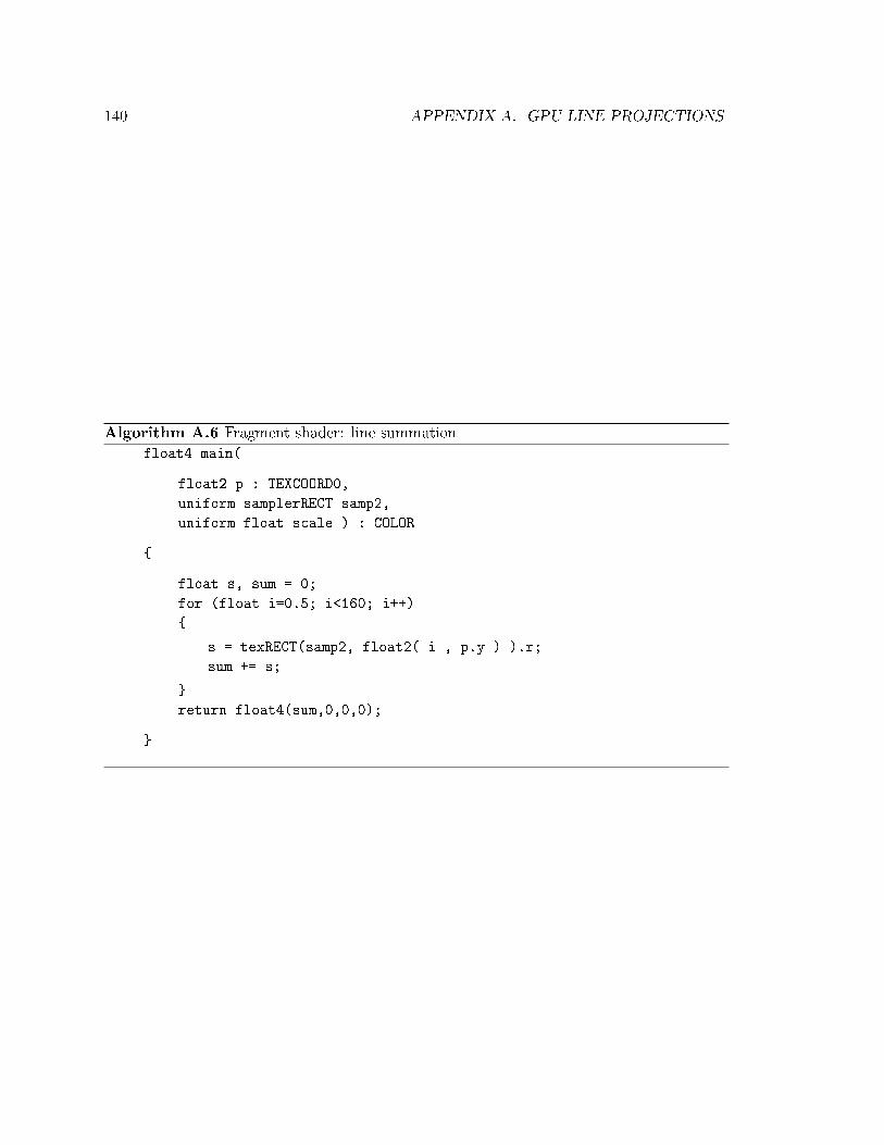
140 APPENDIX A. GPU LINE PROJECTIONS
Algorithm A.6 Fragment shader: line summationfloat4 main(
float2 p : TEXCOORD0,
uniform samplerRECT samp2,
uniform float scale ) : COLOR
float s, sum = 0;
for (float i=0.5; i<160; i++)
s = texRECT(samp2, float2( i , p.y ) ).r;
sum += s;
return float4(sum,0,0,0);
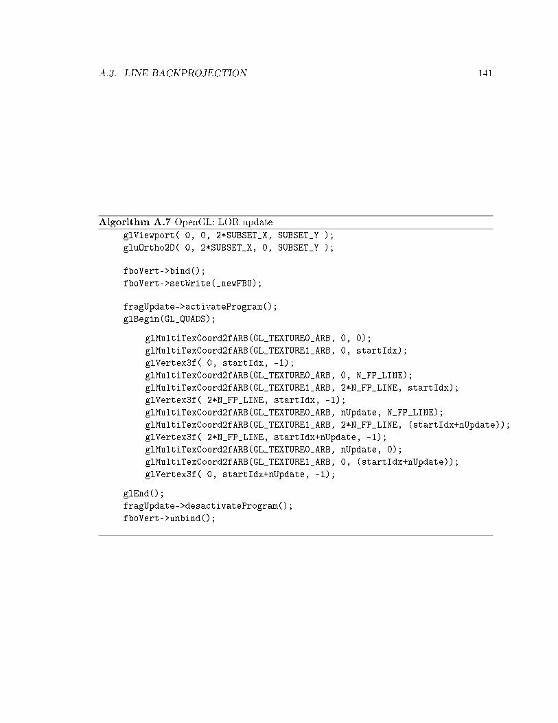
A.3. LINE BACKPROJECTION 141
Algorithm A.7 OpenGL: LOR updateglViewport( 0, 0, 2*SUBSET_X, SUBSET_Y );
gluOrtho2D( 0, 2*SUBSET_X, 0, SUBSET_Y );
fboVert->bind();
fboVert->setWrite(_newFBO);
fragUpdate->activateProgram();
glBegin(GL_QUADS);
glMultiTexCoord2fARB(GL_TEXTURE0_ARB, 0, 0);
glMultiTexCoord2fARB(GL_TEXTURE1_ARB, 0, startIdx);
glVertex3f( 0, startIdx, -1);
glMultiTexCoord2fARB(GL_TEXTURE0_ARB, 0, N_FP_LINE);
glMultiTexCoord2fARB(GL_TEXTURE1_ARB, 2*N_FP_LINE, startIdx);
glVertex3f( 2*N_FP_LINE, startIdx, -1);
glMultiTexCoord2fARB(GL_TEXTURE0_ARB, nUpdate, N_FP_LINE);
glMultiTexCoord2fARB(GL_TEXTURE1_ARB, 2*N_FP_LINE, (startIdx+nUpdate));
glVertex3f( 2*N_FP_LINE, startIdx+nUpdate, -1);
glMultiTexCoord2fARB(GL_TEXTURE0_ARB, nUpdate, 0);
glMultiTexCoord2fARB(GL_TEXTURE1_ARB, 0, (startIdx+nUpdate));
glVertex3f( 0, startIdx+nUpdate, -1);
glEnd();
fragUpdate->desactivateProgram();
fboVert->unbind();

142 APPENDIX A. GPU LINE PROJECTIONS
Algorithm A.8 Fragment Shader: LOR updatefloat4 main(
float2 uv0: TEXCOORD0,
float2 uv1: TEXCOORD1,
uniform samplerRECT sampVert,
uniform samplerRECT sampFP
) : COLOR
float4 col;
float4 d4 = texRECT(sampVert, uv1);
col.rgb = d4.rgb;
float a = texRECT(sampFP, uv0).r ;
col.a = 1. / ( a + d4.a );
return col;
Algorithm A.9 OpenGL: BackprojectionglLineWidth( LINE_WIDTH );
glBlendFunc( GL_ONE, GL_ONE );
glViewport( 0, 0, VOX_SIZE_X, VOX_SIZE_Y );
for (z=0; z<VOX_SIZE_Z; z+=4)
fboBP->bind();
fboBP->setWrite(1);
glClear( GL_COLOR_BUFFER_BIT );
glEnable( GL_BLEND );
for(i = 0; i<src->number(); i += MAX_LINES)
fboBP->setWrite(0);
glClear( GL_COLOR_BUFFER_BIT );
glMatrixMode( GL_PROJECTION ); glLoadIdentity( );
glOrtho( 0, VOX_SIZE_X, 0, VOX_SIZE_Y, -(z-5), -(z+9) );
cgVertBack->activateProgram();
cgFragBack->activateProgram();
glDrawArrays( GL_LINES, 0, 2*MAX_LINES );
cgVertBack->desactivateProgram();
cgFragBack->desactivateProgram();
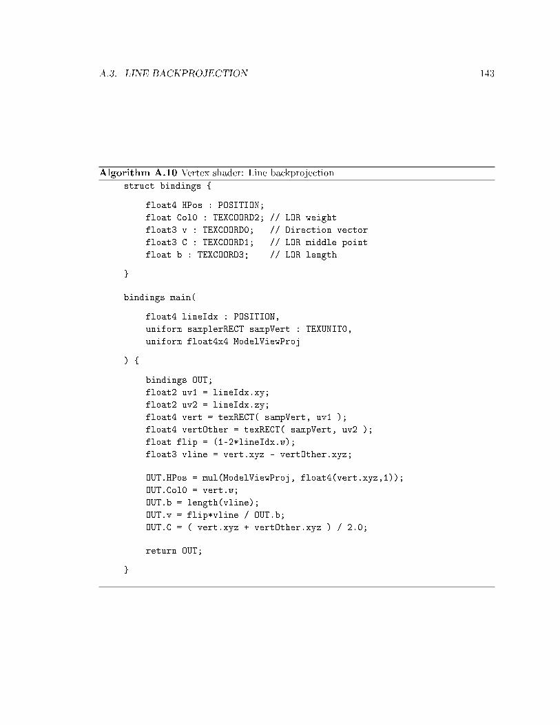
A.3. LINE BACKPROJECTION 143
Algorithm A.10 Vertex shader: Line backprojectionstruct bindings
float4 HPos : POSITION;
float Col0 : TEXCOORD2; // LOR weight
float3 v : TEXCOORD0; // Direction vector
float3 C : TEXCOORD1; // LOR middle point
float b : TEXCOORD3; // LOR length
bindings main(
float4 lineIdx : POSITION,
uniform samplerRECT sampVert : TEXUNIT0,
uniform float4x4 ModelViewProj
)
bindings OUT;
float2 uv1 = lineIdx.xy;
float2 uv2 = lineIdx.zy;
float4 vert = texRECT( sampVert, uv1 );
float4 vertOther = texRECT( sampVert, uv2 );
float flip = (1-2*lineIdx.w);
float3 vline = vert.xyz - vertOther.xyz;
OUT.HPos = mul(ModelViewProj, float4(vert.xyz,1));
OUT.Col0 = vert.w;
OUT.b = length(vline);
OUT.v = flip*vline / OUT.b;
OUT.C = ( vert.xyz + vertOther.xyz ) / 2.0;
return OUT;

144 APPENDIX A. GPU LINE PROJECTIONS
Algorithm A.11 Fragment shader: Line backprojectionfloat4 main(
bindings IN,
uniform samplerRECT zRGBA : TEXUNIT1,
uniform float sigma_sq,
uniform float slice
) : COLOR
float4 zEnc = IN.C.z - (slice + float4(0.5, 1.5, 2.5, 3.5));
float2 v2 = IN.C.xy - IN.WPos.xy;
float4 DP = dot( IN.v.xy , v2 ) + IN.v.z * zEnc;
float4 D2 = dot(v2,v2) + zEnc*zEnc;
float4 DSQ = D2 - DP*DP;
mask = (DSQ < 2);
if ( !any(mask) ) discard;
float4 dexp = exp( - DSQ / (2.0*sigma_sq) );
return( dexp * mask * IN.Col0 );

Appendix B
File Formats
B.1 List Mode and Histogram Mode
A list-mode le is a list of events. For each event, ten properties are stored. For a TOF
PET sytem, these include the spatial coordinates of both detectors and the TOF value c∆τ .Optionally, a random estimate ri and two scatter estimates (sTOFi with TOF information,
si without) can be provided for the LOR in which the event was recorded on. The randoms
are uniformly distributed over all TOF bins, therefore the TOF randoms estimate can be
calculated from the one without TOF. The spatial coordinates can be entered using any unit
of length (mm, cm, inches, etc.), however the choice must be consistent with the units used
in the FOV denition. The TOF value should also be converted into the same unit of length,
according to the relationship ∆x = c∆τ , where c is the speed of light. The randoms and
scatter estimates should provide the number of such events in the duration corresponding to
a subset of data, for a particular LOR or TOF bin. The list-mode data is stored in 32-bits
oating-point format (IEEE 754, little endian). List-mode les can be recognized by their
.bin.f extension. For TOF datasets, an element of a list-mode le is organized as follow:
x(1)i y
(1)i z
(1)i c∆τ ri x
(2)i y
(2)i z
(2)i sTOFi si
When TOF information is not available, the TOF value and the TOF scatter estimate
are set to zero. Similarly, when randoms and scatter estimates are not available, they are
set to zero.
The reconstruction package can also handle PET data in histogram form. Histogram
data is similar to list-mode data, with the only exception that all the events that occurred
145

146 APPENDIX B. FILE FORMATS
on the same LOR are grouped together. The LORs are organized in a list which contains
the coordinates and the number of events (denoted mi) of every LOR. The structure of a
histogram-mode data le is the following:
x(1)i y
(1)i z
(1)i mi ri x
(2)i y
(2)i z
(2)i si N/A
Unlike the histogram-mode format, individual energy and time information can be stored
for each event in list-mode.
B.2 Image Files
The 3-D images used by the application (output, initialization image and sensitivity map)
can be stored to disk. To avoid conversions when moving images to the GPU, the image
voxels are stored in a 2-D tiled array (see Figure A.1). The rst 16 bytes constitute the le
header and dene the image size. The header is comprised of four 32-bit integers. The rst
two (vx and vy) determine the tile size, and the other two (tx and ty) the number of tiles
in each dimension. The rest of the le consists of the voxel values, stored in 32-bits IEEE
oating-point. The resulting le size is 4 × (4 + vx vy tx ty) (in bytes). Image les saved
according to this scheme have a .vs extension.
B.3 Colormap Files
Custom colormaps can be used to visualize data in the interactive mode. Colormap les are
stored in ~/.GpuOsem/, and are recognizable by the .colormap extension. The colormap le
format is consistent with MATLAB's colormaps. Each colormap has 64 color values, with
each color being represented by a 32-bit oating-point quadruple (RGBA). The colormap is
linearly interpolated for better result. The le size is 1024 bytes (= 4× 4× 64 bytes).

Appendix C
User Manual
C.1 Command Line Options
Many parameters can be provided to the application through the command line (see Table
C.1). Most of the parameters are optional and have default values. Most of the time, the
application will check for missing parameters or incorrect values. Some parameters must
be provided for the reconstruction application to work, namely: the image size, the FOV
size, the subset size and the list-mode input le. All the remaining parameters have default
values.
Because the list-mode data is stored in a square texture of size 4κ2 (see A.1.2), the
subset size (specied using -s) is rounded o to the closest integer that can be expressed as
2κ2. Similarly, the number of tiles in the horizontal dimension (ty) must be a multiple of
four. This is because four slices are processed simultaneously in the back-projection using
the four color channels (see Section A.2).
It is sometimes desirable to use very large subsets in the reconstruction. In practice,
there are two limits to the subset size: the amount of memory available on-board, and the
maximal size of a rectangular texture allowed by OpenGL. Therefore, the subset multiplier
(-m) should be used to perform such reconstruction. For example, instead of specifying a
subset of 10 million events (using -s 10000000), one can specify a subset size of two million
and a multiplier of 5 (using -s 2000000 -m 5).
C.2 Conguration File
Some of the application parameters are set up through a conguration le. On a Linux
OS, the conguration le is stored in ~/.GpuOsem/GpuOsem.conf. While the command line
147

148 APPENDIX C. USER MANUAL
Flag Format Description
vsize="vx vy tx ty" INT Size of the image slice, and number of tilesfov="fx fy fz" DOUBLE Size of the eld of view (unit of length)-d LORs are rebinned to the edge of the FOV-j Jitters the line by a random quantity-r Flips x/z dimensions (useful for dual-panel recon)-u DOUBLE Intensity of the uniform image used for initialization-s INT Number of events in subset-m INT Multiplier for subset size-S Saves the image volume after each iteration-C Uses scatter and randoms corrections-T DOUBLE Time-of-ight kernel width (unit length, FWHM)-i INT Number of sub-iterations-D Debug mode on (obsolete)-N Sensitivity map calculation (accumulate mode)-H Input is histogram-mode-l, listmode FILE List-mode input lename-n, norm FILE Sensitivity map lename-I, init FILE Initialization le-c DOUBLE Rebins the LOR to a cylinder of radius <DOUBLE>-t INT Truncate dataset to use only the <INT> rst events-g DOUBLE Standard deviation for Gaussian projection kernel-o, output FILE Output lename-h, help Print help and exit
Table C.1: Command-line options
is used to dene parameters relating to the geometry of the PET system, the parameters
contained in the conguration le do not aect the reconstruction.
C.3 Interactive-Mode Commands
When no iteration number is set (using -i), the application runs in interactive mode. In-
teractive mode allows the user to iterate as needed, and visualize the image as it is being
reconstructed. The following keystrokes can be used during the execution of the application.
The colormap used for visualization, as well as the viewport size can be adjusted in the con-
guration le. When the application is run in batch-mode (using -i), it will exit after the
specied number of iterations has been performed. Therefore, no interactive visualization is
possible in batch-mode.

C.3. INTERACTIVE-MODE COMMANDS 149
Key Action Key Action
V Save Volume W Switch V1/V2
S Screen Shot C Clear V1
RETURN Iterate R Rewind dataESC Exit S Screen shotL Load current dataset D Toggle 2D/3DF Forward project P Print debug infoB Backproject 1 Display V1
F1 Toggle full screen 2 Display V2
F2 Next slice 3 Display NF3 Previous slice 4 Display F1
F4 Toggle y-through 5 Display F2F5 Decrease alpha blending 6 Display B1F6 Increase alpha blending 7 Display B2F7 Decrease intensity 8 Display slice V 1F8 Increase intensity 9 Display slice N
Table C.2: Interactive shortcuts

Appendix D
Gamma Camera Acquisition Software
D.1 Background
A small hand-held gamma camera (Figure D.1a and [142]) was developed in the Molecular
Imaging Instrumentation Lab to be used for radio-guided surgery. Unlike PET, gamma
cameras use a physical collimator to select the projection view. Most of the incoming photons
that are not incident normal to the radiation detector are stopped by highly attenuating
material (such as lead). A gamma camera produces 2-D images that do not require any
tomographic reconstruction.
Gamma cameras are useful in a number of nuclear medicine applications. They are
usually fairly large and used for whole body imaging. Small-FOV handheld gamma cameras
do exist but their use is still under investigation. While large cameras can be used for
surgery planning, small cameras can be useful in the operation room to guide the surgery,
when needed. Sentinel lymph node (SLN) biopsy is a very promising application for such
small-FOV cameras. The SLN biopsy procedure consists in removing the lymph nodes that
most likely drain the tumor site, in order to assay for the spread of the disease. In the
United States, the SLN procedure is standard for aggressive breast and melanoma cancers.
The SLNs are found by injecting, at the tumor site, a radioactive dye (99mTc sulfur colloid)
that accumulates in the lymph nodes.
A software package was developed to interface with the gamma camera prototype. The
software provides camera calibration, real-time imaging and performance analysis. It runs
on a PC, which is connected to the camera through a National Instrument data acquisition
(DAQ) card. The camera and software were evaluated by conducting a preliminary study
using a porcine model, followed by a small clinical prospective trial on 50 patients (Figure
D.1b). This appendix summarizes the implementation of the software package.
150

D.2. HARDWARE 151
(a) (b)
Figure D.1: (a) Gamma camera prototype. (b) Use of the camera for sentinel lymph nodebiopsy in a melanoma patient.
D.2 Hardware
The gamma camera prototype consisted of a parallel hole collimator coupled to a pixelated
NaI(Tl) scintillation crystal array, itself coupled to a at panel, multi-anode Hamamatsu
H8500 position-sensitive photomultiplier tube (PSPMT) [142]. The collimator was 5 × 5cm2 large and 1.5 cm-thick, with 1.3 mm hexagonal holes and 0.2 mm septa (15 cps / µCi).
The crystal array had a 1.7 mm pitch and was composed of 29×29 individual crystals, each
1.5 × 1.5 × 6 mm3 in size. The PSPMT was read out using a symmetric charge division
circuit [143]. Approximately 3 mm of lead shielding was wrapped around the collimator and
the scintillation crystal.
D.3 Software
The software architecture is based on a state machine. The principal states are summarized
in Figure D.2 and are described in more details in the following sections.
The gamma camera software was developed in C++ and runs on a Linux OS. Real-
time visualization was achieved using the SDL media library and OpenGL. The camera was
interfaced through the DAQmx Base C API (National Instruments). When an interaction

152 APPENDIX D. GAMMA CAMERA ACQUISITION SOFTWARE
Figure D.2: Schematics of the seven main states in the gamma camera software. Thered arrows indicate the entry points for the software. The circling arrow means that theapplication stays in that state until some condition is met.
occurs in a scintillation crystal, four signals are produced by the readout electronics. When
the trigger signal (created by summing and delaying the four channels) crosses a certain
threshold, these four voltages are digitized by the DAQ card and stored in a buer on the
card, in list-mode. Periodically, the application reads out the events from the buer for
processing. The event energy and the 2-D position of the centroid of the light distribution
are obtained by Anger logic.
Using command line parameters, the application can start at three possible states (red
arrows in Figure D.2). The camera can be started in calibration mode, in which case a
ood source of 99mTc should be placed on the camera. The calibration le, containing the
crystal segmentation map and camera parameters, can be saved to a le and loaded later
for performance analysis (in red). The application can also be started to perform real-time
imaging (in red) directly, in which case it will load a previously saved calibration le.
D.3.1 Initialization
A ood source, made of a plastic container lled with a solution of 99mTc must be placed
on the camera before the calibration sequence is initiated. Calibration should be performed
monthly to monitor the camera performance and correct for potential drift in its parameters.
Once the DAQ API is initialized, the trigger signal is dened, as well as the size of the
data transfers from the buer. The data acquisition then starts. At rst, a few hundred
thousand events are acquired to estimate the spread of the channel values and maximize
the dynamic range of the ood histogram. The graphical viewport is also initialized. Once
these tasks have been accomplished, the program jumps to the next state.
D.3.2 Flood Acquisition
The ood acquisition sequence is executed in a loop. In this sequence, the DAQ buer is
polled for new events. If a sucient number of events are present, they are transferred to
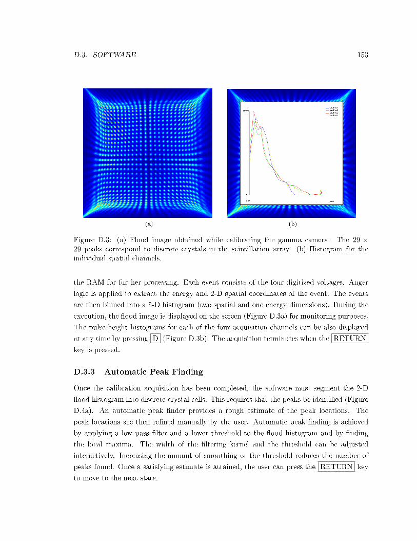
D.3. SOFTWARE 153
(a) (b)
Figure D.3: (a) Flood image obtained while calibrating the gamma camera. The 29 ×29 peaks correspond to discrete crystals in the scintillation array. (b) Histogram for theindividual spatial channels.
the RAM for further processing. Each event consists of the four digitized voltages. Anger
logic is applied to extract the energy and 2-D spatial coordinates of the event. The events
are then binned into a 3-D histogram (two spatial and one energy dimensions). During the
execution, the ood image is displayed on the screen (Figure D.3a) for monitoring purposes.
The pulse height histograms for each of the four acquisition channels can be also displayed
at any time by pressing D (Figure D.3b). The acquisition terminates when the RETURN
key is pressed.
D.3.3 Automatic Peak Finding
Once the calibration acquisition has been completed, the software must segment the 2-D
ood histogram into discrete crystal cells. This requires that the peaks be identied (Figure
D.4a). An automatic peak nder provides a rough estimate of the peak locations. The
peak locations are then rened manually by the user. Automatic peak nding is achieved
by applying a low pass lter and a lower threshold to the ood histogram and by nding
the local maxima. The width of the ltering kernel and the threshold can be adjusted
interactively. Increasing the amount of smoothing or the threshold reduces the number of
peaks found. Once a satisfying estimate is attained, the user can press the RETURN key
to move to the next state.
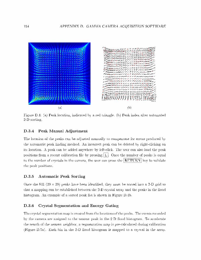
154 APPENDIX D. GAMMA CAMERA ACQUISITION SOFTWARE
(a) (b)
Figure D.4: (a) Peak location, indicated by a red triangle. (b) Peak index after automated2-D sorting.
D.3.4 Peak Manual Adjustment
The location of the peaks can be adjusted manually to compensate for errors produced by
the automatic peak nding method. An incorrect peak can be deleted by right-clicking on
its location. A peak can be added anywhere by left-click. The user can also load the peak
positions from a recent calibration le by pressing L . Once the number of peaks is equal
to the number of crystals in the camera, the user can press the RETURN key to validate
the peak positions.
D.3.5 Automatic Peak Sorting
Once the 841 (29 × 29) peaks have been identied, they must be sorted into a 2-D grid so
that a mapping can be established between the 2-D crystal array and the peaks in the ood
histogram. An example of a sorted peak list is shown in Figure D.4b.
D.3.6 Crystal Segmentation and Energy Gating
The crystal segmentation map is created from the locations of the peaks. The events recorded
by the camera are assigned to the nearest peak in the 2-D ood histogram. To accelerate
the search of the nearest neighbor, a segmentation map is pre-calculated during calibration
(Figure D.5a). Each bin in the 2-D ood histogram is mapped to a crystal in the array.

D.3. SOFTWARE 155
(a) (b)
(c) (d)
Figure D.5: (a) Crystal segmentation map (color) and Voronoi graph (black lines). (b)Per-crystal energy resolution. (c) Energy spectrum for a crystal with good energy resolution(13.8%) (center of the FOV). (d) Degraded energy resolution (75.5%) for an edge crystal.
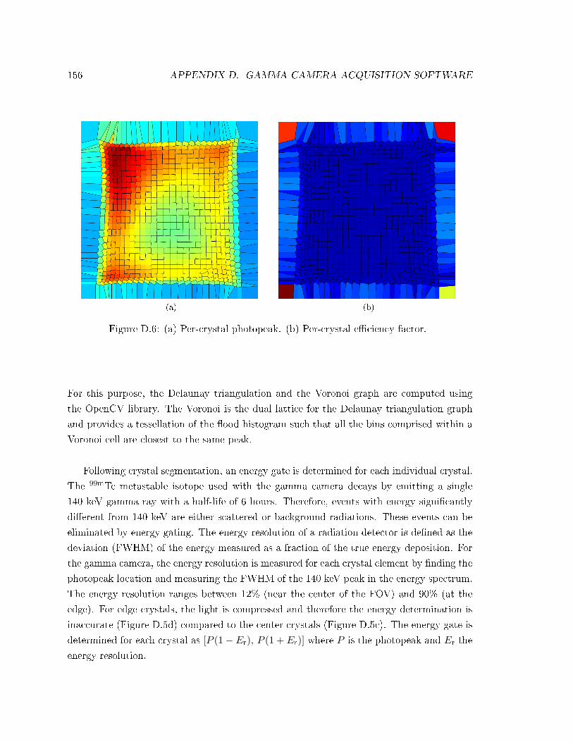
156 APPENDIX D. GAMMA CAMERA ACQUISITION SOFTWARE
(a) (b)
Figure D.6: (a) Per-crystal photopeak. (b) Per-crystal eciency factor.
For this purpose, the Delaunay triangulation and the Voronoi graph are computed using
the OpenCV library. The Voronoi is the dual lattice for the Delaunay triangulation graph
and provides a tessellation of the ood histogram such that all the bins comprised within a
Voronoi cell are closest to the same peak.
Following crystal segmentation, an energy gate is determined for each individual crystal.
The 99mTc metastable isotope used with the gamma camera decays by emitting a single
140 keV gamma ray with a half-life of 6 hours. Therefore, events with energy signicantly
dierent from 140 keV are either scattered or background radiations. These events can be
eliminated by energy gating. The energy resolution of a radiation detector is dened as the
deviation (FWHM) of the energy measured as a fraction of the true energy deposition. For
the gamma camera, the energy resolution is measured for each crystal element by nding the
photopeak location and measuring the FWHM of the 140 keV peak in the energy spectrum.
The energy resolution ranges between 12% (near the center of the FOV) and 90% (at the
edge). For edge crystals, the light is compressed and therefore the energy determination is
inaccurate (Figure D.5d) compared to the center crystals (Figure D.5c). The energy gate is
determined for each crystal as [P (1− Er), P (1 + Er)] where P is the photopeak and Er the
energy resolution.

D.3. SOFTWARE 157
D.3.7 Camera Performance Analysis
The parameters of the camera calibration can be analyzed interactively. Clicking on a cell
shows the energy histogram for this crystal (Figure D.5c and (d)). The photopeak value can
be displayed for each crystal (Figure D.6a), as well as the crystal eciency i.e. the number
of counts recorded in each crystal during the ood source calibration (Figure D.6b). If the
performance of the calibration is found unsatisfying, it is possible to repeat the previous
steps (Figure D.2).
After the calibration has been completed, a calibration le is automatically created for
subsequent imaging sessions.
D.3.8 Real-Time Imaging
The real-time imaging state is designed for clinical imaging procedures. In this state, the
software alternatively fetches new events from the DAQ buer, and displays the resulting
image frame onto the graphical viewport. Imaging can be performed either in accumulation
or dynamic mode.
D.3.8.1 Accumulation Mode
A data frame consists of a 29× 29 array of pixels that represent the ux of radiation hitting
the crystal array. Each event read out from the DAQ is rst assigned to a crystal according
to the crystal segmentation map. If the event is within the energy gate for that particular
crystal, then it is added to the data frame.
The data frame is corrected for non-uniform eciency (Figure D.6b). For optimal lymph
node detectability, the data frame undergoes several processing steps, including square-root
compression and bilinear interpolation [142].
When the camera is moved, the accumulation frame must be cleared. In the current
software, this is achieved by pressing C or by pressing a foot pedal (Figure D.1).
Figure D.7 shows images taken with the gamma camera from a melanoma patient case.
The rst image shows the three injections. A cluster of three SLNs was then imaged intra-
operatively. Two of these SLNs were imaged later, after their excision. After all SLNs were
removed, an image survey conrmed that no SLNs were left in the patient.
D.3.8.2 Dynamic Mode
In dynamic mode, imaging can be performed while the camera is being moved. Because
of the very low statistics, binning the counts in independent time frames does not provide
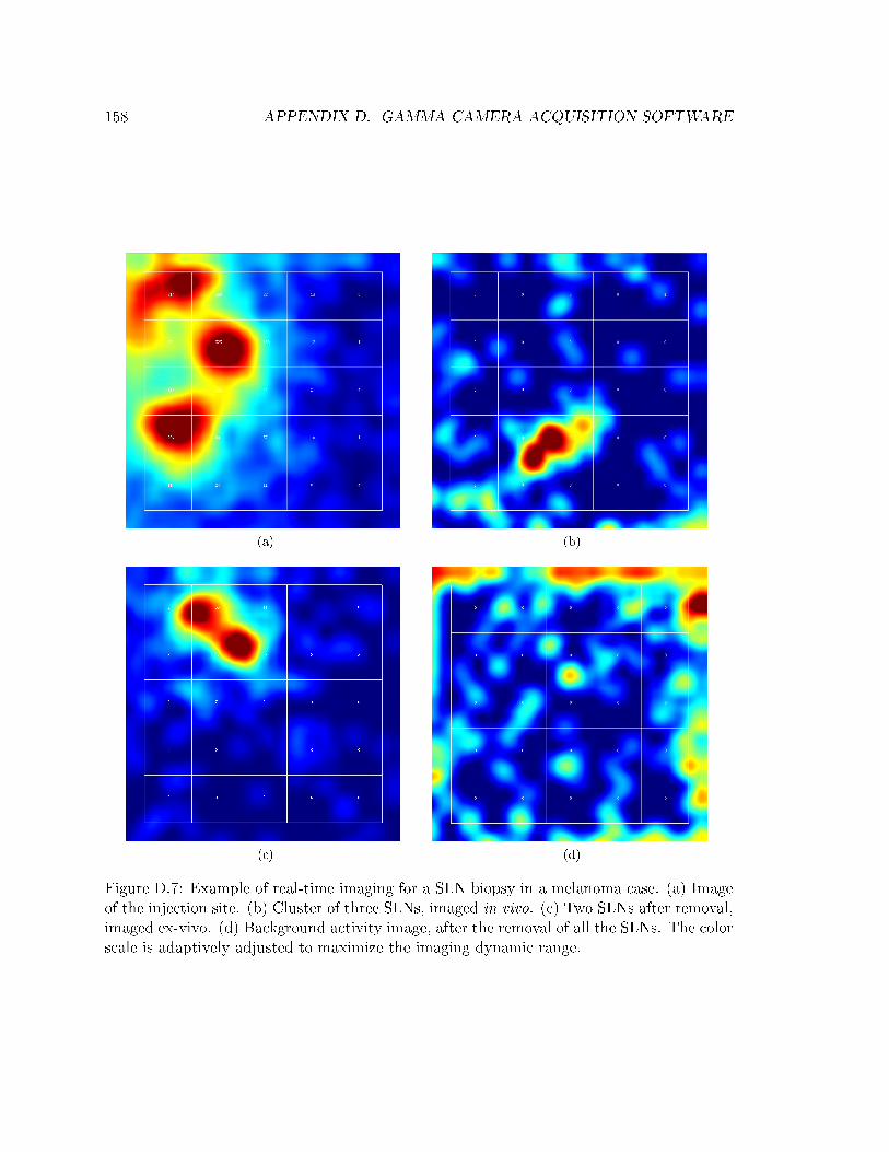
158 APPENDIX D. GAMMA CAMERA ACQUISITION SOFTWARE
(a) (b)
(c) (d)
Figure D.7: Example of real-time imaging for a SLN biopsy in a melanoma case. (a) Imageof the injection site. (b) Cluster of three SLNs, imaged in vivo. (c) Two SLNs after removal,imaged ex-vivo. (d) Background activity image, after the removal of all the SLNs. The colorscale is adaptively adjusted to maximize the imaging dynamic range.
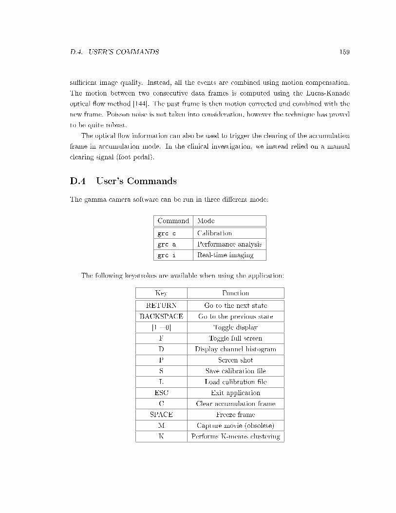
D.4. USER'S COMMANDS 159
sucient image quality. Instead, all the events are combined using motion compensation.
The motion between two consecutive data frames is computed using the Lucas-Kanade
optical ow method [144]. The past frame is then motion corrected and combined with the
new frame. Poisson noise is not taken into consideration, however the technique has proved
to be quite robust.
The optical ow information can also be used to trigger the clearing of the accumulation
frame in accumulation mode. In the clinical investigation, we instead relied on a manual
clearing signal (foot pedal).
D.4 User's Commands
The gamma camera software can be run in three dierent mode:
Command Mode
grc c Calibration
grc a Performance analysis
grc i Real-time imaging
The following keystrokes are available when using the application:
Key Function
RETURN Go to the next state
BACKSPACE Go to the previous state
[1 0] Toggle display
F Toggle full screen
D Display channel histogram
P Screen shot
S Save calibration le
L Load calibration le
ESC Exit application
C Clear accumulation frame
SPACE Freeze frame
M Capture movie (obsolete)
K Performs K-means clustering

Appendix E
Analysis of Reconstructed Sphere
Size
In a linear spatially-invariant system, the spatial resolution can be fully characterized by
the point-spread function (PSF). For a linear shift-varying system, the spatial resolution
can also be studied by looking at the local PSF. However, for a non-linear system (i.e.
which does not satisfy the principle of superposition), the spatial resolution is aected by
the distribution of the tracer.
The EM and OSEM reconstruction methods (see Chapter 3) are both non-linear esti-
mators due to the non-linear update rule. As a result, the PSF cannot be dened because
the superposition theorem does not apply. In this work, we looked at the reconstructed
sphere size as a surrogate for spatial resolution. This appendix provides more details on the
interpretation of such measurements.
In the following toy problem, a 1.75 diameter sphere was blurred with a 3-D Gaussian
kernel (Figure E.1). A Gaussian function was then t to a prole through the blurred sphere,
and its standard deviation measured. The width of the Gaussian kernel was varied (E.2).
For the 1 mm FWHM Gaussian kernel, the blurred sphere was measured to be 1.47
mm FWHM, smaller than the original 1.75 mm-diameter sphere. For a 1.5 mm kernel, the
blurred sphere was measured to be 1.80 mm FWHM. Therefore, the FWHM size of a blurred
sphere can be larger or smaller than the original sphere diameter. Hence, the FWHM size
of a blurred sphere should not be compared to the original sphere diameter. The sphere
blurred with a 1.5 mm FWHM kernel has a FWHM size closer to the original 1.75 mm
sphere, despite more aggressive blur.
More generally, the blurred sphere FWHM size is a monotonically increasing function
160

161
(a)
(b)
Figure E.1: (a) A 1.75 mm-diameter sphere (left) was blurred by a 3-D, 1 mm FWHMGaussian kernel (middle), resulting in a blurred sphere (right). (b) One-dimensional prolesthrough the above images. The blurred sphere is narrower at FWHM than the original 1.75mm one.

162 APPENDIX E. ANALYSIS OF RECONSTRUCTED SPHERE SIZE
Figure E.2: FWHM size of blurred (or reconstructed) sphere as a function of the blurringkernel FWHM.
of the blurring kernel width. Therefore, lower values indicate lower blur. As a result, if we
assume that imaging followed by reconstruction of a 3-D object is equivalent to applying a
Gaussian blurring kernel, then the FWHM size of reconstructed spheres can be related to
the width of the equivalent blurring kernel (E.2).
Appendix F
Glossary of Terms
• APD: Avalanche photo-diode. Sensitive semiconductor light detector
• Back-projection: y→ ATy, where A is the system matrix
• Blending: In graphics, combining fragments with an existing frame buer by adding
them on a pixel-by-pixel basis, using the alpha channel as a weight
• CDRF: Coincident detector response function
• CG: Conjugate gradient
• CNR: Contrast over noise ratio
• Coincidence: Event selection consisting of the detection of two high-energy photons
within some selected time interval
• CPU: central processing unit, or processor.
• CR (contrast recovery): contrast measured in the reconstructed image, expressed as
a percentage of the original activity concentration ratio
• CZT: Cadmium Zinc Telluride: Semiconductor material used for radiation detection
• DOI: Depth of interaction
• FBO: Frame-buer object
• FDG: 2-[18F]uoro-2-deoxy-D-glucose. A common tracer used in PET as a marker
for glucose utilization.
163

164 APPENDIX F. GLOSSARY OF TERMS
• Forward-projection: x→ Ax, where A is the system matrix.
• FOV: Field of view
• Fragment: In graphics, all the data necessary to generate a pixel in the frame buer.
• FWHM: Full-width at half-maximum
• GPU (graphics processing unit): The main processor on a computer graphics
card. It is a specialized processor, optimized for geometrical computing. In a rendering
task, the role of the GPU includes calculating lighting eects, object transformations,
texture mapping, and rastering.
• IDRF: Intrinsic detector response function
• LOR (line of response): In PET, a line of response joins two detection elements
and can measure annihilation photon pairs
• List-mode: Acquisition mode in which the events are stored individually, in the orderthey are measured. Other acquisition modes include sinogram and histogram mode.
• List-mode OSEM: A variant of OSEM that processes directly individual events
rather than a sinogram
• MAP: Maximum a posteriori
• ML: Maximum likelihood
• MIPE: Multiple-interaction photon event
• OSEM (ordered-subset expectation-maximization): A popular, iterative, to-
mographic image reconstruction algorithm that is used in PET and SPECT
• Parallax error: Loss of spatial resolution caused by the obliquity of 511 keV photons
entering a detector element
• PCG: Preconditioned conjugate gradient
• PET: Positron emission tomography
• PMT: Photomultiplier tube. Sensitive light detector
• Positron: An elementary particle with positive charge; interaction of a positron and
an electron results in annihilation, yielding two oppositely-directed 511 keV photons

165
• PSF: Point-spread function
• Random coincidence: Background coincidence event formed from two photons orig-
inating from dierent positron decays
• Rastering: Operation that converts a vectorial primitive (line, triangle, quadrangle)
into a set of fragments
• Reconstructed image: A 3-D array, where each cell is an estimate of the tracer
distribution in the patient
• Shader (fragment / vertex): A program that runs on the GPU. The vertex and
fragment shaders are applied to all the vertices processed, and all the fragment pro-
duced, respectively
• Sinogram: Data structure in which the measurements are ordered by projection angleand radial distance
• Scattered coincidence: Background coincidence event in which one or both photonshave scattered one or more times before being detected
• SNR: Signal to noise ratio
• System matrix: Matrix that models the linear relationship between the tracer spatial
distribution and the data measured in PET
• Texture: In computer graphics, a 2D rectangular color image
• Texture mapping: In computer graphics, operation that applies a texture onto a
polygon of arbitrary shape
• TOF: Time of ight
• Vertex: In geometry, a corner point of a polygon
• WLS: Weighted least-squares
• X-Ray CT: X-Ray Computed Tomography

Bibliography
[1] R. Weissleder and U. Mahmood, Molecular imaging, Radiology, vol. 219, no. 2,
pp. 316333, 2001.
[2] T. Massoud and S. Gambhir, Molecular imaging in living subjects: Seeing fundamen-
tal biological processes in a new light, Genes Dev., vol. 17, pp. 4580, Mar 2003.
[3] P. Som, H. L. Atkins, D. Bandoypadhyay, J. S. Fowler, R. R. MacGregor, K. Matsui,
Z. H. Oster, D. F. Sacker, C. Y. Shiue, H. Turner, C.-N. Wan, A. P. Wolf, and
S. V. Zabinski, A Fluorinated Glucose Analog, 2-uoro-2-deoxy-D-glucose (F-18):
Nontoxic Tracer for Rapid Tumor Detection, J Nucl Med, vol. 21, no. 7, pp. 670675,
1980.
[4] S. Gambhir, Molecular imaging of cancer with positron emission tomography, Nat
Rev Cancer, vol. 2, pp. 68393, Sep. 2002.
[5] M. Phelps, E. Homan, C. Selin, S. Huang, G. Robinson, N. Mac-Donald, H. Schel-
bert, and K. DE, Investigation of 18F-2-uoro-2-deoxy-glucose for the measure of
myocardial glucose metabolism, J Nucl Med, vol. 19, pp. 13111319, 1978.
[6] M. Reivich, D. Kuhl, A. Wolf, J. Greenberg, M. Phelps, T. Ido, V. Casella, J. Fowler,
E. Homan, A. Alavi, P. Som, and L. Sokolo, The 18F-uorodeoxy-glucose method
for the measurement of local cerebral glucose utilization in man, Circ Res, vol. 44,
pp. 127137, 1979.
[7] R. Etzioni, N. Urban, S. Ramsey, M. McIntosh, S. Schwartz, B. Reid, J. Radich,
G. Anderson, and L. Hartwell, The case for early detection, Nat Rev Cancer, vol. 3,
pp. 243252, Apr 2003.
[8] R. Weissleder, Molecular imaging in cancer, Science, vol. 312, no. 5777, pp. 1168
1171, 2006.
166

BIBLIOGRAPHY 167
[9] M. Rudin and R. Weissleder, Molecular imaging in drug discovery and development,
Nature Reviews Drug Discovery, vol. 2, pp. 123131, Feb 2003.
[10] G. D. Rabinovici, A. J. Furst, J. P. O'Neil, C. A. Racine, E. C. Mormino, S. L.
Baker, S. Chetty, P. Patel, T. A. Pagliaro, W. E. Klunk, C. A. Mathis, H. J. Rosen,
B. L. Miller, and W. J. Jagust, 11C-PIB PET imaging in Alzheimer disease and
frontotemporal lobar degeneration, Neurology, vol. 68, no. 15, pp. 12051212, 2007.
[11] R. Weissleder and V. Ntziachristos, Shedding light onto live molecular targets, Nature
Medicine, vol. 9, pp. 123128, 2003.
[12] T. Ido, C. Wan, and V. Casella, Labelled 2-deoxy-D-glucose analogs. 18F-labeled-
2-deoxy-2-uoro-D-glucose, 2-deoxy-2-uoro-D-mannose and 14C-2-deoxy-2-uoro-D-
glucose., J Labell Comp Radiopharm, vol. 14, pp. 175183, 1978.
[13] T. Ido, C. Wan, J. Fowler, and A. Wolf, Fluorination with molecular uorine. A con-
venient synthesis of 2-deoxy-2-uoro-D-glucose, The Journal of Organic Chemistry,
vol. 42, no. 13, pp. 23412342, 1977.
[14] E. Bustamante and P. L. Pedersen, High aerobic glycolysis of rat hepatoma cells in
culture: Role of mitochondrial hexokinase, PNAS, vol. 74, no. 9, pp. 37353739, 1977.
[15] J. K. Moran, H. B. Lee, and M. D. Blaufox, Optimization of urinary FDG excretion
during PET imaging, J Nucl Med, vol. 40, no. 8, pp. 13521357, 1999.
[16] C. S. Levin, New imaging technologies to enhance the molecular sensitivity of positron
emission tomography, Proceedings of the IEEE, vol. 96, no. 3, pp. 439467, 2008.
[17] J. Zhang, A. Foudray, P. Olcott, R. Farrell, K. Shah, and C. Levin, Performance
characterization of a novel thin position-sensitive avalanche photodiode for 1 mm res-
olution positron emission tomography, IEEE Trans. Nucl. Sci., vol. 54, pp. 415421,
June 2007.
[18] A. Foudray, F. Habte, C. Levin, and P. Olcott, Positioning annihilation photon inter-
actions in a thin LSO crystal sheet with a position-sensitive avalanche photodiode,
Nuclear Science, IEEE Transactions on, vol. 53, pp. 25492556, Oct. 2006.
[19] A. F. Chatziioannou, S. R. Cherry, Y. P. Shao, R. W. Silverman, K. Meadors, T. H.
Farquhar, and M. P. amd M. E. Phelps, Performance evaluation of microPET: A
high-resolution lutetium oxyorthosilicate PET scanner for animal imaging, J. Nucl.
Med., vol. 40, pp. 11641175, Jul 1999.
168 BIBLIOGRAPHY
[20] A. F. Chatziioannou, Y. C. Tai, N. Doshi, and S. R. Cherry, Detector development
for microPET II: a 1 mu l resolution PET scanner for small animal imaging, Phys.
Med. Bio., vol. 46, pp. 28992910, Nov 2001.
[21] R. Weisslede, Scaling down imaging: molecular mapping of cancer in mice, Nat Rev
Cancer, vol. 2, pp. 1118, Jan 2002.
[22] L. A. Green, C. S. Yap, K. Nguyen, J. R. Barrio, M. Namavari, N. Satyamurthy, M. E.
Phelps, E. P. Sandgren, H. R. Herschman, and S. S. Gambhir, Indirect monitoring
of endogenous gene expression by positron emission tomography (PET) imaging of
reporter gene expression in transgenic mice, Mol Imag Bio, vol. 4, no. 1, pp. 71 81,
2002.
[23] M. Bergeron, J. Cadorette, J. F. Beaudoin, J. A. Rousseau, M. Dumoulin, M. D. Lep-
age, G. Robert, V. Selivanov, M. A. Tetrault, N. Viscogliosi, T. Dumouchel, S. Thorn,
J. DaSilva, R. A. deKemp, J. Norenberg, R. Fontaine, and R. Lecomte, Performance
evaluation of the LabPET APD-based digital PET scanner, IEEE Nuclear Science
Symposium Conference Record, vol. 6, pp. 41854191, November 2007.
[24] A. L. Goertzen, A. K. Meadors, R. W. Silverman, and S. R. Cherry, Simultaneous
molecular and anatomical imaging of the mouse in vivo, Phys. Med. Bio., vol. 47,
pp. 43154328, Dec 2002.
[25] A. L. Goertzen, V. Nagarkar, R. A. Street, M. J. Paulus, J. M. Boone, and S. R.
Cherry, A comparison of x-ray detectors for mouse CT imaging, Phys. Med. Bio.,
vol. 49, pp. 52515265, Dec 2004.
[26] J. Joung, R. S. Miyaoka, and T. K. Lewellen, cMiCE: a high resolution animal PET
using continuous LSO with a statistics based positioning scheme, Nucl. Instr. Meth.
Phys. Res., vol. 489, pp. 584598, Aug 2002.
[27] B. J. Pichler, B. K. Swann, J. Rochelle, R. E. Nutt, S. R. Cherry, and S. B. Siegel,
Lutetium oxyorthosilicate block detector readout by avalanche photodiode arrays for
high resolution animal PET, Phys. Med. Bio., vol. 49, pp. 43054319, Sep 2004.
[28] Y. C. Tai, A. Chatziioannou, S. Siegel, J. Young, D. Newport, R. N. Goble, R. E.
Nutt, and S. R. Cherry, Performance evaluation of the microPET P4: a PET sys-
tem dedicated to animal imaging, Physics in Medicine and Biology, vol. 46, no. 7,
pp. 18451862, 2001.

BIBLIOGRAPHY 169
[29] Y. Wang, J. Seidel, B. M. W. Tsui, J. J. Vaquero, and M. G. Pomper, Performance
evaluation of the GE healthcare eXplore Vista dual-ring small-animal PET scanner,
J Nucl. Med., vol. 47, pp. 18911900, 2006.
[30] Y. F. Yang, Y. C. Tai, S. Siegel, D. F. Newport, B. Bai, Q. Z. Li, R. M. Leahy, and
S. R. Cherry, Optimization and performance evaluation of the microPET II scanner
for in vivo small-animal imaging, Phys. Med. Bio., vol. 49, pp. 25272545, Jun 2004.
[31] T. E. Schlesinger, J. E. Toney, H. Yoon, E. Y. Lee, B. A. Brunett, L. Franks, and R. B.
James, Cadmium Zinc Telluride and its use as a nuclear radiation detector material,
Mat Sci Eng: Reports, vol. 32, no. 4-5, pp. 103 189, 2001.
[32] F. Habte, A. M. K. Foudray, P. D. Olcott, and C. S. Levin, Eects of system geometry
and other physical factors on photon sensitivity of high-resolution positron emission
tomography, Phys. Med. Bio., vol. 52, pp. 37533772, 2007.
[33] N. K. Doshi, Y. Shao, R. W. Silverman, and S. R. Cherry, Design and evaluation of
an LSO PET detector for breast cancer imaging, Med. Phys., vol. 27, no. 7, pp. 1535
1543, 2000.
[34] V. H. Tran, R. W. Silverman, A. L. Goertzen, and S. R. Cherry, Design and initial
performance of a compact rotating PET scanner for tomographic breast imaging, J.
Nucl. Med., 2003.
[35] C. S. Levin, F. Habte, A. M. K. Foudray, J. Zhang, and G. Chinn, Impact of high
energy resolution detectors on the performance of a PET system dedicated to breast
cancer imaging, Physica Med., vol. 21, pp. 2834, 2007.
[36] Y. Wu, S. L. Bowen, K. Yang, N. Packard, L. Fu, G. B. Jr, J. Qi, J. M. Boone,
S. R. Cherry, and R. D. Badawi, PET characteristics of a dedicated breast PET/CT
scanner prototype, Phys Med Bio, vol. 54, no. 13, pp. 42734287, 2009.
[37] D. Brasse, P. E. Kinahan, R. Clackdoyle, M. Defrise, C. Comtat, and D. Townsend,
Fast fully 3-D image reconstruction in PET using planograms, IEEE Trans Med
Imag, vol. 23, no. 4, pp. 413425, 2004.
[38] A. Rahmim, J. C. Cheng, S. Blinder, M. L. Camborde, and V. Sossi, Statistical
dynamic image reconstruction in state-of-the-art high-resolution PET, Phys. Med.
Bio., vol. 50, pp. 48874912, Oct 2005.
170 BIBLIOGRAPHY
[39] H. Hudson and R. Larkin, Accelerated image reconstruction using ordered subsets of
projection data, IEEE Trans Med Imag, vol. 13, pp. 601 609, Dec 1994.
[40] L. A. Shepp and Y. Vardi, Maximum likelihood reconstruction for emission tomogra-
phy, IEEE Trans Med Imag, vol. 2, pp. 113122, 1982.
[41] R. Bracewell and A. Riddle, Inversion of fan beam scans in radio astronomy, Astro-
phys. J., vol. 150, pp. 427434, 1967.
[42] J. Qi, R. M. Leahy, S. R. Cherry, A. Chatziioannou, and T. H. Farquhar, High-
resolution 3D bayesian image reconstruction using the microPET small-animal scan-
ner, Phys. Med. Bio., vol. 43, pp. 10011013, Jul 1998.
[43] J. L. Herraiz, S. Espana, J. J. Vaquero, M. Desco, and J. M. Udias, FIRST: Fast
iterative reconstruction software for (PET) tomography, Phys. Med. Bio., vol. 51,
pp. 4547 4565, Sep 2006.
[44] M. Defrise, P. Kinahan, D. Townsend, C. Michel, M. Sibomana, and D. F. Newport,
Exact and approximate rebinning algorithms for 3-D PET data, IEEE Trans Med
Imag, vol. 16, pp. 145 158, Apr 1997.
[45] X. Liu, C. Comtat, C. Michel, P. E. Kinahan, M. Defrise, and D. Townsend, Compar-
ison of 3-D reconstruction with 3D-OSEM, and with FORE+OSEM for PET, IEEE
Trans Med Imag, vol. 20, pp. 804 814, Aug 2001.
[46] F. C. Sureau, A. J. Reader, C. Comtat, C. Leroy, M.-J. Ribeiro, I. Buvat, and R. Tre-
bossen, Impact of image-space resolution modeling for studies with the high-resolution
research tomograph, J Nucl Med, vol. 49, no. 6, pp. 10001008, 2008.
[47] A. Alessio, P. Kinahan, and T. Lewellen, Modeling and incorporation of system re-
sponse functions in 3-D whole body PET, IEEE Trans Med Imag, vol. 25, pp. 828837,
July 2006.
[48] V. Y. Panin, F. Kehren, C. Michel, and M. E. Casey, Fully 3D PET reconstruction
with system matrix derived from point source measurements, IEEE Trans Med Imag,
vol. 25, no. 7, pp. 907921, 2006.
[49] G. Pratx and C. S. Levin, Bayesian reconstruction of photon interaction sequences
for high-resolution pet detectors, Phys. Med. Bio., vol. 54, pp. 50735094, 2009.

BIBLIOGRAPHY 171
[50] C. S. Levin and E. J. Homan, Calculation of positron range and its eect on the
fundamental limit of positron emission tomography system spatial resolution, Phys
Med Bio, vol. 44, no. 3, pp. 781799, 1999.
[51] S. DeBenedetti, C. E. Cowan, W. R. Konneker, and H. Primako, On the angular
distribution of two-photon annihilation radiation, Phys. Rev., vol. 77, pp. 205212,
Jan 1950.
[52] P. A. Dokhale, R. W. Silverman, K. S. Shah, R. Grazioso, R. Farrell, J. Glodo, M. A.
McClish, G. Entine, V.-H. Tran, and S. R. Cherry, Performance measurements of a
depth-encoding PET detector module based on position-sensitive avalanche photodi-
ode read-out, Phys Med Bio, vol. 49, no. 18, pp. 42934304, 2004.
[53] V. Spanoudaki, Development and performance studies of a small animal positron emis-
sion tomograph with individual crystal readout and depth of interaction information.
Dissertation, Technische Universitat München, 2008.
[54] C. Levin, M. Dahlbom, and E. Homan, A monte carlo correction for the eect
of compton scattering in 3-D PET brain imaging, IEEE Trans Nucl Sci, vol. 42,
pp. 11811185, Aug 1995.
[55] C. Watson, New, faster, image-based scatter correction for 3-D PET, IEEE Trans
Nucl Sci, vol. 47, pp. 15871594, Aug 2000.
[56] J. Radon, On the determination of functions from their integral values along certain
manifolds, IEEE Trans Med Imag, vol. 5, pp. 170176, Dec 1986.
[57] H. H. Barrett and K. J. Myers, Foundations of Image Science. Wiley-Interscience,
2003.
[58] M. E. Casey and E. J. Homan, A technique to reduce noise in accidental coincidence
measurements and coincidence eciency calibration, J CAT, vol. 10, no. 6, pp. 845
850, 1986.
[59] E. Homan, T. Guerrero, G. Germano, W. Digby, and M. Dahlbom, PET system
calibrations and corrections for quantitative and spatially accurate images, IEEE
Trans Nucl Sci, vol. 36, pp. 11081112, Feb 1989.
[60] J. M. Ollinger, Detector eciency and compton scatter in fully 3d pet, IEEE Trans
Nucl Sci, vol. 42, no. 4, 1995.

172 BIBLIOGRAPHY
[61] P. E. Kinahan, D. W. Townsend, T. Beyer, and D. Sashin, Attenuation correction for
a combined 3D PET/CT scanner, Medical Physics, vol. 25, no. 10, pp. 20462053,
1998.
[62] R. E. Carson, C. Barker, J. S. Liow, and C. A. Johnson, Design of a motion-
compensation OSEM list-mode algorithm for resolution-recovery reconstruction for the
HRRT, IEEE Nuclear Science Symposium and Medical Imaging Conference Record,
2004.
[63] M. Rafecas, B. Mosler, M. Dietz, M. Pogl, A. Stamatakis, D. McElroy, and S. Ziegler,
Use of a monte carlo-based probability matrix for 3-D iterative reconstruction of
madpet-ii data, IEEE Trans Nucl Sci, vol. 51, pp. 25972605, Oct. 2004.
[64] A. Rahmim, J. Tang, M. A. Lodge, S. Lashkari, M. R. Ay, R. Lautamaki, B. M. W.
Tsui, and F. M. Bengel, Analytic system matrix resolution modeling in PET: an
application to Rb-82 cardiac imaging, Phys. Med. Bio., vol. 53, no. 21, pp. 5947
5965, 2008.
[65] J. A. Sorenson and M. E. Phelps, Physics in nuclear medicine. Grune & Stratton,
New York, 1980.
[66] R. Lecomte, D. Schmitt, and G. Lamoureux, Geometry study of a high resolution PET
detection system using small detectors, IEEE Trans Nucl Sci, vol. 31, pp. 556561,
Feb. 1984.
[67] D. Schmitt, B. Karuta, C. Carrier, and R. Lecomte, Fast point spread function com-
putation from aperture functions in high-resolution positron emission tomography,
IEEE Trans Med Imag, vol. 7, pp. 212, Mar 1988.
[68] V. Selivanov, Y. Picard, J. Cadorette, S. Rodrigue, and R. Lecomte, Detector response
models for statistical iterative image reconstruction in high resolution PET, IEEE
Trans Nucl Sci, vol. 47, pp. 11681175, Jun 2000.
[69] G. Brix, J. Zaers, L.-E. Adam, M. E. Bellemann, H. Ostertag, H. Trojan, U. Haberkorn,
J. Doll, F. Oberdorfer, and W. Lorenz, Performance evaluation of a whole-body PET
scanner using the NEMA protocol, J Nucl Med, vol. 38, no. 10, pp. 16141623, 1997.
[70] S. Jan, G. Santin, D. Strul, S. Staelens, K. Assie, D. Autret, S. Avner, R. Barbier,
M. Bardies, P. M. Bloomeld, D. Brasse, V. Breton, P. Bruyndonckx, I. Buvat, A. F.
Chatziioannou, Y. Choi, Y. H. Chung, C. Comtat, D. Donnarieix, L. Ferrer, S. J.

BIBLIOGRAPHY 173
Glick, C. J. Groiselle, D. Guez, P. F. Honore, S. Kerhoas-Cavata, A. S. Kirov, V. Kohli,
M. Koole, M. Krieguer, D. J. van der Laan, F. Lamare, G. Largeron, C. Lartizien,
D. L. M. C. Maas, L. Maigne, F. Mayet, F. Melot, C. Merheb, E. Pennacchio, J. Perez,
U. Pietrzyk, F. R. Rannou, M. Rey, D. R. Schaart, C. R. Schmidtlein, L. Simon, T. Y.
Song, J. M. Vieira, D. Visvikis, R. V. de Walle, E. Wieers, and C. Morel, GATE:
a simulation toolkit for PET and SPECT, Phys. Med. Bio., vol. 49, pp. 45434561,
Oct 2004.
[71] S. Orlov, Theory of three dimensional reconstruction. I. Conditions for a complete
set of projections, Sov. Phys. Crystallography, vol. 20, pp. 312314, 1976.
[72] S. Orlov, Theory of three dimensional reconstruction. II. The recovery operator, Sov.
Phys. Crystallography, vol. 20, pp. 429433, 1976.
[73] J. G. Colsher, Fully-three-dimensional positron emission tomography, Phys Med Bio,
vol. 25, no. 1, pp. 103115, 1980.
[74] J. G. Rogers, R. Harrop, and P. E. Kinahan, The theory of three-dimensional image
reconstruction for PET, IEEE Trans Med Imag, vol. 6, pp. 239243, Sept. 1987.
[75] P. Kinahan and J. Rogers, Analytic 3D image reconstruction using all detected
events, IEEE Trans Nucl Sci, vol. 36, pp. 964968, Feb 1989.
[76] M. E. Daube-Witherspoon and G. Muehllehner, Treatment of axial data in three-
dimensional PET, J Nucl Med, vol. 28, no. 11, pp. 17171724, 1987.
[77] R. M. Lewitt, G. Muehllehner, and J. S. Karp, Three-dimensional image reconstruc-
tion for PET by multi-slice rebinning and axial image ltering, Phys Med Bio, vol. 39,
no. 3, pp. 321339, 1994.
[78] R. M. Leahy and J. Qi, Statistical approaches in quantitative positron emission to-
mography, Statistics and Computing, vol. 10, pp. 147165, Apr 2000.
[79] A. M. Alession and P. E. Kinahan, Improved quantitation for PET/CT image recon-
struction with system modeling and anatomical priors, Med. Phys., vol. 33, no. 11,
pp. 4095 4103, 2006.
[80] L. Kaufman, Maximum likelihood, least squares, and penalized least squares for
PET, IEEE Trans Med Imag, vol. 12, pp. 200214, Jun 1993.

174 BIBLIOGRAPHY
[81] J. Qi, Calculation of the sensitivity image in list-mode reconstruction for PET, IEEE
Trans Med Imag, vol. 53, pp. 2746 2751, 2006.
[82] E. Mumcuogluyz, R. Leahy, and S. Cherry, Bayesian reconstruction of PET images:
Methodology and performance analysis, Phys. Med. Bio., vol. 41, pp. 17771807,
1996.
[83] R. H. Huesman, List-mode maximum-likelihood reconstruction applied to positron
emission mammography (PEM) with irregular sampling, IEEE Trans Med Imag,
vol. 19, pp. 532 537, 2000.
[84] A. J. Reader, K. Erlandsson, M. A. Flower, and R. J. Ott, Fast accurate iterative
reconstruction for low-statistics positron volume imaging, Phys. Med. Bio., vol. 43,
pp. 1001 1013, Jul 1998.
[85] A. J. Reader, S. Ally, F. Bakatselos, R. Manavaki, R. J. Walledge, A. P. Jeavons, P. J.
Julyan, S. Zhao, D. L. Hastings, and J. Zweit, One-pass list-mode EM algorithm for
high-resolution 3-D PET image reconstruction into large arrays, IEEE Trans Nucl
Sci, vol. 49, pp. 693 699, 2002.
[86] L. Parra and H. H. Barrett, List-mode likelihood: EM algorithm and image quality
estimation demonstrated on 2-D PET, IEEE Trans Med Imag, vol. 17, pp. 228 235,
1998.
[87] A. Rahmim, M. Lenox, A. Reader, C. Michel, Z. Burbar, T. J. Ruth, and V. Sossi,
Statistical list-mode image reconstruction for the high resolution research tomograph,
Phys. Med. Bio., vol. 49, pp. 42394258, Aug 2004.
[88] T. Budinger and G. Gullberg, Three-dimensional reconstruction in nuclear medicine
emission imaging, IEEE Trans Nucl Sci, vol. 21, pp. 220, 1974.
[89] R. Fletcher and C. Reeves, Function minimization by conjugate gradients, Computer
Journal, vol. 7, pp. 149154, 1964.
[90] J. R. Shewchuk, An introduction to the conjugate gradient method without the ago-
nizing pain, unpublished paper, Aug 1994.
[91] E. Polak and G. Ribière, Note sur la convergence de méthodes de directions con-
juguées, Revue Francaise d'Informatique et de Recherche Opérationnelle, vol. 16,
pp. 3543, 1969.

BIBLIOGRAPHY 175
[92] J. D. Flores, The conjugate gradient method in the presence of clustered eigenvalues,
SIGSMALL/PC Notes, vol. 19, no. 2, pp. 2529, 1993.
[93] E. Mumcuoglu, R. Leahy, S. Cherry, and Z. Zhou, Fast gradient-based methods for
Bayesian reconstruction of transmission and emission PET images, IEEE Trans Med
Imag, vol. 13, pp. 687701, Dec 1994.
[94] G. Chinn and S.-C. Huang, A general class of preconditioners for statistical iterative
reconstruction of emission computed tomography, IEEE Trans Med Imag, vol. 16,
no. 1, pp. 110, Feb 1997.
[95] G. Pratx, A. J. Reader, and C. S. Levin, Faster maximum-likelihood reconstruction
via explicit conjugation of search directions, IEEE Nuclear Science Symposium Con-
ference Record, 2008, pp. 50705075, Oct. 2008.
[96] C. J. Jaskowiak, J. A. Bianco, S. B. Perlman, and J. P. Fine, Inuence of recon-
struction iterations on 18F-FDG PET/CT standardized uptake values, J Nucl Med,
vol. 46, no. 3, pp. 424428, 2005.
[97] I. Hsiao, P. Khurd, A. Rangarajan, and G. Gindi, An overview of fast convergent
ordered-subsets reconstruction methods for emission tomography based on the incre-
mental EM algorithm, Nucl Instr Meth Phys Res, vol. 569, no. 2, pp. 429 433,
2006.
[98] C. A. Johnson, J. Seidel, and A. Sofer, Interior-point methodology for 3-D PET
reconstruction, IEEE Trans Med Imag, vol. 19, no. 4, pp. 271283, Apr 2000.
[99] K. Proudfoot, W. R. Mark, S. Tzvetkov, and P. Hanrahan, A real-time procedural
shading system for programmable graphics hardware, Proceedings of the 28th annual
conference on Computer graphics and interactive techniques, pp. 159 170, 2001.
[100] J. D. Owens, D. Luebke, N. Govindaraju, M. Harris, J. KrÃ×ger, A. E. Lefohn,
and T. J. Purcell, A survey of general-purpose computation on graphics hardware,
Computer Graphics Forum, vol. 26, no. 1, pp. 80113, 2007.
[101] B. Cabral, N. Cam, and J. Foran, Accelerated volume rendering and tomographic
reconstruction using texture mapping hardware, Symp. on Volume Visualization,
pp. 9198, 1994.
[102] K. Chidlowy and T. Mollerz, Rapid emission tomography reconstruction, Vol.
Graph., pp. 1526, 2003.

176 BIBLIOGRAPHY
[103] F. Xu and K. Mueller, Accelerating popular tomographic reconstruction algorithms
on commodity PC graphics hardware, IEEE Trans Nucl Sci, vol. 52, pp. 654663,
Jun 2005.
[104] J. Kole and F. Beekman, Evaluation of accelerated iterative X-ray CT image recon-
struction using oating point graphics hardware, Phys. Med. Bio., vol. 51, pp. 875
889, 2006.
[105] Z. Wang, G. Han, T. Li, and Z. Liang, Speedup OS-EM image reconstruction by PC
graphics card technologies for quantitative SPECT with varying focal-length fan-beam
collimation, IEEE Trans Nucl Sci, vol. 52, pp. 1274 1280, Oct 2005.
[106] F. Xu and K. Mueller, Real-time 3D computed tomographic reconstruction using
commodity graphics hardware, Phys. Med. Bio., vol. 52, pp. 34053419, 2007.
[107] G. Pratx, G. Chinn, P. Olcott, and C. Levin, Accurate and shift-varying line pro-
jections for iterative reconstruction using the GPU, IEEE Trans Med Imag, vol. 28,
pp. 415422, Mar 2009.
[108] S. Green, The OpenGL framebuer object extension, Game Developers Conference,
2005.
[109] W. Mark, R. Glanville, K. Akeley, and M. Kilgard, Cg: a system for programming
graphics hardware in C-like language, ACM Trans. Graphics, vol. 22, no. 3, pp. 896
907, 2003.
[110] R. L. Siddon, Fast calculation of the exact radiological path for a three-dimensional
CT array, Med. Phys., vol. 12, pp. 252255, Mar 1985.
[111] J. Nickolls, I. Buck, K. Skadron, and M. Garland, Scalable parallel programming with
CUDA, ACM Queue, vol. 6, pp. 4053, Mar 2008.
[112] G. Chinn, A. M. K. Foudray, and C. S. Levin, Comparing geometries for a PET
system with 3-D photon positioning capability., IEEE Nuclear Science Symposium
and Medical Imaging Conference Record, 2005.
[113] P. Olcott, S. Buss, C. Levin, G. Pratx, and C. Sramek, GRAY: High energy photon ray
tracer for PET applications, IEEE Nuclear Science Symposium Conference Record,
pp. 20112015, November 2006.
BIBLIOGRAPHY 177
[114] D. Strul, R. B. Slates, M. Dahlbom, S. R. Cherry, and P. K. Marsden, An improved
analytical detector response function model for multilayer small-diameter PET scan-
ners, Phys. Med. Bio., vol. 48, no. 8, pp. 979994, 2003.
[115] S. Surti, A. Kuhn, M. E. Werner, A. E. Perkins, J. Kolthammer, and J. S. Karp,
Performance of Philips Gemini TF PET/CT scanner with special consideration for
its time-of-ight imaging capabilities, J Nucl Med, vol. 48, no. 3, pp. 471480, 2007.
[116] N. A. Mullani, J. Markham, and M. M. Ter-Pogossian, Feasibility of time-of-ight
reconstruction in positron emission tomography, J Nucl Med, vol. 21, no. 11, pp. 1095
1097, 1980.
[117] S. Surti, S. Karp, L. Popescu, E. Daube-Witherspoon, and M. Werner, Investigation
of time-of-ight benet for fully 3-D PET, IEEE Trans Med Imag, vol. 25, pp. 529
538, May 2006.
[118] M. Defrise, M. E. Casey, C. Michel, and M. Conti, Fourier rebinning of time-of-ight
PET data, Phys Med Bio, vol. 50, no. 12, pp. 27492763, 2005.
[119] S. Surti and J. S. Karp, Experimental evaluation of a simple lesion detection task
with time-of-ight PET, Phys Med Bio, vol. 54, no. 2, pp. 373384, 2009.
[120] S. Matej and R. Lewitt, Practical considerations for 3-D image reconstruction using
spherically symmetric volume elements, IEEE Trans Med Imag, vol. 15, pp. 6878,
Feb 1996.
[121] C. Watson, Extension of single scatter simulation to scatter correction of time-of-ight
PET, IEEE Trans Nuc Sci, vol. 54, pp. 16791686, Oct. 2007.
[122] C. S. Levin, M. P. Tornai, S. R. Cherry, L. R. MacDonald, and E. J. Homan, Comp-
ton scatter and X-ray crosstalk and the use of very thin intercrystal septa in high-
resolution PET detectors, IEEE Trans. Nucl. Sci., vol. 44, pp. 218224, Apr 1997.
[123] J. R. Stickel and S. R. Cherry, High-resolution PET detector design: Modelling com-
ponents of intrinsic spatial resolution, Phys. Med. Bio., vol. 50, no. 2, pp. 179195,
2005.
[124] K. A. Comanor, P. R. G. Virador, and W. W. Moses, Algorithms to identify detector
Compton scatter in PET modules, IEEE Trans. Nucl. Sci., vol. 43, pp. 22132218,
Aug 1996.

178 BIBLIOGRAPHY
[125] Y. Shao, S. R. Cherry, S. Siegel, and R. W. Silverman, A study of inter-crystal scatter
in small scintillator arrays designed for high resolution PET imaging, IEEE Trans.
Nucl. Sci., vol. 43, no. 3, pp. 19381944, 1996.
[126] C. Lehner, Z. He, and F. Zhang, 4π Compton imaging using a 3-D position-sensitive
CdZnTe detector via weighted list-mode maximum likelihood, IEEE Trans. Nucl.
Sci., vol. 51, pp. 16181624, Aug. 2004.
[127] M. Rafecas, G. B. Oning, B. J. Pichler, E. Lorenz, M. Schwaiger, and S. I. Ziegler,
Inter-crystal scatter in a dual layer, high resolution LSO-APD positron emission to-
mograph, Phys. Med. Bio., vol. 48, pp. 821848, 2003.
[128] U. G. Oberlack, E. Aprile, A. Curioni, V. Egorov, and K. L. Giboni, Compton scat-
tering sequence reconstruction algorithm for the liquid xenon gamma-ray imaging
telescope (LXeGRIT), Proc. SPIE, vol. 4141, pp. 168177, 2000.
[129] S. Boggs and P. Jean, Event reconstruction in high resolution Compton telescopes,
A&A, vol. 145, pp. 31121, Aug. 2000.
[130] G. J. Schmidt, M. A. Deleplanque, I. Y. Lee, F. S. Stephens, K. Vetter, R. M. Clark,
R. M. Diamond, P. Fallon, A. O. Macchiavelli, and R. W. MacLeod, A γ-ray tracking
algorithm for the GRETA spectrometer, Nucl. Instrum. Methods Phys. Res., vol. 430,
pp. 6983, Feb. 1999.
[131] O. Klein and T. Nishina, Uber die streuung von strahlung durch freie elektronen
nach der neuen relativistischen quantendynamik von Dirac, Zeitschrift fur Physik A
Hadrons and Nuclei, vol. 52, pp. 853868, Nov 1929.
[132] J. van der Marel and B. Cederwall, Backtracking as a way to reconstruct Compton
scattered γ-rays, Nucl. Instrum. Methods Phys. Res., vol. 437, pp. 538551, 1999.
[133] M. J. Berger, J. H. Hubbell, S. M. Seltzer, J. Chang, J. S. Coursey, R. Sukumar, and
D. S. Zucker, XCOM: Photon cross sections database. NIST Standard Reference
Database 8 (XGAM), 1998.
[134] C. S. Levin, A. M. Foudray, and F. Habte, Impact of high energy resolution detectors
on the performance of a PET system dedicated to breast cancer imaging, Physica
Medica, vol. 21, no. Supplement 1, pp. 28 34, 2006.

BIBLIOGRAPHY 179
[135] G. Chinn and C. S. Levin, A method to reject random coincidences and extract
true from multiple coincidences in PET using 3-D detectors, IEEE Nuclear Science
Symposium Conference Record, 2008.
[136] G. Chinn, A. M. K. Foudray, and C. S. Levin, PET image reconstrction with a
bayesian projector for multi-electronic collimation schemes., IEEE Nuclear Science
Symposium and Medical Imaging Conference Record, 2007.
[137] A. Rose, Vision: Human and Electronic. Plenum Press, 1973.
[138] Y. F. Du, Z. He, G. F. Knoll, D. K. Wehe, and W. Li, Evaluation of a compton scat-
tering camera using 3-D position sensitive CdZnTe detectors, Nucl. Instrum. Methods
Phys. Res., vol. 457, pp. 203211, Jan. 2001.
[139] Y. Gu, G. Pratx, F. W. Y. Lau, and C. S. Levin, Eects of multiple photon inter-
actions in a high resolution pet system that uses 3-d positioning detectors, in IEEE
Nuclear Science Symposium Conference Record, pp. 38143819, Oct. 2008.
[140] G. Chinn, A. Foudray, and C. Levin, A method to include single photon events in
image reconstruction for a 1 mm resolution PET system built with advanced 3-D
positioning detectors, IEEE Nuclear Science Symposium Conference Record, 2006.
[141] G. Chinn, A. Foudray, and C. Levin, Accurately positioning and incorporating tissue-
scattered photons into PET image reconstruction, IEEE Nuclear Science Symposium
Conference Record, 2006.
[142] P. Olcott, F. Habte, A. Foudray, and C. Levin, Performance characterization of
a miniature, high sensitivity gamma ray camera, IEEE Trans Nucl Sci, vol. 54,
pp. 14921497, Oct 2007.
[143] P. D. Olcott, J. A. Talcott, C. S. Levin, F. Habte, and A. M. K. Foudray, Compact
readout electronics for position sensitive photomultiplier tubes, IEEE Trans Nucl Sci,
vol. 52, pp. 21 27, Feb 2005.
[144] B. Lucas and T. Kanade, An iterative image registration technique with an application
to stereo vision, Proceedings of imaging understanding workshop, pp. 121130, 1981.