UNIVERSITY OF TRENTO

DIPARTIMENTO DI INGEGNERIA E SCIENZA DELL’INFORMAZIONE

38123 Povo – Trento (Italy), Via Sommarive 14 http://www.disi.unitn.it A MULTI-RESOLUTION TECHNIQUE BASED ON SHAPE OPTIMIZATION FOR THE RECONSTRUCTION OF HOMOGENEOUS DIELECTRIC OBJECTS M. Benedetti, D. Lesselier, M. Lambert, and A. Massa January 2009 Technical Report # DISI-11-032

.

A Multi-Resolution Te hnique based onShape Optimization for the Re onstru tionof Homogeneous Diele tri Obje tsM. Benedetti1,2, D. Lesselier2, M. Lambert2, and A. Massa1

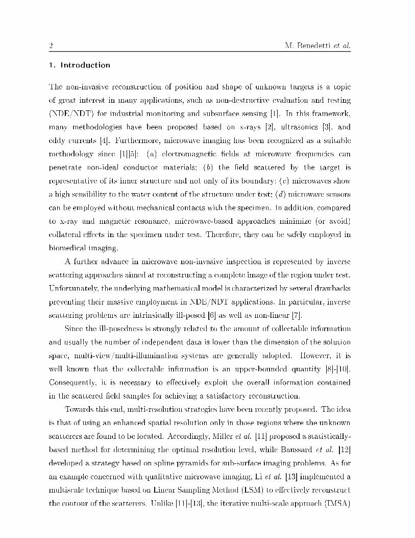
1 Department of Information Engineering and Computer S ien e, ELEDIA Resear hGroup, University of Trento, Via Sommarive 14, 38050 Trento - Italy, Tel. +39 0461882057, Fax. +39 0461 8820932Département de Re her he en Éle tromagnétisme - Laboratoire des Signaux etSystèmes, CNRS-SUPELEC Univ. Paris Sud 11, 3 rue Joliot-Curie, 91192Gif-sur-Yvette CEDEX, Fran eE-mail: manuel.benedetti�disi.unitn.it, lesselier�lss.supele .fr , lambert�lss.supele .fr,andrea.massa�ing.unitn.itAbstra t. In the framework of inverse s attering te hniques, this paper presents theintegration of a multi-resolution te hnique and the level-set method for qualitativemi rowave imaging. On one hand, in order to e�e tively exploit the limited amountof information olle table from s attering measurements, the iterative multi-s alingapproa h (IMSA) is employed for enabling a detailed re onstru tion only whereneeded without in reasing the number of unknowns. On the other hand, the a-prioriinformation on the homogeneity of the unknown obje t is exploited by adopting ashape-based optimization and representing the support of the s atterer via a levelset fun tion. Reliability and e�e tiveness of the proposed strategy are assessed bypro essing both syntheti and experimental s attering data for simple and omplexgeometries, as well.Key Words - Mi rowave Imaging, Inverse S attering, Level Sets, Iterative Multi-S aling Approa h, Homogeneous Diele tri S atterers.Classi� ation Numbers (MSC) - 45Q05, 78A46, 78M50

2 M. Benedetti et al.1. Introdu tionThe non-invasive re onstru tion of position and shape of unknown targets is a topi of great interest in many appli ations, su h as non-destru tive evaluation and testing(NDE/NDT) for industrial monitoring and subsurfa e sensing [1℄. In this framework,many methodologies have been proposed based on x-rays [2℄, ultrasoni s [3℄, andeddy urrents [4℄. Furthermore, mi rowave imaging has been re ognized as a suitablemethodology sin e [1℄[5℄: (a) ele tromagneti �elds at mi rowave frequen ies anpenetrate non-ideal ondu tor materials; (b) the �eld s attered by the target isrepresentative of its inner stru ture and not only of its boundary; ( ) mi rowaves showa high sensibility to the water ontent of the stru ture under test; (d) mi rowave sensors an be employed without me hani al onta ts with the spe imen. In addition, omparedto x-ray and magneti resonan e, mi rowave-based approa hes minimize (or avoid) ollateral e�e ts in the spe imen under test. Therefore, they an be safely employed inbiomedi al imaging.A further advan e in mi rowave non-invasive inspe tion is represented by inverses attering approa hes aimed at re onstru ting a omplete image of the region under test.Unfortunately, the underlying mathemati al model is hara terized by several drawba kspreventing their massive employment in NDE/NDT appli ations. In parti ular, inverses attering problems are intrinsi ally ill-posed [6℄ as well as non-linear [7℄.Sin e the ill-posedness is strongly related to the amount of olle table informationand usually the number of independent data is lower than the dimension of the solutionspa e, multi-view/multi-illumination systems are generally adopted. However, it iswell known that the olle table information is an upper-bounded quantity [8℄-[10℄.Consequently, it is ne essary to e�e tively exploit the overall information ontainedin the s attered �eld samples for a hieving a satisfa tory re onstru tion.Towards this end, multi-resolution strategies have been re ently proposed. The ideais that of using an enhan ed spatial resolution only in those regions where the unknowns atterers are found to be lo ated. A ordingly, Miller et al. [11℄ proposed a statisti ally-based method for determining the optimal resolution level, while Baussard et al. [12℄developed a strategy based on spline pyramids for sub-surfa e imaging problems. As foran example on erned with qualitative mi rowave imaging, Li et al. [13℄ implemented amultis ale te hnique based on Linear Sampling Method (LSM) to e�e tively re onstru tthe ontour of the s atterers. Unlike [11℄-[13℄, the iterative multi-s ale approa h (IMSA)

A Multi-Resolution Te hnique based on Shape Optimization 3developed by Caorsi et al. [14℄ performs a multi-step, multi-resolution inversion pro essin whi h the ratio between unknowns and data is kept suitably low and onstant at ea hstep of the inversion pro edure, thus redu ing the risk of o urren e of lo al minima [9℄in the arising optimization problem.On the other hand, the la k of information a�e ting the inverse problem has beenaddressed through the exploitation of the a-priori knowledge (when available) on thes enario under test by means of an e�e tive representation of the unknowns. As far asmany NDE/NDT appli ations are on erned, the unknown defe t is hara terized byknown ele tromagneti properties (i.e., diele tri permittivity and ondu tivity) and itlies within a known host region. Under these assumptions, the imaging problem redu esto a shape optimization problem aimed at the sear h of lo ation and boundary ontoursof the defe t. Parametri te hniques aimed at representing the unknown obje t in termsof des riptive parameters of referen e shapes [15℄[16℄ and more sophisti ated approa hessu h as evolutionary- ontrolled spline urves [17℄[18℄, shape gradients [19℄-[21℄ or level-sets [22℄-[30℄ have then been proposed. As far as level-set-based methods are on erned,the homogeneous obje t is de�ned as the zero level of a ontinuous fun tion and, unlikepixel-based or parametri -based strategies, su h a des ription enables one to represent omplex shapes in a simple way.In order to exploit both the available a-priori knowledge on the s enario under test(e.g., the homogeneity of the s atterer) and the information ontent from the s atteringmeasurements, this paper proposes the integration of the iterative multi-s aling strategy(IMSA) [14℄ and the level-set (LS ) representation [23℄.The paper is stru tured as follows. The integration between IMSA and LS isdetailed in Se t. 2 dealing with a two-dimensional geometry. In Se tion 3, numeri altesting and experimental validation are presented, a omparison with the standard LSimplementation being made. Finally, some on lusions are drawn (Se t. 4).2. Mathemati al FormulationLet us onsider a ylindri al homogeneous non-magneti obje t with relativepermittivity ǫC and ondu tivity σC that o upies a region Υ belonging to aninvestigation domain DI . Su h a s atterer is probed by a set of V transverse-magneti (TM) plane waves, with ele tri �eld dire ted along the axis of the ylindri al geometry,

4 M. Benedetti et al.namely ζv(r) = ζv(r)z (v = 1, . . . , V ), r = (x, y). The s attered �eld, ξv(r) = ξv(r)z, is olle ted at M(v), v = 1, ..., V , measurement points rm distributed in the observationdomain DO.In order to ele tromagneti ally des ribe the investigation domain DI , let us de�nethe ontrast fun tion τ(r) given byτ(r) =

τC

0

r ∈ Υotherwise (1)where τC = (ǫC − 1)− j σC

2πfε0, f being the frequen y of operation (the time dependen e

ej2πft being implied).The s attering problem is des ribed by the well-known Lippmann-S hwinger integralequationsξv (rm) =

(2π

λ

)2 ∫

DI

τ (r′)Ev (r′)G2D (rm, r′) dr′, rm ∈ DO (2)ζv (r) = Ev (r) −

(2π

λ

)2 ∫

DI

τ (r′)Ev (r′)G2D (r, r′) dr′, r ∈ DI (3)where λ is the ba kground wavelength, Ev is the total ele tri �eld, and G2D (r, r′) =

− j

4H

(2)0

(2πλ‖r − r′‖

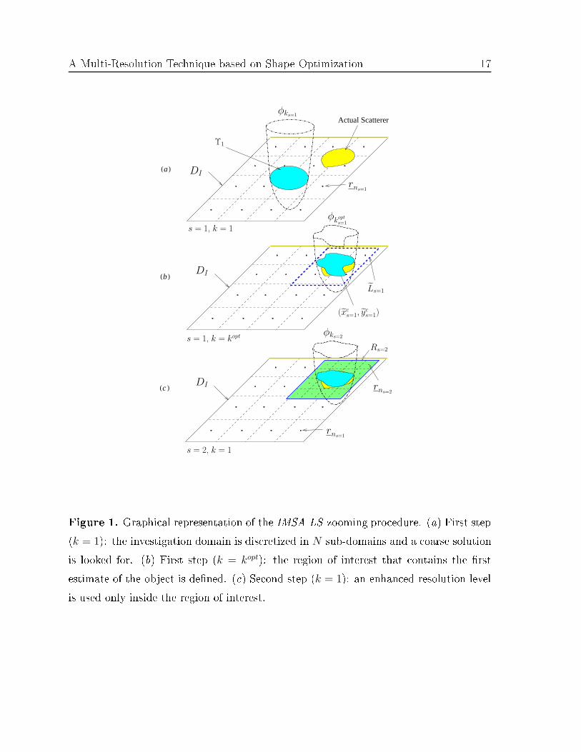
) is the free-spa e two-dimensional Green's fun tion, H(2)0 being these ond-kind, zeroth-order Hankel fun tion.In order to retrieve the unknown position and shape of the target Υ by step-by-step enhan ing the spatial resolution only in that region, alled region-of-interest (RoI),

R ∈ DI , where the s atterer is lo ated [14℄, the following iterative pro edure of Smaxsteps is arried out.With referen e to Fig. 1(a) and to the blo k diagram displayed in Fig. 2, at the�rst step (s = 1, s being the step number) a trial shape Υs = Υ1, belonging to DI ,is hosen and the region of interest Rs [ Rs=1 = DI ℄ is partitioned into NIMSA equalsquare sub-domains, where NIMSA depends on the degrees of freedom of the problem athand and it is omputed a ording to the guidelines suggested in [9℄.In addition, the level set fun tion φs is initialized by means of a signed distan efun tion de�ned as follows [23℄[25℄:φs (r) =

−minb=1,...,Bs‖r − rb‖ if τ (r) = τCminb=1,...,Bs‖r − rb‖ if τ (r) = 0

(4)where rb = (xb, yb) is the b-th border- ell (b = 1, . . . , Bs) of Υs=1.Then, at ea h step s of the pro ess (s = 1, ..., Smax), the following optimizationpro edure is repeated (Fig. 2):

A Multi-Resolution Te hnique based on Shape Optimization 5• Problem Unknown Representation - The ontrast fun tion is represented interms of the level set fun tion as follows

τks(r) =

s∑

i=1

NIMSA∑

ni=1

τkiB

(rni

)r ∈ DI (5)where the index ks indi ates the k-th iteration at the s-th step [ks = 1, ..., kopt

s ℄,B

(rni

) is a re tangular basis fun tion whose support is the n-th sub-domain at thei-th resolution level [ni = 1, ..., NIMSA, i = 1, ..., s℄, and the oe� ient τki

is givenbyτki

=

τC ifΨki

(rni

)≤ 0

0 otherwise (6)lettingΨki

(rni

)=

φki

(rni

) if i = s

φkopti

(rni

) if (i < s) and (rni

∈ Ri

) (7)with i = 1, ..., s as in (5).• Field Distribution Updating - On e τks

(r) has been estimated, the ele tri �eld Evks

(r) is numeri ally omputed a ording to a point-mat hing version of theMethod of Moments (MoM) [31℄ asEv

ki

(rni

)=

∑NIMSApi=1 ζv

(rpi

) [1 − τki

(rpi

)G2D

(rni

, rpi

)]−1,

rni, rpi

∈ DI

ni = 1, ..., NIMSA .

(8)• Cost Fun tion Evaluation - Starting from the total ele tri �eld distribution(8), the re onstru ted s attered �eld ξv

ks(rm) at the m-th measurement point,

m = 1, ..., M(v), is updated by solving the following equationξvks

(rm) =s∑

i=1

NIMSA∑

ni=1

τki

(rni

)Ev

ki

(rni

)G2D

(rm, rni

) (9)and the �t between measured and re onstru ted data is evaluated by the multi-resolution ost fun tion Θ de�ned asΘ {φks

} =

∑Vv=1

∑M(v)m=1

∣∣∣ξvks

(rm) − ξvks

(rm)∣∣∣2

∑Vv=1

∑M(v)m=1

∣∣∣ξvks

(rm)∣∣∣2 . (10)

• Minimization Stopping - The iterative pro ess stops [i.e., kopts = ks and τ opt

s = τks℄when: (a) a set of onditions on the stability of the re onstru tion holds true or (b)when the maximum number of iterations is rea hed [ks = Kmax℄ or ( ) when the

6 M. Benedetti et al.value of the ost fun tion is smaller than a �xed threshold γth. As far as the stabilityof the re onstru tion is on erned [ ondition (a)℄, the �rst orresponding stopping riterion is satis�ed when, for a �xed number of iterations, Kτ , the maximumnumber of pixels whi h vary their value is smaller than a user de�ned threshold γτa ording to the relationshipmaxj=1,...,Kτ

NIMSA∑

ns=1

|τks(rns

) − τks−j (rns)|

τC

< γτ · NIMSA. (11)The se ond riterion, about the stability of the re onstru tion, is satis�ed when the ost fun tion be omes stationary within a window of KΘ iterations as follows:

1

KΘ

KΘ∑

j=1

Θ {φks} − Θ {φks−j}

Θ {φks}

< γΘ. (12)KΘ being a �xed number of iterations and γΘ being user-de�ned thresholds;. Whenthe iterative pro ess stops, the solution τ opt

s at the s-th step is sele ted as the onerepresented by the �best� level set fun tion φopts de�ned as

φopts = arg [minh=1,...,k

opts

(Θ {φh})]. (13)

• Iteration Update - The iteration index is updated [ks → ks + 1℄;• Level Set Update - The level set is updated a ording to the following Hamilton-Ja obi relationship

φks(rns

) = φks−1 (rns) − ∆tsVks−1 (rns

)H{φks−1 (rns)} (14)where H{·} is the Hamiltonian operator [32℄[33℄ given as

H2 {φks(rns

)} =

max2{Dx−

ks; 0

}+ min2

{Dx+

ks; 0

}+

+max2{Dy−

ks; 0

}+ min2

{Dy+

ks; 0

}if Vk(s)

(rn(s)

)≥ 0min2

{Dx−

ks; 0

}+ max2

{Dx+

ks; 0

}+

+min2{Dy−

ks; 0

}+ max2

{Dy+

ks; 0

}otherwise(15)

and Dx±ks

=±φks(xns±1,yns)∓φks(xns ,yns)

ls, Dy±

ks=

±φks(xns ,yns±1)∓φks (xns ,yns)

ls. ∆ts is thetime-step hosen as ∆ts = ∆t1

lsl1with ∆t1 to be set heuristi ally a ording to theliterature [23℄, ls being the ell-side at the s-th resolution level. Vks

is the velo ity

A Multi-Resolution Te hnique based on Shape Optimization 7fun tion omputed following the guidelines suggested in [23℄ by solving the adjointproblem of (8) in order to determine the adjoint �eld F vks. A ordingly,

Vks(rns

) = −ℜ

{∑V

v=1τCEv

ks(rns)F

vks

(rns)∑V

v=1

∑M(v)

m=1 |ξvks

(rm)|2

},

ns = 1, ..., NIMSA

(16)where ℜ stands for the real part.When the s-th minimization pro ess terminates, the ontrast fun tion is updated[τ opts (r)= τks−1 (r), r ∈ DI (5)℄ as well as the RoI [Rs → Rs−1℄. To do so, the followingoperations are arried out:• Computation of the Bary enter of the RoI - the enter of Rs of oordinates

(xcs, y

cs) is determined by omputing the enter of mass of the re onstru ted shapesas follows [14℄ [Fig. 1(b)℄

xcs =

∫DI

xτ opts (r)B (r) dx dy

∫DI

τ opts (r)B (r) dx dy

(17)yc

s =

∫DI

yτ opts (r)B (r) dx dy

∫DI

τ opts (r)B (r) dx dy

; (18)• Estimation of the Size of the RoI - the side Ls of Rs is omputed by evaluatingthe maximum of the distan e δc (r) =

√(x − xc

s)2 + (y − yc

s)2 in order to en losethe s atterer, namely

Ls = maxr

{2 ×

τ opts (r)

τC

δc (r)

}. (19)On e the RoI has been identi�ed, the level of resolution is enhan ed [ks → ks−1℄ onlyin this region by dis retizing Rs into NIMSA sub-domains [Fig. 1( )℄ and by repeatingthe minimization pro ess until the syntheti zoom be omes stationary (s = sopt), i.e.,

{|Qs−1 − Qs|

|Qs−1|× 100

}< γQ, Q = xc, yc, L (20)

γQ being a threshold set as in [14℄, or until a maximum number of steps (sopt = Smax)is rea hed.At the end of the multi-step pro ess (s = sopt), the problem solution is obtained asτ opt

(rni

)= τ opt

s

(rni

), ni = 1, ..., NIMSA, i = 1, ..., sopt.

8 M. Benedetti et al.3. Numeri al ValidationIn order to assess the e�e tiveness of the IMSA-LS approa h, a sele ted set ofrepresentative results on erned with both syntheti and experimental data is presentedherein. The performan es a hieved are evaluated by means of the following error �gures:• Lo alization Error δ

δ|p =

√(xc

s|p − xc|p)2

−(yc

s|p − yc|p)2

λ× 100 (21)where rc|p =

(xc|p , yc|p

) is the enter of the p-th true s atterer, p = 1, ..., P , Pbeing the number of obje ts. The average lo alization error < δ > is de�ned as< δ >=

1

P

P∑

p=1

δ|p . (22)• Area Estimation Error ∆

∆ =

I∑

i=1

1

NIMSA

NIMSA∑

ni=1

Nni

× 100 (23)where Nni

is equal to 1 if τ opt(rni

)= τ

(rni

) and 0 otherwise.As far as the numeri al experiments are on erned, the re onstru tions have beenperformed by blurring the s attering data with an additive Gaussian noise hara terizedby a signal-to-noise-ratio (SNR)SNR = 10log∑V

v=1

∑M(v)m=1 |ξv (rm)|2

∑Vv=1

∑M(v)m=1 |µv,m|2

(24)µv,m being a omplex Gaussian random variable with zero mean value.3.1. Syntheti Data - Cir ular Cylinder3.1.1. Preliminary Validation In the �rst experiment, a lossless ir ular o�- entereds atterer of known permittivity ǫC = 1.8 and radius ρ = λ/4 is lo ated in a squareinvestigation domain of side LD = λ [23℄. V = 10 TM plane waves are impinging fromthe dire tions θv = 2π (v − 1)/V , v = 1, ..., V , and the s attering measurements are olle ted at M = 10 re eivers uniformly distributed on a ir le of radius ρO = λ.As far as the initialization of the IMSA-LS algorithm is on erned, the initial trialobje t Υ1 is a disk with radius λ/4 and entered in DI . The initial value of the timestep is set to ∆t1 = 10−2 as in [23℄. The RoI is dis retized in NIMSA = 15 × 15sub-domains at ea h step of the iterative multi-resolution pro ess. Con erning the

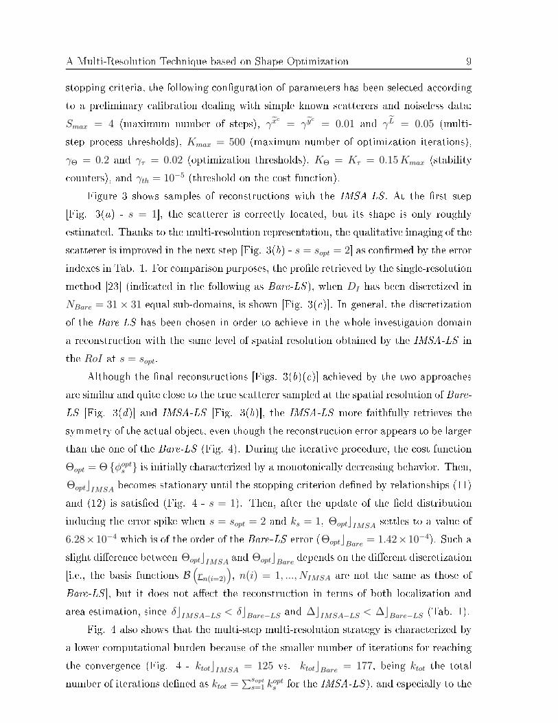
A Multi-Resolution Te hnique based on Shape Optimization 9stopping riteria, the following on�guration of parameters has been sele ted a ordingto a preliminary alibration dealing with simple known s atterers and noiseless data:Smax = 4 (maximum number of steps), γxc

= γ yc

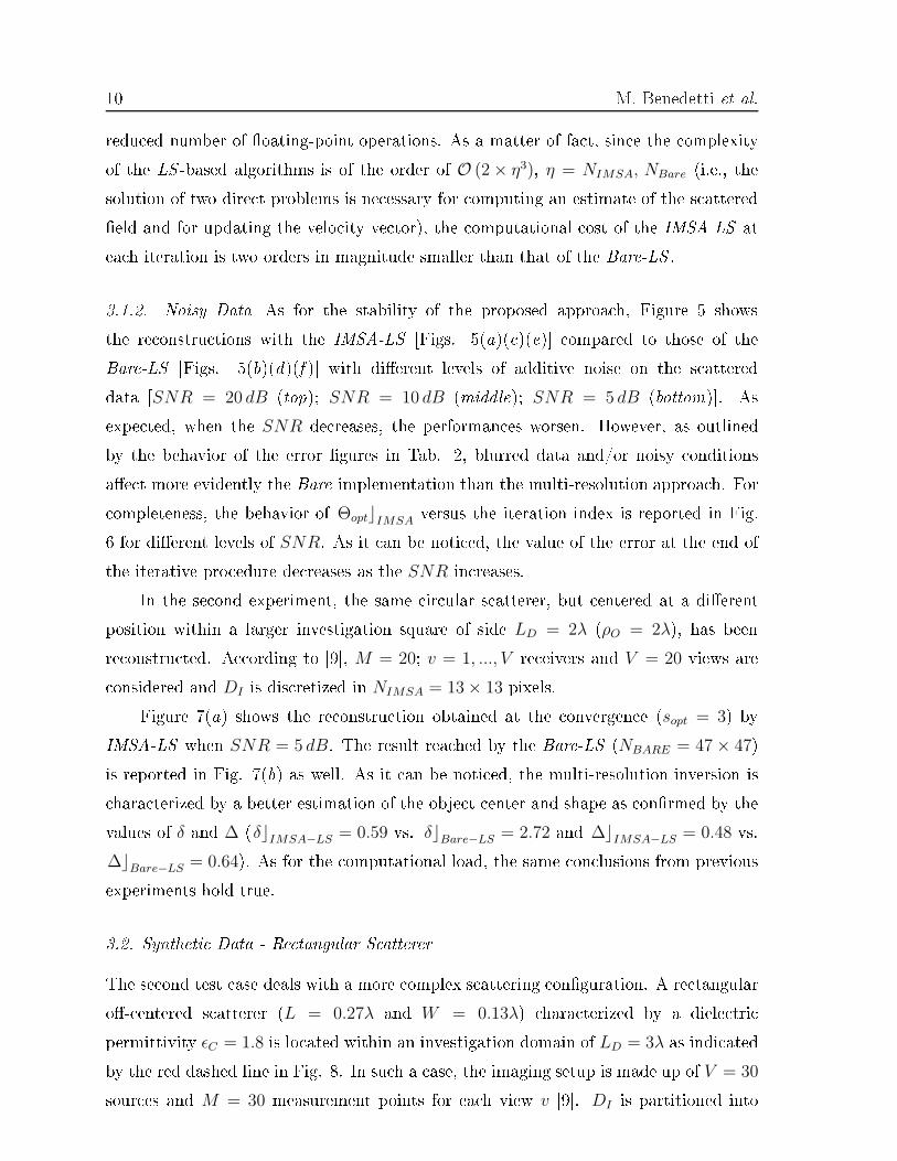
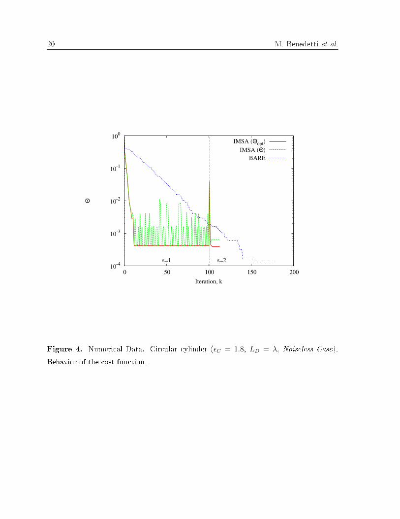
= 0.01 and γL = 0.05 (multi-step pro ess thresholds), Kmax = 500 (maximum number of optimization iterations),γΘ = 0.2 and γτ = 0.02 (optimization thresholds), KΘ = Kτ = 0.15 Kmax (stability ounters), and γth = 10−5 (threshold on the ost fun tion).Figure 3 shows samples of re onstru tions with the IMSA-LS . At the �rst step[Fig. 3(a) - s = 1℄, the s atterer is orre tly lo ated, but its shape is only roughlyestimated. Thanks to the multi-resolution representation, the qualitative imaging of thes atterer is improved in the next step [Fig. 3(b) - s = sopt = 2℄ as on�rmed by the errorindexes in Tab. 1. For omparison purposes, the pro�le retrieved by the single-resolutionmethod [23℄ (indi ated in the following as Bare-LS ), when DI has been dis retized inNBare = 31 × 31 equal sub-domains, is shown [Fig. 3( )℄. In general, the dis retizationof the Bare-LS has been hosen in order to a hieve in the whole investigation domaina re onstru tion with the same level of spatial resolution obtained by the IMSA-LS inthe RoI at s = sopt.Although the �nal re onstru tions [Figs. 3(b)( )℄ a hieved by the two approa hesare similar and quite lose to the true s atterer sampled at the spatial resolution of Bare-LS [Fig. 3(d)℄ and IMSA-LS [Fig. 3(b)℄, the IMSA-LS more faithfully retrieves thesymmetry of the a tual obje t, even though the re onstru tion error appears to be largerthan the one of the Bare-LS (Fig. 4). During the iterative pro edure, the ost fun tionΘopt = Θ {φopt

s } is initially hara terized by a monotoni ally de reasing behavior. Then,Θopt⌋IMSA

be omes stationary until the stopping riterion de�ned by relationships (11)and (12) is satis�ed (Fig. 4 - s = 1). Then, after the update of the �eld distributionindu ing the error spike when s = sopt = 2 and ks = 1, Θopt⌋IMSAsettles to a value of

6.28×10−4 whi h is of the order of the Bare-LS error (Θopt⌋Bare= 1.42×10−4). Su h aslight di�eren e between Θopt⌋IMSA

and Θopt⌋Baredepends on the di�erent dis retization[i.e., the basis fun tions B

(rn(i=2)

), n(i) = 1, ..., NIMSA are not the same as those ofBare-LS ℄, but it does not a�e t the re onstru tion in terms of both lo alization andarea estimation, sin e δ⌋IMSA−LS < δ⌋Bare−LS and ∆⌋IMSA−LS < ∆⌋Bare−LS (Tab. 1).Fig. 4 also shows that the multi-step multi-resolution strategy is hara terized bya lower omputational burden be ause of the smaller number of iterations for rea hingthe onvergen e (Fig. 4 - ktot⌋IMSA = 125 vs. ktot⌋Bare = 177, being ktot the totalnumber of iterations de�ned as ktot =∑sopt

s=1 kopts for the IMSA-LS ), and espe ially to the

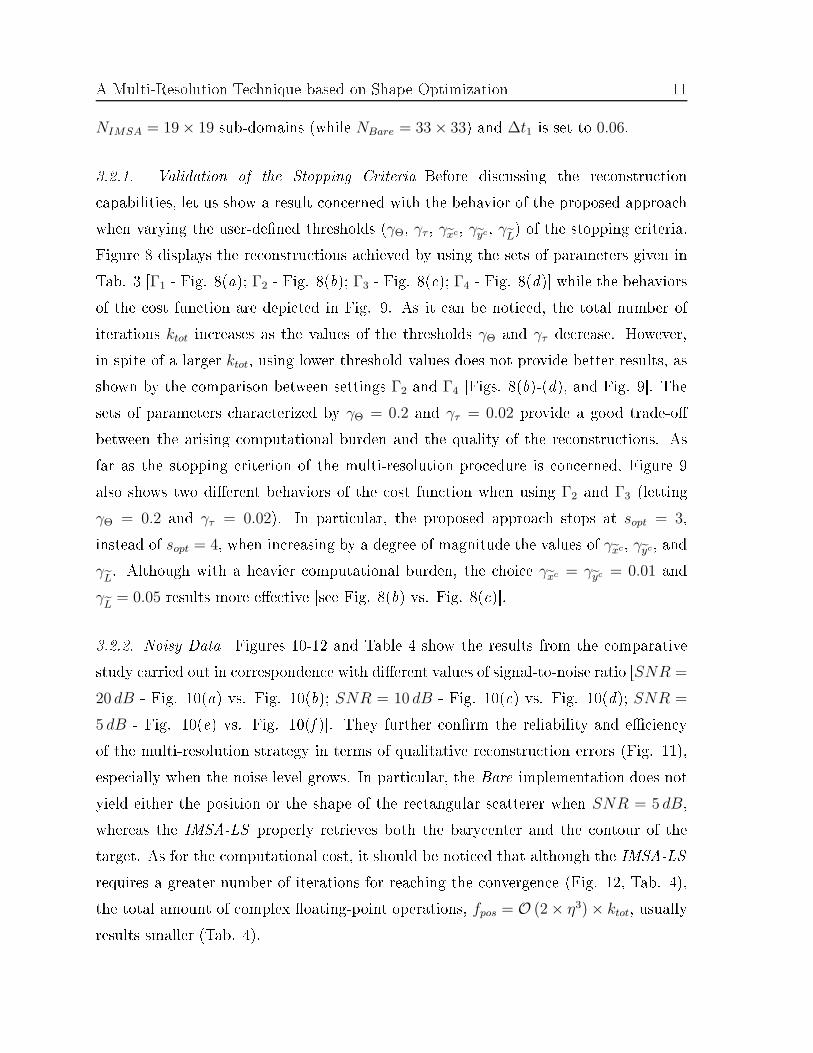
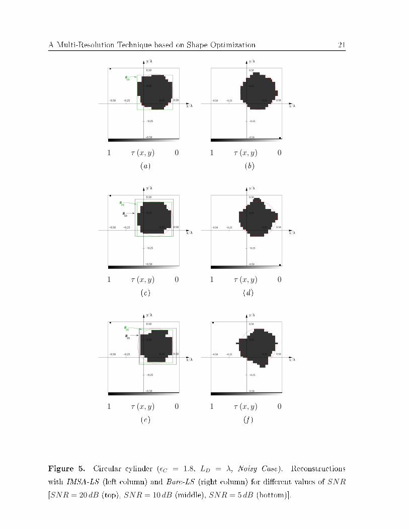
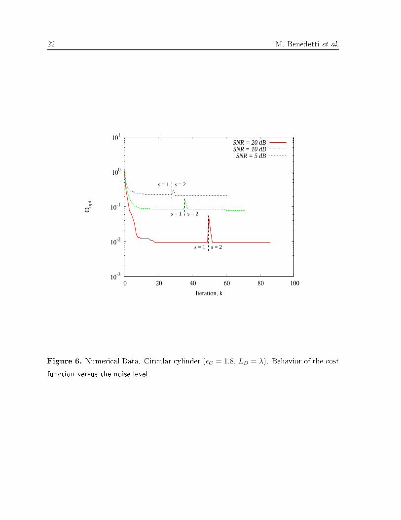
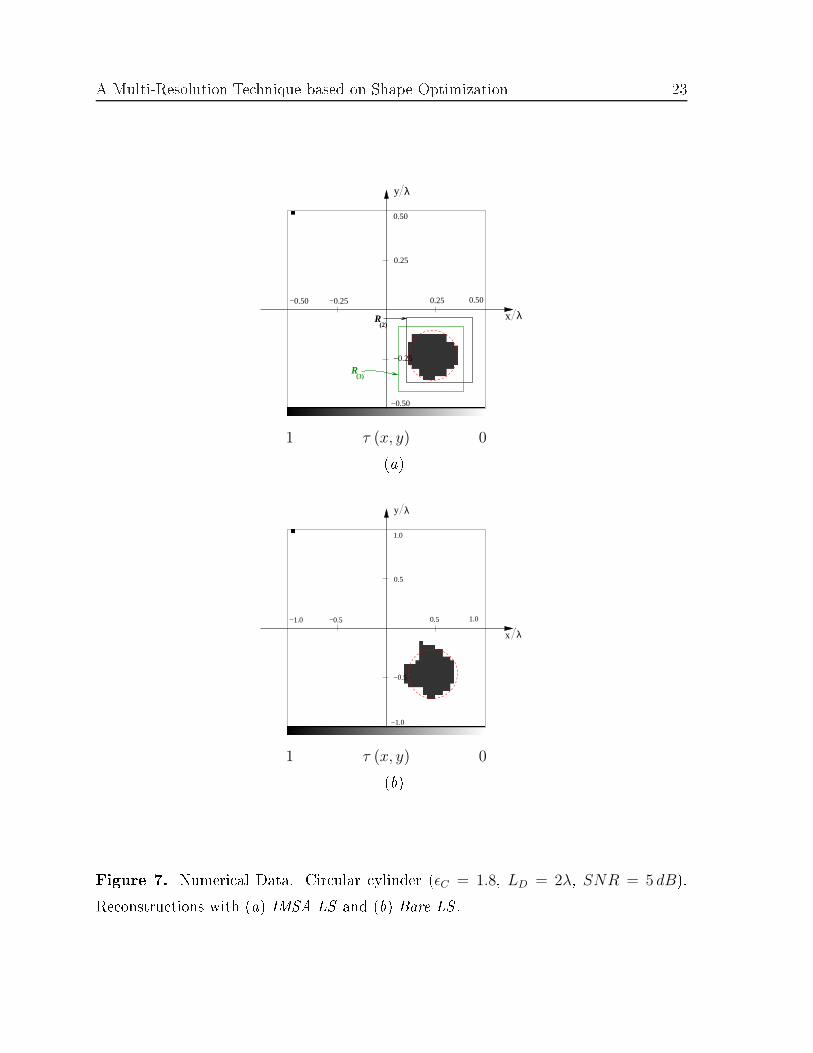
10 M. Benedetti et al.redu ed number of �oating-point operations. As a matter of fa t, sin e the omplexityof the LS -based algorithms is of the order of O (2 × η3), η = NIMSA, NBare (i.e., thesolution of two dire t problems is ne essary for omputing an estimate of the s attered�eld and for updating the velo ity ve tor), the omputational ost of the IMSA-LS atea h iteration is two orders in magnitude smaller than that of the Bare-LS .3.1.2. Noisy Data As for the stability of the proposed approa h, Figure 5 showsthe re onstru tions with the IMSA-LS [Figs. 5(a)( )(e)℄ ompared to those of theBare-LS [Figs. 5(b)(d)(f )℄ with di�erent levels of additive noise on the s attereddata [SNR = 20 dB (top); SNR = 10 dB (middle); SNR = 5 dB (bottom)℄. Asexpe ted, when the SNR de reases, the performan es worsen. However, as outlinedby the behavior of the error �gures in Tab. 2, blurred data and/or noisy onditionsa�e t more evidently the Bare implementation than the multi-resolution approa h. For ompleteness, the behavior of Θopt⌋IMSAversus the iteration index is reported in Fig.6 for di�erent levels of SNR. As it an be noti ed, the value of the error at the end ofthe iterative pro edure de reases as the SNR in reases.In the se ond experiment, the same ir ular s atterer, but entered at a di�erentposition within a larger investigation square of side LD = 2λ (ρO = 2λ), has beenre onstru ted. A ording to [9℄, M = 20; v = 1, ..., V re eivers and V = 20 views are onsidered and DI is dis retized in NIMSA = 13 × 13 pixels.Figure 7(a) shows the re onstru tion obtained at the onvergen e (sopt = 3) byIMSA-LS when SNR = 5 dB. The result rea hed by the Bare-LS (NBARE = 47 × 47)is reported in Fig. 7(b) as well. As it an be noti ed, the multi-resolution inversion is hara terized by a better estimation of the obje t enter and shape as on�rmed by thevalues of δ and ∆ (δ⌋IMSA−LS = 0.59 vs. δ⌋Bare−LS = 2.72 and ∆⌋IMSA−LS = 0.48 vs.

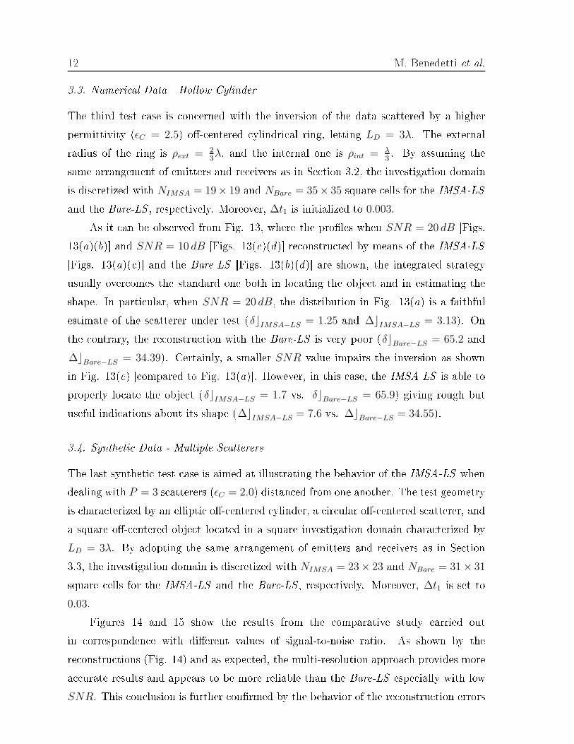
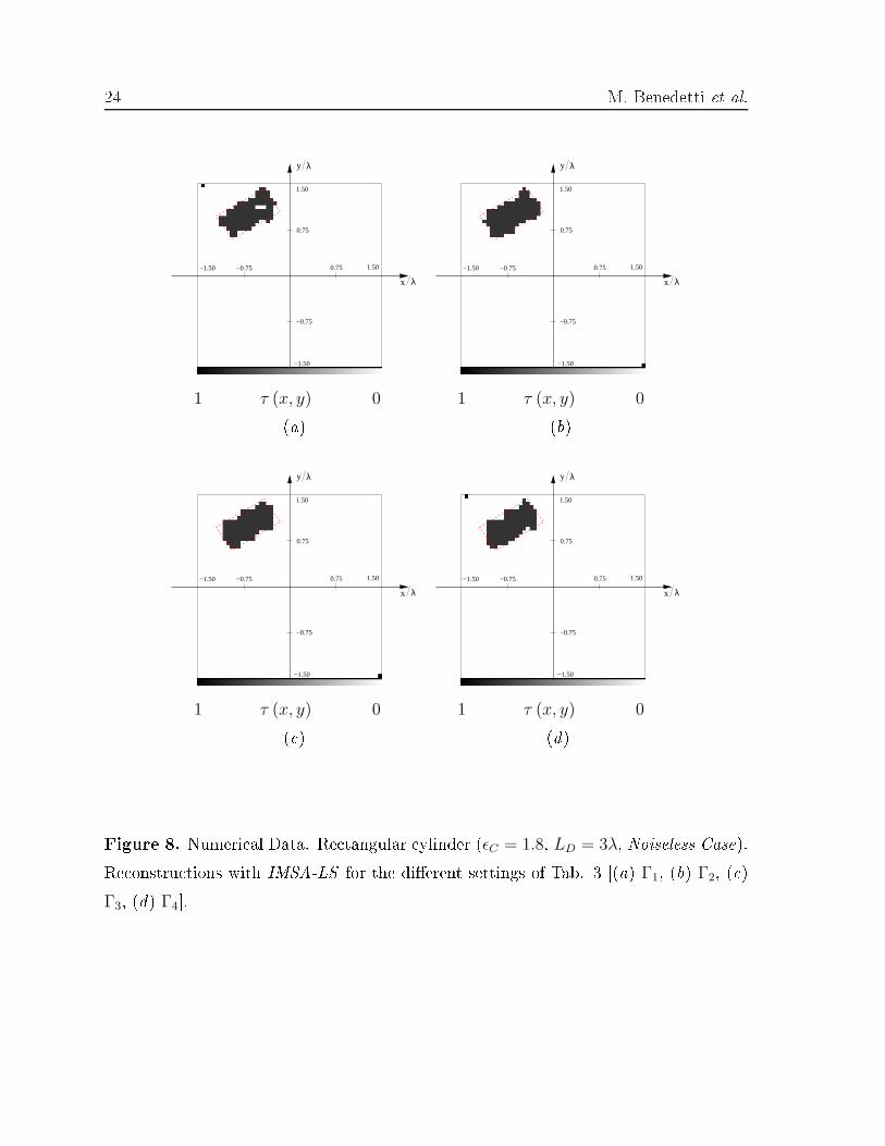
∆⌋Bare−LS = 0.64). As for the omputational load, the same on lusions from previousexperiments hold true.3.2. Syntheti Data - Re tangular S attererThe se ond test ase deals with a more omplex s attering on�guration. A re tangularo�- entered s atterer (L = 0.27λ and W = 0.13λ) hara terized by a diele tri permittivity ǫC = 1.8 is lo ated within an investigation domain of LD = 3λ as indi atedby the red dashed line in Fig. 8. In su h a ase, the imaging setup is made up of V = 30sour es and M = 30 measurement points for ea h view v [9℄. DI is partitioned into

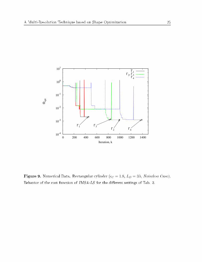
A Multi-Resolution Te hnique based on Shape Optimization 11NIMSA = 19 × 19 sub-domains (while NBare = 33 × 33) and ∆t1 is set to 0.06.3.2.1. Validation of the Stopping Criteria Before dis ussing the re onstru tion apabilities, let us show a result on erned with the behavior of the proposed approa hwhen varying the user-de�ned thresholds (γΘ, γτ , γxc , γyc , γ

L) of the stopping riteria.Figure 8 displays the re onstru tions a hieved by using the sets of parameters given inTab. 3 [Γ1 - Fig. 8(a); Γ2 - Fig. 8(b); Γ3 - Fig. 8( ); Γ4 - Fig. 8(d)℄ while the behaviorsof the ost fun tion are depi ted in Fig. 9. As it an be noti ed, the total number ofiterations ktot in reases as the values of the thresholds γΘ and γτ de rease. However,in spite of a larger ktot, using lower threshold values does not provide better results, asshown by the omparison between settings Γ2 and Γ4 [Figs. 8(b)-(d), and Fig. 9℄. Thesets of parameters hara terized by γΘ = 0.2 and γτ = 0.02 provide a good trade-o�between the arising omputational burden and the quality of the re onstru tions. Asfar as the stopping riterion of the multi-resolution pro edure is on erned, Figure 9also shows two di�erent behaviors of the ost fun tion when using Γ2 and Γ3 (letting

γΘ = 0.2 and γτ = 0.02). In parti ular, the proposed approa h stops at sopt = 3,instead of sopt = 4, when in reasing by a degree of magnitude the values of γxc , γyc , andγ

L. Although with a heavier omputational burden, the hoi e γxc = γyc = 0.01 and

γL

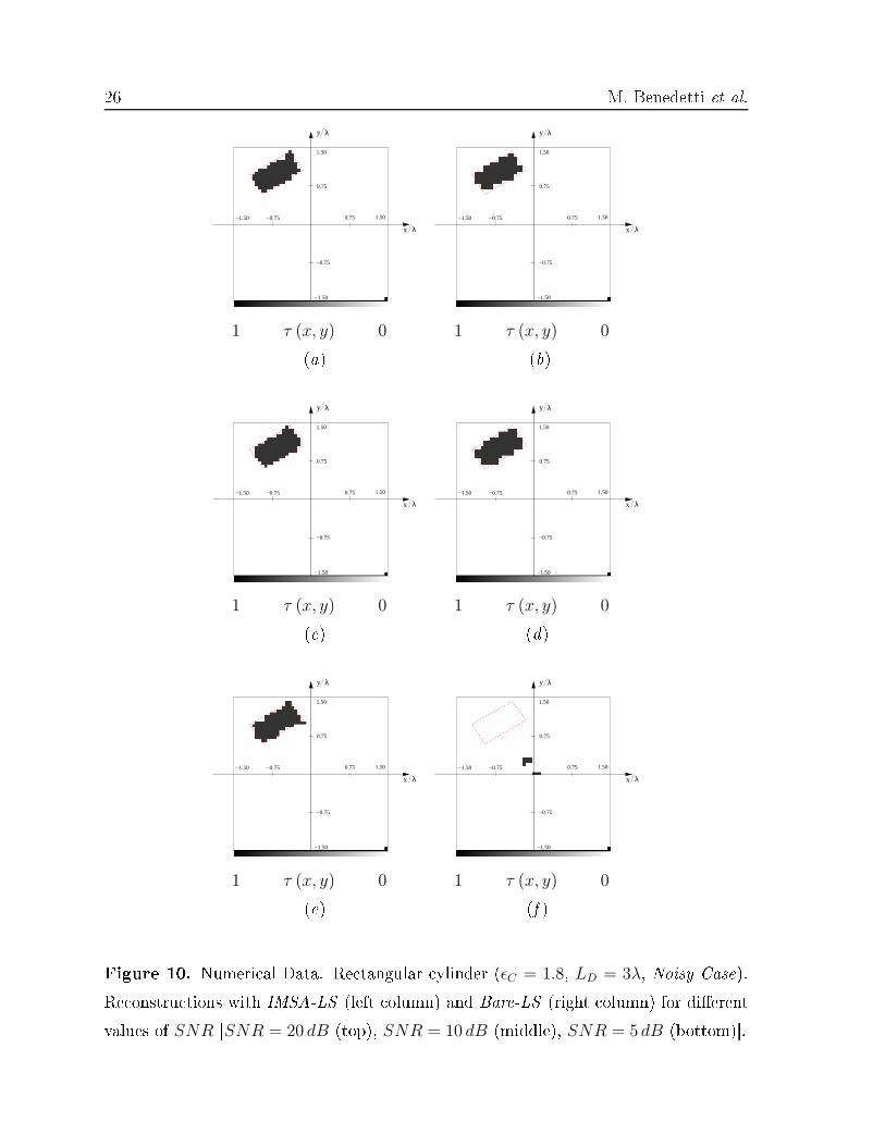
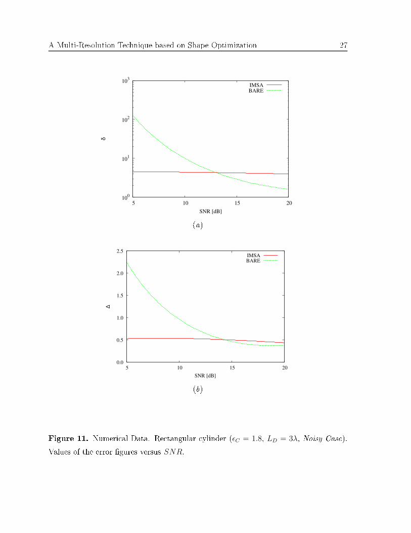
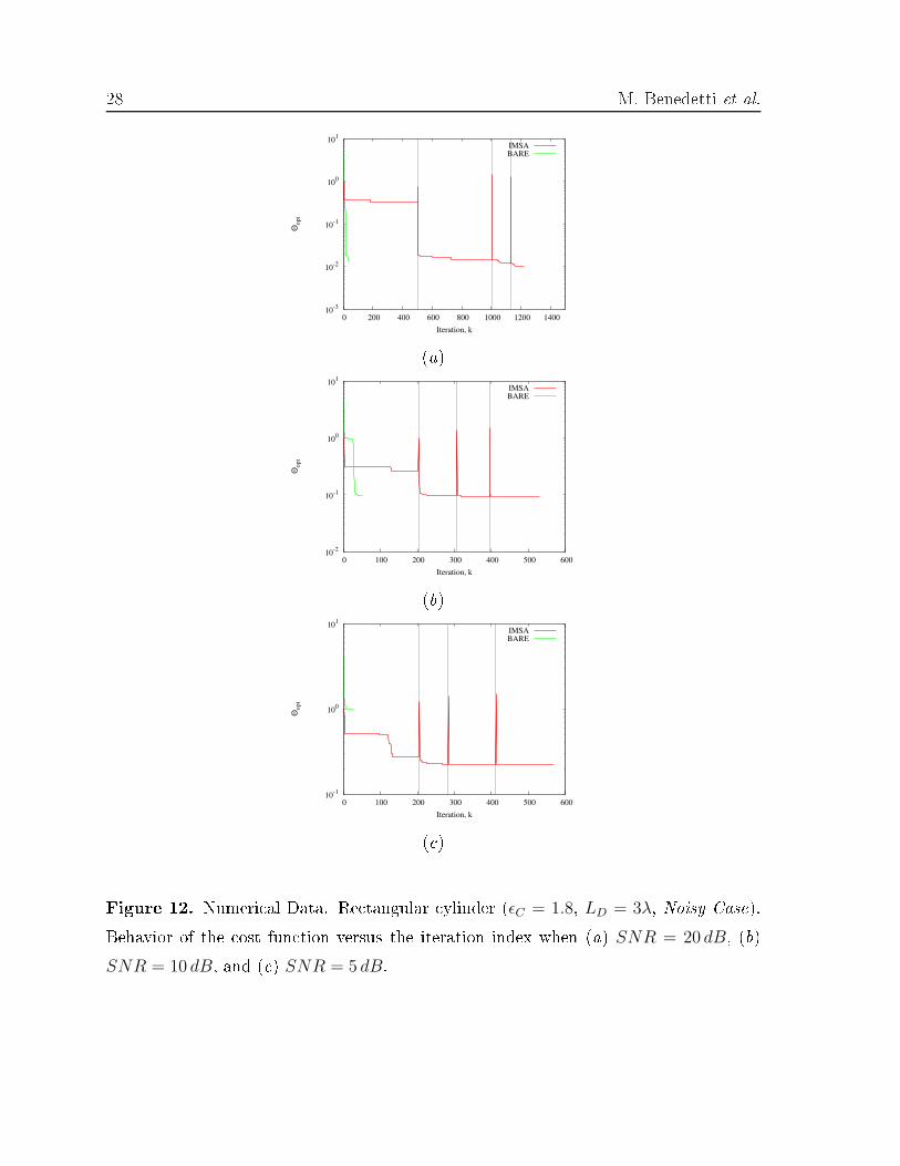
= 0.05 results more e�e tive [see Fig. 8(b) vs. Fig. 8( )℄.3.2.2. Noisy Data Figures 10-12 and Table 4 show the results from the omparativestudy arried out in orresponden e with di�erent values of signal-to-noise ratio [SNR =

20 dB - Fig. 10(a) vs. Fig. 10(b); SNR = 10 dB - Fig. 10( ) vs. Fig. 10(d); SNR =

5 dB - Fig. 10(e) vs. Fig. 10(f )℄. They further on�rm the reliability and e� ien yof the multi-resolution strategy in terms of qualitative re onstru tion errors (Fig. 11),espe ially when the noise level grows. In parti ular, the Bare implementation does notyield either the position or the shape of the re tangular s atterer when SNR = 5 dB,whereas the IMSA-LS properly retrieves both the bary enter and the ontour of thetarget. As for the omputational ost, it should be noti ed that although the IMSA-LSrequires a greater number of iterations for rea hing the onvergen e (Fig. 12, Tab. 4),the total amount of omplex �oating-point operations, fpos = O (2 × η3) × ktot, usuallyresults smaller (Tab. 4).

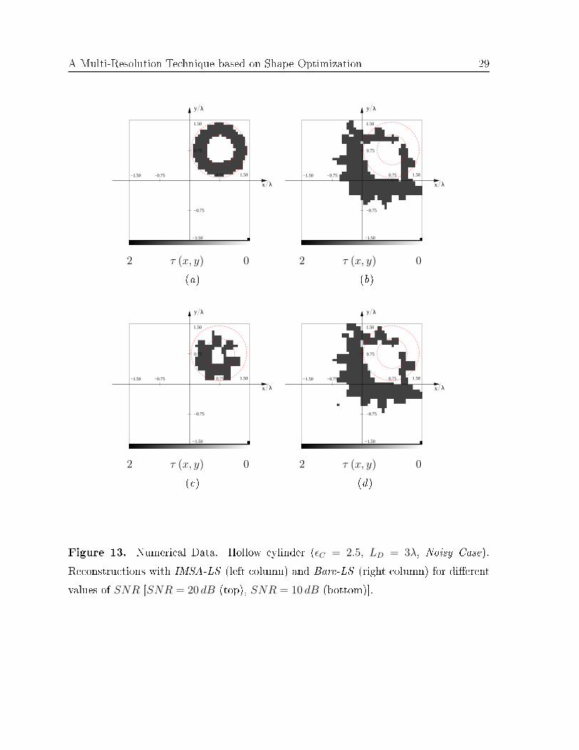
12 M. Benedetti et al.3.3. Numeri al Data - Hollow CylinderThe third test ase is on erned with the inversion of the data s attered by a higherpermittivity (ǫC = 2.5) o�- entered ylindri al ring, letting LD = 3λ. The externalradius of the ring is ρext = 23λ, and the internal one is ρint = λ

3. By assuming thesame arrangement of emitters and re eivers as in Se tion 3.2, the investigation domainis dis retized with NIMSA = 19× 19 and NBare = 35× 35 square ells for the IMSA-LSand the Bare-LS , respe tively. Moreover, ∆t1 is initialized to 0.003.As it an be observed from Fig. 13, where the pro�les when SNR = 20 dB [Figs.13(a)(b)℄ and SNR = 10 dB [Figs. 13( )(d)℄ re onstru ted by means of the IMSA-LS[Figs. 13(a)( )℄ and the Bare-LS [Figs. 13(b)(d)℄ are shown, the integrated strategyusually over omes the standard one both in lo ating the obje t and in estimating theshape. In parti ular, when SNR = 20 dB, the distribution in Fig. 13(a) is a faithfulestimate of the s atterer under test (δ⌋IMSA−LS = 1.25 and ∆⌋IMSA−LS = 3.13). Onthe ontrary, the re onstru tion with the Bare-LS is very poor (δ⌋Bare−LS = 65.2 and

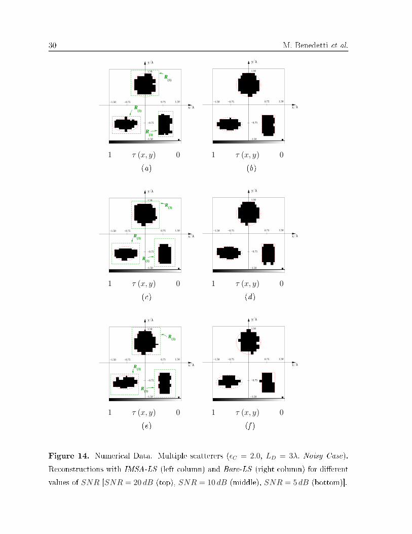
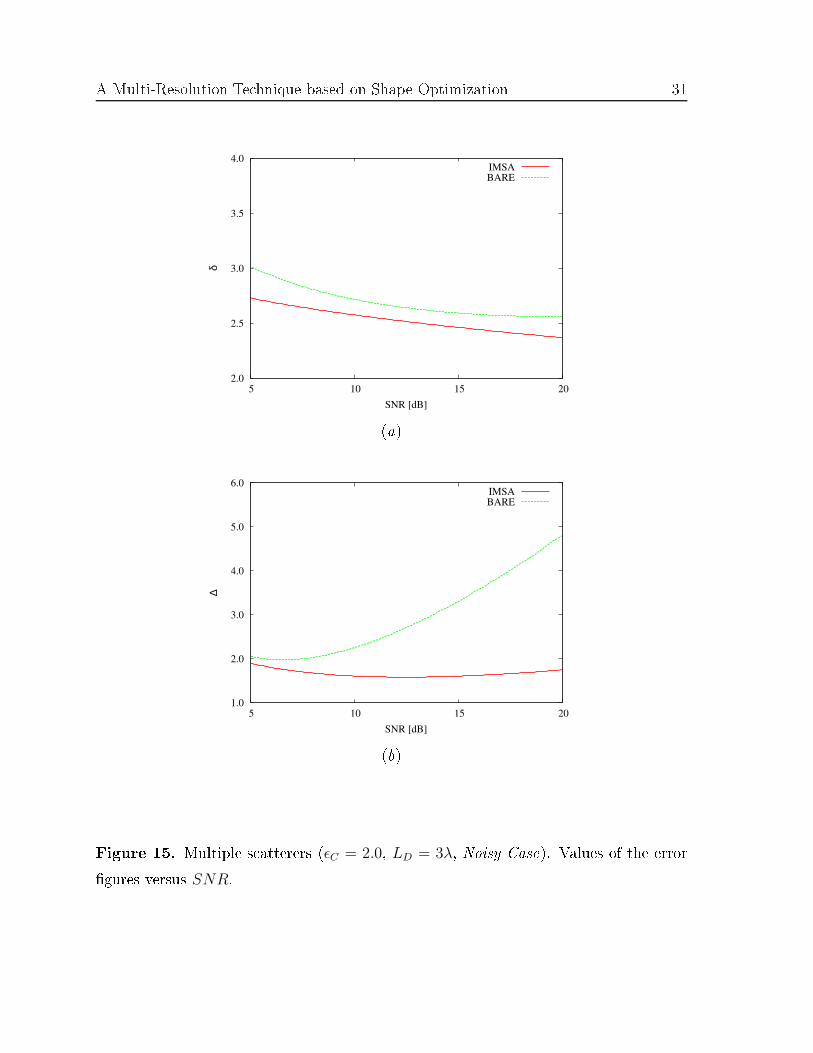
∆⌋Bare−LS = 34.39). Certainly, a smaller SNR value impairs the inversion as shownin Fig. 13( ) [ ompared to Fig. 13(a)℄. However, in this ase, the IMSA-LS is able toproperly lo ate the obje t (δ⌋IMSA−LS = 1.7 vs. δ⌋Bare−LS = 65.9) giving rough butuseful indi ations about its shape (∆⌋IMSA−LS = 7.6 vs. ∆⌋Bare−LS = 34.55).3.4. Syntheti Data - Multiple S atterersThe last syntheti test ase is aimed at illustrating the behavior of the IMSA-LS whendealing with P = 3 s atterers (ǫC = 2.0) distan ed from one another. The test geometryis hara terized by an ellipti o�- entered ylinder, a ir ular o�- entered s atterer, anda square o�- entered obje t lo ated in a square investigation domain hara terized byLD = 3λ. By adopting the same arrangement of emitters and re eivers as in Se tion3.3, the investigation domain is dis retized with NIMSA = 23× 23 and NBare = 31× 31square ells for the IMSA-LS and the Bare-LS , respe tively. Moreover, ∆t1 is set to0.03.Figures 14 and 15 show the results from the omparative study arried outin orresponden e with di�erent values of signal-to-noise ratio. As shown by there onstru tions (Fig. 14) and as expe ted, the multi-resolution approa h provides morea urate results and appears to be more reliable than the Bare-LS espe ially with lowSNR. This on lusion is further on�rmed by the behavior of the re onstru tion errors

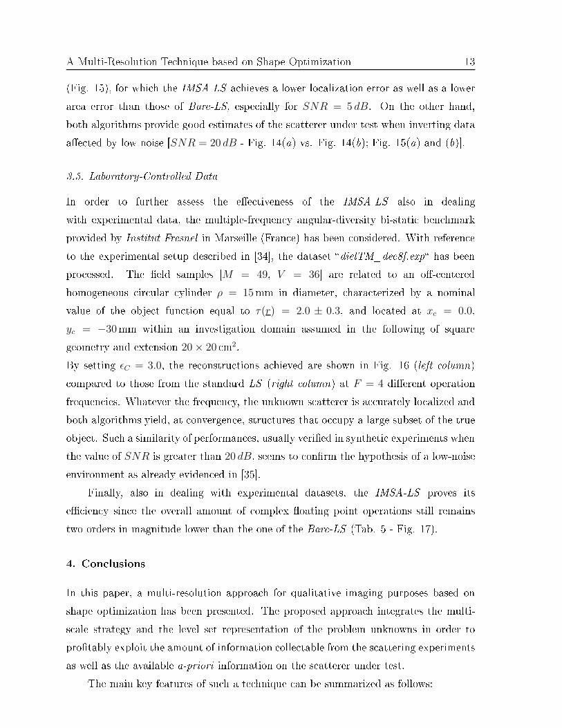
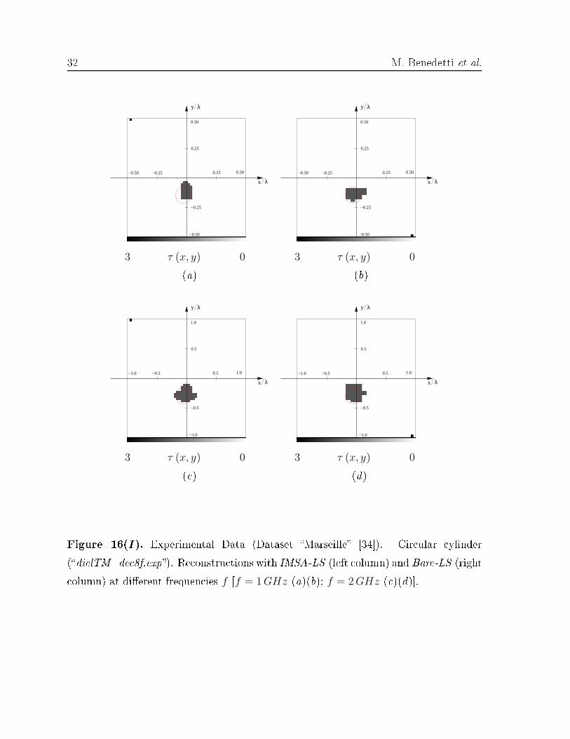
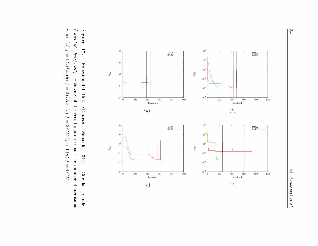
A Multi-Resolution Te hnique based on Shape Optimization 13(Fig. 15), for whi h the IMSA-LS a hieves a lower lo alization error as well as a lowerarea error than those of Bare-LS, espe ially for SNR = 5 dB. On the other hand,both algorithms provide good estimates of the s atterer under test when inverting dataa�e ted by low noise [SNR = 20 dB - Fig. 14(a) vs. Fig. 14(b); Fig. 15(a) and (b)℄.3.5. Laboratory-Controlled DataIn order to further assess the e�e tiveness of the IMSA-LS also in dealingwith experimental data, the multiple-frequen y angular-diversity bi-stati ben hmarkprovided by Institut Fresnel in Marseille (Fran e) has been onsidered. With referen eto the experimental setup des ribed in [34℄, the dataset �dielTM_de 8f.exp� has beenpro essed. The �eld samples [M = 49, V = 36℄ are related to an o�- enteredhomogeneous ir ular ylinder ρ = 15mm in diameter, hara terized by a nominalvalue of the obje t fun tion equal to τ(r) = 2.0 ± 0.3, and lo ated at xc = 0.0,yc = −30mm within an investigation domain assumed in the following of squaregeometry and extension 20 × 20 m2.By setting ǫC = 3.0, the re onstru tions a hieved are shown in Fig. 16 (left olumn) ompared to those from the standard LS (right olumn) at F = 4 di�erent operationfrequen ies. Whatever the frequen y, the unknown s atterer is a urately lo alized andboth algorithms yield, at onvergen e, stru tures that o upy a large subset of the trueobje t. Su h a similarity of performan es, usually veri�ed in syntheti experiments whenthe value of SNR is greater than 20 dB, seems to on�rm the hypothesis of a low-noiseenvironment as already eviden ed in [35℄.Finally, also in dealing with experimental datasets, the IMSA-LS proves itse� ien y sin e the overall amount of omplex �oating point operations still remainstwo orders in magnitude lower than the one of the Bare-LS (Tab. 5 - Fig. 17).4. Con lusionsIn this paper, a multi-resolution approa h for qualitative imaging purposes based onshape optimization has been presented. The proposed approa h integrates the multi-s ale strategy and the level set representation of the problem unknowns in order topro�tably exploit the amount of information olle table from the s attering experimentsas well as the available a-priori information on the s atterer under test.The main key features of su h a te hnique an be summarized as follows:

14 M. Benedetti et al.• innovative multi-level representation of the problem unknowns in the shape-deformation-based re onstru tion te hnique;• e�e tive exploitation of the s attering data through the iterative multi-stepstrategy;• limitation of the risk of being trapped in false solutions thanks to the redu ed ratiobetween data and unknowns;• useful exploitation of the a-priori information (i.e., obje t homogeneity) about thes enario under test;• enhan ed spatial resolution limited to the region of interest.From the validation on erned with di�erent s enarios and both syntheti andexperimental data, the following on lusions an be drawn:• the IMSA-LS usually proved more e�e tive than the single-resolution implementa-tion, espe ially when dealing with orrupted data s attered from simple as well as omplex geometries hara terized by one or several obje ts;• the integrated strategy appeared less omputationally-expensive than the standardapproa h in rea hing a re onstru tion with the same level of spatial resolutionwithin the support of the obje t.

A Multi-Resolution Te hnique based on Shape Optimization 15Referen es[1℄ P. J. Shull, Nondestru tive Evaluation: Theory, Te hniques and Appli ations. CRC Press, 2002.[2℄ J. Baru hel, J.-Y. Bu�ère, E. Maire, P. Merle, and G. Peix, X-Ray Tomography in MaterialS ien e. Hermes S ien e, 2000.[3℄ L. W. S hmerr, Fundamentals of Ultrasoni Nondestru tive Evaluation: A Modeling Approa h.Springer, 1998.[4℄ B. A. Auld and J. C. Moulder, �Review of advan es in quantitative eddy urrent nondestru tiveevaluation�, J. Nondestru tive Evaluation, vol. 18, no. 1, pp. 3-36, Mar. 1999.[5℄ R. Zoughi, Mi rowave Nondestru tive Testing and Evaluation. Dordre ht, The Netherlands:Kluwer A ademi Publishers, 2000.[6℄ O. M. Bu i and T. Isernia, �Ele tromagneti inverse s attering: retrievable information andmeasurement strategies,� Radio S i., vol. 32, pp. 2123-2138, Nov.-De . 1997.[7℄ M. Bertero and P. Bo a i, Introdu tion to Inverse Problems in Imaging . IOP Publishing Ltd,Bristol, 1998.[8℄ O. M. Bu i and G. Fran es hetti, �On the spatial bandwidth of s attered �elds,� IEEE Trans.Antennas Propagat., vol. 35, no. 12, pp. 1445-1455, De . 1987.[9℄ T. Isernia, V. Pas azio, and R. Pierri, �On the lo al minima in a tomographi imaging te hnique,�IEEE Trans. Antennas Propagat ., vol. 39, no. 7, pp. 1696-1607, Jul. 2001.[10℄ H. Haddar, S. Kusiak, and J. Sylvester, �The onvex ba k-s attering support,� SIAM J. Appl.Math., vol. 66, pp. 591-615, De . 2005.[11℄ E. L. Miller, and A. S. Willsky, �A multis ale, statisti ally based inversion s heme for linearizedinverse s attering problems,� IEEE Trans. Antennas Propagat., vol. 34, no. 2, pp. 346-357, Mar.1996.[12℄ A. Baussard, E. L. Miller, and D. Lesselier, �Adaptive mulis ale re onstru tion of buried obje ts,�Inverse Problems , vol. 20, pp. S1-S15, De . 2004.[13℄ J. Li, H. Liu, and J. Zou, �Multilevel linear sampling method for inverse s attering problems,�SIAM J. Appl. Math., vol. 30, pp. 1228-1250, Mar. 2008.[14℄ S. Caorsi, M. Donelli, and A. Massa, "Dete tion, lo ation, and imaging of multiple s atterers bymeans of the iterative multis aling method," IEEE Trans. Mi rowave Theory Te h., vol. 52, no.4, pp. 1217-1228, Apr. 2004.[15℄ S. Caorsi, A. Massa, M. Pastorino, and M. Donelli, �Improved mi rowave imaging pro edure fornondestru tive evaluations of two-dimensional stru tures,� IEEE Trans. Antennas Propag., vol.52, pp. 1386-1397, Jun. 2004.[16℄ M. Benedetti, M. Donelli, and A. Massa, �Multi ra k dete tion in two-dimensional stru tures bymeans of GA-based strategies,� IEEE Trans. Antennas Propagat., vol. 55, no. 1, pp. 205-215,Jan. 2007.[17℄ V. Cingoski, N. Kowata, K. Kaneda, and H. Yamashita, �Inverse shape optimization usingdynami ally adjustable geneti algorithms,� IEEE Trans. Energy Conversion, vol. 14, no. 3,pp. 661-666, Sept. 1999.[18℄ L. Lizzi, F. Viani, R. Azaro, and A. Massa, �Optimization of a spline-shaped UWB antenna byPSO,� IEEE Antennas Wireless Propagat. Lett ., vol. 6, pp. 182-185, 2007.

16 M. Benedetti et al.[19℄ J. Cea, S. Garreau, P. Guillame, and M. Masmoudi, �The shape and topologi al optimizations onne tion,� Comput. Methods Appl. Me h. Eng., vol. 188, no. 4, pp. 713-726, 2000.[20℄ G. R. Feijoo, A. A. Oberai, and P. M. Pinsky, �An appli ation of shape optimization in the solutionof inverse a ousti s attering problems,� Inverse Problems , vol. 20, pp. 199-228, Feb. 2004.[21℄ M. Masmoudi, J. Pommier, and B. Samet, �The topologi al asymptoti expansion for the Maxwellequations and some appli ations,� Inverse Problems , vol. 21, pp. 547-564, Apr. 2005.[22℄ F. Santosa, �A level-set approa h for inverse problems involving obsta les,� ESAIM: COCV , vol.1, pp. 17-33, Jan. 1996.[23℄ A. Litman, D. Lesselier, and F. Santosa, "Re onstru tion of a two-dimensional binary obsta le by ontrolled evolution of a level-set," Inverse Problems , vol. 14, pp. 685-706, Jun. 1998.[24℄ O. Dorn, E. L. Miller, C. M. Rappaport, �A shape re onstru tion method for ele tromagneti tomography using adjoint �elds and level sets,� Inverse Problems , vol. 16, pp. 1119-1156, May2000.[25℄ C. Ramananjaona, M. Lambert, D. Lesselier, and J. P. Zolésio, "Shape re onstru tion of buriedobsta les by ontrolled evolution of a level-set: from a min-max formulation to a numeri alexperimentation," Inverse Problems , vol. 17, pp. 1087-1111, De . 2001.[26℄ R. Ferrayé, J.-Y. Dauvigna , and C. Pi hot, �An inverse s attering method based on ontourdeformations by means of a level set method using frequen y hopping te hnique,� IEEE Trans.Antennas Propagat., vol. 51, no. 5, pp. 1100-1113, May 2003.[27℄ E. T. Chung, T. F. Chan, X. C. Tai, �Ele tri al impedan e tomography using level setrepresentation and total variational regularization,� J. Comput. Phys., vol. 205, no. 2, pp. 707-723, May. 2005.[28℄ K. van den Doel and U. M. Asher, �Dynami level set regularization for large distributed parameterestimation problems,� Inverse Problems , vol. 23, pp. 1271-1288, Jun. 2007.[29℄ J. Strain, �Three methods for moving interfa es,� J. Comput. Phys., vol. 151, pp. 616-648, May1999.[30℄ O. Dorn and D. Lesselier, �Level set methods for inverse s attering,� Inverse Problems , vol. 22,pp. R67-R131, Aug. 2006.[31℄ J. H. Ri hmond, �S attering by a diele tri ylinder of arbitrary ross-se tion shape,� IEEE Trans.Antennas Propagat., vol. 13, pp. 334-341, May 1965.[32℄ S. Osher and J. A. Sethian, �Fronts propagating with urvature-dependent speed: algorithms basedon Hamilton-Ja obi formulations,� J. Comput. Phys., 79, pp. 12-49, Nov. 1988.[33℄ J. A. Sethian, Level Set and Fast Mar hing Methods . Cambridge University Press, Cambridge,UK, 2nd ed., 1999.[34℄ K. Belkebir and M. Saillard, �Testing inversion algorithms against experimental data,� InverseProblems , vol. 17, pp. 1565-1702, De . 2001.[35℄ M. Testorf and M. Fiddy, �Imaging from real s attered �eld data using a linear spe tral estimationte hnique,� Inverse Problems , vol. 17, pp. 1645-1658, De . 2001.

A Multi-Resolution Te hnique based on Shape Optimization 17a( )

b( )

c( )

Actual Scatterer

Υ1

(xcs=1, y

cs=1)

rns=1

rns=1

Rs=2

φkopts=1

φks=1

s = 1, k = 1

s = 1, k = kopt

s = 2, k = 1

DI

DI

DI

Ls=1

rns=2

φks=2

Figure 1. Graphi al representation of the IMSA-LS zooming pro edure. (a) First step(k = 1): the investigation domain is dis retized in N sub-domains and a oarse solutionis looked for. (b) First step (k = kopt): the region of interest that ontains the �rstestimate of the obje t is de�ned. ( ) Se ond step (k = 1): an enhan ed resolution levelis used only inside the region of interest.

18 M. Benedetti et al.

Field Distribution Updating

Determine

Cost Function Evaluation

Level Set Update

Problem Unknown Representation

FALSE

TRUE

TRUE

Stop

Initialization

FALSEIMSA

Stopping Criterion

Stopping CriteriaLS

Compute Evki

(rni

)

rni∈ DI

xcs,y

cs,Ls

Determine ξvks

(rmv

)and compute Θ {φks

}

rmv∈ DO

Compute φksfrom φks−1

τks(r) =

∑si=1

∑NIMSA

ni=1τki

B(rni

)

rni∈ DI

s-th resolution level

ks = ks + 1

Υsopt

Υs = Υ1

ks = 0

s = s + 1

γxc,γyc,γL

γτ , γΘ, γth, Kmax

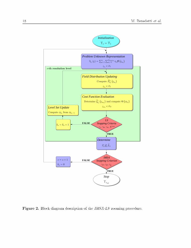
Figure 2. Blo k diagram des ription of the IMSA-LS zooming pro edure.

A Multi-Resolution Te hnique based on Shape Optimization 19x

y λ

λ−0.25 0.25

0.25

−0.25

0.50

−0.50

−0.50

0.50

x

y λ

λ−0.25 0.25

0.25

−0.25

0.50

−0.50

−0.50

0.50

R(2)

1 τ (x, y) 0 1 τ (x, y) 0(a) (b)x

y λ

λ−0.25 0.25

0.25

−0.25

0.50

−0.50

−0.50

0.50

x

y λ

λ−0.25 0.25

0.25

−0.25

0.50

−0.50

−0.50

0.50

1 τ (x, y) 0 1 τ (x, y) 0( ) (d)Figure 3. Numeri al Data. Cir ular ylinder (ǫC = 1.8, LD = λ, Noiseless Case).Re onstru tions with IMSA-LS at (a) s = 1 and (b) s = sopt = 2, ( ) Bare-LS .Optimal inversion (d).

20 M. Benedetti et al.

10-4

10-3

10-2

10-1

100

0 50 100 150 200

Θ

Iteration, k

s=1 s=2

IMSA (Θopt)

IMSA (Θ)

BARE

Figure 4. Numeri al Data. Cir ular ylinder (ǫC = 1.8, LD = λ, Noiseless Case).Behavior of the ost fun tion.

A Multi-Resolution Te hnique based on Shape Optimization 21R

(2)

x

y λ

λ−0.25 0.25

0.25

−0.25

0.50

−0.50

−0.50

0.50

x

y λ

λ−0.25 0.25

0.25

−0.25

0.50

−0.50

−0.50

0.50

1 τ (x, y) 0 1 τ (x, y) 0(a) (b)(3)

R

x

y λ

λ−0.25 0.25

0.25

−0.25

0.50

−0.50

−0.50

0.50

(2)R

x

y λ

λ−0.25 0.25

0.25

−0.25

0.50

−0.50

−0.50

0.50

1 τ (x, y) 0 1 τ (x, y) 0( ) (d)(3)

R

R(2)

x

y λ

λ−0.25 0.25

0.25

−0.25

0.50

−0.50

−0.50

0.50

x

y λ

λ−0.25 0.25

0.25

−0.25

0.50

−0.50

−0.50

0.50

1 τ (x, y) 0 1 τ (x, y) 0(e) (f )Figure 5. Cir ular ylinder (ǫC = 1.8, LD = λ, Noisy Case). Re onstru tionswith IMSA-LS (left olumn) and Bare-LS (right olumn) for di�erent values of SNR[SNR = 20 dB (top), SNR = 10 dB (middle), SNR = 5 dB (bottom)℄.

22 M. Benedetti et al.

10-3

10-2

10-1

100

101

0 20 40 60 80 100

Θopt

Iteration, k

SNR = 20 dBSNR = 10 dBSNR = 5 dB

s = 1 s = 2

s = 1 s = 2

s = 2s = 1

Figure 6. Numeri al Data. Cir ular ylinder (ǫC = 1.8, LD = λ). Behavior of the ostfun tion versus the noise level.

A Multi-Resolution Te hnique based on Shape Optimization 23

(2)R

(3)R

x

y λ

λ−0.25 0.25

0.25

−0.25

0.50

−0.50

−0.50

0.50

1 τ (x, y) 0(a)x

y λ

λ−0.5 0.5

0.5

−0.5

1.0

−1.0

−1.0

1.0

1 τ (x, y) 0(b)Figure 7. Numeri al Data. Cir ular ylinder (ǫC = 1.8, LD = 2λ, SNR = 5 dB).Re onstru tions with (a) IMSA-LS and (b) Bare-LS .

24 M. Benedetti et al.x

y λ

λ−0.75 0.75

0.75

−0.75

1.50

−1.50

−1.50

1.50

x

y λ

λ−0.75 0.75

0.75

−0.75

1.50

−1.50

−1.50

1.50

1 τ (x, y) 0 1 τ (x, y) 0(a) (b)x

y λ

λ−0.75 0.75

0.75

−0.75

1.50

−1.50

−1.50

1.50

x

y λ

λ−0.75 0.75

0.75

−0.75

1.50

−1.50

−1.50

1.50

1 τ (x, y) 0 1 τ (x, y) 0( ) (d)Figure 8. Numeri al Data. Re tangular ylinder (ǫC = 1.8, LD = 3λ, Noiseless Case).Re onstru tions with IMSA-LS for the di�erent settings of Tab. 3 [(a) Γ1, (b) Γ2, ( )Γ3, (d) Γ4℄.

A Multi-Resolution Te hnique based on Shape Optimization 25

10-4

10-3

10-2

10-1

100

101

0 200 400 600 800 1000 1200 1400

Θopt

Iteration, k

Γ3Γ2 Γ4

Γ1

Γ1Γ2, Γ3

Γ4

Figure 9. Numeri al Data. Re tangular ylinder (ǫC = 1.8, LD = 3λ, Noiseless Case).Behavior of the ost fun tion of IMSA-LS for the di�erent settings of Tab. 3.

26 M. Benedetti et al.x

y λ

λ−0.75 0.75

0.75

−0.75

1.50

−1.50

−1.50

1.50

x

y λ

λ−0.75 0.75

0.75

−0.75

1.50

−1.50

−1.50

1.50

1 τ (x, y) 0 1 τ (x, y) 0(a) (b)x

y λ

λ−0.75 0.75

0.75

−0.75

1.50

−1.50

−1.50

1.50

x

y λ

λ−0.75 0.75

0.75

−0.75

1.50

−1.50

−1.50

1.50

1 τ (x, y) 0 1 τ (x, y) 0( ) (d)x

y λ

λ−0.75 0.75

0.75

−0.75

1.50

−1.50

−1.50

1.50

x

y λ

λ−0.75 0.75

0.75

−0.75

1.50

−1.50

−1.50

1.50

1 τ (x, y) 0 1 τ (x, y) 0(e) (f )Figure 10. Numeri al Data. Re tangular ylinder (ǫC = 1.8, LD = 3λ, Noisy Case).Re onstru tions with IMSA-LS (left olumn) and Bare-LS (right olumn) for di�erentvalues of SNR [SNR = 20 dB (top), SNR = 10 dB (middle), SNR = 5 dB (bottom)℄.

A Multi-Resolution Te hnique based on Shape Optimization 27

100

101

102

103

5 10 15 20

δ

SNR [dB]

IMSABARE

(a)2.5

2.0

1.5

1.0

0.5

0.0 5 10 15 20

∆

SNR [dB]

IMSABARE

(b)Figure 11. Numeri al Data. Re tangular ylinder (ǫC = 1.8, LD = 3λ, Noisy Case).Values of the error �gures versus SNR.

28 M. Benedetti et al.10

-3

10-2

10-1

100

101

0 200 400 600 800 1000 1200 1400

Θo

pt

Iteration, k

IMSABARE

(a)10

-2

10-1

100

101

0 100 200 300 400 500 600

Θo

pt

Iteration, k

IMSABARE

(b)10

-1

100

101

0 100 200 300 400 500 600

Θo

pt

Iteration, k

IMSABARE

( )Figure 12. Numeri al Data. Re tangular ylinder (ǫC = 1.8, LD = 3λ, Noisy Case).Behavior of the ost fun tion versus the iteration index when (a) SNR = 20 dB, (b)SNR = 10 dB, and ( ) SNR = 5 dB.

A Multi-Resolution Te hnique based on Shape Optimization 29x

y λ

λ−0.75 0.75

0.75

−0.75

1.50

−1.50

−1.50

1.50

x

y λ

λ−0.75 0.75

0.75

−0.75

1.50

−1.50

−1.50

1.50

2 τ (x, y) 0 2 τ (x, y) 0(a) (b)x

y λ

λ−0.75 0.75

0.75

−0.75

1.50

−1.50

−1.50

1.50

x

y λ

λ−0.75 0.75

0.75

−0.75

1.50

−1.50

−1.50

1.50

2 τ (x, y) 0 2 τ (x, y) 0( ) (d)Figure 13. Numeri al Data. Hollow ylinder (ǫC = 2.5, LD = 3λ, Noisy Case).Re onstru tions with IMSA-LS (left olumn) and Bare-LS (right olumn) for di�erentvalues of SNR [SNR = 20 dB (top), SNR = 10 dB (bottom)℄.

30 M. Benedetti et al.x

y λ

λ−0.75 0.75

0.75

−0.75

1.50

−1.50

−1.50

1.50

R(3)

R(3)

R(3)

x

y λ

λ−0.75 0.75

0.75

−0.75

1.50

−1.50

−1.50

1.50

1 τ (x, y) 0 1 τ (x, y) 0(a) (b)x

y λ

λ−0.75 0.75

0.75

−0.75

1.50

−1.50

−1.50

1.50

R(3)

R(3)

R(3)

x

y λ

λ−0.75 0.75

0.75

−0.75

1.50

−1.50

−1.50

1.50

1 τ (x, y) 0 1 τ (x, y) 0( ) (d)x

y λ

λ−0.75 0.75

0.75

−0.75

1.50

−1.50

−1.50

1.50

R(3)

R(3)

R(3)

x

y λ

λ−0.75 0.75

0.75

−0.75

1.50

−1.50

−1.50

1.50

1 τ (x, y) 0 1 τ (x, y) 0(e) (f )Figure 14. Numeri al Data. Multiple s atterers (ǫC = 2.0, LD = 3λ, Noisy Case).Re onstru tions with IMSA-LS (left olumn) and Bare-LS (right olumn) for di�erentvalues of SNR [SNR = 20 dB (top), SNR = 10 dB (middle), SNR = 5 dB (bottom)℄.

A Multi-Resolution Te hnique based on Shape Optimization 31

2.0

2.5

3.0

3.5

4.0

5 10 15 20

δ

SNR [dB]

IMSABARE

(a)

1.0

2.0

3.0

4.0

5.0

6.0

5 10 15 20

∆

SNR [dB]

IMSABARE

(b)Figure 15. Multiple s atterers (ǫC = 2.0, LD = 3λ, Noisy Case). Values of the error�gures versus SNR.

32 M. Benedetti et al.x

y λ

λ−0.25 0.25

0.25

−0.25

0.50

−0.50

−0.50

0.50

x

y λ

λ−0.25 0.25

0.25

−0.25

0.50

−0.50

−0.50

0.50

3 τ (x, y) 0 3 τ (x, y) 0(a) (b)x

y λ

λ−0.5 0.5

0.5

−0.5

1.0

−1.0

−1.0

1.0

x

y λ

λ−0.5 0.5

0.5

−0.5

1.0

−1.0

−1.0

1.0

3 τ (x, y) 0 3 τ (x, y) 0( ) (d)Figure 16(I ). Experimental Data (Dataset �Marseille� [34℄). Cir ular ylinder(�dielTM_de 8f.exp�). Re onstru tions with IMSA-LS (left olumn) and Bare-LS (right olumn) at di�erent frequen ies f [f = 1 GHz (a)(b); f = 2 GHz ( )(d)℄.

A Multi-Resolution Te hnique based on Shape Optimization 33x

y λ

λ−0.75 0.75

0.75

−0.75

1.50

−1.50

−1.50

1.50

x

y λ

λ−0.75 0.75

0.75

−0.75

1.50

−1.50

−1.50

1.50

3 τ (x, y) 0 3 τ (x, y) 0(e) (f )x

y λ

λ−1.0 1.0

1.0

−1.0

2.0

−2.0

−2.0

2.0

x

y λ

λ−1.0 1.0

1.0

−1.0

2.0

−2.0

−2.0

2.0

3 τ (x, y) 0 3 τ (x, y) 0(g) (h)Figure 16(II ). Experimental Data (Dataset �Marseille� [34℄). Cir ular ylinder(�dielTM_de 8f.exp�). Re onstru tions with IMSA-LS (left olumn) and Bare-LS (right olumn) at di�erent frequen ies f [ f = 3 GHz (e)(f ); f = 4 GHz (g)(h)℄.

34M.Benedettietal.

10-2

10-1

100

101

102

0 200 400 600 800 1000

Θo

pt

Iteration, k

IMSABARE

10-3

10-2

10-1

100

101

102

0 200 400 600 800 1000

Θo

pt

Iteration, k

IMSABARE

(a) (b)

10-3

10-2

10-1

100

101

102

0 200 400 600 800 1000

Θo

pt

Iteration, k

IMSABARE

10-3

10-2

10-1

100

101

102

0 200 400 600 800 1000

Θo

pt

Iteration, k

IMSABARE

( ) (d)

Figure17.ExperimentalData(Dataset�Marseille�[34℄).Cir ular ylinder(�dielTM_de 8f.exp�).Behaviorofthe ostfun tionversusthenumberofiterationswhen(a)

f=

1G

Hz,(b)

f=

2G

Hz,( )

f=

3G

HZ,and(d)

f=

4G

Hz.

A Multi-Resolution Te hnique based on Shape Optimization 35IMSA − LS Bare − LS

s = 1 s = 2

δ 6.58× 10−6 2.19 × 10−6 5.21 × 10−1

∆ 2.36 0.48 0.64

Table 1. Numeri al Data. Cir ular ylinder (ǫC = 1.8, Noiseless Case). Error �gures.

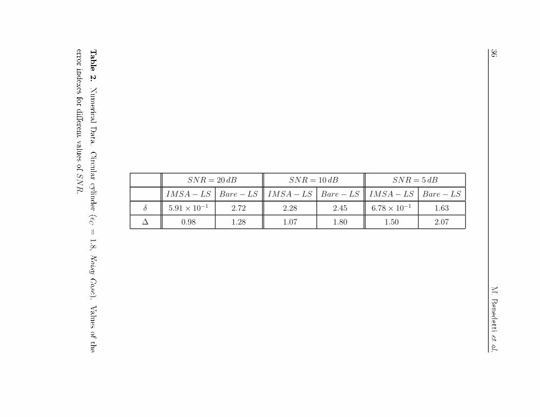
36M.Benedettietal.

SNR = 20 dB SNR = 10 dB SNR = 5 dB

IMSA − LS Bare − LS IMSA − LS Bare − LS IMSA − LS Bare − LS

δ 5.91 × 10−1 2.72 2.28 2.45 6.78 × 10−1 1.63

∆ 0.98 1.28 1.07 1.80 1.50 2.07

Table2.Numeri alData.Cir ular ylinder(ǫC

=1.8,NoisyCase).Valuesofthe

errorindexesfordi�erentvaluesofSN

R.

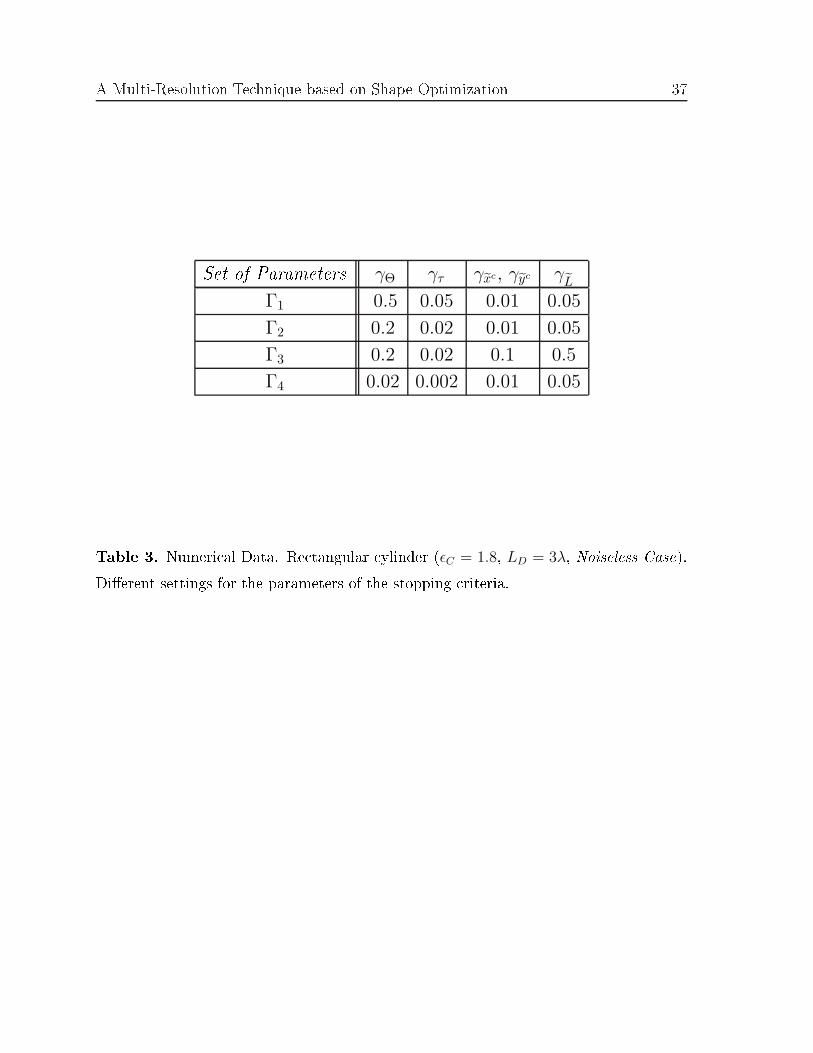
A Multi-Resolution Te hnique based on Shape Optimization 37Set of Parameters γΘ γτ γxc, γyc γ

L

Γ1 0.5 0.05 0.01 0.05

Γ2 0.2 0.02 0.01 0.05

Γ3 0.2 0.02 0.1 0.5

Γ4 0.02 0.002 0.01 0.05

Table 3. Numeri al Data. Re tangular ylinder (ǫC = 1.8, LD = 3λ, Noiseless Case).Di�erent settings for the parameters of the stopping riteria.

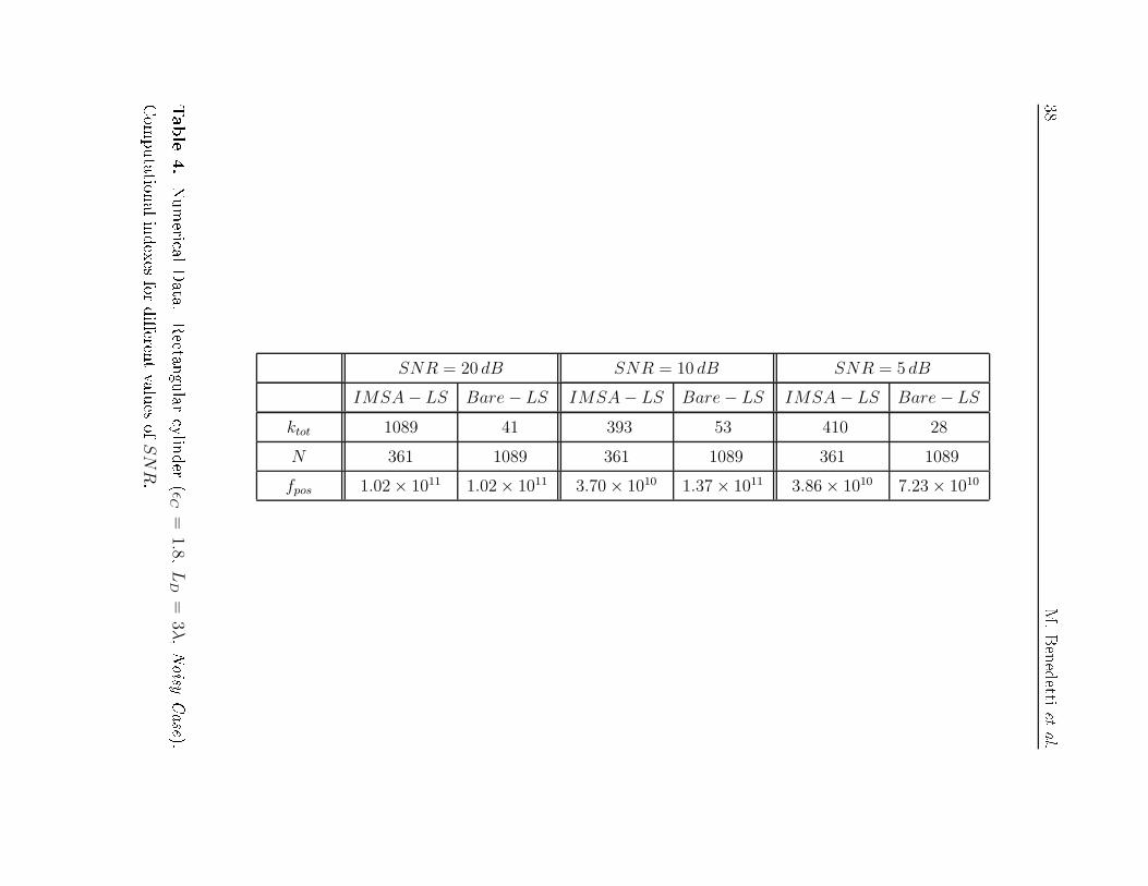
38M.Benedettietal.

SNR = 20 dB SNR = 10 dB SNR = 5 dB

IMSA − LS Bare − LS IMSA − LS Bare − LS IMSA − LS Bare − LS

ktot 1089 41 393 53 410 28

N 361 1089 361 1089 361 1089

fpos 1.02 × 1011 1.02 × 1011 3.70 × 1010 1.37 × 1011 3.86 × 1010 7.23 × 1010

Table4.Numeri alData.Re tangular ylinder(ǫC

=1.8,

LD

=3λ,NoisyCase).

Computationalindexesfordi�erentvaluesofSN

R.

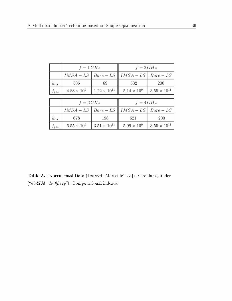
A Multi-Resolution Te hnique based on Shape Optimization 39f = 1 GHz f = 2 GHz

IMSA − LS Bare − LS IMSA − LS Bare − LS

ktot 506 69 532 200

fpos 4.88 × 109 1.22 × 1011 5.14 × 109 3.55 × 1011

f = 3 GHz f = 4 GHz

IMSA − LS Bare − LS IMSA − LS Bare − LS

ktot 678 198 621 200

fpos 6.55 × 109 3.51 × 1011 5.99 × 109 3.55 × 1011

Table 5. Experimental Data (Dataset �Marseille� [34℄). Cir ular ylinder(�dielTM_de 8f.exp�). Computational indexes.