The effect of regularization in motion compensated PET image reconstruction: a realistic

numerical 4D simulation study

This content has been downloaded from IOPscience. Please scroll down to see the full text.

Download details:

IP Address: 211.138.121.35

This content was downloaded on 03/10/2013 at 18:02

Please note that terms and conditions apply.

2013 Phys. Med. Biol. 58 1759

(http://iopscience.iop.org/0031-9155/58/6/1759)

View the table of contents for this issue, or go to the journal homepage for more

Home Search Collections Journals About Contact us My IOPscience

OPEN ACCESSIOP PUBLISHING PHYSICS IN MEDICINE AND BIOLOGY

Phys. Med. Biol. 58 (2013) 1759–1773 doi:10.1088/0031-9155/58/6/1759

The effect of regularization in motion compensatedPET image reconstruction: a realistic numerical 4Dsimulation study

C Tsoumpas, I Polycarpou, K Thielemans, C Buerger, A P King,T Schaeffter and P K Marsden

Department of Biomedical Engineering, Division of Imaging Sciences and BiomedicalEngineering, King’s College London, King’s Health Partners, St. Thomas’ Hospital, London,SE1 7EH, UK

E-mail: Charalampos.Tsoumpas@kcl.ac.uk

Received 16 August 2012, in final form 30 January 2013Published 26 February 2013Online at stacks.iop.org/PMB/58/1759

AbstractFollowing continuous improvement in PET spatial resolution, respiratorymotion correction has become an important task. Two of the most commonapproaches that utilize all detected PET events to motion-correct PET dataare the reconstruct-transform-average method (RTA) and motion-compensatedimage reconstruction (MCIR). In RTA, separate images are reconstructed foreach respiratory frame, subsequently transformed to one reference frame andfinally averaged to produce a motion-corrected image. In MCIR, the projectiondata from all frames are reconstructed by including motion information inthe system matrix so that a motion-corrected image is reconstructed directly.Previous theoretical analyses have explained why MCIR is expected tooutperform RTA. It has been suggested that MCIR creates less noise than RTAbecause the images for each separate respiratory frame will be severely affectedby noise. However, recent investigations have shown that in the unregularizedcase RTA images can have fewer noise artefacts, while MCIR images aremore quantitatively accurate but have the common salt-and-pepper noise. Inthis paper, we perform a realistic numerical 4D simulation study to comparethe advantages gained by including regularization within reconstruction forRTA and MCIR, in particular using the median-root-prior incorporated inthe ordered subsets maximum a posteriori one-step-late algorithm. In thisinvestigation we have demonstrated that MCIR with proper regularizationparameters reconstructs lesions with less bias and root mean square errorand similar CNR and standard deviation to regularized RTA. This findingis reproducible for a variety of noise levels (25, 50, 100 million counts), lesionsizes (8 mm, 14 mm diameter) and iterations. Nevertheless, regularized RTA

Content from this work may be used under the terms of the Creative Commons Attribution-NonCommercial-ShareAlike 3.0 licence. Any further distribution of this work must maintain

attribution to the author(s) and the title of the work, journal citation and DOI.

0031-9155/13/061759+15$33.00 © 2013 Institute of Physics and Engineering in Medicine Printed in the UK & the USA 1759

1760 C Tsoumpas et al

can also be a practical solution for motion compensation as a proper level ofregularization reduces both bias and mean square error.

S Online supplementary data available from stacks.iop.org/PMB/58/1759/mmedia

(Some figures may appear in colour only in the online journal)

1. Introduction

Following continuous improvements in PET spatial resolution, respiratory motion correctionhas become an important task (Schafers 2008). Amongst several approaches to motion-correctPET data (Nehmeh 2013), two are the most common: reconstruct-transform-average (RTA)(Picard and Thompson 1997) and motion-compensated image reconstruction (MCIR) (Qiaoet al 2006, Qi and Huesman 2002). In RTA, separate images are reconstructed for eachrespiratory frame, which are then transformed to one respiratory reference frame and averagedto produce a motion-corrected image. In MCIR, the projection data from all respiratory framesare reconstructed together by including the motion information into the reconstruction systemmatrix, so that a motion-corrected image is produced directly (Rahmim et al 2013). In bothcases it is assumed that an accurate description of the motion is available, for example usingnon-rigid image registrations derived from independently acquired CT, MR images or PETdata itself.

As shown by Thielemans et al (2006) RTA images can have lower regional standarddeviation which may result in higher lesion detectability. However, this has not beencommunicated in recent literature and it has been assumed that RTA has inferior imagequality than MCIR (Lamare et al 2007). Similar conclusions were also drawn by a theoreticalcomparison of RTA versus MCIR using penalized likelihood reconstruction (Asma et al 2006),where it was shown that penalized MCIR would provide lower variance than penalized RTA—at least when there are very few counts per respiratory frame. Another recent theoreticalinvestigation of motion-compensated penalized likelihood reconstruction confirmed that thevariances of MCIR methods are lower than or comparable to the variance of RTA due to thestatistical weighting (Chun and Fessler 2013). However, our recently published investigationdemonstrates that in the unregularized case, MCIR, even though it is quantitatively superiorto RTA, produces images with higher regional standard deviation (Polycarpou et al 2012).The different conclusions may be explained by the definition of variance: regional varianceversus variance over independent realizations can provide different insights on the algorithmperformance. In particular, regional variance corresponds better to visual noise perception thanthe variance of independent realizations (Tong et al 2010).

This study aims to answer how MCIR and RTA perform with regularization and whichof the two approaches has better practical performance with respect to both noise andquantification of lesions in motion-corrected images. The entire analysis in this work is basedon realistic 4D simulated PET data (Tsoumpas and Gaitanis 2013).

2. Theory

Unregularized statistical iterative reconstruction methods estimate an image that is asconsistent as possible with the measured data. However, in PET this problem is ill-conditionedand it generates images with a large amount of noise. As an attempt to improve this ill-conditioned situation regularization approaches have been developed that can significantlyhelp reduce noise in the reconstructed images (Fessler 1994).

Regularization in motion incorporated PET reconstruction 1761

This study makes use of a well-known iterative algorithm with a common regularizationapproach (1): the ordered subsets maximum a posteriori one-step-late, i.e. OSMAPOSL (Green1990a, 1990b) together with the median-root-prior (MRP) (Alenius and Ruotsalainen 1997,2002) which is freely available within the Software for Tomographic Image Reconstruction(STIR)1 library (Thielemans et al 2012). This algorithm has been thoroughly examined byBettinardi et al (2002). In our investigation we extended STIR OSMAPOSL to include motioninformation in order to reconstruct all respiratory gates into one reference frame (MCIR).

RTA-MRP-OSL: equations (1–2) describe the separate reconstruction of each respiratorygate. Equation (3) describes the transformation step that is followed after reconstruction of allgates:

�(s+1)vg = �(s)

vg

1∑b∈Sl

PvbAbg + βg∇�vgE(s)v

∑b∈Sl

PvbYbg∑

v Pbv�(s)vg + Bbg

Abg

(1)

where:2

βg∇�vgE(s)v

de f= βg

�(s)vg − M(s)

v

M(s)v

(2)

�v = 1

G

∑g

∑v′

W −1v′g→v�v′g. (3)

While the corresponding MCIR-MRP-OSL equation (4) is:

�(s+1)v = �(s)

v

1∑b∈Sl ,g

∑v W −1

vg→vPvbAbg + β∇�v

E (s)v

×∑

b∈Sl ,g

∑v

⎛⎝W −1vg→v

PvbYbg∑

v Pbv∑

v Wv→vg�(s)v

+ Bbg

Abg

⎞⎠ . (4)

Notations:

• �(s)v is the estimated radioactivity at voxel v and subiteration s

• Ybg is the number of measured coincident photons of each detector pair (bin) b that belongsto the lth subset S and gate g

• Sl corresponds to the lth subset of the projection space, which is divided into L total subsets• s is the sub-iteration number. A set of L sub-iterations comprises a full iteration• Pbv is the system projection matrix• W, W−1 represent the forward /backward warping operations of the image that move the

activity from one location (e.g. v′) to voxel v using the motion fields and linear interpolation• E is the ‘potential’ function• Mv corresponds to the median 3 × 3 × 3 mask width of neighbourhood voxels centred

at voxel v (Bettinardi et al 2002)• G is the total number of gates• β, βg are the penalization factors for MCIR and RTA, respectively. Note that β = G × βg,

but for simplicity all cases are displayed with respect to βg

• Abg and Bbg are the attenuation coefficient and background (e.g. scatter) term for each binand gate, respectively

1 The STIR library is currently available at: http://stir.sourceforge.net2 In STIR there are two different approaches to applying the MRP: additive or multiplicative. Here, we chose theadditive MRP as originally suggested by Alenius et al (1997).

1762 C Tsoumpas et al

Table 1. Characteristics of the lesions inserted in the computational PET-MR phantom. Note thatthe maximum left-right displacement is larger than the maximum posterior–anterior. This can beexplained when the volunteer is not very well aligned with the direction of the bed.

Maximum MaximumLesion Diameter inferior-superior posterior-anterior Maximum left-rightid (mm) displacement (mm) displacement (mm) displacement (mm) SUV

1 14 16.9 2.7 1.9 9.52 14 13.4 2.7 4.1 7.53 14 3.5 2.4 4.2 7.54 14 15.4 1.8 7.6 6.55 14 13.8 2.9 2.3 4.56 14 8.8 1.4 3.7 4.57 8 11.9 3.5 8.4 6.58 8 12.3 2.1 5.0 4.59 8 3.7 1.2 5.8 4.5

Both RTA-MRP-OSL and MCIR-MRP-OSL made use of the same routines for warpingeach respiratory gate to the reference gate. The motion correction operation was approximatedby warping the image with the ‘inverted’ motion fields that were numerically estimated fromthe motion vectors (Crum et al 2007) which were used to simulate the motion. The operatorW−1 acts to warp all respiratory gates to the reference gate, while the operator W ‘unwarps’ thereference gate to each respiratory gate so that they can be compared with the correspondingprojection gates in the numerator.

3. Experiments and methods

Generation of realistic 4D PET data

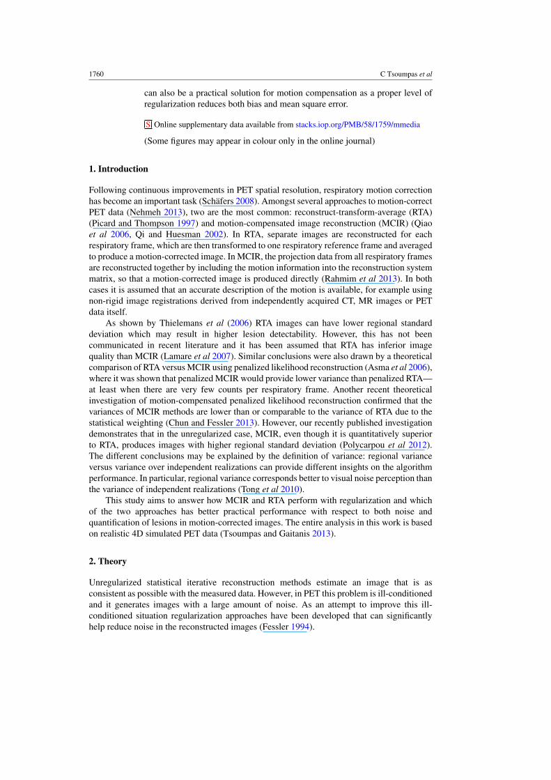
Realistic PET data for the chest were simulated using segmentations of real MR images(Tsoumpas et al 2011). We acquired two different MR sequences from a volunteer to generatethe 4D attenuation and emission maps (Buerger et al 2012). The first acquisition used an ultra-short time-echo (UTE) sequence in order to separate structures such as liver, lung, corticalbone and soft tissues from the background using a semi-automatic segmentation approach withlocal thresholding. These were combined to generate the 3D emission and attenuation maps.The second acquisition was a dynamic MR sequence (35 dynamic frames, 0.7 s duration each)acquired during normal tidal breathing. This acquisition was used to estimate motion fieldswith a non-rigid registration algorithm (Buerger et al 2011) which are essential to simulaterealistic respiratory motion of the 3D emission and attenuation maps. Eight respiratory frameswere selected based on displacement gating of a 1D signal navigator placed at the diaphragmof the dynamic MR.

Realistic attenuation values were assigned to the segmented regions leading to the 3Dattenuation map Av with the following attenuation values: air 0 cm−1, lung tissue 0.03 cm−1,soft tissue 0.099 cm−1, bone 0.15 cm−1. Similarly, realistic emission values were assignedleading to the 3D emission map �v with the following emission values: air 0, lung tissue 0.5,soft tissue 1, bone 2.3, liver 2.5, and myocardium 3.2. Nine soft tissue tumour lesions with theircharacteristics and standardized uptake values (SUV) shown in table 1 were manually insertedat different positions of the 3D computational phantom as shown in figure 1. The attenuationand emission maps (Av,�v) were then combined with the motion fields to compute eightrespiratory-gated maps (Avg, �vg). The reference gate was the one at the mid-respirationposition. The resulting attenuation and emission maps were used to simulate a 4D PET

Regularization in motion incorporated PET reconstruction 1763

Lesion 9

Lesion 3

Lesion 6

Lesion 8

Lesion 5Lesion 2

Lesion 4

Lesion 7

Lesion 1

Figure 1. Location of the nine lesions in the computational phantom.

acquisition with a fast analytic simulation technique (Tsoumpas et al 2011). PET projectiondata accounted for attenuation, scatter (approximately 33%) and resolution effects (Gaussiankernel of 5 mm), but not for randoms. Each of the eight gates was forward-projected simulatinga fully 3D acquisition (maximum ring difference: 43, span: 3) with a range of different totalunscattered photon-pair count measurements for the Philips Gemini PET scanner: 25 × 106,50 × 106, and 100 × 106 Poisson-distributed counts which correspond to approximately 2.5,5 and 10 min of a standard clinical PET acquisition3. Counts are reported as the total numberfor the eight gates with each gate having one eighth of the total counts.

Iterative reconstruction

One of the main questions in iterative reconstruction methods is how many iteration stepsshould be performed to converge? Or at least, how far from convergence can we afford tostop? In particular, for OSEM a higher number of iterations is generally suggested for betterquantification otherwise the value is biased towards the uniform initial image (Barrett et al1994). The noise amplification with increase in iteration number (Wilson et al 1994) canbe handled with some form of regularization, as for example in this paper with the MRPregularization. In particular, this type of regularization can also improve convergence rate(Bettinardi et al 2002). As this study focuses on the regularization term in relationship withmotion compensated reconstruction, one specific question is how the regularization termaffects convergence of MCIR and RTA respectively? Ideally, we should study the results at(numerical) convergence, where the required number of iterations would vary for the differentcases. However, this may require a large number of iterations (Nuyts and Fessler 2003), whichis impractical for such type of investigation, as each 4D equivalent iteration requires about1.5 h (single process on computational platform with two Intel R© Xeon R© L5420 quad coreprocessors running at 2.5 GHz). In order to minimize the computational cost, the main part ofthe investigation compares the figures of merit for a variety of settings fixed at ten iterations(23 subsets). Then, in order to study the impact of iteration number on RTA-MRP-OSL andMCIR-MRP-OSL images, a selected number of reconstructions were performed up to 40iterations. This helps to characterize how the figures of merit are affected at larger number ofiterations and if the main conclusions would have been affected.

Each reconstructed slice consisted of 250 × 250 pixels with size 2 × 2 mm each, and theentire volume consisted of 87 slices with 2 mm thickness. The kernel size for the regularizationwas 3 × 3 × 3 voxels and a range of different weights (0, 0.1, 0.2, 0.5, 1, 2, 5, 10, 20, 50, 100)were selected for the regularization term, also referred to as the penalization weighting factor(βg). These weights were constant and spatially invariant throughout each reconstruction.

Figures of merit

First, we performed a bias versus standard deviation characterization for all lesions, penaltyfactors and three different noise levels. Then, for a selected noise level (50 million counts)

3 The simulated datasets can be obtained following instructions at the webpage: http://www.isd.kcl.ac.uk/pet-mri/simulated-data/

1764 C Tsoumpas et al

we plotted the root mean square error (RMSE) and contrast to noise ratio (CNR) againstthe penalty factor for each lesion. These figures of merit are estimated with the followingequations:

mLi =∑

v∈Li�v∑

v∈Li1

(5)

sLi =√∑

v∈Li(�v − mLi )

2∑v∈Li

1(6)

bLi = midealLi

− mLi (7)

rLi =√

b2Li

+ s2Li

(8)

cLi = mLi − mBi

mBi sBi

(9)

where mL, sL, bL, rL, cL correspond to values of the mean, standard deviation, bias, root meansquare error and contrast to noise ratio of the voxels v of each lesion Li and mB, sB correspondto the mean and standard deviation values of their background respectively, and mL

ideal is themean value of the corresponding lesion in the noiseless PET image. In all cases the backgroundregions were placed in the tissue that surrounds the lesion and selected to have the same sizeand shape with each corresponding lesion. Finally, based on these comparisons we select thebest case of RMSE for MCIR and at matched regional standard deviation levels for RTA weprovide results from twenty independent noise realizations in order to confirm that the regionalcomparisons are representative to make valid conclusions. The following equations (10)–(13)were used to calculate the mean (M), standard deviation (S), bias (B) from the ideal noiselessPET image (�ideal) and root mean square error images (R):

M =√√√√∑20

r=1 �r∑20r=1 1

(10)

S =∑20

r=1 (�r − M)2∑20r=1 1

(11)

B = �ideal − M (12)

R =√

B2 + S2. (13)

Finally, we calculate the average and standard error values for mL, sL, bL, rL, cL overall thetwenty independent noise realizations.

4. Results

In order to show how βg affects the images visually we present in figure 2 coronal planesthrough the three lesions located over the liver dome for 50 × 106 counts (typical for a 5 minFDG scan) and for a selection of βg (i.e. 0, 1, 2, 5, 10, 20, 50, 100) for MCIR-MRP-OSLand RTA-MRP-OSL. Figure 3 shows the visual improvement of images for the simulations of

Regularization in motion incorporated PET reconstruction 1765

Figure 2. Coronal planes through lesions 2, 5, 8 for 50 × 106 counts and different penalizationfactors (βg) after ten iterations of RTA-MRP-OSL and MCIR-MRP-OSL. All images are displayedin SUV scale from 0 to 5.

Figure 3. Coronal planes through lesions 2, 5, 8 for 25 × 106 and 100 × 106 counts reconstructedwithout penalization and with penalization (βg = 50) after 10 iterations of RTA-MRP-OSL andMCIR-MRP-OSL. All images are displayed in SUV scale from 0 to 5.

25 × 106 and 100 × 106 counts for βg = 50 that produces high CNR. To study the effectof regularization in a systematic manner we firstly explore how the weight factor βg affectsregional bias, bL and standard deviation sL values of the nine lesions. This is provided infigure 4 in the form of a graph of bias versus standard deviation as a function of βg for threenoise levels.

The multiple plots in figure 5 (RMSE) and figure 6 (CNR) show the corresponding valuesfor each lesion for the simulation of the 50 × 106 counts as reconstructed with RTA-MRP-OSLand MCIR-MRP-OSL at ten iterations with different βg. For the same number of counts, the

1766 C Tsoumpas et al

Bias versus standard deviation for different noise levels and penalisation factors for RTA and MCIR for each lesion

Figure 4. Bias (b: y-axis) versus regional standard deviation (s: x-axis) for each lesion as computedfrom three different noise realizations (25 × 106 counts: thin lines, 50 × 106 counts: lines withmedium thickness, 100 × 106 counts: thick lines) reconstructed with RTA-MRP-OSL and MCIR-MRP-OSL at 10 iterations with different penalization. The eleven points correspond to βg = 0, 0.1,0.2, 0.5, 1, 2, 5, 10, 20, 50, and 100. Rows correspond to lesion size and columns to lesion organlocation.

Table 2. Indicative mean value of bias (b), standard deviation (s), RMSE (r) and CNR (c) of theSUV over all the nine lesions for one realization.

Units in RTA MCIR RTA MCIR RTA MCIR RTA MCIR RTA MCIRSUV scale βg = 2 βg = 5 βg = 10 βg = 20 βg = 50

Bias (b) 2.35 2.07 2.36 2.12 2.41 2.19 2.50 2.32 2.72 2.59Standard 1.14 1.73 1.03 1.37 0.93 1.14 0.83 0.99 0.71 0.84deviation (s)RMSE (r) 2.62 2.71 2.58 2.53 2.59 2.48 2.64 2.53 2.82 2.74CNR (c) 13.7 11 15.4 13.2 16.8 15.7 18.3 18.3 19.2 20.77

average regional values over all nine lesions for the bias, standard deviation and RMSE of theSUVs are shown in table 2. Inspection of the table values indicates that the RMSE is minimumfor MCIR (β = 10 × 8). The regional standard deviation (s) of this MCIR setting matchesthe one of RTA-MRP-OSL at βg = 2. For these two particular settings we repeated twentyindependent noise realizations and display coronal planes of the M, B, S, and R (figure 7).Figure 8 shows the average values for m, s, r and c over all realizations for each lesion.

Finally, we investigate the impact of iterations in RTA-MRP-OSL and MCIR-MRP-OSLand in particular what is the average bias difference (δb) and the average standard deviationdifference (δs) between iterations 10 and 40, as defined in the equations (14) and (15). Weplot these in figure 9 for three penalty factors (βg = 1, 10, 100) and three count-levels

Regularization in motion incorporated PET reconstruction 1767

RMSE versus penalisation factor for RTA and MCIR for each lesion

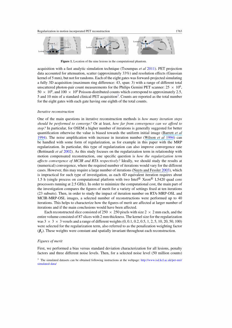
Figure 5. RMSE values (r: y-axis) for each lesion as computed from one realization(50 × 106 counts) reconstructed with RTA-MRP-OSL (thin line) and MCIR-MRP-OSL (thickline) at 10 iterations with different penalization weights (βg: x-axis). Rows correspond to lesionsize and columns to lesion organ location.

(25 × 106, 50 × 106, 100 × 106). Furthermore, in the supplementary data (available athttp://stacks.iop.org/PMB/58/1759/mmedia), we provide additional plots to demonstrate howthe mean ml and standard deviation sl values of each lesion l are changing over iterations (5,. . . , +5, . . . , 40) for the same three penalization factors and noise levels:

δb =9∑

i=1

(b40it.

Li− b10it.

Li

)(14)

δs =9∑

i=1

(s40it.

Li− s10it.

Li

). (15)

5. Discussion

Figures 2 and 3 provide a visual demonstration of the images reconstructed with MCIR-MRP-OSL and RTA-MRP-OSL with different βg and noise levels. It can be noticed that βg

affects MCIR-MRP-OSL and RTA-MRP-OSL differently: A stronger penalty is needed inMCIR-MRP-OSL to obtain images of similar noise level comparing to RTA-MRP-OSL. Atlarger βg e.g. 50 or 100, MCIR-MRP-OSL and RTA-MRP-OSL images become similar. Thisis also confirmed quantitatively by the results in table 2 and figure 4. Figure 3 demonstratessubstantial visual improvement with βg = 50 for both low and high counts. The low countexperiment corresponds to 2–3 min of PET acquisition, which provides a realistic simulationsetup as in current whole body PET/CT scanning protocols.

In figure 4 the quantitative comparison shows that the regional relative bias for the ninelesions is almost unaltered with MCIR-MRP-OSL until β is between 2 × 8 and 10 × 8.This does not appear to be dependent on the lesion location, size or number of simulated

1768 C Tsoumpas et al

CNR versus penalisation factor for RTA and MCIR for each lesion

Figure 6. CNR values (c: y-axis) for each lesion as computed from one realization(50 × 106 counts) reconstructed with RTA-MRP-OSL (thin line) and MCIR-MRP-OSL (thickline) at 10 iterations with different penalization weights (βg: x-axis).

counts. On the other hand, RTA-MRP-OSL always demonstrates considerable improvementwith respect to bias for small βg (e.g. 0.1) with minimum change—even small increase ina few instances—in standard deviation for any type of lesion. The improvement is moreapparent at lower number of counts. For 50 × 106 counts, the RTA bias in the nine lesions is13.7% higher than MCIR, but following regularization it drops to 7.2%. This is an importantfinding as the RTA bias can be substantially improved with regularization possibly becauseit makes the convergence faster, as discussed in a previous section (Bettinardi et al 2002).The remaining bias is probably a result of the image-based transformations (Dikaios andFryer 2011, Polycarpou et al 2012). This bias slightly changes for βg up to 5 for any of thelesions and noise levels. Within this range of βg RTA-MRP-OSL remains less accurate thanMCIR-MRP-OSL. The observed bias/standard deviation trade-off depends on the SUV ofthe background tissue. For example, the lesions 1 and 4 that are located in the liver havevery high standard deviation, which can be explained by their location being near to the edgeof the axial field of view and because the liver has high noise due to its high radioactivity.Further investigation of figure 4 can help understand better the effects of MCIR-MRP-OSL onlesion quantification with different size, SUV and background. In particular lesions 7, 8 and 9have larger bias than the lesions 4, 5, 6 respectively but similar standard deviation. All theselesion pairs (7/4, 8/5, 9/6) have the same SUV and background but different size. Anotherexpected observation is that the larger the SUV is, the larger are the standard deviation andthe bias, which occurs in lesions 1, 2, 3 and 4. Still, while the trend of improvement is thesame for both RTA-MRP-OSL and MCIR-MRP-OSL, the standard deviation of the latter issignificantly reduced without any practical increase in bias. In summary, figure 4 shows thatMCIR-MRP-OSL can provide better quantitative information as long as the penalization factor

Regularization in motion incorporated PET reconstruction 1769

Figure 7. Coronal planes of two selected cases of βg for RTA-MRP-OSL and MCIR-MRP-OSLof the mean (M), bias (B), standard deviation (S) and root mean square error images (R) that havebeen derived from twenty multiple realizations (50 × 106 counts). The images are displayed inSUV scale from: 0 to 4 for the mean, standard deviation and RMSE; and –2 to 2 for the bias withvalues greater than 2 corresponding to white, lower than –2 to black and 0 to grey.

is chosen properly. It also demonstrates that the results are reproducible for different noiselevels and the optimum penalization factor is within similar range. For example with respectto RMSE, as shown in table 2, the optimal β for MCIR is 10 × 8 while for RTA βg is 5–10.

Figure 5 shows how the regional RMSE values change with penalty. Without penalty,RTA-MRP-OSL comparing to MCIR-MRP-OSL has worse RMSE only in lesion 9. Thevalues of RMSE are minimized for RTA-MRP-OSL with βg between 5 and 20 while forMCIR-MRP-OSL with βg 10 for all lesions apart from the lesion 8. On the other hand, figure 6shows that the CNR is maximized at βg = 20–50 for both methods and all lesions apartfrom the first. Figure 6 demonstrates also that the CNR with small and large βg is similar forboth MCIR-MRP-OSL and RTA-MRP-OSL. However, if we compare the CNR for matchedstandard deviation (figure 8), MCIR-MRP-OSL is better than RTA-MRP-OSL in all lesionsapart from lesion 8, where both methods perform equally well.

Figure 7 shows the corresponding mean (M), bias (B), standard deviation (S) and RMSE(R) images for the two methods with βg at matched regional standard deviation (s). All theimages are visually similar but following the quantitative comparison in figure 8 MCIR-MRP-OSL appears to outperform RTA-MRP-OSL. Bias with RTA-MRP-OSL is probablydue to low counts, interpolation errors, regularization, reconstruction inaccuracies (e.g. noresolution modelling) and errors in the numerical inversion of the motion fields. Similarly, inMCIR-MRP-OSL any bias is due to errors in the numerical inversion of the motion fields,

1770 C Tsoumpas et al

Mean (m), standard deviation (s), RSME (r) and CNR (c) for each lesion over twenty independent noise realisations (50 106

counts) for RTA and MCIR

Figure 8. Average values that have been derived from twenty independent noise realizations foreach lesion (id: 1–9) for different figures of merits: mean (m), standard deviation (s), root meansquare error (r) and contrast to noise ratio (c). The error bars indicate the standard error estimatedfrom twenty realizations. Two selected cases of βg for RTA-MRP-OSL (βg = 2) and MCIR-MRP-OSL (β = 10 × 8) are compared. On the left of each pair of bars is the RTA value and on the rightis the MCIR value. The m, s and r are in SUV scale, while c is in inverse SUV scale.

regularization and reconstruction inaccuracies. However, an additional advantage of MCIR-MRP-OSL is that the regularization level can be fine-tuned according to the properties beingoptimized while with RTA-MRP-OSL bias is reduced but only up to a certain extent.

Table 2 demonstrates that the selection of β = 10 × 8 is on average the best for MCIR-MRP-OSL with respect to bias, standard deviation and RMSE over all the lesions. In particular,the comparison with βg = 2 (matched standard deviation with MCIR-MRP-OSL, β = 10 × 8)shows that MCIR-MRP-OSL is on average: 7.0%, 5.5% and 13.8% better in terms of bias,RMSE and CNR than RTA-MRP-OSL. Furthermore, the quantitative statistical comparisonderived from twenty independent noise realizations in figure 8 at matched noise, i.e. regionalstandard deviation s, demonstrates clearly that MCIR-MRP-OSL is better than RTA-MRP-OSL with respect to RMSE and CNR for all lesions (apart from lesion 8 for CNR) independentof their size and background. Also, all mean values are higher for MCIR-MRP-OSL indicatingthat recovery of the SUV is more accurate. Finally, the standard deviation values of the lesionslocated in the liver are lower for MCIR-MRP-OSL while for all the other lesions they arehigher.

Finally, figure 9 demonstrates the impact of regularization effects on bias and standarddeviation when iterating longer. Comparing 40 to 10 MCIR-MRP-OSL iterations, the standarddeviation is affected only for βg = 1 (i.e. 0.3 – 0.5 in SUV), but it is almost insensitive forβg = 10 and βg = 100. This result is observable in all noise levels. Bias shows only minorreduction for all instances. These results support that iterating longer for MCIR-MRP-OSL is

Regularization in motion incorporated PET reconstruction 1771

Figure 9. δb and δs for three penalization factors (100, 10, 1: with higher penalty corresponding tosmaller δs) and three noise levels (25 × 106, 50 × 106, 100 × 106 counts) for RTA and MCIR.This graph displays the differences between iterations 40 and 10.

not necessary, as noise increases with minimum decrease in bias especially for βg � 10. In thesupplementary material (available at http://stacks.iop.org/PMB/58/1759/mmedia), the resultsshow how the mean and the standard deviation are modified with iterations. On the otherhand, in RTA-MRP-OSL (βg <10) the results clearly have not converged. Thus, iterating 40iterations will reduce bias (0.15 – 0.25 in SUV) with small increase in the standard deviation(less 0.1–0.2 in SUV) but then only minor improvement in the RMSE (less than 3% reductionfor βg = 1). Therefore, at relatively late iterations (e.g. 40), the findings of this investigationwould mainly show similar performance for both MCIR-MRP-OSL and RTA-MRP-OSL withrespect to bias, standard deviation, root mean square error and contrast to noise ratio for βg

� 10. For βg = 1, the metrics are affected for both RTA-MRP-OSL and MCIR-MRP-OSLbut differently: RTA-MRP-OSL would have slightly better RMSE while MCIR-MRP-OSLwould become worse. In the case of small βg values, the results have not stabilized even after40 iterations. Even if ideally the comparison should have been performed at convergence,iterating for many hours is not practical.

The novel finding demonstrated in this paper is that regularization improves the imagesin terms of bias mainly for RTA-MRP-OSL and in terms of noise when reconstructed withboth MCIR-MRP-OSL and RTA-MRP-OSL. This was not obvious, as it was expected thatimages reconstructed with MCIR have less noise than those reconstructed with RTA. Thelatter is more biased but less noisy with the most likely explanations for these being the post-reconstruction transformations (Dikaios and Fryer 2011) and the ill-behaved convergenceoccurring due to the highly noisy data within each gate, which enhances the low statisticsbias and non-negativity constraints (Polycarpou et al 2012). This problem is expected to belarger in the case of less measured counts per respiratory position (Dawood et al 2009) but itmay improve when we incorporate resolution modelling (Walker et al 2011) and time of flightinformation (Westerwoudt et al 2012) in the reconstruction. The usefulness of regularization islikely to be similar for any reconstruction algorithm at low count rates. Another way to achievesimilar bias-variance performance with regularization is to smooth the images with a filter

1772 C Tsoumpas et al

after their reconstruction. This is expected to be a good alternative approach to ‘regularize’MCIR especially when quantification is not the main issue.

As a side observation, this study highlights that regularization in both MCIR-MRP-OSLand RTA-MRP-OSL can help balance bias and noise thus improve mean square error andcontrast to noise ratio. On the one hand proper modifications of the iterative reconstructionmethods may be useful to successfully deal with the low statistics bias (Byrne 1998). On theother hand further investigation on the type of regularization can be useful to minimize noisebut also maintain good resolution in small lesions. One recent example is the incorporationof non-conventional priors such as patches (Wang and Qi 2012). Further consideration ofregularization may help achieve isotropic uniform resolution in areas moving with differentmagnitudes (Chun and Fessler 2012). This approach might also be useful as a means toaccount for the effects of inaccuracies in the estimation of motion, which are expected to occurin clinical data.

6. Conclusion

In this investigation we have demonstrated that MCIR has higher regional standard deviationand RMSE than RTA unless proper regularization parameters are included within thereconstruction. As we have shown, MCIR-MRP-OSL with proper regularization outperformsRTA-MRP-OSL both in terms of bias and RMSE for the optimal penalization factors.Nevertheless, regularized RTA can also be a practical solution for motion compensation as aproper level of regularization improves both bias and mean square error.

Acknowledgments

We are thankful to Dr M Jacobson, Dr A Solomon, Dr V Schulz and Dr M Walker fordiscussions and Mr A Cantell and Mr D Poccecai (King’s College London) for invaluableIT support. This work is part of the HYPERImage and SUBLIMA projects supported bythe European Union under the seventh framework program (no: 201651, 241711). Dr KThielemans has received financial support from General Electric Research. The authorsacknowledge additional financial support from: (1) the Department of Health via the NationalInstitute for Health Research (NIHR) comprehensive Biomedical Research Centre award toGuy’s & St Thomas’ NHS Foundation Trust in partnership with King’s College Londonand King’s College Hospital NHS Foundation Trust; and (2) the Centre of Excellence inMedical Engineering funded by the Wellcome Trust and EPSRC under grant number WT088641/Z/09/Z. The views expressed are those of the authors and not necessarily those ofthe NHS, the NIHR or the Department of Health.

References

Alenius S and Ruotsalainen U 1997 Bayesian image reconstruction for emission tomography based on median rootprior Eur. J. Nucl. Med. 24 258–65

Alenius S and Ruotsalainen U 2002 Generalization of median root prior reconstruction IEEE Trans. Med.Imaging 21 1413–20

Asma E, Manjeshwar R and Thielemans K 2006 Theoretical comparison of motion correction techniques for PETimage reconstruction IEEE Nuclear Science Symp. Conf. Record pp 1762–7

Barrett H H, Wilson D W and Tsui B M W 1994 Noise properties of the EM algorithm: I. Theory Phys. Med.Biol. 39 833–46

Bettinardi V, Pagani E, Gilardi M, Alenius S, Thielemans K, Teras M and Fazio F 2002 Implementation and evaluationof a 3D one-step late reconstruction algorithm for 3D positron emission tomography brain studies using medianroot prior Eur. J. Nucl. Med. 29 7–18

Regularization in motion incorporated PET reconstruction 1773

Buerger C, Schaeffter T and King A P 2011 Hierarchical adaptive local affine registration for fast and robust respiratorymotion estimation Med. Image Anal. 15 551–64

Buerger C, Tsoumpas C, Aitken A, King A P, Schleyer P, Schulz V, Marsden P K and Schaeffter T 2012Investigation of MR-based attenuation correction and motion compensation for hybrid PET/MR IEEE Trans.Nucl. Sci. 59 1967–76

Byrne C 1998 Iterative algorithms for deblurring and deconvolution with constraints Inverse Problems 14 1455–67Chun S Y and Fessler J A 2013 Noise properties of motion-compensated tomographic image reconstruction methods

IEEE Trans. Med. Imaging 32 141–52Chun S Y and Fessler J A 2012 Spatial resolution properties of motion-compensated tomographic image

reconstruction methods IEEE Trans. Med. Imaging 31 1413–25Crum W, Camara O and Hawkes D 2007 Methods for inverting dense displacement fields: evaluation in brain image

registration Medical Image Computing and Computer-Assisted Intervention (MICCAI) ed N Ayache et al (Berlin:Springer) pp 900–7

Dawood M, Buther F, Stegger L, Jiang X, Schober O, Schafers M and Schafers K P 2009 Optimal number ofrespiratory gates in positron emission tomography: a cardiac patient study Med. Phys. 36 1775–84

Dikaios N and Fryer T D 2011 Improved motion-compensated image reconstruction for PET using sensitivitycorrection per respiratory gate and an approximate tube-of-response backprojector Med. Phys. 38 4958–70

Fessler J A 1994 Penalized weighted least-squares image reconstruction for positron emission tomography IEEETrans. Med. Imaging 13 290–300

Green P J 1990a Bayesian reconstructions from emission tomography data using a modified EM algorithm IEEETrans. Med. Imaging 9 84–93

Green P J 1990b On use of the EM algorithm for penalized likelihood estimation R. Stat. Soc. 52 443–52Lamare F, Carbayo M J L, Cresson T, Kontaxakis G, Santos A, Le Rest C C, Reader A J and Visvikis D 2007

List-mode-based reconstruction for respiratory motion correction in PET using non-rigid body transformationsPhys. Med. Biol. 52 5187–204

Nehmeh S A 2013 Respiratory motion correction strategies in thoracic PET-CT PET Clinics 8 29–36Nuyts J and Fessler J A 2003 A penalized-likelihood image reconstruction method for emission tomography, compared

to postsmoothed maximum-likelihood with matched spatial resolution IEEE Trans. Med. Imaging 22 1042–52Picard Y and Thompson C J 1997 Motion correction of PET images using multiple acquisition frames IEEE Trans.

Med. Imaging 16 137–44Polycarpou I, Tsoumpas C and Marsden P K 2012 Analysis and comparison of two methods for motion correction in

PET imaging Med. Phys. 39 6474–83Qi J and Huesman R H 2002 List mode reconstruction for PET with motion compensation: a simulation study IEEE

Int. Symp. on Biomedical Imaging: From Nano To Macro pp 413–6Qiao F, Pan T, Clark J W and Mawlawi O R 2006 A motion-incorporated reconstruction method for gated PET studies

Phys. Med. Biol. 51 3769–83Rahmim A, Tang J and Zaidi H 2013 Four-dimensional image reconstruction strategies in cardiac-gated and

respiratory-gated PET imaging PET Clinics 8 51–67Schafers K P 2008 The promise of nuclear medicine technology: Status and future perspective of high-resolution

whole-body PET Phys. Medica 24 57–62Tong S, Alessio A M and Kinahan P E 2010 Noise and signal properties in PSF-based fully 3D PET image

reconstruction: an experimental evaluation Phys. Med. Biol. 55 1453Thielemans K, Manjeshwar R M, Xiaodong T and Asma E 2006 Lesion detectability in motion compensated image

reconstruction of respiratory gated PET/CT IEEE Nuclear Science Symp. and Medical Imaging Conf. pp3278–82

Thielemans K, Tsoumpas C, Mustafovic S, Beisel T, Aguiar P, Dikaios N and Jacobson M W 2012 STIR: softwarefor tomographic image reconstruction release 2 Phys. Med. Biol. 57 867

Tsoumpas C and Gaitanis A 2013 Modeling and simulation of 4D PET-CT and PET-MR images PET Clinics 8 95–110Tsoumpas C et al 2011 Fast generation of 4D PET-MR data from real dynamic MR acquisitions Phys. Med.

Biol. 56 6597–613Walker M D, Asselin M C, Julyan P J, Feldmann M, Talbot P S, Jones T and Matthews J C 2011 Bias in iterative

reconstruction of low-statistics PET data: Benefits of a resolution model Phys. Med. Biol. 56 931–49Wang G and Qi J 2012 Penalized likelihood PET image reconstruction using patch-based edge-preserving

regularization IEEE Trans. Med. Imaging 31 2194–204Westerwoudt V, Conti M and Eriksson L 2012 Comparison of TOF and non-TOF iterative reconstruction at low

statistics IEEE Nuclear Science Symp and Medical Imaging Conf. (M08-6) (Anaheim, California, USA)Wilson D W, Tsui B M W and Barrett H H 1994 Noise properties of the EM algorithm. II. monte carlo simulations

Phys. Med. Biol. 39 847–71