94 IEEE TRANSACTIONS ON IMAGE PROCESSING, VOL. 17, NO. 1, JANUARY 2008

Correspondence

Image Reconstruction and Multidimensional FieldEstimation From Randomly Scattered Sensors

Pan Pan, Student Member, IEEE, andDan Schonfeld, Senior Member, IEEE

Abstract—Many important problems in statistical signal processing canbe formulated as function estimation from randomly scattered sensors ina multidimensional space, e.g., image reconstruction from photon-limitedimages and field estimation from scattered sensors. We present a novelapproach to the study of signal reconstruction from random samples ina multidimensional space. In particular, we study a classical iterative re-construction method and demonstrate that it forms a sequence of unbi-ased estimates for band-limited signals, which converge to the true func-tion in the mean-square sense. We subsequently rely on the iterative es-timation method for multidimensional image reconstruction and field es-timation from sensors scattered according to a multidimensional Poissonand uniform distribution. Computer simulation experiments are used todemonstrate the efficiency of the iterative estimation method in image re-construction and field estimation from randomly scattered sensors.

Index Terms—Field estimation, image reconstruction, random sampling,sensor networks.

I. INTRODUCTION

Aclassical problem in image processing is the task of image re-construction from limited samples. Such images are acquired in

applications that rely on a limited number of sensors, e.g., photon-lim-ited images [1] and emission tomography [2]. This problem has beenmodeled as function estimation from irregular samples. Several itera-tive reconstruction schemes have been proposed for function estimationfrom irregular samples [3]–[5].

Image analysis from limited sensors is a specific problem within thebroad discipline of sensor networks. Tremendous interest in sensor net-works has been gained over the past decade. One of the key problemsin this area is the task of field estimation from scattered sensors. For ex-ample, using temperature sensors scattered over a geographic region,we would like to estimate the temperature at any location in the vicinity.Similar problems have arisen in battlefield surveillance, environmentalmonitoring, biological detection, industrial diagnostics, etc. [6]. Theseapplications require a number of sensors scattered over a contiguousregion to collect critical information such as temperature, pressure, hu-midity, etc. Clearly, the monitored area should be well covered by asufficient number of sensors. This is known as the coverage problem insensor networks [7]. However, the number of sensors available is lim-ited, and, thus, one must rely on discrete sensors for field estimation ofa mutlidimensional continuous space.

Sensor field estimation is an important problem in sensor networks.Most existing methods in the sensor networks community have reliedon function interpolation techniques. For example, it is common touse a mixture of Gaussian interpolation, where a Gaussian function

Manuscript received May 4, 2007; revised October 20, 2007. The associateeditor coordinating the review of this manuscript and approving it for publica-tion was Prof. Stanley J. Reeves.

The authors are with the Multimedia Communications Laboratory, Depart-ment of Electrical and Computer Engineering, University of Illinois at Chicago,Chicago, IL 60607-7053 USA (e-mail: ppan3@uic.edu; dans@uic.edutfuzz).

Digital Object Identifier 10.1109/TIP.2007.912579

is placed at the sensor locations whose amplitude and variance is pro-portional to the sensed data value. A more sophisticated approach tousing Gaussian mixtures has been provided by the use of the expec-tation-maximization algorithm to determine the maximum-likelihoodestimate of the location, amplitude and variance [8].

We formulate the field estimation problem as signal reconstructionfrom scattered sensors. This approach is an extension of the problemof image reconstruction from limited samples. The solution to theseproblems is based on classical methods for function estimation fromirregular samples. The methods used for signal reconstruction from ir-regular samples have been investigated over the past couple of decades[3]–[5], [9]–[12].

A unified format of the classical iterative reconstruction methodsfrom missing samples is fk+1 = fk + A(f � fk) [11], where f isthe original band-limited signal, fk is the reconstruction signal at thekth iteration, and A denotes a composition of distortion and constraintoperators. For instance, the well-known Papoulis–Gerchberg extrap-olation algorithm [3], [4] is an example of this iterative reconstruc-tion which has been used extensively for estimation of missing data inband-limited signals. Sauer and Allebach [5] presented several impor-tant algorithms that form variations of the classical iterative reconstruc-tion scheme for estimation of band-limited images. Early and Long [1]proved that the ART algorithm [2] is functionally equivalent to the it-erative reconstruction algorithm and used it for remote sensing imagereconstruction and resolution enhancement.

The important issue of convergence of the iterative reconstructionhas also discussed. Youla and Webb [9] and Sauer and Allebach [5]used the concept of projection onto convex sets (POCS) and showedthat the iterative reconstruction method converges weakly to a finalstate which adheres to certain desired properties. Marvasti et al. [10]and Gröhenig [11] proved L2 convergence of the iterative reconstruc-tion to the true function. A detailed study of the upper and lower errorbounds, optimum relaxation constant and rate of convergence has beenpresented by Ferreira [12].

Some limited analysis of the statistical properties of random sam-pling has also been developed. However, much of the statistical anal-ysis of random sampling schemes has been limited thus far to a 1-Dprocesses. For example, Papoulis [13] proved that Poisson samples ofa 1-D function form an unbiased estimate of the function in the spec-trum domain. Marvasti used power spectral analysis to explore themean-square convergence of uniform and Poisson sampling of a 1-Dfunction in [14].

In this paper, we propose a novel approach to the study of signalreconstruction from random samples in a mutlidimensional space. Wewill investigate the statistical properties of random sampling using mut-lidimensional constant-mean point processes in Section II. We will sub-sequently show that a special case of the classical iterative reconstruc-tion scheme forms a sequence of unbiased estimates of band-limitedsignals, which converges to the true function in the mean-square sensein Section III. In Section IV, we rely on the iterative estimation methodfor mutlidimensional image reconstruction and field estimation fromrandomly scattered sensors. Finally, in Section V, we present a briefsummary and discussion of our results.

II. MULTIDIMENSIONAL RANDOM SAMPLING

First of all, we establish notation which we follow for the remainderof the paper. An n-dimensional signal f(x) is sampled by a sampling

1057-7149/$25.00 © 2007 IEEE

IEEE TRANSACTIONS ON IMAGE PROCESSING, VOL. 17, NO. 1, JANUARY 2008 95

process z(x) = m

i=1�(x� xi), where x = [x1; x2; . . . ; xn] 2 R

n;xi are the samples; m is the number of samples. F (u) is the Fouriertransform of f(x), whereu = [u1; u2; . . . ; un] 2 R

n.S is a samplingoperator defined as

Sf(x) =f(xi); x = xi; i = 1;2; . . . ;m

0; else

and P is a band-limited operator given by

PF =F (u); u 2

0; else.

This paper is carried out in the view that xi are random samples.Therefore, the sampling function z(x) is also random. The expectationof the sampling function, E[z(x)], is used to denote the spatial densityof the random points. We will now assume that the spatial density of therandom points is constant and show that sampling using constant-meanpoint processes yields an unbiased estimate.

Proposition 1: If E[z(x)] = c, then (1=c)Sf(x) is an unbiasedestimate of f(x), where c is a constant.

Proof: We observe that Sf(x) can be written as

Sf(x) =

m

i=1

f(xi)�(x� xi) =

m

i=1

f(x)�(x� xi)

= f(x)

m

i=1

�(x� xi) = f(x)z(x): (1)

The expectation of z(x) is constant, i.e.,E[z(x)] = c. Therefore, from(1), we observe that

E1

cSf(x) =

1

cf(x)E [z(x)] = f(x) (2)

which shows that (1=c)Sf(x) is an unbiased estimate of f(x).Proposition 1 can also be expressed in the spectrum domain as

follows.Corollary 1: If E[z(x)] = c, then G(u) =

(1=c) m

i=1f(xi)e

�ju x is an unbiased estimate of F (u), where cis a constant.

Proof: G(u) = (1=c) m

i=1f(xi)e

�ju x =

(1=c)R

f(x)e�ju x m

i=1�(x � xi)dx=

R(1=c)Sf(x)e�ju xdx.

From (2), E[G(u)] =R

f(x)e�ju xdx = F (u).When the samples are uniformly distributed or distributed according

to a homogenous Poisson process with infinite number of samples, wecan find the value of c in terms of the spatial density of the randomsamples. Therefore, a special case of Proposition 1 is given as follows.

Corollary 2: If the samples fxig are identically and independently(i.i.d.) uniformly distributed or distributed according to a homogeneousPoisson process with infinite number of samples, (1=�)Sf(x) is anunbiased estimate of f(x), where � is the spatial density of the sam-ples for the uniform distribution and the rate parameter for the Poissonprocess. Moreover, if jf(x)j < 1, then (1=�)Sf(x) ! f(x) as� ! 1.

Proof: Franks [15] proved the expression for E[z(x)] andRz(t; s) for infinite 1-D pulse train fxig, which are uniformly dis-tributed and distributed according to a homogeneous Poisson process.

After we extend the results of Franks to n-dimensional case, weobtain the following: when finite or infinite samples fxig are i.i.d.uniformly distributed with spatial density �, or when infinite samplesfxig, i.e., m = 1, are distributed according to a homogeneousPoisson process with rate parameter �

E [z(x)] = �: (3)

A derivation of (3) is presented in the Appendix. From (3), we obtainc = �. As shown in (14) in the Appendix,� implies the average number

of Poisson points per unit volume of space. Therefore, the rate param-eter of homogeneous Poisson process also describes the spatial densityof the samples.

In Proposition 1, the accuracy of the unbiased estimate is charac-terized by the variance of (1=c)Sf(x). Notice that as � approachesinfinity, we have an infinite number of samples for both cases, and aswe have shown in the Appendix, we have

Rz[t; s] = ��(t� s) + �2: (4)

We now observe that

var1

cSf(x) =E

1

cSf(x)

2

� E1

cSf(x)

2

=1

�2f2(x)Rz(x;x)� f2(x)

=1

�f2(x)�(0): (5)

Since jf(x)j < 1, we observe that jf2(x)j < 1 and (5) im-plies that the variance of the unbiased estimate reduces to zero as �approaches infinity. Therefore, (1=�)Sf(x)! f(x) as �!1.

Corollary 2 can be also stated in the spectrum domain. Papoulis [13]gave a 1-D case of Corollary 2 expressed in the spectrum domain whenfxig are distributed according to a 1-D homogeneous Poisson process.

Equation (3) reveals the reason that we usually use random uniformdeployment and random Poisson deployment as models for sensor de-ployment in the sensor coverage problem.

III. ITERATIVE RECONSTRUCTION

In this section, we use Proposition 1 to study the classical iterativereconstruction scheme presented in Section I. We show that a specialcase of the classical iterative reconstruction scheme forms a sequenceof unbiased estimates of band-limited signals, which converges to thetrue function in the mean-square sense. We begin with one definitionand one proposition.

Definition 1: [16] A contraction mapping, or contraction, on ametric space (M; d) is a function f from M to itself, with the propertythat there is some real number 0 � r < 1 such that

d (f(x); f(y)) � rd(x;y); for all x; y 2M:

In a normed space with norm k � k, if an operator A : M ! Mis a contraction, then kAx � Ayk � rkx � yk. If A is linear andcontraction, then kAxk � rkxk. If the above condition is satisfied for0 � r � 1, then the mapping is said to be nonexpansive.

Proposition 2: In a normed space, if the operator A(�) is a contrac-tion, then the operator T (�) = A(�) + h is also a contraction.

Proof: Since the operator A is a contraction, kAx � Ayk �rkx; yk, where 0 � r < 1. Therefore, kTx � Tyk = kAx + h �Ay � hk = kAx � Ayk� rkx � yk. This indicates the operatorT (�) = A(�) + h is also a contraction.

We now establish that the iterative reconstruction forms a sequenceof unbiased estimates, which converges to the true function in themean-square sense.

Proposition 3: If E[z(x)] is a constant c, an n-dimensional band-limited signal f(x) can be reconstructed from its scattered samples it-eratively by fk+1(x) = P [fk(x)+ S(f(x)�fk(x))], given f0(x) =(1=c)Sf(x) and jvar(f0(x))j < 1. This iteration procedure gener-ates a sequence of unbiased estimates which converge in the mean-square sense for 0 < < 2.

Proof: We prove that in each iteration the estimation is unbi-ased by induction. Given f0(x) = (1=c)Sf(x), Proposition 1 tellsus E[f0(x)] = f(x), which is the unbiased estimate when k = 0.

96 IEEE TRANSACTIONS ON IMAGE PROCESSING, VOL. 17, NO. 1, JANUARY 2008

By assuming E[fk(x)] = f(x), we obtain

E [fk+1(x)] =E [Pfk(x) + PS (f(x)� fk(x))]

=PE [fk(x)] + PE [Sf(x)]

� PE [Sfk(x)] (6)

= f(x): (7)

We can view (6) in two ways: If the sampling in each iteration main-tains the same samples as in f0, the randomness of the iteration is onlyattributed to the random sampling of f0. Therefore, we can change theorder of expectation and sampling operator S

PE [fk(x)] + PE [Sf(x)]� PE [Sfk(x)]

= Pf(x) + PSE [f(x)]� PSE [fk(x)]

= f(x) + PSf(x)� PSf(x) = f(x): (8)

The other possibility is that the sampling in each iteration is random,i.e., each iteration will determine a new collection of random samples.We note that the new sampling in the (k+1)th iteration is uncorrelatedwith the reconstruction result of the kth iteration, i.e., fk(x). Therefore,by using Proposition 1, we have

PE [fk(x)] + PE [Sf(x)]� PE [Sfk(x)]

= Pf(x) + P cf(x)� PcE [fk(x)]

= f(x) + Pcf(x)� Pcf(x) = f(x): (9)

This induction of (7) proves that each iteration of the reconstructionmethod generates an unbiased estimate given f0(x) = (1=c)Sf(x),where c = E[z(x)].

Then, we prove that the variance of the unbiased estimation decaysto zero. We define a new operator T , where T (�) = PSf(x) + [P � PS](�). Therefore, fk+1(x) = Tfk(x). Marvasti et al. proved thatthe operatorP� PS is a contraction when 0 < < 2 for 1-D signalsin Sections II and III-A in [10]. Similar results about the iteration of theoperator P � PS have been presented by Sauer and Allebach in [5].One can easily check that the contraction of operator P � PS can beextended to mutlidimensional, e.g., the 2-D case in [17]. According toProposition 2, the operator T is also a contraction when 0 < < 2,i.e., kTfk(x)k � rkfk(x)k, where 0 � r < 1, 0 < < 2. Therefore

var (fk+1(x))� rvar (fk(x))

= E kfk+1(x)k2 � f2(x)� rE kfk(x)k

2 + rf2(x)

< E kfk+1(x)k2 � rE kfk(x)k

2

= E kTfk(x)k2 � r kfk(x)k

2

� E kTfk(x)k2 � r2 kfk(x)k

2 � 0:

Therefore, var(fk+1(x)) < rvar(fk(x)) < . . . < rk+1var(f0(x)),which implies that if jvar(f0(x))j < 1, the variance of iterationreaches zero as k reaches infinity. We note that a sequence of unbiasedestimates whose variance decays to zero implies convergence in themean-square sense [18]. Therefore, we observe that fk(x) convergesto f(x) in the mean-square sense, when 0 < < 2.

In general, Proposition 3 can be applied to any sampling structureprovided that z(x) is a constant-mean point process and the initialconditions are satisfied. However, when the samples are uniformly dis-tributed or distributed according to a homogeneous Poisson processwith infinite number of samples, we observe that E[z(x)] = �, whichis the spatial density of the samples. This observation allows us to esti-mate the density � from the observation data and recover the signalfrom its samples without prior knowledge of the mean E[z(x)] asshown in Corollary 2. The method used to estimate � from the obser-vation data is presented in Section IV.

Fig. 1. Image Pepper. (a) Original image; (b) sampled image (Poisson sam-pling with � = 0:278); (c) reconstructed image at the fifth iteration.

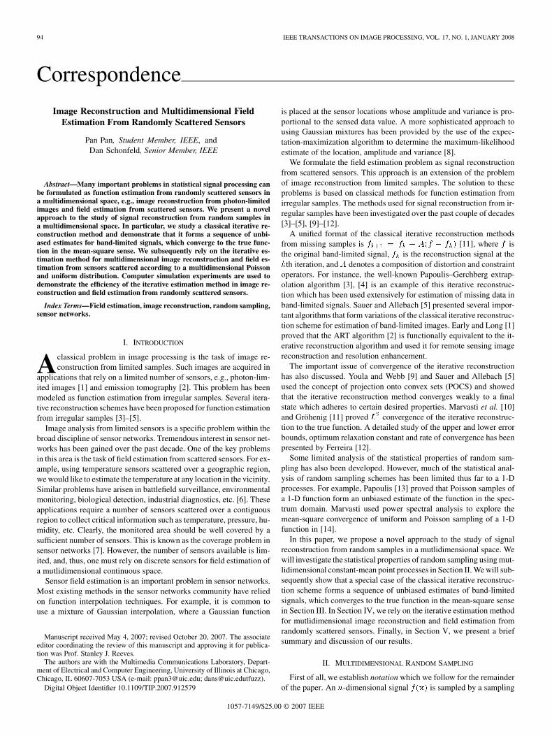
Fig. 2. Image House. (a) Original image; (b) sampled image (uniform sam-pling with � = 0:5); (c) reconstructed image at the ninth iteration.

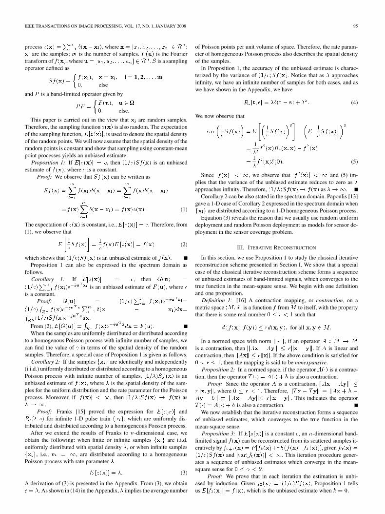
Fig. 3. Altitude over an area. (a) True altitude; (b) sensed data (Poisson sam-pling with � = 0:278); (c) reconstructed signal at the eighth iteration.

Corollary 3: Iffxig are i.i.d. uniformly distributed or distributed ac-cording to a homogeneous Poisson process with infinite number of sam-ples, ann-dimensional band-limited signalf(x) can be reconstructed it-eratively byfk+1(x) = P [fk(x)+ S(f(x)�fk(x))], givenf0(x) =(1=�)Sf(x) and f(x) < 1, where � is the spatial density of the sam-ples for the uniform distribution and the rate parameter for the Poissonprocess. This iteration procedure generates a sequence of unbiased es-timates which converge in the mean-square sense for 0 < < 2.

Proof: Similar to the proof of Proposition 3, by using Proposition2 we can easily show that each iteration is an unbiased estimate whosevariance converges to zero as k approaches infinity.

IV. IMAGE RECONSTRUCTION AND FIELD ESTIMATION

We, therefore, apply the iterative reconstruction algorithm presentedin Section III to the application of image reconstruction and sensor fieldestimation over [1; 256] [1; 256]. We generate Poisson points by the“dart-throwing” algorithm in [19].

As discussed in Section II, for both uniform sampling and Poissonsampling, � describes the spatial density of samples, which is equal tothe average number of samples per unit volume of space. Therefore, �can be obtained by the sensed data as follows.

1) Get many different volumes within the space, B1; B2; . . . ;Bk 2 Rn.

2) Get their density �k by calculating the average points per unitvolume.

3) The � of these points is estimated by � = (1=k) k

i=1�i.

Figs. 1 and 2 and Figs. 3 and 4 show the simulation results of imagereconstruction and field estimation from sensors scattered according

IEEE TRANSACTIONS ON IMAGE PROCESSING, VOL. 17, NO. 1, JANUARY 2008 97

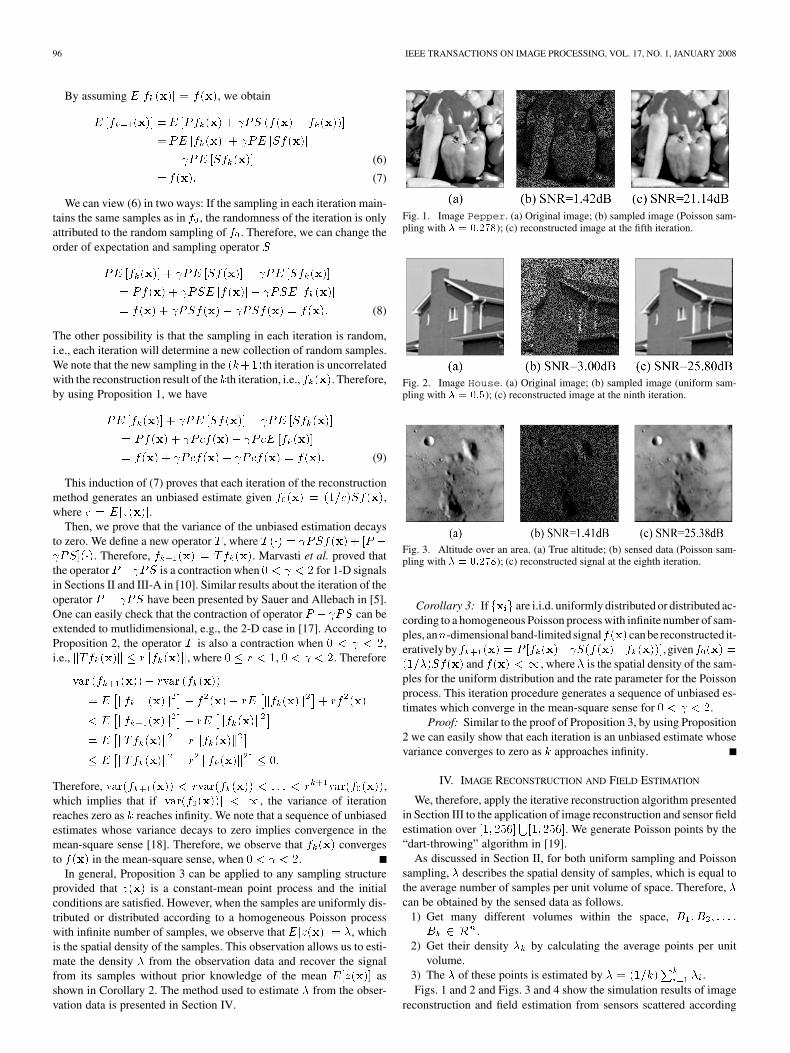
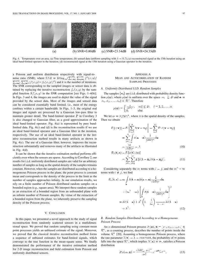
Fig. 4. Temperature over an area. (a) True temperature; (b) sensed data (uniform sampling with � = 0:5); (c) reconstructed signal at the 15th iteration using anideal band-limited operator in the iteration; (d) reconstructed signal at the 15th iteration using a Gaussian operator in the iteration.

a Poisson and uniform distribution respectively with signal-to-noise ratio (SNR), where SNR = 10 log10(

256x=1

256y=1 f

2(x; y)=256x=1

256y=1(f(x; y)�fk(x; y))

2) and k is the number of iterations.The SNR corresponding to the sampled images or sensor data is ob-tained by replacing the iterative reconstruction fk(x; y) by the sam-pled function Sf(x; y) in the SNR computation [see Figs. 1–4(b)].In Figs. 3 and 4, the images are used to depict the value of the signalprovided by the sensor data. Most of the images and sensed datacan be considered essentially band limited, i.e., most of the energyconfines within a certain bandwidth. In Figs. 1–3, the original realimages and signals are processed by a Gaussian low-pass filter tomaintain greater detail. The band-limited operator P in Corollary 3is also changed to Gaussian filter, as a good approximation of theideal band-limited operator. Fig. 4(a) is represented by pure band-limited data. Fig. 4(c) and (d) is the reconstruction results if we usean ideal band-limited operator and a Gaussian filter in the iteration,respectively. The use of an ideal band-limited operator in the iter-ative reconstruction method results in many artifacts as shown inFig. 4(c). The use of a Gaussian filter, however, improves the recon-struction substantially and removes many of the artifacts as illustratedin Fig. 4(d).

It can be shown that the iterative estimation method performs effi-ciently even when the sensors are sparse. According to Corollary 2, ourresults for i.i.d. uniformly distributed samples are valid for an arbitrarynumber of samples as long as the spatial density of the samples remainsconstant. However, when the samples are distributed according to a ho-mogeneous Poisson process in the plane, the point process is constantmean and corresponds to the density of the process in the limit as thenumber of samples approaches infinity. In our simulation results, werely on a finite number of Poisson distributed random samples on abounded region (e.g., square area). We interpret these random samplesas an extraction of a bounded region from an unbounded plane withan infinite number of Poisson samples. By virtue of the extraction ofa bounded region from the plane, we inherently preserve the samplingdensity of the Poisson process.

V. CONCLUSION

In this paper, we presented a novel approach to the study of signalreconstruction from randomly scattered sensors in a mutlidimen-sional space. We proved that random sampling using constant-meanpoint processes yields an unbiased estimate of the signal. Moreover,we proved that the classical iterative reconstruction method formsa sequence of unbiased estimates for band-limited signals, whichconverge to the true function in the mean-square sense. We finallydemonstrated the performance of the iterative estimation methodfor 2-D image reconstruction and field estimation from Poisson anduniformly distributed sensors.

APPENDIX AMEAN AND AUTOCORRELATION OF RANDOM

SAMPLING PROCESSES

A. Uniformly Distributed I.I.D. Random Samples

The samples fxig are i.i.d. distributed with probability density func-tion p(���), where p(���) is uniform over the space j�lj � D and ��� =[�1; �2; . . . ; �n] 2 Rn. Therefore

p(���) =1

(2D); j�lj � D; l = 1; 2; . . . ; n

0; else.

We let m = �(2D)n, where � is the spatial density of the samples.Then we obtain

E [z(x)] =E

m

i=1

�(x� xi) =

m

i=1

E [�(x � xi)]

=

m

i=1���

�(x� ���)1

(2D)nd���

=m

(2D)n= � (10)

Rz(t; s) =E [z(t)z(s)]

=

m

i=1

m

j=1

E [�(t� xi)�(s� xj)] : (11)

Considering separately the m terms with i = j, and the m2 � mterms with i 6= j, we find

Rz(t; s) =m

���

�(t� ���)�(s� ���)1

(2D)nd���

+ (m2 �m)

���

�(t� ���)1

(2D)nd���

2

=��(t� s) + �2 1�1

m����!m!1

��(t� s)

+ �2: (12)

B. Random Samples Distributed According to a HomogeneousPoisson Process

An n-dimensional Poisson process N(x), x = [x1; x2; . . . ; xn] 2Rn, as a counting process, describes the number of points inside thevolume Rn [20]. Assuming a homogeneous Poisson process, wherethe rate parameter �(x) = � = constant, the probability of m pointsfalls into the space Rn, which implies N(x) = m, satisfies a Poissondistribution

PN(m;x) =(��n

l=1xl)m

m!e��� x : (13)

98 IEEE TRANSACTIONS ON IMAGE PROCESSING, VOL. 17, NO. 1, JANUARY 2008

The expectation of the Poisson process is

E [N(x)] =

1

m=0

mPN (m;x)

=

1

m=0

m(��n

l=1xl)m

m!e��� x

=

1

m=0

(��nl=1xl)

m�1

(m� 1)!(��n

l=1xl) e��� x

=��nl=1xl : (14)

From (14), we can see � implies the average number of Poisson pointsper unit volume of space.

The samples fxig are distributed according to a Poisson process withrate parameter �. To evaluate the mean and autocorrelation of z(x), weneed the probability density function of the random variable xi as wellas the joint probability density for pairs of points xi and xj.

The probability density function of xi is related to the probabilitythat the ith point occurs in a small space at the arbitrary point x [15];i.e., for a small positive space dx

px (x)dx =Pr [N(x) = i� 1]Pr [N(dx) = 1]

=PN (i� 1;x)�dx: (15)

Thus, we have

px (x) = �PN (i� 1;x); xl � 0; l = 1; 2; . . . ; n: (16)

Similarly, assuming i > j

px x (t; s)dtds = Pr [N(s) = j � 1]Pr [N(ds) = 1]

�Pr [N(t)�N(s) = i� j � 1]Pr [N(dt) = 1] : (17)

Therefore, we have

px x (t; s) = �2PN (j � 1; s)PN(i� j � 1; t� s)

i > j; tl > sl � 0; l = 1; 2; . . . ; n: (18)

Now we obtain

E [z(x)] =

m

i=1

E [�(x� xi)]

=

m

i=1���

�(x� ���)�PN (i� 1; ���)d���

=�

m

i=1

PN (i� 1;x)

=�

m

i=1

(��nl=1xl)

i�1

(i� 1)!e��� x

����!m!1

�: (19)

Again, considering separately the terms for which i = j, i > j, andi < j, and from (11), we observe that

Rz(t; s) =

m

i=1

E [�(t� ti)�(s� ti)]

+

m

j=1

m

i=j+1

E [�(t� ti)�(s� tj)]

+

m

i=1

m

j=i+1

E [�(t� ti)�(s� tj)] : (20)

Note that

m

i=1

E [�(t� ti)�(s� ti)]

=

m

i=1���

�(t� ���)�(s� ���)�PN (i� 1; ���)d�������!m!1

��(t� s):

(21)

We also observe that

m

j=1

m

i=j+1

E [�(t� ti)�(s� tj)]

=

m

j=1

m

i=j+1��� ���

�(t� ���)�(s� ���)

� �2PN (j � 1; ���)PN (i� j � 1; ���� ���)d���d���

����!m!1

�2; �l > �l � 0; l = 1; 2; . . . ; n: (22)

Similarly, we have

m

i=1

m

j=i+1

E [�(t� ti)�(s� tj)]����!m!1

�2

�l > �l � 0; l = 1; 2; . . . ; n: (23)

Therefore, from (20)–(23), we obtain

Rz(t; s) = ��(t� s) + �2: (24)

This completes the proof.

ACKNOWLEDGMENT

The authors would like to thank the anonymous reviewers for theirhelpful suggestions, which greatly improved the quality of this paper,as well as J. Yang and N. Bouaynaya for their comments.

REFERENCES

[1] D. S. Early and D. G. Long, “Image reconstruction and enhanced res-olution imaging from irregular samples,” IEEE Trans. Geosci. RemoteSens., vol. 39, no. 2, pp. 291–302, Apr. 2001.

[2] A. C. Kak and M. Slaney, Principles of Computerized TomographicImaging. Philadelphia, PA: SIAM, 2001.

[3] R. W. Gerchberg, “Super resolution through error energy reduction,”Opt. Acta, vol. 21, no. 9, pp. 709–721, 1974.

[4] A. Papoulis, “A new algorithm in spectral analysis and band-limitedextrapolation,” IEEE Trans. Circuits Syst., vol. CAS-22, no. 9, pp.735–742, Sep. 1975.

[5] K. D. Sauer and J. P. Allebach, “Iterative reconstruction of bandlim-ited images from nonuniformly spaced samples,” IEEE Trans. CircuitsSyst., vol. 34, no. 12, pp. 1497–1506, Dec. 1987.

[6] I. Akyildiz, W. Su, Y. Sankarasubramaniam, and E. Cayirci, “Wire-less sensor networks: A survey,” Comput. Netw. J., vol. 38, no. 4, pp.393–422, 2002.

[7] M. Cardei and J. Wu, Coverage in Wireless Sensor Networks, ser.Handbook of Sensor Networks, M. Ilyas and I. Magboub, Eds. BocaRaton, FL: CRC, 2004, ch. 19.

[8] H. Hong and D. Schonfeld, “Maximum-entropy expectationmaximiza-tion algorithm for image processing and sensor networks,” in Proc.SPIE Electronic Imaging: Science and Technology Conf. Visual Com-munications and Image Processing, 2007, vol. 6508, no. 1, p. 65080D.

[9] D. Youla and H. Webb, “Image restoration by the method of convexprojections: Part I–Theory,” IEEE Trans. Med. Imag., vol. MI-1, no. 2,pp. 81–94, Feb. 1982.

IEEE TRANSACTIONS ON IMAGE PROCESSING, VOL. 17, NO. 1, JANUARY 2008 99

[10] F. Marvasti, M. Analoui, and M. Gamshadzahi, “Recovery of signalsfrom nonuniform samples using iterative methods,” IEEE Trans. SignalProcess., vol. 39, no. 4, pp. 872–878, Apr. 1991.

[11] K. Gröhenig, “Reconstruction algorithms in irregular sampling,” Math.Comput., vol. 59, no. 199, pp. 181–194, 1992.

[12] P. J. S. G. Ferreira, “Interpolation and the discrete Papoulis–Gerch-berg algorithm,” IEEE Trans. Signal Process., vol. 42, no. 10, pp.2596–2606, Oct. 1994.

[13] A. Papoulis, Probability, Random Variables, and Stochastic Processes,4th ed. New York: McGraw-Hill, 2002.

[14] F. Marvasti, “Spectral analysis of random sampling and error free re-covery by an iterative method,” Trans. Inst. Electron. Commun. Eng.Jpn. E, vol. E69-E, no. 2, pp. 79–82, 1986.

[15] L. Franks, Signal Theory. Englewood Cliffs, NJ: Prentice-Hall, 1969.[16] R. P. Agarwal, M. Meehan, and D. O’Regan, Fixed Point Theory and

Applications. New York: Cambridge Univ. Press, 2001.[17] F. A. Marvasti, C. Liu, and G. Adams, “Analysis and recovery of mul-

tidimensional signals from irregular samples using nonlinear and iter-ative techniques,” Signal Process., vol. 36, no. 1, pp. 13–30, 1994.

[18] J. M. Mendel, Lessons in Digital Estimation Theory. EnglewoodCliffs, NJ: Prentice-Hall, 1987.

[19] D. P. Mitchell, “Generating antialiased images at low sampling den-sities,” ACM SIGGRAPH Comput. Graph., vol. 21, no. 4, pp. 65–72,1987.

[20] D. L. Snyder and M. I. Miller, Random Point Processes in Time andSpace. New York: Springer-Verlag, 1991.