Scattering of Electromagnetic Waves from Two-Dimensional Randomly Rough Penetrable Surfaces

Waves in Random and Complex MediaVol. 18, No. 2, May 2008, 255–274

Scattering of electromagnetic waves from two-dimensional perfectlyconducting random rough surfaces – study with the curvilinear coordinate

method

Karim Aıt Brahama, Richard Dusseauxa∗ and Gerad Granetb

aUniversite de Versailles Saint-Quentin en Yvelines, Centre d’ etude des Environnements Terrestre etPlanetaires (CETP), Velizy, France; bUniversite Clermont-Ferrand II, Laboratoire des Sciences et

Materiaux pour l’electronique et d’Automatique (LASMEA), Aubiere, France

(Received 2 February 2007; final version received 12 October 2007)

We present a method giving the bi-static scattering coefficient of two-dimensional (2-D)perfectly conducting random rough surface illuminated by a plane wave. The theory isbased on Maxwell’s equations written in a nonorthogonal coordinate system. This methodleads to an eigenvalue system. The scattered field is expanded as a linear combinationof eigensolutions satisfying the outgoing wave condition. The boundary conditions al-low the scattering amplitudes to be determined. The Monte Carlo technique is appliedand the bi-static scattering coefficient is estimated by averaging the scattering amplitudesover several realizations. The random surface is represented by a Gaussian stochastic pro-cess. Results are compared to published numerical and experimental data. Comparisons areconclusive.

1. Introduction

The problem of electromagnetic wave scattering from random surfaces continues to attract re-search interest because of its wide broad applications in optics, radio wave propagation and remotesensing. The analysis of rough surfaces with parameters close to the incident light wavelengthrequires a rigorous vectorial formalism. Numerous methods based on Monte Carlo simulationsare available for the study of electromagnetic wave scattering from one-dimensional (1-D) andtwo-dimensional (2-D) random rough surfaces [1–4].

In previous papers, we have shown that the curvilinear coordinate method is an efficientand versatile theoretical tool for analysing 1-D rough surfaces [5–7]. The C method is based onMaxwell’s equations written in a nonorthogonal coordinate system fitted to the structure geometry[5–10].

In the present paper, for the first time, the curvilinear coordinate method is applied foranalysing 2-D perfectly conducting random rough surfaces. The scattering problem is presentedin Section 2 and the C method is described in Section 3. Section 4 deals with the random scatteringproblem. The numerical procedure for the generation of a random surface is reported. The randomsurface is represented by a Gaussian stochastic process with a Gaussian roughness spectrum. TheMonte Carlo technique is applied for estimating the averaged bi-static scattering coefficient and

∗Corresponding author. Email: [email protected]

ISSN: 1745-5030 print / 1745-5049 onlineC© 2008 Taylor & Francis

DOI: 10.1080/17455030701749328http://www.informaworld.com

256 K. Aıt Braham et al.

the incoherent intensity from the results over different realizations.The main aim of this paperis to present the principle of the C method applied to 2-D perfectly conducting random roughsurfaces and to check our results by comparison with published numerical and experimental data(Section 5).

2. The field scattered from a rough surface

We consider a rough surface described by equation z = a(x, y), where a(x, y) is a local functiondefined over the surface area L × L. The structure is illuminated by a monochromatic plane wavewith wavelength λ. The incident wave vector �ki is defined by the zenith angle θi and the azimuthangle ϕi

�ki = αi �ux + βi �uy − γi �uz (1)

with

αi = k sin θi cos ϕi ; βi = k sin θi sin ϕi ; γi = k cos θi (2)

and

k = 2π

λ(3)

Both fundamental cases of horizontal and vertical polarizations are considered. For horizontal(or E//) polarization, the electric field vector is parallel to the Oxy plane and for vertical (or H//)polarization, this is the case for the magnetic field vector (4). The time-dependence factor variesas exp(jωt), where ω is the angular frequency. Hereafter, any vector function is represented by itsassociated complex vector function and the time factor is suppressed. Z is the intrinsic impedanceof free space and the symbol ∧ designates the vector product.

�E(h)i (x, y, z)

Z �H (v)i (x, y, z)

}= �Vi exp(−j �ki�r) and Z �Hi =

�ki

k∧ �Ei (4)

with�Vi = − sin ϕi �ux + cos ϕi �uy (5)

and

�r = x �ux + y �uy + z �uz (6)

�ux, �uy and �uz are the unit vectors of the Cartesian coordinate system (x, y, z).Without any deformation, the total field is the sum of the incident field ( �Ei ; �Hi) and the

specularly reflected field ( �Esr ; �Hsr ) with

�E(h)sr (x, y, z)

Z �H (v)sr (x, y, z)

}= ρ �Vi exp(−j �ksr�r) and Z �Hsr =

�ksr

k∧ �Esr (7)

Waves in Random and Complex Media 257

and

�ksr = αi �ux + βi �uy + γi �uz (8)

ρ is the Fresnel reflection coefficient with ρ = −1 and ρ = 1. For a locally deformedplane, we consider, in addition to the incident and reflected plane waves, a scattered field�E(a)

d (x, y, z). The problem consists in working out the h-polarized component and the v-polarizedcomponent:

�E(a)d (x, y, z) = �E(aa)

d (x, y, z) + �E(ba)d (x, y, z)

Z �H (a)d (x, y, z) = Z �H (aa)

d (x, y, z) + Z �H (ba)d (x, y, z)

(9)

Hereafter, the upper script (a) denotes the incident plane wave polarization and (b), the scatteredwave polarization.

Outside the modulated zone, the scattered field �E(a)d (x, y, z) can be represented by a superpo-

sition of a continuous spectrum of outgoing plane waves [11, 12], the so-called Rayleigh integral.Above the highest point of the surface, the h-polarized component of scattered field is defined asfollows

For z > max(a(x, y)), ∀x, y,

�E(ha)d (x, y, z) = 1

4π2

∫ +∞

−∞

∫ +∞

−∞R(ha)(α, β) �V (α, β) exp(−j �kd (α, β)�r) dα dβ (10)

Z �H (ha)d (x, y, z) = 1

4π2

∫ +∞

−∞

∫ +∞

−∞R(ha)(α, β)

( �kd (α, β)

k∧ �V (α, β)

)

× exp(−j �kd (α, β)�r) dα dβ (11)

with

�kd (α, β) = α�ux + β �uy + γ �uz; Im(γ ) ≤ 0 (12)

and

�V (α, β) = − β√α2 + β2

�ux + α√α2 + β2

�uy (13)

When α2 + β2 > k2, γ (α, β) is a pure imaginary and the corresponding waves are evanescentwaves. Otherwise, γ is real and the propagation vector �kd of the propagating wave is defined bythe zenith angle θ and the azimuth angle ϕ.

α = k sin θ cos ϕ

β = k sin θ sin ϕ

γ (α, β) =√

k2 − α2 − β2 = k cos θ

(14)


In the far-field zone, the Rayleigh expansion (10–11) is reduced to the only contribution of thepropagating waves. The method of stationary phase leads to the asymptotic field [13, 14] at thepoint M(r, θ, ϕ):

�E(ha)dfar(r, θ, ϕ) = −R(ha)(k sin θ cos ϕ ; k sin θ sin ϕ)

cos θexp(−jkr)

λrexp

(−j

π

2

)�uϕ (15)

Z �H (ha)dfar (r, θ, ϕ) = R(ha)(k sin θ cos ϕ ; k sin θ sin ϕ)

cos θexp(−jkr)

λrexp

(−j

π

2

)�uθ (16)

Substituting �E(ha) by Z �H (va) and Z �H (ha) by − �E(va) in Equations (10), (11), (15) and (16) weobtain the v-polarized components of magnetic and electric field vectors. For an incident wavein (a) polarization and a scattered wave in (b) polarization, the normalized bistatic scatteringcoefficient σ (ba) (θ, ϕ) is defined as follows

σ (ba)(θ, ϕ) = 1

P(a)i

dP(ba)s

d�=

∣∣R(ba)(k sin θ cos ϕ ; k sin θ sin ϕ) cos θ∣∣2

λ2L2 cos θi

(17)

dP(ba)s

d�is the power scattered per unit solid angle d� = sin θ dθ dϕ with

dP(ba)s = 1

2Re

[(�E(ba)

dfar ∧ �H (ba)∗df ar

)dS �ur

](18)

The symbol * designates the complex conjugate. dS is the element surface with dS = r2d�. The

unit vectors �ur , �uθ and �uϕ are drawn in the direction of increasing r , θ and ϕ such as to constitute

a right-hand base system. P(a)i is the flux of incident power through the modulated region:

P(a)i = 1

2

∫ +L/2

−L/2

∫ +L/2

−L/2Re

[(�E(a)

i ∧ �H (a)∗i

)dxdy �uz

](19)

The normalised bi-static scattering coefficients fulfil the power balance criterion (20) [6, 14, 15].

P (a)s = P

(a)si (20)

with

P (a)s =

∫ θ=+π/2

θ=−π/2

∫ ϕ=π

ϕ=0(σ (aa)(θ, ϕ) + σ (ba)(θ, ϕ)) dθdϕ (21)

P(a)si = −2ρ(a)

L2Re

(R(aa)(k sin θi cos ϕi ; k sin θi sin ϕi)

)(22)


P(a)s is the ratio between the total scattered power and the incident power in the polarization (a).

P(a)si represents the electromagnetic coupling between the incident, reflected and scattered waves

divided by the incident power [14]. In subsection 5.2, the method is numerically investigated inthe far-field zone by means of convergence on the power balance criterion.

3. Analysis with the curvilinear coordinate method

3.1. Coordinate system – covariant components of field

The scattered field cannot be expressed by the Rayleigh integral in the modulated zone if theperturbation amplitude is too large [11]. We can obtain an expression of fields that is valid overthe surface by solving Maxwell’s equations in the translation coordinate system. This system isobtained from the Cartesian system (x, y, z) [8, 10]

x ′ = x

y ′ = y

z′ = z − a(x, y)(23)

In this new coordinate system, the height function z = a(x, y) coincides with the coordinatesurface z′ = 0 [8] and the change from Cartesian components (Kx ; Ky ; Kz) of vector �K tocovariant components (Kx ′ ; Ky ′ ; Kz′) is given by [8, 10, 16]

Kx ′ (x ′; y ′; z′) = Kx(x; y; z) + ∂a(x, y)

∂xKz(x; y; z)

Ky ′ (x ′; y ′; z′) = Ky(x; y; z) + ∂a(x, y)

∂yKz(x; y; z)

Kz′ (x ′; y ′; z′) = Kz(x; y; z)

(24)

The covariant component Kz′ is simply the vertical component Kz. Moreover, the covariantcomponents Kx ′ and Ky ′ are parallel to surface coordinate z′ = z0 and in particular, parallel tointerface z′ = 0.

In a source-free medium, it can be shown from the time harmonic Maxwell equations and theconstitutive relations expressed in the translation system that the longitudinal components Ez′

and ZHz′ obey to the same propagation Equation (25) [10]

− ∂

∂z′

[gx ′z′ ∂ ψ

∂x ′ + ∂ gx ′z′ψ

∂x ′

]− ∂

∂z′

[gy ′z′ ∂ ψ

∂y ′ + ∂ gy ′z′ψ

∂y ′

]+ jkgz′z′ ∂ψ ′

∂z′

= ∂2ψ

∂x ′2 + ∂2ψ

∂y ′2 + k2ψ (25)

with

ψ ′ = j

k

∂ψ

∂z′ (26)


and ψ(x ′, y ′, z′) = Ez′(x ′, y ′, z′) or ZHz′ (x ′, y ′, z′). gx ′z′, gy ′z′

and gz′z′are elements of metric

tensor which depend on the derivatives of function a(x ′, y ′) with respect to x ′ and y ′ [10]

gx ′z′ = − ∂a

∂x ′

gy ′z′ = − ∂a

∂y ′

gz′z′ = 1 +(

∂a

∂x ′

)2

+(

∂a

∂y ′

)2

(27)

We obtain expressions of components E′x , E′

y , H ′x and H ′

y in terms of longitudinal componentsEz′ and ZHz′ only [10]

∂2Ex ′

∂z′2 + k2Ex ′ = ∂2Ez′

∂x ′∂z′ − k2gx ′z′Ez′ − jkgy ′z′ ∂ZHz′

∂z′ − jk∂ZHz′

∂y ′ (28)

∂2Ey ′

∂z′2 + k2Ey ′ = ∂2Ez′

∂y ′∂z′ − k2gy ′z′Ez′ + jkgx ′z′ ∂ZHz′

∂z′ + jk∂ZHz′

∂x ′ (29)

∂2ZHx ′

∂z′2 + k2ZHx ′ = ∂2ZHz′

∂x ′∂z′ − k2gx ′z′ZHz′ + jkgy ′z′ ∂Ez′

∂z′ + jk∂Ez′

∂y ′ (30)

∂2ZHy ′

∂z′2 + k2ZHy ′ = ∂2ZHz′

∂y ′∂z′ − k2gy ′z′ZHz′ − jkgx ′z′ ∂Ez′

∂z′ − jk∂Ez′

∂x ′ (31)

The covariant components Ex ′ and Ey ′ are parallel to the perfectly conducting inter-face. Consequently, we have Ex ′ = Ey ′ = 0 at z′ = 0 (i.e. z = a(x, y)). In the next subsec-tion, we propose a procedure for solving the propagation Equation (25)-(26) in the spec-tral domain [7]. The Oz-components are expanded as a linear combination of eigensolu-tions satisfying the outgoing wave condition. We deduce from Equations (28) to (31) theh-polarised components of electric and magnetic fields �E(ha)

d and �H (ha)d by taking Ez′ = 0 and

the v-polarized components �E(va)d and �H (va)

d by taking Hz′ = 0. Finally, both h-polarized andv-polarized amplitudes of eigensolutions are found by solving the boundary conditions.

3.2. Eigenvalues system and elementary wave functions

After a Fourier transform (TF) with respect to x ′ and y ′, Equations (25) and (26) take the followingform

∂

∂z′[jα( gx ′z′ ∗ ψ) + j gx ′z′ ∗ (α ψ) + jβ( gy ′z′ ∗ ψ) + j gy ′z′ ∗ (β ψ)

]

+ jk gz′z′ ∗ ∂ψ ′

∂z′ = γ 2ψ (32)

j

k

∂ψ

∂z′ = ψ ′ (33)


K ∗ L is the convolution product of two Fourier Transforms K(α, β, z′) and L(α, β). In a secondstage, convolution products are approximated as follows

(K ∗ L) (α, β, z′) = 1

4π2

∫ +∞

−∞

∫ +∞

−∞K(α′, β ′, z′) L(α − α′, β − β ′) dα′ dβ ′

≈ �α2

4π2

∑p

∑q

K(αp, βq, z′) L(α − αp, β − βq) (34)

where

αp = k sin θi cos ϕi + p�α, βq = k sin θi sin ϕi + q�α (35)

�α is the spectral resolution. As �α decreases, approximations (34) become more accurate.Finally, from substituting Equation (34) into Equations (32) to (33) and applying the pointmatching method at discrete values (αs ; βt ), we obtain two sets of coupled first-order differentialequations relating coefficients ψ(αs, βt , z

′) and ψ ′(αs, βt , z′) to each other.

j

k

∂

∂z′

(∑p,q

(αs

kgx ′z′

s−p,t−q + gx ′z′s−p,t−q

αp

k+ βt

kg

y ′z′s−p,t−q + g

y ′z′s−p,t−q

βq

k

)ψ(αp, βq, z

′)

)

+ j

k

∂

∂z′

(∑p,q

gz′z′s−p,t−q ψ ′(αp, βq, z

′)

)= γ 2

st

k2ψ(αs, βt , z

′) (36)

j

k

∂ψ(αs, βt , z′)

∂z′ = ψ ′(αs, βt , z′) (37)

with

gx ′z′p,q = �α2

4π2gx ′z′

(αp, βq) (38)

gy ′z′p,q = �α2

4π2gy ′z′

(αp, βq) (39)

gz′z′p,q = δpq +

∑u,v

gx ′z′p−u,q−vg

x ′z′u,v +

∑u,v

gy ′z′p−u,q−vg

y ′z′u,v (40)

where δpq denotes the Kronecker symbol. Equations (36) and (37) can be written in matrix form

j

kLl

∂

∂z′

( �ψ�ψ ′

)= Lr

( �ψ�ψ ′

)(41)

Ll and Lr are square matrices specified by the left-hand side and the right-hand side of (36) and(37). With a Mth-order truncated approximation, the matrices Ll and Lr are 2Ms-dimensional


ones with Ms = (2M + 1)2. The upper vector �ψ and the lower vector �ψ ′ have componentsψ(αs, βt , z

′) and ψ ′(αs, βt , z′) with −M ≤ s, t ≤ +M . The elementary solutions of (41) are

defined as follows

( �ψmn

�ψ ′mn

)=

( �φmn

�φ′mn

)exp (−jkrmn z′) (42)

with

rmnLl

( �φmn

�φ′mn

)= Lr

( �φmn

�φ′mn

)(43)

�φmn and �φ′mn represent the upper eigenvector and the lower eigenvector associated with the

eigenvalue rmn. We write φmn(αs,βt ) and φ′mn(αs,βt ) the components of vectors �φmn and �φ′

mn,respectively. The eigenvalue problem (43) gives 2Ms eigensolutions. According to the samplingtheorem [7, 17, 18], the elementary wave functions ψmn(α, β, z′) and ψ ′

mn(α, β, z′) can be con-structed from samples φmn(αs,βt ) and φ′

mn(αs,βt ) by the following interpolations

ψ ′mn(α, β, z′) = exp(−jkrmnz

′)

×+M∑

s=−M

+M∑t=−M

φ′mn(αs,βt )sinc

(π

�α(α − αs)

)sinc

(π

�α(β − βt )

)(44)

ψ ′mn(α, β, z′) = exp(−jkrmnz

′)

×+M∑

s=−M

+M∑t=−M

φ′mn(αs,βt )sinc

(π

�α(α − αs)

)sinc

(π

�α(β − βt )

)(45)

Function ψmn(α, β, z′) represents an outgoing wave propagating with no attenuation ifRe(rmn) > 0 and Im(rmn) = 0. For an evanescent wave, Im(rmn) < 0. It is observed numericallythat among the 2Ms eigenfunctions (44), Ms of them correspond to outgoing waves ((m, n) ∈ Ds)and as many to incoming waves. The numerically computed eigenvalues and eigenvectors dependon the truncation order M . Depending on whether M is a sufficiently large number, we note nu-merically that the real eigenvalues rmn are on the interval [−1;+1] and correspond to the cosineof scattering angles with rmn = cos θmn [8]. We can write

r2mn = γ 2(αm, βn)

k2= 1 −

(αm

k

)2

−(

βn

k

)2

= cos2(θmn) (46)

Finally, the Fourier transform of Oz-component is defined as a linear combination of Ms

eigensolutions (44) satisfying the outgoing wave condition.

ψd (α, β, z′) =∑

(m,n)∈Ds

Amnψmn(α, β, z′) (47)

ψ ′d (α, β, z′) =

∑(m,n)∈Ds

Amnψ′mn(α, β, z′) (48)


Substituting Ez′ = 0 into Equations (28) to (31) and applying the same procedure in the spectraldomain, we obtain the Fourier transforms of h-polarised transverse components.

ψ(ha)dT (α, β, z′) =

∑(m,n)∈Ds

A(ha)mn ψ

(ha)T ,mn(α, β) exp(−jkrmnz

′) (49)

with

ψ(ha)dT (α, β, z′) =

E(ha)dx ′ (α, β)

E(ha)dy ′ (α, β)

ZH(ha)dx ′ (α, β)

ZH(ha)dy ′ (α, β)

and ψ

(ha)T ,mn(α, β) =

E(ha)x ′,mn(α, β)

E(ha)y ′,mn(α, β)

ZH(ha)x ′,mn(α, β)

ZH(ha)y ′,mn(α, β)

(50)

According to the sampling theorem [17, 18], we write

ψ(ha)T ,mn(α, β) =

+M∑s=−M

+M∑t=−M

ψ(ha)T ,mn(αs,βt )sinc

(π

�α(α − αs)

)sinc

(π

�α(β − βt )

)(51)

where

E(ha)x ′,mn(αs,βt ) = −k2

+M∑p=−M

+M∑q=−M

gy ′z′s−p,t−qφ

′mn(αp, βq ) − kβtφmn(αs, βt ) (52)

E(ha)y ′,mn(αs,βt ) = k2

+M∑p=−M

+M∑q=−M

gx ′z′s−p,t−qφ

′mn(αp, βq) + kαsφmn(αs, βt ) (53)

ZH(ha)x ′,mn(αs,βt ) = −k2

+M∑p=−M

+M∑q=−M

gx ′z′s−p,t−qφmn(αp, βq ) − kαsφ

′mn(αs, βt ) (54)

ZH(ha)y ′,mn(αs,βt ) = −k2

+M∑p=−M

+M∑q=−M

gy ′z′s−p,t−qφmn(αp, βq ) − kβtφ

′mn(αs, βt ) (55)

Taking Hz′ = 0 and substituting �E(ha) by Z �H (va) and Z �H (ha) by − �E(va) in (49) to (55), we obtainthe v- polarized components of magnetic and electric-fields.

3.3. Boundary conditions and Scattering amplitudes

The scattering amplitudes A(ha)mn and A

(va)mn are found by solving the boundary conditions. The

electric field components Ex ′ and Ey ′ are parallel to surfaces z′ = z0 and appear in the boundaryconditions at z′ = 0, i.e. at z = a(x, y). So, for an incident wave in (a) polarization, we canwrite

E(ha)dx ′ (x ′, y ′, z′) + E

(va)dx ′ (x ′, y ′, z′) = − (

E(a)ix ′ (x ′, y ′, z′) + ρ(a)E

(a)rs,x ′ (x ′, y ′, z′)

)


E(ha)dy ′ (x ′, y ′, z′) + E

(va)dy ′ (x ′, y ′, z′) = − (

E(a)iy ′ (x ′, y ′, z′) + ρ(a)E

(a)rs,y ′ (x ′, y ′, z′)

)(56)

After a Fourier transform, the point-matching method is applied to (56) at discrete values(αs ; βt ). According to Equations (4) to (7), (24), (49) and (56), a 2Ms-dimensional matrix systemis obtained, the inversion of which leads to scattering amplitudes A

(ha)mn and A

(va)mn .

The bi-static scattering coefficients σ (ba)(θ, ϕ) are defined from the scattering amplitudesR(ba)(α, β) (17). Outside the modulated zone, the Fourier-Rayleigh integrals are valid. So, fora scattered field in (h) polarisation, according to Equations (10), (12), (13), (24) and (49), thefollowing continuity relations on transverse electric components can be written:

At z0 > max(a(x, y)), ∀x, y,

E(ha)dx ′ (x, y, z′

0) = − 1

4π2

∫ +∞

−∞

∫ +∞

−∞

β R(ha)(α, β)√α2 + β2

exp (−jαx − jβy − jγ z0) dα dβ

E(ha)dy ′ (x, y, z′

0) = 1

4π2

∫ +∞

−∞

∫ +∞

−∞

α R(ha)(α, β)√α2 + β2

exp (−jαx − jβy − jγ z0) dα dβ (57)

with z′0 = z0 − a(x, y). Function R(ha)(α, β) is obtained by solving the continuity relations (57)

in the spectral domain. In final, we find

R(ha)(α, β) =(

α√α2 + β2

TF[E

(ha)dy ′ (x, y, z′

0)]

− β√α2 + β2

TF[E

(ha)dx ′ (x, y, z′

0)])

exp(jγ z0) (58)

For a scattered field in (v) polarisation, the scattering amplitudes R(va)(α, β) are derived from thecontinuity relations of transverse magnetic field components.

4. Scattering by random rough surfaces

4.1. Generation of the random surface

First, we consider an isotropic random process g(x, y) with a Gaussian height probability distri-bution characterized by the root-mean-square height h. The average value of the Gaussian variateg(x, y) is zero. The correlation function used is also Gaussian. lc is the correlation radius. Therealizations are obtained by a Gaussian filter applied to random uncorrelated numbers charac-terized by a normalized Gaussian distribution [15, 19]. In the second stage, the local functiona(x, y) is defined

a(x, y) = g(x, y)V (x)V (y) (59)

with

V (x) = 0 if |x| > +L

2(60a)


V (x) = 1 if − L

2+ lt < x < +L

2− lt (60b)

V (x) = x + L/2

lt− 1

2πsin

(2π

lt

(x + L

2

))if − L

2< x < −L

2+ lt (60c)

V (x) = L/2 − x

lt− 1

2πsin

(2π

lt

(L

2− x

))if

L

2− lt < x <

L

2(60d)

V (x) is a step function having continuous first and second derivatives and equal to zerooutside the interval [−L/2; +L/2]. The rough surface z = a(x, y) has a finite modulation areaL × L with transition zones of width lt [7, 15]. It is worth noting that the profile g(x, y) and thedistribution of height are unchanged when −L

2 + lt < x, y < +L2 − lt .

4.2. Coherent intensity and incoherent intensity

The averaged bi-static coefficient is defined as follows [7]

〈σ (ba)(θ, ϕ)〉 = I (ba)c (θ, ϕ) + I

(ba)f (θ, ϕ)

= 1

λ2L2

cos2 θ

cos θi

⟨|R(ba)(k sin θ cos ϕ ; k sin θ sin ϕ) cos θ |2⟩ (61)

where the angular bracket 〈〉 stand for ensemble averaging. I (ba)c (θ, ϕ) is the coherent intensity

and I(ba)

f (θ, ϕ), the incoherent intensity.

I (ba)c (θ, ϕ) = 1

λ2L2

cos2 θ

cos θi

∣∣⟨R(ba)(k sin θ cos ϕ ; k sin θ sin ϕ)⟩∣∣2 (62)

Some authors prefer to use the normalized incoherent radar cross-section (4π cos θiI(ba)

f (θ, ϕ)).The Monte Carlo technique is applied to estimate the averaged bi-static coefficient and theincoherent intensity from the results over NR different realizations [7].

5. Results

5.1. Truncation order and size of matrices

In the spectral domain, the Mth-order truncation removes the highest spatial frequencies of thefield components. As a consequence, the part of the electromagnetic field consisting of higherorder evanescent eigen waves is also removed. So, integration variables α and β vary withininterval [−αmax; +αmax] with

αmax = αM = M�α (63)

The proportion of evanescent waves is larger when αmax increases, so that the coupling phenomenaare better described. We can note that in the convolution products of Equations (36) and (52)–(54),


integration variables α and β for the Fourier transforms of metric tensor elements vary within theinterval [−2αmax; +2αmax].

The C method requires solving a 2Ms-dimensional eigenvalue system and inverting a 2Ms-dimensional matrix that leads to the scattering amplitudes. The C method has been imple-mented in Matlab language on several Xeon-Pentium-3.4 GHz- bi-processor PC with 4 GBRAM.

5.2. Results for a single surface

We consider a single surface with an area of L2 = 64λ2 and illuminated under incidence anglesθi = 30◦ and ϕi = 0◦. The Gaussian random surface has a correlation length lc = λ. If themethod is numerically stable, the accuracy on the power balance and the results increase withincreasing the truncation order M . To illustrate this idea, two measures of error are defined asfollows

�P (a) = ∣∣1 − P(a)si /P (a)

s

∣∣ (64)

�F (ba) =∫ +π/2−π/2

∣∣∣∣F (ba)

ref(θ, ϕ) − F

(ba)(θ, ϕ)

∣∣∣∣ dθ∫ +π/2−π/2 F

(ba)

ref(θ, ϕ) dθ

(65)

�P (a) defines the error on the power balance for the incident polarization (a) and �F (ba), arelative error between the energetic magnitude under study F

(ba)(θ ) and the reference energetic

magnitude F(ba)

ref(θ ) obtained from experiment data or another exact method. F

(ba)represents either

σ(ba)

or 〈σ (ba)〉 obtained in the plane of incidence.Table 1 lists the errors �P (a) for different pairs (h; M) in both polarizations and shows that

for a given rms height, the errors decrease with increasing the truncation order. We can alsopoint out that the more h increases, the slower the power balance converges (The surfaces underconsideration are obtained by a proportional transformation). This means that as the rms heightincreases, more and more evanescent waves must be taken into consideration to describe thescattering phenomenon. If we consider the h-polarized plane wave incidence and a truncationorder M of 12, the maximum value that the rms height can reach is about 0.45λ in order to satisfythe power balance to within 1%. With M = 24, the maximum value is about 0.75λ. If we con-sider the v-polarized plane wave incidence, the corresponding values are about 0.35λ and 0.8λ,respectively. Table 2 lists the higher spatial frequency, the number of unknowns and the CPU timefor several truncation orders. With M = 12 and M = 24, the method gives 1250 and 4802 un-knowns amplitudes, respectively. As shown in Table 2, the computation time varies approximatelyas M3

s .It’s important to show that an electromagnetic model checks the power balance. Nevertheless,

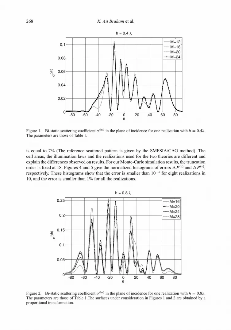
the power balance criterion is not sufficient to ensure the validity of any numerical method. So, it’simportant to study the convergence of the C-method results with respect to the truncation order[5] and to verify the theory by comparison with other exact methods and experimental data. Figure1 shows the normalised bi-static scattering coefficient σ (vh) in the plane of incidence for varioustruncation order values. The rms height is h = 0.4 wavelength. The convergence on results isensured for M ≥ 16. Relative error �σ

(vh)(θ ) between σ

(vh)(θ,M = 16) and σ

(vh)ref (θ,M = 28) is

equal to 5%. With M = 16, the error on power balance is weak, the accuracy on far-field resultsis good and the computation time is reasonable (12 minutes). Figure 2 shows the normalized


Table 1. Error �P on the power balance versus truncation order and rms height. The surfacesunder consideration are obtained by a proportional transformation. Rough-surface parameters: lc = λ,lt = λ/2, L = 8λ; incident angles: θi = 30◦ and ϕi = 0◦; Spectral resolution: �α = k / 8.

M / h Error 0.2 λ 0.4 λ 0.6 λ 0.8 λ 1.0 λ

12 �P(h) 1.0 × 10−4 5.0 × 10−3 0.14 2.2 6310�P(v) 4.0 × 10−4 1.6 × 10−2 4.0 × 10−2 2.6 1585

16 �P(h) 1.3 × 10−4 1.3 × 10−3 6.3 × 10−3 0.05 63�P(v) 4.0 × 10−4 2.5 × 10−3 3.2 × 10−3 0.1 40

20 �P(h) 7.9 × 10−6 3.2 × 10−4 3.2 × 10−3 2.5 × 10−2 4.0�P(v) 3.2 × 10−6 4.0 × 10−4 4.0 × 10−3 1.3 × 10−2 1.6

24 �P(h) 1.6 × 10−6 1.0 × 10−4 1.9 × 10−3 1.6 × 10−2 0.32�P(v) 1.6 × 10−7 5.0 × 10−5 7.9 × 10−4 1.0 × 10−2 0.25

28 �P(h) 1.0 × 10−7 2.0 × 10−5 4.0 × 10−4 6.3 × 10−3 1 × 10−2

�P(v) 7.9 × 10−8 2.0 × 10−5 2.0 × 10−4 4 × 10−3 2 × 10−2

bi-static scattering coefficient σ (vh) with a rms height h = 0.8 wavelength. The convergence isensured if the truncation order is larger than 24. Relative error �σ

(vh)(θ ) between σ

(vh)(θ,M =

24) and σ(vh)

ref (θ,M = 28) is equal to 9%. With M = 24, the CPU time becomes important(135 minutes).

In the next section, we present some results obtained by the C method for perfectly conductingsurfaces illuminated by an incident plane wave and we check their validity against the scatteringpatterns given by methods based on solutions of surface integral equations [20, 21] and given byexperiments [22].

5.3. Comparison with exact numerical simulations and experimental data

We consider random rough surfaces with an area of L2 = 64λ2 illuminated under incidence anglesθi = 10◦ and ϕi = 0◦. The rms height is h = 0.2 wavelength with a correlation radius lc = 0.6wavelength. Figure 3 shows the averaged bi-static coefficient in the plane of incidence with a (h)-polarized incident plane wave. The co-polarized component < σ (hh) > and the cross-polarizedcomponent 〈σ (vh)〉 are performed over NR = 780 realizations. In Figure 3, the Monte-Carlosimulation results given by the SMFSIA/CAG method (Sparse-Matrix Flat-Surface IterativeApproach with CAnonical Grid) are also plotted [20]. The authors in [20] have used surfaceswith an area of 256 square wavelengths illuminated by a tapered wave [23]. The ensembleaveraging is performed over 280 realizations that are different from 780 realizations used forour simulation. The comparison is satisfactory. Relative error �σ (hh) is equal to 10% and �σ (vh)

Table 2. System size, higher spatial frequency and CPUtime versus truncation order. The parameters are those ofTable 1.

M 2Ms = 2 (2M + 1)2 2αmax Speed

12 1250 3k 130 sec16 2178 4k 12 min20 3362 5k 45 min24 4802 6k 2 h 15 min28 6498 7k 5 h 40 min


-80 -60 -40 -20 0 20 40 60 800

0.02

0.04

0.06

0.08

0.1

θ

σ(vh)

h = 0.4 λ

M=12M=16M=20M=24

Figure 1. Bi-static scattering coefficient σ (hv) in the plane of incidence for one realization with h = 0.4λ.The parameters are those of Table 1.

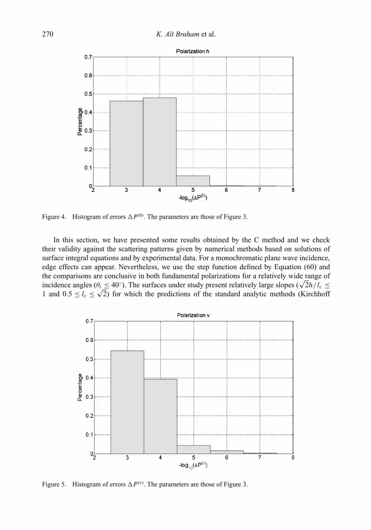
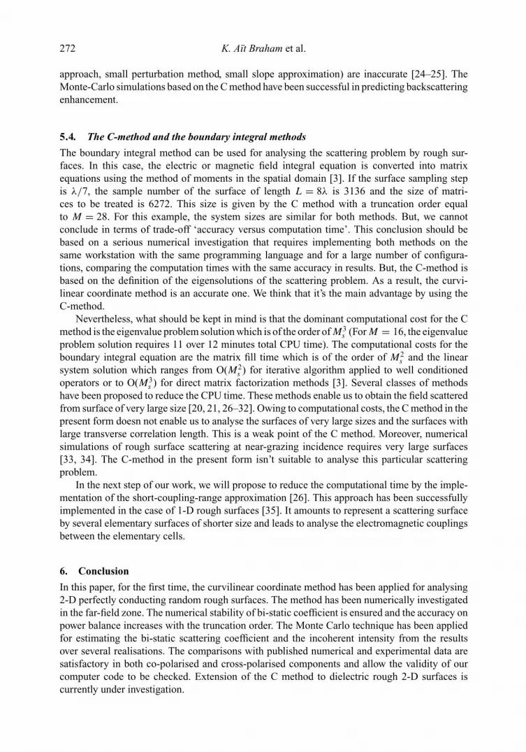
is equal to 7% (The reference scattered pattern is given by the SMFSIA/CAG method). Thecell areas, the illumination laws and the realizations used for the two theories are different andexplain the differences observed on results. For our Monte-Carlo simulation results, the truncationorder is fixed at 18. Figures 4 and 5 give the normalized histograms of errors �P (h) and �P (v),respectively. These histograms show that the error is smaller than 10−3 for eight realizations in10, and the error is smaller than 1% for all the realizations.

-80 -60 -40 -20 0 20 40 60 800

0.05

0.1

0.15

0.2

0.25

θ

σ(vh)

h = 0.8 λ

M=16M=20M=24M=28

Figure 2. Bi-static scattering coefficient σ (hv) in the plane of incidence for one realization with h = 0.8λ.The parameters are those of Table 1.The surfaces under consideration in Figures 1 and 2 are obtained by aproportional transformation.


-80 -60 -40 -20 0 20 40 60 800

0.1

0.2

0.3

0.4

0.50.5

θ

Ave

rage

d bi

-sta

tics

catte

ring

coef

ficie

nt

Polarizations (hh) and (vh)

: C methode: SMFSIA/CAG co-polarization

cross polarization

Figure 3. Comparison between the SMFSIA/CAG method and the C method: Averaged bi-static scatteringcoefficient in the plane of incidence, (h) incidence. Rough-surface parameters h = 0.2λ, lc = 0.6λ, lt = lc/2,L = 8λ; incident angles θi = 10◦ and ϕi = 0◦; Spectral resolution �α = k/8. Truncation order M = 18;Number of realizations NR = 780. Results of the SMFSIA/CAG method are taken in [20].

In Figure 6, the averaged bi-static coefficient is plotted in the plane incidence for the cross-polarized incoherent intensities (4π cos θiI

(vh)f and 4π cos θiI

(hv)f ). We consider random rough

surfaces with an area of L2 = 64λ2 illuminated under incidence θi = 40◦ and ϕi = 0◦. The rmsheight is h = 0.5 wavelength with a correlation radius lc = 1.41 wavelength. Each elementarycell dimensions are about 32 square correlation lengths. The averaged bi-static coefficients areperformed over NR = 300 realizations. With M = 18, the error on the power balance is smallerthan 1% for all the realizations. In Figure 6, the Monte-Carlo simulation results given by theFB-NSA method (Forward-Backward/Novel Spectral Acceleration method) are also plotted [21].The authors in [21] have used surfaces with an area of 128 × 32 square wavelengths illuminatedby a tapered wave. The ensemble averaging is performed over 150 realizations. Although theelementary cell area is reduced to 32l2

c , comparison is satisfactory.Figure 7 shows the averaged bi-static coefficients in the plane of incidence for Monte Carlo

simulations and millimeter-wave experiments under v-polarized incident waves [22]. The rmsheight is h = 1 wavelength with a correlation radius lc = 1.41 wavelength. For our simulations,the incident plane wave is characterized by the zenith angle θi = 20◦ and the azimuth angle ϕi

= 0◦. Elementary cells present an area of 64 square wavelengths. We generate 300 elementarysurfaces and for each realization, we use a truncation order that leads to an error on the powerbalance smaller than 5%. With M = 21, the power balance criterion is verified on 236 realizations.Among the remaining 64 realizations, the truncation order is fixed at 24 and the criterion is verifiedon 48 realizations. Among the remaining 16 realizations, the truncation order is fixed at 28 andthe criterion is only verified for 13 realizations. The curves in Figure 8 are performed over these297 realizations. Although the elementary cell area is reduced to 32l2

c , the comparison withexperimental data is satisfactory. Relative error �σ (vv) is equal to 13% and �σ (hv) is equal to12% (The reference scattered patterns are given by experiment data). The backscattering peakscoincide well enough.


Figure 4. Histogram of errors �P (h). The parameters are those of Figure 3.

In this section, we have presented some results obtained by the C method and we checktheir validity against the scattering patterns given by numerical methods based on solutions ofsurface integral equations and by experimental data. For a monochromatic plane wave incidence,edge effects can appear. Nevertheless, we use the step function defined by Equation (60) andthe comparisons are conclusive in both fundamental polarizations for a relatively wide range ofincidence angles (θi ≤ 40◦). The surfaces under study present relatively large slopes (

√2h/lc ≤

1 and 0.5 ≤ lc ≤ √2) for which the predictions of the standard analytic methods (Kirchhoff

Figure 5. Histogram of errors �P (v). The parameters are those of Figure 3.


-80 -60 -40 -20 0 20 40 60 800

0.1

0.2

0.3

0.4

0.5

0.6

0.7

0.8

θ

Cross-polarizations

-80 -60 -40 -20 0 20 40 60 800

0.1

0.2

0.3

0.4

0.5

0.6

0.7

0.8

θ

In c

oher

ent i

nten

sity

Cross-polarizations

: hv - C method : hv - FBNSA method method : vh - C method : vh - FBNSA method method

Figure 6. Comparison between the FBNSA method and the C method: Normalized incoherent radar cross-section in the plane of incidence for both cross-polarizations. Rough-surface parameters h = 0.5λ, lc = √

2λ,lt = λ/2, L = 8λ; incident angles θi = 40◦ and ϕi = 0◦; Spectral resolution �α = k/8. Truncation orderM = 18; Number of realizations NR = 300. Results of the FBNSA method are taken in [21].

-80 -60 -40 -20 0 20 40 60 800

1

2

3

4

5

θ

Ave

rage

d bi

-sta

ticsc

atte

arin

g co

effic

ient

Polarizations vv and hv

: Experimental data: C method co-polarization

cross polarization

Figure 7. Monte-Carlo simulation comparison of the C method and the experimental data: Averagedbi-static scattering coefficient in the plane of incidence, (v) incidence. Rough-surface parameters h = λ,lc = √

2λ, lt = λ/2, L = 8λ; incident angles θi = 20◦ and ϕi = 0◦; Spectral resolution �α = k/8. Truncationorder M = 21, M = 24 or M = 28; Number of realisationsNR = 297. Experimental data are taken in [22].


approach, small perturbation method, small slope approximation) are inaccurate [24–25]. TheMonte-Carlo simulations based on the C method have been successful in predicting backscatteringenhancement.

5.4. The C-method and the boundary integral methods

The boundary integral method can be used for analysing the scattering problem by rough sur-faces. In this case, the electric or magnetic field integral equation is converted into matrixequations using the method of moments in the spatial domain [3]. If the surface sampling stepis λ/7, the sample number of the surface of length L = 8λ is 3136 and the size of matri-ces to be treated is 6272. This size is given by the C method with a truncation order equalto M = 28. For this example, the system sizes are similar for both methods. But, we cannotconclude in terms of trade-off ‘accuracy versus computation time’. This conclusion should bebased on a serious numerical investigation that requires implementing both methods on thesame workstation with the same programming language and for a large number of configura-tions, comparing the computation times with the same accuracy in results. But, the C-method isbased on the definition of the eigensolutions of the scattering problem. As a result, the curvi-linear coordinate method is an accurate one. We think that it’s the main advantage by using theC-method.

Nevertheless, what should be kept in mind is that the dominant computational cost for the Cmethod is the eigenvalue problem solution which is of the order of M3

s (For M = 16, the eigenvalueproblem solution requires 11 over 12 minutes total CPU time). The computational costs for theboundary integral equation are the matrix fill time which is of the order of M2

s and the linearsystem solution which ranges from O(M2

s ) for iterative algorithm applied to well conditionedoperators or to O(M3

s ) for direct matrix factorization methods [3]. Several classes of methodshave been proposed to reduce the CPU time. These methods enable us to obtain the field scatteredfrom surface of very large size [20, 21, 26–32]. Owing to computational costs, the C method in thepresent form doesn not enable us to analyse the surfaces of very large sizes and the surfaces withlarge transverse correlation length. This is a weak point of the C method. Moreover, numericalsimulations of rough surface scattering at near-grazing incidence requires very large surfaces[33, 34]. The C-method in the present form isn’t suitable to analyse this particular scatteringproblem.

In the next step of our work, we will propose to reduce the computational time by the imple-mentation of the short-coupling-range approximation [26]. This approach has been successfullyimplemented in the case of 1-D rough surfaces [35]. It amounts to represent a scattering surfaceby several elementary surfaces of shorter size and leads to analyse the electromagnetic couplingsbetween the elementary cells.

6. Conclusion

In this paper, for the first time, the curvilinear coordinate method has been applied for analysing2-D perfectly conducting random rough surfaces. The method has been numerically investigatedin the far-field zone. The numerical stability of bi-static coefficient is ensured and the accuracy onpower balance increases with the truncation order. The Monte Carlo technique has been appliedfor estimating the bi-static scattering coefficient and the incoherent intensity from the resultsover several realisations. The comparisons with published numerical and experimental data aresatisfactory in both co-polarised and cross-polarised components and allow the validity of ourcomputer code to be checked. Extension of the C method to dielectric rough 2-D surfaces iscurrently under investigation.


AcknowledgmentThe authors thank the ‘Programme National de Teledetection Spatiale’ that has supported the research ofthis paper.

References[1] J.A. Ogilvy, Theory of Wave Scattering from Random Rough Surfaces, Hilger, Bristol, 1991.[2] L. Tsang, J.A. Kong, K.H. Ding, and C.O. Ao, Scattering of Electromagnetic Waves – Numerical

Simulations, Wiley-Interscience, New York, 2001.[3] K.F. Warnick and W.C. Chew, Numerical simulation methods for rough surface scattering, Waves

Random Media 11 (2001), R1–R30.[4] M. Saillard and A. Sentennac, Rigorous solutions for electromagnetic scattering from rough surfaces.

Waves Random Media 11 (2001), pp. R103–R137.[5] R. Dusseaux and R. de Oliveira, Scattering of a plane wave by 1-dimensional rough surface – Study

in a nonorthogonal coordinate system, PIER 34 (2001), pp. 63–88.[6] R. Dusseaux and C. Baudier, Scattering of a plane wave by 1-dimensional dielectric rough surfaces –

study of the field in a nonorthogonal coordinate system, PIER 37 (2003), pp. 289–317.[7] C. Baudier, R. Dusseaux, K.S. Edee, and G. Granet, Scattering of a plane wave by one-dimensional

dielectric random surfaces – study with the curvilinear coordinate method, Waves Random Media 14(2004), pp. 61–74.

[8] J. Chandezon, D. Maystre, and G. Raoult, A new theoretical method for diffraction gratings and itsnumerical application, J. Opt (Paris) 11 (1980), pp. 235–241.

[9] L. Li and J. Chandezon, Improvement of the coordinate transformation method for surface-reliefgratings with sharp edges, J. Opt. Soc. Am. A 13 (1995), pp. 2247–2255.

[10] G. Granet, Diffraction par des surfaces bi-periodiques: resolution en coordonnees non orthogonales,Pure Appl. Opt. 4 (1995), pp. 777–793.

[11] P.M. Van Den Berg, and J.T. Fokkema, The Rayleigh hypothesis in the theory of diffraction by aperturbation in a plane surface, Radio Sci. 15 (1980), pp. 723–732.

[12] A. Voronovich, Small-slope approximation for electromagnetic wave scattering at a rough interfaceof two dielectric half-spaces, Waves Random Media 4 (1994), pp. 337–367.

[13] M. Born and E. Wolf, Principles of Optics – Electromagnetic Theory of Propagation Interference andDiffraction of Light, Appendix III, Pergamon, Oxford, 1980.

[14] C. Baudier and R. Dusseaux, Scattering of an E//- polarized plane wave by one-dimensional roughsurfaces: numerical applicability domain of a Rayleigh method in the far-field zone, PIER 34 (2001),pp. 1–27.

[15] D. Maystre, Electromagnetic scattering from perfectly conducting rough surfaces in the resonanceregion, IEEE Trans. Antennas Propagat. 31 (1983), pp. 885–895.

[16] J.A. Stratton, Electromagnetic Theory, McGraw-Hill, New York, 1941.[17] D. Middleton, Introduction to Statistical Communication Theory, McGraw-Hill, New York, 1960.[18] C.E. Shannon, Mathematical theory of communication, Bell System Tech. J. 27 (1948), pp. 379–423.[19] A.K. Fung and M.F. Chen, Numerical simulation of scattering from simple and composite surface,

J. Opt. Soc. Am. A. 2 (1985), pp. 2274–2283.[20] K. Pak, L. Tsang, C.H. Chan, and J.T. Johnson, Backscattering enhancement of electromagnetic waves

from two-dimensional perfectly conducting random rough surfaces based on Monte-Carlo simulations.J. Opt. Soc. Am. A 12 (1995), pp. 2491–2499.

[21] D. Torrungrueng and J.T. Johnson, Numerical studies of backscattering enhancement of electromag-netic waves from two-dimensional random rough surfaces with the forward-backward/novel spectralacceleration method. J. Opt. Soc. Am. A. 18 (2001), pp. 2518–2526.

[22] J.T. Johnson, L. Tsang, R.T. Shin, K. Pak, C.H. Chan, A. Ishimaru, and K. Yasuo, Backscatteringenhancement of electromagnetic waves from two-dimensional perfectly conducting random roughsurfacers: A comparison of Monte-Carlo simulations with experimental data, IEEE Trans AntennasPropagat. 44 (1996), pp. 748–756.

[23] E.I. Thorsos, The validity of the Kirchhoff approximation for rough surface scattering using a Gaussianroughness spectrum, J. Acoust. Soc. Am. A 82 (1988), pp. 78–92.

[24] T.M. Elfouhaily and C.A. Guerin, A critical survey of approximate scattering wave theories fromrandom rough surfaces. Waves Random Media 14 (2004), R1–10.

[25] C.A. Guerin, G. Soriano, and T.M. Elfouhaily, Weighted curvature approximation: numerical tests for2D dielectric surfaces, Waves Random Media 14 (2004), pp. 349–363.


[26] D. Maystre and J.P. Rossi, Implementation of a rigorous vector theory of speckle for two-dimensionalmicrorough surfaces, J. Opt. Soc. Am. A 3 (1986), pp. 1276–1282.

[27] M. Saillard and D. Maystre, Scattering from random rough surfaces: a beam simulation method,J. Opt (Paris) 19 (1988), pp. 173–176.

[28] G. Soriano and M. Saillard, Scattering of electromagnetic waves from two-dimensional rough surfaceswith an impedance approximation, J. Opt. Soc. Am. A 18 (2001), pp. 124–133.

[29] R.L. Wagner, J. Song, and W.C. Chew, Monte Carlo simulations of electromagnetic scattering fromtwo-dimensional random rough surfaces. IEEE Trans. Antennas Propagat 45 (1997), pp. 235–245.

[30] K. Pak, L. Tsang, and J.T. Johnson, Numerical simulations and backscattering enhancement of elec-tromagnetic waves from two-dimensional dielectric random rough surfaces with the sparse-matrixcanonical grid method. J. Opt. Soc. Am. A 18 (1997), pp. 1515–1529.

[31] L. Tsang, D. Chen, and P. Xu, Wave scattering with the UV multilevel partitioning method: 1. Two-dimensional problem of perfect electric conductor surface scattering, Radio Sci. 39 (2004), pp. 1–13.

[32] L. Tsang, Q. Li, D. Chen, P. Xu, and V. Jandhyala, Wave scattering with the UV multilevel partitioningmethod: 2. Three-dimensional problem of nonpenetrable surface scattering, Radio Sci. 39 (2004), pp.1–11.

[33] H.D. Ngo and C.L. Rino., Application of beam simulation to scattering at low grazing angles – 1Methodology and validation, Radio Sci. RS00823 (1994), pp. 1365–1379.

[34] H.D. Ngo and C.L. Rino, Application of beam simulation to scattering at low grazing angles – 2oceanlike surfaces, Radio Sci. RS01924 (1994), pp. 1381–1391.

[35] K. Aıt Braham and R. Dusseaux, Analysis of the Scattering from Rough Surfaces with the C Methodand the Short-Coupling Range Approximation. Applied Computational Electromagnetics Society Con-ference (ACES).Verona, Italy, March 19–24, 2007, pp. 1880–1886.

Scattering of Electromagnetic Waves from Two-Dimensional Randomly Rough Penetrable Surfaces

Documents

Transcript of Scattering of Electromagnetic Waves from Two-Dimensional Randomly Rough Penetrable Surfaces