composite material aircraft electromagnetic properties

II

COMPOSITE MATERIAL AIRCRAFT

ELECTROMAGNETIC PROPERTIES

AND

DESIGN GUIDELINES

, .A. BI'KEN ,

W. G.D . .FF ..

1). Rt. PFLUGA

* 7_, NA AL AIR SYSTEM COMlMANI,LIJ U.S. I)EIAR'rMENT OF rl-E NAVY

8 02 OO|

UNCLASSIFIEDr~~I *CVftITV CLAI~iPiCA7ION OF 1.115 PAGE W1. D*1ýA#0eI 041,d___________________

"REPORT DOCUMENTA.TION PAGE ... AD INSTRUCTISNSD&FoRZ COM .LICTIN FORM1, ptoGo l UiT/ .m, OOVT ACCCASION No,, RICIPICNT's CAT€A6OO humI .

4. TIIC (ant 'al . TYPE OF 09PORT A P"IRIO COvI.g.Composite Material Aircraft Electromagnetic Jan 19"1Properties and Design Guidelines

"6. PERFORMING ORS. REPORT NUNSIIR

50 - 57797 ,AIT4OR(.J '. CONTRACT OR GRANT "NUMSrR(aj

'J.Birken R. Wallenberg H00019-79-C-0634W." DuffD.tPflug

,. PIqrOAIgNO OROANIZATION NAME AND ADORLIS 10. PROORAM CLE[INT,PROJ[CT. TASK

Atlantic Research Corporation ARIA A wORK UNIT NUMIIRI

5390 CherokeeAlex'andria, VA 22314

I). CONTROLLING OPFICINAM9 AND ACOF4Rl IS. REPORT DATENaval Air Systems ComandATTN: J. A. Birken (AIR-5161D) , W NUMIIPOF PAGISWashington, D. C. 20361 369

IA. MONITORING AGINCY NAMI A ADORoIffIerent frm ControlDli O1hat) IL 89CUMITY CLASS, (of this report

"UNCLASSIFIED1".. OI€ L AS5111IC ATI N/OOw NGR AOINlG

LLI N/A

DISTRIBUTION STATEMENIT (of Athi oepeal)

Unilimited DistributionAPPROVED FOR PUBLIC RELEAS,DI8IRJ5UIION UNLIMIUQ

17. DISllT RIUU ION TATEIMINT (of tie aboel • ,1119,1011 i &look 10, It EiltltAm t 0e# 0 I0 er-U '_, .D T,,Iri0 c t Aircraft-Electr.maan

,., • ', IS. KIY WOROS (CenEMu. pci aeae;.e aid.~ Ite~ee~aca mi •.lleatlyI bok ,.mll) _,

-Advanced Composite AircraftElectromagnetic Pulse (EMP) Composite Material Avionics-Lightnng Composite Aircraft Safety Sblid State Devices.Radar Electromagnetic TestingE lectromagnetic Compatibility Communicationg\ trnn.in War'fare CoU2uters

2W A" STRACT (Cocntlinue oni @votes Sid Idnfsesea p a4* 1nd Idenhity by bleak nAumb.,)'

This document collects and primarily suimariezes aircraft advanced compositematerial electromagnetic properties, and seconda.rily, aumarizes composite materialmechanicalj thermal, environmental fabricattonpropertiss noting their ramificationson electromagnstic performance. It then overvie•. the electromagnetic sub-disciplineof threats.external to internal aircraft coupling, component and subsystems suscepta

, .bility, protective methods as veil as test and evaluation of small sample to totalaircraft composite material electromagnetic performance. The sub-disciplines

: constitute a partioned set of independent variables which allow the reader to locate' hig -aea of interest in one section of the book. (man other side)

DD , 1473 o0TION OF, INOVY 5IS 1oUOLITS .. CLAssimI-lCURITY CL A$11VICATION OF THIS PACE f'4in Dole ,nIOeP00

The sub-discipline are then combined to perform total aircraft electromnagneticsystem performance noting the protective methods, advantages and penalties.

Of 'ý1

100

Table of Contents

Section Page1.0 Introduction -'--2.0 Electromagnetic Threats 2-1

2.1 Natural Threat 2-12.1.1 Lightning 2-12.1.2 Precipitation Static 2-16

2.2 Friend/Foe Threat 2-192.2.1 RF Threat 2-192.2.2 EMP Threat 2-262.2.3 High Energy Laser, Nuclear Thermal Radiation

and Particle Beam Threat 2-282.3 References 2-31

3.0 Composition, Fabrication and Mechanical Propertiesof Composite Materials 3-13.1 Composition of Composite Materials 3-1

3.1.1 Fibers 3-13.1.2 Matrix Materials 3-3

3.2 Fabrication of Composite Materials 3-53.2.1 Tape (Prepreg) and Broad Goods Fabrication 3-53.2.2 Layup Process 3-53.2.3 Laminate Orientation Code 3-53.2.4 Composite Fabrication Processes 3-7

3.3 Mechanical Properties 3-93.3.1 Composite Fiber Properties 3-93.3.2 Compositia Matrix Properties 3-123.3.3 Single Laminate Composite Properties 3-123.1.4 Croasplied Laminate Composite Properties 3-18

3.4 Environmental Effects on Composite Materials 3-353.5 Composite Fatigue 3-353.6 References 3-43

4.0 Applications of Composite Materials 4-14.1 'Early (pre-1973) Aerospace Composite Materials Applications 4-14.2 Recent (post-1973) and Current Aerospace Composite

Material Applications 4-14.2.1 Aircraft Systems 4-14.2.2 Propulsion Systems 4-8 ..4.2.3 Space Systems 4-84.2.4 Helicopter Systems 4-94.2.5 Other Aerospace Applications 4-9

4.3 Problems in Composite Material Applications 4-10* 4.3.1 Graphite Fiber Release 4-10

4.3.2 Galvanic Corrosion 4-11,4.3.3 Fabrication Techniques 4-11

4.4 Future Uses of Composite Materials 4-11- 4.4.1 Future Composite Uses in Aerospace Systems 4-11

4.5 References 4-1b

S•..............". . . . . . .

Table of Contents(Continued)

Section PIte

5.0 Intrinsic Material Properties 5-I.5.1. Material EM Parameters 5-1

5.1.1 Permeabilityk 5-1.5.1.2 Permittivity5.1.3 Conductivity 5-2

5.2 Improvement of Intrinsic Parameters 5-125.2.1 Doping 5-1.25.2.2 Intercalation 5-13

5.3 Thermal Modification of EM Intrinsic Parameters 5-195.3.1 Conductivity 5-19

5.4 Environmental Modification of EM Intrinsic Parameters 5-195.4.1 Moisture 5-19

5.5 Nonlinear Effects 5-225.5.1 High-Field Effects 5-22

5.6 References 5-226.0 External-to-Internal Coupling 6-1

6.1 Airframe Shielding Effectiveness 6-16.1.1 Shielding Effectiveness - Theoretical Considerations 6-1"6.1.2 Measured and Predicted Composite Shielding

Effectiveness 6-256.1.3 Metallic/Composite Aircraft Weight-Shielding

Tradeoffs 6-336.2 Composite Joints 6-41

"6.2.1 Theory 6-416,2.2 Effect on Shielding Effectiveness 6-46

6.3 References 6-517.0 Component and Subsystem Susceptibility 7-1

7.1 Component and Circuit Susceptibility 7-17.1.1 Analog Circuits 7-1 r'.

7.1.2 Digital Circuits 7-27.1.3 Semiconductor Devices 7-27.1.4 Integrated Circuits 7-97.1.5 Electro-Explosive Detonators 7-16

7.2 Subsystem Susceptibility 7-167.2.1 Communication and Navigation 7-167.2,2 Flight Control Equipment 7-187.2.3 Weapons 7-217.2.4 Radar 7-21

7.3 References 7-258.0 General Analysis and Tradeoff Philosophy 8-1

8.1 Standards and Specifications 8-18.2 The System Approach 8-2

8.2.1 Electromagnetic Compatibility (EMC) Program 8-28.2.2 Electromagnetic Compatibility (EMC) Plans 8-38.2.3 EMC ProgrAm Implementation 8-7

ii

VIi , " " ' .," - -.

Table of Contents .

(Continued)Section PRae

8.3 EMC Systems Analysis Procedure Synthesis 8-78.3.1 Drivers in Procedure Synthesis 8-78.3.2 Guide to EMC Procedure Synthesis 8-15

8.4 Description of Programs and Facilities 8-158.4.1 Electromagnetic Compatibility Analysis Center (RADC) 8-16

8.4.2 Intrasystem Analysis Program 8-248.4.3 Interference Prediction Process - Number 1 (lIP-l) 8-348.4.4 The Cosite Analysis Model (COSAM) 8-358.4.5 Specification and Electronfagnatic Compatibility .,

Analysis Program (SEMCAP) 8-368.4.6 Shipboard Electromagnetic Compatibility

Analysis (SEMCA) 8-378.5 Data Base Management 8-37

8.5.1 ECAC Data Base Management 8-388.5.2 lAP Data Base Management 8-38

8.6 References 8-409.0 Measurement Test and Evaluation 9-1

9.1 Techniques for Measuring Intrinsic Parameters 9-19.1.1 Permeability 9-19.1.2 Permittivity 9-39.1.3 Resistivity 9-59.1.4 Conductivity 9-7

9.2 EM Shielding Effectiveness Measurement Techniques 9-209.2.1 Coupling Between Loops and Probes 9-209.2.2 Plane Wave Transmission/Reflection Methods 9-249.2.3 Surface Impedance Parameters 9-289.2.4 Joint Measurement Techniques 9-329.2.5 High Current Injection 9-369.2.6 High Voltage Charging-Discharging Phenomena 9-43

9.3 References 9-45 S.•

10.0 Protection Methods and Techniques 10-i10.1 Present Aircraft Protection Systems 10-1.

10.1.1 Static Dischargers 10-210.1.2 Lightning Arresters 10-210.1.3 Radome Strips 10-210.1.4 Composite Coating Protection Systems l0-.2

10.2 Future Composite Protection-Doping and Intercalation 10-2110.3 References 10-27

11.0 Design Guidelines 11-1i1.1 Overview 11-111.2 Electromagnetic Design Guidelines 11-3

11.2.1 External Electromagnetic Fields 11-511.2.2 Electromagnetic Shielding [Tl(f) and T2 (f)] 11-511.2.3 Joint Leakage [T3 (f)] 11-1511.2.4 Cables [T4(f)] 11-1711.2.5 Subsystem Susceptibility [T5 (f)] 11-21 •.2

11.3 Unprotected Aircraft Performance Guidelines 11-23

i~i

List of Illustrations

1.1 Aerospace Avionics Device Technology Trends 1-21.2 Electromagnetic System Parameters 1-4 ...1.3 Peak Open Circuit Voltage Versus Line Length for Three

Threats and Four Coupling-Transmission Line Confipurations,

X- O,05m, Z - 100n 1-51.4 Upper Bounds on Peak Power Versus Line Length E..: Three

Threats and Four Coupling-Transmission Line CoafigurationB• .,.X w 0.5m, Z - 1000 1-6

1.5 Wunsch Constant Versus Line Length for Three Threats andFour Coupling-Transmission Line Configurations, X 1-7

1.6 Top View of F-14 Using Triangular Patch Data Base 0

of Reference 4 1-81.7 Side View of F-14 Using Triangular Patch Data Base

of Reference 4 1-91.8 Comparison of Surface Current Density with MRC/EMA :1

Code and Surface Patch Model Used in This Report 1-111.9 Skin Current Density JS on Edge No. 29 for Near-Strike

Lightning Excitation an• Different Rise Times, T 1-121.10 Skin Current Density on Edge No. 29 of Triangular Patch

Model of F-14 Aircraft for Various Rise Times T ofIncident NEMP 1-13

1.11 Transfer Impedance Shielding of S'tructural Materials andProtective Electromagnetic Coatings 1-14

1.12 Improvement Protective Coatings Provided Relative to8 -ply Graphite/Epoxy 1-14

1.13 Weight Penalty Imposed by Protective Coatings 1-151.14 Weight/Shielding Figure of Merit of EM Protective Coatings 1-15 •

2.1 Thundercloud Profile Showing Charge Centers and Temperatureand Pressure Gradients (after (1)) 2-2

2.2 Current Waveform (not to scale) for a Lightning Flash to Ground 2-5 ,.2.3 Radiated Lightning Spectrum Normalized to 10 km (an EMP spectrum ,

is inluded for comparison) 2-62.4 Radiated Lightning Spectrum Normalized to One Statute Mile 2-62.5 Triangular Lightning Current Waveform. 2-82.6 Space Shuttle Lightning Current Waveform 2-8 *1

2.7 Double Exponential Lightning Current Waveform 2-82.8 Triple Exponential Lightning Current Waveform 2-102.9 Quadruple Exponential Lightning Current Waveform 2-102.10 Spectrum of Space Shuttle Current Lightning Waveform 2-112.11 Spectrum of Space Shuttle Current Lightning Waveform 2-122.12 Exponential Current Lightning Waveforms 2-12 ,2.13 Superposition of All Lightning Current Waveforms 2-132.14 Lightning Attachment 2-152.,.5 Swept Stroke Phenomenon 2-152.16 Aircraft Lightning Strike Zones 2-152.17 Lightning Strike Zones 2-152.18 Noise Spectrum Properties 2-182.19 Noise Spectrum Properties 2-182.20 Current Pulses Resulting from Streamers of Several Lengths 2-18

iv

LisL. of Illustrations(Continued)

2.21 RF Environment (10 kHz - 100 MHz) 2-202.22 RF Environment (100 - I GHz) 2-21

2.23 RF Environment (1 - 10 GHz) 2-21

2.24 RF Environment (10 - 100 GHz) 2-212.25 EMP Time Domain Waveform 2-27 62.26 EMP in Frequency Domain 2-272.27 Back-face Temperature of Graphite/Epoxy Substrate for Several

Pulse Fluence Levels 2-302.28 Laser Energy Density Necessary to Produce a Level of Stress

for Two Failure Modes 2-303.1 Fiber-reinformced Composite Material 3-23.2 PAN Fiber Graphitization Process 3-43.3 Graphite Fiber Tow 3-4

3.4 Boron Fiber Manufacturing Process together with a BoronCross-section 3-4

3.5 Tape (prepreg) and Broad Goods Fabrication Processes 3-6 '3.6 Symmetrical Balanced Layup 3-6 I..

3.7 Composite Fiber Densities Compared to Aircraft Metals 3-10

3.8 Tetisilo Strength and Modules of Various Composite Fibersand Metals 3-10

3.9 Stress-strain Curves for Composite Fibers 3-11

3.10 Specific Tensile Strength and Modules for Various CompositeFibers and Metals 3-1.1

3.11 Longitudinal Tensile Strength for Various Single LaminteComposites at Room Temperature (RT) and 350*F) 3-13

3.12 Transverse Tensile Strength for Various Single LaminateComposites at Room Temperature (RT) and 350*F 3-13

3.13 Diagonal Tensile/Compressive Strength for Various SingleLaminate Composites at Room Temperature (RT) and 350OF 3-13

3.14 Longitudinal Compressional Strength for Various SingleLaminate Composites at Room Temperature (RT) and 350*F 3-13

3.15 Transverse Commissional Strength for Various SingleLaminate Compositeu at Room Temperature (RT) and 350*F 3-14

3.16 In-plane Shear Strength for Various Single LaminateComposites at Room Temperature (RT) and 350'F 3-14

3.17 Interlaminar Shear Strength for Various Single LaminateComposites at Room Temperature (RT) and 350OF 3-14

3.18 Diagonal In-plane Shear Strength for Various SingleLaminate Composites at Room Temperature (RT) and 350*F 3-14

3.19 Longitudinal Tensile/compression Modulus for Various SingleLaminate Composites at Room Temperature (RT) and 350*F 3-15

3.20 Transverse Tension/Compression Modulus for Various SingleLaminate Composites at Room Temperature (RT) and 350*F 3-15

3.21 Diagonal Tension/compression modulus for Various SingleLaminate Composites at Room Temperature (RT) and 350"F 3-15

3.22 In-plane Shear Modulus for Various Single Laminate Compositesat Room Temperature (RT) and 350OF 3-15 .

3.23 Diagonal In-plane Shear Modulus for Various Single LaminateComposites at Room Temperature (RT) and 350OF 3-1.6

3.24 Loagitudinal Poisson's Ratio for Various Single LaminateComposites at Room Temperature (RT) and 350*F 3-16

vS

List of Illustrations(Continued)

3.25 Transverse Poisson's Ratio for Various Single LaminateComposites at Room Temperature (RT) and 350*F 3-16

3.26 Diagonal Poisson's Ratio for Various Single LaminateComposites at Room Temperature (RT) and 350*F 3-16

3.27 Longitudinal Thermal Expansion Constant for Various SingleLaminate Composites at Room Temperature (RT) and 350*F 3-17

3.28 Transverse Thermal Expansion Constant for Various SingleLaminate Composites at Room Temperature (RT) and 350°F 3-17

3.29 Diagonal Thermal Expansion Constant for Various SingleLaminate Composites at Room Temperature (RT) and 350*F 3-17

3.30 Single Laminate Composite Densities at Room Temperature (RT)and 350OF 3-18

3.31 Longitudinal Tension Stress-Strain Curve for Various Single

Laminate Composites at Room Temperature (solid lines) and

350*F (dotted lines) 3-1.9

3,32 Transverse Tension Stress-Strain Curve for Various Single

Laminate Composites at Room Temperature (solid lines) and

3501F (dotted lines) 3-19

3.33 Diagonal Tension Stress-Strain Curves for Various SingleLaminate Composites at Room Temperature (solid lines).and 350')F 3-19

3.34 Bending Stress-Strain Curve for Kevlar 49/Epoxy Compared to

Graphite/Epoxy and Aluminum 3-193,35 Boron/Epoxy Tensile Strength Curves for the. [Oi/+ 4 5 j/ 9 0]

Laminate Family 3-203.36 Boron/Epoxy Compressive Strength Curves for the [Oi/+45j/90k]

Laminate Family 3-203.37 Boron/Epoxy In-plane Shear Strength and Modulus Curves

[0i/+ 4 5j/90k] Laminate Family 3-213.38 Boron/Epoxy Extensional Modulus Curves for the [0i/+ 4 5 j/ 9 0k] 3.2

Laminate Family 3-213,39 Boron/Epoxy Poisson's Ratio Curves for the [Oi/+ 4 5j/ 9 0k] 3-22

Laminate Family3.40 Boron/Epoxy Thermal Expansion Coefficient Curves for the

[Oi/+ 4 5J/ 90 k] Laminate Family 3-223.41. High-Strength Graphite/Epoxy Tensile Strength Curves for the

[0i/+45j/9Ok] Laminate Family 3-233.42 High-Strength Graphite/Epoxy Compressive Strength Curves for

the [Oi/+ 4 5 j/9 0k] Laminate Family 3-233.43 Shear Strength Curves for the High-Strength Graphite/Epoxy

(0[/+451/90k] Laminate Family at Room Temperature (RT) and 350*F 3-243.44 Extensi6nal Modulus Curves for the High-Strength Graphite/EpoxyS[Oi/+45j/90kI Laminate Family 3-243-45 Shear Modulus Curves for the High-Strength Graphite/Epoxy

[Oi/±J/ 90k] Laminate Family at Room Temperature (RT) and 350'F 3-243.46 Poisson's Ratio Curves for the High-Strength Graphite/Epoxy

[Oi/± 4 5j/ 90 k] Laminate Family 3-25

3.47 Thermal Expansion Coefficient Curves for the High-StrengthGraphite/Epoxy [Oi/+ 4 5j/90k] Laminate Family 3-25

3.48 Tensile Strength Curves for the Hligh-Modulus Graphite/Epoxy[Oi/+ 45j/90k] Laminate Family 3-26

3.49 Compressive Strength Curves for the High-Modulus Graphite/Epoxy[Oi/+45./90k] Laminate Family 3-26 4-

3.50 Shear S8rength Curves for the High-Modulus Graphite/Epoxy[0i/+45-1/90k] Laminate Family at Room Temperature (R'r) And 3500F 3-27

vi


Figure __

3.51 Extensional Modulus Curves for the High-Modulus Graphite/Epoxy[ 0i/+45j/ 9 0k] Laminate Family 3-27

3.52 Shear Modulus Curves for the High-Modulus Graphite/Epoxy[0i/+45j/90k] Laminate Family at Room Temperature and 350*F 3-27

3.53 Poisson's Ratio Curves for the High-Modulus Graphite/Epoxy[Oi/+ 4 51/90k] Laminate Family 3-28

3.54 Thermal Expansion Coefficient Curves for the High-ModulusGraphite Epoxy [Oi/+ 4 5j/9 0k] Laminate Family 3-28

3.55 Tensile Strength Curves for the Intermediate StrengthGraphite Epoxy [Oi/+ 4 5j/90k] Laminate Family 3-29

3.56 Compressive Strength Curves for the Intermediate-StrengthGraphite/Epoxy [Oi/± 4 5j/ 9 0k] Laminate Family 3-29

3.57 Shear Strength Curves £or the Intermediate-StrengthGraphite/Epoxy [01/+ 4 5j/90k1 Laminate Family 3-30

3.58 Extensional Modulus Curves for the Intermediate StrengthGraphite/Epoxy ([i/+ 4 5j/ 9 0 k] Laminate Family 3-30

3.59 Shear Modulus Curves for the Graphite/Epoxy [oi/+4 5j/ 9 0k]-.3-3Laminate Family at Room Temperature (RT) and 350F 3-30

3.60 Poisson's Ratio Curve for the Intermediate-StrengthGraphite/Epoxy [Oi/± 4.5j/90k] 3-31

3.61 Thermal Expansion Coefficient Curves for the Intermediate-Strength Graphite/Epoxy [Oi/+ 4 5j/ 9 0k] Laminate Family 3-31

3.62 Longitudinal Tensile Strength for the [0/60) Boron/Epoxy andGraphite/Epoxy Laminate at Room Temperature (RT) and 350 0 F 3-32

3.63 Transverse Tensile Strength for the (0/60] Boron/Epoxy andGraphite/Epoxy Crossplied Laminates at Room Temperature (RT)and 350'F 3-32

3.64 Longitudinal Compressive Strengths for the [0/60] Boron/Epdxyand Graphite/Epoxy Crossplied Laminates at Room Temperature (RT)and 350 0 F 3-32

3.65 Transverse Compressive Strengths for the [0/60] Boron/Epoxy andGraphite/Epoxy Crossplied Laminates at Room Temperature (RT) and350OF 3-32

3.66 In Plan Shear Strengths for the [0/601 Boron/Epoxy andGraphite/Epoxy CrossplLed Laminates at Room Temperature (RT)and 350*F 3-33

3.67 Tension/Compression Modulus for the [0/60] Boron/Epoxy andGraphite/Epoxy Crossplied Laminates at Room Temperature (RT)and 350eF 3-33

3.68 In-Plane Shear Modulus for the [0/601 Boron/Epoicy and 0Graphite/Epoxy Crossplied Laminates at Room Temperature (RT)and 350OF 3-33

3.69 Poisson's Ratio for the (0/60] Boron/Epoxy and Graphite/EpoxyCrossplied Laminates at Room Temperature (RT) and 350*F 3-33

3.70 Thermal Expansion Constants for the [0/60] Boron/Epoxy andGraphite/Epoxy Crossplied Laminates at Room Temperature (RT)and 350OF 3-34

'3.71. Denisites for [2/60] Boron/Epoxy and Graphite//Epoxy CrosspliedLaminates 3-34

vii

List of Illustrations(Continued)i.Fil~d r e P agae+

3.72 Lamflnate Ultimate Tensile and Shear Strength Versus Percent ofLaminate, S-CL/T300/S-GL (0°/+450/90*) Family 3-39

3.73 Laminate Ultimate Compression. Strength Versus Percent ofLaminate, S-GI,/T300/S-GL (00/+450/900) Family 3-39

3.74 Laminate Ex & Gxy Versus Percent Laminate S-GL/T300/S-GL(00/+4.5/90 ) Family 3-39

,3.75 Poisson's Ratio U., S-GI,/T300/S-GL (00/+459/90*) Family 3-39

3.76 Longitudinal Coefficient of Thermal Expansion S-GL/T300/S-GL(00/+45"/900) Family 3-339

3.77 Laminate Ultinmate Tensile and Shear Strength Versus Percent.of LamLnate T300/K-49/T300 (0O/+451/90*) Family 3-39

3.78 Laminate Ultimate Compressive Strength Versus Percent ofLaminate T300/K'-49/T300 (0/+45/90*) Family 3-40

3.79 Laminate Ex & GxY Versus Percent of Laminate T300/K-49/T300(0*/+450/90') Family 3-40

3.80 Poisson's Ratio uxy T300/KEV-49-181/T300 (00/+450/90") Family 3-40

3.81 Longitudinal Coefficient of Thermal Expansion T300/KEV-49-181/"1300 (00/+45o/90*) Family 3-41

3,82 Constant Amplitude Fatigue Data for Unidirectional Boron/EpoxyFor R-0.1 At Variois Temperatures 3-41

3,83 Constant Amplituide Fatigue Data for (0/90'1 and (0/+45/90] Cross-plied Boron/Epoxy Laminates at Room Temperature at kX0.1 3-41

3.84 Constant Amplitude Fatigue Data for Unidirectional High-Strength(1S) and High-Modulus (HM) Graphite/Epoxy Laminates at RoomTemperature and R-0.1 3-.42

4,1 Lear Fan 2100, All-Composite Business Aircraft 4-54.2 Advanced Composites on the Boeing 7.67 Transport 4-5

4.3 Navy/McDonnell Douglas AV-8B Advance Harrier Composite Aircraft 4-54.4 Use of Composites on the Navy F/A-18 4-74.5 Composite Applications on the Dornier Light Transport Aircraft 4-74.6 Rolls-Royce RB.211-535 Aircraft Engine 4-74.7 Simple Beam Builder Concept for Space Applications

Using the Space Shuttle 4-74.8 Weight and Cost Savings Possible by Use of Composites for

Primary Structures In Transport Aircraft. Chart prepared byNASA 5- 1.3

4.9 Graphite/Epoxy Wing Box 5-134.10 Experimental Ford LTD Graphice/Epoxy Automobile 5-155.1 Conduc.tL:vty a(mhos/m) of Kevlar/Epoxy as a Function of E--Field 5-55.2 Conductivity Vs Frequency for Graphite/Epoxy Multi-Play Samples

of Narmteo 5208 and Mercules 3501. The Field is Parallel to 0'Fibers 5-9

5.3 Conductivity Vs Frequency for Unidirectional Samples of Narmco5208 and Mercules 3501 Graphifte/Epoxy Composite Material. TheField is Parallel to the Fibers 5-9

5i, 4 Conductivity Vs Frequency for Multi-Ply and UnidirectionalSamples of Narmco 5208 and Mercules 3501 Graphite/EpoxyComposite. T'he Field is Normal to the 0* Fibers 5-O0

5.5 Con5uctivity Vs Frequency o1 Samples of Graphite/Epoxy Compos Ltu

Compared to Samples of Boron/Epoxy and to Aluminum (75MHz-2G1Hz) 5-105.6 Bulk Conductivity Vs Frequency for Samples of 2-Ply and 4-Ply

Graph ite/Epoxy Composite Material. (Mc r:ulhs AS350].) 5-I.5.7 Surface Conductivity of Samples of HerctLles AS 3501 Graphite/

Epoxy Composite Materioal. as a Funaction of Frequency 5-1.1

Svi1] I

List of Illustrations

FLgure (Continued) Pa-.

5.8 Conductivity Enhancement for Samples of Hercules AS 3501Graphite/Epoxy Composite Materials at Two Temperatures 5-14

5.9 Conductivity Enhancement in Samples of Boron Fibers in theTemperature Range 1000*C-1200°C 5-14

5.10 Graphite Crystal Structure 5-155.1.1 Stage Structure for Graphite Interrelated with Potassium 5-175.1.2 Conductivity of Intercalated and Regular Graphite/Epoxy

Composite Samples as a Function of Filling Factor 5-175.13 Typical Conductivity-Temperature Profile for a Semiconductor 5-205.14 Boron Fiber Resistance as a Function of Temperature 5-205.15 Transverse Conductivity of Graphite/epoxy (Unidirectional as a,

Function of Immersion Time in Water at 230c. 5-206.1 Coaxial Loops Separated by An Infinite Plate 6-26.3 Normal Incidence Excitation of n Isotropic Composite Layers 6-7"6.4 Oblique Incidence Excitation of n Isotropic Composite Layers 6-76.5 Anisotropic Composite Layer Principal Coordinates (Primed) as . .

"* Related to Global Coordinates (Unprimed) 6-106.6 Surface Transfer Impedance as a Function of Frequency 6-266.7 Measured Surface Transfer Impedance of 24 Ply T-300 Graphite/

Epoxy 6-266.8 Magnetic Shielding Effectiveds of a Flat Plate under a Uniform

Magnetic Field 6-286.9 Magnetic Shielding Effectiveness With a Uniform Incident

Magnetic Field 6-28- . 6.10 Magnetic Shielding Effectiveness of an Enclosure under a

"Uniform Magnetic Field as a Function of Volume-to-Surface Ratio 6-286.1-1. Magnetic. Shielding Effectiveness Breakpoint Behavior for

Enclosures 6-286.12 Magnetic Shielding of 12 ply (0,+±45*, 90*) Graphite/Epoxy Bare

. and with Protection 6-296.13 Magnetic Shielding for 24-Ply (0°,+45o,9OO) Graphite/Epoxy Bare

"and with Protection 6-296.14 Magnetic Shielding Effectiveness for a Mixed-Orientation

Graphite/Epoxy Composite Enclosure under a Uniform Field on aFunction of Volume-to-Surface. Conducti.vity - 104. ShieldThickness - 0.003 m 6-30

"6.15 Infinite Flat Plate with a Nonuniform Incident Magnetic FieldTest Results 6-30

6.16 Magnetic Shielding Effectiveness of a Flat Plate under a Non-"uniform Magnetic Field Generated by a Loop Antenna Parallel. tothe Plate 6-31

6.17 Shielding Effectiveness using Surface Transfer impedance 6-326.18 Electric Shielding Effectiveness of an Enclosure under a

Uniform Electric Field 6-346.19 Electric Shielding Effectiveness of an Enclosure under a Uniform

Electric Field as a Function of Enclosure Volume-to-SurfaceRatio 6-34

,.. ix'4


6.20 E-Field Shielding for 12-ply Graphite/Epoxy Composite Panel 6-35

6.20 E-Field Shielding for 24-ply Graphite/Epoxy Composite Panel 6-35

6.22 Plane-Wave Shielding Effectiveness for 12 -ply Graphite/Epoxy -

Compos ite Panel 6-366,23 Plane-Wave Sh.elding Effectiveness for 24-ply Graphite/Epoxy 3-366.24 High Frequency Graphite/Epoxy Shieldiag Effectiveness Data 6-376.25 Transfer Impedance Shielding of Structural Materials and

Protective 6-396.26 Improvement Protective Coatings Provide Relative to 8-Ply

Graphite/Epoxy (Valid for Frequ ncies below 105 Hz) 6-396.27 Forward Fuselage (area - 100 ft ) Weight Penalty (lbs) Imposed

by EM Protective Coatings 6-406.28 Weight Shielding Figure of Merit (Shielding Beyond 8-Ply

Graphite/Epoxy) of EM Protective Coatings 6-40"6.29 Gain i1. the Magnetic Shielding Effectivense of 24-Ply T-300

Graphite Composite Through Applications of Aluminum Foil,Aluminum Screen, and Phosphor Bronze Screen to 24-Ply T-300Graphite 6-40-

6.30 Coating Thickness and Weight Penalty for Zst--40 dB at LowFrequency 6-43

6.31 Costing Thickness and Weight Penalty for Zst9-60 dB at LowFrequency 6-43

6.32 Coating Thickness and Weight Penalty for Zst--72 at LowFrequency 6-4 4

6.33 Joint Coupling 6.-4446.34 Structural Joints 6-456.35 Measured Joint Admittance 6-456-36 Equivalent Circuit for a Narrow Slot in a Thick Conducting

Screen 6-476-37 Magnetic Shielding Effectiveness for Tightly Joined Panels 6-486-38 Electric Shielding Effectiveness of Tightly Joined Panels 6-486-39 Plane-Wave Shielding Effectiveness of Tightly Joined Panels 6-496-40 Variation of Magnetic Shielding Effectiveness of 12-.Ply

Graphite/Epoxy Panels Joined to 24 Ply Graphite/Epoxy DoublerWith Iii-Loks 6-49

6.41 Variation of ".-Field Shielding Effectivess of 12-Ply Graphite/Epoxy Joined to 24 Ply Graphite/Epoxy Doubler with Hi-Loks 6-50 ,

6.42 Variation of Plane-Wave Shielding Effectiveness for 12 PlyGraphite/Epoxy Panels Joined to 24 Play Graphite/Epoxy DoublerWith LII-Loks 6-50.

7.1 Amplifier Susceptibility 7-37.2 Digital Computer Emission Spectrum 7 -37.3 Typical Digital Circuit Susceptibility Curves 7-47.4 RF Induced Diode Characteristics for IN914 Diode at 220 MHz 7-67.5 Characteristics of a 2N2369A Transitor With and Without

RF Interference on the Collector Lead 7-67.6 CharacteriStics of a 2N2222A Transistor With and Without RF

Interference on the Collector Lead 7-6

x

--4

List of Illustrations(Continued) "

Figure.,

7.7 RF Induced Beta Reduction at 220 MHz. RF stimulates thebase lead 7-6

7.8 Modified Ebers-Moll NPN Transistor Model Including RFInterference Effects 7-6

7.9 Transistor Characteristics Calculated Using Modified Ebers-MollModel for the 2N2369A and 2N2222A Transistors 7-6

7.10 Wunsch Constant Range for Representative Transistors 7-87.11 Worst Case Susceptibility Values for TTL Devices 7-107.12 Worst Case Susceptibility Values for CMOS Devices 7-107.1.3 Worst Case Susceptibility Values ror Line Drivers and

Receivers 7-117.14 Worst Case Susceptibility Values for 0 Amps 7-117.15 Worst Case Susceptibility Values for Voltage Regulators 7-117.16 Worst Case Susceptibility Values for Comparators 7-127.17 Worst Case Susceptibility Value& for IC Devices 7-127.18 Integrated Circuit Power Density Susceptibility Curves 7-147.19 Modified Ebers-Moll Model of 7400 NAND Gate. with External

Model Configuration used With Computer Circuit Program SPICE 7-147.20 Output Voltage for Three 7400 NAND Gate Types Vs Incident RF

Power as Simulated by SPICE. Susceptibility Levels of 0.8V forlow State and 2.OV for High State Are Shown 7-15

7.21 Values of RF Power Which Cause EM Susceptibility Criteria ToBe Exceeded for Three 7400 NAND Gate Types 7-15

7.22 Worst Case IC Failure Levels 7-157.23 Range of A for Various Devices 7-157.24 Damage Levels for Linear and Digital IC Devices 7-177.25 Upset and Burnout Energy of Various Circuit Elements 7-177.26 Maximum Field Strength Limits for EEDs 7-177.27 Signal-to-Interference Ratio Versus Articulation Score 7-177.28 Inertial Navigation System 7-207.29 Flight Control System Block Diagram 7-207.30 EM Threshold Limits for Various Weapon Systems 7-227.31 EM Threshold Limits for Nuclear Weapons 7-227.32 Radar Receiver Represenation 7-227.33 Radar Performance Prediction Flow Chart 7-237.34 Radar Range Reduction Due to Rader Desensitization 7-248.1 EMC - Cost Effectiveness Tradeoff Model for a System

Configuration 8-i.8.2 Driving Elements in EMC Procedure Synthesis 8-118.3 IEMCAP Functional Flow 8-138.4 TEMACS Structure 8-139.1 Permeability Measure Apparatus 9-29.2 Permittivity Measurement Apparatus 9-49.3 Use of a Guarded Electrode in Composite Sample Capacitors 9-49.4 The Two-Point Method for Measurement of Resistivity or

Conductivity 9-69.5 Four-Point Method for Measurement of Resistivity or

Conductivity 9-8

xi

? . • . : _ . . . ... •i • .. . . . J• i• i i . . .0


9.0 The Slotted Stripline 9-109.7 Low Conductivity Stripline Togethox with Transission Line Model 9-129.8 Longitudinal Conductivity Model 9-149.9 Longitudinal Conductivity Model for Boron/Epoxy 9-169.10 Random Fiber Model 9-199.11 Two Dipole Method 9-219.12 Fully Enclosed System for Measuring Shielding 9-239.13 Uniform Plane Wave Shielding Concepts 9-259.14 Coaxial System 9-259.15 Rectangular Waveguide System 9-259.16 Anechoic Chamber System 9-27 •'... '.9.17 TEM Cell System 9-27 P9.18 Near Field Antenna Measurement System 9-279.19 Bridge Configuration 9-299.20 Equivalent Circuit of Non Ideal Partition 9-299.21 Surface Transfer Admittance Measurement With Short Circuit

Termination 9-319.22 Quadaxail Schematic 9-339.23 Schematic of Quadraxial Test Fixture 9-339.24 Joint Admittance (different materials Joined) 9-359.25 Group 1 Standard Lightning Waveform 9-389.26 Group 2 Component D Standard Lightning Waveform 9-399.27 Basic Circuit For Generating Standard Test Current Waveforms 9-419.28 Precipitation Static Test Technique 9-4410.1 Aircraft Protection Devices 10-310.2 Radome Lightning Protection Using Metallic and Segmented

Diverters 10-3 "10.3 Relative Merit of Lightning Protective Systems 10-710.4 Relative Damage Estimates 10-710.5 Tension Data on Lightning Protected 10 Ply Gtaphite/EpoxyLaminates 10-8

10.6 Tension Data for Lightning Protected Graphite-Glass/Epoxy10 Ply Hybrid Laminates 10-8

10.7 Tension Data for Lightning Protected Graphite-Boron/Epoxy10 Ply Hybrid Laminates 10-9

10.8 Tension Data for Lightning Protected Graphite-Kevlar/Epoxy .10.9 Bolted Joint Panel with Protection 10-1110.10 Bonded Joint Panel with Protection 10--1.10.11 Laminate with Substructure with Protection Isolated and

Grounded Fasteners 10-1210.12 Honeycomb Panel with Bonded Titanium Substructure with 10'"2

Protection 10-12 .10.13 Relative Protection Grades of Specimens Exposed to 140*F/I00%

RH for 1,000 Hours 10-1310.14 Relative Protection Grades of Specimens Exposed to 1,000 Cycles

in the Webber Chamber (-65 0F to +250 0 F) 10-1310.15 Relative Protection Grades of Environmentally Exposed Specimens

Zone IA Lightning Tests 10-1.3

xii

'............., ." .-. .. ..... . .. ... ."


Section jaye

10.16 Relative Protection Grades of 20 Play Laminates - MechanicallyDamaged and Repaired 10-15

10.17 Relative Protection Grades of Sandwich Panels MechanicallyDamaged and Repaired 10-15

10.18 Relative Protection Grades of 20 Ply Laminates LightningD-maged and Repaired 1.0-15

10.19 Relative Protcction Grades of Sandwich Panels LightningDamaged and Repaired 10-15

10.20 Spray-and-Bake Coating Selection - Humidity Tests 10-1810.21 Relative Coating Effectiveness in Moisture Penetration Under

Humidity Exposure (6 x 6 in. Panels) 10-1810.22 Relative Coating Effectiveness in Moisture Penetration Under

Thermal Spiking Exposure (6 x 6 in. Panels 10-191.0.23 Coating Selection - Flexural Stress (260*F) as Percent of

Unexposed Strength 10-2010.24 Coating Selection - Horizontal Shear Strength (260*F) as Percent

of Unexposed Strength 10-2010.25 Effect of Paint Protection on Moisture Pickup of Solid-Foil-

Coated Graphite/Epoxy 10-2210.26 Effect of Paint Protection on Moisture Pickup of Alumazite

Z-Coated Graphite/Epoxy 10-2210.27 Effect of Paint Protection on Moisture Pickup of Thermally

Spiked Solid Foil-Coated Graphite/Epoxy 10-2210.28 Effect of Paint Protection on Moisture Pickup of Thermally

Spiked Alumazite Z-Coated Graphite/Epoxy 10-2210.29 Coating Serviceability Evaluatiou - Flexural Stress (260*F)

as Percent of Unexposed Strength 10-2310.30 Coating Serviceability Evaluation - Horizontal Shear Strength

(260*F) as Percent of Unexposed Strength 10-23" 10.31 Magnetic Shielding Effectiveness for 10 Ply Graphite/Epoxy

Panel 10-2310.32 Magnetic Shielding Effectiveness for 24 Ply Graphite/Epoxy

Panel 10-2310.33 Electric Shielding Effectiveness for 12 Ply Graphite/Epoxy '

"Panel 10-2410.34 Electric Shielding Effectiveness for 24 Ply Graphite/Epoxy."3 Panels 10-24

1.0.35 Plane Wave Shielding Effectiveness for 12 Ply Graphite/EpoxyPanel 10-24

10.36 Plane Wave Shielding Effectiveness for 24 Play Graphite/EpoxyPanel 10-24

" 11.1 Integrated, Multidiscipline Approach to CompositeAircraft Design 11-2

1 11.2 Composite Aircraft Electromagnetic System Parameters 1.1-4• 11.3 Threat Spectrum 11-6

11.4 RF Signal Threat 1.1-711.5 Transmitter Strengths on Carrier Flightdeck 11-7

xiii1

, . .


,Figure Y! I,,. ..

"11.6 Summary of Composite Material Intrinsic Properties 11,-811.7 Material Conductivities 11-811.8 Published Graphite/Epoxy Shielding Data 1.i-.I).0111.9 Composite Material Electromagnetic Shielding for 8-Ply

Material. (0.00107 m) Thickness 11-1111.10 Magnetic Shielding Effectiveness for Various Shapes 11-1211.11 Magnette Shielding Effectiveness for Various Shapes 11-1211.12 Surface Transfer impedanceýý for Different Material. 11-14"11.13 Joint Admittance/Unit Width as a Function of Frequency 11-1611.14 Two-Wire Line Illuminated by Uniform EM Field 11-1811.15 Wire Over a Ground Plane 11-20.

, 11.16 Shielded Cable Geometry 11-22-'11.17 Aerospace Technology Trends 11-22

11.18 Electronic Component Upset and Burnout Energies 11-2411.19 Worst Case Absorbed Power Susceptibility 11-2411.20 Worst Case Power Density Susceptibility Values Assuming

A/2 Aperature 11-2511.21 Upper Bounds on Open-Circuit Voltage and Short-Circuit

Current Due to Diffusion Through Graphite/Epoxy 11-2611.22 Upper Bounds on Power Delivered to Transmission Line

Termination; Minimum Wunsch Constant of Devices thatWill Survive Threat 11-27

11.23 Upper Bounds, Due to Joint Coupling, on Open-Circuit Voltage,Short-Circuit Current, and Power Delivered to TranamissionaLine Termination; Minimum Wunsch Constant of Devices thatWill Survive Threat 11-28

11.24 Voltage, Current, Power and Energies Caused by LEMP, NEMPExternal Fields in Aluminum and Graphite/Epoxy 11-30

11.25 Transfer Impedance Shielding of Structural Material andProtective EM Coatings 11-31

11.26 Improvement Protective Coatings Provided Relative to"8-Ply Graph ite/Epoxy 11-32

11.27 Weight Penalty Imposed by Protective Coatings 11.-3411.28 Weight/Shielding Figure of Merit of EM Protective Coatings 11-35

xiv% , . . •

List of TablesTable Page

2.1 Representative Characteristics for Cloud-to-GroundLightning Flashes 2-5

2.2 Coneralized Off-Axis Antenna Data 2-252.3 Effect of Variable on CW Laser Response of Graphite/Epoxy 2-293.1 Composite Fibers and Vendors 3-23.2 Matrix Systems - General Characteristics 3-63.3 Mechanical Properties for the Boron:graphite/epoxy Hybrid

Laminate Systems [OB/+ 4 5GE/90GE] 3-363.4 Mechanical Properties of the (S-glass/T-300 graphite/S-glass]

Hybrid System 3-363.5 Mechanical Properties of the (T-300 graphite/Kevlar 49/T-300

graphite] Hybrid System for Several Test Orientation andTemperatures 3-37

3.6 Data Summary of Environmental Effects on Composite MaterialProperties 3-38

4.1 Composite Application History (before 1973) 4-24.2 Present (post 1973) and Near Future Aerospace Composite

SApplications 4-3

5.1 Composite Material Relative Permeability 5-45.2 Relative Permittivity (Dielectric Constant of Kelvar/Epoxy,Boron/Epoxy, Epoxy Resin, and Graphite/Epoxy in the Frequency

Range D.C. - 50 MHz 5-45.3 The Conductivity a(mhos/m) of Kevlar/Epoxy as a Function

of Frequency 5-45.4 Conductivities of Boron/Epoxy Fibers and Resin in Frequency

Range D.C. - 50 MHz 5-45.5 Effective Conductivity of Boron/Epoxy as a Function of Number

of Plies and Ply Orientation. These results are calculated bySkouby using electromagnetic shielding results 5-4

5.6 Preliminary Conductivities for Multiply Boron/epoxyComposites from Allen (DC to 50 MHz) 5-7

5.7 Final Boron/epoxy Conductivites of Multiply UnidirectionalSamples Together with an Average Conductivity from Gajda 5-7

5.8 Maximum, Minimum and Average Conductivities Found in a 60Fiber Sample of Thornel T300 Fiber-type Taken from Narmco 5209Pre-ply Types of Graphite/epoxy 5-7

5.9 Edge-to-Edge Resistivity of Graphite/epoxy as a Function ofPly Thickness at 1 kHz 5-7

5.10 Volume Resistivity of Graphite/epoxy as a Function of PlyThickness at 1 kHz 5-7

5.11 Conductivites of Selected Donor and Acceptor IntercalatedGraphite Compounds Compared to Pure Graphite and Common Metals 5-18 .

5.12 Changes in Mechanical Properties of Thornel 75 Graphite Fibersafter Intercalation with HNO 5-18

5.1.3 Nonlinear Thresholds for Unidirectional Uniply Graphite/epoxy 5-216.1 High Frequency Graphite/Epoxy Shielding Effectiveness Data 6-376.2 Coating Thickness and Weight Penalty for Fixed Shielding 6-42

xv

9

List of Tables(Continued)

Table PL |

7.1 Radio Navigation System 7-197.2 Interference Effects on Radar Receiver Stages Shown in

Figure 7.32 7-238.1 Outline of Content of EMC Program Plan 8-4"8.2 Outline of Content of EMC Control Plan 8-48.3 Outline of Content of EMC Test Plans 8-68.4 Phases of the System Acquisition Life Cycle 8-98.5 EMC Decisions Within System Life Cycle 8-98.6 EMC Guidance Categories 8-I08.7 Guidance for EMC Decisions 8-108.8 Data Available Versus Phases of Life Cycle 8-138.9 Major Parameter Fields Contained in Environmental File

" (E-File) 8-178.10 Description of Environmental Data Subfiles 8-188.11 Major Parameter Fields in the Nominal Characteristics

Field (NCF) 8-20,8.12 Organization and Platform Allowance Files (OPAF) 8-208.13 International Source Documents (SAUF) 8-218,14 National Source Documents (SAUF) 8-218.15 US Military Source Documents (SAUF) 8-228.16 Major Data Fields in the Frequency Allocation Application

File (FAAF) 8-238.17 Data Fields in the Spectrum Signature File 8-238.1.8 Listing of ECAC Models 8-258.19 ECAC Data Base Management Program 8-399. 1 Lightning Parameters and Lightning Effects 9-379.2 Group I Lightning Waveform Parameters 9-389.3 Group 2 Component D Parameters 9-399.4 Current Generator Specifications to Produce Standard

Lightning Waveforms 9-419.5 Waveform Requirements for Component Testing of Aircraft Zones 9-42

10. 1 Possible Lightning Protection Systems io-510.2 Lightning Protection System Ranking 10-610.3 Shielding Effectiveness Measurements 10-25

xv i

1.0 INTRODUCTION

In recent years, with the advent of expensive aviation fuel andthe possibility of a cutoff of strategic minerals, composite materials havebecome more and more attractive as substitutes for metals in aircraft due totheir superior strength and weight properties. The use of graphite/epoxy,boron/epoxy and, more recently, Kevlar/epoxy on most modern high performanceaircraft is increasing at a steady pace to include much secondary structure.By the 1990 time frame, primary structures such as airframes, fuselages andwings are projected to be wholly composites.

The electromagnetic properties of composite materials differ sig-nificantly from those of aircraft metals such as aluminum and titanium.Electricel conductivity may vary from essentially zero (Kevlar/epoxy) tovalues beginning to approach those of metals, (graphite/epoxy). The electri-cal properties of composites have a large impact on such aircraft character-istics as lightning protection, shielding effectiveness, electrical systems,antenna operation, static electricity buildup and radar cross sections.

Composites vary considerably in their electromagnetic (EM) proper-ties and in their susceptibility to EM hazards. Most interest in compositesto date has focused on their mechanical and structural properties; lessinterest has been placed on their electromagnetic properties. Such EMinformation is vital in order for aircraft manufacturers to provide adequate ,, ,EM shielding and grounding in order that the aircraft electronic systemsoperate acceptably in their expected service environment.

Although several studies have been undertaken to identify and :measure all relevant composite EM properties, there exists a need to collectand summarize these studies in a form that will be useful to an 34C engineerworking with composite structures. It is the purpose of this handbook tohelp satisfy that need.

Figure 1-1 depicts a need to know the ramifications on aircraft p

design when combining the technologies of:

* Low-level avionic devices ' '

* Composite materials

* High-level threats

to assure adequate protection which allows aircraft to survive/operate inthe high-level threat environments of nuclear electromagnetic pulse (NEMP),lightning (LEMP), and radar. Metallic aircraft design has had over thirtyyears to mature. However, these established design philosophies must be Scarefully reexamined when incorporating the above cited new technologies.Especially critical is flight crew safety and missiori effectiveness asfly-by-wire composite aircraft and computer-controlled weapons systemsreplace traditional human-actuated mechanical systems.

1-1

S

ip

oU IK#IT PfTIGMATI6 ~ LARGO uE VIMN LAWOC KALIDtCII IIRA1 TIGNAT IO N1 ~ L ICTRANIIIMIOlS CIRCUITS JbC; WOTIIr | .l SNAVCIACW14

pitIv-v IV/ i•,3 jV-v ASV-SV

I WATIOCIVSIC WS--I,•- gmL 5 -S .- 1..-4 16 s1.-WATISINVIC4 WAITTAAMD WAIIITRA0M4 qAIIVI~ A'

'-iIP. t Q"OL AW MtIALI M41AU WITAU C iAMI"h IALI CIIAMIC CaIRAMICI CIEAMI•I IPONV

CIlAMIP IPONY IFOMY

A . A r- p-4 T P-I vlOt.

A) ARA ALUmNiM ALUMUM ALUMWUMITITAN OAAD411T-SPOXV ONAFN?1-SaNIy

/.IAT~~RI.'A. j MINMIM _ _ _ _ _

TIAIE win-ie. mu. Iw, uw. ewrims pal -IN• low$, loi "We "w•e. .'

Figure 1.1. Aerospace Avionics Device Technology Trends

Lose of aircraft control or mission effectiveness degradation may

be categorized by the following:

"Ca~t e Determinini Parametoe ,,,

• Device upset VOC, ISC

Device burnout Energy into device

Airframe damage Temperature rise and,mechanical displacement

The first category to simply a transient condition on a device notresulting in permanent damage, but which may implant erroneous data result-ing in incorrect digital system operation. The second condition permanentlydestroys electronic devices, rendering portions of the avionic system inop-erable until replaced. Electromagnetic effects resulting from nuclear 124Pand lightning can cause upset or burnout. In addition, lightning can phys-ically damage airframe sections, which may or may not affect flight safetyand mission effectiveness depending on the strike location and aircraft do-sign.

The capability of evaluating the magnitude of these effects duringy

aircraft design or upgrade can

0 Realize a 609 electromagnetic "hardening" cost savings

0 Shorten the design cycle

1-20

. Prevent significant redesign efforts

* Aid contractor in meeting government specifications,thereby reducing government/contractor paperworkefforts in modifying specifications

" Increase government/contractor better insight priorto hardening testing

The electromagnetic effects on aircraft avionics can be oval zedwith the knowledge of six baoic frequency dependent functions. These are Sdenoted by D(f) and Tl(f) through T5 (f), which are illustrated in Figure1-2. Combining these functions determines the amount of electromagneticprotection T6 (f) required to bring the avionics box open circuit terminalvoltage VOC to levels which will not upset or burn out the avionics cor-pornents. The open circuit voltage, VOC, which represents an upper boundfor the actual voltage, may be calculated from the relati.on

V - D(f)T (f)T 2 (f)T 3 (f)T 4 (f)T (f)T 6 "(f)

where:

D(f) - appropriate threat driving function

Tl(f) - material shielding transfer function1

T2 (f) - current distribution resulting from the aircraftshape and material distribution

T3 (f) - joint transfer function - 1 + Z-1 Y-1

3 t j

T4 (f) - cable shielding transfer function ,

T(f) - avionics box terminal penetration characteristicfunction

T6 (f) - protective transfer function9

This section deals only with the threat D(f), the resulting volt-age protection, and the resulting weight penalties imposed by the protec-t ion.

Figure 1-3 shows peak avionics box terminal open circuit voltageresulting from the electromagnetic threats of

Direct strike lightning

Near strike lightning - . .,-..

Nuclear electromagnetic pulse p .

1-3 S

Quantities in dB

01". 4TIM ri 4 111$l 1. INW V.1 tTS*v~ iM

'ft II q i I J41"

'ace.

,.. NI V

PIZ,

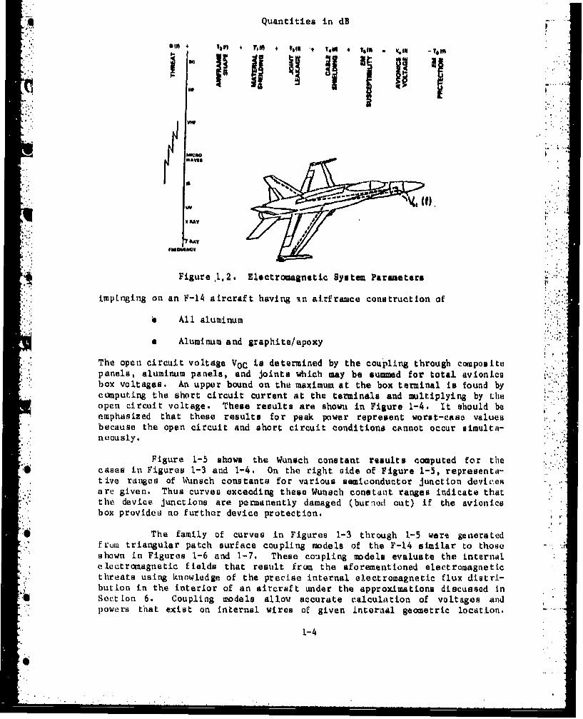
Figuire 1.2. Electromagnetic System Parameters

Impinging on an F-14 aircraft having in airframee construction of

is All aluminum

* Aluminum and graphite/epoxy

The open circuit voltage V0C is determined by the coupling through compositepanels, aluminum panels, and joints which may be summed for total avionicsbox voltages. An upper bound on the maximum at the box terminal is found bycomputing the short circuit current at the terminals and multiplying by L heopen circuit voltage. These results are shown in Figure 1-4. It should beamphagized that these results for peak power represent worst-case valuesbecause the open circuit and short circuit conditions cannot occur simultia-neously.

Figure 1-5 shows the Wunsch constant results computed for thecases in Figures 1-3 and 1-4. On the right aide of Figure 1-5, representa-tive ranges of ,unsch constants for various semiconductor junction devicesare given. Thus curves exceeding these Wunsch constant ranges indicate thatthe device junctions are permanently damaged (burned out) if the avionicsbox provideu no further device protection.

* The family of curves in Figures 1-3 through 1-5 were geaeratedf rum triangular patch surface coupling models of the F-14 similar to thoseshown in Figures 1-6 and 1-7. These coupling models evaluate the. internalelectromagnetic fields that resuilt from the aforementioned electromagneticthreats using knowledge of the precise internal electromagnetic flux drstri-bution in the interior of an aircraft under the approximations discussed AnSect Lon 6. Coupling models allow accurate calculation of voltages andpowers that exist on Internal wires of given Internal geometric location.

1-4

0cmuigtesotcrutcreta h emnl n utpyn ytm•:"•

v-4-

E~-Wii~i~i I bO

t m00 0 r- 1 * 0 10o

DO~

(SI.A A nu4

a -5

- 0

~ iiC.C'

p-B. 0

-f~~ Htfr 0wr I I' 1I,1 -1*

0 0 1 0 0 0 0 0

(M HM('A) HMd Vd

SLM) 'A 1UV1SNOD IIDSNflMwMu LJt)J~ i, I hnih1Z/ -.

1 1111 L-J k i0

a) C.

~~iI~i4-a-0-.0

In 0(n r.)I

rItr1I~? P-

04 w

.14 ýl

(I TM 1VSO HNIM

1-7-

XI I

I L

Figure 1.6. Top View of F-14 Using Triangular PatchData Base of Reference 4

4 1-8

r4r

444)

> 44

'aq4.

60

r34

1-9U

Figure 1-8 illustrates the outstanding agreement in surface cur-runt density JSC, calculated by the well known THREDE code and the triang-ular patch surface model sued in this report. The early time and peak valuedifference between the codes is being resolved at present in the full-scale'F-14 testing currently underway in the Navy's FAANTAEL effort.

The significance of threat rise time, L, on aircraft vulnerabilityis examined in Figures 1-9 through 1-12. Figure 1-9 shows an increase inskin current density by a factor of three for a reduction in threat risetimes from 0.1 jis to 0.2 Ws for near strike lightning. For the NM24P caseshown in Figure 1-10, the peak skin current density increased by a factor of14 for a decrease in rise time from .001 vis to 0.1 lis. These increases inpeak surface current due to the higher frequency content in the short risetime threat spectra. However, they have little effect on interior clrcultvoltages where only joint and panel coupling occurs. This behavior is to beexpected in light of the joint admittance and transfer impedance functioncharacteristics.

Figures 1-11 and 1-12 show the transfer impedance shielding capa-bility of coated panels and the improvement obtainable over an B-ply panelconsisting of graphite/epoxy. The weight penalties imposed by the variouscoating is illustrated in Figure 1-13. Finally, a weight shielding figureof merit is shown in Figure 1-14 using the 8-ply composite panel as abaseline.

The second chapter reviews electromagnetic threats that compositeaircraft may expect to experience. The threats will be natural (lightning,precipitation static) and foe (EMP, laser and electronic warfare).

The third chapter describes the composition, fabrication andmechanical properties for composite materials in detail. The effects ofmodifications, coatings, repairs and environment will be assessed.

The fArvrth chapter discusses present and future composite material andapplications. A review of past composite use for aircraft is presented and • '

future uses, including uses outside the aircraft industry, are reviewed.

The fifth chapter investigates and discusses the intrinsic mate-rial properties (conductivity, permittivity and permeability) as a functionof frequency for graphite/epoxy, boron/epoxy and Kevlar/epoxy. Environ-mental factor influence is discussed and nonlinear properties investigated.

The sixth chapter discusses electromagnetic shielding in detail asit applies to general composite structures. A current list of shieldingeffectiveness measurements is presented for graphite/epoxy and boron/epoxy.A discussion is given for joint coupling in composite panels.

The seventh chapter surveys the susceptibility of modern digitaland integrated circuits to EM energy. Susceptibility curves are presentedfor a number of modern integrated circuits and the implications for the useof modern digital and integrated circuits on composite aircraft are dis-cussed.

1-10

pop

I IW

04

44 -

4.1440 U 0

I g4)

I"

S.) 0

09

. al-

.30E 0

.20E 0

.IOE O

.OOE DO-n21

.20E 0

I ~ -30E 0

* 40E 02

-.60E 02%o~jiO1.~1

OE 02C 0

-,OE 02

9.0E 0

-.I9OE 0.1

DOEf 00 .40E-04 .80E-04 12~E-03 .I6E-03 .20E-03

TIME (1140

* Figure 1.9. Skin Current Density JSC on Edge No. 29 forNear-Strike Lightning Excitation and DifferentRise Times, T

T US

.SCE 031

It a 0.as)

7iue .0. kin CuI en Denit 0c oJEgiN.2mo ranua

Patc Moe0fF13irrf-o aiosRs ie

ofE 0ni3n-NM

410 0-43 --

OCE O SO-07 CE06 IISE-S .2~wO

EM PROTECTION OF METALS AND COMPOSITES ITO"Transfer Impedance Shielding of Structural Materials and

Protective Electromagnetic Cati•ngsIVid kw F tarcnl Sol&* 101 Hi)

?~ ~ ~ ~~ ~~~~7 -if -a? ,,., ,.?..,..•. , .,, .11 A

Alunmwm Panel 0.0010•1Um

Cope r Fo l , 4 wil

ANikel P.11 4 o i

Tin Fel1 4 no

Aluminum Moth

Theltmn 4 ml

oraph~t. Epoxy

PltII

+ n14 Ab K lV LA AI'.:

Figure 1.11. Transfer Impedance Shielding of Structural MaterialsSand Protective Electromagnetic Coatings

EM PROTECTION (rT

Protective Coatings Improvement Relative to Sl-Ply 0/ECVdd fu Pmqueh hidw 10t H,,)

A~1--IL". Ge 4 rollC U U I1 Ir U r !F- or ". M1 M db

AhwukCwwwgldai

A k " * o F ee• 4 w A..

Th- Pd 4 0•11

Ahmb•aM ,Mh 12114 WA

Ahg*MI imi Sony 4 me

Abw~rj Aftrg~rION iAf 1,*AVjeA4?V

Figure 1 12. Improvement Protective Coatings Provided Relativeto 8-Ply Graphite/Epoxy

1-14

EM PROTECTION WEIGHT PENALTIES IT.)

Forward Fuselage AV-8B (Am. - 100 FtM Weight Penalty(Pounds) Imposed by Electromnagnetic Protective Coatings

MONGT MIALTY ILIjh

PeN4 PON4 n

AhWroo Me"134 WA

7 -Ahuebmk PwomNm n 4 m~l

Figure 1. 13. Weight Penalty Imposed by Protective Coatings

EM PROTECTION CT.)

Weight S hielding Figure of MeritlprtsIcla6ondUy" -Ply hU/9vNoydby hiiW*41hof ISquaiFoot of mIrolevs

Akmaml ..m] Pe4 4 A

A4kw Mb10 *iTin~w P1m pas 4 to

Monk FOR 4.N6

Figure 1.14. Weight/Shie~lding Figure of Merit of EM

Protec'tive Coatings

1-15

S- .- - - - - - . - - - ,

The eighth chapter discusses the achievement of EMC in a modernelectronic system from a systems perceptive. The various tools that areused to design and tailor EMC specifications for a given system (in 0h11case, a composite aircraft) are enumerated and described.

The ninth chapter reviews the various methods and techniques formeaauring the electromagnetic properties of composite materials.

The tenth chapter reviews the various protection methods that arenow being used on composite aircraft. The major task of these methods is toprovide lightning and precipitation statics protection. A second task is toprovide increased electromagnetic shielding.

The last chapter discusses the various electromagnetic guidelinesthat are suggested for use in designing electromagnetic compatibility into acomposite aircraft system.

1-16

~ - - - - .. •

2.0 ELECTROMAGNETIC THREATS

The ability to operate successfully under adverse conditions is . -* .Tan extremely important consideration in the design of aircraft using compos-

ite material. The adverse conditions discussed in this section are electro-magnetic in origin and are termed electromagnetic threats. Some threats,such as lightning and precipitation static, occur naturally in the environ-ment or as a result of normal system operation. Others, such as highpowered RF from radars, nuclear electromagnetic pulse, or high energy lasersare man-made and originate from both friendly and hostile sources. Eachthreat Is described in some detail and an assessment made of its possible

posites will be discussed in Section 10.0 on Protection Methods and Tech-niques.

2.1 Natural Threat

In this section the naturally occurring threats of lightning andprecipitation static are discussed. A general description is given for eachthreat; certain mathematical models are presented that describe the mainthreat mechanisms, and a brief assessment is made of the impact of thethreat on system performance.

2.1.1 Liahtni.

Lightning may be generally described as a sequence of transient,high current electrical discharges in the atmosphere.' The lightning flashthat is usually observed is in reality several individual lightning strokesseparated by 40 milliseconds or more. Lightning is most commonly associated 'with thunderstorm activity but may occur in sandstorm snowstorms, dustclouds from erupting volcanos, or even in clear air,.I) Only dischargesfrom thunderclouds to ground will be discussed since most available experi-mental data pertains to this situation.

2.11.1 The Lightning Process - Overview(1,4,5,).

A thundercloud is a dynamic mixture of water droplets, water vaporand ice under the influences of a temperature gradient, a pressure gradientand a gravitational field. The various processes occurring within the cloud

'4 cause a separation of electrical charge to occur with large positive chargegenerally accumulating at the cloud top and large negative charge generallyaccumulating at the cloud bottom. A cloud profile illustrating chargeseparation versus the temperature and pressure gradients involved is showntn Figure 2.1. The charge distributions are usually described in terms ofmajor or minor charge centers in the cloud. These centers act as equivalentsources which reproduce the measured E and H fields external to the cloudbut do not necessarily coincide with the actual charge distribution. The ,magnitudes of the charge centers are typically +t40 coulombs for m:!jurcenters and +10 coulombs for minor centers. The detailed mechanism of thecharge separation process is not known but is probably similar to thefamilar tribelectric or thermoelectric frictional charging processes. Th•potentlal difference between major charge centers is on th.e order of 109volts. This voltage will give a cloud energy of 4 K 104 joules whichrepresents an upper bound on the energy available for the lightning process.

2-1

.. ......._. - ... .... .... . ...... .. . :. . ~....... .. .... .... ..... ...... .. .. ...... ... . . . . . . . . . . . . .

2.0 -W..~) 0,6

+

10-50

ILmure 2.1. Thun~dercloud prol'Llm mhowitng havrge aantori (')Iii -And temnpurilturu md pr -. murtmMramdliamtpi

Ikftor (1))

2-2

Lightning (cloud-to-ground) will occur whenever the separation ofcharge in the thundercloud produces an electric field sufficient to causeelectrical breakdown of the air gap between cloud and ground. The goodweather electric field intensity at the ground is 100 volts/m while theuniform field intensity needed to cause electrinal breakdown of dry air atnormal atmospheric pressure is 300 kV/m. For non-uniform fields, the fieldintensity for breakdown will always be less. The electric fields thatproduce lightning discharges are very non-uniform, being relatively strot4gat the cloud base and relatively weak at the ground.

There are two mechanisms that are thought to occur in the dis-charge process. In the first mechanism, which is dominant for unifonmfields, the free electrons existing in the air gap are accelerated by theelectric field and interact with atoms and molecules in the air to produceadditional electrons and ions through electron-impact ionization and photo-ionization. These growths of electron and ion densities are termed ava-lanches. Numberous avalanches will eventually lead to breakdown of the airgaps

A second mechanism becomes dominant for non-uniform fields.Luminous pulses of ionization, called streamers, propagate out at highvelocity from the high field region to the low field region. The streamerhead contains an interwe electric field capable of producing ionization inthe surrounding air allowing the streamer to propagate rapidly. The stream-er that initiates the lightning process is unique in that it propagates in a

* characteristic stepping fashion. This streamer, called the stepped leader,typically propagates at a velocity of 1.5 x I0• n/sec in steps 50m longwith a pause of 50 microseconds between steps. About 5 coulombs of changeare deposited along the leader channel, which may be 3 km long and a fewmeters wide, in about 20 msec. The detailed plysics of the stepped leader"are not well understood although several theories have been proposed.(1)"

.. Many utilize the concept of a non-luminous pilot leader which precedes andguides the luminous stepped leader.

As the stepped leader propagates downward, the high field in theleader head causes upward moving streamers to be launched from ground or asharp object. Such streamers will be initiated for ground electric fieldintensities of 106 volt/m or greater. When the upward and downwardleaders meet, a conducting channel is formed. The leader head is effective-ly grounded while the leader tail is r;till ac high potential. The result Isa very luminous, positive dischar6o up the leader channel called the firstreturn stroke. Tremendous energy (typically 5 x 108 Joules) is deliveredto the leader channel in a few microseconds. A L-rge fraction of thisenergy causes the leader channel to expand and its temtperature to rise (upto 3 0,00O°K). This, in turn, produces an explosive cy3indrical shock wave

' which is the main source for thunder. A small fraction (about 1%) of theenergy produces the electromagnetic spectrum. The return stroke current ischaracterized by a rapid rise in current. peak value (up. to 100 kamps within10 microseconds) and a propagation velocity of 5 x 10o m/sec. rho strokelasts typically 70 - 100 microseconds.

2-3

- * * , t , A - * * * - * I * .* i

After the return stroke has traversed the channel, current up tohundreds of amperes will continue to flow for several milliseconds. Dur1ngthis time tens of coulombs of charge may be transferred to the channeL.This corntinuinig current is thought to be an important mechanism for main-taining ionization along the cunducting channel for subsequent returnstrokes.

If sufficient chnrge is made avatlable to the channel from thethundercloud in a time of 100 milliseconds or less, a streamer call-ed a dartleader will travrerse the channel. This streamer precedes a subsequentreturn stroke and is similar to a stepped leader except that the steppingprocess is usually absent. Subsequent returrh strokes are usually of lessLnLensity than the first return stroke but otherwise similar in character-istLcs. The total set of strokes constitutes the lightning flash seen bythe eye and is typically a fraction of a second in duration.

Lightning flashes vary widely in their properties depending onlightning type and location on the earth. Table 2.1 .ists a range of values

*for the various ecraponents of a lightning flash as fonuad in the literatture.The values in this table are meant to give a feoling for the orders ofmagnitude involved and to serve as a guideline. The total lightning dis-charge provess is illustrated in Figure 2.2 in the time domain. The wave-fonm is not to scale but serves to illustAte the trend of the data given inTable 2.1 and to summarize the predeeding discussion.

2.1.1.2 Radiated Lightning Spectrum (Far Field)( 4 16, 7 )

Two measured lightning spectra are shown in Figures 2.3 and 2,4and include the contributions of many investigators. The measured range i.'fran a few kHz to a few GHiz. The spectra are normalized respectively to 10km and one statute mile and have bandwidths of 1 kHz, The frequency raigeof maximum signal amplitude is 5-10 kHzl and the amplitude decreases roughlyas the inverse of the frequency. Beyond a few GHz the spectrum has not beennearly measured.

2.1.1.3 _Light Ing Near Fields(2, 4 )

For points reasonably near the discharge channel, the near fieldsof the lightning are dominant. The near electric field is produced by thecharge deposited along the stepped leader channel. An estimate for thisfield can be given by considering the electric field produced by a uniformline of charge of finite lungth. Such a field is given by

P~~ .(1 ,1

27 C- D "--7(31~ 17 2 7 (2.1)(L41)

2-4

Table 2.1 Rhipr~amintativ a Chaucteristics for NuuJd-Lo.-(oulnd,ightuni nq r1a. b n

M4I n irnitial A vor Max' Irnum

Stoppipd Wauder.S op Long th (in) 3 50 21

CTinri I)tw~ ~S1Lo! (tic 0W

Ditut LeadurVe I le t y -, Ptupligaixton (mis/ua) LKJ.0

6 IZ o1fI) ZX10 7

Charge Dep~axitiod on~ Chaunnid (cou) 0, 2

Return SLrukeVelocity of P'ropagMation (m/mkic) 2x1,) 7

U10 3'? .4xRate of Curru~a Rise (ka/usetc) 1 10. 10Timv 70 Paink Current (uski) 0.25 230Pia~k Cuvr,ent (Ka) I 1010,1 M~

Charg, Transferred (vnu) 07 2 2

Channot ~ ~ 6 Legt km A51

totnun CurnCurrent~ ~ ~ ~ ~ DuaiulilA.)5 1 0

Curn Value (a 011 0

ChIar Trnfrio Icu 7

60 11A

Sit .2v106 0 TAKAGI

106 1 nNii 0 HORNER

/gNA HALLGRZN7OENNIS AND PIERC.E o0 OETZEL

Ao 0e~0 ArLA3

o m ClIANOIS.OETZ611.

IS' HOR~NER

0 LT Spectrum20

-C

10 NOFV.IALIZEO TO A DISTANCK

10-4 10.3 10.2 .01I to 102 103 104 Jo

FP 11111.1INCV - WeUFQi'tre 2. 3 Radiated 1.tghtninS spectrum normalized to 10 km (an EMP spectrumis included for couiparison) (4,6)

110 ~ Iap~ HNot"V and 111adla OY441 n

1 13

* ~ ~ ~ ~ ~ ~ ~ ~ Wl .n -A.i 11.-. )WlinadMn.d -~n, .I~!62 1.I L .. i wakes sadI arcu sts.Ila Wi t anm-*11 7 II)kan It.~n IJtI.''yWin *lon'J, ij

t Ham and SIM~1,4* so 7 . SLOPE..~ /IJ '.H 44 ot14

¶0~o and oICOi 0961111t0 4k70~,LC

Fl ~ ~ ~ ~ AvreV 27 Raitdlgtigspcrmnraie o n ttemi 6

I2-we 411Ns1 nl

where p is the charge density, L is the length of the leader channel inmeters, and D is the distance from the channel in meters. As an order ofmagnitude estimate, for p equal to 1 coulomb per kin, L equal to 2.5 kin, andD equal to lOOm, the field is 200 kV/m which is close to the measured value jof 100 kV/mo.

The magnetic near field is produced primarily by the large return .

stroke current which forces the magnetic field to lag behind the electricfield. The magnetic near field can be estimated by considering a currentmoving along a thin cylindrical column. This model for the current givesthe magnetic field

f2j ( 2.2 )

where I is the return stroke current and L and D are as in (2.1).

Several expressions for the current waveform of the return stroke.current have been proposed and are in common usage." 5 ) One very simple,.waveform that is often used is the simple triangular function shown inFigure 2.5. This function has a quick rise to a maximum and a slow decaywhich are the basic requirements for the return stroke current waveform.

The waveform defining the Space Shuttle Lightning Current Wavefonn*is shown in Figure 2.6 and consists of several straight lines bounding thevarious parts of the actual waveform. The result is a more detailed expres-sion for the current which is still simple.

Analytic expressions commonly used for the waveform are doubleand quadruple expoentials. A triple exponential is also occasionally used,but this waveform forces the current to jump discontinuously. A typicaldouble exponential function is given by

lct) -f 1o( '0 - e- t" . :

I - 206 ka (2.3)

a 1.7 x 104 1Iz

1 = 3.5 x 10 1Iz

The waveform for this double exponential is shown in Figure 2.7.

A tripLe exponential waveform is

(2.4) -lI M I o( e 'a t -e '6 t ) + l I 0..

2-7

," , " ' .

74-

200

S100

02 6040 '0 80 0

. Tr Lonti 3 At lightning ;,trtellt WdV.1rM ' (5)

I kA A

,.: " "- .2 20 I 0' 00 A0 11* Ai

I'Igtirv ~( Space shuttle ligiltnin&1 curren~t W-tVufr,tff1

m

ISOA

140

so

1 1

11.6. -7 T q £1IM

I .

4 SI. . .D"

2iue.7 Dojuble expunIerltiaJ lightning 4cutr4Imt HAVohturif

2-8

whe re

Io0 30 k.A1 2.5 kA

a - 2 x 10 lz18 - 2 x 10' lzY - 2 x 10iz ,

,ind it quadruple exponential function is

1(t) " (e -at -t-e')Ot+.I,(C"Yte't) (2.5)

where

10 - 30 ka

1 -2.5 ka.

c 2 x 104 lHz

8 2 x 10 Itz

Y - 1x l0 z 1.6 w 2 x Hz

The waveform for the triple exponential function is shown in Figure 2.8 and '.

the one for the quadruple exponential function is in Figure 2.9. The doubleexponential in (2.3) has a maximum current of 206 kA and actually represents .it , "worst case" situation. The triple and quadruple exponential functionshave maximum currents of 30 kA and are more typical of the average currentIn the return stroke.

The frequency domain representations of these waveforms are in-teresting and are given in Figures 2.10 - 2.13. The last figure shows thesuperposition of all the waveforms and indicates general agreeuent with theoverall waveform for a lightning flash given in Figures 2.3 - 2.4.

2.1.1.4 Attachment of t4itning to Aircraft .

In addition to the effects of the near and far field RF spectra, Atlure is the effect of the direct attachment of the lightning channel to theaircraft itself. The process of lightning attachment is illustratud in

Figure 2.14. As the stepped leader moves downward from the base of thecioud, streamers propagate toward the leader, usually fiom a sharp point of

* thi, aircraft, and away from the aircraft toward another cloud charge centeror ground. When the streamers make contact with the .dtepped leader and

2-9

S-. _..,, +.,.:.:.~u.: .... -._ 4..-.,.,... i.. , :,..... , .... .. " ...... .. . " ....... .. . .-.-. .. .•...... .

U. I

1`4r Ti pl exonn iallihn g curn t waefr

29~~~~ ~ ~ ~ 4- inii010 1w w 10 V

TIME (MIC.IMI o1.

.,1 :tira , A Q ruple sixponentiLl Ilghtning current weveforrn(5

2 0.. 1l

I.

•I ,J 4) 10 10) It*' 1JO ti I40 r Q '111

__.:. TIME (MIC NOSECOXjD5)

___. i.'ll~~~ure •. QuadrupLe iexp~nenliLd £~iahttnln c.utrrnt wevllfu~rmtl•)5

11

*1

* .

\4

SLO"'

L i ' to

wMUCKYM t).,

Figure 2.10 spectrum of triangular current lightning wavefctorm.:

* "9

to

to t .: to0 to,

Figure 2.11 Spectrum of Space shuttle current lightnring waveform' )

2-11

!S

L0

Four-Term blie4IuL&I Pldo.t

to

Figu t 2 12 Uponential. currfnt lightniiof idSveforsM~

to

10"Go -

lig~rs 2.13 Superposition of all l1igtniang currenit w.taotoa~5M

2-12

Stopped leader channelApProachi~ns aircraft

Leader channelH pusslng throush aircraft

Return stroke peaiingback toward cloud

Figure 2.14 LightninS Attachment (10 ) .

2v13

another cloud charge center or ground, then a conducting lightning channelwhich includes the aircraft has been established. A return stroke dischargeup the channel quickly takes place. There are two initial attaChments forthe lightning which represent the entry and exit points for the stroke overthe aircraft.

Although the motion of the lightning stroke is relatively station-ary, the aircraft forward velocity may be quite significant. The result ofthis velocity differential is that the lightning channel is snwept back overthe surface of the aircraft from it. initial point of attachment to newpoints of attachment. This process is illustrated in Figure 2.15. Theimportance of the swept stroke phenomenon is that portions of the aircraftthat would not normally be considered likely points of initial lightningattachment may become involved in the lightning process as a 'result of thebackward sweep of the stroke. This swept stroke phenomenon leads to thedivision of an aircraft into lig1 ning a ieznsbsdo h rbbltof attachment. These zones are ý911 1ikeznsbsdo h rbblt

Zone 1: Aircraft surfaces for which there is a highprobability of initial lightning attachment(entry or exit).

Zone 21 Aircraft surfaces acroes which there is ahigh probability of a lightning channel beingswept from a Zone 1 attachment point.

*Zone 3: All other aircraft surfaces not involved inZones 1 or 2. There is a low probability oflightning attachmoint but the surface mayUcarry considerable current.

Zones 1 and 2 may be further subdivided into A and B regions (6,10,11)depending on the probability that the flash will hang on for a period oftime. These zones are

Zone WA Initial attachment with low probability offlash hang on,)~. a leading edge

Zone IB: Initial attachment with high probability offlash on, e.g., a trailing edge .

Zone 2A: Swept stroke zone with low probability offlash hang on, e.g. , wing mid-cord

Zone 2R: Swept stroke zone with high probability offlash hang on, evg., inboard trailing edge.

Two examples of aircraft strike zones are given in Figure 2.16 and Figure 2.17.

2.1.1.5 Lightning Threat Assessment

The threat to composite aircraft from lightning results fromeither a direct strike or a near miss. Both categories of lightning threatwill be discussed separately since different threat mechanisms are involved.

2-14

,M*

4,

TOt

IS~~ zonet Itth

Zonne -

Cfl Zone 3

Figu~re 2.11 Lightning Itriks Zone

2-1.5

A direct strike on an aircraft takes place when the stepped leaderchannel becomes attached to the aircraft structure. The aircraft then be-comes part of the path traversed by the return strcke. As noted in Section2.1.1.1 and illustrated in Figure 2.2, the return stroke is characterized byvery high currents and explosive shock waves. Tremendous heat will begenerated in the aircraft structure due to the finite conductivity of thestructure material. Because of their lower conductivity compared to alu-mirnm and other metals, structures made from cOMposites are more susceptibleto physical damage (pitting and puncture points) and even complete burnoutof the composite structures of the aircraft. Other vulnerable structuresinclude radomes, canopies, external antennas and special composite panels.The shock waves will produce, in addition, extreme mechanical forces andshock wave heating in the aircraft structure.

In addition to physical damage, composite structures ,re vulner-able to the high electric and particularly magnetic fields that are gene-rated from a near miss or a direct strike. Because unprotected composit:structures tend to offer less EM shielding than metal structures, th_'"electromagnetic fields can more easily penetrate and couple tc the intrualaircraft avionics. Low power integrated circuits on modern aircraft areparticularly sensitive to induced transients of this type. The result ofsuch coupling can then be disruption and/or catastrophic failure of theaircraft avionic systems.

Several lightning protection methods do exist for composite air-craft structureF to contro.e the lightning threats that have been discussed.These protectir-n methods will be treated in Section 10.0 on protection

1 . .Methods and Te.ýhniques,

2.1.2 Precipitation Static

2.1.2.1 Overview

The motion of an aircraft or missile through the atmosphere willcause the vehicle to be struck with dust, ice crystals, rain and othermaterial particles. Continuous particle bombardment of the vehicle willcause charges (positive or negative) to separate from the particles. The

. result is a net charge transfer from the particles to the vehicle creating a"possibly large electric potential. The charging rate depends primarily onthe vehicle geometry, velocity, and the nature of the colliding particles.Generally, charging is greatest for smaller vehicles with high velocitiesand for dust and ice crystal.. If the surface is sufficiently conducting,

*' the excess charge will move to areas of high field intensity, usuallytrailing edges or points of the vehicle. For sufficiently high chargingrates, corona discharge into Lhe atmosphere will occur. These dischargesare in the form of short pulses and are a major source of EN noise inavionic systems. These pulses can be modeled with the waveform(5)

4(2.6)

f(t) Ae*'ot

4 2..

• • 2-16

Both the amplitude A and the depay constant depoiid upon the atmosphericpressure p , as a function of altitude. The atmospheric :.ressure p is givenby

h+O, 002h2760 exp -. ..... (2.7) '

where h is in kilofeet and p is in torra. The para',teters A and = in ,

(2.6) are chosen to be

(2.8)A - 7.90569 x 1S 0 25(2.

a t 2,7777 x 10- 2 (P ~~(2.9) "

to give a good fit to the exponential data for A and a . The noise psec-trum is then given by

s ^(• 1//2 2 ", 12,!." * A( IT (W 41 -1/2 (2.10)

where Y is the number of pulses per minute. This parameter is also afunction of atmospheric pressure and good values of Y are given by

y " 3.83767 x 10 p0 4 8 (2.11)

The noise spectrum is shown in Figures 2.18 - 2.19. In Figure 2.18, theimpact of altitude on the spectrum is shown for several altitudes. InFigure 2.19, the noise level of the spectrum is shown as a function ofdischarge current for a fixed altitude (sea level). ' "'

When electric charge is deposited on dielectric media such asradanes, windshields, or structures of intermediate conductivity such as '"conposite structures, the motion of the charge is restricted due to the S

: partial or non-conducting characteristics of these surfaces. For highenough potentials, streamer discharges will occur on the surface. Thecurrent for a streamer discharge can be modeled as a double exponentialfunction of the form (5)

(2.12)

2-17

100 1 T-rn-OTT rrrr-T-rT-T1rT-7F7-rTTT

40.000 it

20,000 It i--

20,000

IIhI LIV LOKtYN - ______

0.1 1A AC ig-AOW11INCY - Ve

hINUPIMALIRID SPICTAUM INOWING WI.TUOS 9PIC?5

I ArLTITUI 11UA LIVIL

I1l4.JII ASIUM41 COUP~LING MIASUPIGO 10" OUT PAOM TifION PULL-SCAJ IRRAP

,0.10 F L L -LL LLLL-, LLJ j.JLuOIGSrHAM431 (.ýIIMN? -MJA

Ibi 551.AVIONSiIiP OP A16IESOLiJY NO.55 LIVIL TO DISCHASNOS11 CURAIINT

Tlinme 2,19 Noiuse spectruim rpti

CWPMAINY PULSIS180 a 10* COMP TID FOR

-9 A . A1.0M

3 10-4 I,*OCA

I * a

U~ GO"4oC

4of several Lengths 5),a

2-18

where (t) *I (ae"t +be'ot)

im 0,001 ampa - 0.597a w1.67 x 10 lINb - 0.403

6 ft .47 x 10 Z

This current discharge is several orders of magnitude smaller than lightning,discharges. One effect of such streamer discharges is that the EM fieldspenetrate the system arnd couple onto the system avionics. To illustrate themagnitude of this ef fact, the current induced on a wire located just belowthe streamer has been calculated for several streamer lengths; using atypical coupling factor' Y-:3m 1. The results are shown in Figure 2.20.

2.1.2.2 Precipitation Static Threat Assessment

frantheThe threat to composite vehicles from precipitation static resultsf rm hebroad ER fields radiated during the corona or sparking process.

Such fields are a major source of antenna noise. In addition, coupling toavionics can occur by penetration of the fields through composite surfaces(aircraft fuselages) and apertures (joints), such as radosnes or canopies.

Specific protection methods exist to minimize precipitation araticIand are discussed in Section 10.0 on Protection Methods and Techniques.

2.2 Friend/1~oa Threat

In this section, the external man-made electromagnetic threats toaircraft composites are described in detail. The threats considered arestrong RF sources, nuclear electromagnetic pulse and high energy lasers andparticle-beam weapon. systems. A general description. is given of the elec- -

tromagnetic field produced by each threat followed by relevant mathematicalmodels and a threat assessment. :

2.2.1 RF Threat

In this section, a realistic but unclassified, e: ctroinagneticarxvirormient is presented which might be encountered by a composite aerospacevehicle in an operational scenario. This environment is shown in Figur'pa2.21 - 2.24 and is expressed in terms of an RE power density as a functionof frequency from 10 k~z to 100 G1-iz. The power density levels were computedassuming mainbeam illumination at a distance of 500 meters from the radiat-

* ~ing antenna with the target continuiously illuminated.

* 2.2.1.1 RFt Environment(8,9)

The power density at a point R meters from the transmitting

antenna is expressed by

2-19

.41

THI

71 47

...- - -. -i -o~ 81,D

T. -:

94 - R::Tjima tt~z

35ua22 IVVhflft(0 4:-IG:

4 2-2oU

z ITraqmni il35ua22 V~V.~iun 1-1.1C)W

zI

N 1` *~gCy(O: 1oi

- --- .. ~r t - -"---

P CPd (2.13)

where

Pd - antenna power density in watts/M2

Pt o power transmitted in wattsGt - distance from transmitting antenna in moters

The quantity PtGt is often referred to as effective radiated power andrepresents the antenna power available for propagation. Converting (2.13) "into logarithmic form with appropriate units conversion yields

Pd Pt+Gt-10 log(41 R2 ) (2.14)

wherePd " antenna power density in dBm/cm2 .

II Pt - power transmitted in dim :'...•Gt - transmitting antenna gain in dBR l distance from antenna in centimeters

For a distance of 500 meters (2.14) becomes

Pd - Pt+Gt-105 (2.15) "

The input data required for (2.15) are transmitter power output Pt and.transmitting antenna gain Gt. From (2.14), the power density is inversely .proportional to the square of the distance from the source. Doubling thedistance from antenna to target results in a 6 dB decrease in power density ,regardless of whether the target is illuminated by the mainbeam, sidelobesor backlobe of the antenna pattern.

The transmitter power output date was obtained from various mare-lacturer's published specifications of commercially available power tubes.(~8) Several types of tubes were considered and include power triodes,pentodes, traveling wave tubes, crossed field amplifiers, klystrons, magne-trons and gyrotrons. Antenna gains were selected based on typical equipment '

characteristi.s in the frequency range of interest.

In the VLF (3-30 klz) and LF (30-300 kHz.) portions of the spectrumrelatively Sew emitters are operational, the most prominent being the OmegaRadio Navigation stations. Power density calculated based on these emittersassumed a transmitter output power of 150 IW operating into a 32 efficientantenna system. The MF (300-3000 kliz) portion of the EM spectrum is dedi-cated primarily to commercial radio broadcasting. Power densities shown inFigure 2.21 are based on an available transmitter output power of 250 GW andan antenna gain of 3 dB.

iFThe HF (3-30 MHz) communications band is used iostl'y !or medium .

and long range communications. Power density levels in this frequency rangewere obtained using a nominal 50 kW PEP transmitter output power and antennagains ranging from 5 to 12 dB. It is possible to achieve transmitter outputpower of about 250 kW PEP in this frequency range but stations this largeare quite few.

2-22

In the 30-50 MHz public service band (U.S. allocation) the powerdensity levels were obtained using 50 watt transmitters operating into acollinear antenna array having a gain of approximately 3 dB.

Power densities in the VHF TV band were based on the maximum per-missible ERP levels allowed by the U.S. Federal Communications Commission.

Above about 200 Mhz output tube powers were obtained from mami-facturer's published data contained in commercial catalogs and data sheets.(8) The antenna gain data in the 225-400 MHz range was based on variousdipole array configurations. Above 400 MHz, truncated parabolic dishes witha (casecant) 2 vertical pattern and a narrow horizontal beamwidth (for beamantenna) or full parabolic dishes (pencil beam antenna) were used.

Radar systems usually employ a form kf pulse modulation. Thus theoutput tubes need not be able to operate at fu'.l power output continuously(CW) but rather they are turned ON and OFF intermittently (pulsed). TheON/OFF ration is, referred to an the duty cycle., In those cases where thenominal tube data specified duty cycle limitation3 both the peak and averagepower levels were recorded. These are shown as double power density linesfor given frequency range's on the graphs of FiSures 2.22-2.23. The higher

* power density value is the peak power density; the lower line is the averagepower density. If no duty cycle limitations were specified, it was assumed

' that it could be operated continuously (CW); i.e., the peak and averagepower outputs are the same.

- These are the types of tubes most commonly employed in communica-tions systems. The average power levels are useful in, determining componentheating produced by the absorbed RF energy. The effects of average power on

- components are usually frequency independent and will result in thermal"damage or burnout. Pulsed RF fields usually cause induced signals inelectronic circuits and/or components. Knowledge of the peak power levelsto which these circuits/components have been exposed aids in estimating thevoltage spikes induced. These spikes may cause erroneous signal levels inanalog processing circuits; e.g., if they are sufficient to affect a fastacting AGC circuit, bit errors in digital circuits may occur or, if theinduced spikes are large enough, component damage due to short durationvoltage or current overload is possible.

ete In. general, communications or navigation system antennas areeither omnidirectional, fixed installation arrays, or fixed orientationparabolic dishes which have a fixed area of coverage. If an aircraft is"flying a radial course toward or away from one of these antennas it wouldremain under continuous illumination from the mainlobe if the craft is inthe mainbeam pattern or the sidelobe/backlobe if outside of the mainbeam

4 pattern.

Radar antennas are usually designed to scan a volume in space.Fan beam antennas are usually scanned in azimuth only vhereas pencil beamantennas are usually scanned in both azimuth and elevation. When used for asearch function, pencil beam antennas may be trained on a target duringtracking operation. If an antenna is in motion a target may be illuminatedonly a short time during each antenna scan cycle. In the case of simplefixed elevation, 3600 azimuth rotation, the time a given target will beilluminated for each full azimuth scan -- termed dwell time -- is givenby

2-23

".............................- .- -. , -,. ...........-. "...-I • . *'...-.- -... -

T -

•6 (SCN R(2.6)where

TD - dwell time in secondsB - antenna beamwidth in degrees

SCAN RATE - antenna rotation rate in revolutionsper minute (RPM)

Typical search radar antenna scan rates vary from I to 12 RPM. The antennabeamwidths may range from 1.5 to 30. Using these Independent variableranges, dwell times from 20 to 500 ma may be considered typical. In the caseof sector scanning antennas -- either horizontal or vertical scan -- similarrelationships can be developed.

The power density levels of Figures 2.22 and 2.23 were calculatedassuming mainbeam illumination. This is true when the antenna is omnidirec-tional or when a target is being tracked by a high gain antenna. Intermit-"tent mainbeam illumination defined by (2.16) will occur when the target isscanned by a search radar. In fixed installations such as lauding fieldsand carrier decks the radar antennas are usually mounted no that the air-craft parking areas, taxiways, and runways will not be illuminated by themainbeam. In these cases, the aircraft will be subjected to sidelobe andbacklobe radiation. For S4I prediction, it is necessary to specify antennacharacteristics in the unintentional off-axis radiation region. .

A directional antenna has, in addition to a mainbeam or major lobe"of radiation, several smaller lobes about the major lobe known as minor

"*: lobes of the pattern. In general, an antenna pattern may be subdivided intoa mainbeam region, a major sidelobe region and a side- and backlobe region.The mainbeam region is the 10 dB beamwidth of the major lobe of radiation.,

* The major sidelobe region extends to +4 times the 10 dB beamwidth of themajor lobe of radiation for high gain antennas (0>25 dB). For medium gainantennas (10 dB<G<25 dB), the main sidelobe region extends to only + onebeamwidth (10 dB). Side- and backlobe regions extend over the ramainder ofthe pat•ern.

"The sidelobe gain in the major sidelobe region of an antenna willvary depending primarily on two factors: (1) the nature of the physicalsurroundings of the site on which the antenna is located and (2) the main-beam gain of the antenna. As a general rule the approximate sidelobe gainof an antenna may be determined from the information in Table 2.2. Thus,the more crowded the site, i.e., more electromagnetic reflecting objects andthe highe- the gain of the transmit antenna, the higher the sidelobe levels.Therefore the power density levels incident on objects outside the antennamainbeam could be anywhere from 3 dB to 50 dB below the mainbeam gans usedto perform the computations required for Figures 2.22 and 2.23.

2.2.1.2 RF Threat Assessment

The primary RF threat to composite aircraft will come from highpowered radar systems, particularly for aircraft in low level flight.Average power levels primarily result in local heating effects and arefairly insensitive to frequency. Peak power bursts can be much higher inmagnitude and consequently be a threat to devices in avionic systems thatare peak power sensitive.

2-24

Table 2.2 Generalited Of-Axis Antenna Data

Side and BackLobe Region Hajor Side Lobe Region Hainbeam Rea ion

S I9 III 0. G. G,

Antenna Siting 03 '1 'a ' S 'S ~ M 8

Type d 5.l dB deg deg dl B, • S ad An :LB dB dB

Lao Zian To 0.nXibeam beam beam

- a - -

igh Gain open .45 (G+00 ) a 88l Go-33 -35 80 >25 dl Ave -10 (00+.0) 6 ao 8i0 GO-31 -31 6 an So 00 0 2

4 Gal Crowd - 5 -(0O+5) 4 Sao Go %o-7 -27 m- --- '- -

Kedium Gain Open -10 -(0+10) 6 2ac 20 o Go-20 -20 6

10 dlq_< 25 dl AV$ - 8 .(Go+) 5 2a 0 20o-18 -18 5 (o 00 Go 2200 Me 016 tX Crowd - 5 -(1o+5) 4 2o 200 Go-1s -15 4

Low Gain Open - 7 4G Ic10 dl Avg - 5 3 *0 so Go

0<200 NH: crovd - 3 2

0 a, 10 dDi Horiaontal Beamvwidth

0 0 10 dl Vertical leamwidth

If 10 dB beaumvdths cannot be determined, a goodapproximation is to use twice the 3 dB beamvidth

2-25

•",' '_'' '.'L •" ' " ' : ,j " '°J j ' " " ' jJ i J --' " "-J.

*!2.2.2 EMP Threat

The explosion of mnclear weapons in the atmosphere represents aserious electromagnetic threat to composite aircraft. A nuclear explosionproduces an E4 pulse (EMP) as well as higher frequency components in thevisible, x-ray and gamma ray regions of the spectrum. Only the lowerfrequency EMP will be discussed since this threat is well known.

2.2.2.1 Overview( 5 )

The EM pulse in assumed to arise from a high altitude air burst ofthe kind commonly discussed in unclassified literature. The electric fieldfram such a pulse can be modeled by a double exponential waveform which, inthe time domain, has the functional form

SE*t) - o('t oe't) (2.17)

where

o 58.15 kV/m- 6.3 MHzS-189 HHM-

This wvewform has a maximum value of 50 kV/m; a rise to peak time of 0.019microseconds and a time to half peak amplitude of 0.185 microseconds. Themagnetic field is assumed to be given by

no (2.18) V

where no - 377 ohms and is the free space impedance. The SHP wavefors isshown in Yigure 2.25. This waveform in similar in appearance to the doubleexponential waveform for lightning in Section 2.1.1.3 but the time scale forEMP is 100 times smaller. This difference in the time scales of the twothreats serves to distinguish their impacts on a given aircraft. Because of"the time scale difference, there are different frequency components innuclear EMP than in lightning.

The frequency domain representation of (2.18) is the Fourier* Transform given by

e~t)* ~0(2.19)

ii Th+Z1Tjf) (+zr TT

where f is the frequency. This frequency domain representation of the E24Pthreat is shown in Figure 2.26. A comparison to the lightning spectrum inSection 2.1.1.3 indicates that EMP has a larger number of high frequencycomponents than does lightning.

2-26

'-. •i2

60 I

*~40

.~30

.h-.

20

0 0.1 0.2 0A 0,4 0' 0.6 0.7 0.1 0.9

Time (meet~)

figure 2.25 EKW Time DOAmLiA WaVelarv (5)

10"

.- 10- B

.4.4

10",

F Ii• I -- i i

12 1 0 , 1 0 .4 o,10 0, 1 0 1 0 , 7 0 .a 0 , 9

FREQUENCY (HO)

Figure 2.26 IMP in Frequency Domain (5)

2-27

4 S04"

2.2.2.2 SHP Threat Assessment

The &HP threat to composite aircraft Is primarily EM field pene-tration through composite structures and is similar in many ways to thelightning threat. The EKP spectrum shown in Figure 2.26 shows the existenceof many more high frequency components than in the lightning spectrum (seeFigure 2.12). Thus EMP amplitudes will tend to be higher than lightningamplitudes for a given common frequency.

2.2.3 High Energy Laser, Nuclear Thermal Radiation 'and Particle Beam Three atk

Future electromagnetic envirornments will probably include laserand particle beam weapons. These devices are presently the subject ofintensive classified research and development so .nly a very general over-view will be given here. A e tv ne

A primary candidate for laser weapon systems is the deuteriumflorid. laser which operates at 3.8 and is capable of several hundred kW(about 500 kW) CW operation. Another prime candidate is the CO2 lanerwhich operates at 10.6 with an output power of 50 - 135 kW. Otherchemical lasers are being examined such as the Excimer laser" which operatesin the V region (0.25 - 0.25 ) and the Free Electron laster tunable in thevicinity of 3.4 at several kW. There are two primary limitations on theselaser devices:

1. Thermal blooming which is air heating in the beam that reduces ,the energy density on the target. The result is an increase in diffractionwhich defocuses the beam.

2. Aerosol breakdown which is the ionization of particulatematter in the air. A plasma is formed that expands until the entire beam ablocked. This effect occurs at power densities of approximately 10 MW/cm'.

Particle bcam weapon systems are currently being developed by theU.S. and U.S.S.R. It is expected that the effective ranges of these weaponswill be"

1. Up to 300 moters - single pulse2. 4 to 5 km - continuous low PRF3. Greater than 10 km - continuous pulse propagation

The expected effects on the intended target are

1. Detonation of the high explosive charge in

the nuclear warhead carried by the target

2. Disruption of guidance/control/fusingelectronics of the target

3. Reduction or voiding of the yield of thenuclear warhead carried by the target.

Energy levels on the order of 100 - 125 joules/gram are required to cause hdestruction or slumping of nuclear materials, while 210 joules/gram arerequired to melt lead.

2-28

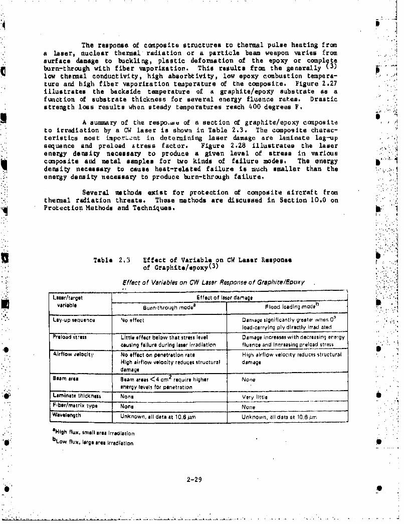
The response of composite structures to thermal pulse heating froma laser, nuclear thermal radiation or a particle beam weapon varies fromsurface damage to buckling, plastic deformation of the epoxy or compl teburn-through with fiber vaporization. This results from the generally (3)

low thermal conductivity, high absorbtivity, low epoxy combustion tempera-ture and high fiber vaporization tewperature of the composite. Figure 2.27illustrates the backside temperature of a graphite/epoxy substrate as afunction of substrate thickness for several energy fluence rates. Drasticstrength loes results when steady temperatures reach 400 degrees F.

A summary of the respo.Lbe of a section of graphite/epoxy compositeto irradiation by a CW laser is shown in Table 2.3. The composite charac-teristics most imporL.nt in determining laser damage are laminate lag-up 'I

sequence and preload Ftress factor. Figure 2.28 illustrates the laserenergy density necessary to produce a given level of stress in variouscomposite and metal samples for two kinds of failure modes, The energy ".density necessary to cause heat-related failure is much smaller than theenergy density necessary to produce burn-through failure.

Several methods exist for protection of composite aircraft fromthermal radiation threats. These methods are discussed in Section 10.0 onProtection Methods and Techniques.

Table 2.3 Effect of Variable on CW Laser Response .

of Graphite/epoxy( 3 )

Effect of Variables on CW Laser Response of GraphitelEpoxy

Laste/target Effect of laser darmagevariable Burn.through modea Flood loading modeb

Lay-up sequence No effect Damage significantly greater when 0'load.carrying ply directly irradiated

Preload stress Little effect below that stress level Damage increases with decreasing energycausing failure during laser irradiation fluence and Innreasirig prelcad stress

,iirflow velocity' No effect on penetration rate High airflow velocity reducts structuralHigh airflow velocity reduces structural damagedamage . . ..__"

Beam area Beam areas <4 cm 2 require higher Noneenergy levels for penetration

Laminate thickness None Very little

Fiber/matrix type None None .i

Wavelength Unknown, all data at 10,6 Mm Unknown, all data at 10.6jum

aHigh flux, small ares irradiation

bLow flux, large area irradiation

2-29

0O

,. . • , -' -- '- - --.- -.- fo

A.

400 .

300100 cal/cm2

20 En r•

100 . '

* 2 mil. White Polyurothee CoatingI% Pf. 4,14 Test Dots

0

WEG SUISTnATE THIcKNuES (NILS)

toIadte 2.17 k-14* temperature of lrApbL4/lP%•a b.

, w~blatrite for several thimlal pus1ue fLuelie 3Avil"*1

- • AIUAN,TH A OUOH

004 - " "i AT"TO

* FAILURE 0 ORAPHIT1tIPOXY (UNPAINTED)'PECII1NS I a BORON EPOXY (UNPAINTiO)

'a B MORON ALUMINUM 1UNPAINTED).. .ORION ALUMINUM (PAINTEO)

* I TI.SAI4V IPAINTEO)-I A1071.TTi (PAINTYDi

.01 .10 102 ,a 1;3 10

ENE ROY OENSITY, kJ1CM"

ftiuIv 2.2 Laser Snarly dlnsity R4OessatY to p1@gO s 'level of stress Env teau lAilue uo 3)

2-30

.,*. 1: i : :i I I i ! i + l II + I

2.3 References

lo tilman, M.A., Lightning, McGraw-Hill, 1969.

2. Strawe) Do., Lightntng Source Hodel. Development, Lightning Workshop, 'NOSC, San Diego, California, 1978,

3. Strawe, et. al., Lnvestigation of Effects of Electromagnetic Energyon Advanced COM20ste Aircraft Structuras and their Associated Avionic/Electrical Equipment, Phase 112, Volume 1, Th-e Boeing Company, 1977.

4. J. Allen, et. al., ATcchnology Plan for Electromagnetic Character-istice of AdvancwŽ.domppaites, RADC-TR-76-206, July 1976.

5,. Wallenberg., et. al., Advanced Composite AMrcraft Electjomaznstic Design r~U and Synthasis, Interim Report, Syracuse Rese~arch Corp., April 1.980.

6. Notebook on Electrical Properties of Comeosites for Frequencies AboveL: LGM:, Atlantic Research Corp., April 1979o

7. Oh, L. Lo, Measured and Calculated Spectral Amplitude Distribution of1 Lighning IEEE Trans. EMC, November 1969.

8. Output Tubu Data Sources (Catalogs): Hughes (lfectron Dynkamics Div);Thompson-CSF; Varian (Palo Alto Tube Division)i Hawawaki; NipponElectric Corp. (NEC); English Electric Valve Coo (ME), Litton Indus-tries; Continental Electronics Corp.

9. Transmitting Antenna Data Sources are based on general antenna charac-teristics act forth in: (1) Antenna fn ineering Handbook, (Jauik);(2) Reference Deta for RadioEngineers, 4th Edithiuo, (TT-r Handbook);(3) ARRL Antena Bo, 3th Edition (1977); (4) AtanaBlake, JohnWiley & Soils, 19966.;(5) A Handbook Series'on Electromagnatic Interfer-ence and Compatibility., Vol. 5; (6) Interference Notebook, RADC-TR-66-1June 1966.

10. J. Phillpott, Recommended Practice fo ihnn Smlto n TestingTechnique for Aircraft, Cuiham Laboratory Report CLM-RH3, AbingdonOxfordshire Engla nd,(19 77).

*11. Schneider, Kendricks and Olson, Vunrblt, uvvblt of Com~ps-ite Structures AFiikA FDL-T-TR-7-127 Vol.. 1(1978).

3.0 COMPOSITION, FABRICATION AND MECHANICAL PROPERTIESOF COMPOSITE MATERIALS

In the first two parts of this section, a general descriptionis given of the composition and fabrication processes of graphite, boron andKevlar composite materials, The various fiber and matrix materials forfiber-reinforced materials are discussed as well as the processes by whichthey are manufactured.

Several procedures in the fabrication process of composites arediscussed. The discussion begins with paper tapes and broad goods, contin-ues with layup procedures and ends with an overview of the different kindsof fabrication procedures used to cure the composites.

Mechanical properties are presented in a series of graphs for thefibers, unidirectional laminates, croesplied laminates and hybrid compos-ites. A brief summary is given of composite fatigue data and environmentaleffects on composites.

3.1 Composition of Composite Materials

The term "composite materials," in principle, may be applied toany material substance composed of heterogeneous parts with distinct inter-faces between the parts. For the purposes of this handbook, the term "corn-posite material" will mean fiber-reinforced materials containing highperformance fibers and suitable proportions of a bonding or matrix materialin order to obtain material properties comparable or superior to metals andfiberglass.(I)

The composite fibers determine the overall material strength andstiffness characteristics while the composite matrix determines the trans-verse mechanical properties (those normal to the fibers , interlaminar shearcharacteristics and service operating temperatures.(U- Both fiber andmatrix are equally important in determining the overall performance charac-teristics of composite materials. A typical fiber-reinforced compositematerial schematic is shown in Figure 3.1.

3.1.1 Fibers

A number of different fibers are available commercially for use"In composite materials. The most commonly used fibers are graphite, boron, 'aramid (Kevlar), glass, aluminum and silicon carbide, Only the first threefibers are treated in this handbook. A general list of fiber types andvendors is given in Table 3.1.

3.1*.1,1 Graphite Fiber

Most of the commercially used graphite fiber is produced by pyro-lyzing precursor polyacrylonitrite (PAN) fibers under tension in furnacesoperating between 250°-3000°OC(1,2) Typically the PAN fiber ispulled through an initial heating stage of 250°C-4000 C where it isoxidized to a stable state. The fiber is then pyrolized at "igh temperaturevarying between 1000 0 C - 3000°C depending on the amounL graphitiza-tion required. Both the mechanical and electrical properties ot the result-ing graphite fibers depend on the degree of graphite crystal structure in

3-1

-4 u 0

1111li ifit II Il 1.

1% lk

E I ~Z

the fiber and the degree of crystal orientation along the fiber axes.( 2 )Both of these quantities depend on the fiber tension and temperature used inthe graphitization process. A diagram of the PAN fiber conversion processis given in Figure 3.2.

Graphite fiber can also be made by heating and crystallizingpitch.( 1 2 ) Such pitch fiber has considerably lower strength than PANfiber. Rowever, pitch fiber procese is quicker, cheaper to manufacture,while the high fiber stiffness would allow its use in automotive compos-ires (),

Once the graphite fibers are produced, approximately 10,000 of theindividual fibers are wound together to produce a larger braid called a tow(shown in Figure 3.3). The tows are then combined with the matrix materialto form the cemposite.( 3 )

3.1.1.2 Boron Fiber

The production of boron fibers is based on a chamical vapordeposition prociss.(1,3) The precursor fiber is tungsten wire preheatedto 12000 C to clean the wire surface. Boron is then deposited on thetungsten wire by passing the wire through a heated atmosphere of borontrichloride vapor and hydrogen gas. Various boron-tungsten compounds areformed in the process. The final boron fiber consists of an inner core ofunconverted tungsten surrounided by a sheath of boron and boron-tungstencompounds.(3) Some attempts have been made to use carbon substrates toreplace the tgungsten wire, but fiber properties are poorer.(I) rhe boronfiber manufacturing process and a cross section of a boron fiber are shownin Figure 3.4. The overall boron fiber manufacturing process is quitee xpe na ive. (1 2)

"p....3.1.1.3 Aramid (Kelvar) Fiber

Kevlar aramid fiber is produced from long chain organic polyimidepolymers.(l,4) The polymer is drawn into a fiber under appropriatetension and temperature using standard textile processes. The fiber has low

density, high tensile strength, low cost but poor compressive properties..The fiber is then woven into fabrics or, less frequently, used in tapes.

3.1.2 Matrix Materials

The most commonly used matrix materials are epoxy resin tapes andchopped fiber-filled thermoplastic injection molding compounds. l,2)Other non-metallic matrices such as polyimide, thermoplastics, polyester andvinyl ester compounds, are upder development. The most common metallicmatrices are aluminum alloys.(I) Choice of a particular matrix depend's onthe composite properties desired and the service temperature likely to beencountered.

The epoxy resins most often used are the diglycidyl ether ofbisphenol A and its dimers, the tetraglycidyl ether of tetraphenolethanetetraglycidylmethyldianiline, and the epoxies derived from novolacs.(2) 14The curing temperatures are typically 3501F or 260°F f~p military orcommercial aircraft and other high performance applications.

3-3S

I•.... .. .

(•wIat|.m C i,•.'n.I.l Ca~r mj,,' aOrrIdll5 i ...

1.000.. 1.501 ..0 1, l el06.

Il e . T,rn4a .. l• TeiI. .'S~

Fib;, S"OvIe jAll. IfingI 7408114. lush

Vibovg ?lbris P0%o,.

TOWMOIIIII|

FIgure 3.2 PAN Fiber •raphLtivation Froce..3 .,

I.,-

0. to"

its e1 IBM$I

rer4'

. 0001D Is .0004 UIs aK+ACTOL sIpoled hiam• atlvrerrib.,,,00

TV4640%O Wife .

Is, 00 Fibers p, Shoeth of Movneanad Tungsltenlompounds

Figure 3.3 Graphite Fiber Tow(3) 3.4 Bor thv WeaUturtug Fracas,

Tog~ther witi 4 locos fiber Cwo~se-goitan

3-4

.. te,.,, t~rŽ .. zn L . -~ -- - I -- -....

Graphite/polyimide materials are being developed for applicationson missile and engine components which permit an operating temperaturebeyond that offered by graphite/epoxy (350 0 F). Current operating tempera-ture limitations are about 600°F.N) These matrices, however, requireexpensive high pressure curing processes (up to 200 psi). A summary ofmatrix characteristics is given in Table 3.2.

3.2 Fabrication of Composite Materials

This section presents a review of the various fabrication pro-cesses t at are used to transform a fiber and matrix into a compositematerial.(I) The fibers are first fabricated into tapes or broad goodsw.hen they may be laid up in a croesplied laminate structure of the propershape. The layup is then cured by a high temperature and/or high pressureprocess. The total fabrication process has a very large impact upon mate-rial properties and total cost of composite materials.

3.2.1 Tape (Prepreg) and Broad Goods Fabrication

As a first step in the manufacture of composites, a set of 'tapes* may be prepared that contain collimated fibers (or tows) preimpregnated with

binding resin. Such tapes are called prepregs.(1) Alternatively, a broadsheet of material may be prepared as a woven fabric if it is necessary toproduce parts that are difficult to lay up from tape, e.g, flanged rings.0()The cost of such broad goods is higher than tape(l) and is Justifiableonly by low.r labor costs or by being able to make the part at all. Aschematic illustrating the prepreg and broad good position in the totalfabrication process is shown in Figure 3.5.

3.2.2 Layup Process

" Thý prepreg or broad goods usually must be laid in a part mold oron a tool.( 1 ) The original process involved manual layups. Such a processis extremely costly because it is very labor intensive. More recent ap-proaches have stressed automated tape layup procedures.(1)

A basic decision that must be made at this point is which talayup method is to be used. One method, the ply-on-ply layup system,''"is a single step process In which the plies are laid on top of each other toform a simple shape. A drawback is that inpection of the total layup is Adifficult and repair of defects very costly. ' A solut on to this problem

--* is provided by another method the ply-on-film process,( 1 ) however a second.. operation is needed to stack the plies on the tool.

The individual plies may be laid up in a variety of styles de-pending on the desired properties and shape of the part being manufactured. ,A symmetric balanced layup is shown in Figure 3.6.

* 3.2.3 Laminate Orientation Code

Because of the numerous multi-ply laminates that are possible forcomposites with tailored or "engineered" properties, some systematic method ,is required for describing the orientations of the fibers in a generalcomposite laminate structure.

3-5.0

: 0 '0

k, * I ,..

SI. p . ".',.'

Ky I +t. c,' -- ' "','*""• .l *1 '

* - -".- f- '1

Iluf i ,.,.,.,..- . 0.' .

p: l~i 'l ,, ...

•1 ,I V. .

* + . .. I j ., -- t~i. .' -..'.' . ..".[j , . . . ..i., ,1 '..,- ".f " - ' I• j _ 1 -

S, ! nni n S.,

"The most commn procedure defines a laminate structure by specify-ing the orientation angles (in degrees) of the various lamina with respect"to a reference direction (which is arbitrary). The orientation angle oflamina with fibers parallel to the orientation direction is 00. Otherorientation angles (including negative angles) are specified similarly. The

* complete set of periodic lamina angles are listed in stacking order, sepa-.. rated by slashes (or commas), with the complete set enclosed within brack-

ets. For example, the orientation code for the layup shown in Figure 3.6,i s y',.•:''

(0o/_45o/90o/45o/0o/0o/45o/900o/45o10o) 0

A simplification is commonly made for orientation codes of thistype. The center 00 laminates act as a mirror for the other lamina."Consequently, the code can be simplified to

(00/-450/900/450/00)s

wha~re the "s" indicates a minor reflection at the right-handed 00 laminateis required for the remaining laminate structure.

"Another common code( 3 ) lists all the laminate orientation anglesas before but not in stacking order. Again, referring to Figure 3.6, thisorientation code would be

indicating four. 00 plies, four +450 plies (two of each sigii) and two900 plies. In using ply orientat-on codes, care is required to determineif ply stacking order is considered.

3.2.4 Composite Fabrication Processes

In this section a brief description is given of the major manu-facturing processes that are used for making coy.osite materials. Theprocesses are of two kinds: direct and indirect. ,') In direct processes,the fiber is combined with the matrix and the composite formed in oneprocess. The advantages to this method are that the method is simple andc; ost-effective. A disadvantage is that the types of geometric shapes thatcan be fabricated are usually restricted. Indirect processes first combinethe matrix and fiber in a separate intermediate stage. The stage is thenfinished in a second procedure. More general shapes are possible withindirect processes but the total processing time is slow and costly.Examples of both procedures will be discussed in this section.

- 3.2.4.1 Filament Winding

Filament winding is a high-speed process wherein fibers or tapesare wound onto a ,otating mandrel with a certain tension and at carefullycontrolled angles.'1,2) It is an important direct process for manufactur-ing composite tubes, motor cases and pressure vessels.(1"

3-7

-- ,'i ', '". . . . . . . .." " . , . • • '. ..- • . " •.

3.2.4.2 Pultruuion P

This indirect process cons"iste of pulling a bundle of fibersthrough a resin bath and then through a hot die to form the part shape andcure the composite. Pultrusion is a low-cost method for producing sttaight"or slightly curved shapes with constant crous-section.( 1 , 2)

3.2.4.3 Braiding

In the braiding process, a mandrel is fed through the center ofthe machine at a fixed rate while fibers wind around the mandrel at a

." controlled angle. The machine works like a maypole and the process appliesto channol sections and webs.(')

3.2.4.4 j~jIettion Molding

This high-volume direct process involves softening a plasticmaterial (with fibers or fillers) by heat, forcing the material into a moldunder high pressure, cooling the material and then ejecting the part fromthe mold. The process is very fastA inexpensive and applicable to manydifferent kinds of composite parts. )

3.2.4.5 Compression Mldiu "i

In this indirect process, the intermediate material is preasedinto the final shape in the mold. The mold is then heated to the curetemperature to bring about a permanent "met" of the material.( 1 ) Curingtime is typically 2 to 3 minutes..

3.2,4,6 Thermal Expansion Holding

Prepreg layers are wrapped around blocks of rubber and the blocksplaced in a metal cavity. A high temperatures, the blocks expand more thanthe metal restraining cavity resulting in high c ing pressures. Thismethod eliminates the need for a separate autoclave.?.

3.2.4.7 Vacuum - Bag Molding

In this method, the preprega are laid onto a mold one ply at atime. The prepregs are then "sucked" against the mold by evacuation of aplastic bag around the mold. A bleeder system is used to remove excessresin and maintain the correct fiber-volume ration for the composite. The

* bagged mold is then cured in an autoclave under full vacuum. The cycle isquite slow and in usually restricted to low-volum applications or longcure-time camposites.( 1,2)

3.2.4.8 Autoclave Holding

This process is similar to the vacuum-bag process except t atgreater pressures are applied to the layup and denser parts are produced.1)

3.2.4.9 Honeycomb Sandwich Fabrication

Two mathodn exist for bonding composite to core materials inmaking sandwich structures. The first provess involves curing the compositefacings separately and then bonding to the core. The second nmthod cures andbonds the entire sandwich structure in one process.( 1 )

3-8

3.3. Mechanical Properties

In this section a survey of the more common mechanical propertiesis given for graphite/epoxy, boron/epoxy and Keviar. Because of the enor- [mous number of individual laminate structures, a complete survey is out ofthe question. Measured values of the parameters are restricted to unidirec-tional laminates and the (0,60) croesplied laminate. More general cross-plied lamina, including hybrid structures, are estimated using structuralanalysis techniques and presented as carpet plots.3.3.1 Compasite Fiber Properties

A very large number of difierent fiber types are available com-mercially for the manufacture of composite materials. Such fibers may becontinuous or chopped and range frcm the aramid fibers used in Kevlar andother organic composites, to the graphite and boron-tungsten fibers used ingraphite and boron composites. Only continuous fibers will be discussed in"this report because of their overwhelming use in aircraft applications.

The key to successful design of composite materials which tailor-made ,echanical properties has been the development of good fiber technol-ogy.(-) Such a technology can endow a fiber with a unique and outstandingset of mechanical properties that cannot be duplicated in the bulk'materialfrm which the fiber is made. The anisotropic fiber composite may then be"engineered" to have special properties in selected directions by justpicking the required fiber and matrix.

A list of fiber mechanical properties is given in Figures 3.7 to3.10. The properties are those at room temperature. A comparison is madebetween several fiber types and between the fibers and metals commonly usedin aircraft manufacture. Specific comparisons vary somewhat from figure tofigure depending on the data available.

Figure 3.7 shows the density of various composite fibers comparedto the density of steel, titanium and aluminum. The graphite fibers aretypically 30% less dense than aluminum while Kevlar is almost 45% less"dense. Boron fibers have about the same density as aluminum.

"Figure 3.8 is a ploL )f tensile strength and tensile modulus forvarious composite fibers and aluminum and stainless steel. Kevlar, S-glassand E-glass tend to have high tensile strength while boron and graphitefibers have moderate to high tensile strength and high modulus. Stainlesssteel has moderate tensile strength and fairly high tensile modulus whilealuminum has low tensile properties. As a further illustration of compositefiber tensile properties, stress-strain curves are plotted in Figure 3.9 for

4 selected composite fibers.

The most important informati• concerning composite fiber mechan-ical properti;i is shown in Figure 3.10. In this figure, the specific ten-sile strength and specific tensile modulis are plotted for various compos-

, ite fibers, stainless steel and aluminum. By specific tensile strength ormodulus is meant the strength or modulus normalized to the fiber density.These data form the basis for marketing decisions of the fibers for aircraftapplications because they represent the ratio of strength or stiffness toweight. An examination of Figure 3.10 shows Kevlar having the highest

3-9.....

~~...........

LL*~ .... woo... I.. .

IT .

1. 17N L

....... . ... ... .. t..i......

7.4.. ..j.. .... .. .. .. .. ..

I.7

-T I .. . . .. . .. .. .

. .... .. . .. . .. . . . - .

-,HNLI MOUU,1II

fg rs 3. Tesl Stent an Mouu of Varou - opdt Fier an H ( -5

3-1

... ... ...

. .*. . .. . p

VIm m. ...,... ...,o,.

TITTI

.. . .. . . .. I ,

..

specific strength and high modulus (HM) graphite having the best specifictensile modulus. Both stainless steel and aluminum are poor by comparison;steel because of its high density and aluminum, because of its relativelylow tensile strength and modulus.

3.3.2 Composite Matrix Properties

The resin matrix in which the fibers of the composite are immersedperforms two important tasks.( 2 ) First, the matrix separates the fibersto maximize their contributions to composite strength and minimize thepossibility of microcracks and buckling developing in the material because 4

of fibers touching. Second, the matrix binds to the fibers sufficiently toenable the material to bear and transfer stresses safely throughout thematerial.•

The stresses to which the matrix is most sensitive are those

transverse to the fiber direction.( 2 ) Longitudinal stresses are trans-mitted mostly by the fibers. In order for the matrix to safely bear and 2transfer stresses it is necessary that the matrix precursor liquid wet the '.fiber surfaces.(e2) The wetting process brings matrix material closeenough to fiber material to allow chemical bonds to be formed. If R is th,rate of wetting of the composite fibers by the matrix -resin, then (2)

where r is the surface tension of the matrix precursor liquid, 0 is thecontact angle of the liquid on the fiber surface, and is the liquidviscosity. In general, r coo n is small which implies that reasonable "."*,'wetting rates are obtainable only with low viscosity precursor liquids, 2)

A number of different matrix resins are in somrin commercial use.The resins may be thermosetting or thermoplastic. 2 The more commonthermosetting resins are polyesters, vinyl esters, epoxy and polyimide andhave use temperatures from 200OF to 6000F. Thermoplacatic resinsincude nvlon 66, polybutylene, polysulfone, and polyamide with use tempera-

tures from 2800F to 5000F.

The composites giving the best mechanical behavior are made fj,epoxy resins and are the ones normally used in aerospace applications. 2 2The epoxy resins commonly used include the diglycidyl ether of biaphenol Aand its dimers; the tetraglycidyl ether of tetrap•e.olethane, tetraglycidyl -methyldianiline and epoxies derived from novolacs. 1'

3.3.3 Single Laminate Composite Properties

In this section, typical measured values for certain key mechani-cal and physical properties are given for single laminate graphite/epoxy,aboron/epoxy and Kevlar/epoxy composites.2,5 The mechanical propertiesconsidered are tensile, compressional and shear strengths and the tension,compression and shear modulii elastic constants (including Poisson's ra-tios). The physical constants considered are density and thermal expansionconstants. Numerical data is given for each property (except density)measured longitudinally, transverse and diagonally with respect to thefibers (00, 900 and +450 with respect to the fiber axes) at both roomtemperature and 3500F- (Kevlar data is given at room temperature.) Alldata is shown graphically in Figures 3.11 - 3.30.

3-12

.K.

' ,,• ' " ": ' • • . i . o : . - • . • • • . . . , -A ~ J t, . .. -'. - '- .. . .... . . . . . . . . -.. . .. . . . . " . . .

14 F..

3-13

i .. ! ____________ j j.

�Ig ..; _____________ I

r' K.. .. "..

I 1

_______ �mvi

____________ [ iii

_______________ n�I V*' ________I- IuI�

_____________________ MI

** � U ,,

U S a a U II N let 1JM - �i....t

mw.N'.Nt

I P

-I U

I U

K * ,

U

*0 !44K r�FLIuLI'- ��E�juji 1.

Li....7K" Ez�EI.1! - -H--:1 I I __________________________________________________

I .. EIIIIZ�IIIIII�LI� 2- ______________________ Iij�* I-I-I-

U

�su UhIiinU Metil IVMflW-UUMZi.e Mwei�aa monsuw�o �ee

3-14*

...... .I

TT IIT

3J5

p0

EZT flmhlof

-II;~ ~ 7I7z~

TW l oo vI -m-l

JTMa" go~i o

__________ 3 -16

0 In.

9'

9. -

_____________________________ _____________________________________ II -'p. 1

*

ii' I

_______________ .- I.; W I: �-� I

An I

* ill

I.,. ri

______ ii �. -

an� U

3 3 3 3 0 P.IaJ1 /u?�Mt *MrntNO� MOZSWf�IU ThUItia& 0 0 6

utguao

I

9

EZZI�� K- H-9.

ii.... 'aIi

�d* �I-'. [L.

p 0 I*awuiso.uasav�u ow;'

.9 .9 t� , * a..' P. * 99 an .9 anuw�e.� zmvm �UMMa

43-17

- - �

"*, The most notable feature of the numerical data is its strong de-pendence on the composite orientation. Longitudinal properties are essen-tialiy those of the fibers as is shown by the large shear strengths andelastic modulii. Transverse properties are much weaker and reflect thepresence of the matrix material. Diagonal properties tend to fall betweenthe transverse and longitudinal properties.

Both mechanical and physical properties tend to degrade somewhatwith temperature. The amount ,of degradation varys with each property but,in general, boron/epoxy appears more temperature-sensitive than eithergraphite/epoxy or Kevlar/epoxy.

_ Figures 3.31 - 3.33 show typical tensile stress-strain curves forboth graphite and boron composites. Longitudinal, transverse and diagonalstresses are considered at room temp.rature and 350°F. The transverse anddiagonal stress-strain curves are considerably more temperature sensitivethan the longitudinal curve.

Figure 3.34 illustrates a bending stress-strain curve for Kevlar,graphite and aluminum. Unidirectinal Kevlar 49/epoxy has a linear stress-strain curve when tested in tension to failure. When tested in comp esuion,Kevlar 49 is elastic in low strain, but plastic at high strain (4) (seeFigures 3.11 and 3.14). This unique compressive behavior of Kevlar 49 makesit resemble a metal in its ductility which is illustrated in Figure 3.34

3.3.4 Crosplied Laminate Composite Properties

Crosaplied laminate design strengths, elastic properties and phy- "sical constants are presented for the boron/epoxy and graphite/epoxy sys-tems, Croseplied laminate property data are difficult to treat in generalbecause of the many structures that are possible. The croosplied laminatesystems presented in this section are limited to (0/+60) orientations andthe general orientation family (0i/+ 4 5j/90k) for graphite and boron/epoxy, where the i, J, and k coefficients can be adjusted to any proportion(including none) of the three lamina angles. By proper adjustment, virtual-ly any design requirement can be met for preliminary estimates of crossplied . ,laminate properties.

The properties for the (Oi:+4 51/ 9 0k) are given in Figures3.35 to 3.61 in the form of carpet plots with the percent of 00 and +450plies treated as independent variables. The remaining percentage of pliesare 900 by definition. The carpet plots were generated by computer usingstandard structural analysis algorithms.( 3 ) The unidirectional laminadata (such as given in Figures 3.11 - 3.30) are a basic input for theanalysis. The curves given in Figures 3.35 - 3.61 should be construed as aguide to general croesplied composite behavior and not as a set of designcurves.

Figures 3.62 - 3.71 present measured mechanical and physicalproperty data for the (0/60) laminate family fQr boron/epoxy and graphite!epoxy at room temperature (RT) and 350°F.(3 The properties are mea-sured with stresses longitudinal (00 with respect to fiber axis) andtransverse (900 with respect to fiber axis) to the fibers. Where no

, direction to the fiber is given, the property is isotropic. As in the caseof a single laminate, the properties of the (0/60) crosaplied lamina degradesomewhat with temperature, especially in the case of boron/epoxy.

3-18

f .t, a

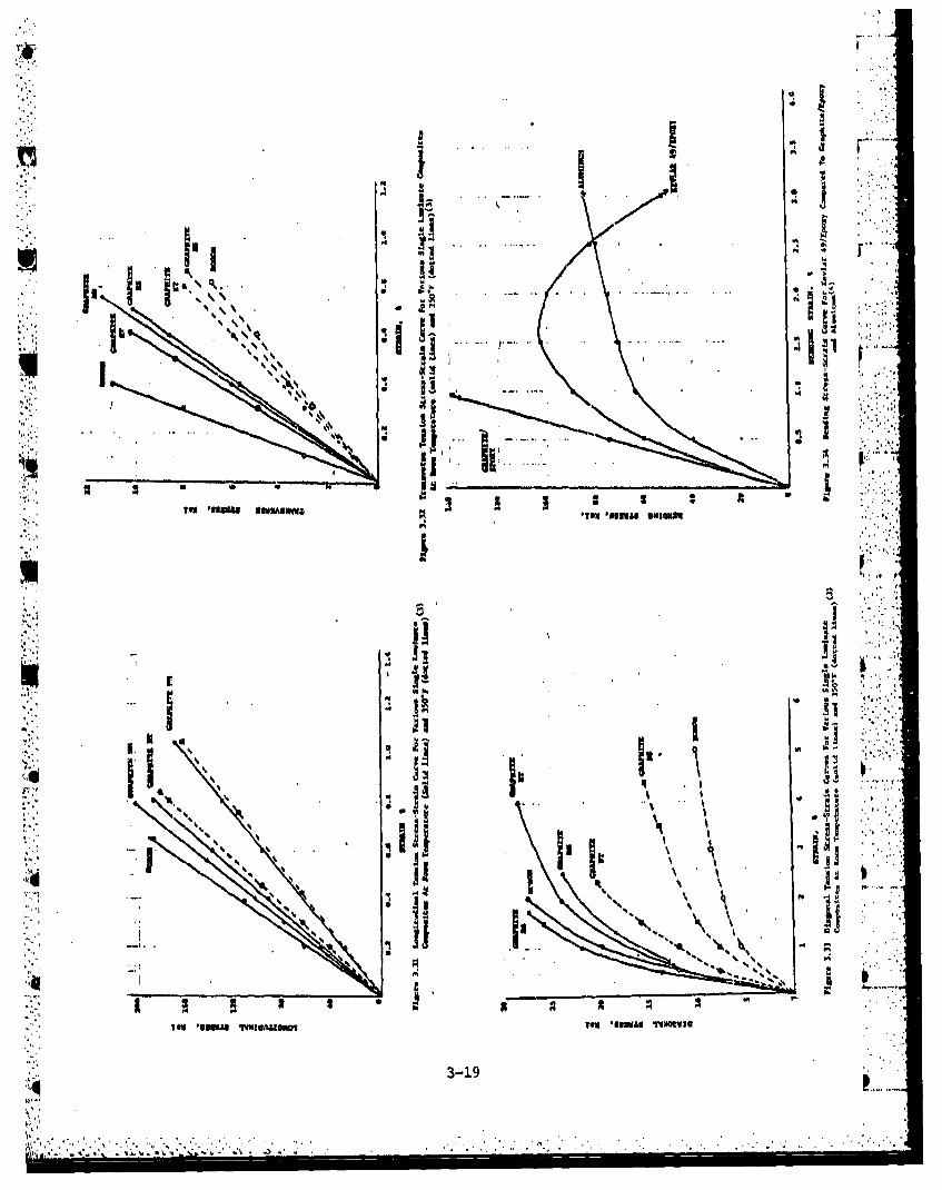
141

To INN U 0ma

3-19

IA

C3 2

Ukj L. .

'4l

I rf -7-

Tori ano HUH 56VdN

3-21 :..

k W I.-

C PC

3-22

a FLJo I ..

II' 0I

"Tom I I& UM g01 od~o Ta IIA BSS dO

'S 0 *0

* II~ ~ IV5, . I.

a 0I * . - I *

o , ., .5 5.1 ~IA

lax 0INW1 WTSIX NH!NI~ RISR

- . 'I, 3-23

-. . .

Il I l

........................................... 4.- .,...~. *.*go

U...II 9 -

~4 5 0 * 1 \sT w v n c m v w

LiIITI smnl WHISUM

mm 41o wog~m

- I3-24

ini

I.a C,14 ] L o 00/UT/ýT a /UTU~n P

L 1

I cci1

. jaL v 9. .*97 O o l .; j 0 1 ' 0 -. 9 ,

~j*~ .t N~ N w*,3-254

q

I I*I *I*,,.�' r.1 I! �.,

F I- ii

- 2*3-I

3--� 34

I a - -. I-- *.. I .� -i-...

-

WM113 I

- .

-, '� m.� � �-K-*>.-ii I *� ,�

� Iv I.-'U � .TIJ7�K ii V

A A �I , � �j !

I. - , S* I I.z .

I I

.. �

a,I..I IIovIii> .:� i *'�j�*�� II .�

*�3%

.1 -

a .1...;..

.�L *�!

TUN 'It�ONR1bLg 2'IIBN�La

3-26

* K

~K.MOULU1 MODULUIONITE/ITPOXY

A. A

InMICH2. i.CLS0IANU1PX

If 0 40 .0 x a Ili

00 411 to4 60 111.

4 41' P~ies

Figure 3.50 Shear Strength Curveso For The Iligh-Nodulus (b) 3501FGraphUti/Epoxy (0i/+t4 Sj/90k Laminnate IFamily -ouuAt ERo&N Tinaperatursl (P.?) and 350. (3) Figure 3.51 Ext.onu~olia1 Modulus Curves For' the High-lous

(Jr0IIhita/El1oxy (Oi/±45j/9Okl Laminate Fdoiiiy~i)

HIGH.MOOUIUSO41APHIIu7Ipoxy]

iiiliiillilW .N )S . ,-

0 10 so 30 40 SO 0 70 b0 I') c

Figure 3.52 Shear Modulus Curves For The 4igh-Modulus CrAp~iits/F~pooyrO±I±45j190'kJ Laiae Uaily AL R~oom Tompwratture (lIT)

and 350,F(3)

3-27

q

I . III I IIi iii

- I.'.. V

I I I K.I - I : : �

I I

EL.. �R

I� � , I.I� :.� !�

-

-� � *1I -

I-. I a- *1 - U - 0 - - N S y a

A 0/uT.iuTrI,�NZroXdd�oD � .LNZI�?AA�O� NOr9NVdX3 4'

I..

- I *jL. I**Ib� --..i�I .Iv .� .

* I2 K 4Th

I' -0

V I �I . SI 1w 'I

6 I

,--....�.

2

.411.3 I .. �..:

SI �*

K a* I..

'U II .* I C .J 0 U,

oI.LVU i.ossxou or.LW S.NOfltO.I

6 I-I-

3-28

.4, S4J

b'4 4,

' 'si 44

ri a '� .. ,�04 4.4k. S44 0� Ii

4., I � IN 1404,

In 44 '4

rs Vi�4. I a at

Ii,4, S. S11 '4

'.4 0 '4

.4 �. m� ' �

* IN

- 4* 0 -' I,,

'.4 '4 �

4-.0 N

0 0 0 - p� *� ri II

I-. - 44 -�U)I *,..rn.n.s... " N .�

nuaiauwo �AL0V��dWOO I .4.

444

444

01*�,4��I

'.4

44� '.�

If I'*p..I.4.4 . 11.411

b. .444

* - I

4.. , _

* �' K� Is. � I I

4 v j � � '*1 �' _... �.

a . .� �.

4. 0 .

.4 � . I *

.4 j . - . I � V4�-.14 . 44

-� I! I '� I

I I 031; � 441

- - - -

1')4 'lILDN�4�IJg 3�IISN3,L lfX 'I � IIISMId.L -'

44

6

3-29

I..�A 4� AŽ � *** *�.*. * � ............................ *

diiIn InI

Ifdo do

* --- 4. I.. \.*--f

taw0 Isnqao im sm s&* wwinno v

6.w I 'inlw11HKNZ

7 al

4,A

U, a~ *Sol

To m1N0142idsNv*l

I3 30

41Mmm iv5,

/UTU,

0i 0 mM 3 0 a4o N, , , . . .~ T"

7 .u

.114

041

*~~ - , J '3-314.

*

4'I'

____________ I .. -4

I'll . � ____

*1

S .-..

k I_____________ -�..-.- .,. V.

________________________________________________ '4

______________ I -.

3 3 2 1 3 3 .1 � �.. U j1,1 uaminumauua I �, isuu.aa 3 0

p.:.

*1

�

I E±II'�.0 III .

_____________________________ -iiIII1, r

_____________________ II- EZIIIIIIZIIIIIIZIIIZIZIZZII

3 3 1 £

im UImM WIIgUA iIu auiinu inainriim

3-32

*

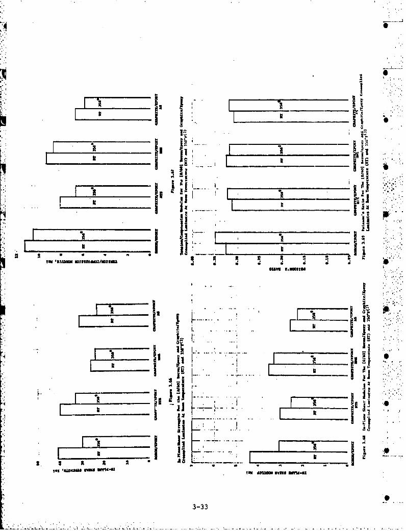
4 O

3.

I.

II LTmIII.1

� -w 0�

iiW... ii________________ I�IL.. ______

______________________________

ii A

* a 10oxaw vunsiw

I'

i�L--

A:11ik .11

I.. * '.1F L

h I _________ I .�4

:a a * 1 II Liii�i � iS

3-33

. . , .

4.0

.14

13560T ST 35

soikOH/ sWo2xv 411G INAP NFlIU O X 0KAPIu1TN/ qtp gIY O NAPIIITU/U1IPOXV

"MT o "No A s

figure 3.10 Thermal SUPAnhiOn COM tnm fti for The 10/601 IWirn/NpoXYq Craphit.m/1IIL 1KY

Cromiiplied Laminate*a At Rol., Temperature (IT) end 3 304PIS1

a.'t

fil 7

J,,

polio

POXas3 4: .

01IuHtaaPr(,'O r.8a~ n (ght)PX raialu Mi~tU 3

QMPITIOUIHI3-34lIT

SLOX Epx .

. -

3.3.5 Hybrid Composite Properties

Hybrid composite structure, consist of a combination of two ormore different composite fiber types in a matrix material. Since a myriadof hybrid structures is possible, three common structures (boron: graphite/epoxy, S-glass: graphite/epory and Kevlar: graphite/epoxy), will be con-s ide red.

The boron: graphite/epoxy system is (08/+45GE/90 E)s with keyproperties listed in Table 3.3. Values are given for longitudinal (00) andtransverse (900) orientations with respect to the laminate and for roomteomperature and 3500 F.

The S-glass: graphite/epoxy and Kevlar: graphite/epoxy hybridsystems have been recently evaluated by Boeing as possible approaches to lowcost composite structures.( 6 ) The basic idea is to place low-cost fibers,such as S-glass or Kevlar, in secondary load directions and place high costfibers, such as boLon or graphite, in the primary load direction. Costsavings for the hybrid laminate over regular laminates range from 10% to40%.

The S-glass: graphite/epoxy system is (S-glass/T-300 graphite/S-glass) and the measured mechanical properties are given in Table 3.4 foraeveral test orientations and temperatures. The Kevlar: graphite/epoxyhybrid system has the configuration (T-300 graphite/Kevlar-49/T-300 graph-ite). The mechanical pg~erties are given in Table 3.5 for several orienta-tions and temperatures. . .

Boeing( 6 ) has generated a set of design curves in carpet plotformat for use in constructing hybrid composites composed of S-glass:graphite/epoxy and Kevlar: graphite/epoxy. The curves for the S-glass:graphite/epoxy hybrid aro given in Figures 3.72 - 3.76 while those forKevlar: graphite/epoxy are given in Figures 3.77 - 3.81.

3.4 Environmental Effects on Com osite Materials

The information in this section is a summary of data available onthe various environmental effects on the mechanical properties of graphite/epoxy, boron/epoxy and Kevlar/epoxy composite materials. All data ispresented In Table 3.6 and the impact of each environmental effect ismeasured as a percent degradation of the unperturbed properties. The rresults should be regarded as general trends applicable to a whole class ofmaterials.

3.5 Composite Fatigue

A limited set of fatigue data is presented for boron/epoxy, 4graphite/epoxy and Kevlar/epoxy in the form of stress-failure curves underconstant amplitude cyclic loading conditions. The data are meant to give ageneral feel for the fatigue behavior of composites and not to be used indetailed design curves. The data is displayed in Figures 3.82 - 3.85. Ingeneral, the unidirectional laminates give the best fatigue results with ageneral lessening of values for crossplied laminates. Fatigue characteris-tics also tend to degrade somewhat with temperature as is shown for boron/epoxy in Figures 3.82 - 3.85.

3-35

Table 3.3 Mechanical Ptapertlao for The boiren;graphits/spescyHybrid L~mlnato System [0 /±4509/9001)

PROPERTY VALUE

PROPERTY ORIENTATION_________ _________

___________________ROOM TEMPERATURE 330*

TINSILS STREbGTHi, kaL 04 54 4090, 5i. 40

'7COMPR'ESSIVE SITRENGTH, kal 06 177 9690, 38 22 40 -

IN-PLANE SHEAR sTRINGTH, kal 0of' 27

TENSION MODULUS, mei 06 1. 10.5

90, 6 5

COMPRESSION MODULUS, lat of 11.5 10.5

90' 6 5*IKMAL RXPANS?104CONSTANT r.±n/±in/' 06 2.5

900 3.0

DINSITY Wbin 3 -0.061 0.061

Table 3.4 Mechanical Properties qf The (8-slams/T-300 graphite/* Us-glass) Hybrid Syfstem 6)

(S-OL/T300S-OL)

rST ORIEN- AVERAGE PROPERTY ATIPROERTY TATION -65F 75F 260F 350F

TENSION STRENGTH. kSl do 151.4 106.2 160.6 131.145O 28.0 33.7 34.7 28.8

pop 90 2.6 25.3 28.5 27.4

TENSION MODULUS, 10,. psi do 6.1 5.7 1.9 6.1P450 4.2 4.4 3.9 4.0900 4.6 3.6 3,4 2.9

COMPRESSIVE STRENGTH, 00 102.2 101.0 58.4 43.8kii 450 68.2 63.8 S6.2 43.1

90* 51.3 51.3 41.2 33.8

COMIPRESSIVE MODULUS, 00 8.7 9.2 8.5 8.6108 psi 450 4.1 4.7 4.1 3.5

too 3.7~ 3.8 3.4 3.1

IN-PLANE SHEAR SIRENOTHO 00 67 27.6 26.4 22.14 ksi

INP NE EAR MODULUS 0 1.9 1.8 1.6 2.I

INTERLAINAR SHEAR, 00 9.0 8.7 8.2 4.9ksi

.3-36

Table 33~ Machaic~~al Froportt.us of the (T-300 Rgraphits/KoviAr 49/T-300 gaphihtt@I Hybrid Syst,. ~ eea.TaOrLoutstioas and Twpratura

(T300/K-049/T300)

PROER' I!T 0IEN - AVERAGE PROPERTY AT:TATION -6FS 7F 250F 35OF

TENSION STRCNGTH. ksl op 93.6 '109.6 110.1 89.7450 42.4 41.0 41.9 30.7

TESIN ODLU, o6pa 0: 3::: 32:3 33.6 33.1

450 4.0 3.8 3.0 2.6.00 3.1 3.7 3.4 3.6

COMPRESSIVE STRENGTH. 0P 31.8 ' 112.5 113.? 102.7kii 45 41.4 37.3 23.1 14.8

30P 40.1 53.5 44.3 20.9 1-COMPRESSIVE M9ODULUS, 0* 6.5 6.7 6.6 6.1

106 pdt 450 4.4 3.5 2.6 2.0

too 7.3 3.8 3.5 3.5

IN-PLANE ShEAR STRENGTH$ 00 23.9 27.2 23.2 16.2ksl

IN-PLANE SKIAR MODULUS. 00 1.4 1.6 1.1 .9106 psi

INTERLANINAR SHEAR, 00 9.3 6.7 4.8 3.2

3-37

Table 1.6 Data Sumary of tavitesteal tffesis on olopsimts 14M64wsi prteerite*s4

MA

* fiFOSTU SOsOa/tPOXY GRAPNITM/2100111 KRYLAS/9UUXO

Iliaidley Ambient humidity has little offset it Oil Ambient humididty bee little offsetrelative weiusiity for $00 hours at M"I. at *Sl relative humidity add l20'r301 toddtitnIni int atolamitar shear fat 23 day, little Change inItuiolti find 010 reducituio In flexure 'aor strength tos eima..

* tfrilth~l At010 add 251.1 lealikodlsivlflosural, trangth rodomad by 60140d 101. T1ign"evf. lexurestranghti mild ifiterl~imar ahever

salt splay The 250.10 fleure. atressgirieardg ,do .s worem ; HMR 1 .' tap.W.- Pr. n snit water sal.wasaiduf 201, tirtarliMiAGt WOAtiahS UelSAtij,. turd Vaeralsional strength after toelsle stralketh tidued

Ittresa4id panll ahmwd 251 doormens. In 35 day walwoirs- Plausa filre"4111 4y0.52

aepasura ~ ~ 14 a ar aprtr.iiat. romt g lrahsa gae .121a

leftolop straothsV.,1464 f&.: 30 ays eotlm Isd ahunt.ov astreath

ares teprts isra eaa yaltur4 1 W hair boil

over ~ ~ ~ ~ ~ ~ ~ spoe to11 4Alsste*16Per Itpisai *Tumap.roo wollatio reolven~. flag.hreue affclearrdat bay 90 oass Exposure

Iner on sraonloo ranod byIll Alstar $ shousea4fr mvsAysv kl s.etalshwe is eraagtrdxouwia ro 11-411prtr.ala.N rpiegv 4 i taost oline sn2-4o

-~~~~euku In______ flated I0-lZ0Lfi1ill!-

aaClwmm~tland"a 071'7 mo mid In Utr~fit. Fame-M b

1 1, hydrlluorc &a3-38i

.II

'S ~ il I.",...A !]• .,

I I IL

d., -,3,'~Ii I! I;• ..ii . .'- . ,.,.

Sit '4i/I

IS-i., .:: .•1

' U. I,.', '

S' t 1,'.

• I i e% i

3-39b S

K" nMR~n#io 4

0n IF 140A

AS IHIA Ma~uLAW (0")

%,i~eKIV-40 IS 416 1V-49

lip J~t kMNAILITIMII~mmsiim~imFlom. 2.1 LAMAINA" I 1 a VIRIUS PIECINf1416W~O LArnN? OP LtC.&IPUCXCIM

(0VIUA KIIOf ' IAIt0" e 4~) FAMILY (4)

lom TIMNIAIWI

full

POIUONI LIAllOhi~ (a,, W) TIIIIAL

.0 *6 '5, IN

meV

.. .

f~ ~eiPIIN6PTO4T1O01V-49-181/fln Flow. 3.81 LONGITUDINAL COEFFICIENT OF VIERUAL IC~WANIOPlOW. ~ o 1.6IFOCNWARI I ~.CY.049-)IIAlo le *ee FAMILY 46),ela~elpe) FAMILY I

3-40

IGO 7,

. . . . . ...... ... . . . . . . . . . . . .1Lh~iJ.J ~14 TLH ~ FmPERM'u1 sI' I H

160

azo

140

12 1

IGOI

r fTF 4I~fi V u103 4 5 6 1 7

10 1010 0 0CYQI TO rA.. . .-

.1 A20~~:1 0 .i I

40L 7I. ...... . .. 1

3-4iiA0/4/4 1

m- - . - .,'.:..-. *-.... . - -

1 .171 ~ ~1if~ ~VT 1F r

II GAPIIZTU/XPGXY

10 .. .. ..... '

Fi~~u1ru 384 PliLAIT2UL7XV .. 4

... T O.

10

I.-

I T.I

.I ... .... .

71. 7.1

10 100 100

TMIN TO MOR~U~E, HIOURS ~Figure] 3,815 (.onntant Amplitude VAtIgue Data Fa~r Unidirectional KSvvlar/Epoxy

AL Room TemrperatureA anR01( 4)

3-42

I!

3.6 References

1. DOD/NASA Structural Composites Fabrication Guide, 2nd Edition, Vol. IMay 1979.

2. P. Beardmore, et.al, Fiber-Reinforced Composites: Engineered Structur-al Materials, Science, Vol. .208, 23 May 1980, p. 833.

3. Advanced Composites Design Guide, Thiri Edition, Air Force MaterialsLaboratory, Wright-Patterson Air Force Base, Ohio, Vol. I, 1973.

4. DuPont Technical Information, Characteristics and Uses of Kevlar 49Aramid High Modulus Organic Fiber, Bulletin K-2, February 1978.

5. Graphite Materials, Hercules Inc., 1976.

6. J. T. Hoggatt and A. L. Dobyns, Evaluation of Hybrid Composit(s, AFML-TR-76-53, May 1976.

3-43,

o , . ,

4.0 APPLICATIONS OF COMPOSITE MATERIALS

Composite materials have been in extensive use in the aerospace in-dustry and other commercial sections of the economy for a number of years.The first two sections of this chapter profile the past and present applica-tions of composites to various commercial and military aircraft systems withsome space applications. No attempt is made to be complete but a good rep-resentative survey of such applications is given. The third section dealswith certain specific problems in using composites on aircraft. The lastsection projects future trends in composite use for both the aerospace andautomobile industries.

4.1 Early (pre-1973) Aerospace Composite MaterialsApplications

Composite materials have been used on aircraft and spacecraft fora number of years. Although much interest in using these materials has beenvoiced, past applications have been limited to small secondary structuresand have involved principally boron and glass-fiber composites. A represen-tative history of pre-1973 composite applications is given in Table 4.1.The history is not meant to be inclusive but rather to illustrate the typesof composite structures that have been fabricated, the variety of compositesthat have been used, the aerospace companies involved, and the weightsavings obtained from composite structures over the counterpart metallics tructures,.

4.2 Recent (post-1973) and Current Aerospace CompositeMaterial Applications

"Numerous applications of composites to aerospace systems have beenmade since 1973 and will continue to be made in the present and near future.The prirwcipal materials are graphite/epoxy and Kevlar, both individually indas hybrid compos'ites. This section presents a representative sample ofrecent composite applications to aircraft, propulsion, spacecraft and phelicopter systems. Two very interesting applications, composite mechanicalfasteners and aircraft seats and galleys, are included. Each application isdescribed and the actual or projected weight or cost savings obtained usingcomposites is given. All recent composite applications are summarized inTable 4.2.

lp4.2.1 Aircraft Systems

Twelve uses of composites on various aircraft are presented inthis section. Both military and civilian aircraft are included.

4 4.2.1.1 McDonnell Douglas DC-10

the )C-10 uses composites on both a secondary structure and asmall primary structure. The primary structure is the vertical stabilizer(2) which is fabricated from graphite epoxy. The composite stabilizer hasa proJeoted weight savings of 20-22%(3) and is scheduled for completion in1982. 2)

4-1

Table 4,.1 Composite Application History (b-qforo 1073)(1)

FecIFTWei± ht

Component Manufa'tursr campagits Savin

Aircraft SystemsF-ill Horizontal Stabilizer General Dynamics Boron/Epoxy 27%P-4 Rudder McDonnell Douglas Boron/Epoxy 36%P-14A Horizontal Stabilizer Grumman Boron/Epoxy 191P-l5 Horizontal Stabilizer McDonnell Douglas Boron/EpoxyA-4 Horizontal Stabilizer McDonnell Douglas Graphite/Epoxy 201P-100. Wing Skin Rockwell Boron/Epoxy 25.8%

P-111B Wing Box Extrusion Grumman Boron/EpoxyC-IA Leading Edge Slat Lockheed Boron/EpoxyP-1l1 Aft Fuselage IrBoron/Epoxy

General Dynamics jGraphite/Wpxy 191P-6 Aft Fuselage) (Boron/AluniinumF-S Landing Gear Door Northrop Boron/Epoxy 221

Engine SystemsJFT22 FIrst-Stage Pan Blade Pratt A Whitney floron/Platinuir 441Pan Blade General Motors Boron/Titanium SolJT422 Third-Stage Fan Blade Pratt 4iWhitney Boron/Aluminum 3..T56-A-16 Gearbox Case General Motors Boron-Glass/

Epoxy 3

Space Systems"Reentry Frustru i General Electric Boron/EpoxyMissile Interstage Boeing Graphito/Spoxy 271Missile Payload Adapter General Dynamics Boron/Aluminum 401T,"bular S truts Rockwell Boron/Epoxy 301Tubular Struts Northrop roa raphite/Epoxy

IGIass/Epoxy46

* Helicopter SystemsCH-47 R.tor Blade Boking-Vrtk l Boron/Epoxy

(Glass/Epoxy

S-61 Tail Rotor Sikorsky (Boron/Epoxy 5

CH-54B Tail Cone Saorsky Boron/Epoxy

4-2

-. 1--- .1

Tlable 4.2 Present (post 1973) and Near Future Aerosplace Composite Applications '

Comeponent Manufactura r Composite Commenft aAircraft SystemsDc C10 Vertical Stabilizer (2 ,3 ) McDonnell Dlouglas clrsphlte/lipoxy Ready ii 1982i 20-22t

wei44 sav ingsIXD-10 Upper Aft Hudder (2,3) McDonnell Douglas Graphitu/1lpoxy 17% wolgIht saviiigs

*727 iLlovator( 2 ) Boeing Graphite/Spoxy 26% weight suvings737 Hlorizontal Stabilizer(2 ) Boeing Graphites/Epoxy Ready In 1980-81; 23t

we ight sauvings11L-1011 Inboard Aileron0() Lockheed (lraphite/llpoxy Roudy in 1980; 2011

weight savingsL-1011 Vertical Ilin (314) Lockheed Graphite/Hpoxy Read inl 19821; 301

*Lear Ilani 21OU~ Lear Avisa araphite/Upoxy All-composite air-frame and wings

7S7/767 cnntrol -SurfacsC23 Booing raphite/Iox ed inicIU%'

747 utbord Alero ju261 weight savings74ubard Cowl Panels Boeing Graphite/klpoxy on ailerons Lind 38%on cowl punuls

*AV-4B Wing Skin and Prumes 1-I McDonnell Douglas Grsphitti/ipoxy 20% weLight savingsiP*16 'rail Structure( 7 ) General Dynamics Graphite/ilpoxyP/A-19 Wing Skin Mc!)onnell Doumglau/ araphite/Hpoxy Sol of aircrart stir-

Northrop face is compositeC-141 Wing section110 ) Lockheed Graphite-UluWs 751 lower mainten-

Epoxy ance anid repair costsTIIK-90 Lamiding (ler DJoors(")~ Mosserschmidt- Pliberfiass/Iipoxy'1

11nd Ila rings Booikow-Blohm Graphite/poxyIlormiler Light 'rrrunsport(12) Dornier Glass/Kevlar Ready inl 19801s;

Graphite/Epoxy largo coepositoPronulsign gystems surfAce areaR11,211-535 Engine Thrust Reverser Rolls-Royce Graphito/Upoxy To be used on Boeing

and PFn Noa Access 7S7; reduction ofDoors' 15-201 in enginme

weightComposito Propelier( 14'15 ) Hiartsull Xaviar

T . 1. DevelopmentDowty-Rotol

pressure Jet Rotor Blade 15 T.14, Development KevieAr

* ~ pl S Sa~y tonIntelsat V Truss and Disht 61) Ford Aerospace Graphite/ilpoxy

* ~~~~~Antennas GumnTeml n18SpaLe 8eani -Builder (16) GumnTea.Plasties Readyin18

heL9Icopt!Lr Systems20bil LongRanger Vertic-al Bell Textran Graphite/lipoxy Vertical fins saves

Fin end Ilor lit al 27.51 by weight,a Stabill zerM 11J orizontal stabilizer

saves 151 by i~eighst2061, LongRanger Fairing, Bell Textron Keviar Fairing sxvom 211

Littej~our and Baggage by weight, L~itterd Door( 8 dour savims 371and bag aodosaves 12. 51 byweight.

Othur Applicationis

Mechanical Plasttners( 19) Vought Glass/ilpoxy Competitive with

Aircraft Seats and (Islleys( 12 ) Weber Aircraft Graphito/iipo.;uam-ml_______Aerospace Div., UOP

4-3

4.2.1.2 Boeing 727/737

One secondary graphite/epoxy application tko both the 727 and 737,an elevator, is scheduled to be completed in 1980.(2) This composite struc-structure produces a 26% weight reduction.

he Boeing 737 is being modified with a composite horizontalstabilizear 2 ) box and is scheduled to be completed in the 1980-1981 timefrme Thi copnn r..r Titframe. This component represents a medium size primary structure. Theprojected weight savings 1s 23%.2)

4.2.1.3 Lockheed L-1011

There are two graphite/epoxy applications on the L-1011. Thefirst application, finished in 1980, was the composite inboard aileron. The

,. • weight savings on this secondary structure was 2 The second application,to be finished in 1982, is to the vertical fin. 3,4) The projected weight

savings is 300.(3)

4.2.1.4 Lear Fan 2100

The Lear Fan 2100, a business aircraft, represents the first air-"craft with a nearly all-composite airframe.(3) The aircraft uses graph-ite/epoxy, Kevlar and graphite/Nomex honeycomb as shown in Figure 4.1. TheLear Fan 2100 is scheduled for test flight in October 1980 and certificationby 1982, An estimated 11-18o is saved in fabrication costs.

"4.2.1.5 Boeing 757/767 Transports

The Boeing 757 and 767 wide body transport aircraft represent the. Boeing entry for the next generation of air transports. Both aircraft will

- e extensive use of composite materials on such secondary structures asmovable surfaces, Seat doors, fixed trailing edges, fairings and cowl 7

doors. Graphite/epoxy is to be used on control surfaces such as ailerons,-evators, rudders and 'poilers because of its stiffness and light weight.

23 A graphite-erKI r hybrid composite will replace glass fiber in the"wing/body fairings.* 2 ) Great care is being taken in the aircraft designto avoid graphite/aluminum interfaces and the resulting galvanic corrosion'which hau been the chief complaint of airlines about graphite composites intie past.(2) The location of composites on the Boeing 767 is shownin Figure 4.2.

4.2.1.6 Boeing 747 Transport

Boeing aircraft has undertaken an in-house effort to retrofit the"747 wi th graphite/epoxy outboard ailerons and engine inlet outer cowlpanels.I. 3 ) The effort is e.)pected to save 26% by weight on the aileronsand 38% on the cowl panels I

4.2.1.7 Navy/McDonnel Douglas AV-8B Advance Harrier

The AV-8B Advance Harrier represents the most ambitious use toV date of composites on military systems.f3) Graphite/epoxy composites are

used for the first time on cover skins and sub-structure frames on an

4-4

* .

Ad VI o,

gwiin v g ow

0Figure 4. 1 Figure 4.2Lear Fan 2100, All-Composite business Ad1ne (omost) on the ..i~ '

~~~ ~~Aircraft~3 rnpr 6

I.: GrAlP/8OM xy ..... M.... SX.y

5,004 Lb& Of BfRuo~ur1, 317 L b. Of Gruphite/EPaXY

Figure 4.3

Navy/McDonn 11 Dou~ las AV-SB Advance HurrierCmoieArcraftf3)-

4-5

aircraft wing.( 3 ) Approximately 75% of wing weight is composi;e whichresults in a 20% savings over an aluminum//titonium wing design.(3) Theoverall aircraft weight savings is 260.(3) The use of composites on theAV-8B Harrier is illustrated in Figure 4.3.

4.2.1.8 USAF/General Dynamics P-16

The General Dynamics F-16 in the original version has a tailstruct~ure made of graphite/epoxy skin bonded to full-depth aluminum honey-comb.(7) Modifications of the F-16 tail structure are currently underwaywhich will permit better handling characteristics with the wider variety ofmissile loads the F:-16 will be required to carry.(7) Primary componentoof the new tail will be graphite/epoxy top and bottom skins connected to acorrugated aluminum sheet substructure tapered in span and chord.( 7 ) Thenew tail will have 30Z greater area.

4.2.1.9 Navy/McDonnell Douglas/Northrop F/A-iS

' The F/A-18 is the second Navy aircraft (ofter the AV-8B Harrier)to make major use of composite materials.( 3 ) More than 50e of the air-craft surface area is covered by graphite/epoxy accounting for 10% ofstructural weight..( 3 ) The use of composites on the T/A-18 is illustratedin Figure 4.4.

4.2.1.10 USAF/Lockheed/C-141 Composite Wing Section

The inboard leading edge sections on the C-141 aircraft are comt-posed of aluminum honeycomb. This material suffers from core corrosionresulting in high repairs and maintenance costs. 10) A graphite-&laute/epoxy leading edge has been substituted for the metal edge. The skin of theleading edge consists of 10 plies of glass fiber and 8 plies of graphite/ ,epoxy tape.(10) The ribs are fabricated with glams fiber and the rib caphas 11 plies of graphite tape..10) one layer of aluminum flame spraygives0 lightninfoproteaction. Maintenance and repair costs are estimated tobe 75% lowertO)

4.2.1.11 Panavia Tornado Multirole Combat Aircrafts .THK-90 and THK-190

The THK-90 is a West German fighter =.de by MeseerschmJidt-Boel-know-blokm with Britain and France as coproduction partners.,1l) Theaircraft has landing gear doors and spine ho 9d fairings made of glass fibercomposite and a graphite/epoxy taileron.( 1 1 ) An advanced model, theTHK-190,i11 have graphite/epoxy wings, conLrol surfaces and parts of thefuselage I) '.

4.2.1.12 Dornier Light Transport

The Dornier light transporL aircraft (shown in Figure 4.5) will beproduced in France in the 1980 time frame and will use graphite/a oxy andglass/Kevlar composite over large areas of the aircraft surface.(L2) Theglass/Kevlar composite will be used on the fuselage and wing surfaces andthe graphite/epoxy on wing and tail control surfaces.(1 2 )

4-6

iS

*44

~4 U

.14 R .

4 , 4 -14.

44 4 .4

U 41

-H L

44V4 . l1.

ba-4

44/1

4-7-

- 4.2.2 Propulsion Systems

In this section, one example is given of composite application inthe construction of a jet engine. Two examples are presented of all-compos-ite propeller blades and one example is given of an all-composite helicopter"rotor blade,

4.2.2.1 Rolls-Royce RB.211-535 Aircraft Jet Engine

Rolls-Royce is currently committed to a major use of composites onthe RB-211-535 engine which will be used on the Boeing 757 transport air-craft. Plans call for use of graphite/epoxy and aluminum honeycomb for areduction in engine weight by 15-20012F Composites will be used on the

: � tau thrust ru."'rser and fan case access doors," 1 0 ) and are being cpnsid-* ered for ligr•i.-• loaded parts of the engine cowl and hearing spokes. 2) A

diagram of tin -,gine is given in Figure 4.6.

. 4.2.2.2 Composite Propeller and Pressure-Jet Helicopter Rotor Blade

An all-composite Kevlar/epoxy has been developed by HartzellPropeller, Inc. and T _M. Development, Inc. for the CASA C.212 feederlinetransport aircraft.(M ' Certification of the blade by the Federal Avia-"tion Administration (FAA) was achieved in September, 1978.(15) T. M.Development, Inc. has also recently produced the first all-composite pres-sure-jet helicopter rotor blade.

A second all-composite blade will soon be produced by Dowty-Rotoein Englnd. The blade will be used on the Saub-Fairchild commuter trans-port. 4.

"4.2.3 Space Systems

One example is given of a communications satellite constructed* with composites. A further example involves a composite beam builder using

the space shuttle.

4.2.3.1 Intelsat V

* The Intelsat V series of advanced communication satellites by FordAerospace is one example of prent satellite systems that make extensive-- ..use .o .h .r s .. .. .use of composite materials o.6) Graphite/epoxy a used for the trussstructure and large dish antennas of the satellite.- ) It is scheduled to

*_" be launched by NASA in 1980 and carry telephone calls, television, telex andtelegrams.6

4.2.3.2 Structural Beam Builder Assembly in Space

"Marshall Space Flight Center and Grumman are studying deployable

- trrctures for use on platforms deployed by single space shuttle missions

One current configuration is a simple beam builder designed byGrumman using composite materials and plastics. These materials are attrac-tive because of their light weight, strength and insensitivity to thermalvariations. The beam builder is targeted for 1985 and could double as a

-s pace applications platform. The beam builder concept is illustrated in"Figure 4.7.

4-8

0

4.2.4 Helicopter Systems

Two helicopter composite programs are discussed. The first one isthe Bell 206L Long Ranger and the second is a Bell/Grumman study of anall-composite helicopter airframe.

4.2.4.1 Bell Helicopter Textron/206L Long Ranger Helicopter

Bell Helicopter Textron has a NASA/Army research ( itract for the'flight testing and servicing of the composite 206L Long Riiger helicopter.S~(17J

Two helicopter primary cumponents, the vertical fin and the hori-zontal stabilizer, involve graphite/epoxy composites.( 17 ) Three secondarycomponents, the upper forward rotor mast fairing, litter door and a baggage .,

compartment door, are constructed from Kevlar/epoxy.(17) Weight savingsestimates for the graphite/epoxy components are 27.5% (vertical fin), and15% (horizontal stabilizer), for the Kevlar compo.nents, ,he figures are 21%(fairing), 37% (litter door) and 12.5% (baggage door).Q 7 )

. 4.2.4.2 Bell/Grumman All-Composite Helicopter Airframe

Bell Helicopter and Grumman Aerospace Corporation are worki n~ on-*' U.S. Army studies on the application of composites to helicopters. 18).

* .One study involves the investigation of crash characteristics ofhelicopter composite structures.(1 8 ) The second study is of an all-compos-ite airframe having a goal of reductions of 17% in cost and 22% in weightover a metal airfraime. Structural and radar cross-section characteristicsare to be optimizedo( 1 8 )

"4.2.5 Other Aerospace Applications

Three additional aerospace composite applications, mechanicalfas -- j and aircraft seats and galleys are discussed in this section.

"4.k.5.1 Composite Mechanical Fasteners

Two types of glass-fiber composite fasteners have been developed': by Vought Corporation for use in joining composite materials containing

graphite.(1 9 ) Use of conventional mechanical fasteners with graphite/epoxy composite may cause serious galvanic corrosion unleus expensivetitanium or special stainless steel alloy fasteners are used.(19) Conven-tional fasteners and installation methods a so may cause composite fiberdamage and delamination of the joined pieces.M19)

One fastener type consists of two pieces (the pin and the sleeve) 0fabricated from thermoset epoxy rasin reinforced with glass fiber.(19)Both pieces are bonded together during installation using an epoxy adhesive"that is applied under heat and pressure.(19)

"4 The second fastener type consists of a single piece designed likethat of a conventional fastener (a pin with a head) and fabricated from ....

themoplastic polysulfone resin reinforced with glass fiber.(19) Thefastener is installed under heat and pressure using a machine that producesa second head on the fastener opposite the permanent head,( 19 )

4--9 .

* " • .

4 Both fast ner types have shear properties similar to conventionalaluminum fasteners.Z19) They are competitive in cost, weight and stre9Ito the titanium fasteners presently used to Join composite structures.Mý

Fasteners made from graphite/ olyimide composite hays also beenproduced by Vought Corporation for NASA. 19) These composite fasteners areusable at hi her temperatures than is possible with glass-fiber compositefas teners. ( 193

4.2.5.2 Composite Aircraft Seats and Galleys

Considerable interest currently exists for producing a lighter,more durable aircraft seat for use in the coming generation of wide-body Stransports. These transports will emphasize more passengers, greaterseating comfort and economy of operations.

Weber Aircraft, a division of Walter Kidde & Cob - an aircraftseat manufacturer -- is studying the use oa composites in seals and galleys.Aeraspace Divisionof UOP, Inc. is testing a graphite/epoxy material forseats using a molding rather than a lay-up technique. A 4ý% weight reduc-tion in seats is considered possible using this technique.

4.3 Problems in Composite Material Applications

Three important problems involved with the use of composites arediscussed in this section. The first problem, graphite fiber release, hasbeen studied intensely for the past 3 years and has been resolved onlyrecently. A second problem, galvanic corrosion, has been a major complaintfrom aircraft companies about graphite composites. The third problemconcerns the high production costs of composite fabrication. Attempts toimprove the manufacturing process are discussed. 0

4.3.1 Graphite Fiber Release

Graphite/epoxy composite material has been used extensively onmany recent aircraft, spacecraft and helicopter systems (see Table 4.2 for arepresentative list of composite applications) and plans currently existthat involve fabrication by the major aerospace f~rll of primary airframes.and possible whole aircraft using this composite. '2) A major obstacle tothe continuing advances in composite development has been the concern overpossible graphite fiber release into the atmosphere due to crashes, firend/or explosion of graphite composite commercial transport aircraft.

A govertment-wide graphite fiber hazard study was initiated inJuly 1977 which included a NASA risk-analysis study directed by the Execu-tive Branch's Office of Science and TEchnology. The major initial

. impact of the study effort was an immediate freeze upon all new graphite/epoxy composite component development work funded through the NASA Aircraft SEnergy Efficiency Program at L ngley Research Center until the magnitude ofthe threat could be evaluated.( 2U) The study did not address fiber"release from military aircraft but only from commercial transports.(2, 3 ,2 0 )

4-10

* •

The concern that motivated the study was that the fine, conductinggraphite fibars, released by fire or explosion of a composite aircraft andblown possibly tens of kilometers by wind, could posgibly penetrate build-ings and electrical equipment enclosures to short out or disrupt elaectronicequipment for which the airline would be financially liable,(2,3,20)"Related concerns were effects upon human health from inhaling the fibers(3) and effects arising from deliberate fiber release by terrorists.(2)

After extensive testing, which included large scale fires and- arge test rigs, the threat of fiber release was judged to be very small.(3,11) Tests with consumer appliances, industrial electronic systems and

avionics revealed them to be very nonsuacepLible to damage by graphitefibers.( 3 , 2 1 ) No adverse effects on human health were found because ofthe inconsequential amount of fiber released.( 3 )

The final report on the NASA graphite fiber hazard was due in bDecember 1980. A recommendation is expected that will rejuvinate the largeNASA composite program.

4.3.2 Galvanic Corrosion

The chief complaint of the aerospace companies regarding the useof graphite/epoxy composite material is the very severe corrosion that,

results from galvanic action between graphite and other aircraft material(chiefly aluminum). Galvanic corrosion weakens the metal and makes afastened joint s1bq ct to poor electromagnetic shielding and even to catas-trophic failr... Consequently, direct aluminum-to-graphite compositejoints are avoided. Titanium alloy fasteners are the best metals to use to

.* bond graphite composite joints. Some recent work on all-composite fastenershas been done 4nd ia promising as a solution to the graphite/epoxy composite

* joint problem.09)

* 4.3.3 Fabrication Techniques

A major problem using composite materials is the large tooling andfabrication costs involved. Many composite parts are very labor intensivebecause lay-up procedures are usually used during the fabrication process.Some steps have been taken, chiefly by automobile companies and makers of

.. certain composite aircraft parts to use molding and mass production tech-niques to make composite parts more cost-effective.

4.4 Future Uses of Composite Materials

A small survey is given of several future efforts involving ex-tenolve use of composite materials. Examples are discussed in the aerospaceindustry and other commercial sections.

4.4.1 Future Composite Uses in Aerospace Systems

A common-factor runs through all future approaches to civilian andmany military aircraft designs: fuel efficiency.(2) This factor issepociall 2 ritical for future transport aircraft to be competitive interna-

tionally.' 2 ) A major determinant of fuel efficiency is aircraft weight.Small secondary composite structures have already been used on past aircraft

"* 4-11

•. .°

I,

systems with weight savings typically 10-30% over the equivalent metallicstructures. Secondary structures, however, 1 present a small part of totalsystem weight (3% for Boeing 757 and 76 7()). In& order to meet futureaircraft fuel efficiency requirements, a commitment must be made by the bigairframe manufacturers and the government towards large composite primarystructurea such as the wings and wing box, stabilizer box and fuselagesections.(2,3) Efforts are underway in both government and industry todetermine the most cost-effective ways of making this commitment.

The composites that will be used to fabricate the large primarystructures are graphite/epoxy with advanced resins and hybrid compositesconsisting of alternating graphite and Kevlar,(2,3) Increased resintoughness iA being emphasized as a major means of improving composite per-formance, particularly for graphite/epox,,.( 2 ) Future aircraft fabricatedfrom these composites will be more than 50-55% composite by weight. ( 3,9)

The weight and cost savingA realized on transports using the compositeprimary structures are shown in Figure 4.8o

After composites are used to remove large amounts of weight fromtho primary structures, a second determinant of fuel efficiency can comeinto play: new aircraft aerodynamic shapes. Such shapes, impossible orimpractical with metal structures, could allow a given aircraft performanceto be achieved using smaller, more efficient engines, or allow betterperformance with the present engines.(2)

The main factor that gives the major airframe companieu pausebefore making a massive commitment to composites is the tremendous cost ofnew facilities required in converting from aluminum to composites*( 3 ) inorder to lower costs, such facili-ties must be based on rapid and automated .

mass-rpoduction of campasit. structures that are of high quality, reliabil-ity, and low unit coat. Such an automated factory would greatly reduce thecurrent labor-intensive character of present composite processing tech-niques. Northrop currently is operating a prototype automated compositemanufacturing plant, referred to as the Integrated rlexible AutomationCenter, in Los Angeles, California,(18 It will evaluate robotics andcomputerized curing temperature and cycle control for use in automatedcomposite mamrfacturing.

A further strategy to lower composite costs is increased cosiseer-cial applications. Although graphite/epoxy golf c .ubs, tennis rackets andfishing roads are expanding in sales volume,( 6 ) the main h ope•is forgreatly expanded use of composites in the automobile industry.169) Tiuletopic will be discussed in section 4.4.2.

The first primary structures, as currently envisioned by NASA,would be a graphite/epoxy wing box and fuselage segment. One design for thewing box is shown in Figure 4.9. Both structures would be available about1985 if funding begins in 1981.

Future efforts by Boeing are to attain the capability of buildingan all-composite advanced tra9spor8 with the major primary structures, wills

and fuselage sections, fabricated from graphite and Kevlar compcsites.tA $200 million in-house investment has been proposed to prepare the necet-sary facilities,( 2 )

4-12

~Igure 4.8

Weight and Co%- Sakvings Possible by UAL- OfCumpcsites for Primary Structures in Tr~ans portAircraft, Chart prepared by NASA.' 3

Graphito/lipoxy Winig Bijx l

Douglas Aircraft is currently involved with two efforts for largecomposite aircraft. Under study is an Advanced Technology Medium Range"(ATMR) transport designed to compete with the Boeing 757, ') The secondeffort is a DC-9 super 80 using Kevlar nacelles and graphite/epoxy ruddercontrols and possibly a graphite/epoxy wing box.(22)

An ongoing study has been performed by Grumman on the Advanced De-sign Composite Aircraft (ADCA)( 2 3 ) concept. Such a design, a fighter,would have 60-70% composites, have a deeF strike and penetration capability"and be available in the 1990 time frame. 239)

4.,-

S

.: '., -. .

SI"

4.5 References

:1. Advanced Composites Design Guide, U of I, Air Force Materials Labora-tory, Wright-Patterson AFB, Ohio, January 1973.

2. Aviation Week and Space Technology, Nov. 12, 1979.

3. Aviation Week and Space Technology, Sept. 15, 1980,

4. Aviation Week and Space Technology, June 9, 1980.

5. Aviation Week and Space Technology, Dec. 4, 1978.

6. P. Beardmore, et al, Fiber Reinforced Composites: Engineered Struc-

"tural Materials, Science, Vol* 208, 23 Hay 1980,

S7. Aviation Week and Space Technogoa, Sept. .1, 1980. 5 ,

8. Aviation Week and Space Technology, July 21, 1980.

9. Aviation Week and Space Technology, Oct. 8, 1979.

10. Aviation Week and S ce Technolog, Dec. 10, 1979.

11. Aviation Week and Space Technology, April 2, 1979.

12. Aviation Week and Space Technology, Sept. 4, 1978.

13. Aviation Week and Space Technology, Sept. 10, 1979.

14. Aviation Week and Space Technology, Sept. 1, 1980, p. 281.

15. Aviation Week and Space Technology, Oct. 13, 1980, p. 88.

16. Aviation Week•and Space Technology, April 14, 1980, p. 50.

17. Aviation Weekeand Space Technology,, Feb. 26, 1979, p. 42.

18. Aviation Week and Space Technology, Oct. 8, 1979, p. 18.

19. Aviation Week and Space Technology, Feb. 18, 1980, pp. 38-45. .

20. Aviation Week and Space Technology, March 5, 1979, p. 47.

21. Aviation Week and Space Technology, Dec. 17, 1979, p. 74.

S22. Aviation Week and Space Technology, Oct. 23, 1980.

23. Aviation Week and Space Technology April 19, 1976.

"4-15

--*

5.0 INTRINSIC MATERIAL PROPERTIES(1) • -.

The electrc.agnetic behavior of composite materials is ultimatelydetermined by their intrinsic material properties. The key properties -.

considered :,n this section are thc composite material permeability, permit-tivity, and conductivity as functions of frequency and field strength. Abrief analysis of composite material resistivity is presented separately.Property modification is discussed and includes property improvement throughdoping and intercalation, and property changes due to thermal and environ-mental effects. Nonlinear properties of composites are also briefly con-sidered.

5.1 Material EM Parameters

The measured relative values of permeability and permittivity andthe measured values of conductivity as functions of frequency and fieldstrength, for boron/epoxy, Kelvar/epoxy and graphite/epoxy composites are "tabulated in this section. Some data is presented on the resistivity ofcomposites. Separate data is given on the conductivity of boron/spoxy andgraphite/epoxy for individual fibers, the epoxy and bulk composite material.

5.1.1 Permeability

The basic macroscopic parameter used to characterize the magneticstate of a material is the permeability. This parameter (designated by )is defined in terms of the magnetic induction (B) and the magnetic fieldintensity (H) by the aquation

B= uH (5-1)

In view of the fact that the composites boron/epoxy, graphite/epoxy and ,Kevlar/epoxy are presently fabricated using nonmagnetic materials, it may beanticipated that their magnetic permeability will be essentialy that of freespace.

icrmeability measurements for the composites boron/epoxy, graph-ite/epoxy and Kevlar/epoxy have been performed(S,4) using the standard ,testing rrocedures specified by the American Society for Testing and Mater-ials (ASTh). The permeabilities of representative samples of each compositewere determined at D.C. and 60 lRz using the sample weighing technique and at100 H z using the most sensitive vibrating sample magnetometer. All resultsindicated that these materials were weakly diamagnetic with a measuredmagnetic susceptibility Xm x 10-7. The permeability is given in terms ofthe magnetic susceptibility by the equation

W M u(U+ X) (5-2)0 In.0

where Uo is the permeability of free space. The results tre tabulated inTable 5.1 in terms of the relative permeability u/uo. These results indi-cate that boron/epoxy, graphite/epoxy and Kevlar/epoxy all have the perme-ability of free space to the accuracy measured and the frequencies checked.Due to the apparent lack of sensitivity of the measured permeabilities tofrequency, no higher frequency measurements have been undertaken. Furtherdetails on the measurement process may be found in Section 9.0 on Measure-ment, Test and Evaluation or in the references.3,4,36)

5-1

,•5.1 .2 Permittivity

The electrical parameter analogous to the magnetic permeabilityis the electric permittivity (designated by C ) and is defined in terms of,"the applied electric field (E) and electric displacement (D) by the equation

D FE (5-3)

Because composite materials are heterogeneous substances by virtue of theirprocess of manufacture, the permittivity of these materials can be expectedto be anisotropic and to be frequency dependent. A further complicatingfactor !n the measurement of the permittivity is the existence of conducting 5 "charge in the composite materials. As a consequence, the conduction current(as measured by the conductivity o) and the displacement current (asmeasured by the permittivity c) are mixed together as shown in the equation

V x IT (C + jwe) • (5-4)

where W is the angular frequency. The measureability of the permittivity"then depends on the magnitude of the material conductivity.

"The standard ASTh method used to measure permittivity involves"the measurement of the capacitance of a composite filled capacitor. Detailsof the measurement process are gien in Section 9.0 on measurement, test andevaluation and in the references.(34,6)

The relative permittivity E/C (also called the dielectric con-stant where is the permittivity of 0 free space) of Kevlar/epo•yo raph-its/epoxy and boron/epoxy have been measured from D.C. to 50 M•z- .l Theresults are tabulated in Table 5.2. These results show that Kevlar/epoxy is 'a very good insulator with the permittivity essentially a constant indepen-,"dent of direction and frequency. The range of values reported for theKelvar/epoxy permittivity are attributed to variations in epoxy chemistry.

The permittivity of graphite/epoxy was found to be a*,sentiallyunmeasurable at any test frequency due to the high value (102 - 10,

Smhos/m) of the conductivity in any direction in the composite.(3, 4 ) Ithas been estimated that the permittivity of grapJite/ppoxy will not be

*:'::. measurable until frequencies are of the order of 10"" Hz. ..-

The permittivity of boron/epoxy falls be.ween the two extremecases of Kevlar/epoxy and graphite/epoxy. This permitrivity was found to bemeasurable only when the existing fields were normal to the direction of thecomposite fibers. In this case the permittivity was constant and frequencyindependent from D.C. to 50 MHz. The permittivity in. the direction parallelto the cam posite fibers proved to be unmeasurable dule to high fiber conduc-

, tivity.(4) Finally the permittivity of the epoxy resins which hold the0: fibers was measured from D.C. to 50 MHz with tne result listed in Table 5.2* 'for 1 MHz. The permittivity of the epoxy resin was found to be independent

"of direction and frequency in the range considered.(3,4)

5.1.3 Conductivity

In this section, the conductivity of Kevlar/epoxy, boron/epoxyand graphite/epoxy composite materials is discussed in detail. Measured

5-2

j.

conductivities are given for Kevlar/epoxy at two frequencies. Conductivi-ties for boron/epoxy and graphite/epoxy are reported for the bulk compositein several ply orientations as well as for the constituent fibers andepoxy. #,.

5.1.3.1 Kevlar/Epoxy

The( onductivity of several samples of Kevlar/epoxy have beeninvestigated 35 to a limiied extent as a function of frequency and"electric field strength.. The experimental method used was the standardtwo-point probe method specified by the American Society fov Testing andMaterials (ASTM). Details on this method and related methods can be foundin Section 9.0 on Measurement, Test and Evaluation and in the references. 4)These investigations show that Kevlar/epoxy conductivity has a slightdependence on frequency and field strength. The conductivity decreasesslightly with increasing frequency and increases slightly with increasingfield strength. The results are also independent of direction. The conduc- . ,

;* tivity results for frequency are tabulated in Table 5.3 and the results forfield strength are graphed in Figure 5.1. Because of the apparent ineensi-tivity of the conductivity to low frequency, high frequency conductivities"have not been investiaged to date.

5.1J3.2 Boron/Epoxy

Conductivity studies on boron/epoxy have dealt with the conduc-tivity of the individual boron fibers, of the epoxy resin matrix holding thefibers, and of the total boron/epoxy composite. These results are presentedand discussed in the three separate sections that follow.

5.1.3.2.1 Boron Epoxy Resins

Samples of the uncured epoxy resins were obtained from AVCO, amaker of boron/epoxy composite, and heated as is done during the manufactureof pbhe composite. The conductivity was then measured at a frequency of IMHz(4) The result is listed in Table 5.4. This result was found to be

", frequency and direction independent in the range D.C. - 50 M•lz.

"* 5.1.3.2.2 Boron Fibers( 2 )

Boron fibers used in boron/epoxy composite materials are typically *"10- 2 cm in diameter. Although considerably larger than graphite fibers,boron fibers prove hard to characterize electrically becuase of the diffi-cult In fabricating reliable, low resistance ohmic contacts to the fibers.The reasons for these difficulties lie in the process used to make thefibers. Boron is deposited on hot tuugsten wire (of diameter 1.8 x 10 3 ca)in an atmosphere of hydrogen (H2 ) and boron chloride (BCl 3 ). The boronreacts with the tungsten to form an inner core of boron-tungsten compounds(such as WB4 , W2 B5 with possibly some free tungsten) surrounded by anouter sheath of pure boron. The details of the process are proprietary.

Great care is necessary in fabricating the electrical contacts.Mounting the fiber using conducting points or ink gives very nonlinear, evenmemory-displaying V-I characteristics. One successful approach is to platenickel contacts onto the sheath and the core separately. Linear V-I charac-teristics result and it is possible to characterize the sheath and core by

5-3

r0

4 I-

• - •1'~- ,.;•-.. .,

wl%

C6

S15-4

•. • i e'. i ' ama

,, ,r.I ."

:,o .g

5-.5

.. . .. ...... .. ..... ... ... .. ; ... .. . . .. .. .. .. . ... .. .. . . _.. . . .... . . . . .•.. . . .. . . . . .. .. . . . . . .

I

II- X Ai '+i

2 (10)

*(i11"8)) 4(, .

4 .4 6(14) g(104) 110)

I-FIELD (Volta/H)

Figure $.1, Conductivity a(mhot/m) of Kevr ".Epoxy as a Punction of B-F1. ,)

5 -5

, p

i'" 5-5

-0

conductivities together with an effective fiber conductivity. These conduc-tivities are given in TabLe 5.4. Boron fibers conductivitles are seen to bevery anisotropic with most of the current confined to the inner core of thefiber.

5.1.3.2.3 Boron/Epoxy Composite

There have been several investigations on the conductivity ofboron/epoxy with varying results. One set of effective conductivities wasobtained during an investigation of the shielding effectivenessof advanced compos3.res. The shielding data becomes consistent with shield-ing theory provided the effective conductivity of boron/epoxy is taken as10 mhos/m at low frequencies (50 kHz-70 Muz) and 100 mhos/m at high

"' frequencies (100 MHz-18 GHz). These boron/epoxy test speciments range fromI-ply to 8-ply and involve several ply orientations esm listed in Table 5.5.Preliminary Investigation reported by Allen ot.al, 4) on samples of AVCORigidite 5505 Boron/epoxy over a frequency range from DC0 to 50 MHz (givenin Table 5,6) tend to confirm these results. More recent work involvinggreat care in forming ohmic contacts using thin nickel-plated films ontoabradAd edges of boron/epoxy has resulted in revised figures fort( e longi-tudinal conductivities of multiply unidirectional samples. These

. results are given in Table 5.7. They show conductivities much higher thanpreviously reported with an average of about 1000 mhoe/m, Included forcomparison in Table 5.7 is (ý unidirectional conductivity value (Cwh)obtained by Walker and Heintz using a standing wave pattern on aslotted stripline at a frequency of 2 GOs. This conductivity value is

Ssignificantly higher than values obtained by other methods and does notdepend on ohmic contacts made to the composite. The basic conclusionreached by GaJda(d) was that the longitudinal conductivity of boron/ epox"is about 1000 mhos/m while the transverse conductivity is about 2x10omhos/m. The large anisotropy in conductivity is explained by the lack offiber-to-fiber contact (confirmed by optical vicrographs) in boron/epoxy.Little dependence on frequency was observed for low frequency conductivi-ties, however the high conductivity value obtained by Walker and Heintz at 2GHz raises the possibility of significantly higher conductivities at. fre-quencies higher than 50 MHz.

5.1.3.3 Graphite/Epoxy

Conductivity measurements have been peformed on the epoxy resinsand graphite fibers used in making graphite/epoxy as well as on the compos-

4j ite mnaterial itself. These results are presented in 5.1.3.3.1 - 5.1.3.3.3.

5.1.3.3.1 Graphite/Epoxy Fibers

The electrical characteristics of individual graphite fibers havebeen studies foa onj fiber type - Thorneel T300 which is found in Narraco 5208

'4 pre-preg tapes. 2,1) Some variation in conductivities is to be expected inibers produced by different companies.

The fiber tows were unwound and cleaned with solvent and mountedon glass slides. Ohmic contact was made with conductive ink. All fiberdisplayed linear V-I characteristics up to fields of 4000 volts/rn. Non-

"5-6

- 4 6 _

. f j,.

...

Ilk

"",". " Ii "

I ..1? ,l I

, ' [ ,.. , .. . , ..

0 :ii I

•" p

oo , .

5-7,

, , a

. ,

"Im" N- '

S• o - o- 7

*' •B• '•''"

linear characteristics were also observed and these results are given inSection 5.5 on nonlineat properties of composites. Conductivities of a 60fiber sample are listed in Table 5.8. These results indicate that graphitefibers may be classed as reasonably good conductors with an average conduc-tivity of 2 x I04 mhoe/m. Fibers with conductivities of 2 x I0 5 mhos/mnave also been reported.(9) Because of their high conductivity, the 7permittivity of the graphite fibers could not be measured in the frequencyrange D.C. - 50 K14z. All nmasuremento were done at D.C. but it was verifiedthat the conduct ivities of graphite fibers are independent of frequency inthe range D.C. - 50 Wiz.

5.1.3.3.2 Epoxy Resins

The resins used in graphite/epoxy had similar electrical permit-tivity and conductivity as was given for boron/epoxy resins. The permittiv-ity is listed in Table 5.2 and the conductivity in Table 5.4.

5.1.3.3.3 Graphite/Epoxy Composites -*

There have been several investigations into the conductivity ofgraphite/Itpxy as a function of frequency. O'e set of measurements was doneby GaJda'." in the frequency range D.C. - 50 MHz. The details of themeasurement process are described in Section 9,0 Measurement, Test andEvaluation and in the references,(C6) The results are illustrated inFigures 5.2 - 5.4. Figure 5.2 is a plot of conductivity vs frequency formultiply laminates for the case of the existing field parallel to the 00fibers. Figure 5.3 is a plot of conductivity vs frequency for unidirection-al graphite/epoxy samples with the existing fieold parallel to the fibers.Figure 5.4 is a plot of conductivity vs frequency for multiply samples withthe field normal to the 00 fibers. The conductivity for all samples isessentially constant below 5 MHz after which it may increase or decreaseslightly. A combination of skin effect and inductive and capacitativecoupling between fibers has been used to explain and model this effect.

Higher frequency conductivity data has been reported by Walker andHeintz( 5 ) for unidirectional samples of graphite/epo::y with the fieldparallel to the fibers. The measurement apparatus used was a slotted stripline with the conductivity being extracted from the standing wave data.Details are given in Section 9.0 on Measurement, Test and Evalu&tion and inthe references.( 5 ) The results are plotted in Figure 5.5. Included forcomparison are conductivities of aluminum, boron/epoxy and transverseconductivity of the graphite/epoxy at selected frequencies. All conductivi-ties were compvted by the same stripline method. These results are particu-larly important because these measurements are essentially free of theelectrical contact ambiguities present in other measurements.

A further investigAtion of the conductivity of graphite/epoxy wasundertaken by Boeing Corp.o'- Boeing measured the free space tranamis-sivities of 2-ply (0,90) and 4-ply (0,145,90) samples made from Hercules AS3501-6B material over the frequency range 1.0 - 18 GHz. Measurements werelaken using an anechoic chamber test system described in detail elsewhere.

7) The transmission data was umoothed using least squares method and theconductivity extracted frctr the data using standard theory. The results are

*- shown in Figure 5.6 for bulk conductivity (fields penetrating the material)and Figure 5.7 for surface conductivity (fields propagating parallel to thesurface). Surface conductivity data was taken using waveguide methods.

5-8

* S

• " i ... i : : '

r0

'13

Figure ,2I

12~'ni Coitduati~tY4ty viFeGeryf at~phitua/aShoxv.I li~ulti-pl. Null".oE ia~c 52080 .nd 116.iyl~s

II3501, The yilad to Parallel to 0) I'il1ra.'

LO i t-fy (010.90.9010,0)

A. .LI -Ply .0 ,50

I 1, , i~3 -F ly (0 ,4 5 , 90,4 5 ,0 )

JII ,

0 I. jrj10j~ '1 0 3 0I

144

CooductilyU; Ye Pgoquency for UnidiCL'ettunal

12osoo llma SIeOuc a2( nd Hatleanle 301

1. raphits/nPoxy COOaPoet. lietario The

.5 a .5 2 3 0 5

5-9'

1.3 I

J0.3 V~~igure 5,4. ,.1H

~~ 0 C~aiductivit, vs ,,,,uenay rmr Iumtrly I. .40

:lid lonIal. IlO 0r~t/ . ,Mayoia~O

0.1 riald 1. lIioraal to then 1) iber.:i'

A. IS-Pily

0.3 . 3

1.5 o Ii. IQ40 s

1Al1w1 I I'

01,1

1000 ~:i11

II,'T~/nx 'IIirIIAL

'''4,,L I I ,Ie

sinnpilo nt ioron/lflaxy Anad to AlutinuE I a

(3~~~~ HIM -21. I

so 100 Von0 1100 1000 2000

Poqul.U mtC (loll')

5-10

sulli couiiuatlytt Ya rcoquency Vor lm eso

13 ~~~~2-1'ly m~d 4-Ply H.0,11.07) C~pliI

11 le va 350

14~ ~ - ---

~{i 2 ~b4~ Vt~u4noyY10 11OUI ,9

*~8RIT (12 ItI C1119)T~f --

1,0 20Il.q..~l ( .t.lls)

I4--gyr 3.7I,.jufc Codutiit of 5610b nti"~ 'tPIf(U

I7 1

7. .- 71,1.07 S I 10 I 2 i ~ 1 ~ ,

...... .. 'l l"n P P 11.)UL X T

q1 5-liATOI

All existing conductivity data indicates that graphite/epoxy is agood conductor even in the direction transverse to the fibers. The conduc-tivity is nearly constant for low frequencies and generally decreases as thefrequency increases. The relatively large value of the conductivity perpen-dicular to the fiber directior' 'irect result of the high fiber-to-fibercontact (observable by optic. Aph) in graphite/epoxy composite. Thiscontact is a consequence of .ie manufacturing process in which large numbersof individual fibers are wound together to make a tow which is then im-planted in the composite.

5 [email protected] Resistivity

A few limited measurements of the resistance of graphite/epoxylaminates have been reported by Boeing.( 7 ) All measurements were made ata frequency of I kHz.

The edge-to-edge resistivity of 16-ply and 32-ply laminates wasmeasured with the results listed in Table 5.9. The epoxy surface coatingwas removed from the edges and copper contacts deposited by plating.

The volume resistivity of 4-ply, 16-ply and 32-ply laminates wasalso measured using a pressure contact method. The resistance was measuredas a function of pressure until linear slope was obtained. Such a slope waspresumed to indicate a good electrical contact. The resistance at zeropressure was then determined by extrapolation. The resulting resistivitiesare given in Table 5.10.

It proved impossible to uniquely define a surface resistivity atI kHz for the laminates used. At this frequency the skin depth or penetra-tion of the radiation is far larger than the laminate thickness. AllI '"surface" resistances are then actually volume resistances and show theexpected increase in resistance with laminate thickness.

5.2 Improvement of Intrinsic Parameters

This section describes the methods currently in use to improve theEM performance of composite materials by changing the intrinsic propertiesof the composite. All methods fall under the general headings of doping ofthe composite fibers and intercaltion of the composite layers. Most effortsto date have concentrated on increasing the composite conductivity in orderto better approximate the properties of a metal. The basic constraint thatmust be observed in any method of changing the intrinsic EK properties of a 'Scomposite is that the mechanical, properties should not be degraded in theprocess. This immediately rules out increasing fiber-to-fiber contact in acomposite to increase the conductivity because microbuckling in the compos-ite will .reatly increase and the mechanical strength will correspondinglydecrease.) Coating the fibers with metallic sheaths to increase conduc-tivity and/or permeability is ruled out for similar reasons and for adding Oan unacceptable weight penalty. Other methods are required and are dis-cussed in the following sections.

5.2.1 Doping

"In semiconductor physics, doping is the process of adding caretul-ly controlled amounts of inpurities to certain semiconductor crystals in

5-12

4 0

order to increase electron and hole densities and/or mobilities. Theconductivity will. then be increased, possibly by many orders of magnitude.In the cases of graphite (crystallized carbon) and boron, their positions inthe periodic chart of the elements makes them fairly good candidates forsemiconductors. Some supporting evidence is available to support thisstatement. 2,3)

However, most semiconductor activity depends on a high degree ofcrystalline order. While most details of the manufacturing process ofcomposite fibers are not available, most fibers are not ordered crystals andconsequently conductivity improvements by doping techniques can be expectedto be less than for crystalline semiconductors. More attention could begiven to the iiber manufacturing procass in order to optimize the efficiencyof the doping process.

A thermal diffusion process was investigated by Gajda( 2 ) toassess in a preliminary manner the effects of doping or, graphite and boronfibers. The details of the diffuuion process are described in Section 9.0on Measurements, Testing and Evaluation and in the references. 2 ).

One set of experiments involved using borosilicate compounds andboron nitride (BN) as the impurity for graphite fibers. Ths semiconductorprocess is the doping of graphite with boron. The experiments were carriedout at temperatures up to 12000 C and for as long as 20 hours. A secondset of experiments using improved equipment was performed at a temperatureof 28000 C. The results are shown in Figure 5.8.

For the lower temperature case, conductivities were not increasedmore than a factor of five even after 20 hours of baking in the dtffusionoven. At the higher temperature conductivity increased by' a factor of 50with some fiber conductivities reading 106 mhos/m.

Only a few experiments were done with boron doped with carbon dueto the difficulties with proper ohmic contacts. The first experiments wererun at 10000 - 12000 C for up to 20 hours. The results are given inFigure 5.9 and show significant increases in conductivity.

5.2.2 Intercalation(8-10)

4 One procedure that holds great promise for increasing the conduc-tivity of graphite/epoxy composite is the intercalation of graphite fiberswith various metallic or nonmetallic molecular species. The intercalationprocess is very much dependent for its success upon the physical and chemi-cal properties of graphite.

-.4 Pure graphite is a crystallized form of carbon whose crystal- structure is shown in Figure 5.10. All the carbon atoms are hexagonally

packed into individual planar layers. The intraplane chemical bonds holdingthe carbon atoms in a given plane are sp 2 hybridized 0-type bonds and are"quite strong. These bonds give the planar layer a high degree of stabilityand order. The various carbon planes are then btacked on tope of each other

, Ln an ABAB...sequence as shown in Figure 5.10. The interplane chemical 10bonds hulding the carbon planes together are Tr-type bonds and are weakcompared to the i-itraplane a-bonds. Because the interplane bonds are weak,it is possible to insert various chemical species between the carbon lay rs

5-13

.'. '

TI

.1'r

~7 T

Jitij~jIIL fil'

-IT U1 ~ ~ ~ *.u, PAW~I

5-14

X.C.

VigSre 5.10 Graphite Crystal Structure(8

.41

to form what are called intercalation compounds. The composition of thesecompounds is described by stage, the definition of which is portrayed inFigure 5.11.

The molecular species used in the intercalation process are char-acterized as electron donors or acceptors. Donors are typically metalsusually from Group I in the periodic table (the alkali metals). Commonchoices are potassium, cesium, rubidium and lithium. In addition, manyadditional compounds that also act as donors can be formed from these metalstogether with hydrogen and aromatic molecules such as benzene and toluene.Acceptors are usually nonmetallic compounds such as bromine, sulphuric acid,nitric acid and halide and oxide compounds. The intercalation of thegraphite fibers is easily accomplished by simple exposure of the fibers tothe liquid or vapor of the interc'ilant.

A list of conductivities for selected acceptor and donor inter-calated graphite compounds is given in Table 5.11 together with the conduc-tivities of pur graphite and various metal conductors. Compared to graph-ite, donor intercalated graphite increased the interplane conductivity by afactor of aix to eight while for acceptor intercalated graphite, the in-crease was a factor of fifteen or more. Intraplane conduct ivities areincreased for donor compounds and decreased for acceptor compoundso Conductivities of acceptor intercalated graphite are comparable and even superiorto conductivities of copper, aluminrum and silver.

"Less dramatic results are obtained when commercially availablegraphite fiber is intercalated because the conductivity of such fibers isone to two orders of magnitude below the intraplane conductivity of puregraphite (see Table 5.8). The fiber may be viewed as a highly defectivegraphite crystal having lower electron mobility and hence lower conductiv-ity. Conductivities of typical 3-ply graphite/epoxy laminates with andwi thout intercalated fibers are shown in Figure 5.12 an a function of fiber '*content. For a given fiber filling factor, the intercalated composite isabout a factor of twenty to forty times higher than the regular composite.These results suggest that more attention should be given to the manufactur-ing process of graphite fibers to attain as high a conducting fiber as

,'., possible.

An important tradeoff to be considered is the effect of intercala-tion on the graphite/epoxy mechanical properties. Reports of no decreaseand significant decrease i tensile strength and elastic modules have beenmade in the literature (9 depending on the intercalation process used.It is also possible to enhance certain mechanical properties. Table 5.12shows the results of intercalating Thornel 75 graphite/fibers with red,fuming nitric acid (HNO 3 ). There was a 17% average decrease in tensilestrength and a 69% average increase in eleastic modulus. The tensilestrength is sensitive to micro defects in the fibers which act as concentra-tors of stress. Fuming, red ni.tric acid etches out surface impuritiesleaving voids in the fiber which act as defects. The elustic modulus issensitive to the crystal perfection. Intercalation serves to reorder theABAB...graphite crystal pattern to AAA. .on either side of the intercalatedlayer. The result is a greater crystal perfection and a higher modulus.

S ' ....1

•: 5-16

Iii II� � I

-I CI.

II I.

b

I �.::�i'Lj 1I

III' ::.�!I�'j ..:'i!�i' .

.5.,, r,.IsI iii, i.h.,q, ., **

4�4 *4 4 1leIssli

I :i::: :11

4 4 5, 4 a S 4 4J

*�* III*ss4. �i 3558 85* 81

II A

� �il�I � . -

in

Ii� :i: III I -U..Ui...i�j ill I

5-174 e

Table 5.11 Conductivitile of Selected Donor and AcaeptrorIntercalated Graphit. Compounds Jpmparsd toPure Oraphits and Coowa Metals (°

Compound Interplan" Intrailasu

Donor Intercalated Compounds

3 2.9it10 7

Rb-l 1.0H107 Range of Values lot"2 1,3xl07 Donor Can

vCi-l l,.xJ.O7 0

3L- 1.2X,1.07 '

U-1 1.pht 2,6x1071-10

Accepir t Inte:rcalat•od Compouhds - I

2 3 3KI073 2, gxlO•7

4 2 . 410- -

"3 .5l ,116 2.6310' 2,3x0' 2316 ,.1

3A I 5.X107 23

3 2 6 .3 :1 0 7 2

105-1 35-18y4 px%)

3 -,•x 07 --.6 3.8%107'; ,.

r013:1:)1 I,1v107 1000 12 2 .5s an7

Copper' 5,gxlO"..,A l.- in,,- 3.1. 10,, 'iSilver 6,3"107Pure Gra'phitel 2,6XIO6 10-1000 .::

Table S-.12 Changes in Neohantowlt Propert(ies of 'l•OlrnllY 5k G r ap h i te F ib e r s af t e r" In te rc a l a t io n wi t h N W 0 3 ( ) ,

Conductivity Tensil At.qIrantllth Modul]usi..

sam.ple i~niltial final Ini.tial Final Initiaml final. '

1. 1.3%105• 1,•xlO6 4,5xlO5 2.5xl05 8924O6 $99K106

2, l.,7xI05 1, 3xl06 4.nxl05 3,8X103 65XI06 10OX106

3. 1,5X105 1, xXO06 2.5•X1O- ,3.xLO"• 42x,,16 92KIO06 ,

5.3 Thermal Modification of EM Intrinsic Parameters

A preliminary investigaio, t on the temperature dependence ofconductivity has been done by GaJda. Z) No work on the temperature de-pendence of the permittivity or permeability has been found.

5.3.1 Conductivit.

Since graphite and borom display semiconductor behavior to someextent, it is useful to display a conductivity vs. temperature curve for atypical semiconductor. Such a curve is shown in Figure 5.13 and is composedof three regions: intrinsic, extrinsic and freeze out. In the intrinsicregion, the thermally generated charge carriers are large in number comparedto the carriers of the impurity. There is an exponential dependence on thereciprocal of the absolute temperature. The extrinsic region is character-ized by the thermal charge carriers being few compared to the impuritycharge carriers. The freeze-out region begins typically at 1000 and isnot considered significant,

Preliminary studies were made with boron fibers whose resistancewas measured as a function of temperature. In terms of resistance K, the

* conductivity a is given by

(5.4) ,.

where V depends on the fiber geometry and is essentially constant (neglect-ing thermal expansion effects). The results are shown in Figure 5.14 andshow boron to be in the intrinsic range.

"5.4 Environmental Modification of EMIntrinsic Parameters

"A limited investigation(2) of the effects of moisture on the EM

"properties of composite materials is given in this section.

5.4.1 Moisture

Because of the anticipated exposure of composites to high temper-atures and high humidities (e.g., in tropical environments), it is important

W that the effects of moisture on composites be studied. Most moisturestudies have been concerned with its effect on the mechanical properties.One study of the effects of moisture on conductivity of composites has beendone by Oajda,(2)

Samples of Kevlar/epoxy, boron/epoxy and graphite/epoxy were im-5mersed in distilled, deionized water for up to 40 days (to simulate a "worst

case" humidity) and their conductivites measured. No changes in Kevlar/epoxy or boron/epoxy were found for any direction of the current. Forunidirectional samples of graphite/epoxy (the only samples measured) changesin conductivity were found to occur only in the transverse direction. Therewas a fairly large decrease in conductivity found and the results are shownin Figure 5.15. One possible explanation for this behavior is that the

, •major mechanical effect of the absorbed water is expansion of the epoxy anda reduction in fiber-to-fiber contact. The transverse conductivity thusdecreases.

5-19*,:

**~*r~if !;Itl * LULL..;; . ... '. * 1~j~1 t 1 T~

I t iiae 46 lx 'IIV1I

4ii

*1,A

-

2

I0

Ii.1.,

INM

I3rt �

Lp�

Mi Ii. i -

.4 5

2 (�uo/IimU) (� b

4-. EUii U

* . II U:

iiIiI ii.

*� -

'-4

'C'-1

---------- �---4----�--- I(,�uoI aduuir

5-21

5.5 Nonlinear Effects

A limited investigation on high field conduct ivites uf graphite/epoxy is given in this section.

5,5,1 Hish-Field Effects

Nonlinear threcholds for unidirectional samples of Narmco 5213single ply laminates have been determined at D.C. The voltage-currentcharacteristics were determined in the longitudinal and transverse direc-tions. All current was confined to the surface. The voltage-currentcharacteristics are given in Figurei, 5,16 and 5.17 while the nonlinearthresholds are listed in Table 5.13. In the longitudinal case, the currentis linear up to the threshold at which time the current is greater than alinear response. In the transverse €aae the current is less than a linearresponse after the threshold is passed. The transverse non2inearity isexplained as local* ohmic heating cakusing a decrease in f iber-to-f ibercontact and a subsequent drop in conductanc'. No explanation is availablefoc the lingitudinal nonlinearity.

5.6 References

1. G. Dike et.al., Electromagnetic Relationship. Between Shielding Effec-tiveness and Transfer Impedance, IEEE EMC Symposium, October 1979.

2. W, J. ajdea, A Fundamental Study of the Elecromalnstc Properiss ofAdvanced Composite Materials, R.ADC-TR-78-158.

3. W. 1. Gajda, Measurement of the Electrical Properties of Com•oliteMaterials in the Frequency Rane' of-D.C. to 30 MHz.

4. J, L. Allen et.al., Electromagnetic Properties and Effects of AdvancedComposite Haterials: M4&suremet and Modeling, RADC-TR-78-156, June 1978.

5. W. F. Walker and Roger E. Heintz, Measurement of Electrical Conductiv-ýtx in Carbon/EpoxX composite Material Over the Frequoncy- Range >3'to2,o0 Gs,• RAC-TR-79,255, Octobe-r 1979, ""...

6. A Technolo&y Plan for Blectromranetic Characteristics of. AdvancedComposites, RADC-TR-76-206, July 1976.

7, R. Force, P Green et.al., Investigation of Effects of ElectromagneticEnergy on Advanced Composite Aircraft Structures and Their Associated "

* Avionii/Electrical Equipment, Phase -I, Vol. I Boeing Aircraft Corp.(D180-20186-4), September 177.

8. Vogel, F. L., Intercalation Corounds of Graphite, Molecular Metas,Plenum Publishing Co., 1979.

9. Vogel, F. L., Carbon, 14, 175 (1976).

1'). Vogel, F. L., Some PotentialApplications for Intercalations Comroundsof Graphite with High Electric Conductivity (to ge published). :. "

5-22

S

- - = . .

S. . . . I

6.0 EXTERNAL-TO-INTERNAL COUPLING

In this chapter, electromagnetic shielding by advanced compositematerials is presented in detail from both a theoretical and measurementpoint of view. The shielding data is prevented for both low and highfrequency situations.

A brief theoretical discussion of joint and aperture coupling isalso presented along with measured joint admittance for three comtmon compos-ite joints.

6.1 Airframe Shielding Effectiveness

In this section, the shielding effectiveness to be expected from"composite airframes is presented both in theory and with measured valuesfrom composite structures. A general theory of shielding is given in Sec-tion 6.1.1 for very general composite structures. Section 6.1.2 thenpresents measured values for shielding effectiveness. Finally a briefdiscussion is given on composite and metallic weight-shielding tadeoffs.

6.1.1 Shielding Effectiveness - Theoretical Considerations

womposite iirframes, equipment boxes, etc., generally afford lessEM shield.Lng than do their metal counterparts. The shielding effectiveness"of comp,'.ite enclosures is generally a function of enclosure shape and in-

, ternal complexity (e.g., devices, tables, support structures) as well as thecomposite thickness, and constitutive parameters, and frequency and direc-tion of excitation and source location and types In this section a generaldiscussion of sheilding effectiveness for composite airframes is presented.

Shielding effectiveness, for plane wave penetration of an infiniteflat, isotropic, homogeneous material with identical media on either side,has been defined by Scholkunoff as (1,2)

S -20 log1Tl (6-1)

where T is the normal incidence transmission coefficient derived by Schel-kunoff from analogy with transmission line theory as

6 --z -

• " + i ITL '+t'++ (6-2) ..

where

*' Ti =n/nf or l/n0 0

""• = wave Impedance in shield

. a frae space wave impedance either side of shield

- complex propagation constant of shield (W-jk where k isthe complex wavenumber of shield)

d shield thickness

* 6-1

Schelkunoff also considered shields compo.ied of n ciscaded homogeneouslayers of differing material.( 2 )

., Equati~p• (6-1) with T given by (6-2) hnu been shown by Mosur(l)*:,.! and Bannister •"a to yield good agreemer, with both experiment and an

approximate vector wave w.tuation solution Lor the low frequency shieldingeffectiveness of a highly conducting shield excited and observed by uniform

. current source loops as shown in Figure 6.1 For this agreement, rlo-Jwuoz/3' where W is the radian frequency and I is th, free space permeability,

z<<d, z>>a, z<< X air, d, must exceed two shield skin depths, and z must.'* exceed 10 times the shields skin depth vivided by its relative permeability.

At higher frequencies a source f:Leld often can be decomposed intoa relatively few significant plane wrves, and transmission analysis per'-formed on each component wave in assessing shielding effectiveneas.

Relations predicting plans w.ave transmission through planar comn-posite shields, therefore, are highly useful, It is desirable that themerelations apply to oblique incidence excitation and shields composed oflayers of homogeneous anisotropic material. These relations are derived inthe following section in a general transmission parameter framework. Thetransmission parameters are defined below in Section 6.1,1.2 (Equation 6-11)and provide the transmission coefficient Tj as defined above, immediatelyas

T T 21 T12

T... ; . .. 1

1

Since T12- -T2 1 and it can be shown that TIl T2 2 +(T 1 2 ) 2 - I'"1 1 1 1 1'

it follows that

and, from (6-1)

S + 20 logIT 2 2 .

* LOOPI .L0O 2SOURCE O131VA, ON

POINT

F11. &I C1u11ht0 h0rpn steparAled by im lnfliilte plate,Fig. 6.1. Coaxial Loops Separated By An Infinite Plate.

6-2

',

6.1-1.1 Plane Wave Excitition of Cascaded Composite Lyrs

Plane wave penetration through and reflection from homogeneouslayers of composite material will be analyzed in this section. The layersare of varying thickness in the cascaded dimension. Each layer is homogen-eous; however, the constitutive parameters and thicknesses may differbetwe'3n layers. Expressions are derived for anisotropic layers as %ll asfor isotropic layers and for oblique incidence excitation as well as fornormal incidence excitAtion.

The tranAmission parameters (4) are employed because they lead •

naturally to a cascading of any number of layers and because they dealdirectly with incident and scattered E-fields rather than total E- andH-fields. Allen, et.eal.,( 5 ) derived equivalent expressions in a lessdirect manner using the ABCD chain parameters for the cascading property andtransforming the overall ABCD parameters, relating total E- and H-fields oneither side of the multilayer composite- to scattering parameters. Theisotropic case and anisotropic/normal incidence case are considered inReference (5); , he anisotropic/oblique incidence case will be treated in alater report The t; ismission parameter treatment reported here is ..

similar to that of Collin.'-) So

6.1.1.2 Iotropic Layers/Normal Incidence

A homogeneous, isotropic composite layer of infinite extent in thex and y directions and width d in the z direction is shown in Figure 6.2.The madium conductivity ap permittivity c, and permeability 11 are related tothe medium complex wave number kj and complex wave impedance nl. by 0

"' k1• U (6-3)

""n (6-4,

a r. wr

where W is the radian frequency.

The field quantity superscripts i or r denote "incident" or "reflected"respectively. The field quantity subscripts a, b, or I denote that thefield medium is free space to the "left" of the composite (z<O), is free

space to the "right" of the composite (z>d), or the composite (o<z<d)respectively, The subscript 0 or 1 on madia quantities (k, ti , E, * p 9 a) denote "free space" or "composite" respectively. The E-fields are givenby

6-3

6-3S

Region itZ A

(6-5)rr * r 0 jkz A

Ar Ejko(z-d)^ :11Eb =A bx Region 1) (6-6)

cj k _(I- ) A

;

'b bA .

xib " .A .

'o "

..

S A1 e'" t'x Composite

. 1 r eJkizx (Region 1 (6-7)1'. 1 1 t

whore " indiectes "unit vector;' The corrosponding It-tfie1ds that

.%atisfy the source fro o Maxwell Iequations are ' i.

Ai- -- A "'k "

zn0

Rego~ion a (6-8)

: AI oIlko ZA0 -.0

K. A' -jko(z'd)^11 rio 4 o Y Rgion

Il x .-1 A' Jko z y"!

S-.0

E -A

I•' " A c'kl~y Com om pote tL"',"

I

64v

ko0'no ki.,I r1i k noro,,

W H x S P' A C S 3 -0 C ~ t O M IT & 3 -o d r ut g $ P A Ut ,

Figure 6.2 No r'mal Incidence of a S ingle isotropic .

Compo site Lisyer • ;

6-4

A A A

where the y coordinate direction is given, as usual, by y - z x x ("out ofthe page" in Figure 6.2).

The boundary conditions at z - 0 and z - d are contimAity of totaltangential E- and H-fields. In combination with (6-5) - (6-10) theseconditions yield the matrix equation

Abi r1 T A a(6-11)

relating Ab and Aa coefficients. In (6-11), the "transmission coefficients"Ti are given by

jk d

[1 -(1 , ,-1) [eik l d ( l.e 1)2 . .1 -

( 2-1)2 ( e e.d

(e k (6-12)1 41

T 21 ,-., .,22 (1+ý1)2 (1. l) "' "j

-•- T 2 [ej 1l e" k ]"".-2 2

with '"n /no

Consider a second composite layer located in the z>d region. Thefield incident on Lhis second layer is 9 and the field reflected is -4. lowThis natural "cascading" trait is why A9 is ordered ahead of A4 in (6-11).From (6-5), (6-6), and (6-11), it is immediately apparent that for the cas-cading of n inotropie coaposite layers between z=O and z-d (Figure 6.3) theRegion a and Region b fields are given by (6-5), (6-6), (6-8) and (6-9)where

b n b (6-13)

6-50

The iYh1 layer transmission parameters Ti in (6-13) are given by

I] - ,_

(6-14)S, 12 = (I' ) "jk idi eJkidi .

T1 2

ikidi (1-fi-) -Jk 1 diT2•2 t lnl o i 0

(1i

where fi n./no.

where

"6.1.1.3 Ioropic Lay-ers/Oblique Incidence

"The transmitted and reflected fields excited by plane waves ob-liquely incident on a planar, isotropic medium are analyzed by decomposingall fields into two decoupled "modal" fields. Let the normal to the mediumand the propagation direction of the incident wave form the "incidenceplane" (plane of the paper in Figure 6-4). One mode is characterized ashaving an H-field normal to the incidence plane and the other as having anE-field normal to the incidence plane. All obliquely incident fields can-beanalyzed by decomposition into these two modes. Each modal component can be.analyzed separately (they "decouple") only for isotropic media in general.

"6-6

EI

-T

Region A. R.-AIon -(Ire space) , . a (Free ) space")

i e 1 2 A n

Ftiguv 6.3 Normal Incid•nco Etxcitation of n IsotropicComposite Layers, .

E Prop. . .,

X Eb '?rop.oirection

E Pvp Prp-• .1 . . .

koo k, .o.k42 k•,o,,nob °*°*"Reglion a PResion b " '

(Free space) (Free Space) ". . .

dd2 d

0zmd

Figure 6.4 Oblique Incidence Excitation of n IsotropicComposite Lmayers.

6-7

6.1.1.3.1 H-Field Normal

The E-fields incident and reflected on the layered composite ofFigure 6-4 are, for the H-field normal to incidence plane mode, given by

"-Jkoz coso (6-15)- A' • o e'Jkox e a (cose 0 i-sine0 i) (6-15)

r Ar jk 0 z coSOO "jk0 x sino 0 0• r,,n " 1 ^; c 0 •. s n 0 ) .

for z<() (Ruglon ii) cud by

r "Jko(ý-d)coso0 "jk 0 x sin0" 'AE , A e 0 (cose 0 i-sino0)

(6-16)

i jk 0 (z-d)cose 0 "jk xsln°0 pH.'.o A 0 (cose 0 sin• .)

for z>d (Region b). The fields in each composite layer are constrained tohaving the same x variation. Then, the boundary condition of continuity oftangential components of total E-field and total H-field across each inter-f ace boundary, and the cascading property of the transmission parametersyields (6-13) with the ith layer transmission parameters. Ti now given by

-- _ *jk d CosO (l-;iv jk d41+Yi i1i.. l . v) (e_ -7 e Ii, ,

1 ",+-"" -

"(11- 2 ".kidlico,0 1 Jkldico°S01.."" i 7)ivl (6-17)

22(1+ri~vj) 2 jk idi coOS (1 -Y1 v) j kik djCoSi)

In (6-17)•: "01 Si ' , 0 "S....:.,, . sin" - (i-.. slnc0) ;.sin

"Vi osi ~~0

6-80

"6.1,1.3.2 K-Field Normal

"The Region a and Region b incident and reflected E-fields for the

E-f teld normal to the incidence plane mode take the form

a j k0z coso 0 jk 0 x sine,0

"4 "• . jk " COSO 0 Jkox sinO01, Ar e0o 0 °' Jo sno

1~a -Aa a . .

for z 0 and

SJkO(z-d)c°SOj "jkoxsinao '"•b bA ^ oey ':. .

i .A iozd)COs00 Jkox s5no00 (6-19)b bJ . 'I.

. for z>d. The A coefficients are related again by (6-13) with the Ti now

given by

2 2

1 2 2

(6-20)421 1.2

T +v.2 "jkidico0 (n "j) 2 kdcs1 .""k i4,,I i- .i (ei iY 1 2~ k- ., ... 0.9.

Tl - ro - e ) ".-c".'.'

Note that (6-17) with 'Vireplaced by l/vi yields (6-20).

6-9

• 2 ..

6.1.1.4 Anisotropic LayersJNormal Incidence

Consider a homogeneous composite layer with anisotropic conductiv-ity U and permittivity c and isotropic permeability p. The compositefiber directions determine the principal constitutive coordinates (x', y',z). These coordinates are assumed to diagonalize both the and tensors,and the z axis is normal to the fiber directions and also the compositeplane as in Figure 6.2.

The x' and y' coordinates are related to the x and y coordinatesof Figure 6.2 (y is directed out of the page) by the rotation angle 4) shownin Figure 6.5. The principal components of complex wave number and rela- ..tive complex impedance are given respectively by

kp " / jjo (a p +J Wp)

j WV/ w./op+j W..¼p n- o ,.,

where p x x' or y'.

The anistropy generally results in coupling between x polarizednormally incident fields and y polarized reflected and transmitted fields.However, x' polarized normally incident fields yield only x' polarized re-flected and transmitted fields. Also, y' polarized normally incident fieldsyield only y' polarized reflected and transmitted fields. The approachtaken here for obtaining the normal incidence t anrmission parameters, Mtherefore, is similar to that employed by Allen (S whereby the transmis-sion parameters of normally incident and reflected fields are expressed aslinear combinations of the transmission parameters of the two fields:

1. E-field polarized parallel to principalcoordinate x'

2. E-field polarized parallel to principalcoordinate y'.

This approach is described below.

Consider a single anisotropic composite layer of thickness d nor-mally excited as in Figure 6.2. The Region a and Region b incident and re-flected E-fields are given by

x

Y1; Wiure 0, 9 A~lot-Uroptc Cumpultit * ayr Pft•pik'i•..

Caord itite a Primed i) x eM ated to...Global Coordinatoo OLnprimad)

6-10

, . ' . . . . . • , . , • , .• . ,• ,. . . . .

i A! e'jk0 z iA "j 0z

-r AT j 0z + AT 0 ~0z A 6-1a ax ay

•r r -jkoJ * j (zk-d)b Abx b x y a (6-22)

"r Jko(z-d) " Jko(z-d) bb Abx x Aby y

in terms of the "Slobal" coordinates (x,y,s) and by

a • e iO 0 jz (6-23)

jkz jk z"aukaxgO x' Aay, i,

it A 1 a R, + ATyl Y 1

A , 0, J kaz d + A Tx y l O'. 0 ".-

(6-24)

"+ AJkO( 3d( '

A ' A y '

in terms of the composites principal coordinates (x', y', z). Equations(6-21) and (6-22) equated ralptctively with (6-23) and (6-24) and therelatlonsx mx'coso -y'sirin and y-x'ainý+y'coseP yield

A n" I A ll x

Aa] Arx (6-25)

""y' Aly

r A oLAay• L a6-

6-11

r rAbx, bx

A, * [1 At (6-26)bx' bx

A>, At>"b y by

Li by. .J L by

where- E, 0 0 Si0lo 0 (6-27),"0] 0 COSO 0 Nino ,

.sine 0 Cos0 0 .0 -sino 0 cos,, .

Fquations (6-21) (6-27) relate the incident and reflected fields in termsof the global coordinates to theme fields in terms of the principal coordl-nates. The x' polarized fields are decoupled from the y' polarized fieldsand, therefore, may be analyzed separately.

6.1.1,4.1 E-Field Polarized Parallel to x'

'Ilcr.', Ile incidliit anni reflectod fields are given by

(6-28)k-j(z-d)E r A X"a,.

A"*t jko(zcd)b bxe

for 3<0 (Region a in Figure 6.2) and 2,

(6-29)* ~ -jk zEa ax X+r. r J U,L a Aaxe

6-12

0

for i>d (Region b in Figure 6.2). A solution to the anisotropic Maxwell's"equations in the composite (O<z<d) end continuity conditions on totaltangential 9- and li-fields yields

r 12['" [ 1."'~~ ~ PX Px Al ": "

"""I X' x (6-30)

A AP P... A.L bx .,'"2.i L K'.

whore.22k+x(1, ,(

2

-',,~ X• d- J,,kx' c ,) a k~d

',e (6-31)

,21 ,,12

-- II X1..

d'+P2• ,2 .xkx,d (I -i-)x, ) J ,"

d

II

,

,N

I

.,, ..,6

6.1.14.2 E-Field Polarized Parallel Y'

Here, the incident and reflected fields are given by

-jk I.'1 *A , e 0

A r jk 0 z (6-32)

6-13

for z<O and

",•r r e*Jko(z-d):Eb Aby ..

S i Jk 0 (z-d), (6-33)

b by1

for O>d. As with the x' polarized came, the A coefficients here are relatedby

1by, P3 , )y, A^y1 (6-34)

whure the Py are given by (6-31) with x' replaced by y'.Let F "

I I i I22P2 I p

and '.i :

(Py'y(1'>,y ,,...* ,!

21 24b

Equations (6-30) and (6-34) then combine to form

6-14

--x ', ,] 0o A ax""[ ax' (6-35)

A Ar, 0 [P . Jay

AL J

A A r,

by B

where (0) is the 2x2 null matrix. Also, (6-25), (6-26) and (6-35) combineto form

rA A1

Abx "x

Abx [x] 0O Arx[,* [ 1(6-36) I "

A Ar. by 1 --0 1 ",., a,

A ii Aby y

The generalization of (6-36) to n Iayers between the a and b re-gions is obtained directly from the cascading property of the transmisson..coef ficients to

""A x! A I''"bx ' "AIx (6-37)41 0i [

ALM \i [a]

by

6-15

* .' . , . .-..

where a subscript i denotes parameters peculiar to the ith layer. Notethat in using (6-27) and (6-31) to obtain (6-37), ?1,, and kx, are func-tions of, the ith layer and d is the ith layer thickness. Also, the Acoefficients in (6-37) relate the fields on either aide of the layered com-posite via (6-21) and (6-22) where d in (6-22) is now the thickness of theentire layered composite as in Figure 6.3.

"6,1.1.5 Anisotropic Layers/Oblique Indence

"The transmission parameters for oblique incidence plane wave exci-tation of cascaded anisotropic composite layers are derived in this section.A composite layer is defined, as in the previous section, with homogeneous,isotropic impedivity

jWW (6-38)

and enisotropic. admittivity defined by the tensor

Y - Y,,1 (6-39)

with respect to the composite's principal coordinates (x',y',z) where ,

"p C1 + j~rp (6-40)

for p x',y', or z. As before, the x',y' plane in parallel to the g•obalx,y plane and the , coordinates in both systems are coincident and normal tothe plane of the composite layers,'" ,,'

Since composite layers with dti)ering principal axis directions

are to be cascaded, the transmission p,-'wneters for a single layer mustrelate the global x and y components of incident and reflected fields oneither side of the composite. As before, Region a and Region b sandwich thecomposite with the coordinate system as in Figure 6.2. The fields now are

* I oblique~ly incidents however, as in Figure 6.4 with incidence angle 0,measured in the plane of incidence (defined in Section 6.1,1.3). TheRegion's a and b incident and reflected fields can be decomposed into H-normal-t o-t he-plane-of-incidence and E-normal-to-the-plane-of-incidence

* modes. For Region a the H-normal incident and reflected E-fields are respec-

tively

S"Jk 0 (x sino0 +z caso 0 ) I

.. Aa ho (coso 0 i-sine0 )

(6-411)

.Jk (x sin00 z COS,a o (cos0 0 i+sillo0

6-1.6

-1

*

The E-normal E-f ielda are

•Ci "Jk0 (x sine0 +z cose 0 )"'

(6-42)

÷er er. ".Jk0 (x slne0 -z cosO0 ),"Ea ae

For Region b the H-normal reflected and incident E-fields are respectively

4hr h J(x sineo+(z-d)cose ecoso) R-sin )Bb Ab 0 CSQXSfOoi

(6-43)

-hi h k(x shno0 -(z-d)cos0O) pb Ab e (+sino-

The E-normal E-fields are

•e =Aor -Jko(x sinno+(z-d)coseO)

"b b y

'. *1 0 sinoO-(z.d)cosoO) (6-44)

bb

The transmisulon parameters relate

hr hAi cr O., ,.

Ahr Abhi, Ar , ind Ab of (6-43) and (6-44) to

A h hr 01.n er .Ahs Ahi A d ArA of (6-41) and (6-42)

This, relation is obtained by constructing solutions to the anisotropicMaxwell's equations for the composite medium and satisfying the boundaryconditions at' the layer interfaces,

A decomposition of the composite medium field into two decoupledmodeswith respect to the composite's principal coordinates is not obvioushere as it was for normal incidence excitation (Section 6.1.1.4). Theglobal components of the composite field, therefore, are found by satisfyingMaxwell's equations with respect to the global coordinates (x,y,z). Theadmiativity tensor • is then (from Figure 6.5 and Maxwell's equations)

6-17

-. 4

O xcos2+ ' sin ) (sin -Y ,)cos€ sine 0

S (Yx "-Y ,)co,• s2nx 2 2" X, ,in , +Y Cos 0) 0 .*

0 0 1

A solution to the homogeneous Maxwell's equations that exhibits the x "4

variation of (6-41) - (6-44) then has x any y components of E and Ht given by

"j (k0x s lne 0 ÷ ctZ) , ,,

-J(k Ox sino 0+tz Z)rly -r 0

-J(k 0 X sil,,10 +C*ZZ) (6-45)I .•....f-.-- ax Ti. tl (I

fly C-l--* f' ) J~kOx sin°0eazz) 'H (

'.Z

x 0 I

"WX •Je,./(t) 0C osyXsin

nxy" Ja /(IJoC°Sý sill.ý (Y^x''Yy)

(6-46)*z "2/(Jaz2 ' 0) .-os *

7.:k •c s 0in gill 0 ( .1-0y + 3 oS= ; '1

5 -2os sin(ixsr'

and (z, the complex z component of wave msmber, satisfies

:z Cl-, + ,3 c (6-47)

6-18

"' i . . .. .

where

b + 2c1' ' 2 5 +.. 2.X y 1+')k sir0o 0

c ~~(Y 1Y I+ ?j )k - sin 4 u q+ k2il0YZ Xu0 0 00 X

=.1. ,cos 2 ,+, , sin 2 ,)

_!, There are four solutions for czt,, ",

The positive sign is for positive z traveling waves and the negative Sign- for negative z traveling waves. For normal innidence, sin 0-0 and (6-47)

reduces to

and a

as expected for agreement with the analysis of Section 6.1A1.4. F9r a.isotropic composite with oblique incidence excitation, Yx~yly ýW

A and (6-47) reduces to cwth ukicosaj where kv= and 0i isdefined following (6-17) thus agreeing with the analysis of Section 6.1.1.3.

Decomposition of the composite imedium field into the four compo-- nent fields corresponding to the solutions to (6-47), and satisfaction of

the boundary conditions at the composite interface with Regi,-ns a and b"(tangential continuity with E-fields of (6-41) - (6-44) and their H-field

:. counterparts) yields

Ah r A a

b a (6-48)"A1' 101 (F] ID] F] [0] A1 ('0'-)

"A or a

_6-19i A

;: 6-19

wherecoso 1s

"cO0 CO 0 -0

1 -1 0 0101 . 00 1 1

0 oCOSo COSo0~ 01-os

7 j (1 o.ý d ,ai" "l0 0

0 0 0 0

-•':_ ~- j c'd .-0 0 0

.

' I i 1~i l I 0... :

/ ' , ,,

S). ,g 10 0

,'". g • n-~x + xy !:"'-

and u primed fg, or h indicates evaluation at 0( . and double primed

""f, or h indicates evaluation at c'= ;"

Equation (6-48) defines the transmission parameter matrix [T] au

-- ; T I - [ 1 [11'1 t ][F1 111 o] .. .

for a single anisotropic composite layer for oblique incidence excitation.

The cascading property of the transmission parameters generalizes (6-48)

immediately to n layerg as

Shr '" hi : '

A Ahb aa ,

iA hi .~~( ( ty - t0 hr

A or [of ([I: fly 1F]jj o ACi (6-49)Ab a

6-20

=

where a subscript i denotes parameters peculiar to the ith layer. Thediscussion following (6-37) regarding d applies here as well.

6.1.1.6 Shielding Effectiveness For a Uniform Magnetic Field

The magnetic shielding effectiveness is commonly defined by the

*" expression

"MSE * 20 logI 0oMSR-II -;

where the inverse magnetic shielding ration, MSR-, is given byHINCIDENT

MSRIH INTERTOR

and HING[DENT and HINTERIOR are the H-fields incident on the shield andinterior to the shield respectively. A general problem with this definition

J. is that it is very dependent on shield geometry and is not unique to the. material and the incident radiation. For uniform magnetic fields and

certain geometric shapes, the magnetic shielding effectiveness can becharacterized uniquely.6.1I".1.6.1 Flat Plate Geometry '"

The exact expression for the magnetic shielding effectiveness is

wh.re MSH * 20 logl 0 tcosh(,Yd)+ " sinh yd] (6-50)where : '' ;

yn- (ju/oJ 1 / 2

d - shield thickness

For low frequencies, the magnetic shielding effectiveness in (6-50) can bewell--approximated by

"MSE 2•0 1og 1ol1+377cid,

where the frequency f satisfies

0.1f "x • • -'•..

The low frequency shielding effectiveness is determined by the shieldthickness and conductivity, i.e., material parameters only.

For f< - the shielding effectiveness increases sharply .

with frequency as In (6-50).

6.1.1.6.2 Enclosure Geometries

For enclosure geometries such as parallel plates, cylindricil.shells and spherical shells, the magnetic shielding effectiveness can bewritten as

6-21

NIMSI 20 logl 0 lcosh(yd) + y sinh(yd) (6-51)

where I is the volume-to-surface ration in MSK units of the anclosure.

0.1For low frequencies satisfying f .

the magnetic shielding effectiveness in (6-51) can be written as

MSI: z 20 log10 1 (g)y 2 dI (6-52)

S,'or the enclosure geometries, the magnetic shielding effectiveness depends

on the incident magnetic field frequency and the enclosure geometry (ex-

pressed as , ) as well as the material parameters (a and d) of the shield.

At a freque. ey gtven by

f2 Q, ývc

the magnetic shielding effectiveness in (6-52) has a "break point" below

"which the shielding effectiveness is essentially zero above this frequency.The shielding effectiveness increases as

20 logio(rb)bOi

for high frequencies satisfying

(6-53)2nit jad

For frequencies less than (6-53), the magnetic shielding effectiveness is given by

ME 20 log,,10 + 1 -y+ 2n sinh(N(dIco-, ,d n- [(6-54)

* The variable R is a geometry dimension equal to one-half the plate separa-

tion for paral•,.l plates or to the radius of a sphere or cylinder.

6.1.1.7 Shielding Effectiveness For a Uniform Electric Field

Analogously to magnetic shielding effectiveness, electric shield-

ing effectiveness can be defined as

-. lg R(6-55).,:':,.PIS)" 20 .Ologi llSR II

"6-220

where the inverse electric shielding ratio is

'• E~SR"l E INCI DENT .. , .

I NINrREI OR

The same problems infect this definition of electric shielding as formagnetic shielding. Following Schelkunoff, (6-55) can be written as

ESE - A + R + B

where A is absorption loss, R is reflection loss and B accounts for loss dueto multiple reflections in thin shields.

For a planar interface, the absorption loss is given by

A- 8.686 (6-56)

where d is the shield thickness and is the skin depth. Since

-* (6-56) becomes

A• 8i. 6 86A-' 866 d(6-57)

SReflective losses occur primarily as a characteristic impedance differencebetween different media. The reflection loss can then be written as

41ZIIH 20 Iog iI (6-58)

where ZI is the wave impedance of the media multiple reflection lose (B)is small for incident electric fields due to the large impedance mismatchpresent.

The inverse electric shielding ratio for enclosures (cylinder,parallel plates and spheres) is

1ESRl . sih( (6-59),.4 i) ""

6-23

For frequencies sufficiently low that the skin depth. is greaterthan 567Od, (d is shield thickness) and

(6-60)

20 lo20 1 0 20 lop1 0 t

and is primarily reflective lose at f requte nci ea where the skin depth Istclose to V'_Od absorption losses become large and grow exponentially. Tficresult is a 'Mlinimum in thE. electric shielding effectiveness at a frequtencywhere the skin depth is approvmimately one-third the shield thickness.

6.1.1.8 Transfer Impedance as a Measureof Shielding Effectiveness

The main difficulty with the usual methods of measuring the I1-Mshielding effectiveness of materials is that the shielding effectiveness so

* . measured depends upon the material geometry as well as the material physicAlproperties* The measured values of shielding effectiveness are than validonly for the geometr of the measurement and cannot be extended to irwrecomplex geometries.*OT

One comm~ent, valid for shield@ that are thin compared to theirradii or curvature and for wjhich the wavelength of the incident EM fieldwithin the shield is in smaller than that external to the shield, is thatof transfer impedance.M The surf ace transfer impedance of a homogenwu.ie

*conducting shield (also applicable to mixed-orientation graphite/epoxycomposites) is given by the ratio of the intedor tangin~ ial electric fieldto the exterior current inductedI by the external field-"8

(6-61)

z Yj csh(rd)St J

wh~ere,1,

r -[w~Jo1/2

d -shiold thickness

4The low frequency limit for the surface tratnsfer impedance Is

z (W Smu1ll)(t)

which depends only on material thickness and conductivity.

6-24

The surface trats fer iapedance can be rli Lod Lo the nu~igt. Ixshhiolding effectiveness for the case of a uniform magnetic field by therelaton),

*j 20 101 1 0 1 Z-1 (6-63)"St

where

Z - (E) for flat plato

z (-) j9tit for a cylindrietl spherical Or"

parallel. place enclosure with

voluine-to-skutrfacc ratio V

For a homogeneous conducting enclosure (parallel plates, cylinderor sphere) the surfa e transfer impedance is related to the electric shield-ing effectiveness by 8) .

*N 20 log1 0 jl -1~ (6-64)

where. ,.

Both (6-63) and (6-64) are valid over a frequency interval dependent onshield geometry, conductivity and thickness. b

The dependence of surface transfer impedance function on frequency

to shown In Figure 6-6. Measured surface transfer impedance of 24 -ply T-300graphite/epoxy is shown in Figure 6.7.

6.1.2 Measured and Predicted CompositeShielding Effectiveness

In this section, the shielding effectiveness of graphite and boroncomposite materials is presented in graphical form as a function of frequen-cy. A comparison is made to titanium where data is available. Severaldifferent composite laminates are considered in several geometrical shapesto show the dependence of shielding effectiveness on the enclosure geometry.

The shielding effectiveness data will be presented in two parts,low frequency data (frequency less than 1 G1z) and high frequency data(frequency greater than I GHz), because of the different shielding behaviorof the composites in each frequency range. 4

6.1.2.1 Low Frequten• .Shieldin

The low frequency shielding data presented in this section isdivided into magnetic shielding, electric shielding and plane wave shieldingbecause of their fundamentally different behavior.

6-25

", , ., ' . "... - ,'. ,, -*, . 1"'• ,. *"_ _ 2 • . . . . . . .

4 ,,... * *1*�� I 'YY*Y*�Y-� - 1 �.-

a

I_____ F-r I

-4

(N

__ I*-�..--.��--!j IK,

I...

* U

9� (*9 *9

I U U I I

l��i I

#*

I. I (U eulb fl

-J .- ' -

uI

I.9 1

-. - N .1Em (A

U q IS. UI�-

I! I '""*1d I 99'

I -�1. 9.p

______________ '8

S S S 9 UIt s� lot �O 1 V

.1

6-26

.4

* . -,.. * - *.. *I1.. * - * - ,

6.1.2.1.1 Magnetic Shielding Effectiveness

The penetration of magnetic fields through aircra.t enclosures ismost serious at low frequency. Figure 6.8 shown the magnetic shieldingeffectiveness of composites and metals shaped into flat plates and illumi-

.* nated by a uniform magnetic field. The shielding in the low frequency limittoa determined by the conductivity and shield thickness alone. The metals '.have highest conductivity and shield most; the composites, having lessconiductivity, shield correspondingly less.

For an enclosure geometry (parallel plates, cylinder or sphere)the magnetic shielding decreases with frequency sharply to a breakpointwhere there is essentially no shielding at all. In figure 6.9 the magneticshielding effectiveness of an enclosure is compared to that of a flat plate,Only at about 100 MH, is enclosure shielding as good as that of the plte..The shielding effectiveness also depends upon the shield geometry throughthe 'oluma-to--surface ratio X. Figure 6.10 illustrates the shielding effec-

S.�.2 tivonuss of an enclosed geometry as a function of VI a higher V yields a bet-

S S, ter shielding effectiveness for uniform magnetic fields. The breakpoint

where magnetic shielding drups to a very small value is shown in Figure 6.11for a uniform magnetic field. The breakpoint is lower in frequency forhigher conducting materials. Consequently metals, such as aluminum andtitanium, have the breakeven point lowest in frequency followed by compos-i tem.' ' "

The magnetic shielding effectiveness can be improved by using a "metallic coating to protect against lightning and surface charging hazards.Figures 6.12 and 6.13 show the measured magnetic shielding effec-tiveness of 12- and 24-ply graphite/epoxy both bare and protected usin"various lightning protection schemes. Considerable improvement in magneticshielding is possible with proper lightning protection.

The magnetic shielding effectiveness is also sharply dependent onthe external field. In Figure 6.14 the shielding for an infinite flat plateis shown for both a uniform and nomnniform magnetic field. The tiornitiform.field shielding drops with frequency to zero very fast while a uniform filedlevels out at a high value.

"Figure 6.15 illustrates measurements of shielding effectivenessmade with a nonuniform magnetic field produced by a loop antenna for severalflat graphite/epoxy composite laminate structures. The results indicateessentially no shielding below 1 MHz. Figure 6.16 shows magnetic shielding

_ effectiveness for a noruniform magnetic field for various metal and compos-. ite (8-, 12- and 24-ply) flat plates. The metals (aluminum and titanium)

shield best and are followed by graphite. Boron has essentially no shield-ing in nomnni.

"� form fields up to 100 MHz.

Figure 6.17 illustrates the use of surface transfer impedance tocalculate magnetic shielding effectiveness for a flat plate under both auniform and nonuniform field, and for a volume in a uniform field. Transferimpedance offers the advantage that is is a characteristic of the material

- only, not of its shape or of the external field incident on it.

"6-27- -• .0

LiI.it) 0

44iV * tit

n.lm m y "

6-28

*MIANUAIIS 110o TRIA~ric, 10ALum MIsH, * vi

* A MASAJIOI 11001 TRIATIC, NO0 ALUM M116I,t 31S AA

0~ MKAS4JME 1011)(1 TRIATIRD, ALUM PLAMN SflIAY, r 31'

0 ARAAUUAW 110(31 TIIIATIOC BANK, . S"I

V M@AUAkUS (11)001 TRIIATIO, ALOMINIZIIS PINIISOLMO, 3")l

* 01 V1

0 .01MI (004 1,0TRU 120 ALU MS

13 MIASUPIqI 11001 THIKA1IC, IALUM &M1 WAY, .3111

S MRAS~~OL, (OO INDOI ATIO, BAPIA,, -W-

V MIAIUJIID INO? 1001 TRIATID, ALIIMINIZUO PISSILANSS 2"1'

INDICATIS OMWAIN INAN MIANURIMINT OAPAIIILITY

'44

0.01 OA1 1 10 I'mP'INQUINCY - IAHa

4 I'1~~Vliie h.143 Ila~tiet..a Shimu'dling For 24-Ply CO.,445'.90*) (lrophits/Itpo~y Barm aiir With l'ruLeetiUin 1

6-29

2100 INFINITI FLAT PLATE1-CONc)UCYIVITY 104o r1*01111

180- D~ 0.0032 ni

140 F

100 O1ELOINO EFFECTIVE1NESS FR)UNIFORHM FIELD

NCUNUNIFOIIM FIELD /40-

101 Io2 C1(3' ;ON iol101

III~ Shilad ThIuIknvs a 0 003 111 (8)..

I @h/41/900 LMyu

I: Ill

(b) 01/4~90 Layup

yiel~,d 'res Reuit

1- ___ __6 30

NN

8 1; r

It I

~ii .41.

- I~8 b'u

II ~IA3~0

6-31

1.4

00

lull

10 h-120p ~ .

Al Sj

"•.-7.

6.1.2.1.2 Electric Shielding Effectiveness

Figure 6.18 illustrates electric shielding effectiveness for an8-piy graphite/epoxy enclosed shield compared to an aluminum structure.Because the low frequency shielding is primarily reflective loss, theelectric shielding effectiveness decreases with frequency at high frequencyuntil absorption (which increases with frequency) becomes more important.In between, the electric shielding effecti.veness goes through a minimum asshown in Figure 6.18 for aluminum.

Electric shielding effectiveness also depends on the volume-to-surface ratio, V of the enclosure. The higher the ratio, the less

S

"electric shielding. This behavior is shown in Figure 6.19 for 8-ply graph-ite/epoxy for several volume to surface ratios.

E-field shielding for 12- and 24 -ply graphite/epoxy panels whichare bare and protected is shown In Figures 6.20 and 6.21. The frequencyrange is from 10 kHz to 1 GHz.

6.1.2.1.3 Plate Wave Shielding Effectiveness.

Somi limited data on low frequency plane wave shielding effective-ness is given in Figures 6.22 and 6.23 for 12-ply and 2 4 -ply graphite/epoxycomposite panels.

6.1.2.2 High Freency Shielding

Most measurements to date appear to confirm the opinion thatgraphite/epoxy composites tend to behave like metals at frequencies above200I GHz. The best data to date on high frequency composite shielding weretaken by Boeing (10) using anechoic chamber techniques. The frequencyrange was from I GHz to 18 GHz and the composite panels were 2-ply and 4 -plygraphite/epoxy laminates. The data are given in Figure 6.24 as a set ofpoints with o range of uncertainty. A least-squares fit was then performed hand is represented in Figure 6.24 by the smooth curves. The trend is clear-.ly towards higher shielding as frequency increases. These curves shouldrepresent good lower bounds for multiply graphite composite laminates.

' Boron/epoxy and especially Kevlar/epoxy require higher frequenciesbefore much shielding is apparent.

"" 6.1.3 MetalliT/Composite Aircraft Weight-Shielding_ Tradeoffs

This section presents some preliminary work (8) that has done in*formulatLing the weight-shielding tradeoffs necessary in evaluating various

' matelrials and protective coatings for use in modern aircraft. An appropri-ate measure of EM shielding is combined with physical data from variousmaterials (metals, graphite/epoxy, boron/epoxy and Kevyar/epoxy) to make thet radeoffs.

*6 The daLa used in formulating the tradeuffs is given in Table 6.1..'he chta assumes a frequency less than 100 kHz so the tradeoffs should bei:ofl.dered valid cnl.y in the low frequency situation (where poor shieldingmay be a problem).

6-33

4'Ia

g�

I"

-'I

�4.

h�fl� 14�tJ .�

N � . .- U�1

-4.40-4 coo

�H i�I-��1� -m Wbi� F

� *1S

�. IN'

U

'4 -. 5

35 II- U, S

* N -

NI

� NI j'iI!.40

3;r

g q S

6 (0) U)U2IIA�1ii3 �s�aiI,,n �IuL�j4j

6-34

0

SINTIMAT40 Isc IG WMhusiM, UNFMCIICYII3, 31

* MEANUMMO I10(11 TREATED, LJNPAOTICT6 dII

110 N MEASURE() 11001 TFIqATIO, UNrPROTECTED, 3 21

QMRAW1413160 R1I TREATED, VAICII 125POSITG ALUM, r3")

AMEASURED0 11001 THRATED, VAPOR DEPOSITED ALUM

Ito - AND ALUM PLAIME SPHAY, t 3"1

SINDICATES GRIA1160 THAN MEASUREIMENT CAPABILIITY

j Ito

o0 6

0 00

u 101 1.0 IQ 100 low0

FREQCUENCY - MIH

I'turm 0.20 V.-PieId Shielding for l2-p1ly (lraphlitg/Epolly Compouslto Ipanul (11)

IN

so 9

tillIATI) I,/g 1100 6M1.gaJn, UNPUtL(CT~I.IF 3 IN)

MI, A61IIIIW 1Ikill(1 TREkATED, 120 ALUM MMIII,, 3 IN.IINDIJIAI Ell GH&A TER 1IIAN MiASUUPLMiNT CAPA9ILI1Y

tot 0.0 log- 1 1000

PSIfOLIENCY - MII

F~igure 6 .21. E.-Field Shuielding for 24-ply (IrapiLIe/4pulcy Cthrpiwite Panluo

6-35

140-

A MIAIUM&O MOON1 TYiATRO, UNPIIOIECYNO,e 1 32"0 12"1

O MgASUAELI 11001 TIMEATIED, VAPOR OKP0111112 ALUM.. 3"1

100 INUICAtill IFICATIM ]HAN MhAUIIEMIMNT CAPAIItIITY

613

401

IIIIOUkPCY- MHS

I'li~uru b,22 PlaIno-Wave ghlollding ~Iffect1vunams For 12-ply araphitia/11poxy CO~pMUU)~ I'ane)(Ii)

140 1 2TIMATDIIZ 113) j 17 IM I iWodm. UNPIIOIICIII.. 1 31la MiASIURIDI8005 INIATID, 120 ALUM MAIH,. I 32"C 12"1 C2tIN131CATIS 014AAINM THAN M&AAUHIMI1NT CAPASILITY

120

40

~0l0.11.0 Is woO13PNIIUUINCY MH#

Figure. 6.23 Pla~nu-WMuve Shiaold~in Ktffctiven~es for 24-ply owgphite/spoxy Palm

6-36

SIGNAL KLOW

ESTIMATEDOIE ~120 NCERTAIflY

(120

190

ao~! LEAST SQUARES FIT

70 2 PLY '0, 90)0

60

,D 2 4 6 8 10 12 14 16 IS

FRZO (GI:)

Figurze 6.2.. High Frequency araphiteI3poxy Shielding Effectiveness Data~

'I_________ Tble 6.1 maera - -aeeo0adi 111lo rdof

LONIXJCT IVITV OENS ST WE~ I WI PENALTY ýIb) SHIEILU~iNG(ATE/I)L (i/i. AT 105Ii WRI G/E I7T ARE[A - 98.6 sq L WRII

MATERIAL___ (dB) lt (dB) -T-

0*pIiy Alum~i~num 3. 12 A IU9 - -102.32 -

AliInIUA toll 3.2 Az 10? U0506 - 70,04 43 141.3 b.52 2523.2(4 wl0

Cufoil (4 mill 7) ,29 x 0 0.1666 - 77.0 s0 327.3 111,4 0114.0

Alusmlitum (4 1l11 0.046 60.0 ?3 14.1 - 4.44 313.3

I I dnium ill 2.1 10 0.0965 4. 19.C. 9.56 9.6 B.

( mlI)

lintol (4 niii 10.19 in, U. 146 - .9.U 32.0 19.8 14.4 2?2.6

rI9t1.311"i0 U

.p s E p 27.0Ilroit Epoxy 30.0Ko var - 224.0-

6-37

or Th measure of EM shielding adopted in this tradeoff study is t1tesurface transfer impedance. For all materials considered and for a frequen-cy less than 100 kHz, the transfer impedance is independent of frequency andis given by

Sz (6-65)ta t. ad.

"This impedance depends only on the conductivity (a) and the shield thickness(d) of the material.

The transfer impedance is given in Figure 6.25 for various air-craft materials and protective coatings including metals and composites.All transfer impedance data is listed in Table 6.1 and all samples are, 4mils thick. The results list the metals as having the best shieldingcharateristics as measured by the transfer impedance.' The composites followwith graphite/epoxy the best in shielding. At frequencies less than 100 kiz'boron/epoxy and Kevlar/epoxy have no shielding characteristics. Figure 6.25shows the improvement in shielding provided by various protect v coatings

"*i relative to 8-ply graphite/epoxy. It has beam shown by BoeongL that Lhetransfer impedance of a coated material at low frequency is due almostentirely to the coating and the shielding improvement is just the ratio ofthe transfer impedances

Z5 t(graphite/epoxy)"Improvement - (6-66)

, 0 t(coating)

"The data is listed in Table 6.1 and the results shown in Figure 6.26Copper coatings give the best improvement in shielding while titanium feLlgives the least improvement.

Any protective coating extracts a weight penalty. The weightpenalties for 100 ft 2 (about the forward fuselage surface area of theAV-'8B) of the coatings given in Figure 6.26 are shown in Figure 6.27.Besides giving the best shielding improvement, copper also -extracts thehighest weight penalty. The least penalty is paid by using aluminum flamespray.

Both the shielding and weight penalty produced b) a given coatingScan be combined in an overall figure of merit defined as

Impr oveine ntFigure of merit - (6-67)

surface densityof coating

The results are given in Figure 6.28 and show aluminum foil the best Eol.,lowed by copper foil and aluminum flame spray.

Figure 6.29(a) and 6.29(b) illustrate the gain in shielding effec-tiveness of a 24 -ply and 8-ply graphite/epoxy respectively after applicationof various protective coatings. The tradeoff made determines the resultingshielding. A second set of tradeoffs involves the thickness of variouscoatings required to produce a given amount of shielding.k8) All data for

6-38

'0l

SUOACE TI4AMIIN IigLUA)Ct (10 lwOl 1C ) ~d111 40 111 111 10 U IC) -1)0 -*U .) -4 0 .00-fi .1) U101 VQ1 .11xl -11I)

ALMIU 00.400 O.IaM aTjI QyVIMIIIAT G.INIM2 1110,11

Il~~~uro A 2 ~ CnIPI FOILg)lu iiisdai 4 oh.dig o tu~rl utraI ~

IIIS1TE U0POI GAHTEEOY

0 25 6~ ~~0 7.352 100 2p 6 7 20 25 20 27 0 2 5

d24 ALUlU MES 12ifn~

F~igure .125 lmLrUaulaterliI. aics Shieldn of~1~ Strviucua M~aterial Las8ilCiruL'4itai/kpax (Validg (Vali f~or Freqiuecs below 105 I~(la)

6S.(-39 RAHT EOY

a. . a ' .I.. -..

S4'.' . \ \ \/ II 9.4,.'

z C4

-:i " I .i a.' /" i,, ':

ii

LU ,.,, - ,,U t

- . i- -- ',';U. - - A ...Uk'''i

,U. -• • r..

R4PJ

u C£_ _ ... . l = ] . ,.. . , ', ,:

C-4

i5.,, , r.,

.. . . '...

-- I - flu•i•.w.', I t , - -- , ,.i

i I L

10

0 S i ] -. i i Aia.i .1 • !i 1 S.i .l.., ,

0 I I -u l ,, ,, - ii ,...I. -,

m- 1 I

-Na A

_•:.,, " I9 , I f I: I F, i!• •

I.';. ~~~~~ ~ ~ P Is 41 N tI"I"1II • ,,o•' .'--I ."6-4.

•." ' •. .. . . ... •'I [

- - 2 , .

I - • .,',,',,, S .• I I V

• i ; "e r. i::! _.i.

this set of tradeoff studies is listed in Table 6.2. Again the surfacetransfer impedance is used as the measure of shielding effectiveness. Table :

6.2 lists thicknesses of various composite coatings to achieve 40 dB, 60 dBand 72 dB shielding effectiveness along with the weight penalties involved.The results are given in Figures 6.30, 6.31 and 6.32 respectively. Copperfoil requires the thinnest coating for a given improvement in shieldingeffectiveness and is closely followed by aluminum foil. Titanium foilrequires the thickest coat with aluminum flame spray somewhat thinner.Aluminum foil extracts the least weight penalty with copper a close secondand aluminum flame spray third. Titanium extracts the largest weightpenalty by far with tin foil the next worst.

6.2 Composite Joints

In this section a theoretical overview is given of joints in air-frame skins together with some measured joint admittance data. Measuredchanges in shielding effectiveness are given for composite panels with rjoints.

6.2.1 Tory

External EM fields will induce currents on the surface of bothmetal and composite aircraft. The existence of a joint in the aircraft skinresults in a voltage drop across the joint as shown in Figure 6.32t Theexternal field induces a surface current J on the skin which produces afield Ej across the joint. The joint voltage drop Vj is then

bf Ihr (668)Y(6

where Yj is the joint admittance per unit joint width.

Three common types of joint construction are shown in Figure 6.34.The measured joint admittances for these joints are given in Figure 6.35.These joint admittances range from a few mhos/m to a few hundred mhos/mdepending on the joint type. Joint 2 with Yk 15 mhos/in is typical of thejoints currently used in aircraft. The joint admittance is rather ineensi-tive to frequency over a large frequency range.

A theor,.atical model can be developed for the simple infinite buttjoint shown in Figure 6.36a modeled as a uniform slot of width W. Anequivalent transmission line circuit for the butt joint is shown in Figure6.36b which results in the following expression for Yj:

YJ c (YoCl+yCcSh(Ybd)+(Yo+ Yy-.i -)sinh(Y d) (6-69)

6-41

.~ ~ ~~~~~~~ ~~~~ .-• . , ... .h, .. . ... .. .. ... . . . . .... . . . . . .............-

Table 6.2 Coating Thicknoss and Weight Penaltyfor riKed Shidlding(O)

Cuating Thicknesm i sits

20 10410 z.t

shielding a 40 dB 60 d6 72 d5

Aluminum rail 3.12 x 107 0.1259 1.259 5.0121

"Copper ?oil 7.29 x 10A 0.054 . 0.54 2.14151

T't"ni,,m Faol 2.L a 100 1.7 La.? 74.46.

Nickel roil 1.28 xt 107 0.31 311 12.317"Tin P-.,Il 8.78 x 10 0.45 4.47 17.61

-luaLnum Flamm.Sprity 2.46 z 106 1.6 16.0 63.6

0iaphiis/Spoxy 10 392 1 3929.0 15038.0

WeiuhL Penalty/ft 2 Applied

ViealLy (Ib/Ilt) for 20 log 1 a

Shielding I all Coating (i1) 40 dll 60 di ?2 dl

Ailuminum Vail 04014 0.0017? 0.0171 0.0702

CoppLI•C fuil 0.04665 0,00252 0.0252 0.100

'rLtaniu Foll 0,024125 0.45 0.45 Q.797

Nickel Fuil 0,0405 0.0126 0.126 0.49!J

Tin Full 0,0365 0.016 0.16 0.65

Aluminum FlameSpray a.00243 0.004 0.04 0.155

6-42

g :~~. '

,j'N

'8.0

-.

I., ,....

;:1. - .n4 -0 n

-,:, ! ' .. .. •I.

S. ,

6 --42 .',

.44

_ • 1 . .. • . ..... • i . i ,,• .. ,=... . =.. .. . r.•l - , " " I~'• ' • " 'r l ' "! ': - •

LI

COPPER FOIL

ALLMINUM FOIL

1ICKLL. FOIL

TIN FOIL

ALLUOINU14 FLAME 5PHA;

IITANIiN FOIL

0 11 2 30 40 511 oi 10 DOCOATING 111ICKNiSS (oils)

A Ni

i FOIL,...,O

/ALUJMINum rLAME SPRAY

NICKLL F01L .. ..-

" ,

UNH FOIL

TI TANIUM• FUIL ' " "

"U IU iU JU 40 oU u 7h0 Uto (I LO0i klu 11 130 1401, 1 IGO It It•O

WEIOilT PINALIY 0i0)

Figure (C.2 Cotating Thickneme aid Weight Pana-ly for Z -72 dl atL I ta Vrquuetuy"',

Joint

Intogration Path

Figure 6.33 Joint Couplal()'"

L ,,

6-44

, L

00 -69

I.- - 4A

I a.I

V; U.

1 7---N.. - - -

~ ~ 6-4 5

Here ya and Yc are the admittances of a thin slot looking into Region aand Region c as in Figure 6.36a and Yo is given in 6.36b. The apertureadmittance is given by

Y a W [(T-2J ln(C k W)] (6-70) .a

where,ria, X. and ka are the impedance, wavelength and wave number forRegion A. The constant C depends on how the tangential electric fieldvaries in the slot. For a quasi-static field in a slot of zero thickness( 8 )C 0.2226,."

For a highly lossy slot, equation (6-69) reduces to:

y 0 Cbd (6-71)J w

independent of frequency, This is the behavior shown by the measured joint

admittances in Figure 6.35.

6.2.2 Effect on Shielding Effectiveness

As part of its Protection Optimization Program, GrummAn(' 1 ) has 'performed measurements on graphite/epoxy panels with various types ofdoublers and fasteners. Tests were made under various conditions, such astight joints, loose joints or no joints, to verify that degrading thequality of the joint reduces the shielding effectiveness of the compositepanels.

"The tightly jointed panel shielding effectiveness is shown InFigures 6.37 - 6,39 for magnetic, electric and plane wave shielding as afunction of frequency, The results indicate that little difference tnshielding resulted from use of different fasteners to join the panels. Twojoined alumirum, plates were also tested for shielding effectiveness as astandard and performed better than the joined composite panels.

Figure 6.40 shows the magnetic shielding behavior of two joinedcaomposite pan'els; one 12 ply the other a 24 ply. As the joint qualLty isdegraded the magnetic shielding decreases dramatically for high frequencies.The satme general trend, although less dramatic, held for electric and planewave shielding effectivenews as shown in Figures 6-41 and 6-42. 2

4 b t

4' I

j•

6-46

4l

r~egion a dregion cIA. I Ordiq Ibd

I /L,~ w

\At

conductor

figure 6.369 Uniform Slotof Wit naPerfectly Conducting

I yI

figure Ii.1fb Equival.ent Circuit for a N~rrowi Slot in a Thick ConductingScreen (8)

6-47

0- ALUMINUM PLA ISO JOINED TO ALUMINUM DOUILIH WITMH 141I.UNS0 - O1API4ITSJIMPOX PLATES J0IKdhU ToJ ALUMINUM DOUISLIR WITH HI-LOKI

- . HAR'ICITJAPOIIV PLATSh .OINSU TO ALUMINUM DOUVLI;H WITH ST"111N.011I TSI~q O.0- - OMAPHITEINIOIY PLATES JOINIED To OflAPHITEISPOMY CO(USLSIA WITHI HILOICS

IINDICA TEE OREATIR THAN MEASUftINO CAPASILITINIE6

400

SOON

Gal 0. 0 oIUlg

Oil 0,1PHIGINOUNV - MI41

FiMUTrI 1-31 Magnetic ShIielding EIffectivenIIs For Tightly Joined a ls(L

0 --. ALUMINUM PLATU JOINID TO ALUMINUM SIOUSLEII WITH 141.-LOKI

0 0APIIIT116P0MY PLATES1 JOINED TO ALUMINUM UUUSL1N WiTH HI-LOMS

A RAPHITINTJEOIY PLATES JOINED-TO ALUMINUM UOUNLEPI WITH ITNIISI 11IVITE O.-

0-- GRAPHITEIEPOXV PLATES JOINED TO GRAPIIITS11POKY DOUSLERI WITH HI-LOKIC

10 INDIOAXAS UIAINEAE THAN MEASURING CAPABILITY ,*

1126

PA

0.01 0.1 1.0 10 140 low0

PREIJEINGV - W41

figure 6.30 Itleetrte Shielding K~ffectiveness of Tightly Jojind Pnl

[* 6-48

0 - ALUMINUM PLATESI JOIiNED TO ALUMINUM 0OUILE&A WITH HI.LOKS

0-- - (IMAPHIIT/PVKY FLAT@$ JOINNU TO ALUMINUM DOUELER WITH HI-LOXIE

ISO A- aRAPHI1TE1EPONY PLAME JOINK10 TO ALUMI NUM DOaUL i F WITH ITRICS ASlViTS

0-- RA411ITEIEPOKY PLATES JOINED TO GRAPH ITRIEPOKY DOUSLEM WIIH HI LOKI

fINDICATES GREATER THAN MIA5UMING CAPABIILITY

100

PRItOUINCY -lil

VilpLru 6.39 11hiInu-Waivu SthivIdtflM rffuctivensuea of 'Tightly *inileId atj

SO Q- T113HT HILOKS0

0- LOOSE HI.-LOIS

- -- - -- NO HI.LOKE

so 0 --- 1443H:LOK@, NoMOUNTING OLYS ON OOUILIA

N..OOUDULIM, NO HI.I.OKI

40 A

PR0OUENCY - i

Figue 6.40 Vatiollom of 10gnietle 6111slhfinj Affolivaelss ul 12-ply (OraphIict/hpoIw"PlineIs Joined to 24 Ply Oraphile/Spoxey Doubler With lI-Loks (11)

6-49

4 *1

.'w IZ

0 - .0066NI.L.OKI

13-- - L ODI NI.LOK

0 - - NO NLK.NO MOUNTING soLTI ON OCumlU

20

oil In , I A IWJU

PNIOUINCV -&641

104mis b.41 VSUi&NU of I.PlI* Ohieldleq aEfee.Ivygnou 61 12-PlY Ira~lshits Klhing

Joined to 24 Mly CleealaiII.Ipolly Dm~lai With Hk*Lsks (tIi)

0 TIGHT HI!LOK1

LOOI 41o-NLOKI

A NO HItLOK8

so NO 141LOKS, NO MIOUNTINQ IOLTS ON DOUBLIN

SNO D0UILIPI, NO NIL.OKI

44j4b"

PAS6OUINaV - 4

Pip", bA2 var~tallof~6 lmene~os. hisidlil affot~uv fwe Gui -ply4komtlt/lEpst post$ j Is24 Ply OraWIlao/Upoxy

6-50

6.3 References

1. J. R. Moser, "Low Frequency Shielding of a Circular Loop Electromag-netic Field Source, "IEEE Trans. Elec. Comp., Vol EMC-9, No. 1, pp6-18, March 1967.

2. S. A. Schelkunoff, Electromagnetic Waves, Van Nostrand, 1943. SII3. P. R. Bannister, "New Theoretical Expressions for Predicting Shielding ,i

Effectiveness for the Plane Shield Case," IEEE Trans. Elec. Comp.,Vol EMC-10, No. 1, pp 2-7, March 1968.

4. R. F. Harrington, Time Harmonic Electromagnetic Fields, McGraw HilL,Section 8-5, 1961.

5. J, L. Allen, et. al., "Electromagnetic Properties and Effects of Ad-vanced Composite Materials: Measurement and Modeling," USAF Rome AirDevelopment Center, TR-78-156, Phase Report, June 1978,

6. R. F. Stratton, USAF Rome Air D~evelopment Center, Private Communica-tion, December 1980.

7. R.E. Collin, Field Theory of Guided Waves, McGraw-Hill, Section 3.4,[• • 1960.

8. R. Wallenberg, et. al,, "Advanced Composite Aircraft ElectromagneticDesign and SynLheses," Interim Report, SRC-TR-79-490, April 1980.

9. D. Strawe, L. Piszher, Interaction of vancedComouites With Electro-magnetic Pulse (EMP) Environment, The Boeing Co.

10. F. Force, et. al., Investigation of Effects of Electromagnetic Energon Advanced Composite Aircraft Structure and Their Associated AvionicElectrical Eguipment Phase D, Vol 1, The Boeing Coo, Final Report,Peptember 19-77. ,,

1I. Protection Optimization For Advanced Composite Structures, FourthQuarter Report, Grumman Aerospace Corp. 15 June 197T.

12. "Engineartng Design Handbook, Electromagnetic Cumpatibility," DARCOM-P-706-410, Hq USA Material Development and Readiness Command, March1977.

6-51

7.0 COMPON~ENT AN4D SUBSYSTEM1 SUSCEPTIBILITY

This chapter will discuss the susceptibility of various electroniccomponents and subsystemis that may be expected to be found aboard compositeaircraft. The origin of the component or subsystem susceptibility istreated and susceptibility curves presented for those components and sub-systems for which models that are available and able to predict systemdegradation due to RF interference are also discussed. The componentstreated ate analog and digital circuits, diodes, transistors, integratedcircuits, microwave devices and elect ro-explos ive detonators. Subsystemsinclude communication and navigation equipments, control equipment, weapons,and radar.

7.1 Comonent and Circuit Susceptibility

In this section the susceptibility of a number of electronic corn-! ponents and circuits to interference and damage from various RF energylevels is examined. General analog and digital circuits are discussed andrepresentative susceptibility curves presented. A more detailed examinationis given to semi-conductor devices and integrated circuits with numerousperformance curves and some device models described. Finally * descriptionis given of the susceptibility of elect ra-exp los ive detonators and microwavedovices.

*7.1.1 Analog Circuits

Analog (or linear) circuits are characterited by electronic opera-tions over a continuous parameter range or by having a continuous output.interference in such a circuit will exist when an unwanted signal is super-

?imposed upon a desired signal. The amount of degradation caused by this --

Lnterf erence may be ,either proport ionial to the amount of interf erencepresent or depend on the existence of an interference threshold level.

* IBelow the threshold, almost no degradation may result but above it there may3 be almost total degradation of circuit performance. Analog circuits operate

over a very wide range or levels from a few rianovolts to several kilovolts.The low level circuits can be expected to be the most sensitive to interfer-

* ~ ence.

The most susceptible part of an analog circuit is usually theL nput because of 'its lower signal level. The circuit susceptibility can becontrolled by the use of balanced circuits at low frequency and coaxialshields at. high frequency.

Other parts of the system may exhibit significant susceptibilitylevels. Power lines and control cables, especially near~high field regionssuch as cathode ray tubes, can be sources of susceptibility unless properly

* shiielded.

* One analog device that operates at high voltage but is still. quitesusceptible to interference is the synchro. This device, which is used to

*tranismit position or control information, operates on a null principle usinga reference circuit. Consequently, even a small coupling of undesiredsignals onto the reference circuit can cause significant errors in the

* nulling process.

7-1

4p

7A susceptibility curve for a typical amplifier is shown in Figuru

7.1. The linear susceptibility is defined al the field level producing avoltage equal to the internal circuit noise.(l)

7.1.2 Digital Circuits

Digital circuits are characterized b. 0'ectronie operations inone of two levels designated as high or low.(19,4 ' Such circuits requirethat signal levels must surpass a certain threshold level before the devicewill respond. Consequently, digital devices tend to be insensitive tointerference below the threshold level, but a fu 1-level bit error is likelyif the interference exceeds the threshold level.N1)

Digital circuits generate interfering signals primarily throughthe operation of numerous internal switching circuits with rapid risetimes.(1) The circuits are synchronized by clock-timing logic. For thistype of interference the interference spectrum frequencies will be the clockfrequency and its harmonics. •;

Other potential sources of interference are the basic oscillator,time pulse distributors, register counters, drums, discs and magnetic tapedevices. An emission spectrum for a digital computer is shown in Figure 7.2as an example of interference frequencies and voltage levels that could beencountered in nearby equipment.

There are several coupling mechanisms responsible for the sunc,tibility of digital equipment. One mechanism is induction coupling,'either externally from cables and connectors or internally within the deviceitself. Both forms of inductive coupling result from parasitic mutualcapacitance and inductance present in the neighborhood of the digitaldevice, The result' is either internal cros.stalk between device gates orextraneous external signals induced in a given gate. In particular, mag 6netic material in tapes, discs drums, shift registers, decoders, bufferstorage and memory are all sensitive to external magnetic fields which mayarbitrarily shift bit nog ions and destroy stored data. A second mechanismis conduction coupling.ffi The high speed switching circuits that arecharacteristic of digital devices may produce large switching transients inthe power and ground circuits which can couple into sens tive digitalcircuits. A third coupling mechanism is radiation coupling.. 1) Strong RP.sources such as high powered radar, lightning, and even precipitation staticmay penetrate and couple to digital circuits. Significant interference mayresult if the radiation is close to the clock frequency. A typical set of 'susceptibility curves for digital circuits is shown in Figure 7.3.

7.1.3 Semiconductor Devices

Individual solid state devices such as diodes and transistors aresusceptible to interference and damage from external RP sources. In thissection, the mechanisms for interference and damage of semiconductor devicesby RF signals is discussed in detail. Models for transistors and diodes arepresented that are capable of assessing the effect of RP interference ondevice operating characteristics. Damage characteristics of semiconductorsare discussed using the Wunsch model.

7-2

p'

10,

it) LINrAR *NONLINEAR

*49 10"1 :

10

1nEffective area of circuit *0.10 In!.; IMATchE DIPOLE CRCUIT

A AREA

in .. L.I.l..10.in,..0 . L 0 10, 100

ryltquency, Ili

FigurI: I AmnplIfhr 01I414Hp1.biLy'')

0 625 kill Oachllator

0~ 369 kHz Drum Wardl Rate~

Drum Wnrr quencycaMHt

4 40

1 '111 ad M7-l3

1 04

1 1 1 ef * *fec tive circuit Areal0

~10~.100

101 a 1Itoo-b10-"

1 0 1 I 1 0 -1

to' 1to*io

to, to, cy, Hi.

- P~~Fgura 7.3 Typtcal. DiKitaI Circuit Runceptibillc uvu 1

7-4

7.1.3.1 Device Interference

In electronic systems, undesired electromagnetic signals can bepicked up on circuit wiring and conducted into individual semiconductordevices such as diodes and transistors. These devices are constructed outoE PM junctions which have non-linear DC voltage-current characteristics.( 5 )When an RF signal is induced on the device, rectification of the RF by thesemiconductor junction results.( 4 , 5 ) The effect of the rectified RF onthe device is to change the device operating point by modifying the DCvoltage-current characteristics. The RE-modified diode characteristics areshown in Figure 7. 4 a for several different induced RF power levels. Theshift is towards increased current and decreased voltage.K5)

Figure 7.4b shows a circuit constructed to model( 5 ) the diode DCvoltage-current characteristics given in Figure 7.4a. The device voltageand current are id and vd, respectively. Diode D1 with current iDj isassumed not to be under the influence of an RF signal. The diode D2 (as-sumed for simplicity to have characteristics identical to diode D1 andcurrent iD2, the current source iX, and shunt resistor RX model the RFinduced offset voltage and current and depend on the RF power level frequen-cy and source impedance. A given choice of RX and iX simulates thediode interference for a given frequency and source impedance.

Transistors, like diodes, will exhibit interference characteristicswhen coupled to RF signals. Again like diodes, the transistor operatingpoint is modified by RP rectification at the transistor junctions. Thismodif at on bwn be seen in the transistor DC voltage-current characteris-titics,(4,5I Figures 7.5 and 7.6 show the voltage-current characteristiccurves for two different NPN transistors with and without interference RF onthe collector lead. The shift in voltage and current is readily apparent int the -figures.

When an NPN transistor has RF induced on the base or emitterleads, beta reduction usually takes place.(5) This effect is illustratedtn Fiure 7.7 for several transistors stimulated on the base by RF at 220

The properties of NPN transistors, including nonlinear effectsat junctions, can be accurately modeled by the standard Ebers-Moll NPNtransistor representation.( 5) This representation is shown in Figure 7.8aas an equivalent circuit. In order to take RF interference effects intoaccount each diode in the Ebers-Moll transistor model is replaced by thediode interference model shown in Figure 7.4b. The result is the modifiedEbers-Moll transistor model shown in Figure 7.8b that is capable of modeling.RF interference effects.05) The RF-modified DC voltage-current character-istics of two NMN transistors calculated with the model are shown in Figure S

7.9. The results compare favorable with the measured RF-modified charcter-Latic shown in Figures 7.5 and 7.6.

The semiconductor models described in this section have beenused( 6 ) to develop models for IC devices to predict IC susceptibilities.A discussion, of this approach together with some results are given inSection 7.1.4.

'7-5

1 -34. I ...-.. .

.. ,'..,

-7-

*, -. • •:• " "

_ _ _ _ -I l'"

I U

4 Nf• , ,.

S......

:2/ 7-6

7.1.3.2 Device Damage'and FailureI

-"

If the absorbed RF interference level exceeds the susceptibilitylevel of a semiconductor by a sufficiently large amount, device damageand/or catastrophic failure will result. The burnout characteristics of a 0semiconductor are commonly described by the Wunsch model (4) given by

P - kt 1 / 2 (7.1)

where P is the power to fail the device (in watts), k is the damage (Wunsch)constant (in watt-sec 1/2) determined by device junction properties and 0geometry, and t is the RF pulse time (in seconds).

A range of values for the Wunsch constant is given in Figure 7.40afor selected diodes( 4 ) and in Figure 7.10b for selected transistors. ,4)

Three computational procedures exis for the calculation of theWunsch constant K. The most accurate method(4) of determining K is fromthe device junction area. The appropriate rrlations( 4 ) are

for diodes: K 550A (7.2)

for transistors: K - 470A (7.3)

where A. is the junction area in cm2. Device junction areas are notreadily obtainable from manufacturer's data sheets so the method is usuallynot used in practice.

A second method depends on the thermal resistance of the de-Vice.0 4) The equations for K define three categories of semiconductord~evice: (4)

Category I - Germanium diodes and transistorsCategory 2 - Silicon diodes and transistors

except planer and mesa P ItCategory 3 - Silicon planar and mesa transistors

The relations for K are then(4)

Category I - Insufficient data (7.4)

Category 2 - K - 31.5 jc (-1 ) (7.5)

K - 972.2 0jc(-1.24) (7.6)

Category 3 -K - 338.3 ejc(-1.73) (7.7)

K - 4.625x10 6 6ja(-3.0 8 ) (7.8)where @ '

Tj (max)-Tc ..9 ic - (7.9) iPd

Tj(max)-TambSj a - ( 7 . 1 0 ) '

Pd

7-7

1"filI*, Died. a

S.w1chiq Died**.

.0.1001 0.1 log 10Damage Co..,sl.., X

Figure 7.10a Wunsch Constant Rlange forRepresentative DrniutA .. .. ..

II

and T (max) is the maximum operating junction temperature, Tc is thecase aemi'erature, Tamb is the ambient temperature, and Pd is the powerdissipated. Usuall either ejc or Oja can be calculated from manufac-turer's data sheets.(4

The third, and most reliable method, calculating K utilizes theJun tion capacitance Cj and breakdown voltages Vbd. The equations for Kare( 4 )

Category I - K - 2.2xlO- 3 C, Vbd(0.2 0 ) (7.11)

Category 2 - K L.lxlO- 3 Cj Vbd( 0 .8 1 ) (7.12)

Category 3 - K - O.O08xlO- 3 Cj Vbd(1 6 3 ) (7.13)

The junction capacitance and breakdown voltage are usually available on data '"sheets, making this method quite practical.

Typical upset and burnout energies for various semiconductor de-

vices are given in Figure 7.25 in Section 7.1.4.2.

7.1.4 Integrated Circuits

Integrated circuits (ICs), like individual circuit components,are susceptible to interference effects and catastrophic failure from RFradiation. The IC susceptibility and failure data presented in this sectionare based in large part on the IC susceptibility handbook developed byMcDonnell-Doug las. 2 .. .4i

7.1.4.1 IC Interference

The basic cause of interference in an IC device is rectificationof the interfering s inal in the nonlinear pn or up transistor or diodeJunction in the IC.(k,4) The rectified signal shifts the current orvoltage operating point of the IC device. The practical effect in thecircuit is that the- IC may be driven from a "low" state to a "high" state orvice versa.( 4 )

The suscep tibility curves for a number of IC devices tested byMcDonnell-Douglas(1) are given in Figures 7.11 to 7.16 inclusive. The IC ,devices types are transistor-transistor logic devices (TTL's), CMOS devices,line dividers and receivers, operatioaal amplifiers (op amps), voltageregulators and comRarators. Each IC devide figure consists of a partdescribing the varieties of each device tested (part a) and 'a part givingthe device susceptibility curve (part b). The susceptibility curves for alldevices represent the "worst-case" situation o• power absorbed by the device .through leads that are half-wave dipoles.( 4J The general trend of thesusceptibility curves !.s for a decreasing device susceptibility as frequencyiacreases over the range from 0.1 GHz to 10 GHz. Operational amplifierswere found to be the most susceptible to RF interference, and 3-pin regula-

. tors were the least susceptible. The susceptibility curves for all devicesare shown in Figure 7.17 for comparison.

A power density curve for each device can be constructed using theFigure 7.17 power curves. If the worst case aperture of a half-wave dipole

7-9 0

• i0

0q

4 ~Ii FM

101

.d

if Ii Uýg~A

wmW-dIA d wfl wiNi w

7-10

00

SPA

mw-- _ _- wio v -oiI

:C'a* 4to

7-1

4 0l u 0

7-12

is nissumed for the circuit, the IC power density susceptibility, Pd' isrelated to the IC power susceptibility P given in Figure 7.L7 by

P 0.13 X2Pd (7.14)

where X is the radiation wavelength. The superimposed power densitysusceptibility curves for all IC devices are shown in Figure 7.18. Usingthese curves, it would be possible to assess the M! shielding required toprotect IC devices against a given RF threat level (such as described inSection 2.0).

Besides experimental susceptibility curves, IC device models havebeen developed which allow IC susceptibilities to be predicted theoretical-ly.( 6 ) The IC models consist of a collection of models of the individualsemiconductor components that comprise the IC. The semiconductor models are

.* described in Section 7.1.3 of this handbook.

The modified Ebers-Moll transistor model( 5 ) described in Section- 7.1.3 has been used to construct a model of a 7400 NAND gate IC that is

"usuful in describing interference in the device.( 6 ) A schematic circuitdiagram of a 7400 NAND gate IC device is shown in Figure 7.19a and themodified Ebers-Moll circuit model of the IC is in Figure 7.19b. Bothcircuits are configured for use in the IC circuit analysis program SPICE(Simulation Program with Integrated Circuit Emphasis). 6l9) The results of

* the simulation are given in Figure 7.20 for three 7400 NAND gate types (74,"74H and 74L). The simulations show device output voltages vs. the incidentRF power. Two susceptibility levels, one for a low state (0.8V) and one fora high -state (2.OV) are also shown. Figure 7.21 gives the values of RF

*. power predicted by SPICE which cause the susceptibility levels in the three7400 NAND gate types to be exceeded. The results compare favorabley to theexperimental data that is available.( 2 . 4 )

_ 7.1.4.2 Device Damage and Failure

Integrated circuits can be subjected to excessively high levels ofRF energy just like individual semiconductor devices. Damage results at- ome level above the device susceptibility. The result will then be im-

* paired IC operation or catastrophic failure of the whole device. Devicefailure results frce excessive RF heating of the silicon junctions or wireswhich causes thermal destruction of the IC. The peak power absorbed by anIC is a function of pulse width and is illustrated in Figure 7.22. Thisfigure shows a zone of definite IC operation, a zone of definite IC failureand a zone of uncertainty where the IC may or may not fail.

Integrated circuit device failure caused by electromagnetic pulse

(E.MP) can be modeled by the equation .0

P - At-B (7. 15)

where P is the average failure power (in watts), t is pulse duration (sec),and A, B are experimental constants. This model is analogous to the Wunschmodel used for semiconductor failure. The empirical values of the constantA are given in Figure 7.23 for a number of T' devices and semiconductors.The constant B has yet to be evaluated in the same manner, however the datain Figure 7.22 corresponds to a choice of A of 3.5xi0-3 and 11 of 0.5.

7-13 S

u &I

IV

or~ 1,0

L -.... uu A,1-. ý

I * L

7L1

PI PINSe411 N 161101110041

PO Fp0XVe 44 414'a SO ?-1 40 lP 1 14 440

1`40D 1F:111 14 40 SO6 1441

44 1~~~400 IF41 40 4

?4004I-11 1 * 011

IS tILIdm

INCIDK74? X7 POWER (0 SM

PAigurs 1.20 Output voltage for three 7400 ?IMID gate Figure 7.21 Values of S.F Power Which Causetypes vs 1Incident 1.1 power so stimulated EN Susceptibility Criteria Toby SPICE. Sutceptibility levels of 0.8V 1e Zmoeedej ;o, Three 7400 NANDfrlow ay a and 2.0'. for high state Oa~t. Tye"are mhownW~

FAILURE MODEL$ FORIWW FAILURES OBSERVED BOND WIRE

ONLY IN THIN AREA ALUMINUM10 ~DIAMETER ;m 0.001778 *im

*POSSIBLE FAILURE LENGTH C~ 0- 1 cmIAREA FROM MODELS JUNCTION

SILICON E 00I 06S"FAILURE AME 0 mCHIP THICKNESS14 0,032 at"

METAL LIzATIONS ALUMINUM 1- n0.1 4FAILURE AREA ýI, 6 It a~

CHIP THICKNESS < 0.032 am'

0.001 0.01 0.1 11 10 100PULSE DURATION - mSEC

Figure 7.22 Worst Case IC Failure Levels (4)

SWITCI4IN(1 flifel

POINT-CONTACT DI017tIS

MICROWAVI 0101255I Ill11l1-1OW1111 TflANKISTOIIS

SILICON CONTI1OLLEI2 FECtTIF4IC-11

GEIOIMANIUM TRANSISTORSS

SWITOIIING TFIAN915TORS

LOW-I'0OWAP TnANSISTOPIS

INERAE C I I I ITO

10-4 10-3 10 0.1 Ia1 j102

Figure 7.23 Range (if A for Vnrious e ce .

Some distinction can be drawn between linear and digital ICdevices in terms of damage caused by EMP. Usually linear IC devices areless susceptible than digital devices. The general trend in both devicetypes is illustrated in Figure 7.24 for IC damage power as a function ofpulse width.

A general ranking of circuit elements (both solid state and IC)is given in Figure 7.25 on the basis of susceptibility to upset and burnout.Integrated circuits are clearly the most susceptible devices.

7.1.5 Electro-Explosive Detonators

The criteria for the proper design of electro-explosive detonators(EED's) and their 4-tegration into systems such that the electroxnagnet icradiation hazardE i-, EED's are minimal are contained in MIL-STD-833 andMIL-STD-1385. Thi, .•xitmum allowable field strength levels of exposure ofEMD's to electromagnetic radiation'3) are given in Figure 7.26.

7.2 Subsystem Susceptibility

A number of subsystems c-amonly found on aerospace vehicles areexamined in this section for their susceptibility to RF interference. Thesubsystems include communication equipment (voice, digital, and picture),navigation equipment, flight control equipment, weapons, and radar. Thediscussion is general and describes how susceptibility to interference is

measured. Some susceptibility and performance curves are presented fors ubsystems,

7.2.1 Communication and Navigation

Interference in and susceptibility of communication subsystems is .usually treated by first dividing the systems ing Two types; those whichare voice and those which are teletype or digital. .

* 7.2.1.1 Voice Communication

The problems encountered in specifying the susceptibility or otherperformance criteria for voice communication systems revolves around therandom nature of the received voice signal, and differences in hearing andunderstanding abilities of one receiver operator as compared to another.( 7 18 )

Two general. approaches have been formulated to treat this problem.

One approach uses trained talkers and listeners to determine thelevels of intelligibility in various communication receivers. The figure ofmerit in this procedure is the articulation score for the receivers undertest. The articulation score can be related to a signal-to-interferenceratio as shown in Figure 7.27 for different receivers.

Another method of evaluating voice communications is the articula-tion index of the receiver.e() To determine this index, the audio spec-

* trum is first divided into weighted bands in such a way that they contributeequalLy to voice intelligibility. The signal-to-interference-plus-noiseratio S/(1+N) is then specified for each band. The percentage contribution

4 of each band to the articulation index will then depend on the signal-to-in-

7-16

Ho.

164

0, FjV .77

a~~~~l C, ~~e a.,g

- - - IA - m y~~I .

a a ' a aa - I~llII Ia-. ft!1

40 N A~I a *fr I

I I I -

"WA14IIIL I ii 1

(talno) 7-17

terference ratio S/I in the band. The band is said to contribute in amaximum sense if the S/(I+N) is greater than or equal to +18 dB, and in aminimum sense if S/(I+N) is less than or equal to -12 dB. In between, thecontribution is defined by linear extrapolation between the extreme values.

7.2.1.2 Teletype of Digital Communication

Digital or teletype comraun 4tion susasystems can be evaluated byfinding their probability of error.'I) Two types of error are mistakiinginterference for the signal (false acceptance), and not recognizing thepresence of the signal (false dismissal). From a knowledge of the statistL-cal nature of the particular digital communication subsystem under test, itI s pospible to relate the error rate to the signal-to-noise ratio of tiesystem(7,8) to determine the susceptibility.

7.2.1.3 Picture Communication

Picture communicat'ions in the form -of television and facsimilesubsystems have become increasingly important. Interference takes the formof dots, lines and bars i 97the picture or may cause the picture to beblurred, lose sync or roll. 7) Susceptibility and interference levels aredifficult to define because of the variable perceptions of 'the images bydifferent observers. Digital images can be improved in quality using moderndigital signal processing and image enhancement techniques.

7.2.1.4 Navigation Systems

Radijg navigation systems are widely used in marine and aerospaceapplications.'') The characteristics of some of the more common radionavigation systems are given in Table 7.1. For proper use, the station mustbe correctly identified and the information in the signal correctly deter-mined. Interference can cause incorrect identifi¢ tion of station and '

message information resulting in navigational errors,(7.8)

Modern aircraft depend on sophisticated inertial navigation sub-systems for the proper fulfillment of mission requirements. A typicalnavigation subsystem consists of a stabel platform consisting of a set ogyro-stabilized accelerometers whose outputs are fed to a computer.The -computer calculates aircraft position and velocity as well as gyroprecession signals which maintain platform stability. Other equipmentincludes a display and control panel, power supplies and a backup batteryfor the computer.' 1 ) A block diagram of an inertial navigation system isshown in Figure 7.28.()

Becausn the inertial navigation subsystem is a precision instru-ment, care must be taken to reduce transients and variations in current ndisolate sources of such transients and variations from the instrument.( 1)

Cables carrying digital and analog data to and from synchros may be suscep-tible because of the precision required in the data.0(1)

7.2.2 Flight Control Equipment

Flight control equipment is concerned with the qd ustment of air-craft surfaces for purposes of maneuvering the aircraft.r,) A block dLa-gram of flight control operation is shown in Figure 7.29.( 1) Sensors

7-18

" ., , • .- • -.. ,,. .. ' , • ..

Table~ 7-1 Radi~o Navigaotion ucs

Sltoti trequatncy (Nautikcal milli) P1opa6nLu.n TIalimtrutn ytm I ** ynt.

Ititeetian (itidur Ma~ny 200 xOnrlitt radio havilatioanGround vliIVUiiI is ?lglgll 14 0' P ystaio stll in Ufa mas A

I.LtVIpeI~~ 1,lyT j00 k~li UP to 2% V V Voara~1e b~ ViW amilt UuldeMandlgci I UWto I Wor u VLiaus -jh IrbadvW

Lenar1I700 kill I 200 __-.I.Vi~dreclion 7~ir~.ON, ucl ~ F?5 il 200 Hgi~jtiJhbr Gono Tdrft -79-=ttLU.N.a

points alonig mirways and dim-ta ob aers in iiihrtiowntt-

YM? lullia'- cageoar to luhi-Faiquernoy r1111001tionAl ralimi 116 Mlii IU0 Ha1iaivblm 3' ie 31S' ittiptud Iintorniltloil. otoIiditd

130 kill 200 10,000 ft None 20 It 10,000 ft usmed extensively in Rutupts Ilymhiau ftv fishing floets,

_AiOMPOO Nlii 200 HIliiUIAMO Noneo 1.O0 V1~/1000 ft WidLUadLutin-A 2 Hil LINI 100i fir "Nue iil~i-it 1MOri 730 ;iT rang" ~i~

96 oP-'d *Qs~1_j1y PNý_ andV( shortan ran mas w1iaa;hht

memmiurv ll 1211 Mliz 200 Hagltigibl Nona 200 1t to 3000 It located with VIOR to rurm a mingi.

-- providi. sI,.-thim na Y ý

~~~b ~ ~ ~ ~ omo t~ *i6* o tcmI)i..t-Al1200 fl Juni or tr lo and a ovii. ic

lorn-I 10 ~irobtained by cyrlu-a-itchrI S tuch- :

toit i.biulv --- yiia L i gT l

7-19

a tur ;, I ;nita .- iatn yLa 1

* leist CeeielqisAe5~ts~ Cs~,oIA~r~if

I'±ur 7.2d "WRYh Co- o "MtWhokDa~as

ePNM7-206*4

914r opaWM6 I

detect one or more airframe motions and a control signal. The signal l

activates the activator to produce the required surface motion. The con-troller ia in general a computer system.( 1 ) Sensors required Lncl.udegyroscopes, accelerometere, angle of attack sensors and sensors to meastiretemperature and pressure.•')

The actIvators are not directly susceptible due to the high volt-ages commonly used. The sensors are much more susceptible especially thosethat use a null principle to produce accurate readings(o) (e.g., potenti-ometers). Transients can also be propagated into the subsystem and inter-preted as a signal.

7.2.3 Weapons

Boeing Aircraft Corporation(3) has compiled a list of unclassifieddata on 04 threshold levels for various weapon systems that is useful as aweapons system susceptibility guide. The list is given in Figure 7.30. Anunclassified E4 radiation limit for nuclear weapons is given in Figure 7.31.

7.2.4 Radar

Because a radar subsystem can be quite extensive, it is useful todivide it into several cascaded stages when determining radar susceptibilityIIto interference. A useful representation of this type is given in Figure.7.32. It allows radar p 0ormance to be determined by determining theperformance of each stage. The major sources of interference for etchstage are shown in Table 7.2 and the flow chart shown in Figure 7.33 out.-lines the overall radar interference prediction process.( 7 )

Because radars are very complicated subsystems, they may be sub-Jected to many possible interference situations. Most pulse radars use asingle antenna for both transmitter and receiver, Consequently, the radartransmittrr itself can be an interference source.(s) Other sourcesinclude .1) undesired echoes from ground, sea, clouds, rain or birds,extraneous environmental fields from machinery, natural sources such as ,stars or the sun (sunspots), communication and navigation equipment, andmost importantly, other radars and ECM devices that have frequencies closeto the radar operating frequency.

For surveillance radars with pulse interference the main inter-ference effect is distorted receiver output at the radar scope. The factor "of merit for the scope output is termed the scope condition. To determinethe scope condition, a set of parameters Ni are first calculated, one forLiach combination of antenna mainbeam orientation and uninte tional regionorientation. The parameters are determined by the equation( 7 )

Ni I 20 Q2 0 + E Qi(Pr-Pmde) (7.16)Pi

where Q20 number of pulses/scan with level greaterthan (Pmds+ 2 0) dBm"

Pmds= minimum discernible signal in dBmQi - number of pulses/scan at level Pi where

Pmds P Pi •-Pemds + 20

7-21S

p.

.1

I!

o V -

IIU mh.

.4

*u ?�. -

�! -�

� t

4,S.. .�- &e�.

- �. �'�E'U- �

1,�,�.,,

C,

K: .. , C)

I

4,) 4)

�_�9;7§ 7?F Ii t*1L _________________________

6 _______ '1

4' Cln d .4, .4___ _ A �

* �'1 r p .4

*� �

-'I-.: -' �'rv�. �

,, �4) - .4

7-22* 1

"Table 7.2 Interferonce Effocts on Raidnr (7)Receiver Stages Shown in NJguro 7.32

• eceiver IitLUrfvtIvca cnesult onUi~ fev L j .Li.Lil Purfniinanco, l,,Iortant Factors

OuLput Scupu CluLtor May ,auk dusired asiina) Type OfutputError Voltauen Incronsa Acquiuition Clherac:ter Itics of Intorior-

Tittie Lone Track anrts at Output

Pont- )ay Reduce Cortain May Ii•prove in presence Typa u(f Processing; Interfer-Detuetor tntorfot'nce of ltut fi•ranca but may iag Pulse level, Width, and

Proci'n;slii EffeCts be reduend otherwaia KiteO Out of Detect~or

Detector Production of. Interfarrnce appears onm Duoirud Signal Pulse L,•va,.Intertarotico at scopo and may tend to ob- Width and Ratol InterferingDetector Output scure or mauk doairud Signal Loval.,"W.,th, aicd illit

, UJgnal. at IF ,

Pro- May Reduce Certain May improve in thn pro- Type of Procauinsc Inter-detector Interference ance of lnterferonce Coring Pulae L.vel, WJdth,

Procesuing Effects but may ba teduced other- Hate and ,roquu•cty at IFLwise

AGC Ducronao Range and/or AGC L.ovov l and Tine Conat i tProbability of D)etection Interfuring Pul., Level, Width,

"Ratea and ,raqueucy lit IF

IF Saturation eucreasa Range and/or IF Saturation Lovel antiProbability of Dtiection IBladwidth; Interfering l'ulse

Lowv.-, Width, Rat.e andtrYequoncy at IV

ItF Saturction Decreaso Rangeo and/or HiP Saturation Levgl andPtobability of Dutection Interfering Pulse leavl., Width 40

& .Kate and Prol. u•nicy Ut 1wl.

ItM MS R Rduction °,• mm

SltDecrease inu Probability of Ttati -

NoYs

Y4

are; t'. ,,;

Cmlculet P~rfor~ C alculadteo """"

No AGC or Output Otu orc .

Fpigure 7,33 Radar Parformance PredictionFlow Chart(

7)

7-23 .

q After Ni is calculated, if those antenna orientations involvju1the antenna main beams make Ni>O then the scope condition is unity.(7)If antenna orientations involving unintentional regions make Ni>O, then aparameter N* is calculated as follows( 7 )

N* 10_ E NN*=1 4 Z Ni (7.17)ii i

The scope condition is then determined by the following conditions.( 7 )

if 0 < N* < 3.7 scope condition 1 9if 3.8 < Nr < 9.4 scope condition 2if 9.5 < N* < 14.7 scope condition 3if 14.8 < N*-< 25.2 scope condition 4if N* > 25.3 scope condition 5

An increasing scope condition corresponds to an increasing. degradation ofscope image.

The effect of CW interference on a surveillance radar is to desen-sitize the RF and IF stages making the receiver less sensitive to thedesired signal. This desensitization translates into a fractional decreasein maximum antenna range as expressed by the equation(7)

Fractional range = 10210-1 (sensitivity reduction in dB)40 (7.18)

The fractional range reduction is illustrated in Figure 7.34.

Tracking radars experience problems similar to the surveillanceradars. System degradation for tracking radars in usually expressed interms of an ineease in tarp t acquisition time. This increase in time canbe expressed uy the equatione(7 )

Ats MT .

Ws (7.19)

whereAts a increase in target acquisition time (see)0 - angle searched (deg)'Ws - angular scan rate (deg/sec)

M - average number of interference pulses/secT - antenna dwell time upon detection

.1 Is m ." .1

T Ir lie

Range Reduction Ratio

Figure 7.34 Radar Rang. Reduction Due toRadar Diasnsltization(

7 )

7-24

7.3 References

1. Engineering Design Handbook, Electromagnetic Compatability, USAMaterial Development and Readiness Command, DARCOM-P-706-410,March 1977.

2. IC Susceptibility Handbook, McDonnell-Douglas Company, ReportNo. MDC E1929, August 1978.

3. R. Force, P Green P.t. al., Investigation of Effects of Electro-.magnetic Energy_ on Advanced Composite Aircraft Structures andTheir Associated Avionic/Electrical Equipment, Phase II, Vol. IBoeing Aircraft Corp. (D180-20186-4), September 1977.

4. Wallenberg, et. al., Advanced Composite Aircraft ElectromagneticDesign and Synthesis, Interim Report, Syracuse Research Corp.,April 1980.

5. C, E. Larson and J. M. Roe, A Modified Ebers-Moll TransitionModel for RF Interference Analysis, 1978 IEEE ElectromagneticCompatibility Symposium Record, Atlanta Georgia, June 20-22, 1978.

6. J. J. Wilen, J. Tront, C. E. Larson, J. M. Roe, Computer-AidedAnalysis of RFI Effects in Integrated Circuits, 1978 IEEEElectromagnetic Compatibility Symposium Record, Atlanta Georgia,June 20-22, 1978.

7. W. G. Duff and D. R. J. White, EMI Prediction and AnalysisTechniques, Vol. 5, Don White Consultants, Inc., 1972.

8. Interference Notebook, Vol. I, RADC-TR-66-1, 1966.

9. L. W. Nagel and D. 0. Pederson, "SPICE: Simulation Program withIntegrated Circuit Emphasis," Technical Memorandum No. ERL-M382,Electronics Research Laboratory, University of California,

IIBerkeley, California 94720, 12 April 1973.

4 S

4 0o

7-25

8.0 GENERAL ANALYSIS AND TRADEOFF PHILOSOPHY

A prime goal in the conception, development and deployment of newor modified communication and electronic (C-E) systems is the achievement of Isatisfactory system performance at acceptable cost under all anticipated"operating conditions. Such a goal is not easily met in the modern electron-"ics world, and all indications suggest that the problem will worsen in themoru complicated electronics world of the future. To meet this goal, a wel.lorganized, comprehensive analysis is required of all variables affectingsystem performance beginning with system conception and ending with system ""deployment.

Total system performance is described by a number of generalfactors such as reliability maintainability vulnerability, and electro-magnetic compatibility (EMC). Ideally, each factor should be studied bothseparately and in conjunction with all other factors in determining totalimpact on system performance. By performing the analysis at every stage inthe system life cycle, performance problems will tend to be caught or"predicted early in the system design stage or pinpointed if they develop ,

"later. Tradeoff studies are performed as a part of the analysis to resolveincompatibilities between system performance variables in such a way as toproduce a satisfactory cost-effective system.

Such an analysis requires a judicious use of various theoreticalt analysis tools, pectinent standards and specifications and actual systemmeasurements. The analysis and standards are particularly useful early inthe conception and design phases when measurements may not be available. Inlater system phases, measurements can augment and validate analysis effortsand serve as an overall check on system performance.

In keeping with the emphasis of the report, this chapter willfocus on the analysis and tradeoffs required to achieve system EMC. To besure, the EMC analysis and tradeoffs program must interface a more compre-hensive system performance program, yet the E4C program is comprehensive and 'important enough in itself to merit individual discussion.

8.1 Standards and Slecifications

For a number of years, the triservices have required that certain"" standards and specifications be met on all procured electrical and electron-

ic equipments for the general purpose of interference suppression. Threestandards, MIL-STD-461, -462, and -463 provide overall coordination foremission and susceptibility control. In MIL-STD-461, acceptable limits of"emission and susceptibility are given for various equipments. MIL-STD-462descilbes test 'procedures for determining actual equipment emission andsusceptibility. MIL-STD-463 defines terms and specifies units. A list ofstandards and specifications is given in the references.

The limits set by the standards and specifications regulate thecontribution of electronic emissions and susceptibilities to the systemelectromagnetic eavironment. This environment is taken to be a "typical" or"normal" equipment and operating environment, and the system designer is touse the standards to insure that this environment is not degraded.

8-1

The standards and specifications will control E4C problems formany equipments in many situations. It is nevertheless important to realizethat compliance to the standards does not imply system EmC; conversely,noncompliance does not imply system incompatibility. The reason is thateach system operating envirornent is unique and often requires unique EMCspecifications to ensure system compatibility. The standards serve as -.general guidelines to EMC but may not completely solve a specific EMC Sproblem.

8.2 The System Approach

To achieve EmC in modern electronics systems, EMC specifications 'for very many equipments often must be tailored to the system operatingenvironment. Such a tailoring may require an evaluation of all interactionsbetween system emitters and susceptors on a pair by pair basis. Such anevaluation should begin during system conception and continue through eachacquisition phase to system deployment and modification in order that costlyand time consuming MC fixes caused by unforeseen interference problems beavoided or at least minimized.

Evaluation of EMC in any phase of the Pystem life cycle is doneby theoretical analysis, measurements or a combination of both. Interfer-ence analysis requires the existence of adequate models for all emitters,susceptors and the coupling between them. Such an analysis performed duringsystem conception using simple models and general system data is relativelyinexpensive, straight-forward to perform and is a valuable tool in engineer-ing EMC into the system. In later system phases, an accurate analysis using"complex models and detailed system data can be costly and time consuming.Unfortunately, any analysis will, be only as accurate as the interferencemodels being used in the interference prediction process. Measurement, onthe other hand, deal with real equipments and subsystems but require costlytest equipment, facilities and prototype systems. Such measured data (if itexists) is usually available only in later system phases, however, it doesserve both as a guide to analysis and as an overall check on system 04C.

Once the M4C status of a system has been determined, informationon interference reduction techniques and their costs must be used to performappropriate system tradeoffe to ensure system EMC in a cost-effectivemanner. Such a tailoring of EMC specifications either by analysis or bymeasurements is designed to produce satisfactory system performance at leastSos t.8.2.1 Electromagnetic Compatibility ENO Proram

The Department of Defense (DOD) has established an integrated RmCprogram to ensure the compatibility of all procured electronic equipmentsand subsystems during all phases of the system life cycle.( 1 1 ) Goals ofthe EMC program include the following.

A. Achievement of EMC for all equipments.

B. Initial design of EMC into the systemrather than later EXC fixes.

8-2

- - S --- • 'r - s • - •" t " ' " :

C. Traceability of EMC requirements and modi-fications throughout the system lifecycleto allow the impact of design changes andtradeoffs to be assessed.

D. Redefinition of EMC roquirements to reflectsystem changes.

E. Tailoring of EtC specLficattuns to eachunique system.

F. Smooth integration of the EMC program withalL other programs that impact system per-fo rmance.

The EMC program for a particular Communications - Electronics(C-E) system should be directed by an authority ablc to designate specificrus pns Ibilities for preparation of EMC control plans, test plans, reportsand documentation, as well as EMC testilng at all levels. The authorityshould coordinate all EMC activities with all other syste ngineering re-quirements and provide overall guidance to the EMC program.1 in i

8.2.2 Electrumagnetic Compatibility (EMC) Plans

Thý complete system FMC plan typically consists of the Eotltowingthru ptans., )

A. ElMC program plan.

B. IMC control plan.

C. EMC test plans.AdditlonalLy, or in conjunction with the EMC control plan, prcvision is .7ustialLy made for theoretical interference analysis ef.forts, equipmentFreqLu(JenV.y assignments and coot-effective tradeoff studies. These topicswill he discussed separately from the control plan.

8.2.2.1 EMC Program Plan

The EMC program plan describes the overall FRMC program for the C-Esyst:.em ii) IUestion and l.[ usually a separate part of a proposal or statementof work.m1 ) The program plan clearly defines tasks to be accomplished and "inilestonos to be met. Particular attention is given to establishing aninterface with other system engineering programs. An outline of such aprogram plan is giveii In Table 8.1.

11.2.2.2 EMC Control Plaii.E _.o ... "0

The control plan is the major EMC document to be produced by the*Hystitm program as rLJuired by MIL-STD-461 and MIL-E-6051. It is the source)1: all system EMC information and defines all requirements, lines of: respon-sibility and authority and directives such as organization, design criteria,anaLysts, frequency allocation assignments and test plans.(i0 Many oftIkesu directives may exist as separate documents which together comprisc the 0ciontrol plan. An outline for an 04C control plan Is illustrated in ThbLie8.2.

8-3

1A I

fn I. w

, ] i t .i,

S0, .. K, , • '1 , U

S'i~ I I ii t

B-4

"4i1l[' iI

8.2.2.3 EMC Test Plans

Test plans include all facilities and instrumentation required,all test procedures used on equipments, subsystems or systems and all testdocuments needed to perform the measurements. The tests may be conducted atthe equipment or subsystem level (as per MIL-STD-461), the system level (asper MIL-E-6051), or at the intersystem level to show the system is compati-"ble with itself and with other deployed systems in the operating environ-meont. An outline for E4c test plans is illustrated in Table 8.3.

8.2.2.4 Theoretical EMC Analysis

In order that EMC be designed into the system, serious interfer-ence problems must be foreseen as early in the system life cycle as possi-

* ble. Interference analysis is particularly appropriate for this purposesince detailed system measurements usually do not exist during early systemphases while sufficient emitter, receptor and coupling models may exist toallow an initial EMC analysis to be performed.

As the system life cycle proceeds and more detailed system databecomes available, sophisticated EMC analysis (supplemented possibly bymeasurements) can be performed. This analysis can evaluate possible trou-blespots that were predicted early in the system life cycle using simpleranalysis, and predict or pinpoint interference problems 'in later life cyclephases. This is particularly important for situations in which measurementsare not possible or not feasible.

If system interference occurs after deployment or modification,the test and analytical data base accumulated during system design can beused to quickly pinpoint a problem and propose a solution. The overall"result of the analysis program will be a more effective, reliable systemwith more internally engineered EMC and fewer costly EMC fixes.

8.2.2.5 FrequencyAllocations

One of the most important parts of the E4C control plan is herequesting and obtaining of equipment frequency allocations for a system

. Such atn allocation begins during system conception with an application foran experimental RF spectrum allocation. As the system proceeds to thevalidation phase, it is necessary to apply for a developmental RF spectrum

4 alLocation. Finally, during f4lk-scale development, the actual operating 'frequency allocations are wade.k 1 ) The details of the allocation processfollow guidelines set down by the Department of Defense and related govern-ment agencies.

11.2.2.6 Cost-Effectiveness Tradeoff"4-s

Cost-effectiveness considerations enter into system performance?va]luation at every stage in the system life cycle. Because of the expensesinvolved in both time and money to develop and deploy an electronics system,Lt is necessary that a tradeoff be made between system performance andsystem cost.(1)

8-5

Table 8.3

Outlino of Content of IOIC Tost Plans 1

1.] SLtAVIfL-fLt of purpono of plan and itu rel.ation to the Loal EMC problorn1.2 List or till tusts to ho Conducted

2,* Al' I, CABLE,l 1xX:U-*lNTS

2.2 C~ompliny2.3 Other

3... TIP 8 1

3.1 Ilosuript on or test f~acility3.2 Ground pinnu da~or ipt ion niang withi grounding and bond in&.3.3 Ainbiunt ulveLromanant ic vrnvirornment

4, TErSTr INSTRUMNT~'lATrION

4.1 E~qui pmnlt I imt44 4.2 Instruinouaction ban~dwid~him

4, 3 Tiratimfornivi, and fiiLt'r chiaracteristics

5, SAMP'LE' Tent scruiV

5.1 Ph5,wlcnJ. layout of acquipmont .mdur tuat5.,2 :Lyout of Tnotlmurement: Hyntomrn

6. TEWI~' SMANX OPE 'lRAr ION6,1 Oricrnt ioit iodum for uac'h testL6. 2 Contro]. HVLtiflhl list6,3 Tent frrt!Iumnciou6.4 Purforionnio ch~ocks6.5 OtutpIML1 tu hov monitoredi

* 6,6 Tvia narunc.fuiotn criturtal

7. TE S T PROCE~DURE~*7.1 Test octup block dingram ....

7,2 T('Ht oqo I pmnwn umid together With gtokmd i ng, bonding, and 1h I old ing7.3 Procceiuiio a f'or probing tc'nt Fnnrnpl o

8. SUIISYSTEM 'rlIS'i*8.1 Ruccivor to voceivur int~Urtctions

8'.2 1'rannmitti-t to rocecivor inturactioan8. 31 Tranont ILl 'r to act ivu 111d liamsVe~ (ev Ice

9. D)ATA TO IIH, RW1G,0~D1-)

9.1 SamipleU (l11(a Oloullt

* 9.3 Saniplo lgraillm

8-6

To achieve system EMC requires a judicious choice between inter-feaence analysis and measurements at each stage in the system life cycle.Analysis allows a tailoring of EMC specification to be performed to preventincompatibilities yet not require too stringent specifications to be made.

Measurements validate the analysis and supply data for situations analysiscannot treat. The final result, ideally, is satisfactory system performanceat least cost. A typical cost-effectiveness model for selecting a compati-

. ble system configuration is shown in Figure 8.1.

8.2.3 EMC Proraimplementation

The successful design of EMC into the system at each system phaseurequires that certain EMC decisions be made and certaitn milestones met. Areview of the system acquisition life cycle is given in Table 8.4, alongwith tasks to be performed at each phase.

Besides the tasks listed in Table 8.4, a set of decisions must bemade during the system life cycle in order that EMC be incorporated into thesystem. A list of these decisions is given in Table 8.5, along with thesystem phase in which they must be made.

In order that EMC decisions be made correctly, a set of guidancecategories has been assembled to guide the EMC program manager and arelisted in Table 8.6. Each EMC decision is reached through consideration ofone or more of these categories. A matrix of EMC decisions and relevantcategories is illustrated in Table 8.7. The EMC decisions and guidancecategories provide for a systematic evaluation of system EMC design.

8.3 EMC Systems Analysis Procedure Synthesis( 3 ) .

In this section a set of guidelines is presented for constructLngan analysis tool (or p ocedure) to perform an EMO interference analysis ofan electronics system.(3) Such a tool is, in general, quite complicatedto assemble owing to the large number and variety of electronic components .- ""to be modeled, irregular system geometries that are required, and compli-cated electronic component coupling that is present and limited time andfunds that are available. Depending on the system life cycle phase, thesystem data available may be limited, incomplete or overwhelming. A syste-natic method for EMc systems analysis procedure synthesis Is clearly destr-able .( 3 ) .

8.3.1 Drivers in Procedure S~nhsis

There is a logical sequence of steps or flow in constructing ain* EMC procedure to perform an EMC systems analysis. The driving elements areshown schematically in the flow chart in Figure 8.2. The procedure consistsof available data, nossible tasks, problem constraints, electromagnetic 0

emitter, receptor aita coupling models all interfaced by appropriate expres-sions (systems equationr) that relate electromagnetic source characteristicsto receptor responses. '3) This procedure is usually realized in terms ofone €>r more computer codes. The individual driving elements comprising tLieprocedure will now be discussed.

8-7 •

, . ,.U .

w L-

I-.3 L

Go

8-84

1 0

,1 S

-.'.•. ,

I , i. . .

U, . 4 .- '',;

-- g q I ,I, ,

-' 11.1, rd..

.4, 8-9 9 i

44 H .4 1 .4 N

1.4

1.4 M141.

0414 1. N N N ~ iN 1.

H __ _ __ _ __ ____lip_

IN14 1 4 4 14 1 4 . 4 N 1

Ls0

LID 4 . 4

41 41.4 NN 1 4 1

eI N 02- ~ Al 14 1

I V1

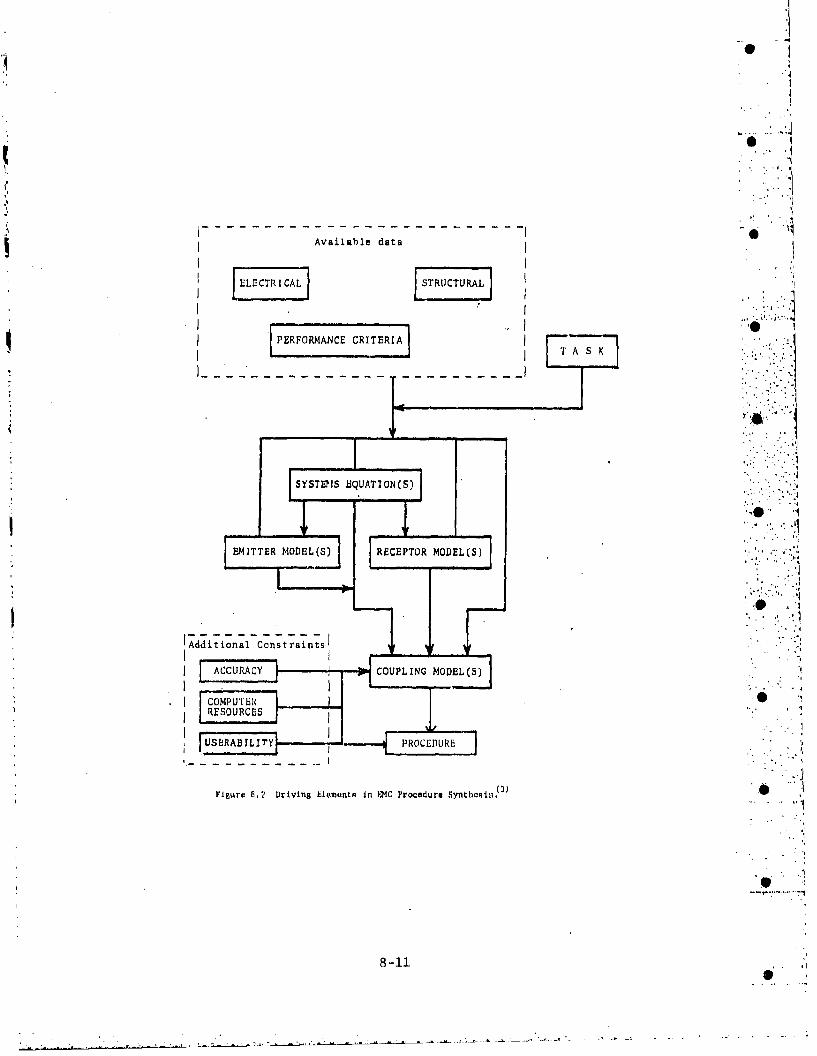
Available data

ELECTRICAL FSRUTUAL '

PEFOMNC CIERIA

T A S

'Additional Constraintl

COMPUTERRESOURCES

Figure 8.2 Drivin~g E~lements in M~C Procedure Synthesis;~ 1

8.3.1.1 Tasks

Each procedure is guided by the particular purpose or task to beperformed. The analyst is responsible tor identifying the task which may be

* Ito survey a receptor for interference when in the field of one or moreemitters. Other taske may involve waiver analysis or tradeoff studies suchas the frequency assignment of many receivers among many emitters.

8.3.1.2 Available Data

The data available for analysis is a prime determinant of any EWC.procedure. Clearly detailed analysis is impossible if only general data isavailable. The complexity of data available is primarily a function of thesystemi life cycle. Table 8.8 illustrates the system data as a function ofLife cycle.

Structural data includes the physical size and shape of thesystem. Detailed analysis such as method of moments requires structuregeomAetry. accurate to fractions of a wav.length, while for more generalanalysis generic shapes may suffice.

tailed"asThe electrical data needed by various procedures may be as de-tailed as time waveforms or as general as frequency bands of operation." Many coupling models require waveform source descriptions in terms ofamplitude versus frequency while other more detailed models may requirephase information. .'.*.

Performance criteria in the form of performance degradation .curves, or thresholds are also viewed as data because they are necessary fordetermining parameters (such a8 receptor susceptibility) necessary for any ,

EMC analysis. ...

8.3.1,3 Additional Constraints ]Any analytical tool must operate within certain physical con-,

straints. The previously discussed available data is an example of one such.,constraint powerful enough to drive the analysis. Examples of other con-straIltts are computer resources,, accuracy, and userability.

"8.3.1.3.1 Co mputer Resources

"The majority of analytical tools used for W4C analysis are comn-puter programs. As such, the analysis is limited by the resources of the"computer, primarily processing time and main memory storage size. Computerlimitations restrict the accuracy of EMC analysis because of the necessityof using simpler models and procedures to tailor the analysis capability tothe computer. Computer technology continues to progress at a rapid rateallowing for more accurate EMC analysis on future systems.

" a8.3.1.3.2 Accuracy

"Any E'MC analysis is at least approximate. The approximations thatenter Into kn analysis generally arise from two sources: problem idealiza-tion and model analysis.

8-12

• A. P

Table 8.3

DataL Avaiilable VersuB 1imascus of Life Cyclt2(3 )

0 Syn Lvcm Componcift lunJcia o Def in iL ionu* Orgitian nt ionnisWioa for I'aui Systern Coinpoi'ent* Cvnc r c Sys tem Componont

Power CircuLt8Commrunleation CircuiitsTeloniutry CiircuitsData Procensing Circuits

9 Expectod Ccometry

SizeWeightGeneric Shape

VAIidat ioil

* Characteristics of Individual Component Puwer ReuqlirementB

Power RequirementeTime W4aveforms

Spec t rumF . . Prototype Spe*cificat~ionsGoomcetvic DataSchomat~ics and DiLngrtimsMaterial Characteristic&4

* upport Equipmeint Chiuarnteristicsi

Full Scale Dcvcloun.en

e Goomelirlc Data

Deployme t Reu ts t ll

@ MantEnianco i' .FL~a Mod IIIcii L filn Spvc fi Ical: lnn

8-13

In problem idealization, the actual problem is replaced by asimpler, more treatable problem. The simpler problem should include allimportant factors of the actual problem in order that the solution of thesimple problem should resemble the solution of t ý actual problem in allimportant respects. The quality of the simpler solutions is Judged bycomparison with experiment or other analysis or by increasing the complexityof the simpler problem until the problem parameters show little change.

In model analysis, a model or method of solution is applied to thesimple or idealized problem. Different models or methods of solution will.

" result in different solutions to the same problem. Accurate model analysisdepends on the accuracy with which an analytical tool predicts important S4 ystetm parameters

8.3.1.3.3 Userability

Userability refers to the level of competence assumed for the W24Canalyst in search of an analytical procedure or tool. There are two aspectsof userability: understanding of the implementation and execution ofassociated computer codes, and understanding of the applicabilities and

"* limitations of the tool or p&,ocedure.

"The first aspect depends on the ease of use of the computer code.This aspect impacts the learning curve for a procedure but not the resultingSan alysis. a

The second aspect pertains to the level of understanding necessary"to correctly apply the analysis and interpret the results. Many analystismodels require years of experience to adequately use and understand. If auser has a choice between a complicated but accurate analysis tool that ispoorly understood and a simplified, less accurate tool that is well under-stood, the user should choose the latter procedure.

8.3.1.4 Emitter,_Recpetor,_and Coupling Models

Due to the large number of sources of electromagnetic emissions,the variety of emission models is very large, ranging from lightning andnuclear electromagneLic pulse models on the one hand to solid state devicemodels on the other. The number of possible coupling paths between emittersand a given receptor can be very large in a sophisticated electronicsequipment and are becoming increasingly important to accurately assess dueto modern digital devices which are sensitive to low power interference. PSimilar comments apply to receptors. The result is that a large number ofsuch models in either the time domain or the frequency domain are usuallyrequired for any general systems analysis procedure. The emitter, receptorand coupling models are chosen to simulate system equipment operation and assuch are strongly dependent on available data, computer power, accuracy anduserability discussed earlier.-.

8.3.1.5 Systems Equations

Systems equations relate electromagnetic source characteristicsto receptor responses. Such equations form the basis for the interference

8-14

S*. . . . . .*. . . . . . . . . . ..• . .. .

prediction process. The emitter, receptors and coupling model character-Istics are used to form a mathematical expression for assessing the inter-ference present at a receptor due to a set of emitters. The assessment is"oten in the form of a figure of merit. The form taken by the systemequations depends on the system models used. If waveforms, such as a time 0varying voltage, are used then waveform system equations are required and

. take the form of voltage and/or current margin calculations. If waveform.parameters, such as average power or peak power, are used then parametertype system equations are required. For average power sensitive receptors

:* the systems equations may be power margin calculations in terms of signalbandwidth. 0

8.3.2 Guide to EMC Procedure Synthesis(3)

As an aid to the analyst, a logical sequence of steps that act as* :a guide to constructing an EMC analysis procedure is now presented. The

sequence of steps is based on the flow chart illustrated in Figure 8.2. Byfollowing the steps the analyst can choose emitter and receptor models,coupling models, and system equations that make best use of the availablesystem data yet fit the constraints of the problem.

'Step• . The task to be performed is clearly defined. It may beto survey a system for interference, conduct tradeoff analysis or generate "tailored EMc specifications.

LStep2. The performance criteria for all receptors are examined."The receptors may, for example, be "peak" power or average power sensitive.

. Based upon the task to be performed and the receptor performanc, criteria, achoice of systems equations can be made. O

Step 3. All emitter and receptor models are now selected on thebasis of available data and chosen systems equations. Performance criteriatare also used -in selecting the receptors. For example, if emitter dataavailable is average power spectral density, then the emitter model is powerversus frequency and an emitter time waveform model would be inappropriate.

Step 4. A choice of coupling models is now made based upon avail-" able data, systems equations and emitter and receptor models chosen. At.

this point, a complete :list of coupling models is assembled that fits withthe above emitter and receptor models.

Ste2 S. A choice is now made among the coupling models, emittermodels and receptor models to form the analysis procedure with the systemsequations. The choice is constrained in accordance with tradeoffs definedby the task and the further constraints of computer resources, userabilityand accuracy.

The procedure synthesis is now complete when all models have beenidentified, interface specifications defined, limitations and inaccuraciesdocumented and computer codes assembled.

8.4 Description of Programs and Facilities

This section presents an overview of various analysis programs arid

8-15

-- h .. .. . ,

facilities supported by the Department of Defense that are available to theanalyst as tools to perform a systems analysis of a complex electronicssystem.

Two facilities, the Electromagnetic Compatibility Analysis Center(ECAC) and the Air Force Intrasystem Analysis Program (IAP) support centerare discussed in detail regarding both their EMC data bases and analysis .capabilities. Abrief discussion is also given of the IAP data base manage-ment system.

8.4.1 Electromagnetic Compatibility Analysis Center(A sa'

The Electromagnetic Compatibility Analysis Center (ECAC) to anorganization under the direction of the Department of Defense (DOD) whosemission is to provide data and expertise to the DOD on matters pertaining tointersystem and intrasystem electromagnetic compatibility. Other governmentagencies and go.?ernment contractors are served on a limited bas-is.(-,2)

ECAC maintains a data base which consists of environmental infor- Smation on deployed C-E equipment, detailed technical information about such .,equipment, and various kinds of topographic information. Portions of thedata are stored on magnetic tape or random access devices; other portionsexist in technical reports and documents,(1,2)

ECAC provides EMC engineering and consulting services through itscollection of mathematical models and computer programs that are designed toprudict potential electromagnetic interference (EMI) problems.

The data base and services provided by ECAC are discussed in somendetail in the following sections.

8.4.1.1 Data Base

The following nine files and subfiles are maintained by ECAC as a"primary EMC resource. l,2) Information stored on ccmputer files may beretrieved using data base management programs maintained by ECAC.

8.4.1.1.1 Environmental File(l, 2 )

The environmental file is a set of subfiles which describe thelocation and operating characteristics of communications and electronic

. equipment. The principal use of the data is to identify equipments locatedin a particular environment which may pose an interference threat to aproposed receiver, or which may be susceptible to interfereuce from aproposed transmitter. The data is divided into files that are eitherfrequency oriented or equipment oriented (E-file). A list of environmentalparameters collected in the environmental file is given in Table 8.9. Table8.10 is a description of the individual environmental subfiles.

8.4.1.1.2 Nominal Characteristics File (NCF)( 1 , 2 )

The Nominal Characteristics File (NCF) is a set of technical dataon various characteristics of both civilian and military communications and

O electronic equipment used in the United States and certain foreign couin-.

"...". .

0

0

Table 8.9 Major Parameter Fields ConLained

In Environmental File (E-File)

Identity number Operating cycle 0Security classification Modulation typesDate of Report Emission bandwidthCognizant military service or Pulse Width Values

agency Pulse repetition rate valuesOrganizational Unit name Power levels usedCity/Ease Frequency and/or frequency raiisgState/Country Lquipment function 0Mobility class Deactivation dateNumber of equipments Call Sign/linkage identifierLatitude Antenna vertical beamuidthLongitude Antenna horizontal boamwidthSite elevation Mainbeam gainTerrain type Area of OperationEquipment nomenclature Activation dateAntenna nomenclature Image Rejection levelAntenna height Harmonic Output LevelAntenna elevation angle IF selectivityAntenna azimuth or scan rate Preaelector.bandwidth

Output device type

8-17

lilt 191P"" I" I

.114 jai

i !I I b

~H H

S •i l l818

"" 111111II 11111111 Iii

•l •! i ti~ 1 I- ,",.,

S , . ,8.18

*.

5 ••• •l ••'

'

tries. Individual electronic components are, cross-indexed to the equipmentsof which they are a part. The computer stored data originates mostly fromtechnical manuals and manufacturer's data sheets. The data fields includedin the NCF file aru given in Table 8.11.

"8.4.1.1.3 Organization and Platform Allowance File (OPAF)(1)

All equipment data contained in the E-fiile and NCF file arefixed-site oriented. The Organization and Platform Allowance File (OPAF)contains information on computers, by subfile, which when merged with the 0E-file and NCF file information, describes C-E equipmenLa on mobile systemss such as ships, aircraft, missiles, satellites and tactical ground units.. Ifthe mobile system is known, the OPAF gives a list of equipments that are on

S* it. The OPAF subfiles are listed in Table 8.12.

8.4.1.1.4 Spectrum Allocation and Use File (SAUF)( 1 )

The SAUF contains information on agreements, regulations and laws"concerning the use of the various allocated bands in the frequency spectrum,The information has been extracted from available source documents and iscomputer stored. All information concerning a frequency band of interestcan be obtained upon request, within appropriate security requirements. Thedocuments in SAUF are listed in Tables 8.13 - 8.15.

8.4.1.1.5 To, graphic File(l, 2 )

The Topographic File consists of computer stored terrain elevationdata extracted from topographic maps obtained from the Army Topographic 0"Command. The data are used to construct topographic profiles (elevations

_ and obstructions) between any two points in the Continental United Sta eg(CONUS) as well as parts of Vietnam, Korea, Alaska, Hawaii and Germany.().Grid point separation is variable biut is nominally 30 seconds of arc (about.1/2 mile).( 1 )

8.4.1.1.6 Frequency Allocations Application File(FAAy)(1,2)

The FAAF comprises information pertaining to the frequency allo-cation status of present and future military C-E systems. Detailed data iskept of the operational and functional features of the systems. The file.4 may be interrogated by application number, frequency, operational data, 0geographic area, operational environment and equipment function. A partiallist of data fields in the FAAF is given in Table 8.16.

8.4.1.1.7 Spectrum Signature File(I,2)

The Spectrum Signature File contains spectrum signature hard copy 0

reports that characterize the emission and reception characteristics ofselected C-E equipments. Thp spectrum signature measurements ara made inaccordance with MIL-STD-449(2) (Radio Spectrum Measurement Characteris-tics). A list of parameters contained in the Spectrum Signature File Isgivon in Table 8.17.

0-19

.. S

Table 8.11 Major Paramoter F~ieds In the Niominal.Charataceristics Filud (NCP)(2)

cAitput Tube Type Vortleal boaaidthAveraea pouar output glaetrital tilt east. tean"Peak power oustput Mustier at eaintaautreqhovkey tang# hatzeetor divensineePulses ailti Capability vertical eatorss goal rateFly capability frlqosoasy lector Stan limitsP*CI deviation vatic Mttvisontal DeeM an.tkmisslip b$andvidth elevation Ingle raneamking line Ra~tOt hIM - UAWe Ofl blavbacsy time Anile tCleting bandwidthFirst if Argl* tresbtris open loop gaiePinet If eslots~i ity Rejal tracking 1iaadvidithseconid IF Range ttaskitig spase loap gainIsroan 10 aalantivity Velocity tracking bendvid~tThird If Velocity tierbiass open tso" gainThird IF selectivity Frequency laferation $eohmeIsensitivity smass beedvidthNoles Pleua. 116ianeSmie etouts levelAmounti type Presaeats ofSelectivityAnemonea load typo 1046 reisamige lavalAntelins tead type MAntmag lead eatafi IcequmanyNafleetet shaps Polavlaatteaalurdadmostat antenne malin Detaeste typettovilontll befisaidtil SPecidl gircuittrY reMank

ORGANIZATION AND PLATFORM ALLOWANCE FILES (o)PAV)(1

WATER Contains daetk on the C.1 equipen a o Navy Oirelpigmentt on Navy arnd Coeat amindi moholpe Can ~tiOsid hmaSssaalyby type class, hull ntumber, mad ship name, Army kamleeatauallyThe Cn complements aer listed by systems Commercial Maritime As tequirednomenclettare end do not Includen tampo.Montie of systems unless The component isoperating independenly from the smysseeThe US Army waermcraft aer entered mietypical C.! configutrations by besic dsigalnnumber rot each typoeof vemal, The Illo elemcontain% actual *-E sonlhurstionk (atCommeiciall Dry Cargo end Tanker Marl.t ime mhlpe operelirir under the Us Fill.

Alp. Containsm Air Force, Army, Navy, end Ma. Air Force Antsttlayrine Corps Aircraft by 7 pe/Madel/Serle Navy knelasnuffllyof aircraft tolether with Xt~sircomPlete C- Army Depends an evalslaW.eanflauralions. Insformation as to what Ity of poiisabllotinaeqtuliponsa may be Inetalled non specific tall Commercial Air Carrier Annuitlynumberm withins a ty-p/nodel/eeriea of ir.craft Is niot aneillbie, The file alim cointalnsthe quantities or the type/,odel/aaries of

* - aircraft In the preeent Inventory for eachService, The nit tantalum the Typic.? C.!Consfiguration of Commercial Ai CarrierType Aircraft by typo, model, and nienu.faclurer. [I dome not contain informatlionon Air Carrier Aircraft maenufactured by

a LOtbheed Corporation.LAND Contalnt the complemrent of equipmint in Army .No fixed echodule

US Army, US Marine Corps, end US Air , (Update esrene Wen$Force Land Tacticel unita including mobile Invaeilgated)tactical unite. The C-E configuration for the US Marine Carps * QuanerlyUS Armoy unlits it entered as typical conflA. US Air Force .Annually

urtilori for TO& 9Compan leattary Levelof Tsciltal Ground Units. The C.9 rarrflguratlon for the US Metins CorpI and UAir Force Tactical Units Is based n the at.test on hand C-11 equipment.

8-20

Atlantic Research Corporation0N00019-79-C-0634AIR-518.-5Jan 1981

* ~~THIS PAGE~ HAS BEE1N [)ELFETD

8-21

-W,

Atlantic Research CorporationN00019-79-C-0634AIR~-518-5Jan 1981

0

THIS PAGEh HAS BEEN PELETEfl

8-22

Table 8.16

(2)Major Date Fields in the Frequency Allocation Application File (FAAF)~

DateTitleAgencyStatusApplication numbers (include supporting referenceii)Security clausificationFunctionOperational. en rionntGeographic area of useNomenclaturePhysical installation or platformNumber of equiipmentsOperation dateSpectrum signature requirementFrequency rangeFrequency control methodModulation typePowerPulse width end pulse repetition frequency0Receiver IF bandwidthAntenna bgamwwidthAntenna polarization

Table 8.17'4

Data Fields in the Spectrum Signature Filer".

Power output Standard responseEmission spectrum characteristics Receiver intermodulationModulation characteristics Pulse and CW desensitizationTransmitter entexmvdulation Adjarent signal InterferenceModulator bandwidth Dynamic r"ngetarriNr frequency r tability Oscillator radiationSensitivity Audio selectivitySelectivity Discriminator' bandtwidthSpurious response Antennt " easurementoverall susceptibility Antenna patternsReceiver modulation

8-23

Power

I .. .. . .. .. ...........................................................

8.4.1.1.8 Tactical File( 2 )

The Tactical File contains information that pertains to variousmilitary tactical deployments, simple and complex. The file also containsroutine C-E envirokiments present in various regions as well as the EquipmentAllowance File (EAF), an inventory of equipments used by v bus categories(ships, aircraft operation centers, etc.) of the military. ."

8.4.1.1.9 Future I'ile(I)

This file contains equipment characteristics data concerning Iefuture communications and electronic systems. 0-

8.4.1.2 Analyt cal Models( 1 )

ECAC maintains a collection of analytical models that operateeither as a part of EMC systems analysis computer codes or in a stand-alonemode. These models and codes provide users with solutions to variouselectromagnetic interference (EMI) problems as well as an E4I predictioncapability. A list of analytical models maintained by ECAC is given inTable 8.18.

8.4.1.3 Engineering Servj•cs(2)

Based on the analytical techniques and data available, the following services are available from ECAC.

* assistance to C-E equipment developers onall aspects of frequency selection andequipment design.

* guidance in analysis of potential sitelocations for new equipment.

0 power density analysis as a function ofdistance and topography.

* prediction of EMC loss for various tacti-cal operations.

* prediction of EMC effects by incorporatingnew electronic systems into existing and Pfuture environments. 7

The outputs supplied by ECAC are not in a standard format but aretailored to the particular task. They range from narrative di', ussions totabulations of data in numerical or graphical form.

8.4.2 Intraaystem Analysis Program

The Intrasystem Analysis Program (IAP) is a set of computer codesused in analyzing electromagnetic compatibility (EMC) problems for aircraft,space/satellite, and ground based systems. The emphasis of the IAP ison intrasystem compatibility, i.e., the compatibility of numerous electri-

8-24

Table. 8.18

LISTING OF ECAC MODELS(1

I. S1URSYSi EM MOIýELS 4 COSITE MODELSTrarnsmitter Limivsiors Specturum Synthesib Cn iCe Analysis Model (COSAM)Transmittet Ensihs~sn Spectrums Models Airframe Comsnsnicutlons Anralysis (AVPAK.)Fourier Transformn of I'M Tiapenioldal pulses Aircrafl Ordinance RP' Analy~si (AVPAK 2)

Receiver Wuveforrn Sinmultuion Model (RWS) J. SPECTRUM MANAGEMENT ANALYSISFreueny Autysa ubrutie (AS)MODELS (FREQUENCY ASSIGNMENT)

Recuiver Response to a Fnskirily or Pulses Multiple Channel Assignment Systems (MCAS)Butterwortth and Cirebyahes' Digital Filters LOS Angle Data Chsterln- AmeligrimantPulse Cumpirresolon Motched Filter Mutual Irittrrerenrw TableImpedance Computation and Analysis Program Fisqluency Assignmrent Support Subroutine

(ZCAP) (ORAFAS)

Multiple Ltvti Antentia Model (MLSI PAA-ATC.VIIF Frequency ModelAntienna Data Anuly'sis Programn (ANDATA) Tactical Landing Force EM4C Iis'alusetlonPattern Anaatysis Subroutine (PATAS) o1rFr.Prqumncy Rejections.Distance CalculationTrasamilter/Recelver Atiternse Coupler (PCL

(TRACE,

lertermodulutlion Analysis Model 6. DEGRADATION ANALYSIS MODELSpurious Responsae Idntilfeatlon Model Destradratite AnalylsiMiser Reiponse ModelAdjacent Channel Interference Summary

7. STATISTICAL AND NUMERICALI. PROPAGATION MODELS ANALYSIS

MASTER PROPAGATION SYSTEM. Auto-Croik Correlation Analysis ModelTerrain Integrated Roultl Earth Model (ACCAM)

(TIREM) List Proeeasing Routines rtr DigitalIntegrated Propagation System lIPS) Simsulationst

Smorothe Curve Smooth Earth (SCSIS) Oemtralltzd File Statistics Analyzer (Q63)flislance Free Space Spherical Raflectiot MATH-PACKField (SFSRFI STAT-PACK

Simpllfled Theoretical Ground Wuse (STOW) Random E-iile Generator (REG)Modiflcd YEH Troporicutter IMYEH-) E-Fie Equipment Statistics (XOIKS6)

NLAMBDA (NX) Ground Wave Model Antenna Data Analysis Symeemn (ADAS2)SKYWAVE H-F PROPAGATION MODEL. Topogruplic Dais Scatter Diagrarn (SCATER)COSITE COUPLING MODEL Experinmental Calculation-INK DistribationPROPAGATION STATISTICS GENERATOR

3. ENVIRONMENT ANALYSIS SYSTEMSDemnaed Anulyais ProgramsModel BPulse Density ModelSite Analysis Modal (SAM)Target Acquisition Modal (TlAM)Power Density Display program (POOP)1FF MARK X (SIFI Modet IAIMS.PPM)

"I 1IFF MARK XII Model (AIMS-PPM)Rapid Cutl ModelEqtuipmnent Desnrity Progran.

8-25

cally connected equipments and subsystems residing in a relatively smallvolume and regarded as a single system. The IA? effort is directed by theReliability Branch, Rome Air Development Center (RADC/RBCT), Air ForceSystems Command, at Griffiss Air Force Base, New York.

The principal component of the IAP is the Intrasystem Electro-magnetic Compatibility Analysis Program (IEMCAP). The IEMCAP code providesthe basic EMC computer analysis at the system level for all phases of thesystem lifecycle. The IEMCAP can survey a system for interference, providetradeoff and waiver analysis and generate specification limits. Aircraft,spacecraft and ground installations can be analyzed with' the IEMCAP code.SIDCAP contains models for sources of electromagnetic signals, receptors of ,such signals and transfer coupling of electromagnetic energy between sourceand receptor.

A set of supplemental computer codes are included with IEMCAP inin the IAP. One code, The General Electromagnetic Model for the Analysis ofComplex Systems (GEMACS), is a user-oriented general purpose program forsolving electromagnetic radiation and scattering problems using thin-wire, ,method of moment (MOM) techniques. GEMACS provides a near-field analysiscapability for the IAP and a more detailed backup analysis to supplementIEiCAP.

A nonlinear circuit analysis capability is provided by the Non-linear Circuit Analysis Program (NCAP). Analysis of transmission lines issupported by the IAP codes XTAIK, XTALK2, FLAATPAK and FLATPAK2 while precip-itation static charging is handled by the IAP code PSTAT. The IAP codes arediscussed in more detail in the following sections. *18.4.2.1 sntrasystem Electromagnet Compatibility

.Analyis Prog.,,(ECAP),

The Intrasystem Electromagnetic Compatibility Analysis Program(IEICAP) is an IAP computer code designed to perform an EMC analysis on acomplete electronic system level at any or all stages of the system lifecycle, from conceptual des iefn of the new system to retrofit and/or modil-i-cation of the old system.(1") In accomplishing the system's analysis, anyor all of the following tasks may be performed.TI,4)

provide a data base that can be continuouslymaintained and updated to follow systm de-sign changes. " '"

* generate EMC specification limits tailoredto the system.

0 survey a system for interference.

0 evaluate the impact of granting waivero tothe tailored specifications.

0 assess the effect of design changes onsystem LKC.

0 provide comparative analysis results on

which to base EMC tradeoff decisions.

8-26

8.4.2.1.1 Emitter and Receptor Models( 4 )

Each IEMCAP emitter and receptor is modeled as a part character-ized by an emission or susceptibility spectrum. Each spectrum consists of abroadband component, which represents contiruous spectra in units of powerspectral density, and a narrowband component, which represents discretespectra in units of power. Each spectrum is also divided Into a requred,

* spectrum deemed necessary for system operation, and a nonrequired spectrum,not required for system operation but present as a spurious emission orsusceptibility. The required spectrum may be specified by the user orcalculated by IEMCAP using a model in the code. The emitter models presenttn IEMCAP are:( 4 )

* binary frequency-shift keying.

, amplitude modulation with stochastic process.

* angle modulation with stochastic process.

. single sideband amplitude, phase and frequen-"cy modulation with a stochastic process.

* chirp radar.

* pulse code modulation/amplitude modulation - , .. "nonreturn to zero.

* pulse position modulation.

0 pulse code modulation/amplitude - biphase.

• pulse amplitude modulation/frequencymodulation.

* pulse duration modulation.

* sirigle pulse.

* pulse train (rectangular, trapezoidal,triangular, sawtooth, high frequency ex-ponential, damped sinusoidal).

The susceptibility model in IECAP equates an RF receptor portsusceptibility to the receiver sensitivity that is provided in the inputdata, over the entire receptor spectrum, as defined by the user-specifiedbandwidth. For a signal, or control port, the susceptibility is the operat-ing level less 20 dB. The nonrequired spectra are s8t to the levels speci- .fied by MIL-STD-461A or MIL-I-6181D unless a change is specified by theuser.

8.4.2.1.2 Transfer Models( 4 )

The coupling and transfer of electr-xnagnetic energy from emitter ........port to receptor port in IEMCAP is accomplished by the transfer modelsdiscussed in the following sections.

8-27

4 .

8.4.2.1.2.1 Antenna-Coupled Models( 4 )

Included in this model are antenna-to-antenna and antenna-to-wirecoupling on an aircraft, spacecraft or ground system at all common emitterand receptor frequencies. In computing the coupling path, propogationthrough free space, around the fuselage, and diffraction from wing edges aretaken into account. Two groups of antennas are considered in this model.The first group is a set of low gain antennas including the dipole, slotloop and monopole antennas. They are modeled by trigonometric expressions,or as specified by the user. The second type is a set of high gain antennassuch as arrays or reflectors, and is modeled by a three section representa-tion of the gain pattern. The gain of each sector currently is frequencyindependent and is a user input. For antenna-to-wire coupling to occur, the

-* wire must have at leaRt one segment behind an aperture.

8.4.2.1.2.2 Wire-To-Wire Model( 4 )

wirWire-to-wire coupling occurs if a wire connected to an emitter and

a wire connected to a receptor are in the same wire bundle segment. Thewire-to-wire routine calculates the voltage induced in the receptor wire .tueto the presence of the emitter wire at each common emitter-receptor frequen-cy. Models for open wires, shielded wires and double shielded wires in abalanced or unbalanced configuration are used as required.

8.4.2.1.2.3 Case-to-Case Model( 4 )

This model computes coupling between equipment cases. These casesare modeled as dipoles.

8.4.2.1i.2.4 Environmental Field Models( 4 )

These models compute the coupling of external and internal EMvfields to a recpeptor port. The port may be an antenna, wire, or equipmentcase. Induced current is calculated for wire or antenna receptor ports,while the impressad field is determined for an equipment case port. -

8.4.2.1.2.5 Filter Models( 4 ) L

The filter models available in IEMCAP are: single tuned, lowpass, high pass, band pass and band reject. The models calculate theinsertion loss in dB provided by the filter at a given frequency.

The filters are represented as ideal lossless networks made uponly of capacitors and inductors. Dissipation is considered in the inodelsby providIng for a minimum insertion loss at the tuned frequency or in thepass band. A maximum insertion loss is provided in the rejection band.These minimum and maximum insertion losses bound the filter transfer func-tion.

8.4.2.1.3 S pectrum Representation( t ,4 )

Each emitter and receptor port is characterized by an emission orsusceptibility spectrum. A table of up to 90 frequencies ranging from 30 Hzto 18 GHz is assigned to each equipment in the system. This is used to es-tablish the characteristics of all port spectra within the equipment. The

8-28

• -- - [- " . . .. . - - " .. " i % - ' ,- • ,-

frequencies are specI.,d ini two ways. (1) The user may specify the up:,erand lower frequency limits, the maximum number of frequencies, and number of"•requencies per octave. The IEMCAP code then generates a set of geometri-cally spaced frequencies within the set limits. (2) Alternatively, the usermay specify the upper and lower frequency limits, the maximum number offrequencies, and a set of specific frequencies to be included (up to themaximum number). The code then generates geometrically spaced frequenciesto fill in the frequencies not specified.

At the port level, the required frequency range is specifiedwithin the overall equipment frequency range. In order not to miss peaks orvalleys between sample frequencies, the spectrum is sampled in the half-in-terval between a given frequency and each of its neighboring frequencies.The maximum frequency is picked for emission spectra, and the minimum, forsusceptibility spectra. This process quantizes the port spectra relative tothe sample frequencies.

8.4.2.1,4 Basic Systems Analysis Approach( 4 )

All system ports are considered to be emitters and/or receptorsof electromagnetic energy. Each port is characterized by both a requiredand a nonrequired spectrum. An EMC problem is said to exist when sufficientelectromagnetic energy is unintentionally coupled into a receptor port toexceed its susceptibility threshold. If no threshold is exceeded for anyreceptor, the system is said to be compatible.

The required spectrum for each port is nonadjustable in the code.

The nonrequired spectrum can be adjusted, to make the system compatible, Anadjustment limit is usually included to prevent too stringent a spectrumadjustment.

To determine if interference is present at a given receptor port,the level of power coupled into the receptor at its terminals must becalculated. This task is accomplished by a set of linear systems equationsthat relate receptor models, transfer models and emitter models to eachother. '.he systems equations in IEMCAP characterize the power coupled intoa ruceptor in terms of power spectral density. This adequately character-izes devices sensitive to average power, but may not be sufficient to treatpeak power devices. Electromagnetic interference (EMI) is a sessed bycomputation of an EMI margin that serves as a figure of merit,(6) The EMImargin is first calculated for a given receptor by computing the ratio (indR) of power from a given emitter incident at the receptor's input to the 0'.given receptor power susceptibility level at each frequency common to agiven emitter-receptor port pair. The ratio is called the EMI point marginfor the port pair at the given frequency. The integrated E4I margin is thencalculated over all frequencies common to the port pair. The calculationsare repeated for every emitter-receptor port pair. Total M14I margins arenext calculated for each receptor by summing the contributions to thereceptor fromu each coupled emitter, at each frequency (total point margins),and over all frequencies (total integrated margin). The total Lntegra edEML margin represents the overall figure of merit for the receptor.

8.4.2.1.5 Program Flow and Task Analysis( 4 )

The .IEMCAP work is divided into two sections. ThQ first section,

8-29

. ........ ...

called the Input Decode and Initial Processing Routine (IDIPR), reads andchecks data for correct format, builds working files, interfaces withspectrum models, analyzes wire bundles and wire connections to ports, andconstructs the initial port spectra. The second section. called the TaskAnalysis Routine (TART), performs the requested EMC systems analysis. A"functional flow chart of IEHCAP is given in Figure 8.3.

"Two permanent files of major importance are constructed during"execution of IEHCAP. The first file, called the Intrasystem Signature File(1SF), is initially built in IDIPR and is a data base containing all inputdata defining the system and the port spectra. The ISF file can be updatedIn IDIPR or TART as the system design is modified. The second file is' thePost Processor File (PPF) and contains all of the IEMCAP output from I[)PRand TART. The file is either in printed form or in a computer file. Database management tools are being developed to manage both the ISF and PPFfiles.

The TART section of IEMCAP can perform four different EMC analysistasks.

One task is a Baseline System EMC Survey that simply scans thesystem for interference, If the integrated EMI margin for an emitter-recep-tor port pair exceeds a user-supplied limit, a summary of the port pairinterference is printed as well as total signal received by the receptor.

A second IFA•CAP task is Specification Generation, The nonr-quiredemitter and receptor port spectra are adjusted until the system is compati-ble to within a user-specified limit, Any incompatibilities that stillexist are reported as unresolved interference, The adjusted spectra repre-sent the maximum emission and minimum susceptibility specifications.

A third task is a tradeoff analysis. The IEMCAP code compares theinterference of a modified system to that from a previous baseline orspecification generation run. The effects on interference of antennachanges, filter changes, spectrum parameter changes, and wire changes can be Lassessed. No ports, equipments or subsystems may be deleted or spectrafrequencies changed in this analysis.

' The fourth task is Specification Waiver Analysis. Portions ofspecific port spectra are shifted and the resulting interference compared toa previous baseline or specification generation run. The effects of grant-ing waivers for specific ports can then be asessed.

8.4.2.2 Electromagnetic Modal for the A. alysisof Complex Systems (GERACSYJ'io) -

The GEMACS program is a general user-oriented code designed tosolve radiation and scattering problems using thin-wire method of moment(MOM) techniques.

A high level functional flow chart of GEMACS is shown in Figure8.4. The executive routines control file manipulation, take checkpointsin the analysis and handle restart from the checkpoints. The input ian-guage processor handles the command language and sends the data; the task

8-30

L,.. .

UlU

04J

ba

UV

>I

ILI

(iiVE, u

wj .I u-,

I - r

I8 31

4P

execution processor calls the appropriate subprocesaor to perform thearnalysis; and the run termination processor ends the analysis. The proces-sor and executive routine constitute a data management system.

The subprocessors solve a radiation or scattering problem formu- .

lated using an electric field, integral equation. The system geometry ismodeled in GEMACS as a thin-wire g'rid structure. The integral equation i"then reduced by standard MOM techniques( 1 0 ) to a matrix equation with the ,!>1following general form

Z I hE (8-1) '.: ,

where Z is the inte=raction matrix that represents field coupli.ag between thevarious currents on the wire grid, I is the current matrix, and E is theUxcLtation matrix.

tn order to calculate _, the Z matrix must be inverted and GEMACScontains a matrix inversion routine. Gn the case of a large Z matrix, fu.Lltnversion is impractical and GEMACS employs an approximate so ution proce-dure called the Banded Matrix Iteration (BMI) technique.( 8 ) In thisteclnique, the Z matrix is divided into a banded matrix B, a lower trIang-ular matrix L, and an upper triangular matrix U as shown in (8-2), whore Mis the bandwidth.

M ,.N.,

1o (8-2)L [L

Equations (8-1) and (8-2) lead to the following iterative equationfor the current. I:

B j+ E-(L+U)Ij (8-3)S ii

The first step in the solution process is to decompose the bandei matriA H,into upper and lower triangular matrices B and B respectively. Equa-Ition 88-3) is written in the form

B1. Y - E-(ItU)I (8-4)

iThe matrix Yj is solved by forward elimination, using IT, the currents4t the jtn iterative step. The matrix j is just the product of -,.with wIJ+1

_ !j+l - YJ (8-5)

The current matrix I is then solved by backward substitution. Theprocess is repeated untll convergence Ls obtained. The convergence rate issharply dependent on M, the bandwidth of B. Many field problems have buentreated with success uulng GEMACS.

8-.32

"The GEMACS code belongs to the Air Force Intrasystem AnalysisProgram (IAP). It provides a near-field analysis capability and serves asa complement to Ih'M4CAP, the TAP system level E14C program. GEMACS has a

. checkpoint/restart capability allowing long analyaes to be stopped and*. restarted at will, both as a protection against computer failures and as an

aid in changing the command language stream. An extensive debugging and: e~rror-checking capability is built into the code to aid analysis and future. ,upgrading of the software.

8.4.2.3 Nonlinear Circuit Analysis Program (NCAP)( 9 )

The Nonlinear Circuit Analysis Program (NCAP) calcutlates the non-[inear transfer functions of an electronic cirtcuit. Standard circuitelements are used in interconnecting networks containing utp to 500 nodes.The following circuit element models are included in NCAP:

6 Independent Voltage Source* Linear Dependent Sources"* Nonlinear Dependent Sources* Linear Components. Nonlinear ComponentsS, Vacuum Diode* Vacuum Triode* Vacuum Pentode* Semiconductor Diode0 Bipolar Junction Transistor0 Field Effect Transistor

NCAP has a free-field format for input data, a user-oriented com-mand language, a capability to build device models, in addition to the-tored models and a frequency sweep feature that allows an analysis of the

. circuit to be done over a range of frequencies in one run.

NCAP solves the nonlinear network problems by forming the modeladmittance matrix for the entire network, and first order generator (currenttsource) exitation vector for all linear sources in the network, The firstorder model voltage vector, which contains the first order transfer func-

* tions at the given frequency, is then calculated. Higher order LransfertfuctLons are then solved interactively.

"8.4.2.4 Precipitation Charging, Noise Generation and Coupling (PSTAT)1)

The program Precipitation Charging, Noise Generation and Coupling(PSTAT) predicts the effect of precipitation static noise upon a widevariety of aircraft under many different flight situations. The code Isbased upon the results of both theory and experiment. The accuracy of PSTATvaries from a few percent to tens of percent depending on the aircraft

• design. It cannot be applied to helicopters or missiles because theirgeometrLcs are radically different from aircraft.

8.4.2.5 Transmission Line Codes

Four transmission line codes are supported in the IAP.( 1 2 ) The- first code, XTALK, analyzes N+1 bare wires; N bare wires above an infinite* ground plane, and N wires within a cylindrical shield containing a homogen-

.ou. dielectric. All wires are considered in equivalent XTALK except the

8-33•

wires may be imperfect conductors. The code FLATPAK analyzes N+1 wireribbon cables for perfectly conducting wires. The code FLATPAK2 consLderst-he N+1 wire ribbon cable problem for imperfectly conducting wires. Allcodes assume a steady state sinusoidal excitation and a losuless mediumaround the condutctors.

8.4.3 Interference Prediction Process - Number 1 1LIP -1)

The Interference Prediction Process - Number I (IPP-i) is a can-puter code developed by the Rome Air Development Center (RADO), Griffins Al.rIForce Base, New York to analyze and predict possible interference situ tions"for any proposed or existing delo ment of transmitters and receivers.4 t,2,5)

. The IPP-1 code can be used for:(20)A. the preliminary development of system or

equipment requirements and specifications. , ,B. the preparation of specification compliance

test plans.

"C. the evaluation of test results.

D. the revision of specifications or equipmentsfor conditions of noncompliance.

E. the evaluation of systems in a specificoperational environment.

Specific problems that tPP-l may analyze include the following:(2)

A. Examine the EMC situation for a complex ofequipments and identify problem areas.

B. Examine the impact of changing the operatingfrequency of one or more equipments in thecomplex.

C. Examine the impact of adding a transmitter toan existing complex of equipments.

,D. Examine the interference produced in a receiverwhen added to an existing complex.

h. Determine which one of several possible loca-"tions for a receiver provides the least probableinterference.

F P. Determine the source and cause of a known inter-ference problem.

G. Determine the amount of suppression required tocorrect a specified interference situation.

H. Obtain site survey or EMC environment type ofinformation for a given location.

8-34

0'

I. Obtain site survey or EMC environment type ofinformation for a given receiver or group ofreceivers.

J. Determins propagation 0ose over a specifiedpath.

K. Obtain. specifi.c interference characteristicdata on transmitters, receivers or antennascontained on the equipment characteristic tape

In addition, several hasic types of analysis may be requested

"which tnclude:(2 , 1 3 )

A. Data base management.

h. Rapid cull RMC analysis.

C. Frequency cull EMC analysis.

1 0. Detailed EMC analysis.

E. Propagation loss.

F. Power density and field strength analysis.

G. Interinodulation analysis.

SR. Frequency band analysis,

"I. Adjacent signal analysis.

J Frequency/signal analysis.

The IPP-I code is controlled by an executive routine that pro-cesses data, builds files and oversees the type of analysis to be performed.

The remaining routines c.,irry out the analysis.( 11 3 ) The inter-u urencL analysis is divided into two parts: (1) a rapid cull used for

eliminating the obviously noninterfering parts of the problem by means ofsimple criteria, and (2) a frequency cull which involves a frequency depen-

,* dent analys:is of possibly interfering situations.

The frequency Cull uses detailed emitter, receptor and propagation*• models to predict a figure of merit (interference margin) for each receiver.

Included in the analysis is a statistical description of emitter output gig-nal propagation, and receiver response. The figures of merit are then tab-ulated for each receiver.

13..4.4 The Cosite Analysis Model (COSAM)

The Cosite Analysis Model. (COSAM) is a computer code designed toevaluate the electromagnetic compatibility of a single site in the neighbor-hood of a ).arge number (50) of communication transmitting and receivinguquipmentH. 14,) A coafte P2MC problem implies close proximity of trans-mitting and receiving receiver input.

8-35

In performing the interference analysis, up to five interactionsare considered by COSAM: (1) adjacent signal, (2) spurious emissions, (3)spurious responses, (4) receiver intermodulation, and (5) transmitterintermodulation. The results from each required interaction are combined inCOSAM to produce an output signal-to-noise (S/N) and signal-to-interferenceplus noise (S/I+N) ration that serve as performance scores.

8.4.5 Specification and Electromagnetic CompatibilityAn alysis Program (SEMCAPI :'.

A Specification and Electromagnetic Compatibility Analysis Program" (SEMCAP) is a computer code developed by T1l4 Systems, Redondo BeaghI Cali- :-wJ [~~ornia for the NASA Manned Spacecraft Center, Houston, Texag.(0,15-17) ""-

",.The code is designed to:

A. analyze a system for electromagnetic compatibility;"B. develop EMC specificatioix generation and suscepti-

bility limits consistent with desired signals;

C. perform a waiver analysis on the system.

SEMCAP is a systemo level ENC code and is very similar in designto the IEMCAP code discussed in Section 8.2.2.1.

864.5.1 Analysis Models

The analysis models used in SIMCAP include models for emitters,receptors and coupling paths between an emitter-receptor pair.

Emitters and receptors are each given a spectrum representationdivided into a priority I functional port (similar to the IEMCAP coderuquired spectrum) and a priority 2 extraneous port (similar to the IFMCAPcode nonrequired spectrum).

Coupling paths are modeled by the foulowing electromagnetic trans-fer functions- (1) antenna-to-antenna, (2) antenna-to-wire, (3) wire-to- ,"wire and (4) field-to-wire. All transfer function models are similar to themodels found in the IU2.CAP code (Section 8.2.2.1).

8.4.5.2 Compatibility Analysis

SThe first step in the analysis is the calculation of the requiredspectrum (priority) interference of emitters upon receptors. Unless thespectra are incompatible wi th the priority 1 recepture spectra, a marginbetween interference and malfunction will exist for the receptor. Priority2 (nonrequired) emission spectra are then not allowed to exceed this margin.

The voltage Vii included by generator i at receptor J is cal-culated by

8-36

4b

"V Gi(b) IT (b) P (b) 'db (8-6)

where Gi(f) is the amplitude at frequency f of the source i; voltage

spectrumi Pi is the amplitude at frequency f of the receptor j voltage

"spectrum, and TLj(f) is the amplitude at frequency f of the voltage

transfer function between generator i and receptor J. Equation (8-6) gives

the peak response of a receptor model due to source and coupling models

"characterized by an amplitude density. The SFMCAP compatibility analysis is

then best suited for treatin3 transient or impulsive signals and devices

characterized, by peak power. This is in contrast to the IEMCAP code

which uses a power spectral density model for emitters, receptors and

transfer functions and characterizes devices sensitive to average power.

8.4.5.3 Specification Generition and Waiver Analysis

Besides surveying the system for interference, SENCAP generates

tailored specifications by modifying the extraneous emitter and receptor

,spectra to produce a compatible system, and assesses the effect on the

system cf granting waivers to the specifications. The general procedure ts

similar to the specification generation and waiver analysis capability in

the IEMCAP code (Section 8.2.2.1).

8.4.6 Shipboard Electromagnetic Compatibility Analysis (SEMCA)

The Shipboard Electromagnetic Compatibility Analysis model (SE4CA)

La a set of teukr u;dj% ~l%$f-d alW~ -1; M trc~mjytgt--•Beah . Flord (T ,.18,1 '0r -ef e .n

rucewing equOlpments located on a ship. The SILCA code is tailored to

shipboard design in that intraship coupling is tied to ship topside model-

ing. SU4CA is used primarily in the VLF/LF/HF and VHF/WHF frequency ranges,

but has been extended to microwaves in the SEMCAM (Shipboard Electromagnetic

Compatibility Analysis Microwave) code. This code has been used el) in

topside design of new ships, to assess EMC impact of alternate equipment and

, anetnna site, for frequency. assignment, and for generation of EMC specifi-cations for new equipment design. The code has been expanded from a cosite

model which considers only intraship probleams to include off-ship signals %H sour ca. .

8.5 Data Base Management .

"In Section 8.2 of this chapter, a number of facilities and pro-

grzns were described that are necessary and useful in performing an EMC

analysis. In performing such an analysis, the systematic manipulation of

"large amounts of data may be required, both as program input and output.Such data handling is best performed by proper data basr "anagement software

tos8-37

.. '. . . ,

8.5.1 ECAC Data Base Manaement P

The Electromagnetic Compatibility Analysis Center (ECAC) has n setof programs that: are designed to primarily retrieve specific tnformatLonfrom its collection of EMC data files. These files have been described inSection 8.2.1 of this report. A list of ECAC iata base query programs isgiven in Table 8.19.

* .8.5.2 IAP Data Base Management

The Intrasystem Analysis Program (IAP), under the direction uf theRome Air Development Center, Griffis Air Force Base# New York, is being **

currently expanded to include a number of data base management tools. Abrief description of existing and currently planned programs is given in thefoLlowing sections.

8.5.2.1 ,System File Handler

The System File Handler (SFI1) is a FORTRAN software code capableof building and editing sequential files on magnetic tape or randon do-vices.(20) The primary function of the SFH is to access the TAP files inthe Electromagnetic Compatibility Analysis Program (IMCAP) called theIntrasystem Signature File (ISF) and the Post Processor File (PPF), as wellas to access the TAP System Data File (SDF) which is described in the nextsection. The SFH provides a variety of services and is designed so thiatadditional services can be easily incorporated as they become available.

The basic services offered by the SFH are: ACCESS, LOAD andUPDATE. The ACCESS function allows a user to query a file to obtain speci-fic attributes about the data, display requested information, or create asubset copy of the original file. The LOAD function allows a user -togenerate a data file from scratch. The UPDATE functions allow for filemodification and malntenance.

The SFH is designed to be used on a general purpose digital comi-puter and to be essentially free of any particular machine or operatingsystem. The command language is designed to be as user oriented as posui-ble. The SFH will allow the user to access the wealth of data that exists:ither as input data for the various lAP codes, or output data from an lAPanalysis of a system.

8.5.2.2 System Data File

The System Data File (SDF) is a data base that digitally stores ina standard format all of the electrical and physical characteristics Of asystem necessary to perform an EMC analysis using any code in tile IAF,(21)A SDF will exist for each system analyzed using the IAP codes.

"Access to the SDF will be by means of the System File Handler(SFH) described in Section 8.3.2.1. The SFH will be used in conjunct tonwith an IEMCAP translator (currently under development at RADC) to accessthe SDF and automatically prepare most of the input data required to performan IEMCAP analysis on a given system. This will relieve the user of theburden of preparing the data manually. All codes will be available in thenear future.

8-38

i --

Table 8.19 ECAC Data Base Management Program

DATA BASE SELECT CAPABILITIES 6

On-Line E-File GewseruI Format and Print Program -vOn-Line E-File General Select CapabilityOn-Line E-File (SPACJE)The C&E Deployment SystemTopographic Data File Select and Print Program

(TO PSEL)Profile Print Prog~ramOperational Platrorm Allowance File (OPAF)General Format and Print ProgramNominal Characteristics File (NCF) Equipment

Selection Programs* Propagation Measurement Retrieval System (PM IRS)

8-39

Sb ......

8.6 References

1. Engineering Design Handbook Electromagnetic Compatibility, prepared byHeadquarter US Army Material Development and Readiness Command,DARCOM-P706-410, March 1977.

2. William G. Duff, Electromagnetic Interference and Compatibility, Vol.5,Don White Consultants Inc., 1972.

3. Intrasystem Analysis Program (IAP) Structural Design Stuy, AtlanticResearch Corporation, ARC No. 53-6111, April 1980.

4. J. L. Bogdanor, R. A. Pearlman, and M. D. Siegel, Intrasystem Electro-magnetic Compatibility Analysis Program, Volume II: "User's ManualUsage Section, "Final Report prepared by McDonnell Aircraft Company forRome Air Development Center under Contract F30602-72-C-0277, RADC-tr--74-342, December 1974.

5. Interference Notebook, RADC-TR-66-1, Rome Air Development Center,Griffiss Air Force Base, NY, June 1.966.

6. R. A. Pearlman, "Physical Interpretation of thA IEMCAP Integrated EMIMargin," IEEE 1978 Symposium. n Electromagnetic Compatibility, June,1978.

7. Kenneth R. Siarkiewics, "General Electromagnetic Model for the Analymisof Complex Systems," IEEE 1978 Symposium on Electromagnetic Compati- ..

bili•, June 1978.

8. General Electromagnetic Model for the Analysis of Complex Systems,Vol. I, Il, th BeDM Corporation, RAP•.-R-77-137, April 1977.

9. J. Spina, et.al., "Nonlinear Circuit Analysis Program (NCAY) Documen-tation," RADC-TR-79-245, Vol. 1 - Engineering Manual; Vol. 2 - User'sManual; Vol 3 - Programmer's Manual, Rome Air Development Center,Griffis Air Force Base, NY, 1979.

10. R. F. Harrington Field Computation by Moment Methods, The MacMilLiamCo., 1968.

11. J. E. Nanevicz and D. G. Douglas, "Static Electricity Analysis Program,Vols. I and II, SAMSO-TR--75-44, Standord Research Institute, Oct. 1974. p

12. C. R. Paul, "Applications of Multiconductor Transmission Line Theory tothe Prediction of Cable Coupling," RADC-TR-76-101, Volume VII, RomeAir Development Center, Griffiss APB, NY, July 1977.

13. W. G. Duff, et.al., "IPP-1 User's Manual, RADC-TR-71-300, Rome Air "Development Center, Griffiss AFB, NY, January 1972. (See also "IPP-1Program Improvements," Atlantic Research Corp., Alexandria, VA, 1972.

8-40

-- -*.

14. M. N. Lustgarten, "COMSAM (co-Site Analysis Model)," 1970 IEEE Electro-magnetic Compatibility Symposium Recnrd, 394-406, July 14, 15, 16,1970.

15. W. R. Johnson, B. D. Cooperstein, and A. K. Thomas, "Development of aSpace Vehicle Electromagnetic Interference/Compatibility Specifica-tion," TRW Document No. 08900-6001-TOOO, TIU Systems, One Space Park,Redondo Beach, CA 90878, 28 June 1968.

16. W. R. Johnson, J. A. Spagon, and A. K. Thomas, "Application of Com-puter Technology to the Implementation of EMC Programs" 1969 IE"'Electromagnetic Compatibility Symposium Record, pp. 155-166, Jur17-19, 1969.

17. A. K. Thomas, "Math Modeling Techniques for a Computerized EMCAnalysis," SEMCAP Selected Technical P!apers, T1 Systems Group, RedondoBeach, CA, 1969 IEEE WC Symposium Record.

18. Shipboard Electromagnetic Compatibility Analysis, SL'4CA III, Vol. VIIA,User's Reference Manual, General Electric Company Apollo Systems,Daytona Beach) FL,.Jaruary 1970.

19. SEMCA V, Volumes C, XA and XB, General Electric Co. Daytona Beach, FL.

"20. IEMCAP PRE/POST Processor System File Handler, Atlantic Research Corp.,Report prepared for RADC/RBCT, February 1980.

21. System Data File (SDF) for the Intrasystem Analysis Program (IAP),RADC-TR-79-213 Vols 1 and 2, Dec. 1979.

d ~8-41

9.0 MEASUREMENT TEST AND EVALUATION

This chapter addresses the alternative methods by which the vari-ous parameters of composite materials are experimentally measured. Section9.1 outlines the various experimental techniques used to measure variouscomposite intrtnsic properties such as permeability, perm:Lttivity, resistiv-ity and conductivity. Several mathematical models of conductivity have beendeveloped and they are included for comparison. Section 9.2 addresseselectric and magnetic shielding effectiveness measurement techniques usingseveral different approaches of what constitutes shielding. The advantagesand limitations of all techniques are reviewed.

9.1 Techniques for Measuring Intrinsic Parameters

In this 'ection the methods used to measure the permeability,permittivity, conductivity and resistivity of composite materials arediscussed in detail, In addition, certain mathematical models for theconductivity of composites are presented.

9.1.1 Permeability

. Because the present fabrication of Kevlar/epoxy, boron/epoxy andgraphite/epoxy does not involve magnetic materials, permeability measure-ments have been somewhat limited in scope. Low frequency permeabilitymeasurements have been made using the sample weighing ASIM method(1) whichis illustrated schematically in Figure 9.1. In this method, a strip ofcomposite sample of known dimensions is suspended in an air gap between twomagnetic poles. The sample is attached to an analytic balance and theweight of the sample is recorded with the magnetic field on and off. Thepermeability is then given by the formula%3)

S 124.6F (9-1)a 2o AH2 i

where F is the magnetic force (in mg), 1I is the magnetic field strength (inoersteds) and A is the area of the magnetic poles (in cm2 ), The stripdimensions are a function of the formula (9-1). The accuracy of the methodis limited primarily ,y the sensitivity of the analytic balance and theaccuracy of the strip dimensions.

At 100 Hz the permeabitity of the composites was determined usinga vibrating sample magnotometer.3) For the frequency range 100 Hz - 1000Hz, Epstein frames(lo) consisting of alternating strips of composite and*Ferranagnetic material in a solenoid core can be used to determine thepermeability. Higher frequency techniques have not been developed since thehigh frequency permeability of present day boron/epoxy, Kevlar/epoxy andgraphite/epoxy is not expected to differ much from the permeability of freespace (Po).

9-1

9.1.2 Permittivity

Two methods of measuring the permittivity are reviewed in this.secti|on,...

9,1.2.1 ASTM Standard Method

The ASIM standard procedure( 4 ) for measuring the permitttvityof composite materials consists of constructing a capacitor containing acomposite sample between two flat, parallel metal electrodes. The capaci- .tance is then measured using a standard capacitance bridge. The permittiv-

, ity is then calculated using the formula

CL (9-2) >*,

where C is the capacitance, L is the sample length between the electrodes,.....qu.io

and A is the sample crnet-section between the electrodeo.(2,3) Equation.(9T2) assumes the flat parallel plate geometry Illustrated in Figure 9,2.This is the beat geometry to use since the capacitance can be accuratelycalculated and the composite simples are easy to prepare.

Sample preparation is extremely important in order for this methodto give reliable results. Proper sample and electrode cleaning proceduresare required since an impure surface will give poor capacitance data. GoodeLectrical contact is required to give low contact resistance, To accomp-lish this goal, a vacuum deposition technique is usually necessary. "

The principal limitation of the method is the fringing of theelectric field at the electrodes. This effect can be greatly reduced byusing guarded electrodes which are illustrated in Figure 9.3 for a dielec-tric sample holder. The top electrode consists of a center piece and eachedge piece. For gaps small compared to sample thickness and if all topelectrode potentials are assumed the same, the center electrode will notFringe. The mettiod is valid from D.C. to about 30 MHz.

9.1.2.2 Effective Permittivity

An eoffective or average permittivity can be calculated using planewave EM shielding measurements. Plane wave shielding is discussed in........1-1Scctions 6.1 and 9.2 of this report so only a summary of the relevant .formulas will be given here.

The plane wave transmission coefficient through a compositebarrier is

2 -2rt (9-3)1-p e

9-3

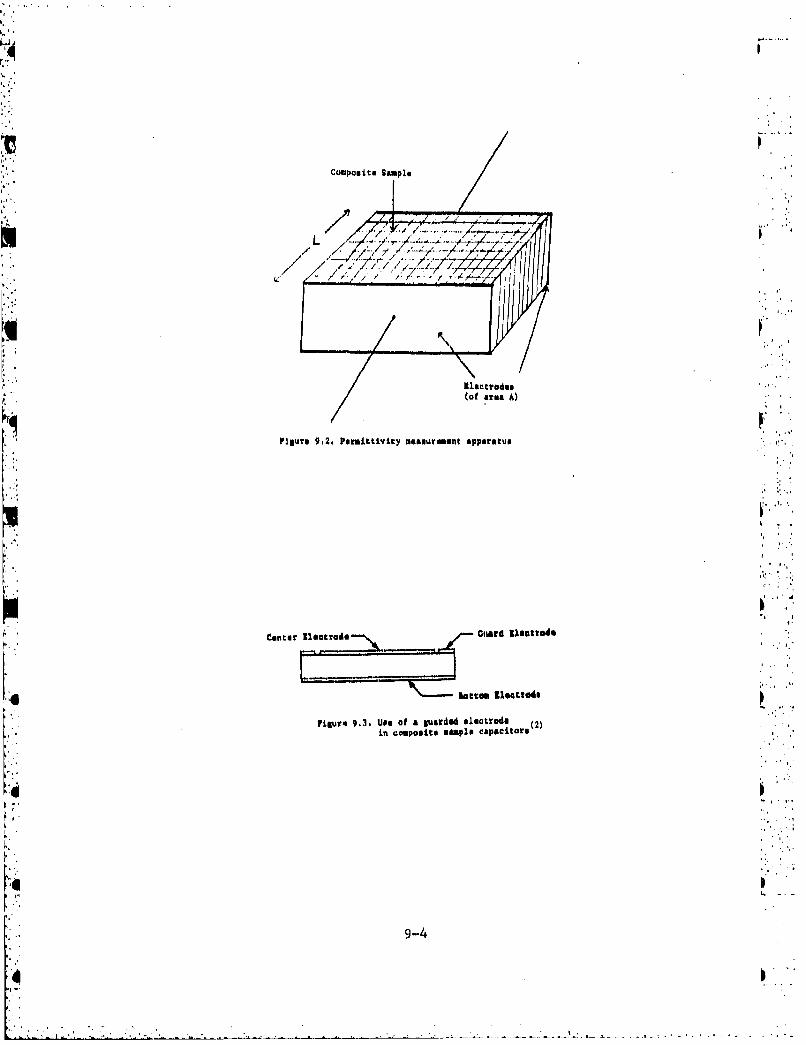
Composit Sample

~~C7

rigure 9.2. Permittivity measurement Apparatus

center g1actrode Goard IlecetrdS .

bottom gleattads

Figure 9.3. Use of a ~td~(2)in composite sample capacitors

9-4

where P is the reflection coefficient, r is the propagation constant, and tis the composite sample thickness. Shielding measurements that yieldamplitude and phase information on T allow P to be determined.(2b9)

" Knowledge of P allows the effective complex permittivity ex to be detrMined.

E X=E(l-j tan 6) (9-4)

where n t the real part of the effective permittivity and tan 6 is the lossta ngentj•2)

9.1.3 Resistivit.

The two ASTM standard methods for measuring the low frequencyresistiv ty of composite materials are the two-point and four-point probemethods, 2,3,5) described in this section.

9.1.3.1 Two-Point Method

Ohmic contacts are made to the ends of a rectangular cross sectionof material. A known current is passed through the sample and the voltageis measured. The resistance of the sample is taken to be

R.i (9-5>

where V is the measured sample voltage and I is the known test current. Theresistivity is then given by

; ' ~~RWE ,f..,- RW (9-6)

where W is the sample width; Lp the sample length between the drive con-tacts, and t the sample thickness. The two-point iethod is illustrated inFigure 9.4. Results are valid to about 30 - 50 Mz.* 2)

face.and The two-point method assumes a uniform eurcent across the sample.ace and a hoogeneous material.( 2 ) The most reliable resistivity measure-ments in practice are done on single material crystals. For materials ofmixed orientation such as cot,ý'osites the two-point method works best.( 3 )It is necessary that low resistance ohmic contacts be made to the sample,preferably by vacuum deposition of aluminum or indium. Sample preparationis critical for reliable results to be obtained. At high excitation levels,the two-point method can be used by just increasing the voltage. Because ofpossible nonlinear response, equations (9-3)-(9-4) are replaced by

P. Wt dV (9-7)

9-5

aJ. .i L dI - |" ~ * - -

ligurs 9.4. The two-poist method for meUtaa2&s)t ofresistivity of oad~uctivity)

9-6

9.1.3.2 Four-Point Method

In this technique, four probes are aligned equidistant on a ma-terial sample as illustrated in Figure 9.5. The outer two probes inject andextract a known current. A voltage (both DC and AC) is then measured at the

*. surface across the inner two orobes. The resistivity is then given by oneof the following two formulas

p - 2 _ (9-8)

if e<<t

p 45 (9-9). '

if tWs

This method has the advantage that no ohmic contacts need be made to the"composite surface. A disadvantage to them thod is that it is sensitive to1., the composite surface state and geometry. In addition, localized pointcontacts on composites are unreliab , because of the presence of brokenfibers (especially in graphite/epoxy)'')

9.1.4 Conductivi,

Three methods for measuring the conductivity of composite mateki- 'als will be discussed in the first section. One method ts the standard ASTMtest procedure which applies for relatively low frequencies. The second

" method uses a slotted stripline and applies for higher frequency. The thirdmethod extracts "effective" conductivity from E4 shielding measurements. Inthe second section, various mathmatical models for the conductivity ofcomposite materials will be discussed.

9.1.4.1 Measurements

"Individual methods for measuring conductivity in composite ma-tertals are now discussed in detail.

9.1.4.2 ASTM Method

The ASTM method for measuring the conductivity for composites(2,3.5)consists of measuring the resistance of a rectangular sample of compositeusing the 2-point and 4-point probe technique as described in Section 9.1.3.The expression for the conductivity is then

C L (9-10)RWt

-)-7

F>

p

�. ."

I

* I

E2�4V±ute � Pout-potut method for meagu�gp.mt of

resiStiVity or coduivy�.'1

I

I

* 1

9-8

4

.1.

9..3.2 Four-Point Method

In this technique, four probes are aligned equidistant on a ma-terial sample as illustrated in Figure 9.5. The outer two probes inject andextract a known current. A voltage (both DC and AC) is then measured at thesurface across the inner two obes. The resistivity is then given by oneof the following two formulasM..

P- 2rre (9-8)

if 8<t

P 4.5t. (9-9)

if tts

This method has the advantage that no ohmic contacts need be made to thecomposite surface. A disadvantage to the aithod is that it is sensitive tothe composite surface state and geometry.~' In addition, localized pointconltacts on composites are unreliabll because of the presence of brokenf ibers (especially in graphite/epoxy) '

9#1.4 Conductivity

Three methods for measuring the conductivity of composite mateifi-als will be discussed in the first section. One method in the standard ASThtest procedure which applies for relatively low frequencies. Tie second

method uses a slotted stripline and applies for higher frequency. The thirdmethod extracts "effective" conductivity from EM shielding measurements. Inthe second section, various mathematical models for the conductivity of

composite materials will be discussed.

9.1.4.1 Measurements

Individual methods for measuring conductivity in composite ma-terials are now discussed in detail.

9.1.4.2 ASTM Method

The ASTM method for measuring the conductivity for comnposites(2i3,5)* consists of measuring the resistance of a rectangular sample of cauposite

using the 2-point and 4-point probe technique as described in Section 9.1.3.0The expression for the conductivity is then -

L (9-10)RWt

4h opst ufc tt n emty nadtolclre on :Scomosits ar unelial~beaus, ofthe resece f brken "-. ",

resi.s.ivity or conductivitylil

9-8

where L is the sample length; R is the resistance; W, the sample width, andt, the sample thickness (see Figure 9.4). Equation\(9-10) assumes a uniformcurrent across the slab and a homogeneous slab of material. Composites arenot homogeneous so the conductivity of (9-10) r4presents an "average"conductivity which need not correspond to the "local" conductivity in thecomposite. Other limitations on the method mentioned in Section 9.1.3 forresistivity apply equally well for the conductivity. The frequency rangefor the model is typically from D.C. to 30 - 50 MHz.

9.1.4.1.2 Slotted Stripline "

In this method a slotted stripline(6) using unidirectional cor-posite materials is used for conductivity measurements from 50 MHz to a fewGHt-. The geometry of the stripline is shown in Figure 9.6 and consists of acenter conductor of composite separated from an outer metallic conductor bya dielectric strip (Teflon). A movable probe measures the electric field(or voltage) at any point ou the line. The slotted line is driven by RF atone end and teiminated at the other ead in an "open circuit." The lineconstitutes a lossy transmission line and the probe measures a lousy VSWRpatiern. '• "'

From analysis( 3 ,6 ) of the line, the magnitude of the square of

the electric field (or voltage) is given by

JE2 1, K[cosh(2ax+2VI)+cos(20x+2ý)] (9-11)

where K is a gain factor depending on the source (volts/m); x is the dia-

tance (in meters) from the line termination; a is the 6eal part of th,.propagation constant (nepers/m); P is the imaginary part of the propagationconstant (radians/m), and W and 4 are termination factors for the line (zerofor a pure open circuit). If the skin depth is small compared to thethickness of the composite strip and the composite fibers are parallel tothe line (high conductivity case) the conductivity in mhos/m is(3,6)

0~ 0

2 2 2'22

where 2 d is the permittivity of the dielectric space, the quantity 2 isequal to W•2 ýocd where w i• the angular frequency and Po is the permeabil- .,..ity of free space (4 10* henries/m), and t is the dielectric spacer .thicknesa. -":

For the case of the conduc.tivity being sufficiently low so thatthe skin depth is large coapared to sample thickness (as in transverse con-ductivity of graphite/epoxy), a uniform current over the sample may beassumad resulting in a simple transmission line model( 6 ) used for calcu-lating the conductivity. The approximate value for the conductivity is

9-9.0

ii I •

robe

I-il -,olo Dielectric

iit

tube

cress-section

Outer Coniductor• "

Or lo-ll cc~oSpa. ..

r

coinpositt

Figura 9.6. The Blotted Striplinse6)

9410

4-

.

4 9-10,

WedP4 = (9-13)

2ata

where "a" is the sample thickness.The justification of (9,13) is given elsewhere.( 6 ) Thid model for lowconductivity is shown in Figure 9.7.

The advantages of the slotted stripline method include the lackof ohmic contacts and a broad band of experimental frequencies. The lowerfrequency limit is set by the requirement to obtain at least one cycle ofstanding wave. data. The upper lirai'. is determined by the line cross sectionas shown in Figure 9.6. One disadvantage is that the method is applicableto unidirectional samples and not to multi-ply crossed samples.

9.1.4.1.3 ConductivitLFrom EM Shielding Measurements

It is very common and convenient to use EM shielding measurementsto calculate an "effective" conductivity for composite material test panels.A summary of the necessary equations are given here with details reserved forfor Section 6.1 of this handbook and the references at the end of this chap-ter,(2,3 9 ) A coaxial transmission line or waveguide structures filledwith a planar composite test panel can be used to calculate the RF transmis-sion through the panel. Details on these experimental methods are discussedin Section 9.2,2 of this handbook. The transmission coefficient across thecomposite panel is given by

(9-14)

where p is the reflection coefficient for the panel, r is the panel propaga-tion constant, and t is the panel thickness. Measurements of the panelshielding effectiveness enable the reflection coefficient ( P ) and thecomplex permittivity C - co(E'+jE") to be determined. The "effective"conductivity Geff of the panel is then given by*I

aeff W •Eo" (9-15)

where ( is the angular frequency of the radiation, o the free space per-mittivity, and F" the relative loss factor.

A second method of calculating an effective conductivity utilizesthe concept of transfer impedance. The theory of transfer impedance isdiscussed in Section 6.1 while the measurement process is summarized inSection 9.2.3.1. Further details may be found in the references.(2,3,10)The effective conductivity Ceff in terms of transfer impedance Z. is

9-11

* v . - . .,- , . . " - . . i . . . . != = - . • . . . ._

~TTo

L *iiiductance/moiter

0--- series vasistanceIintet~2JA onal - lengsth of

figue 9.. LwConductivitY StTiPI ,no together with

tut 'Transmission Line NcodeM'

9-12

f -(9-16)Ueff Usi

where t is the panel thickness.

9.1.4.2 Analytical Models

In this section, several composite conductivity models that havebeen recently developed are presented and discussed.

9.1.4.2.1 Single Ply Longitudinal Conductivity Model

In this model) the longitudinal conductance of a sample of corn-posfite material is taken to be the sum of the conductances of the individualfibers plus the conductance of the epoxy material. The sample is shown inFigure 9.8 and is modeled as a set of ide tical conductances in parallel.( 3 . 7 )For a single fiber the conductance js(3,7)

a 1A1 (9-17)L

where i is the fiber conductivity, Al is the fiber cross section, and Lis the fiber length. The conductance of the epoxy is

aA

G2 L- (9-18)

dwhere 2 is the conductivity of the epoxy and A2 is the epoxy crosssection. For an N fiber composite as in Figure 9.8, the total conductanceis given by

alAIN1 o2 (A-NIAI) (9-19)G -+ (9-19)

L L

where the total epoxy cross section A2 is written as (A-NIAI); A isthe total composite cross section and N is the number of fibers.

The c miosite conductivity a L is the longitudinal direction isnow defined as(3,)

9-13

S. • -• .,, • . :...,,, -- * ,.,., - . * , . .* . * -. .

0 0 0000

0o 0 000

Figure 9.&. Longitudinal Conductivity Model 31)

9-14 4

aAS--(9-20)

where A and L are the sample dimensions and G is the total conductance givenin (9.19). The conductivity aL becomes

o1lAN 1 c 2 (A-N A1 )S A + A (9-21)

or more conveniently ,

aL. al f + a2 (1-F) (9-22)

LI 1 2 .. :

where f is the volume fraction of fiber in the composite. If

the compositeLfibers are orders of magnitude more conducting than the epoxy,

L can be well approximated as

aL 1 f (9-23)

This model works well for graphite/eppxy or Kevlar/epoxy. A more generalmodel is required for boron/epoxy.(8) For this composite the fibers.,". 'consist of a sheath of boron surrounding a conducting inner core. Thelongitudinal conductance G is then the sum of the conductances 9f all fiber ,....

sheaths, fiber cores and epoxy. For N fibers the conductance is(8)"

A b N% NA "cG e e + + c c (9-24) .0L L Le

where ae' 0 hb, c arp the conductivities of epoxy, sheath and core respec-tively; Ae, Ab, Ac are the cross sections of epoxy, sheath and core respec-tively; and L is the sample length. The model is shown in Figure9.9.

The effective longitudinal conductance is

u AL -(9-25)

9-15

.40

As, epoxy area (st5

A

0 0

Figure 9.9 Logiudna g~vity IWoi for

4 ~9-169

and CL becomes( 8 )

a - e(l-f) ab f ÷ (9.26a)

where

KC(9.26b)

and Ab is the cross section of a fiber in boron/epoxy composite. Thisratio depends on the core size in the boron/epoxy fiber. S nce the fiber bcore is the most conductive part of the boron/epoxy fiber,A8) the longi-tudinal conductivity L can be approximated by

L •Oc n (9.27)

The core size of a bo-ron/epoxy fiber (as measured by rj) in a criticalparameter in this boron/epoxy longitudinal conductivity model. Because thecore size depends on the extent of reaction of boron with tungsten duringthe fiber manufacturing process, this parameter may be difficult to deter-mine for general samples of boron/epoxy.

9.1.4.2.2 Single Ply Transverse Conductivity Model

The transverse conductivity model to be discussed applies only tographite/epoxy composite. Both Kevy,.ar/epoxy and boron/epoxy have negligabletransverse conductivity, but this conductivity is significant for graphite/epoxy because of the large number of tibers that touch.

In this model, called the random fiber model,(3 7 ) the sample isdivided into a set of parallel planes. The fibers are then distributedrandomly in each plane in accordance with the fiber volume fraction f. Themodel is shown in Figure 9.10 for two planes. At any lateral points themeasured conductivity depends on whether the probe contacts are fiber-fiber,fiber-epoxy, epoxy.fiber, or epoxy-epoxy. The transverse conductivity canbe shown- 3r to be

ST al f2+ 4 a' 02 f(l-f) +a2(1-f)2 (9.28)

where al is the fiber conductivity, 02 is the epoxy conductivity, and f,

the volume fraction of fibers. A basic assumption made is that the electricfield is uniform through both layers. For graphite/epoxy where 01>02,o(rcan be written as

9-17 S

'- • ,-I, • -. -. • ,. . •. • .. .-.-.. . . .. ... ... .. ....... .. ,,,. ... ". . ... , -- -.... -..---... . . . . . .. . . . .- -- -.. '. , -- . . . . . .. . .

02

a 2 + 402 f(1-f) , o2 (1.f) (9.29)

If f does not approach zero, the expression for aT simplifies to

f2,

oT t 1 (9.30)

For N layers in the model, T becomes

T N(9.31)

This value for the conductivity is strongly dependent on thenumber of planes used in the random fiber model. Results to date with this

model are fair.7

"7)

9.1.4.2.3 Multi-Ply Conductivity Model

The simplest model for multi--ply structures treats the individualplies as conductances in parallel.(3,8) For the ith ply, the conductanceIs of the form( 3 , 8 )

0 C iWt

where--- i- (9.32) "where W is the sample width; L, the sample length; t, the ply thickness(assumed identical for all plies) and cri, the ith ply conductivity. Thetotal conductance of the sample (composed of N plies) is

N oGWt (9.33)

An effective conductivity, 0 e' of the multi-ply sample is defined( 3 ,8)

asciA

Cy A

- . (9.34)

where A is the total sample cross section and L, the sample length. Thesample cross section is given by

A - NWt (9.35)

•w.here N is the number of plies; W, the sample widt h; and t, the common plythickness. The effective conductivity is then

9-18

f i u r 9 . 0 , U m F i b r M d e

9-19

F,-", o = i'dl °i (9-36) ,.."-"

The basic assumptions in the model are uniform ply thickness, uniformexcitation of the sample and electrical independence of the plies.O,8)The results of the model are mixed( 8 ) with indications that the electri-cally independent ply assumption is somewhat poor even under low frequencyS~~extations.•',

9.2 EM Shielding Efiectiveness Measurement Techniques

In this section, the various methods of measuring the electromag-netic shielding of composite materials are discussed in detail. The firstthree parts of this section treat shielding as measured by coupled loops or .probes, plane wave transmission and reflection, and surface impedanceparameters. The advantages and disadvantages of each method are reviewed.Shielding measurements when joints are present as discussed as well as thespecial situations of composite structures under high current and highvoltage conditions.

9.2.1 Coupling Between Loops and Probes

"In this section the coupling between two loop antennas, two dipoleantennas, and two monopole antennas is examined as a measure of shieldingeffectiveness for an infinite homogeneous (or multi-ply composite) planarshield and for one or more parts of the test system in an enclosure.

9.2.1.1 Infinite, Planar Shield

The shielding effectiveness is defined as the insertion losscaused by the introduction of an infinite, planar shield of compositematerial betweun a source and detector antenna system. The antennas arecoaxial with a line perpendicular to the ohield. The coupled antenna""systems discussed are two loops, two dipoles and two monopoles.

-. 9.2.1.1.1 Two Loop Method

. The two loop method(2,3,10) is illustrated in Figure 9.l1a. Thesource loop is driven by a current I, and a voltage E2 ib measured at theterminals of the detector loop. The source loop has radius al and is adistance rI away from the shield. The detector loop has radius a2 andIs a distance r 2 away from the shield. A voltage E2a is measured firstwith air between the antennas and a voltage E2m is measured with the

4 composite shteld between the antennas. The magnetic shielding effectivenessis given by (2)

SM 20 108lo10 (9-37)

9--20

4-" 9"0" '

!.-

r r

Source 1amCurrent,,a

F, Induced2 Voltage

Figure 9.116. Two Loop Met~hod~

I, ..

r -4

2U

1000

AkK

Source ySensor

Figure 9.11b. Two Dipole Method~2

K -, 9-21

The voltages E2m and E are complicated functions of aI, a2, rI, r 2 andthe shield thickness t.

9.2.1.1.2 Twohod ....ho

The two dipole methodý 2 , 3 ) is illustrated in Figure 9.11b. Thedipoles are of length L 1, L2 and are located at distances rl, r 2 fromthe shield. The source dipole is driven by a current I1 and a current12 is measured in the detector dipole. The shielding effectiveness isthan given by(2)

a 20 log10 2? (9-38)

where 12a is the dipole detector current without the shield and 12m. thecurrent with composite shield present. The currents 12a and 1 2m arecomplicated functions of 11, 2, rl, r 2 and the shielded thickness t,

9.2.1.1.3 Two Monopole Method

This method(2) is similar to the two' dipole method illustratedin Figure 9.11b except the two dipoles are replaced by two monopoles over aground plane. If the monopoles used each have a length h th~n the monopolecoupling is the same as Coupling between dipoles of length , where X isthe radiation wavelength.' 2 )

9.2.1.1.4 Limitations

One basic limitation of these measutement methods is the extent towhich data obtained from a finite composite shield can replicate the dataobtained using an infinite shield to which these methods strictly apply.Some leakage around the edges will always occur and the amount of leakage isfrequency dependent. This limitation is criticaA fr good shields whereleakage may be comparable to the penetrating field(2,03

A second limitation is that the shielding effectiveness pertainsonly to the antenna pair and composite shield oeometry. It cannot easily be. .related to other methods or other geometries.(2,3,10)

9.2.1.2 Enclosed Shield

When actually making a measurement of shielding effectiveness, itis usually more practical to enclose one or more parts of the measurementsystem. Figure 9.12a shows the use of a metal enclosure around the sourc..loop of a two loop system. The purpose of this enclosure i- to eliminatethe edge leakage which occurs in the infinite plane methods when using afinite plane, as discussed in Section 9.2.1. This permits use of a finitecomposite shield. The disadvantage of this approach is that the &hielding

9-22

.. ' . . .* - .

Sealed Intloamra Uhisidiag varriar

Sout.......

F 2 p i I

"lii

atoad© l boxFigure 9.12b. paryluly %olosod •ypern•or

mleaeurLng ShLedi 3.1" For

9-23

i',' • • ~sh eet of i eelel~t r ., , '

4• Pi L r e 9 . 12 b . ' ?u l ~ y I~ n , l o s d l 5 y, at 11• i~ t"- . " '

,. • ,

4I 9-23

effectiveness now depends on the box geometry since the box charges the

field of the source because of reflections and resonances from the enclosurewalls. These problems could be reduced if the box were an anechoic chamberwith the composite shielding barrier being one side of the chamber and theother sides covered with absorbing material.

A second method involves enclosing the entire measurement appara-

tus (including composite shielding barrier) in a large anechoic chamber.This method is illustrated in Figure 9.12b for a two loop system. It allows.

the use of a finite piece of material and assures minimum interference from

reflections and resonances. However the shielding effectiveness still

depends on the chamber geometry to some extent and may be hard to relate to

other methods of measurement. For certain test frequencies the size of the

chamber required would be too big to be practical.

9.2.2 Plane Wave Transmission/Reflection Methods

A very simple definition(2, 3 "10 ) of shielding effectiveness arises'

from the case of a uniform plane wave incident on an infinite homogeneous,

or multi-ply composite. This situation is shown in Figure 9.13. For

shields of nonzero thickness, the overall effect is composed of reflections

from the incident wave striking the shield surface and ýhe internal material

boundaries, plus transmission loss through the shield. Several experimental

methods for measuring the shielding effectiveness for incident plane waveson shields wll be discussed. "

9.2.2.1 Sample Experimental Methods

In this section several different methods for mounting and illu-

minating the test sample with a uniform M1 plane wave are described.

9.2.2.1.1 Coaxial System

The coaxial system( 2 , 3 ) is illustrated in Figure 9.14. This

system gives rise to a radial electric field and propagates a transverse

electric and magnetic (TEM) wave. The radial nature of the electric fieldis a significant departure from the required linearly polarized uniform

plane wave. Unambiguous results are obtained only for homogeneous materialsor multi-ply composites. This system is not useful for unidirectional.composites or other highly anisotropic materials.

9.2.2.1.2 Rectangular Waveguide System

This system is shown in Figure 9.15. These guiding structures can

give rise to a transverse electric (TE) or transverse magnetic (TM) propa-

gatitg wave in the fundamental mode,(2, 3 ) and are useful becauses of the

unidirectional nature of the electric or magnetic fields produced, This

transverse field can be aligned with the composite fibers or at leastaligned with a principal symmetry axis of an anisotropic material. The

other field, then, is then not aligned with the axis. The waveguide fields

can be resolved into two obliquely incident plane waves. The incidentangles of t 1ese waves depend on the ratio of operating frequency to cutoff

frequency.-(2) Thus the incident wave from the waveguide cannot be consid-

ered a uniform plane wave with a different wave impedance.

9-24

.-... . . -... I . ... .. -. . .. .. . . .

Sealead Inclosure Shielding Barrier

Figure 9.12a. Partially Inclosed 8 stem ForMeasuring Shielding(l)

Looop I

Sheet of Material

4 Figure 9.12b. Fully Inclosed SYst PFarYleasuring Shielding

4 9-23

4 .~~~ Wave31 Icdnr

It7

Wave I -mihite PlaneWhelding Panel

Incident WaveTanutedWv

ligure 9.13. uniform plans Vge. Uhjmldiq4 (2)apa

Transverse Disk ofM4aterial Under Tou

Viluve 9.14. Coaxaial Iystuiw3

Transverse Sarrier ofMaterial Under Test

Filure 9.15. Rectansular Waveguid. 3ystm( 3 )

9-25

9.2.2.1.3 Far Field Anechoic Chamber System

A typical chamber setup is shown in Figure 9.16. The use of achamber avoids many of the problems of sample preparation inherent in tilecoaxial and waveguide systems. Chamber measurements should very closely .

approximate the results 9f uniform plane wave illumination for a properchoice of test antennae.') The main limitation of this system is the

lower frequency limit imposed by the chamber size (typically 500 MHz).(2)

"9.2.2.1.4 TEM Cell

This method avoids the difficulties of coaxial or waveguidesystetns in producing linearly polarized uniform plane electric and magneticfields over the composite material barrier *' 2) The TE2 cell is i]~1stratedin Figure 9.17 and resembles a distorted coaxial transmission line 2 having

an inner conductor and an outer conductor with extended edges. The designallows the existence of a T4 wave over a large section of the test barrier.The orientation of the electric and magnetic fields with respect to prini-,

, pal axes of symmetry in anisotropic materials can then be controlled.(f2)

"Proper design of the extended edges minimizes the fringing effects.

"There are two main limitations on TM4 cells.( 2 ) The probability"of higher modes propagating on the line increases if too wide a line is used

to reduce fringing and improve the TH4 wave illumination. This limits thefrequency of operation of the device. Also, a TE1 cell designed to minimizefringing and optimize TE4 wave propagation may have a characteristic imped-.ance consicarably different from the impedance of the feed lines for thecell (typically 50 ohm lines). This results in a mismatch in the T04 celt.

test system* 2) This problem places a further restriction on the operat-

ing frequency of the cell. The mismatch can be controlled, however, by useof proper interfaco devices between feed lines and cell.

9.2,2.1.5 Near Field Method

The near field( 2 ) antenna measurement test setup is shown iiiFigure 9.18. A source antenna illuminates a test barrier of compositematerial and an antenna in the near field of the source makes field measure-ments in a plane parallel to the barrier. Field measurements are made both

with and without the barriers. These field values are then Fast FourierTransformed to far field values. The theory is described in Section 6.1 ofthis handbook and in the referen8es.( 2 1 1 Y) The plane wave shielding ef-

I' fectiveness (Se) i. then given by(2)

"se -- 20 logft T (9-iY)

whare

4'.• T is the transmission coefficient i

E.. T E • (9-4 0)

0E is the field at the barrier and Ho is the field in the absence of thebarrier.

9 -

:! ~9-26 •

Z 544I-L5 a c a

4.9 -4

Jail 9-27

The basic limitation to this method is a limitation on the fre-quency range where large enough barriers are available to minimize fringing.Also the theory applies strictly to homogeneous, isotropic and possibley tumulti-ply composites.

9.2.2.2 Instrumentation Configurations

In this section, two common, instrumentation configurations usedfor measuring plane wave shielding effectiveness using transmission/reflec-tion methods are discussed along with limitations in the configurations.

9.2.2.2.1 Substitution

This configuration(2) is shown schematically in Figure 9,19a. Anyof the methods (coaxial line, waveguide, TE( cell) discussed in Section9.2.2.1 for mounting and illuminating the composite sample may be used inthis configuration provided the necessary isolation techniques are avail-able. The shielding effectiveness is then the difference in attenuatorreadings when the sample and lossless line are excited separately.(2)

9.2.2.2.2 Bridge

In this configuration( 2 ) a suitably isolated sample mounted and-F 'tiluminated by any method (coaxial line, waveguide TWM cell) in Section9,2.2.1 is connected in parallel with an attenuator and phase shifter withsuitable isolation, The configuration is shown in Figure 9.19b. The properamplitude and phase adjustment to produce a null in the detector constitutesthe shielding measurement. In this approach both amplitude and phaseshielding information is obtained.

9.2.2.2.3 Limitations

Great care is required in preparig and mounting the test material,in the material holder to properly interface it to the rest of the test

configuration. An idealized interface is shown by a network in Figure 9.20aand is repreuented as three cascaded transmission lines with the samplerepresented by a transmission line of modified impedance and propagationconstants. Poor interfacing and mounting of the sample will introducecoupling between the sample input/output ports and between gapa in thematerial sample and holder walls. This situation is illustrated in Figure9.20b by a network. Elements Y5 and Y6 represent leakage through samplegaps.

9.2.3 Surface Impedance Parameters

Surface impedance parameters offer a very useful way to character-

ize the shielding effectiveness of shield that are thin with respect totheir radii of curvature, and for which the wavelength of the field in theshield is much smaller than the wavelength of the fie d external to theshield. Such a shield is said to be locally planar,(3,i1)

For shields envolving closed surfaces, the surface transfer fin-

podanc, is defined as(2,3,9,I0)

9-28

*

N rN II

a

-4

N V.6�

a �6.�0 0

o 4.4 4..

-- YT 1.2'U �.I I F

.1'a

U' U'

'a-

a -4

o I'a

0

w

I.4. f '4

�4.', .4

"a----i-IF UI A

5. * a'

.�.

'1* *�4 I

I. p

9-29

i-7

4. . *..,.-. . - a.

zt ,-

St

where Et is the inner shield surface tangential electric field, and J. is theouter shield surface current density. The theoretical treatment of transferimpedance and its relation to 124 shielding may be found in Section 6.1 ofthis report and the references.(2,3,9310)"

F r locally planar shields the surface transfer impedance has thefonn(23,10

,t n1 cs4ch(rd) (9-42)

where

1/2

r lieu 1/2(9-44)

and d is the shield thickness.

The transfer impedance in (9,42) can be shown( 2 ,3 ,"0 ) to be equalto the "two-port" surface impedance parameters( 2 ) used to characterize theshielding of an infinite planar plate, thus justifying the term "locally"planar" to describe the shield.

9.2.3.1 Measurement Techniques

This section will treat two methods for measuring the surfacetransfer impedance: triaxial and quadraxial cable techniques.

9.2.3.1.1 Triaxial Method

This method Is a modification of a lichnique used to measure theshielding effectiveness of shielded cables, 2,12) The composite undertest is first fabricated into a cylinder which takes the place of the cableshield. This shield and an enclosed sensing wire conductor become the innerconductor of a coaxial transmission line driven by RF at one end and terml-

nated in an "open" circuit at the other end. The situation is depicted*,":schematically in Figure 9.21a. The composite shield is driven with a

current I, and a voltage V ý is measured at the termination. The surface.rai fer impedance is then'.:..

(;; 9-30

I. I Z I

f~igre 9.21a. wfac Tr~anfer tapadano e tenan~ft

CONCINPIM CAULK.CoNDUCTOR 1I12.

Figure 9,21b. Surface Translfer AdmittafOnce He tenanWith Short Circuit Termination

9-31

LiiVo.

zt = C (9-45):

where ka is the length of the coaxial line and 2,s«)< where X is the radia-tion wavelength. This same device can be usod to measure the surfacetransfer admittance. The coaxial line is now driven with a voltage sourceand terminated in a short circuit (Figure 9.21b). The short circuit currentq c is measured and the surface transfer admittance YTis( 2 )

* Ksc.2"YT = (9-46)m siti

One limitation on this method is the fact that the coaxial linemust satisfy ts << X in order that the open ctrcuit termination can be used •'

and line resonances avoided. This places a constraint on the frequencyrange of operation(2) A further limitation involves the radii on the '"outer two cylinders. They must be chosen so as to avoid cavity resonancewhich places a further restriction on the frequency of operation.(2) '

Detectors used in the measurement should ba well isolated from the lineitself, It is essential to have proper sample preparation and good electri-cal contact between sample and measuring apparatus.

9.2.3.1.2 Quadraxial Method,,

This method is a modification of the triaxial structure to mini-mize resonances and external perturbations in the measured data.( 2 p1 2 )

A sensing conductor (wire) is placed inside a cylinder made of thecomposite to be tested and the coaxial line terminated in its characteristicimpedance. This coaxial structure then becomes the inner conductor of acoaxial line with an outer conducting cylinder. This outer coaxial line isalso terminated in its characteristic impedance. This is similar to Figure's9.21a and 9.21b except that the terminal contains a finite nonzero imped-ance. This triaxial structure is shown in Figure (9.22.). The signal lineserves as a reference line but the reference is different at points A and B. ', AThe quadraxial structure in Figure 9.22b uses the signal line as the sourceline while a balance line goes from the composite inner cylinder to theouter cylinder and serves both at a referenge and as a method of maintaininguniform current on the composite cylinder.2 212) Measurements of transferimpedance or admittance are then carried out as in the triaxial methoddescribed in 9.3.2.1.1.

One realization of this quadraxial method is the Boeing quadrax

test conf isurationt 2 1 2 ) pictured schematically in figure 9.23.

9.2.4 Joint Measurement Techniques.

A very important determinant of the overall shielding effective-ness of aircraft structures fabricated from composite and/or metallicmaterials is the existence of joints in the structure. Skin currents

9-32.

S.. ... . . . .. ... ... ..._. ._. • .• . . .•. .. :. •i .. • • " ..-• "•. . . . . _ , ." i• . . .• .' , , •' , .: .•. i. :. ... . . . . , , , . - .. ,,

~~MyIS 1'IUMYII

Figure 9.22a. Triaxiul Schwa.tic(2 ) ,

TEST EQJUIWET TE 1ST FACILITY

KKAHP IOOO NM IU4NL5CI

FURa.922.~~2 5hmte 2

OpenWN Fogui it

(021

IBMI

9 NJ 33Q FAAl aZo O 7104INL SITIO

flowing on the surface of the material create electric fields that arecoupled onto aircraft avionic systens through the joint, The appropriateparameter for measuring this joint coupling is the joint admittance per unitlength of joint (Yj). The theory of joint admittance and its contributionto composite shielding effectiveness is described in Section 6,1 of thishandbook.

One set of measurements for Yj uses basically the same measure-ment techniques that are used in measuring the surface transfer admittanceof can osite panels described in 9.2.3.1. The Boeing Quadrax test Configu-ration?12) (see Figure' 9.23) has been used to measure joint admittancesand the procedure is summarized in Figure 9.24a. The cylinder consists oftwo identical materials jointed together and is assumed to have a surfacetransfer impedance ZT. The circumferential joint has a joint admittanceper unit length, Yj. The cylinder is driven by a known current 1s(current density is J.) and the open circuited voltage Voc measured.,Then oc *is.

Vocc L Iz ZT + Y 21a (9-47)

where L is the cylinder length and a, the cylinder radius. The jointadmittance is then

1 Is (9-48), 27Ta Voc -ZTL Is

The surface transfer impedance ZT is assumed known from measurements on acylinder with the same material but no joint.

This procedure can be generalized to joints between two dissimilar•-materials (different composites, different metals or metal and composite)

and is shown in Figuve 9.24b. The dissimilar materials have surface trans-fer impedances ZTL and the ZT2 and thejoint has an admittance Yj. The [open-circuited voltage at the line termination is

_ Is (9-49),oc 1 ZTl 2I ZT 2 Yj 2Tra

where Ll and L2 are the lengths of the two dissimilar cylinder sections anda is the cylinder radius. The joint admittance is then

•.*lt Is (9-50)2,ra V -ZTLIS-Z T2L2

9-3

. .9-34

t .,I

JE I ".

ZT Yj

Figure 9.2a. Joint AMIttaso otdestcal "

materia.l Joated)

tVL

ZTI /Y Z.

F*igure 9.24b. Joint Admittance (differentmaterLals joined)

* F

9-35

J

9.2.5 Hish Current Injection

In this section the effects of high current injection onto com-poqite structures are discussed. The high current is assumed to result froma lightning strike or near miss. Methods of simulating lightning strokes onaircraft are treated and the various effects of lightning on aircraft arereviewed.

"9.2.5.1 Standard Current Waveforms

In order to ascertain the effects of high current on compositestructures, a standard waveform for the test current must be chosen. Sincealmost all high current phenomena involving composite aircraft are due tolightning, the standard high current waveform is chosen to be as close as"possible to the current waveform of natural lightning. Numerous experimen-tal studios of natural lightning flashes have assigned nominal valuLs to a"number of different lightning parameters such as peak current, rise time,amplitude and charge transfer. A general list of these parameter values isgiven in Table 2.1.1 of this report.

The effects on compositt .rcraft due to high currents are con-veniently divided into two groups.

Group 1 includes effects such as burning, eroding, blasting,structural deformation, high pressure shock wave and magnetic forces. Theseeffects are associated witi tjhe high currents and charge transfer caused by"a direct lightning strike.s 4 '

Group 2 effects arise from the electromagnetic field produced bythe lightning and include induced voltages on interior avionic systems andsparking across bonded structures. These effects are associated with highpeak currents and large rates of change of current caused by a directlightning strike or a near miss. A list of important lightning effectstogether with the lightning parameters that significantly, influence thee'effects is given in Table 9.1.

The reason for dividing the lightning effects and parameters intotwo groups is because it is experimentally difficult to adequately simulateall significant lightning parameters in one standard current waveform.() ;.Diferent lightning parameters, and hence different lightning effects, areusually sensitive to different parts of the lightning waveform. Consequent-ly, when investigating various lightning effects only portions of the totalcurrent waveform need to be simulated.

To meet Jhese requirements, a standard lightning current waveformhas been proposed. 13,15) The waveform for investigating Group I lightningeffects is shown in Figure 9.25 and consists of four basic components. Thevalues of the parameters that describe the components are given in TableS9.2.

The waveform for investigating Group 2 lightning effects is thesame as that for Group 1 except that component D is modified. This modifi-"cation is given in Figure 9.26 and the lightning parameters describing thecomponent are listed in Table 9.3.

9-36

I ..-

Table 9-1 Lightning Parametesr and Ltghtniq Iffeats(14)

Basic Effect Important Parameter

Group I

metal skin puncture

hot spiot formationmechanical damage Couloeby

magnetic forues 2damage to uompomits 2

s tructures afuel ignition

damage to lightningarresters

sparking

induced voltage$ n

vo1tAge flashoversparking di/dt

fuel ignition d21d1/dt2

n in the nijinber of restrikes in a flashI to the peak vale• of the current

L LI the instantasneous value of the current

9-379

* .. . • .. .'.i.

KSAF2A AMPLMOUC-tE kAkwACTION INTEC3RAL-2i IDIA2-5ECONDS

A IN III I At"L

-

A

" '

.i

COMPONENTkIPI D INE MSKT IURET

A k

COWMMaPNET (C IOTipW

AMPLITUU 14 7-

II

I-.,C0MPONINT 0 111T MAPIATIq CURRENTE

T4EGUIC T EAXOIMUM OMA E5CINTOINFR1 ICOUL MOMB$

-IRAI AMPU, - I kA

Tabl 9- IONp LIN'flORi l. ¶4vfv p0a'tiCO tt.N'1 5 . 1".:

CO MNN aI'T INT

,D•~ l'-

:,.:

CHAROKK Tplul-q ANkaA mom

€OMPONENT r (CONTINUIN URNT

Fighcurent e25aGr cr t Litni2n-00I r itmTal 0- Gru, ihnn aytrPraty

component A action integral 2 10 Ae a 1l10

pulse length'rise tine* 25118~

intermediate current Average amplitude 2k?. f 10%componen~t 5 charge transfer IcC 1 10111

continuing current amplitude 200-900A.component C charge transfer 200C 204

restrie (group I peak amplitue 1.k?.A 1 10effects) 10, 10component D cinitgrl 02 ~

Lpulse length 5 SCpe

L419-38

.. . -' .<

Current

10(0kA

~' *..

. 1 Tire

iO " / i

b.~' 0.su

Cu 25kA/ua - -,--'- ,,

F'igure 9.26 Group 2 Component D Standard ~~t~ILightning WaveforuC 14)

Table 9-3 Group 2 Component D Parametest

Component Parameter Value Tolerance

restrike (group peak current lookA 1 10%2 effect",-component D peak initial rate of rse of '

time for which di/dt should 1Oexceed 25kA/ma 05j 0

9-39

In determining the different effects of lightning on a test speci-

men, the components of the waveform can be used separtely or in combinationwith other components as needed.

9.2.5,2 High Current Waveform Generation

The basic circuit used for producing the various test current"waveforms is illustrated in Figure 9.27. The energy used to produce thelightning waveforms is initially stored in the circuit capcitor whichrepresents a large capacitor bank. The waveform is generated i14 by firstclosing the starting switch to discharge the capacitor bank into an induc-"tive, underdamped circuit. When the current It, Is maximum, the switch inthe clamp or short circuit is closed. Because of the low impedance of theclamp, the inductor will discharge through the clamp. The advantage of thissystem is that the current is offectively coming from a constant current

source without limitations on the voltage. The sample to be tested isplaced in the AB or CD position depending on which current components are tobe simulated. A set of circuit parameters necessary to produce the standardcurrent waveform is given in Table 9.4. More recent developments in gsaee Frating lightning waveforms have been reporteA by Hanson.

9.2.5.3 High Current Methods and Techniques

Test techniques involving the use of high currents on test speci -mans will now be described,. .

9.2.5.3.1 Stationary Arc Testing(14"1 6 )

"A very common test technique consists of a stationary electrode"suspended a measured distance above a test specimen. An electric arc thendischarges into the test specimen. The arc current, waveform and voltageare recorded. In addition, each discharge is photographed to determine thearc root location and quality of the arc.

Careful placement of the current return conductor is requiredsince the magnetic field produced by the conductor can interact with the arcsignificantly.

9.2.3.3.2 Swept Stroke Testing

The basic items needed to measure wept lightning strokes are atest specimen, a discharge electrode and apparatus to mve the dischargeelectrode at the aircraft relative air velocity. Several detailed methodsfor measuring aaept •ightning strokes experimentally have been described inthe literature. 1- 6),.

A primary use of swept stroke testing is to determine the aircraftstrike zones. In order to determine thee zones, a proper combination ofstandard current waveform components must be used. The standard combina-tions used are given in Table 9.5 for both groups of lightning effects..

Other important quantities to be measured during a swept stroketest are a number of attachment points, arc dwell time, dielectric orcoating material breakdown, and puncture points. These can be determined byhigh speed photographs of the arc. 7'

9-40

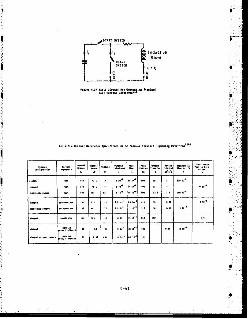
sTART SW1ITCH

S2 InductiveStore

CLAMIP

'C A

Tigre 9,27 Basic Oiroutit Pot Comas siln Standard

Teat Current Vavlfown.

Table 9.4 Current Generator Specifications to Produce Standard L~ightning Waveftrian 1'

I s...

m irldi curen t,, Awi I77 i t %i

atoo i 1 041.1 74 6 to' as 10, No to I 1oo 0o'

aVMa ast 110 42,1 74 &0 to * 10~ 200 11 IS to*1

vr141.glIV .a4.s last 602 104 131 a 10, 4 iso0, too 6I 19q 10to.

cleepsi Ditenodlsto 64) 12) Is 7.1 to,) ),1o' 4. 0 10 0.01 4lo , 5,

fsitioasll isoped intenswdiate 71 441 It 1.5 to" 1 to" 3.1 10 0.01 1 to'

oomaiapa4 Igo~h14 oil Ia t 0.21 is to" 0.6 300 .0,

alsapd ,4t~1ta ~ 4 94,*.4 .

"ofsf1ie 0 as64 104 10 104 10o 0316 10 10*

ssaatf or5 o~s0 II 50to 6 10' 1.1 10' 100

9-41

Table 9-5 Waveform lequiTmento for •pponentTesting of Aircraft Zonea(AsEO

(a) Group I Compolit te rest

current componentTest sons,

A S C ,

IA N U x (note ris x x a x (nets 2)

2A x x (note 1) x (note 2)

21 K a a (note 2)

3 t (note 3) .(note 2)

(b) Group 2 omwponent Teots

Current Coponent'Test gone

Ab

IA x

1I X m (note 4)

2 x (note 4)

S N (nete 3) (notes 3 a 4)

Note I Asesue a current duration of 45mm for sontinulng current @9l-

ponents unleus swept, stroke testing ohome otherwse,

"tote The continuing ourrent should drop to near lsro before therestrike commenoes.

pole 2 current to be applied through a solid connection notM an age.

I Component D to have a rate of rtie of LOOMA/um A Los

9-42

4. .2':2.

Swept stroke phenomena are important because they cause sectionsof the aircraft not normally involved in the lightning process to becomevulnerable because of the sweeping action.

9,2.5.3.3 Induced Voltage Testing and Sparking

Induced voltage and sparking is primarily a function of high peakcurrent and high rate of change of current which correspond to Group 2lightning parameters. The physical layout is very important for the testsetup. In particular, the return lines should be arranged to yhield a ' .;minimal magnetic field at the test specimen, and the monitoring equipmentplaced so it wll. i•t influence the results.

9.2.6 Klith .. -aze Charaing-Dischargins Phenomena , ,The principal high voltage charging-discharging phenomenon in-

volving composite aircraft is the procipitation static threat discussed inSection 2.0 of this handbook.

9.2.6.1 Test Techniques

One commonly used test method involves the direct connection ofthe speciment to the source of charge. This method is not a very realisticsimulation of the preoipitation static charging process.

Another method involves blowing "wondra" flour particles across a. test speciment. This method simulates the actual charging process more

closely than direct connection but results in a low charging rate. This .procedure is discussesI in Chapter 2 in connection with precipitation static

2i'. charging of aircraft-...)

A precipitation static t'st technique has been developed byBoeing( 9 ) which combines high charging rates with carefully controlled -,.1

. conditions. The apparatus is shown schematically in Figure 9.28. A di.-charge probe is connected to a high voltage source and is used to sprayelectric charge directly onto a test specimen. The height of the probeabove the specimen controls the charging rate. All charge leakage away fromthe specimen is carefully monitored by current test probes. This apparatushas been used successfully in measuring the charging process of variousgraphite/epoxy panels.

9-.4 3

NO 17 POWE(R SUPPLY

DEXTER DISCHARGE PRO44E360141s, ~. 004, 1~

STY TEST SPECIMCENE

SHIET WIT P.. AI E A

ALI4WITHOUAP THE C LRMENUM

ALUMINUMP TAEP "LATE DC CURRENT

DPm1LT C CURAIT

5,58e 0 n..26pro tatiom I4taic atokTesqe)

9-44

9.3 References

1. 1974 Annual Book of ASTM Standards, Part 44, p. 39, 1974.

2. Allen, at. &l., A Technology Plan for Electromagnetic Characteristicsof Advanced Comosites, RADC-TR-76-206, July 1976.

3. Allen, et. al., Electromagnetic Properties and Effects of AdvancedCo52os te Mat.etrials: Measue~ment and Modeling, RADC'TR-T8-139. June !-4. 1974 Annual Book of ASTM Standard Part 39, p. 23, 1974.

5. 1974 Annual Book of ASTM Standard Part 43, p. 206, 1974.

6. W. F. Walker and Roger E. Heintz, Measurement of Electrical Conduc-tivity in Carbon/E oxy Composite Material over the Frequency Range75 M1z to 2.0 GHz, RADC-TR-79-253, October 1979.

7. W. J. Gajda, A Fundamental Study of the Electromagnetic Propertiesof Advanced Composite-Materiels RADC-TR-78-158, July 1978.

8. W. J. Gayda, Measurement of the Electrical Properties. of CompositeMaterials in the Frequency Ragne of D.C. to 30 MHz, RADC-TR-79-203,August 1979.

9. Straws, et, also Investigation of Effects of Electromagnetic Energy.on Advanced Composite Aircraft Structures and their Associated Avionic/Electrical Equipment, Phase II, Volume 1, The Boeing Company, 1977.

10. Wallenberg, at. al., Advanced Composite Aircraft ElectromagneticDesign and Synthesis, Interim Report, Syracuse Research Corp.,

April 1980.

11. E. B. Joy, D. T. Paris, "Spatial Sampling and Filtering in Near-fieldMeasurement," IEEE Trans. on Ant. & Prop., Vole AP-20, No. 3, May,1972.

12. D. Strawe, L. Pis.ker, "Electromagnetic Shielding of Advanced Com-posites in the 10 kHz to 100 MHz Frequency Range," (AFML) Final Report,July 1975 Contract F33515-74-C-5158, Boeing Aerospace Co.

13. Lightningiest Waveforms and Techniques for Aerospace Vehicles and "Hardware, Report SAE Committee AE4, Special Task F, (1976).

14. J. Phillpott, Recommended Practice for Lightning Simulation andTesting Techniques for Aircraft, Culham Laboratory Report CLM-RH3,Abington Oxfordshire England, (1977).

15. Schneider, Kendrichs and Olson, Vulnerability/SurvivabilitZ of Com-

20omte Structures - Lightning Strike, AFFDL-TR-77-127 Vol. 1 (1978).

16, Protection Optimizatin for Advanced Composite Structures, FourthQuarterly Progress Report prepared by Gruman Aerospace Corporation forAir Force Systems Command, Wright-Patterson Air Force Base underContract F33615-77-C-5169, June 1978.

4l 9-45 .

,'.", .. L." ." ." ."....tL ' " ,: :..L. .. .. .. <L• . L.:, .: . ..t"A i• ,* •:'.I .. 'I - Z..• ",.. _. - . ,-.. *. . _ , .- -,-.-- - .- - . , ..

10.0 PROTECTION METHODS AND TECHNIQUES

Structures involving composites such as graphite/epoxy, boron/epoxyand Kavlar/epoxy are a common feature on present day commercial and militaryhigh-performance aircraft. The high strength and stiffness of these mate-rials together with their low densities make them excellent for constructingthe high-performance and fuel efficient aircraft required for the future.

Composite materials, however, are not without their'problems. Becauseof their lower conductivities compared to most metals (such as aluminum),composites are more susceptible to lightnign strikes, static charge buildupand possess poorer electromagnetic shielding properties. Possible conse-quences include structural damage, EM interference in sensitive digitalelectronic equipment, and possible catastrophic failure of the aircraft.Protection systems are needed that will protect t.ompnoite aircraft adequate-ly, yet not extract a severe weight or cost penalty nor degrate mechanicalproperties unacceptably. Such systems also must bo compatible with thethermal, fatigue and moisture environments the composite aircraft mayexperience. Finally, adequate repair techniques should exist for theprotection system.

In this section, a number of different aircraft protection systems will"be examined. The main emphasis is on lightning protection but other systems"for protection against precipitation static, EH field penetration of theaircraft structure, moisture and chemical action will also be considered.

10.1 Present Aircraft Protection Systems

In this section a brief survey in given of protection systems cur-rently being used on modern aircraft. The main protection afforded by thesesystems is agairst lightning and precipitation static, although some of thecoatings applied to' composites increase their shielding effectiveness andprotect against moisture and chemicals.

Both lightning and precipitation static threats have been de-scribed in detail in Chapter 2.0 (electromagnetic threats) and only a briefsynopsis will be given here. Lightning damage to composite aircraft iscaused by thermal effects and high current densities. Thermal effects occurat the lightning arc attachment point where temperatures as high as 27,000c"are possible.(1) The usual result is burning or charring of the compos-ite. Damage from high current densities tends to occur away from theattachment point and results in vaporization and rupture of t e compositefibers due to their lower conductivities compared to metals. Lightningdamage is proportional to the arc attachment time which, in turn, depends onthe aircraft strike zone involved. Typical strike zones are shown inFigures 2.16 and 2.17.

aircraftPrecipitation static is caused by triboelectric charging of an,aircraft region due to particle or precipitation bombardment. The resultingcorona discharge causes RF interference. Composites (especially Kevlar) aremore prone to charge buildup due to their lowered conductivities. Bothlightning and precipitation static can be controlled by use of proper ""protection devices which will now be described.

10-1

Wiiilp

t0.1.1l Static Dischargers "

Static dischargers are commonly positioned at points of hilhstatic charge buildup on aircraft to quietly discharge the aircraft..()The oldest type of dischargek is the "discharge wick". The wick is usuallymade from graphite-impregnated cotton sealed in a plastic tube. Mounting Isusually done by bolts, rivets or resin. A discharge wick is shown in Figurei.' ~~10. (a).• i

Ortho-coupled dischargers( 5 ) consist of a high impedance rod witha tungsten pin through the rod angled to minimize coupling of corona dis-charge RF noise to antennas. These devices are used mainly on high perfor- rmance aircraft. An example is shown in Figure 10.1(b).

10,1.2 Lightning Arresters

Lightning arresters were developed to prevent the direct coupln-of lightning to sensitive electronic equipment via an aircraft antenna.)5jArresters usually include a spark gap between antenna and aircraft struc-ture, a blocking capacitor and leak resistor as shown in Figure 10.1(c).The gap provides a path for the lightning to jump from the antenna to theairframe before the electronic equipment is reached. Arresters aze commonly

,* used in conjunction with static dischargers.

10.1.3 Radome Strips

"Because radomes arp made from dielectric material to provide.transparent protection for radar systems, they are very susceptible tolightning strike. A common protection device consists of metallic foil"strips pl aqI c on the radome which act as lightning diverters. Loublas .Aircraft (6, has developed a protection method based on segmenteddiverters connected together by high resistance material.. The diverterprovides a controlled conductive channel to the airframe by flashover fron.segment to segment. Radome diverters are illustrated in Figure 10.2.

10.1.4 Composite Coating Protection Systems

A variety of protection systems presently exist that rely on coat-"ings or coverings to protect the composite structure. Such systems range

, from screens and foils to metallic coatings, paints and sprays. Thesesystems are principally protectors against lightning and static charging butoften increase the electromagnetic shielding of the aircraft as well. Eachsystem, of course, has advantages and disadvantages which usually requiresthat a tradeoff study be done to pick a best system.

Both Boeing and Grumman Aircraft have done such studies of protec-tion under a variety of test conditions. The results of these studies aregiven in the following sections.

10.1.4.1 Boeing Composite Protection System Evaluation(l)

A study of composite protection systems was performed recently byBoeing(l) to determine those systems which would be optimum choices undervarious cost and weight constraints* The results of the study are presentedin this section.

S10-2

qB

(a) Discharge Wick

(b) Ortho Decoupled Dischargar

,, ,,./

(c) Lightning Arrester

Figure 10,1 Aircraft Protection Devices(),

,.,I,Metal Buttons

- Dielectric Material

Hish Resistivity, \ ~ ~~Substrate

Metallic Strips - Segmented

"or Diverter,

• M.

"Piqure 10-7. Radome Lightninig Protection Using'Metallkc and Segmented

Diverterm. 7

10-3 0 •o

• , . . , . , . . '' . .

10.1.4.1.1 Standard Laminates

All candidate protection systems studied by Boeing are listed inTable 10.1 together with aircraft zones where applied, installation methods,advantages and disadvantages of each system and certain weight information. -All candidate system screening and subsequent evaluation were performed onflat laminates and sandwich speciments of graphite, boron, glass and Kevlarcomposites. A very limited study was performed using nickel foil, nickelplate and titanium foil protection 6ystems, however, these systems will notbe discussed further since all information on them is very preliminary.

A subset of the original candidate systems was chosen for finalevaluation. Table 10.2 ranks these protection nystems in terms of manufac-turability which includes material availability, cost, weight and ease ofapplication and repairability. Each factor is rated on a numerical scale;the higher the scale, the more favorable the factor.

Lightning tests were conducted on eauli protection system as ap- ,plied to 10-ply composite laminates. The oelatnve merits of each protectionm

system as a function of aircraft lightning strike zone are summarized inFigure 10.3. Relative damage to both substrate and protective coating issummarized in Figure 10.4. Each system offered some protection.

Tension tests were conducted before and aften lightning strikes onthe laminates with and without protection systems. 1) . The unprotectedgraphite/epoxy laminates lost about 50% terwile strength and 40% tensilestrain when struck in the !A or lB lightning zone. Graphite-glass/epoxyhybrids lost about 50% tensile strain while graphite-boron/epoxy lost 60% intensile strength and 50% in tensile strain. The panels with protectionshowed various levels of improvement depending on the system used. Theresults are shown in Figure 10.5 - 10.8.

The damage done to composite laminates by Zone 2A or 2B lightningstrikes was considerably less than that done by Zone IA or LB strikes.

10.1.4.1.2 Protection System Evaluation

The lightning-protection systems were evaluated from severalpoints of view. The primary consideration, of course, was system effective-ness but other considerations played a major role. One such considerationwas material availability. The materials required for the system must becommercially available. Other considerations were material cost, manufac-turability and repairability. All systems were ranked according to meritfor each consideration and the results are listed in Table 10.2.

10.1.4.1.3 Joints and Panels With Substructure4D

Any lightning protection system development must evaluate theeffects of Joints and panels with substructure on the protection system.

Composite Joints are of two types: bolted or bonded. In boltedJoints, the required electrical continuity across the joint is maintained by

. the fasteners that join the surface panels to the substructure. Such abolted joint panel is shown in Figure 10.9. Currents are transmitted from

10-4

4 t , ..

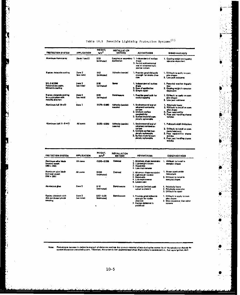
lrable 10.1 Posmlble L~ightninlg Prluo1tec ion Systaon lu (

WSIOIGH INITALLAWiN

PROTECTION SBTMW APPLICATION IWft1

METHOD ADVANTAME 011ADVANTAOFS.-

Aiwisinsim Items speoV Zoo~s I and 2 0.06 Cgocwrsoa secndaruy 1, Indepmpdwst of swimfes 1, Conlinis welist andi Iimaltyloillsrstedl appicaion~lsi 0aslni opstituo-dipsisI..t

2. Partial e~lonnreoriffoilfeel of ulvanoed e0M.pooltas sils,.c

Kapltn dig.Iactlecalaling Zone 1 00? Adhesivebondsd 1. Provildtsgood ialeleula I . Ctflwit to 91,14y won cmlife not") lostloris~iat slrsntith lot .Iiso. divas. PION shows.

lion 2. Lowe peol #ssltuia

MIL-C.122 Ions 1 0.06 Illormy I. Independentl of surface 1. Potentnia weather sispetta.Pilurevsawus pelnl lates riol loollinstesd ti"Sa 0. .. L'

Dilet il eeing 2. law of miplatlastlo 1. Cosllin weight Is operantor3. Simples tipai dowendnt

Motiopna dibtaelooti tosting lam. 2 0.03 Susnalsma, 1. Polaritisi Po patha for I, Difficl~t to appily on eao.In tunintlahlon with toiesnotecis~al lfifaedl stroke slaping" PION tisaps11111t611I1 jenrlort 1. Low peol resinstnce

*Allehsonl fell If1 mill lnn.al O0,00-0.01g0 Adhsoule bosssled 1. EnIaeWr ntM el of1. I. Relatiesly heanvysecured sdwwsued .onpoltll 2. hiflIsuli to Insitall on staft

furfae 'hoof2. Uniformnwhoms 21 l0.esrseltielill~tv

g0ndueIvlly 4. Pow paut hsandling shine.3. surfacea maesrial trami. 101ilt011

phlstly rnpilecoblolAlwyilnwn loeft il1-11ml) All jonas 0.020-0.030 Aiholusv bonqsd- I, Environmntaflsi"all of I. PON Itank wimdthllnhllotions

toteuld ilaaa e'nlsuet.. 2. 01hf1teulltoI Ingtall el eons

2. Uniformt wilue lon. POWe slesI"toa~plstellv fsla4sIlM 2. Pown espslntilfily theraas

0. Swrfm~ material euns. 18fhst1asplealey repleacte" 4, Pow purt handing chhars,

WEIGHIT, INSTA LATIONPROTECTION SYSTEM APPLICATION blbitO MITHOC ADVAI4TAGEE DIWI VANTAGEA

*.Alnenins. wife Ilarkl Ag nsamss 0.030-0.026 Comwand I. Minlimum sips& Sornnwink I. CII letillto 1.1,5141 INIWooles nag... 2. Livlflwl Il~' system eionsplet shnrps4200. 200) 3. hpallatais

4. Lowe mainlartanrs.Alnhum i ltio *Ira ooic Allatans. 0.040 Cocssiad 1. Minimumn allow constrainti 1. 81c~ienntock width(hailttdl icrson Ist'itsl2. LihwoiliIWti Inaliltlons1200 a 2001 2. Reps~aslfa 2. Di) ileullto1 Install lIn

4. Low mailntenance conmplen shopsa%S LowsstetonI

Akiwinland glass ZWe42 0.10 Sontdf00515 I. Potential limitedl epolIl. I. Iilaotlaaly heavyloollinalwill motion lei Zons 2 2. Relativesly anpoilliso

3. Ijltlicullto so lialiKopltos dielsectric mIti Units a 0.07-0.09 *oind4ocurC I, Provides good dlielectric 1. 13fcl~t toe~s1 aillow Io Colnthin reinforced plustle log. oatal lssslnsntsdl ssrsnslit lot wonke plan 6hlns.,

s~l~ligdivesionm 2. Mores sepentles Olin other2. Ksap dietlslano Is nytisms

Nbut, Pinltinilitogor itleials In sialtsoild otiongih of dilaelctilecoa~tlings Ine to onowls onnsrtall Olelfss dlicilia she ton1,10lif of.0 hs veshicle ninty, ilepsab iissystem boaymit sn unsoated sir item. Thoerofare, ths system Isnrot Fsacomindodas what, Rb/ilh safely In cnalosltied II.e., fuel opnrs Irlnsi~. e01J. -

10-5

Table 10.2 Lightning Protection System Ranking~1

SYTMMATERIAL 1 a ATERIAL WSIGHor APPLICAT100A(i0AtLTY CSTA lei CON~ ItPAlNADII.TY4

I. Aluminum Metal Flaea spray4-9.9 MYL, 1001 Coverage .1 4 8 9

2. Aluminum Metal Flame Spary4-6.9 NIL, 301 Coverage 5 2 12 8

3. 120 x 120 Aluminum Witre Screen100 2Coverage 2 2 1 6

4. 200 x 200 Aluminum Wire Burson

100 S Coverage 2 2 2 75. Aluminum Fall, 2 NIL.,

100% Coverage 3 3 4 2

6. Aluminum Foil, 2 MIL,501 Coverage 3 3 if) 3

7, Aluninum Fail. 3 NIL,1002 C~overage 3 3 3 4

aS Aluminum Foil, 3 NIL,502 coverage 3 3 7 3

1). Aluminum Voil Tape, 2 NIL,Adlaisavely Backed. 1002 Coverage 4 S 9

U(. Aluminum Foil Tape, 2 Hit.,Adh...4tvely Backed, 301 Coverage 4 5 13 3

It. Aluminum Foil Tape, 3 NIL,Adhesively Backed, 1001 Coverage 4 5 5 2

12. Aluminum Foil Tape, 3 NIt.,Adhesively BAcked, S0X Coveraeg 4 5 11 3

13. Kepton film, 2 NIL + 2 NILAluminum Fail Stri1ps 1 1 6

n. The hfgher tite number the more fovorable the faitor

10-6

LIGHITNING ZONE IA LIGHTNINa ZONE 11 LIGHTNING ZONE 2A LIGHTNING ZONE 23

"NOPROTICTION'

AL FLAME SPRAY,IN0%

x JIEOBCREEN

32 2 10. ISCII91N

2MIL AL FOIL 1100%)1

3.UII. AL FOIL 110111. -

$MIL AL FOIL 1O00 1

IEMIL KAPTflN 110011142-MIL AL FOIL (I11%1

WORIT BUET WORST BSUT WORAT 011T WORST Bill

ýgPROTECTION SYSTEM

Figure 10.3 Relative Merit of Lightning Protective Systems

P110TECTION OYMM ZONE IA ZONkE ZON 204 A ZONE 21

'I17

Alumilinu llama ipacy

4 ~~~~~120 x 120 Alueminmun IeawIt:1I~7;

V V

VV

Ka T 77971811F oigure1. lliieDmneBII1tsl

Puimhm10-7

TENSILE STRINGI`M, KIPPE

PROTECTION ZONE NI - -

NONE II5A111LINK S/L) NON1NONE IS

NONE i

ALP LAM! SPRAY AISL I NONEAL FLA4I SPRAY 26 n

200 X 200 SCAREN AI/LI NONE200 x200 SCREEIN IA

10X120 IICA I2SC N 1111h)NONEKI" X I" SCRAIN IA

I*MIL AL FOIL I2/1.1 NONE _____

%2'MIL AL FOIL a5

3-MIL ALPOIL 111/1.) NONE I

32MIL AL FOIL I/ILI NONE-N.NCN WIDTH3.MI LAL POIL 21U~NCH WIDTH2.MILALPOIL+ IBIL) NONK2.MIL KAPTON- -

2.MIL AL FOIL+ Is2.MIL KAPTON

LEGENCi TENSION TITNENOTH @wwA TENSILE STRAIN, IN,/IN,TENSION STRAIN

Figure 10,5 Tension Data on Lightning Protected10-Ply Graphite/Epoxy ISminlates~

1 )

TENSILE STRENGTH. KIPS

PROTECTION ZONE1

NNEI (ISAISLINE SJ)UNONiNONKENONE 25

AL PLAN(I PRAY IS/LINONKALPLAMS SPRAY IAA LFLAME SPRAY S1

200 X 200 SCREEN S/LII NONE-=0X 200 SORKEN 2A-

i2ON 120 SCREEIIN IS/LI NONEK120 x 20 scREE NN Is12OXID& 12SREN ZA ____

120 X 120 SCREEN 21

a*MIL AL FOIL IS/LI NONE-

3.MIL AL FOIL IS/LI NONE - E3.MIL ALPFOIL is

3.MIL AL FOIL (ISL) NONE-34INCI4 WIDTH ___

2.&IIL AL FOIL IA-

3.INCI4 WIDTH T3.MIL AL FOIL 2A3*INCN WIDTH2.MIL AL FOIL + (ISLI NONE m2-MIL KAPTON2.MIL AL FOIL * IA mm2-MIL KAPTON

a CW 0.004 0.012l 06016LIGID: ENSON YNKOTHTENSILE ETMAIPI, IN/IN,

TENSION STRAIN

rigure 10,6 Tension D~ata for Lightning Protected

Graphite-Glass/lipoxy 10-P~ly

Hybrid Laminates~1

10-8

TENSIL STRENGTH, KIPS

PR"OTECTION ZONE -

NONI MSAELINE SIL) NONE

AL FLAMI SPRAY 11ML NONEAL F LAME SPRAY MAAL FLAME SPRAY is

NO 3W SCREEN IS/LI NoN Iimx2w0 X 1SCMEN IA-

1 20 N11120 SICRENN ISBL NO:E[lIONX IlsO SCREN IA

2-MIL AL POIL IBML NONE mo2-M ILAL POIL IA3lMlL AL POlL 11111. NONE3.MILAL FOIL SA

I'M IL AL FOIL IS/LI NONEA3-IN014 WIDTH SA3-MIL AL FOIL3.INCN WIDTH4

'M IL ALFPOIL - ISIL) NONEN2IL KAPTON

I.MIL AL FOIL 4 II'MIL NAPTONI.AIL AL POIL 4 3HIlMIL KAPTON

LIGENa, TENSILE STRENGTHTENSILE STRAIN MENILE STRAIN, IN /IN.

Figure 10.7 Tension Data for Lightning ProtectedUraphite-Boron/Spoxy 10-Ply HybridLaminatts~l

TENSILE STRENGTH, Kinl

PROTECTION ZONE

NONE (IASI LINE SIIIUNONE -

A.L FLAME SPRAY (1141. NCNEAL FLAME SPRAY 2A

2M X 200 CHINN Iu/LI NONE-200 X 211 SCREEN SA

120 X 120 SCREEIN IE/LI NONE 1UIn xInSCREEN IN n ~

2.MIL AL FOIL ISLi NONEI-2.MIL AL FOIL IAI.MIL AL FOIL ISI

3-MIL AL FOIL (ISLI NONE

3.MIL AL POIL (ISLI NONI3.INCI4 WIDTH3.ISIL Al FOIL Is,3.INCH WIDTH2-MIL AL POIL

4 (M)L NONEa

2-UIL KAFTONa 0004 g.008 0.012 0.0 IS

LEGENI~i TENSILE STAENGTIITENSILE STRAIN TENSILS STRAIN, IN/IN.

Figure 10,8 Tonmion [)at& for Lightning ProtecteidGraphite-K~ewl r/Epoxy 10-Ply

Hybrid Laminates (1)

10-9

the composite to the fasteners which in turn transmit it to the substruc-

ture. As shown in Figure 10.9, glavanic isolation of titanium splice pl~toand aluminum lightning protective coating is maintained across the joint toprevent electrochemical action.

A bonded joint is shown in Figure 10.10. In contrast to boltedjoints where currents follow the fasteners, bonded joints have discontinuityat the metal-to-composite adhesive bond line, Heating and internal arcingare possible at the interface if the cross-section is too small to carrylarge current loads that may be produced by lightning. Figures 10.11 and10.12 illustrate the panels with substructure (laminate and honeycomb) thatwere also tested.

After lightning tests were conducted, structural damage was foundto be most severe for the adhesively bonded joints and least severe for themechanically bolted joints. Composite structures that utilize an aluminumhoneycomb core are particularly susceptible to damage due to the low resis- L

tance of the honeycomb compared to the graphite skin. Lightning willpuncture the skin and flow through the honeycomb,

10.1.4,1.4 Environmental Exposure

It is necessary that the lightning protectton systems be compati-ble with the expected service environments. Two different exposure condi-tions were imposed on protected composite panels: 1000 continuous hours at140°F/100% relative humidity, and simulated flight cycling (1000 cycles)from -650 to 250°F in a Webger chamber, The results are given inFigures 10.13 to 10.15 and show no corrosion to the aluminum and no loss oflightning protection.

10.1.4.1.5 Damage Repair

The effectiveness of the lightning protection systems were eval-uated after repair of the system following damage. Two types of damage wereconsidered. minor damage comparable to a tool drop, and major Impact damagecaused by a heavy or sharp object.

Repair of the damaged laminates consisted in rebuilding the coan-posite structure with reapplication of lightning protection across therepaired area. Heat bond and cold bond repair procedures were used. Thehot bond procedure consisted of the following steps:

1. Abrade away damaged material (taper 0.25 in,per ply).

2. Abrade away paint to expose base protection foro.5 in. minimum in excess of damage area.

3. Place adhesive (AF143, 10 mil) over damaged area.

4. Place tapered prepreg plies in damaged area(mechanically damaged panels) or precured patch(lightning damaged panel) to match panel con-tours

10-10

*•.•,

lI.

144

10-11I4.

.• 4

I-., -,J'

• .' ,•*

Ii"

IAI

41 m4

OHL?4 ill

U~ u'0

*444

-0n

C

.3

0 In

4~1 *.n

10-13

qP

5. Cure laminated prepreg patch plies to panelusing pressure plate and autoclave cure.

6. Mask off undamaged panel area using 3-miladhesive-backed aluminum tape.

7. Apply aluminum flame spray.

8. Apply MIL-P-23277 yellow primer.

9. Apply MIL-C-23286 Polyurethane enamel.

and the cold bond procedure war,

1. Abrade away damaged material (taper 0.25in. per ply).

2. Abradu away paint to expose base protectionfor 0 • in, minimum in excess of damagearua.

3. Fill damaged area with potting compound.

4. Allow potting to cure at room temperatureor for 2 hours at 1600F.

5. Fair potting to panel contour.

6. Apply 3-mil adhesive-backed foil to repairarea.

7. Mask off undamaged panel area.

8. Apply MIL-P-23277 yellow primer.

9. Apply MIL-C-23286 polyurethane enamel.

After repair, the composite panels were struck with simulatedlightning with the results shown in Figure 10.16 - 10.19.a

The results indicate that damage to composite protective systemsand the composite substrate can be repaired acceptably. The electrical -,continuity between the repaired area protective coating and that of the basestructure is the critical repair. Good temporary repiar can be accomplishedusing aluminum foil tape. The ideal permanent repair is aluminum flamespray but it requires special personnel and facilities not usually availablein the field

10.1.4.1.6 Discussion of Protection Systems,

In this section, overall conclusions on the various lightningprotection systems are discussed. The first three systems were judged best.

10-1.4

- . . .- . . .. .~ . .!± * . ,. ...

dIj

'.41

IA P4

*141

.41 0

u U,

L -a o

4.4 AG

. ,.10-5a

I0.1.4.1.6.1 Aluminum Metal Flame Spray i ,4.0 - 6.9 milThickness, 100% Coating

This coating was judged one of three superior lightning protectionsystems. It can be applied to simple or complex parts, is easily repairedand gives good lightning protection for Zone 1 and Zone 2. It does requirespecial equipment and well trained personnel to obtain good coatings.

10.1.4.1.6.2 Aluminum Metal Flame Spraya Styips L 4 .0 - 6.9 milTh ickness X650•r cove rage)

This system was judged one of three superior lightning protectionsystems. This provides Zone 2 protection in strips typically 3-inches widewith 3-inch spacing.10.1.4.1,6.3 Aluminum Wire Screen (120 x 120)

This system was one of three superior protection systems. Goodprotection is provided in Zone 1 and Zone 2, but is restricted to applica-tion on simple shapes. Screen is at most 36 inches wide,

10.1.4.1.6.4 Aluminum Screen (200 x 200)

This system provides limited Zone 2 protection. It is restrictedto application on simple shapes and is at most 36 inches wide. C

10.1.4.1.6a5 Aluminum Foil (2 mil)

This system offers limited Zone 1 and Zone 2 protection. A goodquality surface finish is hard to obtain except for simple, flat surfaces. .Width is limited to 36 inches.

10.1.4.1.6.6 Aluminum Foil (3 mil)

This system offers limited Zone I and Zone 2 protection. Restric-tioas mentioned in 10.1.4.1.6.5 apply here. "

10.1.4.1.6.7 Aluminum Foil (2 mlk3 mil adhesively backed)"

This system is best applied to cured composite surface. It offerslimited Zone I and Zone 2 protection. Strip width is limited to 3 inchen.

10.1.4.1.6.8 Aluminum Foil Tape Strips (3 mil, adhesively backed) ke,3-inch Width and 3-inch Spacing

This system is best applied to the composite surface. It is meantfor Zone 2 swept-stroke conditions only.

I10.1.4.1.6,9 Kapton Film (2 mil) Plus Aluminum Foil Strips

(2 mil, adhesively backed)

This system is the most complex to install (cocured) and the mostdL'ficult to repair. System is limited to simple contour or flat surfaces.

10-16

10.1.4.2 Grumman Composite Metallic Coatings Evaluation( 2 )

Grumman( 2 ) has made a study of metallic coatings that can beapplied to graphite/epoxy used on high performance aircraft. The coatingsare designed to prevent moisture absorbtion, improve shielding effective-ness, reduce lightning strikes and protect against paint strippers duringaircraft refinishing.

Three types of protective coatings were applied to test panels ofHercules AS/3501-6 graphite/epoxy preimaregnated tapes: .

* solid aluminum foil bonded to graphite/epoxylaminate

0 perforated aluminum foil cocured with graphite/epoxy laminates

* spray-and-bake metal-filled organic coatings ,,.applied to graphite/epoxy laminates.

Three spray-and-bake coatings, Kerimid 500 with aluminum powder,Alumazite Z with silver and Alumazite Z, were tested initially. Alumazite Zwas chosen for further testing because of its lack of moisture pickupcompared to theother two as shown in figure 10.20.

10.1.4.2.1 Moisture Resistance

The metallic coating systems were exposed to an environment of "* 140OF and 98% relative humidity for 90 days. Periodic measurements were' taken of the percent moisture pickup. The results are shown in Figure

10.21. The solid foil and cocured foil coatings significantly protectagainst moisture pickup while the Alumazite Z coating itself absorbedmoisture and thus had greater moisture pickup than bare graphite/epoxy.

The moisture resistance was also evaluated under humidity thermalspiking conditions. The cycle was 1400 F and 98% relative humidity for 72hours followed by 260°F for 2 hours to simulate ground storage and super-sonic flight. The panels underwent 40 cycles and the results are shown inFigure 10.22. A slight decrease in moisture resistance occurred for thefoil coatings while no change was observed for the Alumazite Z coating. ,l

After humidity and thermal spiking exposure the flexural and hori-zontal shear strengths were measured. The effects of humidity and thermalspiking were found to be severe: a 45-50% reduction in 260°F flexural

fstress and a 50-50% reduction in 260°F horizontal shear strength. Bothsolid foil and cocured foil offered significant protection but the Alumazite ,,Z coating offered little protection. The results are given in Figure 10.23and 10.24.

10.1.4.2.2 Effects of Paint and Paint Remover

Graphite/epoxy laminates were painted with standard Navy paint .finish (epoxy polyimide primer (Mil-P-2377) with polyurethane topcoat(MIL-C-81773) and exposed to humidity (140°F and 98% relative humidity)

10-17

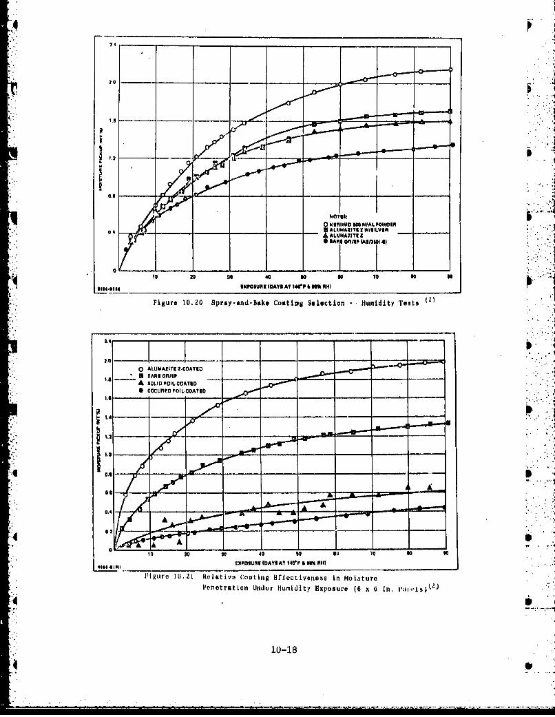
4

20

20~~ IM- __

4~. _ _____ ___ _____ _________ ____

.: IIWilLI

_ _MA _ _ S

0 AR0110 Aw10.1

.0.

0~~ ALMZT ALUMAITER UAUR annlipl2oIg

A SOLUAID PI ZCOATED

1.

.7S

AA

P'enetration Under Humidity Exp'osure (6 x 6 In. Ilvl)2

10-18

fl, I

1 -L. At JI~a

1OLID FQIL COA1IINO

cocuflUOPOI *COAINUI

*I~OS4CYCLI NO. 11 HINVI' .N & 114S% ONM, 2 1111120 01

P~ig ure 10,22 Relat ivo C;oating offg,'tiveiehJB ill Moisrt~rc ao tz. ci

IUndor Ihormalc Spiking HXp1n.41re (6 x 6 Ili PaInel%

10-19

DO NOTE MOIOTUPIE LlVELS SHOWN

00

40

if 0

40

.- UNSIIPOIE-- --- 0- -- HUMIDITY 100 OAYSI--i.l -. SPKCI00OEIb

% 111ure 10.,23 COAtlIlR 9010ctiOfl -- I'lexural Streoo(O )s

Percent uf thineposad Strength (2)

100 NI IT~lLVL HWAT BOTTOM OF RAHl OnrAPH1E

600

400

1,0

1002

and thermal spiking (3 days at 140OF and 98% relative humidity followed by2 hours at 260 0 F), The results are given in Figurea 10.25 - 10.30. Thepainted foil protect-d laminates showed considerable protection from mois-ture pickup and no loss of flexural or horizontal shear stress. • "i

Paint was removed using Turco T-5469 stripper conforming toMIL-R-81294 and the horizional shear strength and flexural stress measured.The results are given in Figures 10.29 and 10.30 and show good strengthretention by painted foil protected laminates and little change due tohumidity or thermal spiking. The Alumazite Z coating protects against paintstripper but not moisture.

1.0.1.4.2.3 EMI Shielding Effectiveness

The EMI shielding effectiveness of 18-ply graphite/epoxy was mea-sured for both E-field, H-field and plane wave fields. Improvements greater"than 30% in E-field, 150% in H-field and 55% in plane wave field shieldingwas obtained by coating both sides of the laminate with 2 mil solid foilhumidity and thermal spiking produced a slight decrease in shielding effec-,tiveness. Alumazite Z coating provided no effect on the shielding effec-tiveness.

10.1.4.3 Shieldin Effectiveness of Aircraft Protection Systems

In addition to providing protection to composite aircraft, many ofthe protection systems may afford a certain improvement in EM shieldingeffectiveness. A general study of this problem has been done by Grumman apart of its Protection optimization program for composite structures.e(,

I-lectric, magnetic and plane wave shielding effectiveness measure-ments were performed on 12- and 24-ply graphite/epoxy panels treated withthe protection systems listed inTable 10.3. All panels were fabricatyedfrom Hercules AS/3501-5A graphite/epoxy. The 12-ply panel has the laminates(2/2/8) and the 24-ply panel has the laminates (4/4/16) where the orienta-tions are (00/90°/+450) respectively.

The protected panel shielding effectiveness measurement results

are shown in Figures 10.31 to 10.36. These results indicate that thealuminum flame spray gave the best overall protection, probably because ofthe continuous coat. The 120 aluminum mesh also did quite well al-though the 12-ply panel did not perform as well as the 24 -ply panel. with thesame protection. The vaper deposited aluminum and aluminized fiberglass didpoorly.. . . :' .

10.2 Future Composite Protection-Doping and Intercalation

Future protection systems for composite aircraft structures tendto stress methods of increasing the composite shielding effectiveness byincreasing its conductivity, i.e., making it behave more like a metal.Current efforts stress increasing fiber conductivity since the matrix resinmaterial is a dielectric.

Two methods, doping and intercalation of the graphite fibers, havebeen described in detail in Chapter 5.0 (Intrinsic Material Properties) andwill only be described here in general terms.

10-21

4' - ' . . i. - i . . , . , i .:. -

46 -

- - - -~*

-

16.

-------J '

.- ~1.

~~~ rz

- -.

- - iii_ I( .L ::~-7- 7--K -

102

K IWAO#.IU - ICSkNI WMAIiV A

01NIII -I3itM

11041011Ibd 1101

161vo-I11AMl lb_ _ _ _ _ _ _ _ _ _ _ _ -100alo

SIbANIII d-I dI~ tt 11INY E11

111VAOMAN! Oil 111111-1WVWWII

11Clld WYN~ojIm

14moo*nW~dWV 61O~sm nsP

.............. .......w ..eo rn

~EIWE0 ANI~d ~ 10i-23

I'• i S j ,

St 0 -.4 U

ii I~oi~~a~•IIdO•

oIi i 0-211 ,,

ill jill* 6 .h".__ _ _ _ _ _

ii:2.. ... :...:-.. ,•..,-. -:/.,'. -:.. . .. .. . .. ...... .. . -; ..... .....' . .. - . . .... . .. . . ... .. . . .. .. . .. .. . . . .. .. .

Thhle 10.3 Ihielding Effectivenuua Musgrmen.I.ItNm3

P'P0TECTtW MiYSTV4 MUHRIR OF PLIKS 11- FI XL I-FIKIb PLAN WAVEC

B,12 x IC x24 x

120 Al urninm M.'ah 12 x x x24 x

201) Alumintim MOOm 11 x

Aluminum Pla.. Liptmy (4-6 Mllm) 124 X24

Vaparn?-bCto.ited Atumlnum 12 K x

Aluminum Flow. Spray Anud 12 x xVapor-b.I'oafted Aluminum

Aluminimed Piberglmgm 12 x

-ve

10-25

The doping of graphite fibers is similar to doping a semiconductorby introducing an impurity into the crystal. Results have indicated anincrease in fiber conductivity by a factor of 50 in some cases, however thedoping process may be hard to control.

Intercalation is the process of inserting metallic or nonmetallicchemical species between graphite crystal layers in graphite fibers. Verydramatic increases have been reported for pure intercalated graphite withconductivities about the same as copper or silver. For commercially avail- ,.able fibers, the resulting intercalated fiber conductivities are about 20 to40 times that of the regular fiber. These results could probably be im-proved significantly if more care was taken in the graphite fiber manufac-turing process to ensure a more perfect graphite fiber crystal structure.

q1 .,

', . As*

04

10,26

* 10-26..l

"10.3 References

1. S. D. Schneider, C. L. Kendricks and G. 0. Olson, Vulnerability/Survivability of Copousite Structures - Lightning Strike, Vol. 1TI-rogram Results) and Vol. 2 (Design Guidelines), Boeing Corp. AFFDL-"TR-77-127, Feb. 1978.

2. C. J. Staehler and B. F. Simpers, Metallic, Coating For Graphite/Epoxy Composites, Grumman Aerospace Co., prepared for NAVAIR, May 1979.

3. Protection Optimization for Advanced Composite Structures, GrummanAerospace Co., Fourth Quarterly Progress Report, June 1978.

4. Advanced Composite Aircraft Electromagnetic Designn and Synthesis,SRC-TR-79-490 April, 1980.

5. J. A. Davis, Atmospheric Electricity Protection for Electric and rElectronic Systems, Federal Aviation Administration Report No.AAC-213-15 April, 1975.

10-27

4 ,

-- !.7-V: "'"-

I.

11.0 DESIGN GUIDELINES

In this chapter, the information developed and discussed in theprevious chapters is condensed into a sat of guidelines for designing elec-tromagnetic compatibility into composite aircraft. The approach taken indeveloping the guidelines is to represent the overall voltage transferfunction from external field to internal electronic device feed point as acascaded set of transfer functions, each one involving only a portion of thewhole process. Guidelines are then given for each portion separately.

Section 11.1 describes in general terms the required interactionof a number of separate disciplines to produce a compatible compositeaircraft. A description is given of the individual transfer functions thatcollectively describe the voltage induced at an interior device port as aresult of an external electromagnetic field.

Section 11.2 specifically describes each individual transfer func-tion and gives guidelines for its use.

Section 11.3 provides a baseline case, an unprotected compositeaircraft, as an example to which the guidelines can be applied. The analy-sis for -his case provides an estimate of the amount of protective shieldingthat wil" be required for compatibility. AA/AA,,

Suction 11.4 provides characteristics on various protective de-vices used on aircraft to protect against external fields. Simple tradeoffguidelines are estimated to allow required protection to be chosen atminimum weight and least cost.

11.1 Overview

The earlier chapters in the handbook tended to focus on certainindividual aspects of composite materials. For example, Chapter 2 treatedelectromagnetic threats; Chapter 5, intrinsic material properties, andChapter 7, subsystem susceptibilities. The material typically took theform of formulas and/or diagrams which often had little obvious connection ,to material found in other chapters. Such analysis, although indispensablefor understanding composite material behavior, tends to obscure the funda-mental fact that an integrated, interdisciplinary, "total" systems approachis required in all (not just later) phases of aircraft system design whenworking with composite materials., This procedure is in contrast to proce-dures used for metallic aircraft of earlier times Then, the structural, "avionic and electromagnetic parts of system design could proceed separatelyin the early stages. Unification of the parts took place in the later, .detailed design phases and usually was accomplished without significant costor time overruns. For composte aircraft, a number of individual disciplinesmust be combined (usually on a computer) using mathematical models and/or -. ,'measurements to produce designs having the required structural, avionic and . .A'

electromagnetic properties. The situation is illustrated in Figure 11.1.Because such properties are interdependent and rarely optimum, tradeoffsamong the system parameters usually are required. The crucial point to bemade here is that the use of a few isolated disciplines to determine evenpreliminary aircraft design, an acceptable strategy for earlier generations

i li1-1 .

4' . p

A. " " " "0 A .. A

CORRO0SION VULNERABILITY/4URVIVABILITY

MATERIALS M4AINTENANCE AND

* .4

* , 41

R~ NEPAIR C N

LIFE CYCLE ELECTROMAGNET ICDEGRADATION SIIIELDING

STRUCTURES AERODYNAMI CS

CAD/CAM

PLATFORM

Figure 11.1 Integrated, Multidiscipline ApproachTo Composite Aircraft Design

11-2

11-2

4.

of metallic aircraft and their electronics, is unacceptable for compositeaircraft and its electronics. For example, using aluminum foil over agraphite/epoxy panel can solve electromagnetic shielding problems but notcorrosion, maintenance or repair problems. A special coating over a compos-ite surface can solve -corrosion problems but the weight penalty may be toogreat and the electromagnetic shielding too poor. Without a "total" s, temsapproach to designing with composites, the final result may be electronical-ly incompatible and require costly and time consuming fixes if, indeed, suchfixes can be found. Even if a compatible design is produced the lack of a"total" systems analysis compatability means the ability is lost to gaugequickly the impact upon composite system performance of rapidly changingtechnologies and military postures. Such an inability would make the futurevulnerability/survivability of a presently sound composite aircraft diffi-cult and/or expensive to determine.

To prevent such shortcomings, a set of design guidelines for theuse of composite materials on aircraft is clearly required. This chapterwill develop and discuss composite electromagnetic design guidelines only.Such guidelines can be used by design engineers in assessing the electromag-netic performance of composite aircraft at any stage in the system procure-ment cycle. Although the guidelines focus on the electromagnetic aspects ofsystem performance, the effects of other .factors on electromagnetic perfor- ,mance, as illustrated in Figure 11.1, will be taken into account when Ideveloping the guidelines.

An overview of the general problems of electromagnetic compatibil-ity for a composite aircraft is given in Figure 11.2. An aircraft, composedin some part of composite materials, is situated in a perturbing electromag-netic environment. One quantity of interest is the frequency dependentopen-circuited voltage Vij(f) induced at ports on avionic and other electro-magnetic equipment boxes by the external electromagnetic fields. Suchvoltages must be sufficiently small to prevent avionic or electronicsubsystem incompatibility, upset or burnout. They can be estimated byexpressing them as a sum of the frequency-dependent transfer functions D(f),T,(f), T2 (f)...T 6 (f) as shown in Figure 11.2. D(f) is the intensity ofthe external electromagnetic fields T 1(f), the material airframe electro-magnetic shielding function; T2 (f), the shielding influence of the airframeshape; T3 (f), the joint leakage termi T4 (f), the cable shielding term;T5 (f) the subsystem susceptibility term, and T6 (f), a term that reflects theprotection methods used in the system. Each of these terms will be dia-cussed in the following sections. The results will constitute a set ofguidelines to be used to design electromagnetic compatibility into a compos-ite aircraft and will form a basis from which tradeoff studies involvingweight, cost and protection can be performed.

11.2 Electromagnetic Design Guidelines

In the following section, electromagnetic design guidelines foraircraft using composit~e materials will be developed and discussed. Theseguidelines summarize the detailed findings in the earlier chapters of thehandbook and present the results in the form of diagrams and tables. Theguidelines are organized in such a way that the evaluation of the transferfunctions D(f), TI(E), T2 (f)---T 5 (f) is straightforward. The protoc-tion transfer function, T 6 (f), is discussed in Section 11.4.

11-3

4WAMOA

9 SONOt.LA.OV

14J

SSINIOIAr

S A.3dVILdOS l

9 IDNIC11IHSfrNGVOW

lvahlU

11-4

11.2.1 External Electromanetic Fields

The external electromagnetic fields are presumed to arise fromlightning, nuclear electromagnetic pulse (NEMP), radio frequency (RF) andhigh ennrgy laser radiation and precipitation static discharge. A suitablecombination of these threats will determine the frequency dependent transferfunction D(f).

The lightning, NEMP and laser threats are summarized in Figure11.3. The threat amptitudes are given as a function of frequency and allowthe determination of D(f) in terms of field strength. The precipitationstatic spectrum is similar to lightning but is many orders of magnitudesmaller and is not shown.

The RF threat; spectrum is given in Figures 11.4 and 11.5 as afunction of frequency. Two cases are considered. Figure 11.4 is a generalunclassified RF envirorment extending from 10 kHz to 100 GHz. The RF fieldsare made up of a variety of commercial and military transmitters. Figure11.5 is similar to -Figure 11.4 but considers the RF environment in thevicinity of a Navy carrier. In this case, only communication and highpowered radars are considered. The information from these figures can beused to estimate the field strengths incident on an aircraft containingcomposites under a variety of external field conditions.

11.2.2 Electromagnetic Shieldin [Tikf) and 2_2f)j.

The electromagnetic shielding provided by composite shields dif-furs substantially from that provided by metals. This lack of shielding isdue to the different electrical properties of composites, notably poorconductivities, when compared to those of metals. A summary of compositeintrinsic electrical properties is given in Figure 11.6 while a comparisonof composite and metallic conductivities is shown in Figure 11.7. Fromthese data, giaphite/epoxy is seen to have the highest conductIvity of thecomposites surveyed. Even so, it is still about 3O00 times less conductivethan aluminum and qualifies as only a fair conductor. Boron/epoxy is muchless conductive than graphite/epoxy while Keviar is a nonconducting dielec-tric. Compared to aluminum, graphite/epoxy will offer reduced shielding,boron/epoxy, poor shielding, and Kevlar. no shielding at all in the frequen-cy spectrum of interest (up to 18 Gi~z).

The standard measures of electromagnetic shielding of a materialshield are the magnetic and electric shielding effectiveness,. SH and S1,.. -.

These qt'antities are defined in terms of external and internal electromnag-"netic fields as.

smW20 log10 INjj

H.20 x Iog-o IZ E (11-2)

11-5

9 * IS - . . . . . - -

UI

doF4t-4

t6IS(WA)3(ni'dW TN/ S

11-

NI

40120

-20

-40

~ 100

0.10.1 1.0 10 100 1.000 10,000 100,000

FlR3qqJKICY (MlI)

Figre115ures11.4 RF Stregths o Thr at re lih

11-

Graphite/Ryoax ISZrUnlony5 IrA1*Z

?sFe:Lttvlty C Idetemimlans . ,

'ILlongituadinal L2(104) 30 49

transv'erse0, 100 2C10) 6(109Anisotropy Ratios (aL/ar 90 .(1'

811h Yield Threshold@

ZL (volta/rn) 250 o no

2~(aspap/u ) (10) usasixed, usasuiasd

%L(volts/rn) 4000 sot sot3IL

-&iguru 11.6 SummAry of Composite Material Intrinsic Properties

MATERIAL CONDUCTIVITYLow Composite Material Electrical Conductivity

Provides Low Electromagnetic Shielding.

160 ~*. Metals

140 -Composl .mj 4

2100

160

R .z

~-20

~-40

-00

Figure 11.7 Material conductivities

11-8

Considerable published measured data exists for both SE #and SH for variousmaterials. Published results for graphite/epoxy are given in Figure 11.8along with theoretical curves. Considerable variation in the measured re-sults is apparent, especially for low frequency SE. The reasons for thisvariation are that SH and SE not only depend on the shield material butalso on the shape of the shield, the nature of the incident field and eventhe configuration of the test apparatus. The latter fact, in particular,explains why two carefully conducted, but different, shielding experimentsmay produce very different results. The values for SH and SE may be correctfor the test apparatus in question, but they cannot be used to characterizeaccurately the shielding for any other test apparatus or for different mate-rial shapes in the same test apparatus.

The electromagnetic shielding for composite materials is illus-trated in Figure 11.9 for a small cylindrical test. sample and is compared tothe shielding of aluminum. Only SH for aluminum is shown since SE >200dB in this frequency range. The electric shielding, SE, is high at lowfrequencies and decreases at higher frequencies. The magnetic shielding SHhas the opposite behavior. Both shielding terms are larger for higher con-ducting materials for a fixed frequency. There exists a frequency (calledthe cutoff frequency) below which the magnetic shielding is essentiallyzero. The poorer the material conductivity, the larger this frequency.Figure 11.9 can be used to design TI(f) for a particular shape and illus-tration.

If the shape of the material shield changes, the electromagneticshielding changes. The effect of the shape on magnetic shielding is illus-trated in Figure l1.i0 for certain generic shapes, High shielding effec- .tiveness is evident for a single flat plate. Such a shape is called an"open" geometry. Aircraft structures, however, are "closed" geometries andare better represented by two parallel plates, a cylinder or a sphere. Suchgeometrics do -not provide good uniform shielding across the spectrum butrather have a cutoff frequency below which the shielding is effectivelyzero* For more general shield geometries illuminated by uniform externalfields, the critical shape parameter is the volume-to-surface area ratioFor uniform magnetic fields, the magnetic shielding effectiveness increases

V.for larger -. Thus, a structure with large v, like a bomber, has greatermagnetic nhFelding than a structure like a missile with a small Y.• Electricshielding effectiveness will tend to behave the opposite way.

To design using SE and SH, shielding effectiveness curves analo-gous to Figures 11.8 - 11.11 must be constructed for the particular compos-ite shield material and for the shape the shield will be. Figures 11.9 -

11.11 assume uniform electromagnetic fields. For nonuniform fields, the ,'shielding will be different. Finally, if attempts are made to measure theshielding to verify design specifications, the experimental test setup canaffect the results significantly. Clearly, SE and SI1 are very trickyparameters to use for designing Tl(f) and T2 (f) shielding transfer functionsbecaus.e of their sensitivity to factors other than composite material proper-ties.

11-9

,, , . ,.. , ... . . - , - . .. ., .. , . . . . .. . .. . .- - -. . . , . '

IAONITIC I--)-AN

In

in

0 AIN 010 M

U A*~~M I MMS~hIS* .aI n iM MT

10g

* 0'UU6 ANC WN

Fiur 11W 8 Pulse 11Graht/px ShedngDt

MI 116 l I111W10

w4P

PI

t4J

~1) r

I44

11P1SOOWI11-O1011

bo U

.4P)9NIAAJ.OWddUNIC15IH3 OtULNDVW

u~I P~ to

44

* 0

cm c

IIUP 99INDAU.OWUd ONIGlININ OLUP4OYIA

11-12

'I

A more promising shielding design parameter, valid for shieldswhose local radius of curvature is large with respect to wavelength in theshield, is the surface transfer impedance. This parameter is definedby

ZST " - (11-3) 0

where E is the tangential component at the shield surface of the intern-al electric field, while JsEX is the external surface current density. Anequivalont relation, valid for all frequencies, is

Z e csch(vd) (11-4)

where N- (jtWP/ a) is the intrinsic impedance of the shield; V UWPo),the propagation factor and d, the shield thickness. These quantities dependonly on the composite intrinsic properties (p, ) and on the angular fre-quency (Qw). Consequently, the material shape does not influence transferimpedance - material, transfer impedauces for different shapes and the same.This is the advantage of ZST over SE amd Sq and makes it a much bettershielding design'parameter.

The low frequency asymptote of ZST is given by

SZT a(d-5)

which is a very simple function of material properties and shield thickness..The transfer impedance is shown in Figure 11.12 for composites, aluminum andtLtanium for thicknesses corresponding to 8-ply composite (O.001069m).These curves can be uced to design Tl(f).

The effect of shape on the electromagnetic shielding can be ascer-tained from the relationship between shielding effectiveness and transferimpedance. For homogeneous, conducting shield

s. 0o80(11 -6) 0'.9 20 losio M

E

'

H 20 10g 8 (11-7) '

whlere ZE O(SEer/(v/5))" 1

IAnd ZM * (u/0)11 for a flat plate

ZM j tv for a cylindrical, spherical orparallel plate enclosure.

lHere r is the material permittivity; P, the material permeability; w, theangular frequency, and -. , the volume-to-surface area ratio. The quantities

11-13

.......

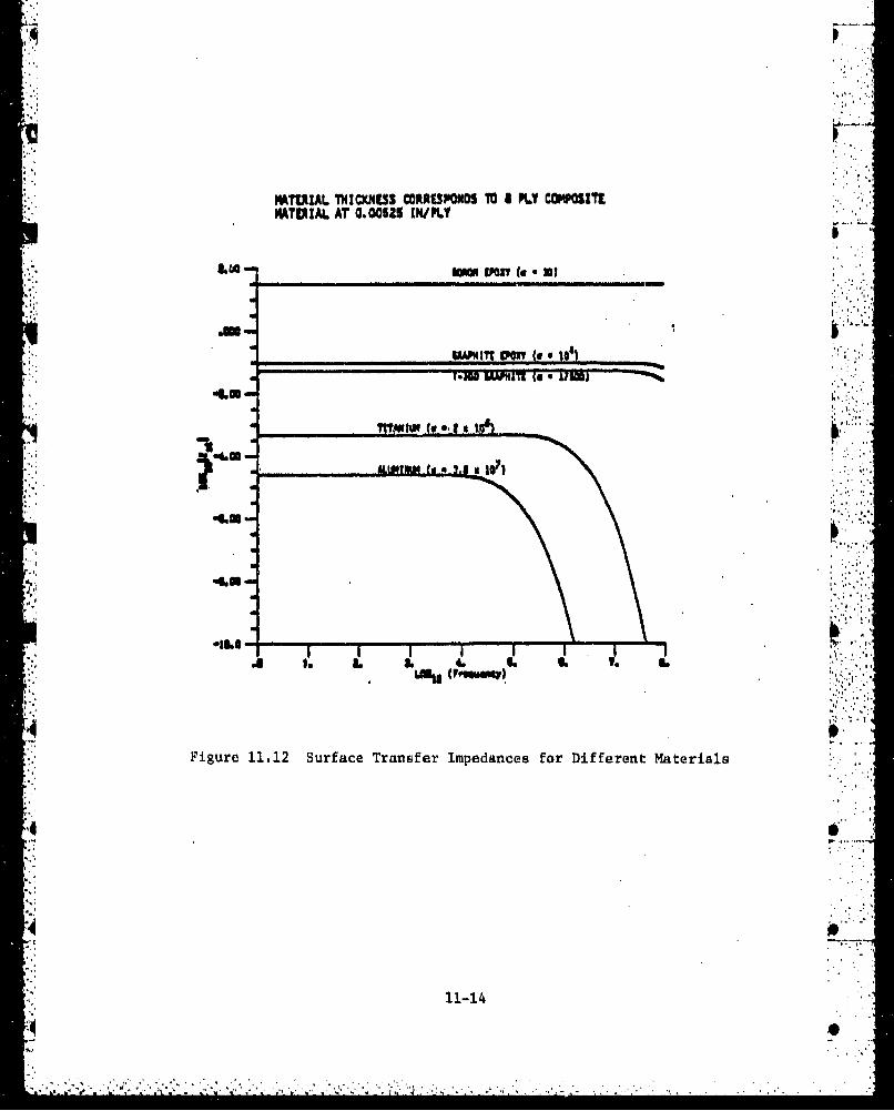
FM1ERAL THICKNESS CORRESPONDS MO I PLY CONPSZIEPATERIAL AT 0.00525 IN/PLY

4..)

a a. ~AM" to .. 6. go y

o"UU

Figure 11.12 Surface Trarasfer Impedances for Different Materials

11-14

is..

ZE and ZM will vary with shield geometry and with the nature of the illumi-nating electromagnetic f ield.

To design TI(f) and T2 (f), the transfer impedance (material-dependent only) is combined with an appropriate shape factor to produce therequired shielding effectivenes,.

11.2.3 Joint Leaka&g! LT3(f)]

The leakage of electromagnetic energy through composite joints,though very important, has been difficult to assess until recently. Part ofthe reason is that composite joint technology has been viewed largely as astructural and manufacturing problem. In fact, composite joint technologyis a prime example of how the manufacturing process together with structuraland electromagnetic design considerations must all interact if a joint thathas both structural and electromagnetic integrity is to be produced.

Aircraft joints involve connecting two separate components byfasteners or adhesive. Because composite fibers are responsible for most ofthe material conductivity, most joints involving composites have signifi-.cantly lower conductivity than that of the components being Joined. Thisgeneral result is due to the lack of fiber continuity across the Joint.This problem will be particularly acute if, as has often been the caue, anonconducting adhesive is used thereby allowing electromagnetic energy toleak through the joint. The joint may be structurally sound but will not beelectromagnetically "tight".

The most common aircraft joint is one Joined with metal fasteners.In contrast to adhesively fastened joints, the use of proper fastenersallows better fiber-to-fiber electrical contact through the fastener. Theconductivity is improved but still limited.

Other electromagnetic joint leakage problems can arise from theattempt to prevent galvanic corrosion between aluminum and composite, anacute problem for graphite/epoxy. The common solution, insertion of adielectric coating between metal and composite panels, prevents corrosionbut spoils the electromagnetic integrity of the structure by forming anaperture or slot.

Electromagnetic leakage through joints is described by a jointimpedance or admittance. The admittance Yj is defined by

where Av is the voltage across the joint and J. is the current densityflowil•g through the joint. Measured data has recently become available on afew joint types and is given in Figure 11.13. The joint admittance isfairly constant for low frequencies and gradually rises for high frequen-cies.

11-15

- ca

I'WIN

1-4'

YinMW/OW ) amii~/3N~ilOViNr

11-16

A limited amount of work has been done to model joint admiLtances.For a butt joint, the joint admittance has been shown to be approximately

nA nc nA n, 2J tn (CIAW) 2j In(CkcW) (11-9) ,.Y ni

where IA kA and rb, XC, kC are the impedance, wavelength and wavenumberiJn regions A" and "C" on either side of the joint of width W. The constant .C is 0.2226.

Considerable work remains to be done to characterize and controLjoint leakage. Data on the effect of mechanical stressea and strains or.,joint admittances would be very useful. The current standard for jointimpedance is 2.5 miliohms/mater which is satisfied only by spenially manu- 'factured graphite/epoxy joints.

11.2.4 Cables . [.4_() ... '

The coupling of elettromagnetic fields to internal cables andwiring is an extremely difficult problem for the general multicable, multi-wire bundles found in aircraft. The existence of significant composit,structure in the airframe will affect the electromagnetic shielding and the '1nature of the field incident on the wiring. '4

This section will consider only the case of a uniform electro- '"taugnetic field incident on both a shielded and unshielded transmission line.Although simplified, this case does provide a means for estimating thevoltage, current and power levels that occur on real aircraft cable systems.

An isolated two-wire transmission line is shown in Figure 11.14. -The uniform E-field is assumed to be polarized parallel to the line and to

strike it broadside. The line has characteristic impedance Zo, terminat-ing impedances ZI and Z2 , wire diameter a, wire separation b, and line.length L. For lossless lines, the open circuit voltage and short circuit a'""'

current can be shown to be

VO C(t) 1 0 00 + 1 r1 (12n -'1 2n- 1)."

ZO (ct)-= 0 OCt) 4. i ('lil*'(I 2 i ....P (.11,

(n+.l) '.1

I (t) - V f -(t - T)dT :'

nT.

where v is the velocity of propagation on the .ine, Eo(t) :!.s the amplitudeof' the incident field; T. = L, and ]', the voltage reflection coeff icent '0

11-17

xb

Figure 11.14 Two-Wire Line Illuminated by Uniform EM Field

at the terminated end of the line. is given by.

z2 -

minor parameter modifications allow (11-10) to be used when only a portionof the lino is exposed to the incident field or if the problem involves asingle wire over a ground plane (image theory, see Figure 11.15).

Using (11.10), bounds can be calculated on the peak open-circultedPEAK PEAK PEAK

voltage Voc , peak short-circuited current loc , and peak power p .

PEAK PEAKThe quantities Voc and Isc are

Iv0~ '. mx"1 11(11-12) • ... ,

where 'max can be calculated or estimated as 1 rnai< L Eiai

IV~~ 00mxx/

These estimates can be modified for fields with a rapid rise timeto peak, such as lightning and EMP. Then, only a few terms of (11-10) arenon zero and better current and voltage estimates are: .

i 'peakI < , + Ir) --1-.3

0 eI_< 'max(' + il

The peak power can then be estimated as (11-.4)

2 + ' .. ,

ppeak < V peak I peak < max

and the delivered energy, by

2,.2I 1 H ]z cli + L•jr.LL (11-15)- zo (1 - Irl1

2 1whe1re

11-19 .......

" • . . . . . . .

a

z /2 Z0/2 b/2 z /2

""- .. "

zO 9 t GROUNO PLANE

()PHYSICAL REPRESENTATION

FExa

Z Z/2 Z2/2

z /2

EIMAGE

(b) IMAGE PROBLEM

Figure 111.i5 Wire Over ra Ground Plane

11-20

-- - ;t • .. .. -

0

Li the line is electrically short then

,Vpak =L t (11-17) V.-oc m~ax(t1- 7..,.1

peakk .. " .

m .e _ (11-18) .:.2

A shielded wire above a ground plane is shown in Figure 11.16.Again, with minor modifications of some of the parameters (shown in Figure11.16), the two-wire transmission line theory can be used to treat shielded

wire provided an estimate is available for the effective field illuminatingthe Interior wire.

The effective field, Eeff, can be shown, for low frequencies, to beapproximately: ...L

2 Z Eo L ' ;<

ff z + Z(11-19)1 +. 2

where Eo is the Incident field amplitude; L, the line length; Z1 andZ2 , the terminating impedances of the shield, and Zt, the surface trans-fer impedance of the shield. Then, fow low frequencies:

Lzt 0 i "V - o (11-20)

0 ZI + Z2(11-2.)

Oe''IBse Zb .

11. 2.5 S~ub Ysystem_ Su.sc~pib-il~t__Tif- ,. ! ..

Advances in electronic devices has been one of the most tapidl.y de-veloptng technologies in recent tilnes. Vacuum tube and discrete transistortechnology have been replaced by integrated circuits and large scale inte-grated circuit (LSI) technology. These trends are expected to continue withthe advent of very large scale integrated circuit (VLSI) technology in thenear future.

Figure 11.17 shows changes in electronic device characteristics inparallel with changes in airframe materials and components from pre 1950 tothe 1980's. In determining device susceptibility, both the upset voltageacross the device and the power foL burnout of the device must be consLd-ered. As Figure 11.17 shows, the push )f technology has lowered deviceupset voltage and burnout energy dramatically. A key point to note is that ,

11-21 0

L.I

00-. z 2 b/ 12/

N .

OR1.11 IW

1iue1.6SilddCbeGoer

TEHOOYTED

LARGSCAE VEY L"GE CALDISRET INERAE

TRANSISTORS C~CINTSOA (ICICAE CIRCUT L~

WR-' 2'7f

250V 12V-94V BV-12V 5V-7V I.SV-3VI WATTiDEVICE io-1-iO-2 10-2-10-3103041-0506

WATTS/flEVICE WATTS/TnANIS WATTsiTflANS IVATTS/TnANS

GLASS/ METALI METAL/ METAL/ cEnAMIC/METAL/ CERAMIC cenAMICI CEIIAMICI EPOXY

CERAMIC EPOXY EPOXY

F-9 F-4 F-14 F-10 VSTOI.

VALUMINUM ALUMINUM ALUMINUMITITAN CAAPHITE-EPOXY CPAMIT-PX

ALUMINUM

PRIlOS'. 950lo160$ 1970's lmocos

Figure 11.17 Aerospace Technology Trends

11-22

t

the development of the most susceptible devices coincides with the increaseduse of composite materials. Because of the poorer shielding provided bycomposites compared to aluminum, the vulnerability of modern electronicdevices to upset and burnout will be greatly increased unless adequateprotection methods are used.

The upset and burnout energies for various circuit components and "devices are shown in Figure 11.18. These levels can serve as a generalguide to the maximum energy levels a particular device should experience.Key facts are that integrated circuits are most susceptible and burnoutenergy is 10 times upset. Figures 11.19 and 11.20 present worst case sus-ceptibility data for CKOS and TTL technologies, operational amplifiers and3-pin and multi-pin regulators as a function of frequency. Device suscep-tibility becomes much worse below I GHs. This trend renders the devicespotentially vulnerable to lightning and EMP threats. Protection methodswill be discussed in Section 11.4.

11.3 Unprotected Aircraft Performance Guidelines

Section 11.2 discussed the factors that must be considered whendesigning electromagnetic compatibility into composite aircraft. Thesefactors were characterized as frequency-dependent transfer functions D(f),TI(f) --- T5(f). The calculation of these functions for a given inci-dent electromagnetic field (considered a threat) will allow an estimate to..: "',.,2be made of the induced voltages, currents, powers and energies that willappear at electronic subsystem entry ports. One important baseline is theperformance of an unprotected all-composite aircraft exposed to strong "external electromagnetic fields (lightning, RF EMP). The results of such ananalysis, of course, will vary with the parameters of the specific problem.In this section, a single example of such an analysis will be given for aset of "typical" conditions. A comparison then will be made between alumi-num and graphite/epoxy.airframe.

Tpe parameters used in the analysis are. graphite/epoxy conduc-tivity, 10'mhos/m; composite thickness, 0.0025 m (19 plies); lightningand EMP threats, worst case double exponential waveforms; the characteristicimpedance of the transmission line, 100 ohms, and the reflection coeffi-cient, 1 1-0.54. The integral Imax is approximated as LEmax where L isthe exposed line length and Emax, the maximum amplitude of incident field.A shipboard RF threat is given as 400 V/rn.

The results are shown in Figures 11.21 and 11.22 as a set oEcurves. Estimates are given on the open-circuited voltage Voc, the short-circuited current lec and the power, VoS 'sc delivered to the line termina-tion as functions of line length L and threat type. Estimates are also :4given on minimum required Wunsch constants for devices that will survive thethreat.

The contribution to the upper bounds on VocW Isc, power andminimum Wunsch constant due to joint coupling is shown in Figure 11.23. Be-low 100 MEz the joint admittance was taken as a constant 15 mhos/m. Above2 GHz the joint admittances becomes frequency dependent as shown in Figure.11.13.

11-23

* EM SUSCEPTABILITY (TS)

Upset and Burnout Energies for Various Circuit Elements.

Suuueptible 10*

10.1 Low-Nolse

10-7- 10.8111t Diodes

HighUpood,

Ice

Signal Dindu18... 10-3 Medium-Poweq

* ~~~Timulilwa elae

1023. 104- High*Powat CaWIl4iar, vacuum TWA~Tranaileto Ci i~p-6Ition

10.1 ~ f HolMialded10.1- ~Paws! Diode, aww

Sumaslib~ 101 1011

UPST BURNOUT

F~igure 11.18 Electronic Component Upset and Burnout Energies

OWN BURNOUT

A 3#IN RIOULATOP111

a CMOs

LOGIC

I MULTIAIN PROULATORI

II OPINATIONALSILI A'aPLIPIPRS

li6.01--

0.1 1 t

FRHEUINCY -oft

Figure 11.19 Worst Case Absorbed Power .Susceptibility

11-24

I.M -o -r

- ~A PIN RSOLUATOfI

Ia AL 0.

p

I I Sir~1101 1841

If 6A

I Icy

Ir

IWI W* I.

4i.

* Figure 11.20 Worst-Case Power Density Susceptibility ValuesAssuming X/2 Aperature

11-25

P.

CURV## PORGA,

VO.

~~f*3

00 aIREICT STRIKElLq-~ y

400 NIAR IW 8 UQHOTIVING

-w -.m -Mm m

iato

1101 -1ETSRXILGTI

LENL mIrN L 0m)1"Igr~-~ 11. 1 Up er lO~ f(!~ oti P~ n.C~r U~t Vo~t g~ Nd Sow~C~~~rcuit~~sa

momen ýu o I) fw~o~ r r

11-26640 FRI "

10-1

.1 WAVMU PON GRADWITUJIPONV -

INCIP? AN NOTED

POWIR

104~

ILICTROMAONETIO

lot..ILICTROMAONETIC - -1

:K,4

op .0*4 - (IOIIOUS .o-

0-0 IANT STIKELIGHNIN

*1~~~0 LEGH m

Figure 11.22 Upper Bounds on Power Delivered to Transmission LineTermination; Minimum Wunsch Constant of Devices thatWill Survive Threat

11-27

. .*. * *,. ... . . . . . '"

14H

jg-3Vs, IV)

WUNSCHCONI TAN2 WUNSCH CONSTANT

(W~gIU3POWER11 ASSUMINGXM AP11FITUR (WI

o 2 4 6 1 1 12 1411 If Is

(a) above 1 MHz

voc 4 Paver Wunsch Constant(V) (A) (W) (R-0

Direct strike Lightning S'S a 10~ IS0 1.4 x 10 0.76 x 1

Near by Lightning 460u H0 7.1 3.2 x LS0 16

"" UP 27.7 0.37 10231 0.0030

shi~pboard a? 3.06 0.047 0.144 0.00363

(b) below I MHzFigure 11.23 Upper Bounds, Due to Joint Coupling, on Open-Circuit

Voltage, Short-Circuit Current, and Power Deliveredto Transmission Line Termination; Minimum WunschConstant of Devices that will Survive Threat

1.1-28

This type of analysis can be used to estimate Voc, Isc, powerand energy induced on wires running the length of a fighter size aircraft,For an aluminum aircraft Voc - 10.1 volts and Ic - 0.3A. The resultsfor a composite aircraft are given in Figure 11.2A. These estimates havebeen well confirmed by experiment. Direct lightning strike is seen to bethe worst threat.

These estimates on the various parameters can now be compared todevice susceptibility curves such as shown in Figures 11.19 and 11.20. Thiscomparison allows an estimate to he made of the amount of protection re-quired for the composite aircraft to insure electromagnetic compatibility.The amount of protection required can be represented by a frequency depen-dent transfer function T6 (f) which, when added to D(f), T1 (f) --- T5 (f),will reduce the induced voltage, current and power below device susceptibil-ity levels. For convenience T6 (f) can be represented as a sum of terms

m)Tter"' _shape + Toi + nt _cable _+ box (11-22)T6 (b) T . 2 6 36 46 56

where T1 6 --- T56 repreent transfer functions for different kinds of pro-tection. The use of composites directly alters T1 6 MATERIAL, T3 6 JO.NTSand T56BOX, Changes in T2 6 SHAPE and T4 6 CABLE result from advance inother technologies.

The low frequency electromagnetic hardness of composites and varl-,ous metals is shown in Figure 11.25 in terms of material surface transferimpedance. Low frequency lightning directly striking an aircraft inducesthe greatest voltages and current on internal circuits and represents thegreatest threat considered here. As Figure 11.25 shows, considerable pro-tection is afforded by various metallic systems. However, weight penaltiespaid and degradation occurring during the system life cycle must also beconsidered.

The amount of protection provided by different 4 mll coatingscovering graphite/epoxy is shown in Figure 11.26. The improvement inshielding can be expressed as a ratio of material transfer impedances '

zcomposite

SHIELDING satIMIROVEMENT z conting

,t ~~(1I1-23) 0 ;

ocoating cooating

c oomposite. composit

where and d represent. conductivity and thickness. Copper reduces thefields by a factor of 325 while an equal thickness of aluminum reduces the ".7,Sfields by a factor of 140. Although nickel and' tin reduce the fields only

11-29

N...

AVIONICS POWER AND ENERGY

%4

., .

Baseline Wt Copsie Geoetr

Fiur 1.4 olagCuret Power andMaiu Energie

V4 /4 - -

Diec.trk

No) (mp) 1KOT 181 ,~eNos@T*NWifeMos/Tal Atach11-32000 11031X IU.

4*1

* m

= U

MW H

ILI.

, 1

w~4.JC ''4

'ILI00 411

olho-4

a.1-3

by a factor of 58 and 40, they are attractive because they are~ non-corrosfl.vewith graphite/epoxy.

Figure. 11.27 shows the weight penalty that is incurred by adding100 ft 2 of the 4 mil coatings, given in Figure 11.26, to the composite.rhis area conveniently approximates the area of the AV-8B forward fuseLagewhich is under development. This figure illustrates that copper, besidesproviding superior shielding, also extracts the worst weight penalty. Theleast weight penalty Is extracted by the various aluminum prntectton sys-t ems.

l Both the shielding and the weight penalty can be combined into an

oealfitgure of merit defined as:

FIGURE or, MERIT -SHIELDING IMPROVEMENT (11-24)SURFACE D"ENSITYi

The surface densities of the various coatings are given in Figure 11.27.

The tradeoff results are given in Figure 11.28. Aluminum foil isshown to have P. superior figure of metit than copper because of its muchlower weight. Aluminum flame spray, much considered, ranks third due mainlyto Its lower cond'tctvity.

A final tradeoff factor, not directly considered here, is cost.Because of the chaniging price on material commodities, specific price datais not considered. Such a tradeoff, however, must be done during each stageol the system design.

The discussion has considered only the airframe material aspectsol: electronic system protection. Use of aiuminum protection systems oil the;a Irf rame allows a 100) fold improvement in electromagnetic shielding with

*.only a 5-15% weight penalty. Thicker coatings will provide better protec-tion but extr~acr rin increasingly large weight penalty. Consequentl fur-

Sther irutectrve measures should be provided by T4 6 T 5 6 andT3 6~lNS A well protected airframe simplifies the hardening of joints,cables and equipmert boxes. Cables should be well. shielded or, for missionc r t Lca~l systems, provided with fiber optic lines.

11-33

, 0, ,.

I,...................*-r' . "-' .- -- -. . .. . . .

in

0u

-0 a 41

LUU

CL)

V 4a~P4

1-1-3

CD,

0.0

LLL2

.4.

I- U

0~,I 0CL E o

uu ID

S 00- -~CL

S =I

11-3

composite material aircraft electromagnetic properties

Documents

Transcript of composite material aircraft electromagnetic properties