Predicting Visibility of AircraftAndrew Watson*, Cesar V. Ramirez, Ellen Salud

NASA Ames Research Center, Moffett Field, Virginia, United States of America

Abstract

Visual detection of aircraft by human observers is an important element of aviation safety. To assess and ensure safety, itwould be useful to be able to be able to predict the visibility, to a human observer, of an aircraft of specified size, shape,distance, and coloration. Examples include assuring safe separation among aircraft and between aircraft and unmannedvehicles, design of airport control towers, and efforts to enhance or suppress the visibility of military and rescue vehicles. Wehave recently developed a simple metric of pattern visibility, the Spatial Standard Observer (SSO). In this report we examinewhether the SSO can predict visibility of simulated aircraft images. We constructed a set of aircraft images from three-dimensional computer graphic models, and measured the luminance contrast threshold for each image from three humanobservers. The data were well predicted by the SSO. Finally, we show how to use the SSO to predict visibility range foraircraft of arbitrary size, shape, distance, and coloration.

Citation: Watson A, Ramirez CV, Salud E (2009) Predicting Visibility of Aircraft. PLoS ONE 4(5): e5594. doi:10.1371/journal.pone.0005594

Editor: Alex O. Holcombe, University of Sydney, Australia

Received January 15, 2009; Accepted April 17, 2009; Published May 20, 2009

This is an open-access article distributed under the terms of the Creative Commons Public Domain declaration which stipulates that, once placed in the publicdomain, this work may be freely reproduced, distributed, transmitted, modified, built upon, or otherwise used by anyone for any lawful purpose.

Funding: This research was supported by NASA Grants 21-131-50-20-04 and 21-131-50-10-08 (http://www.nasa.gov/) and by NASA/FAA Interagency AgreementDTFAWA-08-X-80023 (http://www.faa.gov/). The funders had no role in study design, data collection and analysis, decision to publish, or preparation of themanuscript.

Competing Interests: NASA has applied for a patent for technology related to the Spatial Standard Observer. ABW is named as the inventor of this technology.

* E-mail: Andrew.b.watson@nasa.gov

Introduction

The need for visibility metric in aviationIn the United States National Air Space (NAS), Federal

Aviation Regulations require that pilots in visual meteorological

conditions (VMC) be able to ‘‘see and avoid’’ other aircraft, in

order to assure safe separation. However, little research has been

done to determine the feasibility or effectiveness of this

requirement [1]. The widespread adoption by commercial aircraft

of TCAS, which incorporates transponders that warn of nearby

aircraft, has reduced reliance on see-and-avoid. But the rule still

applies under VMC, and most general aviation aircraft do not

have TCAS. Mid-air collisions remain a serious problem for small

aircraft in general aviation [2].

Further, the see-and-avoid requirement has become a signifi-

cant barrier to the introduction of unmanned aircraft (UA) into the

NAS [3]. The problem is twofold: first, the visibility of a UA to

piloted aircraft is unknown. Second, the UA is piloted from a

remote location, usually via video from an on-board camera, and

visibility of piloted aircraft to the UA pilot is also unknown.

Visual detection of aircraft is also crucial in military operations.

Of two opposing fighter pilots, the one who first detects the other is

most likely to prevail. And in this context, visibility may depend

upon the optical qualities of devices such as visor and canopies.

Visibility of aircraft will depend upon their size, shape, distance,

and coloration, as well as upon atmospheric and lighting

conditions, but collection of human empirical data for all of the

possible variations among these quantities is not practical. An

alternative approach is to develop a general model for visibility of

aircraft targets to a human viewer. Such a model would enable

rapid evaluation of aircraft visibility in particular contexts. In

particular, it could be used to assess the limitations of the see-and-

avoid principle under diverse conditions, in order to provide better

protective measures.

A visibility metric would also have important applications in

evaluation of military operations and procedures that depend

upon visual detection of other aircraft, vehicles, missiles, and

targets. These applications could extend beyond aviation, to

ground and naval operations as well.

Previous researchDespite the centrality of the ‘‘see and avoid’’ doctrine, there

have been few experimental or theoretical studies of the practice.

Here we review the few attempts that have been made to measure

or model the see and avoid process, focusing on those studies that

address the visual detection component of the problem. A

comprehensive analysis of the see and avoid problem must

consider at least the following aspects: visual search, field of view,

speed and angle of approach, and detectability of the target [4].

Here we are concerned with only the last of these elements (see [2]

for discussion of visual search).

Howell [5] carried out a field study in which pilots attempted to

detect another aircraft (DC-3) approaching on a collision course.

Over various conditions, the average distance at which detection

by the pilot occurred (‘‘detection distance’’) was from 5.5 to

8.7 km. Of greater relevance to this study, the subject aircraft also

carried an experimenter who knew exactly the approach angle of

the target aircraft, and ‘‘kept constant vigil with his naked eye’’

until he detected the intruder aircraft. This ‘‘threshold distance’’,

over the same conditions, averaged from 17.3 to 23 km, about

three times larger than the detection distance. We will return to

these results later in this paper. Analyzing these data, Graham and

Orr concluded that see and avoid failures were due primarily to

failure to detect the target [1]. No attempt was made to predict

aircraft visibility.

One early report that did attempt such predictions was that of

Harris [6,7]. Digitized photographs of three scale aircraft models

PLoS ONE | www.plosone.org 1 May 2009 | Volume 4 | Issue 5 | e5594

(DC-3, DC-8, and 737) in the three poses (0, 45, and 90 deg from

nose-on) were convolved with a ‘‘summative function,’’ designed

to represent the spatial summation properties of the human visual

system. Various ranges were simulated by scaling the size of the

aircraft image. The calculations also took into account exponential

contrast attenuation by atmospheres of different meteorological

ranges. The exercise was repeated for three aircraft at three

different orientations. This allowed calculation of the range at

which each of the aircraft could be detected under specified

atmospheric conditions. For example, the DC-3, at 45u orienta-

tion, would be detected at 18 km with no atmospheric attenuation.

While a remarkable advance for its time, the model could only

make predictions for the particular scaled aircraft models and

poses employed. The present effort is quite similar in spirit and

methods, though we use digital aircraft models and take advantage

of a more advanced model of human vision.

Andrews [4,8] analyzed actual approaches between a subject

and an interceptor aircraft. He developed a mathematical model

for probability of acquisition that included a wide variety of

factors, such as search, field of view, speed of approach, and

aircraft detectability. Detectability was assumed to be simply

proportional to the product of target solid angle and contrast, with

the proportionality constant estimated from the data for different

aircraft. Simplifications were adopted to approximate the area of

complex aircraft shapes viewed from arbitrary angles. While the

model provided a good fit to the data, it is unclear how predictions

would be made for other aircraft with different shapes or contrasts.

One long-established method for calculating visibility of targets

in technical applications is the so-called Johnson metric and its

successors such as NVTherm and TTP [9]). These metrics

consider the modulation transfer function of the imaging system,

and the contrast sensitivity function of the human observer, and

the size and contrast of the target, to compute an effective number

of visible ‘‘cycles on target.’’ These values can be converted into a

probability of success in a given task with the aid of calibration

factors (N50, V50). However, these calibration factors must be

determined empirically for each task (e.g. detection, or discrim-

ination of a class of vehicles, or identification of a specific vehicle

type). Since determination of these factors is laborious and subject

to experimental error, this limits the utility and generality of this

approach.

Some research has addressed the relationship between proper-

ties of human vision and aircraft detection [10,11]. That work

showed a correlation between individual contrast sensitivity and

performance in detection of aircraft or ground targets. However it

did not provide a metric to predict visibility of aircraft.

Aircraft images and contrast thresholdsViewed from a distance, an aircraft projects an image upon the

eye of an observer. In analyzing the response of the eye to a visual

image, we usually express the dimensions of the image in degrees

of visual angle: the angle subtended by a triangle with one vertex

at the eye and the other two enclosing the object. We also often

convert the brightness (luminance) of the object to contrast: the

difference from the background expressed as a proportion of the

background. After these conversions, the aircraft image becomes a

two-dimensional distribution of contrast over space measured in

degrees. A fundamental question in vision science is when such

a distribution becomes visible. For each distribution, we can

consider varying its contrast, without varying its shape. We can

then define the contrast threshold as the contrast at which the

distribution can just be detected. From measurements of the

contrast threshold of many different distributions, a few key

principles have emerged. First, threshold varies as function of the

spatial frequency of the distribution. Spatial frequency is the

frequency of a sinusoidal variation in contrast across space, but

intuitively corresponds to the fineness of detail. High spatial

frequencies (fine details) are more difficult to see (require more

contrast) than do middle frequencies (medium detail). This

variation is captured in a function called the contrast sensitivity

function, which expresses sensitivity (the inverse of threshold) as a

function of spatial frequency. Second, not surprisingly, patterns

are more visible when they are close to the point of fixation. The

third, less obvious principle is that spatial integration of the

distribution is non-linear. Rather than pooling the contrast,

the brain pools something close to the contrast energy of the

distribution. Just these three principles, accurately applied, can

account for much of the variation in contrast thresholds for a wide

variety of patterns [12]. We have combined these principles into a

simple metric called the Spatial Standard Observer (SSO), that

will be described in more detail below [13].

Since aircraft images are simply another class of contrast

patterns, it is reasonable to suppose that their contrast thresholds

can be predicted by the SSO. If that proves true, then the SSO will

provide a valuable tool to predict visibility of arbitrary aircraft

under arbitrary viewing conditions. As we will show, it can also be

used to predict the distance at which an aircraft can be detected.

In this analysis we have ignored the dimension of time. The

time dimension will be important when aircraft are near to the

observer, or move against a patterned background, or display

blinking lights at nighttime. But for a broad range of important

conditions — distant aircraft, daytime, homogeneous sky back-

ground — time plays little role. Under such conditions, the aircraft

are effectively stationary.

Spatial Standard ObserverThe Spatial Standard Observer (SSO) is a new metric that

computes contrast thresholds for arbitrary grayscale images

[12,13]. An outline of the SSO is shown in Figure 1. The input

to the metric is the pair of images that are to be discriminated. The

grayscale of the pixels in each image are proportional to

luminance. The two images pass through a contrast sensitivity

filter (CSF) and are subtracted. The difference is then multiplied

by a Gaussian spatial aperture, and the result is pooled using a

Minkowski summation (the pixels are rectified, raised to a power b,

summed over both spatial dimensions, and the result raised to the

power 1/b). Output of the metric is in just-noticeable difference

(JND) units. For a detection task, one of the images is a uniform

luminance, and the other contains a target embedded in a uniform

luminance, and threshold occurs when the output has a value of 1

JND.

The SSO is based on a set of data collected in a research project

called ModelFest (Carney et al., 1999; Carney et al., 2000;

Watson, 1999). The data set consisted of contrast thresholds for 43

stimuli from 16 observers in 10 labs. In the present experiment, we

will measure a subset of those thresholds to test agreement

between our observers and those of the ModelFest project.

Experimental ApproachIn principle, the SSO could provide a means for estimating the

distance at which an aircraft of a specific type, size, and coloration

could be seen, whether by a ground observer, or by a pilot in

another aircraft, or by a UA pilot on the ground viewing other

craft remotely from a UA-mounted sensor. But before this metric

can be entrusted with these tasks, we must verify that it can indeed

predict the visibility of images of aircraft.

The purpose of this experiment is to first measure the visibility

of aircraft images using human observers, and then to compare

Aircraft Visibility

PLoS ONE | www.plosone.org 2 May 2009 | Volume 4 | Issue 5 | e5594

those results with values predicted by the SSO. To measure

visibility, we have obtained contrast thresholds for aircraft targets.

A contrast threshold is a measure of the smallest target contrast

that can be detected reliably.

To create aircraft images that vary in size, shape, and

orientation, we have used 3D computer graphic models of aircraft.

These can be posed in a desired position with appropriate lighting,

and rendered into 2D images, which can then be used in the

experiment. This approach, as opposed to the use of photographs

of real aircraft or scale models, is inexpensive and flexible. We can

easily acquire a wide range of aircraft, and can pose them in any

desired position, lighting, or distance, and with any desired

coloration. Although these models lack some detail and ‘‘realism’’

that might be evident in photographs, and lack both color and

markings, it should be noted that we are interested in these images

when they are at the threshold of visibility, at which point the

realism of the image is unlikely to be evident.

It should also be recognized that there are an infinity of possible

views of aircraft, from among which we have selected only 38. We

emphasize that this experiment is not intended to provide a

comprehensive database of thresholds for all possible views of all

possible aircraft. Rather, the two purposes of this experiment are

1) to provide a small set of empirical thresholds for targets whose

images are likely to span the dimensions of interest (size,

brightness, shape, orientation), and 2) to test whether the SSO is

able to make accurate predictions of those thresholds. If validated

in this way, the SSO could then be used to predict thresholds for

arbitrary views of arbitrary aircraft.

Methods

Ethics StatementInformed consent was obtained from all human observers in this

project, and the research protocol was reviewed and approved by

the Human Research Institutional Review Board of NASA Ames

Research Center.

StimuliStimuli were presented on a black and white CRT monitor

(Clinton/Richardson M20DCD1RE Monochrome CRT) with a

resolution of 32 pixels/cm. The display was viewed from a

distance 215 cm, yielding a visual resolution of 120 pixels/degree

of visual angle. The display was controlled by BITS++ digital

video processor (Cambridge Research Systems), which interposes

a 14-bit look-up-table between the 8-bit digital computer display

output (DVI) and the analog monitor. This allowed us to linearize

the display and control contrast by loading appropriate LUTs

constructed with reference to a previously measured monitor

gamma function [14]. The maximum luminance of the monitor

was set to 200 cd/m2. Observers viewed the display binocularly

with natural pupils in an otherwise dark room.

All stimuli were constructed as digital movies using the

QuickTime media architecture (Apple Computer). They were

displayed using the ShowTime software that we have developed

for calibrated presentation of QuickTime movies [15,16]. Each

movie consisted of a sequence of images (frames) presented at a

frame rate of 75 Hz. Each movie frame was 2566256 pixels

(2.13362.133 degree) in size. The LUT ensured that the relation

between the graylevel G of each pixel and the resulting luminance

of that pixel was given by

L~L0 1zC

127G{128ð Þ

� �ð1Þ

where C is the peak contrast of the image and L0 is the mean

luminance. In these experiments, L0 = 100 cd/m2. The values of G

ranged from 1 to 255. The peak contrast was used to control both

the time course of the stimulus and the overall peak contrast of the

Figure 1. Overview of the Spatial Standard Observer. The upper diagram shows the sequence of operations. The lower left shows the CSF inthe spatial frequency domain, and the lower right image shows the Gaussian spatial aperture in the space domain.doi:10.1371/journal.pone.0005594.g001

Aircraft Visibility

PLoS ONE | www.plosone.org 3 May 2009 | Volume 4 | Issue 5 | e5594

movie. From frame to frame, the contrast of each image was

varied as a Gaussian function of time, with a standard deviation of

0.125 msec. This time-course was not intended to simulate the

real-world time course of an aircraft, but rather was selected to

limit the duration of each stimulus, but also to ensure that the

target did not appear or disappear abruptly. Other research has

shown that this slow onset and offset yields contrast thresholds

similar in properties for those of stationary targets [19]. The total

duration was 37 frames, or 0.493 sec. One example movie is

shown in supporting file Movie S1.

Stimuli were presented at the center of an otherwise uniform

gray (G = 128) screen. Two sets of fixation marks were provided.

The first were dark corner marks (G = 1) at each corner of the

2566256 stimulus region. These marks were visible throughout

the block of trials, and were the same as those used in a previous

experiment from which the SSO was derived [12,17]. The second

type of mark was a fixation point (a cross of size 363 pixels, G = 0)

at the center of the stimulus region. It was present at all times

except during the actual stimulus presentation.

Gabor stimuliTwo types of stimuli were used: Gabor patterns and rendered

images of aircraft. As shown in Figure 2, each of the eleven Gabor

stimuli was the product of a Gaussian and a sinusoid. The

Gaussian standard deviation was fixed at 0.5 deg and the

frequencies of the sinusoids were 0, 1.12, 2, 2.83, 4, 5.66, 8,

11.31, 16, 22.63, and 30 cycles/deg. These Gabor stimuli were

identical to those used in the ModelFest experiment, and were in

fact extracted from a file available online (http://journalofvision.

org/5/9/6/modelfest-stimuli.raw) containing those stimuli [12].

We collected Gabor thresholds in order to compare the

performance of our present observers with that of the ModelFest

observers, and with the corresponding predictions of the SSO.

Aircraft stimuliThe aircraft images were obtained by rendering three-

dimensional graphic aircraft models, as shown in Figure 3. Ten

different aircraft were used, as shown in Figure 4. For reference,

we introduce brief names for the ten aircraft: ah64d, b747,

balloon, c17, cessna172, erj145, f16, firescout, ghawk, mq9. The

aircraft were selected to provide a broad cross-section of current

vehicles, and to provide a broad range of shapes. All models were

purchased on the internet (http://www.amazing3d.com/), and

varied in the number of triangles included (a simple measure of the

complexity of the model). Aircraft dimensions were obtained from

online information provided by aircraft manufacturers or other

public sources. Data regarding each model are provided in

Table 1.

Figure 2. Gabor stimuli. Each is a luminance variation that is the product of a Gaussian and a sinusoid. The Gaussian standard deviation was fixedat 0.5 deg and the frequencies are 0 (pure Gaussian), 1.12, 2, 2.83, 4, 5.66, 8, 11.31, 16, 22.63, and 30 cycles/deg. Each square is 2.133 degree per side.doi:10.1371/journal.pone.0005594.g002

Aircraft Visibility

PLoS ONE | www.plosone.org 4 May 2009 | Volume 4 | Issue 5 | e5594

To render the model into a two-dimensional image, it was first

necessary to specify the lighting conditions, the viewpoint, the

viewing distance, and the color of the aircraft surfaces. The aircraft

image was rendered against a uniform gray background of graylevel

128. The movie was constructed as for the Gabor stimuli, by setting

the contrast on each frame to a Gaussian function of time.

The aircraft images were obtained using the rendering

capabilities of the Mathematica programming system [25]. We

used Mathematica 5.2 on an Apple Macintosh computer. The

rendering was governed by a number of parameters, which we set

down here for future reference. Because changes in software

versions and platforms cannot guarantee the same result, we also

provide a file of all 38 aircraft images used in these experiments.

Each 2D image was rendered by exporting the 3D graphic

model to an image file, using a number of graphic options that are

listed below in Table 2. Where multiple values of an option are

shown, these were used to create alternate versions of the image,

for different brightnesses or viewpoints.

Figure 3. Rendering of aircraft stimuli from 3D graphic models. The first panel shows the 3D graphic model, depicted as a collection oftriangular facets. The second panels shows the conditions that determine the rendering of the model. The third panel shows an example of arendered 2D image. The third panel represents one frame from the stimulus movie created from the rendered 2D image. The corresponding movie isprovided as supporting file Movie S1.doi:10.1371/journal.pone.0005594.g003

Figure 4. The ten aircraft used in the experiment. A 2D rendered image and short name for each model is shown.doi:10.1371/journal.pone.0005594.g004

Table 1. Aircraft models and aircraft dimensions in meters.

Name Aircraft Triangles Wingspan Length Height

ah64d AH 64-D helicopter 3,278 14.63 17.73 3.87

b747 Boeing 747 4,426 64.4 70.7 19.4

balloon Hot air ballooon 16,000 10

c17 MD C-17 2,450 51.76 53.04 16.79

cessna172 Cessna 172 1,300 10.92 8.21 2.68

erj145 Embraer ERJ-145 7,209 20.04 29.87 6.75

f16 F-16 4,400 9.8 14.8 4.8

firescout Firescout UAV 2,521 8.38 6.98 2.87

ghawk Global Hawk 10,773 35.4 13.5 4.6

mq9 MQ-9 Predator 15,924 20.1 11 2.4

doi:10.1371/journal.pone.0005594.t001

Aircraft Visibility

PLoS ONE | www.plosone.org 5 May 2009 | Volume 4 | Issue 5 | e5594

Viewing distance was varied using the PlotRange option. It was

set, in each dimension, to plus and minus a distance that was in

turn specified as a multiple of the radius of a sphere enclosing the

aircraft model. In the experiment size was indexed by an integer k

from 0 to 4. In each case the radius multiplier was 2k+.5. Thus for

an index 0, the viewing distance wasffiffiffi2p

radii.

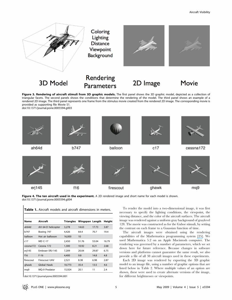
The file containing all 38 aircraft images is called WatsonAir-

craftImages.zip. It is a compressed binary file. After decompres-

sion, pixels are represented as 8-bit unsigned integers in row-major

order. The images are in alphabetical order of their symbolic

names, which are of the form c-v-s-b, where c = craft name,

v = viewpoint (1, 2, 3), s = size (0, 1, 2, 3, 4), and b = brightness (1,

2). The complete set of symbolic names, and the order in which

they appear in the file, is: {ah64d-1-0-1, ah64d-1-2-1, ah64d-2-0-

1, ah64d-2-2-1, ah64d-3-0-1, ah64d-3-0-2, ah64d-3-2-1, b747-3-

0-1, b747-3-0-2, balloon-3-0-1, balloon-3-0-2, c17-3-0-1, c17-3-0-

2, cessna172-3-0-1, cessna172-3-0-2, erj145-3-0-1, erj145-3-0-2,

f16-1-0-1, f16-1-2-1, f16-2-0-1, f16-2-2-1, f16-3-0-1, f16-3-0-2,

f16-3-1-1, f16-3-2-1, f16-3-3-1, f16-3-4-1, firescout-3-0-1, fire-

scout-3-0-2, ghawk-3-0-1, ghawk-3-0-2, mq9-1-0-1, mq9-1-2-1,

mq9-2-0-1, mq9-2-2-1, mq9-3-0-1, mq9-3-0-2, mq9-3-2-1}. This

is also the order in which the images appear in Figure 5.

This file can be read into an array of images using the following

Mathematica command:

images = Fold[Partition, Import[‘‘WatsonAircraftImages.zip’’,

‘‘Byte’’], {256, 256}];

In the experiment, the rendered aircraft images varied in size,

orientation, and contrast polarity. Sizes varied in steps of a factor

of two over a range of a factor of 16. The three orientations were:

head on, from the side, and from an oblique direction. The two

contrast polarities were positive (aircraft brighter than back-

ground), and negative (aircraft darker than background). The

complete collection of 38 aircraft stimuli is shown in Figure 5.

Data collectionContrast thresholds were measured in a block of 32 two-interval

forced-choice trials in a Quest adaptive procedure [18]. The two

presentation intervals were marked by tones, and feedback was

provided after the observers response. Responses were made using

a game controller (Mad Catz. http://www.madcatz.com/). The

sequence of trials in each block was converted to a contrast

threshold by fitting the percent correct with a Weibull function

[19,20] and locating the 82% correct point. Each block of 32 trials

contained only a single stimulus. Stimuli were divided into five

sets: 1) Gabors (n = 11), 2) all aircraft at the largest size with

positive contrast (n = 10), 3) all aircraft at the largest size with

negative contrast (n = 10), 4) one aircraft (f16) at five different sizes

(n = 5), and 5) three different viewpoints for three different aircraft

at two different sizes (n = 18). The total number of images is 38

(the sets overlap). Within each set, a block of trials was run for each

stimulus in random order. This was repeated three times, with a

new random sequence each time. Thus three replications of each

threshold were obtained for each stimulus and observer.

Each block took about four minutes to complete. Observers

were encouraged to rest between blocks, and no more than ten

blocks were completed by a single observer on a single day.

Experimental protocols were approved by the Human Research

Institutional Review Board of NASA Ames Research Center.

ObserversThree observers took part in the experiment: ABW, a 56 year

old male, CVR, a 36 year old male, and ES, a 30 year old female.

ABW wore a recent spectacle correction. Immediately prior to the

experiment, CVR and ES were examined by an optometrist and

assigned a new spectacle correction (ES) or no correction (CVR).

All three are experienced observers; only ABW (the author) was

aware of the purposes of the experiment at the time of data

collection.

Results

In most of the figures that depict basic contrast threshold results,

we show contrast on the vertical log scale, and use a fixed range

extending from 0.003 to 0.8. This range is large enough to include

all of our data, and the use of a fixed scale, while wasting some

amount of space on the page, allows a more consistent and direct

comparison of data from the several figures.

Gabor StimuliThe experimental methods used here, and the Gabor stimuli,

and one of the observers (ABW) were identical to those used in the

ModelFest experiment. This enables a direct comparison of the

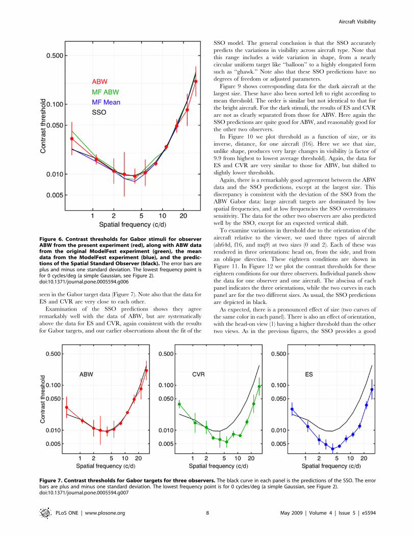
results from the two experiments. In Figure 6 we plot the contrast

thresholds for Gabor targets for observer ABW from the present

experiment (red), along with three measures derived from the

ModelFest experiment. These are: the ModelFest data of observer

Table 2. Rendering parameters for aircraft images.

Option Value 1 Value 2 Value 3

Boxed False

SphericalRegion True

Format ‘‘PGM’’

ImageResolution 72

ImageSize {256, 256}

Viewpoint 1 Viewpoint 2 Viewpoint 3

ViewPoint {0, 21, 0} {1, 0, 0} {1, 21, 1}/Sqrt[3]

Lighting {{‘‘Ambient’’, GrayLevel[0.2]}, {‘‘Point’’, White,Scaled[{2, 0, 2}]}}

{{‘‘Ambient’’, GrayLevel[0.2]}, {‘‘Point’’,White, Scaled[{2, 2, 2}]}}

{{‘‘Ambient’’, GrayLevel[0.2]}, {‘‘Point’’,White, Scaled[{2, 2, 2}]}}

Bright aircraft Dark aircraft

SurfaceColor GrayLevel[.8] GrayLevel[.2],

SurfaceSpecularity Specularity[.2, 3] Specularity[0.2, 5]

doi:10.1371/journal.pone.0005594.t002

Aircraft Visibility

PLoS ONE | www.plosone.org 6 May 2009 | Volume 4 | Issue 5 | e5594

ABW (green), the mean of 16 ModelFest observers (blue), and the

predictions of the SSO model (black), that was derived from the

ModelFest data.

The close agreement among all four curves suggests that we

have closely duplicated the conditions of the ModelFest exper-

iment, and that the sensitivity of observer ABW has not changed

markedly since the ModelFest data were collected (1999). It also

indicates that for this observer, at least, the SSO model continues

to provide a good description of the data.

In Figure 7 we plot the data for all three observers, along with

the SSO predictions. It is evident that observers ES and CVR are

considerably more sensitive at mid to high frequencies than either

ABW or the SSO model. They have lower minimum thresholds,

and they are more acute (they can see higher spatial frequencies).

However, the general shape of the results is consistent among

observers. This outcome suggests that the SSO model may

underestimate sensitivity and acuity for young, well-corrected

observers.

Another discrepancy between the present data, for all observers,

and the SSO model is the behavior at the lowest frequency.

Though plotted at 0.5 cycles/deg, this is the 0 cycle/deg Gabor, or

simple Gaussian (the first target in Figure 2). For all three

observers this lies above the model prediction, and lies on a

trajectory smoother and more upward going than the SSO. This

behavior is also evident in the ModelFest data for observer ABW

(green curve in Figure 6). This may be due to an artifact in the

method used by some laboratories in the ModelFest experiment

[17,21], which may in turn have distorted the shape of the SSO

CSF at the lowest frequencies. In brief, the ModelFest mean

observer, and the SSO, may overestimate sensitivity to the lowest

spatial frequencies.

The purpose of collecting threshold for Gabor targets in this

experiment was twofold: to measure the contrast sensitivity

function for each observer, and to verify that they agreed with

the predictions of the SSO. The results indicate that the SSO is

well matched to the CSF of observer ABW, but underestimates

sensitivity of observers ES and CVR in systematic ways. Since the

SSO is intended to mirror a population average, it cannot be

expected to agree with the results of every observer. But the

discrepancy between model and observers should be borne in

mind as we look at subsequent predictions for these observers.

Later, we will show how the SSO can be adjusted to better match

the results of our two more sensitive observers.

Aircraft StimuliFigure 8 plots contrast thresholds for individual aircraft targets of

the largest size. We selected this size because we believed that

differences in visibility based on shape would be most evident at the

largest sizes. Pictures of the targets are shown within the graph. The

figure also shows the SSO predictions. The horizontal positions of

the aircraft are in order of the mean threshold for the three

observers. Note that the trend for each observer is similar or

identical to the mean trend. This indicates that there are systematic

differences between thresholds for the different aircraft. The range

of mean values spans a factor of 2.08. However, relative to the range

of thresholds for Gabor targets, these differences are small.

The data for observer ABW lie about a factor of 1.5 above the

data for ES and CVR, consistent with the differences in sensitivity

Figure 5. Aircraft images used in the visibility experiment. Aircraft vary in type, size (distance), orientation, and contrast (darker or lighter thanbackground).doi:10.1371/journal.pone.0005594.g005

Aircraft Visibility

PLoS ONE | www.plosone.org 7 May 2009 | Volume 4 | Issue 5 | e5594

seen in the Gabor target data (Figure 7). Note also that the data for

ES and CVR are very close to each other.

Examination of the SSO predictions shows they agree

remarkably well with the data of ABW, but are systematically

above the data for ES and CVR, again consistent with the results

for Gabor targets, and our earlier observations about the fit of the

SSO model. The general conclusion is that the SSO accurately

predicts the variations in visibility across aircraft type. Note that

this range includes a wide variation in shape, from a nearly

circular uniform target like ‘‘balloon’’ to a highly elongated form

such as ‘‘ghawk.’’ Note also that these SSO predictions have no

degrees of freedom or adjusted parameters.

Figure 9 shows corresponding data for the dark aircraft at the

largest size. These have also been sorted left to right according to

mean threshold. The order is similar but not identical to that for

the bright aircraft. For the dark stimuli, the results of ES and CVR

are not as clearly separated from those for ABW. Here again the

SSO predictions are quite good for ABW, and reasonably good for

the other two observers.

In Figure 10 we plot threshold as a function of size, or its

inverse, distance, for one aircraft (f16). Here we see that size,

unlike shape, produces very large changes in visibility (a factor of

9.9 from highest to lowest average threshold). Again, the data for

ES and CVR are very similar to those for ABW, but shifted to

slightly lower thresholds.

Again, there is a remarkably good agreement between the ABW

data and the SSO predictions, except at the largest size. This

discrepancy is consistent with the deviation of the SSO from the

ABW Gabor data: large aircraft targets are dominated by low

spatial frequencies, and at low frequencies the SSO overestimates

sensitivity. The data for the other two observers are also predicted

well by the SSO, except for an expected vertical shift.

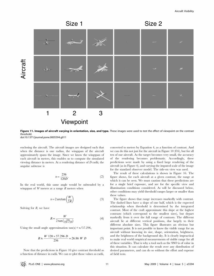
To examine variations in threshold due to the orientation of the

aircraft relative to the viewer, we used three types of aircraft

(ah64d, f16, and mq9) at two sizes (0 and 2). Each of these was

rendered in three orientations: head on, from the side, and from

an oblique direction. These eighteen conditions are shown in

Figure 11. In Figure 12 we plot the contrast thresholds for these

eighteen conditions for our three observers. Individual panels show

the data for one observer and one aircraft. The abscissa of each

panel indicates the three orientations, while the two curves in each

panel are for the two different sizes. As usual, the SSO predictions

are depicted in black.

As expected, there is a pronounced effect of size (two curves of

the same color in each panel). There is also an effect of orientation,

with the head-on view (1) having a higher threshold than the other

two views. As in the previous figures, the SSO provides a good

Figure 7. Contrast thresholds for Gabor targets for three observers. The black curve in each panel is the predictions of the SSO. The errorbars are plus and minus one standard deviation. The lowest frequency point is for 0 cycles/deg (a simple Gaussian, see Figure 2).doi:10.1371/journal.pone.0005594.g007

Figure 6. Contrast thresholds for Gabor stimuli for observerABW from the present experiment (red), along with ABW datafrom the original ModelFest experiment (green), the meandata from the ModelFest experiment (blue), and the predic-tions of the Spatial Standard Observer (black). The error bars areplus and minus one standard deviation. The lowest frequency point isfor 0 cycles/deg (a simple Gaussian, see Figure 2).doi:10.1371/journal.pone.0005594.g006

Aircraft Visibility

PLoS ONE | www.plosone.org 8 May 2009 | Volume 4 | Issue 5 | e5594

Figure 8. Contrast thresholds for three observers for ten different aircraft. All the aircraft have positive contrast (are brighter than thebackground). Actual aircraft images are shown in the figure. The black points are SSO predictions. The data are sorted from left to right according tothe mean threshold for the three observers.doi:10.1371/journal.pone.0005594.g008

Figure 9. Contrast thresholds for three observers for ten different aircraft. All the aircraft have negative contrast (are darker than thebackground). Actual aircraft images are shown in the figure. The black points are SSO predictions. The data are sorted from left to right according tothe mean threshold for the three observers.doi:10.1371/journal.pone.0005594.g009

Aircraft Visibility

PLoS ONE | www.plosone.org 9 May 2009 | Volume 4 | Issue 5 | e5594

description of these variations. The fit is best for ABW, but the

deviations for the other two observers are primarily a vertical shift

consistent with their higher sensitivity. They also show a smaller

elevation at the smallest size with viewpoint 1, which is consistent

with their higher acuity.

Comparison of Data and SSOIn the previous sections and figures we have seen that the SSO

provides a good account of the contrast thresholds for a range of

aircraft images. It correctly mirrors the variations in threshold due

to aircraft type, size, and orientation, as well as interactions among

these variables. Here we summarize those results by looking at all

38 aircraft thresholds for each of the three observers. In Figure 13

we plot each threshold against the SSO prediction for the same

target. The observers are depicted by the standard colors.

Accurate predictions would fall along the line of unit slope. As

can be seen, the points for observer ABW are very close to this

line. The results for the other two observers follow a similar

pattern, but fall below the line. This is consistent with our earlier

observation that observers CVR and ES are more sensitive and

more acute than observer ABW or than the SSO. For reference,

the RMS errors between data and model for ABW, CVR, and ES,

in log units, are 0.077, 0.187, 0.152, respectively.

To this point in our analysis we have used the default

parameters of the SSO model. The parameters of the SSO

govern the shape of the contrast sensitivity function, and the

nature of the pooling over space. For further details on these

parameters consult [12]. To evaluate the effect of a misfit between

the SSO and our observers, we fit the SSO to both Gabor and

aircraft thresholds, allowing the seven parameters of the SSO to

vary till they provide the minimum squared error for each of the

three observers. The results are shown in Figure 14.

The points lie close to the unit-slope line, indicating a good fit

for each observer. For reference, we provide the old and new

parameters in Table 3, along with residual RMS errors. Observer

ABW, as expected, shows only a small reduction in RMS error,

while the other two observers show much larger improvements. As

expected, observers CVR and ES show substantial increases in

sensitivity (Gain) and acuity (f0) relative to either observer ABW or

the default SSO.

For comparison, we show in Figure 15 the contrast sensitivity

functions for the three observers derived from the new fits, along

with the default SSO function. It is evident that the functions for

ES and CVR show greater sensitivity and acuity than the SSO.

Discussion

Fit of data and modelIn general, the SSO provides a good overall prediction of

contrast thresholds for aircraft images varying in aircraft type, size,

contrast polarity, and orientation. The predictions are excellent for

one observer, and slightly under-predict sensitivity for the two

other observers. When model parameters are adjusted to match

observers sensitivity and acuity, all predictions are excellent.

Observer differencesIt is clear that two of our observers (ES and CVR) are more

sensitive and more acute than ABW. This is perhaps related to

their younger age, and up-to-date refraction. It also seems possible

that the ModelFest population, and by extension the SSO,

underestimates the sensitivity of young emmetropic observers.

Model adjustmentsTwo of our three observers are more sensitive and more acute

than the SSO. Likewise, there are indications that the SSO may

overestimate sensitivity to very low frequencies. Finally, measure-

ment of the spatial MTF of the display reveals that a significant

part of the attenuation of high spatial frequencies measured in the

ModelFest experiment, and incorporated in the SSO, is due to the

display rather than the observer (see Appendix C). This suggests

the possibility of adjustments to the SSO to better represent the

performance of young emmetropic observers, viewing high-

resolution displays or real world images. We leave those

adjustments for a future project.

Computing threshold rangeOne goal of this research is to provide technology and tools that

will enable easy and accurate calculation of the maximum distance

at which an aircraft will be visible to the human eye: the threshold

range. We have seen that the SSO provides predictions that are

highly accurate for one observer and only slightly less accurate for

the other two observers. This validates the use of the SSO to

calculate threshold range estimates, as we now describe.

To compute threshold range values in real world units (meters),

we need to relate our stimulus image dimensions to corresponding

real world dimensions. First we note that the angular subtense of

our stimulus images is 256/120 = 2.133 degrees. Recall that the

nominal viewing distance from each aircraft, for purposes of

rendering, was specified in units of the radius of the sphere

Figure 10. Contrast thresholds for aircraft targets varying insize. Results from three observers and predictions of the SSO areshown. Actual aircraft images are shown in the figure.doi:10.1371/journal.pone.0005594.g010

Aircraft Visibility

PLoS ONE | www.plosone.org 10 May 2009 | Volume 4 | Issue 5 | e5594

enclosing the aircraft. The aircraft images are designed such that

when the distance is one radius, the wingspan of the aircraft

approximately spans the image. Since we know the wingspan of

each aircraft in meters, this enables us to compute the simulated

viewing distance in meters. At a rendering distance of D radii, the

angular subtense is

a~256

120D: ð2Þ

In the real world, this same angle would be subtended by a

wingspan of W meters at a range R meters when

a~2 arctanW

2R

� �ð3Þ

Solving for R, we have

R~W

2 tan 256120|2D

� � ð4Þ

Using the small angle approximation tan(x) = x/57.296,

R&W 120|57:296 D

256~26:86 W D ð5Þ

Note that the predictions in Figure 10 give contrast threshold as

a function of distance in radii. We can re-plot those values as radii,

converted to meters by Equation 4, as a function of contrast. And

we can do this not just for the aircraft in Figure 10 (f16), but for all

ten of our aircraft. As the target becomes very small, the accuracy

of the rendering becomes problematic. Accordingly, these

predictions were made by using a fixed large rendering of the

aircraft (as in Figure 4), and varying the imputed scale of the image

for the standard observer model. The side-on view was used.

The result of these calculations is shown in Figure 16. The

figure shows, for each aircraft at a given contrast, the range at

which it can be seen. We must caution that these predictions are

for a single brief exposure, and are for the specific view and

illumination conditions considered. As will be discussed below,

other conditions may yield threshold ranges larger or smaller than

these values.

The figure shows that range increases markedly with contrast.

The dashed lines have a slope of one half, which is the expected

relationship when threshold is determined by the integrated

contrast. Most of the craft approximate this slope at the highest

contrasts (which correspond to the smallest sizes), but depart

markedly from it over the full range of contrasts. The different

aircraft lie at different vertical positions, due largely to their

different absolute sizes. This figure illustrates an obvious but

important point. It is not possible to know the visible range for an

aircraft without knowing its size, shape, orientation, brightness,

and the brightness of the background sky. It is clearly impractical

to make real world empirical measurements of visible range for all

of these variables. That is why a tool such as the SSO is of value in

this situation. It can calculate the result over any distribution of

desired parameters, and can do so without the effort and expense

of field tests.

Figure 11. Images of aircraft varying in orientation, size, and type. These images were used to test the effect of viewpoint on the contrastthreshold.doi:10.1371/journal.pone.0005594.g011

Aircraft Visibility

PLoS ONE | www.plosone.org 11 May 2009 | Volume 4 | Issue 5 | e5594

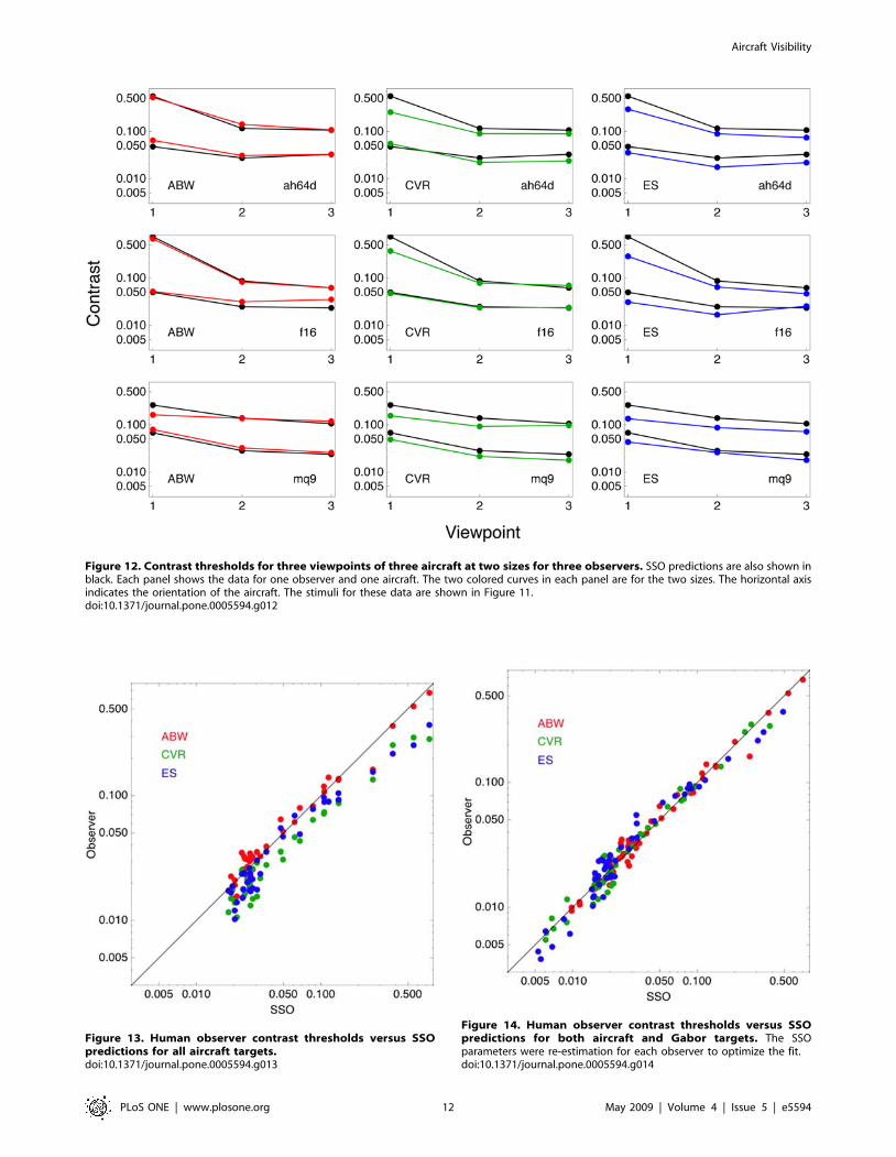
Figure 12. Contrast thresholds for three viewpoints of three aircraft at two sizes for three observers. SSO predictions are also shown inblack. Each panel shows the data for one observer and one aircraft. The two colored curves in each panel are for the two sizes. The horizontal axisindicates the orientation of the aircraft. The stimuli for these data are shown in Figure 11.doi:10.1371/journal.pone.0005594.g012

Figure 13. Human observer contrast thresholds versus SSOpredictions for all aircraft targets.doi:10.1371/journal.pone.0005594.g013

Figure 14. Human observer contrast thresholds versus SSOpredictions for both aircraft and Gabor targets. The SSOparameters were re-estimation for each observer to optimize the fit.doi:10.1371/journal.pone.0005594.g014

Aircraft Visibility

PLoS ONE | www.plosone.org 12 May 2009 | Volume 4 | Issue 5 | e5594

Comparison with Howell data. As discussed in the

introduction, Howell [5] measured the ‘‘threshold distance’’ at

which an aircraft (DC-3) could be detected by a vigilant observer

precisely aware of the direction of approach. We can now

compare the predictions of the SSO to these data. To achieve this,

we secured a 3D graphic model of the DC-3 aircraft, and

generated range predictions as described above. In Howell’s

experiment, the intruder aircraft approached the subject aircraft

from four different angles: 0u, 30u, 60u, and 100u. These

correspond to rotations of the view of the intruder aircraft of 0u,30u, 60u, and 50u. We computed separate predictions for these

four approach angles. In his report, Howell noted that the greatest

threshold distances occurred for negative contrast (dark aircraft

against a bright sky). Accordingly we generated predictions for two

illumination conditions: one in which the sun was above the

subject aircraft, and the other in which there was no sun

illumination at all. The latter case yields a black silhouette

against a light background, which is the extreme case of negative

contrast. The rendered aircraft images for these various conditions

are shown in Figure 17.

In addition, noting the superiority of two of our observers to the

SSO, both in sensitivity and acuity (see Figure 15), we also

generated predictions for our most sensitive observer ES. Our

range predictions, along with the data of Howell, are shown in

Figure 18.

Our predictions for the two illumination conditions differ by

almost a factor of three, and it should be clear that, depending on

environmental conditions and aircraft coloration, even larger

differences can be expected. These variations ultimately effect the

contrast, and hence the predicted range. Howell, commenting on

the very large variability in his results, attributes it largely to this

cause. The upper curves, for silhouette targets, are a relatively

Table 3. SSO parameters before and after estimation from present data.

Observer RMS Gain f0 f1 a r s b

SSO 373.083 4.17263 1.36254 0.849338 0.778593 1.57237 2.4081

ABW 0.0664 0.679 1.035 0.889 1.052 0.959 2.111 1.076

CVR 0.0731 1.090 2.416 1.013 1.106 1.520 0.941 0.903

ES 0.0975 1.991 1.501̀ 1.520 1.107 1.128 0.854 0.780

Original parameters are given for observer ‘‘SSO.’’ For the three human observers, we show the ratio of new and old parameters.doi:10.1371/journal.pone.0005594.t003

Figure 15. Contrast sensitivity functions derived from SSOparameters optimized for each observer. The black curve is theoriginal SSO CSF. For two of the observers, the curves lie above and tothe right of the original curve, indicating that they have greatersensitivity and acuity than the SSO.doi:10.1371/journal.pone.0005594.g015

Figure 16. Threshold range as a function of contrast for tenaircraft. Threshold range is the largest distance at which an aircraft canbe seen. Dashed lines have slope = K. These results depend upon aparticular set of lighting conditions.doi:10.1371/journal.pone.0005594.g016

Aircraft Visibility

PLoS ONE | www.plosone.org 13 May 2009 | Volume 4 | Issue 5 | e5594

fixed upper bound, but the lower curves are highly dependent on

the specific environmental conditions. With these caveats in mind,

we can say that our various predictions evidently bracket Howell’s

data. The data show some effect of angle, but the large variability

obscures the significance of these effects. Our predictions mirror

the decline in range at the 0u approach angle, due presumably to

the smaller profile, but do not show the observed small decline at

the two largest angles.

Additional caveats regarding these predictions should be

mentioned. We have assumed a meteorological range of infinity

(no atmospheric attenuation of contrast) so our predictions are an

upper bound. On the other hand, our predictions are for a very

brief presentation (,1/4 sec), while the real world target persists

until detected. Visibility rises slowly (approximately fourth root)

with duration following the first quarter second [19], but

extending the duration would nonetheless elevate our predictions

somewhat. For example, if the observer could maintain fixation on

the target for a full second, that might lower contrast threshold by

a factor of !2. From the curves in Figure 16, we see that this would

yield an increase of range of only about 25%.

Limitations. First, as noted in the introduction, we have not

measured or predicted the visibility of aircraft against patterned

backgrounds. Uniform backgrounds provide a best case, with

respect to visibility and range, and are thus a critical first step. But

in the future we hope to employ the masking capability of the SSO

to include patterned backgrounds as well. We should note that a

patterned background may introduce two fundamental visual

problems: masking and relative motion. The latter problem, in

particular, may require attention to the time domain, which we

have largely ignored in this report. We speculate that cloud

backgrounds, because they are dominated by low spatial

frequencies with low contrast, do not cause much masking or

relative motion, but that terrain backgrounds will produce both

masking and relative motion.

A second limitation is that we analyze and predict thresholds for

photopic (daylight) vision only. At dimmer illuminations, the

contrast sensitivity function (e.g., Figure 7) moves lower and to the

left, which will alter the predicted thresholds. Nonetheless, these

new thresholds could be predicted with a suitable change in model

parameters. Nightime conditions may introduce a rather different

challenge: understanding the visibility of warning lights, which we

do not deal with here.

Second, as noted in the discussion of prior research, the

challenge of locating an aircraft in the sky depends upon contrast

detection, as modeled here, but also upon the process of visual

search, which we have not modeled. (This is why we have

compared our predictions to the data of Howell, in which the

location of the approaching aircraft was known.) We can be

certain, however, that search cannot succeed without contrast

Figure 17. Rendered images of DC-3 aircraft at four approach angles and two illumination conditions. These are the approach anglesused in the experiment of Howell [5].doi:10.1371/journal.pone.0005594.g017

Figure 18. Threshold distance for a DC-3 aircraft at fourviewing angles. The points are data from Howell [5], and the blacklines show mean and plus and minus one standard deviation. The redcurve is the SSO prediction for a well-lit craft and the green curve is SSOprediction for a dark silhouette. The blue and purple curves arecomparable predictions for a highly sensitive observer (ES).doi:10.1371/journal.pone.0005594.g018

Aircraft Visibility

PLoS ONE | www.plosone.org 14 May 2009 | Volume 4 | Issue 5 | e5594

detection; thus our model provides a lower bound on the contrast

required, or an upper bound on the distance at which detection is

possible. A model of visibility, like that provided here, is an

essential component of any model of visual search.

Extensions. We have demonstrated the validity and utility of

the SSO as a tool for computing visibility range. This utility can be

extended in a number of ways. Elsewhere, we have shown how the

SSO can be extended with an optical module that can simulate

any specified set of waveform aberrations of the eye [22]. This

would allow us to simulate a pilot or ground observer, or a

population of such individuals, with specified optical limitations.

Since age has somewhat predictable effects on visual sensitivity

[23,24], it would be possible to observers of a specific age as well.

Because the SSO operates on images, the limitations of the

viewing system can be incorporated into the calculations. For

example, the effects of remote viewing through a low-resolution

video channel with limited dynamic range could be simulated.

This would allow simulation of the viewing conditions for the UA

pilot.

The visibility range predictions in Figure 16 do not take into

account the diminution in contrast due to attenuation by the

atmosphere. This effect can of course be small or large, depending

on atmospheric conditions. However, there are already well-

developed models for these atmospheric effects, which can

calculate the reduction in contrast of the aircraft image at a

specified distance under specified atmospheric conditions [6,7]. It

is a relatively simple matter to incorporate such an atmospheric

model into the detection range calculations of the SSO.

Display MTF. In order to better understand the rendition of

our aircraft images on our display we measured the modulation

transfer function (MTF) of the CRT. This was achieved by

capturing digital photographs of horizontal and vertical single

pixel wide lines, and averaging over columns or rows, respectively,

to obtain the linespread function. The magnitude of the Fourier

Transform of the linespread function is an estimate of the

modulation transfer function (MTF) of the display, which describes

the attenuation of contrast of sinusoids of various frequencies. We

fit each MTF with a Gaussian to provide a summary measure of

the MTF. We repeated this exercise at two line graylevels (128 and

255) on a black (0) background, because the CRT spot size is

known to grow with brightness, which will alter the MTF. One

case is shown in Figure 19.

The figure shows that the display imposes considerable

attenuation of visible spatial frequencies in the horizontal

dimension. Similar results, with somewhat less attenuation, were

found in the vertical dimension. A summary of Gaussian scale

parameters for the four cases (two orientations and two graylevels)

is shown in Table 4. The significance of these results is that they

show that both this experiment, and the ModelFest experiment

(which used a CRT for every observer and this particular CRT for

three observers) are likely to underestimate the acuity of observers.

Likewise the aircraft targets, particularly the small ones, did not

have as much contrast as their digital representations would

suggest, because they would be attenuated by the display.

It is important to note that the ModelFest experiment, this

experiment, and the SSO are all mutually consistent; their only

shared flaw is that they all misattribute some attenuation to the

observer that should properly be attributed to the display. This has

implications for future, more accurate versions of the SSO, and for

future psychophysical experiments.

Conclusions

1. Contrast thresholds were collected from three observers for 38

different images of aircraft superimposed on a uniform gray

background. The aircraft differed in type, orientation, distance,

and brightness.

2. Contrast thresholds were collected from the same three

observers for eleven Gabor targets.

3. Predictions for both Gabor and aircraft targets were computed

by the Spatial Standard Observer (SSO) model.

4. Gabor target thresholds were predicted well for one observer,

while the other two observers showed greater sensitivity and

acuity than the SSO.

5. With adjustments for the greater sensitivity of two observers,

aircraft predictions for all three observers were excellent.

6. Threshold range can be computed by the SSO for arbitrary

aircraft and viewing conditions.

Figure 19. Estimation of display MTF. A) Captured image of a vertical line on the CRT display (graylevel = 255). B) The linespread functionobtained by averaging the image over columns of pixels. The red curve is a Gaussian fit. C) MTF obtained as the Discrete Fourier Transform of thelinespread function. The red curve is a Gaussian fit.doi:10.1371/journal.pone.0005594.g019

Table 4. Estimated Gaussian scale parameters for the CRTdisplay.

128 255

Space Frequency Space Frequency

Horizontal modulation 103.177 107.514 84.8073 84.238

Vertical modulation 132.901 125.103 106.142 102.385

Values are shown derived from fits to the linespread and to the MTF, and forgrayscales of 128 and 255. The scale is the frequency in cycles/deg at which theGaussian declines to e2p = 0.0432.doi:10.1371/journal.pone.0005594.t004

Aircraft Visibility

PLoS ONE | www.plosone.org 15 May 2009 | Volume 4 | Issue 5 | e5594

Supporting Information

Movie S1 Movie showing an example of a Gabor stimulus with

a Gaussian timecourse.

Found at: doi:10.1371/journal.pone.0005594.s001 (3.93 MB

MOV)

Acknowledgments

We thank Key Dismukes and Kim Jobe for providing helpful references.

Author Contributions

Conceived and designed the experiments: ABW. Performed the experi-

ments: ABW CVR ES. Analyzed the data: ABW. Contributed reagents/

materials/analysis tools: CVR. Wrote the paper: ABW. Edited the paper:

CVR. Revised the paper: ES.

References

1. Graham W, Orr RH (1970) Separation of air traffic by visual means: An

estimate of the effectiveness of the see-and-avoid doctrine. Proceedings of the

IEEE 58: 337–361.

2. Colvin K, Dodhia R, Dismukes RK (2005) Is pilots’ visual scanning adequate to

avoid mid-air collisions? Proceedings of the 13th International Symposium on

Aviation 13: 104–109.

3. Rosenkranz W (2008) Detect, sense, and avoid. Aerosafety World. pp 34–39.

http://www.filghtsafety.org/asw/jul08/uas-forum.html. Accessed 2009 Mar 1.

4. Andrews JW (1977) Air-to-air visual acquisition performance with pilot warning

instruments (PWI). Federal Aviation Administration.

5. Howell WD (1957) Determination of daytime conspicuity of transport aircraft.

IndianapolisIndiana: Civil Aeronautics Administration Technical Development

Center, 304 304. Accessed 2009 Mar 1.

6. Duntley SQ, Gordon JI, Taylor JH, White CT, Boileau AR, et al. (1964)

Visibility. Applied Optics 3: 549–598. http://www.opticsinfobase.org/ao/

abstract.cfm?URI = ao-3-5-549. Accessed 2009 Mar 1.

7. Harris JL (1973) Visual aspects of air collision. Visual search. Washington DC:

National Academy of Sciences. pp 26–50.

8. Andrews JW (1991) Unalerted air-to-air visual acquisition. Lexington, MA:

Massachusetts Institute of Technology Lincoln Laboratory, Project Report

ATC-152, DOT/FAA/PM-87/34 Project Report ATC-152, DOT/FAA/PM-

87/34.

9. Vollmerhausen RH, Jacobs E, Driggers RG (2004) New metric for predicting

target acquisition performance. Optical Engineering 43: 2806–2818. http://link.

aip.org/link/?JOE/43/2806/1. Accessed 2009 Mar 1.

10. Ginsburg A, Easterly J (1983) Contrast sensitivity predicts target detection field

performance of pilots. Proceedings of the Human Factors Society. pp 269–273.

11. Ginsburg AP, Evans DW, Sekuler R, Harp SA (1982) Contrast sensitivity

predicts pilots’ performance in aircraft simulators. Am J of Optometry and

Physiological Optics 59: 105–109.

12. Watson AB, Ahumada AJ Jr (2005) A standard model for foveal detection of

spatial contrast. Journal of Vision 5: 717–740. http://journalofvision.org/5/9/

6/ Accessed 2009 Mar 1.

13. Watson AB (2005) A spatial standard observer for vision technology. Proceedings ofthe SPIE-IS&T Electronic Imaging 5666: 1–3. http://spiedl.aip.org/getabs/

servlet/GetabsServlet?prog = normal&id = PSISDG005666000001000001000001&idtype=cvips&gifs=yes. Accessed 2009 Mar 1.

14. Watson AB, Nielsen KRK, Poirson A, Fitzhugh A, Bilson A, et al. (1986) Use ofa raster framebuffer in vision research. Behavioral Research Methods,

Instruments, & Computers 18: 587–594.

15. Watson AB, Hu J (1999) ShowTime: A QuickTime-based infrastructure forvision research displays. Perception 28: 45.

16. Watson AB (2000) ShowTime Web Site. NASA.17. Carney T, Tyler CW, Watson AB, Makous W, Beutter B, et al. (2000)

Modelfest: year one results and plans for future years. Human Vision, Visual

Processing, and Digital Display IX 3959: 140–151.18. Watson AB, Pelli DG (1983) QUEST: a Bayesian adaptive psychometric

method. Perception & Psychophysics 33: 113–120.19. Watson AB (1979) Probability summation over time. Vision Research 19:

515–522.

20. Watson AB, Solomon JA (1997) Psychophysica: Mathematica notebooks forpsychophysical experiments. Spatial Vision 10: 447–466.

21. Ahumada A, Scharff L (2007) Lines and dipoles are efficiently detected. Journalof Vision 7: 337. doi:10.1167/7.9.337. http://journalofvision.org/7/9/337/.

Accessed 2009 Mar 1.22. Watson AB, Ahumada AJ Jr (2008) Predicting visual acuity from wavefront

aberrations. Journal of Vision 8: 1–19. doi:10.1167/8. http://journalofvision.

org/8/4/17/. Accessed 2009 Mar 1.23. Owsley C, Sekuler R, Siemsen D (1983) Contrast sensitivity throughout

adulthood. Vision Res 23: 689–699. http://www.ncbi.nlm.nih.gov/entrez/query.fcgi?cmd=Retrieve&db=PubMed&dopt=Citation&list_uids=6613011 Ac-

cessed 2009 Mar 1.

24. Rohaly AM, Owsley C (1993) Modeling the contrast-sensitivity functions ofolder adults. J Opt Soc Am A 10: 1591–1599. http://www.ncbi.nlm.nih.gov/

entrez/query.fcgi?cmd=Retrieve&db=PubMed&dopt=Citation&list_uids = 8350148Accessed 2009 Mar 1.

25. Wolfram S (2003) The Mathematica Book. Champaign, IL: Wolfram Media.

Aircraft Visibility

PLoS ONE | www.plosone.org 16 May 2009 | Volume 4 | Issue 5 | e5594