Journal of Biomolecular NMR, 3 (1993) 515 533 515 ESCOM

J-Bio NMR 137

Improved frequency resolution in multidimensional constant-time experiments by multidimensional Bayesian

analysis

R o g e r A. Chy l l a a n d J o h n L. M a r k l e y *

Department of Biochemistry, University of Wisconsin-Madison, 420 Henry Mall, Madison, W153706, U.S.A.

Received 30 March 1993 Accepted 2 June 1993

Keywords: NMR data processing; Multidimensional NMR analysis; Parameter estimation; Protein NMR spectroscopy

S U M M A R Y

The resolution of spectral frequencies in NMR data obtained from discrete Fourier transformation (DFT) along D constant-time dimensions can be improved significantly through extrapolation of the D-dimensional free induction decay (FID) by multidimensional Bayesian analysis. Starting from Bayesian probability theory for parameter estimation and model detection of one-dimensional time-domain data [Bretthorst, (1990) J. Magn. Reson., 88, 533-551; 552-570; 571 595], a theory for the D-dimensional case has been developed and implemented in an algorithm called BAMBAM (BAyesian Model Building Algorithm in Multidimensions). BAMBAM finds the most probable sinusoidal model to account for the systematic portion of any D-dimensional stationary FID. According to the parameters estimated by the algorithm, the FID is extrapolated in D dimensions prior to apodization and Fourier transformation. Multidimensional Bayesian analysis allows for the detection of signals not resolved by the DFT alone or even by sequential one-dimensional extrapolation from mirror-image linear prediction prior to the DFT. The procedure has been tested with a theoretical two-dimensional dataset and with four-dimensional HN(CO)CAHA (Kay et al. (1992) J. Magn. Reson., 98, 443-450) data from a small protein (8 kDa) where BAMBAM was applied to the 13C~ and H~ constant-time dimensions.

I N T R O D U C T I O N

The estimation of spectral frequency, amplitude, phase and decay rate parameters f rom N M R time-domain data is accomplished conventionally by examination of the absorption spectrum of the discrete Fourier t ransform (DFT) of the data. The frequency resolution obtained f rom the

DFT, however, is limited when acquisition times are short, as is the case for the indirectly detected dimensions of 3D and 4D N M R experiments. In many 4D experiments, for example, as few as eight complex points may be acquired along one or more of the indirectly detected dimensions.

*To whom correspondence should be addressed.

0925-2738/$10.00 �9 1993 ESCOM Science Publishers B.V.

516

TABLE 1 RECEIVER TIME AND PHASE VALUES FOR VARIOUS METHODS OF ACQUISITION a

Method of acquisition Position (x) Time (t) Phase (~)

Redfield b 1 0 x (0) 2 At y (~/2)

3 2At x (0) 4 3At y (~/2)

TPPV 1 0 x (0) 2 At y (n/2) 3 2At - x (~) 4 3At - y (3n/2)

States d 1 0 x (0) 2 0 y (~/2) 3 At x (0) 4 At y (~/2)

States-TPPI d 1 0 x (0) 2 0 y (r~/2) 3 At - x (n) 4 At - y (3g/2)

a For each point Yl in the D-dimensional data matrix, there is a vector Xi = [x~j,x~2,...XiD ] which specifies the position of the point along dimension d = [1,2,...D] of the matrix. The vector X~ uniquely specifies the time and phase of y~ along each dimension according to the method of acquisition displayed in the table.

b Redfield and Kunz, 1975. c Bodenhausen et al., 1980. a States et al., 1982.

Extrapolation of the FID by linear prediction (Barkhuijsen et al., 1985) prior to the Fourier transform (Gesmar and Led, 1989; Zhu and Bax, 1990; Led and Gesmar, 1991; Kay et al., 1992) has been one approach to increasing the resolution of highly truncated NMR data (see Stephen- son, 1988; Gesmar et al., 1990 for reviews). Although computationally stable and relatively fast, 1D linear prediction is sensitive to noise and is reliable only if the number of frequency compo- nents is less than one quarter of the number of available data points (Kumaresan and Tufts, 1982). Even with the use of constant-time experiments (Bax et al., 1979; Kessler et al., 1984) to increase the number of available data points through mirror-image time projection (Zhu and Bax, 1990), 1D linear prediction of highly truncated data can produce lineshape distortions and artifacts. A recently reported algorithm for simultaneous 2D linear prediction (Zhu and Bax, 1992) reduces these problems but only at a large computational expense.

Recently, Bayesian probability theory has been used to estimate relevant spectral information from 1D NMR data (Bretthorst, 1990a,b,c) with much greater resolution and accuracy than by

Abbreviations: NMR, nuclear magnetic resonance; 1D, 2D, etc., one-dimensional, etc; BAMBAM, Bayesian model- building algorithm in multidimensions; DFT, discrete Fourier transform; FID, free induction decay. Software for carrying out multidimensional Bayesian analysis of constant-time data is available from the National Magnetic Resonance Facility at Madison, 420 Henry Mall, Madison, WI 53706, U.S.A.

517

conventional Fourier transform processing (Kotyk et al., 1992). Through assigning probabilities to questions relating to parameter estimation and model selection, Bayesian analysis can con- struct the most probable mathematical model that is consistent with the NMR data and any known prior information. NMR data acquired with constant-time acquisition periods are partic- ularly amenable to Bayesian analysis because the mathematical models describing such data need not include decay terms. We develop here an extension of 1D NMR parameter estimation by Bayesian analysis to the D-dimensional case. The theory is implemented in an algorithm for extrapolating D-dimensional stationary NMR data which, when used in conjunction with the Fourier transform, can significantly increase the frequency resolution obtainable from NMR experiments containing D constant-time dimensions. Preliminary results of this study have been presented elsewhere (Chylla and Markley, 1993).

THEORY

Bayesian probability theory as applied to the estimation of spectral parameters in 1D NMR data (Bretthorst, 1990a,b,c) has been extended here to D dimensions. Bretthorst's notation has been retained insofar as appropriate.

Consider a D-dimensional, rectangular matrix of time-domain NMR data in which the number of data points along dimensions d ---- [1, 2 . . . . , D] is defined by nd= [nl, n2 . . . . . nD] respectively. The total number of data points, N, is given by

D

N = H nd (1) d = l

For convenience, the D-dimensional data matrix can be expressed as a 1D vector of N data points Y -= [Y~, Y2 ..... YN], where the position, time and phase in D-dimensional space of each data point Yi is defined by matrices X, T, and �9 respectively:

-Xl l X21 . . . XNI ] [ tll t21 ... tNl X ~-- XI2 X22 " ' " XN2 T - t12 t22 -.. tN2

LXlD x2D ..- XNDJ t,D tm ... tND

F(DI, (D2, ... ~_=/(D,2 (D22 ... (DN2 /

L(D'o (D2o ' (D o/

According to this notation, Xid , tid and (Did define, respectively, the position, time and phase of Yi along dimension d. These values are known parameters determined by the method of quadrature along d. Table 1 displays values for x, t and (D for several methods of quadrature assuming uniform data sampling.

A model describing the dataset may assume that the data can be separated into a systematic portion (signal) and a random portion (noise), both of which are functions of T and ~:

Yi (Ti,Oi) = f (Ti,~i) + e(Ti,~i), 1 ~ i ~ N (2)

The systematic portion can be modeled as a linear combination of J signal functions: J

f (T,~) = ~ BjUj(T,~,| j = l

(3)

518

where Uj(T,O,Oj) is the j th signal function, Bj is the amplitude of the j th signal function, and Oj represents the relevant nonlinear parameters (frequency, phase and decay rate) associated with Uj. The signal function Uj, for the case of D-dimensional time-domain N M R data, is a D- dimensional decaying sinusoid:

D

U s (Ti,Oi,Oj) = l"I COS(%dtia + ~id + 0Sd) e-~jdtid, 1 <-- i ~ N; 1 --< j --< J (4) d = l

where Us(Ti,Oi,Os) is the value of thejth signal function at data point i, tid and Oid are the respective time and phase of the ith data point along dimension d, and O)Sd, 0Sd, and %d are the respective angular frequencies, phases and decay rates of thej th signal function along dimension d. For the special case of NMR data in which all D dimensions have been acquired by using a constant-time evolution period, the signal function U s can be modeled by a stationary sinusoid without decay terms:

D

Uj(Ti,Oi,Oj) = l-I COS(o)jdtia + Oid + 0Sd), 1 --< i <-- N; 1 - - j --< J (5) d = l

It is important to note the very different natures of r and 0Sd. Although both represent phase terms in Eq. 5, ~id is a known acquisition term determined by the method of quadrature; in contrast, 0jd is an unknown parameter to be estimated from the data. To minimize the number of unknown, nonlinear parameters, 0 can be expressed as an amplitude (linear) rather than as a phase (nonlinear) parameter. A sinusoid of amplitude B and phase ~ is equivalent to the linear

rt combination of two sinusoids differing in phase by 2:

B cos(o) t + 0) = AI cos(o) t) + A 2 cos(o) t + n 5) (6)

Application of this one-dimensional trigonometric identity to the D-dimensional Eq. 3 yields the following expression for f(T,O)

J K

fiT,O) = ]~ E AjkVjk (T,O,W s) (7) j = l k = l

where K = 2 D is the number of amplitudes per sinusoid, ASk is the kth amplitude of the flh sinusoid, W s =- [o)jl, %2 . . . . . %D], and Vsk(T,q~,Ws), the kth signal function of the j th sinusoid, is given by

D

Vjk(Ti,Oi,Wj) = I-I COS(%dtid + ~id 4- It/kd), 1 -< i -< N; 1 -< j -< J; 1 --< k -< K (8) d = l

[,w\ ~kd = [ 2 ) [ ( ( k - 1) / (2d-l)) % 2], 1 --< d - - < D; 1 - < k - < K (9)

The operators / and % represent the integer division and integer modulus operators respectively. Table 2 displays values of qJka for the cases o fD = 1, 2, and 3. The parameters B (Eq. 3) and ~ (Eq. 5) can be calculated from A (Eq. 7) according to

B j = ~ k = l Ajk2, 1 --< j --< J (10)

TABLE 2 KNOWN VALUES FOR Wkd AS A FUNCTION OF k AND d

519

Dimensions ktJkd a

d k = l k = 2

D = l 1 0 n/2

k = l k = 2 k = 3

D = 2 1 0 n/2 0 2 0 0 n/2

D=3

k=4 rd2 ~/2

k = l k = 2 k = 3 k = 4 k = 5 k = 6 k = 7 k = 8

1 0 hi2 0 hi2 0 hi2 0 hi2

2 0 0 hi2 hi2 0 0 n/2 n/2

3 0 0 0 0 n/2 n/2 n/2 n/2

"There are k = [1, 2,...K = 2 ~ phase terms along each dimension. Each hUkd corresponds to the phase term appearing in dimension d of the kth basis function of Eq. 8.

Ojd=arctan(AJ-~i~) ,z=(l+/~ 2 d - l ) ; 1 - < j - < J ; 1 - < d - < D (11)

It is convenient to express the jk subscripts in terms of a single subscript, m = 1 ... M, where M - JK and m takes the M possible combinations ofjk. With this change in notation, A m = Ajk , V m is given by

V~(T,O,W i) = Vjk (T,C~,Wi), m = (k - 1)J + j (12)

and f(T,~) is given by

M

f(T,O) = • nmVm(T,~,Wj), j = [ ( m - 1 ) / J ] + 1 (13) m = l

Equation 13 is a model that is sufficient to describe the systematic portion of all D-dimensional N M R data that can be described by a sum of stationary sinusoids.

Given a specified set o f ( J + 1) possible models and S = {fo,fl,f2 ..... fj}, Bayesian statistics can determine quantitatively which model f~ is the most probable given the data and any known prior information. This probability can be expressed as P(D[f,O,I), the global likelihood of the data D, given the form of the data f, the nonlinear parameters O associated with f, and any prior information I. Bretthorst (1990b) derived an expression for P(DIf, O,I) for any dataset that satis- fies Eqs. 2 and 3 and whose noise carries a finite total power:

P(D I f,O,I) oc F F 2 (14)

In the above equation, F(x) is the gamma function, M is the number of signal functions, N is the total number of data points, d 2 is the mean-square data value

520 N

~'~ = 1 i ='~lyi2

h 2 is the mean-square projection of the data unto a set of orthonormal basis functions H,

(15)

N h m = ,~_~ yiHm(Ti,qbi), 1 -< m ~ M (17)

i=l

Hm(Ti,~/~i ) 1 = ~ l=le~ Vl(Ti,~i), 1 -< m -< M (18)

eml is the ruth component of the / th eigenvector, and k m is the ruth eigenvalue of the interaction matrix Glm defined by

N glm ~--" E Vl(Ti,tI)i)Vm(Ti,(I)i), glm ~ Glm, 1 -< 1 -< M, 1 -< m -< M (19)

i=l

The global likelihood of the data P(Dlfj,Oj,I) depends upon the number of sinusoids J in the model (M = 2 D J) and the values of the nonlinear parameters Oj. For the special case of NMR data acquired with constant-time evolution periods, the nonlinear parameters are exclusively frequency parameters (Oj = Wj). P(DIf, O,I) can be evaluated independent of the linear parameters A m (Eq. 13). A m a r e 'nuisance parameters' (Bretthorst, 1990a) which can be removed from the expression for P(DIf, O,I) by integration over all possible values of A m. The values of Am, which maximize P(DJf, O,I) for a given set of nonlinear parameters, are given by

hi elm A m ------- - - m - M (20)

1= 1 ~ ' - 1 , 1 < <

Equation 13 can be used not only to estimate the nonlinear parameters that maximize P(DIfj,| but also to estimate the number of signals present in the data. A dataset can be said to contain evidence for J signals if

P(DIfj+ ,,O,I) P(DIfj,O,I) <1 and >1 ,

a(D[fj,O,I) a(DIfj_ ~,O,I)

where fj refers to a model containing J signals. In view of the data and any prior information, application of Bayesian probability theory selects the simplest model that still accurately accounts for the systematic portion of the data.

Bayesian probability theory indicates the conditions under which the Fourier transform pro- vides an accurate estimation of the frequencies prese__nt in NMR data. For a model with a fixed number of sinusoids, P(D[fj,O,I) increases as h 2 increases. For J = 1 (M = 2 D) and O = W = [~01,tah ..... O)D], it can be shown that

(N)Dm~= ITm2(W), ~-= M = 2 D =

,1 Tm(W) -- i =~1 yi I COS(O)dtid + 0id

(21)

(22)

M 1 m~b ~ (16)

521

m

Equation 22 is simply the D-dimensional Fourier transform of the data and the quantity h: is proportional to the power spectrum evaluated at W = [0~,r ..... COD]. For a model consisting of a single stationary frequency, the position of Tm(W)max (maximum of the Fourier transform power spectrum) represents the values of W that are most 'probable' as expressed by the quantity P(DIfj,O,I).

ALGORITHM

The preceding section has outlined a theory for evaluating the relative probability of different D-dimensional sinusoidal models of NMR data. This section applies that theory in an algorithm designed to construct the most probable sinusoidal model for a D-dimensional N M R dataset acquired under conditions where decay of the time-domain signals is negligible (e.g., constant- time evolution periods). We have dubbed the algorithm BAMBAM (BAyesian Model Building Algorithm in Multidimensions). BAMBAM will be explained through an example: Bayesian analysis of a synthetic 2D (8 • 8 complex) dataset with added random noise.

Consider a synthetic 2D matrix of N M R data Y, where eight complex points are 'acquired' along each dimension by using the procedure of States et al. (1982) for quadrature detection. This dataset can also be viewed as a linear array of (N = (2 x 8) 2 = 256) time-domain data points, Y = [Y~,Y2,Y3 . . . . . YN]. The time and phase along dimension d for point Yi are given according to the States quadrature scheme outlined in Table 1. The time-domain dataset Y contains 15 sinu- soids whose amplitudes and frequencies along each dimension are tabulated in Table 3. The phases and decay rates of the sinusoids are all zero. The frequencies in Table 3 are expressed in dimensionless units -1 ~ f ~ 1, which represent the angular frequency range - n -< co ~ n. Y was constructed by calculating the time-domain data points according to the theoretical parameters in Table 3 and then by adding Gaussian noise with a mean of zero and a standard deviation of unity to each of the N data points.

BAMBAM applies a sequential strategy in order to find the most probable model for a given dataset. BAMBAM first calculates the quantity P(D[fj,O,I) for a model containing no sinusoids (J = 0, M = 1), i.e. a model which is simply a constant. It then compares the value of P(D[fj = 0, | to the posterior probability of a model containing one sinusoid (J = 1, M = J x 2 D = 1 • 2 = 4). I f

P (D[fj = ~,O,I) >1 ,

P (Dlfj = o,O,I)

then the most probable model contains at least one sinusoid; otherwise, BAMBAM 'concludes' that the most probable model is simply a constant and the algorithm terminates. In the former case, BAMBAM then calculates P(D[fj,O,I) for a model containing two sinusoids (J = 2, M = 2 x 2 2 = 8). BAMBAM repeats these steps until the termination criteria are met, namely that

P(DIfj + ~,0,I) P(DIfj,O,I) < 1 and

P(DIfj, O,I) P(DIfj -~, O,I) >1.

With the synthetic dataset Y as an example, the following cases detail how P(D[fj,O,I) is calculat- ed for J = 0, 1, 2 . . . . Z.

522 Case ( J = O)

For a model containing no sinusoids, the systematic portion of the data is equivalent to a constant f (T,~) = A (Eq. 13), and the b__asis function Vm(Ti,~i,| (Eqs. 8 and 12) is equal to one. For this minimal model, the statistic h 2 is equivalent to the square of the sum of the data

= Yi (Eqs. 16 and 17). The necessary quantities, N=256 , M = 1, h --7, and d ---5 (calculated i = l

according to Eq. 15), are known so that P(Dlfj=0,| can be calculated according to Eq. 14. Because of the large absolute values of the exponents in Eq. 14, P(DIfj = 0,19,1) is more convenient- ly expressed in logarithmic form

ln[P(D[ f,19,I)] oc I~F(~)] + ln[F(-~)]- (M) 1~--~ ]- [ -~1 ln{ N~2M~] (23) Case ( J = 1)

The next simplest model is one consisting of a single sinusoid (J = 1, M = 4). Equation 21 indicates that the most probable single frequency describing a dataset is given by the position of the maximum of the Fourier transform power spectrum (Tm(W) . . . . Eq. 22). The Tm(W)max for

TABLE 3

COMPARISON BETWEEN THE THEORETICAL VALUES OF SIGNAL PARAMETERS AND THE VALUES

DERIVED FROM BAYESIAN ESTIMATES OF A SYNTHETIC TWO-DIMENSIONAL DATASET WITH ADD-

ED RANDOM NOISE a

Peak Theoretical values Bayesian estimates

A ~1 m2 A m~ m2

a 3.00 0.4000 -0.7000 3.10 0.4053 -0.6875

b 8.00 -0.6000 -0.6000 7.70 -0.6067 -0.6007

c 5.00 -0.1000 -0.4000 4.95 -0.1321 -0.4026

d 4.50 -0.4000 -0.3000 4.72 -0.3818 -0.3229

e 5.00 0.2000 -0.3000 4.81 0.2035 -0.2822

f 6.00 0.0000 0.0000 6.00 -0.0089 -0.0051

g 2.00 -0.9500 0.0000 2.13 -0.9507 0.0042

h 4.00 0.3000 0.1000 4.70 0.3297 0.1158

i 4.00 0.4000 0.1500 4.65 0.3768 0.1441

j 8.00 -0.7000 0.3000 8.22 -0.7014 0.3074

k 4.00 -0.1000 0.4000 4.04 -0.0954 0.4011

1 6.00 -0.6000 0.4000 6.68 -0.6081 0.4218

m 6.00 -0.8000 0.5000 6.56 -0.7799 0.4883

n 5.00 -0.6000 0.6000 5.84 -0.6025 0.5826

o 3.50 0.4000 0.8000 3.51 0.4040 0.8135

a The theoretical time-domain dataset is an 8 x 8 complex array of data points (N = (2 x 8) 2 = 256) consisting of 15

sinusoids (~o ) computed using the corresponding frequency and amplitude parameters listed in the table. The decay rate

and phase along dimensions one and two of each sinusoid are zero. Random noise with a standard deviation of unity was

added to each data point prior to Bayesian analysis. The frequencies coj and ~ are displayed in the Nyquist interval -1 -< f-< 1 representing the angular frequency range - n -< o~ -< n.

523

dataset Y occurs at the frequency coordinate [(01 = -0.663n, (02 = 0.313n]. A model consisting of a single 2D sinusoid at this coordinate [(0,(02] can be constructed by Eqs. 7-9, 12 and 13:

fj=l(Ti,(I)i) -- A 1 cos((01til + i~il)COS(0)2ti2 + t~i2) -t- A 2 cos((01til -I- ~)il d- ~)cos((02ti2 -t- ~i2) -t- (24)

A 3. cos((01til + ~il)COS((02ti2 -I- ~i2 -t- ~) q- A 4 cos((01til + ~il -1- ~2)c0S((02ti2 -1 ~i2 1- 5)

With the following shorthand:

Cd ~ COS((0dtid + ~id) (25)

Sd ~ sin((0dtid + l~id) ~-" COS((0dtid + ~id q- 2 ) (26)

fJ = 1 can be rewritten as

t~ = l(Ti,(I)i) = A I C I C 2 -t- A2S1C 2 -I- A3C1S 2 -t- A4S1S 2 (27)

The interaction matrix for the single sinusoidal model (Eq. 19) is given by

G =

N N N N E C12C22 E C151C22 E CIS1C2 2 E CISIC2S2

i=1 i=1 i=l i=l

N N N N E C1SIC22 E 512c22 E c i s i c 2 s 2 E s12c2s2 i=1 i=1 i=l i=1

N N N N E ElSiE22 E ClSlC2S2 E C12522 E ClSlS22

i=l i=l i=l i=l

N N N N Z CIS1C252 E 512c252 E c151s22 E s12822

i=l i=1 i=l i=l

N

o N _

4

0 0

0 0

0 0

0 0

N

N

(28)

The eigenvectors and eigenvalues from the diagonal matrix G were used with the values [0)1,(02]

to construct the orthogonal basis functions, n m = 14(Ti,~i) (Eq. 18). The projections of the data onto the orthogonal basis functions h m = 14 and the mean-square value of this projection h 2 were calculated according to Eqs. 17 and 16, respectively.

For a fixed value of M, h 2 is a sufficient statistic to determine the values of the nonlinear parameters, (01 and (02, that represent the most probable frequencies contained in the data. The Tm(W)max at [(01 = -0.663n, (02 = 0.313~] was used as an estimate for the frequencies that maxi- mize h 2. The precision of this estimate was limited, however, by the size of the frequency grid over which the FT was performed. A more precise estimate was obtained from a two-parameter nonlinear maximization algorithm using h 2 as the criterion for maximization. The nonlinear max- imization yielded a n h2max at the frequency coordinate [(01 = -0.673n, 0) 2 = 0.3077]. The amplitude values A m = 14 consistent with this model were calculated from h m = 14 according to Eq. 20.

The values of h 2 . . . . d 2, M = 4 and N = 256 were used to calculate ln[P(D[fj = ,O,I)], the logarithm of the posterior probability of the data, given a model containing a single sinusoid. A function A(J), defined as

524

70

60

50

40

a(~ 3o

20

10

0

-10 I I I

5 lO 15

J (# of Sinusoids)

!

2O

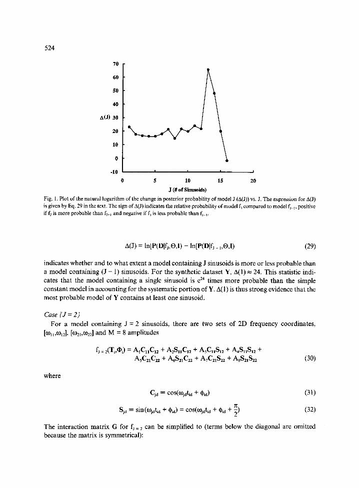
Fig. 1. Plot of the natural logarithm of the change in posterior probability of model J (A(J)) vs. J. The expression for A(J) is given by Eq. 29 in the text. The sign of A(J) indicates the relative probability of model fj compared to model fj_~, positive if fj is more probable than fJ-1 and negative if fs is less probable than fJ-v

A(J) = ln[P(Dlfj,O,I) - ln[P(Dlfj_ l,O,I) (29)

indicates whether and to what extent a model containing J sinusoids is more or less probable than a model containing (J - l) sinusoids. For the synthetic dataset Y, A(1) ~ 24. This statistic indi- cates that the model containing a single sinusoid is e 24 times more probable than the simple constant model in accounting for the systematic portion of Y. A(1) is thus strong evidence that the most probable model of Y contains at least one sinusoid.

Case ( J = 2)

For a model containing J = 2 sinusoids, there are two sets of 2D frequency coordinates,

[O~ll,C01z], [0)21,C022] and M = 8 amplitudes

fJ : 2(Ti,(I)i) = A~CnCI2 + A2S11C12 + A3CIISI2 + A4S11S12 +

A5C21C22 + A6S21Czz + A7C21822 + A8S21S22 (30)

where

Cjd ~ COS(%dtid + r (31)

-= sin (%atia + r = COS(C%tid + ~id + 2 ) (32)

The interaction matrix G for fj = 2 can be simplified to (terms below the diagonal are omitted because the matrix is symmetrical):

525

G =

N 7 o

N

4

0 0

0 0

N N N N

E C 1 IC12C21C22 E C11C12S21C22 E C11C12C21S22 E CllC12S21S22 i=l i=l i=l i=l

N N N N

E S1 IC12C21C22 Z S11C12S21C22 E 511C12C21S22 E s11c12s21s22 i=l i=l i=l i=l

N N

N 0 E C11S12C21C22 E Cl1S12S21C22 4 i=l i=l

N N

E C11512C21S22 E Cl1St2S21822 i=l i=l

N N N N

N E s11s12c21c22 E $11s12s21c22 E s11s12c21s22 Z s11s12s21s22 4 i=l i=l i=l i=l

N 0

4

N

4

0 0

0 0

N 0

N

4

(33)

For a general model, the summations shown in Eq. 33 cannot be evaluated analytically; the

summations are dependent upon the specific values of [(011,(0~2] and [(02~,(022]. An estimate for [(01L,(0~z] was obtained from the fj = 1 model, and an estimate for [(021,(022] was

generated from the residual R(2) between the original dataset and fj = 1. For a model consisting of

J frequencies, the residual R(J) is defined as

R(J) = Y - fJ-1 (34)

The estimate [(021 = -0.606n, (022 = -0.596n] was obtained from the Tm(W)max of the residual R(2). A starting estimate for the nonlinear parameters comprising the most probable two-sinus- oid model was thus given by the pair of coordinates [(01~ = -0.673x, (012 = -0.307n] and [(021 = -0.606n, (022 = -0.596x]. The eigenvectors and eigenvalues derived from G were used to calculate values for Hm= 1-8, hm= 1-8 and h 2 as done previously (Eqs. 16-18). The quantity h2max w a s found by a four-parameter nonlinear maximization of [(0H,(012] and [~,(02z], which yielded [(011 = -0.674n, (012 = -0.309n] and [o~ = -0.598n, (022 = -0.587n]. Val- ues of A m = I 8 consistent with this model were calculated according to Eq. 20. The value A(2) (Eq. 29) indicated that the model consisting of two sinusoids was e ~9 times more probable than the model consisting of a single sinusoid.

Case (J = Z ) BAMBAM determines the most probable values for the nonlinear parameters

([(01D(012],[(02~,(022] . . . . [(0z~,(0z2]) for the case J = Z in the same manner as the case J = 2. Each

526

model consists of Z 2D frequency coordinates which are used to define a basis set of M = 4Z amplitudes and 4Z basis functions (Eqs. 7-9). The Tm(W)max value of the residual R(Z) is used to obtain a starting frequency estimate for [O~z~,O~z2], and the frequency estimates from fj = ~-z yield starting values for ([o~l~,o~2],[ohl,o~zz] . . . . [O~(z-1)l,CO(z-~)2]). From these nonlinear parameters, the interaction matrix G can be calculated numerically, and its eigenvectors and eigenvalUes deter- mine Hm = ~-M, hm = l-M, and h 2 according to Eqs. 16-18. The search for h2max is accomplished through a 2Z nonlinear parameter maximization (see Appendix: Nonlinear Maximization of h2). The values for A m =1-M consistent with the most probable nonlinear parameters (the frequencies [coH,o~12],[Ohl,Ohz], �9 ..[COz~,~z2] which maximize h 2) are calculated according to Eq. 20. The values obtained for ([0311,(1)12],[0)21,0)22] . . . . [O~ZI , ( I )z2]) and A m = I-M define the new model f j = z according to Eqs. 7-9. The quantityA(Z) then determines the relative probabilities of models fz and fz + 1.

RESULTS

Synthetic dataset The most probable model of dataset Y found by Bayesian analysis is presented in Table 3 next

to the actual values that define the systematic portion of Y. The algorithm accurately predicted the number of sinusoids contained within the data. Figure 1 displays a plot of A(J) vs. J for J = 1-16. Bayesian statistics indicated that the 15-sinusoid model was e 3~ times more probable than the 14-sinusoid model and e 3"7 times more probable than the 16-sinusoid model. Although the 16-sinusoid model 'fits' the data better, the better fit was statistically unjustified by the greater number of basis functions required by the model. The inequality A(16) < 0 (see Fig. 1) was the hallmark of the greater likelihood of the 15- vs. 16-sinusoid model.

In order to estimate the precision and the accuracy of each of the Bayesian-derived parameters in Table 3, identical analyses were performed upon a total of eight datasets. Each dataset was identical to dataset Y in its systematic component (signals a-o) but different in its random (noise) component. The accuracy and precision determined from the Bayesian estimates of the eight datasets are displayed in Table 4. The terms 'precision' and 'accuracy' as used here are defined as the root-mean-square (rms) deviation of each estimate from the mean value (of the eight datasets) and the 'true' value (left-hand portion of Table 3) respectively. The greater accuracy of the frequency vs. the amplitude estimates is not unexpected because the frequencies are much better determined by the data than are the amplitudes (Bretthorst, 1990c). The results of Tables 3 and 4 show clearly that, even though a zero-filled Fourier transform of dataset yields a frequency

2n resolution of(4 x 8 -- 0.0625~), Bayesian analysis was able to estimate the frequencies contained in

dataset Y within an average accuracy of 0.013~ <-co-< 0.018n. Clearly, the actual frequency information contained in a highly-truncated dataset is much greater than is conventionally obtained from a zero-filled Fourier transform.

A graphical comparison of Bayesian analysis with the zero-filled Fourier transform (ZFT) and with the ZFT enhanced by 1D mirror-image linear prediction is shown in Fig. 2. Contour plots of the real frequency-domain spectrum of a noise-free (black contours, 64 x 64 complex) and a truncated (red contours, 8 x 8 complex) noise-added version of the same dataset are displayed in the figure. The noise-added, truncated dataset was processed by three different methods: (A) apodization and zero-filling, followed by Fourier transformation; (B) extrapolation of each dimension by separate 1D linear prediction prior to apodization, zero-filling and Fourier trans-

527

formation; and (C) extrapolation of both dimensions simultaneously by 2D Bayesian analysis prior to apodization, zero-filling and Fourier transformation (see legend to Fig. 2 for additional details). Processing of dataset Y with the simple zero-filled Fourier transform (Fig. 2A) resolved only 9 of the 15 actual frequencies contained within the data. Moreover, severe overlap distorted the positions of many of the frequencies and produced a large amplitude at (o~1 ~ - ~, ~o2 = 0) where no frequency actually exists. Extrapolation of the time-domain data by linear prediction (Fig. 2B) significantly improved the quality of the spectrum but still resolved only 12 of the 15 frequencies contained within the data. Extrapolation of the time-domain data by Bayesian analy- sis (Fig. 2C) prior to FT produced a real frequency-domain spectrum with all the frequencies of sinusoids a-o fully resolved within a 4% error. The amplitudes of signals h and i were only partially resolved by Bayesian analysis. They tended to be systematically overestimated in each of the eight datasets. This can be seen from the high accuracy-to-precision ratio for these two signals (Table 4).

Analysis of experimental data To illustrate the applicability of Bayesian analysis to the processing of constant-time data in 3D

and 4D experimental datasets, B A M B A M was used to extrapolate the 2D H~C ~ planes from a 4D

TABLE 4

THE CALCULATED PRECISION AND ACCURACY DERIVED FROM BAYESIAN ESTIMATES OF A SERIES

OF EIGHT SYNTHETIC TWO-DIMENSIONAL DATASETS WITH ADDED RANDOM NOISE a

Peak Accuracy Precision

A ol o2 A ol oh

a 0.13 0.0076 0.0133 0.13 0.0067 0.0086

b 0.15 0.0053 0.0056 0.11 0.0053 0.0054

c 0.39 0.0284 0.0059 0.31 0.0085 0.0059

d 0.30 0.0307 0.0147 0.24 0.0166 0.0066

e 0.17 0.0069 0.0169 0.12 0.0068 0.0038

f 0.16 0.0124 0.0077 0.14 0.0124 0.0040

g 0.14 0.0151 0.0088 0.12 0.0119 0.0035

h 1.87 0.0355 0.0192 1.24 0.0265 0.0187

i 1.60 0.0259 0.0118 0.80 0.0062 0.0054

j 0.45 0.0039 0.0105 0.28 0.0029 0.0057

k 0.16 0.0046 0.0042 0.16 0.0046 0.004 1

1 0.89 0.0116 0.0127 0.54 0.0079 0.0080

m 0.49 0.0131 0.0093 0.29 0.0082 0.0074

n 0.71 0.0099 0.0211 0.40 0.0075 0.0139

o 0.13 0.0094 0.0170 0.08 0.0033 0.0114

ALL 0.74 0.0177 0.0129 0.45 0.0107 0.0085

"Each theoretical time-domain dataset is an 8 x 8 complex array of data points (N = (2 x 8) 2 = 256) consisting of 15

sinusoids (a o) computed using the corresponding frequency and amplitude parameters listed in Table 3. Random noise with a standard deviation of unity was added to each data point prior to Bayesian analysis. The eight datasets are thus identical with respect to their systematic components and differ only in their random (noise) components. The frequen-

cies o~ and oh are displayed in the Nyquist interval -1 -< f -< 1 representing the angular frequency range - n -< o <- n.

528

Fig. 2. Contour plots of the real frequency-domain spectrum of a noise-free (black contours) and a truncated, noise-added (red contours) version of the dataset defined by Table 3. The systematic portion of the dataset consisted of 15 sinusoids (a o) with an amplitude range of 2-8. The noise-added dataset (8 x 8 complex points) was processed in three different ways prior to Fourier transformation: (A) Prior to Fourier transformation, each dimension was digitally filtered by a cosine-squared bell apodization function followed by zero-filling from 8 to 128 complex points. After Fourier transforma- tion, the imaginary portion of the spectrum along each dimension was discarded; (B) Time domain t2 was Fourier transformed. Mirror-image linear prediction was used to extend the length of the FID along t~ from 8 to 15 complex points. Time domain t~ was then digitally filtered with a cosine-squared bell apodization function and zero-filled from 15 to 128 complex points prior to Fourier transformation. After Fourier transformation, the imaginary portion of 0~ was discarded. Frequency domain to2 was then inverse Fourier transformed and processed in the same manner as h; (C) The best estimates of the number, amplitude, frequency and phases of all detectable signals in the data were obtained by using the algorithm described in the text. The model derived from this Bayesian analysis was used to perform a 2D extrapolation of the (t~,t2) 8 x 8 complex dataset to a 64 x 64 complex array. Each dimension was then digitally filtered with a cosine- squared bell apodization function and zero-filled from 64 to 128 complex points prior to Fourier transformation. After Fourier transformation, the imaginary portion of the spectrum along each dimension was discarded.

529

HN(CO)CAHA experiment (Kay et al., 1992) performed upon uniformly 15N-~3C-labeled protein subunit c (DDT binding protein, 8 kDa) from E. coli. Although subunit c is a relatively small protein, it consists of predominantly a-helical regions and thus exhibits poor chemical-shift dispersion in both the backbone and side-chain NMR resonances. The dataset was collected on a Bruker 500 MHz spectrometer with a frequency resolution of (256 • 16 • 8 x 8) complex points in the amide proton (acquisition, t4) , nitrogen (tO, or-proton (t2) and t~-carbon (t3) dimensions, respectively. The H a and C a (t2,t3) dimensions were acquired by using shared constant-time acquisition periods (Kay et al., 1992).

The acquisition dimension t 4 w a s processed using conventional apodization, zero-padding and Fourier transformation, followed by discarding of the imaginary portion of the frequency- domain data. The nitrogen tl dimension was then extrapolated from 16 to 24 complex points by linear prediction after Fourier transformation of the t2 and t 3 dimensions. After apodization with a cosine-squared bell filter function, zero-filling to 64 complex points, Fourier transformation and discarding of the imaginary data points along the o)~ dimension, the o)2 and o)3 dimensions were inverse Fourier transformed. The result of this series of operations was a 4D matrix consist- ing of 256 (COn) • 64 (c~ = 16 384 planes of data, each containing 8 • 8 complex points along dimensions t2 and t 3 ( H a and C a, respectively).

Each of the 256 • 64 (t2,t3) 2D FIDs was extrapolated from 8 • 8 to 32 • 32 complex points using multidimensional Bayesian analysis. The total processing time required to analyse the 16 384 planes was 23.1 h on a Silicon Graphics Indigo workstation. After extrapolation by Bayesian analysis, each of the (t2,t3) planes was apodized, zero-filled to 64 complex points and Fourier transformed. A single plane from the 4D dataset occurring at [o)4 = 6.32 ppm, o)~ = 120.6 ppm] was processed according to the three different methods (A, B and C) as described above, and the results are shown in Figs. 3A-C.

CONCLUSIONS

Bayesian probability theory applied to the analysis of stationary, multidimensional NMR data is a practical technique for extrapolating D-dimensional constant-time data prior to apodization, zero-filling and Fourier transformation. Bayesian analysis of constant-time data can resolve frequencies that conventional processing techniques and 1D mirror-image linear prediction can- not. Although a portion of the analysis requires a nonlinear optimization step, the optimized parameters interact only weakly with each other (partially orthogonal), and the initial values of the parameters are close to their optimal values, thus allowing stable and rapid convergence of the algorithm. Future work will be directed toward the addition of decay rates to the Bayesian models. This development would remove the constant-time constraint and allow simultaneous Bayesian analysis of all indirectly detected dimensions of any NMR experiment that can be modeled by the sum of simple D-dimensional decaying sinusoids. In the near future, however, computational limitations probably will prohibit simultaneous modeling of all dimensions in multidimensional NMR experiments of medium-sized and large proteins. The vast number of signals present in an entire dataset is too large to model according to the strategy outlined here. New approximations and a different approach will be required to reduce the size of the interac- tion matrices and the number of required Fourier transforms. If these barriers can be surmount- ed, complete estimation of frequencies, amplitudes, phases and decay rates of multidimensional

48.0

52.0

56.0

60.0

64.0

I 6.0

A

5 I 5 5.0 4.5 4~0 3,5

H a ( p p m )

48.0 B

52.0

e~ 56.0

d

60.0

64.0

I I ~'0 2?5 6; 55 50 I

4.5 4.0

Ha (ppm)

iT"

530

I 3.0

I 2.5

48.0

52.0

& 56.0

60.0

64.0

C O

O

O

I I I I I I I I 6.0 5.5 5.0 4.5 4.0 ~.5 30 z.5

H~ (ppm)

Fig. 3. Contour plots of the Fourier-transformed spectra (real portion) of the 2D H~C ~ (co~,0~3) plane at [co4 (H) = 6.32 ppm, c% (N) = 120.59 ppm] from the 4D HN(CO)C"H ~ experiment performed upon the ~ 5N-13C uniformly labeled protein subunit c (DDT binding protein) from E. coli. The t~ and h (acquisition) dimensions were processed according to conventional methods described in the text. The 2D H~C ~ (t2,t3) plane defined by [co4 (H) = 6.32 ppm, oJ1 (N) = 120.59 ppm] was then copied from the 4D matrix and processed according to three different methods: (A) Prior to Fourier transformation, each dimension was digitally filtered by a cosine-squared bell apodization function followed by zero- filling from 8 to 64 complex points. (B) Time dimension t2 was Fourier transformed. Mirror-image linear prediction was used to extend the length of the FID along t 3 from 8 to 15 complex points. Time dimension t 3 w a s then digitally filtered with a cosine-squared bell apodization function and zero-filled from 15 to 64 complex points prior to Fourier transforma- tion. Frequency dimension oh was then inverse Fourier transformed and processed in the same manner as h. (C) The best estimates of the number, amplitude, frequency and phases of all detectable signals in the data were obtained by using the algorithm described in the text. The model derived from this Bayesian analysis was used to perform a 2D extrapolation of the (tz,h) 8 • 8 complex dataset to a 32 • 32 complex array. Each dimension (t2,t3) was then digitally filtered with a cosine-squared bell apodization function and zero-filled from 32 to 64 complex points prior to Fourier transformation.

531

N M R data could be accomplished by Bayesian analysis with greater accuracy than by conven- tional processing techniques. In addition, the direct extraction of relevant N M R parameters from the data and the inherent ability of Bayesian analysis to perform signal recognition would facili- tate automated approaches to the process of resonance assignment.

A C K N O W L E D G E M E N T S

We thank Mark Girvin, Robert Fillingame, Frits Abildgaard and Ed Mooberry for allowing us to use the experimental 4D dataset as an illustration in this study. This work was carried out at the National Magnetic Resonance Facility at Madison under support from N IH grants LM04958 and RR02301. Equipment in the facility was purchased with funds from the University of Wisconsin, the NSF Biological Instrumentation Program (grant DMB-8415048), the NIH Biomedical Research Technology Program (grant RR02301), N IH Shared Instrumentation Pro- gram (grant RR02781) and the U.S. Department of Agriculture. Roger Chylla was principally supported by NIH Postdoctoral Fellowship GM14177.

R EF ER ENC ES

Barkhuijsen, J., De Beer, W.M., Bovee, W.M.M.J. and Van Ormondt, D. (1985) J. Magn. Reson., 61,465-481. Bax, A., Mehlkopf, A.F. and Smidt, J. (1979) J. Magn. Reson., 35, 167-173. Bodenhausen, G., Void, R.L. and Void, R.R. (1980) J. Magn. Reson., 37, 93 106. Bretthorst, G.L. (1990a) J. Magn, Reson., 88, 533-551. Bretthorst, G.L. (1990b) J. Magn. Reson., 88, 552-570. Bretthorst, G.L. (1990c) J. Magn. Reson., 88, 571 595. Chylla, R.A. and Markley, J.L. (1993) J. Cell. Biochem., suppl. 17C, 250 (Abs. L7-103). Gesmar, H., Led, J.J. and Abildgaard, F. (1990) Prog. NMR Spectrosc., 22, 255-288. Gesmar, H. and Led, J.J. (1989) J. Magn. Reson., 83, 53-64. Kay, L.E., Wittekind, M., McCoy, M.A., Friedrichs, M.S. and Mueller, L. (1992) J. Magn. Reson., 98, 443-450. Kessler, H., Griesinger, C., Zarbock, J. and Loosli, H.R. (1984) J. Magn. Reson., 57, 331-336. Kotyk, J.J., Hoffman, N.G., Hutton, W.C., Bretthorst, G.L. and Ackerman, J.J.H. (1992) J. Magn. Reson., 98, 483-500. Kumaresan, R. and Tufts, D.W. (1982) leee Trans. Acoust. Speech Sign. Proces., 30, 833-840. Led, J.J. and Gesmar, H. (1991) J. Biomol. NMR., 1,237-246. Redfield, A.G. and Kunz, S.D. (1975) J. Magn. Reson., 19, 250-254. States, D.J., Haberkorn, R.A. and Ruben, D.J. (1982) J. Magn. Reson., 48, 286-292. Stephenson, D.S. (1988) Prog. NMR Spectrosc., 20, 515-595. Zhu, G. and Bax, A. (1992) J. Magn. Reson., 98, 192-199. Zhu, G. and Bax, A. (1990) J. Magn. Reson., 90, 405-410.

APPENDIX

m

Nonl inear max imi za t ion o f h 2

For a D-dimensional dataset Y modeled by a fixed number of sinusoids (J), h 2 is dependent upon the nonlinear parameters that comprise the basis functions. If the time-domain data are stationary, then the nonlinear parameters for a D-dimensional model containing J sinusoids are the set of frequencies ([(l)ll,O)12 . . . . . (,01D], [(021,0)22 . . . . . O)2D ] . . . . . [(,l)jl,O)j2 . . . . . (I)jD]). T h e quantity h2max is thus obtained from an optimization of the nonlinear parameters ([o311 .... o312 ..... o3~D], [o32,,o322 . . . . . o32D] . . . . . [o3~1,o3J2 . . . . . o3 ,o1) .

532

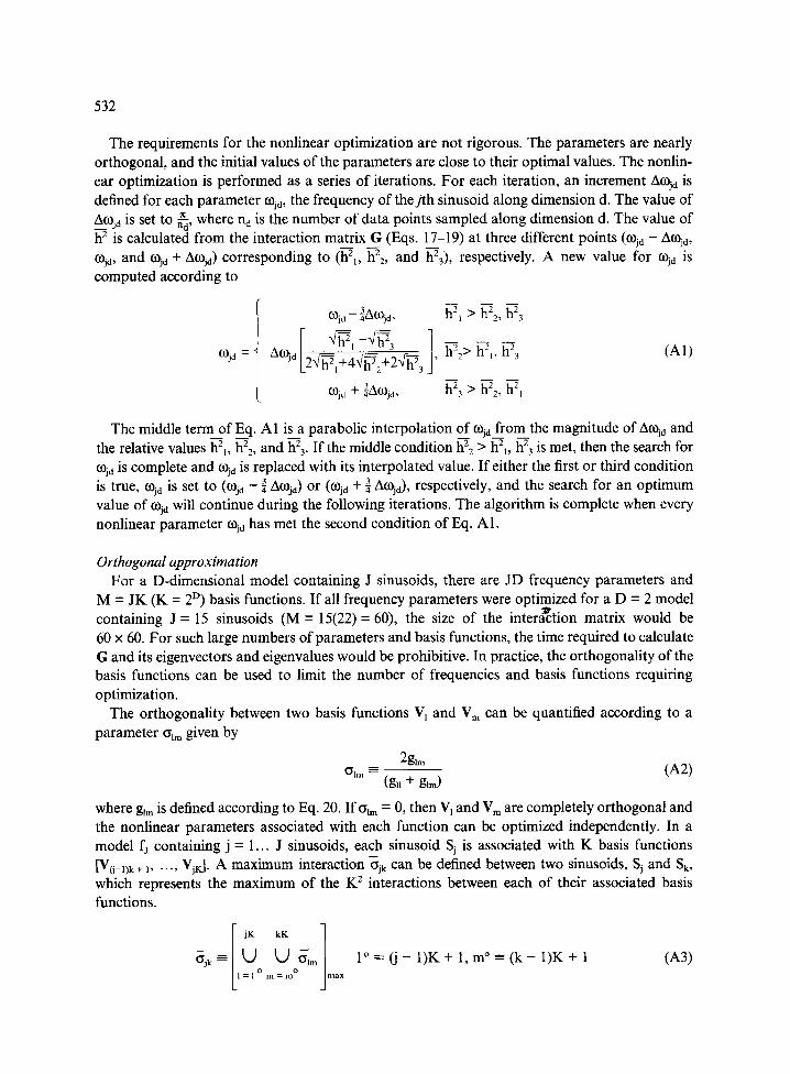
The requirements for the nonlinear optimization are not rigorous. The parameters are nearly orthogonal, and the initial values of the parameters are close to their optimal values. The nonlin- ear optimization is performed as a series of iterations. For each iteration, an increment AC0jd is defined for each parameter o~d, the frequency of thej th sinusoid along dimension d. The value of AO~jd is set to n-~, where nd is the number of data points sampled along dimension d. The value of h 2 is calculated from the interaction matrix G (Eqs. 17-19) at three different points (coj~ - Ao~jd, C0jd, and c0jd + At0jd) corresponding to (h2., h22, and h23), respectively. A new value for o)jd is computed according to

~jd =

%d--3~(Ojd' h21 > h22, h23

F ]. Amid ~2,~21+4@2+2,@7, 3 h22> h2,, h23

3 2 ~ ooja + ~Amjd, h 3 > h-2, h21

(A1)

The middle term of Eq. A1 is_a parabolic interpolation of coja from the magnitude of Atoja and the relative values h21, hZ2, and h23. If the middle condition h2~ > h21, h23 is met, then the search for coja is complete and cojd is replaced with its interpolated value. If either the first or third condition is true, 0~jd is set to (Ojd -- ] Aojd) or (C0jd + ] At%), respectively, and the search for an optimum value of o)ja will continue during the following iterations. The algorithm is complete when every nonlinear parameter C0jd has met the second condition of Eq. A1.

Orthogonal approximation For a D-dimensional model containing J sinusoids, there are JD frequency parameters and

M = JK (K = 2 D) basis functions. If all frequency parameters were optimized for a D = 2 model the mterachon matrix would be containing J = 15 sinusoids (M = 15(22) = 60), the size of " ~" ' "

60 x 60. For such large numbers of parameters and basis functions, the time required to calculate G and its eigenvectors and eigenvalues would be prohibitive. In practice, the orthogonality of the basis functions can be used to limit the number of frequencies and basis functions requiring optimization.

The orthogonality between two basis functions Vl and Vm can be quantified according to a parameter (3;lm given by

2glm (~Im = (gn + glm) (A2)

where glm is defined according to Eq. 20. I f o ~ = 0, then Vl and Vm are completely orthogonal and the nonlinear parameters associated with each function can be optimized independently. In a model fj containing j = 1... J sinusoids, each sinusoid Sj is associated with K basis functions [V(j-1)k + 1 . . . . . VjK ]. A maximum interaction ~jk can be defined between two sinusoids, Sj and Sk, which represents the maximum of the K z interactions between each of their associated basis

~k ------

jK kK J

U US m [= l~ ~ max

functions.

l~ - 1 )K+ 1, m ~ (k - 1 )K+ 1 (A3)

533

In the BAMBAM algorithm, two sinusoids Sj and Sk are considered to be orthogonal to one another if ~jk < 0.025.

This orthogonality property allows BAMBAM to reduce the number of nonlinear parameters requiring optimization. For a given model containing J sinusoids Sj = S I , S 2 . . . . Sj , all of the sinusoids that are orthogonal to a particular sinusoid, Sj, are eliminated from optimization of Sj. All of the nonlinear parameters associated with Sj are then simultaneously optimized on the nonorthogonal set of sinusoids. This is done for all J sinusoids until the middle condition of Eq. A 1 is met on the first iteration for all JD frequency parameters.