5. Transient and multidimensional conduction - EPFL
60
5. Transient and multidimensional conduction John Richard Thome 5 avril 2008 John Richard Thome (LTCM - SGM - EPFL) Heat transfer - Conduction 5 avril 2008 1 / 60
-
Upload
khangminh22 -
Category
Documents
-
view
2 -
download
0
Transcript of 5. Transient and multidimensional conduction - EPFL

5. Transient and multidimensional conduction
John Richard Thome
5 avril 2008
John Richard Thome (LTCM - SGM - EPFL) Heat transfer - Conduction 5 avril 2008 1 / 60

5.2 Lumped capacitance method - Dimensional analysisWe consider a clearly representative problem of one-dimensional transient heatconduction, without internal heat conduction and constant thermal conductivity
∂2T∂x2 =
1α
∂T∂t with
i.c. : T (t = 0) = Tib.c. : T (t > 0, x = 0) = Tl
b.c. : −k ∂T∂x
∣∣∣∣x=L
= h (T − Tl)x=L
The solution of this problem must take the form of the following dimensionalfunctional equation
T − Tl = fn[(Ti − Tl) , x , L, t, α, h, k
]Nondimensionalizing :
Θ ≡ T − TlTi − Tl
ξ ≡ xL
Fo ≡ αtL2
John Richard Thome (LTCM - SGM - EPFL) Heat transfer - Conduction 5 avril 2008 2 / 60

5.2 Lumped capacitance method - Dimensional analysiswhere Fo = Fourier number (dimensionless time). Then
∂2Θ
∂ξ2 =∂Θ
∂Fo
Θ(ξ, 0) = 1∂Θ
∂ξ
∣∣∣∣ξ=0
= Tl
∂Θ
∂ξ
∣∣∣∣ξ=1
= −BiΘ(1, Fo)
Finally, in dimensionless form
Θ = fn [ξ, Fo, Bi ]
Notice, that t/T can be viewed as
tT =
hk (V /A) tρc (V /A)2 k
= Bi · Fo (5.7)
John Richard Thome (LTCM - SGM - EPFL) Heat transfer - Conduction 5 avril 2008 3 / 60

5.2 Lumped capacitance method
We turn our attention to an analysis of unsteady heat transfer, beginning with amore detailed consideration of the lumped-capacity system.Basis of method : we assume that the solid is uniform in temperature and that its
mean temperature changes with time, i.e. negligible temperaturegradients.
SettingΘ ≡ T − T∞ =⇒ dΘ
dt =dTdt
The problem is that of predicting the transient cooling of a convectively cooledobject (cooling of a hot metal forging, for example). With reference to figure nextslide, we apply our familiar first law statement
Q =dUdt
−hA (T − T∞) = ρcV dTdt
John Richard Thome (LTCM - SGM - EPFL) Heat transfer - Conduction 5 avril 2008 4 / 60

5.2 Lumped capacitance method
The cooling of a body for which the Biot number is small :
John Richard Thome (LTCM - SGM - EPFL) Heat transfer - Conduction 5 avril 2008 5 / 60

5.2 Lumped capacitance method
Then, first law becomes−Θ =
ρcVhA
dΘ
dtSeparating variables and integrating from time = 0, where T (0) = Ti
ρcVhA
∫ Θ
Θi
dΘ
Θ= −
∫ t
0dt
where Θi = Ti − T∞. ThenρcVhA
ln ΘiΘ
= t
OrΘ
Θi=
T − T∞Ti − T∞
= exp[−
(hAρcV
)t]
John Richard Thome (LTCM - SGM - EPFL) Heat transfer - Conduction 5 avril 2008 6 / 60

5.2 Electrical analogy
The term capacitance is adapted from electrical circuit theory to the heattransfer problem. We can defined a thermal time constant
τt =
(1
hA
)(ρcV ) = RtCt
wherethermal resistance : Rt =
1hA
lumped thermal capacitance : Ct = ρcV
Electrical solution for E (t) is analogous to the thermal response. Total heattransfer up to time t is
Q = (ρcV ) Θi
[1− exp
(− t
τt
)]
John Richard Thome (LTCM - SGM - EPFL) Heat transfer - Conduction 5 avril 2008 7 / 60

5.2 Electrical analogy
A simple resistance-capacitance circuit (Fig 5.1) :
John Richard Thome (LTCM - SGM - EPFL) Heat transfer - Conduction 5 avril 2008 8 / 60
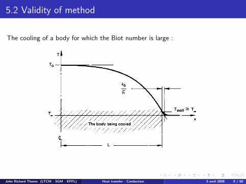
5.2 Validity of method
The cooling of a body for which the Biot number is large :
John Richard Thome (LTCM - SGM - EPFL) Heat transfer - Conduction 5 avril 2008 9 / 60

5.2 Validity of method
Normally, in a heat conduction problem the thermal capacitance is distributed inspace. But when the Biot number is small, T (t) is uniform in the body (almostconstant within the body at any time) and we can lump the capacitance into asingle circuit element. Thus
Bi ≡ hLk � 1 =⇒ Tb (x , t) ' T (t) ' Tsurface
and the thermal conductivity, k, becomes irrelevant to the cooling process. Utilizelumped capacitance method when
Bi ≡ hLk < 0.1
Where L = V /A, equal to :L for wall 2L thickr0/2 for long cylinder of radius r0
r0/3 for a sphere of radius r0
John Richard Thome (LTCM - SGM - EPFL) Heat transfer - Conduction 5 avril 2008 10 / 60

5.2 Transient cooling of a slabFigure 5.6 : Transient cooling in a one-dimensional slab.
John Richard Thome (LTCM - SGM - EPFL) Heat transfer - Conduction 5 avril 2008 11 / 60

5.6 Transient conduction - Semi-infinite solid
Constant surface temperature
The calculation of the temperature distribution in a semi-infinite region poses adifficulty in that we can impose a definite b.c. at only one position - the exposedboundary. We shall be able to get around that difficulty in a nice way with thehelp of dimensional analysis.
John Richard Thome (LTCM - SGM - EPFL) Heat transfer - Conduction 5 avril 2008 12 / 60

5.6 Transient conduction - Semi-infinite solid
The dimensional function equation is
T − T∞ = fn [t, x , α, (Ti − Tinfty )]
We have two dimensional groups
T − T∞Ti − T∞
= fn(
x√αt
)Θ = fn (ζ)
Thus, we transform each side of
∂2T∂x2 =
1α
∂T∂t
John Richard Thome (LTCM - SGM - EPFL) Heat transfer - Conduction 5 avril 2008 13 / 60

5.6 Transient conduction - Semi-infinite solid
as follows∂T∂t = ∆T ∂Θ
∂ζ
∂ζ
∂t = ∆T(− x
2t√
αt
)∂Θ
∂ζ;
∂T∂x = ∆T ∂Θ
∂ζ
∂ζ
∂x =∆T√
αt∂Θ
∂ζ;
∂2T∂x2 =
∆T√αt
∂2Θ
∂ζ2∂ζ
∂x =∆Tαt
∂2Θ
∂ζ2 .
We getd2Θ
dζ2 = −ζ
2dΘ
dζ
John Richard Thome (LTCM - SGM - EPFL) Heat transfer - Conduction 5 avril 2008 14 / 60

5.6 Transient conduction - Semi-infinite solid
If we call dΘ/dζ ≡ χ, then equation becomes the first-order equation
dχ
dζ= −ζ
2χ
which can be integrated twice to get
Θ = C∫ ζ
0e−ζ2/4dζ + Θ(0)
Thus the solution to the problem of conduction in a semi-infinite region, subjectto a b.c. of the first kind is
Θ =1√π
∫ ζ
0e−ζ2/4dζ =
2√π
∫ ζ/2
0e−s2
ds ≡ erf (ζ/2)
John Richard Thome (LTCM - SGM - EPFL) Heat transfer - Conduction 5 avril 2008 15 / 60

5.6 Transient conduction - Semi-infinite solid
Error function and complementary error function :
John Richard Thome (LTCM - SGM - EPFL) Heat transfer - Conduction 5 avril 2008 16 / 60

5.6 Transient conduction - Semi-infinite solid
Temperature distribution in a semi-infinite region (Fig 5.15) :
John Richard Thome (LTCM - SGM - EPFL) Heat transfer - Conduction 5 avril 2008 17 / 60

5.6 Transient conduction - Surface convection
If repeated the problem with a boundary condition of the third kind, we wouldexpect to get Θ = Θ(Bi , ζ), except that there is no length, L, upon which tobuild a Biot number. Therefore, we must replace L with
√αt, so
Θ = Θ
(ζ,
h√
αtk
)≡ Θ(ζ, β)
withβ ≡ Bi
√Fo
The solution of this problem is
Θ = erf(
ζ
2
)+ exp
(βζ + β2) [
erfc(
ζ
2 + β
)]
John Richard Thome (LTCM - SGM - EPFL) Heat transfer - Conduction 5 avril 2008 18 / 60

5.6 Transient conduction - Surface convection
Fig 5.16 : The cooling of a semi-infinite region by an environment at T∞, througha heat transfer coefficient, h. (Θ function of βζ).
John Richard Thome (LTCM - SGM - EPFL) Heat transfer - Conduction 5 avril 2008 19 / 60

5.6 Example 5.4
For what maximum time can a samurai sword be analyzed as a semi-infiniteregion after it is quenched, if it has no clay coating and hexternal = infinity ?
Temperature distribution in a semi-infinite region.
John Richard Thome (LTCM - SGM - EPFL) Heat transfer - Conduction 5 avril 2008 20 / 60

5.6 Example 5.4
Solution : First, we must guess the half-thickness of the sword (say, 3 mm) andits material (probably wrought iron with an average α around 1.5x10⁻⁵m2/s).The sword will be semi-infinite until δgg equals the half-thickness. We find
δ2gg
3.642α=
0.0032
13.3(1.5)(10−5)= 0.045s
Thus the quench would be felt at the centerline of the sword within only 1/20 s.The thermal diffusivity of clay is smaller than that of steel by a factor of about 30,so the quench time of the coated steel must continue for over 1 s before thetemperature of the steel is affected at all, if the clay and the sword thicknesses arecomparable.
John Richard Thome (LTCM - SGM - EPFL) Heat transfer - Conduction 5 avril 2008 21 / 60

5.7 Two-dimensional conduction
The two-dimensional flow of heat between two isothermal walls (Fig 5.20) :
John Richard Thome (LTCM - SGM - EPFL) Heat transfer - Conduction 5 avril 2008 22 / 60

5.7 Two-dimensional conduction
The general equation for T(−→r )
withsteady conduction.constant thermal conductivity.without internal heat generation.
Is called Laplace’s equation :∇2T = 0
It looks easier to solve than it is, since the Laplacian is a sum of several secondpartial derivatives. Faced with a steady multidimensional problem, four routes areopen to us
Find out whether or not the analytical solution is already available in a heatconduction text or in other published literature.Solve the problem analytically (chapter 4).Obtain the solution graphically.Solve the problem numerically.
John Richard Thome (LTCM - SGM - EPFL) Heat transfer - Conduction 5 avril 2008 23 / 60
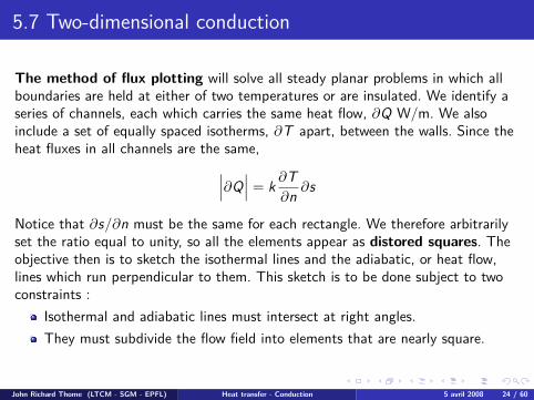
5.7 Two-dimensional conduction
The method of flux plotting will solve all steady planar problems in which allboundaries are held at either of two temperatures or are insulated. We identify aseries of channels, each which carries the same heat flow, ∂Q W/m. We alsoinclude a set of equally spaced isotherms, ∂T apart, between the walls. Since theheat fluxes in all channels are the same,∣∣∣∂Q
∣∣∣ = k ∂T∂n ∂s
Notice that ∂s/∂n must be the same for each rectangle. We therefore arbitrarilyset the ratio equal to unity, so all the elements appear as distored squares. Theobjective then is to sketch the isothermal lines and the adiabatic, or heat flow,lines which run perpendicular to them. This sketch is to be done subject to twoconstraints :
Isothermal and adiabatic lines must intersect at right angles.They must subdivide the flow field into elements that are nearly square.
John Richard Thome (LTCM - SGM - EPFL) Heat transfer - Conduction 5 avril 2008 24 / 60

5.7 Two-dimensional conduction
Steps in constructing a flux plotIdentify all lines of symmetry (from thermal and geometrical considerations)Note that lines of symmetry are adiabatic and no flux crosses themIdentify all isotherms at boundaries and then try to sketch in the isothermlines within the system (with all isotherms normal to the adiabatic lines)Heat flow lines are then drawn trying to create curvilinear squares (with heatflow lines and isotherms intersecting at right angles and trying to keep allsides of the square about the same lenght)If you goof, erase and go back to start !
John Richard Thome (LTCM - SGM - EPFL) Heat transfer - Conduction 5 avril 2008 25 / 60

5.7 Two-dimensional conduction
A first rough sketching :
John Richard Thome (LTCM - SGM - EPFL) Heat transfer - Conduction 5 avril 2008 26 / 60

5.7 Two-dimensional conduction
The evolution of the flux plot :
John Richard Thome (LTCM - SGM - EPFL) Heat transfer - Conduction 5 avril 2008 27 / 60

5.7 Two-dimensional conduction
A flux plot with no axis of symmetry to guide construction :
John Richard Thome (LTCM - SGM - EPFL) Heat transfer - Conduction 5 avril 2008 28 / 60
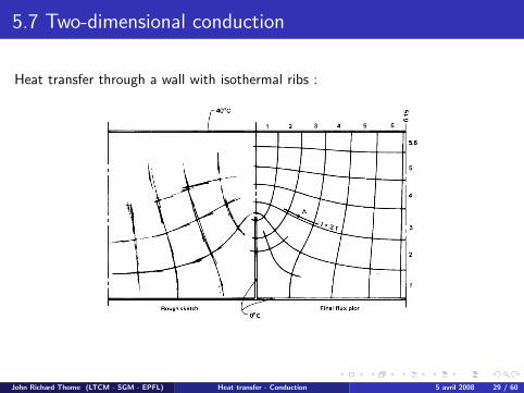
5.7 Two-dimensional conduction
Heat transfer through a wall with isothermal ribs :
John Richard Thome (LTCM - SGM - EPFL) Heat transfer - Conduction 5 avril 2008 29 / 60

5.7 Two-dimensional conduction
Once the grid has been sketched, the temperature anywhere in the field can beread directly from the sketch. And the heat flow per unit depth into the paper is
Q = Nk∂T ∂s∂n =
NI k∆T
where N is the number of heat flow channels and I is the number of temperatureincrements, ∆T/∂T .
John Richard Thome (LTCM - SGM - EPFL) Heat transfer - Conduction 5 avril 2008 30 / 60

5.7 Two-dimensional conduction
A heat conduction shape factor S may be defined for steady problems involvingtwo isothermal surfaces as follows
Q ≡ Sk∆T
where for a flux plotS =
NI
It follows that the thermal resistance of a two-dimensional body is
Rt =1
kS where Q =∆TRt
The virtue of the shape factor is that it summarizes a heat conduction solution ina given configuration. Once S is known, it can be used again and again.
John Richard Thome (LTCM - SGM - EPFL) Heat transfer - Conduction 5 avril 2008 31 / 60

5.7 Two-dimensional conduction
The shape factor for two similar bodies of different size (Fig 5.24) :
Some tables in the course include a number of analytically derived shape factorsfor use in calculating the heat flux in different configurations.
John Richard Thome (LTCM - SGM - EPFL) Heat transfer - Conduction 5 avril 2008 32 / 60

5.7 Two-dimensional conduction : example 5.9
Calculate the shape factor for a one-quarter section of a thick cylinder.
Solution : We already know Rt for a thick cylinder. From it we compute
Scyl =1
kRt =2π
ln(r0/ri)
so on the case of a quarter-cylinder,
S =π
2ln(r0/ri)
The quarter-cylinder is pictured in Fig. 5.24 for a radius ratio, ro/ri =3, but fortwo different sizes. In both cases S = 1.43. (Note that the same S is also given bythe flux plot shown.)
John Richard Thome (LTCM - SGM - EPFL) Heat transfer - Conduction 5 avril 2008 33 / 60

5.7 Two-dimensional conduction : example 5.10
Calculate S for a thick hollow sphere (picture 5.25)
The general solution of the heat diffusion equation in spherical coordinates forradial heat flow is
T =C1r + C2
John Richard Thome (LTCM - SGM - EPFL) Heat transfer - Conduction 5 avril 2008 34 / 60

5.7 Two-dimensional conduction : example 5.10
The boundary conditions are Ti and To and substituting the general solution weget
Ti =C1ri
+ C2 and T0 =C1r0
+ C2
ThereforeC1 =
Ti − T0r0 − ri
r0ri and C2 = Ti −Ti − T0r0 − ri
r0
In the general solution we get
T = Ti + ∆T[
ri r0r (r0 − ri)
− r0r0 − ri
]Then
Q = −kAdTdr =
4π (ri r0)
r0 − rik∆T
S =4π (ri r0)
r0 − ri[m]
John Richard Thome (LTCM - SGM - EPFL) Heat transfer - Conduction 5 avril 2008 35 / 60

5.7 Two-dimensional conduction : example 5.11
A spherical heat source of 6 cm in diameter is buried 30 cm below the surface of avery large box of soil and kept at 35C. The surface of the soil is kept at 21C. Ifthe steady heat transfer rate is 14 W, what is the thermal conductivity of thissample of soil ?
Solution :Q = Sk∆T =
(4πR
1− R/2h
)k∆T
where S is that for situation 7 in Table 5.4 (see book). Then
k =14
(35− 21)
1− (0.06/2)/2(0.3)
4π(0.06/2)= 2.545 W /mK
John Richard Thome (LTCM - SGM - EPFL) Heat transfer - Conduction 5 avril 2008 36 / 60

5.comp. Numerical method
Nodal Network :
John Richard Thome (LTCM - SGM - EPFL) Heat transfer - Conduction 5 avril 2008 37 / 60

5.comp. Numerical method
Another approximate solution is use of numerical techniques : finite-difference,finite-element, and boundary-element methods. We will present thefinite-difference method.
Each node represents a small zone with an average temperature of the zoneassigned as the node’s temperature. The nodes and mesh are set to the user’sconvenience, the finer the mesh the more accurate the calculation (but thisincreases the computation time).
John Richard Thome (LTCM - SGM - EPFL) Heat transfer - Conduction 5 avril 2008 38 / 60

5.comp. Numerical methodThe value of the second derivative, ∂2T/∂x2 is
∂2T∂x2
∣∣∣∣∣m,n
=
∂T/∂x∣∣∣m+1/2,n
− ∂T/∂x∣∣∣m−1/2,n
∆x
The temperature gradients in terms of nodal temperatures are
∂T∂x
∣∣∣∣∣m+1/2,n
=Tm+1,n − Tm,n
∆x
∂T∂x
∣∣∣∣∣m−1/2,n
=Tm,n − Tm−1,n
∆x
Substituting equations
∂2T∂x2
∣∣∣∣∣m,n
=Tm+1,n + Tm−1,n − 2Tm,n
(∆x)2
John Richard Thome (LTCM - SGM - EPFL) Heat transfer - Conduction 5 avril 2008 39 / 60
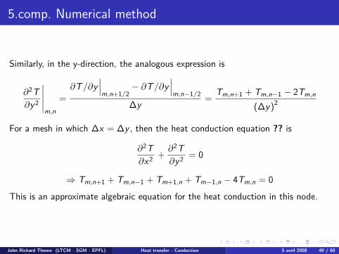
5.comp. Numerical method
Similarly, in the y-direction, the analogous expression is
∂2T∂y2
∣∣∣∣∣m,n
=
∂T/∂y∣∣∣m,n+1/2
− ∂T/∂y∣∣∣m,n−1/2
∆y =Tm,n+1 + Tm,n−1 − 2Tm,n
(∆y)2
For a mesh in which ∆x = ∆y , then the heat conduction equation ?? is
∂2T∂x2 +
∂2T∂y2 = 0
⇒ Tm,n+1 + Tm,n−1 + Tm+1,n + Tm−1,n − 4Tm,n = 0
This is an approximate algebraic equation for the heat conduction in this node.
John Richard Thome (LTCM - SGM - EPFL) Heat transfer - Conduction 5 avril 2008 40 / 60

5.comp. Numerical method
Energy balance approach - First approach
John Richard Thome (LTCM - SGM - EPFL) Heat transfer - Conduction 5 avril 2008 41 / 60

5.comp. Numerical methodThe modal equation from an energy balance : here assuming all heat flows intothe node, steady-state conditions and internal heat generation
Q(m−1,n) 7−→(m,n) = k (∆y · 1)Tm−1,n − Tm,n
∆x
Q(m+1,n) 7−→(m,n) = k (∆y · 1)Tm+1,n − Tm,n
∆x
Q(m,n+1) 7−→(m,n) = k (∆x · 1)Tm,n+1 − Tm,n
∆y
Q(m,n−1) 7−→(m,n) = k (∆x · 1)Tm,n−1 − Tm,n
∆yWith equilibrius equation
Ein + Eg = 0 ⇒4∑
i=1Q(i) 7−→(m,n) + Q (∆x∆y1) = 0
we obtain (∆x = ∆y)
Tm,n+1 + Tm,n−1 + Tm+1,n + Tm−1,n +Q (∆x)2
k − 4Tm,n = 0
John Richard Thome (LTCM - SGM - EPFL) Heat transfer - Conduction 5 avril 2008 42 / 60

5.comp. Numerical method
Energy balance approach - Second approach, with convection
John Richard Thome (LTCM - SGM - EPFL) Heat transfer - Conduction 5 avril 2008 43 / 60

5.comp. Numerical method
Q(m−1,n) 7−→(m,n) = k (∆y · 1)Tm−1,n − Tm,n
∆x
Q(m+1,n) 7−→(m,n) = k(
∆y2 · 1
)Tm+1,n − Tm,n
∆x
Q(m,n+1) 7−→(m,n) = k (∆x · 1)Tm,n+1 − Tm,n
∆y
Q(m,n−1) 7−→(m,n) = k(
∆x2 · 1
)Tm,n−1 − Tm,n
∆yAnd for convection
Q(∞) 7−→(m,n) = h(
∆x2 · 1
)(T∞ − Tm,n) + h
(∆y2 · 1
)(T∞ − Tm,n)
Then, for ∆x = ∆y , we obtain
Tm−1,n + Tm,n+1 +12 (Tm+1,n + Tm,n−1) +
h∆xk T∞ −
(3 +
h∆xk
)Tm,n = 0
John Richard Thome (LTCM - SGM - EPFL) Heat transfer - Conduction 5 avril 2008 44 / 60

5.comp. Numerical method ∆x = ∆y
Case 1 : Interior node
Tm,n+1 + Tm,n−1 + Tm+1,n + Tm−1,n − 4Tm,n = 0
John Richard Thome (LTCM - SGM - EPFL) Heat transfer - Conduction 5 avril 2008 45 / 60

5.comp. Numerical method ∆x = ∆y
Case 2 : Node at an internal corner with convection
2 (Tm−1,n + Tm,n+1) + (Tm+1,n + Tm,n−1) + 2h∆xk T∞ − 2
(3 +
h∆xk
)Tm,n = 0
John Richard Thome (LTCM - SGM - EPFL) Heat transfer - Conduction 5 avril 2008 46 / 60

5.comp. Numerical method ∆x = ∆y
Case 3 : Node at a plane surface with convection
(2Tm−1,n + Tm,n+1 + Tm,n−1) +2h∆x
k T∞ − 2(
h∆xk + 2
)Tm,n = 0
John Richard Thome (LTCM - SGM - EPFL) Heat transfer - Conduction 5 avril 2008 47 / 60

5.comp. Numerical method ∆x = ∆y
Case 4 : Node at an external corner with convection
(Tm,n−1 + Tm−1,n) + 2h∆xk T∞ − 2
(h∆x
k + 1)
Tm,n = 0
John Richard Thome (LTCM - SGM - EPFL) Heat transfer - Conduction 5 avril 2008 48 / 60

5.comp. Numerical method ∆x = ∆y
Case 5 : Node at a plane surface with uniform heat flux
(2Tm−1,n + Tm,n+1 + Tm,n−1) +2Q′′∆x
k − 4Tm,n = 0
John Richard Thome (LTCM - SGM - EPFL) Heat transfer - Conduction 5 avril 2008 49 / 60
5.comp. Numerical method
Depending upon your mathematical background and the specific problem, thenumerical solution can be found with
Matrix inversion.Gauss-Seidel iteration....
The reader who wishes to study such analyses in depth should refer to specificpublications.
John Richard Thome (LTCM - SGM - EPFL) Heat transfer - Conduction 5 avril 2008 50 / 60

5.comp.2 Finite-difference methods for transient heatconductionFor transient conditions with two-dimensional effects, constant properties and nointernal heat generation, the general expression
∂2T∂x2 +
∂2T∂y2 +
∂2T∂z2 +
Qk =
1α
∂T∂t
reduces to∂2T∂x2 +
∂2T∂y2 =
1α
∂T∂t
To obtain the finite-difference form, we can use the central-difference form of
∂2T∂x2
∣∣∣∣∣m,n
=Tm+1,n + Tm−1,n − 2Tm,n
(∆x)2
∂2T∂y2
∣∣∣∣∣m,n
=Tm,n+1 + Tm,n−1 − 2Tm,n
(∆y)2
John Richard Thome (LTCM - SGM - EPFL) Heat transfer - Conduction 5 avril 2008 51 / 60

5.comp.2 Finite-difference methods for transient heatconduction
We discretize in time using the integer p as : t = p∆t and obtain
∂T∂t
∣∣∣∣∣m,n
=T p+1
m,n + T pm,n
∆t
Hence, the time derivative is in terms of the difference in temperatures at time(p+1) new and (p) previous, separated by the time interval ∆t.
Explicit method : the temperatures are evaluated at (p)Implicit method : the temperatures are evaluated at (p+1)
John Richard Thome (LTCM - SGM - EPFL) Heat transfer - Conduction 5 avril 2008 52 / 60

5.comp.2 Finite-difference methods : Explicit
It’s a forward-difference method. Evaluate the terms on the right-hand side ofequations at p.
1α
T p+1m,n − T p
m,n∆t =
T pm+1,n + T p
m−1,n − 2T pm,n
(∆x)2 +T p
m,n+1 + T pm,n−1 − 2T p
m,n
(∆y)2
Solving for new nodal temperature at p+1 for ∆x = ∆y :
T p+1m,n = Fo
(T p
m+1,n + T pm−1,n + T p
m,n+1 + T pm,n−1
)+ (1− 4 Fo) T p
m,n
withFo =
α∆t(∆x)2
For a one-dimensional transient heat conduction, the expression becomes
T p+1m = Fo
(T p
m+1 + T pm−1
)+ (1− 2 Fo) T p
m
John Richard Thome (LTCM - SGM - EPFL) Heat transfer - Conduction 5 avril 2008 53 / 60

5.comp.2 Finite-difference methods : Explicit
Equations are explicit since the unknown nodal temperatures at time p+1 aredetermined with known temperatures at time p in each time step.
Initial condition must be known so that the temperature of each node is known attime t = 0 when p = 0. Then, the temperatures at t = ∆t for p = 1 arecalculable and the calculations proceed for t = 2∆t for p = 2 and so forth.
Accuracy is increased by decreasing the size of the time step ∆t and the size of∆x , at the expense of increasing calculation time.
John Richard Thome (LTCM - SGM - EPFL) Heat transfer - Conduction 5 avril 2008 54 / 60

5.comp.2 Finite-difference methods : Stability ofcalculation
Stability criterion for 1-D interior node : Fo ≤ 12
Stability criterion for 2-D interior node : Fo ≤ 14
John Richard Thome (LTCM - SGM - EPFL) Heat transfer - Conduction 5 avril 2008 55 / 60

5.comp.2 Finite-difference methods : Stability ofcalculationEquations may also be derived from an energy balance. For example, for a surfacenode with a convection boundary 1-D. Starting with
Ein + Eg = Est
We obtain
hA (T∞ − T p0 ) +
kA∆x
(T 0
1 − T p0)
= ρcA∆x2
T p+10 − T p
0∆t
And solving for the surface temperature at t + ∆t
T p+10 =
2h∆tρc∆x (T∞ − T p
0 ) +2α∆t(∆x)2 (T p
1 − T p0 ) + T p
0
since2h∆tρc∆x = 2h∆x
kα∆t
(∆x)2 = 2 Bi Fo
John Richard Thome (LTCM - SGM - EPFL) Heat transfer - Conduction 5 avril 2008 56 / 60

5.comp.2 Finite-difference methods : Stability ofcalculation
ThenT p+1
0 = 2Fo (T p1 + Bi T∞) + (1− 2Fo − 2Bi Fo) T p
0
The finite-difference form of the Biot number is
Bi =h∆x
k
For stability, we require that the coefficient for T p0 ≥ 0, so
1− 2 Fo − 2 Fo Bi ≥ 0
orFo (1 + Bi) ≤ 1
2Note : The stability limit for the most restrictive requirement must be used !
John Richard Thome (LTCM - SGM - EPFL) Heat transfer - Conduction 5 avril 2008 57 / 60

5.comp.2 Finite-difference methods : Implicit
Implicit method, obtained using
∂T∂t
∣∣∣∣∣m,n
=T p+1
m,n + T pm,n
∆t
to approximate the time derivative and evaluating all other temperatures at timep+1 rather than p. This gives a backward-difference method, which intwo-dimensional form is
1α
T p+1m,n − T p
m,n∆t =
T p+1m+1,n + T p+1
m−1,n − 2T p+1m,n
(∆x)2 +T p+1
m,n+1 + T p+1m,n−1 − 2T p+1
m,n
(∆y)2
or for ∆x = ∆y it becomes
T pm,n = (1− 4 Fo) T p+1
m,n − Fo(
T p+1m+1,n + T p+1
m−1,n + T p+1m,n+1 + T p+1
m,n−1
)
John Richard Thome (LTCM - SGM - EPFL) Heat transfer - Conduction 5 avril 2008 58 / 60

5.comp.2 Finite-difference methods : Implicit
Notice :
Thus, the new temperature at node m,n depends on the new unknowntemperatures at the other adjacent nodes. Consequently, a simultaneous solutionis required using Gauss-Seidel iteration or matrix inversion.
The implicit solution scheme is implicitly unconditionally stable. Hence, we canchoose time steps ∆t and node spacings ∆x and ∆y to our own advantage.
John Richard Thome (LTCM - SGM - EPFL) Heat transfer - Conduction 5 avril 2008 59 / 60

5.comp.2 Finite-difference methods : Energy balancemethod
Energy balance method :
Surface node :
(1 + 2Fo + 2Bi Fo) T p+10 − 2Fo T p+1
1 = 2Fo Bi T∞ + T p0
Interior node :
(1 + 2Fo) T p+1m − Fo
(T p+1
m−1 + T p+1m+1
)= T p
m
John Richard Thome (LTCM - SGM - EPFL) Heat transfer - Conduction 5 avril 2008 60 / 60