PAPER • OPEN ACCESS

Multidimensional photoemissionspectroscopy—the space-charge limitTo cite this article: B Schönhense et al 2018 New J. Phys. 20 033004

 

View the article online for updates and enhancements.

Recent citationsPushing the space-charge limit in electronmomentum microscopyKai Rossnagel

-

This content was downloaded from IP address 131.169.225.94 on 18/04/2018 at 16:35

New J. Phys. 20 (2018) 033004 https://doi.org/10.1088/1367-2630/aaa262

PAPER

Multidimensional photoemission spectroscopy—the space-chargelimit

BSchönhense1, KMedjanik2, O Fedchenko2, S Chernov2,MEllguth2, DVasilyev2, AOelsner3, J Viefhaus4,DKutnyakhov4,WWurth4,5, H J Elmers2 andGSchönhense2

1 Department of Bioengineering, Imperial College, London,United Kingdom2 Institut für Physik, JohannesGutenberg-UniversitätMainz, Germany3 Surface ConceptGmbH,Mainz, Germany4 DESYHamburg, Germany5 PhysicsDepartment andCFEL,Universität Hamburg, Germany

E-mail: b.schoenhense14@imperial.ac.uk

Keywords: space-charge effect, photoemission spectroscopy, time-resolved photoemission

Supplementarymaterial for this article is available online

AbstractPhotoelectron spectroscopy, especially at pulsed sources, is ultimately limited by theCoulombinteraction in the electron cloud, changing energy and angular distribution of the photoelectrons. Adetailed understanding of this phenomenon is crucial for future pump–probe photoemission studiesat (x-ray) free electron lasers and high-harmonic photon sources.Measurements have been performedfor Ir(111) at hν=1000 eVwith photon flux densities between∼102 and 104 photons per pulse andμm2 (beamline P04/PETRA III, DESYHamburg), revealing space-charge induced energy shifts of upto 10 eV. In order to correct the essential part of the energy shift and restore the electron distributionsclose to the Fermi energy, we developed a semi-analytical theory for the space-charge effect incathode-lens instruments (momentummicroscopes, photoemission electronmicroscopes). Thetheory predicts a Lorentzian profile of energy isosurfaces and allows us to quantify the charge cloudfrommeasured energy profiles. The correction is essential for the determination of the Fermi surface,as we demonstrate bymeans of ‘k-spacemovies’ for the prototypical high-Zmaterial tungsten. In anenergy interval of about 1 eV below the Fermi edge, the bandstructure can be restored up to substantialshifts of∼7 eV. Scattered photoelectrons strongly enhance the inelastic background in the regionseveral eV belowEF, proving that themajority of scattering events involves a slow electron. Thecorrection yields a gain of two orders ofmagnitude in usable intensity comparedwith the uncorrectedcase (assuming a tolerable shift of 250meV). The results are particularly important for futureexperiments at SASE-type free electron lasers, since the correction alsoworks for strongly fluctuating(but known) pulse intensities.

1. Introduction

Thefield of photoelectron spectroscopy andmicroscopy has seen decades of continuous improvement ofanalysers and excitation sources. The energy resolution has been driven to amazing limits ranging from sub-meV at low energies to the 10 meV region in the soft x-ray regime [1]. High angular resolution (down to<0.1°)or spectroscopy up to the hard x-ray range demand small footprints of the photon beamon the sample surface.The vastmajority of today’s high-performance photon sources are pulsed, with lengths down to the fs range forlasers, sources based on high-harmonic generation (HHG) or free-electron lasers (FELs). The high density ofelectrons released by intense, short photon pulses in a small area on the sample leads to significant Coulombinteraction, which alters the energy and angular distribution and sets the ultimate limit to the performance ofphotoemission experiments. Depending on the number of electrons in the cloud and their spatio-temporaldistribution, this effect can deteriorate the photoelectron spectra dramatically [1–11].

OPEN ACCESS

RECEIVED

9 September 2017

REVISED

29November 2017

ACCEPTED FOR PUBLICATION

18December 2017

PUBLISHED

5March 2018

Original content from thisworkmay be used underthe terms of the CreativeCommonsAttribution 3.0licence.

Any further distribution ofthis workmustmaintainattribution to theauthor(s) and the title ofthework, journal citationandDOI.

© 2018TheAuthor(s). Published by IOPPublishing Ltd on behalf ofDeutsche PhysikalischeGesellschaft

Although the conditions (pulse intensity, pulse length and repetition rate) are quite different for synchrotronradiation sources, FELs orHHG sources, the Coulomb forcesmanifest comparably. Footprints of the photonbeamwith sizes on the order of 10 μmdiameter are becoming standard atmodern high-brilliance beamlines;photon pulse lengths range from∼70 ps for storage ring sources down to<100 fs for FEL andHHG sources. Insuch a small initial confinement (in space and time) the high electron density gives rise to large Coulomb forcesand e–e scattering processes.When the cloud is expanding, the scattering rate drops but the integral long-rangeCoulomb forces persist up tomacroscopic distances. In the cases discussed below there is still significantinteraction up to 80 mm from the sample surface.

It has long been known that theCoulomb interaction of an individual electronwith all other electrons leadsto energy shifts and changes of electron trajectories, in electronmicroscopy termed the Boersch effect [12, 13].Fully considering themany-body system, an electron feels a Coulomb term from each other electron. Thenwecan approximate the cloud of electrons as a space-charge continuumwith somedensity, andwe take the‘average’ of that as the origin of the effective force. This ‘deterministic’ component has been considered inmuchdetail andwas even discussed as ameans for aberration correction [14]. In addition, individual e–e scatteringevents occur stochastically, causing irreversible changes in energy andmomentum (thermal broadening). Thesemake up the stochastic component of the Coulomb term.Note that the stochastic and deterministic terms aredecoupled. The deterministic contribution can be seen as an approximation based on a homogenised charge-density distribution (or a deterministic source of equidistantly spaced electrons). The stochastic component is aresult of inhomogeneities in the charge distribution and reflects the stochastic nature (granularity) of thephotoelectron beam. The usual strategy to copewith the space-charge problems is to reduce the charge perpulse.

In photoemission, themajor contribution to space-charge induced energy shifts stems from the largenumber of secondary electrons. Intense clouds of slow electrons can also occur in pump-and-probe experimentswhen the pump laser gives rise tomultiphoton photoemission [5–10]. The coexistence of a small number of fastphotoelectronswith a large number of slow electrons (from the secondary cascade or generated by a pump laser)leads to a specific behaviour due to the different longitudinal and transversalmomentum components of the twospecies. The slowly travelling charge cloud exerts an anisotropic force on the rapidly expanding photoelectrondistribution.

The space-charge effect becomes particularly severe in the x-ray range, see e.g. [3]. The cascade of inelasticscattering events of photoelectrons as a ‘multiplication effect’hasmaximumeffectiveness in soft x-rayphotoemission. At hν=1000 eV ourmeasurements for the Ir(111) surface reveal a total electron yield of∼0.1 e/photon. Assuming a photon flux of∼107 photons per pulse (a typical value for the experiments shownbelow), each photoelectron from the valence-band is accompanied by a cloud of secondary electrons of the orderof 0.1 1 pC.

We present a combined experimental, analytical and simulated study of the space-charge effect inmultidimensional photoemission (resolving all threemomentum coordinates and the energy in the presentexperiment) using cathode-lens type instruments. The electrostatic field between sample surface and anode andthe subsequent immersion lens optics cause a special signature of the space-charge effect. The cloud of slowelectrons travels close to the optical axis along the surface normal, whereas the fast photoelectrons form a rapidlyexpanding disc due to their larger transversalmomentum. Based on a hybrid approach of analytical treatmentand ray-tracing calculations, we propose amodel that predicts a Lorentzian shape of the energy isosurfaces, ingood agreement with experiment. Afit of the general functional expression to themeasured shape of theisosurfaces disentangles the isotropic acceleration in the homogeneous electrostatic field and the anisotropicacceleration in the lens field. Exploiting the different signature of the space-charge effect in these two regimes,thefit yields the value for the total charge of the low-energy electrons. An algorithm is presented that can correctthe deterministic part of the Coulomb interaction. The correction yields intactmomentumdistributions atspace-charge induced energy shifts up to∼7 eV, corresponding to an intensity gain of 2 orders ofmagnitude incomparison to similarmeasurements without correction. The stochastic contribution from individualscattering events appears as an increased diffuse background intensity in the spectral region some eV below theFermi edge. The region close to the Fermi energy is least affected by this blur since the electrons ‘surviving’ at thisenergy did not suffer inelastic scattering events. The correction is crucial for the determination of Fermi surfacesaswe demonstrate by the example of the prototypical high-Zmaterial tungsten. ‘k-spacemovies’ reveal thatuncorrected distributions lead tomissing features in the Fermi surface.

More generally, the present study yielded a better understanding of space-charge effects in strong electricfields. Since the correction is based on an analytical expression, it can be applied even in cases of strong (butquantitatively known)fluctuations of the pulse intensities. Such conditions are found at SASE-type free electronlasers where the intensity of each individual photon pulse can bemonitored and used for the correction of thecorresponding individual electron events. It can be expected that the correction algorithmdescribed in thispaperwill bemost important for future photoemission experiments at FELs using themomentummicroscopy

2

New J. Phys. 20 (2018) 033004 B Schönhense et al

technique. Since the delay between ‘pump’ (intense fs laser pulse) and ‘probe’ (FEL orHHGpulse) can bemodelled using the same algorithm, extended (complete) correction schemes for ultrafast time-resolvedphotoemission experiments are possible.

2. Experimental results

2.1.Multidimensional photoemission spectroscopyThe discovery of exciting electronic systems such as topological insulators, topological semimetals,Weyl systemsor novel superconductingmaterials has posed a challenge for angular-resolved photoemission experiments. Thefocus has shifted to complex questions regarding topologies in k-space, the number of Fermi-level crossings ofbands, or the spin texture, which is afingerprint for time-reversal invariance. The quantities which contain thecomplete information on the electronic structure are the spectral density function ρ (EB, k) and the correspondingspin-polarisation vectorP (EB, k). Themeasured quantity I (EB, k) is the discretized experimental representationof ρ, weighted by the transitionmatrix element. In the general case of a bulk sample, the 4Ddata array I containsthe information on all band dispersions, partial and total band gaps, the Fermi surface and all other energyisosurfaces, and the effectivemass.P describes the spin texturewhich often (e.g. formost topological surfacestates) is composed of three independent vector components. Hence, for a bulk electronic systemwith spintexture the full information is contained in a scalar and a vector function in 4Dparameter space: [I,P] (EB, k).

The experimental approach of recording these quantities can be termedmultidimensional photoemissionspectroscopy. Four classes of instruments have been developed in order to tackle this problem:Hemisphericalanalysers can detect a certain angular range along one direction (up to+/−15°with good angular resolution)and an energy interval (up to several eV) in parallel. The perpendicular angular direction can be accessed eithervia sample rotation or using a deflector arrangement and sequential recording [15, 16]. The angular coordinateshave to be converted intomomentum coordinates. These analysers have reached a high degree ofmaturity withenergy resolution down to<1 meV and angular resolution<0.1°. The identical lens systems have recently beencombinedwith time-of-flight (ToF) energy recording, constituting a new family of angular-resolving ToFspectrometers [17, 18]. Themost recent approaches employ a cathode lens to visualise directly the ‘k-image’, i.e.the pattern of the transversalmomentum components. The required energy resolution can be implementedeither in terms of a dispersive analyser [19] or via ToF recording [20]. The dispersive-analyser approach isindependent of the time structure of the photon sourcewhich, for continuous sources, bears the advantage oftheminimum space-charge effect. The ToF-approach requires pulsed photon sources such as lasers, HHGsources, storage rings or FELs; its advantage is parallel energy recording. Simultaneous detection of a (kx, ky)momentum range exceeding the first Brillouin zone and an energy range ofEkin comprising the d-band complexof a transitionmetal yieldsmaximumdegree of parallelisation.Hence the ToF-method is ideal for developing acorrection algorithmof the space-charge effect and has thus been used for the present experiments.

Combinedwith an imaging spin filter, the ToF-approach allows us tomeasure data arrays of one spincomponentP (EB, kx, ky); in the future even all three components [21]. Existing imaging spin filters are not yetfully optimised; howeverfirst results look very promising [22, 23]. Due to the rather narrow spin-asymmetryprofiles, the results of the present study have essential consequences for spin-filtered k-imaging in the presenceof significant space-charge shifts.

2.2. Space-charge effect in k-microscopy using soft x-raysMomentummicroscopes are based on a special type of cathode lens (objective lenswith a strong immersion fieldin front of the sample), being optimised for full-field imaging of a largemomentum range (kx, ky) at high k-resolution [19, 20]. The photoelectron distribution is detected directly in k-space by imaging of the Fourier planewhich represents a cross section through the k-sphere with radius defined by thefinal-state energy. Herewe usedToF parallel energy recording, but all considerations and evaluations apply equally to k-microscopes withdispersive energy analysers, and also to photoemission electronmicroscopes (PEEMs).

We have investigated the space-charge induced effects at hν=1000 eV using the high-brilliance photonbeamof beamline P04 at PETRA III (DESY,Hamburg). In a k-spacemicroscope the k-image is formed in thebackfocal plane of the cathode lens (for details, see e.g. [19]). A subsequent lens systemprojects this image of thetransversalmomentum components onto the time-resolving image detector (delay-line detector [24, 25]), withvariablemagnification. The kinetic energy Ekin is recorded in an interval of several eVwidth via the ToF. Thisnovel technique is capable of recording the 4D spectral density function ρ (EB, k) in the entire Brillouin zone andd-band complexwithin a fewhours (for details, see [20]).

In order to study the signature of the increasing Coulomb interaction, we varied the photon flux by graduallyopening the exit slit of themonochromator. Slit widths of 10, 100, 300, 1000 and 1500 μmyielded values of

3

New J. Phys. 20 (2018) 033004 B Schönhense et al

∼1012 to 1014 photons per second at 5 MHz pulse rate [26] in a photon footprint of about 35 μmon the samplesurface. In the following these settings are referred to as I0, 10 I0, 30 I0, 100 I0 and 150 I0, respectively.

Themomentumdependence of the space-charge interaction has been visualised in a large radial range byadjusting thefield of view off-centre, reaching amaximum radius of almost 4 Å−1. Figure 1 shows sectionsthrough asmeasured data arrays I (Ekin, kx, ky) for an Ir(111) sample. The constant-energy sections (first row)were taken for the intensity level of 100 I0. Given the photon energy of 1000 eV and awork function of∼5 eV themaximumkinetic energy (at the Fermi level) is expected at∼995 eV. Instead, we observe the onset of the electrondistributions at kinetic energies of 1002 eV for an intensity of 100 I0 (figure 1(a)) and 1005 eV for 150 I0 (e, f). Itmeans that the respective space-charge induced energy gains for 100 I0 and 150 I0 are 7 eV and 10 eV,respectively.

The kinetic energy sequence in the top rowoffigure 1 reveals how the distribution starts on the optical axis,here at the bottom corner of image (a) and then graduallymoves upwards (b–d). In (d) the cutoff has reached thetop corner. For theEkin-vs-k|| sectionsmeasured at 150 I0 (e, f) the space-charge induced shift reaches itsmaximumof 10 eVon the axis and drops to half of this value at 3.5 Å−1, see (e). The cut along the radialdirection, here Ekin-vs-ky, reveals the profile shown in panel (e), which can be readily fitted by a Lorentzian curve(see theory section). TheEkin-vs-kx cut (f) intersects the Lorentzian profile in a transversal direction. The correctposition of the Fermi edge for vanishing space-charge interaction is denoted by the dash-dotted line in (e, f). Thisposition is determined by reducing the photon flux to I0 as discussed in the next section (cf. figure 2(a)). Despitethe strong energy shift and distorted Ekin-vs-k|| cuts, the section close toEF (panel d) is surprisingly wellpreserved, even in these raw data. The deformation of the energy isosurfaces is caused by the net Coulomb forceexerted on the photoelectrons by the large amount of slow electrons travelling close to the optical axis in theacceleration field above the sample surface and in the lensfield of the cathode lens.

2.3. Correction of the space-charge effectFigure 2 shows a systematic study of the changes of the spectral distribution functions forfive different values ofthe photonflux, revealing details of the signature of Coulomb interaction in the beam.Columns 1–5 display theresults for intensities I0 to 150 I0, corresponding to photonflux densities between∼102 and∼104 photons perpulse andμm2. Thefirst row shows the energy shift and deformation of the Fermi cutoff. Starting from thelowestflux I0 (10 μmexit slit) the intensity was increased by a factor of 10, 30, 100 and 150. The correspondingspace-charge induced shifts of the kinetic energy reachmaxima of 0.8, 2.8, 7.4 and 10 eV, respectively. For (e) thetotal electron count rate in the delay-line detector, corresponding to the topmost 20 eV of the photoelectronspectrum and the given k-region, was∼5×106 cps.

The functional formof the Lorentzian (given in equation (5) in section 3.3)was fitted to the shape of theFermi-level cutoff taken from the as-measured (tF, kx, ky) raw data stacks; tF is the ToF corresponding to this

Figure 1. Space-charge induced deformation of the spectral distribution I (Ekin, kx, ky) for the Ir(111)-surface at hv=1000 eV. Inorder to probe a large k||-range, the image has been adjusted to the Fermi-surface cut in thefirst repeated Brillouin zone along ky. (a)–(d) show electron distributions at four kinetic energies as given in the panels, taken at a photon intensity of 100 I0. (e), (f)Ekin-vs-ky and-kx sections for a photon intensity of 150 I0, revealing a space-charge induced acceleration of up to 10 eV at k||=0. The dashed curvein (e) denotes thefit, the dash-dotted line denotes the position of the Fermi energy in case of absence of space-charge interaction.

4

New J. Phys. 20 (2018) 033004 B Schönhense et al

cutoff. For strongly structuredmomentumpatterns at the Fermi energy, an array of points used forinterpolation has proven superior to a fully automatised procedure because it better accounts for low-intensityregions. Next, the data stack is corrected according to the parameter set obtained by thefit. The correctedsections are shown in the second rowoffigure 2. The deformation has disappeared, the Fermi cutoff is straightand coincides for all distributions (dash-dotted lines in (f–j)).

The contribution of the stochastic e–e scattering events is clearly visible in terms of the increasing diffusebackground intensity that sets in at 30 I0 and becomes very significant at higher intensities. In the sequence (f, g,h, i, j) the brightness in the lower part of the panels increases dramatically and finallymasks the band features.We see, however, that the background intensity is smaller near the Fermi cutoff. This gives a hint on the nature ofthe individual e–e scattering processes. These processes aremost likely to occur close to the sample surface,where the electron density is high and the velocity-dependent separation of the electrons did not yet set in.Photoelectrons from the valence range preferably scatter at low-energy cascade electrons because of their largenumber.When scatteringwith a slow electron, the fast electron loses energy andmomentum. The electrons thatescape from the cloudwith initial energies close to the Fermi cutoff did not suffer from such scattering eventsand hence largely retained their initial distribution.

Despite the space-charge induced energy shift, the band features are quite well conservedwithin an intervalof approx. 1 eV from EF. The 30 I0 pattern shows almost no deterioration in the region close toEF. Section (m)appears even slightly better focused than (k) and (l); most likely the space-charge shift of 3 eV at 30 I0compensates a slight defocusing at I0 and 10 I0. At 100 I0 an additional blur of the bands is evident (i, n) andfinally at 150 I0 this blur, togetherwith the diffuse background,masks the band features (j, o). In panels (n, o) theband pattern shows a significant reduction in size. Upon scatteringwith a slow electron, the fast photoelectronalso losesmomentum. In this regime of very high scattering probability longitudinalmomentummight also belost, resulting in a (stochastic) contribution to the total energy shift, counteracting the deterministic shift.

Part of the blur infigure 2(h)–(j) originates from the increasing photon bandwidth of 35, 170 and 500 meVfor I0, 10 I0 and³30 I0, respectively. Above 30 I0 thefield-of-view acts like a virtual exit slit.We conclude thattwo orders ofmagnitude in usable intensity is gained by the correction, if the interest is focused on the bandsclose toEF.

Figure 2. Sequence of distributions for Ir(111) taken at identical settings but different photon intensities (I0 to 150 I0) between∼105(column1) and∼107 (column5) photons per pulse. EB-vs-kx cuts through the as-measured data (a-e) are comparedwithcorresponding cuts after space-charge correction (f)–(j). In the corrected sections the deterministic part of the Coulomb interaction iseliminated by fitting a generic functional expression to the Fermi-level cutoffs in the stacks corresponding to (a)–(e) and re-normalising the energy scale.What remains is the stochastic contribution, visible in the enhanced diffuse background of inelastically-scattered electrons (increasing in sequence (f)–(j)). At the Fermi cutoff the band contours resulting from a section through the 3DFermi surface persist up to intensity 100 I0 (k)–(n). At 150 I0 (o) they are still visible but appear strongly blurred.

5

New J. Phys. 20 (2018) 033004 B Schönhense et al

3. Theoreticalmodel

3.1. Ray-tracing simulations for cathode lensesPrior to the development of the analyticalmodel, we performed simple ray-tracing simulations [27] (withoutspace-charge and for the short-pulse limit) forfive initial kinetic energies: 1 eV representing the secondarycascade electrons (which in reality extend over several eV), 16 eV being a typical photoelectron kinetic energy intheVUV (e.g. for table-topHHG sources), 120 eV is typical for EUV excitation at Synchrotron-radiationsources, 1 keV represents a soft x-ray energy and 3.5 keV corresponds to the tender (or lower end of the hard)x-ray regime. The simulation assumed a source spot on the sample surface of 35 μm, identical to ourexperimental conditions.

Figure 3 shows the spatio-temporal behaviour of the 1 eV electrons (black rays) together with the fourspecies of faster electrons. Panels (a–c) show the results for 16 eV, 120 eV and 1 keV in the first 30 mm from thesample surface. These data were simulated for the standard lens geometry with 4 mmgap, used in theexperiments. The result for 3.5 keV (panel d) corresponds to a larger region of about 60 mm, simulated for a newhigh-energy lens with 10 mmgap, developed for soft, tender and hard x-ray excitation. This lens accepts anorder ofmagnitude larger k-space area than the standard lens.

The ray patterns can be separated into three regimeswith different signatures of theCoulomb interaction. Inthe initial stage close to the surface (stochastic regimeA) all electrons are confined in the region-of-interest (ROI),which here is 35 μmdiameter. Fast and slow electrons are not yet separated, the electron density is high, andindividual e–e scattering events happen. The origin of the stochastic events lie in the fact that the electron beamitself originates from a stochastic process; theCoulomb interaction between all electrons is of course fullydeterministic. Since the slow electrons outnumber the fast ones by several orders ofmagnitude, the latterexperience predominantly inelastic scattering events with loss of energy andmomentum.Hence, scatteredelectrons show up as diffuse background in the region several eV belowEF. In this early stage, there is only a small netacceleration due to compensation of Coulomb forces in all directions. An inhomogeneous footprint of thephoton beam can induce a net radial force in this initial phase. This can be important in pump-and-probeexperiments if the two beams are not exactly concentric or if the pumpbeam causes inhomogeneous emissionpatterns. Then the early phase can be characterised by strong inhomogeneous forces acting in various directions,depending on the emission pattern.

The experimental data in section 2 do not show effects of a radial force on themomentumpatterns, soweconclude that the influence of the photon beamprofile is negligible under our experimental conditions. Instead,themomentumpatterns appear broadened at very high photon intensities, revealing that in regionA elasticscattering events between two fast electrons can also occur. In the vicinity of the surface, the image chargeinduced in ametallic sample surface causes an attractive force towards the surface [28]. In non-metallic systems,long-lived photoholes in thematerial cause a similar effect [29].

In the acceleration field between sample surface and anode (radially uniform force regime B) the electroncloud of a given energy expands isotropically in an accelerated inertial system (acceleration a=−eε/m; forelectric field strength ε). The electrons stay on hemispherical shells that expand linearly with their initialvelocities; the snapshots at 50, 100 and 150 ps infigure 3(a), (b) capture this situation. For 1 eV, 16 eV and 120 eVthe distributions represent the full half space above the sample. For 1 and 3.5 keV the objective lens cannot imagethe full half space, sowe restricted the simulated angular range to+/−18° (corresponding tomomentumdiscswith diameters of 10 and 18 Å−1). Due to their largermomenta, the shells of the photoelectrons expandmorerapidly than the cloud of the slow secondary electrons. The initial photoelectronmomenta are 2, 5.5, 16 and30 Å−1 forEkin=16, 120, 1000 and 3500 eV, respectively. In comparison, themomentumof the 1 eV electronsis only 0.5 Å−1. This leads to an isotropic separation between photoelectrons and slow electrons of 0.2, 0.6, 1.8and 3.4 mmafter 100 ps (cf. panels a, b, c and d). In regimeB, the Coulomb repulsion by the slowly expandingcloud of secondary electrons leads to a uniform radial acceleration of the fast photoelectrons, regardless of theirdirection. For slow laser-induced electrons the situation is different because the different instants of emission ofslow and fast electrons lead to a shift in the centres of the expanding shells.

The saddle point of the potential in the anode boremarks the beginning of the non-uniform force regimeC,where the decelerating forces cause a deformation of the electron shells. The anode bore (in particle opticstermed aperture lens [13]) has the unusual property of being diverging, as visible in the ray paths. It forms avirtual source spot in front of the sample at a distance of 1/3 of the gap distance [30]. In the strongly deceleratingfield behind the aperture lens the electron shells attain an increasingly flattened (oblate) shape as visiblemostpronounced in theVUV-case (a) above 400 ps and in the tender x-ray case (d) at 300 ps, where the distributionsare close to planar discs. Now the cloud of slow electrons exerts a non-uniform force on the photoelectron discswith itsmaximumat the optical axis where the distance isminimal. Due to the non-isotropic Coulombrepulsion, the energy distribution of the photoelectrons at the Fermi energy approximately attains a Lorentzianshape (see section 3.2). In all cases, the isotropic shift extends from threshold to∼150 ps, whereas the anisotropic

6

New J. Phys. 20 (2018) 033004 B Schönhense et al

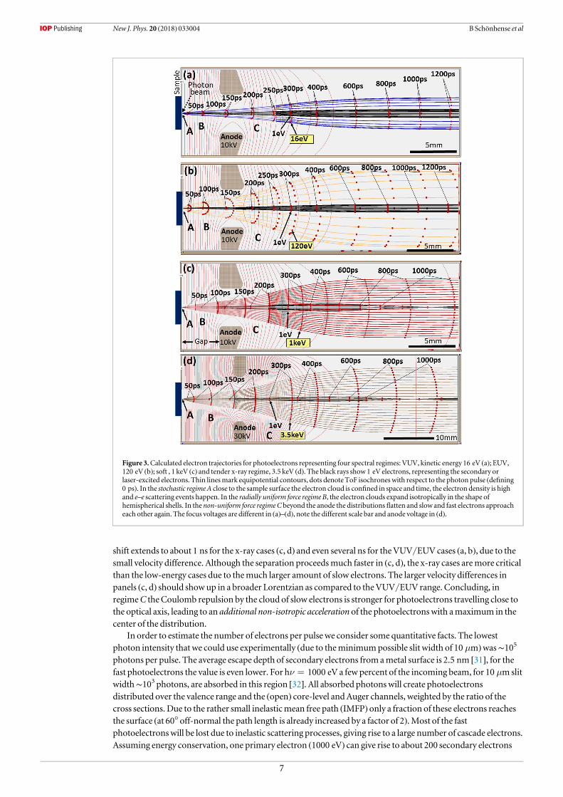
shift extends to about 1 ns for the x-ray cases (c, d) and even several ns for theVUV/EUV cases (a, b), due to thesmall velocity difference. Although the separation proceedsmuch faster in (c, d), the x-ray cases aremore criticalthan the low-energy cases due to themuch larger amount of slow electrons. The larger velocity differences inpanels (c, d) should showup in a broader Lorentzian as compared to theVUV/EUV range. Concluding, inregimeC the Coulomb repulsion by the cloud of slow electrons is stronger for photoelectrons travelling close tothe optical axis, leading to an additional non-isotropic acceleration of the photoelectronswith amaximum in thecenter of the distribution.

In order to estimate the number of electrons per pulse we consider some quantitative facts. The lowestphoton intensity that we could use experimentally (due to theminimumpossible slit width of 10 μm)was∼105

photons per pulse. The average escape depth of secondary electrons fromametal surface is 2.5 nm [31], for thefast photoelectrons the value is even lower. For hν=1000 eV a few percent of the incoming beam, for 10 μmslitwidth∼103 photons, are absorbed in this region [32]. All absorbed photonswill create photoelectronsdistributed over the valence range and the (open) core-level andAuger channels, weighted by the ratio of thecross sections. Due to the rather small inelasticmean free path (IMFP) only a fraction of these electrons reachesthe surface (at 60° off-normal the path length is already increased by a factor of 2).Most of the fastphotoelectronswill be lost due to inelastic scattering processes, giving rise to a large number of cascade electrons.Assuming energy conservation, one primary electron (1000 eV) can give rise to about 200 secondary electrons

Figure 3.Calculated electron trajectories for photoelectrons representing four spectral regimes: VUV, kinetic energy 16 eV (a); EUV,120 eV (b); soft , 1 keV (c) and tender x-ray regime, 3.5 keV (d). The black rays show 1 eV electrons, representing the secondary orlaser-excited electrons. Thin linesmark equipotential contours, dots denote ToF isochrones with respect to the photon pulse (defining0 ps). In the stochastic regimeA close to the sample surface the electron cloud is confined in space and time, the electron density is highand e–e scattering events happen. In the radially uniform force regime B, the electron clouds expand isotropically in the shape ofhemispherical shells. In the non-uniform force regimeC beyond the anode the distributionsflatten and slow and fast electrons approacheach other again. The focus voltages are different in (a)–(d), note the different scale bar and anode voltage in (d).

7

New J. Phys. 20 (2018) 033004 B Schönhense et al

with energies equally distributed in the interval between EF and 10 eV aboveEF (corresponding to∼5 eV kineticenergy in vacuum). Due to the energy-dependence of the hot-electron lifetime the cascade has its intensitymaximum right above the Fermi energy. However, only the high-energy fraction above thework functionthreshold can escape from the surface. The potential barrier of the surface not only acts as high-passfilter, butalso induces a strong restriction inmomentum space. Slow electrons leaving the surface experience strongrefraction due to the inner potentialV0∼15 eV for Ir. The 1 eV electrons filling the full half space on thevacuum side correspond to an ‘escape cone’ of only+/−14° inside of the crystal. Hence, only electronstravelling close to the surface normal within a solid-angle fraction of 1.6%of 4π can escape from the surface.

At very low photon intensities, the stochastic nature of the emission process becomes relevant. There is nevermore than 1 escaping fast valence photoelectron per photon pulse and the probability that it is accompanied by alow-energy charge cloud tends to zero for very low intensities. In this limit the space-charge interaction vanishes.With increasing photon intensitymore andmore photoelectrons are created in a single pulse andmost of themare scattered, causing themultiplication effect. From comparisonwith our simulation, we calculate samplecurrents of∼1 μA at the highest photon intensity of∼107 photons per pulse, corresponding to∼106 electronsper pulse at 5 MHz. Regarding the given photon flux (see experimental section), we estimate a total yield(photoelectrons and secondaries) of∼0.1.

Concluding these considerations, we point out that the expansion of the electron distributions with differentenergies shows a counter-intuitive behaviour. The distance between themdoes not continuously increase (asonemight expect due to their initial relative velocities) but is a non-monotonous function of time. In thedecelerating region, the faster electrons have been retardedmore strongly at a given instant and hence thedistance between populations shrinks in regionC (figure 3(a)–(d)).Wewill discuss this phenomenon further inthe framework of the theoreticalmodel and see that the shape of themeasured energy isosurfaces allowsdisentangling the isotropic and non-isotropic shifts and quantifying the amount of charge per pulse.

In pump-and-probe experiments the delay between pumppulse (creating low-energy electrons) and probepulse (defining time zero for the photoelectrons)must be taken into account. For delays in the range of a few psor less (as used for the study of ultrafast processes), the delay does not showup in the plots infigure 3.We expectthat the space-charge shift does not change as long as the emission pattern of the laser-induced slow electrons ishomogeneous and the total number of low-energy electrons does not change. For larger delays (>100 ps)Plötzing et al [8] have observed substantial changes in energy positions of the photoelectrons. This can beunderstood by shifting the timemarkers on the black trajectories infigure 3 to earlier times (i.e. to the right-handside), leading to a deceleration of the photoelectrons. Since the electron cloud emitted by the pumppulseappears earlier, all photoelectrons have to cross the cloud and the e–e scattering probabilitymight thus besignificantly enhanced.

So far, all considerations are valid formetallic samples where excess charges are efficiently screened, yieldinga constant, well-defined surface potential. The situation is different for semiconductors due to the surfacephotovoltage [33]. Optically-induced electron-hole pairs lead to a diffusion of carriers into the surface depletionzone. The transient change of carrier concentration reduces the band bending at the surface and generates anelectric fieldwhen the pumppulse arrives, persisting until the carriers recombine (mostly radiatively). Yang et al[34] have observed that the outgoing photoelectrons are influenced by this short electric field pulse. Althoughthe decay constant of the photovoltage is only 1.5 ps in the case of GaAs, the outgoing photoelectron experiencesthe transient field pulse formacroscopic delay times up to several 100 pswhere the force exerted by thephotovoltage pulse is still significant. The time scale depends on the photoelectron velocity. Note that this effectoriginates in a different surface potential, not in vacuum space-charge. In our experiment it would thus lead to arigid displacement of thewhole spectral distribution. Photovoltage-induced energy shifts are expected for avariety of semiconductors, topological insulators, or layeredmaterials with reduced interlayer conductivity.

Figure 3 reveals one obvious advantage of the cathode-lens geometry for long pulses. By the time the lateelectrons of a 50 ps pulse (typical for synchrotron radiation sources) are emitted, the early ones have alreadytravelled 1.5 mmaway from the sample, thanks to the strong acceleration field. This strongly diminishes theelectron density in the stochastic regime.With decreasing pulse length, however, this advantage is reduced.

3.2. Semi-analytical theoryIn our analytical approach, we consider the slow secondary electrons to be a point charge, while the fast primaryelectrons form a shell. This approximation is particularly good for high energy photoelectrons, cf. figure 3.Wecan consider fast electrons to start at the same point, with velocities v v v v vsin , cos , ,r z0 0 0q q= =( ) ( ) where θismeasured from the optical axis z, andwe only consider one radial direction r. In the rest frame of slowelectrons, which is at constant accelerationwhile in the uniform accelerating field, the shell of primary electronsexpands isotropically.

8

New J. Phys. 20 (2018) 033004 B Schönhense et al

For electric field strength ε, acceleration along z is given by v t e md dz e= - which is independent ofv t 0 .z =( ) As seen in regimeB offigure 3, the spatial profile of the primary electrons remains spherical, see 100 psdistributions. As thefirst (on-axis) primary electrons exit the accelerating field, the rest of the spherical shell isstill being accelerating along z. Upon exit of the accelerating field (at the centre of the anode bore infigure 3), therelative velocity in the axial direction between electrons at different starting angles is smaller than that in theradial direction. Equating the energy before and after acceleration under the assumption of a uniform fieldwith asharp cut-off at z=L, we canwrite

E m v v m v m v L1

2cos

1

2sin

1

2. 1zkin 0

202 2

02 q q= + D + = +( ) ( )

Because of the concavity of the square-root function, this term is smaller for large cos θ, and hence small θ, that isfor starting angles close to the axis. Electronswith larger initial axial velocity are accelerated less, so the velocityprofile in regionC, after passing through the acceleration field is flattened along the axial direction. This leads tothe spatial profiles infigure 3, 200–400 ps distributions. For L mv ,0

2 thefinal axial velocity of the primaryelectrons is effectively uniform.

Once the spatial profile hasflattened as in regimeC, the effective situation is approximately that of a pointchargeQ of secondary electrons (black rays close to the axis infigure 3) repelling primary electrons in a radialdisk. A sketch of thismodel is shown infigure 4(a), with the dashed circle denoting the disc of photoelectrons.

The axial force component is

F FQe

r z

z

r z r zcos

4

1 1 1

1 tan. 2z Coulomb

02 2 2 2 2 2 3 2 2 3

2f

p f= =

+ +µ

+µ

+( ) ( ) ( )( )

/

To recover the real-space profile at the end of the trajectory, wewould integrate twice

z rF

mt td d 3

T tz

0 0ò òD = ¢

⎛⎝⎜

⎞⎠⎟( ) ( )

for total ToFT. If, for a given electron, f is independent of time, we can take all radial dependence out of theintegral to get an integral of the form

z r g z t t t1

1 tand d , 4

T t

2 3 2 0 0ò òf

D =+

¢ ¢ ⎛

⎝⎜⎞⎠⎟( )

( )( ( )) ( )

/

where g is not easily integrable, but crucially has no radial dependence.As the observed relative shift in z between on- and off-axis electrons is small relative to the distance between

primary and secondary electrons, wewould expect this Lorentzian profile to be reflected in velocity, energy(square-root), and hencefinal position andToF profiles. Themeasured energy gainΔE (dots) on the axis as a

Figure 4. (a)Origin of the Lorentzian-shaped space-charge acceleration of the fast primary electrons (dashedmomentumdisc) by theslow secondary electronsmodelled as a point chargeQ; z is referred to the centre of gravity of the slow electron cloud. (b)Measuredenergy gainΔEon the z-axis as function of photon intensity (dots) in comparisonwith the extrapolated initial slope (dashed line). (c)Calculated on-axis Coulomb force (on a log scale,−18 denotes attoN) and (d) space-charge induced energy gain for a 1 keVphotoelectron andQ=1.3×106 e; hereZ is referred to the sample surface. The four colours correspond to different anodepotentials and two cathode-lens geometries (HEdenotes the high-energy lenswith 10 mmgap between sample and anode); details ofthe calculation see text.

9

New J. Phys. 20 (2018) 033004 B Schönhense et al

function of photon intensity is shown infigure 4(b).With increasing intensity, the slope of the curve is reducedin comparisonwith its initial slope (dashed line). The increasing amount of charge in front of the surfacemay actas a high-pass filter for slow electrons. The extrapolation shown infigure 4(b) reveals that even the distributionmeasured at the lowest photon intensity I0 (10 μmexit slit) already shows a small space-charge acceleration of250 meV. Itmeans that at this comparatively low photon flux of 105 photons per pulse we are not yet in theregimewhere the photoelectron is not accompanied by secondary electrons (see discussion in section 3.1). Thepersistence of a space-charge induced shift in cathode-lens type instruments down to such lowphotonintensities underlines the importance of the correction shownbelow.

In fact, the inner shell of secondary electrons does also expand, strongly dependent on the focusingconditions of the lens, comparefigure 3(a)–(d). Furthermore, we have neglected the acceleration in the radialdirection, which varies throughout the disk. Significant radial forces would change themomentumdistribution;however, this is not observed in the experiment. The double integral along the full trajectory is intractable, butthe term in equation (4) is the dominant one in the deterministic part of the space-charge effect, and the profileof the shift seen in real data (figures 1, 2) is well-described by a Lorentzian. This assumption is validated by thequality offit of a generic Lorentzian to the observed shift pattern (cf. figure 1(e)).

At realistic experimental conditions, the number of primary electrons is small and theCoulomb interactionwithin the shell of primary electrons can be neglected. In the experiments shown below, nomore than oneprimary electron is recorded per photon pulse. This conditionmay change in future experiments at FEL sourceswhere the number of photon pulses per second ismuch smaller (e.g. 27 000 for the EuropeanXFEL compared totypically 106 at storage rings) and the average photon intensity is similar. In pump-and-probe experiments theslow laser-induced electronsmay alter the behaviour because the different instants of emission of slow and fastelectrons lead to a shift in the centres of the expanding shells. The profile of the deterministic componentwouldlikely still be approximately Lorentzian, while the stochastic componentmay be increased for equal chargedensities.

Forces on electrons travelling along the optical axis (shown logarithmically as a function of position infigure 4(c)) have been computedwith distances extracted fromSIMIONusing equation (2) and numericallyintegrated by adaptive quadrature [35] to give the energy gainΔE of the on-axis fast electrons due to therepulsion by the secondary charge cloud (figure 4(d)).

Since the integral over theCoulomb force would diverge for z→0, we have to introduce an effective cut-offz0 which accounts for an average initial distance of the interacting electrons. The value of z0 can be determinedexperimentally. By fitting a Lorentzian profile to the observed isosurface at the Fermi energy (see figures in theexperimental section), we can decompose the observed on-axis shifts into the isotropic part (asymptotic limit,offset of the Lorentzian) and non-isotropic part (amplitude of the Lorentzian). The effective z-cutoff and chargeQ are derived from thefit by assuming a sharp transition between regimes B andC at the anode bore, requiringthat the isotropic and Lorentzian componentsmatch those observed. For themaximumphoton intensitystudied, we calculate a charge ofQ=1.3×106 e and a cutoff of z0=2 mm. In calculating on-axis shifts fordifferent geometries and anode potentials, we have assumed a constant effective early cutoff, which is to bevalidated in future experiments. It roughly corresponds to the initial spread of the electron distribution due tothe pulsewidth of∼70 ps.

As a point of comparison, Long et al estimate the space-charge induced energy spread for a systemwithnegligible pulsewidth (equationA1 in [6]). Plugging in our source-spot radius andmaximal observed space-charge shift, we get an estimated secondary charge of approximately 105 e.Qualitatively, then, the calculatedsecondary charge fromour simulation is reasonable, as the non-negligible pulse duration results in a largeraverage initial separation and thus a smaller effect.

The four curves infigure 4(c), (d)have been calculated for a cathode lenswith 4 mmgap between sample andanode for two anode potentials (labelled 4 kV and 10 kV) and for a high-energy cathode lens with 10 mmgapand higher anode potentials (labelled 10 kVHE and 30 kVHE). Forces and resulting energy gain dependstrongly on anode potential and lens geometry. For 10 kV anode voltage the energy shift is smaller by a factor of 2for the larger lens (compare 10 kV and 10 kVHE). For both lens geometries, the shift increases with increasinganode voltage (cf. 4 kV and 10 kV aswell as 10 kVHE and 30 kVHE). In the region of decelerating lensfield(regionC infigure 3) the fast and slow electrons approach each other again. Theminimumdistance decreaseswith increasing anode voltage andwith decreasing geometric size of the lens.Minimisation of the space-chargeshift thus demands a larger lens geometry and smaller anode voltages. However, the latter is connectedwith asacrifice in k-resolution [19].

Concluding this section, wemention that the effect of re-approaching of fast and slow electronswasoverlooked in the earlier work [11]. The Lorentzian is clearly visible in the space-charge simulation using theGPT code (cf. figure 6 of [11]). In view of the long-range Coulomb forces evident infigure 4(c), (d), it seemsfavourable to cut off the secondary electrons, exploiting the high-pass filter action of the high-energy objectivelens by suitable lens settings as depicted infigure 5(a) of [11].

10

New J. Phys. 20 (2018) 033004 B Schönhense et al

3.3. Correction algorithmRather than trying to predict the space-charge induced energy shifts quantitatively, we take a hybrid approach,wherebywe assume the following generic functional formof the space-charge effect, which is then fitted to theobserved data

t x y ta b

b x x y y, 5F F

03

20

20

2 3 2= -

+ - + -( )

( ( ) ( ) )( )

/

t x yQ

b x x y y, . 6F 2

02

02 3 2

D µ+ - + -

( )( ( ) ( ) )

( )/

Here, x, y refers to the spatial coordinates along the screen, while successive slices are labelled by their ToF t. Agiven profile in axial position z in themoments before impact translates directly to the same temporal profile inthe recorded time-slices.

The shape of the space-charge effect is clearly visible at the Fermi energy (figure 1(e)), so the quantity t x y,F( )we are investigating is the ToF corresponding to the Fermi edge, which varies across the screen. The freeparameters are the centre of the Lorentzian x y, ;0 0( ) the base Fermi ToF t ,F

0 which corresponds to the ToF forelectronswith uniform space-charge interaction; themagnitude of the effect a, which gives themaximaldifference in ToF between starting angles 0 andπ; and the parameter b, which controls the radial width of theLorentzian. As themodel exhibits radial symmetry, we consider a circular profile withwidth b, rather than amore generic elliptical profile.

For a given pixel on the detector (spatially-resolving delay-line detector), the ToF corresponding to theFermi edge is determined by a threshold betweenwhen the count is zero (within noise) and non-zero. This issampled for a range of x y,( ) positions, and the five parameters x y t a b, , , ,0 0 F

0( ) arefit to the samples bymeansof the Levenberg–Marquardt algorithm [36] for unconstrained optimisation.Having obtained these parametersfrom the fit, the complete t x y,( ) data stack is corrected by adjustment of the ToF values using the Lorentzianfunctional as ‘zero’ reference, yielding a planar Fermi surface tF

0 and hence a planar Fermimomentumdisc(EB=0, kx, ky).

Time-slices correspond to layers of voxels with a specific ToF, while the above procedure generates acontinuously valued function, sowe linearly interpolate between voxels, which preserves the total count.

Since the force is proportional to themacrochargeQ (see equation (2)),Q appears as scaling factor in front ofthe integrals in equations (3) and (4) and also in the functional form equation (6). This scalingwithQ opens thepossibility of correcting even distributions with strongly fluctuating pulse-to-pulse intensities, a prominentexample being SASE-type FELs. In the data streaming architecture each photon pulse ismonitored concerningtime and individual pulse energy. Assuming thatQ is approximately proportional to the intensity of a givenphoton pulse, each counting event can be corrected according to equation (6) by its individual correction factor,depending onQ. The gross effect of space-charge shifts for strongly fluctuating intensities can thus beeliminated.

Having access to the full spectral distribution functions I (EB, k) in amomentum range exceeding thefirstBrillouin zone and several eV range of binding energy, we can apply further data treatment and corrections. Thefollowing routines have been implemented into an automated processing pipeline (see appendix): Time-to-energy conversion, correction of chromatic aberration, tilt of the optical axis and image-field curvature, as wellas elimination of (periodic) detector artefacts by Fourier-filtering in logarithmic space. In practice,most orsometimes even all of these contributions are negligible. The significance of the different terms depends on theexperimental conditions and the settings of the electron optics. Space-charge shifts are corrected routinely, evenif they are in the 100 meV range. Uncorrected data stacks would lead tomissing parts of the Fermi surface, evenfor such small shifts.

3.4. First practical result of space-charge correction algorithm in Fermi-surface imagingFigure 5 shows how the space-charge correction acts on a 4Ddata stack as needed formapping of the Fermisurface and Fermi velocity, here for the prototypical high-ZmaterialW(110). The top row shows the as-measuredmomentumdistributions at the Fermi energy for three different photon energies, corresponding tothree different values of kz asmarked in (g). Direct transitions into a free-electron likefinal state band, with thephoton energy determining themomentumperpendicular to the sample surface allow tomeasure size, shapeand topology of the 3DFermi surface. Technically, data arrays taken at sufficientlymany photon energies areconcatenated, in a tomographic-likemanner (for details, see [20, 37]). Panels (d–f) show the Fermi-energy cutsof the same data arrays after space-charge correction. The centres of the images look practically identical,howeverwith increasing distance from the centre, band features change size or becomemore intense (cf. arrowsin (d, e)) or additional features appear (arrows in (f)). In the experimental Fermi surface, these subtle differences

11

New J. Phys. 20 (2018) 033004 B Schönhense et al

lead to the disappearance of some of the ellipsoid-shaped hole pockets (arrows in (g and h)). This ismost clearlyseen in the ‘k-spacemovies’ in the supplementarymaterial.

The results for tungsten shownhere and in the supplementarymaterial have been takenwith standardsettings as used in [20, 37], with rather small space-charge shifts of<1 eV.Nevertheless, the subtle differencesbetween uncorrected (a–c) and corrected Fermi-energy cuts (d–f) showup strikingly in terms ofmissing parts inthe experimental Fermi surface.

Given the present state of knowledge it is not possible to directly compare these results with previous workusing dispersive spectrometers [1–9]. In a cathode lens we have the special behaviour of trajectories of fast andslow electrons as sketched infigure 3, whereas in conventional spectroscopy the electrons travel for typically60 mm in thefield-free region in front of the sample. Electronswith kinetic energies of 1000, 120 and 16 eVpassthis distance in 3, 9 and 24 ns, respectively; a time scalemuch longer than that offigure 3. The simplemodel of aspherical electron cloud in the field of a point-symmetric capacitor [6] predicts the samemagnitude of space-charge shift and broadening as a truemulti-particle simulation [7]. In the latter theoretical paper andexperimental data using aHHG source [8] shift and broadening have approximately the same value. In recent

Figure 5.Energy isosurfaces for photoemission fromW(110) before (a)–(c) and after space-charge correction (d)–(f), taken at thephoton energies stated on the top. Thewhite lines in (a)mark the surface Brillouin zone; N , H and S denote high-symmetry points.Before correction the outer regions of the k-patterns areweak or evenmissing (see arrows in (d)–(f)). In the Fermi surface derivedfrom corrected (g) and uncorrected sections (h) themissing features lead to deformations ormissing outer hole pockets (see arrows).

12

New J. Phys. 20 (2018) 033004 B Schönhense et al

work at the FEL source SACLA, SPring-8, Japan [5, 29] themeasured broadeningwas found to be larger than themeasured shift (by up to one order ofmagnitude) aswell as larger than the simulated shift. Fromfigure 1(e)weconclude that in our rawdata thewidth of the Fermi cutoff is at least one order ofmagnitude smaller than theenergy shift on-axis (at sufficient angular resolution). After correction, the energy width is two orders ofmagnitude smaller than the initial energy shift (figure 2(f)–(i)). A quantitative estimation of the space-chargelimit for dispersive spectrometers in comparisonwith that of cathode-lens instruments would requirecomparativemeasurements at similar conditions; this was not intended in the present work. In particular, thepositive sample bias for rapid redirecting of the secondaries asmentioned in [7] and our high-pass cutoff in theobjective lens have both not been explored yet.

4. Conclusion

The spatio-temporal confinement of the electrons released by intense, short photon pulses in a small area on asolid sample leads to significant Coulomb interaction, which alters the energy and angular distribution and setsthe ultimate limit to the performance of photoemission experiments. In the present workwe have explored thespace-charge effect bymeans of experiments in the soft x-ray range, revealing large space-charge induced energyshifts of up to 10 eV at the conditions of the high-brilliance soft x-ray beamline P04 at the storage ring PETRA IIIatDESY,Hamburg. Inworking towards a solution of this problemwe developed a semi-analytical theory,supported by ray-tracing simulations. In particular we studied the case ofmomentummicroscopy, providingcomplete I (Ekin, k) data sets that reveal the space-charge induced shifts in a singlemeasurement for an energyrange comprising the d-band complex of a transitionmetal and amomentum range exceeding the Brillouinzone. The aimof the investigationwas to test a newway of space-charge correction and elucidate the limit ofexperimental conditions that still yield usable photoemission data.

Starting from the analyticalmodel, a correction algorithmwas developed that eliminates the deterministicpart of theCoulomb interaction. This contribution results from the net force exerted on a given photoelectronby all other electrons. Calculations and experiments reveal that the deterministic contribution arises in the formof a Lorentzian-shaped deformation of the photoelectron energy isosurfaces. Themain effect is an accelerationof the photoelectrons due toCoulomb repulsion of the large amount of slow secondary electrons. Thisacceleration is anisotropic because the secondary electron cloud travels slower and expands less than thephotoelectron cloud. The correction is based on the experimentally-measured deformation of the electrondistributions at the Fermi-level cutoff. A generic functional formof the space-charge induced energy shift isfitted to the observed Fermi isosurface. This fit yields the required parameters for the subsequent correction ofthe complete data array. In addition, the fit gives the value of the charge of slow electrons that cause themain partof the energy shift.What remains after the correction is the contribution of individual e–e scattering processesreflecting the stochastic nature of the photoelectron beam. The stochastic contributions cause an irreversibleblur of the band features and a strongly enhanced inelastic background. This non-deterministicmechanism,sometimes referred to as ‘stochastic heating’ of the beam [38], defines the ultimate limit of the tolerable intensityof pulsed photoemission experiments.

In the characteristics of the interactionwe can distinguish three regimes: initially, the electron density is veryhigh and the interaction is dominated by stochastic scattering processes. The photoelectrons of a given energythen expand as a hemispherical shell, and hence separate from the cloud of slow secondary electrons. In thisphase the net Coulomb force is radially uniform. In the decelerating lens field beyond the anode, thephotoelectron shellflattens, and hence the force becomes non-uniform. Itsmaximumoccurs in the centre of thephotoelectron distribution, thus causing the Lorentzian deformation. The net action of this non-uniform forcedepends crucially on the lens geometry and the voltage of the anode. For larger lens geometries and smalleranode potentials the shifts are substantially reduced. This non-uniform force regime has been overlooked inearlier work [11], although the Lorentzianwas clearly visible in the space-charge simulation using theGPT code(cf. figure 6 of [11]).

The experimental results confirm the predictions of the theoreticalmodel for the deterministiccontribution. Themeasured distributions further reveal important details of the stochastic contribution: In anenergy interval of about 1 eVbelow the Fermi edge the bandstructure persists up to high intensities (figure 2(h),(i)). This proves that themajority of photoelectron scattering events involves a slow electron so that thephotoelectron loses energy. The inelastically-scattered electrons appear as strongly enhanced diffusebackground in the region several eV below EF. Hence the electrons observed close to the Fermi cutoff did notsuffer from loss scattering, whichmeans that high space-charge shifts can be tolerated especially for Fermi-surface imaging or bandmapping close toEF. At high intensities a visible size reduction of the bandstructurepatterns appears, giving evidence of a loss of (transversal)momentumof the photoelectrons. Such ‘fast e—slowe’ scattering events can only occur before the energetic separation, i.e. very close to the sample surface (stochastic

13

New J. Phys. 20 (2018) 033004 B Schönhense et al

regimeA infigure 3). High-pass filtering in a special geometry of the objective lens allows to remove the slowelectrons in the lensfield.

Due to the rather narrow spin-asymmetry profiles, the results of the present study have essentialconsequences for spin-filtered k-imaging in the presence of significant space-charge shifts. The space-chargeinduced energy shiftsmust be accounted for in the setting of the spin filter in order to retain the optimal workingpoint of the spin filter.

The theoretical and experimental results of the present work provide valuable design criteria for thedevelopment of next-generation k-spacemicroscopes withminimised sensitivity toCoulomb interaction in thebeam. An inherent problemof SASE-type free electron lasers is their strongly fluctuating pulse-to-pulseintensity. In the data-recording routine each individual counting event is labelledwith the time and intensityparameters of the corresponding photon pulse. Given the information on pulse intensity, the analyticalexpression for the correctionwill allow removal of themain part of the energy shift even in such cases of strong(but known) intensityfluctuations. First pump-and-probe experiments with fs sources leave no doubt that thespace-charge problem is the central obstacle of future photoemissionwork at pulsed high-brilliance photonsources. The present study raises some hope that we are not defenceless to these effects.

Acknowledgements

We thank the staff of PETRA (beamline P04) for excellent support during themeasurements. Sincere thanks gotoChristian Tusche, Forschungszentrum Jülich, for fruitful cooperation and discussions and toKai Rossnagel,Universität Kiel for a critical reading and constructive comments. The project was funded by BMBF(05K13UM2, 05K13GU3, 05K16UM1) andDFG (Transregio SFB/TRR173 ‘Spin+X’).

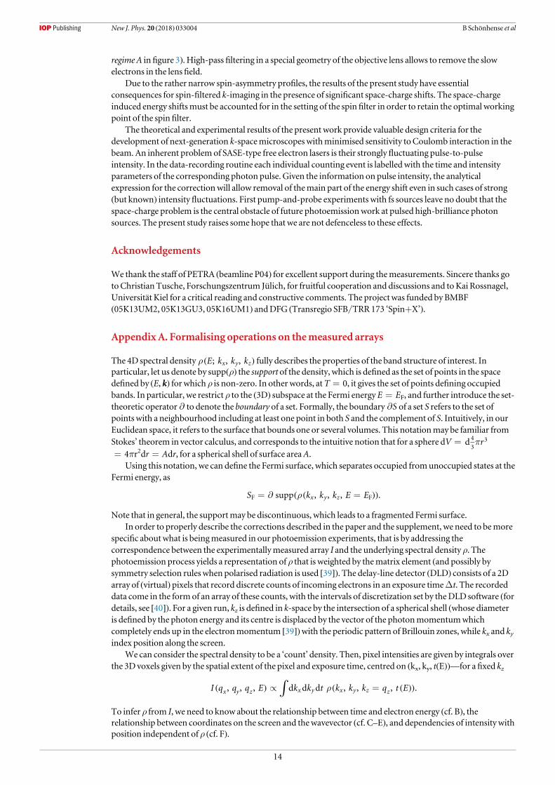
AppendixA. Formalising operations on themeasured arrays

The 4D spectral density E k k k; , ,x y zr ( ) fully describes the properties of the band structure of interest. Inparticular, let us denote by supp(ρ) the support of the density, which is defined as the set of points in the spacedefined by (E, k) for which ρ is non-zero. In other words, atT=0, it gives the set of points defining occupiedbands. In particular, we restrict ρ to the (3D) subspace at the Fermi energyE=EF, and further introduce the set-theoretic operator ¶ to denote the boundary of a set. Formally, the boundary S¶ of a set S refers to the set ofpoints with a neighbourhood including at least one point in both S and the complement of S. Intuitively, in ourEuclidean space, it refers to the surface that bounds one or several volumes. This notationmay be familiar fromStokes’ theorem in vector calculus, and corresponds to the intuitive notion that for a sphere dV= rd 4

33p

=4πr2dr=Adr, for a spherical shell of surface areaA.Using this notation, we can define the Fermi surface, which separates occupied fromunoccupied states at the

Fermi energy, as

S k k k E Esupp , , , .x y zF Fr= ¶ =( ( ))

Note that in general, the supportmay be discontinuous, which leads to a fragmented Fermi surface.In order to properly describe the corrections described in the paper and the supplement, we need to bemore

specific aboutwhat is beingmeasured in our photoemission experiments, that is by addressing thecorrespondence between the experimentallymeasured array I and the underlying spectral density ρ. Thephotoemission process yields a representation of ρ that is weighted by thematrix element (and possibly bysymmetry selection rules when polarised radiation is used [39]). The delay-line detector (DLD) consists of a 2Darray of (virtual) pixels that record discrete counts of incoming electrons in an exposure timeΔt. The recordeddata come in the formof an array of these counts, with the intervals of discretization set by theDLD software (fordetails, see [40]). For a given run, kz is defined in k-space by the intersection of a spherical shell (whose diameteris defined by the photon energy and its centre is displaced by the vector of the photonmomentumwhichcompletely ends up in the electronmomentum [39])with the periodic pattern of Brillouin zones, while kx and kyindex position along the screen.

We can consider the spectral density to be a ‘count’ density. Then, pixel intensities are given by integrals overthe 3D voxels given by the spatial extent of the pixel and exposure time, centred on (kx, ky, t(E))—for afixed kz

I q q q E k k t k k k q t E, , , d d d , , , .x y z x y x y z zò rµ =( ) ( ( ))

To infer ρ from I, we need to know about the relationship between time and electron energy (cf. B), therelationship between coordinates on the screen and thewavevector (cf. C–E), and dependencies of intensity withposition independent of ρ (cf. F).

14

New J. Phys. 20 (2018) 033004 B Schönhense et al

Affinemappings between coordinate systems are given by (affine) transformationmatrices, givingtransformations q q ¢ of the form q qM ,¢ = where to allow translations, we use projective coordinates (qx, qy,1). To apply these transformations to images, we take themidpoint of a pixel in the new coordinate system, applythe inverse transformM−1 to identify the corresponding location in the old coordinate system, and calculate thenewpixel value by (bilinear) interpolation between the four closest corresponding old pixels.

Appendix B. Time to energy conversion

Individual images acquired by the delay-line detector are equally spaced in time.However, to obtain theelectronic band structure to investigate physical properties, the quantity wewish tomeasure is kE; ,r ( ) whichrequires converting from the time scale to energy. For a constant velocity, wewould have

v E tv E

and1 1

.µ µ µ

In practice these relations are only approximate because the velocity varies along the ray path. To obtain thefunctional relationship for the present system, we usefinite element simulation [27] yielding specific (t, E) pairsfor a range of values spanning those observed experimentally, and use them to approximate themapping bypolynomial interpolation.

This approximation is non-linear, so at higher energies, the constant difference in energies corresponds to asmaller ToF difference than at lower energies. To account for this, we calculate the effective time differencebetween slices, as a ratio of the original time spacing, and scale all intensities by this ratio. By doing this,intensities correspond to counts in a specific energywindowoffixedwidth.

AppendixC. Chromatic aberration ofmagnification

As a result of chromatic aberration, slices at different energies can be subject to varying degrees ofmagnification[13]. Tofind the energy dependence of thismagnification, we computedmagnification values at 10 energies inthe observed range by finite element simulation [27] and, linearising in the observed range, determine the linearfunctional relationship between energy andmagnification by ordinary least squares. After converting from thetime scale to energy, we correct the aberration by calculating the affine transformationmatrix corresponding tothe rescaling by a factor of s=s(E) [41]

Ms 0 00 s 00 0 1

.scale =⎛⎝⎜⎜

⎞⎠⎟⎟

To recover the physical relevant quantity of counts per voxel, we rescale intensities tomaintain the total numberof counts per slice. A square of initial area 1 has area s2 after transformation, sowe rescale intensities by this valueto retain the total count.

AppendixD. Field curvature

As in every electronmicroscope the electron opticsmay also introduce barrel and pincushion distortions as aresult of image-field curvature [13]. To correct these, we approximate the distortion by a shear transformation,which is valid for small imaged regions. The shear angleα is determined by requiring the appropriate reflectionsymmetries, and the following affine transformation is applied to all images in a stack

M1 a 00 1 00 0 1

,shear =⎛⎝⎜⎜

⎞⎠⎟⎟

where a cot .a= Since the transformation is affine and does not involve a scale factor, total intensities arepreserved.

More generally, radial distortion can bemodelled by the transformation

r r k r1 2* +( )

for distortion parameter k. To apply this to images, we transform to radial coordinates centred on the symmetrypoint of the distortion, and calculate intensities by interpolation, scaling intensities by a factor of ,

kr

1

1 3 2+to

conserve total counts.

15

New J. Phys. 20 (2018) 033004 B Schönhense et al

Appendix E. Tilt of the optical axis

Magnetic strayfields of non-centric adjustmentmay result in an energy-dependent position of the beam centrein the image. To correct this tilt of the optical axis through a stack of images, the centre of symmetry isdetermined for slices early and late in the stack, and the relationship is linearised (in a region of a few eV) toobtain translationmatrices for all slices in the stack of the following form:

Mxy

1 00 1

0 0 1trans =

DD

⎛

⎝⎜⎜

⎞

⎠⎟⎟

for translation x y x x y y, , . + D + D( ) ( ) As all transformations retain the opticalmask entirely within theimage, this transformation retains the correct count density.

Appendix F.Detector artefacts

As a result of the periodic arrangement of the delay-line detector a systematic gridded artefact can besuperimposed on the images (identical in each image). Specifically, the artefact appears to bemultiplicative, ofthe form

r r b rI I a1 sin¢ + ⋅( ) ( )( )

formagnitude a and grid direction b.To remove this artefact, we applied Fourier filtering in logarithmic space. Fourier theory assumes additive

superposition of frequencies, so to apply it to the present case, wewrite the grid artefact in the form

r r b rI I alog log log 1 sin .¢ + + ⋅( ) ( ) ( )

In this representation, the two-dimensional discrete Fourier transform [42] reveals pronouncedmaximacorresponding to spatial frequency of the grid and its harmonics. Other periodic features of the slices are not aspronounced as these frequencies, which enables the use ofMAXLIST, an algorithm for finding localmaxima[43, 44] for identifying the frequencies that need to be suppressed. This is done bymultiplying the image by anotchfilter, which is 1 everywhere except forGaussian ‘notches’ centred on each found peak. Converting backfrom frequency to real-space by taking the inverse Fourier transform reproduces the same images with the gridartefact removed. As the frequencies around 0 are not affected, the total intensity of the image is conserved.

AppendixG. Video comparison of tungsten Fermi surface

In the supplementarymaterials, we provide a video that compares the Fermi surface of tungsten asmeasured,with (left) andwithout (right) space-charge correction. As remarked for panels g–h offigure 5 in themain text,there are prominent features (e.g. some of the hole pockets at theN-points)missing in the uncorrected surface.

References

[1] Suga S and SekiyamaA 2014Photoelectron Spectroscopy (Berlin: Springer)[2] Dell’AngelaM et al 2015 Struct. Dyn. 2 025101[3] Hellmann S,Hellmann S, Rossnagel K,Marczynski-BühlowMandKipp L 2009Phys. Rev.B 79 035402[4] Hellmann S et al 2010Phys. Rev. Lett. 105 187401[5] Oloff L-P et al 2014New J. Phys. 16 123045[6] Long J P et al 1996 J. Opt. Soc. Am.B 13 201[7] VernaA,GrecoG, Lollobrigida V,Offi F and Stefani G 2016 J. Electron Spectrosc. Relat. Phenom. 209 14[8] PlötzingM, AdamR,Weier C, Plucinski L, Eich S, Emmerich S, RollingerM, AeschlimannM,Mathias S and Schneider CM2016Rev.

Sci. Instrum. 87 043903[9] Schiwietz G, KühnD, FöhlischA,HolldackK,Kachel T and PontiusN 2016 J. Synchrotron Rad. 23 1158[10] Oloff L-P et al 2016 J. Appl. Phys. 119 225106[11] SchönhenseG,Medjanik K, TuscheC, de LoosM, van derGeer B, ScholzM,Hieke F, GerkenN,Kirschner J andWurthW2015

Ultramicr. 159 499[12] BoerschH1954Zeitschr. Physik 139 115[13] Hawkes PWandKasper E 1996Principles of ElectronOptics (Amsterdam: Elsevier)[14] Chao LC andOrloff J 1997 J. Vac. Sci. Technol.B 15 2732[15] http://scientaomicron.com/en/products/da30-arpes-system/

[16] http://specs.de/cms/front_content.php?idcat=366[17] Ovsyannikov R et al 2013 J. Electron Spectrosc. Relat. Phenom. 191 92[18] BerntsenMH,GötberO andTjernbergO 2011Rev. Sci. Instrum. 82 095113[19] TuscheC, KrasyukA andKirschner J 2015Ultramicr. 159 520[20] MedjanikK et al 2017Nat.Materials 16 615

16

New J. Phys. 20 (2018) 033004 B Schönhense et al

[21] Schäfer ED, Borek S, Braun J,Minar J, Ebert H,MedjanikK, KutnyakhovD, SchönhenseG andElmersH J 2017 Phys. Rev.B 95 104423[22] KutnyakhovD et al 2016 Sci. Rep. 6 29394[23] ElmersH J et al 2016Phys. Rev.B 94 201403 (R)[24] Oelsner A, SchmidtO, SchicketanzM,KlaisM J, SchönhenseG,Mergel V, JagutzkiO and Schmidt-BöckingH 2001Rev. Sci. Instrum.

72 3968[25] Oelsner A, RohmerM, Schneider C, BayerD, Schönhense G andAeschlimannM2010 J. Electron Spectrosc. Relat. Phenom. 178 317[26] Viefhaus J, Scholz F, Deinert S, Glaser L, IlchenM, Seltmann J,Walter P and Siewert F 2013Nucl. Instrum.Meth. 710 151[27] ManuraD andDahlD 2008 SIMION (R) 8.0UserManual (Scientific Instrument Services, Inc. Ringoes, NJ 08551, (http://simion.

com/)[28] ZhouXL et al 2005 J. Electron Spectrosc. Relat. Phenom. 142 27[29] Oloff L-P et al 2016 Sci. Rep. 6 35087[30] Bauer E 2012Ultramicr. 119 18[31] NakajimaR, Stöhr J and Idzerda YU1999Phys. Rev.B 59 6421[32] http://henke.lbl.gov/optical_constants/filter2.html[33] Kronik L and Shapira Y 1999 Surf. Sci. Rep. 37 1–206[34] Yang S-L, Sobota J A, Kirchmann P S and ShenZ-X 2014Appl. Phys.A 116 85[35] Shampine L F 2008 J. Comput. Appl.Math. 211 131[36] LevenbergK 1944Q.Appl.Math. 2 164[37] ElmersH J, KutnyakhovD,Chernov SV,MedjanikK, FedchenkoO, Zaporozhchenko-Zymakova A, EllguthM, TuscheC,

Viefhaus J and SchönhenseG 2017 J. Phys. Condens.Matter 29 255001[38] Debernardi N, vanVliembergenRWL, EngelenW J,HermansKHM,ReijndersMP, van derGeer S B,Mutsaers PHA, LuitenO J and

Vredenbregt E JD 2012New J. Phys. 14 083011[39] SchönhenseG et al 2017Ultramicr. 183 19[40] http://surface-concept.com/[41] Hartley R andZissermanA 2003Multiple ViewGeometry inComputer Vision (Cambridge: CambridgeUniversity Press)[42] Jones E SciPy:Open Source Scientific Tools for Python, 2001-, (http://scipy.org/) (Accessed: 18 February 2017)[43] van derWalt S, Schönberger J L,Nunez-Iglesias J, Boulogne F,Warner JD, YagerN,Gouillart E, YuT and the scikit-image contributors

2014 scikit-image: image processing in PythonPeerJ 2 e453[44] Douglas SC 1996 IEEETrans. Signal Process. 44 2872

17

New J. Phys. 20 (2018) 033004 B Schönhense et al