Essays in Financial Economics - Infoscience - EPFL
132
2019 Acceptée sur proposition du jury pour l’obtention du grade de Docteur ès Sciences par JULIEN ARSÈNE BLATT Présentée le 18 janvier 2019 Thèse N° 9136 Essays in Financial Economics Prof. E. Morellec, président du jury Prof. S. Malamud, directeur de thèse Prof. N. Schürhoff, rapporteur Prof. J. Cujean, rapporteur Prof. J. Hugonnier, rapporteur au Collège du management de la technologie Chaire du Prof. associé Malamud Programme doctoral en finance
-
Upload
khangminh22 -
Category
Documents
-
view
2 -
download
0
Transcript of Essays in Financial Economics - Infoscience - EPFL

2019
Acceptée sur proposition du jury
pour l’obtention du grade de Docteur ès Sciences
par
JULIEN ARSÈNE BLATT
Présentée le 18 janvier 2019
Thèse N° 9136
Essays in Financial Economics
Prof. E. Morellec, président du juryProf. S. Malamud, directeur de thèseProf. N. Schürhoff, rapporteurProf. J. Cujean, rapporteurProf. J. Hugonnier, rapporteur
au Collège du management de la technologieChaire du Prof. associé MalamudProgramme doctoral en finance


Thesis CommitteeAssociate Professor Semyon Malamud Professor Erwan MorellecEcole Polytechnique Federale de Lausanne Ecole Polytechnique Federale de LausanneQuartier UNIL Dorigny, Extranef Quartier UNIL Dorigny, ExtranefCH-1015 Lausanne CH-1015 LausanneSwitzerland SwitzerlandPhone: +41 21 693 01 37 Phone: +41 21 693 01 16Email: [email protected] Email: [email protected]
Associate Professor Julien Hugonnier Professor Norman SchurhoffEcole Polytechnique Federale de Lausanne Universite de LausanneQuartier UNIL Dorigny, Extranef Quartier UNIL Dorigny, ExtranefCH-1015 Lausanne CH-1015 LausanneSwitzerland SwitzerlandPhone: +41 21 693 01 14 Phone: +41 21 692 34 47Email: [email protected] Email: [email protected]
Associate Professor Julien CujeanUniversity of BernEngehaldenstrasse 4CH-3012 BernSwitzerlandPhone: +41 31 631 38 53Email: [email protected]
iii


Acknowledgements
I wish to express my sincere gratitude to all those who supported me throughout
these four years. Several people contributed to the quality of my thesis, but above
all, these people encouraged me and supported me.
I would like to thank my supervisor, Professor Semyon Malamud who made the
writing of this thesis feasible. He provided many valuable comments, as well as a
continuous flow of smart ideas. He guided me and I learned a great deal from him.
He helped me to become the researcher I am and for that I will always be grateful.
I would like to acknowledge the rest of my thesis committee, Professor Erwan
Morellec, Professor Julien Hugonnier, Professor Norman Schurhoff and Professor
Julien Cujean for their advice, comments and strong support.
I wish to express my sincere gratitude to Professor Williams Fuchs for having
invited me to the University of Texas at Austin and for his valuable feedback.
I am grateful to Dr. Colin Buffam for having proofread my work. Our discussions
helped me to significantly improve the quality of my thesis.
I also would like to thank Professor Philip Valta. I was Philip’s TA for three years
and he has always given me great support. I learned a lot from him and he helped
me to become the teacher I am. I am very grateful for all his support and advice.
For four years I had the chance to work with extremely nice people. My colleagues
and especially Sander Willems, Jakub Hajda, Aleksey Ivashchenko and Magdalena
Tywoniuk, as well as the administrative staff, Sophie Cadena and Lorraine Dupart
helped me significantly in my work and made my professional life very rewarding.
I would like to warmly thank them for that.
v

Acknowledgements
Finally, I would like to acknowledge my family who supported me with patience,
love and encouragement. Although they are certainly not aware of that, my thesis
could not have been written without their tremendous support. They were there
every minute of my life and for that, I owe them recognition forever. Lastly, I
would like to dedicate my thesis to my wife, Severine and my daughter Alice.
Lausanne, Switzerland, 2018 Julien Blatt
vi

Abstract
I started my PhD studies in August 2014 with a strong desire to push my own
limits without knowing precisely the areas I wanted to cover in detail. To me, it
was clear that I was interested by many different fields, however, I was particularly
concerned with behavioural finance and with the fact that simple actions could be
followed by strong market reactions.
It is in this context that my supervisor, Prof. Semyon Malamud, advised me
to derive/measure the consequences of the large acceptance of the RiskMetrics
variance model on the price of financial assets. Indeed, this method has the
advantage of providing a simple formula to estimate the volatility of any financial
asset, but above all, has been used significantly by practitioners in the financial
industry. The question then arises, “Is there a link between this method and the
price of financial assets?” In order to answer this question, I have designed a simple
portfolio optimization model in which agents update volatility estimates with the
RiskMetrics formula. Thanks to this simple idea my first project was born and I
quickly realized that I could design an elegant model. With this framework I have
been able to establish the existence of a risk factor of which the economic literature
was unaware. Moreover, the empirical strategy allows me to estimate the relative
risk aversion coefficient independently from established procedures. Importantly,
my estimates are in line with the ones obtained with these (standard) approaches.
Meanwhile, I was also interested in a topic that covers a large part of all trades and
is known as “over-the-counter markets”. These markets are characterized by their
high level of decentralization. Indeed, every transaction is settled directly between
a buyer and a seller. In these markets, the only way to secure a trade is to find
another agent that is willing to take the counter-party. I became very interested in
vii

Abstract
a series of books and articles that were modeling financial assets traded under these
conditions. Hence, I have started to work in this field by solving different models.
I was particularly interested in understanding how the price of assets traded with
this constraint would react under stressful situations, that is, when agents had to
liquidate their investments. After a trial and error process, I found that my model
generated puzzling results. Indeed, this model made predictions that were against
traditional wisdom. Above all, that model predicted that a large level of capital
mobility could impair welfare.
Hence, I had eventually found the link between all the fields I wanted to cover in
my thesis, where I debate the optimal allocation of capital under different types
of frictions. While my first article treats the case of a centralized market with an
agent who forecasts volatility using a particular method, the second article concerns
how capital flows across markets when agents are subject to searching frictions.
My third article is based on the second and discusses the interaction between
innovation and the competition between firms supplying the same products. This
article focuses on how capital is used by firms to innovate and how firms grow.
Key words: Asset Pricing, General Equilibrium, Volatility, Risk Premium, Search
and Matching Frictions, OTC Markets, Oligopolistic Competition, Firm Size
Dynamics, Game Theory.
viii

Resume
J’ai commence mes etudes doctorales en automne 2014 avec l’ambition de repousser
mes limites, sans avoir pour autant une idee precise des sujets dont je voulais
traiter. Il etait evident que je m’interessais a beaucoup de domaines, a commencer
par la finance comportementale et l’impact que de simples decisions prises par les
intervenants financiers pouvaient engendrer sur les prix des actifs financiers.
C’est dans cette dynamique que mon superviseur, Prof. Semyon Malamud, m’a
propose de tenter d’estimer l’impact que l’adoption a grande echelle de la base
de donnees Riskmetrics pouvait avoir sur le prix des actifs. En effet, la procedure
utilisee pour etablir cette base de donnees a le grand avantage de conduire a une
formule de mise a jour des estimations de volatilite tres simple et d’etre largement
utilisee dans l’industrie financiere. Existe-t-il donc un lien entre cette methode
et le prix des actifs financier ? Pour repondre a cette question, j’ai developpe un
modele d’optimisation de portefeuille ou les agents utilisent cette technique pour
estimer le risque des actifs. Grace a cette simple idee, mon premier projet etait ne.
Je me suis rapidement rendu compte qu’il etait possible de deriver un modele tres
elegant mathematiquement. Ce modele m’a permis d’etablir l’existence d’un lien
entre les primes de risques et un facteur qui n’etait pas connu dans la litterature
economique. De plus, l’evaluation empirique de mon modele permet d’estimer
l’aversion moyenne au risque des agents financier independamment des methodes
utilisees jusqu’a ce jour.
En parallele, je me suis interesse a un sujet couvrant une large partie des echanges,
tant financiers que commerciaux : les marches de gre a gre. Ces marches sont
caracterises par une importante decentralisation. En effet, une transaction y est
conclue directement entre un acheteur et un vendeur. Les individus intervenant sur
ix

Abstract
de tels marches doivent donc trouver d’autres acteurs avant de pouvoir effectuer
une transaction. J’ai rapidement ete passionne par toute une serie d’articles et de
livres modelisant les actifs financiers lorsqu’ils sont echanges dans ces circonstances.
En accord avec mon superviseur, j’ai donc commence a travailler dans ce domaine,
et a resoudre differents modeles. En particulier, je m’interessais a comprendre
comment reagissent le prix des actifs financiers echanges dans ce type de marches
en situation de stress, c’est-a-dire lorsqu’un individu, pour des raisons exogenes,
doit liquider ses positions. Apres de multiples tentatives, mon modele a genere des
resultats particulierement troublants, car allant a l’encontre de certaines croyances
fondamentales en economie. En effet, mon modele prevoyait que dans certains cas,
une grande mobilite du capital pouvait avoir des effets dommageables.
Le lien entre ces sujets, pourtant si differents au premier abord, etait tout trouver :
ma these allait traiter de l’allocation optimale du capital lorsque les agents
economiques sont soumis a diverses contraintes. En effet, alors que mon premier
sujet traite d’allocation du capital dans un marche centralise, les intervenants
estiment le risque de leurs positions a partir d’une unique approche. Le second sujet
s’interesse a la facon dont le capital est alloue lorsque les agents sont soumis a des
frictions de recherche. Mon troisieme article etend mon second afin de determiner
les effets de l’interaction entre l’activite de recherche et developpement avec la
concurrence entre produits finaux. Cet article se focalise sur la facon dont le capital
(physique dans ce cas) est utilise par les entreprises dans le but d’accroıtre leur
taille et leur importance.
Mots-cles : Evaluation d’actifs financiers, modele d’equilibre general, volatilite,
prime de risque, frictions de recherche, marches OTC, concurrence oligopolistique,
taille des entreprises, theorie des jeux.
x

Contents
Acknowledgements v
Abstract vii
List of figures xii
List of tables xiii
1 The RiskMetrics Anomaly 1
1.1 Introduction . . . . . . . . . . . . . . . . . . . . . . . . . . . . . . . 1
1.2 Related Literature . . . . . . . . . . . . . . . . . . . . . . . . . . . 3
1.3 Model . . . . . . . . . . . . . . . . . . . . . . . . . . . . . . . . . . 7
1.3.1 The Benchmark Case . . . . . . . . . . . . . . . . . . . . . . 8
1.3.2 The Full Case . . . . . . . . . . . . . . . . . . . . . . . . . . 9
1.3.3 Risk-Return Tradeoff . . . . . . . . . . . . . . . . . . . . . . 11
1.3.4 Risk-Return Tradeoff, a Generalization . . . . . . . . . . . . 12
1.4 Data and Methodology . . . . . . . . . . . . . . . . . . . . . . . . . 14
1.4.1 Data . . . . . . . . . . . . . . . . . . . . . . . . . . . . . . . 14
1.4.2 Estimation Strategy . . . . . . . . . . . . . . . . . . . . . . 15
1.4.3 Analysis of the Results . . . . . . . . . . . . . . . . . . . . . 24
1.5 Conclusion . . . . . . . . . . . . . . . . . . . . . . . . . . . . . . . . 26
2 Slow Arbitrage 29
2.1 Introduction . . . . . . . . . . . . . . . . . . . . . . . . . . . . . . . 29
2.1.1 Related literature . . . . . . . . . . . . . . . . . . . . . . . . 31
2.2 Model . . . . . . . . . . . . . . . . . . . . . . . . . . . . . . . . . . 33
2.2.1 Stationary Distribution . . . . . . . . . . . . . . . . . . . . . 37
2.2.2 Value Functions and Equilibrium Characterization . . . . . . 40
2.2.3 Is Perfect Capital Mobility Socially Efficient? . . . . . . . . 47
2.2.4 Endogenous Search . . . . . . . . . . . . . . . . . . . . . . . 51
2.3 Cash-in-the-Market-Pricing . . . . . . . . . . . . . . . . . . . . . . 53
2.3.1 Generalities . . . . . . . . . . . . . . . . . . . . . . . . . . . 53
xi

Contents
2.3.2 Government Interventions . . . . . . . . . . . . . . . . . . . 55
2.4 Concluding remarks . . . . . . . . . . . . . . . . . . . . . . . . . . . 59
Appendix 2.A Proofs . . . . . . . . . . . . . . . . . . . . . . . . . . . . 61
3 Sequential Competition and Innovation 65
3.1 Introduction . . . . . . . . . . . . . . . . . . . . . . . . . . . . . . . 66
3.2 Related Literature . . . . . . . . . . . . . . . . . . . . . . . . . . . 68
3.3 Model . . . . . . . . . . . . . . . . . . . . . . . . . . . . . . . . . . 70
3.3.1 The entrepreneurs’ decision . . . . . . . . . . . . . . . . . . 70
3.3.2 Market Structure . . . . . . . . . . . . . . . . . . . . . . . . 72
3.3.3 Markets Dynamics . . . . . . . . . . . . . . . . . . . . . . . 73
3.3.4 Firm-Size Dynamics . . . . . . . . . . . . . . . . . . . . . . 77
3.3.5 The Long-Run Economy . . . . . . . . . . . . . . . . . . . . 79
3.3.6 Value Functions in Equilibrium . . . . . . . . . . . . . . . . 81
3.4 Implications of the Model . . . . . . . . . . . . . . . . . . . . . . . 87
3.4.1 Following Markets . . . . . . . . . . . . . . . . . . . . . . . 87
3.4.2 Following Firms . . . . . . . . . . . . . . . . . . . . . . . . . 90
3.4.3 The Model With Fixed-Costs . . . . . . . . . . . . . . . . . 92
3.5 Concluding Remarks . . . . . . . . . . . . . . . . . . . . . . . . . . 97
Appendix 3.A Proof . . . . . . . . . . . . . . . . . . . . . . . . . . . . . 100
4 Bibliography 107
5 Curriculum Vitae 113
5.1 Research Interests . . . . . . . . . . . . . . . . . . . . . . . . . . . . 113
5.2 Education . . . . . . . . . . . . . . . . . . . . . . . . . . . . . . . . 114
5.3 Professional Experience . . . . . . . . . . . . . . . . . . . . . . . . . 114
5.4 Working Papers . . . . . . . . . . . . . . . . . . . . . . . . . . . . . 115
5.5 Conference Presentations . . . . . . . . . . . . . . . . . . . . . . . . 115
5.6 Honors & Awards . . . . . . . . . . . . . . . . . . . . . . . . . . . . 115
5.7 Other Information . . . . . . . . . . . . . . . . . . . . . . . . . . . 115
5.7.1 Languages . . . . . . . . . . . . . . . . . . . . . . . . . . . . 115
5.7.2 Computer Skills . . . . . . . . . . . . . . . . . . . . . . . . . 116
5.8 References . . . . . . . . . . . . . . . . . . . . . . . . . . . . . . . . 116
xii

List of Figures
2.1 Dynamics of the aggregate capital in a single market . . . . . . . . 34
2.2 The main mechanisms of the model . . . . . . . . . . . . . . . . . . 35
2.3 Stationary distribution when the profit function is linear . . . . . . 39
2.4 Value function when the profit function is linear . . . . . . . . . . . 43
2.5 The model’s main statistical properties . . . . . . . . . . . . . . . . 46
2.6 Visual representation of the strategy used to measure the welfare loss 48
2.7 Welfare loss when capital is abundant . . . . . . . . . . . . . . . . . 49
2.8 Welfare loss when capital is scarce . . . . . . . . . . . . . . . . . . . 50
2.9 Cash-in-the-market-pricing: stationary distribution and welfare loss 56
2.10 Cash-in-the-market-pricing: main statistical properties . . . . . . . 57
2.11 Cash-in-the-market-pricing: the case with taxes . . . . . . . . . . . 58
3.1 Stationary cross-sectional distribution of markets . . . . . . . . . . 76
3.2 Firms’ size process . . . . . . . . . . . . . . . . . . . . . . . . . . . 78
3.3 The dynamics of the model’s main statistical properties . . . . . . . 80
3.4 Probability mass function: number of competitors per market . . . 82
3.5 Value associated with competing in a market . . . . . . . . . . . . . 84
3.6 Value associated with searching with n employees . . . . . . . . . . 86
3.7 The model’s implied aggregate intensity and Herfindahl index . . . 89
3.8 The model’s implied stationary firm-size distribution . . . . . . . . 92
3.9 The model’s implied ratio of the largest firms to the average-sized firm 93
xiii


List of Tables
1.1 Summary Statistics: Major markets (excl. U.S.) . . . . . . . . . . . 15
1.2 Summary Statistics: U.S. stocks . . . . . . . . . . . . . . . . . . . . 16
1.3 Estimates of the relative risk aversion for the Asian market . . . . . 18
1.4 Estimates of the relative risk aversion for the European market . . . 19
1.5 Estimates of the relative risk aversion for the Japanese market . . . 20
1.6 Estimates of the relative risk aversion for the U.S. market with daily
returns . . . . . . . . . . . . . . . . . . . . . . . . . . . . . . . . . . 21
1.7 Estimates of the relative risk aversion for the U.S. market with
monthly returns . . . . . . . . . . . . . . . . . . . . . . . . . . . . . 22
1.8 Estimates of the relative risk aversion for the U.S. market with
annual returns . . . . . . . . . . . . . . . . . . . . . . . . . . . . . . 23
xv


1 The RiskMetrics Anomaly
This paper develops an overlapping-generations economy where the agents forecast
future variance with the RiskMetrics variance model. I show that this feature
induces a two-factor asset pricing model in which risk premiums are determined
by both the market beta and the “RiskMetrics beta” (this latter results from
an interaction between the past returns of the asset and the market). I confirm
this prediction by estimating the model with panel regressions; importantly, the
RiskMetrics beta provides a direct estimate of the relative risk aversion. The
predicted range is consistent with previous studies. Furthermore, this effect is
found in each of the major financial markets, except in Europe. The RiskMet-
rics anomaly is stronger when the forecasting horizon is short. The effect is
robust when considering the three Fama-French factors and the Momentum factor.
1.1 Introduction
An elementary belief at the foundation of mean-variance analysis is that investors
expect a higher return for increased risk. However, assessing the riskiness of a
1

Chapter 1. The RiskMetrics Anomaly
financial security requires adopting a methodology that can capture this feature
efficiently. The RiskMetrics variance model, which was first established as a J.P.
Morgan’s internal risk management resource, was quickly endorsed by a large
percentage of the market participants. In fact, the simplicity of this technology
makes it highly transparent and easily reproducible. The success of this apparatus
opens a channel for distortions in the pricing of financial assets. The goal of the
current paper is to develop a theoretical model that accounts for this channel and
then empirically test this model.
To this end, I develop an overlapping-generations (OLG) model in which mean-
variance agents live two periods. In the first period, an agent is born with some
initial capital and solves a portfolio allocation problem. In the second period
the agent consumes the proceeds of the investment and dies, while a new agent
is born into the economy. Importantly, I take into consideration the case when
the conditional volatility, which is an important state variable into the agent’s
optimization problem, is computed with the RiskMetrics Variance model. Thus, the
price of the financial security today feeds back into future prices via the volatility
channel. I show that this behaviour induces a two-factor asset pricing model in
which risk premiums are determined by both the market beta and the “RiskMetric
beta” (this latter results from an interaction between the past returns of the asset
and the market). Lastly, I validate this prediction by estimating the model with
panel regressions. Importantly, my empirical strategy allows me to estimate the
relative risk aversion coefficient independently from established procedures. My
estimates are in line with the ones obtained with those approaches.
My model predicts that the expected risk premiums are linearly related to the
conditional volatility. However, this relation, known as the risk-return tradeoff, is
weaker than mainstream theories usually predict. With a simple adjustment to my
2

1.2. Related Literature
model, I extend the analysis to the case where the conditional volatility is instead
computed with a generalized autoregressive conditional heteroskedasticity (GARCH)
model. This approach allows me to compute the risk-return tradeoff in closed-form.
My findings suggest that the slope of the relation decreases monotonically with
the parameter that controls for the persistence of the variance. Most strikingly,
the relation can turn negative, which is consistent with the intense debate on this
subject. Finally, my model uses an alternative methodology to test for market
anomalies; the main innovation resides in the fact that I use panel regressions
instead of the more standard Fama-MacBeth procedure. Since some variables are
indexed both by asset and time (i.e. heterogenous), while the control variables
are only indexed by time (i.e. homogenous), I orthogonalize sequentially for all
homogenous variables and use the residual of these regressions in a second-step
panel regression.
This paper is organized as follows: Section 1.2 discusses the related literature,
Section 1.3 describes the model and derives the main predictions, Section 1.4
introduces the data and provides empirical support for the model’s predictions and
Section 1.5 presents the conclusions.
1.2 Related Literature
Because my paper provides an alternative to the capital asset pricing model
(CAPM), it undeniably belongs to the literature that test this benchmark. Tests of
the CAPM can be traced back to Black et al. (1972) and Fama and MacBeth (1973)
who find, as predicted by the theory, a positive relation between average stock
returns and asset betas. Following these findings, researchers discovered patterns
in contradiction with this paradigm (which are nowadays known as “anomalies”)
3

Chapter 1. The RiskMetrics Anomaly
and are surveyed in depth in Schwert (2003). The author defines an anomaly as a
pattern that seems to be inconsistent with asset pricing theories. This includes
for instance the value and the size effects. The value effect refers to the relation
between asset returns and value-related variables. Empirical evaluation of this
anomaly started with Basu (1977), who finds that low price-earnings portfolios
have earned higher returns than the high price-earnings securities. This finding
is in contradiction with the efficient market hypothesis. Basu’s paper has been
followed by many others, which include for instance Rosenberg et al. (1985) and
Bondt and Thaler (1987). Another well-known anomaly is the size effect, first
discussed by Banz (1981). The author shows that smaller firms provide higher risk
adjusted returns on average than larger firms and concludes that the capital asset
pricing model is misspecified. Tests of the ICAPM are also subject to empirical
peculiarities. In particular, Boguth et al. (2010) demonstrate that unconditional
alphas are biased when conditional beta covaries with the volatility. Fortunately,
this finding does not affect my results since the equation estimated in my paper is
different than the one pointed out here. (In fact, although conditional beta covaries
with volatility, all the necessary information required to compute beta is available
to investors ex ante. Furthermore, the relative risk aversion coefficient, which is
the parameter estimated in my model, is unconditional and does not covary with
the RiskMetrics factor).
A cornerstone of the asset pricing literature is provided by the arbitrage pricing
theory from Ross (1976) which offers an alternative to the standard capital asset
pricing model and importantly builds the theoretical foundations of factor models,
which include seminal contributions such as Fama and French (1992), Fama and
French (1993) and Carhart (1997). More recently, Frazzini and Pedersen (2013)
argue that because many investors are constrained in the leverage that they can
4

1.2. Related Literature
take, they overweight risky securities. Consistent with that, they show that a
betting against beta factor, which is long leveraged low-beta assets and short
high-beta assets, produces significant positive risk-adjusted returns. Malkhozov
et al. (2014) study how funding constraints affect asset prices. Consistent with
their framework they find that by holding betas constant, stocks with higher
illiquidity earn higher alphas and Sharpe ratios. Finally, Malamud and Vilkov
(2018) develop an OLG model in which investors differ in their investment horizons.
They predict that in equilibrium the hedging demand of non-myopic investors leads
to a two factor intertemporal capital asset pricing model and find evidence for their
conjectures.
My model is based on the idea that agents take for granted the fact that volatility
features clustering and strong persistence in time. Hence, my article belongs to
the literature that analyses the dynamics of the volatility of financial returns. This
body of literature is based on Engle (1982) and comprises notable contributions
such as Bollerslev (1986), Engle and Bollerslev (1986), Glosten et al. (1993) and
Andersen et al. (2001). Interestingly, Christoffersen et al. (1998) established that
volatility forecastability declines quickly with the horizon; while the volatility
fluctuations are highly predictable for daily horizons, the forecastability vanishes
beyond horizons of two weeks. This is of primary importance in my paper since the
volatility is one of the main variables used to design the agent’s portfolio. Hence,
investors with long holding periods cannot take advantage of the predictability of
volatility. Ma et al. (2007) show that estimated standard errors of the GARCH(1,1)
model are in general biased downward, implying that the persistence of volatility
is less strong than it usually appears. This is also of great importance here since
my model predicts that these parameters have a direct effect on the slope of the
risk-return tradeoff.
5

Chapter 1. The RiskMetrics Anomaly
My model is also closely related to Bacchetta et al. (2010). The authors design
a model with which they analyze the large spikes in asset price risk during the
recent financial crisis. My framework shares some important features with their
model. In particular, all their findings are based on the link between the current
asset price and the risk about the future asset price, which is also key in my model.
Nevertheless, while their focus is on financial crisis and self-fulfilling shifts in risk,
mine is on equilibrium risk premiums, which is complementary to their analysis.
My paper belongs to the risk-return tradeoff literature. Virtually all models in asset
pricing exhibit a tradeoff between the risk premium and the conditional volatility.
However, the empirical evidence in favour of this relationship is weak. While many
authors find a positive relationship between the expected excess market return and
conditional variance (for example, French et al. (1987), Chou (1988), Campbell
and Hentschel (1992) and Bansal and Lundblad (2002)), others find the opposite
(for instance, Baillie and DeGennaro (1990), Nelson (1991) and Glosten et al.
(1993)). Interestingly, Lundblad (2007) shows with simulations that even 100 years
of data constitute a small sample that may easily lead to a negative association
between risk premiums and conditional volatility, even though the true relation
is positive. Hence, the author uses nearly two centuries of history of returns and
concludes in favour of a positive and significant risk-return tradeoff. Hedegaard
and Hodrick (2016) proposes an alternative to increase the sample size. On the
theory side, some models have emerged such as Bandi and Perron (2008) and
Bonomo et al. (2015). The first paper found that the tradeoff is mild for short
horizons, but increases with the time horizon, while the second paper proposed a
model to reconcile stylized facts. My article contributes to this field of literature
by providing an analytical characterization of this tradeoff when agents forecast
future volatility with a GARCH(1,1) model. Importantly, the relation is positive in
6

1.3. Model
general, however, it is weaker than expected and can even turn negative for some
parameterizations.
1.3 Model
The model presented here is an overlapping-generations economy in which a new
representative agent is born at each time t with wealth Wt and lives for two periods.
There are N securities, each one paying a dividend Dnt and having wn shares
outstanding. While the old agent consumes the proceeds of their investment and
dies, the young representative agent chooses a portfolio and invests the remainder
of their wealth in the risk-free asset (which pays the risk-free return rf ) to maximize
their utility:
maxxnN1
N∑n=1
xn(Et[Dn
t+1 + P nt+1]− (1 + rf )P
nt
)− γ
A
2
N∑n=1
N∑j=1
xnxjPnt P
jt σ
n,jt+1, (1.1)
where γA is the representative’s absolute risk aversion, P nt is the time t price of
security n, P nt+1 is the time t+ 1 price of security n, Dn
t+1 is the time t+ 1 dividend
paid by security n and σi,jt+1 is the covariance of the returns between securities i and
j at time t+ 1. Each agent estimates the time t+ 1 covariance between the returns
of securities i and j with an exponential weighted moving average (EWMA),
σi,jt+1 = φσi,jt + (1− φ)ritrjt ∀i, j, t. (1.2)
where φ is a constant to be defined. For instance, the RiskMetrics database
(produced by JP Morgan, now known as ISS and maintained by Wharton Research
7

Chapter 1. The RiskMetrics Anomaly
Data Services) uses an EWMA with φ = 0.94 for updating daily volatility.1 Finally,
I am interested in the properties of the competitive equilibrium in which the
demand for securities equals the supply, xn = wn ∀n.
1.3.1 The Benchmark Case
I consider first the case when φ = 1 and σi,jt+1 = σi,j ∀t. This benchmark is a
simple textbook portfolio optimization problem, which will lead to the capital asset
pricing model (CAPM). To derive equilibrium, let us consider the agent’s first
order condition:
Et[Dnt+1 + P n
t+1]− (1 + rf )Pnt − γAP n
t
N∑j=1
wjPjt σ
n,j = 0 ∀n, t.
In this economy, the total market capitalization is given by Ω :=∑N
i=1 Pi × wi. It
follows that the market portfolio weight for security n is given by wnPnt /Ω. Thus,
dividing the first-order condition (FOC) by P nt implies that it can be rearranged
as follows,
Et[rnt+1 − rf ] = γN∑j=1
πjσn,j ∀n, t, (1.3)
where∑N
j=1 πjσn,j is the covariance between the market portfolio and asset n.
Thanks to equation (1.3), which must hold for any asset and at any time t, one
1One important remark is that equation (1.2) is closely related to,
σi,jt+1 = ωi,j + αi,jσi,jt + βi,jr
itrjt ∀i, j, t.
which is a diagonal vech GARCH(1,1) equation. Hence, equation (1.2) is simply a particularcase with ωi,j = 0, αi,j = φ, and βi,j = (1 − φ), ∀i, j. All the following computations couldhave been made with GARCH, nevertheless, the main advantage of EWMA resides in the factthat practitioners use some well-defined constants (i.e. RiskMetrics variance model), whichreduces the dimensionality of the estimation. Moreover, I find an equilibrium relation which issignificantly more comprehensible.
8

1.3. Model
can construct the expected market risk premium; multiplying (1.3) by the market
portfolio weights for each security n and summing over all assets gives:
Et[rMt+1 − rf ] = γ
N∑i=1
N∑j=1
πjπiσi,j, (1.4)
where∑N
i=1
∑Nj=1 πjπiσ
i,j is the variance of the market portfolio. Thus, using the
fact that βn := σn,M
σ2M
, the CAPM relation follows from dividing (1.3) by (1.4),
Et[rnt+1 − rf ] = βn × Et[rMt+1 − rf ] ∀n, t. (1.5)
Finally, analogous to the Intertemporal CAPM (ICAPM), the expected risk
premium depends linearly on the (conditional) variance,
∂Et[rnt+1 − rf ]∂σ2
= γ.
1.3.2 The Full Case
Here, I consider the case when φ < 1. It follows that the representative agent
who is born at time t believes that the covariance between assets i and j at time
t + 1 is provided by equation (1.2). To derive equilibrium, let us consider the
representative agent’s (born at time t) first order condition for security n after
having replaced σ2t+1 by equation (1.2):
Et[Dnt+1 + P n
t+1]− (1 + rf )Pnt =
γAP nt
[φ
N∑j=1
wjPjt σ
n,jt + (1− φ)rnt
N∑j=1
wjPjt r
jt
]= 0 ∀n, t.
9

Chapter 1. The RiskMetrics Anomaly
In this economy, the total market capitalization is still given by Ω :=∑N
i=1 Pi ×wi.
Thus, the market portfolio weight for security n is given by wnPnt /Ω. Since the
market return is given by rMt :=∑N
j=1 πjrjt , dividing the FOC by P n
t implies that
it can be rearranged as follows,
Et[rnt+1 − rf ] = φγ
N∑j=1
πjσn,jt + (1− φ)γrnt r
Mt ∀n, t, (1.6)
where∑N
j=1 πjσn,jt is the covariance between the returns of the market portfolio
and the returns of the asset n at time t. Multiplying this equation by the market
portfolio’s weight for security n and summing over all assets gives the expected
market risk premium,
Et[rMt+1 − rf ] = φγN∑i=1
N∑j=1
πiπjσi,jt + (1− φ)γrMt × rMt , (1.7)
where∑N
i=1
∑Nj=1 πiπjσ
i,jt is the variance of the market portfolio at time t. Substi-
tuting equation (1.7) into equation (1.6) and using the fact that βnt :=σn,Mt
(σMt )2 leads
to Proposition 1.1.
Proposition 1.1 The equilibrium expected risk premium of security n at time t is
given by,
Et[rnt+1 − rf
]= βnt × Et
[rMt+1 − rf
]+ (1− φ)γrMt
[rnt − βnt rMt
]∀n, t. (1.8)
In this framework, not only the systemic risk is compensated for, but there is an
additional factor (which comprises two parts) that derives from the above equations.
The first part is the square of the last holding period return of the market rMt . The
higher this quantity, the lower the expected return of any financial asset during
10

1.3. Model
the next period. The second part is the product between the last holding period
returns of the market and asset n rMt × rnt . If both quantities have the same sign,
the expected return of security n will increase with the product of the returns. On
the other hand, the expected return of security n will decrease with that product
if returns have opposite signs. Lastly, the betas are time-varying; because both the
variance of the market and the covariance between financial assets and the market
are not constant the sensitivity to the market factor changes over time.
1.3.3 Risk-Return Tradeoff
Here, I consider the case where there is only one risky asset (equivalently, where
each of the assets are independent from each other). To derive equilibrium I
substitute equation (1.2) into the first order condition of the agent’s problem.
Then, because demand equals supply x = w. Hence, the following identity must
hold at any time,
Et[rt+1] = rf + γ[φσ2
t + (1− φ)r2t
]. (1.9)
The risk-return tradeoff characterizes the relation between expected returns and
financial securities’ risk. Thus, this association can be illustrated by deriving the
right-hand side of equation (1.9) by σ2t which gives,
∂Et[rt+1]
∂σ2t
:= γφ+ γ(1− φ)∂r2
t
∂σ2t
.
Then, I use the implicit function theorem to pin down∂r2t
∂σ2t. Let us define F (σ2
t , r2t ) :=
Et[rt+1] − rf − γφσ2t − γ(1 − φ)r2
t . Equation (1.9) implies that F (σ2t , r
2t ) = 0.
Furthermore, because the partial derivative of F with respect to Et[rt+1] never
11

Chapter 1. The RiskMetrics Anomaly
vanishes (as long as Et[rt+1] 6= 0), the IFT holds, which implies that,
∂r2t
∂σ2t
= −1− φφ
.
Proposition 1.2 follows from substituting this quantity into ∂Et[rt+1]
∂σ2t
.
Proposition 1.2 The sensitivity of expected returns to conditional variance is
given by,
∂Et[rt+1]
∂σ2t
= γ
(φ− (1− φ)2
φ
). (1.10)
Importantly, this proposition predicts that the risk-return tradeoff is constant;
if σ2t increases by ∆ the expected return will increase by ∆γ
(φ− (1−φ)2
φ
). This
is strictly smaller than the prediction of the benchmark case (i.e. ∆γ). Hence,
when agents use the exponentially weighted moving average to assess the risk in
the future, the risk-return tradeoff is weaker than the one predicted by Merton’s
ICAPM. This relation can even turn negative if φ < 1/2, where the larger the risk
the less the expected return.
1.3.4 Risk-Return Tradeoff, a Generalization
In the previous section I showed that when agents forecast future volatility with the
RiskMetrics variance model, the relation between expected returns and conditional
variance is weaker than the relation predicted by mainstream theories. Here, I
generalize this result by extending the analysis to the GARCH(1,1) model instead
of the EWMA. The aim of this extension is to provide a potential justification
for why researchers tend to find a weaker relation between excess returns and
conditional volatility when they use that methodology with other methods (see for
12

1.3. Model
instance Lundblad (2007)). Accordingly, the GARCH(1,1) one-step ahead variance
forecast is given by,
σ2t+1 = ω + ασ2
t + βr2t .
Hence, the counterpart of equation (1.9) is given by,
Et[rt+1] = rf + γ[ω + ασ2
t + βr2t
].
Thus, deriving the right-hand side of this relation gives, ∂Et[rt+1]
∂σ2t
:= γα + γβ∂r2t
∂σ2t.
Then, I use the implicit function theorem to determine∂r2t
∂σ2t. Let us define
F (σ2t , r
2t ) := Et[rt+1] − rf − γασ2
t − γβr2t . The IFT implies that
∂r2t
∂σ2t
= −βα.
Proposition 1.3 follows from substituting this quantity into ∂Et[rt+1]
∂σ2t
.
Proposition 1.3 The sensitivity of expected returns to conditional variance is
given by,
∂Et[rt+1]
∂σ2t
= γ × α2 − β2
α. (1.11)
Here, α is the parameter that controls for the persistence of the variance (i.e. the
GARCH effect), while β controls the sensitivity to the surprise (i.e. the ARCH
effect). There are many observations that are important to mention. Firstly,
the long-term variance does not affect the risk-return tradeoff. Secondly, today’s
variance influences the expected returns via two channels. On the one hand,
conditional variance is persistent; when it is high today, it will be high in the
near future as well; on the other hand, the higher the variance today, the higher
the security’s risk and the lower today’s price, hence, today’s squared return
tends to be lower too. As long as α > β the first effect dominates the second.
13

Chapter 1. The RiskMetrics Anomaly
However, when the relation is reversed the risk-return tradeoff turns negative.
Depending on the financial security and on the frequency of the returns, the ARCH
parameter β is found between 0 and 0.1, while α is found between 0.7 and 0.9.
With this parameterization the risk-return tradeoff appears significantly weaker
than traditionally (around 30% weaker). Importantly, Ma et al. (2007) show that
the GARCH parameter is overestimated when the ARCH parameter is low, which is
typical for financial securities. This effect further deepens the relationship between
expected returns and volatility, though testing for this channel is outside of the
scope of this paper.
1.4 Data and Methodology
1.4.1 Data
The data are taken from Kenneth French’s data library. For the sake of replicability
I believe it is essential to use a dataset that is widely accepted. Because the factors
and portfolios provided here rely on standard procedures, this dataset respects
this important criterion. The data consists of different subsamples summarized in
Tables 1.1 and 1.2.
Each sample consists of 25 portfolios. Each portfolio is constructed at the
intersection of five portfolios formed on one characteristic (such as size) and
five portfolios formed on one different characteristic (such as Book-to-Market,
Momentum, etc.). While most subsamples span the period 1927-2018, others cover
only the years 1963-2018. This feature is reported in columns three and four of each
table. As with portfolios, all the factors (risk-free rate, market, small minus big,
high minus low and momentum) come from Kenneth French’s data library. Hence,
14

1.4. Data and Methodology
Table 1.1: Summary Statistics: Major markets (excl. U.S.)
This table shows summary statistics of the different subsamples used to test my modelfor all major markets except for the U.S. market. The first column indicates the market.The second explains how stocks are sorted. The third column illustrates the frequency ofthe returns. Finally, columns four and five describe the period of time covered by eachsample.
Market Stocks sorted by Frequency Start date End dateAsia Size and Book-to-Market D,M,A 1991-01-01 2018-03-30Asia Size and Investment D,M,A 1991-01-01 2018-03-30Asia Size and Profitability D,M,A 1991-01-01 2018-03-30Asia Size and Momentum D,M,A 1991-01-01 2018-03-30Europe Size and Book-to-Market D,M,A 1991-01-01 2018-03-30Europe Size and Investment D,M,A 1991-01-01 2018-03-30Europe Size and Profitability D,M,A 1991-01-01 2018-03-30Europe Size and Momentum D,M,A 1991-01-01 2018-03-30Japan Size and Book-to-Market D,M,A 1991-01-01 2018-03-30Japan Size and Investment D,M,A 1991-01-01 2018-03-30Japan Size and Profitability D,M,A 1991-01-01 2018-03-30Japan Size and Momentum D,M,A 1991-01-01 2018-03-30
the one-month Treasury bill rate proxies the risk-free rate. The construction of the
other factors are explained in Fama and French (1993) and Carhart (1997).
1.4.2 Estimation Strategy
In this section, I test Proposition 1.1. My model predicts that the expected risk
premium of a financial security can be decomposed into two different factors; the
first is the sensitivity to the market premium, as predicted by the capital asset
pricing model. However, the sensitivity of the assets’ risk premium to the market
premium is time-varying, which is not the case in the standard CAPM. The second
factor, which is novel in the literature, results from the interaction between the last
holding period returns of both the market and the assets. Hence, that proposition
15

Chapter 1. The RiskMetrics Anomaly
Table 1.2: Summary Statistics: U.S. stocks
This table shows summary statistics of the different subsamples used to test my modelfor the U.S. market. The first column describes how stocks are sorted. The secondillustrates the frequency of the returns. Finally, the last two columns describe the periodof time covered by each sample.
Stocks sorted by Frequency Start date End dateBook-to-Market and Investment D,M,A 1926-11-03 2018-03-29Book-to-Market and Profitability D,M,A 1926-11-03 2018-03-29Profitability and Investment D,M,A 1926-11-03 2018-03-29Size and Accruals M,A 1963-07 2018-03Size and Book-to-Market D,M,A 1926-11-03 2018-03-29Size and Investment D,M,A 1926-11-03 2018-03-29Size and LT Reversal D,M,A 1926-11-03 2018-03-29Size and Momentum D,M,A 1926-11-03 2018-03-29Size and Market Beta M,A 1963-07 2018-03Size and Net Share Issues M,A 1963-07 2018-03Size and Profitability D,M,A 1926-11-03 2018-03-29Size and Residual Variance M,A 1963-07 2018-03Size and ST Reversal D,M,A 1926-11-03 2018-03-29Size and Variance M,A 1963-07 2018-03
can be rewritten as the following (panel) equation,
yt,i = βt,i[rMt − rft
]+ (1− φ)γrMt−1
[rit−1 − βt,irMt−1
]+ ut,i. (1.12)
As emphasized earlier the asset beta is time dependent. In fact, because both the
variance of the market premium and the correlation of the asset returns with the
market are time dependent, the beta is no longer constant. Hence, I use formula
1.2 to reestimate this parameter at every point in time. Then, I rearrange the
equation by shifting the market premium factor to the left-hand side. Equation
(1.12) then becomes,
yt,i = γ × xt,i + ut,i,
16

1.4. Data and Methodology
where yt,i := yt,i − βt,i[rMt − rft
], βt,i := σi,Mt ×
[σM,Mt
]−1and xt,i := (1 −
φ)rMt−1
[rit−1 − βt,irMt−1
]. This is a simple panel equation with one homogenous
parameter γ. Importantly, γ provides a direct estimate of the relative risk aversion
coefficient. Hence, a conclusive test in favour of my framework would be that γ is
both statistically significant and greater than zero.
The first column of Tables 1.3–1.8 reports the estimate of the relative risk aversion
without any control or fixed effects. The second column shows the estimate of
γ while controlling for the market risk premium. The third column exhibits the
estimate of γ while controlling for all three Fama-French factors (i.e. market risk
premium, small minus big and high minus low). Finally, I control for Carhart four
factors model (Fama-French plus momentum) in the last column. Hence, models
(1)–(3) are nested in model (4), which can be rewritten as follows,
yt,i = γ×xt,i+βMi Markett+βSi SMBt+β
Hi HMLt+β
Ci Momentumt+ut,i. (1.13)
Estimating model (1) is trivial, however, this is not the case for models (2)–(4). In
these specifications the main complication resides in the fact that the parameters
for the control variables βMi , βSi , βHi , βCi are allowed to be heterogenous, while the
last γ is homogenous. Serlenga et al. (2001) propose an interesting approach for this
type of problem. An alternative procedure is to pre-multiply each cross-sectional
unit equation,
yi,1
yi,2...
yi,T
︸ ︷︷ ︸
yi
=
M1 S1 H1 C1
M2 S2 H2 C2
...
MT ST HT CT
︸ ︷︷ ︸
w
×
βM1
βS1
βH1
βC1
+γ×
xi,1
xi,2...
xi,T
︸ ︷︷ ︸
xi
+
ui,1
ui,2...
ui,T
︸ ︷︷ ︸
ui
, i = 1...N
17

Table 1.3: Estimates of the relative risk aversion for the Asian market
This table summarizes my main findings for the Asian market. Columns 1–4 reportestimates of the relative risk aversion computed with daily returns. Columns 5–8 reportestimates of the relative risk aversion computed with monthly returns. Finally, columns9–12 report estimates of the relative risk aversion computed with annual returns.
(1) (2) (3) (4)Size and Book-to-Market 35.851*** 31.134*** 20.677** 19.884**
(3.641) (3.352) (2.370) (2.273)Size and Investment 40.268*** 32.584*** 21.271*** 20.898***
(4.157) (3.823) (2.737) (2.685)Size and Momentum 21.147 18.635 13.254 4.800
(1.547) (1.381) (1.023) (0.391)Size and Profitability 38.560*** 30.723*** 19.461*** 18.955***
(4.284) (3.867) (2.696) (2.626)Size and Book-to-Market 2.199 5.191* 2.194 1.888
(0.714) (1.829) (1.164) (1.042)Size and Investment 0.827 5.422* 1.671 0.491
(0.227) (1.759) (0.872) (0.271)Size and Momentum 8.770*** 9.395*** 7.929*** 1.274
(2.682) (3.405) (3.756) (0.809)Size and Profitability 3.359 6.730** 2.245 1.594
(1.031) (2.350) (1.340) (0.989)Size and Book-to-Market −0.521 0.779 0.211 0.433
(−0.428) (0.933) (0.298) (0.569)Size and Investment −1.222 −0.001 −0.512 −0.816
(−1.140) (−0.001) (−0.755) (−1.197)Size and Momentum −1.108 0.084 −1.105 −0.285
(−0.934) (0.094) (−1.319) (−0.387)Size and Profitability −1.721* −0.194 −0.775 −0.824
(−1.716) (−0.305) (−1.428) (−1.514)Filtered by Market Factor no yes yes yesFiltered by SMB & HML Factors no no yes yesFiltered by Momentum Factor no no no yes
Note: * p < 0.1, ** p < 0.05, *** p < 0.01. Standard errors in parentheses.

Table 1.4: Estimates of the relative risk aversion for the European market
This table summarizes my main findings for the European market. Columns 1–4 reportestimates of the relative risk aversion computed with daily returns. Columns 5–8 reportestimates of the relative risk aversion computed with monthly returns. Finally, columns9–12 report estimates of the relative risk aversion computed with annual returns.
(1) (2) (3) (4)Size and Book-to-Market 14.373*** 11.763*** 3.319** 3.195**
(4.413) (5.735) (2.062) (2.120)Size and Investment 15.100*** 11.946*** 2.320 2.288
(4.367) (5.574) (1.300) (1.376)Size and Momentum 10.468*** 9.070*** 1.118 2.309
(3.128) (3.572) (0.495) (1.340)Size and Profitability 14.800*** 11.957*** 2.024 2.006
(4.363) (5.749) (1.194) (1.291)Size and Book-to-Market −5.124 −5.115 3.525 2.480
(−1.069) (−1.165) (1.311) (0.944)Size and Investment −5.856 −1.452 −3.057 −4.709*
(−1.085) (−0.360) (−1.203) (−1.945)Size and Momentum 23.538*** 20.120*** 21.158*** 8.273***
(4.712) (6.044) (7.446) (4.111)Size and Profitability 5.557 4.908 5.897** 4.459*
(1.243) (1.251) (2.065) (1.663)Size and Book-to-Market 9.669*** 4.603** 3.693*** 3.634***
(3.657) (2.125) (2.811) (2.730)Size and Investment 9.870*** 4.857** 2.158 1.886
(3.834) (2.452) (1.536) (1.408)Size and Momentum 6.126 2.157 0.623 2.007
(1.557) (0.864) (0.280) (0.977)Size and Profitability 13.824*** 9.195*** 5.667*** 5.825***
(6.229) (4.809) (3.886) (4.003)Filtered by Market Factor no yes yes yesFiltered by SMB & HML Factors no no yes yesFiltered by Momentum Factor no no no yes
Note: * p < 0.1, ** p < 0.05, *** p < 0.01. Standard errors in parentheses.

Table 1.5: Estimates of the relative risk aversion for the Japanese market
This table summarizes my main findings for the Japanese market. Columns 1–4 reportestimates of the relative risk aversion computed with daily returns. Columns 5–8 reportestimates of the relative risk aversion computed with monthly returns. Finally, columns9–12 report estimates of the relative risk aversion computed with annual returns.
(1) (2) (3) (4)Size and Book-to-Market 13.773*** 12.856** 11.167*** 9.468***
(2.671) (2.324) (3.419) (2.969)Size and Investment 14.923*** 14.053** 11.555*** 10.593***
(2.923) (2.543) (3.338) (3.096)Size and Momentum 20.543*** 19.530*** 16.184*** 8.651***
(4.997) (4.731) (5.964) (3.829)Size and Profitability 14.846*** 14.005*** 12.606*** 11.104***
(3.177) (2.812) (4.054) (3.648)Size and Book-to-Market 21.218*** 19.866*** 3.859** 3.255*
(5.741) (5.305) (2.016) (1.673)Size and Investment 19.750*** 19.718*** 1.690 0.507
(5.452) (5.919) (0.948) (0.291)Size and Momentum 25.453*** 23.740*** 10.323*** 2.411
(7.353) (7.681) (4.846) (1.612)Size and Profitability 21.074*** 20.364*** 2.974 2.321
(6.080) (6.290) (1.634) (1.278)Size and Book-to-Market −6.388*** −1.272 1.033 0.729
(−5.877) (−1.078) (1.201) (0.873)Size and Investment −5.313*** −2.011* 0.392 0.124
(−5.488) (−1.815) (0.522) (0.164)Size and Momentum −6.049*** −2.076** 0.120 −0.830
(−7.737) (−2.187) (0.173) (−1.524)Size and Profitability −3.997*** −1.684 −0.660 −1.056
(−2.881) (−1.269) (−0.916) (−1.509)Filtered by Market Factor no yes yes yesFiltered by SMB & HML Factors no no yes yesFiltered by Momentum Factor no no no yes
Note: * p < 0.1, ** p < 0.05, *** p < 0.01. Standard errors in parentheses.

Table 1.6: Estimates of the relative risk aversion for the U.S. market with daily returns
This table summarizes my main findings for the U.S. market at the daily frequency. Eachrow represents a different type of sorting.
(1) (2) (3) (4)Size and Book-to-Market 22.734*** 22.920*** 8.634** 8.446**
(6.049) (5.761) (2.338) (2.314)Size and Investment 34.960*** 33.585*** 4.235* 4.412**
(6.001) (5.777) (1.943) (2.087)Size and Momentum 28.555*** 27.583*** 12.900*** 9.295***
(9.347) (9.397) (5.094) (4.131)Size and Profitability 34.036*** 31.799*** 6.625*** 6.670***
(5.801) (5.461) (2.697) (2.778)Book-to-Market and Investment 34.493*** 31.502*** 20.970*** 20.409***
(5.473) (5.354) (5.059) (4.985)Book-to-Market and Profitability 31.877*** 26.538*** 20.582*** 20.336***
(5.488) (4.993) (4.595) (4.548)Profitability and Investment 22.614*** 18.924*** 19.010*** 18.089***
(3.858) (3.306) (4.124) (4.012)Size and LT Reversal 12.127*** 11.943*** 5.026** 4.827**
(3.112) (3.145) (2.342) (2.294)Size and ST Reversal 34.774*** 33.751*** 23.299*** 23.118***
(10.715) (11.180) (6.951) (6.908)Filtered by Market Factor no yes yes yesFiltered by SMB & HML Factors no no yes yesFiltered by Momentum Factor no no no yes
Note: * p < 0.1, ** p < 0.05, *** p < 0.01. Standard errors in parentheses.
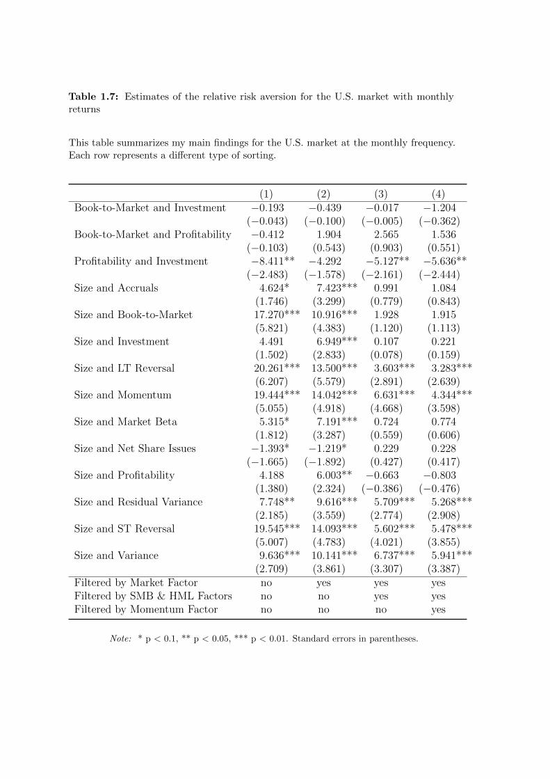
Table 1.7: Estimates of the relative risk aversion for the U.S. market with monthlyreturns
This table summarizes my main findings for the U.S. market at the monthly frequency.Each row represents a different type of sorting.
(1) (2) (3) (4)Book-to-Market and Investment −0.193 −0.439 −0.017 −1.204
(−0.043) (−0.100) (−0.005) (−0.362)Book-to-Market and Profitability −0.412 1.904 2.565 1.536
(−0.103) (0.543) (0.903) (0.551)Profitability and Investment −8.411** −4.292 −5.127** −5.636**
(−2.483) (−1.578) (−2.161) (−2.444)Size and Accruals 4.624* 7.423*** 0.991 1.084
(1.746) (3.299) (0.779) (0.843)Size and Book-to-Market 17.270*** 10.916*** 1.928 1.915
(5.821) (4.383) (1.120) (1.113)Size and Investment 4.491 6.949*** 0.107 0.221
(1.502) (2.833) (0.078) (0.159)Size and LT Reversal 20.261*** 13.500*** 3.603*** 3.283***
(6.207) (5.579) (2.891) (2.639)Size and Momentum 19.444*** 14.042*** 6.631*** 4.344***
(5.055) (4.918) (4.668) (3.598)Size and Market Beta 5.315* 7.191*** 0.724 0.774
(1.812) (3.287) (0.559) (0.606)Size and Net Share Issues −1.393* −1.219* 0.229 0.228
(−1.665) (−1.892) (0.427) (0.417)Size and Profitability 4.188 6.003** −0.663 −0.803
(1.380) (2.324) (−0.386) (−0.476)Size and Residual Variance 7.748** 9.616*** 5.709*** 5.268***
(2.185) (3.559) (2.774) (2.908)Size and ST Reversal 19.545*** 14.093*** 5.602*** 5.478***
(5.007) (4.783) (4.021) (3.855)Size and Variance 9.636*** 10.141*** 6.737*** 5.941***
(2.709) (3.861) (3.307) (3.387)Filtered by Market Factor no yes yes yesFiltered by SMB & HML Factors no no yes yesFiltered by Momentum Factor no no no yes
Note: * p < 0.1, ** p < 0.05, *** p < 0.01. Standard errors in parentheses.
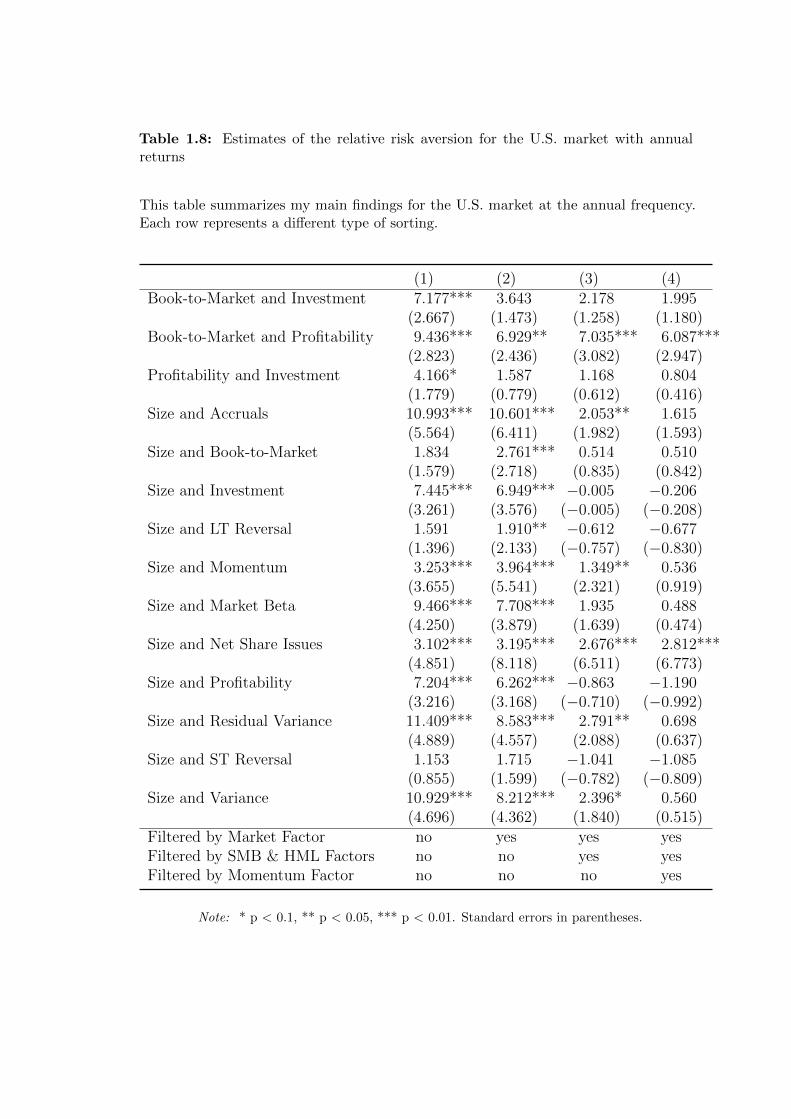
Table 1.8: Estimates of the relative risk aversion for the U.S. market with annualreturns
This table summarizes my main findings for the U.S. market at the annual frequency.Each row represents a different type of sorting.
(1) (2) (3) (4)Book-to-Market and Investment 7.177*** 3.643 2.178 1.995
(2.667) (1.473) (1.258) (1.180)Book-to-Market and Profitability 9.436*** 6.929** 7.035*** 6.087***
(2.823) (2.436) (3.082) (2.947)Profitability and Investment 4.166* 1.587 1.168 0.804
(1.779) (0.779) (0.612) (0.416)Size and Accruals 10.993*** 10.601*** 2.053** 1.615
(5.564) (6.411) (1.982) (1.593)Size and Book-to-Market 1.834 2.761*** 0.514 0.510
(1.579) (2.718) (0.835) (0.842)Size and Investment 7.445*** 6.949*** −0.005 −0.206
(3.261) (3.576) (−0.005) (−0.208)Size and LT Reversal 1.591 1.910** −0.612 −0.677
(1.396) (2.133) (−0.757) (−0.830)Size and Momentum 3.253*** 3.964*** 1.349** 0.536
(3.655) (5.541) (2.321) (0.919)Size and Market Beta 9.466*** 7.708*** 1.935 0.488
(4.250) (3.879) (1.639) (0.474)Size and Net Share Issues 3.102*** 3.195*** 2.676*** 2.812***
(4.851) (8.118) (6.511) (6.773)Size and Profitability 7.204*** 6.262*** −0.863 −1.190
(3.216) (3.168) (−0.710) (−0.992)Size and Residual Variance 11.409*** 8.583*** 2.791** 0.698
(4.889) (4.557) (2.088) (0.637)Size and ST Reversal 1.153 1.715 −1.041 −1.085
(0.855) (1.599) (−0.782) (−0.809)Size and Variance 10.929*** 8.212*** 2.396* 0.560
(4.696) (4.362) (1.840) (0.515)Filtered by Market Factor no yes yes yesFiltered by SMB & HML Factors no no yes yesFiltered by Momentum Factor no no no yes
Note: * p < 0.1, ** p < 0.05, *** p < 0.01. Standard errors in parentheses.

Chapter 1. The RiskMetrics Anomaly
by a T × T idempotent matrix, Q := IT×T −w(w′w)−1w′. This procedure starts
by projecting both y and x onto the vector space generated by the columns of w
and then regresses the residual of the first regression on the residual of the second.
Consequently, this allows me to remove all the control variables in the right-hand
side (pre-multiplying vectors M , S, H, or C by matrix Q results in a T × 1 vector
of zeros). Hence, each cross-sectional unit equation becomes2,
Qyi︸︷︷︸Ai
= γ Qxi︸︷︷︸Bi
+Qui︸︷︷︸vi
, i = 1...N. (1.14)
Once that procedure is applied to all the cross-sectional unit equations the panel
can be reshaped and the estimate of the relative risk aversion can be assessed by
simply regressing Ai on Bi.3
1.4.3 Analysis of the Results
I test my model with different subsamples and at different return frequencies.
Tables 1.3–1.5 shows my results for the Asian, European and Japanese markets.
For each of these tables rows 1–4 show estimates computed with daily returns.
Rows five to eight estimates are computed with monthly returns. Finally, the last
rows show estimates which are computed with annual returns. Tables 1.6–1.8 only
show estimates of γ for the U.S. market. Table 1.6 shows estimates computed with
daily returns. Table 1.7 and 1.8 report estimates computed with monthly and
annual returns respectively.
2Let us define V to be the space spanned by the columns of w. Then, Ai corresponds to theprojection of yi onto the space orthogonal to V . Likewise Ai is the residual of the regression ofyi onto the vector of controls w, while Bi corresponds to the projection of xi onto the spaceorthogonal to V . Finally, vi is the residual of the regression of ui on w. Thus, only the noiseorthogonal to V is left.
3Note that the estimator of the relative risk aversion, γ, is both, unbiased and consistent asillustrated by Wawro (2009).
24

1.4. Data and Methodology
The analysis of Tables 1.3–1.8 reveals an interesting result. Though all specifications
are reported I discuss only the last column of each table which provides the most
robust estimates. While the parameters are always strongly significant at the
daily frequency for the Asian, Japanese and the U.S. market, whatever the sorting
applied to stocks, this is less clear for Europe. In addition, the range where the risk
aversion appears is coherent with previous studies (in general below 20). The fact
that the coefficients are so strongly significant at that frequency argues in favour
of an anomaly, the “RiskMetrics effect”, identified in most of the (main) financial
markets around the world. Importantly, my model is robust even after controlling
for well-established factors in the empirical asset pricing literature (i.e. the market
premium, the momentum and the Fama-French factors).
Christoffersen et al. (1998) established that volatility forecastability declines quickly
with the horizon; while the volatility fluctuations are highly forecastable for short
horizons (such as with daily returns), the forecastability seems to vanish beyond
horizons of two weeks. When choosing a portfolio a mean-variance agent balances
the expected return with the risk, measured here by the conditional variance.
Moreover, an investor must also decide how long they will keep their portfolio
without altering its composition. Therefore, it is natural to conjecture that
agents who rebalance their portfolios frequently care more about the volatility
forecastability than agents who do not. If the holding period is a month almost
all the predictable part of the variance is gone. Thus, the simple benchmark case
derived in Section 1.3.1 (i.e. with constant variance) is expected to hold, implying
that the effect predicted by my model should disappear. Contrarily, when the
holding period is a day volatility is highly predictable. Hence, the model derived in
Section 1.3.2 should hold. Consequently, I expect to find a “RiskMetrics” anomaly
with daily data but not necessarily with lower frequency returns. This is confirmed
25

Chapter 1. The RiskMetrics Anomaly
by the data; the quantity of significant coefficients for monthly and annual returns
is drastically smaller than with daily returns. It turns out that the regression
coefficients are never statistically different from zero for both the Asian and the
Japanese markets at the monthly and annual frequencies (with one minor exception
that I consider insignificant). For the U.S. market the quantity of significant
estimates decreases monotonically with the return frequency, consistent with my
conjecture.
Contrastingly, the European market appears as the exception; the anomaly is
observed more frequently at lower frequencies, which is puzzling. A possible
explanation is that the behaviour towards risk is different across the world. This
is not the first time that a study concludes that financial markets are not that
integrated. Another possible interpretation could be related to the fact that the
volatility is less persistent in Europe than in the other markets. Because of this
feature, the risk becomes harder to forecast, which reduces the magnitude of the
anomaly.
1.5 Conclusion
This paper considers an overlapping-generations economy where the agents forecast
future variance with the RiskMetrics variance model. I show that this feature
induces a two-factor asset pricing model in which risk premiums are determined
by both the market beta and the “RiskMetrics beta”; this latter results from
the interaction between the past returns of the asset and the market. I validate
this prediction by estimating the model with panel regressions; importantly, my
empirical strategy allows me to estimate the relative risk aversion coefficient
26

1.5. Conclusion
independently from established procedures. My estimates are in line with the ones
obtained with these approaches.
Furthermore, this effect is found in each of the major financial markets, except
in Europe. The magnitude of the effect depends on the frequency of the returns;
with high frequency data (here, daily returns) the RiskMetrics anomaly is easier to
detect as compared with low frequency data (monthly or annually). The effect is
robust to the major pricing factors found in the empirical asset pricing literature,
which are the three Fama-French factors and the Momentum factor.
Finally, I extend my model and show that the risk-return tradeoff predicted by my
model when the volatility is forecasted with a GARCH model is significantly weaker
than the relation predicted by mainstream finance theories. This can provide a
potential explanation as to why the relationship between expected returns and
conditional volatility is, empirically, so weak.
27


2 Slow Arbitrage
This paper develops a dynamic model in which financially constrained agents
search for markets which are subject to decreasing returns to scale. In equilibrium,
agents only invest in markets with total capital below an endogenous threshold that
depends on the equilibrium distribution of capital across markets. Strikingly, I show
that perfect capital mobility is not necessarily the most efficient outcome, breaking
down the common belief that perfect mobility is always better. Furthermore, I
extend the model and allow the redistribution of wealth from buyers to sellers
through taxation. With this extension I demonstrate that in the case of parameter
uncertainty taxing too much will cause less damage than taxing too little, which
has significant implications for fixing tax rates.
2.1 Introduction
Market efficiency depends crucially on capital mobility; in an efficient market
capital quickly flows to positive net present value (NPV) projects. In this paper I
29

Chapter 2. Slow Arbitrage
show that this conventional wisdom can break down; capital mobility can have an
adverse effect on welfare.
I build a model and study the equilibrium properties of capital flows through
a continuum (a non-atomic measure space) of segmented markets; those are
indistinguishable except for the amounts of capital invested in each. This economy
is populated by risk-neutral investors all endowed with one unit of capital. These
agents search markets and, upon meeting one, invest all their capital. At Poisson
times markets return a profit to all investors present on top of their investment.
Then, these investors return to searching. As a matter of supply and demand I
assume that the profit paid to the agents in that market is strictly decreasing with
the aggregate capital. Finally, I conjecture that investors cease to enter into a
particular market once its aggregate capital is above a level, settled endogenously.
With this model I show that an economy characterized by perfect capital mobility
is not desirable.
My results suggest that the intensity at which investors search, a proxy for capital
mobility, is the main driver of market liquidity; this has strong consequences on
welfare. When searching is not allowed the economy performs very badly; there are
no markets for liquidity and no benefits from trade, since there are no means of
exchange. As searching frictions vanish investors coordinate without difficulty. In
this regime the agents’ optimal strategy is to spread across the entire universe of
markets and, since there are no search frictions, they can do that easily. Surprisingly,
the first-best outcome is not necessarily achieved here. Because their reservation
value is small investors lower their sights; the level above which agents cease to
enter is set higher. Then I investigate what happens when investors can set their
search intensity. This is particularly useful when it comes to discussing taxation
and financial incentives.
30

2.1. Introduction
Finally, I explore a simple extension of the model; some agents (the seekers of
capital) sell their own assets to cover a sudden need for cash. The buyers—the
former investors—that have allocated their capital to that particular seller, pool
their capital, buy the asset, consume the proceeds and return to searching. Then I
allow for the redistribution of wealth from buyers to sellers through taxation. I
am particularly interested in rescue packages offered by government institutions,
which guarantee toxic assets in significant proportions. My results establish that a
simple tax scheme on search technology provides a smart solution for the financing
of these interventions and incites buyers to set search intensity at its first-best level.
Last but not least, I show that in the case of parameter uncertainty taxing too
much will always cause less damage than taxing too little.
2.1.1 Related literature
My model belongs to the literature on search and matching frictions applied to
economics and finance. An important early paper on this is Diamond (1982);
agents are searching for production opportunities and, upon meeting one, pay
the associated cost of production or return to searching. This literature has been
extended in many directions, including asset prices and allocations in OTC markets
(e.g., Ricardo et al. (2011), Vayanos and Wang (2007), Vayanos and Weill (2008)
and Weill (2007)). An important paper in this field of literature is Duffie et al.
(2005); the authors study the consequences of search frictions in a single market.
Similarly, Duffie et al. (2007) examine the impact of search and bargaining frictions
on asset prices. Afonso and Lagos (2015) build a model of the market for federal
funds where banks face search and bargaining frictions. More recently, Hugonnier
et al. (2016) design a search and bargaining model with investors’ valuations drawn
from any arbitrary distribution.
31

Chapter 2. Slow Arbitrage
My model is closely related to Duffie and Strulovici (2012). The authors design a
model with which they analyze the equilibrium movements of capital between two
partially segmented markets; these are indistinguishable except for the amount
of capital invested in each. My framework shares some important ingredients
with their model. Firstly, investors are not assigned to one particular market;
rather, they can trade in all of them. Secondly, markets are distinguished by the
quantity of capital invested in each. In contrast I study a continuum of markets.
Additionally, while their focus is on the intermediation channel I have abstracted
from that; my results put more emphasis on the consequences of capital mobility
on welfare, which is complementary to their analysis.
Section 2.3 investigates the idea that assets may be sold at a discount when buyers
are financially constrained (papers related to this literature include, for example,
Allen and Gale (1994), Allen and Gale (2004), Allen and Gale (2005), Shleifer and
Vishny (1992) and Shleifer and Vishny (1997)). This endeavour is related to the
seminal work of Acharya et al. (2013). The authors argue that outside arbitrageurs
do not necessarily come in and take advantage of a fire sale because they face a
tradeoff; arbitrage capital entails both benefits, when assets are sold at a discount
and costs, such as opportunity cost of not investing in other profitable activities.
This tradeoff also shows up in my framework, nevertheless, my contribution to this
literature is very different. Firstly, this investigation is an extension of my model,
rather than its primary purpose. Secondly, my methodology is very different; my
model is a continuous time model, while they work with a stylized three-period
model. To summaries, while the importance of the dynamics of arbitrage capital is
stressed in both papers, our respective approaches are completely different. Lastly,
this section also refers to Kondor (2009), who studies a model of (limited) capital
allocation. Interestingly he suggests that, despite the magnitude of arbitrage
32

2.2. Model
opportunities arbitrageurs keep some capital aside in case these opportunities
become more profitable. He focuses on risk arbitrage and my model shares that
feature; when capital is limited and the probability that a new (better) opportunity
appears is strictly positive, keeping capital aside is optimal. Nevertheless, the
mechanisms at work are quite different. In Kondor’s paper arbitrageurs save some
capital because, as time goes by, prices might diverge further. Contrastingly, my
model is built such that the profitability of a given opportunity can only disappear
over time; the arbitrage capital is generated by the large dimension of the market
space.
This paper is structured as follows: Section 2.2 presents the model and its main
consequences, Section 2.3 applies this framework to a fire sale of assets, discussing
some equilibrium properties, welfare implications and potential policy interventions.
Finally, I summarize the main results and present my conclusions in Section 2.4.
2.2 Model
The economy is populated by a mass A of agents (arbitrageurs), each endowed
with one dollar. There is a continuum of markets where profits are a decreasing
function π(k) of the capital invested in that market k. Agents arrive at a rate λ
and decide whether to stay or keep searching further. When an agent decides to
stay, they invest their dollar and wait until the profits, π(k) are paid. The time
at which a market pays off is exponentially distributed with intensity η (this is
the time when the fruit matures). At that moment the agent consumes the net
profit π(k)− 1 and returns to searching with their suddenly liberated dollar. In the
meantime new opportunities appear at the same rate η so that the total number of
opportunities remains constant. I define M as the total mass of agents which have
33

Chapter 2. Slow Arbitrage
currently invested their money in a market waiting for profits to be paid. Similarly,
A −M corresponds to the fraction of the total mass of arbitrageurs searching
for opportunities. Then, from the law of large numbers for independent random
matching, the total meeting rate at which agents find markets is λ(A−M). For
any given market traders arrive at Poisson times, thus the aggregate capital in
each market follows a Poisson process. Some possible paths are shown in Figure
2.1. Therefore, if the previous capital invested in a given market was k, it jumps to
Figure 2.1: Dynamics of the aggregate capital in a single market
This figure shows the dynamics of the aggregate capital in one single market.Importantly, the aggregate capital behaves as a Poisson process (it jumps fromk to k + 1 at exponentially distributed random times with mean 1/Λ or dies atexponentially distributed random times with mean 1/η).
k0 k0 + 1 k0 + 2 k0 + bk∗ − k0c − 1 k0 + bk∗ − k0c
Λ Λ Λ Λ
· · ·
η
k + 1. Finally, I assume that when new opportunities appear they are immediately
filled with some initial capital drawn from an arbitrary exogenous distribution F .
I consider an equilibrium where agents enter only when k + 1 ≤ k∗. Whenever an
agent finds a market with capital larger than k∗ − 1 they immediately return to
searching without investing. This mechanism is summarized in Figure 2.2. The
stationary cross-sectional distribution of masses across markets is given by p(k) to
34
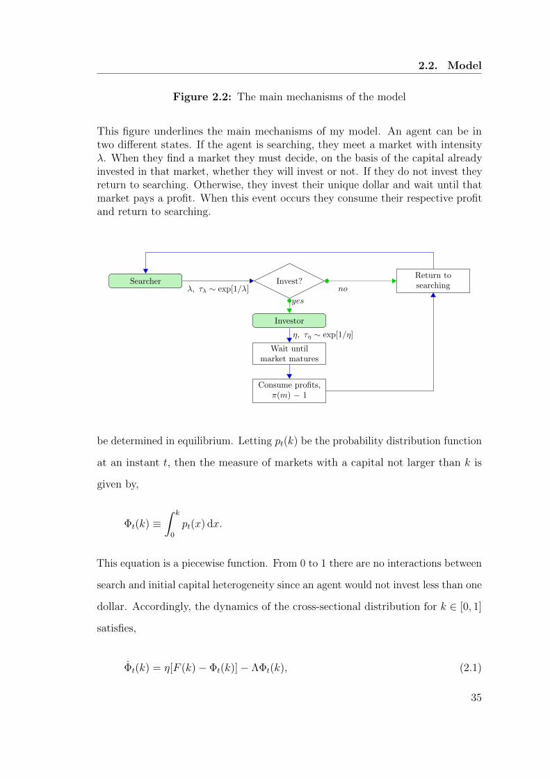
2.2. Model
Figure 2.2: The main mechanisms of the model
This figure underlines the main mechanisms of my model. An agent can be intwo different states. If the agent is searching, they meet a market with intensityλ. When they find a market they must decide, on the basis of the capital alreadyinvested in that market, whether they will invest or not. If they do not invest theyreturn to searching. Otherwise, they invest their unique dollar and wait until thatmarket pays a profit. When this event occurs they consume their respective profitand return to searching.
Invest?
Investor
Wait untilmarket matures
Consume profits,π(m) − 1
Return tosearchingSearcher
yes
no
η, τη ∼ exp[1/η]
λ, τλ ∼ exp[1/λ]
be determined in equilibrium. Letting pt(k) be the probability distribution function
at an instant t, then the measure of markets with a capital not larger than k is
given by,
Φt(k) ≡∫ k
0
pt(x) dx.
This equation is a piecewise function. From 0 to 1 there are no interactions between
search and initial capital heterogeneity since an agent would not invest less than one
dollar. Accordingly, the dynamics of the cross-sectional distribution for k ∈ [0, 1]
satisfies,
Φt(k) = η[F (k)− Φt(k)]− ΛΦt(k), (2.1)
35

Chapter 2. Slow Arbitrage
where the dot stands for the time derivative. From 1 to k∗ − 1, searching interacts
with capital heterogeneity. It is worth mentioning that a market in that range could
already have experienced multiple rounds of financing. However, agents finding
that market would still invest as long as k ≤ k∗ − 1. Accordingly, the dynamics of
the cross-sectional distribution for k ∈]1, k∗ − 1] satisfies,
Φt(k) = η[F (k)− Φt(k)]− ΛΦt(k) + ΛΦt(k − 1). (2.2)
The dynamics of the cross-sectional distribution for this range is very similar to
equation (2.1); the only difference is regarding how searching interacts with capital
heterogeneity. When a meeting occurs the agent invests their capital and a capital
of k results from adding 1 to k − 1. On the contrary, no one would invest if the
market’s aggregate capital was larger than k∗ − 1. This implies that the dynamics
of the cross-sectional distribution for k ∈]k∗ − 1, k∗] satisfies,
Φt(k) = η[F (k)− Φt(k)]− ΛΦt(k∗ − 1) + ΛΦt(k − 1). (2.3)
All markets born with an initial capital larger than k∗ are located between k∗
and ∞. The first term on the right-hand side of equation (2.1) reflects that at
every instant, a measure η of new markets appear, with initial capital drawn from
F (k). Meanwhile, there is a measure ηΦt(k) of markets with capital m ≤ k which
matures. Then, the total meeting rate is Λ ≡ λ(A−Mt). Finally, the total mass
of agents who have their capital in a market is given by Mt which must satisfy the
following differential equation,
Mt = λ(A−Mt)Φt(k∗ − 1)− ηMt (2.4)
The first term on the right-hand side of (2.4) reflects the rate at which agents meet
36

2.2. Model
markets. Since agents invest in a market only if k ≤ k∗ − 1, the total meeting rate
must be adjusted by the probability of meeting non-saturated markets, Φt(k∗ − 1).
Then ηMt is the measure of agents that return to searching.
2.2.1 Stationary Distribution
The stationary cross-sectional distribution results from setting the time derivative
equal to zero. Since the shape of the distribution depends on the functional form
of F (k) I discuss two different approaches to solve for the model’s equilibrium.
The first method is very general; I discretize the state (capital) space and solve
for the equilibrium recursively. This procedure has the advantage of not requiring
setting the functional form of F (k) and π(k). However, this approach can not
provide a closed-form solution for the cross-sectional distribution. The second
technic is based on the theory of difference equations; while this method requires
to parameterize both F (k) and π(k) the cross-sectional solution can be computed
in closed-form.
Capital takes value on the set Γ ≡ [0, 1/N, · · · , ku], where N ∈ N∗ (the case
N →∞ reduces to the continous case) and ku is chosen large enough to ensure k∗
belongs to Γ (for that, I use ku = π−1(1)). While the investment capacity of agents
is constant (i.e. one dollar), the initial capital in all existing markets is drawn
from the distribution F (k) and is distributed over the whole set Γ. Therefore, the
stationary cross-sectional distribution is characterized by a recursive system, which
can be rewritten as a system of equations, A× x = y, where A ∈ RN×k∗+1,N×k∗+1
and, x,y ∈ RN×k∗+1,1. In particular, I define Ai,j as the i, j element of the
matrix A. Then, all elements in the diagonal equal one. Any element satisfying
Ai+N,i, i ∈ (1, · · · , N × (k∗ − 1) + 1) equals −Λ/(η + Λ). Any element satisfying
Ai+N,i, i ∈ (N × (k∗ − 1) + 2, · · · , N × k∗) equals −Λ/η. Finally, any element
37

Chapter 2. Slow Arbitrage
satisfying Ai,N×(k∗−1)+1, i ∈ (N×(k∗−1)+2, · · · , N×k∗) equals Λ/η. All the other
elements are zero. Concerning the vector y, all elements i ∈ (1, · · · , N×(k∗−1)+1)
take the value η/(η+Λ)×F ((i−1)/N), while all the others are simply F ((i−1)/N).
The vector x is the stationary cross-sectional distribution function. Accordingly,
all elements equal Φ((i− 1)/N). Eventually, since matrix A is diagonally dominant
it can be inverted, resulting in Φ = A−1 × y.
The second approach uses the fact that the cross-sectional distribution satisfies a
first order linear difference equation. Accordingly, the equation characterizing the
stationary distribution must be,
Φ(k) = C ×(
Λ
η + Λ
)k+ g(k), 1 ≤ k ≤ k∗ − 1,
where the first part is the general solution (C is a constant to be defined) and g(k)
is the particular solution (which depends on the functional form of F (k))1. For
example, assuming that the initial capital is uniformly distributed over the range
[0, ku], F (k) := kku
results in the following stationary distribution,
Φ(k) =
1ku
(Λ
η+Λ
)bkc [Λη− Λ
η+Λ(k − bkc)
]+ 1
ku
[k − Λ
η
]0 ≤ k ≤ k∗ − 1,
kku
+ Λη[Φ(k − 1)− Φ(k∗ − 1)] k∗ − 1 ≤ k ≤ k∗,
kku
k ≥ k∗.
Where b·c is the floor function. Figure 2.3 shows different cross-sectional distri-
butions. The first piece of this equation describes the cross-sectional distribution
1For difference equations, the treatment of the boundary condition is different from that ofdifferential equations. For example, let us assume that the initial capital of a market is k0 and kτis the aggregate capital invested in this market when it pays off. Importantly, kτ belongs to theset k0, k0 + 1, · · · , k0 +m where m is a natural number such that k∗ − 1− k0 ≤ m ≤ k∗ − k0.By varying k0 one modifies the entire set. Hence, it must be keeped in mind that there is oneconstant for each path (one path being the set defined previously). This implies that one mustcompute the constant for any k ∈ [0, 1[.
38
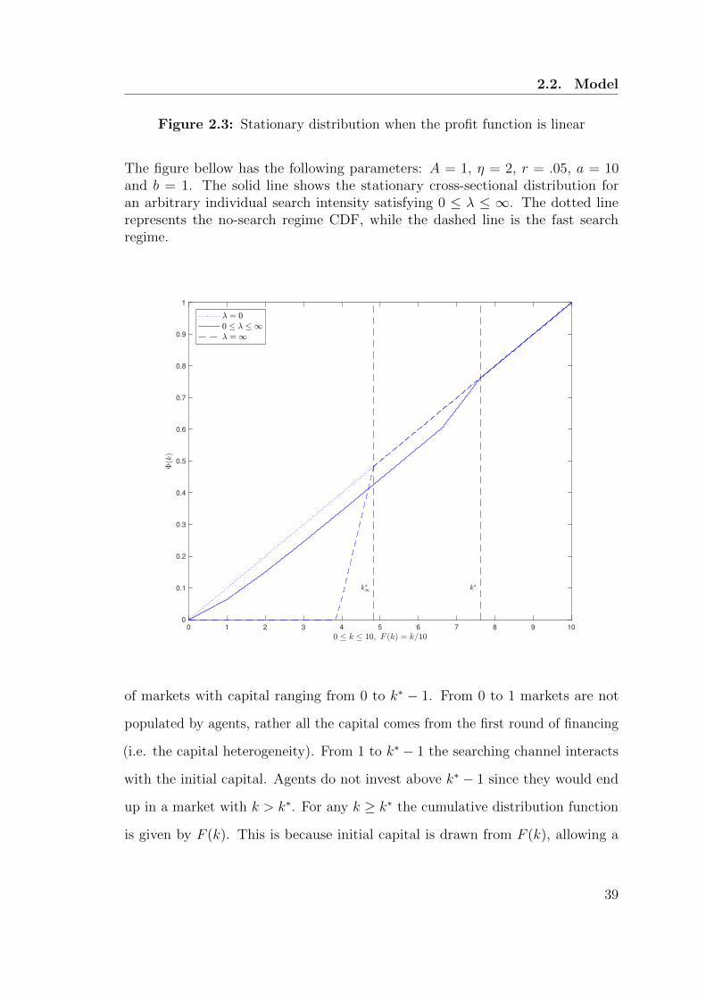
2.2. Model
Figure 2.3: Stationary distribution when the profit function is linear
The figure bellow has the following parameters: A = 1, η = 2, r = .05, a = 10and b = 1. The solid line shows the stationary cross-sectional distribution foran arbitrary individual search intensity satisfying 0 ≤ λ ≤ ∞. The dotted linerepresents the no-search regime CDF, while the dashed line is the fast searchregime.
0 1 2 3 4 5 6 7 8 9 10
0
0.1
0.2
0.3
0.4
0.5
0.6
0.7
0.8
0.9
1
of markets with capital ranging from 0 to k∗ − 1. From 0 to 1 markets are not
populated by agents, rather all the capital comes from the first round of financing
(i.e. the capital heterogeneity). From 1 to k∗ − 1 the searching channel interacts
with the initial capital. Agents do not invest above k∗ − 1 since they would end
up in a market with k > k∗. For any k ≥ k∗ the cumulative distribution function
is given by F (k). This is because initial capital is drawn from F (k), allowing a
39

Chapter 2. Slow Arbitrage
positive measure of markets to be filled with some initial capital greater than k∗.
Finally, since Λ feeds into the cross-sectional distribution of markets, which itself
depends on M , one must substitute Φ(m) in equation (2.4) (when Mt = 0) to solve
for the endogenous stationary distribution. Because the dynamics of Φt(x) and Mt
are nonlinear it is not guaranteed ex ante that a unique equilibrium exists. The
following proposition treats this problematic.
Proposition 2.1 There is only one fixed point that satisfies system (2.1)− (2.4)
with the restriction that M lies between 0 and A. Hence, there is a unique cross-
sectional distribution associated with each k∗.
2.2.2 Value Functions and Equilibrium Characterization
Bellman’s principal of optimality implies that the value function for an agent in a
market characterized by a capital of k ≤ k∗ − 1 satisfies,
V (k) = E[e−r(τη∧τΛ)1τη≤τΛ[π(k)− 1 + VS] + 1τη>τΛV (k + 1)
].
Here, τη denotes the time at which this specific market matures. Similarly, τΛ is
the time at which a new agent invests in this market. An agent that has invested
their capital in this market faces two different outcomes; either a new investor
discovers this market, or this market pays off. Thus, the expectation is computed
with respect to the distribution of the minimum between τη and τΛ := τη ∧ τΛ.
The indicator function 1τη≤τΛ corresponds to the probability that the investment
opportunity matures before another agent invests multiplied by the corresponding
payoff (the agent collects the profits [π(k) − 1] and returns to searching, with
continuation utility VS). The second part is essentially the same; 1τη>τΛ accounts
for the probability that one investor discovers this market before it pays off. When
40

2.2. Model
this event occurs the aggregate capital in this market will increase by one dollar,
which means that the continuation value, conditional on this event, is V (k + 1).
After integrating both sides with respect to the distribution of τη∧τΛ, this equation
becomes,
(r + η + Λ)V (k) = η[π(k)− 1 + VS] + ΛV (k + 1). (2.5)
Similarly, the value function of an agent in a saturated market (i.e. where k∗− 1 ≤
k ≤ k∗) satisfies,
V ∗(k) =η
r + η[π(k)− 1 + VS]. (2.6)
For these markets only the time at which these specific investment opportunities
mature matters. The term [π(k)−1+VS] corresponds to the profit of an arbitrageur
once the market matures. Similarly, I find that the value associated to searching,
VS, satisfies,
VS = E[e−rτλ
(∫ k∗−1
0
V (x+ 1)p(x) dx+ [1− Φ(k∗ − 1)]VS
)].
Here, τλ denotes the time at which one particular investor finds a market. Condi-
tional on finding a market with capital k ≤ k∗ − 1, the agent invests one dollar,
resulting in the capital in that market to jump from k to k+ 1. After some algebra
that equation becomes,
VS =λ
r + λΦ(k∗ − 1)
∫ k∗−1
0
V (x+ 1)p(x) dx. (2.7)
Since equations (2.5), (2.6) and (2.7) belong to the class of linear difference
equations, the approaches used to solve for the cross-sectional distribution are still
41

Chapter 2. Slow Arbitrage
applicable. Hence, the general method detailed in the previous section implies that
the vector of value functions can be characterized by a recursive system which can be
rewritten as a system of equations A′× x′ = y′, where A′ ∈ RN×(k∗−1)+2,N×(k∗−1)+2
and x′,y′ ∈ RN×(k∗−1)+2,1. In the diagonal, all elements satisfying A′i,i, i ∈
(1, (k∗ − 2)×N + 1 equal r + η + Λ, while all the other diagonal elements equal
r+ η except the very last term, which equals rλ
+ Φ(k∗− 1). Any element satisfying
A′i,i+N equals −Λ except the very last term (i.e. A′N×(k∗−2)+2,N×(k∗−1)+1). Then, any
element satisfying A′N×(k∗−1)+1,i, i ∈ (1, · · · , N × (k∗ − 1)) equals −η. Finally, all
elements in the last row equal p(i), except the very last one, which has already been
discussed. Eventually, since matrix A′ is diagonally dominant it can be inverted,
resulting in V = A′−1 × y′.
The second approach uses the fact that value functions satisfy a first order linear
difference equation. The equation characterizing the value functions satisfies,
V (k) = C ×(r + η + Λ
Λ
)k+ g(k), 1 ≤ k ≤ k∗ − 1,
where the first part is the general solution (C is a constant to be defined) and g(k)
is the particular solution (which depends on the functional form of π(k)2). For
instance, assuming that the profit is a linear function of the form π(k) = a− bk3
results in the following equation,
V (k) =bηΛ
(r + η)2
(r + η + Λ
Λ
)−bk∗−kc+
η
r + η
[a− 1 + VS − b
(Λ
r + η+ k
)].
Figure 2.4 shows the value function when the profit is linear in the market’s
aggregate capital. To proceed further I substitute V (k) back into VS. Finally, the
2Once again, the reader must keep in mind that there is one constant for each possible path.This implies that one must compute the constant for any k ∈ [k∗ − 1, k∗[.
3Assuming this implies ku = (a− 1)/b.
42

2.2. Model
Figure 2.4: Value function when the profit function is linear
When π(k) = a−bk, V (k), the value that a buyer associates with being in a marketwith aggregate capital k satisfies,
V (k) =bηΛ
(r + η)2
(r + η + Λ
Λ
)−bk∗−kc+
η
r + η
[a− 1 + VS − b
(Λ
r + η+ k
)].
.
0 1 2 3 4 5 6 7
0
1
2
3
4
5
6
last variable to identify is the threshold k∗. In order to find this quantity one must
remember that if an agent finds a market with current capital k < k∗ − 1 the
associated equilibrium strategy is to invest, which reveals that the value they extract
from searching is strictly lower than the value they would receive by investing. If an
investor finds a market with aggregate capital k > k∗−1, their equilibrium strategy
is not to invest, implying that there is a greater value in searching for another
opportunity. Finally, if k + 1 = k∗, an agent is indifferent between searching or
43

Chapter 2. Slow Arbitrage
investing. Accordingly, the equilibrium k∗ must satisfy the following conditions,
VS ≤ V (k), ∀k ≤ k∗,
VS > V (k), ∀k > k∗.
To put it another way, this set of conditions describes the outcome of a Nash
Equilibrium. It is not valuable for an agent to deviate from their optimal strategy
given that the other agents play their own optimal strategy. Practically, one must
check each criterion for a given k∗ ∈ [1, ku] and iterate the procedure until those
conditions are met. If these criteria are satisfied for a particular configuration,
then it is an equilibrium. When one uses the closed-form solution for V (k) instead,
the necessary and sufficient condition for a candidate to be an equilibrium is
V ∗(k∗)−VS(k∗) = 0. The next proposition characterizes the equilibrium in general.
Proposition 2.2 An equilibrium is characterized by the optimal threshold k∗ that
solves equation (2.8),
η[π(k∗)− 1]− rVS = 0, (2.8)
once all pieces of the problem are treated simultaneously (that means equations (2.1)-
(2.4) are set to zero, (2.5) and (2.6) are substituted into (2.7), which is substituted
back into (2.8)).
2.2.2.1 Comparative statics
Figure 2.5 consists of four plots summarizing the main properties of the equilibrium,
for a given set of parameters, when one varies the search intensity. In this figure,
the profit function is simply linear, π(k) = a− bk. The upper left plot shows the
44

2.2. Model
shape of the aggregate search intensity (the total meeting rate Λ). The upper
right plot shows how the proportion of agents who have invested their capital into
a market varies with respect to λ. The shape of this function results from the
interaction of two competing forces. Since λ represents the speed at which investors
find markets, the proportion of agents who are searching must decrease accordingly.
This is because an increase in the search intensity reflects an increase in the mass
of markets found. On the other hand, because the agents find a market more easily
the value function associated with searching rises. Hence, it becomes more valuable
to skip some opportunities. Figure 2.5 shows a monotonic increasing function that
converges asymptotically to M < 1. The lower left plot illustrates how the value of
searching evolves when one varies λ. This plot has to be analyzed simultaneously
with the last one which shows the endogenous threshold. Both plots suggest that
the agents see an increase of λ as beneficial. They can find more markets in a given
time frame and reject more potential opportunities.
2.2.2.2 Model without search technology (λ0)
In this section I discuss the equilibrium when agents can not search (i.e. λ0).
Because searching is absent from this model, Φ(k) = F (k) and M = 0. Moreover,
the value of searching is worth zero. Therefore, the equilibrium threshold k∗ equals
ku ≡ π−1(1).
2.2.2.3 Fast Search (λ∞)
While the previous section illustrates how the equilibrium behaves when arbitrageurs
do not search, it remains only to explore its characteristics as search frictions vanish
(i.e. λ∞). In the following proposition I describe the main features of that limiting
case.
45

Chapter 2. Slow Arbitrage
Figure 2.5: The model’s main statistical properties
The figures bellow have the following parameters: A = 1, η = 2, r = .05, a = 10and b = 1. The top-left plot shows the aggregate intensity Λ. The top-right panelshows the fraction of the measure of agents, who have their capital in a market atthat moment. The bottom left panel illustrates the value associated with searching.Finally, the last diagram shows the endogenous threshold k∗.
0 200 400 600 800 1000
4
5
6
7
8
9
10
0 200 400 600 800 1000
0
0.2
0.4
0.6
0.8
1
0 200 400 600 800 1000
0
20
40
60
80
100
120
0 200 400 600 800 1000
0
50
100
150
200
Proposition 2.3 When the search intensity tends to infinity, Λ→∞ and M ≤ A,
the optimal threshold k∗∞ is the quantity that solves equation (2.8) when VS is
characterized by the following relation,
[r(A−M) + ΛΦ(k∗ − 1)]VS =
∫ k∗−1
0
V ∗(x+ bk∗ − xc)Λp(x) dx. (2.9)
Because Λ→∞, both p(x) and Φ(x)→ 0, implying that their product with the
aggregate search intensity is indeterminate. The hospital theorem helps resolve this
46
2.2. Model
problematic; specifically, when F (x) ∼ U [0, a/b], these quantities are respectively,
Λp(x) = b/a× η(bxc+ 1),
ΛΦ(k∗ − 1) = b/a× ηbk∗c(k∗ − 1− 1
2bk∗ − 1c
).
It remains to substitute these objects into VS to solve for the equilibrium.
2.2.3 Is Perfect Capital Mobility Socially Efficient?
In the previous sections I have discussed two antithetical regimes; in the first one
(λ0) arbitrageurs have no search technology. Agents can not invest their capital
leading to the worst possible outcome (as previously shown). This first case is
contrasted by the second case (λ∞) in which agents search at an infinite intensity.
I show in this section that while λ∞ is usually regarded as the most efficient
outcome it is not always desirable. To understand why I start by drawing the
cross-sectional distribution of markets for three levels of search intensity. This is
represented in Figure 2.3. While the continuation value of arbitrageurs is a strictly
monotonic increasing function of the search intensity as depicted in Figure 2.5, this
relation is ambiguous for the agents that would draw their expected utility from the
cross-sectional distribution. This follows simply from the fact that the stationary
CDF for the infinite search intensity does not second-order stochastically dominate
the stationary CDF of the finite intensity. I discuss welfare more formally in the
following section.
2.2.3.1 Social Surplus and Dead Weight Loss
In light of the above the profit function π(k) can be generally considered as a
demand for capital. For simplicity I review the case when this function is linear,
47

Chapter 2. Slow Arbitrage
π(k) = a− bk. Furthermore, I assume that the distribution from which the initial
capital is drawn satisfies F (k) = a−1bk. Then, I designate the old agents as the
providers of capital, while the new agents (those who provide the demand function)
are the seekers of capital. Finally, k0, which was defined as the initial capital,
is considered here as demand heterogeneity (some markets saturate faster than
others). Then, the consumer surplus is defined as the area between the demand
Figure 2.6: Visual representation of the strategy used to measure the welfare loss
This graph shows the offer and consumer surplus (green and blue respectively) andthe welfare loss in red for k = 5 (the accumulated capital at exit time), k0 = 1 andk∗ = 7. The profit function is linear and capital can take values on the set [0, a/b].
0 2 4 6 8 100
2
4
6
8
10
k0 k k∗
CS
OS WL
0 ≤ k ≤ a/b, a = 10, b = 1
π(k)=a−bk
function, the price function (the horizontal line at π(k) = a− bk) and the vertical
line that goes through k04 weighted by the stationary CDF5;
4Figure 2.6 shows the consumer and producer surplus and welfare loss.5Since the capital accumulated until an exit event k is at the aggregate level, distributed accordingto the stationary CDF, any surplus or welfare loss must be weighted by this distribution.
48

2.2. Model
CS(λ, k0) =
∫ k∗
0
b
2(k − k0)2p(k) dk, k ≥ k0.
Figure 2.7: Welfare loss when capital is abundant
This graph shows the dead weight loss function with the following parameters:A = 1, η = 2, r = .05, a = 10 and b = 1. Here, the profit function is linear. Theminimum is reached when λ =∞.
0 100 200 300 400 500 600 700 800 900 1000
6
6.5
7
7.5
8
8.5
9
9.5
10
10.5
11
The offer surplus is defined as the area of the rectangle bounded by the vertical
lines that goes through k0 and k and the horizontal lines that goes through 1 and
p.
OS(λ, k0) =
∫ k∗
0
(k − k0)(a− bk − 1)p(k) dk, k ≥ k0.
49

Chapter 2. Slow Arbitrage
Figure 2.8: Welfare loss when capital is scarce
This graph shows the dead weight loss function with the following parameters:A = 0.01, η = 2, r = .05, a = 10 and b = 1. Here, the profit function is linear. Theminimum is reached well before λ = ∞, which is in contradiction to traditionalwisdom.
0 1000 2000 3000 4000 5000 6000 7000 8000 9000 10000
11.85
11.9
11.95
12
12.05
12.1
12.15
Finally, the welfare loss is defined as the area between the demand function, the
price function and the vertical line that goes through k. Since the dead weight loss
depreciates welfare λ should be set such that this quantity is minimized.
WL(λ) =
∫ a−1b
0
1
2(a− bk − 1)
(a− 1
b− k)p(k) dk. (2.10)
It is important to note that the upper boundary is beyond k∗. This follows from the
fact that beyond this threshold markets are not populated (there is no offer), which
is inefficient from a social planner’s point of view. Since welfare loss is not affected
50

2.2. Model
by k0 it is the simplest object to compute. Additionally welfare loss provides an
intuitive description of the magnitude of the inefficiency in the whole economy
and is shown in Figures 2.7 and 2.8. As expected, welfare loss is the highest at
λ = 0, then the magnitude of the inefficiency decreases rapidly. While the loss of
welfare decreases monotonically in Figure 2.7, it reaches a minimum (well before
λ =∞) in Figure 2.8. Clearly this is in contradiction with the belief that perfect
capital mobility is always better. These results are summarized in the following
proposition.
Proposition 2.4 From a social planner’s point of view, perfect capital mobility is
not always the most desirable scenario.
2.2.4 Endogenous Search
The following section explores which level of search intensity an agent, who seeks
to maximize the value of searching, would employ. For this purpose I assume that
searching is costly. Moreover, once an agent chooses the search technology they
must stick with it. This makes the computations increasingly more tractable and
can be interpreted as the result of the presence of large adjustment costs. Fixing a
cost function c(λ) which can be differentiated, Bellman’s principal of optimality
implies that the value associated with searching is given by,
VS(λ) = E[e−rτλ
(∫ k∗−1
0
V (m+ 1)p(m) dm+ VS(λ)[1− Φ(k∗ − 1)]
)−∫ τλ
0
e−ruc(λ) du
].
The first part of the right-hand side of this equation is the standard searching
value function. The second term corresponds to the present value of the costs.
51

Chapter 2. Slow Arbitrage
Integrating this equation results in,
[r + λΦ(k∗ − 1)]VS(λ) = λ
[∫ k∗−1
0
V (m+ 1)p(m) dm− c(λ)
].
At this stage one can rely on both steady-state and non-steady state analyses. The
first type of analysis regards the agents as perfectly rational; they internalize the
fact that their own decisions have an impact on the equilibrium realization since
they all solve the same problem. In that case an equilibrium is defined as a triplet
(k∗,Λ, λ∗∗) that solves equations (2.4) and (2.8) and satisfies,
∂V (s;λ)
∂λ≡ −λ
[∫ k∗−1
0
V (m+ 1)p(m) dm− c(λ)
]Φ(k∗ − 1)−[∫ k∗−1
0
V (m+ 1)p(m) dm− c(λ) + λ∂
∂λ
(∫ k∗−1
0
V (m+ 1)p(m) dm− c(λ)
)]×
[r + λΦ(k∗ − 1)] = 0.
On the other-hand, the non-steady-state type of analysis builds on the assumption
that agents believe they have no impact on the equilibrium, in particular that the
cross-sectional distribution is fixed. Here the equilibrium is defined as a triplet
(m∗,Λ, λ∗) which simultaneously solves equations (2.4) and (2.8) and satisfies,
∂V (s;λ)
∂λ≡[∫ k∗−1
0
V (m+ 1)p(m) dm− c(λ)− ∂
∂λc(λ)× λ
][r + λΦ(k∗ − 1)]−
λ
[∫ k∗−1
0
V (m+ 1)p(m) dm− c(λ)
]Φ(k∗ − 1) = 0.
While the first approach is consistent, λ∗∗ can never be solved in closed-form, which
is not true for λ∗. Therefore, I discuss that case and assume a linear functional
form for the searching costs (c(λ) = κλ). Under these assumptions the optimal
52

2.3. Cash-in-the-Market-Pricing
intensity results in,
λ∗ =
√r2 + κ−1rΦ(k∗ − 1)
∫ k∗−1
0V (m+ 1)p(m) dm− r
Φ(k∗ − 1). (2.11)
This suggests, empirically, that the intensity at which arbitrageurs search for
opportunities is roughly proportional to 1/√κ.
2.3 Cash-in-the-Market-Pricing
In this section I explore a simple extension of the model where some agents sell
their assets to cover their sudden need for cash. Those assets are eventually split
and consumed by all the respective buyers.
2.3.1 Generalities
I study an economy populated by two classes of agent. There is a unit continuum
of sellers (the seekers of capital), each born with one asset which has a constant
intrinsic value of a. For any of these agents a sudden need of cash occurs as the
first jump of a Poisson process, of intensity η. There is one (independent) Poisson
process for each seller. When a seller faces financial distress, they sell their asset,
consume the proceeds and disappear. The buyers (or the liquidity providers) that
have allocated their capital to that particular market, pool their capital, buy and
consume the asset and return to searching. To justify this behaviour I recall that
buyers never face financial distress. Therefore, they can keep the asset until the
market recovers and sell it at its fair value (however, it is simpler to assume that
the market recovers immediately after the buyers purchase the asset). At the same
time new sellers are born at a rate of η making the measure of sellers constant over
53

Chapter 2. Slow Arbitrage
time. There is a measure A of buyers (the providers of capital). Each of them is
endowed with one dollar. I define M as the measure of buyers that have allocated
their capital in a market. Thus, A −M is the measure of buyers that are still
searching. Buyers meet a seller at a rate λ and decide whether to stay or keep
searching further. From the law of large numbers for independent random matching
the total meeting rate between buyers and sellers is Λ ≡ λ(A−M). Given k, the
quantity of capital present in a market, the buyers in that market each receive
a/k. When new sellers are born, I assume that each receives some money, drawn
from an arbitrary exogenous distribution. Therefore, depending on the money a
seller has, they can keep a fraction of the asset and sell it when the market for that
particular asset has recovered.
Once I feed these parameters into the model, the main primitives that affect the
equilibrium are η, λ, r and A. I recall that they are respectively, the intensity at
which a financial distress occurs and a new seller is born, the intensity at which an
individual buyer searches, the rate of return of the risk-free asset and the measure
of buyers. Normalizing A to one and recalling that buyers provide capital if and
only if k, the quantity of capital invested in a particular market, is lower than k∗−1,
an endogenous threshold, an equilibrium is characterized by the usual conditions
discussed in the previous section. When I further assume that the profit function
is given by π(k) = a/k, which is consistent with the economy under investigation
in that section, the value that a buyer associates with being in a market with
aggregate capital k is provided in the following proposition.
Proposition 2.5 Given π(k) = a/k, V (k), the value that a buyer associates with
54

2.3. Cash-in-the-Market-Pricing
being in a market with aggregate capital k, satisfies,
V (k) = C(k + bk∗ − kc)× ξk−1 +η
r + η(VS − 1)+
a
∆
[L(ξ−1, 1, k) + ξk log
(r + η
r + η + Λ
)],
(2.12)
where,
ξ =(r + η + Λ)/Λ,
∆ =(r + η + Λ)/η,
C(x) =η
r + ηπ(x)ξ1−x − a
∆ξ1−x
[L(ξ−1, 1, x) + ξx log
(r + η
r + η + Λ
)],
L(z, s, a)6 =∞∑n=0
zn
(n+ a)s.
Solving for the equilibrium leads to important statistics which are reproduced in
Figures 2.9 and 2.10. First of all, the optimal threshold, as it was the case for
linear profit functions, is a monotonic decreasing function of the search intensity.
As capital mobility improves sellers receive less. The welfare loss, shown in Figure
2.10, reaches a minimum which is not located in λ =∞, breaking down the common
belief that perfect capital mobility is (always) the first-best outcome.
2.3.2 Government Interventions
In the following lines I extend the model and allow the redistribution of wealth
from buyers to sellers through taxation. My intention is to contribute to the
literature on fire sales of assets by discussing policy maker interventions, mainly
6This function is known as the Lerch Transcendent function.
55

Chapter 2. Slow Arbitrage
Figure 2.9: Cash-in-the-market-pricing: stationary distribution and welfare loss
The figures bellow have the following parameters: A = 1, η = 2, r = .05, a = 10.The profit function is given by π(k) = a/k. In the first panel the solid blue lineshows the stationary cross-sectional distribution for an arbitrary individual searchintensity satisfying 0 ≤ λ ≤ ∞. The dotted blue line represents the no-searchregime CDF, while dashed-dotted blue line is the fast search regime. The secondgraph shows the magnitude of the welfare loss.
0 1 2 3 4 5 6 7 8 9 10
0
0.2
0.4
0.6
0.8
1
0 10 20 30 40 50 60 70 80 90 100
8
8.2
8.4
8.6
8.8
9
9.2
9.4
through the search channel. I am particularly interested in rescue packages offered
by government institutions, which guarantee toxic assets in significant proportions.
To this end I assume that the profit function generalizes to π(k) = a/(b+ k), where
b is the proceed of the taxation to sellers. I investigate the situation when buyers
are free to fix their search intensity, yet once they choose it they must stick with it.
On top of that, policy makers tax the search process at a constant rate c(λ), which
is for simplicity assumed to be equal to κλ. Accordingly, the entire proceeds of
taxation equals (A−M)× c(λ), since only buyers who are currently searching pay
56

2.3. Cash-in-the-Market-Pricing
Figure 2.10: Cash-in-the-market-pricing: main statistical properties
The figures bellow have the following parameters: A = 1, η = 2, r = .05, a = 10.The profit function is given by π(k) = a/k. The top-left plot shows the aggregateintensity, Λ. The top-right panel shows the fraction of the measure of agents, whohave their capital in a market at that moment. The bottom left panel illustrates thevalue associated with searching. The last diagram shows the endogenous thresholdk∗.
0 20 40 60 80 100
4
5
6
7
8
9
10
0 20 40 60 80 100
0
0.2
0.4
0.6
0.8
1
0 20 40 60 80 100
0
5
10
15
20
25
0 20 40 60 80 100
0
10
20
30
40
50
taxes. I assume that this capital is transmitted uniformly to all sellers (except to
those which have k ≥ k∗). In consequence, every seller receives,
b ≡ κΛ
ηΦ(k∗).
The value that a buyer associates with being in a market with aggregate capital k,
V (k), is provided in the following proposition.
Proposition 2.6 Given π(k) = a/(b+ k), V (k), the value that a buyer associates
57

Chapter 2. Slow Arbitrage
Figure 2.11: Cash-in-the-market-pricing: the case with taxes
The figures bellow have the following parameters: A = 1, η = 2, r = .05, a = 10.The profit function is given by π(k) = a/(b+ k). This is an extension of the modelthat allows for the redistribution of wealth from buyers to sellers through taxation.The constant b is the proceeds of the taxation to sellers. The top-left plot showsthe magnitude of the welfare loss. The top-right panel shows the fraction of themeasure of agents who have their capital in a market at that moment. The bottomleft panel illustrates the endogenous search intensity. The last diagram shows theendogenous threshold k∗.
0 0.002 0.004 0.006 0.008 0.01
1
2
3
4
5
6
7
0 0.002 0.004 0.006 0.008 0.01
0.4
0.5
0.6
0.7
0.8
0.9
1
0 0.002 0.004 0.006 0.008 0.01
5.6
5.8
6
6.2
6.4
6.6
0 0.002 0.004 0.006 0.008 0.01
0
10
20
30
40
50
with being in a market with aggregate capital k, satisfies,
V (k) = C(k + bk∗ − kc)× ξk−1 +η
r + η(VS − 1)+
a
∆
[L(ξ−1, 1, b+ k)− ξkL(ξ−1, 1, b)
],
(2.13)
58

2.4. Concluding remarks
where, ξ, ∆ and L(z, s, a) are defined in Proposition 2.5 and,
C(x) =η
r + ηπ(x)ξ1−x − a
∆ξ1−x [L(ξ−1, 1, b+ x)− ξxL(ξ−1, 1, b)
].
This case is shown in Figure 2.11. The top-left plot exhibits the magnitude of
the welfare loss with respect to κ, the marginal cost of searching (the tax rate).
When κ = 0 the individual search intensity, represented in the bottom-left plot,
is infinite, corresponding to the perfect capital mobility regime. On the contrary,
when κ =∞ the regime is so costly that buyers do not search, leading to λ = 0.
The endogenous threshold k∗ follows the analogue pattern, which is also true for
the measure of buyers searching and for those who already met a seller. While the
precise level of tax rate that minimize welfare loss is not very important per se,
the shape of the dead weight loss function provides very important implications for
policy makers. Indeed, the optimal tax rate might be hard to reach in practice,
mainly because of parameter uncertainty. However, the slope of the welfare loss
function is significantly larger, in absolute value, for rates under the optimal tax
rate compared to the slope beyond the optimal tax rate. This suggests that, under
parameter uncertainty, taxing too much will cause less welfare loss than the reverse.
Therefore a policy maker, under parameter uncertainty, fixing a tax rate on search
technology, should always tax more rather than less.
2.4 Concluding remarks
In this paper I design a dynamic model where financially constrained agents are
searching for an investment opportunity and once they find one decide whether
or not they should invest. I use a simple extension of the model to show that
this framework can provide interesting predictions and, more importantly, can
59

Chapter 2. Slow Arbitrage
be used to explore a wide range of economic inquiries. After conjecturing that
one agent’s decision to enter depends on the aggregate capital in this market,
I find that the steady-state cross-sectional distribution of markets, for a given
threshold, satisfies a linear difference equation and is therefore unique and stable.
Furthermore, I show that the dynamic programming problem that pins down this
barrier, which depends on the cross-sectional distribution, is also characterized
by a linear difference equation. Eventually, the equilibrium is achieved when one
simultaneously solves for the cross-sectional distribution and the threshold. This
step, though it relies on numerical methods, still allows almost all the parts of the
model to be expressed in closed-form.
With my model I show that an economy characterized by perfect capital mobility
is not always desirable. When searching is not allowed, the economy performs
very badly; there are no markets for liquidity and no benefits from trade, since
there are no means of exchange. As searching frictions vanish, investors coordinate
without difficulty. In this regime the optimal strategy of agents is to spread across
the entire universe of markets and, since there are no search frictions, they can do
this easily. Surprisingly, the first-best outcome is not necessarily achieved when
searching frictions vanish.
Finally, I explore a simple extension of the model and discuss the fire sale of
assets. After allowing for the redistribution of wealth from buyers to sellers through
taxation, I show that a simple tax scheme on search technology provides an original
solution for the financing of government interventions and to stimulate buyers to
set search intensity at its first-best level.
60

2.A. Proofs
2.A Proofs
Proof of Proposition 2.1. The stationary cross-sectional distribution satisfies
the following difference equation,
Φ(k) =η
η + ΛF (k) +
Λ
η + ΛΦ(k − 1). (2.14)
Moreover,
Φ(k∗ − bk∗c) =η
η + ΛF (k∗ − bk∗c).
By iterating equation (2.14) forward Φ(k∗ − 1) can be rewritten as follows,
Φ(k∗ − 1) =η
η + Λ
bk∗c−1∑j=0
(Λ
η + Λ
)j× F (k∗ − j − 1).
Using equation (2.4) and substituting M , this equation becomes P(Φ(k∗ − 1)) = 0
where,
P := Φ(k∗ − 1)[Φ(k∗ − 1) + A+ η/λ]bk∗c−
[Φ(k∗ − 1) + η/λ]
bk∗c−1∑j=0
Aj[Φ(k∗ − 1) + A+ η/λ]bk∗c−j−1 × F (k∗ − j − 1).
(2.15)
Notice that P(0) < 0. Then, let us make a change of variable and define z =
Φ(k∗ − 1) + A+ η/λ. This equation can be rewritten as follows,
zbk∗c+1−(A+η/λ)zbk
∗c−bk∗c−1∑j=0
Ajzk−jF (k∗−j−1)+
bk∗c−1∑j=0
Aj+1zk−j−1F (k∗−j−1) = 0.
61

Chapter 2. Slow Arbitrage
After changing the index of each sum, this equation becomes P∗(z) = 0 where,
P∗ := zbk∗c+1 − zbk∗c[A+ η/λ+ F (k∗ − 1)]+
bk∗c−1∑j=1
Ajzk−j[F (k∗ − j)− F (k∗ − j − 1)] + AkF (0).(2.16)
Descartes’ sign rule implies that this equation has at most two positive real roots.
Notice further that P∗(1 + η/λ + A) > 0 which implies that P(1) > 0. Because
P has at most two positive real roots and P(0) < 0 < P(1), Φ∗(k∗ − 1) is the
only real root of P such that 0 < P(Φ∗(k∗ − 1)) < 1 (i.e. since Φ∗(k∗ − 1) is the
probability of the realization of an event, it must be between 0 and 1). Hence, each
k∗ is associated with exactly one stationary cross-sectional distribution.
Proof of Proposition 2.2. Treated directly in Section 2.2.
Proof of Proposition 2.3. The uniqueness of the cross-sectional distribution is
guaranteed (thanks to Proposition 2.1). Hence, Φ(k∗ − 1) = 0 is the only real
root of polynomial (2.15) when λ→∞. Since Λ = ηAΦ(k∗−1)+ η
λ, the limit of Λ when
Φ(k∗ − 1) → 0 and λ → ∞ is ∞. Finally, equation (2.9) follows by multiplying
equation (2.7) with A−M .
Proof of Proposition 2.4. Treated directly in Section 2.2.3.1.
Proof of Proposition 2.5. Follows from Proposition 2.6.
Proof of Proposition 2.6. Let us substitute equation (2.13) into equation 2.5.
62

2.A. Proofs
Equation 2.5 can be rewritten as follows,
(r + η + Λ)V (k)− ΛV (k + 1) = η[π(k)− 1 + VS].
Firstly, notice that C(k) = C(k + 1) ∀k. Hence,
(r + η + Λ)C(k + bk∗ − kc)× ξk−1 − ΛC(k + 1 + bk∗ − k − 1c)× ξk = 0.
Secondly,
(r + η + Λ)η
r + η(VS − 1)− Λ
η
r + η(VS − 1) = η(VS − 1).
Thirdly,
a
∆ξkL(ξ−1, 1, b) [(r + η + Λ)− Λξ] = 0.
Then, let us recall that L(ξ−1, 1, b+k) =∑∞
n=0ξ−n
n+b+k, which implies that L(ξ−1, 1, b+
k + 1) = ξ[L(ξ−1, 1, b+ k)− 1
b+k
]. Therefore,
a
∆
[(r + η + Λ)L(ξ−1, 1, b+ k)− ΛL(ξ−1, 1, b+ k + 1)
]= ηπ(k).
Finally, since k + bk∗ − kc = k ∀k > k∗ − 1,
V (k + bk∗ − kc) = V ∗(k) =η
r + η(π(k) + VS − 1), ∀k > k∗ − 1.
63


3 Sequential Competition and
Innovation
There is not a day goes by without a passionate debate concerning Big Tech
companies; while the main concern of governments seems to be related to social
justice, a growing worry is associated with the consequences that large firms have on
consumer welfare; nowadays these big entities engage in the serial acquisition of start-
ups to preclude the entrance of competitors in their markets. Accordingly, I build a
dynamic model where firms are endowed with a search technology used for designing
new products that are subject to linear price-inverse demand function. Thanks to
the relative tractability of my framework I compute many important statistics in
closed-form. Then I show that the rise of large entities is part of a natural mechanism
where giants emerge from the ashes of their predecessors. Though the actions of
large technological companies impair welfare in the short-run, their consequences
in the long-run seem negligible, suggesting a laissez-faire approach in which orga-
nizations engaging in these types of misconduct simply disappear in the long-term.
65

Chapter 3. Sequential Competition and Innovation
3.1 Introduction
It has been a little while since the dominance of the “Big Tech ” companies, such
as Facebook, Amazon, Apple, Netflix and Alphabet, seems to pose a problem
for governments.1 While the main concerns here are related to social justice
with respect to traditional taxpayers and wealth redistribution across countries a
growing worry is that these large entities, which are embarking on a large scale
serial acquisition of start-ups, do that to preclude the entrance of competitors into
their markets. Hence, the aim of this paper is twofold. Firstly, it is essential to
understand whether the rise of the giants is part of a natural mechanism. Secondly,
I debate the consequences that large firms have on consumer welfare and whether
they really threaten the economy.
I create a dynamic model where firms are endowed with a search technology which
they use for creating new products and study the firm-size distribution conditional
on sequential competition. The economy is populated by a unit continuum of
risk-neutral agents and a continuum of markets. Agents can either be entrepreneurs
or employees. Each entity develops new technologies; upon finding a product
they enter sequentially into the market for that product and compete strategically,
taking into account the actions of their incumbents and the strategies of their
(potential) new entrants. Despite the fact that there is no growth in my model,
every product becomes obsolete eventually and is replaced by a newer version,
making my model adopt the paradigm of Schumpeter’s creative destruction; at
Poisson times, a measure η of new markets appears, making a measure η of actual
products obsolete. At this instant all of these “mature” markets pay a profit to
1For instance a report made public by the European Commission on the 21st of September 2017underlines that a fair and efficient tax system in the European Union for the digital marketis one of its top priorities; this report stresses the fact that technology corporations paid, onaverage, less than half the tax of traditional firms.
66

3.1. Introduction
all the firms that are competing in each of these markets. The profit function
depends both on the aggregate supply in that market and the individual supply. I
assume that the price-inverse demand function depends linearly on the aggregate
supply. Furthermore, I suppose that within a market goods are homogenous and
companies all share the same marginal costs. These assumptions make the model
easily tractable and the stationary cross-sectional distribution of quantities in each
market solvable in closed-form.
Finally, an important feature for firms to grow (and for the firm-size distribution
to be realistic) is to assume that the search technology increases (linearly) with
the entities’ size; large corporations have access to more talented people, benefits
from customers’ spillovers and have more resources to finance the research and
development phase of new products. With these assumptions the firm-size process
belongs to the class of birth-death processes, which makes the aggregate matching
rate and the firm-size distribution solvable in closed-form. Due to the overall
tractability of my model I can compute some important statistics related to the
concentration within and across markets, to markups and the continuation value
of firms. All these implications can be tested empirically.
My model suggests that the rise of large entities belongs to a natural mechanism;
the firm-size distribution is a mixture of a power law and a distribution with
exponential decay. My results indicate that the closest the search intensity is
from the obsolescence rate, the largest is the aggregate intensity and the greater
the consumer welfare is. Although this prediction seems puzzling, sequential
competition implies that each entity behaves as a monopolist facing a residual
demand curve. When the search intensity is larger, the measure of firms is smaller
(because companies are larger), but consumers are better off because the average
67

Chapter 3. Sequential Competition and Innovation
number of entities in each market is larger. Finally, I discuss the case with entry
costs and show that my argument still applies.
This paper is structured as follows: Section 3.3 presents the model and its main
consequences, Section 3.4 derives the main implications. Finally, I summarize the
main results and present my conclusions in Section 3.5.
3.2 Related Literature
My paper is associated with the literature on Stackelberg Competition (SC), which
started with von Stackelberg (1934) and includes, for example, Robson (1990),
He et al. (2007) and Julien (2011). Interestingly, Anderson and Engers (1992)
show that when the price-inverse demand function is linear each firm behaves
as a monopolist facing a residual demand curve inherited from its predecessors.
This article also demonstrates that this result can be extended to a wide class of
demand functions (i.e. the exponential demand functions). In Etro (2008) the
author examines a market in which a firm has a first-mover advantage over other
competitors and entry in that market is endogenous; the behaviour of the leader
is very different from a traditional SC model. Instead of being concerned with
the reaction of competitors to its own choices it now cares about the effect of
its choices on the entry decision. In particular, the leader becomes significantly
more aggressive. Lastly, Julien et al. (2011) shows that under linear demand and
constant marginal costs firms operate as myopic rational agents; the number of
potential followers is deliberately ignored in the decision process and strategies
are the same, irrespective of where a firm is in the hierarchy. My paper builds on
these articles and provides a mechanism to make the quantity of competitors in
68

3.2. Related Literature
a market endogenous. In addition, I compute in closed-form some concentration
measures implied by SC.
To that extent my paper belongs to the recent field on the relationship between
markups and the labour share. Notably Autor et al. (2017) is an empirical paper
that relates the rise of giant firms with a fall in the aggregate labour share. The
authors test several implications of that hypothesis and find evidence that some
mechanisms at work favour the most productive firms, leading to an increase in
product-market concentration, which translates into a reduction of the labour
share. Related to this Loecker and Eeckhout (2017) take the rise in markups as
given and derive a series of macroeconomic implications that should result from
that. In particular, they show that the rise in markups has a negative effect on the
labour share, capital share and low skilled wages. My model shows that when the
economy is converging to a distribution with larger tails, markups should increase
in unison with a fall in the aggregate labour share, which is consistent with these
observations.
A significant part of my analysis relates to the literature on firm-size dynamics,
which started with the seminal work of Hopenhayn (1992). In his paper, Hopenhayn
designed a dynamic stochastic model which characterizes processes for entry and
exit and for individual firms’ outputs and employment. He investigates the long-run
properties of the economy and in particular, size, age, profits and the value of
companies. This article has been followed by a large amount of literature on
firm-size distribution, which includes for instance Gabaix (2009), Luttmer (2010),
Luttmer (2011) and Gabaix (2016). Most of these papers are refinements of
Hopenhayn’s article and generate more realistic predictions. However, the majority
of these articles belong to the class of expanding variety models where markups
are constant, which is far from reality. In addition these models cannot account for
69
Chapter 3. Sequential Competition and Innovation
creative destruction, in which economic growth is driven by new entities replacing
incumbents (i.e. Acemoglu (2008)). My framework contributes to this literature
by providing a new approach for modeling firm growth. Importantly, it explicitly
models markups and pricing strategies through sequential competition.
Finally, my model belongs to the literature on search and matching frictions which
is based on Diamond (1982) and includes Burdett and Vishwanath (1988), Stahl
(1989) and Duffie et al. (2005). The paper which is the most closely related to mine
is probably Luttmer (2006). This article designs a model of search and matching
between consumers and firms. Given some specific conditions (i.e. the population
of consumers grows at a positive rate and the mean rate at which incumbent firms
gain customers is positive) the model is able to generate a firm-size distribution
which has a Pareto-like right tail which is consistent in the data. What makes
my framework very different is that I do not model consumers explicitly; instead,
my economy is formed by a continuum of markets which are subject to linear
price-inverse demand functions. Because of this I can discuss markups which are
constant in Luttmer’s paper.
3.3 Model
3.3.1 The entrepreneurs’ decision
Time is continuous. The economy is populated by a measure A of agents and a
unit continuum of segmented markets i ∈ [0, 1]. An entrepreneur can set up a firm
by finding a valuable idea (i.e. a market). The arrival of an idea is random and
comes at a cost; as long as entrepreneurs pay a flow utility cost κ, they will find
a market after an exponentially distributed waiting time with mean 1/λ. Firms
70

3.3. Model
enter sequentially into market i and behave strategically, taking into account the
strategies of entrants. Firm j finds a market with a search intensity λt,j. Upon
finding a market firm j has to decide which quantity to supply. I assume that there
are no barriers to entry, nor fixed costs. Each market is characterized by a linear
inverse demand function, Pi(Qi) = ai−bQi, where Qi is the total quantity produced
in this market. Each firm located in market i produces a homogenous product and
competes in quantities, submitting a quantity of qi,j. Thus, the aggregate supply
in market i is the sum of all individual productions, Qi =∑J
j=0 qi,j. When firms
choose their production level qi,j they must stick with it. Profits in market i are
collected at the event of a Poisson jump, distributed with intensity η. Then, the
market disappears. When this event occurs every firm in market i consumes their
profit πj(qj, Qi) = qj× [ai−bQi−c], where c is the marginal cost.2 In the meantime,
new markets appear at the same rate η so that the measure of markets remains
constant. From the law of large numbers for independent random matching the
total meeting rate is Λ(t) := A×∫R+ λ(t)dFt. For any given market firms arrive
in the event of a Poisson jump. Thus, if the previous aggregate production in the
market i was Qi it jumps to Qi + q∗(Qi). Finally, I assume that ai, the intercept of
the demand function in market i, is distributed over [c, a], a > c. This formulation
is equivalent to assuming that markets are born with some initial quantity q0 drawn
from Fq0(x) := (a−x)/b (i.e. a uniform random variable distributed over [c/b, a/b]).
Nevertheless, since the latter formulation is more tractable I use this approach
in my calculations along with the first formulation (i.e. the heterogeneity of the
intercept of the demand function). To show the equivalence of both formulations
in general let us rewrite the inverse demand function as follows,
D(q, q0) = a− bq0︸ ︷︷ ︸:=ai
−bq.
2Which I assume to be the same across all markets and firms.
71

Chapter 3. Sequential Competition and Innovation
Since ai is linearly related to q0, the probability distribution function (PDF) of q0
is a translation of the PDF of ai.
3.3.2 Market Structure
Firms compete sequentially as discussed in von Stackelberg (1934); when a firm
enters into a market they take the present supply as given and choose their quantity
by taking into account the strategy of potential entrants. An equilibrium, if it
exists, is therefore a Subgame Perfect Equilibrium. In contrast to Etro (2008) a
firm that discovers a market will always enter if it can; because there are no fixed
costs, an incumbent willing to prevent the entrance of a competitor has to produce
q = (ai − c)/b, which makes that strategy a zero-profit investment. Furthermore,
not only will the firm make a profit but they can also search faster.3 Because at
the market level firms enter randomly the profit of the ith firm, conditional on the
entrance of l entities, equals,
πj(qj,Qi) = qj ×[ai − b
(j−1∑k=1
qk +I∑
k=j+1
ρkqk + qj
)− c]
︸ ︷︷ ︸:=markup in market i
,
where ρk is the probability that entity k enters. The first part is the quantity
produced by firm j and the rest is the markup at the time this market pays off.
Some papers, such as Anderson and Engers (1992), show that this problem can
be solved for a wider class of demand functions as long as the marginal cost is
constant. Hence, solving this problem by backward induction leads to the next
proposition.
Proposition 3.1 (Stackelberg Competition) The subgame perfect Nash equi-
3This assumption is relaxed at the end of the paper.
72

3.3. Model
librium of the Stackelberg Competition game with search frictions is entirely
characterized by the following strategy; upon finding a market with production
Q−j, the entrant produces,
q∗i,j(Q−j) =ai − c− bQ−j
2b.
3.3.3 Markets Dynamics
Let us define a = a−c, where a is the demand intercept, c is the marginal cost and a
is the upper limit of the support of F (x). The stationary cross-sectional distribution
of quantity produced across all markets is given by p(q), to be determined in
equilibrium. Letting pt(q) be the PDF at an instant t, the measure of markets with
aggregate production Q ≤ q is given by,
Φt(q) :=
∫ q
0
pt(x)dx.
This equation is piecewise; from 0 to a2b
there are no interactions between the search
channel and the heterogeneity of the demand function, since a firm would never
produce less than a2b
when Q = 0. Accordingly, the dynamics of the cross-sectional
distribution for q ∈ [0, a2b
] satisfies,
Φt(q) = η[F (q)− Φt(q)]− ΛΦt(q), (3.1)
where the dot stands for the time derivative. From a2b
to ab
the search channel
interacts with the demand heterogeneity. A firm that finds a market with an
aggregate quantity Q ∈ [ a2b, ab] will set its own production according to Proposition
73

Chapter 3. Sequential Competition and Innovation
3.1. Hence, the dynamics of the measure of markets with Q ≤ q is given by,
Φ(q) = ηF (q)− (Λ + η)Φ(q) + ΛΦ(2q − a/b), (3.2)
where the dynamic is very similar to equation (3.1), except that there is a measure
Λ[1 − Φ(2q − a/b)] of markets which are contacted and still obey the condition
Q ≤ q. The first term on the right-hand side of equation (3.1) reflects that at every
instant a measure η of new markets appear. Meanwhile ηΦt(q) is the measure of
markets which pay off. Upon finding a market a firm chooses its individual supply;
the post-meeting aggregate production Qi results from summing up q∗i,j(Qi,−j)
with Qi,−j. It is worth noting that because prices are defined on the positive real
line, 0 < Q < a/b. In the long term Φt(q) = 0 and it follows that the stationary
distribution satisfies the functional equation,
Φ(Q) =η
η + ΛF (Q) +
Λ
η + ΛΦ(2Q− a/b)1Q≥ a
2b. (3.3)
This functional equation falls into the class of Schroder’s Equation. Lemma 3.1
establishes how to solve an Abel Equation which clarifies how to solve Schroder’s
Equation.
Lemma 3.1 (Abel Equation) Let f(x) = a+ bx and h(c) = 0. Then,
h(x) = log
(a+ x(b− 1)
a+ c(b− 1)
)/ log(b),
is the only function that satisfies the Abel Equation,
h(f(x)) = h(x) + 1.
74

3.3. Model
For the cross-sectional distribution of markets: c = 0, the intercept equals −a/b
and the slope equals 2. Hence, Lemma 3.2 builds on Lemma 3.1 to solve the
Schroder’s Equation.
Lemma 3.2 (Schroder’s Equation) Let f(x) = a+ bx and h(c) = 0. Then,
g(x) = sh(x), h(x) := log
(a+ x(b− 1)
a+ c(b− 1)
)/ log(b),
is the only function that satisfies the Schroder’s Equation,
g(f(x)) = sg(x).
From that point I further assume that F (x) = (b/a)x, though equation 3.3 admits
a unique distribution. After substituting F (x) the next proposition establishes
the functional form of the stationary cross-sectional (cumulative) distribution of
markets with aggregate production Q ≤ q, Φ(q).
Proposition 3.2 (Stationary Distribution) The stationary cross-sectional (cu-
mulative) distribution of markets with aggregate production Q ≤ q satisfies,
Φ(q) =
[Λ
η − Λ− 2Λη
(η + Λ)(η − Λ)
b
ag(q)
]×(η + Λ
Λ
)α(q)−α(g(q))
+
b
a
η
η − Λq − Λ
η − Λ,
(3.4)
where,
α(x) =log(1− x b
a
)log(2)
,
g(x) =2b−α(x)c(x− a
b
)+a
b.
75

Chapter 3. Sequential Competition and Innovation
Figure 3.1 shows this distribution for different levels of aggregate intensity. What
Figure 3.1: Stationary cross-sectional distribution of markets
This figure shows the stationary cross-sectional distribution of markets Φ(x) withaggregate supply Q ≤ x. Each object is computed with different levels of aggregateintensity, ranging from its lower bound := ηλ0A
η+2λ0(when λ→ 0) to its upper bound
:= ηA (when λ → η). It appears that the higher Λ the lower Φ(x) is. Thus,Φ(x; Λ1) second order stochastically dominates Φ(x; Λ2), with Λ1 > Λ2.
remains is the analysis of the stability and the uniqueness of this fixed point. Since
equation 3.3 is a difference equation uniqueness is guaranteed. Then, the next
proposition establishes that the stationary distribution is unique and globally stable
as long as the aggregate intensity Λ only depends on time.
Proposition 3.3 (Global Stability) When Λ(t), the aggregate intensity, con-
76

3.3. Model
verges to a unique fixed point Φt(q), the measure of markets with Q ≤ q, converges
globally to a unique distribution (i.e. the one that satisfies equation (3.3)).
3.3.4 Firm-Size Dynamics
This model allows firms to grow as a function of the number of markets in which
they are competing. The search intensity of firm j at time t, λt,j is a function of
the number of markets Nt,j in which this firm is present. It is defined as follows,
λt,j :=
λNt,j, λ < η for Nt,j > 0,
λ0 for Nt,j = 0.(3.5)
This parameterization generates spillovers on the size of a firm; the larger a firm
the bigger its research and development unit and the faster its contact rate. Since
each market independently pays off with intensity η, the intensity at which firm j,
competing in N markets, sees one of its markets pay off is given by η ×N . This
process is shown in Figure 3.2. When a firm is not competing in any market the
entrepreneur is alone and searches at a rate λ0. Since this firm cannot receive
profits from markets in which it is not competing the state space is bounded above
zero. Then, given that a firm is competing in one market, it must hire one employee
and can search at a total rate of λ. If the market in which this firm is competing
pays off before it finds a new market this firm would have to fire its employee.
Hence, the entrepreneur would be alone again. Otherwise, this firm would be
competing in two markets. Finally, each market pays off independently at rate η.
Thus the total rate is η×N when a firm competes in N markets. The process that
characterizes the number of markets in which a firm is competing is therefore a
birth-death process (BDP). The infinitesimal generator is given by the following
77

Chapter 3. Sequential Competition and Innovation
matrix,
Q :=
−λ0 λ0
η −(η + λ) λ
2η −2(η + λ) 2λ
3η −3(η + λ) 3λ
. . .. . .
. . .
Nη −N(η + λ) Nλ
.
Figure 3.2: Firms’ size process
This figure underlines the main mechanisms behind the firms’ size process.Entrepreneurs start by searching for an idea at a rate λ0. Once they find one theytransform it into a final product, hire one employee and search for a new idea witha searching intensity λ. At this stage they can either find a new idea, transform itinto a final product, hire a new employee and search at a new intensity 2× λ, orsee their product become obsolete. In the last case they must fire one employee.This mechanism can then be transposed for any size of firm.
0 1 2 3 n− 1 n n+ 1
λ0 λ λ× 2 λ× (n− 1) λ× n
η × (n+ 1)η × nη × 3η × 2η
The Backward Kolmogorov (BK) equation satisfies P = QP(t). Using the fact
that P(0) = Q, the explicit solution of the BK equation can be formally rewritten
as P(t) = eQt =∑∞
n=0Qntn
n!. Given an initial firm-size distribution F0 the time t
78

3.3. Model
cross-sectional distribution equals,
Ft = P(t)× F0. (3.6)
Importantly, the time t average intensity at which firms find markets is given
by Λ(t) = λ0ft(0) + λ∑∞
i=1 i × ft(i), where ft(i) is element i + 1 of vector Ft.
Consequently, the joint dynamics of firm-size and market supply for an initial
distribution of firms F0 and markets Φ0 satisfies equations (3.1)-(3.6). Since the
firm-size process is an infinite state continuous-time Markov chain, matrix Q is
of infinite dimensions. To avoid this problem I assume that N is bounded bellow
some threshold N . Hence, I replace the very last diagonal element with −Nη
instead of −N(η + λ), which makes the cross-sectional distribution sum to one.
Then, when N is chosen to be large enough, this procedure allows the process to
be simulated easily and does not distort it. Figure 3.3 exhibits the dynamics of the
important statistics produced by the model. The top panel shows the aggregate
search intensity for different levels of λ0. The bottom panel plots the measure
of firms competing in the economy as time passes. Importantly, there is a large
reduction in the number of firms with time. While the average firm size increases
this effect is counterbalanced by the reduction of the number of firms. This means
that if entrepreneurs innovate at a faster pace than the rate at which products
become obsolete (λ0 > η) an economy in which entrepreneurs do not hire leads to
a higher aggregate search intensity.
3.3.5 The Long-Run Economy
Using standard results in the birth-death process literature I characterize the
stationary distribution in the next proposition.
79

Chapter 3. Sequential Competition and Innovation
Figure 3.3: The dynamics of the model’s main statistical properties
The upper figure shows the dynamics of the aggregate intensity and the lower figureshows the measure of firms against time. I have assumed that when t = 0 theeconomy is populated by entrepreneurs only (i.e. P(n > 0) = 0). This explains whythe measure of firms is monotonically decreasing over time. On the other hand, asthe average firm size grows the average search intensity increases. Nevertheless, thiseffect is counterbalanced by the reduction of the number of firms. This behaviouris shown in the upper diagram.
0 2 4 6 8 10 12 14 16 18 20
1
1.5
2
2.5
3
0 2 4 6 8 10 12 14 16 18 20
0
0.2
0.4
0.6
0.8
1
Proposition 3.4 The stationary firm-size distribution is given by,
F∞ = 〈f∞(0), f∞(1), f∞(2), · · · 〉,
80

3.3. Model
where,
f∞(0) = 1/S,
f∞(i) = λ0
ηS
(λη
)i−1 (1i
), i > 0,
S = 1 + λ0
η
∑∞i=1
(λη
)i−11i
= 1− λ0
λlog(
1− λη
)<∞.
Figure 3.4 shows the firm-size distribution for different levels of λ. Thanks to
Proposition 3.4 the long-run average matching intensity converges to,
λ∞ =λ0
S
η
η − λ.
Because the measure of workers is constant the measure of firms J is strictly smaller
than A. In particular, the aggregate intensity must satisfy λ∞× J . Proposition 3.4
implies that the labour force required by the model has to be∑∞
i=0 f∞(i)×(i+1) =
1 + λ0
S(η−λ). However, recalling that the measure of workers is constant and equals
A, the measure of firms J is given by A×(
1 + λ0
S(η−λ)
)−1
, which implies that the
long-term aggregate intensity satisfies,
Λ∞ =Aηλ0
λ0 + S(η − λ).
Hence, an economy with large firms has a smaller measure of entities.
3.3.6 Value Functions in Equilibrium
Bellman’s principal of optimality implies that the value function for a firm that
supplies quantity x in a market with aggregate supply Q satisfies,
V (Q, x) = E[e−r(τη∧τΛ)
1τη≤τΛ(a− bQ)x+ 1τη>τΛV
(a+ bQ
2b, x
)].
81
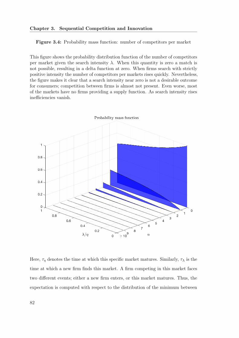
Chapter 3. Sequential Competition and Innovation
Figure 3.4: Probability mass function: number of competitors per market
This figure shows the probability distribution function of the number of competitorsper market given the search intensity λ. When this quantity is zero a match isnot possible, resulting in a delta function at zero. When firms search with strictlypositive intensity the number of competitors per markets rises quickly. Nevertheless,the figure makes it clear that a search intensity near zero is not a desirable outcomefor consumers; competition between firms is almost not present. Even worse, mostof the markets have no firms providing a supply function. As search intensity risesinefficiencies vanish.
Here, τη denotes the time at which this specific market matures. Similarly, τΛ is the
time at which a new firm finds this market. A firm competing in this market faces
two different events; either a new firm enters, or this market matures. Thus, the
expectation is computed with respect to the distribution of the minimum between
82
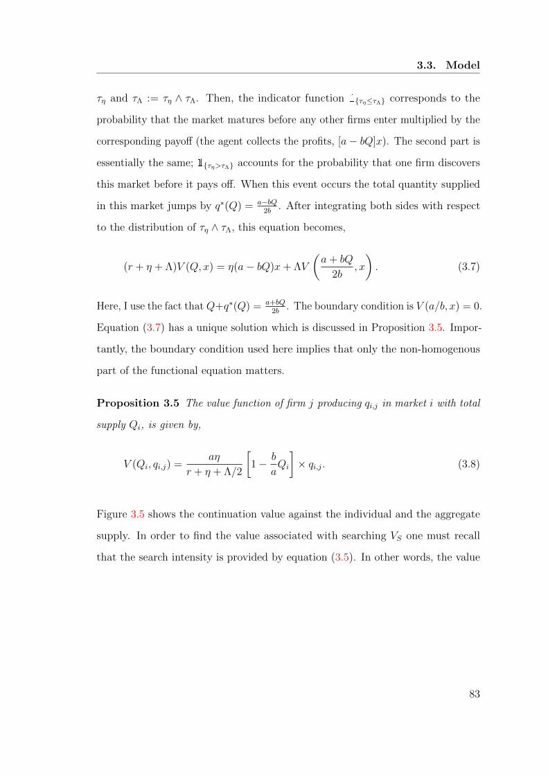
3.3. Model
τη and τΛ := τη ∧ τΛ. Then, the indicator function 1τη≤τΛ corresponds to the
probability that the market matures before any other firms enter multiplied by the
corresponding payoff (the agent collects the profits, [a− bQ]x). The second part is
essentially the same; 1τη>τΛ accounts for the probability that one firm discovers
this market before it pays off. When this event occurs the total quantity supplied
in this market jumps by q∗(Q) = a−bQ2b
. After integrating both sides with respect
to the distribution of τη ∧ τΛ, this equation becomes,
(r + η + Λ)V (Q, x) = η(a− bQ)x+ ΛV
(a+ bQ
2b, x
). (3.7)
Here, I use the fact that Q+q∗(Q) = a+bQ2b
. The boundary condition is V (a/b, x) = 0.
Equation (3.7) has a unique solution which is discussed in Proposition 3.5. Impor-
tantly, the boundary condition used here implies that only the non-homogenous
part of the functional equation matters.
Proposition 3.5 The value function of firm j producing qi,j in market i with total
supply Qi, is given by,
V (Qi, qi,j) =aη
r + η + Λ/2
[1− b
aQi
]× qi,j. (3.8)
Figure 3.5 shows the continuation value against the individual and the aggregate
supply. In order to find the value associated with searching VS one must recall
that the search intensity is provided by equation (3.5). In other words, the value
83

Chapter 3. Sequential Competition and Innovation
Figure 3.5: Value associated with competing in a market
This figure shows the value of competing in a market which depends on Q, theaggregate supply in this market and q, the individual supply.
0
10
5
810
10
6 8
15
64
20
42
2
0 0
of searching depends on the number of markets in which the firm is competing.
Accordingly, it must satisfy,
VS(N) = E
[e−r(τλ(N)∧τη×N)
1τλ(N)>τη×NVS(N − 1) +
1τλ(N)<τη×NVS(N + 1)
], N ≥ 1,
(3.9)
84

3.3. Model
and VS(0) = E [e−rτλ0VS(1)]. Here, τλ(N) denotes the time at which firm j,
competing in N markets, finds market N + 1. Upon finding a market a firm
produces the quantity q∗(Q) = a−bQ2b
, making the total production in this market
jump from Q to a+bQ2b
. Otherwise, τη×N denotes the time at which one market of
firm j pays off. After some algebra equation (3.9) becomes,
[r + (λ+ η)×N
]VS(N) = λ×NVS(N + 1) + η ×NVS(N − 1). (3.10)
When N = 0 the value associated with searching satisfies (r + λ0)VS(0) = λ0VS(1);
these firms receive the continuation value of competing in one market, discounted at
a rate adjusted by the entrepreneur’s search intensity. When N is large this equation
is well approximated by the following second order linear difference equation with
constant coefficients,
VS(N + 1)− λ+ η
λVS(N) +
η
λVS(N − 1) = 0.
The solution of this equation is VS(N) = AxN1 +BxN2 , where x1 = η/λ > 1, x2 = 1
and A and B are two constants. Hence, when N is large the following relation
holds,
log[VS(N)] = c+ log(x1)N,
where c is a constant. Figure 3.6 shows the continuation value associated with
searching. The value associated with searching increases exponentially with
N , which can be interpreted as the number of employees in the research and
development unit. Finally, let us define nj := 〈Qj,1, Qj,2, · · · , Qj,N〉 ∈ RN,1,
the vector of the aggregate supply in each market firm j is competing in and
xj := 〈qj,1, qj,2, · · · , qj,N〉 ∈ RN,1 the vector of its individual production. Then, the
85

Chapter 3. Sequential Competition and Innovation
Figure 3.6: Value associated with searching with n employees
This figure shows the value associated with searching with n employees. While theapproximation is not exact, I show in this paper that the log of this function isapproximately linear with a slope of log(x1), where x1 = η/λ.
0 100 200 300 400 500 600 700 800 900 1000
0
100
200
300
400
500
600
0 2 4 6 8 10 12 14 16 18 20
0
2
4
6
8
10
continuation value of a firm FV : RN,2 → RN,1 is given by,
FV (nj,xj) = VS(Nj) +N∑i=1
V (Qj,i, xj,i).
86
3.4. Implications of the Model
3.4 Implications of the Model
Given my characterization of the steady-state equilibrium above, it is possible to
derive many objects analytically. In this section I use my model as a laboratory and
focus on analytical results that are important to the literature. In Section 3.4.1 I
follow a market and characterize the probability distribution function of the number
of firms competing in a given market. Equipped with this object I can discuss
how competitors share the market and how this competition structure affects the
consumer welfare. I also relate these statistics with some of the exogenous variables
which are, for instance, the search intensity λ and η the rate at which products
are rolled over. In Section 3.4.2 I follow a firm and discuss the stationary firm size
distribution implied by my model and also discuss the consequences of having large
firms in an economy.
3.4.1 Following Markets
Since every market represents consumption needs it becomes apparent that some
of these will not be supplied with any products. The structure of the model makes
it clear that once we know Q0 and Q we can deduce the number of firms in that
market. Nevertheless, it is more interesting to infer the probability distribution
function given Q only. Thus, one can use that function ex ante to characterize any
expected variables related to markets.
Claim 3.1 The probability that i firms are competing in market j is given by,
P (N = i) :=η
Λ
(Λ
η + Λ
)i+1
.
This PDF is independent of the functional form of F (x). The probability P (N = 0)
87

Chapter 3. Sequential Competition and Innovation
corresponds to the likelihood that a market has no current supplier. Similarly, the
probability P (N = 1) corresponds to the likelihood that customers in a market
face a monopolist, etc. One can easily characterize the vector of market shares
[a1, · · · , aN ] in a particular market.
Claim 3.2 The market share of the ith > 0 firm is given by,
ai :=1
2− 21−N
(1
2
)i−1
.
A corollary of Proposition 3.1 is that the market share decreases geometrically.
Nevertheless, since the shares must sum up to one, one must adjust a1 such that
this equality is satisfied. Equipped with this I can obtain a measure reflecting
the market concentration; the Herfindhal index is an intuitive metric fulfilling this
purpose which is defined as the sum of the squared market shares.
Claim 3.3 The Herfindhal index in a market with N > 0 firms is given by,
H(N) := a21
N∑i=1
(1
4
)i−1
.
Combining the probability distribution function discussed here with the cross-
sectional distribution of markets I can find a new distribution reflecting, ex ante,
the measure of markets with exactly N firms competing in it. Then, associating
this with a concentration index I obtain the expected concentration across the
whole market space, which is shown in Figure 3.7. Finally, I compute two additional
important distributions in closed-form.
Claim 3.4 (ΦM(x) and Φq∗(x)) The cross-sectional distribution of markups ΦMt (x)
is defined as P(a − bX ≤ x) = P(X ≥ a−x
b
)= 1− Φt
(a−xb
). The cross-sectional
88

3.4. Implications of the Model
Figure 3.7: The model’s implied aggregate intensity and Herfindahl index
The figure shows different statistics from the model. The first panel plots theaggregate intensity, which is a strictly monotonic increasing function of λ in therange (0, η). The lower panel shows the expected Herfindahl index, which is ameasure of the competition in a market. Here I compute this quantity for allmarkets and weight these indexes by their respective probabilities. As might alsobe expected this quantity is decreasing with λ.
0 0.1 0.2 0.3 0.4 0.5 0.6 0.7 0.8 0.9 1
0.4
0.5
0.6
0.7
0.8
0.9
1
0 0.1 0.2 0.3 0.4 0.5 0.6 0.7 0.8 0.9 1
0.8
0.85
0.9
0.95
1
distribution of individual supply per market Φq∗
t (x) is defined as P(a−bX
2b≤ x
)=
P(X ≥ a
b− 2x
)= 1− Φt
(ab− 2x
).
The function ΦMt (x) characterizes the measure of markets where the markup m is
bounded bellow x. Written differently, there is a measure ΦMt (x) of markets with
89

Chapter 3. Sequential Competition and Innovation
markups m ≤ x. It is worth noting that markups are the same for all the firms
that are competing in the same market. This is the case because marginal cost is
constant across all markets and for all firms. The function Φq∗
t (x) characterizes
the distribution of the reaction function of firms; when a firm finds a market its
aggregate quantity is distributed according to Φt(x). Since the optimal response of
the entrant is to produce q∗(x), the distribution of the reaction before knowing the
exact aggregate market supply x is drawn from Φq∗
t (x).
3.4.2 Following Firms
The framework discussed in this paper enables me to model the firm-size process
explicitly; Section 3.3.4 treats this problematic in greater detail. The fact that
the size of firms follows a birth-death process renders possible the calculations of
the firm-size distribution in closed-form. I recall that the meeting rate of a firm
competing in n markets equals λ× n. Alternatively, n can be interpreted as the
number of employees working in that firm.
Claim 3.5 (Firm-size) The probability that a firm has i employees is proportional
to,
(λ
η
)i−1(1
i
), i > 0.
Importantly, the model predicts that above a critical size, which depends on how
close η and λ are to each other, the behaviour of the firm-size distribution changes
dramatically; the firm-size distribution is a mixture of a power law with a unit
exponent (a Zipf law) when i is small and an exponential distribution when i is
large. The closer λ is from η the longer the distribution behaves like a power law.
Nevertheless, for a stationary distribution to exist, λ must be smaller than η. Hence,
90

3.4. Implications of the Model
the distribution will always behave like an exponential distribution when i is large;
a larger λ will simply delay the change of regime. Figure 3.8 consists of two plots;
the upper panel shows the firm-size distribution for different levels of the search
intensity λ. Since η is fixed, the higher λ the longer it takes for the exponential
part to come into play. The second panel illustrates the firm-size distribution when
η ≈ λ; here the power law clearly dominates the exponential part. Hence, as long
as λ is maintained close to η the endogenous firm-size distribution is consistent with
what is seen in the data. The question then arises “When do large firms appear
larger than the others?”. Is it when λ is small or when λ ≈ η? It turns out that
the higher λ the larger large firms compared to average-sized firms. This relation is
illustrated in Figure 3.9, which is computed by normalizing the average size of large
firms (above xth percentile) by the average size. For 0 < λ < η, the probability of
n being larger than x is, P(n ≥ x) = λ0
λS
∑∞i=x
(λη
)i1i. Therefore I can find x by
solving the fixed-point equation P(n ≥ x) = 1− xth. Then the average firm size of
the firms that are above the xth percentile equals λ0
λS
∑∞i=x
(λη
)i1+1i
. After some
algebra the average firm size of the top firms becomes,(λη
)xL(λ/η, 1, x).
Claim 3.6 The ratio of the average size of large firms normalized by the average
size of all firms satisfies,
η
η − λL−1(λ/η, 1, x).
where L(z, s, a) :=∑∞
k=1zk
(a+k)sis the so-called Lerch Transcendent function and x
satisfies P(n ≥ x) = 1− xth.
When λ is zero there are only two types of firm; either the entrepreneur is alone,
or the firm has one employee, which implies that the largest firms have at most
91

Chapter 3. Sequential Competition and Innovation
Figure 3.8: The model’s implied stationary firm-size distribution
This figure shows the stationary firm-size distribution for different levels of λ. Asdiscussed in this paper, the function behaves proportionally to a power law for lowi and proportionally to an exponential distribution when i is large. The secondplot treats the case when λ = 0.9999η.
100
101
102
103
10-50
100
100
101
102
103
10-5
100
two workers. Taking the percentile high enough the average firm size above that
threshold is two while the average firm size equals η+2λ0
η+λ0.
3.4.3 The Model With Fixed-Costs
In this paper I design a model where firms do not face fixed costs upon entering a
market. This assumption makes the model highly tractable since the strategy of
92

3.4. Implications of the Model
Figure 3.9: The model’s implied ratio of the largest firms to the average-sizedfirm
This figure shows the model’s implied ratio of the largest firms to the average-sizedfirm for different levels of λ. As discussed in this paper, this function behavesproportionally to a power law for low i and proportionally to an exponentialdistribution when i is large. The second plot treats the case when λ = 0.9999η.
0 0.1 0.2 0.3 0.4 0.5 0.6 0.7 0.8 0.9 1
0
5
10
15
20
25
30
0 0.1 0.2 0.3 0.4 0.5 0.6 0.7 0.8 0.9 1
0
5
10
15
20
entrants is relatively trivial, as exhibited in Proposition 3.1. Thus, a firm invests in
these projects that only have positive net present value. Though this assumption
is fairly realistic in the Tech area, it is less so in other fields. Accordingly, I will
discuss what occurs when this assumption is relaxed.
93

Chapter 3. Sequential Competition and Innovation
3.4.3.1 Generalities
When fixed costs are introduced into the model incumbents have to take into
consideration the impact of their strategies on the entry decision of potential
competitors. In Etro (2008) the entry decision is endogenous and the behaviour
of the leader is very different from the traditional behaviour. Instead of being
concerned with the reaction of competitors to its supply the leader focuses on the
entry decision and becomes significantly more aggressive. This paper shows that
when goods are homogeneous and marginal costs are constant the leader finds it
optimal to increase output until no rivals want to enter. Here, because entrants
show up only with some probabilities incumbents will behave somewhere in between
these two scenarios. Moreover, I also need some conditions on the level of the fixed
costs c which are discussed in Assumption 3.1.
Assumption 3.1 (Nontrivial solution) c ≤(a4
)2 1b.
In order to guarantee the existence of a nontrivial solution (when c > 0) I need
Assumption 3.1 to hold. To see why assume it does not; then, q∗∗ := ab− 2√bc >
q∗ := a2b
. Thus, an incumbent that chooses the monopoly quantity is guaranteed
never to face entrants. Hence, given Assumption 3.1 holds, let us further assume for
illustrative purposes that at most three firms can enter in market i and the value
associated with searching does not matter (the case with VS is treated separately
later). Additionally, let us call the first firm to enter A, the second B and the
third C. Firm C will always act as discussed earlier and produce q∗(Q) = a−bQ2b
,
Q = qA + qB. However, if Q ≥ Q∗ := ab− 2√
cb, then q∗(Q) ≤ 0. Hence, firm
C chooses q∗ = 0. Building on this B has the option to preclude the entrance
of C by choosing q∗∗ := a−qAb− 2√
cb, where qA is the quantity produced by A.
In this case the profit of firm B is π∗∗B = 2(a − bqA)√
cb− 5c. If B chooses not
94

3.4. Implications of the Model
to prevent C from entering B chooses q∗ := a−bqA2b
and makes an expected profit
of π∗B := (a−bqA)2
4b
(1− 1
2ρ)− c. Therefore, B will choose q∗ if π∗B ≥ π∗∗B and q∗∗
otherwise. Let us assume now that B do not preclude the entrance of C; then
A can allow other firms to enter by choosing q∗ = a2b
or preclude entrants from
joining with q∗∗ = ab− 2√
cb. However, the actions of B must be consistent (i.e. A
chooses its quantity by presuming B will not preclude C). Lastly, in the case that
B does not let C enter, A can preclude B from entering as well by choosing q∗∗. If
A chooses not to do so its quantity must be consistent with the behaviour of B.
Thus, A chooses q∗∗∗ := a2b
+ ρ1−ρ√
cb> q∗4. What matters here is that, conditional
on the behaviour of its followers, A will produce at least the monopolist quantity q∗
(which corresponds almost one-to-one to the no fixed-costs model). If A precludes
competitors from entering into the market consumers will immediately receive Q∗,
which makes them strictly better off. Alternatively, the leader can also presume
that one of its followers could enter and itself saturate the market. Here again
consumers are better off since q∗∗∗ > q∗.
When leaders always preclude the entrance of their followers the dynamics of the
cross-sectional probability mass function (PMF) of markets satisfies5,
pt(0) = η − (η + Λ)pt(0),
pt(Q∗) = Λpt(0)− ηpt(Q∗).
Hence, the stationary PMF is given by,
p(0) = ηη+Λ
,
p(Q∗) = Λη+Λ
.
4It is worth noting that in a three firm model as long as b ≤ 1 the leader will always preclude theentrance of its followers knowing that the 2nd firm will exclude the 3rd.
5Assuming no heterogeneity across markets.
95

Chapter 3. Sequential Competition and Innovation
Therefore, the higher the search intensity the higher the consumer surplus. Building
on Sections 3.3.4 and 3.3.5, a firm finding a market has a probability p(Q∗) that
it is already saturated. Thus, the search intensity at which a firm finds a non-
saturated market is λt,j×p0. Substituting that rate into the infinitesimal generator
of the birth-death process the aggregate search intensity Λ satisfies,
Λ∞ =Aηλ0 × p0
λ0 × p0 + S(η − λ× p0), S = 1− λ0
λlog
(1− λ× p0
η
).
3.4.3.2 Impact of Searching on the Equilibrium Strategy
In this section I discuss a model where firms only produce in non-saturated markets;
if joining a market is a positive NPV project, the firm enters. If the entry costs are
higher than the benefits associated with joining that market the firm abstains from
starting production. Alternatively, firms could take into consideration that joining
a market that would not appear profitable at first can be optimal; by growing,
the value associated with searching increases. Hence, the decision to enter is no
longer static; it depends on the number of markets the firm is competing in. If
VS(N) ≥ VS(N + 1)− c the firm does not enter. Nevertheless, if the gain associated
with entering that market covers the entry cost, the firm will join. When a firm
uses this strategy small firms are more affected by fixed costs than large firms.
Since VS(N) behaves approximately as xN1 , any N larger than log(
cx1−1
)/ log(x1)
would make a firm of that size always willing to enter, no matter the loss that will
materialize. On the other hand an entrepreneur would not adopt this strategy.
In this alternative economy the number of active firms is even smaller. This
problematic is reinforced when large firms can influence the entrance costs; by
setting it higher their decision to enter is not affected, while small firms are even
96

3.5. Concluding Remarks
more reluctant to enter. Hence, large firms tend to over invest while small firms are
inactive. In my framework the economy is not impacted by such deadweight costs.
Moreover, since the measure of active firms is larger consumers end up better off.
This discussion clarifies how bad anti-competitive practices are and in particular
dumping. It is worth noting that when this behaviour is banned my framework is
more realistic and, because the law prohibits dumping, it is consistent to assume
that such strategies cannot be part of any equilibrium outcome.
3.5 Concluding Remarks
In this paper I design a dynamic model where firms are endowed with a search
technology which they use for creating new products. Firms compete sequentially
in segmented markets, taking into account the strategies of potential entrants to
determine their respective actions. Assuming a linear price-inverse demand function,
homogenous goods and constant marginal costs make the model easily tractable
and the stationary cross-sectional distribution of quantities in each market solvable
in closed-form. With these assumptions the firm-size process belongs to the class
of birth-death processes, which make the aggregate matching rate and the firm-size
distribution solvable in closed-form as well. Building on this framework I can
compute many objects of potential interest such as some measures of concentration
within and across markets, the cross-sectional distribution of markups or the
continuation value of firms. All these implications are discussed in great detail and
can be tested empirically.
My paper tackles the problematic of large companies and, specifically, the conse-
quences that they have on consumer welfare. My model suggests that the rise of
large entities is part of a natural mechanism; the firm-size distribution will always
97

Chapter 3. Sequential Competition and Innovation
be a mixture of a power law and a distribution with exponential decay. My results
clearly advocate that the closest λ is to η, the largest is the aggregate intensity.
Hence, the fatter the tails the greater the consumer welfare. At first, this result
might seem surprising. Indeed, companies grow by cannibalizing others; if the
measure of firms is small one can expect corporations to act as a monopolist. It
turns out that under sequential competition, as modeled here, each entity behaves
as a monopolist facing a residual demand curve. Therefore, they all operate like
monopolists and hope no one else will join. The only credible way for incumbents
to preclude the entrance of opponents is to saturate the market, which is even
better for consumers. Thus, though the measure of firms is smaller, consumers
are better off when the matching rate increases, because the average number of
entities in each market is larger. With fixed costs, the reasoning still applies though
the intuition is slightly different; consumers are better off because the measure of
saturated markets increases with the aggregate search intensity.
In general, one sees entry costs as an anti-competitive toolkit that is used in order
to keep opponents outside of their respective markets. While this statement is true
my model shows that it is not necessarily at the expense of consumers. Indeed, with
sequential competition the only way for the incumbent to preclude the entrance
of rivals is to adopt a strategy that makes the reservation value associated with
joining that market lower than their reservation value. Here, the incumbent has to
choose a quantity that would immediately saturate the market (no one would have
entered beyond that point, no matter the structure of the market).
Finally, a question raised initially was related to whether big technological compa-
nies are impairing consumer welfare. While these companies spend large amounts of
capital for acquiring start-ups it is fair to see this strategy as a way to preclude the
entrance of potential competitors. Though in the short-run this behaviour is indeed
98

3.5. Concluding Remarks
problematic my model suggests that the firm-size distribution and specifically the
rise of large corporations is a natural mechanism. Down scaling these entities will
result in other rivals taking their dominant place. More importantly, if Amazon,
Facebook and Co. acquire start-ups with the aim of maintaining their relative
position they can only expand at a suboptimal growth rate and will eventually be
replaced by organizations that have not engaged in these types of misconduct.
99

Chapter 3. Sequential Competition and Innovation
3.A Proof
Proof of Proposition 3.1. Let N ≥ 1 be the number of firms competing in i.
Moreover, Qi,j is the quantity produced in market i before firm j enters. Assume
firm j enters and knows no other firm will join that market afterwards. Then, the
profit function of firm j in market i is,
πj(qi,j, Qi,j) = qi,j(a− b[qi,j +Qi,j]).
Firm j chooses qi,j := argmaxπj(qi,j, Qi,j). Rearranging the first-order condition
(FOC), the optimum is q∗i,j(Qi,j) =a−bQi,j
2b. Moreover, because πj is a second order
polynomial uniqueness is guaranteed and it is sufficient to show that∂2πj(qi,j ,Qi,j)
∂q2i,j
< 0
to prove that q∗i,j is a maximum, which is true since it equals −b < 0. Now, take
firm j − 1. This is the very last firm which joined market i before firm j. Firm
j − 1 chooses its strategy without knowing if firm j will find that market or not.
The profit function of firm j − 1 in market i satisfies,
πj−1(qi,j−1, Qi,j−1) = qi,j−1(a− b[qi,j−1 +Qi,j−1 + ρqi,j]), Qi,j = Qi,j−1 + qi,j−1,
where ρ is defined as the probability that firm j enters (in this model it equals
Λ/(η + Λ)). Substituting q∗i,j(Qi,j), the profit function can be rewritten as follows,
πj−1(qi,j−1, Qi,j−1) = qi,j−1
(1− ρb
2
)(a− b[qi,j−1 +Qi,j−1]),
Accordingly, the optimal strategy of firm j−1, taking into account firm j’s strategy,
is to produce,
q∗i,j−1(Qi,j−1) =a− bQi,j−1
2b.
100

3.A. Proof
Finally, take firm n which entered just before firm n+1. Firm n chooses its optimal
quantity without knowing if firms ≥ n would eventually enter or not. The profit
function of firm n in market i satisfies,
πn(qi,n, Qi,n) = qi,n(a− b[qi,n +Qi,n + qi,n+1]).
Substituting q∗i,n+1(Qi,n) the profit function can be rewritten as follows,
πn(qi,n, Qi,n) = qi,n
(1− ρb
2
)(a− b[qi,n +Qi,n]).
Accordingly, the optimal strategy for firm n, taking into account the strategy of all
following firms is to produce,
q∗i,n(Qi,n) =a− bQi,n
2b.
This confirms what Anderson and Engers (1992) show: when the price-inverse
demand function is linear each firm behaves as a monopolist facing a residual
demand curve inherited from its predecessors. However, one must also consider a
strategy in which incumbents choose their supply in order to prevent the entrance
of new firms. Because I assumed that there are no fixed costs, the only quantity
that would make a new entrant not willing to enter is when q = a/b, which makes
the incumbent’s profit equal to zero. Thus, this strategy will never be adopted in
equilibrium since it makes them worse off.
Proof of Lemma 3.1. Let x = ψ(y) and f(x) = ψ(y + 1). Substituting x and
f(x) into h(f(x)) = h(x) + 1, Abel shows that this equation can be rewritten as,
psi(y + 1) = f(ψ(y)). Using f(x) = a + bx and substituting successively y + 1,
101

Chapter 3. Sequential Competition and Innovation
y + 2, etc., the previous equation becomes,
ψ(y + n) = an−1∑i=0
bi + bnψ(y).
Letting y = 0 and ψ(0) = c, this equation becomes ψ(y) = a∑y−1
i=0 bi + byc, which
must be equal to a+ bx. Taking the reciprocal of that function leads to,
h(x) =log(a+x(b−1)a+c(b−1)
)log(b)
.
Proof of Lemma 3.2. Taking the base s logarithm of g(f(x)) = sg(x) on both
sides, this equation becomes h(f(x)) = h(x) + 1, which is the Abel equation
discussed in Lemma 3.1. Thus, Lemma 3.1 implies g(x) = sh(x).
Proof of Proposition 3.2. The homogenous part of equation 3.3 is a Schroder’s
Equation. Using Lemma 3.2, the solution of that equation is,
ΦG(q) = C ×(η + Λ
Λ
)α(q)
, α(x) =log(x− a/b)
log(2)− 1.
Similarly, the inhomogeneous part of equation 3.3 is solved by the particular
solution,
ΦP (q) =b
a
η
η − Λq − Λ
η − Λ.
The uniqueness of the Abel Equation guarantees the uniqueness of equation (3.3).
The treatment of the boundary condition is slightly more complex since there is
one condition for each quantity q0 (the initial quantity in a particular market).
102

3.A. Proof
Thus, the path of the aggregate quantity in that market can only take values on
the set Q(q0)i∈0,1,··· ,imax, where Q(q0) = (2i−1)a+bq02ib
and imax are to be defined.
In other words, when computing the constant one must bear in mind that there
is exactly one path for each q0 ∈ [0, a2b
[. For instance, take Qmax ≡ ba
= 10 and
QF = 8. I recall that the optimal strategy is to produce q∗(Q) = a−bQ2b
. Therefore,
knowing that Q+ q∗(Q) must equal Q′, we can find Q := 2×Q′ − a/b. Given i,
the number of firms in the market, Q is simply,
Q(i) = 2i ×Q′ − (2i − 1)a
b. (3.11)
Using this one knows there are at most two firms in my example; the new firm
produces 2 = q∗(Q), while the first firm produces 4 = q∗(Q(2)), which leads to
q0 = 2 > 0. Hence, using the appropriate boundary condition the constant C must
satisfy the following equation,
η
η + Λ
b
a2 = C ×
(η + Λ
Λ
)α(2)
+b
a
η
η − Λ2− Λ
η − Λ,
which is the same for any market that can reduce to q0 = 2 (i.e. Q ∈ 2, 6, 8). I
show in the following lines that it is possible to automate this procedure. Let us
choose i ≥ 0 such that i satisfies the following inequality,
2i − 1
2ia
b≤ Q ≤ 2i+1 − 1
2i+1
a
b.
Then, the maximal number of firms competing in a market with total quantity
Q is i. In general, finding i with respect to Q simply requires to take the floor
function of the following functional equation,
h(f(Q)) = h(Q) + 1, f(Q) =a+ bQ
2b. (3.12)
103

Chapter 3. Sequential Competition and Innovation
The unique solution of this Abel equation is h(x) = − log(1−xb/a)log(2)
= −α(x). Thus,
equation (3.11) can be rewritten as follows g(x) = 2b−α(x)cx − (2b−α(x)c − 1)ab.
Finally, α(x) returns an imaginary part. It can be rearranged as follows,
α(x) =log(−ab
)log(2)︸ ︷︷ ︸/∈ R
+log(1− x b
a
)log(2)
− 1︸ ︷︷ ︸≡α(x)
,
which still returns an imaginary part. Nevertheless, once plugged into the cross-
sectional distribution the complex part cancels out.
Proof of Proposition 3.3. First of all I recall that the cross-sectional distribution
is a piecewise function. For x ∈[0, a
2b
], Φt(x) satisfies,
Φt(x) = ηF (x)− (η + Λ(t))Φt(x). (3.13)
This is a first-order linear differential equation. I conjecture that Λ is a function of
time only and later verify that this is true. Thus, the stability of Φt(x) can be treated
under the assumption that Λ(t) = Λ (I could alternatively write Λ :=∫ t
0Λ(u)du).
Thus, the solution of (3.13) is given by,
Φt(x) =η
η + ΛF (x) + c(x) exp[−(η + Λ)t],
where c(x) is a function that depends only on x. As t → ∞, Φt(x) → Φ(x), if
η + Λ > 0, which is true by construction. Assuming now that 3a4b≥ x ≥ a
2b, the
cross-sectional distribution satisfies,
Φt(x) = ηF (x)− (η + Λ(t))Φt(x) + Λ(t)Φ(2x− a/b). (3.14)
Since 2x− a/b ≤ a2b
, Φt(2x− a/b) = ηη+Λ
F (2x− a/b) + c(2x− a/b) exp[−(η + Λ)t].
104

3.A. Proof
Therefore, using the assumption made above equation (3.14) can be rewritten as
follows,
Φt(x) = ηF (x)−(η+Λ)Φt(x)+Λ
[η
η + ΛF (2x− a/b) + c(2x− a/b) exp[−(η + Λ)t]
].
This is a first-order linear differential equation, where the non-homogenous part
is a function of x only and an exponential of t, with the same exponent as in
the homogenous part. Thus as t → ∞, Φt(x) → Φ(x), if η + Λ > 0. Hence
the function Φt(x), for x ∈[a2b, 3a
4b
]has a unique stationary distribution, which
is globally attractive. By applying the same argument iteratively, it follows that
Φt(x), x ∈ (0, a/b) can be rewritten as a first-order linear differential equation,
where the condition regarding stability is reduced to η + Λ > 0. Therefore, I
conclude that the cross-sectional distribution of markets has a unique fixed point
which is globally stable.
Proof of Proposition 3.4. The firm-size process is a so-called birth-death pro-
cess (BDP). Using standard results coming from this area, a BDP with infinitesimal
generator Q defined as,
Q :=
−λ0 λ0
η1 −(η1 + λ1) λ1
η2 −(η2 + λ2) λ2
. . .. . .
. . .
ηN −(ηN + λN ) λN
,
has a unique stationary distribution if and only if the following condition is satisfied;
S = 1 +∞∑i=1
∏i−1j=0 λj∏ij=1 η1
<∞.
105

Chapter 3. Sequential Competition and Innovation
Using my generator this condition can be rewritten as,
S = 1 +λ0
η
∞∑i=1
(λ
η
)i−11
i= 1− λ0
λlog
(1− λ
η
)<∞.
When this condition is satisfied it is again standard in the BDP literature that the
cross-sectional distribution can be rewritten as the one presented in Proposition
3.4.
Proof of Proposition 3.5. The homogenous part of equation 3.7 is a Schroder’s
Equation. Using Lemma 3.2 the solution of that equation is,
ΦG(Q) = C ×(r + η + Λ
Λ
)−α(Q)
, α(x) =log(1− x b
a
)log(2)
.
Similarly, the inhomogeneous part of equation 3.7 is solved by the particular
solution,
ΦP (Q, q) =aη
r + η + Λ/2
[1− b
aQ
]× q.
Then the treatment of the boundary condition implies that C = 0 for all paths
and thus Φ(Q, q) = ΦP (Q, q).
106

4 Bibliography
Bibliography
Acemoglu, D. (2008). Introduction to Modern Economic Growth. Princeton, NJ:
Princeton Univ. Press.
Acharya, V., Shin, H.-S., and Yorulmazer, T. (2013). A theory of arbitrage capital.
Review of Corporate Financial Studies, 2(1):62–97.
Afonso, G. and Lagos, R. (2015). Trade dynamics in the market for federal funds.
Econometrica, 83:263–313.
Allen, F. and Gale, D. (1994). Limited market participation and volatility of asset
prices. The American Economic Review, 84(4):933–955.
Allen, F. and Gale, D. (2004). Financial intermediaries and markets. Econometrica,
72(4):1023–1061.
Allen, F. and Gale, D. (2005). From cash-in-the-market pricing to financial fragility.
Journal of the European Economic Association, 3(2-3):535–546.
Andersen, T. G., Bollerslev, T., Diebold, F. X., and Ebens, H. (2001). The
distribution of realized stock return volatility. Journal of Financial Economics,
61:43–76.
Anderson, S. P. and Engers, M. (1992). Stackelberg versus cournot oligopoly
equilibrium. International Journal of Industrial Organization, 10:127–135.
107

Chapter 4. Bibliography
Autor, D., Dorn, D., Katz, L. F., Patterson, C., and Reenen, J. V. (2017). The fall
of the labor share and the rise of superstar firms.
Bacchetta, P., Tille, C., and van Wincoop, E. (2010). Self-fulfilling risk panics.
American Economic Review.
Baillie, R. T. and DeGennaro, R. P. (1990). Stock returns and volatility. Journal
of Financial and Quantitative Analysis, 25(2):203–214.
Bandi, F. M. and Perron, B. (2008). Long-run risk-return trade-offs. Journal of
Econometrics, 143(2):349–374.
Bansal, R. and Lundblad, C. (2002). Market efficiency, asset returns, and the
size of the risk premium in global equity markets. Journal of Econometrics,
109(2):195–237.
Banz, R. W. (1981). The relationship between return and market value of common
stocks. Journal of Financial Economics, 9(1):3–18.
Basu, S. (1977). The investment performance of common stocks in relation to their
price/earnings ratio: A test of the efficient market hypothesis. The Journal of
Finance, 32(3):663–682.
Black, F., Jensen, M. C., and Scholes, M. (1972). Studies in the Theory of Capital
Markets, chapter The Capital Asset Pricing Model: Some Empirical Tests. New
York: Praeger.
Boguth, O., Carlson, M., Fisher, A., and Simutin, M. (2010). Conditional risk and
performance evaluation: Volatility timing, overconditioning, and new estimates
of momentum alphas.
Bollerslev, T. (1986). Generalized autoregressive conditional heteroskedasticity.
Journal of Econometrics, 31(3):307–327.
Bondt, W. F. M. D. and Thaler, R. H. (1987). Further evidence on investor
overreaction and stock market seasonality. The Journal of Finance, 42(3):557–
581.
Bonomo, M., Garcia, R., Meddahi, N., and Tedongap, R. (2015). The long and
the short of the risk-return trade-off. Journal of Econometrics, 187(2):580–592.
108

Bibliography
Burdett, K. and Vishwanath, T. (1988). Balanced matching and labor market
equilibrium. The Journal of Political Economy, 96(5):1048–1065.
Campbell, J. Y. and Hentschel, L. (1992). No news is good news: An asymmetric
model of changing volatility in stock returns. Journal of Financial Economics,
31(3):281–318.
Carhart, M. M. (1997). On persistence in mutual fund performance. The Journal
of Finance, 52(1):57–82.
Chou, R. Y. (1988). Volatility persistence and stock valuations: Some empirical
evidence using garch. Journal of Applied Econometrics, 3(1):279–294.
Christoffersen, P. F., Diebold, F. X., and Schuermann, T. (1998). Horizon problems
and extreme events in financial risk management. Economic Policy Review, pages
109–118.
Diamond, P. A. (1982). Aggregate demand management in search equilibrium.
Journal of Political Economy, 90(5):881–894.
Duffie, D., Garleanu, N., and Pedersen, L. H. (2005). Over-the-counter markets.
Econometrica, 73(6):1815–1847.
Duffie, D., Garleanu, N., and Pedersen, L. H. (2007). Valuation in over-the-counter
markets. The Review of Financial Studies, 20(6):1865–1900.
Duffie, D. and Strulovici, B. (2012). Capital mobility and asset pricing. Economet-
rica, 80(6):2469–2509.
Engle, R. F. (1982). Autoregressive conditional heteroscedasticity with estimates
of the variance of united kingdom inflation. Econometrica, 50(4):987–1007.
Engle, R. F. and Bollerslev, T. (1986). Modelling the persistence of conditional
variances. Econometric Reviews, 5(1):1–50.
Etro, F. (2008). Stackelberg competition with endogenous entry. The Economic
Journal, 118(532):1670–1697.
Fama, E. F. and French, K. R. (1992). The cross-section of expected stock returns.
The Journal of Finance, 47(2):427–465.
109

Chapter 4. Bibliography
Fama, E. F. and French, K. R. (1993). Common risk factors in the returns on
stocks and bonds. Journal of Financial Economics, 33(1):3–56.
Fama, E. F. and MacBeth, J. D. (1973). Risk, return, and equilibrium: Empirical
tests. Journal of Political Economy, 81(3):607–636.
Frazzini, A. and Pedersen, L. H. (2013). Betting against beta. Journal of Financial
Economics, 48(3):261–297.
French, K. R., Schwert, G. W., and Stambaugh, R. F. (1987). Expected stock
returns and volatility. Journal of Financial Economics, 19(1):3–29.
Gabaix, X. (2009). Power laws in economics and finance. The Annual Review of
Economics, 1:255–293.
Gabaix, X. (2016). Power laws in economics: An introduction. The Journal of
Economic Perspectives, 30(1):185–206.
Glosten, L. R., Jagannathan, R., and Runkle, D. E. (1993). On the relation between
the expected value and the volatility of the nominal excess return on stocks. The
Journal of Finance, 48(5):1779–1801.
He, X., Prasad, A., Sethi, S. P., and Gutierrez, G. J. (2007). A survey of stackelberg
differential game models in supply and marketing channels. J Syst Sci Syst Eng,
16(4):385–413.
Hedegaard, E. and Hodrick, R. J. (2016). Estimating the risk-return trade-off with
overlapping data inference q. Journal of Banking and Finance, 67(1):135–145.
Hopenhayn, H. A. (1992). Entry, exit, and firm dynamics in long run equilibrium.
Econometrica, 60(5):1127–1150.
Hugonnier, J., Lester, B., and Weill, P.-O. (2016). Heterogeneity in decentralized
asset markets.
Julien, L. A. (2011). A note on stackelberg competition. The Journal of Economics,
103(2):171–187.
Julien, L. A., Musy, O., and Saıdi, A. W. (2011). Do followers really matter in
stackelberg competition?
110

Bibliography
Kondor, P. (2009). Risk in dynamic arbitrage: The price effects of convergence
trading. The Journal of Finance, 64(2):631–655.
Loecker, J. D. and Eeckhout, J. (2017). The rise of market power and the
macroeconomic implications.
Lundblad, C. (2007). The risk return tradeoff in the long run: 1836-2003. Journal
of Financial Economics, 85(1):123–150.
Luttmer, E. G. (2006). Consumer search and firm growth.
Luttmer, E. G. (2010). Models of growth and firm heterogeneity. The Annual
Review of Economics, 2:547–576.
Luttmer, E. G. (2011). On the mechanics of firm growth. Review of Economic
Studies, 78:1042–1068.
Ma, J., Nelson, C. R., and Startz, R. (2007). Spurious inference in the garch(1,1)
model when it is weakly identified. Studies in Nonlinear Dynamics and
Econometrics, 11(1):1–27.
Malamud, S. and Vilkov, G. (2018). Non-myopic betas. Journal of Financial
Economics.
Malkhozov, A., Mueller, P., Vedolin, A., and Venter, G. (2014). International
liquidity capm.
Nelson, D. B. (1991). Conditional heteroskedasticity in asset returns: A new
approach. Econometrica, 59(2):347–370.
Ricardo, L., Rocheteau, G., and Weill, P.-O. (2011). Crises and liquidity in
over-the-counter markets. Journal of Economic Theory, 146(6):2169–2205.
Robson, A. J. (1990). Stackelberg and marshall. The American Economic Review,
80(1):69–82.
Rosenberg, B., Reid, K., and Lanstein, R. (1985). Persuasive evidence of market
inefficiency. The Journal of Portfolio Management, 11(3):9–16.
Ross, S. A. (1976). The arbitrage theory of capital asset pricing. Journal of
Economic Theory, 13(3):341–360.
111
Chapter 4. Bibliography
Schwert, G. W. (2003). Handbook of the Economics of Finance, chapter Anomalies
and Market Efficiency. Elsevier Science.
Serlenga, L., Shin, Y., and Snell, A. (2001). A panel data approach to testing
anomaly effects in factor pricing models.
Shleifer, A. and Vishny, R. W. (1992). Liquidation values and debt capacity: A
market equilibrium approach. The Journal of Finance, 47(4):1343–1366.
Shleifer, A. and Vishny, R. W. (1997). The limits of arbitrage. The Journal of
Finance, 52(1):35–55.
Stahl, D. O. (1989). Oligopolistic pricing with sequential consumer search. The
American Economic Review, 79(4):700–712.
Vayanos, D. and Wang, T. (2007). Search and endogenous concentration of liquidity
in asset markets. Journal of Economic Theory, 136:66–104.
Vayanos, D. and Weill, P.-O. (2008). A search-based theory of the on-the-run
phenomenon. The Journal of Finance, 63(3):1361–1398.
von Stackelberg, H. (1934). Marktform und Gleichgewicht. J. Springer.
Wawro, G. (2009). Advanced topics in maximum likelihood models for panel and
time-series cross-section data. In 2009 ICPSR Summer Program.
Weill, P.-O. (2007). Leaning against the wind. Review of Economic Studies,
74:1329–1354.
112

5 Curriculum Vitae
Julien Blatt
Ecole Polytechnique Federale de Lausanne
Swiss Finance Institute at EPFL
Quartier UNIL-Dorigny, Extranef 129
CH-1015 Lausanne, Switzerland
Phone: +41 79 342 94 24
Email: [email protected]
5.1 Research Interests
Corporate Finance, Market Microstructure, Financial Economics, Continuous-
Time Asset Pricing, Portfolio Selection, behavioural Economics, Machine Learning,
Macroeconomics.
113

Curriculum Vitae
5.2 Education
8/2014 –11/2018: PhD Candidate in Finance, Swiss Finance Institute @ EPFL,
Switzerland.
Advisor : Prof. Semyon Malamud
1/2018–4/2018 Visiting Scholar, Mccombs School of Business, UT Austin.
Sponsor : Prof. William Fuchs.
2012–2014: M.Sc. in Finance, HEC Lausanne, Switzerland.
2009–2012 B.Sc. in Economics, HEC Lausanne, Switzerland.
5.3 Professional Experience
08/2016–11/2018: Lead Trainer for the Swiss Banking School Certification technical
contents of the Wealth Management Profiles in French, Swiss Finance Institute.
09/2015–11/2018: Teaching Assistant, Real Options and Financial Structuring,
M.Sc. in Financial Engineering, EPFL.
09/2013–02/2014:Teaching Assistant, Mathematics, M.Sc. in Finance, HEC
Lausanne.
09/2010–08/2013:Teaching Assistant, Microeconomics, Macroeconomics, Finance,
B.Sc. in Economics, HEC Lausanne.
09/2009–11/2018: Project Manager, ORCEF SA, Switzerland.
114

5.4. Working Papers
5.4 Working Papers
“Slow Arbitrage”
“Sequential Competition and Innovation”
“The RiskMetrics Anomaly”
5.5 Conference Presentations
“Sequential Competition and Innovation”, Seminar, University of Texas at Austin,
2018
“Slow Arbitrage”, Brownbag, University of Lausanne, 2017
5.6 Honors & Awards
M.Sc. in Finance, University of Lausanne, “Summa Cum Laude”, 2014
B.Sc. in Economics, University of Lausanne, “Magna Cum Laude”, 2012
5.7 Other Information
Swiss Citizen
5.7.1 Languages
French: mother tongue
English: fluent
German: good understanding and basic spoken knowledge
115

Curriculum Vitae
5.7.2 Computer Skills
Mathematica, Matlab, R , Python, Stata, C++, Latex, Office, VBA.
5.8 References
These persons are familiar with my personality, research, and teaching skills.
Associate Professor Semyon Malamud Professor Erwan Morellec
Ecole Polytechnique Federale de Lausanne Ecole Polytechnique Federale de Lausanne
Quartier UNIL Dorigny, Extranef Quartier UNIL Dorigny, Extranef
CH-1015 Lausanne CH-1015 Lausanne
Switzerland Switzerland
Phone: +41 21 693 01 37 Phone: +41 21 693 01 16
Email: [email protected] Email: [email protected]
Associate Professor Julien Hugonnier Professor Norman Schurhoff
Ecole Polytechnique Federale de Lausanne Universite de Lausanne
Quartier UNIL Dorigny, Extranef Quartier UNIL Dorigny, Extranef
CH-1015 Lausanne CH-1015 Lausanne
Switzerland Switzerland
Phone: +41 21 693 01 14 Phone: +41 21 692 34 47
Email: [email protected] Email: [email protected]
Associate Professor Julien Cujean Dr. Christoph Gosdenoz
University of Bern Director Continuing Education, SFI
Engehaldenstrasse 4 Walchestrasse 9
CH-3012 Bern CH-8006 Zurich
Switzerland Switzerland
Phone: +41 31 631 38 53 Phone: +41 44 254 30 58
Email: [email protected] Email: [email protected]
Lausanne, September 29, 2018
116