Essays on Macroeconomics - DiVA
469
Essays on Macroeconomics José Elías Gallegos Dago Institute for International Economic Studies Monograph Series No. 115 Doctoral Thesis in Economics at Stockholm University, Sweden 2022
-
Upload
khangminh22 -
Category
Documents
-
view
0 -
download
0
Transcript of Essays on Macroeconomics - DiVA

Essays on Macroeconomics José Elías Gallegos Dago
José Elías Gallegos D
ago Essays on M
acroeconom
ics115
Institute for International Economic StudiesMonograph Series No. 115
Doctoral Thesis in Economics at Stockholm University, Sweden 2022
Department of Economics
ISBN 978-91-7911-882-2ISSN 0346-6892
José Elías Gallegos Dagoholds a M.Sc. in Economics fromUniversidad Carlos III and a B.Sc. inEconomics from UniversidadComplutense.
This thesis consists of four independent and self-contained essays ontopics within monetary policy and macroeconomics. Monetary Policy and Liquidity Constraints: Evidence from the EuroArea quantifies the relationship between the response of output tomonetary policy shocks and the share of liquidity constrainedhouseholds. Reconciling Empirics and Theory: The Behavioral Hybrid NewKeynesian Model develops and estimates a behavioral New Keynesianmodel. HANK beyond FIRE studies the interaction between financial andinformation frictions, and its consequences for the macroeconomy. Inflation Persistence, Noisy Information and the Phillips Curveexplains the fall in inflation persistence and the changes in the Phillipscurve through information frictions.


Essays on MacroeconomicsJosé Elías Gallegos Dago
Academic dissertation for the Degree of Doctor of Philosophy in Economics at StockholmUniversity to be publicly defended on Friday 10 June 2022 at 09.00 in NordenskiöldsalenGeovetenskapens hus, Svante Arrhenius väg 12.
Abstract
Monetary Policy and Liquidity Constraints: Evidence from the Euro AreaWe quantify the relationship between the response of output to monetary policy shocks and the share of liquidity
constrained households. We do so in the context of the euro area, using a Local Projections Instrumental Variablesestimation. We construct an instrument for changes in interest rates from changes in overnight indexed swap rates in anarrow time window around ECB announcements. Monetary policy shocks have heterogeneous effects on output acrosscountries. Using micro data, we show that the elasticity of output to monetary policy shocks is larger in countries that havea larger fraction of households that are liquidity constrained.
Reconciling Empirics and Theory: The Behavioral Hybrid New Keynesian ModelStructural estimates of the standard New Keynesian model are at odds with the microeconomic estimates. To reconcile
these findings, we develop and estimate a behavioral New Keynesian model augmented with backward-looking householdsand firms. We find (i) strong evidence for bounded rationality, with a cognitive discount factor estimate of 0.4 at a quarterlyfrequency; and (ii) that the behavioral setting with backward-looking agents helps us harmonize the New Keynesian theorywith empirical studies. We suggest that both cognitive discounting and anchoring are essential, first, to match the empiricalestimates for certain parameters of interest and, second, to obtain the hump-shaped and initially muted impulse-responsefunctions that we observe in empirical studies.
HANK beyond FIREThe transmission channel of monetary policy in the benchmark New Keynesian (NK) framework relies on the
counterfactual Full–Information Rational–Expectations (FIRE) assumption, both at the partial and general equilibrium(GE) dimensions. We relax the Full-Information assumption and build a Heterogeneous-Agents NK model under dispersedinformation. We find that the amplification multiplier is dampened. This result is explained by the lessened and lagged roleof GE effects in our framework. We then conduct the standard full-fledged NK analysis: we find that the determinacy regionis widened as a result of as if aggregate myopia and show that our framework beyond FIRE does not suffer from the forwardguidance puzzle. Finally, we find that transitory “animal spirits” shocks generate persistent effects in output and inflation.
Inflation Persistence, Noisy Information and the Phillips CurveA vast literature has documented that US inflation persistence has fallen in recent decades. However, this empirical
finding is difficult to explain in monetary models. Using survey data on inflation expectations, I document a positive co-movement between ex-ante average forecast errors and forecast revisions (suggesting forecast sluggishness) from 1968 to1984, but no co-movement afterwards. I extend the New Keynesian (NK) setting with noisy and dispersed informationabout the aggregate state, and show that inflation is more persistent in periods of greater forecast sluggishness. My resultsshow that the change in firm forecasting behavior, documented in survey data, explains around 90% of the fall in inflationpersistence since the mid 1980s. I also find that the disconnect between inflation and the real side of the economy inrecent decades can be explained by the change in information frictions. Contrary to the literature which has emphasizeda flattening of the NK Phillips curve in recent data, I do not find any evidence of the change in the structural slope of thePhillips curve once I control for the change in information frictions.
Keywords: Macroeconomics, Monetary Policy, Inequality, Financial Frictions, Information Frictions, NoisyInformation, Behavioral Frictions, Bounded Rationality.
Stockholm 2022http://urn.kb.se/resolve?urn=urn:nbn:se:su:diva-204070
ISBN 978-91-7911-882-2ISBN 978-91-7911-883-9ISSN 0346-6892
Department of Economics
Stockholm University, 106 91 Stockholm


ESSAYS ON MACROECONOMICS
José Elías Gallegos Dago


Essays on Macroeconomics
José Elías Gallegos Dago

©José Elías Gallegos Dago, Stockholm University 2022 ISBN print 978-91-7911-882-2ISBN PDF 978-91-7911-883-9ISSN 0346-6892 Cover picture: "The Scream, Oil, Tempera and Pastel on Cardboard", Edvard Munch ©Munchmuseet. Back-cover photo by Cecilia López-Diéguez Piñar. Printed in Sweden by Universitetsservice US-AB, Stockholm 2022

To José Elías


Doctoral DissertationDepartment of EconomicsStockholm University
Abstracts
Monetary Policy and Liquidity Constraints: Evidence from theEuro Area We quantify the relationship between the response of out-put to monetary policy shocks and the share of liquidity constrainedhouseholds. We do so in the context of the euro area, using a Local Pro-jections Instrumental Variables estimation. We construct an instrumentfor changes in interest rates from changes in overnight indexed swap ratesin a narrow time window around ECB announcements. Monetary policyshocks have heterogeneous effects on output across countries. Using mi-cro data, we show that the elasticity of output to monetary policy shocksis larger in countries that have a larger fraction of households that areliquidity constrained.
Reconciling Empirics and Theory: The Behavioral HybridNew Keynesian Model Structural estimates of the standard New Key-nesian model are at odds with the microeconomic estimates. To recon-cile these findings, we develop and estimate a behavioral New Keynesianmodel augmented with backward-looking households and firms. We find(i) strong evidence for bounded rationality, with a cognitive discountfactor estimate of 0.4 at a quarterly frequency; and (ii) that the behav-ioral setting with backward-looking agents helps us harmonize the NewKeynesian theory with empirical studies. We suggest that both cognitivediscounting and anchoring are essential, first, to match the empiricalestimates for certain parameters of interest and, second, to obtain thehump-shaped and initially muted impulse-response functions that we ob-serve in empirical studies.
HANK beyond FIRE The transmission channel of monetary pol-icy in the benchmark New Keynesian (NK) framework relies on theFull–Information Rational–Expectations (FIRE) assumption, both at the

partial and general equilibrium (GE) dimensions. We relax the Full–Information assumption and build a Heterogeneous-Agents NK modelunder dispersed information. We find that the amplification multiplieris dampened. This result is explained by the lessened and lagged role ofGE effects in our framework. We then conduct the standard full-fledgedNK analysis: we find that the determinacy region is widened as a resultof as if aggregate myopia and show that our framework beyond FIREdoes not suffer from the forward guidance puzzle. Finally, we find thattransitory “animal spirits” shocks generate persistent effects in outputand inflation.
Inflation Persistence, Noisy Information and the PhillipsCurve A vast literature has documented that US inflation persistencehas fallen in recent decades. However, this empirical finding is difficult toexplain in monetary models. Using survey data on inflation expectations,I document a positive co-movement between ex-ante average forecast er-rors and forecast revisions (suggesting forecast sluggishness) from 1968to 1984, but no co-movement afterwards. I extend the New Keynesian(NK) setting with noisy and dispersed information about the aggregatestate, and show that inflation is more persistent in periods of greaterforecast sluggishness. My results show that the change in firm forecast-ing behavior, documented in survey data, explains around 90% of the fallin inflation persistence since the mid 1980s. I also find that the discon-nect between inflation and the real side of the economy in recent decadescan be explained by the change in information frictions. Contrary to theliterature which has emphasized a flattening of the NK Phillips curve inrecent data, I do not find any evidence of the change in the structuralslope of the Phillips curve once I control for the change in informationfrictions.

Acknowledgments
“This is not the end. It is not even the beginning of the end.But it is, perhaps, the end of the beginning.”
Winston Churchill, 1942.
Dear reader,
This will probably be the most read part of this thesis. I encourageyou to read the introduction, in case you might be interested in theresults and evidence I find, and we can discuss them whenever you want.But I have to be frank with you. Reading the articles in detail is goingto be tedious.
Given these circumstances, I have reserved these lines to tell you, inconfidence and with an open heart, the adventures (and misadventures)that this experience as a doctoral student has brought to me. I couldnot start this section without honestly confessing to you that I considermyself the luckiest person in the world. It is frankly surprising that, everytime I have been exposed to randomness in my life, I have been lucky.Different situations come to mind. Choosing economics without havingfull knowledge of what it entailed, being able to access the bachelor’sdegree with a grade of five out of ten, meeting professors who encouragedme to continue specializing with a master’s degree, and who pushed forme to be admitted to the doctorate in Stockholm, that the IIES selectedme as a doctoral student, and that it gave me the possibility to studyfor a year at Harvard, and finally to find a job at the Banco de España,where I had always dreamed of working. In each of those moments theroad could have been twisted, and all the successes I celebrate todaywould be nothing more than a dream. That is why, I insist on confessingto you, I think I am the luckiest person in the world.
I would like to dedicate a few lines to remember the people who havesupported and helped me the most in these years. First of all, my eternalthanks to my supervisors, Alex and Per. Here comes again the fortune

that I had told you before. First, I sincerely believe that Alex is the mostintrinsically intelligent person at the IIES, and to have his help has beenwonderful. I met Alex through a math course I took at the IIES, andthen I went deeper with a course on imperfect expectations in macroeco-nomics. Although I was passionate about the subject, I found it equallyimpenetrable. However, I continued to be interested in those topics be-cause I saw how fundamentally exciting they were for Alex. Another ofthe qualities that I highlight most about Alex is his closeness. The pa-per thanks to which I got the job at the Banco de España was writtenmainly during the darkest times of the COVID-19 pandemic. Imagine,reader, how insecure I felt working on a subject that was mathematicallycomplex from the home office. However, I had the invaluable support ofAlex, whom I frequently stole time to ask questions and discuss the re-sults I was obtaining. I can say, without a doubt, that this thesis wouldnot have been possible without Alex.
I met Per a little later, when I asked him for a meeting because Iwanted to apply for a PhD student position at the IIES. To put yourselfin a situation: Per is probably the most reputable macroeconomist inSweden, and one of the most reputable in the world. Imagine my surprisewhen I entered his office, and I found a warm person who also spoke tome in Spanish. From Per I have learned what a true academic is. Honestwith the truth, fussy with details, relentless in the face of mediocrity,and a fantastic person outside of work.1 If I have already told you thatmy thesis would not be possible without Alex, I can also tell you thatits level would not have been possible without Per. His deep scientifichonesty has pushed me to my limits on so many occasions that, obviously,it has been reflected in the product. I thank them for the accompanimentduring this journey, especially during the job market in which they werealways available to speak and offer me their help.
I also want to thank the rest of the IIES macroeconomics community.In particular Tobi, who supported me decisively in the labor market. I
1I can also confirm that his football team is not so fantastic.

also remember the hours that Timo, Gustavo, John, Kieran, Kurt, Joshuaand Yimei dedicated to me. I do not know if ever in my life I will everlisten to such intellectually stimulating cateries as the ones we have inthe Macro Group. Outside of macroeconomics, I have enjoyed discussionswith Ingvild, Tessa, Konrad, Jon, Mitch, Arash, Laia, Torsten, Peter,David, Jakob and Anna. A million thanks to them for being interestedin my research topics.
During my year in Boston I was fortunate (again) to meet brilliantscholars from both Harvard and MIT, who were also very generous withtheir time. That is why I thank Xavier, Pol, Iván, Arnaud, Dave, Martín,Emmanuel and Gita for all the comments they made to me and thewarmth with which they made them to me. It was an unforgettableexperience.
Of course, dear reader, I also remember my professors in Spain. AtComplutense I had the incalculable fortune of coinciding with José An-tonio, who transmitted to me the passion for economics. At Carlos III,Luisa was an essential support to get to come to Stockholm to do thedoctorate. Without them, this wonderful journey would not have evenbegun.
I would also like to thank my patient and brilliant co-authors:Mattias, John, Ricardo, Atahan, Richard and Edgar. Certainly, I havelearned more from them than they have been able to learn from me. Iam mainly sticking with Mattias’ logic and economic thinking, thinkingmore outside of the model corset than I do, and how perfectionist andinsightful John is. I would love to look more like them.
Throughout this adventure I have met wonderful people. In my firstyear I spent most of my time with Julian, Francesco and Max. In thesecond year I discovered Luis and Markus. In the third year, my first ofmarriage, Marc, Martin and Miguel Ángel welcomed us with open arms.In the fourth I met Gualti, Stefan and Sebastian, with whom I have hadlunch every day here. In the fifth year I met Juan and Tiago. With allof them I have had wonderful moments.2
2It has been the intense interaction with them that motivated me to explore de-

I have also had wonderful colleagues both on IMDb and outside:Agneta, Iacopo, Dom, Max, Tillmann, Mamarz, Ida, Philipp, Carolina,Evelina, Patrizia, Fredrik, Markus P., Sreyashi, Marijo, Fabian, Xueping,Claire, Binnur, Joakim, Andrew, Domenico, Andrea, Divya, Richard,Markus K., Karin, Kasper, Benni, Has, Serena, Saman, Jaakko, Jonna,Jósef, Sirus, Karl, Mathias, Matilda, Hannes and Erik. From each of themI have learned something, and I have enjoyed very happy moments.
Finally, I would like to thank Christina, Ulrika, Hanna, Tove andKarl. Christina, apart from being the leader of an administrative areathat works fantastically, has been the person who has helped me proof-reading the thesis. I thank her very much for that. Furthermore, I thankUlrika for her help in the printing process in the very last moment.
Outside of academia, I have been fortunate for having started a familyhere. With Uge, Elena, Pepe and Raquel I have learned what is it liketo have a family when ours is far away. They have made this adventuremuch more fun.
In these years in Sweden I have missed my family very much. Theyare the ones who have suffered me when I gave my unsolicited opinions,both on the economy and on other issues. I especially remember Tito,who taught me to program in Mathematica and was a great help for thethesis. Thanks to my grandparents, uncles, cousins, and nephews. I amnot easy to bear.
As for the closest family, dear reader, what am I going to tell yougiven how well you know me. I am a very family-oriented person. WhatI am, I am thanks to them. Thanks to Papá and Mamá not only for theeducation they gave me, but for always giving me their sincere opinioneven though it may contradict what I would like to hear. I know theyhave not agreed with all the steps I have taken in my career, but it makesme very happy to have arrived at a port that makes us all proud. I couldnot have had better parents. As for my siblings, the same. My eternalgratitude to Tití, Paula, Jaime, Jorge and Quique for being as they are
viations from rationality in my research.

with me. Finally, a message: be calm, I found a job. Only took me 30years.
Now that I have gone over people, let me go on to remember a partic-ularly bittersweet moment that keeps repeating itself in my head everyday. On 22 March 2016 I formally received the PhD offer from Jörgen,and just 5 days later I had to send a reply. I knew that it was an offerI could not refuse, but also that the costs were unbearable. I rememberanswering yes between sobs. I knew that leaving my home, my city, andmy life could affect my friendships and my courtship with Cecilia, and Iwas certain that I was saying goodbye to my grandparents, with whomI probably would not have time to say goodbye. And so it was. I hopethey will be able to forgive me for the time together I stole from them.
These years I have had the immense fortune of living in a city likeStockholm. I have lived for the first time in a city with sea, which is alsoa great capital, with a tranquility that I will miss for the rest of my life.Here I have also lived the premieres of Star Wars (on Wednesdays!) andthree Champions League titles for Real Madrid. But what I will alwaysbe grateful to Stockholm for is for giving me the greatest gift I have everreceived: our little suequito. A souvenir for a lifetime. Only the tree isleft.
And what about Cecilia. My life changed when I met her. I still won-der what have I done to make me worthy of her perfectionism, generosityand unconditional love that have shaped me so much.3 She has been theone who has supported the family in the most tense moments. And theone who has put aside her career to join this wonderful adventure thathas taken us to Stockholm, Boston and our first baby. I could not beluckier.
Finally, I wanted to leave the last lines for you, José Elías. If you arehere, receiving compliments and reaping fruits, it is because other JoséElías got up at 5 in the morning or went to bed at 3 in the morningworking. Be aware of it, and fight for your dreams. If they take you to
3From time to time I pinch myself to realize that, for real, I am dating CeciliaLópez-Diéguez, aka the popu.

academia, so it will be. If you are taken to the post of governor, so itwill be. And if they take you into politics, so it will be. Fight intenselyfor each of them, so that the José Elías of the future is as proud of youas I am now of the José Elías of the past.
When I was little I frequently read interviews with footballplayers, my idols. In them, they said they were fulfillinga dream by playing for Real Madrid. I had other dreams,perhaps more mundane, but I knew that dreams are notfulfilled except for a small number of lucky ones. Today, onJune 10, I can say the same thing as my football idols: dreams come true.
An affectionate greeting,
José Elías Gallegos DagoStockholm, Sweden
June 2022

Contents
Introduction i
1 Monetary Policy and Liquidity Constraints: Evidencefrom the Euro Area 11.1 Introduction . . . . . . . . . . . . . . . . . . . . . . . . . . 21.2 Effects of Monetary Policy Shocks on Output . . . . . . . 71.3 Measuring Financial Constraints . . . . . . . . . . . . . . 141.4 Liquidity Constrained Households and Monetary Policy
Effectiveness . . . . . . . . . . . . . . . . . . . . . . . . . . 211.5 Conclusion . . . . . . . . . . . . . . . . . . . . . . . . . . . 41References . . . . . . . . . . . . . . . . . . . . . . . . . . . . . . 431.A Income elasticities . . . . . . . . . . . . . . . . . . . . . . 491.B Additional Figures and Tables . . . . . . . . . . . . . . . . 521.C The Global VAR Setting . . . . . . . . . . . . . . . . . . . 571.D Panel LPIV . . . . . . . . . . . . . . . . . . . . . . . . . . 611.E European Overnight Indexed Swap Data . . . . . . . . . . 641.F Obtaining HtM Shares Using Data from the HFCS . . . . 641.G Tenure Status, Mortgages and HtM Status . . . . . . . . . 681.H Local Projections Data . . . . . . . . . . . . . . . . . . . . 71
2 Reconciling Empirics and Theory: The Behavioral Hy-brid New Keynesian Model 752.1 Introduction . . . . . . . . . . . . . . . . . . . . . . . . . . 762.2 The Behavioral Agents and Firms Setting . . . . . . . . . 82

CONTENTS
2.3 Estimation . . . . . . . . . . . . . . . . . . . . . . . . . . 922.4 Findings . . . . . . . . . . . . . . . . . . . . . . . . . . . . 962.5 Conclusion . . . . . . . . . . . . . . . . . . . . . . . . . . . 105References . . . . . . . . . . . . . . . . . . . . . . . . . . . . . . 1072.A Model Derivation . . . . . . . . . . . . . . . . . . . . . . . 1142.B Robustness Checks . . . . . . . . . . . . . . . . . . . . . . 1292.C Narrative VAR Identification . . . . . . . . . . . . . . . . 130
3 HANK beyond FIRE 1333.1 Introduction . . . . . . . . . . . . . . . . . . . . . . . . . . 1343.2 The Analytical HANK Model . . . . . . . . . . . . . . . . 1403.3 Information Structure and Equilibrium Dynamics . . . . . 1513.4 Applications and Additional Insights . . . . . . . . . . . . 1563.5 Conclusion . . . . . . . . . . . . . . . . . . . . . . . . . . . 185References . . . . . . . . . . . . . . . . . . . . . . . . . . . . . . 1873.A Proofs of Propositions in Main Text . . . . . . . . . . . . 1923.B Useful Mathematical Concepts . . . . . . . . . . . . . . . 245
4 Inflation Persistence, Noisy Information and the PhillipsCurve 2494.1 Introduction . . . . . . . . . . . . . . . . . . . . . . . . . . 2504.2 Empirical Challenges . . . . . . . . . . . . . . . . . . . . . 2554.3 Evidence on Information Frictions . . . . . . . . . . . . . 2614.4 Noisy Information . . . . . . . . . . . . . . . . . . . . . . 2664.5 Results . . . . . . . . . . . . . . . . . . . . . . . . . . . . . 2804.6 Conclusion . . . . . . . . . . . . . . . . . . . . . . . . . . . 289References . . . . . . . . . . . . . . . . . . . . . . . . . . . . . . 2914.A Proofs of Propositions in Main Text . . . . . . . . . . . . 2994.B Robustness on Inflation Persistence and Information Fric-
tions . . . . . . . . . . . . . . . . . . . . . . . . . . . . . . 3294.C Extending Information Frictions to Households . . . . . . 3504.D Persistence in NK Models . . . . . . . . . . . . . . . . . . 3544.E History of Fed’s Gradual Transparency . . . . . . . . . . . 363

CONTENTS
4.F Model Derivation . . . . . . . . . . . . . . . . . . . . . . . 3674.G Extensions to the Benchmark New Keynesian Model . . . 3884.H Useful Mathematical Concepts . . . . . . . . . . . . . . . 413
Sammanfattning (Swedish Summary) 416

CONTENTS

Introduction
This thesis consists of four independent and self-contained essays ontopics within monetary policy and macroeconomics. Although each es-say contributes to a specialized topic, they can be said to have a commondenominator. All essays are, at least in part, an investigation into theimportance of various frictions and their implication for understandingthe behavior of households, firms, and the effect of monetary policy.If individuals face frictions such as borrowing constraints, bounded ra-tionality or dispersed information, monetary shocks and central bankactions have different implications as compared to traditional models,such as representative agent models, in which ex-ante identical individ-uals act as a representative or average agent. In this dissertation I doc-ument, theoretically and empirically, that the aforementioned frictionshave consequences for the overall power of monetary policy, the recon-ciliation between micro and macro parameters, the role of partial andgeneral equilibrium effects, the forward guidance puzzle, the foundationof animal spirits shocks, the fall in the persistence of inflation in recentdecades and the flattening of the Phillips curve.
Having provided the reader with this overall summary, I now proceedto summarize the findings and the contribution of each essay in turn.
Monetary Policy and Borrowing Constraints In this strand of myresearch agenda I am interested in understanding how household wealthheterogeneity affects the transmission of aggregate shocks in the econ-omy. In Monetary Policy and Liquidity Constraints: Evidence from the
i

ii INTRODUCTION
Euro Area (American Economic Journal: Macroeconomics, forthcoming)Mattias Almgren, John Kramer, Ricardo Lima (graduate students at theIIES) and I provide empirical evidence for a mechanism, the amplifica-tion of shocks by financially constrained households, present in modernmonetary models that include household wealth heterogeneity.
Heterogeneous agent models which include constrained agents canhave different policy implications than their representative agent coun-terparts, but empirical evidence on how heterogeneity matters for thetransmission from monetary policy to output is scant. This strand ofthe literature argues that, under household heterogeneity, the partialequilibrium effect (the one arising from households’ consumption-savingoptimal choice) is dampened and the general equilibrium effect (arisingfrom second-order effects on prices, wages and firms’ profits) is enlarged.Whether this framework produces a larger (smaller) effect of monetarypolicy shocks on output will depend on model assumptions.
The theoretical mechanism at play is the following. Consider an econ-omy with financially constrained households and optimizers. A monetaryshock affects consumption through a substitution effect mandated by theoptimizers’ Euler condition, which we denote as the partial equilibrium(PE) effect. Households’ consumption demand is affected, firms adapt tothe new demand schedule and wages (endogenous to labor demand andsupply) in turn change. This income effect through wages affects finan-cially constrained agents, which exhibit large MPCs, and will magnifythe effects of monetary policy. We denote this second round as the gen-eral equilibrium (GE) effect. Under plausible assumptions, constrainedhouseholds amplify the effect of monetary policy.
We quantify the relationship between the response of output to mon-etary policy shocks and the share of liquidity constrained households. Wefocus on the euro area, where member countries have been exposed tothe common monetary policy conducted by the European Central Bank(ECB) since the introduction of their shared currency. However, becauseof long-standing country idiosyncrasies and slow convergence, they stilldiffer along many dimensions, including the share of liquidity constrained

iii
households, as we show. Since we choose this “bird’s eye view”, we canconduct a standard monetary policy analysis, while taking wealth andincome heterogeneity and its influence on output responses into account.
First, we estimate output impulse response functions (IRFs) atmonthly frequencies for each country to the same monetary policyshocks, using Local Projections (LP). Because of endogeneity concernsbetween policy rate changes and output responses, we augment the LPestimation with an instrumental variable (IV) framework. We usehigh-frequency movements in Overnight Indexed Swap (OIS) rates ina 45-minute time window around ECB policy announcements as aninstrument for monetary policy surprises. Because OIS are forwardlooking interest rate derivatives, large rate movements during thewindow imply that ECB’s announcement was not in line with themarket expectations. The identifying assumption is that this measure isuncorrelated with other shocks to output.
In the second part of the paper, we incorporate the income and as-set dimensions by relating the IRFs to the share of liquidity constrainedhouseholds in each country. The idea is that a higher fraction of house-holds less able to smooth the income fluctuations caused by monetarypolicy shocks may lead to a stronger aggregate output response in acountry. While it is not possible to directly measure the fraction, weapproximate it by classifying households in the Household Finance andConsumption Survey (HFCS) as Hand-to-Mouth (HtM) or non-HtM.They show that such a measure is strongly correlated with estimates ofmarginal propensities to consume (MPC). Since the HFCS can only pro-vide data on recent years, we complement it with data from the EuropeanUnion Survey on Income and Living Conditions (EU-SILC), which hasbeen conducted since 2005. In this survey, participating households areasked whether they could finance an unexpected financial expense, fromwhich we infer whether they are financially constrained. Both surveyspoint to a large variation across countries in the share of constrainedconsumers and the pattern is broadly consistent over time.
Our first finding is that, in line with the previous literature, out-

iv INTRODUCTION
put responses to a common European monetary policy surprise are nothomogeneous across countries. There is a significant heterogeneity interms of cumulative impact and peak values. Second, all our measuresof the fraction of liquidity constrained households are significantly cor-related with the strength of the IRFs. On average, countries with higherfractions of liquidity constrained households exhibit stronger cumulativeoutput responses and bigger peak responses to an unexpected interestrate change. We show that the results are driven by the “wealthy HtM”,i.e. households with low levels of liquid wealth, but positive and possiblylarge levels of illiquid wealth. In addition, we calculate aggregate outputIRFs for a constrained and a less-constrained group of countries. Thetwo responses are significantly different at most horizons, with the moreconstrained countries reacting more strongly to the common shock.
The results we present are important for several reasons. First, ourfindings suggest that heterogeneity in the composition of household bal-ance sheets across countries affects the transmission of monetary policyto their economies. The finding that a higher share of low-liquidity house-holds amplifies the output response to an unexpected interest rate changecan guide future theoretical and quantitative work on monetary policy ina Heterogeneous Agent New Keynesian framework. Understanding thereasons for the differences we uncover is crucial in order to calibrate fu-ture policies. Second, we show that LP methods can be used to estimatethe impact of monetary policy for countries within a currency union.Lastly, our results are robust across different specifications of liquidityconstraints.
Importantly, our findings support the notion that research on mon-etary policy needs to account for heterogeneity across the income andwealth distributions. Furthermore, they imply that liquidity is an im-portant factor in how monetary policy shocks affect households and thereal economy. Additional empirical research is needed, however, to un-derstand the mechanism through which this heterogeneity in liquiditydirectly shapes the responses of output to monetary policy shocks. Weconsider this to be a fruitful avenue for future research.

v
Monetary Policy and Bounded Rationality In this strand of myresearch agenda I am interested in reconciling macro-estimated parame-ters with their micro counterpart. In Reconciling Empirics and Theory:The Behavioral Hybrid New Keynesian Model, Atahan Afsar, RichardJaimes, Edgar Silgado and I start from the observation that a set ofmacro-estimated structural estimates of the standard New Keynesianmodel are at odds with the microeconomic estimates. To reconcile thesefindings, we develop and estimate a behavioral New Keynesian modelaugmented with backward-looking households and firms.
An important characteristic of the standard New Keynesian (NK)model is that it can be synthesized in a system of two first-order stochas-tic difference equations that are easy to interpret: the Dynamic IS curveor the demand side, and the Phillips curve or the supply side. Everyslope in these curves is a combination of different parameters in themodel, namely the discount factor, the degree of risk aversion, the Frischelasticity and the Calvo-fairy probability. As a result, by estimating theslopes of the final system of equations, one can retrieve the structuralparameters of the model. However, when the monetary economics liter-ature performed such analyses, the estimated parameters were at oddswith the microeconometric studies.
Our contribution to the literature is threefold. First, we extend thebounded rationality NK setting to allow for household habit persistenceand firm price indexation, inducing anchoring in the model dynamics.Second, we estimate all the structural parameters behind the coefficientsin the behavioral DIS and hybrid NK Phillips curves using Bayesian tech-niques. Thus, we reconcile three key parameters in the theory that wereat odds with the empirical evidence: the subjective discount factor, thedegree of external habits, and the degree of price stickiness. Third, wealso find empirical evidence for considerable bounded rationality behav-ior, supporting the deviation from the standard fully rational behavioralframework. A salient feature of our model is that it can easily be reducedto the benchmark by turning off certain key parameters such as the de-gree of habit persistence, the degree of price indexation, or the bounded

vi INTRODUCTION
rationality parameter. As a result, our model nests those frameworks andallows us to easily compare the estimates.
On the behavioral dimension, we assume an attention coefficient thatthe decision-makers on both sides of the economy assign to a piece ofnewly arriving information, so that the posterior expectation is a convexcombination of the prior mean and the realization value. We follow thisreduced-form approach for two main reasons. First, our core interestis to reconcile the theory with empirical evidence, and this behavioralapproximation of a limited attention model affords us to arrive at thesimple closed-form solutions that are typical of the standard NK modelwhile incorporating the first-order effects of limited inattention. Second,since we estimate this coefficient in our two-sided economy, explicitlymodeling the cost structure and estimating the cost coefficient wouldadd an extra layer without necessarily providing any further insight.
Cognitive discounting is successful in producing myopia but does notproduce anchoring on its own. In fact, when we estimate the forward-looking model, we find an excessively low cognitive discount factor, bi-ased towards zero due to the anchoring that we observe in the data andthat, thus, the model is unable to produce. We find that the cognitive dis-count factor, together with habit persistence and price indexation, is keyfor obtaining macro estimates that align with their micro counterparts,and its estimated coefficient is nearly twice as large as in the benchmarkcase with no backward-looking agents. The cognitive discount factor in-creases the relative weight of the past (anchoring) and reduces the weightof the future (myopia).
For the estimation of the structural parameters, we follow a Bayesianapproach that allows a transparent comparison across models. We es-timate four different models: the standard NK model, the hybrid NKmodel, the behavioral NK model, and the behavioral hybrid NK model.We show that cognitive discounting is successful in producing myopiabut does not produce anchoring on its own. In fact, when we estimatethe behavioral NK model, we find an excessively low bounded rationalityparameter, biased towards zero due to the anchoring that we observe in

vii
the data and that the model is unable to produce. Finally, in order to testthe ability of our set of models to replicate empirical impulse-responsefunctions, we compare them with an estimated monetary policy shock.We find that only our Behavioral NK model with both habit formationand backward-looking firms is able to generate, at the same time, hump-shaped responses and as much output and inflation persistence as weobserve in the data.
We find strong evidence of aggregate myopia, with a cognitive dis-count factor estimate of 0.4 at a quarterly frequency, and we reconcilethree key parameters in the theory that were at odds with the empiricalevidence: the subjective discount factor, the degree of external habits,and the degree of price stickiness.
Monetary Policy and Noisy Information In this strand of my re-search agenda I am interested in understanding how information frictionsaffect the transmission of monetary shocks in the economy.
In HANK beyond FIRE I study the interaction between wealth in-equality and information frictions. There is mounting evidence that in-equality and information frictions are quantitatively relevant and matterfor the transmission of aggregate shocks. The share of financially re-stricted agents is estimated to be 34% in the U.S., in an upward trendsince 2001, and around 31% in Europe with some countries exhibit-ing values greater than 40%. Recent empirical evidence suggests thateconomies with a larger degree of inequality respond more to fiscal andmonetary shocks. On the other hand, surveys of expectations to con-sumers, firms and professional forecasters suggest that agents’ expecta-tions differ significantly from the Full Information Rational Expectations(FIRE) benchmark, thus giving rise to an aggregate underreaction tonews in average forecasts. At the same time, empirical evidence suggeststhat households’ and firms’ aggregate underreaction reduces the effect ofaggregate shocks.
To understand the mechanism of the interaction of these two forces ina clean and transparent manner, I build a tractable heterogeneous agents

viii INTRODUCTION
New Keynesian (HANK) model. Despite its simplicity, this frameworkcaptures the key micro-heterogeneity inputs of the quantitative liter-ature: cyclical inequality, idiosyncratic risk and precautionary savings,which together generate heterogeneous marginal propensities to consume(MPCs). The transmission channel, as discussed under “Monetary Policyand Borrowing Constraints”, relies heavily on the FIRE assumption: notonly are agents (households and firms) perfectly aware that an aggregateshock has occurred, but they are also certain that others have observedit, that others are aware that others have observed it, ad infinitum. Inparticular, the step at which the GE effects kick in, the change in wagesand their income effect, depends deeply on the FIRE assumption. It isat this step when the financially constrained agents magnify the aggre-gate response, since their high MPC interacts with the aggregate wagerate change, giving in turn the well-known amplification result. In thispaper we are interested in exploring whether this result is robust to amicro-consistent deviation from the FIRE assumption.
I couple the HA dimension with a deviation from the benchmarkFIRE assumption. In particular, I assume that agents form rational ex-pectations but have imperfect and dispersed information. In the standardFIRE setting, agents face no uncertainty about the exogenous fundamen-tal, and since the information sets are homogenous across individuals, onothers’ actions. In this paper I accommodate any such doubts. At theindividual level, agents do not only need to forecast the exogenous fun-damental (the monetary policy shock) but also aggregate variables thatare endogenous to individual actions (output and inflation). As a result,an agent needs to predict other agents’ actions.
I find that the magnitude of the amplification multiplier is damp-ened in the dispersed information framework, in which partial equilib-rium (PE) effects initially dominate general equilibrium (GE) effects,compared to the FIRE case. In this private and dispersed informationeconomy, agents need to forecast the exogenous fundamental and aggre-gate inflation and output. While the information friction environmentcomplicates the forecast of the fundamental, it does not give rise to any

ix
higher-order beliefs since the realization does not depend on others’ ac-tions and an agent does not need to predict others’ beliefs about thefundamental. However, forecasting aggregate output and inflation hasthe additional complication of having to deal with higher-order beliefs.In the standard framework, the role of higher-order beliefs is null sincethey coincide with first-order beliefs, whereas in our case higher-orderbeliefs differ from first-order beliefs, and move less than lower-order be-liefs since they are more anchored to the prior. As a product of this, theexpectations of aggregate variables adjust little to the news, and the GEeffect is attenuated.
The main consequence of the different PE vs. GE role is that ag-gregate dynamics will initially be entirely driven by PE effects. Aftersome periods and a sequence of signals, agents will learn that a mon-etary policy shock has occurred, and the aggregate dynamics will relymore and more on GE effects, until the PE vs. GE share converges to thefull information benchmark. Formally, imperfect information reduces thedegree of complementarity of actions across agents, and partially mutesthe amplification multiplier mechanism that critically relies on them. Ifind that (i) the peak response of output is about 1/3 of that in the FIREcase; (ii) impulse responses are hump-shaped, which the standard FIREframework can only produce if there is habit formation, price indexationand lumpy investment; and (iii) when income inequality is countercycli-cal, the response of output after a monetary policy shock is amplified byaround 6%, compared to 10% in the benchmark model. That is, dispersedinformation effectively reduces the amplification multiplier.
I use the theory to shed some light on other questions of first-order im-portance. We find that our framework produces hump-shaped IRFs with-out resorting to ad-hoc micro-inconsistent adjustment costs in habits,pricing or investment decisions. Instead, we microfound aggregate slug-gishness using dispersed information and expectation formation sluggish-ness, for which we provide empirical evidence. This results in a differentPE vs. GE role than in standard FIRE models. We also show that dis-persed information produces “as if” myopia, which extends the equilib-

x INTRODUCTION
rium determinacy region, and is crucial for the solution of the forwardguidance puzzle. Finally, we find that “animal spirits” or belief transitoryshocks produce large and persistent effects in output and inflation.
As in standard noisy information models, individual forecasts of en-dogenous aggregate variables are anchored to agents’ own priors. Becauseexpectations play a key role in determining aggregate variables in modernmacroeconomics, anchoring in expectations effectively translates into ag-gregate anchoring in endogenous aggregate variables and myopia towardsthe future. These two results, taken together, enlarge the determinacyregion of interest rate rules and solve the forward guidance puzzle (FGP).In the NK framework the determinacy result is ultimately linked to theforward-looking behavior of the model equations. The Taylor rule pro-vides an essential stabilization role, and an excessively dovish monetaryauthority ends up creating explosive dynamics in the model equations.Adding information frictions produces aggregate myopia and widens thedeterminacy region. Similarly, the FGP is solved by dispersed informa-tion via the introduction of aggregate myopia.
The last contribution is to study expectation shocks. We considerthe case of public information, and we show that although the non-fundamental shock is only transitory, its effects are persistent. Becauseagents cannot fully disentangle whether the shock to the signal that theyhave observed comes from the fundamental monetary policy rule or thenon-fundamental noise part, the “animal spirits” shock partially inheritsthe properties of the pure monetary shock, which in turn explains itspersistent consequences. In a second extension we consider both publicand private information. We find that monetary policy is more effectiveand closer to the FIRE benchmark, and the effect of belief shocks islessened, as a result of effectively reducing the degree of informationfrictions by including an additional signal.
In Inflation Persistence, Noisy Information and the Phillips CurveI show that a change in firm belief formation in the 1980s can help usunderstand two empirical challenges in the literature: the fall in inflationpersistence and the flattening of the Phillips curve. Using survey data on

xi
US firms’ forecasts, I document sluggishness in responses to informationuntil the 1980s, but no evidence of sluggishness afterwards. This breakcoincides with a change in the communication policy of the US FederalReserve, which became more transparent after the 1980s.
Expectations have played a central role in macroeconomics for a longperiod of time. However, most of the work considers a limited theory ofexpectation formation, in which agents are perfectly and homogeneouslyaware of the state of nature and others’ actions. In this paper, I embed atheory of expectation formation that incorporates significant heterogene-ity and sluggishness in agents’ forecasts into an otherwise standard NKmodel by introducing noisy and dispersed information about the centralbank action. I use this framework to interpret two empirical challengesin the literature: the fall in inflation persistence and the flattening of thePhillips curve.
As for the first empirical challenge, inflation exhibits a high degreeof persistence from the 1960s up until the mid 1980s, falling significantlysince then. This fall in inflation persistence is not easily understoodthrough the lens of monetary models, which has resulted in the infla-tion persistence puzzle. This break coincides with a change in the USFederal Reserve’s communication policy, which became more transpar-ent and informative after the mid 1980s.
Using survey data on US Professional Forecasters and Livingston,I document a positive co-movement between ex-ante average forecasterrors and forecast revisions (suggesting forecast sluggishness) until themid 1980s, but no evidence of co-movement afterwards. This positiveco-movement is informative about forecast sluggishness. It implies thatpositive forecast revisions predict positive forecast errors, thus suggestingthat updated forecasts fall short in predicting inflation.
The theoretical framework I build is consistent with this evidence. Iargue that the change in the Fed communication improves firms’ infor-mation and I use my model to show that the reduced stickiness in firms’inflation forecasts explains the fall in inflation persistence. I assume thatfirms do not have complete and perfect information about the aggregate

xii INTRODUCTION
economic conditions. They observe a noisy signal that provides informa-tion on the state of the economy, the monetary policy shock in this case.In terms of the details of my model, I explain the fall in inflation persis-tence through a decrease in the degree of information frictions that firmsface on central bank actions. I show that inflation is more persistent inperiods of greater forecast sluggishness. Noisy information generates anunderreaction to new information because individuals shrink their fore-casts towards prior beliefs when the signals they observe are noisy. Sinceinflation depends on the expectations of future inflation, the change inexpectation formation feeds into inflation dynamics, which endogenouslyreduces the inflation persistence. I find that this change in firm forecast-ing behavior explains around 90% of the fall in inflation persistence sincethe mid 1980s.
The second empirical challenge documents that the Phillips curvehas flattened in recent decades, implying that inflation is less affected byother real variables (the inflation disconnect puzzle). I study the dynam-ics of the Phillips curve over time through the lens of my model. Theprevious literature has documented a fall in the sensitivity of inflationand the real side of the economy. This finding implies that central bankactions, understood as nominal interest rate changes, are less effective inaffecting inflation. In the standard model, the inflation dynamics are re-duced to the Phillips curve, which relates current inflation to the currentoutput gap and expected future inflation. The only possible explanationfor the lack of dependence of inflation on output is a fall in the slope.The literature has focused extensively on this slope, in the hope of doc-umenting that this relation has weakened and that the inflation processis therefore largely independent of any change from the demand side ofthe economy, including changes in the policy rate.
I argue from the perspective of my model that the Phillips curve isenlarged with a backward-looking term on lagged inflation and myopiatowards expected future inflation. Once I correct for the misspecificationin the Phillips curve, there is no evidence of a fall in its slope, but evidenceof a reshuffling from backward-lookingness towards forward-lookingness.

xiii
I also show that, under a general information structure, the Phillipscurve is modified such that current inflation is related to current andfuture output through two different channels: the slope of the Phillipscurve and firms’ expectation formation process. I show that there is noempirical evidence of a change in the slope once I control for a declinein information frictions, using SPF forecasts.
In summary, contrary to the literature which has emphasized a flat-tening of the NK Phillips curve in recent data, I do not find any evidenceof the change in the structural slope once I control for imperfect expec-tations.

xiv INTRODUCTION

Chapter 1
Monetary Policy andLiquidity Constraints:Evidence from the EuroArea∗
∗This chapter has been jointly written with Mattias Almgren, John Kramer and Ri-cardo Lima. We are grateful to Tobias Broer, Per Krusell, Kurt Mitman and KathrinSchlafman for their advice and support. Further, we would like to thank the editorGiorgio Primiceri, four anonymous referees, Adrien Auclert, Martín Beraja, MitchDowney, Xavier Gabaix, Alessandro Galesi, Pierre-Olivier Gourinchas, John Hassler,Greg Kaplan, Peter Karadi, Karin Kinnerud, Kasper Kragh-Sørensen, Jesper Lindé,Benjamin Moll, Haroon Mumtaz, Morten Ravn, Ricardo Reis, Giovanni Ricco, Fed-erica Romei, Maria Sandström, David Schönholtzer, Jósef Sigurdsson, Xueping Sun,Javier Vallés, Has van Vlokhoven, Iván Werning and seminar participants at theIIES, Queen Mary University of London, Stanford University, Stockholm University,Stockholm School of Economics, Università Bocconi and Yale University for usefulfeedback and comments. Björn Hagströmer generously aided us in accessing the swap-rate data. José-Elías Gallegos and John Kramer gratefully acknowledge funding fromthe Tom Hedelius foundation. This paper uses data from the Eurosystem HouseholdFinance and Consumption Survey. The results published and the related observationsand analysis may not correspond to results or analysis of the data producers.
1

2 MONETARY POLICY AND LIQUIDITY CONSTRAINTS
1.1 Introduction
In 2016, 30 percent of households in Germany reported that they couldnot meet an unexpected, immediate financial expense of 985 euros. Atthe same time, 40 percent of Italian households reported that they wereunable to meet an unexpected expense of 800 euros.1 Figures like thesesuggest that a significant portion of households hold little liquid assets,which potentially makes them vulnerable to unexpected shocks to theeconomy. Especially in monetary economics, these households have re-ceived special attention recently.
While theoretical research has shown that heterogeneous agent mod-els which include constrained agents can have different policy implica-tions than their representative agent counterparts, empirical evidence onhow heterogeneity matters for the transmission from monetary policy tooutput is scant.2 In this paper we provide such evidence, showing that ahigher share of liquidity constrained households in a country is associatedwith a stronger output response to a monetary policy surprise.
We focus on the euro area, where member countries have been ex-posed to the common monetary policy conducted by the European Cen-tral Bank (ECB) since the introduction of their shared currency. How-ever, because of long-standing country idiosyncrasies and slow conver-gence, they still differ along many dimensions, including the share of liq-uidity constrained households, as we show. Since we choose this “bird’seye view”, we can conduct standard monetary policy analysis, while tak-ing account of wealth and income heterogeneity and its influence onoutput responses.
First, we estimate output impulse response functions (IRFs) atmonthly frequencies for each country to the same monetary policy
1According to the European Union Survey of Income and Living conditions. Themonetary values represent the country-specific at-risk-of-poverty threshold, definedas 60 % of the national median equivalized disposable income after social transfers.
2See e.g., Bilbiie (2008) for an early theoretical contribution in a two agent settingor Auclert (2019) and Hagedorn et al. (2019) for a setting with fully heterogeneousagents.

INTRODUCTION 3
shocks, relying on the Local Projection (LP) approach pioneered byJordà (2005).3 Because of endogeneity concerns between policy ratechanges and output responses, we augment the LP estimation withan instrumental variable (IV) framework Stock and Watson (2018).4
We use high-frequency movements in Overnight Indexed Swap (OIS)rates in a 45 minute time window around ECB policy announcementsas an instrument for monetary policy surprises. Because OIS areforward looking interest rate derivatives, large rate movements duringthe window imply that the ECB’s announcement was not in line withmarket expectations. The identifying assumption is that this measure isuncorrelated with other shocks to output.
In the second part of the paper, we incorporate the income and as-set dimensions by relating the IRFs to the share of liquidity constrainedhouseholds in each country. The idea is that a higher fraction of house-holds less able to smooth the income fluctuations caused by monetarypolicy shocks may lead to a stronger aggregate output response in acountry. While it is not possible to measure the fraction directly, weapproximate it by classifying households in the Household Finance andConsumption Survey European Central Bank, HFCS as Hand-to-Mouth(HtM) or non-HtM according to a measure proposed by Kaplan et al.(2014). They show that such measure is strongly correlated with esti-mates of marginal propensities to consume (MPC). Since the HFCS canonly provide data on recent years, we complement it with data from theEuropean Union Survey on Income and Living Conditions (EU-SILC),which has been conducted since 2005. In it, participating households
3Mandler et al. (2016) investigate a similar question using a Bayesian VAR for thefour largest economies in the euro area: Germany, Italy, Spain and France. Altavillaet al. (2016) investigate heterogeneous effects of Outright Monetary Transactions(OMT) on the same countries, similarly employing a VAR framework.
4As a robustness check to our main empirical framework, we construct an instru-mented Global VAR (GVAR) based on Georgiadis (2015) and Burriel and Galesi(2018). We build a more structural –and restricted– setting than the LPIV, moresimilar to the widespread VAR estimation in the literature, identifying monetary re-sponses in a GVAR setting using exogenous instruments. To our knowledge, we arethe first to estimate such an instrumented GVAR. We find similar results.

4 MONETARY POLICY AND LIQUIDITY CONSTRAINTS
are asked whether they could finance an unexpected financial expense,from which we infer whether they are financially constrained. Both sur-veys point to large variation across countries in the share of constrainedconsumers and the pattern is broadly consistent over time.
Our first finding is that, in line with previous literature, output re-sponses to a common European monetary policy surprise are not ho-mogeneous across countries. There is significant heterogeneity in termsof cumulative impact and peak values. Secondly, all of our measures ofthe fraction of liquidity constrained households are significantly corre-lated with the strength of the IRFs. On average, countries with higherfractions of liquidity constrained households exhibit stronger cumulativeoutput responses and bigger peak responses to an unexpected interestrate change. For the measure constructed according to Kaplan et al.(2014), we show that the results are driven by the “wealthy HtM”, i.e.households with low levels of liquid wealth, but positive and possiblylarge levels of illiquid wealth. In addition, we calculate aggregate outputIRFs for a constrained and a less-constrained group of countries. Thetwo responses are significantly different at most horizons, with the moreconstrained countries reacting more strongly to the common shock.
The results we present are important for several reasons. First, ourfindings suggest that heterogeneity in the composition of household bal-ance sheets across countries affects the transmission of monetary policyto their economies. The finding that a higher share of low-liquidity house-holds amplifies the output response to an unexpected interest rate changecan guide future theoretical and quantitative work on monetary policy ina Heterogeneous Agent New Keynesian framework. Understanding thereasons for the differences we uncover is crucial in order to calibrate fu-ture policies. Second, we show that LP methods can be used to estimatethe impact of monetary policy for countries within a currency union.Lastly, our results are robust across different specifications of liquidityconstraints, corroborating the measure put forth by Kaplan et al. (2014).
Our research is related to several strands of literature. There is alarge body of research which performs cross-country monetary policy

INTRODUCTION 5
analysis. An early example is Gerlach and Smets (1995) who performa Structural VAR analysis of the G-7 countries and find that responsesto country-specific monetary policy shocks are similar. Mandler et al.(2016), using a large Bayesian VAR, show that output in Spain is lessresponsive to monetary policy, compared to Germany, France and Italy,while prices in Germany respond most within this set or countries. Fewpapers estimate IRFs for multiple countries and try to investigate thetransmission mechanism of monetary policy by relating their findings tocountry characteristics. Two recent examples, both of which use a GlobalVAR (GVAR) method, are Georgiadis (2015) and Burriel and Galesi(2018). Both papers find heterogeneous responses of real GDP acrosscountries and explain some of the variation with wage rigidities and thefragility of the banking sector. Calza et al. (2013) provide evidence thatin countries where the use of flexible mortgage rates is more prevalent,responses to monetary policy shocks are stronger and Corsetti et al.(2021) find that the responses of output and private consumption arelarger in countries where home ownership rates are higher. We try toaccount for previous findings by conducting several robustness checks.
To our knowledge, we are the first to use OIS rates as an instru-ment to identify a cross-country LP estimation in the euro area. Kuttner(2001), Nakamura and Steinsson (2018) and Gertler and Karadi (2015)use high-frequency movements in Federal Funds futures rates in a shortwindow around the Federal Reserve’s policy announcements to identifymonetary policy surprises in the U.S. In the European context, there areno financial instruments equivalent to Fed funds futures which has ledresearchers to employ high-frequency movements in OIS rates instead.Ampudia and van den Heuvel (2019) and Jarociński and Karadi (2020)construct monetary policy shocks from movements in these derivatives.
The empirical results in this paper tie in with the results from theo-retical two-agent New Keynesian (TANK) models such as those in Bilbiie(2008), Galí et al. (2007) and Bilbiie (2020), as well as richer models byGornemann et al. (2016), Werning (2015), Auclert (2019) and Hagedornet al. (2019). As laid out by Bilbiie (2019), a result these models have in

6 MONETARY POLICY AND LIQUIDITY CONSTRAINTS
common is that whether aggregate shocks have bigger or smaller effectson aggregate consumption, compared to the representative agent frame-work, is ambiguous. In a model that combines the tractability of TANKmodels with the most important elements of heterogeneneous agent mod-els, Bilbiie (2019) shows that the output response to shocks is amplifiedif the income elasticity of constrained agents with respect to aggregateincome is larger than one. He refers to this case as cyclical income in-equality; a channel which is strengthened if a larger fraction of agents isconstrained.5 This is in line with our empirical findings, which can guidefuture modeling efforts aimed at understanding the interaction betweenaggregate and distributional outcomes in response to shocks.
Lastly, our findings imply that it is important to separately treatliquid and illiquid assets when describing the wealth distribution of aneconomy. This is in support of the view that wealthy households canhave high marginal propensities to consume, as pointed out by Kaplanet al. (2014), Kaplan and Violante (2014) and Kaplan et al. (2018).6
The paper proceeds as follows. In section 1.2, we describe our identi-fication strategy, how we estimate country-specific local projections andpresent the resulting IRFs. Section 1.3 discusses how we construct theproxies for the fraction of liquidity constrained households across coun-tries. Section 1.4 relates the IRFs to our measures of the fraction ofliquidity constrained households across countries. Section 1.5 concludes.
5In models that focus on the cyclicality of income risk (e.g., Werning, 2015), am-plification of aggregate shocks is caused by an increase in the probability of becomingconstraint for the unconstrained, which leads the latter to save more and consumeless. Our empirical analysis, however, focuses mainly on the level of the HtM shares,as opposed to their changes, and is therefore more closely related to Bilbiie (2019).
6Using data from Norwegian lottery winners, Fagereng et al. (2021) find thathouseholds at the highest liquidity quartile have a significantly lower MPC thanhouseholds at the lowest liquidity quartile.

1.2. EFFECTS OF MONETARY POLICY SHOCKS ON OUTPUT 7
1.2 Effects of Monetary Policy Shocks on Output
1.2.1 Identifying Monetary Policy Shocks
In order to estimate the effects of monetary policy to a variable of interestwe need to identify unexpected deviations from an interest rate rule. Toidentify these in the United States, researchers have used high frequencymovements in Federal Funds futures in a narrow time window aroundannouncements by the Federal Reserve Kuttner (2001), Nakamura andSteinsson (2018). More recently, Ampudia and van den Heuvel (2019)and Jarociński and Karadi (2020) apply the approach to European datausing Overnight Indexed Swap (OIS) rate movements around ECB an-nouncements. These derivatives are traded over-the-counter between twoparties exchanging a fixed interest rate for the floating Eonia overnightinterest rate, both on a notional principal, for a pre-specified amount oftime. Since the principal is not exchanged at any time and the contractsare highly collateralized, there is only minimal counterparty credit risk.When the contract ends, the difference between (i) the fixed interest ac-crued on the principal and (ii) the interest accrued on the principal byinvesting it at the overnight interest rate every day is calculated and thecontract is cash settled.7
We follow the literature and use changes in Eonia OIS during a shorttime window around the ECB’s monetary policy announcement and thesubsequent press conference as our instrument Jarociński and Karadi(2020).8 On days when the Governing Council of the ECB decides thepolicy rate for the euro area, the decision is communicated to the pub-lic via a press statement at 13:45 CET and motivated during a pressconference chaired by the president and vice-president at 14:30 CET.We construct a time series encompassing all such monetary policy an-
7For a detailed discussion of similarities between federal funds futures andovernight indexed swaps, see Lloyd (2020).
8We obtain time series on OIS rates at the minute frequency from Datascope,using the #RIC EUREON3M= and EUREON1Y=. The time format is GMT/UTC.For more information, see Appendix 1.E.

8 MONETARY POLICY AND LIQUIDITY CONSTRAINTS
nouncements by the ECB, starting in December 19999. Figure 1.1 dis-plays the OIS rate on July 5, 2012. The first window starts 15 minutesbefore the press release and ends 30 minutes after. The second windowstarts 15 minutes before the beginning of the press conference and ends30 minutes after. To construct our instrument, on each announcementdate, we calculate the change in the average OIS rates of the pre- andpost-windows for both the press statement and the press conference andthen sum the two.
The OIS can be viewed as an indicator for expectations about futureovernight interest rates in the European interbank market. Hence, a sig-nificant change in the OIS rates shortly after an ECB monetary policyannouncement implies that the content of the announcement was at leastpartly unexpected. The identifying assumption is that there is no otherinformation released during the time window that is systematically re-lated to the policy decision and that the market has access to the sameinformation about economic fundamentals as the ECB. As pointed out byJarociński and Karadi (2020), many of the Bank of England’s announce-ment dates coincide with announcement dates of the ECB, with policystatements released at 13:00 CET and 13:45 CET, respectively. Thismakes the high-frequency approach especially important in our setting.The use of instruments measured at the daily frequency would confoundthe effect of the former and the latter.
We use the 3 month OIS rate obtained from Datascope. To convertthe instrument series obtained in this way to monthly frequency, wefollow Gertler and Karadi (2015). Because the announcement days are atdifferent times during each month, we weigh each observation accordingto when in a month it occurred. Let ad be the cumulative shock series
9To construct monetary shocks starting from January 2000, we start collectingmovements in OIS rates from December 1999, due to the way we construct our in-strument (see below).

EFFECTS OF MONETARY POLICY SHOCKS 9
.12
.14
.16
.18
.2.2
23
Mon
th E
ON
IA O
IS
12:30:00 13:53:20 15:16:40 16:40:00Time
Figure 1.1: Overnight Indexed Swap rates on 05.07.2012.
Note: This figure shows the time series of the 3 month EONIA Overnight IndexedSwap for July 5, 2012. The blue lines represent the borders of our measurementwindows, the red lines indicate the policy events, i.e. the ECB’s press release at 13:45CET and the start of the press conference at 14:30 CET. The first pre-window runsfrom 13:30-13:44 CET and then the first post-window is active between 13:45-14:14CET. Then a second pre-window runs from 14:15-14:29 CET and the second post-window is active between 14:30-14:59 CET.

10 MONETARY POLICY AND LIQUIDITY CONSTRAINTS
at day d in the month, which evolves in the following way
ad =
ad−1 + ∆fd if announcement at day dad−1 otherwise
where ∆fd is the change in the OIS rates calculated as described above.We then weight the series according to
Ft =1Dm
∑d∈m
ad
where Dm is the number of days in month m. Finally, the instrumentfor each month t is
Zt = Ft − Ft−1.
1.2.2 The Effect of Monetary Policy Shocks on Output
We follow Jordà (2005) and Stock and Watson (2018) and estimate theresponse of output to monetary policy shocks using the local projec-tions instrumental variable (LPIV) method, employing the instrumentdiscussed in the previous section. Impulse responses, for each country n,are constructed from the sequence βhnHh=0 from the estimated equations
yn,t+h − yn,t−1 = αhn + βhnit +
p∑j=1
Γhn,jXt−j + un,t+h, h = 0, . . . ,H
(1.1)
where yn is log of output in country n, X is a set of control variablesand i are the fitted values from the first-stage regression10
it = c+ ρZt +
p∑j=1
Dhj Xt−j + et (1.2)
10For a detailed description of the data series used we refer the reader to Appendix1.H.

EFFECTS OF MONETARY POLICY SHOCKS 11
As a benchmark we set the number of lags to p = 3 and the horizon ofthe impulse responses to H = 36.11 In all specifications we include theinterest rate (i), the instrument Z, aggregate euro area output and theprice level in our set of control variables, X.12,13 Notice that Equation(1.2) resembles standard Taylor rule for the ECB: the current interestrate depends on lags of euro area output and inflation, plus lags on theinterest rate itself.14
Our dependent variable, monthly GDP, is measured as the logarithmof real GDP. Given that GDP is only available at quarterly frequencywe follow Chow and Lin (1971) to interpolate real GDP into a monthlyfrequency.15 We use the Euro Overnight Index Average (EONIA) as themonetary policy rate and the logarithm of the deseasonalized Harmo-nized Index of Consumer Prices (HICP) as the measure of the aggregateprice level. We use data from January 2000 to December 2012, capturingthe initial stages of the adoption of the euro and ending during the yearwhen the interest rate hit the zero lower bound.
Figure 1.2 presents impulse responses of real GDP for each countryin our sample to an expansionary shock of one standard deviation inour instrument, following Jarociński and Karadi (2020). The IRFs are
11We also estimate specifications in which the number of lags is allowed to varyacross the countries using the Akaike Information Criteria (AIC). Doing so leaves theresults unaltered and therefore, for simplicity, we choose the same number of lags forall countries.
12As pointed out by Ramey (2016), the construction of the instrument as in Gertlerand Karadi (2015) introduces auto-correlation into the instrument, invalidating ouridentifying assumptions. To alleviate this problem, we include the instrument in ad-dition to the other control variables in X.
13Removing the set of lagged control variables in (1.2), specially the interest rate,leads to very low F-statistics. Since the interest rate is persistent, contemporaneousshocks account for only a small part of its variance. Furthermore, of the contemporaryshocks, the monetary policy shock is only a fraction. Therefore, the explanatory powerof the instrument alone on the interest rate can be expected to be fairly low Stockand Watson (2018). The first state F-statistic in our benchmark specification is 17.42.
14As a robustness check, we conduct the same exercise, including country-specificlags in Equation (1.2), leading to country specific first-stage regressions and countryspecific i s. The results are reported in Figure 1.11 in the Appendix.
15For each euro area country as well as the aggregate euro area we use monthlydata for industrial production, retail trade and unemployment to construct monthlyseries for real GDP.

12 MONETARY POLICY AND LIQUIDITY CONSTRAINTS
represented by the blue lines and, following Stock and Watson (2018),we construct 1 and 2 standard deviation confidence bands that surroundthe point estimates, using Newey-West estimators.16
The estimated impulse response functions reveal that expansionarymonetary policy shocks cause output to increase in most countries. Out-put increases significantly after little less than a year, with the maximumimpact most often occurring later. The response of aggregate euro areaoutput, for example, reaches its peak of 0.23 percentage points after 27months.
There is considerable heterogeneity in the magnitude of theresponses, both in peak and cumulative effect. Moreover, the initialimpacts of monetary policy shocks seem to be on average small andoften not statistically different from zero.
Using the results from Georgiadis (2015) as a proxy for the VARcounterpart of our analysis, we find that the peak values are stronglycorrelated for the subset of countries that overlap with his sample, witha correlation coefficient of approximately 0.84.17 Given that the relativepositions of countries is important for the analysis in the upcoming sec-tion, we consider it to be reassuring that our estimates are in line withthe findings in Georgiadis (2015).
We proceed now by relating the strength of the output responses tothe share of liquidity constrained households in each country.
16The local projection impulse responses for prices are presented in Figure 1.12 inthe Appendix.
17Georgiadis (2015) estimates responses for Austria, Belgium, Finland, France, Ger-many, Greece, Ireland, Italy, Netherlands, Portugal, Slovakia, Slovenia and Spain.

EFFECTS OF MONETARY POLICY SHOCKS 13
0.0
0.5
1.0
0 10 20 30
Out
put (
%)
Austria
0.0
0.5
1.0
0 10 20 30
Belgium
0.0
0.5
1.0
0 10 20 30
Cyprus
0.0
0.5
1.0
0 10 20 30
Estonia
0.0
0.5
1.0
0 10 20 30
Out
put (
%)
Finland
0.0
0.5
1.0
0 10 20 30
France
0.0
0.5
1.0
0 10 20 30
Germany
0.0
0.5
1.0
0 10 20 30
Greece
0.0
0.5
1.0
0 10 20 30
Out
put (
%)
Ireland
0.0
0.5
1.0
0 10 20 30
Italy
0.0
0.5
1.0
0 10 20 30
Latvia
0.0
0.5
1.0
0 10 20 30
Lithuania
0.0
0.5
1.0
0 10 20 30
Out
put (
%)
Luxembourg
0.0
0.5
1.0
0 10 20 30
Malta
0.0
0.5
1.0
0 10 20 30
Netherlands
0.0
0.5
1.0
0 10 20 30
Portugal
0.0
0.5
1.0
0 10 20 30Horizon
Out
put (
%)
Slovakia
0.0
0.5
1.0
0 10 20 30Horizon
Slovenia
0.0
0.5
1.0
0 10 20 30Horizon
Spain
0.0
0.5
1.0
0 10 20 30Horizon
Euro area
Figure 1.2: Impulse responses for output in euro area countries – LPIV.
Note: This figure shows impulse responses of real GDP to an expansionary monetarypolicy shock of one standard deviation. For each euro area country, the response isestimated using LPIV (Equation 1.1). The solid blue lines represent the IRFs producedby our preferred specification (see text for details). The dark and light blue shadedareas represent 1 and 2 standard deviation confidence bands, respectively, constructedusing Newey-West estimators.

14 MONETARY POLICY AND LIQUIDITY CONSTRAINTS
1.3 Measuring Financial Constraints
Bilbiie (2020) describes a TANK economy in which household hetero-geneity is collapsed to being either financially constrained or not. Takingthis idea to the data, our aim is to construct variables that measure thedegree of financial constraints in a given country. To do so, we rely onthe Eurosystem Household Finance and Consumption Survey (HFCS)and the European Union Statistics on Income and Living Conditions(EU–SILC). In the next subsections, we describe these datasets and theconstruction of our measures for financial constraints used in the subse-quent analysis.
1.3.1 The Household Finance and Consumption Survey
The HFCS is conducted by the Household Finance and ConsumptionNetwork (HFCN), tasked by the Governing Council of the ECB. Thesurvey is modeled after the U.S. Survey of Consumer Finances and isharmonized across the euro area, set up to collect micro data on house-hold finances Honkkila and Kavonius (2013). It contains data from in-terviews with over 84,000 households. Three waves have been conducted,with data releases in 2013, 2016 and 2020. In our main analysis, we relyon data from the second wave.
In approximating the share of households who have high MPC, wefollow Kaplan et al. (2014).18 A household is categorized as living HtMif its liquid wealth is smaller than a certain share of monthly income. Intheir set of countries, the share of HtM households is between 20 to 35percent Kaplan et al. (2014).19
Let mi denote liquid assets, ai denote illiquid assets, yi denote in-come and mi be a credit limit for household i.20 We categorize a house-
18Kaplan et al. (2014) find that households categorized as HtM according to theirmeasure have an estimated MPC of more than twice that of non-HtM households.
19U.S., Canada, Australia, U.K., Germany, France, Italy, Spain.20See Appendix 1.F for details about the classification of assets as liquid and illiquid.

MEASURING FINANCIAL CONSTRAINTS 15
hold as HtM if:
0 ⩽ mi ⩽yi2
(1.3)
or if:
mi ⩽ 0, and mi ⩽yi2
−mi (1.4)
The credit limit mi is set to be the household’s monthly income, cap-turing the possibility of spending using a credit card and repaying thedebt once a month. For our sample, the fraction of households who arecategorized according to Equation (1.4) is small.
We further divide households into wealthy and poor HtM Kaplanet al. (2014). A household is categorized as wealthy HtM if, in additionto fulfilling one of the conditions in Equations (1.3) and (1.4), it haspositive illiquid wealth:
ai > 0 (1.5)
If a household satisfies either one of Equations (1.3) or (1.4), but not thecondition in Equation (1.5), we label that household as poor HtM.21
Figure 1.3a plots the total fraction of HtM households as well as thesplit between wealthy and poor. The cross-country variation is striking,with the fraction of HtM households ranging from just above 10 percentin Malta to almost 65 percent in Latvia. In most countries (exceptionsbeing Austria, France, Germany and Ireland) the fraction of wealthyHtM households exceeds the fraction of poor HtM households, which isin line with the findings in Kaplan et al. (2014).22.
A concern with the measure described above is that households are21For a discussion about the theory behind this classification scheme, we refer the
reader to Kaplan et al. (2014).22The data shows that in most countries the majority of households that have been
classified as W-HtM do not have a mortgage; the fraction varies between 0.12 and 0.67with mean (median) of 0.34 (0.34). This fraction appears to be negatively correlatedwith the fractions of W-HtM across countries. Most households that are classified asW-HtM own the residence in which they live. See Appendix 1.G.1 for more details

16 MONETARY POLICY AND LIQUIDITY CONSTRAINTS
0 .2 .4 .6Fraction
LVGR
SICYIE
EESKPTDEESITFI
FRLUBENLATMT
(a)
0 .2 .4 .6 .8Fraction
GRLVCYSKEESIIE
ATPTESMTNLFRDELUBEIT
(b)
Figure 1.3: HFCS proxies for Hand-to-Mouth status.

MEASURING FINANCIAL CONSTRAINTS 17
0 .2 .4 .6Average
GRLTSKIE
LVDEMTSIIT
ATCYBEFRLUPTNL
(c)
Figure 1.3: HFCS proxies for Hand-to-Mouth status (cont.)
Note: Panel (a): This figure shows the fraction of households that are classified as HtMin each country. The total fraction, given by the total length of each bar, is dividedup into two parts: poor (black) and wealthy (gray). The vertical line indicates theunweighted average of total HtM in our sample of countries. We do not have datafor Lithuania. Panel (b): The figure shows the fraction of households that have hadexpenses over the last 12 months that were “about the same as” or exceeded theirincome over the same period. The total fraction is given by the total length of each bar.The vertical line indicates the average of the fractions in our sample of countries. Datais missing for Finland and Lithuania, hence they are not included in the figure. Panel(c): The figure shows the average of fractions of lottery winnings, in each respectivecountry, that the households would spend over the next 12 months. See text for amore detailed description. Data does not exist for Estonia, Finland and Spain. Forpanels (a) and (b), we use data from the second wave of the Eurosystem HouseholdFinance and Consumption Survey (HFCS). For panel (c), we use data from the thirdwave of the HFCS.

18 MONETARY POLICY AND LIQUIDITY CONSTRAINTS
interviewed at different points during the month or the year. If there aresystematical differences across countries in when households are inter-viewed, this could lead to biased estimates. To combat this, we constructa second proxy for a household’s MPC which relies on the past year’sincome and expenses.
In the HFCS questionnaire, households are asked if, over the last 12months, their expenses (i) exceeded income, (ii) were about the same asincome or (iii) were less than income. A household in categories (i) or (ii)is likely more sensitive to unexpected shocks than one in category (iii),and is, therefore, likely to have a higher MPC. We compute the fractionof households whose expenses were about the same as or exceeded income(categories (i) and (ii)) and label households that fulfill this criteria asbeing “Potentially Financially Vulnerable type 1” (PFV1).
The fractions are presented in Figure 1.3b. Again, there is hetero-geneity across countries and the average, indicated by the vertical line,is above 60%. For all countries, the share of PFV1 households is higherthan the HtM share. We consider this statistic an upper bound for thefraction of households who have high MPC, as it disregards the pos-sibility that they might have substantial amounts of liquid assets. Thecorrelation between PFV1 and HtM is 0.68, which we see as encouraging.
The most recent wave of the HFCS introduces a new question whichattempts to capture MPC in a more direct way. Households are askedwhat percent of a hypothetical lottery win they would spend over thenext 12 months.23 Within each country, we compute the average of thesereported MPC across all households. Figure 1.3c presents the resultingaverages and we can see that there is considerable variation across thecountries. The correlation between this measure and our HtM measureis 0.49.
23The question reads: “Imagine you unexpectedly receive money from a lottery,equal to the amount of income your household receives in a month. What percentwould you spend over the next 12 months on goods and services, as opposed to anyamount you would save for later or use to repay loans?”

MEASURING FINANCIAL CONSTRAINTS 19
1.3.2 The European Union Statistics on Income and Liv-ing Conditions Survey
The sample period for the two measures derived above coincides withthe end of the European Sovereign Debt Crisis. To ensure that this isnot driving our results, we construct two additional variables from theEuropean Union Statistics on Income and Living Conditions (EU-SILC)questionnaire. The EU-SILC is a yearly survey with the objective tomeasure income, poverty, social exclusion and living conditions in theEuropean Union and is executed by the national statistical authorities.At its introduction in 2003 it covered seven countries, and since 2005has covered all the countries in our sample, with a sample size of closeto 90,000 households.24 Because of its early inception, the survey allowsus to construct proxies for the share of households with high MPC withdata from before the Great Recession.
First, we use a question on whether a household, out of its own re-sources, would be able to cover a hypothetical, unexpected, required fi-nancial expense, equal to the national monthly at-risk-of-poverty thresh-old.25 Households who expect not to be able to do so are likely to havehigh MPC out of transitory income shocks. We take the share of house-holds unable to face an unexpected expense as a percentage of all house-holds in 2005 and label it “Potentially Financially Vulnerable type 2”(PFV2). Figure 1.4a displays the variable across countries. Although itis calculated using a different survey and a different sampling period, thecorrelation coefficient between PFV2 and HtM is 0.67.
We construct one more variable using the EU-SILC survey from 2005.In the survey, households are asked if they were unable to pay utility billsduring the last year on time (have been in arrears) due to financial diffi-culties.26 We assume that households to whom this applies will consume
24The sample size for the whole survey is about 130,000 households. The figurein the text refers to the 19 countries in our sample. The country specific averagesproduced from the SILC-EU survey are obtained from Eurostat.
25The at-risk-of-poverty threshold is defined as 60% of the national median equiv-alized disposable income after social transfers.
26Utility bills include heating, electricity, gas, water, etc.

20 MONETARY POLICY AND LIQUIDITY CONSTRAINTS
0 .2 .4 .6 .8Fraction
LVLTSKCYSI
GRFREEESMT
FIIT
ATNLDEBEIE
LUPT
(a)
0 .05 .1 .15 .2 .25Fraction
GRLTLVSIIT
EECYSKMT
FIFRIE
BEPTESLUNLDEAT
(b)
Figure 1.4: PFV2 and PFV3.
Note: Panel (a): The figure shows the fraction of households that believe that theyare unable to face unexpected expenses with the use of own resources (PFV2). Thefraction is given by the length of each bar. The vertical line indicates the averageof the fractions in our sample of countries. Data is from European Union Statisticson Income and Living Conditions (EU-SILC), obtained from Eurostat (i). Panel (b):The figure shows the fraction of households that over the last year were in arrears ontheir utility bill (PFV3). The fraction is given by the length of each bar. The verticalline indicates the average of the fractions in our sample of countries. Data is fromEuropean Union Statistics on Income and Living Conditions (EU-SILC), obtainedfrom Eurostat (a).

RESULTS 21
a large share of an unexpected income shock and therefore classify thesehouseholds as having high MPC and all others as having low MPC. Theshare of the former in the population is “Potentially Financially Vulnera-ble type 3” (PFV3). The cross-sectional distribution of PFV3 is shown inFigure 1.4b. For all countries, this measure is the lowest. Intuitively, allother indicators measure the potential of not being able to “make endsmeet” for a household, while PFV3 is the share of households who arealready behind on making payments. Therefore, it can be viewed as thestrictest proxy among the ones presented in this section and we view it asthe lower bound of households with high MPC. The correlation betweenPFV3 and the HtM measure is 0.80.
1.4 Liquidity Constrained Households and Mon-etary Policy Effectiveness
1.4.1 Results
The results in section 1.2.2 indicate that the countries in our sample donot respond homogeneously to monetary policy shocks. We proceed tolink this finding with country-specific aggregates which relate to asset-and income positions of households. Our primary focus is on the share ofhouseholds living HtM, but we also report results for the three alternativemeasures introduced in Sections 1.3.1 and 1.3.2: PFV1, Lottery MPC,PFV2 and PFV3.
Scatterplots between different measures of monetary policy effective-ness and the shares of households living HtM are presented in Figure1.5. Both panels show the share of HtM households on the horizontalaxis and the vertical axes display different measures of the effectivenessof monetary policy. Figure 1.5a shows the peak of the output impulseresponse, which exhibits a significant positive correlation with the HtMshare across countries.27 Figure 1.5b instead uses the cumulative impulse
27Because we calculate both the peak responses and the HtM shares, there is uncer-tainty associated with our point estimates. In order to not clutter the figure reported

22 MONETARY POLICY AND LIQUIDITY CONSTRAINTS
response, with very similar results. Both suggest that an accommodatingmonetary policy shock has bigger effects on output in countries with ahigher share of HtM households.
We interpret these results in light of a standard TANK model asin Bilbiie (2020). Here, a certain fraction of households consume theirincome every period, by construction, while the remainder can save andborrow. This simple setup captures an important element of monetarypolicy transmission with heterogeneous agents: a partial and a generalequilibrium effect. The former describes output effects which occur dueto the Euler equation of the unconstrained households. A shock whichlowers the real interest rate makes these households demand more outputin the current period. The general equilibrium effect includes the changesin output caused by changes in wages and profits. In the model, whetherthe share of constrained households amplifies (dampens) the aggregateoutput response depends on whether income, i.e. the sum of wage andprofit income, of constrained households moves more (less) than one-for-one with aggregate income.
The results in Figure 1.5 show that a higher share of liquidity con-strained households amplifies an economy’s response to monetary policysurprises. As explained above, this is in line with Bilbiie (2020) if theincome elasticity of constrained households with regard to aggregate in-come is larger than one. Richer models such as those in Auclert (2019)or Hagedorn et al. (2019) feature more channels through which differenthouseholds can be differently affected by aggregate shocks; still, they im-ply that if the income of the highest MPC agents co-moves more withaggregate income than that of the low MPC agents, this mechanismamplifies the economy’s response to shocks relative to RANK models.
Using the panel dimension of the HFCS, we find suggestive evidencethat the elasticity of HtM households’ three year income growth with re-spect to aggregate (three year) income growth is significantly higher thanthat of non-HtM households. For details, see Appendix 1.A. These find-
here, we relegate the scatterplot including confidence intervals to Figure 1.10a in theAppendix.

RESULTS 23
AT
BE
CY
EE
FI
FR
DE
GR
IE
IT
LV
LU
MTNL
PT
SK SI
ES
0.2
0.4
0.6
0.2 0.4 0.6
Hand−to−Mouth
Pea
k
ρ = 0.783 , p−value < 0.001
(a)
AT
BE
CY
EE
FI
FR
DE
GR
IE
IT
LV
LU
MT
NL
PT
SK
SI
ES
1
2
3
0.2 0.4 0.6
Hand−to−Mouth
Cum
ulat
ive
effe
ct
ρ = 0.747 , p−value < 0.001
(b)
Figure 1.5: Monetary policy effectiveness and Hand-to-Mouth shares.
Note: This figure plots the effectiveness of monetary policy, as measured by the peakeffect and cumulative effect of the real GDP impulse responses, calculated using thebenchmark LPIV estimation, against the share of households classified as living HtMin each euro area country (except Lithuania, not included in the HFCS). The HtMshares are calculated using data from the Eurosystem Household Finance and Con-sumption Survey. The impulse is an expansionary monetary policy shock of one stan-dard deviation. The blue lines are fitted from regressions of Peak/Cumulative valueson HtM shares. In the upper left corner of each panel we report the correlationcoefficient ρ and the p-value. Panel (a): Peak effects and share of Hand-to-Mouth.Panel (b): Cumulative effects and share of HtM, normalized by aggregate euro areacumulative effect.

24 MONETARY POLICY AND LIQUIDITY CONSTRAINTS
ings are in line with Patterson (2019), who, in a U.S. context, providesevidence for MPCs being larger for individuals who are more affected bybusiness cycles.
We now turn to our alternative measures of MPC, namely PFV1-PFV3 and the self-reported propensity to consume out of lottery win-nings. Our focus is on peak responses, but as before, results are similarusing cumulative responses as the measure for monetary policy effective-ness.
The four scatterplots are presented in Figure 1.6. Correlations be-tween the peak responses and each of the four statistics are strong. Weview this as encouraging for two reasons. First, the results lend credenceto the measure proposed by Kaplan et al. (2014). The correlations arevery similar, although the alternative proxies use different approachesand, in two cases, different surveys. Second, the proxies for MPC in pan-els (c) and (d) were calculated using data from 2005, giving us confidencethat our results are not driven by the Financial Crisis or the Europeansovereign debt crisis. On the contrary, the correlations we find are apersistent feature of European monetary policy transmission.
Next, we investigate the importance of the distinction between liquidand illiquid asset holdings in more detail. Kaplan and Violante (2014)and Kaplan et al. (2014) argue that it is important to disaggregate thesetwo types of assets by partitioning households into Wealthy HtM house-holds (liquidity constrained but owning positive illiquid wealth) and PoorHtM households (zero or negative illiquid wealth). They estimate theMPC of P-HtM (W-HtM) households to be twice (thrice) as large as theMPC of unconstrained households. However, a sole focus on differencesbetween P-HtM and W-HtM households in MPC overlooks that theirincomes might adjust differently and a potential revaluation of illiquidasset portfolios of W-HtM households, following a shock to the inter-est rate Auclert (2019). Our data does not allow us to investigate howincome and asset values change following the shocks.
Figure 1.7 shows the relationship between the peak responses acrosscountries and their shares of wealthy and poor HtM households, in panels

RESULTS 25
AT
BE
CY
EE
FR
DE
GR
IE
IT
LV
LU
MTNL
PT
SKSI
ES
0.2
0.4
0.6
0.4 0.6 0.8
PFV1
Pea
kρ = 0.729 , p−value = 0.001
(a)
AT
BE
CY
FR
DE
GR
IE
IT
LVLT
LU
MTNL
PT
SKSI
0.2
0.4
0.6
0.8
30 40 50
Lottery MPC
Pea
k
ρ = 0.564 , p−value = 0.023
(b)
Figure 1.6: Impact of monetary policy and alternative liquidity constraintmeasures.

26 MONETARY POLICY AND LIQUIDITY CONSTRAINTS
AT
BE
CY
EE
FI
FR
DE
GR
IE
IT
LVLT
LU
MTNL
PT
SKSI
ES
0.2
0.4
0.6
0.8
0.2 0.4 0.6
PFV2
Pea
k
ρ = 0.755 , p−value < 0.001
(c)
AT
BE
CY
EE
FI
FR
DE
GR
IE
IT
LVLT
LU
MTNL
PT
SK SI
ES
0.2
0.4
0.6
0.8
0.0 0.1 0.2
PFV3
Pea
k
ρ = 0.686 , p−value = 0.001
(d)
Figure 1.6: Impact of monetary policy and alternative liquidity constraintmeasures (cont.)
Note: This figure plots the effectiveness of monetary policy, as measured by the peakeffect, calculated using the benchmark LPIV estimation, against different statistics ineach euro area country. The impulse is an expansionary monetary policy shock of onestandard deviation. The blue lines are fitted from regressions of peak values on therespective statistics. In the upper left corner of each panel we report the correlationcoefficient ρ and the p-value. Panel (a): Peak effects and PFV1. Panel (b): Peak effectsand Lottery MPC, calculated using data from the Eurosystem Household Finance andConsumption Survey (HFCS). Panel (c): Peak effects and PFV2. Panel (d): Peakeffects and PFV3. PFV1-PFV3 and Lottery MPC as defined in Section 1.3. PFV1 iscalculated using data from the HFCS and to calculate PFV2 and PFV3 we use datafrom European Union Statistics on Income and Living Conditions (EU-SILC).

RESULTS 27
(a) and (b), respectively. While the W-HtM share is strongly correlatedwith the peak values of the IRFs, this is not the case for the share ofP-HtM households. This suggests that disregarding households’ liquiditypositions, in theoretical models and empirical work, can lead to erroneousconclusions about the effects of monetary policy, as argued by Kaplanet al. (2014). We view this as an interesting question for future research.
As a complementary test, we investigate the relationship betweenpeak responses and the fraction of asset poor. Kaplan et al. (2014) arguethat total net wealth, which is the standard metric for high MPC behav-ior in heterogeneous-agent macroeconomic models, is a poor predictor ofMPC. As in Kaplan et al. (2014), a household is labeled as asset poor ifthe sum of its net wealth is zero or negative. Panel (c) in Figure 1.7 givesno evidence for a relationship between output responses and the share ofasset poor and the statistic is outperformed by all of our other measuresin predicting by how much output is affected through monetary policyshocks.
1.4.2 Robustness
First, we test whether our results are affected by restricting the sample tothe countries who adopted the Euro by the year 2002, when the currencywas introduced. For this set of countries, the ECB was the relevant mon-etary policy institution throughout our sample period. The first columnof Table 1.1, for reference, reports the results outlined in the previoussection (reported in Figure 1.5a). The second column reports the samestatistics for the sample of initial euro area members. Although the cor-relation between the share of HtM households and the peaks of the IRFsis attenuated slightly, it is still 0.7 and statistically significant. We seethis as encouraging, as the conclusions drawn in the previous section arenot driven by countries which joined the currency union after 2002.

28 MONETARY POLICY AND LIQUIDITY CONSTRAINTS
AT
BE
CY
EE
FI
FR
DE
GR
IE
IT
LV
LU
MTNL
PT
SKSI
ES
0.2
0.4
0.6
0.0 0.1 0.2 0.3 0.4 0.5
Wealthy Hand−to−Mouth
Pea
kρ = 0.848 , p−value < 0.001
(a)
AT
BE
CY
EE
FI
FR
DE
GR
IE
IT
LV
LU
MTNL
PT
SKSI
ES
0.2
0.4
0.6
0.05 0.10 0.15 0.20
Poor Hand−to−Mouth
Pea
k
ρ = 0.244 , p−value = 0.33
(b)
Figure 1.7: Monetary policy effectiveness and Wealthy and Poor Hand-to-Mouth shares.

RESULTS 29
AT
BE
CY
EE
FI
FR
DE
GR
IE
IT
LV
LU
MTNL
PT
SKSI
ES
0.2
0.4
0.6
0.05 0.10 0.15
Asset poor
Pea
k
ρ = 0.162 , p−value = 0.522
(c)
Figure 1.7: Monetary policy effectiveness and Wealthy and Poor Hand-to-Mouth shares (cont.)
Note: This figure plots the effectiveness of monetary policy, as measured by the peakeffect, calculated using the benchmark LPIV estimation, against the share of house-holds classified as living as Wealthy HtM, Poor HtM and asset poor Kaplan et al.(2014), respectively, in each euro area country (except Lithuania). The impulse is anexpansionary monetary policy shock of one standard deviation. The blue lines arefitted from regressions of peak values on Wealthy HtM shares, Poor HtM shares andthe share of asset poor, respectively. In the upper left corner of each panel we reportthe correlation coefficient ρ and the p-value. Panel (a): Peak effects and share ofWealthy Hand-to-Mouth. Panel (b): Peak effects and share of Poor HtM. Panel (c):Peak effects and asset poor. Wealthy HtM shares, Poor HtM shares and shares ofassets poor are calculated using data from the Eurosystem Household Finance andConsumption Survey.

30 MONETARY POLICY AND LIQUIDITY CONSTRAINTS
Tab
le1.
1:Rob
ustn
ess
Tes
ts
(1)
(2)
(3)
(4)
(5)
(6)
(7)
Bas
elin
eIn
itM
embe
rs1s
tw
ave
Con
sum
ptio
nC
ons
-IM
GVA
RJK
ρ0.
780.
700.
690.
750.
880.
780.
58t-
stat
isti
c5.
043.
072.
874.
435.
844.
912.
86p-
valu
e0.
000.
010.
020.
000.
010.
000.
01
The
tabl
esh
owsth
eco
rrel
atio
nco
effici
entρ
betw
een
am
easu
reof
the
shar
eof
HtM
hous
ehol
dsan
dth
epe
akou
tput
resp
onse
toa
mon
etar
ypo
licy
shoc
kac
ross
coun
trie
s.T
hese
cond
and
thir
dro
wdi
spla
yth
eas
soci
ated
t-st
atis
tic
and
p-va
lue.
The
first
colu
mn
show
sth
ere
sult
sfo
rou
rba
selin
esp
ecifi
cati
on.T
hese
cond
colu
mn
show
sth
ere
sult
sw
hen
we
rest
rict
the
sam
ple
toeu
roar
eaco
untr
ies
whi
chw
ere
mem
bers
in20
02.T
heth
ird
colu
mn
rest
rict
sth
esa
mpl
eto
earl
yeu
roar
eam
embe
rsus
ing
the
first
wav
eof
the
HFC
Sto
com
pute
HtM
shar
es.
The
four
thco
lum
nus
esth
epe
akre
spon
sefr
oma
cons
umpt
ion
IRF,
asop
pose
dto
GD
P.T
hefif
thco
lum
nus
espe
akre
spon
ses
from
aco
nsum
ptio
nIR
Fan
dre
stri
cts
the
sam
ple
toea
rly
euro
area
coun
trie
s.T
hesi
xth
colu
mn
obta
ins
the
peak
resp
onse
sfr
oma
GVA
Rou
tlin
edin
App
endi
x1.
C.
The
seve
nth
and
last
colu
mn
uses
peak
resp
onse
spr
oduc
edus
ing
the
Mon
etar
yPol
icy
shoc
ksse
ries
inJa
roci
ński
and
Kar
adi(
2020
).

RESULTS 31
Along similar lines, we can test whether using the first wave of theHFCS, conducted in 2010, affects our conclusions. Column 3 in Table 1.1reports the correlation between HtM shares computed from the HFCS’first wave and peak responses of GDP after a monetary policy surprise.Importantly, during the first wave, the HFCS was not conducted in allcountries in our sample, which leads us to restrict the analysis to theinitial members of the euro area. The relevant comparison, hence, is thesecond column in table 1.1. While the t-statistic becomes slightly smaller,the point estimates are almost equivalent across different survey waves.28
Because consumption, as opposed to GDP, is the relevant metric forhousehold welfare, columns 4 and 5 in Table 1.1 repeat the exercise fromsection 1.4.1, substituting GDP with a quarterly measure of householdconsumption. As before, we interpolate it to monthly frequency.29 Theresults for the full sample (column 3) are very similar to those esti-mated using the monthly GDP series. The correlation coefficient fallsvery slightly from 0.78 to 0.75.30 Restricting the sample to the initialmembers of the euro area (column 5), the correlation coefficient increasesconsiderably to 0.88. The scatterplots associated with these estimationsare reported in Figure 1.8. These results indicate that our initial findingsare not driven by heterogeneous investment demand or fiscal responsesacross countries.31
As another robustness check, we construct a GVAR for the euro areabased on the work by Georgiadis (2015) and Burriel and Galesi (2018),and repeat our analysis in this framework. See Appendix 1.C for detailson the model setup. We utilize the same data as for the LPIV estimationand to our knowledge, we are the first to combine the instrumental VARtechniques laid out in Stock and Watson (2018) with the GVAR setting.
28We report the fractions of HtM households across countries according to all threesurvey waves of the HFCS in Figure 1.13 in the Appendix. The fractions are remark-ably stable across time.
29For each euro area country we again use monthly data for industrial production,retail trade and unemployment to construct monthly series for monthly householdconsumption.
30See Figure 1.10b for the associated scatterplot including confidence bands.31This conclusion assumes GDP = C+ I+G.

32 MONETARY POLICY AND LIQUIDITY CONSTRAINTS
ATBE
CY
EE
FI
FRDE
GRIE
IT
LV
LU
MT
NL
PT
SK
SIES
0.0
0.3
0.6
0.9
0.2 0.4 0.6
Hand−to−Mouth
Pea
k
ρ = 0.753 , p−value < 0.001
(a)
ATBE
CY
EE
FIFR
DE
GRIE
IT
LV
LU
MT
NL
PT
SK
SI
ES
0.0
2.5
5.0
7.5
0.2 0.4 0.6
Hand−to−Mouth
Cum
ulat
ive
effe
ct
ρ = 0.631 , p−value = 0.005
(b)
Figure 1.8: Monetary policy effectiveness and Hand-to-Mouth shares – Con-sumption responses.
Note: This figure plots the effectiveness of monetary policy, as measured by the peakeffect and cumulative effect of the total household consumption impulse responses,calculated using the benchmark LPIV estimation, against the share of householdsclassified as living HtM in each euro area country (except Lithuania, not included inthe HFCS). The HtM shares are calculated using data from the Eurosystem House-hold Finance and Consumption Survey. The impulse is an expansionary monetarypolicy shock of one standard deviation. The blue lines are fitted from regressions ofPeak/Cumulative values on HtM shares. In the upper left corner of each panel wereport the correlation coefficient ρ and the p-value. Panel (a): Peak effects and shareof Hand-to-Mouth. Panel (b): Cumulative effects and share of HtM.

RESULTS 33
The correlation coefficient between the peak responses estimated usingthis approach and the HtM shares across countries is reported in column6 of Table 1.1. It is the same as the same statistic obtained from theLPIV estimation, and highly significant.
Lastly, we show that our results are robust to using the shock-seriesproduced in Jarociński and Karadi (2020), who distinguish between mon-etary policy shocks and information shocks. We use the former series andrepeat the analysis above, constructing new impulse response functionsand obtaining new peak values.32 Column 7 in Table 1.1 shows thatthe correlation statistic between the share of HtM households and thepeak responses is lower than it is with our shock series, but still highlysignificant.
Next, we show that our results are robust to changing the horizonat which the effects of monetary policy are measured. In the previoussection, we mainly rely on peak values. Here we instead focus on thepoint estimates at different horizons h = 0, 1, . . .H and first extractthe point estimate for each country n, βhn, to then correlate each ofthese with the HtM values.
The horizontal axis in Figure 1.9a shows the horizon (h) and thevertical axis shows the correlation between the country specific HtMmeasures and IRF point estimates. During the majority of the first year,the correlation is not significant. This is unsurprising, as monetary policyaffects output with a lag. After a year, however, the correlation is statis-tically and economically significant until it dies out towards the end ofour estimation horizon. The latter, again, is unsurprising, as Figure 1.2indicates that the effect of a common monetary policy shock peters outafter three years in most countries.
Second, we divide the countries into two groups based on HtM shares;countries with HtM shares below the median are placed in the first groupand countries with HtM shares above the median are placed in the second
32The resulting impulse responses for output and prices are reported in Appendix1.B.

34 MONETARY POLICY AND LIQUIDITY CONSTRAINTS
−0.5
0.0
0.5
1.0
0 10 20 30Horizon
ρ
(a)
0.0
0.2
0.4
0 10 20 30Horizon
Out
put (
%)
(b)
Figure 1.9: Monetary policy effectiveness and Wealthy and Poor Hand-to-Mouth shares.
Note: Panel (a): correlation between HtM and responses at different horizons, re-trieved from the impulse responses using the benchmark specification, for each hori-zon h = 0, 1, . . . ,H. The shaded area is the 95% confidence band around the pointestimates. Panel (b): IRFs for two groups of countries. The blue line represents theIRF for the group consisting of countries with HtM shares below the median and thered line represents the IRF for the group consisting of countries with HtM sharesabove the median. See text for details. The shaded areas give 68% confidence bandsaround the point estimates. Calculations of HtM shares are based on data from theEurosystem Household Finance and Consumption Survey.

RESULTS 35
group. We then re-estimate Equation (1.1) for each of the two groups.33
Figure 1.9b graphs the results for the two group specific IRFs. Wefind again that output reacts more to monetary policy shocks in coun-tries with higher HtM shares. We view these results as strengtheningour previous conclusion that the share of HtM households is a relevantstatistic for the effectiveness of monetary policy across countries.34
Next, we investigate whether other country-specific characteristicscan account for the heterogeneity in impulse responses that we observe.We focus on a set of variables that could be correlated with both HtMshares and the effectiveness of monetary policy. Our strategy is the fol-lowing: First, we gather data on variables suggested in the literature asrelevant for the effectiveness of monetary policy in a cross country per-spective. Subsequently, for each variable we investigate whether (i) it iscorrelated with HtM shares, (ii) it is correlated with the peak effects wefind in section 1.2 and (iii) whether after controlling for the variable, theHtM share still explains a part of the output responses we observe.35
Cloyne et al. (2020) find that households who own a mortgaged prop-erty adjust consumption spending more than both renters and homeown-ers without mortgages, in response to unexpected interest rate changes.The authors find that consumption among homeowners without mort-gages is insensitive to changes in monetary policy. It is furthermore pos-sible that monetary policy can affect house prices and output via the col-lateral channel (see Cloyne et al., 2019). Corsetti et al. (2021) find thatthe strength of the housing channel is related to home ownership rates.These results lead us to the first three variables that are introduced inthis section. The first variable is labelled Own and represents the frac-tion of households in each country that own their main residence. We
33After dividing countries into the two groups, we then index the GDP series ofeach country and use the average index values within each group as a measure forGDP.
34We can perform the same analysis using a Panel IV setup, including country fixedeffects. This approach is discussed in Appendix 1.D, where we show that the inclusionof such fixed effects does not change our conclusions.
35Most of these control variables are constructed using data from the HFCS, sincemany of them are related to housing and how it is financed.

36 MONETARY POLICY AND LIQUIDITY CONSTRAINTS
allow for an outstanding mortgage to be tied to the residence. A closelyrelated variable is Mort, which represents the fraction of households ineach country that have a mortgage. Additionally, in each country thereare households that own their main residence but do not have a mortgageattached to it. We label the variable for the fraction of these householdsin each country as HO.
It is possible that the effectiveness of monetary policy depends onhow highly indebted households are (e.g., Flodén et al., 2020) and on howcommon it is that mortgages have an adjustable interest rate (e.g., Calzaet al., 2013, Flodén et al., 2020). We calculate the fraction of householdsthat have at least one mortgage with an adjustable interest rate and labelthe variable Flex. To test if HtM shares and effectiveness of monetarypolicy are related to how highly indebted households are, we calculateaverage loan-to-value ratios and average loan-to-income ratios amonghouseholds with mortgages in each country and label them LTV andLTI, respectively. Observations (households) with LTV above 1.5 wereremoved in the calculations of LTV and observations with LTI above10 were removed from the calculations of LTI, to limit the influence ofoutliers.
In Section 1.4.1 we argued that it is mainly the fraction of wealthyHtM households that explains why the total fraction of HtM householdsis correlated with peak values. It is possible that this result is drivenby the share of households with positive amounts of illiquid wealth, notnecessarily by the share of HtM. We can rule this out by showing thatthere is much variation in wealthy HtM shares that is not due to variationin the shares of wealthy people that is correlated with peak values. Wetherefore calculate the share of wealthy households in each country andlabel the variable Wealthy.36
Wong (2019) finds that, in the U.S., especially younger householdsrefinance loans following changes in the interest rate and drive mostof the aggregate response in consumption. Examining the HFCS data,
36A household whose net illiquid assets are positive is labelled as wealthy.

RESULTS 37
we observe that older households, on average, are less likely to be HtM.Moreover, the probability of being wealthy HtM increases between age 20and the late 30s, and decreases after this threshold. We find it importantto test if including the average age in each country as a control variablechanges our results. The average age of household heads in our data iscalculated and is labelled Age.
The growing literature using GVAR models (e.g., Burriel and Galesi,2018, Georgiadis, 2015) emphasizes the importance of consideringspillover effects of monetary policy and the size of these spillovers arepartly related to trade flows. We include a measure of trade opennessdue to its importance in the Dynamic IS equation in the small openeconomy literature Galí and Monacelli (2008). We calculate tradeopenness as the sum of imports and exports as a share of GDP in eachcountry to test if what we find is related to trade. We use the WorldBank national accounts data to calculate this statistic and label itTrade.
The next variable is labelled ROL and is related to how regulatedlabor markets are. Georgiadis (2015), using data from a subset of thecountries that we consider, estimates that output in countries with moreregulation respond less to monetary policy shocks. We construct it bycalculating the average of the “Employment laws index” and the “Collec-tive relations laws index” from Botero et al. (2004). Georgiadis (2015)also finds that the share of GDP accounted for by services is closelyconnected to the effectiveness to monetary policy, showing that coun-tries that have the lowest shares compared to countries with the highestshares exhibit responses of output which are half as large. We have men-tioned that our estimates for the effectiveness of monetary policy aresimilar to the estimates in his paper. Hence it is likely that our measuresare also correlated with service shares and it becomes important to see ifthere is variation left in HtM shares, even after having controlled for ser-vice shares, that is correlated with effectiveness of monetary policy. Welabel the variable Service and to calculate it we average over the sharesreported in the World Bank WDI database between years 2000-2012 for

38 MONETARY POLICY AND LIQUIDITY CONSTRAINTS
each country.Our sample period coincides with large house-price fluctuations in
some European countries. In order to show that the size of our HtMshares are uncorrelated with these changes, we control for a measure ofhouse price growth across European countries. We utilize Eurostat (g)house price index, which starts in 2005. House price growth is calculatedas the average quarterly year-on-year change in the index between thefirst quarter for which data are available and the last quarter of 2012.37
We label the variable HP Growth.Economic development is potentially correlated with how countries
respond to shocks and with the share of HtM households. For this reason,we control for GDP per Capita of 2008. We label the variable as GDPpc.
All results are summarized in Table 1.2. The first column in the ta-ble presents raw correlations between the peak effects and the differentvariables that vary across the rows in the table. In the second columnwe see the correlations between the HtM shares and the variables thatvary across the rows. Most often the absolute values of the correlationcoefficients are relatively close to zero. One exception is HO for whichthe correlation is positive and of significant magnitudes with both peakeffects and HtM shares38. Another is Services which is negatively cor-related with peak effects (confirming the result from Georgiadis (2015))and also negatively correlated with HtM shares.
That peak effects and/or HtM shares are correlated with some ofthese variables was expected. The important question is whether theseother variables are likely to be the reason we find such a strong correla-tion between peak responses and HtM shares. To get a sense of whetherthis could be the case, we calculate semipartial correlations between the
37For most countries, the first data point is available in 2005. Data for Italy andAustria is only available since 2010. The index is not available for Greece
38The negative correlation between Mort and HtM might seem surprising since itappears plausible that Wealthy HtM households often have mortgages. In appendix1.G.1 we show this to not be the case. Another potentially surprising finding, givenresults in Cloyne et al. (2020), is the positive correlation between Peak and HO. Weinvestigate and discuss it further in appendix 1.G.2

RESULTS 39
Table 1.2: Correlations and semipartial correlations
X ρ(Peak,X) ρ(HtM,X) ρ(Peak,HtM− X)
Peak 1.00 (0.000) 0.78 (0.000) NA (NA)HtM 0.78 (0.000) 1.00 (0.000) NA (NA)Own 0.42 (0.086) 0.36 (0.146) 0.68 (0.003)Mort -0.35 (0.155) -0.32 (0.196) 0.71 (0.001)HO 0.54 (0.022) 0.47 (0.047) 0.60 (0.011)Wealthy 0.35 (0.148) 0.23 (0.35) 0.72 (0.001)Flex -0.04 (0.894) -0.03 (0.914) 0.79 (0.000)Age -0.05 (0.851) 0.10 (0.703) 0.79 (0.000)LTV -0.34 (0.163) -0.26 (0.296) 0.72 (0.001)LTI -0.37 (0.135) -0.22 (0.37) 0.72 (0.001)Trade 0.10 (0.67) -0.18 (0.483) 0.81 (0.000)ROL -0.08 (0.797) 0.11 (0.726) 0.88 (0.000)Services -0.41 (0.083) -0.19 (0.442) 0.73 (0.001)HP Growth 0.34 (0.166) -0.13 (0.623) 0.83 (0.000)GDPpc -0.44 (0.058) -0.47 (0.048) 0.68 (0.003)
The first column shows the correlation coefficient between estimated peakvalues and the variables that vary across the rows in the table. The secondcolumn shows the correlation coefficient between HtM shares and the variablesthat vary across the rows in the table. The third column shows the semipartialcorrelation between the estimated peak values and HtM shares. The p-valuesfor the correlation coefficients are reported within parentheses to the right ofeach coefficient. Calculations of Peak, HtM, Own, Mort, HO, Wealthy, Flex,Age, LTV and LTI are based on data from the HFCS. HP Growth is theaverage quarterly year-on-year growth in Eurostat’s house price index from thefirst data point (2006Q1 for most countries) until 2012Q4. Greece is missingfrom the index. GDP per Capita is for 2008. See text for information aboutthe source of the other variables.

40 MONETARY POLICY AND LIQUIDITY CONSTRAINTS
estimated peak effects and HtM shares. These semipartial correlationsare reported in the third column of Table 1.2 and indicate the correlationcoefficient between the peak effects and HtM shares, after the variationin HtM shares explained by these other variables, varying across the rowsin the table, has been accounted for. Going down the rows, we concludethat the coefficient remains large. From being 0.78 without having “con-trolled for” any other variable, it reaches its lowest value at 0.60 whenwe account for the variation in HtM explained by HO and as high as0.88 when we instead extract the variation in HtM explained by ROL.Based on the results presented in Table 1.2, we find no variable thatsupports the conclusion that correlation between the peak effects andHtM shares is driven by omitted variables. For example, it could havebeen the case that all HtM households, but no non-HtM households,had mortgages. In such a case, the correlation between output responsesand shares of HtM could potentially be explained by the fact that highershares of households with mortgages caused larger output responses. Theresults presented in table 1.2 suggest that a higher fraction of constrainedhouseholds causes output to respond more to monetary policy shocks.
Intuitively, many of the variables considered in the table, such ashome ownership (Own) and mortgage holdings (Mort), seem closely re-lated to the HtM status of a household. Hence it may be surprising thatnone of the variables in the table are able to attenuate the correlationwe find significantly. It is important to realize, however, that none ofthe variables in table 1.2, except for the constructed variable HtM it-self, take the liquidity of a household’s asset positions into account. Inparticular, the latter quantifies the relationship liquid assets-to-income.Together with the estimated effects for monetary policy shocks on out-put, the results in table 1.2 suggests that, if one is to construct a statisticbased on household asset data, with the intent to capture MPC, then nosingle variable by itself is satisfactory but one must classify assets basedon liquidity and set them in relation to income.

1.5. CONCLUSION 41
1.5 Conclusion
The introduction of heterogeneous agents into New Keynesian modelsis becoming widespread. However, there is still a lack of empirical evi-dence on how household heterogeneity in income and wealth affects theresponse of aggregate output following a monetary policy shock. In thispaper we provide such evidence, showing that aggregate output responsesare larger in countries with a higher share of liquidity constrained house-holds.
We estimate country specific output responses in the euro area, fol-lowing an expansionary monetary policy shock. The IRFs are producedusing Local Projections Jordà (2005). To identify surprise changes in thepolicy rate, we construct an instrument based on movements in EoniaOIS rates during a narrow time window around the ECB’s monetarypolicy announcement and the subsequent press conference. Given thatthe countries within the euro area share a central bank, we can rule outthat any heterogeneity in IRFs is due to differences in the success of ouridentification method across countries.
We find that output responses to a common monetary policy shock inthe euro area are heterogeneous across countries in terms of cumulativeimpact and peak values.
Subsequently, we correlate the country specific responses with proxiesfor the share of liquidity constrained households across countries. Intu-itively, these households are less able to smooth income fluctuations fol-lowing monetary policy shocks. Our main measure is the share of house-holds that are classified as HtM, according to the definition by Kaplanet al. (2014), but we construct four additional measures of the shareof constrained households, which are distinct in the surveys and timeperiods used to construct them.
On average, countries with a higher share of liquidity constrainedhouseholds react more strongly to a monetary policy shock. When split-ting the sample by shares of HtM households, the aggregate response ofthe high-HtM countries is significantly stronger than that of the low-HtM

42 MONETARY POLICY AND LIQUIDITY CONSTRAINTS
countries. These findings are in line with theoretical work, given plausi-ble assumptions about the elasticity of constrained households’ incomesto aggregate income Bilbiie (2020).
Our findings support the notion that research on monetary policyneeds to account for heterogeneity across the income and wealth distri-butions. Furthermore, they imply that liquidity is an important factor inhow monetary policy shocks affect households and the real economy. Ad-ditional empirical research is needed, however, to understand the mech-anism through which this heterogeneity in liquidity directly shapes theresponses of output to monetary policy shocks. We consider this a fruitfulavenue for future research.

REFERENCES 43
References
C. Altavilla, D. Giannone, and M. Lenza. The Financial and Macroeco-nomic Effects of the OMT Announcements. International Journal ofCentral Banking, 12(3):29–57, September 2016.
M. Ampudia and S. J. van den Heuvel. Monetary Policy and BankEquity Values in a Time of Low and Negative Interest Rates. Financeand Economics Discussion Series 2019-064, Board of Governors of theFederal Reserve System (U.S.), Aug. 2019.
A. Auclert. Monetary policy and the redistribution channel. AmericanEconomic Review, 109(6):2333–67, 2019.
F. O. Bilbiie. Limited asset markets participation, monetary policy and(inverted) aggregate demand logic. Journal of economic theory, 140(1):162–196, 2008.
F. O. Bilbiie. Monetary Policy and Heterogeneity: An Analytical Frame-work. Mimeo, 2019.
F. O. Bilbiie. The new keynesian cross. Journal of Monetary Economics,114:90–108, 2020.
J. C. Botero, S. Djankov, R. L. Porta, F. Lopez-de Silanes, andA. Shleifer. The regulation of labor. The Quarterly Journal of Eco-nomics, 119(4):1339–1382, 2004.
P. Burriel and A. Galesi. Uncovering the heterogeneous effects of ECBunconventional monetary policies across euro area countries. EuropeanEconomic Review, 101:210–229, 2018.
A. Calza, T. Monacelli, and L. Stracca. Housing finance and monetarypolicy. Journal of the European Economic Association, 11:101–122,2013.

44 MONETARY POLICY AND LIQUIDITY CONSTRAINTS
C. Carroll, J. Slacalek, K. Tokuoka, and M. N. White. The distribu-tion of wealth and the marginal propensity to consume. QuantitativeEconomics, 8(3):977–1020, 2017.
C. Chow and A. Lin. Best Linear Unbiased Interpolation, Distribution,and Extrapolation of Time Series by Related Series. The Review ofEconomics and Statistics, 53(4):372–375, 1971.
J. Cloyne, K. Huber, E. Ilzetzki, and H. Kleven. The effect of houseprices on household borrowing: A new approach. American EconomicReview, 109(6):2104–36, June 2019.
J. Cloyne, C. Ferreira, and P. Surico. Monetary policy when householdshave debt: new evidence on the transmission mechanism. The Reviewof Economic Studies, 87(1):102–129, 2020.
O. Coibion, Y. Gorodnichenko, L. Kueng, and J. Silvia. Innocent by-standers? monetary policy and inequality. Journal of Monetary Eco-nomics, 88:70–89, 2017.
G. Corsetti, J. B. Duarte, and S. Mann. One Money, Many Mar-kets. Journal of the European Economic Association, 20(1):513–548,06 2021.
Datascope. Euro Overnight Indexed Swap (3-month and 1-year).
European Central Bank. Eurosystem Household Finance and Consump-tion Survey.
Eurostat. Arrears on utility bills - EU-SILC survey, Total , a.
Eurostat. Final consumption expenditure of Households, Chain linkedvolumnes (2010), million euro, Seasonally and calendar adjusted, b.
Eurostat. Money market interest rates - monthly data, Euro Area, c.
Eurostat. Gross domestic product at market prices, Chain linked volumes(2010), million euro, Seasonally and calendar adjusted, d.

REFERENCES 45
Eurostat. Gross domestic product at market prices, Chain linked volumes(2010), euro per capita, 2008, e.
Eurostat. All Item HICP (2015 = 100) - monthly data (index), f.
Eurostat. House price index (2015 = 100) - quarterly data, Annual rateof change, g.
Eurostat. Production in Industry, Mining and quarrying; manufacturing;electricity, gas, steam and air conditioning supply, Volume index ofproduction (2010 = 100), Seasonally and calendar adjusted, h.
Eurostat. Inability to face unexpected financial expenses - EU-SILCsurvey, Total, i.
Eurostat. Retail trade, except of moter vehicles and motorcycles, Indexof deflated turnover (2010 = 100), Seasonally and calendar adjusted,j.
Eurostat. Unemployment - monthly data, Percentage of active popula-tion from 25 to 74 years, Seasonally adjusted, not calendar adjusted,k.
A. Fagereng, M. B. Holm, and G. J. Natvik. Mpc heterogeneity andhousehold balance sheets. American Economic Journal: Macroeco-nomics, 13(4):1–54, October 2021.
M. Flodén, M. Kilström, J. Sigurdsson, and R. Vestman. HouseholdDebt and Monetary Policy: Revealing the Cash-Flow Channel. TheEconomic Journal, 131(636):1742–1771, 12 2020.
J. Galí and T. Monacelli. Optimal monetary and fiscal policy in a cur-rency union. Journal of International Economics, 76(1):116–132, 2008.
J. Galí, J. D. López-Salido, and J. Vallés. Understanding the effectsof government spending on consumption. Journal of the EuropeanEconomic Association, 5(1):227–270, 2007.

46 MONETARY POLICY AND LIQUIDITY CONSTRAINTS
G. Georgiadis. Examining asymmetries in the transmission of monetarypolicy in the euro area: Evidence from a mixed cross-section globalVAR model. European Economic Review, 75(January):195–215, 2015.
S. Gerlach and F. Smets. The Monetary Transmission Mechanism: Evi-dence from the G-7 Countries. BIS Working Papers, 26, 1995.
M. Gertler and P. Karadi. Monetary Policy Surprises, Credit Costs,andEconomic Activity. American Economic Journal: Macroeconomics, 7(1):44–76, 2015.
N. Gornemann, K. Kuester, and M. Nakajima. Doves for the rich, hawksfor the poor? distributional consequences of monetary policy. Inter-national Finance Discussion Paper, 2016:1–40, 05 2016.
F. Guvenen, S. Ozkan, and J. Song. The nature of countercyclical incomerisk. Journal of Political Economy, 122(3):621–660, 2014.
M. Hagedorn, J. Luo, I. Manovskii, and K. Mitman. Forward guidance.Journal of Monetary Economics, 102(C):1–23, 2019.
J. Honkkila and I. K. Kavonius. Micro and Macro Analysis on HouseholdIncome, Wealth and Saving in the Euro Area. ECB Working PaperSeries, 1619(1619), 2013.
M. Jarociński and P. Karadi. Deconstructing monetary policy sur-prises—the role of information shocks. American Economic Journal:Macroeconomics, 12(2):1–43, April 2020.
Ò. Jordà. Estimation and Inferenec of Impulse Responses by Local Pro-jections. American Economic Review, 95(1):161–182, 2005.
G. Kaplan and G. L. Violante. A model of the consumption response tofiscal stimulus payments. Econometrica, 82(4):1199–1239, 2014.
G. Kaplan, G. L. Violante, and J. Weidner. The Wealthy Hand-to-Mouth. Brookings Papers on Economic Activity, 2014(1):77–138, 2014.

REFERENCES 47
G. Kaplan, B. Moll, and G. L. Violante. Monetary policy according tohank. American Economic Review, 108(3):697–743, 2018.
K. N. Kuttner. Monetary policy surprises and interest rates: Evidencefrom the Fed funds futures market. Journal of Monetary Economics,47(3):523–544, 2001.
S. P. Lloyd. Estimating nominal interest rate expectations: Overnightindexed swaps and the term structure. Journal of Banking & Finance,119(C), 2020.
M. Mandler, M. Scharnagl, and U. Volz. Heterogeneity in euro-area mon-etray policy transmission: Results from a large multi-country BVARmodel. Deutsche Bundesbank Discussion Paper, (03), 2016.
E. Nakamura and J. Steinsson. High-frequency identification of mone-tary non-neutrality: The information effect. The Quarterly Journal ofEconomics, 133(3):1283–1330, 2018.
Organisation for Economic Co-operation and Development. Unemploy-ment rate (monthly), Aged 25 and over, All persons, Jan 2000, Estonia.
C. Patterson. The Matching Multiplier and the Amplification of Reces-sions. Technical report, 2019.
V. A. Ramey. Macroeconomic Shocks and Their Propagation. Handbookof Macroeconomics, 2:71–162, 2016.
J. H. Stock and M. W. Watson. Identification and estimation of dy-namic causal effects in macroeconomics using external instruments.The Economic Journal, 128(610):917–948, 2018.
M. P. Timmer, E. Dietzenbacher, B. Los, R. Stehrer, and G. J. de Vries.An illustrated user guide to the world input–output database: the caseof global automotive production. Review of International Economics,23(3):575–605, 2015.
I. Werning. Incomplete markets and aggregate demand. Mimeo, 2015.

48 MONETARY POLICY AND LIQUIDITY CONSTRAINTS
A. Wong. Refinancing and the transmission of monetary policy to con-sumption. Mimeo, 2019.
World Bank. Services, Value added (Percent of GDP) Series name:NV.SRV.TOTL.ZS.
World Input Output Database. World Input-Output Tables.

1.A. INCOME ELASTICITIES 49
Appendices
1.A Income elasticities
The amplification result outlined in Bilbiie (2019) requires that con-strained (unconstrained) households’ income elasticities with respect toaggregate income be larger (smaller) than one. Empirical evidence to thiseffect is scarce.39 We therefore test for the income elasticity mechanismusing the HFCS dataset.
A subset of households in our sample, from a subset of countries thatparticipate in the HFCS, are interviewed in multiple survey waves. Weuse data for these households and investigate their income elasticitieswith respect to aggregate income. Since data from three waves currentlyexist, we compute the individual growth rates between (i) the first andsecond waves and (ii) second and third waves. To limit the influence ofoutliers, households whose income or income growth rates were below orabove the 1st and 99th percentiles, respectively, in each country and timeperiod, were removed.40 Since the HtM status of a household can changebetween the survey waves, we choose to classify a household as HtM if itwas classified thusly in the first wave contributing to the income growthrate.41 Sample weights are employed in the estimation.
We run the following regression, following, e.g. Guvenen et al. (2014),39Coibion et al. (2017) find that inequality rises after contractionary monetary
policy in the U.S. They estimate that the change in labor earnings of high net–worthhouseholds is lower than that of low net–worth households after monetary shocks,and that incomes of households at the 90th percentile rise somewhat relative to themedian household, while households at the 10th percentile see their relative incomesfall particularly sharply. Patterson (2019) documents a positive covariance betweenworkers’ MPCs and their earnings elasticity to GDP that is large enough to increaseshock amplification.
40The result presented in Equation (1.6) is robust to trimming below and abovethe 5th and 95th percentiles, respectively.
41As is discussed more in detail in Appendix 1.F, the HFCS imputes data for missingvalues for some variables and this is done five times, which results in five implicates. Asa result of the imputation, the HtM status that we assign to households can possiblevary across implicates. For the exercise that we perform in the current section, weclassify a household as HtM if it was classified as HtM in at least three out of fiveimplicates.

50 MONETARY POLICY AND LIQUIDITY CONSTRAINTS
but distinguishing by HtM status:
∆yi,n,t = α[9.307](1.143)
+ β[−1.401](2.670)
HtMi,n,t−1 + γ[1.168](0.137)
∆Yn,t
+ δ[0.643](0.326)
∆Yn,t ×HtMi,n,t−1 + ei,n,t (1.6)
where the left-hand-side variable is the growth rate of labor income forhousehold i in country n between two periods t − 1 and t, HtM isthe variable that indicates the Hand-to-Mouth status of the household(in period t − 1) and ∆Yn,t is the growth rate of aggregate income incountry n between periods t − 1 and t. Lastly, the regression includesan interaction between aggregate income growth and Hand-to-Mouthstatus. The coefficients of interest are γ and δ, where γ captures the(average) elasticity of individual income growth with respect to aggregateincome growth for unconstrained households, and γ + δ captures the(average) elasticity of individual income growth with respect to averageincome growth for financially constrained households.
The estimated coefficients are reported below their respective param-eters and standard errors are placed inside parentheses.42 The first coef-ficient of interest, γ, is estimated to be 1.17 and is statistically significantat the 95 percent level.43 On the other hand, δ is estimated to be 0.64and is statistically significant at the 95 percent level (p-value 0.049) . Thevalue indicates that a one-percentage point increase in aggregate incomeis associated with financially constrained households’ incomes increasingby 0.64 percentage points more than for unconstrained agents. Taken to-gether, these findings suggest that if aggregate income grows, the income
42Robust standard errors are clustered at the individual level. We explore otheralternatives, like country level clustered standard errors or estimate the standarderrors using a wild bootstrap with standard errors clustered at the country level. Theformer yields a δ coefficient that is statistically significant at the 95% confidence level,with only 12 clusters, and the δ coefficient is statistically significant at the 90% levelin the latter case.
43Within each country, higher levels of income are associated with lower levels ofincome growth. It has the consequence that average income growth exceeds aggregateincome growth, which explains why the estimated value for γ is greater than one.

INCOME ELASTICITIES 51
of financially constrained households grows by more and would, throughthe lens of Bilbiie (2019), lead to amplification, as our results in Section1.4.1 suggest.

52 MONETARY POLICY AND LIQUIDITY CONSTRAINTS
1.B Additional Figures and Tables
ATBE
CY
EE
FI
FR
DE
GR
IE
IT
LV
LU
MTNL
PT
SK SI
ES
0
.1
.2
.3
.4
.5
.6
.7
.8
.9
1
Peak
(out
put)
.2 .4 .6Hand-to-Mouth
(a)
ATBE
CY
EE
FI
FRDE
GRIE
IT
LV
LU
MT
NL
PT
SK
SIES
0.1.2.3.4.5.6.7.8.91
1.11.21.3
Peak
(con
sum
ptio
n)
.2 .4 .6Hand-to-Mouth
(b)
Figure 1.10: Monetary policy effectiveness and Hand-to-Mouth shares – Out-put and consumption responses with confidence bands.
Note: This figure plots Hand-to-Mouth shares against peak responses of output (panel(a)) and consumption (panel (b)). The HtM shares are calculated using data fromthe Eurosystem Household Finance and Consumption Survey. The vertical lines andhorizontal lines represent (1 std) confidence bands for the peak responses and HtMshares, respectively. See appendix 1.F for more information about the standard errorsfor HtM.

ADDITIONAL FIGURES AND TABLES 53
AT
BE
CY
EE
FI
FR
DE
GR
IE
IT
LVLU
MTNL PT
SK
SI
ES0.2
0.3
0.4
0.5
0.2 0.4 0.6
Hand−to−Mouth
Pea
k
ρ = 0.699 , p−value = 0.001
(a)
AT
BE
CY
EE
FI
FRDE
GR
IE
IT
LV
LU
MT
NLPT
SK
SI
ES
0.5
1.0
1.5
2.0
0.2 0.4 0.6
Hand−to−Mouth
Cum
ulat
ive
effe
ct
ρ = 0.712 , p−value = 0.001
(b)
Figure 1.11: Robustness including country specific lags.
Note: This figure plots the effectiveness of monetary policy, as measured by the peakeffect and cumulative effect of the real GDP impulse responses, calculated using theLPIV estimation with country specific lags, against the share of households classi-fied as living HtM in each euro area country (except Lithuania, not included in theHFCS). The LPIV estimation includes three country specific lags. The HtM sharesare calculated using data from the Eurosystem Household Finance and ConsumptionSurvey. The impulse is an expansionary monetary policy shock of one standard devi-ation. The blue lines are fitted from regressions of Peak/Cumulative values on HtMshares. In the upper left corner of each panel we report the correlation coefficientρ and the p-value. Panel (a): Peak effects and share of Hand-to-Mouth. Panel (b):Cumulative effects and share of HtM, normalized by aggregate euro area cumulativeeffect.

54 MONETARY POLICY AND LIQUIDITY CONSTRAINTS
−0.10−0.05
0.000.05
0 10 20 30
Pric
es (
%)
Austria
−0.10−0.05
0.000.050.10
0 10 20 30
Belgium
−0.10.00.10.20.30.4
0 10 20 30
Cyprus
0.00.20.40.6
0 10 20 30
Estonia
−0.10−0.05
0.000.050.10
0 10 20 30
Pric
es (
%)
Finland
−0.050.000.050.10
0 10 20 30
France
−0.050.000.050.100.15
0 10 20 30
Germany
−0.050.000.050.10
0 10 20 30
Greece
0.00.10.20.3
0 10 20 30
Pric
es (
%)
Ireland
−0.08−0.04
0.000.04
0 10 20 30
Italy
0.0
0.5
1.0
0 10 20 30
Latvia
0.00.20.40.60.8
0 10 20 30
Lithuania
0.0
0.1
0.2
0 10 20 30
Pric
es (
%)
Luxembourg
−0.10.00.1
0 10 20 30
Malta
−0.10−0.05
0.000.05
0 10 20 30
Netherlands
−0.050.000.050.100.15
0 10 20 30
Portugal
−0.1
0.0
0.1
0.2
0 10 20 30Horizon
Pric
es (
%)
Slovakia
−0.10.00.10.2
0 10 20 30Horizon
Slovenia
−0.050.000.050.10
0 10 20 30Horizon
Spain
−0.05
0.00
0.05
0.10
0 10 20 30Horizon
Euro area
Figure 1.12: Impulse responses for prices in euro area countries – LPIV.
Note: This figure shows impulse responses of real GDP to an expansionary monetarypolicy shock of one standard deviation. For each euro area country, the response isestimated using LPIV (Equation 1.1). The solid blue lines represent the IRFs pro-duced by our preferred specification (see text for details). The dark and light blueshaded areas represent 1 and 2 standard deviation confidence bands, constructed usingNewey-West estimators. Note that the y-axes are scaled differently across countries.

ADDITIONAL FIGURES AND TABLES 55
0
.2
.4
.6
.8
AT BE CY DE EE ES FI FR GR IE IT LT LU LV MT NL PT SI SK
wave 1wave 2wave 3
Figure 1.13: Fraction of HtM households across HFCS survey waves.
Note: This figure shows the fraction of HtM households, calculated according to theapproach in Kaplan et al. (2014), utilizing data from three different survey waves ofthe Eurosystem Household Finance and Consumption Survey.

56 MONETARY POLICY AND LIQUIDITY CONSTRAINTS
−0.1
0.0
0.1
0 10 20 30
Out
put (
%)
Austria
−0.10−0.05
0.000.050.10
0 10 20 30
Belgium
−0.2
−0.1
0.0
0 10 20 30
Cyprus
−0.5
0.0
0.5
0 10 20 30
Estonia
−0.10.00.10.20.3
0 10 20 30
Out
put (
%)
Finland
−0.10−0.05
0.000.050.10
0 10 20 30
France
0.00.10.20.30.4
0 10 20 30
Germany
0.00.10.20.30.4
0 10 20 30
Greece
−0.50−0.25
0.000.25
0 10 20 30
Out
put (
%)
Ireland
−0.2−0.1
0.00.1
0 10 20 30
Italy
−0.50−0.25
0.000.250.500.75
0 10 20 30
Latvia
0.000.250.500.75
0 10 20 30
Lithuania
−0.2
0.0
0.2
0 10 20 30
Out
put (
%)
Luxembourg
0.00.10.20.3
0 10 20 30
Malta
0.0
0.1
0.2
0 10 20 30
Netherlands
−0.1
0.0
0.1
0 10 20 30
Portugal
0.0
0.2
0.4
0.6
0 10 20 30Horizon
Out
put (
%)
Slovakia
0.00.10.20.30.40.5
0 10 20 30Horizon
Slovenia
−0.15−0.10−0.05
0.000.050.10
0 10 20 30Horizon
Spain
−0.1
0.0
0.1
0.2
0 10 20 30Horizon
Euro area
Figure 1.14: Impulse responses for output in euro area countries – LPIV –JK.
Note: This figure shows impulse responses of real GDP to an expansionary monetarypolicy shock of one standard deviation. The shock series is the Monetary Policyshock series reported in Jarociński and Karadi (2020). For each euro area country,the response is estimated using LPIV (Equation 1.1). The solid blue lines representthe IRFs produced by our preferred specification (see text for details). The darkand light blue shaded areas represent 1 and 2 standard deviation confidence bands,constructed using Newey-West estimators. Note that the y-axes are scaled differentlyacross countries.

1.C. THE GLOBAL VAR SETTING 57
0.000.020.040.06
0 10 20 30
Pric
es (
%)
Austria
−0.020.000.020.04
0 10 20 30
Belgium
0.000.050.100.150.200.25
0 10 20 30
Cyprus
0.00.10.20.3
0 10 20 30
Estonia
0.0
0.1
0.2
0 10 20 30
Pric
es (
%)
Finland
−0.050−0.025
0.0000.0250.050
0 10 20 30
France
−0.010.000.010.020.030.04
0 10 20 30
Germany
−0.050−0.025
0.0000.0250.050
0 10 20 30
Greece
0.00.10.20.3
0 10 20 30
Pric
es (
%)
Ireland
0.00
0.04
0.08
0 10 20 30
Italy
−0.10.00.10.20.3
0 10 20 30
Latvia
0.00.10.20.3
0 10 20 30
Lithuania
−0.05
0.00
0.05
0 10 20 30
Pric
es (
%)
Luxembourg
−0.10−0.05
0.000.05
0 10 20 30
Malta
0.000.050.100.150.20
0 10 20 30
Netherlands
0.000.050.100.150.20
0 10 20 30
Portugal
−0.3−0.2−0.1
0.0
0 10 20 30Horizon
Pric
es (
%)
Slovakia
0.00.10.20.30.4
0 10 20 30Horizon
Slovenia
0.00
0.05
0.10
0 10 20 30Horizon
Spain
0.000.020.040.060.08
0 10 20 30Horizon
Euro area
Figure 1.15: Impulse responses for prices in euro area countries – LPIV –JK.
Note: This figure shows impulse responses of real GDP to an expansionary monetarypolicy shock of one standard deviation. The shock series is the Monetary Policyshock series reported in Jarociński and Karadi (2020). For each euro area country,the response is estimated using LPIV (Equation 1.1). The solid blue lines representthe IRFs produced by our preferred specification (see text for details). The darkand light blue shaded areas represent 1 and 2 standard deviation confidence bands,constructed using Newey-West estimators. Note that the y-axes are scaled differentlyacross countries.
1.C The Global VAR Setting
As a robustness check to our main empirical framework, we constructan instrumented GVAR. We build a more structural –and restricted–setting than the LPIV, more similar to the widespread VAR estimationin the literature. We follow the GVAR setting in Burriel and Galesi(2018), except that we remove contemporaneous variables on the righthand side for endogeneity issues. All N economies are represented by the

58 MONETARY POLICY AND LIQUIDITY CONSTRAINTS
following system:
ΛQt = κ0 +
r∑j=1
KjQt−j + νt (1.7)
where Qt = (y1t,π1t, ...,yNt,πNt, it) ′ is a (2N+1)×1 vector containingoutput and inflation for each country, and the global interest rate. Pre-multiplying both sides by Λ−1 yields
Qt = h0 +
r∑j=1
HjQt−j + vt (1.8)
where h0 = Λ−1κ0, Hj = Λ−1Kj and vt = Λ−1νt. We seek to estimate(1.8). Unfortunately, this is unfeasible due to the curse of dimensionality:there are too many parameters to estimate for the restricted number ofobservations that we have. In order to overcome this situation, we bor-row two key assumptions from the GVAR literature: we assume that (i)foreign variables affecting country i will be a composite of an aggregatecoefficient and the trade weight to each foreign economy, and (ii) thatthe ECB reacts to euro area aggregates and not to individual countries.In this way, our setting is akin to a standard GVAR but without assum-ing the Small Open Economy framework that is necessary to rule outpotential endogeneity biasness.
We now explore each equation inside the (1.8) system. We start withthe first block, that includes the Dynamic IS curve and the New Keyne-sian Phillips curve. Each domestic economy is represented by the follow-ing reduced-form VAR:
Yit = ci +
pi∑j=1
AijYi,t−j +
qi∑j=1
BijY∗i,t−j +
qi∑j=1
CijXt−j + uit (1.9)
where ci is a country specific intercept vector, Yit is a 2 × 1 vector ofdomestic variables (i.e., output and inflation), Y∗it is a 2 × 1 vector ofaggregate foreign variables, Xt is a the ECB policy rate and uit is a

THE GLOBAL VAR SETTING 59
vector of idiosyncratic country-specific reduced form shocks. The foreignvariables are computed as trade weighted aggregates Y∗it =
∑j=iwijYjt
with∑j=iwij = 1, where we assume that weights wij calculated using
bilateral trade flows from the World Input Output Database (WIOD),are fixed over time.44
Stacking all countries in our model, using that Y∗it =WiYt with Wibeing country-specific weight matrices, we can write equation (1.9) as
Yt = c+
p∑j=1
GjYt−j +
q∑j=1
CjXt−j + ut (1.10)
whereGj =(Aj + BjW
), Yt = (Y′1t, . . . , Y
′Nt)
′, ut = (u′1t, . . . ,u′Nt)
′, c =(c′1, . . . , c
′N)
′, Cj = (C′1j, . . . ,C
′Nj)
′, p = max(pi,qi) and q = max(qi).Next, the second building block consists of variables which affect all
countries, i.e. the interest rate controlled by the ECB,
Xt = cx +
px∑j=1
DjXt−j +
qx∑j=1
FjYt−j + uxt (1.11)
where uxt is a vector of idiosyncratic reduced-form shocks and Yt is aweighted average of all countries’ domestic variables, with weights basedon GDP shares Yt = WYt =
∑j wjYjt with
∑j wj = 1.
Notice that equation (1.11) is no more than a standard Taylor rulethat the ECB is assumed to follow: the current interest rate depends onlags of output and inflation, plus lags on the interest rate itself. Stackingthe two blocks given by (1.10) and (1.11), we obtain the following systemof equations, which is exactly the same as in (1.8),
Qt = h0 +
r∑j=1
HjQt−j + vt (1.12)
where r = max(p, s), and the vector Qt = (Y′t,X′t)
′ includes all country-44The weights are calculated used bilateral trade flows for years 2002 through 2012.
See Timmer et al. (2015) for a user guide to the World Input Output Database.

60 MONETARY POLICY AND LIQUIDITY CONSTRAINTS
specific and common variables, h0 =
[c
cx
], Hj =
[Gj Cj
FjW Dj
]and vt =[
ut
uxt
]In our baseline estimation, we set pi = qi = 3 ∀i ∈ N, and
px = qx = 3.A novelty in this paper is that we identify monetary responses in a
GVAR setting using exogenous instruments. In particular, we identifythe structural monetary policy shock from the reduced-form errors. The
structural error vector can be written as vt =
(ut
uxt
)= Λ−1
(εt
εxt
).
Λ−1 being unknown, we would not be able to obtain the true impulseresponses. We use external instruments to identify (part of) Λ−1. Sincewe are only interested in a monetary policy shock, we need to identifythe relevant column of the variance-covariance matrix that describes theeffect of εxt on the other structural errors in vt.
The first part of the identification strategy is similar to the LPIV: weestimate the model in equations (1.9) and (1.11) using OLS. As before,one can verify that the reduced form errors vt are linear combinations ofthe structural errors εit ∀i ∈ N and εxt, where Λ−1 is a 2N + 1 squarematrix with elements on its 2 × 2 block diagonal and zeroes elsewhere.Without further restrictions, we cannot identify the full matrix Λ−1 de-scribing the relationship between reduced form and structural errors.We can, however, identify the column of the matrix describing the in-fluence of the structural component of the interest rate εxt on the othervariables. The relevant column of Λ−1 can be identified by introducingthe contemporaneous interest rate on the RHS of the system of equa-tions (1.9), making use of 2SLS. Following Stock and Watson (2018), weidentify the relative response a variable j to a structural shock in x intwo steps. First, we instrument Xt using a valid instrument satisfyingE [Ztεxt] = α and E
[Ztεjt
]= 0 where j = x, and regress the contempo-
raneous interest rate on the instrument Zt, lags of the instrument andthe rest of the variables that will enter the second stage of the 2SLS

1.D. PANEL LPIV 61
estimation:
Xt = ci +
pi∑j=1
AijYi,t−j +
qi∑j=1
BijY∗i,t−j +
si∑j=1
CijXt−j + θSWix Zt + uit
From this first stage we obtain the fitted policy rate Xit and we can thenestimate the system (1.13). Second, we estimate the following system ofequations for every country i,
Yit = ci +
pi∑j=1
AijYi,t−j +
qi∑j=1
BijY∗i,t−j +
si∑j=1
CijXt−j +ΘSWix Xit + uit
(1.13)The contemporaneous effect of a monetary policy shock on other vari-ables is captured through ΘSWix , which is used together with the endoge-nous variables’ coefficient matrix to obtain the impulse responses.
1.D Panel LPIV
In Figure 1.9b, we compare the average impulse responses of output intwo sets of countries: those with high and low levels of liquidity con-strained individuals, according to our HtM variable. This approach doesnot allow for country-specific heterogeneity beyond the two HtM cate-gories. Hence, in this section, we estimate a Panel LPIV which allowsus to control for country fixed effects in addition to the high/low-HtMdummy.
We run the following regression, following Jordà (2005), as before:
yn,t+h − yn,t−1 =αh + βhit + δh it × htmn + γhn
+ ξhnhtmn +
p∑j=1
Γhn,jhtmnXt−j + un,t+h, h = 0, . . . ,H
(1.14)
where yn is log of output in country n, i and it × htmn are the fitted

62 MONETARY POLICY AND LIQUIDITY CONSTRAINTS
values from the first-stage regression, htmn takes value of 0 if the HtMshare in a country is below the median value across all countries and1 otherwise, and γhn represents the country fixed effects. The controlvariables Xt−j are the same for all countries, namely lags of euro areareal GDP, euro area HICP, lags of the policy variable and lags of theinstrument Z. We interact these control variables with the htm dummy.We construct the instrument for it×htmn by multiplying our instrumentfor the policy rate, Zt with the high-HtM dummy: Zt × htmn.
The coefficient of interest in this estimation is δhn, which measuresthe additional impact of an interest rate change on real GDP in countrieswith higher-than-median shares of HtM individuals, beyond the impactalready captured in βhn.
Figure 1.16 plots both coefficients across horizons h. The left panelindicates that GDP falls for all countries, in response to a one standarddeviation shock. As already suggested in Figure 1.9b in the main body ofthe paper, however, GDP falls by significantly more in countries with ahigher share of HtM households. The crucial difference between the twoexercises is that here, we are able to control for country-specific fixed-effects beyond the high/low-HtM classification. We view the fact thatthe conclusions are unchanged as encouraging.

PANEL LPIV 63
-.3
-.2
-.1
0
.1O
utpu
t (%
)
0 5 10 15 20 25 30 35
Horizon
(a)
-.3
-.2
-.1
0
.1
Out
put (
%)
0 5 10 15 20 25 30 35
Horizon
(b)
Figure 1.16: Panel LPIV.
Note: The Left Panel plots the coefficient βh from Equation (1.14) for each horizonh in response to a one standard deviation shock to our instrument. The Right Panelplots the coefficient δh from Equation (1.14). The blue shaded area represents 1standard deviation confidence bands.

64 MONETARY POLICY AND LIQUIDITY CONSTRAINTS
1.E European Overnight Indexed Swap Data
We obtain a minute-frequency series for Eonia Overnight Indexed Swapsfrom Datascope. We compute the fixed rate of the swap as the mid pointbetween the bid and ask price at the close of each minute. We then dropall dates from the sample that are not ECB announcement dates.
The resulting series contains implausible outliers, e.g. the rate de-creasing to zero for one minute, or short fluctuations of more than 5standard deviations. Consequently, we drop the highest and lowest per-centile of observations on each announcement day. Lastly, we manuallydrop remaining implausible observations if they fall within either of thetwo announcement windows.
For our final series, we exclude the observation on November 6th,2008. On this day, the ECB cut interest rates by 50 BP, one of thelargest cuts during our sample period. However, the market reaction inthe overnight indexed swap rates indicates that markets perceived it ascontractionary. Likely, this is due to the Bank of England having loweredits policy rate by 150 BP hours prior. Including the observation does notchange our results or the conclusions, except for the first stage F-statistic,which falls to 4.4.
1.F Obtaining HtM Shares Using Data from theHFCS
The HFCS imputes data for missing values related to assets, liabilitiesand income variables. Our calculations are partly based on these im-puted data. A missing value is imputed five times (multiple imputation),where each time a different random term is added to the predicted value.If this would not be done, imputation uncertainty would not be takeninto account. This has the consequence that statistics can vary betweenimplicates.
To find point estimates for the statistics based on HFCS data, weaverage over all the implicates. We consistently use the cross-sectional

HTM SHARES 65
(full sample) weights, which are mainly intended to compensate for somehouseholds being more likely to be selected into the sample than other.In other words, if a type of household has been over-sampled, then theyare given less weight in the estimation.
We use techniques that are standard when computing variance esti-mates for multiple imputed survey data. In short, there are two sources ofuncertainty that we need to account for. The first (B) is the uncertaintythat is associated with the imputation. This is given by the variance ofthe point estimates (using the full sample weights). The second (W) isthe uncertainty associatied with sampling and the weights that shouldbe given each observation. The HFCS contains 1, 000 replicate weightsand the uncertainty for a statistic associated with sampling and weightsis given by the variance of the estimators from using different replicateweights, averaged across the implicates. The total variance, T , is givenby T =W + 6
5B. We refer the reader to the HFCS user manual for moredetails about finding the variance estimates.
Before we label households, we drop observations where the age ofthe reference person in the household is below 20 or above 80. As inKaplan et al. (2014) we drop observations when the only income that thehousehold receives is from self-employment. The results do not changemarkedly if we choose to keep these observations.
We need to categorize variables as liquid wealth, illiquid wealth, liquiddebt and illiquid debt. We follow Kaplan et al. (2014) to a large extent. InTable B1 we present what variables go into respective category and theName refers to its unique name in the HFCS data. The difference betweenhow we categorize the variables and how Kaplan et al. (2014) do it is thatwe categorize saving accounts as liquid assets while they categorize it asilliquid for the European countries. We choose to categorize it as liquidas it is our view that households can, in general, make adjustments to thebalance on saving accounts without incurring substantial costs. In thePanel Study of Income Dynamics (PSID), saving accounts are combinedwith other assets such as checking accounts. Moreover, in the calibrationof the model in Carroll et al. (2017), saving accounts are categorized as

66 MONETARY POLICY AND LIQUIDITY CONSTRAINTS
liquid.In the calculation of HtM shares, Kaplan et al. (2014) assume that
households on average are paid bi-weekly. In our calculations we willassume that households on average are paid once every month, which webelieve is a more accurate assumption about the payment frequency inEuropean countries. We define liquid wealth = liquid assets−liquid debtand illiquid wealth = illiquid assets − illiquid debt.

HTM SHARES 67
Nam
eD
escr
ipti
onC
omm
ent
Inco
me
di11
00em
ploy
eein
com
edi
1610
unem
ploy
men
tbe
nefit
sdi
1620
othe
rso
cial
tran
sfer
shg
0210
inco
me
from
regu
lar
priv
ate
tran
sfer
sdi
1510
gros
sin
com
efr
ompu
blic
pens
ions
Liq
uid
asse
tshd
1110
valu
eof
sigh
tac
coun
tsSc
aled
by1.
0556
toad
just
for
cash
mis
sing
inth
eH
FCS.
45
da21
02m
utua
lfun
ds,t
otal
da21
05sh
ares
,pub
licly
trad
edda
2103
bond
shd
1210
valu
eof
savi
ngac
coun
tsIlliq
uid
inK
apla
net
al.(
2014
)Illiqu
idas
sets
hb09
00cu
rren
tpr
ice
ofho
useh
old
mai
nre
side
nce
hb28
0xot
her
prop
erty
$x:c
urre
ntva
lue
x= 1
,2,3
hb29
00ad
diti
onal
prop
erti
escu
rren
tva
lue
sum
ofpf
0710
acro
ssH
Hm
embe
rscu
rren
tva
lue
ofal
locc
upat
iona
lpen
sion
plan
sth
atha
vean
acco
unt
da21
09vo
lunt
ary
pens
ion/
who
lelif
ein
sura
nce
Liq
uid
debt
hc02
20am
ount
ofou
tsta
ndin
gcr
edit
line/
over
draf
tba
lanc
ehc
0320
amou
ntof
outs
tand
ing
cred
itca
rds
bala
nce
Illiqu
idde
bthb
170x
HM
Rm
ortg
age
$x:a
mou
ntst
illow
edx
= 1
,2,3
hb37
0xot
her
prop
erty
mor
tgag
e$x
:am
ount
still
owed
x=
1,2
,3
hb41
00m
oney
still
owed
onad
diti
onal
othe
rpr
oper
tylo
ans
hb21
00m
oney
still
owne
don
addi
tion
alH
MR
loan
shc
080x
non-
colla
tera
lised
loan
$x:o
utst
andi
ngba
lanc
eof
loan
x=
1,2
,3
hc08
0xco
unte
dif
hc05
0xa⩽
2
Tab
le1.
3:C
lass
ifica
tion
ofIn
com
ean
das
sets
inth
eH
FC
S.

68 MONETARY POLICY AND LIQUIDITY CONSTRAINTS
1.G Tenure Status, Mortgages and HtM Status
1.G.1 Ownership Rates and Mortgages Among W-HtMHouseholds
Figure 1.17 shows that the majority of households who have been clas-sified as W-HtM households own the property in which they live (rep-resented by the total length of each bar). However, in most countriesthe majority of W-HtM households do not have a mortgage (black). Thecountries are ordered according to their shares of W-HtM households,with the country with the lowest share of W-HtM households on top(Austria).
1.G.2 HtM status among homeowners
Cloyne et al. (2020) find that the consumption responses of homeownersare significantly smaller than the consumption responses of mortgagorsand renters. They use data from the U.K. and U.S. and classify veryfew homeowners as Hand-To-Mouth (see Figure 10 in their paper). Inour data, however, homeowners make up a substantial fraction of HtMhouseholds in many countries (see Figure 1.18). In some countries, it iseven the case that a majority of HtM households are homeowners. Hence,we do not think that our results contradict the mentioned study, sincehomeowners appear to have different characteristics in the countries inour sample, compared to homeowners in the U.K. or the U.S.

TENURE STATUS, MORTGAGES AND HTM STATUS 69
0 .2 .4 .6 .8 1Fraction
LVSI
GRSKCYEEESIE
PTIT
DEFI
LUNLBEFRMTAT
Figure 1.17: Ownership and mortgages among the Wealthy HtM.
Note: This figure shows three things: (i) the fraction of W-HtM households who ownthe residence in which they live (total length of each bar), (ii) the fraction of W-HtMhouseholds who have a mortgage (black) and the fraction of W-HtM who own theirresidence but do not have a mortgage (gray). The countries are ordered according totheir shares of W-HtM households, with the country with the lowest share of W-HtMhouseholds on top (AT). The fractions are computed using data from the EurosystemHousehold Finance and Consumption Survey (HFCS).

70 MONETARY POLICY AND LIQUIDITY CONSTRAINTS
0 .2 .4 .6Fraction
181716151413121110
987654321
Figure 1.18: HtM status among homeowners.
Note: This figure divides HtM shares (total length of each bar) up in to householdswho are homeowners (black) and not homeowners (renters or mortgagors, gray). Thecountries are ordered according to their share of HtM households, with the countrywith the lowest share of HtM households on top (MT). The fractions are computed us-ing data from the Eurosystem Household Finance and Consumption Survey (HFCS).

1.H. LOCAL PROJECTIONS DATA 71
1.H Local Projections Data
Inflation: We obtain the monthly Harmonized Index of Consumer Pricesfor all items for all countries in our sample and the euro area from Eu-rostat (prc_hicp_midx ). See Eurostat (f).Industrial Production: We obtain monthly values for Industrial Pro-duction (excluding construction) from Eurostat. The series is seasonallyand calendar adjusted (sts_inpr_m). Because Ireland changed its for-mula for the calculation of some national aggregates, we make some as-sumptions to keep the series as coherent as possible. The change affectsthe value of Industrial Production in the first two months of 2015, re-sulting in growth rates in excess of 10%. We substitute these two growthrates with the average growth over 2014, which results in a level shift forall IP values after March 2015. See Eurostat (h).Unemployment rate: We obtain monthly values of the unemploymentrates for all countries in our sample from Eurostat (une_rt_m). Therates are measured for the active population aged 25 to 74 and are sea-sonally and calendar adjusted. For Estonia, the value of January 2000 ismissing. We obtain it from the Organisation for Economic Co-operationand Development (LRHUADTT). The rest of the series coincides withthe values from Eurostat. See Eurostat (k).Real GDP: We obtain the quarterly values for Real GDP for all coun-tries in our sample from Eurostat (namq_10_gdp). The series measureschain-linked volumes of Gross Domestic Product and is seasonally andcalendar adjusted. Again, we adjust the series of Ireland due to implau-sibly high GDP growth in the first quarter of 2015. We substitute thereported growth rate in 2015Q1 with the average growth rate during2014, which results in a level shift of all subsequent observations. SeeEurostat (d).Eonia: We obtain values for the European OverNight Index Averagefrom Eurostat (irt_st_m). See Eurostat (c).Retail trade: We obtain monthly data on Retail trade, except of motorvehicles and motorcycles from Eurostat for all countries in our sample.

72 MONETARY POLICY AND LIQUIDITY CONSTRAINTS
The series refers to deflated turnover and is seasonally and calendaradjusted (sts_trtu_m). See Eurostat (j).Consumption: We obtain data on the final consumption expenditureof households from Eurostat (namq_10_fcs). The series is seasonallyand calendar adjusted. See Eurostat (b).GDP per Capita: We obtain data on Real GDP per capita in 2008from Eurostat (SDG_08_10). See Eurostat (e).

73

74

Chapter 2
Reconciling Empirics andTheory: The BehavioralHybrid New KeynesianModel∗
∗This chapter has been jointly written with Atahan Afsar, Richard Jaimes andEdgar Silgado. We would like to thank Xavier Gabaix, Mark Gertler, Per Krusell,Jesper Lindé, Lars E.O. Svensson, Jörgen Weibull and seminar participants at theMacro Workshop in Bogotá, the IIES, and the Stockholm School of Economics foruseful feedback and comments. Declarations of interest: none. The views expressed inthis paper are those of the authors and do not necessarily reflect the position of theCentral Bank of Ireland or the European System of Central Banks.
75

76 RECONCILING EMPIRICS AND THEORY
“Despite the advances in theoretical modeling, accompany-ing econometric analysis of the ‘new Phillips curve’ has beenrather limiting [...]. The work to date has generated someuseful findings, but these findings have raised some troublingquestions about the existing theory.”
J. Galí and M. Gertler, Inflation dynamics: A structuraleconometric analysis (1999).
2.1 Introduction
The most important characteristic of the standard New Keynesian (NK)model is that it can be synthesized in a system of two first-order stochas-tic difference equations that are easy to interpret: the Dynamic IS curveor the demand side, and the Phillips curve or the supply side. Everyslope in these curves is a combination of different parameters in themodel, namely the discount factor, the degree of risk aversion, the Frischelasticity and the Calvo-fairy probability. As a result, by estimating theslopes of the final system of equations, one can retrieve the structuralparameters of the model. However, when the monetary economics liter-ature performed such analyses, the estimated parameters were at oddswith microeconometric studies.
Reconciling the NK theory with the data has proved to be a difficultexercise. One of the main criticisms of the benchmark NK model is thatit is purely forward-looking, and therefore lacks the ability to captureany sort of endogenous persistence in output and inflation (see Galí andGertler, 1999, Fuhrer and Moore, 1995, Fuhrer, 2010, Christiano et al.,2005). As a result, the model does not produce the usual anchoring thatwe observe in the data. The main approach to enforce anchoring in themodel is to include backward-looking households and firms, either assum-ing a backward-looking utility function for households or a sticky priceindexation for firms. Unfortunately, the parameter values that charac-terize the frictions required to produce the degree of anchoring that the

INTRODUCTION 77
data suggests are at odds with the micro evidence. To reconcile thesedifferences between empirics and theory, we put forward a behavioralNK model, similar in spirit to the one described in Gabaix (2020), thatis additionally extended with external habit persistent households andbackward-looking firms.1 We show that the combination of backward-looking agents and bounded rationality helps reduce the discrepancybetween macro and micro estimates.
Our contribution to the literature is threefold. First, we extend thebehavioral NK setting in Gabaix (2020) to allow for household habitpersistence and firm price indexation, inducing anchoring in the modeldynamics. Second, we estimate all the structural parameters behind thecoefficients in the behavioral DIS and hybrid NK Phillips curves usingBayesian techniques. Thus, we reconcile three key parameters in the the-ory that were at odds with the empirical evidence: the subjective discountfactor, the degree of external habits, and the degree of price stickiness.Third, we also find empirical evidence for considerable bounded rational-ity behavior, supporting the deviation from the standard fully rationalbehavioral framework. A salient feature of our model is that it can be eas-ily reduced to the ones described in Galí and Gertler (1999), Galí (2015)or Gabaix (2020) by turning off certain key parameters such as the de-gree of habit persistence, the degree of price indexation, or the boundedrationality parameter. As a result, our model nests those frameworks andallows us to easily compare estimates.
The first approach to induce anchoring in the NK framework datesback to Galí and Gertler (1999). The authors only focus on the sup-ply side of the model and estimate two different (micro-founded) NKPhillips curves: the standard curve (NKPC) and the Hybrid curve (H-NKPC), which has a backward-looking component. In an empirical ex-ercise, they show that the H-NKPC produces dynamics closer to whatthe data suggests. However, even in the hybrid version, the structural
1These ingredients are necessary to obtain hump-shaped IRFs in the theoreticalmodel, which is what we observe in empirical research (see Christiano et al., 2005,Altig et al., 2011.)

78 RECONCILING EMPIRICS AND THEORY
parameter estimates are at odds with the micro evidence. For example,the discount factor estimate at a quarterly frequency is generally below0.9. In subsequent research, Christiano et al. (2005) suggest to induce in-flation persistence by assuming that firms that cannot re-optimize theirprices update them according to past inflation. Other approaches ableto generate intrinsic inflation persistence can be found in Roberts (1997)and Milani (2007) through the modeling of adaptive expectations andlearning, respectively; in the form of sticky information as in Mankiwand Reis (2002); incomplete information as in Woodford (2003), or byrelaxing the Calvo assumption of a random selection of firms that areable to change their prices as in Sheedy (2010).2 Likewise, Christianoet al. (2005) also extend the backward-looking behavior to householdsby including internal habits.3 They find that the degree of habits nec-essary to match the impulse response after a monetary shock is threeor four times larger than the one estimated in the micro literature (foran extensive meta-analysis, see Havranek et al., 2017). From these ex-tensions we take the lesson that adding a backward-looking behavior isno panacea, at least on its own, for a reconciliation between micro andmacro estimates.
We include backward-looking firms along the lines of Galí and Gertler(1999) and Christiano et al. (2005). This is done in order to obtain ahybrid NK Phillips curve that is closer to empirical evidence, in the sense
2Other studies have stressed alternative mechanisms. For example, Grauwe (2011)generates non-fundamental (animal spirit) business cycles by introducing optimisticand pessimistic agents. In the same vein, Hommes and Lustenhouwer (2019) describehow Central Bank credibility can be affected by the share of rational and naïve agents,each agent type optimally decided at the individual level. They provide the conditionsunder which a self-fulfilling liquidity trap can occur, and how Central Bank credibilityaffects the equilibrium. Finally, in a model that features both rational and naïveagents, Cornea-Madeira et al. (2019) generate anchoring and myopia in aggregateinflation dynamics. Importantly, their mean estimate of myopia, 0.353, is similar tothe estimates presented in this paper.
3Christiano et al. (2005) model the backward-looking behavior by means of in-ternal habits (each agent cares about its own consumption growth). In this paper,we instead focus on external habits (each agent cares about the difference betweenits consumption today and aggregate consumption yesterday). We take this routemotivated by the meta-analysis in Havranek et al. (2017).

INTRODUCTION 79
that it also includes lags of inflation and helps explain its persistence.The motivation for this is mostly empirical, since previous studies havefound the inflation equation to be largely inertial.4 We include householdhabit persistence in the light of Christiano et al. (2005) and Blanchardet al. (2015). Christiano et al. (2005) find a quantitatively importantdegree of household habit persistence for the U.S. Most importantly,they show that including habit persistence is critical to obtain hump-shaped impulse responses in the model, as the empirical VAR literaturehas observed. Given that our intention is to build a model that is closerto the data, we follow their approach in order to consistently estimatethe behavioral DIS curve.
Our departure from the standard Full-Information Rational Expecta-tions (FIRE) assumption is motivated by empirical evidence. Using sur-vey data from households’ and firms’ expectations, Coibion and Gorod-nichenko (2015) test for the null of FIRE, which is rejected by the data.However, their empirical findings are inconclusive on the direction of theFIRE departure, whether it is Full-Information or Rational Expectationsthat is rejected. This leaves room for different extensions beyond FIRE,some being more empirically robust than others.
The consideration of departures from full information undoubtedlyhas a long history in the literature. On the one hand, Phelps (1969) andLucas (1972) put forth the idea that imperfect information can have realeffects in the economy. Mankiw and Reis (2002) and Ball et al. (2005)assume that information is sticky, with a share of the population’s expec-tations not being up to date. They show that accounting for informationstickiness is sufficient to generate a non-neutral monetary policy. Thisframework has recently been adapted to a HANK economy in Auclertet al. (2020). Woodford (2003), Lorenzoni (2009), Nimark (2008) andAngeletos and Huo (2021) show that an imperfect information economyinherits anchoring from the sluggish expectations, and would thus notrequire backward-looking households and firms to generate hump-shaped
4Since the seminal paper by Fuhrer and Moore (1995), a sizable literature hastried to estimate the NKPC. See, Mavroeidis et al. (2014), for an extensive review.

80 RECONCILING EMPIRICS AND THEORY
dynamics.On the other hand, Sims (1998, 2003, 2006) endogenizes the atten-
tion choice and finds that the limited capacity of processing informationprevents agents from fully incorporating available information into theirdecision making process.5 Maćkowiak and Wiederholt (2009) assume lim-ited information acquisition in order to explain the real effect of monetarypolicy shocks. Their model is able to produce impulse responses of pricesthat are sticky, without the need for Calvo frictions, and the Phillipscurve, consistent with Lucas (1973), becomes steeper as the variance ofnominal aggregate demand increases as a result of increased attention.Other work that tries to explain macroeconomic dynamics under the lensof rational inattention includes Maćkowiak and Wiederholt (2009, 2015),Matějka (2015), Steiner et al. (2017) and Zorn (2020).6
There have been other approaches within the rubric of bounded ratio-nality, where the model of level-k thinking is one notable example. In thisframework, agents have access to all information about the state of na-ture, but agents only reason up to a level k, in the sense that their bestresponses are only iterated k times. That is, agents satisfy the FIREassumption up to a level k, after which they just play the default ac-tion. Recent applications to macroeconomics include Farhi and Werning(2019), García-Schmidt and Woodford (2019) and Iovino and Sergeyev
5These papers find that imperfect information can explain the sluggishness ob-served in macro aggregates either through incomplete information or optimally choseninattention.
6This rational inattention paradigm has gained attraction ever since, especially af-ter Matějka and McKay (2015) and Caplin et al. (2018) helped the application of thestatic framework beyond the linear-quadratic settings. In its canonical form, the ra-tional inattention framework models the cost of information acquisition as a functionof reduction in uncertainty, which is measured as the expected mutual informationbetween the prior and the posterior belief. The decision-maker then chooses the condi-tional distribution of the noisy information in each possible state of the world in orderto maximize the expected utility subject to the information cost. When specified byusing the Shannon entropy and linear cost, this model exhibits a stochastic choice inthe multinomial logit form, endogenously biased towards ex-ante favorable alterna-tives. The resulting stochastic choice comes from the fact that the elimination of apriori possible states is prohibitively costly. One major qualitative implication is theunder-reaction of beliefs and actions. See Caplin et al. (2019) and Maćkowiak et al.(2018) for comprehensive reviews of the framework and its behavioral implications.

INTRODUCTION 81
(2018), showing that level-k thinking produces anchoring.One notable approach that lies between the models of less than full
information and the models of less than full rationality has been devel-oped in a series of papers by Gabaix (2014, 2020), which provides anoperational, very tractable framework by incorporating the behavioralassumption that the decision makers allocate their attention optimallyaccording to a simplified version of the full model, where their utilityis replaced by a linear-quadratic approximation, and then solve the fullmodel with this partial attention vector. The framework captures someof the essential features of the rational inattention framework, namelythe under-reaction of beliefs and actions, while it allows tractability fordynamic models beyond linear-quadratic forms.
In this paper, we follow this last strand of the literature by assumingan attention coefficient that the decision-makers on both sides of theeconomy assign to a piece of newly arriving information, so that theposterior expectation is a convex combination of the prior mean andthe realization (i.e. full-information) value. We follow this reduced-formapproach for two main reasons. First, our core interest is to reconcile thetheory with empirical evidence, and this behavioral approximation of alimited attention model affords us to arrive at the simple closed-formsolutions that are typical of the standard New Keynesian model whileincorporating the first-order effects of limited inattention. Second, sincewe estimate this coefficient in our two-sided economy, explicitly modelingthe cost structure and estimating the cost coefficient would add an extralayer without providing any further insight.
Cognitive discounting, as presented in Gabaix (2020), is successful inproducing myopia but does not produce anchoring on its own. In fact,when we estimate the forward-looking model in Gabaix (2020), we findan excessively low cognitive discount factor, biased towards zero due tothe anchoring that we observe in the data and thus, the model is unableto produce. We find that the cognitive discount factor, together withhabit persistence and price indexation, is key to obtain macro estimatesthat align with their micro counterpart, and its estimated coefficient is

82 RECONCILING EMPIRICS AND THEORY
nearly twice as large as in the benchmark case with no backward-lookingagents. The cognitive discount factor increases the relative weight of thepast (anchoring) and reduces the weight of the future (myopia).
For the estimation of the structural parameters, and being able tocompare our New Keynesian models, we follow a Bayesian approach asin Fernández-Villaverde and Rubio-Ramírez (2004), Rabanal and Rubio-Ramírez (2005) and Milani (2007). This approach has some advantagesover limited-information methods such as GMM. For example, Bayesianestimation mitigates the misspecification problem and allows a trans-parent comparison across models. In particular, we estimate four differ-ent models using U.S. data: (i) the standard NK model; (ii) the hybridNK model; (iii) the behavioral NK model, and (iv) the behavioral hy-brid NK model. We find that the latter model reports estimates thatare micro-consistent with previous empirical evidence. Likewise, in orderto test the ability of our set of models to replicate empirical impulse-response functions, we also estimate a monetary policy shock by meansof a Bayesian VAR using narrative sign restrictions as in Antolín-Díazand Rubio-Ramírez (2018). We find that only our Behavioral NK modelwith both habit formation and backward-looking firms is able to gen-erate, at the same time, hump-shaped responses and enough inflationpersistence as we observe in the data.
The paper proceeds as follows. In section 2 we introduce the be-havioral model. In section 3 we estimate the structural parameters ofthe model. In section 4 we discuss our findings. Section 5 concludes thepaper.
2.2 The Behavioral Agents and Firms Setting
2.2.1 Bounded Rationality Assumptions
Before introducing a behavioral version of the New Keynesian model,we here briefly explain the cognitive discounting approach à la Gabaix(2020) that we operationalize in this paper. Let Xt ∈ Ω be the state

THE BEHAVIORAL AGENTS AND FIRMS SETTING 83
vector at period t, that might include TFP shocks and announced mon-etary policy actions for that period, and ϵt ∈ E is an additive stochasticnoise with 0 mean.
Now letG : Ω×E→ Ω be the function that represents the equilibriumlaw of motion for the state variable,
Xt+1 = G(Xt, ϵt+1)
Let us assume that the deterministic economy has a unique non-exploratory steady-state, and is denoted by X. Likewise, let Xt := Xt− Xdenote the period t deviation from the steady state.
Here, the cognitive discounting assumption states that the agents donot fully internalize the expected equilibrium deviations from the steadystate by partially anchoring their belief to the steady state. Let m ∈ [0, 1]denote the degree of cognitive discounting, and let GB : Ω× E→ Ω
GB(Xt, ϵt) = mG(Xt, ϵt) + (1 − m)X
denote the law of motion perceived by the behavioral agent.For notational simplicity, in the rest of this section, we will assume
that the state vector is de-meaned, i.e. the steady state is given by thezero vector; however, the analysis holds true for the generic case as well.Under this assumption the above expression simplifies to
GB(Xt, ϵt) = mG(Xt, ϵt)
Observe that the linearization of the actual law of motion and renor-malization gives
Xt+1 = ΓXt + ϵt+1
for some matrix Γ . Likewise, the perceived law of motion by the behav-ioral agents linearizes to
Xt+1 = m(ΓXt + ϵt+1)

84 RECONCILING EMPIRICS AND THEORY
However, since the noise parameter has 0 mean, we have the followingrelation between the expectation of a behavioral agent, denoted by theexpectation operator with a superscript B, and the rational expectation
EBt [Xt+1] = mΓXt = mEt[Xt+1]
Likewise, iterating for k periods we obtain
EBt [Xt+k] = mkEt[Xt+k]
Throughout the paper, we will assume that all forecasts, made by house-holds or firms and across different macroeconomic variables, are cogni-tively discounted by the same factor m.
2.2.2 Households
Rational Preferences
Let us first describe the full rational case. There is a population of house-holds that is treated as a continuum of unit mass. Each household choosesits consumption and labor supply level for each period. We assume iden-tical preferences over expected lifetime utility and hence omit indexingfor notational ease. The preference of a representative household can begiven by
E0
∞∑t=0
βt
[(Ct − hCt−1)
1−σ
1 − σ−N1+φt
1 +φ
](2.1)
where Ct is a consumption index given by
Ct ≡(∫1
0Cϵ−1ϵ
it di
) ϵϵ−1
with Cit denoting the quantity of good i ∈ [0, 1] consumed by the house-hold in period t, Nt denotes employment or labor supply, Ct−1 denotesthe average consumption level in the economy (which is taken as givenby the individual household), σ is the intertemporal elasticity of substi-

THE BEHAVIORAL AGENTS AND FIRMS SETTING 85
tution and 1/φ is the Frisch elasticity. The period-t consumption utilityof each household is affected by a reference level, which we assume tobe given by a linear function of the average consumption level in theprevious period. Thus, the household preferences exhibit a keeping upwith the Joneses element.7 h ∈ [0, 1] represents the sensitivity towardsthis reference point. The household’s budget constraint is given by
PtCt +QtBt = Bt−1 +WtNt + Tt (2.2)
where Pt is the price of the consumption good, Bt stands for bond hold-ings at the household, Qt is the price of each bond, Wt is the wage ratefor each unit of labor supply and Tt are transfers to households. We showin Appendix 2.A.1 that the demand for good i is given by
Yit =
(PitPt
)−ϵ
Yt (2.3)
where Yt = Ct (since we are in a representative household economy),and the aggregate price index Pt is given by
Pt =
(∫1
0P1−ϵit di
) 11−ϵ
which is also derived in Appendix 2.A.1.The optimization problem of the household is represented as max-
imizing lifetime utility (2.1) subject to its budget constraint (2.2) andthe usual transversality condition limt→∞ βtu′(Ct)Bt = 0. The rationalhousehold optimality conditions, derived in Appendix 2.A.1, are
Wt
Pt=
Nφt(Ct − hCt−1)−σ
(2.4)
Qt = βEt
[(Ct+1 − hCt
Ct − hCt−1
)−σPt
Pt+1
](2.5)
7The consequences of such an assumption are similar to assuming habit persis-tence, albeit simplifying the computation.

86 RECONCILING EMPIRICS AND THEORY
Notice that, since households are identical and of unit mass, we can takethe average consumption of the past period as the consumption of therepresentative agent in that period, Ct = Ct for all periods t.
Behavioral Preferences
Let us now focus on the behavioral household. The behavioral householdsexhibits the cognitive discounting as described in Section 2.2.1, hence itsmean expectation of the stochastic variables in the economy is dampenedtowards its steady-state values compared to the expectation of a rationalagent. This effect is even more nuanced, especially for events that are farinto the future. We can rewrite conditions (2.4)-(3.2) as
Wt
Pt=
Nφt(Ct − hCt−1)−σ
(2.6)
Qt = βEBt[(
C(Xt+1) − hC(Xt)
C(Xt) − hC(Xt−1)
)−σP(Xt)
P(Xt+1)
](2.7)
As one can see, the labor supply condition is kept unchanged: since itis an intratemporal condition, cognitive discounting plays no role here.Importantly, fully rational and behavioral households do not differ inintratemporal considerations, but in their perception of the future. Onthe other hand, the Euler condition now has a different expectation op-erator. The log-linearized version of both optimality conditions, derivedin Appendix 2.A.2, is
wt − pt = φnt +σ
1 − hct −
σh
1 − hct−1 (2.8)
ct =h
1 + hct−1 +
11 + h
mEtct+1 −1 − h
σ(1 + h)
(it −mEtπt+1
)(2.9)
where a hat on top of a variable denotes the log deviation from steady-state xt = Xt−X
X , and it = − logQt is the short-term nominal interestrate. Here we have made use of the BR assumptions described in theprevious section, setting EBt ct+1 = mEtct+1 and EBt πt+1 = mEtπt+1.

THE BEHAVIORAL AGENTS AND FIRMS SETTING 87
The Euler condition (2.9) can be rewritten in terms of the output gapas the Behavioral DIS (BDIS) curve
yt = λbyt−1 + λfEtyt+1 + λr
(it −mEtπt+1 − r
nt
)(BDIS)
where λb = h1+h , λf = 1
1+hm, λr = − 1−hσ(1+h) , r
nt is the natural interest
rate; and a tilde denotes the log deviation with respect to the naturallevel zt = zt − znt .
2.2.3 Firms
There is a continuum of firms with unit mass, each producing a differenttype of good. Good i is produced by a monopolistic firm i with technology
Yit = AtNit (2.10)
where At represents the level of technology, assumed to be commonacross firms. Given Yt = Ct and Yit = Cit,8 we know that the final goodis produced competitively in quantity Yt.
Each firm chooses the price level of the good that it produces. Pricesare set subject to Calvo-style friction, i.e., in each period, a firm is onlyallowed to reset its price with probability 1− θ, independent of the timeelapsed since it last adjusted its price. Thus, in each period a measure1− θ of producers reset their prices freely. However -and departing fromthe standard NK setting- it is assumed that when a firm is unable toreoptimize, its price is partially indexed to past inflation as in Christianoet al. (2005), i.e.,
Pit = Pit−1Πωt−1 (2.11)
where Πt = PtPt−1
is the gross rate of inflation between t − 1 and t, andω is the elasticity of prices with respect to past inflation.9 As a result,
8No firm will choose to produce more that what is demanded.9This assumption is equivalent to the more ad-hoc derivation of backward-looking
firms in Galí and Gertler (1999). However, since firms are identical, its consequencesare equivalent: ω could be interpreted as the share of backward-looking firms.

88 RECONCILING EMPIRICS AND THEORY
a firm that last reset its price in period t will in period t + k have anominal price of P∗tχt,t+k, where
χt,t+k =
Πωt Π
ωt+1Π
ωt+2 · · ·Πωt+k−1 if k ⩾ 1
1 if k = 0
Rational Preferences
The rational firm’s problem is to maximize its discounted profit stream
E0
∞∑t=0
Qt[PitYit −WtNit] (2.12)
subject to the sequence of demand constraints (2.3) and technology con-straints (2.10). We can rewrite the objective function (profits) as
PitYit −WtNit = PitYit −WtYitAt
=
[Pit −
Wt
At
]Yit
= [Pit − PtMCt][PitPt
]−εYt
where the marginal costs are defined as MCt = (Wt/Pt)(∂Yt/∂Nt) =
Wt/(PtAt).Consider a firm reoptimizing its price at time t. Let the firm’s optimal
price be denoted P∗t(i), such that in this setting at time t + k its pricewill be P∗itχt,t+k. Ignoring states in which reoptimization is allowed, itsmaximization program is
maxP∗it
Et∞∑k=0
θkQt+k[P∗itχt,t+k − Pt+kMCt+k]
[P∗itχt,t+k
Pt
]−ϵYt+k

THE BEHAVIORAL AGENTS AND FIRMS SETTING 89
which yields the following first-order condition10
P∗it = MEt
∑∞k=0(θβ)
k(Ct+k − hCt+k−1)−σCt+kP
ϵt+kP
−ωϵt+k−1MCt+k
Et∑∞k=0(θβ)
k(Ct+k − hCt+k−1)−σCt+kPϵ−1t+kP
ω(1−ϵ)t+k−1
Pωt−1
(2.13)where we have used the Euler condition (2.7), χt,t+k =
(Pt+k−1Pt−1
)ωand
M = ϵϵ−1 , which stands for the mark-up. Notice that with flexible prices
(i.e., θ = 0), the optimal pricing condition (2.13) collapses to the familiarmonopolistic competition price-setting rule
P∗it = MPtMCt (2.14)
where (2.14) is the frictionless mark-up. Since all firms who get to resetare facing an identical environment (i.e., we can treat them as if they werea representative firm), they choose to set the same price: P∗it = P∗t ∀i.The log-linearized version of the optimal pricing condition (2.13) is
p∗t = pt + (1 − θβ)Et∞∑k=0
(θβ)k[(πt+1 + ... + πt+k) −ω(πt + ... + πt+k−1)
+ mct+k] (2.15)
where mct = mct−mc = mct+µ and µ = −mc = − log MC = − log 1M
=
logM. That is, a resetting firm will choose a price that corresponds tothe desired mark-up over a convex combination of current and expectedfuture prices and nominal marginal costs, in addition to the prices in theprevious period.
Behavioral Preferences
The behavioral firm faces the same problem, with a less accurate viewof reality. Most importantly, the behavioral firm perceives the future viathe cognitive discounting mechanism discussed in Section 2.2.1. To beprecise, we model that at time t, the firm perceives the future inflation
10A detailed derivation can be found in Appendix 2.A.3.

90 RECONCILING EMPIRICS AND THEORY
and marginal costs at date t+ k as
EBt [πt+k] = mkEt[πt+k]
EBt [mct+k] = mkEt[mct+k]
Note that the cognitive discount factor is not required to be the sameacross households and firms. The equivalent condition of equation (2.15)for a behavioral firm is
p∗t = pt + (1 − θβ)
∞∑k=0
(θβ)kEBt [(πt+1 + ... + πt+k) −ω(πt + ... + πt+k−1)
+ mct+k]
= pt + (1 − θβ)
∞∑k=0
(θβm)kEt[(πt+1 + ... + πt+k) −ω(πt + ... + πt+k−1)
+ mct+k] (2.16)
where the future is additionally discounted by a cognitive discount factorm.
2.2.4 Aggregate Price Dynamics
In this economy, in every period, there are two types of firms: thoseallowed to reset their price and those who are not, whose price is updatedwith previous aggregate inflation. We can describe the price dynamics as
Pt =[Πω(1−ϵ)t−1 θP1−ϵ
t−1 + (1 − θ)(P∗t)1−ϵ] 1
1−ϵ
Notice that all firms resetting their price in any given period will choosethe same price because they face an identical problem. A log-linear ap-proximation to the aggregate price index around a zero inflation steady-state yields11
πt = θωπt−1 + (1 − θ)(p∗t − pt−1) (2.17)
11Derived in Appendix 2.A.4.

THE BEHAVIORAL AGENTS AND FIRMS SETTING 91
2.2.5 The Behavioral Hybrid New Keynesian Curve
After some algebra relegated to Appendix 2.A.5, a rearrangement ofexpressions (2.16) and (2.17) yields the Behavioral Hybrid NK Phillipscurve in terms of marginal costs
πt = γbπt−1 + γµmct + γfEtπt+1 (2.18)
where
γb =ω
1 +ωβm[θ+ (1 − θ) 1−θβ
1−θβm
]γµ =
(1 − θ)(1 − θβ)
θ
1 +ωβm[θ+ (1 − θ) 1−θβ
1−θβm
]γf =
βm[θ+ (1 − θ) 1−θβ
1−θβm
]1 +ωβm
[θ+ (1 − θ) 1−θβ
1−θβm
]In order to obtain the Behavioral Hybrid NK Phillips curve in terms
of the output gap, recall that in this economy with technological progress,MCt = Wt/(AtPt). Taking logs, we can write mct = wt − pt − at.Additionally, firm technology implies yt = at + nt and the aggregateresource constraint implies yt = ct. Finally, thanks to the labor supplycondition (2.6) we know wt−pt = φnt+ σ
1−hct−σh1−hct−1. Using these
four expressions together yields
mct =(φ+
σ
1 − h
)yt −
σh
1 − hyt−1 (2.19)
Introducing (2.19) into (2.18) leads to the Behavioral Hybrid NKPhillips curve
πt = γbπt−1 + αbyt−1 + αcyt + γfEtπt+1 (BHNKPC)
where αb = −γµσh1−h and αc = γµ
(φ+ σ
1−h
). The Behavioral Hybrid
NK Phillips curve (BHNKPC), together with the Behavioral Dynamic

92 RECONCILING EMPIRICS AND THEORY
IS curve (BDIS) and a reaction function for the Central Bank (an ad-hocinertial Taylor rule)
it = (1 − ρr)(ϕππt + ϕyyt) + ρrit−1 + et (TR)
constitute the Behavioral New Keynesian framework with keeping upwith the Joneses households and hybrid firms. Finally, we can write themodel in system form as
Acxt = Abxt−1 + AfEtxt+1 + Asut (2.20)
where
xt =
ytπtit
, ut =
[rnt
et
]
and
Ac =
1 0 −λr
−αc 1 0−(1 − ρr)ϕy −(1 − ρr)ϕπ 1
, Ab =
λb 0 0αb γb 00 0 ρr
Af =
λf −λrm 00 γf 00 0 0
, As =
−λr 00 00 1
2.3 Estimation
This section lays out the approach we follow for the estimation of ourstructural parameters of interest through Bayesian techniques. First, wediscuss the time series data we use and their transformation, for sta-tionarity. Second, we describe our estimation procedure, that is, priorselection, calibration of certain parameters, and evaluation of the like-lihood function using the Kalman Filter and the Metropolis-Hastingsalgorithm for finding posterior distributions as well as moments for our

ESTIMATION 93
structural parameters.As we have previously introduced, one of the objectives of this paper
is to compare our results with those in Galí and Gertler (1999). In theirseminal paper, they exclusively estimate different versions of the Phillipscurve by GMM methods, whereas we estimate complete versions of theNew Keynesian model. Given our strategy, we instead rely on Bayesianinference.
There are some advantages associated with full-information methodssuch as Bayesian estimation and that is the route we follow below.12
For example, Bayesian approaches can improve the estimator precisionand can lessen the identification problems, at least asymptotically; canreduce the risk of misspecification and can deal with model uncertaintyand, finally, the results can be easily compared to the point estimatesfrom standard BVARs.13
2.3.1 The Data
We estimate the model using three U.S. time series at the quarterlyfrequency: 1) the log of real GDP per capita, 2) the log-difference of theinflation rate, and 3) the nominal interest rate. In particular, to proxyfor the output gap, we apply a one-sided HP filter to the log of realGDP per capita.14 We demean both the inflation rate and the nominalinterest rate which is the effective Federal Funds rate. The underlyingdata comes from FRED.15
12Mavroeidis et al. (2014) present an excellent survey of studies using limited-information methods for the estimation of the New Keynesian Phillips curve.
13See Rabanal and Rubio-Ramírez (2005) and Fernández-Villaverde and Rubio-Ramírez (2004), for instance, for a more detailed discussion.
14In the spirit of Bouakez et al. (2005), we use the per capita series to controlfor population growth. Nonetheless, our results do not depend on this particularspecification. We also estimate the Behavioral Hybrid NK model by using outputgrowth as an observable instead of the one-sided HP filtered GDP series (see Appendix2.B).
15We obtain real GDP from the U.S. Bureau of Economic Analysis (retrieved fromFRED), “Real Gross Domestic Product [GDPC1]”; the price index from the U.S.Bureau of Labor Statistics (retrieved from FRED), “Consumer Price Index for AllUrban Consumers: All Items in U.S. City Average [CPIAUCSL]”; and the nominal

94 RECONCILING EMPIRICS AND THEORY
We use two different samples that differ regarding their time spans.The first sample starts in 1960:I and ends in 1997:IV. We choose thisperiod to be able to compare our results to those reported by Galí andGertler (1999). The second sample, on the other hand, starts earlier in1955:I and ends later in 2007:III. The only purpose of extending thesample is to improve the quality of the estimations.
2.3.2 A Bayesian Approach
Before estimating the model by using the aforementioned data, we intro-duce two additional sources of disturbance in our equations (BDIS) and(BHNKPC): an aggregate demand shock and an aggregate supply shockbecause we should have at least as many structural shocks as observablevariables. As usual in Bayesian analysis, we need to specify the prior dis-tributions for the structural parameters. To avoid identification problemswe also decide to fix a small set of parameters at particular values. Fi-nally, using prior information and the observable variables, we apply theKalman Filter to evaluate the likelihood function of each model and theMetropolis-Hastings algorithm to draw from the posterior distributionsand estimate their moments.16
Calibration and Prior Selection
To reduce the dimensionality of our problem and identification concerns,we fix the value for the coefficient of risk aversion and the inverse of theFrisch elasticity at unity, that is, σ = φ = 1. These parameters are not ofany interest for this paper, so we simply set them to their standard valuesin the literature. The prior distribution for the others parameters is alsostandard (see e.g., Smets and Wouters, 2007) and reported in Table 2.1.
interest rate from the Board of Governors of the Federal Reserve System (retrievedfrom FRED), “Effective Federal Funds Rate [FEDFUNDS]”. To convert real GDP inper capita terms we use population from the U.S. Bureau of Labor Statistics (retrievedfrom FRED), “Population Level [CNP16OV]”.
16As usual, the posterior distribution can be approximated by the product of theprior and the likelihood function.

ESTIMATION 95
For the subjective discount factor, β, we use a Beta distribution withmean 0.85 and standard deviation 0.10.17 Along the lines of Smets andWouters (2007), for price stickiness, θ, and price indexation, ω, we alsochoose a Beta distribution with mean 0.5 and standard deviation 0.10.18
For habit persistence, h, and inattention, m, we set a Beta distributionwith mean 0.75 and standard deviation 0.15.19
For the parameters entering the Taylor rule, we use a Normal distri-bution with mean 1.5 and standard deviation 0.15 for the response tochanges in inflation, ϕπ. Likewise, for the response to deviations frompotential output, ϕy, we set a normally distributed prior with mean 0.15and standard deviation 0.10. As in Smets and Wouters (2007), we usea Beta distribution for the persistence parameters using a mean of 0.5and a standard deviation of 0.2. Finally, for the standard deviation ofthe shocks we use an Inverse Gamma Distribution with a mean of 0.01and infinite standard deviation.
Bayesian Inference
We solve the model and estimate the remaining parameters for eachspecification using Dynare.20 We use the CMA-ES algorithm for com-puting the mode which is robust to multiple local maxima (Hansen et al.,2003). To sample and estimate the moments of the posterior distribu-tions, we use a Markov Chain Monte Carlo with 500.000 draws fromthe Metropolis-Hastings algorithm and burn-in the first 125.000 (25%).The acceptance rate was of 24%. Since we only employ one chain for the
17We also provide evidence that including σ in the estimation and fixing β to thestandard value of 0.99 does not alter our main results (see Appendix 2.B).
18This prior would imply that the average length of price contracts is 6 months.19Notice that for the habit persistence parameter, Smets and Wouters (2007) use
slightly different numbers: a mean of 0.7 and a standard deviation of 0.10. For theparameter measuring inattention, we have less prior information available. For exam-ple, Ilabaca et al. (2020) set a Beta distribution with a mean of 0.8 and a standarddeviation of 0.15. Since these two key parameters interact in distinct ways as dis-cussed below, we use the same prior for both parameters over a mean range. Overall,the estimations are not sensitive to small changes in either the mean or the standarddeviations of the priors.
20See Adjemian et al. (2011) for more details.

96 RECONCILING EMPIRICS AND THEORY
Metropolis-Hastings algorithm to reduce estimation time, convergence ischecked using the test proposed by Geweke (1991).
2.4 Findings
This section discusses the estimation results for our parameters of inter-est and their implications for the business cycle. First, we pay attentionto how those estimates change when we include new features into thestandard New Keynesian model. Second, we examine the ability of ourmodel specifications to reconcile previous empirical estimates. Finally,we consider whether our analytical models can replicate the responses ofoutput gap and inflation to a monetary policy shock estimated by meansof a BVAR using narrative sign restrictions.
2.4.1 Posterior Distributions and Moments
Standard New Keynesian Model
Table 2.1 displays the main results. We report the posterior median andthe 90% error bands. We begin by estimating an otherwise standard NewKeynesian model using the first sample that goes from 1960:I to 1997:IV.The first column reports the estimation of the standard NK model. Thatis, we estimate the system (2.20) restricting h = ω = 0 and m = 1. Inthis standard framework there is no aggregate anchoring in the systemsince λb = γb = αb = 0, and the model exhibits an extreme forward-looking behavior. We find that this extreme forward-looking behavior inthe theory can only be reproduced by the data if the agents discount thefuture at a very high rate, resulting in a discount factor of 0.805 at aquarterly frequency.
Even though there has not been any consensus on the level of thediscount rate, or even the shape of time preferences in general (see Fred-erick et al., 2002 and Cohen et al., 2020 for excellent reviews), there isa sizeable literature, both experimental and empirical, which suggeststhat: (i) individuals do not exhibit any significant present-bias in mon-

FINDINGS 97
etary choices (see Augenblick et al., 2015) and (ii) individuals do notexhibit any high future discounting in such long-term monetary choices,with the estimated discount factors above 0.9 (see Angeletos et al., 2001,Laibson et al., 2015, Andreoni and Sprenger, 2012, Andersen et al., 2014and Attema et al., 2016). Such a high discount rate is also at odds withthe common practice in macroeconomics, where a very high discountfactor is usually assumed. For instance, the textbook NK model in Galí(2015) assumes a discount factor β of 0.99 at a quarterly frequency.
Hybrid New Keynesian Model
In order to provide a microfoundation for the value of the subjective dis-count factor β that is closer to its standard measure (close to unity), weadd a backward-looking dimension into the model that produces aggre-gate anchoring. In particular, we add external habits on the householdside (“keeping up with the Joneses”) and inflation indexation on the firmside. That is, we estimate the system (2.20) relaxing h and ω. We alsomake this choice guided by a well-known failure of the benchmark NKmodel with respect to the data: it is unable to reproduce the hump-shaped IRFs observed in empirical macro studies, due to its extremeforward-looking behavior.

Tab
le2.
1:Est
imat
edSt
ruct
ural
Par
amet
ers
Pri
orD
istr
ibut
ion
Pos
teri
orD
istr
ibut
ion
Mea
n19
60:I-1
997:
IV19
55:I-2
007:
III
(S.d
)N
KH
NK
BN
KB
HN
KB
HN
Kβ
Bet
a0.
850.
805
0.96
40.
935
0.96
00.
967
(0.1
0)(0
.621
,0.9
78)
(0.9
05,0
.999
)(0
.842
,0.9
98)
(0.8
98,0
.998
)(0
.916
,0.9
99)
ϕπ
Nor
mal
1.50
1.80
21.
344
1.34
11.
351
1.35
1(0
.15)
(1.6
10,1
.995
)(1
.148
,1.5
46)
(1.1
41,1
.550
)(1
.137
,1.5
62)
(1.1
45,1
.556
)ϕy
Nor
mal
0.15
0.08
40.
293
0.33
70.
275
0.33
3(0
.10)
(0.0
01,0
.175
)(0
.188
,0.4
00)
(0.2
30,0
.449
)(0
.156
,0.3
92)
(0.2
23,0
.449
)θ
Bet
a0.
500.
622
0.91
60.
795
0.88
20.
901
(0.1
0)(0
.545
,0.6
97)
(0.8
85,0
.946
)(0
.743
0.84
7)(0
.841
,0.9
22)
(0.8
67,0
.935
)h
Bet
a0.
75–
0.87
0–
0.65
10.
631
(0.1
5)(–
)(0
.809
,0.9
27)
(–)
(0.4
83,0
.814
)(0
.455
,0.8
02)
ωBet
a0.
50–
0.83
5–
0.78
60.
778
(0.1
5)(–
)(0
.722
,0.9
36)
(–)
(0.1
52,0
.896
)(0
.699
,0.8
60)
mBet
a0.
75–
–0.
203
0.39
40.
360
(0.1
5)(–
)(–
)(0
.087
,0.3
26)
(0.1
89,0
.614
)(0
.153
,0.5
82)
ρi
Bet
a0.
500.
407
0.78
70.
797
0.83
80.
857
(0.2
0)(0
.235
,0.7
65)
(0.7
45,0
.844
)(0
.737
,0.8
54)
(0.7
88,0
.885
)(0
.821
,0.8
93)
ρd
Bet
a0.
500.
832
0.30
90.
859
0.70
80.
647
(0.2
0)(0
.765
,0.8
94)
(0.1
70,0
.456
)(0
.798
,0.9
18)
(0.5
95,0
.820
)(0
.522
,0.7
60)
ρs
Bet
a0.
500.
970
0.13
30.
858
0.12
90.
061
(0.2
0)(0
.939
,0.9
90)
(0.0
23,0
.264
)(0
.796
,0.9
21)
(0.0
17,0
.776
)(0
.010
,0.1
27)
ρei
Bet
a0.
500.
458
0.20
80.
226
0.19
00.
174
(0.2
0)(0
.368
,0.5
39)
(0.0
85,0
.337
)(0
.087
,0.3
73)
(0.0
71,0
.304
)(0
.071
,0.2
74)
σd
Inv.
gam
ma
0.01
0.00
240.
0030
0.00
690.
0051
0.00
57(∞)
(0.0
017,
0.00
32)
(0.0
025,
0.00
36)
(0.0
059,
0.00
78)
(0.0
040,
0.00
62)
(0.0
047,
0.00
69)
σs
Inv.
gam
ma
0.01
0.00
480.
0024
0.00
370.
0033
0.00
35(∞)
(0.0
029,
0.00
68)
(0.0
021,
0.00
28)
(0.0
032,
0.00
42)
(0.0
027,
0.00
38)
(0.0
029,
0.00
40)
σi
Inv.
gam
ma
0.01
0.00
460.
0025
0.00
250.
0025
0.00
21(∞)
(0.0
034,
0.00
58)
(0.0
023,
0.00
28)
(0.0
023,
0.00
28)
(0.0
022,
0.00
27)
(0.0
020,
0.00
23)
Not
e:R
esul
tsar
ere
port
edat
the
post
erio
rm
edia
n.90
%co
nfide
nce
inte
rval
sin
pare
nthe
ses.

FINDINGS 99
To understand how these two new parameters, h and ω, affect themodel dynamics, let us see how the hyper-parameters are affected bythem. We begin with the Dynamic IS curve. Recall that in the standardmodel there is no anchoring in the Dynamic IS curve when h = 0 sinceλb = 0. However, once we relax h and allow it to be in the closed unitinterval, we find that λb = h
1−h . One can then show that an increase inh from its initial 0 value leads to a rise in the backward-looking hyper-parameter in the Dynamic IS curve: ∂λb/∂h > 0. In our model, this isa consequence of the “keeping up with the Joneses” utility function thatwe assume, in which agents maximize a quasi-difference in consumption.Because large increases in current consumption can be harming tomor-row’s felicity, agents take into account past consumption levels and, afteraggregating across agents, this results in anchoring in the Dynamic IScurve. We can similarly interpret the forward-looking hyper-parameterλf. Once we relax h we find that λf = 1
1−h , which is decreasing in h:∂λf/∂h < 0. This is an expected result after our prior discussion. Anincrease in the backward-looking behavior, parameterized by h, impliesthat the agent assigns less importance to the future. Likewise, regard-ing the hyper-parameters of the contemporaneous variables, we find thatλr = − 1−h
σ(1+h) . One can then show that the introduction of h reducesthe importance of the present: ∂(−λr)/∂h < 0. That is, overall, the pastbecomes more important at the cost of the present and the future. As aresult, the forward-looking dimension of the Dynamic IS curve is damp-ened, and anchoring gains momentum.
Turning now to the NK Philips curve, a similar argument follows.Recall that in the standard model there is no price indexation, so thatω = 0. Extending the model to price indexation generates anchoring inthe Philips curve, because current pricing decisions by firms are indexedto prior inflation. Notice also that there are two backward-looking termsin the Phillips curve, the output gap and the inflation rate. The addi-tional backward-looking output gap term appears after inserting the out-put gap into the marginal costs, which establish a direct relation betweenthe marginal rate of substitution, driven by households’ preferences, and

100 RECONCILING EMPIRICS AND THEORY
the output gap.Let us start with the backward-looking inflation term. Relaxing h
and ω, thus allowing each of them to be in the closed unit interval,we find that γb = ω
1+ωβ . The backward-looking nature of the infla-tion term is affected by ω, the degree of indexation. As in the Dy-namic IS curve, increasing the degree of price indexation from its bench-mark value ω = 0 enlarges the backward-looking hyper-parameter at-tached to inflation: ∂γb/∂ω > 0. The backward-looking output gap termαb is affected both by h, since marginal costs are endogenous to themarginal rate of substitution, and ω. It is increasing in h, decreasingin ω and decreasing in both: ∂(−αb)/∂ω < 0,∂(−αb)/∂h > 0 and∂(−αb)/(∂ω∂h) < 0, thus generating anchoring when external habitsand price-indexation are introduced into the model. As in the DynamicIS curve, the forward-looking term γf is decreasing in ω: the relativeimportance of hyper-parameters is transferred from forward-looking tobackward-looking ones. Moreover, the hyper-parameter interacting withthe contemporaneous output gap, αc, is increasing in h, decreasing inω and in both: ∂αc/∂ω < 0,∂αc/∂h > 0 and ∂αc/(∂ω∂h) < 0. As aresult of anchoring, aggregate dynamics are more determined by the pastand less by the present, as is the case in the standard NK model.
Our estimates of h = 0.870 and ω = 0.835 are on the upper boundof the estimated values in the literature. In a meta-analysis, Havraneket al. (2017) find that the standard value of external habits in the macroliterature is around 0.7, while the micro-consistent estimate is 0.4. Thereis less micro-empirical evidence on the true value of ω, since this form ofindexation is a model artifact. This value is nevertheless not far from thestandard assumed value in the literature (see e.g., Christiano et al., 2005and Auclert et al., 2020). On top of these, we estimate an excessivelyhigh pricing friction θ = 0.916: on average firms change prices every 12quarters. For instance, Bils and Klenow (2004) find that, on average,prices change every six-to-nine months, and Nakamura and Steinsson(2008) find that, on average, prices change every seven-to-nine months.This lack of micro-consistency of aggregate parameters leads us to our

FINDINGS 101
last extension: a Behavioral Hybrid NK model à la Gabaix (2020).
Behavioral Hybrid New Keynesian Model
Despite being successful in obtaining hump-shaped impulse responses(see the next subsection), these are obtained assuming an excessive de-gree of household external habits and a too large a pricing friction. Theabove results then motivate our departure from full rationality. Here, weassume that agents (households and firms) in the model are boundedrational and discount the future with a cognitive discount factor m. Be-cause the cognitive discount factor interacts with the degree of externalhabits h and the Calvo price rigidity parameter θ backward-, contem-poraneous and forward-looking terms, relaxing the cognitive discountfactor, to be different from one, helps match the other parameters totheir micro empirical estimates.
To understand how this new parameter m is affecting the model dy-namics, let us see how the hyper-parameters are influenced by its intro-duction. Let us start with the Dynamic IS curve. Recall that in the HNKmodel there is no role for bounded rationality. However, once we relax mand allow it to be in the closed unit interval, we find that λf = m
1−h andλr = −
(1−h)mσ(1+h) , while the other two hyper-parameters are unaffected by
m. One can see that both affected hyper-parameters are increasing inthe degree of attention m.
Because attention in our last model takes the form of cognitive dis-counting, introducing inattention generates household myopia and re-duces the importance of the parameters interacting with forward-lookingvariables, doing so without affecting the parameters linked to past andcontemporaneous variables. Turning now to the NK Philips curve, asimilar argument follows. The main difference relies on the fact thathyper-parameters interacting with backward-looking and contempora-neous variables are now also affected. Recall that in the standard model(m = 1) there is no role for inattention. Extending the model to boundedrationality generates anchoring in the Philips curve, since cognitive dis-

102 RECONCILING EMPIRICS AND THEORY
counting also interacts with price-indexation. To see the implications ofthis feature, let us start with the backward-looking inflation term. Re-laxing m by allowing it to be in the closed unit interval, we find that γbis decreasing in attention: ∂γb/∂m < 0 as long as
(1 − βθ)(1 − βθ2m2) + βθ2(1 −m)2 > 0 (2.21)
which is always satisfied.Differently from the Dynamic IS curve, the backward-looking output
gap term αb is now affected by inattention, and is decreasing inm as longas condition (2.21) is satisfied. Again, as in the previous discussion, inat-tention and anchoring coming from price indexation lead to more anchor-ing. As in the Dynamic IS curve, the forward looking term γf is increasingin m: with inattentive firms the relative importance of hyper-parametersis transferred from forward-looking to backward-looking ones. Besides,the hyper-parameter interacting with the contemporaneous output gap,αc, is decreasing inm, as in the Dynamic IS curve. We now find values ofexternal habits and price frictions that are closer to their microfoundedand standard values in the literature. Regarding the degree of inattentionin the economy, we estimate a posterior median of 0.394.21 Although wefind this estimated value to be in the lower range, there is no consensusamong previous studies regarding the value of this parameter.22
As a robustness check, we estimate the full model using the sec-ond sample that goes from 1955:I to 2007:III, right before the GreatRecession. Our estimates are quite stable and we do not observe anyconsiderable differences.
21Notice that when we consider the behavioral model without backward-lookingagents, we estimate an even lower value of 0.203 for the bounded rationality param-eter.
22For instance, Ilabaca et al. (2020) estimate a cognitive discount factor that isaround 0.5 using Bayesian techniques, and Andrade et al. (2019) report a value of0.67 using maximum likelihood inference.

FINDINGS 103
2.4.2 Monetary Policy Shocks: NK Models vs. a Narra-tive BVAR
A failure of the standard model is that it does not produce hump-shapedimpulse responses after an exogenous monetary policy shock, which is atodds with empirical macro evidence (see e.g., Christiano et al., 2005 andAltig et al., 2011). Applied macro studies generally find that the peakeffect of a monetary policy shock appears after 4-8 quarters, whereasin the standard model without anchoring the peak effect occurs instan-taneously, and the impulse responses are monotonically decreasing overtime.
To see this more clearly, in Figure 2.1 we plot the impulse responsefunctions (IRFs) of output, inflation and nominal interest rates after anexogenous monetary policy shock of −25bp for the standard model whichwe label “NK”. The excessively low discount factor and the counterfac-tual shape of the impulse responses motivate our departure from thebenchmark model and the introduction of new features. For instance,Figure 2.1 also displays the IRFs for this model with anchoring labelled“HNK”. The inclusion of those new features leads to strong hump-shapedresponses for output gap and inflation following an exogenous monetarypolicy shock.
In order to compare our set of models to the data, we also estimate aBVAR and reproduce the impulse responses after a negative 25bp mone-tary policy shock, using the narrative sign restrictions approach followedby Antolín-Díaz and Rubio-Ramírez (2018) (see Appendix 2.C for de-tails on the identification strategy). As we show in Figure 2.1, includingthe backward-looking elements in the HNK model generates aggregateanchoring and improves the match between theoretical and empiricalimpulse responses’ hump shapes. In addition, since the model is not asextremely forward-looking as the benchmark NK model, we are able toreconcile the discount factor to its microfounded value thanks to the in-troduction of h andω. We are not successful, however, in matching otherparameters with their established values in the literature. Concretely, the

104 RECONCILING EMPIRICS AND THEORY
two key parameters that we use to generate the factual anchoring in theimpulse responses are excessively high for the HNK model.
When we introduce behavioral features into the HNK model, nowlabelled “BHNK”, we observe that cognitive discounting dampens theaggregate response to a monetary policy shock. Adding the backward-looking behavior together with cognitive discounting helps obtain im-pulse responses that align much better with the data — the reaction issmaller, more persistent and closer to the empirical counterpart whilemaintaining the hump-shaped dynamics. Overall, as we see in the out-put gap and inflation responses in Figure 2.1 for the BHNK model, therewill be smaller responses than in the NK and HNK models. Intuitively,because there is anchoring due to price indexation, less attentive firms’actions will be determined by past aggregates to a larger extent.
For completeness, we also report the results for the behavioral NewKeynesian model without anchoring which we label “BNK”. We observethat the exclusion of external habits and inflation indexation implies thatthe IRFs are not hump-shaped. We then argue that we need both cog-nitive discounting and anchoring, first to match the empirical estimatesfor certain parameters of interest, and second to obtain hump-shapedIRFs and initially muted responses for both output gap and inflation. Inparticular, the strong inflation persistence obtained in VAR frameworksis exclusively present in the BHNK model.

2.5. CONCLUSION 105
0 3 6 9 12
Time
-0.05
0
0.05
0.1
0.15
0.2
0.25
0.3 Output Gap
0 3 6 9 12
Time
-0.02
0
0.02
0.04
0.06
0.08
0.1
0.12
0.14
0.16
0.18 Inflation
0 3 6 9 12
Time
-0.3
-0.25
-0.2
-0.15
-0.1
-0.05
0
0.05
0.1 Nominal Rate
NKHNKBNKBHNKVAR 68% CIVAR median
Figure 2.1: Dynamic Responses to a Monetary Policy Shock
Note: The dynamic paths for the variables are reported under different model specifi-cations after an expansionary 25bp monetary policy shock: (i) a standard NK modelin black lines (squares), (ii) a hybrid NK model in blue lines (circles), (iii) a behav-ioral NK model in red lines (asterisks), and (iv) a behavioral hybrid NK model inpurple lines (dashed). The VAR-based monetary policy shock is identified by meansof narrative sign restrictions as in Antolín-Díaz and Rubio-Ramírez (2018). Appendix2.C details the identification strategy. The horizontal axis displays the time which ismeasured in quarters. Vertical axis values refer to deviations from steady state inpercentage.
2.5 Conclusion
The benchmark NK model is purely forward looking, and therefore, itlacks the ability to capture any sort of endogenous persistence in out-

106 RECONCILING EMPIRICS AND THEORY
put and inflation that we observe in the data. In order to avoid this,the literature has included backward-looking agents, either assuming abackward-looking utility function for households or sticky price index-ation for firms. Unfortunately, the parameter values that characterizethe frictions required to produce the degree of anchoring that the datasuggests are at odds with empirical evidence. In this paper, we harmo-nize these discrepancies between empirics and theory by building andestimating a New Keynesian model augmented with backward-lookingagents and cognitive discounting. We find strong evidence for aggregatemyopia, with a cognitive discount factor estimate of 0.4 at a quarterlyfrequency, and we reconcile three key parameters in the theory that wereat odds with the empirical evidence: the subjective discount factor, thedegree of external habits, and the degree of price stickiness.
For the estimation of the structural parameters, we follow a Bayesianapproach that allows a transparent comparison across models. We es-timate four different models: the standard NK model, the hybrid NKmodel, the behavioral NK model, and the behavioral hybrid NK model.We show that cognitive discounting is successful in producing myopiabut does not produce anchoring on its own. In fact, when we estimatethe behavioral NK model, we find an excessively low bounded rationalityparameter, biased towards zero due to the anchoring that we observe inthe data and the model is unable to produce. We find that the cogni-tive discount factor, together with habit persistence and price indexa-tion, is key to obtain macro estimates that align better with their microcounterpart, and its estimated coefficient is nearly twice as large as inthe benchmark case with no backward-looking agents. Finally, in orderto test the ability of our set of models to replicate empirical impulse-response functions, we compare them with an estimated monetary policyshock. We find that only our Behavioral NK model with both habit for-mation and backward-looking firms is able to generate, at the same time,hump-shaped responses and enough output and inflation persistence aswe observe in the data.

REFERENCES 107
References
S. Adjemian, H. Bastani, M. Juillard, F. Karamé, J. Maih, F. Mihoubi,G. Perendia, J. Pfeifer, M. Ratto, and S. Villemot. Dynare: Referencemanual, version 4. Dynare Working Papers, 1, CEPREMAP, 2011.
D. Altig, L. Christiano, M. Eichenbaum, and J. Linde. Firm-SpecificCapital, Nominal Rigidities and the Business Cycle. Review of Eco-nomic Dynamics, 14(2):225–247, April 2011.
S. Andersen, G. W. Harrison, M. I. Lau, and E. E. Rutström. Discountingbehavior: A reconsideration. European Economic Review, 71:15–33,2014.
J. Andrade, P. Cordeiro, and G. Lambais. Estimating a Behavioral NewKeynesian Model. 2019.
J. Andreoni and C. Sprenger. Estimating time preferences from convexbudgets. American Economic Review, 102(7):3333–56, December 2012.
G.-M. Angeletos and Z. Huo. Myopia and anchoring. American Eco-nomic Review, 111(4):1166–1200, April 2021.
G.-M. Angeletos, D. Laibson, A. Repetto, J. Tobacman, and S. Wein-berg. The hyperbolic consumption model: Calibration, simulation, andempirical evaluation. Journal of Economic Perspectives, 15(3):47–68,September 2001.
J. Antolín-Díaz and J. F. Rubio-Ramírez. Narrative sign restrictions forsvars. American Economic Review, 108(10):2802–29, October 2018.
A. E. Attema, H. Bleichrodt, Y. Gao, Z. Huang, and P. P. Wakker.Measuring discounting without measuring utility. American EconomicReview, 106(6):1476–94, June 2016.
A. Auclert, M. Rognlie, and L. Straub. Micro jumps, macro humps: Mon-etary policy and business cycles in an estimated hank model. WorkingPaper 26647, National Bureau of Economic Research, January 2020.

108 RECONCILING EMPIRICS AND THEORY
N. Augenblick, M. Niederle, and C. Sprenger. Working over Time:Dynamic Inconsistency in Real Effort Tasks. The Quarterly Journalof Economics, 130(3):1067–1115, 05 2015.
L. Ball, N. Gregory Mankiw, and R. Reis. Monetary policy for inattentiveeconomies. Journal of Monetary Economics, 52(4 SPEC. ISS.):703–725, 2005.
M. Bils and P. J. Klenow. Some Evidence on the Importance of StickyPrices. Journal of Political Economy, 112(5):947–985, October 2004.
O. Blanchard, C. J. Erceg, and J. Lindé. Jump starting the euro area re-covery: Would a rise in core fiscal spending help the periphery? Work-ing Paper 21426, National Bureau of Economic Research, July 2015.
H. Bouakez, E. Cardia, and F. J. Ruge-Murcia. Habit formation and thepersistence of monetary shocks. Journal of Monetary Economics, 52(6):1073–1088, September 2005.
A. Caplin, M. Dean, and J. Leahy. Rational Inattention, Optimal Consid-eration Sets, and Stochastic Choice. The Review of Economic Studies,86(3):1061–1094, 07 2018.
A. Caplin, M. Dean, and J. Leahy. Rationally Inattentive Behavior:Characterizing and Generalizing Shannon Entropy. Journal of Chem-ical Information and Modeling, 2019.
L. J. Christiano, M. Eichenbaum, and C. L. Evans. Nominal Rigiditiesand the Dynamic Effects of a Shock to Monetary Policy. Journal ofPolitical Economy, 113(1):1–45, 2005.
J. Cohen, K. M. Ericson, D. Laibson, and J. M. White. Measuringtime preferences. Journal of Economic Literature, 58(2):299–347, June2020.
O. Coibion and Y. Gorodnichenko. Information rigidity and the expecta-tions formation process: A simple framework and new facts. AmericanEconomic Review, 105(8):2644–78, August 2015.

REFERENCES 109
A. Cornea-Madeira, C. Hommes, and D. Massaro. Behavioral hetero-geneity in u.s. inflation dynamics. Journal of Business & EconomicStatistics, 37(2):288–300, 2019.
E. Farhi and I. Werning. Monetary policy, bounded rationality, andincomplete markets. American Economic Review, 109(11):3887–3928,November 2019.
J. Fernández-Villaverde and J. F. Rubio-Ramírez. Comparing dynamicequilibrium models to data: a Bayesian approach. Journal of Econo-metrics, 123(1):153–187, November 2004.
S. Frederick, G. Loewenstein, and T. O’Donoghue. Time discounting andtime preference: A critical review. Journal of Economic Literature, 40(2):351–401, June 2002.
J. Fuhrer and G. Moore. Inflation Persistence. The Quarterly Journalof Economics, 110(1):127–159, 1995.
J. C. Fuhrer. Inflation Persistence. Handbook of Monetary Economics,2, 2010.
X. Gabaix. A sparsity-based model of bounded rationality. QuarterlyJournal of Economics, 129(4):1661–1710, 2014.
X. Gabaix. A Behavioral New Keynesian Model. American EconomicReview, 110(8):2271–2327, 2020.
J. Galí and M. Gertler. Inflation dynamics: A structural econometricanalysis. Journal of Monetary Economics, 44(2):195–222, 1999.
J. Galí. Monetary Policy, Inflation, and the Business Cycle: An Intro-duction to the New Keynesian Framework and Its Applications Sec-ond edition. Number 10495 in Economics Books. Princeton UniversityPress, 2015.

110 RECONCILING EMPIRICS AND THEORY
M. García-Schmidt and M. Woodford. Are low interest rates deflation-ary? a paradox of perfect-foresight analysis. American Economic Re-view, 109(1):86–120, January 2019.
J. F. Geweke. Evaluating the accuracy of sampling-based approaches tothe calculation of posterior moments. Technical report, 1991.
P. D. Grauwe. Animal spirits and monetary policy. Economic Theory,47(2/3):423–457, 2011.
N. Hansen, S. D. Müller, and P. Koumoutsakos. Reducing the timecomplexity of the derandomized evolution strategy with covariancematrix adaptation (cma-es). Evolutionary Computation, 11(1):1–18,2003.
T. Havranek, M. Rusnak, and A. Sokolova. Habit formation in consump-tion: A meta-analysis. European Economic Review, 95(C):142–167,2017.
C. Hommes and J. Lustenhouwer. Inflation targeting and liquidity trapsunder endogenous credibility. Journal of Monetary Economics, 107:48–62, 2019.
F. Ilabaca, G. Meggiorini, and F. Milani. Bounded rationality, monetarypolicy, and macroeconomic stability. Economics Letters, 186(C), 2020.
L. Iovino and D. Sergeyev. Central Bank Balance Sheet Policies With-out Rational Expectations. CEPR Discussion Papers 13100, C.E.P.R.Discussion Papers, Aug. 2018.
D. Laibson, P. Maxted, A. Repetto, and J. Tobacman. Estimating dis-count functions with consumption choices over the lifecycle. 2015.
G. Lorenzoni. A theory of demand shocks. American Economic Review,99(5):2050–84, December 2009.
R. E. Lucas. Expectations and the neutrality of money. Journal ofEconomic Theory, 1972.

REFERENCES 111
R. E. Lucas. Some international evidence on output-inflation tradeoffs.The American Economic Review, 63(3):326–334, 1973.
B. Maćkowiak and M. Wiederholt. Optimal sticky prices under rationalinattention. American Economic Review, 99(3):769–803, 2009.
B. Maćkowiak and M. Wiederholt. Business cycle dynamics under ratio-nal inattention. Review of Economic Studies, 2015.
N. G. Mankiw and R. Reis. Sticky information versus sticky prices:A proposal to replace the new Keynesian Phillips curve. QuarterlyJournal of Economics, 117(4):1295–1328, 2002.
F. Matějka. Rationally Inattentive Seller: Sales and Discrete Pricing.The Review of Economic Studies, 83(3):1125–1155, 10 2015.
F. Matějka and A. McKay. Rational inattention to discrete choices: Anew foundation for the multinomial logit model. American EconomicReview, 105(1):272–98, January 2015.
S. Mavroeidis, M. Plagborg-Møller, and J. H. Stock. Empirical Evidenceon Inflation Expectations in the New Keynesian Phillips Curve. Jour-nal of Economic Literature, 52(1):124–188, March 2014.
B. Maćkowiak, F. Matějka, and M. Wiederholt. Dynamic rational inat-tention: Analytical results. Journal of Economic Theory, 176:650–692,2018.
F. Milani. Expectations, learning and macroeconomic persistence. Jour-nal of Monetary Economics, 54(7):2065–2082, October 2007.
E. Nakamura and J. Steinsson. Five Facts about Prices: A Reevaluationof Menu Cost Models. Quarterly Journal of Economics, 123(4):1415–1464, 2008.
K. Nimark. Dynamic pricing and imperfect common knowledge. Journalof Monetary Economics, 55(2):365–382, 2008.

112 RECONCILING EMPIRICS AND THEORY
E. S. Phelps. The New Microeconomics in Inflation and EmploymentTheory. American Economic Review, 59(2):147–160, May 1969.
P. Rabanal and J. F. Rubio-Ramírez. Comparing New Keynesian mod-els of the business cycle: A Bayesian approach. Journal of MonetaryEconomics, 52(6):1151–1166, September 2005.
J. M. Roberts. Is inflation sticky? Journal of Monetary Economics, 39(2):173–196, July 1997.
K. D. Sheedy. Intrinsic inflation persistence. Journal of Monetary Eco-nomics, 57(8):1049–1061, November 2010.
C. A. Sims. Stickiness. Carnegie-Rochester Conference Series on PublicPolicy, 49:317–356, 1998.
C. A. Sims. Implications of rational inattention. Journal of MonetaryEconomics, 50(3):665–690, 2003.
C. A. Sims. Rational inattention: Beyond the linear-quadratic case.American Economic Review, 96(2):158–163, 2006.
F. Smets and R. Wouters. Shocks and Frictions in US Business Cycles:A Bayesian DSGE Approach. American Economic Review, 97(3):586–606, June 2007.
J. Steiner, C. Stewart, and F. Matějka. Rational inattention dynamics:Inertia and delay in decision-making. Econometrica, 85(2):521–553,2017.
H. Uhlig. What are the effects of monetary policy on output? results froman agnostic identification procedure. Journal of Monetary Economics,52(2):381 – 419, 2005.
M. Woodford. Imperfect Common Knowledge and the Effects of Mone-tary Policy. Information and Expectations in Modern Macroeconomics,2003.

REFERENCES 113
P. Zorn. Investment under Rational Inattention: Evidence from US Sec-toral Data. Technical report, 2020.

114 RECONCILING EMPIRICS AND THEORY
Appendices
2.A Model Derivation
2.A.1 Demand for good i, Aggregate Price Index and Op-timality Conditions
The representative household derives utility from consumption of differ-ent goods, indexed i ∈ I = [0, 1], according to the consumption index. LetC = Ct ∈ L1 : Ct : I → R is quasi-concave and Borel measurable, t ∈Z+ be the set of consumption choice functions over the set of goods Iin the economy at a given period t.
Given the price function Pt : I → R+ with ∥Pt∥∞ < ∞, and for afixed endowment Zt ∈ R+, the representative household’s maximizationproblem at period t is:
Ct = maxCt∈C
[∫1
0Ct(i)
ϵ−1ϵ di
] ϵϵ−1
(2.22)
subject to the budget constraint:∫1
0Pt(i)Ct(i) di ⩽ Zt (2.23)
which will be satisfied with equality in the optimum. The derivative ofthe Lagrangian with respect to Ct(i), the consumption level of good i,yields:
[∫1
0Ct(i)
ϵ−1ϵ di
] 1ϵ−1
Ct(i)− 1ϵ − λtPt(i) = 0 =⇒ Ct
1ϵCt(i)
− 1ϵ = λtPt(i)
where λt is the sequence of Lagrange multipliers attached to the sequenceof restrictions (2.23). By dividing the last expression for two differentgoods i, j ∈ I, we find relation between the optimal consumption levelsof two different goods:

MODEL DERIVATION 115
Ct(i) =
[Pt(j)
Pt(i)
]ϵCt(j) (2.24)
and inserting (2.24) into (2.23),
Zt =
∫1
0Pt(i)
[Pt(j)
Pt(i)
]ϵCt(j) di =⇒ Ct(j) =
ZtPt(j)−ϵ∫1
0 Pt(i)1−ϵdi
(2.25)
we obtain an expression for the optimal consumption levels of almost allgoods in terms of prices and the initial endowment.
Integrating the last equation over all goods gives the optimal aggre-gate consumption level:
Ct =
[ ∫1
0
(ZtPt(i)
−ϵ∫10 Pt(i)
1−ϵdi
)ϵ−1ϵ
di
] ϵϵ−1
= Zt
[∫1
0Pt(i)
1−ϵdi
] 1ϵ−1
Now, let’s define Pt as the unit cost of the aggregate consumptionlevel Ct at endowment level Z, PtCt = Zt. Hence,
PtZt
[∫1
0Pt(i)
1−ϵdi
] 1ϵ−1
= Zt =⇒ Pt =
[∫1
0Pt(i)
1−ϵdi
] 11−ϵ
(2.26)
where (2.26) is the price index. Inserting (2.26) into (2.25)
Ct(j) =ZtPt(j)
−ϵ
Pt1−ϵ =
Zt
Pt
[Pt
Pt(i)
]ϵ(2.27)
And finally replacing Zt, we find the desired optimal consumption forgood i in terms of the aggregate good and the aggregate price:
Ct(i) =
[Pt(i)
Pt
]−ϵCt (2.28)
With market clearing and a representative household setting, Ct(i) =
Yt(i) and Ct = Yt, and we obtain expression (2.3). Since we deal withthe aggregate quantities in the rest of the paper, with a slight abuse of

116 RECONCILING EMPIRICS AND THEORY
notation we drop the tilde from the aggregate terms.Finally, in order to obtain the optimality conditions we form the
lagrangian
L = E0
∞∑t=0
βt
[(Ct − hCt−1)
1−σ
1 − σ−N1+φt
1 +φ+
+ λt [Bt−1 +WtNt + Tt − PtCt −QtBt]
]
The FOCs with respect to Ct, Bt and Nt yield
Ct : λtPt = (Ct − hCt−1)−σ
Nt : λtWt = Nφt
Bt : λtQt = λt+1
Combining them and cancelling the lagrange multiplier λt we obtain theoptimality conditions
Wt
Pt=
Nφt(Ct − hCt−1)−σ
Qt = βEt
[(Ct+1 − hCt
Ct − hCt−1
)−σPt
Pt+1
]
2.A.2 Log-linearization of Behavioral Household’s Opti-mality Conditions
We now proceed to log-linearize (2.6)-(2.7). Starting with (2.6), takinga first order Taylor approximation,
W
P+
1P(Wt −W) −
W
P2 (Pt − P) =Nφ
[C(1 − h)]−σ+φ
Nφ−1
[C(1 − h)]−σ(Nt −N)+
+ σNφ
[C(1 − h)]1−σ(Ct − C) − σh
Nφ
[C(1 − h)]1−σ(Ct−1 − C)
W
P
1 +
Wt −W
W−Pt − P
P
=
Nφ
[C(1 − h)]−σ×

MODEL DERIVATION 117
×
1 +φNt −N
N+
σ
1 − h
Ct − C
C−
σh
1 − h
Ct−1 − C
C
wt − pt = φnt +
σ
1 − hct −
σh
1 − hct−1
where any variable x satisfies xt = xt − x = logXt − logX = Xt−XX .
Turning to (2.7). Taking logs
logQt = logβ+ EBt− σ log[Ct+1 − hCt] + σ log[Ct − hCt−1]+
+ log Pt − log Pt+1
Since Qt = 1/(1 + it), one can show that it ≈ − logQt. We then setρ = − logβ and πt+1 = log Pt+1/Pt. Let us now log-linearize the termsthat include consumption
log[Ct+1 − hCt] ≈ log[(1 − h)C] +1
(1 − h)C[Ct+1 − C] −
h
(1 − h)C[Ct − C]
= log[(1 − h)C] +1
1 − h[ct+1 − c] −
h
1 − h[ct − c]
= log[(1 − h)C] +1
1 − hct+1 −
h
1 − hct
proceeding in a similar manner with the other consumption term, andplugging into the above expression leads to
0 = EBtit − ρ−
σ
1 − h[ct+1 − hct − ct + hct−1] − πt+1
By Lemma 1, EBt [z(Xt+k)] = mzmkEt[z(Xt+k)]. Hence,
0 = miit−σ
1 − hmymEt [ct+1]−
(1 + h)σ
1 − hmyct−
hσ
1 − hct−1−mπmEtπt+1
which, denoting zt ≡ z(Xt) and it = it − i = it − ρ, leads to (2.9).Written in natural terms and denoting rt = miit −mπmEtπt+1 yields
cnt =h
1 + h
1my
cnt−1 +1
1 + hmEtcnt+1 −
1 − h
σ(1 + h)
1my
rnt

118 RECONCILING EMPIRICS AND THEORY
Since ct = yt, we can rewrite it in terms of the output gap yt =
yt − ynt and it yields (BDIS).
2.A.3 Solving the Firm Problem
Taking the first-order condition of (2.2.3) with respect to P∗t(i) yields
Et∞∑k=0
θkQt,t+k
[P∗t(i)χt,t+kPt+k
]−ϵCt+k
[χt,t+k(1 − ϵ) + ϵ
Wt+kP∗t(i)At+k
]= 0
Et∞∑k=0
θkQt,t+k
[P∗t(i)χt,t+kPt+k
]−ϵCt+k
[P∗t(i)χt,t+k −M
Wt+kAt+k
]= 0
where M = ϵϵ−1 . Separating both sides,
Et∞∑k=0
θkQt,t+k[P∗t(i)χt,t+k
]1−ϵPϵt+kCt+k =
= Et∞∑k=0
θkQt,t+k
[P∗t(i)χt,t+kPt+k
]−ϵCt+kM
Wt+kAt+k
Inserting Qt,t+k = βk(Ct+k−hCt+k−1Ct−hCt−1
)−σPtPt+k
and χt,t+k =(Pt+k−1Pt−1
)ω,
and solving for P∗t , we can write the left-hand side as
Et∞∑k=0
θkβk(Ct+k − hCt+k−1
Ct − hCt−1
)−σPt
Pt+k
[P∗t(i)
(Pt+k−1
Pt−1
)ω]1−ϵ
Pϵt+kCt+k
= Et∞∑k=0
(θβ)k(Ct+k − hCt+k−1
Ct − hCt−1
)−σ
Ct+kPtPϵ−1t+kP
∗t(i)
1−ϵ(Pt+k−1
Pt−1
)ω(1−ϵ)
= (Ct − hCt−1)σPtP
∗t(i)
1−ϵP−ω(1−ϵ)t−1 ×
× Et∞∑k=0
(θβ)k(Ct+k − hCt+k−1)−σCt+kP
ϵ−1t+kP
ω(1−ϵ)t+k−1

MODEL DERIVATION 119
Similarly with the right-hand side
Et∞∑k=0
θkβk(Ct+k − hCt+k−1
Ct − hCt−1
)−σPt
Pt+k
P∗t(i)(Pt+k−1Pt−1
)ωPt+k
−ϵ
Ct+kMWt+kAt+k
= MEt∞∑k=0
(θβ)k(Ct+k − hCt+k−1
Ct − hCt−1
)−σ
Ct+kPtPϵ−1t+kP
∗t(i)
−ϵPωϵt−1P−ωϵt+k−1
Wt+kAt+k
= M(Ct − hCt−1)σPtP
∗t(i)
−ϵPωϵt−1×
× Et∞∑k=0
(θβ)k(Ct+k − hCt+k−1)−σCt+kP
ϵ−1t+kP
−ωϵt+k−1
Wt+kAt+k
Finally, equating both sides of the equality gives
(Ct − hCt−1)σPtP
∗t(i)
1−ϵP−ω(1−ϵ)t−1 × (2.29)
× Et∞∑k=0
(θβ)k(Ct+k − hCt+k−1)−σCt+kP
ϵ−1t+kP
ω(1−ϵ)t+k−1
= M(Ct − hCt−1)σPtP
∗t(i)
−ϵPωϵt−1× (2.30)
× Et∞∑k=0
(θβ)k(Ct+k − hCt+k−1)−σCt+kP
ϵ−1t+kP
−ωϵt+k−1
Wt+kAt+k
And solving for the optimal reset prices gives
P∗t(i) = MEt
∑∞k=0(θβ)
k(Ct+k − hCt+k−1)−σCt+kP
ϵ−1t+kP
−ωϵt+k−1
Wt+k
At+k
Et∑∞k=0(θβ)
k(Ct+k − hCt+k−1)−σCt+kPϵ−1t+kP
ω(1−ϵ)t+k−1
Pωt−1 =
= MEt
∑∞k=0(θβ)
k(Ct+k − hCt+k−1)−σCt+kP
ϵt+kP
−ωϵt+k−1MCt+k
Et∑∞k=0(θβ)
k(Ct+k − hCt+k−1)−σCt+kPϵ−1t+kP
ω(1−ϵ)t+k−1
Pωt−1
(2.31)
where we have used MCt+k = Wt+k
At+kPt+k. With flexible prices, (2.31)
collapses to

120 RECONCILING EMPIRICS AND THEORY
P∗t(i) = M(Ct − hCt−1)
−σCtPϵt P
−ωϵt−1 MCt
(Ct − hCt−1)−σCtPϵ−1t P
ω(1−ϵ)t−1
Pωt−1 = MPtMCt (2.32)
where (2.32) is the frictionless mark-up. To simplify computation, I nowlog-linearize (2.31): separating (back) both sides,
P∗tEt∞∑k=0
(θβ)k(Ct+k − hCt+k−1)−σCt+kP
ϵ−1t+kP
ω(1−ϵ)t+k−1 =
= MEt∞∑k=0
(θβ)k(Ct+k − hCt+k−1)−σCt+kP
ϵt+kP
−ωϵt+k−1MCt+kP
ωt−1
(2.33)
We know that, in steady-state, P∗t = Pt = Pt−1 = P, Πt = Π = 1,Ct = C, Qt,t+k = βk and MCt = MC. It lasts to find MC. To obtainit, write (2.31) in steady-state and solve for MC,
P = M
∑∞k=0(θβ)
kC1−σ(1 − h)−σPϵ(1−ω)MC∑∞k=0(θβ)
kC1−σ(1 − h)−σP−(1−ϵ)(1−ω)Pω =
= MC1−σ(1 − h)−σPϵ(1−ω)MC 1
1−θβ
C1−σ(1 − h)−σP−(1−ϵ)(1−ω) 11−θβ
Pω =
= MP1−ωMCPω
Hence, MC = 1M
. Before log-linearizing, divide (2.34) by Pt−1,
P∗tPt−1
Et∞∑k=0
(θβ)k(Ct+k − hCt+k−1)−σCt+kP
ϵ−1t+kP
ω(1−ϵ)t+k−1 =
= MEt∞∑k=0
(θβ)k(Ct+k − hCt+k−1)−σCt+kP
ϵt+kP
−ωϵt+k−1MCt+kP
ω−1t−1
(2.34)

MODEL DERIVATION 121
Log-linearizing the LHS,
P∗tPt−1
Et∞∑k=0
(θβ)k(Ct+k − hCt+k−1)−σCt+kP
ϵ−1t+kP
ω(1−ϵ)t+k−1 ≃
≃∞∑k=0
(θβ)kC1−σ(1 − h)−σP−(1−ϵ)(1−ω)+
+1P
∞∑k=0
(θβ)kC1−σ(1 − h)−σP−(1−ϵ)(1−ω)(P∗t − P)−
−P
P2
∞∑k=0
(θβ)kC1−σ(1 − h)−σP−(1−ϵ)(1−ω)(Pt−1 − P)+
+
∞∑k=0
(θβ)kC1−σ(1 − h)−σ(ϵ− 1)Pϵ−2Pω(1−ϵ)(Pt+k − P)+
+
∞∑k=0
(θβ)kC1−σ(1 − h)−σPϵ−1ω(1 − ϵ)Pω(1−ϵ)−1(Pt+k−1 − P)+
+
∞∑k=0
(θβ)k(−σ)[C(1 − h)]−σ−1C+ [C(1 − h)]−σ︸ ︷︷ ︸
C−σ(1−h)−σ−1(1−h−σ)
P−(1−ϵ)(1−ω)(Ct+k − C)+
+
∞∑k=0
(θβ)k (−σ)[C(1 − h)]−σ−1(−h)C︸ ︷︷ ︸σhC−σ(1−h)−σ−1
P−(1−ϵ)(1−ω)(Ct+k−1 − C) =
=
∞∑k=0
(θβ)kC1−σ(1 − h)−σP−(1−ϵ)(1−ω)×
×
1 + p∗t − p− pt−1 + p− (1 − ϵ)(pt+k − p) +ω(1 − ϵ)(pt+k−1 − p)+
+
(1 −
σ
1 − h
)(ct+k − c) +
σh
1 − h(ct+k−1 − c)
Log-linearizing the RHS,
MEt∞∑k=0
(θβ)k(Ct+k − hCt+k−1)−σCt+kP
ϵt+kP
−ωϵt+k−1MCt+kP
ω−1t−1 ≃
≃ M
∞∑k=0
(θβ)kC1−σ(1 − h)−σP−(1−ϵ)(1−ω)MC+

122 RECONCILING EMPIRICS AND THEORY
+M
∞∑k=0
(θβ)kC1−σ(1 − h)−σPϵP−ωϵMC(ω− 1)Pω−2(Pt−1 − P)+
+M
∞∑k=0
(θβ)kC1−σ(1 − h)−σϵPϵ−1P−ωϵMCPω−1(Pt+k − P)+
+M
∞∑k=0
(θβ)kC1−σ(1 − h)−σPϵ(−ωϵ)P−ωϵ−1MCPω−1(Pt+k−1 − P)+
+M
∞∑k=0
(θβ)kC−σ(1 − h)−σ−1(1 − h− σ)P−(1−ϵ)(1−ω)MC(Ct+k − C)+
+M
∞∑k=0
(θβ)kC−σ(1 − h)−σ−1σhP−(1−ϵ)(1−ω)MC(Ct+k−1 − C)+
+M
∞∑k=0
(θβ)kC1−σ(1 − h)−σP−(1−ϵ)(1−ω)(MCt+k −MC) =
=
∞∑k=0
(θβ)kC1−σ(1 − h)−σP−(1−ϵ)(1−ω)
1 − (1 −ω)(pt−1 − p)+
+ ϵ(pt+k − p) −ωϵ(pt+k−1 − p) +
(1 −
σ
1 − h
)(ct+k − c)+
+σh
1 − h(ct+k−1 − c) +mct+k −mc
Set LHS=RHS, eliminating C1−σ(1 − h)−σP−(1−ϵ)(1−ω) on both
sides,
∞∑k=0
(θβ)k
1 + p∗t − p− pt−1 + p− (1 − ϵ)(pt+k − p) +ω(1 − ϵ)(pt+k−1 − p)+
+
(1 −
σ
1 − h
)(ct+k − c) +
σh
1 − h(ct+k−1 − c)
=
=
∞∑k=0
(θβ)k
1 − (1 −ω)(pt−1 − p) + ϵ(pt+k − p) −ωϵ(pt+k−1 − p)+
+
(1 −
σ
1 − h
)(ct+k − c) +
σh
1 − h(ct+k−1 − c) +mct+k −mc

MODEL DERIVATION 123
Rearranging and cancelling terms, we end up with
Et∞∑k=0
(θβ)k [p∗t −ωpt−1 − pt+k +ωpt+k−1] = Et∞∑k=0
(θβ)k [mct+k −mc] =⇒
=⇒ p∗t = (1 − θβ)
∞∑k=0
(θβ)kEt [pt+k −ω(ωpt+k−1 − pt−1) +mct+k −mc]
= (1 − θβ)
∞∑k=0
(θβ)kEt [pt+k −ω(ωpt+k−1 − pt−1) + mct+k]
= pt + (1 − θβ)
∞∑k=0
(θβ)kEt [(pt+k − pt) −ω(ωpt+k−1 − pt−1) + mct+k]
which can be rewritten as (2.15).
2.A.4 Aggregate Price Dynamics
Let St denote the subset of firms not reoptimizing at time t,
Pt =
[∫1
0Pt(i)
1−ϵdi
] 11−ϵ
=
=
∫St
[Pt−1(i)Πωt−1]
1−ϵdi︸ ︷︷ ︸Πω(1−ϵ)t−1
∫StPt−1(i)1−ϵdi
+
∫SCt
(P∗t)1−ϵdi
11−ϵ
=
=
[Πω(1−ϵ)t−1 θ
∫1
0Pt−1(i)
1−ϵdi+ (1 − θ)
∫1
0(P∗t)
1−ϵdi
] 11−ϵ
=
=[Πω(1−ϵ)t−1 θP1−ϵ
t−1 + (1 − θ)(P∗t)1−ϵ] 1
1−ϵ
Moving the exponent from the RHS to the LHS, and dividing in bothsides by P1−ϵ
t−1 ,
(Pt
Pt−1
)1−ϵ
= Πω(1−ϵ)t−1 θ+ (1 − θ)
(P∗tPt−1
)1−ϵ
=⇒
=⇒ Π1−ϵt =
(Pt−1
Pt−2
)ω(1−ϵ)
θ+ (1 − θ)
(P∗tPt−1
)1−ϵ
(2.35)

124 RECONCILING EMPIRICS AND THEORY
To simplify computation, I now log-linearize the left-hand side of (2.35),
Π1−ϵt ≃ Π1−ϵ + (1 − ϵ)Π−ϵ (Πt − Π)︸ ︷︷ ︸
πt
=
= 1 + (1 − ϵ)πt
since Π = PP = 1. A log-linearization of the right-hand side around a
zero-inflation steady-state yields(Pt−1
Pt−2
)ω(1−ϵ)
θ+ (1 − θ)
(P∗tPt−1
)1−ϵ
≃(P
P
)ω(1−ϵ)
θ+ (1 − θ)
(P∗
P
)1−ϵ
+
+ (1 − θ)(1 − ϵ)P−ϵPϵ−1(P∗t − P)+
+[θω(1 − ϵ)Pω(1−ϵ)−1P−ω(1−ϵ) − (1 − θ)(1 − ϵ)P1−ϵP2−ϵ
]×
× (Pt−1 − P) − θω(1 − ϵ)Pω(1−ϵ)P−ω(1−ϵ)−1(Pt−2 − P) =
= θ+ 1 − θ+ (1 − θ)(1 − ϵ)p∗t+
+ [θω(1 − ϵ) − (1 − θ)(1 − ϵ)]pt−1 − θω(1 − ϵ)pt−2 =
= 1 + (1 − θ)(1 − ϵ)p∗t − (1 − ϵ)[1 − θ(1 +ω)]pt−1−
− θω(1 − ϵ)pt−2 =
= 1 + (1 − θ)(1 − ϵ)p∗t − (1 − ϵ)[1 − θ(1 +ω)]pt−1−
− θω(1 − ϵ)pt−2
Writing xt = xt−x, luckily happens that all p’s are cancelled. LHS=RHS:
1 + (1 − ϵ)πt = 1 + (1 − θ)(1 − ϵ)p∗t − (1 − ϵ)[1 − θ(1 +ω)]pt−1−
− θω(1 − ϵ)pt−2
πt = (1 − θ)p∗t − [1 − θ(1 +ω)]pt−1 − θωpt−2
= θωπt−1 + (1 − θ)(p∗t − pt−1)

MODEL DERIVATION 125
2.A.5 Deriving the Behavioral Hybrid New KeynesianPhillips Curve
Rewriting θβm = δ, the firm’s problem optimality condition (2.16) reads
p∗t = pt+
+ (1 − θβ)
∞∑k=0
δkEt [m(πt+1 + ... + πt+k) −ωm(πt + ... + πt+k−1) +mmct+k]
= pt + (1 − θβ)Et
[m
∞∑k=0
δk(πt+1 + ... + πt+k)−
−ωm
∞∑k=0
δk(πt + ... + πt+k−1) +m
∞∑k=0
δkmct+k
](2.36)
We can calculate the following
Ht =
∞∑k=1
δk(πt+1 + ... + πt+k)
=
∞∑j=1
πt+j
∞∑k=j
δk
=
∞∑j=1
πt+jδj
1 − δ
=1
1 − δ
∞∑j=1
πt+jδj
=1
1 − δ
∞∑k=0
πt+kδk1k>0
Ht =
∞∑k=1
δk(πt + ... + πt+k−1)
=
∞∑j=1
πt+j−1
∞∑k=j
δk
=
∞∑j=1
πt+j−1δj
1 − δ

126 RECONCILING EMPIRICS AND THEORY
=1
1 − δ
∞∑j=1
πt+j−1δj
=1
1 − δ
∞∑k=0
πt+k−1δk1k>0
Rewriting (2.36),
p∗t − pt = (1 − θβ)Et
[mHt −ωmHt +m
∞∑k=0
δkmct+k
]
= (1 − θβ)Et
[m
11 − δ
∞∑k=0
πt+kδk1k>0 −ωm
11 − δ
∞∑k=0
πt+k−1δk1k>0
(2.37)
+m
∞∑k=0
δkmct+k
]
= (1 − θβ)Et∞∑k=0
δk[m
11 − δ
πt+k1k>0 −ωm1
1 − δπt+k−11k>0 +mmct+k
]
= Et∞∑k=0
δk
[m
1 − θβ
1 − δπt+k1k>0 −ωm
1 − θβ
1 − δπt+k−11k>0+
+m(1 − θβ)mct+k
]
= Et∞∑k=0
δk[mππt+k1k>0 −ωmππt+k−11k>0 + mµmct+k
](2.38)
where mπ = m1−θβ1−δ and mµ = m(1−θβ). Rewriting the price evolution
expression (2.17),
p∗t −pt−1 +pt−pt =πt − θωπt−1
1 − θ=⇒ p∗t −pt =
θ
1 − θ(πt−ωπt−1)

MODEL DERIVATION 127
Hence, we can rewrite (2.38) as
θ
1 − θ(πt−ωπt−1) = Et
∞∑k=0
δk[mππt+k1k>0 −ωmππt+k−11k>0 + mµmct+k
](2.39)
Let us now introduce the forward operator F such that Fkxt = xt+k.Using the forward operator, we can write
∞∑k=0
δkxt+k =
∞∑k=0
δkFkxt =
∞∑k=0
(δF)kxt =xt
1 − δF(2.40)
Rewriting (2.39) using (2.40)
θ
1 − θ(πt −ωπt−1) = mπEt
[ ∞∑k=0
δkπt+k1k>0
]−
−ωmπEt
[ ∞∑k=0
δkπt+k−11k>0
]+ mµEt
[ ∞∑k=0
δkmct+k
]
= mπEt
[ ∞∑k=0
(δF)kπt1k>0
]−ωmπEt
[ ∞∑k=0
(δF)kπt−11k>0
]
+ mµEt
[ ∞∑k=0
(δF)kmct
]
= mπEt
[ ∞∑k=0
(δF)kπt − πt
]−ωmπEt
[ ∞∑k=0
(δF)kπt−1 − πt−1
](2.41)
+ mµEt
[ ∞∑k=0
(δF)kmct
]
= mπEt[πt
1 − δF− πt
]−ωmπEt
[πt−1
1 − δF− πt−1
]+ mµEt
[mct
1 − δF
]= mπEt
[δFπt
1 − δF
]−ωmπEt
[δFπt−1
1 − δF
]+ mµEt
[mct
1 − δF
]Premultiplying by (1 − δF),
θ
1 − θ(1 − δF)(πt −ωπt−1) = mπEt [δFπt] −ωmπEt [δFπt−1] + mµEt [mct]

128 RECONCILING EMPIRICS AND THEORY
which can be rearranged as (2.18). Let us now derive the BehavioralHybrid New Keynesian Phillips curve. We have the following expressions
mct = wt − pt − at (2.42)
yt = at + nt (2.43)
wt − pt = φnt +σ
1 − hct −
σh
1 − hct−1 (2.44)
ct = yt (2.45)
Hence, we can write
mct = wt − pt − at
= φnt +σ
1 − hct −
σh
1 − hct−1 − at
= φ(yt − at) +σ
1 − hct −
σh
1 − hct−1 − at
= φ(yt − at) +σ
1 − hyt −
σh
1 − hyt−1 − at
=
(φ+
σ
1 − h
)yt −
σh
1 − hyt−1 − (1 +φ)at
In the natural equilibrium (with no price frictions), the marginal costis constant at its steady-state level
mcrt = mc = −µ =
(φ+
σ
1 − h
)ynt −
σh
1 − hynt−1 − (1 +φ)at
hence, we can write
mct = mct −mc =
(φ+
σ
1 − h
)yt −
σh
1 − hyt−1
which, inserted into the (2.18), yields the Behavioral Hybrid New Key-nesian Phillips curve (BHNKPC).

2.B. ROBUSTNESS CHECKS 129
2.B Robustness Checks
Table 2.2: Estimated Structural Parameters: Robustness Checks
Prior Distribution Posterior DistributionMean(S.d) Output Growth Estimating σ
β Beta 0.85 0.956 –(0.10) (0.890, 0.998) (–)
σ Normal 1.50 – 1.109(0.375) (–) (0.487, 1.712)
ϕπ Normal 1.50 1.320 1.349(0.15) (1.107, 1.531) (1.137, 1.567)
ϕy Normal 0.15 0.303 0.273(0.10) (0.171, 0.437) (0.154, 0.391)
θ Beta 0.50 0.865 0.878(0.10) (0.823, 0.907) (0.833, 0.919)
h Beta 0.75 0.513 0.664(0.15) (0.354, 0.666) (0.476, 0.844)
ω Beta 0.50 0.795 0.784(0.15) (0.704, 0.892) (0.165, 0.899)
m Beta 0.75 0.323 0.404(0.15) (0.147, 0.508) (0.188, 0.634)
ρi Beta 0.50 0.821 0.838(0.20) (0.766, 0.872) (0.787, 0.885)
ρd Beta 0.50 0.102 0.703(0.20) (0.017, 0.204) (0.583, 0.817)
ρs Beta 0.50 0.102 0.129(0.20) (0.013, 0.209) (0.014, 0.769)
ρei Beta 0.50 0.208 0.185(0.20) (0.090, 0.335) (0.068, 0.303)
σd Inv. gamma 0.01 0.0082 0.0051(∞) (0.0072, 0.0091) (0.0039, 0.0062)
σs Inv. gamma 0.01 0.0035 0.0032(∞) (0.0029, 0.0040) (0.0026, 0.0038)
σi Inv. gamma 0.01 0.0025 0.0025(∞) (0.0023, 0.0027) (0.0022, 0.0027)
Note: Results are reported at the posterior median. 90% confidence in-tervals in parentheses. The column labelled Output Growth estimates themodel by using output growth as an observable instead of the one-sidedHP filtered GDP series. The second column Estimating σ includes the es-timation of the risk parameter σ, while fixing β to the standard value of0.99. Both columns refer to the benchmark HBNK model.

130 RECONCILING EMPIRICS AND THEORY
2.C Narrative VAR Identification
We identified the VAR monetary policy shock by means of sign restric-tions. Table 2.3 displays the signs imposed for the standard sign re-striction approach. Besides the monetary policy shock, we control foran aggregate demand shock and an aggregate supply shock. The tableimposes well-known sign restrictions required to identify these three dif-ferent shocks. We assume that an expansionary monetary policy shockis the one that reduces the nominal rate and rises output gap, infla-tion, non-borrowed reserves and total reserves for the first two quarters.We also include non-borrowed and total reserves as Uhlig (2005) for thesake of completeness. The timing restriction is similar to the one in theaforementioned studies.
In addition to pure sign restrictions, we impose narrative sign re-strictions as in Antolín-Díaz and Rubio-Ramírez (2018). Therefore, it isrequired that the identified monetary policy shock series and the histor-ical decomposition are constrained on particular dates. In particular, weconsider the Volcker reform in 1979:IV as a period of an exogenous mon-etary policy change. For this event we impose the following restrictions:
• Narrative Restriction 1: The monetary policy shock must bepositive for the observation in 1979:IV.
• Narrative Restriction 2: The monetary policy shock is the mostimportant contributor to the observed changes in the federal fundsrate in 1979:IV.
The VAR includes the same observables as in the theoretical modelover the period 1960:I through 1997:IV. It features three lags (giventhe Akaike information criterion) and is estimated by Bayesian methodsunder a conjugate normal inverse-wishart prior following Antolín-Díazand Rubio-Ramírez (2018).

NARRATIVE VAR IDENTIFICATION 131
Table 2.3: Sign Restrictions
MP shock Demand shock Supply shock
Output gap + + +Inflation + + −Nominal interest rate − + −Non-borrowed reserves + ? ?Total reserves + ? ?
Note: Sign restrictions are imposed for the first two quarters. Symbols + and− refer to the direction of the response for the considered period of time. Whenagnostic about the sign, the symbol ? is employed.

132 RECONCILING EMPIRICS AND THEORY

Chapter 3
HANK beyond FIRE∗
∗I am grateful to Tobias Broer, Alex Kohlhas and Per Krusell for their adviceand support, and to Florin Bilbiie and Rajssa Mechelli for discussing my paper atthe Oxford NuCamp conference. Further, I would like to thank Mattias Almgren,Gualtiero Azzalini, José Luis Dago Elorza, Richard Foltyn, John Hassler, PhilippHochmuth, Markus Kondziella, John Kramer, Kurt Mitman, Markus Peters, ClaireThurwächter, Magnus Åhl and seminar participants at the IIES Macro Group and theIIES IMDb for useful feedback and comments. I am indebted to Marios Angeletos forthe title of the paper, which I took from his MIT graduate course “Macroeconomicsbeyond FIRE”. I thank Zhen Huo for graciously sharing his teaching materials.
133

134 HANK BEYOND FIRE
3.1 Introduction
There is mounting evidence that inequality and information frictionsare quantitatively relevant and matter for the transmission of aggregateshocks. On the one hand, the share of financially restricted agents is34% in the U.S., in an upward trend since 2001, and around 31% in Eu-rope with some countries exhibiting values greater than 40%.1 Recenttheoretical and empirical evidence suggests that economies with a largerdegree of inequality respond more to fiscal and monetary shocks.2 Onthe other hand, surveys of expectations to consumers, firms, professionalforecasters and central bankers suggest that agents’ expectations do notsatisfy the Full Information Rational Expectations (FIRE) assumption.In particular, there is evidence of an aggregate underreaction to news inaverage forecasts.3 At the same time, empirical evidence suggests thathouseholds’ and firms’ aggregate underreaction reduces the effect of ag-gregate shocks; and that the role of GE effects after a monetary policyshock is initially dampened.4
To understand in a clean and transparent manner the mechanism ofthe interaction of these two forces, we build a tractable heterogeneousagents New Keynesian (HANK) model, based on Bilbiie (2020). Despiteits simplicity, this framework captures the key micro-heterogeneity inputsof the quantitative literature: cyclical inequality, idiosyncratic risk andprecautionary savings, which together generate heterogeneous marginalpropensities to consume (MPCs). In the benchmark FIRE setup, moreunequal economies react more to exogenous shocks under plausible as-sumptions. This amplification result arises from the higher MPCs of
1We consider a household to be financially restricted if it has no liquid savingsto self-insure against adverse shocks. The figures reported in the text are taken fromKaplan et al. (2014) and Almgren et al. (2020).
2See Brinca et al. (2016) for the fiscal policy case, and Almgren et al. (2020),Bilbiie (2008) for the monetary policy case.
3Coibion and Gorodnichenko (2015) find that when agents, on average, revise theirforecasts on unemployment and inflation upwards, they systematically undershoot therealization. These results suggest a rejection of the FIRE assumption as a whole.
4See Angeletos et al. (2021) and Holm et al. (2021).

INTRODUCTION 135
financially constrained households, and depends on the FIRE assump-tion at the GE dimension.5 In this paper we are interested in exploringwhether this result is robust to a data-consistent deviation from theFIRE assumption. We couple the HA dimension with a deviation fromthe benchmark FIRE assumption in which we assume that agents haveimperfect and dispersed information about the state of nature. We findthat this framework is consistent with available evidence on the aggre-gate underreaction to news (Coibion and Gorodnichenko, 2015) and thelagged response of GE effects after a monetary policy shock (Holm et al.,2021).
This paper quantifies the amplification multiplier from the HA litera-ture away from the counterfactual FIRE assumption. We use our settingto pursue the standard positive and normative analysis in the NK tra-dition: studying determinacy with interest rate rules, where imperfectinformation relaxes the lower bound on the monetary authority dovish-ness; and solving the forward-guidance puzzle (FGP). Finally, we studythe different effect of a pure monetary policy shock vs. a belief or “animalspirits” shock.
In the standard FIRE setting, agents face no uncertainty on the ex-ogenous fundamental, and since information sets are homogenous acrossindividuals, not on others’ actions either. In this paper, we accommodate
5The mechanism at play is the following. Consider an economy with financially con-strained households and optimizers. A monetary shock affects consumption througha substitution effect mandated by the optimizers’ Euler condition, which we denoteas the partial equilibrium (PE) effect. Households’ consumption demand is affected,firms adapt to the new demand schedule and wages (endogenous to labor demandand supply) in turn change. This income effect through wages affects financially con-strained agents, which exhibit large MPCs and will magnify the effects of monetarypolicy. We denote this second round as the general equilibrium (GE) effect. Thetransmission channel relies heavily on the FIRE assumption: not only are agents(households and firms) perfectly aware that an aggregate shock has occurred, theyare also certain that others have observed it, that others are aware that others haveobserved it, ad infinitum. In particular, the step at which the GE effects kick in, thechange in wages and their income effect, depends deeply on the FIRE assumption. Itis at this step that the financially constrained agents magnify the aggregate response,since their high MPC interacts with the aggregate wage rate change, in turn givingthe well-known amplification result.

136 HANK BEYOND FIRE
such doubts. At the individual level, agents do not only need to forecastthe exogenous fundamental (the monetary policy shock) but also ag-gregate variables that are endogenous to individual actions (output andinflation). As a result, an agent needs to predict other agents’ actions.We show that the economy can be described as a pair of across–groupdynamic beauty contests between consumers and firms (the inflation-spending NK multiplier), with each group playing a within-group dy-namic beauty contest (the spending-income multiplier running withinthe demand block and the strategic complementarity in price-settingrunning within the supply block), and provide new insights into how thePE vs. the GE mechanism is dampened through higher-order beliefs inthe beyond FIRE framework.6
We extend the textbook NK framework in Galí (2015) in two di-mensions: financial frictions at the household level and dispersed infor-mation. We focus on the amplification multiplier. As laid out by Bilbiie(2019, 2008), Galí et al. (2007), as well as richer models by Gornemannet al. (2016), Werning (2015), Auclert (2019) and Hagedorn et al. (2019),whether aggregate shocks have bigger or smaller effects on aggregate con-sumption, compared to the representative agent framework, is ambigu-ous. In a model that combines the tractability of TANK models with themost important elements of heterogeneneous agent models, Bilbiie (2019)shows that the output response to shocks is amplified if the income elas-ticity of constrained agents with respect to aggregate income is largerthan one. He refers to this case as cyclical income inequality; a channelwhich is strengthened if a larger fraction of agents is constrained.7 Brincaet al. (2016), Almgren et al. (2020) find empirical evidence for the ampli-fication multiplier in the case of fiscal and monetary policy, respectively.
6A dynamic beauty contest is a class of games in which the optimal decision foran individual agent depends on the expectation of the current and future decisions ofothers.
7In models that focus on the cyclicality of income risk , e.g., Werning (2015),the amplification of aggregate shocks is caused by an increase in the probability ofbecoming constrained for the unconstrained, which leads the latter to save more andconsume less.

INTRODUCTION 137
Regarding the latter, we extend the model to include dispersed infor-mation following Lucas’s (1972) approach to noisy information. Morrisand Shin (2002) and Woodford (2003) are the first to study the econ-omy as a static beauty contest, and Allen et al. (2006), Bacchetta andVan Wincoop (2006), Morris and Shin (2006), Nimark (2008) extendthe economy to a dynamic beauty contest. More recently, Angeletos andLian (2018), Angeletos and Huo (2018), Huo and Takayama (2018) showthat dispersed information attenuates the GE effects associated with theKeynesian multiplier and the inflation-spending feedback in a RANKeconomy, causing the economy to respond to news about the future asif the agents were myopic. We extend the framework in Angeletos andHuo (2018) by merging the two building blocks, the Dynamic IS andNK Philips curves, and study the inflation-spending feedback and itsimplications for the amplification multiplier.
We also study forward guidance in the beyond FIRE framework. Weare not the first ones to attempt to solve the FGP: Del Negro et al. (2012),McKay et al. (2016), Andrade et al. (2019), Hagedorn et al. (2019), An-geletos and Lian (2018) have contributed to a growing literature thattries to find an explanation for the FGP from different angles, our ap-proach combining that of Hagedorn et al. (2019) and Angeletos and Lian(2018). We find that, although there is compounding at the aggregateDIS curve arising from countercyclical income inequality, higher-orderuncertainty induces enough anchoring to cure the FG puzzle, a failure ofthe standard NK framework. That is, our model is not subject to whatBilbiie (2019) denotes Catch-22.
The magnitude of the amplification multiplier is dampened in the dis-persed information framework, in which partial equilibirum (PE) effectsinitially dominate general equilibrium (GE) effects, as compared to theFIRE case. In this private and dispersed information economy, agentsneed to forecast the exogenous fundamental and aggregate inflation andoutput. While the information friction environment complicates the fore-cast of the fundamental, it does not give rise to higher-order beliefs sincethe realization does not depend on others’ actions and an agent does not

138 HANK BEYOND FIRE
need to predict others’ beliefs about the fundamental. However, fore-casting aggregate output and inflation has the additional complicationof having to deal with higher-order beliefs. In the standard framework,first-order and higher-order beliefs coincide, whereas in our case higher-order beliefs differ from first-order beliefs, and move less than lower-orderbeliefs since they are more anchored to the prior. As a product of this, theexpectations of (endogenous) aggregate variables adjust less to news, andthe GE effect is attenuated. The main consequence of the different PEvs. GE role is that aggregate dynamics will initially be entirely drivenby PE effects, as estimated in Holm et al. (2021). After some periodsand a sequence of signals, agents will learn that a monetary policy shockhas occurred, and the aggregate dynamics will rely more and more onGE effects, until the PE share converges to the full information bench-mark.8 We find that (i) the peak response of output is about 1/3 of thatin the FIRE case; (ii) impulse responses are hump-shaped, which thestandard FIRE framework can only produce if there is habit formation,price indexation and lumpy investment;9 and (iii) when income inequal-ity is countercyclical (the case studied in Bilbiie (2008)), the response ofoutput after a monetary policy shock is amplified by around 8%, com-pared to 10% in the benchmark model. That is, dispersed informationeffectively reduces the amplification multiplier and the overall effect ofmonetary policy.
Dispersed information adds aggregate anchoring and myopia. Un-der noisy information, individual forecasts are anchored to agents’ own
8Formally, imperfect information reduces the degree of complementarity of ac-tions across agents, and partially mutes the amplification multiplier mechanism thatcritically relies on them.
9Havranek et al. (2017) present a meta-analysis of the different estimates of habitsin the macro literature and the available micro-estimates. In general, macro modelstake values around 0.75, whereas micro-estimates suggest a value around 0.4. Grothand Khan (2010) conduct a similar analysis for the investment adjustment frictionscase, finding that the microeconomic estimates an order of magnitude below the onesused in the empirical macro literature, in which they are estimated to minimize thedistance between model dynamics and empirical IRFs. Finally, the price-indexationmodel suggests that every price is changed every period, which is inconsistent withthe micro-data estimates provided by Nakamura and Steinsson (2008).

INTRODUCTION 139
priors. Because expectations play a key role in the determination of ag-gregate variables in modern macroeconomics, anchoring in expectationstranslates into aggregate anchoring in endogenous aggregate variablesand myopia towards the future. These two results, taken together, en-large the determinacy region of interest rate rules and solve the FGP. Inthe NK framework, the determinacy region is ultimately linked to theforward-looking behavior of the model equations. The Taylor rule pro-vides an essential stabilization role, and an excessively dovish monetaryauthority ends up creating explosive dynamics in the model equations.Adding information frictions produces aggregate myopia and widens thedeterminacy region, a result consistent with the behavioral NK frame-work in Gabaix (2020). Similarly, the FGP is solved by dispersed infor-mation via the introduction of aggregate myopia.
Our last contribution is to study expectation shocks. We considerthe case of public information, and we show that although the non-fundamental shock is only transitory, its effects are persistent, whichaligns with the findings in Lorenzoni (2009). Because agents cannotfully disentangle whether the shock to the signal that they have ob-served comes from the fundamental monetary policy rule or the non-fundamental noise part, the “animal spirits” shock partially inherits theproperties of the pure monetary shock, which in turn explains its per-sistent consequences. In a second extension we consider both public andprivate information. We find that monetary policy is more effective andcloser to the FIRE benchmark, and the effect of belief shocks is lessened,as a result of effectively reducing the degree of information frictions byincluding an additional signal.
Roadmap The paper proceeds as follows. In section 3.2 we describeour theoretical framework, focusing on both household financial hetero-geneity and dispersed information. Section 3.3 derives the equilibriumdynamics. In section 3.4 we discuss the different implications and in-sights provided by our HANK model beyond FIRE: amplification multi-plier, the role of the PE vs. GE share, equilibrium determinacy, forward

140 HANK BEYOND FIRE
guidance and “animal spirits” shocks. Section 4.6 concludes the paper.
3.2 The Analytical HANK Model
The HANK framework described in this section is a reduced-form ver-sion of the standard incomplete markets (SIM) model, based on Bilbiie(2019). Households face an idiosyncratic risk of not being able to ac-cess asset markets and firm profits, instead of risk in their labor income.This simplifying assumption allows us to solve the model in paper andpencil, and still provides the desired precautionary savings motive thattwo-agents New Keynesian (TANK) models lack. On the firm side, themodel is kept close to the standard NK framework.
On top of household heterogeneity with respect to their market par-ticipation, agents (households and firms) face uncertainty about the stateof nature. They receive idiosyncratic signals about the true state, whichendogenously generates heterogeneous information sets. Since agents relyon different information, their beliefs and forecasts will differ. This as-pect will be crucial for forecasts of endogenous aggregate variables likeoutput or inflation. This gives rise to higher-order beliefs: in order toforecast these endogenous outcomes, an agent needs to forecast the ac-tion of other agents, other agents need to forecast the action of others,ad infinitum.
3.2.1 Households
Households save in one-period (liquid) bonds and consume. They haveaccess to financial income, labor income, firm profits and governmenttransfers.
Financial frictions Financial frictions are exogenous to individual be-havior, in contrast to the SIM model. In every period, a household iseither financially constrained or not. If the household is financially con-strained, it is unable to save and loses access to the firm profits, but

THE ANALYTICAL HANK MODEL 141
keeps access to previous-period savings. We denote constrained house-holds as Hand-to-Mouth (HtM). In contrast, unconstrained householdsbenefit from having access to asset markets and firm profits. To insureagainst the risk of becoming constrained, which entails losing access topart of their resources (firm profits) and the ability to borrow, uncon-strained households save in bonds. That is, precautionary savings takethe form of liquid bonds. As is standard in simple NK models, we assumethat assets are in zero net supply.10
In every period there is a realized idiosyncratic shock. The householdthen knows if it will be financially constrained or not in that period. Theexogenous shock takes the form of a Markov chain. Denote by s theprobability of remaining unconstrained, denote by h the probability ofremaining constrained, and denote by 1−s and 1−h the respective tran-sition probabilities. For simplicity, we assume that the markov processinduces a stationary distribution. Formally,
(λ 1 − λ
)( h 1 − h
1 − s s
)=(λ 1 − λ
)=⇒ λ =
1 − s
2 − s− h
Notice that this analytical HANK framework nests the standard TANKmodel when s = h = 1 (i.e., in the first period the state of each householdis revealed and will never change). We show below that another conve-nient aspect of this model is that it also nests the RANK framework,and makes a comparison between the three settings conveniently easy.
Information frictions On top of the financial heterogeneity dimen-sion, which has a similar structure as Bilbiie (2019), there is an additionalsource of heterogeneity. Households are able to observe their own currentprivate variables (the salary they are paid, the consumption and savingdecision they make, the transfers they receive) but not all of the currentaggregate variables. For instance, they observe all goods prices and arethus able to see the (current) aggregate price index, but they do not
10There is no institution providing liquidity and there is no capital accumulation.

142 HANK BEYOND FIRE
observe output, inflation or the nominal interest rate.11 In particular,they are not able to perfectly observe the aggregate (monetary policy)shock, the only state variable. Instead, households observe an imper-fectly correlated signal. The signal and information structure will be in-troduced in section 3.3. For now it is only important to keep in mind thatthe aggregate expectation operator does not satisfy the Law of IteratedExpectations (LIE). This information structure produces heterogeneousinformation sets across households, since each of them has observed adifferent reality over time. It also hinders households’ decisions, since itis harder for them to predict what other households’ actions will be.
Household problem
There is a measure-1 continuum of ex-ante identical consumers in theeconomy, indexed by i ∈ Ic = [0, 1]. Household i maximizes an infinitestream of its expected utility over consumption and its dis-utility overlabor supply,
∞∑t=0
βtEitu(Cit,Nit)
where Cit denotes household i’s consumption decision at time t, and Nitdenotes its labor supply choice. Notice that, differently from standardFIRE models, there is an i subscript in the expectation operator, as aresult of the heterogeneity in information sets and forecasts.
Unconstrained households A share (1− λ) of unconstrained house-holds have access to financial income Bit; they also have access to laborincome WtNit, where Wt is the aggregate wage rate. Finally, they re-ceive the untaxed share of firm profits 1−τ
1−λEt, where τ is the profit tax
11Vives and Yang (2016) motivate this through bounded rationality and inatten-tion, while Angeletos and Huo (2018) argue that inflation contains little statisticalinformation about real variables. Huo and Takayama (2018) allow for endogenous in-formation, but such a choice complicates the dynamics and the concept of persistencebecomes less clear.

THE ANALYTICAL HANK MODEL 143
rate and Et. With these resources, an unconstrained household can ei-ther consume or save in bonds Bit for tomorrow. The solution to theirproblem, derived in Appendix 3.A, is given by an individual Euler con-dition,
C−σit ⩾ βEit
[RtC
−σit+1
](3.1)
where we have assumed that utility takes a CRRA form, with σ denotingthe intertemporal elasticity of substitution and φ the inverse Frisch elas-ticity. Opening up the expectation operator, depending on which statethe household can potentially go to (Markov structure), the conditioncan be written as
(CSit)−σ = βEit
Rt[s(CSit+1)
−σ + (1 − s)(CHit+1)−σ]
(3.2)
Notice that this setting preserves the standard individual Euler condi-tion. However, at the aggregate level, there will be a discounted Eulercondition.
The intratemporal optimality condition of the household i ∈ S prob-lem is
EitWt = (CSit)σ(NSit)
φ (3.3)
which is the optimal labor supply decision.
Constrained households In contrast, a share λ of households is fi-nancially constrained. They are banned from asset markets and do nothave access to firm dividends, but they still have an intratemporal deci-sion on how much labor to supply, and receive the taxed share of firmprofits as government transfers, τλEt. Formally, household i ∈ H onlyfaces an intratemporal labor decision,
EitWt = (CHit)−σ(NHit)
φ (3.4)
which is the optimal labor supply decision.

144 HANK BEYOND FIRE
Aggregate Consumption Function
The following proposition summarizes the aggregate consumption func-tion for each household type.
Proposition 3.1. The log-linearized aggregate consumption functionsfor households of type S and H at time t are
cSt = −β
σ
∞∑k=0
βkEctrt+k − (1 − s)φ
φ+ σ
(1 − τ
1 − λ−τ
λ
) ∞∑k=1
βkEctet+k
+ (1 − β)
∞∑k=0
βkEit[
1 +φ
φ+ σEctwt+k +
φ
φ+ σ
1 − τ
1 − λEctet+k
](3.5)
cHt =1 +φ
φ+ σEctwrt +
φ
φ+ σ
τ
λEctet (3.6)
where Ect(·) =∫1
0 Eit(·) di is the cross-sectional average forecast acrosshouseholds.
Proof. See Appendix 3.A.
That is, we can write current aggregate consumption of the S type asa function of future streams of the real interest rate and future aggregateincome of the S andH type. On the other hand, the consumption functionof the H type depends on the current aggregate wage rate and the currentshare of transfers they receive.
Condition (3.5) has been derived without assuming a particular in-formation structure, we have simply not applied the LIE at the aggre-gate level. Therefore, it should be interpreted as a general aggregateconsumption function. Notice also that we have replaced the standardFIRE expectation operator by Ect(·), the average expectation operatorfor households.

THE ANALYTICAL HANK MODEL 145
3.2.2 Firms and the Phillips Curve
Households consume an aggregate basket of goods j ∈ Iπ = [1, 2], whichtakes the form of the standard CES aggregator
Ct =
(∫2
1Cε−1ε
jt dj
) εε−1
where ε > 1 is the elasticity of substitution between different varieties.Cost minimization from the final good firm implies that the demandfrom each good is Cjt+k =
(PjtPt+k
)−εCt+k, where Pjt
Ptis good j’s price
in relative terms to the aggregate price index,
Pt =
(∫2
1P1−εjt dj
) 11−ε
Each good is produced by an intermediate monopolistic firm that usestechnology linear in labor Yjt = Njt.
Aggregate Price Dynamics As in the benchmark NK model, pricerigidities take the form of Calvo-lottery friction. In every period, eachfirm is able to reset its price with probability (1−θ), independent of thetime of the last price change. That is, only a measure (1 − θ) of firmsis able to reset their prices in a given period, and the average durationof a price is given by 1/(1 − θ). Such an environment implies that theaggregate price dynamics are given (in log-linear terms) by
πt =
∫If
πjt dj
= (1 − θ)
[∫If
p∗jt dj− pt−1
]= (1 − θ) (p∗t − pt−1) (3.7)
Optimal Price Setting A firm re-optimizing in period t will choosethe price P∗jt that maximizes the current market value of the profits

146 HANK BEYOND FIRE
generated while the price remains effective. Formally,
P∗jt = arg maxPjt
∞∑k=0
θkEjtΛt,t+k
1Pt+k
[PjtYj,t+k|t − Ct+k(Yj,t+j|t)
]
subject to the sequence of the demand schedules
Yj,t+k|t =
(Pjt
Pt+k
)−ε
Yt+k
where Λt,t+k ≡ βk(Ct+kCt
)−σis the stochastic discount factor, Ct(·) is
the (nominal) cost function, and Yj,t+k|t denotes output in period t+ kfor a firm j that last reset its price in period t.
Note that, under flexible prices (θ = 0), P∗jt = εε−1Wt. Aggregat-
ing over firms we obtain the standard result that the aggregate pricelevel is greater than the aggregate marginal cost, due to the markup ofmonopolistic firms: Pt = ε
ε−1Wt. Aggregating the optimal labor supplycondition (3.3) over households, we obtain Nφt = WtC
−σt . Combining
the last two conditions, we can write
NφtC−σt
=Wt =ε− 1εPt < P
spt =Wt
where Pspt is the price set by a hypothetical social planner. That is, theinequality implies that output and employment are below their efficientlevels, which comes as a result of monopolistic competition. To solve thissuboptimality, the government implements the standard optimal sub-sidy that induces marginal cost pricing, so that the model is efficient inequilibrium: with the desired markup defined by P∗jt =
εε−1
11−τsWt, the
optimal subsidy is τs = 1ε−1 . The profit function is
Djt = (1 + τs)PjtYjt −WtNjt − Tft
The subsidy is financed by taxing firms Tft = τsYt, which gives thetotal profits Dt = PtYt −WtNt.

THE ANALYTICAL HANK MODEL 147
Proposition 3.2. The firm-level Phillips curve is given by
πjt = κθEjtyt + (1 − θ)Ejtπt + βθEjtπi,t+1 (3.8)
where πjt = (1 − θ)(p∗jt − pt−1
), κ =
(1−θ)(1−βθ)θ
(σ+φ), and theaggregate Phillips curve can be written as
πt = κθ
∞∑k=0
(βθ)kEftyt+k + (1 − θ)
∞∑k=0
(βθ)kEftπt+k (3.9)
where Eft(·) =∫1
0 Ejt(·) dj is the cross-sectional average forecast acrossfirms.
Proof. See Appendix 3.A.
Just as in the household’s case, conditions (3.8)-(3.9) are derivedunder a general information structure, in which we relax the assumptionthat the aggregate firm expectation operator satisfies the LIE. Noticethat this approach gives rise to an individual Phillips curve (3.8), eachfirm j’s policy function. Each firm decision can be described as a beautycontest in which they need to forecast current output and inflation, whichin turn depend on each household’s and firm’s actions, and their ownfuture optimal action.
3.2.3 Fiscal and Monetary Policy
We assume that the government and the monetary authority do not faceany information frictions and know the current state of nature. The gov-ernment conducts fiscal and monetary policy. In fiscal terms, on top ofthe aforementioned optimal production subsidy, it conducts a redistribu-tion scheme: it taxes profits from unconstrained households and rebatesthe proceedings to the constrained. In log-linear terms
eSt =1 − τ
1 − λet
eHt =τ
λet

148 HANK BEYOND FIRE
Monetary policy is conducted following a Taylor rule of the form
it = ϕππt + ϕyyt + vt (3.10)
vt = ρvt−1 + ηt (3.11)
where the error term follows an AR(1) process to match the empiricallyobserved inertia in the interest rate.
3.2.4 The Dynamic IS Curve
As in the textbook NK, the model can be summarized in a system oftwo equations, representing the demand and the supply side. Unlike thetextbook NK, the system cannot be collapsed into two first-order expec-tational difference equations. The hierarchy of beliefs prevents the LIEfrom holding, and the system representation is given by the followingproposition.
Proposition 3.3. The average-household-level DIS curve is given by
cit = −β
σ(1 − λ)Eitrt + [1 − β(1 − λχ)]Eityt + β[δ(1 − λχ) − 1]Eitct+1+
+ βEitci,t+1 (3.12)
and the aggregate DIS curve can be written as
yt = −β
σ(1 − λ)
∞∑k=0
βkEtrt+k + [1 − β(1 − λχ)]Etyt+
+ (δ− β)(1 − λχ)
∞∑k=1
βkEtyt+k (3.13)
where χ = 1+φ(1 − τ
λ
)measures the degree of amplification with respect
to RANK (if χ > 1 there is an amplification and if χ < 1 there islessening), and δ = 1 +
(χ−1)(1−s)1−λχ measures the degree of compounding
at the consumer’s Euler condition (if δ > 1 there is compounding and ifδ < 1 there is discounting).

THE ANALYTICAL HANK MODEL 149
Proof. See Appendix 3.A.
Again, conditions (3.12)-(3.13) are derived under a general informa-tion structure, in which we relax the assumption that the aggregatehousehold expectation operator satisfies the LIE and where agents donot observe aggregate variables. Notice that this approach gives rise toan individual DIS curve (3.12), each household i’s policy function. Eachhousehold decision can be described as a beauty contest in which it needsto forecast current real interest rates and future output, which in turndepend on each household’s and firm’s actions, and their own futureoptimal action.
Note that, given that the inverse of the Frisch elasticity is strictlypositive (φ > 0), χ > 1 if τ < λ. As we will show below, there is anamplification of the effects of monetary policy if χ > 1, and a dampeningotherwise, or if income inequality is countercyclical (τ < λ). If insteadthere were too much redistribution, poor households would be better offat a recession, making income inequality procyclical and switching theresult..12 Almgren et al. (2020) find empirical evidence for the ampli-fication effects of monetary policy, and we therefore focus on the caseχ > 1.
A further remark helps in understanding the dynamics. Consider ourbenchmark framework with amplification (χ > 1), which in turn impliesδ > 1. In an economy without financial frictions, Bilbiie (2019) showsthat δ > 1 (coming from the precautionary savings motive) induces com-pounding in the aggregate DIS curve. To understand the mechanism,consider our DIS curve beyond FIRE (3.13). Absent information fric-tions, first-order beliefs coincide with higher-order beliefs and one cansimplify the above expression by making use of the LIE and obtain
yt = −1ιEtrt + δEtyt+1 (3.14)
12Werning (2015) argues that there is an amplification as long as the income in-equality is countercyclical and liquidity is not countercyclical. In our model with zeroliquidity we are in the acyclical liquidity case.

150 HANK BEYOND FIRE
where ι = σ1−λχ1−λ . It can be seen that δ > 1 induces compounding at the
aggregate DIS curve. A counterfactual consequence of compounding isthat the FGP is exacerbated. That is, in the full information benchmark,one cannot have any amplification of monetary policy and cure the FGP.This is a situation that Bilbiie (2019) denominates Catch-22.
An additional benefit of our framework beyond FIRE is that it solvesthe Catch-22. In our case, even if δ > 1, there will be discounting in theaggregate DIS curve (even if the individual Euler conditions preservecompounding due to precautionary savings). Aggregate discounting is,however, hard to see from the beyond FIRE DIS curve (3.13). In fact, itis hidden inside the cross-sectional average expectations. In the beyondFIRE economy, individuals optimally update their expectations usingthe Wiener-Hopf filter, a close cousin of the Kalman filter. As a result,current expectations are partially anchored to lagged expectations andonly move sluggishly. Since, as is common in the forward-looking NKframework, aggregate outcomes crucially depend on expectations, thisanchoring in expectations translates into both anchoring in outcomes andmyopia about the future. This myopia, the consequence of informationfrictions, is sufficiently large to outweigh the compounding induced bythe precautionary savings motive, hereby parameterized in reduced formby δ > 1.
As noted before, a convenient feature of this model is that it neststhe more commonly known RANK and TANK settings. If s = 1 thenδ = 1 and we are in TANK; if further λ = 0 and τ = 0, then χ = 1 and weare in RANK. We now show in section 3.3 that the equilibrium solutionto the above system (3.13), (3.9), (3.10) and (3.11) can be reduced to asystem of 2 first-order difference equations.

3.3. INFORMATION STRUCTURE AND EQUILIBRIUM DYNAMICS151
3.3 Information Structure and Equilibrium Dy-namics
Let us now describe the information structure. We take a deviation fromFIRE that is standard and well-known in the literature: dispersed andnoisy information. Similar to Lucas (1972), we assume that agents donot observe the fundamental shock and are therefore uncertain aboutthe state of nature. Every period, each agent receives a dose of privateinformation on the aggregate fundamental. Formally, there is a collectionof private Gaussian signals, one per agent and per period. In particular,the period–t signal received by agent k in group g is given by
xkgt = vt + ukgt, ukgt ∼ N(0,σ2g) (3.15)
where g = household, firm, σg ⩾ 0 parameterizes the noise in groupg. Notice that, by allowing σg to differ by g, we accommodate richinformation heterogeneity (for example, firms could on average be moreinformed than households).
Suppose that an agent wants to forecast an unobserved fundamentalvt that follows the AR(1) process (3.11) where ηt ∼ N(0,σ2
η). In suchan environment, an agent’s optimal expectation (Kalman filter) of anexogenous AR(1) process takes the following form
Ekgtvt = (1 −Gg)Ekg,t−1vt +Ggxkgt (3.16)
where Gg is the Kalman gain, the weight that agents (optimally) as-sign to new information xkgt relative to the previous forecast, whichdepends on the variance of the exogenous marginal cost process σ2
η, onthe variance of the signal noise variance σ2
u and on vt persistence ρ. Inorder to test the null of the FIRE assumption, or the role of dispersedinformation, Coibion and Gorodnichenko (2015) suggest the following:regress the ex-ante average forecast error, computed as the differencebetween the realized variable at t + 1 and the expectation at time t of

152 HANK BEYOND FIRE
that variable at t+ 1 (that is, we compute the average mistake), on theaverage forecast revision. We define the average forecast revision as thechange in the forecast of a variable at time t+ 1 formed at time t minusthe forecast of that same variable formed at time t − 1. Therefore, theforecast revision measures the rigidity of agents’ expectations.
vt+1 − Egtvt+1 = γgv(Egtvt+1 − Eg,t−1vt+1) + ut (3.17)
where γv =1−GgGg
under noisy information. Notice that, under the fullinformation rational expectations assumption, γgv should be zero. Un-der full information, each agent individual forecast of a future outcomeis identical to each other agent’s forecast. As a result, the average expec-tation operator in (4.3) could be interpreted as a representative agentforecast. Therefore, (4.3) would be effectively regressing the forecast er-ror of the representative agent on its forecast revision. In that case, theforecast revision (dated at time t) should not consistently predict theforecast error. Otherwise, a rational representative agent would incorpo-rate this information, dated at time t, into his information set. Therefore,the above regression suggests that the FIRE assumption is violated inthe data if γgv = 0, but is uninformative on whether the full informa-tion or the rational expectations (or both) are violated. In our modelwe will maintain the rational expectations assumption, and assume thatagents face information frictions, thus generating heterogenous beliefs(information sets) across households.13
As we show below, the nowcast of inflation will take a similar func-tional form as (3.16), with the difference that the gain will not only
13Bordalo et al. (2020) and Broer and Kohlhas (2019) find evidence of a violationof the rational expectations assumption by regressing (4.3), finding evidence of agentoverconfidence when forecasting inflation at the individual level. Notice that, even ifwe assume information frictions, the above regression at the individual level shouldreport a β estimate of zero, because at the individual level the forecast revision shouldnot consistently predict the forecast error. We do not assume a departure from ratio-nal expectations because, as Angeletos and Huo (2018) show, over-confidence wouldhave no effect on aggregate dynamics and would therefore not affect the inflationpersistence.

INFORMATION STRUCTURE 153
depend on the information structure Gg but also on the other modelparameters and on each agent policy function as a result of higher-orderbeliefs. Therefore, one can regress
πt+1 − Egtπt+1 = γgπ(Egtπt+1 − Eg,t−1πt+1) + uπt (3.18)
for which Coibion and Gorodnichenko (2015) find γgπ > 0 in the data.
Equilibrium Dynamics The equilibrium dynamics must thereforesatisfy the individual-level optimal policy functions (3.12) and (3.8), andrational expectation formation should be consistent with the Taylor rule(3.10), the exogenous monetary shock process (3.11) and the signal pro-cess (3.15).
In this class of global games in which there is a signal about thestochastic fundamental, the literature has extensively used the Kalmanfilter to solve for optimal expectation updating, a form of Bayesian learn-ing. A caveat from the Kalman method is that it requires the knowledgeof the dynamics of the forecasted variables. Recent work by Huo andTakayama (2018) shows that an equivalent version of the Kalman fil-ter, namely the Wiener-Hopf filter, can be used to solve for the optimalupdating solution in closed-form without knowing the equilibrium dy-namics of the forecasted variable. We derive such a Wiener-Hopf filter inAppendix 4.H.
In summary, although the system (3.13), (3.9), (3.10) and (3.11)has only been solved numerically in the literature, we take Huo andTakayama’s (2018) approach and show in Proposition 3.4 that the so-lutions to the fixed points are simply two ARMA(2,1) processes, whichcan be written jointly as a VAR(1).
Proposition 3.4. In equilibrium the aggregate outcome obeys the fol-lowing law of motion
at = A(ϑ1, ϑ2)at−1 + B(ϑ1, ϑ2)vt (3.19)

154 HANK BEYOND FIRE
where at =
[yt
πt
]is a vector containing output and inflation, A(ϑ1, ϑ2)
is a 2 × 2 matrix and B(ϑ1, ϑ2) is a 2 × 1 vector
A =1
ψ11ψ22 −ψ12ψ21
[ψ11ψ22ϑ1 −ψ12ψ21ϑ2 −ψ11ψ12(ϑ1 − ϑ2)
ψ21ψ22(ϑ1 − ϑ2) −(ψ12ψ21ϑ1 −ψ11ψ22ϑ2)
]
B =
ψ11
(1 − ϑ1
ρ
)+ψ12
(1 − ϑ2
ρ
)ψ21
(1 − ϑ1
ρ
)+ψ22
(1 − ϑ2
ρ
)where (ψ11,ψ12,ψ21,ψ22) are fixed scalars that depend on deep parame-ters of the model, satisfying the following conditions,
ψ11 +ψ12 = −1 − ρβ
(1 − βρ)[ι(1 − δρ) + ϕy] + κ(ϕπ − ρ)(3.20)
ψ21 +ψ22 = −κ
(1 − βρ)[ι(1 − δρ) + ϕy] + κ(ϕπ − ρ)(3.21)
and (ϑ1, ϑ2) are two scalars that are given by the reciprocal of the twolargest roots of the characteristic polynomial of the following matrix
C(z) =
[C11(z) C12(z)
C21(z) C22(z)
]
where
C11(z) = λ1
(β− z)
(z−
1ρ
)(z− ρ)+
+σ2η
ρσ21βz
[z
(1 − λχ+
ϕy(1 − λ)
σ
)− δ(1 − λχ)
]
C12(z) = −λ1zσ2η
ρσ21
β
σ(1 − λ)(1 − zϕπ)
C21(z) = −λ2z2 σ
2η
ρσ22κθ
C22(z) = λ2
[(βθ− z)
(z−
1ρ
)(z− ρ) +
σ2η
ρσ22θz (z− β)
]

INFORMATION STRUCTURE 155
where λg, g ∈ 1, 2 is the inside root of the following polynomial
D(z) ≡ z2 −
(1ρ+ ρ+
σ2η
ρσ2g
)z+ 1
Proof. See Appendix 3.A.
The first aspect to notice is that the equilibrium dynamics follow aVAR(1) process. This result is consistent with the empirical macro lit-erature, and easy to interpret. The square coefficient matrix A(ϑ1, ϑ2) isendogenous to ϑ1 and ϑ2 (in fact, ϑ1 and ϑ2 are its roots). In our frame-work, ϑ1 and ϑ2 are two parameters that govern information frictions.When the signal noise is high enough such that the signals are completelyuninformative, ϑ1 and ϑ2 reach their maximum value of ρ. On the otherhand, when the signals are perfectly informative, ϑ1 = ϑ2 = 0. Sincethey are the roots of A(ϑ1, ϑ2), A(0, 0) = 0. In that case, which is simplythe standard NK model with full information, the model dynamics areinstead at = B(0, 0)vt.
Two aspects are worth discussing. First, the beyond FIRE modelproduces anchoring, in the sense that A(ϑ1, ϑ2) = 0. Importantly, itdoes so wouthout assuming habits, adjustment costs or backward-lookingfirms. As shown by Havranek et al. (2017) and Groth and Khan (2010),the microeconomic estimates of those channels are well below those in theempirical macro literature, in which they are estimated to minimize thedistance between model dynamics and empirical IRFs. In summary, ourmodel fixes the well-known failure of standard models to produce hump-shaped IRFs by introducing information frictions, and not by assummingad-hoc sluggishness. Second, the equilibrium dynamics are less sensitiveto monetary policy changes. Using our framework, we can compare theimpact effect of monetary policy shocks on output and inflation. Thisis easily verified by comparing B(ϑ1, ϑ2) and B(0, 0): each element inB(ϑ1, ϑ2) is smaller (in absolute terms) than each element in B(0, 0),given that ϑ1, ϑ2 ∈ (0, ρ).

156 HANK BEYOND FIRE
3.4 Applications and Additional Insights
In this section we study the different implications of our HANK be-yond FIRE by conducting several policy experiments. We exploit thetwo main frictions, financial and informational, and explain their jointinteraction and consequences. In particular, we show that the TaylorPrinciple is satisfied in the economy beyond FIRE (with the determi-nacy region widened), we explain the key role of PE vs. GE effects andhow these are affected by financial frictions, we show that the modelsolves the FGP, and we obtain the effect of an “animal spirits” shock.
Table 3.1 reports the parameters used in the different policy analyses.All these values are standard in the literature. The first block containsthe standard RANK parameters. The discount factor β, the Calvo inac-tion probability θ, the intertemporal rate of substitution σ, the inverseFrisch elasticity φ and the variance of the monetary policy shock σ2
η
have standard values in the literature, taken from Bilbiie (2019). Wetake ρ = 0.8 from Christiano et al. (2005) and Lindé (2005) to matchthe empirically observed inertia in the Taylor rule. We set the Taylorrule parameters ϕy and ϕπ to the values used in Galí (2015).

APPLICATIONS AND ADDITIONAL INSIGHTS 157
Tab
le3.
1:Par
amet
erva
lues
.
Par
amet
erD
escr
ipti
onV
alue
Sour
ce
βD
isco
unt
fact
or0.
99B
ilbiie
(201
9)θ
Cal
vopr
obab
ility
0.75
Bilb
iie(2
019)
σIn
tert
empo
rale
last
icity
ofsu
bsti
tuti
on1
Bilb
iie(2
019)
φIn
vers
eFr
isch
elas
tici
ty1
Bilb
iie(2
019)
ϕπ
Infla
tion
resp
onse
inTay
lor
rule
1.5
Gal
í(20
15)
ϕy
Out
put
resp
onse
inTay
lor
rule
0.12
5G
alí(
2015
)ρ
Aut
ocor
rela
tion
ofm
onet
ary
shoc
k0.
8C
hris
tian
oet
al.(
2005
)σ
2 ηV
aria
nce
ofm
onet
ary
shoc
k1
Bilb
iie(2
019)
τP
rofit
tax
rate
0.19
Bilb
iie(2
019)
λSh
are
ofH
tM0.
37B
ilbiie
(201
9)s
Pr(
unco
nstr
aine
d t+
1|un
cons
trai
ned t
)0.
96B
ilbiie
(201
9)
σ2 1
Con
sum
ersi
gnal
inno
vati
onva
rian
ce2.
18Tab
le3.
2σ
2 2Fir
msi
gnal
inno
vati
onva
rian
ce2.
18Tab
le3.
2

158 HANK BEYOND FIRE
The second block contains the parameters related to household finan-cial heterogeneity. These are taken from Bilbiie (2019), and include theprobability of being financially restricted s, set to match the quarterlyautocorrelation of the income process in Guvenen et al. (2014), the profittax rate τ and the share of HtM λ, jointly set to match the aggregateMPC and the amplification magnitude in Kaplan et al. (2018).
The third block contains the parameters related to imperfect infor-mation. The informational friction in our HANK beyond FIRE settingand its dynamics depend critically on how precise are the signals thatconsumers and firms receive. Coibion and Gorodnichenko (2015) werethe first to point out the overall failure of the FIRE assumption. Theysuggest regressing (3.18) on survey data on expectations. Under FIRE,aggregate forecast errors (the left-hand-side term) should be uncorrelatedwith aggregate forecast revisions (the right-hand-side term). Because theeconomy can be reduced to a single representative agent, any additionalpiece on its information set should not produce any systematical biasin forecast errors, for he would adjust his optimal action. Coibion andGorodnichenko (2015) find γgπ to be consistently positive across vari-ables and agents, suggesting an underreaction in aggregate forecasts.This, on its own, does not point to the correct model: it provides evi-dence to reject FIRE as a whole, but does not suggest if the failure iscoming from FI (but maintaining rational expectations) or from RE (butmaintaining full information). Very likely, it is a convex combination ofthe failure of both in the real world. The latter finding motivated a line ofresearch that has produced great advances in the behavioral macro area.Gabaix (2020) proposes a behavioral NK model in which agents misper-ceive the persistence of the exogenous monetary policy shock. Farhi andWerning (2019) suggest a level-k theory in which common knowledge isbroken at some level k, such that individual best responses are only iter-ated k times. However, these models are restrictive, in the sense that theydo not allow for learning since agents are cognitively bounded. Instead,the FI deviation that we take maintains RE and allows for learning.14
14In a previous version of this paper we allowed for bounded rationality, in the sense

APPLICATIONS AND ADDITIONAL INSIGHTS 159
Table 3.2: Regression table
FE InflationFR Inflation 0.643∗∗∗
(0.120)Constant 0.00964
(0.0314)Observations 203HAC robust standard errorsin parentheses∗ p < 0.05, ∗∗ p < 0.01, ∗∗∗ p < 0.001
In order to find the values for σ1 and σ2 that are consistent withthe available empirical evidence, we follow Coibion and Gorodnichenko(2015) and regress (3.18). Although our framework is flexible to accom-modate heterogeneous signals precision, the literature has extensivelyfocused on inflation forecasts when estimating (3.18). Therefore, we re-strict attention to inflation, which gives us a single moment to match, andcalibrate the informational parameters to match empirical evidence.15
We report our estimates our estimates in Table 3.2. We see that theforecast revision coefficient is positive and statistically significant. Thatis, in our HANK beyond FIRE we calibrate the private information pre-cisions (σ1 = σ2) to match the empirical evidence on forecast revisions,γ2π = 0.643. For this purpose, we first need to obtain the model-impliedcoefficient in our HANK beyond FIRE, γM2π. The following propositionserves that purpose.
Proposition 3.5. In our beyond FIRE framework the regression coeffi-
that agents misperceive signals’ precision (over- and underconfidence) and misperceivethe exogenous shock persistence (overextrapolation). The former helps us to matchthe individual-level version of (3.18), but is irrelevant for the aggregate dynamicspresented in the IRFs. The latter has a small effect on the aggregate dynamics, drivenby the fact that the data suggests a tiny degree of overextrapolation.
15We use data from the Survey of Professional Forecasters (SPF). This survey isinteresting for us in many aspects. The most important one is that these professionalsare asked to give a forecast for each future quarter, which allows us to obtain theforecast revision at any point in time in the data. Second, professional forecasters arean ideal match to firms in our model.

160 HANK BEYOND FIRE
cient Kg is given by
γMπ =λ2
1ρ− λ1
ψ21(ρ− ϑ1)(1 − ϑ2λ1)[ρ(1 − ϑ1λ1) + ϑ1(1 − ρλ1) − ρϑ
21(1 − λ2
1)]
(1 − ϑ1λ1)[ψ21(ρ− ϑ1)(1 − ϑ2λ1) +ψ22(ρ− ϑ2)(1 − ϑ1λ1)]
+ψ22(ρ− ϑ2)(1 − ϑ1λ1)[ρ(1 − ϑ2λ1) + ϑ2(1 − ρλ1) − ρϑ
22(1 − λ2
1)]
(1 − ϑ2λ1)[ψ21(ρ− ϑ1)(1 − ϑ2λ1) +ψ22(ρ− ϑ2)(1 − ϑ1λ1)]
(3.22)
Proof. See Appendix 3.A
Note that the set (λ1, ϑ1, ϑ2,ψ21,ψ22) is endogenous to the signals’precisions σ1 and σ2. In order to find the noise levels that are consistentwith our empirical findings, we need to solve the fixed point described by(3.22). We calibrate the pair (τ1, τ2) by minimizing the square distancebetween the model-implied coefficients γMπ and the empirically observedcoefficients γπ. As already reported in Table 3.1, these values imply that(σ2
1,σ22) = (2.18, 2.18).
3.4.1 The Taylor Principle beyond FIRE
As in the standard NK model, the Taylor Principle boils down to study-ing the determinacy of the system (3.13), (3.9), (3.10) and (3.11). Inthe standard model, the equilibrium is determinate whenever the systemis not explosive. It turns out that in these forward-looking models, theequilibrium is indeterminate when the current outcomes are excessivelyaffected by expectations of the future. One should therefore expect, asdiscussed in Gabaix (2020), that introducing myopia should widen thedeterminacy region, making the system (3.13), (3.9), (3.10) and (3.11)stable for a larger set of (ϕπ,ϕy) combinations.
Let us start by discussing the full-information rational-expectationsbenchmark. We are interested in isolating the role of financial frictions.As discussed earrlier, these are modelled in reduced-form by 1−λ
1−λχ andδ. In the empirically factual case of amplification, both terms are greaterthan unity. As we discussed in (3.14), δ > 1 generates compounding in

APPLICATIONS AND ADDITIONAL INSIGHTS 161
the DIS curve. As a result, the model becomes more forward-looking,and the stability region is reduced. To see this formally, we conductthe standard Blanchard and Kahn (1980) analysis in the FIRE case,summarized by the following proposition.
Proposition 3.6. The FIRE equilibrium is determinate if
(1 − βδ) +1ι(κϕπ + ϕy) > 0 (3.23)
(1 − β)(1 − δ) +1ι[κ(ϕπ − 1) + (1 − β)ϕy] > 0 (3.24)
(1 + β)(1 + δ) +1ι[κ(ϕπ + 1) + (1 + β)ϕy] > 0 (3.25)
Proof. See Appendix 3.A.
In order to isolate the role of each of the financial frictions terms, wefirst compare a TANK model (in which δ is restricted to 1, for there isno precautionary savings motive) with the benchmark RANK. In thesecases, (3.25) is always satisfied for strictly positive Taylor rule coeffi-cients, and conditions (3.23)-(3.24) are reduced to
1 − β+1ι(κϕπ + ϕy) > 0 (3.26)
κ(ϕπ − 1) + (1 − β)ϕy > 0 (3.27)
Notice that condition (3.27) implies that (3.26) will always hold.16 Asone can see from (3.27), the term ι is completely innocuous when westudy determinacy (it will be of interest when we study the sensitivityto aggregate shocks). As a result, the determinacy region in RANK andTANK is identical. This makes it transparently clear that it is ultimatelyδ, which is the companion of the forward-looking element in (3.14), thatwill drive the restrictions on the Taylor Principle. If we now compare the
16Notice that we can rewrite (3.26) as
1 − β
σ
1 − λχ
1 − λ+ κ+ βϕy + κ(ϕπ − 1) + (1 − β)ϕy > 0

162 HANK BEYOND FIRE
HANK model (with δ > 1) with the benchmark RANK, we verify thatthe determinacy region is reduced. In that case, (3.25) is always satisfiedso we only need to consider the other two. As one can see from (3.23)-(3.24), δ > 1 is affecting the leftmost term in both equations, by makingit negative. As a result, the rightmost element on the left-hand side inboth conditions needs to be sufficiently larger. Precautionary savingsare therefore reducing the determinacy region, which we see visually inFigure 3.1 panel 3.1a, since they generate compounding in the individualEuler condition.
We now turn to the more interesting beyond FIRE case. Under theparameter values reported in Table 3.1, we conduct the beyond FIREequivalent of Blanchard and Kahn (1980), which we summarize in Propo-sition 3.7.
Proposition 3.7. Equilibrium exists and is unique if
1 − ϑ1ϑ2 > 0 (3.28)
(1 − ϑ1)(1 − ϑ2) > 0 (3.29)
(1 + ϑ1)(1 + ϑ2) > 0 (3.30)
and ϑ1 and ϑ2 are the only two outside roots of polynomial C(z), definedin Proposition 3.4.
Proof. See Appendix 3.A.
Condition (3.29) is usually the only one that we consider in thestandard framework, since the FIRE equivalent of conditions (3.28) and(3.30) is trivially satisfied. In our beyond FIRE framework (3.28)-(3.30)are satisfied since ϑ1 ∈ (0, ρ) and ϑ2 ∈ (0, ρ), with ρ < 1. In fact, themost restrictive condition is that ϑ1 and ϑ2 are the only outside roots ofpolynomial C(z). Note that ϑ1 and ϑ2 are endogenously determined bythe deep parameters in the model, so that some parameterizations canyield an indeterminacy even if conditions (3.28)-(3.30) are met but C(z)contains more than two outside roots.

APPLICATIONS AND ADDITIONAL INSIGHTS 163
(a) RANK vs. HANK (standard)
(b) RANK vs. RANK beyond FIRE
Figure 3.1: Determinacy regions.

164 HANK BEYOND FIRE
(c) HANK vs. HANK beyond FIRE
Figure 3.1: Determinacy regions (cont.)

APPLICATIONS AND ADDITIONAL INSIGHTS 165
In order to compare how the equilibrium determinacy is affected bythe imperfect information structure, it is useful to plot the determinacyregions both beyond FIRE and under FIRE. Figure 3.1 plots the de-terminacy regions under both frameworks. As one can see, imperfectinformation widens the determinacy region. This is a result of aggregatemyopia. As we discuss in section 3.4.3, the aggregate dynamics behav-ior is as if agents were myopic. This aggregate myopia is microfoundedthrough (optimal) sluggishness updating of expectations. In the beyondFIRE economy, the current expectations are partially anchored to laggedexpectations (each individual’s prior about the state of nature). Since,as is common in the forward-looking NK framework, aggregate outcomesdepend crucially on expectations, this anchoring in expectations trans-lates into both anchoring in outcomes and myopia about the future.Because the present aggregate actions are less sensitive to future actions(than in the standard NK model), the determinacy region is widened.
3.4.2 Response after a Monetary Policy Shock
Our HANK beyond FIRE differs from the textbook NK in two dimen-sions: household heterogeneity, or HA, and information frictions. In orderto isolate the effects of financial and information frictions, we will studythese separately.
Amplification Let us first consider financial frictions. We are not thefirst to study the HA dimension. Galí et al. (2007) and Bilbiie (2008)are two early examples of this literature. Their key result is that, un-der (plausible) parametric assumptions, adding rule-of-thumb householdsamplifies the response of aggregate variables to exogenous (monetary andfiscal) shocks. The proposed transmission mechanism works as follows.Unconstrained households change their consumption choice after a mon-etary policy shock (according to their individual Euler condition), whichin turn affects aggregate demand. Because the wages are fully flexible,they adjust to the new schedule. This is how the effects of monetary pol-

166 HANK BEYOND FIRE
icy reach the HtM. Because they have a unity MPC, they will consumeall income change from wages and will magnify any change in aggregatedemand.17
We show this graphically in Figure 3.2. In panel 3.2a we plot theimpulse response of output and inflation in the FIRE RANK framework
at = B(0, 0)vt
after a monetary policy shock.18 It is important to notice that in thestandard framework without information frictions, the peak responseoccurs on impact. This, as argued before, is due to the lack of anchor-ing. Christiano et al. (2005) show that introducing consumption habits,investment adjustment costs and price indexation helps produce hump-shaped IRFs. However, as argued in section 3.3, the microestimates forthese frictions are an order of magnitude lower than those required in themacro literature, which simply calibrates them to match empirical IRFs.On top of this, empirical evidence suggests that individual consumptionresponses following an income shock have a monotonically decreasingpattern, which makes the consumption habits channel counterfactual(see Fagereng et al. (2019)). A second remark is that the HtM trans-mission channel is present. In order to quantify the effects from the HAchannel, consider a TANK and a HANK economy that are perturbed bythe same monetary policy shock. We plot them in panel 3.2b, togetherwith their RANK counterpart. We find that both output and inflationare more responsive in the HA economies, consistent with the empiricalfindings in Almgren et al. (2020), due to the HtM channel (χ > 1). In
17Almgren et al. (2020) test this mechanism in the data. Focusing on euro areaeconomies, which are subject to the same monetary policy shock (for they sharethe central bank), they show that monetary policy has heterogeneous effects acrosscountries and that the HtM channel drives these results: the larger the share of HtM(or rule-of-thumb) households in an economy, the larger are the effects of monetarypolicy.
18A convenient feature of our model beyond FIRE, as already discussed, is that itnests the standard framework when we restrict ϑ1 = ϑ2 = 0, and makes the comparisoneasier.

APPLICATIONS AND ADDITIONAL INSIGHTS 167
particular, the TANK economy produces a peak value in the output IRFthat is 190bp larger; and these effects are maximized in the HANK set-ting with precautionary savings where the peak value in the output IRFis 280bp larger.
Two problems arise in the light of Figure 3.2. First, the finding thatoutput increases by 0.3% after a 25bp monetary policy shock seems ex-cessive. The empirical macro literature generally presents results in therange of 0.05% − 0.15% (see e.g. Ramey (2016) for a literature review.)Second, we find that IRFs’ peak occurs on impact. Empirical evidencesuggests that there is sluggishness both for output and inflation at the ag-gregate level, but the necessary micro adjustments made in theoreticalframeworks are generally not micro-consistent. We propose a solutionto these puzzles that takes the form of dispersed information, and wefind that our framework beyond FIRE reconciles the micro- and macro-econometric evidence.
PE vs. GE In line with the empirical evidence, the HtM channel pro-posed by Galí et al. (2007) and Bilbiie (2008) is also present in our HANKbeyond FIRE, yet partially muted. As long as there is not excessive fis-cal redistribution, parameterized by τ < λ, there is an amplification ofmonetary policy. Our main finding is that the amplification magnitudeis dampened. In order to interpret the role of information frictions in themodel, it is convenient to decompose the total response in the DIS curve(3.13) into partial (direct) and general (indirect) effect components:
yt = −β
σ(1 − λ)
∞∑k=0
βkEtrt+k︸ ︷︷ ︸PE effect
+
+[1 − β(1 − λχ)]Etyt + (δ− β)(1 − λχ)
∞∑k=1
βkEtyt+k︸ ︷︷ ︸GE effect
(3.31)

168 HANK BEYOND FIRE
(a) RANK
(b) RANK, TANK and HANK
Figure 3.2: Output gap and Inflation dynamics after a 25bp monetary policyshock

APPLICATIONS AND ADDITIONAL INSIGHTS 169
In IRF-terms, we can write the IRF at time τ ∈ t, t + 1, t + 2, ... interms of the two PE and GE components,
IRFt,τ =∂PEτ∂ηt
+∂GEτ∂ηt
; τ ⩾ t
where IRFt,τ = ∂yτ∂ηt
, and PEτ and GEτ are the direct (or partial equilib-rium) effect and the general equilibrium effect, respectively. Let us nowdefine the PE share µτ as
µτ =PEτ
PEτ + GEτ
The following proposition provides the PE share µτ beyond FIRE
Proposition 3.8. Beyond FIRE, the time-varying PE share µτ is givenby
µτ = −β
σ(1 − λ)ρ
δ1ρτ + δ2λ
τ1 + δ3ϑ
τ1 + δ4ϑ
τ2
ψ11(ρτ+1 − ϑτ+11 ) +ψ12(ρτ+1 − ϑτ+1
2 )
where
δ1 =1 + ϕy(ψ11 +ψ12) + (ϕπ − ρ)(ψ21 +ψ22)
1 − ρβ
δ2 =λ1
ρ2(1 − ρβ)
− ρ+ ϕy
2∑j=1
(ρ− ϑj)[λ1 − ρϑj[β+ λ1(1 − β(ρ+ ϑj − λ1))]]ψ1j
(1 − βϑj)(ϑj − λ1)(1 − ϑjλ1)
+ ϕπ
2∑j=1
(ρ− ϑj)[λ1 − ρϑj[β+ λ1(1 − β(ρ+ ϑj − λ1))]]ψ2j
(1 − βϑj)(ϑj − λ1)(1 − ϑjλ1)
−
2∑j=1
(ρ− ϑj)[ρλ1(1 + ρβϑ2j) − ϑj(ρ− λ1(1 − ρ(β+ λ1)))]ψ2j
(1 − βϑj)(ϑj − λ1)(1 − ϑjλ1)
δ3 = −ϑ2
1(ρ− λ1)(1 − ρλ1)[ϕyψ11 + (ϕπ − ϑ1)ψ21]
ρ2(1 − βϑ1)(ϑ1 − λ1)(1 − ϑ1λ1)
δ4 = −ϑ2
2(ρ− λ1)(1 − ρλ1)[ϕyψ12 + (ϕπ − ϑ2)ψ22]
ρ2(1 − βϑ2)(ϑ2 − λ1)(1 − ϑ2λ1)
Proof. See Appendix 3.A

170 HANK BEYOND FIRE
We plot the total response, the PE response and the PE share overtime µτ in Figure 3.3. We find that, while the total effect is initiallymuted, the PE effects arise immediately. This result, consistent with theempirical findings in Holm et al. (2021), comes from the information fric-tions dimension. The GE effects depend on the hierarchy of beliefs, witheach higher-order belief creating more anchoring. In contrast, PE effectsdo not depend on higher-order beliefs, since the outcome realization doesnot depend on agents’ beliefs.19 The beyond FIRE PE share µτ is ini-tially high (even above 1, consistent again with the empirical evidencein Holm et al. (2021)) and converges to the FIRE PE share over time.
In order to interpret the differences as compared to the FIRE case,it is key to understand that the transmission mechanism proposed byGalí et al. (2007) and Bilbiie (2008) relies heavily on GE effects. The keyimpact of constrained households’ MPC relies on them being perfectlyaware of the state of nature and of others’ actions for the nowcast of realwages. Notice that in this framework, agents need not only to forecast theexogenous fundamental (the monetary policy shock) but aggregate infla-tion and output. While the information friction environment complicatesthe forecast of the fundamental, it does not give rise to any higher-orderbeliefs since the realization does not depend on others’ actions. On theother hand, forecasting aggregate output and inflation has the additionalcomplication of having to deal with higher-order beliefs: agents need toinfer what others believe, agents need to infer what others think theybelieve, ad infinitum. This rise of higher-order beliefs, which are moreanchored to the prior at each increasing order, increases the anchoringin the GE dimension. As a result, aggregate dynamics will initially beentirely driven by PE effects. After some periods, agents will learn thata (persistent) monetary policy shock has occurred, and the aggregatedynamics will rely more and more on GE effects, until the PE vs. GEshare converges to the full information benchmark. As one can see in
19A caveat to this result is that the PE effects will depend on higher-order beliefsin our case, since the real interest rate is endogenous to the stabilization role of theTaylor rule. Quantitatively, we find that PE effects are less anchored than GE effects.

APPLICATIONS AND ADDITIONAL INSIGHTS 171
Figure 3.3b, the GE multiplier is arrested in the first periods. As timegoes by and agents have received enough signals, their aggregate actionconverges to the FIRE one (as we will see in Figure 3.4) and the PEshare µτ converges to the standard FIRE value.
To summarize the PE vs. GE discussion, imperfect information re-duces the degree of complementarity of actions across agents, although itis important to remark that the amplification mechanism is still presentin the model. Higher-order uncertainty, or beliefs, effectively arrests andslows down the GE effect.
Impulse Response Functions Now that we understand how the HtMchannel is modified by dispersed information and the role of PE vs. GEeffects, let us study the equilibrium dynamics. Suppose that the mone-tary authority shocks the economy (3.19) with a 25bp monetary policyshock. Figure 3.4 plots the impulse response of output and inflation.
Two aspects are worth mentioning. First, the HtM channel is stillpresent. A larger degree of financial frictions leads to an economy thatis more responsive to aggregate shocks (see table 3.3). This result, asargued before, is due to countercyclical income inequality (here parame-terized by χ > 1). Our main finding is that the role of such a mechanismis partially muted by dispersed information. The TANK economy pro-duces a peak value in the output IRF that is 51bp larger; and theseeffects are maximized in the HANK setting with precautionary savingswhere the peak value in the output IRF is 77bp. Table 3.3 gives numbersfor the amplification magnitude lessening in the dispersed informationframework. Second, the peak effect in output is around 1/3 of that ofthe standard framework, around 0.10% and in line with the findings inRamey (2016), and the IRFs have the hump-shape that we observe inthe data (see e.g., Christiano et al. (2005), Ramey (2016)) without com-promising the individual (monotonically decreasing) responses to incomeshocks documented in Fagereng et al. (2019).

172 HANK BEYOND FIRE
(a) Total vs. PE effect.
(b) PE share µτ over time.
Figure 3.3: Total, Direct and Indirect Effects.

APPLICATIONS AND ADDITIONAL INSIGHTS 173
Figure 3.4: Impulse responses after a monetary policy shock.
Note: FIRE dynamics in dashed lines, beyond FIRE dynamics in solid lines. RANKdynamics in blue, TANK dynamics in red and HANK dynamics in black.
Table 3.3: Amplification magnitude from Output IRFs
Framework Comparison (vs. RANK) Amplification (peak)Standard TANK 6.76%
HANK 9.97%Beyond FIRE TANK 5.33%
HANK 8.05%

174 HANK BEYOND FIRE
3.4.3 Forward Guidance
A documented failure of the standard NK model is the Forward GuidancePuzzle. Forward guidance is an unconventional monetary policy tool thatcan be used by central banks in a situation in which the nominal interestrate (their main policy tool) is stuck at zero, so that further expansionaryconventional policy is unfeasible. The central bank commits to keepingthe nominal interest rates low (relative to what their Taylor rule wouldmandate), in the hope of unanchoring the inflation expectations andoutput. Several Central Banks made use of it in the recent financialcrisis (see e.g. Angeletos and Sastry (2020) for a more comprehensivetreatment). The excessively forward-looking standard NK model predictsthat a forward guidance τ−shock (i.e., a promise at time t to shock theeconomy in period τ ⩾ t by using the real interest rate) has the same(or more) effect the more into the future it is promised. To see this, weiterate forward the FIRE DIS curve (3.14)
yt = −1ι
∞∑j=0
δjEtrt+j
where we have assumed that the expectations of the long-run output gapare equal to the steady-state value, limT→∞ δTEtyT+1 = 0. Recall that inthe standard NK, ι = σ and δ = 1. In that case, yt = −1/σ
∑∞j=0 Etrt+j,
and any future shock on the nominal interest rate (a forward guidanceshock) has an identical impact on today’s output, irrespective of the pe-riod where it is realized. This is aggravated in the case in which there arefinancial constraints, since the precautionary savings motive and ampli-fication induce compounding (δ > 1) at the aggregate level, thus makingthe process explosive: the further into the future that the shock takesplace, the larger is the increase in the output gap today. This is thesituation that Bilbiie (2019) denominates Catch-22: a realistic ampli-fication of monetary policy effects aggravates the FGP. It is, however,wishful-thinking that this policy tool, perfectly valid in zero lower bound(ZLB) periods, is so effective. Del Negro et al. (2012) were the first to

APPLICATIONS AND ADDITIONAL INSIGHTS 175
study this empirically, and found that forward guidance is indeed lesseffective than what the theoretical model suggests.
We argue in Proposition 3.9 that the information frictions at the in-dividual level induce anchoring and myopia at the aggregate level, asdiscussed in Angeletos and Huo (2018). This result will be sufficient inorder to cure the FGP, while still maintaining the amplification result.In order to analyze the effects of forward guidance in our HANK beyondFIRE framework, consider a situation in which the economy is stuck ina liquidity trap. Suppose that the zero lower bound (ZLB) for nomi-nal interest rates is binding between periods t and τ, such that τ ⩾ t.The following proposition rewrites the DIS curve beyond FIRE in FIREterms, and proves that there is no FGP anymore.
Proposition 3.9. The ad-hoc equilibrium dynamics
at = ωbat−1 +ωfδEtat+1 +φvt (3.32)
produce identical dynamics to the supply-side dispersed informationmodel for certain pair of 2 × 2 matrices (ωb,ωf). The DIS curve andthe Phillips curve can be written in FIRE terms as
yt = ωbyyt−1 +ωbππt−1 −1ι(it − Etπt+1) +ωfyEtyt+1+
+
(ωfπ −
1ι
)Etπt+1 (3.33)
πt = δbyyt−1 + δbππt−1 + κyt + δfyEtyt+1 + δfπEtπt+1
where ωby,ωbπ,ωfy,ωfπ, δby, δbπ, δfy, δfπ are scalars defined inAppendix 3.A. Dispersed information cures the Forward GuidancePuzzle if one of the roots of the polynomial P(x) ≡ ωfyx
2 − x + ωby
lies outside the unit circle, and the other root lies inside the unit circle.Furthermore, the effect of forward guidance at period τ on consumptionin period t is given by
FGt,t+τ =∂yt
∂Etrt+τ= −
(ωfπωfyζ
+ωbπωfyζ3
)1ζτ

176 HANK BEYOND FIRE
where |ζ| > 1 is the outside root of the polynomial P(x).
Proof. See Appendix 3.A
A caveat of the above proposition is that the scalarsωby,ωbπ,ωfy,ωfπ, δby, δbπ, δfy, δfπ are not unique, although thedynamics are unique. That is, different weights are consistent withthe equilibrium dynamics described by (3.19). Intuitively, agents’actions can be anchored/myopic with respect to aggregate outputor inflation, or a combination of both. Hence, in order to study thedynamics in the Phillips curve and the FGP, the theorist is left withtwo degrees of freedom. Therefore, we restrict ωby and δbπ to equatetheir empirical counterparts, reported in Table 3.4, and the myopiaparameters ωfy and ωfπ will then be determined endogenously.20
Second, in the benchmark NK model with no information frictions wehave ωby = ωbπ = δby = δbπ = δfy = 0, ωfy = δ, ωfπ = 1/ι andδfπ = β and the DIS and Phillips curves are reduced to (3.14) and(3.84), respectively.
Proposition 3.9 derives the general DIS curve in FIRE terms (3.33).In order to analyze the effects of forward guidance in our HANK beyondFIRE framework, consider a situation in which the economy is stuck atthe ZLB in which nominal interest rates are binding at the zero con-straint, ik = 0 for k ∈ (t, τ). As a result, the ex-ante real interest rateis the (log) inverse of expected inflation, Etrk = −Etπk+1. In this case,the DIS curve (3.33) becomes
yt = ωbyyt−1 +ωbππt−1 −ωfπEtrt +ωfyEtyt+1
Notice how dispersed information adds anchoring and myopia in the DIScurve: anchoring is added both via output and inflation by introducingtwo additional lagged terms. On the other hand, myopia is introduced
20To estimate the DIS and Phillips curves we rely on GMM methods, using fourlags of the Effective Fed Funds rate, GDP Deflator, CBO Output Gap, CommodityPrice Inflation, Real M2 Growth and the spread between the long-term bond rateand the three-month Treasury bill rate as instruments.

APPLICATIONS AND ADDITIONAL INSIGHTS 177
Table 3.4: Regression table
(1) (2)DIS Phillips Curve
yt−1 0.407∗∗∗ -0.196∗∗
(0.0473) (0.0992)
πt−1 -0.0813∗ 0.348∗∗∗
(0.0464) (0.0767)
rt 0.0123(0.00987)
yt 0.502∗∗∗
(0.194)
yt+1 0.622∗∗∗ -0.331∗∗∗
(0.0542) (0.126)
πt+1 0.0793∗ 0.638∗∗∗
(0.0473) (0.0771)
Observations 203 203Standard errors in parentheses∗ p < 0.10, ∗∗ p < 0.05, ∗∗∗ p < 0.01

178 HANK BEYOND FIRE
Figure 3.5: The effect of Forward Guidance on current output, RANK. Stan-dard FIRE response in dashed line, beyond FIRE response in solid line.
Note: Results shown for the RANK framework. FGP is also cured in the TANK andHANK cases (|ζ| > 1), but exhibit an oscillatory pattern driven by ζ < −1.
by introducing a term ωfy < 1 ⩽ δ. Since Etrk = −Etπk+1 duringthe ZLB, and there is also myopia with respect to future inflation, thecontemporaneous effect of a real interest rate shock is also diminished,ωfπ < 1/ι. In Figure 3.5 we plot the impact of a forward guidance shockin period τ on today’s output for each τ. The FGP is cured, so that thefurther in time the forward guidance is implemented, the lesser is theeffect.

APPLICATIONS AND ADDITIONAL INSIGHTS 179
3.4.4 Beliefs Shock
Public Information
In this section we replace private information by public information, andobtain the model dynamics after a shock to the common signal. Thebenchmark model does not allow for this exercise, since a shock to anindividual signal (whether household or firm) does not have any effecton aggregate variables, since agents are atomistic. We keep the rest ofthe model unchanged, except for the information structure. Instead ofthe individual signal xigt = vt + uigt, all agents receive a common andpublic noisy signal informing them on the monetary policy shock vt.Formally, there is a collection of public Gaussian signals, one per periodand common across agents. In particular, the period–t signal received byall agents, regardless of their group g, is given by
zt = vt + ϵt, ϵt ∼ N(0,σ2ϵ)
where σϵ ⩾ 0 parameterizes the noise in the common signal. The fol-lowing proposition summarizes the equilibrium dynamics under publicinformation.21
Proposition 3.10. In equilibrium the aggregate outcome obeys the fol-lowing law of motion
at = A(ϑ1, ϑ2)at−1 + B(ϑ1, ϑ2)vt + B(ϑ1, ϑ2)ϵt (3.34)
where at is a vector containing output and inflation, A(ϑ1, ϑ2) is a 2×2matrix and B(ϑ1, ϑ2) is a 2 × 1 vector, both already presented in Propo-sition 3.4, where (ψ11,ψ12,ψ21,ψ22) are fixed scalars already presentedin Proposition 3.4 and (ϑ1, ϑ2) are two scalars that are given by the re-ciprocal of the two largest roots of the characteristic polynomial of the
21Although an extension in which the common signal is only common within eachgroup is perfectly feasible, we find that the extension significantly complicates the(simple) representation of the model dynamics in (3.34).

180 HANK BEYOND FIRE
following matrix
C(z) =
[C11(z) C12(z)
C21(z) C22(z)
]where
C11(z) = λ
(β− z)
(z−
1ρ
)(z− ρ) +
σ2η
ρσ2ϵ
z
[z
(1 +
ϕy
ι
)− δ
]
C12(z) = −λzσ2η
ρσ2ϵ
β
ι(1 − zϕπ)
C21(z) = −λz2σ2η
ρσ2ϵ
κθ
C22(z) = λ
[(βθ− z)
(z−
1ρ
)(z− ρ) +
σ2η
ρσ2ϵ
θz (z− β)
]
where λ is the inside root of the following polynomial
D(z) ≡ z2 −
(1ρ+ ρ+
σ2η
ρσ2ϵ
)z+ 1
Proof. See Appendix 3.A.
The first aspect to notice is that the equilibrium dynamics still followa VAR(1) process, with an additional contemporaneous exogenous shockϵt. This term can be interpreted as a belief or “animal spirits” shock.Notice that both shocks have identical effects on the impact on aggregatevariables, given that agents cannot completely disentangle the noise andthe fundamental shock from the signal. However, since the belief shock ϵtis transitory and not autocorrelated, it has less long-lasting effects thanthe monetary policy shock. We plot the impulse responses of output,inflation and the policy rate in Figure 3.6.22
Although the belief shock is purely transitory, it produces persistentand hump-shaped dynamics of output over time. This is the result of hav-ing imperfectly informed agents, which cannot immediately differentiate
22We set the public signal noise to the value reported in Table 3.1, σ2ϵ = 2.22.

APPLICATIONS AND ADDITIONAL INSIGHTS 181
Figure 3.6: Impulse Responses of output, inflation and the policy rate after amonetary policy shock (solid line) and a belief shock (dashed line) in the HANKeconomy.

182 HANK BEYOND FIRE
between a belief shock and a true monetary policy shock. Notice also thedifferent response of the policy rate: after the expansionary monetarypolicy shock the policy rate moves down. On the other hand, after thenon-fundamental belief shock, the central bank raises the interest ratesto cool down the economy, which reduces the general equilibrium effectof the belief shock.
Private and Public Information
What if instead of replacing private by public signals, we allow agents toobserve two signals, one private and one public? In this section, we extendthe model to include public information, and obtain the model dynamicsafter a shock to the common signal. On top of the individual signalxigt = vt + uigt, all agents receive a common and public noisy signalinforming them about the monetary policy shock vt. Formally, thereis a collection of public Gaussian signals, one per period and commonacross agents. In particular, the period–t signal received by all agents,regardless of their group g, is given by
zt = vt + ϵt, ϵt ∼ N(0,σ2ϵ)
where σϵ ⩾ 0 parameterizes the noise in the common signal. The fol-lowing proposition summarizes the equilibrium dynamics under publicinformation.
Proposition 3.11. In equilibrium the aggregate outcome obeys the fol-lowing law of motion
at = Qv
∞∑k=0
ΛkΓvt−k +Qϵ
∞∑k=0
ΛkΓϵt−k (3.35)

APPLICATIONS AND ADDITIONAL INSIGHTS 183
where at =
[yt
πt
]is a vector containing output and inflation, and
Qv =
[ψ11 ψ12
ψ21 ψ22
], Qϵ =
[ϕ11 ϕ12
ϕ21 ϕ22
]
Λ =
[ϑ1 00 ϑ2
], Γ =
[1 − ϑ1/ρ
1 − ϑ2/ρ
]
where (ψ11,ψ12,ψ21,ψ22,ϕ11,ϕ12,ϕ21,ϕ22) are fixed scalars that dependon deep parameters of the model, and (ϑ1, ϑ2) are two scalars that aregiven by the reciprocal of the two largest roots of the characteristic poly-nomial of the following matrix
C(z) =
C11(z) C12(z) C13(z) C14(z)
C21(z) C22(z) C23(z) C24(z)
C31(z) C32(z) C33(z) C34(z)
C41(z) C42(z) C43(z) C44(z)
where
C11(z) = β
[(1 − λχ)
(1 −
δσ2η
z
)+ϕy(1 − λ)
σ
]
C12(z) = −λ1σ
4η
β[δ(1 − λχ) − 1] + z
[1 − β
(1 − λχ+
ϕy(1−λ)σ
)](z− λ1)(1 − λ1z)ρσ2
ϵ
C13(z) =β(1 − λ)σ2
η
σ
(ϕπ −
1z
)C14(z) = −
λ1σ4ηβ(1 − λ) (1 − ϕπz)
σ(z− λ1)(1 − λ1z)ρσ2ϵ
C21(z) = 0
C22(z) = 1 −βσ2η
z+ C12(z)
σ2ϵ
σ21
C23(z) = 0

184 HANK BEYOND FIRE
C24(z) = C14(z)σ2ϵ
σ21
C31(z) = −σ2ηκθ
C32(z) = −λ2σ
4ηκθz
(z− λ2)(1 − λ2z)ρσ2ϵ
C33(z) = 1 − σ2η
[1 − θ
(1 −
β
z
)]C34(z) = −
λ2σ4η (1 − θ) z
(z− λ2)(1 − λ2z)ρσ2ϵ
C41(z) = 0
C42(z) = −λ2σ
4ηκθz
(z− λ2)(1 − λ2z)ρσ22
C43(z) = 0
C44(z) = 1 − σ2η
[βθ
z+
λ2σ2η(1 − θ)z
(z− λ2)(1 − λ2z)ρσ22
]
where λg, g ∈ 1, 2 is the inside root of the following polynomial
D(z) ≡ z2 −
[1ρ+ ρ+
(σ2g + σ
2ϵ)σ
2η
ρσ2gσ
2ϵ
]z+ 1
Proof. See Appendix 3.A.
The first aspect to notice is that the equilibrium dynamics do nolonger follow a VAR(1) process anymore, unless Qv = Qϵ which is notgenerally satisfied. In this case the two exogenous shocks no longer sharethe impact effect, since agents can partly disentangle them through thetwo signals. Notice that by introducing an additional signal, we are ef-fectively reducing the degree of information frictions that agents face.Even if there is an exogenous shock to the common signal, private sig-nals will be unaffected. As a result, agents will not fully react to the“animal spirits” shock. In fact, we find that the effect of the belief shockis smaller than before, and the monetary policy shock is more powerfuland the produced dynamics are closer to the standard FIRE dynamics,

3.5. CONCLUSION 185
Figure 3.7: Impulse Responses of output and inflation after a monetary policyshock (solid line) and a shock to the common signal (dashed line).
as plotted in Figure 3.7.To summarize this, adding public information reduces the informa-
tion frictions, which in turn dampens the effect of any belief shock andenlarges the effect of monetary policy shocks.
3.5 Conclusion
The amplification result in the FIRE benchmark relies on financially con-strained households being immediately affected after a monetary policyshock through the GE effects. We provide a new theory to explain thetransmission channel of monetary policy in HANK economies. By intro-ducing dispersed information, the GE considerations are dampened inthe initial periods, thus reducing the magnitude of the multiplier.
We use our theory to shed some light on other questions of first-

186 HANK BEYOND FIRE
order importance. We find that our framework produces hump-shapedIRFs without resorting to ad-hoc micro-inconsistent adjustment costs inhabits, pricing or investment decisions. Instead, we microfound aggre-gate sluggishness using dispersed information and expectation formationsluggishness, for which we provide empirical evidence. This results in adifferent PE vs. GE role than in standard FIRE models, and is consistentwith recent empirical evidence. We also show that dispersed informationproduces as if myopia, which extends the equilibrium determinacy re-gion, and is crucial for the solution of the forward guidance puzzle.
Finally, we find that purely transitory “animal spirits” shocks cangenerate large and persistent effects in output and inflation.

REFERENCES 187
References
F. Allen, S. Morris, and H. S. Shin. Beauty Contests and Iterated Ex-pectations in Asset Markets. The Review of Financial Studies, 19(3):719–752, 03 2006.
M. Almgren, J.-E. Gallegos, J. Kramer, and R. Lima. Monetary Policyand Liquidity Constraints: Evidence from the Euro Area. 2020.
P. Andrade, G. Gaballo, E. Mengus, and B. Mojon. Forward guidanceand heterogeneous beliefs. American Economic Journal: Macroeco-nomics, 11(3):1–29, July 2019.
G.-M. Angeletos and Z. Huo. Myopia and Anchoring. NBER WorkingPaper Series, page 54, 2018.
G.-M. Angeletos and C. Lian. Forward guidance without common knowl-edge. American Economic Review, 108(9):2477–2512, September 2018.
G.-M. Angeletos and K. A. Sastry. Managing Expectations: InstrumentsVersus Targets. The Quarterly Journal of Economics, 136(4):2467–2532, 12 2020.
G.-M. Angeletos, Z. Huo, and K. A. Sastry. Imperfect macroeconomicexpectations: Evidence and theory. NBER Macroeconomics Annual,35:1–86, 2021.
A. Auclert. Monetary policy and the redistribution channel. AmericanEconomic Review, 109:2333–2367, 2019.
P. Bacchetta and E. Van Wincoop. Can information heterogeneity ex-plain the exchange rate determination puzzle? American EconomicReview, 96(3):552–576, June 2006.
F. O. Bilbiie. Limited asset markets participation, monetary policy and(inverted) aggregate demand logic. Journal of Economic Theory, 140(1):162–196, 2008.

188 HANK BEYOND FIRE
F. O. Bilbiie. Monetary Policy and Heterogeneity: An Analytical Frame-work. Mimeo, 2019.
F. O. Bilbiie. The new keynesian cross. Journal of Monetary Economics,114:90–108, 2020.
O. J. Blanchard and C. M. Kahn. The solution of linear difference modelsunder rational expectations. Econometrica, 48(5):1305–1311, 1980.
P. Bordalo, N. Gennaioli, Y. Ma, and A. Shleifer. Overreaction in macroe-conomic expectations. American Economic Review, 110(9):2748–82,September 2020.
P. Brinca, H. A. Holter, P. Krusell, and L. Malafry. Fiscal multipliers inthe 21st century. Journal of Monetary Economics, 77:53–69, 2016.
T. Broer and A. N. Kohlhas. Forecaster (Mis-)Behavior. 2019.
L. J. Christiano, M. Eichenbaum, and C. L. Evans. Nominal Rigiditiesand the Dynamic Effects of a Shock to Monetary Policy. Journal ofPolitical Economy, 113(1):1–45, 2005.
O. Coibion and Y. Gorodnichenko. Information rigidity and the expecta-tions formation process: A simple framework and new facts. AmericanEconomic Review, 105(8):2644–78, August 2015.
M. Del Negro, M. P. Giannoni, and C. Patterson. The Forward GuidancePuzzle. SSRN Electronic Journal, 2012.
A. Fagereng, M. B. Holm, B. Moll, and G. Natvik. Saving behavior acrossthe wealth distribution: The importance of capital gains. WorkingPaper 26588, National Bureau of Economic Research, December 2019.
E. Farhi and I. Werning. Monetary policy, bounded rationality, andincomplete markets. American Economic Review, 109(11):3887–3928,November 2019.
X. Gabaix. A Behavioral New Keynesian Model. American EconomicReview, 110(8):2271–2327, 2020.

REFERENCES 189
J. Galí, J. D. Lopez-Salido, and J. Valles. Understanding the Effectsof Government Spending on Consumption. Journal of the EuropeanEconomic Association, 5(1):227–270, 2007.
J. Galí. Monetary Policy, Inflation, and the Business Cycle: An Intro-duction to the New Keynesian Framework and Its Applications Sec-ond edition. Number 10495 in Economics Books. Princeton UniversityPress, 2015.
N. Gornemann, K. Kuester, and M. Nakajima. Doves for the rich, hawksfor the poor? distributional consequences of monetary policy. Inter-national Finance Discussion Paper, 2016:1–40, 05 2016.
C. Groth and H. Khan. Investment adjustment costs: An empirical as-sessment. Journal of Money, Credit and Banking, 42(8):1469–1494,2010.
F. Guvenen, S. Ozkan, and J. Song. The nature of countercyclical incomerisk. Journal of Political Economy, 122(3):621–660, 2014.
M. Hagedorn, J. Luo, I. Manovskii, and K. Mitman. Forward guidance.Journal of Monetary Economics, 102:1–23, 2019.
J. D. Hamilton. Time Series Analysis. Princeton University Press, 1994.
T. Havranek, M. Rusnak, and A. Sokolova. Habit formation in con-sumption: A meta-analysis. European Economic Review, 95:142–167,2017.
M. B. Holm, P. Paul, and A. Tischbirek. The transmission of monetarypolicy under the microscope. Journal of Political Economy, 129(10):2861–2904, 2021.
Z. Huo and N. Takayama. Rational Expectations Models with HigherOrder Beliefs. 2018.
G. Kaplan, G. L. Violante, and J. Weidner. The Wealthy Hand-to-Mouth. Brookings Papers on Economic Activity, 2014(1):77–138, 2014.

190 HANK BEYOND FIRE
G. Kaplan, B. Moll, and G. L. Violante. Monetary policy according tohank. American Economic Review, 108(3):697–743, March 2018.
J. Lindé. Estimating New-Keynesian Phillips curves: A full informationmaximum likelihood approach. Journal of Monetary Economics, 52(6):1135–1149, 2005.
G. Lorenzoni. A theory of demand shocks. American Economic Review,99(5):2050–84, December 2009.
R. E. Lucas. Expectations and the neutrality of money. Journal ofEconomic Theory, 4(2):103–124, 1972.
A. McKay, E. Nakamura, and J. Steinsson. The power of forward guid-ance revisited. American Economic Review, 106(10):3133–58, October2016.
S. Morris and H. S. Shin. Social value of public information. AmericanEconomic Review, 92(5):1521–1534, December 2002.
S. Morris and H. S. Shin. Inertia of forward-looking expectations. Amer-ican Economic Review, 96(2):152–157, May 2006.
E. Nakamura and J. Steinsson. Five Facts about Prices: A Reevaluationof Menu Cost Models. Quarterly Journal of Economics, 123(4):1415–1464, 2008.
K. Nimark. Dynamic pricing and imperfect common knowledge. Journalof Monetary Economics, 55(2):365–382, 2008.
V. A. Ramey. Macroeconomic Shocks and Their Propagation. Handbookof Macroeconomics, 2:71–162, 2016.
X. Vives and L. Yang. A model of costly interpretation of asset prices.SSRN Electronic Journal, 01 2016.
I. Werning. Incomplete Markets and Aggregate Demand. National Bu-reau of Economic Research Working Paper Series, 2015.

REFERENCES 191
M. Woodford. Imperfect Common Knowledge and the Effects of Mone-tary Policy. Information and Expectations in Modern Macroeconomics,2003.

192 HANK BEYOND FIRE
Appendices
3.A Proofs of Propositions in Main Text
Proof of Proposition 3.1. An unconstrained agent i ∈ S chooses con-sumption, asset holdings and leisure solving the standard intertempo-ral problem: maxEi0
∑∞t=0 β
tU(CSit,N
Sit
), subject to the sequence of
constraints:
Bit +Ωi,t+1Vt ⩽ Zit +Ωit (Vt + PtDt) +WtNSit − PtC
Sit (3.36)
where CSit,NSit are consumption and hours worked, Bit is the nominal
value at end of period t of a portfolio of all state-contingent assets held,except for shares in firms. Likewise for Zit, beginning of period wealth.Vt is average market value at time t of shares, Dt their real dividendpayoff and Ωit are share holdings. Absence of arbitrage implies thatthere exists a stochastic discount factor Qi,t,t+1 such that the price att of a portfolio with uncertain payoff at t + 1 is (for state-contingentassets and shares respectively, for an agent i who participates in thosemarkets):
Bit = Eit[Qi,t,t+1Zi,t+1
Pt
Pt+1
](3.37)
1 = Eit[Qi,t,t+1
(Pt
Pt+1
Vt+1
Vt+Pt
VtDt+1
)](3.38)
which iterated forward gives the fundamental pricing equation: 1 =
Eit[PtVt
∑∞k=1Qi,t,t+kDt+k
]. The riskless gross short-term real interest
rate Rt is a solution to:
1 = Eit(RtQi,t,t+1
)Note that for nominal assets we have the nominal interest rate 1 =
Eit(PtPt+1
ItQi,t,t+1
). Substituting the no-arbitrage conditions (3.37)-
(3.38) into the wealth dynamics equation (3.36) gives the flow budget

PROOFS OF PROPOSITIONS IN MAIN TEXT 193
constraint. Together with the usual no-borrowing limit for each state,and anticipating that in equilibrium all agents will hold a constant frac-tion of the shares (there is no trade in shares) Ωi, whose integral acrossagents is 1, this implies the usual intertemporal budget constraint:
Eit[Pt
Pt+1Qi,t,t+1Xi,t+1
]⩽ Eit
[Xit +WtN
Sit − PtC
Sit
]where
EitXit = Eit [Zit +Ωi (Vt + PtDt)]
= Eit
[Zit +Ωi
( ∞∑k=0
PtQi,t,t+kDt+k
)]
and
Eit∞∑k=0
Qi,t,t+kCSi,t+k ⩽ Eit
[XitPt
+
∞∑k=0
Qi,t,t+kWt+kPt+k
NSi,t+k
]
= Eit∞∑k=0
Qi,t,t+kYSi,t+k (3.39)
whereYSi,t+k = ΩiDt+k +
Wt+kPt+k
NSi,t+k
is income of agent i. Maximizing utility subject to this constraint givesthe first-order necessary and sufficient conditions at each date and ineach state:
βUC
(Ci,t+1
)UC (Ct)
= Qi,t,t+1
along with (3.39) holding with equality (or alternativelyflow budget constraint holding with equality and transver-sality conditions ruling out Ponzi games be satisfied:limk→∞ Eit
[Qi,t,t+kZi,t+k
]= limk→∞ Eit
[Qi,t,t+kVt+k
]= 0). Using
(3.39) and the functional form of the utility function the short-term

194 HANK BEYOND FIRE
nominal interest rate must obey:
1 = βEit
RtUC(CSi,t+1
)UC
(CSit)
Denote by small letter log deviations from steady-state, except for ratesof return (where they denote absolute deviations). Notice that
Qt,t+k = βkUC
(CSi,t+k
)UC
(CSit)
and in steady state: Qk = βk. Thus we have
qi,t,t+k = lnQSi,t,t+k
QSik
= lnUC
(CSi,t+k
)UC
(CSit)
= −σ(cSi,t+k − c
Sit
)where
qi,t,t+k = qi,t,t+1 + qi,t+1,t+2 + . . . + qi,t+k−1,t+k
Using the stochastic discount factor notation, we can write the un-constrained Euler condition as
1σqSt,t+1 = cSit − sEitcSi,t+1 − (1 − s)EitcHi,t+1
Iterating forward the above condition,
cSit = skEitcSt+k −
k−1∑j=0
[1σEitqSt,t+1 + (1 − s)EitcHi,t+j
](3.40)

PROOFS OF PROPOSITIONS IN MAIN TEXT 195
Using the definition of the stochastic discount factor, we can write
1σqSt,t+k = cSit − sEitcSi,t+1 − (1 − s)EitcHi,t+1 + c
Si,t+1 − sEitcSi,t+2−
− (1 − s)EitcHi,t+2 + cSi,t+k−1 − sEitcSi,t+k − (1 − s)EitcHi,t+k
and we can thus write
1σEitqSt,t+k = cSit + (1 − s)Eit
k∑j=1
(cSi,t+k − cHi,t+k)
Log-linearizing the intertemporal budget constraint around a steady-state with no shocks nor information frictions, zero profits and no in-equality, CS = CH
∞∑k=0
βkcSit+k =
∞∑k=0
βkySi,t+k (3.41)
Adding σ−1EitqSt,t+k on each side
∞∑k=0
βkE[
1σqSt,t+k + c
Sit+k
]=
∞∑k=0
βkEit[
1σqSt,t+k + y
Sit+k
](3.42)
Using the iterated Euler condition (3.40), the LHS is reduced to
11 − β
cSit +1 − s
1 − β
∞∑k=1
βkEit(cSi,t+k − cHi,t+k) =
=1σ
∞∑k=0
βkEitqSt,t+k +∞∑k=0
βkEitySit+k
We can also write
∞∑k=0
βkEitqSt,t+k = −
∞∑k=1
βkk−1∑j=0
Eitrt+k
= −β
1 − β
∞∑k=0
βkEitrt+k

196 HANK BEYOND FIRE
Hence, we can write the consumption policy function as
cSit = −(1 − s)
∞∑k=1
βkEit(cSi,t+k − cHi,t+k) −β
σ
∞∑k=0
βkEitrt+k+
+ (1 − β)
∞∑k=0
βkEitySit+k (3.43)
We assume that the government implements an optimal steady-statesubsidy such that there are zero profits and perfect consumption insur-ance in steady state, τS = (ϵ−1)−1, and that the government implementsa redistribution scheme by taxing profits, τ. Log-linearizing the budgetconstraints
cSit = wt + nSit +
1 − τ
1 − λet
= ySit (3.44)
cHit = wt + nHit +
τ
λet
= yHit (3.45)
Using the intratemporal labor supply conditions
Eitwrt = σcSit +φnSit (3.46)
Eitwrt = σcHit +φnHit (3.47)
Combining (3.44)-(3.47), we can write
cSit =1 +φ
φ+ σEitwt +
φ
φ+ σ
1 − τ
1 − λEitet (3.48)
cHit =1 +φ
φ+ σEitwt +
φ
φ+ σ
τ
λEitet (3.49)
Hence, we can rewrite the consumption function (3.43) as
cSit = −(1 − s)
∞∑k=1
βk[
φ
φ+ σ
(1 − τ
1 − λ−τ
λ
)Eitet+k
]−β
σ
∞∑k=0
βkEitrt+k

PROOFS OF PROPOSITIONS IN MAIN TEXT 197
+ (1 − β)
∞∑k=0
βkEit[
1 +φ
φ+ σEitwt+k +
φ
φ+ σ
1 − τ
1 − λEitet+k
](3.50)
Aggregating across i ∈ S agents, we can write
cSt = −(1 − s)
∞∑k=1
βk[
φ
φ+ σ
(1 − τ
1 − λ−τ
λ
)Etet+k
]−β
σ
∞∑k=0
βkEtrt+k
+ (1 − β)
∞∑k=0
βkEit[
1 +φ
φ+ σEtwt+k +
φ
φ+ σ
1 − τ
1 − λEtet+k
](3.51)
Proof of Proposition 3.2. The First-Order Condition is
∞∑k=0
θkEjt[Λt,t+kYj,t+k|t
1Pt+k
(P∗jt −MΨj,t+k|t
)]= 0
where Ψj,t+k|t ≡ C′t+k(Yj,t+j|t) denotes the (nominal) marginal cost for
firm j, and M = ϵϵ−1 . Log-linearizing around the zero inflation steady-
state, we obtain the familiar price-setting rule
p∗jt = (1 − βθ)
∞∑k=0
(βθ)kEjt(ψj,t+k|t + µ
)(3.52)
where ψj,t+k|t = logΨj,t+k|t and µ = logM.Market clearing in the goods market implies that
Yjt = Cjt =∫IhCijt di for each j good/firm. Aggregating across firms,
we obtain the aggregate market clearing condition: since assets arein zero net supply and there is no capital, investment, governmentconsumption nor net exports, production equals consumption:∫
If
Yjt dj =
∫Ih
∫If
Cijt dj di
Yt = Ct

198 HANK BEYOND FIRE
Aggregate employment is given by the sum of employment acrossfirms, and must meet aggregate labor supply
Nt =
∫Ih
Nit di
=
∫If
Njt dj
Using the production function and consumption demand, together withgoods market clearing
Nt =
∫If
Yjt dj
= Yt
∫If
(Pjt
Pt
)−ϵ
dj
Log-linearizing the above expression yields to
nt = yt (3.53)
The (log) marginal cost for firm j at time t+ k|t is
ψj,t+k|t = wt+k −mpnj,t+k|t
= wt+k
where mpnj,t+k|t and nj,t+k|t denote (log) marginal product of laborand (log) employment in period t + k for a firm that last reset its priceat time t, respectively.
Let ψt ≡∫Ifψjt denote the (log) average marginal cost. We can
then write
ψt = wt
Thus, the following relation holds
ψj,t+k|t = ψt+k (3.54)

PROOFS OF PROPOSITIONS IN MAIN TEXT 199
Introducing (3.54) into (3.52), we can rewrite the firm price-setting con-dition as
p∗jt = (1 − βθ)
∞∑k=0
(βθ)kEjt (pt+k − µt+k)
where µ = µt − µ is the deviation between the average and desiredmarkups, where µt = −(ψt − pt).
Suppose that firms observe the aggregate prices up to period t − 1,pt−1, then we can restate the above condition as
p∗jt − pt−1 = −(1 − βθ)
∞∑k=0
(βθ)kEjtµt+k +∞∑k=0
(βθ)kEjtπt+k
Define the firm-specific inflation rate as πjt = (1− θ)(p∗jt − pt−1). Thenwe can write the above expression as
πjt = −(1 − θ)(1 − βθ)
∞∑k=0
(βθ)kEjtµt+k + (1 − θ)
∞∑k=0
(βθ)kEjtπt+k
= (1 − θ)Ejt[πt − (1 − βθ)µt]+
+ βθEjt
(1 − θ)
∞∑k=0
(βθ)k[πt+1+k − (1 − βθ)µt+1+k]
= (1 − θ)Ejt[πt − (1 − βθ)µt]+
+ βθEjt
(1 − θ)
∞∑k=0
(βθ)kEj,t+1[πt+1+k − (1 − βθ)µt+1+k]
= −(1 − θ)(1 − βθ)Ejtµt + (1 − θ)Ejtπt + βθEjtπj,t+1 (3.55)
where πt =∫Ifπjt dj.
Note that we can write the deviation between average and desiredmarkups as
µt = pt −ψt
= pt −wt

200 HANK BEYOND FIRE
= −(σyt +φnt)
= − (σ+φ)yt
As in the benchmark model, under flexible prices (θ = 0) the averagemarkup is constant and equal to the desired µ. Consider the naturallevel of output, ynt as the equilibrium level under flexible prices and full-information rational expectations. Rewriting the above condition underthe natural equilibrium,
µ = −(σ+φ)ynt
which we can write as
ynt = ψy
where ψy = − µσ+φ . Therefore, we can write
µt = −(σ+φ) yt
where yt = yt − ynt is defined as the output gap. Finally, we can write
the individual Phillips curve as
πjt = (1 − θ)(1 − βθ) (σ+φ)Ejtyt + (1 − θ)Ejtπt + βθEjtπi,t+1
= κθEjtyt + (1 − θ)Ejtπt + βθEjtπi,t+1 (3.56)
where κ =(1−θ)(1−βθ)
θ(σ+φ), and the aggregate Phillips curve can be
written as
πt = κθ
∞∑k=0
(βθ)kEftyt+k + (1 − θ)
∞∑k=0
(βθ)kEftπt+k (3.57)
Proof of Proposition 3.3. Denote aggregate consumption and aggregate

PROOFS OF PROPOSITIONS IN MAIN TEXT 201
labor supply for the unconstrained household as
CSt =
∫CSit di, NSt =
∫NSit di
and aggregate consumption and aggregate labor supply for the con-strained household given by
CHt =
∫CHit di, NHt =
∫NHit di
Equilibrium in the goods market requires that consumption of un-constrained and constrained households equals total consumption
Ct = λCHt + (1 − λ)CSt
Since we are in a closed economy without investment and governmentspending, the resource constraint is Yt = Ct. Equilibrium in the labormarket requires
Nt = λNHt + (1 − λ)NSt
With uniform stady-state hours by normalization (NS = NH = N), andthe fiscal policy inducing CS = CH = C, the above log-linearized marketclearing conditions yields
yt = ct = λcHt + (1 − λ)cSt (3.58)
nt = λnHt + (1 − λ)nSt (3.59)
Finally, because the final good sector is competitive and observes allrelevant prices pjt, we have
pt =
∫pjt dj
yt =
∫yjt dj =
∫njt dj
yt = nt =
∫nit di (3.60)

202 HANK BEYOND FIRE
yt = ct =
∫cit di (3.61)
Combining the (expectation augmented) optimal labor supply conditionof unconstrained households (3.46) and that of constrained households(3.47), and the labor and goods market clearing conditions (3.58)-(3.59),we can write
Ectwt = σEctct +φE
ctnt (3.62)
= (φ+ σ)Ectyt
where we have used the aggregate market clearing condition in goods andlabor sectors. As is common in NK models without nominal wage rigidi-ties, profits are countercyclical. This results in dividends (and transfersreceived by firms) being countercyclical. Using the fact that et = −wt,we can write (3.49) as
cHt =1
φ+ σ
[1 +φ
(1 −
τD
λ
)]Ectwt
=
[1 +φ
(1 −
τD
λ
)]Ectyt
= χEctyt
Hence, we can finally write the aggregate consumption function as
ct = (1 − λ)cSt + λcHt
= −β
σ(1 − λ)
∞∑k=0
βkEctrt+k + [1 − β(1 − λχ)]Ectyt+
+ (δ− β)(1 − λχ)
∞∑k=1
βkEctct+k (3.63)
where δ = 1 +(χ−1)(1−s)
1−λχ and ι = σ1−λχ1−λ . Finally, notice that this is
implied by the following beauty-contest game for a representative house-

PROOFS OF PROPOSITIONS IN MAIN TEXT 203
hold i,
cit = −β
σ(1 − λ)Eitrt + [1 − β(1 − λχ)]Eityt + β[δ(1 − λχ) − 1]Etct+1+
+ βEitci,t+1
is equivalent to (3.63) provided that limT→∞ βTEitci,t+T , which isbroadly assumed in the literature given β < 1.
Replacing the real interest rate by the Taylor rule process in the DIScurve (3.63), rt = it − πt+1 = ϕππt + ϕyyt + vt − πt+1, we obtain
cit =
[1 − β
(1 − λχ+
ϕy
σ(1 − λ)
)]Eityt −
βϕπ
σ(1 − λ)Eitπt−
−β
ι(1 − λ)Eitvt + β[δ(1 − λχ) − 1]Eitct+1 +
β
ι(1 − λ)Eitπt+1+
+ βEitci,t+1
Proof of Proposition 3.4. The final goal is to write the DIS curve andthe NKPC (3.13)-(3.9) in a similar way to Huo and Takayama (2018).That is,
ai1t = φ1Ei1tξt + β1Ei1tai1t+1 + γ11Ei1ta1t + α11Ei1ta1t+1+
+ γ12Ei1ta2t + α12Ei1ta2t+1 (3.64)
aj2t = φ2Ej2tξt + β2Ej2taj2t+1 + γ21Ej2ta1t + α21Ej2ta1t+1+
+ γ22Ej2ta2t + α22Ej2ta2t+1
To show this, let me focus on (3.64). Iterating forward
ai1t = φ1
∞∑k=0
βk1Ei1tξt+k + γ11Ei1ta1t+
+ (β1γ11 + α11)
∞∑k=0
βk1Ei1ta1t+k+1 + γ12Ei1ta2t+

204 HANK BEYOND FIRE
+ (β1γ12 + α12)
∞∑k=0
βk1Ei1ta2t+k+1
And the aggregate action for households is
a1t = φ1
∞∑k=0
βk1E1tξt+k + γ11E1ta1t+
+ (β1γ11 + α11)
∞∑k=0
βk1E1ta1t+k+1 + γ12E1ta2t+
+ (β1γ12 + α12)
∞∑k=0
βk1E1ta2t+k+1 (3.65)
In a similar way, we can derive the aggregate action for firms
a2t = φ2
∞∑k=0
βk2E2tξt+k + γ21E2ta1t+
+ (β2γ21 + α21)
∞∑k=0
βk2E2ta1t+k+1 + γ22E2ta2t+
+ (β2γ22 + α22)
∞∑k=0
βk2E2ta2t+k+1 (3.66)
Notice that (3.65)–(3.66) are equivalent to (3.13) and (3.9), respec-tively, if a1t = yt, a2t = πt, ξt = vt, E1t(·) = Ect(·), E2t(·) = Eπt(·)and the following parametric restrictions are satisfied

PROOFS OF PROPOSITIONS IN MAIN TEXT 205
φ1 = −β(1 − λ)
σ
β1 = β
γ11 = 1 − β
[1 − λχ+
ϕy
σ(1 − λ)
]γ12 = −β(1 − λ)
ϕπ
σ
α11 = β[δ(1 − λχ) − 1]
α12 =β
σ(1 − λ)
φ2 = 0
β2 = βθ
γ21 = κθ
γ22 = 1 − θ
α21 = 0
α22 = 0
The best response of agent i in group g is specified as follows
aigt = φgEigtξt + βgEigtaigt+1 +
2∑j=1
γgjEigtajt +2∑j=1
αgjEigtajt+1
(3.67)where a−gt is the aggregate action of the other group at time t. Param-eters βg, γgk, αgk help parameterize PE and GE considerations.Notice that GE effects run not only within groups but also across groups(the interaction of the two blocks of the NK model). Parameters φg
capture the direct exposure of group g to the exogenous shock.23
Let at = (agt) be a column vector collecting the aggregate actionsof all groups (e.g., the vector of aggregate consumption and aggregateinflation)
at =
[a1t
a2t
]Let φ = (φg) be a column vector containing the value of φg across
23The parameter φg is allowed to be zero for some, but not all, g. For instance,if ξt represents a monetary policy shock, it shows up in the Dynamic IS curve butnot in the NKPC (and the converse would be true for a markup shock, for example,which we do not study in this paper).

206 HANK BEYOND FIRE
groups
φ =
[φ1
φ2
]Let β = diag(βg) be a 2 × 2 diagonal matrix of discount factors, withoff-diagonal elements equal to 0.
β =
[β1 00 β2
]
Let γ be a 2 × 2 matrix collecting the (contemporaneous) interactionparameters γgj
γ =
[γ11 γ12
γ21 γ22
]Let α = (αgk) be a 2 × 2 matrix collecting the (future) interactionparameters αgj
α =
[α11 α12
α21 α22
]Finally, let δ ≡ β+ α,
δ =
[β1 + α11 α12
α21 β2 + α22
]
Let us now have a look at the fundamental representation of the signalprocess. We know that
ξt = ρξt−1 + ηt
=1
1 − ρLηt, ηt ∼ N(0,σ2
η)
xigt = ξt + uigt, uigt ∼ N(0,σ2g)
Notice that the signal process admits the following state-space represen-tation
Zt = FZt−1 +Φsigt

PROOFS OF PROPOSITIONS IN MAIN TEXT 207
Xt = HZt + Ψsigt
with F = ρ, Φ =[ση 0
], Zt = ξt, H = 1, Ψ =
[0 σg
]and Xt = xigt.
Define τη ≡ 1σ2η, τg ≡ 1
σ2g. The signal system can be written as
xigt =1
1 − ρLηt + uigt
=ση
1 − ρLηt + σguigt
=[ση
1−ρL σg
] [ ηtuigt
]
=[τ−1/2η
1−ρL τ−1/2g
] [ ηtuigt
]= Mg(L)sigt, sigt ∼ N(0, I)
Suppose that there exists Bg(L),wgt such that
xigt = Mg(L)sigt
= Bg(L)wigt (3.68)
with Bg(L) invertible, wigt serially uncorrelated and wt ∼ (0,V). Thenxigt = Bg(L)wigt is a fundamental representation of xigt. Since Bg(L)is invertible, xtig and wtig contain the same information. (3.68) impliesthat both processes share the same autocorrelation function
Ggx(z) ≡ ρgxx(z) = Mg(z)M′g(z
−1)
= Bg(z)VgB′(z−1)
By Propositions 13.1-13.4 in Hamilton (1994),
Bg(L) = I+H(I− FL)−1FKg
Vg = HPgH′ + ΨgΨ
′g

208 HANK BEYOND FIRE
We need to find
Pg = F[Pg − PgH′(HPgH
′ + ΨgΨ′g)
−1HPg]F+ΦΦ′ (3.69)
Kg = PgH′(HPgH
′ + ΨgΨ′g)
−1 (3.70)
We can write (3.69) as
Pg =ρ[Pg − Pg(Pg + σ2g)
−1Pg]ρ+ σ2η
=⇒ P2g + Pg[(1 − ρ2)σ2
g − σ2η] = σ
2ησ
2g (3.71)
Denote κg = P−1g . Then we can rewrite (3.71) as
σ2gσ
2ηκ
2g = [(1 − ρ2)σ2
g − σ2η]κg + 1
=⇒ κg =τη
2
1 − ρ2 −τg
τη±
√[τg
τη− (1 − ρ2)
]2
+ 4τg
τη
We also need to find Kg. From (3.70)
Kg = Pg(Pg + σ2g)
−1 =1
1 + κgσ2g
Using the Kalman filter, the forecast of the fundamental is given by
Eigtξt = (I− KgH)FEigt−1ξt−1 + Kgxigt
= λgEigt−1ξt−1 + Kgxigt
where
λg = (I− KgH)F
=κgσ
2gρ
1 + κgσ2g
=12
1ρ+ ρ+
τg
ρτη∓
√(1ρ+ ρ+
τg
ρτη
)2
− 4
(3.72)

PROOFS OF PROPOSITIONS IN MAIN TEXT 209
where we choose the λ1,2 root that lies inside the unit circle (the onewith the ‘−’ sign). We can also write
Vg = κ−1g + σ2
g
=ρ
λgτg
where I have used the identity κg = λgτg/(ρ− λg). Finally, we can obtainBg(L)
Bg(L) = 1 +ρL
(1 − ρL)(1 + κgσ2g)
=1 − λgL
1 − ρL
z and therefore one can verify that
Bg(z)VgB′g(z
−1) =Mg(z)M′g(z
−1)
with
Bg(z)VgB′g(z
−1) =ρ
λgτg
(1 − λgL)(L− λg)
(1 − ρL)(L− ρ)
Mg(z)M′g(z
−1) =τηL
(1 − ρL)(L− ρ)+ τg
Finally, we can write
M′g(L
−1)B′(L−1)−1 =G(L)∏u
τ=1(L− λτ)
Let us now move to the forecasting part. The forecast of a randomvariable ft
ft = A(L)st
can be obtained using the Wiener-Hopf prediction filter24
24To explain the [ · ]+ operator, let us give an example. Suppose g(z) is a rational

210 HANK BEYOND FIRE
Eitft =[A(L)M ′(L−1)B(L−1)−1]
+B(L)−1xit
Based on this result, we can solve the model. Denote agent i in groupg policy function
aigt = hg(L)xigt
(in this model, agents only observe signals. As a result, the policy func-tion can only depend on current and past signals). The aggregate out-come in group g can then be expressed as follows
agt =
∫aigt di
=
∫hg(L)xigt di
=
∫hg(L)
(ση
1 − ρLηt + σguigt
)di
= hg(L)ση
1 − ρLηt
Let us now obtain the forecast of the fundamental ξt. We can writethe fundamental as
ξt =ση
1 − ρLηt
=[τ−1/2η
1−ρL 0] [ ηtuigt
]=[τ−1/2η
1−ρL 0]sigt
Consider now the forecast of the own and average contemporaneous
function of z that does not contain negative powers of z in expansion, and all its rootslie inside the unit circle (|ξj| < 1 ∀j). Then
[g(z)
(z− ξ1)(z− ξ2) . . . (z− ξl)
]+
=g(z)
(z− ξ1)(z− ξ2) . . . (z− ξl)−
l∑k=1
g(ξk)
(z− ξk)∏lτ =k(ξk − ξτ)

PROOFS OF PROPOSITIONS IN MAIN TEXT 211
and future actions. Using the guess that aigt+1 = hg(L)xigt+1 andagt+1 = hg(L)ξt+1, we have
agt+1 = hg(L)ξt+1
=hg(L)
Lξt
=hg(L)
L
[τ−1/2η
1−ρL 0]sigt
=[τ−1/2η
hg(L)L(1−ρL) 0
]sigt
agt = hg(L)ξt
= hg(L)[τ−1/2η
1−ρL 0]sigt
=[τ−1/2η
hg(L)1−ρL 0
]sigt
aigt+1 = hg(L)xigt+1
=hg(L)
Lxigt
=hg(L)
LMgsigt
=hg(L)
L
[τ−1/2η
1−ρL τ−1/2g
]sigt
=[τ−1/2η
hg(L)L(1−ρL) τ
−1/2g
hg(L)L
]sigt
aigt+1 − agt+1 =[0 τ
−1/2g
hg(L)L
]sigt
Let us now obtain the forecasts. Recall that, for
ft = A(L)st =a(L)∏d
τ=1(L− βτ)st
The optimal forecast is given by
Eitft =[A(L)M ′(L−1)B ′(L−1)−1]
+V−1B(L)−1xt
=a(L)∏d
τ=1(L− βτ)M ′(L−1)ρxx(L)
−1xt−

212 HANK BEYOND FIRE
−
u∑k=1
a(λk)G(λk)V−1B(L)−1
(L− λk)∏uτ =k(λk − λτ)
∏dτ=1(λk − βτ)
xt−
−
d∑k=1
a(βk)G(βk)V−1B(L)−1
(L− βk)∏kτ=1(βk − λτ)
∏dτ =k(βk − βτ)
xt
Hence, applying this general example to our particular case
Eigtξt =[τ−1/2η
1−ρL 0]τ−1/2
η L
L−ρ
τ−1/2g
τgλgρg
(1 − ρL)(L− ρ)
(1 − λgL)(L− λg)xit−
−[τ−1/2η
1−ρλg 0]τ−1/2
η λgλg−ρ
τ−1/2g
(λg − ρ)(λg − λg)
(λg − λg)(L− λg)
τgλg
ρ
(1 − ρL)
(1 − λgL)xigt
=τgλg
ρτη(1 − λgρ)
11 − λgL
xigt
= G1g(L)xigt
Eigtakt+1 =[τ−1/2η
hk(L)L(1−ρL) 0
] τ−1/2η
1−ρL−1
τ−1/2g
(L− ρ)(1 − ρL)
(L− λg)(1 − λgL)
λgτg
ρxigt−
−[τ−1/2η
hk(λg)λg(1−ρλg)
0] τ
−1/2η
1−ρλ−1g
τ−1/2g
(λg − ρ)(1 − ρL)
(L− λg)(1 − λgL)
λgτg
ρxigt
=λgτg
ρτη
[hk(L)
(L− λg)(1 − λgL)−
(1 − ρL)hk(λg)
(1 − ρλg)(L− λg)(1 − λgL)
]xigt
= G2k(L)xigt
Eigtakt =[τ−1/2η
hk(L)1−ρL 0
] τ−1/2η
1−ρL−1
τ−1/2g
(L− ρ)(1 − ρL)
(L− λg)(1 − λgL)
λgτg
ρxigt−
−[τ−1/2η
hk(λg)1−ρλg 0
] τ−1/2η
1−ρλ−1g
τ−1/2g
(λg − ρ)(1 − ρL)
(L− λg)(1 − λgL)
λgτg
ρxigt
=λgτg
ρτη
[Lhk(L)
(L− λg)(1 − λgL)−
(1 − ρL)λghk(λg)
(1 − ρλg)(L− λg)(1 − λgL)
]xigt
= G3k(L)xigt

PROOFS OF PROPOSITIONS IN MAIN TEXT 213
Eigt(aigt+1 − agt+1
)=[0 τ
−1/2g
hg(L)L
] τ−1/2η
1−ρL−1
τ−1/2g
(L− ρ)(1 − ρL)
(L− λg)(1 − λgL)
λgτg
ρxigt−
−[0 τ
−1/2g
hg(λg)λg
] τ−1/2η
1−ρλ−1g
τ−1/2g
(λg − ρ)(1 − ρL)
(L− λg)(1 − λgL)
λgτg
ρxigt−
− τ−1g
hg(0)L
(1 − ρL)τg1 − λgL
xigt
=λg
ρ
[(L− ρ)hg(L)
L(L− λg)−
(λg − ρ)hg(λg)
λg(L− λg)−ρhg(0)λgL
]1 − ρL
1 − λgLxigt
= G4g(L)xigt
Recall the best response for agent i in group g (3.67), which we rewritefor convenience
aigt = φgEigtξt + βgEigtaigt+1 +
2∑j=1
γgjEigtajt +2∑j=1
αgjEigtajt+1
The fixed point problem is
hg(L)xigt = φgG1g(L)xigt + βgG4g(L)xigt +
n∑k=1
γgkG3k(L)xigt+
+
n∑k=1
αgkG2k(L)xigt + βgG2g(L)xigt
=φgλgτg
(1 − λgL)(1 − λgρ)ρτηxigt+
+βgλg
ρ
[(L− ρ)hg(L)
L(L− λg)−
(λg − ρ)hg(λg)
λg(L− λg)−ρhg(0)λgL
]1 − ρL
1 − λgLxigt+
+
n∑k=1
γgkλgτg
ρτη
[Lhk(L)
(L− λg)(1 − λgL)−
(1 − ρL)λghk(λg)
(1 − ρλg)(L− λg)(1 − λgL)
]xigt+
+
n∑k=1
αgkλgτg
ρτη
[hk(L)
(L− λg)(1 − λgL)−
(1 − ρL)hk(λg)
(1 − ρλg)(L− λg)(1 − λgL)
]xigt+
+βgλgτg
ρτη
[hg(L)
(L− λg)(1 − λgL)−
(1 − ρL)hg(λg)
(1 − ρλg)(L− λg)(1 − λgL)
]xigt

214 HANK BEYOND FIRE
Rearranging terms on the LHS and RHS
hg(L)
[1 −
βgλg(L− ρ)(1 − ρL)
ρL(L− λg)(1 − λgL)−
βgλgτg
ρτη(L− λg)(1 − λgL)
]xigt−
−
n∑k=1
hk(L)γgkλgτgL
ρτη(L− λg)(1 − λgL)xigt−
−
n∑k=1
hk(L)αgkλgτg
ρτη(L− λg)(1 − λgL)xigt =
=φgλgτg
(1 − λgL)(1 − λgρ)ρτηxigt−
− hg(λg)
[βg(λg − ρ)(1 − ρL)
ρ(L− λg)(1 − λgL)+
βgλgτg(1 − ρL)
ρτη(1 − ρλg)(L− λg)(1 − λgL)
]xigt−
− hg(0)βg(1 − ρL)
L(1 − λgL)xigt−
−
n∑k=1
hk(λg)γgkλ
2gτg(1 − ρL)
ρτη(1 − ρλg)(L− λg)(1 − λgL)xigt−
−
n∑k=1
hk(λg)αgkλgτg(1 − ρL)
ρτη(1 − ρλg)(L− λg)(1 − λgL)xigt
Multiplying both sides by L(L− λg)(1 − λgL),
hg(L)
L(L− λg)(1 − λgL) −
βgλg
ρ
[(L− ρ)(1 − ρL) +
τg
τηL
]xigt−
−λgτg
ρτηL
n∑k=1
hk(L)[γgkL+ αgk
]xigt
=φλgτg
ρτη(1 − λgρ)L(L− λg)xigt − hg(0)βg(1 − ρL)(L− λg)xigt−
−
hg(λg)βg
[λg − ρ
ρ+
λgτg
ρτη(1 − λgρ)
]+
+λgτg
ρτη(1 − λgρ)
n∑k=1
hk(λg)[λgγgk + αgk]
L(1 − ρL)xigt
(3.73)

PROOFS OF PROPOSITIONS IN MAIN TEXT 215
Aggregating across agents, we can write the above system of equationsin terms of h(L) in matrix form
C(L)h(L)xt = d(L)xt
C(L)h(L) = d(L) (3.74)
where
C(L) = diag L(L− λg)(1 − λgL)− β diagλg
ρ
[(L− ρ)(1 − ρL) +
τg
τηL
]−
− diagλgτg
ρτηL2γ− diag
λgτg
ρτηL
α (3.75)
One can verify from (3.72) the following identity
λg +1λg
= ρ+1ρ+τg
ρτη
and, to simplify algebra, one can rewrite (3.75) as
C(L) = diag−λgL
[L2 − L
(λg +
1λg
)+ 1]
−
− β diag−λg
[L2 − L
(1ρ+ ρ+
τg
ρτη
)+ 1]
−
− diagλgτg
ρτηL2γ− diag
λgτg
ρτηL
α
= diag λg
[(β− IL) diag
L2 −
(1ρ+ ρ+
τg
ρτη
)L+ 1
−
− L2 diagτg
ρτη
γ− L diag
τg
ρτη
α
]
= diag λg
[(β− IL) diag
(L−
1ρ
)(L− ρ)
−
− (β− IL)L diagτg
ρτη
−

216 HANK BEYOND FIRE
− L2 diagτg
ρτη
γ− L diag
τg
ρτη
α
]
That is, we can write C(z) =
[C11(z) C12(z)
C21(z) C22(z)
], where
C11(z) = λ1
[(β1 − z)
(z−
1ρ
)(z− ρ) +
τ1
ρτηz [z(1 − γ11) − δ11]
]C12(z) = −λ1z
τ1
ρτη(zγ12 + δ12)
C21(z) = −λ2zτ2
ρτη(zγ21 + δ21)
C22(z) = λ2
[(β2 − z)
(z−
1ρ
)(z− ρ) +
τ2
ρτηz [z(1 − γ22) − δ22]
]We can also write the RHS of (3.73) as
dg(L) =φgλgτg
ρτη(1 − λgρ)L(L− λg) − βg(1 − ρL)(L− λg)hg(0)−
−
hg(λg)βg
[λg − ρ
ρ+
λgτg
ρτη(1 − λgρ)
]+
+λgτg
ρτη(1 − λgρ)
n∑k=1
hk(λg)(λgγgk + αgk)
L(1 − ρL)
Hence, we can write d(z) =
[d1[z;h1(·)]d2[z;h2(·)]
], where
d1[z;h1(·)] =φ1λ1τ1
ρ(1 − λ1ρ)τηz(z− λ1)−
−1ρ
[β1(λ1 − ρ) + (δ11 + λ1γ11)
λ1τ1
(1 − λ1ρ)τη
]z(1 − ρz)h1(λ1)−
− β1(z− λ1)(1 − ρz)h1(0)
d2[z;h2(·)] =φ2λ2τ2
ρ(1 − λ2ρ)τηz(z− λ2)−
−1ρ
[β2(λ2 − ρ) + (δ22 + λ2γ22)
λ2τ2
(1 − λ2ρ)τη
]z(1 − ρz)h2(λ2)−

PROOFS OF PROPOSITIONS IN MAIN TEXT 217
− β2(z− λ2)(1 − ρz)h2(0)
From (3.74), the solution to the policy function is given by
h(L) = C(L)−1d(L) =adj C(L)
det C(L)d(L)
Hence, we need to obtain det C(L). Note that the degree of det C(L)
is a polynomial of degree 6 on z. Denote the inside roots of det C(L)
as ζ1, ζ2, ζ3, ζ4, and the outside roots asϑ−1
1 , ϑ−12
. Because agents
cannot use future signals, the inside roots have to be removed. Note thatthe number of free constants in d(L) is 4:
h1(0)h1(λ1)β1
[λ1 − ρ
ρ+
λ1τ1
ρτη(1 − λ1ρ)
]+
λ1τ1
ρτη(1 − λ1ρ)
2∑k=1
hk(λ1)(λ1γ1k + α1k)
h2(0)h2(λ2)β2
[λ2 − ρ
ρ+
λ2τ2
ρτη(1 − λ2ρ)
]+
λ2τ2
ρτη(1 − λ2ρ)
2∑k=1
hk(λ2)(λ2γ2k + α2k)
With a unique solution, it has to be the case that the number of outsideroots is 2. By Cramer’s rule, hg(L) is given by
h1(z) =
det
[d1(z) C12(z)
d2(z) C22(z)
]det C(z)
h2(z) =
det
[C11(z) d1(z)
C21(z) d2(z)
]det C(z)
Which are the policy function for groups 1 (consumers) and 2 (firms).The degree of the numerator is 5, as the highest degree of dg(L) is 1degree less than that of C(L). By choosing the appropriate constantsh1(0), h(λ1),h2(0), h(λ2)
, the 4 inside roots will be removed. There-

218 HANK BEYOND FIRE
fore, the 4 constants are solutions to the following system of linear equa-tions
det
[d1(ζ1) C12(ζ1)
d2(ζ1) C22(ζ1)
]= 0
det
[d1(ζ2) C12(ζ2)
d2(ζ2) C22(ζ2)
]= 0
det
[C11(ζ3) d1(ζ3)
C21(ζ3) d2(ζ3)
]= 0
det
[C11(ζ4) d1(ζ4)
C21(ζ4) d2(ζ4)
]= 0
After removing the inside roots in the denominator, the degree of thenumerator is 1 and the degree of the denominator is 2. The above de-terminants can be written as a system of 4 equations and 4 unknowns(our free constants). Once we have set the appropriate free constants thepolicy functions will be
hg(z) =ψg1 + ψg2z
(1 − ϑ1z)(1 − ϑ2z)
and hence we have
agt = hg(L)ξt
=ψg1 + ψg2z
(1 − ϑ1z)(1 − ϑ2z)ξt
= ψg1
(1 −
ϑ1
ρ
)1
1 − ϑ1Lξt +ψg2
(1 −
ϑ2
ρ
)1
1 − ϑ2Lξt
= ψg1ϑ1t +ψg2ϑ2t
We can write
at =
[a1t
a2t
]

PROOFS OF PROPOSITIONS IN MAIN TEXT 219
= Qϑt
=
[ψ11 ψ12
ψ21 ψ22
][ϑ1t
ϑ2t
]
=
[ψ11ϑ1t +ψ12ϑ2t
ψ21ϑ1t +ψ22ϑ2t
]
Notice that we can write
ϑ1t(1 − ϑ1L) =
(1 −
ϑ1
ρ
)ξt =⇒ ϑ1t = ϑ1ϑ1t−1 +
(1 −
ϑ1
ρ
)ξt
ϑ2t(1 − ϑ2L) =
(1 −
ϑ2
ρ
)ξt =⇒ ϑ2t = ϑ2ϑ2t−1 +
(1 −
ϑ2
ρ
)ξt
Which we can write as a system as
ϑt = Λϑt−1 + Γξt
where
Λ =
[ϑ1 00 ϑ2
], Γ =
[1 − ϑ1
ρ
1 − ϑ2ρ
]
Hence, we can write
at = Qθt
= Q(Λθt−1 + Γξt)
= QΛθt−1 +QΓξt
= QΛQ−1at−1 +QΓξt
= Aat−1 + Bξt (3.76)
Finally, we need to show that (3.20)-(3.21) hold. First, notice that inthe standard FIRE framework there is no information friction, ϑ1 = ϑ2 =

220 HANK BEYOND FIRE
0.25 Therefore, the dynamics under equilibrium follow at = AFIREat−1+
BFIREξt where
AFIRE =
[0 00 0
], BFIRE =
[ψ11 +ψ12
ψ21 +ψ22
]
Under the standard FIRE case (3.86), which I rewrite for convenience
at = (I− γ)−1φξt + (I− γ)−1δEtat+1
In order to find the solution dynamics under FIRE, we proceed with aguess and verify approach. Assume that at = Dξt. Using the method ofundetermined coefficients
Dξt = (I− γ)−1φξt + (I− γ)−1δEtDξt+1
= (I− γ)−1φξt + (I− γ)−1δDρξt
D = (I− γ)−1φ+ (I− γ)−1δDρ
hence, it must be that D = [I − (I − γ)−1δρ]−1(I − γ)−1φ. Noticethat, for consistency, BFIRE = D. As a result, even if we cannot findthe analytical form of the individual (ψ11,ψ12,ψ21,ψ22), we know thatconditions (3.20)-(3.21) hold.
Proof of Proposition 3.5. We know that
agt+1 = hg(L)ξt+1 =
[ψg1(ρ− ϑ1)
ρ(1 − ϑ1L)+ψg2(ρ− ϑ2)
ρ(1 − ϑ2L)
]ξt+1
Egtagt+1 =(ρ− λg)(1 − ρλg)
ρ(L− λg)(1 − λgL)
[hg(L) −
1 − ρL
1 − ρλghg(λg)
]ξt
25To verify this, solve the household problem as if there were no firms (only theconsumer group), assuming that the nominal interest rate follows an AR(1) process.In that case one can obtain analytically ψ1, and verify that we are back to thestandard case holds when ϑ1 = 0 (see e.g., Angeletos and Huo (2018)). Alternatively,one can verify numerically that the dynamics implied by the beyond FIRE case whenwe restrict ϑ1 = ϑ2 = 0 coincide with the dynamics of the FIRE case at = Dξt.

PROOFS OF PROPOSITIONS IN MAIN TEXT 221
Egt−1agt+1 =(ρ− λg)(1 − ρλg)
ρ(L− λg)(1 − λgL)
[hg(L)
L−
1 − ρL
λg(1 − ρλg)hg(λg)
]ξt−1
Let us first obtain the LHS of the regression
agt+1 − Egtagt+1 =hg(L)
Lξt −
(ρ− λg)(1 − ρλg)
ρ(L− λg)(1 − λgL)
[hg(L) −
1 − ρL
1 − ρλghg(λg)
]ξt
=
hg(L)
[1L−
(ρ− λg)(1 − ρλg)
ρ(L− λg)(1 − λgL)
]− hg(λg)
(ρ− λg)(1 − ρL)
ρ(L− λg)(1 − λgL)
ξt
=
hg(L)
[1L−
(ρ− λg)(1 − ρλg)
ρ(L− λg)(1 − λgL)
]− hg(λg)
(ρ− λg)(1 − ρL)
ρ(L− λg)(1 − λgL)
1
1 − ρLηt
=
[hg(L)
λg(L− ρ)(1 − ρλg)
Lρ(L− λg)(1 − λgL)(1 − ρL)− hg(λg)
(ρ− λg)
ρ(L− λg)(1 − λgL)
]ηt
=
ψg1(ρ− ϑ1)(1 − ρL)
ρ(1 − ϑ1λg)(1 − ρL)(1 − λgL)−
ψg1(ρ− ϑ1)ϑ1λg(ρ− L)
ρ2(1 − ϑ1λg)(1 − ϑ1L)(1 − λgL)+
+ψg2(ρ− ϑ2)(1 − ρL)
ρ(1 − ϑ2λg)(1 − ρL)(1 − λgL)−
ψg2(ρ− ϑ2)ϑ2λg(ρ− L)
ρ2(1 − ϑ2λg)(1 − ϑ2L)(1 − λgL)
1Lηt
=
[ψg1(ρ− ϑ1)
ρ(1 − ϑ1λg)+ψg2(ρ− ϑ2)
ρ(1 − ϑ2λg)
]1
1 − λgLηt+1
−ψg1(ρ− ϑ1)ϑ1λg
ρ2(1 − ϑ1λg)
ρ− L
1 − ϑ1L
11 − λgL
ηt+1
−ψg2(ρ− ϑ2)ϑ2λg
ρ2(1 − ϑ2λg)
ρ− L
1 − ϑ2L
11 − λgL
ηt+1
=
[ψg1(ρ− ϑ1)
ρ(1 − ϑ1λg)+ψg2(ρ− ϑ2)
ρ(1 − ϑ2λg)
]︸ ︷︷ ︸
Ξg,1
∞∑j=0
λjgηt+1−j
−ψg1(ρ− ϑ1)ϑ1λg
ρ(1 − ϑ1λg)
1 − ρ−1L
(1 − ϑ1L)(1 − λgL)ηt+1
−ψg2(ρ− ϑ2)ϑ2λg
ρ(1 − ϑ2λg)
1 − ρ−1L
(1 − ϑ2L)(1 − λgL)ηt+1
= Ξg,1
∞∑j=0
λjgηt+1−j
−ψg1(ρ− ϑ1)ϑ1λg
ρ(1 − ϑ1λg)
[ϑ1 − ρ
−1
ϑ1 − λg
11 − ϑ1L
+ρ−1 − λgϑ1 − λg
11 − λgL
]ηt+1

222 HANK BEYOND FIRE
−ψg2(ρ− ϑ2)ϑ2λg
ρ(1 − ϑ2λg)
[ϑ2 − ρ
−1
ϑ2 − λg
11 − ϑ2L
+ρ−1 − λgϑ2 − λg
11 − λgL
]ηt+1
= Ξg,1
∞∑j=0
λjgηt+1−j
−ψg1(ρ− ϑ1)ϑ1λg(ϑ1 − ρ
−1)
ρ(1 − ϑ1λg)(ϑ1 − λg)︸ ︷︷ ︸+Ξg,2
∞∑j=0
ϑj1ηt+1−j
−ψg1(ρ− ϑ1)ϑ1λg(ρ− λg)
ρ(1 − ϑ1λg)(ϑ1 − λg)︸ ︷︷ ︸+Ξg,3
∞∑j=0
λjgηt+1−j
−ψg2(ρ− ϑ2)ϑ2λg(ϑ2 − ρ
−1)
ρ(1 − ϑ2λg)(ϑ2 − λg)︸ ︷︷ ︸+Ξg,4
∞∑j=0
ϑj2ηt+1−j
−ψg2(ρ− ϑ2)ϑ2λg(ρ
−1 − λg)
ρ(1 − ϑ2λg)(ϑ2 − λg)︸ ︷︷ ︸+Ξg,5
∞∑j=0
λjgηt+1−j
= (Ξg,1 + Ξg,3 + Ξg,5)︸ ︷︷ ︸χg,1
∞∑j=0
λjgηt+1−j
+ Ξg,2︸︷︷︸χg,2
∞∑j=0
ϑj1ηt+1−j + Ξg,4︸︷︷︸
χg,3
∞∑j=0
ϑj2ηt+1−j
which is the LHS of the regression. Let us now compute the RHS of theregression
Egtagt+1 − Egt−1agt+1 =(ρ− λg)(1 − ρλg)
ρ(L− λg)(1 − λgL)
[hg(L)L
−1 − ρL
L(1 − ρλg)hg(λg)−
−hg(L)
L+
1 − ρL
λg(1 − ρλg)hg(λg)
]ξt−1
=(ρ− λg)hg(λg)
ρλg
11 − λgL
ηt

PROOFS OF PROPOSITIONS IN MAIN TEXT 223
=(ρ− λg)hg(λg)
ρλg︸ ︷︷ ︸χg,4
∞∑j=0
λjgηt−j
and we have the RHS. We can write the numerator of Kg,CG as
C[agt+1 − Egtagt+1,Egtagt+1 − Egt−1agt+1
]=
= C
[χg,1
∞∑j=0
λjgηt+1−j + χg,2
∞∑j=0
ϑj1ηt+1−j + χg,3
∞∑j=0
ϑj2ηt+1−j,χg,4
∞∑j=0
λjgηt−j
]
= σ2η
[χg,1χg,4λg
1 − λ2g
+χg,2χg,4ϑ1
1 − λgϑ1+χg,3χg,4ϑ2
1 − λgϑ2
]The denominator is
V[Egtagt+1 − Egt−1agt+1
]= V
χg,4
∞∑j=0
λjgηt−j
= σ2
η
χ2g,4
1 − λ2g
Finally, the coefficient is
Kg,CG =χg,1
χg,4λg +
χg,2
χg,4
ϑ1(1 − λ2g)
1 − λgϑ1+χg,3
χg,4
ϑ2(1 − λ2g)
1 − λgϑ2
Proof of Proposition 3.6. Recall that equilibrium dynamics satisfy,
at = φvt + δEtat+1 (3.77)
We need to find the conditions under which the equilibrium process isstationary. This sums up to having all the eigenvalues in matrix δ
−1
outside the unit circle. This restriction is satisfied if
det δ−1> 1 (3.78)

224 HANK BEYOND FIRE
det δ−1
− tr δ−1> −1 (3.79)
det δ−1
+ tr δ−1> −1 (3.80)
Introducing the respective values in (3.78)-(3.80), we obtain(3.23)-(3.25).
Proof of Proposition 3.7. Recall the equilibrium dynamics described byProposition 3.4. We need to find the conditions under which the equilib-rium process is stationary. This sums up to having all the eigenvalues inmatrix A inside the unit circle. This restriction is satisfied if
detA < 1 (3.81)
detA− trA > −1 (3.82)
detA+ trA > −1 (3.83)
Notice that trA = ϑ1 + ϑ2, where ϑ1 and ϑ2 are the two roots of thecharacteristic polynomial of A, and det A = ϑ1ϑ2. Therefore, the aboveconditions can be translated to
ϑ1ϑ2 < 1
(ϑ1 − 1)(ϑ2 − 1) > 0
(ϑ1 + 1)(ϑ2 + 1) > 0
Notice that such system can only be satisfied if both roots are inside theunit circle. Introducing the respective values in (3.81)-(3.83), we obtain(3.28)-(3.30).
Proof of Proposition 3.8. The aggregate outcome is
yt = ψ11
(1 −
ϑ1
ρ
)1
1 − ϑ1Lξt +ψ12
(1 −
ϑ2
ρ
)1
1 − ϑ2Lξt
= ψ11
(1 −
ϑ1
ρ
)1
(1 − ϑ1L)(1 − ρL)ηt +ψ12
(1 −
ϑ2
ρ
)1
(1 − ϑ2L)(1 − ρL)ηt

PROOFS OF PROPOSITIONS IN MAIN TEXT 225
= ψ11
(1 −
ϑ1
ρ
)[1
(ρ− ϑ1)L(1 − ρL)−
1(ρ− ϑ1)L(1 − ϑ1L)
]ηt+
+ψ12
(1 −
ϑ2
ρ
)[1
(ρ− ϑ2)L(1 − ρL)−
1(ρ− ϑ2)L(1 − ϑ2L)
]ηt
= ψ11
(1 −
ϑ1
ρ
)1
ρ− ϑ1
[1
1 − ρL−
11 − ϑ1L
]ηt+1+
+ψ12
(1 −
ϑ2
ρ
)1
ρ− ϑ2
[1
1 − ρL−
11 − ϑ2L
]ηt+1
= ψ11
(1 −
ϑ1
ρ
)1
ρ− ϑ1
∞∑j=0
(ρL)jηt+1 −
∞∑j=0
(ϑ1L)jηt+1
+
+ψ12
(1 −
ϑ2
ρ
)1
ρ− ϑ2
∞∑j=0
(ρL)jηt+1 −
∞∑j=0
(ϑ2L)jηt+1
= ψ11
(1 −
ϑ1
ρ
)1
ρ− ϑ1
∞∑τ=0
(ρτ+1 − ϑτ+11 )ηt−τ+
+ψ12
(1 −
ϑ2
ρ
)1
ρ− ϑ2
∞∑τ=0
(ρτ+1 − ϑτ+12 )ηt−τ
=ψ11
ρ
∞∑τ=0
(ρτ+1 − ϑτ+11 )ηt−τ+
+ψ12
ρ
∞∑τ=0
(ρτ+1 − ϑτ+12 )ηt−τ
The PE component is given by
PEt = −β
σ(1 − λ)
∞∑k=0
βkEtrt+k
= −β
σ(1 − λ)
∞∑k=0
βkEct [ϕππt+k + ϕyyt+k + vt+k − πt+k+1]
where
∞∑k=0
βkEctπt+k = EctLπt
L− β=
2∑j=1
ψ2j
(1 −
ϑj
ρ
)Ect[
L
(L− β)(1 − ϑjL)vt
]

226 HANK BEYOND FIRE
∞∑k=0
βkEctyt+k = EctLyt
L− β=
2∑j=1
ψ1j
(1 −
ϑj
ρ
)Ect[
L
(L− β)(1 − ϑjL)vt
]∞∑k=0
βkEtvt+k = EctLvt
L− β
∞∑k=0
βkEctπt+k+1 = Ectπt
L− β=
2∑j=1
ψ2j
(1 −
ϑj
ρ
)Ect[
1(L− β)(1 − ϑjL)
vt
]
with
Ect[
L
(L− β)(1 − ϑjL)vt
]=
=
[ τ−1/2η L
(L−β)(1−ϑjL)(1−ρL)0] τ
−1/2η
1−ρL−1
τ−1/21
1 − ρL−1
1 − λ1L−1
+
λ1τ1
ρ
11 − λ1L
ηt
=ρ
(1 − ρβ)(ρ− ϑj)
∞∑k=0
ρkηt−k
−ϑ2j(ρ− λ1)(1 − ρλ1)
ρ(ρ− ϑj)(1 − βϑj)(ϑj − λ1)(1 − ϑjλ1)
∞∑k=0
ϑkj ηt−k
+λ1
λ1 − ρϑj
[β+ λ1
(1 − β(ρ+ ϑj − λ1)
)]ρ(1 − ρβ)(1 − βϑj)(ϑj − λ1)(1 − ϑjλ1)
∞∑k=0
λk1ηt−k
Ect[
L
L− βvt
]=
[ τ−1/2η L
(L−β)(1−ρL) 0] τ
−1/2η
1−ρL−1
τ−1/21
1 − ρL−1
1 − λ1L−1
+
λ1τ1
ρ
11 − λ1L
ηt
=1
1 − ρβ
∞∑k=0
ρkηt−k −λ1
ρ(1 − ρβ)
∞∑k=0
λk1ηt−k
Ect[
1(L− β)(1 − ϑjL)
vt
]=
=
[ τ−1/2η
(L−β)(1−ϑjL)(1−ρL)0] τ
−1/2η
1−ρL−1
τ−1/21
1 − ρL−1
1 − λ1L−1
+
λ1τ1
ρ
11 − λ1L
ηt
=ρ2
(1 − ρβ)(ρ− ϑj)
∞∑k=0
ρkηt−k

PROOFS OF PROPOSITIONS IN MAIN TEXT 227
−ϑ3j(ρ− λ1)(1 − ρλ1)
ρ(ρ− ϑj)(1 − βϑj)(ϑj − λ1)(1 − ϑjλ1)
∞∑k=0
ϑkj ηt−k
−λ1
ρϑj(1 + λ2
1) − λ1[ρ+ ϑj(1 − ρβ(1 − ρϑj))]
ρ(1 − ρβ)(1 − βϑj)(ϑj − λ1)(1 − ϑjλ1)
∞∑k=0
λk1ηt−k
Hence, we have
∞∑k=0
βkEctπt+k =ψ21 +ψ22
1 − ρβ
∞∑k=0
ρkηt−k
+λ1
ρ2(1 − ρβ)
2∑j=1
(ρ− ϑj)[λ1 − ρϑj[β+ λ1(1 − β(ρ+ ϑj − λ1))]]ψ2j
(1 − βϑj)(ϑj − λ1)(1 − ϑjλ1)
∞∑k=0
λk1ηt−k
−
2∑j=1
ϑ2j(ρ− λ1)(1 − ρλ1)ψ2j
ρ2(1 − βϑj)(ϑj − λ1)(1 − ϑjλ1)
∞∑k=0
ϑkj ηt−k
∞∑k=0
βkEctyt+k =ψ11 +ψ12
1 − ρβ
∞∑k=0
ρkηt−k
+λ1
ρ2(1 − ρβ)
2∑j=1
(ρ− ϑj)[λ1 − ρϑj[β+ λ1(1 − β(ρ+ ϑj − λ1))]]ψ1j
(1 − βϑj)(ϑj − λ1)(1 − ϑjλ1)
∞∑k=0
λk1ηt−k
−
2∑j=1
ϑ2j(ρ− λ1)(1 − ρλ1)ψ1j
ρ2(1 − βϑj)(ϑj − λ1)(1 − ϑjλ1)
∞∑k=0
ϑkj ηt−k
∞∑k=0
βkEtvt+k =1
1 − ρβ
∞∑k=0
ρkηt−k −λ1
ρ(1 − ρβ)
∞∑k=0
λk1ηt−k
∞∑k=0
βkEctπt+k+1 = ρψ21 +ψ22
1 − ρβ
∞∑k=0
ρkηt−k +λ1
ρ2(1 − ρβ)×
×2∑j=1
(ρ− ϑj)[ρλ1(1 + ρβϑ2j) − ϑj(ρ− λ1(1 − ρ(β+ λ1)))]ψ2j
(1 − βϑj)(ϑj − λ1)(1 − ϑjλ1)
∞∑k=0
λk1ηt−k
−
2∑j=1
ϑ3j(ρ− λ1)(1 − ρλ1)ψ2j
ρ2(1 − βϑj)(ϑj − λ1)(1 − ϑjλ1)
∞∑k=0
ϑkj ηt−k

228 HANK BEYOND FIRE
Therefore, the PE share µτ is given by
µτ =∂PEτ/∂ηt∂yτ/∂ηt
= −β
σ(1 − λ)ρ
δ1ρτ + δ2λ
τ1 + δ3ϑ
τ1 + δ4ϑ
τ2
ψ11(ρτ+1 − ϑτ+11 ) +ψ12(ρτ+1 − ϑτ+1
2 )
where
δ1 =1 + ϕy(ψ11 +ψ12) + (ϕπ − ρ)(ψ21 +ψ22)
1 − ρβ
δ2 =λ1
ρ2(1 − ρβ)
− ρ+
+ ϕy
2∑j=1
(ρ− ϑj)[λ1 − ρϑj[β+ λ1(1 − β(ρ+ ϑj − λ1))]]ψ1j
(1 − βϑj)(ϑj − λ1)(1 − ϑjλ1)
+ ϕπ
2∑j=1
(ρ− ϑj)[λ1 − ρϑj[β+ λ1(1 − β(ρ+ ϑj − λ1))]]ψ2j
(1 − βϑj)(ϑj − λ1)(1 − ϑjλ1)
−
2∑j=1
(ρ− ϑj)[ρλ1(1 + ρβϑ2j) − ϑj(ρ− λ1(1 − ρ(β+ λ1)))]ψ2j
(1 − βϑj)(ϑj − λ1)(1 − ϑjλ1)
δ3 = −ϑ2
1(ρ− λ1)(1 − ρλ1)[ϕyψ11 + (ϕπ − ϑ1)ψ21]
ρ2(1 − βϑ1)(ϑ1 − λ1)(1 − ϑ1λ1)
δ4 = −ϑ2
2(ρ− λ1)(1 − ρλ1)[ϕyψ12 + (ϕπ − ϑ2)ψ22]
ρ2(1 − βϑ2)(ϑ2 − λ1)(1 − ϑ2λ1)
Proof of Proposition 3.9. In order to study forward guidance it is con-venient to write the model as if there is full information. To see this,let us first recall the dynamics in the standard model. In the benchmarkNK model the Phillips curve is given by
πt = κyt + βEtπt+1 (3.84)
the DIS curve is given by (3.14), and the Taylor rule is given by (3.10)-(3.11). Inserting the Taylor rule into the DIS curve, one can write the

PROOFS OF PROPOSITIONS IN MAIN TEXT 229
model as a system of two first-order stochastic difference equations
Aat = BEtat+1 + Cvt (3.85)
where at = [yt πt]′ is a 2 × 1 vector containing output and inflation,
A is a 2 × 2 coefficient matrix, B is a 2 × 2 coefficient matrix and C is a2 × 1 vector satisfying
A =
[ι+ ϕy ϕπ
−κ 1
], B =
[ι δ
0 β
], and C =
[−10
]
Premultiplying the system by A−1 we obtain
at = φvt + δEtat+1 (3.86)
where δ = A−1B and φ = A−1C.Notice that the DI DIS and Phillips curves, (3.13) and (3.9), involve
higher-order beliefs. Angeletos and Huo (2018) show that the followingsystem dynamics under FIRE mimic the dynamics of our DI model
at = ωbat−1 +ωfδEtat+1 +φvt (3.87)
Anchoring is obtained by including an ad-hoc term ωbat−1, whereωb is a 2 × 2 matrix. This element will induce inertia in the modeldynamics, as we see in the data. Myopia is obtained by including an ad-hoc term ωf interacting with expected future outcomes. Formally, wereplace δEtat+1 by ωfδEtat+1. Here ωf is a 2×2 matrix that inducesmyopia in the model dynamics as long as its spectral radius lies withinthe unit circle. Effectively, this element is reducing the forward-lookingbehavior in the model. As we will see in the next sections, this is key forour findings on the Taylor Principle or curing the FGP.
To show that the ad-hoc model presented above captures our HANKbeyond FIRE under certain (ωf,ωb), we rely on the Method for Un-determined Coefficients. The ad-hoc behavioral dynamics (3.87) and the

230 HANK BEYOND FIRE
HANK beyond FIRE dynamics (3.19) are observationally equivalent if
Aat−1 + Bξt = φξt +ωfδEtat+1 +ωbat−1
= φξt +ωfδEt(Aat + Bξt+1) +ωbat−1
= φξt +ωfδ(Aat + BEtξt+1) +ωbat−1
= φξt +ωfδ(Aat + Bρξt) +ωbat−1
= φξt +ωfδ[A(Aat−1 + Bξt) + Bρξt] +ωbat−1
=[φ+ωfδ(A+ ρ)B
]ξt +
[ωfδAA+ωb
]at−1
They are thus equivalent if
ωb = [I−ωfδA]A
B−φ = ωfδ(A+ ρ)B (3.88)
Now that we have the system dynamics (3.87), we just need to mul-tiply the system by A to back out the DI DIS and DI Phillips curves,which we can write as
yt =ωyy
ιyt−1 +
ωyπ
ιπt−1 −
1ι(it − Etπt+1) +
δyy
ιEtyt+1 +
δyπ − 1ι
Etπt+1
(3.89)
πt = ωπyyt−1 +ωπππt−1 + κyt + δπyEtyt+1 + δππEtπt+1 (3.90)
where
ωyy = (ι+ ϕy)ωb,11 + ϕπωb,21
ωyπ = (ι+ ϕy)ωb,12 + ϕπωb,22
ωπy = ωb,21 − κωb,11
ωππ = ωb,22 − κωb,12
δyy =ι[(σ+ ϕy)(ωf,11 + κωf,12) + ϕπ(ωf,21 + κωf,22)
]ι+ ϕy + κϕπ
δyπ =1
σ+ ϕy + κϕπ
(δ− βϕπ)[(σ+ ϕy)ωf,11 + ϕπωf,21]+

PROOFS OF PROPOSITIONS IN MAIN TEXT 231
+ [δκ+ β(σ+ ϕy)][(σ+ ϕy)ωf,12 + ϕπωf,22)]
δπy =ι[(ωf,21 − κωf,11) + κ
(ωf,22 − κωf,12
)]ι+ ϕy + κϕπ
δππ =1
ι+ ϕy + κϕπ
(δ− βϕπ)(ωf,21 − κωf,11)+
+ [δκ+ β(σ+ ϕy)](ωf,22 − κωf,12
)In order to analyze the effects of forward guidance in our HANK
beyond FIRE framework, consider a situation in which the economy isstuck in a liquidity trap. Suppose that the zero lower bound (ZLB) fornominal interest rates is binding between periods t and τ, such thatτ ⩾ t. During the ZLB period, nominal interest rates are against theconstraint, ik = 0 for k ∈ (t, τ), and thus the ex-ante real interest rateis the (log) inverse of expected inflation, Etrk = −Etπk+1. In this case,the DIS curve (3.89) becomes
yt =ωyy
ιyt−1 +
ωyπ
ιπt−1 −
δyπ
ιEtrt +
δyy
ιEtyt+1 (3.91)
Using the lag operator, we can factorize (3.91)
Et (δyπrt −ωyππt−1) = Et[(δyyL
−2 − ιL−1 +ωyy)yt−1
]= Et
[δyy
(L−1 − γ1
) (L−1 − γ2
)yt−1
]where γ1 and γ2 are the roots of the polynomial P(x) ≡ δyyx−2− ιx−1+
ωyy, with the two roots satisfying |γ1| < 1 and |γ2| > 1. Dividing bothsides by (L−1 − γ1)
δyyEt[(L−1 − γ2)yt−1] = Et(−δyπ
1γ2 − L−1 rt +ωyπ
1γ2 − L−1πt−1
)= Et
(−δyπ
γ−12
1 − (γ2L)−1 rt +ωyπγ−1
21 − (γ2L)−1πt−1
)

232 HANK BEYOND FIRE
Hence, we can write the dynamics as
yt = γ1yt−1 +ωyπ
δyyγ2πt−1 −
δyπ
δyyγ2
∞∑k=0
(1γ2
)kEtrt+k+
+ωyπ
δyyγ22
∞∑k=0
(1γ2
)kEtπt+k−1
= γ1yt−1 +ωyπ
δyyγ2πt−1 +
ωyπ
δyyγ2rt−2 +
ωyπ
δyyγ22rt−1−
−
(δyπ
δyyγ2+ωyπ
δyyγ32
) ∞∑k=0
(1γ2
)kEtrt+k (3.92)
Therefore, the effect of a forward guidance shock promised at time t inperiod τ is
FGt,t+τ =∂yt
∂Etrt+τ= −
(δyπ
δyyγ2+ωyπ
δyyγ32
)1γτ2
(3.93)
which is decreasing in τ provided that |γ2| > 1. Since γ−12 lies inside
the unit circle, limτ→∞ FGt+τ = 0, and the forward guidance puzzle issolved.
Proof of Proposition 3.10. The proof is identical to the proof of Proposi-tion 3.4, modulo the replacement of σg for σϵ. In the public informationcase, the individual action is given by
aigt = hg(L)zt
= hg(L)(ξt + ϵt)
The policy function of an agent in group g is given by
hg(z) =ψg1 + ψg2z
(1 − θ1z)(1 − θ2z)

PROOFS OF PROPOSITIONS IN MAIN TEXT 233
and hence we have
agt = hg(L)(ξt + ϵt)
=ψg1 + ψg2z
(1 − θ1z)(1 − θ2z)(ξt + ϵt)
= ψg1
(1 −
θ1
ρ
)1
1 − θ1L(ξt + ϵt) +ψg2
(1 −
θ2
ρ
)1
1 − θ2L(ξt + ϵt)
= ψg1θ1t +ψg2θ2t
We can write
at =
[a1t
a2t
]= Qθt
=
[ψ11 ψ12
ψ21 ψ22
][θ1t
θ2t
]
=
[ψ11θ1t +ψ12θ2t
ψ21θ1t +ψ22θ2t
]
Notice that we can write
θ1t(1−θ1L) =
(1 −
θ1
ρ
)(ξt+ϵt) =⇒ θ1t = θ1θ1t−1+
(1 −
θ1
ρ
)(ξt+ϵt)
θ2t(1−θ2L) =
(1 −
θ2
ρ
)(ξt+ϵt) =⇒ θ2t = θ2θ2t−1+
(1 −
θ2
ρ
)(ξt+ϵt)
Which we can write as a system as
θt = Λθt−1 + Γ(ξt + ϵt)
where
Λ =
[θ1 00 θ2
], Γ =
[1 − θ1
ρ
1 − θ2ρ
]

234 HANK BEYOND FIRE
Hence, we can write
at = Qθt
= Q[Λθt−1 + Γ(ξt + ϵt)]
= QΛθt−1 +QΓ(ξt + ϵt)
= QΛQ−1at−1 +QΓ(ξt + ϵt)
= Aat−1 + Bξt + Bϵt (3.94)
Proof of Proposition 3.11. This proof mimicks the proof of Proposition3.4, and extends it to allow for a public signal. In a similar way, we canwrite the aggregate action for households or firms as
agt = φg
∞∑k=0
βkgEgtξt+k + γg1Egta1t + (βgγg1 + αg1)
∞∑k=0
βkgEgta1t+k+1+
+ γg2Egta2t + (βgγg2 + αg2))
∞∑k=0
βkgEgta2t+k+1 (3.95)
where a1t = yt, a2t = πt, ξt = vt, E1t(·) = Ect(·), E2t(·) = Eπt(·) andthe following parametric restrictions are satisfied
φ1 = −1ι
β1 = β
γ11 = −ϕy
ι
γ12 = −ϕπ
ι
α11 = δ− β
α12 =1ι
φ2 = 0
β2 = βθ
γ21 = κθ
γ22 = 1 − θ
α21 = 0
α22 = 0

PROOFS OF PROPOSITIONS IN MAIN TEXT 235
The best response of agent i in group g is specified as follows
aigt = φgEigtξt + βgEigtaigt+1 +
2∑j=1
γgjEigtajt +2∑j=1
αgjEigtajt+1
(3.96)where a−gt is the aggregate action of the other group at time t. Param-eters βg, γgk, αgk help parameterize PE and GE considerations.Notice that GE effects run not only within groups but also across groups(the interaction of the two blocks of the NK model). Parameters φg
capture the direct exposure of group g to the exogenous shock.Let at = (agt) be a column vector collecting the aggregate actions
of all groups (e.g., the vector of aggregate consumption and aggregateinflation)
at =
[a1t
a2t
]Let φ = (φg) be a column vector containing the value of φg acrossgroups
φ =
[φ1
φ2
]Let β = diag(βg) be a 2 × 2 diagonal matrix of discount factors, withoff-diagonal elements equal to 0.
β =
[β1 00 β2
]
Let γ be a 2 × 2 matrix collecting the (contemporaneous) interactionparameters γgj
γ =
[γ11 γ12
γ21 γ22
]Let α = (αgk) be a 2 × 2 matrix collecting the (future) interaction

236 HANK BEYOND FIRE
parameters αgj
α =
[α11 α12
α21 α22
]Finally, let δ ≡ β+ α,
δ =
[β1 + α11 α12
α21 β2 + α22
]
Let us now have a look at the fundamental representation of the signalprocess. We know that
ξt = ρξt−1 + ηt
=1
1 − ρLηt, ηt ∼ N(0,σ2
η)
xigt = ξt + uigt, uigt ∼ N(0,σ2g)
zt = ξt + ϵt, ϵt ∼ N(0,σ2ϵ)
Notice that the signal process admits the following state-space represen-tation
Zt = FZt−1 +Φsigt
Xt = HZt + Ψsigt
with F = ρ, Φ =[0 0 ση
], Zt = ξt, H =
[1 00 1
], Ψ =
[σϵ 0 00 σg 0
]and Xt =
[zt xigt
]′. Define τη ≡ 1
σ2η, τg ≡ 1
σ2g
and τϵ ≡ 1σ2ϵ
. Thesignal system can be written as
Xt =
τ−1/2ϵ 0 τ
−1/2η
1−ρL
0 τ−1/2g
τ−1/2η
1−ρL
[ ηtuigt
]= Mg(L)sigt, sigt ∼ N(0, I)

PROOFS OF PROPOSITIONS IN MAIN TEXT 237
Denote λg as the inside root of det[Mg(L)M′g(L)], which is given by
λg =12
1ρ+ ρ+
τg + τϵρτη
−
√(1ρ+ ρ+
τg + τϵρτη
)2
− 4
(3.97)
We can also write
V−1g =
τgτϵ
ρτη(τg + τϵ)
[ρτg+λgτϵ
τgλg − ρ
λg − ρλgτg+ρτϵ
τϵ
]
Bg(L)−1 =
11 − λgL
[1 −
λgτg+ρτϵτg+τϵ
Lτg(λg−ρ)τg+τϵ
Lτϵ(λg−ρ)τg+τϵ
L 1 −ρτg+λgτϵτg+τϵ
L
]
Let us now move to the forecasting part. The forecast of a randomvariable ft
ft = A(L)st
can be obtained using the Wiener-Hopf prediction filter
Eitft =[A(L)M ′(L−1)B(L−1)−1]
+B(L)−1xit
Based on this result, we can solve the model. Denote agent i in groupg policy function
aigt = hg1(L)zt + hg2(L)xigt
(in this model, agents only observe signals. As a result, the policy func-tion can only depend on current and past private and public signals).The aggregate outcome in group g can then be expressed as follows
agt =
∫aigt di
=
∫hg1(L)zt + hg2(L)xigt di

238 HANK BEYOND FIRE
=
∫hg1(L)
(ση
1 − ρLηt + σϵϵt
)+ hg2(L)
(ση
1 − ρLηt + σguigt
)di
= [hg1(L) + hg2(L)]ση
1 − ρLηt + hg1(L)σϵϵt
Let us now obtain the forecasts. Recall that, for
ft = A(L)st =a(L)∏d
τ=1(L− βτ)st
The optimal forecast is given by
Eitft =[A(L)M ′(L−1)B ′(L−1)−1]
+V−1B(L)−1xt
=a(L)∏d
τ=1(L− βτ)M ′(L−1)ρxx(L)
−1xt−
−
u∑k=1
a(λk)G(λk)V−1B(L)−1
(L− λk)∏uτ =k(λk − λτ)
∏dτ=1(λk − βτ)
xt−
−
d∑k=1
a(βk)G(βk)V−1B(L)−1
(L− βk)∏kτ=1(βk − λτ)
∏dτ =k(βk − βτ)
xt
Hence, applying this general example to our particular case
Eigtξt =λg
ρτη(1 − λgρ)
11 − λgL
[τϵ τg
] [ ztxigt
]
Eigtakt+1 =[hk1(L)Lτη
+ hk2(L)λgτϵ
(L−λg)(1−λgL)ρτ2ηhk2(L)
λgτg(L−λg)(1−λgL)ρτ2
η
] [ ztxigt
]−
−λg(1 − ρL)hk2(λg)
(L− λg)(1 − λgL)ρ(1 − ρλg)τ2η
[τϵ τg
] [ ztxigt
]−
−λghk1(0)
(1 − λgL)(1 − ρλg)τ2η
[(1−λgL)τg+(1−ρL)τϵ
L(ρ−λg)−τg
] [ ztxigt
]
Eigtakt =[hk1(L)τη
+ hk2(L)Lλgτϵ
(L−λg)(1−λgL)ρτ2ηhk2(L)
Lλgτg(L−λg)(1−λgL)ρτ2
η
] [ ztxigt
]−

PROOFS OF PROPOSITIONS IN MAIN TEXT 239
−λ2g(1 − ρL)hk2(λg)
(L− λg)(1 − λgL)ρ(1 − ρλg)τ2η
[τϵ τg
] [ ztxigt
]Eigt
(aigt+1 − agt+1
)=
=λghg2(L)
(L− λg)(1 − λgL)ρτ2η
[−τϵ
(L−ρ)(1−ρL)λgτg+(L−λg)(1−λgL)ρτϵL(ρ−λg)(1−ρλg)
] [ ztxigt
]−
−λg(1 − ρL)hg2(λg)
(L− λg)(1 − λgL)ρ(1 − ρλg)τ2η
[−τϵ τg
] [ ztxigt
]−
−λghg2(0)
(1 − λgL)(1 − ρλg)τ2η
[−τϵ
(1−ρL)τg+(1−λgL)τϵL(ρ−λg)
] [ ztxigt
]
Recall the best response for agent i in group g (3.96), which werewrite for convenience
aigt = φgEigtξt + βgEigtaigt+1 +
2∑j=1
γgjEigtajt +2∑j=1
αgjEigtajt+1
Introducing the expectations just calculated, and rearranging terms,[hg1(L)
(1 −
βg
Lτη
)−
2∑k=1
hk1(L)
τη
(γgk +
αgk
L
)−
−
2∑k=1
hk2(L)λgτϵ(L− λg)(1 − λgL)ρτ2
η
(γgkL+ αgk
),
hg2(L)
(1 −
βg
Lτη
)−
2∑k=1
hk2(L)λgτg(L− λg)(1 − λgL)ρτ2
η
(γgkL+ αgk
) ] [ ztxigt
]=
=
[φgλgτϵ
ρτη(1 − ρλg)(1 − λgL)− hg1(0)
βgλg[(1 − λgL)τg + (1 − ρL)τϵ]
(1 − λgL)(1 − ρλg)τ2ηL(ρ− λg)
+
+ hg2(0)βgλgτϵ
(1 − λgL)(1 − ρλg)τ2η
−
−
2∑k=1
hk1(0)αgkλg[(1 − λgL)τg + (1 − ρL)τϵ]
(1 − λgL)(1 − ρλg)τ2ηL(ρ− λg)
−

240 HANK BEYOND FIRE
−
2∑k=1
hk2(λg)λg(1 − ρL)τϵ
(L− λg)(1 − λgL)ρ(1 − ρλg)τ2η
(αgk + λgγgk),
φgλgτg
ρτη(1 − ρλg)(1 − λgL)+ hg1(0)
βgλgτg
(1 − λgL)(1 − ρλg)τ2η
−
− hg2(0)βgλg[(1 − ρL)τg + (1 − λgL)τϵ]
(1 − λgL)(1 − ρλg)τ2ηL(ρ− λg)
+
+
2∑k=1
hk1(0)αgkλgτg
(1 − λgL)(1 − ρλg)τ2η
−
−
2∑k=1
hk2(λg)λg(1 − ρL)τg
(L− λg)(1 − λgL)ρ(1 − ρλg)τ2η
(αgk + λgγgk)
][zt
xigt
]
We can write the above system of equations in terms of h(L) in matrixform
C(L)h(L) = d(L) (3.98)
where
C(L) =
C11(L) C12(L) C13(L) C14(L)
C21(L) C22(L) C23(L) C24(L)
C31(L) C32(L) C33(L) C34(L)
C41(L) C42(L) C43(L) C44(L)
h(L) =
h11(L)
h12(L)
h21(L)
h22(L)
d[L;h(λ),h(0)] =
d11(L)
d12(L)
d21(L)
d22(L)

PROOFS OF PROPOSITIONS IN MAIN TEXT 241
where
C11(L) = 1 −β1 + α11
Lτη−γ11
τη
C12(L) = −λ1τϵ(α11 + γ11L)
(L− λ1)(1 − λ1L)ρτ2η
C13(L) = −γ12
τη−α12
Lτη
C14(L) = −λ1τϵ(α12 + γ12L)
(L− λ1)(1 − λ1L)ρτ2η
C21(L) = 0
C22(L) = 1 −β1
Lτη−
λ1τ1(α11 + γ11L)
(L− λ1)(1 − λ1L)ρτ2η
C23(L) = 0
C24(L) = −λ1τ1(α12 + γ12L)
(L− λ1)(1 − λ1L)ρτ2η
C31(L) = −γ21
τη−α21
Lτη
C32(L) = −λ2τϵ(α21 + γ21L)
(L− λ2)(1 − λ2L)ρτ2η
C33(L) = 1 −β2 + α22
Lτη−γ22
τη
C34(L) = −λ2τϵ(α22 + γ22L)
(L− λ2)(1 − λ2L)ρτ2η
C41(L) = 0
C42(L) = −λ2τ2(α21 + γ21L)
(L− λ2)(1 − λ2L)ρτ2η
C43(L) = 0
C44(L) = 1 −β2
Lτη−
λ2τ2(α22 + γ22L)
(L− λ2)(1 − λ2L)ρτ2η
and
d1(L) =φ1λ1τϵ
ρτη(1 − ρλ1)(1 − λ1L)− h11(0)
(β1 + α11)λ1[(1 − λ1L)τ1 + (1 − ρL)τϵ]
(1 − λ1L)(1 − ρλ1)τ2ηL(ρ− λ1)
+

242 HANK BEYOND FIRE
+ h12(0)β1λ1τϵ
(1 − λ1L)(1 − ρλ1)τ2η
− h21(0)α12λ1[(1 − λ1L)τ1 + (1 − ρL)τϵ]
(1 − λ1L)(1 − ρλ1)τ2ηL(ρ− λ1)
−
− [h12(λ1)(α11 + λ1γ11) + h22(λ1)(α12 + λ1γ12)]×
× λ1(1 − ρL)τϵ(L− λ1)(1 − λ1L)ρτ2
η(1 − ρλ1)
d2(L) =φ1λ1τ1
ρτη(1 − ρλ1)(1 − λ1L)+ h11(0)
(β1 + α11)λ1τ1
(1 − λ1L)(1 − ρλ1)τ2η
−
− h12(0)β1λ1[(1 − ρL)τ1 + (1 − λ1L)τϵ]
(1 − λ1L)(1 − ρλ1)τ2ηL(ρ− λ1)
+ h21(0)α12λ1τ1
(1 − λ1L)(1 − ρλ1)τ2η
−
− [h12(λ1)(α11 + λ1γ11) + h22(λ1)(α12 + λ1γ12)]×
× λ1(1 − ρL)τ1
(L− λ1)(1 − λ1L)ρτ2η(1 − ρλ1)
d3(L) =φ2λ2τϵ
ρτη(1 − ρλ2)(1 − λ2L)− h11(0)
α21λ2[(1 − λ2L)τ2 + (1 − ρL)τϵ]
(1 − λ2L)(1 − ρλ2)τ2ηL(ρ− λ2)
−
− h21(0)(β2 + α22)λ2[(1 − λ2L)τ2 + (1 − ρL)τϵ]
(1 − λ2L)(1 − ρλ2)τ2ηL(ρ− λ2)
+
+ h22(0)β2λ2τϵ
(1 − λ2L)(1 − ρλ2)τ2η
−
− [h12(λ2)(α21 + λ2γ21) + h22(λ2)(α22 + λ1γ22)]×
× λ2(1 − ρL)τϵ(L− λ2)(1 − λ2L)ρτ2
η(1 − ρλ2)
d4(L) =φ2λ2τ2
ρτη(1 − ρλ2)(1 − λ2L)+ h11(0)
α21λ2τ2
(1 − λ2L)(1 − ρλ2)τ2η
+
+ h21(0)(β2 + α22)λ2τ2
(1 − λ2L)(1 − ρλ2)τ2η
−
− h22(0)β2λ2[(1 − ρL)τ2 + (1 − λ2L)τϵ]
(1 − λ2L)(1 − ρλ2)τ2ηL(ρ− λ2)
−
− [h12(λ2)(α21 + λ2γ21) + h22(λ2)(α22 + λ1γ22)]×
× λ2(1 − ρL)τ2
(L− λ2)(1 − λ2L)ρτ2η(1 − ρλ2)
From (3.98), the solution to the policy function is given by

PROOFS OF PROPOSITIONS IN MAIN TEXT 243
h(L) = C(L)−1d(L) =adj C(L)
det C(L)d(L)
Hence, we need to obtain det C(L). Note that the degree of det C(L)
is a polynomial of degree 8 on L. Denote the inside roots of det C(L)
as ζ1, ζ2, ζ3, ζ4, ζ5, ζ6, and the outside roots asϑ−1
1 , ϑ−12
. Because
agents cannot use future signals, the inside roots have to be removed.Note that the number of free constants in d(L) is 6:h11(0),h12(0),h21(0),h22(0),h12(λ1)(α11 + λ1γ11) + h22(λ1)(α12 + λ1γ12)︸ ︷︷ ︸
h(λ1)
,
h12(λ2)(α21 + λ2γ21) + h22(λ2)(α22 + λ2γ22)︸ ︷︷ ︸h(λ2)
For a unique solution, it has to be the case that the number of outsideroots is 2. By Cramer’s rule, h11(L) is given by
h11(L) =
det
d1(L) C12(L) C13(L) C14(L)
d2(L) C22(L) C23(L) C24(L)
d3(L) C32(L) C33(L) C34(L)
d4(L) C42(L) C43(L) C44(L)
det C(L)
and in a similar manner with the rest policy functions. The degreeof the numerator is 7, as the highest degree of Dg(L) is 1 degreeless than that of C(L). By choosing the appropriate constantsh11(0),h12(0),h21(0),h22(0),h(λ1),h(λ2), the 6 inside roots will beremoved. Therefore, the 6 constants are solutions to the followingsystem of linear equations
det
d1(ζi) C12(ζi) C13(ζi) C14(ζi)
d2(ζi) C22(ζi) C23(ζi) C24(ζi)
d3(ζi) C32(ζi) C33(ζi) C34(ζi)
d4(ζi) C42(ζi) C43(ζi) C44(ζi)
= 0

244 HANK BEYOND FIRE
for i = 1, 2, ..., 6. After removing the inside roots in the denominator, thedegree of the numerator is 1 and the degree of the denominator is 2. Thepolicy functions will be
hg1(L) =ψg1,1 + ψg2,1L
(1 − ϑ1L)(1 − ϑ2L)
hg2(L) =ψg1,2 + ψg2,2L
(1 − ϑ1L)(1 − ϑ2L)
and hence we have
agt = [hg1(L) + hg2(L)]ξt + hg1(L)ϵt
=(ψg1,1 + ψg1,2) + (ψg2,1 + ψg2,2)L
(1 − ϑ1L)(1 − ϑ2L)ξt +
ψg1,2 + ψg2,2L
(1 − ϑ1L)(1 − ϑ2L)ϵt
= ψg1
(1 −
ϑ1
ρ
)1
1 − ϑ1Lξt +ψg2
(1 −
ϑ2
ρ
)1
1 − ϑ2Lξt+
+ ϕg1
(1 −
ϑ1
ρ
)1
1 − ϑ1Lϵt + ϕg2
(1 −
ϑ2
ρ
)1
1 − ϑ2Lϵt
= ψg1ϑξ1t +ψg2ϑ
ξ2t + ϕg1ϑ
ϵ1t + ϕg2ϑ
ϵ2t
We can write
at =
[a1t
a2t
]= Qξϑ
ξt +Qϵϑ
ϵt
=
[ψ11 ψ12
ψ21 ψ22
][ϑξ1t
ϑξ2t
]+
[ϕ11 ϕ12
ϕ21 ϕ22
][ϑϵ1t
ϑϵ2t
]
Notice that we can write
ϑxt = Λϑxt−1 + Γxt = (I−ΛL)−1Γxt

3.B. USEFUL MATHEMATICAL CONCEPTS 245
for x ∈ ξ, ϵ, where
Λ =
[ϑ1 00 ϑ2
], Γ =
[1 − ϑ1
ρ
1 − ϑ2ρ
]
Hence, we can write
at = Qξ(I−ΛL)−1Γξt +Qϵ(I−ΛL)
−1Γϵt
= Qξ
∞∑k=0
ΛkΓξt−k +Qϵ
∞∑k=0
ΛkΓϵt−k
3.B Useful Mathematical Concepts
3.B.1 Wiener-Hopf Filter
Consider the non-causal prediction of ft = A(L)sit given the wholestream of signals
E(ft|x∞i ) = ρyx(L)ρ−1xx(L)xit
= ρyx(L)B(L−1)−1V−1B(L)−1xit
= ρyx(L)B(L−1)−1V−1wit
=
∞∑k=−∞hkwit−k
where ρyx(z) = A(z)M′(z−1) and ρxx(z) = B(z)VB′(z−1). Notice thatwe are using future values of wit. However, if the agent only observesevents or signals up to time t, the best prediction is
E(ft|xti) =
[ ∞∑k=−∞hkwit−k
]+

246 HANK BEYOND FIRE
=
∞∑k=0
hkwit−k
=[ρyx(L)B(L
−1)−1]+V−1wit
=[ρyx(L)B(L
−1)−1]+V−1B(L)−1xit
3.B.2 Annihilator Operator
The annihilator operator [·]+ eliminates the negative powers of the lagpolynomial:
[A(z)]+ =
[ ∞∑k=−∞akz
k
]+
=
∞∑k=0
akzk
Suppose that we are interested in obtaining [A(z)]+, where A(z) takesthis particular form, A(z) = ϕ(z)
z−λ with |λ| < 1, and ϕ(z) only containspositive powers of z. We can rewrite A(z) as
A(z) =ϕ(z) − ϕ(λ)
z− λ+ϕ(λ)
z− λ
Let us first have a look at the second term, We can write
ϕ(λ)
z− λ= −
ϕ(λ)
λ
11 − λ−1z
= −ϕ(λ)
λ(1 + λ−1z+ λ−2z2 + ...)
which is not converging. Alternatively, we can write it as a convergingseries as
ϕ(λ)
z− λ= ϕ(λ)z−1 1
1 − λz−1
= ϕ(λ)z−1(1 + λz−1 + λ2z−2 + ...)
Notice that all the power terms are on the negative side of z. As a result,[ϕ(λ)
z− λ
]+
= 0

USEFUL MATHEMATICAL CONCEPTS 247
Let us now move to the first term. We can write
ϕ(z) − ϕ(λ) =
∞∑k=0
ϕk(zk − λk)
= ϕ0
∞∏k=1
(z− ξk)
where ξk are the roots of this difference polynomial. Since we knowthat λ is a root of the LHS, we can set ξk = λ and write
ϕ(z) − ϕ(λ) = ϕ0(z− λ)
∞∏k=2
(z− ξk) =⇒ ϕ(z) − ϕ(λ)
z− λ=
∞∏k=2
(z− ξk)
which only contains positive powers of z. Hence, we have that[ϕ(z)
z− λ
]+
=ϕ(z) − ϕ(λ)
z− λ
Consider now instead the case A(z) =ϕ(z)
(z−λ)(z−β) . Making use ofpartial fractions, we can write
ϕ(z)
(z− λ)(z− β)=
1λ− β
[ϕ(z)
z− λ−ϕ(z)
z− β
]=
1λ− β
[ϕ(z) − ϕ(λ)
z− λ−ϕ(z) − ϕ(β)
z− β+ϕ(λ)
z− λ−ϕ(β)
z− β
]Following the same steps as in the previous case, we can solve[
ϕ(z)
(z− λ)(z− β)
]+
=ϕ(z) − ϕ(λ)
(λ− β)(z− λ)−
ϕ(z) − ϕ(β)
(λ− β)(z− β)

248 HANK BEYOND FIRE

Chapter 4
Inflation Persistence, NoisyInformation and the PhillipsCurve∗
∗I am grateful to Tobias Broer, Alex Kohlhas, and Per Krusell for their adviceand support. Further, I would like to thank Mattias Almgren, Gualtiero Azzalini,Timo Boppart, John Hassler, Markus Kondziella, John Kramer, Kieran Larkin, KurtMitman, José Montalban, Athanasios Orphanides, Claire Thurwächter, Joshua Weissand seminar participants at the CEBRA 2021 Annual Meeting, EEA-ESEM 2021Congress, Macro Finance Society, RCEA Money, Macro & Finance Conference, UECEConference on Economic and Financial Adjustments, the IIES Macro Group and theIIES IMDb for useful feedback and comments.
249

250 INFLATION PERSISTENCE AND THE PHILLIPS CURVE
4.1 Introduction
Since long, expectations have played a central role in macroeconomics.However, most of work considers a limited theory of expectation forma-tion, in which agents are perfectly and homogeneously aware of the stateof nature and others’ actions. In this paper, I consider a theory of ex-pectation formation that incorporates significant heterogeneity and slug-gishness in agents’ forecasts, thus relaxing the standard full informationrational expectations (FIRE) benchmark.1 I include such expectation for-mation features into an otherwise standard New Keynesian (NK) modelby introducing noisy and dispersed information, rationally processed sep-arately by each agent, and match the information-specific parameters tothe observed sluggishness in forecasts. I use this framework to interprettwo empirical challenges in the literature: the fall in inflation persistenceand the flattening of the Phillips curve.
As for the first empirical challenge, evidence suggests that the dy-namic properties of U.S. inflation have not been constant over time. Inparticular, inflation in the post-war period exhibits a high degree of per-sistence up until the mid 1980s, falling significantly since then. This fallin inflation persistence is not easily understood through the lens of mon-etary models, which has resulted in the “inflation persistence puzzle”(Fuhrer, 2010).2 This break coincides with a change in the U.S. Fed-eral Reserve’s communication policy, which became more transparentand informative after the mid 1980s. Using survey data on U.S. firms’forecasts, I document a significant sluggishness in responses to new infor-mation until the mid 1980s, but no evidence of sluggishness afterwards.The theoretical framework I build is consistent with this evidence. I arguethat the change in the Fed communication improves firms’ information
1I define sluggishness in forecasts as the dependence of current expectations onpast expectations. I measure sluggishness as a positive co-movement between ex-anteaverage forecast errors and forecast revisions.
2Persistence is an important property of a dynamic process since it determinesboth the memory of any past shock on today’s outcome and its volatility. See Fuhrer(2010) for a handbook literature review.

INTRODUCTION 251
and I use my model to show that the reduced stickiness in firms’ inflationforecasts explains the fall in inflation persistence.
The second empirical challenge documents that the Phillips curve hasflattened in recent decades, implying that inflation is no longer affectedby other real variables (del Negro et al., 2020, Ascari and Fosso, 2021).This finding indirectly implies that central bank actions, understood asnominal interest rate changes, are less effective in affecting inflation. Iargue from the perspective of my model that the change in the dynamicsof the Phillips curve can be explained by a lack of backward-lookingnessand an increase in forward-lookingness after the mid 1980s. In particular,I show that there is no evidence of a flattening in the Phillips curve oncewe control for the decline in information frictions.
I extend the textbook NK framework in Galí (2015), Woodford(2003b) to noisy information following Lucas (1972), Woodford (2003a),Nimark (2008), Lorenzoni (2009), Huo and Takayama (2018), Angeletosand Huo (2021). I assume that firms do not have complete and perfectinformation about the aggregate economic conditions. Instead, firmscan observe their own granular conditions, the output they producegiven their price, but they do not have perfect information aboutaggregate variables like inflation, output or interest rates. In place, theyobserve a noisy signal that provides information on the state of theeconomy, in this case the monetary policy shock. With this piece ofinformation, firms form expectations on inflation, aggregate outputand interest rates. This setting leads to a dynamic beauty contest inwhich firms need to form beliefs on what other firms believe about theeconomy. Morris and Shin (2002) and Woodford (2003a) are the first tostudy the economy as a static beauty contest, and Allen et al. (2006),Bacchetta and Van Wincoop (2006), Morris et al. (2006), Nimark(2008) extend the economy to a dynamic beauty contest. More recently,Angeletos and Huo (2021) show that noisy information attenuates thegeneral equilibrium effects associated with the Keynesian multiplierand the inflation-spending feedback, causing the economy to respondto news about the future as if agents were myopic. I extend the

252 INFLATION PERSISTENCE AND THE PHILLIPS CURVE
framework in Angeletos and Huo (2021) by merging the two blocks, theDynamic IS and NK Philips curves, while still obtaining closed-formequilibrium dynamics that facilitate the interpretation of our results.3
In terms of the details of my model, I explain the fall in inflationpersistence through a decrease in the degree of information frictions thatfirms face on central bank actions. Since the late 1960s, there has been agradual improvement in the U.S. Federal Reserve’s public disclosure andtransparency, sending clearer signals of their actions and future inten-tions to the market.4 This has most notably occurred after 1985.5 I showthat in this framework, inflation is more persistent in periods of greaterforecast sluggishness. Noisy information generates an underreaction tonew information because individuals shrink their forecasts towards priorbeliefs when the signals they observe are noisy. This endogenous anchor-ing in forecasts causes firms to set prices to their existing prior, thusslowing the speed of price changes. Using micro-data on inflation ex-pectations from the Survey of Professional Forecasters (SPF) and theLivingston Survey on Firms, I document that firms’ forecasts used to
3Angeletos and Huo (2021) assume that firms observe the history of past pricelevels but do not extract any information from it, thus simplifying the framework. Iassume that firms do not observe the price level.
4See Lindsey (2003) for a comprehensive historical review.5Before 1967 the Federal Open Market Committee (FOMC), the U.S. Fed decision
unit, only announced policy decisions once a year in its Annual Report. In 1967,the FOMC decided to release the directive in the Policy Report (PR), 90 days afterthe decision. In 1976, the PR was enlarged and its delay was reduced to 45 days.Between 1976 and 1993 the information contained in the PR increased, without anyfurther changes in the announcement delay. In 1977, the Federal Reserve ReformAct officially entitled the Fed with 3 objectives: maximum employment, stable pricesand moderate long-term interest rates. In 1979, the first macroeconomic forecasts onreal GNP and GNP inflation from FOMC members were made available. The “tilt”(the likelihood regarding possible future action) was introduced in the PR in 1983.Between 1985 and 1991, the Fed introduced the “ranking of policy factors”, which aftereach meeting ranked aggregate macro variables in importance, signaling prioritieswith regard to possible future adjustments. The minutes, a revised transcript of thediscussions during the meeting, started being released together with the PR in 1993,45 days after the meeting. In 1994 the FOMC introduced the immediate release of thePR after a meeting if there had been a change, coupled with an immediate release ofthe “tilt” (likelihood regarding possible future action) since 1999. Since January 2000there has been an immediate announcement and press conference after each meeting,regardless of the decision.

INTRODUCTION 253
react sluggishly before the mid 1980s. However, there appears to be abreak, and there is no evidence of sluggishness in recent decades. My re-sults suggest that agents became more informed about inflation after thechange in the Federal Reserve disclosure policy in the mid 1980s. Becauseinflation depends on the expectations of future inflation, the change inexpectation formation feeds into inflation dynamics, which endogenouslyreduces inflation persistence. I find that this change in firms’ forecastingbehavior explains around 90% of the fall in inflation persistence sincethe mid 1980s.
I also study the dynamics of the Phillips curve over time throughthe lens of my model. The previous literature has documented a fall inthe sensitivity of inflation and the real side of the economy (“inflationdisconnect” puzzle, see e.g., del Negro et al. (2020), Ascari and Fosso(2021)). In the standard model, inflation dynamics are reduced to theNK Phillips curve, which relates current inflation to the current outputgap and expected future inflation. Inflation is only related to the real sideof the economy through the Phillips curve slope, and the only possibleexplanation for the lack of dependence of inflation on output in recentdecades is a fall in the slope.
The literature has extensively focused on this slope, in the hope ofdocumenting that this relation has weakened and that the inflation pro-cess is therefore largely independent of any change from the demandside of the economy, including changes in the policy rate or central bankactions. Armed with the noisy information framework, I find that thedisconnection between inflation and the real side of the economy can beexplained by the change in information frictions. First, I show that theNK Phillips curve is enlarged with a backward-looking term on laggedinflation and myopia towards expected future inflation. Once I correctfor the misspecification in the NK Phillips curve, there is no evidence ofa fall in its slope, and the noisy information model explains the fall in in-flation sensitivity towards the real side of the economy through changesin beliefs. Second, I show that under a general information structure,the Phillips curve is modified such that current inflation is related to

254 INFLATION PERSISTENCE AND THE PHILLIPS CURVE
current and future output through two different channels: the slope ofthe Phillips curve and firms’ expectation formation process. I show thatthere is no empirical evidence of any change in the slope once I controlfor a decline in information frictions, using SPF forecasts. In summary,contrary to the literature which has emphasized a flattening of the NKPhillips curve in recent data, I do not find any evidence of the change inthe structural slope once I control for imperfect expectations.
Roadmap The paper proceeds as follows. Section 4.2 documents thetwo empirical challenges. In Section 4.3, I document the decrease in fore-cast sluggishness and information frictions in recent decades. In Section4.4, I describe the theoretical framework, and I derive the main resultsin section 4.5. Section 4.6 concludes the paper.
In Appendix 4.D I revisit different theories that produce a structuralrelation between inflation and other forces in the economy, and I showthat they cannot explain the fall in inflation persistence. In the bench-mark NK model, inflation inherits its properties of the exogenous drivingforces. Hence, in order to explain the fall in inflation persistence docu-mented in the data, a fall in the persistence of these exogenous shocksis required. I find that the persistence of exogenous monetary policy, to-tal factor productivity and other shocks has been remarkably stable inthe post-war period. Acknowledging the fact that purely forward-lookingmodels cannot generate intrinsic persistences, I extend the benchmarkand explore backward-looking frameworks. I find that they generate lit-tle endogenous persistence, insufficient to generate the significant fall ininflation persistence that I observe in the data.6
6I extend the setting to price indexation, trend inflation and optimal monetarypolicy under discretion and commitment. I show that these frameworks cannot explainthe large fall in inflation persistence.

4.2. EMPIRICAL CHALLENGES 255
4.2 Empirical Challenges
4.2.1 Inflation Persistence
A vast literature has documented that U.S. inflation persistence hasfallen in recent decades. Fuhrer and Moore (1995), Cogley and Sbordone(2008), Fuhrer (2010), Cogley et al. (2010), Goldstein and Gorodnichenko(2019) find evidence of a structural break in the persistence coefficientin the 1980-1985 window, with persistence falling from around 0.75-0.8to 0.5. In a cross-country analysis, Benati and Surico (2008) find thatcountries with central banks that follow an inflation targeting policyexperience lower persistence. In terms of the second moment, the volatil-ity of aggregate macroeconomic variables fell in the Great Moderation,including inflation. In this section I revisit these empirical challengesand document a fall in inflation persistence and volatility since the mid1980s.7 I use the (annualized) quarterly growth in the GDP Deflator asa proxy for aggregate inflation, but the results presented here are robustto alternative inflation measures.8
The inflation time series is reported in Figure 4.1. I followFuhrer (2010) and divide the sample into two sub-periods, pre- andpost-1985:Q1. I report the mean and 2 standard deviation bandsby each subperiod. Inflation started its upward trend in the 1960s,continuing in the next decade with two local peaks in the mid1970s and in the early 1980s. Then, inflation started its downwardtrend lasting until the early 1990s, and has roughly remained at 2%afterwards. Differentiating between the two subperiods, one can seefrom the previous figure that the level of inflation has fallen from 6% to2%, and that inflation has become less volatile.
In the monetary literature, inflation is generally assumed to followan independent autoregressive stochastic process. In such a case, the
7Inflation data is available at a quarterly frequency since 1947:Q1. However, I willstick to the 1968:Q4-2020:Q2 sample since I seek to link the results presented in thissection to surveys on expectations, which are available since 1968:Q4.
8I define the inflation rate at time t, πt, as the (annualized) log growth in theindex, 400 × (logXt − logXt−1), where Xt is the GDP deflator at time t.

256 INFLATION PERSISTENCE AND THE PHILLIPS CURVE
Figure 4.1: Time series of inflation, with subsample mean and standard de-viation.
Table 4.1: Summary statistics over time.
1968:Q4–2020:Q1 1968:Q4–1984:Q4 1985:Q1–2020:Q1
Mean 3.362 6.160 2.117Volatility 2.400 2.234 1.016First-Order Autocorrelation 0.880 0.754 0.505
stationary mean depends both on the intercept and the lagged inflationcoefficients. On the other hand, the stationary volatility depends bothon the innovation volatility and the lagged inflation coefficients. Table4.1 reports summary statistics on the mean, volatility and first-orderautocorrelation by each subsample.9 In the following, I seek to investigateif these differences across subsamples are statistically significant. I omitthe fall in inflation volatility from the analysis, since an increase in theaggressiveness of the monetary authority towards the inflation gap, forwhich Clarida et al. (2000) provide empirical evidence, already explainsa fall in inflation volatility in the simple New Keynesian model.
Let us assume that inflation follows a simple AR(1) process with adrift. In the previous section I argued that the change in the level docu-mented in Figure 4.1 can be explained by two parameters, the intercept
9The k-th order autocorrelation ρk of a stationary variable πt is defined asρk =
E(πtπt−k)
V(π) where the autocorrelation function is defined as the vector of au-tocorrelations A = [ρ1, . . . , ρk]. For example, in the particular case of an AR(1)process, each k-th order of the autocorrelation function becomes the k-th power:A = [ρ, ρ2, . . . , ρk]. A time series is considered to be relatively persistent if its auto-correlations decay slowly.

EMPIRICAL CHALLENGES 257
and persistence. Once more, I follow Fuhrer (2010) and assume that thebreak date is 1985:Q1. I test for the null of no structural break in infla-tion dynamics around 1985:Q1.10 We reject the null of no break (p-value= 0.000), but the test is inconclusive on whether the intercept or per-sistence (or both) are the culprits of the structural change in inflationdynamics. In order to disentangle the two, I test for a structural breakon intercept and persistence jointly. Formally, I consider the regression
πt = απ + απ,∗1t⩾t∗ + ρππt−1 + ρπ,∗πt−11t⩾t∗ + et (4.1)
where 1t⩾t∗ is an indicator variable equal to 1 if the period is withinthe post-1985 era, and et is the error term. The advantage of relying ona specification like (4.1) instead of a cross-sample analysis as in Table4.1 is that the former allows us to verify if the structural change in thecoefficients is statistically significant. I report my findings in Table 4.G.2.First, I find that both the intercept and the persistence are highly signif-icant when I consider the full sample with no structural break (column1). Second, I find strong evidence of a structural break in persistence,falling from 0.79 in the pre-1985 period to 0.5 afterwards (column 2). Onthe other hand, I do not find any evidence of a structural break in the in-tercept. Considering these findings, and the robustness checks discussedin Section 4.2.1, I conclude that (i) inflation persistence has fallen since1985, and that (ii) the fall in the level of inflation documented in Figure4.1 is explained through a change in the inflation persistence.
Robustness I discuss the robustness of the previous findings in thissection, and report the results in Appendix 4.B.1. First, I use two alter-native measures of inflation: price inflation (CPI) and producer inflation(PCE). All inflation measures exhibit a strong correlation.
Our second robustness dimension entails different persistence analy-ses. First, I follow Fuhrer (2010) and Pivetta and Reis (2007) and com-
10If we instead are instead agnostic about the break date(s), the test suggeststhat the break occurred in 1991:Q1, with the lower and upper 95% confidence bands1986:Q1 and 1996:Q1.

258 INFLATION PERSISTENCE AND THE PHILLIPS CURVE
Table 4.2: Inflation persistence
(1) (2)Full Sample Structural Break
πt−1 0.880∗∗∗ 0.785∗∗∗
(0.0466) (0.0755)
πt−1 × 1t⩾t∗ -0.287∗∗
(0.144)
Constant 0.400∗∗ 1.320∗∗∗
(0.166) (0.471)
Constant×1t⩾t∗ -0.263(0.543)
Observations 206 206HAC robust standard errors in parentheses∗ p < 0.10, ∗∗ p < 0.05, ∗∗∗ p < 0.01
pute rolling-sample estimates of an independent AR(1) process using a14-year window. The results suggest that there is significant time varia-tion in inflation persistence, which rises in the 1970s (from 0 to around0.8), stays roughly constant in the 1980s, falls in the 1990s (0.5-0.6)and falls further in the 2000s (0-0.4). Similarly, I study a Time-VaryingParameter (TVP) AR(1) process, where the time-varying persistence co-efficient is assumed to follow a random walk. The results are consistentwith our main findings, and reported in Appendix 4.B.1.
The two final robustness checks focus on unit roots. If an autorre-gressive process contains a unit root, the persistence is unquestionablylarge. First, restricting ourselves to the class of order 1 processes, I findthat we cannot reject the null of a unit root in the pre-sample whilethe null is rejected in the post-sample. These findings support the no-tion that persistence fell after 1985:Q1. Second, relaxing the order of theautoregressive process, I then study the dominant root of an indepen-dent AR(p) process. The results show that the dominant root fell in thepost-1985 period.

EMPIRICAL CHALLENGES 259
Summary In this section and in Appendix 4.B.1, I provide empiricalevidence on the fall in inflation persistence in recent decades through avariety of analyses, ranging from cross-sample autocorrelation function,unit root tests, a dominant root analysis to structural break tests. How-ever, all the analyses are based on an ad-hoc formulation of the inflationprocess, without a grounded underlying theory.
In Appendix 4.D, I revisit different theories that produce a structuralrelation between inflation and other forces in the economy, based on theNK environment. Then, I investigate if such a framework can explain thedocumented fall in inflation persistence. I show that, although the NKframework is successful in explaining the fall in inflation volatility, thebenchmark NK setting and a variety of common extensions cannot ex-plain the fall in inflation persistence in a way that is consistent with em-pirical evidence. Then, I suggest an extension to the benchmark model,in which the assumption of complete and full information is relaxed, inSection 4.4.
4.2.2 The Phillips Curve
Unemployment has fluctuated between historically large and low lev-els since 1985. During the Great Recession, unemployment increasedto a level comparable to that of the Volcker disinflation. Shortly afterthat, unemployment decreased to unprecedented low levels. Throughoutthis period, inflation seemed to be unaffected and disconnected from thechanges in the real side of the economy, with no disinflation during theGreat Recession and no large inflation afterwards (Hall, 2011, Ball andMazumder, 2011, Coibion and Gorodnichenko, 2015b, del Negro et al.,2012, Lindé and Trabandt, 2019). This contrasts with the Volcker disin-flation experience, which caused a large increase in unemployment andgave rise to the concept of the sacrifice ratio.11
Taking a model-oriented view, this second empirical challenge impliesthat the Phillips curve has flattened in recent decades, implying that
11The sacrifice ratio measures the change in output per each 1% change in inflation.

260 INFLATION PERSISTENCE AND THE PHILLIPS CURVE
inflation is no longer affected by other real variables (del Negro et al.,2020, Ascari and Fosso, 2021, Atkeson and Ohanian, 2001, Stock andWatson, 2019).12 The most well-known (structural) inflation equation isthe NK Phillips curve,
πt = κyt + βEtπt+1 (4.2)
which relates current inflation πt to the current output gap yt and ex-pected future inflation Etπt+1. Notice that, in this framework, inflationis only related to output through the Phillips curve slope κ. In suchframework, the most prominent explanation for the lack of dependenceof inflation on output is the fall in κ.13 The literature has extensivelyfocused on this coefficient, in the hope of showing that this relationhas somehow flattened and that inflation is less dependent on any othervariable. The available empirical evidence is mixed, with most recent ev-idence arguing for a (small and) constant slope over time (McLeay andTenreyro, 2020, Hazell et al., 2020).
In section 4.5.2, I argue that an extension to the benchmark model,in which the assumption of complete and full information is relaxed,enlarges the Phillips curve (4.2) with anchoring and myopia. I arguethat the finding that the slope of the Phillips curve has fallen in recentdecades is simply the result of a misspecified Phillips curve equation(4.2). In particular, I argue from the perspective of my model that thechange in the dynamics of the Phillips curve can be explained by a lackof backward-lookingness and an increase in forward-lookingness after themid 1980s. Once these additional terms have been controlled for, and Iestimate a Phillips curve closer to the hybrid version implied by price-indexation settings, I do not find any evidence of a change in κ.
12This finding indirectly implies that central bank actions, understood as nominalinterest rate changes, are less effective in affecting inflation.
13Another explanation put forward by McLeay and Tenreyro (2020) is that a mon-etary authority conducting optimal monetary policy under discretion could explainthe disconnect without resorting to κ. Although appealing, I find that this changecannot explain the contemporaneous fall in persistence.

4.3. EVIDENCE ON INFORMATION FRICTIONS 261
4.3 Evidence on Information Frictions
As discussed in the introduction, the actions of the Fed have becomemore transparent over time. The delay between the Fed’s action and theannouncement to the public has been shortened from around a year toa few minutes, and the amount of information contained in the PR andother documents released to the public has increased substantially.14 Inthis section, I document a contemporaneous change in beliefs and expec-tation formation around the same date in which inflation persistence isreported to break. Using survey data on U.S. firms’ forecasts, I documenta significant sluggishness in responses to new information until the mid1980s, but no evidence of sluggishness afterwards. Using expectationsdata from the Survey of Professional Forecasters (SPF), I study whetherthere is a significant change in different measures of information frictionsaround 1985:Q1.15
The problem that the econometrician faces when trying to quantifyor estimate the degree of information frictions is that she does not knowwhat each agent, or the average agent, has observed at any given pointin time. The literature has approached this regression design problem bymeasuring the change in actions after an inflow of information. Consider,for example, the average forecast of annual inflation at time t, Etπt+3,t,where πt+3,t is the GDP deflator growth between periods t+3 and t−1.We can think of this object as the action that the average forecastermakes. Let us now consider the average forecast of 4-quarters-ahead in-flation at time t, Et−1πt+3,t. The difference between these two objects,the average forecast revision revisiont ≡ Etπt+3,t−Et−1πt+3,t, providesus with information about the average agent action after the inflow of
14I provide a more detailed historical analysis of the Fed‘s gradual increase intransparency in Appendix 4.E.
15The American Statistical Association and the National Bureau of Economic Re-search started the survey in 1968:Q4, which has been conducted by the Federal Re-serve Bank of Philadelphia since 1990:Q1. Every three months, professional forecastersare surveyed on their forecasts on economic variables like output, inflation or inter-est rates. These forecasters work at Wall Street financial firms, commercial banks,consulting firms, university research centers and other private sector companies.

262 INFLATION PERSISTENCE AND THE PHILLIPS CURVE
information between periods t and t − 1. We plot the raw data in Fig-ure 4.2. Recent research (Coibion and Gorodnichenko, 2012, 2015a) hasdocumented a positive co-movement between ex-ante average forecasterrors, forecast errort ≡ πt+3,t − Etπt+3,t, and average forecast revi-sions.16 Formally, the regression design is
forecast errort = αrev + βrev revisiont + ut (4.3)
Notice that a positive co-movement (βrev > 0) suggests that positive re-visions predict positive forecast errors.17 That is, after a positive revisionof annual inflation forecasts, agents consistently under-predict inflation.Although we only focus on firms in this paper, this form of forecast sticki-ness or sluggishness is consistent across different agent types (see Coibionand Gorodnichenko (2012, 2015a) for evidence on consumers, firms, cen-tral bankers, etc.) This forecast stickiness behavior is also consistent withmany different FIRE extensions of the benchmark setting. The authorsshow that alternative moments in survey data are only consistent withnoisy and dispersed information.
The results, reported in the first column in Table 4.3, suggest a strong16We used the first-release value of annual inflation, since forecasters did not have
access to future revisions of the data.17Under the FIRE assumption, βrev should be zero. Each agent’s individual forecast
is identical to each other agent’s forecast. As a result, the average expectation operatorin (4.3) could be interpreted as a representative agent forecast, and we would beeffectively regressing the forecast error of the representative agent on its forecastrevision. Under RE, the forecast revision should not consistently predict the forecasterror. Otherwise, the agent would incorporate this information in his information set.Therefore, a positive estimate of βrev in the above regression suggests that the FIREassumption is violated. In this model, I maintain the RE assumption, and assume thatagents face information frictions, thus generating heterogenous beliefs (informationsets) across households. Bordalo et al. (2020) and Broer and Kohlhas (2019) findevidence of a violation of the rational expectations assumption by regressing (4.3)at the individual level, finding evidence of agent over-confidence when forecastinginflation. Notice that even if I assume information frictions, the above regression atthe individual level should report a βrev estimate of zero, because at the individuallevel the forecast revision should not consistently predict the forecast error. I donot assume a departure from rational expectations because, as shown in Angeletoset al. (2021), over-confidence would have no effect on aggregate dynamics and wouldtherefore not affect the inflation persistence.

EVIDENCE ON INFORMATION FRICTIONS 263
Figure 4.2: Time series of ex-ante average forecast errors and forecast revi-sions.
violation of the FIRE assumption: the measure of information frictions,βrev, is significantly different from zero. Agents underrevise their fore-casts: a positive βrev coefficient suggests that positive revisions predictpositive (and larger) forecast errors. In particular, a 1 percentage pointrevision predicts a 1.23 percentage point forecast error. The average fore-cast is thus smaller than the realized outcome, which suggests that theforecast revision was too small, or that forecasts react sluggishly.
Following the previous analyses on inflation persistence, I assumethat the break date is 1985:Q1. I test for the null of no structural breakin inflation dynamics around 1985:Q1.18 We reject the null of no break(p-value = 0.01). This structural break finding is also easily visualizedin the scatter plot in Figure 4.3. Following a similar structural breakanalysis as in Section 4.2.1, I study if there is a change in expectationformation (stickiness) around the same break date. Formally, I test fora structural break in belief formation around 1985:Q1 by estimating thefollowing structural-break version of (4.3),
forecast errort = αrev +(βrev + βrev∗1t⩾t∗
)revisiont + ut (4.4)
A significant estimate of βrev∗ suggests a break in the information fric-tions. The results in the fourth and fifth columns in Table 4.3 suggestthat there is a structural break around 1985:Q1. The estimate βrev∗ < 0
18If we are instead agnostic about the break date(s), the test suggests that thebreak occurred in 1980:Q1.
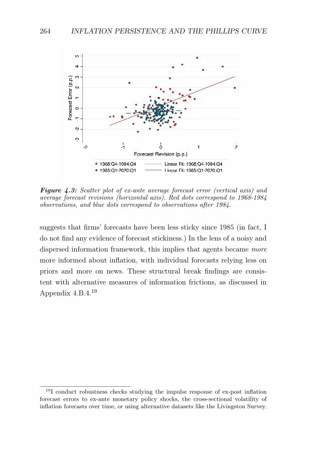
264 INFLATION PERSISTENCE AND THE PHILLIPS CURVE
Figure 4.3: Scatter plot of ex-ante average forecast error (vertical axis) andaverage forecast revisions (horizontal axis). Red dots correspond to 1968-1984observations, and blue dots correspond to observations after 1984.
suggests that firms’ forecasts have been less sticky since 1985 (in fact, Ido not find any evidence of forecast stickiness.) In the lens of a noisy anddispersed information framework, this implies that agents became moremore informed about inflation, with individual forecasts relying less onpriors and more on news. These structural break findings are consis-tent with alternative measures of information frictions, as discussed inAppendix 4.B.4.19
19I conduct robustness checks studying the impulse response of ex-post inflationforecast errors to ex-ante monetary policy shocks, the cross-sectional volatility ofinflation forecasts over time, or using alternative datasets like the Livingston Survey.

EVIDENCE ON INFORMATION FRICTIONS 265
Tab
le4.
3:Reg
ress
ion
tabl
e
Full
Sam
ple
1968
:Q4-
1984
:Q4
1985
:Q1-
2020
:Q1
Stru
ctur
alB
reak
(1)
(2)
(3)
(4)
(5)
Rev
isio
n1.
230∗
∗∗1.
414∗
∗∗0.
169
1.50
1∗∗∗
1.41
4∗∗∗
(0.2
50)
(0.2
83)
(0.1
93)
(0.3
17)
(0.2
81)
Rev
isio
n×1t⩾t∗
-1.1
11∗∗
∗-1
.245
∗∗∗
(0.3
79)
(0.3
41)
Con
stan
t-0
.087
50.
271
-0.3
17∗∗
∗-0
.135
∗0.
271
(0.0
696)
(0.1
85)
(0.0
478)
(0.0
690)
(0.1
84)
Con
stan
t×1t⩾t∗
-0.5
87∗∗
∗
(0.1
90)
Obs
erva
tion
s19
758
139
197
197
HA
Cro
bust
stan
dard
erro
rsin
pare
nthe
ses
∗p<
0.10
,∗∗p<
0.05
,∗∗∗p<
0.01

266 INFLATION PERSISTENCE AND THE PHILLIPS CURVE
In the next section I consider a theory of expectation formation thatincorporates significant heterogeneity and sluggishness in agents’ fore-casts, thus relaxing the standard full information rational expectations(FIRE) benchmark. I include such expectation formation features into anotherwise standard New Keynesian (NK) model by introducing noisy anddispersed information, rationally processed separately by each agent, andmatch the information-specific parameters to the observed sluggishnessin forecasts. I will argue that the change in the Fed communication im-proved firms’ information, and I use my model to show that the reducedstickiness in firms’ inflation forecasts will translate into reduced persis-tence in inflation. I show that in this framework, inflation is more persis-tent in periods of greater forecast sluggishness. Noisy information gen-erates an underreaction to new information because individuals shrinktheir forecasts towards prior beliefs when the signals they observe arenoisy. This endogenous anchoring in forecasts causes firms to set pricesto their existing prior, thus slowing the speed of price changes. Becauseinflation depends on the expectations of future inflation, the change inexpectation formation feeds into inflation dynamics, which endogenouslyreduces inflation persistence. I find that this change in firm forecastingbehavior explains around 90% of the fall in inflation persistence sincethe mid 1980s.
4.4 Noisy Information
I discuss a variety of New Keynesian models in Appendix 4.D, and showthat none of them can produce a significant fall in inflation persistence.The intuition behind that result is that, in purely forward frameworks,inflation is proportional to the exogenous shocks, and only extrinsicallypersistent. I show that the persistence of these exogenous shocks hasnot changed over time. Then, I explore several extensions that producebackward-looking dynamics, such as optimal monetary policy under com-mitment, price indexation or positive trend inflation. I argue that theseextensions generate mild anchoring and cannot explain the documented

NOISY INFORMATION 267
change in inflation persistence.In this section, I extend the benchmark setting to noisy and dis-
persed information and show that this information structure generatesadditional persistence in inflation. As discussed in the introduction, theactions of the Fed have become more transparent over time. The de-lay between the action and the announcement to the public has beenshortened from around a year to a few minutes and there has been asubstantial increase in the amount of information contained in the PRand other documents released to the public has substantially increased.20
I document a contemporaneous change in beliefs and expectation forma-tion around the date when inflation persistence is reported to break. Ishow that this gradual increase in information has reduced the degreeof anchoring in firm expectations. Given that expectations are a crucialdeterminant of inflation, the gradual de-anchoring in expectations hasled to a de-anchoring in inflation.21
4.4.1 Noisy Information New Keynesian Model
In order to relate the previous empirical findings on inflation persis-tence to information frictions, I build a noisy information New Keynesianmodel based on the island setting by Lucas (1972), Woodford (2003a),Nimark (2008), Lorenzoni (2009), Angeletos and Huo (2021).22 Firmsobserve the economic conditions in their island, but they do not havefull information about the economic conditions in the archipielago. Inparticular, firms can observe their own granular conditions, such as their
20I provide a more detailed historical analysis of the Fed’s gradual increase intransparency in Appendix 4.E.
21A criticism to the gradual information disclosure argument is that, although ac-tions themselves could not be known with any certainty until after a year, marketparticipants could observe the changes in interest rates and monetary aggregates in-duced by the action and could thus infer the action, in the spirit of the Grossmanand Stiglitz (1980) paradox. To alleviate this concern, I measure information frictionsusing data from professional forecasters. The underlying assumption here is that pro-fessional forecasters are among the most informed agents in the economy since theirjob is to make predictions for private companies. Obtaining evidence on significantinformation frictions would therefore invalidate the previous criticism.
22The derivation of the model is relegated to Online Appendix 4.F.

268 INFLATION PERSISTENCE AND THE PHILLIPS CURVE
production given their price, but they do not have perfect informationabout aggregate macro variables like inflation, output or interest rates.They observe a noisy signal that provides information on the state ofthe economy, in this case the monetary policy shock. With this piece ofinformation, firms form expectations on inflation, aggregate output andinterest rates. For simplicity, I assume that households and the monetaryauthority have access to full information.23
Apart from this information friction, which I describe formally be-low, firms are subject to the standard Calvo-lottery price friction, whichallows us to write the price-setting problem as a forward-looking one,and compete in a monopolistic economy. There is a continuum of firmsindexed by j ∈ If = [0, 1], each being a monopolist producing a differen-tiated intermediate-good variety with CES ϵ, producing output Yjt andsetting price Pjt. Technology is represented by the production function
Yjt = N1−αjt (4.5)
where 1 − α is the labor share.
Aggregate Price Dynamics As in the benchmark NK model, pricerigidities take the form of a Calvo-lottery. In every period, each firm canreset its price with probability (1 − θ), independent of the time of thelast price change. That is, only a measure (1−θ) of firms is able to resettheir prices in a given period, and the average duration of a price is givenby 1/(1 − θ). Let pt = log Pt denote the (log) aggregate price level andp∗t = log P∗t the (log) aggregate price set by firms which are able to act.Such an environment implies that aggregate price dynamics are given (inlog-linear terms) by
pt = (1 − θ)p∗t + θpt−1, p∗t =
∫If
p∗jt dj (4.6)
23I relax the FIRE assumption on households in Appendix 4.C.

NOISY INFORMATION 269
That is, the (log) aggregate price level at time t is a weighted averageof the average price set by resetters and the average price set by non-resetters, pt−1.
Optimal Price Setting A firm re-optimizing in period t will choosethe price P∗jt that maximizes the current market value of the profitsgenerated while the price remains effective. Formally,
P∗jt = arg maxPjt
∞∑k=0
θkEjtΛt,t+k
PjtYj,t+k −Wt+kNj,t+kPt+k
where Λt,t+k ≡ βk(Ct+kCt
)−σis the stochastic discount factor and
Ejt(·) denotes firm j’s expectation conditional on its information setat time t, and subject to the sequence of demand schedules Yj,t+k =(PjtPt+k
)−ϵCt+k and their production technology (4.5). I assume that
prices are set before wages. Log-linearizing the resulting first-order con-dition around the zero inflation steady-state, I obtain the familiar price-setting rule
p∗jt = (1 − βθ)
∞∑k=0
(βθ)kEjt (pt+k +Θmct+k) (4.7)
where mct = mct − mc is the deviation between real marginal costsand steady-state marginal costs and Θ = 1−α
1−α+αϵ . Comparing the price-setting rule arising in this framework with the one in the benchmark, theonly difference comes from the expectation operator. In the benchmarkcase, information sets are homogeneous and all firms (allowed to act) setthe same price. Instead, in this framework, each firm will set a differentprice based on its own belief structure.
Equilibrium Market clearing in the goods and labor market impliesthat ct = yt = (1 − α)nt. Using the equilibrium aggregate labor sup-ply condition, we can write marginal costs in terms of output, mct =
wt − pt =(σ+ φ+α
1−α
)yt, where σ is the elasticity of intertemporal sub-

270 INFLATION PERSISTENCE AND THE PHILLIPS CURVE
stitution and φ is the inverse Frisch elasticity. Rewriting output in termsof its gap with respect to the flexible-prices equilibrium,
p∗jt = (1 − βθ)
∞∑k=0
(βθ)kEjt[pt+k +Θ
(σ+
φ+ α
1 − α
)yt+k
](4.8)
which we can rewrite recursively as
p∗jt = (1 − βθ)Ejtpt +κθ
1 − θEjtyt + βθEjtp∗j,t+1 (4.9)
where κ =(1−θ)(1−βθ)
θ Θ(σ+ φ+α
1−α
). Condition (4.9) is actually quite
intuitive: when a firm j sets its price, it considers how competitive willits price be compared to the average price in the economy (playing agame of strategic complementarities with other firms), which will be theaggregate demand in the economy, and the future conditions since itsprice will be effective for an unknown number of periods.
Demand side The demand side behaves as in the standard framework.Output gap dynamics are described by the standard DIS curve (4.10),where current output gap depends negatively on the expected real inter-est rate and positively on future aggregate demand; and nominal interestrates are set by the central bank following a Taylor rule (4.11), in whichthe central bank reacts to excessive inflation and output by reducing thenominal interest rates, and releases a monetary policy shock (4.12) thathas an AR(1) structure:
yt = −1σ(it − Etπt+1) + Etyt+1 (4.10)
it = ϕππt + ϕyyt + vt (4.11)
vt = ρvt−1 + σεεvt , εvt ∼ N(0, 1) (4.12)
The monetary policy shock vt will be a key object in this economy. It isthe only aggregate state variable, and I will assume that firms will haveimperfect information on the central bank’s action vt, consistent with

NOISY INFORMATION 271
our evidence on the transparency policy change by the Fed.
Aggregate Phillips curve In order to derive the aggregate Phillipscurve, we aggregate condition (4.8) across firms.24 The aggregate Phillipscurve can then be written as
πt = κθ
∞∑k=0
(βθ)kEftyt+k + (1 − θ)
∞∑k=0
(βθ)kEftπt+k +(Eftpt−1 − pt−1
)(4.13)
where πt = pt−pt−1 is the inflation rate and Eft(·) =∫IfEjt(·) dj is the
average firm expectation operator. Compared to the standard framework,there is an additional term on the right-hand side, the result of firms notperfectly observing the previous price index. Angeletos and Huo (2021)eliminate this term by assuming that firms know the aggregate pricelevel at time t−1, but do not extract any information from it.25 In orderto maintain internal consistence in the theoretical framework, I do notmake any such assumption.
At this point, it is important to stress that in order to derive condi-tion (4.9) I have not yet specified an information structure. Therefore,the price-setting condition (4.9) and the aggregate Phillips curve (4.13)should be interpreted as a general individual price-setting condition anda general aggregate Phillips curve.26
Information Structure In order to generate heterogeneous beliefsand sticky forecasts, I assume that the information is incomplete and
24We subtract pt−1 on both sides, and ±Eftpt−1 on the right-hand side.25Vives and Yang (2016) motivate this through bounded rationality and inatten-
tion, while Angeletos and Huo (2021) argue that inflation contains little statisticalinformation about real variables. Huo and Pedroni (2021) allow for endogenous infor-mation, but such a choice complicates the dynamics and the concept of persistencebecomes less clear.
26In the FIRE NK model, agents perfectly observe inflation and output, and face asymmetric Nash equilibrium game, and thus every firm acts as a representative agentfirm. In such a case, the individual price-setting curve (4.9) can be aggregated to thewell-known New Keynesian Phillips curve (4.2).

272 INFLATION PERSISTENCE AND THE PHILLIPS CURVE
dispersed. Each firm j observes a noisy signal xjt that contains informa-tion on the monetary shock vt, and takes the standard functional formof “outcome plus noise”. Formally, signal xjt is described as
xjt = vt + σuujt, with ujt ∼ N(0, 1) (4.14)
where signals are agent-specific. This implies that each agent’s informa-tion set is different, and therefore generates heterogeneous informationsets across the population of firms.
An equilibrium must therefore satisfy the individual-level optimalpricing policy functions (4.9), the aggregate DIS curve (4.10), the Tay-lor rule (4.11), and rational expectation formation should be consistentwith the exogenous monetary shock process (4.12) and the signal process(4.14).
Solution Algorithm Here I outline the solution algorithm, and theinterested reader is referred to the Proof of Proposition 4.1 in Appendix4.A. I first guess that the dynamics of the output gap are endogenousto the aggregate price index and the monetary shock: yt = aypt−1 +
bypt−2+cyvt for some unknown coefficients (ay,by, cy). This allows usto write the individual price-setting condition (4.9) as a beauty contestin which each firm’s decision will depend on its own expectation of thefundamental and others’ actions. I then compute the expectations. Forexample, using the Kalman filter, we can write the expectation processas27
EjtZt = ΛEj,t−1Zt−1 +Kxjt
= (I−ΛL)−1Kxjt
= Λ(L)xjt, Zt =[vt pt yt
]′(4.15)
27In the case of the Kalman filter, we also need to guess the dynamics of the pricelevel.

NOISY INFORMATION 273
where I have made use of the lag operator L, and Λ(z) = (I −ΛL)−1K
is a polynomial matrix that depends on the guessed dynamics and theinformation noise σu. I then insert these objects into firm j’s price policyfunction (4.9), and obtain aggregate price dynamics. Finally, we verifyour initial guess by introducing the implied price dynamics into the DIScurve (4.10).
Notice that extending the benchmark framework to noisy and dis-persed information generates anchoring through expectations, which nowfollow an autorregressive process. This additional anchoring will resultin inflation being more persistent in the noisy information framework,compared to the benchmark setting.
The following proposition outlines inflation and output gap dynam-ics.
Proposition 4.1. Under noisy information the output gap and pricelevel dynamics are given by
yt =ϑ1[σ(1 − ϑ2) + ϕy](ϑ1 + ϑ2 − 1 − ϕπ) + (1 − ϑ2)(ϕπ − ϑ2)(σ+ ϕy)
[σ(1 − ϑ1) + ϕy][σ(1 − ϑ2) + ϕy]pt−1
+ϑ1ϑ2[σ(1 − ϑ1)(1 − ϑ2) − (ϑ1 + ϑ2 − 1 − ϕπ)ϕy]
[σ(1 − ϑ1) + ϕy][σ(1 − ϑ2) + ϕy]pt−2−
−ψyχy(ϑ1, ϑ2)vt (4.16)
pt = (ϑ1 + ϑ2)pt−1 − ϑ1ϑ2pt−2 −ψπχπ(ϑ1, ϑ2)vt (4.17)
where ϑ1 and ϑ2 are the reciprocal of the two outside roots of the quarticpolynomial
P(z) = −(βθ− z)(1 − θz)(z− ρ) (1 − ρz)
− τz
[(βθ− z)(1 − θz) + z(1 − θ)(1 − βθ)
+ z2κθϑ1[σ(1 − ϑ2) + ϕy](ϑ1 + ϑ2 − 1 − ϕπ) + (1 − ϑ2)(ϕπ − ϑ2)(σ+ ϕy)
[σ(1 − ϑ1) + ϕy][σ(1 − ϑ2) + ϕy]
+ z3κθϑ1ϑ2[σ(1 − ϑ1)(1 − ϑ2) − (ϑ1 + ϑ2 − 1 − ϕπ)ϕy]
[σ(1 − ϑ1) + ϕy][σ(1 − ϑ2) + ϕy]
]

274 INFLATION PERSISTENCE AND THE PHILLIPS CURVE
and χy,χπ are scalars endogenous to information frictions, with τ =
σ2ε/σ
2u.
Proof. See Appendix 4.A
First differencing the price level dynamics (4.17), we can obtain theimplied inflation dynamics as
πt = (ϑ1 + ϑ2)πt−1 − ϑ1ϑ2πt−2 −ψπχπ(ϑ1, ϑ2)∆vt (4.18)
In the noisy information framework, inflation is intrinsically persistentand its persistence is governed by the new information-related param-eters ϑ1 and ϑ2, as opposed to the benchmark framework in which itis only extrinsically persistent. The intuition for this result is simple:inflation is partially determined by expectations (see condition (4.13)under noisy information, or (4.2) under complete information). Undernoisy information, expectations are anchored and follow an autoregres-sive process (see (4.15)), which creates the additional source of anchoringin inflation dynamics, measured by ϑ1 and ϑ2. In particular, we can writethe inflation first-order autocorrelation as
ρ1 =(1 + ρ)(ϑ1 + ϑ2) + (1 − ρ)(ϑ1ϑ2 − 1)
1 + ρϑ1ϑ2,
which is increasing in both ϑ1 and ϑ2. Since our ultimate goal is to un-derstand the break in inflation persistence documented in Section 4.2.1,the following proposition exposes the determinants of ϑ1 and ϑ2, andprovides analytical comparative statics.
Proposition 4.2. The persistence parameters are
(i) ϑ1 ∈ (0, ρ)
(ii) ϑ1 is increasing in σu
(iii) ϑ2 ∈ (θ, 1)
(iv) ϑ2 is decreasing in σu

NOISY INFORMATION 275
Proof. See Appendix 4.A.
Inflation persistence and information frictions are related through ϑ1
and ϑ2. The above proposition is key to understanding the time-varyingproperties of inflation persistence. First, part (i) establishes that ϑ1 isbounded by 0 and ρ. Part (ii) states that ϑ1 is increasing in the degreeof information frictions, formalized via the noise of the signal innovationσu. A decrease in information frictions reduces inflation first-order auto-correlation through a de-anchoring of individual inflation expectations,which would in turn de-anchor inflation dynamics. Figure 4.4a plots thelevel of intrinsic persistence ϑ1 for different degrees of information fric-tions, measured by τ−1. Part (iii) establishes that ϑ2 is bounded byθ and 1. Part (iv) states that ϑ2 is decreasing in the degree of infor-mation frictions. A decrease in information frictions increases inflationfirst-order autocorrelation through an anchoring of individual inflationexpectations, which would in turn anchor inflation dynamics. Figure 4.4bplots the level of intrinsic persistence ϑ2 for different degrees of informa-tion frictions. In the limit of no information frictions σu → 0, ϑ1 → 0and ϑ2 → 1.
Information frictions do, therefore, have opposing effects on persis-tence. On the one hand, information frictions lead to an additional per-sistence through an increase in ϑ1, the standard mechanism in Angeletosand Huo (2021). On the other hand, there is an additional componentϑ2 that is decreasing in information frictions. This element arises fromthe fact that we are solving the NK model in prices, instead of infla-tion as in Angeletos and Huo (2021) or as in the benchmark setting inGalí (2015) in which prices follow a unit root. Since price dynamics fol-low (4.6), when firm j forecasts the aggregate price level pt, she needsto forecast the average action by other firms p∗t , but also backcast theaggregate price level in the past pt−1. Information frictions relax theforward-lookingness of the model equations, as formalized by Gabaix(2020), Angeletos and Huo (2021), resulting in price dynamics no longerfollowing a unit root. In the frictionless limit, prices follow a unit root,

276 INFLATION PERSISTENCE AND THE PHILLIPS CURVE
formalized by ϑ2 → 1. However, as shown in Figure 4.4c, the net resultof an increase in information frictions is an increase in the first-order au-tocorrelation. These key results, coupled with the next result introducedin Proposition 4.3, will explain the overall fall in inflation persistence.
In the next section I relate our theoretical findings on inflation per-sistence to empirical evidence on information frictions, and their fall inthe recent decades.
4.4.2 Calibrating Information Frictions
In our theoretical framework we rationalize the average forecast under-reaction through anchoring to priors. A positive βrev will therefore gen-erate intrinsic persistence in inflation dynamics. Yet, this is not enoughto explain the change in inflation persistence over time. I documented astructural break in belief formation in Section 4.3. This break coincideswith a change in the U.S. Federal Reserve’s communication policy, whichbecame more transparent and informative after the mid 1980s. Using sur-vey data on U.S. firms’ forecasts, I document a significant sluggishnessin responses to new information until the mid 1980s, but no evidenceof sluggishness afterwards. In this section, I calibrate the informationfriction parameter σu to match the observed sluggishness in forecastsacross time. As argued before, the signal noise became more precise inthe dispersed-information model lens.
Propositions 4.1 and 4.2 state that inflation becomes less persistentwhen we relax the information frictions. In the next proposition, I re-late the previous empirical findings on expectations to model-impliedinflation persistence.
Proposition 4.3. The theoretical counterpart of the coefficient βrev in(4.3) is given by
βrev =λ3ρ(1 − ϑ1λ)(1 − ϑ2λ)
(1 − λ4)(ρ− λ)
λ(λ− ξ1)(λ− ξ2)(λ− ξ3)(λ− ξ4)
(λ− ϑ1)(λ− ϑ2)
− (1 − λ2)[ϑ1(ϑ1 − ξ1)(ϑ1 − ξ2)(ϑ1 − ξ3)(ϑ1 − ξ4)
(1 − λϑ1)(λ− ϑ1)(ϑ1 − ϑ2)(4.19)

NOISY INFORMATION 277
(a) Intrinsic persistence ϑ1 and information frictions τ−1
(b) Intrinsic persistence ϑ2 and information frictions τ−1
(c) First-Order Autocorrelation ρ1 and information frictions τ−1
Figure 4.4: Comparative statics.

278 INFLATION PERSISTENCE AND THE PHILLIPS CURVE
+ϑ2(ϑ2 − ξ1)(ϑ2 − ξ2)(ϑ2 − ξ3)(ϑ2 − ξ4)
(1 − λϑ2)(λ− ϑ2)(ϑ1 − ϑ2)
](4.20)
where λ is the inside root of the quadratic polynomial Q1(z) = (1−ρz)(z−ρ)+ σ2
ε
σ2uz, and (ξ1, ξ2, ξ3, ξ4) are the reciprocals of the roots of the quartic
polynomial Q2(z) = ϕ0 + ϕ1z + ϕ2z2 + ϕ3z
3 + ϕ4z4, where ϕ0 = cp,
ϕ1 =(
1λ − 1
ρ
)cp, ϕ2 =
(ρ−λ)cpλ2ρ
, ϕ3 =(ρ−λ)cp[λ
3−ϑ1−ϑ2+λϑ1ϑ2]λ2ρ(1−λϑ1)(1−λϑ2)
, and
ϕ4 =−λ3+λ4ϑ2+λ
4ϑ1−ϑ1ϑ2[λ−(1−λ4)ρ]λ2ρ(1−λϑ1)(1−λϑ2)
.
Proof. See Appendix 4.A.
The empirical results support a fall in information frictions in recentdecades. Proposition 4.3 maps the theoretical information friction, σu,with the Coibion and Gorodnichenko (2015a) estimate. It introduces themodel-implied βrev coefficient, which depends on the monetary policyshock persistence ρ and on the information-related parameters ϑ1, ϑ2
and λ, where λ, in turn, depends on the persistence parameter and thesignal-to-noise ratio. In our noisy information framework, βrev is strictlypositive and increases with the degree of information frictions. I showthis graphically in Figure 4.5a. In the model lens, this underrevision isthe consequence of individual anchoring to priors, and generates forecastunderreaction at the aggregate level.
The most important finding is that βrev and ρ1, the theoretical coun-terparts of Coibion and Gorodnichenko (2015a) underreaction estimateβrev and inflation persistence, are closely related as I show in Figure4.5b. The fall in the first-order autocorrelation can be explained by a fallin information frictions. For this quantitative analysis, I use a standardparameterization in the literature, with the only exception of θ = 0.872,which is calibrated to match a Phillips curve slope κ = 0.06, and ϕy = 0.5which guarantees the existence of a unique equilibrium as σu → 0.28 Fi-nally, I calibrate τ = 0.069 in the pre-1985 sample to match the empiricalevidence on βrev in Table 4.3.
As a last remark, notice that the dynamics generated by the noisy28All parameters are set to the values reported in Table 4.20.

NOISY INFORMATION 279
(a) βrev and information frictions τ−1
(b) First-Order Autocorrelation ρ1 and information frictions βrev
Figure 4.5: Comparative statics.
information model (4.18) resemble those generated by the ad-hocbackward-looking models presented in Appendix 4.D.3. However,differently from those ad-hoc frameworks, in the noisy informationframework, intrinsic persistence is the result of the micro-foundedanchoring in expectations. Extending the model to accommodate noisyinformation introduces anchoring through expectations, for which Ihave empirical evidence, rather than the more ad-hoc consumptionexternal habits or price indexation assumptions, for which there is littleor no evidence.29
29Havranek et al. (2017) present a meta-analysis of the different estimates of habitsin the macro literature and the available micro-estimates. In general, macro modelstake h = 0.75, whereas micro-estimates suggest a value around h = 0.4. On theother hand, the price-indexation model suggests that every price is changed in everyperiod, which is inconsistent with the micro-data estimates provided by Nakamuraand Steinsson (2008).

280 INFLATION PERSISTENCE AND THE PHILLIPS CURVE
4.5 Results
4.5.1 Inflation Persistence
In the noisy information framework, inflation persistence is governed byϑ1 and ϑ2. Propositions 4.1-4.3 establish a direct relation between thefirst-order autocorrelation of inflation ρ1 and βrev, our empirical measureof information frictions. Figure 4.5b shows graphically the monotonicallyincreasing relation between inflation persistence and βrev. In the initialpre-1985 period, with βrev = 1.501, the model-implied inflation first-order autocorrelation is ρ1 = 0.716. In the post-1985 period, with no in-formation frictions, the first-order autocorrelation falls to ρ1 = ρ, whichis the persistence of the monetary policy shock in the benchmark frame-work (see Galí (2015)). Comparing our model results to the empiricalanalysis in Tables 4.1 and 4.G.2, I find that the noisy information frame-work produces persistence dynamics that lie within the 95% confidenceinterval, and can explain around 90% of the fall in the point estimate.Noisy information produces such fall in a micro-consistent manner, com-pared to the more ad-hoc NK models studied in Section 4.D.
Role of Calvo Friction In our framework, information frictions affectthe two roots ϑ1 and ϑ2 in opposing ways. In order for the model toexplain the fall in inflation persistence, it must be that ϑ2 is not verysensitive to information frictions. Since ϑ2 ∈ (θ, 1), a large value of θlimits this sensitivity.
The calibration of the Calvo pricing friction implies a mean priceduration of 7.8 quarters. This estimate is in the upper range in the mi-cro literature. Bils and Klenow (2004), Klenow and Kryvtsov (2008),Nakamura and Steinsson (2008), Goldberg and Hellerstein (2009) find amedian price duration of 4.5-11 months in U.S. micro data. Galí (2015)sets θ = 0.75 to match an implied duration of 1 year. Christiano et al.(2011) set θ = 0.85. Auclert et al. (2020), Afsar et al. (2021) estimateθ between 0.88 and 0.93 from macro data, implying a price duration of12-14 quarters.

RESULTS 281
Figure 4.6: First-order autocorrelation ρ1 and price friction θ
In Figure 4.6, I plot the implied first-order autocorrelation for dif-ferent values of the Calvo price friction in the range of the literature.Depending on this parameter, the noisy information framework explainsbetween 40% and 100% of the fall in the point estimate in the first-orderautocorrelation.
4.5.2 The Phillips Curve
In this section I argue that the mainstream finding that the slope ofthe Phillips curve has fallen in the recent period is simply the resultof a misspecified Phillips curve equation (4.2). The derivation of thePhillips curve relies on the FIRE assumption (and implicitly on the Lawof Iterated Expectations), for which I find a strong rejection in the data.I then conduct two main exercises. First, in a more theoretical exercise,I use the noisy information framework to rewrite its inflation dynamicsas an as if FIRE setting with some wedges (Angeletos and Huo, 2021).According to my theory, the Phillips curve (4.2) needs to be extendedwith a backward-looking inflation term and significant myopia towardsfuture inflation in the pre-1985 sample period. Once these additionalterms are controlled for, and I estimate a Phillips curve closer to thehybrid version implied by price-indexation settings, I do not find anyevidence of a change in κ. Second, by relaxing the FIRE assumption, thePhillips curve is instead given by (4.13). Instead of replacing expectationsof future inflation by its realization, as the literature generally does whenestimating condition (4.2), I use the survey forecasts to estimate (4.13)

282 INFLATION PERSISTENCE AND THE PHILLIPS CURVE
and I do not find any evidence of a change in the slope.
Inflation Disconnect via Expectations Next, I argue that once Iconsider a micro-founded Phillips curve that takes into account noisyinformation, there is no evidence of a change in the slope of the Phillipscurve.
Let us first recall inflation dynamics in the standard model. In thebenchmark NK model, the Phillips curve is given by (4.2), the DIS curveis given by (4.10), the Taylor rule is given by (4.11) and the monetarypolicy shock process is given by (4.12). Inserting the Taylor rule (4.11)into the DIS curve (4.10), one can write the model as a system of twofirst-order stochastic difference equations with reduced-form dynamicsxt = δEtxt+1+φvt, where xt = [yt πt pt]
′ is a 3×1 vector containingoutput, inflation and prices, and
δ =1
σ+ ϕy + κϕπ
σ 1 − βϕπ 0σκ κ+ β(σ+ ϕy) 00 −1 1
, φ =1
σ+ ϕy + κϕπ
−1−κ
0
.
Angeletos and Huo (2021) show that, using the noisy information dynam-ics (4.16)-(4.18), we can reverse engineer an as if system dynamics thatmimics the dynamics of our NI model, such that the following ad-hocsystem of equations
xt = ωbxt−1 +ωfδEtxt+1 +φvt (4.21)
satisfies the model dynamics for some pair of 3 × 3 matrices (ωb,ωf).The next proposition states that, under a certain pair (ωb,ωf), thead-hoc economy produces the same dynamics that our noisy informationframework.
Proposition 4.4. The ad-hoc hybrid dynamics (4.21) produces identical

RESULTS 283
dynamics to the noisy information model if (ωb,ωf) satisfy
B−φ = ωfδ(AB+ ρB)
ωb = (I3 −ωfδA)A(4.22)
where
A =
0 by ay + by
0 ϑ1ϑ2 −(1 − ϑ1)(1 − ϑ2)
0 ϑ1ϑ2 ϑ1 + ϑ2 − ϑ1ϑ2
, B =
−ψyχy(ϑ1, ϑ2)
−ψπχπ(ϑ1, ϑ2)
−ψπχπ(ϑ1, ϑ2)
ay =
ϑ1[σ(1 − ϑ2) + ϕy](ϑ1 + ϑ2 − 1 − ϕπ) + (1 − ϑ2)(ϕπ − ϑ2)(σ+ ϕy)
[σ(1 − ϑ1) + ϕy][σ(1 − ϑ2) + ϕy]
by =ϑ1ϑ2[σ(1 − ϑ1)(1 − ϑ2) − (ϑ1 + ϑ2 − 1 − ϕπ)ϕy]
[σ(1 − ϑ1) + ϕy][σ(1 − ϑ2) + ϕy]
In particular, the “as if ” FIRE Phillips curve dynamics are described by
πt = ωππt−1 +ωppt−1 + γyκyt + δyEtyt+1 + δπβEtπt+1 (4.23)
where (ωπ,ωp,γy, δy, δπ) depend on the (ωb,ωf) pair.
Proof. See Appendix 4.A.
The slope of the Phillips curve is now interacted with γy, a coefficientarising from information frictions. In the benchmark NK model with noinformation frictions, we haveωb,11 = ωb,12 = ωb,21 = ωb,22 = ωf,12 =
ωf,21 = 0 and ωf,11 = ωf,22 = 1. As a result, ωπ = ωp = δy = 0,γy = 1, δπ = 1 and the Phillips curve is reduced to the only forward-looking (4.2).30
I now estimate the Phillips curves. I start from the benchmark NKPhillips curve (4.2). I follow the literature, replace expectations of fu-ture inflation by realized future inflation and estimate the equation with
30Notice that condition (4.22) does not uniquely determine the set of weights ωf
that is consistent with the noisy information dynamics. Different weights in ωf areconsistent with noisy information dynamics, although the dynamics are unique. Intu-itively, agents’ actions can be anchored/myopic with respect to aggregate output orinflation.

284 INFLATION PERSISTENCE AND THE PHILLIPS CURVE
GMM. In table 4.4 column 1, I report the estimated coefficients. I findthat the slope of the Phillips curve is small and not significant. In thesecond column, following my structural break strategy in the previoussections, I test for a structural break after 1985 in the output gap coeffi-cient. I find evidence of a break, which the literature has interpreted asflattening in the Phillips curve (in absolute terms). Guided by the as ifframework, I estimate the wedge Phillips curve (4.23). I report the esti-mated coefficients in column 3. I find that the slope of the Phillips curveis small and not significant. In fact, I find that only inflation-related co-efficients are significant, suggesting support for backward-lookingness. Ireport the structural break results in column 4. I find no evidence of astructural break in the slope (i.e., no evidence of flattening in the Phillipscurve). In column 5 I explore if there has been any other structural breakin the dynamics of the Phillips curve. In particular, our model suggeststhat the backward-looking term should have vanished after 1985, andthat the forward-looking term should have increased. I report these re-sults in column 5. I find a structural break in lagged and forward in-flation: in recent decades the Phillips curve has become more forward-looking and less backward-looking. This last result aligns well with thedocumented drop in inflation persistence and information frictions, andwith the mechanism suggested in the noisy information framework. Inthe light of these noisy estimates, I take the “Phillips curve flatteningpuzzle” as a result of misspecification in the standard Phillips curve.

RESULTS 285
Tab
le4.
4:Reg
ress
ion
tabl
e
(1)
(2)
(3)
(4)
(5)
Stan
dard
Phi
llips
Cur
veB
reak
Out
put
Wed
geP
hilli
psC
urve
Bre
akO
utpu
tB
reak
All
yt
-0.0
278
-0.1
12∗∗
0.06
330.
134
0.37
8(0
.023
7)(0
.045
2)(0
.112
)(0
.123
)(0
.240
)
πt+
10.
989∗
∗∗0.
995∗
∗∗0.
540∗
∗∗0.
509∗
∗∗0.
226
(0.0
179)
(0.0
175)
(0.1
02)
(0.1
08)
(0.2
15)
πt−
10.
447∗
∗∗0.
496∗
∗∗0.
738∗
∗∗
(0.0
978)
(0.1
10)
(0.1
65)
yt+
1-0
.069
5-0
.104
-0.3
43(0
.126
)(0
.125
)(0
.212
)
pt−
10.
0035
4-0
.016
40.
0363
(0.0
162)
(0.0
243)
(0.2
02)
yt×1t⩾t∗
0.11
7∗∗
-0.0
726
-0.1
27(0
.056
0)(0
.063
2)(0
.291
)
πt−
1×1t⩾t∗
-0.6
71∗∗
(0.2
67)
pt−
1×1t⩾t∗
-0.1
05(0
.256
)
yt+
1×1t⩾t∗
0.09
63(0
.328
)
πt+
1×1t⩾t∗
0.86
6∗∗∗
(0.3
35)
Obs
erva
tion
s20
220
220
220
220
2H
AC
robu
stst
anda
rder
rors
inpa
rent
hese
sIn
stru
men
tse
t:fo
urla
gsof
effec
tive
fede
ralf
unds
rate
,CB
OO
utpu
tga
p,G
DP
Defl
ator
grow
thra
te,C
omm
odity
Infla
tion
,M
2gr
owth
rate
,spr
ead
betw
een
long
-an
dsh
ort-
run
inte
rest
rate
and
labo
rsh
are.
∗p<
0.10
,∗∗p<
0.05
,∗∗∗p<
0.01

286 INFLATION PERSISTENCE AND THE PHILLIPS CURVE
In order to understand these findings, I explore which set of wedges(ωb,ωf) is consistent with the documented dynamics. Since I do notfind any evidence of the relevance of the lagged price level and forwardoutput gap, I choose wedges such that they produce the well-knownhybrid Phillips curve. That is, I choose a set of wedges consistent with(4.22) and ωp = δy = 0. In that case, we can reduce the wedge Phillipscurve (4.23) to a micro-founded hybrid Phillips curve with the followingset of coefficients
πt = 0.319πt−1 + 0.181κyt + 0.675βEtπt+1. (4.24)
First, notice that the as if model produces anchoring, which lines upwith the strong inflation persistence during that period, and considerablemyopia towards future inflation. Furthermore, our model suggests thatthe slope of the Phillips curve has increased in recent decades (γy < 1),although this increase is small given that κ = 0.06, and is not significantin the data. More importantly, our model suggests that anchoring andmyopia should vanish in the post-1985 sample. Estimating the micro-founded hybrid NK Phillips curve (4.24), reported in table 4.5, I find thatone cannot empirically reject the null that, since the structural break in1985:Q1, (i) anchoring has gone to zero, (ii) myopia has disappeared, and(iii) the slope moderately increased, which the model can successfullyreplicate.
Controlling for Imperfect Expectations In order to obtain theresults on inflation persistence, I have assumed a particular informa-tion structure, noisy and dispersed information. In this section I take astep back and instead take an agnostic stance on expectation formation.Consider the aggregate Phillips curve (4.13). Inflation is now related tocurrent and future output through two different channels: the slope ofthe Phillips curve, κ, and firms’ expectation formation process. In or-der to test for a potential structural break in the slope controlling fornon-standard expectations, I regress the general Phillips curve (4.13)

RESULTS 287
Table 4.5: Regression table
(1) (2)Full Sample Structural Break
πt−1 0.453∗∗∗ 0.720∗∗∗
(0.0891) (0.131)
yt -0.000813 0.0566(0.0166) (0.0488)
πt+1 0.539∗∗∗ 0.273∗∗
(0.0885) (0.129)
πt−1 × 1t⩾t∗ -0.597∗∗
(0.232)
yt × 1t⩾t∗ -0.0143(0.0781)
πt+1 × 1t⩾t∗ 0.643∗∗∗
(0.244)
Observations 202 202HAC robust standard errors in parenthesesInstrument set: four lags of effective federal funds rate,CBO Output gap, GDP deflator growth rate,Commodity Inflation, M2 growth rate, spread betweenlong- and short-run interest rate, and labor share.∗ p < 0.10, ∗∗ p < 0.05, ∗∗∗ p < 0.01

288 INFLATION PERSISTENCE AND THE PHILLIPS CURVE
(truncated at k = 4), for which I do not assume a particular informationstructure, using real GDP and GDP Deflator growth forecast data fromthe SPF. We set β and θ to their quarterly values 0.99 and 0.872, andregress
πt = α1 + α2yet + α3π
et + ηt (4.25)
where ηt =(Eftpt−1 − pt−1
)+ truncation error, yet =
θ∑4k=0(βθ)
kEftyt+k and πet =∑4k=0(βθ)
kEftπt+k denote thetruncated sums of expected real GDP and inflation. I use standardGMM methods by instrumenting for expectations with 4-quarter laggedannual inflation and real GDP growth expectations. The results arereported in table 4.6. In column 1, I report the full sample coefficients.I find that κ is small, consistent with our choice of κ and similar to thevalue found by Hazell et al. (2020). In column 2, I regress its (output)structural break version. This is the only specification that suggests astructural break on the slope. However, when I also consider a potentialstructural break in inflation, I find an estimate of κ that aligns well withour model assumption, and I find no evidence of a structural break inthe Phillips curve slope.31
Summary To sum up, I find that once we control for imperfect ex-pectations and a potential change in their dynamics, I do not find anyevidence of a structural break in the slope of the Phillips curve. First, Ishowed that the noisy information model can explain the change in thedynamics between inflation and output via changes in belief formationthrough the γy wedge and the different role of forward-lookingness. Sec-ond, I documented empirically that controlling for non standard expec-tations, proxied by the forecasts submitted by professional forecasters, Ido not find any evidence of a change in the slope of the Phillips curve.
31I repeat the analysis using the Livingston Survey on Appendix 4.B, and findsimilar results.

4.6. CONCLUSION 289
Table 4.6: Regression table
(1) (2) (3)Full Sample Break Output Break All
yet -0.00692 0.132∗∗ 0.0909∗
(0.0177) (0.0515) (0.0531)
yet × 1t⩾t∗ -0.103∗∗∗ 0.0112(0.0356) (0.0649)
πet 0.262∗∗∗ 0.214∗∗∗ 0.237∗∗∗
(0.0121) (0.0223) (0.0240)
πet × 1t⩾t∗ -0.0932∗∗
(0.0402)
Observations 199 199 199HAC Robust standard errors in parenthesesInstrument set: four lags of forecasts of annual real GDP growthand annual GDP Deflator growth∗ p < 0.10, ∗∗ p < 0.05, ∗∗∗ p < 0.01
4.6 Conclusion
In this paper I document a fall in inflation persistence since the mid1980s. State-of-the-art monetary models face significant challenges inexplaining this fall in inflation persistence. I show that, by extendingthe benchmark NK in a micro-consistent manner relaxing the FIRE as-sumption, our model generates the documented fall in persistence. Us-ing micro-data on inflation expectations from the Survey of ProfessionalForecasters (SPF), I show that agents became more informed about in-flation after the change in the Federal Reserve disclosure policy, whichendogenously lowers the intrinsic persistence in inflation dynamics.
I revisit different theories that produce a structural relation betweeninflation and other forces in the economy. I show that a variety of NKmodels cannot explain the fall in inflation persistence. Since the bench-mark model is purely forward-looking, inflation exhibits no intrinsic per-sistence, and its dynamic properties are now inherited from monetary

290 INFLATION PERSISTENCE AND THE PHILLIPS CURVE
policy shocks. However, I document that the persistence of monetarypolicy shocks has not changed over time. Acknowledging that purelyforward-looking models cannot generate anchoring or intrinsic persis-tence, I extend the benchmark model to incorporate a backward-lookingdimension. I show that the change in the monetary stance now affectsinflation intrinsic persistence. The effect is small, however.
Then, I show that our noisy and dispersed information extension isconsistent with the micro-data evidence on belief formation, and gener-ates anchoring or intrinsic inflation persistence. Using SPF data, I docu-ment that a structural break in expectation formation, resulting in agentsbeing more informed about inflation, is contemporaneous to the fall ininflation persistence. The model can therefore explain the fall in inflationpersistence in a micro-consistent manner.
I discuss the consequences of noisy and dispersed information on the“inflation disconnect puzzle” and the lack of flattening of the Phillipscurve. In the noisy information model, inflation is related to the demandside through two different channels: the slope of the Phillips curve andfirms’ expectation formation process. The model explains the fall in in-flation sensitivity towards the demand side of the economy via changesin expectations, without resorting to changes in the slope. Finally, tak-ing an agnostic stance on expectations, I show that there is no empiricalevidence of a change in the Phillips curve slope once we control for non-standard expectations.

REFERENCES 291
References
A. Afsar, J. E. Gallegos, R. Jaimes, and E. Silgado. Reconciling Empiricsand Theory: The Behavioral Hybrid New Keynesian Model. 2021.
F. Allen, S. Morris, and H. S. Shin. Beauty Contests and Iterated Ex-pectations in Asset Markets. The Review of Financial Studies, 19(3):719–752, 03 2006.
G.-M. Angeletos and Z. Huo. Myopia and anchoring. American Eco-nomic Review, 111(4):1166–1200, April 2021.
G.-M. Angeletos, Z. Huo, and K. A. Sastry. Imperfect macroeconomicexpectations: Evidence and theory. NBER Macroeconomics Annual,35:1–86, 2021.
G. Ascari and L. Fosso. The Inflation Rate Disconnect Puzzle: On theInternational Component of Trend Inflation and the Flattening of thePhillips Curve. Working Paper, 2021.
G. Ascari and A. M. Sbordone. The macroeconomics of trend inflation.Journal of Economic Literature, 52(3):679–739, September 2014.
A. Atkeson and L. E. Ohanian. Are Phillips curves useful for forecastinginflation? Quarterly Review, 25(Win):2–11, 2001.
A. Auclert, M. Rognlie, and L. Straub. Micro jumps, macro humps: Mon-etary policy and business cycles in an estimated hank model. WorkingPaper 26647, National Bureau of Economic Research, January 2020.
P. Bacchetta and E. Van Wincoop. Can information heterogeneity ex-plain the exchange rate determination puzzle? American EconomicReview, 96(3):552–576, June 2006.
L. Ball and S. Mazumder. Inflation Dynamics and the Great Recession.Brookings Papers on Economic Activity, 42:337–405, 2011.

292 INFLATION PERSISTENCE AND THE PHILLIPS CURVE
S. Basu, J. G. Fernald, and M. S. Kimball. Are technology improve-ments contractionary? American Economic Review, 96(5):1418–1448,December 2006.
L. Benati and P. Surico. Evolving u.s. monetary policy and the declineof inflation predictability. Journal of the European Economic Associ-ation, 6(2/3):634–646, 2008.
B. S. Bernanke, T. Laubach, F. S. Mishkin, and A. S. Posen. Infla-tion Targeting: Lessons from the International Experience. PrincetonUniversity Press, 1999.
M. Bils and P. J. Klenow. Some evidence on the importance of stickyprices. Journal of Political Economy, 112(5):947–985, 2004.
A. S. Blinder. Central-bank credibility: Why do we care? how do we buildit? American Economic Review, 90(5):1421–1431, December 2000.
P. Bordalo, N. Gennaioli, Y. Ma, and A. Shleifer. Overreaction in macroe-conomic expectations. American Economic Review, 110(9):2748–82,September 2020.
T. Broer and A. N. Kohlhas. Forecaster (Mis-)Behavior. 2019.
L. Christiano, M. Eichenbaum, and S. Rebelo. When is the governmentspending multiplier large? Journal of Political Economy, 119(1):78–121, 2011.
L. J. Christiano, M. Eichenbaum, and C. L. Evans. Nominal Rigiditiesand the Dynamic Effects of a Shock to Monetary Policy. Journal ofPolitical Economy, 113(1):1–45, 2005.
R. Clarida, J. Gali, and M. Gertler. Monetary policy rules and macroe-conomic stability: Evidence and some theory. The Quarterly Journalof Economics, 115(1):147–180, 2000.

REFERENCES 293
T. Cogley and A. M. Sbordone. Trend inflation, indexation, and infla-tion persistence in the new keynesian phillips curve. The AmericanEconomic Review, 98(5):2101–2126, 2008.
T. Cogley, G. E. Primiceri, and T. J. Sargent. Inflation-gap persistencein the us. American Economic Journal: Macroeconomics, 2(1):43–69,January 2010.
O. Coibion and Y. Gorodnichenko. What can survey forecasts tell usabout information rigidities? Journal of Political Economy, 120(1):116–159, 2012.
O. Coibion and Y. Gorodnichenko. Information rigidity and the expecta-tions formation process: A simple framework and new facts. AmericanEconomic Review, 105(8):2644–78, August 2015a.
O. Coibion and Y. Gorodnichenko. Is the phillips curve alive and wellafter all? inflation expectations and the missing disinflation. AmericanEconomic Journal: Macroeconomics, 7(1):197–232, January 2015b.
A. Cukierman and A. H. Meltzer. A theory of ambiguity, credibility, andinflation under discretion and asymmetric information. Econometrica,54(5):1099–1128, 1986.
M. del Negro, M. P. Giannoni, and C. Patterson. The Forward GuidancePuzzle. SSRN Electronic Journal, 2012.
M. del Negro, M. Lenza, G. Primiceri, and A. Tambalotti. What’s upwith the Phillips Curve? National Bureau of Economic Research, 2020.
J. Faust and L. E. O. Svensson. Transparency and credibility: Monetarypolicy with unobservable goals. International Economic Review, 42(2):369–397, 2001.
J. Faust and L. E. O. Svensson. The equilibrium degree of transparencyand control in monetary policy. Journal of Money, Credit and Banking,34(2):520–539, 2002.

294 INFLATION PERSISTENCE AND THE PHILLIPS CURVE
J. Fernald. A quarterly, utilization-adjusted series on total factor pro-ductivity. 2014.
N. Francis, M. Owyang, J. E. Roush, and R. DiCecio. A flexible finite-horizon alternative to long-run restrictions with an application to tech-nology shocks. The Review of Economics and Statistics, 96(4):638–647,2014.
J. Fuhrer and G. Moore. Inflation persistence. The Quarterly Journal ofEconomics, 110(1):127–159, 1995.
J. C. Fuhrer. Inflation Persistence. Handbook of Monetary Economics,2, 2010.
X. Gabaix. A Behavioral New Keynesian Model. American EconomicReview, 110(8):2271–2327, 2020.
J. Galí. Technology, employment, and the business cycle: Do technologyshocks explain aggregate fluctuations? American Economic Review,89(1):249–271, March 1999.
J. Galí. Monetary Policy, Inflation, and the Business Cycle: An Intro-duction to the New Keynesian Framework and Its Applications Sec-ond edition. Number 10495 in Economics Books. Princeton UniversityPress, 2015.
P. K. Goldberg and R. Hellerstein. How rigid are producer prices? Tech-nical report, 2009.
N. Goldstein and Y. Gorodnichenko. Macroeconomic Persistence andForward Information: What Else Can We Learn from Survey Expec-tations? Working Paper, 2019.
M. Goodfriend. Monetary mystique: Secrecy and central banking. Jour-nal of Monetary Economics, 17(1):63–92, 1986.

REFERENCES 295
S. J. Grossman and J. E. Stiglitz. On the impossibility of information-ally efficient markets. The American Economic Review, 70(3):393–408,1980.
R. E. Hall. The long slump. American Economic Review, 101(2):431–69,April 2011.
J. D. Hamilton. Time Series Analysis. Princeton University Press, 1994.
T. Havranek, M. Rusnak, and A. Sokolova. Habit formation in con-sumption: A meta-analysis. European Economic Review, 95:142–167,2017.
J. Hazell, J. Herreño, E. Nakamura, and J. Steinsson. The slope ofthe phillips curve: Evidence from u.s. states. Working Paper 28005,National Bureau of Economic Research, October 2020.
K. Holston, T. Laubach, and J. C. Williams. Measuring the naturalrate of interest: International trends and determinants. Journal ofInternational Economics, 108:S59–S75, 2017. 39th Annual NBER In-ternational Seminar on Macroeconomics.
Z. Huo and M. Pedroni. Dynamic information aggregation: Learningfrom the past. 2021.
Z. Huo and N. Takayama. Rational Expectations Models with HigherOrder Beliefs. 2018.
A. Justiniano, G. E. Primiceri, and A. Tambalotti. Investment shocksand the relative price of investment. Review of Economic Dynamics,14(1):102–121, 2011. Special issue: Sources of Business Cycles.
P. J. Klenow and O. Kryvtsov. State-Dependent or Time-DependentPricing: Does it Matter for Recent U.S. Inflation? The Quarterly Jour-nal of Economics, 123(3):863–904, 08 2008.
F. E. Kydland and E. C. Prescott. Time to build and aggregate fluctu-ations. Econometrica, 50(6):1345–1370, 1982.
296 INFLATION PERSISTENCE AND THE PHILLIPS CURVE
D. E. Lindsey. A modern history of fomc communication: 1975-2002,2003.
J. Lindé and M. Trabandt. Resolving the Missing Deflation Puzzle.CEPR Discussion Papers 13690, C.E.P.R. Discussion Papers, Apr.2019.
G. Lorenzoni. A theory of demand shocks. American Economic Review,99(5):2050–84, December 2009.
T. A. Lubik and F. Schorfheide. Computing sunspot equilibria in linearrational expectations models. Journal of Economic Dynamics andControl, 28(2):273–285, 2003.
T. A. Lubik and F. Schorfheide. Testing for indeterminacy: An appli-cation to u.s. monetary policy. American Economic Review, 94(1):190–217, March 2004.
R. E. Lucas. Expectations and the neutrality of money. Journal ofEconomic Theory, 4(2):103–124, 1972.
M. McLeay and S. Tenreyro. Optimal inflation and the identification ofthe phillips curve. NBER Macroeconomics Annual, 34:199–255, 2020.
S. Morris and H. S. Shin. Social value of public information. AmericanEconomic Review, 92(5):1521–1534, December 2002.
S. Morris, H. S. Shin, N. Kiyotaki, M. Angeletos, and A. Atkeson. Inertiaof forward-looking expectations. In American Economic Review, 2006.
J. Nakajima. Time-varying parameter var model with stochastic volatil-ity: An overview of methodology and empirical applications. Monetaryand Economic Studies, 29:107–142, 2011.
E. Nakamura and J. Steinsson. Five Facts about Prices: A Reevaluationof Menu Cost Models. Quarterly Journal of Economics, 123(4):1415–1464, 2008.

REFERENCES 297
C. J. Nekarda and V. A. Ramey. The cyclical behavior of the price-costmarkup. Journal of Money, Credit and Banking, 52(S2):319–353, 2020.
K. Nimark. Dynamic pricing and imperfect common knowledge. Journalof Monetary Economics, 55(2):365–382, 2008.
F. Pivetta and R. Reis. The persistence of inflation in the united states.Journal of Economic Dynamics and Control, 31(4):1326–1358, 2007.
V. A. Ramey. Macroeconomic Shocks and Their Propagation. Handbookof Macroeconomics, 2:71–162, 2016.
C. D. Romer and D. H. Romer. A New Measure of Monetary Shocks:Derivation and Implications. American Economic Review, 94(4):1055–1084, 2004.
S. Schmitt-Grohe and M. Uribe. Optimal Inflation Stabilization ina Medium-Scale Macroeconomic Model. NBER Working Paper No.11854, 2005.
F. Smets and R. Wouters. Shocks and frictions in us business cycles: Abayesian dsge approach. American Economic Review, 97(3):586–606,June 2007.
R. M. Solow. Technical change and the aggregate production function.The Review of Economics and Statistics, 39(3):312–320, 1957.
J. H. Stock and M. W. Watson. Why has u.s. inflation become harder toforecast? Journal of Money, Credit and Banking, 39(s1):3–33, 2007.
J. H. Stock and M. W. Watson. Slack and Cyclically Sensitive Inflation.NBER Working Papers 25987, National Bureau of Economic Research,Inc, June 2019.
X. Vives and L. Yang. A model of costly interpretation of asset prices.SSRN Electronic Journal, 01 2016.

298 INFLATION PERSISTENCE AND THE PHILLIPS CURVE
M. Woodford. Imperfect Common Knowledge and the Effects of Mone-tary Policy. Information and Expectations in Modern Macroeconomics,2003a.
M. Woodford. Interest and prices. Princeton Univ. Press, Princeton, NJ,2003b.

4.A. PROOFS OF PROPOSITIONS IN MAIN TEXT 299
Appendices
4.A Proofs of Propositions in Main Text
Proof of Proposition 4.1. Under noisy information in the firm side,the individual price policy functions are given by (4.9). Let us guess thatthe equilibrium output gap dynamics will take the form of
yt = aypt−1 + bypt−2 + cyvt (4.26)
Making use of the guess I can rewrite the price-setting condition as
p∗it =κθcy
1 − θEitvt +
κθby
1 − θEitpt−2 +
κθay
1 − θEitpt−1 + (1 − βθ)Eitpt
+ βθEitp∗i,t+1 (4.27)
We now turn to solving the expectation terms in (4.27). We canwrite the fundamental representation of the signal process as a systemcontaining (4.12) and (4.14), which admits the following state-space rep-resentation
Zt = FZt−1 +Φsit
Xit = HZt +Ψsit(4.28)
with F = ρ, Φ =[σε 0
], Zt = vt, sit =
[εvt
uit
], H = 1, Ψ =
[0 σu
]and Xit = xit. It is convenient to rewrite the uncertainty parameters interms of precision: define τε ≡ 1
σ2ε
and τu ≡ 1σ2u. The signal system can
be written as
Xit =σε
1 − ρLεvt + σuuit
=[τ−1/2ε
1−ρL τ−1/2u
] [ εvtuit
]

300 INFLATION PERSISTENCE AND THE PHILLIPS CURVE
= M(L)sit, sit ∼ N(0, I) (4.29)
The Wold theorem states that there exists another representation of thesignal process (4.29),
Xit = B(L)wit
such that B(z) is invertible and wit ∼ (0,V) is white noise. Hence, wecan write the following equivalence
Xit = M(L)sit
= B(L)wit (4.30)
In the Wold representation of Xit, observing Xit is equivalent to ob-serving wit, and Xti and wti contain the same information. Further-more, note that the Wold representation has the property that, using theequivalence (4.30), both processes share the autocovariance generatingfunction
ρxx(z) = M(z)M′(z−1)
= B(z)VB′(z−1)
Given the state-space representation of the signal process (4.52), op-timal expectations of the exogenous fundamental take the form of aKalman filter
Eitvt = (I−KH)FEit−1vt−1 +Kxit
= λEit−1vt−1 +Kxit
where K is given by
K = PH ′V−1 (4.31)
P = F(P− PH ′V−1HP)F+ΦΦ ′ (4.32)

PROOFS OF PROPOSITIONS IN MAIN TEXT 301
We still need to find the unknowns B(z) and V. Propositions 13.1-13.4in Hamilton (1994) provide us with these objects. Unknowns B(z) andV satisfy
B(z) = I+H(I− Fz)−1FK
V = HPH′ +ΨΨ′
I can write (4.32) as
P2 + P[(1 − ρ2)σ2u − σ2
ε] − σ2εσ
2u = 0 (4.33)
from which we can infer that P is a scalar. Denote k = P−1 and rewrite(4.33) as σ2
uσ2εk
2 = [(1 − ρ2)σ2u − σ2
ε]k+ 1, which implies
k =τε
2
1 − ρ2 −τu
τε±
√[τu
τε− (1 − ρ2)
]2
+ 4τu
τε
I also need to find K. Now that we have found P in terms of model
primitives, we can obtain K using condition (4.31)
K =1
1 + kσ2u
We can finally write λ as
λ = (I−KH)F
=kσ2uρ
1 + kσ2u
=12
1ρ+ ρ+
τg
ρτε±
√(1ρ+ ρ+
τg
ρτε
)2
− 4
(4.34)
One can show that one of the roots λ1,2 lies inside the unit circle andthe other lies outside as long as ρ ∈ (0, 1), which guarantees that theKalman expectation process is stationary and unique. We set λ to theroot that lies inside the unit circle (the one with the ‘−’ sign). Notice

302 INFLATION PERSISTENCE AND THE PHILLIPS CURVE
that I can also write V in terms of λ
V = k−1 + σ2u
=ρ
λτu
where I have used the identity k = λτu/(ρ− λ). Finally, I can obtain B(z)
B(z) = 1 +ρz
(1 − ρz)(1 + kσ2u)
=1 − λz
1 − ρz
and therefore one can verify that
B(z)VB ′(z−1) = M(z)M ′(z−1)
ρ
λτu
(1 − λz)(z− λ)
(1 − ρz)(z− ρ)=
τεz
(1 − ρz)(z− ρ)+ τu
Let us now move to the forecast of endogenous variables. Considera variable ft = A(L)sit. Applying the Wiener-Hopf prediction filter, wecan obtain the forecast as
Eitft =[A(z)M′(z−1)B(z−1)−1]
+V−1B(z)−1xit
where [·]+ denotes the annihilator operator.32
Recall from condition (4.27) that we are interested in obtaining Ejtvt,Ejtπt and Ejtπj,t+1. Just as we did in the example above, we need to findthe A(z) polynomial for each of the forecasted variables. Let us start fromthe exogenous fundamental vt to verify that the Kalman and Wiener-Hopf filters result in the same forecast. I can write the fundamental as
vt =[τ−1/2ε
1−ρL 0]sit
= Av(L)sit
Let us now move to the endogenous variables. In this case we need to32See Online Appendix 4.H for more details on the Wiener-Hopf prediction filter
and the annihilator operator.

PROOFS OF PROPOSITIONS IN MAIN TEXT 303
guess (and verify) that each agent i’s policy function takes the followingform33
pit = h(L)xit
Aggregate price level can then be expressed as
pt = (1 − θ)
∫h(L)xit di+ θpt−1
= (1 − θ)h(L)τ−1/2ε
(1 − ρL)(1 − θL)εvt
Using the guesses, I have
pt−k =[(1 − θ)τ
−1/2ε
h(L)Lk
(1−ρL)(1−θL) 0]sit
= Apk(L)sit
pi,t+1 =h(L)
LM(L)sit =
[τ−1/2ε
h(L)L(1−ρL) τ
−1/2u
h(L)L
]sit
= Ai(L)sit
We are now armed with the necessary objects in order to obtain thethree different forecasts,
Eitvt =[Av(z)M
′(z−1)B(z−1)−1]+V−1B(z)−1xit
=
[[τ−1/2ε
1−ρz 0] [zτ−1/2
ε
z−ρ
τ−1/2u
]z− ρ
z− λ
]+
λτu
ρ
1 − ρz
1 − λzxit
=
[z
τε(1 − ρz)(z− λ)
]+
λτu
ρ
1 − ρz
1 − λzxit
=
[ϕv(z)
z− λ
]+
λτu
ρ
1 − ρz
1 − λzxit
=ϕv(z) − ϕv(λ)
z− λ
λτu
ρ
1 − ρz
1 − λzxit
33In this framework agents only observe signals. As a result, the policy functioncan only depend on current and past signals.

304 INFLATION PERSISTENCE AND THE PHILLIPS CURVE
=λτu
ρτε(1 − ρλ)
11 − λz
xit
= G1(z)xit (4.35)
Eitpt−k =[Apk(z)M
′(z−1)B(z−1)−1]+V−1B(z)−1xit
=
[[(1 − θ)τ
−1/2ε
h(z)zk
(1−ρz)(1−θz) 0] [zτ−1/2
ε
z−ρ
τ−1/2u
]z− ρ
z− λ
]+
λτu
ρ
1 − ρz
1 − λzxit
=
[h(z)zk+1
(1 − ρz)(z− λ)(1 − θz)
]+
(1 − θ)λτuτερ
1 − ρz
1 − λzxit
=
[ϕπ(z)
z− λ
]+
(1 − θ)λτuτερ
1 − ρz
1 − λzxit
=ϕπ(z) − ϕπ(λ)
z− λ
(1 − θ)λτuρτε
1 − ρz
1 − λzxit
= (1 − θ)λτu
ρτε
[h(z)zk+1
1 − θz− h(λ)λk+1 1 − ρz
(1 − ρλ)(1 − θλ)
]1
(1 − λz)(z− λ)xit
= G2(z)xit (4.36)
Eitpi,t+1 =[Ai(z)M
′(z−1)B(z−1)−1]+V−1B(z)−1xit
=
[[τ−1/2ε
h(z)z(1−ρz) τ
−1/2u
h(z)z
] [zτ−1/2ε
z−ρ
τ−1/2u
]z− ρ
z− λ
]+
λτu
ρ
1 − ρz
1 − λzxit
=
[h(z)
τε(1 − ρz)(z− λ)+h(z)(z− ρ)
τuz(z− λ)
]+
λτu
ρ
1 − ρz
1 − λzxit
=
[h(z)
τε(1 − ρz)(z− λ)
]+
+
[h(z)(z− ρ)
τuz(z− λ)
]+
λτu
ρ
1 − ρz
1 − λzxit
=
[ϕi,1(z)
z− λ
]+
+
[ϕi,2(z)
z(z− λ)
]+
λτu
ρ
1 − ρz
1 − λzxit
=
ϕi,1(z) − ϕi,1(λ)
z− λ+ϕi,2(z) − ϕi,2(λ)
λ(z− λ)−ϕi,2(z) − ϕi,2(0)
λz
×
× λτu
ρ
1 − ρz
1 − λzxit
=λ
ρ
h(z)
z− λ
[τu
τε(1 − ρz)+z− ρ
z
]−h(λ)
z− λ
[τu
τε(1 − ρλ)+λ− ρ
λ
]−ρh(0)λz
× 1 − ρz
1 − λzxit
= G3(z)xit (4.37)

PROOFS OF PROPOSITIONS IN MAIN TEXT 305
where
ϕv(z) =z
τε(1 − ρz), ϕπ(z) =
h(z)z
(1 − ρz)(1 − θz),
ϕi,1(z) =h(z)
τε(1 − ρz), ϕi,2(z) =
h(z)(z− ρ)
τu
Rearranging terms, we obtain (4.38)-(4.40). We can show that expecta-tions satisfy
Eitvt =(
1 −λ
ρ
)1
1 − λLxit (4.38)
Eitpt−k = (1 − θ)
(1 −
λ
ρ
)[h(z)zk+1(1 − ρλ)
1 − θz−h(λ)λk+1(1 − ρz)
1 − θλ
]×
× 1(1 − λz)(z− λ)
xit (4.39)
Eitp∗i,t+1 =
h(z)
z− λ
[(1 −
λ
ρ
)1 − ρλ
1 − ρz+λ(z− ρ)
ρz
]−h(0)z
1 − ρz
1 − λzxit
(4.40)
Recall the best response for firm i, condition (4.27). In order to beconsistent with firm optimization, the policy function h(z) must satisfy(4.27) at all times and signals. Plugging the obtained expressions andrearranging by h(z), we can write
C(z)h(z)xit = d[z;h(λ),h(0)]xit
where
C(z) = (z− βθ)(1 − θz)(z− λ)(1 − λz)
− z2κθ
((1 − θ)(1 − βθ)
κθ+ zay + z2by
)(1 −
λ
ρ
)(1 − ρλ)
= λ
(βθ− z)(1 − θz)(z− ρ)
(z−
1ρ
)
−τ
ρz
[(βθ− z)(1 − θz) + κθ
((1 − θ)(1 − βθ)
κθ+ zay + z2by
)z
]

306 INFLATION PERSISTENCE AND THE PHILLIPS CURVE
= λC(z)
d[z;h(λ),h(0)] =κθcy
1 − θ
(1 −
λ
ρ
)z(z− λ)(1 − θz)
− h(λ)λ
1 − θλ
(1 −
λ
ρ
)κθ
((1 − θ)(1 − βθ)
κθ+ λay + λ2by
)×
× z(1 − ρz)(1 − θz) − h(0)βθ(1 − ρz)(z− λ)(1 − θz)
where I have used the following identity from the Kalman filter
λ+1λ= ρ+
1ρ+τ
ρ=⇒ (ρ− λ)(1 − ρλ) = λτ
Notice that we can write polynomial C(z) in terms of its roots as
C(z) = θλ
(1 −
τκby
ρ
)(z− ζ1)(z− ζ2)(z− ϑ
−11 )(z− ϑ−1
2 )
where ζ1, ζ2 are the inside roots of C(z), and ϑ1 and ϑ2 are the reciprocalsof the outside roots. In order to have a causal h(z) polynomial, we needto eliminate the inside roots in its denominator, λC(z). I choose h(0) andh(λ) so that d[ζ1;h(0),h(λ)] = 0 and d[ζ2;h(0),h(λ)] = 0. As a result,I can write
d[z;h(0),h(λ)] =κθλτcy
(1 − θ)ρ(1 − ρζ1)(1 − ρζ2)(z− ζ1)(z− ζ2)(1 − θz)
and hence the policy function is
h(z) =κcy
1 − θ
τϑ1ϑ2
(ρ− τκby) (1 − ρζ1)(1 − ρζ2)
1 − θz
(1 − ϑ1z)(1 − ϑ2z)(4.41)
Hence, aggregate price dynamics follow
pt = (1 − θ)
∫h(L)xit di
1 − θL
= (1 − θ)h(L)
1 − θLvt
= κcyτϑ1ϑ2
(ρ− τκby) (1 − ρζ1)(1 − ρζ2)
1(1 − ϑ1L)(1 − ϑ2L)
vt

PROOFS OF PROPOSITIONS IN MAIN TEXT 307
We can therefore write inflation dynamics as
πt = (1 − L)pt
= κcyτϑ1ϑ2
(ρ− τκby) (1 − ρζ1)(1 − ρζ2)
1 − L
(1 − ϑ1L)(1 − ϑ2L)vt
= (ϑ1 + ϑ2)πt−1 − ϑ1ϑ2πt−2 + cp∆vt (4.42)
where cp = κcyτϑ1ϑ2
(ρ−τκby)(1−ρζ1)(1−ρζ2).
Inserting inflation dynamics into the DIS equation (4.10) I can obtainoutput gap dynamics
yt =1σ(−ϕπpt + ϕπpt−1 + σEtyt+1 + Etpt+1 − pt − vt)
=(σay + ϑ− ϕπ)(1 + ϑ) + ϕπ + σby − ϑ
σpt−1 −
(σay + ϑ− ϕπ)ϑ
σpt−2
−1 − ρ(cp − σcy) − (σay + ϑ− ϕπ)cp
σvt (4.43)
In order to be consistent with our earlier guess (4.26), it must be that
ay =ϑ1[σ(1 − ϑ2) + ϕy](ϑ1 + ϑ2 − 1 − ϕπ) + (1 − ϑ2)(ϕπ − ϑ2)(σ+ ϕy)
[σ(1 − ϑ1) + ϕy][σ(1 − ϑ2) + ϕy]
by =ϑ1ϑ2[σ(1 − ϑ1)(1 − ϑ2) − (ϑ1 + ϑ2 − 1 − ϕπ)ϕy]
[σ(1 − ϑ1) + ϕy][σ(1 − ϑ2) + ϕy]
and two additional coefficients (cp, cy) irrelevant for persistence.Finally, we can rewrite the C(z) polynomial as
C(z) =λ
ρ
(z− βθ)(1 − θz)(z− ρ)(1 − ρz) − z3(1 − θ)(1 − βθ)(1 − ρ)2
+ τz
[(1 − θz)(z− βθ) − z(1 − θ)(1 − βθ) +
(1 − z)z2θκ
σϑ
]
C(z) =λ
ρ
− (βθ− z)(1 − θz)(z− ρ) (1 − ρz)

308 INFLATION PERSISTENCE AND THE PHILLIPS CURVE
− τz
[(βθ− z)(1 − θz) + z(1 − θ)(1 − βθ)
+ z2κθϑ1[σ(1 − ϑ2) + ϕy](ϑ1 + ϑ2 − 1 − ϕπ) + (1 − ϑ2)(ϕπ − ϑ2)(σ+ ϕy)
[σ(1 − ϑ1) + ϕy][σ(1 − ϑ2) + ϕy]
+ z3κθϑ1ϑ2[σ(1 − ϑ1)(1 − ϑ2) − (ϑ1 + ϑ2 − 1 − ϕπ)ϕy]
[σ(1 − ϑ1) + ϕy][σ(1 − ϑ2) + ϕy]
]
Proof of Proposition 4.2. Let us first show that the polynomial de-scribed by C(z) has two inside roots and two outside roots. To do so, Ievaluate C(z) at z = 0, λ, 1, ρ−1
C(0) = βθλ > 0
C(λ) = −θκλ2(
1 −λ
ρ
)(1 − ρλ)
[(1 − θ)(1 − βθ)
θκ+
+λ
[σ(1 − ϑ1) + ϕy][σ(1 − ϑ2) + ϕy]
× [σ(1 − ϑ1)(1 − ϑ2) (ϕπ − ϑ2 − ϑ1(1 − λϑ2))+
+ ϕy (ϑ1(1 − λϑ2)(ϑ1 + ϑ2 − 1 − ϕπ) + (1 − ϑ2)(ϕπ − ϑ2))]
]< 0
(4.44)
C(1) =λ
ρ
(1 − θ)(1 − βθ)(1 − ρ)2+ (4.45)
+κθτ(1 − ϑ1)(1 − ϑ2)[ϑ1(σ(1 − ϑ2) + ϕy) − (ϕπ − ϑ2)(σ+ ϕy)]
[σ(1 − ϑ1) + ϕy][σ(1 − ϑ2) + ϕy]
> 0
(4.46)
C(ρ−1) = −θλτ
ρ5
(1 − ρ)ρ(1 − ρβ) +
κ
[σ(1 − ϑ1) + ϕy][σ(1 − ϑ2) + ϕy]
× [σ(1 − ϑ1)(1 − ϑ2)[ϑ1(ϑ2 − ρ) + ρ(ϕπ − ϑ2)]+
+ ϕy[ϑ1(ϑ2 − ρ)(1 + ϕπ − ϑ1 − ϑ2) + ρ(1 − ϑ2)(ϕπ − ϑ2)]]
< 0

PROOFS OF PROPOSITIONS IN MAIN TEXT 309
Notice that all conditions are trivially satisfied except for the second(4.44) and third (4.46) conditions, which depend on the model parame-terization. Combining both conditions, we obtain the restriction
τ(1 − ϑ1)(1 − ϑ2)[(ϕπ − ϑ2)(σ+ ϕy) − ϑ1(σ(1 − ϑ2) + ϕy)]
(1 − ρ)2[σ(1 − ϑ1) + ϕy][σ(1 − ϑ2) + ϕy]<
(1 − θ)(1 − βθ)
θκ<
< −1
[σ(1 − ϑ1) + ϕy][σ(1 − ϑ2) + ϕy]
λ[σ(1 − ϑ1)(1 − ϑ2) (ϕπ − ϑ2 − ϑ1(1 − λϑ2))
+ ϕy (ϑ1(1 − λϑ2)(ϑ1 + ϑ2 − 1 − ϕπ) + (1 − ϑ2)(ϕπ − ϑ2))]
It turns out that a standard calibration satisfies both conditions exceptfor the limit case σu = 0. Hence, I can conclude that the polynomial hastwo roots inside the unit circle and two roots outside, and all of themare real.
Let us now show that ϑ1 < ρ. First, it is important to note that λ isthe inside root of the polynomial
C(z) = z2 −
(1ρ+ ρ+
τ
ρ
)z+ 1
which has one inside root and one outside root if ρ < 1 and τ > 0.Furthermore
C(0) = 1 > 0
C(ρ) = −τ
ρ< 0
and, hence, λ < ρ. We have shown that C(ρ−1) < 0, and we haveC(ϑ−1
1 ) = 0. I also know that the function C(z) is always positive forvalues larger than ϑ−1
1 , and hence I can infer ρ−1 < ϑ−11 and ϑ1 < ρ. In
order to show that λ > ϑ1, I obtain
C(λ−1) = −θκτ
ρλ
(1 − θ)(1 − βθ)
θ
+σ(1 − ϑ1)(1 − ϑ2)[ϑ1(ϑ2 − λ) + λ(ϕπ − ϑ2)]
λ2[σ(1 − ϑ1) + ϕy][σ(1 − ϑ2) + ϕy]

310 INFLATION PERSISTENCE AND THE PHILLIPS CURVE
+ϕy[ϑ1(ϑ2 − λ)(1 + ϕπ − ϑ1 − ϑ2) + λ(1 − ϑ2)(ϕπ − ϑ2)]
λ2[σ(1 − ϑ1) + ϕy][σ(1 − ϑ2) + ϕy]
< 0
Following the same argument, knowing that λ < 1 and that the functionC(z) is negative for values of ϑ−1
1 > z > ϑ−12 , I can write λ−1 < ϑ−1
1 andλ > ϑ1. Hence I have proved the relation ϑ1 < λ < ρ.
Let us now show that θ < ϑ2 < 1. We already proved that ϑ−12 > 1,
which implies that ϑ2 < 1. We have that
C(θ−1) = −κτλ
ρθ3
(1 − θ)(1 − βθ)θ
κ
+σ(1 − ϑ1)(1 − ϑ2)[ϑ1(ϑ2 − θ) + θ(ϕπ − ϑ2)]
[σ(1 − ϑ1) + ϕy][σ(1 − ϑ2) + ϕy]+
+ϕy[ϑ1(ϑ2 − θ)(1 + ϕπ − ϑ1 − ϑ2) + θ(1 − ϑ2)(ϕπ − ϑ2)]
[σ(1 − ϑ1) + ϕy][σ(1 − ϑ2) + ϕy]
< 0
Notice that C(θ−1) < 0, given that θ < 1, implies that θ−1 > ϑ−12
and delivers the result ϑ2 < θ. To sum up, the following relation holds:0 < ϑ1 < λ < ρ < θ < ϑ2 < 1.
Finally, I show that ϑ1 is increasing in σu. First, let us obtain theeffect of an increase in τ and ϑ around C(ϑ−1),
∂C(ϑ−11 )
∂τ=θλ(1 − ϑ1)[ϑ1(1 − ϑ1)(1 + β)σ− κ(ϕπ − ϑ1) − ϕy(1 − βϑ1)]
ρϑ31[σ(1 − ϑ1) + ϕy]
> 0
∂C(ϑ−12 )
∂τ=θλ(1 − ϑ2)[ϑ2(1 − ϑ2)(1 + β)σ− κ(ϕπ − ϑ2) − ϕy(1 − βϑ2)]
ρϑ32[σ(1 − ϑ2) + ϕy]
> 0
∂C(ϑ−11 )
∂ϑ1=
θκτλ(ϑ2 − ϑ1)
ρϑ41[σ(1 − ϑ1) + ϕy]2[σ(1 − ϑ2) + ϕy]
× [[σ(1 − ϑ1) + ϕy][σ(1 − ϑ2) + ϕy](1 − ϑ1)+
+ ϕy[(σ+ ϕy)(ϕπ − ϑ1 − ϑ2) + σϑ1ϑ2]] > 0
∂C(ϑ−12 )
∂ϑ2= −
θκτλ(ϑ2 − ϑ1)
ρϑ42[σ(1 − ϑ1) + ϕy][σ(1 − ϑ2) + ϕy]2
× [[σ(1 − ϑ1) + ϕy][σ(1 − ϑ2) + ϕy](1 − ϑ2)+

PROOFS OF PROPOSITIONS IN MAIN TEXT 311
+ ϕy[(σ+ ϕy)(ϕπ − ϑ1 − ϑ2) + σϑ1ϑ2]] < 0
Using the Implicit Function Theorem I can infer that ϑ′1(τ) < 0 andϑ′2(τ) > 0, and so ϑ1 (ϑ2) is increasing (decreasing) in σu.
Proof of Proposition 4.3. We are interested in obtaining βrev =C(forecast errort,revisiont)
V(revisiont). Using the results from the proof of Proposition
4.1 that we can write the forecast error as
πt+3,t − Eftπt+3,t = pt+3 − pt−1 − Eft(pt+3 − pt−1)
=ϕ0 + ϕ1z+ ϕ2z
2 + ϕ3z3 + ϕ4z
4
(1 − λz)(1 − ϑ1z)(1 − ϑ2z)εvt+3
= ϕ0(1 − ξ1z)(1 − ξ2z)(1 − ξ3z)(1 − ξ4z)
(1 − λz)(1 − ϑ1z)(1 − ϑ2z)εvt+3
=ϕ0(λ− ξ1)(λ− ξ2)
(λ− ϑ1)(λ− ϑ2)
k∑k=0
λk[εvt+3−k − (ξ3 + ξ4)εvt+2−k + ξ3ξ4ε
vt+1−k]
−ϕ0(ϑ1 − ξ1)(ϑ1 − ξ2)
(λ− ϑ1)(ϑ1 − ϑ2)
k∑k=0
ϑk1 [εvt+3−k − (ξ3 + ξ4)ε
vt+2−k + ξ3ξ4ε
vt+1−k]
+ϕ0(ϑ2 − ξ1)(ϑ2 − ξ2)
(λ− ϑ2)(ϑ1 − ϑ2)
k∑k=0
ϑk2 [εvt+3−k − (ξ3 + ξ4)ε
vt+2−k + ξ3ξ4ε
vt+1−k]
where ϕ0 = cp, ϕ1 =(
1λ − 1
ρ
)cp, ϕ2 =
(ρ−λ)cpλ2ρ
, ϕ3 =
(ρ−λ)cp[λ3−ϑ1−ϑ2+λϑ1ϑ2]
λ2ρ(1−λϑ1)(1−λϑ2), ϕ4 =
−λ3+λ4ϑ2+λ4ϑ1−ϑ1ϑ2[λ−(1−λ4)ρ]
λ2ρ(1−λϑ1)(1−λϑ2)and
(ξ1, ξ2, ξ3, ξ4) are the reciprocals of the roots of the polynomial ϕ0 +
ϕ1z+ ϕ2z2 + ϕ3z
3 + ϕ4z4.
The average forecast revision is given by
Eftπt+3,t − Eft−1πt+3,t = Eft(pt+3 − pt−1) − Eft−1(pt+3 − pt−1)
cp(ρ− λ)(1 − λ4)
ρλ3(1 − ϑ1λ)(1 − ϑ2λ)(1 − λz)εvt

312 INFLATION PERSISTENCE AND THE PHILLIPS CURVE
=cp(ρ− λ)(1 − λ4)
ρλ3(1 − ϑ1λ)(1 − ϑ2λ)
∞∑k=0
λkεvt−k
and we can finally write βrev as
βrev =C(forecast errort, revisiont)
V(revisiont)
=λ3ρ(1 − ϑ1λ)(1 − ϑ2λ)
(1 − λ4)(ρ− λ)
λ(λ− ξ1)(λ− ξ2)(λ− ξ3)(λ− ξ4)
(λ− ϑ1)(λ− ϑ2)
− (1 − λ2)
[ϑ1(ϑ1 − ξ1)(ϑ1 − ξ2)(ϑ1 − ξ3)(ϑ1 − ξ4)
(1 − λϑ1)(λ− ϑ1)(ϑ1 − ϑ2)+
+ϑ2(ϑ2 − ξ1)(ϑ2 − ξ2)(ϑ2 − ξ3)(ϑ2 − ξ4)
(1 − λϑ2)(λ− ϑ2)(ϑ1 − ϑ2)
]
Proof of Proposition 4.4. In the benchmark NK model the Phillipscurve is given by (4.2), the DIS curve is given by (4.10), the Taylor rule isgiven by (4.11) and the monetary policy shock process is given by (4.12).Inserting the Taylor rule (4.11) into the DIS curve (4.10), one can writethe model as a system of two first-order stochastic difference equations
Axt = BEtxt+1 + Cvt (4.47)
where xt = [yt πt pt]′ is a 3 × 1 vector containing output, inflation
and prices, A is a 3× 3 coefficient matrix, B is a 3× 3 coefficient matrixand C is a 3 × 1 vector satisfying
A =
σ+ ϕy ϕπ 0−κ 1 00 0 1
, B =
σ 1 00 β 00 −1 1
, and C =
−100
Premultiplying the system by A−1 we obtain xt = δEtxt+1+φvt, where
δ = A−1B, φ = A−1C

PROOFS OF PROPOSITIONS IN MAIN TEXT 313
In the dispersed information framework, structural-form dynamicsare given by Asxt = Bsxt−1 + Csvt where
As =
1 0 00 1 −10 0 1
, Bs =
0 by ay + by
0 0 −10 −bp ap + bp
, and Cs =
cy0cp
Premultiplying by A−1
s we obtain the reduced-form dynamics xt =
Axt−1 + Bvt, where
A = A−1s Bs, B = A−1
s Bs
Using the Method for Undetermined Coefficients, the ad-hoc behav-ioral dynamics and the noisy information dynamics are observationallyequivalent if
Axt−1 + Bvt = φvt +ωfδEtxt+1 +ωbxt−1
= φvt +ωfδEt(Axt + Bvt+1) +ωbxt−1
= φvt +ωfδ(Axt + BEtvt+1) +ωbxt−1
= φvt +ωfδ(Axt + Bρvt) +ωbxt−1
= φvt +ωfδ[A(Axt−1 + Bvt) + Bρvt] +ωbxt−1
= [φ+ωfδ(A+ ρ)B] vt + [ωfδAA+ωb] xt−1
They are thus equivalent if
B−φ = ωfδ(AB+ ρB)
ωb = (I3 −ωfδA)A(4.48)
for certain matrices ωb and ωf
ωb =
ωb,11 ωb,12 ωb,13
ωb,21 ωb,22 ωb,23
ωb,31 ωb,32 ωb,33
and ωf =
ωf,11 ωf,12 ωf,13
ωf,21 ωf,22 ωf,23
ωf,31 ωf,32 ωf,33

314 INFLATION PERSISTENCE AND THE PHILLIPS CURVE
The system of restrictions (4.48) implies that ωb,11 = ωb,21 =
ωb,31 = 0. I need to multiply the system by A to back out the structuraldynamics. In particular, we can write inflation dynamics as
πt = ω1πt−1 +ω2pt−1 + κyt +ω3Etyt+1 +ω4Etπt+1 +ω5Etpt+1
=ω1
1 −ω5πt−1 +
ω2 +ω5
1 −ω5pt−1 +
κ
1 −ω5yt +
ω3
1 −ω5Etyt+1+
+ω4 +ω5
1 −ω5Etπt+1 (4.49)
Proof of Proposition 4.5. Recall the policy functions
cit =βϕπ
σEitpt−1 +
(1 − β−
βϕy
σ
)Eityt −
β(1 + ϕπ)
σEitpt+
+β
σEitpt+1 −
β
σEitvt + βEitci,t+1 (4.50)
p∗jt = (1 − βθ)Ejtpt +κθ
1 − θEjtyt + βθEjtp∗j,t+1 (4.51)
We now turn to solving the expectation terms. We can write the funda-mental representation of the signal process as a system containing (4.12)and (4.14), which admits the following state-space representation
Zt = FZt−1 +Φsit
Xit = HZt +Ψsit(4.52)
with F = ρ, Φ =[σε 0
], Zt = vt, slgt =
[εvt
ulgt
], H = 1, Ψg =[
0 σgu
]and Xlgt = xlgt. It is convenient to rewrite the uncertainty
parameters in terms of precision: define τε ≡ 1σ2ε
and τg ≡ 1σ2gu
. Thesignal system can be written as
Xigt =σε
1 − ρLεvt + σguuit

PROOFS OF PROPOSITIONS IN MAIN TEXT 315
=[τ−1/2ε
1−ρL τ−1/2g
] [ εvtulgt
]= Mg(L)slgt, slgt ∼ N(0, I) (4.53)
The Wold theorem states that there exists another representation of thesignal process (4.53),
Xlgt = Bg(L)wlgt
such that Bg(z) is invertible and wlgt ∼ (0,Vg) is white noise. Hence,we can write the following equivalence
Xlgt = Mg(L)slgt
= Bg(L)wlgt (4.54)
In the Wold representation of Xlgt, observing Xlgt is equivalent toobserving wlgt, and Xtlg and wtlg contain the same information.Furthermore, note that the Wold representation has the property that,using the equivalence (4.30), both processes share the autocovariancegenerating function
ρgxx(z) = Mg(z)M′g(z
−1)
= Bg(z)VgB′g(z
−1)
Given the state-space representation of the signal process (4.52), op-timal expectations of the exogenous fundamental take the form of aKalman filter
Elgtvt = (I−KgH)FEit−1vt−1 +Kgxlgt
= λgEit−1vt−1 +Kgxlgt
where Kg is given by
Kg = PgH′V−1g (4.55)

316 INFLATION PERSISTENCE AND THE PHILLIPS CURVE
Pg = F[Pg − PgH′V−1g HPg]F+ΦΦ′ (4.56)
We still need to find the unknowns Bg(z) and Vg. Propositions 13.1-13.4in Hamilton (1994) provide us with these objects. Unknowns Bg(z) andVg satisfy
Bg(z) = I+H(I− Fz)−1FKg
Vg = HPgH′ +ΨgΨ
′g
I can write (4.56) as
P2g + Pg[(1 − ρ2)σ2
gu − σ2ε] − σ
2εσ
2gu = 0 (4.57)
from which we can infer that Pg is a scalar. Denote kg = P−1g and rewrite
(4.57) as σ2guσ
2εk
2g = [(1 − ρ2)σ2
gu − σ2ε]kg + 1, this implies
kg =τε
2
1 − ρ2 −τg
τε±
√[τg
τε− (1 − ρ2)
]2
+ 4τg
τε
I also need to find Kg. Now that we have found Pg in terms of model
primitives, we can obtain Kg using condition (4.55)
Kg =1
1 + kgσ2gu
We can finally write λg as
λg = (I−KgH)F
=kgσ
2guρ
1 + kgσ2gu
=12
1ρ+ ρ+
τg
ρτε±
√(1ρ+ ρ+
τg
ρτε
)2
− 4
(4.58)
One can show that one of the roots λg,[1,2] lies inside the unit circle and

PROOFS OF PROPOSITIONS IN MAIN TEXT 317
the other lies outside as long as ρ ∈ (0, 1), which guarantees that theKalman expectation process is stationary and unique. We set λg to theroot that lies inside the unit circle (the one with the ‘−’ sign). Noticethat I can also write Vg in terms of λg
Vg = k−1 + σ2gu
=ρ
λgτg
where I have used the identity kg = λgτg/(ρ− λg). Finally, I can obtainBg(z)
Bg(z) = 1 +ρz
(1 − ρz)(1 + kσ2gu)
=1 − λgz
1 − ρz
and therefore one can verify that
Bg(z)VgB′g(z
−1) = Mg(z)M′g(z
−1)
ρ
λgτg
(1 − λgz)(z− λg)
(1 − ρz)(z− ρ)=
τεz
(1 − ρz)(z− ρ)+ τg
Let us now move to the forecast of endogenous variables. Considera variable ft = A(L)sit. Applying the Wiener-Hopf prediction filter, wecan obtain the forecast as
Eitft =[A(z)M′(z−1)B(z−1)−1]
+V−1B(z)−1xit
where [·]+ denotes the annihilator operator.34
Recall from conditions (4.50)-(4.51) that we are interested in obtain-ing Elgtvt, Elgtpt−k and Elgtyt−k, k = −1, 0, 1. Just as we did inthe example above, we need to find the A(z) polynomial for each of theforecasted variables. Let us start from the exogenous fundamental vt
34See Online Appendix 4.H for more details on the Wiener-Hopf prediction filterand the annihilator operator.
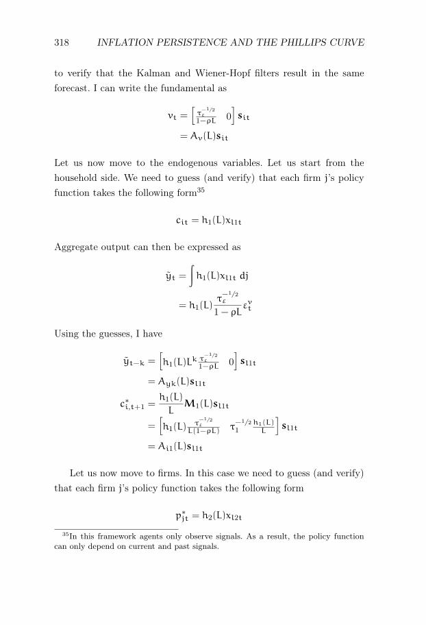
318 INFLATION PERSISTENCE AND THE PHILLIPS CURVE
to verify that the Kalman and Wiener-Hopf filters result in the sameforecast. I can write the fundamental as
vt =[τ−1/2ε
1−ρL 0]sit
= Av(L)sit
Let us now move to the endogenous variables. Let us start from thehousehold side. We need to guess (and verify) that each firm j’s policyfunction takes the following form35
cit = h1(L)xl1t
Aggregate output can then be expressed as
yt =
∫h1(L)xl1t dj
= h1(L)τ−1/2ε
1 − ρLεvt
Using the guesses, I have
yt−k =[h1(L)L
k τ−1/2ε
1−ρL 0]sl1t
= Ayk(L)sl1t
c∗i,t+1 =h1(L)
LM1(L)sl1t
=[h1(L)
τ−1/2ε
L(1−ρL) τ−1/21
h1(L)L
]sl1t
= Ai1(L)sl1t
Let us now move to firms. In this case we need to guess (and verify)that each firm j’s policy function takes the following form
p∗jt = h2(L)xl2t
35In this framework agents only observe signals. As a result, the policy functioncan only depend on current and past signals.

PROOFS OF PROPOSITIONS IN MAIN TEXT 319
Aggregate price level can then be expressed as
pt = (1 − θ)
∫h2(L)xl2t dj+ θpt−1
= (1 − θ)h2(L)τ−1/2ε
(1 − ρL)(1 − θL)εvt
Using the guesses, I have
pt−k =[(1 − θ)τ
−1/2ε
h2(L)Lk
(1−ρL)(1−θL) 0]sl2t
= Apk(L)sl2t
p∗j,t+1 =h2(L)
LM2(L)sl2t
=[τ−1/2ε
h2(L)L(1−ρL) τ
−1/22
h2(L)L
]sl2t
= Ai2(L)sl2t
We are now armed with the necessary objects in order to obtain thethree different forecasts,
Elgtvt =[Av(z)M
′g(z
−1)Bg(z−1)−1]
+V−1g Bg(z)
−1xlgt
=
[[τ−1/2ε
1−ρz 0] [zτ−1/2
ε
z−ρ
τ−1/2g
]z− ρ
z− λg
]+
λgτg
ρ
1 − ρz
1 − λgzxit
=
[z
(1 − ρz)(z− λg)
]+
λτg
ρτε
1 − ρz
1 − λgzxit
=
[ϕv(z)
z− λg
]+
λgτg
ρτε
1 − ρz
1 − λgzxit
=ϕv(z) − ϕv(λg)
z− λg
λgτg
ρτε
1 − ρz
1 − λgzxit
=λgτg
ρτε(1 − ρλg)
11 − λgz
xit
= G1g(z)xit (4.59)
Elgtyt−k =[Ayk(z)M
′g(z
−1)Bg(z−1)−1]
+V−1g Bg(z)
−1xlgt

320 INFLATION PERSISTENCE AND THE PHILLIPS CURVE
=
[[τ−1/2ε
h1(z)zk
1−ρz 0] [zτ−1/2
ε
z−ρ
τ−1/2g
]z− ρ
z− λg
]+
λgτg
ρ
1 − ρz
1 − λgzxlgt
=
[h1(z)z
k+1
(1 − ρz)(z− λg)
]+
λgτg
τερ
1 − ρz
1 − λgzxlgt
=
[ϕy(z)
z− λg
]+
λgτg
τερ
1 − ρz
1 − λgzxlgt
=ϕy(z) − ϕy(λg)
z− λg
λgτg
ρτε
1 − ρz
1 − λgzxlgt
=λgτg
ρτε
[h1(z)z
k+1 − h1(λg)λk+1g
1 − ρz
1 − ρλg
]1
(1 − λgz)(z− λg)xlgt
= G2gk(z)xlgt (4.60)
Elgtpt−k =[Apk(z)M
′g(z
−1)Bg(z−1)−1]
+V−1g Bg(z)
−1xlgt
=
[[(1 − θ)τ
−1/2ε
h2(z)zk
(1−ρz)(1−θz) 0] [zτ−1/2
ε
z−ρ
τ−1/2g
]z− ρ
z− λg
]+
λgτg
ρ
1 − ρz
1 − λgzxlgt
=
[h2(z)z
k+1
(1 − ρz)(z− λg)(1 − θz)
]+
(1 − θ)λgτgτερ
1 − ρz
1 − λgzxlgt
=
[ϕπ(z)
z− λg
]+
(1 − θ)λgτgτερ
1 − ρz
1 − λgzxlgt
=ϕπ(z) − ϕπ(λg)
z− λg
(1 − θ)λgτgρτε
1 − ρz
1 − λgzxlgt
= (1 − θ)λgτg
ρτε
[h2(z)z
k+1
1 − θz− h2(λg)λ
k+1g
1 − ρz
(1 − ρλg)(1 − θλg)
]×
× 1(1 − λgz)(z− λg)
xlgt
= G3gk(z)xlgt (4.61)
Elgtalg,t+1 =[Aig(z)M
′g(z
−1)Bg(z−1)−1]
+V−1g Bg(z)
−1xlgt
=
[[τ−1/2ε
hg(z)z(1−ρz) τ
−1/2g
hg(z)z
] [zτ−1/2ε
z−ρ
τ−1/2g
]z− ρ
z− λg
]+
λgτg
ρ
1 − ρz
1 − λgzxlgt
=
[hg(z)
τε(1 − ρz)(z− λg)+hg(z)(z− ρ)
τgz(z− λg)
]+
λgτg
ρ
1 − ρz
1 − λgzxlgt
=
[hg(z)
τε(1 − ρz)(z− λg)
]+
+
[hg(z)(z− ρ)
τgz(z− λg)
]+
λgτg
ρ
1 − ρz
1 − λgzxlgt

PROOFS OF PROPOSITIONS IN MAIN TEXT 321
=
[ϕig,1(z)
z− λg
]+
+
[ϕig,2(z)
z(z− λg)
]+
λgτg
ρ
1 − ρz
1 − λgzxlgt
=
ϕig,1(z) − ϕig,1(λg)
z− λg+ϕig,2(z) − ϕig,2(λg)
λg(z− λg)−
−ϕig,2(z) − ϕig,2(0)
λgz
λgτg
ρ
1 − ρz
1 − λgzxlgt
=λg
ρ
hg(z)
z− λg
[τg
τε(1 − ρz)+z− ρ
z
]−
−hg(λg)
z− λg
[τg
τε(1 − ρλg)+λg − ρ
λg
]−ρhg(0)λgz
1 − ρz
1 − λgzxlgt
= G4g(z)xlgt (4.62)
where El1tal1,t+1 = Eitci,t+1, El2tal2,t+1 = Ejtp∗j,t+1, and
ϕv(z) =z
1 − ρz, ϕπ(z) =
h2(z)zk+1
(1 − ρz)(1 − θz), ϕy(z) =
h1(z)zk+1
1 − ρz
ϕig,1(z) =hg(z)
τε(1 − ρz), ϕig,2(z) =
hg(z)(z− ρ)
τg
Rearranging terms, we obtain (4.63)-(4.67). We can show that expecta-tions satisfy
Elgtvt =(
1 −λg
ρ
)1
1 − λgzxlgt
= G1g(z)xlgt (4.63)
Elgtak,t−1 = (1 − θk)
(1 −
λg
ρ
)[hk(z)z
2(1 − ρλg)
1 − θkz−hk(λg)λ
2g(1 − ρz)
1 − θkλg
]×
× 1(1 − λgz)(z− λg)
xlgt
= G2k(z)xlgt (4.64)
Elgtak,t = (1 − θk)
(1 −
λg
ρ
)[hk(z)z(1 − ρλg)
1 − θkz−hk(λg)λg(1 − ρz)
1 − θkλg
]×
× 1(1 − λgz)(z− λg)
xlgt
= G3k(z)xlgt (4.65)

322 INFLATION PERSISTENCE AND THE PHILLIPS CURVE
Elgtak,t+1 = (1 − θk)
(1 −
λg
ρ
)[hk(z)(1 − ρλg)
1 − θkz−hk(λg)(1 − ρz)
1 − θkλg
]×
× 1(1 − λgz)(z− λg)
xlgt
= G4k(z)xlgt (4.66)
Elgtalg,t+1 =
hg(z)
z− λg
[(1 −
λg
ρ
)1 − ρλg1 − ρz
+λg(z− ρ)
ρz
]−hg(0)z
×
× 1 − ρz
1 − λgzxlgt
= G5g(z)xlgt (4.67)
Recall the best response for household i and firm j, conditions (4.50)-(4.51). In order to be consistent with agent optimization, the policy func-tions hg(z) must satisfy (4.50)-(4.51) at all times and signals. Pluggingthe obtained expressions, we can write
algt = φgElgtvt + βgElgtalg,t+1 +
2∑j=1
µgjElgtaj,t−1+
+
2∑j=1
γgjElgtaj,t +2∑j=1
αgjElgtaj,t+1
hg(z)xlgt = φgG1g(z)xlgt + βgG5g(z)xlgt +
2∑j=1
µgjG2j(z)xlgt+
+
2∑j=1
γgjG3j(z)xlgt +
2∑j=1
αgjG4j(z)xlgt
hg(z) = φgG1g(z) + βgG5g(z) +
2∑j=1
µgjG2j(z) +
2∑j=1
γgjG3j(z)+
+
2∑j=1
αgjG4j(z)
= φg
(1 −
λg
ρ
)1
1 − λgz+
+ βg
hg(z)
z− λg
[(1 −
λg
ρ
)1 − ρλg1 − ρz
+λg(z− ρ)
ρz
]−hg(0)z
1 − ρz
1 − λgz

PROOFS OF PROPOSITIONS IN MAIN TEXT 323
+
2∑j=1
µgj(1 − θj)
(1 −
λg
ρ
)[hj(z)z
2(1 − ρλg)
1 − θjz−hj(λg)λ
2g(1 − ρz)
1 − θjλg
]×
× 1(1 − λgz)(z− λg)
+
2∑j=1
γgj(1 − θj)
(1 −
λg
ρ
)[hj(z)z(1 − ρλg)
1 − θjz−hj(λg)λg(1 − ρz)
1 − θjλg
]×
× 1(1 − λgz)(z− λg)
+
2∑j=1
αgj(1 − θj)
(1 −
λg
ρ
)[hj(z)(1 − ρλg)
1 − θjz−hj(λg)(1 − ρz)
1 − θjλg
]×
× 1(1 − λgz)(z− λg)
whereφ1 = −
β
σ
β1 = β
µ11 = 0
µ12 =βϕπ
σ
γ11 = 1 − β
(1 +
ϕy
σ
)γ12 = −
β(1 + ϕπ)
σ
α11 = 0
α12 =β
σ
θ1 = 0
φ2 = 0
β2 = βθ
µ21 = 0
µ22 = 0
γ21 =κθ
1 − θ
γ22 = 1 − βθ
α21 = 0
α22 = 0
θ2 = θ
Multiplying both sides by z(z−λg)(1−λgz)(1−θ1z)(1−θ2z) we obtain
hg(z)z(z− λg)(1 − λgz)(1 − θ1z)(1 − θ2z) =
= φg
(1 −
λg
ρ
)z(z− λg)(1 − θ1z)(1 − θ2z)

324 INFLATION PERSISTENCE AND THE PHILLIPS CURVE
+ βg
hg(z)
[(1 −
λg
ρ
)(1 − ρλg)z+
λg
ρz(z− ρ)(1 − ρz)
]−
− hg(0)(z− λg)(1 − ρz)
(1 − θ1z)(1 − θ2z)
+
2∑j=1
µgj(1 − θj)
(1 −
λg
ρ
)×
×
[hj(z)z
3(1 − ρλg)(1 − θ¬jz) −hj(λg)λ
2gz(1 − ρz)(1 − θ1z)(1 − θ2z)
1 − θjλg
]
+
2∑j=1
γgj(1 − θj)
(1 −
λg
ρ
)×
×[hj(z)z
2(1 − ρλg)(1 − θ¬jz) −hj(λg)λgz(1 − ρz)(1 − θ1z)(1 − θ2z)
1 − θjλg
]+
2∑j=1
αgj(1 − θj)
(1 −
λg
ρ
)×
×[hj(z)z(1 − ρλg)(1 − θ¬jz) −
hj(λg)z(1 − ρz)(1 − θ1z)(1 − θ2z)
1 − θjλg
]Rearranging the LHS by hg(z),
hg(z)z(z− λg)(1 − λgz)(1 − θ1z)(1 − θ2z)
− βg
[(1 −
λg
ρ
)(1 − ρλg)z+
λg
ρz(z− ρ)(1 − ρz)
](1 − θ1z)(1 − θ2z)
−
2∑j=1
µgj(1 − θj)
(1 −
λg
ρ
)z3(1 − ρλg)(1 − θ¬jz)hj(z)
−
2∑j=1
γgj(1 − θj)
(1 −
λg
ρ
)z2(1 − ρλg)(1 − θ¬jz)hj(z)
−
2∑j=1
αgj(1 − θj)
(1 −
λg
ρ
)z(1 − ρλg)(1 − θ¬jz)hj(z)

PROOFS OF PROPOSITIONS IN MAIN TEXT 325
and the RHS can be rewritten as
dg(z) = φg
(1 −
λg
ρ
)z(z− λg)(1 − θ1z)(1 − θ2z)−
− hg(0)βg(z− λg)(1 − ρz)(1 − θ1z)(1 − θ2z)
−
(
1 −λg
ρ
) 2∑j=1
1 − θj1 − θjλg
[µgjλ2g + γgjλg + αgj]hj(λg)
×
× z(1 − ρz)(1 − θ1z)(1 − θ2z)
We can write the system in matrix form as
C(z)h(z) = d(z)
where
C(z) =
[C11(z) C12(z)
C21(z) C22(z)
], h(z) =
[h1(z)
h2(z)
], d(z) =
[d1(z)
d2(z)
]Cgg(z) = (z− βg)(z− λg)(1 − λgz)(1 − θ1z)(1 − θ2z)
− (1 − θg)
(1 −
λg
ρ
)(1 − ρλg)(1 − θ¬gz)z(µggz
2 + γggz+ αgg)
Cgn(z) = −(1 − θn)
(1 −
λg
ρ
)(1 − ρλg)(1 − θgz)(µgnz
3 + γgnz2 + αgnz)
dg(z) =
[φg
(1 −
λg
ρ
)z(z− λg) − hg(0)βg(z− λg)(1 − ρz) − hgz(1 − ρz)
]×
× (1 − θ1z)(1 − θ2z)
Cancelling out parameters equal to zero to simplify the expressions,we can write
C11(z) =
[(z− β1)(z− λ1)(1 − λ1z) −
(1 −
λ1
ρ
)(1 − ρλ1)γ11z
2](1 − θ2z)
C12(z) = −(1 − θ2)
(1 −
λ1
ρ
)(1 − ρλ1)z(µ12z
2 + γ12z+ α12)
C21(z) = −
(1 −
λ2
ρ
)(1 − ρλ2)(1 − θ2z)γ21z
2

326 INFLATION PERSISTENCE AND THE PHILLIPS CURVE
C22(z) = (z− β2)(z− λ2)(1 − λ2z)(1 − θ2z)−
− (1 − θ2)
(1 −
λ2
ρ
)(1 − ρλ2)γ22z
2
d1(z) =
[φ1
(1 −
λ1
ρ
)z(z− λ1) − h1(0)β1(z− λ1)(1 − ρz) − h1z(1 − ρz)
]×
× (1 − θ2z)
d2(z) =[−hg(0)β2(z− λ2)(1 − ρz) − h2z(1 − ρz)
](1 − θ2z)
and the solution to the policy functions is given by
h(z) = C(z)−1d(z) =adj C(z)
det C(z)d(z)
Note that the degree of C(z) is 8, given that θ1 = 0. Denotethe inside roots of detC(z) as ζ1, ζ2, ..., ζn1 and the outside roots asϑ−1
1 , ϑ−12 , ..., ϑ−1
n1. Because agents cannot use future signals, the inside
roots have to be removed. Note that the number of free constants ind is 4: hg(0), hg2g=1. For a unique solution, it must be the case thatthe number of outside roots is n2 = 4. Also note that by Cramer’s rule,hg(z) is given by
h1(z) =
det
[d1(z) C12(z)
d2(z) C22(z)
]det C(z)
, h2(z) =
det
[C11(z) d1(z)
C21(z) d2(z)
]det C(z)
The degree of the numerator is 7, as the highest degree of dg(z) is 1degree less than Cgg(z). By choosing the constants hg(0), hg2g=1, the4 inside roots will be removed. Therefore, the 4 constants are solutionsto the following system of linear equations36
det
[d1(ζn) C12(ζn)
d2(ζn) C22(ζn)
]= 0, for ζn
4n=1
36The set of constants that solve the system of equations for h1(z) also solves itfor h2(z), since ζn
4n=1 are roots of detC(z), leaving vectors in C(ζn) being linearly
dependent.

PROOFS OF PROPOSITIONS IN MAIN TEXT 327
where n2 = 4. After removing the inside roots in the denominator, thedegree of the numerator is 3 and the degree of the denominator is 4. Asa result, the solution to hg(z) takes the form
hg(z) =ψg1 + ψg2z+ ψg3z
2 + ψg4z3
(1 − ϑ1z)(1 − ϑ2z)(1 − ϑ3z)(1 − ϑ4z)
Given the model conditions, we have that ϑ4 = θ. We can write
hg(z) =ψg1 + ψg2z+ ψg3z
2 + ψg4z3
(1 − ϑ1z)(1 − ϑ2z)(1 − ϑ3z)(1 − θz)
=ψg4(z− ηg1)(z− ηg2)(z− ηg3)
(1 − ϑ1z)(1 − ϑ2z)(1 − ϑ3z)(1 − θz)
=−ψg4ηg1ηg2ηg3(1 − η−1
g1 z)(1 − η−1g2 z)(1 − η−1
g3 z)
(1 − ϑ1z)(1 − ϑ2z)(1 − ϑ3z)(1 − θz)
=−ψg4ηg1ηg2ηg3(1 − ξg1z)(1 − ξg2z)(1 − ξg3z)
(1 − ϑ1z)(1 − ϑ2z)(1 − ϑ3z)(1 − θz)
where (ηg1,ηg2,ηg3) are the roots of ψg1 + ψg2z + ψg3z2 + ψg4z
3. Wealso have that ξ13 = ξ22 = ξ23 = θ. Hence, we can write
yt = h1(z)vt
=−ψ14η11η12η13(1 − ξ11z)(1 − ξ12z)
(1 − ϑ1z)(1 − ϑ2z)(1 − ϑ3z)vt
= ϕ1(1 − ξ11z)(1 − ξ12z)
(1 − ϑ1z)(1 − ϑ2z)(1 − ϑ3z)vt
= ψ11
(1 −
ϑ1
ρ
)1
1 − ϑ1zvt +ψ12
(1 −
ϑ2
ρ
)1
1 − ϑ2zvt+
+ψ13
(1 −
ϑ1
ρ
)1
1 − ϑ3zvt
= ψ11ϑ1t +ψ12ϑ2t +ψ13ϑ3t
pt = (1 − θ)h2(z)1
1 − θzvt
=−ψ24η21η22η23(1 − θ)(1 − ξ21z)
(1 − ϑ1z)(1 − ϑ2z)(1 − ϑ3z)vt

328 INFLATION PERSISTENCE AND THE PHILLIPS CURVE
= ϕ21 − ξ21z
(1 − ϑ1z)(1 − ϑ2z)(1 − ϑ3z)vt
= ψ21
(1 −
ϑ1
ρ
)1
1 − ϑ1zvt +ψ22
(1 −
ϑ2
ρ
)1
1 − ϑ2zvt+
+ψ23
(1 −
ϑ1
ρ
)1
1 − ϑ3zvt
= ψ21ϑ1t +ψ22ϑ2t +ψ23ϑ3t
Using πt = (1 − L)pt, we can write
πt = (1 − θ)h2(z)1 − z
1 − θzvt
=−ψ24η21η22η23(1 − θ)(1 − ξ21z)(1 − z)
(1 − ϑ1z)(1 − ϑ2z)(1 − ϑ3z)vt
= ϕ2(1 − ξ21z)(1 − z)
(1 − ϑ1z)(1 − ϑ2z)(1 − ϑ3z)vt
= ψ31
(1 −
ϑ1
ρ
)1
1 − ϑ1zvt +ψ32
(1 −
ϑ2
ρ
)1
1 − ϑ2zvt+
+ψ33
(1 −
ϑ1
ρ
)1
1 − ϑ3zvt
= ψ31ϑ1t +ψ32ϑ2t +ψ33ϑ3t
We can finally write
at =
ytptπt
= Qϑt
=
ψ11 ψ12 ψ13
ψ21 ψ22 ψ23
ψ31 ψ32 ψ33
ϑ1t
ϑ2t
ϑ3t
Notice that we can write

ROBUSTNESS 329
ϑkt(1 − ϑkL) =
(1 −
ϑkρ
)vt =⇒ ϑkt = ϑkϑk,t−1 +
(1 −
ϑkρ
)vt
which we can write as a system as
ϑt = Λϑt−1 + Γvt
where
Λ =
ϑ1 0 00 ϑ2 00 0 ϑ3
, Γ =
1 − ϑ1ρ
1 − ϑ2ρ
1 − ϑ3ρ
Hence, we can write
at = Qθt
= Q(Λθt−1 + Γξt)
= QΛθt−1 +QΓξt
= QΛQ−1at−1 +QΓξt
= Aat−1 + Bξt (4.68)
4.B Robustness on Inflation Persistence and In-formation Frictions
4.B.1 Inflation Persistence
We begin our robustness analysis by considering alternative inflationmeasures. Figure 4.7 presents the CPI and PCE series (together withthe GDP Deflator growth). All inflation measures are closely correlated.

330 INFLATION PERSISTENCE AND THE PHILLIPS CURVE
Figure 4.7: Time Series of GDP Deflator, CPI and PCE.
Table 4.7: Correlation matrix
1969-2020Variable GDP Deflator CPI PCEGDP Deflator 1.00CPI 0.86 1.00PCE 0.91 0.96 1.00
1969-1985GDP Deflator 1.00CPI 0.83 1.00PCE 0.88 0.92 1.00
1985-2020GDP Deflator 1.00CPI 0.66 1.00PCE 0.73 0.96 1.00
I report the correlation matrix across different sub-sample periods inTable 4.7. The three main inflation measures exhibit a high and positivecorrelation in the pre-1985 period. In the post-1985 period, there is adetachment between the GDP deflator and the two other price measures,CPI and PCE, which still exhibit a high degree of correlation.
We repeat the structural break analysis discussed in the main bodyfor CPI and PCE inflation, and we find similar results in Table 4.8, withthe structural change in dynamics being less evident in the core series.
Autocorrelation Function Let us start from the most agnostic anal-ysis of inflation persistence. Figure 4.8 plots the autocorrelation function

ROBUSTNESS 331
Table 4.8: Regression table
(1) (2)CPI PCE
πt−1 0.793∗∗∗ 0.837∗∗∗
(0.0827) (0.0672)
πt−1 × 1t⩾t∗ -0.497∗∗∗ -0.434∗∗∗
(0.143) (0.117)
Constant 1.396∗∗ 0.990∗∗
(0.542) (0.431)
Constant×1t⩾t∗ 0.370 0.283(0.607) (0.477)
Observations 206 206Standard errors in parentheses∗ p < 0.10, ∗∗ p < 0.05, ∗∗∗ p < 0.01
for the three main inflation measures across subsamples. Focusing onthe second and third columns, I find a significant fall in the first-orderautocorrelation for the three measures. For instance, the first-order au-tocorrelation for all inflation measures in the pre-1985 sample is around0.75, while the same statistic for the second period ranges from 0.5 to0.3 depending on the measure.
Rolling Sample I compute rolling-sample estimates of an indepen-dent AR(1) process using a 14-year window for the different inflationmeasures. Figure 4.9 plots the time-varying persistence parameter ρtwith 95% confidence bands. The results suggest that there is significanttime variation in inflation persistence.
Time-Varying Parameter Autorregression We assume that thepersistence coefficient in the AR(1) process follows a Random Walk:ρt+1 = ρt + ut, ut ∼ N(0,Σu), where the model is estimated usingBayesian methods. The model is estimated using Bayesian methods. Ourprior selection is standard, following Nakajima (2011), using the invert

332 INFLATION PERSISTENCE AND THE PHILLIPS CURVE
(a) GDP Deflator, 1947-1985
(b) GDP Deflator, 1969-1985
(c) GDP Deflator, 1985-2020
(d) CPI, 1947-1985 (e) CPI, 1969-1985 (f) CPI, 1985-2020
(g) PCE, 1947-1985 (h) PCE, 1969-1985 (i) PCE, 1985-2020
Figure 4.8: Autocorrelation function of GDP Deflator (first row), CPI (secondrow) and PCE (last row)

ROBUSTNESS 333
(a) GDP deflator
(b) CPI
Figure 4.9: First-order autocorrelation of GDP Deflator, CPI and PCE,rolling sample (14y window)

334 INFLATION PERSISTENCE AND THE PHILLIPS CURVE
(c) PCE
Figure 4.9: First-order autocorrelation of GDP Deflator, CPI and PCE,rolling sample (14y window) (cont.)

ROBUSTNESS 335
Figure 4.10: Time-varying persistence.
Wishart and invert Gamma distributions
ρ1 ∼ N(0, 10 × I), σε ∼ IG(2, 0.02), Σu ∼ IW(4, 40 × I)
I plot the estimated ρt with 95% confidence bands in Figure 4.10. Thefall in persistence is delayed until the mid 2000s, but the overall fall isconsistent with our previous findings.
Unit Root Tests Inspecting Figure 4.9, one could imagine that in-flation is characterized by a unit root process in the pre-1985 sampleand not afterwards. In order to investigate this, I proceed via a cross-sample unit root analysis using both the Augmented Dickie-Fuller andthe Phillips-Perron tests. I report our results in Table 4.9, including thep-values of both unit root tests under the null of unit root. Focusing onthe last two rows I find that, consistent with our previous evidence onthe first-order autocorrelation, the null hypothesis of a unit root series

336 INFLATION PERSISTENCE AND THE PHILLIPS CURVE
p-values, null = series has unit root1969-2020
Variable ADF Phillips-Perron
GDP Deflator 0.23 0.02CPI 0.11 0.00PCE 0.16 0.00
1969-1985Variable ADF Phillips-
PerronGDP Deflator 0.15 0.07CPI 0.17 0.09PCE 0.055 0.09
1985-2020Variable ADF Phillips-
PerronGDP Deflator 0.07 0.00CPI 0.00 0.00PCE 0.01 0.00
Table 4.9: Unit Root Tests for Inflation Measures.
cannot be rejected by any of the unit root tests conducted in the differ-ent inflation measures in the pre-1985 period. On the other hand, whenI repeat the similar analysis in the post-1985 period, I find a strong re-jection of the null hypothesis, suggesting that inflation can no longer bedescribed as a unit root process. Having understood the close relationbetween the roots of the inflation dynamic process and its persistence, Ican conclude that inflation persistence fell in the post-1985 period.
Dominant Root A further procedure of studying persistence that re-lies on the roots of the dynamic process of inflation is the dominant rootanalysis. Consider the AR(p) process
πt = ρ1πt−1 + ρ2πt−2 + . . . + ρpπt−p + επt

ROBUSTNESS 337
with companion matrix R(p). The root of the characteristic polynomialof R(p) with the largest magnitude is the dominant root of interest.Notice that in the case of an AR(p) where p > 1, the dominant root willdepend not only on the first lag coefficient but in all of them. An AR(p)is considered to be stable if all the roots of the characteristic polynomialof matrix R(p) have an absolute value lower than 1. One can thereforeproceed as in the unit root case, and study the dominant root of theunderlying inflation process over the different subsamples. We find thatthe dominant root in the 1968:Q4-1984:Q4 period is 0.870 and 0.841 inthe 1985:Q1-2020:Q1 period, suggesting a moderate fall in persistence.
4.B.2 Monetary Policy Shock Process
Persistence
Rolling Sample AR(1) Estimate of Persistence In order to testfor changes in monetary shocks’ persistence, I check nominal interestrates’ autocorrelation. I plot in Figure 4.11a the rolling (14 years) first-order autocorrelation of the nominal Fed Funds rate. I find no evidencefor a fall in the first-order autocorrelation over time.
As a robustness check, I estimate (4.80) and plot the rolling estimateρv over time. Notice that the NK model implies that the error term ξt
in (4.80) is serially correlated. In fact, the NK model suggests that ξtfollows an ARMA(1,1), or equivalently an MA(∞),
ξt = ρvξt−1 + ϕ1εvt + ϕ2ε
vt−1
= ϕ1εvt + ϕ1(ρ+ ϕ2)
∞∑j=0
ρjεvt−1−j
where ϕ1 = 1−ρv(ϕπψπ+ϕyψy) and ϕ2 = −ρv(1−ϕπψπ−ϕyψy)1−ρv(ϕπψπ+ϕyψy)
. How-ever, a standard parameterization of the model suggests that such serialcorrelation is small, in the sense that ϕ1(ρ + ϕ2) < 0.1. To be on thesafe side, I estimate (4.80) using GMM with Bartlett-Newey-West ro-bust standard errors, using as instruments four lags of the Effective Fed

338 INFLATION PERSISTENCE AND THE PHILLIPS CURVE
(a) Non-parametric First-order Autocorrelation
(b) First-order Autocorrelation, GMM
Figure 4.11: First-order autocorrelation of Nominal interest rates

ROBUSTNESS 339
Variable 1954-2020 1969-2020 1954-1985 1969-1985 1985-2020Fed Funds rate 0.97 0.97 0.95 0.90 0.95
Table 4.10: Dominant root of an AR(20) for nominal interest rate.
Funds rate, GDP Deflator, CBO Output Gap, Commodity Price Infla-tion, Real M2 Growth and the spread between the long-term bond rateand the three-month Treasury bill rate, following Clarida et al. (2000).Overall, I find no evidence of a fall in persistence ρ in the recent decades.
Dominant Root Estimate of Persistence I confirm this result byobtaining the dominant root of the nominal interest rate over time. AsI showed in section 4.3, another procedure to measure persistence is tocompute the dominant root of an AR(p) process. I estimate an AR(20)process on nominal interest rates, and obtain the dominant root at eachsub-sample period. Our results are reported in Table 4.10. I find noevidence for a change in nominal rates persistence. If anything, I findevidence for a moderate increase in the nominal interest rate dominantroot over time.
4.B.3 Change in the Monetary Stance
The fall in inflation persistence coincides with a structural change in theFed policy stance around 1985:I, documented in Clarida et al. (2000).Economists generally model the change in the Fed stance around 1985:Ias a structural break in the reaction function of Central Banks. In par-ticular, the break is modelled as if the elasticity of nominal rates withrespect to inflation, ϕπ, went from a previous value of 1 to a value closerto 2. That is, as if the Federal Reserve had become more hawkish in therecent decades. To test this, I estimate a standard Taylor rule in whichnominal rates are elastic to current inflation and output gap, as thebenchmark framework suggests. I test for a structural break in 1985:I,

340 INFLATION PERSISTENCE AND THE PHILLIPS CURVE
and our findings align with those in the literature,37
it = αi + ϕππt + ϕπ,∗πt1t⩾t∗ + ϕyyt + ϕy,∗yt1t⩾t∗ + vt (4.69)
using Bartlett-Newey-West standard errors that take into considerationserially correlated residuals, which the theoretical framework suggests.I report our results in table 4.11. Indeed, our results show that priorto 1985 the elasticity with respect to inflation was around 1.32, and in-creased to 2.28 in the Great Moderation, close to the findings by Claridaet al. (2000). In the following subsection I link this structural change withthe dynamics of inflation produced in the NK model. As I will show, theincrease in ϕπ will effectively reduce inflation volatility but will have noeffect on persistence.
4.B.4 Empirical Evidence on Information Frictions
Rolling Sample Regression I obtain a rolling-sample estimate ver-sion of (4.3). Figure 4.12 plots the rolling estimate βCG,t over time. Thefigure suggests that information frictions were reduced after the 1980s,with a smaller local peak in the late 2000s, which coincides with the localpeak in inflation persistence in Figure 4.9.
Time-Varying Parameter Autorregression I use the following rep-resentation of the time-varying parameter regression model
πt+3,t − Etπt+3,t = βCG,t(Etπt+3,t − Et−1πt+3,t) + ut, ut ∼ N(0,σ2u)
37To estimate the Taylor rule I rely on GMM methods, using four lags of theEffective Fed Funds rate, GDP Deflator, CBO Output Gap, Commodity Price In-flation, Real M2 Growth and the spread between the long-term bond rate and thethree-month Treasury bill rate as instruments. The standard NK model incorporatesinertia in the Taylor rule via the AR(1) component vt instead of including lags of thenominal interest rate on the right-hand side of (4.69), which allows us to obtain aclosed-form solution of the model.

ROBUSTNESS 341
Table 4.11: Regression table
(1) (2)Taylor Rule Break
πt 1.154∗∗∗ 1.323∗∗∗
(0.112) (0.140)
yt 0.353∗∗∗ 0.309∗∗
(0.121) (0.128)
πt × 1t⩾t∗ 0.958∗∗∗
(0.284)
Constant 1.518∗∗∗ -0.517(0.442) (0.844)
Observations 204 204Standard errors in parentheses∗ p < 0.10, ∗∗ p < 0.05, ∗∗∗ p < 0.01
Figure 4.12: Time-varying βCG,t in the CG regression (4.3) using a 14ywindow.

342 INFLATION PERSISTENCE AND THE PHILLIPS CURVE
Figure 4.13: Time-varying Coibion and Gorodnichenko (2015a) regression.
where the time-varying persistence coefficient is assumed to follow a ran-dom walk
βCG,t+1 = βCG,t + ϵt, ϵt ∼ N(0,Σϵ)
The model is estimated using Bayesian methods. Our prior selection isstandard, following Nakajima (2011), using the invert Wishart and invertGamma distributions
βCG,1 ∼ N(0, 10 × I), σu ∼ IG(2, 0.02), Σϵ ∼ IW(4, 40 × I)
I plot the estimated βCG,t with 95% confidence bands in Figure 4.13.After the break in the mid-1980s the estimated values are not statisticallysignificant, unable to reject the FIRE assumption.

ROBUSTNESS 343
Forecast Error Response to Monetary Policy Shocks UnderFIRE, ex-post forecast errors should be unpredictable by ex-ante avail-able information. Therefore, the IRF of forecast errors to monetary policyshocks should be insignificant. Coibion and Gorodnichenko (2012) showthat forecast errors react to several exogenous shocks to the economy.In order to study if the sensitivity of ex-post forecast errors has changedafter the 1985:Q1 structural break, we produce the local projection ofRomer and Romer (2004) monetary policy shocks on the average forecasterror,
errort+h = βhεvt + βh∗ε
vt × 1t⩾t∗ + γXt + ut
where h denotes the horizon and Xt includes four lags of Romer andRomer (2004) shocks and four lags of forecast errors. We report the im-plied impulse responses in Figure 4.14. We find that the IRF is positivein the pre-1985 period, suggesting that forecasts react less to monetaryshocks than the forecasted variable (see Figure 4.14a). After 1985, fore-cast errors do not react to monetary shocks, suggesting that informationfrictions lessened (see Figure 4.14b). I show in Figure 4.14c that thedifference between the IRFs under the two regimes is significant.
Disagreement I define a measure of “disagreement” as the cross-sectional standard deviation of forecasts at each time,
disagreementt = σi(Fitπt+3,t)
Under the assumption of common complete information, disagree-ment should be zero since all agents would have observed the same past,their information set would therefore be the same, and their expecta-tion around a future variable should coincide, provided that agents areex-ante identical. As we observe in Figure 4.15, disagreement was largearound the 1980s, coinciding with the beginning of the Volcker activismand the lack of public disclosure of the Federal Reserve decisions, and

344 INFLATION PERSISTENCE AND THE PHILLIPS CURVE
(a) Pre-1985 period.
(b) Post-1985 period.
(c) Change.
Figure 4.14: Impulse response function of average forecasts to monetary policyshocks.

ROBUSTNESS 345
Figure 4.15: Cross-sectional volatility of (annual) inflation forecasts at eachperiod.
fell dramatically until the 1990s, stabilizing at that level after the 1990s.The previous figure dynamics are reminiscent of the inflation dynam-
ics in Figure 4.1. One could thus argue that, if forecast disagreementdepends on the level of inflation, the fall in disagreement would be en-tirely explained by the fall in inflation. We now show that forecast donot depend on the current level of inflation. First, assuming that infla-tion follows an AR(p) (up to p = 3), we regress the individual (average)forecast of the AR(p) process, and we add realized inflation
Fitπt+3 = ρ1Fitπt+2 + ρ2Fitπt+1 + ρ3Fitπt + γπt−1,t−5 + ut (4.70)
Ftπt+3 = ρ1Ftπt+2 + ρ2Ftπt+1 + ρ3Ftπt + γπt−1,t−5 + ut (4.71)
We report our results in Table 4.12. We find in columns 1-3 (columns4-6) that the lagged inflation coefficient is insignificant in most cases. Wethen regress the average forecast error on the average forecast revision(column 7) or on the lagged forecast error (column 8), controlling forlagged inflation. We find that realized inflation is insignificant in bothcases. We can therefore argue that the fall in cross-sectional forecastvolatility fell after the 1985 period as a result of lessened informationfrictions.

346 INFLATION PERSISTENCE AND THE PHILLIPS CURVE
Tab
le4.
12:
Reg
ress
ion
tabl
e
Indi
vidu
alfo
reca
sts
Ave
rage
fore
cast
Err
orE
rror
AR
(1)
AR
(2)
AR
(3)
AR
(1)
AR
(2)
AR
(3)
F tπt+
21.
284∗
∗∗1.
435∗
∗∗1.
417∗
∗∗1.
356∗
∗∗1.
870∗
∗∗1.
749∗
∗∗
(0.0
162)
(0.0
476)
(0.0
482)
(0.0
190)
(0.0
707)
(0.0
739)
F tπt+
1-0
.232
∗∗∗
-0.0
992
-0.7
75∗∗
∗-0
.390
∗∗∗
(0.0
652)
(0.0
874)
(0.1
02)
(0.1
39)
F tπt
-0.2
14∗∗
∗-0
.414
∗∗∗
(0.0
697)
(0.0
97)
revisiont
1.22
0∗∗∗
(0.2
48)
error t
−1
0.88
1∗∗∗
(0.0
592)
πt−
1,t−
50.
0070
50.
0119
0.01
37∗
-0.0
299∗
∗-0
.018
2-0
.016
90.
0081
9-0
.016
3(0
.009
09)
(0.0
0859
)(0
.008
19)
(0.0
124)
(0.0
115)
(0.0
108)
(0.0
340)
(0.0
131)
Obs
erva
tion
s7,
751
7,75
07,
750
205
205
205
197
203
HA
Cro
bust
stan
dard
erro
rsin
pare
nthe
ses
∗p<
0.10
,∗∗p<
0.05
,∗∗∗p<
0.01

ROBUSTNESS 347
Livingston Survey Using the Livingston survey on firms, I test fora structural break in belief formation around 1985:I. Since the survey isconducted semiannually, I estimate the following structural-break variantof (4.4)
πt+2,t−Etπt+2,t = αCG+(βCG + βCG∗1t⩾t∗
)(Etπt+2,t−Et−2πt+2,t)+ut
(4.72)Our results, reported in the first column in Table 4.13, suggest a strongviolation of the FIRE assumption: the measure of information frictions,βCG, is significantly different from zero. Secondly, a significant estimateof βCG∗ would suggest a break in the information frictions faced byagents. Our results in the second column in Table 4.3 suggest that thereis a structural break around the period in which the Fed changed themonetary stance. Our result βCG∗ < 0 suggests that agents becamemore more informed about inflation, with individual forecasts relyingless on priors and more on news. A t-test under the null that βCG +
βCG,∗ = 0 has an associated p-value of 0.254. I can therefore concludethat information frictions on the CPI vanish, consistent with our findingson CPI persistence in Figure 4.9b.

348 INFLATION PERSISTENCE AND THE PHILLIPS CURVE
Table 4.13: Regression table
(1) (2)CG Regression Structural Break
Revision 0.380∗ 0.412∗∗
(0.202) (0.204)
Revision×1t⩾t∗ -0.880∗∗
(0.414)
Constant -0.183∗ -0.105(0.102) (0.119)
Observations 146 146
Standard errors in parentheses∗ p < 0.10, ∗∗ p < 0.05, ∗∗∗ p < 0.01
As a second exercise, I estimate the following structural-break variantof (4.25)
πt,t−2 =(α1 + α1,∗1t⩾t∗
) ∞∑k=0
(βθ)kEftyt+k,t+k−2
+(α2 + α2,∗1t⩾t∗
) ∞∑k=0
(βθ)kEftπt+k,t+k−2
Since the survey is only conducted semiannually and only asks for 6mand 12m ahead forecasts we only consider the cases k = 2 and k = 4. Ourresults suggest no evidence of a structural break in κ once we control fornon-standard expectations.

ROBUSTNESS 349
Table 4.14: Regression table
(1) (2) (3)NKPC Break Output Break
Eftyt+2,t 1.014∗∗∗ 1.402∗∗∗ 1.079∗∗
(0.262) (0.438) (0.418)
Eftyt+4,t+2 -0.0717 -0.680 -0.354(0.335) (0.553) (0.533)
Eftπt+2,t -0.0552 -0.0352 -0.264∗∗∗
(0.0652) (0.0602) (0.0836)
Eftπt+4,t+2 -0.0375 -0.123 0.237(0.151) (0.147) (0.180)
Eftyt+2,t× 1t⩾t∗ -0.892∗ -0.598(0.526) (0.509)
Eftyt+4,t+2× 1t⩾t∗ 0.882 0.555(0.662) (0.641)
Eftπt+2,t× 1t⩾t∗ 0.303∗∗∗
(0.0955)
Eftπt+4,t+2× 1t⩾t∗ -0.486∗∗
(0.191)
Constant -0.115 0.388 0.479(0.250) (0.398) (0.460)
Observations 99 99 99Standard errors in parentheses∗ p < 0.10, ∗∗ p < 0.05, ∗∗∗ p < 0.01

350 INFLATION PERSISTENCE AND THE PHILLIPS CURVE
4.C Extending Information Frictions to House-holds
In this section we relax the FIRE assumption on households. We show inOnline Appendix 4.F that in such case, the individual household policyfunction is given by
cit = −β
σEitrt + (1 − β)Eityt + βEitci,t+1, with yt =
∫cit di
(4.73)
We still maintain the FIRE assumption on the monetary authority,which is not subject to information frictions. In this case, the modelequations are (4.73), (4.9), (4.11) and (4.12).
Information Structure In order to generate heterogeneous beliefsand sticky forecasts, I assume that the information is incomplete anddispersed. Each agent l in group g ∈ household, firm observes a noisysignal xlgt that contains information on the monetary shock vt, andtakes the standard functional form of “outcome plus noise”. Formally,signal xlgt is described as
xlgt = vt + σguulgt, with ulgt ∼ N(0, 1) (4.74)
where signals are agent-specific. This implies that each agent’s informa-tion set is different, and therefore generates heterogeneous informationsets across the population of households and firms. Notice that we allowfor heterogeneity in the variance that each of the groups (households andfirms) face.
An equilibrium must therefore satisfy the individual-level optimalpricing policy functions (4.9), the individual DIS curve (4.73), the Tay-lor rule (4.11), and rational expectation formation should be consistentwith the exogenous monetary shock process (4.12) and the signal process(4.74).

HOUSEHOLDS’ INFORMATION FRICTIONS 351
The following proposition outlines inflation and output gap dynam-ics.
Proposition 4.5. Under noisy information the output gap, price leveland inflation dynamics are given by
at = A(ϑ1, ϑ2, ϑ3)at−1 + B(ϑ1, ϑ2, ϑ3)vt (4.75)
where at =[yt pt πt
]′is a vector containing output, price level and
inflation, A(ϑ1, ϑ2, ϑ3) is a 3×3 matrix and B(ϑ1, ϑ2, ϑ3) is a 3×1 vector,where (ϑ1, ϑ2, ϑ3) are three scalars that are given by the reciprocal of threeof the four outside roots of the characteristic polynomial of the followingmatrix38
C(z) =
[C11(z) C12(z)
C21(z) C22(z)
]where
C11(z) =
[(z− β)(z− λ1)(1 − λ1z) −
(1 −
λ1
ρ
)(1 − ρλ1)
(1 − β
(1 +
ϕy
σ
))z2]×
× (1 − θ2z)
C12(z) = −(1 − θ)
(1 −
λ1
ρ
)(1 − ρλ1)z
(βϕπ
σz2 −
β(1 + ϕπ)
σz+
β
σ
)C21(z) = −
(1 −
λ2
ρ
)(1 − ρλ2)(1 − θz)
κθ
1 − θz2
C22(z) = (z− βθ)(z− λ2)(1 − λ2z)(1 − θz) − (1 − θ)
(1 −
λ2
ρ
)(1 − ρλ2)(1 − βθ)z2
with λg, g ∈ 1, 2 being the inside root of the following polynomial
D(z) ≡ z2 −(
1ρ+ ρ+
σ2ϵ
ρσ2gu
)z+ 1
Proof. See Appendix 4.A
In the noisy information framework, inflation is intrinsically persis-38The other outside root is always equal to θ and is cancelled out.

352 INFLATION PERSISTENCE AND THE PHILLIPS CURVE
tent and its persistence is governed by the new information-related pa-rameters ϑ1, ϑ2 and ϑ3, as opposed to the benchmark framework in whichit is only extrinsically persistent, A(0, 0, 0) = 0. The intuition for thisresult is simple: inflation is partially determined by expectations (seecondition (4.13) under noisy information, or (4.2) under complete infor-mation). Under noisy information, expectations are anchored and followan autoregressive process (see (4.15)), which creates the additional sourceof anchoring in inflation dynamics, measured by ϑ1, ϑ2 and ϑ3.
Empirical Evidence on Household’s Information FrictionsThere are now two different information parameters to calibrate, sincewe allow for heterogeneity in information precision by group. In order tocalibrate the additional one, we use the Michigan Survey of Consumers’annual forecasts of inflation.39 Consider the average forecast of annualinflation at time t, Ectπt+3,t, where πt+3,t is the inflation between pe-riods t + 3 and t − 1. We can think of this object as the action thatthe average consumer makes. A drawback of this source of expectationsdata is that it is are only available at a forecasting horizon of one yearand therefore revisions in forecasts over identical horizons are not avail-able. Thus, I follow Coibion and Gorodnichenko (2015a) and replacethe forecast revision with the change in the year-aheadforecast, yieldingthe following quasi-revision: revisiont ≡ Ectπt+3,t − Ect−1πt+2,t−1. Theaverage forecast revision provides information about the average agentannual forecast after the inflow of information between periods t andt − 1. Recent research (Coibion and Gorodnichenko, 2012, 2015a) hasdocumented a positive co-movement between ex-ante average forecasterrors and average forecast revisions.40 Formally, the regression design is
forecast errort = αrev + βrev revisiont + ut (4.76)
39Each quarter, the University of Michigan surveys 500–1,500 households and asksthem about their expectation of price changes over the course of the next year.
40We used the first-release value of annual inflation, since forecasters did not haveaccess to future revisions of the data.

HOUSEHOLDS’ INFORMATION FRICTIONS 353
The error term now consists of the rational expectations forecast errorand βrev(E
ct−1πt−1−Ectπt+3) because forecasts horizons do not overlap.
We therefore rely on an IV estimator, using as an instrument the (log)change in the oil price.41
Notice that a positive co-movement (βrev > 0) suggests that positiverevisions predict positive forecast errors. That is, after a positive revi-sion of annual inflation forecasts, consumers consistently under-predictinflation. The results, reported in the first column in Table 4.15, suggesta strong violation of the FIRE assumption: the measure of informationfrictions, βrev, is significantly different from zero. Agents underrevisetheir forecasts: a positive βrev coefficient suggests that positive revisionspredict positive (and larger) forecast errors. In particular, a 1 percentagepoint revision predicts a 1.012 percentage point forecast error. The av-erage forecast is thus smaller than the realized outcome, which suggeststhat the forecast revision was too small, or that forecasts react sluggishly.
Following the previous analyses on inflation persistence, I assumethat the break date is 1985:Q1. I test for the null of no structural break ininflation dynamics around 1985:Q1.42 We cannot the null of no break (p-value = 0.60). Following a similar structural break analysis as in Section4.2.1, I study if there is a change in expectation formation (stickiness)around the same break date. Formally, I test for a structural break inbelief formation around 1985:Q1 by estimating the following structural-break version of (4.76),
forecast errort = αrev +(βrev + βrev∗1t⩾t∗
)revisiont + ut (4.77)
A significant estimate of βrev∗ suggests a break in the information fric-tions. The results in the second column in Table 4.15 suggest that thereis no structural break around 1985:Q1.
41Coibion and Gorodnichenko (2015a) argue that oil prices have significant effectson CPI inflation, and therefore are statistically significant predictors of contempora-neous changes in inflation forecasts and can account for an importantshare of theirvolatility.
42If we instead are agnostic about the break date(s), the test suggests that there is

354 INFLATION PERSISTENCE AND THE PHILLIPS CURVE
Table 4.15: Regression table
(1) (2)All Sample Structural Break
Revision 1.012∗∗∗ 1.706∗
(0.299) (1.018)
Revision ×1t⩾t∗ -1.083(1.066)
Constant -0.571∗∗∗ -0.571∗∗∗
(0.181) (0.180)
Observations 182 182Standard errors in parentheses∗ p < 0.10, ∗∗ p < 0.05, ∗∗∗ p < 0.01
Results I calibrate the two information volatilities σ1u and σ2u tomatch jointly the empirical evidence on forecast sluggishness in Tables4.3 and 4.15. This results in σ1u = 13.919 and σ2u = 12.432 in thepre-1985 sample, and σ1u = 16.566 and σ2u = 0.015. In the pre-1985period, the model-implied inflation first-order autocorrelation is ρπ1 =
0.796. In the post-1985 period, inflation persistence falls to 0.686. The fallis smaller because the output gap, which is still intrinsically persistentbecause of households’ information frictions, reduces the overall effectof the fall in firm information frictions. Comparing our model resultsto the empirical analysis in Tables 4.1 and 4.G.2, I find that the noisyinformation framework can explain around 50% of the point estimatefall.
4.D Persistence in NK Models
In this section I study the determinants of inflation persistence in astructural macro framework. I show that the empirical findings docu-mented in the previous section present a puzzle in the NK model. I cover
no such break.

PERSISTENCE IN NK MODELS 355
a wide range of NK frameworks and show that they cannot explain thefall in inflation persistence in an empirically consistent manner. Regard-ing volatility, I show that its fall can be explained via a change in themonetary stance in the post-Volcker era.
In the benchmark NK model, in which agents form rational expecta-tions using complete information, the demand (output gap) and supplyside (inflation) dynamics are modeled as two forward-looking stochas-tic equations, commonly referred to as the Dynamic IS (DIS) and NewKeynesian Phillips (NKPC) curves.43 Nominal interest rates are set bythe Central Bank following a reaction function that takes the form of astandard Taylor rule. The Central Bank reacts to excess inflation andoutput gap and controls an exogenous component, vt, which follows anindependent AR(1) process which innovations are treated as serially un-correlated monetary policy shocks.
Inserting the Taylor rule (4.11)-(4.12) into the DIS curve (4.10), onecan write the model as a system of two first-order stochastic differenceequations that can be solved analytically. In particular, inflation dynam-ics satisfy
πt = −ψπvt = ρπt−1 −ψπσεεvt (4.78)
where ψπ satisfies,
ψπ =κ
(1 − ρβ)[σ(1 − ρ) + ϕy] + κ(ϕπ − ρ)(4.79)
and output gap dynamics are given by yt = −ψyvt = ρyt−1 −ψyσεεvt .
Notice that inflation is proportional to the exogenous shock. As a resultinflation will inherit its dynamic properties from the exogenous drivingforce.44 A final implication is that inflation is only extrinsically persis-
43The model derivation is relegated to Online Appendix 4.F.44One can also notice that the benchmark model predicts that output gap and infla-
tion are equally persistent, and their dynamics will only differ due to the differentialmonetary policy shock impact effect, captured by ψy and ψπ. Another implication isthat the Pearson correlation coefficient between output gap and inflation is equal to1, an aspect rejected in the data.

356 INFLATION PERSISTENCE AND THE PHILLIPS CURVE
tent: its persistence is determined by the vt AR(1) process’ persistence.In order to explain the fall in inflation persistence and volatility I dis-
cuss each causal explanation separately. First, I explore whether therehas been a change in the structural shocks affecting the economy. I showthat these exogenous forces’ dynamics have been remarkably stable sincethe beginning of the sample. Second, I investigate if a change in the mon-etary stance around 1985:Q1, for which Clarida et al. (2000), Lubik andSchorfheide (2004) provide empirical evidence, could have affected in-flation dynamics. I show that the change in the monetary stance canindeed explain the fall in volatility but has null or modest effects on per-sistence. Finally, I explore if changes in intrinsic persistence, generatedvia backward-looking assumptions on the firm side, have a sizeable ef-fect on persistence. As in the previous case, I show that these have onlymarginal effects.
4.D.1 Structural Shocks
I documented in Section 4.2.1 that inflation persistence and volatility fellin the recent decades. The NK model suggests that such fall is inheritedfrom a fall in the persistence of the monetary policy shock process. I nowseek to find evidence on the time-varying properties of such persistence.
Persistence The challenge that the econometrician faces is that shedoes not have an empirical proxy for vt. The monetary policy shocksestimated by the literature are not serially correlated, and are thereforea better picture of the monetary policy shock εvt .45,46 However, one canuse the model properties and rewrite the Taylor rule (4.11) using the
45In fact, the process vt is a model device engineered to produce inertia yet stillallowing us to obtain a closed-form solution. If inertia is directly introduced in thenominal interest rate equation, I would not be able to obtain the closed-form solution(4.78) since the system would also feature a backward-looking term whose coefficientswould depend on the roots of a quadratic polynomial.
46For example, Romer and Romer (2004) use the cumulative sum of their estimatedmonetary policy shocks to derive the IRFs.

PERSISTENCE IN NK MODELS 357
AR(1) properties of (4.12), as
it = ρit−1 + (ϕππt + ϕyyt) − ρ (ϕππt−1 + ϕyyt−1) + σεεvt (4.80)
where the error term is the monetary policy shock.47 Hence, an estimateof the first-order autoregressive coefficient in (4.80) identifies the mon-etary policy shock process persistence.48 I present here the structuralbreak analysis and leave for Appendix 4.B.2 the robustness analysis. Itest for a potential tructural break in the persistence of the nominal in-terest rate process, described by (4.80), around 1985:Q1. I do this in twodifferent ways. First, I use an unrestricted GMM and estimate
it = αi + αi,∗1t⩾t∗ + ρiit−1 + ρi,∗it−11t⩾t∗ + γXt + ut
where Xt is a set of control variables that includes current and laggedoutput gap and inflation.49 I report our results in the first two columnsof Table 4.16 Panel A. There is no evidence for a decrease in nominalinterest rate persistence (and thus, monetary shock process persistence)over time. Notice however that monetary shock persistence plays a dualrole in (4.80), since it also affects lagged output and inflation. As arobustness check, I estimate the structural break version of (4.80) usinga restricted-coefficient GMM, reported in the last two columns in Table4.16 Panel A. Our findings are similar.
This set of results is inconsistent with the NK model, since the modelsuggests that the empirically documented fall in inflation persistence canonly be explained by an identical fall in nominal interest rates persis-
47Using the lag operator, I can write the monetary policy shock process (4.12) asvt = (1−ρL)−1εvt . Introducing this last expression into (4.11), multiplying by (1−ρL)and rearranging terms, I obtain (4.80).
48Our measure of the nominal rate will be the effective Fed Funds rate (EFFR),calculated as a volume-weighted median of overnight federal funds transactions, andis available at daily frequency. I use the quarterly frequency series.
49The instrument set includes four lags of the Effective Fed Funds rate, GDP De-flator, CBO Output Gap, labor share, Commodity Price Inflation, Real M2 Growthand the spread between the long-term bond rate and the three-month Treasury billrate.

358 INFLATION PERSISTENCE AND THE PHILLIPS CURVE
Table 4.16: Regression table
Panel A (1) (2)Unrestricted GMM Restricted GMM
it−1 0.939∗∗∗ 0.931∗∗∗
(0.0448) (0.0365)
it−1 × 1t⩾t∗ -0.00261 -0.0537(0.0591) (0.0632)
Constant 0.305 0.851∗∗
(0.473) (0.373)
Constant×1t⩾t∗ -0.123 -0.813(0.436) (0.559)
Observations 203 203
Panel B Romer & RomerPre 1985 Post 1985
Standard deviation 0.286 0.0923HAC robust standard errors in parentheses∗ p < 0.10, ∗∗ p < 0.05, ∗∗∗ p < 0.01
tence.
Additional Structural shocks In the model studied above I onlyconsidered monetary policy shocks, but it could be the case that otherrelevant shocks have lost persistence in recent decades and could thusexplain the fall in inflation persistence. I additionally consider demand(technology) and supply (cost-push) shocks. In this case inflation dy-namics follow
πt = ψπvvt +ψπaat +ψπuut (4.81)
where at is the technology shock, ut is the cost-push shock, ψπx forx ∈ v,a,u are scalars that depend on model parameters, defined inOnline Appendix 4.G, and shock processes follow respective AR(1) pro-cesses xt = ρxxt−1 + ε
xt . Using different measures of technology shocks

PERSISTENCE IN NK MODELS 359
Table 4.17: Summary
Panel A: Model ModelPersistence Pre 1985 Post 1985
Monetary 0.50 0.50Add technology & cost-push 0.80 0.80Panel B: DataFirst-Order Autocorrelation Pre 1985 Post 1985Technology Shocks 0.934 0.980Cost-push Shocks 0.933 0.913
from Fernald (2014), Francis et al. (2014), Justiniano et al. (2011) andcost-push shocks from Nekarda and Ramey (2020), I show in OnlineAppendix 4.G that there is no empirical evidence for a fall in their per-sistence. Additionally, I find that an increase in ϕπ from 1 to 2, as theone documented by Clarida et al. (2000), can only generate a fall of0.003% in the first-order autocorrelation. Therefore, I can rule out thisexplanation.
4.D.2 Monetary Stance
We now consider exogenous changes in the reaction function of the mon-etary authority. Let us first consider the benchmark framework, withinflation dynamics described by (4.78). I already argued that changes inthe policy rule do not affect inflation persistence. Let us now considerextensions of the benchmark model that could explain the fall in infla-tion persistence. I begin by considering a hypothetical change in mon-etary policy, conducted via the Taylor rule (4.11)-(4.12). The previousliterature has considered the possibility of the Fed conducting a passivemonetary policy before 1985, which in the lens of the theory would leadto multiplicity of equilibria. For example, Clarida et al. (2000) docu-ment that the inflation coefficient in the Taylor rule was well below one,not satisfying the Taylor principle. Lubik and Schorfheide (2004) esti-mate a NK model under determinacy and indeterminacy, and argue thatmonetary policy after 1982 is consistent with determinacy, whereas the

360 INFLATION PERSISTENCE AND THE PHILLIPS CURVE
pre-Volcker policy is not. I study if this change in the monetary stancecould have affected inflation persistence. I find that inflation dynamicsare more persistent in the indeterminacy region, with an autocorrelationof 0.643, falling to 0.5 in the determinacy region after the mid 1980s.This could explain more than 50% of the overall fall in inflation per-sistence. Another interesting result is that, even in the case of multipleequilibria arising from non-fundamental sunspot shocks, the first-orderautocorrelation coefficient is unique.
The second extension that I inspect is optimal monetary policy underdiscretion. I show that an increase in ϕπ can be micro-founded through achange in the monetary stance in which the central bank follows a Taylorrule in the pre-1985 period, while it follows optimal monetary policy un-der discretion in the post-1985 period. In such case, inflation dynamicsfollow (4.81) in the pre-1985 period, and πt = ρuπt−1 + ψdε
ut in the
post-1985 period, where ψd is a positive scalar that depends on deep pa-rameters and inflation persistence is inherited from the cost-push shock.Compared to the pre-1985 dynamics, described by (4.81), there is nosignificant change in inflation persistence: in the pre-period, model per-sistence is around 0.80,50 while in the post-period persistence is around0.80.51 Therefore, such change in the policy stance would have generatedan increase in inflation persistence, which rules out this explanation.
Consider the benchmark NK model with optimal monetary policy un-der commitment. Under commitment, the monetary authority can credi-bly control households’ and firms’ expectations. In this framework, infla-tion dynamics are given by πt = ρcπt−1 +ψc∆ut, where ρc and ψc arepositive scalars that depend on deep parameters, ∆ut ≡ ut−ut−1 is theexogenous cost-push shock process, with ρc governing inflation intrinsicpersistence. Using a standard parameterization I find that ρc = 0.310,which suggests that this framework, although it produces an excessivefall in inflation persistence, could explain its fall. Its main drawback is
50Measured by the first-order autocorrelation of (4.81).51The estimated persistence of cost-push shocks, ρu, is constant throughout both
periods, as I document in Table 4.23.

PERSISTENCE IN NK MODELS 361
Table 4.18: Summary
ModelPersistence Pre 1985 Post 1985
Indeterminacy 0.643 0.5Discretion 0.799 0.800Commitment 0.799 0.400
that its implied Taylor rule in the post-1985 period would require anincrease in ϕπ from 1 to 4.5, as I show in Online Appendix 4.G, whichis inconsistent with the documented evidence in table 4.16 Panel A.
4.D.3 Intrinsic Persistence
The main reason for the failure in explaining the change in the dynam-ics in the benchmark NK model is that the endogenous outcome vari-ables, output gap and inflation, are proportional to the monetary policyshock process and thus inherit its dynamics. This is a result of havinga pure forward-looking model, which direct consequence is that endoge-nous variables are not intrinsically persistent, and its persistence is sim-ply inherited from the exogenous driving force and unaffected by changesin the monetary stance. I therefore enlarge the standard NK model toaccommodate a backward-looking dimension in the following discussedextensions, including a lagged term in the system of equations.
I consider a backward-looking inflation framework, “micro-founded”through price indexation. In this framework, a restricted firm resets itsprice (partially) indexed to past inflation, which generates anchoring inaggregate inflation dynamics. In such framework, inflation dynamics aregiven by πt = ρωπt−1 +ψωvt. In this framework inflation intrinsic per-sistence is increasing in the degree of price indexation ω, as I show inOnline Appendix 4.G. A fall in the degree of indexation could explainthe fall in inflation persistence. However, the parameterization of suchparameter is not a clear one. Price indexation implies that every priceis changed every period, and therefore one could not identify the Calvo

362 INFLATION PERSISTENCE AND THE PHILLIPS CURVE
restricted firms in the data and estimate ω. As a result, the parame-ter is usually estimated using aggregate data and trying to match theanchoring of the inflation dynamics, and its estimate will therefore de-pend on the additional model equations. Christiano et al. (2005) assumeω = 1. Smets and Wouters (2007) estimate a value of ω = 0.21 tryingto match aggregate anchoring in inflation dynamics. It is hard to justifya particular micro estimate for ω, since it is unobservable in the microdata.52 A counterfactual prediction in this framework is that all pricesare changed in every period, in contradiction with the empirical findingsin Bils and Klenow (2004), Nakamura and Steinsson (2008). As a result,one cannot credibly claim that ω is the causant of the fall in inflationpersistence, since it needs to be identified from the macro aggregate data,which makes unfeasible to identify ω and the true inflation persistenceseparately. Finally, I find that a change in the monetary policy stancehas now a significant effect on inflation persistence: a change of ϕπ from1 to 2 produces a fall in the first-order autocorrelation of inflation fromaround 0.895 to 0.865. However, is not enough to produce the effect thatI observe in the data.
Our last extension is to include trend inflation, for which the liter-ature has documented a fall from 4% in the 1947-1985 period to 2%afterwards (see e.g., Ascari and Sbordone (2014), Stock and Watson(2007)). Differently from the standard environment, I log-linearize themodel equations around a steady state with positive trend inflation,which I assume constant within eras. Augmenting the model with trendinflation creates intrinsic persistence in the inflation dynamics throughrelative price dispersion, which is a backward-looking variable that hasno first-order effects in the benchmark NK model. Inflation dynamicsare now given by πt = ρπ,1πt−1 + ρπ,2πt−2 +ψπ,1vt +ψπ,2vt−1, wherepersistence is increasing in the level of trend inflation. I therefore inves-tigate if the documented fall in trend inflation, coupled with the alreadydiscussed change in the monetary stance, can explain the fall in inflation
52One would need to identify the firms that were not hit by the Calvo fairy in agiven period, yet they change their price.

4.E. HISTORY OF FED’S GRADUAL TRANSPARENCY 363
Table 4.19: Summary
ModelPersistence Pre 1985 Post 1985
Price indexation 0.90 0.87Trend inflation 0.91 0.84
persistence. Although in the correct direction, I find that the fall in trendinflation and the increase in the Taylor rule coefficients produce a smalldecrease in intrinsic persistence, from 0.91 to 0.84.
4.E History of Fed’s Gradual Transparency
Fed’s actions have become more transparent over time. Before 1967 theFOMC only announced policy decisions once a year in the Annual Re-port. The report also included the Memoranda of Discussion (MOD)containing the minutes of the meeting, released with a 5 year lag since1935. In 1967, the FOMC decided to release the directive in the PR, 90days after the decision. The rationale for maintaining a delay was thatearlier disclosure would interfere with central bank best practice due topolitical pressure, both from the Administration and from the Congress.In a letter from Chairman Burns to Senator Proxmire on August 1972,Burns enumerated six reasons for deferment of availability. Among them,Burns argued that earlier disclosure could interfere with the executionof policies, permit speculators to gain unfair profits by trading in secu-rities, foreign exchange, etc., result in unwarranted disturbances in theasset market, or affect transactions with foreign governments or banks.In the same letter Burns hypothesised with reducing the delay shorterthan 90 days, although stressing that a few hours/days delay would harmthe Fed.
In March 1975 David R. Merril, a student at Georgetown University,requested current MOD to be disclosed based on the Freedom of In-formation Act (FOIA). Congressman Patman supported this initiative,and officially asked Chairman Burns for the unedited MOD from the

364 INFLATION PERSISTENCE AND THE PHILLIPS CURVE
period 1971-1974. Burns declined to comply with the request.53 At thesame time, the FOMC formed a subcommittee on the matter, which sug-gested to cut back substantially on details about the members’ forecastsand to allow each member to edit the minutes, but discouraged eliminat-ing the MODs. In May 1976, concerned about the chance of prematuredisclosure, the FOMC discontinued the MOD arguing that it had notbeen a useful tool.54,55 The decision increased the ire of several criticsof the Fed. In the coming years the Congress took several actions toprotect the premature release of the minutes, in order to convince theFed to reinstate the MOD, with no success. Contemporaneously to theseevents, in May 1976 the PR increased its length (expanded to includeshort-run and long-run members’ forecasts) and reduced the delay to 45days, shortly after the next (monthly) meeting.
Merrill’s lawsuit included the request for an immediate release of thedirective (the Fed decision). On November 1977 the Court of Appealsfor the District of Columbia ruled in Merrill’s favor on this regard. InJanuary 1978, Burns asked Senator Proxmire for legislative relief fromthe requirement. Finally, in June 1979 the Supreme Court ruled in theFOMC favor.
Between 1976 and 1993 the information contained in the PR was sig-nificantly enlarged, without further changes in the announcement delay.In November 1977 the Federal Reserve Reform Act officially entitled theFed with 3 objectives: maximum employment, stable prices and moderatelong-term interest rates. In July 1979, the first individual macroeconomicforecasts on (annual) real GNP growth, GNP inflation and unemploy-ment from FOMC members were made available. During this period, theFed was widely criticised for the rise in inflation (see Figure 4.1). TheFOMC stressed in their communication that the increase in inflation was
53The letter exchange is available at Lindsey (2003), pp. 11-15.54Robert P. Black, former president of the Richmond Fed that served at the FOMC,
explained years later that “I did it for the fear that Congress would request accessquite promptly” (see Lindsey (2003), p. 22).
55Whether meetings were still recorded was unclear to the public, until ChairmanGreenspan revealed their existence in October 1993, causing a stir.

HISTORY OF FED’S GRADUAL TRANSPARENCY 365
due to excessive fiscal policy stimulus (see Figure 4.16a) and the cost-push shock on real wages coming from the increased worker unionization(see Figure 4.16b).
From October 1979 to November 1989 the policy instrument changedfrom the fed funds rate to non-borrowed reserves (M1, until Fall 1982)and borrowed reserves (M2 and M3, thereafter), respectively. In the early1980s the Fed had not stablished an inflation target yet. Instead, the fo-cus was on stabilizing monetary aggregates, M1 growth in particular.However, frequent and volatile changes in money demand made it par-ticularly challenging for the Fed to deliver stable monetary aggregates.The aspects of these operational procedures were not explained to thepublic during 1982.
The “tilt” (predisposition or likelihood regarding possible future ac-tion) was introduced in the PR in November 1983. Between March 1985and December 1991 the Fed introduced the “ranking of policy factors”,which after each meeting ranked aggregate macro variables in impor-tance, signaling priorities with regard to possible future adjustments.During this period the FOMC members started discussing internally thepossibility of reducing the delay of announcements. An internal reportfrom November 1982 summarizes the benefits, calling for democratic pub-lic institutions, reducing the criticism due to excessive secrecy, and theinduced misallocation of resources by firms, somehow forced to hire “Fedwatchers”. Yet, the cons, which remained similar as those expressed in1972. In fact, Chairman Volcker defended the Fed’s translucent policyin two letters to Representative Fauntroy in August 1984 and SenatorMattingly in July 1985.
Until then, the FOMC had been successful in convincing politiciansand the judicial system that its secrecy was grounded in a purely eco-nomic rationale, and was not the result of an arbitrary decision. Thefirst critique from the academic profession came from Goodfriend (1986),which argued that opaqueness reduces the power of monetary policy bydistorting agents’ reactions. Cukierman and Meltzer (1986) formalize atheoretical framework in which credibility and reputation induce rich

366 INFLATION PERSISTENCE AND THE PHILLIPS CURVE
(a) Real government spending as a share of real GDP.
(b) Percentage of workers that are members of a Trade Union.
Figure 4.16: Time series.

4.F. MODEL DERIVATION 367
dynamics around a low-inflation steady state. Blinder (2000), Bernankeet al. (1999) stressed the benefits of a more transparent policy, such as in-flation targeting. Faust and Svensson (2001) build a framework in whichthe Central Bank cares about its reputation, and identify a potentialconflict between society and the Central Bank: the general public wantsfull transparency, while the Central Bank prefers minimal transparency.Faust and Svensson (2002) extend their results by endogeneizing thechoice of transparency and the degree of control that the Central Bankhas.
After the successful disinflation episode in the mid 1980s the Fedgained reputation, not fearing criticism of further tightening in the policystance. As a result the FOMC was subject to little political interference,which together with the criticism coming from the academic professionled them to increase transparency. The minutes, a revised transcript ofthe discussions during the meeting, were reintroduced into the PR inMarch 1993 under Chairman Greenspan. In 1994 the FOMC introducedthe immediate release of the PR after a meeting if there had been adecision, coupled with an immediate release of the “tilt” since 1999. SinceJanuary 2000 there is an immediate announcement and press conferenceafter each meeting, regardless of the decision.
4.F Model Derivation
4.F.1 Derivation of the General New Keynesian Model
Households
There is a continuum of infinitely-lived, ex-ante identical households in-dexed by i ∈ Ih = [0, 1] seeking to maximize
Ei0∞∑t=0
βtU(Cit,Nit) (4.82)
where utility takes a standard CRRA shape U(C,N) = C1−σ
1−σ −N1+φ
1+φ . No-tice that I relax the benchmark framework and assume that households

368 INFLATION PERSISTENCE AND THE PHILLIPS CURVE
might differ in their beliefs and their expectation formation. Further-more, the consumption index Cit is given by
Cit =
(∫If
Cϵ−1ϵ
ijt dj
) ϵϵ−1
with Cijt denoting the quantity of good j consumed by household i
in period t, and ϵ denotes the elasticity between goods. Here I haveassumed that each consumption good is indexed by j ∈ If = [0, 1]. Giventhe different good varieties, the household must decide how to optimallyallocate its limited expenditure on each good j. A cost-minimizationproblem yields
Cijt =
(Pjt
Pt
)−ϵ
Cit (4.83)
where the aggregate price index is defined as Pt ≡(∫
IfP1−ϵjt dj
) 11−ϵ .
Using the above conditions, one can show that∫If
PjtCijt dj = PtCit
I can now state the household-level budget constraint. In real terms,households decide how much to consume, work and save subject to thefollowing restriction
Cit + Bit = Rt−1Bi,t−1 +WrtNit +Dt (4.84)
where Nit denotes employment (or hours worked) by household i, Bitdenotes savings (or bond purchases) by household i, Rt−1 denotes thegross real return on savings, Wr
t denotes the real wage at time t, andDt denotes dividends received from the profits produced by firms. Theoptimality conditions from the household problem satisfy
C−σit = βEit
(RtC
−σi,t+1
)

MODEL DERIVATION 369
CσitNφit = EitWr
t
Let us now focus on the budget constraint. Define Ait = Rt−1Bi,t−1
as consumer i’s initial asset position in period t. Rewrite (4.84) at t+ 1
Cit+1 + Bit+1 = RtBi,t +Wrt+1Nit+1 +Dt+1 (4.85)
Combining (4.84) and (4.85) I can write
Cit+(Cit+1+Bit+1)R−1t = Ait+W
rtNit+Dt+(Wr
t+1Nit+1+Dt+1)R−1t
Doing this until t→ ∞ I obtain
∞∑k=0
k∏j=1
1Rt+j−1
Cit+k = Ait +
∞∑k=0
k∏j=1
1Rt+j−1
(Wrt+kNit+k +Dt+k)
Log-linearizing the above condition around a zero inflation steady-stateI obtain
∞∑k=0
βkcit+k = ait +Ωi
∞∑k=0
βk(wrt+k + nit+k) + (1 −Ωi)
∞∑k=0
βkdt+k
(4.86)where a lower case letter denotes the log deviation from steady state,i.e., xt = logXt − logX, except for the initial asset position, defined asait = Ait/Ci; and Ωi denotes the labor income share for household i.
The optimal intratemporal labor supply condition can be log-linearized to
Eitwrt = σcit +φnit (4.87)
and the intertemporal Euler condition can be log-linearized to
cit = −1σEitrt + Eitcit+1 (4.88)
where I define the ex-post real interest rate as rt = it − πt+1.I want to obtain the optimal expenditure of household i in period

370 INFLATION PERSISTENCE AND THE PHILLIPS CURVE
t as a function of the current a future expected wages, dividends andreal interest rates. Using (4.87) and taking expectations, I can rearrange(4.86) as
∞∑k=0
βkEitcit+k = ait +Ωi
∞∑k=0
βkEit(
1 +φ
φwrt+k −
σ
φcit+k
)+
+ (1 −Ωi)
∞∑k=0
βkEitdt+k
=φ
φ+ σΩiait +
∞∑k=0
βkEit[Ωi(1 +φ)
φ+ σΩiwrt+k +
(1 −Ωi)φ
φ+ σΩidt+k
](4.89)
Let us now focus on the left-hand side. Taking individual expecta-tions, I can rewrite it as
∑∞k=0 β
kEitcit+k. Keeping this aside, I canrearrange (4.88) as
Eitcit+1 = cit +1σEitrt
Iterating (4.88) one period forward, I can similarly write
Eitcit+2 = cit +1σEit(rt + rt+1)
and, for a general k,
Eitcit+k = cit +1σ
k∑j=0
Eitrt+j
That is, I can write
∞∑k=0
βkEitcit+k =
∞∑k=0
βkcit +1σ
∞∑k=0
k∑j=0
βkEitrt+j
=1
1 − βcit +
β
σ(1 − β)
∞∑k=0
βkEitrt+k

MODEL DERIVATION 371
Inserting this last condition into (4.89), I can write
cit = −β
σ
∞∑k=0
βkEitrt+k +φ(1 − β)
φ+ σΩait+
+
∞∑k=0
βkEit[Ωi(1 +φ)(1 − β)
φ+ σΩwrt+k +
(1 −Ωi)φ(1 − β)
φ+ σΩdt+k
]
Aggregating, using the fact that assets are in zero net supply,∫Ihait di = at = 0,
ct = −β
σ
∞∑k=0
βkEht rt+k+ (4.90)
+
∞∑k=0
βk[Ω(1 +φ)(1 − β)
φ+ σΩEhtwrt+k +
(1 −Ω)φ(1 − β)
φ+ σΩEht dt+k
](4.91)
where Eht (·) =∫IcEit(·) di is the average household expectation opera-
tor in period t.
Firms
As in the household sector, I assume a continuum of firms indexed byj ∈ If = [0, 1]. Each firm is a monopolist producing a differentiatedintermediate-good variety, producing output Yjt and setting nominalprice Pjt and making real profit Djt. Technology is represented by theproduction function
Yjt = AtN1−αjt (4.92)
where At is the level of technology, common to all firms, which evolvesaccording to
at = ρaat−1 + εat (4.93)
where εat ∼ N(0,σ2a).

372 INFLATION PERSISTENCE AND THE PHILLIPS CURVE
Aggregate Price Dynamics As in the benchmark NK model, pricerigidities take the form of Calvo-lottery friction. At every period, eachfirm is able to reset their price with probability (1 − θ), independent ofthe time of the last price change. That is, only a measure (1−θ) of firmsis able to reset their prices in a given period, and the average durationof a price is given by 1/(1−θ). Such environment implies that aggregateprice dynamics are given (in log-linear terms) by
πt =
∫If
πjt dj
= (1 − θ)
[∫If
p∗jt dj− pt−1
]= (1 − θ) (p∗t − pt−1) (4.94)
Optimal Price Setting A firm re-optimizing in period t will choosethe price P∗jt that maximizes the current market value of the profitsgenerated while the price remains effective. Formally,
P∗jt = arg maxPjt
∞∑k=0
θkEjtΛt,t+k
1Pt+k
[PjtYj,t+k|t − Ct+k(Yj,t+j|t)
]
subject to the sequence of demand schedules
Yj,t+k|t =
(Pjt
Pt+k
)−ϵ
Ct+k
where Λt,t+k ≡ βk(Ct+kCt
)−σis the stochastic discount factor, Ct(·) is
the (nominal) cost function, and Yj,t+k|t denotes output in period t+ kfor a firm j that last reset its price in period t. The First-Order Conditionis ∞∑
k=0
θkEjt[Λt,t+kYj,t+k|t
1Pt+k
(P∗jt −MΨj,t+k|t
)]= 0

MODEL DERIVATION 373
where Ψj,t+k|t ≡ C′t+k(Yj,t+j|t) denotes the (nominal) marginal cost for
firm j, and M = ϵϵ−1 . Log-linearizing around the zero inflation steady-
state, I obtain the familiar price-setting rule
p∗jt = (1 − βθ)
∞∑k=0
(βθ)kEjt(ψj,t+k|t + µ
)(4.95)
where ψj,t+k|t = logΨj,t+k|t and µ = logM.
Equilibrium
Market clearing in the goods market implies that Yjt = Cjt =∫IhCijt di
for each j good/firm. Aggregating across firms, I obtain the aggregatemarket clearing condition: since assets are in zero net supply and thereis no capital, investment, government consumption nor net exports, pro-duction equals consumption:∫
If
Yjt dj =
∫Ih
∫If
Cijt dj di
Yt = Ct
Aggregate employment is given by the sum of employment acrossfirms, and must meet aggregate labor supply
Nt =
∫Ih
Nit di
=
∫If
Njt dj
Using the production function (4.92) and (4.83) together with goodsmarket clearing
Nt =
∫If
(Yjt
At
) 11−α
dj
=
(Yt
At
) 11−α
∫If
(Pjt
Pt
)− ϵ1−α
dj

374 INFLATION PERSISTENCE AND THE PHILLIPS CURVE
Log-linearizing the above expression yields to
nt =1
1 − α(yt − at) (4.96)
The (log) marginal cost for firm j at time t+ k|t is
ψj,t+k|t = wt+k −mpnj,t+k|t
= wt+k − [at+k − αnj,t+k|t + log(1 − α)]
where mpnj,t+k|t and nj,t+k|t denote (log) marginal product of laborand (log) employment in period t + k for a firm that last reset its priceat time t, respectively.
Let ψt ≡∫Ifψjt denote the (log) average marginal cost. I can then
write
ψt = wt − [at − αnt + log(1 − α)]
Thus, the following relation holds
ψj,t+k|t = ψt+k + α(njt+k|t − nt+k)
= ψt+k +α
1 − α(yjt+k|t − yt+k)
= ψt+k −αϵ
1 − α(p∗jt − pt+k) (4.97)
Introducing (4.97) into (4.95), I can rewrite the firm price-setting condi-tion as
p∗jt = (1 − βθ)
∞∑k=0
(βθ)kEjt (pt+k −Θµt+k)
where µ = µt − µ is the deviation between the average and desiredmarkups, where µt = −(ψt − pt), and Θ = 1−α
1−α+αϵ .
Individual and Aggregate Phillips curve Suppose that firms ob-serve the aggregate prices up to period t − 1, pt−1, then I can restate

MODEL DERIVATION 375
the above condition as
p∗jt − pt−1 = −(1 − βθ)Θ
∞∑k=0
(βθ)kEjtµt+k +∞∑k=0
(βθ)kEjtπt+k
Define the firm-specific inflation rate as πjt = (1− θ)(p∗jt − pt−1). ThenI can write the above expression as
πjt = −(1 − θ)(1 − βθ)Θ
∞∑k=0
(βθ)kEjtµt+k + (1 − θ)
∞∑k=0
(βθ)kEjtπt+k
= (1 − θ)Ejt[πt − (1 − βθ)Θµt]+
+ βθEjt
(1 − θ)
∞∑k=0
(βθ)k[πt+1+k − (1 − βθ)Θµt+1+k]
= (1 − θ)Ejt[πt − (1 − βθ)Θµt]+
+ βθEjt
(1 − θ)
∞∑k=0
(βθ)kEj,t+1[πt+1+k − (1 − βθ)Θµt+1+k]
= −(1 − θ)(1 − βθ)ΘEjtµt + (1 − θ)Ejtπt + βθEjtπj,t+1 (4.98)
where πt =∫Ifπjt dj.
Note that I can write the deviation between average and desiredmarkups as
µt = pt −ψt
= pt −wt +wt −ψt
= −(wt − pt) +wt − [wt − at + αnt − log(1 − α)]
= −(σyt +φnt) + [at − αnt + log(1 − α)]
= −
(σ+
φ+ α
1 − α
)yt +
1 +φ
1 − αat + log(1 − α)
As in the benchmark model, under flexible prices (θ = 0) the averagemarkup is constant and equal to the desired µ. Consider the naturallevel of output, ynt as the equilibrium level under flexible prices and full-information rational expectations. Rewriting the above condition under

376 INFLATION PERSISTENCE AND THE PHILLIPS CURVE
the natural equilibrium,
µ = −
(σ+
φ+ α
1 − α
)ynt +
1 +φ
1 − αat + log(1 − α)
which I can write as
ynt = ψyaat +ψy
where ψya = 1+φσ(1−α)+φ+α and ψy = −
(1−α)[µ−log(1−α)]σ(1−α)+φ+α . Therefore, I
can write
µt = −
(σ+
φ+ α
1 − α
)yt
where yt = yt−ynt is defined as the output gap. Finally, I can write theindividual Phillips curve as
πjt = (1 − θ)(1 − βθ)Θ
(σ+
φ+ α
1 − α
)Ejtyt + (1 − θ)Ejtπt + βθEjtπi,t+1
= κθEjtyt + (1 − θ)Ejtπt + βθEjtπi,t+1 (4.99)
where κ =(1−θ)(1−βθ)
θ Θ(σ+ φ+α
1−α
), and the aggregate Phillips curve
can be written as
πt = κθ
∞∑k=0
(βθ)kEftyt+k + (1 − θ)
∞∑k=0
(βθ)kEftπt+k (4.100)
Individual and Aggregate DIS curve In order to derive the DIScurve, let us first log-linearize the profit of the monopolist. The profitDjt of monopolist j at time t is
Djt =1Pt
(PjtYjt −WtNjt
)=Pjt
PtYjt −W
rtNjt

MODEL DERIVATION 377
Log-linearizing around a zero-inflation steady state
Djdjt =Pj
PYj(pjt + yjt − pt) −
Wr
PNj(w
rt + njt)
Aggregating the above expression across firms
yt =WrN
Y(wrt + nt) +
D
Ydt
= Ω(wrt + nt) + (1 −Ω)dt (4.101)
Aggregating the labor supply condition (4.87) across households, andusing the goods market clearing condition
wrt = σyt +φnt
Inserting the above condition in (4.101), I can write
yt =Ω(1 +φ)
φ+Ωσwrt +
(1 −Ω)φ
φ+Ωσdt
Introducing this last expression into the aggregate consumption function(4.91), using again the goods market clearing condition
yt = −β
σ
∞∑k=0
βkEht rt+k + (1 − β)
∞∑k=0
βkEht yt+k (4.102)
Let us now derive the DIS curve. Substracting the natural level ofoutput from (4.102), I obtain
yt = −β
σ
∞∑k=0
βkEht (rt+k − rnt+k) + (1 − β)
∞∑k=0
βkEht yt+k (4.103)
I now need to derive an expression for the natural real interest rate. Recallthat in a natural equilibrium with no price nor information frictions, thenatural real interest rate is given by
rnt = σEt∆ynt+1

378 INFLATION PERSISTENCE AND THE PHILLIPS CURVE
= σψyaEt∆at+1
= σψya(ρa − 1)at (4.104)
Finally, the aggregate DIS curve is given by
yt = −β
σ
∞∑k=0
βkEht (it+k − πt+k+1) + (1 − β)
∞∑k=0
βkEht yt+k−
−ψya(1 − ρa)
∞∑k=0
βkEht at+k (4.105)
Notice that in this case there is no direct individual DIS curve. How-ever, one can show that the following consumption function
cit = −β
σEitrt + (1 − β)Eitct + βEitci,t+1 −ψya(1 − ρa)Eitat
(4.106)
with ct =∫cit di. Notice that (4.106) is equivalent to (4.105) provided
that limT→∞ βTEitci,t+T , which is broadly assumed in the literaturegiven β < 1.
Monetary Authority The model is closed through a Central Bankreaction function. Following Taylor (1993, 1999) I model the reactionfunction in terms of elasticities. The Central Bank reacts to excess infla-tion and output gap through a set of parameters ϕπ,ϕy. On top of that,the monetary authority controls an exogenous component, vt, which Imodel in reduced-form as an AR(1) process to account for interest rateinertia and depends on monetary shocks εvt ∼ N(0,σ2
v) that are seriallyuncorrelated. Formally, I can write the Taylor rule as (4.11)-(4.12).
Discussion on Model Derivation and FIRE
Notice that throughout the model derivation I have not discussed howare beliefs and expectations formed. Therefore, the model derived above,consisting of equations (4.105), (4.100), (4.11), (4.12) and (4.93), should

MODEL DERIVATION 379
be interpreted as a general framework.Under the assumption that expectations satisfy the Law of Iterated
expectations, Et[Et+k(·)] = Et(·) for k > 0, and that they are commonacross agents, Eht (·) = Eft(·) = Et(·), I can write the model in its usualform
yt = −1σ(it − Etπt+1) + Etyt+1 +ψya(ρa − 1)at
πt = κyt + βEtπt+1
together with (4.11), (4.12) and (4.93).
4.F.2 The (FIRE) Trend-Inflation New Keynesian Model
Households
There is a continuum of infinitely-lived, ex-ante identical households in-dexed by i ∈ Ih = [0, 1] seeking to maximize
E0
∞∑t=0
βtU(Cit,Nit) (4.107)
where utility takes a standard CRRA shape U(C,N) = C1−σ
1−σ − N1+φ
1+φ .Furthermore, the consumption index Cit is given by
Cit =
(∫If
Cϵ−1ϵ
ijt dj
) ϵϵ−1
with Cijt denoting the quantity of good j consumed by household i
in period t, and ϵ denotes the elasticity between goods. Here I haveassumed that each consumption good is indexed by j ∈ If = [0, 1]. Giventhe different good varieties, the household must decide how to optimallyallocate its limited expenditure on each good j. A cost-minimizationproblem yields
Cijt =
(Pjt
Pt
)−ϵ
Cit (4.108)

380 INFLATION PERSISTENCE AND THE PHILLIPS CURVE
where the aggregate price index is defined as Pt ≡(∫
IfP1−ϵjt dj
) 11−ϵ .
Using the above conditions, one can show that∫If
PjtCijt dj = PtCit
I can now state the household-level budget constraint. In real terms,households decide how much to consume, work and save subject to thefollowing restriction
Cit + Bit =It−1
ΠtBi,t−1 +writNit +Dit (4.109)
where Nit denotes employment (or hours worked) by household i, Bitdenotes savings (or bond purchases) by household i, It−1 denotes thegross nominal return on savings, Πt ≡ Pt/Pt−1 denotes gross inflationrate at time t, Wr
it denotes the realwage received by household i at timet, and Dit denotes dividends received by household i from the profitsproduced by firms. In order to avoid a potential Grossman-Stiglitz para-dox, I follow the literature and noise up individual wages and dividends,so that agents cannot infer aggregate wages and output from their in-dividual measure. Formally, I assume that wages and dividends have anaggregate and an iid idiosyncratic component, such that Xit = Xtζit.The optimality conditions from the household problem satisfy
C−σit = βEt
(Rt
Πt+1C−σi,t+1
)Nφit = writC
−σit
Aggregating across households and log-linearizing the above conditionsaround a steady state with trend inflation I find
yt = Etyt+1 −1σ(it − Etπt+1)
wrt = φnt + σyt (4.110)

MODEL DERIVATION 381
where xt = logXt − logX.
Firms
As in the household sector, I assume a continuum of firms indexed byj ∈ If = [0, 1]. Each firm is a monopolist producing a differentiatedintermediate-good variety, producing output Yjt and setting nominalprice Pjt and making real profit Djt. Technology is represented by theproduction function
Yjt = AtN1−αjt (4.111)
where At is the level of technology, common to all firms, which evolvesaccording to
at = ρaat−1 + εat (4.112)
where εat ∼ N(0,σ2a).
Aggregate Price Dynamics As in the benchmark NK model, pricerigidities take the form of Calvo-lottery friction. At every period, eachfirm is able to reset their price with probability (1 − θ), independent ofthe time of the last price change. However, a firm that is unable to re-optimize gets to reset its price to a partial indexation on past inflation.Formally,
Pjt = Pj,t−1Πωt−1
where ω is the elasticity of prices with respect to past inflation. As aresult, a firm that last reset its price in period t will face a nominal pricein period t+ k of P∗tχt,t+k, where
χt,t+k =
Πωt Π
ωt+1Π
ωt+2 · · ·Πωt+k−1 if k ⩾ 1
1 if k = 0
Such environment implies that aggregate price dynamics are givenby

382 INFLATION PERSISTENCE AND THE PHILLIPS CURVE
Pt =[θΠ
(1−ϵ)ωt−1 P1−ε
t−1 + (1 − θ)(P∗jt)1−ϵ] 1
1−ϵ
Dividing by Pt and rearranging terms, I can write
Pjt
Pt=
[1 − θΠ
(1−ϵ)ωt−1 Πϵ−1
t
1 − θ
] 11−ϵ
Log-linearizing the above expression around a steady-state with trendinflation I obtain
p∗jt − pt =θπ(ϵ−1)(1−ω)
1 − θπ(ϵ−1)(1−ω)(πt −ωπt−1) (4.113)
Optimal Price Setting A firm re-optimizing in period t will choosethe price P∗jt that maximizes the current market value of the profitsgenerated while the price remains effective. Formally,
P∗jt = arg maxPjt
∞∑k=0
θkEjtΛt,t+k
1Pt+k
[Pjtχt,t+kYj,t+k|t − Ct+k(Yj,t+j|t)
]
subject to the sequence of demand schedules
Yj,t+k|t =
(Pjtχt,t+k
Pt+k
)−ϵ
Ct+k
where Λt,t+k ≡ βk(Ct+kCt
)−σis the stochastic discount factor, Ct(·) is
the (nominal) cost function where
Ct+k =Wt+kNj,t+k|t
=Wt+k
(Yj,t+k|t
At+k
) 11−α

MODEL DERIVATION 383
and Yj,t+k|t denotes output in period t+k for a firm j that last reset itsprice in period t. The First-Order Condition is
∞∑k=0
θkEjtΛt,t+k
[(1 − ϵ)(P∗jt)
−ϵ
(χt,t+k
Pt+k
)1−ϵ
Yj,t+k|t+
+ϵ
1 − α(P∗jt)
α−1−ϵ1−α
Wt+kPt+k
(Yj,t+k|t
At+k
) 11−α(χt,t+k
Pt+k
)− ϵ1−α]
= 0
where Ψj,t+k|t ≡ C′t+k(Yj,t+j|t) denotes the (nominal) marginal cost for
firm j,
Ψj,t+k|t =1
1 − αA
− 11−α
t+k Wt+kYα
1−αj,t+k|t
The FOC can be rewritten as
(P∗it)1−α+ϵα
1−α = M1
1 − α
Et∑∞k=0 θ
kΛt,t+kWt+k
Pt+k
(Yj,t+k|tAt+k
) 11−α(χt,t+kPt+k
)− ϵ1−α
Et∑∞k=0 θ
kΛt,t+k
(χt,t+kPt+k
)1−ϵYj,t+k|t
where M = ϵϵ−1 . Diving the above expression by P
1−α+ϵα1−α
t = P1−ϵ+ ϵ
1−αt =
P1−ϵt P
ϵ1−αt ,
(P∗itPt
) 1−α+ϵα1−α
= M1
1 − α
Et∑∞k=0 θ
kΛt,t+kWt+k
Pt+k
(Yj,t+k|tAt+k
) 11−α(χ− 1−ω
ω
t,t+kΠt
)− ϵ1−α
Et∑∞k=0 θ
kΛt,t+k
(χ− 1−ω
ω
t,t+kΠt
)1−ϵYj,t+k|t
=M
1 − α
Ψt
Φt(4.114)
where the auxiliary variables are defined, recursively, as
Ψt ≡ Et∞∑j=0
(βθ)kY1−σ(1−α)
1−αj,t+k|t A
− 11−α
t+k
Wt+kPt+k
(χ− 1−ω
ω
t,t+kΠt
)− ϵ1−α
=Wt
PtA
− 11−α
t Y1−σ(1−α)
1−αjt|t
+ βθΠ− ϵω
1−αt Et
[Π
ϵ1−αt+1Ψt+1
](4.115)
Φt ≡ Et∞∑j=0
(βθ)kY1−σj,t+k|t
(χ− 1−ω
ω
t,t+kΠt
)1−ϵ

384 INFLATION PERSISTENCE AND THE PHILLIPS CURVE
= Y1−σjt|t
+ βθΠω(1−ϵ)t Et
[Πϵ−1t+1Φt+1
](4.116)
epsilon Log-linearizing (4.114), (4.115) and around a steady state withtrend inflation yields, respectively
ψt − ϕt =1 − α+ ϵα
1 − α(p∗jt − pt) (4.117)
ψt =[1 − θβπ
ϵ(1−ρ)1−α
](wrt −
11 − α
at +1 − σ(1 − α)
1 − αyt
)+ θβπ
ϵ(1−ω)1−α
(Etψt+1 +
ϵ
1 − αEtπt+1 −
ωϵ
1 − απt
)(4.118)
ϕt =[1 − θβπ(ϵ−1)(1−ω)
](1 − σ)yt+
+ θβπ(ϵ−1)(1−ω) [ω(1 − ϵ)πt + Etϕt+1 + (ϵ− 1)Etπt+1]
(4.119)
Equilibrium
Market clearing in the goods market implies that Yjt = Cjt =∫IhCijt di
for each j good/firm. Aggregating across firms, I obtain the aggregatemarket clearing condition: since assets are in zero net supply and thereis no capital, investment, government consumption nor net exports, pro-duction equals consumption:∫
If
Yjt dj =
∫Ih
∫If
Cijt dj di
Yt = Ct
Aggregate employment is given by the sum of employment acrossfirms, and must meet aggregate labor supply
Nt =
∫Ih
Nit di =
∫If
Njt dj
Using the production function (4.111) and (4.108) together with goods

MODEL DERIVATION 385
market clearing
Nt =
∫If
(Yjt
At
) 11−α
dj
=
(Yt
At
) 11−α
∫If
(Pjt
Pt
)− ϵ1−α
dj
=
(Yt
At
) 11−α
St (4.120)
where St is a measure of price dispersion and is bounded below one (seeSchmitt-Grohe and Uribe (2005)). Price dispersion can be understood asthe resource costs coming from price dispersion: the smaller St, the largerlabor amount is necessary to achieve a particular level of production. Inthe benchmark model with no trend inflation, Π = π = 1 and St doesnot affect real variables up to the first order. Schmitt-Grohe and Uribe(2005) show that relative price dispersion can be written as
St = (1 − θ)
(P∗jtPt
)− ϵ1−α
+ θΠ− ϵω
1−αt−1 Π
ϵ1−αt St−1 (4.121)
Log-linearizing (4.120) and (4.121) around a steady state with trendinflation I can write, respectively
nt = st +1
1 − α(yt − at) (4.122)
st = −ϵ
1 − α
(1 − θπ
ϵ(1−ω)1−α
)(p∗jt − pt)+
+ θπϵ(1−ω)
1−α
(−ϵω
1 − απt−1 +
ϵ
1 − απt + st−1
)(4.123)
Aggregate DIS and Phillips Curves Combining the intratemporallabor supply condition (4.110) and the production function (4.122), I canwrite real wages as
wrt = φst +φ+ σ(1 − α)
1 − αyt −
φ
1 − αat (4.124)

386 INFLATION PERSISTENCE AND THE PHILLIPS CURVE
Combining the optimal price setting rule (4.117) and the aggregateprice dynamics condition (4.113), denoting ∆t = πt−ωπt−1, I can writeϕt in terms of ∆t,
ϕt = ψt −1 − α+ ϵα
1 − α
θπ(ϵ−1)(1−ω)
1 − θπ(ϵ−1)(1−ω)∆t (4.125)
Combining the price dispersion dynamics (4.123) and the aggregateprice dynamics condition (4.113), I can write current price dispersionas a backward-looking equation in inflation and price dispersion. Thisequation, which does not affect real variables in the benchmark model,will be key in order to generate anchoring,
st = −ϵ
1 − α
(1 − θπ
ϵ(1−ω)1−α
) θπ(ϵ−1)(1−ω)
1 − θπ(ϵ−1)(1−ω)∆t + θπ
ϵ(1−ω)1−α
(ϵ
1 − α∆t + st−1
)= −
ϵ
1 − α
[(1 − θπ
ϵ(1−ω)1−α
) θπ(ϵ−1)(1−ω)
1 − θπ(ϵ−1)(1−ω)− θπ
ϵ(1−ω)1−α
]∆t + θπ
ϵ(1−ω)1−α st−1
=ϵ
1 − α
δ− χ
1 − χ∆t + δst−1
where δ(π) = θπε(1−ω)
1−α , χ(π) = θπ(ε−1)(1−ω).Inserting the real wage equation (4.124) into the net present value of
marginal costs (4.118)
ψt =[1 − θβπ
ϵ(1−ρ)1−α
] [φst +
1 +φ
1 − α(yt − at)
]+
+ θβπϵ(1−ω)
1−α
(Etψt+1 +
ϵ
1 − αEt∆t+1
)= (1 − βδ)
[φst +
1 +φ
1 − α(yt − at)
]+ βδ
(Etψt+1 +
ϵ
1 − αEt∆t+1
)Finally, introducing (4.125) into (4.119), I can write the New KeynesianPhillips curve,
∆t = Θ1 − χ
χψt −Θ(1 − σ)
(1 − χ)(1 − βχ)
χyt −Θβ(1 − χ)Etψt+1−
− [Θ(ϵ− 1)β(1 − χ) − βχ]Et∆t+1

MODEL DERIVATION 387
where Θ = 1−α1−α+εα .
Monetary Authority The model is closed through a Central Bankreaction function. Following Taylor (1993, 1999) I model the reactionfunction in terms of elasticities. The Central Bank reacts to excess infla-tion and output gap through a set of parameters ϕπ,ϕy. On top of that,the monetary authority controls an exogenous component, the monetarypolicy shock εvt ∼ N(0,σ2
v) that are serially uncorrelated. Formally, I canwrite the Taylor rule as
it = ρiit−1 + (1 − ρi)(ϕππt + ϕyyt) + εvt (4.126)
Steady State In steady-state the model exhibits trend inflation. Themodel consists of 5 equations and 5 variables, which can be written insteady-state as
Y =
[(ϵ− 1)(1 − α)A
1+φ1−α
ϵSφ
] 1−αφ+σ+α(1−σ)
=
[(ϵ− 1)(1 − α)
ϵSφ
] 1−αφ+σ+α(1−σ)
Π = π
1 + i =π
β
Ψ =SφA− 1+φ
1−α Y1+φ1−α
1 − θβπϵ(1−ω)
1−α
=SφY
1+φ1−α
1 − θβπϵ(1−ω)
1−α
=SφY
1+φ1−α
1 − βδ
S =1 − θ
1 − θπϵ(1−ω)
1−α
[1 − θπ(ϵ−1)(1−ω)
1 − θ
] ϵ(ϵ−1)(1−α)
=1 − θ
1 − δ
(1 − χ
1 − θ
) ϵ(ϵ−1)(1−α)
hence, I can write
y =1 − α
φ+ σ+ α(1 − σ)
[log
(ϵ− 1)(1 − α)
ϵ−φs
]π = log π
i = log π− logβ = π− logβ
ψ =1 +φ
1 − αy+φs− log(1 − βδ)

388 INFLATION PERSISTENCE AND THE PHILLIPS CURVE
s = log1 − θ
1 − δ+
ϵ
(ϵ− 1)(1 − α)log
1 − χ
1 − θ
4.G Extensions to the Benchmark New Keyne-sian Model
4.G.1 Forward-Looking Models
Benchmark New Keynesian Model
Inserting the Taylor rule (4.11) into the DIS curve (4.10), one can writethe model as a system of two first-order stochastic difference equations,
xt = δEtxt+1 +φvt (4.127)
where x = [yt πt]′ is a 2 × 1 vector containing output and inflation, δ
is a 2 × 2 coefficient matrix and φ is a 2 × 1 vector satisfying
δ =1
σ+ ϕy + κϕπ
[σ 1 − βϕπ
σκ κ+ β(σ+ ϕy)
], φ =
1σ+ ϕy + κϕπ
[1κ
]
The system of first-order stochastic difference equations (4.127) canbe solved analytically, which is of help for our purpose. In particular,the solution to the above system of equations satisfies xt = Ψvt, whereΨ = [ψy ψπ]
′ with ψπ defined in (4.79) and
ψy = −1 − ρvβ
(1 − ρvβ)[σ(1 − ρ) + ϕy] + κ(ϕπ − ρ)
Model Parameters Model parameters are set to their standard valuesin the NK literature, reported in Table 4.20.
Accommodating Technology and Cost-push Shocks
In this section I extend the general model to accommodate cost-pushshocks. The demand side is still described by (4.105), which under the

EXTENSIONS 389
Table 4.20: Model parameters.
Parameter Description Value Source/Target
σ IES 1 Gali (2015)β Discount factor 0.99 Gali (2015)φ Inverse Frisch elasticity 5 Gali (2015)1 − α Labor share 1/4 Gali (2015)ϵ CES between varieties 9 Gali (2015)θ Calvo lottery 0.872 κ = 0.06ρ Monetary shock persistence 0.5 Gali (2015)ϕπ Inflation coefficient Taylor rule 1.5 Gali (2015)ϕy Output gap coefficient Taylor rule 0.5 Stabilityσε Volatility monetary shock 1 Gali (2015)
FIRE assumption collapses to
yt = −1σ(it − Etπt+1) − (1 − ρa)ψyaat + Etyt+1 (4.128)
In order to accommodate cost-push shocks in a micro-consistent man-ner, I allow the elasticity of substitution among goof varieties, ϵ, to varyover time according to some stationary process ϵt. Assuming constantreturns to scale in the production function (4.92) (α = 0) for simplicity,the Phillips curve becomes
πt = βEtπt+1 − λµt + λµnt
= βEtπt+1 + κyt + ut (4.129)
where µnt = log ϵtϵt−1 is the time-varying desired markup and µnt =
µnt −µ. I assume that the exogenous process ut = λµnt follows an AR(1)process with autorregressive coefficient ρu. Combining (4.128), (4.129),(4.11) and the respective shock processes, I can write the equilibriumconditions as a system of stochastic difference equations
Axt = BEtxt+1 + Cwt (4.130)

390 INFLATION PERSISTENCE AND THE PHILLIPS CURVE
where xt = [yt πt]′ is a 2 × 1 vector containing output and inflation,
wt = [vt at ut]′ is a 3×1 vector containing the monetary, technology
and cost-push shocks, A is a 2×2 coefficient matrix, B is a 2×2 coefficientmatrix and C is a 2 × 3 matrix satisfying
A =
[σ+ ϕy ϕπ
−κ 1
], B =
[σ 10 β
], and C =
[−1 −σ(1 − ρa)ψya 00 0 1
]
Premultiplying the system by A−1 I obtain
xt = δEtxt+1 +φwt (4.131)
where δ = A−1B and φ = A−1C. Notice that wt follows a VAR(1)process with autorregressive coefficient matrix R = diag(ρv, ρa, ρu). Us-ing the method for undetermined coefficients, the solution to (4.131) isconjectured to be of the form
yt = Φywt, where Φy = [ϕyv ϕya ϕyu]
πt = Φπwt, where Φπ = [ϕπv ϕπa ϕπu]
Imposing the conjectured relations into (4.131) allows one to solve forthe undetermined coefficients ϕyv, ϕya, ϕyu, ϕπv, ϕπa and ϕπu, whichsatisfy the following condition
Φ = δΦR+φ
where Φ = [Φy Φπ]′ is a 2 × 3 vector containing all the unknown
parameters. The solution to the above system of unknown parameterssatisfied
ϕyv = −1 − ρvβ
(1 − ρvβ)[σ(1 − ρv) + ϕy] + κ(ϕπ − ρv)
ϕya = −σψya(1 − ρa)(1 − ρaβ)
(1 − ρaβ)[σ(1 − ρa) + ϕy] + κ(ϕπ − ρa)

EXTENSIONS 391
ϕyu = −ϕπ − ρu
(1 − ρuβ)[σ(1 − ρu) + ϕy] + κ(ϕπ − ρu)
ϕπv = −κ
(1 − ρvβ)[σ(1 − ρv) + ϕy] + κ(ϕπ − ρv)
ϕπa = −κσψya(1 − ρa)
(1 − ρaβ)[σ(1 − ρa) + ϕy] + κ(ϕπ − ρa)
ϕπu =σ(1 − ρu) + ϕy
(1 − ρuβ)[σ(1 − ρu) + ϕy] + κ(ϕπ − ρu)
and therefore equilibrium dynamics are given by
yt = ϕyvvt + ϕyaat + ϕyuut (4.132)
πt = ϕπvvt + ϕπaat + ϕπuut (4.133)
In this framework with multiple shocks, I study inflation persistenceas the first-order autocorrelation coefficient ρ1 as
ρ1 =ρvϕ2πvσ
2εv
1−ρ2v
+ ρaϕ2πaσ
2εa
1−ρ2a
+ ρuϕ2πuσ
2εu
1−ρ2u
ϕ2πvσ
2εv
1−ρ2v
+ ϕ2πaσ
2εa
1−ρ2a
+ ϕ2πuσ
2εu
1−ρ2u
Notice that the Taylor rule coefficient ϕπ is now relevant for the first-order autocorrelation of the inflation process. As a result, a fall in in-flation persistence could be explained by a contemporaneous fall in themonetary stance ϕπ. Having shown in Section 4.D.1 that there is noevidence for a change in monetary policy shock persistence, I investi-gate below if the data suggests a structural break in technology and/orcost-push shock persistence. As I show below, I find no evidence of afall in productivity or cost-push shocks’ persistence over time. Using atextbook parameterization, reported in Table 4.20 (first six rows) andTable 4.21, I find the NK model extended with technology and cost-push shocks predicts that aggregate persistence should have decreasedonly moderately after an increase in ϕπ: ρ1,pre = 0.80 vs. ρ1,post = 0.80.I therefore conclude that the standard model cannot explain the fall ininflation persistence after 1985.

392 INFLATION PERSISTENCE AND THE PHILLIPS CURVE
Table 4.21: Estimated parameters
Parameter Description Value Source/Targetρa Technology shock persistence 0.9 Galí (2015)ρu Cost-push shock persistence 0.8 Galí (2015)σεa Technology innovation pre-1985 1 Galí (2015)σεu Cost-push innovation 1 Galí (2015)
Technology Shocks In this section I rely on the vast literature ontechnology shocks, dating back to Solow (1957), Kydland and Prescott(1982). Early work in the literature generally assumed that a regressionon the (log) production function reports residuals that can be interpretedas (log) TFP neutral shocks, as the one discussed in this section. Dueto endogeneity concerns between capital and TFP, the literature movedforward and estimated TFP shocks through different assumptions andmethods. In this new wave, Galí (1999) used long-run restrictions to iden-tify neutral technology shocks by assuming that technology shocks arethe only that can have permanent effects on labor productivity. Follow-ing this idea, Francis et al. (2014) identify technology shocks as the shockthat maximizes the forecast error variance share of labor productivity atsome horizon. Basu et al. (2006) instead estimate TFP by adjusting theannual Solow residual for utilization (using hours per worker as a proxy),and Fernald (2014) extended the series to quarterly frequency. Finally,Justiniano et al. (2011) obtain technology shocks by estimating a NKmodel, incorporating other technology-related shocks such as investment-specific technology and marginal efficiency of investment shocks. Ramey(2016) compares the shocks, and shows that the IRFs of standard ag-gregate variables after the each shock series are similar. In particular,Francis et al. (2014) and Justiniano et al. (2011) produce remarkablysimilar IRFs of real GDP, hours and consumption.
I plot the different series in Figure 4.17. Notice the difference betweenthe left and right panels: while Fernald (2014) estimates directly (log)technology at, Francis et al. (2014), Justiniano et al. (2011) estimatethe technology shock εat . I overcome the difficulty with the estimation

EXTENSIONS 393
.4.5
.6.7
.8.9
ltfp
1970q1 1975q1 1980q1 1985q1 1990q1 1995q1 2000q1 2005q1 2010q1 2015q1date
(a) (Log) TFP process from Fernald (2014)
-4-2
02
4
1970q1 1980q1 1990q1 2000q1 2010q1date
ford_tfp jpt_tfp
(b) Technology shocks from Francis et al. (2014) and Justiniano et al. (2011)
Figure 4.17: TFP dynamics

394 INFLATION PERSISTENCE AND THE PHILLIPS CURVE
of technology persistence by estimating persistence in the natural realinterest rate process. In the standard NK model, the natural real rate isgiven by (4.104), which can be rewritten using the AR(1) properties ofthe technology process as
rnt = ρarnt−1 − σψya(1 − ρa)ε
at (4.134)
I use the Federal Reserve estimate of the natural interest rate series,produced by Holston et al. (2017), as our proxy for rnt . Table 4.22 reportsour results. The first two columns report the (direct) estimate of thetechnology process (4.93) persistence and its structural break around1985:I, while columns three to six report the estimate of the natural realrate process (4.134) using the technology series constructed by Franciset al. (2014), Justiniano et al. (2011), respectively. Our results suggestthat there is no evidence for a fall in technology persistence over time.

EXTENSIONS 395
Tab
le4.
22:
Reg
ress
ion
tabl
e
(1)
(2)
(3)
(4)
(5)
(6)
Tec
hnol
ogy
SBN
atur
alra
teSB
Nat
ural
rate
SB
(Log
)T
FPt−
10.
998∗
∗∗0.
990∗
∗∗
(0.0
0454
)(0
.008
60)
(Log
)T
FPt−
1ch
ange
0.00
323
(0.0
0339
)
Nat
ural
ratet−
10.
951∗
∗∗0.
945∗
∗∗0.
963∗
∗∗0.
957∗
∗∗
(0.0
317)
(0.0
327)
(0.0
367)
(0.0
404)
Tec
hnol
ogy
shoc
kin
Fran
cis
etal
.(20
14)
0.05
11∗∗
0.05
14∗∗
(0.0
234)
(0.0
237)
Nat
ural
ratet−
1ch
ange
-0.0
106
-0.0
0863
(0.0
129)
(0.0
141)
Tec
hnol
ogy
shoc
kin
Just
inia
noet
al.(
2011
)0.
0191
0.01
95(0
.027
8)(0
.028
0)
Con
stan
t0.
0036
00.
0074
3∗0.
128
0.16
20.
0878
0.12
3(0
.003
27)
(0.0
0445
)(0
.096
8)(0
.109
)(0
.114
)(0
.140
)
Obs
erva
tion
s18
618
616
316
316
016
0R
obus
tst
anda
rder
rors
inpa
rent
hese
s∗p<
0.10
,∗∗p<
0.05
,∗∗∗p<
0.01

396 INFLATION PERSISTENCE AND THE PHILLIPS CURVE
.4.45
.5.55
.6
1970q1 1980q1 1990q1 2000q1 2010q1 2020q1date
lmu_cd_ws lmu_ces_yl_zsvar
Figure 4.18: Markup series
Cost-push Shocks In the benchmark NK model with monopolisticcompetition among firms, cost-push shocks are interpreted as the devia-tion from the desired time-varying price-cost markup, which depends onthe elasticity of substitution among good varieties. Nekarda and Ramey(2020) estimate the structural time-varying price-cost markup under aricher framework than the benchmark NK model. In particular, they con-sider both labor and capital as inputs in the production function. Theyargue that measured wages are a better indicator for marginal costs thanlabor compensation, and provide a range of markup measures dependingon the elasticity of substitution between capital and labor. As a result,they obtain markup estimates either from labor side or the capital side.Since our model does not include capital, I will rely on the labor-sideestimates.
Figure 4.18 plots two different measures of the cost-push shock. Inthe first, the authors rely on a Cobb-Douglas production function inorder to estimate the markup, while in the second the authors rely on aCES production function, estimating labor-augmented technology usinglong-run restrictions as in Galí (1999). I therefore estimate the first-order autocorrelation using these two measures. Our results are reported

EXTENSIONS 397
Table 4.23: Regression table
(1) (2) (3) (4)Cobb-Douglas SB CES SB
Markupt−1 0.945∗∗∗ 0.938∗∗∗ 0.963∗∗∗ 0.947∗∗∗
(0.0246) (0.0305) (0.0234) (0.0252)
Markupt−1 × 1t⩾t∗ 0.00187 0.00472(0.00436) (0.00419)
Constant 0.0280∗∗ 0.0307∗∗ 0.0189 0.0252∗∗
(0.0125) (0.0146) (0.0117) (0.0120)
Observations 195 195 195 195Standard errors in parentheses∗ p < 0.10, ∗∗ p < 0.05, ∗∗∗ p < 0.01
in Table 4.23. Columns one and two report the estimates based on theCobb-Douglas production function, while columns three to four reportthe estimates based on the (labor-side) CES production function. I findno evidence of a change in cost-push persistence over time
Optimal Monetary Policy under Discretion
Following Galí (2015), the welfare losses experienced by a representativeconsumer, up to a second-order approximation, are proportional to
E0
∞∑k=0
βt(π2t +
κ
ϵx2t
)(4.135)
where xt ≡ yt−yet is the welfare-relevant output gap, with yet = ψyaatdenoting the (log) efficient level of output. Notice that κ/ϵ regulatesthe (optimal) relative weight that the social planner (or the monetaryauthority) assigns to the welfare-relevant output gap. In this case, theDIS can be written as
xt = −1σ(it − Etπt+1) − (1 − ρa)ψyaat + Etxt+1 (4.136)

398 INFLATION PERSISTENCE AND THE PHILLIPS CURVE
I can also rewrite the Phillips curve as
πt = βEtπt+1 + κxt + ut (4.137)
where ut ≡ κ(yet−ynt ). Again, I assume that the cost-push shock followsan AR(1) process with autorregressive coefficient ρu.
Under discretion, the central bank does not control future outputgap or inflation, but just the current measures. Therefore, the monetaryauthority minimizes π2 + κ
ϵx2t subject to the constraint πt = κxt + ξt,
where ξt ≡ βEtπt+1 + ut is treated as a non-policy shock (one canshow that Etπt+1 is a function of future output gaps). The optimalitycondition is
xt = −ϵπt (4.138)
In case of inflationary pressures, the Central bank will reduce outputbelow its potential, “leaning against the wind”. In this case, the welfare-relevant output gap and inflation follow
yt = −1 − ρuβ+ 2ϵκκ(1 − ρuβ+ ϵκ)
ut (4.139)
πt =1
1 − ρuβ+ ϵκut (4.140)
Using the DIS curve (4.10) and the optimality conditions (4.139) and(4.140), I can reverse-engineer the following Taylor rule, which replicatesthe optimal allocation under discretion
it =ρu + ϵσ(1 − ρu)
1 − βρu + ϵκut − (1 − ρa)ψyaat
= Ψiut − (1 − ρa)ψyaat (4.141)
Unfortunately, such a rule yields multiple equilibria since it doesnot satisfy the Taylor Principle. However, adding a component

EXTENSIONS 399
ϕπ
(πt −
11−ρuβ+ϵκut
)= 0, I can write
it = ϕππt +ϵσ(1 − ρu) − (ϕπ − ρu)
1 − βρu + ϵκut − (1 − ρa)ψyaat
= ϕππt +Θiut − (1 − ρa)ψyaat (4.142)
Inserting condition (4.140) to eliminate the cost-push shock yields
it = ϕππt + [ϵσ(1 − ρu) − (ϕπ − ρu)]πt − (1 − ρa)ψyaat
= ϕππt + ϕπ,1t⩾1985:Iπt − (1 − ρa)ψyaat (4.143)
As a result, one could understand the documented increase in theTaylor rule as a version of optimal discretionary policy. In our bench-mark specification I find ϕπ,1t⩾1985:I = 0.95, which aligns well with thedata. I already discussed that an increase in ϕπ does not affect inflationpersistence. What if the change in the monetary stance was not a mereincrease in the elasticity of nominal rates with respect to inflation, butan additional response to cost-push shocks in the Taylor rule? Recallthat, under discretion, inflation dynamics are given by (4.140), which Ican write as
πt = ρuπt−1 +1
1 − ρuβ+ ϵκεut (4.144)
Compared to the pre-1985 dynamics, described by (4.133) and disregard-ing technology shocks for simplicity, inflation persistence would be evenlarger if ρu > ρv, which I have documented in Tables 4.16 Panel A and4.23. That is, optimal discretionary policy would not explain the fall ininflation persistence, provided that cost-push persistence has been stablethroughout the decades, and that cost-push shocks are more persistentthan monetary policy shocks, which would have generated an increasein inflation persistence.56
56Including technology shocks in the comparison of (4.133) and (4.144) would alterthe results, provided that ρa > ρu > ρv. However, since ρu is in between the twoother highly persistent parameters and none of them have changed over time, the

400 INFLATION PERSISTENCE AND THE PHILLIPS CURVE
Indeterminacy
The previous literature has considered the possibility of the Fed conduct-ing a passive monetary policy before 1985, which in the lens of the NKframework would lead to multiplicity of equilibria. For example, Clar-ida et al. (2000) document that the inflation coefficient in the Taylorrule was well below one, not satisfying the Taylor principle. Lubik andSchorfheide (2004) estimate a NK model under determinacy and inde-terminacy, and argue that monetary policy after 1982 is consistent withdeterminacy, whereas the pre-Volcker policy is not. We study here if thischange in the monetary stance could have affected inflation persistence.
Consider the standard framework in (4.127). We have explored infla-tion dynamics under determinacy. In this section we uncover the (mul-tiple) stable solutions under indeterminacy, where ϕπ < 1 − 1−β
κ ϕy.Following Lubik and Schorfheide (2003), we rewrite the model as
Γ0ξt = Γ1ξt−1 + Ψεvt + Πηt
where ξt = [ξyt ξπt vt]′, ηt = [ηyt ηπt ]
′ and we denote the conditionalforecast ξxt = Etxt+1 and the forecast error ηxt = xt − ξ
xt−1, with
Γ0 =
1 1σ − 1
σ
0 β 00 0 1
, Γ1 =
1 +ϕyσ
ϕπσ 0
−κ 1 00 0 ρ
,
Ψ =
001
, Π =
1 +ϕyσ
ϕπσ
−κ 10 0
Premultiplying the system by Γ−1
0 we obtain the reduced-form dy-
difference (if any) in reduced-form persistence in (4.133) and (4.144) would be small,and would not explain the documented large fall.

EXTENSIONS 401
namics
ξt = Γ∗1 ξt−1 + Ψ
∗εvt + Π∗ηt
Using the Jordan decomposition of Γ∗1 = JΛJ−1, and denoting wt =
J−1ξt, we can write
wt = Λwt−1 + J−1Ψ∗εvt + J
−1Π∗ηt
Let the wit denote ith element of wt, [J−1Ψ∗]i denote the ith row ofJ−1Ψ∗ and [J−1Π∗]i denote the ith row of J−1Π∗. Since Λ is a diagonalmatrix, the dynamic process can be decomposed in 3 uncoupled AR(1)processes. Define Ix denote the set of unstable AR(1) processes, and letΨJx and ΠJx be the matrices composed of the row vectors [J−1Ψ∗]i and[J−1Π∗]i such that i ∈ Ix. Finally, we proceed with a singular valuedecomposition of the matrix ΠJx,
ΠJx =[U1 U2
] [D11 00 0
][V ′
1
V ′2
]= U1D11V ′
1
Lubik and Schorfheide (2003) prove that if there exists a solution inthe indeterminacy region, it is of the form
ξt = Γ∗1 ξt−1 + [Ψ∗ − Π∗V1D
−111 U
′1ΨJx]εvt + Π
∗V2(Mεvt +Mζζt)
Two aspects deserve a discussion. First, matrices M and Mζ do notdepend on model parameters, which yields the multiplicity of equilibria.Following Lubik and Schorfheide (2003), we select the equilibrium thatproduces the same dynamics as the determinate framework on impact.57
Second, the model features i.i.d sunspot shocks ζt that affect equilibrium57We set M such that −V1D
−111U
′1ΨJx + V2M = −ψπ, and Mζ such that V2,2ζ0 =
ψπεv0.

402 INFLATION PERSISTENCE AND THE PHILLIPS CURVE
dynamics.In order to obtain the model dynamics, we set parameters to the
values reported in Table 4.20, with the exception of ϕπ. For the indeter-minate case we set ϕπ,ind = 0.83, the estimate reported by Clarida et al.(2000). I find that a first-order autocorrelation coefficient of 0.643. Inter-estingly, the first-order autocorrelation coefficient is robust to changes inthe non-fundamental response of the economy to sunspot shocks.
4.G.2 Backward-looking New Keynesian Models
The main reason for the failure in explaining the change in the dynam-ics in the benchmark NK model is that endogenous outcome variables,output gap and inflation, are proportional to the monetary policy shockprocess and thus inherit its dynamics. This is a result of having a pureforward-looking model. A direct consequence is that endogenous outcomevariables are not intrinsically persistent, and therefore its persistence issimply inherited from the exogenous driving force. In this section I en-large the standard NK model to accommodate a backward-looking di-mension, including a lagged term xt−1 in the system of equations (4.127).
I do so in two different ways: in the first extension, discussed in section4.G.2, I explore a change in the monetary stance from a passive Taylorrule towards optimal policy under commitment. In the second extension,discussed in section 4.G.2, I include price-indexing firms, which intro-duces anchoring in the supply side. In the third extension I introducelog-linearize the standard model around a steady state with trend infla-tion, which endogenously creates anchoring in the demand and supplysides.
Optimal Monetary Policy under Commitment
Our first backward-looking framework is the benchmark NK model withoptimal monetary policy under commitment. Under commitment, themonetary authority can credibly control household’s and firm’s expec-tations. As a result, the Central bank program is to minimize (4.135)

EXTENSIONS 403
subject to the sequence of constraints (4.137). The optimality conditionsfrom this program yield the following conditions relating the welfare-relevant output gap and inflation
x0 = −ϵπ0 (4.145)
xt = xt−1 − ϵπt (4.146)
for t ⩾ 1. Notice that these two conditions can be jointly represented asan implicit price-level target
xt = −ϵpt (4.147)
where pt ≡ pt−p−1 is the (log) deviation of the price level from an initialtarget. Combining the Phillips curve (4.137) and the optimal price leveltarget (4.147) I obtain a second-order stochastic difference equation
pt = γpt−1 + γβEtpt+1 + γut
where γ = (1+β+ϵκ)−1. The stationary solution to the above conditionsatisfies
pt = δpt−1 +δ
1 − βδρuut (4.148)
where δ =1−
√1−4βγ2
2γβ ∈ (0, 1) is the inside root of the following lagpolynomial
P(x) = γβx2 − x+ γ
Inserting the price level target (4.147) into (4.148), I can write thewelfare-relevant output gap in terms of the cost-push shock
x0 = −ϵδ
1 − δβρuu0
xt = δxt−1 −ϵδ
1 − δβρuut (4.149)

404 INFLATION PERSISTENCE AND THE PHILLIPS CURVE
Notice that (4.151) can be written in terms of the lag polynomial as
∆xt = −ϵδ
1 − δβρu
11 − δL
∆ut
which I can insert back into (4.145)-(4.146) to obtain inflation dynamics
π0 =δ
1 − δβρuu0
πt = δπt−1 +δ
1 − δβρu∆ut (4.150)
Rewriting the output gap dynamics
yt = δyt−1 −1 − δ(βρu − κϵ)
1 − δβρuut +
δ
κut−1 (4.151)
Just as in the case under discretion, the monetary authority canengineer a Taylor rule that produces the optimal dynamics. Inserting(4.147), (4.148) and (4.151) into the DIS curve (4.136) I can specify thefollowing Taylor rule,
it = (1 − δ)(σϵ− 1)pt − σψya(1 − ρa)at
= ϕppt + ξt (4.152)
which produces the same allocation than the optimal policy. Inserting(4.150) in the Taylor rule, I can write
it = (1 − δ)(σϵ− 1)pt − σψya(1 − ρa)at + ϕπ
(πt − δπt−1 −
δ
1 − δβρu∆ut
)= ϕππt + (1 − δ)(σϵ− 1)pt − ϕπδπt−1 −
ϕπδ
1 − δβρu∆ut − σψya(1 − ρa)at
= ϕππt + (1 − δ)(σϵ− 1)(πt + pt−1) − ϕπδπt−1 −ϕπδ
1 − δβρu∆ut−
− σψya(1 − ρa)at
= ϕππt + ϕπ,1t⩾1985:Iπt + ϕπ,1t⩾1985:I pt−1 − ϕπδπt−1 −ϕπδ
1 − δβρu∆ut−

EXTENSIONS 405
Table 4.24: Regression table
(1) (2) (3) (4)Taylor rule SB Optimal MP (CD) Optimal MP (CES)
πt 1.389∗∗∗ 1.247∗∗∗ 1.173∗∗∗ 1.169∗∗∗
(0.0659) (0.0730) (0.0724) (0.0727)
πt × 1t⩾t∗ 0.553∗∗∗ 2.065∗∗ 2.018∗∗
(0.152) (0.944) (0.986)
πt−1 × 1t⩾t∗ 0.581 0.598(0.763) (0.752)
pt × 1t⩾t∗ -0.00252∗∗∗ -0.00243∗∗∗
(0.000794) (0.000830)
ut × 1t⩾t∗ -1.148∗ -1.057(0.629) (0.688)
Observations 203 203 192 192HAC Robust standard errors in parentheses∗ p < 0.10, ∗∗ p < 0.05, ∗∗∗ p < 0.01
− σψya(1 − ρa)at
= ϕππt + ϕπ,1t⩾1985:Iπt + ϕπ,1t⩾1985:I pt−1 − ϕπδπt−1 −ϕπδ
1 − δβρu∆ut + ξt
where ξt is an AR(1) process. Our standard parameterization, reportedin Table 4.20, suggests ϕπ,1t⩾1985:I = 3.56, which is excessive consideringour previous empirical findings. To confirm this, I estimate the aboveTaylor rule.
Table 4.24 reports our results. Columns one and two repeat our previ-ous exercise but assuming no response to output gap deviations. Columnsthree to four report the estimates of the optimal Taylor rule under com-mitment, using Nekarda and Ramey (2020) estimates of markups. Ourresults support the notion that the Fed included the price level and thecost-push shock in its Taylor rule. However, the results are inconsistentwith the theory, since the increase in the inflation coefficient and theincrease in the price level coefficients are of opposite sign. Additionally,the change in the inflation coefficient is still far from the model-impliedchange that supports a commitment-rule.

406 INFLATION PERSISTENCE AND THE PHILLIPS CURVE
Table 4.25: Model Parameters
Parameter Description Value Source/Targetω Price indexation 0.75 Range literature
Price Indexation
Consider a backward-looking version of the Phillips curve, microfoundedthrough price indexation at the firm level and governed by ω
πt =ω
1 + βωπt−1 +
κ
1 + βωyt +
β
1 + βωEtπt+1 (4.153)
The rest of the model equations are the same as in the benchmark model,(4.10), (4.11) and (4.12). The model derivation is relegated to Online Ap-pendix 4.F.2, and the parameterization is identical to that of Table 4.20,with the model enlarged by the price-indexation parameter ω. The pa-rameterization of such parameter is not a clear one. As I show below,price indexation implies that every price is changed every period, andtherefore one could not identify the Calvo restricted firms in the dataand estimate ω. As a result, the parameter is usually estimated usingaggregate data and trying to match the anchoring of the inflation dy-namics, and its estimate will therefore depend on the additional modelequations. I set ω = 0.75, which is in the range of the literature (0.21 inSmets and Wouters (2007), 1 in Christiano et al. (2005)).
The model can be collapsed to a system of three second-order stochas-tic difference equations
xt = Γbxt−1 + ΓfEtxt+1 +Λvt
where xt = [yt πt]′. The solution of the above system satisfies
xt = Axt−1 + Ψvt (4.154)
where both matrices A(ϕπ,Φ) and Ψ(ϕπ,Φ) depend now on ϕπ and therest of the model parameters Φ. Notice that a key difference between the

EXTENSIONS 407
benchmark model and this backward-looking version is that a change inϕπ will have an effect on inflation persistence, and could therefore explainthe fall in inflation persistence.
In Figure 4.19a I show that a change in the monetary policy stancehas now a significant effect on inflation persistence: a change of ϕπ from1 to 2, as I have documented in Table 4.16 Panel A, produces a fall inthe first-order autocorrelation of inflation from around 0.895 to 0.865.However, is not enough to produce the effect that I observe in the data.The target now is to find a candidate parameter that can explain theobserved loss in inflation persistence. The ideal candidate is ω, sincethis term produces anchoring in the Phillips curve (4.153). As I show inFigure 4.19b, as ω decreases so does inflation persistence.
I can see in Figure 4.19b that the decrease in ω from 1 (full indexa-tion) to 0 (no indexation) produces a factual fall in inflation persistence,and I would be back to the standard model with no indexation. Themodel is indeed successful in reducing persistence. The natural questionis then: what is ω? Does a fall from 1 to 0 makes sense? In the backward-looking NK model, a firm i that is unable to reset (log) prices gets toreset its price to
pit = pit−1 +ωπt−1 (4.155)
The presence of the term ωπt−1 is what gives anchoring. What isthe value of ω in the literature? Christiano et al. (2005) assume ω = 1.Smets and Wouters (2007) estimate a value of ω = 0.21 trying to matchaggregate anchoring in inflation dynamics. The main problem here isthat it is hard to justify a particular micro estimate for ω, since it isunobservable in the micro data. One would need to identify the firms thatwere not hit by the Calvo fairy in a given period and then regress (4.155).However, the price indexation suggests that all prices are changed inevery period, which makes unfeasible to identify the Calvo-restrictedfirms. Another aspect in which ω > 0 is inconsistent with the micro-datais that it implies that all prices change every period, in contradictionwith Bils and Klenow (2004), Nakamura and Steinsson (2008). As a

408 INFLATION PERSISTENCE AND THE PHILLIPS CURVE
(a) Change in ϕπ
(b) Change in ω
Figure 4.19: Inflation first-order autocorrelation in the backward-looking NKmodel

EXTENSIONS 409
result, one cannot claim that ω is the causant of the fall in inflationpersistence, since it needs to be identified from the macro aggregate data,which makes unfeasible to separately identify ω and the true inflationpersistence.
I therefore conclude that extending the benchmark framework toprice indexation does not have the quantitative bite to explain the fallin inflation persistence, although the estimates move in the correct di-rection.
Trend Inflation
Although it is well known that Central Banks’ objective is to have astable inflation rate around 2%, most New Keynesian models are log-linearized around a zero inflation steady state since the optimal steadystate level of inflation is 0%. Ascari and Sbordone (2014) extend thebenchmark model to account for trend inflation. The non-linear modelis identical to the one presented in the previous section. Differently fromthe standard environment, they log-linearize the model around a steadywith a certain level of trend inflation π, which is constant over time.Price dispersion, a backward-looking variable that has no first-order ef-fects in the benchmark NK model, is now relevant for the trend NKmodel. Augmenting the model with trend inflation creates intrinsic per-sistence in the inflation dynamics through relative price dispersion. Themodel, similar to the one in Ascari and Sbordone (2014), is derived inOnline Appendix 4.F.2. The model can now be summarized as a systemof six equations, including (4.10), (4.11) and (4.12), with the additionalinclusion of the price dispersion dynamics (4.156)
st =ϵ
1 − α
δ− χ
1 − χπt −
ωϵ
1 − α
δ− χ
1 − χπt−1 + δst−1 (4.156)

410 INFLATION PERSISTENCE AND THE PHILLIPS CURVE
Table 4.26: Model Parameters
Parameter Description Value Source/Targetπ Trend inflation 1.021/4 − 1.041/4 Ascari and Sbordone (2014)
and the Phillips curve, which is now given by the system
πt = κππt−1 + κψψt + κyyt + βψEtψt+1 + βπEtπt+1
ψt = (1 − βδ)φst +1 +φ
1 − α(1 − βδ)yt −
ωϵ
1 − αβδπt + βδEtψt+1+
+ϵ
1 − αβδEtπt+1
where Θ = 1−α1−α+ϵα , δ(π) = θπ
ϵ(1−ω)1−α and χ(π) = θπ(ϵ−1)(1−ω),
κπ = ω1−ω[Θ(ϵ−1)β(1−χ)−βχ] , κψ =
Θ(1−χ)χ1−ω[Θ(ϵ−1)β(1−χ)−βχ] , κy =
−Θ(1−σ)(1−χ)(1−βχ)
χ1−ω[Θ(ϵ−1)β(1−χ)−βχ] , βψ = −Θβ(1−χ)
1−ω[Θ(ϵ−1)β(1−χ)−βχ] and βπ =
−Θ(ϵ−1)β(1−χ)−βχ
1−ω[Θ(ϵ−1)β(1−χ)−βχ] . The parameterization is identical to that ofTables 4.20 and 4.26, extended to trend inflation between 0%-6%, exceptfor the value of ϕy = 0 which is bounded from above by the determinacyconditions. The model can be collapsed to a system of four second-orderstochastic difference equations
xt = Γbxt−1 + ΓfEtxt+1 +Λvt
where xt = [yt πt ψt st]′. The solution of the above system satisfies
xt = Axt−1 + Ψvt (4.157)
where both matrices A(ϕπ, π,Φ) and Ψ(ϕπ, π,Φ) depend now on ϕπ,trend inflation π, and the rest of the model parameters Φ.
In this framework, I define st as (log) price dispersion at time t,and ψt as the present discounted value of future marginal costs. Noticethat I have extended an otherwise standard trend-inflation NK modelwith price indexation (governed by ω) as in (4.155). Even in the zero-indexation case, there will be anchoring coming from the price dispersion

EXTENSIONS 411
equation, which is the only backward-looking equation in the system. Tosee this, under zero-indexation, inflation dynamics are given by
πt = asst−1 + bπvt
=
(as
ϵ
1 − α
δ− χ
1 − χ+ δ
)πt−1 + bπ(vt − δvt−1)
In the price-indexation case, inflation dynamics are given by
πt = aππt−1 + asst−1 + bπvt
=
(aπ + δ+ as
ϵ
1 − α
δ− χ
1 − χ
)πt−1 −
(aπδ+ as
ωϵ
1 − α
δ− χ
1 − χ
)πt−2+
+ bπ(vt − δvt−1)
Most importantly, one can see that the parameter that governs anchor-ing (and persistence) in the system, δ in (4.156), is increasing in thelevel of trend inflation π. This framework, therefore, has the potential ofexplaining the fall in inflation persistence if trend inflation had fallen.Stock and Watson (2007) and Ascari and Sbordone (2014) provide evi-dence of a fall of trend inflation from 4% in the 1969-1985 period to 2%afterwards. They estimate trend inflation using a Bayesian VAR withtime-varying coefficients, which I reproduce here in Figure 4.20. Impor-tantly, they find that their estimated trend inflation is correlated (0.96)with the 10-year inflation expectations reported in the Survey of Profes-sional Forecasters (after 1981).
As I argued before, a fall in the trend inflation π would decrease δ(π)and thus reduce aggregate anchoring in the system. I therefore investigateif such fall, together with the already discussed change in ϕπ, can explainthe documented fall in inflation persistence.
I compute the first-order autocorrelation of inflation for values of(ϕπ,π) ∈ [1.2, 2] × [0%, 6%] in the trend inflation model with price in-dexation. I plot our results in Figure 4.21. As I previewed above, thedecrease in trend inflation documented by Ascari and Sbordone (2014)can explain (part of) the fall in persistence. In particular, a fall in trend

412 INFLATION PERSISTENCE AND THE PHILLIPS CURVE
Figure 4.20: Inflation, Trend Inflation and Mean Inflation, Figure 3 in Ascariand Sbordone (2014).
inflation from 6% to 2% (holding ϕπ = 1.5 constant) produces a fall ininflation persistence from 0.887 to 0.851. Similarly, an increase in the ag-gressiveness towards inflation from 1 to 2 (Clarida et al., 2000), holdingπ = 2% constant, produces a fall in inflation persistence from 0.879 to0.845. Jointly, they produce a fall from 0.912 to 0.845. Although in thecorrect direction, the trend inflation model lacks the enough quantitativebite to produce the large fall documented in Table . I therefore concludethat extending the benchmark framework to trend inflation and priceindexation does not explain the fall in inflation persistence, although theestimates move in the correct direction.

4.H. USEFUL MATHEMATICAL CONCEPTS 413
Figure 4.21: First-order autocorrelation for values (ϕπ,π) ∈ [1.2, 2]×[0%, 6%]
4.H Useful Mathematical Concepts
4.H.1 Wiener-Hopf Filter
Consider the non-causal prediction of ft = A(L)sit given the wholestream of signals
E(ft|x∞i ) = ρyx(L)ρ−1xx(L)xit
= ρyx(L)B(L−1)−1V−1B(L)−1xit
= ρyx(L)B(L−1)−1V−1wit
=
∞∑k=−∞hkwit−k
where ρyx(z) = A(z)M′(z−1) and ρxx(z) = B(z)VB′(z−1). Notice thatwe are using future values of wit. However, if the agent only observesevents or signals up to time t, the best prediction is
E(ft|xti) =
[ ∞∑k=−∞hkwit−k
]+

414 INFLATION PERSISTENCE AND THE PHILLIPS CURVE
=
∞∑k=0
hkwit−k
=[ρyx(L)B(L
−1)−1]+V−1wit
=[ρyx(L)B(L
−1)−1]+V−1B(L)−1xit
4.H.2 Annihilator Operator
The annihilator operator [·]+ eliminates the negative powers of the lagpolynomial:
[A(z)]+ =
[ ∞∑k=−∞akz
k
]+
=
∞∑k=0
akzk
Suppose that we are interested in obtaining [A(z)]+, where A(z) takesthis particular form, A(z) = ϕ(z)
z−λ with |λ| < 1, and ϕ(z) only containspositive powers of z. We can rewrite A(z) as
A(z) =ϕ(z) − ϕ(λ)
z− λ+ϕ(λ)
z− λ
Let us first have a look at the second term, We can write
ϕ(λ)
z− λ= −
ϕ(λ)
λ
11 − λ−1z
= −ϕ(λ)
λ(1 + λ−1z+ λ−2z2 + ...)
which is not converging. Alternatively, we can write it as a convergingseries as
ϕ(λ)
z− λ= ϕ(λ)z−1 1
1 − λz−1
= ϕ(λ)z−1(1 + λz−1 + λ2z−2 + ...)
Notice that all the power terms are on the negative side of z. As a result,[ϕ(λ)
z− λ
]+
= 0

MATHEMATICAL CONCEPTS 415
Let us now move to the first term. We can write
ϕ(z) − ϕ(λ) =
∞∑k=0
ϕk(zk − λk)
= ϕ0
∞∏k=1
(z− ξk)
where ξk are the roots of this difference polynomial. Since we knowthat λ is a root of the LHS, we can set ξk = λ and write
ϕ(z) − ϕ(λ) = ϕ0(z− λ)
∞∏k=2
(z− ξk) =⇒ ϕ(z) − ϕ(λ)
z− λ=
∞∏k=2
(z− ξk)
which only contains positive powers of z. Hence, we have that[ϕ(z)
z− λ
]+
=ϕ(z) − ϕ(λ)
z− λ
Consider now instead the case A(z) =ϕ(z)
(z−λ)(z−β) . Making use ofpartial fractions, we can write
ϕ(z)
(z− λ)(z− β)=
1λ− β
[ϕ(z)
z− λ−ϕ(z)
z− β
]=
1λ− β
[ϕ(z) − ϕ(λ)
z− λ−ϕ(z) − ϕ(β)
z− β+ϕ(λ)
z− λ−ϕ(β)
z− β
]Following the same steps as in the previous case, we can solve[
ϕ(z)
(z− λ)(z− β)
]+
=ϕ(z) − ϕ(λ)
(λ− β)(z− λ)−
ϕ(z) − ϕ(β)
(λ− β)(z− β)

416 INFLATION PERSISTENCE AND THE PHILLIPS CURVE

Sammanfattning
Den här avhandlingen består av fyra fristående och i sig kompletta upp-satser om ämnen inom penningpolitik och makroekonomi. Trots att varjeuppsats bidrar till ett specialiserat ämne, kan de sägas ha en gemensamnämnare. Alla uppsatser utgör, åtminstone delvis, en undersökning avolika friktioners betydelse och deras implikationer för att förstå hushållsoch företags beteenden och penningpolitikens effekt. Om individer drab-bas av friktioner såsom lånerestriktioner, begränsad rationalitet ellerspridd information, har penningpolitiska störningar och centralbankensagerande olika implikationer jämfört med hur det ser ut i traditionellamodeller, såsom i s k representativ-agentmodeller, där ex ante identiskaindivider agerar som en representativ eller genomsnittlig agent. I den häravhandlingen dokumenterar jag, teoretiskt och empiriskt, att dessa tidi-gare nämnda friktioner har effekter på penningpolitikens övergripandemakt, förenligheten mellan mikro- och makroparametrar, den roll sompartiella och generella jämviktseffekter spelar, effekter idag av kommu-nikationen kring den framtida nivån på styrräntan, grunden för s k an-imal spirits-störningar, minskningen av inflationens persistens under desenaste årtiondena och utplaningen av Phillipskurvan.
När jag nu gett läsaren denna översiktliga sammanfattning går jagvidare till att sammanfatta rönen och det bidrag som varje uppsats geri tur och ordning.
Penningpolitik och lånebegränsningar I denna gren av min forskn-ingsagenda är jag intresserad av att förstå hur heterogenitet i hushållens
417

418 SAMMANFATTNING
förmögenhet påverkar spridningen av aggregerade störningar i samhäl-let. I Penningpolitik och likviditetsbegränsningar – evidens från euroom-rådet (Monetary Policy and Liquidity Constraints: Evidence from theEuro Area) (American Economic Journal: Macroeconomics, under ut-givning) tar Mattias Almgren, John Kramer, Ricardo Lima (doktorandervid IIES) och jag själv fram empirisk evidens för en mekanism, nämli-gen en förstärkning av finansiellt begränsade hushålls störningar, somfinns i moderna monetära modeller som inkluderar hushålls förmögen-hetsheterogenitet.
Vi kvantifierar förhållandet mellan produktionens gensvar påpenningpolitiska störningar och andelen likviditetsbegränsade hushåll.Vi fokuserar på euroområdet, där medlemsländerna har exponeratsför den gemensamma penningpolitik som förts av den Europeiskacentralbanken (ECB) efter införandet av deras gemensamma valuta.Emellertid, till följd av de sedan länge existerande specifika länderegen-skaperna och den långsamma konvergensen, skiljer de sig fortfarandeåt i många dimensioner, inklusive andelen likviditetsbegränsade hushåll,såsom vi visar. Eftersom vi väljer detta fågelperspektiv kan vi utföraen standardiserad penningpolitisk analys, där vi tar förmögenhets- ochinkomstheterogenitet i beaktande och dess inflytande på gensvaret iproduktionen.
Först beräknar vi s k impulse response functions (IRFs) med må-natliga frekvenser för varje land på samma penningpolitiska störningar,genom att använda lokala projektioner (local projections, LP). Till följdav oro för endogenitet mellan förändringar i styrräntan och gensvarpå produktionen utvidgas LP-beräkningen med ett ramverk som byg-ger på en instrumentell variabel (IV). Denna IV bygger på att användahögfrekventa rörelser i räntorna på indexswappar från en dag till en an-nan (Overnight Indexed Swap (OIS) i ett 45-minuters tidsfönster kringECB:s politiska kungörelser som ett instrument för penningpolitiskaöverraskningar. Eftersom OIS är framåtblickande räntesatsderivat, indik-erar stora rörelser i räntesatsen inom tidsfönstret att ECB:s kungörelseinte var i enlighet med marknadens förväntningar. Det identifierande an-

419
tagandet är att detta mått inte är korrelerat med andra störningar sompåverkar vår utfallsvariabel (produktion).
I den andra delen av uppsatsen inkorporerar vi inkomst- och tillgångs-dimensionerna genom att relatera IRFs till andelen likviditetsbegränsadehushåll i varje land. Tanken är att en större andel hushåll som har min-dre möjligheter att jämna ut de inkomstfluktuationer som skapats avpenningpolitiska störningar kan leda till ett starkare aggregerat gensvari ett lands produktion. Medan det inte är möjligt att direkt mäta dennaandel, approximerar vi den genom att klassificera hushåll i HouseholdFinance and Consumption Survey (HFCS) som ur-hand-i-mun (Hand-to-Mouth (HtM)) eller icke-HtM.
Vårt första rön är att, i linje med tidigare litteratur, är gensvareni produktionen på en gemensam europeisk penningpolitisk överraskninginte homogena länderna emellan. Det finns en avsevärd heterogenitet itermer av ackumulerad effekt och högsta värde. För det andra är allavåra mått på andelen likviditetsbegränsade hushåll signifikant korrel-erade med styrkan i IRF:en. I genomsnitt uppvisar länder med högreandelar likviditetsbegränsade hushåll starkare ackumulerade gensvar iproduktionen och större gensvar i toppvärdena på en oväntad förändringi räntesatserna. Vi visar att resultaten drivs av hushåll som är“förmögnaHtM”, dvs har låga nivåer av likvid förmögenhet, men positiva och troli-gen höga nivåer av icke likvid förmögenhet. Vidare beräknar vi IRF:er föraggregerad produktion för en begränsad respektive en mindre begränsadgrupp av länder. De två gensvaren är signifikant olika på de flesta nivåer,där de mer begränsade länderna reagerar starkare på den gemensammastörningen.
De resultat vi tar fram är viktiga av flera skäl. För det första tydervåra rön på att heterogeniteten i sammansättningen av hushållens bal-ansräkningar mellan länder påverkar effekten av penningpolitik. Rönetatt en större andel låglikvida hushåll förstärker gensvaret i produktionenpå en oväntad förändring i räntan kan vägleda framtida teoretiska ochkvantitativa arbeten om penningpolitik i teoretiska ramverk som in-nehåller heterogena agenter och nykeynesianska friktioner. Att förstå

420 SAMMANFATTNING
anledningarna till de skillnader som vi blottlägger är avgörande för attkalibrera framtida politik. För det andra visar vi att LP-metoderna kananvändas för att beräkna effekten av penningpolitik för länder inom envalutaunion. Slutligen är våra resultat robusta med avseende på olikaspecifikationer av likviditetsbegränsningar.
Penningpolitik och begränsad rationalitet I denna gren av minforskningsagenda är jag intresserad av att förena parametrar skattademed makrodata med deras mikroekonomiska motsvarigheter. I Att förenaempiri och teori – The Behavioral Hybrid New Keynesian Model (Rec-onciling Empirics and Theory: The Behavioral Hybrid New KeynesianModel), utgår Atahan Afsar, Richard Jaimes, Edgar Silgado och jag självfrån observationen att en uppsättning makroberäknade strukturella skat-tningar av den standardiserade nykeynsianska modellen överensstäm-mer dåligt med mikroekonomiska skattningar. För att förena dessa rönutvecklar vi och beräknar en nykeynesiansk modell för beteende sominkluderar bakåtblickande hushåll och företag.
Vårt bidrag till litteraturen är tredubbelt. För det första utvidgar viden begränsade rationalitets NK-kontexten för att förklara persistensen ihushållens vanor och företagens prisindexering och därmed påverka mod-ellens dynamik. För det andra beräknar vi samtliga strukturella parame-trar som ligger bakom koefficienterna i beteende-DIS och hybrid-NKPhillipskurvorna genom att använda bayesianska tekniker. Sålunda före-nar vi tre nyckelparametrar i teorin som överensstämmer dåligt med deempiriska evidensen: den subjektiva diskonteringsfaktorn, graden av ”ex-ternt” vaneberoende och graden av monopolmakt. För det tredje finnervi även empirisk evidens för avsevärt begränsat rationalitetsbeteende,vilka ger stöd för att avvika ifrån ett standardiserat fullt rationellt be-teenderamverk. En framträdande egenskap i vår modell är att den enkeltkan reduceras till standardmodellen genom att stänga av vissa nyckel-parametrar såsom graden av uthållighet i vanor, graden av prisindexeringeller den begränsade rationalitetsparametern. Som ett resultat av dettaså förenar vår modell dessa olika ramverk till en mer generell struktur

421
och gör det möjligt för oss att enkelt jämföra estimat erhållna genomolika antaganden.
Vi finner starka bevis för att individernas framåtblickande är be-gränsat, med en kognitiv diskonteringsfaktorsberäkning uppgående till0,4 från kvartal till kvartal och vi förenar tre nyckelparametrar i teorinsom i den tidigare litteraturen inte var förenlig med empirisk evidens: densubjektiva diskonteringsfaktorn, graden av externa vanor och graden avmonopolmakt.
Penningpolitik och imperfekt information I denna gren av minforskningsagenda är jag intresserad av att förstå hur informationsfrik-tioner påverkar effekten av penningpolitiska störningar i samhället.
I HANK beyond FIRE studerar jag interaktionen mellan förmögen-hetsojämlikhet och informationsfriktioner. Det finns ökande bevis för attojämlikhet och informationsfriktioner är kvantitativt relevanta och avbetydelse för effekten av aggregerade störningar. Andelen finansiellt be-gränsade aktörer är 34% i USA, i en uppåtgående trend sedan 2001 ochca 31% i Europa där vissa länder uppvisar värden som är högre än 40%.Ny evidens tyder på att samhällen med en större ojämlikhet reagerarmer på finansiella och penningpolitiska störningar. Till yttermera vissotyder många studier av konsumenter, företag och professionella prog-nosmakare på att dessa aktörers förväntningar skiljer sig signifikant frånriktmärket definierat av perfekt information och rationella förväntningar(FIRE: Full Information Rational Expectations), vilket ger upphov tillen aggregerad underreaktion på nyheter i de genomsnittliga prognosernasom tas fram.
För att på ett transparent sätt förstå mekanismen i interaktionenmellan dessa två krafter bygger jag en lätthanterlig nykeynesiansk modellmed heterogena agenter (HANK). Jag finner att multiplikatorstorlekenminskas av ramverket med spridd information, där partiella jämvikt-seffekter (PE) initialt dominerar allmänna jämviktseffekter (GE) i jäm-förelse med FIRE-fallet. I ett dylikt informationssamhälle behöver aktör-erna göra prognoser för den exogena störningen och för den aggregerade

422 SAMMANFATTNING
inflationen och produktionen. Medan informationsfriktionen komplicerarprognoserna för den exogena störningen, ger den inte upphov till koordi-nationsproblem i samband med inferensen, eftersom det utfall som prog-nostiseras inte beror på andra aktörers handlingar och aktörerna därförinte behöver prognostisera varandras prognoser om den fundamentalastörningen. Emellertid leder prognostiserandet av aggregerad produk-tion och inflation till en dylik komplikation: man måste hantera justprognoser av prognoser (av prognoser av prognoser. . . ), vilka är mindrelättrörliga då de är mer förankrade i ren privat information. Som en ef-fekt av detta anpassar sig förväntningarna i de aggregerade variablernasig lite till nyheterna och GE effekten dämpas.
Den huvudsakliga effekten av PE:s kontra GE:s olika roller är att denaggregerade dynamiken initialt helt kommer att drivas av PE effekter.Efter några perioder och en sekvens av signaler kommer aktörerna attförstå att en penningpolitisk störning har inträffat och den aggregeradedynamiken kommer at vara alltmer beroende av GE effekterna, tills PErespektive GE andelen konvergerar till ett riktmärke med fullständiginformation. På ett formellt plan minskar den ofullständiga informatio-nen graden av komplementaritet mellan aktörernas beteende och dämpardärför delvis förstärkningen av multiplikatormekanismen, vilken är kri-tiskt beroende av komplementaritet. Jag finner att (i) gensvaret i termerav den högsta produktionsnivån som åstadkoms är ca en tredjedel av deni fallet med FIRE; (ii) gensvaren på impulserna är puckelformade, vilketdet vanliga FIRE-ramverket enbart kan ge upphov till under starkareantaganden som vanebildning i konsumtionen, prisindexering eller fastakostnader för investeringar; och (iii) när inkomstomjämlikheten är kon-tracyklisk, förstärks gensvaret i produktionen efter en penningpolitiskstörning med 6%, jämfört med 10% i den traditionella modellen. Medandra ord, informationsfriktioner minskar den penningpolitiska multip-likatorn.
Jag använder sedan min teori för att belysa andra frågor av stor vikt.Jag finner att mitt ramverk skapar puckelformade IRFs utan att behövaanta anpassningskostnader vad gäller vanor, prissättning eller invester-

423
ingsbeslut som inte bygger på mikroekonomisk evidens. Istället härledsden aggregerade trögheten genom att använda informationsfriktioner ochde trögheter i förväntningsbildningen som naturligt följer av dessa, vilkaockså visar sig ha stöd i empiri. Detta resulterar i ett annorlunda sam-spel mellan PE och GE än i typiska FIRE-modeller. Jag visar även attspridd information skapar “närsynthet”, vilket utvidgar parameterregio-nen med en unik jämvikt och är av avgörande betydelse för att förståhur kommunikationen kring den framtida nivån på styrräntan påverkarproduktion idag. Slutligen finner vi att s k animal spirits eller kortsik-tiga störningar vad gäller prognoser skapar stora och bestående effekteri produktion och inflation.
I Inflationspersistens, imperfekt information och Phillipskurvan (In-flation Persistence, Noisy Information and the Phillips Curve) visar jagatt en förändring i företagens prognosbeteende på 1980-talet kan hjälpaoss att förstå två empiriska utmaningar i litteraturen: den kraftiga min-skningen i inflationens persistens och utplaningen av Phillipskurvan.Genom att använda enkätdata kring prognoser gjorda av företag i USAdokumenterar jag tröghet i effekterna av ny information fram till 1980-talet, men också att det inte finns evidens för trögheter därefter. Dennastrukturella förändring överensstämmer med en förändring i Federal Re-serves kommunikationspolicy, vilken blev mer transparent efter 1980-talet.
Vad gäller den första empiriska utmaningen så uppvisar inflatio-nen sedan 1960-talet en hög grad av persistens fram till 1980-taletsmitt, varefter denna minskar signifikant. Denna minskning är svårtolkadutifrån penningpolitiska modeller, vilket har sammanfattats med begrep-pet inflationspersistensgåtan. Detta strukturella fenomen sammanfalleralltså med en förändring i Federal Reserves kommunikationspolicy, somblev mer transparent och informativ efter 1980-talets mitt. Genom attanvända enkätdata för professionella prognosmakare i USA (SPF: Sur-vey of Professional Forecasters) dokumenterar jag en positiv samverkanmellan ex-ante genomsnittliga prognosfel och prognosrevideringar (somtyder på tröghet i prognoserna) fram till 1980-talets mitt, men det finns

424 SAMMANFATTNING
inga bevis för någon samvariation därefter. Denna positiva samvariationär informativ vad gäller tröghet i prognoser. Den tyder på att positivarevideringar av prognoserna innebär positiva prognosfel, vilket tyder påatt uppdaterade prognoser inte är tillräckligt informativa när det gälleratt prognostisera inflationen.
Det teoretiska ramverk jag bygger överensstämmer med denna evi-dens. Jag tolkar alltså data som att förändringen i Fed:s kommunikationförbättrar företagens information och jag använder min modell för attvisa att den minskade trögheten i företagens inflationsprognoser förklararminskningen i inflationens persistens. Jag utgår ifrån att företag intehar komplett och perfekt information om de aggregerade storheterna iekonomin. De får istället en imperfekt informationssignal som ger indika-tioner speciellt om den penningpolitiska förändring som skett. I termer avdetaljerna i min modell förklarar jag minskningen i inflationens persistensmed en minskning i graden av imperfekt information som företagen fårom centralbankens agerande. Jag visar att inflationen är mer persistenti perioder med större persistens i prognoserna. Imperfekt informationgenererar en underreaktion på ny information då individer gör försikti-gare revideringar av sin förhandsinformation. Eftersom inflationen idagberor på förväntningar vad gäller framtida inflation, så påverkar förvänt-ningarna inflationsdynamiken, vilket innebär att inflationens persistensminskar. Jag finner att denna förändring i företagens prognosbildningförklarar ca 90% av minskningen i inflationens persistens sedan 1980-talets mitt.
Den andra empiriska utmaningen dokumenterar att Phillipskurvanhar planats ut under de senare årtiondena, vilket tyder på att inflatio-nen är mindre känslig idag för rörelser i diverse reala variabler (det s kinflation disconnect puzzle). Jag tolkar dynamiken i Phillipskurvan övertiden utifrån min modell. Den tidigare litteraturen har dokumenteraten minskning i inflationskänsligheten vad gäller reala variabler. Dettarön antyder att centralbankens handlingar, som ska förstås som förän-dringar i den nominella räntan, är mindre effektiva när det gäller attpåverka inflationen. I standardmodellen reduceras inflationsdynamiken i

425
Phillipskurvan till en relation mellan den nuvarande inflationen och detnuvarande produktionsgapet samt förväntad framtida inflation. Phillip-skurvan måste då återge inflationens bristande beroende av produktionengenom en minskad lutning på kurvan. Litteraturen har i stor utsträckningfokuserat på denna lutning, med förhoppningen om att dokumentera attdenna relation har blivit svagare och att inflationsprocessen därför i storsett är oberoende av alla förändringar från efterfrågesidan i ekonomin,inklusive förändringar i styrräntan.
Ur min modells perspektiv måste Phillipskurvan utvidgas med enbakåtblickande term som fångar fördröjd inflation och kortsiktighet vadgäller framtida förväntad inflation. När jag väl inkluderar dessa termerPhillipskurvan finner jag inga evidens för minskad lutning, men däremotser jag indikationer på att den bakåtblickande inflationstermen minskatmedan den framåtblickande ökat.
Jag härleder också, under en mer allmän informationsstruktur, enmodifierad Phillipskurva där nuvarande inflation är relaterad till nu-varande och framtida produktion genom två olika kanaler: den tradi-tionella termen (som anger en lutning) och ett uttryck för processenför företagens förväntningsskapande. Utifrån denna formulering ser jagheller inga indikationer på en förändring i lutningen när jag väl tagithänsyn till de minskade informationsfriktionerna, såsom jag uppskattatdem utifrån SPF:s prognoser.

426 SAMMANFATTNING

IIES MONOGRAPH SERIES
1. Michaely, Michael, The Theory of Commercial Policy: Trade andProtection, 1973
2. Söderström, Hans Tson, Studies in the Microdynamics of Produc-tion and Productivity Change, 1974
3. Hamilton, Carl B., Project Analysis in the Rural Sector with SpecialReference to the Evaluation of Labour Cost, 1974
4. Nyberg, Lars and Staffan Viotti, A Control Systems Approach toMacroeconomic Theory and Policy in the Open Economy, 1975
5. Myhrman, Johan, Monetary Policy in Open Economies, 1975
6. Krauss, Melvyn, International Trade and Economic Welfare, 1975
7. Wihlborg, Clas, Capital Market Integration and Monetary Policyunder Different Exchange Rate Regimes, 1976
8. Svensson, Lars E.O., On Competitive Markets and IntertemporalResources Allocation, 1976
9. Yeats, Alexander J., Trade Barriers Facing Developing Countries,1978
10. Calmfors, Lars, Prices, Wages and Employment in the Open Econ-omy, 1978
11. Kornai, Jànos, Economics of Shortage, Vols I and II, 1979
12. Flam, Harry, Growth, Allocation and Trade in Sweden. An Empir-ical Application of the Heckscher-Ohlin Theory, 1981
13. Persson, Torsten, Studies of Alternative Exchange Rate Systems.An Intertemporal General Equilibrium Approach, 1982
14. Erzan, Refik, Turkey’s Comparative Advantage, Production andTrade Patterns in Manufactures. An Application of the Factor Pro-portions Hypothesis with Some Qualifications, 1983
15. Horn af Rantzien, Henrik, Imperfect Competition in Models ofWage Formation and International Trade, 1983
427

428 IIES MONOGRAPH SERIES
16. Nandakumar, Parameswar, Macroeconomic Effects of Supply SidePolicies and Disturbances in Open Economies, 1985
17. Sellin, Peter, Asset Pricing and Portfolio Choice with InternationalInvestment Barriers, 1990
18. Werner, Ingrid, International Capital Markets: Controls, Taxes andResources Allocation, 1990
19. Svedberg, Peter, Poverty and Undernutrition in Sub-SaharanAfrica: Theory, Evidence, Policy, 1991
20. Nordström, Håkan, Studies in Trade Policy and Economic Growth,1992
21. Hassler, John, Petter Lundvik, Torsten Persson, and Paul Söder-lind, The Swedish Business Cycle: Stylized facts over 130 years,1992
22. Lundvik, Petter, Business Cycles and Growth, 1992
23. Söderlind, Paul, Essays in Exchange Rates, Business Cycles andGrowth, 1993
24. Hassler, John A.A., Effects of Variations in Risk on Demand andMeasures of Business Cycle Comovements, 1994
25. Daltung, Sonja, Risk, Efficiency, and Regulation of Banks, 1994
26. Lindberg, Hans, Exchange Rates: Target Zones, Interventions andRegime Collapses, 1994
27. Stennek, Johan, Essays on Information-Processing and Competi-tion, 1994
28. Jonsson, Gunnar, Institutions and Incentives in Monetary and Fis-cal Policy, 1995
29. Dahlquist, Magnus, Essays on the Term Structure of Interest Ratesand Monetary Policy, 1995
30. Svensson, Jakob, Political Economy and Macroeconomics: On For-eign Aid and Development, 1996
31. Blix, Mårten, Rational Expectations and Regime Shifts in Macroe-conometrics, 1997
32. Lagerlöf, Nils-Petter, Intergenerational Transfers and Altruism,1997
33. Klein, Paul, Papers on the Macroeconomics of Fiscal Policy, 1997
34. Jonsson, Magnus, Studies in Business Cycles, 1997

429
35. Persson, Lars, Asset Ownership in Imperfectly Competitive Mar-kets, 1998
36. Persson, Joakim, Essays on Economic Growth, 1998
37. Domeij, David, Essays on Optimal Taxation and Indeterminacy,1998
38. Flodén, Martin, Essays on Dynamic Macroeconomics, 1999
39. Tangerås, Thomas, Essays in Economics and Politics: Regulation,Elections and International Conflict, 2000
40. Lidbom, Per Pettersson, Elections, Party Politics and EconomicPolicy, 2000
41. Vestin, David, Essays on Monetary Policy, 2001
42. Olofsgård, Anders, Essays on Interregional and International Po-litical Economics, 2001
43. Johansson, Åsa, Essays on Macroeconomic Fluctuations and Nom-inal Wage Rigidity, 2002
44. Groth, Charlotta, Topics on Monetary Policy, 2002
45. Gancia, Gino A., Essays on Growth, Trade and Inequality, 2003
46. Harstad, Bård, Organizing Cooperation: Bargaining, Voting andControl, 2003
47. Kohlscheen, Emanuel, Essays on Debts and Constitutions, 2004
48. Olovsson, Conny, Essays on Dynamic Macroeconomics, 2004
49. Stavlöt, Ulrika, Essays on Culture and Trade, 2005
50. Herzing, Mathias, Essays on Uncertainty and Escape in TradeAgreements, 2005
51. Bonfiglioli, Alessandra, Essays on Financial Markets and Macroe-conomics, 2005
52. Pienaar, Natalie, Economic Applications of Product Quality Regu-lation in WTO Trade Agreements, 2005
53. Song, Zheng, Essays on Dynamic Political Economy, 2005
54. Eisensee, Thomas, Essays on Public Finance: Retirement Behaviorand Disaster Relief, 2005
55. Favara, Giovanni, Credit and Finance in the Macroeconomy, 2006
56. Björkman, Martina, Essays on Empirical Development Economics:Education, Health and Gender, 2006

430 IIES MONOGRAPH SERIES
57. Larsson, Anna, Real Effects of Monetary Regimes, 2007
58. Prado, Jr., Jose Mauricio, Essays on Public Macroeconomic Policy,2007
59. Tonin, Mirco, Essays on Labor Market Structures and Policies,2007
60. Queijo von Heideken, Virginia, Essays on Monetary Policy andAsset Markets, 2007
61. Finocchiaro, Daria, Essays on Macroeconomics, 2007
62. Waisman, Gisela, Essays on Discrimination and Corruption, 2008
63. Holte, Martin Bech, Essays on Incentives and Leadership, 2008
64. Damsgaard, Erika Färnstrand, Essays on Technological Choice andSpillovers, 2008
65. Fredriksson, Anders, Bureaucracy, Informality and Taxation: Es-says in Development Economics and Public Finance, 2009
66. Folke, Olle, Parties, Power and Patronage, 2010
67. Drott, David Yanagizawa, Information, Markets and Conflict, 2010
68. Meyersson, Erik, Religion, Politics, and Development, 2010
69. Klingelhofer, Jan, Models of Electoral Competition, 2010
70. Perrotta, Maria Carmela, Aid, Education and Development, 2010
71. Caldara, Dario, Essays on Empirical Macroeconomics, 2011
72. Mueller, Andreas, Business Cycles, Unemployment and Job Search,2011
73. von Below, David, Essays in Climate and Labour Economics, 2011
74. Gars, Johan, Essays on the Microeconomics of Climate Change,2012
75. Spiro, Daniel, Some Aspects of Resource and Behavioral Eco-nomics, 2012
76. Ge, Jinfeng, Essays on Macroeconomics and Political Economy,2012
77. Li, Yinan, Institutions, Political Cycles and Corruption, 2012
78. Håkanson, Christina, Changes in Workplaces and Careers, 2013
79. Qin, Bei, Essays on Empirical Development and Political Eco-nomics, 2013

431
80. Jia, Ruixue, Essays on the Political Economics of China’s Devel-opment, 2013
81. Campa, Pamela, Media Influence on Pollution and Gender Equal-ity, 2013
82. Seim, David, Essays on Public, Political and Labor Economics,2013
83. Shifa, Abdulaziz B., Essays on Growth, Political Economy and De-velopment, 2013
84. Panetti, Ettore, Essays on the Economics of Banks and Markets,2013
85. Schmitt, Alex, Beyond Pigou: Climate Change Mitigation, PolicyMaking and Decisions, 2014
86. Rogall, Thorsten, The Economics of Genocide and War, 2015
87. Baltrunaite, Audinga, Political Economics of Special Interests andGender, 2016
88. Harbo Hansen, Niels-Jakob, Jobs, Unemployment, and Macroeco-nomic Transmission, 2016
89. Stryjan, Miri, Essays on Development Policy and the PoliticalEconomy of Conflict, 2016
90. Karadja, Mounir, On the Economics and Politics of Mobility, 2016
91. Kitamura, Shuhei, Land, Power and Technology, Essays on Polit-ical Economy and Historical Development, 2016
92. Malmberg, Hannes, Human Capital in Development Accountingand Other Essays in Economics, 2017
93. Öberg, Erik, On Money and Consumption, 2017
94. Lane, Nathaniel, States of Development: Essays on the PoliticalEconomy of Development in Asia, 2017
95. Prawitz, Erik, On the Move: Essays on the Economic and PoliticalDevelopment of Sweden, 2017
96. Iwanowsky, Mathias, Essays in Development and Political Eco-nomics, 2018
97. Dehdari, Sirus Håfström, Radical Right, Identity, and Retaliation,2018
98. Harmenberg, Karl, Essays on Income Risk and Inequality, 2018
99. Kilström, Matilda, Households’ Responses to Policy in Labor andCredit Markets, 2018

432 IIES MONOGRAPH SERIES
100. Meriläinen, Jaakko, Essays in Political Economics, 2019
101. Sigurdsson, Jósef , Essays on Labor Supply and Adjustment Fric-tions, 2019
102. Cocciolo, Serena, Participatory Governance and Public ServiceProvision , 2019
103. Mitrunen, Matti, Essays on the Political Economy of Development,2019
104. Olsson, Jonna, Work, wealth, and well-being: Essays in macroeco-nomics, 2019
105. Darougheh, Saman, Search and Mismatch, 2019
106. van Vlokhoven, Has, On the Cost of Capital, Profits and the Dif-fusion of Ideas, 2020
107. Foltyn, Richard, Essays in Macroeconomics and Household Fi-nance, 2020
108. Lerva, Benedetta, Worms, Farms and Schools: Three Essays onInvestment Choices in Uganda, 2020
109. Kragh-Sørensen, Kasper, On Housing, Mortgages, and Taxation,2020
110. Karlman, Markus, Essays on Housing: tax treatment, prices, andmacroeconomic implications, 2020
111. Kinnerud, Karin, Financial Choice and Public Policy, 2020
112. Ghisolfi, Selene, Fairness, technology adoption, water sanitationand pandemic control: Six essays on four topics in DevelopmentEconomics, 2020
113. Åhl, Magnus, Essays on Individual-Level Wage Stickiness and For-ward Guidance, 2020
114. Dev, Divya, Essays on Gender, Development and Political Econ-omy, 2021

Essays on Macroeconomics José Elías Gallegos Dago
José Elías Gallegos D
ago Essays on M
acroeconom
ics115
Institute for International Economic StudiesMonograph Series No. 115
Doctoral Thesis in Economics at Stockholm University, Sweden 2022
Department of Economics
ISBN 978-91-7911-882-2ISSN 0346-6892
José Elías Gallegos Dagoholds a M.Sc. in Economics fromUniversidad Carlos III and a B.Sc. inEconomics from UniversidadComplutense.
This thesis consists of four independent and self-contained essays ontopics within monetary policy and macroeconomics. Monetary Policy and Liquidity Constraints: Evidence from the EuroArea quantifies the relationship between the response of output tomonetary policy shocks and the share of liquidity constrainedhouseholds. Reconciling Empirics and Theory: The Behavioral Hybrid NewKeynesian Model develops and estimates a behavioral New Keynesianmodel. HANK beyond FIRE studies the interaction between financial andinformation frictions, and its consequences for the macroeconomy. Inflation Persistence, Noisy Information and the Phillips Curveexplains the fall in inflation persistence and the changes in the Phillipscurve through information frictions.