Essays on the Economics of the 1956 Clean Air Act - DiVA
165
Essays on the Economics of the 1956 Clean Air Act Nanna Fukushima Dissertations in Economics 2021:1 Doctoral Thesis in Economics at Stockholm University, Sweden 2021
-
Upload
khangminh22 -
Category
Documents
-
view
2 -
download
0
Transcript of Essays on the Economics of the 1956 Clean Air Act - DiVA

Essays on the Economics of the1956 Clean Air Act Nanna Fukushima
Nanna Fukushim
a Essays on th
e Econom
ics of the 1956 C
lean A
ir Act
Dissertations in Economics 2021:1
Doctoral Thesis in Economics at Stockholm University, Sweden 2021
Department of Economics
ISBN 978-91-7911-558-6ISSN 1404-3491
Nanna Fukushimaholds a B.Sc. and an M.Sc. inEconomics from StockholmUniversity. Her research interests ineconomics include environmentaleconomics and health economics.
This thesis consists of three essays in environmental and healtheconomics. The UK Clean Air Act, Black Smoke, and Infant Mortality examinesthe impact of banning coal on air quality and infant mortality andestimates the effect of smoke pollution on post-war infant mortality. A Fine Solution to Air Pollution? explores the effects of regulation onair pollution in urban areas in England when the monetary punishmentif convicted is doubled. Environmental Regulation and Firm Performance investigates theeffect of environmental regulation in England in the 1960s–70s onchanges in employment and the entry and exit of manufacturing plants.


Essays on the Economics of the 1956 Clean AirActNanna Fukushima
Academic dissertation for the Degree of Doctor of Philosophy in Economics at StockholmUniversity to be publicly defended on Monday 27 September 2021 at 15.00 in sal G,Arrheniuslaboratorierna, Svante Arrhenius väg 20 C.
AbstractThis thesis consists of three essays in environmental and health economics.
The UK Clean Air Act, Black Smoke, and Infant MortalityThis paper estimates the effects of the 1956 UK Clean Air Act on infant mortality. Using novel data, I exploit the
seasonality in demand for coal to analyze the effects of a staggered expansion of a ban on local smoke emission. Thefindings show that the policy eliminated the seasonal difference in air quality as well as infant mortality. According to myinstrumental variables estimates, the reduction in air pollution between 1957 and 1973 can account for 70 % of the observeddecline in infant mortality during the same period. The results are relevant to explain the fast decline in post-war infantmortality in developed countries and understand the effect of pollution on infant mortality in many developing countries.
A Fine Solution to Air Pollution?This paper studies the effect of an exogenous change in air pollution regulation enforcement on regulation compliance.
I exploit the spatial and temporal variation in the roll-out of zonal bans on smoke from coal in densely populated areasin England between 1963 – 1973 to study the effect of regulation on air pollution when the monetary punishment ifconvicted is doubled. I find that the increase in fine size increased the effect of the regulation on air pollution by 37 percent.However, evidence suggests that the poorest households disproportionally carried the cost of the marginal improvementin air quality from an increase in fine. The findings highlight the distributional concerns associated when designing aneffective environmental regulation.
Environmental Regulation and Firm PerformanceThis paper investigates the effect of environmental regulation in England in the 1960 – 70s on changes in employment
and the entry and exit of manufacturing plants. It matches 1 km2 grid resolution plant data for multiple years with novel dataon the location and timing of a roll-out of a ban on bituminous coal, the leading source of energy and heating in industry atthe time. I show that the regulation negatively affected employment in low-productive plants but increased the probabilityof survival, employment, and the entry of high-productive plants. I present a simple theoretical model with heterogeneousfirms and find empirical evidence in line with model predictions.
Keywords: Environmental economics, Air pollution, Clean Air Act 1956, Environmental regulation, Infant health, Firmheterogeneity, Firm behaviour, Regulation compliance, Economic history.
Stockholm 2021http://urn.kb.se/resolve?urn=urn:nbn:se:su:diva-194653
ISBN 978-91-7911-558-6ISBN 978-91-7911-559-3ISSN 1404-3491
Department of Economics
Stockholm University, 106 91 Stockholm


ESSAYS ON THE ECONOMICS OF THE 1956 CLEAN AIR ACT
Nanna Fukushima


Essays on the Economics of the1956 Clean Air Act
Nanna Fukushima

©Nanna Fukushima, Stockholm University 2021 ISBN print 978-91-7911-558-6ISBN PDF 978-91-7911-559-3ISSN 1404-3491 Printed in Sweden by Universitetsservice US-AB, Stockholm 2021

Till Georg och Edith.


Acknowledgments
Finishing a PhD is a lonely task and perhaps even more sowhen all research projects are single-authored. For this reason,the friendship with fellow PhD students has been invaluable,and I have many to thank for making the years fun, engaging,and less miserable. In reverse chronological order, I wouldespecially like to extend my gratitude to Roza for her kindspirit, and without whom, I would have been clueless about thejob market process. To Ulrika, who, despite being a mother ofyoung children, never seems to fail to take on the responsibilityof arranging and organizing meetings and happenings with asmile on her face. To Erik, my dear roommate, whom I got alongwith from day one, and I have so much to thank. I miss ourlong conversations and your humor and kindness. I am alsoextremely grateful to Vanessa, Felicia, Carl-Johan, Erik,Valentina, Jürg, Nathan, who made the first year not onlytolerable but full of laughter. And to Anita, Louise, Daniel A,Daniel K, Tamara, Jens, Elisabet and many more clever andfunny colleagues I had the pleasure to get to know. You are allamazing. I also like to thank Evelina and Jenny, who I was luckyto befriend long before obtaining our PhDs in economics. I amso very proud of you and amazed that we all got to this stageand are looking forward to the opportunity to start working onprojects together. The graduate year that stands out from the rest is the yearthat I spent at UChicago and the friends I made while there.Elena – my foodie friend – thank you for sharing your officewith me, for your wit, humor, kindness, and Sardiniandelicacies! To Ingvil, Magne, Linda, Manudip, Joanna, Rob,Ingrid, Ola, and many others for your hospitality andfriendship. The restaurant visits, girls' nights, weekendbrunches are all very dear memories to me. Asking David to become my adviser was probably the wisestdecision of mine during my studies. Thank you, David, for allyour sensible and insightful advice and for taking the time to

read through my drafts at times when they were yet barelyreadable documents. Thank you, Peter N. Although you becamemy co-adviser later, I feel like you've been on board muchlonger. I appreciate the many great suggestions and pieces ofadvice and your efforts to reach out and check in on me. I amalso very grateful to Peter F for many issues, small and large,and whose integrity and intelligence are an inspiration. Mårten, thank you for believing in me and making myjourney towards a PhD possible. I am also very grateful toRikard for the support and wisdom you have provided medirectly and indirectly. To Anders, I am indebted both professionally but alsoprivately. I am often amazed by how fast you can provideexcellent advice to my questions related to my projects. Whilethere are likely more peaceful ways to spend an evening ortime off from work, our shared interest in world affairs anddiscussions is always stimulating and inspiring. Also, thankyou for being a caring and loving father. No one can blame usfor not working hard! To my mother. Thank you for your love and for raising me toalways believe in myself, to search deeper to see what liesunderneath, and to love heated debates. My sister, for yourwisdom and for being a living example of what it means to livea meaningful life. My brother, for your excellent dry sense ofhumor, unconditional love, and divine wines! I am grateful to my Dad, who passed away much too earlybut has never ceased to inspire me through my own andothers' many loving memories of you. Thank you to all my dear friends from all walks of life whohave inspired me, encouraged me, supported me, and lovedme. You are many, for which I am truly blessed. Finally, thank you mother earth, for without you there wouldbe nothing. Stockholm, August 2021 Nanna Fukushima

Sammanfattning
Den här avhandlingen består av tre fristående empiriskauppsatser inom miljö- och hälsoekonomi. Uppsats 1: Clean Air Act, sotpartiklar och spädbarnsmortalitet(The UK Clean Air Act, Black Smoke, and Infant Mortality)Denna uppsats undersöker empiriskt effekten av 1956 årsförordning om luftförorening (1956 Clean Air Act) iStorbritannien på luftföroreningshalter samt dess inverkan påspädbarnsmortalitet mellan åren 1957–1973. Studien baseraspå ett unikt dataset och mäter effekten av en gradvisexpansion av förbud mot eldning med kol i hem och industrierinom särskilt angivna områden (smoke control areas). För attundersöka det kausala sambandet mellan förbud motkoleldning och luftkvalitét samt spädbarnsmortalitetkontrollerar jag för lokala och temporära skillnader samtutbredningsgraden av SCA för att sedan jämföra skillnaden iutfall mellan vinter- och sommarsäsong i en så kallade triple-difference modell där jag använder mig av skillnaden iefterfrågan på kol vilket innebar att förbudet bara hade effektunder den kalla årstiden. Resultaten tyder på att områdernahade en stor påverkan på den lokala luftfkvalitén samtspädbarnsmortalitet under vinterhalvåret. Effektstorlekenmotsvarar den genomsnittliga skillnaden i luftföroreningar ochspädbarnsmortalitet mellan säsongerna. För att skilja påminskningen i spädbarnsmortalitet orsakad av luftföroreningarfrån andra spädbarnsmortalitetsreducerande faktorer utnyttjarjag skillnaden i luftkvalitén orsakad av förbudet mot kol i ens.k. instrumental variable regression regression analys.Resultaten visar att för varje mikrogram minskning isotpartikelkoncentrationshalt i luften reducerasspädbarnsmortaliteten med 0.04 dödsfall per 1000 födda.Studien visar vidare att effekten är lika stor oavsett ursprunglig luftföroreningshalt. Andra resultat studien påvisarär att sotpartiklar har en större inverkan på pojkar än på flickorsamt har en fertilitetshämmande effekt. Studien bidrar tillforskningen och den politiska debatten genom att mäta ochpåvisa ett kausalt samband mellan luftföroreningar ochspädbarnsmortalitet på nivåer av föroreningar som tidigareinte studerats men som är aktuella på många platser i världen.

Uppsats 2: Bot mot luftföroreningar? (A Fine Solution to AirPollution?)Trots att penningböter är den vanligaste straffpåföljden imiljölagstiftning är dess effekt på efterlevnad oklar. Dennauppsats studerar effekten av en förändring i storleken på botensom utdelas vid eldning med kol inom särskilt angivnaområden på luftföroreningar i tätbefolkade städer i Englandmellan 1963–1973. I och med att luftförereningsförordningen iStorbritannien från 1956 reviderades 1968 kom man på flerahåll att fördubbla storleken på böterna från 10 till 20 pund. Jagstuderar förändring i luftföroreningshalt orsakad av en ökning istraffavgiften genom att utnyttja effektskillnaden av förbudetöver säsong på samma vis som i uppsats 1, men också genomatt jämföra skillnaden i luftkvalitén före och efter höjning avstraffavgift. Mina resultat visar att en ökning i böter leder tillökad efterlevnad med minskad luftförorening som påföljd. Menresultatet tyder också på att det framförallt var de mest utsattai samhället som drabbades av förändringen i lagstiftningen,vilket belyser vikten av att ta hänsyn till miljölagstiftiningarsfördelningseffekter i samhället. Uppsats 3: Miljöregleringar och företag (EnvironmentalRegulation and Firm Performance)Denna uppsats bidrar till debatten om huruvidamiljöregleringar kan leda till produktivitetsökning och ökadearbetstillfällen i företag. Genom att geografisk kopplaföretagsdata från tillverkningsindustrin i området Merseyside inordvästra England mellan åren 1959–1975 till de särskiltangivna kolförbudområdena studerar jag effekten av förbudetpå företagens chanser till överlevnad, arbetskraft samt effektenpå nyetablering. Jag presenterar en teoretisk modell för attpåvisa sambandet mellan reglering och företag där effektenförväntas skiljas åt beroende på företagets ursprungligaproduktivitetsnivå samt kolintensiteten i tillverkningen. Deempiriska resultaten bekräftar i stort sätt teorins prediktioner.Jag visar att de lokala förbuden mot kol minskadesannolikheten att överleva bland de minst produktivaföretagen men ökade sannorlikheten för överlevad bland demest produktiva. Studien visar också att regleringen ökadeetableringen av mindre kolintensiva företag samt ökade antaletanställda i de mest produktiva företagen.

Table of Contents
Introduction 3
The UK Clean Air Act, Black Smoke, and Infant Mortality 112.1 Introduction . . . . . . . . . . . . . . . . . . . . . . . . . . . . 112.2 Background . . . . . . . . . . . . . . . . . . . . . . . . . . . . 152.3 Data . . . . . . . . . . . . . . . . . . . . . . . . . . . . . . . . 192.4 Empirical strategy . . . . . . . . . . . . . . . . . . . . . . . . . 252.5 Results . . . . . . . . . . . . . . . . . . . . . . . . . . . . . . . 302.6 Discussion . . . . . . . . . . . . . . . . . . . . . . . . . . . . . 422.7 Conclusion . . . . . . . . . . . . . . . . . . . . . . . . . . . . . 45References . . . . . . . . . . . . . . . . . . . . . . . . . . . . . . . . 47Figures and Tables . . . . . . . . . . . . . . . . . . . . . . . . . . . . 68A2 Appendix . . . . . . . . . . . . . . . . . . . . . . . . . . . . . . . 78
A Fine Solution to Air Pollution? 793.1 Introduction . . . . . . . . . . . . . . . . . . . . . . . . . . . . 793.2 Background . . . . . . . . . . . . . . . . . . . . . . . . . . . . 833.3 Data . . . . . . . . . . . . . . . . . . . . . . . . . . . . . . . . 873.4 Identification . . . . . . . . . . . . . . . . . . . . . . . . . . . . 903.5 Results . . . . . . . . . . . . . . . . . . . . . . . . . . . . . . . 923.6 Conclusion . . . . . . . . . . . . . . . . . . . . . . . . . . . . . 95References . . . . . . . . . . . . . . . . . . . . . . . . . . . . . . . . 96Figures and Tables . . . . . . . . . . . . . . . . . . . . . . . . . . . . 106
1

2 TABLE OF CONTENTS
Regulation and Firm Performance 1074.1 Introduction . . . . . . . . . . . . . . . . . . . . . . . . . . . . 1074.2 UK Clean Air Act and Smoke Control Areas . . . . . . . . . . . 1104.3 Theoretical framework . . . . . . . . . . . . . . . . . . . . . . . 1114.4 Data . . . . . . . . . . . . . . . . . . . . . . . . . . . . . . . . 1174.5 Empirical strategy . . . . . . . . . . . . . . . . . . . . . . . . . 1224.6 Results . . . . . . . . . . . . . . . . . . . . . . . . . . . . . . . 1264.7 Conclusion . . . . . . . . . . . . . . . . . . . . . . . . . . . . . 132References . . . . . . . . . . . . . . . . . . . . . . . . . . . . . . . . 134Figures and Tables . . . . . . . . . . . . . . . . . . . . . . . . . . . . 148A4 Appendix . . . . . . . . . . . . . . . . . . . . . . . . . . . . . . . 150

Chapter 1
Introduction
Economic theory often emphasizes the implementation of market-based approachesto deal with externalities and favors the use of permits and taxes to minimizemarket distortions. However, inept political environments and market failuresoften create wedges between conceptual and practical solutions to pressing envi-ronmental problems. In the absence of consensus on how to combat the problemsand the urgent threat of irreversible environmental regime shifts, more blunt po-litical instruments, such as command and control type of policies, may becomemore relevant.1
Command and control policies are usually considered relatively easy to implement,and the impact immediate but also more disruptive to the economy.2 Such claimsmainly stem from theoretical predictions, however, and there is still little empir-
1Regime shifts refers to large and persistent changes in the structure and function ofsocio-ecological systems.
2A command and control policy is a direct regulation of an industry or an activity bylegislation that states what is permitted and not. One can broadly divide the method intotwo branches: Regulation of technology and regulation of performance. The former refers tothe case when regulators require the use of specific technology to meet its targets. A critiqueagainst this policy is that it forsakes the intrinsic ability of an economic agent to adjust andthat one must pass the judgment of monitoring to the hands of bureaucrats. Regulation ofperformance refers to the regulation of emission output. Typically, regulation of performanceprovides firms with more flexibility in choosing a method of abatement and is considered moremoderate. However, since firms can also meet output targets by reducing production, theeffect on the economy is ambiguous. Furthermore, the problems involved in monitoring arethe same as in the regulation of technology.
3
4 CHAPTER 1. INTRODUCTION
ical evidence to support the assertions. This doctoral thesis in environmentaleconomics attempts to fill some of that gap by focusing on understanding theimpacts of a rare air pollution regulation, part of the 1956 UK Clean Air Act,on infant health and the behavior of individuals and firms. Although all threechapters share a common theme in the Clean Air Act, each essay is indepen-dent and answers a specific research question. Using novel data and applyingquasi-experimental methods, the essays explores the underlying mechanism andprovides empirical evidence of the impact of the regulation on a specific topic.
There are several reasons why the Clean Air Act deserves to be at the centerof attention. First, although the air pollution regulation is from the UK, manysimilarities between the UK in the mid-20th century and low- and middle-incomecountries today make the analysis highly policy-relevant. Second, the suddenabrupt political turn on the many centuries-old reliance on coal makes the actunique and the analysis of its impact on the economy compelling. Finally, the1956 Clean Air Act precedes other environmental regulations by several yearssuch that any analysis of its impact is particularly intriguing as it opens up thepossibility of studying the long-term effects of air pollution on individuals.
The analysis is the result of a considerable data collection effort. To assem-ble the historical data, I spent many months extending into years in libraries andarchives in London, Stockholm, and Chicago and benefited from the help of manydedicated and insightful staff. These sources were imperative for the data collec-tion effort, but any chance to compile the data for a student based in Stockholmwould have amounted to zero without the immense source of information madeavailable on the internet. Uploading local historical maps, voluntary work bygenealogy communities to transcribe civil registration records with many millionsof entries, and data deposited by researchers to facilitate research beyond theiroriginal projects are but a few of the fantastic efforts behind this project and towhom I am indebted.
The first chapter explores the effect of a sudden improvement in air qualityon infant mortality, while the second chapter looks at the evidence for a change

5
in monetary punishment on regulation compliance. The effect of regulation onfirm performance is then studied in chapter three.
The UK Clean Air Act, Black Smoke, and Infant MortalityThe Great Smog of London in December 1952, which caused the premature
death of thousands of citizens, brought debate about the adverse impacts of airpollution to an abrupt end. The clear evidence linking air pollution to death setaside previous concerns about the importance of coal to produce energy and heatand the immense popularity of open fires and led to the swift passing of the 1956Clean Air Act. Until that point, the population density of the UK and its heavyreliance on coal had made parts of the country some of the most polluted placesin the world.
Efforts to reduce pollution coincided with a significant fall in post-war infantmortality. Infant mortality in England and Wales declined from over 40 deathsper 1000 live births at the end of the Second World War to around 7 deaths per1000 live births four decades later. However, the role of enhanced air quality inthe improvement of infant health is not yet fully understood. Moreover, mostcontemporary research on the effect of air pollution on health comes from de-veloped countries, where air pollution is comparatively low. Understanding thehealth impacts of improved air quality in the highly polluted, heavily populated,industrialized cities of 1950s Britain, where solid fuel was the primary source ofair pollution and individual households were large emitters, could present a usefulparallel for many developing countries today.
To investigate the causal effect of high-level air pollution on infant health, Istudy the impact of a zonal banning of house coal (bituminous coal) on infantmortality in urban areas in England after the passing of the 1956 Clean Air Act.The Clean Air Act was enacted at the very height of UK coal dependency andprohibited the emission of dark smoke from industries. More importantly, it gavelocal authorities the mandate to create so-called Smoke Control Areas (SCAs)that banned any smoke emission of any color from any premises. An owner or anoccupier of a building could replace house coal with a non-smoke emitting fuel

6 CHAPTER 1. INTRODUCTION
alternative – such as anthracite and manufactured smokeless fuel – to complywith the regulation. Households were also entitled to receive a reimbursementcovering 35–70% of the cost of any building works necessary to comply with theregulation.
To evaluate the effect of the regulation on local air pollution and infantmortality, I first calculate the effect of a gradual expansion of SCAs between1957 and 1973 for the winter and summer seasons separately. Since the demandfor coal was substantially lower in the summer, we expect the SCA effect tobe negligible during the warm season. Indeed, my analysis reveals that SCAdid not affect summer pollution. The method, however, does not account forplace-and-time-varying factors affecting pollution and infant health. Therefore,to also consider such sources of change, I compare the local impact of SCAs inthe winter season to the summer season to remove the influence from factorscommon across the seasons. Given the average SCA coverage, the analysis showsthat SCAs accounted for 18% of the decline in smoke pollution and 15% of thedecline in infant mortality over the period.
In a second step, I link the effect of improved air quality to infant mortality. Toseparate the effect of pollution from other unobserved factors that may explainthe reduction in pollution and infant mortality, I isolate the reduction in airpollution from other sources by restricting the improvement in air quality to theexpansion of SCAs. The method ensures that the estimates are free from theinfluence of other mortality-reducing effects. I find that smoke particles releasedfrom the burning of coal are directly responsible for infant mortality. The effectsize implies that for every one microgram/m3 reduction in smoke pollution, infantmortality declined by 0.04 deaths per 1000 live births meaning that it can explainas much as 70% of the aggregate reduction in infant mortality in urban areas inEngland between 1957 and 1973.
In the study, I also present evidence that the effect of pollution on infantmortality is independent of the initial level of pollution. The findings suggestthat we should expect the same change in infant deaths for the same change in

7
air quality irrespective of the location or period of interest. Thus, my results couldbe used to extrapolate benefits from pollution reduction in developing countriestoday.
Other results from the study indicate that the adverse health effects of airpollution are largest for male infants and the youngest infants in particular, andthat smoke pollution increased the number of miscarriages and stillbirths. Im-provement in air quality drove a 10% reduction in prenatal deaths over the sampleperiod and suggests that air pollution’s effect on infant mortality is likely a lowerbound estimate.
My investigation reveals that improved air quality played a significant role inreducing postwar infant mortality in the UK. The findings are particularly policy-relevant for many high-pollution countries to understand better the impact of airpollution on infant health, which has until now remained unknown.
A Fine Solution to Air Pollution?Despite efforts to bring pollution under control, inefficiency in regulation im-
plementation remains an enormous obstacle to combat environmental problemsin many places globally. Moreover, monitoring and enforcement problems haveoften led to suboptimal compliance rates even if successfully imposed. Whilerecent research has shown that automatization of the monitoring and the report-ing processes have resolved some of the principal-agent problems, the effect ofchanges in regulation enforcement on pollution deterrence is much less under-stood.
This paper looks at the impact of a monetary penalty on environmental regu-lation compliance by studying the effect of a doubling of a fine from breaching alocal ban on bituminous coal on air pollution. The subject is particularly relevantsince financial penalties are the most common penalty adopted in environmentallegislation.
The 1956 UK Clean Air Act gained extensive support after the public percep-tion of coal changed with the December 1952 London smog episode. The actlimited industry emission and gave the local authorities the mandate to intro-

8 CHAPTER 1. INTRODUCTION
duce zones (Smoke Control Areas) by requiring residents and the occupier of abuilding within a Smoke Control Area to replace smoke emitting bituminous coalwith a non-smoke emitting alternative. Because Smoke Control Areas bannedthe emission of smoke from any building in a neighborhood, monitoring did notrequire specific equipment or knowledge, and violation easy to detect. The finefor violating a smoke control order was 10 pounds and corresponded to a malemanual worker’s average gross weekly earnings in Great Britain in 1956. Thepenalty size remained the same until 1968 when some local authorities increasedthe fine to 20 pounds in response to the revised Clean Air Act of 1968.
To investigate the effect of monetary penalty on regulation compliance, Icompare smoke pollution levels before and after doubling the fine. With noregulation effect in the summer, the exercise amount to comparing fine sizeinduced regulation effects in the winter to the summer such that any sources ofchanges in the pollution that may coincide with the timing of the change in fineare removed.
My results show that the increase in penalty had a large effect on winterpollution. In particular, while the regulation effects were substantial even beforea change in fine, doubling of fine reduced winter pollution by an additional 37%.The results suggest that monetary penalty can be an efficient tool in combatingenvironmental issues.
Who then are the households that only switched to comply with regulationafter a change in the penalty? Although lack of individual data and geo-codeddemographical data prevents further analysis at this stage, reasonable deductionsuggests that the marginal offender is likely more price-sensitive and impov-erished than the median household. Thus, the results from the investigationprovide compelling evidence of the effectiveness of the monetary penalty to curbenvironmental regulation deterrence. However, while further investigations arerequired to determine heterogeneity in regulation compliance, the study high-lights the problems associated with a flat fine without adequate support for themost vulnerable in society. As such, a carefully designed environmental policy

9
ought to consider imposing a fine to increase compliance but find a way to makeit less regressive.
Environmental Regulations and Firm PerformanceThe political discussions on the effect of environmental regulation on the
economy are as compelling today as it was several decades ago. The previouschapters show that the Clean Air Act successfully reduced smoke pollution andimproved infant health but did not answer the costs borne by society to facilitatethese changes. This paper attempt to fill the gap by investigating the effect of aban on coal in England on employment and the entry and exit of manufacturingplants.
The premise of the essay is Porters’ controversial proposition from 1991,known as the Porter Hypothesis. In the hypothesis, Porter (1991) claims thatenvironmental regulation can enhance firm productivity by forcing firms to rec-ognize organizational inefficiencies that compel them to innovate and progress.Porter, who did not present a theoretical framework for his arguments, was quicklydismissed by many economists. The critics claimed that profit-maximizing firmswould already have exploited all productivity-enhancing options available suchthat regulation can only be a cost to the firm. With the uncertainty aboutthe mechanism leading to increased productivity, the empirical evidence is so farinconclusive.
In this essay, I propose a theoretical model in which environmental regulationincreases local average productivity and finds empirical evidence to support themodel predictions. Allowing for firm heterogeneity in the theoretical model, Ishow that regulation-induced adverse cost shocks can increase average produc-tivity by forcing low-productivity firms to exit and keeping low-productive firmsfrom entering the market.
The empirical analysis exploits the variation in time and space of the rollout ofa local ban on coal use from the passing of the 1956 UK Clean Air Act to studyits effect on the plant probability of survival, labor demand, and the locationchoice of new entrants. My findings show that the local ban on coal reduced

10 CHAPTER 1. INTRODUCTION
the probability of survival for the least productive firms while survival increasedfor the most productive plants. Also, I find a positive effect of the regulation onthe entry of less coal-dependent firms and employment to increase for the mostproductive incumbent firms.
The investigation into the effect of environmental regulation on manufac-turing plants based on the 1956 Clean Air Act reveals that firm heterogeneityis an important parameter when discussing the regulation effect on the firms.However, the current study also shows that desired environmental effects can beachieved with minimal economic disruption or even lead to positive outcomes,which partially supports Porter’s arguments on the performance-enhancing effectsof environmental regulations.

Chapter 2
The UK Clean Air Act, Black Smoke, and InfantMortality∗
2.1 Introduction
Many high-income countries experienced an extraordinarily rapid decline in infantmortality in the 20th century. The most common explanations for the sharp fallin infant mortality are medical interventions, increased healthcare provision, andpoverty reduction. Less attention is paid to the impact of improvement in airquality to explain the reduction. For example, in London, ambient smoke particleconcentration (black smoke) declined from thirty times the level of exposureconsidered safe by WHO to just above the recommended level between 1956and 1990. One reason for the lack of association between infant mortality andair quality is the scarcity of historical data. Another reason is that most studieson air quality and infant health are from high-income countries with levels andsources of pollution vastly different from those that prevailed well into the secondhalf of the 20th century, particularly in coal-dependent countries such as the UK.
The lack of evidence on the health impact from high-level pollution is also
∗I am grateful to Peter Fredriksson, Michael Greenstone, Jenny Jans, Erik Lindgren, PeterNilsson, Mårten Palme, David Strömberg, Anna Tompsett, Anders Åkerman, and to MemunatuAbu and Eirini Makop for their research assistance. I am also grateful to FORMAS for thegenerous grant that enabled the data collection.
11

12 CHAPTER 2. THE CAA, BS, AND IM
of concern since air pollution exposure for the vast majority living in low- andmiddle-income countries far exceeds any limits considered safe. Three similaritiesbetween pollution in low- and middle-income countries today and the UK inthe 1950s–1970s make the analysis particularly relevant. First, the historicallevels of pollution in the UK and pollution levels in developing countries todayare comparable. Second, coal emission stands for a large share of ambient airpollution. Third, a large fraction of air pollution comes from smoke emitted byhouseholds.
In this paper, I use novel historical data from the 1956 UK Clean Air Actto investigate its largely unknown effects on smoke particles (black smoke) andinfant mortality and explore the role of high-level air pollution on infant mortal-ity.1 In particular, I analyze the effect of a subsection of the act that gave localauthorities in the UK the mandate to ban smoke emission in designated smokecontrol areas (SCA). The work builds on an extensive data collection effort. Ihave digitized information for more than 1,100 smoke control areas and com-piled quarterly sub-national data on infant mortality. Other data work includesdigitizing archived local industry employment, pollution data, and industry inputdata from input-output tables for the UK. The panel data consists of 58 urbanlocations (County Boroughs), excluding London, in England between 1957–1973,representing 20 % of England’s total population in 1961.
The staggered expansion of SCAs across County Boroughs and the seasonalityin demand for heating allows me to exclude possible confounders from the policyeffect using a triple-difference identification strategy. The results show that thepolicy accounted for 18% of the total reduction in black smoke concentrationbetween 1957–1973 and effectively eliminated the seasonal variation in smokepollution caused by a surge in coal demand for heating in the winter season. Theresults also show that the policy successfully erased the difference in summer-and winter-infant mortality and reduced baseline mortality by over 15%.
1The Clean Air Act was enacted as a direct response to the London smog episode inDecember 1952 that is estimated to have killed up to 12,000 people in the weeks following theincident.
2.1. INTRODUCTION 13
A central challenge in the literature estimating the effects of air pollution isthat pollution exposure typically correlates with other factors that may affect theoutcomes of interest. The policy-induced sharp drop in smoke pollution allows meto treat SCA as an instrument for black smoke concentration to analyze the effectof coal burning on infant mortality. The instrumental variable regression (IV)estimates suggest that one microgram reduction in black smoke concentrationreduced infant mortality by 0.04 deaths by 1,000 live births. With smoke particlesfalling by 200µg/m3 on average over the whole period, the effect corresponds toa 30% reduction in baseline mortality and can possibly explain as much as 70%of the sample’s reduction in infant mortality.
The considerable variation in smoke pollution allows me to compare my resultswith estimates in the existing literature and investigate plausible heterogeneityin the marginal effect at levels of pollution not previously studied. The analysisreveals that fears of increasing marginal effects of air pollution on infant mortalityare likely unfounded. Additionally, the results suggest that the impact is largeron male infants and the youngest infants in particular. I also find suggestiveevidence that infants in socioeconomically vulnerable groups are affected themost. Finally, the results reveal that smoke pollution from coal reduces fertility,suggesting that the effect on infant mortality is an underestimation of the trueimpact of pollution on infant health.
This paper contributes to the list of literature that explains the reduction ininfant mortality in the previous century and presents new evidence on the broaderimpacts of the UK Clean Air Act. So far, the existing literature on the historicalreduction in infant mortality has mainly relied on time series data to analyzethe effects of, for example, medical interventions and nutrition (CDC, 1999 andWegman, 2001), poverty reduction (Dorling, 2008; Turner et al., 2020), andmaternal care (Fryer and Ashford, 1972). This paper adds to the literature byusing multiple sources of variation to identify the role of pollution in reducinginfant mortality. Following the pioneering work by Chay et al. (2003) and Chayand Greenstone (2003a), who estimate the effects of the US Clean Air Act on

14 CHAPTER 2. THE CAA, BS, AND IM
health, several studies have studied the impact of air pollution regulation on localair quality and health.2 However, the UK Clean Air Act differs from previousstudies in various aspects by targeting emissions from industries and householdsalike and for providing financial support to private dwellings to enable changesin heating technology, making it a compelling complement to the analysis of theUS Clean Air Act.
This paper also makes several contributions to the literature on the effect ofair pollution on health. Notably, it studies the impact of air pollution at muchhigher levels than in previous studies. It also investigates the health impact ofcoal, which we have little knowledge of despite its widespread and dominantrole as an air pollutant.3 Finally, the paper departs from previous literature byextending the investigation of the effect of air pollution on live birth outcomesto its impact on fertility (see Currie et al., 2014 for an extensive review of thatliterature).
The rest of the paper is organized as follows. Section 2 provides the histor-ical background and descriptive statistics on infant mortality, air pollution, andenvironmental regulations in the UK. Section 3 describes the data. Section 4discusses identification strategies. Section 5 presents the results of the analysis,along with the results from the robustness analysis. A discussion of the resultsis presented in section 6, while section 7 concludes the analysis.
2For papers on the effect of environmental regulations in the US context, see, for example,Sanders and Stoecker (2015) and Auffhammer and Kellogg (2011). For analysis of environ-mental policy impact in developing countries, see Tanaka (2015) and Greenstone and Hanna(2014).
3Some exceptions that study the effect of coal on health are Beach and Hanlon (2017)and Barreca et al. (2014), who use historical data to construct indirect measures of industrialcoal usage and household coal consumption to analyze its effect on infant mortality. However,none of these studies have pollution data to measure the direct linkage between air pollutionon health.

2.2. BACKGROUND 15
2.2 Background
2.2.1 Clean Air Act and Smoke Control Orders
Attempts to curb the problem with smoke pollution started in the late 19thcentury and the early 20th century. However, none proved effective due to thevague formulation of the laws and the fact that dwelling houses were kept exempt(Ashby, 1977). Even as lawmakers were aware that any attempt to control smokeemission was doomed to fail without addressing the households, the immensepopularity of open fires across all social classes was a tremendous obstacle toovercome. It was not until the Great Smog of London in December 1952 thatbrought premature death to thousands of citizens that the public became aware ofthe hazards of smoke and was sufficiently prepared to welcome the swift passingof the Clean Air Act in 1956.
The law was enacted at the very height of UK coal dependency and prohib-ited the emission of dark smoke from chimneys, but, more importantly, gave thelocal authorities the mandate to create Smoke Control Areas (SCAs).4 Insteadof focusing on the shade of smoke from industries, SCAs prohibited the emis-sion of any smoke of any color from any premises within the designated area.5
The banning of all visible smoke emissions within a specified area implied thatmonitoring regulation compliance required no special equipment nor training andtherefore less likely to discriminate houses closer to gauge station to buildingsfurther away. Violating a smoke control order carried a maximum fine of 10pounds per offense until the late 1960s when the fine doubled to 20 pounds.6
4Data on coal consumption from 1853 indicate that the domestic coal consumption peakedin 1956 with 221 million tons. (Department for Business, Energy & Industrial Strategy (2019))
5The Clean Air Act of 1956 and its supplementary Smoke Control Orders only targetedemission of smoke and no other air pollutants including gaseous pollutants. For example,although the high concentration of sulfur dioxide was known to the government, they couldnot amass enough support to regulate the pollutant mainly based on the belief that abatementof sulfur dioxide was unattainable for the industry at the time.
610 GBP in 1956 and 1968 is approximately 200 GBP and 140 GBP in 2017, respectively.The amounts correspond to the gross weekly earnings for a full-time manual adult male workerin each period. In a separate paper, Fukushima (2021) studies the impact the increase in fines

16 CHAPTER 2. THE CAA, BS, AND IM
The local authorities were free to decide the start dates of the orders but requiredto provide a minimum of six months of notice to the public by taking suitablesteps for bringing the effect of the order to the notice of persons affected. Theannouncement of the first orders appeared in 1957. Although few in numbersat the start, it quickly escalated and had by 1973 increased to over 2,500 ordersof varying sizes in about half of the 329 local authorities then in existence inEngland.
To accommodate the new restrictions, the owner of a private dwelling couldeither substitute bituminous coal for smokeless fuel such as anthracite or othermanufactured smokeless fuel and/or carry out adjustment work to the dwellingand expect a minimum 70 percent reimbursement from the local authority.7
The reimbursement scheme, however, did not apply to new dwellings nor tocommercial or industrial plants.8 The local authority would receive a contributionfrom the exchequer as large as “four-sevenths” of the cost to meet the rise inpublic spending due to the generous reimbursement scheme.
It is commonly regarded that coal fires was the predominant form of heatingin most dwellings at the end of the 1950s and remained so far into the 1960s.For example, a random sample data collected for the Schoolchild Chest HealthSurvey (1980) in 1966 in urban and rural areas in England and Wales suggeststhat central heating, the preferred method of heating today, was only adopted inapproximately 17% of households in urban dwellings by 1966 and highly correlatedwith socioeconomic status (see Appendix 2.7 for further details).9 By 1970, the
had on air pollution. She finds that the regulation effect on pollution increased after doublingthe monetary penalty. Nevertheless, the effect is secondary to the main effect why its effectsare studied separately.
7Although the supply of smokeless fuel remained stable initially, concerns over supplyshortage started to appear in the political discussion from 1964. To keep the price of authorizedcoal from rising, the Government began denying approval of smoke control areas in urban localauthorities where air quality was not considered alarming (Scarrow, 1972).
8Furnaces with less than 55,000 British thermal units per hour per house where consideredfor domestic purposes. In addition, an occupier of a private dwelling who is not the ownercould only expect a maximum of 35 percent reimbursement (see Fukushima (2021) for moredetails).
9In comparison, Barreca et al. (2014) report that central heating system was installed in

2.2. BACKGROUND 17
first nationwide data on home heating shows that central heating was installed ina quarter of all homes, although half of these systems still relied on coal burnersto produce heat. Only with the discovery of natural gas in the North Sea in theearly 60s with subsequent production beginning in 1967, did the energy market forindustries and private homes start to transform drastically (Palmer and Cooper,2013). The slow adoption of the central heating system and correlation withsocioeconomic status suggest that liquidity-constrained households facing smokecontrol orders more likely choose to comply with the regulation by switchingsmoke-producing bituminous coal with smokeless fuel.
Black smoke was the first and the most common type of ambient air pol-lutant measured until the late 1990s. At the start, black smoke concentrationwas compiled by the Investigation of Atmospheric Pollution run by the WarrenSpring Laboratory. The organization was first set up in 1912 with less than 30participating bodies but had more than 500 participants and approximately 1,200monitoring sites by 1961 when it changed its name to the National Survey ofSmoke and Sulfur Dioxide and become the world’s first coordinated national airpollution monitoring network. The organization evolved from being an interestgroup consisting of the leading figures in atmospheric research and the smokeabatement movement to a collaboration between clean air groups, the centralgovernment, local authorities, industry, and other institutions by the mid 1960s.Despite their difference in interests and agendas, the collaboration is by manyconsidered a great success (Mosley, 2009).
Black smoke was measured using smoke samplers drawing 50 cubic metersof air through a white filter paper over 24 hours.10 The density of the depositwas then assessed using a reflectometer, or in the earlier days, by the naked eye.Since an early investigation by McFarland et al. (1982) showing that a standard
42 percent of US households in 1940 and only 55 percent of the households depended on theuse of coal for heating. The use of bituminous coal for home heating in the US was as low as9 percent by 1960.
10Black smoke sampler was replaced by the sampling of particulate matter starting in the1990s.

18 CHAPTER 2. THE CAA, BS, AND IM
black smoke sampler was capable of capturing fine particulate matter less than4.4 micrometer in diameter, i.e. PM4.4, additional studies have suggested thatblack smoke sampled in the UK before early 1970s can reasonably be comparedto particulate matter less than 2.5 micrometer in diameter, i.e. PM2.5.11 Par-ticulate matter this small is particularly damaging to health as it can penetrateinto the respiratory system and reach a wide range of internal organs. Besidesblack carbon, coal combustion releases particles containing a complex mixtureof organic carbons and toxic elements such as arsenic, silicon dioxide, cadmiumand calcium oxide, in addition to toxins such as fluorine, selenium, and lead.
2.2.2 Infant mortality
Infant mortality is often preferred to adult mortality to measure the health impactof pollution exposure because it circumvents the issue of “harvesting” and is lesssensitive to variation in hard-to-measure lifetime exposure to pollution. Figure2.1a shows the rapid decline in infant mortality in England and Wales follow-ing WWII. Starting at over 40 deaths per 1,000 live births in 1946, it quicklyplummeted to less than ten deaths per 1,000 births by 1980 and was, of 2017,as low as four death per 1,000 live births. The fall is explained mainly by thedecline in neonatal deaths, i.e., deaths before 28 days. In comparison, stillbirthrates in the postwar period initially remained stable at around 23 deaths per1,000 live births but experienced a rapid decline starting in 1957, converging tothe neonatal death rate by 1973. The high rate of infant mortality in urbanareas compared to rural areas in Britain is well documented, for example, by Lee(1991), and also observed in the current analysis. Comparing the sample meanto the national mean reveals that mean infant mortality rate in the sample startat a much higher rate in 1957 (28 deaths per 1,000 live births compared to 23
11The comparison between black smoke and PM2.5 is possible since most particles emittedfrom combustion of coal is of size smaller than 2.5 micrometer in diameter and given theabsence of air-pollution from other sources in the UK at the time. For further discussion oncomparability, see appendix 2.7.

2.3. DATA 19
deaths per 1,000 live births) but converges to the national mean by 1973.12
Perinatal complications, i.e., the period between 28 weeks of gestation andone week of birth, stands for about half of all infant deaths in the UK at thetime. The two most common type of causes of death in newborns (0 - 28days) related to perinatal complications between 1950–1978 are short gesta-tion/low birth weight alternatively respiratory conditions. These are shown inFigure 2.1b.13 While both graphs show each cause of death falling, we observethe fastest decline in short gestation and low birth weight, led by a reduction indeaths of male infants. Of particular interest for this paper are the kinks observedin 1957, coinciding with the start of the Clean Air Act. While the graphs cannotpoint us to the cause, it seemingly suggests the existence of an exogenous eventthat changed the course of infant health dramatically.
2.3 Data
2.3.1 Smoke Control Areas
The study is confined to densely populated urban areas in England that remainedintact between 1957–1973 without missing data on infant mortality, pollution, orother key covariates. The subjects of the analysis are English county boroughs(CB) and exclude London.14 Combined, these areas represented 20% of the totalpopulation in England in 1961.15 Fifty-eight of a total number of eighty-three
12Common explanations for the higher mortality are housing density, sanitation, miningindustry, and various illnesses.
13The remaining categories are other causes at just under 40 percent, influenza and pneu-monia at approximately 10 percent, and tuberculosis for the remaining share.
14Appendix 2.7 include a comprehensive list of accessible data for all county boroughs.15The first CBs were created in 1889 and referred to cities or boroughs that, owing to its
population size and density, were granted administrative independence from County Councils,which was the administrative body in the absence of such title. Bath, Dudley, and Oxford,however, were granted the status even before reaching the population size due to their historicalsignificance. New CBs appeared as the population surged, but the practice of changing statusto CB was more or less suspended after the second world war and abolished altogether in the1972 Local Government Act.

20 CHAPTER 2. THE CAA, BS, AND IM
CBs in England kept its status and boundaries unchanged between 1955–1973.Of these, 45 CBs introduced at least one smoke control order before 1973 andare henceforward referred to as adopters while the remaining thirteen CBs neverintroduced a smoke control order and are referred to as non-adopters.16
The location and information on more than 1,100 Smoke Control Orders werecollected via communication with local authorities or via local historical archivesbut, in most instances, from public notices in historical editions of the LondonGazette. Although a standard template for an announcement of a smoke controlorder did not exist, most orders state i ) the name of the order, ii) the area ofthe subject, iii) the size of the fine, iv) the operation date, and v) the date ofthe agreement/announcement.17 Data made available from different sources arecross-validated.
The geographic boundary of each SCA was digitized according to the descrip-tion in the order and the fraction of SCA derived as the share of total hectareof land dedicated to SCA within a CB in any given month.18 The ’operationdate’ defines the start date of the ordinance and was considered preferable to’announcement date’ in the analysis. However, to the effect that the operationdate also captures households that complied with the reform in advance of thedate of enactment, the result of the analysis is downward biased.
A local authority would typically announce and publicize a smoke controlorder 12–18 months in advance (Mean: 16.3, SD:11.6), with 75 percent settinga start date in the second half of the calendar year. If the start date was lostbeyond recovery, as in the case of a limited number of orders (96), the averagenumber of months from announcement to start date of the remaining orderswithin the CB was used to replace the missing data.
Figure 2.2 shows the geographic location of the CBs and the fraction of
16Ten additional CBs are dropped from the sample. In particular, six CBs did not monitorair pollution during the period, while birth data was of questionable quality in four.
17For an example of a smoke control order from the London Gazette, see appendix 4.7.18Archived maps of the local area used when the current topography has changed beyond
recognition.
2.3. DATA 21
land covered by SCA in 1957, 1965, and 1973. The graphs illustrate the spatialand temporal variation in the timing and the rate of SCA adoption and revealthe location of adopters and non-adopters. For instance, we see that adoptersare predominantly located in the midlands and the northern regions, while thecoastal cities in the south-east are, to a greater extent, home to non-adoptingCBs. Figure 2.3, complements the previous figure by showing the variation inSCA coverage, i.e., treatment intensity, by year. It shows that just under 50percent of the total land area was covered by SCAs in 1973 by adopters onaverage. Including non-adopters, the number drops to 35 percent.
2.3.2 Infant mortality
The data on infant mortality was compiled using transcribed civil registration in-dex of births, marriages, and deaths for England and Wales published by the ge-nealogy website Freebmd.org.uk. The civil registration index is organized chrono-logically by event, year, and quarter of registration. While the birth registryinclude information on the individual’s surname, given name, mother’s maidenname, and the administrative area of registration, the deaths registry includeinformation on the surname, given name, place name, and the age of the de-ceased in years. Throughout the period, all deaths were legally required to bereported within five days of event while birth must be registered within 42 daysof delivery.19
Data were obtained for the period 1957–1973, and search of the deceasedrestricted to age under 1. No information on gestation period or birth weightexists. However, since the death registry is restricted to death after live birthand life-supporting technology for preterm birth was at the time not yet invented,we may with some confidence bound the age of the children in the death reg-
19While there are few reasons to expect low compliance in the reporting of birth and deathin the UK at the time, free health care service provided by the national health service (NHS)to all residents since 1948 additionally reduces any risk in differences in the incentive to reporta pregnancy across regions or over time.

22 CHAPTER 2. THE CAA, BS, AND IM
istry to 28 weeks from conception to one year after birth.20 Data were cleanedfrom human errors and differences in the registration procedures related to theparents’ marital status considered.21 In addition, county boroughs for which thecivil registration uptake area substantially contrasted that of the administrativeboundary, or where the area suddenly changed affecting the number of reportedbirths where omitted from the analysis.22 A further caveat is the absence of the4th quarter mortality data from 1964 due to only half of the December birthsrecords from 1964 had yet been transcribed at the time of this project.23
Infant mortality is defined as the probability that an infant born in a specificquarter will die before reaching 1 year of age and is derived by dividing thequarterly number of deaths by the quarterly number of live birth*1,000 for eachCB. The total number of births and deaths in the sample is 3,572,147 and 87,670,respectively and the pooled sample mean 24,5 deaths per 1,000 live births.
To study if pollution effect varies by the age of infants, I use the surname(s),given name(s), and the information of the deceased’s location at death (CB)and match it with her birth record in the corresponding quarter or any of thepreceding four quarters prior her death to obtain an approximate age interval inquarters. The matching exercise successfully links death and birth for more thanthree-quarters of the individuals in the death registry while the age at death of theremaining infants remains unidentified. Although one may worry that the quarterof age at death is a somewhat crude estimate, over 80 percent of all identifieddeaths are registered in the same quarter as births, suggesting that most deathsoccurred in the first three months after birth.24 Finally, the sex of the identified
20A separate national register for stillbirths exists but is not available to the public.21For example, misplaced and unspecified individuals were removed before names were
cleaned and standardized. All duplicate birth entries were also dropped from the sample sincea significant share of children were registered twice, which was the custom if it had been bornto an unmarried couple.
22For example, Bootle, Rochdale, Wigan, and York were entirely omitted in the analysis.For other changes, see Appendix 2.7.
23In comparison, Freebmd report that >99% of records are digitized for the remaining years.24In comparison, the official data from the Office of National Statistics report that around
50 percent of all infant deaths in England and Wales occur within the first week after birth at

2.3. DATA 23
group of infant was identified using the first name of the deceased.25 The resultsreveal that 56.4 percent and 39.9 percent of the deceased are males and females,respectively. The gender of the remaining individuals, however, could not beverified.26
2.3.3 Black smoke
The pollution data between 1957–1961 comes from the annual reports publishedby the Investigation of Atmospheric Pollution while the data for 1961–1973 isfreely accessible via the website of Department for Environment, Food & Ru-ral Affairs (DEFRA).27 The transcripts records for black smoke are reported inmonthly units and consist of mean daily concentration and mean highest dailyconcentration recorded at each active gauge site.28 The number of active gaugesites per county borough during the observation period is approximately four withone site per 1,250 ha on average. The pollution data is weighted by the inversedistance from the city center to consider for spatial variation in population densitywithin CBs.29 However, none of the results in the study changes substantially byusing the unweighted pollution records.
Figure 2.4 illustrates the sample average black smoke concentration by quarterof year between 1957 and 1973. Two patterns immediately stand out. First,
the time.25Python gender-guesser 0.4.0. using UK name dictionary. The high matching score is
likely the result of the high prevalence of traditional British names at the time.26See Appendix 2.7 for further details regarding the deaths of unidentified infants.27While the information for the first and the last quarter of 1961 exists, the 1961 summer
quarters, i.e., quarters two and three, are not accounted for in any source.28Despite increasing interest in pollution surveillance, some county boroughs never estab-
lished the practice to measure or only started measuring late in the period. For example, pollu-tion gauging was less common among non-adopters, with Great Yarmouth, Grimsby, Hastings,and Worcester having no data on pollution during the entire period and Canterbury, Carlisle,Chester, Rotherham, and Sunderland having less than ten consecutive years of pollution data.Among adopters, Dewsbury and Southport never measured pollution, while Burton-upon-Trentonly has consecutive data for less than ten years. See appendix 2.7 for further details.
29The eight-digit grid reference system allows us to locate the gauge site to 10-meterprecision.

24 CHAPTER 2. THE CAA, BS, AND IM
black smoke concentration is significantly higher in the colder winter months.30
Second, while all seasons display declining smoke particle concentration, thefastest reduction is observed in the winter season. The graph also suggests thatthe level of exposure to PM2.5 was much higher than current WHO guideline,at an upper bound of 25µg/m2 over a 24-hour period, throughout the analysis,both in regards to level and duration. It also reveals a significant similarity withthe pollution level in developed countries today and shows that pollution in theUK were very much at the same level as the most polluted place in the world onrecords today (horizontal line).31
2.3.4 Additional data
Information on CB industry employment, unemployment, and population comefrom 1951, 1961, 1966 and 1971 Census of England and Wales: Occupation,Industry, Socioeconomic Groups. A per-capita industry fuel-dependency variablehas been constructed using the input-output matrices from 1954, 1963, 1968 and1974 matched against the nearest industry data from 1951, 1961, 1966 and 1971census.32 Annual fiscal data for the county boroughs was compiled in the mid-1970s as part of a project to map local government expenditure and is available
30While industries were by no means innocent, the low height of chimneys, ineffectivecombustion methods, and population density explain why private dwellings were the moresignificant polluters in many urban areas. Similarly, Almond et al. (2009) find that totalsuspended particles (TSP) were 300 mg/m3 higher in cities north of Huai River in China withaccess to a free supply of coal for winter heating in home and offices.
31The highest annual mean level of PM2.5 concentration as per the Ambient Air QualityDatabase by WHO (2018) was measured in Kanpur, India, in 2016. Appendix 2.7 displays thetop 10 most polluted places on records from the same database.
32Industry fuel-dependency ratio (IFDPC);
IFDPCc,t =
∑Ii=i Empi,c,t ∗
Fueli ,t∑Ii=1 Fueli ,t
Popc,t, (2.1)
where Fuel = {Coal,Coke,Oil,Electricity,Gas&Water} and Emp is employment in indus-try i in county borough c in year t.

2.4. EMPIRICAL STRATEGY 25
via UK Data Archive (Le Grand and Winter, 1980).33 With the exception ofrateable property value and tax collection for which information is available from1951, fiscal data exits for the years 1957(59)–1973.34
2.4 Empirical strategy
To identify policy impact, I exploit the spatial and temporal variation in SCAroll-out and its variation in intensity using a staggered difference-in-differenceidentification strategy. A difference-in-difference strategy, however, must satisfythe assumptions of treatment exogeneity and parallel trends. In this paper’scontext, this means that we must be sure that the timing of SCA expansion isorthogonal to unobserved factors explaining the reduction in infant mortality andthat there are no underlying trends that explain the difference in the outcome.Ideally, one would have a long period of pre-intervention data to verify the paralleltrends assumption. However, with no data before 1957, I resort to comparingbaseline observables across different subgroups. The idea behind the comparisonexercise is that if we can show that the observables are the same, it increasesthe likelihood of the unobservables being the same and, therefore, the probabilitythat the parallel trends assumption holds.
However, a comparison of baseline observables between non-adopters andadopters, on the one hand, and between aggressive and moderate SCA adoptersalternatively early or late adopters, on the other hand, reveals considerable differ-ences in several characteristics. Table 2.1 displays the results for the differencein the speed of adoption while the results for early and late adopters are shownin Appendix 2.7. For example, compared to non-adopters, adopters have lessenergy-intensive industries but are still significantly more polluted.35 SCA adopt-
33Although extensive in composition, the parsimonious description of the variables greatlylimits its potentiality. Hence, I restrict the use of the data to include the most intelligiblevariables of interest and limit other plausibly relevant variables in the robustness analysis.
34Rateable value is an official value given to a building in the UK, based partly on its sizeand type, which decided the owner’s size of the local tax.
35While this may seem at odds with the modern perception of the source of pollution in

26 CHAPTER 2. THE CAA, BS, AND IM
ing county boroughs also tend to be more populous, slightly younger, and moreimpoverished than non-adopting county boroughs. While differences betweenmore aggressive and moderate adopters of SCAs are not as pronounced, a ran-dom roll-out of SCA seems unlikely, and although a comparison of the baselinecharacteristics by the timing of adoption shows no difference in observables be-tween early and late adopters with the exception of pollution, the tables revealthat the identification assumptions are less likely to hold.36
To overcome the threats in the proposed identification strategy, I exploit theseasonal variation in the demand for coal in a triple-difference identification strat-egy (DDD). The third source of variation arises from the theory that even if SCAis adopted, the SCA impact will vary with the season due to the seasonal variationin the demand for heating. Thus, if the winter season is treated while summer isnot, we can use the summer season as a natural control group within each countyborough-year-cell to compare the effect of SCA against. The suggested identi-fication strategy will take care of any unobserved factors that is correlated withboth the outcome variable and SCA but that does not vary by season and holdsunder the assumption that the summer season shares all relevant characteristicswith the winter season except for the treatment assignment.
Before proceeding to the formal DDD strategy, however, we must test thatthe assumption of seasonality in reform impact is justified. For the purpose, Iexploit the variation in the adoption of SCAs with respect to space, time, andcoverage intensity to analyze its effect on black smoke concentration. To captureany variation in demand for coal, I allow for heterogeneity in impact by calendarmonth according to the following specification:
the developed countries, the accumulated emission from private dwellings from heating withsolid fuel was in many places more severe than the emission from industries.
3636 CBs implemented their first SCA between 1958 -1963, while only 7 implemented after1965.

2.4. EMPIRICAL STRATEGY 27
BScym =∑m∈M
θmSCAcym + ϕXc,1957 × t + αm + σy + ωc + εcym (2.2)
where BS is the black smoke concentration in county borough c in year y andmonth m and SCA ∈ [0,1] is the corresponding smoke control designated fractionof land that vary by month M = {1,2, ...,12}. The year and month fixed effects,σy and αm, absorb common time-shocks across county borough while the countyborough fixed effects control for all unobserved determinants of black smokeconcentration that are constant over time. A vector of baseline covariates, X,including tax raised per capita, average property value per capita, and the logof 1957 population, is interacted with linear time trend, t.37 The parameter ofinterest is captured by θm.38
The results show that SCAs significantly reduced black smoke concentrationfrom January to March and again from October to December but had no effectin the summer (April–September). Figure 2.5 displays the average effect of SCAsin reducing black smoke concentration across calendar months, along with theaverage level of concentration. The results verify the assumption that SCA wasmost effective in reducing black smoke concentration in the cold season but hadno effect in the summer season when the need for heating was substantiallylower. Also, the lack of effect in the summer and SCA’s proportional impact onblack smoke concentration relative to its mean levels is particularly noteworthyas it shows the effectiveness of SCAs in targeting the use of bituminous coal andreduces the possibility that factors unrelated to SCAs are driving the results.
The heterogeneity in impact provides us with the credible assurance that we
37I use the baseline 1957 value instead of the covariates’ annual value since the latter may beendogenous with treatment. The linear time-trend, on the other hand, is included to considervariable evolution over time.
38The analysis includes non-adopting county boroughs to deal with the issue of negativeweights from heterogeneous treatment effects caused by unit and time fixed effects.(de Chaise-martin and D’Haultfœuille, 2020).

28 CHAPTER 2. THE CAA, BS, AND IM
may separate treatment status by season. By constructing a dummy variable forthe winter season where the quarters covering October–December and January–March are treated (1) and April–June and July–September are untreated (0), Iimplement the following triple-difference specification:
Ycyq = β0 + β1SCAcyq + β2(SCAcyq ×Winterq) + ωqy + σyc + τcq + εcyq (2.3)
where the outcome variable, Y , is black smoke concentration or infant mortalityrate, and SCA ∈ [0,1] is as before the smoke control designated fraction of landin county borough c in quarter q and year y. By interacting SCA with winter, weallow for heterogeneity in effect to depend on the season. β1 will then capturethe average impact of changes in SCA across the summer quarters while β2
capture any deviation in impact from summer season related to the expansionof SCA. The sets of two-way fixed effects are county borough-by-year-, quarter-by-year-, and county borough-by-quarter fixed effects. county borough-by-yearfixed effects control unit and year specific fluctuations, such as local economicactivity or migration flow. In contrast, quarter-by-year fixed effects control factorscommon to a year and quarter, such as severe seasonal influenza outbreaks orweather phenomena, and county borough-by-quarter fixed effects for seasonaldifferences across county boroughs, such as geography induced variation in theimpact of weather.39
2.4.1 Instrumental variable approach
In the next part of the analysis, I estimate the effect of black smoke on infantmortality. Figure 2.6 shows the relationship between the log-transformed average
39For example, location and topography may have different effects on the pollution depend-ing on the season.

2.4. EMPIRICAL STRATEGY 29
quarterly black smoke concentration and IMR by season. Despite the strongassociation between the variables, we cannot presume causality. In particular,we may worry that the relationship is explained by poverty or by secular trendsin infant mortality and black smoke concentration that could generate similarvariable alignments, independent of the effect of pollution on health.40 Althoughunit and time fixed effects are a natural starting point to alleviate biases, thestrategy fails to remedy unobservables that vary with county borough and year.For example, an extreme local drop in temperature may cause a temporal surge indeaths while also increasing coal demand. Failure to consider correlation with theunobservables will then lead us to overestimate black smoke’s impact on infantmortality. Bias in estimates may also arise from a sudden economic shock in acounty borough that may increase infant mortality and decrease the householdresources spent on heating, leading us to underestimate the impact of blacksmoke on health. Moreover, the strategy fails to correct measurement error inthe pollution data, leading to attenuation bias in the estimates.
To cut the ties to possible confounders and correct the measurement errorsin pollution data, I use the shift in black smoke concentration caused by SCAin an instrumental variable (IV) regression analysis. The IV strategy, however,must satisfy the assumptions of instrument relevance and exclusion restriction.In other words, the IV-assumptions require SCA to be relevant enough to explainthe variation in black smoke concentration but not affect the outcome in anyother way than through its effect on black smoke. With the knowledge that SCAis a good predictor of black smoke concentration and the CAA formulated totarget smoke emission explicitly, I claim these conditions are likely satisfied.41
The two stage least square equations identifying the relationship between
40For instance, we can imagine the relationship is explained by improvements in maternitycare and fuel technology.
41Although a limitation when studying the effect of pollution on health is that a specificpollutant seldom exists in confinement from other air pollutants, an advantage in the currentsetting is that smoke particles have a single point of source in coal combustion. In effect,one may consider the strategy to identify a reduced form effect of coal combustion on infantmortality.

30 CHAPTER 2. THE CAA, BS, AND IM
IMR and black smoke are;Second stage:
IMRcyq = µ + ρBScyq + γXc,1957 × t + τ2,q + σ2,y + ω2,c + ε2,cyq (2.4)
First stage:
BScyq = λ0 + λ1SCAcyq + λ2(SCAcyq ×Winterq)+
ϕXc,1957 × t + τ1,q + σ1,y + ω1,c + ε1,cyq (2.5)
where BScyq and IMRcyq are the levels of black smoke concentration and IMR incounty borough c in year y and quarter q. Year, quarter, and county borough fixedeffects are denoted σy, τq and ξc, respectively. X includes the same economic andpopulation covariates from 1957 interacted with linear time trends t to controlfor unobserved trends correlated with the expansion of SCAs and infant mortality.SCA coverage is again interacted with a dummy for the winter-season to capturethe seasonal difference in SCA impact. As such, the first stage equation is a triple-difference equation with causal properties on its own. Finally, the coefficient ofinterest, ρ, in equation 2.4, measures the impact of one microgram increase inblack smoke concentration on infant mortality per 1,000 live births.
2.5 Results
2.5.1 The impact of Clean Air Act
The effects of SCAs is displayed in Table 2.2. Panel A displays the impact onblack smoke concentration while Panel B shows the effect of the SCA on IMR.Column (1) are the results from a difference-in-difference (DD) analysis whilecolumn (2) and (3) display the results of the triple-difference analysis (DDD) as

2.5. RESULTS 31
defined in equation (2.3).The large negative coefficient in Panel A column (1), suggests SCA had a
sizable effect in reducing black smoke concentration. However, in column (2), wesee that once we interact SCAs with a winter-dummy, the effect is exclusive to thewinter season, as also shown in Figure 2.5. The absence of effect in the summerseason and the magnitude of the impact, which is comparable to the averageseasonal difference in black smoke concentration, suggest a high compliance rateand speak to the regulation’s effectiveness in targeting the source of pollution.Column (3) shows that the effect remains robust to including two-way FEs.
Panel B, column (1), shows that SCAs had a seemingly negative effect oninfant mortality, albeit insignificant. However, once we interact SCA with a winterdummy, the results in column (2) reveal that the effect was large and significantin the winter season and increases further when controlling for two-way FE, asshown in column (3). The coefficients suggest a change in SCA coverage from 0to 100% reduced winter mortality by 4.3 - 5.3 deaths per 1,000 births. Notably,the effect size is similar to the difference in the seasonal infant mortality amongadopters.42
The evidence showing that regulation impact is isolated to the winter seasonis compelling for several reasons. First, although the reduced form analysis stud-ies the total effect of the regulation on black smoke concentration and infantmortality separately, the winter season restricted impact of SCA strengthens theprobability of a causal relationship between infant health and air quality. Second,the impact on winter mortality suggests an instantaneous effect of air pollutionon infant health that is less likely the results of, for example, improvements inthe general health status of the mother since such an effect should show acrossboth seasons. Finally, given the winter impact and the lower bound of the ageof the deceased infants in the death registry (i.e., 28 weeks into pregnancy), it istempting to conclude that the pollution has the largest effect on children in the
42The effects remain more or less similar if non-adopters are excluded and do not alter thefindings’ gist.

32 CHAPTER 2. THE CAA, BS, AND IM
last trimester and beyond. Nevertheless, such a conclusion would disregard anyeffect pollution may have on fertility. To establish the direction of bias due todisregarding pollution impact on fertility and better understand the pathophys-iological mechanism of air pollution on the unborn, section 2.5.3 explores theeffects of smoke pollution on fertility.
Despite the results in Table 2.2, we may worry that county borough andseason varying unobservable trends can bias the results. For instance, we wouldviolate the parallel trends assumption if we fail to recognize local variations inimprovement in treatments that reduce winter mortality but not summer mor-tality, such as progress in the treatment of respiratory conditions in children.Therefore, to test the validity of the assumption, I run an event study analysisto study for signs of pre-trends according to the following specification;
∆Yct = α + τt + ςc +
8∑k=−3
βk Dkct + υct (2.6)
where ∆Yct is the difference between summer and winter black smoke concen-tration alternatively IMR in county borough c in year t. The indicator variable,Dk
ct , is defined as Dkct = 1[t = ec + k] where ec = [min{t}|SCA > 0] is the first
year SCA was implemented. However, we should note that with over 70 % of allorders set to begin in the second half of the year, the event year will not pick upthe full effect.
Figure 2.7, Panel (a), shows the results on the seasonal difference in blacksmoke concentration while Panel (b) shows the corresponding graph using theseasonal difference in infant mortality as an outcome. With no visible signs ofpre-trends, the results from the event study analysis suggest that the assumptionof parallel trends is likely satisfied.
The event analysis also plots the evolution of the effects of SCA on blacksmoke concentration and infant mortality, with the triangular line illustrating thestaggered SCA adoption. For instance, it is clear from Figure 2.7a that the impact

2.5. RESULTS 33
of SCA on black smoke concentration increased with SCA expansion, which is theresult of declining bias owing to measurement errors in the pollution data. Notethat although scarcity of monitoring stations produces measurement errors in thedata, all errors constant across seasons are canceled out when using the seasonaldifference in black smoke concentration as the outcome variable. However, whenmonitoring stations are few and the SCA coverage small relative to the total landarea, measurement bias in the regulation-induced winter pollution only waneswith the expansion of SCAs, which explains the steady increase in effect size overtime.43 In contrast, since infant mortality does not suffer from measurement-induced attenuation bias, we see that the effect is immediate and remains stableover time, as shown in Figure 2.7b.
2.5.2 IV results
The effects of black smoke concentration on infant mortality are presented inTable 2.3. Columns (1)–(3) show the OLS estimates with gradually expandingsets of fixed effects. Notably, we can see that the association between blacksmoke and infant mortality observed in Figure 2.6 disappears once we control foryear fixed-effects, suggesting that secular trends in the variables are more likelyto explain the variable relationship in Figure 2.6. Columns (2) and (3) show thatthe inclusion of county borough fixed-effects and baseline controls eradicate anyremaining association between variables. However, the lack of association is alsoamplified by fixed-effect induced attenuation bias in the presence of measurementerror in the pollution data.44
43Weighting black smoke concentration using the inverse distance to the town center isan attempt to alleviate some of the measurement errors in the pollution data. An alternativetechnique uses the inverse of squared distance that gives even more weight to centrally locatedgauge stations. Indeed, an event study exercise using such re-weighted pollution data revealthat the impact on black smoke concentration was decisively more similar to that of infantmortality. However, although quadratic weights may be preferable initially, the weights willlead to new biases by assigning too little weights to the gauge stations in the periphery withthe expansion of SCAs.
44For recent papers on the discussion on measurement error in pollution data, see forexample Arceo et al. (2016), Schlenker and Walker (2016) and Zivin and Neidall (2013).

34 CHAPTER 2. THE CAA, BS, AND IM
In stark contrast to the OLS estimates, the IV estimates suggest a sizableeffect of black smoke on infant mortality. The IV estimates in Table 2.3 columns(4) and (5) imply that a one microgram decrease in the average black smokeconcentration reduces infant mortality with 0.042-0.045 deaths per 1,000 livebirths. The results are robust to including county borough specific trends.45
With the black smoke concentration declining by almost 200µg between 1957and 1973 (BS1957 − BS1973 ≈ 196.5 µg/m3), the numbers translate into a totalreduction in mortality of around 8 deaths per 1,000 live births, or a close to 30percent reduction in baseline mortality. Furthermore, with the infant death ratefalling by an average of 11 deaths per 1,000 births between 1957–1973, the IVestimates suggest that air quality improvement stands for over 70% of the totaldecline in the sample.
Linearity
Figure 2.8 depicts the population-weighted distribution of PM2.5 exposure from801 locations in 53 WHO member countries by income status in bins of 25micrograms, and the coefficient estimates for different ranges of black smokeconcentration on infant mortality from the current study.46 The estimates areobtained by interacting black smoke concentration and the instruments in equa-tions (2.4) and (2.5) with a categorical variable indicating different levels of black
45The effects remain similar when pollution concentration is expressed in levels but sufferfrom less precise first stage regression due to the skewed distribution of pollution. The resultsin levels are available upon request. Separately, I also test for the robustness of the modelspecification by replacing the trends and the fixed effects with a more demanding combinationstwo-way fixed effects. The implication of the change beeing that the first stage regressionbecomes identical to the triple-difference model in equation (2.3). Although the IV estimateis higher in magnitude and remain significant (β =0.643, SE=0.034), the low first stage F-statistics (5.3) is a caution of plausible bias in the estimate. In particular, studies have shownthat even small violation of the exclusion restriction can cause large bias in the IV estimateif the instrument is weak.(Young, 2020) Since we cannot reject that SCA had an effect onreducing other pollutants and the preferred interpretation of the IV estimate is the reducedfrom impact of the ban of bituminous coal, the weak instrument is a cause of concern. Resultsare available upon request.
46See Appendix 2.7 for list of countries and and locations.

2.5. RESULTS 35
smoke concentration to allow flexibility in the treatment effects.First, the graph reveals that most levels of air pollution in low- and middle-
income countries are within the range of pollution in the current analysis. Second,the pollution effect on infant mortality is statistically indistinguishable across allconcentration levels (β : 0.05–0.11 deaths per 1,000 live births), suggesting thatthe impact of fine particulate matter on infant mortality is likely linear. Moreover,the impact magnitudes are similar to many earlier studies despite differencesin the particle sizes and concentration levels analyzed.47 For instance, Chayand Greenstone (2003a,b), one of the first papers in economics to use naturalexperiments to identify the impact of changes in particulate matter on IMR, findsthat 1 microgram reduction in TSP leads to 0.082 and between 0.04–0.07 fewerinfant deaths per 1,000 live birth in an environment where mean TSP is 86 and 64µg/m3, respectively.48 Arceo et al. (2016), who study the impact of air-pollutionon infant mortality in Mexico City with mean PM10 level of 67µg/m3, find that1 microgram reduction in PM10 led to 0.09-0.12 fewer infant deaths per 1,000births, well in line with the results of this study.49 The graph also shows theresults from studies investigating vehicle exhaust, a major source of air pollutionin high-income countries, on infant mortality. These findings are inconclusive,however. For example, while Knittel et al. (2016) show that 1 microgram increase
47To enable comparison, I transform each study’s reported mean level of particulate con-centration according to the ratios PM10 = 0.55 TSP (Knittel et al. (2016)), and PM2.5 = 0.5PM10 and PM2.5 = 0.57 PM10 for high-income and low- and middle-income countries, respec-tively. The PM2.5:PM10 conversion ratio is derived using the Ambient Air Quality Database(WHO, 2018) by regressing PM10 on PM2.5, a dummy variable that indicates the economicstatus of the country, and an interaction term of the two variables, which yields the followingestimates: PM10 = −4.69
(1.093)+ 2 ∗ PM2.5
(0.067)+ 6.83 ∗ LMIC
(2.287)− 0.26 ∗ LMIC × PM2.5
(0.078)+ error.
48TSP is defined as all particulate particulate matters with less than 30 micrometer indiameter, i.e. PM30.
49Note that the size of the particulate matter used in the original analysis is often irrelevantto the result. This is because we usually only care for changes in pollution concentrationcaused by the treatment. Specifically, the vast majority of particulate matter emitted infuel combustion belongs to PM2.5. This means that most studies that analyze the effectsof particles emitted from fuel combustion, including car exhaust, will capture the effect ofchanges in PM2.5 concentration, independent of the size of particles used in the analysis.

36 CHAPTER 2. THE CAA, BS, AND IM
in PM10 reduces infant mortality by 0.10 deaths by 1,000 live births, Currieand Neidell (2005) finds no statistically significant effect (the average level ofpollution is 29 and 39 µg/m3, respectively). The similar effect size with theestimates from studies that analyzes low-level pollution effect on infant mortalityfurther reinforces the linearity proposition and suggests that a reduction in smokeparticle concentration will contribute to the same marginal improvement in infanthealth, independent of the initial level and source of pollution.50
Although the marginal effects are statistically indistinguishable for the differ-ent ranges of pollution concentration, they show a tendency to decline with thelevel of exposure. A plausible explanation for the decline is the raised awarenessof the harmful effects of pollution on health prompted by the London smog inci-dent in 1952.51 In particular, heavy pollution episodes are likely to have triggereda behavioral response since heightened black smoke concentration is easily per-ceptible to the senses. For example, concerned parents may decide to keep youngchildren indoors or protect them from high-level air pollution with the unintendedconsequence of exposing them to even lower pollution levels than usual. Such abehavioral response to higher air pollution would dampen the adverse effect ofpollution on infant health.
Understanding the effect of avoidance behavior is particularly important inthe context of this analysis as the effect of improved air quality may be beeven greater in developing countries where the cost of avoidance is particularly
50In investigating the effects of a policy that restricted the emission from coal-fired powerplants in China, Tanaka (2015) finds the policy reduced IMR with 3.29 deaths per 1,000live births. Although his study focuses on the reduced form effects of the regulation due tolimited pollution data, a back of the envelope calculation using policy impact on pollutionsuggests that the effect corresponds to roughly 0.06 deaths per microgram reduction in TSPin an environment where average TSP is 314TSP. Similarly, Cesur et al. (2017) look at theexpansion of gas infrastructure in Turkey on infant health. Again, despite limited pollution data,their results suggest 0.04 fewer infant deaths per 1,000 births for every percentage reductionin PM10. With an average pre-treatment PM10 concentration at 66 µg/m3, auxiliary resultssuggest a reduction in infant mortality of 0.06 death per 1,000 live births for every microgramreduction in PM10.
51For household perception and reaction to episodes of local air pollution in the 1960s-70s,see Schusky (1966), Stalker and Robison (1967) and Wall (1973).

2.5. RESULTS 37
high Zivin and Neidell (2013).52 While the current analysis cannot provide acomplete account for behavioral response to smoke pollution, if high-level airpollution triggered behavioral response, we may interpret these coefficients asmore likely to capture the total effect of pollution rather than the biologicaleffect of pollution. On the flip side of the same argument, if lower pollutionlevels did not trigger a behavioral response to pollution, we may interpret thelower end of the pollution spectrum to capture the health effect absent of anybehavioral response to pollution.
2.5.3 Heterogeneous treatment effects
Heterogeneity in treatment effects can shed light on the causal mechanism tohelp shape better policies. This section will extend the previous analysis to lookat the effect of black smoke on the age at death, gender composition, and livebirth outcome.
The disproportional age effect of pollution is apparent in Figure 2.9. Theestimates are the results of replacing the dependent variable in equations 2.4 byage-separated infant mortality and reveal that nearly all deaths occurred in thefirst three months of births, with no effect observed in older cohorts. A plausibleexplanation for the difference in effect is young children’s heightened sensitivityto external stimuli, highly correlated with the stage of organ maturation. Yet,another explanation is that pollution has a forward-shifting effect on mortality,causing the weakest infants to die earlier than they would have without pollution,i.e., harvesting effect.
Despite the strong effect on the youngest, the magnitude is now only halfof that in the main analysis. To study if the age-unknown category of childrenexplains the reduced effect, I run a separate regression excluding all age-identifiedinfants from the nominator of infant mortality rate. Indeed, the exercise showsthat the missing effect is picked up by the unidentified group of infants in its
52The failure to account for the social cost of avoidance behavior from the total effect ofpollution is discussed by Zivin and Neidell (2013).

38 CHAPTER 2. THE CAA, BS, AND IM
entirety. Comparing the results to the baseline death ratio in each category revealthat unidentified infants are more than twice as likely to die from pollution beforeone year of age. A plausible explanation for the difference in effect is the higherprevalence of socioeconomically vulnerable individuals among the unidentified,which many studies have proved to be at greater risk of deaths.53 Appendix2.7 discusses the evidence for socioeconomic vulnerability in the group of age-unknown children.
Separately, gender-separated analysis reveals that black smoke is likely onefactor explaining the differences in infant mortality across gender. While infantmortality is typically higher among male infants than among female infants (malemortality in England and Wales was 56 % in 1957), the last two coefficients inFigure 2.9 show how smoke pollution caused greater harm on male infants, withfemale infants approximately 35 % less likely to die from pollution. The differenceis only slightly higher than the pooled mortality difference between the gender((56-40)/56=29%).54
Birth effects
A common assumption when analyzing infant mortality is that treatment onlyaffects the nominator, i.e., the number of deaths, while the denominator, num-ber of births, remains unaffected. That is, the underlying assumption is thatpollution-induced deaths only occur after birth, which disregards the possibilitythat smoke particles may cause lethal harm to fetuses with miscarriage or still-birth as outcomes. Such an assumption, however, stands in considerable contrastto the extensive evidence of air pollution’s adverse effects on fetal health.
The knowledge of when the most harm is inflicted on children is essentialfrom a policy perspective and to determine the direction of possible bias in themain estimates. For example, studies have found evidence of fetal deaths after
53For studies on heterogeneity in the effects of pollution related to SEC, see for exampleJayachandran (2009), Sanders and Stoecker (2015), Currie and Walker (2011), Bharadwajet al. (2017).
54The difference is confirmed by testing for equality of the coefficients.

2.5. RESULTS 39
26 weeks of gestation (Currie and Neidell, 2005) and an increased risk of pre-maturity and low birth weight due to air pollution exposure (Currie and Walker,2011), while Chay and Greenstone (2003a) discusses the in-utero exposure toair pollution as the plausible reason why the largest adverse health impact ofpollution is found among neonatal infants. If fetus exposure to air pollutiondetermines the survival rate, we ought to expect a greater number of births ofchildren of weak constitution and thereby also a greater number of infant deaths.Indeed, such relationship is supported by Knittel et al. (2016) who finds trafficcongestion-induced infant mortality to be 2.0 to 2.6 times larger for prematureinfants and 1.7 to 1.8 times larger for infants of low birth weight. Therefore,failure to account for pollution caused fetal deaths would lead to underestimatingthe true effect on infant mortality.55
Here I suggest that changes in birth counts can substitute for the lack ofdata on prenatal deaths. An advantage of focusing on birth numbers instead ofregistered fetal deaths is that the former does not discriminate between stillbirthand miscarriage and captures all fetal deaths.56 To estimate the effects of blacksmoke on fetal deaths, I replace the outcome variable in the second stage equation(2.4) with the log of birth counts and re-run the SCA instrumented black smokeconcentration analysis.
The main challenge to the proposed identification strategy comes from plau-sible threats to the exclusion restriction assumption. That is, we must considerthe possibility that SCA can have affected births in other ways than through
55Although the physiological mechanism of pollution on fetal development is not yet fullyunderstood, inhaling particulate matter smaller than 10µg can cause inflammatory response inthe lungs of the mother that can induce adverse reactions harmful to the fetus. A long-standingbelief in the medical field was the impenetrability of xenobiotics’ through the placental barrier.However, several recent studies have found evidence of nanoparticles, including black carbonparticles, on the inside of the placental barrier, and no longer discard the possibility that evenlarger particles is able to reach the fetus and cause direct harm to the child. (Wick et al.,2010, Bové et al., 2019 )
56Miscarriages are incredibly challenging to detect since most take place in the first fourweeks of pregnancy. Also, fetal deaths often remain unreported, adding to the concern overofficial prenatal death records’ reliability. The free health care system in the UK may, however,dampen such concern somewhat.

40 CHAPTER 2. THE CAA, BS, AND IM
its effect on black smoke concentration. For example, this would be the caseif parents time conception with the introduction of an SCA.57 Although such areaction to SCA seems unlikely, we can test for behavioral response to SCA bystudying the seasonal difference in the effect of SCA on birth counts since anybehavioral responses to SCA are unlikely to differ with the season.
The reduced from results for all births are shown in Table 2.4 column (1).The clear evidence showing an effect of SCAs on winter fertility but nothing inthe summer suggests that the regulation did not trigger behavioral responsesthat would threaten our exclusion restriction assumption. Column (2) showsthe IV result on the log-transformed total number of births. It tells us thata 10 microgram increase in black smoke concentration reduced births countsby 0.5 percent or, provided physiological symmetry in the outcome, increasedfetal mortality by 0.5 percent. The number translates into just over 10 percentincrease in the total number of births when evaluated at the average reductionin black smoke concentration over the period.
Separately, I also analyze the effect of black smoke on gender composition atbirth.58 Evidence from previous studies have shown unfavorable in-utero shockto skew fetus’ survival ratio in favor of female infants (Almond and Edlund(2007), Almond et al. (2009)).59 Given these results, we expect greater effectof pollution on male birth than on female birth.60 Indeed, the results in columns(3) and (4) suggest that pollution effect was larger on male fetuses with 10microgram increase in black smoke concentration reducing male and female births
57Contraceptive pills were introduced in 1961 but were only prescribed to married womenuntil the law changed in 1967.
58The method follows the idea first adopted by Sanders and Stoecker (2015) who, similarlyto the current study, find that the probability of live male birth increase with reduced pollution.
59According to the evolutionary theory developed by Trivers & Willard Trivers and Willard(1973), to optimize the number of offsprings, we should expect heightened sensitivity to ex-ternal shocks among male fetuses to their female counterparts by cause of natural selection.
60Besides having more children, one may also consider that the unborn child would receivea different degree of care due to its gender. For instance, if expecting mothers avoid pollutionexposure depending on gender preference in society, this could affect survival. However, thesex of the unborn child was only possible to disclose with the introduction of ultrasound in the1970s. The possibility to tamper with the chance of survival by gender is, therefore, limited.

2.5. RESULTS 41
with 0.55% and 0.40%, respectively. Notably, the results provide a plausibleexplanation for the trends in perinatal mortality seen in Figure 2.1. However,the difference in the coefficients in columns (3) and (4) is not significant at95% (p-value: 0.13), suggesting we should be cautious not to over-interpret theresults.
2.5.4 Sensitivity Analysis
The results from a number of alternative IV specifications are presented in Figure2.10. As a first measure, I test the model by excluding non-adopters from theanalysis. While this generates smaller standard errors, the results remain withinthe margin of error.
Second, a violation of the exclusion restriction assumption occurs if resourcesare redirected from sources relevant for infant health to finance the installationof SCAs. To test the model sensitivity to such a possibility, I control for annualhealth and child services expenditure per capita for the years between 1959–1973.The results indicate that this does not seem to be the case.
Next, to test for the possibility that historically healthier economies havea different trajectory in outcome than poorer districts, I exclude the quintilewith the lowest unemployment in 1951 from the analysis. Again, the limitedchange in impact suggests that the identification assumption remains robust tothe particular threat.
The first stage and the reduced form analysis in Figure (2.5) shows hetero-geneity in impact across winter quarters. For example, SCA’s impact on blacksmoke concentration is, on average, much higher in the fourth quarter. To testfor heterogeneity in impact across winter-quarters, I omit the first quarter of theyear from the analysis. However, the coefficient remains similar in size, sug-gesting that the specification does not suffer from bias related to unobserveddifferences across the winter-quarters.
I also test the model specification for birth weighted death counts. With allregression variables aggregated to quarterly county borough means, the weighted
42 CHAPTER 2. THE CAA, BS, AND IM
and the unweighted main analysis should yield similar results.61 Indeed, whilesomewhat lower, the results indicate that the estimate is again within the marginof error.62
The possibility to delay the registration of birth by up to 42 days means thatrecorded births from the third month in the previous quarter could plausibly inflatethe total number of births in the subsequent quarter. For example, it would seemreasonable to assume that if Christmas and New Year’s holidays fall on particularweekdays, a large fraction of parents may decide to postpone the registration oftheir newborn until the end of the holiday season. The unintended consequenceof such delay is that the birth is registered in an index catalog belonging to thesubsequent year and quarter. To test the outcome sensitivity to potential issuescaused by a systematic discrepancy in the registration of births, I replace theoutcome with the 3-quarters moving-average. The result shows no sign of suchconcern.63
Lastly, I investigate that the results are robust to excluding county boroughsfor which the time series data on infant mortality is intermittent. Again, theresults remain robust to the omission.
2.6 Discussion
The problem of pollution from the burning of solid fuel is as old as civilization,yet rapid changes in technology and energy consumption in the second half of the20th Century caused the focus of ambient air pollution to shift from coal to fumesfrom industrial plants and vehicular emissions. However, due to China and India’seconomic progress, smoke pollution has recently regained a spot in the limelight.
61Note that the outcome variable is now county borough and quarter-specific mean survivalrate of infants in the first year of life.
62The death counts are weighted by the square root of the quarterly number of births.63The 3 quarters moving average is defined as;
BirthM Ac,q = (birthsc,q−1 + birthsc,q + birthsc,q+1)/3

2.6. DISCUSSION 43
While the remarkable economic development has lifted many out of poverty, ithas often come at the expense of ambient air quality because of heavy relianceon coal for energy production. Moreover, the ever-so-significant role of small-scale coal furnaces for heating and cooking combined with population densityhas further added to the deterioration of air quality and placed many cities inIndia and China among the most polluted in the world.
Current investigation shows that improved air quality likely played a signif-icant role in reducing postwar infant mortality in the UK. For instance, naivecounterfactual exercise for infant mortality in the UK between 1957–2000 usingthe estimate from the IV analysis shows the role of air pollution in its reduction.In particular, Figure 2.11 shows the rate of infant mortality had the level of blacksmoke concentration remained the same as in 1957 assuming no bias in air pol-lution measurement over time.64 The graph suggests that infant mortality wouldhave changed little between 1957–1975, absent improvement in air quality. It isparticularly noteworthy that counterfactual analysis becomes a straightforwardexercise when the marginal effect of pollution concentration on infant mortalityis known to be linear.
Also, the findings are important for improved understanding of the effect ofair pollution in countries with high-level pollution or estimating the number ofinfant lives affected by a sudden change in air quality. For example, one canapply the study results to evaluate the impact of reduced air pollution on infantmortality due to reduced economic activities or to estimate the effects causedby a sudden increase in smoke pollution from wildfires expected to become morefrequent in the future.65 To provide a topical example, in the attempt to controlthe outbreak of SARS-COV-2 in the spring of 2020, the lockdown in India reducedPM2.5 in New Delhi and Bombay short of 40 µg/m3 compared to preceding four-
64I am grateful to Professor Heal for kindly sharing the data on black smoke concentrationfor the UK.
65Pollution from wildfires can easily reach a similar level of pollution as that in the mid20th century UK. For example, the 1997 wildfire in Indonesia reported PM10 (PM2.5) ofover 1000µg/m3 (500µg/m3) in the worst-hit areas (Jayachandran, 2009) while PM2.5 of over250µg/m3 was measured in the wildfire in California in November 2018.

44 CHAPTER 2. THE CAA, BS, AND IM
year average.66 Applying the results from the current study suggests that theimproved air quality resulting from the lockdown would reduce infant mortalityby approximately 1.6 deaths per 1,000 births, corresponding to a 6-7 % reductionin average local infant mortality.
Infant mortality is not only a measure of the loss of life but also a proxy forpublic health in general. For example, the adverse health impact of exposure topollution may translate into increased medical expenditure and impaired cognitiveability for the surviving children.67 Since human capital is central to economicdevelopment, any adverse health effect of air pollution is particularly damagingin highly polluted struggling economies. The current study reveals that SCAssuccessfully reduced black smoke concentration and improved the health of theyoungest and that monitoring transparency, financial aid, along simple alterna-tives to help conform to the regulation can contribute to the desired effects.
The study also raises concerns about air pollution’s effect on infant mortalitywhen exposure reduces fertility. For instance, if air quality improvement causesmore children to survive pregnancy, we should see increased postnatal deaths.Such a shift in the timing of death would imply that the results in the study arean underestimation of the actual impact of air pollution. Furthermore, anotherlimitation of the study is that it cannot address avoidance behavior. Supposepeople take shelter in response to increased pollution. In that case, the behavioralresponse will downward bias the impact of pollution on health. Since avoidancebehavior is likely greater with visible pollution (or with regular air quality alters),the bias in the estimates may be especially large in the current setting.
66https://www2.iqair.com/sites/default/files/documents/REPORT-COVID-19-Impact-on-Air-Quality-in-10-Major-Cities_V6.pdf [Retrieved: 2020-05-29]
67See Duque and Gilraine (2020) on the effect of coal combustion on student performanceand Almond et al. (2018) for a comprehensive review of recent studies that investigate theeffect of early childhood shock on adult outcome.

2.7. CONCLUSION 45
2.7 Conclusion
While the number of studies on the effect of ambient air pollution on health,and infant mortality, in particular, have rocketed across many fields, only a frac-tion have so far attempted to go beyond establishing a correlational linkage toidentify a causal relationship.68 Even with a persuasive identification strategy,most studies rely on data from developed countries with low air pollution, whichcast doubt on the generalizability of its findings to developing countries. Here, Isuggest that the similarities between the UK in the 1950s and developing coun-tries today can better predict the expected benefits of an efficient environmentalpolicy when adopted in a developing country.
In this paper, I analyze the effects of an early environmental regulation oncoal-induced smoke particles and infant mortality in addition to the causal effectsof smoke pollution on infant mortality. I find that the regulation roughly elimi-nated the intra-annual difference in smoke pollution and that improved air qualityled to reduced infant mortality. The effect size suggests improved air quality canexplain 70 % of the observed reduction in infant mortality. I also find evidencethat the health impact was most significant on children under three months ofage and male infants in particular. The results also suggest that the marginaleffect of pollution on mortality is linear but tends to decline with air pollution.Suggestive evidence shows that children to more vulnerable populations were af-fected the most but that changes in mortality are also affected by the impact ofpollution on fetal mortality.
Although the results are robust to various sensitivity checks, some limitationsremain. In particular, the paper cannot distinguish the biological effects of pol-lution from behavioral responses to pollution. Neither does the study speak tothe pathophysiological mechanism behind the impact nor can separate postnatalmortality due to preterm births from the death of full-term births. In light ofthese circumstances, the results of the study are likely to underestimate the true
68For a good overview of causal studies, see Currie (2013).

46 CHAPTER 2. THE CAA, BS, AND IM
effects.Finally, although medical progress, health care, and improvement in the socio-
economic environment are commonly recognized contributors to the decline ininfant mortality in the previous century, the role of pollution has gained lessattention. The current investigation reveals that improved air quality deservesmore attention for its role in improving infant health.

47
References
Almond, D., Currie, J., and Duque, V. (2018). Childhood Circumstances andAdult Outcomes: Act II. Journal of Economic Literature, 56(4):1360–1446.
Almond, D. and Edlund, L. (2007). Trivers-willard at Birth and One Year:Evidence from US Natality Data 1983-2001. Proceedings of the Royal SocietyB: Biological Sciences, 274(1624):2491–2496.
Almond, D., Edlund, L., and Palme, M. (2009). Chernobyl's Subclinical Legacy:Prenatal Exposure to Radioactive Fallout and School Outcomes in Sweden.Quarterly Journal of Economics, 124(4):1729–1772.
Arceo, E., Hanna, R., and Oliva, P. (2016). Does the Effect of Pollution on InfantMortality Differ Between Developing and Developed Countries? Evidence fromMexico City. The Economic Journal, 126:257–280.
Ashby, Lord; Anderson, M. (1977). Studies in the Politics of EnvironmentalProtection: The Historical Roots of the British Clean Air Act, 1956: III.The Ripening of Public Opinion 1898-1952. Interdisciplinary Science Reviews,2(3):120–206.
Auffhammer, M. and Kellogg, R. (2011). Clearing the Air? The Effects ofGasoline Content Regulation on Air Quality. American Economic Review,101(6):2687–2722.
Barreca, A., Clay, K., and Tarr, J. (2014). Coal, Smoke, and Death: BituminousCoal and American Home Heating. Working Paper 19881, National Bureau ofEconomic Research.
Beach, B. and Hanlon, W. W. (2017). Coal Smoke and Mortality in an EarlyIndustrial Economy. The Economic Journal, 128(615):2652–2675.

48 CHAPTER 2. THE CAA, BS, AND IM
Bharadwaj, P., Gibson, M., Zivin, J. G., and Neilson, C. (2017). Gray Mat-ters: Fetal Pollution Exposure and Human Capital Formation. Journal of theAssociation of Environmental and Resource Economists, 4(2):505–542.
Bové, H., Bongaerts, E., Slenders, E., Bijnens, E. M., Saenen, N. D., Gyselaers,W., Eyken, P. V., Plusquin, M., Roeffaers, M. B. J., Ameloot, M., and Nawrot,T. S. (2019). Ambient Black Carbon Particles Reach the Fetal Side of HumanPlacenta. Nature Communications, 10(1).
CDC (1999). CDC on Infant and Maternal Mortality in the United States: 1900-99. Population and Development Review, 25(4):821–826.
Cesur, R., Tekin, E., and Ulker, A. (2017). Air Pollution and Infant Mortality:Evidence from the Expansion of Natural Gas Infrastructure. Economic Journal,127:330–362.
Chay, K., Dobkin, C., and Greenstone, M. (2003). The Clean Air Act of 1970and Adult Mortality. Journal of Risk and Uncertainty, 27(3):279–300.
Chay, K. Y. and Greenstone, M. (2003a). Air Quality, Infant Mortality, and theClean Air Act of 1970. Working Paper 10053, National Bureau of EconomicResearch.
Chay, K. Y. and Greenstone, M. (2003b). The Impact of Air Pollution on InfantMortality: Evidence from Geographic Variation in Pollution Shocks Induced bya Recession. The Quarterly Journal of Economics, 118(3):1121–1167.
Colley, J. and Reid, D. (1980). School Child Chest Health Survey, 1966 [Com-puter file]. Colchester, Essex: UK Data Archive [distributor].
Currie, J. (2013). Pollution and Infant Health. Child Development Perspectives,7:237–242.
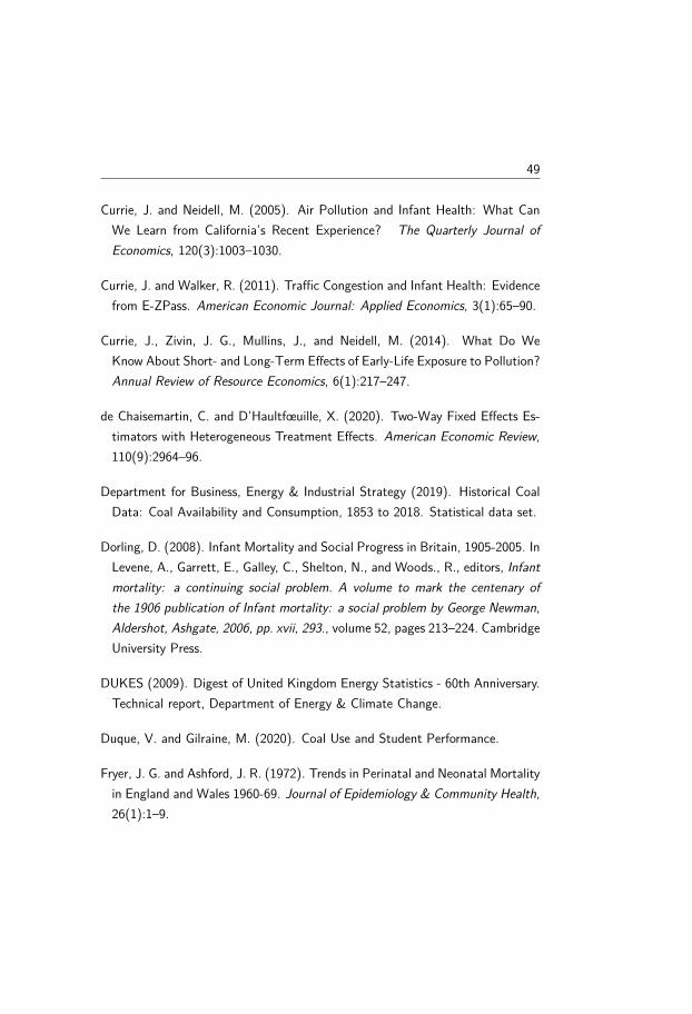
49
Currie, J. and Neidell, M. (2005). Air Pollution and Infant Health: What CanWe Learn from California’s Recent Experience? The Quarterly Journal ofEconomics, 120(3):1003–1030.
Currie, J. and Walker, R. (2011). Traffic Congestion and Infant Health: Evidencefrom E-ZPass. American Economic Journal: Applied Economics, 3(1):65–90.
Currie, J., Zivin, J. G., Mullins, J., and Neidell, M. (2014). What Do WeKnow About Short- and Long-Term Effects of Early-Life Exposure to Pollution?Annual Review of Resource Economics, 6(1):217–247.
de Chaisemartin, C. and D’Haultfœuille, X. (2020). Two-Way Fixed Effects Es-timators with Heterogeneous Treatment Effects. American Economic Review,110(9):2964–96.
Department for Business, Energy & Industrial Strategy (2019). Historical CoalData: Coal Availability and Consumption, 1853 to 2018. Statistical data set.
Dorling, D. (2008). Infant Mortality and Social Progress in Britain, 1905-2005. InLevene, A., Garrett, E., Galley, C., Shelton, N., and Woods., R., editors, Infantmortality: a continuing social problem. A volume to mark the centenary ofthe 1906 publication of Infant mortality: a social problem by George Newman,Aldershot, Ashgate, 2006, pp. xvii, 293., volume 52, pages 213–224. CambridgeUniversity Press.
DUKES (2009). Digest of United Kingdom Energy Statistics - 60th Anniversary.Technical report, Department of Energy & Climate Change.
Duque, V. and Gilraine, M. (2020). Coal Use and Student Performance.
Fryer, J. G. and Ashford, J. R. (1972). Trends in Perinatal and Neonatal Mortalityin England and Wales 1960-69. Journal of Epidemiology & Community Health,26(1):1–9.

50 CHAPTER 2. THE CAA, BS, AND IM
Fukushima, N. (2021). A Fine Sollution to Air Pollution? PhD thesis, StockholmUniversity, Department of Economics.
Greenstone, M. and Hanna, R. (2014). Environmental Regulations, Air andWater Pollution, and Infant Mortality in India. American Economic Review,104(10):3038–3072.
Heal, M. R. and Beverland, I. J. (2017). A Chronology of Ratios Between Blacksmoke and PM10 and PM2.5 in the Context of Comparison of Air PollutionEpidemiology Concentration-Response Functions. Environmental Health, 16.
Jayachandran, S. (2009). Air Quality and Early-Life Mortality. Journal of HumanResources, 44(4):916–954.
Kiernan, K. (1971). The Illegitimacy Phenomenon of England and Wales in the1950s and 1960s. Master’s thesis, London School of Economics.
Knittel, C. R., Miller, D. L., and Sanders, N. J. (2016). Caution, Drivers! ChildrenPresent: Traffic, Pollution, and Infant Health. The Review of Economics andStatistics, 98(2):350–366.
Kuijer, L. and Watson, M. (2017). 'That's When We Started Using the Liv-ing Room’: Lessons from a Local History of Domestic Heating in the UnitedKingdom. Energy Research & Social Science, 28:77–85.
Le Grand, J. and Winter, D. (1980). Determinants of Local Government Ex-penditure, 1951-1974 [Computer file]. Colchester, Essex: UK Data Archive[distributor], SN: 913, http://dx.doi.org/10.5255/UKDA-SN-913-1.
Lee, C. H. (1991). Regional Inequalities in Infant Mortality in Britain, 1861-1971:Patterns and Hypotheses. Population Studies, 45(1):55–65.
McFarland, A. R., Ortiz, C. A., and Rodes, C. E. (1982). Wind Tunnel Evaluationof the British Smoke Shade Sampler. Atmospheric Environment, 16(2):325–328.
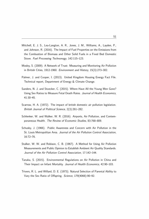
51
Mitchell, E. J. S., Lea-Langton, A. R., Jones, J. M., Williams, A., Layden, P.,and Johnson, R. (2016). The Impact of Fuel Properties on the Emissions fromthe Combustion of Biomass and Other Solid Fuels in a Fixed Bed DomesticStove. Fuel Processing Technonogy, 142:115–123.
Mosley, S. (2009). A Network of Trust: Measuring and Monitoring Air Pollutionin British Cities, 1912-1960. Environment and History, 15(3):273–302.
Palmer, J. and Cooper, I. (2013). United Kingdom Housing Energy Fact File.Technical report, Department of Energy & Climate Change.
Sanders, N. J. and Stoecker, C. (2015). Where Have All the Young Men Gone?Using Sex Ratios to Measure Fetal Death Rates. Journal of Health Economics,41:30–45.
Scarrow, H. A. (1972). The impact of british domestic air pollution legislation.British Journal of Political Science, 2(3):261–282.
Schlenker, W. and Walker, W. R. (2016). Airports, Air Pollution, and Contem-poraneous Health. The Review of Economic Studies, 83:768–809.
Schusky, J. (1966). Public Awareness and Concern with Air Pollution in theSt. Louis Metropolitan Area. Journal of the Air Pollution Control Association,16:72–76.
Stalker, W. W. and Robison, C. B. (1967). A Method for Using Air PollutionMeasurements and Public Opinion to Establish Ambient Air Quality Standards.Journal of the Air Pollution Control Association, 17:142–144.
Tanaka, S. (2015). Environmental Regulations on Air Pollution in China andTheir Impact on Infant Mortality. Journal of Health Economics, 42:90–103.
Trivers, R. L. and Willard, D. E. (1973). Natural Selection of Parental Ability toVary the Sex Ratio of Offspring. Science, 179(4068):90–92.

52 CHAPTER 2. THE CAA, BS, AND IM
Turner, N., Danesh, K., and Moran, K. (2020). The Evolution of Infant MortalityInequality in the United States, 1960–2016. Science Advances, 6(29).
Wall, G. (1973). Public Response To Air Pollution in South Yorkshire, England.Environment and Behavior, 5:219–248.
Wegman, M. E. (2001). Infant Mortality in the 20th Century, Dramatic butUneven Progress. The Journal of Nutrition, 131(2):401S–408S.
Wick, P., Malek, A., Manser, P., Meili, D., Maeder-Althaus, X., Diener, L.,Diener, P.-A., Zisch, A., Krug, H. F., and von Mandach, U. (2010). BarrierCapacity of Human Placenta for Nanosize Materials. Environmental HealthPerspective, 118:432–436.
Young, A. (2020). Consistency without inference: Instrumental variables in prac-tical application. London School of Economics.
Zivin, J. G. and Neidell, M. (2013). Environment, Health, and Human Capital.Journal of Economic Literature, 51(3):689–730.

. FIGURES AND TABLES 53
Figures and tables
Figure 2.1: Infant Mortality in England and Wales by Type and Cause(a) Mortality rate in England and Wales 1946-2017
01
02
03
04
0M
ort
alit
y p
er
1,0
00
liv
e b
irth
s
1945
1950
1955
1960
1965
1970
1975
1980
1985
1990
1995
2000
2005
2010
2015
2020
year
IMR (England & Wales) IMR (Sample)
Neonatal (England & Wales) Stillbirths (England & Wales)
Source: Office for National statistics, UK
(b) Causes of neonate death by gender 1950-1978
0.0
2.0
4.0
6.0
8.1
.12
.14
Sh
ort
ge
sta
tio
n/lo
w b
irth
we
igh
t
1950 1960 1970 1980yr
Male Female
Source: Office for National statistics, UK
Short gestation/low birth weight
0.0
2.0
4.0
6.0
8.1
.12
.14
Re
sp
ira
tory
co
nd
itio
ns
1950 1960 1970 1980yr
Male Female
Source: Office for National statistics, UK
Respiratory conditions
Notes: Figure (a) depicts all infant deaths under one year of age (IMR) and neonatal deaths,i.e., infants’ deaths in the first 28 days of life. Stillbirths are defined as deaths before birth butafter 28 weeks of pregnancy. The vertical lines in 1957 represent the first year a smoke controlarea was enacted. Figures in (b) show the two most common causes of newborn death due toperinatal complications i.e., the period between 28 weeks gestation and one week of birth, inEngland and Wales by gender as a share of total infant mortality.

54 CHAPTER 2. THE CAA, BS, AND IM
Figure 2.2: An illustration on the expansion of Smoke Control Areas in EnglishCounty Boroughs
Notes: The figures depict county boroughs’ geographical location in England and the share ofSCA coverage in 1957, 1965, and 1973.

. FIGURES AND TABLES 55
Figure 2.3: The Rate of Smoke Control Area Expansion
0.2
.4.6
.81
19
57
19
58
19
59
19
60
19
61
19
62
19
63
19
64
19
65
19
66
19
67
19
68
19
69
19
70
19
71
19
72
19
73
Mean Mean ex. non−adopters
Sha
re o
f S
CA
Year
Notes: Each column in the graph corresponds to the annual frequency distribution of SCAcoverage in County Boroughs in England. The dots are the mean rate of coverage includingand excluding non-adopters.
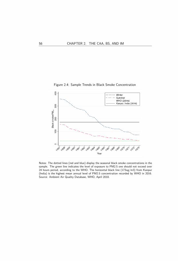
56 CHAPTER 2. THE CAA, BS, AND IM
Figure 2.4: Sample Trends in Black Smoke Concentration
Notes: The dotted lines (red and blue) display the seasonal black smoke concentrations in thesample. The green line indicates the level of exposure to PM2.5 one should not exceed over24 hours period, according to the WHO. The horizontal black line (173ug/m3) from Kanpur(India) is the highest mean annual level of PM2.5 concentration recorded by WHO in 2016.Source: Ambient Air Quality Database, WHO, April 2018.

. FIGURES AND TABLES 57
Table2.1:
SampleStatistics
Non
-ado
pters
Ado
pters
Meandiffe
rence:
(1)
All
(2)
All
(3)
SCA ’
73<0.5
(4)
SCA ’
73≥0.5
(1)-(2)
(3)-(4)
Mean
Std.
Mean
Std.
Mean
Std.
Mean
Std.
Diff.
t-stat
Diff.
t-stat
Baselines
in19
51:
Indu
stry
coal
depend
ency
p.c.
0.06
0.01
0.05
0.01
0.05
0.01
0.05
0.01
0.01
(3.13)
-0.00
(-0.25
)Indu
stry
coke
depend
ency
p.c.
0.05
0.01
0.05
0.01
0.05
0.01
0.05
0.02
0.01
(1.50)
-0.00
(-0.82
)Indu
stry
oild
ependencyp.c.
0.16
0.04
0.12
0.03
0.12
0.03
0.12
0.03
0.04
(3.84)
-0.00
(-0.08
)Indu
stry
electric
itydepend
ency
p.c.
0.09
0.02
0.08
0.02
0.08
0.01
0.08
0.02
0.02
(3.11)
-0.00
(-0.19
)Indu
stry
gasandwa
terd
ependencyp.c.
0.13
0.03
0.10
0.02
0.10
0.02
0.10
0.02
0.03
(3.66)
-0.00
(-0.19
)Ln
(Pop
ulation)
11.39
0.58
11.95
0.75
11.73
0.57
12.31
0.88
-0.56
(-2.48
)-0.58
(-2.69
)Po
pulatio
ndensity
24.57
8.36
36.98
14.64
32.22
10.44
44.81
17.34
-12.40
(-2.91
)-12.59
(-3.05
)CB
Area
(ha)
4226
.5319
98.5456
44.1843
19.7146
28.1025
38.0573
17.7359
71.76-141
7.65
(-1.14
)-268
9.63
(-2.10
)Ag
e>15
/pop
0.79
0.02
0.77
0.02
0.77
0.02
0.77
0.01
0.02
(3.50)
0.00
(0.31)
Shareof
self-em
ployment
0.03
0.01
0.02
0.00
0.02
0.00
0.02
0.00
0.01
(2.16)
-0.00
(-1.20
)La
borforce/p
op0.44
0.02
0.48
0.04
0.47
0.03
0.49
0.03
-0.03
(-3.18
)-0.02
(-2.13)
Rate
ofun
employment
0.03
0.01
0.02
0.01
0.02
0.01
0.02
0.01
0.01
(1.31)
0.00
(0.16)
All-a
gemortalityrate
(%)
1.34
0.24
1.23
0.14
1.22
0.16
1.25
0.12
0.11
(2.14)
-0.03
(-0.70
)Ra
isedtaxp.c.
8.66
1.57
7.20
1.22
7.09
1.19
7.39
1.28
1.46
(3.56)
-0.30
(-0.79
)Est.
expend
iture
p.c.
10.06
1.30
9.02
0.84
8.93
0.84
9.18
0.84
1.04
(3.45)
-0.25
(-0.96
)Ra
teable
valuep.c.
(£00
0)9.79
3.20
7.11
1.28
6.99
1.26
7.30
1.33
2.68
(4.56)
-0.31
(-0.78
)Baselines
in19
59:
Health
service
sp.c.
0.07
0.02
0.10
0.03
0.10
0.03
0.11
0.03
-0.04
(-6.03
)-0.00
(-0.03
)Ch
ildservice
sp.c.
0.03
0.01
0.04
0.01
0.04
0.01
0.04
0.01
-0.01
(-5.24
)-0.00
(-1.14
)Welfareservice
sp.c.
0.04
0.01
0.05
0.02
0.05
0.02
0.05
0.02
-0.01
(-4.20
)0.00
(1.31)
Hou
singservice
sp.c.
0.09
0.05
0.14
0.05
0.14
0.06
0.14
0.03
-0.05
(-4.62
)0.01
(0.60)
Infant
mortalityrate:
1957
:25
.18
6.56
30.35
7.53
30.50
8.22
30.10
6.35
-5.17
(-3.17
)0.40
(0.24)
—Jan-Mar
27.97
5.61
31.31
9.06
32.38
9.60
29.57
7.92
-3.35
(-1.78
)2.81
(1.43)
—Ap
r-Jun
21.69
9.40
29.23
9.45
29.05
10.67
29.53
7.15
-7.54
(-3.58
)-0.49
(-0.24
)—
Jul-S
ep23
.95
9.52
27.24
8.47
27.63
8.50
26.60
8.53
-3.29
(-1.70)
1.03
(0.56)
—Oct-D
ec27
.40
12.69
33.65
10.18
32.74
11.70
35.14
6.89
-6.24
(-2.60
)-2.39
(-1.08
)Black
smoke:
1957
-197
3:67
.65
33.98
133.36
58.97
121.93
56.73
152.20
59.39
-65.71
(-3.82
)-30.27
(-1.71
)—
Jan-Mar
99.82
45.39
179.47
72.71
161.29
66.38
209.41
73.68
-79.65
(-5.29
)-48.12
(-3.20
)—
Apr-J
un34
.59
17.82
73.77
33.14
65.32
29.88
87.68
33.96
-39.18
(-5.78
)-22.36
(-3.27
)—
Jul-S
ep25
.87
13.81
61.88
29.61
55.32
27.26
72.68
30.53
-36.01
(-6.00
)-17.36
(-2.80
)—
Oct-D
ec95
.02
49.10
179.43
78.70
163.10
73.14
206.32
81.18
-84.41
(-5.18
)-43.22
(-2.61
)
Notes:Non
-Ado
pters(13in
total)
arethecoun
tybo
roug
hsthat
neverintrod
uced
aSC
Abefore
1974.Ad
opters
(45in
total)
are
furtherd
ivided
into
grou
psdepend
ingon
ifthesiz
eof
SCA
coverage
exceedinghalfof
thetotallandarea
in1973
orno
t.

58 CHAPTER 2. THE CAA, BS, AND IM
Figure 2.5: The Effect of Smoke Control Areas on Black Smoke ConcentrationAcross Months
−3
00
−20
0−
10
00
10
02
00
30
0
Bla
ck s
moke
1 2 3 4 5 6 7 8 9 10 11 12
Month
Effect of SCA Mean concentration Post intervention
Notes: The graph depicts the effect sizes of SCAs on black smoke concentration (95 CI) bymonth, the average monthly black smoke concentration, and the post-intervention level ofblack smoke concentration. The regression analysis controls for CB, year, and month FE andthe 1957 tax revenue and rateable property value per capita interacted with linear time trends.

. FIGURES AND TABLES 59
Figure 2.6: Infant Mortality and Black Smoke Concentration
15
20
25
30
35
IMR
5 6 7 8 9Log2(Black smoke)
Summer Winter
Notes: The figure depicts the relationship between IMR and the quarterly average 24-hoursconcentration of smoke particles (black smoke) in logs separeted by season for the years between1957-1973.

60 CHAPTER 2. THE CAA, BS, AND IM
Table 2.2: The Effect of Smoke Control AreasDD(1)
DDD(2)
DDD(3)
A. Dependent variable: Black smoke
SCA -75.07∗∗ -23.74 35.23(31.15) (35.41) (31.86)
SCA × Winter -95.58∗∗∗ -97.39∗∗∗(19.71) (25.85)
No. Obs. 2962 2962 2944No. CBs 58 58 58Dep. mean 99.82B. Dependent variable: IMR
SCA -3.477 -1.167 7.851(3.12) (3.05) (9.38)
SCA × Winter -4.300∗∗∗ -5.256∗∗(1.16) (2.28)
No. Obs. 2962 2962 2944No. CBs 58 58 58Dep. mean 23.36CB FE X XYear FE X XQuarter FE X XBaseline controls X XCB × Year FE XQuarter × Year FE XCB × Quarter FE X
Notes: Standard errors are in parentheses and clustered at the CB level. Columns 1-3 showthe DD and DDD results. Baseline controls include the 1957 tax revenue and rateable prop-erty value per capita interacted with linear-year trends in addition to population size in logs.*p<0.10, **p<0.05, p<*** 0.01.

. FIGURES AND TABLES 61
Figure 2.7: Event Study(a) Smoke control areas and the seasonal difference in blacksmoke concentration
0.1
.2.3
SC
Ak
−8
0−
40
04
08
0
βk
−3
−2
−1 0 1 2 3 4 5 6 7 8
k
Obs. 504
(b) Smoke control areas and the seasonal difference in in-fant mortality
0.1
.2.3
SC
Ak
−1
0−
50
51
0
βk
−3
−2
−1 0 1 2 3 4 5 6 7 8
k
Obs. 560
Notes: The event studies analysis shows pre-trends and the dynamic effects of SCA overtime. The outcome variable is the seasonal difference in black smoke concentration by countyborough and year. The event year is the first year an SCA was adopted. The x-axis displaysthe number of years before and after the event year, while the y-axis shows the effect size ofSCAs (95 percent CI). The red triangular lines are the mean SCA coverage for adopters.

62 CHAPTER 2. THE CAA, BS, AND IM
Table 2.3: The 2SLS Effects of Black Smoke on Infant Mortality
IMROLS(1)
OLS(2)
OLS(3)
IV(4)
IV(5)
Black smoke 0.0113 0.00178 0.00453 0.0454∗∗∗ 0.0417∗∗∗(0.007) (0.004) (0.004) (0.017) (0.013)
Obs. 2962 2962 2962 2962 2962CBs 58 58 58 58 58First-stage F-stat 18.46 15.81R2(adj) 0.227 0.510 0.519 0.475 0.525Quarter FE X X X X XYear FE X X X X XCB FE X X X XBaseline controls X X XCB × Year trend X
Notes: Standard errors are in parentheses and clustered at the CB level. The baseline controlsin columns 4-6 include linear-trend interacted tax revenue and rateable property value percapita, and the population size in logs. The F statistics reported in columns 4 and 5 arethe Montiel Olea-Pflueger (2013) effective first-stage F statistic. *p<0.10, **p<0.05, p<***0.01.
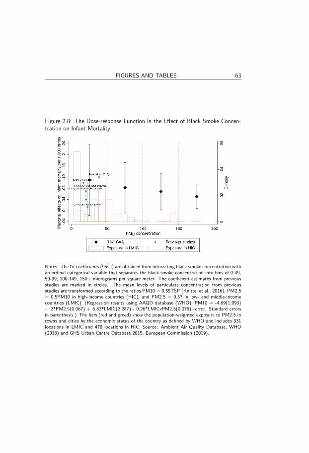
. FIGURES AND TABLES 63
Figure 2.8: The Dose-response Function in the Effect of Black Smoke Concen-tration on Infant Mortality
Notes: The IV coefficients (95CI) are obtained from interacting black smoke concentration withan ordinal categorical variable that separates the black smoke concentration into bins of 0-49,50-99, 100-149, 150+ micrograms per square meter. The coefficient estimates from previousstudies are marked in circles. The mean levels of particulate concentration from previousstudies are transformed according to the ratios PM10 = 0.55TSP (Knittel et al., 2016), PM2.5= 0.5PM10 in high-income countries (HIC), and PM2.5 = 0.57 in low- and middle-incomecountries (LMIC). (Regression results using AAQD database (WHO): PM10 = -4.69(1.093)+ 2*PM2.5(0.067) + 6.83*LMIC(2.287) - 0.26*LMICxPM2.5(0.078)+error. Standard errorsin parenthesis.) The bars (red and greed) show the population-weighted exposure to PM2.5 intowns and cities by the economic status of the country as defined by WHO and includes 331locations in LMIC and 478 locations in HIC. Source: Ambient Air Quality Database, WHO(2018) and GHS Urban Centre Database 2015, European Commission (2019).

64 CHAPTER 2. THE CAA, BS, AND IM
Figure 2.9: Heterogeneous Effects of Black Smoke on Infant Mortality
−.0
20
.02
.04
.06
.08
.1M
arg
ina
l e
ffe
cts
on
in
fan
t m
ort
alit
y
0−3m(64%)
0−6m(8%)
4−9m(3%)
6−12m(3%)
Unknown(22%)
Male(56%)
Female(41%)
Notes: The dependent variables are the quarterly number of infant deaths by the infants’ age inmonths (0-3m, 0-6m, 4-9m, 6-12) divided by the number of live births. Similarly, the unknownsare defined as the quarterly number of deaths of infants with unidentified birth records dividedby the number of live births. Note that each age is the likely age of the infant at the timeof death and depends on if birth is reported in the same quarter as death (0-3 months), onequarter before death (0-6 months), two quarters before death (4-9 months), or between 3-4quarters before death (6-12 months). The gender variables are male (female) mortality underone year of age divided by male (female) live births. The parentheses show the category shareof mortality in 1957. The regression controls for baseline capita CB tax revenue, per capitarateable property value, and log population interacted linear time-trends.

. FIGURES AND TABLES 65
Table 2.4: The Effects of Black Smoke on Births
Reduced form IVTotal Total Male Female
Black Smoke (10mg) -0.00495∗∗∗ -0.00545∗∗∗ -0.00399∗∗(0.002) (0.002) (0.002)
SCA 0.0280(0.105)
SCA × Winter 0.0452∗∗∗(0.012)
Obs. 2962 2962 2962 2962CBs 58 58 58 58First-stage Fstat 15.81 15.81 15.81Quarter FE X X X XYear FE X X X XCB FE X X X XBaseline controls X X X XCB × Year trend X X X XDep. mean 7.907 7.227 7.143
Notes: The first column shows the triple difference reduced form results of the effect of SCAon the total number of births. The remainings columns display the 2SLS estimates of the effectof black smoke concentration on the total number of births, births of male infants, and femaleinfants, respectively. All regressions control for CB specific linear trends and linear year trendsinteracted with baseline covariates, including annual per capita tax revenue, rateable propertyvalue, and log population in addition to CB, year, and quarter FE. The F statistics are theMontiel Olea-Pflueger (2013) effective first-stage F statistics. Standard errors in parenthesesand clustered at the CB level. *p<0.10, **p<0.05, p<*** 0.01.

66 CHAPTER 2. THE CAA, BS, AND IM
Figure 2.10: Sensitivity Analysis
Effects
of bla
ck s
moke o
n infa
nt m
ort
alit
y
0 .02 .04 .06 .08
1. Baseline
2. Ex. non−adopters
3. Health service
4. Child service
5. Ex. quint. lowest unemp. ’51
6. Ex. first quarter
7. Births weighted deaths counts
8. Three quarters MA
9. Complete IMR
Notes: Each number refers to separate robustness analysis. 1: The baseline IV estimate. 2:Excluding non-adopting CBs. 3: Controls for health service expenditure per capita between1959-1973. 4: Controls for child service expenditure per capita between 1959-1973. 5: Ex-cludes quintile with the lowest unemployment in 1951. 6: Excludes the first quarter fromthe analysis. 7: Births weighted deaths counts. 8: Replaces quarterly mortality rate withthree-quarters moving-average mortality. 9: Excludes CBs with missing infant mortality datafor more than one quarter (Gloucester Norwich, Chester, Preston, St Helens, Wakefield, andBirkenhead).

. FIGURES AND TABLES 67
Figure 2.11: Counterfactual and Actual Infant Mortality in the UK
05
01
00
15
02
00
Bla
ck S
mo
ke
(µ
g/m
³)
01
02
03
0In
fan
t m
ort
alit
y p
er
1,0
00
liv
e b
irth
s
1950 1955 1960 1965 1970 1975 1980 1985 1990 1995 2000Year
IMR Counterfacual IMR Black Smoke
Source: UNICEF & Heal and Beverland (2017)
Notes: The graph plots the counterfactual infant mortality rate in the UK using the IV estimatefrom Table 3, column 5. It is defined as the mortality rate that would have been if the UK blacksmoke concentration had remained at the 1957 level. Note of caution: the representativeness ofthe pollution data declines beginning in the 1980s, when the number of sites in the monitoringnetwork started dropping rapidly. For example, a decrease in monitoring sites in less pollutedareas implies that the counterfactual mortality rate is below the true value.

68 CHAPTER 2. THE CAA, BS, AND IM
A2 Appendix
A2.1 Comparing Black Smoke to PM2.5
To compare more recent studies that analyze health impact of exposure to air-borne particulate matter, one must convert black smoke (BS) to its equivalentsize in particulate matter. Although McFarland et al. (1982) find that a standardblack smoke filter can capture particulate matter with a diameter as large as 4.4micrometers, comparing BS to PM4.4 is too liberal a comparison.69 Heal andBeverland (2017) estimate a unit BS:PM2.5 ratio in the UK in 1970 (95CI:0.9-1.1). According to their estimates, the BS:PM2.5 ratio only started to declineafter 1970, reaching a BS:PM2.5 ratio of approximately 0.8 (95CI:0.7-0.9) by1974 and a ratio of 0.7 (95CI:0.6-0.8) by 1980 due to increasing in demandfor petroleum products. This is because while coal remained the predominantenergy source in the UK throughout the 1960s, it coincides with increased de-mand for petroleum products by large-scale industries and electricity generation.Particulate matter emission from motor vehicles, however, was still consideredinsignificant despite an increase in car ownership (DUKES, 2009).70
69For example, Mitchell et al. (2016) shows that 98 percent of PM emitted from combustionof bituminous coal in a standard domestic furnace is smaller than PM2.5.
70To compare, Barreca et al. (2014) report that the share of particulate matter from on-road vehicles with diameter less that 10, i.e. PM10, only accounted for 2 percent of all PM10in the US in 1960.

. A2 APPENDIX 69
A2.2 Top 10 highest PM2.5 concentration
Kanpur (India, 2016)Faridabad (India, 2016)
Gaya (India, 2016)
Varanasi (India, 2016)Patna (India, 2016)Delhi (India, 2016)
Lucknow (India, 2016)
Bamenda (Cameroon, 2012)Agra (India, 2016)
Muzaffarpur (India, 2016)
12
01
30
14
01
50
16
01
70
PM
2.5
Notes: The figure lists the ten most polluted localities and cities in the world measured by theannual mean concentration of particulate matter less than 2.5 micrometer (PM2.5) [ug/m3].Source: Ambient Air Quality Database, WHO, April 2018.

70 CHAPTER 2. THE CAA, BS, AND IM
A2.3 Smoke control order

. A2 APPENDIX 71
A2.4 The Schoolchild Chest Health Survey
The Schoolchild Chest Health Survey (SCHS) includes responses from 11,000children from 11 geographical areas of various backgrounds in the UK in 1966.It reveals that only 16% of the households had central heating. In comparison,66.7% of the homes reported using coal-fired furnaces. A comparison betweenrural and rural households shows that the prevalence of central heating systemsdid not differ between urban and rural households (15.5% versus 17.3%). Still,there was a big difference in the use of coal, with 73.2% of rural householdsusing coal for heating and only 55.6% of the urban households. Other heatingmethods used in urban homes are gas-heated fires (10.7%) and electric stovesand converters (10.9%). The survey also reveals that the prevalence of centralheating increases with socio-economic status (1.- 54%, 2.- 30.6%, 3.- 14.2%,4.- 6.4%, 5.- 4.92%), underscoring the notion that central heating systems werean expensive investment. Finally, central heating was more common among therespondents who reported moving homes between 1961-1966, with 28.5% of themovers having a central heating system installed. The corresponding numberfor non-movers is 11.9 %. The relationship supports anecdotal evidence thatnew buildings came with central heating pre-installed following the recommen-dations from the national housing design guidance of council estates for localgovernments (Kuijer and Watson, 2017).
A2.5 Unidentified deaths
The failure to match an infant death to her birth record is due to one of thefollowing alternatives: 1) No first name was registered at the time of death. 2)The child was born outside the district of death. 3) The names do not match(for instance, due to misspelling). However, a closer examination reveals thatthe number of infants with no given name is scarce (1.7%). In addition, alimited random sample of death of unidentified children shows that a

72 CHAPTER 2. THE CAA, BS, AND IM
substantial share of the children were born outside the district of death,indicating migration between the time of birth and death. Furthermore, byrunning a gender recognition algorithm, we can identify the gender of thedeceased in each category. The exercise reveals a similar gender ratio across thegroup categories (both showing a higher share of male deaths). However,although it is possible to determine the gender of the deceased for the vastmajority of infants in the unidentified group (93.8 %), ambiguous gender namesare twice as common among age-unidentified infants, which is partiallyexplained by the higher prevalence of ethnic minority names and othernon-traditional UK names. The data also reveals higher prevalence of birthoutside wedlock among deceased infant in the age unidentified category.71
To conclude, while the entries in the death registry cannot provide further cluesas to the socio-economic status of the deceased, if migration, minoritybackground, birth outside wedlock, and failure to register a given name at thetime of deaths are characteristics associated with lower SEC, it may suggestthat the unidentified group of infant represents a more disadvantaged group ofchildren on average.
71While neither the birth registry nor the death registry asks for the marital status, achild received her the mother’s surname at birth if she was born outside wedlock. Therefore,minding such cases when the mother and the father coincidentally shared the same surnamebefore marriage, the same surname as the mother suggests birth outside wedlock. However, ifa father was present and recognized the child’s birth despite not being married to the mother,the child automatically received the father’s surname. In such cases, the birth record wasregistered twice, once with the mother’s maiden name as the child’s surname and once withthe father’s name as the surname (the mother’s maiden name does not change). The ratioof birth to unmarried mothers in the analysis is more all less identical to the national meanestimated by Kiernan (1971) and display a similar increasing trend over time, suggesting thatthe identification strategy using marriage status provides reasonable estimates.

. A2 APPENDIX 73
A2.6Sa
mplestatisticsby
year
ofSC
Aadop
tion
Non
-ado
pters
Ado
pters
Meandiffe
rence:
(1)
All
(2)
All
(3)
FirstSC
A<
1964
(4)
FirstSC
A≥
1964
(1)-(2)
(3)-(4)
Mean
Std.
Mean
Std.
Mean
Std.
Mean
Std.
Diff.
t-stat
Diff.
t-stat
Baselines
in19
51:
Indu
stry
coal
depend
ency
p.c.
0.06
0.01
0.05
0.01
0.05
0.01
0.05
0.01
0.01
(3.13)
0.00
(0.57)
Indu
stry
coke
depend
ency
p.c.
0.05
0.01
0.05
0.01
0.05
0.02
0.04
0.01
0.01
(1.50)
0.00
(0.81)
Indu
stry
oild
ependencyp.c.
0.16
0.04
0.12
0.03
0.12
0.03
0.12
0.03
0.04
(3.84)
0.00
(0.32)
Indu
stry
electric
itydepend
ency
p.c.
0.09
0.02
0.08
0.02
0.08
0.02
0.07
0.01
0.02
(3.11)
0.01
(0.85)
Indu
stry
gasandwa
terd
ependencyp.c.
0.13
0.03
0.10
0.02
0.10
0.02
0.10
0.02
0.03
(3.66)
0.00
(0.44)
Ln(P
opulation)
11.39
0.58
11.95
0.75
12.02
0.77
11.57
0.46
-0.56
(-2.48
)0.46
(1.50)
Popu
latio
ndensity
24.57
8.36
36.98
14.64
37.30
15.30
35.22
11.10
-12.40
(-2.91
)2.09
(0.34)
CBAr
ea(ha)
4226
.5319
98.5456
44.1843
19.7160
72.83
4554
.98
3317
.22
1188
.96
-141
7.65
(-1.14
)27
55.61(1.58)
Age>
15/p
op0.79
0.02
0.77
0.02
0.77
0.02
0.77
0.01
0.02
(3.50)
0.00
(0.23)
Shareof
self-em
ployment
0.03
0.01
0.02
0.00
0.02
0.00
0.02
0.00
0.01
(2.16)
0.00
(1.45)
Labo
rforce/p
op0.44
0.02
0.48
0.04
0.48
0.04
0.46
0.03
-0.03
(-3.18
)0.03
(1.79)
Rate
ofun
employment
0.03
0.01
0.02
0.01
0.02
0.01
0.02
0.02
0.01
(1.31)
-0.00
(-0.37
)All-a
gemortalityrate
(%)
1.34
0.24
1.23
0.14
1.23
0.15
1.22
0.07
0.11
(2.14)
0.01
(0.19)
Raise
dtaxp.c.
8.66
1.57
7.20
1.22
7.30
1.12
6.67
1.68
1.46
(3.56)
0.63
(1.26)
Est.
expend
iture
p.c.
10.06
1.30
9.02
0.84
9.11
0.79
8.56
1.02
1.04
(3.45)
0.54
(1.60)
Rateable
valuep.c.
(£00
0)9.79
3.20
7.11
1.28
7.17
1.30
6.74
1.20
2.68
(4.56)
0.44
(0.83)
Baselines
in19
59:
Health
service
sp.c.
0.07
0.02
0.10
0.03
0.11
0.03
0.09
0.03
-0.04
(-6.03
)0.02
(2.31)
Child
service
sp.c.
0.03
0.01
0.04
0.01
0.04
0.01
0.03
0.01
-0.01
(-5.24
)0.01
(1.58)
Welfareservice
sp.c.
0.04
0.01
0.05
0.02
0.05
0.02
0.05
0.01
-0.01
(-4.20
)0.00
(0.73)
Hou
singservice
sp.c.
0.09
0.05
0.14
0.05
0.14
0.05
0.14
0.06
-0.05
(-4.62
)0.00
(0.24)
Infant
mortalityrate:
1957
:25
.18
6.56
30.35
7.53
30.45
7.87
29.80
5.51
-5.17
(-3.17
)0.65
(0.29)
—Jan-Mar
27.97
5.61
31.31
9.06
31.01
9.32
32.96
7.56
-3.35
(-1.78
)-1.95
(-0.74
)—
Apr-J
un21
.69
9.40
29.23
9.45
29.62
9.31
27.13
10.29
-7.54
(-3.58
)2.48
(0.90)
—Jul-S
ep23
.95
9.52
27.24
8.47
27.52
8.98
25.72
4.83
-3.29
(-1.70
)1.80
(0.73)
—Oct-D
ec27
.40
12.69
33.65
10.18
33.75
10.54
33.09
8.26
-6.24
(-2.60
)0.66
(0.22)
Black
smoke:
1957
-197
3:67
.65
33.98
133.36
58.97
138.91
55.17
103.26
74.05
-65.71
(-3.82
)35
.65
(1.49)
—Jan-Mar
99.82
45.39
179.47
72.71
186.45
68.78
141.55
84.04
-79.65
(-5.29
)44
.90
(2.17)
—Ap
r-Jun
34.59
17.82
73.77
33.14
77.28
32.18
54.68
32.87
-39.18
(-5.78
)22
.60
(2.41)
—Jul-S
ep25
.87
13.81
61.88
29.61
65.29
29.18
43.39
25.55
-36.01
(-6.00
)21
.90
(2.63)
—Oct-D
ec95
.02
49.10
179.43
78.70
187.70
75.82
134.54
81.65
-84.41
(-5.18
)53
.15
(2.38)
Notes:Non
-Ado
pters(13in
total)
arethecoun
tybo
roug
hsthat
neverintrod
uced
aSC
Abefore
1974.Ad
opters
(45in
total)
are
furtherd
ivided
into
grou
psby
SCA
adop
tionyear:38
CBsbefore
1964
and7CB
safter1
965.

74 CHAPTER 2. THE CAA, BS, AND IM
A2.7 List of countries (Fig 2.8)
Australia (8), Austria (4), Bangladesh (6), Belgium (7) Brazil (6) Bulgaria (5)Canada (28) Chile (20) China (227) Colombia (4) Croatia (4) Cyprus (1)Czechia (8) Ecuador (1) El Salvador (1) Estonia (2) Finland (4) France (46)Germany (48) Ghana (1) Hungary (3) Iceland (1) India (18) Indonesia (2) Iran(25) Israel (1) Italy (54) Japan (1) Latvia (2) Lithuania (3) Luxembourg (1)Mongolia (1) Netherlands (9) Norway (4) Peru (1) Philippines (1) Poland (24)Portugal (2) Republic of Korea (3) Romania (9) Singapore (1) Slovakia (1)Slovenia (2) South Africa (3) Spain (19) Sweden (3) Switzerland (3)Macedonia (1) Turkey (14) UK (27) US (137) Uruguay (1) Viet Nam (1)

. A2 APPENDIX 75
A2.8 Data availability
County borough:Irregularity:
SCA Pollution Econ.Borders IMR
Barnsley 1959 1958
Barrow-in-Furness . 1978
Bath . 1962
Birkenhead X72 1961 1961
Birmingham 1958 1949
Blackburn 1960 1959
Blackpool . 1961
Bolton 1957 1951
Bootle X 1959 1959
Bournemouth . 1962
Bradford 1959 1951
Brighton . 1962
Bristol 1958 1949
Burnley 1960 1945
Burton upon Trent 1964 1976
Bury 1959 1960
Canterbury (1971)73 1965
Carlisle . 1964
Chester74 X75 . 1960
Coventry 1959 1959
Croydon X . .
Darlington 1965 1963
Derby X 1961 1958
Dewsbury 1958 1976
Doncaster 1960 1954
Dudley X 1958 1951
Eastbourne . 1961
East Ham X . .

76 CHAPTER 2. THE CAA, BS, AND IM
County borough:Irregularity:
SCA Pollution Econ.Borders IMR
Exeter 1957 1955
Gateshead 1959 1960
Gloucester X76 (1963)77 1968
Great Yarmouth . .
Grimsby . .
Halifax 1958 1959
Hartlepool X 1963 1961
Hastings . .
Huddersfield 1958 1957
Ipswich . 1961
Kingston upon Hull 1958 1962
Leeds 1958 1950
Leicester 1958 1955
Lincoln 1960 1960
Liverpool 1957 1956
Luton78 1956 1950 No data
Manchester 1958 1949
Middlesbrough X 1959 .
Newcastle upon Tyne 1958 1954
Northampton 1969 1967
Norwich X79 1968 1959
Nottingham 1959 1954
Oldham 1960 1958
Oxford 1958 1956
Plymouth . 1961
Portsmouth 1973 1956
Preston X80 1958 1954
Reading 1958 1958
Rochdale X 1958 1969
Rotherham 1958 1980

. A2 APPENDIX 77
County borough:Irregularity:
SCA Pollution Econ.Borders IMR
Salford 1959 1949
Sheffield 1958 1949
Smethwick X 1958 .
Solihull81 1959 1960 No data
South Shields 1966 1962
Southampton 1961 1955
Southend-on-Sea . 1961
Southport 1960 1974
St Helens X82 1965 1957
Stockport 1958 1961
Stoke on Trent 1960 1960
Sunderland 1959 1961
Teesside X 1969 1961
Torbay X . 1961
Tynemouth 1962 1958
Wakefield X83 1959 1957
Wallasey 1958 1961
Walsall X 1960 1955
Warley X 1968 1958
Warrington 1959 1950
West Bromwich X 1957 1958
West Ham X . .
West Hartlepool X 1962 .
Wigan X 1962 1959
Wolverhampton X 1960 1944
Worcester . 1974
York X 1968 1959

78 CHAPTER 2. THE CAA, BS, AND IM
72Omitted between 1973q1-1973q4.73Non-adopter: SCO only applied to greenfield area.74Hoole UD was incorporated into Chester CB in 1954.75Omitted between 1971q4-1973q4.76Omitted between 1958q3-1958q4.77Non-adopter: SCO only applied to greenfield area after 1967.78Changed status from Municipal Borough to CB in 1964.79Omitted between 1965q1-1973q4.801973q4 omitted.81Changed status from UD to MB in 1954 and to CB in 1964.82Omitted between 1973q2-1973q4.831973q4 omitted.

Chapter 3
A Fine Solution to Air Pollution?∗
3.1 Introduction
Despite the mounting evidence of health and productivity gains expected fromreduced pollution, the problem of high-level air pollution remains in many parts ofthe world and particularly in developing countries (Currie et al., 2014; Zivin andNeidell, 2012, 2013). Some reasons why air quality remains poor in many placesare the scarcity of evidence of the health impact of high-level air pollution (Zivinand Neidell, 2013, Arceo et al., 2016), household reliance on solid fuel (closelyrelated to indoor air pollution, see Duflo et al. (2008) for an overview), and inef-ficiency in regulation implementation, monitoring, and enforcement (Greenstoneand Hanna, 2014, UNEP, 2019).
Air pollution is particularly severe during the cold seasons in regions wheresmall-scale furnaces are the primary heat source. The low combustion efficiencyof small-scale furnaces combined with high population density contributes tohousehold emissions often exceeding that of the industries. However, despite therole of households in the worsening of ambient air quality, regulations targetingprivate homes are rare. In contrast, restrictions on industry emission are easier tomotivate politically, and likely why environmental regulation targeting industries
∗I am grateful to Peter Nilsson, David Strömberg for their comments, and FORMAS forthe generous grant that enabled the data collection.
79

80 CHAPTER 3. FINES AND AIR POLLUTION
have increased the fastest.1 Nevertheless, despite the efforts to improve airquality, failure to fully implement and enforce the regulations in addition toexcluding households from the pollution equation remains a significant challengein reducing air pollution (UNEP, 2019).
In this analysis, I study the impact of a fine on a ban on smoke emission on airquality in an environment where air pollution is comparable to many developingcountries today. The 1956 UK Clean Air Act, enacted as a direct response tothe Great Smog incident in London in 1952, gave local authorities across the UKthe mandate to introduce Smoke Control Areas (SCAs). Within the boundariesof an SCA, local authorities could ban the emission of smoke from any building.An occupier or an owner of a building who violated a smoke control order wasfined up to ten pounds, corresponding to roughly half of the disposable incomefor a typical household in the UK at the time. The fine remained unchanged until1968, when some local authorities, likely triggered by the revised 1968 Clean AirAct, moved to double the fine permanently.
The purpose of a fine is to increase deterrence by punishing offenders. Theobjectives of the legislative body, law enforcement, and the judiciary is to deter-mine the right probability to detect and convict and find a punishment size suchthat crime does not pay (Becker, 1968). However, in environmental regulations,most changes in punishment are associated with a simultaneous shift in moni-toring activity and enforcement, making it difficult to disentangle the effect ofone from the other. A unique advantage of this paper is that smoke is easy todetect and does not require special equipment or knowledge. Therefore, there islittle reason to worry that monitoring practices would confound the results.
In the paper, I use multiple sources of variations to identify the effect ofan increase in fines on regulation compliance. As the empirical foundation, Iemploy the first stage identification strategy following Fukushima (2021b). Inparticular, I exploit the temporal and spatial variation in SCA adoption, the
1According to the UN Environmental Program (UNEP), the number of environmental lawshas increased 38-fold since 1972.

3.1. INTRODUCTION 81
rate of SCA expansion, and the seasonal variation in the demand for coal in atriple-difference strategy. The difference in demand for coal allows me to use thesummer season as a natural control group to compare the effect of SCA on winterpollution. Furthermore, with SCA impact confined to winter months, any effectsof a change in fine are also limited to the winter season. The seasonal variationimplies that I can compare the difference between summer and winter pollutionbefore and after an increase in fine within the same location and year, holdingthe size of SCAs constant. Also, since the seasonal variation in SCA impactaccounts for any unobserved place- and time-varying confounders, I avoid theissues arising from time-varying heterogeneity in treatment effect that can biasthe results (de Chaisemartin and D’Haultfœuille, 2020).
The results suggest that the doubling of the fine had a large effect on regula-tion compliance with the reduction in winter black smoke concentration increas-ing by an additional 33 % compared to the effect of SCA without a change infine. Evidence suggests that the additional decline in black smoke concentrationresults from at-the-margin risk preferring poorer households that switch to com-ply with the regulation after an increase in fine. The findings suggest that thepoorest households disproportionally carried the cost for improved ambient air.
The paper contributes to two main strands of literature. First, it adds to theliterature on regulation compliance in environmental economics by estimating thecausal effect of a change in a monetary penalty on pollution. Although a grow-ing number of empirical papers in environmental economics now use exogenouschanges in monitoring practices to study regulatory compliance and changes inpollution, the effects of changes in law enforcement, and particularly monetarypenalties, on compliance and pollution are much less understood (Cohen, 2000;Shimshack and Ward, 2005; Glicksman and Earnhart, 2007; Gray and Shimshack,2011).2 Instead, most knowledge of enforcement effect on compliance focuses
2For example, Duflo et al. (2013) and Duflo et al. (2018) use randomized control trialsto study the effect of improving or increasing auditing on industry pollution in India. Axbardand Deng (2020) andGreenstone et al. (2019) both study the effect of automatization of airpollution monitoring in China on air pollution. He et al. (2020) study how changes in the

82 CHAPTER 3. FINES AND AIR POLLUTION
on the effect of historical enforcement on future compliance, i.e., the effect offirm probability of compliance given previous conviction (Cohen, 2000; Gray andShimshack, 2011). A small number of papers, on the other hand, studies thespillover effect of conviction to other firms within the same pollution categoryand state (Shimshack and Ward, 2005), or by geographical proximity (Gray andShadbegian, 2007; Assunção et al., 2013).
The literature that studies the effect of changes in potential legal liability oncompliance is even smaller. A possible reason why the area is under-researched isthat monetary fines are set ex-post in the US (and likely also elsewhere) and pro-portional to the severity of the violation (Rousseau, 2009; Gray and Shimshack,2011). To overcome the issue of endogeneity, Glicksman and Earnhart (2007)rely on surveys responses from plants stating how they would respond to a hypo-thetical rise in fine. The paper that most resembles this paper is that of Stafford(2002), who studies the relationship between a rise in the maximum penalty sizeon hazardous waste handling on compliance. However, while Stafford only ob-serves changes in compliance for plants after realized inspection and thereforerelies on a single event, the current paper exploits multiple sources of variationto control for unobserved covariates to identify the causal effect. Also, to thebest of my knowledge, this paper is the first to study the effect of fines ongeneral deterrence and pollution level. I also deviate from previous literaturein environmental crime by studying the impact of monetary fines on regulatorycompliance that is not exclusive to industry emission. Not limiting the analysisto industries is particularly important from a policy perspective since householdemissions stand for a large share of air pollution in many developing countries.
The paper proceeds as follows. Section 2 provides the historical context ofthe act and explores the regulatory background. Section 3 discusses the data, itssources, and the assumptions involved in its collection. Section 4 discusses theidentification assumptions and the econometric models. Section 5 presents the
incentive system for local politicians affect water pollution using the location of monitors inChinese rivers.

3.2. BACKGROUND 83
results and interpretations, and Section 6 concludes.
3.2 Background
3.2.1 Smoke control orders and black smoke concentration
Given the long history of failed attempts to regulate smoke emission and themonumental role of the act in improving UK air quality, the swift passing of the1956 Clean Air Act was a significant achievement. A big contributing factor to therelatively smooth enactment of the legislation was the change in the perceptionabout smoke following the 1952 Great Smog incident in London, estimated tohave brought premature deaths to approximately 12 000 Londoners.
Coal fires were the predominant form of heating in most dwellings at theend of the 1950s and remained so far into the 1960s. For this reason, theprimary source of air pollution in the UK before the Clean Air Act was by farthe burning of bituminous coal. Also, in densely populated districts, householdemissions typically stood for a greater share of the total emission than from theindustries. However, besides regulating the emission from industrial outlets, theact also gave the local authorities the mandate to issue smoke control orders.The orders would prescribe areas within its jurisdiction where emission of smokefrom bituminous coal was banned, irrespective of source. Subject to approvalfrom the Minister of Housing and Local Government, the local authorities werefree to decided the location and the timing of the so-called smoke control areas(SCA). The act decided the size of the fine for violating a smoke control orderand the process of announcing an order. For example, the legislation states thatlocal authority must take suitable steps for bringing the effect of the order to thenotice of persons affected. SCAs were the first regulation to target bituminouscoal in private dwellings and industries alike.3
3According to Section 34 in the 1956 CAA, industrial plant includes any still, meltingpotor other plant used for any industrial or trade purposes, and also any incinerator used for or inconnection with any such purposes.

84 CHAPTER 3. FINES AND AIR POLLUTION
To accommodate the new restrictions, the owner of a private dwelling couldsimply substitute bituminous coal for smokeless fuel such as anthracite or othermanufactured smokeless fuel, or expect a minimum 70 percent reimbursementfrom the local authority for carrying out adjustment work to the dwelling tocomply with the regulation.4 The reimbursement scheme, however, did not applyto new dwellings nor to commercial or industrial plants.5 Moreover, an occupierof a private dwelling who is not the owner could only expect a maximum of 35percent reimbursement for changing home appliances and was also only entitledto the reimbursement two years after the order came into operation. The localauthority would, in turn, receive a contribution from the exchequer as largeas “four-sevenths” of the cost to meet the rise in public spending due to thereimbursement schemes.
Black smoke was the first and the most common type of ambient air pol-lution measured until the late 1990s. At the start, Black smoke concentrationwas compiled by the Investigation of Atmospheric Pollution run by the WarrenSpring Laboratory. The organization was first set up in 1912 with less than 30participating bodies but had more than 500 participants and approximately 1,200monitoring sites by 1961 when it changed its name to the National Survey ofSmoke and Sulfur Dioxide and become the world’s first coordinated national airpollution monitoring network.
Black smoke was measured using smoke samplers drawing 50 cubic metersof air through a white filter paper over 24 hours.6 The density of the depositwas then assessed using a reflectometer, or in the earlier days, by the naked eye.The particles emitted from the combustion of coal are typically smaller than 2.5micrometers in diameter and small enough to penetrate the lung system andreach the blood circulation and therefore considered particularly harmful.
4For example, one could replace coal furnace with electrical heating system or gas centralheating.
5Furnaces with less than 55,000 British thermal units per hour per house where consideredfor domestic purposes.
6Black smoke sampler was replaced by the sampling of particulate matter starting in the1990s.

3.2. BACKGROUND 85
3.2.2 The revised Clean Air Act and penalty size
The revised Clean Air Act of 1968 included new provisions and amendments tothe 1956 Clean Air Act. The most significant changes to the original act includea regulation targeting the height of industrial furnaces, the government’s abilityto force local authorities to plan new SCAs if air quality was unsatisfactory, andthe ban on the acquisition and sales of unauthorized fuel within SCAs.7
Fines are the most practiced punishment in environmental laws and regula-tions and so also in the case of the UK Clean Air Act. Before the revised 1968act, section 27(2) in the UK Clean Air Act of 1956 states that “A person guilty ofan offence under... [Smoke Control Order]... shall be liable on summary convic-tion to a fine not exceeding ten pounds.” An amount just below the gross weeklyearnings for a full-time manual adult male worker in 1956.8 The local authoritieswould announce the size of the punishment for breaching an order in connectionwith the announcement of a new smoke control order, as shown in an exampleorder from Oxford displayed in Figure 3.12a. The penalty size remained stablefor the next twelve years. However, starting in 1968, 23 out of the 42 countyboroughs part of the analysis doubled the fine for all new SCAs from 10 poundsto 20 pounds per offense, the latter amount again corresponding to the weeklygross earnings of an adult male manual worker.9 The discrepancy in the adoptionof the higher rate is, for example, shown in Panel a and b in Figure 3.12. Bothorders are from October 1971, but while Oxford kept the initial fine size, we seethat Tynemouth had by then moved to double the fine for all new smoke controlorders. Unfortunately, I have not managed to find records explaining why somecountry boroughs decided to double the fine. Still, the most likely explanation isthat county boroughs came to interpret the 20 pounds fine for acquisition and
7The final change in regards to the creation of smoke control areas was miscellaneouschanges in procedures in the relationship between the Minister and the local authorities.
8Obtained from https://www.ons.gov.uk/employmentandlabourmarket/peopleinwork/earningsandworkinghours/adhocs/006301newearningssurveynestimeseriesofgrossweeklyearningsfrom1938to2016 [Accessed: 01 June 2021]
9The inflation ran at over 30% between 1956 and 1968.

86 CHAPTER 3. FINES AND AIR POLLUTION
sales of unauthorized fuel in Smoke Control Areas differently since the legislationdoes not clarify what circumstances constitute an acquisition.
For identification purpose, we must also ask if the doubling of the fine wasan isolated event or coincided with other changes that would have affected theair quality. A particular concern is that the revised Clean Air Act gave theMinistry the possibility to force the planning of new smoke control areas wherethe adoption of SCAs had been lagging. For example, suppose the governmentpressured local authorities to implement SCAs and monitored the progress closely.In that case, the government’s involvement rather than the change in punishmentcould explain the improvement in air quality. However, as stressed by Scarrow(1972), the act did not give the central government the mandate to force localauthorities to adopt SCAs. Furthermore, Scarrow notes that, the minister’s powerhad never been used at the time of the publication of his article.
Another change we must consider is possible changes in monitoring practices.However, while the revised CAA includes an amendment on the measurement ofgrid, dust, and fumes, these changes applied to large-scale furnaces only and notto smoke control orders. Instead, it is important to recall that smoke control areasprohibited the emission of any smoke. Since even the slightest smoke emissionis easily perceptible to the senses and does not require special equipment todetect, monitoring would have been a relatively easy activity for law enforcementand neighbors alike. Nevertheless, to check that an increase in fine did notcoincide with an increased probability of detection, I run an analysis to see ifdoubling of fine is associated with changes in the local policing budget. Myresults, however, show no evidence that that was the case. Finally, we may alsoask if local authorities were inclined to over-report improvements in air quality orendogenously place stations where air quality was better to appease the centralgovernment. The possibility, however, seems highly unlikely since an independentorganization conducted all monitoring and because, if anything, the number ofmonitoring stations increased with time.10
10The number of BS monitoring stations continued to increase until the early 1980s when

3.3. DATA 87
3.3 Data
3.3.1 Gauge stations and black smoke
The units of analysis are gauge stations in English County Boroughs, here dis-played in Figure 3.13, and their immediate surroundings. Country Boroughs(county boroughs) are densely populated urban areas with administrative inde-pendence due to their population size where the 58 county boroughs part of theanalysis make up 20 % of the total population in England in 1961.11
The data for the empirical analysis is a 1963 through 1973 station-by-monthpanel data set. The station area is defined as the area within 500 meters radiusof the station. All stations less than 500 meters from a county borough borderare omitted from the analysis to avoid spillover effects from neighboring localauthorities.12 Also, since a steady increase in gauge stations means that earlyyears are less representative than the later years, I exclude all observations before1963. In addition, I restrict the sample to stations active before 1967 such thatpre-intervention pollution data exists.13 The exercise leaves me with 142 stationsin 42 county boroughs in total, where the average population per gauge site isapproximately 200 000.
The station and pollution data comes from the Department for Environ-ment, Food & Rural Affairs (DEFRA). The transcript records for black smokeare reported in monthly units and consist of mean daily concentration and mean
other sources of pollution started to dominate and interest in BS gauge stations began todecline.
11At the time, there were 85 county boroughs in total. However, only 58 county boroughskept its status and boundaries unchanged between 1955 - 1973 and therfore included in theanalysis. Of these, 45 introduced at least one smoke control order before 1973 while theremaining county boroughs did not. county boroughs were abolished altogether in 1974 withthe 1972 Local Government Act.
1273 of 331 stations are located within 500 meters distance from a county borough border.Increasing the distance matter little for the result of the findings but reduces the estimateprecision since it reduces the number of stations in the sample. Also, ineffective smoke disper-sion due to low chimney stacks means that most smoke pollution stayed local so that betterprecision is obtained from restricted area size.
13Over 80 percent of the total number of gauge stations were active before 1967.

88 CHAPTER 3. FINES AND AIR POLLUTION
highest daily concentration recorded at each active gauge site.14 An 8-digits gridresolution locates the station with a margin of accuracy of 10-meters.
3.3.2 Smoke control areas
The location and information on more than 1,100 Smoke Control Orders were col-lected via communication with local authorities or via local historical archives but,in most instances, from public notices in the London Gazette. Although a stan-dard template for an announcement of a smoke control order did not exist, mostorders state; i ) the name of the order, ii) the area of the subject, iii) the size ofthe fine, iv) the operation date, and v) the date of the agreement/announcement.Data made available from different sources are cross-validated.
The geographic boundary of each SCA was digitized according to the orderdescription and the ’operation date’ used to define the start date.15 A countyborough typically announced and publicized a smoke control order 12 - 18 monthsin advance (Mean: 16.3, SD:11.6), with 75 percent setting a start date in thesecond half of the calendar year.16
3.3.3 Additional data
Fiscal data for the county boroughs were compiled in the mid-1970s to maplocal government expenditure and is available via UK Data Archive (Le Grand
14Despite increasing interest in pollution surveillance, some county boroughs never estab-lished the practice to measure or only started measuring late in the period. For example, pollu-tion gauging was less common among non-adopters, with Great Yarmouth, Grimsby, Hastings,and Worcester having no data on pollution during the entire period and Canterbury, Carlisle,Chester, Rotherham, and Sunderland having less than ten consecutive years of pollution data.Among adopters, Dewsbury and Southport never measured pollution, while Burton-upon-Trentonly has consecutive data for less than ten years. See appendix 2.7 for further details.
15The ’operation date’ was considered preferable to ’announcement date’ in the analysis.To the effect that the operation date also captures households that complied with the reformin advance of the date of enactment, the result of the analysis is downward biased.
16The county borough average number of months from announcement to start date of theremaining orders was used to replace the missing data in a limited number of cases.

3.3. DATA 89
and Winter, 1980). Except for the rateable property value and tax collection forwhich information is available from 1951, fiscal data exits for 1957(59) - 1973.17
3.3.4 Descriptive statistics
Figure 3.14 shows how black smoke concentration decreases with SCA cover-age and how that relationship is particularly striking in the winter season. Theseasonal difference in demand for coal to produce heat explains the lesser associ-ation between black smoke and SCA in the summer compared to the associationbetween SCA and pollution in the winter. Figure 3.15, on the other hand, showsthe share of stations affected by the doubling of fine. We can see that onlyone county borough had changed fine by 1968 but that it quickly escalated withover a third of all stations (51) affected by a doubling of fine by 1973. Figure3.16 shows the changes in the SCA coverage within 500 meters radius of thegauge stations. It shows that average SCA coverage increased rapidly, with 70%of the areas surrounding gauge stations covered by SCAs in 1973. In contrast,Fukushima (2021b) shows that SCA covered around 50% of the total land area inSCA adopting county boroughs in 1973. The difference suggests that gauge sta-tions were more likely located near SCAs and where air pollution was considereda larger problem.
To see if stations not affected by a doubling of fine make a good comparisongroup, we would ideally compare baseline characteristics of location that did notincrease the penalty to those affected by increased fine. However, the lack ofsub-county borough data with the exception of pollution prohibits such analysis.Instead, Table 3.6 shows the results of separating pollution readings and otherbaseline county borough characteristics by the county borough decision to adoptthe higher fine. The results show higher pollution levels before 1968 in countyboroughs converting to a higher fine after 1968 than in the county boroughsthat kept it at 10 pounds throughout the period. With no apparent difference
17Rateable value is an official value given to a building in the UK based partly on its sizeand type which determined the owner’s local tax rate.
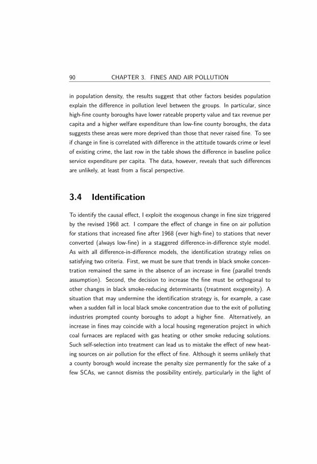
90 CHAPTER 3. FINES AND AIR POLLUTION
in population density, the results suggest that other factors besides populationexplain the difference in pollution level between the groups. In particular, sincehigh-fine county boroughs have lower rateable property value and tax revenue percapita and a higher welfare expenditure than low-fine county boroughs, the datasuggests these areas were more deprived than those that never raised fine. To seeif change in fine is correlated with difference in the attitude towards crime or levelof existing crime, the last row in the table shows the difference in baseline policeservice expenditure per capita. The data, however, reveals that such differencesare unlikely, at least from a fiscal perspective.
3.4 Identification
To identify the causal effect, I exploit the exogenous change in fine size triggeredby the revised 1968 act. I compare the effect of change in fine on air pollutionfor stations that increased fine after 1968 (ever high-fine) to stations that neverconverted (always low-fine) in a staggered difference-in-difference style model.As with all difference-in-difference models, the identification strategy relies onsatisfying two criteria. First, we must be sure that trends in black smoke concen-tration remained the same in the absence of an increase in fine (parallel trendsassumption). Second, the decision to increase the fine must be orthogonal toother changes in black smoke-reducing determinants (treatment exogeneity). Asituation that may undermine the identification strategy is, for example, a casewhen a sudden fall in local black smoke concentration due to the exit of pollutingindustries prompted county boroughs to adopt a higher fine. Alternatively, anincrease in fines may coincide with a local housing regeneration project in whichcoal furnaces are replaced with gas heating or other smoke reducing solutions.Such self-selection into treatment can lead us to mistake the effect of new heat-ing sources on air pollution for the effect of fine. Although it seems unlikely thata county borough would increase the penalty size permanently for the sake of afew SCAs, we cannot dismiss the possibility entirely, particularly in the light of

3.4. IDENTIFICATION 91
the differences we observe in the baseline characteristics of county boroughs, aspreviously shown in Table 3.6.
To solve the problem, I exploit the relationship between fine, SCA, and theseasonal variation in the demand for coal. Specifically, since the effect of fineonly exists in the presence of an SCA, we can exploit the same identificationstrategy adopted by Fukushima (2021b), who shows that the impact of SCAis restricted to the winter season. Then, since the seasonal variation in SCAimpact also means that the effect of a change in fine only appears in the winterseason, we can cut ties to unobserved covariates, much like in the case of SCA.The identification strategy means that I can compare the change in winter blacksmoke concentration to the change in summer black smoke concentration after anincrease in fine within the same county borough and year. However, although thestrategy removes the threat of bias arising from unobserved covariates that varywith county borough and year, it does not account for any unobserved trends thatvary with county borough, year, and season. Availability of monthly observation,however, allows us to further compare the effect on pollution before and aftera rise in fine within the same season, which will remove any source of bias thatarises from season-year-location varying unobserved confounders. Moreover, thestations that never adopted the 20 pounds penalty act as an additional controlgroup.
To summarize, to estimate the causal effect of an increase in fine on blacksmoke concentration, I exploit the staggered change in the rise in fine asso-ciated with the expansion of SCA in addition to the seasonal variation in theuse of bituminous coal in a quadruple difference-in-difference regression analysis.Therefore, the main regression coefficient estimates the impact of doubling themonetary penalty if convicted on winter black smoke concentration conditionalon SCA coverage. Notably, the strategy nets out any season-year-station varyingconfounders from the analysis by comparing the differences in outcome withinand between seasons within a location-year-cell. The regression equation is then;

92 CHAPTER 3. FINES AND AIR POLLUTION
BSimy = β0 + β1SCAimy + β2Winterm
+ β3SCAimy ×Winterm + β4SCAimy × 20Fineimy
+ β5SCAimy ×Winterm × 20Fineimy
+ γi + µm + ηy + εimy
where BSimy is black smoke concentration measured at station i, in monthm, and year y. SCA ∈ [0,1] is the area share covered by the regulation within500 meters distance from the station, Winter is a dummy variable that is onefor any month between October–March, and 20Fine a dummy that takes thevalue 1 when fine is 20 pound, and 0 otherwise. Note that since 20Fine is nota meaningful variable on its own as it only exists in combination with SCA, i.e.,a so-called “nested” variable, its main effect is excluded from the regression.The coefficients of interest, β3, β4, and β5, tell us the effect of SCA on winterblack smoke concentration when the fine size is 10 pounds, the effect of SCAon black smoke concentration when the fine is 20 pound for summer and winter,respectively. In so far that I consider a station treated even if its exposure tohigh-fine SCA is limited, the effect of increase in fine is an underestimation ofthe true effect.
3.5 Results
Figure 3.17 shows the trends in black smoke concentration by penalty size at thestation level and a breakdown of the number of new stations converting from10 pounds to 20 pounds by year. First, it shows that ever-high-fine stationsare, on average, located in more polluted areas than the control stations butfollow a similar trend in black smoke concentration before 1969.18 Notably, it
18In the graph, I restrict the period to 1963 - 1973, but the result holds for including allyears beginning in 1958.

3.5. RESULTS 93
shows that the parallel trends assumption likely holds. Then, as the effect ofthe revised CAA of 1968 on industry emission kicks in, we see an initial drop inblack smoke concentration in both group categories, followed by a small but clearconvergence in black smoke concentration. In particular, the shrinking differencein air pollution appears to increase with the number of stations affected byan increase in fine, suggesting an association between fine size and pollutionconcentration.
Table 3.7, column (1), shows the result from interacting winter SCA withthe fine size in levels. First, the higher winter pollution is apparent from thewinter dummy coefficient. We also see that SCA did not affect pollution in thesummer but had a small positive effect on pollution when interacted with fine.The three-way interaction term, the main coefficient of interest, indicates thatSCA’s effect on winter-pollution increased with -6.6 µg/m3 for every 1 poundincrease in penalty size. Assuming a linear marginal effect in penalty size, theresults suggest that a fine of 20 pounds will lead to a 124 microgram reductionin black smoke concentration, a number not far from the seasonal difference inblack smoke concentration. Nevertheless, since linearity is unlikely, I replace thesize of fine in levels with a dummy as per the main regression equation.
Column (2) reveals the results. First, it shows that SCA had a significantblack smoke-reducing effect in the winter, as expected. The coefficient suggeststhat winter black smoke concentration decreased with 75 µg/m3 with 10 poundspenalty when the SCA coverage increase from 0 to 100% coverage. The nexttwo rows show the effect of an increase in fine from 10 to 20 pounds. Here wesee that a doubling of fine size had no effect on summer pollution but reducedwinter smoke pollution with an additional 28 µg/m3, corresponding to a 37%increase in SCA impact.
What explains this additional effect of SCA on smoke pollution? First, thesizable effect of SCA even without a change in penalty suggests that most resi-dents complied with the regulation. Therefore, a surge in regulation effect mustbe a result of offenders who changed to comply with the regulation only after

94 CHAPTER 3. FINES AND AIR POLLUTION
an increase in fine, or due to the increase in fine coinciding with an increasedprobability of detection. However, a regression analysis studying the associa-tion between penalty size and police spending per capita reveals no relationshipbetween the variables. With no evidence linking increased regulation effect toincreased monitoring activity, we may conclude that the impact is less likely dueto changes in the probability of detection and, instead, the result of increasedregulatory compliance.
Who then are these marginal offenders? A complier who only responds to theregulation after an increase in fine would previously have found the cost of beingcaught and punished smaller than the utility received from breaching the order.Since most prefer non-smoke-emitting coal to the cheaper bituminous coal, acontinued consumption of bituminous coal suggest that the marginal offenderfinds the price discount of bituminous coal more important than the potentialfine they have to pay in case of conviction, and the adverse health effects asa result of the burning of smoke-emitting coal. Such a higher price sensitivitysuggests that the marginal offender is likely poorer than the median citizen.
Although I am unable to identify the marginal offender using the current data,several observations support the logical deduction in the previous section. For in-stance, in Figure 3.17, we see that higher air pollution, which is a strong povertyindicator, was much more prevalent in ever high-fine areas than in always low-fineareas. In addition, although the local authorities offered financial assistance tohelp households comply with the regulation, the policy required capital invest-ment from the owner or the occupier of the dwelling. A household that does nottake up the offer despite the large grant offered to private homes to meet theorder requirements is therefore likely liquidity constrained. The relative hardshipbrought by SCA to already financially constrained households is also documentedby Scarrow (1972), who writes that by 1960, a survey by the National Society forClean Air had reported 774 violations of smoke control orders resulting in twenty-four prosecutions. He continues that “[V]irtually all of the reported violationsand prosecutions for burning coal in smokeless areas have involved low-income

3.6. CONCLUSION 95
householders, and pensioned widows have sometimes been pictured as shiveringin their rooms rather than afford the cost of smokeless fuels.” While a pensionedwidow may be less likely to breach an order, a low-income family’s willingnessto continue using banned coal and risk being caught rather than suffer throughcold winter nights appears more probable.
3.6 Conclusion
The results of the analysis on the effect of an increase in fine on pollution re-duction are compelling. In particular, the analysis reveals that prospective finescan play an important role in increasing compliance and reducing pollution. Theresults are also supported by economic theory on crime, showing that fine is aneffective tool for regulators to deter environmental offenses.
Nevertheless, the results also reveal the complexities associated with imposinga fine from breaching an environmental regulation. While the success of theUK Clean Air Act in improving air quality is spectacular and saved many lives(Fukushima, 2021b), the current analysis reveals that the poorest householdsdisproportionally carried the cost of improved air quality relative to their income.At the same time, we also expect the benefit from improved air quality to bestronger for the poorest with less means to avoid pollution or receive treatmentfor adverse health effects from pollution exposure (Zivin and Neidell, 2013).Since pollution is highly correlated with income, the results are a reminder of theimportance of considering the distributional effects of environmental regulation.
Going forward, the study aims to test the robustness of the results and studyheterogeneity in effect using station characteristics (not yet digitized). For ex-ample, we may want to test the robustness of the analysis to income or otherarea characteristics. Also, by obtaining data on conviction, we can test for anyreputational spillover effects of a crackdown on local compliance to separate theeffect of change in the perception of the probability of conviction from changesin the size of the penalty (Shimshack and Ward, 2005).

96 CHAPTER 3. FINES AND AIR POLLUTION
References
Arceo, E., Hanna, R., and Oliva, P. (2016). Does the Effect of Pollution on InfantMortality Differ Between Developing and Developed Countries? Evidence fromMexico City. The Economic Journal, 126:257–280.
Assunção, J., Gandour, C., and Rocha, R. (2013). A CPI report, DETERringdeforestation in the Brazilian Amazon: Environmental monitoring and law en-forcement. Technical report, Climate Policy Initiative Rio de Janeiro.
Axbard, S. and Deng, Z. (2020). Informed Enforcement Lessons from PollutionMonitoring in China.
Becker, G. S. (1968). Crime and Punishment: An Economic Approach. Journalof Political Economy, 76(2):169–217.
Cohen, M. A. (2000). Empirical Research on the Deterrent Effect of Environmen-talMonitoring and Enforcement. Environmental Law Reporter News & Analysis30, (4).
Currie, J., Zivin, J. G., Mullins, J., and Neidell, M. (2014). What Do WeKnow About Short- and Long-Term Effects of Early-Life Exposure to Pollution?Annual Review of Resource Economics, 6(1):217–247.
de Chaisemartin, C. and D’Haultfœuille, X. (2020). Two-Way Fixed Effects Es-timators with Heterogeneous Treatment Effects. American Economic Review,110(9):2964–96.
Duflo, E., Greenstone, M., and Hanna, R. (2008). Indoor air pollution, healthand economic wellbeing. S.A.P.I.EN.S [Online], 1(1).
Duflo, E., Greenstone, M., Pande, R., and Ryan, N. (2013). Truth-telling byThird-party Auditors and the Response of Polluting Firms: Experimental Evi-dence from India. The Quarterly Journal of Economics, 128(4):1499–1545.

97
Duflo, E., Greenstone, M., Pande, R., and Ryan, N. (2018). The Value ofRegulatory Discretion: Estimates From Environmental Inspections in India.Econometrica, 86(6):2123–2160.
Fukushima, N. (2021). The UK Clean Air Act, Black Smoke, and Infant Mortality.PhD thesis.
Glicksman, R. L. and Earnhart, D. H. (2007). The Comparative Effectivenessof Government Interventions on Environmental Performance in the ChemicalIndustry. Stanford Environmental Law Journal, 26(2):317–372.
Gray, W. B. and Shimshack, J. P. (2011). The Effectiveness of EnvironmentalMonitoring and Enforcement: A Review of the Empirical Evidence. Review ofEnvironmental Economics and Policy, 5(1):3–24.
Greenstone, M. and Hanna, R. (2014). Environmental Regulations, Air andWater Pollution, and Infant Mortality in India. American Economic Review,104(10):3038–3072.
Greenstone, M., He, G., Jia, R., and Liu, T. (2019). Can Technology Solve thePrincipal-AgentProblem? Evidence from China’s War on Air Pollution.
He, G., Wang, S., and Zhang, B. (2020). Watering Down Environmental Regu-lation in China. The Quarterly Journal of Economics, 135(4):2135–2185.
Le Grand, J. and Winter, D. (1980). Determinants of Local Government Ex-penditure, 1951-1974 [Computer file]. Colchester, Essex: UK Data Archive[distributor], SN: 913, http://dx.doi.org/10.5255/UKDA-SN-913-1.
Rousseau, S. (2009). Empirical Analysis of Sanctions for Environmental Offenses.International Review of Environmental and Resource Economics, 3(3):161–194.
Scarrow, H. A. (1972). The Impact of British Domestic Air Pollution Legislation.British Journal of Political Science, 2(3):261–282.

98 CHAPTER 3. FINES AND AIR POLLUTION
Shimshack, J. P. and Ward, M. B. (2005). Regulator reputation, enforcement,and environmental compliance. Journal of Environmental Economics and Man-agement, 50(3):519–540.
Stafford, S. L. (2002). The Effect of Punishment on Firm Compliance withHazardous Waste Regulations. Journal of Environmental Economics and Man-agement, 44(2):290–308.
UNEP (2019). United Nations Environment Programme: Environmental Rule ofLaw: First Global Report. Technical report.
Zivin, J. G. and Neidell, M. (2012). The Impact of Pollution on Worker Produc-tivity. American Economic Review, 102(7):3652–3673.
Zivin, J. G. and Neidell, M. (2013). Environment, Health, and Human Capital.Journal of Economic Literature, 51(3):689–730.

. FIGURES AND TABLES 99
Figures and tables
Figure 3.12: Example smoke control order(a) Oxford - 10pounds
11474 THE LONDON GAZETTE, 22ND OCTOBER 1971
date determined by the Secretary of State for theEnvironment.
Copies of the Order and of the map referred totherein may be inspected free of charge at the CouncilOffices, Easington, at all reasonable times during theperiod of 6 weeks from the 22nd October 1971.
Within the said period any person who will beaffected by the Order may by natice in writing to theSecretary of State for the Environment, Whitehall,London S.W.I, object to the confirmation of theOrder.
SCHEDULEAll lands and premises within an area of 1,273
acres or thereabouts, situated in the designated areaof Peterlee in the Rural District of Easington andbeing that part of the area south of a line drawnfrom the A. 19 along Passfield Way to Burnhope Way,thence to Surtees Road, along Yod'en Way to theeastern1 boundary of the designated area.
Dated' 15th October 1971.D. Conyers Kelly, Cterk of the Council.
Council Offices, Easington,Peterlee, Co. Durham. (299)
CANTERBURY CITY COUNCILThe City of Canterbury (Forty Acres Road) (No. 1)
Smoke Control Order, 1971Notice is hereby given that the Canterbury CityCouncil in exercise of the powers conferred on themby section 11 of the Clean Air Act, 1956, on the 15thday of October 1971, made an Order enltdtled "TheCity of Canterbury (Forty Acres Road) (No. 1) SmokeControl Order, 1971 " declaring the area1 describedin the Schedule hereto to be a smoke control areawhich Order is about to be submitted to the Secretaryof State for Klhe Environment for confirmation.
By virtue of section 11 (4) of the Act if, on anyday after the Order has come into operation, smoke isemitted from a chimney of any building within thesmoke control area the occupier of that building shallbe guilty of an offence and liable ito a fine notexceeding £10 unless he provtes that the emission ofsmoke was not caused by the use of any fuel otherthan an authorised fuel. The authorised fuels includeanthracite, coke and other carbonised fuels, gas andelectricity.
Copies of the Order and of the map referred totherein may be inspected1 frae of charge at the TownClerk's Office, Municipal Buildings, Canterbury, at allreasonable times during the period of 6 weeks frontthe 22nd day of October 1971.
Within the said period any person who will beaffected! by the Order may by notice in writing toThe Secrtetary of State, Department of the Environ-ment, 2 Marsham Street, London, SW1P 3EB, objectto the confirmation of the Order.
SCHEDULEAn area of land within the City of Canterbury
bounded by Forty Acres Road, Salisbury Road, TheGlasshouses, The Nurseries and Whitstable Road, allof which land is shown coloured' pink on the planreferred to in the said Order.
Dated 22nd October 1971.
Municipal Building,Canterbury.
/. Boyle, Town Clerk.
(281)
NEWHAM LONDON BOROUGH COUNCIL'Newham No\ 8 Smoke Control Order, 1971
Notice is hereby given that the Council of theLondon Borough of Newham in exercise of thepowers conferred1 upon them by section 11 of theClean Air Act 1956, on the 12th October 1971, madean Ord'er entitled! the Newham No. 8 Smoke ControlOrder, 1971, declaring the area described! in theSchedule hereto to be a smoke control area, whichOrder is about to be submitted to the Secretary ofState for the Environment for confirmation.
Subject Ho the exemptions provided by the Ordterand by virtue of section 11 (4) of the Act, if, on anyday after the Order has come into operation, smoke isemitted from a chimney of any building within thesmoke control area the occupier of mat building1
shall be guilty of an offence and liable to a fine noliexceeding £20 unless he proves that the emission of
smoke was not caused by the use of any fuel otherthan an authorised fuel. The authorised' fuels includeanthracite, coke and other carbonised fuels, gas andelectricity.
The date of operation specified in the Order isthe 1st October 1972.
A copy of the Order and of the map referredto eherein may be inspected -free of charge at the TownHad, East Ham, London E.6, at all reasonable timesduring the period from the 29th October 1971, to the13th December 1971.
Within the said period any person who will beaffected by the Order may by notice in writing tothe Secretary of State for thje Environment, 2Marsham Street, London, SW1P 3EB, object to theconfirmation of the Order.
SCHEDULEThe area comprising approximately 371 acres is
broadly speaking within the boundaries of the Uptonand Woodgrange Wards and lies to the south of theEastern Region Railway Line and to the north ofthe central part of the Borough.
G. E. Smith, Town Clerk.Town Hall,
East Ham, London E.6.22nd October 1971. (335)
OXFORD CITY COUNCIL
The City of Oxford No. 11 Smoke Control Order,1971
Notice is hereby given mat the Lord Mayor, Alder-men' and Citizens of Oxford in exercise of theirpowers under section 11 of the Clean Air Act, 1956,on the 4uh October 1971, made an Order entitled theCity of Oxford No. 11 Smoke Control Order, 1971,declaring the area described in the Schedule heretoto be a smoke control area, which Order is about tobe submitted to the Secretary of State for theEnvironment for his confirmaion.
Subject: to the exemption provided by the Orderand by virtue of section 11 (4) of the Act, if, on anyday after the Order has come into operation, smokeis emitted from a chimney of any building within thesmoke control area, the occupier of that building shallbe guilty of an offence, and liable to pay a fine notexceeding £10 unless he proves that the emission ofsmoke was not caused by the use of any fuel otherthan an authorised fuel. The authorised fuels includeanthracite, coke, and other carbonised fuels, gas andelectricity.
If confirmed the Order will come into operationon the 1st day of October 1972, or such later dateas may be determined by the Secretary of State forthe Environment.
Copies of the Order and of the map referred totherein may be inspected free of charge at the TownClerk's Office, St. Aldate's Chambers, Oxford, at allreasonable timfes during the period of 6 weeks fromthe 22nd October 1971.
Within the said period' any person who will beaffected by the Order may, by notice in writing to theSecretary of State for the Environment, 2 MarshamStreet, London S.W.I, object to the confirmation ofthe Order.
SCHEDULEAn area of 82 acres or thereabouts within the City
of Oxford, bounded by an imaginary line commencingat ithe centre of the junction of Howard Street andCowley Road, thence in a south-westerly directionalong the centre of Howard Street to the junction ofHoward Street with Iffley Road, thence in a north-westerly direction along the centre of Iffley Road toits junctions with Henley Street, thence in a north-easterly direction along the centre of Henley Streetto its junction with Hurst Street, thence in a south-easterly direction along the centre of Hurst Street toits junction with Leopold Strteet, thence in a north-easterly direction along the centre of Leopold Streetto its junction with Cowley Road, thence in a south-easterly direction along the centre of Cowley Rloaid tothe original point at the junction of Cowley Roadand Howard Street.
Dated' 5th October 1971.
St. Aldate's Chambers,Oxford.
A. T. Brown, Town Clerk.
(388)
(b) Tynemouth - 20 pounds
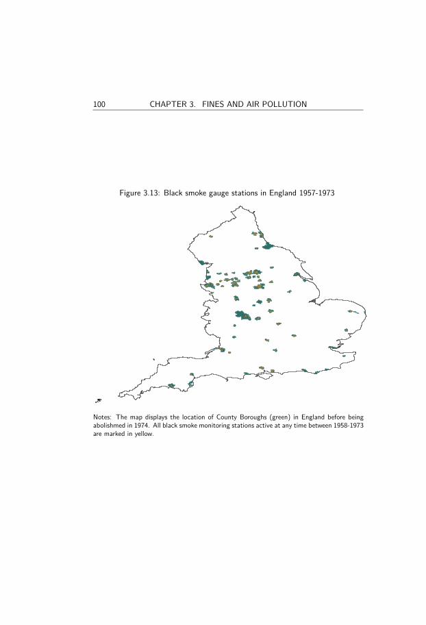
100 CHAPTER 3. FINES AND AIR POLLUTION
Figure 3.13: Black smoke gauge stations in England 1957-1973
Notes: The map displays the location of County Boroughs (green) in England before beingabolishmed in 1974. All black smoke monitoring stations active at any time between 1958-1973are marked in yellow.

. FIGURES AND TABLES 101
Figure 3.14: Relationship between black smoke and SCA coverage0
50
01
,00
01
,50
0B
lack s
mo
ke
co
nce
ntr
atio
n
1 5 6 SCA coverage 8 9 10
BSconc. Winter BSconc. Summer
Notes: The graph displays the median, 25, and 75th percentile black smoke concentration bySCA coverage within 500 meters distance from gauge stations in deciles.
Figure 3.15: Stations subject to 20 pounds smoke control order within 500 metersdistance
0.0
5.1
.15
.2.2
5S
ha
re o
f 2
0 p
ou
nd
s s
tatio
ns
1963
1964
1965
1966
1967
1968
1969
1970
1971
1972
1973
year
Notes: The graph shows the share of black smoke gauge stations within 500-meter from a 20pounds SCA.
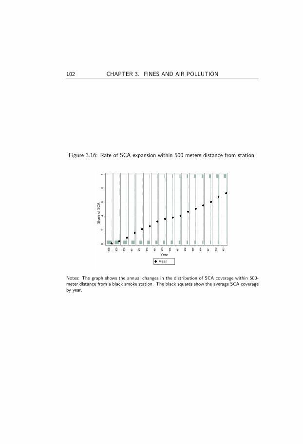
102 CHAPTER 3. FINES AND AIR POLLUTION
Figure 3.16: Rate of SCA expansion within 500 meters distance from station
0.2
.4.6
.81
1958
1959
1960
1961
1962
1963
1964
1965
1966
1967
1968
1969
1970
1971
1972
1973
Mean
Sh
are
of
SC
A
Year
Notes: The graph shows the annual changes in the distribution of SCA coverage within 500-meter distance from a black smoke station. The black squares show the average SCA coverageby year.

. FIGURES AND TABLES 103
Table3.6:
Baselinecoun
tybo
roug
hcharacteristic
sbytre
atments
tatus
Alwayslow-fine
CB
Ever
high
-fine
CB
Meandiffe
rence:
(1)
(2)
(1)-
(2)
Mean
Std.
Mean
Std.
Diff.
p-value
AverageSu
mmer
BSconc.1
963-1967
57.001
32.71
81.310
50.46
-24.31
(0.00)
AverageWinterB
Scon
c.1963-1967
150.161
82.95
222.160
127.19
-72.00
(0.00)
Baselines
in19
58:
Popu
lation
density
(km2)
6.656
2.24
5.546
2.14
1.11
(0.00)
Rateable
valuep.c.
13.200
2.55
11.387
2.12
1.81
(0.00)
Area
sq-m
iles(
inthou
sand
s)18.490
13.27
22.753
14.34
-4.26
(0.06)
Raise
dtaxp.c.
0.013
0.00
0.011
0.00
0.00
(0.00)
Baselines
in19
59:
Healt
hservice
sp.c.
0.101
0.02
0.108
0.02
-0.01
(0.05)
Child
service
sp.c.
0.036
0.01
0.042
0.01
-0.01
(0.00)
Welfareservice
sp.c.
0.044
0.01
0.051
0.02
-0.01
(0.00)
Housingservice
sp.c.
0.140
0.04
0.147
0.04
-0.01
(0.28)
Fire
service
sp.c.
0.042
0.01
0.044
0.02
-0.00
(0.38)
Policeservice
sp.c.
0.165
0.04
0.173
0.04
-0.01
(0.18)
Notes:Th
etableshow
sthe
diffe
rencein
baselinecharacteristic
ofCB
sthatd
oubled
themon
etaryfin
efro
m10
poun
dsto
20po
unds
after1
968(Everh
igh-fin
e)andtheCB
sthat
didno
t(A
lwayslow-
fine).Ba
selines
in1959
referesto
CBexpend
iture
perc
apita
for
each
listedcategory
ofservice
(LeGr
andandWinter,1980).
ThetreatedCB
sare:
Barnsle
y,Birkenhead,B
olton,
Bradford,E
xeter,
Gateshead,
Halifa
x,Hud
dersfield,Leeds,
Leice
ster,Lincoln,
Luton,
Manchester,
Oldham,Preston,
Salfo
rd,Sh
effield
,St
Hele
ns,
Sund
erland
,Tynem
outh,W
akefield
,Wallasey,Warrin
gton
.Th
eno
n-treatedCB
sinclu
de:Birm
ingh
am,B
lackbu
rn,B
ristol,Bu
rnley
,Bu
rton
upon
trent,Bu
ry,C
oventry,Don
caster,K
ingstonup
onhu
ll,Liverpoo
l,New
castle
upon
tyne,N
ottin
gham
,Oxford,
Reading,
Rochdale,
Solihull,So
uthampton
,Stockpo
rt,S
toke
ontrent.

104 CHAPTER 3. FINES AND AIR POLLUTION
Figure 3.17: Number of events and trends in black smoke concentration
05
10
15
20
Nu
mb
er
of
tre
ate
d
50
10
01
50
20
0B
lack S
mo
ke
Co
nce
ntr
atio
n
1963
1964
1965
1966
1967
1968
1969
1970
1971
1972
1973
Year
Always low−fine Ever high−fine
High−fine stations
Notes: The bar chart shows the number of black smoke stations affected by an incrase in finewhile the lines are the trends in black smoke concentration for the stations that raised fine atsome point after 1968 (ever high-fine) and the stations that did not (always low-fine). Thesample includes all stations active before 1967.

. FIGURES AND TABLES 105
Table 3.7: The effect of SCA on black smoke with an increasing fine size
(1) (2)SCA -21.33 7.801
(15.60) (7.81)Winter 159.3∗∗∗ 163.2∗∗∗
(8.19) (8.28)SCA × Fine 2.508∗∗
(1.07)SCA × Winter × Fine -6.649∗∗∗
(0.61)SCA × Winter -74.78∗∗∗
(7.16)SCA × 20 pounds 4.517
(10.43)SCA × Winter × 20 pounds -28.41∗∗∗
(5.20)No. Obs. 11867 11867No. Sites 142 142R2adj. 0.602 0.604Year FE Yes YesMonth FE Yes YesSite FE Yes YesStandard errors in parentheses∗ p < 0.10, ∗∗ p < 0.05, ∗∗∗ p < 0.01
Notes: The dependent variable is black smoke concentration in micrograms per cubic meter.Winter includes the month between October and March. Fine is the level of fine in pounds(i.e., 10 or 20) while 20 pounds is a dummy variable that is 1 when fine is 20 pounds and 0otherwise. The sample excludes all stations inactive before 1967 and the analysis limited tothe period 1963-1973. Standard errors are clustered at the couny borough level.

106 CHAPTER 3. FINES AND AIR POLLUTION
Chapter 4
Environmental Regulation and Firm Performance∗
4.1 Introduction
Thirty years ago, Porter (1991) proposed that environmental regulation can,under the right circumstances and over time, lead to productivity gains by forcingfirms to recognize organizational inefficiencies and compel them to make progressand innovate. However, with only anecdotal evidence at hand and no theoreticalframework for his arguments, the appealing but controversial proposal soon drewcriticism. The main critique pointed out that environmental regulation can onlylead to a surge in operational cost since profit-maximizing firms will already haveinternalized all productivity-increasing options available (Palmer et al., 1995).
Proponents of the hypothesis have, on the other hand, claimed that be-havioral aspects and market and organizational failure could all contribute toproductivity improvements by imposing stricter standards on incumbent firms. Afew papers, such as that by Mohr and Saha (2008), take a more nuanced ap-proach to consider scenarios that generate outcomes consistent with the Porterhypothesis. However, the authors acknowledge the scenarios unlikely and difficultto test empirically.
Many studies have since put the hypothesis to data, but so far, the results are∗I am grateful to Peter Nilsson, David Strömberg, and Anders Åkerman for their comments
and suggestions, and to FORMAS for the generous grant that enabled the data collection.
107

108 CHAPTER 4. REGULATIONS AND FIRMS
inconclusive.1 One reason for the ambiguity is that the literature is still uncertainabout the mechanism leading to increased productivity, making any comparisonacross the analyses difficult. Complexity involving operational decision-makingand differences in regulations are other reasons why the empirical literature hasoften failed to pin down the causal relationship between regulation and firmperformance.2
This study contributes to the discussion by proposing a theoretical modelin which heterogeneity in firm productivity leads to an increase in local averageproductivity and provides empirical evidence to support the model. The paperalso provides a first comprehensive theoretical analysis of the effect of an envi-ronmental regulation on local manufacturing plants by studying the impact of aregulation on firm probability of survival, labor demand, and the location choiceof new entrants.
The theoretical model shows why we expect only highly productive firms toinvest in efficiency-enhancing technology and how regulation-induced negativecost shocks can increase average productivity by forcing low-productivity firmsto exit and keeping low-productive firms from entering the market.
The empirical analysis exploits the variation in time and space of the rolloutof a local ban on coal use from the passing of the 1956 UK Clean Air Act. Novelgeographical data of so-called Smoke Control Areas (SCA) in the Merseysideregion in the northwest of England is matched with plant manufacturing databetween 1959–1975. The detailed geographic information of the plants and thepanel structure of the data allows me to compare different levels of regulationexposure on firm exit, entry, and expansion while holding unobserved locationcharacteristics constant.
The empirical findings largely support the model prediction. The findings
1For a thorough review of the evidence for and against the Porter hypothesis, see Ambecet al (2013).
2For instance, according to Porter, a regulation-induced productivity gain only happenswhen innovation is free for the industry to decide where no technology, including changes inoperation processes, is forced upon it and where no room for uncertainty is left.

4.1. INTRODUCTION 109
reveal that the local ban on coal reduced the probability of survival for the leastproductive firms while the probability of survival increased for high productiveplants. I also find positive effects of the regulation on entry of low coal-intensivefirms and employment to increase for the most productive firms.
An often-repeated concern in the empirical literature on the effect of environ-mental regulation on firm performance is regulation consistency. For example,environmental regulation usually governs multiple standards of measurementssuch as total emissions, emission concentration, or technology that varies withtime, space, industry, ownership, and firm size. Even the same regulation isnot always comparable since pollution standards can change over time. Thelack of environmental regulations that remain consistent across all dimensionsis, therefore, a great weakness in the empirical literature on the effects of envi-ronmental regulation on firm performance. For example, the US Clean Air Actand its amendments are the most studied environmental regulations owing to itssweeping effects across the US. However, the one-off nature of the event oftencomplicates the analysis since it is difficult to distinguish the regulation effectfrom confounders. To not rely on a single event, Berman and Bui (2001) have,for example, indexed local regulations according to their level of stringency toallow for comparison across time. Nevertheless, the study will inevitably sufferfrom subjective judgments in regulation stringency despite the researchers’ bestefforts.3
Another relevant issue in the empirical literature is that environmental regu-lations are often endogenous to firm performance. For instance, possible lossesin employment due to legislation have been debated extensively since the 1980sand are still a source of disagreement.4 Other issues discussed are possible firmmigration to more lax environments leading to a “race to the bottom” (Bar-
3The many complexity involving regulation stringency is discussed in great detail by Bruneland Levinson (2016).
4For early discussion, see for example, Jaffe et al (1995). For a comprehensive overviewof research on environmental policy and job creation, see OECD 2017 and for recent po-litical debate, see for example, https://www.nytimes.com/2019/09/04/climate/climate-job-creation.html [Accessed 09 Mar 2021].

110 CHAPTER 4. REGULATIONS AND FIRMS
tik, 1988) and a pollution-haven effect, but also the fear that relatively morestringent environmental regulations can cause domestic firms to lose their com-petitiveness in international trade (Porter, 1991; Jaffe et al., 1995). The appealof the US Clean Air Act is, therefore, not limited to the legislation’s extensivenature but also because of its role as an exogenous source of change. This paperattempts to avoid endogeneity and subjective judgment in assessing regulatorystringency by exploiting the staggered roll-out of a comprehensive ban character-ized by transparency and consistency, which adds to the current study’s particularadvantage.
The rest of the paper is organized as follows; section 2 provides some back-ground describing the regulation, while section 3 presents the theoretical model.Section 4 presents the data, and section 5 discusses the identification assumptionand the empirical models. Section 6 displays and discusses the results, followedby some concluding remarks in section 7.
4.2 UK Clean Air Act and Smoke Control Areas
The UK Clean Air Act was enacted as a direct response to the Great Smogincident in London in December 1952 that is estimated to have killed around12 000 people. While multiple attempts to control air pollution had faced bigresistance in the past and failed, the UK Clean Air Act was widely acceptedand passed in 1956 and has been accredited with successfully improving the airquality in the UK.5
The act was radical in that it targeted coal usage when the coal sector em-ployed millions of people and was the primary source of energy in the industry(Department for Business, Energy & Industrial Strategy, 2019). Besides prohibit-ing the emission of dark smoke from chimneys, however, the act also providedthe local authorities with the mandate to introduce so-called smoke control areas
5Historically, most claims to improved air quality were anecdotal or relied on a few time-series analyses. For evidence on the causal effect of the Clean Air Act on air quality, seeFukushima (2021b).
4.3. THEORETICAL FRAMEWORK 111
(SCA), geographically defined zones inside smoke emission was banned.6
In this paper, I study the effect of the emission-free zones on firm perfor-mance. Instead of focusing on the color of the smoke, SCA prohibited emissionof smoke of any color from any building. Because the decision to create SCAswere in the hands of the local governments, they varied in location, time andsize.7 For example, the Clean Air Act determined the size of the financial penalty.It also required all orders to be publicly announced at least six months in ad-vance. However, the location of SCAs and their start dates were left to the localgovernments to decide.8 Until the late 1960s, the fine of breaching a smokecontrol order was 10 pounds per offense, irrespective of the type of building butsubsequently raised to 20 pounds per offense.9 10 In contrast to private dwellingsthat would receive financial compensation for 70% of the cost of adjusting thebuilding to comply with the regulation, commercial entities received no such sup-port, meaning that local enterprises were left to their device to find a solution tocomply with the new regulation.
4.3 Theoretical framework
The model studies the effects of a relative increase in the price of coal on firmexit, entry, and average productivity in the presence of heterogeneity in plantproductivity. While banning bituminous coal restricts the choice set leading to anincrease in coal price, the model is generalizable to any situation when regulationcauses the price of an input to increase.
6Appendix 4.7 lists the differences in the implementation of the dark smoke provision andthe local smoke bans.
7An example of a Smoke Control Order is shown in Appendix 4.7.8Data on SCA adoption in English County Boroughs suggest they were usually announced
12 - 18 months in advance. While local authority was free to choose the location, it stillrequired approval from the Minister of Housing and the Local Government.
910 GBP in 1968 corresponds to approximately 150 GBP in 2021.10Four of five local authorities in the study raised the fine from 10 to 20 in 1970/71. Only
Liverpool kept the size of penalty at 10 pounds throughout the period. Sensitivity to changein fine size is studied separately.

112 CHAPTER 4. REGULATIONS AND FIRMS
4.3.1 The model
The model follows Helpman et al. (2004) and their model of firm heterogeneitybut assumes a closed economy that use coal and labor to produce goods in 2sectors, X and M. While the numeraire sector X produces homogenous productsunder perfect competition using one unit of labor per unit output such that laborcost equal to unity, i.e., w = 1, the monopolistic competitive M sector producesdifferentiated products using coal and labor as inputs. If β is the exogenousfraction of income spent on differentiated products of sector M the remaining1 − β is spent on the homogenous good, CX .
Consumer preferences follow a standard CES consumer utility function withan elasticity of substitution ε , where ε > 1. The aggregate consumption ofgoods from sector M is defined by CM = [
´ n0 c(ν)(ε−1)/εdν]ε/(ε−1) where n is the
number of varieties available and c(ν) is the consumption of each variety ν. Thepreference function implies that consumer demand for each variety of good insector M is Ap−ε where A = βY´ n
0 p(ν)1−εdν, Y is the aggregate level of income,
p(ν) is the consumer price of variety ν, and´ n0 p(ν)1−εdν is the price index that
changes in the long run.
4.3.2 Firm profit
To enter a market, firms must pay a sunk entry fixed cost, fE , measured in laborunits. The firm productivity level is decided after drawing an inputs-per unitof output coefficient from a Pareto distribution G(a) at which point the firmdecides to enter or not. If it enters, the firm incurs an additional fixed overheadfactor input cost per period, fo. The monopolistic producer has a Cobb-Douglasproduction function q = φcγl1−γ, where φ = 1/a is the total factor productivityand c and l are the factor inputs, coal and labor, respectively. Solving the firm’sproblem in which r and w are the respective input factor prices, we can show thatthe marginal cost is mc = arγw1−γθ and that price equals to p = ε
ε−1arγw1−γθ

4.3. THEORETICAL FRAMEWORK 113
where ε/(ε − 1) is the markup factor.11 Given the unit labor cost, the profitfunction can thus be written as
Π = (p − mc)q − fo
= a1−ε (rγθ)1−ε (1
ε − 1)A(
ε
ε − 1)−ε − fo (4.7)
Since monopolistic competition implies A is exogenous to supplier, we candefine B = ( 1
ε−1 )A(εε−1 ) as the level of demand, which we assume is the same for
all firms. A firm operates as long as Π ≥ 0 but exits if Π < 0.The minimum productivity level required to remain in operation is solved by
setting profits equal to 0 and solving for a1−ε such that
a∗1−ε =Bε fo(rγθ)1−ε
. (4.8)
where a∗1−ε is the minimum level of productivity required to produce positiveprofit. The equation shows that firms will choose to exit if a1−ε < a∗1−ε butcontinue producing if a1−ε ≥ a∗1−ε . The graphical illustration of this relationshipis presented in Figure 4.18 where Π1 shows the pre-intervention profit for differentlevels of productivity and a1−ε1 is cut-off level of productivity at the baseline.Equation (4.8) shows that the cut-off level increase with coal price.
Proposition 4.1. An increase in the price of coal leads to exit of the leastproductive firms.
Proof. The statement follows directly from equation (4.8) where a higher r im-plies a higher cut-off point. �
Since an increase in coal factor price leads to higher marginal cost and price,productivity must be sufficiently high for a firm to remain operational. The effect
11Where θ is θ = γ−γ(1 − γ)−(1−γ).

114 CHAPTER 4. REGULATIONS AND FIRMS
on an increase in coal factor price on the profit function is displayed in Figure4.18 by the line Π2 where Π2 ≥ 0 iff a1−ε > a1−ε2 .
Proposition 4.2. An increase in per period fixed cost leads to exit of the leastproductive firms .
Proof. This too follows directly from equation (4.8). �
A sudden rise in fixed cost has a similar profit-reducing impact as an increasein coal price. The differences are clear in Figure 4.18 where the new profitfunction, Π3, show lower profits for all firms (Π3 < Π1) and where Π3 > 0 onlywhen a1−ε > a1−ε3 .
4.3.3 The dynamic effects of a change in factor prices withendogenous technology
Once the regulation is implemented, we initially expect firms to comply with theregulation by replacing bituminous coal with authorized fuel and pay a premiumprice. However, in the long run, faced with a lower profit, some firms will chooseto shift factor input share, γ, away from coal by investing in new technology toreduce coal dependency.12 Investing in new technology leads to higher perperiod fixed cost, fN , where fN > fo, and reduces the input share of coal,γ.13 In order to see how the slope of the new profit function changes with a1−ε ,I analyze the derivative of the slope with respect to input factor share, γ.
∂
∂γ
(∂Π
∂a1−ε
)= (1 − ε)B−ε
rγ(1 − γ)γ−1(lnr + ln(1 − γ) − lnγ)
γγ[
rγ(1−γ)(γ−1)γγ
] ε < 0. (4.9)
12New technology define any technology that reduce coal intensity including new innovation,replacing fuel technology or reorganizing operational procedures.
13Berman and Bui (2001) show that local air pollution regulation on heavy manufacturingplants in Los Angeles induces substantial investment in abatement capital.

4.3. THEORETICAL FRAMEWORK 115
(See Section 4.7 in Appendix for details on calculation.)
Proposition 4.3. For a sufficiently high coal price, a reduction in the input shareof coal increases profits.
Proof. With ε > 1, if follows from equation (4.9) that the effect on profit isnegative whenever the price of coal exceeds the price of labor (r > w = 1) . �
The results simply tell us that increasing input share of the relatively moreexpensive input factor has a profit reducing effect. Consequently, firms will investin new technology to minimize coal intensity and increase profits.
Technology induced shift in profit is illustrated by Π4 in Figure 4.18. Notethat the new profit function must lie between Π3 < Π4 < Π1 ∀ a, where thesecond inequality condition, Π4 < Π1, follows the logical assumption that a profitmaximizing firm would already have invested in technology to reduce coal factorshare had it generated greater profit. The first inequality, Π3 < Π4 , on the otherhand, tell us that firms will only invest in new technology to reduce coal share ifit leads to higher profit.
It then follows that the new cut-off level of productivity, a1−ε4 , must lie be-tween a1−ε2 and a1−ε3 . If a1−ε4 = a1−ε2 , we expect all surviving firms to investin new technology since it will generate higher profits. On the other hand,if a1−ε4 > a1−ε2 only firms with productivity level above a1−ε4 will see profitsincrease with investment in new technology.14
Proposition 4.4. Only the most productive firms that can afford to invest innew technology to reduce coal input share will increase profits.
14Formally, the level of productivity that decides if investment in new technology isprofitable is derived by solving for the following inequality:
Bε fo(rγθ)1−ε
< a1−ε <Bε fN(r̃γ̃θ)1−ε
where fo < fN , r̃ > r and γ̃ < γ.

116 CHAPTER 4. REGULATIONS AND FIRMS
Proof. The expressions (4.8) and (4.9) show investing in technology to reducecoal input is only profitable when a1−ε > a1−ε4 ≥ a1−ε2 . �
The results imply that the choice to invest in new technology is determinedby the incumbent firm’s productivity level. For example, profit function Π4
shows a situation when only firms with productivity level above a1−ε4 investin new technology but where firms with productivity level between a1−ε2 ≤
a1−ε < a1−ε4 do not.
4.3.4 Entry
A change in input price does not only affect the exit of incumbent firms butalso the firms entering the market. To see how an increase in coal price affectsselection into entry, we can express the expected operating profit of a potentialentrant accordingly.
ˆ ∞φ∗Π(φ)dG(φ) − fE (4.10)
where φ∗ is the cut-off level of productivity and fE is the sunk entry cost.Free entry condition implies that firms will continue entering the market untilexpression (4.10) equals zero. Since the profit function is the same as theprofit function for the incumbent firms, we can derive the entry productivitycut-off level, which is analogue to equation (4.8), and define it as;
φ∗1−ε =Bε fo(rγθ)1−ε
. (4.11)
As previously, we see that a change in input price also affects marketentry conditions by raising the cut-off level.
Proposition 4.5. A sufficiently high coal price causes the cut-off level of pro-ductivity to increase, leading to a shift in entry towards high-productive firms.

4.4. DATA 117
Proof. The statement follows from (4.11) and (4.10) where we see an increasefo leading to an increase in the entry cut-off level φ∗. �
The proposition implies that an increase in coal price raises the cut-off level,precluding firms with lower productivity from entering the market and raising theaverage productivity of new entrants.
Proposition 4.6. A sufficiently high per-period fixed cost leads to higher ex-pected profits for high-productive new entrants than for less productive newentrants.
Proof. If only firms with productivity above φ∗∗ can afford investing in newtechnology and if φ∗∗ > φ∗, it follows from expressions (4.9) and (4.8) thatprofit is higher for high-productive firms than for low-productive firms. �
The results are analog to the effect of an increase in coal price on incumbentfirms with the difference that exits are replaced with selection into entry.
4.3.5 Average productivity
Although Porter (1991) does not discriminate between the impact of environmen-tal regulation on the individual firm and the economy as a whole, the currentmodel shows that the Porter Hypothesis and the critique of Palmer et al. (1995)can partly be reconciled. In particular, the model shows that under the assump-tion of profit maximization and competitive market, environmental regulationcan lead to exits of the least productive firms and entry of productive firms andthereby increase the average firm productivity.
4.4 Data
The area of study is restricted to North West England in the region of Merseysideto match the availability of manufacturing firm data. The data on the evolutionof Smoke Control Areas (SCA) comes from Fukushima (2021b) and covers the

118 CHAPTER 4. REGULATIONS AND FIRMS
years 1957–1974.15 The data has information on the location of the SCAs,announcement dates, and start dates.
The manufacturing data comes from the North West Industry Unit Researchdatabase collected by the geographic department at the University of Manchesterto investigate the spatial dynamics nature of industries in North West England(Lloyd, 1985). The sample consists of industrial establishments in operationin 1959 and 1966 and has information on the number of manual workers, theStandard Industrial Class (up to 2-digits), and the kilometer grid coordinates ofplant location and their operation status in 1959, 1966, 1972, 1975, and 1981.16
The one square kilometer location data imply that each grid cell can consistof multiple establishments. A map over the Merseyside area, here displayed inFigure 4.19, reveals the location of firms in 1966. While the colored areas showthe administrative boundaries of the local governments, the black lines withineach boundary show the outer contours of all SCAs installed before 1975. Thesize of the pie charts reflects the number of plant establishments in each gridcell, while the red color indicates the share of 1966 firms that had exited by 1975.The map reveals that both firms and SCAs cluster around historical commercialcenters and have a higher firm survival rate than plants located in the periphery.
Table 4.8 shows the total number of industrial plants in each period by theiroperational status; in-situ, entry, or exit. The most rapid phase of plant exitadjusted for the number of years occurred between 1966 and 1972, with 35 % ofplants exiting.17 On the other hand, while exits continued to decline with time,the period also coincides with the entry of 216 new plants.
Because SCAs are matched with one square kilometer large grid cells, reg-ulation exposure is a fuzzy treatment indicator. In particular, it tells us theprobability of a firm being regulated by smoke control order(s) and defined as
15The data is extended to include the areas in what was formerly known as the UrbanDistrict of Bebington, now part of Wirral.
16In the North West Industry Unit Research database, only Merseyside areas have data for1959. However, 1959 data was collected retrospectively and, therefore, conditional on beingin operation in 1966. The first survey year for the remaining data begins in 1966.
17The average exit rate is 16 % between 1966 and 1981.

4.4. DATA 119
the 1km x 1km grid area share covered by one or more SCAs. This is because,although the one square kilometer grid resolution is small considering the age ofthe data, the size of SCAs is often smaller or irregular in shape so that the gridarea does not fully overlap with the boundary of an SCA. Because the treatmentcoverage, or treatment intensity, changes with new SCAs, treatment intensityvary by grid cell and time.
To make sure that no plant is treated before the first year for which infor-mation on operation status exist, the sample firms is restricted to 241 firms inMerseyside region not subject to SCA in 1966. The omission of plants alreadyexposed to SCA before 1966 (220 in total) is important to avoid survival biasin the data. Although information on plant age does not exist, activity statusin 1959 and 1966 ensure us the sample consists of mature plants where youngfirms, often subject to higher default rate, are removed. Operational status isdefined by the variable "Components of Change" with the number of workers setto missing once firms cease to operate.
The manufacturing data also contains information on the geographic locationof all new establishments after 1966 in Merseyside. The entry data has informa-tion on the period of entry, size of employment, and industry classification up to2-digits level. Figure 4.20 reveals the location and the number of new entrants.Although the maps displaying exits and entries do not overlap perfectly, is showsthat manufacturing plants tend to cluster around historical industrial hubs.
Since the use of coal varies by the industry’s need for boilers to produceheat and steam in addition to space heating, we expect the effects of SCA todiffer by industry. Therefore, to study heterogeneity in impact related to industrydependency on coal, I construct a variable that indicates industry coal intensity.The variable is defined as the coal share of total inputs in each 1-digit levelindustry in pounds and calculated using pre-intervention (1954) input-outputtables for the UK. Note that although coal intensity can vary by region andplant, the relative industry coal intensity is less likely to differ and, therefore,useful to compare regulation effects across industries.

120 CHAPTER 4. REGULATIONS AND FIRMS
A central idea of the theoretical model is that the regulation effect shouldvary with total factor productivity (TFP). Although TFP cannot be calculatedusing the current manufacturing data, evidence suggest that firm size distributionis a good approximation for productivity distribution, which means that I can useemployment size as a proxy for firm productivity.18
4.4.1 Comparative statistics
Since local authorities did not pick SCA locations randomly, it is important to un-derstand if plants differed systematically with regulation exposure. For instance,although the primary reason for the roll-out of SCAs was to limit adverse healtheffect of air pollution, we cannot disregard the possibility that local lawmakersbecame concerned over possible regulation impact on the industry. In particular,we may worry that local authorities determined SCA location based on industrycoal intensity since coal intensive plants would be more affected by the regulation.
To study differences in plant characteristics by regulation exposure, I comparebaseline firm characteristics in regards to the number of plants, coal intensity,and employment by treatment status. For this purpose, I separate plants intogroups depending on the grid cell exposure to treatment intensity in 1974 anddefine plants in cells never regulated, i.e., SCA1974 = 0, as non-treated, cells withSCA1974 ∈ (0,1) as partially treated, and cells that lie fully within an SCA1974 = 1
as fully treated. There are 16 never-treated grid cells and 23 treated grid cells intotal. The remaining 23 treated grid cells can be split into grid cells fully coveredby SCA (7), or partially covered by SCA (16).
Table 4.9 shows the mean difference in sector coal dependency, manual em-ployment in 1959 and 1966, and the average number of firms per grid cell bytreatment status. It shows that coal dependency was the same between thetreated and the non-treated on average. Instead, the most striking differenceappears in the 1959 employment. For instance, the fully treated firms employ
18For evidence in the literature on the relationship between firm size and total factor pro-ductivity see, for example, Leung et al. (2008).

4.4. DATA 121
ten times as many manual workers than the non-treated firms and over five timesas many workers than in the partially treated firms. Manual employment in 1966reveals a similar pattern. The number of plants by grid cell, however, shows aconsiderably smaller number of firms in the fully treated areas than in the nevertreated or partially treated areas. Paradoxically and contrary to a priori beliefs,the table reveals that larger firms were more likely a subject of the regulation,suggesting lawmakers were not swayed by concerns over local employment, orpressured by the local industry in the decision making process.
To study if employment size is the result of endogenous clustering of a fewlabor-intensive sectors, I compare industry employment by treatment status andpresent these in Table 4.10. Counts refer to the total number of plants byindustry, while the mean value is the average number of plants by grid cell bytreatment category. Note that most industries are represented despite the limitednumber of plants in the fully treated category, suggesting that the regulation didnot target or avoid specific industries. The average employment size reveals thatelectrical engineering and vehicles particularly stand out regarding employmentsize despite being few in numbers.
Following the theoretical model, we expect to see lower exit rate for highproductive firms and high exit rate for the low productive firms. Figure 4.21,panels (a) and (b), plot the relationship between firm productivity in quintilesand plant exit rate by treatment status for low and high coal-intensive plants.Coal intensity is defines as above or below the mean level of coal intensity for 14industries.19 In general, we can see a negative relationship between firm size andexit rate and that treated plants display lower exit rates than untreated plants.However, the figures also indicate that the negative relationship between firmsize and exit is stronger for treated plants in the high coal-intensive industry.The figures suggest a positive effect of regulation on the survival of the largestand most coal-intensive firms, possibly indicating that these firms had higher
19I exclude the two industry categories with coal intensity more than three standard devi-ations above the mean from the analysis. These are; Chemicals and allied industries, bricks,pottery, glass, and cement industries.
122 CHAPTER 4. REGULATIONS AND FIRMS
incentives and better means to adapt, which increased their probability of survivalin the long run.
4.5 Empirical strategy
To consider the differences in the margin of impact, I dedicate the first part ofthe section to investigating the effect of SCA on the extensive margin, i.e., theregulation impact on firm entry and exit. Then, in the second part, I explore theeffects of SCA on the intensive margin, i.e., changes in employment among thesurviving firms.
4.5.1 Extensive margin
Firm exit
In the first step, I exploit the discrete-time binary outcome for plant exit to analyzehow probability of exit increases with smoke control regulation using a durationmodel. However, since duration models are less suited for heterogeneity analysis,I complement the logistical survival analysis with linear probability models thatallow for greater model flexibility, to estimate SCA changes on firm survival.20
The theory emphasizes the effect of the regulation to vary with firm produc-tivity and regulation sensitivity, which is obtained by interacting the regulationvariable with an indicator variable for firm size and a industry coal intensityvariable accordingly;
20For example, survival model is only able to control for time-varying confounders.

4.5. EMPIRICAL STRATEGY 123
E xitikst = α + τSCAkt + ηCoalst +
5∑q=1
ωqSizeqi,1959
+λSCAkt × Coals,1959 +5∑
q=1
θqSCAkt × Sizeqi,1959 (4.12)
+σk + γs + µt + εikst
where E xitikst is a dummy variable that takes value 0 if firm i in industrys and grid cell k is active in year t, and 1 otherwise. If firm exits in t, thevariable is coded as missing from t + 1. SCA ∈ [0,1] is the probability a firm isexposed to SCA and varies by grid-cell and year. Sizei is an indicator variablefor the employment quintile in 1958, and Coals,1959 is the 1959 industry coalintensity available at 1-digit level.21 The interaction terms capture any effectsof SCA that vary with coal intensity and firm size, respectively. γs, µt , σk , arethe fixed effects for the 2-digits industry classification code, year, and grid cells.In particular, γs and µt control for industry-specific time-invariant characteristicsand SCA correlated business cycles while the grid-cell fixed effects, σk , controlfor unobserved location-specific characteristics.22
The main threats to the identification strategy are unobserved time-and-placevarying confounders, or if local unemployment determined the roll-out of SCAs,which would bias the estimates. To consider these sources of threats, I test therobustness of the result by studying regulation effects on exits within the grid
21The variation in coal intensity is too small to allow for analysis using a categorical variable.Also, while I assume coal intensity at the firm level is endogenous with SCA, there are littlereasons to expect coal intensity at the national level affected by the local regulation. Indeed,the results remain similar when replacing baseline coal intensity with coal intensity that variesover time.
22Although grid-cell fixed effects are preferred to firm fixed effects since most of the variationwe are interested in comes from time-invariant firm characteristics, I also experiment usingfirm fixed effect. While the results are similar to using cell fixed effects, the reduced degree offreedom and limited possibility to conduct heterogeneity analysis based on firm characteristicsspeaks to the advantage of using cell fixed effects.

124 CHAPTER 4. REGULATIONS AND FIRMS
cells since time-and-place varying confounders and selection bias are less likely tovary within the same location and, therefore, remove the issue of endogeneity.23
Firm entry
In the long run, we also expect firms to enter the market. Since we only observefirms that successfully entered the market (left-truncation), the analysis cannotanswer if SCA had an encouraging or discouraging effect on new manufacturingplants. Instead, the analysis intends to study the effect of SCA on the locationchoice of new manufacturing plants. More specifically, I aggregate the numberof new entries to cell-level and look at the regulation effect on the number ofnew plats.24
Under the assumption that entry rate is Poisson distributed, I employ a paneldata Poisson regression model that allow for the presence of time-invariant het-erogeneity using fixed effects. Since a panel Poisson model is the product ofwithin location sequence of plant births conditional on the total birth over thesampling period, the likelihood function is given by:
Prob(Yk1,Yk2, ...,YkT |∑
t
Ykt) =(∑
Ykt)!
Πt(Ykt !)Πt[λkt/
∑λkt]
Ykt (4.13)
where Ykt is the counts of new entrants at time t = 1, ...,T in cell k witha Poisson parameter λkt = eβ1Pr(SCA)kt and SCAkt ∈ [0,1], where any timeinvariant confounders are conditioned out of the likelihood function.25
23However, it should be noted that the negative correlation between plant size and SCAexpansion in Table 4.9 suggests selection bias is likely.
24An alternative approach used in the literature on firm location is the discrete choice modelin which one study the probability of firm i=1,...,N chooses a location j=1,...,J, given locationand firm characteristics. (For an extensive review of these studies, see Arauzo-Cardo et al2010). The modeling technique is common in the earlier literature when firm longitudinal datawere rare or when geographical variation exists but not over time.
25Since the Poisson parameter, λ, is both the mean and the variance of the random variableYkt , I use Wooldridge (1991) robust standard errors to deal with serial correlation, overdisper-sion or similar variance misspecification.

4.5. EMPIRICAL STRATEGY 125
4.5.2 Intensive margin (Labor demand)
To study the effect of regulation on the surviving firms in regards to changes inemployment I estimate the following model;
log(Emp)ikst = α + β1SCAikst + β2Coalst + β3SCAkt × Coals,1959(4.14)+ β4log(Emp)i,1959 + σk + γs + µt + εi j kt
where log(Emp)ikst is the log of manual workers in manufacturing plant i,grid-cell k, in industry s in year t while log(Emp)i,1959 is firm employment in1959 to control for baseline differences in employment. SCA and Coal alongwith its interaction are defined similarly as before while σk , γs, µt are the cell,industry, and year fixed effects, respectively. The period of analysis is restricted to1959–1975 and the sample limited to firms in operation throughout the period.26
Although regulation may induce innovation to offset any increase in marginalcost, it will not generate enough profit to recover the entire shortfall from theimpact of the regulation. The fact that firms cannot recover the pre-interventionlevel of profits means that even when firms invest in new technology, the reg-ulation effect on profits should remain negative, albeit less negative than with-out investments. Ideally, we would have data to identify regulation respondersfrom non-responders to compare the outcomes between the groups. However, inlack of such data, we can bring theory closer to data by studying the effect ofSCA on employment for high- and low-productive firms separately. Since high-productive firms are more likely to invest in technology to improve performancethan low-productive firms, we expect the regulation impact to be smaller forhigh-productive firms than for low-productive firms.
However, another possibility we must consider is that reduced competitionleads to higher profits for all surviving firms.27 In an extreme scenario, such
26Recall that all firms in existence in 1966 were also operational in 1959.27See the discussion in Section 3.5 on Aggregate productivity.

126 CHAPTER 4. REGULATIONS AND FIRMS
an effect may even offset the negative impact of the regulation on firm perfor-mance. While we cannot ex-ante predict the size of this effect, a positive effectof regulation on labor demand suggests that we cannot reject the possibility ofa competition-induced labor demand.
4.6 Results
4.6.1 Firm exits
Table 4.11, column (1), shows the average marginal effect from maximum like-lihood estimation using a complementary log-log model to study the effect ofSCA on the plant probability of survival. The coefficient tells us that a change inSCA coverage from 0 to 100% reduces the probability of exit by 15.4%, which isa large effect considering the pooled sample exit rate is 19%. However, while thesurvival analysis gives us a first glimpse into the statistical relationship betweenthe regulation and firm survival, it cannot show the mechanism explaining thereduced risk of exit. To complement, columns (2)–(7) show the regression resultsfrom linear probability models.
Columns (2)–(4) display the results from using different sets of fixed effects.The coefficient sizes (β: 0.147–0.153) are very close to the maximum likelihoodestimate in column (1) and suggest that the linear probability model does at leastas good a job as the survival analysis. Moreover, columns (5)–(7) show that theresults are remarkably robust even after controlling for baseline employment sizeand coal intensity. Column (5) also highlights the strong positive relationshipbetween employment and firm survival. On the other hand, the relationshipbetween coal intensity and survival is a priori unclear since we have no reasonto assume that more coal-intensive firms should face a worse survival trajectoryin the absence of regulation. Indeed, columns (6) and (7) show a positive butinsignificant association between coal intensity and exit.
Next, while the previous analysis has focused on the average treatment ef-
4.6. RESULTS 127
fect, we expect the regulation effect to differ by coal intensity and the inherentproductivity level of the plant. Table 4.12 shows the regression estimates frominteracting SCA with baseline coal intensity and employment size. Table 4.12,column (1), suggests that the regulation’s effect on firm survival seemingly in-creases with coal intensity.28 A plausible explanation for the result is if an increasein marginal cost prompts coal-intensive firms to adopt new technology to reducecoal intensity, leading to improved relative performance.29
Using an indicator variable for the quintile of employment in 1959, column(2) reveals how SCA impact varies with firm size. For easier interpretation, Iomit the main effect of SCA from the analysis since our main interest is to studyheterogeneity in regulation impact.30 The coefficient magnitude suggests that achange in SCA coverage from 0 to 100% reduces exit probability by 18% – 30% for the three top quintiles of firms. On the other hand, the regulation effecton firms belonging to the two bottom quintiles is less precise and inconclusive.
From an identification point of view, a correlation between SCA and produc-tivity can bias the estimates and is a reason of concern. For example, this wouldbe true if firms cluster by productivity level. Therefore, I also report the resultsfrom separating firms into productivity quintiles within the grid-cells, which willcut the tie between productivity and SCA by comparing SCA impact across firmswithin the same geographically defined cell. Column (3) displays the results. Al-though the effect is much greater for the 5th quintile of firms than in column (2),they follow a similar pattern with no effect in the two least productive quintiles
28Note that the coal-intensity variable is standardized to make interpretation easier.29The time-lapse between the surveys (7, 6, and 3 years) implies that I do not capture the
instantaneous effect of the regulation on the outcome. However, business decisions consideringoperational procedures are usually slow in the process. Therefore, the impact we observe ismore likely to capture the mid- or the long-run effects of the regulation. In addition, althoughdata with higher frequency would reduces the risk of other factors than treatment influencingthe outcome, the longer time-lapse avoids the issue of exit displacement, i.e., that regulationmerely has the effect of hastening the exit of firms who default even without the regulation.(This us closely related to what is referred to as harvesting effect in the health literature.)
30Omission of the main effect is simply a reparameterization of the model that includes themain effect.

128 CHAPTER 4. REGULATIONS AND FIRMS
but a large exit-reducing effect on the top three quintiles. The results providefurther credence to the results in column (2) and are particularly notable sincevariation in employment size is greater when quintiles are constructed within thegrid cells.31
Columns (4) and (5) show the estimates from our full regression model (4.12),in which we can see that the estimates remain robust to controlling for coalintensity. We also see the negative effect of SCA on exit probability decline withcoal intensity. While the coal intensity coefficients are not statistically significantat conventional levels but in column (4), the magnitude remains robust andsuggests that increasing coal intensity with one standard deviation decreases theprobability of exit by 7.5 – 9.1 percent.
The analysis has so far provided suggestive evidence for firm survival increas-ing in firm productivity and, more weakly so, in coal intensity. According to thetheoretical model, investments in new technology can counterbalance an increasein regulation-induced marginal cost. However, since investments are costly, thefinancially constrained least productive firms are more likely to exit. In contrast,high productive firms are better positioned to invest and, therefore, more likelyto survive. Similarly, we expect coal-intensive industries to be more inclined toinvest in new technology when exposed to an increase in cost, which explains thenegative effect of SCA on exits in coal-intensive plants.
4.6.2 Firm entry
This section presents the results from analyzing the effect of regulation on thelocation choice of new entrants. The result in column (1) in Table 4.13 showsthat regulated areas attracted 3.4 new plants per grid cell on average. Never-theless, with the data aggregated to the cell level, it is not obvious if the effectis regulation-induced or explained by location-specific omitted factors. Since we
31For example, the lowest quintile using the full sample has an average employment sizeof 3 (SD:1.31) while the corresponding number for the lowest quintile by grid-cell is 60 (SD :325).

4.6. RESULTS 129
expect non-coal-intensive plants more willing to establish in regulated areas, wecan test the regulation effect on entry decisions by running separate regressionsanalysis by the average coal intensity of the new entrants in each cell.
The results in columns (2) and (3) in Table 4.13 show large differences inoutcomes. For instance, in areas where new industry coal intensity is below themedian, SCA is associated with plant entry 36 times the rate for non-regulatedareas of the same coal intensity. On the other hand, in areas with coal intensityabove the median, the average number of new plants is only 2.7 times morethan in non-regulated areas. The results suggest that less coal-intensive plantsstrongly preferred regulated areas to non-regulated areas. In comparison, morecoal-intensive plants only weakly preferred regulated areas to non-regulated areas.The exercise, however, does not account for the size of the new plants meaningthat it does not consider differences in regulation effect on job opportunities.
To study the association between SCA and employment from the entry ofnew plants, I replace the dependent variable with the log of total number ofworkers in new plants by grid cell. First, column (1) Table 4.14 shows thatSCAs had no effect on new employment on average. However, since we areprimarily interested in how the effect varies with regulation sensitivity, I repeatthe exercise by separating the sample into below and above median grid-cell levelcoal intensity. Indeed, column (2) and column (3) in Table 4.14 reveal that onlybelow-median coal-intensive locations experienced a positive labor effect with a3.9% higher employment than in non-regulated areas. In contrast, we observeno difference in regulation effect on labor in coal-intensive locations. While astrict definition of causality is difficult to meet, the analysis reveals that any fearof the regulation discouraging new firms from establishing is unlikely.
Previous literature on the effect of environmental regulation on firm entry lo-cation is inconclusive.32 For example, Bartik (1988) finds no entry effect on theaverage firm but does not rule out the possibility that regulation had a negative
32See Arauzo-Carod et al. (2009) for a comprehensive literature overview on firm locationchoice, including the impact of environmental regulation.

130 CHAPTER 4. REGULATIONS AND FIRMS
entry effect for the most pollution-intensive firms. List and McHone (2000) testwhether county-level variations in environmental regulatory stringency, as mea-sured by annual county-level attainment status of the primary federal standardfor ozone, affect new pollution-intensive plants’ location decisions in NY state.They find that regulation had an entry-discouraging effect in the later years butno effect in the early year, which they suggest may result from changes in regula-tion stringency over time. A meta-analysis by Jeppesen et al. (2002) summarizedthe research of the location choice of new firms in the presence of environmentalregulation. Their conclusion points to the great difficulty in synthesizing theliterature on environmental regulation’s effect on firm entry decisions due to bigdiscrepancies in methodology, data, and regulation.
4.6.3 Plant relocation
Although concerns over plant relocation are considered trivial in the literaturebecause of the significant costs associated with relocation (Jaffe et al., 1995),we still need to consider the possibility. For example, a plant may decide tomove manufacturing business to areas not covered by SCA to avoid the ban.Unfortunately, the North West Industry Unit Research database does not separatefirm exits from firm relocation but notes that within jurisdiction relocation werefew (Lloyd, 1977). This paper also reveals that small plants dominated exits whileless coal-intensive firms dominated entries. The mismatch in plats characteristicsbetween exit and entry speaks against firm relocation from regulated to non-regulated areas was a common practice.
4.6.4 Manual employment
Table 4.15 shows the results from studying the effect of the regulation on em-ployment sizes in surviving plants. Column (1) shows the effect of SCA and theeffect of SCA interacted with coal intensity on manual employment. The resultssuggest that regulation reduced manual employment in surviving plants and that

4.6. RESULTS 131
the effect was particularly striking in coal intensive industries. However, previousresults suggest that we should expect large differences in impact depending onplant productivity and coal intensity. To test for productivity-dependent hetero-geneity in impact, I analyze the effect of employment by dividing the sample intotwo groups by the firm size in 1959. Columns (2) and (3) show the regulationeffect on below- and above-median-sized firms, separately. Although the smallsample prevents better estimation precision, the differences in the coefficients arestriking. In particular, it shows that SCA had a large negative effect on manufac-turing employment in small firms but a sizable positive effect on manufacturingemployment in large firms. The coefficients from the interaction terms tell thesame story with the negative effect of regulation on employment increasing withcoal intensity for less productive firms while coal intensity enhances SCA’s posi-tive effect on employment for high-productive firms.
Although the theoretical model predicts a less negative effect of regulationon employment in high-productive firms than in low-productive firms, an increasein employment cannot be explained by the model. This is because, under theassumption that firms are profit maximizers and perfect market, new investmentin technology cannot lead to better output than before the regulation. A possibleexplanation of the results is then if reduced competition from exits of firms leadsto increased profits for the surviving firms.33 Another possible explanation isincorrect model assumptions. For instance, if regulation can point out previouslyunrecognized inefficiency in production, coal intensity reducing investment couldmore than compensate for the loss in profits caused by the regulation. Indeed,the evidence from this study suggests that a positive regulation effect on labordemand is reserved for large firms with better means to invest in new technology,which may support such a conclusion.
Finally, we should ask how regulation affected the local labor demand. Whilethe regulation effect on labor demand at the firm level is relevant to understanding
33Although the model in this paper assumes the consumer demand, B, remain unaffectedby the exit of firms, Melitz and Ottaviano (2008) show that firm exits can lead to increasedprofit for the incumbents through increase in demand due to reduced competition.

132 CHAPTER 4. REGULATIONS AND FIRMS
firm behavior, regulation’s impact on local employment is particularly importantfrom a policy perspective. To study the SCA effect on the local labor market, Iaggregate the total number of manufacturing employment by grid cell and year,where manual employment for firms that have ceased to operate is set to zero.I then regress local manufacturing employment in logs on SCA, controlling foryear and grid-cell fixed effect in addition to local average coal intensity. Columns(1)–(3) in Table 4.16 show a large positive effects of the regulation on local man-ufacturing employment robust to the average coal intensity. The result suggeststhat while SCA may have caused premature exits of low productive plants, thepositive effects of regulation on the surviving plants likely compensated for anyloss in local employment due to plant exits.
Previous studies have generated mixed results on the effect of environmentalregulation on employment. For example, Yamazaki (2017) finds that a revenue-neutral carbon tax in British Colombia increased employment on the aggregatebut varied across industries with carbon-intensive and trade-intensive industriesexperiencing negative growth. Berman and Bui (2001), on the other hand, finda positive but insignificant effect on employment following a local air pollutionregulation targeting heavy industries in Los Angeles, Martin et al. (2014) findno effect on labor caused by the introduction of a carbon tax on manufacturingplants in the UK, which they attribute to substitutability between labor andenergy, while Greenstone (2002) find that US CAA Amendments had a negativeeffect on employment.
4.7 Conclusion
The insights from the theoretical model largely remain uncontested by the em-pirical findings. The theoretical model tells us that a regulation-induced increasein average productivity is expected from exits of low productive firms and entryof productive firms. However, departing from the model prediction, the empir-ical analysis shows that the positive effects of regulation are not confined to

4.7. CONCLUSION 133
local average productivity but also the individual plant by increasing its proba-bility of survival. Therefore, dynamic effects of the SCA on firm performance orthe possibility of market failure cannot be disregarded, providing partial supportto Porter’s arguments on the performance-enhancing effects of environmentalregulations.
This paper is the first to investigate heterogeneity in environmental regulationeffect with respect to firm productivity. The policy implication of the findingssuggests that lawmakers need be aware that the impact of environmental reg-ulation is not uniform across firms but vary with productivity and regulationsusceptibility, in this case, coal intensity. A sensitive environmental regulationwith the objectives to minimize environmental damage without causing harmto the labor market may want to consider a temporary redistributive policy tosupport the workers who are adversely affected by the regulation. However, thepaper also finds a positive net effect of the regulation on local employment,meaning that the adverse effects on employment was temporary and the fear ofregulation-induced mass unemployment at its best weak.
Finally, from a policy perspective, it is also interesting to note that the ban-ning of coal seemingly achieved the desired environmental effects with minimaleconomic disruption despite being a command and control-type regulation. Whileeconomists typically prefer a flexible market-based approach to strict commandand control regulations, this study indicates that the latter form can be effective.However, it is important to recall that the SCAs did not stipulate any terms towhich firms must adhere and, therefore, more market-oriented than most com-mand and control types of environmental regulation.
134 CHAPTER 4. REGULATION AND FIRM PERFORMANCE
References
Arauzo-Carod, J.-M., Liviano-Solis, D., and Manjón-Antolín, M. (2009). Em-pirical Studies In Industrial Location: An A ssessment Of Their Methods AndResults. Journal of Regional Science, 50(3):685–711.
Bartik, T. J. (1988). The Effects of Environmental Regulation on BusinessLocation in the United States. Growth and Change, 19(3):22–44.
Berman, E. and Bui, L. T. M. (2001). Environmental regulation and labor de-mand: evidence from the South Coast Air Basin. Journal of Public Economics,79(2):265–295.
Brunel, C. and Levinson, A. (2016). Measuring the Stringency of EnvironmentalRegulations. Review of Environmental Economics and Policy, 10(1):47–67.
Department for Business, Energy & Industrial Strategy (2019). Historical CoalData: Coal Availability and Consumption, 1853 to 2018. Statistical data set.
Fukushima, N. (2021b). The UK Clean Air Act, Black Smoke, and Infant Mor-tality. PhD thesis.
Helpman, E., Melitz, M. J., and Yeaple, S. R. (2004). Export Versus FDI withHeterogeneous Firms. American Economic Review, 94(1):300–316.
Jaffe, A. B., Peterson, S. R., Portney, P. R., and Stavins, R. N. (1995). Envi-ronmental Regulation and the Competitiveness of U.S. Manufacturing: WhatDoes the Evidence Tell Us? Journal of Economic Literature, 33:132–163.A-15.
Jeppesen, T., List, J. A., and Folmer, H. (2002). Environmental Regulationsand New Plant Location Decisions: Evidence from a Meta-Analysis. Journalof Regional Science, 42(1):19–49.

135
Leung, D., Meh, C., and Terajima, Y. (2008). Firm Size and Productivity. StaffWorking Papers 08-45, Bank of Canada.
List, J. A. and McHone, W. W. (2000). Measuring the effects of air quality reg-ulations on "dirty" firm births: Evidence from the neo- and mature-regulatoryperiods. Papers in Regional Science, 79(2):177–190.
Lloyd, P. E. (1977). Manufacturing Industry in the Inner City : A Case Study ofMerseyside. Working paper No.2. University of Manchester, School of Geog-raphy. University of Manchester, School of Geography.
Lloyd, P. E. (1985). North West Industry Research Unit Database, 1959-1981.Technical report.
Martin, R., de Preux, L. B., and Wagner, U. J. (2014). The impact of a carbontax on manufacturing: Evidence from microdata. Journal of Public Economics,117:1–14.
Melitz, M. J. and Ottaviano, G. I. P. (2008). Market Size, Trade, and Produc-tivity. Review of Economic Studies, 75(1):295–316.
Mohr, R. D. and Saha, S. (2008). Distribution of Environmental Costs andBenefits, Additional Distortions, and the Porter Hypothesis. Land Economics,84(4):689–700.
Palmer, K., Oates, W. E., and Portney, P. R. (1995). Tightening EnvironmentalStandards: The Benefit-Cost or the No-Cost Paradigm? Journal of EconomicPerspectives, 9(4):119–132.
Porter, M. E. (1991). Essay: America’s green strategy. Scientific American,264(4):168–168.
Yamazaki, A. (2017). Jobs and climate policy: Evidence from British Columbia'srevenue-neutral carbon tax. Journal of Environmental Economics and Man-agement, 83:197–216.

136 CHAPTER 4. REGULATION AND FIRM PERFORMANCE
Figures and tables
Figure 4.18: Firm profits before and after regulation using different technology
Notes: The lines show profits for different productivity levels before and after regulation,assuming no change in demand. Π1 is the pre-intervention profits and displays the minimumlevel of productivity a plant must obtain to survive. Once the regulation is implemented,however, we initially expect firms to comply with the regulation by opting to replace bituminouscoal with authorized coal and pay a premium coal price. The increase in cost leads to reducedprofit and increase firm exits for the least productive firms (Π2). In the long run, however,we expect profit-maximizing firms to adopt new technology. Since an investment in newtechnology imply higher per period fixed cost, fN > fo, but also reduced coal intensity, theprofit function shifts upwards (Π4).

. FIGURES AND TABLES 137
Figu
re4.19:C
luste
ringandexits
bylocatio
n
Notes:Th
epiecharts
represents
plants
locatio
nandagglom
erationin
theMerseysidearea,wh
ichinclu
desthelocala
uthorities
Bebing
ton,
Birkenhead,B
ootle
,Liverpo
ol,a
ndWallasey.
Theblackcontou
rsinsid
eeach
authority
show
thebo
undarie
sof
Smoke
ControlA
reas
(SCA
)in
1975.Th
eredcolorind
icatestheshareof
baselineplants
that
hadexite
dby
1975.

138 CHAPTER 4. REGULATION AND FIRM PERFORMANCE
Table 4.8: Entry and Exit Summary Table
(1)All
(2)In-situ
(3)Entry
(4)Exit
1959241 241 0 0
1966241 240 0 1
1972285 155 45 85
1975276 165 76 35
1981324 217 95 12
Total1367 1018 216 133
Notes: The table shows the number of plants in-situ, exited, or entered since the previouswave of survey. ’All’ displays the row total.

. FIGURES AND TABLES 139
Figu
re4.20:F
irmentries
bylocatio
n
Notes:Th
ecir
clesdisplay
thelocatio
nandthenu
mberof
new
entrants
intheMerseysidearea
(Bebington
,Birkenhead,Bo
otle,
Liverpoo
l,andWallasey).Th
eblackcontou
rsinsid
eeach
authority
show
thebo
undarie
sof
SmokeCo
ntrolA
reas
(SCA
)in
1975.

140 CHAPTER 4. REGULATION AND FIRM PERFORMANCE
Table4.9:
BaselineCh
aracteristic
sbyTreatm
entS
tatus
(1)
Non-tre
ated
(2)
Alltreated
(3)
Partiallytre
ated
(4)
Fully
treated
(1)-(
2)(3)-(
4)
Coal
intensity
1.low
2.mid
3.high
1.48
1.39
1.43
1.17
0.09
0.29
[0.73]
[0.71]
[0.75]
[0.38]
(0.09)
(0.18)
Manuale
mployment,1959
53.80
155.08
87.47
542.00
-101.28
-472.65
[131.67]
[659.64]
[324.72]
[1500.87]
(61.40)(113.38)
Manuale
mployment,1966
46.82
141.31
86.07
457.44
-94.49
-392.41
[111.80]
[567.96]
[285.48]
[1289.85]
(53.05)
(98.13)
————————-
Numbero
fplan
tsperg
ridcell
7.50
5.86
6.44
2.57
..
Totaln
umbero
fplan
ts120.00
121.00
103.00
18.00
..
Notes:Co
lumns
(1)-(4)show
theaverage1959
sector
coal
intensity,m
anuale
mploymentin
1959
and1966,a
ndthenu
mberof
plants
pergrid
cellby
treatm
entstatus,w
here
thebrackets
arethestandard
deviations.Non
-treated
andtreatedin
columns
(1)
and(2)refert
oindu
strie
singrid
cells
nevers
ubject
toSC
Aor
ever
subjectt
oSC
A.Treatedplants
arefurthers
eparated
bygrid
cell
SCAcoverage
in1974,w
hich
results
aredisplay
edin
(3)and(4).
Thelast
twocolumns
show
themeandiffe
rences
fort
hediffe
rent
grou
pswith
standard
errors
inparentheses.

. FIGURES AND TABLES 141Ta
ble4.10:Ind
ustry
Sector
byTreatm
entS
tatus
Non
-treated
Alltreated
Partially
treated
Fully
treated
(1)
Emp.
(2)
Plants
(3)
Emp.
(4)
Plants
(5)
Emp.
(6)
Plants
(7)
Emp.
(8)
Plants
Mean
Coun
tMean
Mean
Coun
tMean
Mean
Coun
tMean
Mean
Coun
tMean
FOOD
DRINK
AND
TOBA
CCO
81.76
211.31
201.57
281.22
214.35
231.44
142.80
50.71
CHEM
ICAL
SAN
DAL
LIED
INDUS
TRIES
17.83
120.75
169.10
100.43
169.10
100.62
MET
ALMAN
UFAC
TURE
53.75
40.25
10.33
30.13
9.50
20.12
12.00
10.14
MEC
HAN
ICAL
ENGINEE
RING
13.33
30.19
37.44
90.39
21.50
60.38
69.33
30.43
INST
RUMEN
TEN
GINEE
RING
2.00
10.06
ELEC
TRICAL
ENGINEE
RING
11.50
20.12
2111
.33
30.13
5.00
20.12
6324
.00
10.14
SHIPBU
ILDING
AND
MAR
INEEN
GINEE
RING
400.00
10.06
75.18
110.48
75.18
110.69
MET
ALGO
ODSNOT
ELSE
WHER
ESP
ECIFIED
21.72
181.12
28.69
130.57
21.27
110.69
69.50
20.29
TEXT
ILES
142.00
30.19
23.25
40.17
10.33
30.19
62.00
10.14
LEAT
HER
,LEA
THER
GOODSAN
DFU
R11
8.67
30.19
1.00
10.04
1.00
10.06
CLOTH
ING
AND
FOOTW
EAR
162.62
80.50
66.09
110.48
58.70
100.62
140.00
10.14
BRICKS,
POTT
ERY,
GLAS
S,CE
MEN
TET
C.30
.00
50.31
19.50
60.26
19.50
60.38
TIMBE
R,FU
RNITUR
EET
C.23
.09
221.38
18.33
120.52
19.27
110.69
8.00
10.14
PAPE
R,PR
INTING
AND
PUBL
ISHING
63.56
90.56
61.25
40.17
55.00
30.19
80.00
10.14
OTH
ERMAN
UFAC
TURING
INDUS
TRIES
17.62
80.50
14.00
40.17
14.00
40.25
VEHICLE
S10
34.50
20.09
1034
.50
20.29
Notes:Th
etablecomparest
heaveragenu
mbero
fmanualw
orkers
byindu
stry
in1959,c
ountso
fplantsb
yindu
stry,a
ndtheaverage
numbero
find
ustries
perg
ridcellin
1959
bycelltreatm
entstatus.
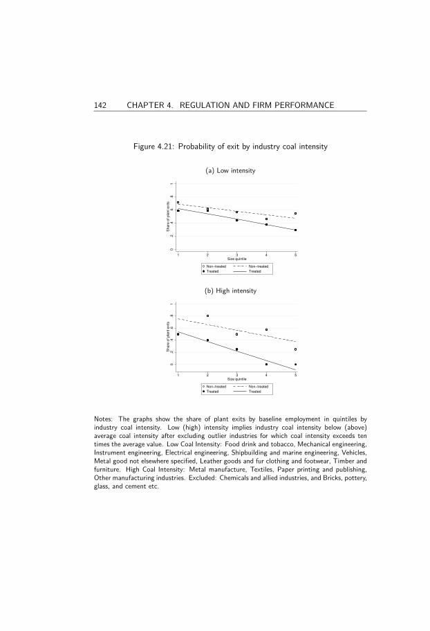
142 CHAPTER 4. REGULATION AND FIRM PERFORMANCE
Figure 4.21: Probability of exit by industry coal intensity
(a) Low intensity0
.2.4
.6.8
1S
ha
re o
f p
lan
t e
xits
1 2 3 4 5Size quintile
Non−treated Non−treated
Treated Treated
(b) High intensity
0.2
.4.6
.81
Sh
are
of
pla
nt
exits
1 2 3 4 5Size quintile
Non−treated Non−treated
Treated Treated
Notes: The graphs show the share of plant exits by baseline employment in quintiles byindustry coal intensity. Low (high) intensity implies industry coal intensity below (above)average coal intensity after excluding outlier industries for which coal intensity exceeds tentimes the average value. Low Coal Intensity: Food drink and tobacco, Mechanical engineering,Instrument engineering, Electrical engineering, Shipbuilding and marine engineering, Vehicles,Metal good not elsewhere specified, Leather goods and fur clothing and footwear, Timber andfurniture. High Coal Intensity: Metal manufacture, Textiles, Paper printing and publishing,Other manufacturing industries. Excluded: Chemicals and allied industries, and Bricks, pottery,glass, and cement etc.

. FIGURES AND TABLES 143
Table4.11:T
heeff
ects
ofSC
Aon
firm
exits
Com
p.log-log
OLS
(1)
(2)
(3)
(4)
(5)
(6)
(7)
SCA
-0.154∗∗
-0.147∗∗
-0.145∗∗
-0.153∗∗
-0.157∗∗
-0.157∗∗
-0.161∗∗
(0.069)
(0.061)
(0.063)
(0.066)
(0.066)
(0.068)
(0.067)
Ln(M
anuale
mp.’59)
-0.0180∗∗∗
-0.0180∗∗∗
(0.005)
(0.005)
Coal
intensity
-0.0185
0.0150
0.0154
(0.020)
(0.021)
(0.021)
No.O
bs.
636
877
877
877
877
877
877
No.C
ells
3939
3939
3939
39R2(a
dj)
0.218
0.216
0.219
0.225
0.218
0.225
CellFE
XX
XX
XX
Year
FEX
XX
XX
XSIC-FE
XIndu
stryFE
XX
XX
Meanexitrate
.19
Notes:Th
edepend
entv
ariableisabinary
varia
bleindicatin
gtheplant’s
operationalstatusb
yyear,w
here
1im
plies
exit.
Column(1)
show
stheaveragemarginale
ffect
ofSC
Ausingadiscrete-tim
eprop
ortio
nalh
azardmod
el(I
exclu
de1959
from
thesampledu
eto
nofirm
exitthat
year).
Columns
(2)-(
7)aretheresults
obtained
usinglinearp
robabilitymod
els.Th
estandard
errors
areclu
stered
atthegrid-cell
level.
Coal
intensity
isthestandardize
dcoal
intensity
byindu
stry
andyear.SC
Aistheshareof
grid
cells
coveredby
SCAregu
latio
n.

144 CHAPTER 4. REGULATION AND FIRM PERFORMANCE
Table 4.12: The dynamic effects of SCA on firm exits
(1) (2) (3) (4) (5)SCA -0.167∗∗
(0.067)Coal intensity ’59 -0.0478 -0.0681 -0.00556
(0.129) (0.163) (0.136)SCA × Coal intensity ’59 -0.0850 -0.0915∗ -0.0753
(0.053) (0.054) (0.054)Manual emp.’59 (q1) × SCA -0.124 -0.141
(0.213) (0.215)Manual emp.’59 (q2) × SCA 0.174 0.164
(0.213) (0.199)Manual emp.’59 (q3) × SCA -0.301∗∗∗ -0.332∗∗∗
(0.091) (0.098)Manual emp.’59 (q4) × SCA -0.250∗∗ -0.244∗∗
(0.116) (0.104)Manual emp.’59 (q5) × SCA -0.179∗ -0.198∗∗
(0.090) (0.088)Manual emp.’59 (q1 Cell) × SCA -0.0682 -0.0862
(0.109) (0.112)Manual emp.’59 (q2 Cell) × SCA -0.129 -0.128
(0.177) (0.172)Manual emp.’59 (q3 Cell) × SCA -0.367∗∗ -0.352∗∗
(0.140) (0.143)Manual emp.’59 (q4 Cell) × SCA -0.154∗ -0.184∗
(0.087) (0.094)Manual emp.’59 (q5 Cell) × SCA -0.568∗∗ -0.586∗∗
(0.217) (0.225)No. Obs. 877 877 877 877 877No. Cells 39 39 39 39 39R2(adj) 0.220 0.227 0.224 0.228 0.224Cell-FE X X X X XYear FE X X X X XIndustry FE X X X X X
Notes: The outcome variable is a dummy variable indicating the operational status of eachplant by year. SCA is the share of grid cell covered by SCA regulation. Manual employment incolumn (3) is the quintiles of manual employment in 1959, while the quintiles in column (4)are defined within each grid cell. Standard errors are clustered at the grid-cell level.

. FIGURES AND TABLES 145
Table 4.13: The effects of SCA on location decision of new manufacturing plants
(1)All
(2)Low Intensity
(3)High Intensity
SCA 3.415∗∗ 36.39∗∗ 2.735∗∗(2.30) (2.38) (2.21)
No. Obs. 171 87 84No. Cells 57 29 28Cell FE X X XYear FE X X XExponentiated coefficients; t statistics in parentheses∗ p < 0.10, ∗∗ p < 0.05, ∗∗∗ p < 0.01
Notes: The dependent variable is the total number of new plants by grid cell for 1966, 1972,and 1975. The coefficients are the exponentiated Poisson regression estimates. Low (high)intensity refers to below (above) median coal intensity at the grid-cell level. Standard errorsare the Wooldridge (1991) robust errors.
Table 4.14: The effects of SCA on local manual employment in new manufac-turing plants
(1)All
(2)Low Intensity
(3)High Intensity
SCA 0.868 2.379∗∗∗ -1.137∗∗∗(0.771) (0.699) (0.404)
No. Obs. 88 45 43No. Cells 54 26 28Cell FE X X XYear FE X X XStandard errors in parentheses∗ p < 0.10, ∗∗ p < 0.05, ∗∗∗ p < 0.01
Notes: The outcome variable is the log of employment where the sample is restricted to plantentries in 1972 and 1975 and estimated using OLS. Standard errors are clustered at the gridcell level. Low (high) intensity refers to below (above) median coal intensity at the grid-celllevel.

146 CHAPTER 4. REGULATION AND FIRM PERFORMANCE
Table 4.15: The effects of SCA on manual employment in surviving firms
(1)All
(2)Below x̃
(3)Above x̃
SCA -0.334∗∗ -0.454 0.666(0.153) (0.403) (0.651)
Coal intensity -0.130 -0.0762 -0.0884(0.295) (0.615) (0.186)
SCA × Coal intensity -0.785∗ -0.994 1.051(0.460) (0.678) (2.000)
No. Obs. 412 216 196No. Cells 29 20 25R2(adj) 0.888 0.607 0.853Cell FE X X XYear FE X X XIndustry FE X X X
Notes: The outcome variable is the log of plant employment in 1959, 1966, 1972, and 1975.Coal intensity is the national 1-digit industry level coal intensity. The sample includes plantsactive between 1959 - 1975. Column (2) consists of plants with below-median employmentin 1959 and (3) with above-median 1959 employment after excluding the outlying industriesChemicals and allied industries, and Bricks, pottery, glass, and cement. All regressions controlfor employment in 1959. Standard errors are clustered at the grid cell level.
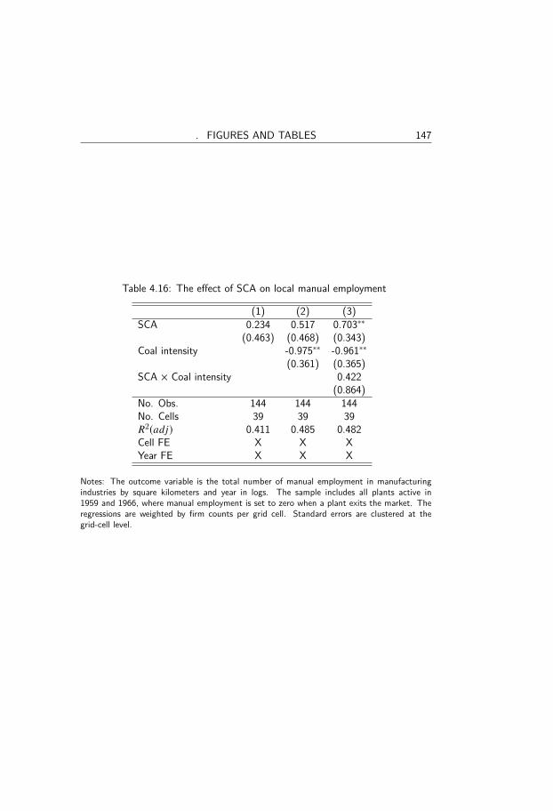
. FIGURES AND TABLES 147
Table 4.16: The effect of SCA on local manual employment
(1) (2) (3)SCA 0.234 0.517 0.703∗∗
(0.463) (0.468) (0.343)Coal intensity -0.975∗∗ -0.961∗∗
(0.361) (0.365)SCA × Coal intensity 0.422
(0.864)No. Obs. 144 144 144No. Cells 39 39 39R2(adj) 0.411 0.485 0.482Cell FE X X XYear FE X X X
Notes: The outcome variable is the total number of manual employment in manufacturingindustries by square kilometers and year in logs. The sample includes all plants active in1959 and 1966, where manual employment is set to zero when a plant exits the market. Theregressions are weighted by firm counts per grid cell. Standard errors are clustered at thegrid-cell level.
148 CHAPTER 4. REGULATION AND FIRM PERFORMANCE
A4 Appendix
A4.1 The Clean Air Act and Smoke Control Areas
There are several distinctions between the nationwide dark smoke ban on indus-tries and the local SCA regulations. First, the dark smoke provision covered thewhole of the UK, while the implementation of SCA varied by local authority, timeand size. Second, the ban on dark smoke targeted the emission of dark smokeonly, while SCAs prohibited smoke of any color. Third, the complete banningof smoke made that violation of the smoke control order easy to detect and didnot require any specific equipment or knowledge. In contrast, dark smoke wasmeasured against a Ringelmann Chart and required special knowledge.34 Fourth,the dark smoke provision set many discretionary start days due to the possibilityof businesses to seek exemption period while the a start date of SCA appliedto all affected inside the zone.35 Finally, the maximum fine for breaching thedark smoke emission was 100 pounds per offence while an offense of the localregulation brought a maximum fine of 10 pounds.
A4.2 Optimal coal input and productivityFirm profit function from (4.7) is:
Π = a1−ε (rγθ)1−εB−ε − fo
34The Ringelmann chart had 5 scales, with shade 5 being black and shade 2 to 4 considereddark.
35Although local authorities could grant exemptions to specific buildings within an SCA,the practice of exempting industries from the order seems rare. One reason is that the purposeof SCA was to prohibit smoke emission not only from households but also from industries suchthat exempting the latter from the provision would be counterproductive to the very nature ofthe regulation.

. A4 APPENDIX 149
Taking the derivative w.r.t. productivity yields,
dΠda1−ε
=1
Bε
[rγ(1 − γ)(γ−1)
γγ
]1−ε
Then take the derivative w.r.t coal factor share γ such that,
d(.)dγ
=1
Bεd
dγ
[rγ(1 − γ)(γ−1)
γγ
]1−ε=
1
Bε(1 − ε)
[rγ(1 − γ)(γ−1)
γγ
]−ε︸ ︷︷ ︸
D
ddγ
[rγ(1 − γ)(γ−1)
γγ
]
= Dddγ
[rγ(1 − γ)γ−1
]γγ − rγ(1 − γ)γ−1 d
dγ γγ
γ2γ
=Dγ2γ
{[(1 − γ)γ−1
ddγ
rγ + rγd
dγ(1 − γ)γ−1
]γγ − rγ(1 − γ)γ−1γγ
ddγ
γlnγ}
=Dγγ
{[(1 − γ)γ−1rγlnr + rγ(1 − γ)γ−1
ddγ(γ − 1)ln(1 − γ)
]− r2(1 − γ)γ−1
[lnγ
ddγ
γ + γd
dγlnγ
]}=
Dγγ
{[(1 − γ)γ−1rγlnr + rγ(1 − γ)γ−1
[ln(1 − γ)
ddγ(γ − 1) + (γ − 1)
ddγ
ln(1 − γ)] ]
− rγ(1 − γ)γ−1 [lnγ + 1]}
=Dγγ
{[(1 − γ)γ−1rγlnr + rγ(1 − γ)γ−1 [ln(1 − γ) + 1]
]− rγ(1 − γ)γ−1 [lnγ + 1]
}=
Dγγ
{rγ(1 − γ)γ−1(lnr + ln(1 − γ) + 1) − rγ(1 − γ)γ−1 [lnγ + 1]
}=
Dγγ
[rγ(1 − γ)γ−1(lnr + ln(1 − γ) − lnγ)
]= (1 − ε)B−ε
rγ(1 − γ)γ−1(lnr + ln(1 − γ) − lnγ)
γγ[rγ (1−γ)(γ−1)
γγ
]ε

150 CHAPTER 4. REGULATION AND FIRM PERFORMANCE
A4.3 Smoke control order

Essays on the Economics of the1956 Clean Air Act Nanna Fukushima
Nanna Fukushim
a Essays on th
e Econom
ics of the 1956 C
lean A
ir Act
Dissertations in Economics 2021:1
Doctoral Thesis in Economics at Stockholm University, Sweden 2021
Department of Economics
ISBN 978-91-7911-558-6ISSN 1404-3491
Nanna Fukushimaholds a B.Sc. and an M.Sc. inEconomics from StockholmUniversity. Her research interests ineconomics include environmentaleconomics and health economics.
This thesis consists of three essays in environmental and healtheconomics. The UK Clean Air Act, Black Smoke, and Infant Mortality examinesthe impact of banning coal on air quality and infant mortality andestimates the effect of smoke pollution on post-war infant mortality. A Fine Solution to Air Pollution? explores the effects of regulation onair pollution in urban areas in England when the monetary punishmentif convicted is doubled. Environmental Regulation and Firm Performance investigates theeffect of environmental regulation in England in the 1960s–70s onchanges in employment and the entry and exit of manufacturing plants.