Essays in behavioural economics
101
HAL Id: tel-01178035 https://tel.archives-ouvertes.fr/tel-01178035 Submitted on 17 Jul 2015 HAL is a multi-disciplinary open access archive for the deposit and dissemination of sci- entific research documents, whether they are pub- lished or not. The documents may come from teaching and research institutions in France or abroad, or from public or private research centers. L’archive ouverte pluridisciplinaire HAL, est destinée au dépôt et à la diffusion de documents scientifiques de niveau recherche, publiés ou non, émanant des établissements d’enseignement et de recherche français ou étrangers, des laboratoires publics ou privés. Essays in behavioural economics Hana Cosic To cite this version: Hana Cosic. Essays in behavioural economics. Economics and Finance. Université de Strasbourg, 2014. English. NNT : 2014STRAB023. tel-01178035
-
Upload
khangminh22 -
Category
Documents
-
view
1 -
download
0
Transcript of Essays in behavioural economics

HAL Id: tel-01178035https://tel.archives-ouvertes.fr/tel-01178035
Submitted on 17 Jul 2015
HAL is a multi-disciplinary open accessarchive for the deposit and dissemination of sci-entific research documents, whether they are pub-lished or not. The documents may come fromteaching and research institutions in France orabroad, or from public or private research centers.
L’archive ouverte pluridisciplinaire HAL, estdestinée au dépôt et à la diffusion de documentsscientifiques de niveau recherche, publiés ou non,émanant des établissements d’enseignement et derecherche français ou étrangers, des laboratoirespublics ou privés.
Essays in behavioural economicsHana Cosic
To cite this version:Hana Cosic. Essays in behavioural economics. Economics and Finance. Université de Strasbourg,2014. English. �NNT : 2014STRAB023�. �tel-01178035�
UNIVERSITÉ DE STRASBOURG
ÉCOLE DOCTORALE Augustin Cournot
[ UMR 7522 ]
THÈSE présentée par :
[ Hana COSIC ]soutenue le : 15 Décembre 2014
pour obtenir le grade de : Docteur de l université de Strasbourg
Discipline/ Spécialité : Behavioural Economics
TITRE de la thèse[Essays in Behavioural Economics]
THÈSE dirigée par :LLERENA Patrick Professor of Economics, Université de StrasbourgNUVOLARI Alessandro Professor of Economics, Scuola Superiore Sant Anna
RAPPORTEURS :DOSI Giovanni Professor of Economics, Scuola Superiore Sant AnnaMARENGO Luigi Professor of Economics, LUISS Univeristy
AUTRES MEMBRES DU JURY :ATTANASI Giuseppe Professor of Economics, Université de StrasbourgPLONER Matteo Professor of Economics, University of TrentoMURADOGLU Gulnur Professor of Finance, Queen Mary University of LondonMONETA Alessio Professor of Economics, Scuola Superiore Sant Anna

Scuola Superiore Sant Anna, Pisa University of Strasbourg
PHD THESIS
Essays in Behavioural Economics
Supervisors: PhD candidate:Prof. Alessandro Nuvolari Hana CosicProf. Patrick Llerena
Pisa, November 2014.

©2014, Hana Cosic.All rights reserved.
Printed in Pisa, Italy.Sant Anna School of Advanced Studies, Institute of Economics-LEM.Piazza Martiri della Liberta 33, 56127Pisa, Italy.

Acknowledgements
I have spent the last three years in Pisa, Strasbourg and London learning about science. This
thesis draws on many different sources of inspiration. On this journey, I want to thank my
advisors Luigi Marengo, Gulnur Muradoglu, Patrik Llerena and Alessandro Nuvolari for
guiding me into this world.
Working so closely with people is one of the best experiences of doing science. I had the
pleasure to work on different chapters of my thesis with Giuseppe Attanasi, Francesco
Passarelli, Giulia Urso, Sebastian Ille and Ajla Cosic.
I owe my deepest gratitude to my parents and sister, who made my PhD journey much easier.
When it was the hardest, they have been there for me. Lastly, I offer my regards and
blessings to all of those who supported me in any respect during the completion of this PhD
thesis, especially my colleagues. And as Ernest Hemingway would say: It is good to have an
end to journey toward; but it is the journey that matters, in the end.

Table of Contents
1 Introduction ...........................................................................................................................1
1.1 Behavioural economics and cultural event management ............................................................ 2
1.2 Nudges and policy making ............................................................................................................ 2
1.3 Behavioural approach to property decisions making ................................................................... 3
References .......................................................................................................................................... 5
2 Private Ownership of a Cultural Event: Do Attendees Perceive it as a Risky Lottery? 7
2.1 Introduction .................................................................................................................................. 9
2.2 La Notte della Taranta Festival: objective, structure, and ownership ................................... 11
2.3 Research methodology .............................................................................................................. 13
2.4 Results......................................................................................................................................... 16
2.4.1 Determinants of willingness to accept private ownership ............................................... 16
2.4.2 Disentangling different social benefits of private ownership ......................................... 19
2.4.3 Disentangling different economic dimensions of private ownership ............................. 20
2.5 Conclusions ............................................................................................................................... 21
References ....................................................................................................................................... 23
3 Nudges Can Affect Students Green Behaviour? A Field Experiment.........................26
3.1 Introduction ................................................................................................................................ 29
3.2 Literature review ........................................................................................................................ 30
3.3 Model ......................................................................................................................................... 31
3.4 Methods ...................................................................................................................................... 34
3.5 Results......................................................................................................................................... 37
3.6 Discussion and conclusion........................................................................................................... 40
3.7 Policy implications....................................................................................................................... 41
References ........................................................................................................................................ 42
Appendix ........................................................................................................................................... 43
4 Expectation Formation in Property Markets .........................................................................45
4.1 Introduction ................................................................................................................................ 46
4.2 Literature review ........................................................................................................................ 47
4.2.1 Theory of expectations .................................................................................................... 47

4.2.2 Anchoring bias ................................................................................................................. 49
4.2.3 Optimism bias .................................................................................................................. 51
4.2.4 Short term versus long term ............................................................................................ 53
4.2.5 Commercial versus residential ......................................................................................... 54
4.3 Methodology............................................................................................................................... 54
4.3.1 Experimental design ......................................................................................................... 54
4.3.2 Measures .......................................................................................................................... 57
4.4 Results......................................................................................................................................... 59
4.4.1 Residential property market expectations ........................................................................ 60
4.4.2 Commercial property market expectations ...................................................................... 63
4.4.3 Comparison of residential and commercial property market expectations ..................... 67
4.4.4 Forecast errors in residential and commercial property markets .................................... 68
4.5 Discussion.................................................................................................................................... 71
4.6 Conclusion................................................................................................................................... 74
Appendix data ................................................................................................................................... 75
References ........................................................................................................................................ 82

List of Tables and Figures
Tables
2.1 Costs of the Festival (in ) in 2007-2009, classified according to nature and sub-events...................................................................................................................................................12
2.2 Funding Sources of La Notte della Taranta Festival ....................................................12
2.3 Population, sample and its representativeness .................................................................14
2.4 Probit Regression, Willingness to Accept Private Ownership (WTAPO) ..........................17
4.1 Expected property price changes and perceived skewness: price forecasts of residentialproperties .................................................................................................................................75
4.2 Expected property price changes and perceived skewness: price forecasts of commercialproperties .................................................................................................................................77
4.3 Expected property price changes and perceived skewness: price forecasts of residentialand commercial properties.......................................................................................................79
4.4 Expected property price changes and perceived skewness: price forecasts and forecasterrors of residential properties ...............................................................................................80
4.5 Expected property price changes and perceived skewness: price forecasts and forecasterrors of commercial properties ..............................................................................................81
Figures
2.1 Attendees with no WTAO, who would change their mind under specific states of theworld .......................................................................................................................................19
2.2 Preferred combination of (Public/Private) Management and (Public/Private) Financing 21
3.1 Dynamics of the control group .......................................................................................33
3.2 Dynamics of treatment 1...................................................................................................34
3.3 Dynamics of treatment 2...................................................................................................34
3.4 Treatment 1 .......................................................................................................................36
3.5 Treatment 2 .......................................................................................................................36
3.6 Survey results....................................................................................................................38
3.7 Percentage of recycled cups over the experimental period...............................................39
3.8 Average of percentage of recycled cups ...........................................................................40

Résumé de la thèse en économie comportementale
Pourquoi prend-on ou non des risques ? Pourquoi ne recycle-t-on pas davantage ? En
situation d incertitude, quels prix immobiliers peut-on anticiper ? Pour d éventuelles
explications et pronostics concernant ces questions, les principes d économie
comportementale peuvent être invoqués.
L économie comportementale (CE) est l association de la psychologie et de l économie ayant
pour but de donner une explication aux comportements observés sur les marchés,
comportements humains faisant preuve de rationalité limitée et de raisonnements complexes
(Mullainathan et Thaler, 2000).
L étude de l économie comportementale a inspiré un grand nombre de théories différentes et
a été utilisée dans de nombreuses applications empiriques et cette thèse suit le même schéma
en explorant différentes applications de l économie comportementale. Cette thèse développe
trois nouvelles extensions de l économie comportementale aux champs du management, du
choix en termes de politiques et en termes de décision d investissement immobilier.
1.1 L économie comportementale et le management des évènements
culturels
Au cours des 20 dernières années, les dépenses publiques pour la culture ont été soumises
à un examen encore plus minutieux en raison des contraintes budgétaires croissantes.
L arbitrage entreparticipation publique ou privée aux évènements culturels est encore le sujet
de débats houleux, au c ur de la politique culturelle. Un argument fréquemment utilisé
contre le soutien privé des arts et de la culture estime que cela revient à rendre ce secteur
davantage commercial, en altérant sa valeur, initialement sociale et culturelle, en quelque
chose de simplement bon à la vente (voir Coalter, 1998). Un contre-argument stipule que le
secteur privé permet de bien mieux cibler les besoins des consommateurs en fournissant des
produits de haute qualité, que les consommateurs sont prêts à payer (Andersson et Getz,
2009). Les instruments de l économie comportementale consistant à révéler l aversion au
risque ou la volonté de payer peuvent permettre de résoudre nombre de problèmes posés par
le management des évènements culturels.
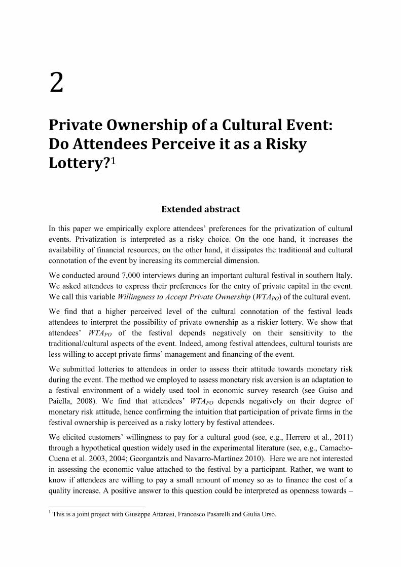
Le chapitre 2 analyse chez les participants leur perception du risque de la participation
privée à un évènement culturel. Nous débutons par le fait que les personnes perçoivent les
avantages (citons la meilleure qualité) et les inconvénients (le manque de véritable identité)de
la privatisation des évènements culturels comme les bénéfices et pertes potentiels d une
loterie. Nous avons mené près de 7000 entretiens lors d un festival culturel majeur dans le
sud de l Italie. Nous avons demandé aux participants d exprimer leurs préférences concernant

l introduction de capitaux privés pour l organisation de l évènement. Nous appelons cette
variable « Willingness to Accept Private Ownership » (WTAPO), littéralement, « la volonté
d accepter la participation privée » pour l évènement culturel. Les loteries ont été soumises
aux participants pour établir leur attitude face à leur aversion monétaire du risque lors de
l évènement. Nous trouvons que les variables WTAPO des participants dépendent
négativement de leur niveau d attitude face au risque monétaire, ce qui confirme donc
l intuition selon laquelle la participation de firmes privées au déroulement du festival est
perçue comme une loterie risquée par les personnes prenant part au festival.
Nous révélons la volonté des clients pour payer un bien culturel (voir Herrero et al., 2011)
à travers une question hypothétique largement répandue dans la littérature expérimentale
(voir par exemple Georgantzis et Navarro-Martinez, 2010). En effet, nous avons constaté que
plus la personne est prête à payer pour une amélioration en termes de qualité pour le bien
culturel, le plus elle sera encline à accepter une participation privée au festival. Ceci s oppose
à un effet de substitution du type « si je paie pour un bien public (par exemple un évènement
culturel), je ne veux pas que les entreprises privées le gèrent et/ou investissent dans ce bien
public ».
Nos résultats fournissent un bon aperçu des préférences établies des consommateurs
concernant les problèmes de management. Bien qu augmentant la qualité du festival,
l implication des entreprises privées lors du financement et du déroulement peut avoir l effet
inverse concernant les attentes des personnes s ils perçoivent le risque d une perte
potentiellement élevée des caractéristiques culturelles initiales du festival.
1.2 Incitations non monétaires (« nudges ») et la décision en termes
de politiques
Comprendre les raisons expliquant le comportement des personnes est essentiel pour
l élaboration des politiques. Les personnes ont souvent un comportement de court-terme
lorsqu il s agit de la protection de l environnement puisqu ils sous-estiment les bénéfices
futurs des bonnes habitudes d aujourd hui. Une littérature en expansion sur l économie
comportementale et la psychologie suggère l utilisation des interventions non monétaires, les
« nudges » dans la littérature anglo-saxonne. Cette incitation non monétaire est une main
tendue qui a pour but de pousser quelqu un à prendre de meilleures décisions à la fois pour
lui-même/elle-même mais également pour l intérêt public (Thaler et Sunstein, 2008). Inciter
de la sorte repose fortement sur la littérature de l économie comportementale et estime qu en
changeant la structure de leurs choix, les gens peuvent être légèrement incités de façon non
monétaire. Le fait de prendre en compte les biais lors de la définition de la politique peut être
plus efficace.
Le chapitre 3 étudie si les incitations non monétaires peuvent être efficaces pour
promouvoir le comportement écologique et le recyclage pour les nouvelles générations. Ce

chapitre étudie également si les différents types d incitations ou leurs combinaisons sont de
meilleurs instruments pour un tel comportement. L étude a été réalisée sur des données
obtenues sur la base de sondages et d expériences sur le terrain réalisés sur des étudiants à
Pise, une des plus grandes villes universitaires italiennes. Le sondage a été mené lors des
mois de mai et juin 2013. L expérience de terrain a été faite sur un laps de temps de 60 jours
(d octobre à décembre 2013). Nous avons rassemblé des données sur 1849 cas de recyclages
de verres en plastique, verres provenant d une machine à café à l école d études avancées
Sant Anna à Pise. Les utilisateurs n étaient pas au courant de leur participation à l étude. Le
comportement de recyclage a été mesuré par le nombre de verres en plastiques jetés à la
poubelle, nombre observé en fin de journée. L analyse des données du sondage a révélé que
la plupart des participants suivraient des interventions indirectes non-monétaires. Les
résultats des traitements expérimentaux montrent des augmentations significatives pour le
nombre de verres en plastique recyclés.
Par ailleurs, le papier introduit un modèle théorique de jeu simple prenant en compte les
décisions individuelles par rapport aux variables développées ci-dessus. Ce modèle peut
répliquer les résultats observés et illustre l effet d un change de perception (la prise de
conscience) chez les individus, un changement dans les normes sociales, aussi bien qu un
changement pour les incitations non monétaires. Notre principale contribution est que les
« nudges » peuvent être utilisés pour induire un comportement respectueux de
l environnement chez les jeunes consommateurs et de ce fait, un effet de long-terme.
1.3 L approche comportementale pour la prise de décision depropriété
De façon globalisée, lors des décennies récentes, on a constaté un engouement prononcé
pour les marchés de l immobilier. Acheter une maison est probablement un des plus grands
investissements réalisés par un individu. Cependant, il semble que les aspects psychologiques
et sociologiques de la prise de décision d accès à la propriété sont souvent négligés. Alors
que les marchés de l immobilier sont plutôt très peu liquides (voire pas du tout), les marchés
de l immobilier sont supposés être efficaces et leurs participants se comporter de façon
rationnelle. A la fin des années 1980, les études concluent que les marchés de l immobilier
sont inefficaces (par exemple, Case et Schiller, 1989). De plus, les recherches développées
par Case et Schiller (1990) stipulent que les changements de prix observés en un an se
répercutent l année suivante.
La recherche sur les marchés de l immobilier devrait aller au-delà des échanges
monétaires et commencer à donner davantage d importance pour le côté psychologique des
parties prenantes aux marchés immobiliers. Ce qui se passe sur ces marchés dépend des
attitudes des personnes, ainsi que leurs croyances et comportements.

Le chapitre 4 étudie les anticipations en termes de prix immobiliers en Grande-Bretagne en
menant une expérience sur Internet. Nous mettons en évidence la formation des prix de
l immobilier et les explications majeurs des comportementsdes agents, notamment
l optimisme ou l effet d ancrage. Ce papier contribue à la littérature des marchés immobiliers
en tant qu un des premiers qui explore les formations des anticipations des prix immobiliers
en utilisant une expérience pour les deux types de propriétés, résidentielles et commerciales.
De plus, l utilisation de prévisions permet d étudier les différences existantes entre les
anticipations en termes de prix à court-terme, moyen-terme et long-terme. Les résultats des
anticipations des prix de l immobilier à la fois sur les marchés résidentiels et commerciaux
montrent que les participants anticipent une tendance se poursuivant sur les marchés
haussiers, une augmentation des prix sur les marchés instables et une inversion des prix sur
un marché baissier, quel que soit l horizon prévisionnel. Les participants au sondage sont
bien plus optimistes concernant les changements de prix de l immobilier à long-terme, ce fait
est valable, peu importe les tendances du marché et les types de propriété (résidentielle ou
commerciale). L analyse des anticipations rationnelles montre que les participants ont eu ce
type d anticipations à court-terme sur les marchés haussiers pour le résidentiel et le
commercial. Des résultats semblables pour les anticipations de court-terme sont développés
dans Case, Shiller et Thompson (2012). Par ailleurs, sur les marchés haussiers de moyen et
long-terme et pour n importe quel horizon prévisionnel sur les marchés (commerciaux et
résidentiels) instables et à la baisse, les participants n ont pas formé d anticipations
rationnelles. La principale contribution de cette étude confirme l affirmation répandue dans la
littérature selon laquelle, soit les investisseurs extrapolent les prix passés de l immobilier, soit
dans la littérature économique standard que les anticipations sont rationnelles uniquement
pour un type d horizon prévisionnel, un type de tendance de marché et un type de propriétés.

Bibliographie
Andersson, T.D. & Getz, D. (2009). Tourism as a mixed industry: Differences between private,public and not-for-profit festivals, Tourism Management, 30, 847-856.
Camerer, C. F., Loewenstein, G., & Rabin, M. (Eds.). (2011). Advances in behavioral
economics. Princeton University Press.
Case, K.E., & Shiller, R.J. (1989). The Efficiency of the Market for Single-Family Homes. The
American Economic Review, 79(1), 125-137.
Case, K. E., & Shiller, R. J. (1990). Forecasting prices and excess returns in the housingmarket. Real Estate Economics, 18(3), 253-273.
Case, K. E., Shiller, R. J., & Thompson, A. (2012). What have they been thinking? Home buyer
behavior in hot and cold markets (No. w18400). National Bureau of Economic Research.
Coalter, F. (1998). Leisure studies, leisure policy and social citizenship: the failure of welfareor the limits of welfare?, Leisure Studies, 17, 21-36.
Georgantzís, N. and D. Navarro-Martínez (2010). Understanding the WTA-WTP gap:Attitudes, feelings, uncertainty and personality, Journal of Economic Psychology, 31, 895-907.
Herrero, L.C., Sanz, J.A., Bedate, A. & Del Barrio, M.J. (2011). Who Pays More for a CulturalFestival, Tourists or Locals? A Certainty Analysis of a Contingent Valuation Application,International Journal of Tourism Research, 14, 495-512.
Mullainathan, S., & Thaler, R. H. (2000). Behavioral economics (No. w7948). National Bureauof Economic Research.
Thaler, R. H., & Sunstein, C. R. (2008). Nudge: Improving decisions about health, wealth, and
happiness. Yale University Press.

1
Introduction
Why do we take risks or we do not? Why do not we recycle more? Under uncertainty what do
we expect will happen to our home prices? These and many other questions are asked on
daily basis. For possible explanations and answers to these and similar questions principles of
behavioural economics can be used. Behavioural economics (BE) is the combination of
psychology and economics that investigates what happens in markets in which some of
agents display human limitations and complications (Mullainathan and Thaler, 2000).
Behavioural economics provides more realistic psychological foundations to increase
explanatory and predictive power of economic theory.
30 years ago behavioural economics did not exist as a field. Today it is a well established
field at the top departments of economics of the world and also used by governments in
policy making.
Most of the ideas in behavioural economics are not new, in fact they return to roots of
neoclassical economics. In the historical context Adam Smith s a less known book, The
Theory of Moral Sentiments is bursting with insights about human psychology and it laid out
psychological principles of individual behaviour.
Later the writings of economists Irving Fisher and Vilfredo Pareto included speculations
about how people think and feel about economic choices. Also Maynard Keynes appealed
frequently to psychological insights. In the second half of the 20th century, Herbert Simon in
his works suggested the importance of psychological measures and bounds of rationality.
However it was really at the end of the 1970s when two psychologists Daniel Kahneman and
Amos Tversky with its works on decision making under risk and heuristics introduced several
new and fundamental concepts relating to reference points, loss aversion, subjective
probability measurement and utility measurement.
In simple words behavioural economists argue that human decision making is influenced by
forces that are familiar to psychologists and other social scientists but in general ignored by
the economists.
According to Camerer, Lowenstein and Rabin (2011), behavioural economics typically
classifies research into two categories: judgment and choice. Judgment research investigates
the processes people use to estimate probabilities, while choice investigates the processes
people use to when selecting among actions and taking account of any relevant judgments
that they have made.
The study of behavioural economics has inspired a number of different theories and has been
used in many applications, and this thesis follows the same path and investigates different
applications of behavioural economics. This thesis explores three novel applications of

2 Introduction
behavioural economics to management, policy making and property investment decision
making.
1.1 Behavioural economics and cultural event management
During the course of the past two decades, public spending for culture has come under
sharper scrutiny due to increased budgetary constraints. The right balance between public and
private ownership of cultural events is at the heart of cultural policy, and is still the subject of
a lively debate. One frequently-heard argument against private-sector provision of arts and
culture is that it results in commodification , turning something of intrinsic social and
cultural value into a mere product for sale (see Coalter, 1998). A counterargument is that the
private sector is often better at meeting consumers needs by delivering high-quality products
that consumers are willing to pay for (Andersson and Getz, 2009). Tools from behavioural
economics such as eliciting risk aversion or willingness to pay can shed light on the issues of
management of cultural events.
Chapter 2 analyzes participants perception of the risk of private ownership of a cultural
event. Our starting point is that people perceive the pros (e.g., higher quality) and cons (e.g.,
lack of genuine identity) of privatization of cultural events like potential benefits and losses
of a lottery. We conducted around 7,000 interviews during an important cultural festival in
southern Italy. We asked attendees to express their preferences for the entry of private capital
in the event. We call this variable Willingness to Accept Private Ownership (WTAPO) of the
cultural event. Lotteries were submitted to attendees to assess their attitude towards monetary
risk aversion during the event. We find that attendees WTAPO depends negatively on their
degree of monetary risk attitude, hence confirming the intuition that participation of private
firms in the festival ownership is perceived as a risky lottery by festival attendees.
We elicited customers willingness to pay for a cultural good (see, e.g., Herrero et al., 2011)
through a hypothetical question widely used in the experimental literature (see, e.g.,
Georgantzís and Navarro-Martínez 2010). Indeed, we found that the more you are willing to
pay for a quality improvement of the cultural good, the more you are willing to accept
festival private ownership. This opposes a substitution effect of a kind that if I pay for a
public good (e.g., a cultural event), I do not want private firms to manage and/or invest in it .
Our findings provide insights into consumers stated preferences on management issues.
Private firms involvement in a festival management and financing, though increasing its
quality, could have the reverse effect in terms of people s attendance if they perceive the risk
of a potential loss of its more genuine cultural characteristics as (being) high.
1.2 Nudges and policy making
Understanding the reasons for people s behaviour is vital for policy making. People often
behave short-sighted when it comes to environment protection as they tend to
underestimate the future benefits of today s good habit. A growing literature on behavioural
economics and psychology suggests the use of non-price interventions nudges . A nudge is a

Introduction 3
helping hand that will lead someone to make better decisions, both for himself/herself and
for the public interest as well (Thaler and Sunstein, 2008). Nudging heavily relies on
behavioural economics literature and argues that by changing choice architecture, people can
be gently nudged . Taking biases into account when designing policy may be more effective.
Chapter 3 studies whether nudges are efficient in promoting ecological behaviour and
recycling of young people, and whether different types of nudges or their combination serve
as better instruments for inducing this. The study was performed on primary data, from both a
survey and field experiment conducted among university students in Pisa, one of the most
important university cities in Italy. The survey was conducted during May and June 2013.
The field experiment was conducted over a 60-day span (from October to December 2013).
We collected data on 1849 instances of plastic cup recycling at a coffee vending machine at
the School of Advanced Studies Sant Anna in Pisa. The users were not aware that they were
participants in the study. Recycling behaviour was measured by number of plastic cups
disposed in the dustbin, observed at the end of a day. Analysis of the survey data revealed
that most of participants would follow indirect non-price interventions. Results of
experimental treatments show significant increases in the number of recycled plastic cups.
The paper further includes a simple game theoretical model that takes account of the
individuals decisions with respect to the variables elaborated above. This model is able to
replicate the results and illustrates the effect of a perceptional change (awareness raising) of
individuals, a shift in the social norm, as well as a switch in the nudges. Our main
contributions are that nudges can be used for inducing green behaviour of young consumers
and thereby generate a long lasting effect.
1.3 Behavioural approach to property decision making
All over the world over the recent decades there is a strong infatuation towards property
markets. Buying a house is probably one of the biggest investments an individual will make.
However it seems that psychological and sociological aspects in property decision making are
often neglected. Though property markets are rather illiquid, property markets are assumed to
be efficient and that participants behave rationally. By the end of the 1980s, studies
concluded that property markets are inefficient (e.g., Case and Schiller 1989). Moreover
extended research by Case and Schiller (1990) asserts that price changes observed in one year
succeed in the following year. Furthermore recent evidence on non-financial motives and
behavioural biases in property decision making suggests that research in property markets
should go beyond cash flows and start providing space for the psychological side of
stakeholders in property markets. What happens in the property markets depends on people s
attitudes, beliefs and behaviours.
Chapter 4 studies property price expectations in the UK by conducting an online experiment.
We shed light on property price expectations formation and on prominent behavioural
explanations of these, in particular optimism and anchoring. This paper contributes to the
literature on property markets as it is one of the first investigating property price expectations

4 Introduction
using an experiment for the both types of properties residential and commercial. Moreover
use of forecast horizons enables studying differences between short term, medium term and
long term property price expectations. Results of property price expectations both in
residential and commercial markets show that participants expect the trend continuation in
bullish markets, a price increase in oscillating markets and a price reversal in bearish markets
for all the forecast horizons. Participants are much more optimistic about long term property
price changes and this is across all the market trends and property types (residential and
commercial). Analysis of rational expectations shows that participants had rational
expectations in the short term in bullish residential and commercial markets. Similar results
for the short term expectations are in Case, Shiller and Thompson (2012). Furthermore in
medium term and long term bull markets, and for all forecast horizons in oscillating and bear
commercial and residential markets participants had no rational expectations. The major
contribution of this study is that the general assertion in the literature that investors either
extrapolate past property prices or on the other hand in the standard economics literature that
expectations are rational is not captured for all the forecast horizons, property types and
market trends.

Introduction 5
References
Andersson, T.D. & Getz, D. (2009). Tourism as a mixed industry: Differences between private,public and not-for-profit festivals, Tourism Management, 30, 847-856.
Camerer, C. F., Loewenstein, G., & Rabin, M. (Eds.). (2011). Advances in behavioral
economics. Princeton University Press.
Case, K.E., & Shiller, R.J. (1989). The Efficiency of the Market for Single-Family Homes. The
American Economic Review, 79(1), 125-137.
Case, K. E., & Shiller, R. J. (1990). Forecasting prices and excess returns in the housingmarket. Real Estate Economics, 18(3), 253-273.
Case, K. E., Shiller, R. J., & Thompson, A. (2012). What have they been thinking? Home buyer
behavior in hot and cold markets (No. w18400). National Bureau of Economic Research.
Coalter, F. (1998). Leisure studies, leisure policy and social citizenship: the failure of welfareor the limits of welfare?, Leisure Studies, 17, 21-36.
Georgantzís, N. and D. Navarro-Martínez (2010). Understanding the WTA-WTP gap:Attitudes, feelings, uncertainty and personality, Journal of Economic Psychology, 31, 895-907.
Herrero, L.C., Sanz, J.A., Bedate, A. & Del Barrio, M.J. (2011). Who Pays More for a CulturalFestival, Tourists or Locals? A Certainty Analysis of a Contingent Valuation Application,International Journal of Tourism Research, 14, 495-512.
Mullainathan, S., & Thaler, R. H. (2000). Behavioral economics (No. w7948). National Bureauof Economic Research.
Thaler, R. H., & Sunstein, C. R. (2008). Nudge: Improving decisions about health, wealth, and
happiness. Yale University Press.

2
Private Ownership of a Cultural Event:Do Attendees Perceive it as a Risky
Lottery?1
Extended abstract
In this paper we empirically explore attendees preferences for the privatization of cultural
events. Privatization is interpreted as a risky choice. On the one hand, it increases the
availability of financial resources; on the other hand, it dissipates the traditional and cultural
connotation of the event by increasing its commercial dimension.
We conducted around 7,000 interviews during an important cultural festival in southern Italy.
We asked attendees to express their preferences for the entry of private capital in the event.
We call this variable Willingness to Accept Private Ownership (WTAPO) of the cultural event.
We find that a higher perceived level of the cultural connotation of the festival leads
attendees to interpret the possibility of private ownership as a riskier lottery. We show that
attendees WTAPO of the festival depends negatively on their sensitivity to the
traditional/cultural aspects of the event. Indeed, among festival attendees, cultural tourists are
less willing to accept private firms management and financing of the event.
We submitted lotteries to attendees in order to assess their attitude towards monetary risk
during the event. The method we employed to assess monetary risk aversion is an adaptation to
a festival environment of a widely used tool in economic survey research (see Guiso and
Paiella, 2008). We find that attendees WTAPO depends negatively on their degree of
monetary risk attitude, hence confirming the intuition that participation of private firms in the
festival ownership is perceived as a risky lottery by festival attendees.
We elicited customers willingness to pay for a cultural good (see, e.g., Herrero et al., 2011)
through a hypothetical question widely used in the experimental literature (see, e.g., Camacho-
Cuena et al. 2003, 2004; Georgantzís and Navarro-Martínez 2010). Here we are not interested
in assessing the economic value attached to the festival by a participant. Rather, we want to
know if attendees are willing to pay a small amount of money so as to finance the cost of a
quality increase. A positive answer to this question could be interpreted as openness towards
1 This is a joint project with Giuseppe Attanasi, Francesco Pasarelli and Giulia Urso.

8 Chapter 2
and, in the second place, as an understatement of the risk of private ownership. Indeed, we
found that the more you are willing to pay for a quality improvement of the cultural good, the
more you are willing to accept festival private ownership. This opposes a substitution effect of
a kind that if I pay for a public good (e.g., a cultural event), I do not want private firms to
manage and/or invest in it .
We also asked whether people trust other participants in the same event, in order to elicit the
social dimension of the cultural experience, i.e., instantaneous social capital (see Attanasi et
al. 2013). We asked the sub-sample of attendees not willing to accept Festival private
ownership (WTAO = 0) if, under specific states of the world where the positive side of private
ownership are stressed, they were willing to change their decision. We find that attendees
averse to accepting private partnership are more reluctant to change their mind if they have
developed instantaneous social capital to a greater extent.
Our findings provide insights into consumers stated preferences on management issues.
Private firms involvement in a festival management and financing, though increasing its
quality, could have the reverse effect in terms of people s attendance if they perceive the risk
of a potential loss of its more genuine cultural characteristics as (being) high.
Keywords: Cultural event, festival ownership, cultural tourism, risk aversion, willingness to
pay, instantaneous social capital.

Private Ownership of a Cultural Event 9
2.1 Introduction
During the course of the past two decades, public spending for culture has come under sharper
scrutiny due to increased budgetary constraints. In response to these constraints, events demand
greater resources; this in turn requires the implementation of new management strategies,
which may eventually involve public-private partnerships in event ownership.
The right balance between public and private ownership of cultural events is at the heart of
cultural policy, and is still the subject of a lively debate. One frequently-heard argument against
private-sector provision of arts and culture is that it results in commodification , turning
something of intrinsic social and cultural value into a mere product for sale (see Coalter, 1998).
A counterargument is that the private sector is often better at meeting consumers needs by
delivering high-quality products that consumers are willing to pay for (Andersson and Getz,
2009).
In this paper, we analyze participants perception of the risk of private ownership of a cultural
event. Our starting point is that people perceive the pros (e.g., higher quality) and cons (e.g.,
lack of genuine identity) of privatization of cultural events like potential benefits and losses of a
lottery. Cultural tourists in particular would show aversion to the commodification that a
private ownership might entail (Cohen, 1988; Shepherd, 2002). Many idiosyncratic and
behavioural determinants then could play a role. First, we investigate a person s attitude
towards different risks related to Festival attendance and, for each of them, we estimate its
effect on the willingness to accept the private ownership lottery .
The first attitude we consider is customers willingness to pay for a cultural good (see, e.g.,
Herrero et al., 2011). Here we are not interested in assessing the economic value attached to the
festival by a participant. Rather, we want to know if attendees are willing to pay a small amount
of money so as to finance the cost of a quality increase. A positive answer to this question
could be interpreted as openness towards and, in the second place, as an understatement of
the risk of private ownership. This opposes a substitution effect of a kind that if I pay for a
public good (e.g., a cultural event), I do not want private firms to manage and/or invest in it .
We elicited customers willingness to pay for a cultural good through a hypothetical question
widely used in the experimental literature (see, e.g., Camacho-Cuena et al. 2003, 2004;
Georgantzís and Navarro-Martínez 2010).
The second attitude is related to monetary risk aversion. In our design this is elicited through
participants willingness to buy a lottery ticket during a concert of the festival. The method we
employed to assess monetary risk aversion is an adaptation to a festival environment of a
widely used tool in economic survey research (see Guiso and Paiella, 2008). Our null
hypothesis is that the greater the elicited festival attendee s monetary risk aversion, the lower
his/her willingness to accept the private ownership lottery .
We also examine attendees perception of the cultural dimension of the event, by focusing in
particular on their perception of its authenticity. Those attendees being more sensitive to this
feature should perceive the private ownership lottery as more risky.
The last attitude measures a participant s willingness to trust other festival attendees. Within
literature on trust, it is assumed that trusting subjects are confronted with a risky choice when

10 Chapter 2
considering whether a counterpart is trustworthy, in a similar manner to gambling or making a
risky investment. Here we rely on instantaneous social capital , which is defined by Attanasi
et al. (2013) as the additional trust due to the event attendance. This specific form of social
capital consists in the reduction of that lack of information which generally discourages people
from trusting other people: knowing that a person shares something special with me
(attendance at a unique cultural experience) reduces the information gap between us and makes
me believe I know at least something about others preferences. This additional trust is limited
in time and circumstances (i.e., it is instantaneous). Despite this, it can play a role on the risk
perception of festival private ownership, given that it is generated by the cultural event.
This paper combines experimental tools with methods specific to literature on events analysis.
First, customers willingness to accept private partnership in a festival ownership is elicited
during their consumption of the cultural good. The field research was conducted on La Notte
della Taranta Festival, one of the most important European festivals dedicated to traditional
music (around 170,000 participants per edition, with more than half being tourists). This
festival is held in a sub-region of southern Italy; it is entirely publicly managed and 75%
publicly financed by local governments. Besides having obtained detailed data about the event
organization and financing structure, we run a large survey, consisting of more than 7,000
interviews to event participants during their festival attendance, over a span of three editions
(2007-2009).
Second, we implement a between-subject design to interview subjects consuming a good that
could be differently perceived in its cultural dimension. Indeed, La Notte della Taranta
Festival consists of two closely related sub-events (a series of small itinerant concerts and a
final mass gathering). These are however characterized by a different (and comparable) degree
of attendees perception of their link with local tradition and culture. This allows us to detect
whether a higher perceived level of the cultural connotation of a festival leads attendees to
interpret the possibility of private ownership as a riskier lottery.
Our research can make great contribution to the literature on festival management given its
experimental and innovative approach. Since the 1970s, there has been considerable research in
the field of cultural events (for a survey, see Getz, 2010). However, studies on festival
management are much more a recent sub-field within this literature (e.g., Silvers et al., 2006).
Recent reviews of the events literature show that impact evaluation is the dominant topic, while
event operations and management is revealed to be a small component in studies within this
field (e.g., Harris et al., 2001; Hede et al., 2003; Getz, 2008). Moreover, issues on event and
festival management are usually analyzed through generic management concepts and methods,
with marketing issues being at the forefront. Among festival management issues that would
deserve being analyzed much further, the evaluation of the effectiveness of different event
management formulas is one of the most interesting. Indeed, type of festival ownership makes a
potentially huge difference to the nature of its management and the experiences offered to
attendees (Getz, 2010). In particular, the influence of types of ownership (public, not-for-profit,
and private) on festivals tourist attraction is still a debated topic (e.g., Frey, 1994; Acheson et
al., 1996; Garrod et al., 2002). Our research aims at investigating attendees willingness to
accept a specific type of private ownership.

Private Ownership of a Cultural Event 11
The remaining of the paper is structured as follows. Sections 2 and 3 respectively outline the
specific features of the festival we investigated and the methodological approach used in the
field research. Section 4 discusses the main findings. Finally, section 5 presents the most
relevant conclusions emerging from the research.
2.2 La Notte della Taranta Festival: objective, structure, and
ownership
La Notte della Taranta Festival (henceforth, Festival) was first held in 1998 on the initiative
of the municipalities of Grecìa Salentina, a linguistic and cultural area within the peninsula of
Salento in southern Italy. Since its first edition in 1998, the main objective of the folk music
festival was to preserve and promote the local cultural heritage, with a particular focus on the
traditional musical repertoire called pizzica salentina . Indeed, the Festival has been an
effective mean of retrieving and internationally promoting this repertoire. Since 2005, the
Festival has gained in popularity, with its audience reaching more than 100, 000 participants
per year.
The Festival is made up of two sub-events closely connected to each other. The first sub-event
consists of a series of 13-15 itinerant concerts (henceforth, minor concerts), with a number of
attendees ranging between 2,000 and 10,000 for each of them. Minor concerts take place once
per day over a time span of about two weeks (from the first half to the end of August) in one of
the villages of Grecìa Salentina. The second sub-event is a mass gathering held every year two
days after the end of the series of minor concerts (henceforth, Final Concert), with a number of
attendees ranging between 100,000 and 150,000 for the editions 2007-2009. Therefore, minor
concerts better preserve those aspects of tradition and familiarity typical of village feasts .
This traditional connotation is weaker in the Final Concert, due to both musical contamination
and the crowded and uncertain atmosphere: one of the villages of the area is functionally
transformed into a one-night huge dance floor. The attendance to all concerts of the Festival is
free.
As regards Festival ownership structure, this is public and it has been managed by a foundation
since 2009 (the last surveyed year of our field research).
In particular, about its management formula, according to an agreement signed in 2005, the
Festival s organizers are: Apulia Region, Province of Lecce, Union of Grecìa Salentina
Municipalities, Carpitella Institute. They mutually cooperate from an operational, technical,
and financial point of view for the Festival planning and realization.2 Given the aims of this
paper, the recent setting-up of an ad hoc Foundation (in 2009) responsible for the Festival
management is undoubtedly relevant. The founding members are always the same public
institutions which started the project of the folk Festival. It is worth noting that it is a
2
The agreement establishes that the Organizing Committee (consisting of the heads of the involved public
institutions) appoints the artistic director, the managing director and the operational staff of the Festival.
Furthermore the committee deals with the Festival program and with the management of its financing sources.
The Union of Grecìa Salentina Municipalities is responsible for festival administrative management while its
organizational structure is made up of a group of experts.

12 Chapter 2
participatory foundation, which means that the statute foresees the potential involvement and
participation, though for an overall share not exceeding 20 perecnt of the shared capital, of
other public or private institutions, entities or enterprises as well as natural persons who meet
the requirements needed to share the foundation and to support its work.
With regard to financing, Table 2.1 summarizes the costs the Festival entailed in the three
editions 2007-2009, classified according to their nature- distinguishing between expenses for
music performers and other expenses , and the specific sub-event they refer to distinguishing
between expenses for the minor concerts and expenses for the Final Concert.
Table 2.1 Costs of the Festival (in ) in 2007-2009, classified according to nature and sub-events.
Nature (N) Sub-event (S)
Festival
Editions
Music
performers (N1)
Other expenses
(N2)
Minor concerts
(S1)
Final Concert
(S2)
Festival
(N1+N2) = (S1+S2)
2007 401.015 783.540 355.366 829.189 1.184.555
2008 260.440 661.128 276.470 645.098 921.568
2009 228.710 578.149 242.058 564.801 806.859
The financing formula of the Festival is highly promiscuous , for at least three reasons. First,
as Table 2.2 shows, the majority of funds are provided by different public bodies. Second, part
of the funds allocated to one of them include in turn financing from other institutions. Third,
sources of private financing are highly heterogeneous and variable over time. Finally, the
realization of the Festival relies on an unstable fundraising mechanism. Despite the promiscuity
and variability of financing sources, the share of private financing has never overcome 25
perecnt in all editions of the Festival, with this share maximum (and constant) in the three
editions analyzed in this paper (2007-2009). Indeed, during this three-year time span, the
Festival was mostly (publicly) financed by local governments (Apulia region and the
municipalities of Grecìa Salentina accounting together for at least 40 perecnt of the funding
each year).
Table 2.2 Funding sources of La Notte della Taranta Festival.
Financing partnersExpenses for 2007:
1.184.555
Expenses for 2008:
921.568
Expenses for 2009:
806.859
European Union 17% 12% 0%
Apulia Region 35% 20% 22%
Province of Lecce 10% 20% 9%
Union of Grecìa Salentina 10% 20% 40%
Chamber of Commerce 3% 3% 4%
Private firms 25% 25% 25%
Therefore, if the private sector to some extent financially contributes to the event, the Festival
management is totally in charge of local institutions, which have recently joined together in the
La Notte della Taranta Foundation, the event owner.

Private Ownership of a Cultural Event 13
2.3 Research methodology
In order to gather data to analyze the issue of attendees preferences on public/private
ownership of a cultural event, we conducted a field research on La Notte della Taranta
Festival. The dataset of this paper partially overlaps with the one used by Attanasi et al. (2013).
Both datasets are based on the same questionnaire used to interview attendees of La Notte
della Taranta Festival. However, Attanasi et al. (2013) focus more on that part of the
questionnaire aimed at assessing the socio-economic impact of the Festival on the region where
it is held and its sociological effects on people attending the concerts. Conversely, this paper
analyzes questions designed to investigate participants willingness to accept private
management and financing of the Festival, under different states of the word. These issues are
not analyzed in Attanasi et al. (2013). Furthermore, although both studies include the same
attendees idiosyncratic features and personal traits in the set of explanatory variables, this
study considers additional variables in the regression model e.g. attendees perception of the
cultural/traditional aspects of the Festival and their willingness to pay for attending it that are
specific to the issue of public/private ownership of a cultural event.
A sample of 7,371 attendees of the Festival was interviewed about the Festival financing and
management issues over a span of three editions from 2007 to 2009, out of around 554,500
attendees over the three years. In each of these three editions, the survey period covered the
whole duration of the Festival, usually ranging from the second till the last week of August.
Interviews were conducted by graduate students previously trained by two of the authors of this
paper. Each interviewee in a concert was randomly and independently selected among the
concert attendees, and people from the same group of attendees or who had already been
interviewed during previous concerts or editions were not interviewed.3 Each interview took
from 7 to 10 minutes to be completed, depending if the interviewees were residents or tourists:
in the latter case, the interview included additional questions related to the status of tourist.
3
The sequence of questions as well as the list of possible answers to each question were presented in oppositeorder to half of the sample, so as to check for order effects in the interviewees answers. Moreover, a series ofcontrol questions was introduced in each questionnaire in order to assess respondents level of attention duringthe interview and the reliability of the answers.

14 Chapter 2
Table 2.3 Population, sample and its representativeness.
FestivalEditions Sub-events
EstimatedPopulation
Sample Size Margin of error SampleProbability
2007Minor concerts 68,000 2,172 0.02 98%
Final Concert 100,000 704 0.04 96%
2008minor concerts 71,500 483 0.04 96%
Final Concert 150,000 416 0.05 95%
2009minor concerts 65,000 2,596 0.02 98%
Final Concert 100,000 1,000 0.03 97%
Table 2.3 shows the number of interviews realized during each of the editions 2007-2009 and
the estimated number of participants in each of the editions. The sample representativeness has
been controlled for through the Marbach test (Marbach, 2000)4: the sample proved to be
representative of the target population (the sample probability oscillating between 95% and
98%). In particular, the number of interviews conducted during the minor concerts and
interviews realized during the Final Concert turned out to be comparable to each other: both
samples are highly representative for all years of the survey.
In the next section we use data from our field research in order to analyze cultural, sociological
and economic determinants of an important management variable linked to a Festival
attendee s cultural demand: his/her willingness to accept private firms intervention in a
cultural event through management and/or financing, i.e. Festival private ownership. Our
regression model relies on three sets of explanatory variables.
The first set includes participants idiosyncratic features not related to Festival attendance:
gender, age, education, and place of residence. For gender we use male vs. female. Furthermore
for age we use an ordinal variable with five categories from under 25 to over 60 years old.
The variable education is determined by the last educational qualification: primary school,
secondary school, high school, university degree and post-graduate degrees. As for the place of
residence, we distinguish four categories, with the first two referring to local attendees
(participants living for most part of the year in the village or in the area where the concert takes
place) and the last two referring to tourists (people living in Italy or in any foreign country).
The second set of explanatory variables is made of idiosyncratic features related to Festival
attendance. The first feature intensity of Festival-related motivation refers to tourists only,
who can be further classed in three sub-categories: participants who are on summer vacation in
the area where the Festival is held for reasons other than the Festival (Not Motivated Tourists);
also for the Festival (In Part Motivated Tourists); just for the Festival (Greatly Motivated
Tourists). Variable Not Motivated is excluded from the regression to avoid collinearity. The
other two features refer to all attendees and are two binary variables Traditional Event and
Cultural Event taking value 1 respectively for attendees thinking that the Festival (or a
4
The Marbach test associates the pair of variables N (size of the target population) and n (sample size) with aparameter x that specifies the tolerated margin of error occurring when the sample of size n is taken asrepresentative of the whole population. In the literature, values of x lower than 0.05 are normally seen asacceptable.

Private Ownership of a Cultural Event 15
specific sub-event) is linked to local traditions and for attendees thinking that it is intrinsically
cultural.
The last set of explanatory variables includes different dispositions to accept some risk due to
Festival attendance: willingness to pay for Festival attendance, willingness to participate in a
monetary lottery during the Festival, and willingness to trust other Festival attendees.
As for the first type of willingness to accept a risk, we use a binary variable (WTP for Quality)
assuming value 1 in the case of a positive answer to the following question: Would you agree
to pay a small price to participate in a cultural event like this one if its quality improved? . As
anticipated above, here we are not interested in knowing if attendees are willing to pay a small
amount of money so as to finance the cost of a quality increase. Although this willingness to
pay is elicited through a hypothetical question, experimental tests of this specific instrument
have proved its reliability. In fact, Camacho-Cuena et al. (2003, 2004) have shown that though
potential distortions with respect to a real-incentive elicitation instrument may emerge, the
measurement bias at an aggregate level is not significant.5 In eliciting monetary risk aversion,
each interviewee was faced with a hypothetical situation: he/she was asked to choose whether
or not to buy a ticket thereby contributing to create a fund, which would be randomly assigned
to one out of 100 subjects (including the interviewee) who were attending the concert and
would have bought the ticket as well. This hypothetical situation was proposed twice to each
interviewee, with a low-price lottery L (with price being equal to either 0.5 or 2), and with a
high-price lottery H (which costs either 5 or 7).6 From a theoretical point of view, for both
lotteries L and H, a risk-neutral subject should be indifferent between buying and not buying
the lottery; a risk-averse subject should buy none of the two lotteries (both variables Lottery L
and Lottery H assume value 0), with the unwillingness to buy being higher for the high-price
lottery; a risk-seeking subject should buy both lotteries (both variables Lottery L and Lottery H
assume value 1), with the willingness to buy being higher for the high-price lottery.
For the third type of willingness to accept a risk, we asked every interviewee in a specific
concert of the Festival whether a person he/she does not know, for the mere fact of participating
that evening in the same concert of the Festival, deserves to be trusted more than another one
he/she does not know, and who is not there at that time. This Instantaneous Social Capital is a
binary variable taking value 1 for positive answers to the question above.
Furthermore, in aggregate regressions, where observations obtained through interviews from
both the minor concerts and the Final Concert, we added a dummy taking value 1 for attendees
interviewed during the latter. Indeed, in order to capture specific effects to the type of sub-event
attended, we also run separate regressions for the minor concerts and the Final Concert.
5
An alternative method would consist in asking attendees their willingness to accept a price against qualityimprovement. Georgantzís and Navarro-Martínez (2010) have shown that the willingness-to-accept-willingness-to-pay gap depends on some responders idiosyncratic features and on his/her familiarity with the product underscrutiny.
6
The order in which the two lotteries were presented to the interviewees has been inverted for half of them tocontrol for order effects.

16 Chapter 2
Finally, we have two binary variables for the data collected across survey years 2007 and 2008,
so as to control for any trend during the three survey years 2007-2009.
2.4 Results
This section reports results about the determinants of attendees willingness to accept private
firms entering the ownership of the Festival (from now on, willingness to accept private
ownership). First, we report results about the determinants of attendees willingness to accept
private ownership (henceforth WTAPO), by disentangling minor concerts from the Final Concert
attendance (section 2.4.1). Then, by restricting the analysis to only those attendees not willing
to accept private ownership, we check under which state of the world they are willing to change
their decision (section 2.4.2). Finally, we analyze the determinants of attendees willingness to
accept private ownership in correspondence to different combinations of its two components:
(public/private) management and (public/private) financing (section 2.4.3).
2.4.1 Determinants of willingness to accept private ownership
During each Festival edition 2007-2009, the question aimed at eliciting WTAPO was: Would
you agree if the private sector contributed to manage and finance a popular cultural event,
making profits from it? . Despite the public nature of the Festival, we found many attendees
willing to accept this possibility, with a positive difference between minor concerts (44%) and
the Final Concert (38%), significant at 1%.
Our data show that attendees are able to perceive the different nature of the two sub-events. As
anticipated above, the two sub-events of the Festival are characterized by a different degree of
attendees perception of their link with local tradition and culture. Indeed, 35% of people
attending minor concerts claim they participate in the event because of the traditions it
embodies, and 33% in the Final Concert (significant at 10%). Also, Final Concert attendees are
more attracted by the opportunity to be together and entertain with many people (44% vs. 31%
in minor concerts, significant at 1%). In section 2 we also stated that the Final Concert is
characterized by a more uncertain atmosphere in respect to the minor concerts. The analysis of
the determinants of WTAPO will show how a higher perceived cultural connotation and/or a
more uncertain environment within the cultural event influence attendees perception of the risk
of Festival private ownership.
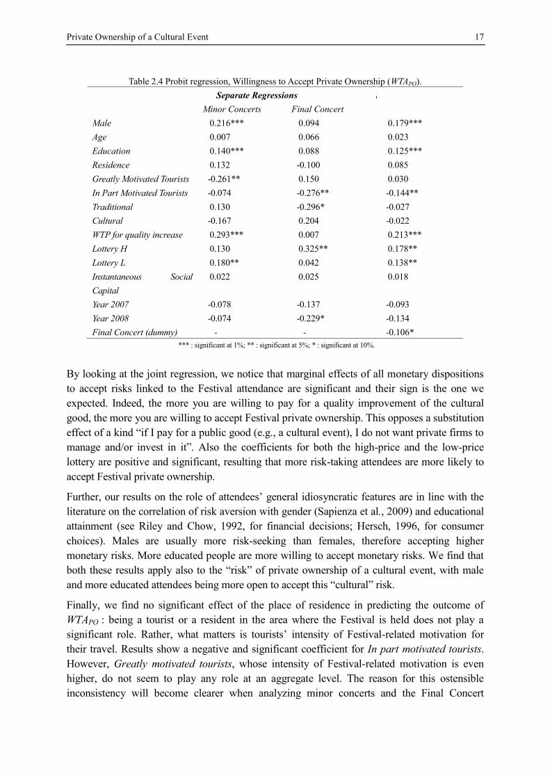
Table 2.4 reports results of the probit regression model we used to predict the outcome of
WTAPO. Coefficients refer to the marginal effects of the explanatory variables described in
section 2.3.
Private Ownership of a Cultural Event 17
Table 2.4 Probit regression, Willingness to Accept Private Ownership (WTAPO).
Separate Regressions n
Minor Concerts Final Concert
Male 0.216*** 0.094 0.179***
Age 0.007 0.066 0.023
Education 0.140*** 0.088 0.125***
Residence 0.132 -0.100 0.085
Greatly Motivated Tourists -0.261** 0.150 0.030
In Part Motivated Tourists -0.074 -0.276** -0.144**
Traditional 0.130 -0.296* -0.027
Cultural -0.167 0.204 -0.022
WTP for quality increase 0.293*** 0.007 0.213***
Lottery H 0.130 0.325** 0.178**
Lottery L 0.180** 0.042 0.138**
Instantaneous Social
Capital
0.022 0.025 0.018
Year 2007 -0.078 -0.137 -0.093
Year 2008 -0.074 -0.229* -0.134
Final Concert (dummy) - - -0.106*
*** : significant at 1%; ** : significant at 5%; * : significant at 10%.
By looking at the joint regression, we notice that marginal effects of all monetary dispositions
to accept risks linked to the Festival attendance are significant and their sign is the one we
expected. Indeed, the more you are willing to pay for a quality improvement of the cultural
good, the more you are willing to accept Festival private ownership. This opposes a substitution
effect of a kind if I pay for a public good (e.g., a cultural event), I do not want private firms to
manage and/or invest in it . Also the coefficients for both the high-price and the low-price
lottery are positive and significant, resulting that more risk-taking attendees are more likely to
accept Festival private ownership.
Further, our results on the role of attendees general idiosyncratic features are in line with the
literature on the correlation of risk aversion with gender (Sapienza et al., 2009) and educational
attainment (see Riley and Chow, 1992, for financial decisions; Hersch, 1996, for consumer
choices). Males are usually more risk-seeking than females, therefore accepting higher
monetary risks. More educated people are more willing to accept monetary risks. We find that
both these results apply also to the risk of private ownership of a cultural event, with male
and more educated attendees being more open to accept this cultural risk.
Finally, we find no significant effect of the place of residence in predicting the outcome of
WTAPO : being a tourist or a resident in the area where the Festival is held does not play a
significant role. Rather, what matters is tourists intensity of Festival-related motivation for
their travel. Results show a negative and significant coefficient for In part motivated tourists.
However, Greatly motivated tourists, whose intensity of Festival-related motivation is even
higher, do not seem to play any role at an aggregate level. The reason for this ostensible
inconsistency will become clearer when analyzing minor concerts and the Final Concert

18 Chapter 2
separately.
Indeed, the marginal effect on WTAPO of the Final Concert dummy is negative and significant,
thus confirming greater openness to private ownership when the cultural connotation of the
event is more pronounced (minor concerts). This result has three complementary explanations.
Firstly, in the separate regression for the minor concerts only, Willingness to Pay for Quality
and Lottery L have a significant positive effect on WTAPO, while the effect of Lottery H is not
significant. The opposite holds in the separate regression for the Final Concert only. Therefore,
paying a small lottery price is sufficient to significantly increase WTAPO in the minor concerts,
while paying a higher lottery price is needed to significantly increase WTAPO in the Final
Concert. Intuitively, private ownership is judged as riskier for the Festival sub-event that
attendees perceive as less oriented to tradition conservation.
The second explanation is actually related to attendees perception of Festival traditional links.
From Table 2.4 we see that this perception significantly decreases WTAPO in the Final Concert.
It seems that, while in the minor concerts private firms ownership of the Festival is understood
as in line with its folkloric trait, in the Final Concert it is felt in a sharp contrast to the Festival
roots, thereby making the private ownership lottery more risky. The intuition is that private
firms management and financing might be aimed at emphasizing its mass-gathering
connotation, thereby further reducing its perceived link with tradition, and ultimately its
cultural intensity.
Lastly, while in the minor concerts Greatly motivated tourists negatively (and significantly)
influence WTAPO, in the Final Concert this role is played by In Part motivated tourists. The null
hypothesis here is straightforward: tourists visiting the area where the Festival is held just or
also for the Festival should prefer the cultural event to be publicly owned. And this preference
should be stronger for greatly motivated tourists, who are more motivated by the Festival.
They should not be disposed to run the risk of seeing their unique source of attraction to the
visited area pillaged of its own nature because of private ownership (and profit). Also, Greatly
motivated tourists have paid more than other attendees so to enjoy the Festival. Indeed,
although Festival attendance is free, they feel they have paid travel and stay expenses just to
attend the event. This is where a sunk cost fallacy steps in. They paid these costs so as to obtain
a sure payoff: the Festival as it is. They do not want this payoff to be decreased by (others )
private (though partial) ownership. This hypothesis is verified for those greatly motivated
tourists attending the minor concerts. It does not hold for the Final Concert. This is because
greatly motivated tourists attending the Final Concert cannot be classified as pure cultural
tourists. Indeed, 53% of them declare they attend the Final Concert because of its
entertainment side and only 28% (difference significant at 1%) for its traditional
connotation. Therefore, their view of the Festival is quite unrelated to traditional and cultural
issues, and so they do not perceive a true risk of commodification due to private ownership of
the cultural event. Differently, in part motivated tourists attending the Final Concert have a
lower entertainment motivation (48%, not significant) and a greater traditional motivation
(38%, difference significant at 10%) than greatly motivated tourists attending the same event.
More importantly, they declare they decided to visit the area where the Festival is held not only
for the Final Concert, but also for other reasons linked to geographical and cultural features of

Private Ownership of a Cultural Event 19
the place hosting the Festival. Hence, their link with the cultural background of the place is
high enough to let them feel the risk of cultural depletion due to Festival private ownership.
This is why WTAPO in the Final Concert is negatively related to the status of being an In part
motivated tourist.
2.4.2 Disentangling different social benefits of private ownership
As shown in the previous section, a large part of the Festival attendees (almost 6/10 on average
over the three surveyed editions) is not willing to accept a private ownership of the cultural
event. During the last of the three analyzed editions (2009), we tried to explore possible
conditions likely to moderate the participants unwillingness.
We asked the sub-sample of attendees not willing to accept Festival private ownership (WTAPO
= 0) if, under a specific state of the world, they were willing to change their decision. We did it
only during the Final Concert (1,000 observations), given that this is the sub-event where
WTAPO is significantly lower.
The question eliciting an attendee s WTAPO (see section 2.4.1) was proposed three more times
to attendees who previously gave a negative answer, by adding each time one of these three
specifications: if quality would increase , if it would lead to public money saving , and if
the Festival would disappear in the absence of private firms intervention . Figure 2.1 reports
the percentage of attendees interviewed during the 2009 Final Concert switching from WTAPO
= 0 to WTAPO = 1 if one of these three states of the world was attached (by the interviewer) to
the private ownership.
Figure 2.1 Attendees with no WTAO, who would change their mind under specific states of the world.
Figure 2.1 shows that, among the three proposed conditions, a potential increase in quality is
the one leading the greatest percentage of attendees with WTAPO = 0 switching to WTAPO = 1,
thereby stressing once more the importance of quality in the demand of a cultural event.
Public money saving is another condition leading the majority of attendees initially averse to
private ownership to become favourable to private firms intervention. This seems to indicate
that, between the two components of a festival private ownership, private financing does not
43%
65%
69%
Festival desappearing
Public money saving
Quality increasing

20 Chapter 2
play a strong role on attendees perceived risk of the cultural lottery. We will come back to this
point in the last paragraph of this section.
Conversely, Festival disappearance in the absence of private intervention is not a sufficient
condition to convince more than half of initially unwilling attendees to accept private
ownership. Indeed, in this state of the world, interviewees are led to envisage a situation where
they do not have an alternative solution (e.g., quality not increasing or public money not saved).
Differently from the other two states of the world, where a situation better than the status quo is
proposed, here the suggested condition is worse than the status quo, which can be restored only
through private intervention. This leads to conclude that cultural consumers are more willing to
accept a festival private ownership when it produces a social welfare increase with respect to
the status quo than when it is the only way to preserve it.
Finally, and more importantly, instantaneous social capital plays a key role in determining
whether an attendee changes his/her answer from WTAPO = 0 to WTAPO = 1 under the states of
the world described above. Under each of the three conditions, the percentage of attendees with
instantaneous social capital turning to WTAPO = 1 is significantly lower than the percentage of
attendees with no instantaneous social capital making the same choice: 60% vs. 72%,
significant at 5%, under quality improving; 54% vs. 68%, significant at 5%, under public
money saving; 28% vs. 46%, significant at 1%, under Festival disappearing. Therefore, if an
attendee is averse to accepting the private ownership lottery, instantaneous social capital has
a negative effect on his/her willingness to change his/her mind when the positive outcomes of
such lottery are explicitly stated. Our intuition for this result follows. Attendees showing no
openness to private firms intervention in the Festival ownership even when its potential
social benefits are stressed conform to the social norm that culture should be publicly
managed: this compliance is positively correlated with instantaneous social capital. Indeed,
more than 2/3 of attendees with instantaneous social capital would not accept private
partnership even when they are told this would be the only way to allow the survival of the
cultural event (the source itself of this social capital).
2.4.3 Disentangling different economic dimensions of private ownership
During the Final Concert of the last analyzed edition we introduced another question aiming
at disentangling private ownership. This was done in correspondence with the forthcoming
birth of La Notte della Taranta Foundation (Fall 2009), which would have soon become
responsible of the Festival ownership structure, with the possibility to open it to other public
institutions or to private firms (see section 2.2).
Therefore, we asked a representative sample of Final Concert attendees (1000 observations)
to indicate their preferred Festival ownership formula, by choosing one among five possible
options: Public Management-Public Financing , Public Management - Private Financing ,
Public/Private partnership over both Management and Financing , Private Management-
Public Financing , Private Management -Private Financing . We controlled the order of
presentation of the given options to interviewees. Figure 2.2 reports the distribution of
attendees preferences for each of the options.

Private Ownership of a Cultural Event 21
Figure 2.2 Preferred combination of (Public/Private) Management and (Public/Private) Financing.
As expected, the most preferred ownership formula (about half of attendees) is the one with
only public institutions involved in both managing and financing the event. Indeed, it is the
closest to the actual ownership formula in 2007-2009 (100% public management and
75%/25% public/private financing).
However, a relevant part of the attendees (3 out of 10) prefer a solution where both public
institutions and private actors are involved in each of the two roles. This can be interpreted
again in terms of attendees demand of a protection against the risk of commodification: the
presence of public institutions in both management and financing might work as a form of
cultural insurance over each aspect of the Festival.
Figure 2.2 also shows that the aspect perceived as more risky by attendees is private
investment. In fact, focusing only on those attendees admitting private intervention in at least
one of the two ownership dimensions, we see that 92% of them prefer a private-management
solution, while only 71% prefers a private-investment one (difference significant at 5%
level). Furthermore, the difference between the percentage of attendees choosing the public-
management and private-investment solution (4%) is not significantly different from the
percentage of those participants choosing purely private ownership (2%). This is further
evidence that the most risky element in private ownership lottery is private financing.
2.5 Conclusions
The organization of a cultural festival which also aims at being a mass gathering usually
requires huge economic investments as well as management efforts on the part of public
institutions. Festival ownership is a crucial variable for the success of the event.
In this paper we empirically explore attendees willingness to accept a private partnership in a
festival ownership. This issue is at the heart of a recent debate about how much private capital
2%
14%
29%
4%
51%
Private M - Private F
Private M - Public F
Partnership
Public M - Private F
Public M - Public F

22 Chapter 2
should be included in the ownership and management of culture and what risk does this entail
for the independence of culture itself. We argue that this kind of risk enters individual
preferences for private partnership, as in a sort of lottery. We therefore expect that the factors
determining an individual s general attitude towards risk play also a role in the preferences for
the private partnership of cultural events. In fact, this is what we find empirically.
Using a large database of interviews conducted during one of the most important European
festivals dedicated to traditional music, we find that attendees who are more favourably
disposed to risk in a generic monetary lottery, they also have a greater propensity toward
private partnership in the event management and financing. We also find that idiosyncratic
features which according to the experimental economics literature positively correlate with
risk aversion (being male and more educated) lead to a greater openness to accept this
ownership formula. This confirms the idea that event attendees perceive a potential private
ownership as a risky lottery.
Furthermore, we find several results that shed light on how cultural features affect this risk
perception. First, attendees willingness to accept the participation of private firms in the
festival ownership positively depends on their sensitivity to the traditional/cultural aspects of
the event. Second, cultural tourists are less willing to accept the private ownership lottery.
Third, the more attendees are willing to pay for a quality improvement of the cultural good, the
more they are willing to accept the above lottery. Fourth, the risks that private ownership may
entail are perceived as smaller when the cultural connotation of the event is more intense.
Finally, attendance at the cultural event leads people to develop a specific kind of social capital.
Among attendees not willing to accept the private ownership lottery, those with instantaneous
social capital stand more their ground when they are shown the positive consequences that a
private ownership may bring to the Festival. This indicates that the social dimension of the
cultural event determines a worse disposition towards the private ownership.
The findings that emerge from our field research may prove useful in gaining an insight into
consumers stated preferences on management issues. There is inadequate attention paid to
consumers view on private management of cultural events in the economic literature, though
this seems to us as a crucial aspect that needs to be taken into account, especially when dealing
with cultural goods. This lack of attention may lead to false inferences regarding the choice of
proper management formulas. As our data show, private firms involvement in a festival
management and financing, though increasing its quality, could have the reverse effect in terms
of people attendance if they perceive the risk of a potential loss of its more genuine cultural
characteristic high.

Private Ownership of a Cultural Event 23
References
Acheson, K., Maule, C. & Filleul, E. (1996). Cultural entrepreneurship and the BanffTelevision Festival, Journal of Cultural Economics, 20, 321-339.
Andersson, T.D. & Getz, D. (2009). Tourism as a mixed industry: Differences between private,public and not-for-profit festivals, Tourism Management, 30, 847-856.
Attanasi, G., Casoria, F., Centorrino, S. & Urso, G. (2013). Cultural tourism, local developmentand instantaneous social capital: a case study of a gathering festival in the South of Italy,Journal of Socio-Economics, 47, 228-247.
Camacho-Cuena, E., García-Gallego, A., Georgantzís, N. & G. Sabater-Grande (2004). Anexperimental validation of hypothetical WTP for a recyclable product, Environmental and
Resource Economics, 27, 313-335.
Camacho-Cuena, E., García-Gallego, A., Georgantzís, N. & G. Sabater-Grande (2003). Anexperimental test of response consistency in contingent valuation, Ecological Economics,47, 167-182.
Coalter, F. (1998). Leisure studies, leisure policy and social citizenship: the failure of welfareor the limits of welfare?, Leisure Studies, 17, 21-36.
Cohen, E. (1988). Authenticity and commodification in tourism, Annals of Tourism Research,15, 371-386.
Frey, B. (1994), The economics of music festivals. Journal of Cultural Economics, 18, 29-39.
Garrod, B., Fyall, A. & Leask, A. (2002). Scottish visitor attractions: managing visitorimpacts, Tourism Management, 23, 265-279.
Georgantzís, N. & D. Navarro-Martínez (2010). Understanding the WTA-WTP gap:Attitudes, feelings, uncertainty and personality, Journal of Economic Psychology, 31, 895-907.
Getz, D. (2008). Event tourism: Definition, evolution, and research, Tourism Management, 29,403-428.
Getz, D. (2010). The Nature And Scope Of Festival Studies, International Journal of Event
Management Research, 5, 1-47.
Guiso, L. & Paiella, M. (2008). Risk aversion, wealth and background risk, Journal of the
European Economics Association, 6, 1109-1150.
Harris, R., Jago, L., Allen, J. & Huyskens M. (2001). Towards an Australian event researchagenda: First steps, Event Management, 6, 213-221.
Hede, A., Jago, L. & Deery, M. (2003). An agenda for special event research: Lessons from thepast and directions for the future, Journal of Hospitality and Tourism Management, 10, 1-14.
Herrero, L.C., Sanz, J.A., Bedate, A. & Del Barrio, M.J. (2011). Who Pays More for a CulturalFestival, Tourists or Locals? A Certainty Analysis of a Contingent Valuation Application,International Journal of Tourism Research, 14, 495-512.
Hersch, J. (1996). Smoking, seat belts and other risky consumer decisions: Differences bygender and race, Managerial and Decision Economics, 17, 471-481.
Marbach, G. (2000). Le ricerche di mercato, Utet, Torino.

24 Chapter 2
Riley, W.B. & Chow K.V. (1992). Asset Allocation and Individual Risk Aversion, Financial
Analysts Journal, 48, 32-7.
Sapienza, P., Zingales, L. & Maestripieri, D. (2009). Gender differences in financial riskaversion and career choices are affected by testosterone, Proceedings of The National
Academy of Sciences - PNAS, 106, 15268-15273.
Shepherd, R. (2002). Commodification, culture and tourism, Tourist Studies, 2, 183-201.
Silvers, J., Bowdin, G., O Toole, W. & Nelson, K. (2006). Towards an international eventmanagement body of knowledge (EMBOK), Event Management, 9, 185-198.

3
Nudges Can Affect Students GreenBehaviour? - A Field Experiment1
Extended abstract
The promotion of sustainable resource use and changing people s behaviour correspondingly
remains the essential long-term social and policy challenges of our planet. Policies ignoring
results of human psychology and reducing decision making of individuals to a simplistic
concept of rationality will hardly reach their aimed level of impact. In this spirit, the paper
follows a growing body of literature on non-price interventions 'nudges' to examine its impact
on the environmental behaviour - recycling.
We study whether nudges are efficient in promoting ecological behaviour and recycling of
young people, and whether different types of nudges or their combination serve as better
instruments for inducing this.
Many obstacles impede ecological behaviour. They are either financial or behavioural.
Traditional policies of price based approaches, raising awareness, or technology based
approaches turned out not being very effective. A growing literature on behavioural
economics and psychology thus suggests the use of non- price intervention nudges. A nudge
is a helping hand that will lead someone to make better decisions, both for himself and for
the public interest as well. Nudges are suggested as a policy instrument of libertarian
paternalism and favoured for its simplicity, relatively low cost of implementation and its
effectiveness. As suggested by (Sunstein and Thaler 2003), 'libertarian' aspect refers to the
necessity of respecting everyone's freedom to act, decide or even change their minds as it suits
them.
The study was performed on primary data, from both a survey and field experiment conducted
among university students in Pisa, one of the most important university cities in Italy. The
survey was conducted during May and June 2013. By using the mailing list provided by the
university administrative departments, 450 emails were sent to university students in Pisa
including a survey link and a description of the aim of the study. The response rate after two
reminders was 47 percent (213 surveys). In this survey, we asked questions about non-price
intervention nudges (social norm, default options and commitment devices) and
demographical data.
The field experiment was conducted over a 60-day span (from October to December 2013).
1 This is a joint project with Ajla Cosic and Sebastian Ille.

Nudges Can Affect Students Green Behaviour? 27
We collected data on 1849 instances of plastic cup recycling at a coffee vending machine at
the School of Advanced Studies Sant Anna in Pisa. The users were not aware that they were
participants in the study. Recycling behaviour was measured by number of plastic cups
disposed in the dustbin, observed at the end of a day.
For the experiment, we used two different treatments. Initially, we had a control period of two
weeks in order to count the number of recycled cups without any intervention. In the
following, we applied the first and second treatment, each for two weeks. Three months after
the experiment, in February 2014, we recollected data on recycled plastic cups for one week
to check for the lasting effect of the second treatment nudges.
In the first treatment, we triggered a behavioural change through two different effects: a social
norm (as a nudge) and an awareness raising message. Before the treatment, students threw
their cups blindly into the biggest bin, without giving much thought that these cups can be
recycled. We could assume that students did not pay attention to recycling because either they
did not know better or they followed the behaviour of their fellow colleagues. Thus ignorance
was paired with a conformity effect that induced students not to care.
In the second treatment, we counteracted the inconvenience of recycling. In the control,
students disposed their plastic cups in the larger bin, not only because it was more salient than
the much smaller bin, but mainly because it was much more accessible. This treatment
aligned the social norm (as a nudge), the awareness raising message, and the convenience to
recycle ('easy to do' nudge).
Analysis of the survey data revealed that most of participants would follow indirect non-price
interventions. The largest number of respondents (over 72 percent of participants) responded
positively to a hypothetical question that they: would participate in the new resource
program by using their towels more than once , following the social norm nudge. The
principal drawback of stated preferences is that they may not correspond to their revealed
(actual) preferences. We thus controlled for a possible convergence between self-reported and
the actual behaviour on the basis of the field experiment data.
Results of the first treatment showed a significant improvement in the amount of recyclable
cups after the first treatment, from average 3.91 percent in the control condition to an average
36 percent in the first treatment. A t-test revealed that this increase due to the social norm
nudge in combination with an awareness raising message was significant at the .05 critical
alpha level (t(10) = 13.63 with p < .0001).
Moreover, results of the second treatment intervention show that on average 97.35 percent
participants recycled plastic cups. A t-test showed that a two nudges treatment (social norm
and 'easy to do' nudge) will significantly increase the amount of recycled plastic cups in
comparison to the single nudge treatment (social norm treatment) (t(15)=22.31 with p<.0001).
Three months after the experiment, results confirmed a lasting effect of the second treatment
as on average 68 percent participants still have recycled plastic cups.
The paper further includes a simple game theoretical model that takes account of the
individuals decisions with respect to the variables elaborated above. This model is able to
replicate the results and illustrates the effect of a perceptional change (awareness raising) of
individuals, a shift in the social norm, as well as a switch in the nudges. Our main
contributions are that nudges can be used for inducing green behaviour of young consumers
and thereby generate a long lasting effect, also in the second treatment.

28 Chapter 3
The results of our studies have clear implications for policy makers. The appeal of nudging
for educational institutions (e.g., universities) is evident, and imply a set of seemingly simple,
low cost solutions that can be applied to a wide array of problems arising from young people's
behaviour. Further research could test effects of nudges applied to an array of other problems
arising from young people's behaviour (e.g., obesity, smoking).
Keywords: Green Behaviour; nudge; experiment; behavioural change; policy.

Nudges Can Affect Students Green Behaviour? 29
3.1 Introduction
As the world s human population is constantly growing, a few places on the globe escaped the
pervasive impact of our species. Many of the world s most difficult conservation problems
result either directly or indirectly from people s everyday behaviour, contributing to air and
water pollution, land degradation, deforestation, water resources loss and climate change
(Akerlof and Keneddy, 2010). One of the important long-term social and policy challenges
our planet is facing is to promote sustainable resource use and to change people s behaviour.
Though awareness and readiness to recycle increased in Italy over the past years, a large
number of consumers still refuses to dispose of recyclable waste in stipulated containers.
Even those Italians, who are willing to contribute to alleviate the environmental consequences
and the challenges of climate change, illustrate fewer incentives to do so after the scandal of
the Campania region hit the news (i.e., Mayr, 2014). Although the Italian legislation attended
the issue of waste disposal in 2001, the industry preferred (and still prefers) paying the Italian
mafia for waste disposal, avoiding the cost of proper waste disposal. Thus in addition to
Italians being unaware of the necessity of recycling, this circumstance offers an excuse for
those unwilling to dispose their waste properly, but also makes those insecure, who wish to
contribute to environmental recovery.
While Italian public authorities provide proper waste collection schemes, Italy is still in need
of a mechanism that promotes acceptance and participation of citizens in the recycling
scheme. Such a mechanism has to go beyond legal measures or monetary incentives, and has
to address three factors influencing recycling behaviour: awareness, attitudes and structural
barriers (Shaw et al. 2007). Traditional policies of raising awareness, price-based as well as
technology-based approaches turned out to be ineffective. Pertinent literature suggests that
behavioural approaches appealing to social norms, commitment devices, and default options
can be very powerful in changing behaviour.
A growing literature on behavioural economics and psychology recommends using non-price
interventions via nudges . A nudge is defined as a helping hand that will lead someone to
make better decisions both for oneself and for the public welfare. The concept of nudges
(Thaler and Sunstein, 2008) suggests a policy of libertarian paternalism, favouring simplicity,
effectiveness and a relatively low cost of implementation. As suggested by Sunstein and
Thaler (2003), 'libertarian' aspect refers to the necessity of respecting everyone's freedom to
act, decide or even change their minds as it suits them.
Following this literature on non-price interventions, we examine the impact of 'nudges' on
recycling behaviour. We study the efficiency of specific nudges for promoting recycling, and
whether the combination of different types of nudges provides a more efficient instrument to
improve recycling behaviour.
This study contributes to the literature on the use of nudges as policy-making interventions,
by testing whether nudges can affect young consumers pro-environmental behaviour. In
addition, we investigate the effect of combined nudges (in our case a social norm nudge with
an 'easy to do' nudge), and study the long lasting effect of nudges on pro-environmental
behaviour.
The first section of this article provides a literature overview. In the second section, we
develop an analytical model from which we derive the hypotheses to be tested. The third

30 Chapter 3
section illustrates the methodology used and the fourth section analysis the results and
compares these to our hypotheses. The fifth section contains the conclusion.
3.2 Literature review
Many studies show that appealing to social norms can affect individual behaviour. People
may follow others due to social penalties for non-compliance, or because they believe that
others may have better and different information about benefits. Additionally, individuals
conform to a norm of pro social behaviour to signal benevolent underlying preferences.
Robert Cialdini was among leading scientists, who characterised and tested this phenomenon,
(Cialdini, Reno and Kallgren, 1990; Goldstein, Cialdini and Griskevicius, 2008). Goldstein,
Cialdini and Griskevicius (2008), partnered with a hotel in Arizona to induce guests to reuse
their towels. In this field experiment, researchers tried different messages: Help Save the
Environment, Preserve Resources for the Future, Partner with the Hotel to Save the
Environment and Join Your Fellow Guests in Helping to Save the Environment . The final
message included the information the majority of hotel guests reuse towels. Inducing
conservation as a social norm, increased towel use by 34 percent and was the most effective.
In the context of environmental protection, nudges have been implemented by Goldstein,
Cialdini and Griskevicius (2008) to improve towel reuse.
Also Allcott (2011) conducted a field experiment on energy conservation using social norms.
Together with a company called OPOWER, they mailed home energy use reports to
residential utility consumers. These reports included energy conservation information as well
as social comparisons between a household's energy use and that of its neighbours. This
monthly program reduced energy consumption by 1.9 to 2.0 percent. His results showed that
non-price interventions-nudges can affect consumer behaviour. These works have provided
supportive evidence that appealing to social norms can affect an individual behaviour.
Results of a recent body of research on default options in many different areas such as
pension savings plan, organ donations, retail electricity supplier, show that people rarely
choose to switch from a default option. Persistence of the default options can be explained
through 'endowment effects' (i.e. possession bias - individuals favour an option they have),
procrastination or inertia (put off doing something for tomorrow and never do) or costs of
searching information and benefits from a new option.
Some programs using a default option triggered strong results. Thaler and Benartzi (2004)
collaborated with a company wanting to increase employees' retirement savings. To tackle the
problem of inadequate pension saving in defined contribution plans, they developed the plan
Save More Tomorrow (SMT). This plan had components of default options such as,
contribution to the plan is increased after a raise of pay or employees can opt out of the plan
at any time. As a result, employees' average savings were increased by 400 percent.
According to the authors this plan worked well due to powerful inertia; once employees enrol
in the plan, few will ever choose opting out.

Nudges Can Affect Students Green Behaviour? 31
Moreover, Madrian and Shea (2001) found that participation rates in a corporate pension
savings plan increased from 65 percent to 98 percent when the default option was changed
from non-enrolment to enrolment. Similar results are observed when it comes to organ
donations in the European Union countries. Johnson and Goldstein (2002) examined the rate
of agreement to become a donor across European countries and illustrated that defaults appear
to make a large difference. In countries where default was used, rates to opt-out of the organ's
donation program was much lower compared to countries where opt-in was used. The authors
suggest that the cost from changing the default option is much higher as it involves filling out
forms, making phone calls and sending mail. Hence, changes in defaults could increase
donations by additional thousands a year.
A growing body of research on policy making shows that raising awareness of end users to
recycle should be promoted at every opportunity. According to Waste and Resources Action
Programme UK (WRAP UK, 2012) greater public awareness of reuse and recycling avenues
can be achieved through a number of good practice measures such as the provision of
marketing materials or developing public engagement. The Department for Environment,
Food and Rural Affairs UK (DEFRA, 2008) has highlighted the roles of producers,
consumers, retailers, local authorities and the waste management industry as key stakeholders,
but highlighted an increasing emphasis in central governments to focus on delivering policy
targets to individuals and households by using awareness raising and policy interventions.
Miranda and Blanco (2010) showed that environmental awareness is still the main actor
influencing paper recovery in European countries. According to Miranda and Blanco (2010)
a large variety of tools are available for promoting the development of awareness, based on
improving information and education. The better-informed people are about recycling, the
more likely they are to commit to it and feel satisfied with their actions. Miranda and Blanco
suggest (2010) that development of awareness can be carried out through various media
depending on the target group: the general public, children or young people.
3.3 Model
Based on Shaw et al. (2007) three factors determine recycling behaviour: awareness, attitudes
and structural barriers. Consequently, we address these factors via a number of different
nudges: consciousness raising, conformity, and improving accessibility. Consciousness
raising makes people aware that certain garbage is recycled and that only a small change in
one s action can make a difference leading to a positive contribution to the environment. The
conformity effect can be channelled by illustrating behaviour of an influential reference group
thereby inducing an external norm and point of reference. Accessibility can be improved by
allowing individuals to recycle in such a way that following the habitual pattern of action is in
fact correct behaviour (e.g., by switching the default). This lowers cognitive requirements
needed to make a correct decision (i.e., which bin has to be chosen?). Similarly, reducing
structural barriers by improving accessibility reduces the cost of the act of recycling.
Oftentimes the cognitively least demanding action is also the least physically demanding

32 Chapter 3
(e.g., the biggest trash bin), we will thus look at an effect, which enhances both cognitive and
physical accessibility.
In order to keep the model as simple as possible, we assume that individuals have only the
choice between choosing an action or refraining from it, and neglect intermediate case in
which individuals more or less sporadically choose the action. Our hypothetical population
can be thus grouped into recyclers and non-recyclers. Assume that each individual has the
same pay-off function (note: we can consider this as averages, it is easy to extend the model
with individually varying parameters, yet the dynamics and thus results will remain identical.)
Define the pay-off of the first type by and the latter by .
If the expected pay-off from not recycling is smaller than the pay-off received from recycling,
individuals will choose to throw recyclable garbage into the recycling bin. They will not do so
if not recycling bears a higher pay-off. Thus, an equilibrium occurs when both pay-offs are
identical, i.e. at
r= rn (1)
We can generally assume that individuals receive a benefit from getting rid of their garbage
that is common for recyclers and non-recyclers, and we set this to a positive constant . In
addition, a non-recycler bears a social cost by throwing waste into the wrong bin. Clearly this
cost depends on the intrinsic values of an individual, but also on the existing social norm and
should be monotonously increasing in the number of recycler the individual observes. Let the
frequency of recyclers be p (0,1). The social cost is, however, not simply linear but s-
curved. This results simply from the fact that a critical number of players is required to make
a normative impact. For simplicity, we can normalise the maximum social cost to one. The
minimum social cost in the absence of any recycler lies at a (0,1]. Let the social / intrinsic
cost be defined by
( ) = (1 ) +( )
(2)
The derivation of this function is straightforward but will be illustrated in the appendix.2
Parameter defines the minimum social pressure (or intrinsic motivation) that is exercised in
the absence of any recyclers (i.e., the intercept at the axis of ordinates), indicates the
reactivity to social pressure (for lower values more linear and for higher values more curved),
and defines the sensitivity/bias to social pressure (lower values move the titling point to the
left of 0.5 and higher values to the right).
The act of recycling is, however, also costly. Costs are partly caused by the action to separate
(the cognitive cost of choosing the right bin) and in addition, by the requirement to place the
object in a small bin that is increasing difficult and repugnant the more plastic trash is put
inside that bin. We have a cost function of the simplest form.
(p) = kp + d (3)
where defines the cost of separation (i.e., the cost of making a choice and choosing the right
bin) and indicates the marginal cost increment with each piece of plastic placed into the
2 Note that this function is not always strictly increasing in p, since for > (1 ) 1 /
(( (1 ) + ) ) it is decreasing. Thus for small p and large a, social cost might fall.

Nudges Can Affect Students Green Behaviour? 33
bin.3Hence, we can define
r= (p) (4)
rn= (p) (5)
Given equation 1, we see that an equilibrium thus occurs if the social / intrinsic cost equals
the cost of recycling, i.e. the equilibrium share of recyclers is defined by the positive real
roots in the unit interval of
+ =( )
( )(6)
These equilibria are only stable, if at this point, the negative reaction of a recycler towards an
additional recycler is stronger than the reaction of a non-recycler (i.e., the recycler loses more
utility than the non-recycler). This translates into the stability condition( ) ( )
< 0 or
( ) ( )> 0 (7)
for the equilibrium .4
Figure 3.1: Dynamics of the control group: a = 0.2, b = 1.5, c = 2.0, k = 1.3, and d = 0.1.
As a reference, figure 3.1 illustrates a control situation, in which less than 10 percent of all
students are recycling. This equilibrium is stable since the slope of the cost of recycling is
steeper than that of the social cost function, i.e. ( )/ > ( )/ .
As argued above, we would like to analyse an effect that operates on the level of awareness
(consciousness raising) and exercises pressure of conformity by setting a higher external
social norm of recycling. The first has an effect on the sensitivity to social pressure in the
form of decreasing . The second shifts up the minimum social pressure, thus increasing .
The result is illustrated in figure 3.2, in which we see that the interior stable equilibrium shifts
up to roughly 40 percent.
3 In the empirical study, we experienced that once some plastic cups were in the small yellow bin, it is dirty anddifficult to squeeze more in.4 Note that in the illustrated graphs of figures 3.1-3.3, there exists only one equilibrium, yet we can have amaximum of three. The first and third will be stable, and the second interior unstable.
Social&IntrinsicCost
CostofRecycling
0.2 0.4 0.6 0.8 1.0
0.2
0.4
0.6
0.8
1.0

34 Chapter 3
Figure 3.2: Dynamics of treatment 1: a = 0.4, b = 1.5, c = 1.0, k = 1.3, and d = 0.1.
We would like to analyse further the effect of an easy-to-do nudge (i.e., reassigning the larger
bin as the one appropriate for recyclable material). As argued above, this reduces the
cognitive cost of making the correct choice since this is the most intuitive bin. It also reduces
the physical cost of placing garbage inside and thus the barrier of recycling. Hence, we can
expect a reduction both in k and d. Figure 3.3 shows such an effect. Here, both cost functions
intersect at a frequency of recyclers close to one.
Figure 3.3: Dynamics of treatment 2: a = 0.4, b = 1.5, c = 1.0, k = 1.0, and d = 0.0, functionsintersect at a frequency of recyclers at one.
From this simple analytical model we can thus derive the following hypotheses:
H1: Using a non-price intervention nudge (social norm) combined with an awareness-raising
message positively influences recycling behaviour by affecting awareness and attitude.
H2: Using a non-price intervention - an 'easy to do' nudge - positively affects recycling
behaviour by improving cognitive and physical accessibility.
H3: Using these two nudges jointly will positively affect recycling behaviour more than if
only a single nudge is applied.
These hypotheses will be tested and analysed in the remaining parts of this article.
3.4 Methods
The study was performed on primary data, from both a survey and field study conducted
Social&Intrinsic Cost
Cost of Recycling
0.2 0.4 0.6 0.8 1.0
0.2
0.4
0.6
0.8
1.0
Social&IntrinsicCost
CostofRecycling
0.2 0.4 0.6 0.8 1.0
0.2
0.4
0.6
0.8
1.0

Nudges Can Affect Students Green Behaviour? 35
among university students in Pisa, one of the largest university cities in Italy. We used both a
survey and a field experiment in order to study independently both stated and revealed
preferences. The principal drawback of individual's stated preferences is that they may not
correspond to their revealed (actual) preferences. We test their validity through a field
experiment and check for possible convergence between self-reported (a survey) and the
actual behaviour.
Data was collected during May and June 2013. By using the mailing list provided by the
university administrative departments, 450 emails were sent to university students in Pisa
including the survey link and a description of the aim of the study. The response rate after two
reminders was 47 percent (213 surveys). The group of participants included 120 males and 86
females. Prior to the final submission, a pre-test was administrated to 30 students during the
month of May. This test was developed to uncover any possible weakness and
misunderstanding arising from the text. Consequently, the final questionnaire was prepared
based on the pre-test results which caused us to summarize and change the statements of some
questions, and eventually to eliminate some questions. In order to overcome methodological
biases affecting behavioural research based on survey techniques, we adopted several
procedural remedies. Because many researchers have pointed out social desirability as one of
the most common sources of bias affecting the validity of experimental and survey research
findings (King and Bruner, 2000; Tourangeau and Yan, 2007) we guaranteed anonymity of
respondents.
Over a span of 60-days (from October to December 2013), we collected data on 1849
instances of plastic cup disposal at a coffee vending machine at the School of Advanced
Studies Sant Anna in Pisa. Users were unaware that they were participants in the study.
Recycling behaviour was measured by the number of plastic cups recycled in dustbins at the
end of a day. During the observation period, our team would count the number of cups
recycled every day before the dustbins were cleaned in the morning. To ensure that participant
were not aware that their recycling behaviour was being monitored, counting took place early
in the morning when nobody was present near the coffee vending machines.
For the experiment we used two different treatments. A control period of two weeks
measured the number of recycled cups without any intervention. In the following, we applied
the first and second treatment, each for two weeks. Three months after the experiment, in
February 2014, we recollected data on recycled plastic cups for one week to check for the
lasting effect of the second treatment nudges.
For treatment 1, we created a message showing signs soliciting participation in a recycling
program in order to raise awareness. The message, which was designed to reflect the
importance of recycling and the environment protection, included an external descriptive
social norm as a nudge to induce recycling. This norm was induced by informing participants
that the majority of other students at one of the world s leading universities recycle. Our
message was the following: Be different! Be better! RECYCLE! Choose the right bin, it is
very easy."Almost 70% of Harvard students RECYCLE." Do you want to lag behind?. At the
School of Advanced Studies Sant Anna, a majority of students are Italians, but for
international students the message was displayed both in Italian and English. Based on the
foregoing analysis, we hypothesized that the message, which conveyed the external social
norm would raise awareness and result in recycling a larger share of the plastic cups.

36 Chapter 3
Figure 3.4: Treatment 1
For treatment 2, we used the 'easy to do' nudge in combination with the social norm. This
way, we made it is easier for subjects to recycle plastic cups (so subjects can do it without a
lot of thinking or effort) by changing the recycling-bin-to-garbage ratio, as it can be seen on
the picture below.
Figure 3.5: Treatment 2We changed the choice architecture. The big green bin was reassigned for recycling and the
small black bin for garbage.

Nudges Can Affect Students Green Behaviour? 37
3.5 Results
First, we measured pro-environmental behaviour by using three different questions that are
able to reflect the possibility of individuals participating in resources reduction,
environmental protection and more sustainable use of energy. The following three questions
tested whether participants would follow non-price interventions nudges. For each of the
following questions respondents reported Yes , No or I do not know . In detail, we ask:
1) Imagine during your next stay in a hotel your read in your bathroom Almost 75 % of
our guests who are asked to participate in our new resource program do help by using
their towels more than once. Would you join your fellow guests in this program to help
to save the environment?5
2) When it comes to energy consumption of appliances (e.g., laptop, phone) I tend to
follow the factory settings (a nudge using default options- 'preference for easy' nudge)
3) Imagine you decided to achieve a monthly goal of energy reduction by 20 euros. Are
you ready to use less of appliances (e.g., air condition, water heater, microwave,
lighting) to achieve this goal? ( a nudge using a commitment device)
Analysis revealed that a majority of participants would follow these indirect non-price
intervention nudges. Over 72 percent of participants stated they would participate in the new
resource program by using their towels more than once, following the social norm nudge. For
the default-effect nudge on consumption of appliances, 40 percent of respondents said they
would follow factory settings and 20 percent said they do not know.
The commitment device nudge showed that approximately 70 percent of the participants
stated they would achieve a monthly goal of energy reduction by 20 Euros by using less of
appliances (e.g., air condition, water heater, microwave, and lighting).
Results are shown in the figure 3.6 below.
5 See Goldstein, Cialdini and Griskevicius (2008)- a nudge using a descriptive social norm.

38 Chapter 3
Figure 3.6: Survey results
The group of participants included 120 males and 86 females. Men are overrepresented, 58
percent of the respondents were men. Over 45 percent of participants were graduate students.
The highest percentage of students (around 40 percent) was between 26-29 years old.
Approximately half of the sample was living in houses while 43 percent were renting a room,
and the rest living at the university dorm. Main source of income for students were
scholarships for more than half of respondents and around 33 percent had a monthly income
between 1000 and 2000 Euros. A majority of students (over 70 percent) were working as
volunteers, and 25 percent worked for environmental organizations. More than one third of
the sample considered themselves liberal, and roughly 40percent stated to be neither liberal
nor conservative.
The survey illustrated a promising response to the two types of nudges; the descriptive social
norm and the easy to do' nudge. Figure 3.7 shows the percentage of recycled cups in the
control period, and in both treatments over the experimental period.

Nudges Can Affect Students Green Behaviour? 39
Figure 3.7: Percentage of recycled cups over the experimental period
In order to determine whether changes occurred in the number of recycled cups after the
implementation of the nudges treatments, we first perform an ANOVA test on our data series.
ANOVA results illustrate a significant effect after the nudge treatments (F (2,9)=786.4 , p <
.0001) and it shows that the means of the populations are not equal. Based on this result, we
tested for differences between means in the control condition and in the treatments.6
Consistent with our hypothesis, a t-test revealed that a raising awareness message in
combination with the nudge - social norm (descriptive norm) yielded significantly higher
recycling, increasing the average of 3.91 percent in the control condition to 36 percent in the
nudge treatment ( t (10) = 13.63 with p< .0001). See figure 3.8 below.
6For testing if the population means of the two groups are equal, when the variances are unknown and
not equal, the following test is applied:
= ( )/ + / where x and are the sample means of the two groups, s represents the standard
deviation and n the number of observations. The result is distributed Student s t.

40 Chapter 3
Figure 3.8: Average of percentage of recycled cups
A t-test revealed that the combined treatment of the 'easy to do' nudge and the social norm
positively affected the amount of recycled plastic cups. The second intervention yielded
significantly higher recycling of the plastic cups 97.35 % on average compared to the average
of 3.91 % in the control treatment (3.91; t (13) = 48.53 with p < .0001).
The combined treatment increased recycling of plastic cups with respect to the one nudge
(social norm treatment). A t-test at the .05 critical alpha level revealed that the two nudges
condition yielded a significantly higher recycling (97.35 %) than the one nudge (social norm)
treatment (36.0; t (15)= 22.31 with p < .0001 ). Our hypotheses thus proved to be consistent
with the data.
3.6 Discussion and conclusion
In the control group, a very low percentage of subjects recycled plastic cups (on average 3.91
percent of recycled cups), illustrating a low level of pro-environmental behaviour, implying a
low awareness about recycling.
In our treatments, we used awareness raising and non-price intervention nudges. Going
beyond existing literature, we studied the joint effect of a combination of nudges. Moreover,
we analysed the long-term effect of the nudges applied and found a long lasting effect three
months after the experiment. Before the treatment, students threw their cups blindly into the
biggest bin, without giving much thought that these cups can be recycled. Since a large
majority was behaving in the same way, we assumed that students did not pay attention to
recycling because either they did not know better or followed others out of conformity, i.e.
ignorance was paired with a norms of not caring. In addition, students disposed their plastic
cups in the larger bin, not only because it was more salient than the much smaller bin, but
mainly because it was also much more accessible.
In the first treatment, we thus triggered a behavioural change via two different effects:
awareness raising and an externally imposed norm. The awareness raising effect in addition to
the external norm lead to a significant improvement in the share of recycled cups (36 percent)
Nudges Can Affect Students Green Behaviour? 41
of recycling cups. These results are in line with the previous research on impact of nudges
(Goldstein, Cialdini and Griskevicius, 2008). Yet, students still bore the additional
inconvenience of opening the correct rubbish bin in order to push their cups inside.
In the second treatment, we counteracted the inconvenience and low accessibility to recycling
by reversing the mapping of the bin, making the large bin the appropriate garbage can for
recyclable plastic cups. This treatment aligned the external norm, the awareness, and the
convenience with the recycling of cups. Consequently, cups were correctly attributed in
almost 100 percent of the cases.
Why did we make it easy? Recycling requires some effort once a large number of plastic cups
is disposed in all available garbage bin. For the second treatment we nudged subjects to
recycle plastics into the easily accessible bin. There were no lids to open nor thinking required
which of the small bins should be used. Results indeed showed that this ' easy to do' nudge
combined with social norm nudge positively affected recycling. On average 97.35 percent of
the students started recycling coffee plastic cups after the second treatment intervention. Both
nudges (social norm and 'easy to do') had a significant impact on changing behaviour. Yet, in
addition, the 'easy to do' nudge triggered the greatest behavioural change.
3.7 Policy implications
By understanding the ways in which individuals are susceptible to biases and irrational
decision-making, policies can assist to improve individual and group decision making.
Nudges are known as the policies of libertarian paternalism. Thaler and Sunstein (2008) in
their book Nudge believe that it is legitimate for governments to design environments and
contexts the choice architecture in which people make decisions in order to make it easier to
maximize their well being.
In this research, we used nudges as soft touches that involve subconscious cues to affect pro-
environmental behaviour recycling. Our results showed that nudges are effective for
successfully changing recycling behaviour of young people. The nudges we used altered the
profile of different choices and made it easier to do recycling.
We used two types of nudges social norm and an ' easy to do' nudge combined with raising
awareness messages. A combination of nudges illustrated the largest increase in the amount of
recycled material.
We think that the application of nudging to educational institutions (e.g., universities) is
fruitful. It proposes a set of seemingly simple, low cost solutions that can be applied to a wide
array of problems arising from young people's behaviour. Further research could test the
effects of nudges applied to an array of other problems arising from young people's behaviour
(e.g., obesity, smoking).

42 Chapter 3
References
Allcott, H. (2011). Social norms and energy conservation. Journal of Public Economics, 95(9),1082-1095.
Akerlof, K., & Keneddy, C. (2010). Nudging toward a healthy natural environment: How
behavioural change research can inform conservation. (Research Report) Retrieved from:http://climatechangecommunication.org/sites/default/files/reports/NudgesforConservation_GMU_061013.pdf
Cialdini, R. B., Reno, R. R., & Kallgren, C. A. (1990). A focus theory of normative conduct:Recycling the concept of norms to reduce littering in public places. Journal of personality and
social psychology, 58(6), 1015.
DEFRA -Department of the Environment Food and Rural Affairs. (2008). Framework for
environmental behaviours DEFRA. Retrieved fromhttps://www.gov.uk/government/uploads/system/uploads/attachment_data/file/69277/pb13574-behaviours-report-080110.pdf
Goldstein, N. J., Cialdini, R. B., & Griskevicius, V. (2008). A room with a viewpoint: Usingsocial norms to motivate environmental conservation in hotels. Journal of Consumer
Research, 35(3), 472-482.
Johnson, E., & Goldstein, D. (2003). Do defaults save lives?. Science, 302, 1338-1339.
King, M. F., & Bruner, G. C. (2000). Social desirability bias: A neglected aspect of validitytesting. Psychology & Marketing, 17(2), 79-103.
Madrian, B. C., & Shea, D. F. (2001). The power of suggestion: Inertia in 401 (k) participationand savings behavior. The Quarterly Journal of Economics, 116(4), 1149-1187.
Mayr, W. (2014, January 16) The Mafia's Deadly Garbage: Italy's Growing Toxic Waste
Scandal Spiegel online. Retrieved from: http://www.spiegel.de/international/europe/anger-rises-in-italy-over-toxic-waste-dumps-from-the-mafia-a-943630.html
Miranda, R., & Blanco, A. (2010). Environmental awareness and paper recycling. Cellulose
Chemistry & Technology, 44(10), 431.
Shaw, P. J., Lyas, J. K., Maynard, S. J., & Van Vugt, M. (2007). On the relationship betweenset-out rates and participation ratios as a tool for enhancement of kerbside household wasterecycling. Journal of environmental management, 83(1), 34-43.
Sunstein, C. R., & Thaler, R. H. (2003). Libertarian paternalism is not an oxymoron. The
University of Chicago Law Review, 1159-1202.
Thaler, R. H., & Sunstein, C. R. (2008). Nudge: Improving decisions about health, wealth, and
happiness. Yale University Press.
Thaler, R. H., & Benartzi, S. (2004). Save more tomorrow : Using behavioural economics toincrease employee saving. Journal of political Economy,112(S1), S164-S187.
Tourangeau, R., & Yan, T. (2007). Sensitive questions in surveys. Psychological
bulletin, 133(5), 859.
Waste Prevention Loan Fund. (2012). Raising public awareness of recycling and reuse.
(Research Report). Retrieved fromhttp://www2.wrap.org.uk/downloads/2.0_Raising_public_awareness_of_recycling_and_reuse_-_Online.ac7fcafb.9261.pdf

Nudges Can Affect Students Green Behaviour? 43
Appendix
Derivation of the social / intrinsic cost
Following our assumptions, a strictly increasing and s-shaped function in p is given by:
( ) =( )
(8)
with a minimum value of 0 at p = 0 and maximum at 1 for p = 1. In order to shift the saddle
point , we extend function ( )by a parameter a, in order to be able to shift the minimum
from 0 to a strictly positive value smaller than 1 without shifting the maximum at 1. Variable
a thus represents the intrinsic norm or motivation to recycle. If sufficiently large, an
individual does not require seeing other recyclers in order to do so. In addition, we assumed
that a shift from one norm to the other is not symmetric. For example, non-recyclers need to
observe a larger number of recyclers before they switch their actions than the number of non-
recycler which recyclers need to observe before changing their actions. Introducing a bias (c)
into equation (8); allows to take account of this. The larger c, the steeper the rights side of the
s-curved function. These assumptions lead to
( ) = (1 ) +( )
(9)
The following graph illustrates the effect of parameter changes
Figure 3.9: Effects of parameter changes.
b 0.5
b 1
b 2
b 3
0.2 0.4 0.6 0.8 1.0
0.2
0.4
0.6
0.8
1.0
c
a


4
Expectation Formation in PropertyMarke2ts1
Abstract
This paper studies property price expectations in the UK by conducting an online experiment.
Both residential and commercial properties are used in the experimental task. The purpose of the
paper is to study property price expectations of individuals and potential biases underlying these
expectations, by using point and interval forecasts given for different forecast horizons in bull,
oscillating and bear markets. This paper contributes to the literature on property markets as it is
one of the first investigating property price expectations using an experiment for the both types
of properties residential and commercial. Moreover use of forecast horizons enables studying
differences between short term, medium term and long term property price expectations. Results
show that participants on average expect continuation of price trends in bull markets, price
increases in oscillating markets and price reversals in bear markets. Their expectations are
optimistic and not extrapolative that is in contrast with one would expect with available
literature. Discussions will be given for differences between expectations in both property types
and forecast horizons, as well as the analysis of rationality of property price expectations.
Keywords: Property price expectations; extrapolation; biases.
1 This is a joint project with Gulnur Muradoglu.

4.1 Introduction
Real estate cannot be lost or stolen, nor can it be carried away. Purchased with common sense,
paid for in full, and managed with reasonable care, it is about the safest investment in the
world. -Franklin D. Roosevelt
Property markets are assumed to be efficient and that its participants behave rationally by
processing all the available information during the decision making process. The efficient
markets theory is highly attributed to Fama (1970) and his academic work that asserts that prices
have rational basis in terms of fundamentals and optimal forecast of earnings. However at the
end of the 1980s, Case and Shiller (1988) find inefficiency in single family home pricing.
Furthermore in extended research Case and Shiller (1990) show that based on fundamentals
changes in houses prices cannot be explained. Clayton (1996) also finds evidence for property
markets inefficiency as home prices in Canada were predicted by historical annual returns.
Farlow (2005) and Kouwenberg and Zwinkels (2010) show that the sharp increase in property
prices over the past decades cannot be explained through fundamentals.
Results of property market inefficiency indicate that what happens in property markets depends
on people s attitudes, beliefs and behaviours. Though property market is larger in valuation than
of the entire stock market (Shiller, 2014), psychological factors and behavioural biases of its
participants are often widely under researched. Glaeser (2013) puts it: Buyers don't appear to be
irrational but rather cognitively limited investors who work with simple heuristic models, instead
of a comprehensive general equilibrium framework".
This study investigates what type of property price expectations are formed both in residential
and commercial property markets. We shed light on property price expectations formation and on
prominent behavioural explanations of these, in particular optimism and anchoring.
Investigating property price expectations and underlying behavioural biases is important for
various reasons. First, buying a house is probably one of the biggest financial decisions an
individual will make. Especially long term property price expectations are important when
judging the long term investment. Similarly, property price expectations of commercial
properties are one of a key factor to consider in assessing investments that are often highly
leveraged. Available literature for e.g., Shiller (2007) supports the argument that expectations on
the housing market are not rational. A kind of social epidemic viewed property investments as
an opportunity because of exaggerated expectations about the future that stimulated the
untenable residential property prices. Studying property price expectations is undoubtedly
important and still under-researched.
The remainder of the paper is structured as follows. Section 1 covers theory on expectations and
available literature on optimism bias and anchoring. Section 2 is on methodology and
experimental design. Results are in Section 3. The last section provides discussion and
conclusion.
Expectation Formation in Property Markets 47
4.2 Literature review
4.2.1 Theory of expectations
The theory of rational expectations was created by John Muth (1961) in his seminal work on
rational expectations drawing on ideas of a seminal work of Modigliani and Grunberg (1954).
But it was given much more prominence and applied to the economy as a whole during the
1970s in works of Robert Lucas Jr. and Thomas Sargent (Sargent, 1986).
Traditional rational expectations theory provides a set of assumptions about the way economic
agents exploit available information to form their expectations. John Muth used the term to
describe the many economic situations in which the outcome depends partly on what people
expect to happen (Sargent, 1986). For example, the value of a currency and its rate of
depreciation depend partly on what people expect that rate of depreciation to be or similarly, the
price of a stock or bond depends partly on what prospective buyers and sellers believe it will be
in the future (Sargent, 1986).
This theory assumes that outcomes of the forecasts do not differ from the market equilibrium
results (Muth, 1961). Similarly said the concept of rational expectations asserts that outcomes do
not differ systematically (i.e., regularly or predictably) from what people expected them to be
(Sargent, 1986).
Muth (1961) states that: since expectations are informed predictions of future events they are
essentially the same as the predictions of the relevant economic theory (p.316). In other words,
people make forecasts and there are no systematic errors when predicting the future. All
deviations from perfect forecasts are only random. Since the works of Muth (1961) and Lucas
(1972) the rational expectations hypothesis has become the most dominant in economics and
rational expectations representative agent models for the analysis. However results of laboratory
experiments and empirical studies especially with applications to finance show boundedly
rational agents employing heterogeneous expectations (Hommes, 2011).
A review of literature in the financial markets suggests that people extrapolate past outcomes
(returns, earnings growth) too far into the future (Lakonishok, Shleifer, Vishny, 1994; Barberis,
Shleifer, Vishny, 1998; Greenwood and Hanson, 2010; Greenwood and Schleifer 2013). The
assumption of extrapolative behaviour in the financial markets is supported by both the
experimental works (De Bondt 1993; Muradoglu 2002; Hey, 1994) and empirical data analysis
(Benartzi 2001; Vissing-Jørgensen 2004).
We investigate what type of property price expectations are formed in an experimental study and
we fill a gap in the literature as this is not done before.
As in this research we use an experiment to investigate property price expectations we will give
a short review of the available experimental studies on the extrapolative behaviour in the
financial markets.
De Bondt (1993) asks subjects to predict value of series (stock price indices or exchange rates) at
48 Chapter 4
different points in the future. His results show that a majority of his subjects are trend
followers and expect recent trends to continue in the future. Hey (1994) asks subjects to
forecast the next draw from an autoregressive process and finds that forecasts are best modelled
as extrapolative. In the recent years Hommes et al. (2005) and Haruvy, Lahav and Noussair
(2007) in experimental stock markets find that subjects expectations are based on the past
trends.
Another asset market of vital importance for the economy is the property market. In the modern
formulation of market dynamics economic agents are assumed to have rational expectations in
the property market (Quigley, 1999). In other words in response to unanticipated shocks in the
property market economic agents on average are able to predict the market response correctly
and are able to act upon that knowledge. However results of studies in a wide variety of market
settings (i.e., financial markets, other macroeconomic expectations) show that people's forecasts
put too much weight on recent trends or extrapolate (Fuster, Laibson and Mendel, 2010).
A belief that the recent growth in home prices is going to continue led to irrational exuberance
(Shiller, 2005) show supportive evidence of following a trend in property markets. Moreover
there is empirical evidence that housing price expectations may not be rational in the sense that
information available in one period can be used to predict house prices in future periods (see e.g.,
Case and Shiller (1989, 1990), Mankiw and Weil (1989)). Likewise Clayton (1996) empirically
tests whether simple forward looking rational expectations model can explain short term
fluctuations in house prices. His empirical results reject rational expectations hypothesis.
Correspondingly other works that provide supportive indirect evidence of extrapolative
expectations in housing market include Case and Shiller (2003), Piazzessi and Schneider (2009),
Granziera and Kozicki (2012), Gelain and Lansing (2013). Piazzessi and Schneider (2009) in
their study of household beliefs during the recent U.S. housing boom show that a fraction of their
sample was positive about future changes in house prices during the upward trend.
However none of the mentioned studies test for extrapolative expectations nor do they have a
direct measure for extrapolative expectations. We contribute to this literature as we test what type
of property price expectations are formed in an experimental study having a measure for the
forecasts given by subjects. Also all the above mentioned studies in the property markets are
non-experimental empirical studies where investor s behaviour and beliefs about future property
prices are unobservable. Experimental economics and finance methods allow overcoming this,
with eliciting predictions of future property prices, where subjects are provided incentives for
accurate forecasts.
When testing experimentally what type of expectations is formed in property price forecasts, we
also investigate whether differences exist between the short-term, medium term and the long-
term expectations. The experimental approach to studying expectations seems appropriate as an
experimental environment allows us to control all available information to subjects when we
elicit their property price forecasts (i.e., property price fundamentals, historical performance of a
property). Also it provides observations on expectations in a controlled environment, which has
an advantage over a survey data on property price expectations as in (Case, Shiller and

Expectation Formation in Property Markets 49
Thompson 2012; Piazzessi and Schneider 2009). Additionally, forecasting task is monetary
incentivized to increase the validity of participants forecasts of property prices.
Most relevant to our paper are studies of Piazzesi and Schneider (2009) and Case, Shiller and
Thompson (2012) as they study household beliefs about houses prices. Though we use
experiment as a method and these two studies use a survey in the following part we give detailed
descriptions of their works.
Piazzesi and Schneider (2009) study household beliefs during the recent U.S housing boom
using data from the Michigan Survey of Consumers. They perform cluster analysis on household
responses from the survey based on the questions: Generally speaking do you think now is a
good time or bad time to buy a house? and if yes Why do you say so? Households who
answered now is a good time were later asked for the reasons. Authors group reasons based on
three characteristics: current credit conditions, the current level of house prices, and the expected
future change in house prices. Their results show that on average 9.2 percent of households are
optimistic about future change in house prices, but the percentage of these households increased
to 20.2 percent in 2005. This cluster of households is positive about housing as they expect
prices to increase.
Case, Shiller and Thomson (2012) undertook questionnaire surveys in 1998 and annually 2003-
2012 of recent home buyers in four U.S. cities to shed light on their expectations and reasons for
buying and selling during the housing boom and subsequent collapse. They find that homebuyers
were well informed and very much aware of trends in house prices at the time they make a
purchase. Their survey data shows there is a strong correlation between the descriptions that the
respondents give to their perceptions of price trends and actual movements in prices. Also
opinions of buyers vary across time. When trends are strong there is a little disagreement among
respondents. On the contrary when there is ambiguity, respondents naturally seem not to have a
clear picture of trends.
These two studies both have in common that people become more optimistic during the boom
markets and as in Case, Shiller and Thomson (2012) adapt their expectations also during a
negative trend.
However from all these mentioned studies, we lack an explanation why people are affected by
recent price changes in the property markets. To the best of our knowledge there is no study
available on exploring the causes of extrapolative behaviour in the property markets. Thus in
addition to our first research question on what type of property price expectations are formed,
our second research question is: Are people prone to anchoring and optimism bias while forming
their property price expectations? With our experimental design, we systematically intend to
disentangle which biases optimism and/or anchoring affect the property price expectations.
4.2.2 Anchoring bias
Anchoring is a heuristic that involves use of a number and value as a starting point and then
adjusting to make a prediction or a decision. Lichtnestein and Slovic (1971) find that persons
carry in their mind arbitrary reference values (anchors) that influence estimates of value and

50 Chapter 4
deviations from these anchors are conservative.
Tversky and Kahneman (1974) define anchoring to occur when people make estimates by
starting from an initial value that is adjusted to yield the final answer . . . adjustments are
typically insufficient . . . [and] different starting points yield different estimates, which are biased
towards the initial values (p. 1128). In their study on anchoring, Tversky and Kahneman (1974)
ask subjects to estimate the percentage of African nations in the United Nations to be higher or
lower than a number between 0 and 100. This number was determined by spinning a wheel of
fortune in the subjects' presence. Their results show that subjects exposed to a higher comparison
number (i.e., 75 %) and gave higher estimates than subjects exposed to a low comparison
number. Furthermore, Tversky and Kahneman (1974) show persistence of anchoring bias even
when subjects were paid for the accuracy of estimates.
Investors following a bull property market trend may be accustomed or anchored to high
property prices and form very high price expectations. High property price expectations can lead
to overpricing of properties and to negative consequences such as bubbles (e.g., Case and Shiller
2003, Piazzessi and Schneider 2009). Consequences of public high property expectations led to
irrational exuberance (Shiller, 2005).
However to the best of our knowledge no study investigated the role of anchoring in the property
price expectations. We are among the first to investigate the role of anchoring in the property
price expectations.
Most relevant to our paper is evidence of anchoring bias in property markets. In the context of
the property markets, available literature suggests that anchoring- and- adjustment heuristic is
present in property appraisal decisions and in the property price negotiation process (Northcraft
and Neale, 1987; Black and Diaz 1996; Lambson et al. 2004; Bokhari and Geltner 2011).
However none of the mentioned studies investigate the role of anchoring in the property price
expectations.
In an experimental study Black and Diaz (1996) investigate the role of anchoring in the
negotiation of a property sale price. They had four different anchors for a property asking price:
low asking price, high asking price, actual asking price, no asking price. Their results show how
that the manipulated asking prices had a strong anchoring effect both on the opening offer and
eventual transaction price.
Bokhari and Geltner (2011) in an empirical study explore the role of anchoring and loss aversion
in pricing of the commercial property in the U.S. and show presence of both of the biases. Their
results show that anchoring had larger effect for the transaction prices than the loss aversion.
Northcraft and Neale (1987) in an experiment ask subjects to make property appraisal decisions.
Their subjects both students and real estate agents make appraisal decisions on houses
(residential property). All subjects were given the same packet of information about the property
and neighbourhood. An essential difference was that different groups were given different initial
prices. Their four anchor values (initial prices) were separated by equal intervals ($ 65, 900 to
83, 900, by $ 6000 intervals). Their results show that the initial asking price of a house, that was
manipulated to be either near or far to the true value of the property, served as an anchor. For
example, students who were told the high list price ($ 83,900) appraised the property for $ 8,625
more than the students with low price condition ($ 65, 900) on average. Remarkably, majority of

Expectation Formation in Property Markets 51
participants said that the asking price should be irrelevant to the property pricing value, but still
they were influenced by it. Though this study is on the property pricing decisions, their results
showing that both novices and professionals are influenced by anchors, signals about importance
of studying the property price expectations of both novices and professionals.
We conduct an experiment in property price expectations and study the role of anchoring in the
expectations and not in the property appraisals as in Northcraft and Neale (1987). There is a
significant difference in studying property appraisals and property price expectations as in the
former subjects are price makers. In the property price expectations, investors are price takers.
Correspondingly, studying the role of anchoring seems very relevant. Furthermore, we are the
first exploring property price expectation both in the residential and commercial property
markets.
To test the role of anchoring in the property price expectations we use time series of property
prices (a trend) as anchors over the past period rather than an initial price. Three time series
(trends) are used as anchors. First trend is a property with an increasing price over the past
period (a bull market trend). Contrary to this we use a property with a decreasing price over the
past period (a bear market trend). And also we use time series trend with rising and falling prices
(oscillating time series trend). It is expected that it is easiest to extrapolate existing trends and
patterns. These trends as anchors are distributed in the experimental task among subjects. By
using trends as anchors we can explore expectations formation.
4.2.3 Optimism bias
Kahneman and Lovallo (1993) define optimistic individuals as those who overestimate
probability of good outcomes and underestimate probability of bad outcomes in the financial
decision making.
Studies in a wide variety of contexts suggest presence of optimism bias in the financial decision
making. Moreover results show presence of optimism bias in asset pricing and its effect on under
and over-reaction to news in stock prices (Lee, Shleifer and Thaler, 1991; Barberis, Shleifer and
Vishny 1998). Likewise optimism can affect corporate financial decision making (Gervais,
Heaton and Odeon, 2002).
Yet there is no study investigating optimism bias in the property price expectations. Our work is
among the first to experimentally test expectations and optimism level in the property markets
(forecast optimism).
Available empirical studies show that residential property markets are characterized by optimism
especially during the boom markets (e.g., Herring and Watcher 2003; Case and Shiller 2003;
Piazzesi and Schneider 2009). Herring and Watcher (2003) suggest that property market is
vulnerable to waves of optimism due to fixed supply in the short term and short term sales
constraints. However this is more a hypothesis than a tested statement.
Case and Shiller (2003) argue that bubble is a situation in which excessive public expectations of
future home price increases cause prices to be temporary elevated and people buy a house they
52 Chapter 4
would consider too expensive, but they believe will be compensated by significant further price
increases.
Furthermore, Shiller (2005) contends that extravagant expectations with the momentum
phenomenon fuelled the unsustainable changes in home prices and that property price deviations
can last for years. Still this is based on an empirical analysis of property fundamentals than
testing extravagant expectations .
Though we do not intend to investigate the previous housing bubble, previous work show how
substantially important is to investigate expectations in the property markets and the level of
optimism experimentally in a controllable environment. Available literature on the optimistic
beliefs (Shiller 2005; Piazzessi and Schneider, 2009) investigates its presence during the boom
property markets.
We are among the first to test experimentally optimism bias in the boom, bear and oscillating
property markets. Our experimental framework allows us to control available information to
subjects and to use all market trends for the experimental design.
An influence of the optimism on the property markets is well described in Geltner et al.(2010).
When there is an actual residential property price increase, expectations of further price increases
in the future may motivate other households to quicken their decision and enter the market
before the prices even increase to higher levels. Furthermore in the commercial property market
(i.e., the office market) expected rent increases may motivate office firms to lease more space
than they currently need.
Piazzesi and Schneider (2009) using a survey data analysis analyze households beliefs in the
U.S. housing market. It calls optimistic households those who are positive about housing,
because they believe that credit conditions are good, and that they expect house prices to rise.
Their estimation of cluster analysis always finds a small cluster of households who believe it is a
good time to buy a house and that house prices will rise.
We think that their major contribution is showing through a theoretical model how a small
cluster of overly optimistic investors was largely responsible for the high house prices even
without buying a large share of the housing stock in a property market. However we believe that
their measure of optimism does not fully capture optimism in the households beliefs on the
housing market.
Furthermore a measure of optimism should be more sophisticated and aimed to directly
investigate optimism in relation to the property price expectations. We intend to contribute to this
literature by developing a more sophisticated measure of optimism and investigating its relation
to property price expectations.
Our measure of optimism differentiates from Piazzesi and Schneider (2009) and Case, Shiller
and Thompson (2012). Piazzessi and Schneider (2009) as a measure of optimism use survey
answers for example, house prices are going up or housing is a good investment . Similarly
Case and Shiller (2003) through survey questions for example What would the average rate of
increase per year over the next ten years? and answers that are high (e.g., appreciation 12 to 16

Expectation Formation in Property Markets 53
percent per year) analysed the level of optimism in different American cities. We think that both
of these measures of optimism are rather arbitrary.
By following the definition of optimism of Kahneman and Lovallo (1993) as already mentioned
above we use a measure of optimism as in (Muradoglu, 2002).
We measure optimism as whether individuals overestimate probability of positive price increases
in their property price expectations in all the market trends. If they expect property prices to
increase in all the markets, optimism bias is present. Furthermore assessing confidence interval
(probability) in the property price forecast task allows studying speculation or hedging on
potential optimism bias. We use it to give us a more reliable measure of optimism (over survey
type answers) and more importantly it allows investigating the direct relationship between the
expectations and optimism. Previous studies use survey responses such as increasing or will
increase by 12% as in (Piazzesi and Schneider 2009; Case and Shiller 2003). We think that
assessing optimism through the described way and with incentivized forecasts validity of our
investigation is increased.
4.2.4 Short term versus long term
Time horizon for property price expectations and investments is very important and cannot be
neglected. For example institutional investors such as pension funds and insurance companies
invest in property estates as a part of their long term investment allocation and their long term
pricing expectations. This contrasts with short-term investors more focused on short term pricing
expectations in a given economic cycle and a potential attractiveness of property estates to other
buyers (Geltner et al., 2010).
In this context we investigate whether differences in property price forecasts exist between the
short term and the long term. Given significant importance of short term versus long term
property price expectations, there are a few studies available on the time horizon and differences
in the property price expectations.
Case, Shiller and Thompson (2012) through a survey based study show there is a large difference
between the short-term (one year) and the long-term (10 years) residential houses price
expectations. Short term expectations data are much more volatile and even in some years of
their survey showed a negative expected growth over the next year. On the contrary the ten year
expectations data are more optimistic peaking around 2004 and then slowly declining. Along all
years and counties in the survey (1988-2011) buyers ten year expectations exceed one year data
expectations.
In our study we also investigate the time horizon perspective in the property price expectations.
We extend work of Case, Shiller and Thompson (2012) on studying property price expectations.
But with a methodological difference as we use experimental method, while on the contrary they
use a survey. Case, Shiller and Thompson (2012) investigate the residential house price
expectations. In addition to the residential properties price expectations we include commercial
properties forecasts in our study as well.

54 Chapter 4
4.2.5 Commercial versus residential
Property is usually described as a medium risk asset. However leverage is used in the vast
majority of property transactions and this distorts return and risk of a property investment. Both
the residential and commercial property markets are specific as the lack of formal clearing
mechanism for property, such as is offered by the equities financial markets, means that on
occasion there maybe few or no transactions increasing the perceived risk of transactions.
Usually neighbourhoods will have their own mix of residential and commercial property estates.
Single family houses, apartments, condominiums are all kind of residential properties as these
are properties that provide residence for individuals and families. The second category of
residential property is income producing and is referred as multi-family housing.
Non-residential properties are divided into five major subcategories: commercial, industrial,
hotel, recreational and institutional. Commercial property includes both office building and retail
space. The same building may contain both the residential and non-residential uses of space and
then it is a mixed use development.
According to (Geltner et al., 2010) the fundamental fact about commercial properties is debt
financing. The essence of the leverage effect in the commercial property is an investor s
expected return (Geltner et al., 2010). Commercial real estate is mostly held by corporations and
REITs (Shiller, 2005).
In this context commercial properties price expectations are important to investigate as a
commercial property has higher risks especially when the economy is doing poorly. It is
expected that expectations in the commercial property markets should be rational as professional
investors have greater knowledge and experience than novices. In light of this we might expect
forecasters to avoid making systematic prediction errors.
However in academic literature studies empirically have investigated residential property
decision making (e.g., loss aversion, anchoring) and not the commercial property market. Also in
terms of property price forecasts and expectations, to the best of our knowledge there are no
studies investigating either residential or commercial property price expectations.
4.3 Methodology
4.3.1 Experimental design
In this study primary data is used as we conducted an online experiment on property price
forecasting between July 8- July 22, 2014. The subject pool is comprised of undergraduate and
graduate students of the School of Business and Management, Queen Mary University London
(QMUL).
All students of the School of Business and Management QMUL were invited by email to
participate in an online property market forecasting experiment and said that as a participation
fee they will receive a £5 Amazon voucher. In total 430 undergraduate students, 265 master s
students and 43 doctoral students were invited by an email to participate in the study.
Furthermore 125 paper invitations were distributed to students in a library of the QMUL. In total

Expectation Formation in Property Markets 55
863 students were invited to participate in the study. 53 subjects participated in the study,
however three participations were not accepted as subjects did not follow the instructions for the
experimental task. For this study we use answers of 50 accepted participations. Given the
number of invited students this gives participation rate of 5.7 percent. Our subject pool consisted
of 50 participants of whom 19 PhD students, 13 master s students and 18 undergraduate students.
Around two thirds of the sample was aged between 20-29 years old. Over 50 percent of the
participants were studying Management and Economics and had taken at least an intro
finance/real estate course. 10 participants in the study were house/flat owners at the time of the
experiment.
The study was described as one that gives participants opportunity to forecast property prices in
the UK and receive a £5 Amazon voucher for their participation. All the participants accessed
the study online via a link where on the first page information about the purpose of the study and
instructions for the experimental task were given. Furthermore the subjects were given six
properties in the UK, three residential properties and three commercial properties and were asked
to provide 1-year, 3- year and 7-year property price forecasts. After participants finished the
experimental task, they were given a questionnaire. The questionnaire was designed to provide
information about the subjects demographical data, year in university , field of study, education
in finance and real estate courses, previous experience in the UK property market trading and
questions on the UK property market trends and prices in general.
The experimental task was designed as a forecast task as the subjects were asked to give property
price forecasts for six properties, 3 commercial and 3 residential properties in Manchester. On
average it was a 20 minutes long task. The subjects were given property descriptions, monthly
rental income and variable interest rate in the UK and a graph showing quarterly property price
over the past 7 years. The graphs provided to subjects were derived from the Nationwide House
Price Index value in the past. For two properties, one residential and one commercial the
quarterly property prices were derived from the Nationwide House price index North West
England 1983-1990 showing a bull trend. Furthermore for another two properties, again one
residential and one commercial in the experimental task, quarterly prices were derived from the
Nationwide House price index North England 1989-1996 showing an oscillating trend. And
lastly for 2 properties in the experimental task quarterly price was derived from Nationwide
House price UK index 1989-1996, showing a bear trend in property price. All three residential
properties had the same market price of £250,000 and this is the average price for a 4 bedroom
detached house in Manchester taken from Halifax property prices index. Each graph was
showing property price on the vertical axis in British pounds (£) and time horizon Q1 2007-Q1
2014 on the horizontal axis. The properties were represented in random order starting with the
residential properties first and numbered 1 to 6 in the task.
All the subjects were asked to give property price forecasts both point forecasts and interval
forecasts for the 6 listed properties. We asked the subjects to give 1 year, 3 year and 7 year price
forecasts in British pounds (£). In addition to point forecasts, the subjects were asked to give
interval forecast where subjects assign a 2.5 percent probability that the price will turn out higher
(X95) and a 2.5 percent probability that the property price will turn out lower. We provide an
example below as each subject was asked to complete 1 year, 3 year and 7 year property price

56 Chapter 4
forecasts.
Residential property example
Imagine you are the head of a household with a partner and 2 children and you are presented
with an opportunity to buy a house in Manchester where you are going to live with your family.
This is a well-proportioned 4 bedroom detached family home situated on one of the region s most
desirable roads. Within short walking distance to the railway station, shops, close to excellent
amenities. Entrance hall, lounge, sitting room, dining room, kitchen, utility room, cloaks/WC,
four bedrooms, en suite bathroom plus shower room. Large carriage driveway with ample
parking to front plus garage. West facing, landscaped rear garden. Its market price is
£250,000.Monthly rental income of this property is £1,200 and variable interest rate in the UK is
1.5%.
The graph below shows quarterly price of this property over the past 7 years. Your partner asks
you to forecast this property s price 1 year, 3 years and 7 years from now.
Commercial property example
Imagine you are a team member of Madison International Property Trust (MIPT). MIPT is
presented with the opportunity to invest in additional equity positions in different cities in the
UK.
The information that follows is about a retail commercial property in Manchester. The subject
property is situated in the heart of the city. It is arranged in two connected buildings. There is a
two story office/ teaching building of brick construction beneath a pitched tile roof which
provides training and conference facilities. And a single storey two bay warehouse of traditional
steel portal frame construction. Male, female and disabled facilities are provided on the ground
and first floor and there is a lift servicing the first floor. Its market price is £2,500,000. Monthly
rental income of this property is £12,000 and variable interest rate in the UK is 1.5%.
The graph below shows quarterly price of this property over the past 7 years. Your boss asks you
to forecast this property s price 1 year, 3 years and 7 years from now.
Each participant was asked to make property price forecasts for both the residential and
commercial properties 1 year, 3 years and 7 years from now as illustrated below:
I estimate that the price of this property one year from now as £ ......k.
The probability that the price of this property one year from now is greater than
£..........k is 2.5 %.

Expectation Formation in Property Markets 57
The probability that the price of this property one year from now is lower than
£............k is 2.5 %.
In the experimental task 1 year, 3 year and 7 year property price forecasts horizons were chosen
to investigate short term, medium term and long term property price forecasts.
4.3.2 Measures
Property price expectations measures
We study what types of expectations are formed and whether optimism or anchoring are
underlying these expectations.
The point property price forecasts given by the participants in the experiment allow us to
examine to participants' tendency to follow past trends or extrapolate past performance in the
future.
The following part on measures is modified from Muradoglu (2002).
We compare participants' forecasts in bull, bear and oscillating property markets and according
to DeBondt (1993) if subjects are trend followers than the expected property price change in bull
markets should exceed the expected price (property) in bear markets,
, bull > , bear
Where EPPCi(=Fijk Po) is the expected property price change, where F is an individual's point
forecast of a property (j) for a forecast horizon (i= 1,3,7) years (Fi jk) and Po is the last known
price of a property. The average EPPCi is calculated as the
= jkEPPCijk
In the experimental property price forecast task, we define a bear market trend with a visible
downward trend, a bull trend with a visible upward trend and an oscillating trend with visible
upward and downward trends (all the graphs are available from the authors upon request). Each
participant is exposed to visible different property market trends and asked to make property
price forecasts.
The property price forecasts are asked for three different time horizons, 1 year - short term
forecasts, 3 year medium term forecasts and 7 year-long term forecasts. Each participant in the
experimental task was exposed to one bull, bear and oscillating market forecast task for three
residential houses in Manchester. Likewise, each participant was exposed to a bull, bear and
oscillating market trend for three retail commercial properties in Manchester.
For both the residential and commercial properties, bull, bear and oscillating markets are defined
using the past prices for a period symmetric to the forecast period.
Risk perceptions
Most forecasts are made in the face of uncertainty due to incomplete evidence. Griffin and

58 Chapter 4
Tversky (1992) refer to information extremity as strength and to information reliability as
weight. They tested strength-weight effect by asking people to give probability judgments.
Griffin and Tversky (1992) results revealed that stated probability for the high strength /low
weight were too high (overconfident) and those for the Bayesian equivalent low strength/high
weight were too low (underconfident). Other studies and influences on extrapolating time series
were examined.
De Bondt (1993) suggests the 'hedging theory of confidence intervals' where subjects hedge their
forecasts through skewed confidence intervals. De Bondt (1993) shows presence of two anchors
in the students' forecasts. The first one is on past price changes that is determined by the
expected continuation of the past price changes as in (Tversky and Kahneman, 1974). The
second anchor is a price determined on the past price level movements. In simple words, an
individual while forecasting the price by adding the price change for a period adjusts the upper
and lower estimates towards the average price level during the anchor period. It results in
asymmetric confidence intervals during rising and declining prices. On the one hand if prices are
rising, the interval forecasts both the upper and lower level estimates are adjusted to the average
price level, making the confidence level negatively skewed. On the other hand, if prices are
falling both the upper and lower level interval forecasts are adjusted ('pulled up') to the average
price level, making the confidence interval positively skewed.
According to De Bondt's (1993) hedging theory of confidence intervals, if most subjects
extrapolate past trends it implies that the average skewness in bull markets should be smaller
than in bear markets giving that :
Si, bull <Si, bear
where
Si = jk (UCIi jk LCIi jk)
De Bondt (1993), through skewness coefficient defines risk perceptions. The skewness
coefficient is defined as difference between the upper level and lower level estimates.
Skewness coefficient (Si jk) is defined as the difference between the upper (UPCi jk) and the lower
confidence interval (LCIi jk). Upper and lower confidence intervals are defined as :
UCIi jk=Hi jk- Fi jk
LCIi jk=Li jk Fi jk
where Fi jk is a subjects' (k) point forecast of a property (j) for a forecast horizon of i weeks. Hi jk
is the high forecast and Li jk is the low forecast of subject k for property j for a forecast horizon of
i weeks. For example if a subject gives symmetrical interval estimates Hi jk and Li jk around the
point estimate, Fi jk the skewness coefficient will have the value zero (Sijk =0). Similarly if a
subject have expectations that the price will be closer to the high estimate (Hijk) rather than the
low estimate (Li jk), the skewness coefficient will have a negative value (Si jk<0) and the skewness
will be Si jk>0 if a subjects expects price to be closer to low estimate (Li jk).

Expectation Formation in Property Markets 59
Test for differences in property price expectations and confidence intervals
Prior to performing Wilcoxon rank sum test, as in De Bondt (1993) and Muradoglu (2002) we
normalize the expected price changes (EPPCi jk) and skewness coefficients (Si jk) by dividing with
the standard deviation ( i j) of the actual quarterly price changes for the 14 years prior to the
forecasts.
In the following part we perform a series of Wilcoxon rank sum tests to investigate whether
differences exist between the short term vs. medium term vs. long term forecasts in all the three
market trends of property markets investigated bullish, oscillating and bearish. Additionally, tests
for differences are performed between residential and commercial properties forecasts.
The experimental task is the same for both types of properties, residential and commercial as
subjects are given the same information: description of properties, monthly rental income,
average variable interest rate, market price of a property and quarterly price over the past 7
years. Given historical time series and different market trends (bullish, bearish and oscillating)
subjects are expected to extrapolate. Together with the market trend, the forecast horizon in
property price expectations is investigated by studying the 1 year, 3 year and 7 year forecasts.
Forecast error measures and rational expectations hypotheses
Rational expectations theory states that outcomes of the forecasts do not differ from the market
equilibrium results (Muth, 1961). In other words, people make forecasts and there are no
systematic errors when predicting the future. All deviations from perfect forecasts are only
random.
As subjects were given historical time series of property prices, we investigate accuracy of their
forecasts by a comparison of forecasts and realized property prices using median forecast error
and median absolute percentage error (MdAPE) for both the residential and commercial
properties. Forecast error is calculated as the difference between forecast property prices and
actual realized property price. This analysis allows investigating whether participants had
rational expectations in property market forecasts as we test whether forecast error is
significantly different from zero for all the forecast horizons and all the market conditions.
4.4 Results
In the Tables 4.1 - 4.3 we present results from forecasts of residential and commercial properties.
Both the mean expected property price changes and skewness of these forecasts for three
forecasts periods 1 year (short term), 3 year (medium term) and 7 year (long term) are presented.
Additionally an analysis of variance is conducted for both the residential and commercial as it
permits analysis of variation and its causes.

60 Chapter 4
4.4.1 Residential property market expectations
[Insert Table 4.1 here]
Table 4.1 reports the results of property price forecasts and skewness of these forecasts for
residential properties in bull, bear and oscillating markets.
Firstly, when considering the signs of EPPC and S, we can notice that in all the markets and for
all the forecast horizons, the signs of EPPC are positive, but the signs of skewness coefficients
are also negative. For bull markets participants expect trends to continue in the short term,
medium term and long term. As forecasts time horizon increases in bull markets participants
expect higher increases in prices, so their level of positive price expectations increases over the
time. In bear property markets participants expect a price reversal, an increase in property prices
for 1-year, 3-year and 7 year- property price forecasts. Also in bear property markets level of
optimism increases as time horizon increases. Similar results of mean EPPC in bear markets are
in oscillating market where participants expect positive trends and increases in prices for all the
forecast predictions.
The mean EPPCs are significantly different in bull and oscillating markets for all the forecast
horizons. Participants are much more optimistic in their price predictions in bull markets than in
oscillating and this is confirmed by the Wilcoxon rank sum between the EPPCs for all the
forecast horizons. Moreover when comparing these two markets, mean skewness is larger in bull
markets than in oscillating for all the forecast periods, which indicates that participants speculate
more on their optimism in bull markets.
Results of Wilcoxon rank sum test and t-test for differences in means of the EPPC confirm that
the differences are significant between bull and bear markets for all the forecasts horizons.
Furthermore when comparing skewness in bull and bear markets, the skewness is larger in bear
markets for the short term and long term forecast horizons, while in the medium term is larger in
bull markets. This is to say that participants speculate on their predictions of an increasing price
in bear markets in the short term and long term by assigning confidence interval such as that the
upper confidence interval is larger than the lower confidence interval.
A comparison of oscillating and bear markets results show that participants forecasts increases in
property prices in these markets, being a bit more optimistic in oscillating market predictions but
not significantly different. Interestingly mean skewness is higher in bear markets than in
oscillating markets, meaning that participants speculate more on their predictions in bear
markets.
Column 2 of Table 4.1 reports the results of price forecasts and skewness in bull markets. We
can notice that participants for 1 year forecasts expect prices to increase from current price of
£250k to mean forecast property price of £269.67k, a property price increase of 7.9 percent. The
mean skewness for the short term forecast is £2.37k indicating that the minimum expected
property price in one year is £233.4k and the maximum expected property price is £308.3k. The
normalized mean expected property price (µ/ ) value is 3.93 indicating that the expected

Expectation Formation in Property Markets 61
property price is 3.93 times the observed standard deviation, followed by the normalized
skewness with value of .47, indicating the distance is .47 times the observed standard deviation.
Participants expect property prices to increase also in the medium term as the mean expected
property price is £312.07k that is an expected increase of 24.8percent. The mean skewness in
medium term is £21.02k indicating that the minimum expected property price is £284.2k and the
maximum expected property price is £361k. In the medium term, the normalized mean expected
property price (µ/ ) value is 12.41 indicating that the forecast property price is 12.41 times the
observed standard deviation, followed by the normalized skewness with value of 4.20,
indicating that the distance is 4.20 times the observed standard deviation.
In the long term bull markets, mean property price expectation is positive but the mean skewness
is negative. The mean expected property price is £420.58k, equivalent to an increase of 68.2
percent in the property price. This is to say that participants on average expect an increase of
£170.59k in property price in their 7-year property price forecasts. In the long term, mean
skewness is -£4.56k indicating that the minimum expected property price in 7 years is £352.8k
and the maximum expected property price is £483.8k. The normalized mean expected property
price (µ/ ) is 34.11, indicating that the forecast property price is 34.11 times the observed
standard deviation, followed by the normalized skewness with value of -.91, indicating that the
distance is -.91 times the observed standard deviation.
Column 3 of Table 4.1, reports results of mean property price forecasts and skewness in
oscillating residential markets. In the short term participants expect property price to increase as
mean property price forecast is £260.58 that is an expected increase of 4.23 percent in the
property price. The mean skewness in the short term is -£3.46k, indicating that the minimum
expected property price in one year is £227.7k and the maximum is £290k. The normalized
mean expected property price (µ / ) is 1.45 indicating that the forecast property price is 1.45
times the observed deviation, followed by the normalized skewness with value of -.47 indicating
that the distance is -.47 times the observed standard deviation.
In 3 year forecast price, mean expected property price is £285.2, equivalent to an increase of
14.1 percent in the property price. The mean skewness in the medium is - £5.05k, indicating that
the minimum expected property price in 3 years is £246.8k and the maximum is £318.5k. The
normalized mean expected property price (µ/ ) is 4.82 indicating that the expected property
price is 4.82 times the observed deviation, followed by the normalized skewness with value of -
.69 indicating that the distance is -.69 times the observed standard deviation.
Furthermore, in the long term in oscillating residential markets mean property price forecast is
£320.42k, an increase of 28.2 percent in the property price is expected. The mean skewness in
the long term is -£5.28k, indicating that the minimum expected property price in one year is
£270.70k and the maximum expected property price is £364.85k. In the long term forecasts, the
normalized mean expected property price (µ/ ) is 9.64 indicating that the forecast property
price is 9.64 times the observed deviation, followed by the normalized skewness with value of
-.72 indicating that the distance is -.72 times the observed standard deviation.

62 Chapter 4
Mean property price forecasts and skewness in bear residential markets are reported in Column 4
of Table 4.1. First, in the short term participants expect property price to increase as mean
expected property price is £257.92k, an increase of 3.2 percent. The mean skewness for the short
term forecast is £12.33k indicating that the minimum expected property price in the short term in
bear markets is £228.37k and the maximum expected property price is £299.80k. The normalized
mean expected property price (µ/ ) value is 1.32, indicating that the expected property price is
1.32 times the observed standard deviation, followed by the normalized skewness with value of
2.05 , indicating the distance is 2.05 times the observed standard deviation.
Participants expect property prices to increase also in the medium term as the mean expected
property price is £276.71k that is an expected increase of 10.7 percent. The mean skewness of 3
year property price forecasts is £2.06k indicating that the minimum expected property price in
bear markets is £234.94k and the maximum expected property price is £320.55k. The normalized
mean expected property price (µ/ ) value is 8.48, indicating that the forecast property price is
8.48 times the observed standard deviation, followed by the normalized skewness with value of
.34, indicating that the distance is .34 times the observed standard deviation.
In the long term bear markets, both the mean property price expectations and skewness are
positive. The mean expected property price is £297.95k, equivalent to an increase of 19.2percent
in the property price. This is to say that participants on average expect an increase of £47.95k in
property price in their 7-year property price forecasts. In the long term, mean skewness is
£17.2636k indicating that the minimum expected property price in 7 years is £257.11k and the
maximum expected property price is £356.06k. The normalized mean expected property price
(µ/ ) is 8, indicating that the forecast property price is 8 times the observed standard deviation,
followed by the normalized skewness with value of 2.87, indicating that the distance is 2.87
times the observed standard deviation.
Column 6 of Table 4.1 reports the results of Wilcoxon rank sum of EPPC and skewness
coefficients between bull and oscillating residential property markets. In the short term z=4.05
with p<0.01 confirms that mean EPPC in bull and oscillating markets are significantly different.
Furthermore in the medium term mean EPPC are significantly different with z=4.49 with p<0.01.
The differences between mean EPPC are also significantly different in the long term as z=4.80
with p<0.01. Results of Wilcoxon rank sum for skewness are not significantly different between
bull and oscillating residential property in all the time horizons.
Column 7 of Table 4.1 reports the results of Wilcoxon rank sum of EPPC and skewness
coefficients between bull and bear residential property markets. In the short term result of
Wilcoxon rank sum z=4.21 with p<0.01 confirms that mean EPPC in bull and bear markets are
significantly different. Furthermore in the medium term mean EPPCs are significantly different
with z=4.32 with p<0.01. The differences between mean EPPC are also significantly different in
the long term as z=4.69 with p<0.01.
A two way ANOVA with a 3 X 3 factorial design was run to analyse interactions between and
within subject variables (bull versus bear versus oscillating markets and the three forecast
periods), with results presented in Panel 2 of Table 4.1. ANOVA results support the above

Expectation Formation in Property Markets 63
analysis. Results confirm that for the both EPPC and skewness there are within group variations
for market trends and forecast horizons. Not only the EPPC and S were significantly different
for bull versus bear versus oscillating markets at different forecast horizons but also F results
show significant results for interaction between market conditions and forecast horizons.
Significant F values of the EPPC on interactions between the studied variables confirm the above
analysis that participants expect price increases in residential property prices, but level of
optimism significantly differs between market conditions and forecast horizons. The highest
increases in prices are expected in bull markets, then in oscillating and bear markets with
gradually increasing property price expectations in property prices and optimism over the
forecast horizon. Results of ANOVA for S show significant F values for between group
variations in market conditions and forecast horizons but the F-value for S interaction
coefficients is not significant. These results support the above analysis that show that participants
give smaller confidence intervals for short term and medium term forecast and larger for long
term forecasts. In the light of this analysis we can say that participants speculate more on their
predictions in bull markets and hedge more on their predictions in bear and oscillating markets.
4.4.2 Commercial property market expectations
[Insert Table 4.2 here]
Table 4.2 reports the results of property price forecasts and skewness of these forecasts for
commercial properties in bull, bear and oscillating markets.
The signs of all mean property price forecasts EPPC in commercial property markets are
positive. On the contrary all the skewness coefficients in commercial property markets have
negative signs. Positive property price expectations in commercial markets indicate that
participants expect price increases in the short term, medium term and long term. Negative
skewness coefficients in commercial property markets indicate that participants expect property
price to be closer to the low estimate (Li jk).
In bull commercial markets participants expect trends to continue for all the forecast horizons,
and their level of optimism increases for longer forecast horizons. Participants in bear markets
expect price reversals in their property price predictions over all the forecasts horizons.
Furthermore in oscillating commercial markets subjects expect prices to increase for all the
forecast horizons but in comparison to bull and bear markets these are the lowest property price
forecasts.
Results of Wilcoxon rank sum test for mean EPPC and skewness are significant for all the
forecast horizons between bull and oscillating markets. The mean skewness is smaller in bull
markets in the short term but in the medium term and the long term, it is very similar and not
significantly different. It indicates that participants assign similar confidence intervals in the both
markets.
Wilcoxon rank sum results between bull and bear EPPC are significant for all the forecasts
periods, indicating that participants in bull markets are more optimistic in their forecasts than in
bear markets. Furthermore when comparing mean skewness in bull and bear markets, it is larger

64 Chapter 4
in bull markets for all the forecast horizons. This is to say that participants speculate on their
predictions of a trend continuation in property prices in bull markets than a price trend reversal
in bear markets.
A comparison of oscillating and bear markets results for mean EPPC shows that participants
expect higher price increases in bear markets than in oscillating markets. Results of Wilcoxon
rank sum test for mean EPPC are significant for 1 year and 3 year property price forecast.
Though participants are more optimistic in their predictions of property prices in bear markets,
they assign slightly higher upper confidence intervals in oscillating markets.
Column 2 of Table 4.2 reports the results of price forecasts and skewness of these in bull
commercial markets. Participants in 1 year property price forecasts expect prices to increase
from current price of £2500k to mean forecast property price of £2661.54k, a property price
increase of 6.4 percent. The mean skewness for the short term is -£8.68k indicating that the
minimum expected property price in one year is £2345.59k and the maximum expected property
price is £2968.81k. The normalized mean expected property price (µ/ ) value is 3.23 indicating
that the expected property price is 3.23 times the observed standard deviation, followed by the
normalized skewness with value of -.17 , indicating the distance is -.17 times the observed
standard deviation.
Participants expect property prices to increase also in the medium term as the mean expected
property price is £2956.30k that is an expected increase of 18.25percent. The mean skewness in
medium term is -£44.66k indicating that the mean minimum expected property price is
£2621.79k and the mean maximum expected property price is £3246.15k. In the medium term,
the normalized mean expected property price (µ/ ) value is 9.12, indicating that the forecast
property price is 9.12 times the observed standard deviation, followed by the normalized
skewness with value of -.89 , indicating that the distance is -.89 times the observed standard
deviation.
In the long term bull markets, mean property price expectations is positive but the mean
skewness is negative. The mean expected property price is £3443.2k, equivalent to an increase
of 37.73 percent in the property price. This is to say that participants on average expect an
increase of £943.2k in property price in their 7-year property price forecasts. In the long term,
mean skewness is -£69.92k indicating that the minimum expected property price in 7 years is
£2992.21k and the maximum expected property price is £3824.264k. The normalized mean
expected property price (µ/ ) is 18.86, indicating that the forecast property price is 18.86 times
the observed standard deviation, followed by the normalized skewness with value of -1.39,
indicating that the distance is -1.39 times the observed standard deviation.
Column 3 of Table 4.2 reports results of mean property price forecasts and skewness in
oscillating commercial markets. In 1 year property price forecasts, participants expect a
marginal increase in property price as the mean expected property price is £2527.96k that is an
increase of 1.1percent in the property price. The mean skewness in the short term is -£86.9k,
indicating that the minimum expected property price in one year is £2277.79k and the maximum
is £2691.23k. The normalized mean expected property price (µ/ ) is .38 indicating that the

Expectation Formation in Property Markets 65
forecast property price is .38 times the observed deviation, followed by the normalized skewness
with value of -1.19, indicating that the distance is -1.19 times the observed standard deviation.
In 3 year expected property price in oscillating market, the mean expected property price is
£2674.18k, equivalent to an increase of 6.9 percent in the property price. The mean skewness in
the medium term is -£60.88k, indicating that the minimum expected property price in 3 years is
£2392.34k and the maximum is £2895.14k. The normalized mean expected property price (µ/ )
is 2.38 indicating that the expected property price is 2.38 times the observed deviation, followed
by the normalized skewness with value of -.83 indicating that the distance is -.83 times the
observed standard deviation.
Furthermore, in the long term in oscillating commercial markets mean property price forecast is
£2832.96k, an increase of 13.32 percent in the property price is expected. The mean skewness in
the long term is -£97.49k, indicating that the mean minimum expected property price in one year
is £2445.24k and the mean maximum expected property price is £3123.179k. In the long term
forecasts, the normalized mean expected property price (µ/ ) is 4.56 indicating that the
forecast property price is 4.56 times the observed deviation, followed by the normalized mean
skewness with value of -1.33 indicating that the distance is -1.33 times the observed standard
deviation.
Mean property price forecasts and skewness of these forecasts in bear commercial markets are
reported in Column 4 of Table 4.2. In the short term participants expect property price to increase
marginally as the mean expected property price is £2563.4k k, an increase of 2.5 percent. The
mean skewness for the short term forecast is -£72.61k indicating that the minimum expected
property price in the short term in bear markets is £2290.89k and the maximum expected
property price is £2763.29k. The normalized mean expected property price (µ/ ) value is 1.08,
indicating that the expected property price is 1.08 times the observed standard deviation,
followed by the normalized mean skewness with value of -1.21 , indicating the distance is -
1.21 times the observed standard deviation.
Participants expect property prices to increase also in the medium term as the mean expected
property price is £2740.1k, an expected increase of 9.6 percent in property price. The mean
skewness in 3 year property forecasts is -£70.42k indicating that the mean minimum expected
property price in bear markets is £2423.17k and the mean maximum expected property price is
£2986.60k. The normalized mean expected property price (µ/ ) value is 4, indicating that the
forecast property price is 4 times the observed standard deviation, followed by the normalized
skewness with value of -1.17, indicating that the distance is -1.17 times the observed standard
deviation.
In the long term in bear commercial markets, the mean expected property price is £3009.2k,
equivalent to an increase of 20.4 percent in the property price. This is to say that participants on
average expect an increase of £509.2k in property price in their 7-year property price forecasts.
The mean skewness is -£110.74k indicating that the minimum mean expected property price in 7
years is £2599.75k and the maximum mean expected property price is £3307.91k. The
normalized mean expected property price (µ/ ) is 8.48, indicating that the forecast property

66 Chapter 4
price is 8.48 times the observed standard deviation, followed by the normalized skewness with
value of -1.84 indicating that the distance is -1.84 times the observed standard deviation.
Column 6 of Table 4.2 reports the results of Wilcoxon rank sum of mean EPPC and skewness
coefficients between bull and oscillating commercial property markets. In the short term z=5.05
with p<0.01 confirms that mean EPPC in bull and oscillating markets are significantly different.
Furthermore in the medium term mean EPPC are significantly different with z=5.51 with p<0.01.
The differences between mean EPPC are also significantly different in the long term as z=5.13
with p<0.01.
Column 7 of Table 4.2 reports the results of Wilcoxon rank sum of mean EPPC and skewness
coefficients between bull and bear commercial property markets. In the short term results of
Wilcoxon rank sum z=4.32 with p<0.01 confirm that mean EPPC in bull and bear markets are
significantly different. Furthermore in the medium term mean EPPC are significantly different
with z=4.24 with p<0.01. The differences between mean EPPC are also significantly different in
the long term as z=3.95 with p<0.01.
In Column 8 of Table 4.2 results of Wilcoxon rank sum of mean EPPC and skewness coefficients
between oscillating and bear markets are reported. In the short term Wilcoxon rank sum z=-2.77
with p<0.05 confirms that mean EPPC in oscillating and bear markets are significantly different.
Also in the medium term mean EPPC are significantly different with z=-2.54 with p<0.05.
A two way ANOVA with a 3 x 3 factorial design was run for analysis of variance also for
commercial properties, results are presented in Panel 2 of Table 4.2. ANOVA results confirm that
EPPC both the interaction coefficients and within group variations for market conditions and
forecast horizons is significant. Significant F-values for within group variations confirm that
participants forecasts differ as participants are more optimistic in bull markets than bear and
oscillating markets for both the EPPC and S. Moreover significant within group variation in
forecast horizon indicates that participants give more optimistic forecast as forecast horizon
increases from the short term to the long term horizons.
Significant F-values confirm within group variations also for S for forecast horizons and market
conditions. This indicates that participants assign higher confidence intervals in bullish property
markets while prices are rising and hedge on their forecast while prices are falling or oscillating.
Similarly, subjects assign wider upper confidence intervals in the long term as it is more
uncertain and smaller confidence interval in the short term and medium term.
In simple words, extrapolative expectations are defined as the way of forming expectations in
which the future value of the variable of interest is solely dependent on the past values or on
extrapolation. Our results show that participants have optimistic expectations as they on average
expect price increases in all the markets and for all the forecast horizons. Results show that
participants do not extrapolate past price trends in oscillating and bear markets, as they expect a
price increase in oscillating and a price reversal in bear markets. But they expect a price
continuation in bull markets and tend to extrapolate past price trends in their forecasts. In regard
to anchoring bias we can say that our study shows that property price trends (bull, oscillating and
bear) as anchors played minor role in property price expectation formation in the short term,

Expectation Formation in Property Markets 67
medium term and long term, as on average participants expect increases in property prices.
However we can say that property price trends as anchors affect the level of optimism between
property price expectations being the highest in bull markets.
On the other hand, results show that optimism bias is present in property price expectations
formation, independent of the market condition, forecast horizons or property types. Thus we can
say that participants have optimistic expectations and not extrapolative.
4.4.3 Comparison of residential and commercial market expectations
[Insert Table 4.3 here]
Table 4.3 reports results of comparison between residential and commercial property price
forecasts and skewness of these forecasts for all the forecast horizons and market conditions.
Results of Wilcoxon rank sum test are also reported in Table 4.3.
We can notice that on average participants are slightly more optimistic in their residential
property forecasts than in the commercial but the difference is not significant. Comparatively
participants speculate more on their predictions of trend continuation in the residential property
markets than in commercial property markets by assessing higher confidence interval for all the
forecasts horizons.
A comparison of bullish residential and commercial markets shows that participants have similar
property price expectations in both types of the properties. The difference between property price
forecasts increases as the forecast horizon increases being the largest in the long term and
significant. Skewness coefficients are positive in short term and medium term in residential
markets indicating that participants speculate more on their predictions in residential bullish
markets.
Participants are more optimistic for all the forecast horizons in oscillating residential markets
than in commercial, but this difference is not significant. Moreover mean skewness results show
that participants have negative skewness coefficients in both markets indicating they hedge on
their optimistic predictions.
Bearish residential and bearish commercial properties price forecasts are very similar in all the
forecast horizons. In bear residential markets participants are a bit more optimistic in their short
term and medium term predictions, while in the long term participants are slightly more
optimistic in bear commercial markets. The mean skewness results show that participants assign
higher upper confidence intervals for all forecasts in bear residential markets. In contrast they
speculate less in bear commercial markets.

68 Chapter 4
4.4.4 Forecast errors in residential and commercial property markets
A Wilcoxon singed rank test is conducted to test hypothesis whether forecast error is
significantly different from zero and if participants had rational expectations in their 1 year, 3
year and 7 year property price predictions in all the market conditions and property types
(residential and commercial).
[Insert Table 4.4 here]
Table 4.4 reports results of forecasts, actual property price, median forecast error as well as the
Wilcoxon signed rank test for rational expectations hypothesis in residential property markets.
Firstly when considering the signs of median forecast error we can notice that participants both
underestimated and overestimated property prices in residential property markets.
In bull markets median 1 year property forecast price is £265k and the actual realized price is
£265k. Median forecast error is £0 and median absolute percentage error (MdAPE) is 0 percent.
Results of Wilcoxon signed rank test z=-0.34 and insignificant confirming that participants had
rational expectations in bull residential property markets in the short term.
In the medium term median expected property price is £300k and the actual realized price is
£261k. Median forecast error is -£39k and the MdAPE is 15 percent indicating that participants
overestimated property price in the medium term in bull markets.
A Wilcoxon signed rank test was conducted to test whether forecast error was significantly
different from zero. Results of that analysis indicate that forecast error is significantly different
from zero and rejects the hypothesis that participants had rational expectations in the medium
term in bull residential property markets, z=-5.17, p<0.01.
Median expected property price in the long term is £350k and the actual realized price is £257k.
Median forecast error is -£93k and the MdAPE is 36.2 percent indicating that participants
overestimated property price in the long term. Results of Wilcoxon signed rank test show that
forecast error is significantly different from zero and rejects the hypothesis that participants had
rational expectations in bull residential markets in the long term, z=-5.87, p<0.01.
In oscillating residential property markets median expected property forecast price is £255k and
the actual realized property price is £268k. Median forecast error is £13k and the MdAPE is 6.7
percent indicating that participants underestimated property price in the short term. Results of
Wilcoxon signed rank test show that forecast error is significantly different from zero and rejects
the hypothesis that participants had rational expectations in oscillating residential markets in the
short term, z=3.24, p<0.01.
Median expected property price in the medium term is £265k and the actual realized property
price is £261k. Median forecast error is £26.7k and the MdAPE is 16.2 percent indicating that
participants overestimated property price in the medium term.
Results of Wilcoxon signed rank test show that forecast error is significantly different from zero
and rejects the hypothesis that participants had rational expectation in the medium term in

Expectation Formation in Property Markets 69
residential oscillating property markets, z=3.40, p<0.01.
In the long term median expected property price is £277.5k and the actual realized property price
is £532k. Median forecast error is £254.5k and the MdAPE is 49.7 percent indicating that
participants underestimated property price in the long term.
Results of Wilcoxon signed rank test show that forecast error is significantly different from zero
and rejects that hypothesis that participants had rational expectations in oscillating residential
markets in the long term, z=5.13, p<0.01.
In bear residential property markets median 1 year property forecast price is £255k and the actual
realized price is £275k. Median forecast error is £20k and the (MdAPE) is 7.3 percent indicating
that participants underestimated property price in the short term. Results of Wilcoxon signed
rank test show that forecast error is significantly different from zero and rejects the hypothesis
that participants had rational expectations in bear residential markets in the short term, z=4.91,
p<0.01.
In the medium term median expected property price is £267.5k and the actual realized price is
£330k. Median forecast error is £62.5k and the MdAPE is 19.7 percent indicating that
participants underestimated property price in the medium term in bear markets. Results of
Wilcoxon signed rank test show that forecast error is significantly different from zero and rejects
the hypothesis that participants had rational expectations in the medium term in bear residential
property markets, z=5.32, p<0.01.
Median expected property price in the long term is £282.5k and the actual realized price is
£509k. Median forecast error is £307.5k and the MdAPE is 52.1 percent indicating that
participants underestimated property price in the long term. Results of Wilcoxon signed rank test
show that forecast error is significantly different from zero and rejects the hypothesis that
participants had rational expectations in bear residential markets in the long term, z=6.14,
p<0.01.
[Insert Table 4.5 here]
Table 4.5 reports results of forecasts, actual property price, median forecast error as well as the
Wilcoxon signed rank test for rational expectations hypothesis in commercial property markets.
Again as in residential property markets when considering the signs of median forecast error we
can notice that participants both underestimated and overestimated property prices in commercial
property markets.
In bull commercial markets median 1 year property forecast price is £2600k and the actual
realized price is £2650k. Median forecast error is -£50k and median absolute percentage error
(MdAPE) is 1.9 percent indicating that participants underestimated the property price. Results of
Wilcoxon signed rank test is 0.96 and insignificant confirming that participants had rational
expectations in bull commercial property markets in the short term.

70 Chapter 4
In the medium term median expected property price is £2790k and the actual realized price is
£2610k. Median forecast error is -£180k and the MdAPE is 6.9 percent indicating that
participants overestimated property price in the medium term in bull markets. Results of
Wilcoxon signed rank test show that forecast error is significantly different from zero and rejects
the hypothesis that participants had rational expectations in the medium term in bull commercial
property markets, z=-5.41,p<0.01.
Median expected property price in the long term is £3000k and the actual realized price is
£2570k. Median forecast error is -£430k and the MdAPE is 16.7 percent indicating that
participants overestimated property price in the long term. Results of Wilcoxon signed rank test
show that forecast error is significantly different from zero and rejects the hypothesis that
participants had rational expectations in bull commercial markets in the long term, z=-5.52,
p<0.01.
In oscillating commercial property markets median expected property forecast price is £ 2500k
and the actual realized property price is £2680k. Median forecast error is £180k and the MdAPE
is 6.7 percent indicating that participants underestimated property price in the short term. Results
of Wilcoxon signed rank test show that forecast error is significantly different from zero and
rejects the hypothesis that participants had rational expectations in oscillating commercial
markets in the short term, z=5.46, p<0.01.
Median expected property price in the medium term is £2650k and the actual realized property
price is £2910k. Median forecast error is £260k and the MdAPE is 8.9 percent indicating that
participants underestimated property price in the medium term. Results of Wilcoxon signed rank
test show that forecast error is significantly different from zero and rejects the hypothesis that
participants had rational expectations in the medium term in commercial oscillating property
markets, z=4.75, p<0.01.
In the long term median expected property price is £2748.5k and the actual realized property
price is £5320k. Median forecast error is £2571.5k and the MdAPE is 48.3 percent indicating
that participants underestimated property price in the long term. Results of Wilcoxon signed rank
test show that forecast error is significantly different from zero and rejects the hypothesis that
participants had rational expectations in oscillating commercial markets in the long term, z=6.12,
p<0.01.
In bear commercial property markets median 1 year property forecast price is £2550k and the
actual realized price is £2750k. Median forecast error is £200k and the (MdAPE) is 7.3 percent
indicating that participants underestimated property price in the short term. Results of Wilcoxon
signed rank test show that forecast error is significantly different from zero and rejects the
hypothesis that participants had rational expectations in bear commercial markets in the short
term, z=6.08, p<0.01.
In the medium term median expected property price is £2700k and the actual realized price is
£3300k. Median forecast error is £600k and the MdAPE is 18.2 percent indicating that
participants underestimated property price in the medium term in bear markets. Results of

Expectation Formation in Property Markets 71
Wilcoxon signed rank test show that forecast error is significantly different from zero and rejects
the hypothesis that participants had rational expectations in the medium term in bear residential
property markets, z=5.42, p<0.01.
Median expected property price in the long term is £2800k and the actual realized price is
£5900k. Median forecast error is £3100k and the MdAPE is 52.5 percent indicating that
participants underestimated property price in the long term. Results of Wilcoxon signed rank test
show that forecast error is significantly different from zero and rejects the hypothesis that
participants had rational expectations in bear residential markets in the long term, z=6.11,
p<0.01.
The above analysis on rational expectations shows that participants had rational expectations in
the short term in bullish residential and commercial markets. Shiller, Case and Thompson (2012)
in their analysis of survey data find that short term expectations are rational. Furthermore our
results show that in medium term and long term bull markets, and for all forecast horizons in
oscillating and bear commercial and residential markets participants had no rational
expectations.
4.5 Discussion
This study investigated important domains that were not captured on property price expectations
before. First, an online experiment was used to investigate property price expectation formation.
Second, both residential and commercial markets were investigated in different market trends.
Third, behavioural biases underlying property price expectations are studied. The focus of the
study is on property price expectations that are assumed to be rational in the standard economics
literature, but also asserted to be extrapolative in some studies.
The major contribution of this study is that the general assertion in the literature that investors
either extrapolate past property prices or on the other hand in the standard economics literature
that expectations are rational is not captured for all the forecast horizons, property types and
market trends. Our study results do not find evidence of extrapolation of trends except in the
bullish markets. Furthermore results show that participants had no rational expectations except in
the short term bullish residential and commercial markets.
Results of property price expectations both in residential and commercial markets show that
participants expect the trend continuation in bullish markets, a price increase in oscillating
markets and a price reversal in bearish markets for all the forecast horizons. Participants are
much more optimistic about long term property price changes and this is across all the market
trends and property types (residential and commercial). Optimistic expectations are present
independent of the past price trend in all the markets. However there are noticeable differences in
mean skewness coefficients between residential and commercial property markets. Mean
skewness coefficients are negative in all commercial markets indicating hedging on optimistic
expectations, while in residential markets participants speculated more on their expectations.

72 Chapter 4
Tests for rational expectations hypothesis of property price predictions give similar results in
residential and commercial markets. Results show that participants had rational expectations in
bull residential and commercial markets in 1-one property price predictions. However results of
tests for rational expectations in medium term and long term in bullish residential and
commercial markets show that participants did not have rational expectations.
Participants in both commercial and residential oscillating and bear property markets for all the
forecast horizons had no rational expectations.
First consider residential property markets in details. In residential bullish markets participants
predict the continuation of bullish trend and appreciation in property price in the short term,
medium term and long term. Their level of optimism in property price expectations increases as
the forecast horizon increases and it is the largest in the long term (7 year property price
expectations). This is also supported by mean skewness coefficients that are positive in the short
term and medium term indicating that participants speculated on their predictions of increasing
property prices.
An analysis of rational expectations in the short term confirms that participants had rational
expectations. On the other hand medium term and long term property price expectations were not
rational.
Second, in oscillating residential markets participants expect property prices to increase for all
the forecast horizons and as the forecast horizon increases they expect larger appreciation in
property price. But their mean skewness coefficients are negative indicating they hedge on their
predictions of increasing property price. Participants had no rational expectations for any of the
forecast horizons in oscillating markets.
In bear residential markets, participants expect a price reversal in property price in their 1 year, 3
year and 7 year property price expectations. As in the bullish and oscillating markets their level
of optimism increases as the forecast horizon increases. Also an investigation of mean skewness
coefficients confirms this type of optimistic behaviour. For all the forecast horizons participants
have positive skewness coefficients indicating that participants speculated on their predictions
for increasing prices in bullish residential markets. Results show that property price expectations
in 1 year, 3 year and 7 year predictions were not rational.
Positive mean property price expectations in bull, oscillating and bear markets for all the forecast
horizons are an indication of optimism. Participants were very optimistic in their property price
predictions independent of the past property prices.
In bullish commercial markets, participants expect property prices further to increase in all the
forecast horizons. Their expectation on property price appreciation increases as the forecast
period increases. But their mean skewness coefficients are negative for all the forecast horizons
indicating they hedge on their predictions of property price increases.
Participants had rational expectations in the short term while their medium term and long term
expectations were not rational.
In oscillating commercial markets, again property price increases are expected in the short term,
medium term and long term. However mean skewness coefficients are negative for all the

Expectation Formation in Property Markets 73
forecast horizons indicating hedging on optimistic predictions of property price appreciation.
Results show that property price expectations in 1 year, 3 year and 7 year predictions were not
rational.
Furthermore in bearish commercial markets, a reversal in price trend is expected for all the
forecast horizons. Moving from 1 year forecasts to 7 year, level of property price appreciation
increases, but as in all the commercial markets predictions mean skewness coefficients are
negative indicating hedging on property price expectations.
As in oscillating also in bear commercial markets property price expectations were not rational
in all the forecast horizons.
Again as in the residential property markets, commercial markets positive price expectations in
all the market conditions are a sign of optimism in property price expectations. Property price
expectations were remarkably optimistic. It is interesting to note that 2 participants used
contrarian strategies in bull residential markets while in the commercial bull markets only 1
participant used contrarian strategies in the forecasts. Number of participants in bear residential
markets increased to 7 while in the commercial bear markets 3 participants used contrarian
strategies.
Though in Kahneman (2011) the evidence suggests the optimism is widespread, stubborn and
costly, our results show that participants have optimistic property expectations independent of
the past market price trend. These optimistic expectations may be due to tendency to
overestimate probability of conjuctive events leads that leads to unwarranted optimism in the
evaluation of the likelihood that a plan will succeed or a that a project will be completed on time
(Kahneman, 2010).
On the other hand this may be due to a connection of optimism and risk taking as suggested by
(Kahneman and Lovallo, 1993). Kahneman and Lovallo (1993) sketched a theory of decision-
making in which the optimism bias is a significant source of risk taking. The standard rational
model of economics suggests that people take risks because the odds are favourable, they accept
some probability of a risky failure because the probability of success is sufficient. However
Kahneman and Lovallo (1993) suggest when people forecast the outcomes of risky projects, they
make decisions based on delussional optimism rather than on a rational weighting of gains,
losses and probabilities. They overestimate benefits and underestimate costs. As a result they
undertake initiatives that are unlikely to come in on budget or on time to deliver the expected
returns.
Furthermore our study results of optimistic property price expectations in the UK can be also
influenced by public perceptions of rising prices in the UK.
Supplementary research on the role of mass media on property prices in the UK could
additionally explain our results, as it can indicate a kind of epidemic spread of the nature of the
news and information media about positive price expectations in the UK property market.
All in all, our results show that optimism bias is present in the property price expectations. In all
the markets, trends and forecast horizons participants expect prices to increase, and thus their
expectations are optimistic rather than extrapolative or rational.

74 Chapter 4
4.6 Conclusion
After the collapse of the sub-prime mortgage market in the United States, the consequences for
the property markets were global. Performance of the IPD All Property Total Return Index for
the UK was -24 percent for 2008 and according to Nationwide the average house price in the UK
fell by 14.7 percent over the period of 2008 (Nationwide, 2014). Thus we believe six years after
the crisis it important to study people s views of the property markets.
This paper focuses on property price expectations formation and underlying potential biases. It
attempts to draw conclusions on investigation of experimental data collected on 50 participants
performing the experimental task in an online experiment. Analysis of results allows us to say a
few things in conclusion. First, participants expected a trend continuation in bull property
markets, a price increase in oscillating markets and a price reversal in bear markets in both
residential and commercial markets. Long term property price expectations were more optimistic
than short term in all the market trends and property types. Results show that extrapolation was
not present for all the forecast horizons and markets trends. Participants tend to have optimistic
expectations rather than extrapolative in both the property types.
A comparison of results between residential and commercial property price forecast shows that
participants are slightly more optimistic in residential property markets. Furthermore they
speculate on their optimistic forecast in residential markets.
Test for rational expectations hypothesis show that short term expectations in bull commercial
and residential markets were rational. In all other markets and forecast horizons investigated
(medium term, long term bull markets, all oscillating and bear markets) participants had no
rational expectations.
Possible implications of these results for property decision making are the following. The
assumption of the efficient market hypothesis that expectations are rational in property markets
should be carefully examined. Evidence on inefficiency of market for single family homes
already exists (Case and Shiller, 1989). Undoubtedly more research is needed on causes of
optimistic expectations and generally optimism bias in property price expectations. Even after
the global housing crisis and a large loss in value investigation of reasons for unjustified
optimism is very welcomed. Further research on causes of optimism in property price
expectations will further validate findings of this study. Works combining insights from
psychology and with more realistic assumptions on agents in the property markets will bring new
insight to theory and practice.

Expectation Formation in Property Markets 75
Appendix data
Table 4.1 Expected property price changes and perceived skewness: price forecasts of residential propertiesPanel 1: Group means
Forecast year Bullmarket
OscillatingMarket
Bearmarket
z-score bull
vs.oscillating
z-score bull
vs.bear
z-scoreoscillating
vs. bear
YEAR 1
Mean EPPC 269.67
7.9 %
2.37
3.93
.47
260.58
4.2 %
-3.46
1.44
-.47
257.92
3.2 %
12.33
1.32
2.05
4.05**
0.07
4.21**
0.16
-1.40
0.06
Mean expectedprice change %
Mean skewness
Mean EPPC
Meanskewness
YEAR 3
Mean EPPC 312.07
24.8 %
21.02
12.41
4.20
285.20
14.1 %
-5.05
4.82
-.69
276.71
10.7%
2.06
4.45
34
4.49**
1.47
4.32**
1.40
-1.40
-0.15
Mean expectedprice change %
Mean skewness
Mean EPPC
Meanskewness
YEAR 7
Mean EPPC 420.58
68.2 %
-4.56
34.11
-.91
320.42
28.2 %
-5.28
9.64
-.72
297.95
19.2%
17.26
7.99
2.87
4.80 **
0.17
4.69**
-0.09
-1.26
-0.11
Mean expectedprice change %
Mean skewness
Mean EPPC
Meanskewness

76 Chapter 4
Panel 2: F-statistics for analysis of variance
Market conditions Forecast year
EPPC
Market conditionsForecast year
24.40**8.63** 49.60**
Skewness
Market ConditionsForecast Year
5.73*0.71 2.75*
Note: In Panel 1, z-scores are reported with * p<0.05 and ** p<0.01.denotes normalized values of mean EPPC and mean skewness.
In Panel 2, F-statistics are reported for interactions between factor variables and variationswithin groups with *p<0.05 and ** p<0.01.

Expectation Formation in Property Markets 77
Table 4.2 Expected property price changes and perceived skewness: price forecasts of commercialpropertiesPanel 1: Group means
Forecast year Bullmarket
Oscillatingmarket
Bearmarket
z-score bull
vs.oscillating
z-score bull
vs.bear
z-scoreoscillating
vs. bear
YEAR 1
Mean EPPC 2661.54
6.4%
-8.68
3.23
-.173
2527.96
1.1 %
-86.90
.38
-1.19
2563.40
2.5 %
-72.61
1.05
-1.21
5.05**
-0.13
4.32**
0.64
-2.77*
1.26
Mean expectedprice change %
Mean skewness
Mean EPPC
Mean skewness
YEAR 3
Mean EPPC 2956.30
18.2 %
-44.66
9.12
-.89
2674.18
6.9 %
-60.88
2.38
-.83
2740.10
9.6 %
-70.42
4.00
-1.17
5.51**
-0.46
4.24**
-0.06
-2.54*
0.70
Mean expectedprice change %
Mean skewness
Mean EPPC
Mean skewness
YEAR 7
Mean EPPC 3443.20
37.7 %
-69.92
18.86
-1.39
2832.96
13.3 %
-97.49
4.56
-1.33
3009.20
20.4%
-110.74
8.48
-1.84
5.13**
-1.10
3.95**
0.15
-1.77
1.42
Mean expectedprice change %
Mean skewness
Mean EPPC
Mean skewness

78 Chapter 4
Panel 2: F- statistics for analysis of variance
Market conditions Forecast year
EPPC
Market conditionsForecast year
35.37 **4.68** 77.39 **
Skewness
Market ConditionsForecast Year
16.53**0.59 7.42**
Note: In Panel 1, z-scores are reported with * p<0.05 and ** p<0.01.denotes normalized values of mean EPPC and mean skewness.
In Panel 2, F-statistics are reported for interactions between factor variables and variationswithin groups with *p<0.05 and ** p<0.01.

Expectation Formation in Property Markets 79
Table 4.3. Expected property price changes and perceived skewness: price forecasts of residential and commercial properties
Residential(bull)
Commercial(bull)
z-score t-statistics Residential(oscillating)
Commercial(oscillating)
z-score t-statistics Residential(bear)
Commercial (bear)
z-score t-statistics
YEAR1
MeanEPPC
3.93
.47
3.23
-.17
0.93
0.37
0.79
0.27
1.44
-.47
.38
-1.19
0.97
0.33
1.52
0.53
1.32
2.05
1.05
-1.21
0.38
1.09
0.62
1.20
MeanSkewness
YEAR 3
MeanEPPC
12.41
4.20
9.12
-.89
1.15
1.91*
1.39
1.83
4.82
-.69
2.38
-.83
0.25
0.04
1.33
0.08
4.45
.34
4.00
-1.17
-0.45
0.62
0.35
0.72
MeanSkewness
YEAR 7
MeanEPPC
34.12
-.91
18.86
-1.39
1.50
0.47
2.33*
0.15
9.64
-.72
4.56
-1.33
0.33
-0.42
1.59
0.28
7.99
2.87
8.48
-1.84
0.08
0.94
-0.17
1.23
Mean
Skewness

80 Chapter 4
Table 4.4. Expected property price changes and perceived skewness: price forecasts and forecast errors
of residential properties
MARKET MedianEPPC
Actualpropertyprice
MFE-MedianForecasterror
MedianAbsolutePercentageerror(MdAPE)
z-score t-statistics
Bullmarket
Year 1 265
300
265
261
0
-39
0 %
15 %
-0.34
-5.17**
-1.32
-5.19**Year 3
Year 7 350 257 -93 36.2 % -5.87 ** -5.61**
Oscillatingmarket
Year 1 255
265
268
291
13
26
6.7 %
11.7 %
3.24**
3.40 **
1.55
0.46Year 3
Year 7 277.5 532 254.5 49.7 % 5.13** 9.61**
Bearmarket
Year 1 255
267.5
275
330
20
62.5
7.3 %
19.7 %
4.91**
5.32**
7.67**
8.74**Year 3
Year 7 282.5 590 307.5 52.1 % 6.14** 26.91**
Note: In Table 4.4 , z-scores and t-statistics are reported for differences in means with * p<0.05and ** p<0.01.
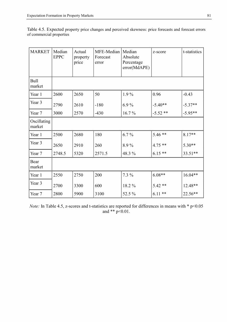
Expectation Formation in Property Markets 81
Table 4.5. Expected property price changes and perceived skewness: price forecasts and forecast errors
of commercial properties
MARKET MedianEPPC
Actualpropertyprice
MFE-MedianForecasterror
MedianAbsolutePercentageerror(MdAPE)
z-score t-statistics
Bullmarket
Year 1 2600
2790
2650
2610
50
-180
1.9 %
6.9 %
0.96
-5.40**
-0.43
-5.37**Year 3
Year 7 3000 2570 -430 16.7 % -5.52 ** -5.95**
Oscillatingmarket
Year 1 2500
2650
2680
2910
180
260
6.7 %
8.9 %
5.46 **
4.75 **
8.17**
5.30**Year 3
Year 7 2748.5 5320 2571.5 48.3 % 6.15 ** 33.51**
Bearmarket
Year 1 2550
2700
2750
3300
200
600
7.3 %
18.2 %
6.08**
5.42 **
16.04**
12.48**Year 3
Year 7 2800 5900 3100 52.5 % 6.11 ** 22.56**
Note: In Table 4.5, z-scores and t-statistics are reported for differences in means with * p<0.05and ** p<0.01.

82 Chapter 4
References
Barberis, N., Shleifer, A., and R. Vishny (1998), A Model of Investor Sentiment, Journal of
Financial Economics 49, 307-343.
Benartzi, S. (2001). Excessive extrapolation and the allocation of 401 (k) accounts to company
stock. The Journal of Finance, 56(5), 1747-1764.
Black, R. T., & Diaz III, J. (1996). The use of information versus asking price in the real property
negotiation process. Journal of Property Research, 13(4), 287-297.
Bokhari, S., & Geltner, D. (2011). Loss aversion and anchoring in commercial real estate pricing:
Empirical evidence and price index implications. Real Estate Economics, 39(4), 635-670.
Case, K.E., & Shiller, R.J. (1989). The Efficiency of the Market for Single-Family Homes. The
American Economic Review, 79(1), 125-137.
Case, K. E., & Shiller, R. J. (1990). Forecasting prices and excess returns in the housing
market. Real Estate Economics, 18(3), 253-273.
Case, K. E., & Shiller, R. J. (2003). Is there a bubble in the housing market?. Brookings Papers on
Economic Activity, 2003(2), 299-362.
Case, K. E., Shiller, R. J., & Thompson, A. (2012). What have they been thinking? Home buyer
behavior in hot and cold markets (No. w18400). National Bureau of Economic Research.
Clayton, J. (1996). Rational expectations, market fundamentals and housing price volatility. Real
Estate Economics, 24(4), 441-470.
De Bondt, W. P. (1993). Betting on trends: Intuitive forecasts of financial risk and return.
International Journal of forecasting, 9(3), 355-371.
Fama, E. F. (1970). Efficient capital markets: A review of theory and empirical work*. The journal
of Finance, 25(2), 383-417.
Farlow (2005). Farlow, UK House prices, Consumption and GDP, in a global context.OxfordUniversity.
Fuster, A., Laibson, D., & Mendel, B. (2010). Natural expectations and macroeconomic
fluctuations. The Journal of Economic Perspectives, 24(4), 67-84.
Gelain, P., & Lansing, K. J. (2013). House prices, expectations, and time-varying fundamentals.
Federal Reserve Bank of San Francisco Working Paper, 3.
Geltner, D. M., Miller, N. G., Clayton, J., Eichholtz, P., Calhoun, J. W., Shaut, D., & Design, C. M.
(2010). Commercial real estate analysis and investments.
Gervais, S., Heaton, J. B., & Odean, T. (2002). The positive role of overconfidence and optimism
in investment policy. Rodney L White Center For Financial Research-Working Papers-.
Glaeser, E. L. (2013). A Nation of Gamblers: Real Estate Speculation and American History. The
American Economic Review, 103(3), 1-42.

Expectation Formation in Property Markets 83
Glaser, M., Langer, T., & Weber, M. (2007). On the trend recognition and forecasting ability of
professional traders. Decision Analysis,4(4), 176-193.
Granziera, E., and Kozicki, S. (2012). House price dynamics: Fundamentals and expectations (No.
2012-12). Bank of Canada Working Paper.
Greenwood, R. and S. Hanson (2010), Issuer Quality and Corporate Bond Returns, Working
paper, Harvard University.
Greenwood, R., and Shleifer, A. (2013). Expectations of returns and expected returns (No.
w18686). National Bureau of Economic Research.
Griffin, D., and Tversky, A. (1992). The weighing of evidence and the determinants of
confidence. Cognitive psychology, 24(3), 411-435.
Haruvy, E., Lahav, Y., & Noussair, C. N. (2007). Traders' expectations in asset markets:
experimental evidence. The American Economic Review, 97(5), 1901-1920.
Herring, R., and Wachter, S. (2003). Bubbles in real estate markets. Asset Price Bubbles: The
Implications for Monetary, Regulatory, and International Policies, 217.
Hey, J. D. (1994). Expectations formation: Rational or adaptive or ?. Journal of Economic
Behavior & Organization, 25(3), 329-349.
Hommes, C., Sonnemans, J., Tuinstra, J., & Van de Velden, H. (2005). Coordination of
expectations in asset pricing experiments. Review of Financial Studies, 18(3), 955-980.
Hommes, C. (2011). The heterogeneous expectations hypothesis: Some evidence from the lab.
Journal of Economic Dynamics and Control, 35(1), 1-24.
Kahneman, D., and Lovallo, D. (1993). Timid choices and bold forecasts: A cognitive perspective
on risk taking. Management science, 39(1), 17-31.
Kahneman, D. (2011). Thinking, fast and slow. Macmillan.
Kouwenberg, R., & Zwinkels, R. (2010). Chasing trends in the US housing market. Erasmus
University Rotterdam working paper.
Lakonishok, J., Shleifer, A., and R. Vishny (1994), Contrarian Investment, Extrapolation, and
Risk, Journal of Finance 49, 1541-1578.
Lambson, V. E., McQueen, G. R., & Slade, B. A. (2004). Do Out of State Buyers Pay More for
Real Estate? An Examination of Anchoring Induced Bias and Search Costs. Real Estate
Economics, 32(1), 85-126.
Lee, C., Shleifer, A., & Thaler, R. H. (1991). Investor sentiment and the closed end fund
puzzle. The Journal of Finance, 46(1), 75-109.
Lichtenstein, S., and Slovic, P. (1971). Reversals of preference between bids and choices in
gambling decisions. Journal of experimental psychology, 89(1), 46.
Lucas Jr, R. E. (1972). Expectations and the Neutrality of Money. Journal of economic
theory, 4(2), 103-124.
Mankiw, N. G., & Weil, D. N. (1989). The baby boom, the baby bust, and the housing
market. Regional science and urban economics, 19(2), 235-258.

84 Chapter 4
Modigliani, F. & Grunberg, E. (1954). The predictability of social events. The Journal of Political
Economy, 465-478.
Muradoglu, G. (2002). Portfolio managers' and novices' forecasts of risk and return: are there
predictable forecast errors?. Journal of Forecasting, 21(6), 395-416.
Muth, J. F. (1961). Rational expectations and the theory of price movements. Econometrica:
Journal of the Econometric Society, 315-335.
Nationwide Nationwide s House Price Index (2014). House Prices Fall. Retrieved from:
http://www.nationwide.co.uk/about/house-price-index/headlines
Northcraft, G. B., and Neale, M. A. (1987). Experts, amateurs, and real estate: An anchoring-and-
adjustment perspective on property pricing decisions. Organizational behavior and human
decision processes, 39(1), 84-97.
Piazzesi, M., & Schneider, M. (2009). Momentum Traders in the Housing Market: Survey
Evidence and a Search Model. The American economic review,99(2), 406-411.
Sargent, Thomas J. (1986). Rational Expectations and Inflation. New York: Harper and Row.
Shiller, R. J. (2005). Irrational exuberance. Random House LLC.
Shiller, R. J. (2007). Understanding recent trends in house prices and home ownership (No.
w13553). National Bureau of Economic Research.
Shiller, R. J. (2011). The Sickness Beneath the Slump. New York Times, 6.
Shiller, R. J. (2014). Speculative asset prices. American Economic Review,104(6), 1486-1517.
Shleifer, A., & Vishny, R. W. (1997). The limits of arbitrage. The Journal of Finance, 52(1), 35-55.
Tversky, A., & Kahneman, D. (1974). Judgment under uncertainty: Heuristics and biases. Science,
185(4157), 1124-1131.
Vissing-Jørgensen, A. (2004), Perspectives on behavioural finance: does irrationality disappear
with wealth? Evidence from expectations and actions in M. Gertler and K. Rogo (eds.), NBER
Macroeconomics Annual 2003. Cambridge, Mass. MIT Press, 139.194.
Quigley, J. M. (1999). Real Estate Prices and Economic Cycles. International Real Estate Review,
2(1), 1-20.


Hana COSIC
Essays in BehaviouralEconomics
Résumé
Insérer votre résumé en français suivi des mots-clés
1000 caractères maximum
Pourquoi prend-on ou non des risques ? Pourquoi ne recycle-t-on pas davantage ? En situation
d incertitude, quels prix immobiliers peut-on anticiper ? Pour d éventuelles explications et pronostics
concernant ces questions, les principes d économie comportementale peuvent être invoqués.
L économie comportementale (CE) est l association de la psychologie et de l économie ayant pour
but de donner une explication aux comportements observés sur les marchés, comportements
humains faisant preuve de rationalité limitée et de raisonnements complexes (Mullainathan et
Thaler, 2000).
L étude de l économie comportementale a inspiré un grand nombre de théories différentes et a
étéutilisée dans de nombreuses applications empiriques et cette thèse suit le même schéma en
explorant différentes applications de l économie comportementale. Cette thèse développe trois
nouvelles extensions de l économie comportementale aux champs du management, du choix en
termes de politiques et en termes de décision d investissement immobilier.

Résumé en anglais
Insérer votre résumé en anglais suivi des mots-clés
Why do we take risks or we do not? Why do not we recycle more? Under uncertainty what do we
expect will happen to our home prices? These and many other questions are asked on daily basis.
For possible explanations and answers to these and similar questions principles of behavioural
economics can be used. Behavioural economics (BE) is the combination of psychology
andeconomics that investigates what happens in markets in which some of agents display human
limitations and complications (Mullainathan and Thaler, 2000). Behavioural economics provides
more realistic psychological foundations to increase explanatory and predictive power of economic
theory. The study of behavioural economics has inspired a number of different theories and has
been used in many applications, and this thesis follows the same path and investigates different
applications of behavioural economics. This thesis explores three novel applications of behavioural
economics to management, policy making and property investment decision making.