The Social Network Mixtape: Essays on the Economics of the Digital World

Guy Aridor

Submitted in partial fulfillment of therequirements for the degree of

Doctor of Philosophyunder the Executive Committee

of the Graduate School of Arts and Sciences

COLUMBIA UNIVERSITY

2022

© 2022

Guy Aridor

All Rights Reserved

Abstract

The Social Network Mixtape: Essays on the Economics of the Digital World

This dissertation studies economic issues in the digital economy with a specific focus on the

economic aspects of how firms acquire and use consumer data.

Chapter 1 empirically studies the drivers of digital attention in the space of social media

applications. In order to do so I conduct an experiment where I comprehensively monitor how

participants spend their time on digital services and use parental control software to shut off

access to either their Instagram or YouTube. I characterize how participants substitute their time

during and after the restrictions. I provide an interpretation of the substitution during the

restriction period that allows me to conclude that relevant market definitions may be broader than

those currently considered by regulatory authorities, but that the substantial diversion towards

non-digital activities indicates significant market power from the perspective of consumers for

Instagram and YouTube. I then use the results on substitution after the restriction period to

motivate a discrete choice model of time usage with inertia and, using the estimates from this

model, conduct merger assessments between social media applications. I find that the inertia

channel is important for justifying blocking mergers, which I use to argue that currently debated

policies aimed at curbing digital addiction are important not only just in their own right but also

from an antitrust perspective and, in particular, as a potential policy tool for promoting

competition in these markets. More broadly, my paper highlights the utility of product

unavailability experiments for demand and merger analysis of digital goods. I thank Maayan

Malter for working together with me on collecting the data for this paper.

Chapter 2 then studies the next step in consumer data collection process – the extent to which a

firm can collect a consumer’s data depends on privacy preferences and the set of available privacy

tools. This chapter studies the impact of the General Data Protection Regulation on the ability of

a data-intensive intermediary to collect and use consumer data. We find that the opt-in

requirement of GDPR resulted in 12.5% drop in the intermediary-observed consumers, but the

remaining consumers are trackable for a longer period of time. These findings are consistent with

privacy-conscious consumers substituting away from less efficient privacy protection (e.g, cookie

deletion) to explicit opt out—a process that would make opt-in consumers more predictable.

Consistent with this hypothesis, the average value of the remaining consumers to advertisers has

increased, offsetting some of the losses from consumer opt-outs. This chapter is jointly authored

with Yeon-Koo Che and Tobias Salz.

Chapter 3 and Chapter 4 make up the third portion of the dissertation that studies one of the most

prominent uses of consumer data in the digital economy – recommendation systems. This chapter

is a combination of several papers studying the economic impact of these systems.

The first paper is a joint paper with Duarte Gonçalves which studies a model of strategic

interaction between producers and a monopolist platform that employs a recommendation system.

We characterize the consumer welfare implications of the platform’s entry into the production

market. The platform’s entry induces the platform to bias recommendations to steer consumers

towards its own goods, which leads to equilibrium investment adjustments by the producers and

lower consumer welfare. Further, we find that a policy separating recommendation and

production is not always welfare improving. Our results highlight the ability of integrated

recommender systems to foreclose competition on online platforms.

The second paper turns towards understanding how such systems impact consumer choices and is

joint with Duarte Gonçalves and Shan Sikdar. In this paper we study a model of user

decision-making in the context of recommender systems via numerical simulation. Our model

provides an explanation for the findings of [1], where, in environments where recommender

systems are typically deployed, users consume increasingly similar items over time even without

recommendation. We find that recommendation alleviates these natural filter-bubble effects, but

that it also leads to an increase in homogeneity across users, resulting in a trade-off between

homogenizing across-user consumption and diversifying within-user consumption. Finally, we

discuss how our model highlights the importance of collecting data on user beliefs and their

evolution over time both to design better recommendations and to further understand their impact.

Table of Contents

Acknowledgments . . . . . . . . . . . . . . . . . . . . . . . . . . . . . . . . . . . . . . . . xiii

Dedication . . . . . . . . . . . . . . . . . . . . . . . . . . . . . . . . . . . . . . . . . . . . xv

Chapter 1: Drivers of Digital Attention: Evidence from a Social Media Experiment . . . . 1

1.1 Introduction . . . . . . . . . . . . . . . . . . . . . . . . . . . . . . . . . . . . . . 1

1.2 Related Work . . . . . . . . . . . . . . . . . . . . . . . . . . . . . . . . . . . . . 9

1.3 Experiment Description and Data . . . . . . . . . . . . . . . . . . . . . . . . . . . 13

1.3.1 Recruitment . . . . . . . . . . . . . . . . . . . . . . . . . . . . . . . . . . 13

1.3.2 Automated Data Collection . . . . . . . . . . . . . . . . . . . . . . . . . . 14

1.3.3 Survey Data . . . . . . . . . . . . . . . . . . . . . . . . . . . . . . . . . . 16

1.3.4 Experiment Timeline . . . . . . . . . . . . . . . . . . . . . . . . . . . . . 18

1.3.5 Experimental Restrictions . . . . . . . . . . . . . . . . . . . . . . . . . . 19

1.3.6 Pilot Experiment . . . . . . . . . . . . . . . . . . . . . . . . . . . . . . . 20

1.4 Descriptive Statistics . . . . . . . . . . . . . . . . . . . . . . . . . . . . . . . . . 21

1.5 Experimental Results . . . . . . . . . . . . . . . . . . . . . . . . . . . . . . . . . 25

1.5.1 Time Substitution During the Restriction Period . . . . . . . . . . . . . . . 25

1.5.2 Time Substitution After Restriction Period . . . . . . . . . . . . . . . . . . 37

1.6 Model of Time Usage with Inertia . . . . . . . . . . . . . . . . . . . . . . . . . . 43

i

1.6.1 Model and Identification . . . . . . . . . . . . . . . . . . . . . . . . . . . 43

1.6.2 Model Estimates and Validation . . . . . . . . . . . . . . . . . . . . . . . 46

1.6.3 Counterfactual: No Long-Term Inertia . . . . . . . . . . . . . . . . . . . . 49

1.7 Merger Analysis . . . . . . . . . . . . . . . . . . . . . . . . . . . . . . . . . . . . 52

1.7.1 Upward Pricing Pressure Test . . . . . . . . . . . . . . . . . . . . . . . . . 53

1.7.2 Data and Additional Discussion . . . . . . . . . . . . . . . . . . . . . . . 55

1.7.3 Merger Evaluation . . . . . . . . . . . . . . . . . . . . . . . . . . . . . . 58

1.8 Conclusion . . . . . . . . . . . . . . . . . . . . . . . . . . . . . . . . . . . . . . 61

Chapter 2: The Effect of Privacy Regulation on the Data Industry: Empirical Evidencefrom GDPR . . . . . . . . . . . . . . . . . . . . . . . . . . . . . . . . . . . . 63

2.1 Introduction . . . . . . . . . . . . . . . . . . . . . . . . . . . . . . . . . . . . . . 63

2.2 Institutional Details . . . . . . . . . . . . . . . . . . . . . . . . . . . . . . . . . . 70

2.2.1 European Data Privacy Regulation . . . . . . . . . . . . . . . . . . . . . . 70

2.2.2 Consumer-Tracking Technology . . . . . . . . . . . . . . . . . . . . . . . 73

2.3 Data and Empirical Strategy . . . . . . . . . . . . . . . . . . . . . . . . . . . . . 76

2.3.1 Data Description . . . . . . . . . . . . . . . . . . . . . . . . . . . . . . . 76

2.3.2 Empirical Strategy . . . . . . . . . . . . . . . . . . . . . . . . . . . . . . 77

2.4 Consumer Response to GDPR . . . . . . . . . . . . . . . . . . . . . . . . . . . . 79

2.4.1 Opt-Out Usage . . . . . . . . . . . . . . . . . . . . . . . . . . . . . . . . 79

2.4.2 Persistence of Identifier . . . . . . . . . . . . . . . . . . . . . . . . . . . . 83

2.5 GDPR and Online Advertising . . . . . . . . . . . . . . . . . . . . . . . . . . . . 88

2.6 GDPR and Prediction of Consumer Behavior . . . . . . . . . . . . . . . . . . . . 93

2.6.1 Prediction Evaluation Measures . . . . . . . . . . . . . . . . . . . . . . . 95

ii

2.6.2 Prediction Performance . . . . . . . . . . . . . . . . . . . . . . . . . . . . 97

2.7 Conclusion . . . . . . . . . . . . . . . . . . . . . . . . . . . . . . . . . . . . . . 99

Chapter 3: Recommenders’ Originals: The Welfare Effects of the Dual Role of Platformsas Producers and Recommender Systems . . . . . . . . . . . . . . . . . . . . . 101

3.1 Introduction . . . . . . . . . . . . . . . . . . . . . . . . . . . . . . . . . . . . . . 101

3.2 Model Setup . . . . . . . . . . . . . . . . . . . . . . . . . . . . . . . . . . . . . . 109

3.3 Consequences of the Platform’s Dual Role . . . . . . . . . . . . . . . . . . . . . . 113

3.3.1 No Platform Production . . . . . . . . . . . . . . . . . . . . . . . . . . . . 113

3.3.2 Platform’s Dual Role . . . . . . . . . . . . . . . . . . . . . . . . . . . . . 115

3.3.3 Welfare Consequences of the Dual Role . . . . . . . . . . . . . . . . . . . 123

3.4 Unbiased Recommendations . . . . . . . . . . . . . . . . . . . . . . . . . . . . . 127

3.4.1 Equilibrium Characterization . . . . . . . . . . . . . . . . . . . . . . . . . 127

3.4.2 Comparison to Dual Role Equilibrium . . . . . . . . . . . . . . . . . . . . 128

3.5 Additional Discussion and Robustness Exercises . . . . . . . . . . . . . . . . . . . 136

3.6 Conclusion . . . . . . . . . . . . . . . . . . . . . . . . . . . . . . . . . . . . . . 138

Chapter 4: Deconstructing the Filter Bubble: User Decision-Making and RecommenderSystems . . . . . . . . . . . . . . . . . . . . . . . . . . . . . . . . . . . . . . 141

4.1 Introduction . . . . . . . . . . . . . . . . . . . . . . . . . . . . . . . . . . . . . . 141

4.2 Related Work. . . . . . . . . . . . . . . . . . . . . . . . . . . . . . . . . . . . . . 144

4.3 Our Model and Preliminaries . . . . . . . . . . . . . . . . . . . . . . . . . . . . . 145

4.3.1 Preliminaries on Expected Utility Theory . . . . . . . . . . . . . . . . . . 145

4.3.2 Model . . . . . . . . . . . . . . . . . . . . . . . . . . . . . . . . . . . . . 146

4.4 Results . . . . . . . . . . . . . . . . . . . . . . . . . . . . . . . . . . . . . . . . . 153

iii

4.4.1 Local Consumption and Filter Bubbles . . . . . . . . . . . . . . . . . . . . 153

4.4.2 User Welfare and Item Diversity . . . . . . . . . . . . . . . . . . . . . . . 155

4.4.3 User Homogenization . . . . . . . . . . . . . . . . . . . . . . . . . . . . . 160

4.5 Recommender System Evaluation . . . . . . . . . . . . . . . . . . . . . . . . . . 161

References . . . . . . . . . . . . . . . . . . . . . . . . . . . . . . . . . . . . . . . . . . . . 165

Appendix A: Supplementary Material for Drivers of Digital Attention: Evidence from aSocial Media Experiment . . . . . . . . . . . . . . . . . . . . . . . . . . . . 181

A.1 Experiment Materials . . . . . . . . . . . . . . . . . . . . . . . . . . . . . . . . . 181

A.1.1 Recruitment Materials . . . . . . . . . . . . . . . . . . . . . . . . . . . . 181

A.1.2 Baseline Survey . . . . . . . . . . . . . . . . . . . . . . . . . . . . . . . . 184

A.1.3 Additional Surveys . . . . . . . . . . . . . . . . . . . . . . . . . . . . . . 189

A.1.4 Software . . . . . . . . . . . . . . . . . . . . . . . . . . . . . . . . . . . . 192

A.1.5 Experiment Timeline . . . . . . . . . . . . . . . . . . . . . . . . . . . . . 194

A.2 Additional Descriptive Statistics Figures and Tables . . . . . . . . . . . . . . . . . 194

A.3 Correlational Relationship Between Welfare and Time . . . . . . . . . . . . . . . . 202

A.4 Additional Experimental Results . . . . . . . . . . . . . . . . . . . . . . . . . . . 206

A.5 Alternative Estimation of Diversion Ratios . . . . . . . . . . . . . . . . . . . . . . 218

A.5.1 Estimation Procedure . . . . . . . . . . . . . . . . . . . . . . . . . . . . . 218

A.5.2 Estimating Diversion Ratios of the Restricted Applications . . . . . . . . . 219

A.5.3 Diversion Ratio Estimates . . . . . . . . . . . . . . . . . . . . . . . . . . 222

A.6 Additional Figures / Tables for Time Usage Model . . . . . . . . . . . . . . . . . . 224

A.7 Upward Pricing Pressure Test Derivation . . . . . . . . . . . . . . . . . . . . . . . 227

iv

A.8 Collection of Survey Responses . . . . . . . . . . . . . . . . . . . . . . . . . . . . 229

Appendix B: Supplementary Material for The Effect of Privacy Regulation on the DataIndustry: Empirical Evidence from GDPR . . . . . . . . . . . . . . . . . . . 234

B.1 Additional Consumer Response Figures . . . . . . . . . . . . . . . . . . . . . . . 234

B.2 Robustness for Consumer Response Results . . . . . . . . . . . . . . . . . . . . . 238

B.2.1 Synthetic Controls . . . . . . . . . . . . . . . . . . . . . . . . . . . . . . 239

B.2.2 Controlling for Differences in Travel Patterns Across Countries . . . . . . . 239

B.3 Consumer Persistence Heterogeneous Treatment Effects . . . . . . . . . . . . . . . 242

B.4 Additional Evidence for “Single Searcher" Inflation . . . . . . . . . . . . . . . . . 247

B.4.1 Setup and Hypotheses . . . . . . . . . . . . . . . . . . . . . . . . . . . . . 247

B.4.2 Data and Estimation . . . . . . . . . . . . . . . . . . . . . . . . . . . . . 248

B.4.3 Results . . . . . . . . . . . . . . . . . . . . . . . . . . . . . . . . . . . . 249

B.5 Additional Advertisement and Auction Figures . . . . . . . . . . . . . . . . . . . 250

B.6 Prediction Evaluation Measures . . . . . . . . . . . . . . . . . . . . . . . . . . . . 251

B.6.1 AUC Primer . . . . . . . . . . . . . . . . . . . . . . . . . . . . . . . . . . 251

B.6.2 Breakdown of MSE . . . . . . . . . . . . . . . . . . . . . . . . . . . . . . 252

B.7 Additional Prediction Figures . . . . . . . . . . . . . . . . . . . . . . . . . . . . . 254

B.8 The Impact of Consumer Persistence and Data Scale on Prediction . . . . . . . . . 255

Appendix C: Supplementary Material for Recommenders’ Originals: The Welfare Effectsof the Dual Role of Platforms as Producers and Recommender Systems . . . 261

C.1 Omitted Proofs . . . . . . . . . . . . . . . . . . . . . . . . . . . . . . . . . . . . 261

C.1.1 Proof of Proposition 1 . . . . . . . . . . . . . . . . . . . . . . . . . . . . 261

C.1.2 Proof of Proposition 2 . . . . . . . . . . . . . . . . . . . . . . . . . . . . 263

v

C.1.3 Proof of Proposition 4 . . . . . . . . . . . . . . . . . . . . . . . . . . . . 263

C.1.4 Proof of Proposition 5 . . . . . . . . . . . . . . . . . . . . . . . . . . . . 265

C.1.5 Proof of Lemma 1 . . . . . . . . . . . . . . . . . . . . . . . . . . . . . . . 266

C.1.6 Proof of Proposition 6 . . . . . . . . . . . . . . . . . . . . . . . . . . . . 266

C.2 Model with Heterogeneous Costs . . . . . . . . . . . . . . . . . . . . . . . . . . . 267

C.2.1 Dual Role: Equilibrium, Welfare Comparison . . . . . . . . . . . . . . . . 267

C.2.2 Unbiased Recommendation: Equilibrium, Welfare Comparison . . . . . . . 268

C.2.3 Discussion . . . . . . . . . . . . . . . . . . . . . . . . . . . . . . . . . . . 270

C.3 Model with Simultaneous Investment . . . . . . . . . . . . . . . . . . . . . . . . . 271

C.3.1 Dual Role Equilibrium Characterization . . . . . . . . . . . . . . . . . . . 271

C.3.2 Welfare Comparison – Dual Role and No Platform Production . . . . . . . 277

C.3.3 Unbiased Recommendation . . . . . . . . . . . . . . . . . . . . . . . . . . 278

vi

List of Figures

1.1 Time on Restricted Applications . . . . . . . . . . . . . . . . . . . . . . . . . . . 40

2.1 Example Consent Notifications . . . . . . . . . . . . . . . . . . . . . . . . . . . . 72

2.2 Illustration of Effects of Different Privacy Means on Data Observed . . . . . . . . 74

2.3 Total Number of Unique Cookies for Two Multi-National Website. . . . . . . . . . 82

2.4 Four Week Persistence for Two Multi-National Websites . . . . . . . . . . . . . . 84

2.5 Change in Search Distribution for One Site . . . . . . . . . . . . . . . . . . . . . . 86

2.6 Week by Week Treatment Effect for Total Clicks, Revenue, and Average Bid . . . . 91

3.1 Equilibrium Investment Levels . . . . . . . . . . . . . . . . . . . . . . . . . . . . 124

3.2 Average Consumer Welfare: Dual Role – No Platform Production . . . . . . . . . 125

3.3 Equilibrium Investment Levels including Unbiased Recommendation . . . . . . . . 129

3.4 Average Consumer Welfare: Dual Role – Unbiased . . . . . . . . . . . . . . . . . 132

3.5 Difference in Market Share for Independent Firm . . . . . . . . . . . . . . . . . . 135

4.1 Local Consumption and Correlation (𝜌) . . . . . . . . . . . . . . . . . . . . . . . 154

4.2 Relationship between Local Consumption and Correlation (𝜌), Risk Aversion (𝛾) . 156

4.3 Relationship between User Welfare, Diversity and Correlation (𝜌), Risk Aversion (𝛾)158

4.4 Diversity vs. Welfare . . . . . . . . . . . . . . . . . . . . . . . . . . . . . . . . . 159

vii

4.5 Relationship between Homogeneity and Common-Value Strength (𝛽), Correlation(𝜌) . . . . . . . . . . . . . . . . . . . . . . . . . . . . . . . . . . . . . . . . . . . 161

A1 Facebook Advertisement . . . . . . . . . . . . . . . . . . . . . . . . . . . . . . . 182

A2 Recruitment Survey . . . . . . . . . . . . . . . . . . . . . . . . . . . . . . . . . . 183

A3 Consent Form and Study Details . . . . . . . . . . . . . . . . . . . . . . . . . . . 185

A4 WTA Elicitation Interface . . . . . . . . . . . . . . . . . . . . . . . . . . . . . . . 188

A5 Hypothetical Consumer Switching Interface . . . . . . . . . . . . . . . . . . . . . 188

A6 Social Media Addiction Scale . . . . . . . . . . . . . . . . . . . . . . . . . . . . . 189

A7 Chrome Extension Interface . . . . . . . . . . . . . . . . . . . . . . . . . . . . . . 192

A8 Parental Control Interface . . . . . . . . . . . . . . . . . . . . . . . . . . . . . . . 193

A9 Experiment Timeline . . . . . . . . . . . . . . . . . . . . . . . . . . . . . . . . . 194

A10 Software Reliability . . . . . . . . . . . . . . . . . . . . . . . . . . . . . . . . . . 195

A11 Distributions of Application Usage Across Treatment Groups . . . . . . . . . . . . 195

A12 Distribution of Daily Phone Usage . . . . . . . . . . . . . . . . . . . . . . . . . . 196

A13 Time on Phone Across the Week . . . . . . . . . . . . . . . . . . . . . . . . . . . 196

A14 Time Off Digital Devices . . . . . . . . . . . . . . . . . . . . . . . . . . . . . . . 197

A15 The Long Tail of Applications . . . . . . . . . . . . . . . . . . . . . . . . . . . . 197

A16 Multihoming . . . . . . . . . . . . . . . . . . . . . . . . . . . . . . . . . . . . . . 199

A17 Distribution of Addiction Classification . . . . . . . . . . . . . . . . . . . . . . . 201

A18 Quantile Treatment Effects of Category Substitution . . . . . . . . . . . . . . . . . 206

A19 Time Spent on Phone Throughout the Week (During Treatment Period) . . . . . . . 210

A20 Quantile Treatment Effects of Overall Phone Time . . . . . . . . . . . . . . . . . . 211

A21 Time on Restricted Applications . . . . . . . . . . . . . . . . . . . . . . . . . . . 212

viii

A22 Quantile Treatment Effects of Post-Restriction Usage . . . . . . . . . . . . . . . . 215

A23 K-means Clustering of Participants . . . . . . . . . . . . . . . . . . . . . . . . . . 224

B1 Week by Week Treatment Effect (Cookies and Recorded Searches) . . . . . . . . . 234

B2 Week by Week Treatment Effect (Consumer Persistence) . . . . . . . . . . . . . . 236

B3 Distribution of Consumer Persistence (1 Week) . . . . . . . . . . . . . . . . . . . 237

B4 Synthetic Controls for Cookies and Recorded Searches . . . . . . . . . . . . . . . 238

B5 Historical Google Trends Travel Patterns . . . . . . . . . . . . . . . . . . . . . . . 240

B6 Week by Week Treatment Effect (Total Advertisements Delivered) . . . . . . . . . 250

B7 Sample ROC Curve . . . . . . . . . . . . . . . . . . . . . . . . . . . . . . . . . . 252

B8 Week by Week Treatment Effect (Average Predicted Probability and Class Propor-tion) . . . . . . . . . . . . . . . . . . . . . . . . . . . . . . . . . . . . . . . . . . 254

B9 Week by Week Treatment Effect (MSE and AUC) . . . . . . . . . . . . . . . . . . 255

C1 Average Welfare Comparisons under Simultaneous Investment . . . . . . . . . . . 279

ix

List of Tables

1.1 Summary Statistics on Usage and WTA . . . . . . . . . . . . . . . . . . . . . . . 22

1.2 Stated Activities . . . . . . . . . . . . . . . . . . . . . . . . . . . . . . . . . . . . 24

1.3 Instagram Category Substitution . . . . . . . . . . . . . . . . . . . . . . . . . . . 30

1.4 YouTube Category Substitution . . . . . . . . . . . . . . . . . . . . . . . . . . . . 30

1.5 Herfindahl–Hirschman Index Across Market Definitions . . . . . . . . . . . . . . . 31

1.6 Newly Installed Applications During the Restriction Period . . . . . . . . . . . . . 33

1.7 Second-Choice Diversion Ratios . . . . . . . . . . . . . . . . . . . . . . . . . . . 48

1.8 Market Shares (No Inertia) . . . . . . . . . . . . . . . . . . . . . . . . . . . . . . 51

1.9 Summary of UPP Merger Analysis . . . . . . . . . . . . . . . . . . . . . . . . . . 58

2.1 Difference-in-Differences Estimates for Cookies and Searches . . . . . . . . . . . 82

2.2 Difference-in-Differences Estimates for Consumer Persistence . . . . . . . . . . . 84

2.3 Difference-in-Differences Estimates for Advertising Outcome Variables . . . . . . 92

2.4 Difference-in-Differences Estimates for Prediction Outcome Variables . . . . . . . 98

A1 Gender Distribution . . . . . . . . . . . . . . . . . . . . . . . . . . . . . . . . . . 194

A2 Age Distribution . . . . . . . . . . . . . . . . . . . . . . . . . . . . . . . . . . . . 195

A3 Time Spent on Application Categories on Phone . . . . . . . . . . . . . . . . . . . 198

A4 Extent of Multihoming . . . . . . . . . . . . . . . . . . . . . . . . . . . . . . . . 199

x

A5 Time Spent on Applications of Interest . . . . . . . . . . . . . . . . . . . . . . . . 200

A6 Post Frequency on Applications of Interest . . . . . . . . . . . . . . . . . . . . . . 201

A7 Time vs. WTA (Collected Data, Levels) . . . . . . . . . . . . . . . . . . . . . . . 203

A8 Time vs. WTA (Collected Data, Logs) . . . . . . . . . . . . . . . . . . . . . . . . 204

A9 Time vs WTA, By Activity . . . . . . . . . . . . . . . . . . . . . . . . . . . . . . 205

A10 Stated Substitution Patterns . . . . . . . . . . . . . . . . . . . . . . . . . . . . . . 207

A11 Instagram Type of App Substitution . . . . . . . . . . . . . . . . . . . . . . . . . 208

A12 YouTube Type of Application Substitution . . . . . . . . . . . . . . . . . . . . . . 208

A13 Survey of Time on Restricted App During Treatment Week Off Phone . . . . . . . 209

A14 Substitution towards the Computer During Treatment Week . . . . . . . . . . . . . 210

A15 Survey of Time Spent on Other Media During Restriction Period . . . . . . . . . . 211

A16 Instagram Post-Restriction Usage . . . . . . . . . . . . . . . . . . . . . . . . . . . 213

A17 YouTube Post-Restriction Usage . . . . . . . . . . . . . . . . . . . . . . . . . . . 214

A18 Perceived Endline Substitution Patterns . . . . . . . . . . . . . . . . . . . . . . . 215

A19 One Month Post-Experiment Survey Results . . . . . . . . . . . . . . . . . . . . . 216

A20 Instagram Post-Restriction Usage of Non-Restricted Applications . . . . . . . . . . 217

A21 YouTube Post-Restriction Usage of Non-Restricted Applications . . . . . . . . . . 217

A22 Diversion Ratio Estimates . . . . . . . . . . . . . . . . . . . . . . . . . . . . . . . 223

A23 Nonparametric Diversion Ratio Estimates . . . . . . . . . . . . . . . . . . . . . . 223

A24 Demand Model Parameter Estimates . . . . . . . . . . . . . . . . . . . . . . . . . 225

A25 Model Validation . . . . . . . . . . . . . . . . . . . . . . . . . . . . . . . . . . . 226

A26 Second-Choice Diversion Ratios (No Inertia) . . . . . . . . . . . . . . . . . . . . 226

A27 Percentage Change in Diversion Ratio (No Inertia) . . . . . . . . . . . . . . . . . 226

xi

A28 Percentage Change in Market Share (No Inertia) . . . . . . . . . . . . . . . . . . . 227

B1 Difference-in-Differences Estimates for Sales Activity . . . . . . . . . . . . . . . . 235

B2 Summary Statistics of Consumer Persistence . . . . . . . . . . . . . . . . . . . . . 237

B3 Difference-in-Differences Estimates With Google Trends controls . . . . . . . . . 241

B4 Consumer Persistence by Week - OS Heterogeneous Treatment Effects . . . . . . . 245

B5 Consumer Persistence - Browser Heterogeneous Treatment Effects . . . . . . . . . 246

B6 Difference-in-Differences Estimates for Advertisements Delivered . . . . . . . . . 250

B7 Summary Statistics, Bids . . . . . . . . . . . . . . . . . . . . . . . . . . . . . . . 251

B8 Difference-in-Differences Estimates for Relevance and Calibration . . . . . . . . . 253

B9 Prediction Error and Scale of Data . . . . . . . . . . . . . . . . . . . . . . . . . . 258

B10 Sliding Window Data Scale and Aggregate Prediction Error . . . . . . . . . . . . . 259

B11 Consumer Persistence and Prediction Error . . . . . . . . . . . . . . . . . . . . . . 260

xii

Acknowledgements

The fact that I was able to complete this dissertation is a testimony to all those helped me

personally throughout my life. I want to thank my parents, Meir and Orly Aridor, for all their

support and encouragement as well as their persistent belief in me that allowed me to be in the

position to complete a PhD. Without the loving support of Melanie Monastirsky I am not sure I

would have been able to finish the dissertation, especially in the last year of the PhD when I was

not sure the first chapter was going to work out, and I am eternally grateful. I thank my sister Zoe

Aridor for occasionally picking up my phone calls and always being there for me. I also want to

thank my grandparents – Hedva and Beni Piterman, Edward and Yvette Aridor – for everything

they did to help my family and give me the ability to be lucky enough to be in a situation where I

could complete a PhD. Finally, I want to thank some of my friends for helping me get through

some of the rough patches in the whole process: Matt Auerbach, Vinayak Iyer, Austin Kipp,

Haaris Mateen, Maayan Malter, Haaris Mateen, Felipe Netto, Silvio Ravaioli, Shan Sikdar,

Russell Steiner, Yeji Sung, Molly Varoga, Lauren Wisbeski, and Xiao Xu.

Academically, I was blessed with a set of advisors whose open-mindedness and intellect allowed

me to explore a diverse set of topics of interest during graduate school. I thank Yeon-Koo Che for

his open-mindedness that enabled me to craft what I hope is a high quality dissertation. I thank

Tobias Salz for continuing to advise me despite his move to MIT and for his constant stream of

creative and insightful feedback that helped me push my work forward. I thank Michael

Woodford for introducing me to a fascinating selection of topics and encouraging me to pursue

work at the intersection of economics and computer science. I thank Andrey Simonov for helping

xiii

me develop my first chapter to its full potential and providing me incredibly high quality and

insightful feedback as I worked through the project. I thank Andrea Prat and John Asker for

providing excellent feedback on my work in the industrial organization colloquium during my

time at Columbia. I thank Matt Backus for his insights into antitrust issues that shaped the

approach that I took in the first chapter of my dissertation. I thank Alex Slivkins for teaching me

the ropes of how to write a good paper and navigating the publication process – our paper on

competing bandits which I did not include in this dissertation taught me a great deal. I thank

Maayan Malter for helping me out with the data collection on the first chapter of the dissertation.

I thank Duarte Gonçalves for his inspirational and dogged persistence in the face of obstacles and

for many entertaining academic conversations. I thank Shan Sikdar for not only being a dummy

test subject for my experiments with parental control software but also for foraying into academic

work with me on the fourth chapter of the dissertation. Finally, I would be remiss to not thank my

academic advisors from my undergraduate days at Boston University – Hsueh-Ling Huynh, Jordi

Jaumandreu, and Robert King — for pushing me even back then to explore the eclectic set of

topics at the intersection of economics and computer science that ended up shaping the scope of

topics I studied in graduate school.

xiv

Dedication

To all the people who I’ve crossed paths with who, directly or indirectly, shaped the way I

see the world.

xv

Chapter 1: Drivers of Digital Attention: Evidence from a Social Media

Experiment

1.1 Introduction

In the past two decades social media has evolved from a niche online tool for connecting with

friends to an essential aspect of people’s lives. Indeed, the most prominent social media applica-

tions are now used by a majority of individuals around the world and these same applications are

some of the most valuable companies in the modern day.1 Due to the sheer amount of time spent on

these applications and concentration of this usage on only a few large applications, there has been a

global push towards understanding whether and how to regulate these markets [2, 3].2 At the heart

of the issue is that consumers pay no monetary price to use these applications, which renders the

standard antitrust toolkit difficult to apply as the lack of prices complicates the measurement of de-

mand and identification of plausible substitutes for these applications.3 The demand measurement

problem is further compounded by the fact that some fraction of usage may be driven by addiction

to the applications or, more broadly, inertia [5, 6]. This facet of demand inflates the market share

of these applications and makes it difficult to disentangle whether substitution between prominent

applications is due to habitual usage or direct substitutability. This decomposition is further infor-

1For instance, Facebook, which owns several prominent social media and messaging applications, is the 6th mostvaluable company in the world with over a trillion dollars in market capitalization. Additionally, Twitter has a marketcapitalization of over 50 billion dollars and is in the top 500 highest valued companies in the world according tohttps://companiesmarketcap.com/ on August 30th, 2021.

2As pointed out by [4], the increased concentration of consumer attention can have ramifications far beyond thismarket alone since increased concentration in this market influences the ability for firms to enter into product marketsthat rely on advertising for product discovery.

3This issue was at the heart of the Facebook-Instagram and Facebook-WhatsApp mergers. Without prices, regula-tory authorities resorted to market definitions that only focused on product characteristics, as opposed to substitutionpatterns of usage. For instance, Instagram’s relevant market was only photo-sharing applications and WhatsApp’s rel-evant market was only messaging applications. This issue continues to play a role in the ongoing FTC lawsuit againstFacebook where a similar debate is ongoing.

1

mative about whether policies aimed at curbing digital addiction are important from an antitrust

perspective. These two complications together have led to substantial difficulties in understanding

the core aspects of consumer demand that are crucial for market evaluation and merger analysis.

In this paper I empirically study demand for these applications and illustrate how these findings

can be used for conducting merger evaluation in such markets. I conduct a field experiment where,

using parental control software installed on their phone and a Chrome Extension installed on their

computer, I continuously track how participants spend time on digital services for a period of 5

weeks.4 I use the parental control software to shut off access to YouTube or Instagram on their

phones for a period ranging from one to two weeks. I explicitly design the experiment so that there

is variation in the length of the restriction period and continue to track how participants allocate

their time for two to three weeks following the restrictions. The time usage substitution patterns

observed during the restriction period allow me to determine plausible substitutes, despite the lack

of prices. The extent to which there are persistent effects of the restrictions in the post-restriction

period allows me to uncover the role that inertia plays in driving demand for these applications.

I exploit the rich data and variation generated by the experiment to investigate aspects of de-

mand related to competition policy and merger analysis. I provide an interpretation of the time

substitution observed when the applications are restricted; this interpretation sheds light on rele-

vant market definitions for the restricted applications – the set of applications that are considered

substitutable relative to the application of interest – which have played a prominent role in antitrust

policy debates. I further use the experimental substitution patterns to determine whether there is

evidence of “dynamic" elements of demand as well as important dimensions of preference hetero-

geneity. Guided by these results, I estimate a discrete choice model of time usage with inertia to

produce an important measure of substitution that is crucial for merger analysis: diversion ratios.

I provide estimates of diversion ratios both with and without inertia, disentangling the extent of

diversion due to inertia versus inherent substitutability of the applications. In order to understand

how important inertia is for merger analysis, I apply the two sets of diversion ratio estimates to

4This ensures that I have objective measures of time usage which is crucial for my study as subjective measuresof time spent on social media applications are known to be noisy and inaccurate [7].

2

evaluate mergers between social media applications. One important policy interpretation of the no

inertia counterfactual is to provide insight into how and whether policies aimed at curbing digi-

tal addiction are important not just in their own right, but also in influencing usage and diversion

between the applications to the extent that they would influence merger assessments.

Broader antitrust concerns motivate the following two questions about substitution patterns:

what types of activities do participants substitute to and is this substitution concentrated on promi-

nent applications or dispersed among the long tail? The most directly relevant question is whether

or not there is evidence that they substitute across application categories. This has featured promi-

nently in debates between these applications and regulators since the degree to which applications

such as YouTube and Instagram are substitutable is important for monopolization claims about

Facebook and mergers between different types of applications. Even if there is cross-category

substitution, then it is also important to understand to what extent this is concentrated towards

popular applications such as YouTube, within the vast Facebook ecosystem which spans applica-

tion categories, or dispersed towards smaller applications competing with them. I argue that the

set of applications that consumers substitute to during the restriction period serves as the broadest

market definition since it measures consumer substitution at the “choke" price – the price which is

sufficiently high so that no one would use the application at all.5 Thus, even with zero consumer

prices, the product unavailability variation alone allows me to assess the plausibility of claims that

applications such as YouTube and Instagram directly compete against each other for consumer

time.

In order to assess the extent of cross application category substitution, I manually pair each

observed application in the data with the category it is assigned to on the Google Play Store. For

the Instagram restriction group, I find a 22.4% increase in time spent on other social applications,

but also a marginally significant 10.2% increase in time spent on communication applications.

For the YouTube restriction group, I find that there is a null effect of substitution towards other

5This is similar to the interpretation given to such experiments in [8]. Note that the variation does not isolate theobserved substitution to be about price exclusively. Indeed, one can broadly interpret this as the substitution at thechoke advertising load or application quality as well. This will lead to some nuance in the value of this variation in thedemand model, but is not first-order for the relevant market definition exercise.

3

entertainment applications, but also find a 15.2% increase in time spent on social applications.

While this provides evidence for cross-category substitution, there is a notable asymmetry where

blocking Instagram, a social media application, does not lead to substitution towards entertainment

applications such as YouTube, whereas blocking YouTube, an entertainment application, leads to

substitution towards social applications such as Instagram and Facebook.6 Pairing these results

with the conservative relevant market definition test implies that market definitions ought to span

across the application categories between which I observe substitution. I show that, under this

market definition, concentration is meaningfully lower relative to only using application categories

as the relevant market definition.

There are several nuances to the implications of the application category substitution on the

degree of market concentration. First, for both the YouTube and Instagram restriction, there is

considerable substitution towards the outside option – off the phone.7 This indicates that, even if I

consider substitutes across all the categories on the phone, participants were not able to find a viable

substitute in any other application. The framing of the debate in terms of within versus across

category substitution therefore is potentially misleading as this shift towards the outside option

implies that both YouTube and Instagram have considerable market power. Second, a large part of

this market concentration is due to Facebook’s joint ownership of Facebook, Instagram, Messenger,

and WhatsApp; considering these as being independently owned applications substantially reduces

the degree of market concentration even more so than multi-category market definitions. Indeed,

non-Instagram Facebook owned applications have a 17.9% increase in time spent for the Instagram

restriction group. Thus, some of the observed cross-category substitution is substitution within the

Facebook ecosystem. Third, I elicit a subjective measure of how each participant uses the set of

prominent social media, entertainment, and communication applications and find that, especially

for social media applications, participants use the applications for different reasons ranging from

6This casts some subtlety to a debate in [3] between Facebook and regulators where Facebook uses outages ofYouTube to claim that they compete with them. My experimental results point to a similar result in response to theYouTube restriction, but notably I observe an asymmetry where the reverse is not true during the Instagram restriction.Indeed, for Instagram, there is more within category substitution relative to cross category substitution.

7Using the data from the weekly surveys and the Chrome Extension, I am able to conclude that only a smallfraction of this time is due to substitution to the restricted application on other devices.

4

social connection to pure entertainment. This points to the application categories not necessarily

capturing the different uses of these applications and partially explaining some of the observed

cross-category substitution.

The experimental design further allows me to understand whether there are potentially dynamic

elements associated with demand by assessing whether the restrictions modify post-restriction time

allocations on the restricted application as well as those substituted to during the restriction period.

There are two possible channels through which the restrictions could impact post-restriction usage.

The first possible channel is that the restriction could serve as a shock to participants’ habits and

depress usage after the restriction period. While I remain agnostic about the mechanism through

which this change would occur, one important descriptive statistic is that up to 51% of the partic-

ipants in the study are psychologically addicted to social media according to the scale by [9] that

participants complete in the baseline survey. Thus, the experiment could serve as a shock to the

addictive habits of the participants in the experiment. The second possible channel is intertempo-

ral substitution whereby the restrictions lead participants to defer consumption until the restriction

period is lifted. These two channels are not mutually exclusive and the aim is to assess which

of these is first-order in modeling demand. This motivates why I design the experiment so that

the restriction lengths are relatively long and also varied in length as one might expect that these

effects are more apparent the longer the restriction length is.

I explicitly test whether there is a spike in usage of the restricted application on the day that

it is no longer blocked for the participants and find no evidence of this for either the one or two

week restriction group. I use this as evidence that the intertemporal substitution channel is not

prominent as one would expect the built up usage during the restriction period to lead to a spike

in usage when the application was returned. I find a consistent body of evidence that there is a

persistent reduction in time spent on the restricted applications and that this is primarily driven

by the participants that had the two week restriction, but not those for the one week restriction.

For the Instagram restriction, the two week restriction group reduced average daily usage relative

to the control group by 5 minutes and had a similar reduction relative to the one week restriction

5

group. Estimating quantile treatment effects indicates that this is mainly driven by the heaviest

users of the applications. A survey sent after the study indicates that this reduction in time spent

persists even a month following the conclusion of the study. For the YouTube restriction, there

is suggestive evidence of a similar difference between the one and two week restriction group,

but the resulting difference in average daily usage is not statistically significant. However, I find

that participants in the YouTube restriction spent more time on applications installed during the

restriction period relative to the control group and persisted to use these applications even in the

post-restriction period. I use both the persistent reduction in usage of Instagram and the increased

usage of applications installed during the restriction period of YouTube as evidence that inertia

plays a role in demand for these applications.

The experimental results shed light on aspects of demand required to understand the usage

of these applications. However, in order to conduct merger analyses, an important output of a

demand study is estimates of diversion ratios. The diversion ratio from application 𝑖 to application

𝑗 is defined as the fraction of sales / consumption that gets diverted from application 𝑖 to application

𝑗 as a result of a change in price / quality / availability of application 𝑖. Diversion ratios provide

a quantitative magnitude of substitution between two applications and are especially important for

merger analysis as they play a prominent role in the current US horizontal merger guidelines for

measuring possible unilateral effects. I estimate a discrete choice model of time usage between

prominent social media and entertainment applications and use the estimates to compute second-

choice diversion ratios – diversion with respect to a change in availability. I incorporate the insights

from the experimental results directly into the demand model. I incorporate inertia by including

past usage into consumer utility similar to state-dependent demand estimation models [10, 11].

Furthermore, I directly incorporate the heterogeneity in subjective usage of the applications into

the utility function in order to capture the preference heterogeneity indicated by the experimental

results and exploit the granular time usage data that I collect in order to have a flexible outside

option that varies across time.

The main counterfactual that I consider is to shut down the inertia channel and compute how

6

this impacts overall usage of the set of considered applications as well as the estimated diversion

ratios. I find that longer term inertia drives nearly 40% of overall usage of the considered applica-

tions. I provide two interpretations of this counterfactual – an upper bound of how policies aimed

at curbing digital addiction impact diversion and a more direct measure of substitutability between

applications. For the first interpretation, while I remain agnostic to the behavioral mechanism be-

hind the estimated inertia, a large portion of it is likely from addictive usage as indicated by the

qualitative evidence accumulated throughout the study.8 Since my experiment does not precisely

isolate the extent to which usage is driven by addiction, I consider the results as an upper bound

on how the addiction channel influences usage and diversion. Regulators around the world are

actively debating about how to deal with these digital addiction issues, whether through directly

regulating the time usage on these applications or indirectly regulating the curation algorithms and

feed designs used on them.9 Thus, my counterfactual sheds light on whether these policies would

influence usage of these applications sufficiently much in order to meaningfully change merger

assessments. The second interpretation is that this allows me to disentangle the extent to which

the diversion between two applications is due to inherent substitutability or inertia. For instance,

there is large observed diversion from Snapchat to Instagram, which could be due to Snapchat and

Instagram being inherently substitutable applications or it could be due to the fact that people are

more likely to have built up habit stock of Instagram that induces them to be more likely to use it

in the absence of Snapchat. However, it could also increase the converse diversion from Instagram

to Snapchat since, for smaller applications, they are less likely to have built up habit stock and may

8Indeed, contemporaneous work by [12] similarly shows that 31% of usage of these applications is driven bybehavior consistent with rational addiction.

9There are bills proposed in the US Congress, such as the Kids Internet Design and Safety Act, https://www.congress.gov/116/bills/s3411/BILLS-116s3411is.pdf, aimed at regulating certain design featuresthat encourage excess usage and the Social Media Addiction Reduction Technology (SMART) Act, https://www.congress.gov/bill/116th-congress/senate-bill/2314/text, directly aiming to limit time spenton these applications. In the European Union the currently debated Digital Services Act has several stipulations on reg-ulating curation algorithms, https://digital-strategy.ec.europa.eu/en/policies/digital-services-act-package. In China, the government has explicitly set a time limit of 40 minutes on chil-dren’s usage of the popular social media application TikTok, https://www.bbc.com/news/technology-58625934. Furthermore, there is a constant stream of popular press articles focusing on additional proposals tolimit the addictive nature of these applications (e.g. see https://www.wsj.com/articles/how-to-fix-facebook-instagram-and-social-media-change-the-defaults-11634475600).

7

actually benefit from the lack of built up habit stock on larger applications such as YouTube. The

diversion estimates without inertia thus filter out the second channel and provide a more natural

measure of substitution between these applications. I argue that this measure of diversion is use-

ful for common merger assessments in these markets between prominent and nascent applications

by parsing out the fact that the nascent application may not have built up substantial habit stock

of consumers in aggregate, resulting in low diversion in the baseline even if the applications are

highly substitutable.

I conclude the paper by applying the diversion ratios to hypothetical merger evaluations be-

tween prominent social media and entertainment applications. I develop a version of the Upward

Pricing Pressure test for attention markets where applications set advertising loads (i.e. number of

advertisements per unit time) and advertisers’ willingness to pay depends on the time allocations of

consumers. As is standard, I use the estimates of consumer diversion from my model, set a thresh-

old on the efficiency gains in application quality arising from a merger, and determine whether a

merger induces upward pressure on advertising loads. My formulation captures a unique aspect

of online “attention" markets where additional consumer time on an application induces greater

ability to target consumers and increases advertiser willingness to pay.

I find that, depending on how sensitive advertising prices are to time allocations, many merg-

ers between prominent social media applications should be blocked with inertia, but many do not

without inertia. The main intuition behind this is that with inertia the mergers that get blocked,

such as Snapchat-YouTube, are due to the merged firm’s incentive to increase advertising loads on

the smaller application (Snapchat) in order to divert consumption towards the larger application

(YouTube). When there is no inertia in usage, the diversion from the smaller to the larger appli-

cation is lower since YouTube does not get the benefit of already being a popular application with

a large amount of consumer habit stock built up. Thus, my results indicate that the role of inertia

in inflating market shares and diversion ratios towards the largest applications is important for jus-

tifying blocking mergers between the smaller and larger applications. This highlights how digital

addiction issues are directly relevant to antitrust policy as they inflate the time usage and diversion

8

between applications by a sufficient amount to lead to meaningfully different conclusions about

mergers between these applications.

More broadly, this paper highlights the usefulness of product unavailability experiments for

demand and merger studies between digital goods. I exploit the insight that digital goods enable

individual level, randomized controlled experiments of product unavailability that are difficult to

conduct with other types of goods and in other markets. These experiments enable causal es-

timates of substitution patterns and identify plausible substitutes even when consumers pay no

prices. Furthermore, they can be used to estimate the relevant portions of consumer demand that

are difficult to estimate using only observational data and are required for relevant market defini-

tion and merger assessment. As a result, they serve as a practical and powerful tool for antitrust

regulators in conducting merger assessments in digital markets.

The paper proceeds as follows. Section 2.1 surveys papers related to this work. Section 1.3

provides a full description of the experiment and the resulting data that I collect during it. Sec-

tion 1.4 describes pertinent descriptive statistics of the data that are useful for understanding how

participants spend their time and use the social media applications of interest. Section 1.5 docu-

ments the experimental results with respect to time substitution both during and after the restriction

period. Section 1.6 develops and estimate the discrete choice time usage model with inertia. Sec-

tion 1.7 posits the Upward Pricing Pressure test that I use for hypothetical merger evaluation and

applies it to mergers between prominent social media applications. Section 2.7 concludes the paper

with some final remarks and summary of the results.

1.2 Related Work

This paper contributes to four separate strands of literature, which I detail below.

Economics of Social Media: The first is the literature that studies the economic impact of social

media. Methodologically my paper is closest to [13, 14, 15] who measure the psychological and

economic welfare effects of social media usage through restricting access to services. [13, 15]

restrict access to Facebook and measure the causal impact of this restriction on a battery of psy-

9

chological and political economy measures. [14] measures the consumer surplus gains from free

digital services by asking participants how much they would have to be paid in order to give up

such services for a period of time. This paper utilizes a similar product unavailability experiment,

but uses the product unavailability experiment in order to measure substitution patterns as opposed

to quantifying welfare effects.

A concurrent paper that is also methodologically related is [12]. They utilize similar tools to

do automated and continuous data collection of phone usage.10 They focus on identifying and

quantifying the extent of digital addiction by having separate treatments to test for self-control

issues and habit formation. I argue that my experimental design also enables me to understand

the persistent effects of the restriction, which I use to identify a demand model of time usage with

inertia. While my experiment does not allow me to identify the precise mechanism behind this

inertia effect, I rely on [12] to argue that the most likely possible mechanism is tied to digital

addiction. Thus, I view [12] as being complementary to my work as I focus on the competition

aspect between these applications, but also find patterns consistent with their results.11

Finally, there is a burgeoning literature on the broader economic and social ramifications of

the rise of social media applications. [18] study the impact of limiting social media usage to ten

minutes a day on academic performance, well-being, and activities and observes similar substitu-

tion between social media and communication applications. The broader literature has focused on

political economy issues associated with social media [19, 20, 21, 22] as well as its psychological

impact [23, 24, 25, 26, 27, 28].

Product Unavailability and State-Dependent Demand Estimation: The second is the literature

10An important antecedent of this type of automated data collection is the “reality mining" concept of [16] whofirst used mobile phones to comprehensively digitize activities done by experimental participants and, at least for theauthor, served as an important point of inspiration. One further point worth noting is that the study done by [12] relieson a custom-made application, whereas the primary data collection done in my paper relies on a (relatively) cheap,publicly available, parental control application and an open source Chrome extension which is more accessible toother researchers. Furthermore, [12] are only able to comprehensively track participants on smartphones, whereas Ican additionally comprehensively track substitution towards other devices without having to rely on self-reported data.

11In the theory literature, [17] study competition between addictive platforms where platforms trade off applicationquality for increased addictiveness, whereas in this paper I study the role of addiction in diversion estimates betweenprominent applications.

10

in marketing that studies brand loyalty and, more broadly, state-dependent demand estimation. The

discrete choice model of time usage that I consider closely follows the formulation in this litera-

ture where past consumption directly enters into the consumer utility function and the empirical

challenge is to disentangle the inertia portion of utility from preference heterogeneity [29, 10, 30].

I consider that consumers have a habit stock that enters directly into the utility function, which I

interpret as inertia that drives usage of the applications and is similar to the formulation in [11].

Relative to this literature, I exploit the fact that I conduct an experiment and induce product

unavailability variation as a shock to consumer habits in order to identify this portion of consumer

utility. [31, 8, 32] explore the value of product unavailability in identifying components of con-

sumer demand. In this paper my focus is on using this variation to understand the impact of inertia,

though in section A.5 I directly use the results of [8, 32] who utilize the treatment effect interpreta-

tion of the product unavailability experiment as an alternative approach to estimate diversion ratios.

Finally, [33] studies a natural experiment of product unavailability due to website outages in order

to understand the medium term effects of inertia on overall usage.

Attention Markets: The third is the literature that studies “attention markets" (see [34], Section 4

for an overview). An important modeling approach taken in the theoretical literature, starting from

[35] and continuing in [36, 37, 38] is modeling the “price" faced by consumers in these markets

as the advertising load that the application sets for consumers. In the legal literature a similar

notion has emerged in [39, 40] who propose replacing consumer prices in the antitrust diagnostic

tests with “attention costs." Relative to the theoretical literature in economics, [39, 40] interpret

these “attention costs" as being broader than just advertising quantity and including, for instance,

reductions in application quality. I use this notion to interpret product unavailability as being

informative about the relevant market definition exercise through observing substitution at the

choke value of attention costs. I develop an Upward Pricing Pressure (UPP) test, following [41], for

this setting where I model the market in a similar manner and treat the advertising load experienced

by consumers as implicit prices on their time. In the UPP exercise, similar to [4], applications can

provide hyper-targeted advertisements based on the amount of “attention" of consumers that they

11

capture. This formulation differs from existing UPP tests that have been developed for two-sided

markets, such as [42], by explicitly relying on the notion of advertising load as the price faced by

consumers.

Mobile Phone Applications: The fourth is the literature that studies the demand for mobile ap-

plications, which typically focuses on aggregate data and a broad set of applications. This paper,

on the other hand, utilizes granular individual level data to conduct a micro-level study of the most

popular applications. [43] study competition between mobile phone applications utilizing aggre-

gate market data and focus on download counts and the prices charged in the application stores,

as opposed to focusing on time usage. [44, 45] study the demand for time usage of applications

in Korea and China respectively building off the multiple discrete-continuous model of [46]. [44]

extends [46] to allow for correlation in preferences for applications and applies this to a panel

of Korean consumers mobile phone usage. [45] further extended [44] and explicitly models and

separately identifies the correlation in preferences and substitutability / complementarity between

applications. [45] considers the impact of pairwise mergers between applications, but mainly fo-

cuses on the pricing implications of the applications (i.e. how much they could charge for the

application or for usage of the application). Relative to these papers there are two important dif-

ferences. First, I exploit the granularity of the data to model time allocation as a panel of discrete

choices instead of a continuous time allocation problem. Second, I exploit my experimental vari-

ation to study the role of inertia in usage of these applications as opposed to complementarity /

substitutability.

This paper also contributes to a broader literature that studies other aspects of competition in

the mobile phone application market. This literature focuses on the impact that “superstar" ap-

plications have on firm entry and the overall quality of applications in the market [47, 48, 49].

One interpretation of my study is that I shut off a “superstar" application, such as Instagram or

YouTube, and characterize the consumer response. One key variable that I study is the extent to

which participants downloaded and spent time on new applications during the period when these

“superstar" applications were temporarily “removed" from the market. I find that the restriction

12

induces participants to download and spend time on new applications, highlighting that the iner-

tia from the usage of these applications may impede consumers from actively seeking out new

applications and serve as a barrier to entry.

1.3 Experiment Description and Data

1.3.1 Recruitment

I recruit participants from a number of university lab pools, including the University of Chicago

Booth Center for Decision Research, Columbia Experimental Laboratory for Social Sciences, New

York University Center for Experimental Social Science, and Hong Kong University of Science

and Technology Behavioral Research Laboratory. A handful of participants came from emails

sent to courses at the University of Turin in Italy and the University of St. Gallen in Switzer-

land. Furthermore, only four participants were recruited from a Facebook advertising campaign.12

The experimental recruitment materials and the Facebook advertisements can be found in subsec-

tion A.1.1. Participants earned $50 for completing the study, including both keeping the software

installed for the duration of the study as well as completing the surveys. Participants had an oppor-

tunity to earn additional money according to their survey responses if they were randomly selected

for the additional restriction.

Preliminary data indicated that there was a clear partition in whether participants utilized so-

cial media applications such as Facebook, Instagram, Snapchat, and WhatsApp as opposed to

applications of less interest to me such as WeChat, Weibo, QQ, and KakaoTalk.13 As a result,

the initial recruitment survey (see Figure A2) ensured that participants had Android phones as

well as used applications such as Facebook/Instagram/WhatsApp more than applications such as

WeChat/Weibo/QQ/KakaoTalk. I had 553 eligible participants that filled out the interest survey.

12While these participants only ended up making up a small fraction of overall participants, in order to ensurethat the nature of selection was consistent across the different recruiting venues the Facebook advertisements weregeographically targeted towards 18-26 year olds that lived in prominent college towns (e.g. Ann Arbor in Michigan,Ames in Iowa, Norman in Oklahoma, etc.). This was to ensure that there was similar demographic selection as thoseimplicitly induced by recruitment via university lab pools.

13This was from another experiment that collected mobile phone data from the same participant pool.

13

The resulting 553 eligible participants were then emailed to set up a calendar appointment to go

over the study details and install the necessary software. This occurred over the period of a week

from March 19th until March 26th. At the end, 410 participants had agreed to be in the study,

completed the survey, and installed the necessary software.

There are two points of concern that are worth addressing regarding recruitment. The first is

whether there is any selection into the experiment due to participants seeking limits on their use

of social media applications. In the initial recruitment it was emphasized that the purpose of the

study was to understand how people spend their time with a particular focus on the time spent in

their digital lives, in order to dissuade such selection into the experiment. Once the participants

had already registered, they were informed about the full extent of the study. However, they were

still broadly instructed that the primary purpose of the study was to understand how people spend

their time and that they may face a restriction of a non-essential phone application. The precise

application that would be restricted was not specified in order to further ensure there were no

anticipatory effects that would bias baseline usage. The second is that I do not exclusively recruit

from Facebook or Instagram advertisements as is done in several other studies (e.g. [13, 22, 12]),

but instead rely on university lab pools. This leads to an implicit selection in the type of participants

I get relative to a representative sample of the United States (e.g. younger, more educated), however

it does not induce as much selection in the intensity of usage of such applications that naturally

comes from recruiting directly from these applications. For a study such as this some degree of

selection is inevitable, but in this case I opted for selection in terms of demographics instead of

selection on intensity of application usage as for a study on competition this was more preferable.

1.3.2 Automated Data Collection

The study involved an Android mobile phone application and a Chrome Extension. Partici-

pants were required to have the Android mobile phone application installed for the duration of the

study and were recommended to install the Chrome Extension. Despite being optional, 349 of the

participants installed the Chrome Extension. It is important that I collect objective measures of

14

time allocations for the study as subjective measurements of time on social media are known to be

noisy and inaccurate [7].

The Android mobile phone application is the ScreenTime parental control application from

ScreenTime Labs.14 This application allows me to track the amount of time that participants spend

on all applications on their phone as well as the exact times they’re on the applications. For

instance, it tells me that a participant has spent 30 minutes on Instagram today as well as the time

periods when they were on the application and the duration of each of these sessions. Furthermore,

it allows me to restrict both applications and websites so that I can completely restrict usage of a

service on the phone.15 This application is only able to collect time usage data on Android, which

is why I only recruit Android users.

For the purposes of the study, I create 83 parental control accounts with each account having

up to 5 participants. The parental control account retains data for the previous five days. The data

from the parental control application was extracted by a script that would run every night. The

script pulls the current set of installed applications on the participant’s Android device, the data

on time usage for the previous day, the most up to date web history (if available) and ensures the

restrictions are still in place.16 It also collects a list of participants whose devices may have issues

with the software.17 I pair the data with manually collected data on the category of each application

pulled from the Google Play Store.

14For complete information on the application see https://screentimelabs.com.15For instance, if I want to restrict access to Instagram then it’s necessary to restrict the Instagram application

as well as www.instagram.com. It does this by blocking any HTTP requests to the Instagram domain, so that therestriction works across different possible browsers the participant could be using.

16Note that the only usage of the web history would be to convert browser time to time on the applications ofinterest.

17The script flags if a participant had no usage or abnormally low usage (∼10% usage relative to the runningaverage). The next morning I reach out to the participants who are flagged and ask them to restart their device or, inextreme cases, reinstall the software. I keep a list of participants who were contacted this way and confirmed there maybe an issue with the software and drop the day from the data when the software is not working properly. The primaryreason for the instability is usually based on the device type. Huawei devices have specific settings that need to beturned off in order for the software to run properly. The vast majority of issues with Huawei devices were resolvedin the setup period of the study. OnePlus and Redmi devices, however, have a tendency to kill the usage trackingbackground process unless the application is re-opened every once in a while. As a result, participants with thesephones were instructed to do so when possible. This is the most common reason a phone goes offline. Figure A10plots a histogram of the number of active days with the software working across participants and shows that this issueonly impacts a small fraction of participants.

15

The Chrome Extension collects information on time usage on the Chrome web browser of

the desktop/laptop of participants.18 All the restrictions for the study are only implemented on

the mobile phone so that participants have no incentive to deviate to different web browsers on

their computers at any point during the study.19,20 Participants can optionally allow time tracking

on all websites and can view how much time the application has logged to them in the Chrome

Extension itself (see Figure A7).21 The final data that I make use of from the extension are time

data aggregated at the daily level as well as time period data (e.g. 9:50 - 9:55, 10:30-10:35 on

Facebook).

1.3.3 Survey Data

In order to supplement the automated time usage data, I elicit additional information via sur-

veys. The surveys allow me to validate the software recorded data, to get information about how

participants spend time on non-digital devices, and to elicit qualitative information about how par-

ticipants use the set of prominent social media and entertainment applications. There are three

types of surveys throughout the study.

Baseline Survey: The first is the baseline survey that participants complete at the beginning of

the study. This survey is intended to elicit participants’ perceived value and use of social me-

dia applications as well as basic demographic information. The full set of questions is provided

18The source code for the Chrome Extension is available here: https://github.com/rawls238/time_use_study_chrome_extension. The extension is modified and extended based off David Jacobowitz’s original code. Some partic-ipants had multiple computers (e.g. lab and personal computers) and installed the extension on multiple devices.

19By default the Chrome Extension only collects time spent on entertainment and social media domains with therest of the websites logged under other. In particular, it only logs time spent on the following domains: instagram.com,messenger.com, google.com, facebook.com, youtube.com, tiktok.com, reddit.com, pinterest.com, tumblr.com, ama-zon.com, twitter.com, pandora.com, spotify.com, netflix.com, hulu.com, disneyplus.com, twitch.tv, hbomax.com.

20The software is setup with the participants over Zoom where they were instructed that the restriction was onlyon the phone and they should feel free to use the same service on the computer if they wished to do so. Thus, it wasimportant that participants did not feel as though they should substitute between web browsers on the computer as thiswould lead me to not observe their true computer usage.

21The time tracking done by the Chrome Extension is crude due to limitations on how Chrome Extensions caninteract with the browser. The Chrome Extension script continually runs in the background and wakes up everyminute, the lowest possible time interval, observes what page it is on, and then ascribes a minute spent to this page.This process induces some measurement error in recorded time, but gives me a rough approximation of time spenton each domain. The recorded data is continually persisted to my server, which allows me to see what the recordedwebsite was for every minute as well as aggregates by day.

16

in subsection A.1.2.

There are two questions which require additional explanation. The first is that I elicit the mon-

etary value that participants assign to each application using a switching multiple price list [50]. I

provide them with a list of offers ranging from $0 - $500 and ask them if they would be willing to

accept this monetary offer in exchange for having this application restricted on their phone for a

week. I ask them to select the cut-off offer, which represents the minimum amount they would be

willing to accept to have the application restricted. This elicitation is incentive-compatible since

the participants are made aware that, at the end of the study period, two participants will have one

application and one offer randomly selected to be fulfilled and thus have an additional restriction

beyond the one in the main portion of the study.

The second is a hypothetical consumer switching question, a commonly used question in an-

titrust cases where regulatory authorities ask consumers how they think that they would substitute

if a store was shut down or prices were raised [51]. In this scenario, the question asks how par-

ticipants think they would substitute if the application was made unavailable. I ask which general

category they think they would substitute their time to, instead of particular applications. For in-

stance, I ask whether losing their Instagram would lead to no change or an increase in social media,

entertainment, news, off phone activities, or in-person socializing. I ask participants to choose only

one category so that they are forced to think about what the biggest change in their behavior would

be.

Weekly Surveys: Every week throughout the study there are two weekly surveys that participants

complete. The first is sent on Thursdays, which contains a battery of psychology questions and

was part of the partnership for this data collection and not reported on in this paper.22 The second

is sent on Saturday mornings and asks participants to provide their best guess at how much time

they are spending on activities off their phones. It is broken down into three parts: time spent on

applications of interest on other devices, time spent on necessities off the phone, and time spent on

leisure activities off the phone.

22However the questions that participants answered are presented with the survey instruments in subsection A.1.2.

17

Endline Survey: The endline survey contains the following questions geared towards understand-

ing participants’ response to the restrictions. The goal is to try to disentangle the mechanisms at

play in potential dynamic effects of the restrictions. The questions are all multiple choice questions

that ask how participants think they reallocated their time during the week of the restrictions and

how they think their time spent after the restrictions changed relative to before the restrictions. The

full details of the questions and possible responses can be found in subsection A.1.3.

One Month Post-Experiment Survey: I send the participants a survey one month following the

conclusion of the main study period. They are told that if they fill out the survey they will have an

opportunity to receive a $100 Amazon Gift Card, but it is separate from the experimental payment.

The survey asks if they think they are spending a lot less, somewhat less, similar, somewhat more,

or a lot more time compared to the pre-experiment levels of usage on their phone, social media in

general, and each of the applications of interest. It also asks them to expand on why they think their

behavior has changed, if they claim that it has. There are also a number of psychology questions

asked in the survey, which I do not report here.

1.3.4 Experiment Timeline

The experiment timeline is as follows. There is an initial week where the software is set up

on the devices and I remove participants where the software does not work at all with their phone.

After all of the participants have the software set up on their devices, there is a week where I collect

baseline, pre-restriction, time usage data. Following this, there is a two week restriction period, but

some participants have no restrictions at all or restrictions that last only a week. Participants do not

know whether they will have a restriction at all or which applications I target for the restrictions

beyond the fact that it will be a non-essential social media or entertainment application. They are

only informed of the restriction and its duration two hours before the restriction went into effect

at 11:59 PM on Friday night so that they have limited time to anticipate the restriction. After the

restrictions, there are two weeks where I collect time allocations when there are no restrictions, so

that I can measure any persistent effects on behavior for the participants. Finally, the participants

18

complete the endline survey and then, to ensure a degree of incentive compatibility for the WTA

elicitations, two participants are randomly selected and potentially have an additional week of

restriction depending on their survey responses and the randomly selected offer. The following

summarizes the timeline:

• March 19th - March 26th: Participants complete the baseline survey and install required

software

• March 27th- April 2nd: Baseline Usage period

• April 3rd - April 17th: Restriction period

• April 18th - May 2nd: Post-Restriction period

• May 3rd - May 10th: Additional Restriction for two participants

1.3.5 Experimental Restrictions

For the main experimental intervention, I restrict to participants that make use of either YouTube

or Instagram. From the original 410 participants, 21 had phones that were incompatible with the

parental control software and so were dropped from the study. There were 15 participants that did

not use either YouTube or Instagram and so were given idiosyncratic applications restrictions.23

The remaining 374 of the participants are the primary focus – 127 of which have YouTube re-

stricted, 124 of which have Instagram restricted, and 123 which serve as a control group.24 Within

the set of participants that have Instagram blocked, 65 have it restricted for two weeks and 59 have

it restricted for one week. Within the set of participants that have YouTube blocked, 64 have it

restricted for two weeks and 63 have it restricted for one week. There was minimal attrition from

the experiment with only 2 participants from the control group, 2 participants from the YouTube

23For most participants in this group this restriction comprised of Facebook or WhatsApp, but for some subset ofparticipants this restriction was Twitch, Twitter, or Facebook Messenger.

24The remaining participants who did not use Instagram or YouTube were idiosyncratically restricted from a singleapplication for one week. For most participants this was Facebook or WhatsApp, but it also included Messenger andTwitter as well.

19

restriction group, and 4 participants from the Instagram restriction group dropping from the exper-

iment – in most cases due to reasons orthogonal to treatment (e.g. getting a new phone, tired of

surveys). The experimental timeline, treatment assignments, and participant attrition are summa-

rized in Figure A9.

In order to ensure that the experimental groups are balanced on usage of the applications of

interest, I employ block randomization utilizing the baseline usage data from March 27th until

April 1st. I categorize the quartile of usage for Instagram and YouTube for each participant and

assign each participant into a block defined as the following tuple: (Instagram quartile, YouTube

quartile). Within each block, I determine the treatment group uniformly at random (Instagram,

YouTube, Control) and then again to determine whether the restriction is one or two weeks. The

resulting distribution of usage across the treatment groups for the applications of interest can be

found in Figure A11. It shows that the resulting randomization leads to balanced baseline usage

between the groups both on the restricted applications as well as other social media applications.

1.3.6 Pilot Experiment

In order to get additional power for my experimental estimates, I will sometimes pool data

with the pilot experiment that I ran between 9/29/2020 and 12/4/2020. The phone data collection

software is the same as the main experiment, but there was no Chrome Extension for this version

of the study. The primary differences between the two experiments are that the pilot experiment

included several restrictions for each participant and the sample size was substantially smaller.

The study consisted of 123 participants recruited from the Columbia Business School Behavioral

Research Lab. Participants were similarly paid $50 for completing the study.25

The timeline for the study was as follows. Participants had a virtual meeting to set up the

software from 9/29 - 10/10. The vast majority of participants were set up before 10/3, but a

handful were set up between 10/3-10/10. There are two experimental blocks. The first block runs

25In order to ensure that there was little cross-contamination of participants from the pilot study in the larger study,different lab pools were utilized for the pilot vs. main study. However, to my knowledge, there were only 3 participantswho overlapped between the two different experiments.

20

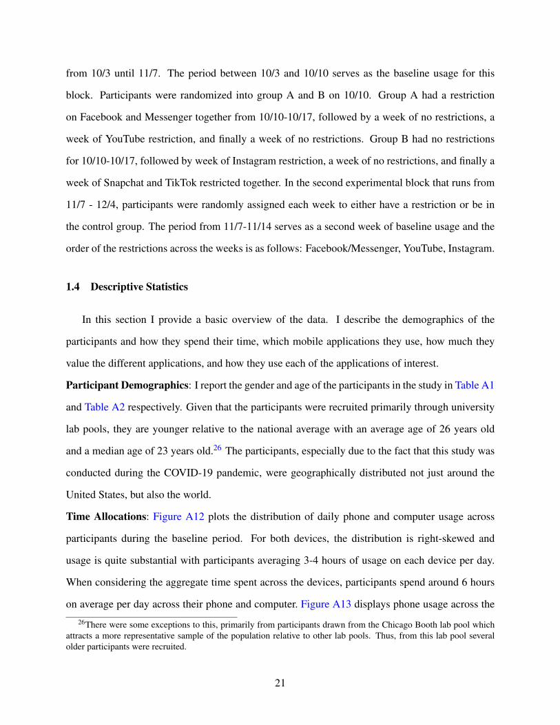
from 10/3 until 11/7. The period between 10/3 and 10/10 serves as the baseline usage for this

block. Participants were randomized into group A and B on 10/10. Group A had a restriction

on Facebook and Messenger together from 10/10-10/17, followed by a week of no restrictions, a

week of YouTube restriction, and finally a week of no restrictions. Group B had no restrictions

for 10/10-10/17, followed by week of Instagram restriction, a week of no restrictions, and finally a

week of Snapchat and TikTok restricted together. In the second experimental block that runs from

11/7 - 12/4, participants were randomly assigned each week to either have a restriction or be in

the control group. The period from 11/7-11/14 serves as a second week of baseline usage and the

order of the restrictions across the weeks is as follows: Facebook/Messenger, YouTube, Instagram.

1.4 Descriptive Statistics

In this section I provide a basic overview of the data. I describe the demographics of the

participants and how they spend their time, which mobile applications they use, how much they

value the different applications, and how they use each of the applications of interest.

Participant Demographics: I report the gender and age of the participants in the study in Table A1

and Table A2 respectively. Given that the participants were recruited primarily through university

lab pools, they are younger relative to the national average with an average age of 26 years old

and a median age of 23 years old.26 The participants, especially due to the fact that this study was

conducted during the COVID-19 pandemic, were geographically distributed not just around the

United States, but also the world.

Time Allocations: Figure A12 plots the distribution of daily phone and computer usage across

participants during the baseline period. For both devices, the distribution is right-skewed and

usage is quite substantial with participants averaging 3-4 hours of usage on each device per day.

When considering the aggregate time spent across the devices, participants spend around 6 hours

on average per day across their phone and computer. Figure A13 displays phone usage across the

26There were some exceptions to this, primarily from participants drawn from the Chicago Booth lab pool whichattracts a more representative sample of the population relative to other lab pools. Thus, from this lab pool severalolder participants were recruited.

21

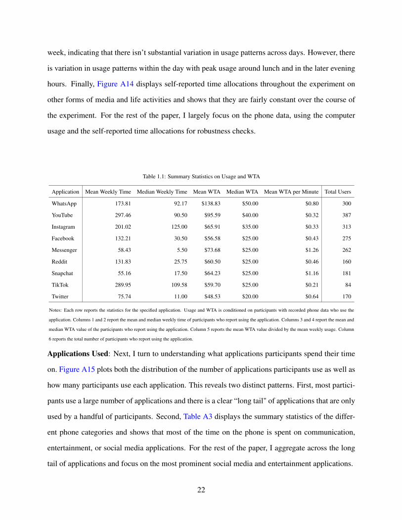
week, indicating that there isn’t substantial variation in usage patterns across days. However, there

is variation in usage patterns within the day with peak usage around lunch and in the later evening

hours. Finally, Figure A14 displays self-reported time allocations throughout the experiment on

other forms of media and life activities and shows that they are fairly constant over the course of

the experiment. For the rest of the paper, I largely focus on the phone data, using the computer

usage and the self-reported time allocations for robustness checks.

Table 1.1: Summary Statistics on Usage and WTA

Application Mean Weekly Time Median Weekly Time Mean WTA Median WTA Mean WTA per Minute Total Users

WhatsApp 173.81 92.17 $138.83 $50.00 $0.80 300

YouTube 297.46 90.50 $95.59 $40.00 $0.32 387

Instagram 201.02 125.00 $65.91 $35.00 $0.33 313

Facebook 132.21 30.50 $56.58 $25.00 $0.43 275

Messenger 58.43 5.50 $73.68 $25.00 $1.26 262

Reddit 131.83 25.75 $60.50 $25.00 $0.46 160

Snapchat 55.16 17.50 $64.23 $25.00 $1.16 181

TikTok 289.95 109.58 $59.70 $25.00 $0.21 84

Twitter 75.74 11.00 $48.53 $20.00 $0.64 170

Notes: Each row reports the statistics for the specified application. Usage and WTA is conditioned on participants with recorded phone data who use the

application. Columns 1 and 2 report the mean and median weekly time of participants who report using the application. Columns 3 and 4 report the mean and

median WTA value of the participants who report using the application. Column 5 reports the mean WTA value divided by the mean weekly usage. Column

6 reports the total number of participants who report using the application.

Applications Used: Next, I turn to understanding what applications participants spend their time

on. Figure A15 plots both the distribution of the number of applications participants use as well as

how many participants use each application. This reveals two distinct patterns. First, most partici-

pants use a large number of applications and there is a clear “long tail" of applications that are only

used by a handful of participants. Second, Table A3 displays the summary statistics of the differ-

ent phone categories and shows that most of the time on the phone is spent on communication,

entertainment, or social media applications. For the rest of the paper, I aggregate across the long

tail of applications and focus on the most prominent social media and entertainment applications.

22

Usage of Social Media and Entertainment Applications: I restrict attention to the most popular

social media and entertainment applications. Despite the long tail observation, there is extensive

multi-homing across these applications as observed in Figure A16, which shows that most partic-

ipants use between 4 and 7 of the applications of interest. Table A4 displays the complete multi-

homing matrix which computes the fraction of users of application X that also use application Y

and finds no obvious clusters of usage patterns.

Table 1.1 provides summary statistics for the applications of interest on the reported value

of each application as well as the amount of time spent on the different applications.27,28 I report

only participants that either stated in the activity question on the initial survey that they use this

application or if there is recorded time on the application on their phone. Since these were elicited

at the beginning of the study period, I compute summary statistics for the observed phone time

during the baseline week. There are several takeaways from the summary statistics. First, the

most used and valued applications among participants are Instagram, YouTube, and WhatsApp.

There is a stark drop-off between these applications and the rest both in terms of value and time

spent. Indeed, not only do more participants make use of and value these applications more, but,

even conditional on usage, participants spend more time on them. This motivates the applications

that I choose to restrict from participants. Second, distributions of value and time usage are both

right skewed, especially for applications such as TikTok and YouTube, which motivates estimating

treatment effects across the distribution and not just average treatment effects.29 Furthermore, it

means that there will be meaningful differences in interpreting the results of specifications using

logs versus levels. The correlation between the average time spent and average value of the appli-

cations is confirmed by a more detailed analysis in section A.3 that finds that an additional minute

of daily usage corresponds to a 5.8 cents increase in value.

27In the results reported here I drop participants that filled in the maximum monetary amount for each application.28 Table A5 reports the time allocations on the computer as well as the phone. It shows that for the applications of

interest most of the time is spent on the phone with the exception of YouTube where participants spend a significantamount of time on the application on both the computer and the phone.

29It is important to further point out that my participants are for the most part consumers of content on theseapplications and do not post content that often. Table A6 shows that most participants are mainly consumers of contenton applications such as YouTube, Reddit, and TikTok, while they most often post content on Instagram and Snapchat.However, even on these applications, there are not many participants who post at a relatively high frequency.

23

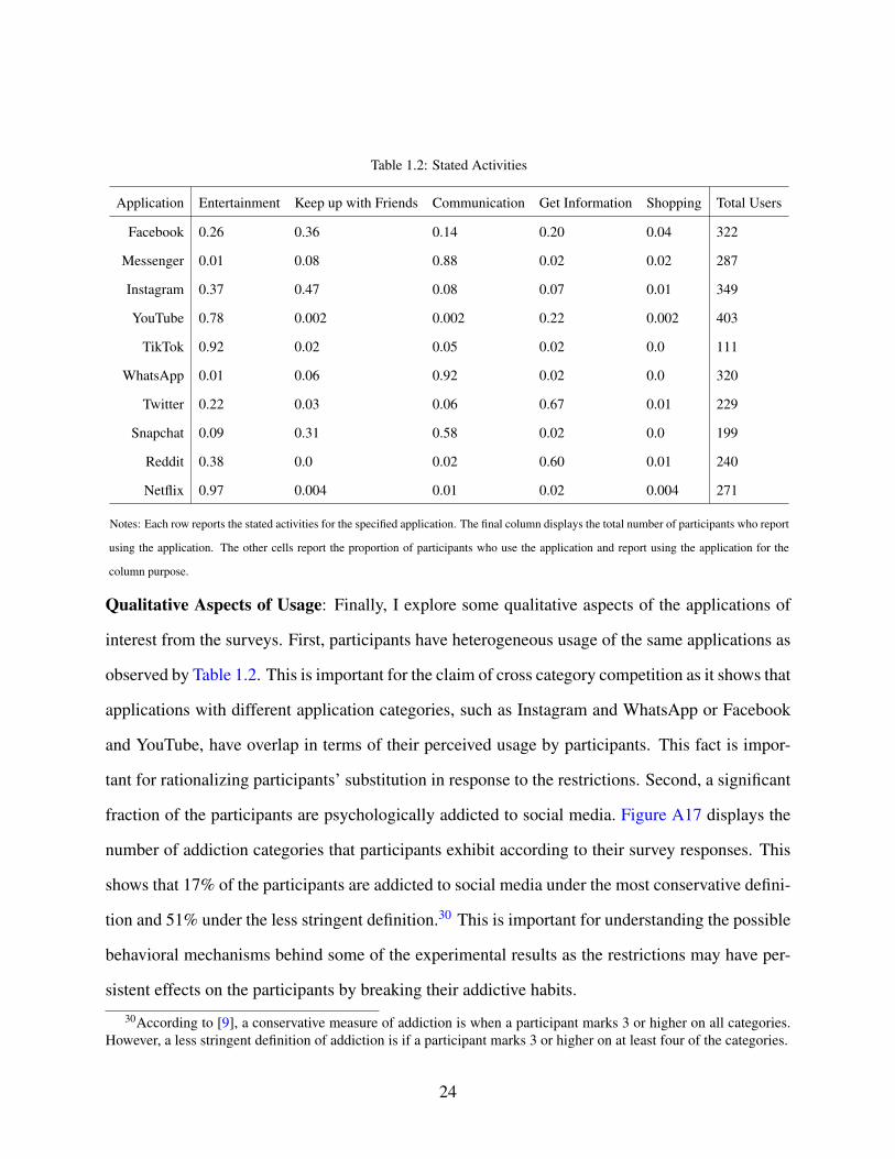
Table 1.2: Stated Activities

Application Entertainment Keep up with Friends Communication Get Information Shopping Total Users

Facebook 0.26 0.36 0.14 0.20 0.04 322

Messenger 0.01 0.08 0.88 0.02 0.02 287

Instagram 0.37 0.47 0.08 0.07 0.01 349

YouTube 0.78 0.002 0.002 0.22 0.002 403

TikTok 0.92 0.02 0.05 0.02 0.0 111

WhatsApp 0.01 0.06 0.92 0.02 0.0 320

Twitter 0.22 0.03 0.06 0.67 0.01 229

Snapchat 0.09 0.31 0.58 0.02 0.0 199

Reddit 0.38 0.0 0.02 0.60 0.01 240

Netflix 0.97 0.004 0.01 0.02 0.004 271

Notes: Each row reports the stated activities for the specified application. The final column displays the total number of participants who report

using the application. The other cells report the proportion of participants who use the application and report using the application for the

column purpose.

Qualitative Aspects of Usage: Finally, I explore some qualitative aspects of the applications of

interest from the surveys. First, participants have heterogeneous usage of the same applications as

observed by Table 1.2. This is important for the claim of cross category competition as it shows that

applications with different application categories, such as Instagram and WhatsApp or Facebook

and YouTube, have overlap in terms of their perceived usage by participants. This fact is impor-

tant for rationalizing participants’ substitution in response to the restrictions. Second, a significant

fraction of the participants are psychologically addicted to social media. Figure A17 displays the

number of addiction categories that participants exhibit according to their survey responses. This

shows that 17% of the participants are addicted to social media under the most conservative defini-

tion and 51% under the less stringent definition.30 This is important for understanding the possible

behavioral mechanisms behind some of the experimental results as the restrictions may have per-

sistent effects on the participants by breaking their addictive habits.

30According to [9], a conservative measure of addiction is when a participant marks 3 or higher on all categories.However, a less stringent definition of addiction is if a participant marks 3 or higher on at least four of the categories.

24

1.5 Experimental Results

In this section I analyze the substitution patterns of time allocations throughout the study pe-

riod. I characterize what applications and activities are considered substitutes for the restricted

applications by measuring participant substitution during the restriction period. I relate these sub-

stitution patterns to issues of relevant market definition. I then explore the extent to which there

were persistent effects of the restriction by investigating how time allocations differ after the treat-

ment period relative to before it. The insights from this section will be used to guide the demand

model estimated in Section 1.6.

1.5.1 Time Substitution During the Restriction Period

I focus on understanding what applications participants substitute to during the restriction pe-

riod.

Conceptual Framework

There are a wide range of possible activities that participants could substitute towards and it

is challenging to define the precise substitution patterns that are most relevant to the question of

consumer demand and merger analysis. There are two broad questions of interest that guide the

analysis. The first is what types of activities do participants substitute to and the second is how

dispersed across different applications are the substitution patterns. These questions are at the

heart of the debate about monopolization arguments surrounding Facebook and, more generally, in

merger evaluation between applications in this market.

Substitutable Activites: A directly relevant question to the ongoing debate between Facebook

and regulators is which types of applications are most substitutable for the restricted applications.

For instance, in [3] Facebook contends that it competes with a broad range of applications that

compete for consumer time such as YouTube, which is not traditionally considered a social media

application, whereas regulators contend that the most relevant competitors are other social media

25

applications such as Snapchat. One of the challenges underlying this debate has been the lack of

prices in these markets as standard market definition tests rely on understanding substitution with

respect to price. Despite the lack of prices, the theoretical literature on two-sided media markets

(starting from [35]) and the legal literature [39, 40] have noted that in these markets consumers

face implicit costs on their time and attention that are direct choice variables for the application.

This indicates that one alternative harm in lieu of higher prices is an increased cost on consumer

attention, which can take the form of increased advertising load or decreased quality.31

Under this interpretation, the substitution observed during the restriction period is a limit case

of taking “attention costs" to their choke values where no one would consume the application.

Thus, it can serve as a conservative test of substitutability and, in particular, can function as the

most conservative possible market definition – only including the applications and activities that are

at all substitutable. This has appeal as a tool for practitioners as well since, in practice, variation

in “attention costs" is substantially more ambiguous and difficult to come by relative to price

variation in other markets. Furthermore, experiments such as the one analyzed in this paper are

feasible due to the nature of digital goods.32 Since the default approach taken by regulators has

been to consider only applications within the same application category as relevant substitutes, a

direct empirical question is whether there is only substitution within application category or across

application categories as well. In order to study this in a disciplined manner, I use the categories

assigned to the applications in the Google Play Store and characterize substitution across these

different application categories. If I observe no cross-category substitution at this point, then the

implication is that smaller increases in “attention costs" would similarly not lead to considerable

substitution between these categories. If I do observe cross-category substitution, then it only says

that such a market definition is not entirely unreasonable.

31[39, 40] propose modifications of the standard Small but significant and non-transitory increase in price (SSNIP)test explicitly considering this harm in lieu of the standard price test. This test was used in the FTC’s lawsuit againstFacebook by arguing that the Cambridge Analytica scandal was an exogenous decrease in quality through privacyharms and measured substitution in monthly active users to do the market definition exercise.

32Even without directly implemented experiments, natural experiments caused by product outages would inducesimilar variation and enable similar estimates. For example, extended outages such as the Facebook, WhatsApp,Messenger, and Instagram outage on 10/4/2021 could be utilized to a similar extent, https://www.nytimes.com/2021/10/04/technology/facebook-down.html.

26

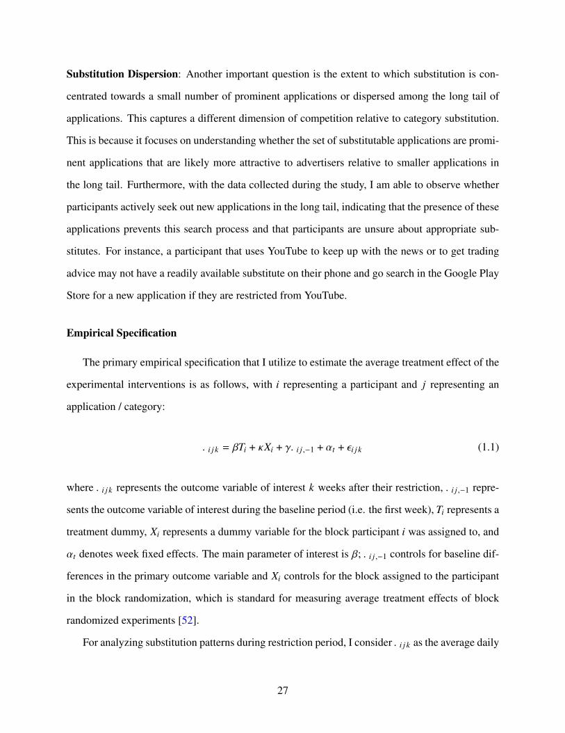
Substitution Dispersion: Another important question is the extent to which substitution is con-

centrated towards a small number of prominent applications or dispersed among the long tail of

applications. This captures a different dimension of competition relative to category substitution.

This is because it focuses on understanding whether the set of substitutable applications are promi-

nent applications that are likely more attractive to advertisers relative to smaller applications in

the long tail. Furthermore, with the data collected during the study, I am able to observe whether

participants actively seek out new applications in the long tail, indicating that the presence of these

applications prevents this search process and that participants are unsure about appropriate sub-

stitutes. For instance, a participant that uses YouTube to keep up with the news or to get trading

advice may not have a readily available substitute on their phone and go search in the Google Play

Store for a new application if they are restricted from YouTube.

Empirical Specification

The primary empirical specification that I utilize to estimate the average treatment effect of the

experimental interventions is as follows, with 𝑖 representing a participant and 𝑗 representing an

application / category:

𝑌𝑖 𝑗 𝑘 = 𝛽𝑇𝑖 + ^𝑋𝑖 + 𝛾𝑌𝑖 𝑗 ,−1 + 𝛼𝑡 + 𝜖𝑖 𝑗 𝑘 (1.1)

where 𝑌𝑖 𝑗 𝑘 represents the outcome variable of interest 𝑘 weeks after their restriction, 𝑌𝑖 𝑗 ,−1 repre-

sents the outcome variable of interest during the baseline period (i.e. the first week), 𝑇𝑖 represents a

treatment dummy, 𝑋𝑖 represents a dummy variable for the block participant 𝑖 was assigned to, and

𝛼𝑡 denotes week fixed effects. The main parameter of interest is 𝛽; 𝑌𝑖 𝑗 ,−1 controls for baseline dif-

ferences in the primary outcome variable and 𝑋𝑖 controls for the block assigned to the participant

in the block randomization, which is standard for measuring average treatment effects of block

randomized experiments [52].

For analyzing substitution patterns during restriction period, I consider𝑌𝑖 𝑗 𝑘 as the average daily

27

time spent on applications / categories during the days when the participant’s software was active

and logging data. When analyzing the substitution during the restriction period, I focus on the

outcome variables only during the first week of the restriction. Due to this, I omit the week fixed

effects and report heteroskedasticity-robust standard errors. When I consider multiple weeks of

usage, as in subsection 1.5.2, I include this term and cluster standard errors at the participant level.

I also consider 𝑌𝑖 𝑗 𝑘 as the number of newly installed applications, but for this outcome variable, I

do not have any baseline data and so estimate the specification omitting the baseline usage term.

I am interested in not just the average treatment effects, but also effects across the distribution

since, for instance, one might imagine that heavy users of an application or category would respond

differently than infrequent users of an application or category at the baseline. As a result, I also

estimate quantile treatment effects using the same specification. I estimate these effects using a

standard quantile regression since the fact that treatment status is exogenous allows for identifica-

tion of the conditional QTE with a quantile regression [53]. Finally, since the distribution of usage

is skewed and, occasionally, sparse I consider the specifications in both logs and levels. In order to

accomodate the zeros in my data, I use the inverse hyperbolic sine transform in lieu of logs, which

leads to a similar interpretation of coefficient estimates [54].

Category Market Definition and Cross-Category Substitution

Cross-Category Substitution: I test the extent of cross-category substitution by measuring the

average treatment effect of time substitution towards other categories as a result of the restriction.

Table 1.3 displays the results for the Instagram restriction. Each cell in the table reports the es-

timated average treatment effect in order to make the results digestible. I consider the effects of

each restriction on category usage separately. I report the results both from this experiment as well

as pooled with the pilot study that included two separate restriction periods for different subsets of

participants. For these results, I additionally control for the experimental period as well as cluster

standard errors at the participant level. I report the results of each restriction on category time in

levels, logs, and share of phone usage (i.e. not including time off phone). However, due to the

28

skewed distribution of usage, I primarily focus on the log specification as it captures the response

of the average participant and is not driven by the most intense users of the applications.

The overall amount of time spent on all social applications drops across all specifications (col-

umn 1), but the time spent on non-Instagram social applications increases by 22.4% (column

2). This means that there was considerable substitution towards other social applications, but

not enough to entirely counteract the loss of Instagram. Column (3) indicates that there is some

cross-category substitution to communication applications with the logs specification pointing to a

marginally significant 10-12% increase in time spent on such applications. This is consistent with

the qualitative evidence from the participants in section A.8. For instance, one participant stated

Instagram was restricted for me and because I mainly use it as a communication app, I was not sig-

nificantly affected. I just used regular text, video call, and Snapchat to keep up socially. I observe

fairly precise null results for substitution from Instagram to entertainment or other applications.

Table 1.4 displays the results for the YouTube restriction. Similar to the results for the Insta-

gram restriction, there is a sharp decrease in own-category time during the restriction period (see

column 1). However, unlike the results of the Instagram restriction, there is a precise null of sub-

stitution towards other applications within the same category (see column 4). Column (1) points to

an increase in time spent on social applications with a roughly 15% increase in time spent on these

applications, while columns (3) and (5) suggest little increase in time spent on communication and

other applications. Finally, Figure A18 displays the effects of the restriction along the entire distri-

bution and shows that the own-category substitution for both applications is upward sloping across

deciles, indicating that more intensive overall users of social media and entertainment applications

respectively were more likely to look for close substitutes.

29

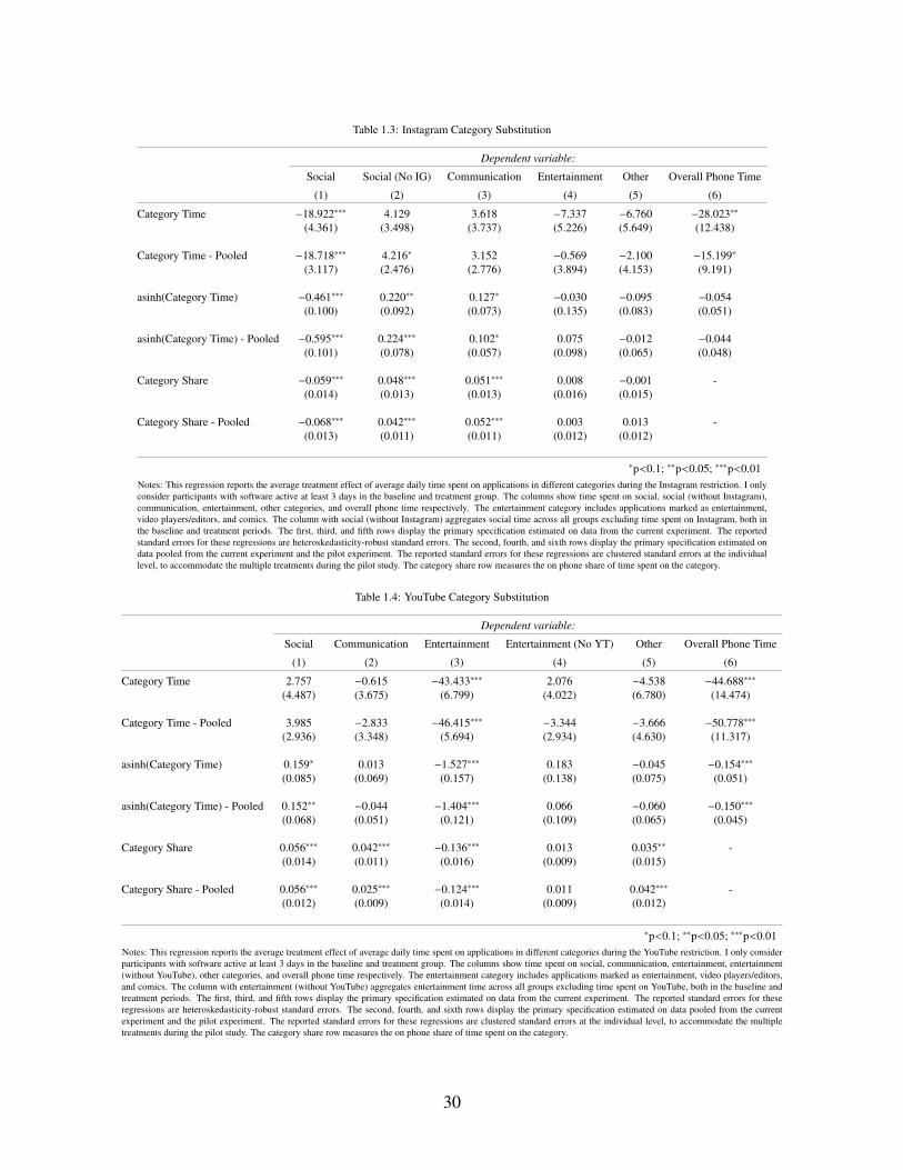
Table 1.3: Instagram Category Substitution

Dependent variable:

Social Social (No IG) Communication Entertainment Other Overall Phone Time

(1) (2) (3) (4) (5) (6)

Category Time −18.922∗∗∗ 4.129 3.618 −7.337 −6.760 −28.023∗∗

(4.361) (3.498) (3.737) (5.226) (5.649) (12.438)

Category Time - Pooled −18.718∗∗∗ 4.216∗ 3.152 −0.569 −2.100 −15.199∗

(3.117) (2.476) (2.776) (3.894) (4.153) (9.191)

asinh(Category Time) −0.461∗∗∗ 0.220∗∗ 0.127∗ −0.030 −0.095 −0.054(0.100) (0.092) (0.073) (0.135) (0.083) (0.051)

asinh(Category Time) - Pooled −0.595∗∗∗ 0.224∗∗∗ 0.102∗ 0.075 −0.012 −0.044(0.101) (0.078) (0.057) (0.098) (0.065) (0.048)

Category Share −0.059∗∗∗ 0.048∗∗∗ 0.051∗∗∗ 0.008 −0.001 -(0.014) (0.013) (0.013) (0.016) (0.015)

Category Share - Pooled −0.068∗∗∗ 0.042∗∗∗ 0.052∗∗∗ 0.003 0.013 -(0.013) (0.011) (0.011) (0.012) (0.012)

∗p<0.1; ∗∗p<0.05; ∗∗∗p<0.01Notes: This regression reports the average treatment effect of average daily time spent on applications in different categories during the Instagram restriction. I onlyconsider participants with software active at least 3 days in the baseline and treatment group. The columns show time spent on social, social (without Instagram),communication, entertainment, other categories, and overall phone time respectively. The entertainment category includes applications marked as entertainment,video players/editors, and comics. The column with social (without Instagram) aggregates social time across all groups excluding time spent on Instagram, both inthe baseline and treatment periods. The first, third, and fifth rows display the primary specification estimated on data from the current experiment. The reportedstandard errors for these regressions are heteroskedasticity-robust standard errors. The second, fourth, and sixth rows display the primary specification estimated ondata pooled from the current experiment and the pilot experiment. The reported standard errors for these regressions are clustered standard errors at the individuallevel, to accommodate the multiple treatments during the pilot study. The category share row measures the on phone share of time spent on the category.

Table 1.4: YouTube Category Substitution

Dependent variable:

Social Communication Entertainment Entertainment (No YT) Other Overall Phone Time

(1) (2) (3) (4) (5) (6)

Category Time 2.757 −0.615 −43.433∗∗∗ 2.076 −4.538 −44.688∗∗∗

(4.487) (3.675) (6.799) (4.022) (6.780) (14.474)

Category Time - Pooled 3.985 −2.833 −46.415∗∗∗ −3.344 −3.666 −50.778∗∗∗

(2.936) (3.348) (5.694) (2.934) (4.630) (11.317)

asinh(Category Time) 0.159∗ 0.013 −1.527∗∗∗ 0.183 −0.045 −0.154∗∗∗

(0.085) (0.069) (0.157) (0.138) (0.075) (0.051)

asinh(Category Time) - Pooled 0.152∗∗ −0.044 −1.404∗∗∗ 0.066 −0.060 −0.150∗∗∗

(0.068) (0.051) (0.121) (0.109) (0.065) (0.045)

Category Share 0.056∗∗∗ 0.042∗∗∗ −0.136∗∗∗ 0.013 0.035∗∗ -(0.014) (0.011) (0.016) (0.009) (0.015)

Category Share - Pooled 0.056∗∗∗ 0.025∗∗∗ −0.124∗∗∗ 0.011 0.042∗∗∗ -(0.012) (0.009) (0.014) (0.009) (0.012)

∗p<0.1; ∗∗p<0.05; ∗∗∗p<0.01Notes: This regression reports the average treatment effect of average daily time spent on applications in different categories during the YouTube restriction. I only considerparticipants with software active at least 3 days in the baseline and treatment group. The columns show time spent on social, communication, entertainment, entertainment(without YouTube), other categories, and overall phone time respectively. The entertainment category includes applications marked as entertainment, video players/editors,and comics. The column with entertainment (without YouTube) aggregates entertainment time across all groups excluding time spent on YouTube, both in the baseline andtreatment periods. The first, third, and fifth rows display the primary specification estimated on data from the current experiment. The reported standard errors for theseregressions are heteroskedasticity-robust standard errors. The second, fourth, and sixth rows display the primary specification estimated on data pooled from the currentexperiment and the pilot experiment. The reported standard errors for these regressions are clustered standard errors at the individual level, to accommodate the multipletreatments during the pilot study. The category share row measures the on phone share of time spent on the category.

30

Survey Evidence of Cross-Category Substitution: In order to provide further evidence for cross-

category substitution, I utilize the results from the hypothetical switching survey question asked at

the beginning of the experiment. In this question, participants are asked to broadly assign which

category of activities and applications they would substitute to if they lost access to the application.

The results are reported in Table A10, which show that only 46% of participants stated they would

switch to other entertainment applications in lieu of YouTube and only 23% stated they would

switch to other social media applications in lieu of Instagram.

Indeed, for Instagram around the same percentage stated they would substitute to other hobbies

compared to other social media applications. The large drop in own-category time and general time

on digital devices paired with cross-category substitution would be consistent with these results.

Furthermore, they are consistent with the heterogeneity in stated activities reported in Table 1.2.

The fact that the uses of the applications are heterogeneous and intersect with applications that

are not in the same formal application category helps to understand why I observe cross-category

substitution. It further suggests a broader issue with using the functional product categories for

applications whose content and use mostly come from user-generated content.

Table 1.5: Herfindahl–Hirschman Index Across Market Definitions

Social Entert. Comm. Social + Entert. Social + Comm. Social + Entert. + Comm.

Current Ownership 0.344 0.572 0.232 0.222 0.271 0.184

Independent Ownership 0.203 0.572 0.163 0.181 0.094 0.101

Notes: This table displays the Herfindahl–Hirschman Index (HHI) based on different application category market definitions using the baseline

period data. I take the category(s) in each column as the definition of the market and compute the HHI of this market. The first row displays the

HHI under the current ownership structure (i.e. Facebook owns Facebook, Instagram, Messenger, and WhatsApp). The second row displays

the HHI if each of these applications was independently owned.

Implications for Market Concentration: A natural question is whether different market defi-

nitions would result in qualitatively different assessments of the degree of concentration in the

market. I focus on the categories between which substitution was observed and compute the most

common market concentration index, the Herfindahl–Hirschman Index (HHI), using the different

31

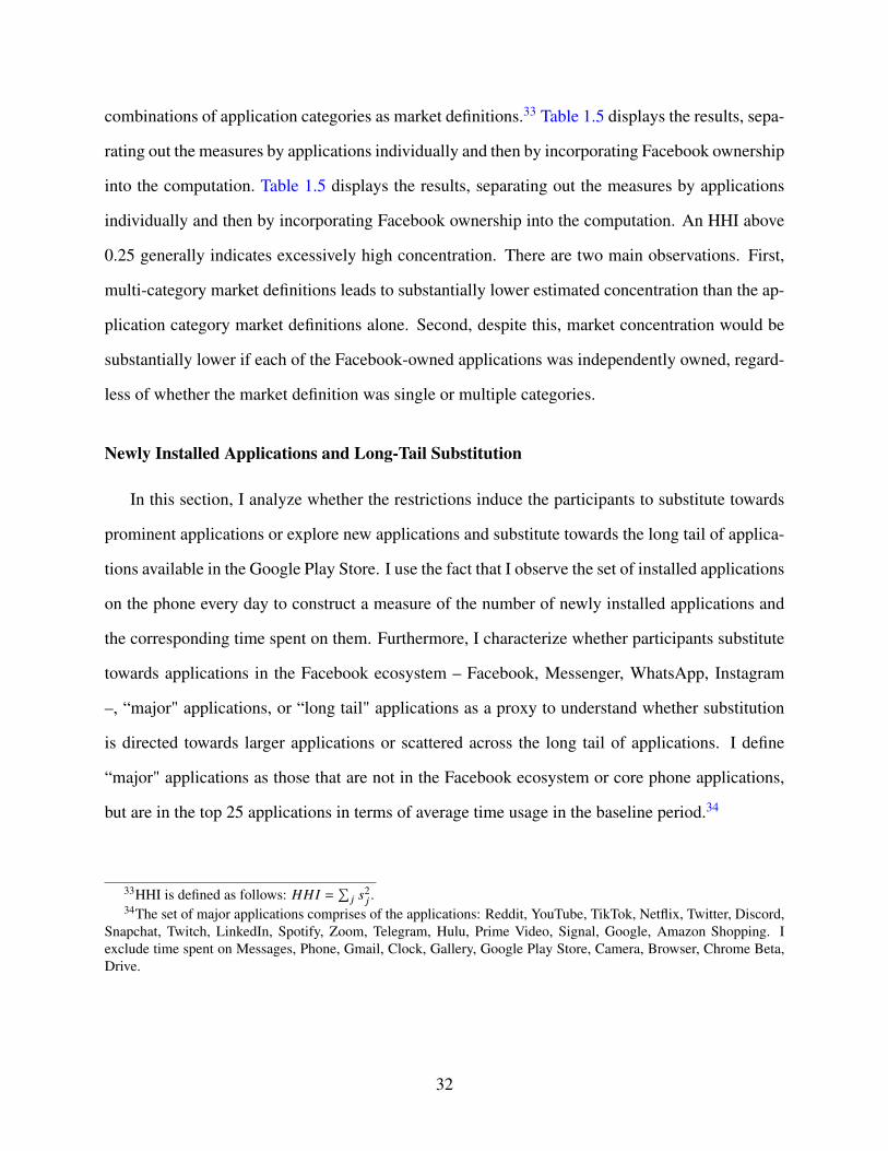
combinations of application categories as market definitions.33 Table 1.5 displays the results, sepa-

rating out the measures by applications individually and then by incorporating Facebook ownership

into the computation. Table 1.5 displays the results, separating out the measures by applications

individually and then by incorporating Facebook ownership into the computation. An HHI above

0.25 generally indicates excessively high concentration. There are two main observations. First,

multi-category market definitions leads to substantially lower estimated concentration than the ap-

plication category market definitions alone. Second, despite this, market concentration would be

substantially lower if each of the Facebook-owned applications was independently owned, regard-

less of whether the market definition was single or multiple categories.

Newly Installed Applications and Long-Tail Substitution

In this section, I analyze whether the restrictions induce the participants to substitute towards

prominent applications or explore new applications and substitute towards the long tail of applica-

tions available in the Google Play Store. I use the fact that I observe the set of installed applications

on the phone every day to construct a measure of the number of newly installed applications and

the corresponding time spent on them. Furthermore, I characterize whether participants substitute

towards applications in the Facebook ecosystem – Facebook, Messenger, WhatsApp, Instagram

–, “major" applications, or “long tail" applications as a proxy to understand whether substitution

is directed towards larger applications or scattered across the long tail of applications. I define

“major" applications as those that are not in the Facebook ecosystem or core phone applications,

but are in the top 25 applications in terms of average time usage in the baseline period.34

33HHI is defined as follows: 𝐻𝐻𝐼 =∑

𝑗 𝑠2𝑗.

34The set of major applications comprises of the applications: Reddit, YouTube, TikTok, Netflix, Twitter, Discord,Snapchat, Twitch, LinkedIn, Spotify, Zoom, Telegram, Hulu, Prime Video, Signal, Google, Amazon Shopping. Iexclude time spent on Messages, Phone, Gmail, Clock, Gallery, Google Play Store, Camera, Browser, Chrome Beta,Drive.

32

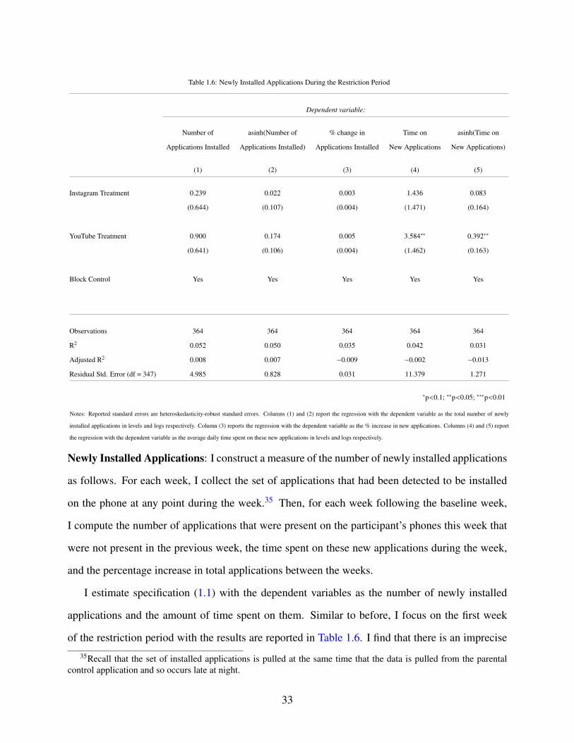
Table 1.6: Newly Installed Applications During the Restriction Period

Dependent variable:

Number of

Applications Installed

asinh(Number of

Applications Installed)

% change in

Applications Installed

Time on

New Applications

asinh(Time on

New Applications)

(1) (2) (3) (4) (5)

Instagram Treatment 0.239 0.022 0.003 1.436 0.083

(0.644) (0.107) (0.004) (1.471) (0.164)

YouTube Treatment 0.900 0.174 0.005 3.584∗∗ 0.392∗∗

(0.641) (0.106) (0.004) (1.462) (0.163)

Block Control Yes Yes Yes Yes Yes

Observations 364 364 364 364 364

R2 0.052 0.050 0.035 0.042 0.031

Adjusted R2 0.008 0.007 −0.009 −0.002 −0.013

Residual Std. Error (df = 347) 4.985 0.828 0.031 11.379 1.271

∗p<0.1; ∗∗p<0.05; ∗∗∗p<0.01

Notes: Reported standard errors are heteroskedasticity-robust standard errors. Columns (1) and (2) report the regression with the dependent variable as the total number of newly

installed applications in levels and logs respectively. Column (3) reports the regression with the dependent variable as the % increase in new applications. Columns (4) and (5) report

the regression with the dependent variable as the average daily time spent on these new applications in levels and logs respectively.

Newly Installed Applications: I construct a measure of the number of newly installed applications

as follows. For each week, I collect the set of applications that had been detected to be installed

on the phone at any point during the week.35 Then, for each week following the baseline week,

I compute the number of applications that were present on the participant’s phones this week that

were not present in the previous week, the time spent on these new applications during the week,

and the percentage increase in total applications between the weeks.

I estimate specification (1.1) with the dependent variables as the number of newly installed

applications and the amount of time spent on them. Similar to before, I focus on the first week

of the restriction period with the results are reported in Table 1.6. I find that there is an imprecise

35Recall that the set of installed applications is pulled at the same time that the data is pulled from the parentalcontrol application and so occurs late at night.

33

increase in the number of newly installed applications for YouTube, but that there is a statistically

and economically significant increase of 3.5 minutes per day in time spent on these applications.

For Instagram, there does not appear to be an increase in the number of installed applications or

a difference in the time spent on them. One interpretation of this result is that for Instagram the

substitutes are more apparent to participants (e.g. Facebook), which leads to less need to install

new applications. For YouTube, the substitutes are less apparent so participants are less likely to

have readily available substitutes and thus spend more time off the phone as well as be more likely

to explore new alternatives.

Table A18 further shows that a substantial proportion of participants not only believe they

substituted towards other applications during the restriction, but also actively “invested" in them so

that they could source better content from them. For instance, one participant wrote “I had to figure

out what I want from other applications I didn’t know offered similar content before time, after the

restriction elapsed, I had adjusted to sourcing for such content on both apps". This suggests that

not only was there active adjustment in the extensive margin of installing new applications, but

also adjustments to the extent to which participants more fully explored the capabilities of other

applications.

Substitution to the Long-Tail: I now study whether participants are substituting to a few promi-

nent applications or dispersed amongst the long tail of applications. To investigate this question,

I use the same empirical specification as the cross-category substitution regressions, but consider

the categories as overall time on the Facebook ecosystem, major applications, and long tail appli-

cations. Table A11 displays the results for Instagram. Indeed, while there is little observed substi-

tution to “long tail" applications or other major applications, there is a clear pattern of substitution

towards other Facebook-owned applications with a 17.9% increase in non-Instagram Facebook-

owned applications. Table A12 displays the results for YouTube. The effects in this case are more

muted with a clear drop in “major applications" due to the drop in YouTube time, but only a small

amount of substitution towards the other categories. Once I condition on phone usage, I find that

the largest share gain is to the Facebook ecosystem and the long tail applications. Thus, substitu-

34

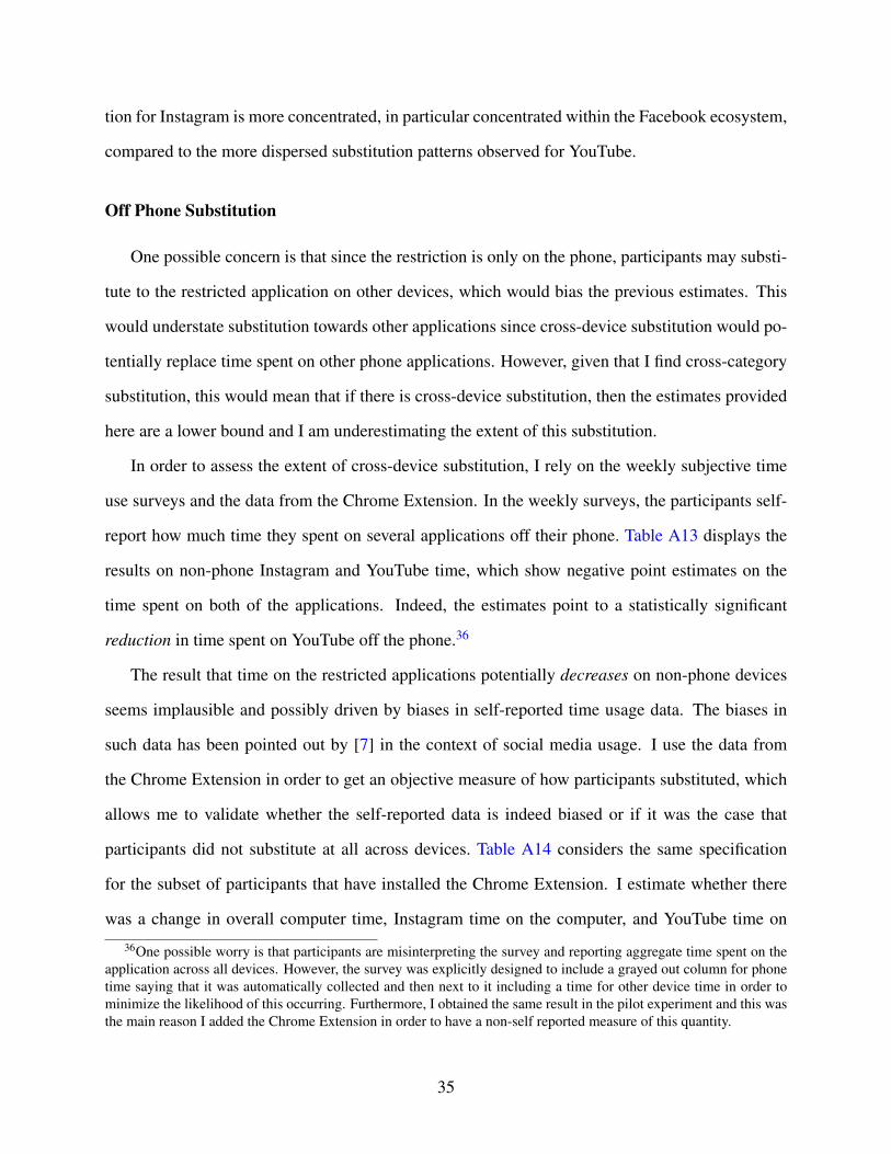
tion for Instagram is more concentrated, in particular concentrated within the Facebook ecosystem,

compared to the more dispersed substitution patterns observed for YouTube.

Off Phone Substitution

One possible concern is that since the restriction is only on the phone, participants may substi-

tute to the restricted application on other devices, which would bias the previous estimates. This

would understate substitution towards other applications since cross-device substitution would po-

tentially replace time spent on other phone applications. However, given that I find cross-category

substitution, this would mean that if there is cross-device substitution, then the estimates provided

here are a lower bound and I am underestimating the extent of this substitution.

In order to assess the extent of cross-device substitution, I rely on the weekly subjective time

use surveys and the data from the Chrome Extension. In the weekly surveys, the participants self-

report how much time they spent on several applications off their phone. Table A13 displays the

results on non-phone Instagram and YouTube time, which show negative point estimates on the

time spent on both of the applications. Indeed, the estimates point to a statistically significant

reduction in time spent on YouTube off the phone.36

The result that time on the restricted applications potentially decreases on non-phone devices

seems implausible and possibly driven by biases in self-reported time usage data. The biases in

such data has been pointed out by [7] in the context of social media usage. I use the data from

the Chrome Extension in order to get an objective measure of how participants substituted, which

allows me to validate whether the self-reported data is indeed biased or if it was the case that

participants did not substitute at all across devices. Table A14 considers the same specification

for the subset of participants that have installed the Chrome Extension. I estimate whether there

was a change in overall computer time, Instagram time on the computer, and YouTube time on

36One possible worry is that participants are misinterpreting the survey and reporting aggregate time spent on theapplication across all devices. However, the survey was explicitly designed to include a grayed out column for phonetime saying that it was automatically collected and then next to it including a time for other device time in order tominimize the likelihood of this occurring. Furthermore, I obtained the same result in the pilot experiment and this wasthe main reason I added the Chrome Extension in order to have a non-self reported measure of this quantity.

35

the computer. Table A14 finds little evidence that overall computer time changed as a result of the

treatment. However, there is a marginally significant increase of 9.3 minutes of computer time

on YouTube during the YouTube treatment and a statistically significant increase of 1.58 minutes

of computer time on Instagram during the Instagram treatment. These point estimates indicate

that there was a small amount of cross-device substitution due to the restrictions only being on

the phone. In order to interpret the magnitude of the cross-device substitution, it is important to

recall from Table A5 that the baseline usage of Instagram computer usage is only 1 minute a day

on average. Furthermore, Figure A21 shows the time series of usage of the restricted applications

across both devices and indicates that the aggregate usage of the applications drops dramatically

during the treatment week.

Thus, the objective data provided by the Chrome Extension allows me to conclude that there

was a small amount of cross-device substitution. This means that I am likely underestimating the

degree of substitution towards other applications on the phone, but not too substantially. Further-

more, the discrepancy in the sign of the effect between the survey-based measures and the objective

measure from the Chrome Extension highlights the importance of collecting non-self reported data

for time allocations.

Beyond the extent of cross-device substitution towards the restricted application, there is a

broader question of whether there are non-digital substitutes to the restricted applications. Column

(6) of Table 1.3 and Table 1.4 displays the estimated average treatment effects for overall phone

usage during the Instagram and YouTube treatments respectively. It shows that there is a reduction

of 29 minutes and 44 minutes per day of phone time as a result of the Instagram and YouTube

treatments respectively. The logs specification shows a lesser effect with a statistically significant

and meaningful drop in phone time for YouTube, but an imprecise, negative point estimate for

Instagram. Consistent with this, I find that this is primarily driven by reductions in phone usage

of participants in the upper deciles of phone usage.37 Figure A19 shows that while the YouTube

37Figure A20 plots the quantile treatment effects for each decile for logs of overall phone time. It shows that theQTE of the Instagram treatment is quite similar across deciles, whereas for YouTube it is more likely to be driven byreductions in the lower deciles.

36

restriction leads to fairly depressed phone usage throughout the entirety of the day, the reduction

in phone usage for the Instagram treatment is largely in the afternoon and evening hours. Thus,

it is plausible that, especially for Instagram, participants are substituting to non-digital substitutes

during these hours. These results indicate that the restrictions led to substantial diversion towards

the outside option, suggesting that many participants are unable to find viable substitutes and thus

that the restricted applications have large market power over phone usage. It is unclear what

activities off the phone participants are substituting to as Table A15 displays the estimated average

treatment effect on the most natural off-phone substitutes, such as cable television, video games

and streaming services, and finds no effect on time spent on these services.

1.5.2 Time Substitution After Restriction Period

In this section I explore the extent to which there are persistent effects as a result of the re-

strictions. This is important for understanding whether there are potentially dynamic elements of

demand for such services and will be used to guide the demand model in Section 1.6.

Conceptual Framework and Empirical Specification

In order to build intuition for the mechanisms that may lead to dynamic considerations, consider

the following informal dynamic model of demand for social media. There are 𝑡 = 1, ..., 𝑇 time

periods throughout the day. At each time period 𝑡, there is a focal activity that participants are

engaged in. This could be being in class, hanging out with friends at a bar, doing homework at

the library, cleaning their place of residence, going to sleep, etc. This focal activity is assumed not

to include consumption of content on the applications, meaning that consumers never explicitly

schedule to spend time on these applications. Activity on the applications of interest comes about

for two possible reasons. First, at some time period 𝑡, with some probability they seek out specific

information. For instance, this could be that they want to search for specific content – profiles of

people they went to high school with, content that their friends sent, pictures of a party their friends

went to from the previous weekend, etc. Second, at time period 𝑡, with some probability they want

37

to “kill time" – for instance taking a break from studying/work, waiting for a friend to arrive at a

restaurant, finding some entertainment when the focal task is boring (e.g. taking the subway).38

This is consistent with the survey responses of some of the participants in the experiment as they

said they were habituated to open up the application to take a break from their main tasks and

sometimes attempted to do so though even though they knew the application was restricted.39

Let’s consider the effect of the restriction on the first possible reason for using such applications

– seeking out specific content. Suppose a participant who has their Instagram restricted wants to

look up a specific profile on Wednesday during the restriction week. They have the following

alternatives. They can either substitute to another application that may be able to retrieve similar

content (e.g. if such information is available on Facebook instead of only just Instagram), they may

substitute to the computer if there is some urgency, or they may intertemporally defer accessing

this information until the restriction is over on Saturday, leading to a temporary spike in usage.40,41

Given this, I formulate the following hypothesis:

Hypothesis 1. There is a spike of usage on the day the participants get the restricted application

back. Furthermore, this spike is larger for the two week restriction group compared to the one

week group.

38In the mid-2000’s these perpetual short periods of downtime were termed “micro boredom" by Motorola, indi-cating that the mobile phone could fill up these brief lulls in life.

39As some examples from survey responses from participants on how they dealt with the restrictions:

• At first restricting instagram was frustrating as I had the application on my homescreen and built musclememory for the past 4 years to press that part of the screen where the instagram shortcut is. I removedinstagram from my home screen and after 5 days of the restriction i completely realized instagram was norimportant at all for me and only time i open it is when i receive a direct message.

• I kept opening instagram time after time forgetting that is was blocked

• It’s strange, because I didn’t feel like I needed YouTube, I just knew I had spent a lot of time on it. However,when it became restricted, I noticed how much time I had spent simply laying about and watching YouTube.It felt weird knowing that my instinct was to immediately press the YouTube button when I got bored, and Irealized I perhaps need/use it more than I think.

40Indeed, one participant noted that It was a little annoying especially whenever my friend shared something thatcan only open on that platform. But after a couple of days I was able to make my peace with it.

41While the possibility of computer substitution would dampen this effect, especially if the most important contentis the one that consumers would be less likely to intertemporally substitute and more likely to substitute immediatelyto a different device, one would expect that if it is present at all there should still be a spike in activity the day thatparticipants get the application back on their phones.

38

The effect of the second possible reason for using such applications – “killing time" – does not

imply such intertemporal substitution. The fact that I want to view Instagram to kill time on the

subway on Wednesday does not mean that I will delay this until I get Instagram back on Saturday

since the main utility from this is to make my subway experience less boring – not anything to

do with particular content on Instagram. However, it does imply that there is a habitual aspect

of this behavior that could play an important role in determining demand. If I am habituated to

open up Instagram or YouTube to entertain myself, then this will naturally increase the amount of

time spent on these applications and their resultant market share. The experiment could reveal the

extent to which this is present as the restriction serves as a shock to the habits of the participants

and, if such an effect is present, may lead to changes in how participants spend their time after

the restrictions. The underlying assumption driving this is that the restriction will not change how

the participant’s spend their day (i.e. which focal activities they engage in), but could change their

habits which would change the activity that they decide to engage in to fill up the void of time.

This leads to the following two hypotheses:

Hypothesis 2. There is a persistent change in usage of the restricted applications once the restric-

tions are lifted. Furthermore, this persistent change is larger for the two week restriction group

compared to the one week group.

Hypothesis 3. There is a persistent change in usage of applications that participants substituted to

during the study period. Furthermore, this persistent change is larger for the two week restriction

group compared to the one week group.

In order to empirically test these hypotheses, I consider the same specification as in Sec-

tion 1.5.1 with (1.1) as the primary specification that I estimate. I consider the two weeks after

the restrictions for the participants, 𝑘 ∈ {1, 2}, in order to test Hypothesis 2 and Hypothesis 3.

Since, for these hypotheses, there are potentially important differences between restriction lengths,

I will also estimate heterogeneous treatment effects across the restriction lengths. For all of these

regressions, I cluster standard errors at the participant level. Finally, I directly test Hypothesis 1

39

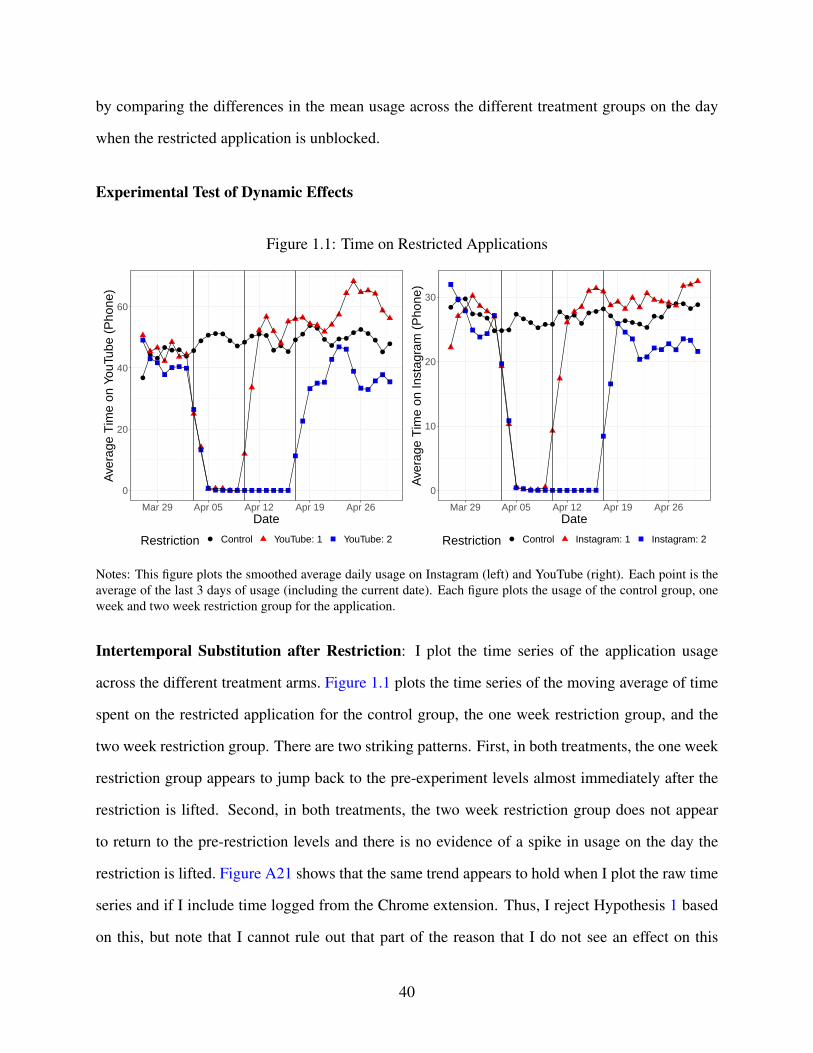
by comparing the differences in the mean usage across the different treatment groups on the day

when the restricted application is unblocked.

Experimental Test of Dynamic Effects

Figure 1.1: Time on Restricted Applications

0

20

40

60

Mar 29 Apr 05 Apr 12 Apr 19 Apr 26Date

Ave

rage

Tim

e on

You

Tube

(P

hone

)

Restriction Control YouTube: 1 YouTube: 2

0

10

20

30

Mar 29 Apr 05 Apr 12 Apr 19 Apr 26Date

Ave

rage

Tim

e on

Inst

agra

m (

Pho

ne)

Restriction Control Instagram: 1 Instagram: 2

Notes: This figure plots the smoothed average daily usage on Instagram (left) and YouTube (right). Each point is theaverage of the last 3 days of usage (including the current date). Each figure plots the usage of the control group, oneweek and two week restriction group for the application.

Intertemporal Substitution after Restriction: I plot the time series of the application usage

across the different treatment arms. Figure 1.1 plots the time series of the moving average of time

spent on the restricted application for the control group, the one week restriction group, and the

two week restriction group. There are two striking patterns. First, in both treatments, the one week

restriction group appears to jump back to the pre-experiment levels almost immediately after the

restriction is lifted. Second, in both treatments, the two week restriction group does not appear

to return to the pre-restriction levels and there is no evidence of a spike in usage on the day the

restriction is lifted. Figure A21 shows that the same trend appears to hold when I plot the raw time

series and if I include time logged from the Chrome extension. Thus, I reject Hypothesis 1 based

on this, but note that I cannot rule out that part of the reason that I do not see an effect on this

40

dimension is because the treatment allows for substitution to the computer.42

Persistent Effects on Restricted Applications: Figure 1.1 points to the fact that there may be

a persistent reduction in usage after the restriction, in particular for the 2 week treatment group.

I estimate specification (1.1) with heterogeneous effects across restriction lengths and for the 2

week group alone with the results reported in Table A16 and Table A17. Columns (1) and (2)

of Table A16 and Table A17 show the change in restricted application time in levels and logs for

Instagram and YouTube respectively. For Instagram, there is a statistically significant difference in

post-restriction time between these two for the levels specification and the 2 week restriction group.

Furthermore, columns (3) and (4) drops the 1 week group entirely and estimates the treatment effect

for only the 2 week group. This further confirms that there is a drop of approximately 5 minutes of

time on Instagram on average for the Instagram restriction group. For YouTube, there is a negative,

but imprecise point, estimate for both specifications. Given the skewed usage distribution and the

discrepancy between logs and levels, one might expect that the changes in post-restriction usage

are driven by those at the high end of the usage distribution. Figure A22 estimates the QTE of

post-restriction effects and confirms this intuition.

A natural question is, if such post-restriction effects exist, how persistent are they? It is plausi-

ble that these effects dissipate very quickly, but I only observe participants for 2-3 weeks following

the restriction. In order to understand how much longer the effects last, I rely on an optional survey

that was sent one month following the conclusion of the study asking how they had been spending

their time relative to before the experiment.43 Participants could mark whether they were spending

a lot less time (1), somewhat less time (2), the same amount of time (3), somewhat more time (4),

or a lot more time (5). They could also mark if they did not use the application or had started to use

it during the study period. I estimate the impact of the restrictions on overall phone, overall social

media, Instagram, and YouTube usage. Table A19 displays the estimated average treatment effect,

which shows that there is still a large drop in the Instagram treatment group’s overall social media

42Even though I observe that this substitution is minimal it’s possible that this usage was more “directed" forspecific usage which dampens the possible intertemporal effect.

43Participants were incentivized by being able to enter the chance to win a $100 Amazon Gift Card by completingthe survey. However, they had already been paid their experimental payment after the conclusion of the study period.

41

and Instagram usage. This result must be caveated for the following two reasons. First, there is

potential for selection bias since participants with stronger responses to the treatment may be more

willing to respond. However, roughly an equal number of participants from both the treatment and

control group responded, indicating this may not be a large concern.44 Second, these are unverifi-

able survey responses, so it is possible that some of the results are driven by experimenter demand.

Subject to these caveats, these results show that a one or two week restriction led to a reduction in

usage nearly two months later. Combined with the other results, this provides evidence that there

were persistent effects of the restrictions and thus support for Hypothesis 2.

Persistent Effects on Non-Restricted Applications: Table A20 and Table A21 provide estimates

for persistent changes on usage of non-restricted applications as a result of the Instagram and

YouTube treatments. I focus on applications / categories where I observed substitution towards

during the restriction period and the applications installed during the restriction period.45 I find

little evidence of persistent changes in usage along these dimensions. The only notable persistent

increase is in the amount of time spent on applications that were installed during the restriction

period for YouTube. There is a marginally significant increase in time spent on Instagram for par-

ticipants in the YouTube treatment.46 However, beyond this, there are minimal persistent changes

on other applications. It must be noted that these are average treatment effects and I observed het-

erogeneous substitution during the restriction period itself, so it does not rule out that there were

persistent changes in time usage but that these are so heterogeneous that they would not be picked

up by this specification. Indeed, Table A18 indicates that participants self-report having persistent

effects on other applications, but the effect sizes may be too small for them to be detectable given

the power of the experiment. However, given this evidence, I reject Hypothesis 3.

44Note that since there is only partial response I do not include the controls for randomization block.45In order to economize on space I do not include in the interaction term in the reported estimates. Instead, I

estimate the ATE of the persistent for both restriction lengths (without an interaction) and then report point estimatesfor the 14-day treatment group alone.

46A similar effect was observed during the pilot study.

42

1.6 Model of Time Usage with Inertia

Motivated by the experimental results, I estimate an individual level discrete choice model of

time usage with inertia. There are two experimental results in particular that point to the importance

of inertia. First, participants spent time on newly installed applications and persisted to use these

applications, even once the restriction period was over. Second, there is a reduction in usage of the

restricted application in the post-restriction period, especially for the heaviest participants. One

interpretation of this result is that the restriction serves as a shock to participants’ habits, which

induces them to reduce their usage of the application. In the remainder of the section, I will detail

and provide estimates of the model. The main outputs of interest from the model are to quantify the

role of inertia in usage and produce diversion ratios between the considered applications. These

will provide a more refined view of substitution between the applications of interest.

1.6.1 Model and Identification

I model participant’s choices as a panel of discrete choices. This is a formalization of the

informal model in Section 1.5.2 where the participant chooses a single application at each time

period to use and this choice is partially determined by the habits of the participant.47,48 There is a

set of applications J = {1, ...𝐽}, indexed by 𝑗 , and a set of participants I = {1, ..., 𝐼}, indexed by

𝑖. I consider each application restriction as its own separate “market", indexed by 𝑘 , which dictates

the choice set available to consumers.49 I use the disaggregated time period data, denoted by 𝑡, at

the time interval of 15 minutes.50 Participant 𝑖 receives the following utility from application 𝑗 in47Other models of time demand for applications such as [44] and [45] consider a multiple discrete-continuous

framework. [55] takes a similar approach as mine when considering time allocation demand for channels on cabletelevision. One benefit to the discrete choice approach is that it enables me to flexibly control for variation in usagethroughout the day and week, which is apparent in Figure A13, as well as directly incorporate past usage into theutility function.

48Recall that in the experimental section there was little evidence of intertemporal substitution, evidenced by thelack of a spike of usage on the day the restriction was returned. Thus, the formulation assumes that participants aremyopic in their choices so that their usage does not directly take into account how their choice this period will impactfuture period usage.

49Beyond the experimental restrictions to Instagram and YouTube, some participants were restricted from Twitter,WhatsApp, Facebook, or Messenger since they did not use the main experimental applications of interest.

50In order to construct this I compute the time allocations allotted to each application in each interval, includingoff the phone time, and assign the chosen application as the maximum of these quantities. I aggregate the minute by

43

market 𝑘 and time period 𝑡:

𝑢𝑖 𝑗 𝑘𝑡 = 𝛽𝑞(𝑖) · ℎ𝑖 𝑗 𝑡 + Z𝑞(𝑖) · 𝑟𝑖 𝑗 𝑡 + 𝜔𝑞(𝑖) · 𝑟2

𝑖 𝑗 𝑡 + 𝛾𝑞(𝑖)𝑗

+ ^𝑞(𝑖) · 𝑎𝑐𝑖 𝑗 + 𝜖𝑖 𝑗 𝑘𝑡 (1.2)

𝛾𝑞(𝑖)𝑗

denotes application fixed effects, 𝑎𝑐𝑖 𝑗 incorporates the subjective usage of application 𝑗 ,

which comes from Table 1.2, for participant 𝑖, and 𝜖𝑖 𝑗 𝑘𝑡 is the Type-1 Extreme Value error. 𝑞(𝑖)

denotes the type of participant 𝑖 that is determined by running k-means on the aggregated base-

line data of the considered applications in order to group participants into different types. Thus,

the specification accommodates preference heterogeneity across participants both by having type-

specific estimates of the coefficients and by incorporating the subjective uses of the applications

directly into the utility function.51

The main parameters of interest are those that relate to consumer inertia. There are broadly two

types of inertia effects that are present – short-term and long-term inertia. The primary interest is

in understanding long-term inertia, but it is important to account for short-term inertia. Short-term

inertia accounts for the fact that a participant is more likely to choose application 𝑗 in period 𝑡 if

they used the application in period 𝑡 − 1. I include a term, 𝑟𝑖 𝑗 𝑡 , which is defined as the number

of directly consecutive periods which participant 𝑖 has used application 𝑗 . Since this short-term

component potentially has satiation effects, it enters both linearly and quadratically into the utility

function. It is important to emphasize that the short-term inertia is largely a nuisance term that

allows me to better estimate the more important longer term aspect of inertia.52

The second type of inertia, which is my primary interest, is the longer-term “habit" portion

of usage. In order to capture this, I formulate this in a similar manner as [11] with a continuous

stock of usage that the participant accumulates. Motivated by the apparent difference in long-run

behavior between the one and two week restriction groups, I define the habit stock, ℎ𝑖 𝑗 𝑡 , as the total

minute data to a 15 minute interval so that the computations are not too cumbersome, but the estimates from the modelare nearly identical if I use smaller time intervals.

51Incorporating some degree of preference heterogeneity is key in order to ensure that the estimates on the inertiaterms are not positive due to misspecification [56, 10].

52Without properly controlling for short-term inertia, it is likely that the 𝜖𝑖 𝑗𝑘𝑡 would be serially correlated whichwould bias the estimates of 𝛽𝑞 (𝑖) .

44

amount of time participant 𝑖 has spent on application 𝑗 in the past two weeks.53 Thus, under this

formulation, the experiment induces a shock to the longer-term habit portion of usage, but, beyond

the initial period when the restrictions are lifted, not the short-run inertia portion.

The granularity of the data allows me to vary the outside option flexibly across time. For any

time index 𝑡, I allow the outside option to vary across the week of the experiment 𝑤(𝑡), day of the

week 𝑑 (𝑡), and hour of the day 𝑜(𝑡). I collapse the hours of the day into morning (7 AM - 12 PM),

afternoon (12 PM - 6 PM), evening (6 PM - 1 AM), and late night (1 AM - 7 AM). I normalize

the outside option to zero at afternoons, Fridays, and the final week of the experiment. Thus, the

utility for the outside option is denoted as follows where 𝛼𝑜(𝑡) denotes hour of day fixed effects,

]𝑑 (𝑡) denotes day of week fixed effects, and `𝑤(𝑡) denotes week fixed effects:

𝑢𝑖0𝑡𝑘 = 𝛼𝑜(𝑡) + ]𝑑 (𝑡) + `𝑤(𝑡) + 𝜖𝑖0𝑡𝑘

The assumption that 𝜖𝑖 𝑗 𝑘𝑡 are independent and identically distributed according to a Type-1 ex-

treme value distribution induces the following probability that application 𝑗 will be chosen by

participant 𝑖:

𝑙 (ℎ𝑖 𝑗𝑡 , 𝑎𝑖 𝑗 , 𝑟𝑖 𝑗𝑡 ; \) =exp(𝛽𝑞 (𝑖) · ℎ𝑖 𝑗𝑡 + Z 𝑞 (𝑖) · 𝑟𝑖 𝑗𝑡 + 𝜔𝑞 (𝑖) · 𝑟2

𝑖 𝑗𝑡+ 𝛾

𝑞 (𝑖)𝑗

+ ^𝑞 (𝑖) · 𝑎𝑐𝑖 𝑗 )

exp(𝛼𝑜 (𝑡 ) + ]𝑑 (𝑡 ) + `𝑤 (𝑡 ) ) +∑

𝑗′ exp(𝛽𝑞 (𝑖) · ℎ𝑖 𝑗′𝑡 + Z 𝑞 (𝑖) · 𝑟𝑖 𝑗′𝑡 + 𝜔𝑞 (𝑖) · 𝑟2𝑖 𝑗′𝑡 + 𝛾

𝑞 (𝑖)𝑗′ + ^𝑞 (𝑖) · 𝑎𝑐𝑖 𝑗′ )

(1.3)

Identification: The primary parameter of interest is 𝛽𝑞(𝑖) . The identification argument for this

parameter is as follows. First, following the literature on state-dependent demand estimation (e.g.

[10]), it is important that the specification sufficiently captures individual preference heterogeneity.

This is captured by incorporating the subjective usage of each of the considered applications as well

as having type-specific estimates.54 Second, the experiment induces exogenous variation in the

53Note that there is an initial conditions problem at the beginning of the experiment since there is no previous datato use to define this. Because of this I drop the first two days of data entirely from the estimation and, for any date inthe first two weeks, I multiply the accumulated “stock" by the inverse of the fraction of the current time period by thetime period exactly 2 weeks from the start of the experiment. I chose two days since the descriptive statistics point tousage not varying drastically across the days of the week and preliminary experiments showed that after two days thehabit stock variable is fairly constant in the baseline period.

54The biggest worry about unobserved heterogeneity in usage comes from the extreme users of specific applications

45

habit stock of the restricted applications as well as the other applications (via substitution during

the restriction period). Thus, the core identification assumption is that the experiment only serves

as a shock to the habits of the participants.

Estimation: I restrict myself to the most prominent social media and entertainment applications

– Facebook, TikTok, Twitter, Reddit, YouTube, Instagram, and Snapchat – and denote every other

application or off phone activity as the outside option. For these applications, I collect the average

daily usage in the baseline period for each participant and cluster the participants according to

k-means. I then estimate the model separately for each type. Since my model is likelihood-based,

I estimate the parameters using maximum likelihood estimation.

1.6.2 Model Estimates and Validation

The first step of estimation requires classifying the participants into different types using k-

means. There is a large literature in data mining and statistics about choosing the “optimal" 𝑘 that

trades off the parsimony of having fewer clusters against the reduction in within-cluster variance

that arises from additional clusters. In this case an additional consideration is that it is important to

ensure that the clusters have sufficiently many individuals to allow for estimation of the parameters

of interest for this group, but also having sufficiently many clusters to capture the unobserved

preference heterogeneity. I consider an index of these measures for choosing the “optimal" 𝑘

which reports 𝑘 = 3 and 𝑘 = 6. In order to accommodate additional heterogeneity in consumer

preferences, I utilize 𝑘 = 6.55 Figure A23 displays the resulting clusters and the time allocations

within each of them. The resulting clustering of participants identifies sets of power users. Cluster

1 captures the more typical users of these applications who have moderate usage of each of the

applications. Clusters 2 and 3 capture the YouTube intensive participants. Cluster 4 captures the

or bundles of applications. The clustering formulation is able to capture the differences in preference intensity forthese participants and consider separate estimates for them. The approach of discretizing a potentially continuousdistribution of unobserved heterogeneity through k-means has precedent in [57].

55I additionally consider density-based spatial clustering of applications with noise (DBSCAN) [58] and spectralclustering [59] which are clustering algorithms that do not restrict themselves to convex regions. Following bestpractices for the methods, I find that they do not result in substantially different clusterings with DBSCAN leading to3 clusters and spectral clustering leading to 7. Both pick out similar clusterings as k-means with 𝑘 = 3 and 𝑘 = 6, so Iopt for using k-means.

46

power users of Reddit. Cluster 5 identifies participants who are power users of TikTok, but also

use the other social media applications extensively. Cluster 6 identifies participants who are power

users of Facebook and Instagram.

The estimates from the model are presented in Table A24. I report the estimates of each type

separately. The first observation is that the coefficient on ℎ𝑖 𝑗 𝑡 is fairly consistent across the differ-

ent types as well as the estimate for the influence of short-term inertia, 𝑟𝑖 𝑗 𝑡 and 𝑟2𝑖 𝑗 𝑡

. Both of these

terms are statistically different from 0, indicating that both the short-term and long-term inertia

channels play a role. The coefficient on 𝑟2𝑖 𝑗 𝑡

is negative, indicating satiation effects. The differ-

ences in the natural usage of each of the applications across the different types, which is reflected

in Figure A23, naturally translates to differences in the estimated application fixed effects. The

estimated time fixed effects that vary the outside option are similar across the different types and

follow the variation in phone usage across the week depicted in Figure A13. The coefficients on

the different subjective uses of the applications varies across the types in accordance with the most

used applications by participants classified as that type.

I validate the in-sample fit of the model by comparing how well the model is able to match the

actual market shares throughout the study period. Recall that the model is estimated including the

restriction period. Thus, I compare how well the model is able to predict the average market shares

in the non-restriction period in addition to how well it is able to predict the substitution during

the restriction period. In particular, I compare how well the model is able to capture substitution

towards other applications and the outside option in the Instagram and YouTube restriction periods

respectively. Table A25 shows that the model fits the data reasonably well as it matches the non-

restriction period market shares and predicts the extent of substitution towards other applications

and the outside option as a result of the experimental restrictions.56

56The estimates of the main parameters of interest are robust to model specification. Preliminary specificationsdid not include application fixed effects, but rather only included application characteristics and were estimated overthe entire sample. Over these different specifications, the model had a poorer fit of the overall data, but had a similarestimate of roughly 0.01 for ℎ𝑖 𝑗𝑡 across the different types. Furthermore, omitting either the short-term inertia orsubjective application usage from the utility function leads to an increase in the coefficient of ℎ𝑖 𝑗𝑡 but does not changethe resulting estimates or main outputs from the model dramatically.

47

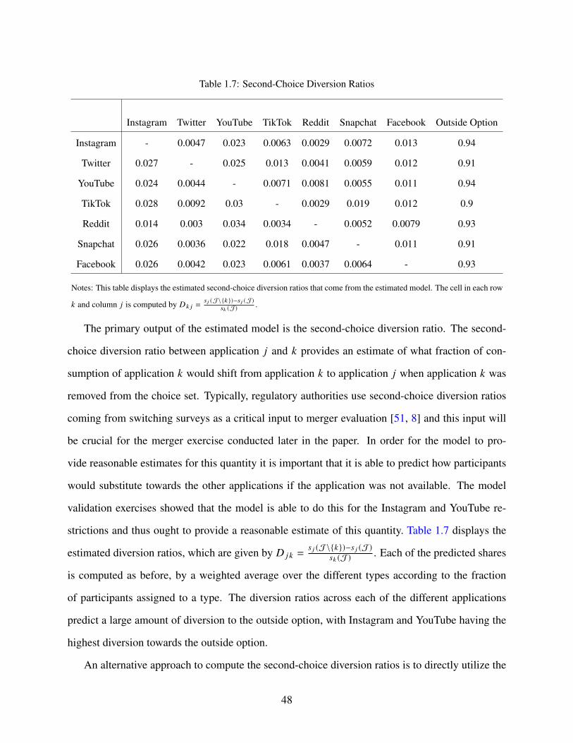
Table 1.7: Second-Choice Diversion Ratios

Instagram Twitter YouTube TikTok Reddit Snapchat Facebook Outside Option

Instagram - 0.0047 0.023 0.0063 0.0029 0.0072 0.013 0.94

Twitter 0.027 - 0.025 0.013 0.0041 0.0059 0.012 0.91

YouTube 0.024 0.0044 - 0.0071 0.0081 0.0055 0.011 0.94

TikTok 0.028 0.0092 0.03 - 0.0029 0.019 0.012 0.9

Reddit 0.014 0.003 0.034 0.0034 - 0.0052 0.0079 0.93

Snapchat 0.026 0.0036 0.022 0.018 0.0047 - 0.011 0.91

Facebook 0.026 0.0042 0.023 0.0061 0.0037 0.0064 - 0.93

Notes: This table displays the estimated second-choice diversion ratios that come from the estimated model. The cell in each row

𝑘 and column 𝑗 is computed by 𝐷𝑘 𝑗 =𝑠 𝑗 (J\{𝑘 })−𝑠 𝑗 (J)

𝑠𝑘 (J) .

The primary output of the estimated model is the second-choice diversion ratio. The second-

choice diversion ratio between application 𝑗 and 𝑘 provides an estimate of what fraction of con-

sumption of application 𝑘 would shift from application 𝑘 to application 𝑗 when application 𝑘 was

removed from the choice set. Typically, regulatory authorities use second-choice diversion ratios

coming from switching surveys as a critical input to merger evaluation [51, 8] and this input will

be crucial for the merger exercise conducted later in the paper. In order for the model to pro-

vide reasonable estimates for this quantity it is important that it is able to predict how participants

would substitute towards the other applications if the application was not available. The model

validation exercises showed that the model is able to do this for the Instagram and YouTube re-

strictions and thus ought to provide a reasonable estimate of this quantity. Table 1.7 displays the

estimated diversion ratios, which are given by 𝐷 𝑗 𝑘 =𝑠 𝑗 (J\{𝑘})−𝑠 𝑗 (J)

𝑠𝑘 (J) . Each of the predicted shares

is computed as before, by a weighted average over the different types according to the fraction

of participants assigned to a type. The diversion ratios across each of the different applications

predict a large amount of diversion to the outside option, with Instagram and YouTube having the

highest diversion towards the outside option.

An alternative approach to compute the second-choice diversion ratios is to directly utilize the

48

estimated average treatment effects of substitution during the product unavailability period. [8]

provide a treatment effects interpretation of second-choice diversion ratios that does this and, in

[32], provide a method to compute the rest of the matrix of diversion ratios for applications with-

out experimental variation. In section A.5, I apply their methods to get an alternative estimate of

the diversion ratios, shown in Table A22. The estimated diversion ratios are similar to those esti-

mated using the model. The main noticeable difference is that the diversion between, for instance,

Instagram-Facebook, YouTube-Instagram, and Instagram-TikTok is noticeably larger than the es-

timates produced from the model. This is due to the fact that these are nonparametric and driven

by the difference in point estimates of the treatment effects. The nonparametric diversion ratio

estimates are displayed in Table A23, which shows the degree of imprecision in their estimation.

This is since the power requirements to get precisely estimated diversion ratios are not just being

able to distinguish the estimated substitution towards one application as being greater than zero,

but rather being able to distinguish estimated substitution towards one application as being greater

than other applications with positive substitution. Thus, my experiment is not sufficiently powered

to determine whether these differences in the estimated diversion ratios come from imprecision or

actual differences. As a result, I rely on the estimated diversion ratios from the model.57

1.6.3 Counterfactual: No Long-Term Inertia

The counterfactual I consider is to understand the role of the long-term inertia channel in driv-

ing the usage of the social media and entertainment applications. Concretely, I impose 𝛽𝑞(𝑖) = 0

and characterize the change in the resulting market shares and diversion ratios, which will allow

me to consider how this channel influences merger assessments in Section 1.7. It is important to

understand the interpretation of this counterfactual since it is not a direct policy counterfactual.

This inertia channel comprises a number of different aspects of usage – ranging from addictive im-

pulses to more natural mechanisms such as switching costs — and I provide several interpretations

of the counterfactual that are directly motivated by regulatory and antitrust concerns.

57Another important consideration is that this method does not allow me to consider how the diversion ratio changeswith and without inertia.

49

First, while some aspects of inertia are natural components of application choice, there are

addictive elements of these applications and a number of policy instruments have been proposed

for alleviating this issue. Indeed, the evidence from the baseline survey indicates that, for my

sample, one of the behavioral mechanisms at play is addictive concerns as a substantial fraction of

the participants are psychologically addicted to social media services. There has been a contention

that some of this addiction may arise from design choices made directly by these applications.

For instance, the objective function of the content curation algorithms and design patterns such

as infinite scroll news feeds encourage excessive usage of these applications [60]. As a result, a

number of policy proposals have been raised aimed at regulating these aspects of the applications in

order to indirectly impact the extent of addiction to these applications, while other policy proposals

aim to directly limit the time spent on these applications in order to directly address the problem.

One interpretation of the counterfactual is to understand the effect of these proposed regulations

by shutting down the role of these addictive concerns in usage. However, since the long-term

inertia channel in my model comprises a number of different behavioral mechanisms beyond the

addictive concerns, the resulting market shares and diversion ratios can be viewed as a limit case

that characterizes an upper bound for how such policies would impact usage and diversion.

Second, the diversion ratios produced under the no inertia counterfactual are more natural

measures of substitution between the applications than in the baseline. This is since the baseline

diversion ratios include the extent of diversion due to both direct substitutability and habitual usage.

This leads to naturally higher diversion for applications with higher habitual usage (e.g. Instagram,

YouTube). Thus, the diversion ratios produced by the no inertia counterfactual are plausibly more

policy-invariant measures of diversion that focus only on the direct substitutability of any given

two applications. This measurement of diversion is useful for evaluating a common type of merger

in this market where a prominent application acquires a nascent application (e.g. see [61] more

generally and [62] for mobile applications specifically).58 In this case, the prominent application

58This was one purported motivation for instance behind the Facebook and Instagram merger, seehttps://www.theverge.com/2020/7/29/21345723/facebook-instagram-documents-emails-mark-zuckerberg-kevin-systrom-hearing.

50

acquires the nascent application before it is able to build up the habit stock of consumers and so

the estimated measures of diversion in the baseline may be low mainly due to the fact that the

nascent application has not been around sufficiently long to build up the habit stock of consumers.

Thus, the more direct measures of diversion produced under this counterfactual could be useful for

evaluating these types of mergers.

Table 1.8: Market Shares (No Inertia)

ApplicationNo Inertia:

Weeks 1,4,5

Baseline:

Weeks 1,4,5

No Inertia:

Weeks 4,5

Baseline:

Weeks 4,5

No Inertia:

Week 1

Baseline:

Week 1

Instagram 0.0148 0.0276 0.0149 0.0276 0.0145 0.0275

Outside Option 0.941 0.901 0.94 0.899 0.943 0.904

Twitter 0.00364 0.0044 0.00371 0.0045 0.00345 0.00411

YouTube 0.0191 0.0339 0.0195 0.0347 0.0179 0.0318

TikTok 0.00388 0.00797 0.00392 0.00817 0.00376 0.00743

Reddit 0.00471 0.00644 0.00479 0.00673 0.00447 0.00563

Snapchat 0.00456 0.00679 0.00456 0.00682 0.00456 0.00672

Facebook 0.00852 0.0122 0.00858 0.0121 0.00833 0.0124

Notes: Columns 1 and 2 display the predictions of the model over week 1, 4, and 5 including the long-term inertia term

and without. Columns 3 and 4 display the prediction of the model only over weeks 4 and 5. Columns 5 and 6 display

the prediction of the model only over week 1. Each cell displays the market share of the row application under the

specification designated by the column.

Table 1.8 compares the average market shares with and without the inertia term across different

weeks of the experiment when participants had the full set of applications available to them. Since

the results across the different subsets of weeks are quantitatively very similar, I restrict focus

to the first two columns which compare the differences across all weeks in the experiment. The

first observation is that the overall market share of the set of inside applications drops by nearly

51

40% when this channel is shut down.59 Table A28 displays the reduction of usage in percentages,

showing that YouTube, Instagram, and TikTok have the largest percentage reduction in average

usage when this channel is shut down. Recall that TikTok in particular has a smaller number of

users in my sample relative to the other applications, but, conditional on using the application, has

one of the highest average time allocations. As a result, it is not too unsurprising that the model

predicts that inertia is a large driver of usage for this application.

I further compute the estimated second-choice diversion ratios when the inertia channel is

shut down. The estimates are displayed in Table A26 with the percentage differences between

the baseline and no inertia case presented in Table A27. There is a drop in the diversion ratios

from other applications towards the most prominent applications such as Instagram or YouTube,

but there is not a reduction across the entire matrix of diversion ratios. For instance, there is an

increase in diversion from Instagram to Reddit as well as from Snapchat to Twitter, which indicates

that the smaller applications in my sample can actually benefit from the lack of inertia for the larger

applications such as Instagram or YouTube.

1.7 Merger Analysis

In this section I conduct hypothetical merger analysis between the prominent social media and

entertainment applications. I propose a variant of the standard Upward Pricing Pressure (UPP) test

for attention markets and then use the estimated diversion ratios from Section 1.6 to implement

this test. I implement the test using the estimated diversion ratios with and without inertia and

characterize which merger decisions would change due to the influence of inertia.

59This observed decrease is qualitatively similar across other model specifications. Allowing application-specificcoefficients on ℎ𝑖 𝑗𝑡 leads to a quantitatively identical change in the overall usage of the applications. A separate modelmodel specification that did not include application fixed effects and instead used application characteristics reporteda range of 32-40% reduction in overall usage. Furthermore, concurrent work by [12] estimates a similar quantity usinga substantially different model specification, a slightly different set of applications, and experimental design and finda 31% reduction.

52

1.7.1 Upward Pricing Pressure Test

In order to evaluate a merger between two applications, I need to specify the profit function

of the applications and, importantly, their choice variables. I retain the same notion discussed

in Section 1.5.1 where the primary choice variable of the applications is to set the attention costs

faced by consumers. I follow the literature on two-sided media markets by supposing that the

primary manifestation of this is through choosing the advertising load of the application – the

number of advertisements per unit time experienced by the consumer. The model is necessarily

stylized, but captures the fundamental elements of the market.

Formally, I consider that the applications are playing a Bertrand-Nash game where each ap-

plication 𝑗 sets its advertising load in order to maximize profits. The application revenue per unit

time depends on the quantity of advertisements per unit time, 𝑎 𝑗 , and the price that advertisers are

willing to pay for advertising on this application, 𝑃 𝑗 (𝑡 𝑗 (𝒂)), which depends on the time allocations

of consumers, 𝑡 𝑗 (𝒂). The marginal cost of the application, denoted 𝑐 𝑗 , is the marginal cost of serv-

ing these advertisements to consumers. Thus, the profit maximization problem for application 𝑗 is

given by:

arg max𝑎 𝑗

𝜋 𝑗 (𝒂) = (𝑎 𝑗 · 𝑃 𝑗 (𝑡 𝑗 (𝒂)) − 𝑐 𝑗 ) · 𝑡 𝑗 (𝒂) (1.4)

Consumers face differentiated goods where the main “price" that they face is the advertising quan-

tity set by the application, which induces a disutility that depresses their time allocations. Adver-

tising is modeled as a homogenous good that is differentiated only through the time that consumers

spend on the application. This is the main channel through which network effects show up in this

formulation as it captures that advertisers have a willingness to pay that varies with the ability to

target consumers and depends on the time allocations of consumers. The prices are set through

second-price auctions so that they reflect the willingness to pay of advertisers to acquire the atten-

tion of the consumers on that application at a given point in time. Consequently, the application

does not directly set the advertising prices.

53

Given this formulation, I propose an Upward Pricing Pressure (UPP) test to conduct merger

analysis [41]. The goal of the test is to determine whether a merger would lead to “upward pres-

sure" on prices and, if so, the merger is blocked. The effect of a merger is ambiguous since it

exerts upward pressure on prices by enabling the firm to internalize the diversion between the

merged firms’ applications, but also puts downward pressure on prices through the efficiency gains

resulting from the merger. In this setup, the relevant quantity is not whether the merger induces

higher prices, but whether it induces higher advertising loads.

In order to formulate the test, I need to specify the joint profit function of the merged firm.

The main change is that the merger induces efficiency gains that arise through an increase in the

quality of the applications. Following [63], I incorporate this by supposing that consumers face a

quality-adjusted advertising load. One possible interpretation of this is that the increased ability to

target advertising leads to more useful advertisements for consumers, though the quality gains are

broader than just the impact on advertising. Thus, the merged profit function between applications

1 and 2 is as follows:

𝜋1 + 𝜋2 =

(𝑃1(𝑡1(𝒂)) · (𝑎1 + a1) − 𝑐1

)· 𝑡1(𝒂) +

(𝑃2(𝑡2(𝒂)) · (𝑎2 + a2) − 𝑐2

)· 𝑡2(𝒂)

where a1, a2 denote the quality gains for application 1 and 2 respectively as a result of the merger.

The UPP evaluates whether, for each application individually, the first-order condition of the

merged profit function is positive (i.e. whether 𝜕 (𝜋1+𝜋2)𝜕𝑎1

> 0 or 𝜕 (𝜋1+𝜋2)𝜕𝑎2

> 0) when evaluated

at the current equilibrium advertising loads and prices (e.g. the pre-merger advertising loads and

prices). The derivation of the UPP test is provided in section A.7 and is given by:

𝑈𝑃𝑃1 = 𝐷12 ·(𝑃2 · (𝑎2 + a2) − 𝑐2︸ ︷︷ ︸Revenue from Diversion

+ 𝑑𝑃2𝑑𝑡2

· (𝑎2 + a2) · 𝑡2(𝒂)︸ ︷︷ ︸Price Change from Diversion

)−

(a1 ·

(𝑑𝑃1𝑑𝑡1

· 𝑡1(𝒂) + 𝑃1

)︸ ︷︷ ︸

Quality Efficiency Gains

)

𝐷12 denotes the diversion ratio from application 1 to 2. There are two separate channels that

put upwards pressure on the quality-adjusted advertising load faced by consumers. The first is that

the diversion towards application 2 from application 1’s increase in advertising load enables the

54

application to gain additional revenues due to the additional time spent on the application. The

second captures the impact of the diversion towards application 2 on the advertising prices for

application 2. There is one channel that puts downward pressure on the quality-adjusted advertis-

ing load, which is that the merger induces quality improvements. This quality gain could come

through a number of channels, such as improved curation algorithms, better product infrastructure,

or improvements in advertising targeting.

1.7.2 Data and Additional Discussion

In order to be able to conduct merger evaluation using the UPP test, I need to collect or estimate

the following quantities. I require data on the advertising quantities, advertising prices, time allo-

cations of consumers, and marginal costs. Further, the test necessitates an estimate of consumer

diversion between the two applications being merged as well as an estimate for how responsive

advertising prices are to additional time spent on an application.

Advertising Load and Prices Data: The data that I use is as follows. The time allocation data

comes from the baseline period during the experiment. The advertising load data comes from

self-reported data from experimental participants where they were asked to report how many ad-

vertisements they experience per minute of usage on each of the applications. I take the average

across all the participants to get a measure of the advertising load for each application. The ad-

vertising price data comes from the average price per impression on each application in 2021 as

reported in trade blogs.60 Finally, I suppose that the marginal cost of serving advertisements is

zero.61

Measure of Consumer Diversion: The main variable in the UPP formulation that comes from

consumer demand is the estimated diversion ratio. In the UPP formulation, it enters as − 𝜕𝑡2𝜕𝑎1

/ 𝜕𝑡1𝜕𝑎1

,

which is the diversion ratio with respect to advertising load. Since the advertising load is constant

60Note that these prices are relatively low. For instance the average price per impression on Instagram is $0.00791,which is contrast to the larger value of additional time on the application documented in section A.3.

61This is a reasonable approximation since the marginal cost of serving an individual advertisement involves thecomputational cost of coordinating a (generalized) second-price auction and serving an HTTP request. This is com-mon in technology infrastructure where fixed costs are relatively high, but the marginal cost of network requests isnegligible.

55

over the period of the study, I do not have the variation to identify the advertising load coefficient,

and consequently the diversion ratio with respect to advertising load, in a demand model. How-

ever, the product unavailability variation and estimated model in Section 1.6 provides me with an

estimate of the second-choice diversion ratio. Second-choice diversion ratios are commonly used

instead of price-based diversion ratios in merger evaluation cases [51, 8]. Furthermore, [8] show

that the difference between these estimates depends on the curvature of demand with respect to

the variable of interest. This means that whether or not second-choice diversion ratios are reason-

able proxies for advertising load diversion ratios depends on the curvature of demand with respect

to advertising load. The main empirical evidence from the literature on the relationship between

advertising loads and time allocations comes from [64] who show a strikingly linear relationship

between time allocations and advertising load in a 21 month experiment on Pandora. Follow-

ing the results of [8], this linearity indicates that second-choice diversion ratios should provide a

reasonable approximation to diversion with respect to advertising load.

Advertising Price Setting: The modeling of the advertising market requires some additional dis-

cussion as it is stylized on several dimensions. The assumption that advertising, holding constant

consumer time allocations, is a homogeneous good is consistent with qualitative evidence in [3]

and discussions with industry professionals who state that the primary determining factor of where

to spend their advertising budget is the reach and ability to target on the application.62,63 The

assumption that the applications do not explicitly set prices is consistent with practice where ad-

vertising prices are typically set via generalized second-price auctions.

The formulation utilizes the following assumptions on how components of the model impact

advertising prices. The first assumption is that advertising is a homogenous good whose main

differentiation is through the reach and targeting that depends on consumer time spent on the

62The main differentiation factor beyond this that is within control of the application is the advertising form – forinstance the distinction between video and non-video advertising is considered important. However, this is generallyconsidered secondary to the targeting aspect and thus I omit it from modeling considerations.

63In this formulation I am only focusing on the price of an impression. In reality advertisers pay a price based onthe number of impressions (denoted CPM) and the number of clicks (denoted CPC). If I make the assumption thatthe click-through rate is identical across applications then this can alternatively interpreted as CPC instead of CPM.However, I do not explicitly model these two channels separately.

56

application. The second is that the price does not change based on the advertising load.64 Thus

the only channel through which an application is disincentivized from increasing its advertising

load is through the disutility incurred by consumers and the resulting impact on advertising price.

For the UPP exercise, I only consider that the elasticity of advertising price with respect to time

is non-negative. This is since the advertisements in the applications of interest are predominantly

behaviorally targeted display advertising, which crucially is reliant on consumer histories in order

to target advertising effectively. The literature in marketing that quantifies the value of consumer-

specific information on the willingness to pay of advertisers in these markets finds a substantial

increase in advertiser willingness to pay as a result of having this information [65, 66, 67].65 Thus,

due to these assumptions, I naturally consider evaluating mergers on a grid of parameters where

𝑑𝑃1𝑑𝑡1

=𝑑𝑃2𝑑𝑡2

.

Quality Efficiency Gains: I suppose that the merger induces efficiency gains through improved

application quality. Predicting the extent of these efficiency gains at the time of a merger is a

challenging problem and the typical approach is to assign a fixed efficiency credit as a result of

the merger [41]. The efficiency credit assignment is typically done by setting the value of this

parameter to a fraction of the pre-merger quantity. In this case, when considering whether there

is upward pressure for application 𝑖 when evaluating a merger between applications 𝑖 and 𝑗 , I set

a𝑖 = 0.1 · 𝑎∗𝑖

and a 𝑗 = 0 so that the efficiency credits for application 𝑖 are set to be 10% of the

pre-merger advertising levels.

64These two aspects implicitly rely on the following two assumptions. The first is that there are no explicit crowdingout effects between advertisers when the quantity of advertisements on a single application is increased. The second isthat I have omitted directly specifying advertiser payoffs, but one possible (strong) assumption would be if advertisersare homogeneous in the value of a conversion. In this case the price increase from additional time allocations is thatadditional precision in targeting increases the probability of conversion, thus increasing the price they are willing topay for the unit of attention.

65An additional piece of evidence for this is in [68] who study the value of consumers to advertisers after the EU’sGeneral Data Protection Regulation and argue that more persistently trackable consumers result in an increase in thevaluation of an average consumer.

57

1.7.3 Merger Evaluation

All of the terms in the UPP formulation are specified besides 𝑑𝑃1𝑑𝑡1

. In order to provide sharper

intuition about the different mechanisms at play, I consider two separate cases to provide a cleaner

characterization of the results: zero advertising price elasticity, 𝑑𝑃1𝑑𝑡1

= 0, and non-zero advertising

price elasticity, 𝑑𝑃1𝑑𝑡1

> 0. I consider these cases using the diversion ratios with inertia and then

without inertia with the results summarized in Table 1.9.

Merger Evaluation With Inertia

For each case, I compute the UPP for the merger between each pair of applications and report

which gets blocked. Recall that a merger is blocked if𝑈𝑃𝑃𝑖 > 0 is larger than zero for at least one

of the applications 𝑖 involved in the merger.66

Table 1.9: Summary of UPP Merger Analysis

𝑑𝑃1𝑑𝑡1

= 0 𝑑𝑃1𝑑𝑡1

> 0

With Inertia

Snapchat-Instagram, Reddit-Instagram,

Snapchat-YouTube, Reddit-YouTube,

Reddit-Facebook

Snapchat-Instagram, Reddit-Instagram,

Snapchat-YouTube, Reddit-YouTube,

Twitter-YouTube, TikTok-Instagram,

TikTok-YouTube, Twitter-Instagram

Without InertiaReddit-YouTube, Reddit-Instagram,

Snapchat-YouTube

Reddit-YouTube, Reddit-Instagram,

Snapchat-YouTube

Notes: This table summarizes the results of the UPP merger analysis exercise. I consider mergers between each pair of

applications in the list: YouTube, Instagram, Snapchat, Reddit, Instagram, TikTok, Twitter, Facebook. I do not consider

the fact that Facebook and Instagram are jointly owned and, consequently, do not consider a hypothetical merger between

the two. For the case when 𝑑𝑃1𝑑𝑡1

> 0, I report the results when 𝑑𝑃1𝑑𝑡1

> 0.004.

66Note that I do not include Facebook-Instagram since these applications are already merged in reality and, formergers involving these applications, I do not explicitly take into account the joint effect of these.

58

Zero Advertising Price Elasticity: This assumption isolates the tradeoff between the (Revenue

from Diversion) and (Quality Efficiency Gains) terms. In this case, the following mergers get

blocked: Snapchat-Instagram, Reddit-Instagram, Snapchat-YouTube, Reddit-YouTube, Reddit-

Facebook. These are predominantly mergers between smaller applications with relatively low

advertising loads and prices (i.e. Reddit, Snapchat) and larger applications (i.e. Facebook, Insta-

gram, YouTube). This is primarily caused by upward pressure on advertising load for the smaller

application. There are two underlying reasons behind this. First, there is relatively high upward

pressure due to diversion from the smaller to the larger applications. By increasing advertising

load and inducing time substitution towards the larger applications, the joint firm earns additional

revenues since a large share of time gets diverted towards the larger application and a single unit of

time on e.g. Instagram is more valuable than a single unit of time on e.g. Reddit. Second, there is

relatively lower downward pressure since these smaller applications have lower advertising loads

inducing smaller values for the efficiency gain threshold.

Non-Zero Advertising Price Elasticity: Now I consider the case when the own advertising price

elasticity is non-zero. This introduces additional upward pressure relative to the previous case

since now the (Price Change from Diversion) term is non-zero, which depends on the own-price

elasticity with respect to time as well as the pre-merger advertising load and average time allo-

cations of application 2. However, it also induces additional downward pressure that depends on

the own-price elasticity with respect to time and the pre-merger average time allocations of ap-

plication 1. I consider the grid of 𝑑𝑃1𝑑𝑡1

=𝑑𝑃2𝑑𝑡2

∈ {0.0001, 0.0002, ..., 0.009}, which leads to the

same set of mergers to be blocked as in the zero advertising price elasticity case, with the one

exception of Reddit-Facebook. Once 𝑑𝑃1𝑑𝑡1

> 0.0004, then the following mergers also get blocked:

Twitter-YouTube, TikTok-Instagram, TikTok-YouTube, Twitter-Instagram. In this case, the same

mechanism as before is at play – there is an incentive for the merged firm to increase advertising

loads from the smaller application (e.g. TikTok) to divert additional time towards the larger appli-

cations. Since the average time allocations on the larger application are higher than on the smaller

application, the upward pressure wins out relative to the downward pressure and induces additional

59

upward pressure relative to the previous case. This is not always the case, however, as evidenced

by the fact that the Reddit-Facebook merger is no longer blocked.

Merger Evaluation Without Inertia

I consider the same merger evaluation exercises under the counterfactual that the inertia channel

is shut down. This leads to two changes in the UPP evaluation relative to Section 1.7.3: the time

allocations across applications are lower, given by Table 1.8, and the subsequent diversion between

the applications is lower for most of the applications, given by Table A26. Note that the percentage

changes in the diversion ratios and market shares relative to the baseline inertia case are provided

in Table A27 and Table A28.

Zero Advertising Price Elasticity: In this case, the only term which changes relative to the iner-

tia baseline is the diversion weights on (Revenue from Diversion). This means that the downward

pressure remains the same as before, but the upward pressure is potentially softened due to the

decrease in diversion between these applications. Due to this, the following mergers are no longer

blocked: Snapchat-YouTube, Reddit-Facebook. However, Reddit-YouTube, Reddit-Instagram,

and Snapchat-Instagram remain blocked indicating that the softening of diversion between these

applications due to the lack of inertia is not sufficiently strong to induce all mergers to not be

blocked.

Non-Zero Advertising Price Elasticity: I consider the same range for 𝑑𝑃1𝑑𝑡1

as before. In this case,

both the additional upward and downward pressure are suppressed due to the lack of inertia. The

upward pressure from (Price Change from Diversion) is suppressed due to the decrease in diversion

as well as the decrease in the average time allocations on application 2. The downward pressure

from (Quality Efficiency Gains) is suppressed due to the decrease in average time allocations on

application 1. In the cases when a merger was previously blocked, the upward pressure is softened

more relative to the downward pressure, which leads to the following mergers no longer being

blocked across all values in the set of considered parameters: TikTok-Instagram, TikTok-YouTube,

Twitter-Instagram, Snapchat-YouTube, and Twitter-YouTube. Indeed, not only are no additional

60

mergers blocked beyond those that were present before including this channel, but, for 𝑑𝑃1𝑑𝑡1

>

0.0002, even the merger between Reddit and Instagram is no longer blocked. Thus, in this case

the role of inertia is so strong that it is the primary reason for blocking the mergers between these

applications.

1.8 Conclusion

In this paper I report the results of an experiment where I continuously monitor how participants

spend time on digital services and shut off their access to Instagram or YouTube on their phones for

one or two weeks. I use the resulting data on how participants substitute their time during and after

the restrictions in order to uncover a rich picture of the demand for social media and entertainment

applications. I illustrate how the estimated substitution patterns can be used to guide questions of

market definition and merger evaluation that have troubled regulators.

I find that participants with the YouTube restriction spend time on applications installed during

the restriction period and that participants with the two week Instagram restriction reduce their

time spent on Instagram even after the restrictions are lifted. Motivated by this, I estimate a discrete

choice model of time usage with inertia and find that inertia accounts for a substantial fraction of

usage. Finally, I develop an Upward Pricing Pressure Test for attention markets and show that

the presence of inertia is crucial for justifying blocking several mergers between social media

applications. Overall, my results emphasize the usefulness of product unavailability experiments

for demand and merger analysis in attention markets. These experiments provide a clean way of

measuring substitution patterns in these markets as well as identifying addiction/inertia effects,

which allow for a comprehensive picture of demand for these applications that are relevant to

antitrust issues. These experiments are feasible to conduct for regulatory authorities since the

nature of digital goods enables individual level, randomized controlled experiments of product

unavailability.

My results point to a broad competition for time between social media applications, but also

emphasize that inertia drives a substantial fraction of their usage and diversion towards larger ap-

61

plications such as Facebook and YouTube. There are two broader policy takeaways from these

results. The first is that, due to the personalized nature and importance of user-generated con-

tent on these applications, determining plausible substitutes according to similarities in product

characteristics alone – as has been done in several prominent merger cases – is likely to be insuf-

ficient. The second is that due to the role of consumer inertia in driving usage and its importance

in determining merger assessments, policies aimed at curbing aspects of these applications that are

conducive to addictive usage are an important policy tool at the disposal of regulators aiming to

promote competition in these markets. I believe that the insights from this paper can help push for-

ward the regulatory debate and lead to a better understanding of these zero price attention markets.

Going forward, one important direction for future work is to further incorporate the networked

aspect of these applications into the demand analysis in order to provide a richer picture of the

longer run substitution patterns.

62

Chapter 2: The Effect of Privacy Regulation on the Data Industry:

Empirical Evidence from GDPR

2.1 Introduction

Technological advances in the past several decades have led to enormous growth in the scale

and precision of consumer data that firms collect. These advances have been followed by progress

in machine learning and other data processing technologies that have allowed firms to turn data

into successful products and services and earn vast economic returns along the way.1 However, at

the same time, there has been an increasing number of high profile data breaches and a growing

feeling of despondency amongst consumers who lack control over this process.2,3 Beyond the

immediate economic harm resulting from such data breaches consumers might also value privacy

for its own sake.4 Against this backdrop, government regulators have proposed and enacted data

privacy regulation that empowers consumers to have more control over the data that they generate.

The European Union was the first to enact such legislation, the General Data Protection Regulation,

which has served as a blueprint for privacy legislation in California, Vermont, Brazil, India, Chile,

and New Zealand.5 However, we lack empirical evidence on the effectiveness and broader impact

1Several popular press outlets have gone as far as stating that “data is the new oil" meaning that the world’s mostvaluable resource is now data, not oil (e.g. The world’s most valuable resource is no longer oil, but data https://www.

economist.com/leaders/2017/05/06/the-worlds-most-valuable-resource-is-no-longer-oil-but-data. Re-trieved on January 9th, 2020.).

2There have been many but among the most prominent are the Cambridge Analytica and Equifax data breaches.Cambridge Analytica harvested the personal data of millions of people’s Facebook profiles without their consent andused it for political advertising purposes. The Equifax data breach exposed the names, dates of birth, and socialsecurity numbers of 147 million individuals.

3We Hate Data Collection. That Doesn’t Mean We Can Stop it. https://www.nytimes.com/2019/11/15/

opinion/privacy-facebook-pew-survey.html. Retrieved on January 3rd, 2020.4For the different motivations for privacy, see, for instance: [69]. As noted by [70], consumer privacy preferences

contain both an instrumental and non-instrumental component.5While such regulation is not entirely novel, the scope and robustness of previous regulation pales in comparison

to that of GDPR. Several states in the United States and countries around the world are debating and implementingtheir own privacy regulations with similar scope and stipulations as GDPR. For more information on the specifics of

63

of such regulation. Such evidence is critical not only for guiding the design of upcoming regulation,

but also to understand fundamental questions in the economics of privacy.

This paper empirically studies the effects of the EU’s General Data Protection Regulation

(GDPR), in particular, its requirement that consumers be allowed to make an informed, specific,

and unambiguous consent to the processing of their data. The consent requirement provides a

frontline defense of privacy for consumers: by denying consent, a consumer can block a website

from collecting personal data and sharing it with third-party affiliates. At the same time, consent

denial inhibits firms from tracking consumers across time and across websites, thereby building

historical profiles of consumers. Without them, these firms may not be able to learn and predict

consumer behavior and target their services and advertising accordingly.

Our investigation focuses on three broad questions. First, to what extent do consumers exercise

the consent right enabled by GDPR? Anecdotal and survey evidence suggests that consumers value

their privacy. Yet, as commentators argue, consumers may not be willing to act on their privacy

concerns even at little cost or inconvenience.6 We do not yet have clear empirical answers on this

question, and consumers’ decisions in their GDPR opt-out could shed light on their “revealed”

value of privacy.

Second, how does GDPR change the composition of consumers observed by firms? Even prior

to GDPR, consumers were able to protect their privacy by utilizing browser-based privacy protec-

tion means. However, utilizing these privacy means does not eliminate their footprints altogether

but rather simply generate “spurious” identifiers that are difficult for firms to distinguish from gen-

uine footprints left by consumers who do not adopt them. This process creates noise in the data

observed by firms that could make it difficult for them to track consumers and predict their behav-

ior. Under the GDPR regime, however, the same consumers may simply opt out, in which case

they do not leave any footprints, and this could in principle make the remaining consumers more

the various laws and how they relate to GDPR: 6 New Privacy Laws Around The Globe You Should Pay Attention To.https://piwik.pro/blog/privacy-laws-around-globe/. Retrieved on March 10th, 2020.

6A prevalent theme in the economics of privacy literature consistently finds a privacy paradox - the apparentinconsistency between individual’s strong stated preferences for privacy and their willingness to give away personalinformation at little cost [69]. This directly implies that a natural hypothesis is that consumers may ask legislators forsuch privacy means but, ultimately, make little use of them.

64

easily trackable and identifiable. This raises an interesting question of externalities created by pri-

vacy tools on the other consumers and for the firms. To the best of our knowledge, these forms of

privacy externalities not only differ from those recognized in the theoretical literature [71, 72, 73]

but more importantly have never been empirically identified.

Third, how does the GDPR privacy protection impact firms that rely crucially on consumer

data? Specifically, how does consumer opt-out affect firms’ abilities to learn and predict consumer

behavior and to provide targeted advertising? And how do advertisers react to such a change?

These questions are particularly important for the competitive landscape of the digital economy.

While big technology firms such as Google or Facebook enjoy virtually unlimited access to con-

sumer data based on their extraordinary reach and presence, many third-party companies can only

access the data shared by first-party affiliates. A concern is that the playing field of these firms,

already threatened by the big tech companies, may be further weakened by the increased consent

requirement of data regulation.7 How such a third-party firm copes with GDPR could provide a

valuable clue on how data regulation may influence the competitive playing field of the digital

economy.

To answer these questions, we use the data provided by an anonymous intermediary that con-

tracts with many of the largest online travel agencies and travel meta-search engines around the

world. The dataset is uniquely suited for the current inquiries in several respects. An integral part

of the intermediary’s business is to predict consumer behavior. Upon each visit by a consumer at

an online travel agency (its first-party affiliate), this firm predicts the likelihood of the consumer

buying from the website and places advertisements from alternative travel agencies to consumers

it deems unlikely to purchase from the original website.

The data links consumers’ behavior across time and across websites using cookies (set by the

7This concern has been raised in the recent literature [74, 75] and the popular press (GDPR Has Been a Boonfor Google and Facebook. https://www.wsj.com/articles/gdpr-has-been-a-boon-for-google-and-facebook-

11560789219. Accessed on June 2nd, 2020) which show that GDPR led to an increase in market concentration of webtrackers, favoring those from Google and Facebook. This concern is exacerbated by the scope of these companiesthat allows them to collect data across many different devices and domains that are not feasible for smaller third-partyvendors (All the Ways Google Tracks You—And How to Stop It. https://www.wired.com/story/google-tracks-you-privacy/. Accessed on June 2nd, 2020).

65

intermediary)—small files stored attached to a consumer’s web browser that allow the intermediary

to identify consumers. We observe (in anonymized and aggregated form) the same rich consumer

information as the intermediary and link them just as the intermediary can. If a consumer does not

consent to data storage using GDPR opt-out, then his/her cookies cannot be stored, so the consumer

is no longer observed by the intermediary. We can directly infer consumer privacy choices from the

number of consumer visits as seen by this (third-party) intermediary and the change in composition,

necessary to answer the first two questions. We also observe revenues from keyword-based online

advertising, and observe the output of a proprietary machine learning algorithm that predicts the

purchase likelihood, which will help us to address the third question.

Our empirical design exploits the fact that the intermediary contracts with many different plat-

forms all around the world who were differentially impacted by the introduction of GDPR. Fur-

thermore, the machine learning algorithm is trained and deployed separately for each online travel

website. This means that changes in data on one website, due to GDPR or other factors, do not

impact the performance of the algorithm on other websites. We exploit these features of our data

and the geographic reach of GDPR to utilize a difference-in-differences design for several outcome

variables across major European countries and other countries where GDPR was not implemented.

We find that GDPR resulted in approximately a 12.5% reduction in total cookies, which pro-

vides evidence that consumers are making use of the increased opt-out capabilities mandated by

GDPR. However, we find that the remaining set of consumers who do not opt out are more per-

sistently trackable. We define trackability as the fraction of consumers whose identifier a website

repeatedly observes in its data over some time period. We find that trackability has increased by

8% under GDPR.

We explore the mechanisms behind the increased trackability and argue that the most plausible

explanation is that the individuals who make use of GDPR opt-out are primarily substituting away

from other browser-based privacy means, such as cookie blockers, cookie deletion, and private

browsing. While the latter generates many “bogus” short-lived consumers (as a new ID is assigned

to a consumer, thus making her appear as a new user, each time she visits the site), the former—the

66

GDPR opt-out—simply removes these individuals from the data. As a result, those consumers that

remain in the data after the implementation of GDPR are more persistently identifiable.

Given this change in consumer composition, we explore the extent to which this affects adver-

tising revenues. In our setting the revenues that we observe come from keyword-based advertising

and, further, when consumers opt out they are no longer exposed to advertisements from the third

party intermediary. We find that there is an immediate drop in the total number of advertise-

ments clicked and a corresponding immediate decline in revenue. Over time, though, advertisers

on average increase their bids for the remaining consumers, leading to a smaller overall decline

in revenue. This indicates that the remaining set of consumers are higher value consumers com-

pared to the pre-GDPR set of consumers. One possible mechanism for this is that the increased

identifiability of consumers allows for advertisers to better attribute purchases to advertisements

than before. This increased attribution ability leads to an increase in perceived overall value of

consumers by advertisers.

Finally, we study the effect that GDPR had on the intermediary’s ability to predict consumer

behavior. In particular, we study the performance of the classifier used by the intermediary, which

is a crucial element of its business. The classifier provides a prediction of the probability that a con-

sumer will purchase on the website where she is currently searching. We find that there is evidence

that the classifier did not immediately adjust to the post-GDPR distribution. However, despite this,

we still find that the ability of the classifier to separate between purchasers and non-purchasers

did not significantly worsen after GDPR and that, if anything, the changes to the data observed

by the intermediary should lead to improvement in its ability to separate between purchasers and

non-purchasers.

Our results suggest a novel form of externalities that privacy-conscious consumers exert on the

rest of economy—including other consumers and the firms and advertisers relying on consumer

data. Their switching away from inefficient browser-based means of privacy protection to an ex-

plicit opt-out (enabled by data privacy regulation) could expose the digital footprints of those who

choose not to protect their privacy and make them more predictable. These externalities have po-

67

tentially important implications. First, third-party firms will suffer from loss of consumers who

opt out, but this loss will be mitigated by the increased trackability of those consumers who re-

main. Indeed, our analysis suggests that the mitigating effect could be important; while we find a

negative point estimate on overall advertising revenue, this decrease is not statistically significant.

Meanwhile, the welfare effect on the remaining consumers depends on how their data is used by

the firms. If their data is used to target advertising and services to their needs, as appears to be

so far the case, the externality is largely positive and they will be also better off. However, if the

data is used to extract their surplus—a possibility in the future—, they could be harmed by the

increased trackability.

Related Work

The protection of consumer privacy and its consequences has been studied by economists, legal

scholars, and computer scientists for several decades. We contribute to three strands of literature

in the economics of privacy.

Consequences of Data Privacy Regulation: A closely related study that also explores the short

run effect of GDPR is [76]. We see these two studies as complementary in terms of the data

scenario and findings. Our study utilizes data at a more dis-aggregate level but is confined to one

industry whereas [76] have a broad cross-section of different websites and are able to investigate

to what extent the effect of the GDPR works through a user acquisition channel. Instead, we are

able to look in more detail at cookie lifetime and how GDPR has affected advertising revenues of

third party firms.

Several other papers have studied the impact of the GDPR in other domains [77, 78, 79, 80, 81].

[75, 74] show that GDPR increased market concentration amongst web technology services. [82,

67] study the effectiveness of previous data privacy regulations on online advertising. [83] conduct

an experiment with a European telecommunications provider to test how consumers respond to the

more stringent opt-in requirements that are mandated by GDPR. Finally, [84] estimates a structural

model of advertising auctions and shows through counterfactual calculations that advertisement

68

revenue drops substantially more under an opt-in rather than an opt-out policy. We complement

these papers by utilizing the scope of our setting to tie each of these pieces together and characterize

how they interact with each other and are impacted by data privacy regulation.

Information Externalities: An important consequence of a consumer’s privacy decision is the

informational externality generated by that decision, as information revealed by one consumer can

be used to predict the behavior of another consumer.8,9 Several recent theoretical studies argue how

such externalities can lead to the underpricing of data, and results in socially excessive data col-

lection [94, 71, 72, 73, 95]. [96] theoretically studies how privacy choices by consumers can have

pecuniary externalities on other consumers by affecting firms’ incentives for price discrimination.

The current paper identifies a novel form of informational externalities. While the existing research

focuses on how a consumer’s decision to reveal her private data can predict the behavior of, and

thus can inflict externalities on, those who do not reveal their data, we recognize externalites that

run in the opposite direction. Namely, we show that the decision by a privacy-concerned consumer

to switch from obfuscation to a more effective GDPR-enabled opt-out may increase the trackabil-

ity of, and thus exert externalities on, the opt-in consumers who choose to reveal their data. More

importantly, to the best of our knowledge, this is the first paper that identifies privacy externalities

empirically.10

Preferences for Privacy: The broader literature on the economics of privacy, recently surveyed

in [69], has studied the privacy preferences of individuals. One prevalent research strand is under-

standing the privacy paradox, which is the apparent disparity between stated and revealed prefer-8There is also an emerging, broadly related, literature that studies implications of a more data-driven economy

[85, 86, 87, 88, 89, 90]9Implicit in the study of the effect on consumer predictability is the notion that privacy is not simply about the

revelation of a consumer’s information but also the ability of a firm to predict the behavior of a consumer. The ideathat privacy is additionally a statistical notion is a common thread in the literature on differential privacy [91, 92].Differential privacy studies the marginal value of an individual’s data for the accuracy of a statistical query and givesa mathematical framework for trading off the privacy loss of an individual revealing her information and the marginalchange in the accuracy of a statistical query. For a discussion of the economic mechanisms at play in differentialprivacy based methods, see [93]. While the intuition behind differential privacy is similar to what we study, we donot explore the design of algorithmic privacy tools. Rather, we empirically document the statistical consequences ofprivacy choices made by individuals on the predictability of others.

10Our explanation for these externalities is consistent with work which shows that the inability to link consumersover time may lead to difficulties in measuring experimental interventions [97, 98].

69

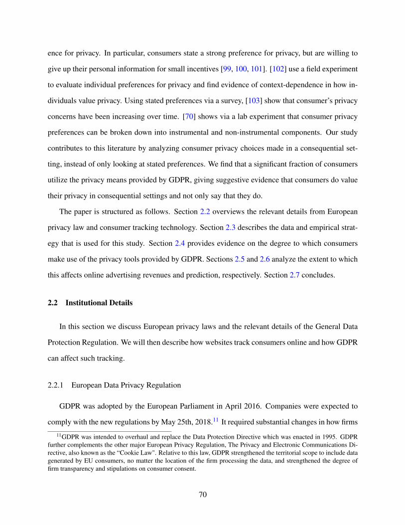
ence for privacy. In particular, consumers state a strong preference for privacy, but are willing to

give up their personal information for small incentives [99, 100, 101]. [102] use a field experiment

to evaluate individual preferences for privacy and find evidence of context-dependence in how in-

dividuals value privacy. Using stated preferences via a survey, [103] show that consumer’s privacy

concerns have been increasing over time. [70] shows via a lab experiment that consumer privacy

preferences can be broken down into instrumental and non-instrumental components. Our study

contributes to this literature by analyzing consumer privacy choices made in a consequential set-

ting, instead of only looking at stated preferences. We find that a significant fraction of consumers

utilize the privacy means provided by GDPR, giving suggestive evidence that consumers do value

their privacy in consequential settings and not only say that they do.

The paper is structured as follows. Section 2.2 overviews the relevant details from European

privacy law and consumer tracking technology. Section 2.3 describes the data and empirical strat-

egy that is used for this study. Section 2.4 provides evidence on the degree to which consumers

make use of the privacy tools provided by GDPR. Sections 2.5 and 2.6 analyze the extent to which

this affects online advertising revenues and prediction, respectively. Section 2.7 concludes.

2.2 Institutional Details

In this section we discuss European privacy laws and the relevant details of the General Data

Protection Regulation. We will then describe how websites track consumers online and how GDPR

can affect such tracking.

2.2.1 European Data Privacy Regulation

GDPR was adopted by the European Parliament in April 2016. Companies were expected to

comply with the new regulations by May 25th, 2018.11 It required substantial changes in how firms

11GDPR was intended to overhaul and replace the Data Protection Directive which was enacted in 1995. GDPRfurther complements the other major European Privacy Regulation, The Privacy and Electronic Communications Di-rective, also known as the “Cookie Law". Relative to this law, GDPR strengthened the territorial scope to include datagenerated by EU consumers, no matter the location of the firm processing the data, and strengthened the degree offirm transparency and stipulations on consumer consent.

70

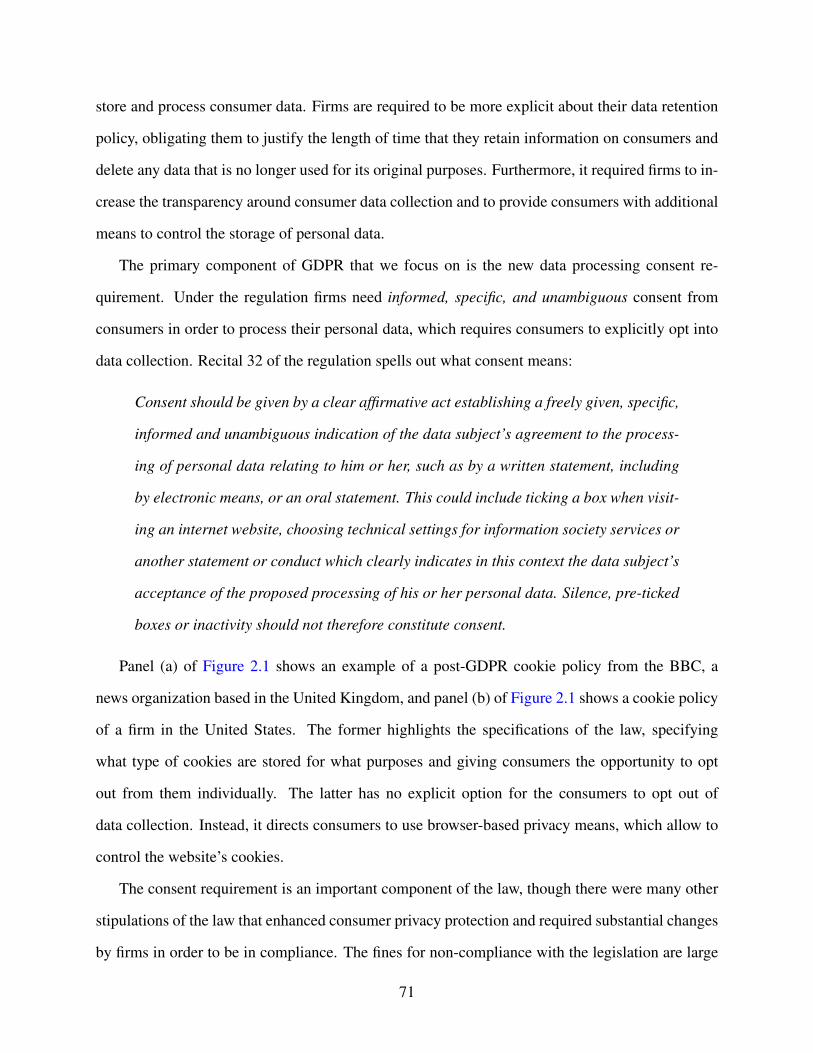
store and process consumer data. Firms are required to be more explicit about their data retention

policy, obligating them to justify the length of time that they retain information on consumers and

delete any data that is no longer used for its original purposes. Furthermore, it required firms to in-

crease the transparency around consumer data collection and to provide consumers with additional

means to control the storage of personal data.

The primary component of GDPR that we focus on is the new data processing consent re-

quirement. Under the regulation firms need informed, specific, and unambiguous consent from

consumers in order to process their personal data, which requires consumers to explicitly opt into

data collection. Recital 32 of the regulation spells out what consent means:

Consent should be given by a clear affirmative act establishing a freely given, specific,

informed and unambiguous indication of the data subject’s agreement to the process-

ing of personal data relating to him or her, such as by a written statement, including

by electronic means, or an oral statement. This could include ticking a box when visit-

ing an internet website, choosing technical settings for information society services or

another statement or conduct which clearly indicates in this context the data subject’s

acceptance of the proposed processing of his or her personal data. Silence, pre-ticked

boxes or inactivity should not therefore constitute consent.

Panel (a) of Figure 2.1 shows an example of a post-GDPR cookie policy from the BBC, a

news organization based in the United Kingdom, and panel (b) of Figure 2.1 shows a cookie policy

of a firm in the United States. The former highlights the specifications of the law, specifying

what type of cookies are stored for what purposes and giving consumers the opportunity to opt

out from them individually. The latter has no explicit option for the consumers to opt out of

data collection. Instead, it directs consumers to use browser-based privacy means, which allow to

control the website’s cookies.

The consent requirement is an important component of the law, though there were many other

stipulations of the law that enhanced consumer privacy protection and required substantial changes

by firms in order to be in compliance. The fines for non-compliance with the legislation are large

71

Figure 2.1: Example Consent Notifications

(a) Post-GDPR consent dialog

(b) Standard opt-out on US websites

Notes: The top panel shows a GDPR opt in consent dialog for the BBC. The dialog is explicit about the data that thewebsite collects and requires the consumer to opt into all non-essential data collection. Each separate purpose of dataprocessing is consented to individually. The bottom panel shows an “opt out" dialog for a website in the US that is notrequired to be GDPR compliant. The website directs consumers to manage their browser cookies and does not haveany direct options for the consumer to opt out of data collection.

- the maximum of C20 million, or 4% of total global annual sales for the preceding financial year

- giving strong incentives for firms to comply with the regulation. According to Pricewaterhouse-

Coopers, many firms are spending millions of dollars in order to comply with the regulation.12

However, despite this observation, there was still considerable non-compliance around the onset of

the law and in the next section we will discuss how this non-compliance affects the interpretation

of our estimates.12Pulse Survey: GDPR budgets top $10 million for 40% of surveyed companies. https://www.pwc.com/us/en/

services/consulting/library/general-data-protection-regulation-gdpr-budgets.html. Retrieved on De-cember 15th, 2019.

72

2.2.2 Consumer-Tracking Technology

The primary consumer tracking method that we focus on in this study are web cookies.13 Cook-

ies are small text files that are placed on consumer’s computers or mobile phones. The attachment

of a cookie gives websites, in principle, a persistent identifier. As long as the same cookie persists,

they can attribute different sessions to the same consumer and, as a result, track them across time

and different websites. However, privacy-conscious consumers can make use of various privacy

means to control the degree of persistence of this identifier. The primary means available to them

are browser-based tools, such as manual deletion of cookies, “private browsing" mode,14 or cookie

blockers.15 These browser-based privacy means regenerate the cookie identifier but the data that

is generated on the website is still sent and stored. The data is attributed to different consumers,

even though they originate from the same consumer. One important detail to note is how cookie

blockers work in this context. According to our discussions with employees of the intermediary,

these services continually regenerate the identifier utilized by the intermediary while still allowing

consumers to see the advertisements. Thus, these consumers leave a distinct mark in the data as

“single searchers" who only have one observation associated with their identifier.

The GDPR opt-in rule provides another way for consumers to protect their privacy. The stip-

ulations of GDPR, properly implemented and utilized by consumers, arguably provide a stronger

protection than the aforementioned means since they block all non-essential information from be-

ing sent to the third-party website.16 In our context, this means that by simply opting out consumers

13Common alternatives are other forms of storage in the browser as well as device fingerprinting, which use InternetProtocol (IP) addresses combined with device specific information to identify individuals. However, these are lesscommonly utilized and importantly not utilized by the intermediary.

14Private browsing modes create “sandbox" browser environments where cookies are only set and used for theduration of the private browsing session. As a result, the website cannot link together data from the same consumerboth before and after the private browsing section.

15There also exist industry opt-out services, such as the Ad Choices program, but these are relatively hard to useand have little usage [67]. Survey-based evidence informs us that the most utilized privacy means by consumers ismanual cookie deletion [104]

16It is important to note that GDPR does not prevent “essential" information from being sent to a website. Forinstance, the ability to store consumer session cookies that allow them to provide a consistent consumer experiencefor the consumer may be considered “essential" information. The intermediary that we partner with, however, is athird-party service that provides complementary services to the primary functioning of the websites and so is not an“essential" service on any website where we observe data. As a result, any usage of GDPR opt-out shuts out data frombeing sent to the intermediary.

73

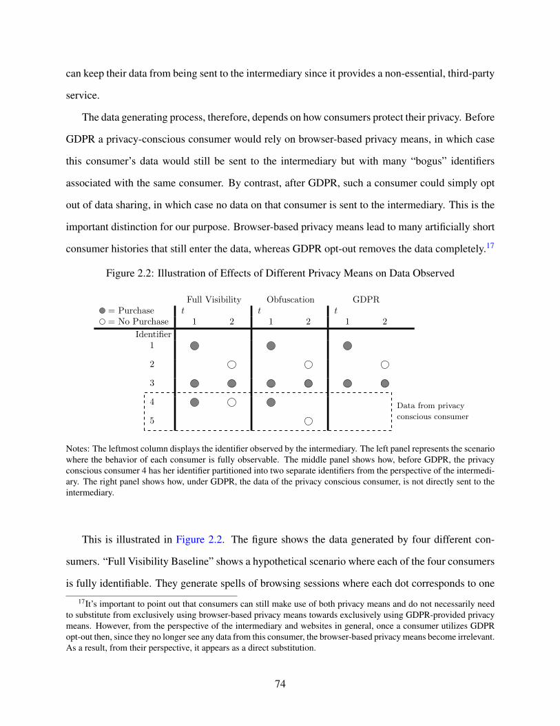
can keep their data from being sent to the intermediary since it provides a non-essential, third-party

service.

The data generating process, therefore, depends on how consumers protect their privacy. Before

GDPR a privacy-conscious consumer would rely on browser-based privacy means, in which case

this consumer’s data would still be sent to the intermediary but with many “bogus” identifiers

associated with the same consumer. By contrast, after GDPR, such a consumer could simply opt

out of data sharing, in which case no data on that consumer is sent to the intermediary. This is the

important distinction for our purpose. Browser-based privacy means lead to many artificially short

consumer histories that still enter the data, whereas GDPR opt-out removes the data completely.17

Figure 2.2: Illustration of Effects of Different Privacy Means on Data Observed

Full Visibility Obfuscation GDPR= Purchase t t t= No Purchase 1 2 1 2 1 2

Identifier1

2

3

4 Data from privacy

conscious consumer5

Notes: The leftmost column displays the identifier observed by the intermediary. The left panel represents the scenariowhere the behavior of each consumer is fully observable. The middle panel shows how, before GDPR, the privacyconscious consumer 4 has her identifier partitioned into two separate identifiers from the perspective of the intermedi-ary. The right panel shows how, under GDPR, the data of the privacy conscious consumer, is not directly sent to theintermediary.

This is illustrated in Figure 2.2. The figure shows the data generated by four different con-

sumers. “Full Visibility Baseline” shows a hypothetical scenario where each of the four consumers

is fully identifiable. They generate spells of browsing sessions where each dot corresponds to one

17It’s important to point out that consumers can still make use of both privacy means and do not necessarily needto substitute from exclusively using browser-based privacy means towards exclusively using GDPR-provided privacymeans. However, from the perspective of the intermediary and websites in general, once a consumer utilizes GDPRopt-out then, since they no longer see any data from this consumer, the browser-based privacy means become irrelevant.As a result, from their perspective, it appears as a direct substitution.

74

session and the color of the dot indicates whether or not the consumer purchased a good on the

website as a result of that search. Suppose that only consumer four is privacy-conscious. Before

GDPR, consumer four can protect her privacy by deleting her cookies and regenerating her identi-

fier. This is illustrated in the second panel (“Obfuscation”) of the figure where the two sessions for

this consumer are associated with two separate identifiers from the perspective of the intermediary.

However, the third panel shows that, when GDPR opt-out is available, this consumer opts out and

his data completely disappears.

The figure also illustrates how the different data scenarios impact the intermediary’s ability to

predict consumer behavior, and in particular, how a consumer’s choice of privacy means may affect

that ability. The four consumers have distinct histories, and these differences may signal different

future behavior for them. For example, consumer 4 may be less likely than consumer 1 to purchase

from the website next time she visits the website. Under Full Visibility, the prediction machine will

correctly recognize this distinction and assign a different prediction score to consumer 4 than to

consumer 1. Suppose, however, in the pre-GDPR regime, consumer 4 deletes her cookies and gets

partitioned into two separate identifiers, 4 and 5. This behavior confounds the intermediary’s abil-

ity to predict not only 4’s behavior but also 1 and 2’s: consumer 1 is now indistinguishable from

consumer 4 and consumer 2 is indistinguishable from consumer 5 (the same person as consumer

4) from the intermediary’s view point. For instance, the intermediary will assign a lower than ac-

curate purchase odds to consumer 1, influenced by the fact that consumer 4 with the same history

simply disappears after the visit at 𝑡 = 1. Note that this problem exists even when the interme-

diary’s prediction machine eventually “learns” about the presence of obfuscators, since it cannot

tell who obfuscates and who does not. Under GDPR, on the other hand, consumer 4’s data is not

observed at all. While this leads to a loss in the amount of data, it removes the confounding that the

intermediary suffered from 4’s obfuscation in understanding and predicting 1 and 2’s behavior.18

18Importantly, the pre-GDPR intermediary cannot simply replicate the same dataset as post-GDPR since the ob-fuscators’ identities are latent to the intermediary, so their data cannot be surgically cleaned away; for instance, elimi-nating single-search data will eliminate not only 4 but also 1 and 2 from the data.

75

2.3 Data and Empirical Strategy

We obtained access to a new and comprehensive dataset from an anonymous intermediary that

records the entirety of consumer search queries and purchases across most major online travel

agencies (OTAs) in the United States and Europe as well as most prominent travel meta-search

engines. We observe consumer searches, online advertising, and the intermediary’s prediction of

consumer behavior. Our primary analysis utilizes data from this intermediary ranging from April

to July 2018.

2.3.1 Data Description

The disaggregated data contains each search query and purchase made on these platforms as

well as the associated advertising auction for each query. In a single search query the data contains:

the identifier of the consumer, the time of the query, the details of the query (i.e. travel information),

an identifier for the platform, the browser, the operating system, and the estimated probability

of purchase on the website according to the predictive machine learning algorithm employed by

the intermediary. For a subset of the websites, we observe purchase information containing the

consumer identifier and time of purchase.

Each query can trigger an advertising auction. In that case, the data contains: the number of

bidders in the auction, the values of the winning bids, and an identifier for the winning bidders.

Furthermore, if a consumer clicks on the resulting advertisement, the click itself and the resulting

transfer between the advertiser and the intermediary are recorded.

Our analysis utilizes an aggregation of this dataset by week, operating system, web browser,

website identifier, and country.19 The data was aggregated on a weekly level to remove unim-

portant day-of-the-week fluctuations. Furthermore, the GDPR compliance date was May 25th,

2018, which was on a Friday and, as a result, our data was aggregated on a Friday-to-Friday level.

Note that the GDPR compliance date corresponds to the beginning of the 22nd week in the year

19We drop from this aggregation observations which are labeled as coming from bots.

76

according to our labeling.20

2.3.2 Empirical Strategy

To understand the causal effect of GDPR we rely on a difference-in-differences design that

exploits the geographic reach of the EU GDPR regulation. The regulation stipulates that websites

that transact with EU consumers were required to ask consumers for explicit consent to use their

data through an opt-in procedure, while those who processed non-EU consumers data were not

obligated to do so. Even though many online travel companies transact with consumers in several

countries around the world this specification works well in our setting since it is common for online

travel websites to have separate, country-specific, versions of their websites and only the websites

intended for EU countries are made GDPR compliant.

Our analysis focuses on the effect of the overall policy and not the effect of specific implemen-

tations of the policy. Thus, the treatment date of the policy corresponds to the GDPR compliance

date, which was May 25th, 2018 (or the beginning of week 22). Our treatment group consists

of nearly the universe of travel websites in major EU countries (at the time): Italy, the United

Kingdom, France, Germany, and Spain. Our control group consists of nearly the universe of travel

platforms in the United States, Canada, and Russia. These countries were chosen as controls since

EU laws do not directly apply to them, but their seasonal travel patterns are similar to those in the

EU countries as a result of similar weather and vacation patterns in the time period of interest.

Our primary regression specification is the following for the outcome variables of interest

where 𝑐 denotes country, 𝑗 denotes the website, 𝑜 denotes operating system, 𝑏 denotes web

browser, 𝑝 denotes product type (hotels or flights), and 𝑡 denotes the week in the year:

𝑦𝑡𝑐 𝑗𝑜𝑏𝑝 = 𝛼𝑡 + 𝛿 𝑗𝑐 + 𝛾𝑜 + Z𝑏 + 𝜔𝑝 + 𝛽(𝐸𝑈 𝑗 × 𝑎 𝑓 𝑡𝑒𝑟) + 𝜖𝑡𝑐 𝑗𝑜𝑏𝑝 (2.1)

20Note that we further enforce a balanced panel by dropping any observation that has zero logged searches in anyperiod during our sample period. We do this in order to ensure that our estimates are not biased from entry / exit ofwebsites into our data during the sample period. According to discussions with our data provider, this entry and exit isusually a result of varying contractual relations between the intermediary and the websites and so is largely orthogonalto our variables of interest.

77

𝐸𝑈 𝑗 denotes a website subject to the regulation, 𝑎 𝑓 𝑡𝑒𝑟 denotes whether the current week is

after the GDPR compliance date (i.e. week 22 or later), 𝛼𝑡 denotes time fixed effects, 𝛿 𝑗𝑐 denotes

country-specific website fixed effects, 𝜔𝑝 denotes product type fixed effects, 𝛾𝑜 denotes operating

system fixed effects, and Z𝑏 denotes browser fixed effects. Our standard errors are clustered at the

website-country level.21

In order to validate parallel trends and to understand the persistence of the treatment effect,

we further utilize a regression specification that captures the potentially time-varying nature of the

treatment:

𝑦𝑡𝑐 𝑗𝑜𝑏𝑝 = 𝛼𝑡 + 𝛿 𝑗𝑐 + 𝛾𝑜 + Z𝑏 + 𝜔𝑝 +𝑇∑︁𝑘=

¯𝑇

𝛽𝑘𝐸𝑈 𝑗 + 𝜖𝑡𝑐 𝑗𝑜𝑏𝑝 (2.2)

The variable definitions are the same as before and we similarly cluster our standard errors at

the website-country level.

We run our regressions over the time period between weeks 16 and 29 of 2018, which is be-

tween April 13th and July 20th. The GDPR compliance date aligns with the beginning of week

22. Furthermore, week 20 is consistently the baseline week in our regressions since there are some

firms that began to implement GDPR near the end of week 21 and so week 20 is the last week

where there should be no direct impact from GDPR as a result of website implementation.22,23

Our empirical strategy centers around the official GDPR implementation date. However, each

website had to individually implement the changes stipulated by GDPR and there is evidence that

there was considerable heterogeneity in compliance among firms. Furthermore, even within the

subset of firms that complied with the regulation, the degree to which consumers responded varied

21We cluster at the website-country level because of differences in privacy concerns across countries [105] anddifferences in consent implementations across websites within jurisdiction [80].

22Our dataset ends on July 31st, 2018, which is a Tuesday, and an important measure that we want to track isthe amount of consumer persistence on a weekly level, which looks at the fraction of observed cookies that remainobservable in the data after some number of weeks. Since this measure requires a complete week of data to computeproperly, we drop the incomplete week at the end of July as well as the full last week in July so that we can haveconsistency between the regressions on aggregate consumer response and those on consumer persistence.

23Our analysis ends at the end of July since this was the time period over which we were able to obtain data fromour data provider.

78

considerably based on the nature of implementation [80]. As a result, we would want to include

information on the timing and degree of implementation across the various websites in our sample.

However, due to technical limitations, we cannot directly observe the timing and degree of GDPR

implementation during the time period we study.24

Thus, any effects that we observe with our empirical specification are a combination of the

explicit consequences as a result of implementing the stipulations of GDPR for the subset of web-

sites that implemented it and any changes in advertiser and consumer behavior in response to the

increased saliency of privacy considerations on the Internet.25 Since we do not observe the full

extent of non-compliance, our estimates can be viewed as a lower bound on the true impact of the

policy had websites all fully complied with it.

2.4 Consumer Response to GDPR

In this section we quantify the extent to which consumers utilize the GDPR-mandated ability

to opt out. We measure how GDPR opt-out impacts the total number of cookies and searches

observed by the intermediary. We then explore whether there were any changes in the composition

of the remaining, opted-in consumers.

2.4.1 Opt-Out Usage

Recall that we do not directly observe opt-out in our dataset because consumers who opt out

are no longer part of our dataset. As a result, at time 𝑡, the total number of consumers on a website

𝑗 is given by the true number of consumers subtracted by the number of consumers who have opted

24We attempted to utilize tools such as the Wayback Machine, which takes snapshots of websites across the entireInternet frequently. However, the coverage of relevant websites on the Wayback Machine is spotty and, given thatmany of the consent dialogs for GDPR consent are dynamically generated, are not always picked up by the snapshottaken of the website.

25It would be interesting to isolate the effects of each possible channel, though our data limitations prohibit us fromdoing so. We were able to verify that several websites in our sample implemented GDPR consent guidelines aroundthe time of the policy and that several websites in our sample did not, though there are a considerable number forwhich we are uncertain when they implemented the policy.

79

out.26

𝑈𝑂𝐵𝑆𝑗𝑡 = 𝑈𝑇𝑅𝑈𝐸𝑗𝑡 −𝑈𝑂𝑃𝑇−𝑂𝑈𝑇𝑗𝑡

In the control group,𝑈𝑂𝑃𝑇−𝑂𝑈𝑇𝑗𝑡

= 0, whereas post-GDPR𝑈𝑂𝑃𝑇−𝑂𝑈𝑇𝑗𝑡

≥ 0. We assume parallel

trends in𝑈𝑇𝑅𝑈𝐸𝑗𝑡

, which means that any change in𝑈𝑂𝐵𝑆𝑗𝑡

allows us to identify𝑈𝑂𝑃𝑇−𝑂𝑈𝑇𝑗𝑡

.27,28

Figure 2.3 displays the total unique cookies for two multi-national websites, one of which

implemented the consent guidelines of the GDPR and the other which does business in the EU but

did not immediately comply with the regulations. The multi-national website which implemented

the consent guidelines shows a clear drop in observed cookies on European websites at the onset of

GDPR. Columns (1) and (2) of Table 2.1 report the result of regression (2.1) with total number of

observed unique cookies as the outcome variable. We consider the specification in both levels and

logs. The estimates show that, in aggregate, GDPR reduced the total number of unique cookies

by around 12.5%. As previously mentioned, our estimates should be interpreted in the context of

mixed compliance with the consent guidelines of GDPR as evidenced from Figure 2.3.

It is important to note that this result does not imply that 12.5% of consumers made use of the

opt-out features. This is because the unit of observation is a cookie, rather than a consumer. A

single consumer can appear under multiple cookie identifiers if they make use of the aforemen-

tioned browser-based privacy means. Nonetheless, the results point to a relatively large usage of

the opt-out features by consumers.

26Note that a website here serves as a first-party affiliate of our intermediary; so the true number of consumers forwebsite 𝑗 is not the true number of consumers for the intermediary, as opt-out consumers become out of its reach.

27As noted in [76], another possible complication is that this could be a result of firms changing the type of datathat they send to third party services. To our knowledge there is no change in the data the websites send to theintermediary as a result of GDPR since the intermediary and the data are crucial for generating advertising revenue forthese websites. Furthermore, if a website decided to stop using the intermediary altogether then, as noted previously,they would not be part of our sample.

28Another possible confounding factor is the sales activity of the intermediary. For instance, it’s possible forthe intermediary to sell additional advertising units to a website that can appear on pages of the website where theintermediary previously was not tracking before. If there was a differential effect from this around the date of thetreatment then this could systematically bias the number of unique cookies and searches that we observe. To test theplausibility of this hypothesis, we run our difference-in-differences specification with total advertising units and totalpages on which the intermediaries advertising appears as the outcome variables. The results in Table B1 show thatthere was no significant change in either of those two variables. Thus, we rule this alternative explanation out.

80

Another measure of consumer response is the total number of searches that are recorded by the

intermediary. This outcome measure can also be interpreted as the overall data size observed by

the intermediary and how it is affected by GDPR. We re-run the same specification with recorded

searches as the dependent variable and report the results in columns (3) and (4) of Table 2.1. We

find that there’s a 10.7% drop in the overall recorded searches which is qualitatively consistent

with the effect size of the specification using the number of unique cookies.

In order to provide evidence for the validity of the difference-in-differences strategy we rely

on our time-varying treatment specification. Figure B1 displays the resulting treatment effect over

time and points to parallel pre-trends as well as a consistent treatment effect size over our sample

period though there is a slight decrease in the estimated treatment effect as we approach the end

of our sample period. Finally, as further evidence of robustness, we employ a synthetic control

approach, which is reported in subsection B.2.1 and produces qualitatively similar results.

We want to discuss two further potential threats to the validity of our empirical strategy. The

first is a potential contamination between treatment and control groups that may result from multi-

national companies implementing the consent mechanisms across all of their websites. The second

is that the results may be driven by seasonal travel differences between the treatment and control

groups. The first is not a big concern in our setting because multinational online travel agen-

cies serve customers through country-specific websites and have incentives to only make their EU

domains compliant with GDPR. For the online travel agencies where we can directly verify com-

pliance we do indeed see that most of them only implement it for their respective EU domains as

evidenced by Figure 2.3. Furthermore, to the extent that there is still residual contamination, it

would mean that our estimates are a lower bound of the true effect size.

81

Figure 2.3: Total Number of Unique Cookies for Two Multi-National Website.

●●●●●

●

●● ●

●

● ●●

● ●

● ● ●

● ●● ● ●

● ●●

● ●

●●

●

●●

●

●

●

●●

● ● ●● ● ●

●●

●

●

●

● ●● ●

●●

●

●

●

●●

●

●

● ●

●●

●● ●

●

−1.0

−0.5

0.0

0.5

1.0

16 17 18 19 20 21 22 23 24 25 26 27 28 29Week of Year

Tota

l Coo

kies

Dev

iatio

n

Website Location ● EU non−EU

●

●

●

●

●

●

●

● ●

●●

● ●

●

−1.0

−0.5

0.0

0.5

1.0

16 17 18 19 20 21 22 23 24 25 26 27 28 29Week of Year

Tota

l Coo

kies

Dev

iatio

n

Website Location ● EU non−EU

Notes: Each point on the graph represents the total number of unique cookies for a single country, reported in terms ofits percent deviation relative to week 20, or 𝑈𝑡−𝑈𝑡=20

𝑈𝑡=20∀𝑡 ≠ 20. The figure on the left presents a multi-national website

that we were able to verify implemented the consent guidelines of GDPR. In this figure, the black dots represent therepresented European countries (United Kingdom, France, Germany, Italy, Spain) and the two white dots represent thetwo non-EU countries where this website functions - the United States and Canada. The figure on the right presents amulti-national website that we were able to verify did not implement the consent guidelines of GDPR. The black dotsrepresent the values from the United Kingdom and the white dots represent the values from the United States.

Table 2.1: Difference-in-Differences Estimates for Cookies and Searches

(1) (2) (3) (4)log(Unique Unique log(Recorded RecordedCookies) Cookies Searches) Searches

DiD Coefficient -0.125∗∗ -1378.1∗ -0.107∗ -9618.3∗∗

(-2.43) (-1.71) (-1.87) (-2.24)

Product Type Controls ✓ ✓ ✓ ✓OS + Browser Controls ✓ ✓ ✓ ✓Week FE ✓ ✓ ✓ ✓Website × Country FE ✓ ✓ ✓ ✓

Observations 63840 63840 63840 63840∗ 𝑝 < 0.10, ∗∗ 𝑝 < 0.05, ∗∗∗ 𝑝 < 0.01

Notes: t-statistics are reported in parentheses. The standard errors for every regression areclustered at the website-country level. We aggregate every dependent variable to the website-country-browser-OS-product type-week level between weeks 16 and 29, including both weeks16 and 29 (April 13th - July 20th). The dependent variables in the regression reported in thefirst and second column are the log and overall level of the number of unique cookies observed.The dependent variables in the regression reported in the third and fourth column are the logand overall level of the number of total recorded searches.

82

For the second issue, this is the reason that we focus our analysis on a tight window around the

GDPR implementation date and select control countries that ought to have similar travel patterns

during this time period. However, since European travel patterns have a somewhat steeper summer

gradient than US travel patterns we would expect this to bias against our results. We therefore

further supplement our analysis with Google Trends data on travel searches, which should be

unaffected by GDPR and provide a good picture into travel trends across these different countries.

Using this data, we first graphically show that in the period of the year that we consider, travel

patterns between the countries in the analysis are similar. When we augment our primary analysis

with country-specific seasonal controls based on Google Trends data we find quantitatively very

similar results with slightly stronger effect sizes than before. The full details of this exercise are

deferred to subsection B.2.2.

2.4.2 Persistence of Identifier

A natural question is whether GDPR affects the ability to persistently track consumers. To

address this question, we define an identifier persistence measure that tracks how often cookies

that we see in a given week return after 𝑘 weeks, where we explore different values for 𝑘 (1,2,3,

and 4 weeks). Let 𝐶 𝑗 𝑡 be the set of cookies seen in week 𝑡 on website 𝑗 , the measure is then given

by:

𝑝𝑒𝑟𝑠𝑖𝑠𝑡𝑒𝑛𝑐𝑒𝑘𝑡 =|𝐶 𝑗 ,𝑡 ∩ 𝐶 𝑗 ,𝑡+𝑘 |

|𝐶 𝑗 ,𝑡 |

In Figure 2.4 we set 𝑘 = 4 and display the persistence measure for the same two multi-national

websites with country-specific versions of their website over time. At the onset of GDPR there is

a clear increase in persistence on the EU-based websites, but no noticeable difference in the non-

EU websites. We further validate this increase by running our baseline difference-in-differences

specification using the persistence outcome variable for 𝑘 ∈ {1, 2, 3, 4}.29,30

29In order to run specification (2.1) we drop the last 4 weeks of our sample so that we are utilizing the same sampleas we vary 𝑘 . However, our results are qualitatively robust to including these weeks when the data for them is available.

30Note that the units on the regression and Figure 2.4 are not the same. Figure 2.4 displays the persistence measure

83

Figure 2.4: Four Week Persistence for Two Multi-National Websites

●●●●●

●

●

●

● ●

●

●

●

●

●

●

●

●

●●

●

●

●

●●

●

●

●

●

●

●

●

●● ●

●

●

●

●

●

●

●

●●

●

●

●

●

●

●

●

●

●

● ●

−1.0

−0.5

0.0

0.5

1.0

16 17 18 19 20 21 22 23 24 25 26Week of Year

Per

sist

ence

Dev

iatio

n

Website Location ● EU non−EU

●● ●

●

●

●●

●●

●●

−1.0

−0.5

0.0

0.5

1.0

16 17 18 19 20 21 22 23 24 25 26Week of Year

Per

sist

ence

Dev

iatio

n

Website Location ● EU non−EU

Notes: Each point on the graph represents the four week persistence fraction for a single country, reported in termsof its percent deviation relative to week 20, or 𝑝𝑒𝑟𝑠𝑖𝑠𝑡𝑒𝑛𝑐𝑒4,𝑡−𝑝𝑒𝑟𝑠𝑖𝑠𝑡𝑒𝑛𝑐𝑒4,𝑡=20

𝑝𝑒𝑟𝑠𝑖𝑠𝑡𝑒𝑛𝑐𝑒4,𝑡=20∀𝑡 ≠ 20. The figure on the left presents

a multi-national website that we were able to verify implemented the consent guidelines of GDPR. In this figure, theblack dots represent the represented European countries (United Kingdom, France, Germany, Italy, Spain) and the twowhite dots represent the two non-EU countries where this website functions - the United States and Canada. The figureon the right presents a multi-national website that we were able to verify did not implement the consent guidelines ofGDPR. The black dots represent the values from the United Kingdom and the white dots represent the values from theUnited States.

Table 2.2: Difference-in-Differences Estimates for Consumer Persistence

(1) (2) (3) (4)1 Week 2 Weeks 3 Weeks 4 Weeks

Persistence Persistence Persistence Persistence

DiD Coefficient 0.00308∗ 0.00416∗∗∗ 0.00382∗∗∗ 0.00505∗∗∗

(1.96) (3.40) (3.10) (3.50)

Product Type Controls ✓ ✓ ✓ ✓OS + Browser Controls ✓ ✓ ✓ ✓Week FE ✓ ✓ ✓ ✓Website × Country FE ✓ ✓ ✓ ✓

Observations 50160 50160 50160 50160∗ 𝑝 < 0.10, ∗∗ 𝑝 < 0.05, ∗∗∗ 𝑝 < 0.01

Notes: t-statistics are reported in parentheses. The standard errors for every regression areclustered at the website-country level. We aggregate every dependent variable to the website-country-browser-OS-product type-week level between weeks 16 and 26, including both weeks16 and 26 (April 13th - June 29th). The dependent variables in the regression are the consumerpersistence measures for 𝑘 = 1, 2, 3, 4, respectively.

in terms of percent deviations from week 20 whereas the coefficients in Table 2.2 are changes in levels.

84

Table 2.2 shows the results of this regression, which indicate that there is a statistically signifi-

cant and meaningful increase in consumer persistence and that this effect gets more pronounced as

𝑘 increases.31 We further run the time-varying treatment specification (2.2) in order to validate that

parallel trends holds and to understand the consistency of the effect over time. Figure B2 shows

that while for 𝑘 = 1 the time dependent treatment effects are more noisy, for all 𝑘 ≥ 2 parallel

trends hold and the treatment effect is stable over time.32 The treatment effect remains roughly the

same as 𝑘 grows, even though Table B2 shows that the mean persistence declines as 𝑘 increases.

For instance, in the pre-treatment period, the mean persistence for EU websites was 0.0597 and

the estimated treatment effect is 0.005 indicating a roughly 8% increase in persistence.

There are two possible hypotheses for the increased persistence. The first is a selective consent

hypothesis where consumers only consent to data processing by websites that they frequently use.

According to this hypothesis, infrequent users of a website are more likely to opt out of data sharing

than frequent users, so the opt-in set of consumers will naturally appear to be more persistent. The

second is a privacy means substitution hypothesis where privacy conscious consumers who were

previously making use of browser-based privacy means now utilize GDPR opt-in to protect their

privacy. Recall that the utilization of these privacy means would result in many artificially short-

lived consumers. If these same consumers utilize GDPR opt-in instead, they would no longer

show up in the intermediary’s dataset and the remaining set of consumers would appear to be more

persistent even though their true search and purchase behavior may not have changed.

These alternative hypotheses have different economic implications. If the selective consent

hypothesis is the predominant explanation for the increased persistence, then privacy regulation

may favor firms with more established reputations or offer a wider variety of services.33 The

31It is important to note that the persistence measure may have some noise when 𝑘 = 1 due to consumer activitynear the end of the week that spills over into the next week and falsely appears as persistence. As a result, the mostreliable measures of consumer persistence are for 𝑘 ≥ 2, but we report 𝑘 = 1 for completeness.

32Furthermore, Figure B3 in the appendix shows the overall distributions of consumer persistence for the EU vs.non-EU and note that there are some outliers. In particular, there is a large mass of high persistence observationsand persistence measures close to 0. Our results are qualitatively robust to running our specifications winsorizing anddropping these observations as well. They are also robust to the addition of seasonal travel controls using the sameprocedure as in subsection B.2.2.

33There is a connection of this hypothesis to the theoretical predictions in [106], who argue that consent-based datacollection practices would allow larger firms to collect more data than smaller firms since they offer a wider scope of

85

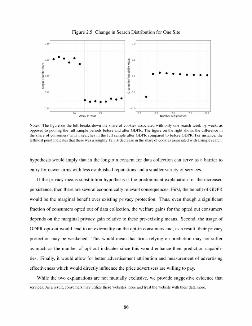
Figure 2.5: Change in Search Distribution for One Site

●●

●

●

●

●

●● ● ● ●

● ● ●

0.35

0.40

0.45

0.50

0.55

20 25Week In Year

Sin

gle

Sea

rch

Sha

re

●

●● ● ● ● ● ● ● ●

−0.2

−0.1

0.0

0.1

0.2

0.0 2.5 5.0 7.5 10.0Number of Searches

Cha

nge

in P

roba

bilit

y M

ass

Notes: The figure on the left breaks down the share of cookies associated with only one search week by week, asopposed to pooling the full sample periods before and after GDPR. The figure on the right shows the difference inthe share of consumers with 𝑥 searches in the full sample after GDPR compared to before GDPR. For instance, theleftmost point indicates that there was a roughly 12.8% decrease in the share of cookies associated with a single search.

hypothesis would imply that in the long run consent for data collection can serve as a barrier to

entry for newer firms with less established reputations and a smaller variety of services.

If the privacy means substitution hypothesis is the predominant explanation for the increased

persistence, then there are several economically relevant consequences. First, the benefit of GDPR

would be the marginal benefit over existing privacy protection. Thus, even though a significant

fraction of consumers opted out of data collection, the welfare gains for the opted out consumers

depends on the marginal privacy gain relative to these pre-existing means. Second, the usage of

GDPR opt-out would lead to an externality on the opt-in consumers and, as a result, their privacy

protection may be weakened. This would mean that firms relying on prediction may not suffer

as much as the number of opt out indicates since this would enhance their prediction capabili-

ties. Finally, it would allow for better advertisement attribution and measurement of advertising

effectiveness which would directly influence the price advertisers are willing to pay.

While the two explanations are not mutually exclusive, we provide suggestive evidence that

services. As a result, consumers may utilize these websites more and trust the website with their data more.

86

the privacy means substitution hypothesis is the more plausible one. Both hypotheses imply that

the drop in relative probability mass should be concentrated towards the lower end of the support.

However, recall from section 2.2 that in our context one signature of browser-based privacy pro-

tection is a large mass of “single search" consumers. This is due to the continuing regeneration of

cookie-identifiers after every request. Indeed, Figure 2.5 shows that the fraction of single searchers

significantly dropped after the implementation of GDPR. Instead, under the selective consent hy-

pothesis, we would expect that the loss in probability mass would be more evenly distributed across

search counts.

Based on this observation, we test for the presence of excess single searchers using a [107]

test both before and after the implementation of GDPR. The test is based on a simple model in

which obfuscating and non-obfuscating consumers together give rise to an observed distribution of

cookie counts. We implement this test under two different distributional assumptions. Under the

first assumption, the true number of visits per consumer follows a conditional Poisson distribution.

To allow for more dispersion we, alternatively, assume that the true underlying distribution follows

a negative binomial distribution. For the empirical implementation, we focus on a large website

which we know faithfully implemented the consent mechanism. In short, the test suggests the

presence of excessive single searchers in the pre-GDPR period but not in the post-GDPR period.

The full details of the exercise are deferred to section B.4.

We implement the test separately for the pre- and post-GDPR period. In the pre-GDPR period,

the test rejects a model without excess single searchers in favor of a model in which the number

of single searchers is inflated under both distributional assumptions. The same is true for the post-

GDPR period under the Poisson distribution, but the estimated fraction of single searchers is lower

in this period relative to the pre-GDPR period. However, under the more flexible negative binomial

distribution, we still find statistical evidence for excessive single searchers in the pre-GDPR period

whereas the evidence is not significant in the post-GDPR period.

Finally, we analyze the entire set of websites again and estimate heterogeneous treatment ef-

fects across popular web browsers and operating systems. We find that the increase in persistence

87

occurs on all browsers except for Internet Explorer and find weak evidence that the increase in

persistence is more prominent on desktop operating systems compared to mobile operating sys-

tems. While the differences on these dimensions are difficult to explain according to the selective

consent hypothesis, they are plausible under the privacy means substitution hypothesis, in light of

the alleged lack of technical sophistication by the consumers who use Internet Explorer and the

technical difficulty of utilizing browser-based privacy means on mobile/Internet Explorer.34 The

results and a full discussion are deferred to section B.3. Overall, these results provide additional

evidence in favor of the privacy means substitution hypothesis although additional research on this

distinction is certainly warranted.

2.5 GDPR and Online Advertising

The advertisements in our setting are sold via real-time auctions that are held when a consumer

makes a search query.35 Advertisers bid on search keywords such as the origination, destination,

or dates of travel. For example, an advertiser may submit a bid to show an advertisement for a

consumer searching for a flight from JFK to LAX and upon winning displays a price comparison

advertisement for this particular route. Thus, bids reflect the value of the set of consumers that

search for certain keywords and not particular consumer histories. Bids are submitted per click

and a payment from the advertiser to the intermediary occurs only if the consumer clicks on the

advertisement. An important fact for the interpretation of our results is that consumers who opt

out are never shown any advertisements. Thus, the intermediary generates no advertising revenues

from these consumers.36

We separately investigate the changes in advertising revenue, prices, and quantity of advertise-

34In the time period of interest, the new Microsoft Edge browser was the default on Windows computers andInternet Explorer is predominantly utilized on computers running the Windows OS. Microsoft Edge was the default onWindows since 2015, thus users of Internet Explorer are predominantly those on older computers. Internet Explorerusers tend to be older than Chrome or Firefox users ( https://elie.net/blog/web/survey-internet-explorer-

users-are-older-chrome-seduces-youth/ ) and thus less inclined to adopt browser-based privacy practices [108].35The auction format is a linear combination of a generalized first and second price auction where there are 𝑁

advertisers and 𝑘 slots.36An implication of this is that although GDPR opt-out restricts the data observed by the intermediary and the

website, we observe the advertising revenue for the intermediary generated from opt-in consumers.

88

ment. First, we look for the change in the number of clicks for advertisements following GDPR.

Columns (1) - (2) of Table 2.3 show that there is a statistically significant decrease of 13.5% in

the total number of clicks. The magnitude of this effect is in line with the drop in total cookies

and searches. We next look for changes in the number of clicks from distinct cookies to see if any

changes were driven by some small set of consumers. Columns (3) - (4) show that this measure

also decreases significantly. Figure 2.6 displays the time-varying specification for these outcome

variable and shows that the effect on the number of clicks is relatively constant.

Columns (5) and (6) of Table 2.3 show the effects on revenue. The magnitude of the point

estimates suggests an economically significant drop, though it is imprecise and not statistically

significant. The time-varying treatment effect displayed in Figure 2.6 shows that revenue initially

falls sharply after the implementation of GDPR and then begins to recover. Importantly, column (7)

of Table 2.3 shows that the average bid of the advertisers increases. At roughly 12% this increase

is economically sizable.37 The time-varying coefficient in Figure 2.6 shows that the average bid

does not change initially after the policy and then increases gradually. In summary, the immediate

drop in clicks following GDPR leads to a sharp drop in revenue, but the gradual increase in the

average bids leads to a recovery of some of the lost revenue for the intermediary and advertisers.

In light of these results one may wonder how the quantity of advertisements is affected. Using

the same difference-in-differences specification with total number of advertisements as the depen-

dent variable we find that the number of advertisements has dropped but that this change is not

significant (see Table B6 and Figure B6 in section B.5 for the time varying treatment effect).

We now discuss the plausible mechanisms behind the increase in prices (bids). The first mech-

anism, which is consistent with the evidence that we establish above, is that remaining consumers

are of higher average value to advertisers.38 Our discussion with the intermediary indicates that

advertisers’ value is determined according to the observed conversion rate of their advertisements,

which is the fraction of consumers that end up purchasing a good after clicking on an advertise-

37Note that in order to preserve the privacy of our intermediary, the bid and revenue values are obfuscated by acommon multiplier. However, the interpretation of percentage changes is preserved under this transformation.

38In contemporary work and in a different e-commerce setting, [76] reach a similar conclusion about the value ofconsumers post-GDPR.

89

ment. Since the measurement of conversion rests on the ability to track consumers, it is plausible

that the increased trackability of consumers following GDPR improved the measurement of con-

version rates, thus contributing to an increase in value of consumers as perceived by the adver-

tisers.39 Suppose, instead, that GDPR opt-out is available and consumer 𝐴 is removed from the

sample of the advertiser and therefore never clicks on an advertisement. The advertiser’s estimated

conversion rate is 0.5 now, as opposed to 0.4 and so the perceived value of consumers weakly in-

creases regardless of consumer 𝐴’s true behavior. More generally, dropping individuals similar to

consumer 𝐴 from the observed sample can only weakly increase the advertiser’s perceived value.

This points to the explanation that the increased ability to accurately measure conversion rates has

led advertisers to gradually increase prices (bids) over time.

However, there might be two plausible alternative explanations. The first is that GDPR has

decreased the “supply” of consumers to whom advertisements can be served. As we have demon-

strated above, there is a significant reduction in the number of advertisements served because

consumers opt out. This reduction in advertising targets might increase the value of the marginal

remaining consumer. While this is certainly plausible, the pattern of price increases is not fully

consistent with the supply shock explanation. Since this shock materializes right after the im-

plementation date and advertising budgets are set daily, one would expect a sharp price increase.

Instead, we observe a gradual price increase (Figure 2.6), which is more consistent with advertisers

slowly adjusting to the increase in conversion rates.

39To illustrate, suppose that there are five consumers who click on an advertisement. Suppose one of them (fromhere on consumer 𝐴) makes us of cookie blockers but ends up purchasing and, from the remaining four, suppose twoof them end up purchasing. Thus, regardless of the behavior of consumer 𝐴, the advertiser’s estimated conversion rateis 0.4 as opposed to 0.6—a correct rate including 𝐴.

90

Figure 2.6: Week by Week Treatment Effect for Total Clicks, Revenue, and Average Bid

−0.50

−0.25

0.00

0.25

0.50

16 17 18 19 20 21 22 23 24 25 26 27 28 29Week Number

DiD

Est

imat

e

asinh(Total Clicks)

−0.50

−0.25

0.00

0.25

0.50

16 17 18 19 20 21 22 23 24 25 26 27 28 29Week Number

DiD

Est

imat

e

asinh(Total Revenue)

−80

−40

0

40

80

16 17 18 19 20 21 22 23 24 25 26 27 28 29Week Number

DiD

Est

imat

e

Average Bid

91

Table 2.3: Difference-in-Differences Estimates for Advertising Outcome Variables

(1) (2) (3) (4) (5) (6) (7)

asinh(Total Total asinh(Distinct Distinct Average

Clicks) Clicks Clicks) Clicks asinh(Revenue) Revenue Bid

DiD Coefficient -0.135∗∗ -251.9∗ -0.133∗∗ -214.9∗ -0.168 -32972.3 15.41∗∗∗

(-2.32) (-1.91) (-2.33) (-1.84) (-1.54) (-0.75) (2.90)

OS + Browser Controls ✓ ✓ ✓ ✓ ✓ ✓ ✓

Product Category Controls ✓ ✓ ✓ ✓ ✓ ✓ ✓

Website× Country FE ✓ ✓ ✓ ✓ ✓ ✓ ✓

Week FE ✓ ✓ ✓ ✓ ✓ ✓ ✓

Observations 62328 62328 62328 62328 62328 62328 62328

∗ 𝑝 < 0.10, ∗∗ 𝑝 < 0.05, ∗∗∗ 𝑝 < 0.01

Notes: t-statistics are reported in parentheses. The standard errors for every regression are clustered at the website-country level. We aggregate

every dependent variable to the website-country-browser-OS-product type-week level between weeks 16 and 29, including both weeks 16 and

29 (April 13th - July 20th). The dependent variable in the regression reported in the first column is the total number of clicks associated with

each observation and the second column is the inverse hyperbolic sine transform of this value. Likewise, the dependent variables in the third

and fourth columns are the total number and inverse hyperbolic sine transform of the total number of unique cookies who interacted with

advertisements. The dependent variables in the fifth and sixth column are the total number and inverse hyperbolic sine transform of the total

revenue. The dependent variable in the seventh column is the average bid by advertisers. We utilize the inverse hyperbolic sine transform

instead of the logarithm as in previous sections as some of the outcome variables we consider in this section can take zero values. The inverse

hyperbolic sine transform is given by 𝑦 = 𝑎𝑟𝑐𝑠𝑖𝑛ℎ(𝑦) = ln(𝑦 +√︁𝑦2 + 1) and results in a similar coefficient interpretation as taking logarithms

[54], but does not remove the zero valued observations from the data. We retain the zero values here so that there is a clearer comparison

between the estimates before and after the transformation.

92

Another plausible alternative explanation is that GDPR is a positive “demand shock” for the

type of advertising offered by the intermediary. Advertisers in our setting submit bids based on the

context in which advertising is shown (e.g. based on travel search details) instead of on individual

consumer histories. The relative efficiency of such “contextual advertising" compared to behav-

iorally targeted display advertising, which is even more dependent on consumer tracking, may have

increased as a result of GDPR.40 However, our setting also contains a personalized element: the

decision to place advertisements is personalized based on the predictions of the intermediary. It is

therefore less plausible that the intermediary would be one of the clear-cut winners under such a

shift in the market.

To sum up, it seems plausible that advertising prices, at least in part, increased because the

average consumer is more trackable. This interpretation is in line with the evidence of previous

sections and alternative explanations are less plausible based on our institutional knowledge and

prevailing patterns in the data.

2.6 GDPR and Prediction of Consumer Behavior

In this section we investigate whether the changes due to GDPR have affected the intermedi-

ary’s ability to predict consumer behavior. Beyond this particular context, such an investigation

is also of broader interest. Sophisticated machine learning technologies that attempt to predict

consumer purchase behavior are becoming increasingly common41 and our results provide a case

study on how their accuracy is affected by data privacy regulation.

Based on our analysis we expect there to be three predominant reasons why we might observe

a change in the ability to predict. First, GDPR has significantly reduced the overall amount of data.

Second, remaining consumers have longer histories and are more trackable. Third, in line with our

illustration in Figure 2.2, GDPR might reveal correlation structures between consumer behavior40Personalization diminished: In the GDPR era, contextual targeting is making a comeback. https:

//digiday.com/media/personalization-diminished-gdpr-era-contextual-targeting-making-comeback/. Ac-cessed on December 15th, 2020.

41See, for example, Retailers Use AI to Improve Online Recommendations for Shoppers, https://www.wsj.

com/articles/retailers-use-ai-to-improve-online-recommendations-for-shoppers-11604330308, Accessedon March 31st, 2021.

93

and the length of consumer histories that were previously obfuscated by the use of alternative

privacy means. We would expect the first effect to decrease prediction performance and the second

and third to increase prediction performance.

We take as given both the setup of the prediction problem and the algorithm that the interme-

diary uses. This allows us to understand the effects of GDPR on the prediction problem “in the

field." Its problem is to predict whether a consumer will purchase from a site she visits based on

utilizing the history that the intermediary observes about this consumer. Specifically, its algorithm

classifies a search by a consumer into two categories: purchasers and non-purchasers, based on

whether the consumer will purchase a product on the current website within some time window.

Formally, each query is classified into

𝑦𝑖 𝑗 𝑘 =

1, if 𝑖 is a purchaser on website 𝑗 after search 𝑘

0, if 𝑖 is not a purchaser on website 𝑗 after search 𝑘,

for a consumer 𝑖 on website 𝑗 on the 𝑘th query observed by the intermediary. We denote the

classification made in real-time by the intermediary as �̂�𝑖 𝑗 𝑘 . For every consumer 𝑖 we observe

a series of searches on website 𝑗 , 𝑋𝑖 𝑗1, 𝑋𝑖 𝑗2, ..., 𝑋𝑖 𝑗𝑛 and, if the consumer ended up making a

purchase on this website, the timestamp of when consumer 𝑖 purchased on website 𝑗 . This allows

us to further construct the ground truth label, 𝑦𝑇𝑅𝑈𝐸𝑖 𝑗 𝑘

, which we use to evaluate the performance of

the classifier.42 We will denote the class proportion as the proportion of searches whose ground

truth label is purchaser.

For each search, the intermediary produces a probability estimate that the consumer is a pur-

42The ground truth labels are constructed by setting 𝑦𝑇𝑅𝑈𝐸𝑖 𝑗𝑘

= 1 if the purchase occurs within 𝑁 𝑗 days of the searchand 𝑦𝑇𝑅𝑈𝐸

𝑖 𝑗𝑘= 0 otherwise. While in practice the value of 𝑁 𝑗 is website-dependent, we do not observe this value

for each website so we restrict focus to 𝑁 𝑗 = 2 across all websites. For the majority of websites in our sample ,theintermediary informed us that they set 𝑁 = 1 or 𝑁 = 2. Furthermore, from our preliminary analysis, the results do notqualitatively differ between 𝑁 = 1 and 𝑁 = 2.

94

chaser:

𝑝𝑖 𝑗 𝑘 = Pr(𝑦𝑇𝑅𝑈𝐸𝑖 𝑗 𝑘 = 1 | 𝑋𝑖 𝑗1, ..., 𝑋𝑖 𝑗 𝑘 ),∀𝑖, 𝑗 , 𝑘 (2.3)

We observe the intermediary’s predicted 𝑝𝑖 𝑗 𝑘 and �̂�𝑖 𝑗 𝑘 for every search as well as the 𝑦𝑇𝑅𝑈𝐸𝑖 𝑗 𝑘

which

we construct. The conversion of probability estimate, 𝑝𝑖 𝑗 𝑘 , to actual classification, �̂�𝑖 𝑗 𝑘 , is based

on whether the consumer’s “score” 𝑝𝑖 𝑗 𝑘 is above or below a chosen threshold �̂�. The threshold is

chosen based on revenue considerations and other factors irrelevant to the quality of the predic-

tions and, as a result, we focus on analyzing the prediction error associated with the probabilistic

estimate 𝑝𝑖 𝑗 𝑘 and not �̂�𝑖 𝑗 𝑘 .

2.6.1 Prediction Evaluation Measures

To evaluate the performance of the classifier deployed by the intermediary, we use two standard

measures from the machine learning literature: the Mean Squared Error (MSE) and Area under the

ROC Curve (AUC).43

The MSE computes the mean of the squared errors associated with the predicted estimate 𝑝𝑖 𝑗 𝑘

relative to the realized binary event. Specifically, let I𝑗 be the set of all consumers on website 𝑗

and let K𝑖 𝑗 be the set of all events for consumer 𝑖 on website 𝑗 . Then, the MSE of website 𝑗 is

given by,

𝑀𝑆𝐸 𝑗 =1∑

𝑖∈I𝑗|K𝑖 𝑗 |

∑︁𝑖∈I𝑗

∑︁𝑘∈K𝑖 𝑗

(𝑝𝑖 𝑗 𝑘 − 𝑦𝑇𝑅𝑈𝐸𝑖 𝑗 𝑘 )2, (2.4)

with a low MSE indicating a good prediction performance.

43[109] and [110] provide a comprehensive analysis of classification evaluation metrics and differentiate betweenthree classes of evaluation metrics. (1) Metrics based on a threshold that provide an error rate on actual classificationsas opposed to predicted probabilities. (2) Metrics based on a probabilistic interpretation of error, which capture thedifference between the estimated and true probabilities. (3) Metrics based on how the classifier ranks the samples interms of likelihood to be a purchaser as opposed to a non-purchaser. As mentioned previously, we ignore the first classof metrics since there are idiosyncrasies in how the threshold is set across websites and so do not analyze the actualclassifications. We select the most commonly utilized metrics from the latter two classes. From the second class ofevaluation metrics we choose the MSE and from the third class we choose the Area Under the ROC Curve (AUC)metric.

95

Although commonly used, the MSE has a couple of drawbacks for the current purpose. First,

the measure is sensitive to the skewness of, and the change in, the class distribution. In the current

context, about 90% of the searches result in non-purchase, which means that the estimate 𝑝𝑖 𝑗 𝑘 tends

to be low; intuitively, the estimate would tolerate more errors associated with the “infrequent”

event (purchase) in order to minimize the errors associated with the more “frequent” event (non-

purchase). Suppose now the class distribution changes so that more searches result in purchases.

This is indeed what happens in our data after GDPR. Then, even though the consumer may not

have become less predictable, MSE would rise artificially, due to the convexity associated with the

formula, especially if the prediction algorithm does not adjust to the change in the distribution.

Second, perhaps not unrelated to the first issue, the MSE is not the measure that the intermediary

focuses on for its operation as well as for communicating with its partners. Instead, it focuses on

AUC (the area under the curve), which we now turn to.

The AUC measures the area under the Receiver Operating Characteristic (ROC) curve.44 The

ROC curve in turn measures how well the classifier trades off Type I (“false positive”) with Type II

(“false negative”) errors. The AUC provides a simple scalar measure of the prediction performance.

If either the prediction technology improves or the consumer becomes more predictable, then the

ROC will shift up and AUC will increase. Aside from the fact that the intermediary focuses on this

measure, the AUC is invariant to the change in class distribution [111]. Suppose for instance the

proportion of purchasers increases. As long as the prediction technology remains unchanged the

ROC and AUC remain unchanged.

These two measures capture different aspects: AUC captures the ability for the classifier to sep-

arate the two different classes whereas MSE captures the accuracy of the estimated probabilities.

Hence, we will report the effect on both since they provide two qualitatively different measures of

prediction performance.

44We provide additional details on the construction of the AUC and its interpretation in Appendix B.6.1. For anextended discussion of ROC analysis, see [111].

96

2.6.2 Prediction Performance

In this section we investigate the impact of GDPR on predictability at the immediate onset of its

implementation. We utilize the same empirical strategy that we described in section 2.3. The same

empirical design is valid because the intermediary trains separate models for each website using

only the data from the respective website. As a result, any changes to the collected data from EU

websites due to GDPR should not impact non-EU websites. However, there are two limiting factors

in our analysis. The first is the restriction on the data; unlike the search and advertising data, the

prediction performance requires additional purchase data, which is available only for a subset of

websites.45 The second is that the models are trained utilizing a sliding window of the data, which

means that, even if there is a sudden change to the underlying data distribution, there may be a

slow adjustment period that would vary across the different websites. Since the pool of consumers

has changed with GDPR our predictability regressions compare the larger set of consumers before

GDPR with a smaller set of consumers after GDPR. Changes in predictability are therefore a

function of both the quantity of data and the selection of consumers where consumers with longer

histories remain in the data.

Table 2.4 displays the difference-in-differences estimates for all of the relevant prediction re-

lated outcome variables. First, column (1) shows that GDPR results in a small but significant

increase in the proportion of purchasers. Meanwhile, the insignificant coefficient for average pre-

diction probability (i.e. 𝑝𝑖 𝑗 𝑘 ) in column (2) shows that little adjustment by the classifier of the

firm to this change. Figure B8 in section B.7 displays the time-varying specification for these

outcome variables indicating that the average predicted probability remains constant whereas the

class proportion fluctuates but appears to increase.

Columns (3) and (4) show the impact of GDPR on the prediction performance of the intermedi-

ary as measured in MSE and AUC, respectively. Column (3) shows a significant increase in MSE

45We drop observations that either have no purchase data or where the class proportion is degenerate. There arealso two websites that we know had a reporting error for purchase data during our sample period and we drop themfrom our analysis. Further, we drop any (𝑏𝑟𝑜𝑤𝑠𝑒𝑟, 𝑂𝑆, 𝑝𝑟𝑜𝑑𝑢𝑐𝑡, 𝑤𝑒𝑏𝑠𝑖𝑡𝑒, 𝑐𝑜𝑢𝑛𝑡𝑟𝑦) tuple that, on average, has fewerthan 50 consumers a week since these observations are very noisy due to low sample sizes and the performance of theprediction problem is less interesting in these cases.

97

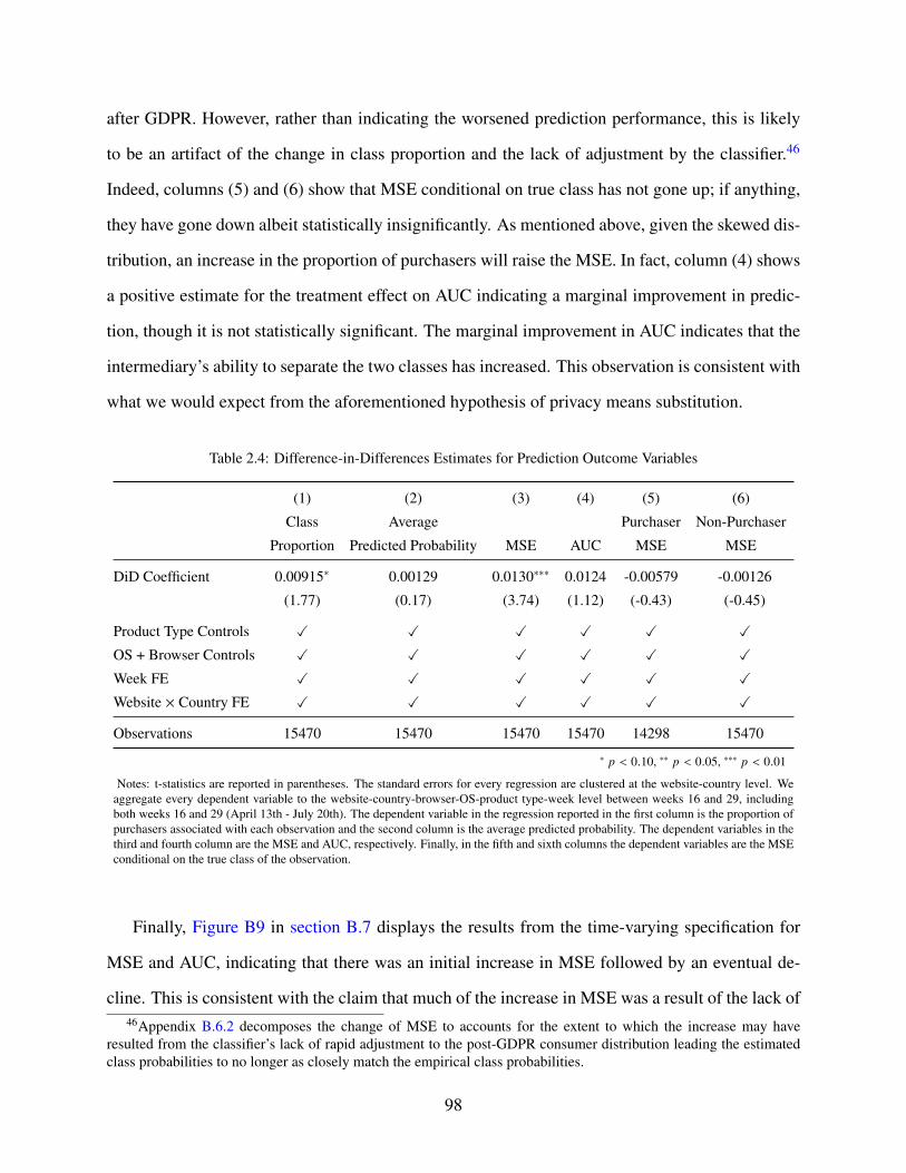
after GDPR. However, rather than indicating the worsened prediction performance, this is likely

to be an artifact of the change in class proportion and the lack of adjustment by the classifier.46

Indeed, columns (5) and (6) show that MSE conditional on true class has not gone up; if anything,

they have gone down albeit statistically insignificantly. As mentioned above, given the skewed dis-

tribution, an increase in the proportion of purchasers will raise the MSE. In fact, column (4) shows

a positive estimate for the treatment effect on AUC indicating a marginal improvement in predic-

tion, though it is not statistically significant. The marginal improvement in AUC indicates that the

intermediary’s ability to separate the two classes has increased. This observation is consistent with

what we would expect from the aforementioned hypothesis of privacy means substitution.

Table 2.4: Difference-in-Differences Estimates for Prediction Outcome Variables

(1) (2) (3) (4) (5) (6)

Class Average Purchaser Non-Purchaser

Proportion Predicted Probability MSE AUC MSE MSE

DiD Coefficient 0.00915∗ 0.00129 0.0130∗∗∗ 0.0124 -0.00579 -0.00126

(1.77) (0.17) (3.74) (1.12) (-0.43) (-0.45)

Product Type Controls ✓ ✓ ✓ ✓ ✓ ✓

OS + Browser Controls ✓ ✓ ✓ ✓ ✓ ✓

Week FE ✓ ✓ ✓ ✓ ✓ ✓

Website × Country FE ✓ ✓ ✓ ✓ ✓ ✓

Observations 15470 15470 15470 15470 14298 15470

∗ 𝑝 < 0.10, ∗∗ 𝑝 < 0.05, ∗∗∗ 𝑝 < 0.01

Notes: t-statistics are reported in parentheses. The standard errors for every regression are clustered at the website-country level. Weaggregate every dependent variable to the website-country-browser-OS-product type-week level between weeks 16 and 29, includingboth weeks 16 and 29 (April 13th - July 20th). The dependent variable in the regression reported in the first column is the proportion ofpurchasers associated with each observation and the second column is the average predicted probability. The dependent variables in thethird and fourth column are the MSE and AUC, respectively. Finally, in the fifth and sixth columns the dependent variables are the MSEconditional on the true class of the observation.

Finally, Figure B9 in section B.7 displays the results from the time-varying specification for

MSE and AUC, indicating that there was an initial increase in MSE followed by an eventual de-

cline. This is consistent with the claim that much of the increase in MSE was a result of the lack of46Appendix B.6.2 decomposes the change of MSE to accounts for the extent to which the increase may have

resulted from the classifier’s lack of rapid adjustment to the post-GDPR consumer distribution leading the estimatedclass probabilities to no longer as closely match the empirical class probabilities.

98

rapid adjustment. Furthermore, the increases in AUC do not occur directly after GDPR but rather

also occur gradually.

Overall, our results suggest that GDPR has not negatively impacted the ability to predict con-

sumer behavior and if at all, the sign of the treatment effect suggests the opposite. This is further

validated by the exercise in section B.8 which identifies the expected “long run" changes in predic-

tion performance as a result of the changes to the data observed in section 2.4. This exercise shows

that an increase in trackability will likely improve prediction performance, whereas the change in

the overall size of data as a result of GDPR should not adversely impact prediction performance

significantly.

2.7 Conclusion

In this paper we empirically study the effects of data privacy regulation by exploiting the intro-

duction of GDPR as a natural experiment. We use data from an intermediary that contracts with

many online travel agencies worldwide, which allows us to investigate the effect of GDPR on a

comprehensive set of outcomes. Our analysis focuses on the stipulation of GDPR that requires

firms to ask consumers for explicit consent to store and process their data.

Our results paint a novel and interesting picture of how a consumer’s privacy decision— partic-

ularly the means by which she protects her privacy—may impact the rest of the economy, including

other consumers, and the firms and advertisers relying on consumer data. The strong and effective

means of privacy protection made available by laws such as GDPR and the recent CCPA (Califor-

nia Consumer Privacy Act) should help the privacy-concerned consumers to protect their privacy

by eliminating their digital footprints. These consumers are thus clear winners of the laws. How-

ever, the impacts on the others are less clear. Our results suggest the possibility that a consumer’s

switching of the means of privacy protection makes the opt-in consumers who share their data more

trackable and possibly more predictable to the firms with which they share data. If this increased

trackability makes up for decreased data (resulting from opt-outs), as indicated by section B.8, then

the firms using consumer data could also come out as winners. What about those consumers who

99

opt in? Their welfare will depend on how their data is used by the firms. If their data is used to

target advertising and services to their needs, they too could very well be winners of privacy laws,

even if their decision to opt in may not have accounted for the externality. However, if their data

is used for extracting consumer surplus, e.g., via personalized pricing, the externalities could harm

them.

While these qualitative implications are clear, our reduced-form approach does not allow us to

quantify the welfare implications for both consumers and advertisers. We leave for future work a

structural analysis of the interactions that we identify in order to better understand the magnitude of

each of the channels by which consumers and advertisers are affected. Given the large compliance

costs associated with data privacy regulation, decomposing the welfare effects in this manner is a

fruitful direction for research and important for further building on our insights in order to guide

the design and understanding the value of such regulation.

Finally, our paper has broader implications beyond the online travel industry and keyword-

based advertising markets. Firms in this industry, as with many markets in the digital economy,

increasingly compete with the large technology firms such as Google whose reach expands across

many different online markets and for whom consumers have little choice but to accept data pro-

cessing. As a result, while our results highlight that increased consent requirements may not be

wholly negative for firms, if consumers are similarly using such opt-out capabilities at our esti-

mated rates in other markets (such as behaviorally-targeted advertising markets) then such regu-

lation may put firms in these markets at a disadvantage relative to these larger firms. It would be

important to study the extent and magnitude of these adverse effects. We believe that these insights

and directions for future work are useful for the design of the many proposed regulations in the US

and around the world that follow in the footsteps of GDPR.

100

Chapter 3: Recommenders’ Originals: The Welfare Effects of the Dual Role

of Platforms as Producers and Recommender Systems

3.1 Introduction

An increasing number of online platforms deploy recommender systems to assist consumers

with purchase decisions by providing information on available goods, which determinedly impacts

consumer choice. These systems facilitate information acquisition on product quality by con-

sumers in environments where there are thousands or even millions of alternatives available. Ex-

isting experimental literature supplies causal evidence of these systems’ immense power in steer-

ing demand, with market shares being significantly affected even by recommendation systems that

supply simple information to consumers [112]. Moreover, anecdotal evidence reflects the huge in-

fluence the information provided by these systems has on consumption choices individuals make:

recommendations are said to account for 75% of consumed content on Netflix and 35% of page

views on Amazon [113].

However, online platforms increasingly not only deploy recommender systems, but also pro-

duce and make available their own goods alongside other firms’, with unclear implications to

consumer welfare. Major platforms and technological leaders in the development and deployment

of recommender systems — such as Amazon, Netflix, and Spotify — all now develop their own

goods that are then made available on their platforms: Amazon produces more than 22,000 goods

that are available on the firm’s platform [114], Netflix hosts more than 2,300 “Netflix Originals”

titles [115], and Spotify is now investing in producing its own audio content [116].

One possible consequence of this dual role of the platforms as both a recommender system

and a producer is that platforms may systematically bias their search and recommendation systems

towards their own goods. Indeed, not only is there a substantial amount of popular press coverage

101

suggesting this,1 there are also a number of recent legislative initiatives that appear motivated by

potential abuse of this dual role, both in trying to prevent platforms in this dual role from biasing

their recommendation systems in favor of their own goods and in proposing the separation of

the roles of recommender and producer.2 While the goal of regulators is to increase consumer

welfare in such markets, it is unclear whether these regulatory initiatives will ultimately harm or

hurt consumers once equilibrium effects are taken into account.

In this paper we study the welfare consequences of a platform acting as both a producer and a

recommender and consider the specific role played by the deployment of a recommender system.

We set up a stylized model of a pay-for-access platform where producers make investment deci-

sions about the quality of their goods and revenue is split according to each goods’ market share.

Our main focus is in contrasting resulting consumer welfare, investments, and market shares across

three different scenarios: the no platform production case, where only a good by an independent

firm is available; the platform dual role case, where the platform can both produce a good and

design recommendations, and both the platform’s good and the independent firm’s are available;

and the unbiased recommendations case, where we modify the dual role case by imposing an

exogenous policy that requires that recommendation be unbiased, or truthful and neutral.

Unlike other papers that study the consequences of platform steering (e.g. [122, 123, 124]), we

model the platform’s recommendation as providing information on good quality to consumers as

opposed to directly influencing the search order or choosing the consumed good for a fraction of

consumers. Producers have access to stochastic investment technology that affects the likelihood

that goods are of high versus low quality. Consumers’ prior beliefs on good quality stem from the

observed investments, and they update their beliefs on each good’s quality based on the recommen-

dation policy of the platform. This allows us to build credibility of recommendation directly into

1For instance, [117] discusses Amazon’s bias towards its own goods via recommendation and search. [118]discusses how Google manipulates its search results to steer consumers. According to [119], upon release of Houseof Cards, Netflix recommended that consumers watch it regardless of their past behavior. Pandora has stated in courtthat it manipulates its recommendations based on the ownership of the sound recordings.

2An example of tackling possible biases in recommendations is the European Commission’s legislative proposalcalled “Digital Markets Act” [120], whereas the recent bill H.R. 3825 - “Ending Platform Monopolies Act” proposedto the House of Representatives of the United States aims to terminate situations of this dual role altogether [121].

102

our model, where the platform’s ability to steer the behavior of rational and Bayesian consumers

is naturally limited and depends on the design of its recommendations.

In our model, the revenue generated by the platform is based on pay-for-access and producers

are compensated according to their (expected) consumption share. We believe this captures the

fundamental elements that platforms in this dual role face (e.g. Spotify, Netflix), and constitutes

one of the primary drivers in motivating the platforms to bias recommendations towards their own

goods. Additionally, as a reduced-form proxy for the extent to which the independent firm is reliant

on the platform for revenues, we allow the independent firm to have access to alternative sources

of revenue, and characterize their impact on equilibrium investment decisions and consumer wel-

fare. For instance, in the movie industry, [125] reports that box office revenues are an essential

source of revenue for movie producers, while [126] highlights that in the music industry, recording

artists made most of their revenues from touring despite the widespread usage of online streaming

services.3 We show that the degree to which the independent firm depends on the platform as its

main source of revenue is decisive for whether the platform’s dual role has a positive or a negative

effect on consumer welfare.

The platform’s entry into the upstream market affects consumer welfare both via investments in

good quality, as well as through the platform’s recommendation policy, which provides consumers

with information on realized good quality.

Although limited by the need for recommendations to be credible in order for consumers to

choose the recommended good, the platform is able to bias recommendations towards its own good

so as to reappropriate the gains from information provision to increase its market share. Hence,

the platform’s dual role leads to biased recommendations that induce a significant pressure on the

independent firm’s equilibrium investment decisions: for the independent firm to appropriate a

share of platform demand it need not only to invest more than the platform, but it also needs the

realized quality of its good to be strictly higher than the platform’s.

3Exploiting the exogenous negative demand shock on movie theaters as a result of COVID-19 illustrates themarginal incentives of movie producers to respond to the relative weight of platform vs. offline sources of revenue[127].

103

While it would be natural to expect consumer welfare to increase with the platform’s entry

— as product variety increases and as more information cannot harm consumers — the prospect

of biased recommendation and its resulting equilibrium effect on investment levels leads to an

ambiguous effect on consumer welfare. When the independent firm is heavily dependent on the

platform and recommendation bias favoring the platform is most significant, the platform’s entry

results in lower investment levels and consumer welfare. However, if the alternative sources of

revenue are sufficiently large, the platform’s entry increases consumer welfare.

This result is driven by two opposing forces which influence the marginal incentives of the

independent firm to invest in quality, compared to when the independent firm is the sole producer.

The first is a revenue expansion channel, which expresses the ability of the firm to expand the

revenue it obtains from the platform by increasing its investment level. This channel is depressed

by platform entry and its use of biased recommendations as these significantly decrease the in-

dependent firm’s market share and, therefore, the independent firm receives but a fraction of its

marginal impact on total platform revenue. The second is a new share expansion channel, whereby

additional investment by the independent producer allows it to increase its market share. The plat-

form uses its recommendation policy to appropriate a share of the demand, but its ability to bias is

limited by the difference in investments in good quality. Then, larger investment by the firm natu-

rally limits the platform recommendation bias, which then expands the firm’s market share. These

two opposing forces generate a threshold effect for the investment levels of the independent firm

in terms of its reliance on the platform as its main source of revenue: When the independent firm

overly relies on revenue obtained from the platform, the platform’s dual role effectively depresses

its incentives to invest in quality, resulting in lower consumer welfare; if instead it has access to

other sources of revenue that are significant enough, the independent firm invests more strongly

than when it is the sole producer, driving up consumer welfare.

One important consequence of the platform’s dual role and the resulting recommendation bias

is the possibility of foreclosure of the independent firm. In equilibrium, this occurs when the

independent firm’s alternative revenue sources are small relative to the platform size, in which

104

case the platform finds it profitable to become the product-quality leader. Then, due to to the

ability to bias recommendations towards its own good, it completely drives demand away from

its competition, capturing the entire demand on the platform. Although this is a sharp prediction,

it echoes recent trends in video streaming markets, where platforms’ original content quality —

as indicated by awards received — has notably risen while their own content has simultaneously

dominated platform viewership. When the independent firm’s revenue sources are large enough

compared to the platform’s revenue potential, the platform becomes a product-quality follower.

Even then, the platform still partially forecloses the independent firm by biasing recommendations

in favor of its own goods, enabling it to achieve a higher market share and profit than otherwise.

We explore a natural policy remedy: ensuring that the platform cannot simultaneously provide

recommendation services and produce goods; or, equivalently, a policy that prevents the platform

from providing biased recommendations towards its own goods.4 This analysis further provides

insight into how much of the distortion in consumer welfare and investment decisions is due to

the platform’s ability to bias recommendations relative to entry and information provision alone.

Although it would be reasonable to expect an unambiguous improvement in consumer welfare —

since more informative recommendations should only help consumers relative to biased recom-

mendations — we find that this policy can actually harm consumers under certain conditions.

There are two observations that lead to this result, which stem from the fact that the unbi-

ased recommendation policy induces downward equilibrium adjustments in investment decisions

that can outweigh the welfare gains arising from unbiased recommendation. The first is that the

revenue expansion channel is more responsive to investments by the quality follower, and less to

investments by the quality leader. This is because, under the dual role, the platform’s use of rec-

ommendations to expand its demand share leads to fully dissipating any informational gains to

consumers, and revenue is completely determined by the investments of the quality leader. Un-

biased recommendations maximize informational gains and expand overall revenue, but lead to

the aforementioned effect on how investments by the platform and the firm affect total revenue at

4We define unbiased recommendations as recommendations that are both truthful (i.e. always recommending thehighest quality good) and neutral (breaking ties uniformly at random).

105

the margin. The second is that imposing unbiased recommendations results in a depressed share

expansion channel relative to the dual role for both the independent firm and the platform. Thus,

imposing a fairer competition for demand share between the platform and the independent firm by

requiring unbiased recommendations has the unexpected negative effect of reducing pressure to

invest in quality by both parties.

Combined, these two observations result in an ambiguous welfare effect of imposing unbiased

recommendations. Relative to the dual role, unbiased recommendations improve consumer welfare

when the platform’s market size is comparable to the firm’s alternative market size. However,

when the platform’s market size is large enough or when the independent firm relies mostly on

alternative revenue sources, stripping the platform from its power to bias recommendations in its

favor overwhelmingly depresses incentives to investment and entails a loss in consumer welfare.

Further, the magnitude of welfare effects of such a policy depends crucially on the industry’s

structure and the relative weight of different revenue sources.

Our results illustrate how platforms entering the upstream production market benefit from bias-

ing recommendations. However, the resulting distortion from this entry does not necessarily harm

consumers, as it may spur other producers to invest more aggressively in good quality to counter

not only increased product competition, but especially recommendation bias. An important ele-

ment to consider is how dependent the other producers are on revenues from the platform. Only

when this dependence is significant will policies targeting bias in recommender systems or separat-

ing recommendation and production altogether have a positive effect on consumer welfare. While

platforms and online retailers have other means at their disposal to distort consumption choices

that are not explicitly addressed in this paper, our model suggest caution when considering pol-

icy interventions: the bias in recommender system may be inducing independent firms to produce

higher quality goods than what they otherwise would. Indeed, our results provide a rationale for

the stipulations of the Ending Platform Monopolies Act that ends the dual role only for dominant,

“gatekeeper” firms. In such cases the welfare effect for consumers is likely to be positive, whereas

for smaller platforms it will have an ambiguous or lesser effect.

106

Related Work

Our paper lies in the intersection of three different literatures: biased intermediation, recom-

mender systems and, more broadly, vertical integration and foreclosure.

Most relevant to our paper is the nascent biased intermediation literature and, more generally,

biased information provision. This emerged from the traditional intermediation and two-sided

market literature [128, 129], and focuses on the incentives of an intermediary to bias consumption

decisions. While the majority of the literature focuses on the consequences of an intermediary ma-

nipulating the search process of a user, we instead model the intermediary as providing information

to consumers. The intermediary in our model, the recommender, is thus an information designer as

in the Bayesian persuasion literature [130, 131]. This has two main advantages. The first is that it

provides a more accurate model of how recommender systems function, where recommendations

provide imperfectly informed consumers with information about goods on the platform whose

true consumption values are only learned from experience. The second is that it requires recom-

mendations to be credible in order to affect consumer behavior, thereby disciplining the ability of

platforms to steer demand.

Within this literature, the papers closest to ours are [132], [123] and [122]. [132] study the

incentives of a pay-for-access platform to bias their recommendation in order to reduce the market

power of the upstream content providers. They also consider that the payouts between the produc-

ers and the platforms are split via royalty fees that depend on consumer’s consumption choices.

They focus on perfectly horizontal preferences with fixed good characteristics, whereas our model

considers the effect that platform recommendation bias has on quality investments. [123] study a

model of biased intermediation where the recommendation is sold through an auction while [122]

examine a setting where consumers perform costly and sequential search and the intermediary

directs the consumers to a seller; in both cases, uninformed consumers naively follow the recom-

mendation, without any credibility constraint. In contrast, in our model recommendations have to

be credible and depend on investment levels, and both are endogenously determined. Other re-

lated papers — where investment decisions are absent — focus on price competition among sellers

107

on the platform [133], advertising and search [134, 135, 136], and commission and price setting

(Inderst and Ottaviani [138, 137], [124]).

Naturally, this paper contributes to the literature on recommender systems which analyzes the

consequences of recommendation on consumer choice, pricing, and sales. [139] analyzes model

with horizontally differentiated products where a platform with a recommender system competes

with a fringe of distribution channels without such system. In this paper, the recommender’s

information advantage is modeled as deriving observing past users’ experience in a two-period

model and consumers are able to obtain a recommendation at no cost. Opposite to our model, the

emphasis in this paper is on the optimal pricing by the recommender, and investment decisions

are absent as all firms are intermediaries selling the same products. Other, less related works are

[140], [141], [142]. [140] characterizes the optimal information provision by a welfare maximizing

recommender that learns a good’s quality through consumer feedback. [141] discuss the role that

recommender systems can play in diversifying sales due to their personalized nature, but do not

endogenize production or consider incentives to bias recommendation. [142] examines how a

recommender would trade-off between optimizing for profit and maintaining reputation amongst

consumers, but do not consider good investment or platform production.

Subsequent to our work, [143] and [144] study economic models of the impact of recommender

systems on consumption choices with implications for competition policy. [143] focus on how

recommender systems lead to excessive market concentration, and [144] explore recommendation

performance as a function of consumer data and consumption choices, taking into account the

degree of misalignment between the platform and consumers.

Finally, our paper broadly contributes to a classic literature in industrial organization that stud-

ies vertical integration, upstream entry, and investment [145, 146, 147], and vertical foreclosure

[148, 149]. We are most interested in the dual role of platforms as producers — upstream entry —

and information providers, which has not received as much attention in the literature. Two papers

that look at related problems are [150] — studying the role of vertical information restraints in

a retail market that involves search frictions with a focus on understanding minimum advertising

108

price restrictions — and [151], who introduces a vertical industry structure into a consumer search

model where consumers are uninformed about wholesale prices. These papers are complementary

to ours, but, to our knowledge, we are the first to study the integration of recommendation and

production and how this can lead to a novel form of vertical foreclosure.

The remainder of the paper is structured as follows: Section 3.2 provides the setup for the

model. The impact of the platform’s dual role on equilibrium investment decisions and consumer

welfare consequences is analyzed in Section 3.3. In Section 3.4, we explore the value of recom-

mendation and characterize the equilibrium welfare consequences of a policy that imposes unbi-

ased recommendations. We discuss the robustness of the results to the different assumptions in

Section 3.5, before concluding with some final remarks in Section 3.6. Proofs are omitted from the

main text and can be found in Appendix C.1.

3.2 Model Setup

This section introduces the main elements of our model.

Production. There are two firms, the independent firm 𝐹 and the platform 𝑃. We consider two

cases: one in which only 𝐹, the independent firm, makes production decisions, and another where

both 𝐹 and 𝑃 make production decisions. We denote by 𝐽 the set of firms making production

decisions. In the case where both 𝐹 and 𝑃 make production decisions, we suppose that the in-

dependent firm’s investment 𝑞𝐹 is observable by the platform before deciding its investment. We

argue that this timing assumption is realistic as platforms are usually second-movers in production

decisions. However, as we discuss in Section 3.5, our conclusions do not rely on this: a setting

where production decisions are simultaneous yields the same qualitative results.

Each firm 𝑗 ∈ 𝐽 produces a single good 𝑥 𝑗 , which is either of high quality, 𝑥 𝑗 = 1, or low

quality, 𝑥 𝑗 = 0. The realized quality of the goods ultimately produced (𝑥 𝑗 ) is stochastic and

depends on the firms’ investments. Each firm initially makes investment decisions 𝑞 𝑗 ∈ [0, 1]

which determine the probability that the realized quality of the good is high, that is, 𝑞 𝑗 = P(𝑥 𝑗 =

1). This need not be taken as pure vertical differentiation: high quality can be interpreted as

109

idiosyncratic to a given consumer and 𝑞 𝑗 then refers to the probability that a given consumer will

enjoy the good and deem it high quality. For simplicity, we assume that firms face a quadratic cost

to this investment in (stochastic) quality: 𝐶 𝑗 = 𝑞2𝑗.

Good Distribution. We focus on a subscription-based pricing model, which is ubiquitous in many

markets where recommender systems are widely deployed — such as media streaming or news

platforms. Firm 𝑃 serves as a platform for consumers in the market to access the goods produced.

It sets a single price 𝜏, a subscription fee, that consumers need to pay in order to gain access to the

platform. Once on the platform, consumers can choose which of the available goods to consume

without incurring additional cost.

Consumers. All consumers prefer high-quality goods to low-quality goods, but vary in their

willingness-to-pay. Consumer 𝑖’s utility from joining the platform (𝑒𝑖 = 1), consuming good 𝑥 and

paying access fee 𝜏 is given by 𝑢(𝑥, \𝑖, 𝜏) = \𝑖𝑥 − 𝜏, where \𝑖 denotes consumer 𝑖’s willingness-

to-pay for high quality goods; not joining the platform (𝑒𝑖 = 0) gives the consumer zero utility.

Consumers’ willingness-to-pay \𝑖 is uniformly distributed on [0, \̄], and its distribution function

is denoted by 𝐺. Consumers maximize expected utility and we assume they are well-informed in

that they observe investments prior to deciding whether to access the platform and which good to

consume. Finally, we denote by 𝑀𝑃 the measure of consumers that access the produced goods

exclusively through the platform; for simplicity we denote a given consumer as 𝑖 ∈ [0, 𝑀𝑃].

Recommendation Policy. We model platform recommendations as providing consumers with

information on the realized good qualities. We define a recommendation policy 𝜌 as the probability

of recommending firm 𝑗’s good to consumers contingent on good quality.5 The platform then acts

as an information designer who chooses a recommendation policy before the quality of goods 𝑥𝑃

and 𝑥𝐹 is realized. Upon observing the realized recommendation 𝑚 ∈ 𝐽, consumers update their

beliefs on the quality of the goods and choose the one that maximizes their expected utility.

A key goal is to understand how different properties of the recommendation policy affect con-

5Note that this specification is without loss: While information provision by the platform would generically consistof a a mapping from the set of possible states, the realized good qualities {0, 1}𝐽 to distributions over an arbitrarymessage space M, it is well-known that it is without loss of optimality to consider the message spaces that correspondto the available actions.

110

sumer welfare. Two important aspects of recommendations for policy considerations are whether

they convey truthful information to consumers about which good is best, and that they do not con-

fer undue advantage to any given good. Formally, we say that a recommendation policy is truthful

if, given realized qualities 𝑥𝑃, 𝑥𝐹 , the recommended good is of weakly higher quality than the

non-recommended good (P𝜌 (𝑚 ∈ arg max 𝑗∈𝐽{𝑥𝐹 , 𝑥𝑃}) = 1); and recommendations are said to be

neutral if ties in quality are broken uniformly at random (P𝜌 (𝑚 = 𝑥𝑃 | 𝑥𝑃 = 𝑥𝐹) = 1/2). Unbiased

recommendation policies are those that are both truthful and neutral.

Although allowing the platform to commit to a recommendation policy is ultimately a sim-

plifying modeling device, commitment is a common and arguably well-grounded assumption in

the literature in economics and computer science studying strategic interactions between recom-

mender systems and Bayesian consumers [140, 152, 153]: Not only can it be justified by the need

for credibility in the context of repeated interactions, but also by the fact that existing recommender

systems are stable deployed algorithms which imply commitment to a predefined recommendation

strategy.

We focus on the role of recommendations as being utilized purely for steering subject to the

constraint of rational, Bayesian consumers. For that purpose, we will assume that consumers’

decision whether to enter the platform occurs prior to the choice of a recommendation policy by

the platform. This timing is not devoid of justification: consumers’ decision to join the platform or

not is arguably more stable when compared to the more frequent adjustment of recommendation

systems, taking as given (and make use of the information from) the pool of consumers on the

platform.

Revenue Sources Outside the Platform. We suppose that firm 𝑃 only gets revenue from the

platform itself, as is common for private-label goods — “recommender’s originals” such as Net-

flix’s, Spotify’s, Hulu’s, where their good is only available on their own platform. Contrastingly,

we allow the independent producer, 𝐹, to obtain additional revenue streams off the platform, 𝑅𝐹 ,

depending implicitly on its investment in quality. We interpret these additional revenue as the re-

liance of the independent firm on the platform revenues. This can be seen as a reduced-form proxy

111

for revenues from offline alternatives to the online platform. For instance, in the case of Spotify,

this could be the revenue achieved from concerts or album purchases; for Netflix, it could be the

revenue achieved from movie theaters. In order to study how equilibrium and consumer welfare

change as the strength of the outside option for the producing firms increases we parameterize

𝑅𝐹 = 𝑟𝐹 · 𝑞𝐹 with 𝑟𝐹 > 0. We interpret the parameter 𝑟𝐹 as the size or relevance of this alternative

market in which firm 𝐹 operates.6 We discuss the robustness of our results to the existence of

alternative revenue sources for the independent firm in Section 3.5.

Revenue on the Platform. The platform revenue 𝑅𝑃 will depend on the recommendation policy,

pricing and quality investments of both firms. We suppose that it is split between the platform and

the independent firm according to their expected consumption share on the platform, which we

denote as 𝛼𝑃 and 𝛼𝐹 , 𝛼𝑃 +𝛼𝐹 = 1. This split rule can be interpreted as the reduced form of a linear

contract agreed to by the platform and the independent producer where the independent producer

gets a royalty fee for each consumer that consumes her good. This type of contractual relationship

is common on pay for access platforms — for instance, Spotify pays musicians a royalty in accor-

dance with the number of times their song is played on the platform, and on YouTube Premium

the membership fees are distributed based on how many members watch a producer’s content. We

take this split rule as an exogenous industry benchmark and study its consequences.

The overall expected payoffs for each firm is therefore given by:

𝜋𝑃 = 𝛼𝑃 · 𝑅𝑃 − 𝐶𝑃

𝜋𝐹 = 𝛼𝐹 · 𝑅𝑃 + 𝑅𝐹 − 𝐶𝐹 ,

where the dependence on investment levels, recommendation policy, and access fee is implicit.

Timing. In line with the setup defined above, the timing of events in the model is summarized as

follows:6 If consumers preferences in this unrelated market are also quasilinear and their willingness-to-pay is uniformly

distributed on [0, \̂], then were firm 𝐹 a monopolist in such market optimally setting a uniform price given the choseninvestment level, one would have that the generated revenue would be 𝑟𝐹 · 𝑞𝐹 , with 𝑟𝐹 = 𝑀𝐹 · \̂/4.

112

1. Production decisions are made sequentially, first by the independent firm, then by the plat-

form.

2. The platform determines access fee 𝜏 and consumers decide whether to join the platform or

not, resulting in revenue 𝑅𝑃.

3. The platform commits to a recommendation policy.

4. Good qualities realize.

5. The platform makes recommendations.

6. Consumers decide which good to consume conditional on investment probabilities and plat-

form recommendation.

7. The independent firm and the platform split the platform revenue according to their con-

sumption share, and the independent firm accrues outside revenue 𝑅𝐹 .

Other variations on the timing are discussed in Section 3.5.

3.3 Consequences of the Platform’s Dual Role

In this section we study the consequences of the platform’s dual role. We contrast the case

where only the independent firm’s good is available on the platform to the equilibrium in the case

where the platform can itself choose to produce a good and steer consumers via its recommender

system.

3.3.1 No Platform Production

We first consider the case where the independent firm is the sole producer in the market. The

timing is the same, but the platform does not make production decisions. As there is only one

good available on the platform and the platform does not observe good quality before consumers

make the decision to join the platform, there is no scope for recommendation policy to impact

consumers’ valuation of paying to access the platform.

113

We assume that pricing is still profit maximizing.7 The expected value of subscribing to the

platform for a consumer of type \ is then E𝑢(𝑥, \, 𝜏) = \E[𝑥] − 𝜏, where in the case we are ana-

lyzing we have the expected quality of the consumed good is E[𝑥] = E[𝑥𝐹] = 𝑞𝐹 . A consumer of

type \ then subscribes to the platform whenever E𝑢(𝑥𝐹 , \, 𝜏) ≥ 0,8 and therefore 𝑒𝑖 = 1\𝑖≥𝜏/E[𝑥𝐹 ] .

The platform’s pricing problem is then

𝜏 ∈ arg max𝑡≥0

𝑀𝑝 · 𝑡 ·∫ \̄

0𝑒𝑖 𝑑𝐺 (\) = arg max

𝑡≥0𝑡 ·

(1 − 𝐺

(𝑡

𝑞𝐹

)).

Given the uniform distribution assumption, the solution to the pricing problem is given by 𝜏 =

12 \̄𝑞𝐹 . This implies that 𝑅𝑃 =

𝑀𝑃 ·\̄4 𝑞𝐹 .

For convenience, we define 𝑟𝑃 := 𝑀𝑃 ·\̄4 , so that 𝑅𝑃 = 𝑟𝑃 · 𝑞𝐹 . The parameter 𝑟𝑃 represents

the total potential revenue that can be accrued on the platform. Both 𝑟𝑃 and 𝑟𝐹 can be taken as

reduced form measures of market size and relative comparison between the two provides us with

a notion of the relative dependence of the independent firm on the platform. The implications of

the platform’s dual role will crucially depend on how large the platform market size is relative to

alternative markets available to the independent firm.

The firm’s production decision problem is then given by

max𝑞𝐹∈[0,1]

𝛼𝐹 · 𝑅𝑃 + 𝑅𝐹 − 𝐶𝐹 = max𝑞𝐹∈[0,1]

𝑟𝑃 · 𝑞𝐹 + 𝑟𝐹 · 𝑞𝐹 − 𝑞2𝐹

where 𝛼𝐹 = 1, as the firm is the only producer in the market. The firm’s optimal production

decision in the “no-platform-production” (NP) case is

𝑞𝑁𝑃𝐹 = min{𝑟𝑃 + 𝑟𝐹

2, 1

}.

7Although the platform has no incentive to set profit maximizing prices in the current setup, as it effectivelyaccrues no revenue, it can be seen — and indeed it is — the limit case of a related setup where the platform gets afixed share 𝑠 of the overall revenue, where this share is arbitrarily small. This analysis of this exact case yields thesame qualitative results.

8Although the tie-breaking rule favors subscribing, this is not consequential for investment decisions as types arecontinuously distributed.

114

Finally, we note that consumer welfare is linear in expected quality of the good consumed,9 given

that

𝑊𝑁𝑃 = E[𝑒𝑖 · 𝑢(𝑥𝐹 , \, 𝜏)] =∫ \̄

\̄2

\𝑞𝐹 − 𝜏 𝑑𝐺 (\) = 38\̄

2𝑞𝑁𝑃𝐹 .

3.3.2 Platform’s Dual Role

We now characterize the equilibrium investment levels of the case where the platform can also

make production decisions. Given that now more than one good is available on the platform,

recommendations play a role in determining how much consumers value having a platform sub-

scription.

A subgame-perfect equilibrium is a tuple (𝜌, 𝜏, 𝑞𝑃, 𝑞𝐹) where the platform 𝑃 chooses a recom-

mendation policy 𝜌, an access fee 𝜏, and an investment level 𝑞𝑃, the independent firm 𝐹 chooses

investment level 𝑞𝐹 in order to maximize their respective profits, and each consumer 𝑖 ∈ [0, 𝑀𝑃]

makes a decision on whether to join the platform (𝑒𝑖) and which good to consume (𝑥𝑖) so as to

maximize their expected utility.

As is standard, we solve for equilibrium via backward induction. We recall the (inverse) timing

of events:

9. The independent firm and the platform split the platform revenue according to their con-

sumption share and the independent firm accrues outside revenue 𝑅𝐹 .

8. Each consumer 𝑖 selects the good 𝑥𝑖 with the highest expected utility conditional on recom-

mendation and investment probabilities:

𝑥𝑖 ∈ arg max𝑥 𝑗∈{𝑥𝑃 ,𝑥𝐹 } E[𝑢(𝑥 𝑗 , \𝑖, 𝜏) | 𝜌, 𝑚] given the recommendation policy 𝜌 and the

realized recommendation, breaking ties in favor of the platform.

7. The platform’s recommendations realize:

9If one considers a similar market structure underlying the alternative revenue sources for the independent firm(see Footnote 6), this linearity of consumer welfare in expected quality of the independent firm’s good extends also tothis alternative independent market.

115

𝑚 ∼ 𝜌(𝑥𝑃, 𝑥𝐹), where 𝜌 : {0, 1}2 → Δ(𝐽) and 𝑚 ∈ 𝐽.

6. Good qualities realize:

𝑥 𝑗 ∼ P(𝑥 𝑗 = 1) = 𝑞 𝑗 and P(𝑥 𝑗 = 0) = 1 − 𝑞 𝑗 , with 𝑗 = 𝑃, 𝐹.

5. The platform commits to a recommendation policy 𝜌:

𝜌 ∈ arg max𝑟:{0,1}2→Δ(M) 𝛼𝑃 · 𝑅𝑃 − 𝐶𝑃 given 𝑅𝑃, 𝑞𝑃 and where the platform’s market share

is given by 𝛼𝑃 = E[1𝑥𝑃=𝑥𝑖 | 𝑒𝑖 = 1

].

4. Each consumer 𝑖 decides whether to join the platform (𝑒𝑖 = 1) or not (𝑒𝑖 = 0):

𝑒𝑖 ∈ arg max𝑒∈{0,1} 𝑒 · E[𝑢(𝑥𝑖, \𝑖, 𝜏) | 𝜌].

3. The platform determines access fee 𝜏, resulting in revenue 𝑅𝑃:

𝜏 ∈ arg max𝑡≥0 𝑡 · 𝑀𝑃 · E\ [𝑒𝑖].

2. The platform determines its investment level, 𝑞𝑃:

𝑞𝑃 ∈ arg max𝑞′𝑃∈[0,1] 𝛼𝑃 · 𝑅𝑃 − 𝐶𝑃.

1. The independent firm determines its investment level, 𝑞𝐹 :

𝑞𝐹 ∈ arg max𝑞′𝐹∈[0,1] 𝛼𝐹 · 𝑅𝑃 + 𝑅𝐹 − 𝐶𝐹 .

Optimal Recommendation Policy

The first step is to solve for the optimal recommendation policy. The platform faces a standard

Bayesian persuasion problem [130], choosing a conditional signal distribution to maximize its

profits. As the consumer has two actions — choosing either the platform’s or the independent

firm’s good — it is without loss to consider recommendation policies with at most two messages,

𝐽 = {𝐹, 𝑃}, where we interpret 𝜌(𝑥𝑃, 𝑥𝐹) = 𝑃 (= 𝐹) as recommending the consumer to choose the

platform’s (resp. firm’s) good. The only constraint is one of credibility: the consumers cannot be

left worse off by following the recommendation than if they were not to follow it. The problem

can then be written as

max𝜌:{0,1}2→Δ(𝐽)

𝛼𝑃 · 𝑅𝑃 − 𝐶𝑃

116

subject to credibility constraints

E[𝑢(𝑥𝑃, \𝑖, 𝜏) | 𝜌(𝑥𝑃, 𝑥𝐹) = 𝑃] ≥ E[𝑢(𝑥𝐹 , \𝑖, 𝜏) | 𝜌(𝑥𝑃, 𝑥𝐹) = 𝑃]

E[𝑢(𝑥𝐹 , \𝑖, 𝜏) | 𝜌(𝑥𝑃, 𝑥𝐹) = 𝐹] ≥ E[𝑢(𝑥𝑃, \𝑖, 𝜏) | 𝜌(𝑥𝑃, 𝑥𝐹) = 𝐹] .

The next proposition characterizes the platform’s optimal recommendation policy and its implica-

tions for the expected good quality and market shares:

Proposition 1. The optimal recommendation policy by the platform is such that

(i) if 𝑞𝑃 ≥ 𝑞𝐹 , the platform always recommends its good;

(ii) if 0 ≤ 𝑞𝑃 < 𝑞𝐹 ≤ 1, then the platform always recommends its own good whenever

it has weakly higher quality than the independent firm’s, P (𝜌(𝑥𝑃, 𝑥𝐹) = 𝑃 | 𝑥𝑃 ≥ 𝑥𝐹) =

1, and, when its own good has strictly lower quality, it is recommended with probability

P (𝜌(𝑥𝑃, 𝑥𝐹) = 𝑃 | 𝑥𝑃 < 𝑥𝐹) = 𝑞𝑃1−𝑞𝑃

1−𝑞𝐹𝑞𝐹

.

Moreover, the expected good quality is given by E[𝑥𝑚 | 𝜌] = max{𝑞𝑃, 𝑞𝐹}, and the expected

market shares of the platform and the independent firm are 𝛼𝑃 = min{1, 1 − (𝑞𝐹 − 𝑞𝑃)} and

𝛼𝐹 = 1 − 𝛼𝑃 = max{0, 𝑞𝐹 − 𝑞𝑃}, respectively.

Proposition 1 highlights how the platform is able to use recommendations to heavily favor its own

goods and brings forth two key insights. First, that in order to have its good recommended and

subsequently consumed on the platform, the firm not only needs to initially invest strictly more

than the platform, but it also needs its good’s realized quality to be strictly higher than that of the

platform’s. And, even then, the platform will in general still be able to steer consumers to choose

its good with positive probability. Second, that, with the platform-optimal recommendation policy,

consumers are left as well off from following recommendations than from defaulting to their prior

and choosing the good that entailed the largest investment. As we explain below, this is because

rent extraction by the platform warrants recommendation bias and, even though recommendations

117

cannot hurt consumers — more information is always weakly beneficial to decision-makers —

optimal recommendation bias leads to dissipating any informational gains to consumers.

Let us discuss the intuition underlying the results in Proposition 1. When the platform invests

more than the independent firm (𝑞𝑃 ≥ 𝑞𝐹), it can capture all the market share (𝛼𝑃 = 1) by always

recommending its good. This is because, without additional information, consumers always default

to choosing the good with greater probability of realizing of high quality. Then, in this case, the

optimal recommendation policy is credible, given that consumers are left no worse off by following

the recommendation; and, as recommendations are uninformative and independent of realized

good quality, it actually leaves consumers exactly as well off by following the recommendation as

they would be defaulting to their prior. Furthermore, we note that if there is ex-ante uncertainty

about which good is best (1 > 𝑞𝑃 ≥ 𝑞𝐹 > 0), then the optimal recommendation policy is also

biased, as the platform always recommends its good even when the independent firm’s is of strictly

higher realized quality.

When instead the independent firm invests strictly more than the platform in good quality

(𝑞𝑃 < 𝑞𝐹), the platform has to choose an informative recommendation policy in order to garner

some market share for its own good. If we consider the cases where it is ex-ante known that

the independent firm’s good will always be of weakly higher quality than the platform’s (1 = 𝑞𝐹

or 0 = 𝑞𝑃), since credibility constraints require consumers not to be left worse off by following

recommendations, only truthfully recommending the best good available is credible. To see this,

note that any small bias toward the platform’s good beyond tie-breaking leads to consumers strictly

preferring to ignore the recommendation and choose the independent firm’s good. Hence, the best

the platform can do is to commit to truthfully recommend the best good available and, if possible,

use recommendations only to break ties in favor of its own good and capture some market share.

As soon as we step away from that extreme case and have ex-ante uncertainty over which

good is of higher realized quality (1 > 𝑞𝐹 > 𝑞𝑃 > 0), the platform will be able to credibly

recommend its good even when the strictly better alternatives are available. In such a case, there is

a possibility that the platform’s realized good quality is high and the independent firm’s is low —

118

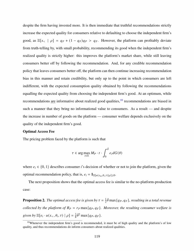
despite the firm having invested more. It is then immediate that truthful recommendations strictly

increase the expected quality for consumers relative to defaulting to choose the independent firm’s

good, as E[𝑥𝑚 | 𝜌] = 𝑞𝐹 + (1 − 𝑞𝐹)𝑞𝑃 > 𝑞𝐹 . However, the platform can profitably deviate

from truth-telling by, with small probability, recommending its good when the independent firm’s

realized quality is strictly higher: this improves the platform’s market share, while still leaving

consumers better off by following the recommendation. And, for any credible recommendation

policy that leaves consumers better off, the platform can then continue increasing recommendation

bias in this manner and retain credibility, but only up to the point in which consumers are left

indifferent, with the expected consumption quality obtained by following the recommendations

equalling the expected quality from choosing the independent firm’s good. At an optimum, while

recommendations are informative about realized good qualities,10 recommendations are biased in

such a manner that they bring no informational value to consumers. As a result — and despite

the increase in number of goods on the platform — consumer welfare depends exclusively on the

quality of the independent firm’s good.

Optimal Access Fee

The pricing problem faced by the platform is such that

𝜏 ∈ arg max𝑡∈R

𝑀𝑃 · 𝑡 ·∫ \̄

0𝑒𝑖𝑑𝐺 (\)

where 𝑒𝑖 ∈ {0, 1} describes consumer 𝑖’s decision of whether or not to join the platform, given the

optimal recommendation policy, that is, 𝑒𝑖 = 1E[𝑢(𝑥𝑚,\𝑖 ,𝜏) |𝜌]≥0.

The next proposition shows that the optimal access fee is similar to the no-platform-production

case:

Proposition 2. The optimal access fee is given by 𝜏 = 12 \̄max{𝑞𝑃, 𝑞𝐹}, resulting in a total revenue

collected by the platform of 𝑅𝑃 = 𝑟𝑃 max{𝑞𝑃, 𝑞𝐹}. Moreover, the resulting consumer welfare is

given by E[𝑒𝑖 · 𝑢(𝑥𝑚, \𝑖, 𝜏) | 𝜌] = 38 \̄

2 max{𝑞𝑃, 𝑞𝐹}.10Whenever the independent firm’s good is recommended, it must be of high quality and the platform’s of low

quality, and thus recommendations do inform consumers about realized qualities.

119

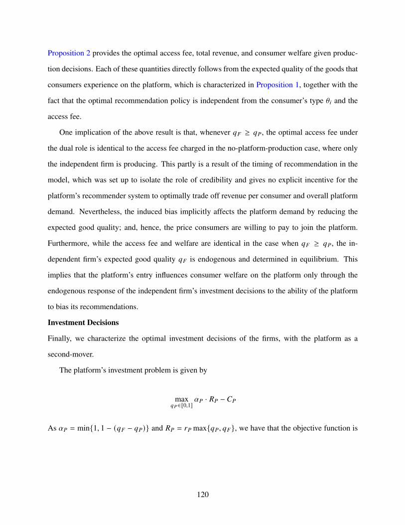
Proposition 2 provides the optimal access fee, total revenue, and consumer welfare given produc-

tion decisions. Each of these quantities directly follows from the expected quality of the goods that

consumers experience on the platform, which is characterized in Proposition 1, together with the

fact that the optimal recommendation policy is independent from the consumer’s type \𝑖 and the

access fee.

One implication of the above result is that, whenever 𝑞𝐹 ≥ 𝑞𝑃, the optimal access fee under

the dual role is identical to the access fee charged in the no-platform-production case, where only

the independent firm is producing. This partly is a result of the timing of recommendation in the

model, which was set up to isolate the role of credibility and gives no explicit incentive for the

platform’s recommender system to optimally trade off revenue per consumer and overall platform

demand. Nevertheless, the induced bias implicitly affects the platform demand by reducing the

expected good quality; and, hence, the price consumers are willing to pay to join the platform.

Furthermore, while the access fee and welfare are identical in the case when 𝑞𝐹 ≥ 𝑞𝑃, the in-

dependent firm’s expected good quality 𝑞𝐹 is endogenous and determined in equilibrium. This

implies that the platform’s entry influences consumer welfare on the platform only through the

endogenous response of the independent firm’s investment decisions to the ability of the platform

to bias its recommendations.

Investment Decisions

Finally, we characterize the optimal investment decisions of the firms, with the platform as a

second-mover.

The platform’s investment problem is given by

max𝑞𝑃∈[0,1]

𝛼𝑃 · 𝑅𝑃 − 𝐶𝑃

As 𝛼𝑃 = min{1, 1 − (𝑞𝐹 − 𝑞𝑃)} and 𝑅𝑃 = 𝑟𝑃 max{𝑞𝑃, 𝑞𝐹}, we have that the objective function is

120

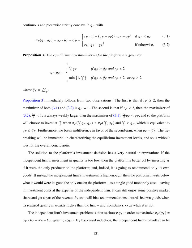
continuous and piecewise strictly concave in 𝑞𝑃, with

𝜋𝑃 (𝑞𝑃, 𝑞𝐹) = 𝛼𝑃 · 𝑅𝑃 − 𝐶𝑃 =

𝑟𝑃 · (1 − (𝑞𝐹 − 𝑞𝑃)) · 𝑞𝐹 − 𝑞𝑃2 if 𝑞𝑃 < 𝑞𝐹 (3.1)

𝑟𝑃 · 𝑞𝑃 − 𝑞𝑃2 if otherwise. (3.2)

Proposition 3. The equilibrium investment levels for the platform are given by:

𝑞𝑃 (𝑞𝐹) =

𝑟𝑃2 𝑞𝐹 if 𝑞𝐹 ≥ 𝑞𝐹 and 𝑟𝑃 < 2

min{1, 𝑟𝑃2

}if 𝑞𝐹 < 𝑞𝐹 and 𝑟𝑃 < 2, or 𝑟𝑃 ≥ 2

where 𝑞𝐹 ≡ 𝑟𝑃4−𝑟𝑃 .

Proposition 3 immediately follows from two observations. The first is that if 𝑟𝑃 ≥ 2, then the

maximizer of both (3.1) and (3.2) is 𝑞𝑃 = 1. The second is that if 𝑟𝑃 < 2, then the maximizer of

(3.2), 𝑟𝑃2 < 1, is always weakly larger than the maximizer of (3.1), 𝑟𝑃2 𝑞𝐹 < 𝑞𝐹 , and so the platform

will choose to invest at 𝑟𝑃2 when 𝜋𝑃 ( 𝑟𝑃2 𝑞𝐹 , 𝑞𝐹) ≤ 𝜋𝑃 ( 𝑟𝑃2 , 𝑞𝐹) and 𝑟𝑃2 ≥ 𝑞𝐹 , which is equivalent to

𝑞𝐹 ≤ 𝑞𝐹 . Furthermore, we break indifference in favor of the second-arm, when 𝑞𝐹 = 𝑞𝐹 . The tie-

breaking will be immaterial in characterizing the equilibrium investment levels, and so is without

loss for the overall conclusions.

The solution to the platform’s investment decision has a very natural interpretation: If the

independent firm’s investment in quality is too low, then the platform is better off by investing as

if it were the only producer on the platform; and, indeed, it is going to recommend only its own

goods. If instead the independent firm’s investment is high enough, then the platform invests below

what it would were its good the only one on the platform – as a single good monopoly case – saving

in investment costs at the expense of the independent firm. It can still enjoy some positive market

share and get a part of the revenue 𝑅𝑃 as it will bias recommendations towards its own goods when

its realized quality is weakly higher than the firm – and, sometimes, even when it is not.

The independent firm’s investment problem is then to choose 𝑞𝐹 in order to maximize 𝜋𝐹 (𝑞𝐹) =

𝛼𝐹 · 𝑅𝑃 + 𝑅𝐹 − 𝐶𝐹 , given 𝑞𝑃 (𝑞𝐹). By backward induction, the independent firm’s payoffs can be

121

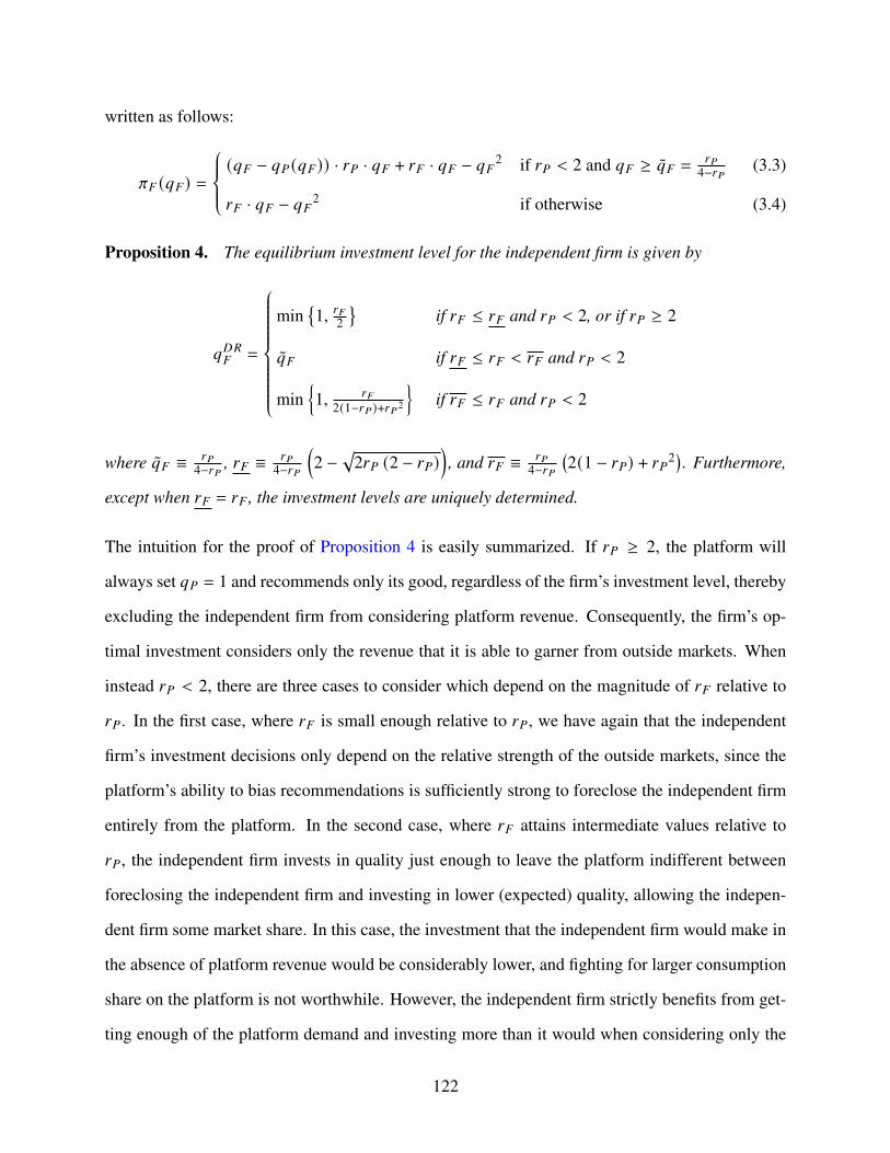
written as follows:

𝜋𝐹 (𝑞𝐹) =(𝑞𝐹 − 𝑞𝑃 (𝑞𝐹)) · 𝑟𝑃 · 𝑞𝐹 + 𝑟𝐹 · 𝑞𝐹 − 𝑞𝐹2 if 𝑟𝑃 < 2 and 𝑞𝐹 ≥ 𝑞𝐹 =

𝑟𝑃4−𝑟𝑃 (3.3)

𝑟𝐹 · 𝑞𝐹 − 𝑞𝐹2 if otherwise (3.4)

Proposition 4. The equilibrium investment level for the independent firm is given by

𝑞𝐷𝑅𝐹 =

min{1, 𝑟𝐹2

}if 𝑟𝐹 ≤ 𝑟𝐹 and 𝑟𝑃 < 2, or if 𝑟𝑃 ≥ 2

𝑞𝐹 if 𝑟𝐹 ≤ 𝑟𝐹 < 𝑟𝐹 and 𝑟𝑃 < 2

min{1, 𝑟𝐹

2(1−𝑟𝑃)+𝑟𝑃2

}if 𝑟𝐹 ≤ 𝑟𝐹 and 𝑟𝑃 < 2

where 𝑞𝐹 ≡ 𝑟𝑃4−𝑟𝑃 , 𝑟𝐹 ≡ 𝑟𝑃

4−𝑟𝑃

(2 −

√︁2𝑟𝑃 (2 − 𝑟𝑃)

), and 𝑟𝐹 ≡ 𝑟𝑃

4−𝑟𝑃(2(1 − 𝑟𝑃) + 𝑟𝑃2) . Furthermore,

except when 𝑟𝐹 = 𝑟𝐹 , the investment levels are uniquely determined.

The intuition for the proof of Proposition 4 is easily summarized. If 𝑟𝑃 ≥ 2, the platform will

always set 𝑞𝑃 = 1 and recommends only its good, regardless of the firm’s investment level, thereby

excluding the independent firm from considering platform revenue. Consequently, the firm’s op-

timal investment considers only the revenue that it is able to garner from outside markets. When

instead 𝑟𝑃 < 2, there are three cases to consider which depend on the magnitude of 𝑟𝐹 relative to

𝑟𝑃. In the first case, where 𝑟𝐹 is small enough relative to 𝑟𝑃, we have again that the independent

firm’s investment decisions only depend on the relative strength of the outside markets, since the

platform’s ability to bias recommendations is sufficiently strong to foreclose the independent firm

entirely from the platform. In the second case, where 𝑟𝐹 attains intermediate values relative to

𝑟𝑃, the independent firm invests in quality just enough to leave the platform indifferent between

foreclosing the independent firm and investing in lower (expected) quality, allowing the indepen-

dent firm some market share. In this case, the investment that the independent firm would make in

the absence of platform revenue would be considerably lower, and fighting for larger consumption

share on the platform is not worthwhile. However, the independent firm strictly benefits from get-

ting enough of the platform demand and investing more than it would when considering only the

122

outside revenue. Finally, in the last case, where 𝑟𝐹 is large relative to 𝑟𝑃, it is now profitable for the

independent firm to invest in even higher quality, securing a larger share of the platform demand

and leading to higher revenue from platform subscriptions.

3.3.3 Welfare Consequences of the Dual Role

We now study the implications of the dual role on consumer welfare. Our primary question of

interest is whether the increased competition in the production market through the entry of platform

increases or decreases consumer welfare. We now state the main result comparing welfare between

the two cases:

Proposition 5. Consumer welfare is weakly higher under the dual role than under the no platform

production case if and only if 𝑟𝐹 ≥ 2(1−𝑟𝑃)+𝑟2𝑃

max{1,2−𝑟𝑃} or 𝑟𝑃 ≥ 2.

It is strictly higher if and only if 2 − 𝑟𝑃 > 𝑟𝐹 >2(1−𝑟𝑃)+𝑟2

𝑃

2−𝑟𝑃 .

Proposition 5 shows that, despite the increased competition in the upstream market, the plat-

form’s dual role results in lower quality investments and lower welfare when the independent

firm’s alternative market relevance is small compared to the platform’s – cf. Figures 3.1 and 3.2.11

This shows that when the platform steers a substantial fraction of the demand utilizing biased

recommendations, platform upstream competition decreases consumer welfare. It not only ad-

versely impacts consumer welfare, but also strictly depresses the industry’s total profits since, if

the independent firm is the sole producer, its profits attain the industry’s maximum. Therefore,

the increased competition leads to an overall, unambiguous, decrease in total surplus. However,

in situations where the independent firm has access to significant alternative revenue sources, the

platform’s dual role becomes welfare improving.

11While Proposition 5 only focuses on consumer welfare on the platform, if one further assumes identical consumerpreferences in the revenue sources outside of the platform, then the conclusion from Proposition 5 that for the dualrole can either improve or harm consumer welfare extends to including these sources as well, although the thresholdswould differ. Moreover, if the dual role strictly improves on on-platform consumer welfare, it also improves on off-platform consumer welfare. A notable difference would be that if 𝑟𝑃 ≥ 2, the platform invests such that 𝑞𝑃 = 1,leaving on-platform consumer welfare unchanged, but as the independent firm is foreclosed, it will invest strictly lessthan in the no-platform-production case, with negative welfare consequences for off-platform consumers.

123

Figure 3.1: Equilibrium Investment Levels

0.00 0.25 0.50 0.75 1.00 1.25 1.50

rF

(rP = 0.5)

0.0

0.2

0.4

0.6

0.8

1.0

(a)

0.00 0.25 0.50 0.75 1.00 1.25 1.50

rP

(rF = 0.1)

0.0

0.2

0.4

0.6

0.8

(b)

Firm: Dual Role Firm: No Platform Production Platform: Dual Role

Notes: This figure displays the investment levels across the no platform production and dual role cases. Panel (a)shows how investment levels change as we increase the alternative revenue sources for a fixed level of platformpotential revenue. Panel (b) shows how investment levels change as we increase the platform potential revenue for afixed level of alternative revenue sources.

In order to better understand the reason that the platform’s entry and recommendation bias

change the investment incentives of the independent firm, consider the total derivative of the inde-

pendent firm’s profit function with respect to its investment choice:

𝑑𝜋𝐹

𝑑𝑞𝐹=

𝜕𝛼𝐹

𝜕𝑞𝐹· 𝑅𝑃︸ ︷︷ ︸

Share Expansion

+ 𝛼𝐹 · 𝜕𝑅𝑃𝜕𝑞𝐹︸ ︷︷ ︸

Revenue Expansion

+𝜕𝑅𝐹𝜕𝑞𝐹

− 𝜕𝐶𝐹

𝜕𝑞𝐹

In the no platform production case, the share expansion term is always zero since the independent

firm always has 𝛼𝐹 = 1 due to its being the only good on the platform. This allows the independent

firm to extract the full impact of its investment on expanding the overall platform revenue through

the revenue expansion term. In the dual role case, the marginal incentives to increase investment

are driven by both of these terms: while the entry of the platform softens the marginal gains

from revenue expansion, it introduces the marginal gains coming from the introduction of business

124

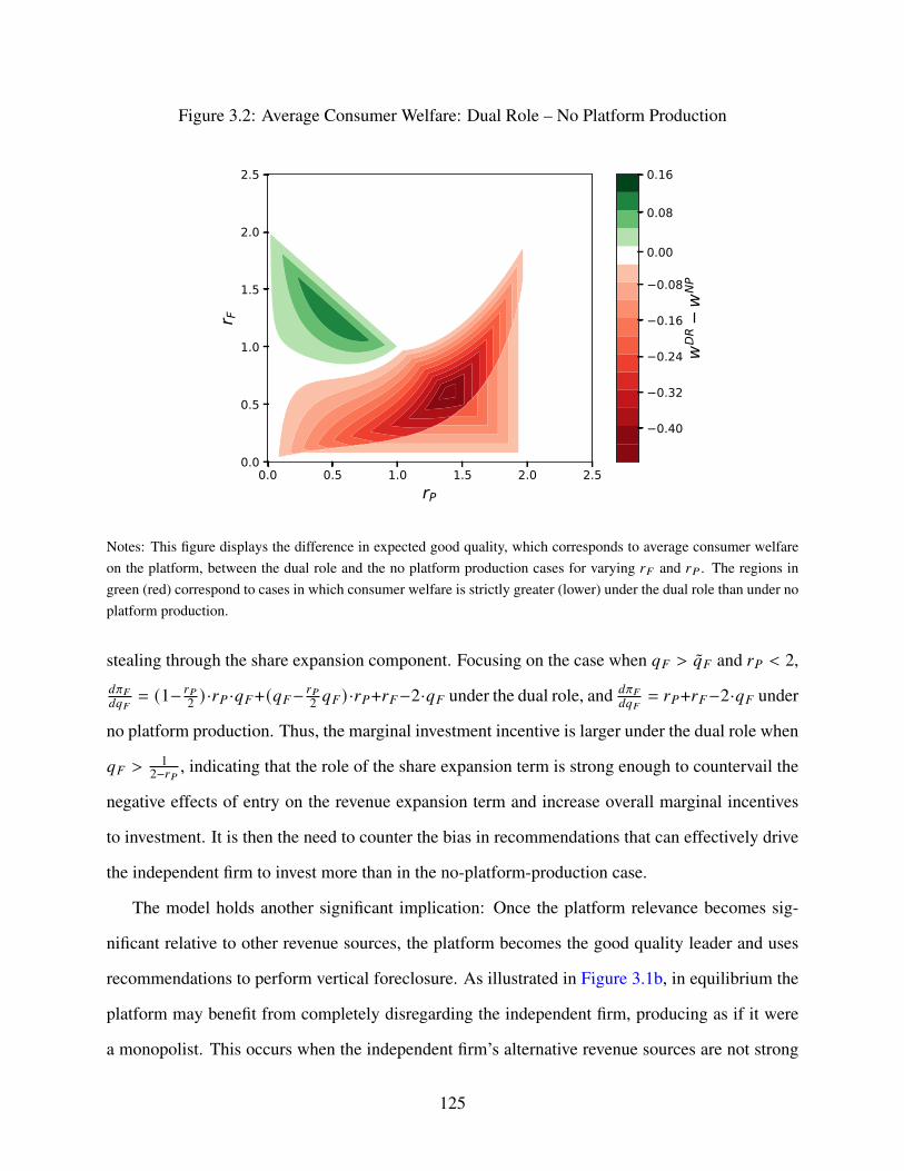
Figure 3.2: Average Consumer Welfare: Dual Role – No Platform Production

0.0 0.5 1.0 1.5 2.0 2.5rP

0.0

0.5

1.0

1.5

2.0

2.5

r F

0.40

0.32

0.24

0.16

0.08

0.00

0.08

0.16

wD

Rw

NP

Notes: This figure displays the difference in expected good quality, which corresponds to average consumer welfareon the platform, between the dual role and the no platform production cases for varying 𝑟𝐹 and 𝑟𝑃 . The regions ingreen (red) correspond to cases in which consumer welfare is strictly greater (lower) under the dual role than under noplatform production.

stealing through the share expansion component. Focusing on the case when 𝑞𝐹 > 𝑞𝐹 and 𝑟𝑃 < 2,

𝑑𝜋𝐹𝑑𝑞𝐹

= (1− 𝑟𝑃2 ) ·𝑟𝑃 ·𝑞𝐹+(𝑞𝐹− 𝑟𝑃

2 𝑞𝐹) ·𝑟𝑃+𝑟𝐹−2·𝑞𝐹 under the dual role, and 𝑑𝜋𝐹𝑑𝑞𝐹

= 𝑟𝑃+𝑟𝐹−2·𝑞𝐹 under

no platform production. Thus, the marginal investment incentive is larger under the dual role when

𝑞𝐹 >1

2−𝑟𝑃 , indicating that the role of the share expansion term is strong enough to countervail the

negative effects of entry on the revenue expansion term and increase overall marginal incentives

to investment. It is then the need to counter the bias in recommendations that can effectively drive

the independent firm to invest more than in the no-platform-production case.

The model holds another significant implication: Once the platform relevance becomes sig-

nificant relative to other revenue sources, the platform becomes the good quality leader and uses

recommendations to perform vertical foreclosure. As illustrated in Figure 3.1b, in equilibrium the

platform may benefit from completely disregarding the independent firm, producing as if it were

a monopolist. This occurs when the independent firm’s alternative revenue sources are not strong

125

enough relative to platform potential revenue to induce it to compete for market share with the

platform as a producer. The outcome of this interaction is then a form of vertical foreclosure by

means of the platform’s use of biased recommendations — the independent firm’s good is never

recommended to consumers, even if it is of higher realized quality than the platform’s — which

establishes the platform as the quality leader by precluding the independent firm’s access to the

platform’s demand. This necessarily has a negative effect on consumer welfare as the expected

good quality on the platform is lower than it would be when compared to a case where only the

independent firm’s good is available.

This prediction echoes anecdotal evidence on streaming platforms. First, the already men-

tioned concerns that platforms bias their recommendation systems towards their own goods to

the detriment of goods produced by other firms manifests itself in our model through the biased

recommendations the platform uses to steer consumers towards its own goods. Second, data on

viewer and subscriber patterns on streaming platforms indicates that there is a positive correlation

between number of subscribers, platform original content’s share of the total platform viewership,

and ranking of platform’s original content.12 Even though the model’s prediction is sharp and

reality is necessarily more complex and nuanced, the model suggests one possible mechanism

underlying such anecdotal evidence.

Nevertheless, the need to compete for market share on the platform can still drive the inde-

pendent firm to stronger quality investments as the platform’s audience loses its overwhelming

relevance within the industry, possibly due to the emergence of alternative platforms. When the

independent firm has a base incentive to support sufficiently high quality investments — when the

alternative revenue sources are significant enough relative to the platform’s — it is worthwhile for

the firm to invest even more and compete for market share on the platform. In this case, the plat-

form becomes a quality follower relative to the independent firm, making use of recommendations

to appropriate a substantial fraction of the market share that the independent firm’s production

decisions attract.12See, for the case of Netflix, e.g. “Netflix Original Series Viewing Climbs, but Licensed Content Remains Majority

of Total U.S. Streams” [154] and “Netflix Subscriber Numbers Soar, Showing the Sky Is Not Falling” [155].

126

3.4 Unbiased Recommendations

In this section we consider a natural policy remedy: requiring the platform’s recommendations

to be unbiased — truthful and neutral. Truthfulness requires that the platform always recommends

a good when it is of strictly higher quality than the other, while neutrality requires that the platform

always breaks ties uniformly. Another interpretation of the unbiased recommendation case is as

a separation (or divestiture) between the platform’s production and recommendation activities.

Therefore, this also corresponds to a benchmark of two producers, independent from the platform.

As it is unclear the extent to which the platform’s dual role is distinct from a case of simple

upstream entry with information provision — known to have ambiguous welfare consequences in

cases of pure vertical differentiation — this section further provides clarification on the distinctive

effects of the platform’s dual role.

3.4.1 Equilibrium Characterization

The model remains the same, up to imposing unbiased recommendations: The platform now

recommends whichever good realizes the highest quality, with uniform tie-breaking. This implies

that the expected good quality that consumers end up getting is

𝑞𝑈 := 𝑞𝑃 · 𝑞𝐹 + 𝑞𝑃 · (1 − 𝑞𝐹) + (1 − 𝑞𝑃) · 𝑞𝐹 = 𝑞𝑃 + (1 − 𝑞𝑃) · 𝑞𝐹

The solution to the optimal access fee is analogous to the one from before, leading also to a similar

expression for platform revenue 𝑅𝑃. In fact, the revenue maximizing access fee is the same up to

replacing max{𝑞𝑃, 𝑞𝐹} with the new expression for expected good quality 𝑞𝑈 . Thus, the optimal

access fee and resulting revenue are given by 𝜏 = 12 \̄ · 𝑞

𝑈 and 𝑅𝑃 = 𝑟𝑃 · 𝑞𝑈 .

Expected market shares are given by 𝛼𝑃 = 1−𝛼𝐹 = 12 (1 − (𝑞𝐹 − 𝑞𝑃)), resembling the form of

market share under biased recommendations with two noteworthy differences. First, market shares

are always strictly positive for any strictly positive quality investment. This immediately implies

that the independent firm is now able to capture a share of the market, even when it invests less than

127

the platform, as imposing unbiased recommendations precludes the use of this policy instrument

by the platform to induce vertical foreclosure. Second, the incentives for the firm to compete

for market share are dampened: the marginal change in the firm’s market share from increasing

its investment is halved when compared to the biased recommendation case with positive market

share.

The platform’s production problem is given by the same expression up to the changes in 𝑅𝑃

and 𝛼𝑃:

𝜋𝑃 (𝑞𝑃, 𝑞𝐹) = 𝛼𝑃𝑅𝑃 − 𝐶𝑃 =12(1 − (𝑞𝐹 − 𝑞𝑃)) · 𝑟𝑃 · (𝑞𝐹 + (1 − 𝑞𝐹)𝑞𝑃) − 𝑞𝑃2 (3.5)

We note that the platform has a unique best response to the independent firm’s investment level:

Lemma 1. The platform’s optimal investment, 𝑞𝑈𝑃(𝑞𝐹) := arg max𝑞𝑃∈[0,1] 𝜋𝑃 (𝑞𝑃, 𝑞𝐹) is unique

and continuous in 𝑞𝐹 .

The firm’s investment problem is now given by

𝜋𝐹 (𝑞𝑃, 𝑞𝐹) = 𝛼𝐹𝑅𝑃 + 𝑅𝐹 − 𝐶𝐹 =12(1 − (𝑞𝑃 − 𝑞𝐹)) · 𝑟𝑃 · (𝑞𝐹 + (1 − 𝑞𝐹)𝑞𝑃) + 𝑟𝐹 · 𝑞𝐹 − 𝑞𝐹2

with 𝑞𝑃 = 𝑞𝑈𝑃(𝑞𝐹).

It results that this problem has a unique maximizer and therefore we obtain a unique equilib-

rium:

Proposition 6. Equilibrium investment levels with unbiased recommendations are uniquely de-

fined.

3.4.2 Comparison to Dual Role Equilibrium

Investment Levels

We now directly compare the equilibrium investment levels in the different cases. Figure 3.3 de-

picts the equilibrium investment levels as we vary the significance of the firm’s alternative revenue,

128

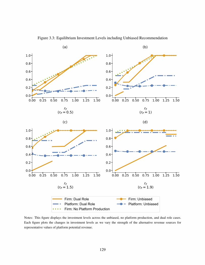
Figure 3.3: Equilibrium Investment Levels including Unbiased Recommendation

0.00 0.25 0.50 0.75 1.00 1.25 1.50

rF(rP = 0.5)

0.0

0.2

0.4

0.6

0.8

1.0

(a)

0.00 0.25 0.50 0.75 1.00 1.25 1.50

rF(rP = 1)

0.0

0.2

0.4

0.6

0.8

1.0

(b)

0.00 0.25 0.50 0.75 1.00 1.25 1.50

rF(rP = 1.5)

0.0

0.2

0.4

0.6

0.8

1.0

(c)

0.00 0.25 0.50 0.75 1.00 1.25 1.50

rF(rP = 1.9)

0.0

0.2

0.4

0.6

0.8

1.0

(d)

Firm: Dual RolePlatform: Dual RoleFirm: No Platform Production

Firm: UnbiasedPlatform: Unbiased

Notes: This figure displays the investment levels across the unbiased, no platform production, and dual role cases.Each figure plots the changes in investment levels as we vary the strength of the alternative revenue sources forrepresentative values of platform potential revenue.

129

𝑟𝐹 , for different representative values of platform market sizes, 𝑟𝑃. The figure shows that imposing

unbiased recommendations has an ambiguous effect on firm equilibrium investment levels.

We first focus on the independent firm. Similarly to before, the independent firm invests less

in the unbiased case compared to the dual role when 𝑟𝐹 is high and 𝑟𝑃 is low (see Figure 3.3b).

There are two channels that depress the incentives for the independent firm to invest. First, we

note that the share expansion term, the marginal gain on market share(𝜕𝛼𝐹

𝜕𝑞𝐹

), is halved under

unbiased recommendations compared to the dual role. Second, we have that the revenue expansion

term, the marginal increase in overall platform revenue as a result of increasing independent firm

investment(𝜕𝑅𝑃

𝜕𝑞𝐹

), is 𝑟𝑃 in the dual role case when 𝑞𝐹 > 𝑞𝑃, but is only 𝑟𝑃 (1−𝑞𝑃) under unbiased

recommendations.

However, there are also two forces that act in the opposite direction and encourage the indepen-

dent firm to increase investment. The first is that the platform’s reaction to the independent firm’s

quality investment is milder as it can no longer bias recommendations in its favor. The other is that

even though the marginal effect of investment on market share is lower, unbiased recommendation

still fosters higher market shares for the independent firm.

When 𝑟𝐹 is high enough and 𝑟𝑃 is low enough, the mechanisms that depress incentives are

stronger and drive the independent firm to invest less under unbiased recommendations compared

to biased recommendations. With higher 𝑟𝑃, the channels that drive the independent firm to invest

more become stronger than those that depress investment. Thus, when 𝑟𝑃 is sufficiently high,

the forces that lead to higher investment dominate the investment-depressing channels, leading to

overall higher investment levels in the unbiased case.

We now investigate the effect that unbiased recommendation has on the platform’s production

decision, which can similarly be seen in Figure 3.3. We highlight three main results.

First, when the platform potential revenue is high relative to the firm’s alternative markets, we

previously noted that the platform is able to use recommendation to effectively become a monopo-

list. When recommendations have to be unbiased, the resulting competition leads to a decrease in

the platform’s equilibrium investments. Although it is reasonable to expect that the platform being

130

unable to capture the whole market would lead to more aggressive investment by the platform, this

is not the case. As the independent firm has higher returns to investments than the platform — due

to its alternative revenue sources — it results that it will always obtain at least half of the market

share under unbiased recommendations. This leads to competition resulting in lower investment

by the platform.

Second, unbiased recommendations depress platform investment when the independent firm’s

alternative revenue is large enough. When the platform can bias recommendations, it has a stronger

incentive to keep up with the independent firm’s investments as 𝑟𝐹 increases. In contrast, under

unbiased recommendations, this effect turns negative as the alternative revenue sources grow more

and more significant. In this case, as happens for the independent firm, unbiased recommendations

actually dampen competition incentives, making it less worthwhile for the platform to produce

higher quality goods given the halved effect on the market share and virtually no marginal change

in total revenue when 𝑞𝐹 is close to 1.

Finally, if the platform’s potential revenue is high enough and the firm’s alternative markets

are not too significant, the firm’s investment under unbiased recommendations is lower than the

platform’s when it can bias recommendations. As it is possible to observe in Figures 3.3c and 3.3d,

when 𝑟𝑃 is high enough and 𝑟𝐹 is low, in order to capture full platform demand in the dual role

case, the platform invests more in expected quality than it does in the unbiased recommendations

case. Moreover, the platform’s equilibrium investment levels are then consistently higher under

the dual role, than it is when imposing unbiased recommendations.

The two main findings regarding to investment levels are then the following:

Remark 1.

1. When the platform’s market size is small and the firm’s alternative market size is large,

imposing unbiased recommendations leads to lower investments by the independent firm.

2. When the platform’s market size is large relative to the firm’s alternative market size or when

the latter is large enough, imposing unbiased recommendations leads to lower investments

131

by the platform.

Figure 3.4: Average Consumer Welfare: Dual Role – Unbiased

0.0 0.5 1.0 1.5 2.0 2.5rP

0.0

0.5

1.0

1.5

2.0

2.5r F

0.40

0.32

0.24

0.16

0.08

0.00

0.08

0.16

wD

Rw

U

Notes: This figure displays the difference in expected good quality, which corresponds to average consumer welfareon the platform, between the dual role and unbiased recommendations cases for varying 𝑟𝐹 and 𝑟𝑃 . The regions ingreen (resp. red) correspond to cases in which consumer welfare is strictly greater (resp. lower) under the dual rolethan under no platform production.

Consumer Welfare

The analysis of the resulting differences in consumer welfare between the two regimes does not

follow immediately from assessing the platform’s and the independent firm’s investment levels sep-

arately since the expected market shares further differ as a result of the change in recommendation

policy. In both of these regimes consumer welfare depends in the exact same manner on expected

good quality and so our results here have direct parallels to the previously discussed changes in in-

vestment levels. There are two channels through which this policy affects welfare. The first is that,

fixing investment levels and prices, unbiased recommendations have an unambiguously positive

effect on consumer welfare, owing to consumers being better informed about each good’s realized

quality. This leads to differences in expected market shares for the producers, and, as a result, the

second channel comes from responses in equilibrium investment levels.

132

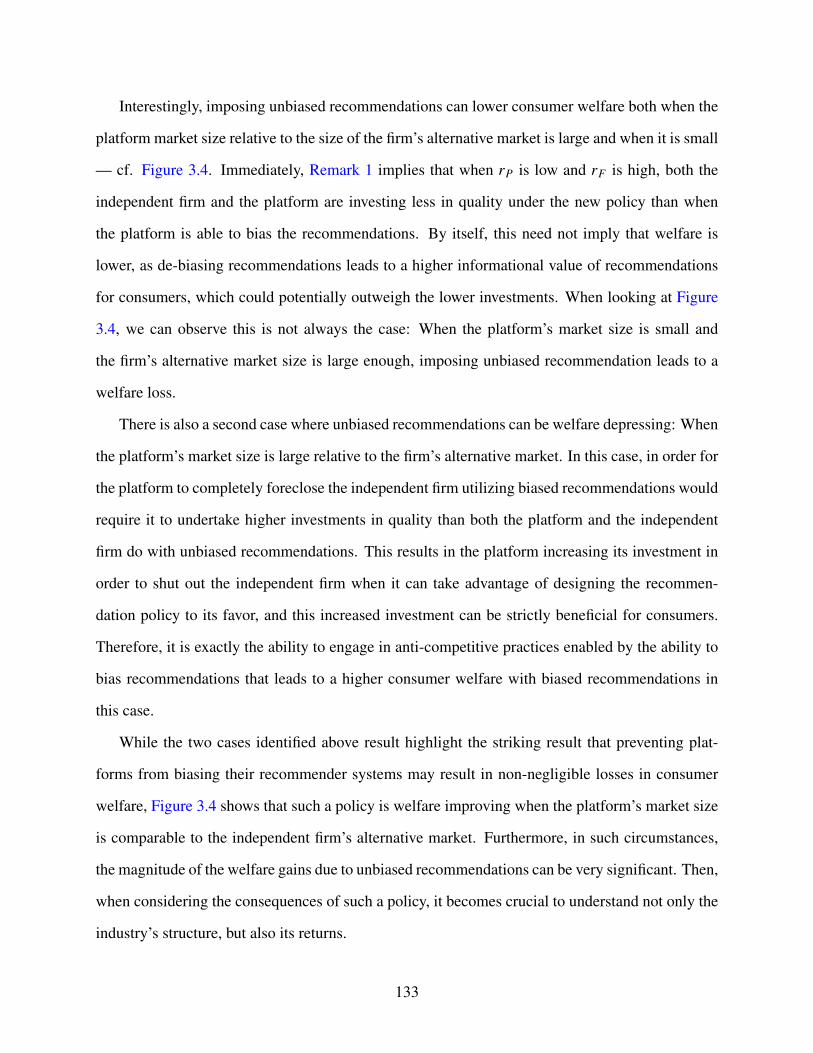
Interestingly, imposing unbiased recommendations can lower consumer welfare both when the

platform market size relative to the size of the firm’s alternative market is large and when it is small

— cf. Figure 3.4. Immediately, Remark 1 implies that when 𝑟𝑃 is low and 𝑟𝐹 is high, both the

independent firm and the platform are investing less in quality under the new policy than when

the platform is able to bias the recommendations. By itself, this need not imply that welfare is

lower, as de-biasing recommendations leads to a higher informational value of recommendations

for consumers, which could potentially outweigh the lower investments. When looking at Figure

3.4, we can observe this is not always the case: When the platform’s market size is small and

the firm’s alternative market size is large enough, imposing unbiased recommendation leads to a

welfare loss.

There is also a second case where unbiased recommendations can be welfare depressing: When

the platform’s market size is large relative to the firm’s alternative market. In this case, in order for

the platform to completely foreclose the independent firm utilizing biased recommendations would

require it to undertake higher investments in quality than both the platform and the independent

firm do with unbiased recommendations. This results in the platform increasing its investment in

order to shut out the independent firm when it can take advantage of designing the recommen-

dation policy to its favor, and this increased investment can be strictly beneficial for consumers.

Therefore, it is exactly the ability to engage in anti-competitive practices enabled by the ability to

bias recommendations that leads to a higher consumer welfare with biased recommendations in

this case.

While the two cases identified above result highlight the striking result that preventing plat-

forms from biasing their recommender systems may result in non-negligible losses in consumer

welfare, Figure 3.4 shows that such a policy is welfare improving when the platform’s market size

is comparable to the independent firm’s alternative market. Furthermore, in such circumstances,

the magnitude of the welfare gains due to unbiased recommendations can be very significant. Then,

when considering the consequences of such a policy, it becomes crucial to understand not only the

industry’s structure, but also its returns.

133

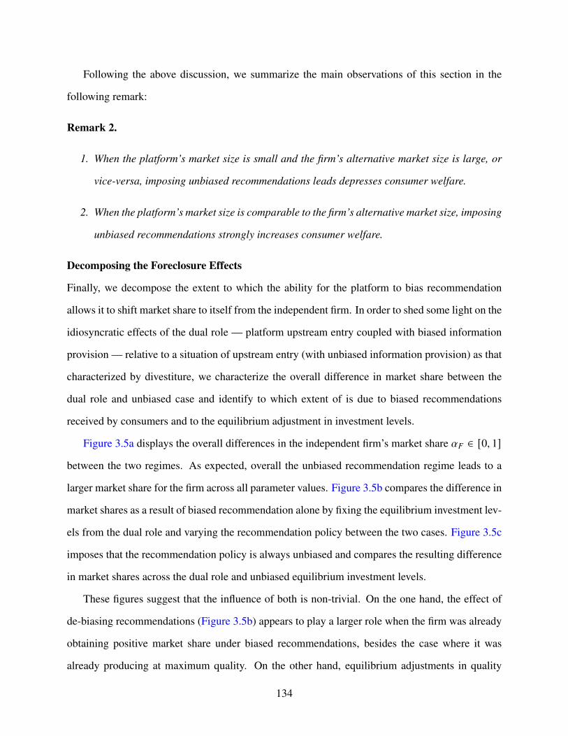
Following the above discussion, we summarize the main observations of this section in the

following remark:

Remark 2.

1. When the platform’s market size is small and the firm’s alternative market size is large, or

vice-versa, imposing unbiased recommendations leads depresses consumer welfare.

2. When the platform’s market size is comparable to the firm’s alternative market size, imposing

unbiased recommendations strongly increases consumer welfare.

Decomposing the Foreclosure Effects

Finally, we decompose the extent to which the ability for the platform to bias recommendation

allows it to shift market share to itself from the independent firm. In order to shed some light on the

idiosyncratic effects of the dual role — platform upstream entry coupled with biased information

provision — relative to a situation of upstream entry (with unbiased information provision) as that

characterized by divestiture, we characterize the overall difference in market share between the

dual role and unbiased case and identify to which extent of is due to biased recommendations

received by consumers and to the equilibrium adjustment in investment levels.

Figure 3.5a displays the overall differences in the independent firm’s market share 𝛼𝐹 ∈ [0, 1]

between the two regimes. As expected, overall the unbiased recommendation regime leads to a

larger market share for the firm across all parameter values. Figure 3.5b compares the difference in

market shares as a result of biased recommendation alone by fixing the equilibrium investment lev-

els from the dual role and varying the recommendation policy between the two cases. Figure 3.5c

imposes that the recommendation policy is always unbiased and compares the resulting difference

in market shares across the dual role and unbiased equilibrium investment levels.

These figures suggest that the influence of both is non-trivial. On the one hand, the effect of

de-biasing recommendations (Figure 3.5b) appears to play a larger role when the firm was already

obtaining positive market share under biased recommendations, besides the case where it was

already producing at maximum quality. On the other hand, equilibrium adjustments in quality

134

Figure 3.5: Difference in Market Share for Independent Firm

(a) Difference in Market Share: Unbiased – Dual Role

0.0 0.5 1.0 1.5 2.0 2.5rP

0.0

0.5

1.0

1.5

2.0

2.5r F

0.0

0.2

0.4

0.6

0.8

U F(q

U)

DR

F(q

DR)

(b) Difference in Market Share: Unbiased with DualRole Investments – Dual Role

0.0 0.5 1.0 1.5 2.0 2.5rP

0.0

0.5

1.0

1.5

2.0

2.5

r F

0.0

0.2

0.4

0.6

0.8

U F(q

DR)

DR

F(q

DR)

(c) Difference in Market Share: Unbiased - Unbi-ased with Dual Role Investments

0.0 0.5 1.0 1.5 2.0 2.5rP

0.0

0.5

1.0

1.5

2.0

2.5

r F

0.0

0.2

0.4

0.6

0.8

U F(q

U)

U F(q

DR)

Notes: This figure displays the differences in the independent firm’s market share, 𝛼𝐹 ∈ [0, 1], between the unbiasedand dual role cases. Panel (a) displays the overall difference in market share in equilibrium between the unbiasedand dual role case. Panel (b) displays the difference in market share for the independent firm between the unbiasedrecommendation regime with investment levels fixed at the dual role levels, and the equilibrium in the dual role. Panel(c) displays the difference in market share between the equilibrium in the unbiased recommendation regime, and themarket share under unbiased recommendations but with investment levels fixed at the equilibrium values for the dualrole.

135

lead to extremely significant changes in market share when the firm’s alternative revenue sources

are meager, as under unbiased recommendations it can do always at least as well as the platform,

increasing market share from zero to over 50% (Figure 3.5c). This underscores the extent to

which the ability of platforms to bias recommendation can undeservedly shift substantial market

share from independent firms’ goods to the platform’s goods. The clearly identifiable discontinuity

is given by 𝑟𝐹 = 𝑟𝐹 (as given in Proposition 4), which determines the threshold at which the

independent firm starts enjoying strictly positive market share in the dual role case.

3.5 Additional Discussion and Robustness Exercises

In this section we provide additional discussion about the assumptions in the model as well as

several robustness exercises in order to show that the qualitative conclusions from our analysis are

robust to different modeling assumptions.

Heterogeneous Costs: The model that we consider crucially relies on the ability of the indepen-

dent firm to access outside revenue sources as this provides it with some advantage relative to the

platform. Although we consider such outside revenue sources as an important element in reality,

one could alternatively consider the independent firm to have a more efficient production process

and thus has a lower marginal cost to invest in quality. This is can be an important difference in

situations where independent producers are likely to have mature production processes for their

goods, whereas the platforms are usually new entrants and unlikely to have as efficient production

processes.

In Appendix C.2 we consider a setup where there is no outside revenue for the independent

producer (𝑅𝐹 = 0), and, instead, there is a cost advantage, leading to potentially heterogeneous

cost structures: The platform’s production cost will still be 𝐶𝑃 (𝑞𝑃) = 𝑞2𝑃

, but the independent

firm’s is now 𝐶𝐹 (𝑞𝐹) = 𝑐𝐹 · 𝑞2𝐹

, with 𝑐𝐹 ∈ (0, 1). Keeping the remaining elements of the setup

in the baseline model, we highlight the robustness of the main conclusions regarding the ambigu-

ous welfare effects of both platform upstream entry and the requirement of recommendations be

unbiased to this alternative specification.

136

While, in contrast to our benchmark model specification, recommendation bias and upstream

entry by the platform results in the independent firm investing either maximally (𝑞𝐹 = 1) or min-

imally (𝑞𝐹 = 0), the dual role of the platform as both a recommender and a producer retains an

ambiguous effect on consumer welfare in comparison to the other two situations: it will strictly

improve consumer welfare when the independent producer’s cost advantage is neither too signifi-

cant nor too negligible and the potential market size of the platform —- as given by 𝑟𝑃 —- is not

too large; and depress it if otherwise.

Simultaneous Investment Timing: We show that our main conclusions are robust to the assump-

tion on the timing of investments. The baseline model that we consider has investment decisions

decided in a sequential manner with the independent firm moving first followed by the platform.

While this timing is most natural, we further consider the case in which investments are simulta-

neous rather than sequential, keeping everything else in the model the same.

In Appendix C.3 we characterize the equilibria in the dual role and unbiased case under this

timing. This modification of the timing implies that there might be multiple equilibria in the dual

role case for a given range of parameters 𝑟𝑃, 𝑟𝐹 . In spite of this, the resulting welfare comparisons

are remarkably consistent with the sequential timing. Specifically, we obtain conclusions that are

analogous to Proposition 5 and Remark 2: the platform’s dual role may induce either higher or

lower consumer welfare relative to both the no-platform-production and the unbiased recommen-

dation benchmarks. The welfare comparisons are summarised in Figure C1 in Appendix C.3, and

show that nearly the same parameter regions induce the no platform production case to be welfare

improving relative to the dual role case as well as the unbiased recommendation case to be welfare

improving relative to the dual role case.

Information Disclosure Timing: The recommendation provision by the platform was modeled

as an optimal information design problem with commitment [130]. An alternative modeling as-

sumption is that the platform could determine its recommendations after quality realizations, akin

to a cheap talk problem [156]. While this could be an interesting avenue in other setups, in the

context of our model, this would result in no information being conveyed in equilibrium, with only

137

“babbling” equilibria persisting.13

Pricing: We consider a model of subscription-based pricing in order to restrict attention to the

interplay between good quality and recommendation without introducing the additional complexity

due to item pricing and issues of price competition. Many of the prominent online platforms which

rely on recommender systems, such as media streaming platforms and news websites, follow a

subscription-based model and, to our knowledge, platforms such as Spotify and YouTube have

similar revenue splitting rules between independent producers and themselves.14 In contrast, the

insights of our model are not directly applicable to e-commerce platforms, such as Amazon or

Wayfair, due to this modeling specification.

3.6 Conclusion

In this paper we study a stylized model of strategic interaction between a platform that de-

ploys a recommender system and producers of the goods distributed on this platform. Using this

model we explore the welfare consequences of the entry of the platform into the production mar-

ket. Opposite to the common intuition that increased competition in good production is welfare

improving, we find that the ability by the platform to deploy a recommender system enables it to

steer demand towards its own goods which leads to lower consumer welfare in equilibrium as a

result of the platform’s entry. When the primary revenue sources for the independent producers are

from the platform, the bias in recommendation leads to depressed incentives to invest both for the

independent producers and the platform itself.

The policy implications from our model are clear — the increasing trend of online platforms

to produce their own goods should be viewed with caution by regulators. A unique element of

these platforms is their deployment of recommender systems, which provide utility for consumers

by providing them with information on which goods on the platform they should consume. As our13Note that if the platform’s message were able to persuade the consumer to choose its good given knowledge of

the realized qualities, then it would do so regardless of the realized qualities. This mechanism renders equilibriummessages uninformative.

14While it does not directly map to the procedure on a platform such as Netflix, one can interpret the contractualagreements between the independent film distributors and Netflix as being determined by the expected consumptionshare on the platform.

138

model points out, the clear evidence of bias in both search and recommendation can lead to neg-

ative equilibrium effects on the quality of the goods that get produced and threatens the ability of

independent producers to thrive when they are dependent on the platform as their primary revenue

source. It must be noted that while we primarily consider the role of strategic information design

to consumers as a mechanism for the platform to appropriate rents and foreclosure competition,

online retailers have other channels to distort consumption patterns, such as the ability to make

consumers unaware of the existence of certain goods or through the pricing channel. Thus, the

extent of concern arising from this trend is underestimated by our analysis.

A natural policy remedy is to require that platforms have unbiased recommendations or, equiv-

alently, force a separation between recommendation and production. Surprisingly, we find that the

equilibrium effects of biased recommendation lead to this policy not being unambiguously welfare-

improving for consumers. In the case in which the platform is the primary revenue source for the

independent producers, we find that this policy does improve welfare for consumers: unbiased

information disclosure directly generates positive consumer welfare gains. In contrast, when the

alternative revenue sources for the independent producers are large relative to the platform poten-

tial revenue, biased recommendations induce higher investment levels and lead to higher consumer

welfare when compared to unbiased recommendations. It is important to further note that beyond

the sign of the difference in welfare, the magnitude of the effects depends on the relative weight of

the different revenue sources.

As a result, if independent producers are primarily dependent on the platform for revenue

then policies enforcing the separation between recommendation and production will be welfare-

improving. But if independent producers have access to large alternative revenue sources relative

to the platform’s potential revenue, then these policies targeting the integration of recommendation

and production may have adverse effects on consumer welfare.

Finally, there are several aspects of the integration between recommendation and production

that warrant further study. The first is a better understanding of the interaction between the infor-

mation accumulated about consumer preferences due to intermediation and dynamic production

139

decisions. This is particularly amplified in the case of recommender systems since, in order to de-

velop a good recommendation system, the intermediary needs to collect fine-grained information

about consumer preferences. For instance, Netflix and Amazon are primarily relying on “data-

driven" approaches to production decisions using the data they get to power their recommendation

systems. Moreover, consumer choices in these markets may have a path-dependence as illustrated

by [157], and so, understanding the dynamic consequences of the integration of production and

recommendation seems a fruitful and important direction for future work. As the role of recom-

mender systems in online platforms increases and platforms increasingly integrate production and

recommendation, examining their effects on competition, investment, and consumer welfare of all

these considerations becomes increasingly more important for better policy design for the digital

economy.

140

Chapter 4: Deconstructing the Filter Bubble: User Decision-Making and

Recommender Systems

4.1 Introduction

Recommender systems (RS) have become critical for assisting users in navigating the large

choice sets that they face on many online platforms. For instance, users have to choose from thou-

sands of movies on Netflix, millions of products on Amazon, and billions of videos on YouTube.

Users in many cases are not aware of most items, let alone have full information about their prefer-

ences over them. To make matters worse, the items in these contexts are usually experience goods

whose true value for users can only be learned after consumption.

RS have driven a significant fraction of consumer choice on these platforms with 75% of

movies watched on Netflix and 35% of page-views on Amazon coming from recommendations.1

While there are many positive effects from these systems, there is an increasing worry about their

unintended side-effects. There have been claims that personalized RS lead users into filter bub-

bles where they effectively get isolated from a diversity of viewpoints or content [158], and that

personalized RS may also lead users to become increasingly homogenized at the same time [159,

160].

Understanding how RS influence user behavior is important not only for characterizing the

broader consequences of such systems but also for guiding their design. In this paper, we develop

a theoretical model of user decision-making in contexts where RS are traditionally deployed. We

utilize previous empirical studies that characterize how RS influence user choice as a benchmark

and our theoretical model provides an intuitive mechanism that can explain these empirical results.

1MacKenzie et al. (2013, Oct.), How retailers can keep up with consumers. https://www.mckinsey.com/industries/retail/our-insights/how-retailers-can-keep-up-with-consumers.Retrieved on October 3, 2019.

141

The key insight of our model is that user beliefs drive the consumption choices of users and that

recommendations provide them with information that leads them to update their beliefs and alter

their choices. A crucial component of our model is that users’ beliefs about items are driven not

only by recommendations, but also from their previous experiences with similar items. We use

these insights to provide guidance for RS design, highlighting that understanding users’ beliefs

about the quality of the available items is essential to design recommendations and evaluate their

impact.

Our Model. We analyze a model of user choice with four central components.

The first component of our model is that users sequentially consume items and face large choice

sets. In our setting of interest, users are long-lived, but they only consume a small fraction of this

choice set over their lifetime. This is traditionally the case on online platforms that have thousands

or millions of options for users.

The second component is that, prior to consuming them, users are uncertain about how much

they value the different items. This is motivated both by the fact that recommender systems are

traditionally deployed in contexts with experience goods, whose true value can only be learned

after consumption, and the fact that such uncertainty is why RS exist in the first place. Thus, users

face a sequential decision-making problem under uncertainty.

The third, and most crucial, element is that consumption of an item reveals information that

changes user beliefs about their valuation of similar items. Unlike in standard sequential decision-

making problems, once an item is consumed all uncertainty about its valuation is resolved and

provides information that enables users to update their beliefs about similar items. This exploits

the fact that the valuations of similar items are correlated which assists users in navigating the vast

product space. The idea that users make similarity-based assessments to guide their choice has

grounding in empirical evidence on how users navigate large choice sets [161].

Finally, in our model recommendation provides users with information about the true valu-

ations. We model the realized valuations as being a weighted sum of a common-value and an

idiosyncratic component. This formulation gives a stylized notion of predictability of user prefer-

142

ences where the idiosyncratic component is inherently unpredictable given other users’ preferences

and the common-value component is what the recommender can learn from previous users’ data.

We suppose that the recommender knows the common-value component for each item and com-

bines it with users’ beliefs over the product space when designing personalized recommendation.

Our Contributions. We provide a clear mechanism that explains the empirical results in [1] who

show that, in the context of movie consumption, user behavior is consistent with filter-bubble

effects even without recommendation and that recommendation leads to users being less likely to

fall into such filter bubbles. In this context, filter-bubble effects are defined as users consuming

items in an increasingly narrow portion of the product space over time. The simple and intuitive

driving force of this is that preferences for similar items are correlated, which implies that when

an item is consumed and the user learns its value, it provides information about similar items.

Crucially, this not only impacts the underlying belief about the expected value of similar items, but

also how uncertain the user is about their valuation of them. Consequently, this learning spillover

induces users to consume items similar to those they consumed before that had high realized value,

leading to an increasing narrowing of consumption towards these regions of the product space.

This effect is further amplified when users are risk-averse, a concept from decision theory where

all else being equal, users have a preference for items with lower uncertainty to those with higher

uncertainty. However, by providing information to users, recommendation leads users to be more

likely to explore other portions of the product space, limiting the filter bubble effect.

We find that, while recommendation leads a single user to be more likely to explore diverse

portions of the product space, it also coordinates consumption choices across users. This leads to

an increase in homogeneity across users, resulting in a trade-off between homogenizing across-user

consumption and diversifying within-user consumption. We explore the relationship between the

overall diversity of consumed items and user welfare and find that more diverse sets of consumed

items do not always correspond to higher user welfare.

Lastly, we discuss how our model and findings can be used to inform the design and evaluation

of RS as well as the data that is traditionally collected for them. This highlights the importance of

143

user beliefs in determining user consumption choices and how both recommendation and informa-

tional spillovers determine how these beliefs change over time. By collecting information on user

beliefs, RS designers can understand what items a user would consume without recommendation

and then predict how providing information to the user would change her beliefs and resulting

consumption decisions. Thus, our evaluation measure determines the value of a recommendation

based on the marginal welfare gain associated with providing a user with a recommendation over

what the user would do without it. We discuss how this provides an additional rationale as to why

“accurate” recommendations are not always good recommendations.

4.2 Related Work.

The first set of related works studies the extent and implications of filter bubbles. [158] first

informally described the idea of the “filter bubble” which is that online personalization services

would lead users down paths of increasingly narrower content so that they would effectively be

isolated from a diversity of viewpoints or content. Following this, a number of empirical studies in

various disciplines, have since studied the extent to which this phenomenon exists in a wide range

of contexts [162, 160, 163, 1]. The most relevant to our study is [1] who study whether this effect

exists in the context of movie consumption. They find that even users whose consumption choices

are not guided by recommendations exhibit behavior consistent with “filter bubbles” and that RS

can actually increase the diversity of the content that users consume. To our knowledge there

are no theoretical models that rationalize these empirical findings and we provide a theoretical

framework through which to view this problem. Moreover, we provide a clear mechanism that

drives such effects and how recommendation interacts with them.

Another set of papers has examined whether RS can lead users to become increasingly homog-

enized. [164, 165] show that incorporating content popularity into RS can lead to increased user

homogenization. [159] shows how user homogenization may arise from training RS on data from

users exposed to algorithmic recommendations. [141] show that homogenization can increase due

to a popularity recommendation bias that arises from lack of information about items with lim-

144

ited consumption histories. We show similar results as previous work where RS lead to increased

user homogenization. However, the mechanisms behind this differ from existing work as homog-

enization arises due to the fact that recommendation leads users to coordinate their consumption

decisions in certain portions of the product space.

A third strand in the literature studies the impact of human decision-making on the design and

evaluation of RS. [166] surveys the literature on the relationship between human decision mak-

ing and RS. The closest set of papers pointed out in this survey are those related to preference

construction [167, 168] whereby users develop preferences over time through the context of a de-

cision process. We point out that the true underlying preferences of users may be stable over time,

but, due to the nature of items in contexts where RS are deployed, they have incomplete informa-

tion of their valuations and both consumption and recommendation provide them with information

to reduce their uncertainty. Thus, the primary insight of our paper is that user beliefs and how

users update their beliefs about similar items after consumption are important and previously un-

considered elements of human decision making that are critical for understanding the design and

consequences of RS. Within this literature, [169, 170, 171] focus on “user-centric” approaches to

recommendation whereby user evaluation of the usefulness of recommendation is a key evaluation

measure. Our evaluation measure is similar, but, unlike previous approaches, emphasizes the im-

portance of user beliefs. Finally, [172] considers a similar model as ours where users engage in

“spatial learning” and exploit the correlation of their preferences in the environment, but consider

it in the context of search for a single item.

4.3 Our Model and Preliminaries

4.3.1 Preliminaries on Expected Utility Theory

For every item 𝑛 in the product space J , we assume that each user 𝑖 assigns a monetary equivalent

𝑥𝑖,𝑛 ∈ R to the experience of consuming it. Each user can value the same item differently. However,

we assume that users have the same utility over money, given by a utility function 𝑢 : R → R,

strictly increasing and continuous. So, ex-post, the value of item 𝑛 for user 𝑖 is given by 𝑢(𝑥𝑖,𝑛).

145

Before consuming the item, the user does not know exactly how she will value it. In particular,

even users that will end up having the same ex-post valuation of item 𝑛 may differ in their ex-ante

valuation because they hold different beliefs about it. We denote by 𝑝𝑖 the beliefs user 𝑖 has about

how she will value each of the items in the product space. Note that this implies that consuming

item 𝑛 is the same as taking a gamble. Each user evaluates the item according to the expected

utility associated with the item, i.e. 𝑈𝑖 (𝑛) = E𝑝𝑖 [𝑢(𝑥𝑛)].

Risk aversion captures how different users react to the risk associated to a particular consump-

tion opportunity. It is formalized as follows: a given gamble 𝑥 takes real values and follows

distribution 𝑝. Then, for every gamble 𝑥, there is a certain amount of money that makes the user

indifferent between taking the gamble or taking the sure amount of money. This sure amount of

money is called the certainty equivalent of gamble 𝑥 and is denoted as 𝛿(𝑥). A user 𝑖 is more risk-

averse than another user 𝑗 if whenever user 𝑗 prefers a sure thing to the gamble, then user 𝑖 does

too. Therefore, a more risk-averse user is more willing to avoid the risk of taking the gamble. We

assume that the utility function takes a flexible functional form 𝑢(𝑥) = 1− exp(−𝛾𝑥) for 𝛾 ≠ 0 and

𝑢(𝑥) = 𝑥 for 𝛾 → 0 – known as constant absolute risk-aversion preferences (from hereon CARA).

Higher 𝛾 implies higher risk-aversion, with 𝛾 → 0 corresponding to the risk-neutral case and

𝛾 > 0 to the risk-averse one. Our formulations here follow standard economic consumer theory

(see [173] for a textbook treatment of these topics).

4.3.2 Model

Users. We consider a set of users 𝐼 where each user 𝑖 ∈ 𝐼 faces the same finite set of 𝑁 items

J = {0, 1, ..., 𝑁 − 1}. For simplicity, we assume that users only derive pleasure from item 𝑛 ∈ J

the first time they consume it.

We denote by 𝑥𝑖,𝑛 user 𝑖’s realized value from consuming item 𝑛. In particular, we consider

that the realized value derived from a given item can be decomposed in the following manner:

𝑥𝑖,𝑛 = 𝑣𝑖,𝑛 + 𝛽𝑣𝑛, where 𝑣𝑖,𝑛 denotes an idiosyncratic component – i.e. user 𝑖’s idiosyncratic taste

for item 𝑛 – and 𝑣𝑛, a common-value component. One can interpret 𝑣𝑛 as a measure of how much

146

item 𝑛 is valued in society in general and, in a sense, 𝑣𝑖,𝑛 denotes how 𝑖 diverges from this overall

ranking. The scalar 𝛽 ∈ R+ denotes the degree to which valuations are idiosyncratic to each user

or common across users. If 𝛽 = 0, it is impossible to generate meaningful predictions of any one’s

individual preferences based on others, while if 𝛽 is large, every individual has similar preferences.

Stacking values in vector-form, we get the vector of values associated with each item

(𝑥𝑖,𝑛

)𝑛∈J =: 𝑋𝑖 = 𝑉𝑖 + 𝛽𝑉,

where 𝑉𝑖 =(𝑣𝑖,𝑛

)𝑛∈J and 𝑉 = (𝑣𝑛)𝑛∈J .

User Decision-Making. We assume the user makes 𝑇 choices and therefore can only consume up

to 𝑇 items, where 𝑇 is a small fraction of 𝑁 . This captures the idea that users are faced with an

immense choice set, but that ultimately they end up experiencing (and learning) about just a small

fraction of it. For tractability, we impose that users are myopic and every period consume the item

that they have not yet tried (𝑛𝑡𝑖) that gives them the highest expected utility given the information

from past consumption (𝐶𝑡−1𝑖

= (𝑛1𝑖, ..., 𝑛𝑡−1

𝑖)) and their initial beliefs.

User Beliefs. We assume that all the true realized values are drawn at 𝑡 = 0. However, users do not

know the realized values before consuming an item, but rather have beliefs over them. Formally,

user 𝑖 starts with some beliefs about 𝑋𝑖, namely that the idiosyncratic and common-value parts of

the valuations are independent – 𝑉𝑖 ⊥⊥ 𝑉 – and that each is multivariate normal:

1. 𝑉𝑖 ∼ N(𝑉 𝑖, Σ𝑖); and

2. 𝑉 ∼ N(𝑉, Σ) with 𝑉 = 0.

We impose the normality assumption for two reasons. The first is that this allows for simple and

tractable belief updating. The second is that it allows us to incorporate an easily interpretable

correlation structure between the items. The precise formulation of Σ and Σ𝑖 that we consider is

defined below when we discuss user learning.

Recalling that 𝑉𝑖 represents idiosyncratic deviations from 𝑉 , we assume that, on the population

level, prior beliefs 𝑉 𝑖 =(𝑣𝑖,𝑛

)𝑛∈J are drawn independently from a jointly normal distribution,

147

where 𝑣𝑖,𝑛 ∼ N(0, 𝜎2) are independent and identically distributed. These 𝑣𝑖,𝑛 denote the prior

belief that individual 𝑖 holds about her valuation over item 𝑛. As people are exposed to different

backgrounds, their beliefs about how much they value a given item also varies and 𝑣𝑖,𝑛 denotes this

idiosyncrasy at the level of prior beliefs.

We assume users are expected utility maximizers. User 𝑖’s certainty equivalent for item 𝑛, the

sure value that makes user 𝑖 indifferent between it and consuming the item 𝑛, conditional on the

consumption history, is given by 𝛿𝑖 (𝑛) | 𝐶𝑡−1𝑖

= `𝑛 − 12𝛾Σ𝑛𝑛, where `𝑛 and Σ𝑛𝑛 are the expected

value and variance for item 𝑛 that the user has given their initial beliefs and consumption history up

until time 𝑡. Note that this expression is known to be the certainty equivalent for CARA preferences

in a Gaussian environment [173]. As it is immediate from this expression, the user assigns greater

value to items for which the expected monetary equivalent, `𝑛, is higher, but penalizes those about

which there is greater uncertainty Σ𝑛𝑛, the more so the greater the user’s degree of risk aversion 𝛾.

User Learning. When a user consumes an item 𝑛 she learns the realized value for that item. We

consider the case where learning about the value of item 𝑛 reveals more about the value associated

to items that are closer to it, which captures the idea that trying an item provides more information

about similar items than about dissimilar ones.2 In order to have a well-defined notion of similarity

we need to define a distance function between items, which we define as 𝑑 (𝑛, 𝑚) := min{|𝑚 −

𝑛|, 𝑁 − |𝑚 − 𝑛|} where 𝑚 and 𝑛 are indices of items in J . This distance function is not intended to

model the intricacies of a realistic product space, but instead to provide a stylized product space to

help us understand the effects of informational spillovers on user behavior. The basic intuition, in

the context of movie consumption, is that a user’s valuation of John Wick (item 𝑛) provides more

information about how much she will like John Wick: Chapter Two (item 𝑚) than Titanic (item 𝑞)

since 𝑑 (𝑛, 𝑚) < 𝑑 (𝑛, 𝑞).

We consider that the entry of 𝑛-th row and the (𝑚)-th column of Σ𝑖 is given by 𝜎2𝑖𝜌𝑑 (𝑛,𝑚) , and

that of Σ is given by 𝜎2𝜌𝑑 (𝑛,𝑚) . The scalar 𝜌 ∈ [0, 1] therefore impacts the covariance structure:

2[161] empirically studies how individuals solve sequential decision-making problems under uncertainty in largechoice sets in the context of mobile food delivery orders. They find that individuals engage in similarity-based gen-eralizations where learning about the realized value of a particular item provides them with information about similaritems. We incorporate this finding into our model in a stylized manner.

148

a higher 𝜌 implies that learning the utility of 𝑛 is more informative about items nearby and, for

𝜌 ∈ (0, 1), this effect is decreasing in distance. The particular distance function that we rely on

leads to a simple covariance structure, where the (𝑛, 𝑛+1)-th entry in the covariance matrix is 𝜎2𝜌,

the (𝑛, 𝑛 + 2)-th entry is 𝜎2𝜌2, etc.3

The precise updating rule is as follows. Recall that at time 𝑡 the user’s consumption history is

given by 𝐶𝑡𝑖

and we denote the utility realizations of these items as 𝑐𝑡 . We denote `𝑡 as the initial

mean beliefs the user has over the items in 𝐶𝑡𝑖

and `𝑁−𝑡 as the initial mean beliefs the user has over

the remaining 𝑁 − 𝑡 items, J \ 𝐶𝑡𝑖. We partition the covariance matrix as follows:

Σ =©­­«Σ(𝑁−𝑡,𝑁−𝑡) Σ(𝑁−𝑡,𝑡)

Σ(𝑡,𝑁−𝑡) Σ(𝑡,𝑡)

ª®®¬ .After consuming the items in 𝐶𝑡

𝑖, the resulting beliefs over the remaining items are given by

N( ¯̀, Σ̄) where ¯̀ and Σ̄ are as follows:

¯̀ | 𝑐𝑡 = `𝑁−𝑡 + Σ(𝑁−𝑡,𝑡)Σ−1(𝑡,𝑡) (𝑐𝑡 − `𝑡);

Σ̄ | 𝑐𝑡 = Σ(𝑁−𝑡,𝑁−𝑡) − Σ(𝑁−𝑡,𝑡)Σ−1(𝑡,𝑡)Σ(𝑡,𝑁−𝑡) .

An Illustrative Example. We illustrate the main intuitions of our model with a simple example.

Suppose that there are four items: 0, 1, 2, 3. The items are in different places of the product space,

where 0 is close to 1 and 3 but more distant from 2. For the sake of expositional clarity, suppose

that the initial mean beliefs are given by ` = (E[𝑥𝑛])3𝑛=0 = (0)3

𝑛=0.

In period 1, every item is ex-ante identical since they have the same mean and variance and so

suppose that the user breaks the tie arbitrarily and consumes item 0. The underlying correlation

structure implies that upon observing that 𝑥0 = 𝑦 the user will update beliefs about the remaining

three items according to the previously specified updating rule. For concreteness, we suppose that

3This exponential decay correlation structure can be related to the tenet of case-based similarity of [174] – see[175] for an axiomatization of exponential similarity.

149

𝜎 = 1 and 𝜌 = 0.5, but the intuitions hold for any value of 𝜎 and 𝜌 > 0. First, we consider the

case when the realization of 𝑦 > 0 and, specifically, 𝑦 = 0.5 – though the general intuitions hold

for any 𝑦 > 0. The resulting beliefs after observing 𝑦 are then as follows:

¯̀ = (` | 𝑥0 = 𝑦) =

©­­­­­­«E[𝑥1 | 𝑥0 = 𝑦]

E[𝑥2 | 𝑥0 = 𝑦]

E[𝑥3 | 𝑥0 = 𝑦]

ª®®®®®®¬=

©­­­­­­«𝜌𝑦

𝜌2𝑦

𝜌𝑦

ª®®®®®®¬=

©­­­­­­«

14

18

14

ª®®®®®®¬Σ̄ = (Σ | 𝑥0 = 𝑦) =

©­­­­­­«

34

38 0

38

1516

38

0 38

34

ª®®®®®®¬Thus, upon learning 𝑥0 = 𝑦, the user updates beliefs about the remaining items. Note that E[𝑥1 |

𝑥0 = 𝑦] = E[𝑥3 | 𝑥0 = 𝑦] > E[𝑥2 | 𝑥0 = 𝑦] since item 0’s value is more informative about

similar items’ values, items 1 and 3, than items further away in the product space such as item 2.

Moreover, Σ̄11 = Σ̄33 < Σ̄22 as the uncertainty about items 1 and 3 is further reduced compared to

item 2. Thus, since 𝑦 > 0, the user in the next period will consume items nearby to item 0 since,

even though initially she believed that all items had the same mean, the spillover from consuming

item 0 leads her to believe that items 1 and 3 have higher expected valuations. Since both the mean

is higher for these items and the variance is lower, the user will consume items 1 and 3 regardless

of her risk aversion level.

Now we consider the case when item 0 ends up having a negative valuation so that 𝑦 = −0.5 <

0. This results in E[𝑥1 | 𝑥0 = 𝑦] = E[𝑥3 | 𝑥0 = 𝑦] = −14 < −1

8 = E[𝑥2 | 𝑥0 = 𝑦] with Σ̄

remaining the same as when 𝑦 = 0.5. In this case the risk-aversion levels of the user determine the

choice in the next period. If the user is risk-neutral (𝛾 = 0), then she will go across the product

space to consume item 2 in the next period since it has a higher expected value. However, if she

is sufficiently risk-averse then she may still consume item 1 or 3 since her uncertainty about these

150

items is lower than item 2. In particular, this will happen when

𝛿(3) = 𝛿(1) = 𝜌𝑦 − 12𝛾Σ̄11 > 𝜌

2𝑦 − 12𝛾Σ̄22 = 𝛿(2)

Given the aforementioned parametrization and 𝑦 = −0.5, the user will consume item 1 or 3 when

𝛾 > 43 and will consume item 2 when 𝛾 < 4

3 . Thus if the user is risk averse enough, then she might

be willing to trade-off ex-ante lower expected values for lower risk and stick to consuming nearby

items just because these items have lower uncertainty.

This example illustrates the main mechanisms that can lead to excessive consumption of similar

items. Once the user finds items in the product space with high valuations she will update her

beliefs positively about items in this portion of the product space and continue consuming these

items regardless of her level of risk aversion. However, this same updating leads to a reduction in

uncertainty of these items and so, if she is sufficiently risk-averse, she still may continue consuming

items in this portion of the product space, even if she has bad experiences with them, since they

are perceived to be less risky.

Recommendation. Our model of recommendation is stylized in order to provide qualitative in-

sights into how recommendation shapes behavior, instead of focusing on the details of how RS

are implemented in practice. We model recommendation as giving users information about the

valuation of the items.

We will consider three cases. The case of primary interest is recommendation where the recom-

mender observes values accrued and knows 𝑉 but does not know 𝑉𝑖.4 However, the recommender

does know the users’ beliefs �̄�𝑖. Thus, at any given period, the recommender provides a personal-

ized recommendation that combines the knowledge of the common value component 𝑉 with the

user beliefs �̄�𝑖. Knowing the user’s beliefs about her valuation of each item become crucial in this

case: just providing the user with information about 𝑉 may change the user’s original ranking, but,

without considering the user’s beliefs, she will not necessarily follow the recommendation.5

4We do not consider the acquisition of information for the recommender to know 𝑉 and suppose that she hassufficient data to learn 𝑉 with arbitrary precision at 𝑡 = 0.

5The notion of recommendation that we consider is idealized where the recommendation does the Bayesian up-

151

We further consider two cases that serve mainly as benchmarks. The first is no recommen-

dation, where users get no additional information and make consumption choices based on their

beliefs and consumption history. This gives us a benchmark as to how users would behave without

recommendation so that we can analyze what changes with the introduction of recommendation.

The second is the oracle recommendation where the recommender knows the true realized utility

of each item for each user and can therefore recommend the best remaining item in every period.

This gives us a full information benchmark, which is the optimal consumption path for a user if

all uncertainty about their preferences was resolved. Comparison to the oracle regime benchmark

provides an analog to the standard regret measures utilized in the multi-armed bandit literature,

which look at the difference in the expected value of the ex-post optimal action and the expected

value of actions that were taken.

Simulation Details. We analyze our model using numerical simulation since the sequential decision-

making component paired with the rich covariance structure between the items makes it hard to

characterize optimal behavior analytically.6

We explore how consumption patterns differ as we consider different recommendation regimes

and report representative results from our simulations. We run this simulation over 100 popula-

tions of users with 100 users per population for each combination of parameters. A given set of

parameters and a user are a single data point in our dataset.

We simulate over risk-aversion parameters 𝛾 ∈ {0, 0.3, 0.6, 1, 5}, standard-deviation 𝜎 ∈

{0.25, 0.5, 1.0, 2.0, 4.0}, correlation parameters 𝜌 ∈ {0, 0.1, 0.3, 0.5, 0.7, 0.9} and degree of id-

iosyncrasy of individual valuations 𝛽 ∈ {0, 0.4, 0.8, 1, 2, 5}. The range of considered parameter

values cover the relevant portions of the parameter space in order to provide full insight into the

behavior of the model. When we consider results varying a single parameter, we group the results

over the other parameters and provide reports varying only the parameter of interest. We report

results for a relatively small consumption history 𝑇 = 20 with a product space size 𝑁 = 200.7

dating for users, but the results are equivalent to if the users did the updating themselves.6The Gaussian assumption allows for closed form belief updating which enables us to simulate our model, but

does not provide much help in analytical characterizations.7Due to space constraints, we only report the values for 𝑁 = 200. However, we further conducted the same

152

4.4 Results

4.4.1 Local Consumption and Filter Bubbles

We characterize “filter bubble” effects as the degree to which users engage in local consump-

tion. We define local consumption in terms of the average consumption distance between the items

consumed by the users at time 𝑡 − 1 and 𝑡. Thus, in the context of our model, filter-bubble effects

arise when the average consumption distance decreases over time and, across regimes, when the

levels are lower for a given recommendation regime compared to another.

Our first finding can be summarized as follows:

Finding 1. The impact of recommendation on local consumption:

1. When 𝜌 = 0, there is no difference in consumption distance between the three recommenda-

tion regimes.

2. When 𝜌 > 0, no recommendation induces more local consumption than both recommenda-

tion and oracle regimes. This effect is amplified as 𝜌 increases as well as when users are

more risk averse (𝛾 increases).

First, the right panel of Figure 4.1 shows that, when 𝜌 = 0, there is no difference in consumption

distance between the three regimes. This is due to the fact that when 𝜌 = 0, there is no reason that

items that are close in the product space should have similar values and so the optimal consumption

path does not depend on the similarity of the items. However this also means that users do not

learn anything about neighboring items and so there is limited path-dependence in consumption.

Not only is there no difference in the levels between the three regimes, but they all have the same,

flat, average consumption distance path. This underscores the fact that if there were no correlation

between the realized utilities then there would be no reason for users to consume similar items and

thus no narrowing effect, regardless of the information on the true utility of the items that users

had.

exercises for 𝑁 = 100 and 𝑁 = 500 and the results are qualitatively similar to those reported here.

153

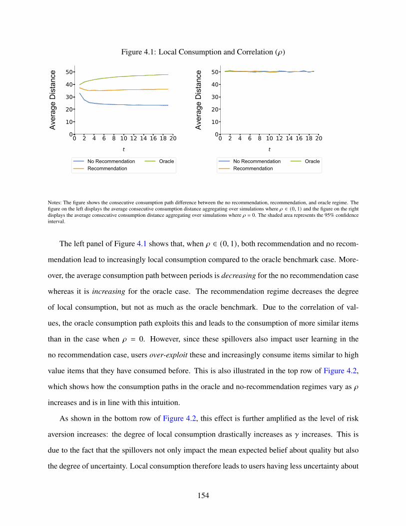
Figure 4.1: Local Consumption and Correlation (𝜌)

0 2 4 6 8 10 12 14 16 18 20t

0

10

20

30

40

50

Ave

rage

Dis

tanc

e

No RecommendationRecommendation

Oracle

0 2 4 6 8 10 12 14 16 18 20t

0

10

20

30

40

50

Ave

rage

Dis

tanc

e

No RecommendationRecommendation

Oracle

Notes: The figure shows the consecutive consumption path difference between the no recommendation, recommendation, and oracle regime. Thefigure on the left displays the average consecutive consumption distance aggregating over simulations where 𝜌 ∈ (0, 1) and the figure on the rightdisplays the average consecutive consumption distance aggregating over simulations where 𝜌 = 0. The shaded area represents the 95% confidenceinterval.

The left panel of Figure 4.1 shows that, when 𝜌 ∈ (0, 1), both recommendation and no recom-

mendation lead to increasingly local consumption compared to the oracle benchmark case. More-

over, the average consumption path between periods is decreasing for the no recommendation case

whereas it is increasing for the oracle case. The recommendation regime decreases the degree

of local consumption, but not as much as the oracle benchmark. Due to the correlation of val-

ues, the oracle consumption path exploits this and leads to the consumption of more similar items

than in the case when 𝜌 = 0. However, since these spillovers also impact user learning in the

no recommendation case, users over-exploit these and increasingly consume items similar to high

value items that they have consumed before. This is also illustrated in the top row of Figure 4.2,

which shows how the consumption paths in the oracle and no-recommendation regimes vary as 𝜌

increases and is in line with this intuition.

As shown in the bottom row of Figure 4.2, this effect is further amplified as the level of risk

aversion increases: the degree of local consumption drastically increases as 𝛾 increases. This is

due to the fact that the spillovers not only impact the mean expected belief about quality but also

the degree of uncertainty. Local consumption therefore leads to users having less uncertainty about

154

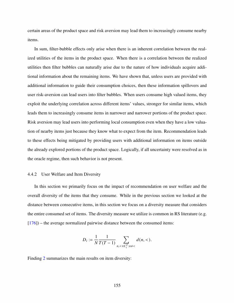
certain areas of the product space and risk aversion may lead them to increasingly consume nearby

items.

In sum, filter-bubble effects only arise when there is an inherent correlation between the real-

ized utilities of the items in the product space. When there is a correlation between the realized

utilities then filter bubbles can naturally arise due to the nature of how individuals acquire addi-

tional information about the remaining items. We have shown that, unless users are provided with

additional information to guide their consumption choices, then these information spillovers and

user risk-aversion can lead users into filter bubbles. When users consume high valued items, they

exploit the underlying correlation across different items’ values, stronger for similar items, which

leads them to increasingly consume items in narrower and narrower portions of the product space.

Risk aversion may lead users into performing local consumption even when they have a low valua-

tion of nearby items just because they know what to expect from the item. Recommendation leads

to these effects being mitigated by providing users with additional information on items outside

the already explored portions of the product space. Logically, if all uncertainty were resolved as in

the oracle regime, then such behavior is not present.

4.4.2 User Welfare and Item Diversity

In this section we primarily focus on the impact of recommendation on user welfare and the

overall diversity of the items that they consume. While in the previous section we looked at the

distance between consecutive items, in this section we focus on a diversity measure that considers

the entire consumed set of items. The diversity measure we utilize is common in RS literature (e.g.

[176]) – the average normalized pairwise distance between the consumed items:

𝐷𝑖 :=1𝑁

1𝑇 (𝑇 − 1)

∑︁𝑛,𝑚∈𝐶𝑇

𝑖:𝑛≠𝑚

𝑑 (𝑛, 𝑚).

Finding 2 summarizes the main results on item diversity:

155

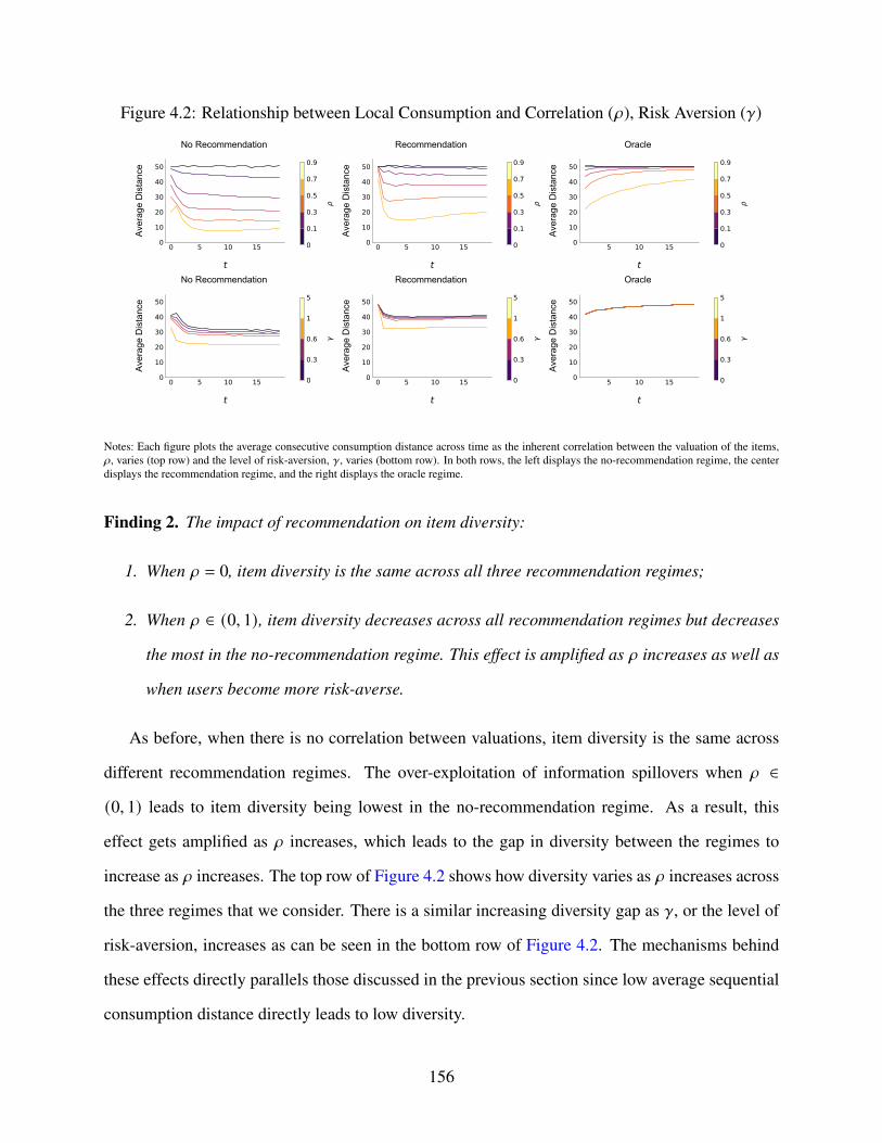
Figure 4.2: Relationship between Local Consumption and Correlation (𝜌), Risk Aversion (𝛾)

0 5 10 15

t

0

10

20

30

40

50

Ave

rage

Dis

tanc

eNo Recommendation

0

0.1

0.3

0.5

0.7

0.9

0 5 10 15

t

0

10

20

30

40

50

Ave

rage

Dis

tanc

e

Recommendation

0

0.1

0.3

0.5

0.7

0.9

5 10 15

t

0

10

20

30

40

50

Ave

rage

Dis

tanc

e

Oracle

0

0.1

0.3

0.5

0.7

0.9

0 5 10 15

t

0

10

20

30

40

50

Ave

rage

Dis

tanc

e

No Recommendation

0

0.3

0.6

1

5

0 5 10 15

t

0

10

20

30

40

50

Ave

rage

Dis

tanc

e

Recommendation

0

0.3

0.6

1

5

5 10 15

t

0

10

20

30

40

50

Ave

rage

Dis

tanc

e

Oracle

0

0.3

0.6

1

5

Notes: Each figure plots the average consecutive consumption distance across time as the inherent correlation between the valuation of the items,𝜌, varies (top row) and the level of risk-aversion, 𝛾, varies (bottom row). In both rows, the left displays the no-recommendation regime, the centerdisplays the recommendation regime, and the right displays the oracle regime.

Finding 2. The impact of recommendation on item diversity:

1. When 𝜌 = 0, item diversity is the same across all three recommendation regimes;

2. When 𝜌 ∈ (0, 1), item diversity decreases across all recommendation regimes but decreases

the most in the no-recommendation regime. This effect is amplified as 𝜌 increases as well as

when users become more risk-averse.

As before, when there is no correlation between valuations, item diversity is the same across

different recommendation regimes. The over-exploitation of information spillovers when 𝜌 ∈

(0, 1) leads to item diversity being lowest in the no-recommendation regime. As a result, this

effect gets amplified as 𝜌 increases, which leads to the gap in diversity between the regimes to

increase as 𝜌 increases. The top row of Figure 4.2 shows how diversity varies as 𝜌 increases across

the three regimes that we consider. There is a similar increasing diversity gap as 𝛾, or the level of

risk-aversion, increases as can be seen in the bottom row of Figure 4.2. The mechanisms behind

these effects directly parallels those discussed in the previous section since low average sequential

consumption distance directly leads to low diversity.

156

We now study how recommendation impacts user welfare. In our model users make consump-

tion decisions that maximize their current period ex-ante utility that depends on their beliefs in that

period. Thus, from an ex-ante perspective, they make optimal decisions, but our primary interest is

in understanding how the ex-post, or realized, utility varies across regimes and parameter values.

We define user’s ex-post welfare as the average of the realized values, controlling for the effect of

𝑇 :

𝑊𝑖 :=1𝑇

∑︁𝑛∈𝐶𝑇

𝑖

𝑥𝑖,𝑛

Finding 3 states our main findings of the impact of recommendation on ex-post welfare, which can

be seen in the rightmost plot of Figure 4.3:

Finding 3. The impact of recommendation on consumer welfare is as follows:

1. Under oracle recommendation, welfare is invariant with respect to 𝜌.

2. Under no recommendation, welfare is increasing in 𝜌.

3. Recommendation introduces welfare gains relative to no recommendation, but these gains

are decreasing as 𝜌 increases.

The most interesting observation is that the value of recommendation decreases as 𝜌 decreases.

While welfare in the recommendation regime is flat as we increase 𝜌, it is increasing in the no-

recommendation regime and thus the welfare gap between the two shrinks as 𝜌 increases. The

intuition is clear as recommendation provides users with information that allows them to better

guide their decisions and increase welfare. However, as 𝜌 increases users get increasingly more

information from consuming items since the realized utility is now more informative about the

utility of nearby items. Thus, since consumption decisions themselves yield valuable information,

the information provided by recommendation is less valuable to the user.

One striking observation is that the decrease in diversity does not appear to be associated with

a decline in welfare. Indeed, it appears that the opposite is the case - that low diversity is associated

157

Figure 4.3: Relationship between User Welfare, Diversity and Correlation (𝜌), Risk Aversion (𝛾)

0.0 0.2 0.4 0.6 0.80.10

0.15

0.20

0.25D

iver

sity

No RecommendationRecommendation

Oracle

0 2 4

0.16

0.18

0.20

0.22

Div

ersi

ty

No RecommendationRecommendation

Oracle

0.0 0.2 0.4 0.6 0.8

1

2

3

4

Wel

fare

No RecommendationRecommendation

Oracle

Notes: The figures on the left and center display the relationship between 𝜌 and overall consumed item diversity (left) as well as 𝛾 and overallconsumed item diversity (center). The figure on the right displays the relationship between 𝜌 and overall welfare. The shaded area represents the95% confidence interval.

with higher welfare and vice versa. We next explore the relationship between welfare and diversity,

which is summarized in Finding 4.

Finding 4. In the no-recommendation regime, diversity and welfare are:

1. Negatively correlated when users have no risk-aversion;

2. Uncorrelated when users have high levels of risk-aversion.

In the recommendation regime, diversity and welfare are:

1. Uncorrelated when users have no risk-aversion;

158

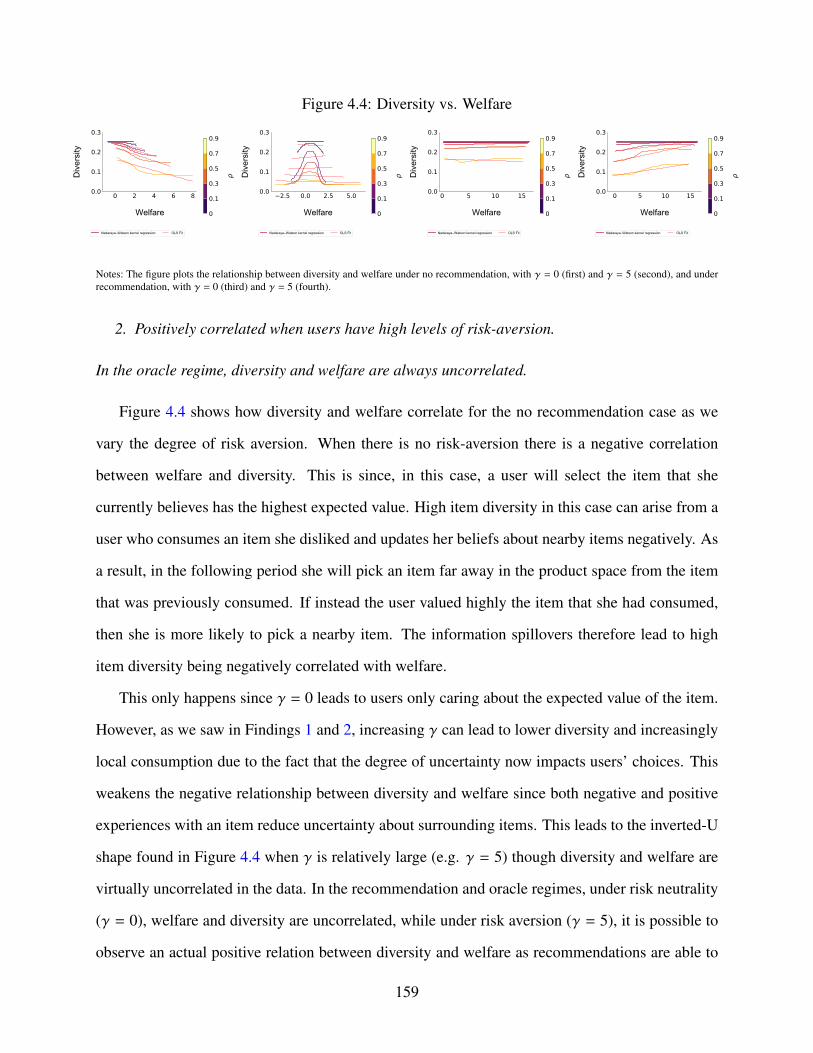
Figure 4.4: Diversity vs. Welfare

0 2 4 6 8

Welfare

0.0

0.1

0.2

0.3

Div

ersi

ty

0

0.1

0.3

0.5

0.7

0.9

Nadaraya Watson kernel regression OLS Fit

2.5 0.0 2.5 5.0

Welfare

0.0

0.1

0.2

0.3

Div

ersi

ty

0

0.1

0.3

0.5

0.7

0.9

Nadaraya Watson kernel regression OLS Fit

0 5 10 15

Welfare

0.0

0.1

0.2

0.3

Div

ersi

ty

0

0.1

0.3

0.5

0.7

0.9

Nadaraya Watson kernel regression OLS Fit

0 5 10 15

Welfare

0.0

0.1

0.2

0.3

Div

ersi

ty

0

0.1

0.3

0.5

0.7

0.9

Nadaraya Watson kernel regression OLS Fit

Notes: The figure plots the relationship between diversity and welfare under no recommendation, with 𝛾 = 0 (first) and 𝛾 = 5 (second), and underrecommendation, with 𝛾 = 0 (third) and 𝛾 = 5 (fourth).

2. Positively correlated when users have high levels of risk-aversion.

In the oracle regime, diversity and welfare are always uncorrelated.

Figure 4.4 shows how diversity and welfare correlate for the no recommendation case as we

vary the degree of risk aversion. When there is no risk-aversion there is a negative correlation

between welfare and diversity. This is since, in this case, a user will select the item that she

currently believes has the highest expected value. High item diversity in this case can arise from a

user who consumes an item she disliked and updates her beliefs about nearby items negatively. As

a result, in the following period she will pick an item far away in the product space from the item

that was previously consumed. If instead the user valued highly the item that she had consumed,

then she is more likely to pick a nearby item. The information spillovers therefore lead to high

item diversity being negatively correlated with welfare.

This only happens since 𝛾 = 0 leads to users only caring about the expected value of the item.

However, as we saw in Findings 1 and 2, increasing 𝛾 can lead to lower diversity and increasingly

local consumption due to the fact that the degree of uncertainty now impacts users’ choices. This

weakens the negative relationship between diversity and welfare since both negative and positive

experiences with an item reduce uncertainty about surrounding items. This leads to the inverted-U

shape found in Figure 4.4 when 𝛾 is relatively large (e.g. 𝛾 = 5) though diversity and welfare are

virtually uncorrelated in the data. In the recommendation and oracle regimes, under risk neutrality

(𝛾 = 0), welfare and diversity are uncorrelated, while under risk aversion (𝛾 = 5), it is possible to

observe an actual positive relation between diversity and welfare as recommendations are able to

159

reduce uncertainty and facilitate exploration of the product space.

4.4.3 User Homogenization

In this section, we focus on comparisons across users and investigate how the consumed set

of items across users varies across different recommendation regimes and parameter values. In

particular we look at the degree of homogenization between users. Similar to other papers that

study the degree of homogenization in RS (e.g. [159]) we measure homogeneity via the Jaccard

index between the consumption sets of users:

𝐻 :=1

|𝐼 | ( |𝐼 | − 1)∑︁

𝑖, 𝑗∈𝐼:𝑖≠ 𝑗𝑑𝐽 (𝐶𝑇𝑖 , 𝐶𝑇𝑗 )

where 𝑑𝐽 denotes the Jaccard index and 𝐻 ∈ [0, 1].

Finding 5 summarizes our findings on the impact of recommendation on user homogeneity:

Finding 5. The impact of recommendation on homogeneity is as follows:

1. Highest under recommendation and lowest under no recommendation;

2. Increasing in 𝛽, or the weight of the common-value component;

3. Decreasing in 𝜌 for partial recommendation, but weakly increasing in 𝜌 for no recommen-

dation.

First, we study how the degree of homogenization varies as we increase 𝛽, the weight of the

common value component. As 𝛽 increases we expect that users should become increasingly homo-

geneous as the realized utilities of the items are now increasingly similar. Figure 4.5 confirms that

as the weight of the common-value component 𝛽 increases, users consume increasingly similar

sets of items. The homogenization effect is strongest under the recommendation regime since the

revelation of the common-value component induces users to consume items in similar areas of the

product space. As 𝛽 increases, some amount of homogenization is optimal as can be seen from

160

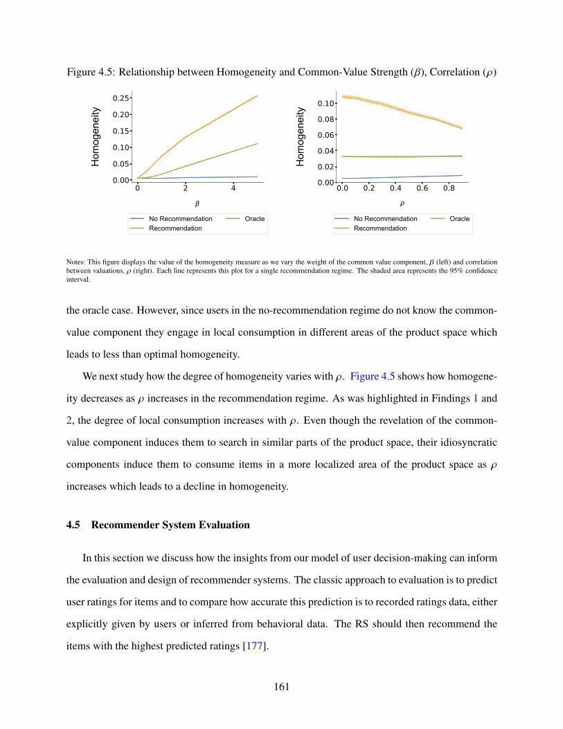
Figure 4.5: Relationship between Homogeneity and Common-Value Strength (𝛽), Correlation (𝜌)

0 2 40.00

0.05

0.10

0.15

0.20

0.25H

omog

enei

ty

No RecommendationRecommendation

Oracle

0.0 0.2 0.4 0.6 0.80.00

0.02

0.04

0.06

0.08

0.10

Hom

ogen

eity

No RecommendationRecommendation

Oracle

Notes: This figure displays the value of the homogeneity measure as we vary the weight of the common value component, 𝛽 (left) and correlationbetween valuations, 𝜌 (right). Each line represents this plot for a single recommendation regime. The shaded area represents the 95% confidenceinterval.

the oracle case. However, since users in the no-recommendation regime do not know the common-

value component they engage in local consumption in different areas of the product space which

leads to less than optimal homogeneity.

We next study how the degree of homogeneity varies with 𝜌. Figure 4.5 shows how homogene-

ity decreases as 𝜌 increases in the recommendation regime. As was highlighted in Findings 1 and

2, the degree of local consumption increases with 𝜌. Even though the revelation of the common-

value component induces them to search in similar parts of the product space, their idiosyncratic

components induce them to consume items in a more localized area of the product space as 𝜌

increases which leads to a decline in homogeneity.

4.5 Recommender System Evaluation

In this section we discuss how the insights from our model of user decision-making can inform

the evaluation and design of recommender systems. The classic approach to evaluation is to predict

user ratings for items and to compare how accurate this prediction is to recorded ratings data, either

explicitly given by users or inferred from behavioral data. The RS should then recommend the

items with the highest predicted ratings [177].

161

There has been a recent movement away from such evaluation measures due to the observation

that accurate recommendations are not necessarily useful recommendations [178]. Our model

illustrates a mechanism behind this observation. Consider the domain of movie recommendation

and suppose a user has just watched the movie John Wick and rated it highly. A RS attempting to

predict user ratings may then predict that this user is very likely to enjoy the sequel, John Wick:

Chapter Two, as well. However, the user herself may also have made this inference since the two

movies are very similar to each other. Thus, recommending this movie would not be not useful

since the recommendation gives the user little information that she did not already know. The key

insight is it is not useful since it ignores the inference the user themselves made and their updated

beliefs. The user may watch John Wick: Chapter Two, then, even without recommendation, and

the value of the recommendation was small.

This intuition implies that RS should collect additional data beyond that which is traditionally

recorded. The first and most crucial type of data to collect is individual user beliefs about items that

they have not yet consumed. As illustrated by our model, these beliefs are what drive the future

consumption decisions of users and understanding these beliefs is crucial for determining the value

of recommending certain items.8 The second type of data that is relevant for RS designers to collect

is how user beliefs change over time and, in particular, not just how individuals value the item they

just consumed, but also how it impacts their beliefs about the quality of similar items.9 The third

type of data is the risk-aversion levels of users as our model illustrates that the risk preferences of

users are important for understanding what information RS can provide that materially leads users

to alter their consumption patterns.

A natural follow-up question is how this additional data should be utilized in the design of

good recommendations. Our model posits that recommendation provides value to users by provid-

ing them with information about the true valuation of an item if they were to consume it. Thus, the

8Additionally, user beliefs contain information that may not have been observed by the recommender that onlyobserves user choices on the platform.

9Characterizing the similarity between items has been an important goal of designing content-based recommenda-tions, though as noted by [179], how users perceive similarity between items is not always in line with how similarityis computed in content-based RS. Understanding how this impacts which items users update their beliefs about is animportant direction for future work.

162

prediction problem for the recommender becomes predicting what item the user would choose with

no recommendation and, correspondingly, what would be the most useful information to provide

to the user that would lead her to consume a better item than she would without recommendation.

This links back to the intuition our model provided for the John Wick example whereby collect-

ing user beliefs and measuring how the user updated beliefs about similar items would lead the

recommender to understand that the user would consume John Wick: Chapter Two. Our approach

would therefore imply that, with this as a starting point, the recommender’s problem would be to

predict what is the most useful information to give the user leading them to change the item that

they eventually consume.

There have been a number of alternative recommendation evaluation metrics proposed in the

literature with the aim of providing more useful recommendations than those provided by accu-

racy metrics, such as serendipity [180], calibration [181], coverage [182], novelty [183], and many

others. Our approach most closely follows the set of proposed serendipity measures which are

surveyed in [180]. As discussed by [184], serendipitous recommendations are said to “have the

quality of being both unexpected and useful” which is in line with the primary intuition behind our

approach. The primary difference between our proposed approach and those existing in the liter-

ature is that ours crucially hinges on understanding user beliefs and the risk-preferences of users.

For instance, [183, 185] propose unexpectedness metrics that look at the dissimilarity of the pro-

posed recommended items compared to what the recommender already knows the user likes. This

metric depends only on the proposed item-set and not necessarily on the user’s beliefs or how such

a recommendation will change the item that the user consumes. [186] provide a comprehensive

overview of possible definitions of serendipity and ours is closest to their “motivational novelty"

definition, which is that the user was persuaded to consume an item as a result of recommendation.

Indeed, our approach allows us to give precise definitions for what it means for a recommen-

dation to be unexpected and useful in the spirit of serendipitous recommendations. Our evaluation

measure leads to useful recommendations since it leads users towards better items than they would

consume without recommendation. It further results in “unexpected” recommendations since it

163

explicitly incorporates user beliefs and thus allows the RS to understand how “unexpected” a rec-

ommendation would be from the perspective of a user. Finally, such a measure may lead to a

perceived broadening of user preferences as has been discussed in [187, 188]. However, under

our interpretation, it may be that their underlying preferences are unchanged and, instead, that rec-

ommendation and consumption themselves provides information that encourages users to explore

different portions of the product space.

164

References

[1] T. T. Nguyen, P.-M. Hui, F. M. Harper, L. Terveen, and J. A. Konstan, “Exploring thefilter bubble: The effect of using recommender systems on content diversity,” inProceedings of the 23rd international conference on World wide web, ACM, 2014,pp. 677–686.

[2] F. Scott Morton et al., “Committee for the study of digital platforms: Market structure andantitrust subcommittee report,” Stigler Center for the Study of the Economy and the State,2019.

[3] CMA, Online platforms and digital advertising: Market study final report, 2020.

[4] A. Prat and T. M. Valletti, “Attention oligopoly,”American Economic Journal: Microeconomics, Forthcoming, 2021.

[5] Y. Hou, D. Xiong, T. Jiang, L. Song, and Q. Wang, “Social media addiction: Its impact,mediation, and intervention,”Cyberpsychology: Journal of psychosocial research on cyberspace, vol. 13, no. 1, 2019.

[6] F. M. S. Morton and D. C. Dinielli, “Roadmap for an antitrust case against facebook,”Technical report, Omidyar Network, Tech. Rep., 2020.

[7] S. K. Ernala, M. Burke, A. Leavitt, and N. B. Ellison, “How well do people report timespent on facebook? an evaluation of established survey questions with recommendations,”in Proceedings of the 2020 CHI Conference on Human Factors in Computing Systems,2020, pp. 1–14.

[8] C. T. Conlon and J. H. Mortimer, “Empirical properties of diversion ratios,” NationalBureau of Economic Research, Forthcoming at The RAND Journal of Economics, Tech.Rep., 2018.

[9] C. S. Andreassen, T. Torsheim, G. S. Brunborg, and S. Pallesen, “Development of afacebook addiction scale,” Psychological reports, vol. 110, no. 2, pp. 501–517, 2012.

[10] J.-P. Dubé, G. J. Hitsch, and P. E. Rossi, “State dependence and alternative explanationsfor consumer inertia,” The RAND Journal of Economics, vol. 41, no. 3, pp. 417–445,2010.

[11] B. J. Bronnenberg, J.-P. H. Dubé, and M. Gentzkow, “The evolution of brand preferences:Evidence from consumer migration,” American Economic Review, vol. 102, no. 6,pp. 2472–2508, 2012.

165

[12] H. Allcott, M. Gentzkow, and L. Song, “Digital addiction,” Working Paper, Tech. Rep.,2021.

[13] H. Allcott, L. Braghieri, S. Eichmeyer, and M. Gentzkow, “The welfare effects of socialmedia,” American Economic Review, vol. 110, no. 3, pp. 629–76, 2020.

[14] E. Brynjolfsson, A. Collis, and F. Eggers, “Using massive online choice experiments tomeasure changes in well-being,” Proceedings of the National Academy of Sciences,vol. 116, no. 15, pp. 7250–7255, 2019.

[15] R. Mosquera, M. Odunowo, T. McNamara, X. Guo, and R. Petrie, “The economic effectsof facebook,” Experimental Economics, vol. 23, no. 2, pp. 575–602, 2020.

[16] N. Eagle and A. S. Pentland, “Reality mining: Sensing complex social systems,”Personal and ubiquitous computing, vol. 10, no. 4, pp. 255–268, 2006.

[17] S. Ichihashi and B.-C. Kim, “Addictive platforms,” 2021.

[18] A. Collis and F. Eggers, “Effects of restricting social media usage,”Available at SSRN 3518744, 2019.

[19] E. Bakshy, S. Messing, and L. A. Adamic, “Exposure to ideologically diverse news andopinion on facebook,” Science, vol. 348, no. 6239, pp. 1130–1132, 2015.

[20] J. R. Corrigan, S. Alhabash, M. Rousu, and S. B. Cash, “How much is social mediaworth? estimating the value of facebook by paying users to stop using it,” Plos one,vol. 13, no. 12, e0207101, 2018.

[21] R. Enikolopov, A. Makarin, and M. Petrova, “Social media and protest participation:Evidence from russia,” Econometrica, vol. 88, no. 4, pp. 1479–1514, 2020.

[22] R. Levy, “Social media, news consumption, and polarization: Evidence from a fieldexperiment,” American Economic Review, vol. 111, no. 3, pp. 831–70, 2021.

[23] D. M. Levy, Mindful tech: How to bring balance to our digital lives. Yale UniversityPress, 2016.

[24] M. Burke and R. E. Kraut, “The relationship between facebook use and well-beingdepends on communication type and tie strength,”Journal of computer-mediated communication, vol. 21, no. 4, pp. 265–281, 2016.

[25] D. J. Kuss and M. D. Griffiths, “Social networking sites and addiction: Ten lessonslearned,” International journal of environmental research and public health, vol. 14, no. 3,p. 311, 2017.

166

[26] E. R. Bailey, S. C. Matz, W. Youyou, and S. S. Iyengar, “Authentic self-expression onsocial media is associated with greater subjective well-being,” Nature communications,vol. 11, no. 1, pp. 1–9, 2020.

[27] N. K. Baym, K. B. Wagman, and C. J. Persaud, “Mindfully scrolling: Rethinkingfacebook after time deactivated,” Social Media+ Society, vol. 6, no. 2,p. 2 056 305 120 919 105, 2020.

[28] L. Braghieri, R. Levy, and A. Makarin, “Social media and mental health,”Available at SSRN, 2021.

[29] M. Shum, “Does advertising overcome brand loyalty? evidence from the breakfast-cerealsmarket,” Journal of Economics & Management Strategy, vol. 13, no. 2, pp. 241–272,2004.

[30] A. Simonov, J.-P. Dubé, G. Hitsch, and P. Rossi, “State-dependent demand estimationwith initial conditions correction,” Journal of Marketing Research, vol. 57, no. 5,pp. 789–809, 2020.

[31] C. T. Conlon and J. H. Mortimer, “Demand estimation under incomplete productavailability,” American Economic Journal: Microeconomics, vol. 5, no. 4, pp. 1–30, 2013.

[32] C. Conlon, J. Mortimer, and P. Sarkis, “Estimating preferences and substitution patternsfrom second choice data alone,” Working Paper at IIOC 2021, 2021.

[33] A. Goldfarb, “The medium-term effects of unavailability,”Quantitative Marketing and Economics, vol. 4, no. 2, pp. 143–171, 2006.

[34] E. Calvano and M. Polo, “Market power, competition and innovation in digital markets: Asurvey,” Information Economics and Policy, p. 100 853, 2020.

[35] S. P. Anderson and S. Coate, “Market provision of broadcasting: A welfare analysis,”The Review of Economic Studies, vol. 72, no. 4, pp. 947–972, 2005.

[36] A. Ambrus, E. Calvano, and M. Reisinger, “Either or both competition: A" two-sided"theory of advertising with overlapping viewerships,”American Economic Journal: Microeconomics, vol. 8, no. 3, pp. 189–222, 2016.

[37] S. P. Anderson, Ø. Foros, and H. J. Kind, “Competition for advertisers and for viewers inmedia markets,” The Economic Journal, vol. 128, no. 608, pp. 34–54, 2018.

[38] S. Athey, E. Calvano, and J. S. Gans, “The impact of consumer multi-homing onadvertising markets and media competition,” Management Science, vol. 64, no. 4,pp. 1574–1590, 2018.

167

[39] J. M. Newman, “Antitrust in zero-price markets: Applications,” Wash. UL Rev., vol. 94,p. 49, 2016.

[40] T. Wu, “Blind spot: The attention economy and the law,” Antitrust Law Journal, vol. 82,no. 3, 2017.

[41] J. Farrell and C. Shapiro, “Antitrust evaluation of horizontal mergers: An economicalternative to market definition,” The BE Journal of Theoretical Economics, vol. 10, no. 1,pp. 1–41, 2010.

[42] P. Affeldt, L. Filistrucchi, and T. J. Klein, “Upward pricing pressure in two-sidedmarkets,” The Economic Journal, vol. 123, no. 572, F505–F523, 2013.

[43] A. Ghose and S. P. Han, “Estimating demand for mobile applications in the neweconomy,” Management Science, vol. 60, no. 6, pp. 1470–1488, 2014.

[44] S. P. Han, S. Park, and W. Oh, “Mobile app analytics: A multiple discrete-continuouschoice framework,” Management Information Systems Quarterly (MISQ), Forthcoming,2015.

[45] H. Yuan, “Competing for time: A study of mobile applications,” Mimeo, 2020.

[46] C. R. Bhat, “The multiple discrete-continuous extreme value (mdcev) model: Role ofutility function parameters, identification considerations, and model extensions,”Transportation Research Part B: Methodological, vol. 42, no. 3, pp. 274–303, 2008.

[47] B. Li, P. Singh, and Q. Wang, “Zoom in ios clones: Examining the antecedents andconsequences of mobile app copycats,” 2014.

[48] D. Ershov, “Competing with superstars in the mobile app market,”Available at SSRN 3265662, 2018.

[49] W. Wen and F. Zhu, “Threat of platform-owner entry and complementor responses:Evidence from the mobile app market,” Strategic Management Journal, vol. 40, no. 9,pp. 1336–1367, 2019.

[50] S. Andersen, G. W. Harrison, M. I. Lau, and E. E. Rutström, “Elicitation using multipleprice list formats,” Experimental Economics, vol. 9, no. 4, pp. 383–405, 2006.

[51] G. Reynolds and C. Walters, “The use of customer surveys for market definition and thecompetitive assessment of horizontal mergers,”Journal of Competition Law and Economics, vol. 4, no. 2, pp. 411–431, 2008.

[52] A. S. Gerber and D. P. Green, Field experiments: Design, analysis, and interpretation.WW Norton, 2012.

168

[53] A. Abadie, J. Angrist, and G. Imbens, “Instrumental variables estimates of the effect ofsubsidized training on the quantiles of trainee earnings,” Econometrica, vol. 70, no. 1,pp. 91–117, 2002.

[54] M. F. Bellemare and C. J. Wichman, “Elasticities and the inverse hyperbolic sinetransformation,” Oxford Bulletin of Economics and Statistics, 2019.

[55] D. Byzalov, “Unbundling cable television: An empirical investigation,” working paper,Tech. Rep., 2008.

[56] J. J. Heckman, “Statistical models for discrete panel data,”Structural analysis of discrete data with econometric applications, vol. 114, p. 178, 1981.

[57] S. Bonhomme, T. Lamadon, and E. Manresa, “Discretizing unobserved heterogeneity,”University of Chicago, Becker Friedman Institute for Economics Working Paper,no. 2019-16, 2017.

[58] M. Ester, H.-P. Kriegel, J. Sander, X. Xu, et al., “A density-based algorithm fordiscovering clusters in large spatial databases with noise.,” in Kdd, vol. 96, 1996,pp. 226–231.

[59] U. Von Luxburg, “A tutorial on spectral clustering,” Statistics and computing, vol. 17,no. 4, pp. 395–416, 2007.

[60] A. Narayanan, A. Mathur, M. Chetty, and M. Kshirsagar, “Dark patterns: Past, present,and future: The evolution of tricky user interfaces,” Queue, vol. 18, no. 2, pp. 67–92,2020.

[61] C. Cunningham, F. Ederer, and S. Ma, “Killer acquisitions,” Available at SSRN 3241707,2019.

[62] P. Affeldt and R. Kesler, “Big tech acquisitions—towards empirical evidence,”Journal of European Competition Law & Practice, vol. 12, no. 6, pp. 471–478, 2021.

[63] R. Willig, “Unilateral competitive effects of mergers: Upward pricing pressure, productquality, and other extensions,” Review of Industrial Organization, vol. 39, no. 1-2, p. 19,2011.

[64] J. Huang, D. Reiley, and N. Riabov, “Measuring consumer sensitivity to audioadvertising: A field experiment on pandora internet radio,” Available at SSRN 3166676,2018.

[65] H. Beales and J. A. Eisenach, “An empirical analysis of the value of information sharingin the market for online content,” Available at SSRN 2421405, 2014.

169

[66] A. Aziz and R. Telang, “What is a digital cookie worth?” Available at SSRN 2757325,2016.

[67] G. A. Johnson, S. K. Shriver, and S. Du, “Consumer privacy choice in online advertising:Who opts out and at what cost to industry?” Marketing Science, 2020.

[68] G. Aridor, Y.-K. Che, and T. Salz, “The economic consequences of data privacyregulation: Empirical evidence from gdpr,” National Bureau of Economic Research, Tech.Rep., 2020.

[69] A. Acquisti, C. Taylor, and L. Wagman, “The economics of privacy,”Journal of Economic Literature, vol. 54, no. 2, pp. 442–92, 2016.

[70] T. Lin, “Valuing intrinsic and instrumental preferences for privacy,”Available at SSRN 3406412, 2019.

[71] J. P. Choi, D.-S. Jeon, and B.-C. Kim, “Privacy and personal data collection withinformation externalities,” Journal of Public Economics, vol. 173, pp. 113–124, 2019.

[72] D. Acemoglu, A. Makhdoumi, A. Malekian, and A. Ozdaglar, “Too much data: Prices andinefficiencies in data markets,” National Bureau of Economic Research, Tech. Rep., 2019.

[73] D. Bergemann, A. Bonatti, and T. Gan, “The economics of social data,” 2019.

[74] G. Johnson, S. Shriver, and S. Goldberg, “Privacy & market concentration: Intended &unintended consequences of the gdpr,” Available at SSRN 3477686, 2020.

[75] M. Batikas, S. Bechtold, T. Kretschmer, and C. Peukert, “European privacy law andglobal markets for data,” 2020.

[76] S. Goldberg, G. Johnson, and S. Shriver, “Regulating privacy online: An economicevaluation of the gdpr,” Available at SSRN 3421731, 2021.

[77] J. Jia, G. Z. Jin, and L. Wagman, “The short-run effects of gdpr on technology ventureinvestment,” National Bureau of Economic Research, Tech. Rep., 2018.

[78] ——, “Gdpr and the localness of venture investment,” Available at SSRN 3436535, 2020.

[79] R. Zhuo, B. Huffaker, S. Greenstein, et al., “The impact of the general data protectionregulation on internet interconnection,” National Bureau of Economic Research, Tech.Rep., 2019.

[80] C. Utz, M. Degeling, S. Fahl, F.Schaub, and T. Holz, “(un) informed consent: Studying gdpr consent notices in the field,” in

170

Proceedings of the 2019 ACM SIGSAC Conference on Computer and Communications Security,ACM, 2019, pp. 973–990.

[81] M. Degeling, C. Utz, C. Lentzsch, H. Hosseini, F. Schaub, and T. Holz, “We value yourprivacy... now take some cookies: Measuring the gdpr’s impact on web privacy,”arXiv preprint arXiv:1808.05096, 2018.

[82] A. Goldfarb and C. E. Tucker, “Privacy regulation and online advertising,”Management science, vol. 57, no. 1, pp. 57–71, 2011.

[83] M. Godinho de Matos and I. Adjerid, “Consumer consent and firm targeting after gdpr:The case of a large telecom provider,” Management Science, 2019.

[84] G. Johnson, “The impact of privacy policy on the auction market for online displayadvertising,” 2013.

[85] A. Goldfarb and C. Tucker, “Privacy and innovation,” Innovation policy and the economy,vol. 12, no. 1, pp. 65–90, 2012.

[86] L. Einav and J. Levin, “Economics in the age of big data,” Science, vol. 346, no. 6210,p. 1 243 089, 2014.

[87] L. Chiou and C. Tucker, “Search engines and data retention: Implications for privacy andantitrust,” National Bureau of Economic Research, Tech. Rep., 2017.

[88] P. J. Kehoe, B. J. Larsen, and E. Pastorino, “Dynamic competition in the era of big data,”Working paper, Stanford University and Federal Reserve Bank of Minneapolis, Tech.Rep., 2018.

[89] G. Aridor, K. Liu, A. Slivkins, and Z. S. Wu, “The perils of exploration undercompetition: A computational modeling approach,” inProceedings of the 2019 ACM Conference on Economics and Computation, 2019,pp. 171–172.

[90] P. Bajari, V. Chernozhukov, A. Hortaçsu, and J. Suzuki, “The impact of big data on firmperformance: An empirical investigation,” in AEA Papers and Proceedings, vol. 109,2019, pp. 33–37.

[91] C. Dwork, “Differential privacy,” Encyclopedia of Cryptography and Security,pp. 338–340, 2011.

[92] C. Dwork, A. Roth, et al., “The algorithmic foundations of differential privacy,”Foundations and Trends® in Theoretical Computer Science, vol. 9, no. 3–4, pp. 211–407,2014.

171

[93] J. M. Abowd and I. M. Schmutte, “An economic analysis of privacy protection andstatistical accuracy as social choices,” American Economic Review, vol. 109, no. 1,pp. 171–202, 2019.

[94] J. A. Fairfield and C. Engel, “Privacy as a public good,” Duke LJ, vol. 65, p. 385, 2015.

[95] A. Liang and E. Madsen, “Data sharing and incentives,” Available at SSRN 3485776,2019.

[96] L. Braghieri, “Targeted advertising and price discrimination in intermediated onlinemarkets,” Available at SSRN 3072692, 2019.

[97] D. Coey and M. Bailey, “People and cookies: Imperfect treatment assignment in onlineexperiments,” in Proceedings of the 25th International Conference on World Wide Web,2016, pp. 1103–1111.

[98] T. Lin and S. Misra, “The identity fragmentation bias,” arXiv preprint arXiv:2008.12849,2020.

[99] B. Berendt, O. Günther, and S. Spiekermann, “Privacy in e-commerce: Stated preferencesvs. actual behavior,” Communications of the ACM, vol. 48, no. 4, pp. 101–106, 2005.

[100] P. A. Norberg, D. R. Horne, and D. A. Horne, “The privacy paradox: Personal informationdisclosure intentions versus behaviors,” Journal of consumer affairs, vol. 41, no. 1,pp. 100–126, 2007.

[101] S. Athey, C. Catalini, and C. Tucker, “The digital privacy paradox: Small money, smallcosts, small talk,” National Bureau of Economic Research, Tech. Rep., 2017.

[102] A. Acquisti, L. K. John, and G. Loewenstein, “What is privacy worth?”The Journal of Legal Studies, vol. 42, no. 2, pp. 249–274, 2013.

[103] A. Goldfarb and C. Tucker, “Shifts in privacy concerns,” American Economic Review,vol. 102, no. 3, pp. 349–53, 2012.

[104] S. C. Boerman, S. Kruikemeier, and F. J. Zuiderveen Borgesius, “Exploring motivationsfor online privacy protection behavior: Insights from panel data,”Communication Research, p. 0 093 650 218 800 915, 2018.

[105] J. Prince and S. Wallsten, “How much is privacy worth around the world and acrossplatforms?” Available at SSRN, 2020.

[106] J. Campbell, A. Goldfarb, and C. Tucker, “Privacy regulation and market structure,”Journal of Economics & Management Strategy, vol. 24, no. 1, pp. 47–73, 2015.

172

[107] Q. H. Vuong, “Likelihood ratio tests for model selection and non-nested hypotheses,”Econometrica: Journal of the Econometric Society, pp. 307–333, 1989.

[108] Y. Zou, K. Roundy, A. Tamersoy, S. Shintre, J. Roturier, and F. Schaub, “Examining theadoption and abandonment of security, privacy, and identity theft protection practices,” inProceedings of the 2020 CHI Conference on Human Factors in Computing Systems,2020, pp. 1–15.

[109] C. Ferri, J. Hernández-Orallo, and R Modroiu, “An experimental comparison ofperformance measures for classification,” Pattern Recognition Letters, vol. 30, no. 1,pp. 27–38, 2009.

[110] J. Hernández-Orallo, P. Flach, and C. Ferri, “A unified view of performance metrics:Translating threshold choice into expected classification loss,”Journal of Machine Learning Research, vol. 13, no. Oct, pp. 2813–2869, 2012.

[111] T. Fawcett, “An introduction to roc analysis,” Pattern recognition letters, vol. 27, no. 8,pp. 861–874, 2006.

[112] M. J. Salganik, P. S. Dodds, and D. J. Watts, “Experimental study of inequality andunpredictability in an artificial cultural market,” Science, vol. 311, no. 5762, pp. 854–856,2006.

[113] I. MacKenzie, C. Meyer, and S. Noble, “How retailers can keep up with consumers,”McKinsey Retail Insights, 2013,https://www.mckinsey.com/industries/retail/our-insights/how-retailers-can-keep-up-with-consumers.

[114] D. Davis, “Amazon triples its private-label product offerings in 2 years,”Digital Commerce 360, 2020, https://www.digitalcommerce360.com/2020/05/20/amazon-triples-its-private%E2%80%91label-product-offerings-in-2-years/.

[115] Netflix, Complete list of netflix originals,https://www.whats-on-netflix.com/originals/. Accessed June 20,2021, 2021.

[116] M. Binder, “Spotify bets big on podcasts with acquisition of gimlet and anchor,”Mashable, 2020, https://mashable.com/article/spotify-acquires-podcast-gimlet-anchor.

[117] J. Creswell, “How amazon steers shoppers to its own products,” New York Times, 2018,https://www.nytimes.com/2018/06/23/business/amazon-the-brand-buster.html.

173

[118] K. Grind, S. Schechner, R. McMillan, and J. West, “How google interferes with its searchalgorithms and changes your results,” Wall Street Journal, 2019,https://www.wsj.com/articles/how-google-interferes-with-its-search-algorithms-and-changes-your-results-11573823753.

[119] D. Carr, “Giving viewers what they want,” New York Times, 2013, https://www.nytimes.com/2013/02/25/business/media/for-house-of-cards-using-big-data-to-guarantee-its-popularity.html.

[120] European Commission, “Com(2020) 842 final: Proposal for a regulation of the europeanparliament and of the council on contestable and fair markets in the digital sector (digitalmarkets act),” 2020, https://eur-lex.europa.eu/legal-content/EN/TXT/HTML/?uri=CELEX:52020PC0842&from=en.

[121] U.S. House. 117th Congress, 1st Session, “H.r.3825 - ending platform monopolies act,”2021, https://www.congress.gov/bill/117th-congress/house-bill/3825/text.

[122] A. Hagiu and B. Jullien, “Why do intermediaries divert search?”The RAND Journal of Economics, vol. 42, no. 2, pp. 337–362, 2011.

[123] A. de Corniere and G. Taylor, “A model of biased intermediation,”RAND Journal of Economics, vol. 50, no. 4, pp. 854–882, 2019.

[124] T.-H. Teh and J. Wright, “Intermediation and steering: Competition in prices andcommissions,” American Economic Journal: Microeconomics, 2020.

[125] S. Follows, “How movies make money: $100m+ hollywood blockbusters,”Stephen Follows, Film Data and Education, 2016,https://stephenfollows.com/how-movies-make-money-hollywood-blockbusters/.

[126] J. Lynch, “Musicians only got 12% of the $43 billion the music industry generated in2017, and it mostly came from touring,” Business Insider, 2018, https://www.businessinsider.com/musicians-received-12-percent-43-billion-generated-by-music-industry-study-2018-8.

[127] S. Roxborough, “Will the cannes film festival kick off a global comebackpost-lockdown?” Hollywood Reporter, 2021,https://www.hollywoodreporter.com/movies/movie-news/cannes-film-festival-global-comeback-post-lockdown-1234975291/.

[128] A. Rubinstein and A. Wolinsky, “Middlemen,” The Quarterly Journal of Economics,vol. 102, no. 3, pp. 581–593, 1987.

174

[129] J.-C. Rochet and J. Tirole, “Platform competition in two-sided markets,”Journal of the European Economic Association, vol. 1, no. 4, pp. 990–1029, 2003.

[130] E. Kamenica and M. Gentzkow, “Bayesian persuasion,” American Economic Review,vol. 101, no. 6, pp. 2590–2615, 2011.

[131] D. Bergemann and S. Morris, “Information design: A unified perspective,”Journal of Economic Literature, vol. 57, no. 1, pp. 1–57, 2019.

[132] M. Bourreau and G. Gaudin, “Streaming platform and strategic recommendation bias,”Available at SSRN 3290617, 2018.

[133] M. Armstrong, J. Vickers, and J. Zhou, “Prominence and consumer search,”The RAND Journal of Economics, vol. 40, no. 2, pp. 209–233, 2009.

[134] A. Hagiu and B. Jullien, “Search diversion and platform competition,”International Journal of Industrial Organization, vol. 33, pp. 48–60, 2014.

[135] R. Burguet, R. Caminal, and M. Ellman, “In google we trust?”International Journal of Industrial Organization, vol. 39, pp. 44–55, 2015.

[136] A. de Cornière, “Search advertising,” American Economic Journal: Microeconomics,vol. 8, no. 3, pp. 156–88, 2016.

[137] R. Inderst and M. Ottaviani, “How (not) to pay for advice: A framework for consumerfinancial protection,” Journal of Financial Economics, vol. 105, no. 2, pp. 393–411, 2012.

[138] ——, “Competition through commissions and kickbacks,” American Economic Review,vol. 102, no. 2, pp. 780–809, 2012.

[139] D. Bergemann and D. Ozmen, “Optimal pricing with recommender systems,” inProceedings of the 7th ACM Conference on Electronic Commerce, ACM, 2006,pp. 43–51.

[140] Y.-K. Che and J. Hörner, “Recommender systems as mechanisms for social learning,”The Quarterly Journal of Economics, vol. 133, no. 2, pp. 871–925, 2017.

[141] D. Fleder and K. Hosanagar, “Blockbuster culture’s next rise or fall: The impact ofrecommender systems on sales diversity,” Management Science, vol. 55, no. 5,pp. 697–712, 2009.

[142] K. Hosanagar, R. Krishnan, and L. Ma, “Recomended for you: The impact of profitincentives on the relevance of online recommendations,” ICIS 2008 Proceedings, 2008.

175

[143] E. Calvano, G. Calzolari, V. Denicolò, and S. Pastorello, “Product recommendations andmarket concentration,” Working Paper, 2021.

[144] G. Lee and J. Wright, “Recommender systems and the value of user data,”Working Paper, 2021.

[145] S. J. Grossman and O. D. Hart, “The costs and benefits of ownership: A theory of verticaland lateral integration,” Journal of Political Economy, vol. 94, no. 4, pp. 691–719, 1986.

[146] O. E. Williamson, “The vertical integration of production: Market failure considerations,”The American Economic Review, vol. 61, no. 2, pp. 112–123, 1971.

[147] M. K. Perry, “Vertical integration: Determinants and effects,”Handbook of Industrial Organization, vol. 1, pp. 183–255, 1989.

[148] O. Hart, J. Tirole, D. W. Carlton, and O. E. Williamson, “Vertical integration and marketforeclosure,” Brookings papers on economic activity. Microeconomics, vol. 1990,pp. 205–286, 1990.

[149] J. A. Ordover, G. Saloner, and S. C. Salop, “Equilibrium vertical foreclosure,”The American Economic Review, pp. 127–142, 1990.

[150] J. Asker and H. Bar-Isaac, “Vertical information restraints: Pro-and anticompetitiveimpacts of minimum-advertised-price restrictions,” The Journal of Law and Economics,vol. 63, no. 1, pp. 111–148, 2020.

[151] M. Janssen and S. Shelegia, “Consumer search and double marginalization,”American Economic Review, vol. 105, no. 6, pp. 1683–1710, 2015.

[152] I. Kremer, Y. Mansour, and M. Perry, “Implementing the “wisdom of the crowd”,”Journal of Political Economy, vol. 122, no. 5, pp. 988–1012, 2014.

[153] Y. Mansour, A. Slivkins, and V. Syrgkanis, “Bayesian incentive-compatible banditexploration,” inProceedings of the Sixteenth ACM Conference on Economics and Computation, ACM,2015, pp. 565–582.

[154] T. Spangler, “Netflix original series viewing climbs, but licensed content remains majorityof total u.s. streams,” Variety.com, 2019,https://variety.com/2018/digital/news/netflix-original-series-licensed-viewing-friends-the-office-1203085230/.

[155] D. Vena, “Netflix subscriber numbers soar, showing the sky is not falling,” fool.com,2019, https://www.fool.com/investing/2019/10/17/netflix-subscriber-numbers-soar-showing-the-sky-is.aspx.

176

[156] V. P. Crawford and J. Sobel, “Strategic information transmission,”Econometrica: Journal of the Econometric Society, pp. 1431–1451, 1982.

[157] G. Aridor, D. Goncalves, and S. Sikdar, “Deconstructing the filter bubble: Userdecision-making and recommender systems,” inFourteenth ACM Conference on Recommender Systems, 2020, pp. 82–91.

[158] E. Pariser,The filter bubble: How the new personalized web is changing what we read and how we think.Penguin, 2011.

[159] A. J. Chaney, B. M. Stewart, and B. E. Engelhardt, “How algorithmic confounding inrecommendation systems increases homogeneity and decreases utility,” inProceedings of the 12th ACM Conference on Recommender Systems, ACM, 2018,pp. 224–232.

[160] K. Hosanagar, D. Fleder, D. Lee, and A. Buja, “Will the global village fracture intotribes? recommender systems and their effects on consumer fragmentation,”Management Science, vol. 60, no. 4, pp. 805–823, 2013.

[161] E. Schulz, R. Bhui, B. C. Love, B. Brier, M. T. Todd, and S. J. Gershman, “Structured,uncertainty-driven exploration in real-world consumer choice,”Proceedings of the National Academy of Sciences, p. 201 821 028, 2019.

[162] S. Flaxman, S. Goel, and J. M. Rao, “Filter bubbles, echo chambers, and online newsconsumption,” Public opinion quarterly, vol. 80, no. S1, pp. 298–320, 2016.

[163] J. Möller, D. Trilling, N. Helberger, and B. van Es, “Do not blame it on the algorithm: Anempirical assessment of multiple recommender systems and their impact on contentdiversity,” Information, Communication & Society, vol. 21, no. 7, pp. 959–977, 2018.

[164] Ò. Celma and P. Cano, “From hits to niches?: Or how popular artists can bias musicrecommendation and discovery,” inProceedings of the 2nd KDD Workshop on Large-Scale Recommender Systems, ACM,2008, p. 5.

[165] J. Treviranus and S. Hockema, “The value of the unpopular: Counteracting the popularityecho-chamber on the web,” in2009 IEEE Toronto International Conference Science and Technology for Humanity (TIC-STH),IEEE, 2009.

[166] L. Chen, M. De Gemmis, A. Felfernig, P. Lops, F. Ricci, and G. Semeraro, “Humandecision making and recommender systems,”ACM Transactions on Interactive Intelligent Systems (TiiS), vol. 3, no. 3, pp. 1–7, 2013.

177

[167] J. R. Bettman, M. F. Luce, and J. W. Payne, “Constructive consumer choice processes,”Journal of consumer research, vol. 25, no. 3, pp. 187–217, 1998.

[168] S. Lichtenstein and P. Slovic, The construction of preference. Cambridge UniversityPress, 2006.

[169] Ò. Celma and P. Herrera, “A new approach to evaluating novel recommendations,” inProceedings of the 2008 ACM conference on Recommender systems, 2008, pp. 179–186.

[170] P. Cremonesi, F. Garzotto, and R. Turrin, “User-centric vs. system-centric evaluation ofrecommender systems,” in IFIP Conference on Human-Computer Interaction, Springer,2013, pp. 334–351.

[171] P. Pu, L. Chen, and R. Hu, “A user-centric evaluation framework for recommendersystems,” in Proceedings of the fifth ACM conference on Recommender systems, 2011,pp. 157–164.

[172] C. Hodgson and G. Lewis, “You can lead a horse to water: Spatial learning and pathdependence in consumer search,” inProceedings of the 2019 ACM Conference on Economics and Computation, ser. EC ’19,Phoenix, AZ, USA: Association for Computing Machinery, 2019, p. 215, ISBN:9781450367929.

[173] A. Mas-Colell, M. D. Whinston, J. R. Green, et al., Microeconomic theory. Oxforduniversity press New York, 1995, vol. 1.

[174] I. Gilboa and D. Schmeidler, “Case-based decision theory,”The quarterly Journal of economics, vol. 110, no. 3, pp. 605–639, 1995.

[175] A. Billot, I. Gilboa, and D. Schmeidler, “Axiomatization of an exponential similarityfunction,” Mathematical Social Sciences, vol. 55, no. 2, pp. 107–115, 2008.

[176] C.-N. Ziegler, S. M. McNee, J. A. Konstan, and G. Lausen, “Improving recommendationlists through topic diversification,” inProceedings of the 14th international conference on World Wide Web, ACM, 2005,pp. 22–32.

[177] G. Adomavicius and A. Tuzhilin, “Toward the next generation of recommender systems:A survey of the state-of-the-art and possible extensions,”IEEE Transactions on Knowledge & Data Engineering, no. 6, pp. 734–749, 2005.

[178] S. M. McNee, J. Riedl, and J. A. Konstan, “Being accurate is not enough: How accuracymetrics have hurt recommender systems,” inCHI’06 extended abstracts on Human factors in computing systems, ACM, 2006,pp. 1097–1101.

178

[179] A. A. Winecoff, F. Brasoveanu, B. Casavant, P. Washabaugh, and M. Graham, “Users inthe loop: A psychologically-informed approach to similar item retrieval,” inProceedings of the 13th ACM Conference on Recommender Systems, 2019, pp. 52–59.

[180] D. Kotkov, S. Wang, and J. Veijalainen, “A survey of serendipity in recommendersystems,” Knowledge-Based Systems, vol. 111, pp. 180–192, 2016.

[181] H. Steck, “Calibrated recommendations,” inProceedings of the 12th ACM conference on recommender systems, 2018, pp. 154–162.

[182] M. Ge, C. Delgado-Battenfeld, and D. Jannach, “Beyond accuracy: Evaluatingrecommender systems by coverage and serendipity,” inProceedings of the fourth ACM conference on Recommender systems, ACM, 2010,pp. 257–260.

[183] S. Vargas and P. Castells, “Rank and relevance in novelty and diversity metrics forrecommender systems,” inProceedings of the fifth ACM conference on Recommender systems, ACM, 2011,pp. 109–116.

[184] A. Maksai, F. Garcin, and B. Faltings, “Predicting online performance of newsrecommender systems through richer evaluation metrics,” inProceedings of the 9th ACM Conference on Recommender Systems, ACM, 2015,pp. 179–186.

[185] M. Kaminskas and D. Bridge, “Measuring surprise in recommender systems,” inProceedings of the workshop on recommender systems evaluation), Citeseer, 2014.

[186] D. Kotkov, J. A. Konstan, Q. Zhao, and J. Veijalainen, “Investigating serendipity inrecommender systems based on real user feedback,” inProceedings of the 33rd Annual ACM Symposium on Applied Computing, 2018,pp. 1341–1350.

[187] J. L. Herlocker, J. A. Konstan, L. G. Terveen, and J. T. Riedl, “Evaluating collaborativefiltering recommender systems,” ACM Transactions on Information Systems (TOIS),vol. 22, no. 1, pp. 5–53, 2004.

[188] Y. C. Zhang, D. Ó. Séaghdha, D. Quercia, and T. Jambor, “Auralist: Introducingserendipity into music recommendation,” inProceedings of the fifth ACM international conference on Web search and data mining,2012, pp. 13–22.

[189] S. Berry and P. Haile, “Identification in differentiated products markets,”Annual review of Economics, vol. 8, pp. 27–52, 2016.

179

[190] A. Abadie, A. Diamond, and J. Hainmueller, “Synthetic control methods for comparativecase studies: Estimating the effect of california’s tobacco control program,”Journal of the American statistical Association, vol. 105, no. 490, pp. 493–505, 2010.

[191] A. C. Cameron and P. K. Trivedi, Microeconometrics: methods and applications.Cambridge university press, 2005.

[192] D. Lambert, “Zero-inflated poisson regression, with an application to defects inmanufacturing,” Technometrics, vol. 34, no. 1, pp. 1–14, 1992.

[193] B. A. Desmarais and J. J. Harden, “Testing for zero inflation in count models: Biascorrection for the vuong test,” The Stata Journal, vol. 13, no. 4, pp. 810–835, 2013.

[194] A. C. Cameron and P. K. Trivedi, “Regression-based tests for overdispersion in thepoisson model,” Journal of econometrics, vol. 46, no. 3, pp. 347–364, 1990.

[195] M. H. DeGroot and S. E. Fienberg, “The comparison and evaluation of forecasters,”Journal of the Royal Statistical Society: Series D (The Statistician), vol. 32, no. 1-2,pp. 12–22, 1983.

180

Appendix A: Supplementary Material for Drivers of Digital Attention:

Evidence from a Social Media Experiment

A.1 Experiment Materials

A.1.1 Recruitment Materials

The following are the recruitment materials that were used for the study. Participants were ei-

ther recruited from university lab pools or Facebook advertisements. For the participants who came

from university lab pools they received the invitation in Section A.1.1 via email. The Facebook

advertisement that was used for recruitment is shown in Figure A1.

Recruitment Letter

Hello [NAME OF PARTICIPANTS]!

We are inviting you to participate in an Internet experiment via Zoom. You will be able to earn

money while contributing to science and hopefully having fun!

We are running an experiment to better understand how people spend their time online. We

will ask you to install an application that will allow us to track how much time you spend on your

phone and computer and periodically restrict access to certain applications on your phone [we only

observe the time spent, not what happens on the app itself]. We will meet with you on zoom for

five minutes to make sure the app is set up on your phone properly and then you will take a fifteen

minute intro survey. You will not have to actively do anything during the rest of the experiment,

beyond answering a short 4-minute survey once a week for five weeks.

Participants will earn $50 for successfully completing the experiment (i.e. keeping the applica-

181

tion installed and completing all the survey questions each week). Note that only individuals with

Android phones can participate in this experiment.

To sign up for the study, please click the link below to express your interest and we will follow

up via email to schedule an initial meeting to set up the software and start the study: [link]

Thanks for your interest in participating in this study.

Figure A1: Facebook Advertisement

Recruitment Survey

Once the participants clicked on the link in the email sent from the lab pool or the Facebook

advertisement, they were sent to an interest survey to complete. The recruitment survey had two

182

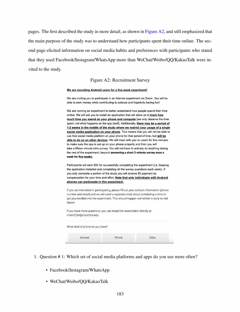
pages. The first described the study in more detail, as shown in Figure A2, and still emphasized that

the main purpose of the study was to understand how participants spent their time online. The sec-

ond page elicited information on social media habits and preferences with participants who stated

that they used Facebook/Instagram/WhatsApp more than WeChat/Weibo/QQ/KakaoTalk were in-

vited to the study.

Figure A2: Recruitment Survey

1. Question # 1: Which set of social media platforms and apps do you use more often?

• Facebook/Instagram/WhatsApp

• WeChat/Weibo/QQ/KakaoTalk

183

2. Question # 2: Which of these apps do you use frequently (at least once a week)? Select all

that are applicable.

• Facebook, Instagram, Messenger, YouTube, WhatsApp, TikTok, Reddit, Snapchat,

Twitter, WeChat, QQ, Weibo, KakaoTalk, Line, Telegram

3. Question # 3: Which web browser do you use most often?

• Google Chrome, Safari, Internet Explorer, Firefox, Other

4. Question # 4: Contact Information - name, phone number, email

A.1.2 Baseline Survey

The baseline survey that participants fill out when they set up the software starts with the

standard experimental consent form and study details. It then proceeds to ask a number of questions

about their usage of social media applications.

184

Figure A3: Consent Form and Study Details

The questions were then as follows:

1. Question #1: Subjective Time Use. For each application write in your best guess for the

number of hours you spend on it each week (in 30 minute increments, e.g. 1.50 hours for 1

hour and 30 minutes per week). The first column asks how much time you think you spend

on the application on your phone and the second column asks how much time you think you

spend on the application on your other devices.

• Facebook, Twitter, WhatsApp, TikTok, Instagram, Snapchat, Facebook Messenger, At-

tention Check. Write 99., YouTube, Reddit, Netflix

2. Question #2: Content Production. How frequently do you post content (including stories, re-

sharing posts) on each of the following applications? For each of the following applications,

185

the participants were asked to select one of the following options.

• Applications: Facebook, Instagram, YouTube, Reddit, TikTok, Netflix, Snapchat, Twit-

ter

• Options: Never, Less than once a month, At least once a month, At least once a week,

2 or 3 times per week, Every day

3. Question #3: Subjective Activity on Application. The main activity I do on each application

on my phone is as follows. For each of the following applications the participants were asked

to select one of the following options.

• Applications: Facebook, Instagram, YouTube, Reddit, TikTok, Netflix, Snapchat, Twit-

ter, Messenger, WhatsApp

• Options: Get Information (e.g. news about politics, sports, business, etc.), Online

Shopping, Keep up with my friends’ lives, Communicate with my friends, Entertain-

ment content (e.g. memes, influencers, videos, etc.), I don’t use this application

4. Question #4: Connections. For each application, write in the number of people you are

connected to on the application. Please put your best guess for the range, there is no need to

check for the exact values. For applications with followers / following, please let us know

approximately how many individuals you follow on the application. For applications without

direct connections, please let us know approximately how many individuals you interact with

each week on the application.

• Facebook (Friends): 0, 1-49, 50-149, 150-299, 300-499, 500-749, 750-999, 1000-2499,

2500-4999, 5000+

• Twitter (Following): 0, 1-49, 50-149, 150-299, 300-499, 500-749, 750-999, 1000-

2499, 2500-4999, 5000+

• WhatsApp (Contacts): 0, 1-4, 5-9, 10-19, 20-29, 30-39, 40-49, 50-99, 100-249, 250+

186

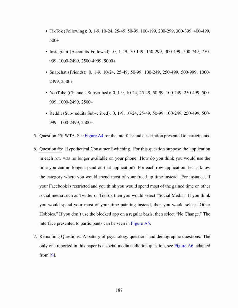
• TikTok (Following): 0, 1-9, 10-24, 25-49, 50-99, 100-199, 200-299, 300-399, 400-499,

500+

• Instagram (Accounts Followed): 0, 1-49, 50-149, 150-299, 300-499, 500-749, 750-

999, 1000-2499, 2500-4999, 5000+

• Snapchat (Friends): 0, 1-9, 10-24, 25-49, 50-99, 100-249, 250-499, 500-999, 1000-

2499, 2500+

• YouTube (Channels Subscribed): 0, 1-9, 10-24, 25-49, 50-99, 100-249, 250-499, 500-

999, 1000-2499, 2500+

• Reddit (Sub-reddits Subscribed): 0, 1-9, 10-24, 25-49, 50-99, 100-249, 250-499, 500-

999, 1000-2499, 2500+

5. Question #5: WTA. See Figure A4 for the interface and description presented to participants.

6. Question #6: Hypothetical Consumer Switching. For this question suppose the application

in each row was no longer available on your phone. How do you think you would use the

time you can no longer spend on that application? For each row application, let us know

the category where you would spend most of your freed up time instead. For instance, if

your Facebook is restricted and you think you would spend most of the gained time on other

social media such as Twitter or TikTok then you would select “Social Media." If you think

you would spend your most of your time painting instead, then you would select “Other

Hobbies." If you don’t use the blocked app on a regular basis, then select “No Change." The

interface presented to participants can be seen in Figure A5.

7. Remaining Questions: A battery of psychology questions and demographic questions. The

only one reported in this paper is a social media addiction question, see Figure A6, adapted

from [9].

187

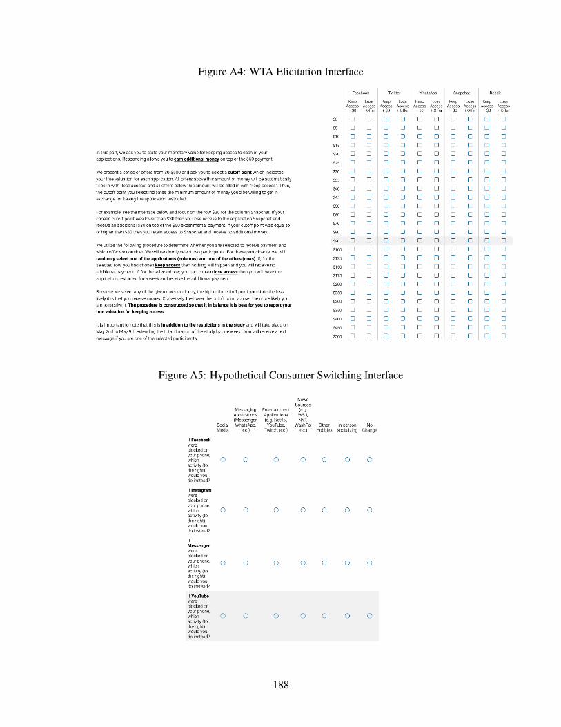
Figure A4: WTA Elicitation Interface

Figure A5: Hypothetical Consumer Switching Interface

188

Figure A6: Social Media Addiction Scale

A.1.3 Additional Surveys

There are two weekly surveys throughout the study. The first is during the week and sent

on Thursdays as part of the data collection partnership for this study. It is meant to capture in-

stantaneous psychology measures, which is why it is sent during the week while the application

restrictions are ongoing. The second is sent on Saturday mornings and is meant to record subjective

perceptions of time usage throughout the week.

The Thursday survey asks the participants how fast they felt the week had passed, questions

about their social connectedness and well-being, a question about whether they made any big

purchases in the past week, and finally whether there were any major life events in the past week.

The Saturday survey is broken into three separate components. The first component asks par-

ticipants how much time they felt they spent off their phones on Facebook, Instagram, YouTube,

Facebook Messenger, WhatsApp, Netflix, TikTok, Twitter, and Reddit. The second component

189

asks participants how much time they spent on life necessities, including sleeping, studying, at-

tending classes, paid work, cooking/eating, cleaning, socializing in person, and child care. The

final component asks participants how much time they spent on leisure activities off the phone,

including playing video games, reading books, watching cable TV, streaming on TV / tablet, exer-

cising, shopping (in person), artistic hobbies, and reading print media.

Finally there is an endline survey that is attached to the final weekly time use survey, which

asks the following questions:

1. Question #1: Ability to revise WTA. The participants are given the same WTA question as

the initial survey, but the results are pre-filled based on their initial survey responses. They

are instructed to revise the values if they wish.

2. Question #2: Reason for revision. The participants are asked why they revised the WTA

value.

• Applications: Facebook, Instagram, YouTube, Reddit, TikTok, Netflix, Snapchat, Twit-

ter, Messenger, WhatsApp

• Options: Have a better idea of how much time I spend on the application, Reduced

my usage of the application during the study period, Started using the application dur-

ing the study period, Increased my usage of the application during the study period,

Realized the application is more/less important to me than I thought, I realized I mis-

understood this question when I first answered it, No Change

3. Question #3: What did you think the purpose of the study and the restrictions was? Open-

Response.

4. Question #4: During the restriction period, select the following statement which you think

most accurately describes your behavior. Multiple choice.

• I downloaded new applications and spent most of the gained time using them.

190

• I spent more time on applications I already had installed and spent time curating better

content on these applications (e.g. following more accounts/channels on YouTub/TikTok/Instagram,

figuring out how different features worked).

• I spent more time on applications I already had installed, but did not significantly invest

time in improving my experience on them.

• I spent more time on my computer.

• I spent more time off my devices.

• I had no restrictions.

• No change.

5. Question #5: After the restriction period, I started to use the restricted application on my

phone. Multiple choice with the following possible responses: More time than before the

restrictions, the same time as before the restrictions, Less time than before the restrictions, I

had no application restriction.

6. Question #6: Select the following statement which you think most accurately how your

behavior after the restrictions compares to before the restrictions. Multiple choice.

• I spent my time more or less the same.

• I spent more time on applications I downloaded during the restriction period.

• I spent more time on applications I already had installed but did not significantly invest

time in improving my experience on them during the restriction period.

• I spent more time on applications I already had installed, but had invested time in

making my experience on them better.

• I spent more time on my computer.

• I spent more time off my devices.

• I had no application restrictions

191

7. Question #7: (Optional) If you want to describe in words how you responded to the restric-

tions, feel free to elaborate below.

8. Question #8: (Optional) How do you think you will change your behavior with respect to

social media applications going forward?

A.1.4 Software

Figure A7: Chrome Extension Interface

192

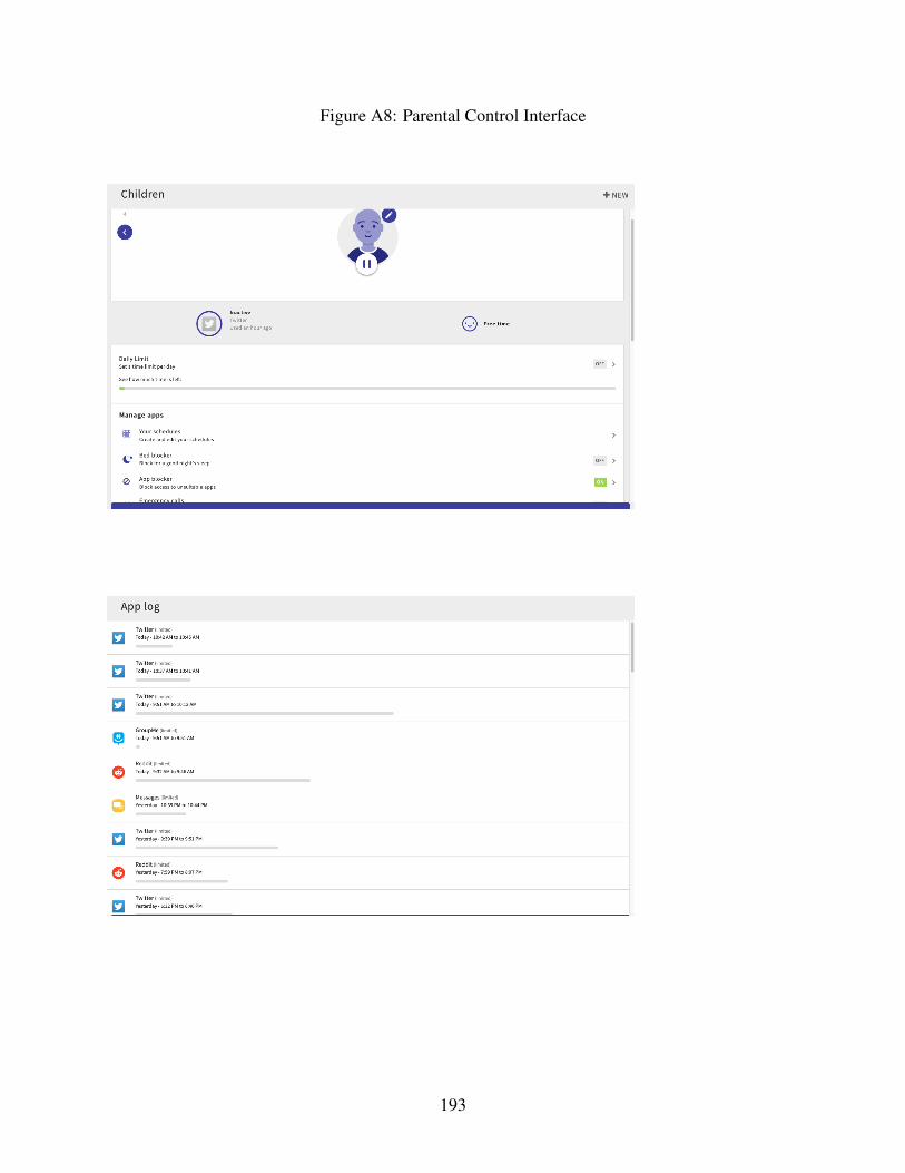
Figure A8: Parental Control Interface

193

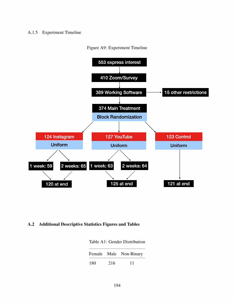
A.1.5 Experiment Timeline

Figure A9: Experiment Timeline

A.2 Additional Descriptive Statistics Figures and Tables

Table A1: Gender Distribution

Female Male Non-Binary

180 216 11

194

Table A2: Age Distribution

Minimum 25th Percentile 50th Percentile Mean 75th Percentile Maximum

18 21 23 25.92 27.0 73

Figure A10: Software Reliability

0

100

200

300

10 20 30Days with Active Software

Num

ber

of P

artic

ipan

ts

Active Software (All Participants)

0

100

200

300

20 30Days with Active Software

Num

ber

of P

artic

ipan

ts

Active Software (Main Restrictions)

Notes: The figure on the left shows the number of days with active software for all participants, including those whodropped out but whose data I do not drop entirely. The figure on the right shows the number of days with activesoftware for participants in the main experimental group and who stayed through the entirety of the study.

Figure A11: Distributions of Application Usage Across Treatment Groups

0.00

0.05

0.10

0.15

0 2 4 6asinh(Time on YouTube)

dens

ity

Treatment Control Instagram YouTube

0.0

0.1

0.2

0.3

0 2 4 6asinh(Time on Instagram)

dens

ity

Treatment Control Instagram YouTube

0.0

0.1

0.2

0.3

0.4

0 2 4 6asinh(Time on Other Social Media)

dens

ity

Treatment Control Instagram YouTube

Notes: The figures show the distribution of usage on YouTube (left), Instagram (middle), and other social media (right)during the baseline period across the different experimental treatment groups.

195

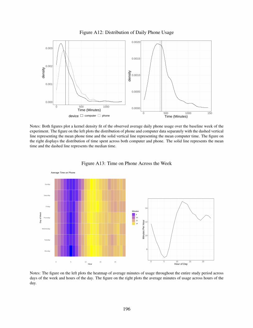
Figure A12: Distribution of Daily Phone Usage

0.000

0.001

0.002

0.003

0 500 1000Time (Minutes)

dens

ity

device computer phone

0.0000

0.0005

0.0010

0.0015

0.0020

0 500 1000 1500Time (Minutes)

dens

ityNotes: Both figures plot a kernel density fit of the observed average daily phone usage over the baseline week of theexperiment. The figure on the left plots the distribution of phone and computer data separately with the dashed verticalline representing the mean phone time and the solid vertical line representing the mean computer time. The figure onthe right displays the distribution of time spent across both computer and phone. The solid line represents the meantime and the dashed line represents the median time.

Figure A13: Time on Phone Across the Week

Monday

Tuesday

Wednesday

Thursday

Friday

Saturday

Sunday

0 5 10 15 20Hour

Day

of W

eek

Minutes

8

10

12

14

Average Time on Phone

8

10

12

14

0 5 10 15 20Hour of Day

Min

utes

Per

Hou

r

Notes: The figure on the left plots the heatmap of average minutes of usage throughout the entire study period acrossdays of the week and hours of the day. The figure on the right plots the average minutes of usage across hours of theday.

196

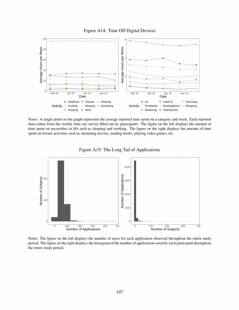
Figure A14: Time Off Digital Devices

0

10

20

30

40

50

Mar 29 Apr 05 Apr 12 Apr 19Date

Ave

rage

Hou

rs p

er W

eek

ActivityChildCare Classes Cleaning

Cooking Sleeping Socializing

Studying Work

2

4

6

Mar 29 Apr 05 Apr 12 Apr 19Date

Ave

rage

Hou

rs p

er W

eek

ActivityArt CableTV Exercising

PrintMedia ReadingBooks Shopping

Streaming VideoGames

Notes: A single point on the graph represents the average reported time spent on a category and week. Each reporteddata comes from the weekly time use survey filled out by participants. The figure on the left displays the amount oftime spent on necessities in life such as sleeping and working. The figure on the right displays the amount of timespent on leisure activities such as streaming movies, reading books, playing video games, etc.

Figure A15: The Long Tail of Applications

0

100

200

0 100 200 300 400 500Number of Applications

Num

ber

of S

ubje

cts

0

1000

2000

3000

4000

0 100 200 300 400Number of Subjects

Num

ber

of A

pplic

atio

ns

Notes: The figure on the left displays the number of users for each application observed throughout the entire studyperiod. The figure on the right displays the histogram of the number of applications used by each participant throughoutthe entire study period.

197

Table A3: Time Spent on Application Categories on Phone

Category Average Time Median Time Average Time | Usage Average Time | Usage Numbers of Users

social 66.09 52.22 68.74 53.73 374

entertainment 56.20 21.32 60.19 25.57 366

communication 54.75 40.86 55.17 41.00 389

game 23.77 0.57 42.38 16.93 175

tools 11.65 6.54 11.80 6.64 387

education 5.25 0.14 8.65 1.00 216

maps 4.51 0.83 6.39 2.11 276

business 4.49 0.50 6.58 2.39 254

productivity 4.32 1.43 4.73 1.64 358

news 3.77 0.00 8.51 1.50 130

shopping 3.32 0.29 5.26 1.46 230

sports 3.06 0.07 5.61 1.21 55

art 2.96 1.29 3.37 1.79 345

lifestyle 2.69 0.14 4.60 0.64 212

finance 2.19 0.71 2.64 1.29 316

dating 2.02 0.07 3.40 0.57 219

food 1.76 0.29 2.79 1.29 190

health 1.60 0.07 3.03 0.43 176

music 1.55 0.00 4.15 0.61 144

Notes: This table displays the time allocations for the product categories on the phone. The product categories are those assigned to the applica-

tions in the Google Play Store. I report average daily minutes spent on each category during the baseline week for the days when there were no

known issues with application usage logging. The first column displays the name of the application. The second and third columns display the

average and median minutes per day, respectively, across all participants. The fourth and fifth columns display the same quantities respectively,

but conditional only on the participants that make use of those applications. The sixth column displays the number of participants that use the

application.

198

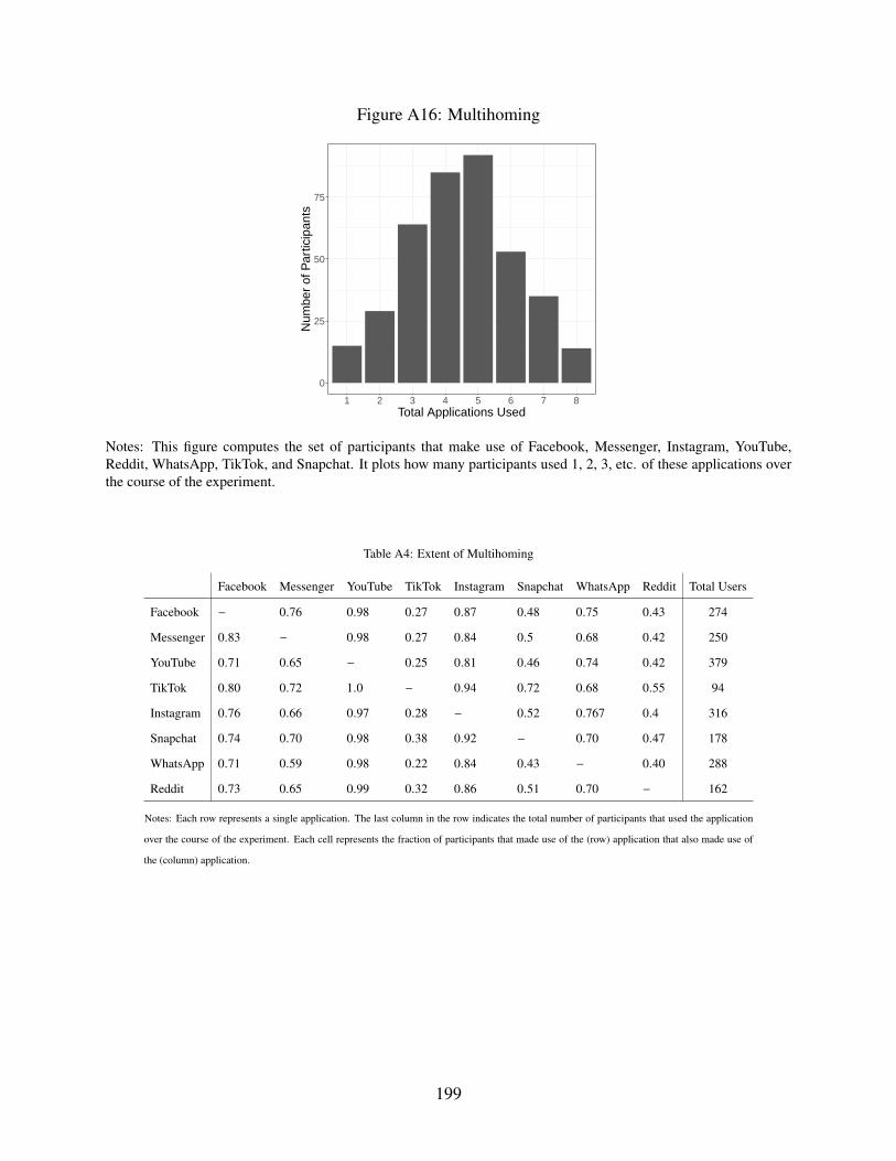
Figure A16: Multihoming

0

25

50

75

1 2 3 4 5 6 7 8Total Applications Used

Num

ber

of P

artic

ipan

ts

Notes: This figure computes the set of participants that make use of Facebook, Messenger, Instagram, YouTube,Reddit, WhatsApp, TikTok, and Snapchat. It plots how many participants used 1, 2, 3, etc. of these applications overthe course of the experiment.

Table A4: Extent of Multihoming

Facebook Messenger YouTube TikTok Instagram Snapchat WhatsApp Reddit Total Users

Facebook − 0.76 0.98 0.27 0.87 0.48 0.75 0.43 274

Messenger 0.83 − 0.98 0.27 0.84 0.5 0.68 0.42 250

YouTube 0.71 0.65 − 0.25 0.81 0.46 0.74 0.42 379

TikTok 0.80 0.72 1.0 − 0.94 0.72 0.68 0.55 94

Instagram 0.76 0.66 0.97 0.28 − 0.52 0.767 0.4 316

Snapchat 0.74 0.70 0.98 0.38 0.92 − 0.70 0.47 178

WhatsApp 0.71 0.59 0.98 0.22 0.84 0.43 − 0.40 288

Reddit 0.73 0.65 0.99 0.32 0.86 0.51 0.70 − 162

Notes: Each row represents a single application. The last column in the row indicates the total number of participants that used the application

over the course of the experiment. Each cell represents the fraction of participants that made use of the (row) application that also made use of

the (column) application.

199

Table A5: Time Spent on Applications of Interest

Application Medium Average Median Average | Usage Median | Usage Number of Participants

Other Applications computer 143.69 106.71 147.49 110.00 340

Other Applications phone 112.36 84.18 112.36 84.18 392

YouTube phone 41.56 11.71 48.63 17.86 335

YouTube computer 24.99 5.57 32.67 11.86 267

Instagram phone 22.44 9.29 29.82 19.00 295

WhatsApp phone 18.30 4.79 26.66 15.64 269

Facebook phone 13.10 0.71 21.86 7.57 235

TikTok phone 8.80 0.00 50.71 28.86 68

Reddit phone 7.61 0.00 21.62 5.36 138

Netflix computer 5.82 0.00 25.69 10.14 79

Messenger phone 5.55 0.07 10.47 1.96 208

Twitter phone 4.58 0.00 13.41 3.79 134

Netflix phone 4.16 0.00 22.65 3.57 72

Snapchat phone 3.58 0.00 9.30 3.86 151

Reddit computer 2.81 0.00 7.73 1.00 127

Facebook computer 2.63 0.14 5.19 1.57 177

Twitter computer 1.81 0.00 6.79 0.86 93

Messenger computer 1.28 0.00 13.96 6.21 32

Instagram computer 1.00 0.00 4.05 0.43 86

WhatsApp computer 0.15 0.00 8.52 6.07 6

TikTok computer 0.03 0.00 0.95 0.36 12

Snapchat computer 0.00 0.00 - - 0

Notes: This table displays the time allocations for the applications of interest. I report average daily minutes spent on each application during

the baseline week for the days when there were no known issues with application usage logging. The first and second column display the

name of the application and whether it was on the computer or phone. The third and fourth columns display the average and median minutes

per day, respectively, across all participants. The fifth and sixth columns display the same quantities respectively, but conditional only on the

participants that make use of those applications. The seventh column displays the number of participants that use the application.

200

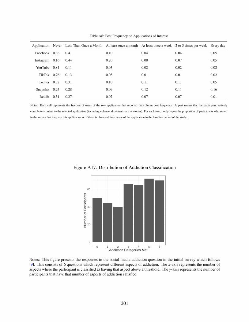
Table A6: Post Frequency on Applications of Interest

Application Never Less Than Once a Month At least once a month At least once a week 2 or 3 times per week Every day

Facebook 0.36 0.41 0.10 0.04 0.04 0.05

Instagram 0.16 0.44 0.20 0.08 0.07 0.05

YouTube 0.81 0.11 0.03 0.02 0.02 0.02

TikTok 0.76 0.13 0.08 0.01 0.01 0.02

Twitter 0.32 0.31 0.10 0.11 0.11 0.05

Snapchat 0.24 0.28 0.09 0.12 0.11 0.16

Reddit 0.51 0.27 0.07 0.07 0.07 0.01

Notes: Each cell represents the fraction of users of the row application that reported the column post frequency. A post means that the participant actively

contributes content to the selected application (including ephemeral content such as stories). For each row, I only report the proportion of participants who stated

in the survey that they use this application or if there is observed time usage of the application in the baseline period of the study.

Figure A17: Distribution of Addiction Classification

0

20

40

60

0 1 2 3 4 5 6Addiction Categories Met

Num

ber

of P

artic

ipan

ts

Notes: This figure presents the responses to the social media addiction question in the initial survey which follows[9]. This consists of 6 questions which represent different aspects of addiction. The x-axis represents the number ofaspects where the participant is classified as having that aspect above a threshold. The y-axis represents the number ofparticipants that have that number of aspects of addiction satisfied.

201

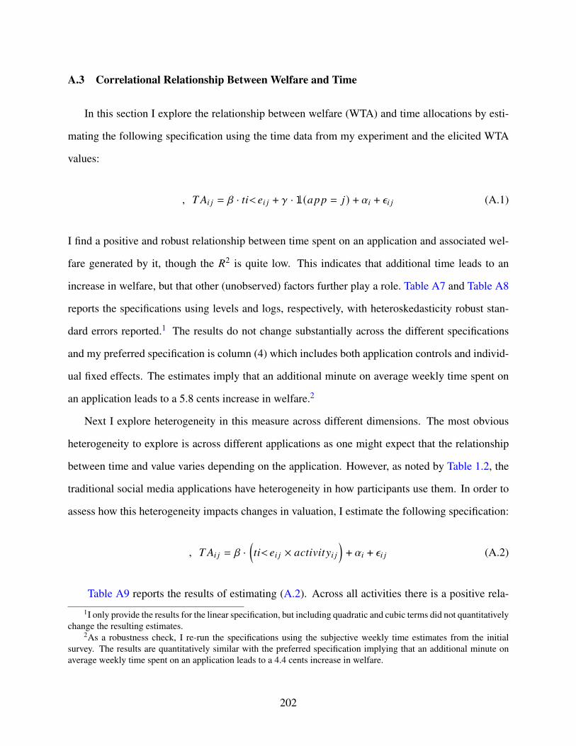
A.3 Correlational Relationship Between Welfare and Time

In this section I explore the relationship between welfare (WTA) and time allocations by esti-

mating the following specification using the time data from my experiment and the elicited WTA

values:

𝑊𝑇𝐴𝑖 𝑗 = 𝛽 · 𝑡𝑖𝑚𝑒𝑖 𝑗 + 𝛾 · 1(𝑎𝑝𝑝 = 𝑗) + 𝛼𝑖 + 𝜖𝑖 𝑗 (A.1)

I find a positive and robust relationship between time spent on an application and associated wel-

fare generated by it, though the 𝑅2 is quite low. This indicates that additional time leads to an

increase in welfare, but that other (unobserved) factors further play a role. Table A7 and Table A8

reports the specifications using levels and logs, respectively, with heteroskedasticity robust stan-

dard errors reported.1 The results do not change substantially across the different specifications

and my preferred specification is column (4) which includes both application controls and individ-

ual fixed effects. The estimates imply that an additional minute on average weekly time spent on

an application leads to a 5.8 cents increase in welfare.2

Next I explore heterogeneity in this measure across different dimensions. The most obvious

heterogeneity to explore is across different applications as one might expect that the relationship

between time and value varies depending on the application. However, as noted by Table 1.2, the

traditional social media applications have heterogeneity in how participants use them. In order to

assess how this heterogeneity impacts changes in valuation, I estimate the following specification:

𝑊𝑇𝐴𝑖 𝑗 = 𝛽 ·(𝑡𝑖𝑚𝑒𝑖 𝑗 × 𝑎𝑐𝑡𝑖𝑣𝑖𝑡𝑦𝑖 𝑗

)+ 𝛼𝑖 + 𝜖𝑖 𝑗 (A.2)

Table A9 reports the results of estimating (A.2). Across all activities there is a positive rela-

1I only provide the results for the linear specification, but including quadratic and cubic terms did not quantitativelychange the resulting estimates.

2As a robustness check, I re-run the specifications using the subjective weekly time estimates from the initialsurvey. The results are quantitatively similar with the preferred specification implying that an additional minute onaverage weekly time spent on an application leads to a 4.4 cents increase in welfare.

202

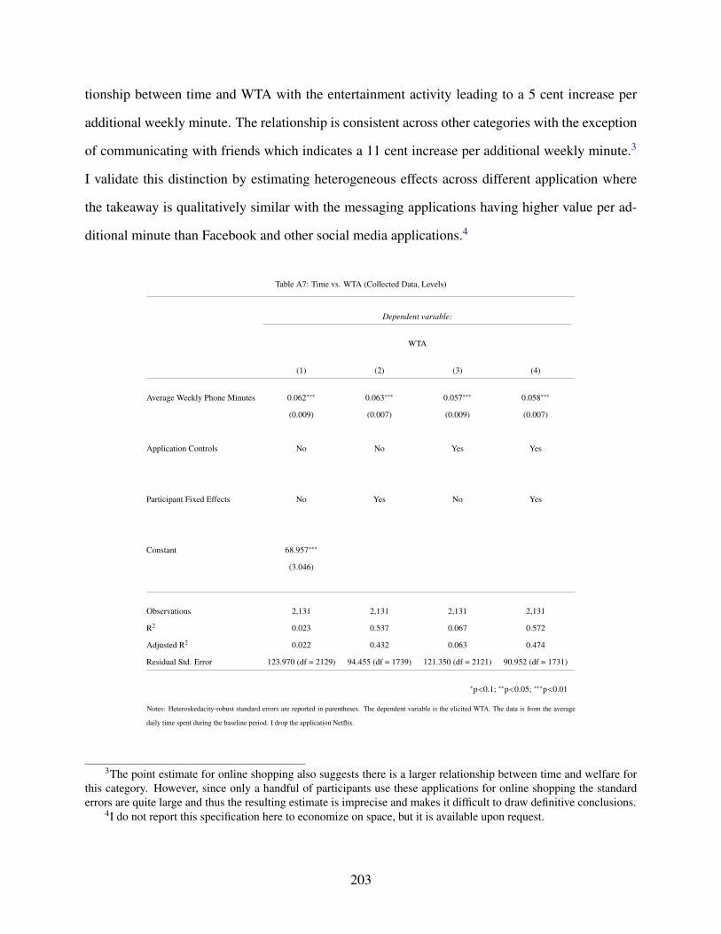
tionship between time and WTA with the entertainment activity leading to a 5 cent increase per

additional weekly minute. The relationship is consistent across other categories with the exception

of communicating with friends which indicates a 11 cent increase per additional weekly minute.3

I validate this distinction by estimating heterogeneous effects across different application where

the takeaway is qualitatively similar with the messaging applications having higher value per ad-

ditional minute than Facebook and other social media applications.4

Table A7: Time vs. WTA (Collected Data, Levels)

Dependent variable:

WTA

(1) (2) (3) (4)

Average Weekly Phone Minutes 0.062∗∗∗ 0.063∗∗∗ 0.057∗∗∗ 0.058∗∗∗

(0.009) (0.007) (0.009) (0.007)

Application Controls No No Yes Yes

Participant Fixed Effects No Yes No Yes

Constant 68.957∗∗∗

(3.046)

Observations 2,131 2,131 2,131 2,131

R2 0.023 0.537 0.067 0.572

Adjusted R2 0.022 0.432 0.063 0.474

Residual Std. Error 123.970 (df = 2129) 94.455 (df = 1739) 121.350 (df = 2121) 90.952 (df = 1731)

∗p<0.1; ∗∗p<0.05; ∗∗∗p<0.01

Notes: Heteroskedacity-robust standard errors are reported in parentheses. The dependent variable is the elicited WTA. The data is from the average

daily time spent during the baseline period. I drop the application Netflix.

3The point estimate for online shopping also suggests there is a larger relationship between time and welfare forthis category. However, since only a handful of participants use these applications for online shopping the standarderrors are quite large and thus the resulting estimate is imprecise and makes it difficult to draw definitive conclusions.

4I do not report this specification here to economize on space, but it is available upon request.

203

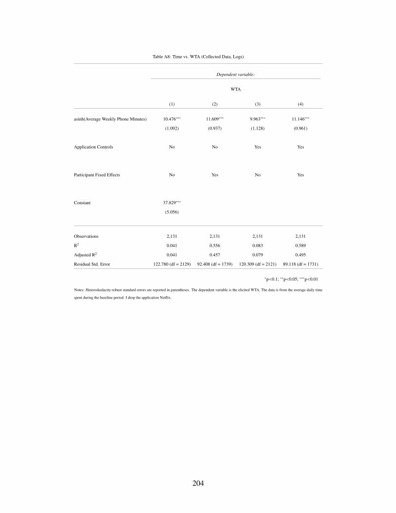
Table A8: Time vs. WTA (Collected Data, Logs)

Dependent variable:

WTA

(1) (2) (3) (4)

asinh(Average Weekly Phone Minutes) 10.476∗∗∗ 11.609∗∗∗ 9.963∗∗∗ 11.146∗∗∗

(1.092) (0.937) (1.128) (0.961)

Application Controls No No Yes Yes

Participant Fixed Effects No Yes No Yes

Constant 37.829∗∗∗

(5.056)

Observations 2,131 2,131 2,131 2,131

R2 0.041 0.556 0.083 0.589

Adjusted R2 0.041 0.457 0.079 0.495

Residual Std. Error 122.780 (df = 2129) 92.408 (df = 1739) 120.309 (df = 2121) 89.118 (df = 1731)

∗p<0.1; ∗∗p<0.05; ∗∗∗p<0.01

Notes: Heteroskedacity-robust standard errors are reported in parentheses. The dependent variable is the elicited WTA. The data is from the average daily time

spent during the baseline period. I drop the application Netflix.

204

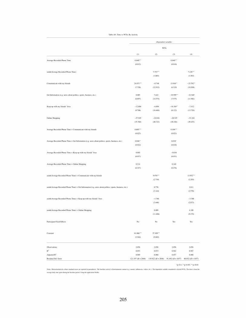
Table A9: Time vs WTA, By Activity

Dependent variable:

WTA

(1) (2) (3) (4)

Average Recorded Phone Time 0.040∗∗∗ 0.040∗∗∗

(0.012) (0.010)

asinh(Average Recorded Phone Time) 7.753∗∗∗ 7.126∗∗∗

(1.865) (1.563)

Communicate with my friends 24.071∗∗∗ −0.748 13.916∗∗ −25.792∗∗

(7.728) (12.912) (6.319) (10.508)

Get Information (e.g. news about politics, sports, business, etc.) 0.085 7.422 −19.599∗∗∗ −22.540∗

(8.897) (14.574) (7.575) (11.982)

Keep up with my friends’ lives −12.806 −6.894 −16.184∗∗ −7.412

(9.708) (16.460) (8.122) (13.720)

Online Shopping −37.945 −22.816 −28.525 −31.164

(35.760) (48.723) (30.326) (39.453)

Average Recorded Phone Time × Communicate with my friends 0.095∗∗∗ 0.109∗∗∗

(0.025) (0.021)

Average Recorded Phone Time × Get Information (e.g. news about politics, sports, business, etc.) 0.046∗∗ 0.034∗

(0.022) (0.018)

Average Recorded Phone Time × Keep up with my friends’ lives 0.003 −0.016

(0.037) (0.031)

Average Recorded Phone Time × Online Shopping 0.214 0.140

(0.327) (0.276)

asinh(Average Recorded Phone Time) × Communicate with my friends 9.976∗∗∗ 13.952∗∗∗

(2.710) (2.203)

asinh(Average Recorded Phone Time) × Get Information (e.g. news about politics, sports, business, etc.) 0.776 2.811

(3.144) (2.578)

asinh(Average Recorded Phone Time) × Keep up with my friends’ lives −1.766 −3.388

(3.440) (2.873)

asinh(Average Recorded Phone Time) × Online Shopping 0.089 4.108

(11.406) (9.279)

Participant Fixed Effects No No Yes Yes

Constant 61.886∗∗∗ 37.109∗∗∗

(5.564) (9.602)

Observations 2,056 2,056 2,056 2,056

R2 0.053 0.072 0.562 0.587

Adjusted R2 0.049 0.068 0.457 0.488

Residual Std. Error 121.107 (df = 2046) 119.922 (df = 2046) 91.492 (df = 1657) 88.852 (df = 1657)

∗p<0.1; ∗∗p<0.05; ∗∗∗p<0.01

Notes: Heteroskedasticity-robust standard errors are reported in parentheses. The baseline activity is Entertainment content (e.g. memes, influencers, videos, etc.). The dependent variable considered is elicited WTA. The data is from the

average daily time spent during the baseline period. I drop the application Netflix.

205

A.4 Additional Experimental Results

Figure A18: Quantile Treatment Effects of Category Substitution

0.2 0.4 0.6 0.8

−2.

5−

2.0

−1.

5−

1.0

−0.

50.

0

YouTube QTE (Entertainment)

tau

asin

h(M

inut

es P

er D

ay)

0.2 0.4 0.6 0.8

−2.

5−

2.0

−1.

5−

1.0

−0.

50.

0

Instagram QTE (Social Media)

tauas

inh(

Min

utes

Per

Day

)

0.2 0.4 0.6 0.8

−2.

5−

2.0

−1.

5−

1.0

−0.

50.

0

YouTube QTE w/ Computer (Entertainment)

tau

asin

h(M

inut

es P

er D

ay)

0.2 0.4 0.6 0.8

−2.

5−

2.0

−1.

5−

1.0

−0.

50.

0Instagram QTE w/ Computer (Social Media)

tau

asin

h(M

inut

es P

er D

ay)

0.2 0.4 0.6 0.8

−0.

4−

0.2

0.0

0.2

0.4

Instagram QTE (Communication)

tau

asin

h(M

inut

es P

er D

ay)

0.2 0.4 0.6 0.8

−0.

4−

0.2

0.0

0.2

0.4

YouTube QTE (Social Media)

tau

asin

h(M

inut

es P

er D

ay)

Notes: Each figure shows the QTE for an outcome variable. The title of the figure indicates the treatment and theparentheses indicates the outcome variable. The figure on the first row and first column is titled YouTube QTE(Entertainment) meaning that I focus on the YouTube treatment and the entertainment category. The figures in themiddle row include time from the Chrome extension, whereas the rest only include time from the phone.

206

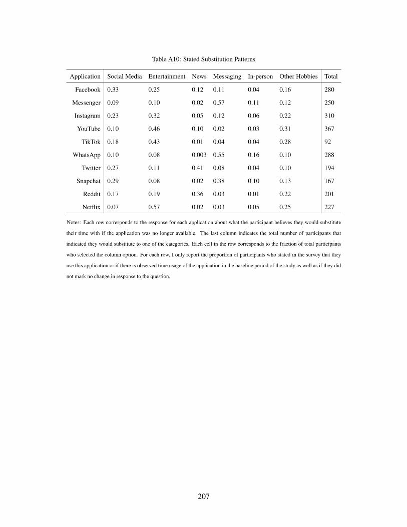
Table A10: Stated Substitution Patterns

Application Social Media Entertainment News Messaging In-person Other Hobbies Total

Facebook 0.33 0.25 0.12 0.11 0.04 0.16 280

Messenger 0.09 0.10 0.02 0.57 0.11 0.12 250

Instagram 0.23 0.32 0.05 0.12 0.06 0.22 310

YouTube 0.10 0.46 0.10 0.02 0.03 0.31 367

TikTok 0.18 0.43 0.01 0.04 0.04 0.28 92

WhatsApp 0.10 0.08 0.003 0.55 0.16 0.10 288

Twitter 0.27 0.11 0.41 0.08 0.04 0.10 194

Snapchat 0.29 0.08 0.02 0.38 0.10 0.13 167

Reddit 0.17 0.19 0.36 0.03 0.01 0.22 201

Netflix 0.07 0.57 0.02 0.03 0.05 0.25 227

Notes: Each row corresponds to the response for each application about what the participant believes they would substitute

their time with if the application was no longer available. The last column indicates the total number of participants that

indicated they would substitute to one of the categories. Each cell in the row corresponds to the fraction of total participants

who selected the column option. For each row, I only report the proportion of participants who stated in the survey that they

use this application or if there is observed time usage of the application in the baseline period of the study as well as if they did

not mark no change in response to the question.

207

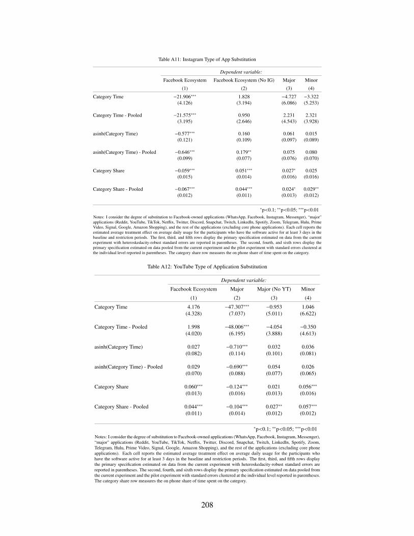
Table A11: Instagram Type of App Substitution

Dependent variable:

Facebook Ecosystem Facebook Ecosystem (No IG) Major Minor

(1) (2) (3) (4)

Category Time −21.906∗∗∗ 1.828 −4.727 −3.322(4.126) (3.194) (6.086) (5.253)

Category Time - Pooled −21.575∗∗∗ 0.950 2.231 2.321(3.195) (2.646) (4.543) (3.928)

asinh(Category Time) −0.577∗∗∗ 0.160 0.061 0.015(0.121) (0.109) (0.097) (0.089)

asinh(Category Time) - Pooled −0.646∗∗∗ 0.179∗∗ 0.075 0.080(0.099) (0.077) (0.076) (0.070)

Category Share −0.059∗∗∗ 0.051∗∗∗ 0.027∗ 0.025(0.015) (0.014) (0.016) (0.016)

Category Share - Pooled −0.067∗∗∗ 0.044∗∗∗ 0.024∗ 0.029∗∗

(0.012) (0.011) (0.013) (0.012)

∗p<0.1; ∗∗p<0.05; ∗∗∗p<0.01Notes: I consider the degree of substitution to Facebook-owned applications (WhatsApp, Facebook, Instagram, Messenger), “major"applications (Reddit, YouTube, TikTok, Netflix, Twitter, Discord, Snapchat, Twitch, LinkedIn, Spotify, Zoom, Telegram, Hulu, PrimeVideo, Signal, Google, Amazon Shopping), and the rest of the applications (excluding core phone applications). Each cell reports theestimated average treatment effect on average daily usage for the participants who have the software active for at least 3 days in thebaseline and restriction periods. The first, third, and fifth rows display the primary specification estimated on data from the currentexperiment with heteroskedacity-robust standard errors are reported in parentheses. The second, fourth, and sixth rows display theprimary specification estimated on data pooled from the current experiment and the pilot experiment with standard errors clustered atthe individual level reported in parentheses. The category share row measures the on phone share of time spent on the category.

Table A12: YouTube Type of Application Substitution

Dependent variable:

Facebook Ecosystem Major Major (No YT) Minor

(1) (2) (3) (4)

Category Time 4.176 −47.307∗∗∗ −0.953 1.046(4.328) (7.037) (5.011) (6.622)

Category Time - Pooled 1.998 −48.006∗∗∗ −4.054 −0.350(4.020) (6.195) (3.888) (4.613)

asinh(Category Time) 0.027 −0.710∗∗∗ 0.032 0.036(0.082) (0.114) (0.101) (0.081)

asinh(Category Time) - Pooled 0.029 −0.690∗∗∗ 0.054 0.026(0.070) (0.088) (0.077) (0.065)

Category Share 0.060∗∗∗ −0.124∗∗∗ 0.021 0.056∗∗∗

(0.013) (0.016) (0.013) (0.016)

Category Share - Pooled 0.044∗∗∗ −0.104∗∗∗ 0.027∗∗ 0.057∗∗∗

(0.011) (0.014) (0.012) (0.012)

∗p<0.1; ∗∗p<0.05; ∗∗∗p<0.01Notes: I consider the degree of substitution to Facebook-owned applications (WhatsApp, Facebook, Instagram, Messenger),“major" applications (Reddit, YouTube, TikTok, Netflix, Twitter, Discord, Snapchat, Twitch, LinkedIn, Spotify, Zoom,Telegram, Hulu, Prime Video, Signal, Google, Amazon Shopping), and the rest of the applications (excluding core phoneapplications). Each cell reports the estimated average treatment effect on average daily usage for the participants whohave the software active for at least 3 days in the baseline and restriction periods. The first, third, and fifth rows displaythe primary specification estimated on data from the current experiment with heteroskedacity-robust standard errors arereported in parentheses. The second, fourth, and sixth rows display the primary specification estimated on data pooled fromthe current experiment and the pilot experiment with standard errors clustered at the individual level reported in parentheses.The category share row measures the on phone share of time spent on the category.

208

Table A13: Survey of Time on Restricted App During Treatment Week Off Phone

Dependent variable:

Other Device

Instagram Time

Other Device

YouTube Time

asinh(Other Device

Instagram Time)

asinh(Other Device

YouTube Time)

(1) (2) (3) (4)

YouTube Treatment −8.151 −0.409∗∗

(6.850) (0.207)

Instagram Treatment −1.941 −0.042

(1.964) (0.181)

Baseline Time Controls Yes Yes Yes Yes

Block Control Yes Yes Yes Yes

Observations 231 238 231 238

R2 0.103 0.182 0.316 0.311

Adjusted R2 0.036 0.123 0.265 0.261

Residual Std. Error 14.854 (df = 214) 52.686 (df = 221) 1.370 (df = 214) 1.594 (df = 221)

∗p<0.1; ∗∗p<0.05; ∗∗∗p<0.01

Notes: Heteroskedasticity-robust standard errors are reported in parentheses. The first and third columns present the results of a regres-

sion of self-reported time on Instagram on other devices between the Instagram restriction group and the control group. The second and

fourth columns present the results of a regression of self-reported time on YouTube on other devices between the YouTube restriction

group and the control group. The dependent variable considered in the regressions is the average daily minutes of usage on the column

variable.

209

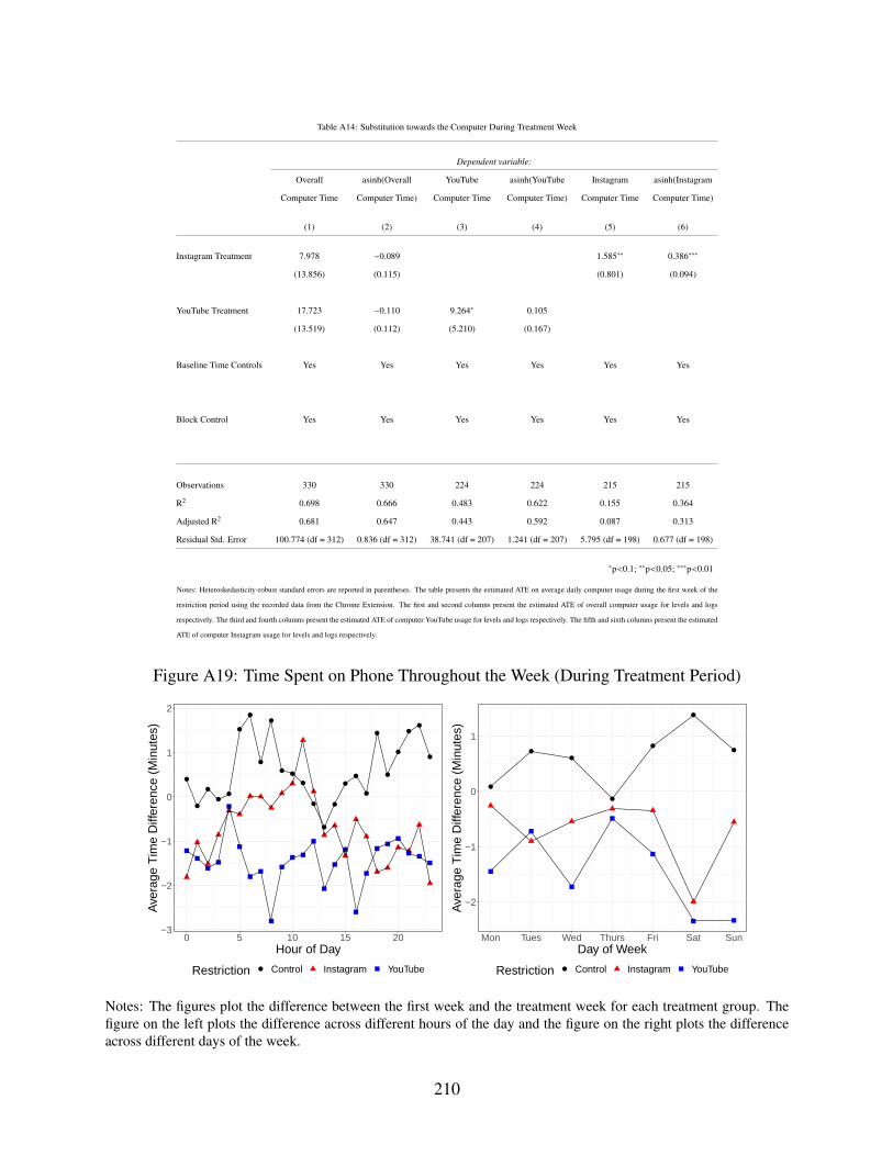
Table A14: Substitution towards the Computer During Treatment Week

Dependent variable:

Overall asinh(Overall YouTube asinh(YouTube Instagram asinh(Instagram

Computer Time Computer Time) Computer Time Computer Time) Computer Time Computer Time)

(1) (2) (3) (4) (5) (6)

Instagram Treatment 7.978 −0.089 1.585∗∗ 0.386∗∗∗

(13.856) (0.115) (0.801) (0.094)

YouTube Treatment 17.723 −0.110 9.264∗ 0.105

(13.519) (0.112) (5.210) (0.167)

Baseline Time Controls Yes Yes Yes Yes Yes Yes

Block Control Yes Yes Yes Yes Yes Yes

Observations 330 330 224 224 215 215

R2 0.698 0.666 0.483 0.622 0.155 0.364

Adjusted R2 0.681 0.647 0.443 0.592 0.087 0.313

Residual Std. Error 100.774 (df = 312) 0.836 (df = 312) 38.741 (df = 207) 1.241 (df = 207) 5.795 (df = 198) 0.677 (df = 198)

∗p<0.1; ∗∗p<0.05; ∗∗∗p<0.01

Notes: Heteroskedasticity-robust standard errors are reported in parentheses. The table presents the estimated ATE on average daily computer usage during the first week of the

restriction period using the recorded data from the Chrome Extension. The first and second columns present the estimated ATE of overall computer usage for levels and logs

respectively. The third and fourth columns present the estimated ATE of computer YouTube usage for levels and logs respectively. The fifth and sixth columns present the estimated

ATE of computer Instagram usage for levels and logs respectively.

Figure A19: Time Spent on Phone Throughout the Week (During Treatment Period)

−3

−2

−1

0

1

2

0 5 10 15 20Hour of Day

Ave

rage

Tim

e D

iffer

ence

(M

inut

es)

Restriction Control Instagram YouTube

−2

−1

0

1

Mon Tues Wed Thurs Fri Sat SunDay of Week

Ave

rage

Tim

e D

iffer

ence

(M

inut

es)

Restriction Control Instagram YouTube

Notes: The figures plot the difference between the first week and the treatment week for each treatment group. Thefigure on the left plots the difference across different hours of the day and the figure on the right plots the differenceacross different days of the week.

210

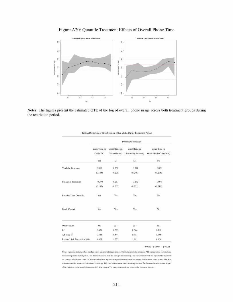
Figure A20: Quantile Treatment Effects of Overall Phone Time

0.2 0.4 0.6 0.8

−0.

4−

0.3

−0.

2−

0.1

0.0

0.1

0.2

Instagram QTE (Overall Phone Time)

tau

asin

h(M

inut

es P

er D

ay)

0.2 0.4 0.6 0.8

−0.

4−

0.3

−0.

2−

0.1

0.0

0.1

0.2

YouTube QTE (Overall Phone Time)

tau

asin

h(M

inut

es P

er D

ay)

Notes: The figures present the estimated QTE of the log of overall phone usage across both treatment groups duringthe restriction period.

Table A15: Survey of Time Spent on Other Media During Restriction Period

Dependent variable:

asinh(Time on asinh(Time on asinh(Time on asinh(Time on

Cable TV) Video Games) Streaming Services) Other Media Composite)

(1) (2) (3) (4)

YouTube Treatment 0.015 0.258 −0.381 −0.076

(0.185) (0.205) (0.248) (0.208)

Instagram Treatment −0.290 0.217 −0.292 −0.079

(0.187) (0.207) (0.251) (0.210)

Baseline Time Controls Yes Yes Yes Yes

Block Control Yes Yes Yes Yes

Observations 357 357 357 357

R2 0.471 0.565 0.344 0.386

Adjusted R2 0.444 0.544 0.311 0.355

Residual Std. Error (df = 339) 1.423 1.575 1.911 1.604

∗p<0.1; ∗∗p<0.05; ∗∗∗p<0.01

Notes: Heteroskedasticity-robust standard errors are reported in parentheses. This table reports the estimated ATE on time spent on non-phone

media during the restriction period. The data for this come from the weekly time use survey. The first column reports the impact of the treatment

on average daily time on cable TV. The second column reports the impact of the treatment on average daily time on video games. The third

column reports the impact of the treatment on average daily time on non-phone video streaming services. The fourth column reports the impact

of the treatment on the sum of the average daily time on cable TV, video games, and non-phone video streaming services.

211

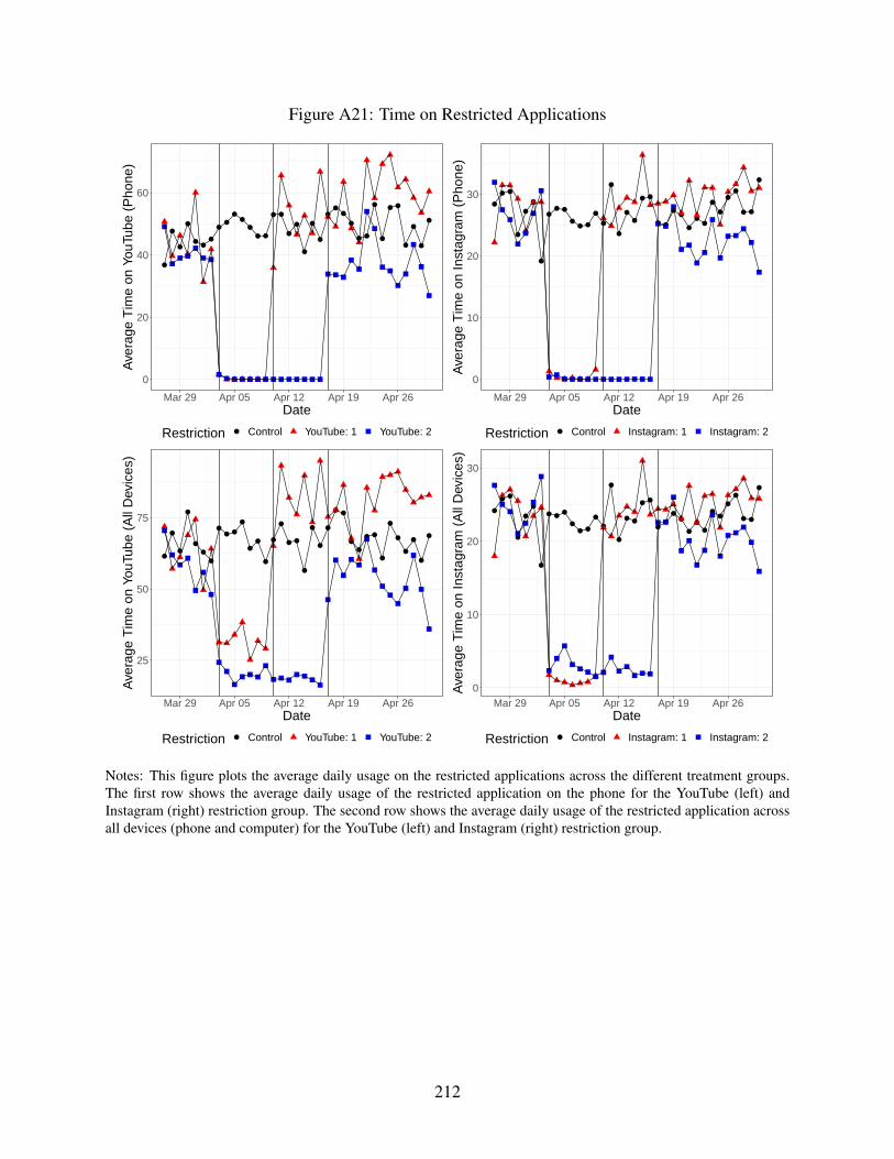
Figure A21: Time on Restricted Applications

0

20

40

60

Mar 29 Apr 05 Apr 12 Apr 19 Apr 26Date

Ave

rage

Tim

e on

You

Tube

(P

hone

)

Restriction Control YouTube: 1 YouTube: 2

0

10

20

30

Mar 29 Apr 05 Apr 12 Apr 19 Apr 26Date

Ave

rage

Tim

e on

Inst

agra

m (

Pho

ne)

Restriction Control Instagram: 1 Instagram: 2

25

50

75

Mar 29 Apr 05 Apr 12 Apr 19 Apr 26Date

Ave

rage

Tim

e on

You

Tube

(A

ll D

evic

es)

Restriction Control YouTube: 1 YouTube: 2

0

10

20

30

Mar 29 Apr 05 Apr 12 Apr 19 Apr 26Date

Ave

rage

Tim

e on

Inst

agra

m (

All

Dev

ices

)

Restriction Control Instagram: 1 Instagram: 2

Notes: This figure plots the average daily usage on the restricted applications across the different treatment groups.The first row shows the average daily usage of the restricted application on the phone for the YouTube (left) andInstagram (right) restriction group. The second row shows the average daily usage of the restricted application acrossall devices (phone and computer) for the YouTube (left) and Instagram (right) restriction group.

212

Table A16: Instagram Post-Restriction Usage

Dependent variable:

Instagram Time asinh(Instagram Time) Instagram Time asinh(Instagram Time)

(1) (2) (3) (4)

Instagram Treatment 4.845 0.177 −5.164∗∗ −0.061

(3.438) (0.166) (2.483) (0.134)

2 week restriction 3.180 0.038

(3.048) (0.179)

Instagram Treatment × 2 week restriction −10.452∗∗ −0.231

(4.746) (0.232)

Baseline Usage Yes Yes Yes Yes

Week Fixed Effects Yes Yes Yes Yes

Block Control Yes Yes Yes Yes

Observations 410 410 312 312

R2 0.696 0.731 0.707 0.732

Adjusted R2 0.680 0.717 0.689 0.716

Residual Std. Error 17.437 (df = 389) 0.912 (df = 389) 16.398 (df = 293) 0.918 (df = 293)

∗p<0.1; ∗∗p<0.05; ∗∗∗p<0.01

Notes: The standard errors for the regression are clustered at the participant level. The regression is estimated on the data of weekly time usage of Instagram in the

weeks following the restriction period. The dependent variables reported are both the levels and logs of Instagram usage. The first two columns report the regression

across all restriction groups with heterogeneous effects across restriction lengths. The last two columns report the regression on the entire control group and restricting

focus to the 2 week Instagram restriction group.

213

Table A17: YouTube Post-Restriction Usage

Dependent variable:

YouTube Time asinh(YouTube Time) YouTube Time asinh(YouTube Time)

(1) (2) (3) (4)

YouTube Treatment 1.067 −0.078 −9.028 −0.173

(10.492) (0.160) (6.762) (0.191)

2 week restriction −9.093 −0.258

(9.021) (0.213)

YouTube Treatment × 2 week restriction −6.640 0.004

(10.639) (0.273)

Baseline Usage Yes Yes Yes Yes

Week Fixed Effects Yes Yes Yes Yes

Block Control Yes Yes Yes Yes

Observations 480 480 360 360

R2 0.558 0.674 0.531 0.619

Adjusted R2 0.539 0.660 0.506 0.599

Residual Std. Error 55.046 (df = 459) 1.190 (df = 459) 56.989 (df = 341) 1.266 (df = 341)

∗p<0.1; ∗∗p<0.05; ∗∗∗p<0.01

Notes: The standard errors for the regression are clustered at the participant level. The regression is estimated on the data of weekly time usage of YouTube in

the weeks following the restriction period. The dependent variables reported are both the levels and logs of YouTube usage. The first two columns report the

regression across all restriction groups with heterogeneous effects across restriction lengths. The last two columns report the regression on the entire control group

and restricting focus to the 2 week YouTube restriction group.

214

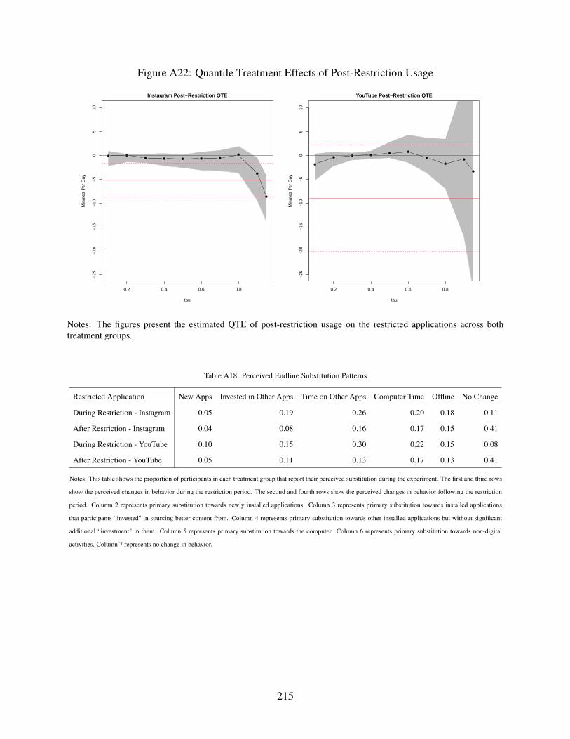
Figure A22: Quantile Treatment Effects of Post-Restriction Usage

0.2 0.4 0.6 0.8

−25

−20

−15

−10

−5

05

10Instagram Post−Restriction QTE

tau

Min

utes

Per

Day

0.2 0.4 0.6 0.8

−25

−20

−15

−10

−5

05

10

YouTube Post−Restriction QTE

tau

Min

utes

Per

Day

Notes: The figures present the estimated QTE of post-restriction usage on the restricted applications across bothtreatment groups.

Table A18: Perceived Endline Substitution Patterns

Restricted Application New Apps Invested in Other Apps Time on Other Apps Computer Time Offline No Change

During Restriction - Instagram 0.05 0.19 0.26 0.20 0.18 0.11

After Restriction - Instagram 0.04 0.08 0.16 0.17 0.15 0.41

During Restriction - YouTube 0.10 0.15 0.30 0.22 0.15 0.08

After Restriction - YouTube 0.05 0.11 0.13 0.17 0.13 0.41

Notes: This table shows the proportion of participants in each treatment group that report their perceived substitution during the experiment. The first and third rows

show the perceived changes in behavior during the restriction period. The second and fourth rows show the perceived changes in behavior following the restriction

period. Column 2 represents primary substitution towards newly installed applications. Column 3 represents primary substitution towards installed applications

that participants “invested" in sourcing better content from. Column 4 represents primary substitution towards other installed applications but without significant

additional “investment" in them. Column 5 represents primary substitution towards the computer. Column 6 represents primary substitution towards non-digital

activities. Column 7 represents no change in behavior.

215

Table A19: One Month Post-Experiment Survey Results

Dependent variable:

Phone Time Social Media Time Instagram Time YouTube Time

(1) (2) (3) (4)

Instagram Restriction −0.115 −0.305∗∗ −0.316∗ −0.113

(0.147) (0.150) (0.189) (0.178)

YouTube Restriction 0.087 −0.003 0.189 −0.268

(0.145) (0.148) (0.186) (0.176)

Block Control No No No No

Constant 2.811∗∗∗ 2.698∗∗∗ 2.756∗∗∗ 3.113∗∗∗

(0.106) (0.107) (0.137) (0.127)

Observations 168 168 149 167

R2 0.012 0.033 0.051 0.014

Adjusted R2 −0.00004 0.021 0.038 0.002

Residual Std. Error 0.768 (df = 165) 0.783 (df = 165) 0.920 (df = 146) 0.927 (df = 164)

∗p<0.1; ∗∗p<0.05; ∗∗∗p<0.01

Notes: Heteroskedasticity-robust standard errors are reported in parentheses. The data comes from the survey sent one month

after the study concluded where participants indicated whether they were spending significantly less time (1), somewhat less

time (2), the same time (3), somewhat more time (4), or significantly more time (5) on each outcome variable. The dependent

variable in column 1 is the overall phone time, in column 2 is overall social media time, in column 3 is Instagram time, and

column 4 is YouTube time. For the YouTube and Instagram time dependent variables, I drop participants who marked that they

do not use the respective application or started to use it during the study.

216

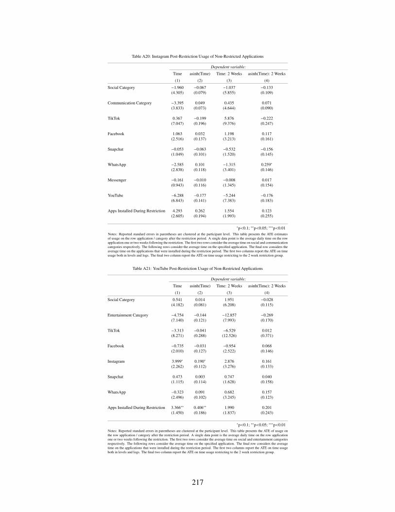
Table A20: Instagram Post-Restriction Usage of Non-Restricted Applications

Dependent variable:

Time asinh(Time) Time: 2 Weeks asinh(Time): 2 Weeks

(1) (2) (3) (4)

Social Category −1.960 −0.067 −1.037 −0.133(4.305) (0.079) (5.855) (0.109)

Communication Category −3.395 0.049 0.435 0.071(3.833) (0.073) (4.644) (0.090)

TikTok 0.367 −0.199 5.876 −0.222(7.047) (0.196) (9.376) (0.247)

Facebook 1.063 0.032 1.198 0.117(2.516) (0.137) (3.213) (0.161)

Snapchat −0.053 −0.063 −0.532 −0.156(1.049) (0.101) (1.520) (0.145)

WhatsApp −2.585 0.101 −1.315 0.259∗

(2.838) (0.118) (3.401) (0.146)

Messenger −0.161 −0.010 −0.008 0.017(0.943) (0.116) (1.345) (0.154)

YouTube −6.288 −0.177 −5.244 −0.176(6.843) (0.141) (7.383) (0.183)

Apps Installed During Restriction 4.293 0.262 1.554 0.123(2.605) (0.194) (1.993) (0.255)

∗p<0.1; ∗∗p<0.05; ∗∗∗p<0.01Notes: Reported standard errors in parentheses are clustered at the participant level. This table presents the ATE estimatesof usage on the row application / category after the restriction period. A single data point is the average daily time on the rowapplication one or two weeks following the restriction. The first two rows consider the average time on social and communicationcategories respectively. The following rows consider the average time on the specified application. The final row considers theaverage time on the applications that were installed during the restriction period. The first two columns report the ATE on timeusage both in levels and logs. The final two column report the ATE on time usage restricting to the 2 week restriction group.

Table A21: YouTube Post-Restriction Usage of Non-Restricted Applications

Dependent variable:

Time asinh(Time) Time: 2 Weeks asinh(Time): 2 Weeks

(1) (2) (3) (4)

Social Category 0.541 0.014 1.951 −0.028(4.182) (0.081) (6.208) (0.115)

Entertainment Category −4.754 −0.144 −12.857 −0.269(7.140) (0.121) (7.993) (0.170)

TikTok −3.313 −0.041 −6.529 0.012(8.271) (0.288) (12.526) (0.371)

Facebook −0.735 −0.031 −0.954 0.068(2.010) (0.127) (2.522) (0.146)

Instagram 3.999∗ 0.190∗ 2.876 0.161(2.262) (0.112) (3.276) (0.133)

Snapchat 0.473 0.003 0.747 0.040(1.115) (0.114) (1.628) (0.158)

WhatsApp −0.323 0.091 0.682 0.157(2.496) (0.102) (3.245) (0.123)

Apps Installed During Restriction 3.366∗∗ 0.406∗∗ 1.990 0.201(1.450) (0.186) (1.837) (0.243)

∗p<0.1; ∗∗p<0.05; ∗∗∗p<0.01Notes: Reported standard errors in parentheses are clustered at the participant level. This table presents the ATE of usage onthe row application / category after the restriction period. A single data point is the average daily time on the row applicationone or two weeks following the restriction. The first two rows consider the average time on social and entertainment categoriesrespectively. The following rows consider the average time on the specified application. The final row considers the averagetime on the applications that were installed during the restriction period. The first two columns report the ATE on time usageboth in levels and logs. The final two column report the ATE on time usage restricting to the 2 week restriction group.

217

A.5 Alternative Estimation of Diversion Ratios

In this section I provide an alternative method of estimating the diversion ratios required for the

UPP test. I follow the methods proposed in [8, 32] that directly exploit the experimental product

unavailability variation to estimate the diversion ratios. The method proceeds by first using the

estimated average treatment effects between the restricted applications and the other applications

of interest to estimate the diversion ratios from the restricted applications to other applications.

This provides a nonparametric estimate of the diversion ratio between these applications. Then, I

impose a semiparametric logit assumption and, using the aggregate market shares and the estimated

diversion ratios, an MPEC procedure enables the estimation of the rest of the matrix of diversion

ratios.

A.5.1 Estimation Procedure

I restrict to the same set of prominent social media and entertainment applications as in the

main text: Snapchat, Facebook, Reddit, TikTok, Instagram, YouTube, and Twitter. The outside

option is defined as time not on the phone and other applications on the phone. Thus, I have a

choice set of 𝐽 = 7 applications plus an outside option and the goal is to estimate the 𝐽 × (𝐽 + 1)

matrix of diversion ratios. I aggregate time spent during these time periods as follows. I consider

that each time of day has 𝑇 time periods of half minute units. I aggregate time spent during these

time periods in order to compute market shares for each individual. I drop the “late night" hours

so that I only consider 17 hours in the day.

There are 𝐼 individuals, 𝐽 + 1 applications (including outside option), and 𝑇 time periods. I

denote the choice decision of each individual 𝑖 for application 𝑗 at time period 𝑡 as a discrete

choice:

𝑑𝑖 𝑗 ,𝑡 =

{ 1, if 𝑢𝑖 𝑗 ,𝑡 > 𝑢𝑖 𝑗 ′,𝑡 ∀ 𝑗 ′ ∈ J \ 𝑗

0, otherwise

218

Thus, the individual choice shares for individual 𝑖 as well as the aggregate choice shares for

application 𝑗 are given as follows:

𝑠𝑖 𝑗 (J) = 1𝑇

𝑇∑︁𝑡=1

𝑑𝑖 𝑗 ,𝑡 𝑠 𝑗 (J) = 1𝐼𝑇

𝐼∑︁𝑖=1

𝑇∑︁𝑡=1

𝑑𝑖 𝑗 ,𝑡

A.5.2 Estimating Diversion Ratios of the Restricted Applications

I estimate the diversion ratios for the restricted applications. I denote S as the vector of aggre-

gate market shares. Following [8], I can directly compute the diversion ratios from the restricted

application to other applications of interest using the estimated treatment effect of the application

restrictions:

�̃�𝑘 𝑗 =S 𝑗 (J \ 𝑘) − S 𝑗 (J)

S𝑘 (J)

In order to compute the numerator, I estimate the baseline specification (1.1) for each applica-

tion of interest and, for the denominator, I use the average share of application 𝑘 in the baseline

period. However, this formulation does not guarantee that the resulting diversion ratios sum to 1 or

are non-negative. I impose the assumption that the resulting diversion ratios must be non-negative

(i.e. the applications are substitutes) and that they sum to 1. Thus, given the resulting estimates of

the diversion ratio, I first impose that they are non-negative and then normalize them so that the

resulting estimated diversion ratios all sum to 1.

For additional precision in the estimates of the diversion ratios, I make use of the empirical

Bayesian shrinkage estimator used by [32]. The estimator is given as follows where 𝑞 𝑗 denotes the

share of daily time on application 𝑗 :

�̂�𝑘 𝑗 = _ · `𝑘 𝑗 + (1 − _) · �̃�𝑘 𝑗 , _ =𝑚𝑘 𝑗

𝑚𝑘 𝑗 + 𝑞 𝑗

The idea is that one can view the diversion ratio as a binomial with S𝑘 (J) “trials" and S 𝑗 (J \

219

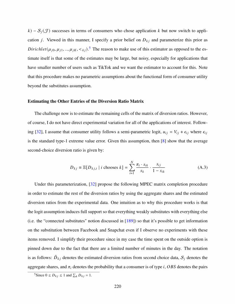
𝑘) − S 𝑗 (J) successes in terms of consumers who chose application 𝑘 but now switch to appli-

cation 𝑗 . Viewed in this manner, I specify a prior belief on 𝐷𝑘 𝑗 and parameterize this prior as

𝐷𝑖𝑟𝑖𝑐ℎ𝑙𝑒𝑡 (` 𝑗0, ` 𝑗1, .., ` 𝑗𝐾 , 𝑚𝑘 𝑗 ).5 The reason to make use of this estimator as opposed to the es-

timate itself is that some of the estimates may be large, but noisy, especially for applications that

have smaller number of users such as TikTok and we want the estimator to account for this. Note

that this procedure makes no parametric assumptions about the functional form of consumer utility

beyond the substitutes assumption.

Estimating the Other Entries of the Diversion Ratio Matrix

The challenge now is to estimate the remaining cells of the matrix of diversion ratios. However,

of course, I do not have direct experimental variation for all of the applications of interest. Follow-

ing [32], I assume that consumer utility follows a semi-parametric logit, 𝑢𝑖 𝑗 = 𝑉𝑖 𝑗 + 𝜖𝑖 𝑗 where 𝜖𝑖 𝑗

is the standard type-1 extreme value error. Given this assumption, then [8] show that the average

second-choice diversion ratio is given by:

𝐷𝑘 𝑗 ≡ E[𝐷𝑘 𝑗 ,𝑖 | 𝑖 chooses 𝑘] =𝑁∑︁𝑖=1

𝜋𝑖 · 𝑠𝑖𝑘𝑠𝑘

·𝑠𝑖 𝑗

1 − 𝑠𝑖𝑘(A.3)

Under this parameterization, [32] propose the following MPEC matrix completion procedure

in order to estimate the rest of the diversion ratios by using the aggregate shares and the estimated

diversion ratios from the experimental data. One intuition as to why this procedure works is that

the logit assumption induces full support so that everything weakly substitutes with everything else

(i.e. the “connected substitutes" notion discussed in [189]) so that it’s possible to get information

on the substitution between Facebook and Snapchat even if I observe no experiments with these

items removed. I simplify their procedure since in my case the time spent on the outside option is

pinned down due to the fact that there are a limited number of minutes in the day. The notation

is as follows: �̂�𝑘 𝑗 denotes the estimated diversion ratios from second choice data, S 𝑗 denotes the

aggregate shares, and 𝜋𝑖 denotes the probability that a consumer is of type 𝑖,𝑂𝐵𝑆 denotes the pairs5Since 0 ≤ 𝐷𝑘 𝑗 ≤ 1 and

∑𝑘 𝐷𝑘 𝑗 = 1.

220

of applications for which I have second-choice measures of diversion.

min𝑠𝑖 𝑗 ,𝜋𝑖

∑︁(𝑘, 𝑗)∈𝑂𝐵𝑆

(�̂�𝑘 𝑗 − 𝐷𝑘 𝑗 )2 + _∑︁𝑗

(S 𝑗 − 𝑠 𝑗 )2 (A.4)

subject to: 𝑠 𝑗 =∑︁𝑖

𝜋𝑖 · 𝑠𝑖 𝑗 (A.5)

𝐷𝑘 𝑗 =∑︁𝑖

𝜋𝑖 ·𝑠𝑖 𝑗

1 − 𝑠𝑖𝑘· 𝑠𝑖𝑘𝑠𝑘

(A.6)

0 ≤ 𝑠𝑖 𝑗 , 𝜋𝑖, 𝑠 𝑗 , 𝐷𝑘 𝑗 ≤ 1,∑︁𝑖

𝜋𝑖 = 1,∑︁𝑗

𝑠𝑖 𝑗 = 1 (A.7)

This procedure involves an exogenous selection of 𝐼 latent types of individuals each with dif-

ferent preferences as well as the penalization parameter _ > 0. The idea is that, as in standard

random coefficients logit demand models, the resulting aggregate market shares come from a mix-

ture of different types of consumers whose preferences each follow a different logit. Thus, (A.3)

pins down the average second-choice diversion ratio and the MPEC procedure optimizes over the

space of possible mixtures of different possible types of individuals in order to best fit the observed

diversion ratios and aggregate market shares.

I implement this procedure and choose the exogenous parameter _ by the model with the best

in-sample fit according to the mean-squared error or mean absolute error.6 I consider the set of

𝐼 ∈ {1, 2, ..., 8, 9} and for each 𝐼 choose _ ∈ {0.2, 0.6, 1.0, ...., 9.2, 9.6, 10}. Given the fixed _

for each 𝐼, I then choose across 𝐼 by comparing whether the resulting estimate correctly fits the

market shares and whether the resulting estimated diversion ratios could reasonably be implied

by the noisier experiments from the pilot experiment which included two applications (Facebook-

Messenger and Snapchat-Tiktok) and a smaller sample size. The nonparametric diversion ratios

from the joint restrictions in the pilot experiment are reported in Table A23.

6I alternatively considered a cross-validation procedure where the model is estimated holding out one set of di-version ratios (i.e. holding out one of the two experiments) but found that this led to unreasonable estimates, likelysince I have a small number of experiments and in this case the procedure is relying only on the estimates from oneexperiment.

221

A.5.3 Diversion Ratio Estimates

I report the nonparametric diversion ratio estimates for Instagram and YouTube that I compute

directly using the experimental variation. I pool together the data from the pilot and larger-scale

experiment in order to get more precise estimates. For the estimates I use an informative prior so

that the prior follows the predictions of logit and the diversion is proportional to market shares,

`𝑘 𝑗 =𝑠 𝑗

1−𝑠𝑘 and 𝑚𝑘 𝑗 = 10. I compute standard errors using simple block bootstrap with the

blocks being participants and utilizing the bootstrap percentile 95% confidence interval with 20000

replications. Table A23 reports the estimated diversion ratios as I vary the value of 𝑚𝑘 𝑗 . Recall that

increasing 𝑚𝑘 𝑗 places additional weight on the prior, which is the predicted diversion from logit,

at the expense of the experimental estimates.7 Furthermore, I also report the estimated diversion

ratios from the joint removal of Snapchat and TikTok as well as Facebook and Messenger. I do

not directly incorporate these into D since they contain multiple application restrictions and are

less precisely estimated due to smaller sample sizes and multiple restrictions, but rather use them

to choose between resulting estimates.

Table A22 reports the estimated diversion ratios for the rest of the applications using the MPEC

procedure for 𝐼 = 3 and _ = 6.6. For lower values of 𝐼, the selected _ do a poor job at fitting the

market shares, whereas for the higher values of 𝐼 the selected _ predict very little diversion to

the outside option for the other applications. The resulting estimates to the outside option for the

reported specification in Table A22 are in line with what one would expect given the nonparametric

diversion estimates in Table A23 for the joint Snapchat and TikTok as well as the joint Facebook

and Messenger restrictions.

7This also varies across applications since, for instance, Snapchat and TikTok have lower aggregate usage theestimator naturally places more weight on the prior for diversion to these applications relative to diversion to diversionfor more used applications like YouTube and Instagram.

222

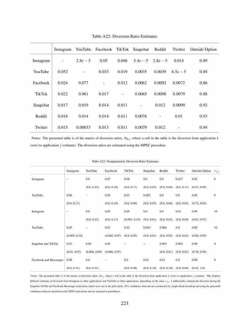
Table A22: Diversion Ratio Estimates

Instagram YouTube Facebook TikTok Snapchat Reddit Twitter Outside Option

Instagram - 2.8𝑒 − 5 0.05 0.046 5.4𝑒 − 5 2.8𝑒 − 5 0.014 0.89

YouTube 0.052 - 0.033 0.019 0.0035 0.0039 6.5𝑒 − 5 0.89

Facebook 0.024 0.077 - 0.012 0.0062 0.0092 0.0072 0.86

TikTok 0.022 0.061 0.017 - 0.0065 0.0098 0.0079 0.88

Snapchat 0.017 0.019 0.014 0.011 - 0.012 0.0099 0.92

Reddit 0.016 0.014 0.014 0.011 0.0076 - 0.01 0.93

Twitter 0.015 0.00033 0.013 0.011 0.0079 0.012 - 0.94

Notes: The presented table is of the matrix of diversion ratios, 𝐷𝑘 𝑗 , where a cell in the table is the diversion from application 𝑘

(row) to application 𝑗 (column). The diversion ratios are estimated using the MPEC procedure.

Table A23: Nonparametric Diversion Ratio Estimates

Instagram YouTube Facebook TikTok Snapchat Reddit Twitter Outside Option 𝑚𝑘 𝑗

Instagram − 0.0 0.07 0.08 0.0 0.0 0.027 0.82 0

(0.0, 0.22) (0.0, 0.18) (0.0, 0.17) (0.0, 0.03) (0.0, 0.04) (0.0, 0.11) (0.51, 0.95)

YouTube 0.06 − 0.05 0.03 0.002 0.0 0.0 0.86 0

(0.0, 0.13) (0.0, 0.10) (0.0, 0.09) (0.0, 0.03) (0.0, 0.04) (0.0, 0.02) (0.72, 0.94)

Instagram − 0.0 0.05 0.05 0.0 0.0 0.01 0.89 10

(0.0, 0.22) (0.0, 0.13) (0.003, 0.10) (0.0, 0.01) (0.0, 0.02) (0.0, 0.05) (0.61, 0.97)

YouTube 0.05 − 0.03 0.02 0.003 0.004 0.0 0.89 10

(0.005, 0.10) (0.002, 0.07) (0.0, 0.05) (0.0, 0.01) (0.0, 0.02) (0.0, 0.01) (0.80, 0.95)

Snapchat and TikTok 0.03 0.04 0.03 − − 0.003 0.002 0.90 0

(0.01, 0.07) (0.004, 0.09) (0.006, 0.07) (0.0, 0.01) (0.0, 0.01) (0.78, 0.95)

Facebook and Messenger 0.08 0.0 − 0.0 0.01 0.01 0.0 0.90 0

(0.0, 0.31) (0.0, 0.31) (0.0, 0.08) (0.0, 0.10) (0.0, 0.10) (0.0, 0.04) (0.42, 1.0)

Notes: The presented table is of the matrix of diversion ratios, 𝐷𝑘 𝑗 , where a cell in the table is the diversion from application 𝑘 (row) to application 𝑗 (column). This displays

different estimates of diversion from Instagram to other applications and YouTube to other applications, depending on the value 𝑚𝑘 𝑗 . I additionally compute the diversion during the

Snapchat-TikTok and Facebook-Messenger restrictions which were run in the pilot study. 95% confidence intervals are constructed by simple block bootstrap and using the percentile

confidence interval calculation with 20000 replications and are reported in parentheses.

223

A.6 Additional Figures / Tables for Time Usage Model

Figure A23: K-means Clustering of Participants

YT

IG

TWTR

REDDIT

FB

TT

SNAP

YT

IG

TWTR

REDDIT

FB

TT

SNAP

YT

IG

TWTR

REDDIT

FB

TT

SNAP

YT

IG

TWTR

REDDIT

FB

TT

SNAP

YT

IG

TWTR

REDDIT

FB

TT

SNAP

YT

IG

TWTR

REDDIT

FB

TT

SNAP

4 5 6

1 2 3

Notes: The figures display the results of k-means clustering for 𝑘 = 6. Each pane shows the average (log) timeallocations across the different applications for the participants in the cluster. For instance, if a point is closer to theouter edge for an application 𝐴 than application 𝐵 then that indicates that that application 𝐴 has more usage on averagethan application 𝐵. The application names are abbreviated so that the figure is readable. TT is TikTok, FB is Facebook,YT is YouTube, IG is Instagram, SNAP is SnapChat, REDDIT is Reddit, and TWTR is Twitter.

224

Table A24: Demand Model Parameter Estimates

Type (1) (2) (3) (4) (5) (6)

ℎ𝑖 𝑗 𝑡 0.013 0.0045 0.0087 0.0052 0.011 0.0086

(0.00012) (0.00017) (8.7e-5) (0.00016) (0.00019) (0.00014)

𝑟𝑖 𝑗 𝑡 1.5 0.94 1.1 1.4 1.1 1.3

(0.016) (0.018) (0.021) (0.091) (0.026) (0.021)

𝑟2𝑖 𝑗 𝑡

-0.038 -0.033 -0.023 -0.083 -0.029 -0.062

(0.0013) (0.001) (0.004) (0.02) (0.0019) (0.0037)

App - Instagram -5.0 -5.0 -4.3 -5.1 -4.8 -4.2

(0.026) (0.07) (0.038) (0.14) (0.077) (0.039)

App - Twitter -5.8 -6.4 -5.2 -6.4 -5.0 -5.2

(0.03) (0.11) (0.051) (0.16) (0.092) (0.065)

App - YouTube -5.5 -4.4 -4.3 -4.3 -5.1 -4.9

(0.023) (0.086) (0.04) (0.079) (0.091) (0.056)

App - TikTok -5.7 -5.1 -4.7 -4.2 -4.8 -5.3

(0.031) (0.1) (0.043) (0.13) (0.094) (0.085)

App - Reddit -5.9 -5.2 -5.1 -3.8 -7.0 -6.5

(0.032) (0.088) (0.041) (0.064) (0.16) (0.11)

App- Snapchat -5.5 -7.2 -4.5 -5.9 -4.9 -5.0

(0.032) (0.19) (0.041) (0.18) (0.11) (0.051)

App - Facebook -5.3 -4.7 -4.7 -5.7 -5.0 -4.7

(0.025) (0.072) (0.041) (0.2) (0.085) (0.042)

𝑎𝑖 𝑗 - Online Shopping -0.52 0.53 0.064 0.0 0.0 -0.46

(0.065) (0.13) (0.055) (0.0) (0.0) (0.17)

𝑎𝑖 𝑗 - Entertainment content 0.11 0.38 0.25 -0.032 0.23 -0.057

(0.014) (0.05) (0.025) (0.047) (0.059) (0.02)

𝑎𝑖 𝑗 - Keep up with my friends’ lives 0.0 0.0 0.0 0.0099 -0.22 0.0

(0.0) (0.0) (0.0) (0.16) (0.068) (0.0)

𝑎𝑖 𝑗 - Get Information -0.26 0.24 0.25 0.0 0.0 -0.016

(0.021) (0.061) (0.031) (0.0) (0.0) (0.03)

𝑎𝑖 𝑗 - I don’t use this application -4.4 -5.6 -4.4 -4.4 -3.1 -2.9

(0.086) (2.8) (0.12) (0.3) (0.26) (0.11)

𝑎𝑖 𝑗 - Communicate with my friends -0.096 0.75 0.077 0.7 0.41 0.29

(0.016) (0.095) (0.029) (0.18) (0.087) (0.041)

ℎ𝑡 - EVENING -0.59 -0.74 -0.0044 -0.55 -0.04 -0.42

(0.023) (0.046) (0.026) (0.048) (0.038) (0.03)

ℎ𝑡 - LATE NIGHT -0.75 -1.1 -0.29 -0.53 -0.69 -0.64

(0.02) (0.047) (0.022) (0.042) (0.042) (0.029)

ℎ𝑡 - MORNING -0.77 -1.1 -0.29 -0.43 -0.72 -0.53

(0.019) (0.048) (0.024) (0.048) (0.03) (0.028)

ℎ𝑡 - AFTERNOON 0.0 0.0 0.0 0.0 0.0 0.0

(0.0) (0.0) (0.0) (0.0) (0.0) (0.0)

𝑑𝑡 - Sunday 0.048 0.0073 0.018 0.17 0.032 -0.044

(0.018) (0.047) (0.034) (0.063) (0.046) (0.035)

𝑑𝑡 - Monday 0.046 0.093 0.061 0.19 -0.081 0.0069

(0.018) (0.048) (0.027) (0.077) (0.047) (0.037)

𝑑𝑡 - Tuesday 0.031 0.11 0.039 0.16 -0.066 0.027

(0.018) (0.053) (0.027) (0.07) (0.046) (0.036)

𝑑𝑡 - Wednesday 0.081 0.097 0.04 0.17 -0.023 0.00086

(0.023) (0.05) (0.031) (0.068) (0.042) (0.034)

𝑑𝑡 - Thursday 0.069 0.064 0.076 0.1 -0.032 -0.018

(0.019) (0.045) (0.032) (0.065) (0.042) (0.036)

𝑑𝑡 - Friday 0.0 0.0 0.0 0.0 0.0 0.0

(0.0) (0.0) (0.0) (0.0) (0.0) (0.0)

𝑑𝑡 - Saturday -0.008 0.11 -0.038 0.062 -0.04 0.0074

(0.02) (0.057) (0.028) (0.062) (0.05) (0.036)

𝑤𝑡 - Week 1 0.029 0.064 -0.088 -0.0075 -0.15 0.02

(0.017) (0.055) (0.027) (0.057) (0.048) (0.033)

𝑤𝑡 - Week 2 -0.11 -0.0029 -0.12 -0.096 -0.0086 -0.043

(0.015) (0.052) (0.022) (0.054) (0.045) (0.026)

𝑤𝑡 - Week 3 -0.068 -0.0036 -0.14 -0.14 0.0023 -0.058

(0.013) (0.046) (0.028) (0.057) (0.033) (0.022)

𝑤𝑡 - Week 4 -0.018 -0.0021 -0.13 0.043 0.039 -0.12

(0.015) (0.036) (0.024) (0.05) (0.042) (0.023)

𝑤𝑡 - Week 5 0.0 0.0 0.0 0.0 0.0 0.0

(0.0) (0.0) (0.0) (0.0) (0.0) (0.0)

Notes: This table presents the estimated parameters of the demand model. The estimates for each type are presented in a separate

column. Standard errors in parentheses are computed by 50 bootstrap samples.

225

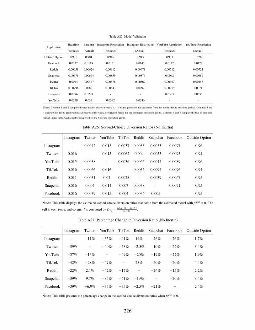
Table A25: Model Validation

ApplicationBaseline

(Predicted)

Baseline

(Actual)

Instagram Restriction

(Predicted)

Instagram Restriction

(Actual)

YouTube Restriction

(Predicted)

YouTube Restriction

(Actual)

Outside Option 0.901 0.901 0.916 0.913 0.933 0.928

Facebook 0.0122 0.0118 0.0131 0.0145 0.0122 0.0127

Reddit 0.00651 0.00624 0.00912 0.00971 0.00712 0.00721

Snapchat 0.00671 0.00694 0.00859 0.00876 0.0062 0.00689

Twitter 0.0044 0.00447 0.00576 0.00569 0.00407 0.00455

TikTok 0.00796 0.00801 0.00843 0.0092 0.00759 0.0071

Instagram 0.0276 0.0278 - - 0.0303 0.0335

YouTube 0.0339 0.034 0.0392 0.0386 - -

Notes: Columns 1 and 2 compare the true market shares in week 1, 4, 5 to the predicted market shares from this model during this time period. Columns 3 and

4 compare the true to predicted market shares in the week 2 restriction period for the Instagram restriction group. Columns 5 and 6 compare the true to predicted

market shares in the week 2 restriction period for the YouTube restriction group.

Table A26: Second-Choice Diversion Ratios (No Inertia)

Instagram Twitter YouTube TikTok Reddit Snapchat Facebook Outside Option

Instagram - 0.0042 0.015 0.0037 0.0033 0.0053 0.0097 0.96

Twitter 0.016 - 0.015 0.0062 0.004 0.0053 0.0093 0.94

YouTube 0.015 0.0038 - 0.0036 0.0065 0.0044 0.0089 0.96

TikTok 0.016 0.0066 0.016 - 0.0036 0.0094 0.0096 0.94

Reddit 0.011 0.0031 0.02 0.0028 - 0.0039 0.0067 0.95

Snapchat 0.016 0.004 0.014 0.007 0.0038 - 0.0091 0.95

Facebook 0.016 0.0039 0.015 0.004 0.0036 0.005 - 0.95

Notes: This table displays the estimated second-choice diversion ratios that come from the estimated model with 𝛽𝑞 (𝑖) = 0. The

cell in each row 𝑘 and column 𝑗 is computed by 𝐷𝑘 𝑗 =𝑠 𝑗 (J\{𝑘 })−𝑠 𝑗 (J)

𝑠𝑘 (J) .

Table A27: Percentage Change in Diversion Ratio (No Inertia)

Instagram Twitter YouTube TikTok Reddit Snapchat Facebook Outside Option

Instagram − −11% −35% −41% 14% −26% −26% 1.7%

Twitter −39% − −40% −53% −2.5% −10% −22% 3.4%

YouTube −37% −13% − −49% −20% −19% −22% 1.9%

TikTok −42% −28% −47% − 23% −50% −20% 4.4%

Reddit −22% 2.1% −42% −17% − −26% −15% 2.2%

Snapchat −39% 9.7% −35% −61% −19% − −20% 3.4%

Facebook −39% −6.9% −35% −35% −2.5% −21% − 2.4%

Notes: This table presents the percentage change in the second-choice diversion ratios when 𝛽𝑞 (𝑖) = 0.

226

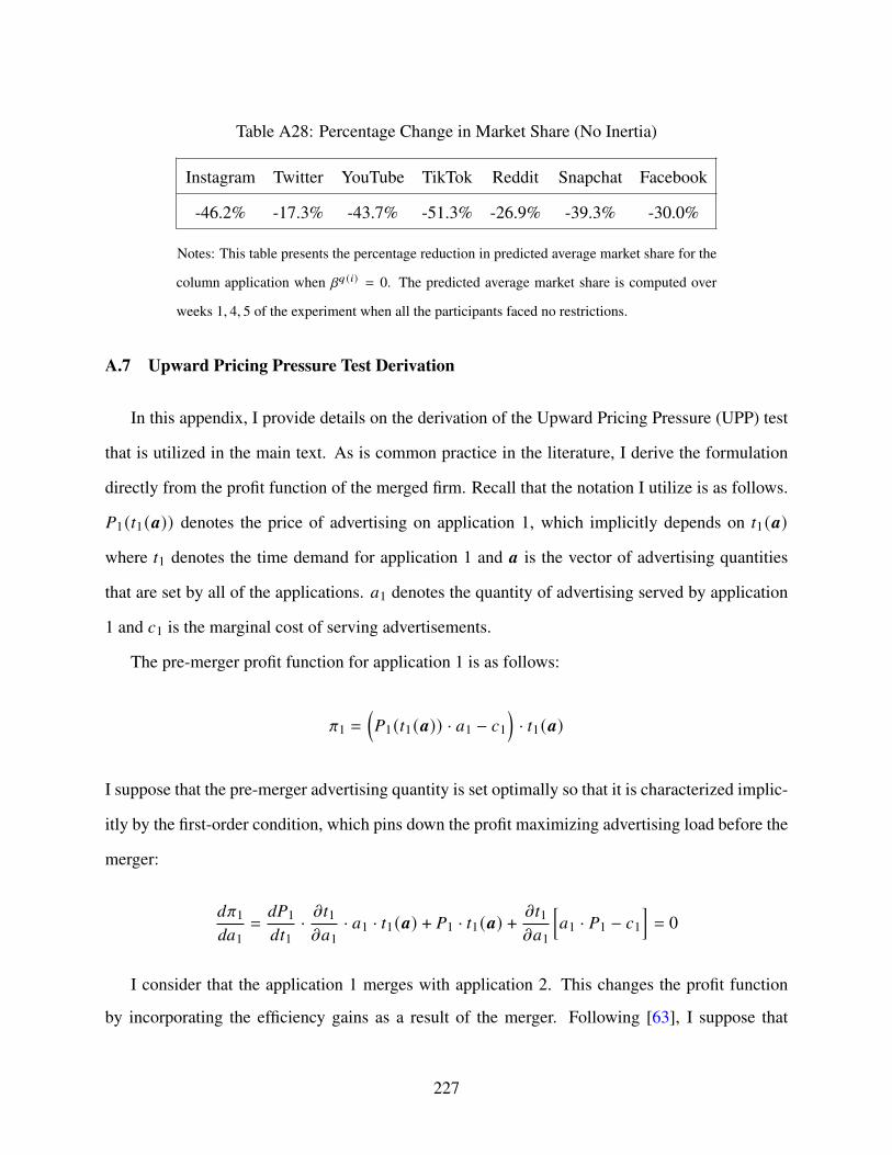
Table A28: Percentage Change in Market Share (No Inertia)

Instagram Twitter YouTube TikTok Reddit Snapchat Facebook

-46.2% -17.3% -43.7% -51.3% -26.9% -39.3% -30.0%

Notes: This table presents the percentage reduction in predicted average market share for the

column application when 𝛽𝑞 (𝑖) = 0. The predicted average market share is computed over

weeks 1, 4, 5 of the experiment when all the participants faced no restrictions.

A.7 Upward Pricing Pressure Test Derivation

In this appendix, I provide details on the derivation of the Upward Pricing Pressure (UPP) test

that is utilized in the main text. As is common practice in the literature, I derive the formulation

directly from the profit function of the merged firm. Recall that the notation I utilize is as follows.

𝑃1(𝑡1(𝒂)) denotes the price of advertising on application 1, which implicitly depends on 𝑡1(𝒂)

where 𝑡1 denotes the time demand for application 1 and 𝒂 is the vector of advertising quantities

that are set by all of the applications. 𝑎1 denotes the quantity of advertising served by application

1 and 𝑐1 is the marginal cost of serving advertisements.

The pre-merger profit function for application 1 is as follows:

𝜋1 =

(𝑃1(𝑡1(𝒂)) · 𝑎1 − 𝑐1

)· 𝑡1(𝒂)

I suppose that the pre-merger advertising quantity is set optimally so that it is characterized implic-

itly by the first-order condition, which pins down the profit maximizing advertising load before the

merger:

𝑑𝜋1𝑑𝑎1

=𝑑𝑃1𝑑𝑡1

· 𝜕𝑡1𝜕𝑎1

· 𝑎1 · 𝑡1(𝒂) + 𝑃1 · 𝑡1(𝒂) +𝜕𝑡1𝜕𝑎1

[𝑎1 · 𝑃1 − 𝑐1

]= 0

I consider that the application 1 merges with application 2. This changes the profit function

by incorporating the efficiency gains as a result of the merger. Following [63], I suppose that

227

the primary efficiency gains for consumers come from increased application quality as a result

of a merger as opposed to a marginal cost reduction. I consider that consumers face quality-

adjusted advertising loads given by 𝑎1 = 𝑎1 − a1. Thus, the demand for application 𝑖 is as follows:

𝑡𝑖 (𝑎1 − a1, ..., 𝑎𝑁 − a𝑁 ) ≡ 𝑡𝑖 (�̃�1, ..., �̃�𝑁 ). Before the merger 𝑎1 = 𝑎1 so that the pre-merger levels of

application quality are already captured in the demand functions. Combined these imply that the

profit function of the merged firm is as follows:

𝜋1 + 𝜋2 =

(𝑃1(𝑡1(𝒂)) · (𝑎1 + a1) − 𝑐1

)· 𝑡1(𝒂) +

(𝑃2(𝑡2(𝒂)) · (𝑎2 + a2) − 𝑐2

)· 𝑡2(𝒂)

As is customary, I derive a UPP expression for each application individually. Indeed, as noted by

[63], in this case it is sufficient to focus on characterizing whether there is upward pricing pressure

for each application individually as if this is the case for one of the applications then it implies

that the two applications jointly have upward pricing pressure as well. The UPP expression is

typically derived by solving for the first-order condition of the profit function of the merged firm

and characterizing the conditions under which this term is positive. If this is positive then there is

“upward pressure" for the firm to increase (quality-adjusted) prices post-merger. Therefore without

loss of generality I focus on the first-order condition for application 1.

𝜕𝜋1𝜕𝑎1

=𝑑𝑃1𝑑𝑡1

· 𝜕𝑡1𝜕𝑎1

· 𝑎1 · 𝑡1(𝒂) + 𝑃1 · 𝑡1(𝒂) +𝜕𝑡1𝜕𝑎1

[𝑎1 · 𝑃1 − 𝑐1

]︸ ︷︷ ︸

=0 at pre-merger

+ 𝑑𝑃1𝑑𝑡1

· 𝜕𝑡1𝜕𝑎1

· a1 · 𝑡1(𝒂) +𝜕𝑡1𝜕𝑎1

· a1 · 𝑃1

+ 𝜕𝑡2𝜕𝑎1

· (𝑃2 · (𝑎2 + a2) − 𝑐2) +𝑑𝑃2𝑑𝑡2

· 𝜕𝑡2𝜕𝑎1

· 𝑡2(𝒂) · (𝑎2 + a2) = 0

The term noted in the brackets corresponds to the first-order condition of application 1 which,

at the pre-merger advertising quantities, evaluates to 0. Recall that the diversion ratio is defined

as 𝐷12 ≡ −1 ·𝜕𝑡2𝜕𝑎1𝜕𝑡1𝜕𝑎1

. I divide the remaining terms through by −1 · 𝜕𝑡1𝜕𝑎1

and reorganize to obtain the

228

following UPP expression:

𝑈𝑃𝑃1 = 𝐷12 ·(𝑃2 · (𝑎2 + a2) − 𝑐2︸ ︷︷ ︸Revenue from Diversion

+ 𝑑𝑃2𝑑𝑡2

· (𝑎2 + a2) · 𝑡2(𝒂)︸ ︷︷ ︸Price Change from Diversion

)−

(a1 ·

(𝑑𝑃1𝑑𝑡1

· 𝑡1(𝒂) + 𝑃1

)︸ ︷︷ ︸

Quality Efficiency Gains

)

A.8 Collection of Survey Responses

In this section are the responses to the optional question in the endline survey which asked the

participants to describe in words how they responded to the restrictions.

• Addiction

– I hated it while it happened, but it really broke the app’s addictive nature.

– I never realized that I am tsuch addicting to instagram until I found myself opened it

absentmindedly several times during mY restrictions period. my usage time of ig has

decreased from averagely 6.5 hrs before the restrictions to 3 hr in the first week, but

bounce back to 7 hrs this week, even exceeding the number before.

– It’s strange, because it didn’t feel like I needed YouTube, I just knew I had spent a lot

of time on it. However, when it became restricted, I noticed how much time I had spent

simply laying about and watching YouTube. It felt weird knowing that my instinct was

to immediately press the YouTube button when I got bored, and I realized I perhaps

need/use it more than I think.

– It was crazy how addicted I am to these apps. During the restrictions, I kept accidentally

trying to open the app -all the time. I didn’t realize how much time I spent on them.

– I kept opening instagram time after time forgetting that is was blocked

– I had one restriction on Instagram and it was weird breaking the habit of accessing and

took some getting used to avoiding the app

– When the restriction started I got a feeling I was gonna be a little anxious. I was wrong.

229

– It was frustrating - did not know I was so addicted to YouTube

– I felt out of the loop so I often tried to access Instagram using my laptop.

– At first restricting instagram was frustrating as i had the application on my home screen

and built muscle memory for the past 4 years to press that part of the screen where the

instagram shortcut is. I removed instagram from my home screen and after 5 days of

the restriction i completely realized instagram was nor important at all for me and only

time i open it is when i receive a direct message.

• Shifted Towards Other Apps

– It wasn’t easy at first as I tried to access the restricted application about two different

times but I received the restriction message from screen time app with a grin on my

face....lol. I had to figure out what I want from other applications I didn’t know offered

similar content before time, after the restriction elapsed, I had adjusted to sourcing for

such content on both apps.

– Well at first after my YouTube was restricted, I thought I could access it using my

browser but then i realised that was also impossible. I was like, how will I cope without

streaming videos on YouTube? But after some time I adjusted and got used to it.

– At the beginning i felt like damn this is an important application (Youtube) and what

if i need it for anything Turns out i dont need it as much and there are other options

available

– Pre-COVID, I would listen to a lot of podcasts when driving, walking to class, etc.

So when Youtube was restricted, I mostly just listened to more podcasts like I used

to. I think I also probably watched more Youtube on my PC and smart TV during this

period.

– At the beginning it felt like something was missing but eventually I started using other

apps and filled that vacancy

230

– I spent time on twitch watching streamers vs. Youtube where I had watched them

before.

– I think the restriction gave me the opportunity to spend more time on other applications

i had already installed but hardly use.

– I often use youtube for music on my phone when I don’t want to pay for Spotify pre-

mium, but during the restriction period I ended up resubscribing to Spotify Premium

for $5 so I could listen to music on my phone easily

• Realized Value of Application

– It was a bit hard to adapt at first but I eventually got used to it.Eventually I realized I am

better off without it so I ended up deleting it and till now am okay with my decision.

– After the restriction I definitely started spending more time on the app that was re-

stricted. I started to use the app more because I wanted to track local businesses which

can be hard to discover by googling. I’m not sure if it was a coincidence that I de-

veloped an interest in small businesses and increased my app usage or if it was the

restriction that caused me to appreciate what I could do on the app more.

– I felt that I missed using it I realized I was spending to much time on the app

– Struggling to access Instagram, but when there’s no restrictions, i found that the content

i wanna access previously is very trivial

– I felt minorly inconvenienced since I could still access on my computer if it were an

emergency like an insta dm I needed to respond to. Having time away from insta

definitely helped me mentally.

– Sometimes I misses to use but nothing as bad as I thought. Most of time I have not

importante to do, Its just a way to spend time

– I felt after restrictions that I need this application more and I can’t take this restrictions

for a long.

231

– YouTube was restricted, so it was a little difficult when my baby was having a meltdown

in public, but it also wasn’t as often as usual, thankfully. It was difficult also if I

needed to learn something off of YouTube pertaining to my career like a how-to or new

technique.

• Shifted Towards Non-Digital Activities

– Honestly I spent more time outdoor and with friends.

– I initially felt bored, since a common reflex I had was to open up Youtube whenever

I had nothing to do. However, within a few days, I started doing other things instead,

such as reading. It was actually a good experience.

– At first it was difficult because YouTube is the most used app by me.Whatever it is

YouTube is a go to for me in my daily life.After that I made up my mind to concentrate

in different things and spent more time off the devices.I tried to concentrate more on

my studies and spent time with my family.

– I was surprised my youtube was restricted. For me its a big part of the content i consume

and it is was hard to not have it on my phone. Initially I tried watching it on my

computer but it was something i couldn’t keep up all the time. Over time my useage

dropped from watching a lot to, mainly watching when i am on my computer taking a

small break (even then only watching the videos i really like and not wasting time on

YT)

• Impact on Socializing

– I realized I spent a lot of time on an app establishing really ineffective communication.

I changed the way in which I communicate online.

– I didn’t think I used Instagram very much but the restriction turned out to be very

annoying as friends would message me there and wonder why I wasn’t responding

232

– I used Instagram to communicate with friends less frequently when it was restricted,

but used WhatsApp more instead. These were reverted after restrictions were lifted

– I felt frustrated because I feel like I was missing out. I wasn’t able to keep up with the

people I followed on Instagram as much because the app was restricted

– I felt it was a very interesting experience. I don’t feel like I have an addiction to certain

applications and could probably live my life without it. The only limit I faced was that

I could not contact certain people, who I only talk with on that application. But to

be honest, I could live even without those conversations or certain people and would

probably find other apps to contact them on. But I did not do that.

– Instagram was restricted for me and because I mainly use it as a communication app, I

was not significantly affected. I just used regular text, video call, and Snapchat to keep

up socially.

– It was a little annoying especially whenever my friend shared something that can only

open on that platform. But after a couple of days I was able to make my peace with it

– I did a bit of communication on Instagram, so told the person I was chatting to to switch

and that didn’t really happen so it ended up reducing how much we messaged

233

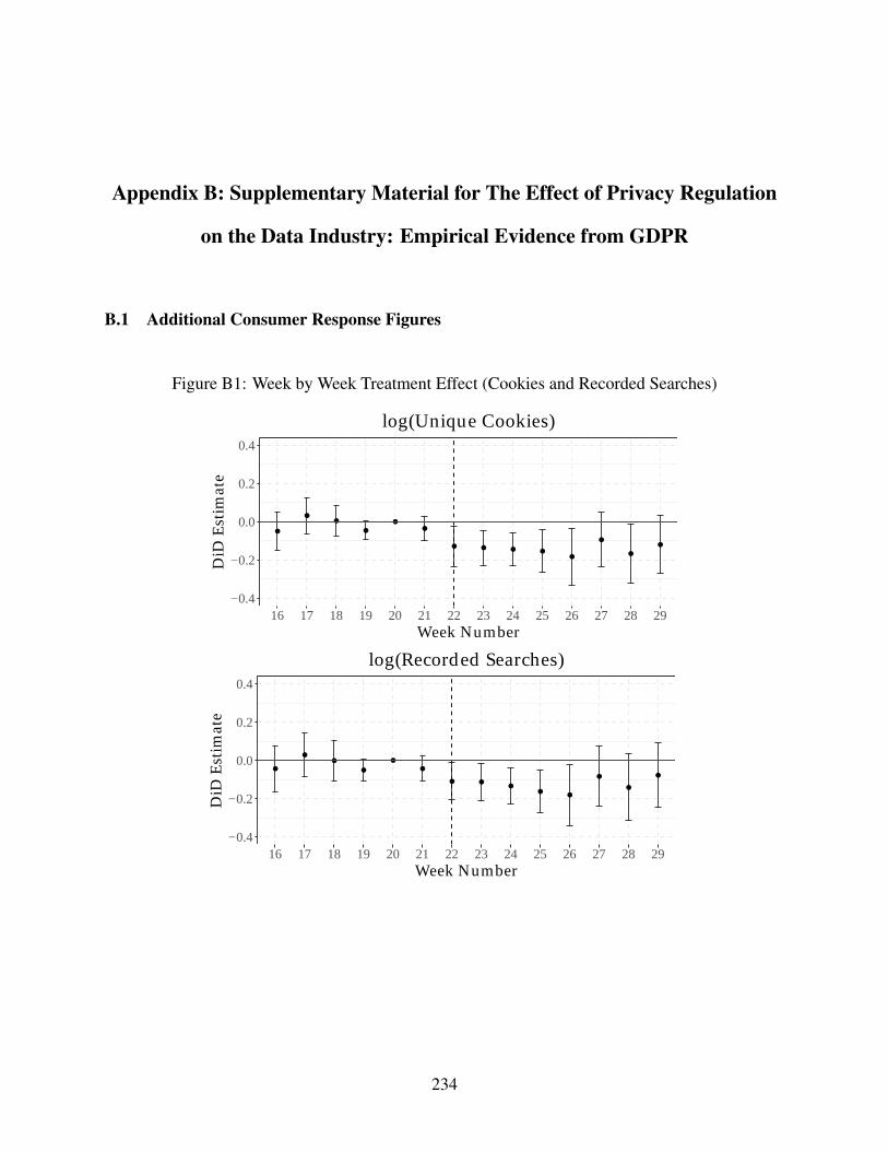
Appendix B: Supplementary Material for The Effect of Privacy Regulation

on the Data Industry: Empirical Evidence from GDPR

B.1 Additional Consumer Response Figures

Figure B1: Week by Week Treatment Effect (Cookies and Recorded Searches)

●

●●

●

●

●

● ● ● ●●

●

●

●

−0.4

−0.2

0.0

0.2

0.4

16 17 18 19 20 21 22 23 24 25 26 27 28 29Week Number

DiD

Est

imat

e

log(Unique Cookies)

●

●●

●

●

●

● ●●

●●

●

●

●

−0.4

−0.2

0.0

0.2

0.4

16 17 18 19 20 21 22 23 24 25 26 27 28 29Week Number

DiD

Est

imat

e

log(Recorded Searches)

234

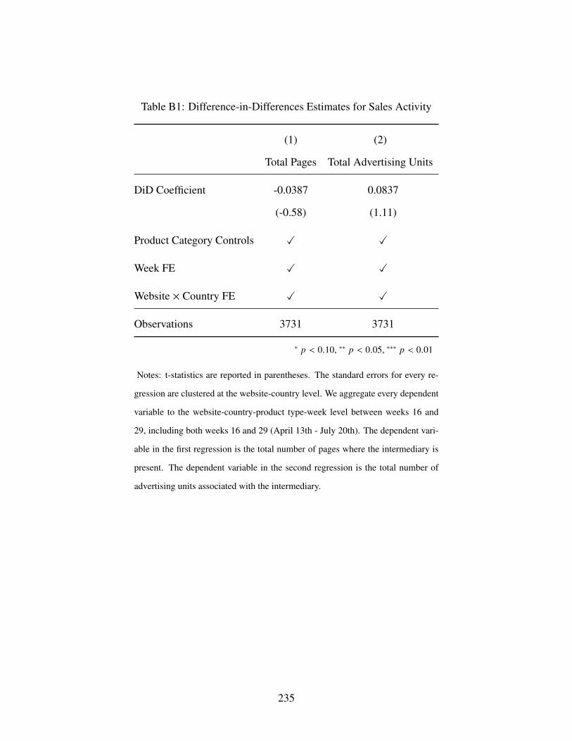
Table B1: Difference-in-Differences Estimates for Sales Activity

(1) (2)

Total Pages Total Advertising Units

DiD Coefficient -0.0387 0.0837

(-0.58) (1.11)

Product Category Controls ✓ ✓

Week FE ✓ ✓

Website × Country FE ✓ ✓

Observations 3731 3731

∗ 𝑝 < 0.10, ∗∗ 𝑝 < 0.05, ∗∗∗ 𝑝 < 0.01

Notes: t-statistics are reported in parentheses. The standard errors for every re-

gression are clustered at the website-country level. We aggregate every dependent

variable to the website-country-product type-week level between weeks 16 and

29, including both weeks 16 and 29 (April 13th - July 20th). The dependent vari-

able in the first regression is the total number of pages where the intermediary is

present. The dependent variable in the second regression is the total number of

advertising units associated with the intermediary.

235

Figure B2: Week by Week Treatment Effect (Consumer Persistence)

●

●●

●

● ●

●●

●

●

●

−0.02

−0.01

0.00

0.01

0.02

16 17 18 19 20 21 22 23 24 25 26Week Number

DiD

Est

imat

e

Consumer Persistence (1 Week)

●●

●

●●

●

● ●●

● ●

−0.02

−0.01

0.00

0.01

0.02

16 17 18 19 20 21 22 23 24 25 26Week Number

DiD

Est

imat

e

Consumer Persistence (2 Weeks)

●●

●●

●

●●

● ● ●

●

−0.02

−0.01

0.00

0.01

0.02

16 17 18 19 20 21 22 23 24 25 26Week Number

DiD

Est

imat

e

Consumer Persistence (3 Weeks)

●

● ●● ●

●●

●● ●

●

−0.02

−0.01

0.00

0.01

0.02

16 17 18 19 20 21 22 23 24 25 26Week Number

DiD

Est

imat

e

Consumer Persistence (4 Weeks)

236

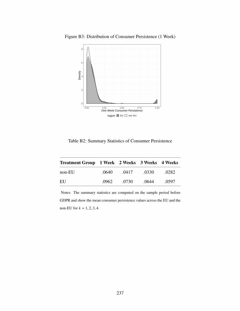
Figure B3: Distribution of Consumer Persistence (1 Week)

0

2

4

6

8

0.00 0.25 0.50 0.75 1.00One Week Consumer Persistence

Den

sity

region EU non−EU

Table B2: Summary Statistics of Consumer Persistence

Treatment Group 1 Week 2 Weeks 3 Weeks 4 Weeks

non-EU .0640 .0417 .0330 .0282

EU .0962 .0730 .0644 .0597

Notes: The summary statistics are computed on the sample period before

GDPR and show the mean consumer persistence values across the EU and the

non-EU for 𝑘 = 1, 2, 3, 4.

237

B.2 Robustness for Consumer Response Results

Figure B4: Synthetic Controls for Cookies and Recorded Searches

16 18 20 22 24 26 28

4000

5000

6000

7000

GDPR Impact (Cookies)

Week

Uni

que

Coo

kies

TreatedSynthetic

16 18 20 22 24 26 28

−10

00−

500

050

010

00

Gaps: Treated − Synthetic

Week

Uni

que

Coo

kies

16 18 20 22 24 26 28

1000

012

000

1400

016

000

1800

020

000

2200

0

GDPR Impact (Searches)

Week

Rec

orde

d S

earc

hes

TreatedSynthetic

16 18 20 22 24 26 28

−40

00−

2000

020

0040

00

Gaps: Treated − Synthetic

Week

Rec

orde

d S

earc

hes

Notes: The plots in the leftmost column display the time series of the average treated unit and the constructed syntheticcontrol for the number of unique cookies (top) and number of recorded searches (bottom). The plots in the rightmostcolumn display the difference at every point in time between the averaged treated unit and the constructed syntheticcontrol for the number of unique cookies (top) and number of recorded searches (bottom).

We provide additional evidence of robustness for our estimated effects on the usage of consent-

based opt-out as a result of GDPR. subsection B.2.1 mimics the exercise in the main text, but

utilizes a standard synthetic control based approach and recovers similar results as our difference-

238

in-differences approach. subsection B.2.2 augments our analysis with Google Trends data and uses

this to control for seasonality differences in travel patterns across the countries in our analysis.

B.2.1 Synthetic Controls

In order to provide additional validation for the difference-in-differences results in subsec-

tion 2.4.1, we supplement our primary analysis with a synthetic controls analysis, following [190]

and utilizing the corresponding R package, Synth. We aggregate the data to the same level as

we do in the primary analysis.1 We expand the set of control countries beyond the United States,

Canada, and Russia to include Argentina, Brazil, Australia, Japan, and Mexico in order to allow

for additional flexibility in the design of the synthetic control group.2 Thus, the travel websites

in these countries serve as the possible donor pool for the construction of the synthetic control.

In order to apply the synthetic control method to our data we construct a single average treated

unit for each outcome variable from the set of treated units. The set of predictor variables that we

utilize in order to fit the weights assigned to each control unit are the two outcome variables that

we consider—the total number of searches and the total number of unique cookies observed. We

fit the weights to match the outcome variable between weeks 16 and 21. The results of applying

this method are reported in Figure B4. Qualitatively, the results match what we find utilizing the

difference-in-differences analysis with a stark drop at the onset of GDPR with a small recovery

nearing the end of our sample period.

B.2.2 Controlling for Differences in Travel Patterns Across Countries

Since our paper tries to understand the impact of privacy regulations utilizing data from the

online travel industry, a potential concern is that differential seasonality trends in travel across

1We also do this exercise aggregating at the website-country level and find qualitatively similar results. One mightargue for this aggregation since the way we utilize the synthetic control method involves collapsing all treated unitsinto a single average treated unit and it seems more natural to do so at the website-country level so that the syntheticcontrol represents a synthetic European website. However, this makes the comparison of estimated treatment effectsto the primary specification more difficult since the underlying units are different.

2Our results are nearly identical if we use the same set of control countries as we do in the baseline difference-in-differences specification, but use the larger set of countries due to the flexibility of the synthetic control method whichmakes this a special case of the reported exercise.

239

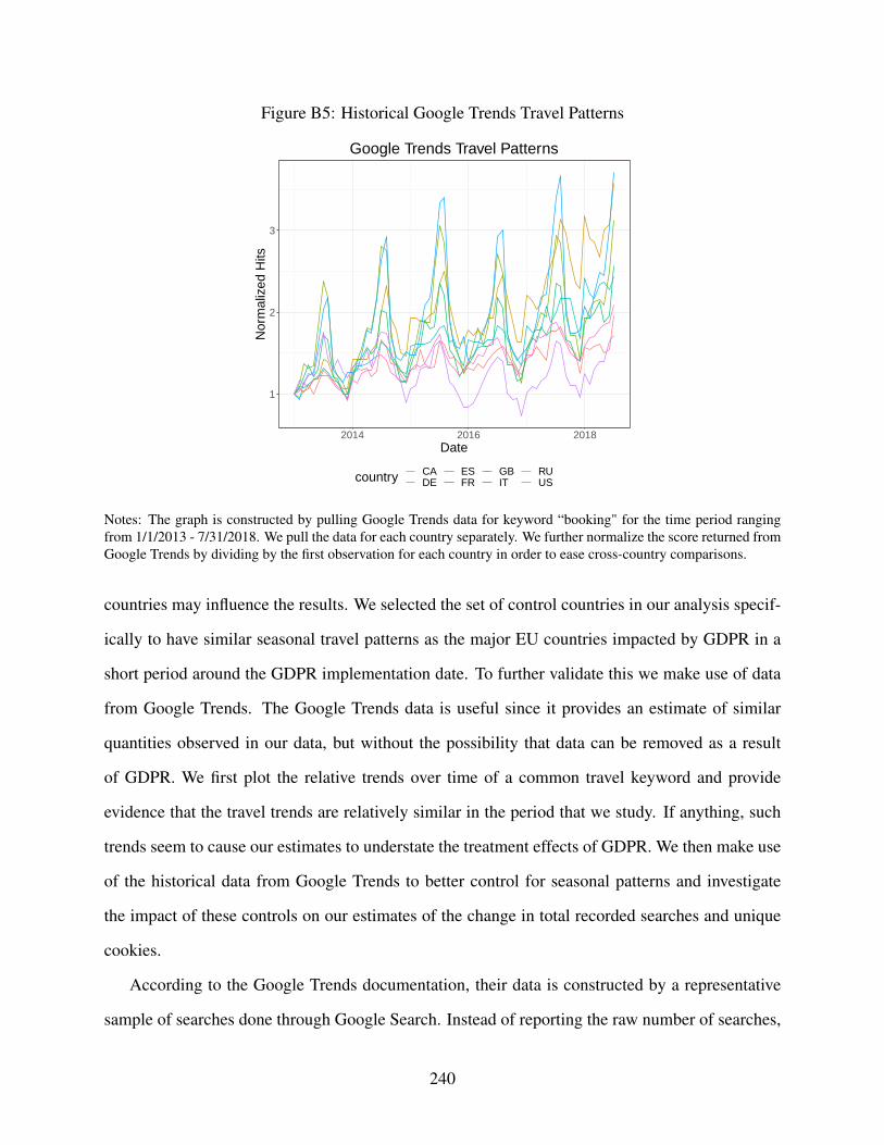
Figure B5: Historical Google Trends Travel Patterns

1

2

3

2014 2016 2018Date

Nor

mal

ized

Hits

country CADE

ESFR

GBIT

RUUS

Google Trends Travel Patterns

Notes: The graph is constructed by pulling Google Trends data for keyword “booking" for the time period rangingfrom 1/1/2013 - 7/31/2018. We pull the data for each country separately. We further normalize the score returned fromGoogle Trends by dividing by the first observation for each country in order to ease cross-country comparisons.

countries may influence the results. We selected the set of control countries in our analysis specif-

ically to have similar seasonal travel patterns as the major EU countries impacted by GDPR in a

short period around the GDPR implementation date. To further validate this we make use of data

from Google Trends. The Google Trends data is useful since it provides an estimate of similar

quantities observed in our data, but without the possibility that data can be removed as a result

of GDPR. We first plot the relative trends over time of a common travel keyword and provide

evidence that the travel trends are relatively similar in the period that we study. If anything, such

trends seem to cause our estimates to understate the treatment effects of GDPR. We then make use

of the historical data from Google Trends to better control for seasonal patterns and investigate

the impact of these controls on our estimates of the change in total recorded searches and unique

cookies.

According to the Google Trends documentation, their data is constructed by a representative

sample of searches done through Google Search. Instead of reporting the raw number of searches,

240

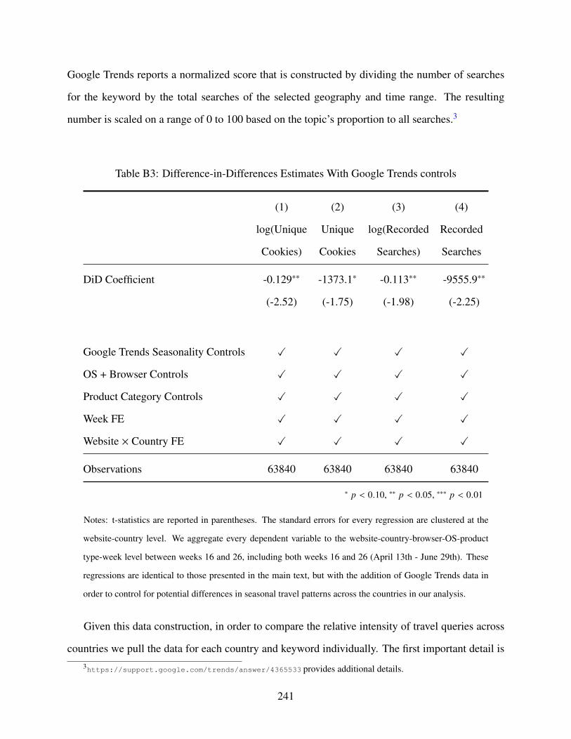
Google Trends reports a normalized score that is constructed by dividing the number of searches

for the keyword by the total searches of the selected geography and time range. The resulting

number is scaled on a range of 0 to 100 based on the topic’s proportion to all searches.3

Table B3: Difference-in-Differences Estimates With Google Trends controls

(1) (2) (3) (4)

log(Unique Unique log(Recorded Recorded

Cookies) Cookies Searches) Searches

DiD Coefficient -0.129∗∗ -1373.1∗ -0.113∗∗ -9555.9∗∗

(-2.52) (-1.75) (-1.98) (-2.25)

Google Trends Seasonality Controls ✓ ✓ ✓ ✓

OS + Browser Controls ✓ ✓ ✓ ✓

Product Category Controls ✓ ✓ ✓ ✓

Week FE ✓ ✓ ✓ ✓

Website × Country FE ✓ ✓ ✓ ✓

Observations 63840 63840 63840 63840

∗ 𝑝 < 0.10, ∗∗ 𝑝 < 0.05, ∗∗∗ 𝑝 < 0.01

Notes: t-statistics are reported in parentheses. The standard errors for every regression are clustered at the

website-country level. We aggregate every dependent variable to the website-country-browser-OS-product

type-week level between weeks 16 and 26, including both weeks 16 and 26 (April 13th - June 29th). These

regressions are identical to those presented in the main text, but with the addition of Google Trends data in

order to control for potential differences in seasonal travel patterns across the countries in our analysis.

Given this data construction, in order to compare the relative intensity of travel queries across

countries we pull the data for each country and keyword individually. The first important detail is3https://support.google.com/trends/answer/4365533 provides additional details.

241

that Google Trends aggregates across specific strings and not terms, which means that when we do

cross country comparisons we have to be careful about the precise keyword we utilize. In order to

overcome this difficulty, we use the term of a common and popular OTA across all the countries

in our analysis: booking. Figure B5 plots the results from Google Trends for the trends for this

keyword from January 1st, 2013 until July 31st, 2018. Figure B5 shows that the keyword appears

to pick up the seasonal trends we would expect across the different countries as well as that these

appear to be similar across this set of countries, especially in the periods of our analysis.

We now consider the same specification as in (2.1), but make use of the Google Trends data to

additionally construct controls for seasonal travel trends. We run the following regression in order

to construct these controls, using the daily Google Trends data from 2013-2018:4

𝑔𝑜𝑜𝑔𝑙𝑒𝑐𝑡 = 𝜒

[𝑤𝑒𝑒𝑘 × 𝑐𝑜𝑢𝑛𝑡𝑟𝑦

]+ 𝜖𝑐𝑡 (B.1)

where as in the main specification, 𝑡 denotes week and 𝑐 denotes country. We then take �̂� and add

into our primary specification:

𝑦𝑡𝑐 𝑗𝑜𝑏𝑝 = 𝛼𝑡 + �̂�𝑡𝑐 + 𝛿 𝑗𝑐 + 𝛾𝑜 + Z𝑏 + 𝜔𝑝 + 𝛽(𝐸𝑈 𝑗 × 𝑎 𝑓 𝑡𝑒𝑟) + 𝜖𝑡𝑐 𝑗𝑜𝑏𝑝 (B.2)

where the notation is identical to that utilized in the main text and �̂�𝑡𝑐 denotes the coefficient

on 𝑤𝑒𝑒𝑘 × 𝑐𝑜𝑢𝑛𝑡𝑟𝑦 that comes from from running (B.1). The regression results are reported

in Table B3 and are qualitatively consistent with the results from our main specification.

B.3 Consumer Persistence Heterogeneous Treatment Effects

We further investigate the mechanisms behind the increased consumer persistence by estimat-

ing heterogeneous treatment effects across web browsers and operating systems. We exploit the

fact that different browsers and operating systems attract different types of individuals with dif-

4For this analysis we aggregate the daily Google Trends normalized scores to a weekly level. We define a week inan identical manner as in the primary analysis, from Friday-to-Friday, and take the average normalized score over theweek in order to construct this data.

242

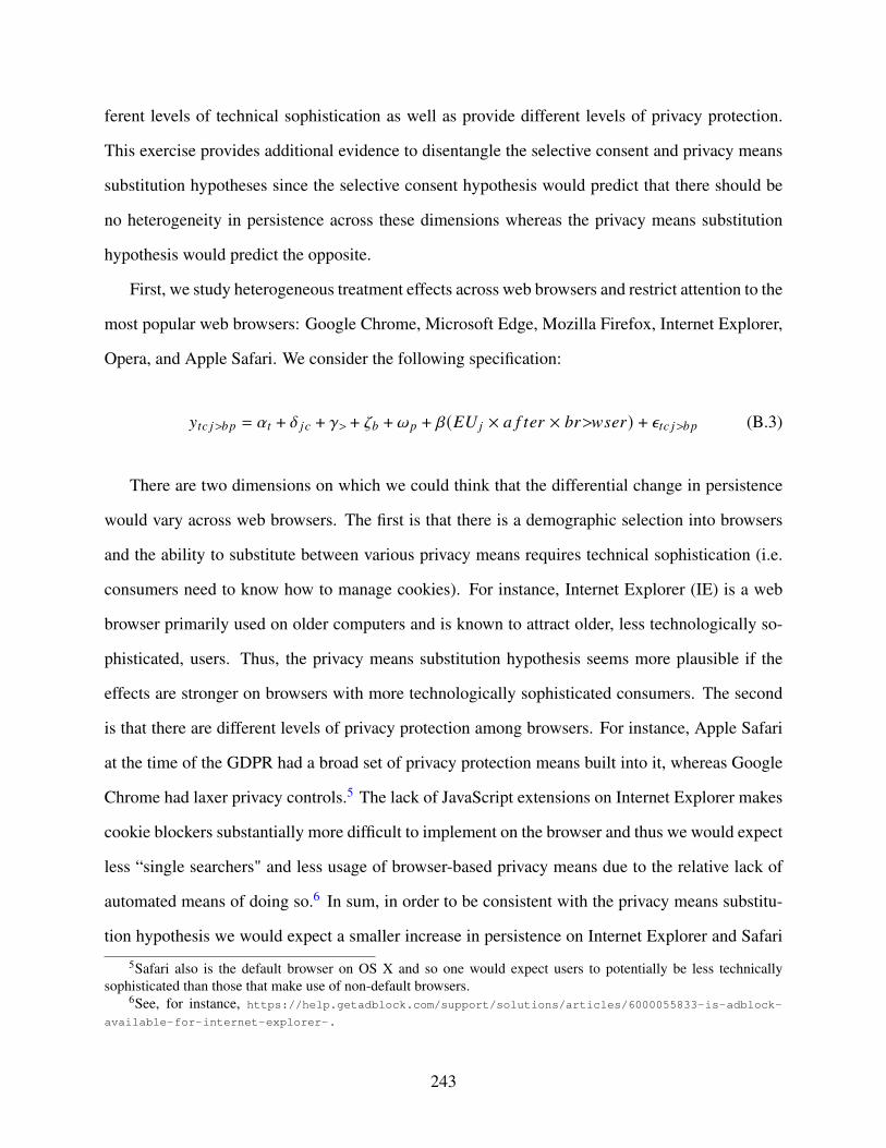
ferent levels of technical sophistication as well as provide different levels of privacy protection.

This exercise provides additional evidence to disentangle the selective consent and privacy means

substitution hypotheses since the selective consent hypothesis would predict that there should be

no heterogeneity in persistence across these dimensions whereas the privacy means substitution

hypothesis would predict the opposite.

First, we study heterogeneous treatment effects across web browsers and restrict attention to the

most popular web browsers: Google Chrome, Microsoft Edge, Mozilla Firefox, Internet Explorer,

Opera, and Apple Safari. We consider the following specification:

𝑦𝑡𝑐 𝑗𝑜𝑏𝑝 = 𝛼𝑡 + 𝛿 𝑗𝑐 + 𝛾𝑜 + Z𝑏 + 𝜔𝑝 + 𝛽(𝐸𝑈 𝑗 × 𝑎 𝑓 𝑡𝑒𝑟 × 𝑏𝑟𝑜𝑤𝑠𝑒𝑟) + 𝜖𝑡𝑐 𝑗𝑜𝑏𝑝 (B.3)

There are two dimensions on which we could think that the differential change in persistence

would vary across web browsers. The first is that there is a demographic selection into browsers

and the ability to substitute between various privacy means requires technical sophistication (i.e.

consumers need to know how to manage cookies). For instance, Internet Explorer (IE) is a web

browser primarily used on older computers and is known to attract older, less technologically so-

phisticated, users. Thus, the privacy means substitution hypothesis seems more plausible if the

effects are stronger on browsers with more technologically sophisticated consumers. The second

is that there are different levels of privacy protection among browsers. For instance, Apple Safari

at the time of the GDPR had a broad set of privacy protection means built into it, whereas Google

Chrome had laxer privacy controls.5 The lack of JavaScript extensions on Internet Explorer makes

cookie blockers substantially more difficult to implement on the browser and thus we would expect

less “single searchers" and less usage of browser-based privacy means due to the relative lack of

automated means of doing so.6 In sum, in order to be consistent with the privacy means substitu-

tion hypothesis we would expect a smaller increase in persistence on Internet Explorer and Safari

5Safari also is the default browser on OS X and so one would expect users to potentially be less technicallysophisticated than those that make use of non-default browsers.

6See, for instance, https://help.getadblock.com/support/solutions/articles/6000055833-is-adblock-

available-for-internet-explorer-.

243

relative to the other browsers.

Table B5 displays the regression results for this specification with Chrome as the omitted

browser. The treatment effect is consistent across browsers with the exception of Internet Explorer

which has almost no change in persistence, consistent with our hypothesis. The estimated treat-

ment effect is lower in Safari relative to Chrome, but the difference is not statistically significant.

Both of these observations are consistent with the privacy means hypothesis.

Next, we study heterogeneous treatment effects across operating systems and narrow down the

sample to only look at the most popular operating systems: Android, Chrome OS, iOS, Linux, Mac

OS X, and Windows. We consider the following specification:

𝑦𝑡𝑐 𝑗𝑜𝑏𝑝 = 𝛼𝑡 + 𝛿 𝑗𝑐 + 𝛾𝑜 + Z𝑏 + 𝜔𝑝 + 𝛽(𝐸𝑈 𝑗 × 𝑎 𝑓 𝑡𝑒𝑟 ×𝑂𝑆) + 𝜖𝑡𝑐 𝑗𝑜𝑏𝑝 (B.4)

We are mainly interested in differences in the treatment effects between mobile and desktop

consumers. The reason is that there are less readily available privacy means for cookie management

on the mobile web compared to desktop and consumer behavior in general tends to be different

on mobile compared to desktop. For consistency with the privacy means substitution hypothesis,

we would expect a larger difference in persistence on desktop compared to mobile whereas for

consistency with the selective consent hypothesis we should expect a smaller difference.

Table B4 displays the regression results with Windows as the omitted operating system that

indicates that Android and iOS have no or weak increases in persistence for 𝑘 = 1, 2 but appear to

have an increase in persistence for 𝑘 = 3, 4. Otherwise, the treatment effect is approximately the

same across the different operating systems. Since there seems to be a weak difference between

persistence on mobile and desktop this appears to be suggestive of the privacy means substitution

hypothesis, but does not provide conclusive evidence.

244

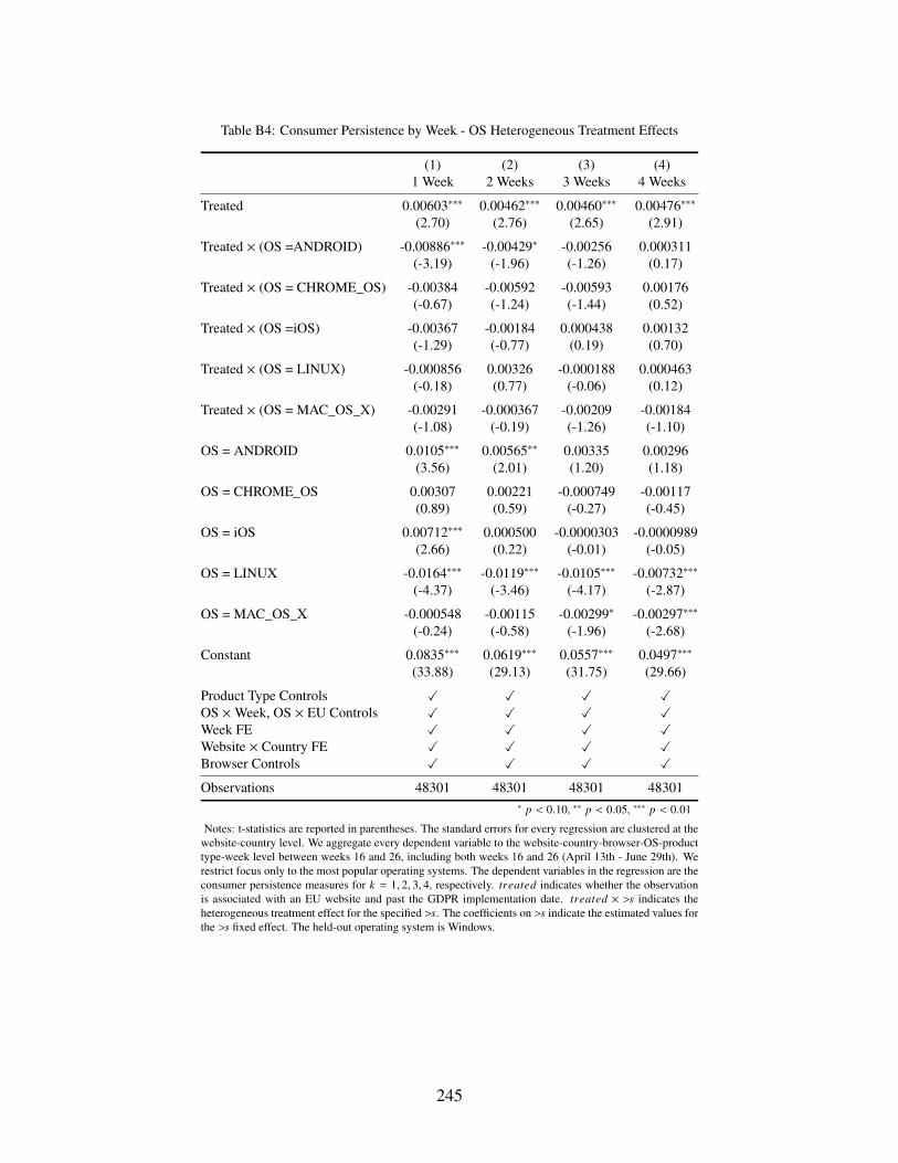
Table B4: Consumer Persistence by Week - OS Heterogeneous Treatment Effects

(1) (2) (3) (4)1 Week 2 Weeks 3 Weeks 4 Weeks

Treated 0.00603∗∗∗ 0.00462∗∗∗ 0.00460∗∗∗ 0.00476∗∗∗

(2.70) (2.76) (2.65) (2.91)

Treated × (OS =ANDROID) -0.00886∗∗∗ -0.00429∗ -0.00256 0.000311(-3.19) (-1.96) (-1.26) (0.17)

Treated × (OS = CHROME_OS) -0.00384 -0.00592 -0.00593 0.00176(-0.67) (-1.24) (-1.44) (0.52)

Treated × (OS =iOS) -0.00367 -0.00184 0.000438 0.00132(-1.29) (-0.77) (0.19) (0.70)

Treated × (OS = LINUX) -0.000856 0.00326 -0.000188 0.000463(-0.18) (0.77) (-0.06) (0.12)

Treated × (OS = MAC_OS_X) -0.00291 -0.000367 -0.00209 -0.00184(-1.08) (-0.19) (-1.26) (-1.10)

OS = ANDROID 0.0105∗∗∗ 0.00565∗∗ 0.00335 0.00296(3.56) (2.01) (1.20) (1.18)

OS = CHROME_OS 0.00307 0.00221 -0.000749 -0.00117(0.89) (0.59) (-0.27) (-0.45)

OS = iOS 0.00712∗∗∗ 0.000500 -0.0000303 -0.0000989(2.66) (0.22) (-0.01) (-0.05)

OS = LINUX -0.0164∗∗∗ -0.0119∗∗∗ -0.0105∗∗∗ -0.00732∗∗∗

(-4.37) (-3.46) (-4.17) (-2.87)

OS = MAC_OS_X -0.000548 -0.00115 -0.00299∗ -0.00297∗∗∗

(-0.24) (-0.58) (-1.96) (-2.68)

Constant 0.0835∗∗∗ 0.0619∗∗∗ 0.0557∗∗∗ 0.0497∗∗∗

(33.88) (29.13) (31.75) (29.66)

Product Type Controls ✓ ✓ ✓ ✓OS × Week, OS × EU Controls ✓ ✓ ✓ ✓Week FE ✓ ✓ ✓ ✓Website × Country FE ✓ ✓ ✓ ✓Browser Controls ✓ ✓ ✓ ✓

Observations 48301 48301 48301 48301∗ 𝑝 < 0.10, ∗∗ 𝑝 < 0.05, ∗∗∗ 𝑝 < 0.01

Notes: t-statistics are reported in parentheses. The standard errors for every regression are clustered at thewebsite-country level. We aggregate every dependent variable to the website-country-browser-OS-producttype-week level between weeks 16 and 26, including both weeks 16 and 26 (April 13th - June 29th). Werestrict focus only to the most popular operating systems. The dependent variables in the regression are theconsumer persistence measures for 𝑘 = 1, 2, 3, 4, respectively. 𝑡𝑟𝑒𝑎𝑡𝑒𝑑 indicates whether the observationis associated with an EU website and past the GDPR implementation date. 𝑡𝑟𝑒𝑎𝑡𝑒𝑑 × 𝑜𝑠 indicates theheterogeneous treatment effect for the specified 𝑜𝑠. The coefficients on 𝑜𝑠 indicate the estimated values forthe 𝑜𝑠 fixed effect. The held-out operating system is Windows.

245

Table B5: Consumer Persistence - Browser Heterogeneous Treatment Effects

(1) (2) (3) (4)1 Week 2 Weeks 3 Weeks 4 Weeks

Treated 0.00615∗∗∗ 0.00645∗∗∗ 0.00519∗∗∗ 0.00628∗∗∗

(2.99) (3.51) (3.29) (3.49)

Treated × (Browser = EDGE) -0.00134 -0.00169 0.00230 0.000132(-0.35) (-0.61) (0.74) (0.04)

Treated × (Browser = FIREFOX) -0.00413 -0.00214 -0.00260 -0.00166(-1.60) (-0.89) (-1.43) (-0.84)

Treated × (Browser = IE) -0.0101∗∗ -0.00838∗∗∗ -0.00375 -0.00497∗∗

(-2.53) (-2.67) (-1.54) (-2.03)

Treated × (Browser = OPERA) -0.00935∗ -0.00396 -0.00344 -0.00335(-1.95) (-0.83) (-0.94) (-0.86)

Treated × (Browser = SAFARI) -0.00185 -0.00332 -0.00280 -0.00225(-0.69) (-1.43) (-1.44) (-1.12)

Browser = EDGE 0.00125 -0.00226 -0.00144 -0.000568(0.36) (-0.78) (-0.42) (-0.18)

Browser = FIREFOX -0.00503∗∗ -0.00381∗ -0.00465∗∗∗ -0.00409∗∗∗

(-2.29) (-1.96) (-3.13) (-2.92)

Browser = IE -0.0164∗∗∗ -0.0113∗∗∗ -0.00801∗∗∗ -0.00764∗∗∗

(-6.73) (-5.15) (-3.29) (-4.18)

Browser = OPERA -0.00151 -0.00337 -0.00665∗∗ -0.00596∗∗

(-0.39) (-1.00) (-2.22) (-2.15)

Browser = SAFARI -0.00315 -0.00229 -0.00309∗ -0.00211(-1.22) (-1.06) (-1.80) (-1.20)

Constant 0.0861∗∗∗ 0.0647∗∗∗ 0.0575∗∗∗ 0.0568∗∗∗

(32.30) (29.30) (34.48) (12.53)

Product Type Controls ✓ ✓ ✓ ✓OS × Week, OS × EU Controls ✓ ✓ ✓ ✓Week FE ✓ ✓ ✓ ✓Website × Country FE ✓ ✓ ✓ ✓OS Controls ✓ ✓ ✓ ✓

Observations 40810 40810 40810 40810∗ 𝑝 < 0.10, ∗∗ 𝑝 < 0.05, ∗∗∗ 𝑝 < 0.01

Notes: t-statistics are reported in parentheses. The standard errors for every regression are clustered at thewebsite-country level. We aggregate every dependent variable to the website-country-browser-OS-producttype-week level between weeks 16 and 26, including both weeks 16 and 26 (April 13th - June 29th). Werestrict focus only to the most popular web browsers. The dependent variables in the regression are theconsumer persistence measures for 𝑘 = 1, 2, 3, 4, respectively. 𝑡𝑟𝑒𝑎𝑡𝑒𝑑 indicates whether the observationis associated with an EU website and past the GDPR implementation date. 𝑡𝑟𝑒𝑎𝑡𝑒𝑑 × 𝑏𝑟𝑜𝑤𝑠𝑒𝑟 indicatesthe heterogeneous treatment effect for the specified 𝑏𝑟𝑜𝑤𝑠𝑒𝑟. The coefficients on 𝑏𝑟𝑜𝑤𝑠𝑒𝑟 indicate theestimated values for the 𝑏𝑟𝑜𝑤𝑠𝑒𝑟 fixed effect. The held-out browser is Google Chrome.

246

B.4 Additional Evidence for “Single Searcher" Inflation

In this section we more formally investigate the “single searcher" observation from subsec-

tion 2.4.2. Our main objective is to determine statistically whether there is an excess amount of

single searchers, which is consistent with the privacy means substitution hypothesis. The test re-

sults in this section provide evidence for the following two claims. First, consumers were making

use of such privacy means prior to the introduction of GDPR. Second, the fraction of consumers

doing so has decreased after GDPR is introduced.

B.4.1 Setup and Hypotheses

We first describe a simple model that motivates our empirical exercise. Suppose that there are

two types of consumers – obfuscators (𝑜) and non-obfuscators (𝑛) – and that each type of consumer

generates an observed search history length of 𝑘 . Each consumer has a history of length 𝑘 ≥ 1.

The distribution of observed history length for the obfuscation consumer type 𝑜 is degenerate with

probability mass 1 at 𝑘 = 1. For the obfuscation type 𝑜, we hypothesize that their observed history

length is 𝑘 = 1 with probability one. For the non-obfuscation consumer type 𝑛, the probability

of observing search history length 𝑘 ≥ 1, conditional on observing a consumer, is denoted by

𝑄(𝑘; \ (𝑥)), where \ contains the relevant parameters of probability distribution 𝑄 and 𝑥 denotes a

set of observable consumer characteristics. In our setting the lowest count is one, which is why we

subtract one from each observation to map it into a standard count model. We denote the fraction

of consumers that are obfuscators conditional on observable characteristics 𝑥 as

𝜋(𝑥) := Pr{obfuscator | 𝑥}

This setup maps into the following observed share of visits 𝑆𝑘 , where 𝑘 denotes history length:

𝑆1 = 𝜋(𝑥) + (1 − 𝜋(𝑥)) · 𝑄(1; \ (𝑥)) (B.5)

𝑆𝑘 = (1 − 𝜋(𝑥)) · 𝑄(𝑘; \ (𝑥)), ∀𝑘 ≥ 1 (B.6)

247

We note that given this set-up 𝜋 and \ are identified and that we can separately estimate 𝜋 and

\ for the pre-GDPR and post-GDPR period, giving us estimates for �̂�𝑃𝑅𝐸 , �̂�𝑃𝑂𝑆𝑇 , \̂𝑃𝑅𝐸 , \̂𝑃𝑂𝑆𝑇 .

Given this setup, our informal hypotheses can be stated as the following null hypotheses:

1. 𝐻0 : �̂�𝑃𝑅𝐸 = 0, 𝐻𝑎 : �̂�𝑃𝑅𝐸 ≠ 0

2. 𝐻0 : �̂�𝑃𝑂𝑆𝑇 = �̂�𝑃𝑅𝐸 , 𝐻𝑎 : �̂�𝑃𝑂𝑆𝑇 ≠ �̂�𝑃𝑅𝐸

B.4.2 Data and Estimation

For this exercise we restrict attention to the same large hotel website shown in Figure 2.5 which

exhibited the noticeable change in “single searchers" at the onset of GDPR). We measure how

many searches are associated with each identifier observed before and after GDPR is introduced.

In total, we observe more than three million unique identifiers.

We allow the parameters of the model to depend on both the web browser and the operating

system. Thus, we allow both the arrival rates and the fraction of obfuscators to vary across these

dimensions. Next, we parameterize 𝜋(𝑥) as follows:

𝜋(𝑥) =[

exp(𝑥′𝛾)]/[1 + exp(𝑥′𝛾)

],

where 𝛾 is a parameter to be estimated. We consider two possible distributional assumptions for𝑄:

a Poisson distribution and a negative binomial distribution, where the latter allows for additional

dispersion. For the Poisson distribution we allow the arrival rate _(𝑥) to vary across observables

and we do similarly for the negative binomial parameters `(𝑥), 𝛼(𝑥).7

Our setup maps almost directly to standard zero-inflation Poisson models (e.g. [192]. We

follow [192, 191] and estimate the parameters of the model via maximum likelihood estimation.

The model with a positive share of obfuscators is tested against either a standard Poisson regression

or a negative binomial regression. We then conduct a Vuong test [107] to evaluate whether a model

7See section 20.4.1 of [191] for full details of the parameterization for Poisson and Negative Binomial regressionsthat we utilize.

248

with type 𝑜 consumers leads to a better fit to the observed data [193]. In order to test our second

hypothesis of interest, we do a t-test comparing the vectors of �̂�𝑃𝑅𝐸 and �̂�𝑃𝑂𝑆𝑇 .

B.4.3 Results

We first consider the specification where we assume that 𝑄 follows a Poisson distribution.

The results of the Vuong test strongly conclude that there is evidence for the existence of type 𝑜

consumers in both periods with a z-statistic of −244.85 in the pre-GDPR period and −246.28 in

the post-GDPR period.

We then compare the resulting �̂� in the pre-GDPR and post-GDPR periods, denoted by �̂�𝑃𝑅𝐸

and �̂�𝑃𝑂𝑆𝑇 , respectively. We run a t-test with the null hypothesis that �̂�𝑃𝑂𝑆𝑇 = �̂�𝑃𝑅𝐸 . We are able

to reject the null with 𝑝 < 2.2𝑒 − 16. The difference is also economically significant as we note

that �̂�𝑃𝑅𝐸 = 0.478 and �̂�𝑃𝑂𝑆𝑇 = 0.354, suggesting a significant drop of obfuscators after GDPR.

One concern with the parameterization of 𝑄 as Poisson is that it does not account for overdis-

persion or underdispersion. We can directly test for overdispersion. Let 𝑌𝑖 denote the observed

history length for consumer 𝑖 and _̂𝑖 the implied variance of the poisson distribution. One can then

test the null that 𝛼 = 0 for VAR(𝑌𝑖) = _̂𝑖 + 𝛼 · _̂𝑖 against the alternative that 𝛼 is larger than zero

[194]. We reject the null (𝑝 < 2.2𝑒 − 16) in both the pre and post period. Thus, we conclude that

the data is overdispersed and consider the common remedy that imposes that 𝑄 follows a negative

binomial distribution, instead of a Poisson distribution [191].

Under the the assumption of a negative binomial, the Vuong test still concludes that there is

evidence for the presence of type 𝑜 consumers (𝑧 = −6.97) in the pre-GDPR period. However,

we no longer reject the model without excess single searchers in the post-GDPR period (𝑧 =

−1.81,AIC-corrected: 𝑧 = −0.84, BIC-corrected: 𝑧 = 4.94). Furthermore, we are able again to

reject the null hypothesis that �̂�𝑃𝑂𝑆𝑇 = �̂�𝑃𝑅𝐸 with 𝑝 < 2.2𝑒 − 16.

In sum, we document statistical evidence for excess “single-searchers" in the pre-GDPR period

under both distributional assumptions. Once we take into account the overdispersion relative to a

Poisson count model, we do not find evidence for excess single searchers in the post-GDPR period.

249

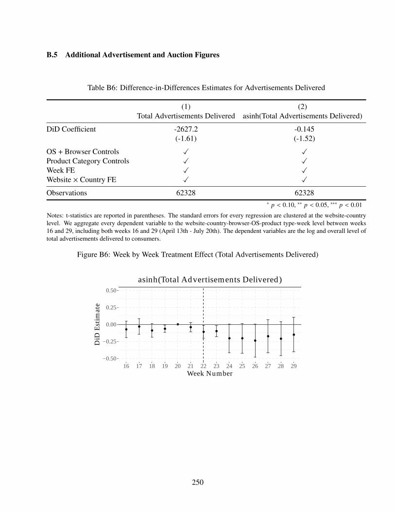
B.5 Additional Advertisement and Auction Figures

Table B6: Difference-in-Differences Estimates for Advertisements Delivered

(1) (2)Total Advertisements Delivered asinh(Total Advertisements Delivered)

DiD Coefficient -2627.2 -0.145(-1.61) (-1.52)

OS + Browser Controls ✓ ✓Product Category Controls ✓ ✓Week FE ✓ ✓Website × Country FE ✓ ✓

Observations 62328 62328∗ 𝑝 < 0.10, ∗∗ 𝑝 < 0.05, ∗∗∗ 𝑝 < 0.01

Notes: t-statistics are reported in parentheses. The standard errors for every regression are clustered at the website-countrylevel. We aggregate every dependent variable to the website-country-browser-OS-product type-week level between weeks16 and 29, including both weeks 16 and 29 (April 13th - July 20th). The dependent variables are the log and overall level oftotal advertisements delivered to consumers.

Figure B6: Week by Week Treatment Effect (Total Advertisements Delivered)

●

●

●●

●

●

● ●

● ●●

●●

●

−0.50

−0.25

0.00

0.25

0.50

16 17 18 19 20 21 22 23 24 25 26 27 28 29Week Number

DiD

Est

imat

e

asinh(Total Advertisements Delivered)

250

Table B7: Summary Statistics, Bids

Treatment Group Average Bidnon-EU 394.053EU 126.947

Notes: The table reports the mean of theaverage bid across observations in the pre-GDPR time period for the EU and non-EUrespectively.

B.6 Prediction Evaluation Measures

B.6.1 AUC Primer

In this section we provide additional details on how to calculate the AUC measure and its

interpretation. To begin, fix the classification threshold at any �̂�. Then, a consumer with score 𝑝𝑖 𝑗 𝑘

is classified as a purchaser if 𝑝𝑖 𝑗 𝑘 > �̂� and a non-purchaser if 𝑝𝑖 𝑗 𝑘 < �̂�. This would result in a

false positive rate—a rate at which a non-purchaser is misclassified into a purchaser:

𝐹𝑃𝑅 :=False Positive

True Negative + False Positive=

∑𝑖 𝑗 𝑘 |{𝑝𝑖 𝑗 𝑘 > �̂�, 𝑦𝑇𝑅𝑈𝐸𝑖 𝑗 𝑘

= 0}|∑𝑖 𝑗 𝑘 |{𝑦𝑇𝑅𝑈𝐸𝑖 𝑗 𝑘

= 0}|.

At the same time, it would result in a true positive rate—or a rate at which a purchaser is correctly

classified as a purchaser:

𝑇𝑃𝑅 :=True Positive

True Positive + False Negative=

∑𝑖 𝑗 𝑘 |{𝑝𝑖 𝑗 𝑘 > �̂�, 𝑦𝑇𝑅𝑈𝐸𝑖 𝑗 𝑘

= 1}|∑𝑖 𝑗 𝑘 |{𝑦𝑇𝑅𝑈𝐸𝑖 𝑗 𝑘

= 1}|.

The ROC then depicts the level of 𝑇𝑃𝑅 a prediction machine achieves for each level of 𝐹𝑃𝑅 it

tolerates.

The ROC is obtained by tracing the locus of (𝐹𝑃𝑅,𝑇𝑃𝑅) by varying the classification thresh-

old �̂�.8 The slope of the ROC corresponds to the additional power (in rate) the prediction gains

8For extreme cases, with �̂� = 1, all consumers are classified as non-purchasers, which yields (𝐹𝑃𝑅,𝑇𝑃𝑅) =

251

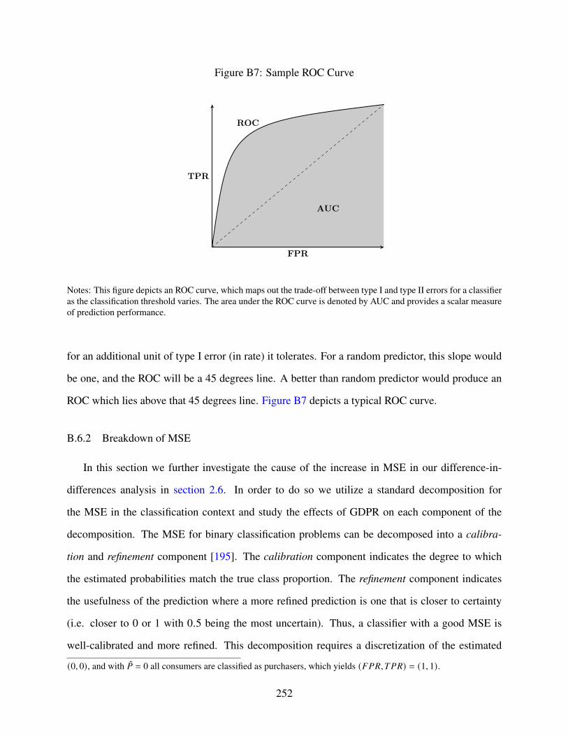
Figure B7: Sample ROC Curve

AUC

ROC

FPR

TPR

Notes: This figure depicts an ROC curve, which maps out the trade-off between type I and type II errors for a classifieras the classification threshold varies. The area under the ROC curve is denoted by AUC and provides a scalar measureof prediction performance.

for an additional unit of type I error (in rate) it tolerates. For a random predictor, this slope would

be one, and the ROC will be a 45 degrees line. A better than random predictor would produce an

ROC which lies above that 45 degrees line. Figure B7 depicts a typical ROC curve.

B.6.2 Breakdown of MSE

In this section we further investigate the cause of the increase in MSE in our difference-in-

differences analysis in section 2.6. In order to do so we utilize a standard decomposition for

the MSE in the classification context and study the effects of GDPR on each component of the

decomposition. The MSE for binary classification problems can be decomposed into a calibra-

tion and refinement component [195]. The calibration component indicates the degree to which

the estimated probabilities match the true class proportion. The refinement component indicates

the usefulness of the prediction where a more refined prediction is one that is closer to certainty

(i.e. closer to 0 or 1 with 0.5 being the most uncertain). Thus, a classifier with a good MSE is

well-calibrated and more refined. This decomposition requires a discretization of the estimated

(0, 0), and with �̂� = 0 all consumers are classified as purchasers, which yields (𝐹𝑃𝑅,𝑇𝑃𝑅) = (1, 1).

252

probabilities into a series of 𝐾 bins.9 For notation, 𝑝𝑘 denotes the 𝑘th estimated probability bin, 𝑛𝑘

denotes the number of probability estimates falling into the 𝑘th bin and 𝑜𝑘 denotes the true class

proportion in the 𝑘th bin in the data. This allows us to rewrite (2.4) as:

𝑀𝑆𝐸 𝑗 =1∑

𝑖∈I𝑗|K𝑖 𝑗 |

𝐾∑︁𝑘=1

𝑛𝑘 (𝑝𝑘 − 𝑜𝑘 )2

︸ ︷︷ ︸calibration error

+ 1∑𝑖∈I𝑗

|K𝑖 𝑗 |

𝐾∑︁𝑘=1

𝑛𝑘𝑜𝑘 (1 − 𝑜𝑘 )

︸ ︷︷ ︸refinement error

(B.7)

Table B8: Difference-in-Differences Estimates for Rel-evance and Calibration

(1) (2)Calibration Refinement

DiD Coefficient 0.00735∗∗∗ 0.00576∗∗

(2.84) (2.64)

OS + Browser Controls ✓ ✓Product Category Controls ✓ ✓Week FE ✓ ✓Website × Country FE ✓ ✓

Observations 15470 15470∗ 𝑝 < 0.10, ∗∗ 𝑝 < 0.05, ∗∗∗ 𝑝 < 0.01

Notes: t-statistics are reported in parentheses. The standard errorsfor every regression are clustered at the website-country level. Weaggregate every dependent variable to the website-country-browser-OS-product type-week level between weeks 16 and 29, includingboth weeks 16 and 29 (April 13th - July 20th). The dependent vari-able in the regression reported in the first column is the calibrationcomponent of the MSE. The dependent variable in the regressionreported in the second column is the refinement component of theMSE.

We run the same specification utilizing each component of the decomposition of the MSE as the

outcome variable. These results are reported in Table B8. They indicate that both the refinement

and calibration components increased after GDPR. Both of the components are approximately

equally responsible for the increase in MSE with the calibration component being only slightly

9Throughout this paper, when calculating the decomposed MSE we will primarily utilize equally spaced bins ofsize 0.01. Note that since the decomposition requires this discretization, the decomposed MSE and the standard MSEare not precisely the same quantities but are approximately the same.

253

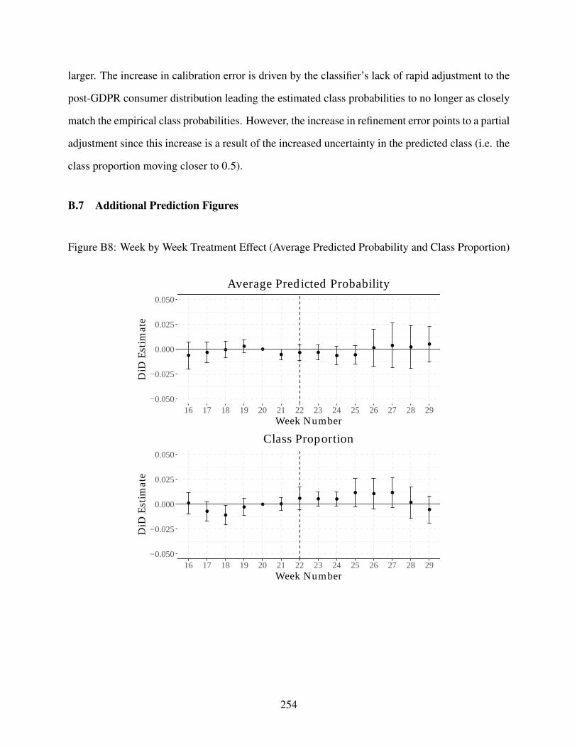
larger. The increase in calibration error is driven by the classifier’s lack of rapid adjustment to the

post-GDPR consumer distribution leading the estimated class probabilities to no longer as closely

match the empirical class probabilities. However, the increase in refinement error points to a partial

adjustment since this increase is a result of the increased uncertainty in the predicted class (i.e. the

class proportion moving closer to 0.5).

B.7 Additional Prediction Figures

Figure B8: Week by Week Treatment Effect (Average Predicted Probability and Class Proportion)

●●

●●

●

●● ●

● ●

●● ●

●

−0.050

−0.025

0.000

0.025

0.050

16 17 18 19 20 21 22 23 24 25 26 27 28 29Week Number

DiD

Est

imat

e

Average Predicted Probability

●

●●

●● ●

● ● ●

● ● ●

●

●

−0.050

−0.025

0.000

0.025

0.050

16 17 18 19 20 21 22 23 24 25 26 27 28 29Week Number

DiD

Est

imat

e

Class Proportion

254

Figure B9: Week by Week Treatment Effect (MSE and AUC)

●

●

●

●●

●

● ● ●

●●

●

●

●

−0.04

−0.02

0.00

0.02

0.04

16 17 18 19 20 21 22 23 24 25 26 27 28 29Week Number

DiD

Est

imat

e

MSE

● ● ●

●

●●

● ●

●

●

●

● ●●

−0.10

−0.05

0.00

0.05

0.10

16 17 18 19 20 21 22 23 24 25 26 27 28 29Week Number

DiD

Est

imat

e

AUC

B.8 The Impact of Consumer Persistence and Data Scale on Prediction

The analysis in section 2.6 on the effect of GDPR on the firm’s ability to predict is limited by

the data restrictions and the apparent lack of adjustment by its prediction algorithm to the post-

GDPR environment. To fully understand the implications for prediction, therefore, we now take

a different approach. Instead of asking how the firm’s prediction was actually impacted in the

immediate aftermath, we now ask what would happen to predictive performance in the long run

when the algorithm were fully adjusted.

As observed in section 2.4, GDPR reduces the number of consumers that the intermediary

observes but remaining consumers are more persistently trackable. Our approach is to study how

these two features—number of observed consumers and the persistence of observed consumers—

255

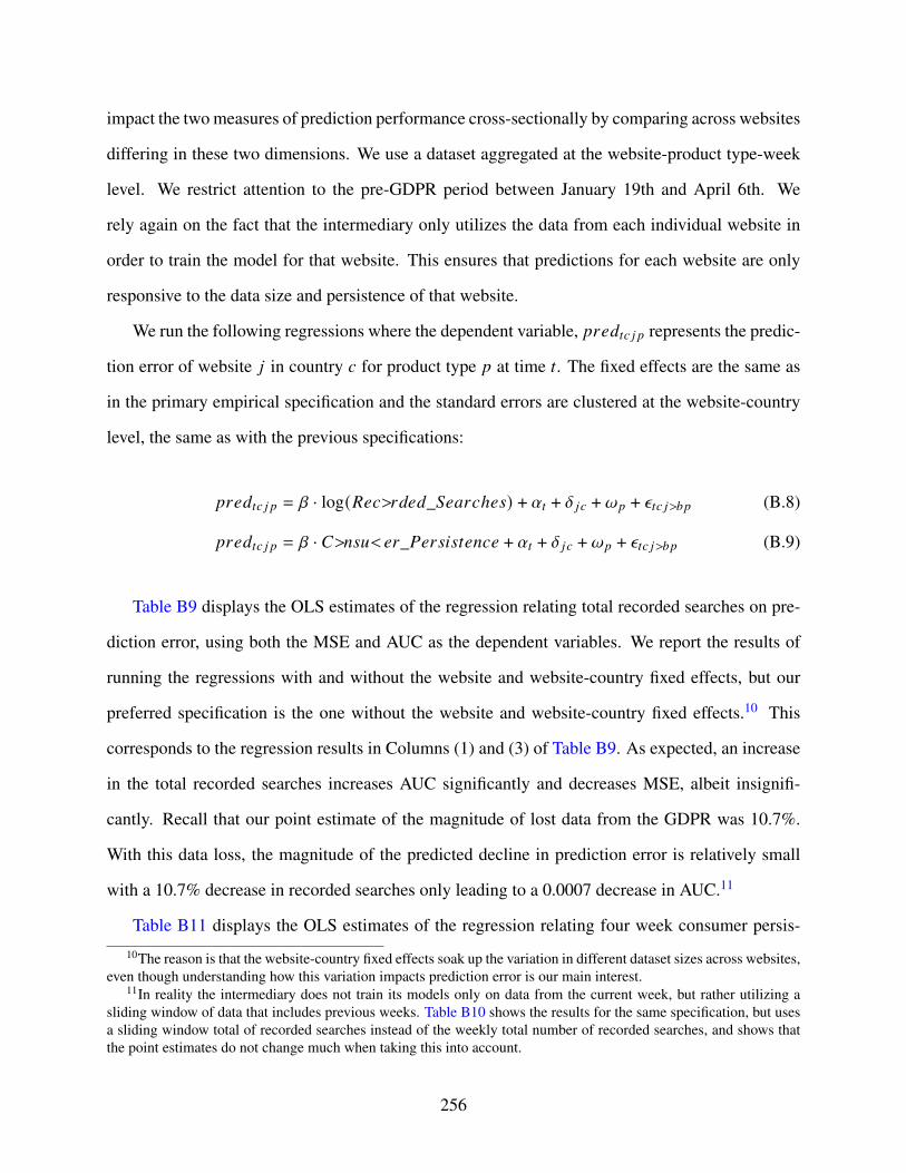
impact the two measures of prediction performance cross-sectionally by comparing across websites

differing in these two dimensions. We use a dataset aggregated at the website-product type-week

level. We restrict attention to the pre-GDPR period between January 19th and April 6th. We

rely again on the fact that the intermediary only utilizes the data from each individual website in

order to train the model for that website. This ensures that predictions for each website are only

responsive to the data size and persistence of that website.

We run the following regressions where the dependent variable, 𝑝𝑟𝑒𝑑𝑡𝑐 𝑗 𝑝 represents the predic-

tion error of website 𝑗 in country 𝑐 for product type 𝑝 at time 𝑡. The fixed effects are the same as

in the primary empirical specification and the standard errors are clustered at the website-country

level, the same as with the previous specifications:

𝑝𝑟𝑒𝑑𝑡𝑐 𝑗 𝑝 = 𝛽 · log(𝑅𝑒𝑐𝑜𝑟𝑑𝑒𝑑_𝑆𝑒𝑎𝑟𝑐ℎ𝑒𝑠) + 𝛼𝑡 + 𝛿 𝑗𝑐 + 𝜔𝑝 + 𝜖𝑡𝑐 𝑗𝑜𝑏𝑝 (B.8)

𝑝𝑟𝑒𝑑𝑡𝑐 𝑗 𝑝 = 𝛽 · 𝐶𝑜𝑛𝑠𝑢𝑚𝑒𝑟_𝑃𝑒𝑟𝑠𝑖𝑠𝑡𝑒𝑛𝑐𝑒 + 𝛼𝑡 + 𝛿 𝑗𝑐 + 𝜔𝑝 + 𝜖𝑡𝑐 𝑗𝑜𝑏𝑝 (B.9)

Table B9 displays the OLS estimates of the regression relating total recorded searches on pre-

diction error, using both the MSE and AUC as the dependent variables. We report the results of

running the regressions with and without the website and website-country fixed effects, but our

preferred specification is the one without the website and website-country fixed effects.10 This

corresponds to the regression results in Columns (1) and (3) of Table B9. As expected, an increase

in the total recorded searches increases AUC significantly and decreases MSE, albeit insignifi-

cantly. Recall that our point estimate of the magnitude of lost data from the GDPR was 10.7%.

With this data loss, the magnitude of the predicted decline in prediction error is relatively small

with a 10.7% decrease in recorded searches only leading to a 0.0007 decrease in AUC.11

Table B11 displays the OLS estimates of the regression relating four week consumer persis-

10The reason is that the website-country fixed effects soak up the variation in different dataset sizes across websites,even though understanding how this variation impacts prediction error is our main interest.

11In reality the intermediary does not train its models only on data from the current week, but rather utilizing asliding window of data that includes previous weeks. Table B10 shows the results for the same specification, but usesa sliding window total of recorded searches instead of the weekly total number of recorded searches, and shows thatthe point estimates do not change much when taking this into account.

256

tence to prediction error, using both the MSE and AUC as the dependent variable. As before, we

have regressions with and without website and website-country fixed effects, and focus primarily

on the regressions without them. Recall that we previously found a 0.00505 increase in the four

week persistence as a result of GDPR. Combined with the point estimates from Table B11, this

implies an increase of 0.013 for AUC and a decrease of 0.007 for MSE.

Putting these two results together point to the fact that the decline in the overall scale of data

should have little impact on predictability, but the change in the nature of the data towards more

identifiable consumers should marginally improve prediction according to both AUC and MSE.

However, this does not imply that the scale of data is unimportant which would run counter to

standard statistical intuition; on the contrary, prediction ability improves substantially as the scale

of data increases. Rather, the change in the scale of the data as a result of GDPR is not large

enough to cause meaningful changes in prediction error in the long run. However, the increase in

persistence as a result of GDPR should lead to an improvement in prediction capabilities in the

long run.

257

Table B9: Prediction Error and Scale of Data

(1) (2) (3) (4)AUC AUC MSE MSE

log(Recorded Searches) 0.0154∗ 0.0178 -0.00435 0.000937(1.84) (0.98) (-0.88) (0.15)

Constant 0.505∗∗∗ 0.510∗∗ 0.191∗∗∗ 0.0987(4.60) (2.45) (2.82) (1.31)

Product Category Controls ✓ ✓ ✓ ✓Week FE ✓ ✓ ✓ ✓Country FE ✓ ✓ ✓ ✓Website × Country FE ✓ ✓

Observations 874 874 874 874𝑅2 0.129 0.699 0.138 0.936

∗ 𝑝 < 0.10, ∗∗ 𝑝 < 0.05, ∗∗∗ 𝑝 < 0.01Notes: t-statistics are reported in parentheses. The standard errors for every regressionare clustered at the website-country level. We aggregate every dependent variable tothe website-country-product type-week level between weeks 4 and 14, including bothweeks 4 and 14 (January 9th - April 5th). The dependent variable in the regressionreported in the first and second column is AUC. The dependent variables in the thirdand fourth column is the MSE. The regression results reported in column (1) and (3)do not include website or website-country fixed effects, whereas those reported incolumn (2) and (4) include these fixed effects.

258

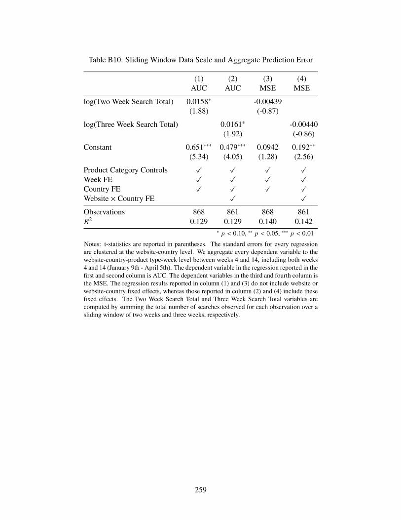
Table B10: Sliding Window Data Scale and Aggregate Prediction Error

(1) (2) (3) (4)AUC AUC MSE MSE

log(Two Week Search Total) 0.0158∗ -0.00439(1.88) (-0.87)

log(Three Week Search Total) 0.0161∗ -0.00440(1.92) (-0.86)

Constant 0.651∗∗∗ 0.479∗∗∗ 0.0942 0.192∗∗

(5.34) (4.05) (1.28) (2.56)

Product Category Controls ✓ ✓ ✓ ✓Week FE ✓ ✓ ✓ ✓Country FE ✓ ✓ ✓ ✓Website × Country FE ✓ ✓

Observations 868 861 868 861𝑅2 0.129 0.129 0.140 0.142

∗ 𝑝 < 0.10, ∗∗ 𝑝 < 0.05, ∗∗∗ 𝑝 < 0.01Notes: t-statistics are reported in parentheses. The standard errors for every regressionare clustered at the website-country level. We aggregate every dependent variable to thewebsite-country-product type-week level between weeks 4 and 14, including both weeks4 and 14 (January 9th - April 5th). The dependent variable in the regression reported in thefirst and second column is AUC. The dependent variables in the third and fourth column isthe MSE. The regression results reported in column (1) and (3) do not include website orwebsite-country fixed effects, whereas those reported in column (2) and (4) include thesefixed effects. The Two Week Search Total and Three Week Search Total variables arecomputed by summing the total number of searches observed for each observation over asliding window of two weeks and three weeks, respectively.

259

Table B11: Consumer Persistence and Prediction Error

(1) (2) (3) (4)AUC AUC MSE MSE

Four Week Persistence 2.621∗∗∗ 0.758 -1.401∗∗ 0.611∗

(4.55) (0.95) (-2.58) (1.67)

Constant 0.542∗∗∗ 0.686∗∗∗ 0.221∗∗∗ 0.0852∗∗∗

(11.35) (20.17) (4.91) (5.30)

Product Category Controls ✓ ✓ ✓ ✓Week FE ✓ ✓ ✓ ✓Country FE ✓ ✓ ✓ ✓Website × Country FE ✓ ✓

Observations 874 874 874 874𝑅2 0.230 0.691 0.223 0.938

∗ 𝑝 < 0.10, ∗∗ 𝑝 < 0.05, ∗∗∗ 𝑝 < 0.01Notes: t-statistics are reported in parentheses. The standard errors for every regressionare clustered at the website-country level. We aggregate every dependent variable tothe website-country-product type-week level between weeks 4 and 14, including bothweeks 4 and 14 (January 9th - April 5th). The dependent variable in the regressionreported in the first and second column is AUC. The dependent variables in the thirdand fourth column is the MSE. The regression results reported in column (1) and (3) donot include website or website-country fixed effects, whereas those reported in column(2) and (4) include these fixed effects.

260

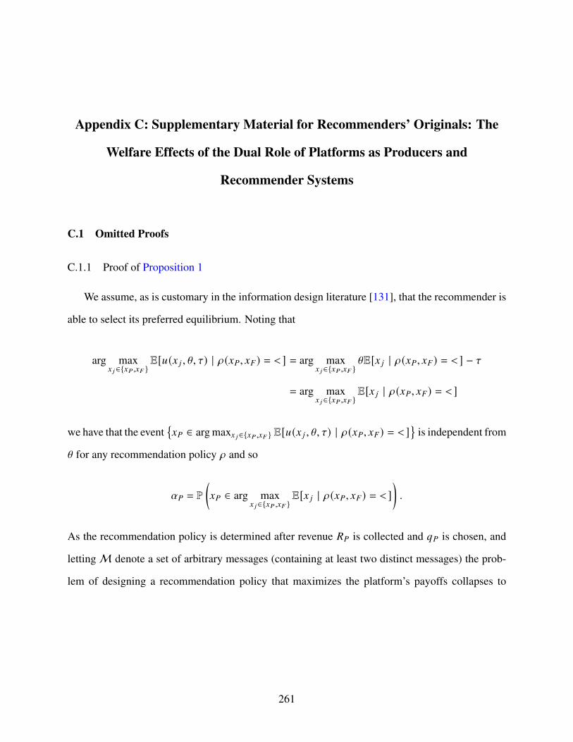
Appendix C: Supplementary Material for Recommenders’ Originals: The

Welfare Effects of the Dual Role of Platforms as Producers and

Recommender Systems

C.1 Omitted Proofs

C.1.1 Proof of Proposition 1

We assume, as is customary in the information design literature [131], that the recommender is

able to select its preferred equilibrium. Noting that

arg max𝑥 𝑗∈{𝑥𝑃 ,𝑥𝐹 }

E[𝑢(𝑥 𝑗 , \, 𝜏) | 𝜌(𝑥𝑃, 𝑥𝐹) = 𝑚] = arg max𝑥 𝑗∈{𝑥𝑃 ,𝑥𝐹 }

\E[𝑥 𝑗 | 𝜌(𝑥𝑃, 𝑥𝐹) = 𝑚] − 𝜏

= arg max𝑥 𝑗∈{𝑥𝑃 ,𝑥𝐹 }

E[𝑥 𝑗 | 𝜌(𝑥𝑃, 𝑥𝐹) = 𝑚]

we have that the event{𝑥𝑃 ∈ arg max𝑥 𝑗∈{𝑥𝑃 ,𝑥𝐹 } E[𝑢(𝑥 𝑗 , \, 𝜏) | 𝜌(𝑥𝑃, 𝑥𝐹) = 𝑚]

}is independent from

\ for any recommendation policy 𝜌 and so

𝛼𝑃 = P

(𝑥𝑃 ∈ arg max

𝑥 𝑗∈{𝑥𝑃 ,𝑥𝐹 }E[𝑥 𝑗 | 𝜌(𝑥𝑃, 𝑥𝐹) = 𝑚]

).

As the recommendation policy is determined after revenue 𝑅𝑃 is collected and 𝑞𝑃 is chosen, and

letting M denote a set of arbitrary messages (containing at least two distinct messages) the prob-

lem of designing a recommendation policy that maximizes the platform’s payoffs collapses to

261

maximizing the platform’s market share subject to consumer credibility constraints:

arg max𝜌:{0,1}2→Δ(M)

𝛼𝑃 · 𝑅𝑃 − 𝐶𝑃 (RP)

= arg max𝜌:{0,1}2→Δ(M)

P

(𝑥𝑃 ∈ arg max

𝑥 𝑗∈{𝑥𝑃 ,𝑥𝐹 }E[𝑥 𝑗 | 𝜌(𝑥𝑃, 𝑥𝐹) = 𝑚]

).

Given that there are only two relevant actions that the recommendation policy induces 𝑥𝑃, 𝑥𝐹 ,

the problem is equivalent to having (stochastic) direct recommendations, that is, to having 𝜌 :

{0, 1}2 → Δ(𝐽). We can then recast the optimal recommendation policy from the optimization

problem given in (RP) to:

max𝜌:{0,1}2→Δ(𝐽)

∑︁𝑎,𝑏∈{0,1}

P (𝜌(𝑥𝑃, 𝑥𝐹) = 𝑃 | 𝑥𝑃 = 𝑎, 𝑥𝐹 = 𝑏) P(𝑥𝑃 = 𝑎, 𝑥𝐹 = 𝑏)

subject to credibility constraints

E[𝑥𝑃 | 𝜌(𝑥𝑃, 𝑥𝐹) = 𝑃] ≥ E[𝑥𝐹 | 𝜌(𝑥𝑃, 𝑥𝐹) = 𝑃] (1)

E[𝑥𝐹 | 𝜌(𝑥𝑃, 𝑥𝐹) = 𝐹] ≥ E[𝑥𝑃 | 𝜌(𝑥𝑃, 𝑥𝐹) = 𝐹] (2)

Given independence of 𝑥𝑃 and 𝑥𝐹 , the objective function becomes 𝑞𝑃𝑞𝐹P (𝜌(1, 1) = 𝑃) + 𝑞𝑃 (1 −

𝑞𝐹)P (𝜌(1, 0) = 𝑃) + (1− 𝑞𝑃)𝑞𝐹P (𝜌(0, 1) = 𝑃) + (1− 𝑞𝑃) (1− 𝑞𝐹)P (𝜌(0, 0) = 𝑃), which is linear

and increasing in P (𝜌(𝑎, 𝑏) = 𝑃), 𝑎, 𝑏 ∈ {0, 1}.

Note that the unconstrained optimum is setting P (𝜌(𝑥𝑃, 𝑥𝐹) = 𝑃) = 1 regardless of the quality

realizations, implying that the platform always recommends its own goods. This is indeed the

solution to the optimal recommendation policy problem whenever 𝑞𝑃 ≥ 𝑞𝐹 as, in this case, the

unconstrained optimum is feasible as, without further information, the consumers will always con-

sume the platform’s good.

The solution to the case where 0 = 𝑞𝑃 < 𝑞𝐹 is similarly straightforward, as recommendations

are ineffective and thus the only policy that complies with obedience is to send consumers truthful

recommendations to choose the independent firm’s good whenever it is of high quality, and break

262

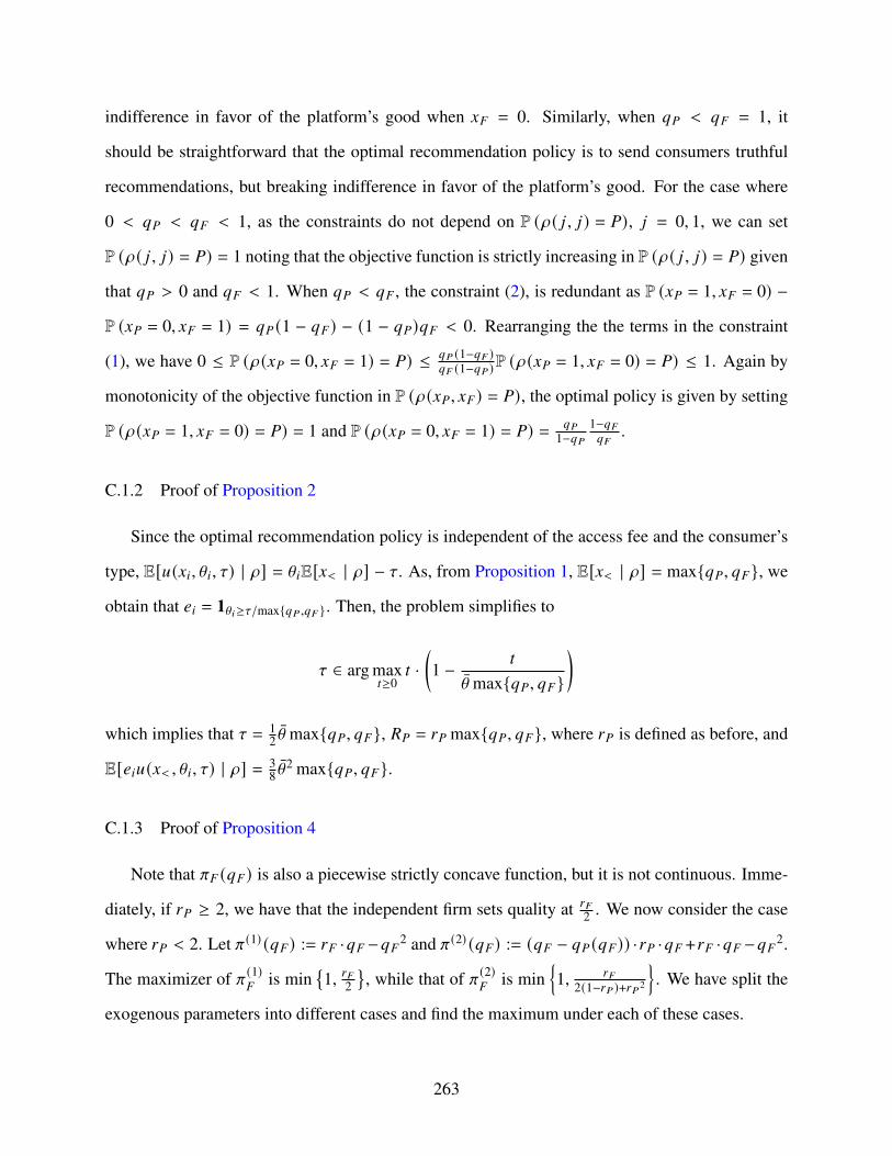
indifference in favor of the platform’s good when 𝑥𝐹 = 0. Similarly, when 𝑞𝑃 < 𝑞𝐹 = 1, it

should be straightforward that the optimal recommendation policy is to send consumers truthful

recommendations, but breaking indifference in favor of the platform’s good. For the case where

0 < 𝑞𝑃 < 𝑞𝐹 < 1, as the constraints do not depend on P (𝜌( 𝑗 , 𝑗) = 𝑃), 𝑗 = 0, 1, we can set

P (𝜌( 𝑗 , 𝑗) = 𝑃) = 1 noting that the objective function is strictly increasing in P (𝜌( 𝑗 , 𝑗) = 𝑃) given

that 𝑞𝑃 > 0 and 𝑞𝐹 < 1. When 𝑞𝑃 < 𝑞𝐹 , the constraint (2), is redundant as P (𝑥𝑃 = 1, 𝑥𝐹 = 0) −

P (𝑥𝑃 = 0, 𝑥𝐹 = 1) = 𝑞𝑃 (1 − 𝑞𝐹) − (1 − 𝑞𝑃)𝑞𝐹 < 0. Rearranging the the terms in the constraint

(1), we have 0 ≤ P (𝜌(𝑥𝑃 = 0, 𝑥𝐹 = 1) = 𝑃) ≤ 𝑞𝑃 (1−𝑞𝐹 )𝑞𝐹 (1−𝑞𝑃)P (𝜌(𝑥𝑃 = 1, 𝑥𝐹 = 0) = 𝑃) ≤ 1. Again by

monotonicity of the objective function in P (𝜌(𝑥𝑃, 𝑥𝐹) = 𝑃), the optimal policy is given by setting

P (𝜌(𝑥𝑃 = 1, 𝑥𝐹 = 0) = 𝑃) = 1 and P (𝜌(𝑥𝑃 = 0, 𝑥𝐹 = 1) = 𝑃) = 𝑞𝑃1−𝑞𝑃

1−𝑞𝐹𝑞𝐹

.

C.1.2 Proof of Proposition 2

Since the optimal recommendation policy is independent of the access fee and the consumer’s

type, E[𝑢(𝑥𝑖, \𝑖, 𝜏) | 𝜌] = \𝑖E[𝑥𝑚 | 𝜌] − 𝜏. As, from Proposition 1, E[𝑥𝑚 | 𝜌] = max{𝑞𝑃, 𝑞𝐹}, we

obtain that 𝑒𝑖 = 1\𝑖≥𝜏/max{𝑞𝑃 ,𝑞𝐹 }. Then, the problem simplifies to

𝜏 ∈ arg max𝑡≥0

𝑡 ·(1 − 𝑡

\̄max{𝑞𝑃, 𝑞𝐹}

)which implies that 𝜏 = 1

2 \̄max{𝑞𝑃, 𝑞𝐹}, 𝑅𝑃 = 𝑟𝑃 max{𝑞𝑃, 𝑞𝐹}, where 𝑟𝑃 is defined as before, and

E[𝑒𝑖𝑢(𝑥𝑚, \𝑖, 𝜏) | 𝜌] = 38 \̄

2 max{𝑞𝑃, 𝑞𝐹}.

C.1.3 Proof of Proposition 4

Note that 𝜋𝐹 (𝑞𝐹) is also a piecewise strictly concave function, but it is not continuous. Imme-

diately, if 𝑟𝑃 ≥ 2, we have that the independent firm sets quality at 𝑟𝐹2 . We now consider the case

where 𝑟𝑃 < 2. Let 𝜋(1) (𝑞𝐹) := 𝑟𝐹 ·𝑞𝐹 −𝑞𝐹2 and 𝜋(2) (𝑞𝐹) := (𝑞𝐹 − 𝑞𝑃 (𝑞𝐹)) ·𝑟𝑃 ·𝑞𝐹 +𝑟𝐹 ·𝑞𝐹 −𝑞𝐹2.

The maximizer of 𝜋(1)𝐹

is min{1, 𝑟𝐹2

}, while that of 𝜋(2)

𝐹is min

{1, 𝑟𝐹

2(1−𝑟𝑃)+𝑟𝑃2

}. We have split the

exogenous parameters into different cases and find the maximum under each of these cases.

263

1. When 𝑞𝐹 ≥ 𝑟𝐹2 , then the maximizer can only be that of 𝜋(2)

𝐹. This follows by strict concavity

of 𝜋(1)𝐹

which then leads to the fact that 𝑑𝑑𝑞𝐹

𝜋(1)𝐹

(𝑞𝐹) |𝑞𝐹=𝑞𝐹> 0. As such, max𝑞𝐹∈[𝑞𝐹 ,1] 𝜋(2)𝐹

(𝑞𝐹) ≥

𝜋(2)𝐹

(𝑞𝐹) > 𝜋(1)𝐹

(𝑞𝐹). Finally, when 𝑞𝐹 ≥ 𝑟𝐹2 we also have that 𝑑

𝑑𝑞𝐹𝜋(2)𝐹

(𝑞𝐹) |𝑞𝐹=𝑞𝐹≥ 0,

which implies that arg max𝑞𝐹∈[0,1] 𝜋(2)𝐹

(𝑞𝐹) = min{1, 𝑟𝐹

2(1−𝑟𝑃)+𝑟𝑃2

}.

2. When 𝑟𝐹2 ≥ 𝑞𝐹 ≥ 𝑟𝐹

2(1−𝑟𝑃)+𝑟𝑃2 , then simple but cumbersome algebraic manipulations show

that max𝑞𝐹∈[0,𝑞𝐹 ] 𝜋(1) (𝑞𝐹) < max𝑞𝐹∈[𝑞𝐹 ,1] 𝜋(2) (𝑞𝐹) whenever this is the case and therefore

arg max𝑞𝐹∈[0,1] 𝜋(2)𝐹

(𝑞𝐹) = min{1, 𝑟𝐹

2(1−𝑟𝑃)+𝑟𝑃2

}.

From the conditions in this and the above case, we have that min{1, 𝑟𝐹

2(1−𝑟𝑃)+𝑟𝑃2

}is a maxi-

mizer whenever (i) 𝑞𝐹 ≥ 𝑟𝐹2 or (ii) 𝑟𝐹

2 ≥ 𝑞𝐹 ≥ 𝑟𝐹2(1−𝑟𝑃)+𝑟𝑃2 , which, given 𝑟𝑃 < 2, leads to the

condition that 𝑟𝐹2 ≥ 𝑞𝐹 2(1−𝑟𝑃)+𝑟𝑃2

2 .

3. Finally, when 𝑟𝐹2(1−𝑟𝑃)+𝑟𝑃2 < 𝑞𝐹 , there are two candidates for maximizers: the discontinuity

point, 𝑞𝐹 , which corresponds to the unique (corner) solution to arg max𝑞𝐹∈[𝑞𝐹 ,1] 𝜋(2) (𝑞𝐹),

and 𝑟𝐹2 = arg max𝑞𝐹∈[0,𝑞𝐹 ] 𝜋(1) (𝑞𝐹). The discontinuity point is a maximizer whenever, to-

gether with the above inequalities,

𝜋𝐹 (𝑞𝐹) ≥ 𝜋𝐹

(𝑟𝐹2

)⇐⇒

(𝑟𝑃

2 − 𝑟𝑃2

− 1)(𝑞𝐹)2 + 𝑟𝐹 · 𝑞𝐹 ≥ 𝑟𝐹

2

4

⇐⇒𝑟𝐹

2∈

[𝑞𝐹

(1 −

√︂𝑟𝑃

2 − 𝑟𝑃2

), 𝑞𝐹

(1 +

√︂𝑟𝑃

2 − 𝑟𝑃2

)]

As 𝑞𝐹

(1 +

√︃𝑟𝑃

2−𝑟𝑃2

)≥ 𝑟𝐹

2(1−𝑟𝑃)+𝑟𝑃2 whenever 𝑟𝑃 < 2, we have that the discontinuity point

is a maximizer whenever 𝑟𝐹2 ∈

{𝑞𝐹

(1 −

√︃𝑟𝑃

2−𝑟𝑃2

), 𝑞𝐹

2(1−𝑟𝑃)+𝑟𝑃2

2

)and 𝑟𝐹

2 is a maximizer

when 𝑟𝐹2 ≤ 𝑞𝐹

(1 −

√︃𝑟𝑃

2−𝑟𝑃2

).

264

C.1.4 Proof of Proposition 5

As welfare in both cases is given by 𝐾 · max{𝑞𝐷𝑅𝑃, 𝑞𝐷𝑅

𝐹

}and 𝐾 · 𝑞𝑁𝑃

𝐹for the same positive

constant 𝐾 , it suffices to compare the resulting quality investments in both cases. If 𝑟𝑃 ≥ 2, then

𝑞𝐷𝑅𝑃

= 𝑞𝑁𝑃𝐹

= 1, attaining the same welfare. We proceed by analyzing the case where 𝑟𝑃 < 2. Note

that

max{𝑞𝐷𝑅𝑃 , 𝑞𝐷𝑅𝐹

}=

min{1, 𝑟𝐹

2(1−𝑟𝑃)+𝑟𝑃2

}if 2(1−𝑟𝑃)+𝑟𝑃2

2 𝑞𝐹 ≤ 𝑟𝐹2

𝑞𝐹 if 𝑞𝐹

(1 −

√︃𝑟𝑃

2−𝑟𝑃2

)≤ 𝑟𝐹

2 <2(1−𝑟𝑃)+𝑟𝑃2

2 𝑞𝐹

𝑟𝑃2 if 𝑟𝐹2 ≤ 𝑞𝐹

(1 −

√︃𝑟𝑃

2−𝑟𝑃2

)As 𝑞𝐷𝑅

𝑃≤ 𝑟𝑃

2 <𝑟𝑃+𝑟𝐹

2 ≤ 𝑞𝑁𝑃𝐹

, if max{𝑞𝐷𝑅𝑃, 𝑞𝐷𝑅

𝐹

}= 𝑞𝐷𝑅

𝑃, welfare is lower in the dual role case.

Suppose that max{𝑞𝐷𝑅𝑃, 𝑞𝐷𝑅

𝐹

}= 𝑞𝐹 ≥ 𝑟𝑃+𝑟𝐹

2 = 𝑞𝑁𝑃𝐹

⇐⇒ 𝑞𝐹 − 𝑟𝑃2 ≥ 𝑟𝐹

2 . As max{𝑞𝐷𝑅𝑃, 𝑞𝐷𝑅

𝐹

}=

𝑞𝐹 implies that 𝑞𝐹2(1−

√︃𝑟𝑃

2−𝑟𝑃2

)2 ≤ 𝑟𝐹

2 . However, 𝑞𝐹2(1−

√︃𝑟𝑃

2−𝑟𝑃2

)2 > 𝑞𝐹 − 𝑟𝑃

2 ∀𝑟𝑃 < 2, which then

leads to a contradiction.

We then have the case where max{𝑞𝐷𝑅𝑃, 𝑞𝐷𝑅

𝐹

}= min

{1, 𝑟𝐹

2(1−𝑟𝑃)+𝑟𝑃2

}. Note that 𝑟𝐹

2(1−𝑟𝑃)+𝑟𝑃2 ≥𝑟𝑃+𝑟𝐹

2 =⇒ 𝑟𝐹 ≥ 2(1−𝑟𝑃)+𝑟𝑃2

2−𝑟𝑃 . Moreover, as max{𝑞𝐷𝑅𝑃, 𝑞𝐷𝑅

𝐹

}=

𝑟𝐹2(1−𝑟𝑃)+𝑟𝑃2 =⇒ 𝑟𝐹 ≥

(2(1 − 𝑟𝑃) + 𝑟𝑃2) 𝑟𝑃

4−𝑟𝑃

and 12−𝑟𝑃 ≥ 𝑟𝑃

4−𝑟𝑃 , we have that only if 𝑟𝐹 ≥ 2(1−𝑟𝑃)+𝑟𝑃2

2−𝑟𝑃 do we have 𝑞𝐷𝑅𝐹

≥ 𝑞𝑁𝑃𝐹

and that if

𝑟𝐹 ≥ 2(1−𝑟𝑃)+𝑟𝑃2

2−𝑟𝑃 and if 𝑞𝑁𝑃𝐹

= min{1, 𝑟𝑃+𝑟𝐹2

}=𝑟𝑃+𝑟𝐹

2 then 𝑞𝐷𝑅𝐹

≥ 𝑞𝑁𝑃𝐹

.

Finally, note that 𝑟𝑃+𝑟𝐹2 ≥ 𝑞𝑁𝑃

𝐹= 1 >

𝑟𝐹2(1−𝑟𝑃)+𝑟𝑃2 implies that 2(1−𝑟𝑃)+𝑟𝑃2

2−𝑟𝑃 > 𝑟𝐹 , which is

necessary and sufficient for this case. To see this note that max{𝑞𝐷𝑅𝑃, 𝑞𝐷𝑅

𝐹

}=

𝑟𝐹2(1−𝑟𝑃)+𝑟𝑃2 implies

𝑟𝐹 ≥(2(1 − 𝑟𝑃) + 𝑟𝑃2) 𝑟𝑃

4−𝑟𝑃 and as 12−𝑟𝑃 ≤ 𝑟𝑃

4−𝑟𝑃 when 𝑟𝑃 < 2, this imposes no further constraint.

Consequently, 𝑟𝐹 ≥ 2(1−𝑟𝑃)+𝑟𝑃2

max{1,2−𝑟𝑃} is a necessary and sufficient for 𝑞𝑁𝑃𝐹

≤ max{𝑞𝐷𝑅𝑃, 𝑞𝐷𝑅

𝐹

}.

Moreover, 𝑞𝑁𝑃𝐹

< max{𝑞𝐷𝑅𝑃, 𝑞𝐷𝑅

𝐹

}if and only if 𝑟𝐹 >

2(1−𝑟𝑃)+𝑟𝑃2

2−𝑟𝑃 and 1 ≥ 𝑟𝑃+𝑟𝐹2 .

265

C.1.5 Proof of Lemma 1

If 𝑟𝑃 ≥ 21−𝑞𝐹 , then 𝜋𝑃 (𝑞𝑃, 𝑞𝐹) is convex and strictly increasing in 𝑞𝑃, which immediately

implies that the platform optimally sets 𝑞𝑃 = 1. If 21−𝑞𝐹 > 𝑟𝑃 ≥ 4

3(1−𝑞𝐹 )+𝑞𝐹2 , then 𝜋𝑃 (𝑞𝑃, 𝑞𝐹)

is strictly concave but 𝜕𝜕𝑞𝑃

𝜋𝑃 (𝑞𝑃, 𝑞𝐹) |𝑞𝑃=1≥ 0 and still implies that the platform optimally sets

𝑞𝑃 = 1. Finally, if 43(1−𝑞𝐹 )+𝑞𝐹2 > 𝑟𝑃, then 𝜋𝑃 (𝑞𝑃, 𝑞𝐹) is strictly concave and the platform sets

investments optimally at 𝑞𝑃 = 𝑞𝑃 (𝑞𝐹) := 𝑟𝑃2

1−𝑞𝐹 (1−𝑞𝐹 )2−𝑟𝑃 (1−𝑞𝐹 ) . As ∀𝑞𝐹 ∈ [0, 1] and ∀𝑟𝑃 > 0, 𝜋𝑃 is

either strictly increasing or strictly concave in 𝑞𝑃, it is strictly quasiconcave in 𝑞𝑃. Moreover, as

𝜋𝑃 is continuous in (𝑞𝑃, 𝑞𝐹), then we have that 𝑞𝑃 (𝑞𝐹) is continuous, by Berge’s theorem of the

maximum. Hence, the platform’s optimal investment, as a function of the firm’s investment, is

given by

𝑞𝑃 (𝑞𝐹) =

1 if 4

3(1−𝑞𝐹 )+𝑞𝐹2 ≤ 𝑟𝑃

𝑞𝑃 (𝑞𝐹) if otherwise

and is a continuous function of 𝑞𝐹 .

C.1.6 Proof of Proposition 6

Recall that 𝑞𝑃 (𝑞𝐹) = 1 if 43(1−𝑞𝐹 )+𝑞𝐹2 ≤ 𝑟𝑃. Note that 4

3(1−𝑞𝐹 )+𝑞𝐹2 ≤ 4 for any 𝑞𝐹 ∈ [0, 1].

Hence, if 𝑟𝑃 ≥ 4, then 𝑞𝑃 (𝑞𝐹) = 1 for any 𝑞𝐹 ∈ [0, 1], in which case 𝑞𝑈𝐹

:= arg max𝑞𝐹∈[0,1] 𝜋𝐹 (1, 𝑞𝐹) =

min{1, 𝑟𝐹+𝑟𝑃/2

2

}.

If 𝑟𝑃 < 4, then 1 > 𝑞𝑃 (𝑞𝐹) ⇐⇒ 1 > 𝑞𝑃 (𝑞𝐹) ⇐⇒ 𝑞𝐹 > 𝑞𝐹 := 12

(3 −

√︃16−3𝑟𝑃𝑟𝑃

), where 𝑞𝐹 < 1.

We define:

𝜋(1)𝐹

(𝑞𝐹) = 𝜋𝐹 (1, 𝑞𝐹)

𝜋(2)𝐹

(𝑞𝐹) = 𝜋𝐹 (𝑞𝑃 (𝑞𝐹), 𝑞𝐹)

where 𝜋𝐹 (𝑞𝑃 (𝑞𝐹), 𝑞𝐹) = 𝜋(1)𝐹 (𝑞𝐹) if 𝑞𝐹 ≤ 𝑞𝐹 and 𝜋𝐹 (𝑞𝑃 (𝑞𝐹), 𝑞𝐹) = 𝜋(2)𝐹 (𝑞𝐹) if otherwise. Note

that

266

1. 𝜋(1)𝐹

is strictly concave

2. When 𝑟𝑃 < 4, it is also the case that 𝑑𝑑𝑞𝐹

𝜋(1)𝐹

(𝑞𝐹) > 0 ∀𝑞𝐹 ∈ [0, 𝑞𝐹].

3. Straightforward computations show that 𝑑𝑑𝑞𝐹

𝜋(2)𝐹

(𝑞𝐹) |𝑞𝐹=𝑞𝐹> 0

4. 𝑑2

(𝑑𝑞𝐹 )2 𝜋(2)𝐹

(𝑞𝐹) < 0 ∀𝑞𝐹 ∈ [0, 1] when 𝑟𝑃 < 4.

(1) - (3) directly imply that arg max𝑞𝐹∈[0,1] 𝜋𝐹 (𝑞𝑃 (𝑞𝐹), 𝑞𝐹) = arg max𝑞𝐹∈[𝑞𝐹 ,1] 𝜋(2)𝐹

(𝑞𝐹).

(4) implies that arg max𝑞𝐹∈[𝑞𝐹 ,1] 𝜋(2)𝐹

(𝑞𝐹) is a singleton.

The direct implication of these two results is that arg max𝑞𝐹∈[𝑞𝐹 ,1] 𝜋(2)𝐹

(𝑞𝐹) = arg max𝑞𝐹∈[0,1] 𝜋(2)𝐹

(𝑞𝐹) =

arg max𝑞𝐹∈[0,1] 𝜋𝐹 (𝑞𝑃 (𝑞𝐹), 𝑞𝐹) is uniquely defined.

C.2 Model with Heterogeneous Costs

In this appendix, we consider the a setup where there is no outside revenue for the independent

producer (𝑅𝐹 = 0), and, instead, there is a cost advantage, leading to potentially heterogeneous cost

structures: the platform’s production cost will still be 𝐶𝑃 (𝑞𝑃) = 𝑞2𝑃

, but the independent firm’s is

now 𝐶𝐹 (𝑞𝐹) = 𝑐𝐹 · 𝑞2𝐹

, with 𝑐𝐹 ∈ (0, 1). Keeping the remaining elements of the setup in the main

text, we show that the results on the comparison of the dual role case with both the no-platform-

production and the unbiased recommendations cases are robust to this alternative specification.

C.2.1 Dual Role: Equilibrium, Welfare Comparison

Keeping the same timeline as in the main text, this change in the setup affects only the invest-

ment decisions. In the no-platform-production benchmark, the independent firm solves

max𝑞𝐹∈[0,1]

𝑟𝑃 · 𝑞𝐹 − 𝑐𝐹 · 𝑞2𝐹

which results in

𝑞𝑁𝑃𝐹 = min{𝑟𝑃

2 · 𝑐𝐹, 1

}.

267

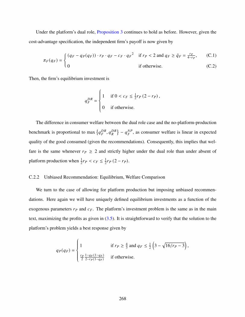
Under the platform’s dual role, Proposition 3 continues to hold as before. However, given the

cost-advantage specification, the independent firm’s payoff is now given by

𝜋𝐹 (𝑞𝐹) ={ (𝑞𝐹 − 𝑞𝑃 (𝑞𝐹)) · 𝑟𝑃 · 𝑞𝐹 − 𝑐𝐹 · 𝑞𝐹2 if 𝑟𝑃 < 2 and 𝑞𝐹 ≥ 𝑞𝐹 =

𝑟𝑃4−𝑟𝑃 , (C.1)

0 if otherwise. (C.2)

Then, the firm’s equilibrium investment is

𝑞𝐷𝑅𝐹 =

1 if 0 < 𝑐𝐹 ≤ 1

2𝑟𝑃 (2 − 𝑟𝑃) ,

0 if otherwise.

The difference in consumer welfare between the dual role case and the no-platform-production

benchmark is proportional to max{𝑞𝐷𝑅𝐹, 𝑞𝐷𝑅

𝑅

}− 𝑞𝑁𝑃

𝐹, as consumer welfare is linear in expected

quality of the good consumed (given the recommendations). Consequently, this implies that wel-

fare is the same whenever 𝑟𝑃 ≥ 2 and strictly higher under the dual role than under absent of

platform production when 12𝑟𝑃 < 𝑐𝐹 ≤ 1

2𝑟𝑃 (2 − 𝑟𝑃).

C.2.2 Unbiased Recommendation: Equilibrium, Welfare Comparison

We turn to the case of allowing for platform production but imposing unbiased recommen-

dations. Here again we will have uniquely defined equilibrium investments as a function of the

exogenous parameters 𝑟𝑃 and 𝑐𝐹 . The platform’s investment problem is the same as in the main

text, maximizing the profits as given in (3.5). It is straightforward to verify that the solution to the

platform’s problem yields a best response given by

𝑞𝑃 (𝑞𝐹) =

1 if 𝑟𝑃 ≥ 4

3 and 𝑞𝐹 ≤ 12

(3 −

√︁16/𝑟𝑃 − 3

),

𝑟𝑃2

1−𝑞𝐹 (1−𝑞𝐹 )2−𝑟𝑃 (1−𝑞𝐹 ) if otherwise.

268

The independent firm’s payoffs are given by

𝜋𝐹 (𝑞𝐹) =12(1 − (𝑞𝑃 (𝑞𝐹) − 𝑞𝐹)) · 𝑟𝑃 · (𝑞𝐹 + (1 − 𝑞𝐹)𝑞𝑃 (𝑞𝐹)) − 𝑐𝐹 · 𝑞𝐹2

It is easy to see that if we substitute 𝑞𝑃 (𝑞𝐹) = 1, then the firm’s profit function simplifies to

12𝑞𝐹 · 𝑟𝑃 − 𝑐𝐹 · 𝑞𝐹2

being maximized at 𝑞𝐹 = min{1 , 𝑟𝑃

4·𝑐𝐹

}.

Given that, ∀𝑐𝐹 ∈ (0, 1) and 𝑟𝑃 ∈[ 4

3 , 4), 𝑟𝑃

4·𝑐𝐹 >12

(3 −

√︁16/𝑟𝑃 − 3

), then 𝑞𝑈

𝑃= 1 if and only if

𝑟𝑃 ≥ 4, in which case 𝑞𝑈𝐹= 1. Moreover, as 𝑑𝜋𝐹 (𝑞𝐹 )

𝑑𝑞𝐹

��𝑞𝐹=1 =

𝑟𝑃4

(6 − 2𝑟𝑃 + 3

8𝑟2𝑃

)−2𝑐𝐹 , then equilib-

rium investments (𝑞𝑈𝐹, 𝑞𝑈

𝑃) are both strictly smaller than 1 if and only if 𝑐𝐹 > 𝑟𝑃

8

(6 − 2𝑟𝑃 + 3

8𝑟2𝑃

).

This also imposes a constraint on the size of the platform, as 1 >𝑟𝑃8

(6 − 2𝑟𝑃 + 3

8𝑟2𝑃

). Let

𝑟𝑃 ∈ (0, 4) be the solution to 1 =𝑟𝑃8

(6 − 2𝑟𝑃 + 3

8𝑟2𝑃

)}, which is uniquely defined (with 𝑟𝑃 ≈ 2.38).

Then 𝑐𝐹 > 𝑟𝑃8

(6 − 2𝑟𝑃 + 3

8𝑟2𝑃

)requires 𝑟𝑃 < 𝑟𝑃. In contrast, when 𝑐𝐹 ≤ 𝑟𝑃

8

(6 − 2𝑟𝑃 + 3

8𝑟2𝑃

), we

again have 𝑞𝑈𝐹= 1, with 𝑞𝑈

𝑃< 1 if and only if 𝑟𝑃 < 4.

Here too, the dual role can yield greater welfare than imposing unbiased recommendation

policies. If 1 = max{𝑞𝐷𝑅𝑃, 𝑞𝐷𝑅

𝐹

}> 𝑞𝑈

𝑃+ (1 − 𝑞𝑈

𝑃)𝑞𝑈𝐹

, then this is trivially the case, occur-

ring for intermediate values of the cost advantage of the independent firm (fixing 𝑟𝑃 < 𝑟𝑃):

12𝑟𝑃 (2 − 𝑟𝑃) ≥ 𝑐𝐹 > 𝑟𝑃

8

(6 − 2𝑟𝑃 + 3

8𝑟2𝑃

). In this case, the platform’s threat of sending non-truthful

recommendations induces larger investments by the independent firm to the point of strictly ex-

ceeding the investments that would have occurred under unbiased recommendations, to the benefit

of consumers.

However, it can also be the case that 1 > max{𝑞𝐷𝑅𝑃, 𝑞𝐷𝑅

𝐹

}= 𝑞𝐷𝑅

𝑃> 𝑞𝑈

𝑃+ (1 − 𝑞𝑈

𝑃)𝑞𝑈𝐹

for

any fixed 𝑟𝑃 in so far as the cost advantage of the independent firm is small enough (i.e. 𝑐𝐹 is

close enough to 1).1 Note that this implies that, in the dual role case, even when the threat of

1The derivation of the exact expression for the lower bound on 𝑐𝐹 is tedious and provides no significant additionalinsight.

269

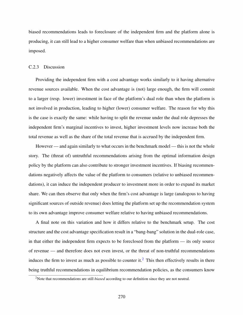
biased recommendations leads to foreclosure of the independent firm and the platform alone is

producing, it can still lead to a higher consumer welfare than when unbiased recommendations are

imposed.

C.2.3 Discussion

Providing the independent firm with a cost advantage works similarly to it having alternative

revenue sources available. When the cost advantage is (not) large enough, the firm will commit

to a larger (resp. lower) investment in face of the platform’s dual role than when the platform is

not involved in production, leading to higher (lower) consumer welfare. The reason for why this

is the case is exactly the same: while having to split the revenue under the dual role depresses the

independent firm’s marginal incentives to invest, higher investment levels now increase both the

total revenue as well as the share of the total revenue that is accrued by the independent firm.

However — and again similarly to what occurs in the benchmark model — this is not the whole

story. The (threat of) untruthful recommendations arising from the optimal information design

policy by the platform can also contribute to stronger investment incentives. If biasing recommen-

dations negatively affects the value of the platform to consumers (relative to unbiased recommen-

dations), it can induce the independent producer to investment more in order to expand its market

share. We can then observe that only when the firm’s cost advantage is large (analogous to having

significant sources of outside revenue) does letting the platform set up the recommendation system

to its own advantage improve consumer welfare relative to having unbiased recommendations.

A final note on this variation and how it differs relative to the benchmark setup. The cost

structure and the cost advantage specification result in a “bang-bang” solution in the dual-role case,

in that either the independent firm expects to be foreclosed from the platform — its only source

of revenue — and therefore does not even invest, or the threat of non-truthful recommendations

induces the firm to invest as much as possible to counter it.2 This then effectively results in there

being truthful recommendations in equilibrium recommendation policies, as the consumers know

2Note that recommendations are still biased according to our definition since they are not neutral.

270

that, if the independent firm’s good is available, it is a high quality good for sure. Then, Bayes

plausibility requires the recommendation to guarantee at least as good quality in expectation, the

platform has no leeway to send non-truthful recommendations (in contrast to what occurs in our

benchmark setup), implying that the consumers will only be told to choose the platform’s good

instead if and when it is at least as good as the available alternative. Therefore, the threat of

non-truthful recommendations alone is enough to drive up the firm’s investment incentives.

C.3 Model with Simultaneous Investment

In this appendix we show that our main conclusions are robust to our assumption on the timing

of investments. In particular, we consider the case in which investments are simultaneous rather

than sequential, keeping everything else the same case as in the main text.

C.3.1 Dual Role Equilibrium Characterization

Naturally, the only changes that occur are for the independent producer in the dual role and

in the unbiased recommendations cases, as they no longer take as given the platform’s sequential

reaction to their investment choices. Hence, in the dual role we still have that the platform’s best

response to the producer’s chosen quality is given by

𝑞𝑃 (𝑞𝐹) =

𝑟𝑃2 𝑞𝐹 if 𝑞𝐹 ≥ 𝑞𝐹 and 𝑟𝑃 < 2

min{1, 𝑟𝑃2

}if 𝑞𝐹 < 𝑞𝐹 and 𝑟𝑃 < 2, or 𝑟𝑃 ≥ 2.

Differently from the baseline, the independent firm’s profit function is now given by

𝜋𝐹 (𝑞𝐹 , 𝑞𝑃) := max{0, 𝑞𝐹 − 𝑞𝑃}𝑟𝑃𝑞𝐹 + 𝑟𝐹𝑞𝐹 − 𝑞2𝐹 .

Proposition 7. For any 𝑟𝑃, 𝑟𝐹 > 0, there is an equilibrium in the dual role with simultaneous

investments. There are 𝑟𝑃, 𝑟𝐹 such that consumer welfare is strictly higher under the dual role

than under the no-platform-production case.

271

The proof for Proposition 7 provides a complete characterization of the equilibria. In general,

a result similar to our baseline model follows, that is, consumer welfare is weakly higher under the

dual role than under the no-platform-production case if and only if 𝑟𝐹 is large enough relative to

𝑟𝑃. However, given potential multiplicity of equilibria when 1 > 𝑟𝑃 > 𝑟𝐹 > 0, the characterization

holds only when the equilibrium selection across the parameter space is monotone in max{𝑞𝑃, 𝑞𝐹}.

There are multiple of such selection rules, for instance, selecting the equilibrium that attains the

highest (or the smallest) max{𝑞𝑃, 𝑞𝐹} whenever multiple equilibria exist.

Proof. We characterize all equilibria by studying different cases of the parameter space.

Case 1: 𝑟𝑃 ≥ 2 and 𝑟𝐹 > 0.

In this case, the platform will choose 𝑞𝑃 = 1 regardless of the firm’s choice of investment, leading

a unique equilibrium where 𝑞𝑃 = 1 and 𝑞𝐹 = min{1, 𝑟𝐹/2}.

Case 2: 2 > 𝑟𝑃 ≥ 1 and 𝑟𝐹 ≥ 𝑟𝑃.

Note that 𝑟𝑃 ≥ 1 =⇒ 𝜋𝐹 is convex on [𝑞𝑃, 1]. Moreover, 𝜋𝐹 is strictly concave on [0, 𝑞𝑃].

Any equilibrium has either 𝑞𝑃 =𝑟𝑃2 or 𝑞𝑃 =

𝑟𝑃2 𝑞𝐹 < 𝑞𝐹 . Then, if 𝑞𝑃 =

𝑟𝑃2 , we have that

0 ≤ 𝜕

𝜕𝑞𝐹𝜋𝐹 (𝑞𝐹 , 𝑞𝑃)

����𝑞𝐹=

𝑟𝑃2

−= −𝑟𝑃 + 𝑟𝐹 < −𝑟𝑃 + 𝑟𝐹 +

𝑟2𝑃

2=

𝜕

𝜕𝑞𝐹𝜋𝐹 (𝑞𝐹 , 𝑞𝑃)

����𝑞𝐹=

𝑟𝑃2

+.

This implies that arg max𝑞𝐹∈[0,1] 𝜋𝐹 (𝑞𝐹 , 𝑞𝑃) = arg max𝑞𝐹∈[𝑞𝑃 ,1] 𝜋𝐹 (𝑞𝐹 , 𝑞𝑃) = 1, where the last

equality follows by convexity of 𝜋𝐹 on [𝑞𝑃, 1]. As 𝑞𝐹 = 1 ≥ 𝑟𝑃4−𝑟𝑃 and 𝑞𝑃 =

𝑟𝑃2 𝑞𝐹 =

𝑟𝑃2 , we have

that (𝑞𝑃, 𝑞𝐹) =( 𝑟𝑃

2 , 1)

is an equilibrium.

To see that, in this case, this is the unique equilibrium, suppose that we have an equilibrium

where 𝑞𝐹 < 1. Then we must have that 𝑞𝑃 =𝑟𝑃2 𝑞𝐹 . But then 𝑞𝑃 < 𝑞𝐹 and, by convexity of 𝜋𝐹 on

[𝑞𝑃, 1], 𝑞𝐹 ∈ {𝑞𝑃, 1}. By assumption 𝑞𝐹 < 1 and if instead 𝑞𝐹 = 𝑞𝑃, then 𝑞𝑃 =𝑟𝑃2 𝑞𝑃 = 0 = 𝑞𝐹 ,

which contradicts the fact that 𝜕𝜕𝑞𝐹

𝜋𝐹 (𝑞𝐹 , 𝑞𝑃)����𝑞𝐹=𝑞𝑃=0

> 0.

Case 3: 2 > 𝑟𝑃 > 1 and 𝑟𝑃 > 𝑟𝐹 > 0.

As 𝑟𝑃 ≥ 1, 𝜋𝐹 remains convex on [𝑞𝑃, 1], but 𝑟𝑃 > 𝑟𝐹 implies that there is a unique interior

272

maximum on [0, 𝑞𝑃] whenever 𝑞𝑃 =𝑟𝑃2 due to 𝜋𝐹 being strictly concave on this region and

0 > −𝑟𝑃 + 𝑟𝐹 =𝜕

𝜕𝑞𝐹𝜋𝐹 (𝑞𝐹 , 𝑞𝑃)

����𝑞𝐹=

𝑟𝑃2

−.

The associated maximizer is 𝑟𝐹2 , that is, the investment that the independent firm when foreclosed.

Thus, if, at an equilibrium, 𝑞𝑃 =𝑟𝑃2 𝑞𝐹 ≤ 𝑞𝐹 , we must have that 𝑞𝐹 = 1. If not, as by convexity

of 𝜋𝐹 on [𝑞𝑃, 1], arg max𝑞𝐹∈[𝑞𝑃 ,1] 𝜋𝐹 (𝑞𝐹 , 𝑞𝑃) ∈ {𝑞𝑃, 1}, we would again have 𝑞𝐹 = 𝑞𝑃 =𝑟𝑃2 𝑞𝐹 =

0, a contradiction. Then, as 1 ≥ 𝑟𝑃4−𝑟𝑃 , it suffices to check that 𝜋𝐹

( 𝑟𝐹2 ,

𝑟𝑃2)≤ 𝜋𝐹

(1, 𝑟𝑃2

), which

holds whenever 𝑟𝐹 ≥ 2 −√

2𝑟𝑃√

2 − 𝑟𝑃.

Now suppose that, at an equilibrium, 𝑞𝐹 =𝑟𝐹2 < 𝑞𝑃 =⇒ 𝑞𝑃 =

𝑟𝑃2 =⇒ 𝑟𝐹

2 ≤ 𝑟𝑃4−𝑟𝑃 . Furthermore,

when 2 > 𝑟𝑃 ≥ 1 and 𝑟𝑃 > 𝑟𝐹 , some algebra shows that

2 −√︁

2𝑟𝑃√︁

2 − 𝑟𝑃 ≤ 2𝑟𝑃

4 − 𝑟𝑃.

Then, given 2 > 𝑟𝑃 > 1 and 𝑟𝑃 > 𝑟𝐹 > 0,

(1) if 𝑟𝐹 < 2 −√

2𝑟𝑃√

2 − 𝑟𝑃, there is a unique equilibrium with (𝑞𝑃, 𝑞𝐹) =( 𝑟𝑃

2 ,𝑟𝐹2);

(2) if 2−√

2𝑟𝑃√

2 − 𝑟𝑃 ≤ 𝑟𝐹 ≤ 2 𝑟𝑃4−𝑟𝑃 , there are two equilibria, where (𝑞𝑃, 𝑞𝐹) ∈

{( 𝑟𝑃2 , 1

),( 𝑟𝑃

2 ,𝑟𝐹2)}

;

(3) if 2 𝑟𝑃4−𝑟𝑃 < 𝑟𝐹 , there is a unique equilibrium, where (𝑞𝑃, 𝑞𝐹) =

( 𝑟𝑃2 , 1

).

Case 4: 𝑟𝑃 = 1 > 𝑟𝐹 > 0.

Note that ∀𝑞𝑃 < 𝑞𝐹 , 𝜕𝜕𝑞𝐹

𝜋𝐹 (𝑞𝐹 , 𝑞𝑃) = −𝑞𝑃 + 𝑟𝐹 . Then, not only do we have the same equilibria

from Case 3,3 we have one additional equilibrium, where 𝑞𝑃 = 𝑟𝐹 =𝑟𝑃2 𝑞𝐹 =⇒ 𝑞𝐹 = 2𝑟𝐹 , whenever

2𝑟𝐹 ≥ 𝑟𝑃4−𝑟𝑃 ⇐⇒ 𝑟𝐹 ≥ 1

6 .

Case 5: 1 > 𝑟𝑃 > 0 and 𝑟𝐹 ≥ 𝑟𝑃.

In this case we have that 𝜋𝐹 is strictly concave on [0, 𝑞𝑃] and on [𝑞𝑃, 1]. At an equilibrium where

3The only difference is that instead of having that arg max𝑞𝐹 ∈[𝑞𝑃 ,1] 𝜋𝐹 (𝑞𝐹 , 𝑞𝑃) ∈ {𝑞𝑃 , 1}, we havearg max𝑞𝐹 ∈[𝑞𝑃 ,1] 𝜋𝐹 (𝑞𝐹 , 𝑞𝑃) ∩ {𝑞𝑃 , 1} ≠ ∅.

273

𝑞𝑃 =𝑟𝑃2 , as 𝑟𝑃 ≤ 𝑟𝐹 , we have that

0 ≤ 𝜕

𝜕𝑞𝐹𝜋𝐹 (𝑞𝐹 , 𝑞𝑃)

����𝑞𝐹=

𝑟𝑃2

−= −𝑟𝑃 + 𝑟𝐹 < −𝑟𝑃 + 𝑟𝐹 +

𝑟2𝑃

2=

𝜕

𝜕𝑞𝐹𝜋𝐹 (𝑞𝐹 , 𝑞𝑃)

����𝑞𝐹=

𝑟𝑃2

+.

This implies that

arg max𝑞𝐹∈[0,1]

𝜋𝐹 (𝑞𝐹 , 𝑞𝑃) = arg max𝑞𝐹∈[𝑞𝑃 ,1]

𝜋𝐹 (𝑞𝐹 , 𝑞𝑃) = min{1,𝑟𝐹 − 𝑟𝑃𝑞𝑃2(1 − 𝑟𝑃)

}.

Then, given 𝑞𝑃 =𝑟𝑃2 , as

min{1,𝑟𝐹 − 𝑟𝑃𝑞𝑃2(1 − 𝑟𝑃)

}= 1 ⇐⇒ 𝑟𝐹 ≥ max

{𝑟𝑃,

(2 − 𝑟𝑃)2

2

},

and(2 − 𝑟𝑃)2

2> 𝑟𝐹 ≥ 𝑟𝑃 =⇒ 𝑟𝐹 − 𝑟𝑃𝑞𝑃

2(1 − 𝑟𝑃)≥ 𝑟𝑃

4 − 𝑟𝑃,

there is an equilibrium with 𝑞𝑃 =𝑟𝑃2 if and only if 𝑟𝐹 ≥ max

{𝑟𝑃,

(2−𝑟𝑃)2

2

}; in which case the

equilibrium is given by (𝑞𝑃, 𝑞𝐹) =( 𝑟𝑃

2 , 1).

Noting that

𝜕

𝜕𝑞𝐹𝜋𝐹 (𝑞𝐹 , 𝑞𝑃)

����𝑞𝐹=𝑞

−𝑃

= 𝑟𝐹 − 2𝑞𝑃 < 𝑟𝑃𝑞𝑃 + 𝑟𝐹 − 2𝑞𝑃 =𝜕

𝜕𝑞𝐹𝜋𝐹 (𝑞𝐹 , 𝑞𝑃)

����𝑞𝐹=𝑞

+𝑃

,

if at an equilibrium 𝑞𝑃 =𝑟𝑃2 𝑞𝐹 , then we further have that 𝑟𝐹 − 2𝑞𝑃 = 𝑟𝐹 − 𝑟𝑃𝑞𝐹 ≥ 0, which again

delivers

arg max𝑞𝐹∈[0,1]

𝜋𝐹 (𝑞𝐹 , 𝑞𝑃) = arg max𝑞𝐹∈[𝑞𝑃 ,1]

𝜋𝐹 (𝑞𝐹 , 𝑞𝑃) = min{1,𝑟𝐹 − 𝑟𝑃𝑞𝑃2(1 − 𝑟𝑃)

}.

Replacing 𝑞𝑃 =𝑟𝑃2 𝑞𝐹 and solving for 𝑞𝐹 yields 𝑞𝐹 = min

{1, 4

(2−𝑟𝑃)2𝑟𝐹2

}, and when 1 > 𝑟𝑃 > 0

and 𝑟𝐹 ≥ 𝑟𝑃, 𝑞𝐹 > 𝑟𝑃4−𝑟𝑃 . Moreover, 𝑟𝐹 ≥ (2−𝑟𝑃)2

2 ⇐⇒ 𝑞𝐹 = 1.

Therefore, we have shown there is a unique equilibrium, where (𝑞𝑃, 𝑞𝐹) =( 𝑟𝑃

2 , 1)

if 𝑟𝐹 ≥

274

max{𝑟𝑃,

(2−𝑟𝑃)2

2

}and (𝑞𝑃, 𝑞𝐹) =

(𝑟𝑃2

4(2−𝑟𝑃)2

𝑟𝐹2 ,

4(2−𝑟𝑃)2

𝑟𝐹2

)if (2−𝑟𝑃)2

2 > 𝑟𝐹 ≥ 𝑟𝑃.

Case 6: 1 > 𝑟𝑃 > 0 and 𝑟𝑃 > 𝑟𝐹 > 0.

As before, given that 1 > 𝑟𝑃, 𝜋𝐹 is strictly concave on [0, 𝑞𝑃] and on [𝑞𝑃, 1]. Then, in any

equilibrium, 𝑞𝑃 ∈{𝑟𝑃2 ,

𝑟𝑃2 𝑞𝐹

}and 𝑞𝐹 ∈

{𝑟𝐹2 ,min

{1, 𝑟𝐹−𝑟𝑃𝑞𝑃2(1−𝑟𝑃)

}}.

Immediately we see that there is no equilibrium where (𝑞𝑃, 𝑞𝐹) =( 𝑟𝑃

2 𝑞𝐹 ,𝑟𝐹2), seeing that if

𝑞𝑃 < 𝑞𝐹 , then 𝑞𝐹 corresponds to the maximizer of 𝜋𝐹 on [𝑞𝑃, 1], which is given by min{1, 𝑟𝐹−𝑟𝑃𝑞𝑃2(1−𝑟𝑃)

},

and this quantity is always strictly larger than 𝑟𝐹2 .

Case 6.1: There is an equilibrium where (𝑞𝑃, 𝑞𝐹) =( 𝑟𝑃

2 , 1)

if and only if (i) 𝜋𝐹( 𝑟𝐹

2 ,𝑟𝑃2)≤

𝜋𝐹(1, 𝑟𝑃2

)⇐⇒ 2−

√2𝑟𝑃

√2 − 𝑟𝑃 ≤ 𝑟𝐹 , and (ii) 𝜕

𝜕𝑞𝐹𝜋𝐹 (𝑞𝐹 , 𝑞𝑃) |𝑞𝐹=1,𝑞𝑃=𝑟𝑃/2 ≥ 0 ⇐⇒ (2−𝑟𝑃)2

2 ≤ 𝑟𝐹 .

Note that if 𝑞𝐹 = 1, then the platform best-responds by choosing 𝑞𝑃 =𝑟𝑃2 as their investment level.

Consequently, such an equilibrium exists whenever

1 > 𝑟𝑃 > 𝑟𝐹 ≥ max{2 −

√︁2𝑟𝑃

√︁2 − 𝑟𝑃,

(2 − 𝑟𝑃)2

2

}.

Case 6.2: An equilibrium in which (𝑞𝑃, 𝑞𝐹) =(𝑟𝑃2 𝑞𝐹 ,min

{1, 𝑟𝐹−𝑟𝑃𝑞𝑃2(1−𝑟𝑃)

})≠

( 𝑟𝑃2 , 1

)implies (𝑞𝑃, 𝑞𝐹) =(

𝑟𝑃2

4(2−𝑟𝑃)2

𝑟𝐹2 ,

4(2−𝑟𝑃)2

𝑟𝐹2

). Note that, if 𝑟𝑃

24

(2−𝑟𝑃)2𝑟𝐹2 ≤ 𝑟𝐹

2 ⇐⇒ 𝑟𝑃 ≤ (2−𝑟𝑃)2

2 , we have that 𝜋𝐹 is

maximized at 𝑞𝐹 > 𝑟𝐹2 . Then, there is such an equilibrium if

(i) 𝑟𝑃 ≤ (2 − 𝑟𝑃)2

2or 𝜋𝐹

(𝑟𝐹

2,𝑟𝑃

24

(2 − 𝑟𝑃)2𝑟𝐹

2

)≤ 𝜋𝐹

(4

(2 − 𝑟𝑃)2𝑟𝐹

2,𝑟𝑃

24

(2 − 𝑟𝑃)2𝑟𝐹

2

)(ii) 𝑞𝐹 = 4

(2−𝑟𝑃)2𝑟𝐹2 < 1 ⇐⇒ min

{𝑟𝑃,

(2−𝑟𝑃)2

2

}> 𝑟𝐹 , and

(iii) 𝜋𝑃

(𝑟𝑃

2,

4(2 − 𝑟𝑃)2

𝑟𝐹

2

)≤ 𝜋𝑃

(𝑟𝑃

24

(2 − 𝑟𝑃)2𝑟𝐹

2,

4(2 − 𝑟𝑃)2

𝑟𝐹

2

)⇐⇒ 𝑟𝐹 ≥ 2

𝑟𝑃

4 − 𝑟𝑃(2 − 𝑟𝑃)2

4.

Combining these, we find

min{𝑟𝑃,

(2 − 𝑟𝑃)2

2

}> 𝑟𝐹 ≥ 𝑟𝑃

4 − 𝑟𝑃(2 − 𝑟𝑃)2

2and

(2 − 𝑟𝑃)2

2≥ 2

𝑟𝑃

4 − 𝑟𝑃.

Case 6.3: Finally, the last possible equilibrium to consider is one such that (𝑞𝑃, 𝑞𝐹) =( 𝑟𝑃

2 ,𝑟𝐹2).

If min{1,max

{0, 𝑟𝐹−𝑟

2𝑃/2

2(1−𝑟𝑃)

}}≤ 𝑞𝑃 =

𝑟𝑃2 , then arg max𝑞𝐹∈[0,1] 𝜋𝐹 (𝑞𝐹 , 𝑞𝑃) =

𝑟𝐹2 . So equilibrium

275

conditions are given by

(i) 𝜋𝑃(𝑟𝑃

2,𝑟𝐹

2

)≤ 𝜋𝑃

(𝑟𝑃2𝑟𝐹

2,𝑟𝐹

2

)⇐⇒ 𝑟𝐹 ≤ 2

𝑟𝑃

4 − 𝑟𝑃, and

(ii)𝑟𝐹 − 𝑟2

𝑃/2

2(1 − 𝑟𝑃)≤ 𝑟𝑃

2or

𝑟𝐹 − 𝑟2𝑃/2

2(1 − 𝑟𝑃)>𝑟𝑃

2and 𝜋𝐹

(𝑟𝐹2,𝑟𝑃

2

)≥ 𝜋𝐹

(min

{1,𝑟𝐹 − 𝑟2

𝑃/2

2(1 − 𝑟𝑃)

},𝑟𝑃

2

).

Simplifying the above, we find the conditions supporting this equilibrium to be

min{2

𝑟𝑃

4 − 𝑟𝑃, 2 −

√︁2𝑟𝑃

√︁2 − 𝑟𝑃

}≥ 𝑟𝐹 > 0.

We now verify that there is always an equilibrium where 1 > 𝑟𝑃 > 𝑟𝐹 . First, note that Cases

6.1 and 6.3 have disjoint conditions, as

min{2

𝑟𝑃

4 − 𝑟𝑃, 2 −

√︁2𝑟𝑃

√︁2 − 𝑟𝑃

}< max

{2 −

√︁2𝑟𝑃

√︁2 − 𝑟𝑃,

(2 − 𝑟𝑃)2

2

}.

If (2−𝑟𝑃)2

2 ≥ 2 𝑟𝑃4−𝑟𝑃 , then

(2 − 𝑟𝑃)2

2= max

{2 −

√︁2𝑟𝑃

√︁2 − 𝑟𝑃,

(2 − 𝑟𝑃)2

2

}and

2𝑟𝑃

4 − 𝑟𝑃= min

{2

𝑟𝑃

4 − 𝑟𝑃, 2 −

√︁2𝑟𝑃

√︁2 − 𝑟𝑃

}.

Consequently, the conditions for either Case 6.1, 6.2, or 6.3 are satisfied, as

(0, 𝑟𝑃) =(0, 2

𝑟𝑃

4 − 𝑟𝑃

)∪

(2

𝑟𝑃

4 − 𝑟𝑃· 1

2(2 − 𝑟𝑃)2

2,(2 − 𝑟𝑃)2

2

)∪

[(2 − 𝑟𝑃)2

2, 𝑟𝑃

).

If (2−𝑟𝑃)2

2 ≤ 2 𝑟𝑃4−𝑟𝑃 ,

2 −√︁

2𝑟𝑃√︁

2 − 𝑟𝑃 = max{2 −

√︁2𝑟𝑃

√︁2 − 𝑟𝑃,

(2 − 𝑟𝑃)2

2

}= min

{2

𝑟𝑃

4 − 𝑟𝑃, 2 −

√︁2𝑟𝑃

√︁2 − 𝑟𝑃

},

276

and therefore,

(0, 𝑟𝑃) =(0, 2 −

√︁2𝑟𝑃

√︁2 − 𝑟𝑃

)∪

[2 −

√︁2𝑟𝑃

√︁2 − 𝑟𝑃, 𝑟𝑃

),

implying that the conditions for either Case 6.1 or 6.3 are satisfied.

□

C.3.2 Welfare Comparison – Dual Role and No Platform Production

We now directly compare the resulting consumer welfare in the dual role case with simulta-

neous investment decisions to the no platform production case. Recall that in the no platform

production case, consumer welfare is given by 𝑞𝑁𝑃𝐹

=𝑟𝑃+𝑟𝐹

2 , whereas in the dual role case, con-

sumer welfare is given by max{𝑞𝐷𝑅𝑃, 𝑞𝐷𝑅

𝐹

}.

In Case 1, consumer welfare is maximal under both the dual role and the no-platform-production

scenarios. In Cases 2, 3, and 4, i.e. 2 > 𝑟𝑃 ≥ 1, consumer welfare is (strictly) higher under the

dual role in some equilibrium if and only if 2 −√

2𝑟𝑃√

2 − 𝑟𝑃 ≤ 𝑟𝐹 (and 𝑟𝐹 < 2 − 𝑟𝑃). If,

moreover 2 𝑟𝑃4−𝑟𝑃 < 𝑟𝐹 (< 2 − 𝑟𝑃), it is (strictly) so in any equilibrium. In Case 5, consumers

are (strictly) better off under the dual role when max{𝑟𝑃,

(2−𝑟𝑃)2

4−𝑟𝑃

}≤ 𝑟𝐹 (< 2 − 𝑟𝑃). In Case

6.1, i.e. 1 > 𝑟𝑃 > 𝑟𝐹 ≥ max{2 −

√2𝑟𝑃

√2 − 𝑟𝑃, (2−𝑟𝑃)

2

2

}, the dual role is always strictly ben-

eficial to consumers. Case 6.2 is (strictly) consumer-welfare-improving whenever its conditions

hold and (2−𝑟𝑃)2

4−𝑟𝑃 ≤ 𝑟𝐹 (< 2 − 𝑟𝑃), where this lower-bound on 𝑟𝐹 is binding. Finally, Case 6.3 —

min{2 𝑟𝑃

4−𝑟𝑃 , 2 −√

2𝑟𝑃√

2 − 𝑟𝑃}≥ 𝑟𝐹 > 0 — has the dual role being always strictly detrimental to

consumers.

These comparisons are displayed graphically in Figure C1a and Figure C1b. Due to the mul-

tiplicity of equilibria, we have to consider some equilibrium selection criteria in order to be able

to compare the cases. We compare the two extreme selection cases and find that there are no

significant qualitative differences. In Figures C1a and C1b we consistently select the equilibrium

investment levels in the dual role case which induce minimal and maximal welfare, respectively.

277

C.3.3 Unbiased Recommendation

Now we examine the case of simultaneous investments with unbiased recommendations.

Equilibrium Characterization: The payoff functions for the platform and the independent firm

are similar to the main text:

𝜋𝑃 (𝑞𝑃, 𝑞𝐹) := 𝑟𝑃12(1 − (𝑞𝐹 − 𝑞𝑃)) (𝑞𝐹 + (1 − 𝑞𝐹)𝑞𝑃) − 𝑞2

𝑃;

𝜋𝐹 (𝑞𝐹 , 𝑞𝑃) := 𝑟𝑃12(1 − (𝑞𝑃 − 𝑞𝐹)) (𝑞𝐹 + (1 − 𝑞𝐹)𝑞𝑃) + 𝑟𝐹𝑞𝐹 − 𝑞2

𝐹 .

As 𝜕2

(𝜕𝑞𝐹 )2 𝜋𝐹 (𝑞𝐹 , 𝑞𝑃) = −2 + (1 − 𝑞𝑃)𝑟𝑃 and 𝜕2

(𝜕𝑞𝑃)2 𝜋𝑃 (𝑞𝑃, 𝑞𝐹) = −2 + (1 − 𝑞𝐹)𝑟𝑃, and as

𝜕

𝜕𝑞𝐹𝜋𝐹 (𝑞𝐹 , 𝑞𝑃) |𝑞𝐹=0

𝜕

𝜕𝑞𝑃𝜋𝑃 (𝑞𝑃, 𝑞𝐹) |𝑞𝑃=0 > 0,

we know that their best-responses are uniquely defined:

𝑞∗𝑃 (𝑞𝐹) := arg max𝑞𝑃∈[0,1]

𝜋𝑃 (𝑞𝑃, 𝑞𝐹) =

1 , if 𝑞𝐹 ≤ 𝑟𝑃−2

𝑟𝑃

min{1, 𝑟𝑃2

1−𝑞𝐹 (1−𝑞𝐹 )2−𝑟𝑃 (1−𝑞𝐹 )

}, if 𝑞𝐹 > 𝑟𝑃−2

𝑟𝑃

𝑞∗𝐹 (𝑞𝑃) := arg max𝑞𝐹∈[0,1]

𝜋𝐹 (𝑞𝐹 , 𝑞𝑃) =

1 , if 𝑞𝑃 ≤ 𝑟𝑃−2

𝑟𝑃

min{1, 𝑟𝐹 1

2−𝑟𝑃 (1−𝑞𝑃) +𝑟𝑃2

1−𝑞𝑃 (1−𝑞𝑃)2−𝑟𝑃 (1−𝑞𝑃)

}, if 𝑞𝑃 > 𝑟𝑃−2

𝑟𝑃

.

Moreover, algebraic manipulations show that −2+(1−𝑞∗𝑃(𝑞𝐹))𝑟𝑃,−2+(1−𝑞∗

𝐹(𝑞𝑃))𝑟𝑃 ≤ 0 for any

𝑞𝐹 , 𝑞𝑃 ∈ [0, 1], which implies that, at any equilibrium we have 𝑞𝑃, 𝑞𝐹 ≥ 𝑟𝑝−2𝑟𝑃

(trivially satisfied if

𝑟𝑃 ≤ 2).

For any 𝑞𝐹 > 𝑟𝑃−2𝑟𝑃

, 𝜕2

(𝜕𝑞𝐹 )2 𝑞∗𝑃(𝑞𝐹) < 0. For simplicity, we restrict ourselves to the case where

𝑟𝐹 ≤ 3 as ∀𝑟𝐹 > 3 we already know that consumer welfare is maximal under the dual role. Under

such condition, we also have that 𝑞𝑃 >𝑟𝑃−2𝑟𝑃

, 𝜕2

(𝜕𝑞𝑃)2 𝑞∗𝐹(𝑞𝑃) < 0. Then, we can further verify

algebraically that 𝑞∗𝑃

(min1≥𝑞𝑃≥(𝑟𝑃−2)/𝑟𝑃 𝑞

∗𝐹(𝑞𝑃)

)≤ arg min1≥𝑞𝑃≥(𝑟𝑃−2)/𝑟𝑃 𝑞

∗𝐹(𝑞𝑃), which delivers

the uniqueness of an equilibrium.

278

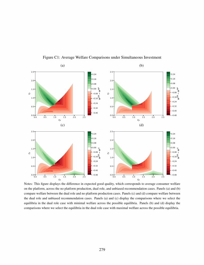
Figure C1: Average Welfare Comparisons under Simultaneous Investment

(a)

0.0 0.5 1.0 1.5 2.0 2.5rP

0.0

0.5

1.0

1.5

2.0

2.5

r F

0.40

0.32

0.24

0.16

0.08

0.00

0.08

0.16

0.24

wD

Rw

NP

(b)

0.0 0.5 1.0 1.5 2.0 2.5rP

0.0

0.5

1.0

1.5

2.0

2.5

r F

0.48

0.40

0.32

0.24

0.16

0.08

0.00

0.08

0.16

0.24

wD

Rw

NP

(c)

0.0 0.5 1.0 1.5 2.0 2.5rP

0.0

0.5

1.0

1.5

2.0

2.5

r F

0.48

0.40

0.32

0.24

0.16

0.08

0.00

0.08

0.16

0.24

wD

Rw

U

(d)

0.0 0.5 1.0 1.5 2.0 2.5rP

0.0

0.5

1.0

1.5

2.0

2.5

r F

0.48

0.40

0.32

0.24

0.16

0.08

0.00

0.08

0.16

0.24

wD

Rw

U

Notes: This figure displays the difference in expected good quality, which corresponds to average consumer welfareon the platform, across the no platform production, dual role, and unbiased recommendation cases. Panels (a) and (b)compare welfare between the dual role and no platform production cases. Panels (c) and (d) compare welfare betweenthe dual role and unbiased recommendation cases. Panels (a) and (c) display the comparisons where we select theequilibria in the dual role case with minimal welfare across the possible equilibria. Panels (b) and (d) display thecomparisons where we select the equilibria in the dual role case with maximal welfare across the possible equilibria.

279

Welfare Comparisons We display the welfare comparisons between the dual role and unbiased

recommendation case in Figures C1c and C1d. Since we only characterize the unique best-response

functions, we compute the equilibrium for parameter values numerically. Similarly to the previous

case, we plot the comparison between the equilibrium selection that induces minimal and maximal

welfare in the dual role case in Figure C1c and C1d respectively. We find comparable results to the

welfare comparisons in the sequential investment case.

280