Essays in Experimental Economics

Essays in Experimental Economics

Inauguraldissertation zur Erlangungdes akademischen Grades eines Doktors

der Wirtschaftswissenschaften derUniversität Mannheim

Timo Hoffmann

Herbstsemester 2016

Abteilungssprecher: Prof. Dr. Carsten TrenklerReferent: Prof. Dr. Dirk EngelmannKorreferent: Prof. Dr. Henrik Orzen

Tag der mündlichen Prüfung: 22. November 2016

Eidesstattliche Erklärung

Hiermit erkläre ich, dass ich die vorliegende Dissertation selbstständig angefertigt und diebenutzten Hilfsmittel vollständig und deutlich angegeben habe.

Erlangen, 27. September 2016Timo Hoffmann

iii

Contents

General introduction 1Chapter 1 . . . . . . . . . . . . . . . . . . . . . . . . . . . . . . . . . . . . . . . . . . . 2

Chapter 2 . . . . . . . . . . . . . . . . . . . . . . . . . . . . . . . . . . . . . . . . . . . 3

Chapter 3 . . . . . . . . . . . . . . . . . . . . . . . . . . . . . . . . . . . . . . . . . . . 5

Acknowledgments . . . . . . . . . . . . . . . . . . . . . . . . . . . . . . . . . . . . . 7

1 The Effect of Belief Elicitation on Game Play: The Role of Game Properties 91.1 Introduction . . . . . . . . . . . . . . . . . . . . . . . . . . . . . . . . . . . . . . 9

1.2 Experimental design and hypotheses . . . . . . . . . . . . . . . . . . . . . . . . 13

1.2.1 Overall experimental design . . . . . . . . . . . . . . . . . . . . . . . . 13

1.2.2 The games . . . . . . . . . . . . . . . . . . . . . . . . . . . . . . . . . . 15

1.2.3 Hypotheses . . . . . . . . . . . . . . . . . . . . . . . . . . . . . . . . . 18

1.3 Results . . . . . . . . . . . . . . . . . . . . . . . . . . . . . . . . . . . . . . . . . 20

1.3.1 Preliminaries . . . . . . . . . . . . . . . . . . . . . . . . . . . . . . . . 20

1.3.2 Belief elicitation and the role of game properties . . . . . . . . . . . . 21

1.3.3 Treatment effects on subjects’ choices . . . . . . . . . . . . . . . . . . 25

1.3.4 Descriptive statistics of stated beliefs . . . . . . . . . . . . . . . . . . . 31

1.3.5 Relationship between actions and stated beliefs . . . . . . . . . . . . . 33

1.4 Discussion and conclusion . . . . . . . . . . . . . . . . . . . . . . . . . . . . . 35

A Appendix Chapter 1 37A.1 Appendix . . . . . . . . . . . . . . . . . . . . . . . . . . . . . . . . . . . . . . . 37

A.1.1 Classification . . . . . . . . . . . . . . . . . . . . . . . . . . . . . . . . 37

A.1.2 OLS and logit regression . . . . . . . . . . . . . . . . . . . . . . . . . . 37

A.1.3 Non-uniform beliefs . . . . . . . . . . . . . . . . . . . . . . . . . . . . 39

A.1.4 Instructions . . . . . . . . . . . . . . . . . . . . . . . . . . . . . . . . . 39

2 Profitability of Tournaments with Worker Sorting: An Experiment 432.1 Introduction . . . . . . . . . . . . . . . . . . . . . . . . . . . . . . . . . . . . . . 43

v

2.2 Experimental design . . . . . . . . . . . . . . . . . . . . . . . . . . . . . . . . . 47

2.2.1 The real-effort task . . . . . . . . . . . . . . . . . . . . . . . . . . . . . 47

2.2.2 Structure of the experiment . . . . . . . . . . . . . . . . . . . . . . . . 48

2.2.3 Treatments and procedures . . . . . . . . . . . . . . . . . . . . . . . . . 52

2.2.4 Hypotheses . . . . . . . . . . . . . . . . . . . . . . . . . . . . . . . . . 54

2.3 Results . . . . . . . . . . . . . . . . . . . . . . . . . . . . . . . . . . . . . . . . . 57

2.3.1 Managers’ choices . . . . . . . . . . . . . . . . . . . . . . . . . . . . . 57

2.3.2 Workers’ performances - the incentive effect . . . . . . . . . . . . . . 58

2.3.3 Managers’ profits and payoff-maximizing contracts . . . . . . . . . . 60

2.3.4 Sorting of workers . . . . . . . . . . . . . . . . . . . . . . . . . . . . . 62

2.3.5 Workers’ payoff-maximizing choices . . . . . . . . . . . . . . . . . . . 68

2.3.6 Main result . . . . . . . . . . . . . . . . . . . . . . . . . . . . . . . . . . 71

2.3.7 Fixed wages and gift-exchange . . . . . . . . . . . . . . . . . . . . . . 72

2.4 Discussion and conclusion . . . . . . . . . . . . . . . . . . . . . . . . . . . . . 74

B Appendix Chapter 2 77B.1 Appendix . . . . . . . . . . . . . . . . . . . . . . . . . . . . . . . . . . . . . . . 78

B.1.1 Productivity indicators . . . . . . . . . . . . . . . . . . . . . . . . . . . 79

B.1.2 Scatter plot of fixed wages and workers’ output . . . . . . . . . . . . . 79

B.2 Appendix II - Instructions . . . . . . . . . . . . . . . . . . . . . . . . . . . . . . 81

3 Flip a coin or vote: An Experiment on Choosing Group Decision Rules 913.1 Introduction . . . . . . . . . . . . . . . . . . . . . . . . . . . . . . . . . . . . . . 91

3.2 Related literature . . . . . . . . . . . . . . . . . . . . . . . . . . . . . . . . . . . 94

3.3 Experimental design . . . . . . . . . . . . . . . . . . . . . . . . . . . . . . . . . 96

3.3.1 The game . . . . . . . . . . . . . . . . . . . . . . . . . . . . . . . . . . 97

3.3.2 The four mechanisms . . . . . . . . . . . . . . . . . . . . . . . . . . . . 99

3.3.3 Treatments . . . . . . . . . . . . . . . . . . . . . . . . . . . . . . . . . . 99

3.3.4 Procedures . . . . . . . . . . . . . . . . . . . . . . . . . . . . . . . . . . 100

3.4 Theoretical predictions . . . . . . . . . . . . . . . . . . . . . . . . . . . . . . . 101

3.5 Results . . . . . . . . . . . . . . . . . . . . . . . . . . . . . . . . . . . . . . . . . 104

3.5.1 Realized surplus . . . . . . . . . . . . . . . . . . . . . . . . . . . . . . . 104

3.5.2 Ex-ante choices . . . . . . . . . . . . . . . . . . . . . . . . . . . . . . . 105

3.5.3 Impossibility results . . . . . . . . . . . . . . . . . . . . . . . . . . . . 108

3.5.4 Ad-interim choices . . . . . . . . . . . . . . . . . . . . . . . . . . . . . 109

3.5.5 Voting and reporting behavior . . . . . . . . . . . . . . . . . . . . . . . 111

3.6 Conclusion . . . . . . . . . . . . . . . . . . . . . . . . . . . . . . . . . . . . . . 114

C Appendix Chapter 3 117C.1 Appendix . . . . . . . . . . . . . . . . . . . . . . . . . . . . . . . . . . . . . . . 118

vi

C.1.1 Derivation of predictions . . . . . . . . . . . . . . . . . . . . . . . . . . 118C.1.2 Further results - All choices . . . . . . . . . . . . . . . . . . . . . . . . 120C.1.3 Translated instructions . . . . . . . . . . . . . . . . . . . . . . . . . . . 121

Bibliography 127

vii

List of Figures

1.1 Histogram of NE actions for both treatments . . . . . . . . . . . . . . . . . . . 261.2 Histogram of not uniformly stated beliefs per subject . . . . . . . . . . . . . . 311.3 Histogram of best responses per subject to stated beliefs . . . . . . . . . . . . 34

A.1 Histogram of stated beliefs above 70% . . . . . . . . . . . . . . . . . . . . . . 38

2.1 Example of task . . . . . . . . . . . . . . . . . . . . . . . . . . . . . . . . . . . 472.2 Mean number of correctly solved tables by workers with different payment

schemes . . . . . . . . . . . . . . . . . . . . . . . . . . . . . . . . . . . . . . . . 592.3 Mean profit of managers from workers’ output with different payment schemes 612.4 Fraction of workers opting for the different payment schemes by productivity 652.5 Hypothetical tournament payoff vs. payoff with piece rate for workers paid

with a piece rate in the competition stage . . . . . . . . . . . . . . . . . . . . . 692.6 Hypothetical tournament payoff vs. hypothetical payoff with piece rate for

workers paid with a tournament in the competition stage . . . . . . . . . . . . 71

B.1 Scatterplot of fixed wages and workers’ performances . . . . . . . . . . . . . 80

3.1 Ex-ante binary choices (symmetric treatment) . . . . . . . . . . . . . . . . . . 1063.2 Ex-ante choices between AGV and SM mechanism (by treatment) . . . . . . 1073.3 Mechanism choice by positive/negative private valuation (symmetric treat-

ment) . . . . . . . . . . . . . . . . . . . . . . . . . . . . . . . . . . . . . . . . . . 1093.4 Ad-interim choices between AGV and RAND mechanism (by treatment) . . 1103.5 Ad-interim choices between AGV and SM mechanism (by treatment and

valuation) . . . . . . . . . . . . . . . . . . . . . . . . . . . . . . . . . . . . . . . 111

ix

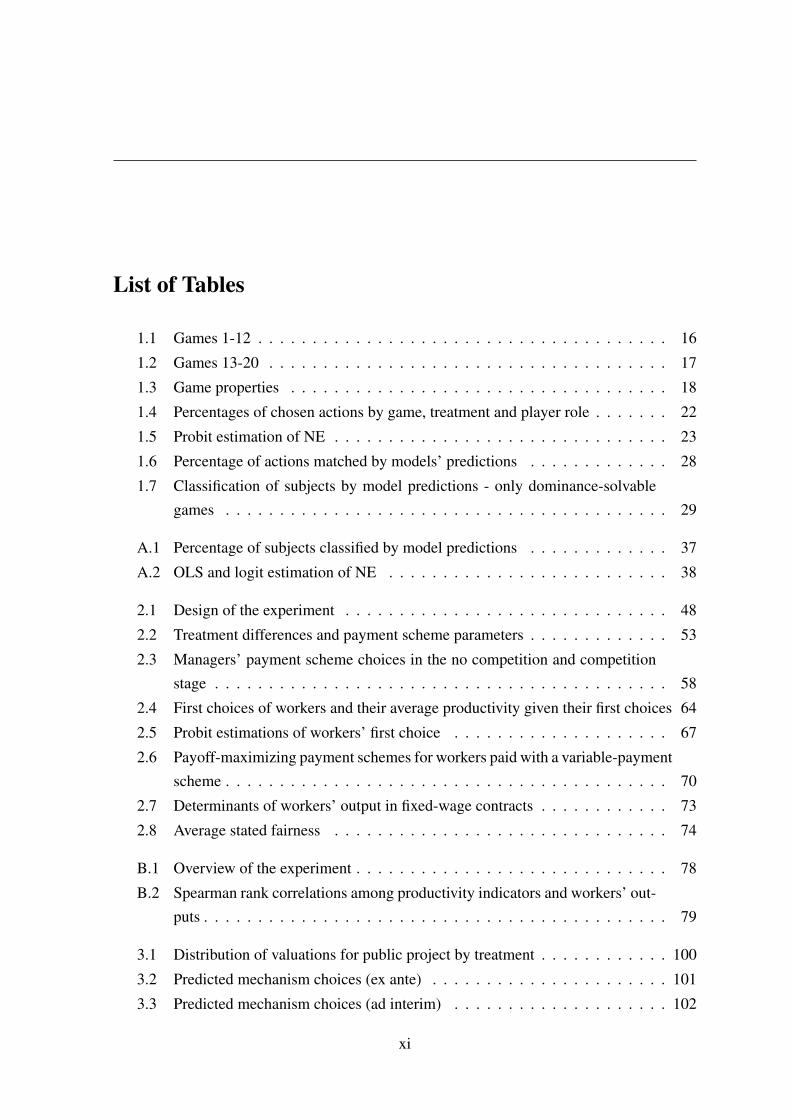
List of Tables

1.1 Games 1-12 . . . . . . . . . . . . . . . . . . . . . . . . . . . . . . . . . . . . . . 16

1.2 Games 13-20 . . . . . . . . . . . . . . . . . . . . . . . . . . . . . . . . . . . . . 17

1.3 Game properties . . . . . . . . . . . . . . . . . . . . . . . . . . . . . . . . . . . 18

1.4 Percentages of chosen actions by game, treatment and player role . . . . . . . 22

1.5 Probit estimation of NE . . . . . . . . . . . . . . . . . . . . . . . . . . . . . . . 23

1.6 Percentage of actions matched by models’ predictions . . . . . . . . . . . . . 28

1.7 Classification of subjects by model predictions - only dominance-solvablegames . . . . . . . . . . . . . . . . . . . . . . . . . . . . . . . . . . . . . . . . . 29

A.1 Percentage of subjects classified by model predictions . . . . . . . . . . . . . 37

A.2 OLS and logit estimation of NE . . . . . . . . . . . . . . . . . . . . . . . . . . 38

2.1 Design of the experiment . . . . . . . . . . . . . . . . . . . . . . . . . . . . . . 48

2.2 Treatment differences and payment scheme parameters . . . . . . . . . . . . . 53

2.3 Managers’ payment scheme choices in the no competition and competitionstage . . . . . . . . . . . . . . . . . . . . . . . . . . . . . . . . . . . . . . . . . . 58

2.4 First choices of workers and their average productivity given their first choices 64

2.5 Probit estimations of workers’ first choice . . . . . . . . . . . . . . . . . . . . 67

2.6 Payoff-maximizing payment schemes for workers paid with a variable-paymentscheme . . . . . . . . . . . . . . . . . . . . . . . . . . . . . . . . . . . . . . . . . 70

2.7 Determinants of workers’ output in fixed-wage contracts . . . . . . . . . . . . 73

2.8 Average stated fairness . . . . . . . . . . . . . . . . . . . . . . . . . . . . . . . 74

B.1 Overview of the experiment . . . . . . . . . . . . . . . . . . . . . . . . . . . . . 78

B.2 Spearman rank correlations among productivity indicators and workers’ out-puts . . . . . . . . . . . . . . . . . . . . . . . . . . . . . . . . . . . . . . . . . . . 79

3.1 Distribution of valuations for public project by treatment . . . . . . . . . . . . 100

3.2 Predicted mechanism choices (ex ante) . . . . . . . . . . . . . . . . . . . . . . 101

3.3 Predicted mechanism choices (ad interim) . . . . . . . . . . . . . . . . . . . . 102

xi

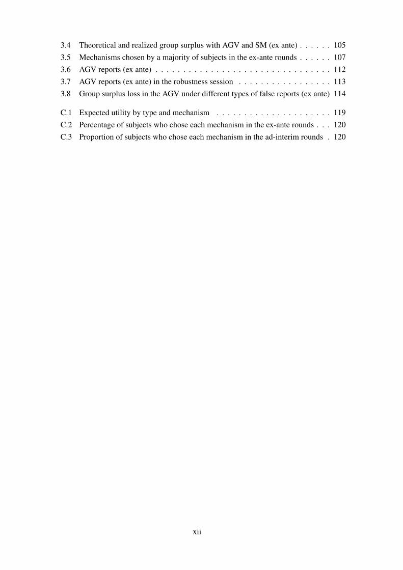
3.4 Theoretical and realized group surplus with AGV and SM (ex ante) . . . . . . 1053.5 Mechanisms chosen by a majority of subjects in the ex-ante rounds . . . . . . 1073.6 AGV reports (ex ante) . . . . . . . . . . . . . . . . . . . . . . . . . . . . . . . . 1123.7 AGV reports (ex ante) in the robustness session . . . . . . . . . . . . . . . . . 1133.8 Group surplus loss in the AGV under different types of false reports (ex ante) 114

C.1 Expected utility by type and mechanism . . . . . . . . . . . . . . . . . . . . . 119C.2 Percentage of subjects who chose each mechanism in the ex-ante rounds . . . 120C.3 Proportion of subjects who chose each mechanism in the ad-interim rounds . 120

xii

General introductionEconomics is concerned with all kinds of human interactions as well as the role institutionsplay in these interactions. The research presented in this dissertation is motivated by the ideathat challenges and problems that arise in the functioning of economies and societies aredriven by human behavior. Studying human behavior is not only helpful in understandingthe reasons for the observed behavior, but might provide valuable insights into the originsof these problems. I believe that a better description of human behavior is a necessary firststep in finding solutions for many challenges our societies face. More generally, I considerthe research of human behavior crucial in order to develop institutions and mechanisms forsolving or even preventing these problems and to improve existing organizations.

This dissertation consists of three independent chapters, which analyze different aspectsof human behavior. All chapters share the feature that laboratory experiments are used toinvestigate and describe the behavior of agents. Chapter 1 focuses on a methodologicalissue of eliciting expectations of players about the likely behavior of their opponent(s) inexperiments - the so called beliefs - and investigates the influence of this belief elicitationon observed behavior. Thereby this research touches on the process of belief formation.Chapter 2 analyzes the importance of worker sorting and its interplay with incentive effectsfor the profitability of rank-order tournaments. More precisely I consider two environments,with and without the possibility of worker sorting, to examine how worker sorting affects theprofitability of a tournament for employers. Lastly, chapter 3 investigates the role of privateinformation and available mechanisms on choosing group decision rules. This experimenttests several theoretical predictions made in the economic literature regarding the role ofparticipation constrains for choosing efficient group decision rules. Chapters 1 and 2 aresingle-authored essays, while chapter 3 is based on joint work with Sander Renes.

Each chapter is followed by an appendix that includes supplementary material such asadditional figures, further analyses and provides the instructions for the conducted experi-ments. The references for all three chapters are collected in one bibliography at the end ofthis dissertation.

1

2 GENERAL INTRODUCTION

Chapter 1

To understand subjects’ decisions it is useful to know more about why a subject makes acertain choice. Especially in the context of strategic interactions, the expectation of a personwhat others will do - the so called “belief” - can be helpful in understanding the motivation ofa subject for choosing a certain action. Beliefs can be used to differentiate between modelsthat predict identical behavior and they provide useful insights in the reasoning of subjects.Specifically if predictions made by models and observed choices diverge, beliefs can bevaluable in understanding why model predictions fail. The experiment presented in chapter 1is concerned with the question whether asking subjects for their beliefs about the expectedbehavior of their counterpart influences which actions are chosen.

My motivation for this paper is twofold. First, the described advantages of knowingsubjects’ beliefs when explaining their behavior and the relatively simple possibility of di-rectly eliciting beliefs in laboratory experiments have made belief elicitation frequent in theexperimental literature. But beliefs and actions elicited in an experiment can only be usedwithout restrictions if subjects’ actions are not changed by the elicitation. In the literaturethat uses belief elicitation it is mostly assumed that action choices are not altered by a properelicitation of beliefs. Some studies explicitly consider a potential effect of belief elicitationon game play, however their results are mixed. While a few papers report significant effectson subjects’ choices, others claim that choices are not affected by the elicitation. Since thedifferent results might be partially driven by different game properties, I consider it importantto analyze whether and how game properties play a role for the effect of belief elicitation ongame play. Second, understanding how and specifically in which situations belief elicitationmight affect chosen actions can provide useful insights in the decision process of subjects.

Therefore in chapter 1 I investigate whether belief elicitation influences the behavior ofsubjects in two-person normal-form games. Using games with different properties allowsme to analyze whether and how game properties play a role for the effect. In the experimentthere are two treatments. In the first treatment subjects’ choices and beliefs are elicitedsimultaneously. Therefore subjects have to think about their beliefs when choosing an action.In the second treatment all choices are made without the elicitation of beliefs. The beliefsare elicited as a surprise after subjects have made all their action choices. Besides enablingme to analyze whether choices are affected by the belief elicitation, this procedure allowsme to compare the belief statements between treatments.

Comparing the choices from both treatments, I find that subjects’ choices are affectedby the belief elicitation for two subgroups of games. In dominance-solvable games subjectsare more likely to choose an action that is part of a Nash equilibrium if they state beliefs andactions at the same time. In games that have a symmetric alternative outcome to the Nashequilibrium, belief elicitation decreases the probability of equilibrium play. These resultsdemonstrate that belief elicitation is not always neutral, but can have significant effects on

GENERAL INTRODUCTION 3

game play. Dependent on game properties the belief elicitation can lead to an increase ordecrease of equilibrium play.

In the data there are no differences between the beliefs stated simultaneously with theaction choice and the beliefs stated after action choices have already been made. However,there is a clear difference in the number of action choices, which are best responses to ownstated beliefs. When beliefs and choices are elicited simultaneously, chosen actions are moreoften best responses to the stated beliefs compared to a sequential elicitation of actions andbeliefs. A possible explanation of this finding is that subjects revise their beliefs when theyare asked to make explicit belief statements. The elicitation of beliefs might lead to modifiedbeliefs and these modified beliefs result in a change in the action subjects want to choose.However, subjects can actually “change” their action only if beliefs and actions are elicitedsimultaneously. In the treatment in which action choices and belief statements are madesequentially subjects cannot change their previously made action choices. Consequently, thepreviously chosen actions are less often a best response to the stated “modified” beliefs.

The data shows that not only whether an effect exists depends on game properties, butalso whether belief elicitation increases or decreases the probability of equilibrium play.Thereby these findings highlight the importance of different game properties for the effect.Furthermore the data indicates that the decision process of subjects does not always includethe formation of exact beliefs. The fact that the effect of belief elicitation varies with gameproperties could suggest that subjects’ decision processes are slightly different for differentgames / environments. I therefore consider the presented study also as a step towards a betterunderstanding of the role of belief formation in the decision process of subjects.

Chapter 2

The importance of worker sorting for the observed output differences between paymentschemes is well documented in the economic literature. However, little evidence exists on therole of worker sorting on the profitability of payment schemes for employers. In chapter 2I analyze the profitability of a rank-order tournament for employers in two environments,which differ in whether self-selection of workers into payment schemes is possible or not.

Rank-order tournaments have the feature that workers’ earnings depend on their relativeperformance and not directly on their output. Consequently, for employers the costs of atournament are independent of workers’ performance - at least when prizes are independentof output. This independence can result in cost savings, if there are high effort provisionsof workers despite a relatively cheap tournament. If that is the case, the firm might generatea larger profit with a tournament compared to output-based payment schemes. But such atournament is usually cheap, because the expected earnings for workers are low. Thereforeit is not clear whether a cheap tournament is sufficiently well liked by productive workers,such that they choose the tournament over other payment schemes.


My experimental design exploits the advantage of the laboratory environment to dis-entangle a potential sorting from the incentive effect. In the first part employers choose apayment scheme among the offered possibilities of a fixed wage, a piece rate and a rank-ordertournament. Since workers are exogenously matched with an employer, only an incentiveeffect is possible. In the second part three employers are grouped together and sorted to thedifferent payment schemes based on their stated preferences. At the same time, six work-ers are grouped together and state their preferences over the payment schemes. Since eachpayment scheme has to be offered by exactly one employer, workers can choose betweenall three payment schemes. Therefore, workers are no longer exogenously matched with anemployer, but select their preferred payment scheme. This matching procedure provides anopportunity for worker sorting.

Additionally there are two treatments with different tournament prizes. In the low-prizetreatment the tournament is relatively cheap for employers. These low prizes yield lowexpected incomes, even for productive workers. In the high-prize treatment the prizes arelarger and therefore the expected payoff of workers in the tournament, but also the costs foremployers, are higher.

My results demonstrate that tournaments provide incentives for workers and thereforelead to high effort provisions. In both tournaments the observed output is similar to thepiece-rate performance. Consequently, if worker sorting is not possible - in part one - a low-prize tournament results in higher firm profits than a piece rate. A finding which illustratesthe potential cost advantage of rank-order tournaments for firms. However, the tournamentin the high-prize treatment, with the larger costs, results in the same average profits as thepiece rate. In the second part, in which worker sorting is possible and indeed observed,the cheap low-prize tournament does not yield a larger employer profit than the piece rate.The main reason for this finding is productivity sorting of workers. Productive workersprefer the piece rate if the tournament prize is low. While the high-prize tournament is moreattractive to workers, the additional costs for the tournament prizes result in the same profitfor employers for the high-prize tournament and the piece rate. Therefore, neither the lownor the high-prize tournament yields a larger employer profit compared to the piece rate ifworker sorting is feasible.

The main finding of the paper is therefore that with worker sorting rank-order tourna-ments are hardly simultaneously attractive for workers and employers. Despite its low costsfor employers, a low-prize tournament does not yield larger profits than a piece rate due toworker sorting. A high-prize tournament might be attractive for workers, but it is too costlyfor employers. This result might be part of the explanation why a tournament is usually notthe main contract scheme for workers in labor markets, despite its good incentives.

GENERAL INTRODUCTION 5

Chapter 3

In the third chapter the problem of (efficient) mechanism selection in a group decision exper-iment is analyzed. We study binary comparisons between four decision rules and investigatethe role of different outside options and private information on subjects’ mechanism choices.By having subjects choose between two available mechanisms, we can test the influence ofparticipation constraints on the selection of mechanisms. Participation constraints are ubiq-uitous in economic theory. The possibility of “going elsewhere” provides a credible threatfor economic agents. Therefore these outside options result in strong bargaining positionsand have to be taken into account by the respective counterparts. Despites their impor-tance and their prominent role in economic theory, there is little empirical evidence of theeffect of participation constraints on behavior. A major reason for the lack of evidence isthat participation constraints generally depend on the choice not made, and thus on unob-served counterfactuals. Without assuming a participation constraint binds strictly, it is nearlyimpossible to give an estimate of the value attached to the best of the options not taken. Toovercome this problem, Sander Renes and I conduct an experiment, which allows us to studythe effects of participation constraints on mechanism choices in social choice situations.

Before a group or society can take a decision, whether it is about what restaurant to visitor about the implementation of a reform, the group has to select a decision rule. It wouldseem that groups should select a rule that maximizes the value of the final decision to thegroup. In their seminal paper Myerson and Satterthwaite (1983) show that with private in-formation about their preferences over outcomes, there is no efficient decision rule that isunanimously preferred by all group members over the non-implementation status quo. Inour experiment we test whether this impossibility theorem can be found in subjects’ mecha-nism choices. Furthermore, we investigate several proposed possibilities in the literature toovercome this impossibility theorem by changing the outside option of subjects.

In our experiment groups of three participants make a collective decision about the im-plementation of a public project. If implemented, all group members receive a payoff fromthe project. However, these payoffs are heterogeneous and might be positive or negative foran individual. The decision whether to implement the project or not is taken in a two-stagevoting game. In the first stage the group decides between two available mechanisms and inthe second stage the selected decision rule is used to determine whether or not the projectis implemented. In the experiment we contrast two different environments. In the first part,subjects select a decision rule without being informed about their private payoff from projectimplementation. However, they know the distribution of possible payoffs and are informedabout their private payoff after a decision rule has been chosen, but before they apply the de-cision rule to determine the project implementation. In the second part subjects are informedabout their potential project payoff before selecting a decision rule.

In total there are four group decision rules: (1) an efficient direct revelation mechanism -


called AGV, (2) simply majority voting, (3) a non-implementation status quo mechanism thatalways prevents project implementation and (4) a random mechanism that implements theproject in 50% of cases. Providing subjects with the choice between two of these rules andtherefore defining the outside option, allows us to assess the role of participation constraintson mechanism choices. The within-subject variation of the private information about theproject payoffs enables us to perform a straight forward test of the impossibility theorem byMyerson and Satterthwaite. We compare the mechanism choices of the same subjects withand without private information about the project payoff.

Our results show that before the revelation of private information, subjects choose themore efficient mechanism, because it yields the largest expected payoff. In the first part of theexperiment a large majority of choices is in line with the expected payoffs of the mechanisms.In the second part, when subjects are informed about their valuation for the project, they onlyprefer the (more) efficient mechanism if their valuation is positive. Otherwise they opt forthe non-implementation status quo whenever possible. This result confirms the impossibilitytheorem of Myerson and Satterthwaite. Furthermore we find evidence that it is easier toget individuals to agree on more efficient mechanisms if the outside option involves riskyoutcomes.

These results suggest that participation constraints play an important role in the optimaldesign of institutions. A group that is stuck in an inefficient mechanism might require anoutside influence or coercive power to break away from the status quo. Even in the smallgroups in our experiment private information about the project make the implementation ofefficient mechanisms infeasible. The difficulties of negotiating a public project on the scaleof a nation would seem close to unsurmountable if unanimity is required. Centralized organi-zations with an amount of coercive power, like the state or the company, allow participants tobundle individual projects and reforms and take them away from purely decentralized mech-anisms like open markets. Our results therefore provide some rational for the existence ofsuch institutions. By forcing group members to participate in individual projects, the groupsurplus can be increased since not all participation constraints need to be satisfied. In thissense our findings give one reason for the existence of states and their coercive powers, sinceit does make dealing with participation constraints easier.

Acknowledgments

I foremost would like to thank my supervisor Dirk Engelmann for his continuous supportand the excellent guidance over the last six (plus) years. Without his feedback and encour-agement this thesis would not have been possible. Furthermore my thesis greatly benefitedfrom the feedback and comments I received in individual talks, many presentations and con-secutive discussions with numerous people. While I will acknowledge the feedback of manypeople in the beginning of each chapter separately, I in particular want to thank Hans PeterGrüner, Christian Koch, Henrik Orzen, Stefan Penczynski, my co-author Sander Renes andJohannes Schneider for all their input and advice.

I gratefully acknowledge the financial support from the Deutsche Forschungsgemein-schaft (SFB 884), which financed the experiments for the third chapter of this thesis.

Moreover, I thank my fellow doctoral students from the Center for Doctoral Studiesin Economics (CDSE) for the inspiring atmosphere within the graduate school. Interactingwith you on a professional, and sometimes even more on a personal level, was supportiveand very enjoyable. Finally, I thank Eva for her continuous support and encouragement.Thank you for always being there for me.

Erlangen, September 27th 2016 Timo Hoffmann

7

Chapter 1

The Effect of Belief Elicitation on Game Play: The Role ofGame Properties1

1.1 Introduction

Understanding, describing and explaining individual choices is one of the core objectives ofeconomics. A main ingredient for this analysis are models that are formulated to explain andpredict behavior. An integral part of most models, especially in strategic situations, are be-liefs of subjects about the likely behavior of their opponent(s). In many models the resultingaction is the best response to these beliefs. However, a large part of the experimental litera-ture demonstrates that observed choices often are not in line with the equilibrium predictionsof various models (for overviews see Kagel et al. (1995) or Camerer (2003)). The source ofthese differences can be non-equilibrium beliefs or a failure to best respond to beliefs. Todifferentiate between these explanations subjects’ beliefs need to be known. Furthermore,subjects’ beliefs can provide useful insights for understanding the reasons for model failuresand help to differentiate between competing explanations for observed behavior. But differ-ent than action choices beliefs are usually not directly observed. Therefore to know subjects’beliefs they have either to be inferred or elicited.

If beliefs are directly elicited the question whether these elicitations affect subjects’choices arises. Only if subjects’ action choices are unchanged by the elicitation of beliefscan the elicited beliefs be used to determine subjects’ motives for action choices withoutrestrictions. Additionally, the elicited beliefs can only be directly utilized to explain behavior

1I appreciate the comments and the advice received from Dirk Engelmann, Jana Friedrichsen, WernerGüth, Nikos Nikiforakis, Henrik Orzen, Stefan Penczynski, Philipp Schmidt-Dengler, Johannes Schneider,Stefan Trautmann and Roberto Weber. I thank the participants at the Behavioral and Experimental Workshopin Florence, the EEA in Gothenburg, VfS Meeting in Hamburg, GfeW Meeting in Helmstedt, the THEEMWorkshop in Kreuzlingen, RES Meeting in Manchester, NERD Workshop in Nuremberg, ENTER Jamboree inStockholm, the Experimental Conference in Xiamen and the ESA World Meeting in Zurich, as well as seminarparticipants in Mannheim, Nuremberg and Tilburg for many helpful comments and fruitful discussions. Anearlier draft of this paper circulated under the title “The Effect of Belief Elicitation on Game Play”.

9

10 CHAPTER 1

in similar situations without belief elicitation if subjects’ choices are not affected by theelicitation. In this paper I examine whether belief elicitation affects subjects’ choices in one-shot two-person normal-form games. The previous literature analyzing possible effects ofthe elicitation on observed choices obtained mixed results. Therefore the main aim of thepaper is to analyze whether the (potential) effects of belief elicitation on game play dependon game properties, since the mixed results might be at least partially explained by differentgame properties.

Croson (1999, 2000) shows that subjects tend to contribute less in a public good gameand defect more often in a prisoner’s dilemma if beliefs are elicited.2 In her study beliefelicitation is therefore not neutral, but with belief elicitation subjects’ choices are more in linewith the theoretical predictions. Costa-Gomes and Weizsäcker (2008) analyze equilibriumplay and stated beliefs in normal-form games and examine whether belief elicitation affectsgame play. They do not find any significant effects on chosen actions.3 Recent articlesabout belief elicitation (Schlag et al. 2015; Holt and Smith 2016) conclude that there is arelatively limited number of studies on the effect of belief elicitation on choices and thatthe reported results are inconclusive.4 Hence two main facts emerge from the literature:Most importantly belief elicitation does not always affect game play. Additionally, not in allstudies with a significant effect belief elicitation drives subjects towards equilibrium choices.Different game properties are one possible reason for the divergent results.

To analyze whether and how belief elicitation affects choices I contrast subjects’ choicesin 20 two-person normal-form games in two treatments. In a first treatment (baseline) sub-jects state their action choices without being inquired about beliefs. In a second treatment(belief) a separate group of subjects plays the same games, but subjects always state theiraction choices and their beliefs about their opponents behavior simultaneously. By usinggames that differ in many dimensions I assess whether an effect exists for some, but possiblynot all games. Furthermore beliefs of subjects are collected in both treatments. In the belieftreatment beliefs are stated together with the action choices, while in the baseline treatmentthe belief elicitation follows after all action choices have been made, but before subjects re-ceive any feedback. Collecting beliefs of all subjects allows me to analyze whether beliefs

2 Results in other studies of the public good game are less clear: Wilcox and Feltovich (2000) do not findan effect of belief elicitation on contributions, Gächter and Renner (2010) report increased contributions anda meta-study by Zelmer (2003) documents decreased contributions. However, this meta-study contains only alimited number of experiments with belief elicitation.

3 There are several notable differences of Costa-Gomes and Weizsäcker (2008) to my analysis. First, inCosta-Gomes and Weizsäcker (2008) the elicitation is always done before or after the action choice. In mydesign the two tasks are carried out simultaneously. Second, they find no differences on the game level, butalso do not analyze the individual behavior across games explicitly as I do in section 1.3.2. Third, my studyconsiders a greater variety of games and their properties.

4 Nyarko and Schotter (2002) elicit beliefs in a repeated 2x2 game in the context of (belief) learning. Theydo not find an effect of belief elicitation on game play. Rutström and Wilcox (2009) report that belief elicitationin a repeatedly played asymmetric matching pennies game affects subjects’ choices for subjects with a largeasymmetry of payoffs and especially in the first rounds. However, these studies are less applicable to minesince they consider repeated interactions, while I concentrate on one-shot games.

CHAPTER 1 11

are different when elicited together with action choices.Understanding whether the effect of belief elicitation depends on game properties is also

an important step for advancing our knowledge on subjects’ decision making processes indifferent situations. Especially if the effect of belief elicitation is heterogeneous for differentsubjects or circumstances, we can learn a lot about subjects’ reasoning by understandinghow an explicit belief statement influences their behavior. If the elicitation increases theawareness for the incentives of the opponent this might hint that subjects lack some strategicsophistication without belief elicitation.

The direct elicitation of beliefs requires less assumptions on the relationship betweenbeliefs and actions than inferring beliefs from subjects’ choices. This fact is especially ad-vantageous in one-round games, when beliefs cannot be derived from previous behavior.Consequently eliciting beliefs has been frequent in the experimental literature. It has beused to test model assumptions such as actions being best responses to (own) beliefs (Huckand Weizsäcker 2002; Weizsäcker 2003; Costa-Gomes and Weizsäcker 2008) or predictionsof (belief) learning models (Nyarko and Schotter 2002). Belief elicitation has also beenapplied in the literature about fairness and reciprocity to differentiate between reasons for“social” behavior (Offerman et al. 1996; Dufwenberg and Gneezy 2000; Gächter and Ren-ner 2010), as well as in the literature on behavior in one-shot games (Costa-Gomes et al.2001; Costa-Gomes and Weizsäcker 2008; Rey-Biel 2009), and in many other areas.5

Many papers with belief elicitation simply assume that subjects’ behavior (and beliefs)are not altered by these procedures. In Offerman et al. (1996), Haruvy et al. (2007), andFischbacher and Gächter (2010) for example there are no separate treatments without beliefelicitation. Some authors acknowledge a possible effect of the elicitation on stated choices(and beliefs), but argue that the observed behavior is similar to the behavior reported inclosely related studies (Haruvy et al. 2007; Fischbacher and Gächter 2010). Therefore theyconclude that additional treatments without belief elicitation are unnecessary. But a directextension of the results found with belief elicitation to situations without belief elicitationis only possible if the behavior is not affected by the elicitation of beliefs. Furthermore,comparing results with belief elicitation to similar studies without the elicitation disregardsmany possible differences between studies. While studies might be similar, they often dif-fer in the used subject pool, exact wording of instructions and experimental procedures.Therefore claiming that belief elicitation is without effect by simply referring to other exper-iments with qualitatively identical results, ignores many possible reasons why no differenceis found.

A priori it is not obvious that the elicitation is without effect on subjects’ decisions.Belief elicitation might influence game play due to two reasons: First, belief elicitationcould modify existing beliefs of subjects. The elicitation might have subjects focus more

5 For additional references regarding papers with belief elicitation see the papers cited in the introductionof Costa-Gomes and Weizsäcker (2008) or Blanco et al. (2010).

12 CHAPTER 1

on those beliefs and therefore lead to changed action choices. Second, subjects might notbuild beliefs or not base their action choices on beliefs if these beliefs are not elicited. Inthis case, contrary to the standard assumption, play is not belief based. For these subjectsthe elicitation should result in belief formation and consequently in action choices that takethese newly formed beliefs into account.6

Most game-theoretic concepts such as Nash equilibrium (NE) or even somewhat weakerconcepts like rationalizablility (Bernheim 1984; Pearce 1984) assume that players possess(subjective) beliefs, meaning they have an idea in mind what their opponent will do. Oftentimes it is not specified how these beliefs are derived, e.g. through introspection or expe-rience, and without relevance for game play. However, concepts such as introspection orexpectations often serve as the driving force behind beliefs. While those and other conceptsdiffer in their requirements on beliefs, it is a common feature that each player has beliefs.Therefore belief elicitation, in theory, should not modify the behavior compared to a sit-uation without elicitation, since adding a simple statement of something that players haveanyway neither changes the game nor the optimal behavior.

Theory predicts slightly different results if subjects are paid to state correct beliefs, e.g.by a (proper) scoring rule like the quadratic scoring rule. If the payoff for the belief statementis additional to the game payoff, the incentive structure can change and therefore behaviormight be altered. Such a change in incentives is especially likely if subjects are not risk-neutral. My experimental design takes care of this issue by never paying the belief statementand the action choice in the same game. Also the possible payment for the belief statement isin the same range as the potential payoff for the game outcome to ensure that action choicesare made with identical incentives in both treatments.7

In contrast to the leading hypothesis that belief elicitation does not affect subjects’ be-havior, the data shows that action choices in the belief treatment differ from the chosenactions in the baseline treatment for several subgroups of games. While the data revealsno general effect of belief elicitation on game play in all games, more chosen actions inthe belief treatment are in accordance with Nash equilibrium in dominance-solvable games(60.8% compared to 68.4%). In games with a symmetric alternative to the Nash-equilibriumoutcome, fewer action choices are in line with Nash-equilibrium predictions if beliefs areelicited. These results show that the effect of belief elicitation on choices is neither gameindependent nor does the elicitation always drive subjects towards equilibrium play. Whilechosen actions are sometimes affected there seems to be no difference in stated beliefs be-tween treatments. It is important to keep in mind that if the elicitation procedure affects

6 In repeated games belief learning and experience are also relevant, but since this study concentrates onone-shot environments these aspects do not apply.

7 Blanco et al. (2010) analyze the possibility to use incentivized belief statements as a hedging device. Thegeneral message of their paper is that one has to be careful if significant and transparent hedging opportunitiesarise. See section 1.2.1 for details on the incentives in each treatment and how hedging opportunities areaddressed.

CHAPTER 1 13

beliefs, all stated beliefs are always “modified” beliefs. The beliefs subjects hold when mak-ing their action choices in the baseline treatment are not elicited and by definition a directelicitation of these “original” beliefs is impossible. Therefore only stated beliefs can be com-pared between treatments. As I will argue in more detail below these results indicate that theeffect is triggered by subjects who “think harder” about the decision situation when beliefsare elicited.

The remainder of the paper is structured as follows: Section 1.2 outlines the experimen-tal design and states possible reasons why game play might be affected by belief elicitation.The data is analyzed in section 1.3 by first examining the chosen actions and then statedbeliefs, while section 1.4 concludes.

1.2 Experimental design and hypotheses

In this section I first describe the experimental design, the difference between the two treat-ments and how subjects’ beliefs are elicited. Then I present the used games and discuss theirstructure before the hypotheses for the experiment are outlined.

1.2.1 Overall experimental design

The experiment consists of two treatments. In both treatments subjects play a series of 20normal-form games. In the baseline treatment subjects state their choices for all gameswithout stating a belief about the chosen action of the other player. In the belief treatmentsubjects play the games in the same order, but always state their beliefs and their decisionfor a game at the same time. Therefore subjects in the belief treatment are asked to indicatetheir choice and to state their beliefs simultaneously. Beliefs of subjects in the baselinetreatment are elicited for all games after all 20 action choices have been made. For the beliefstatements in the baseline treatment the games are presented to subjects in the same orderas for the action choices. While they see the game matrix of the respective game whenstating their beliefs subjects in the baseline treatment are not reminded of their own actionchoices in this game. Also subjects are only asked to state their beliefs and are not given theopportunity to make a (new) action choice.8

In both treatments no feedback on the choices of the other subjects is provided until theend of the experiment. Subjects can move from one game to the next at their own speed,but once they submitted an action or belief they cannot return to previous games to alter

8 This design reduces the probability that the belief statements of subjects in the baseline treatment arechosen in such a way that the previous action choices are rationalized. It therefore allows to analyze whetherbelief statements differ if they are elicited simultaneously with action choices or after the actions have alreadybeen chosen. However, probably not all subjects remember their action choices (correctly), which might affectthe number of action choices that are best responses to the stated beliefs (see section 1.3.5 for an analysis ofthe stated beliefs).

14 CHAPTER 1

their decisions. In all sessions half of the subjects are randomly assigned the role of “row”-players and the other half are “column”-players. All games are presented to all subjectsas row players to prevent any effect of the game representation on action choices or beliefstatements. For each game subjects are matched with one player of the other type. Thematching is completely anonymous and changes after each round. Having all subjects playeach game only once, disguising the role change for asymmetric games with the isomorphictransformations and rematching subjects ensures that interactions are one-shot as much aspossible. Focusing on one-shot games has the advantage that learning between games isunlikely and that therefore interaction effects between belief elicitation and learning thatcould affect chosen actions are prevented.9

In both treatments each subject’s belief over his or her opponent’s two (or three) actionchoices is elicited with a proper scoring rule. Subjects are asked to state how likely theythink it is that the other subject chooses an action by stating a probability pk ∈ [0,100] foreach possible action k.10 Therefore subjects state a probability distribution over all possibleactions of the other player. The following quadratic scoring rule determines the payoff forthe belief elicitation: Si(p) = α−β Σn

k=1 (Ik− pk)2. α and β are constants, while the indicator

function Ik represents the choice of the other subject. It is set to 100 for the actual choiceand to zero for the other action(s). For both treatments α = 80, β = 0.004 and each point isvalued at 5 cents. The chosen parametrization limits the payoff for belief statements to 4eand ensures that the payoffs for the actions are in the same range as the payoffs for the statedbeliefs.

Subjects are informed that reporting the expected value of their subjective probabilitydistribution over the other player’s actions maximizes their expected payoffs. Stating beliefstruthfully is therefore optimal for risk-neutral subjects.11 In the baseline treatment subjectsare told in the beginning of the experiment that there are two parts. They first enter theirchoices for all games and only after the completion of this first part they are informed aboutthe content of the second part. They are then given instructions for the second part beforethey state their beliefs. The belief treatment consists only of one part, since actions andbeliefs are stated at the same time.

Paying the action and belief of a subject in the same game might result in hedgingopportunities that distort the action choice as demonstrated by Blanco et al. (2010). If onlythe beliefs or the action choice is paid for a game subjects cannot use their belief statementto insure themselves against unwanted outcomes. My experimental design takes care of

9 No-feedback learning as in Weber (2003) is possible, but can be controlled for since due to player rolessubjects play the asymmetric games in a slightly different order (see section 1.3.1).

10 Subjects can also enter decimals. All two/three belief statements for a game have to sum up to 100.11 There exist scoring rules that are more robust to different risk preferences, e.g. see Holt and Smith (2016)

or Schlag et al. (2015). Since these scoring rules are usually more difficult for subjects to understand and thefact that my main research question only relies on the elicitation of the beliefs, but not on the stated beliefsthemselves, I consider the quadratic scoring rule to be appropriate. Potential confounds of the used scoringrule for the reported beliefs are discussed in section 1.3.4.

CHAPTER 1 15

possible hedging opportunities by only paying the belief statement or the chosen action fora given game. A random draw at the end of each session determined six games that wereselected for payment for all individuals in this session. In three games subjects are paid thepayoff resulting from the action choices and in three different games subjects are paid fortheir stated beliefs.

The experiment was carried out in the experimental laboratory of the University ofMannheim (mLab) in November / December of 2012 and March of 2013 using zTree (Fis-chbacher 2007). Six sessions were conducted (three sessions for each treatment) with a totalof 122 subjects, mostly undergraduate students of the University of Mannheim, recruited viaORSEE (Greiner 2015). All subjects participated only in one treatment and earned 15.24eon average.12 A session lasted always less than 90 minutes.

1.2.2 The games

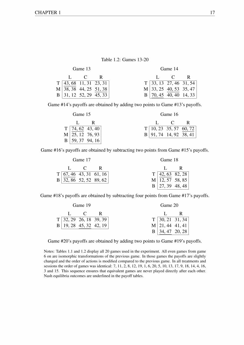
All games in the experiment are two-person games with two or three actions for each in-dividual, which means the games are of the 2x2, 3x3 or 2x3 form. There are 12 distinctgames: 4 symmetric and 8 asymmetric games. Since subjects play every asymmetric gamein both roles there are 20 games in total. However, subjects do not play the exact game inboth roles, but rather isomorphic transformations.13 For each asymmetric game a secondgame is created by transposing the player roles, changing the order of actions and addingor subtracting a constant to all payoffs. Therefore there are eight pairs of equivalent games.This modification leaves all relevant properties of the game (like Nash equilibria and dom-inance relations) unchanged and results in a total of 16 asymmetric games played by eachsubject. Because these non-trivial transformations of payoffs and order of actions disguisethe equivalence of games, it is unlikely that subjects realize that they play each game in bothroles. Additionally two equivalent games are never played in direct sequence. Due to theisomorphic transformations, behavior of row players in asymmetric games can directly becompared to behavior of column players in the equivalent game.

Tables 1.1 and 1.2 list all games and used transformations. To analyze whether gameproperties play a role in the effect of belief elicitation on action choices the used games varyin multiple dimensions. Besides being either symmetric of asymmetric, important character-istics that differ between games are whether a game is dominance-solvable, if it has a uniqueor multiple pure-strategy Nash equilibria, whether the Nash equilibrium is Pareto dominatedby another outcome and whether or not an alternative outcome to the Nash equilibrium withsymmetric payoffs for both subjects exists.14 Table 1.3 summarizes the main differences

12 This average contains only five sessions, since in one session a computer crash made it impossible torecover the matching. Subjects in this session received a fixed payment. The crash occurred after all decisionand belief statements had been recorded. The datafile containing all decisions and belief statements could berecovered and the data is used in the analyses.

13 A similar procedure has been used by Costa-Gomes and Weizsäcker (2008).14 None of the games has a mixed-strategy Nash equilibrium.

16 CHAPTER 1

between games that become relevant in the analysis.

Table 1.1: Games 1-12

Game 1

’T’ ’M’ ’B’T 40, 40 20, 30 0, 20M 30, 20 20, 20 100, 10B 20, 0 10, 100 100, 100

Game 2

’T’ ’B’T 75, 75 25, 85B 85, 25 30, 30

Game 3

’T’ ’ M’ ’B’T 10, 10 49, 58 37, 60M 58, 49 22, 22 16, 36B 60, 37 36, 16 38, 38

Game 4

’T’ ’M’ ’B’T 26, 26 22, 17 18, 24M 17, 22 11, 11 33, 21B 24, 18 21, 33 20, 20

Game 5

L RT 55, 79 84, 52B 31, 46 72, 93

Game 6

L RT 48, 80 89, 68B 75, 51 42, 27

Game #6’s payoffs are obtained by subtracting four points from Game #5’s payoffs.

Game 7

L C RT 74, 38 78, 71 46, 43M 96, 12 10, 89 57, 25B 15, 51 83, 18 69, 62

Game 8

L C RT 73, 80 20, 85 91, 12M 45, 48 64, 71 27, 59B 40, 76 53, 17 14, 98

Game #8’s payoffs are obtained by adding two points to Game #7’s payoffs.

Game 9

L C RT 31, 25 23, 12 42, 33M 36, 36 30, 20 18, 27B 48, 31 29, 42 23, 16

Game 10

L C RT 29, 20 18, 25 35, 44M 22, 32 44, 31 14, 25B 38, 38 33, 50 27, 33


Game 11

L C RT 52, 23 36, 27 16, 41M 61, 31 31, 46 22, 28B 80, 15 12, 40 34, 53

Game 12

L C RT 49, 30 24, 18 37, 12M 11, 76 27, 57 19, 48B 36, 8 42, 27 23, 32


CHAPTER 1 17

Table 1.2: Games 13-20

Game 13

L C RT 43, 68 11, 31 23, 31M 38, 38 44, 25 51, 38B 31, 12 52, 29 45, 33

Game 14

L C RT 33, 13 27, 46 31, 54M 33, 25 40, 53 35, 47B 70, 45 40, 40 14, 33


Game 15

L RT 74, 62 43, 40M 25, 12 76, 93B 59, 37 94, 16

Game 16

L C RT 10, 23 35, 57 60, 72B 91, 74 14, 92 38, 41

Game #16’s payoffs are obtained by subtracting two points from Game #15’s payoffs.

Game 17

L C RT 67, 46 43, 31 61, 16B 32, 86 52, 52 89, 62

Game 18

L RT 42, 63 82, 28M 12, 57 58, 85B 27, 39 48, 48


Game 19

L C RT 32, 29 26, 18 39, 39B 19, 28 45, 32 42, 19

Game 20

L RT 30, 21 31, 34M 21, 44 41, 41B 34, 47 20, 28


Notes: Tables 1.1 and 1.2 display all 20 games used in the experiment. All even games from game6 on are isomorphic transformations of the previous game. In those games the payoffs are slightlychanged and the order of actions is modified compared to the previous game. In all treatments andsessions the order of games was identical: 7, 11, 2, 8, 12, 19, 1, 6, 20, 5, 10, 13, 17, 9, 18, 14, 4, 16,3 and 15. This sequence ensures that equivalent games are never played directly after each other.Nash equilibria outcomes are underlined in the payoff tables.

18 CHAPTER 1

Table 1.3: Game properties

Overview of selected game properties for all gamesProperty/Game # 1 2 3 4 5/6 7/8 9/10 11/12 13/14 15/16 17/18 19/20

unique NE X X X X X X X X X XNE Pareto dominated E X X X X Xdominance-solvable X X X X X X X Xsymmetric alternative W X X X X W XNotes: Game numbers correspond to game numbers in tables 1.1 and 1.2. E for NE Pareto dominated meansthat the other outcome is also a NE, W for symmetric alternative means that the symmetric alternative(s)are weakly dominated by the NE.

1.2.3 Hypotheses

If belief statements and action choices are properly incentivized the payments for the statedbeliefs should not affect subjects’ action choices due to hedging. But there exit two otherchannels through which subjects’ choices might be affected by eliciting beliefs. First, beliefsare usually elicited based on the idea that subjective beliefs are relevant for subjects’ actionchoices. If this assumption is true than chosen actions of subjects might change if beliefsare altered by the elicitation. Existing beliefs could be altered due to the elicitation, becausesubjects modify their otherwise coarse beliefs if they are asked to state exact numbers fortheir beliefs or subjects’ understanding of the decision situation is increased by the beliefstatements. Second, subjects who do not form beliefs if they are not asked to state themor subjects’ whose action choices are not belief based might condition their action choicesmore heavily on their beliefs if they are required to state them. In both cases subjects’ chosenactions in the same decision situation could differ dependent on whether they are asked tostate beliefs or not.

If subjects hold beliefs, even when they are not elicited, and play is belief-based, beingasked to put exact numbers on the expected behavior of the other player could motivatesubjects to think more about the game in general and about the choice of their opponentin particular. This increased effort could lead to a modification of the “original” beliefs(the beliefs a player has without being explicitly asked to state them) though the increasedinvolvement with the game at hand and thus lead to a deeper understanding of the decisionsituation. This “thinking-harder” hypothesis predicts subjects behave “more like a gametheorist” (Croson 2000) compared to situations without belief elicitation. According to thishypothesis belief elicitation should result in an increased frequency of action choices thatare part of a Nash equilibrium and therefore I should observe more equilibrium play in thebelief treatment compared to the baseline treatment.

The differences between the treatments should be larger for games in which beliefs aremore likely to be affected by an increased sophistication of subjects. More specifically, indominance-solvable games stating own beliefs about the action choice distribution of theopponent can lead to the discovery of a dominated action of the other player. When a player

CHAPTER 1 19

observes that an action of the other player is dominated, he or she should place a zero (orvery small) probability on the likelihood that this action is played. In dominance-solvablegames such a belief often results in an own action that should not be chosen, since it is now“iteratively” dominated. The action is only dominated if an action of the other player isassumed not to be chosen. In such a case the modification of beliefs due to the discovery ofan iteratively dominated action can influence the own action choice. Therefore the differencein chosen actions between the treatments should be larger for dominance-solvable games.

If play is not belief based subjects employ other mechanisms or (simple) heuristics todetermine which action to choose. A subject might always pick the action that yields himor her the highest possible payoff, select the action which ensures him or her the highestpayoff for sure (max-min choice) or even choose an action randomly. These strategies do notrequire any expectations about the behavior of the other player. While this behavior mightbe unlikely in situations in which subjects possess a lot of experience, it is more likely in thestudied context of one-shot games in which the question whether subjects hold meaningfulbeliefs at all arises.15

For subjects who do not to base their action choices on beliefs, the elicitation couldinduce some beliefs. As subjects are required to state beliefs and rewarded for correct pre-dictions, it is likely that they actually think about the other player’s most probable actionand thereby form meaningful beliefs. Given that they spend effort in deriving their beliefsand in the belief treatment they have not made a final action choice yet, they might considerthese beliefs to select their action. Therefore for those subjects the elicitation could lead to achange in behavior. Furthermore, for subjects who have beliefs, but do not take these beliefsinto account for their action choice, the elicitation could encourage them to actually considerthese beliefs in their action choice. If that is the case, also for these subjects the chosen ac-tions might be different with belief elicitation. Consequently the choice distribution couldbe changed compared to a situation without belief elicitation for both types of players. Ad-ditionally, if subjects best respond to their beliefs, it is more likely that a player selects anaction which is part of a Nash equilibrium, since a Nash equilibrium exactly defines mutualbest responses. While this effect should be present in all games, it will most likely be morepronounced in games in which the formation of beliefs has a decisive effect on players’ de-cisions. Therefore, similar to the prediction stated above, a stronger effect on game play isexpected for dominance-solvable games.

Furthermore, if eliciting subjects’ beliefs actually influences game play the effect haslikely different implications for very sophisticated subjects and subjects who are less so-phisticated. In the extreme case the action choices of a fully rational subject who alwaysplays according to Nash equilibrium predictions even without belief elicitation should not

15 Although learning between multiple one-shot games could take place, since no feedback about the choicesof the other players is given until the end of the experiment, only “no-feedback learning” is possible, which Iconsider not very likely.

20 CHAPTER 1

be affected. Such a player is already assuming that his or her opponent plays the equilibriumaction and therefore his or her beliefs should not change due to the elicitation. On the otherside of the spectrum are subjects without any beliefs, e.g. a player that chooses the actionwhich can yield him or her the highest possible payoff or a player who does not considerthe incentives of his or her opponent. For these subjects the belief statements might helpto organize their thoughts in a meaningful manner and therefore increase the probability ofequilibrium play. If that is the case models of game play that consider various levels ofsubjects’ sophistication should result in different distributions of subjects’ types between thetreatments. Especially, I consider several player types as defined by the level-k model (Stahland Wilson 1994). I expect a larger share of subjects being classified as relatively sophisti-cated, e.g. showing a higher level of strategic reasoning, in the belief treatment than in thebaseline treatment.

But belief elicitation is also an additional task subjects have to perform. Since sub-jects have to understand how to state their beliefs and how they are rewarded for it, beliefelicitation could lead to more confused subjects and result in more random action choices.Therefore belief elicitation induces a different choice due to confusion. If that is the case,I would not consider it as an effect of the elicitation, but rather the consequence of poorinstructions. Since all decisions in this experiment are made without any time pressure Iconsider it unlikely that the additional task distracted subjects. Nevertheless, if it was thecase, it should result in less equilibrium play, since there is no reason why a confused sub-ject should play as predicted by a theory that has strong demands on subjects’ rationality andstrategic sophistication. Therefore distraction works in the opposite direction as predicted bythe two hypotheses above and would weaken a potential effect. Also if the belief elicitationis rather a burden than a supportive tool for less sophisticated subjects, it is not clear that thedistributions of different “sophistication types” differs between the treatments.

1.3 Results

1.3.1 Preliminaries

The experimental design with row and column players playing isomorphic games was cho-sen assuming that this variation does not affect subjects’ behavior. While for both typesall games are equivalent, the order of games differs between row and column players. Ifthe transformation and the different order of games is without consequences for the chosenactions, I can pool the data across player roles. To test whether the transformations or theorder of games affects subjects’ action choices I contrast row players’ choices in asymmetricgames with the action choices of column players in the transformed game (and vice versa).For symmetric games no test is necessary, since all players see the games as row players.Such a test compares categorical data between independent samples, therefore I conduct

CHAPTER 1 21

Fisher’s Exact Probability Tests (FEPT) for count data.16

Comparing subjects’ aggregate actions separately on each game in each treatment yieldsonly two significantly different distributions between types, which is in line with the ex-pected number of rejections for 40 comparisons.17 For the tests in the next sections the datais therefore pooled across player roles. To analyze whether the chosen actions are differentfrom random play I perform χ2 goodness of fit tests separately for each game. Testing thechosen actions yields 32 significant differences from the uniform distribution (out of 40).18

The frequent deviations from random play in both treatments clearly demonstrates that sub-jects’ choices are not random. These results yield that player roles are without effect ongame play and that actions are not picked randomly.

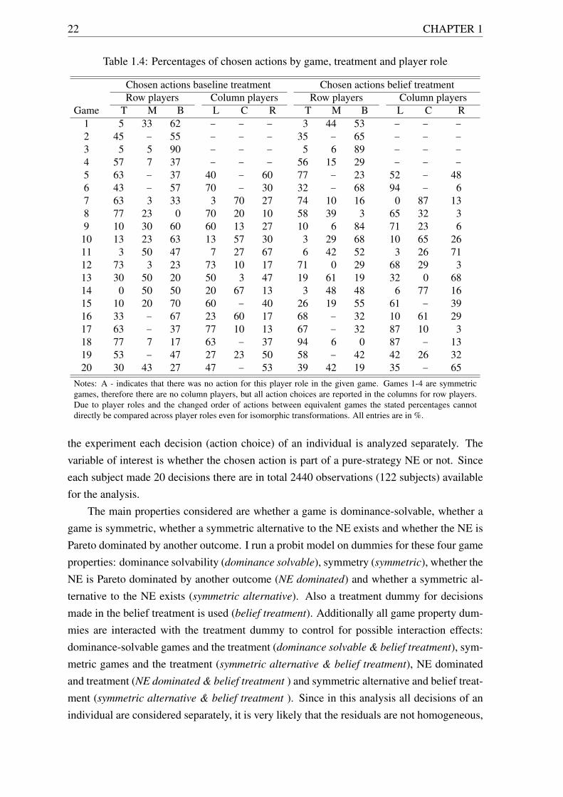
Before discussing the effect of the belief elicitation on the data I provide the frequenciesfor all action choices in all games and treatments. Table 1.4 contains the percentage ofactions chosen for all 20 games separately for the two treatments and player roles.

There are two main take aways from the numbers reported in table 1.4. First, thereseems to be some heterogeneity among subjects’ choices. In very few games an action ischosen by more than 75% of subjects. Second, while subjects’ choices are heterogeneous thechoice frequencies already indicate that subjects’ behavior is not random. In many gamesone action is only chosen by a small fraction of subjects. While subjects seem to havea common understanding of which actions are less desirable, they do not agree on whichaction is the “best” in most cases.

1.3.2 Belief elicitation and the role of game properties

The research about the likelihood of Nash-equilibrium play has shown that various gameproperties and the decision environment affect the predictive power of Nash equilibrium, e.g.see Rey-Biel (2009) for normal-form games. It is likely that the effect of belief elicitation ongame play also depends on game properties. Given the mixed results reported in the literaturewhether belief elicitation affects the likelihood of action choices that are part of a NE, it isespecially interesting to analyze the role of game properties jointly with a possible effect ofthe belief elicitation. In order to exploit the various game properties of the games used in

16 There exists a literature regarding the best tests for contingency tables showing that unconditional testslike Boschloo’s test have greater power than conditional tests like the FEPT at least in 2x2 tables. However, thepower advantage vanishes quickly with sample size for larger tables like 2x3 tables, e.g. see Mehta and Hilton(1993). Since most of the 20 games studied in this paper are not of the 2x2 form, the additional computationaldifficulties for using unconditional tests are large compared to the potential gain in power. Therefore FEPT areused for the following analysis.

17 All test in this paper are two-sided unless explicitly stated otherwise. In game 11 in the baseline treatment(p-value < 0.01) and game 8 in the belief treatment (p-value = 0.02) the differences between the player rolesare significant. All other p-values are above the 5%-level and are usually much higher.

18 For 5 games in the baseline treatment, games 2, 6, 16, 19 and 20, and 3 games the belief treatment, games6, 19 and 20, there are no significant differences from random play. In the pooled data only the choices ingames 6, 16 and 19 are not different from random play.

22 CHAPTER 1

Table 1.4: Percentages of chosen actions by game, treatment and player role

Chosen actions baseline treatment Chosen actions belief treatmentRow players Column players Row players Column players

Game T M B L C R T M B L C R1 5 33 62 − − − 3 44 53 − − −

2 45 − 55 − − − 35 − 65 − − −

3 5 5 90 − − − 5 6 89 − − −

4 57 7 37 − − − 56 15 29 − − −

5 63 − 37 40 − 60 77 − 23 52 − 486 43 − 57 70 − 30 32 − 68 94 − 67 63 3 33 3 70 27 74 10 16 0 87 138 77 23 0 70 20 10 58 39 3 65 32 39 10 30 60 60 13 27 10 6 84 71 23 6

10 13 23 63 13 57 30 3 29 68 10 65 2611 3 50 47 7 27 67 6 42 52 3 26 7112 73 3 23 73 10 17 71 0 29 68 29 313 30 50 20 50 3 47 19 61 19 32 0 6814 0 50 50 20 67 13 3 48 48 6 77 1615 10 20 70 60 − 40 26 19 55 61 − 3916 33 − 67 23 60 17 68 − 32 10 61 2917 63 − 37 77 10 13 67 − 32 87 10 318 77 7 17 63 − 37 94 6 0 87 − 1319 53 − 47 27 23 50 58 − 42 42 26 3220 30 43 27 47 − 53 39 42 19 35 − 65

Notes: A - indicates that there was no action for this player role in the given game. Games 1-4 are symmetricgames, therefore there are no column players, but all action choices are reported in the columns for row players.Due to player roles and the changed order of actions between equivalent games the stated percentages cannotdirectly be compared across player roles even for isomorphic transformations. All entries are in %.

the experiment each decision (action choice) of an individual is analyzed separately. Thevariable of interest is whether the chosen action is part of a pure-strategy NE or not. Sinceeach subject made 20 decisions there are in total 2440 observations (122 subjects) availablefor the analysis.

The main properties considered are whether a game is dominance-solvable, whether agame is symmetric, whether a symmetric alternative to the NE exists and whether the NE isPareto dominated by another outcome. I run a probit model on dummies for these four gameproperties: dominance solvability (dominance solvable), symmetry (symmetric), whether theNE is Pareto dominated by another outcome (NE dominated) and whether a symmetric al-ternative to the NE exists (symmetric alternative). Also a treatment dummy for decisionsmade in the belief treatment is used (belief treatment). Additionally all game property dum-mies are interacted with the treatment dummy to control for possible interaction effects:dominance-solvable games and the treatment (dominance solvable & belief treatment), sym-metric games and the treatment (symmetric alternative & belief treatment), NE dominatedand treatment (NE dominated & belief treatment ) and symmetric alternative and belief treat-ment (symmetric alternative & belief treatment ). Since in this analysis all decisions of anindividual are considered separately, it is very likely that the residuals are not homogeneous,

CHAPTER 1 23

Table 1.5: Probit estimation of NE

Probitdep. variable: NE Marginal Effect (Std. Err.)

belief treatment 0.04 (0.05)

Game propertiesdominance solvable 0.44∗∗∗ (0.04)symmetric 0.36∗∗∗ (0.04)NE dominated −0.43∗∗∗ (0.04)symmetric alternative −0.07 (0.04)

Interaction effectsdominance solvable & belief treatment 0.14∗∗ (0.06)symmetric & belief treatment 0.08 (0.08)NE dominated & belief treatment −0.09 (0.07)symmetric alternative & belief treatment −0.14∗∗ (0.06)

Observations 2440Pseudo R2 0.137Predicted probability 0.562Notes: Probit estimates. Marginal effects (evaluated at the mean of independentvariables); * p < 0.10, ** p < 0.05, *** p < 0.01. All standard errors are clusteredat the subject level.

as the errors of the same subject are most likely correlated. Therefore the shown regressionincludes standard errors that are clustered at the subject level.

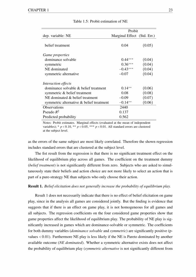
The fist result from the regression is that there is no significant treatment effect on thelikelihood of equilibrium play across all games. The coefficient on the treatment dummy(belief treatment) is not significantly different from zero. Subjects who are asked to simul-taneously state their beliefs and action choice are not more likely to select an action that ispart of a pure-strategy NE than subjects who only choose their action.

Result 1. Belief elicitation does not generally increase the probability of equilibrium play.

Result 1 does not necessarily indicate that there is no effect of belief elicitation on gameplay, since in the analysis all games are considered jointly. But the finding is evidence thatsuggests that if there is an effect on game play, it is not homogeneous for all games andall subjects. The regression coefficients on the four considered game properties show thatgame properties affect the likelihood of equilibrium play. The probability of NE play is sig-nificantly increased in games which are dominance-solvable or symmetric. The coefficientsfor both dummy variables (dominance solvable and symmetric) are significantly positive (p-values < 0.01). Furthermore NE play is less likely if the NE is Pareto dominated by anotheravailable outcome (NE dominated). Whether a symmetric alternative exists does not affectthe probability of equilibrium play (symmetric alternative is not significantly different from

24 CHAPTER 1

zero).

Result 2. Game properties have a significant influence on the chosen actions.

(i) More actions in accordance with NE are played if the game is dominance-solvable or

symmetric,

(ii) and less NE actions are chosen if the NE is dominated by another outcome.

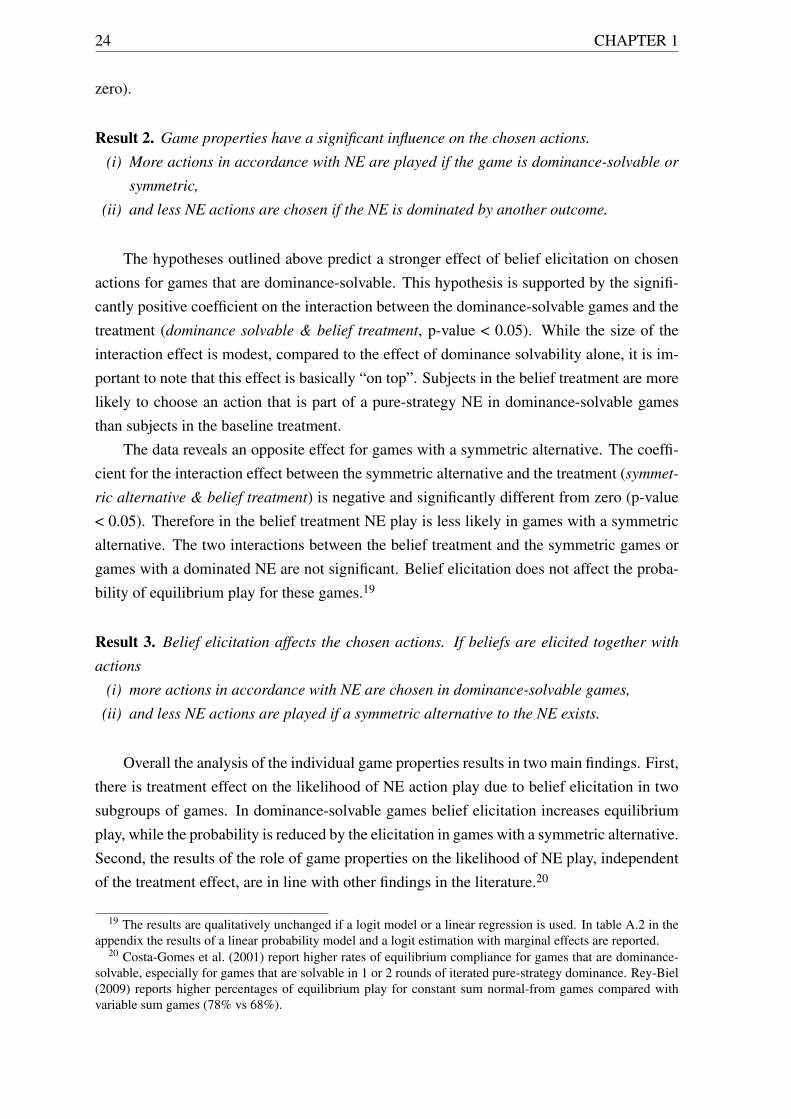
The hypotheses outlined above predict a stronger effect of belief elicitation on chosenactions for games that are dominance-solvable. This hypothesis is supported by the signifi-cantly positive coefficient on the interaction between the dominance-solvable games and thetreatment (dominance solvable & belief treatment, p-value < 0.05). While the size of theinteraction effect is modest, compared to the effect of dominance solvability alone, it is im-portant to note that this effect is basically “on top”. Subjects in the belief treatment are morelikely to choose an action that is part of a pure-strategy NE in dominance-solvable gamesthan subjects in the baseline treatment.

The data reveals an opposite effect for games with a symmetric alternative. The coeffi-cient for the interaction effect between the symmetric alternative and the treatment (symmet-

ric alternative & belief treatment) is negative and significantly different from zero (p-value< 0.05). Therefore in the belief treatment NE play is less likely in games with a symmetricalternative. The two interactions between the belief treatment and the symmetric games orgames with a dominated NE are not significant. Belief elicitation does not affect the proba-bility of equilibrium play for these games.19

Result 3. Belief elicitation affects the chosen actions. If beliefs are elicited together with

actions

(i) more actions in accordance with NE are chosen in dominance-solvable games,

(ii) and less NE actions are played if a symmetric alternative to the NE exists.

Overall the analysis of the individual game properties results in two main findings. First,there is treatment effect on the likelihood of NE action play due to belief elicitation in twosubgroups of games. In dominance-solvable games belief elicitation increases equilibriumplay, while the probability is reduced by the elicitation in games with a symmetric alternative.Second, the results of the role of game properties on the likelihood of NE play, independentof the treatment effect, are in line with other findings in the literature.20

19 The results are qualitatively unchanged if a logit model or a linear regression is used. In table A.2 in theappendix the results of a linear probability model and a logit estimation with marginal effects are reported.

20 Costa-Gomes et al. (2001) report higher rates of equilibrium compliance for games that are dominance-solvable, especially for games that are solvable in 1 or 2 rounds of iterated pure-strategy dominance. Rey-Biel(2009) reports higher percentages of equilibrium play for constant sum normal-from games compared withvariable sum games (78% vs 68%).

CHAPTER 1 25

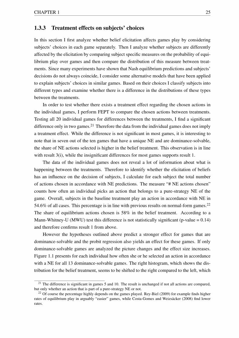
1.3.3 Treatment effects on subjects’ choices

In this section I first analyze whether belief elicitation affects games play by consideringsubjects’ choices in each game separately. Then I analyze whether subjects are differentlyaffected by the elicitation by comparing subject specific measures on the probability of equi-librium play over games and then compare the distribution of this measure between treat-ments. Since many experiments have shown that Nash equilibrium predictions and subjects’decisions do not always coincide, I consider some alternative models that have been appliedto explain subjects’ choices in similar games. Based on their choices I classify subjects intodifferent types and examine whether there is a difference in the distributions of these typesbetween the treatments.

In order to test whether there exists a treatment effect regarding the chosen actions inthe individual games, I perform FEPT to compare the chosen actions between treatments.Testing all 20 individual games for differences between the treatments, I find a significantdifference only in two games.21 Therefore the data from the individual games does not implya treatment effect. While the difference is not significant in most games, it is interesting tonote that in seven out of the ten games that have a unique NE and are dominance-solvable,the share of NE actions selected is higher in the belief treatment. This observation is in linewith result 3(i), while the insignificant differences for most games supports result 1.

The data of the individual games does not reveal a lot of information about what ishappening between the treatments. Therefore to identify whether the elicitation of beliefshas an influence on the decision of subjects, I calculate for each subject the total numberof actions chosen in accordance with NE predictions. The measure “# NE actions chosen”counts how often an individual picks an action that belongs to a pure-strategy NE of thegame. Overall, subjects in the baseline treatment play an action in accordance with NE in54.6% of all cases. This percentage is in line with previous results on normal-form games.22

The share of equilibrium actions chosen is 58% in the belief treatment. According to aMann-Whitney-U (MWU) test this difference is not statistically significant (p-value = 0.14)and therefore confirms result 1 from above.

However the hypotheses outlined above predict a stronger effect for games that aredominance-solvable and the probit regression also yields an effect for these games. If onlydominance-solvable games are analyzed the picture changes and the effect size increases.Figure 1.1 presents for each individual how often she or he selected an action in accordancewith a NE for all 13 dominance-solvable games. The right histogram, which shows the dis-tribution for the belief treatment, seems to be shifted to the right compared to the left, which

21 The difference is significant in games 5 and 10. The result is unchanged if not all actions are compared,but only whether an action that is part of a pure-strategy NE or not.

22 Of course the percentage highly depends on the games played. Rey-Biel (2009) for example finds higherrates of equilibrium play in arguably “easier” games, while Costa-Gomes and Weizsäcker (2008) find lowerrates.

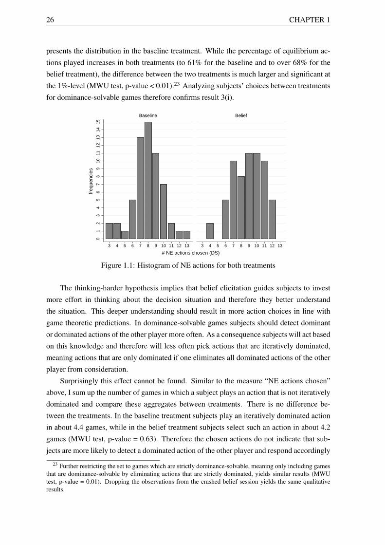
26 CHAPTER 1

presents the distribution in the baseline treatment. While the percentage of equilibrium ac-tions played increases in both treatments (to 61% for the baseline and to over 68% for thebelief treatment), the difference between the two treatments is much larger and significant atthe 1%-level (MWU test, p-value < 0.01).23 Analyzing subjects’ choices between treatmentsfor dominance-solvable games therefore confirms result 3(i).

01

23

45

67

89

1011

1213

1415

3 4 5 6 7 8 9 10 11 12 13 3 4 5 6 7 8 9 10 11 12 13

Baseline Belief

freq

uenc

ies

# NE actions chosen (DS)

Figure 1.1: Histogram of NE actions for both treatments

The thinking-harder hypothesis implies that belief elicitation guides subjects to investmore effort in thinking about the decision situation and therefore they better understandthe situation. This deeper understanding should result in more action choices in line withgame theoretic predictions. In dominance-solvable games subjects should detect dominantor dominated actions of the other player more often. As a consequence subjects will act basedon this knowledge and therefore will less often pick actions that are iteratively dominated,meaning actions that are only dominated if one eliminates all dominated actions of the otherplayer from consideration.

Surprisingly this effect cannot be found. Similar to the measure “NE actions chosen”above, I sum up the number of games in which a subject plays an action that is not iterativelydominated and compare these aggregates between treatments. There is no difference be-tween the treatments. In the baseline treatment subjects play an iteratively dominated actionin about 4.4 games, while in the belief treatment subjects select such an action in about 4.2games (MWU test, p-value = 0.63). Therefore the chosen actions do not indicate that sub-jects are more likely to detect a dominated action of the other player and respond accordingly

23 Further restricting the set to games which are strictly dominance-solvable, meaning only including gamesthat are dominance-solvable by eliminating actions that are strictly dominated, yields similar results (MWUtest, p-value = 0.01). Dropping the observations from the crashed belief session yields the same qualitativeresults.

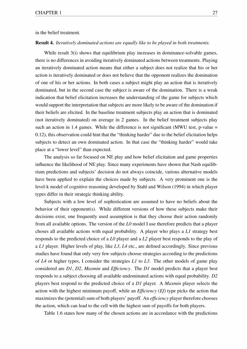
CHAPTER 1 27

in the belief treatment.

Result 4. Iteratively dominated actions are equally like to be played in both treatments.

While result 3(i) shows that equilibrium play increases in dominance-solvable games,there is no differences in avoiding iteratively dominated actions between treatments. Playingan iteratively dominated action means that either a subject does not realize that his or heraction is iteratively dominated or does not believe that the opponent realizes the dominationof one of his or her actions. In both cases a subject might play an action that is iterativelydominated, but in the second case the subject is aware of the domination. There is a weakindication that belief elicitation increases the understanding of the game for subjects whichwould support the interpretation that subjects are more likely to be aware of the domination iftheir beliefs are elicited. In the baseline treatment subjects play an action that is dominated(not iteratively dominated) on average in 2 games. In the belief treatment subjects playsuch an action in 1.4 games. While the difference is not significant (MWU test, p-value =0.12), this observation could hint that the “thinking harder” due to the belief elicitation helpssubjects to detect an own dominated action. In that case the “thinking harder” would takeplace at a “lower level” than expected.

The analysis so far focused on NE play and how belief elicitation and game propertiesinfluence the likelihood of NE play. Since many experiments have shown that Nash equilib-rium predictions and subjects’ decision do not always coincide, various alternative modelshave been applied to explain the choices made by subjects. A very prominent one is thelevel-k model of cognitive reasoning developed by Stahl and Wilson (1994) in which playertypes differ in their strategic thinking ability.

Subjects with a low level of sophistication are assumed to have no beliefs about thebehavior of their opponent(s). While different versions of how these subjects make theirdecisions exist, one frequently used assumption is that they choose their action randomlyfrom all available options. The version of the L0 model I use therefore predicts that a playerchoses all available actions with equal probability. A player who plays a L1 strategy bestresponds to the predicted choice of a L0 player and a L2 player best responds to the play ofa L1 player. Higher levels of play, like L3, L4 etc., are defined accordingly. Since previousstudies have found that only very few subjects choose strategies according to the predictionsof L4 or higher types, I consider the strategies L1 to L3. The other models of game playconsidered are D1, D2, Maxmin and Efficiency. The D1 model predicts that a player bestresponds to a subject choosing all available undominated actions with equal probability. D2

players best respond to the predicted choice of a D1 player. A Maxmin player selects theaction with the highest minimum payoff, while an Efficiency (Ef) type picks the action thatmaximizes the (potential) sum of both players’ payoff. An efficiency player therefore choosesthe action, which can lead to the cell with the highest sum of payoffs for both players.

Table 1.6 states how many of the chosen actions are in accordance with the predictions

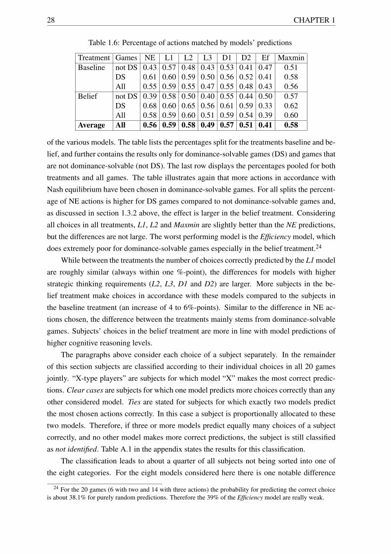
28 CHAPTER 1

Table 1.6: Percentage of actions matched by models’ predictions

Treatment Games NE L1 L2 L3 D1 D2 Ef MaxminBaseline not DS 0.43 0.57 0.48 0.43 0.53 0.41 0.47 0.51

DS 0.61 0.60 0.59 0.50 0.56 0.52 0.41 0.58All 0.55 0.59 0.55 0.47 0.55 0.48 0.43 0.56

Belief not DS 0.39 0.58 0.50 0.40 0.55 0.44 0.50 0.57DS 0.68 0.60 0.65 0.56 0.61 0.59 0.33 0.62All 0.58 0.59 0.60 0.51 0.59 0.54 0.39 0.60

Average All 0.56 0.59 0.58 0.49 0.57 0.51 0.41 0.58

of the various models. The table lists the percentages split for the treatments baseline and be-lief, and further contains the results only for dominance-solvable games (DS) and games thatare not dominance-solvable (not DS). The last row displays the percentages pooled for bothtreatments and all games. The table illustrates again that more actions in accordance withNash equilibrium have been chosen in dominance-solvable games. For all splits the percent-age of NE actions is higher for DS games compared to not dominance-solvable games and,as discussed in section 1.3.2 above, the effect is larger in the belief treatment. Consideringall choices in all treatments, L1, L2 and Maxmin are slightly better than the NE predictions,but the differences are not large. The worst performing model is the Efficiency model, whichdoes extremely poor for dominance-solvable games especially in the belief treatment.24

While between the treatments the number of choices correctly predicted by the L1 modelare roughly similar (always within one %-point), the differences for models with higherstrategic thinking requirements (L2, L3, D1 and D2) are larger. More subjects in the be-lief treatment make choices in accordance with these models compared to the subjects inthe baseline treatment (an increase of 4 to 6%-points). Similar to the difference in NE ac-tions chosen, the difference between the treatments mainly stems from dominance-solvablegames. Subjects’ choices in the belief treatment are more in line with model predictions ofhigher cognitive reasoning levels.

The paragraphs above consider each choice of a subject separately. In the remainderof this section subjects are classified according to their individual choices in all 20 gamesjointly. “X-type players” are subjects for which model “X” makes the most correct predic-tions. Clear cases are subjects for which one model predicts more choices correctly than anyother considered model. Ties are stated for subjects for which exactly two models predictthe most chosen actions correctly. In this case a subject is proportionally allocated to thesetwo models. Therefore, if three or more models predict equally many choices of a subjectcorrectly, and no other model makes more correct predictions, the subject is still classifiedas not identified. Table A.1 in the appendix states the results for this classification.

The classification leads to about a quarter of all subjects not being sorted into one ofthe eight categories. For the eight models considered here there is one notable difference

24 For the 20 games (6 with two and 14 with three actions) the probability for predicting the correct choiceis about 38.1% for purely random predictions. Therefore the 39% of the Efficiency model are really weak.

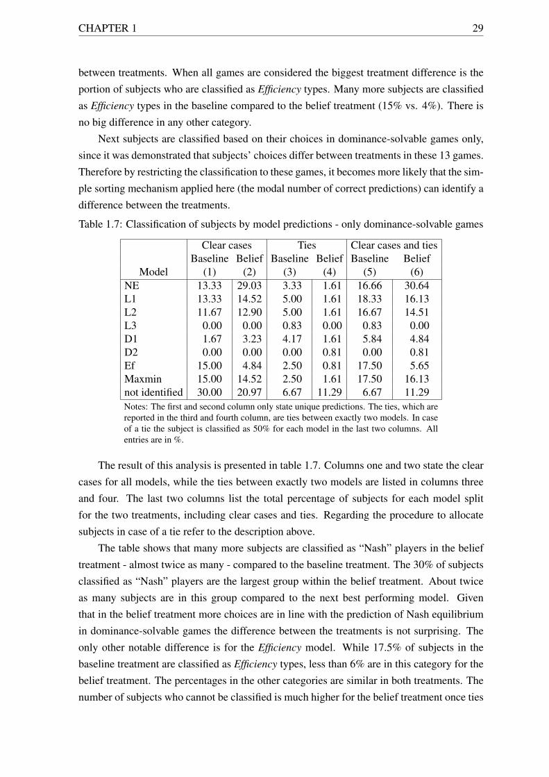
CHAPTER 1 29

between treatments. When all games are considered the biggest treatment difference is theportion of subjects who are classified as Efficiency types. Many more subjects are classifiedas Efficiency types in the baseline compared to the belief treatment (15% vs. 4%). There isno big difference in any other category.

Next subjects are classified based on their choices in dominance-solvable games only,since it was demonstrated that subjects’ choices differ between treatments in these 13 games.Therefore by restricting the classification to these games, it becomes more likely that the sim-ple sorting mechanism applied here (the modal number of correct predictions) can identify adifference between the treatments.

Table 1.7: Classification of subjects by model predictions - only dominance-solvable games

Clear cases Ties Clear cases and tiesBaseline Belief Baseline Belief Baseline Belief

Model (1) (2) (3) (4) (5) (6)NE 13.33 29.03 3.33 1.61 16.66 30.64L1 13.33 14.52 5.00 1.61 18.33 16.13L2 11.67 12.90 5.00 1.61 16.67 14.51L3 0.00 0.00 0.83 0.00 0.83 0.00D1 1.67 3.23 4.17 1.61 5.84 4.84D2 0.00 0.00 0.00 0.81 0.00 0.81Ef 15.00 4.84 2.50 0.81 17.50 5.65Maxmin 15.00 14.52 2.50 1.61 17.50 16.13not identified 30.00 20.97 6.67 11.29 6.67 11.29Notes: The first and second column only state unique predictions. The ties, which arereported in the third and fourth column, are ties between exactly two models. In caseof a tie the subject is classified as 50% for each model in the last two columns. Allentries are in %.

The result of this analysis is presented in table 1.7. Columns one and two state the clearcases for all models, while the ties between exactly two models are listed in columns threeand four. The last two columns list the total percentage of subjects for each model splitfor the two treatments, including clear cases and ties. Regarding the procedure to allocatesubjects in case of a tie refer to the description above.

The table shows that many more subjects are classified as “Nash” players in the belieftreatment - almost twice as many - compared to the baseline treatment. The 30% of subjectsclassified as “Nash” players are the largest group within the belief treatment. About twiceas many subjects are in this group compared to the next best performing model. Giventhat in the belief treatment more choices are in line with the prediction of Nash equilibriumin dominance-solvable games the difference between the treatments is not surprising. Theonly other notable difference is for the Efficiency model. While 17.5% of subjects in thebaseline treatment are classified as Efficiency types, less than 6% are in this category for thebelief treatment. The percentages in the other categories are similar in both treatments. Thenumber of subjects who cannot be classified is much higher for the belief treatment once ties

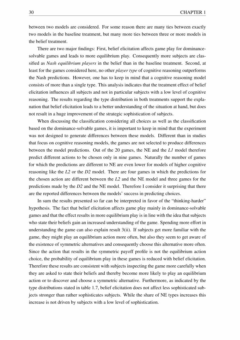
30 CHAPTER 1

between two models are considered. For some reason there are many ties between exactlytwo models in the baseline treatment, but many more ties between three or more models inthe belief treatment.

There are two major findings: First, belief elicitation affects game play for dominance-solvable games and leads to more equilibrium play. Consequently more subjects are clas-sified as Nash equilibrium players in the belief than in the baseline treatment. Second, atleast for the games considered here, no other player type of cognitive reasoning outperformsthe Nash predictions. However, one has to keep in mind that a cognitive reasoning modelconsists of more than a single type. This analysis indicates that the treatment effect of beliefelicitation influences all subjects and not in particular subjects with a low level of cognitivereasoning. The results regarding the type distribution in both treatments support the expla-nation that belief elicitation leads to a better understanding of the situation at hand, but doesnot result in a huge improvement of the strategic sophistication of subjects.

When discussing the classification considering all choices as well as the classificationbased on the dominance-solvable games, it is important to keep in mind that the experimentwas not designed to generate differences between these models. Different than in studiesthat focus on cognitive reasoning models, the games are not selected to produce differencesbetween the model predictions. Out of the 20 games, the NE and the L1 model thereforepredict different actions to be chosen only in nine games. Naturally the number of gamesfor which the predictions are different to NE are even lower for models of higher cognitivereasoning like the L2 or the D2 model. There are four games in which the predictions forthe chosen action are different between the L2 and the NE model and three games for thepredictions made by the D2 and the NE model. Therefore I consider it surprising that thereare the reported differences between the models’ success in predicting choices.

In sum the results presented so far can be interpreted in favor of the “thinking-harder”hypothesis. The fact that belief elicitation affects game play mainly in dominance-solvablegames and that the effect results in more equilibrium play is in line with the idea that subjectswho state their beliefs gain an increased understanding of the game. Spending more effort inunderstanding the game can also explain result 3(ii). If subjects get more familiar with thegame, they might play an equilibrium action more often, but also they seem to get aware ofthe existence of symmetric alternatives and consequently choose this alternative more often.Since the action that results in the symmetric payoff profile is not the equilibrium actionchoice, the probability of equilibrium play in these games is reduced with belief elicitation.Therefore these results are consistent with subjects inspecting the game more carefully whenthey are asked to state their beliefs and thereby become more likely to play an equilibriumaction or to discover and choose a symmetric alternative. Furthermore, as indicated by thetype distributions stated in table 1.7, belief elicitation does not affect less sophisticated sub-jects stronger than rather sophisticates subjects. While the share of NE types increases thisincrease is not driven by subjects with a low level of sophistication.

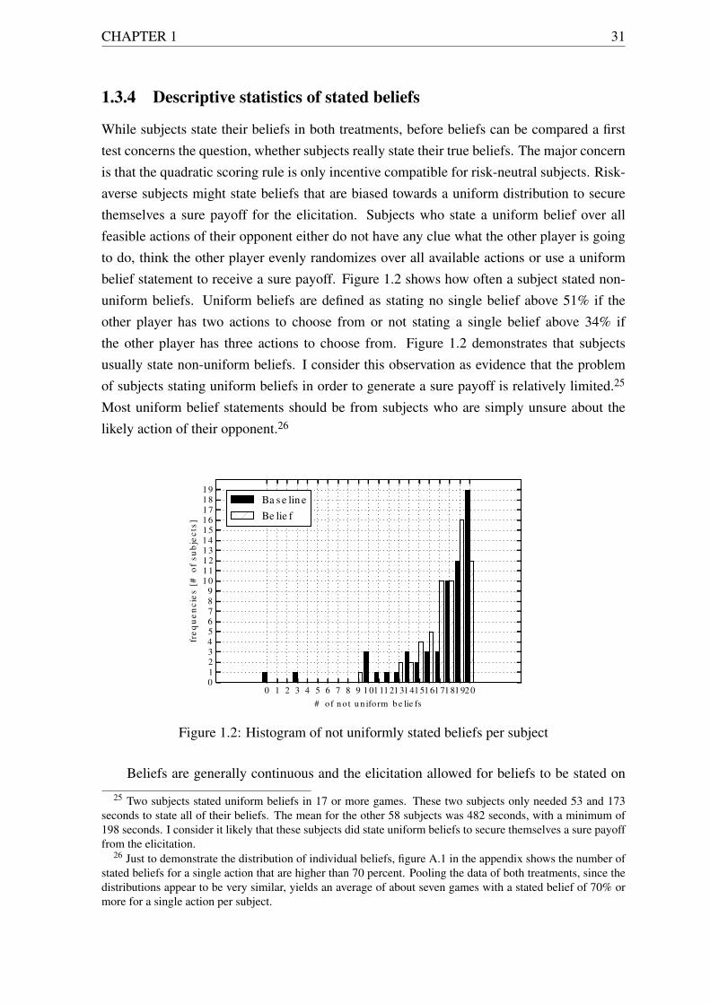
CHAPTER 1 31

1.3.4 Descriptive statistics of stated beliefs

While subjects state their beliefs in both treatments, before beliefs can be compared a firsttest concerns the question, whether subjects really state their true beliefs. The major concernis that the quadratic scoring rule is only incentive compatible for risk-neutral subjects. Risk-averse subjects might state beliefs that are biased towards a uniform distribution to securethemselves a sure payoff for the elicitation. Subjects who state a uniform belief over allfeasible actions of their opponent either do not have any clue what the other player is goingto do, think the other player evenly randomizes over all available actions or use a uniformbelief statement to receive a sure payoff. Figure 1.2 shows how often a subject stated non-uniform beliefs. Uniform beliefs are defined as stating no single belief above 51% if theother player has two actions to choose from or not stating a single belief above 34% ifthe other player has three actions to choose from. Figure 1.2 demonstrates that subjectsusually state non-uniform beliefs. I consider this observation as evidence that the problemof subjects stating uniform beliefs in order to generate a sure payoff is relatively limited.25

Most uniform belief statements should be from subjects who are simply unsure about thelikely action of their opponent.26

0 1 2 3 4 5 6 7 8 9 1 01 11 21 31 41 51 61 71 81 92 0

# of n o t u n iform b e lie fs

0123456789

1 01 11 21 31 41 51 61 71 81 9

fre

qu

en

cie

s [

# o

f s

ub

jec

ts]

Ba s e lin e

Be lie f

Figure 1.2: Histogram of not uniformly stated beliefs per subject

Beliefs are generally continuous and the elicitation allowed for beliefs to be stated on

25 Two subjects stated uniform beliefs in 17 or more games. These two subjects only needed 53 and 173seconds to state all of their beliefs. The mean for the other 58 subjects was 482 seconds, with a minimum of198 seconds. I consider it likely that these subjects did state uniform beliefs to secure themselves a sure payofffrom the elicitation.

26 Just to demonstrate the distribution of individual beliefs, figure A.1 in the appendix shows the number ofstated beliefs for a single action that are higher than 70 percent. Pooling the data of both treatments, since thedistributions appear to be very similar, yields an average of about seven games with a stated belief of 70% ormore for a single action per subject.

32 CHAPTER 1

a 0.1%-point gird. However, no subject stated a belief that is not on the 1%-grid and manystatements are on the 10% grid. To ease a systematic analysis of the stated beliefs I categorizeall belief statements. If a subject stated a belief for a game in which the opponent hasthree actions to choose from I classify his or her belief into one of four possible categories.Category one contains all beliefs statements with at least a weight of 50% on the first action.In the second category are all beliefs of 50% or more on the second action and similarlythe third category contains all beliefs with a weight of at least 50% on the third action. Ifan individual stated beliefs that do not place a weight of at least 50% on an action his orher beliefs are categorized in the fourth category. For games in which the opponent has twoactions the cutoff is changed to 70% and there are three instead of four categories.

I first test for each game whether stated beliefs are different from randomly chosen be-liefs by performing χ2 goodness of fit tests for both treatments separately. This test examineswhether the frequency of the belief categories differs from a uniform distribution over thefour (three) categories. These tests reject random beliefs for 19 games in both treatments.Only for game #2, in both treatments, the stated beliefs are indistinguishable from randomguesses. Comparing the categorized beliefs separately for each treatment, game and playerrole with a FEPT (5% significance level) yields only two rejections of equivalence in 40comparisons.27 These results let me confidently conclude that the stated beliefs are not theresult of random answers and that belief statements do not differ with respect to player roles.In the following analysis I therefore consider the stated beliefs as subjects’ true beliefs andpool the stated beliefs over player roles.

Subjects’ beliefs in the baseline treatment could be systematically different from thosestated in the belief treatment if some (very sophisticated) subjects expect other subjects toselect different actions if they are asked to state beliefs compared to the case when they arenot asked. In part two of the baseline treatment they should state own beliefs that are as closeas possible to the choice distribution in part one. Therefore these subjects might state beliefsthat do not resemble the pattern of action choices they would expect if the other subjectswould be asked to state actions and beliefs simultaneously, as in the belief treatment. WhileI consider this highly unlikely, a difference in the stated beliefs between the treatments couldindicate such a behavior.

A difference in the belief statements between treatments could also be the result of sub-jects in the baseline treatment using their belief statements as rationalizations for their ownbehavior in part one. Then these subjects would not really state what they expect the otherplayer to do, but rather state beliefs that make their previous action choice a best response.Since action choices are significantly different between treatments for some subgroups ofgames the beliefs in the baseline treatment should differ from the ones stated in the belieftreatment if subjects try to rationalize their previous choices.

27 For games 8 and 14 in the belief treatment the stated beliefs are not significantly different from randombeliefs.

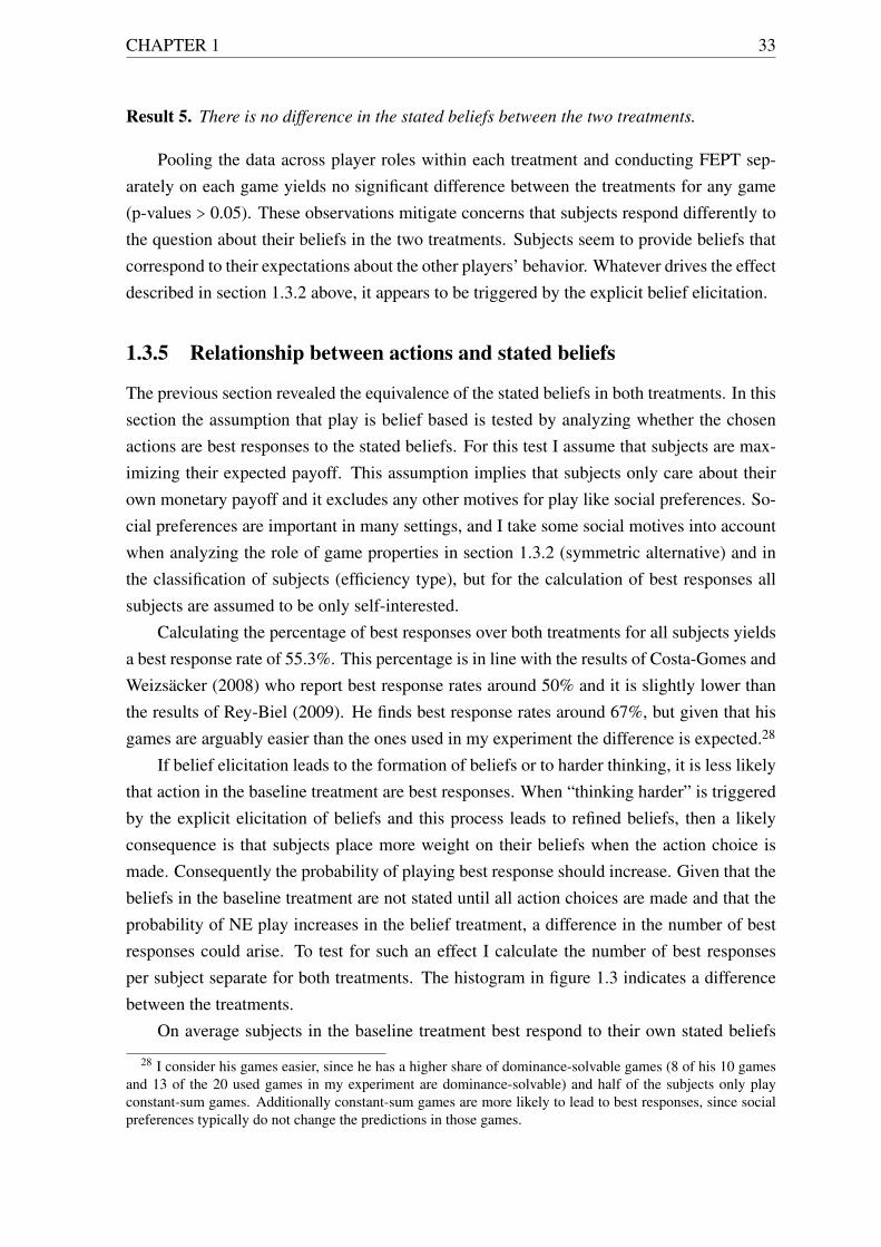
CHAPTER 1 33

Result 5. There is no difference in the stated beliefs between the two treatments.

Pooling the data across player roles within each treatment and conducting FEPT sep-arately on each game yields no significant difference between the treatments for any game(p-values > 0.05). These observations mitigate concerns that subjects respond differently tothe question about their beliefs in the two treatments. Subjects seem to provide beliefs thatcorrespond to their expectations about the other players’ behavior. Whatever drives the effectdescribed in section 1.3.2 above, it appears to be triggered by the explicit belief elicitation.

1.3.5 Relationship between actions and stated beliefs

The previous section revealed the equivalence of the stated beliefs in both treatments. In thissection the assumption that play is belief based is tested by analyzing whether the chosenactions are best responses to the stated beliefs. For this test I assume that subjects are max-imizing their expected payoff. This assumption implies that subjects only care about theirown monetary payoff and it excludes any other motives for play like social preferences. So-cial preferences are important in many settings, and I take some social motives into accountwhen analyzing the role of game properties in section 1.3.2 (symmetric alternative) and inthe classification of subjects (efficiency type), but for the calculation of best responses allsubjects are assumed to be only self-interested.

Calculating the percentage of best responses over both treatments for all subjects yieldsa best response rate of 55.3%. This percentage is in line with the results of Costa-Gomes andWeizsäcker (2008) who report best response rates around 50% and it is slightly lower thanthe results of Rey-Biel (2009). He finds best response rates around 67%, but given that hisgames are arguably easier than the ones used in my experiment the difference is expected.28

If belief elicitation leads to the formation of beliefs or to harder thinking, it is less likelythat action in the baseline treatment are best responses. When “thinking harder” is triggeredby the explicit elicitation of beliefs and this process leads to refined beliefs, then a likelyconsequence is that subjects place more weight on their beliefs when the action choice ismade. Consequently the probability of playing best response should increase. Given that thebeliefs in the baseline treatment are not stated until all action choices are made and that theprobability of NE play increases in the belief treatment, a difference in the number of bestresponses could arise. To test for such an effect I calculate the number of best responsesper subject separate for both treatments. The histogram in figure 1.3 indicates a differencebetween the treatments.

On average subjects in the baseline treatment best respond to their own stated beliefs

28 I consider his games easier, since he has a higher share of dominance-solvable games (8 of his 10 gamesand 13 of the 20 used games in my experiment are dominance-solvable) and half of the subjects only playconstant-sum games. Additionally constant-sum games are more likely to lead to best responses, since socialpreferences typically do not change the predictions in those games.

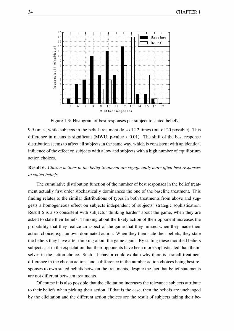
34 CHAPTER 1

5 6 7 8 9 1 0 1 1 1 2 1 3 1 4 1 5 1 6 1 7

# of b e s t re s p on s e s

0

1

2

3

4

5

6

7

8

9

1 0

1 1

1 2

1 3

1 4

1 5

fre

qu

en

cie

s [

# o

f s

ub

jec

ts]

Ba s e lin e

Be lie f

Figure 1.3: Histogram of best responses per subject to stated beliefs

9.9 times, while subjects in the belief treatment do so 12.2 times (out of 20 possible). Thisdifference in means is significant (MWU, p-value < 0.01). The shift of the best responsedistribution seems to affect all subjects in the same way, which is consistent with an identicalinfluence of the effect on subjects with a low and subjects with a high number of equilibriumaction choices.

Result 6. Chosen actions in the belief treatment are significantly more often best responses

to stated beliefs.

The cumulative distribution function of the number of best responses in the belief treat-ment actually first order stochastically dominances the one of the baseline treatment. Thisfinding relates to the similar distributions of types in both treatments from above and sug-gests a homogeneous effect on subjects independent of subjects’ strategic sophistication.Result 6 is also consistent with subjects “thinking harder” about the game, when they areasked to state their beliefs. Thinking about the likely action of their opponent increases theprobability that they realize an aspect of the game that they missed when they made theiraction choice, e.g. an own dominated action. When they then state their beliefs, they statethe beliefs they have after thinking about the game again. By stating these modified beliefssubjects act in the expectation that their opponents have been more sophisticated than them-selves in the action choice. Such a behavior could explain why there is a small treatmentdifference in the chosen actions and a difference in the number action choices being best re-sponses to own stated beliefs between the treatments, despite the fact that belief statementsare not different between treatments.

Of course it is also possible that the elicitation increases the relevance subjects attributeto their beliefs when picking their action. If that is the case, then the beliefs are unchangedby the elicitation and the different action choices are the result of subjects taking their be-

CHAPTER 1 35

liefs more into account when beliefs are elicited. Such an effect would be closer to anexperimenter demand effect by shifting the focus of subjects. Part of the differences in bestresponses between the treatments is also likely to be driven by the fact that subjects in thebaseline treatment are not reminded about their previous action choice in the game whenthey state beliefs. This procedure prevents unwanted ex-post rationalizations by subjects inthe baseline treatment, but for subjects who falsely remember choosing another action orsubjects who were unsure which action to choose the procedure likely results in fewer bestresponses compared to a simultaneous elicitation of actions and beliefs. While the proce-dure is likely to increase the difference in best responses, I believe that the clear differencebetween the treatments is unlikely to be caused by it.

1.4 Discussion and conclusion

The results of this paper show that belief elicitation can have a significant effect on the chosenactions of individuals. The overall effects are rather weak and concentrated on specificsubgroups of games. These findings are good news for experimentalists that elicit beliefs,but usually do not want that the elicitation affects subjects’ choices. But the data also showsthat asking for the beliefs of subjects together with their action choice increases equilibriumplay in dominance-solvable games and reduces it for games with a symmetric alternative.These results demonstrate that game properties play an important role for the presence andthe size of the effect. A possible channel for this finding is that subjects understand thedecision situation better when they state beliefs.

A better understanding of the game means that a subject becomes aware of an as-pect of the game that he or she did not realize without stating beliefs. Depending on thegame increased understanding results in choices closer to the game theoretic predictions,in dominance-solvable games, or in less equilibrium play if a symmetric alternative to theequilibrium exists. These results support the so-called “thinking-harder” hypothesis, whichclaims that belief elicitation raises awareness of subjects for the situation or has subjectsincrease their effort to understand the game. While the experiment is not able to definitelydistinguish between the “thinking-harder” hypothesis and the claim that belief elicitationleads to the formation of beliefs, some support for the hypothesis that the reported differencein actions for dominance-solvable games is not driven by subjects whose play is not beliefbased without the elicitation of beliefs comes from the analysis of the stated beliefs.

Analyzing the belief statements shows that beliefs are not different between treatments,but there is a clear difference in the number of best responses to own beliefs. The fact thatin the belief treatment subjects respond more frequently optimally to their stated beliefs isnot surprising and fits the story of “thinking harder”. Investing more effort in understandingthe game and especially the likely behavior of the opponent leads to more best responses.The setup of the experiment guides subjects to revise their beliefs in part two of the baseline

36 CHAPTER 1

treatment. Since they cannot change their action choices (made in part one), the chosenactions are less often best responses to the stated beliefs compared to the belief treatment.However, I believe that the difference in best responses found in this experiment is morelikely close to an upper bound of the effect. Since subjects in the baseline treatment arenot explicitly reminded of their previous action choice in the given game some part of thereduced number of best responses in the baseline treatment might be driven by subjects whosimply do not remember their action choice(s).

Without specifying a complete model of game complexity, it seems as if belief elicitationis likely to have an effect in games that are “easy”, meaning in games that are dominance-solvable and symmetric. The fact that the treatment effect can only be found in the subgroupof dominance-solvable and in the opposite direction for games with a symmetric alternative,hints that there is an effect of belief elicitation, but that it is too small to show up in morecomplicated games. The “harder thinking” subject therefore seems to be less of a “morestrategic” thinking subject, but rather a subject who spends more effort in understanding theactual game. “Thinking harder” takes place on a lower level than expected and thereforedoes not always lead subjects to behave “more like a game theorist”. This interpretation ofthe “thinking-harder” hypothesis is also supported by the finding that belief elicitation seemsto affect subjects with different levels of strategic sophistication equally.

Given the mixed results other researchers report on the effect of belief elicitation, the“complexity” of the games might be a logical explanation. Assuming the “thinking-harder”hypothesis is true, it is very likely that belief elicitation does not play a major role in very easygames (subjects understand the game anyhow) nor in very complicated games (in which theeffect is not strong enough). The fact that the treatment effect was significant for dominance-solvable games clearly points into this direction. In additional studies it would be interest-ing to test whether further game properties, besides dominance solvability and symmetricalternatives, also play a role and if the effect can be extended to other situations besidesnormal-form games. Also the question how to define game complexity and how it relates tothe effect of belief elicitation is worth being investigated further.

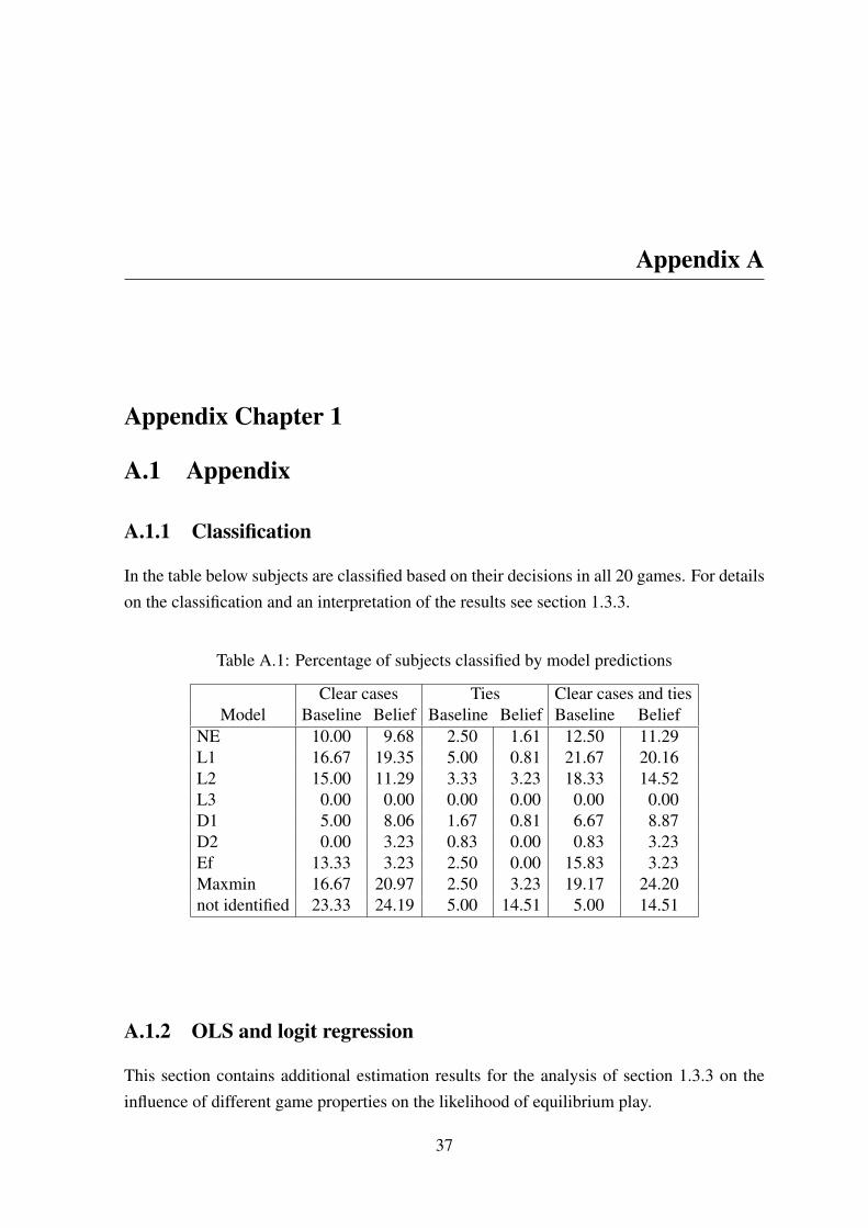
Appendix A

Appendix Chapter 1

A.1 Appendix

A.1.1 Classification

In the table below subjects are classified based on their decisions in all 20 games. For detailson the classification and an interpretation of the results see section 1.3.3.

Table A.1: Percentage of subjects classified by model predictions

Clear cases Ties Clear cases and tiesModel Baseline Belief Baseline Belief Baseline Belief

NE 10.00 9.68 2.50 1.61 12.50 11.29L1 16.67 19.35 5.00 0.81 21.67 20.16L2 15.00 11.29 3.33 3.23 18.33 14.52L3 0.00 0.00 0.00 0.00 0.00 0.00D1 5.00 8.06 1.67 0.81 6.67 8.87D2 0.00 3.23 0.83 0.00 0.83 3.23Ef 13.33 3.23 2.50 0.00 15.83 3.23Maxmin 16.67 20.97 2.50 3.23 19.17 24.20not identified 23.33 24.19 5.00 14.51 5.00 14.51

A.1.2 OLS and logit regression

This section contains additional estimation results for the analysis of section 1.3.3 on theinfluence of different game properties on the likelihood of equilibrium play.

37

38 APPENDIX A

Table A.2: OLS and logit estimation of NE

(1) (2)OLS Logit

dep. variable: NE Coeff. / Marg. Eff. (Std. Err.) Coeff. / Marg. Eff. (Std. Err.)

belief treatment 0.03 (0.05) 0.05 (0.06)

Game propertiesdominance solvable 0.42∗∗∗ (0.04) 0.44∗∗∗ (0.04)symmetric 0.41∗∗∗ (0.05) 0.36∗∗∗ (0.04)NE dominated −0.43∗∗∗ (0.04) −0.45∗∗∗ (0.04)symmetric alternative −0.07∗ (0.04) −0.08∗ (0.05)

Interaction effectsdominance solvable & belief treatment 0.09∗ (0.05) 0.16∗∗ (0.07)symmetric & belief treatment 0.05 (0.07) 0.10 (0.08)NE dominated & belief treatment −0.03 (0.05) −0.12 (0.08)symmetric alternative & belief treatment −0.11∗∗ (0.05) −0.16∗∗ (0.07)

Observations 2440 2440R2 0.176Pseudo R2 0.139Predicted probability 0.563 0.563Notes: Logit estimates: Marginal effects (evaluated at the mean of independent variables); * p < 0.10, ** p < 0.05, ***p < 0.01. All standard errors are clustered at the subject level.

0 1 2 3 4 5 6 7 8 9 1 01 11 21 31 41 51 61 71 81 92 0

# of s t a te d b e lie fs a b ove 7 0

0

1

2

3

4

5

6

7

8

fre

qu

en

cie

s [

# o

f s

ub

jec

ts]

Ba s e lin e

Be lie f

Figure A.1: Histogram of stated beliefs above 70%

APPENDIX A 39

A.1.3 Non-uniform beliefs

The histogram shows the number of individual belief statements above 70% per subject. Itillustrates that most subjects state beliefs that are far away from a uniform distribution.

A.1.4 Instructions

Below are the English translations of the original German instructions for the belief treatment(available upon request). The instructions for the baseline treatment are almost identical,but split in two parts (games and belief statements). The emphases are also in the originalinstructions. The first part (WELCOME) was given to the participants at the start, whilethe second part (Detailed instructions) was handed out right before the start of the actualexperiment.

WELCOME!

Thank you for participating in this experiment. The amount of money you earn depends onyour choices and the choices of the other participants. The entire experiment will last about90 minutes and you receive your payment directly after the experiment in cash.

It is very important that you remain silent and do not talk to other participants during the en-tire experiment. In case you have any questions regarding the procedures of the experiment,please raise your hand. An experimenter will come to you to clarify the question directlywith you. Thank you for your cooperation.

During the experiment you will be matched with other participants. The other participantwill always be called “person B”. In each round you will be matched with a new person.This means you will never be matched with the same person in two successive rounds. Nei-ther during nor after the experiment you will learn with whom who you were matched in around. You and person B will simultaneously see a decision situation. Your decision and thedecision of person B together yield the result. This result determines how many points youand person B receive and therefore your payoff.

We now provide you with a detailed description of the decision situation. If you have anyremaining questions after reading the instructions, please raise your hand. We will come toyour seat and answer any open questions.

Detailed instructions for the decision situation

In this experiment we show you multiple decision situations. An example for such a decisionsituation can be seen in the table below. Please take a good look at the table and read theinstructions below.

40 APPENDIX A

Person B: § Person B: # Person B: +You: & 40 40 10

10 40 10You: % 50 40 0

20 40 20You: = 20 20 40

30 50 10

In the actual decisions you will see a similar table on your computer screen (but with differentnumbers and possibly less cells). You are asked to make a decision, which means that youchoose between the given alternatives (here: &, % and =). Person B decides simultaneouslybetween their alternatives (here: §, # and +). You always choose between rows, while personB always chooses between columns of the table. The cell that results from these decisionsstates the points you and person B receive. Your potential payoffs are given in the bottomleft of a cell, while the potential payoffs for person B are given in the upper right of eachcell. Consider for example the following possibilities:

• You choose & and person B selects §, you receive 10 and person B receives 40 points.

• You choose % and person B selects §, you receive 20 and person B receives 50 points.

• You choose = and person B selects #, you receive 50 and person B receives 20 points.

You encounter multiple of those decision situations in the experiment. At the end of theexperiment three decisions are randomly chosen and you receive the sum of points, whichyou earned in the three selected decisions. All earned points for these three decisions add upto your point total. At the end of the experiment you receive 5 cents for each point. Thismeans 20 points are equivalent to 1e.

Furthermore we ask you about your expectation, which alternative person B will choose.This means for each table we ask you to think about the likely behavior of person B. You caninterpret the question as follows: If 100 persons would make this decision, how often wouldeach of the given alternatives be chosen?

Of course only one person will actually make the decision and not 100 different persons. Butyou can interpret the question about the behavior as how likely it is that a person B chooseseach of the possible alternatives (here: §, # and +).

For example, if you are certain that person B will select alternative § in a decision situationand never alternatives # or +, then you would answer the question by filling in the numbers100, 0 and 0 in the fields of the respective alternatives §, # and +.

If you instead believe that person B will not choose alternative § very often, but alternative #more often and action + most frequently, then you could fill in the numbers 20, 30 and 50 forthe respective alternatives. If you assume that all alternatives are equally likely to be chosen

APPENDIX A 41

you can enter the numbers 33, 34 and 33 for the respective fields.

Please note: The sum of all expectations has to sum up to 100.

Your payment depends on your chosen alternative, the chosen alternative of person Band which expectations you have stated about the behavior of person B.

At the end of the experiment three additional decision situations are randomly selected. Youreceive the sum of points you have earned for your expectations in these three situations. Allpoints you earn in these decision situations are added to your point total.

For each decision situation only the result OR your expectations are paid. This means youare paid for six decision situations. In three decisions you are paid the result and in threedifferent decisions for your expectations. You never receive points for both tasks for thesame decision.

How many points you receive four your expectations depends on how correct your expecta-tions are and therefore on the decision of person B. You receive more points if the differencebetween your expectations and the actual decision of person B is small. The table belowshows you for the examples given above which payoff you might receive.

The first table lists four examples for stated expectations about the behavior of person B.For example in row 1 the following expectations are listed: You believe that person B willchoose alternative § and not alternatives # or +.

Person B: § Person B: # Person B: +Example 1: 100 0 0Example 2: 20 30 50Example 3: 33 34 33Example 4: 80 20 0

The next table states the possible payments for your stated expectations dependent on whetherperson B chooses alternative §, # or +. The first column lists your payoff if person B choosesalternative §, the second column lists your payoff if person B chooses alternative # and thethird column lists you payoff if person B chooses alternative +.

Person B: § Person B: # Person B: +Payoff in example 1: 80 0 0Payoff in example 2: 41 49 65Payoff in example 3: 53 54 53Payoff in example 4: 77 29 13

If you state expectations as given in row 1 and person B chooses alternative §, than youreceive 80 points. If person B selects a different action, # or +, then you receive 0 points.

42 APPENDIX A

If you state expectations as given in row 3 and person B chooses alternative §, than youreceive 53 points. If person B chooses alternative # you receive 54 points and if person Bchooses alternative + you receive 53 points.

The table states for all four examples from above all possible payments depending on thedecision of person B. Each point is worth 5 cents, independently if you receive it for yourdecision or your expectation. You can receive at most 80 points and you receive at least 0points for an expectation. In the example this means when person B selects alternative § andyou are paid for your expectation you receive 80 points (= 4 Euro) in the first example, 41points (= 2.1 Euro) in the second and 53 points (= 2.7 Euros) in the third example. Yourexpected payment is maximized if you state your true expectations.

Please note: The numbers state above are only examples. These examples do NOT provideany suggestions for the decision situations.

Please make sure that you understood the table and that you know how you receive pointsfor your stated expectations. Raise your hand if you have any questions. If you think thatyou understood these instructions and you know how you are paid in the decision situations,please click with the mouse on the OK button. We will then ask you some understandingquestions to a different decision situation. After you have answered these questions correctlyyou can start with the experiment.

Chapter 2

Profitability of Tournaments with Worker Sorting: An Ex-periment1

2.1 Introduction

Offering a contract to potential employees serves two main purposes for employers. First,the incentive scheme included in the contract should attract the right workers. Second, oncea worker has agreed to a contract, the incentive scheme should align the interests of the em-ployer and the employee. In labor market relationships aligning the interests of employersand employees generally means incentivizing workers to produce a large output. Several pa-pers have documented the importance of worker sorting for the observed output differencesbetween payment schemes (Lazear 2000; Dohmen and Falk 2011; Leuven et al. 2011). How-ever, there exists little evidence on the effect of worker sorting on the profitability of paymentschemes for employers. Especially not much is known about the effect of worker sorting onprofits when workers can choose between multiple variable-payment schemes.

In this paper I analyze the profitability of a rank-order tournament for employers whenself-selection of workers in different payment schemes is possible in a laboratory experiment.The following questions are addressed: Can a rank-order tournament be more profitable thana piece rate? In particular I analyze the role of tournament prizes and the possibility ofworker sorting for the profit of employers. Furthermore, how does the sorting decision ofworkers depend on their personal characteristics, such as risk aversion, productivity, genderor self-assessment of their productivity?

The real-effort experiment contrasts two different environments. In the first part, the

1I appreciate the comments and the advice received from Dirk Engelmann, Henrik Orzen, Stefan Penczynskiand Gerhard Riener. I thank participants of the Verein für Socialpolitik meeting 2015 (Münster), the LondonExperimental Workshop 2015 (London), the European meeting of ESA 2014 (Prague), the IMEBESS meeting2015 (Toulouse) and GAMES 2016 (Maastricht), as well as seminar participants in Mannheim and Nurembergfor many helpful comments. A predecessor of this paper was circulated under the title "Performance Pay,Sorting and Employers’ Choice: Are Tournaments an Attractive Payment Scheme?". All remaining errors aremy own.

43

44 CHAPTER 2

no-competition stage, employers - called managers - do not compete for workers. They arerandomly assigned two workers and choose how these workers are paid by selecting oneof the three available payment schemes: fixed wage, piece rate or rank-order tournament.Workers cannot influence which payment scheme they receive. Consequently, in the no-competition stage only the incentive effect of a payment scheme and its costs are relevantfor its profitability. In the second part, the competition stage, three managers compete forsix workers. Managers and workers state their preference ordering over all three paymentschemes. The stated preferences of managers are used to assign each manager a paymentscheme with the restriction that each payment scheme has to be offered. This restriction en-sures that workers have the choice between all three payment schemes. Workers’ preferencesare then considered to sort two workers to a manager and therefore to a payment scheme.The matching procedure of workers to payment schemes gives priority to more productiveworkers to resemble advantages of these workers in the job search. As a result, the com-petition stage allows for workers’ self-selection and thereby introduces competition amongemployers for productive workers. In the competition stage the profitability of a paymentscheme depends on the incentives it provides to workers, its costs and on workers’ sortingbehavior.

The theoretical literature (Lazear and Rosen 1981; Green and Stokey 1983; Nalebuff andStiglitz 1983) as well as experimental studies (Bull et al. 1987; Bartling et al. 2009; Erikssonet al. 2009; Balafoutas et al. 2012) have demonstrated that rank-order tournaments provideincentives for workers to exert effort. Therefore tournaments should be a profitable paymentscheme for employers. However, in practice tournaments as payment schemes are uncom-mon. While they are used in the form of promotion tournaments and to award bonuses, theyare rarely used as main payment scheme for employees. A main feature of rank-order tourna-ments is the dependence of workers’ payments on their rank and not directly on their output.Therefore if prizes are independent of workers’ output, tournament costs do not relate toworkers’ performance. On the one hand this independence can increase employers’ profits,if the tournament results in large worker output while being relatively cheap. In such a casean employer might generate larger profits with a tournament than with output-based paymentschemes, like a piece rate. But on the other hand such a tournament might be unattractivefor (productive) workers, since the tournament will usually be cheap if prizes are low andtherefore provide low expected earnings for workers. Additionally tournaments create un-certainty for workers about their wage, since their payment is neither a priori given nor fullydetermined by their own output. This wage uncertainty could make even tournaments withrelatively large expected wages unattractive for risk-averse workers. Consequently whenworker sorting is feasible it is unclear how profitable such a tournament is for the employer.My experiment addresses this issue. The comparison of the profitability of the tournamentsin the no competition and the competition stage allows me to explicitly analyze the role ofworker sorting.

CHAPTER 2 45

Productivity differences have been shown to be important for worker sorting and there-fore for performance differences between payment schemes. Lazear (2000) documents inhis field experiment that the self-selection into a piece rate accounts for a large share of theobserved performance increase compared to a fixed wage payment. Leuven et al. (2011)demonstrate in a field setting with different tournaments that an observed increase in perfor-mance, attributed to an incentive effect of larger tournament prizes, can mainly be explainedby the sorting of subjects. To be able to account for workers’ individual productivity inthe sorting decision in the experiment first subjects’ productivity in the real-effort task ismeasured. Dohmen and Falk (2011) show that for the sorting between a fixed wage and avariable wage alternative (either a piece rate, a tournament or a rent-sharing contract) notonly workers’ productivity matters. Variable-payment schemes additionally attract individ-uals with certain characteristics, such as higher willingness to take risks. Therefore in myexperiment also workers’ relative ranking beliefs and their risk preferences are elicited and Icollect additional individual characteristics that might be relevant for the sorting behavior.

While many studies show the relevance of worker sorting for output differences work-ers usually do not choose between variable-payment schemes, but either between a fixedwage and a variable-payment scheme (Lazear 2000; Dohmen and Falk 2011) or betweendifferent tournaments (Leuven et al. 2011). Therefore my study differs from these as wellas most other papers on worker sorting, since I explore the sorting behavior of subjects be-tween multiple variable-payment schemes. Bartling et al. (2009), Eriksson et al. (2009), andBalafoutas et al. (2012) are concerned with the endogenous choice of subjects between atournament and a piece rate. They demonstrate that productivity sorting is the main driverfor subjects’ decisions. But these studies do not address the effect of the sorting for the prof-itability of the different payment schemes. Also in these and in most other papers regardingworker sorting, all subjects are workers and their payment scheme choices are independentof other subjects’ choices. Therefore there does not exist a competition for (productive)workers. In my experiment the number of workers in each payment scheme is limited. Thisdesign creates competition among employers for the most productive workers and allows tostudy the effect of worker sorting on the profitability of payment schemes in a competitiveenvironment.

Furthermore, the absence of employers who benefit from the performance of workersmight limit the effect of social preferences, especially in fixed-wage contracts. In particularin small firms with only a few employees social preferences might be an important factorfor the performance of workers and consequently for the profitability of different paymentschemes. That social preference affect the optimal incentive contract is shown by a large(experimental) literature that analyzes the effects of different fixed-wage offers on work-ers’ performance. Fehr et al. (1993) were the first to demonstrate experimentally that largewage “gifts” of employers, in the form of unconditional offers, are indeed on average re-

46 CHAPTER 2

warded with higher effort choices by workers.2 Therefore it pays for employers in these“gift-exchange” experiments to offer above minimum wages.3 In my study social prefer-ences might affect the profitability of the payment schemes also in an additional way. In thegift-exchange game employers do not select a contract type, instead they choose the fixedwage. Therefore employers control a parameter of the contract, the wage, but do not selectthe contract itself.4 Having managers choose the payment schemes instead of exogenouslyassigning them in the no-competition stage allows for social preferences of workers to affecttheir performance. It is possible that the employers’ choice of a specific payment schemehas an effect on the effort provision of workers, similar to the role of reciprocity in setting aprofit-maximizing fixed wage. In the competition stage however, the employer might have tooffer a payment scheme that is not her most favored payment scheme. By comparing work-ers’ performance in the same payment scheme between these stages I can check whether thisdifference matters for their performance or not.

The results obtained illustrate the importance of worker sorting for the profitability ofpayment schemes. The tournament payment scheme provides incentives to workers. Theirperformances in both tournaments and the piece rate are high and do not significantly differbetween these variable-payment schemes. Therefore in the no-competition stage - with-out worker sorting - a low-prize tournament results in larger manager profits than a piecerate due to the low tournament costs for employers. But a high-prize tournament yields thesame manager profits as the piece rate. However, for productive workers a tournament isonly an attractive payment scheme with sufficiently large prizes. As a consequence, in thecompetition stage the cost advantage of the low-prize tournament cannot outweigh that forproductive workers this tournament is not attractive. Due to workers’ self-sorting behaviorthe low-prize tournament does not yield larger manager profits than the piece rate. Whilethe high-prize tournament is attractive for productive workers, the potential advantage fromworker sorting is off-set by the high costs and as a result also a high-prize tournament doesnot result in larger manager profits than a piece rate in the competition stage. These find-ings illustrate that with worker sorting rank-order tournaments are hardly simultaneouslyattractive for workers and employers.

The paper is organized as follows. The next section describes the experiment, treat-ments and outlines the hypotheses. Section 2.3 presents the results. I first discuss managers’payment-scheme choices, then workers’ performances and then compare the resulting prof-

2 The idea was described theoretically before by Akerlof (1982) and Akerlof and Yellen (1990).3 This finding has been replicated in many different environments in the lab and in the field. As a starting

point see Fehr et al. (1997, 1998), Fehr and Falk (1999), and Gneezy and List (2006).4 Similarly in the modified gift-exchange game of Falk and Kosfeld (2006) employers can restrict the

minimum effort level of workers from below. In their setting employers clearly choose what to offer, but thechoice is between different parameterizations of the same contract type. In Anderhub et al. (2002), a test ofthe principal agent model, subjects choose between different parameterizations of the same contract type, butnot between different contracts. Lindner et al. (2013) experimentally investigate employers’ and employees’choices between two equivalent tournaments. However, there is no choice between different payment schemes.

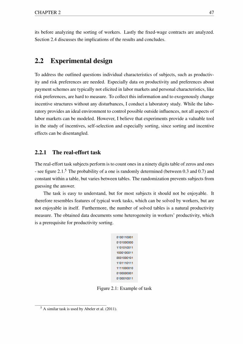
CHAPTER 2 47

its before analyzing the sorting of workers. Lastly the fixed-wage contracts are analyzed.Section 2.4 discusses the implications of the results and concludes.

2.2 Experimental design

To address the outlined questions individual characteristics of subjects, such as productiv-ity and risk preferences are needed. Especially data on productivity and preferences aboutpayment schemes are typically not elicited in labor markets and personal characteristics, likerisk preferences, are hard to measure. To collect this information and to exogenously changeincentive structures without any disturbances, I conduct a laboratory study. While the labo-ratory provides an ideal environment to control possible outside influences, not all aspects oflabor markets can be modeled. However, I believe that experiments provide a valuable toolin the study of incentives, self-selection and especially sorting, since sorting and incentiveeffects can be disentangled.

2.2.1 The real-effort task

The real-effort task subjects perform is to count ones in a ninety digits table of zeros and ones- see figure 2.1.5 The probability of a one is randomly determined (between 0.3 and 0.7) andconstant within a table, but varies between tables. The randomization prevents subjects fromguessing the answer.

The task is easy to understand, but for most subjects it should not be enjoyable. Ittherefore resembles features of typical work tasks, which can be solved by workers, but arenot enjoyable in itself. Furthermore, the number of solved tables is a natural productivitymeasure. The obtained data documents some heterogeneity in workers’ productivity, whichis a prerequisite for productivity sorting.

Figure 2.1: Example of task

5 A similar task is used by Abeler et al. (2011).

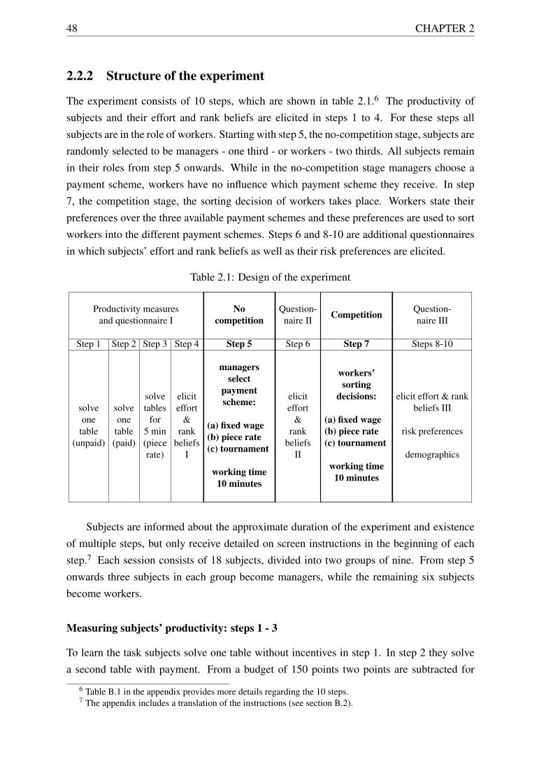
48 CHAPTER 2

2.2.2 Structure of the experiment

The experiment consists of 10 steps, which are shown in table 2.1.6 The productivity ofsubjects and their effort and rank beliefs are elicited in steps 1 to 4. For these steps allsubjects are in the role of workers. Starting with step 5, the no-competition stage, subjects arerandomly selected to be managers - one third - or workers - two thirds. All subjects remainin their roles from step 5 onwards. While in the no-competition stage managers choose apayment scheme, workers have no influence which payment scheme they receive. In step7, the competition stage, the sorting decision of workers takes place. Workers state theirpreferences over the three available payment schemes and these preferences are used to sortworkers into the different payment schemes. Steps 6 and 8-10 are additional questionnairesin which subjects’ effort and rank beliefs as well as their risk preferences are elicited.

Table 2.1: Design of the experiment

Productivity measuresand questionnaire I

Nocompetition

Question-naire II Competition Question-

naire III

Step 1 Step 2 Step 3 Step 4 Step 5 Step 6 Step 7 Steps 8-10

solveonetable

(unpaid)

solveonetable(paid)

solvetables

for5 min(piecerate)

eliciteffort

&rank

beliefsI

managersselect

paymentscheme:

(a) fixed wage(b) piece rate(c) tournament

working time10 minutes

eliciteffort

&rank

beliefsII

workers’sorting

decisions:

(a) fixed wage(b) piece rate(c) tournament

working time10 minutes

elicit effort & rankbeliefs III

risk preferences

demographics

Subjects are informed about the approximate duration of the experiment and existenceof multiple steps, but only receive detailed on screen instructions in the beginning of eachstep.7 Each session consists of 18 subjects, divided into two groups of nine. From step 5onwards three subjects in each group become managers, while the remaining six subjectsbecome workers.

Measuring subjects’ productivity: steps 1 - 3

To learn the task subjects solve one table without incentives in step 1. In step 2 they solvea second table with payment. From a budget of 150 points two points are subtracted for

6 Table B.1 in the appendix provides more details regarding the 10 steps.7 The appendix includes a translation of the instructions (see section B.2).

CHAPTER 2 49

each second until the correct answer is given. For a wrong answer 20 points are subtractedand subjects can enter a new answer, but they cannot make losses. In step 2 all tables havea probability of 40% for a one in each digit. The time needed to solve the first and secondtable are productivity indicators I and II respectively. The main measure of productivity usedin the following analysis comes from step 3. Subjects are asked to solve as many tables aspossible within 5 minutes and are paid with a piece rate (8 points per correct answer and apenalty of 5 points for wrong answers). Productivity indicator III is the number of correctlysolved tables.

Questionnaires and belief elicitation: steps 4, 6 and 8-10

I elicit subjects’ beliefs and their subjective impressions about their stress level at severalpoints during the experiment. Once after the productivity measurements - step 4 - and againafter the no competition - step 6 - and the competition stage - step 8. To elicit their beliefsabout their relative performance I ask subjects “How many of the other workers solved fewertables then you?” (in a group of nine/six) and I ask managers “How many tables did yourworkers solve in this stage?”. Workers’ beliefs are rewarded if they predict their rank cor-rectly, +/- 1. Managers receive a payment if they correctly estimate the number of solvedtables, +/- 3 tables.

In steps 4, 6 and 8 I collect data on subjects’ impressions “How hard did you workin the just completed stage?”, “How difficult was the task?” and “How stressed did youfeel?” on seven point Likert scales (No stress at all - Very stressful). In step 9 I measuresubjects’ risk preferences using a Holt and Laury (2002) lottery choice. In step 10 subjectsstate how fair they perceive the different payment schemes and fill in some demographic andemployment information. All questionnaires are conducted before subjects receive feedbackon their payments for the respective step. Payments for the belief elicitation are revealed atthe end of the experiment.

No competition and competition stage: steps 5 and 7

In the no-competition stage (step 5) managers select their preferred payment scheme andthereby determine how the two workers in their firm are paid. While managers choose oneof the three available payment schemes, workers are aware of the different payment schemes,but cannot influence to which manager and therefore payment scheme they are assigned. Thethree possible payment schemes are a tournament, a piece rate and a fixed wage.

In the tournament subject i competes with the other worker in the firm. Whoever solvesmore tables wins the tournament and receives prize T w, while the other worker receives thelower prize T l . Both workers receive a payoff to limit the downside risk for workers, afeature which is realistically present in labor markets. Prizes are independent of output andthe only determinant for the tournament winner is the comparison between the two workers.

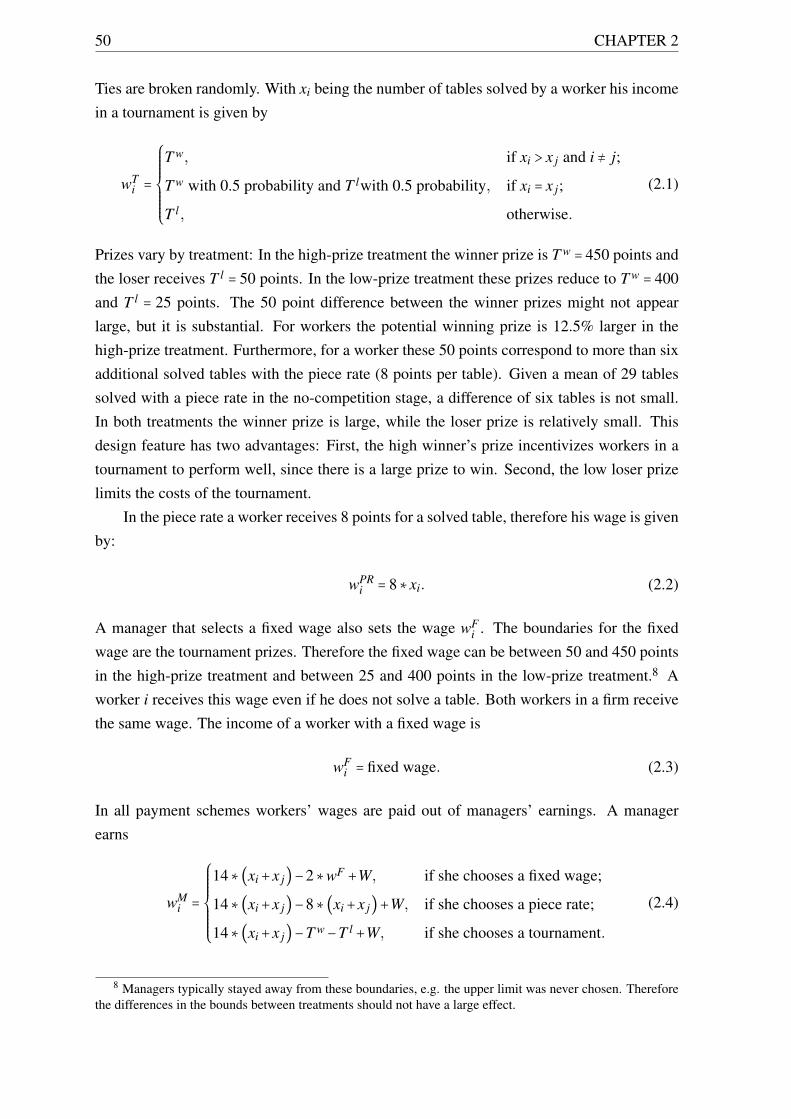
50 CHAPTER 2

Ties are broken randomly. With xi being the number of tables solved by a worker his incomein a tournament is given by

wTi =

⎧⎪⎪⎪⎪⎪⎪⎨⎪⎪⎪⎪⎪⎪⎩

T w, if xi > x j and i ≠ j;

T w with 0.5 probability and T lwith 0.5 probability, if xi = x j;

T l, otherwise.

(2.1)

Prizes vary by treatment: In the high-prize treatment the winner prize is T w= 450 points and

the loser receives T l= 50 points. In the low-prize treatment these prizes reduce to T w

= 400and T l

= 25 points. The 50 point difference between the winner prizes might not appearlarge, but it is substantial. For workers the potential winning prize is 12.5% larger in thehigh-prize treatment. Furthermore, for a worker these 50 points correspond to more than sixadditional solved tables with the piece rate (8 points per table). Given a mean of 29 tablessolved with a piece rate in the no-competition stage, a difference of six tables is not small.In both treatments the winner prize is large, while the loser prize is relatively small. Thisdesign feature has two advantages: First, the high winner’s prize incentivizes workers in atournament to perform well, since there is a large prize to win. Second, the low loser prizelimits the costs of the tournament.

In the piece rate a worker receives 8 points for a solved table, therefore his wage is givenby:

wPRi = 8∗xi. (2.2)

A manager that selects a fixed wage also sets the wage wFi . The boundaries for the fixed

wage are the tournament prizes. Therefore the fixed wage can be between 50 and 450 pointsin the high-prize treatment and between 25 and 400 points in the low-prize treatment.8 Aworker i receives this wage even if he does not solve a table. Both workers in a firm receivethe same wage. The income of a worker with a fixed wage is

wFi = fixed wage. (2.3)

In all payment schemes workers’ wages are paid out of managers’ earnings. A managerearns

wMi =

⎧⎪⎪⎪⎪⎪⎪⎨⎪⎪⎪⎪⎪⎪⎩

14∗(xi+x j)−2∗wF+W, if she chooses a fixed wage;

14∗(xi+x j)−8∗(xi+x j)+W, if she chooses a piece rate;

14∗(xi+x j)−T w−T l

+W, if she chooses a tournament.

(2.4)

8 Managers typically stayed away from these boundaries, e.g. the upper limit was never chosen. Thereforethe differences in the bounds between treatments should not have a large effect.

CHAPTER 2 51

Each table her workers complete yields a manager 14 points, independently of the paymentscheme. Managers can also solve tables to earn additional money, but their income mainlydepends on their workers’ performance.9 A manager receives W depending on her ownperformance xM:

W =

⎧⎪⎪⎪⎪⎪⎪⎪⎪⎪⎪⎨⎪⎪⎪⎪⎪⎪⎪⎪⎪⎪⎩

0, if xM < 10;

50, if 20 > xM ≥ 10;

100, if 40 > xM ≥ 20;

150, if xM ≥ 40.

(2.5)

To ensure that participants do not work on the task out of boredom, they could answer triviaquestions instead. Subjects could go back and forth between the task and the quiz. Allparticipants are first informed about the payment schemes and the quiz. Then a randomdraw determines their role - worker or manager. Finally managers choose a payment schemeand in case of a fixed payment select the fixed wage.10 Workers are informed about theirpayment scheme and then the 10 minute working time starts.

This no-competition stage yields managers’ preferences for payments schemes withoutworker self-selection. But this stage does not deliver any information about workers’ prefer-ences. These preferences are elicited in the competition stage (step 7). In this stage workersorting is feasible. At the beginning of the stage three managers and six workers are groupedtogether - subjects keep their respective roles. Managers first enter the fixed wage they wouldpay in case of a fixed-wage contract and then state their preference ordering of the three pay-ment schemes. This procedure ensures that each manager could rank the payment schemesusing the fixed wage she would like to pay. All subjects are informed that in a group eachpayment scheme has to be offered by exactly one manager.

The payment scheme a manager offers is determined with the following procedure:First, managers’ first choices are considered. If a payment scheme is ranked first by onlyone manager, she receives this payment scheme. If two or more managers rank the samepayment scheme first the tie is broken randomly. Next, the second choices of managerswho did not receive their first choice are considered. Again any ties are broken randomly,such that if multiple managers made identical first and second choices one receives her thirdchoice. This procedure ensures that managers had an incentive to state their preferred order-ing over all three contracts.

While the procedure incentivizes managers to rank their preferred payment schemeshigher, it can be optimal not to rank the most preferred payment scheme first. If a manager

9 The option for managers to solve tables makes it harder for subjects in the lab to identify managers. Italso provides some insurance against losses for managers.

10 Managers are not allowed to choose the level of the piece rate or tournament prizes, to ensure a bettercomparability between groups and sessions as well as between treatments. Not being able to select the piecerate should make the piece rate less attractive for managers.

52 CHAPTER 2

believes a particular payment scheme, e.g. the piece rate, to be popular among all managersand if she wants to avoid another payment scheme, assume the fixed wage, then it could beoptimal to rank the tournament first and the piece rate second, to avoid the fixed wage.

However stating such a ranking is only preferred to revealing the true preferences underseveral conditions: First, a manager needs a smaller “preference difference” between her firstand second option than between her second and third option. Second, she needs to believethat the other managers have the same preference order and third she must believe that othermanagers would not act strategically. Only if all three conditions are fulfilled ranking thesecond most preferred payment scheme first makes sense. Therefore in the results sectionthe first choices of managers are used assuming that the revealed preferences represent truepreferences.11

After managers are allocated to the contracts, the six workers in the group see the pay-ment schemes (including the offered fixed wage) and state their preferences over these con-tracts. Their stated preferences are used to match exactly two workers to each manager (andtherefore payment scheme). Workers are ranked within their group based on their perfor-mance in step 3 from 1st to 6th. Choices of better ranked subjects are fulfilled first, such thatall workers with a rank of three or worse only get their first choice if less than two higherranked workers select this payment scheme. Due to this procedure more productive subjectsare more likely to receive their preferred payment scheme, which reflects the advantages ofmore productive workers in the job search. The mechanism therefore allows for productivitysorting of workers. The procedure is common knowledge and is equivalent to workers choos-ing their preferred payment scheme in the order of their ranking, just that choices are elicitedusing a strategy method. Subjects state a belief about their ranking in step 4 and thereforeprobably thought about their relative ranking. However, they did not receive feedback abouttheir true ranking.12

2.2.3 Treatments and procedures

The two main treatments only differ in the tournament prizes. In the low-prize treatmentthe tournament winner receives 400 points and the loser earns 25 points. Essential thisis a tournament with a prize of 375 points and a sure payoff of 25 points. In the high-prize treatment the prizes are 450 and 50 points respectively. Each subject faces the sametournament in the no competition and the competition stage. For a manager the cost of a

11 In case preferences were not stated truthfully, I consider assumption three (not all managers are believedto behave strategically) to be the likeliest not to be fulfilled. If the first two conditions are fulfilled the likeliestbias is that the preferred payment scheme is stated as second choice with positive probability. Given the actualchoices such a bias should result in the piece rate being ranked second, even if it is the most preferred paymentscheme.

12 Workers in a tournament receive some information about the other worker within the same firm by learningwhether they won the tournament or not in the no-competition stage. Managers only know the total number oftables their workers solved.

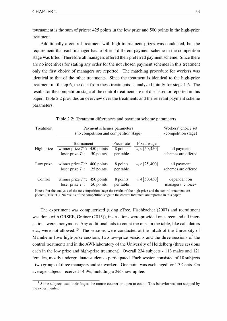
CHAPTER 2 53

tournament is the sum of prizes: 425 points in the low prize and 500 points in the high-prizetreatment.

Additionally a control treatment with high tournament prizes was conducted, but therequirement that each manager has to offer a different payment scheme in the competitionstage was lifted. Therefore all managers offered their preferred payment scheme. Since thereare no incentives for stating any order for the not chosen payment schemes in this treatmentonly the first choice of managers are reported. The matching procedure for workers wasidentical to that of the other treatments. Since the treatment is identical to the high-prizetreatment until step 6, the data from these treatments is analyzed jointly for steps 1-6. Theresults for the competition stage of the control treatment are not discussed or reported in thispaper. Table 2.2 provides an overview over the treatments and the relevant payment schemeparameters.

Table 2.2: Treatment differences and payment scheme parameters

Treatment Payment schemes parameters Workers’ choice set(no competition and competition stage) (competition stage)

Tournament Piece rate Fixed wageHigh prize winner prize T w: 450 points 8 points wi ∈ [50,450] all payment

loser prize T l: 50 points per table schemes are offered

Low prize winner prize T w: 400 points 8 points wi ∈ [25,400] all paymentloser prize T l: 25 points per table schemes are offered

Control winner prize T w: 450 points 8 points wi ∈ [50,450] dependent onloser prize T l: 50 points per table managers’ choices

Notes: For the analysis of the no-competition stage the results of the high prize and the control treatment arepooled (“HIGH”). No results of the competition stage in the control treatment are reported in this paper.

The experiment was computerized (using zTree, Fischbacher (2007) and recruitmentwas done with ORSEE, Greiner (2015)), instructions were provided on screen and all inter-actions were anonymous. Any additional aids to count the ones in the table, like calculatorsetc., were not allowed.13 The sessions were conducted at the mLab of the University ofMannheim (two high-prize sessions, two low-prize sessions and the three sessions of thecontrol treatment) and in the AWI-laboratory of the University of Heidelberg (three sessionseach in the low prize and high-prize treatment). Overall 234 subjects - 113 males and 121females, mostly undergraduate students - participated. Each session consisted of 18 subjects- two groups of three managers and six workers. One point was exchanged for 1.3 Cents. Onaverage subjects received 14.9e, including a 2e show-up fee.

13 Some subjects used their finger, the mouse courser or a pen to count. This behavior was not stopped bythe experimenter.

54 CHAPTER 2

2.2.4 Hypotheses

In order to derive some hypotheses for the behavior of subjects in the no competition andthe competition stage a rough model is outlined below. Let xi be the output of a workeri, meaning the number of tables he solves during a working stage. The output is given bythe production function xi = g(θi,ei)+ εi of the worker, where εi is an error term which isassumed to have a zero mean. This term captures aspects like “luck”, e.g. getting an “easy”task, mood effects, etc. Workers are heterogeneous in their ability θi, which is assumedto be continuously distributed on some interval [θ, θ̄]. ei is the effort exerted by the worker.Furthermore, gθ(θ,e) > 0, ge(θ,e) > 0 and geθ(θ,e) ≥ 0, which means higher ability and moreeffort yield a larger output and the marginal product of effort increases with ability. Assumethe worker has a utility function that is separable in the wage wi he receives and the effortcosts c(ei): u(wi,ei) = wi − c(ei). His utility depends positively on the wage (uw > 0) andnegatively on effort (ue < 0), because exerting effort is painful for the worker (ce > 0).

How many tables xi a worker solves therefore depends on the payment scheme, his abil-ity (θi) and his exerted effort (ei). With a fixed wage ∂wF

∂e = 0 and since ce > 0, the expectedutility of a worker is maximized with the lowest possible effort level e. Independently ofthe paid wage wF

i and their ability, all workers with a fixed wage will provide no effort andtherefore not solve a table xF

i = 0.14

A worker who is paid with a piece rate receives 8 points per table. As long as themarginal benefits from providing some effort outweigh his effort costs (8ge(θi,e) >

∂c(e)∂e ) a

worker will provide some effort, which means he will solve at least one table. The optimaleffort level e∗PR for an individual worker is given by 8ge(θi,e) =

∂c(e)∂e . Given geθ ≥ 0 it is

ensured that workers with higher ability exert more effort. Without specifying g(θ,e), c(e)

and a distribution of ability F(θ) no exact predictions regarding the effort levels can bederived. However, for all θ, it follows that xPR

i ≥ xFi = 0.

In a tournament the optimal effort of a risk-neutral worker also depends on his beliefof the expected productivity of the other worker. As a result the optimal effort is a functionof his productivity, the effort costs, the tournament prize and the probability of winning thetournament (which depends on the expected productivity of the other worker in the tour-nament).15 Assuming that higher effort provisions increase the probability of winning the

tournament, with∂E(wT )

∂e > 0 it follows that xTi > 0 if

∂E(wT )∂e >

∂c(e)∂e . Again, for all feasible θ

it follows that xTi ≥ xF

i = 0.Workers have no influence on their payment scheme in the no-competition stage, since

they are randomly assigned to managers, who select the payment scheme. Given that a

14 While there is no reason to provide effort with a fixed wage (according to standard theory), the results inthe gift-exchange literature show that workers might positively respond to higher fixed wages. I analyze theeffects of different fixed wages on workers’ performance in section 2.3.7.

15 While the optimal effort will most likely be a mixed strategy over some range of feasible efforts, sinceincreasing his own effort (ei) increases his output (xi) and given the tie breaking rule zero effort provision isusually not an equilibrium.

CHAPTER 2 55

worker maximizes his expected utility in a fixed-wage contract by not solving a single tablefor any feasible fixed wage, the manager makes negative profits with any positive wage.With a piece rate and a tournament at least workers with a sufficiently high θ should solvesome tables. Since with a piece rate a manager makes a profit if at least one table is solved, amanager’s expected profit from this contract should be positive. A manager should not offera fixed-wage contract in the no-competition stage, because she can offer a piece rate, whichyields a positive expected profit, instead. The same arguments are true for the competitionstage. Therefore in the competition stage no manager should rank the fixed wage first.

Hypothesis 1. No manager offers / wants to offer a fixed-wage contract in any stage. If a

worker receives a fixed-wage contract he provides no effort.

Workers are assumed to provide no effort with a fixed wage, but potentially providesome effort with the piece rate. Since managers make positive profits with a piece-ratecontract if at least one table is solved, fixed-wage contracts should result in lower profitsthan a piece rate.

Hypothesis 2. Manager profits with a fixed wage are smaller than with a piece rate.

Whether a manager earns more with a tournament than with a fixed wage or the piecerate depends on the output of her workers. Assuming that managers rule out the fixed wage inthe no-competition stage, since it does not result in positive profits, the question is whether atournament or a piece rate yields a larger profit. Both contracts provide incentives for work-ers to exert effort, since with both payment schemes the expected payoff for a worker is largerwith more solved tables. Whether a tournament is profitable for a manager also depends onthe tournament costs, which differ between treatments. For the high-prize tournament work-ers need to solve 36 tables to ensure the manager a positive profit (tournament costs: 500points, profit for each table: 14 points). In the low-prize treatment workers need to solve 31tables for a zero profit of the manager. Similarly, workers have to solve more than 62 tablesin the high-prize and more than 53 tables in the low-prize treatment for a manager to earn alarger profit with the tournament than with the piece rate. Using the performance of workersin the no-competition stage, I can analyze whether the cost difference in the tournamentsaffects the relative profitability of the tournament with respect to the piece rate.

In the competition stage workers rank all three payment schemes. Which paymentscheme yields a worker a higher expected utility depends on his ability, the offered fixedwage and his belief about the productivity of the other worker in the tournament. A workerprefers the piece rate over the fixed-wage contract if his output exceeds the following thresh-old: x̂ = 1

8 (wF−c(e)+c(e∗PR)). With common effort cost c(e) workers with a higher ability

θ need to provide less effort to reach this threshold. For a given wage all workers with asufficiently high ability prefer the piece rate over the fixed wage. The threshold x̂ increaseswith wF .

56 CHAPTER 2

Whether a worker prefers a tournament over the piece rate additionally depends on hisbelief about the productivity of the other worker (θ j) in the tournament. A worker’s expectedutility from the tournament is (T w

−T l) Pr{gi(θi,e∗T )+εi > g j(θ j,e∗T )+ε j} +T l

−c(e∗T ).16

This expected utility needs to exceed the utility from the piece rate 8(g(θi,e∗PR)+εi)−

c(e∗PR) for a worker to choose the tournament over the piece rate. While in this framework thedecision between a piece rate and the fixed-wage contract boils down to productivity sorting,the choice between the tournament and the piece rate is likely to depend on the productivityof a worker (especially if the random component ε of the output has variance close to zero),but a worker’s productivity is not the only determinant for the decision. However, it ispossible that the probability of winning the tournament is increasing in the own ability θi.In this case there might exists a productivity threshold which determines whether a workerprefers the piece rate or the tournament. But since the expected utility of the tournamentalso depends on a worker’s belief about the productivity of the other worker it is not clearwhether such a productivity threshold exists.17

In the competition stage workers rank all three contracts. Because the fixed wage isonly preferred over the piece rate by workers with a low productivity, workers’ averageproductivity in the fixed wage should be lower than in the piece rate.

Hypothesis 3. In the competition stage, the average productivity of workers preferring a

fixed-wage contract is lower than the productivity of those workers who rank the piece rate

first.

With the outlined assumptions no prediction regarding workers’ choice between thetournament and the fixed wage or the piece rate can be made. Whether the tournament ischosen by productive workers or not is therefore an open question that can be answered em-pirically by analyzing workers’ payment scheme choices in the competition stage. I addressthis question as well as the role of the tournament prizes, workers’ risk preferences and otherindividual characteristics for the choice between the payment schemes in the results section.

Managers also rank the payment schemes in the competition stage. Which paymentscheme is preferred by a manager mainly depends on her belief about the expected outputproduced by the workers under the different payment schemes. Since in the competitionstage productivity sorting of workers into the piece rate is possible and expected, I considerit likely that most managers will prefer the piece rate over the fixed wage. Whether managersprefer a tournament over the piece rate or the fixed wage and how the tournament prizes and

16 gi(⋅) and g j(⋅) denote the output of workers i and j, given the individual ability and optimal effort choices.17 A worker chooses the tournament over the fixed wage if his expected utility of entering the tournament

exceeds the utility from choosing the fixed wage wF− c(e). As for the comparison with the piece rate a

worker’s ability θi is likely a main determinant in this decision. However, since for the expected utility fromthe tournament also the expected probability of winning the tournament matters, the decision between the fixedwage and the tournament also depends on the belief of a worker about the productivity of the other worker inthe tournament. Therefore there does not necessarily exist a productivity cut-off for the decision between thefixed wage and the tournament.

CHAPTER 2 57

therefore the two treatments affect this decision is an open question I will consider in theresults section.

Furthermore, this experiment addresses the question whether a tournament is more prof-itable in the absence of worker sorting. In the no-competition stage workers cannot avoid thepayment scheme chosen by their manager. Therefore it is possible that incentives providedby a tournament result in relatively large manager profits and lead to larger manager profitsthan a piece-rate contract. However, whether that is the case cannot be answered definitelywithout further distributional assumptions. But even if a tournament yields larger managerprofits than a piece rate in the no-competition stage, worker sorting in the competition stagecould either reinforce or destroy the advantage of the tournament. On the one hand, theadvantage of the tournament might increase with worker sorting if very productive workersprefer the tournament over the piece rate. On the other hand, the tournament profits mightbe lower than the profits with a piece rate, because productive workers choose the piece rate.The effect of worker sorting on the profitability of the tournament and the piece rate is oneof the main research questions in this paper. It is addressed in section 2.3.3. Also whethera higher tournament prize leads to increasing profits with worker sorting can be tested bycomparing manager profits with a tournament between the two treatments. In the followingsection I describe the results of the experiment.

2.3 Results

In section 2.3.1 I focus on the payment scheme choices of managers. Section 2.3.2 addressesthe performance of workers with different payment schemes and in section 2.3.3 the prof-itability of the payment schemes is analyzed. Which payment schemes workers choose andhow individual characteristics correlate with workers’ choices is analyzed in sections 2.3.4and 2.3.5. Section 2.3.6 highlights and shortly summarizes the main finding before section2.3.7 examines the effect of different fixed wages on workers’ performance.

2.3.1 Managers’ choices

The payment scheme choices of mangers in both stages and all treatments are shown in table2.3. In the no-competition stage of the high-prize treatment 8 managers chose a fixed-wagecontract, 37 the piece rate and 3 selected the tournament. In the low-prize treatment allmanagers selected a variable-payment scheme: 25 choose the piece rate and 5 selected thetournament. Therefore the low-prize tournament was selected by 17%, while the high-prizetournament was chosen by 6% of managers. This difference is not significant (comparingthe distributions of the variable-payment schemes in the two treatments using Fishers ExactProbability Test (FEPT), p-value = 0.28).18 In all treatments the piece rate was the most

18 All tests in this paper are two-sided unless indicated differently.

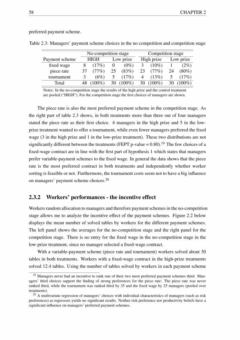
58 CHAPTER 2

preferred payment scheme.

Table 2.3: Managers’ payment scheme choices in the no competition and competition stage

No-competition stage Competition stagePayment scheme HIGH Low prize High prize Low prize

fixed wage 8 (17%) 0 (0%) 3 (10%) 1 (2%)piece rate 37 (77%) 25 (83%) 23 (77%) 24 (80%)

tournament 3 (6%) 5 (17%) 4 (13%) 5 (17%)Total 48 (100%) 30 (100%) 30 (100%) 30 (100%)

Notes: In the no-competition stage the results of the high prize and the control treatmentare pooled (“HIGH”). For the competition stage the first choices of managers are shown.

The piece rate is also the most preferred payment scheme in the competition stage. Asthe right part of table 2.3 shows, in both treatments more than three out of four managersstated the piece rate as their first choice. 4 managers in the high prize and 5 in the low-prize treatment wanted to offer a tournament, while even fewer managers preferred the fixedwage (3 in the high prize and 1 in the low-prize treatment). These two distributions are notsignificantly different between the treatments (FEPT p-value = 0.80).19 The few choices of afixed-wage contract are in line with the first part of hypothesis 1 which states that managersprefer variable-payment schemes to the fixed wage. In general the data shows that the piecerate is the most preferred contract in both treatments and independently whether workersorting is feasible or not. Furthermore, the tournament costs seem not to have a big influenceon managers’ payment scheme choices.20

2.3.2 Workers’ performances - the incentive effect

Workers random allocation to managers and therefore payment schemes in the no-competitionstage allows me to analyze the incentive effect of the payment schemes. Figure 2.2 belowdisplays the mean number of solved tables by workers for the different payment schemes.The left panel shows the averages for the no-competition stage and the right panel for thecompetition stage. There is no entry for the fixed wage in the no-competition stage in thelow-prize treatment, since no manager selected a fixed-wage contract.

With a variable-payment scheme (piece rate and tournament) workers solved about 30tables in both treatments. Workers with a fixed-wage contract in the high-prize treatmentssolved 12.4 tables. Using the number of tables solved by workers in each payment scheme

19 Managers never had an incentive to rank one of their two most preferred payment schemes third. Man-agers’ third choices support the finding of strong preferences for the piece rate: The piece rate was neverranked third, while the tournament was ranked third by 35 and the fixed wage by 25 managers (pooled overtreatments).

20 A multivariate regression of managers’ choices with individual characteristics of managers (such as riskpreferences) as regressors yields no significant results. Neither risk preference nor productivity beliefs have asignificant influence on managers’ preferred payment schemes.

CHAPTER 2 59

to conduct Mann-Whitney U tests (MWU) yields that significantly more tables were solvedwith a variable-payment scheme (high prize-treatment: fixed wage vs. piece rate, p-value< 0.01 and fixed wage vs. tournament, p-value < 0.01).21 The low average performance ofworkers with a fixed wage suggests that the average effort supplied was low, which confirmspart two of hypothesis 1.

010

2030

40

fixed wage piece rate tournament fixed wage piece rate tournament

HIGH Low prize

Mea

n #

of ta

bles

sol

ved

in th

e no

−co

mpe

titio

n st

age

Payment scheme

No−competition stage

010

2030

40fixed wage piece rate tournament fixed wage piece rate tournament

High prize Low prize

Mea

n #

of ta

bles

sol

ved

in th

e co

mpe

titio

n st

age

Payment scheme

Competition stage

Figure 2.2: Mean number of correctly solved tables by workers with different paymentschemes

The data also shows that workers’ performance in the variable-payment schemes is notsignificantly different between payment schemes at any conventional level: piece rate vs.tournament in the high-prize treatment (MWU test, p-value = 0.78) and piece rate vs. tour-nament in the low-prize treatment (MWU test, p-value = 0.20). There is also no significantdifference for each payment scheme between the treatments: piece rate in high prize vs.low-prize treatment (MWU test, p-value = 0.48) and high-prize tournament vs. low-prizetournament (MWU test, p-value = 0.83). These results indicate that the variable-paymentschemes provide incentives for workers to exert effort. Furthermore, the equal output inboth tournaments implies that the different in tournament prizes did not have a big effecton workers’ effort. However, given the low number of observations in the tournaments thisresult might not be very robust.

While workers’ average performance in the variable-payments schemes is not different,the differences in the variances appear large. For the no-competition stage however, onlythe variance for the fixed wage performance is significantly larger than the variance of thetournament in the high-prize treatment (F-test H0 ∶ same variance: p-value = 0.09).22 Iconsider it plausible that the low number of observations in the fixed wage and tournamentin the no-competition stage plays a big role for these results. Given the low number of

21 “HIGH” pools the results of the high-prize treatment and the control treatment for the analysis of theno-competition stage.

22 For the other comparisons the same test yields no significant difference: high-prize treatment, fixed wagevs. piece rate (p-value = 0.26) and piece rate vs. tournament (p-value = 0.18) and for the low-prize treatment:piece rate vs. tournament (p-value = 0.78).

60 CHAPTER 2

subjects in these payment schemes even few outliers have a big influence on the observedresults.

In the competition stage any differences in the performance of workers with differentpayment schemes cannot be completely attributed to an incentive effect, since the allocationof workers to payment schemes is most likely not random. While the results regardingworker sorting are discussed in detail in section 2.3.4, it is useful to note here that the twomain results from the no-competition stage seem to be sustained also with worker sorting.First, workers’ average performance is lower with a fixed-wage contract than in a variable-payment contract. Workers solve more tables with a variable-payment scheme in the high-prize treatment, fixed wage vs. piece rate (MWU test, p-value < 0.01) and fixed wage vs.tournament (MWU test, p-value < 0.01), and in the low-prize treatment, fixed wage vs.piece rate (MWU test, p-value < 0.01) and fixed wage vs. tournament (MWU test, p-value< 0.01). Second, there is also no significant difference in workers’ performance for thevariable-payment schemes between treatments: piece rate in high vs. low-prize treatment(MWU test, p-value = 0.41) and high-prize tournament vs. low-prize tournament (MWUtest, p-value = 0.68).23 These results confirm the findings from the no-competition stage andsince with the applied matching procedure the number of workers in each payment schemeis identical in the competition stage (n=40 for all payment schemes) the caveat of the lownumber of observations for the fixed wage and tournament contracts in the no-competitionstage does not apply. The heterogeneity in workers’ performances in the different paymentschemes in the competition stage is discussed in the section about worker self-selection.

2.3.3 Managers’ profits and payoff-maximizing contracts

To compare managers’ profits between payment schemes I compute the profit per contract.Figure 2.3 displays the mean of manager profits generated by workers, but excludes anyearnings managers made due to their own performance or from their questionnaire answers(profit = # of solved tables * 14 points - wage payment). The left panel shows the results forthe no-competition stage and the right panel shows the results for the competition stage.

In the no-competition stage of the high-prize treatment managers’ profits with a variable-payment scheme are significantly larger than with a fixed-wage contract: fixed wage vs.piece rate (MWU test, p-value < 0.01) and fixed wage vs. tournament (MWU test, p-value= 0.04). Offering a fixed wage was therefore not the profit-maximizing choice of managers.This result is the consequence of the low average worker performance with a fixed wagereported above. Comparing profits from the variable-payment schemes in the high-prizetreatment yields no significant difference: piece rate vs. tournament (MWU test, p-value =0.78). The high-prize tournament and the piece rate are therefore on average equally prof-

23 A comparison of the fixed-wage contracts between the treatments seems not useful, since the paid wagesdiffer. For an analysis of the effect of fixed wages on workers’ performances see section 2.3.7.

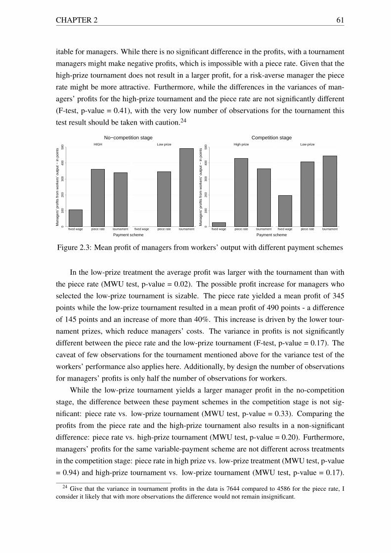
CHAPTER 2 61

itable for managers. While there is no significant difference in the profits, with a tournamentmanagers might make negative profits, which is impossible with a piece rate. Given that thehigh-prize tournament does not result in a larger profit, for a risk-averse manager the piecerate might be more attractive. Furthermore, while the differences in the variances of man-agers’ profits for the high-prize tournament and the piece rate are not significantly different(F-test, p-value = 0.41), with the very low number of observations for the tournament thistest result should be taken with caution.24

010

020

030

040

050

0


HIGH Low prize

Man

ager

s’ p

rofit

s fr

om w

orke

rs’ o

utpu

t − in

poi

nts

Payment scheme


010

020

030

040

050

0



Man

ager

s’ p

rofit

s fr

om w

orke

rs’ o

utpu

t − in

poi

nts

Payment scheme

Competition stage

Figure 2.3: Mean profit of managers from workers’ output with different payment schemes

In the low-prize treatment the average profit was larger with the tournament than withthe piece rate (MWU test, p-value = 0.02). The possible profit increase for managers whoselected the low-prize tournament is sizable. The piece rate yielded a mean profit of 345points while the low-prize tournament resulted in a mean profit of 490 points - a differenceof 145 points and an increase of more than 40%. This increase is driven by the lower tour-nament prizes, which reduce managers’ costs. The variance in profits is not significantlydifferent between the piece rate and the low-prize tournament (F-test, p-value = 0.17). Thecaveat of few observations for the tournament mentioned above for the variance test of theworkers’ performance also applies here. Additionally, by design the number of observationsfor managers’ profits is only half the number of observations for workers.

While the low-prize tournament yields a larger manager profit in the no-competitionstage, the difference between these payment schemes in the competition stage is not sig-nificant: piece rate vs. low-prize tournament (MWU test, p-value = 0.33). Comparing theprofits from the piece rate and the high-prize tournament also results in a non-significantdifference: piece rate vs. high-prize tournament (MWU test, p-value = 0.20). Furthermore,managers’ profits for the same variable-payment scheme are not different across treatmentsin the competition stage: piece rate in high prize vs. low-prize treatment (MWU test, p-value= 0.94) and high-prize tournament vs. low-prize tournament (MWU test, p-value = 0.17).

24 Give that the variance in tournament profits in the data is 7644 compared to 4586 for the piece rate, Iconsider it likely that with more observations the difference would not remain insignificant.

62 CHAPTER 2

Managers earn on average the same profits with the piece rate and with a tournament inboth treatments. For both tournaments the profit variances are larger than for the piece rate:piece rate vs. high-prize tournament (F-test, p-value = 0.03) and piece rate vs. low-prizetournament (F-test, p-value < 0.01).

Like in the no-competition stage the fixed-wage contract was on average not very prof-itable in the competition stage. In both treatments the fixed-wage contract resulted in thelowest manager profits.25 The right part of figure 2.3 also suggests a difference in the prof-itability of fixed-wage contracts between the treatments. But since the paid wages can differsubstantially between contracts and therefore also between treatments, a more detailed anal-ysis is required before such a statement can be made. I analyze how the offered fixed wagesaffect workers’ performance and address potential treatment differences in detail in section2.3.7.

There are two main takeaways for the profitability of the payment schemes. First, man-agers’ profits are larger with a variable-payment scheme in both treatments and stages. Thesefindings are in line with hypothesis 2 and additionally the data shows that a tournament re-sults in larger average profits than a fixed-wage contract. Second, only in the no-competitionstage and with low prizes a tournament is more profitable than the piece rate. Therefore therank-order tournament outperforms the piece-rate contract in this experiment if no workersorting is feasible. However, the next section shows that the low-prize tournament loses itsadvantage in the competition stage due to the productivity sorting of workers.

2.3.4 Sorting of workers

After learning the fixed wage offered in the competition stage workers ranked managers’offers knowing that a higher rank for a contract increased the probability of receiving thiscontract. The mechanism creates an incentive for workers to rank the payment schemesaccording to their preferences. Since priority is given to more productive workers, veryproductive workers are basically guaranteed to receive their first choice. Consequently, theyhave no incentive for stating their true preferences for their second and third choice. Butthey can base their behavior only on their believed ranking, since they do not receive anyfeedback on their relative performance before the end of the experiment.26

Furthermore, an extensive literature in psychology and economics documents that mostpeople are overconfident about their own performance and have too optimistic beliefs re-garding their own relative ranking. Camerer and Lovallo (1999) were among the first todemonstrate that overconfidence can result in above equilibrium entry rates into competi-

25 For the high-prize treatment: fixed wage vs. piece rate (MWU test, p-value < 0.01) and fixed wage vs.tournament MWU test, p-value < 0.01). For the low-prize treatment: fixed wage vs. piece rate (MWU test,p-value = 0.08) and fixed wage vs. tournament (MWU test, p-value = 0.03).

26 The only workers who receive limited feedback on their relative ranking are workers who are paid witha tournament in the no-competition stage. By learning whether they won the tournament these workers knowwhether they solved at least as many tables as one other worker in their group or not.

CHAPTER 2 63

tions, especially if the number of entrants should be low in equilibrium. As a consequenceof excess entry profits in competitions can be below equilibrium predictions.27 If subjects inmy experiment are overoptimistic regarding their performance they might overestimate theprobability of receiving their first contract choice. If that is the case their second and thirdcontract choices might not correspond to their true preferences. Also workers might mis-judge their probability of winning the tournament and enter the tournament too often. Sincethe following analysis focuses on workers’ first choices and the incentives for stating themost preferred contract first are not biased by overconfidence, I assume that workers’ firstchoices are their most preferred contracts. Whether workers in the experiment are overcon-fident regarding their own performance and how their beliefs affect their stated preferencesfor payment schemes is addressed later in this section.

In the left panel of table 2.4 workers’ first choices split for both treatments are shown. Inboth treatments the piece rate was ranked first by at least 50% of workers. The tournamentwas chosen by more workers in the high-prize treatment (18 in high prize vs. 9 in low-prize treatment), but the distributions of workers’ first choices for the two treatments are notsignificantly different (FEPT, p-value = 0.15). The fixed-wage contract was selected by 20%(high prize) respectively 27% of workers (low-prize treatment). The percentages should notbe directly compared, since the offered wages were different.

For the piece rate the wage of a worker only depends on the number of solved tablesand in the tournament his wage depends on whether he outperformed the other worker in thesame firm. A worker’s ability to solve tables is therefore the most important determinant forhis expected wage. Consequently it is likely that workers with different productivities preferdifferent contracts. As a first indicator whether workers’ choices are reflective of self-sortingby productivity consider the right panel of table 2.4. Using productivity indicator III - thenumber of tables solved with a piece rate in step 3 - workers’ average productivity is reportedsplit for their preferred payment schemes.28

In the high-prize treatment workers selecting a fixed wage have the lowest productivity:workers’ productivity with first choice fixed wage vs. piece rate (MWU test, p-value < 0.01)and fixed wage vs. tournament (MWU test, p-value = 0.07). The difference for workerswith a preference for the piece rate or the tournament is not significantly different in eithertreatment: high prize (MWU test, p-value = 0.23) and low-prize treatment (MWU test, p-value = 0.13). In the low-prize treatment workers choosing the fixed wage are significantlyless productive than those who selected the tournament (MWU test, p-value = 0.04), but

27 For a summary of studies regarding endogenous entry into competitions see Camerer (2003). Examples ofexperimental studies that find excess entry, at least under some conditions, are Cason et al. (2010) and Morganet al. (2012).

28 There is a high degree of correlation between all three productivity indicators and therefore most resultsare unchanged if productivity indicator I or II is used instead. Table B.2 in the appendix lists the Spearmanrank correlations between the three indicators and between the indicators and workers’ performance in the twoworking stages.

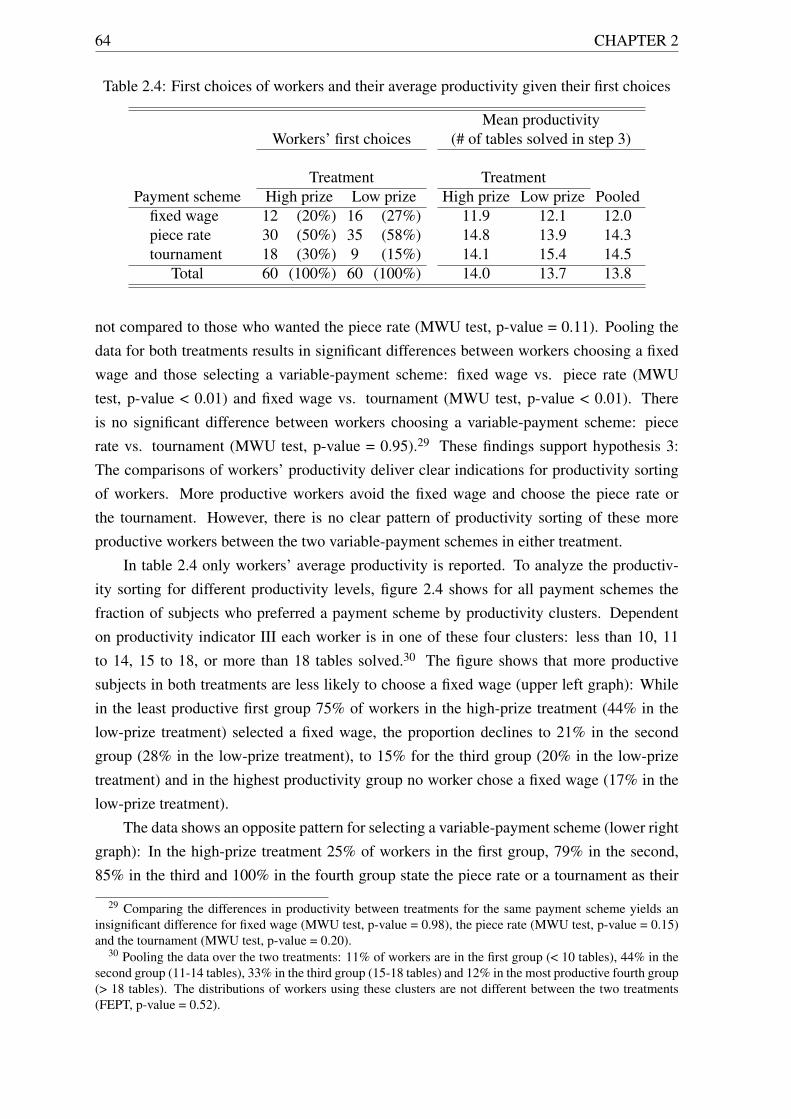
64 CHAPTER 2

Table 2.4: First choices of workers and their average productivity given their first choices

Mean productivityWorkers’ first choices (# of tables solved in step 3)

Treatment TreatmentPayment scheme High prize Low prize High prize Low prize Pooled

fixed wage 12 (20%) 16 (27%) 11.9 12.1 12.0piece rate 30 (50%) 35 (58%) 14.8 13.9 14.3tournament 18 (30%) 9 (15%) 14.1 15.4 14.5

Total 60 (100%) 60 (100%) 14.0 13.7 13.8

not compared to those who wanted the piece rate (MWU test, p-value = 0.11). Pooling thedata for both treatments results in significant differences between workers choosing a fixedwage and those selecting a variable-payment scheme: fixed wage vs. piece rate (MWUtest, p-value < 0.01) and fixed wage vs. tournament (MWU test, p-value < 0.01). Thereis no significant difference between workers choosing a variable-payment scheme: piecerate vs. tournament (MWU test, p-value = 0.95).29 These findings support hypothesis 3:The comparisons of workers’ productivity deliver clear indications for productivity sortingof workers. More productive workers avoid the fixed wage and choose the piece rate orthe tournament. However, there is no clear pattern of productivity sorting of these moreproductive workers between the two variable-payment schemes in either treatment.

In table 2.4 only workers’ average productivity is reported. To analyze the productiv-ity sorting for different productivity levels, figure 2.4 shows for all payment schemes thefraction of subjects who preferred a payment scheme by productivity clusters. Dependenton productivity indicator III each worker is in one of these four clusters: less than 10, 11to 14, 15 to 18, or more than 18 tables solved.30 The figure shows that more productivesubjects in both treatments are less likely to choose a fixed wage (upper left graph): Whilein the least productive first group 75% of workers in the high-prize treatment (44% in thelow-prize treatment) selected a fixed wage, the proportion declines to 21% in the secondgroup (28% in the low-prize treatment), to 15% for the third group (20% in the low-prizetreatment) and in the highest productivity group no worker chose a fixed wage (17% in thelow-prize treatment).

The data shows an opposite pattern for selecting a variable-payment scheme (lower rightgraph): In the high-prize treatment 25% of workers in the first group, 79% in the second,85% in the third and 100% in the fourth group state the piece rate or a tournament as their

29 Comparing the differences in productivity between treatments for the same payment scheme yields aninsignificant difference for fixed wage (MWU test, p-value = 0.98), the piece rate (MWU test, p-value = 0.15)and the tournament (MWU test, p-value = 0.20).

30 Pooling the data over the two treatments: 11% of workers are in the first group (< 10 tables), 44% in thesecond group (11-14 tables), 33% in the third group (15-18 tables) and 12% in the most productive fourth group(> 18 tables). The distributions of workers using these clusters are not different between the two treatments(FEPT, p-value = 0.52).

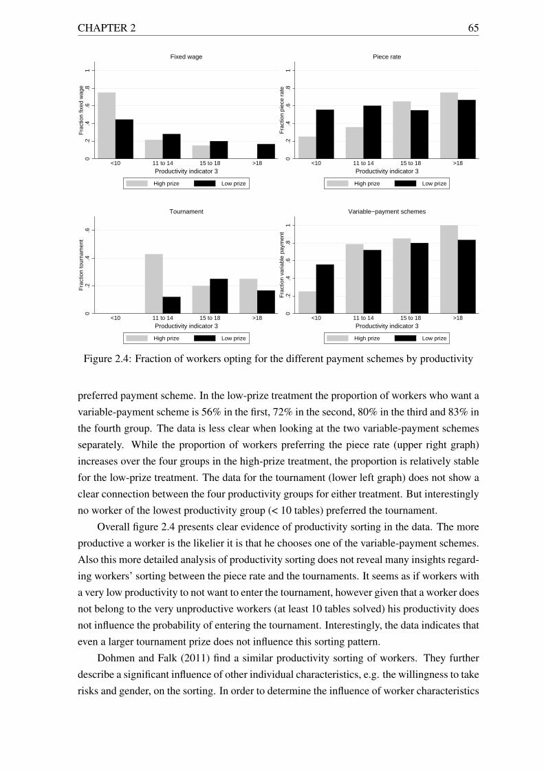
CHAPTER 2 65

0.2

.4.6

.81

Fra

ctio

n fix

ed w

age

<10 11 to 14 15 to 18 >18Productivity indicator 3

Fixed wage


0.2

.4.6

.81

Fra

ctio

n pi

ece

rate


Piece rate


0.2

.4.6

Fra

ctio

n to

urna

men

t


Tournament


0.2

.4.6

.81

Fra

ctio

n va

riabl

e pa

ymen

t


Variable−payment schemes


Figure 2.4: Fraction of workers opting for the different payment schemes by productivity

preferred payment scheme. In the low-prize treatment the proportion of workers who want avariable-payment scheme is 56% in the first, 72% in the second, 80% in the third and 83% inthe fourth group. The data is less clear when looking at the two variable-payment schemesseparately. While the proportion of workers preferring the piece rate (upper right graph)increases over the four groups in the high-prize treatment, the proportion is relatively stablefor the low-prize treatment. The data for the tournament (lower left graph) does not show aclear connection between the four productivity groups for either treatment. But interestinglyno worker of the lowest productivity group (< 10 tables) preferred the tournament.

Overall figure 2.4 presents clear evidence of productivity sorting in the data. The moreproductive a worker is the likelier it is that he chooses one of the variable-payment schemes.Also this more detailed analysis of productivity sorting does not reveal many insights regard-ing workers’ sorting between the piece rate and the tournaments. It seems as if workers witha very low productivity to not want to enter the tournament, however given that a worker doesnot belong to the very unproductive workers (at least 10 tables solved) his productivity doesnot influence the probability of entering the tournament. Interestingly, the data indicates thateven a larger tournament prize does not influence this sorting pattern.

Dohmen and Falk (2011) find a similar productivity sorting of workers. They furtherdescribe a significant influence of other individual characteristics, e.g. the willingness to takerisks and gender, on the sorting. In order to determine the influence of worker characteristics

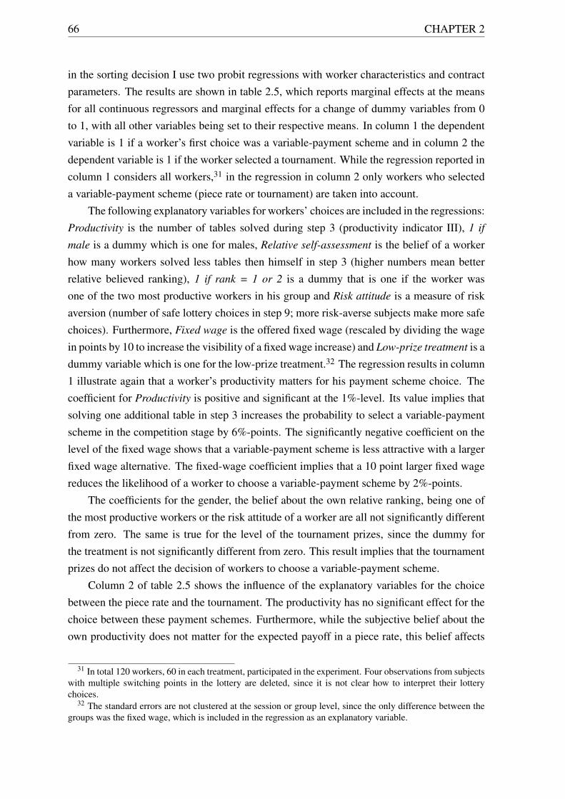
66 CHAPTER 2

in the sorting decision I use two probit regressions with worker characteristics and contractparameters. The results are shown in table 2.5, which reports marginal effects at the meansfor all continuous regressors and marginal effects for a change of dummy variables from 0to 1, with all other variables being set to their respective means. In column 1 the dependentvariable is 1 if a worker’s first choice was a variable-payment scheme and in column 2 thedependent variable is 1 if the worker selected a tournament. While the regression reported incolumn 1 considers all workers,31 in the regression in column 2 only workers who selecteda variable-payment scheme (piece rate or tournament) are taken into account.

The following explanatory variables for workers’ choices are included in the regressions:Productivity is the number of tables solved during step 3 (productivity indicator III), 1 if

male is a dummy which is one for males, Relative self-assessment is the belief of a workerhow many workers solved less tables then himself in step 3 (higher numbers mean betterrelative believed ranking), 1 if rank = 1 or 2 is a dummy that is one if the worker wasone of the two most productive workers in his group and Risk attitude is a measure of riskaversion (number of safe lottery choices in step 9; more risk-averse subjects make more safechoices). Furthermore, Fixed wage is the offered fixed wage (rescaled by dividing the wagein points by 10 to increase the visibility of a fixed wage increase) and Low-prize treatment is adummy variable which is one for the low-prize treatment.32 The regression results in column1 illustrate again that a worker’s productivity matters for his payment scheme choice. Thecoefficient for Productivity is positive and significant at the 1%-level. Its value implies thatsolving one additional table in step 3 increases the probability to select a variable-paymentscheme in the competition stage by 6%-points. The significantly negative coefficient on thelevel of the fixed wage shows that a variable-payment scheme is less attractive with a largerfixed wage alternative. The fixed-wage coefficient implies that a 10 point larger fixed wagereduces the likelihood of a worker to choose a variable-payment scheme by 2%-points.

The coefficients for the gender, the belief about the own relative ranking, being one ofthe most productive workers or the risk attitude of a worker are all not significantly differentfrom zero. The same is true for the level of the tournament prizes, since the dummy forthe treatment is not significantly different from zero. This result implies that the tournamentprizes do not affect the decision of workers to choose a variable-payment scheme.

Column 2 of table 2.5 shows the influence of the explanatory variables for the choicebetween the piece rate and the tournament. The productivity has no significant effect for thechoice between these payment schemes. Furthermore, while the subjective belief about theown productivity does not matter for the expected payoff in a piece rate, this belief affects

31 In total 120 workers, 60 in each treatment, participated in the experiment. Four observations from subjectswith multiple switching points in the lottery are deleted, since it is not clear how to interpret their lotterychoices.

32 The standard errors are not clustered at the session or group level, since the only difference between thegroups was the fixed wage, which is included in the regression as an explanatory variable.

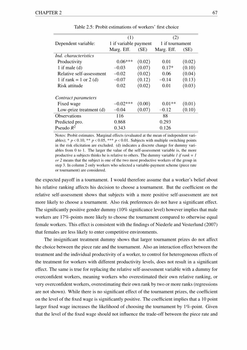
CHAPTER 2 67

Table 2.5: Probit estimations of workers’ first choice

(1) (2)Dependent variable: 1 if variable payment 1 if tournament

Marg. Eff. (SE) Marg. Eff. (SE)Ind. characteristicsProductivity 0.06*** (0.02) 0.01 (0.02)1 if male (d) −0.03 (0.07) 0.17* (0.10)Relative self-assessment −0.02 (0.02) 0.06 (0.04)1 if rank = 1 or 2 (d) −0.07 (0.12) −0.14 (0.13)Risk attitude 0.02 (0.02) 0.01 (0.03)

Contract parametersFixed wage −0.02*** (0.00) 0.01** (0.01)Low-prize treatment (d) −0.04 (0.07) −0.12 (0.10)

Observations 116 88Predicted pro. 0.868 0.293Pseudo R2 0.343 0.126Notes: Probit estimates. Marginal effects (evaluated at the mean of independent vari-ables); * p < 0.10, ** p < 0.05, *** p < 0.01. Subjects with multiple switching pointsin the risk elicitation are excluded. (d) indicates a discrete change for dummy vari-ables from 0 to 1. The larger the value of the self-assessment variable is, the moreproductive a subjects thinks he is relative to others. The dummy variable 1 if rank = 1or 2 means that the subject is one of the two most productive workers of the group instep 3. In column 2 only workers who selected a variable-payment scheme (piece rateor tournament) are considered.

the expected payoff in a tournament. I would therefore assume that a worker’s belief abouthis relative ranking affects his decision to choose a tournament. But the coefficient on therelative self-assessment shows that subjects with a more positive self-assessment are notmore likely to choose a tournament. Also risk preferences do not have a significant effect.The significantly positive gender dummy (10% significance level) however implies that maleworkers are 17%-points more likely to choose the tournament compared to otherwise equalfemale workers. This effect is consistent with the findings of Niederle and Vesterlund (2007)that females are less likely to enter competitive environments.

The insignificant treatment dummy shows that larger tournament prizes do not affectthe choice between the piece rate and the tournament. Also an interaction effect between thetreatment and the individual productivity of a worker, to control for heterogeneous effects ofthe treatment for workers with different productivity levels, does not result in a significanteffect. The same is true for replacing the relative self-assessment variable with a dummy foroverconfident workers, meaning workers who overestimated their own relative ranking, orvery overconfident workers, overestimating their own rank by two or more ranks (regressionsare not shown). While there is no significant effect of the tournament prizes, the coefficienton the level of the fixed wage is significantly positive. The coefficient implies that a 10 pointlarger fixed wage increases the likelihood of choosing the tournament by 1%-point. Giventhat the level of the fixed wage should not influence the trade-off between the piece rate and

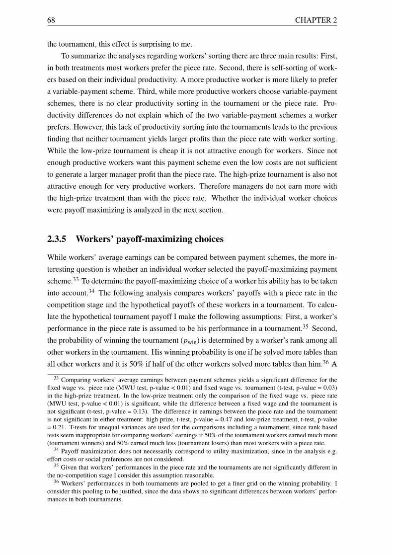
68 CHAPTER 2

the tournament, this effect is surprising to me.To summarize the analyses regarding workers’ sorting there are three main results: First,

in both treatments most workers prefer the piece rate. Second, there is self-sorting of work-ers based on their individual productivity. A more productive worker is more likely to prefera variable-payment scheme. Third, while more productive workers choose variable-paymentschemes, there is no clear productivity sorting in the tournament or the piece rate. Pro-ductivity differences do not explain which of the two variable-payment schemes a workerprefers. However, this lack of productivity sorting into the tournaments leads to the previousfinding that neither tournament yields larger profits than the piece rate with worker sorting.While the low-prize tournament is cheap it is not attractive enough for workers. Since notenough productive workers want this payment scheme even the low costs are not sufficientto generate a larger manager profit than the piece rate. The high-prize tournament is also notattractive enough for very productive workers. Therefore managers do not earn more withthe high-prize treatment than with the piece rate. Whether the individual worker choiceswere payoff maximizing is analyzed in the next section.

2.3.5 Workers’ payoff-maximizing choices

While workers’ average earnings can be compared between payment schemes, the more in-teresting question is whether an individual worker selected the payoff-maximizing paymentscheme.33 To determine the payoff-maximizing choice of a worker his ability has to be takeninto account.34 The following analysis compares workers’ payoffs with a piece rate in thecompetition stage and the hypothetical payoffs of these workers in a tournament. To calcu-late the hypothetical tournament payoff I make the following assumptions: First, a worker’sperformance in the piece rate is assumed to be his performance in a tournament.35 Second,the probability of winning the tournament (pwin) is determined by a worker’s rank among allother workers in the tournament. His winning probability is one if he solved more tables thanall other workers and it is 50% if half of the other workers solved more tables than him.36 A

33 Comparing workers’ average earnings between payment schemes yields a significant difference for thefixed wage vs. piece rate (MWU test, p-value < 0.01) and fixed wage vs. tournament (t-test, p-value = 0.03)in the high-prize treatment. In the low-prize treatment only the comparison of the fixed wage vs. piece rate(MWU test, p-value < 0.01) is significant, while the difference between a fixed wage and the tournament isnot significant (t-test, p-value = 0.13). The difference in earnings between the piece rate and the tournamentis not significant in either treatment: high prize, t-test, p-value = 0.47 and low-prize treatment, t-test, p-value= 0.21. T-tests for unequal variances are used for the comparisons including a tournament, since rank basedtests seem inappropriate for comparing workers’ earnings if 50% of the tournament workers earned much more(tournament winners) and 50% earned much less (tournament losers) than most workers with a piece rate.

34 Payoff maximization does not necessarily correspond to utility maximization, since in the analysis e.g.effort costs or social preferences are not considered.

35 Given that workers’ performances in the piece rate and the tournaments are not significantly different inthe no-competition stage I consider this assumption reasonable.

36 Workers’ performances in both tournaments are pooled to get a finer grid on the winning probability. Iconsider this pooling to be justified, since the data shows no significant differences between workers’ perfor-mances in both tournaments.

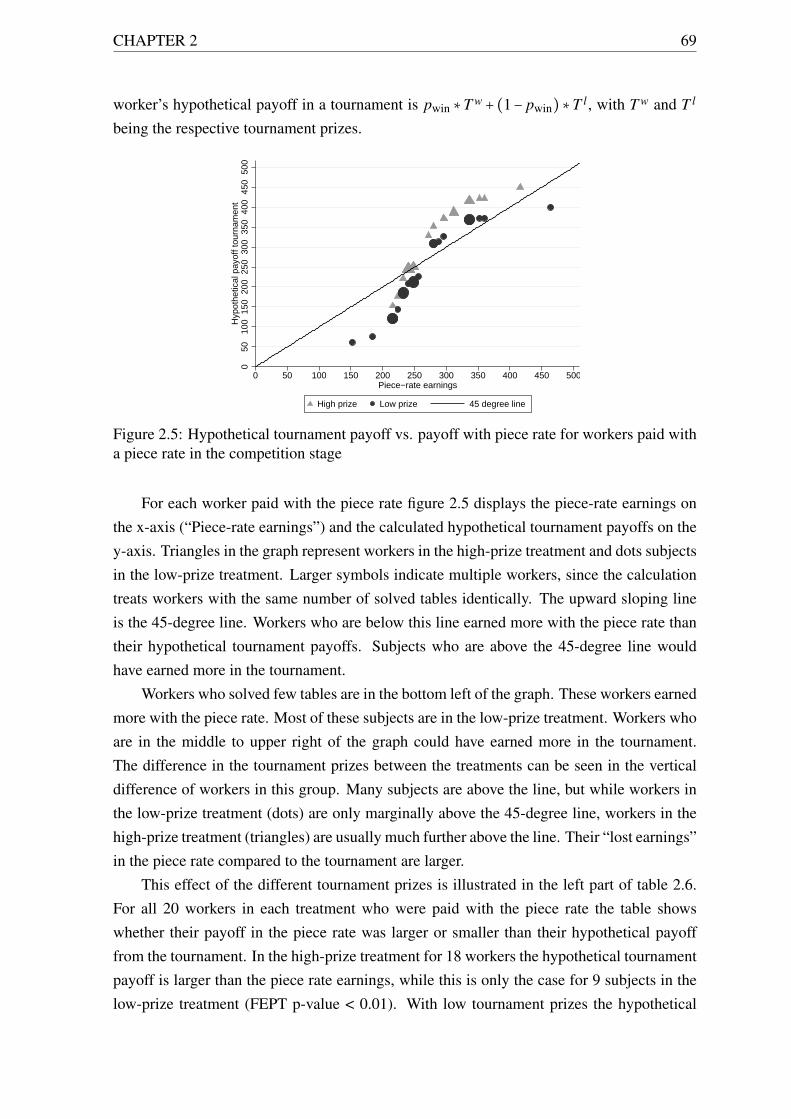
CHAPTER 2 69

worker’s hypothetical payoff in a tournament is pwin ∗T w+ (1− pwin)∗T l , with T w and T l

being the respective tournament prizes.

050

100

150

200

250

300

350

400

450

500

Hyp

othe

tical

pay

off t

ourn

amen

t

0 50 100 150 200 250 300 350 400 450 500Piece−rate earnings

High prize Low prize 45 degree line

Figure 2.5: Hypothetical tournament payoff vs. payoff with piece rate for workers paid witha piece rate in the competition stage

For each worker paid with the piece rate figure 2.5 displays the piece-rate earnings onthe x-axis (“Piece-rate earnings”) and the calculated hypothetical tournament payoffs on they-axis. Triangles in the graph represent workers in the high-prize treatment and dots subjectsin the low-prize treatment. Larger symbols indicate multiple workers, since the calculationtreats workers with the same number of solved tables identically. The upward sloping lineis the 45-degree line. Workers who are below this line earned more with the piece rate thantheir hypothetical tournament payoffs. Subjects who are above the 45-degree line wouldhave earned more in the tournament.

Workers who solved few tables are in the bottom left of the graph. These workers earnedmore with the piece rate. Most of these subjects are in the low-prize treatment. Workers whoare in the middle to upper right of the graph could have earned more in the tournament.The difference in the tournament prizes between the treatments can be seen in the verticaldifference of workers in this group. Many subjects are above the line, but while workers inthe low-prize treatment (dots) are only marginally above the 45-degree line, workers in thehigh-prize treatment (triangles) are usually much further above the line. Their “lost earnings”in the piece rate compared to the tournament are larger.

This effect of the different tournament prizes is illustrated in the left part of table 2.6.For all 20 workers in each treatment who were paid with the piece rate the table showswhether their payoff in the piece rate was larger or smaller than their hypothetical payofffrom the tournament. In the high-prize treatment for 18 workers the hypothetical tournamentpayoff is larger than the piece rate earnings, while this is only the case for 9 subjects in thelow-prize treatment (FEPT p-value < 0.01). With low tournament prizes the hypothetical

70 CHAPTER 2

tournament earnings are not large enough to result in an improvement over the piece rate formost subjects. Workers in the high-prize treatment often could have increased their expectedearnings in the tournament.

Table 2.6: Payoff-maximizing payment schemes for workers paid with a variable-paymentscheme

Workers with piece rate Workers with a tournamentLarger (hypothetical) Treatment Treatment

earnings with High prize Low prize High prize Low prizetournament 18 (90%) 9 (45%) 12 (60%) 9 (45%)piece rate 2 (10%) 11 (55%) 8 (40%) 11 (55%)

Total 20 (100%) 20 (100%) 20 (100%) 20 (100%)Notes: All 80 workers who were paid with a variable-payment scheme in the competition stageare included. Tournament earnings are hypothetical earnings, calculated as described above.Piece-rate earnings are the actual payoff for workers being paid with a piece rate and hypotheticalearnings for workers paid with a tournament.

The results of the identical analysis for workers in a tournament is displayed in figure 2.6and in the right part of table 2.6. The graph includes all 40 workers paid with a tournament inthe competition stage. The y-axis shows their hypothetical tournament payoffs - calculatedas described above - and the x-axis displays the hypothetical piece-rate earnings - 8 pointstimes the number of solved table for each subject. The line is the 45-degree line. Filledsymbols (triangles for the high prize and dots for the low-prize treatment) indicate that thesubject won the tournament, while hollow symbols represent tournament losers.

As for the workers who were paid with the piece rate, there are two groups: Workersabove the 45-degree line had a higher hypothetical payoff in the tournament and workersbelow the line had a higher hypothetical payoff with the piece rate. The data shows thatfor about half of the workers the tournament was the payoff-maximizing payment scheme.Furthermore, there is no visible difference between the treatments. While in figure 2.5 abovemany workers in the high-prize treatment were above the line, in figure 2.6 for both treat-ments there are roughly as many symbols above the 45-degree line as below. The right partof table 2.6 shows that for 8 workers in the high prize and 11 workers in the low-prize treat-ment, the piece rate would have resulted in a higher hypothetical payoff. These distributionsare not significantly different (FEPT, p-value = 0.53).

The analysis so far showed that especially workers paid with a piece rate in the high-prize treatment could have increased their hypothetical payoff by being paid with a tour-nament. However, to answer the question whether workers chose their payoff-maximizingpayment scheme also their choices have to be considered. Of the 20 workers being paidwith a piece rate in the high-prize treatment 17 stated the piece rate as their first choice. For15 of these 17 workers the hypothetical tournament payoff was larger than the payoff withthe piece rate. In the low-prize treatment also 17 of the 20 workers paid with the piece rate

CHAPTER 2 71

050

100

150

200

250

300

350

400

450

Hyp

othe

tical

pay

off t

ourn

amen

t

0 50 100 150 200 250 300 350 400 450Hypothetical payoff piece rate

High prize − winner High prize − loserLow prize − winner Low prize − loser45 degree line

Figure 2.6: Hypothetical tournament payoff vs. hypothetical payoff with piece rate for work-ers paid with a tournament in the competition stage

wanted the piece rate. Of these 17 workers only 6 had a larger hypothetical tournament pay-off. These distributions are significantly different (FEPT, p-value < 0.01). Of the workersbeing paid with the tournament only 13 in the high prize and 8 in the low-prize treatmentstated the tournament as their preferred payment scheme. For 9 of these workers in the highprize and 4 workers in the low-prize treatment the tournament was the payoff-maximizingpayment scheme. These distributions are not significantly different between the two treat-ments (FEPT, p-value = 0.65).

These findings show that the difference in tournament prizes affects workers’ hypothet-ical payoffs. For productive risk-neutral workers the high-prize tournament is attractive. Infact the majority of workers selecting a piece rate in the high-prize treatment would haveincreased their hypothetical payoff by being in the tournament. In the low-prize treatmentfewer workers would have benefited from the tournament. There is no such treatment differ-ences for workers selecting a tournament. Additionally, as figure 2.5 shows, the (potential)advantage in hypothetical payoffs of being in the tournament are larger for workers in thehigh-prize treatment. While these observations suggest that many workers in the high-prizetreatment did not select the payoff-maximizing contract by choosing the piece rate, the anal-ysis does not take other aspects of the different payment schemes into account, e.g. riskinessor “fairness”.

2.3.6 Main result

The results of the previous sections demonstrate the incentives tournaments can provide forworkers. As shown in section 2.3.2 workers’ performances in both tournaments are on parwith the output in the piece rate. Therefore the inexpensive low-prize tournament in theno-competition stage generates a larger manager profit than the piece rate. This findingdemonstrates the potential cost advantage of a fixed-prize tournament compared to a piece

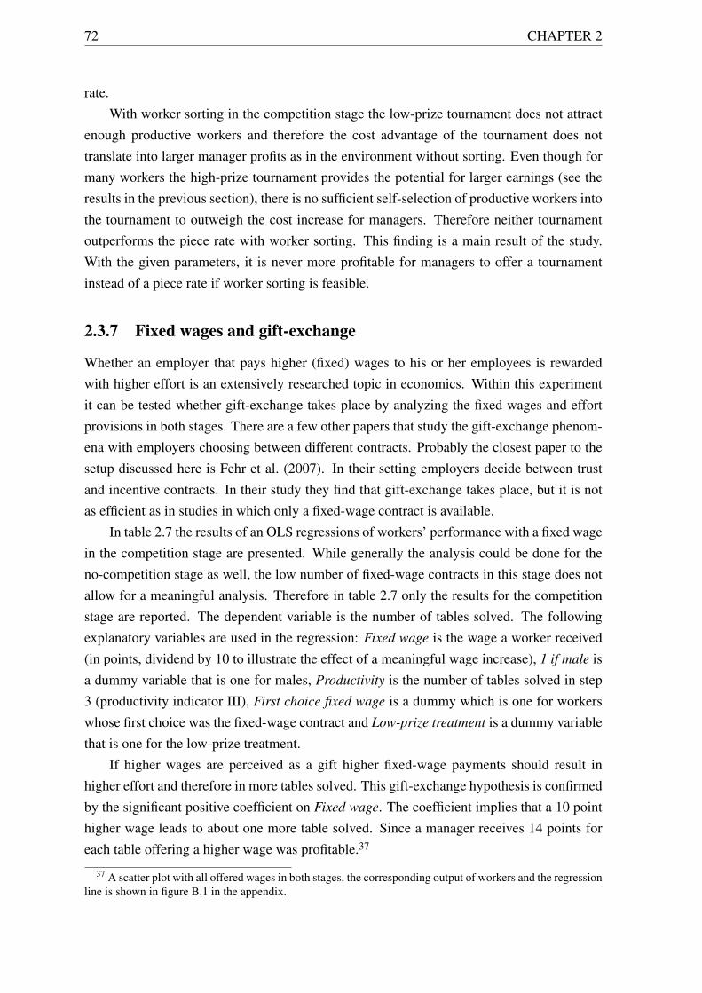
72 CHAPTER 2

rate.With worker sorting in the competition stage the low-prize tournament does not attract

enough productive workers and therefore the cost advantage of the tournament does nottranslate into larger manager profits as in the environment without sorting. Even though formany workers the high-prize tournament provides the potential for larger earnings (see theresults in the previous section), there is no sufficient self-selection of productive workers intothe tournament to outweigh the cost increase for managers. Therefore neither tournamentoutperforms the piece rate with worker sorting. This finding is a main result of the study.With the given parameters, it is never more profitable for managers to offer a tournamentinstead of a piece rate if worker sorting is feasible.

2.3.7 Fixed wages and gift-exchange

Whether an employer that pays higher (fixed) wages to his or her employees is rewardedwith higher effort is an extensively researched topic in economics. Within this experimentit can be tested whether gift-exchange takes place by analyzing the fixed wages and effortprovisions in both stages. There are a few other papers that study the gift-exchange phenom-ena with employers choosing between different contracts. Probably the closest paper to thesetup discussed here is Fehr et al. (2007). In their setting employers decide between trustand incentive contracts. In their study they find that gift-exchange takes place, but it is notas efficient as in studies in which only a fixed-wage contract is available.

In table 2.7 the results of an OLS regressions of workers’ performance with a fixed wagein the competition stage are presented. While generally the analysis could be done for theno-competition stage as well, the low number of fixed-wage contracts in this stage does notallow for a meaningful analysis. Therefore in table 2.7 only the results for the competitionstage are reported. The dependent variable is the number of tables solved. The followingexplanatory variables are used in the regression: Fixed wage is the wage a worker received(in points, dividend by 10 to illustrate the effect of a meaningful wage increase), 1 if male isa dummy variable that is one for males, Productivity is the number of tables solved in step3 (productivity indicator III), First choice fixed wage is a dummy which is one for workerswhose first choice was the fixed-wage contract and Low-prize treatment is a dummy variablethat is one for the low-prize treatment.

If higher wages are perceived as a gift higher fixed-wage payments should result inhigher effort and therefore in more tables solved. This gift-exchange hypothesis is confirmedby the significant positive coefficient on Fixed wage. The coefficient implies that a 10 pointhigher wage leads to about one more table solved. Since a manager receives 14 points foreach table offering a higher wage was profitable.37

37 A scatter plot with all offered wages in both stages, the corresponding output of workers and the regressionline is shown in figure B.1 in the appendix.

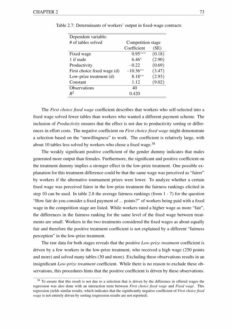
CHAPTER 2 73

Table 2.7: Determinants of workers’ output in fixed-wage contracts

Dependent variable:# of tables solved Competition stage

Coefficient (SE)Fixed wage 0.95∗∗∗ (0.18)1 if male 6.46∗ (2.90)Productivity −0.22 (0.69)First choice fixed wage (d) −10.36∗∗ (3.47)Low-prize treatment (d) 8.18∗∗ (2.93)Constant 1.12 (9.02)Observations 40R2 0.420

The First choice fixed wage coefficient describes that workers who self-selected into afixed wage solved fewer tables than workers who wanted a different payment scheme. Theinclusion of Productivity ensures that the effect is not due to productivity sorting or differ-ences in effort costs. The negative coefficient on First choice fixed wage might demonstratea selection based on the “unwillingness” to work. The coefficient is relatively large, withabout 10 tables less solved by workers who chose a fixed wage.38

The weakly significant positive coefficient of the gender dummy indicates that malesgenerated more output than females. Furthermore, the significant and positive coefficient onthe treatment dummy implies a stronger effect in the low-prize treatment. One possible ex-planation for this treatment difference could be that the same wage was perceived as “fairer”by workers if the alternative tournament prizes were lower. To analyze whether a certainfixed wage was perceived fairer in the low-prize treatment the fairness rankings elicited instep 10 can be used. In table 2.8 the average fairness rankings (from 1 - 7) for the question“How fair do you consider a fixed payment of ... points?” of workers being paid with a fixedwage in the competition stage are listed. While workers rated a higher wage as more “fair”,the differences in the fairness ranking for the same level of the fixed wage between treat-ments are small. Workers in the two treatments considered the fixed wages as about equallyfair and therefore the positive treatment coefficient is not explained by a different “fairnessperception” in the low-prize treatment.

The raw data for both stages reveals that the positive Low-prize treatment coefficient isdriven by a few workers in the low-prize treatment, who received a high wage (250 pointsand more) and solved many tables (30 and more). Excluding these observations results in aninsignificant Low-prize treatment coefficient. While there is no reason to exclude these ob-servations, this procedures hints that the positive coefficient is driven by these observations.

38 To ensure that this result is not due to a selection that is driven by the difference in offered wages theregression was also done with an interaction term between First choice fixed wage and Fixed wage. Thisregression yields similar results, which indicates that the significantly negative coefficient of First choice fixedwage is not entirely driven by sorting (regression results are not reported).

74 CHAPTER 2

Table 2.8: Average stated fairness

TreatmentPayment scheme High prize Low prize

fixed wage:100 points 2.45 2.65200 points 4.90 4.15300 points 5.15 5.35tournament prize 5.20 5.70

tournament 2.50 2.45piece rate 5.20 5.50Notes: “Fairness” is stated on a 1-7 Likert scale. Onlyworkers paid with a fixed wage in the competition stageare included.

Therefore a possible reason of the reported treatment difference might be higher wage offersin the low-prize treatment and not a different perception of the fixed wages.

2.4 Discussion and conclusion

Rank-order tournaments are a frequently studied payment scheme in the theoretical, butalso experimental economic literature. In this paper the profitability of a tournament aspayment scheme with the possibility of worker sorting is analyzed. The data illustratesthe incentive effect of tournaments for workers’ performance, but also that employers onlybenefit from this effect if workers are not able to sort themselves into different contracts. Inthe environment with worker sorting a tournament does not generate larger firm profits than apiece rate. While a tournament can be an attractive payment scheme for productive workersif the prizes are sufficiently large, for a manager a tournament with large prizes does notyield greater profits than a piece-rate contract. Due to productivity sorting also a low-prizetournament does not yield larger profits than a piece rate. This finding is likely part of theexplanation why a tournament is usually not the main contract scheme for many workers inlabor markets, despite its good incentives.

These results could explain why tournaments are usually used as “add-ones” in (implicit)contracts - e.g. a promotion tournament or competition for a bonus - but not as the mainpayment scheme. When other incentive inducing payment schemes are available - the piecerate in the presented experiment - managers have no advantage by offering a tournament.While managers in the presented setting do not earn significantly less with a tournamentcompared to a piece rate, this result could be conditional on the used matching procedure.In the experiment each manager receives a sufficient number of workers with all paymentschemes. In real world labor markets positions with an unattractive payment scheme mightbe unfilled or it might take some time until vacancies are filled.

Workers’ payment scheme choices show a clear sorting pattern. More productive work-

CHAPTER 2 75

ers prefer variable-payment schemes, confirming previous findings. But the individual pro-ductivity does not explain the sorting between the two variable-payment schemes piece rateand tournament. The only personal characteristic with a significant effect on the choicebetween the piece rate and a tournament is the gender. Females are less likely to select atournament, but they are not less likely to select a variable-payment scheme in general.

However, the experiment does not replicate the results regarding the importance of riskpreferences for workers’ choices reported in previous studies. Typically variable-paymentschemes and especially a tournament are considered as risky for workers, since the exactwage payment is unknown before the conclusion of the task. In the presented experimentthere are two factors which might reduce the importance of risk preferences: First the un-certainty in the piece rate is relatively low. Subjects had already worked for more than 15minutes on the task when they stated their preferences over payment schemes. Thereforethey probably had a good idea how many tables they could solve. Second, risk preferenceswere elicited with lottery choices and not with a more general statement “How willing areyou to take risks in general?” as in Dohmen and Falk (2011). They argue that both risk mea-sures - lottery choices and general statement - are highly correlated, but use the questionnaireanswers for their analysis. While it is possible that the lottery task did not accurately mea-sure subjects’ risk attitudes regarding employment choices, I view the non-significance ofthe elicited risk preferences for the payment scheme choices as surprising.

Equally unexpected is the irrelevance of workers’ relative self-assessment of their rankfor the decision whether or not to enter the tournament. Even though there is no significanteffect of workers’ self-assessment for the payment scheme choice, many subjects in theexperiment have overoptimistic beliefs. 30% of workers (36 subjects) overestimate theirown rank in step 3 and 18% (21 subjects) overestimate their rank by at least two ranks.

This study shows that tournaments might not be used very often simply because they areeither unattractive for workers or too expensive for firms. These effects should be true formost tournaments designs, but I cannot exclude the possibility that there exist tournamentsthat are not more expensive for managers and simultaneously more attractive than a piecerate for workers. While the cost argument makes it unlikely that larger tournament prizes area possibility, a smaller prize spread between the winner and the loser prize could be such adesign. Furthermore, a tournament might be more attractive for workers if the other availablepayment schemes are not as well liked as the piece rate in this study. Alternatively the levelof the piece rate could be smaller, such that very productive workers prefer a relatively cheaptournament to the piece rate.

Another aspect that cannot be addressed with the current design is the role of repetition.Workers make the sorting decision exactly once. Despite the fact that they have accumulatedquite some experience in the task when deciding between the available payment schemes,they have relatively little information regarding the productivity of other workers and theirrelative ranking. On the one hand, having subjects perform a real-effort task has the ad-

76 CHAPTER 2

vantage of good measurements of their productivity and the data clearly demonstrates thatproductivity differences between workers are an important factor for the observed sortingbehavior. On the other hand, the real-effort tasks creates a natural limit on the duration ofthe experiment and therefore leaves the question whether the sorting behavior would changewhen workers make the sorting decision several times unanswered.

This paper is a first attempt in understanding the effects of competition for workers onthe profitability of labor-market contracts. The separation of the incentive and sorting effectdemonstrates the importance of worker sorting for firms’ profits. The explicit choice betweendifferent incentive schemes influences which payment schemes are attractive for productiveworkers. In further research it will be interesting to investigate the importance of sortingfor the profitability of tournaments more thoroughly in especially with regard to differentpayment schemes and more variation in tournament prizes and designs.

Appendix B

Appendix Chapter 2

77

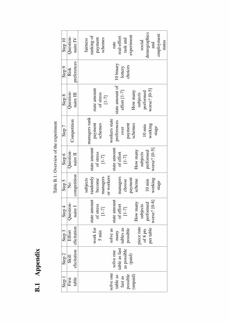
B.1

App

endi

x

Tabl

eB

.1:O

verv

iew

ofth

eex

peri

men

t

Step

1St

ep2

Step

3St

ep4

Step

5St

ep6

Step

7St

ep8

Step

9St

ep10

Firs

tta

ble

Skill

elic

itatio

nE

ffor

tel

icita

tion

Que

stio

n-na

ire

IN

oco

mpe

titio

nQ

uest

ion-

nair

eII

Com

petit

ion

Que

stio

n-na

ire

III

Ris

kpr

efer

ence

sQ

uest

ion-

nair

eIV

solv

eon

eta

ble

asfa

stas

poss

ible

(unp

aid)

solv

eon

eta

ble

asfa

stas

poss

ible

(pai

d)

wor

kfo

r5

min

solv

eas

man

yta

bles

aspo

ssib

le

piec

era

teof

8pt

spe

rtab

le

stat

eam

ount

ofst

ress

[1-7

]

stat

eam

ount

ofef

fort

[1-7

]

How

man

ysu

bjec

tspe

rfor

med

wor

se?

[0-8

]

subj

ects

rand

omly

beco

me

man

ager

sor

wor

kers

man

ager

sch

oose

paym

ent

sche

me

10m

inw

orki

ngst

age

stat

eam

ount

ofst

ress

[1-7

]

stat

eam

ount

ofef

fort

[1-7

]

How

man

ysu

bjec

tspe

rfor

med

wor

se?

[0-5

]

man

ager

sra

nkpa

ymen

tsc

hem

es

wor

kers

stat

epr

efer

ence

sov

erpa

ymen

tsc

hem

es

10m

inw

orki

ngst

age

stat

eam

ount

ofst

ress

[1-7

]

stat

eam

ount

ofef

fort

[1-7

]

How

man

ysu

bjec

tspe

rfor

med

wor

se?

[0-5

]

10bi

nary

lotte

rych

oice

s

fair

ness

rank

ing

ofpa

ymen

tsc

hem

es

rate

real

-eff

ort

task

and

expe

rim

ent

soci

alde

mog

raph

ics

and

empl

oym

ent

stat

us

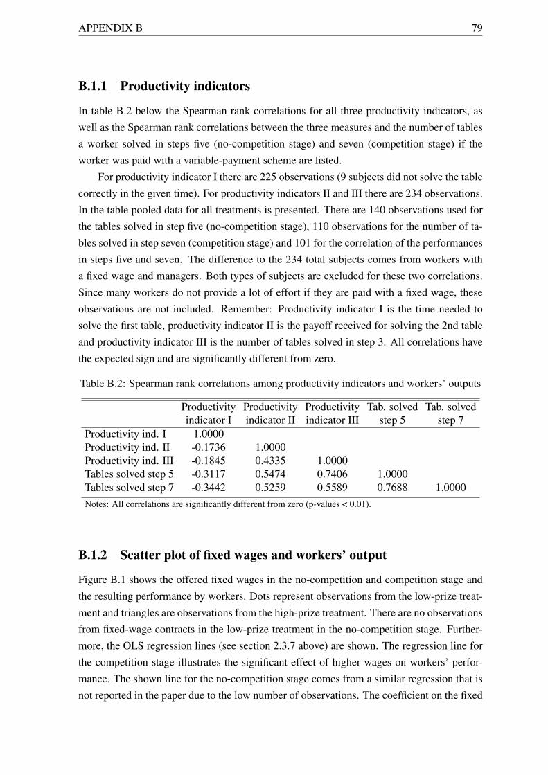
APPENDIX B 79

B.1.1 Productivity indicators

In table B.2 below the Spearman rank correlations for all three productivity indicators, aswell as the Spearman rank correlations between the three measures and the number of tablesa worker solved in steps five (no-competition stage) and seven (competition stage) if theworker was paid with a variable-payment scheme are listed.

For productivity indicator I there are 225 observations (9 subjects did not solve the tablecorrectly in the given time). For productivity indicators II and III there are 234 observations.In the table pooled data for all treatments is presented. There are 140 observations used forthe tables solved in step five (no-competition stage), 110 observations for the number of ta-bles solved in step seven (competition stage) and 101 for the correlation of the performancesin steps five and seven. The difference to the 234 total subjects comes from workers witha fixed wage and managers. Both types of subjects are excluded for these two correlations.Since many workers do not provide a lot of effort if they are paid with a fixed wage, theseobservations are not included. Remember: Productivity indicator I is the time needed tosolve the first table, productivity indicator II is the payoff received for solving the 2nd tableand productivity indicator III is the number of tables solved in step 3. All correlations havethe expected sign and are significantly different from zero.

Table B.2: Spearman rank correlations among productivity indicators and workers’ outputs

Productivityindicator I

Productivityindicator II

Productivityindicator III

Tab. solvedstep 5

Tab. solvedstep 7

Productivity ind. I 1.0000Productivity ind. II -0.1736 1.0000Productivity ind. III -0.1845 0.4335 1.0000Tables solved step 5 -0.3117 0.5474 0.7406 1.0000Tables solved step 7 -0.3442 0.5259 0.5589 0.7688 1.0000Notes: All correlations are significantly different from zero (p-values < 0.01).

B.1.2 Scatter plot of fixed wages and workers’ output

Figure B.1 shows the offered fixed wages in the no-competition and competition stage andthe resulting performance by workers. Dots represent observations from the low-prize treat-ment and triangles are observations from the high-prize treatment. There are no observationsfrom fixed-wage contracts in the low-prize treatment in the no-competition stage. Further-more, the OLS regression lines (see section 2.3.7 above) are shown. The regression line forthe competition stage illustrates the significant effect of higher wages on workers’ perfor-mance. The shown line for the no-competition stage comes from a similar regression that isnot reported in the paper due to the low number of observations. The coefficient on the fixed

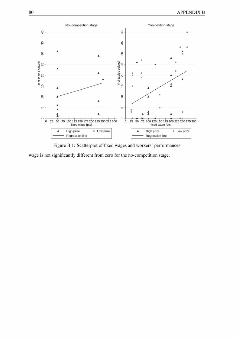
80 APPENDIX B

05

1015

2025

3035

40#

of ta

bles

sol

ved

0 25 50 75 100 125 150 175 200 225 250 275 300fixed wage [pts]


Regression line


05

1015

2025

3035

40#

of ta

bles

sol

ved

0 25 50 75 100 125 150 175 200 225 250 275 300fixed wage [pts]


Regression line

Competition stage

Figure B.1: Scatterplot of fixed wages and workers’ performances

wage is not significantly different from zero for the no-competition stage.

APPENDIX B 81

B.2 Appendix II - Instructions

Below is the translation of the German instructions for the high-prize treatment. The origi-nals are available from the author upon request. Instructions for the low-prize treatment onlydiffer in the tournament prizes and bounds for the feasible fixed wages. Instructions wereprovided on screen before each step. Since the questionnaires in steps 6 and 8 were almostidentical for workers and managers, only the question that differs for managers is includedin the translation for steps 6 and 8. All shown emphasizes are in the original instructions.

Welcome

WELCOME!

Thank you for taking part in this experiment. The experiment lasts approximately 2 hoursand you will receive your reward directly at the end of the experiment.

The experiment consists of multiple parts and at the start of each section you will see theinstructions on your screen. Each screen with instructions will be marked by the headerInstructions. If you still have questions after reading the instructions, please raise yourhand. An experimenter will come to you to answer your question in private.

In the different parts of the experiment you can earn points. At the end of the experiment allpoints are converted to Euros and result in your payment. 10 points are always 13 Cents.

Please remain quite during the experiment and do not talk to other participants. During theexperiment you will have to solve multiple exercises. You have to solve these tasks withoutany aids. Because of this, please store all your cell phones, calculators, paper, pens, booksand so one in your bag.

Please click on CONTINUE.

Step 1

Instruction Part I

It is your task to count how often the digit one appears in the table below. The table consistsof ones and zeros. You can see an example in the lower left. This table has 38 ones.

You have a total of 75 seconds. Please solve the task as quickly as possible.

Here you can enter your answer and confirm your entry.

Please click on CONTINUE. Your time starts as soon as all participants have clicked onCONTINUE and when you see the table on your screen.

82 APPENDIX B

Step 2

Instruction Part II

In this part you have to solve an identical task to the part before.

Different than before you will be paid for the correct solution of the task. Your payment islarger, the quicker you solve the task correctly. You have a total of 75 seconds. The quickeryou enter the correct number, the larger your payment. In the beginning you have 150 points.Each second that elapses until you enter the correct answer results in a deduction of 2 pointsfrom your payment.

If you take 20 seconds to solve the task you receive 110 points for this part.

If you enter a wrong number, 20 points will be deducted from the remaining points and youcan enter a new number. You will only receive a payment if you enter the correct numberwithin 75 seconds. Under no circumstances your payment can be negative.

Please click on CONTINUE. Your time starts as soon as all participants have clicked onCONTINUE and when you see the table on your screen.

Step 3

Instruction Part III

Your task in part three of the study is it to solve as many tables as possible. You will againsee a table with ones and zeros, like in the previous parts. However, now the task is not tosolve one table, but to solve as many tables as possible. A new table will only appear if youhave solved the previous one correctly.

You have a total of 5 minutes to count in as many tables as possible the number of ones.After you have entered the correct answer for a table, a new table appears. If your answer iswrong, you will see a message and you can enter a new answer.

For each correct answer you receive 8 points. Each wrong answer results in a deduction offive points from your payment.

If you solve three tables correctly and enter one wrong answer you receive 19 points for thispart of the study. The remaining time is shown in the upper right corner.

Please click on CONTINUE now. The next part starts as soon as all participants have clickedon CONTINUE.

Step 4

The working time of five minutes is over.

APPENDIX B 83

Please state as how exhausting you experienced the task in the previous part: Very easy -Very hardPlease state how much effort you exerted for the task in the previous stage: Not at all - Asmuch as possible

In total there are 18 participants in this session in two groups. You therefore belong to agroup of 9 participants. Please estimate how many participants in this group solved fewertables than you in the previous part?

Your payment for this task is larger, the better your estimate is. If you estimate is correct youreceive 75.0 points. If your estimate does not over or undershoot by more than one personyou receive 37.5 points. If your estimate over or undershoots by more than one person youdo not receive a payment for this task.

0 - No one, no participant solved fewer tables than me.

8 - I solved the most tables, all other eight participants solved fewer tables than me.

Step 5

Instruction Part IV

The instructions for part four are somewhat longer. Therefore you can go back and forthwith the Page 1 and Page 2 buttons, which are at the bottom of the screen, below the screenwith the instructions.

With the start of the next part there are two different roles in the experiment. Each participantis from now on either an employee or a manager. Despite the fact that employees and man-agers can be female as well as males, the instructions will call all managers female managers(Note: there is a gender distinction in German) while all employees are male employees.

For the next part of the experiment three participants will form a group. Each group acts inthe following part as one firm. In each firm there is one manager and two employees. Alsothe selection who will be a manager and who will be an employee is randomly determinedby the computer.

The task of the employees is, like in the previous parts, to count the number of ones in tables.For this participants have 10 minutes. Which means the working time is exactly twice thetime of the previous part.

How you will be paid for this task depends on the decision of the manager which paymentscheme to choose. The payment of the manager, however, depends mainly on the number ofcorrectly solved tables by the employees (more on this on page 2 of the instructions).

Below the tasks and the choices of managers and employees are described. Please read theseinstructions carefully and raise your hand in case you have some remaining questions after

84 APPENDIX B

reading the instructions.

Managers have three different payment schemes to choose from:

Fixed wage Variable payment Competition

Each employee gets a fixed wage.This wage is independent of thenumber of tables solved by the

employee.

Managers chooses the levelof the fixed wage. It must be at

least 50 points and can maximallybe 450 points.

Each of the two employees withina firm receives the same fixed wage.

Each employee receives for eachcorrectly solved table a payment.

Each correct answer yields anemployee 8 points.

This means the payment of theemployee only depends on thenumber of tables this employee

solved correctly.

At the end of the working periodthe employee, who solved moretables correctly, receives a wageof 450 points. Hereby it is not

relevant how many tables he solved.It is only important whether hesolved more or less tables than

the second employee in his firm.

The employee who solved fewertables receives a wage of 50

points. If both employees solvethe same number of tables alottery draw determines who

receives which wage. The paymentof a employee therefore onlydepends on whether he solved

more or less tables than the2. employee.

Instruction Part IV Page 2

The payment of managers consists of two different components.

1) Each manager receives for each correctly solved table by her employees 14 points. How-ever, she has to pay the employees with this revenue. This means from her earnings thewage payments to the employees are deducted. Here the manager has the choice betweenthe three payment schemes described on the previous page. The manager makes her choiceand workers are told the payment scheme before the start of the working period.

2) A manager receives a payment dependent on the number of tables she solves correctly.

If the manager solves more than 10, but less than 20 tables, she receives 50 points. Does shesolve more than 20 but less than 40 tables, she receives 100 points and if she solves morethan 40 tables she receives 150 points. This payment is added to her earnings.

The payment of a manager therefore depends on the number of tables solved by her workersas well as on the number of tables she solves herself.

APPENDIX B 85

Example

Assume that the manager solved 14 table herself and her employees solved 20 and 10 tables.The manager therefore receives a payment of 50 points + (20+10)*14 = 470 points.

From this payment the wages of the employees are deducted. This means, dependent on thepayment scheme, which the manager selected at the start of this part, the following wagepayments are deducted from her payment:

With the variable payment (20+10)*8 points, so a total of 240 points are deducted. With afixed wage the manager has to pay the fixed wage and with a competition she has to pay atotal of 500 points.

Quiz

In this part of the experiment, both, managers and employees, have the possibility to dosomething else besides counting ones in tables.

Below the table there will be two buttons. With the button “Quiz” a participant can switchto a window in which quiz questions are asked. With the button “Experiment” the screenswitches back to the table.

During the time a participant is on the quiz screen he or she cannot solve any tables. Theanswering of quiz questions is not paid. Each participant can go back and forth between theexperiment and the quiz during the entire working time.

When you have understood these instructions and do not have any further questions, pleaseclick on CONTINUE.

Step 6 - Questionnaire for mangers

First two questions are identical to step 4.

How many tables, do you think, have been solved by your employees?

Your payment for your estimate is larger, the better your estimate is. If your estimate iscorrect you receive 37.5 points. If your estimate is not wrong by more than plus or minusthree tables, you receive 18.8 points. If your estimate is wrong by more than three tables,you do not receive a payment for this task.

(Workers again state how many workers they believe solved less tables than they themselves.

[0-5])

86 APPENDIX B

Step 7

Instruction Part V

This part 5 is very similar to the previous one. Again managers can choose between thethree payment schemes for their employees (competition, fixed wage or variable payment).Also the payment of the managers and the working time stay the same. However, differentto before, the employees are not tied to one manager anymore.

In this part of the experiment three managers and six employees are grouped together. Eachmanager will offer a different payment scheme, which means that each payment schemewill be used by one firm. First managers choose the level of the fixed wage, which they arewilling to pay, if their firm wants / has to pay a fixed wage. Then each of the managers stateswhich payment scheme she wants the most, which one she likes second best and which oneshe likes the least.

If two (or more) managers prefer the same contract (choose the same contract as their “firstchoice”) a random draw determines who can offer this contract. After this the second choiceof the remaining managers are considered and it is tried to fulfill these choices. If again themanagers agree in their second choice one manager has to offer her third choice. Hereby thepreviously chosen fixed wage of the manager who offers a fixed wage is chosen.

After the statements of the managers (and possibly the random draw) decided, which man-ager offers which contract, the employees choose between the different contracts. Eachemployee states which of the three payment scheme he prefers most, which one would behis second choice and which one he likes the least.

Different than the statements of the managers not a random draw decides if multiple em-ployees prefer the same payment system, but the statements of an employee who solvedmore tables in part 3 are fulfilled fist. (This was the part in which each participant wasasked to solve as many tables as possible within five minutes.) According to the choicesof the employees each manager again receives two employees. Each firm therefore againconsists of one manager and two employees.

Summary

Managers again receive 14 points for each table that was correctly solved by one of heremployees. From this payment they have to pay the wage of their employees.

The same three payment schemes as in the part before are possible: Variable payment, com-petition or a fixed wage. The details of the payment schemes of the three methods also havenot changed, e.g. the variable payment is still 8 points per table.

The split in employees and managers remains unchanged. If you have been an employee

APPENDIX B 87

before, you are also an employee in this part. Like in the part before there is again a quiz forall participants. The participation in the quiz is not paid for any participant.

Example

Each manager now states which fixed wage she would pay. Then each manager states theorder in which she would select the different payment schemes.

After these statements have been used to determine which manager offers which contract,each employee sees the choices of all three managers on his screen. Each payment schemehas a number 1-3. The employee then states the order in which they would select these threepayment methods.

The number of the method you prefer the most you please state in the field “1st Choice”,the number of the method you want as your second choice you please state in the field “2ndChoice” and in the field “3rd choice” you state the method you like the least.

Please click on CONTINUE, once you have understood these instructions.

Selection of fixed wage - managers

Your role in this study is unchanged. This means you are still a manager.

Please select now which fixed wage you pay to your employees in case you want / have tooffer a fixed wage in this part.

Reminder: Different than before employees are not directly linked to a manager. This meansworkers see your wage offer, as well as the contracts of the other managers. Each manageroffers a different contract, this means that if you offer a fixed wage, the other two managersoffer a competition and a variable payment.

Please select the level of the fixed wage for your workers [in points]:

Reminder: You receive 14 points for each table that is correctly solved by one of youremployees. If you select a fixed wage, each employee receives the same wage, independentof the number of tables he solved. In the variable payment from the 14 points 8 points go tothe employee. In the competition the employee who solved more tables receives 450 pointsand the employee who solved fewer tables receives 50 points.

Selection of managers

Possibility 1: Fixed wage of X points

Possibility 2: Variable payment

Possibility 3: Competition

88 APPENDIX B

1st choice, 2nd choice, 3rd choice

Reminder: You receive 14 points for each table that is correctly solved by one of youremployees. If you select a fixed wage, each employee receives the same wage, independentof the number of tables he solves. In the variable payment from the 14 points 8 points go tothe employee. In the competition the employee who solved more tables receives 450 pointsand the employee who solved fewer tables receives 50 points.

Worker selection screen

The three managers of your group offer the following contracts:

Offer 1: Fixed wage Offered wage: X points

Offer 2: Competition

Offer 3: Variable payment

Please select your favorite order of the contracts. The higher you rank an offer, the likelier itis that you will receive this offer.

Enter the number of the offer you like best in the first field, the number of the second bestoffer in the second field and the number of the contract you like least in the third field.

Step 8 - Questionnaire

Identical to Step 6 above.

Step 9 - Questionnaire

Questionnaire page 1 of 3

In the questions on this page you play for real money. Below you see 10 bets we offer you.Please decide in each row whether you want bet A (left column) or bet B (right column).

Please indicate now in each row, whether you want the left or the right bet.

Once you have finished the questionnaire, we will play out one of the 10 bets. This means arandom draw will determine which row we will play. In the selected row, we will play thebet you have chosen.

Example

e.g. in the first row you have the choice between bet A, which pays 2 Euros with 10%probability and with 90% 1.60 Euro. You can also choose bet B, which pays with 10%probability 3.85 Euros and with 90% 0.10 Euro.

APPENDIX B 89

Bet A Bet B10% chance of winning 2 Euro and 90% of 1.60 Euro. Bet A / B 10% chance of winning 3.85 Euro and 90% of 0.10 Euro.20% chance of winning 2 Euro and 80% of 1.60 Euro. Bet A / B 20% chance of winning 3.85 Euro and 80% of 0.10 Euro.30% chance of winning 2 Euro and 70% of 1.60 Euro. Bet A / B 30% chance of winning 3.85 Euro and 70% of 0.10 Euro.40% chance of winning 2 Euro and 60% of 1.60 Euro. Bet A / B 40% chance of winning 3.85 Euro and 60% of 0.10 Euro.50% chance of winning 2 Euro and 50% of 1.60 Euro. Bet A / B 50% chance of winning 3.85 Euro and 50% of 0.10 Euro.60% chance of winning 2 Euro and 40% of 1.60 Euro. Bet A / B 60% chance of winning 3.85 Euro and 40% of 0.10 Euro.70% chance of winning 2 Euro and 30% of 1.60 Euro. Bet A / B 70% chance of winning 3.85 Euro and 30% of 0.10 Euro.80% chance of winning 2 Euro and 20% of 1.60 Euro. Bet A / B 80% chance of winning 3.85 Euro and 20% of 0.10 Euro.90% chance of winning 2 Euro and 10% of 1.60 Euro. Bet A / B 90% chance of winning 3.85 Euro and 10% of 0.10 Euro.100% chance of winning 2 Euro and 0% of 1.60 Euro. Bet A / B 100% chance of winning 3.85 Euro and 0% of 0.10 Euro.

We add the money you earn to your total income of the study.


How well did you like the task in this experiment? Not at all - - - - - - - Very good

As how difficult did you perceive the task in this experiment? Very easy - - Very difficult

How well did you like the entire experiment? Not at all - - - - - - - Very good

How fair do you consider the following payment schemes for a worker in parts 4 and 5?

Fixed payment of 100 points Very unfair - - - - - - - Very fair




Variable payment of 8 points per table Very unfair - - - - - - - Very fair

Competition with 450 points for the best worker and 50 for the otherVery unfair - - - - - - - Very fair


Please state your Abitur grade: If your highest school diploma is not a German Abitur e.g.Matura, A-levels, ... please state a 0 in the field.

Please state your final high school math grade: If your final math grade was not in theGerman 15 point system please state a 0.

Please state your final high school German grade: If your final German grade was not in theGerman 15 point system please state a 0.

Please state the year of your highest high school certificate:

Please state your gender: female - - male

Are you currently enrolled in a University / University of Applied Science? Yes - No

Are you working at a University / University of Applied Science?(e.g. as teaching or research assistant, doctoral student or employee) Yes - No

Do you have a job outside of the university? [e.g. employee, teacher, servant, ... ] Yes - No

90 APPENDIX B

Chapter 3

Flip a coin or vote: An Experiment on Choosing Group De-cision Rules1

with Sander Renes

3.1 Introduction

Before a group or society can take a decision, whether it is about what restaurant to visit,or whether to implement a social security reform, the group has to select a decision rule toaggregate individual preferences. To maximize the value of the final decision to the group,its members should agree on a mechanism that maps the vector of individual preferences intoan efficient decision. However, in a seminal paper Myerson and Satterthwaite (1983) showthat if individuals are privately informed about their preferences over outcomes, there is noefficient decision rule that is unanimously preferred over the non-implementation status quo.If a participant can force non-implementation, she2 should do so whenever she learns thatthe (proposed) decision rule can lead to outcomes she likes less than the status quo. Becauseof the existence of an outside option (the status quo), some individuals are better off notparticipating in the efficient mechanism at all. In this paper we address the problem of (ef-ficient) mechanism selection in a group decision experiment. We study binary comparisonsbetween four decision rules and investigate the role of different outside options and privateinformation on subjects’ mechanism choices.

In a collective decision about the implementation of an indivisible public project, an op-timal mechanism results in implementation if the sum of individual valuations is larger thanzero. While such mechanisms exist and groups can in theory replace any existing mecha-

1We appreciate the comments and the advice received from Dirk Engelmann, Hans Peter Grüner, EckhardJaneba, Henrik Orzen, the participants at the ESA conference in Heidelberg, the SEET meeting in Malta, theseventh Bavarian Micro Day in Passau and seminar participants in Mannheim, Nuremberg and Rotterdam.Financial support from the German research foundation (DFG), SFB 884 is gratefully acknowledged. Allremaining errors are our own.

2 For better readability only female pronouns are used.

91

92 CHAPTER 3

nism by a more efficient one, other mechanisms are often selected in practice. The theoreticalliterature has identified private information and outside options as key aspects of the mech-anism choice situation that determine whether an efficient mechanism can be implemented.Comparing Myerson and Satterthwaite (1983), Schmitz (2002), Segal and Whinston (2011),and Grüner and Koriyama (2012) shows that, if individuals can better serve their interest inan inefficient alternative than in the efficient mechanism, they have no reason to select theefficient mechanism. Additionally, the Myerson-Satterthwaite theorem illustrates that anyindividual with private information about her project payoff should use this information todetermine her preferences over the mechanisms. Individuals that dislike the public projectoften have a better chance of blocking the project in an inefficient mechanism, and thereforeare worse off under the efficient mechanism.

In this paper we study the influence of both of these aspects on individuals’ mecha-nism choices. We conduct an experiment with a two-stage voting procedure in a collectivedecision making situation. In the first stage (mechanism choice), individuals select their pre-ferred decision rule from two available mechanisms. In the second stage, each three-persongroup applies the chosen mechanism to determine the group decision on the provision ofan indivisible public good (implementation decision). By varying the distribution of privatevaluations for the public good between treatments and the available mechanisms betweenrounds, we investigate the role of the outside option on the mechanism choice. Furthermore,we vary the moment at which the private information about the individual project payoffsis revealed within treatment. This design enables us to test the relationship between pref-erences and the revelation of private information within subject. Understanding how therevelation of private information alters choices, can help us to shed light on problems thatoccur in many choice institutions. Since in many real-life situations decision rules can be al-tered in the interim stage where individuals have private information, we consider this aspectparticularly important.

In our experiment the mechanism selection is done via a random dictator procedure.We ask subjects to declare their preferred mechanism out of 2 options. After each subjecthas selected her preferred mechanism in the first stage, one group member is randomlychosen in stage two and her preferred mechanism is implemented as the group decisionrule. While this random dictator rule is neither an optimal nor a realistic procedure, it elicitsthe willingness to participate in a mechanism without any distortions. It ensures incentivecompatibility, while it allows us to present the required choices in a randomized order tominimize presentation or order effects. The four group decision rules we use are: the SimpleMajority (SM) mechanism, a first-best optimal direct revelation game known as the Arrow,d’Aspremont Gérard-Varet (AGV) mechanism,3 the Non-implementation Status Quo (NSQ)and the flip of a fair coin, or Random implementation (RAND). Since this two-stage voting

3 This mechanism is also known as the expected externality mechanism. It was originally proposed inArrow (1979) and d’Aspremont and Gérard-Varet (1979).

CHAPTER 3 93

procedure is a game of imperfect information, there are several measures of efficiency thatcould be relevant. We measure efficiency through realized values, and thus efficiency refersto ex-post classical efficiency.

With the chosen design we can conduct a strong within-subject test of the Myerson-Satterthwaite theorem by comparing subjects’ mechanism choices in an ex ante and an ad-interim stages. Ex ante, an uninformed individual should prefer the more efficient mecha-nism. Ad interim, if she knows she has a negative payoff from project implementation, thesame individual should prevent the use of any mechanism that allows for project implemen-tation, and thus prefer NSQ. By changing the two available mechanisms between rounds,we can test the predictions of Schmitz (2002), Segal and Whinston (2011), and Grüner andKoriyama (2012) that participation constraints are less binding if the outside option includesrisky outcomes. The variation of the potential valuations for the public good over treatmentsallows us to demonstrate that the observed change in preferences is driven by changes inexpected payments.

Our results demonstrate that without private payoff information individuals select ef-ficient mechanisms. Subjects choose the more efficient mechanism because it yields thelargest expected payoff ex ante. Ad interim, when they are informed about their valuationfor the project, they only prefer the (more) efficient mechanisms if they have a positive pri-vate valuation, otherwise they opt for the non-implementation status quo whenever possible,exactly as predicted by Myerson and Satterthwaite (1983). Interestingly, we find indicationsthat the differences in expected payoffs from the mechanisms as they are played in the lab,strongly influence the choices made. These results illustrate the importance of thinking aboutthe decision rule to use in a group, or committee, before this group faces any actual deci-sions. Deciding upon a decision rule after an issue comes up is very inefficient. This effectis, for instance, sometimes clearly observed in hiring committees at universities and researchinstitutes. Committees that fail to agree upon a decision rule before meeting the candidates,will likely have different subgroups within the committee that favor different candidates. Inthe ensuing discussion, the subgroups can propose the criteria that favor their preferred can-didate. With different preferred candidates this will lead to a discussion about what set ofcriteria to use, and a costly delay of the decision or even a failure to hire a suitable candidateis likely.

Our results from the ad-interim stage suggest that it can be feasible to implement an ef-ficient mechanism as long as the outside option yields uncertain results. With a risky outsideoption, individuals who know they do not want to implement the public project have no guar-anteed way of blocking the implementation. In the absence of a secure non-implementationoption, these subjects prefer the (more) efficient mechanism because it allows them to influ-ence outcomes. Since both subjects with positive and subjects with negative valuations ofthe public project prefer to have influence over the outcome, agreements on efficient mech-anisms are possible. These results support the predictions of Schmitz (2002), Segal and

94 CHAPTER 3

Whinston (2011), and Grüner and Koriyama (2012).With a safe, non-implementation status quo, our three-person groups are already severely

hindered in implementing an efficient mechanism. Public projects and reforms usually re-quire all involved individuals to cooperate, pay part of the price (through taxes for instance),permit use of their resources or even the reorganization (or removal) of their property rights.In a completely voluntary setting the kind of inertia caused by a non-implementation sta-tus quo in our experiment, would make public projects virtually impossible to negotiate.Simultaneously, virtually all decision bodies require a proposal be brought up for consider-ation before they can change the status quo, such that this type of inertia can occur virtuallyeverywhere.

In many situations the mechanism choice takes place when agents are already informedabout their preferences over outcomes and the outside option is fixed by the existing sit-uation. If the existing situation does not involve an efficient mechanism the group mightneed coercive power to force individual members to cooperate. As a consequence, our re-sults provide a rationale for the role of coercive power in group decisions. By forcing groupmembers to participate in individual projects, the group surplus can be increased since indi-vidual projects no longer need to satisfy all participation constraints. If an entity has coercivepower, the participation constraints of individuals become less relevant. Furthermore, our re-sults also provide evidence that specifying decision procedures in constituting documents is agood idea. By setting a standard procedure and demanding that these procedures can only bechanged through a considerably more demanding procedure, the drafters of the constitutionensure that the mechanisms are de facto established in an ex-ante stage.

The rest of the paper is organized as follows: section 3.2 summarizes the previous re-search on group mechanism choices and participation constraints and section 3.3 outlinesthe experimental design and the three treatments. Section 3.4 states the theoretical predic-tions, while section 3.5 describes the results on all predictions and discusses further findings.Finally, section 3.6 concludes.

3.2 Related literature

Our setup is most closely related to the literature discussing the choice of voting rules orconstitutions. The discussion on constitutional choice features two (connected) ideas: sta-bility and inertia. Since these constitutions contain many meta-rules, changing them oftenis undesirable. In a seminal contribution Barbera and Jackson (2004) show that a consti-tution that specifies the same simple majority rule to implement policy and to change theconstitution, can be hijacked by self-interested majorities. To ensure a stable constitution,it has to adhere to a property these authors call self-stability. Under the rules set-out by theconstitution, the society should not decide to change the constitution. Requiring a qualifiedmajority to change the constitution is an easy way to create more self-stability. A similar

CHAPTER 3 95

idea is proposed in an explicitly dynamic setting by Acemoglu et al. (2012). Given someconstraints that guarantee sufficient patience and prevent Condorcet-like voting cycles, theseauthors show that the stability of the constitution crucially depends on the set of other dy-namically stable constitutions. As long as no winning coalition can be found that prefersanother stable constitution, the state is stable. In this sense the set of stable coalitions formlong-term outside options that should not be preferable to the agents. These results do notimply, however that the self-stable states are efficient (especially in the short-run). In fact, theauthors argue that the inefficiencies in self-stable states could cause several of the seeminglycostly problems observed in many systems.

Inertia is the central concept in a second strand of research, the social choice literature.This, mostly theoretical, literature is riddled with impossibility theorems that show it is notpossible to design a social choice rule, or an implementing mechanism that combines someset of desirable properties in every imaginable circumstance. The most famous impossibilityresult by Arrow (1950) states that non-dictatorship, Pareto efficiency and independence ofirrelevant alternatives cannot be obtained by any social choice function for all potential pref-erence profiles. In similar vein, Myerson and Satterthwaite (1983) show that even in a settingwith only two players and independent valuations, an efficient, interim incentive compatibleand budget neutral mechanism for trade does not exists, as long as players can guaranteethemselves a sufficiently large payoff when not trading.4 The result that individual rational-ity, incentive compatibility and budget balance are incompatible for a N-player public goodsetting, of which our experiment is a special case, was proven by Mailath and Postlewaite(1990). Similar results are obtained by Güth and Hellwig (1986, 1987) for the private supplyof a public good. When the mechanism to decide on production levels is selected througha veto rule (i.e. unanimous acceptation), efficient production cannot be reached unless asubsidy is provided. These impossibility results illustrate how a certain non-implementationstatus quo can stifle any chance of (efficient) mechanism change.

Several papers have derived possibility results that illustrate the dependence of impos-sibility results on the assumptions on the status quo that occurs if the mechanism is rejected.Cramton et al. (1987) show with a status quo of a more or less equal distribution of the good(ownerships rights in their setting), it is possible to design an auction like procedure thatis both ad interim incentive compatible and ex-post efficient, without requiring subsidies.Schmitz (2002) shows that decisions on public good provisions can be made through an ef-ficiently designed mechanism for some particular status quo settings. In many cases a statusquo, either an interim allocation or a probability of implementation between 0 and 1, canbe found that allows an efficient implementation and does not violate the incentive compati-bility constraints at the interim stage. In case the valuation of the public good is identically

4 An older, less general result can be found in Chatterjee (1982), while a more general statement can befound in a.o. Segal and Whinston (2014). The interpretation in this paper is mostly due to Cramton et al.(1987).

96 CHAPTER 3

and independently distributed, such a status quo can always be found. This implies that bothin the bargaining game of Myerson and Satterthwaite (1983) and in a public good provisionproblem, a status quo exists that will incentivize individuals to accept an efficient mecha-nism ad interim. Segal and Whinston (2011) make a similar point by demonstrating howbackground risk, or a status quo that is not quite as secure as the no-trade outcome, canincrease the willingness of individuals to accept mechanism changes. Most importantly forour paper, their proposition 1 states that individuals are willing to accept a more efficientmechanism, if it has the same equilibrium distribution over allocations as the status quo, ordefault mechanism. Grüner and Koriyama (2012) illustrate that it is even possible for groupsto shift from a (simple) majority voting system to the AGV mechanism, without violatinginterim participation constraints. This result is quite remarkable, since majority systems aremuch more efficient than a fixed or random status quo. The efficiency gains of moving to theAGV are therefore limited. However, for some settings and distributions the gains are largeenough to compensate individuals for the potential loss in information rents.

Two closely related experimental papers study the effect of social preferences on mecha-nism choice. Bierbrauer et al. (2014) identify the theoretically optimal mechanism assumingsocial preferences of the players exist. Their experiment shows that choices for a small, butsignificant number of subjects, are better explained by including other-regarding preferences.They also illustrate that if enough of such subjects are present, the optimal mechanism withstrictly self-interested rational players is no longer optimal to a social planner. The articlemost closely related to ours is Engelmann and Grüner (2013). In their experiments, groupsof five subjects select their preferred mechanism out of 5 potential voting mechanisms. Thevoting mechanisms differ in the amount of positive votes required for implementation of acommon project. Individuals differ in their utility from project implementation (utility isequal to zero if it is not implemented). A completely self-interested and rational subjectshould always opt for the voting rule that requires only one (all five) vote(s) for implemen-tation, if she has a positive (negative) valuation of implementation, while voting positively(negatively) in the implementation decision. However, the authors find that subjects oftenchoose mechanisms that require two, three or four positive votes for implementation. Thesedeviations could be explained by efficiency or pro-social concerns in the mechanism choicestage. The authors note that this implies possible efficiency gains in decision making byletting groups vote on voting rules, before they vote on issues. If individuals indeed decideupon mechanisms with more efficiency/equality related criteria then they use for implemen-tation decisions, participation constraints are less binding.

3.3 Experimental design

We first describe the game subjects participated in and explain the mechanisms used. Wethen outline the treatments and describe the procedures of the experiment. The only differ-

CHAPTER 3 97

ence between treatments is the set of potential private valuations for the public project. Theunderlying procedures, game and all other details of the experiment, e.g. number of rounds,group size, available mechanisms, etc. are identical across all treatments.

3.3.1 The game

Subjects interact in groups of three and each group faces the question whether or not to im-plement an indivisible public project. Non-implementation results in a zero payoff for allsubjects. If the project is implemented each player receives a project payoff equal to her val-uation. The private valuations are drawn independently from a known uniform distributionon a given set of four values that depend on the treatment. The distribution and its supportare common knowledge and remain the same within a session.

Each of the 18 experimental rounds proceeds in two steps. First, subjects select a mech-anism to make the group decision. Second, the group decides about the implementation ofthe public project through the chosen mechanism. In all treatments the same four mecha-nisms are used and in each round subjects chose between two of them. The mechanisms weconsider are:

Mechanism I AGV mechanismAll group members report a valuation for the implementation of the project. Theycan only report valuations that are present in the type space. If the sum of reportedvaluations is larger than zero the project is implemented, otherwise the project is notimplemented. Independent of project implementation, subjects pay or receive a trans-fer that depends on the vector of reported valuations.

Mechanism II Voting - Simple Majority (SM)All group members vote for or against the project (no abstention). If two or more groupmembers vote for implementation the project is implemented, otherwise the project isnot implemented.

Mechanism III Non-implementation Status Quo (NSQ)The public project is not implemented.

Mechanism IV Random implementation (RAND)Whether the public project is implemented depends on the flip of a fair coin. If theresult of the coin toss is heads, the project is implemented otherwise the project isnot implemented. Therefore this mechanism has a 50% probability of implementationindependent of subjects’ valuations.

At the beginning of a round subjects are informed about the two available mechanisms.They cannot influence which mechanisms are available in a round, and the order of thecomparisons is randomly altered between sessions. Each subject privately selects one of

98 CHAPTER 3

the two given mechanisms. After mechanism choices have been recorded, the computerrandomly picks one group member as the dictator and the mechanism chosen by this randomdictator is executed. All group members are informed of the selected mechanism, but theydo not learn whose choice was selected nor what mechanism the other two subjects selected.

If the AGV or SM mechanism is selected, all group members state a valuation for theproject (AGV) or vote on the implementation of the project (SM). If the NSQ or RANDmechanism is selected no further action by the subjects is required. The computer deter-mines whether the project is implemented through the selected mechanism and payoffs arerealized accordingly. The project payoff is equal to the private valuations if the project isimplemented, otherwise the project payoffs are 0. In the AGV subjects additionally pay orreceive transfers that depend on the reported valuations but not on project implementation.

The experiment proceeds in two parts. In the first part, the first twelve rounds, subjectslearn their private valuation for the public project ad interim that is, after choosing theirpreferred mechanism but before the mechanism is played. In part two, the last six rounds,subjects are informed about their private valuation for the project at the start of each roundand therefore are aware of their valuation when choosing a mechanism. Subjects are neverinformed about valuations of other subjects. Our subjects face all six possible binary mech-anism choices twice in the ex-ante condition (rounds 1-12), before going to the ad-interimrounds (rounds 13-18). Since subjects make the mechanism choice both in an ex ante and anad-interim setting, we can compare mechanism choices in both settings within subjects.

By design, the choices in the ex-ante rounds are not influenced by previous experiencesin the ad-interim rounds. Since we consider the expected value calculations to be more de-manding in the ex-ante rounds than in the ad-interim rounds, we chose a design that deliversthe cleanest decisions in the ex-ante rounds as our main treatment. Because we did not ob-serve any signs of consistency concerns or order effects in the choices made by our subjects,we did not conduct sessions with a reversed order.

The design is in many aspects similar to the two-step voting procedure studied by En-gelmann and Grüner (2013), but there are three important differences. First, in our studysubjects choose between two mechanisms rather than five. This clearly identifies the outsideoption. Second, we have four very different mechanisms, rather than five mechanisms fromthe class of simple voting rules. This allows us to make the same comparisons studied inthe theoretical papers. We describe the mechanisms used and the reasons for selecting thesefour mechanism in the next section. Third, Engelmann and Grüner (2013) did not look atthe effects of private information on the behavior of subjects. As we show in this paper, thepresence of private information fundamentally changes the choices made by our subjects.

CHAPTER 3 99

3.3.2 The four mechanisms

The four mechanisms are chosen because of their theoretical implications and relevancefor group decision making. The AGV mechanism, or expected externality mechanism, is thetheoretically optimal mechanism for decisions about indivisible public projects, like reforms.It is incentive compatible, ex-post budget balanced and induces efficient implementation. Itwas first suggested by Arrow (1979) and d’Aspremont and Gérard-Varet (1979) who alsogive a formal proof of its properties. The AGV is a direct revelation game in which allindividuals send a message from the type space (they can behave like other types but notinvent new types). Based on the reports the surplus generated by the project is calculatedand the project is implemented if and only if the reported surplus is positive. If individualsreport truthfully, this leads to efficient project implementation. To ensure truthful reports, themechanism calls for transfers equal to the expected externality an individual generates forthe others with her reported valuation.5 This forces individuals to take the expected surplusgenerated for the other players into account, and makes all individuals residual claimants ofa value equal to their expected societal surplus (their own surplus, plus the expected surplusgenerate for others). Consequently, they should send the message resulting in the highestexpected social surplus. Since the mechanism leads to efficient implementation decisions ifall subjects report truthfully, this induces truthful reporting of all types. Because it combinesincentive compatibility with efficiency and budget balance, the AGV provides the theoreticalbenchmark to compare other mechanisms to. If it is impossible to switch from a givenmechanism to the most efficient mechanism, the AGV, a switch to any other (less efficient)mechanism is unlikely.

The SM mechanism is chosen for two reasons. First, it is a common mechanism usedin committee and small group decision making and therefore provides a natural benchmarkfor the empirical performance of the AGV. Second, the comparison between AGV and SMis the focus of the possibility theorem in Grüner and Koriyama (2012), such that we needit to reproduce the theoretical situation. The other two mechanisms, NSQ and RAND, arechosen to reproduce the comparisons studied in Myerson and Satterthwaite (1983), Schmitz(2002), and Segal and Whinston (2011).

3.3.3 Treatments

In all treatments a uniform distribution over a type space with four possible valuations forthe public project is used. We have one treatment with a symmetric and two treatments withskewed distributions. The two skewed treatments differ from the symmetric treatment in thevaluation of a single type. The type spaces and distributions used are shown in table 3.1

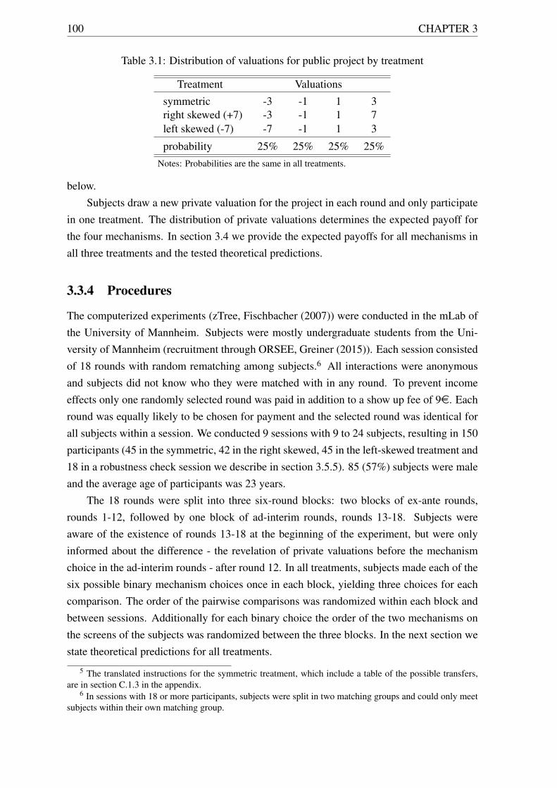
100 CHAPTER 3

Table 3.1: Distribution of valuations for public project by treatment

Treatment Valuations

symmetric -3 -1 1 3right skewed (+7) -3 -1 1 7left skewed (-7) -7 -1 1 3

probability 25% 25% 25% 25%Notes: Probabilities are the same in all treatments.

below.Subjects draw a new private valuation for the project in each round and only participate

in one treatment. The distribution of private valuations determines the expected payoff forthe four mechanisms. In section 3.4 we provide the expected payoffs for all mechanisms inall three treatments and the tested theoretical predictions.

3.3.4 Procedures

The computerized experiments (zTree, Fischbacher (2007)) were conducted in the mLab ofthe University of Mannheim. Subjects were mostly undergraduate students from the Uni-versity of Mannheim (recruitment through ORSEE, Greiner (2015)). Each session consistedof 18 rounds with random rematching among subjects.6 All interactions were anonymousand subjects did not know who they were matched with in any round. To prevent incomeeffects only one randomly selected round was paid in addition to a show up fee of 9e. Eachround was equally likely to be chosen for payment and the selected round was identical forall subjects within a session. We conducted 9 sessions with 9 to 24 subjects, resulting in 150participants (45 in the symmetric, 42 in the right skewed, 45 in the left-skewed treatment and18 in a robustness check session we describe in section 3.5.5). 85 (57%) subjects were maleand the average age of participants was 23 years.

The 18 rounds were split into three six-round blocks: two blocks of ex-ante rounds,rounds 1-12, followed by one block of ad-interim rounds, rounds 13-18. Subjects wereaware of the existence of rounds 13-18 at the beginning of the experiment, but were onlyinformed about the difference - the revelation of private valuations before the mechanismchoice in the ad-interim rounds - after round 12. In all treatments, subjects made each of thesix possible binary mechanism choices once in each block, yielding three choices for eachcomparison. The order of the pairwise comparisons was randomized within each block andbetween sessions. Additionally for each binary choice the order of the two mechanisms onthe screens of the subjects was randomized between the three blocks. In the next section westate theoretical predictions for all treatments.

5 The translated instructions for the symmetric treatment, which include a table of the possible transfers,are in section C.1.3 in the appendix.

6 In sessions with 18 or more participants, subjects were split in two matching groups and could only meetsubjects within their own matching group.

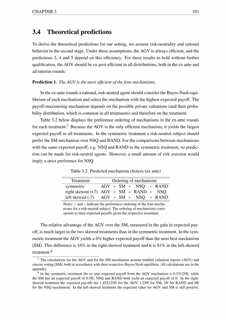
CHAPTER 3 101

3.4 Theoretical predictions

To derive the theoretical predictions for our setting, we assume risk-neutrality and rationalbehavior in the second stage. Under these assumptions, the AGV is always efficient, and thepredictions 2, 4 and 5 depend on this efficiency. For these results to hold without furtherqualification, the AGV should be ex-post efficient in all distributions, both in the ex ante andad-interim rounds:

Prediction 1. The AGV is the most efficient of the four mechanisms.

In the ex-ante rounds a rational, risk-neutral agent should consider the Bayes-Nash equi-librium of each mechanism and select the mechanism with the highest expected payoff. Thepayoff-maximizing mechanism depends on the possible private valuations (and their proba-bility distribution, which is common in all treatments) and therefore on the treatment.

Table 3.2 below displays the preference ordering of mechanisms in the ex-ante roundsfor each treatment.7 Because the AGV is the only efficient mechanism, it yields the largestexpected payoff in all treatments. In the symmetric treatment a risk-neutral subject shouldprefer the SM mechanism over NSQ and RAND. For the comparisons between mechanismswith the same expected payoff, e.g. NSQ and RAND in the symmetric treatment, no predic-tion can be made for risk-neutral agents. However, a small amount of risk aversion wouldimply a strict preference for NSQ.

Table 3.2: Predicted mechanism choices (ex ante)

Treatment Ordering of mechanismssymmetric AGV ≻ SM ≻ NSQ ∼ RANDright skewed (+7) AGV ≻ SM ≻ RAND ≻ NSQleft skewed (-7) AGV ≻ SM ≻ NSQ ≻ RAND

Notes: ≻ and ∼ indicate the preferences ordering of the four mecha-nisms for a risk-neutral subject. The ordering of mechanisms corre-sponds to their expected payoffs given the respective treatment.

The relative advantage of the AGV over the SM, measured in the gain in expected pay-off, is much larger in the two skewed treatments than in the symmetric treatment. In the sym-metric treatment the AGV yields a 6% higher expected payoff than the next best mechanism(SM). This difference is 16% in the right-skewed treatment and it is 81% in the left-skewedtreatment.8

7 The calculations for the AGV and for the SM mechanism assume truthful valuation reports (AGV) andsincere voting (SM), both in accordance with their respective Bayes-Nash equilibria. All calculations are in theappendix.

8 In the symmetric treatment the ex ante expected payoff from the AGV mechanism is 0.53125e, whilethe SM has an expected payoff of 0.5e, NSQ and RAND both yield an expected payoff of 0. In the right-skewed treatment the expected payoffs are 1.452125e for the AGV, 1.25e for SM, 1e for RAND and 0efor the NSQ mechanism. In the left-skewed treatment the expected value for AGV and SM is still positive,

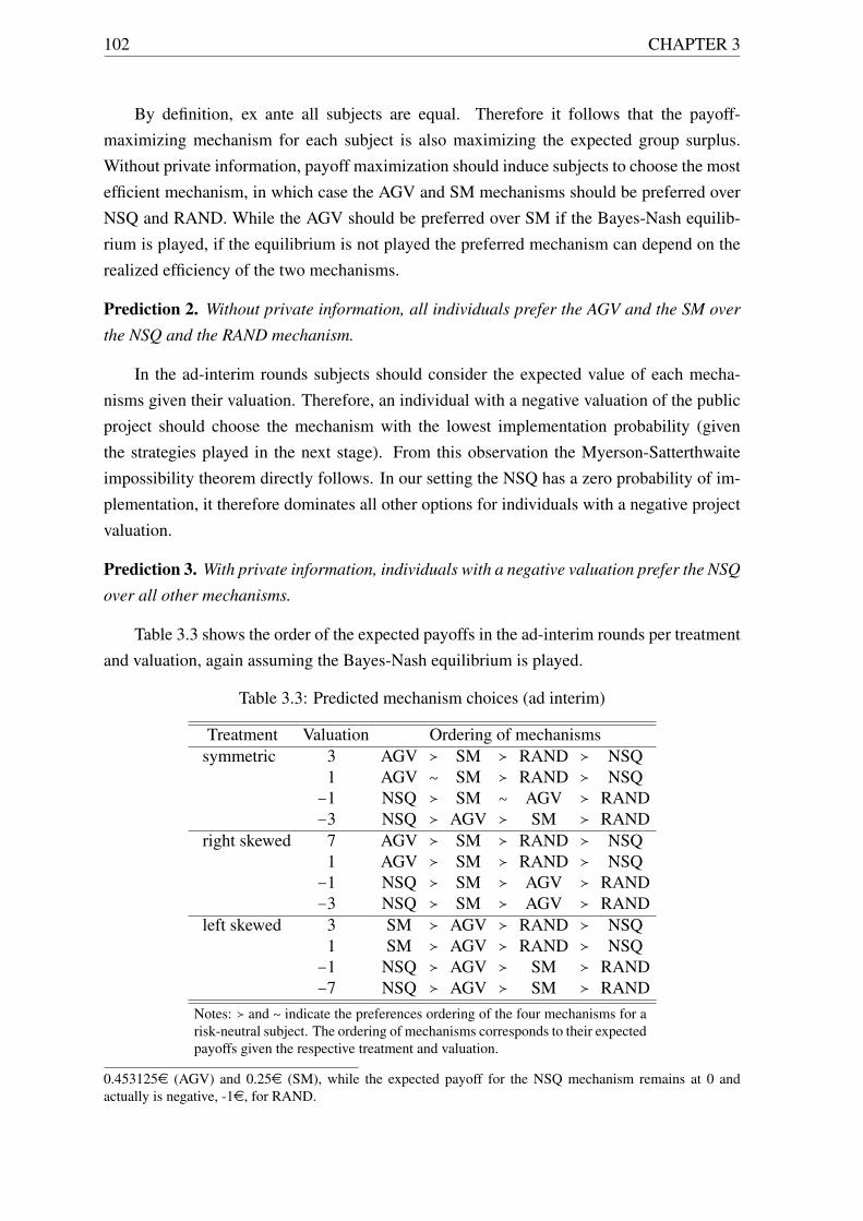
102 CHAPTER 3

By definition, ex ante all subjects are equal. Therefore it follows that the payoff-maximizing mechanism for each subject is also maximizing the expected group surplus.Without private information, payoff maximization should induce subjects to choose the mostefficient mechanism, in which case the AGV and SM mechanisms should be preferred overNSQ and RAND. While the AGV should be preferred over SM if the Bayes-Nash equilib-rium is played, if the equilibrium is not played the preferred mechanism can depend on therealized efficiency of the two mechanisms.

Prediction 2. Without private information, all individuals prefer the AGV and the SM over

the NSQ and the RAND mechanism.

In the ad-interim rounds subjects should consider the expected value of each mecha-nisms given their valuation. Therefore, an individual with a negative valuation of the publicproject should choose the mechanism with the lowest implementation probability (giventhe strategies played in the next stage). From this observation the Myerson-Satterthwaiteimpossibility theorem directly follows. In our setting the NSQ has a zero probability of im-plementation, it therefore dominates all other options for individuals with a negative projectvaluation.

Prediction 3. With private information, individuals with a negative valuation prefer the NSQ

over all other mechanisms.

Table 3.3 shows the order of the expected payoffs in the ad-interim rounds per treatmentand valuation, again assuming the Bayes-Nash equilibrium is played.

Table 3.3: Predicted mechanism choices (ad interim)

Treatment Valuation Ordering of mechanismssymmetric 3 AGV ≻ SM ≻ RAND ≻ NSQ

1 AGV ∼ SM ≻ RAND ≻ NSQ−1 NSQ ≻ SM ∼ AGV ≻ RAND−3 NSQ ≻ AGV ≻ SM ≻ RAND

right skewed 7 AGV ≻ SM ≻ RAND ≻ NSQ1 AGV ≻ SM ≻ RAND ≻ NSQ

−1 NSQ ≻ SM ≻ AGV ≻ RAND−3 NSQ ≻ SM ≻ AGV ≻ RAND

left skewed 3 SM ≻ AGV ≻ RAND ≻ NSQ1 SM ≻ AGV ≻ RAND ≻ NSQ

−1 NSQ ≻ AGV ≻ SM ≻ RAND−7 NSQ ≻ AGV ≻ SM ≻ RAND

Notes: ≻ and ∼ indicate the preferences ordering of the four mechanisms for arisk-neutral subject. The ordering of mechanisms corresponds to their expectedpayoffs given the respective treatment and valuation.

0.453125e (AGV) and 0.25e (SM), while the expected payoff for the NSQ mechanism remains at 0 andactually is negative, -1e, for RAND.

CHAPTER 3 103

Schmitz (2002) and Segal and Whinston (2011) show that by replacing the safe outsideoption with riskier ones, the impossibility problem of prediction 3 can be overcome. In ourexperiment this translates to the prediction that the AGV should be preferred over RAND,even with private information. Similarly, since with a three-person group and the chosendistributions the SM mechanism is much more efficient than the RAND mechanism, allsubjects should choose the SM over the RAND mechanism.

Prediction 4. With private information

(i) all individuals prefer the AGV over the RAND mechanism and

(ii) all individuals prefer the SM over the RAND mechanism.

Grüner and Koriyama (2012) demonstrate that individuals can prefer the AGV over theSM, even with a negative valuation, as long as some conditions are met. Mainly because wehave odd numbered groups, these conditions do not always hold in our setting. However,their results translate to the following qualified prediction:

Prediction 5. In the symmetric treatment

(i) subjects with a private valuation of -3 or +3 strictly prefer the AGV over the SM mech-

anism,

(ii) subjects with a private valuation of -1 or +1 are indifferent between the AGV and the

SM.

In the skewed treatments

(iii) subjects with a private valuation of -3 or -1 (right-skewed treatment) and 3 or 1 (left-

skewed treatment), strictly prefer the SM over the AGV,

(iv) while all other subjects prefer the AGV over the SM mechanism.

Additionally we test whether subjects prefer the theoretical optimal AGV mechanismover other, better known mechanisms. If subjects’ choices in the ex-ante rounds are sensitiveto expected payoff differences, the AGV mechanism should be chosen more often in theskewed treatments than in the symmetric treatment. Furthermore, the AGV transfers in theright-skewed treatment are usually paid by subjects reporting extremely high valuations.This “taxing the winner” property could be seen as fair by subjects, since an individualbenefiting strongly from project implementation has to compensate other group members.In the left-skewed treatment this “tax” is levied from the loser(s). If such fairness concernsplay a role in mechanism selection, the AGV should be more desirable in the right skewedthan the left-skewed treatment. However, we do not believe that the mechanism choicesin the ad-interim rounds will be affected, since the known private valuation for the projectshould make the own payoff consequences of the mechanism choice more focal and thereforefairness concerns might be less relevant.

Prediction 6. The AGV mechanism is chosen more often

104 CHAPTER 3

(i) in the left and right-skewed treatment than in the symmetric treatment due to efficiency

differences,

(ii) in the right-skewed treatment than in the left-skewed treatment, since subjects prefer

“winners” rather than “losers” of the project implementation to pay transfers.

(iii) Both effects are more pronounced in the ex-ante rounds then in the ad-interim rounds.

3.5 Results

We present the results in the same order as the predictions, starting with the realized effi-ciency of the AGV and the SM mechanisms before analyzing subjects’ ex-ante choices inmore detail. Next we present our findings on the Myerson-Satterthwaite impossibility theo-rem and then discuss the ad-interim mechanism choices before concluding with an analysisof subjects’ behavior in stage two of the AGV (value reports) and the SM mechanism (vot-ing).

3.5.1 Realized surplus

Whether the AGV is actually more efficient than the other mechanisms depends on subjects’behavior and especially on the question whether they truthfully report their type (AGV) andvote sincerely (SM mechanism). Theoretically the AGV is incentive compatible, such thattruthful reporting should result in equilibrium. However, we cannot assume perfectly rationalexpected-value maximization. If subjects misreport their valuation it is not clear whether theAGV actually generates the largest surplus.

We do not use the actual surplus generated in the lab as our measure of efficiency, sincethis measure is strongly influenced by the realization of private valuations as well as themechanism choices by the random dictator. Instead, we use the observed distribution of re-ports/votes made by subjects with a specific type in a treatment, as the behavioral strategy forthat type in that treatment. We calculate project implementation probabilities for all permu-tations of the type vector given these strategies. The displayed surplus (in e) is the expectedvalue of the group surplus in the mechanisms given these strategies and the probability thata particular permutation of the type vector occurs. It is therefore the surplus that would haverealized if all possible combinations of private valuations occurred with their expected prob-abilities and all individuals with the same type used the observed reporting/voting strategy.

Table 3.4 below shows the Bayes-Nash equilibrium surplus and the realized group sur-plus for the AGV or SM mechanisms in the ex-ante rounds in all treatments.9 The theoreticalsurplus of each mechanism is reported in columns 2 (AGV) and 5 (SM), the realized surplus

9 We concentrate on the ex-ante results, because we have more observations in these rounds than in thead-interim rounds, which makes the results more reliable. Although they are noisier, results for the ad-interimrounds are qualitatively similar.

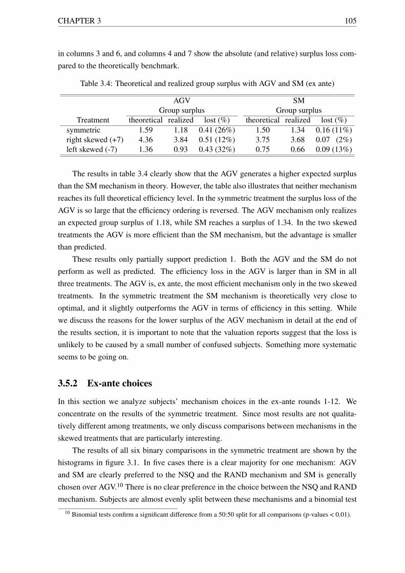
CHAPTER 3 105

in columns 3 and 6, and columns 4 and 7 show the absolute (and relative) surplus loss com-pared to the theoretically benchmark.

Table 3.4: Theoretical and realized group surplus with AGV and SM (ex ante)

AGV SMGroup surplus Group surplus

Treatment theoretical realized lost (%) theoretical realized lost (%)symmetric 1.59 1.18 0.41 (26%) 1.50 1.34 0.16 (11%)right skewed (+7) 4.36 3.84 0.51 (12%) 3.75 3.68 0.07 (2%)left skewed (-7) 1.36 0.93 0.43 (32%) 0.75 0.66 0.09 (13%)

The results in table 3.4 clearly show that the AGV generates a higher expected surplusthan the SM mechanism in theory. However, the table also illustrates that neither mechanismreaches its full theoretical efficiency level. In the symmetric treatment the surplus loss of theAGV is so large that the efficiency ordering is reversed. The AGV mechanism only realizesan expected group surplus of 1.18, while SM reaches a surplus of 1.34. In the two skewedtreatments the AGV is more efficient than the SM mechanism, but the advantage is smallerthan predicted.

These results only partially support prediction 1. Both the AGV and the SM do notperform as well as predicted. The efficiency loss in the AGV is larger than in SM in allthree treatments. The AGV is, ex ante, the most efficient mechanism only in the two skewedtreatments. In the symmetric treatment the SM mechanism is theoretically very close tooptimal, and it slightly outperforms the AGV in terms of efficiency in this setting. Whilewe discuss the reasons for the lower surplus of the AGV mechanism in detail at the end ofthe results section, it is important to note that the valuation reports suggest that the loss isunlikely to be caused by a small number of confused subjects. Something more systematicseems to be going on.

3.5.2 Ex-ante choices

In this section we analyze subjects’ mechanism choices in the ex-ante rounds 1-12. Weconcentrate on the results of the symmetric treatment. Since most results are not qualita-tively different among treatments, we only discuss comparisons between mechanisms in theskewed treatments that are particularly interesting.

The results of all six binary comparisons in the symmetric treatment are shown by thehistograms in figure 3.1. In five cases there is a clear majority for one mechanism: AGVand SM are clearly preferred to the NSQ and the RAND mechanism and SM is generallychosen over AGV.10 There is no clear preference in the choice between the NSQ and RANDmechanism. Subjects are almost evenly split between these mechanisms and a binomial test

10 Binomial tests confirm a significant difference from a 50:50 split for all comparisons (p-values < 0.01).

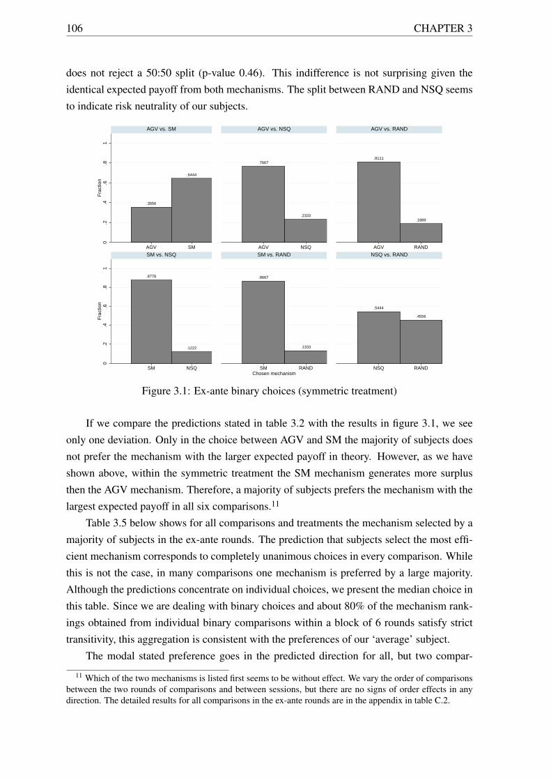
106 CHAPTER 3

does not reject a 50:50 split (p-value 0.46). This indifference is not surprising given theidentical expected payoff from both mechanisms. The split between RAND and NSQ seemsto indicate risk neutrality of our subjects.

.3556

.6444

0.2

.4.6

.81

Fra

ctio

n

AGV SM

AGV vs. SM

.7667

.23330

.2.4

.6.8

1

AGV NSQ

AGV vs. NSQ

.8111

.1889

0.2

.4.6

.81

AGV RAND

AGV vs. RAND

.8778

.1222

0.2

.4.6

.81

Fra

ctio

n

SM NSQ

SM vs. NSQ

.8667

.1333

0.2

.4.6

.81

SM RANDChosen mechanism

SM vs. RAND

.5444

.4556

0.2

.4.6

.81

NSQ RAND

NSQ vs. RAND

Figure 3.1: Ex-ante binary choices (symmetric treatment)

If we compare the predictions stated in table 3.2 with the results in figure 3.1, we seeonly one deviation. Only in the choice between AGV and SM the majority of subjects doesnot prefer the mechanism with the larger expected payoff in theory. However, as we haveshown above, within the symmetric treatment the SM mechanism generates more surplusthen the AGV mechanism. Therefore, a majority of subjects prefers the mechanism with thelargest expected payoff in all six comparisons.11

Table 3.5 below shows for all comparisons and treatments the mechanism selected by amajority of subjects in the ex-ante rounds. The prediction that subjects select the most effi-cient mechanism corresponds to completely unanimous choices in every comparison. Whilethis is not the case, in many comparisons one mechanism is preferred by a large majority.Although the predictions concentrate on individual choices, we present the median choice inthis table. Since we are dealing with binary choices and about 80% of the mechanism rank-ings obtained from individual binary comparisons within a block of 6 rounds satisfy stricttransitivity, this aggregation is consistent with the preferences of our ‘average’ subject.

The modal stated preference goes in the predicted direction for all, but two compar-

11 Which of the two mechanisms is listed first seems to be without effect. We vary the order of comparisonsbetween the two rounds of comparisons and between sessions, but there are no signs of order effects in anydirection. The detailed results for all comparisons in the ex-ante rounds are in the appendix in table C.2.

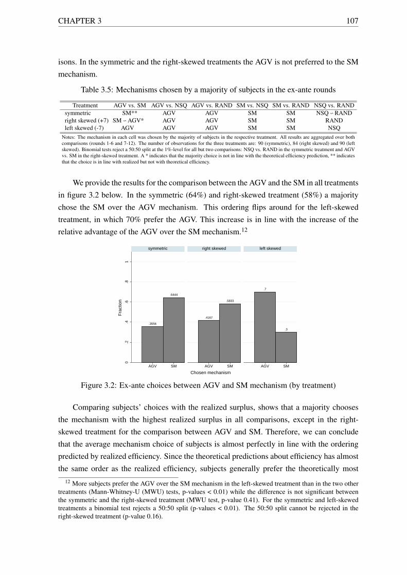
CHAPTER 3 107

isons. In the symmetric and the right-skewed treatments the AGV is not preferred to the SMmechanism.

Table 3.5: Mechanisms chosen by a majority of subjects in the ex-ante rounds

Treatment AGV vs. SM AGV vs. NSQ AGV vs. RAND SM vs. NSQ SM vs. RAND NSQ vs. RANDsymmetric SM** AGV AGV SM SM NSQ ∽RANDright skewed (+7) SM ∽AGV* AGV AGV SM SM RANDleft skewed (-7) AGV AGV AGV SM SM NSQ

Notes: The mechanism in each cell was chosen by the majority of subjects in the respective treatment. All results are aggregated over bothcomparisons (rounds 1-6 and 7-12). The number of observations for the three treatments are: 90 (symmetric), 84 (right skewed) and 90 (leftskewed). Binomial tests reject a 50:50 split at the 1%-level for all but two comparisons: NSQ vs. RAND in the symmetric treatment and AGVvs. SM in the right-skewed treatment. A * indicates that the majority choice is not in line with the theoretical efficiency prediction, ** indicatesthat the choice is in line with realized but not with theoretical efficiency.

We provide the results for the comparison between the AGV and the SM in all treatmentsin figure 3.2 below. In the symmetric (64%) and right-skewed treatment (58%) a majoritychose the SM over the AGV mechanism. This ordering flips around for the left-skewedtreatment, in which 70% prefer the AGV. This increase is in line with the increase of therelative advantage of the AGV over the SM mechanism.12

.3556

.6444

.4167

.5833

.7

.3

0.2

.4.6

.81

AGV SM AGV SM AGV SM

symmetric right skewed left skewed

Fra

ctio

n

Chosen mechanism

Figure 3.2: Ex-ante choices between AGV and SM mechanism (by treatment)

Comparing subjects’ choices with the realized surplus, shows that a majority choosesthe mechanism with the highest realized surplus in all comparisons, except in the right-skewed treatment for the comparison between AGV and SM. Therefore, we can concludethat the average mechanism choice of subjects is almost perfectly in line with the orderingpredicted by realized efficiency. Since the theoretical predictions about efficiency has almostthe same order as the realized efficiency, subjects generally prefer the theoretically most

12 More subjects prefer the AGV over the SM mechanism in the left-skewed treatment than in the two othertreatments (Mann-Whitney-U (MWU) tests, p-values < 0.01) while the difference is not significant betweenthe symmetric and the right-skewed treatment (MWU test, p-value 0.41). For the symmetric and left-skewedtreatments a binomial test rejects a 50:50 split (p-values < 0.01). The 50:50 split cannot be rejected in theright-skewed treatment (p-value 0.16).

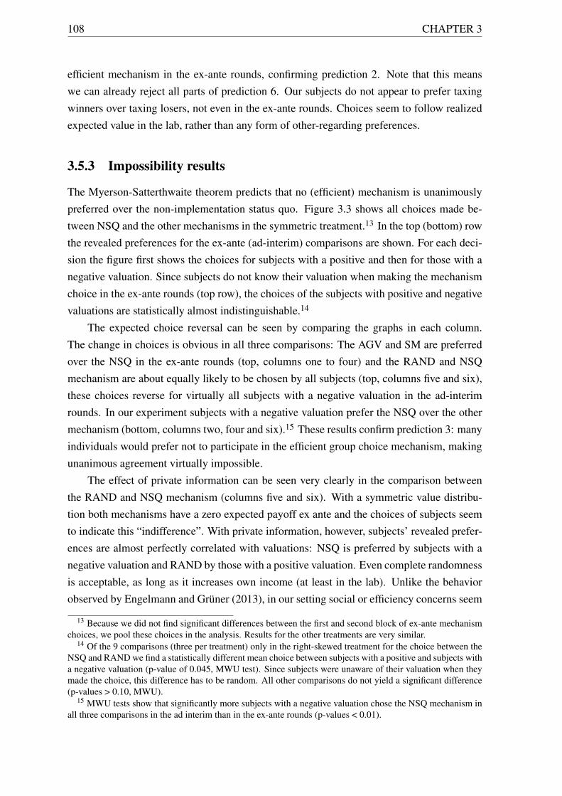
108 CHAPTER 3

efficient mechanism in the ex-ante rounds, confirming prediction 2. Note that this meanswe can already reject all parts of prediction 6. Our subjects do not appear to prefer taxingwinners over taxing losers, not even in the ex-ante rounds. Choices seem to follow realizedexpected value in the lab, rather than any form of other-regarding preferences.

3.5.3 Impossibility results

The Myerson-Satterthwaite theorem predicts that no (efficient) mechanism is unanimouslypreferred over the non-implementation status quo. Figure 3.3 shows all choices made be-tween NSQ and the other mechanisms in the symmetric treatment.13 In the top (bottom) rowthe revealed preferences for the ex-ante (ad-interim) comparisons are shown. For each deci-sion the figure first shows the choices for subjects with a positive and then for those with anegative valuation. Since subjects do not know their valuation when making the mechanismchoice in the ex-ante rounds (top row), the choices of the subjects with positive and negativevaluations are statistically almost indistinguishable.14

The expected choice reversal can be seen by comparing the graphs in each column.The change in choices is obvious in all three comparisons: The AGV and SM are preferredover the NSQ in the ex-ante rounds (top, columns one to four) and the RAND and NSQmechanism are about equally likely to be chosen by all subjects (top, columns five and six),these choices reverse for virtually all subjects with a negative valuation in the ad-interimrounds. In our experiment subjects with a negative valuation prefer the NSQ over the othermechanism (bottom, columns two, four and six).15 These results confirm prediction 3: manyindividuals would prefer not to participate in the efficient group choice mechanism, makingunanimous agreement virtually impossible.

The effect of private information can be seen very clearly in the comparison betweenthe RAND and NSQ mechanism (columns five and six). With a symmetric value distribu-tion both mechanisms have a zero expected payoff ex ante and the choices of subjects seemto indicate this “indifference”. With private information, however, subjects’ revealed prefer-ences are almost perfectly correlated with valuations: NSQ is preferred by subjects with anegative valuation and RAND by those with a positive valuation. Even complete randomnessis acceptable, as long as it increases own income (at least in the lab). Unlike the behaviorobserved by Engelmann and Grüner (2013), in our setting social or efficiency concerns seem

13 Because we did not find significant differences between the first and second block of ex-ante mechanismchoices, we pool these choices in the analysis. Results for the other treatments are very similar.

14 Of the 9 comparisons (three per treatment) only in the right-skewed treatment for the choice between theNSQ and RAND we find a statistically different mean choice between subjects with a positive and subjects witha negative valuation (p-value of 0.045, MWU test). Since subjects were unaware of their valuation when theymade the choice, this difference has to be random. All other comparisons do not yield a significant difference(p-values > 0.10, MWU).

15 MWU tests show that significantly more subjects with a negative valuation chose the NSQ mechanism inall three comparisons in the ad interim than in the ex-ante rounds (p-values < 0.01).

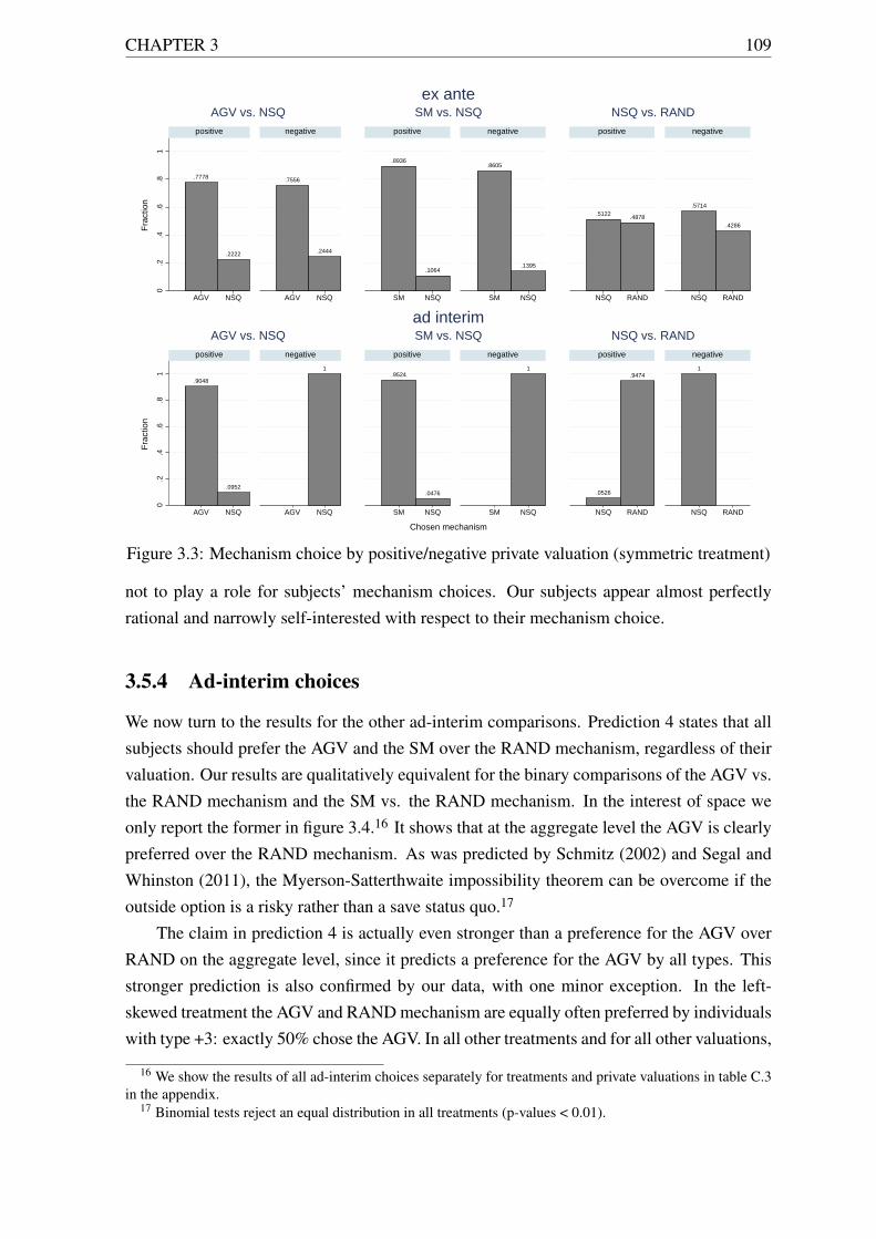
CHAPTER 3 109

.7778

.2222

.7556

.2444

0.2

.4.6

.81

AGV NSQ AGV NSQ

positive negativeF

ract

ion

AGV vs. NSQ

.8936

.1064

.8605

.1395

0.2

.4.6

.81

SM NSQ SM NSQ

positive negative

SM vs. NSQ

.5122 .4878

.5714

.4286

0.2

.4.6

.81

NSQ RAND NSQ RAND

positive negative

NSQ vs. RANDex ante

.9048

.0952

1

0.2

.4.6

.81

AGV NSQ AGV NSQ

positive negative

Fra

ctio

n

AGV vs. NSQ

.9524

.0476

1

0.2

.4.6

.81

SM NSQ SM NSQ

positive negative

Chosen mechanism

SM vs. NSQ

.0526

.94741

0.2

.4.6

.81

NSQ RAND NSQ RAND

positive negative

NSQ vs. RANDad interim

Figure 3.3: Mechanism choice by positive/negative private valuation (symmetric treatment)

not to play a role for subjects’ mechanism choices. Our subjects appear almost perfectlyrational and narrowly self-interested with respect to their mechanism choice.

3.5.4 Ad-interim choices

We now turn to the results for the other ad-interim comparisons. Prediction 4 states that allsubjects should prefer the AGV and the SM over the RAND mechanism, regardless of theirvaluation. Our results are qualitatively equivalent for the binary comparisons of the AGV vs.the RAND mechanism and the SM vs. the RAND mechanism. In the interest of space weonly report the former in figure 3.4.16 It shows that at the aggregate level the AGV is clearlypreferred over the RAND mechanism. As was predicted by Schmitz (2002) and Segal andWhinston (2011), the Myerson-Satterthwaite impossibility theorem can be overcome if theoutside option is a risky rather than a save status quo.17

The claim in prediction 4 is actually even stronger than a preference for the AGV overRAND on the aggregate level, since it predicts a preference for the AGV by all types. Thisstronger prediction is also confirmed by our data, with one minor exception. In the left-skewed treatment the AGV and RAND mechanism are equally often preferred by individualswith type +3: exactly 50% chose the AGV. In all other treatments and for all other valuations,

16 We show the results of all ad-interim choices separately for treatments and private valuations in table C.3in the appendix.

17 Binomial tests reject an equal distribution in all treatments (p-values < 0.01).

110 CHAPTER 3

the AGV receives at least 60% of all votes and in most cases it is chosen by a larger margin.18

Our results therefore clearly confirm prediction 4.

.8667

.1333

.7619

.2381

.7333

.2667

0.2

.4.6

.81

AGV RAND AGV RAND AGV RAND

symmetric right skewed left skewed

Fra

ctio

n

Chosen mechanism

Figure 3.4: Ad-interim choices between AGV and RAND mechanism (by treatment)

The revealed preferences of subjects for the ad-interim choice between the AGV andthe SM mechanism are shown in figure 3.5 per treatment and type. Although the statementsmade in prediction 5 are the most sensitive to the small number of observations in somecells, the comparative statics are largely borne out by the data. In the symmetric treatment,preference for the AGV is more pronounced for the types -3 and 3 then for the types -1and 1. Similarly, the preference for the AGV seems to increase with the valuation in theright-skewed treatment, and decreases with valuation in the left-skewed treatment. The onlyexception being the -3 type in the right-skewed treatment.

While the AGV mechanism is preferred by all subjects with the most extreme privatevaluations (+7 and -7), subjects with a valuation of +/-1 are almost evenly split between themechanisms. The clear preference for the AGV of subjects with an extreme valuation is notonly in line with the prediction, it is also an indication that subjects understood that in theAGV mechanism an extreme valuation report is equivalent to certain implementation (+7),respectively a veto against implementation (-7). Since subjects in the skewed treatments likethe AGV mechanism less than predicted, prediction 5 is not fully confirmed.

The largest deviations from the prediction seems to stem from the fact that the AGV isnot always as efficient in the lab as predicted by theory. This was caused by subjects’ secondstage reporting (AGV) and voting (SM) strategies, which are analyzed in the next section.

18 While the results appear clearly in the appropriate graphs, formal tests cannot confirm the results atthe common significance levels for the different private valuations, since the low number of cases (8-15 pervaluation and treatment) results in relatively high p-values even if 60% or more selected the AGV mechanism.

CHAPTER 3 111

.7778

.2222

.6923

.3077.4

.6

.8462

.1538

0.2

.4.6

.81

1.2

AGV SM AGV SM AGV SM AGV SM

−3 −1 1 3

Fra

ctio

n

symmetric

.625

.375 .4375.5625

.75

.25

1

0.2

.4.6

.81

1.2


−3 −1 1 7

Fra

ctio

n

right skewed

1

.5385.4615 .5 .5

.2857

.7143

0.2

.4.6

.81

1.2


−7 −1 1 3

Fra

ctio

n

Chosen mechanism

left skewed

Figure 3.5: Ad-interim choices between AGV and SM mechanism (by treatment and valua-tion)

3.5.5 Voting and reporting behavior

In section 3.5.1 we showed that both the SM and AGV mechanism perform below theoreticalexpectations. In this section we use the individual reports (AGV) and votes (SM) to analyzethe reasons for this efficiency loss.

In the AGV truthful reporting forms a Bayes-Nash equilibrium. To make sure that oursubjects were aware of this, our subjects were told that if the other subjects report truthfully,it maximizes their expected payoff to report their true valuation as well. However, there isno guarantee that subjects understand and act in accordance with those statements, let alonethat they believe others do. Table 3.6 shows three tables, one for each treatment, with thereported valuations as a function of private valuations for the ex-ante rounds in which theAGV mechanism was used.

If all subjects reported their true valuation all entries should be on the main diagonal ofthe tables. However, as all the off-diagonal elements show, many subjects misreport. Weconsider two types of false reports separately. Over- or under-reporting is defined as sendinga report that is more (or less) extreme than the subjects’ true valuation but has the same sign.This kind of reporting can be caused by the desire to ensure (non-)implementation or avoidpaying transfers. Misreporting the sign of the valuation, e.g. reporting +1 with a valuation of-1, is of a different caliber. There is no reason to misreport the sign of the valuation if a sub-ject is maximizing her expected payoff. A subject with a negative valuation should not wantthe project to be implemented. By reporting a positive valuation she increases the probabilityof implementation, which can never be optimal. Remember that no implementation results

112 CHAPTER 3

Table 3.6: AGV reports (ex ante)

(a) symmetric treatment

true reported valuationsvaluations 3 1 −1 −3 Total

3 41 7 0 0 481 16 28 1 0 45

−1 1 3 28 16 48−3 4 6 7 25 42Total 62 44 36 41 183

(b) right-skewed treatment


7 43 1 0 0 441 13 21 1 0 45

−1 3 8 11 24 46−3 6 5 5 37 53Total 65 43 17 61 183

(c) left-skewed treatment


3 35 10 1 0 461 23 36 0 0 59

−1 1 5 35 14 55−7 4 3 2 53 62Total 63 54 38 67 222

in a zero payoff from the project for all group members, independently of the valuation. Thesame argument, with reversed signs, holds for positive valuations. Therefore, while over- orunder-reporting can be rationalized (at least to some extent) by small mistakes, misreportingthe sign of the valuation cannot.

Table 3.6b shows that the reports that involve an incorrect sign in the right-skewed treat-ment are concentrated on subjects with a negative valuation. Only one of the false reports ofsubjects with a positive valuation misreports the sign. In striking contrast, 22 (43%) of sub-jects’ reports with a negative valuation include an incorrect sign. This pattern is not limitedto the right-skewed treatment, see tables 3.6a and 3.6c, or the ex-ante rounds (not reported).This pattern is not caused by a few individuals. In all three treatments about 30% of reportsdiffer from true valuations and 25% of subjects incorrectly report the sign of their valua-tion at least once. The 30% misreported values are spread over a large share of the subjectpopulation, such that we believe that confusion is not the main reason for the reports.

These averages are also quite stable over rounds. E.g. conditioning on the first 6, first12 or last 6 periods (ad-interim choices), yields similar percentages of misreports. Learningeither does not happen, or again, the underlying behavior is not driven by confusion. How-ever, there does appear to be a significant difference between subjects who select the AGVand those who favor the alternative mechanism. The first group is statistically less likely tomisreport the sign of their valuation (Chi-Square test, p-value < 0.01, using AGV reports forall ex-ante rounds). However, sign misreporting takes place in both groups.

Given these results, we ran an additional session that eliminates most reasons for mis-reporting as a robustness check. Again, the only difference between this treatment and theothers is the type space. Private valuations were drawn from the set {-3 e, -2 e, -1 e, 7 e}.

CHAPTER 3 113

These valuations result in identical transfers and implementation probabilities for all nega-tive reports. Therefore under- or over-reporting has no effect on payoffs. Furthermore, allvaluations had a unique absolute value, decreasing the probabilities of accidentally selecting-1 rather than +1 and vice versa. The AGV reports in the ex-ante rounds of this session areshown in table 3.7.

While we still see reports with an incorrect sign, these are less frequent than could beexpected if the subjects played a similar strategy as in the other treatments. Some of themisreported signs are likely to have been mistakes. In this session all reports of a negativevalue have the same effect on the implementation probability of the project and result inidentical transfers. The fraction of over-reporting subjects with a negative valuation seemsto indicate subjects understood this. Given these observations and the fact that in all sessionsprivate valuations are random, change from round to round, and the experimental screensshowed the sign of the valuation (both the + and the - sign), we have no explanation for thepattern we find.

Table 3.7: AGV reports (ex ante) in the robustness session

true reported valuationsvaluations 7 −1 −2 −3 Total

7 19 1 1 0 21−1 1 9 4 11 25−2 1 0 8 8 17−3 0 0 0 15 15Total 21 10 13 34 78

Notes: As in the other treatments the probability ofeach value is 25%.

In order to approximate the loss in expected group surplus that is caused by the twodifferent types of false reports we repeated the calculations of table 3.4 after excluding over-and under-reporting, and misreported signs respectively. Table 3.8 shows both the original(columns 4-5) and the adjusted results. Comparing the adjusted efficiency without misre-ported signs (columns 6-7) with the adjusted efficiency without under- and over-reporting(columns 8-9) shows that most efficiency is lost through the falsely reported signs. Depend-ing on the treatment between 11% (right-skewed treatment) and 23% (symmetric treatment)of the theoretical group surplus is lost due to valuation reports with an incorrect sign.19

Unlike the reports in the AGV mechanism, the voting behavior of subjects is very closeto theoretical predictions and almost perfectly rational. For all treatments and private valua-tions, subjects vote according to their valuations in 89% to 100% of the rounds. There is no

19 The sum of the surplus from both types of false reports does not sum up to the difference between thetheoretical and realized group surplus, since both types of misreports can occur together and thus interact inthe realization of actual efficiency. The total surplus loss due to the misreporting can thus be higher or lowerthan sum of the separate calculations.

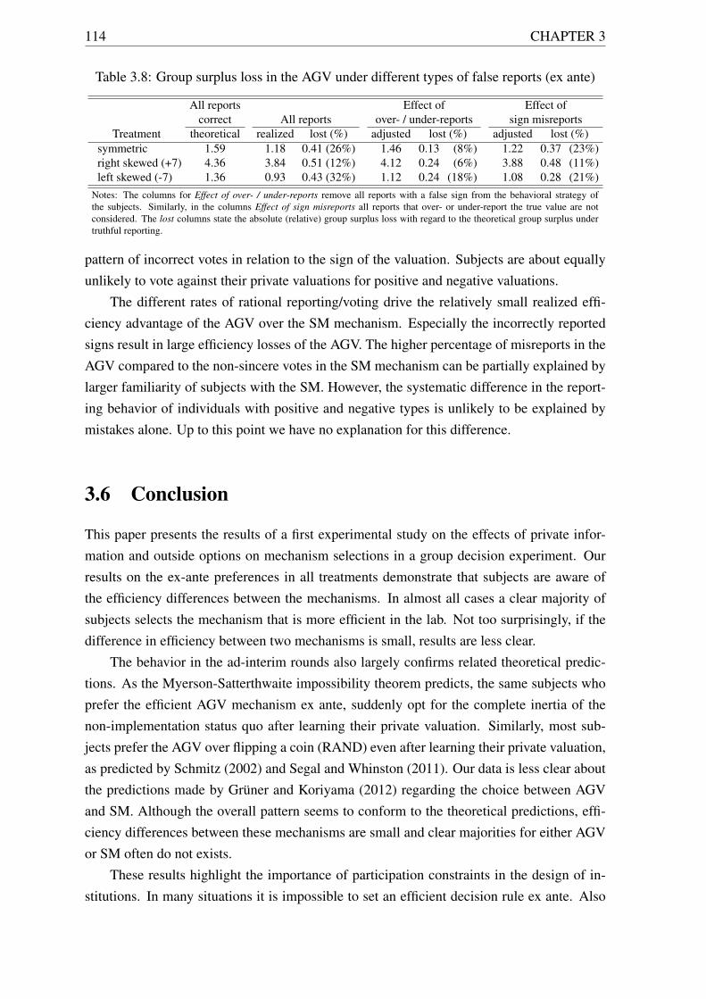
114 CHAPTER 3

Table 3.8: Group surplus loss in the AGV under different types of false reports (ex ante)

All reports Effect of Effect ofcorrect All reports over- / under-reports sign misreports

Treatment theoretical realized lost (%) adjusted lost (%) adjusted lost (%)symmetric 1.59 1.18 0.41 (26%) 1.46 0.13 (8%) 1.22 0.37 (23%)right skewed (+7) 4.36 3.84 0.51 (12%) 4.12 0.24 (6%) 3.88 0.48 (11%)left skewed (-7) 1.36 0.93 0.43 (32%) 1.12 0.24 (18%) 1.08 0.28 (21%)

Notes: The columns for Effect of over- / under-reports remove all reports with a false sign from the behavioral strategy ofthe subjects. Similarly, in the columns Effect of sign misreports all reports that over- or under-report the true value are notconsidered. The lost columns state the absolute (relative) group surplus loss with regard to the theoretical group surplus undertruthful reporting.

pattern of incorrect votes in relation to the sign of the valuation. Subjects are about equallyunlikely to vote against their private valuations for positive and negative valuations.

The different rates of rational reporting/voting drive the relatively small realized effi-ciency advantage of the AGV over the SM mechanism. Especially the incorrectly reportedsigns result in large efficiency losses of the AGV. The higher percentage of misreports in theAGV compared to the non-sincere votes in the SM mechanism can be partially explained bylarger familiarity of subjects with the SM. However, the systematic difference in the report-ing behavior of individuals with positive and negative types is unlikely to be explained bymistakes alone. Up to this point we have no explanation for this difference.

3.6 Conclusion

This paper presents the results of a first experimental study on the effects of private infor-mation and outside options on mechanism selections in a group decision experiment. Ourresults on the ex-ante preferences in all treatments demonstrate that subjects are aware ofthe efficiency differences between the mechanisms. In almost all cases a clear majority ofsubjects selects the mechanism that is more efficient in the lab. Not too surprisingly, if thedifference in efficiency between two mechanisms is small, results are less clear.

The behavior in the ad-interim rounds also largely confirms related theoretical predic-tions. As the Myerson-Satterthwaite impossibility theorem predicts, the same subjects whoprefer the efficient AGV mechanism ex ante, suddenly opt for the complete inertia of thenon-implementation status quo after learning their private valuation. Similarly, most sub-jects prefer the AGV over flipping a coin (RAND) even after learning their private valuation,as predicted by Schmitz (2002) and Segal and Whinston (2011). Our data is less clear aboutthe predictions made by Grüner and Koriyama (2012) regarding the choice between AGVand SM. Although the overall pattern seems to conform to the theoretical predictions, effi-ciency differences between these mechanisms are small and clear majorities for either AGVor SM often do not exists.

These results highlight the importance of participation constraints in the design of in-stitutions. In many situations it is impossible to set an efficient decision rule ex ante. Also

CHAPTER 3 115

it might not be possible to establish an efficient mechanism through a decentralized andcompletely voluntary procedure ad interim. This combined impossibility touches upon oneof the most fundamental questions in mechanism design, political economy, and more gen-erally political philosophy. Since participation constraints already create problems in thesmall groups in our experiment, the difficulties of negotiating a public project on the scaleof a nation would seem close to unsurmountable if unanimity (or completely voluntary par-ticipation by all parties) is required. A group that is stuck in an inefficient mechanism mightrequire an outside influence or coercive power to break away from the status quo. Central-ized organizations with an amount of coercive power, like the state or the company, are ableto force participation and thus avoid these problems. In doing so, these organizations al-low participants to bundle individual projects and reforms and take them away from purelydecentralized mechanisms like open markets. Often the gains in efficiency from extra invest-ment in common projects are large enough to compensate participants for their involvementin projects that are not individually rational to them. In this sense, our findings give onereason for the existence of states. Although a centralized state might not be as efficient indealing with incentive constraints as the market, it does make dealing with the participationconstraints on individual projects a lot easier.

Because our subjects play all mechanisms, we can compare the relative efficiency of theAGV and SM mechanism on the same group of subjects. The SM mechanism is almost asefficient in the lab as theoretical calculations with rational self-interested agents predict. TheAGV is perfectly efficient in theory, but loses a lot of its efficiency in practice due to falsereports. In our experimental results we find a puzzling pattern in the reporting strategy usedby subjects in the AGV. While both subjects with positive and negative valuations sometimesover- or under-report their valuation, only subjects with a negative valuation systematicallymisreport the sign of their valuation. These valuation reports with an incorrect sign accountfor most of the efficiency loss of the AGV in our experiment. Interestingly, this pattern ispresent in all treatments and does not seem to be driven by the behavior of a few individuals.Subjects in our experiment gather some experience in the AGV, but not too much. Dependingon the random allocation of private valuations, a subject might never experience the realadvantage of the AGV over the much more common SM mechanism. In order to havea “fair” comparison, it might be necessary to provide subjects with more opportunities tolearn how the AGV actually works and to demonstrate why the mechanism is more efficient.Given that we do not familiarize our subjects with the AGV in this manner, it is actuallyquite remarkable how often the AGV is chosen. Still our findings indicate that there is roomfor further research in the area of efficient mechanism implementation.

Our setup allows us to vary individual participation constraints and to apply strongwithin-subject tests of theoretical predictions. The crispness of the results obtained is a clearindication of the strength of this methodological setup. We believe the method by whichparticipation constraints are implemented, measured and varied in this experiment could

116 CHAPTER 3

be fruitfully applied to experimentally investigate other questions surrounding participationconstraints.

Appendix C

Appendix Chapter 3

117

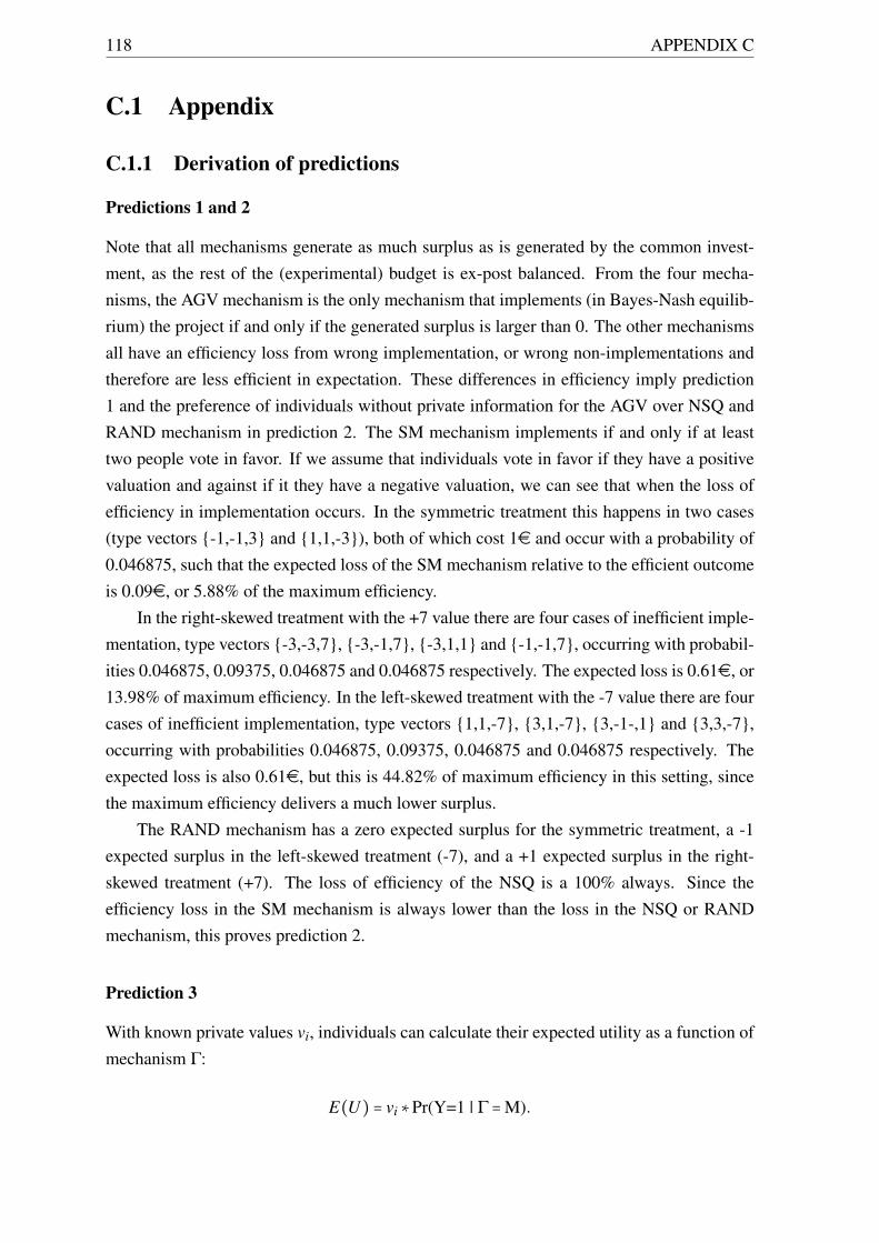
118 APPENDIX C

C.1 Appendix

C.1.1 Derivation of predictions

Predictions 1 and 2

Note that all mechanisms generate as much surplus as is generated by the common invest-ment, as the rest of the (experimental) budget is ex-post balanced. From the four mecha-nisms, the AGV mechanism is the only mechanism that implements (in Bayes-Nash equilib-rium) the project if and only if the generated surplus is larger than 0. The other mechanismsall have an efficiency loss from wrong implementation, or wrong non-implementations andtherefore are less efficient in expectation. These differences in efficiency imply prediction1 and the preference of individuals without private information for the AGV over NSQ andRAND mechanism in prediction 2. The SM mechanism implements if and only if at leasttwo people vote in favor. If we assume that individuals vote in favor if they have a positivevaluation and against if it they have a negative valuation, we can see that when the loss ofefficiency in implementation occurs. In the symmetric treatment this happens in two cases(type vectors {-1,-1,3} and {1,1,-3}), both of which cost 1e and occur with a probability of0.046875, such that the expected loss of the SM mechanism relative to the efficient outcomeis 0.09e, or 5.88% of the maximum efficiency.

In the right-skewed treatment with the +7 value there are four cases of inefficient imple-mentation, type vectors {-3,-3,7}, {-3,-1,7}, {-3,1,1} and {-1,-1,7}, occurring with probabil-ities 0.046875, 0.09375, 0.046875 and 0.046875 respectively. The expected loss is 0.61e, or13.98% of maximum efficiency. In the left-skewed treatment with the -7 value there are fourcases of inefficient implementation, type vectors {1,1,-7}, {3,1,-7}, {3,-1-,1} and {3,3,-7},occurring with probabilities 0.046875, 0.09375, 0.046875 and 0.046875 respectively. Theexpected loss is also 0.61e, but this is 44.82% of maximum efficiency in this setting, sincethe maximum efficiency delivers a much lower surplus.

The RAND mechanism has a zero expected surplus for the symmetric treatment, a -1expected surplus in the left-skewed treatment (-7), and a +1 expected surplus in the right-skewed treatment (+7). The loss of efficiency of the NSQ is a 100% always. Since theefficiency loss in the SM mechanism is always lower than the loss in the NSQ or RANDmechanism, this proves prediction 2.

Prediction 3

With known private values vi, individuals can calculate their expected utility as a function ofmechanism Γ:

E(U) = vi∗Pr(Y=1 | Γ =M).

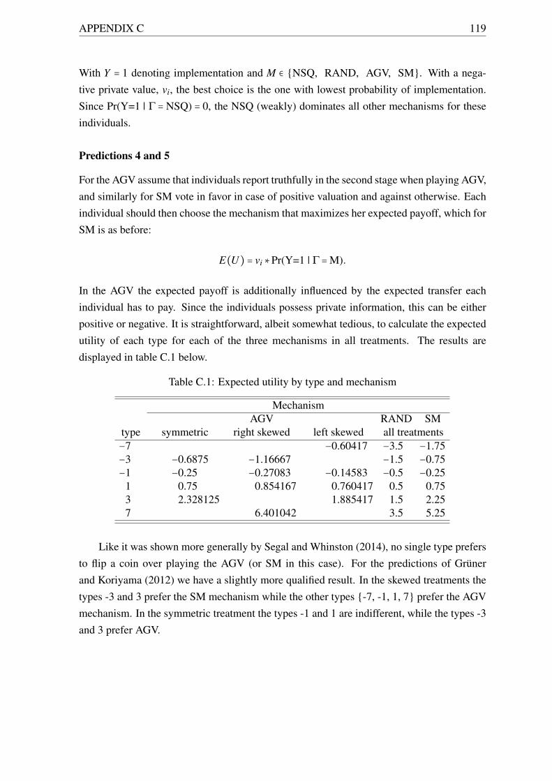
APPENDIX C 119

With Y = 1 denoting implementation and M ∈ {NSQ, RAND, AGV, SM}. With a nega-tive private value, vi, the best choice is the one with lowest probability of implementation.Since Pr(Y=1 | Γ = NSQ) = 0, the NSQ (weakly) dominates all other mechanisms for theseindividuals.

Predictions 4 and 5

For the AGV assume that individuals report truthfully in the second stage when playing AGV,and similarly for SM vote in favor in case of positive valuation and against otherwise. Eachindividual should then choose the mechanism that maximizes her expected payoff, which forSM is as before:

E(U) = vi∗Pr(Y=1 | Γ =M).

In the AGV the expected payoff is additionally influenced by the expected transfer eachindividual has to pay. Since the individuals possess private information, this can be eitherpositive or negative. It is straightforward, albeit somewhat tedious, to calculate the expectedutility of each type for each of the three mechanisms in all treatments. The results aredisplayed in table C.1 below.

Table C.1: Expected utility by type and mechanism

MechanismAGV RAND SM

type symmetric right skewed left skewed all treatments−7 −0.60417 −3.5 −1.75−3 −0.6875 −1.16667 −1.5 −0.75−1 −0.25 −0.27083 −0.14583 −0.5 −0.25

1 0.75 0.854167 0.760417 0.5 0.753 2.328125 1.885417 1.5 2.257 6.401042 3.5 5.25

Like it was shown more generally by Segal and Whinston (2014), no single type prefersto flip a coin over playing the AGV (or SM in this case). For the predictions of Grünerand Koriyama (2012) we have a slightly more qualified result. In the skewed treatments thetypes -3 and 3 prefer the SM mechanism while the other types {-7, -1, 1, 7} prefer the AGVmechanism. In the symmetric treatment the types -1 and 1 are indifferent, while the types -3and 3 prefer AGV.

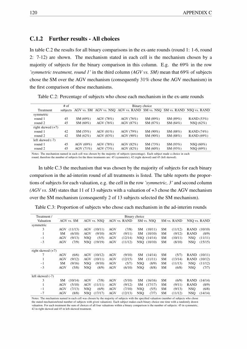
120 APPENDIX C

C.1.2 Further results - All choices

In table C.2 the results for all binary comparisons in the ex-ante rounds (round 1: 1-6, round2: 7-12) are shown. The mechanism stated in each cell is the mechanism chosen by amajority of subjects for the binary comparison in this column. E.g. the 69% in the row’symmetric treatment, round 1’ in the third column (AGV vs. SM) mean that 69% of subjectschose the SM over the AGV mechanism (consequently 31% chose the AGV mechanism) inthe first comparison of these mechanisms.

Table C.2: Percentage of subjects who chose each mechanism in the ex-ante rounds

# of Binary choiceTreatment subjects AGV vs. SM AGV vs. NSQ AGV vs. RAND SM vs. NSQ SM vs. RAND NSQ vs. RAND

symmetricround 1 45 SM (69%) AGV (78%) AGV (76%) SM (89%) SM (89%) RAND (53%)round 2 45 SM (60%) AGV (76%) AGV (87%) SM (87%) SM (84%) NSQ (62%)right skewed (+7)round 1 42 SM (55%) AGV (81%) AGV (79%) SM (90%) SM (88%) RAND (74%)round 2 42 SM (62%) AGV (83%) AGV (90%) SM (90%) SM (88%) RAND (69%)left skewed (-7)round 1 45 AGV (69%) AGV (78%) AGV (82%) SM (73%) SM (93%) NSQ (60%)round 2 45 AGV (71%) AGV (73%) AGV (82%) SM (60%) SM (93%) NSQ (69%)

Notes: The mechanism named in each cell was chosen by the majority of subjects (percentage). Each subject made a choice in eachround, therefore the number of subjects for the three treatments are: 45 (symmetric), 42 (right skewed) and 45 (left skewed).

In table C.3 the mechanism that was chosen by the majority of subjects for each binarycomparison in the ad-interim round of all treatments is listed. The table reports the propor-tions of subjects for each valuation, e.g. the cell in the row ’symmetric, 3’ and second column(AGV vs. SM) states that 11 of 13 subjects with a valuation of +3 chose the AGV mechanismover the SM mechanism (consequently 2 of 13 subjects selected the SM mechanism).

Table C.3: Proportion of subjects who chose each mechanism in the ad-interim rounds

Treatment / Binary choiceValuation AGV vs. SM AGV vs. NSQ AGV vs. RAND SM vs. NSQ SM vs. RAND NSQ vs. RAND

symmetric3 AGV (11/13) AGV (10/11) AGV (7/8) SM (10/11) SM (11/12) RAND (10/10)1 SM (6/10) AGV (9/10) AGV (9/11) SM (10/10) SM (9/12) RAND (8/9)−1 AGV (9/13) NSQ (5/5) AGV (12/14) NSQ (14/14) SM (10/11) NSQ (11/11)−3 AGV (7/9) NSQ (19/19) AGV (11/12) NSQ (10/10) SM (8/10) NSQ (15/15)

right skewed (+7)7 AGV (6/6) AGV (10/12) AGV (9/10) SM (14/14) SM (5/7) RAND (10/11)1 AGV (9/12) AGV (10/11) AGV (12/15) SM (11/11) SM (13/14) RAND (10/12)−1 SM (9/16) NSQ (9/10) AGV (5/7) NSQ (8/9) SM (11/13) NSQ (11/12)−3 AGV (5/8) NSQ (8/9) AGV (6/10) NSQ (8/8) SM (6/8) NSQ (7/7)

left skewed (-7)3 SM (10/14) AGV (7/8) AGV (5/10) SM (16/16) SM (6/9) RAND (14/14)1 AGV (5/10) AGV (11/11) AGV (9/12) SM (17/17) SM (9/11) RAND (8/9)−1 AGV (7/13) NSQ (6/9) AGV (7/10) NSQ (5/5) SM (9/13) NSQ (6/8)−7 AGV (8/8) NSQ (17/17) AGV (12/13) NSQ (7/7) SM (11/12) NSQ (14/14)

Notes: The mechanism named in each cell was chosen by the majority of subjects with the specified valuation (number of subjects who chosethe stated mechanism/total number of subjects with given valuation). Each subject makes each binary choice one time with a randomly drawnvaluation. For each treatment the sum of choices of all four valuations within a binary comparison is the number of subjects: 45 in symmetric,42 in right skewed and 45 in left-skewed treatment.

APPENDIX C 121

C.1.3 Translated instructions

This is the translation of the original instructions used for treatment one (symmetric dis-tribution). The instructions for other treatments only differ with respect to the describeddistribution and therefore the used examples and tables. All emphasizes are in the original.The original instructions for all treatments are available from the authors upon request.

Instructions

Thank you for taking part in this experiment. The amount of money you can earn in thisexperiment depends on your choices and the choices of the other participants. It is thereforeimportant that you understand the instructions. Please do not communicate with the otherparticipants during the experiment. If you have any questions after reading the instructions,please raise your hand. We will then clarify your question.

All the information you provide will be treated anonymously.

You will begin the experiment with a starting budget of 9e. This amount can be increased ordecreased depending on all participants’ choices in one of the 18 rounds of this experiment.In each round each participant receives a payment. This payment can be zero, positive ornegative. At the end of the 18 rounds, one round will be randomly determined for payment.The payment of the selected round will be added to or subtracted from your starting budget.The sum of your starting budget and the payment of the selected round yields your finalpayoff. In each round you should act as if the round was selected for payment. You willreceive your final payoff in cash at the end of the experiment. The payments are chosen insuch a way that you cannot make losses under any circumstances. Each participant can earnbetween 5.75e and 12.25e. Your payment will be treated anonymously.

The entire experiment is organized in two phases. Phase I consists of rounds 1-12 and phaseII of rounds 13-18. You will now receive information about phase I. We will explain anychanges in phase II after round 12, but before the start of round 13 (the start of phase II).

Thank you for participating.

STRUCTURE OF THE EXPERIMENT

In each round of the experiment you will be part of a group with 3 members (you and tworandomly selected other participants). Each group has the possibility to conduct a project,called project A. If you do not conduct the project each group member receives a payoffof 0e for this round. If your group conducts project A, then each group member receiveshis or her private valuation for the project as payment for this round. The private valuationof project A can be different for each member of your group. If your group decides not toconduct project A, all group members receive a payoff of zero. The valuation for project Ais newly determined each round and each participant receives a new private valuation in each

122 APPENDIX C

round. Groups are newly formed in each of the 12 rounds.

The experiment is computer based. Therefore individual participants cannot identify theother group members. You will not know which other participants are in your group inwhich round, neither during nor after the experiment.

One round consists of two parts. In the first part each group choses a decision rule which isused to determine whether project A is implemented or not. In the second part your groupuses the selected rule to determine whether project A is implemented or not. You will beinformed about your private valuation for project A after part one of a round. We will nowdescribe the two different parts of each round as well as the possible decision rules in detail.

PART ONE

In part one you have the choice between two different decision rules, which will be usedin part two to determine whether project A is implemented or not. The two available ruleschange from round to round. Each of the three group members suggests one of the twoavailable rules for part two of this round. The computer randomly picks one of thesesuggestions as group rule. This decision rule determines how in part two the questionwhether project A is implemented or not is resolved. The different rules are explainedbelow. In part one you do not know whose rule suggestions will be the group decisionrule. Your suggestion can be selected, but also the suggestion of another group member.Each group member has the same chance in each round for his or her suggestion to beselected. Non selected suggestions will not be made known to the other group members.Please note that the decision rule is important, because dependent on the decision rule theimplementation of project A is easier or more difficult.

PART TWO

In part two the selected decision rule is used to determine whether project A is implementedor not. The group decision arises directly from the decisions of all group members in parttwo. The decision is announced and each participant is informed about his or her paymentin this round.

VALUATIONS

In case project A is implemented all group members receive a payment dependent ontheir project valuations. This means, if your valuation for project A is positive, you benefitfrom the implementation of project A, and when your valuation for project A is negative, thenyou have to pay if the project is implemented. Your valuation for project A is randomlygiven to you in each round anew. You learn your valuation after part one. Thereforeyou do not know your valuation when you decide between the different decision rules in partone, but you know your valuation in part two, when you decide about the implementation ofproject A according to the selected decision rule.

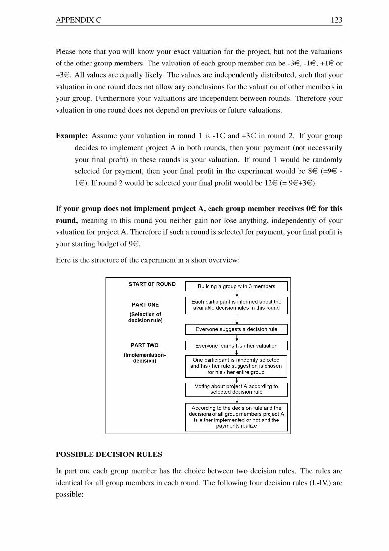
APPENDIX C 123

Please note that you will know your exact valuation for the project, but not the valuationsof the other group members. The valuation of each group member can be -3e, -1e, +1e or+3e. All values are equally likely. The values are independently distributed, such that yourvaluation in one round does not allow any conclusions for the valuation of other members inyour group. Furthermore your valuations are independent between rounds. Therefore yourvaluation in one round does not depend on previous or future valuations.

Example: Assume your valuation in round 1 is -1e and +3e in round 2. If your groupdecides to implement project A in both rounds, then your payment (not necessarilyyour final profit) in these rounds is your valuation. If round 1 would be randomlyselected for payment, then your final profit in the experiment would be 8e (=9e -1e). If round 2 would be selected your final profit would be 12e (= 9e+3e).

If your group does not implement project A, each group member receives 0e for thisround, meaning in this round you neither gain nor lose anything, independently of yourvaluation for project A. Therefore if such a round is selected for payment, your final profit isyour starting budget of 9e.

Here is the structure of the experiment in a short overview:

POSSIBLE DECISION RULES

In part one each group member has the choice between two decision rules. The rules areidentical for all group members in each round. The following four decision rules (I.-IV.) arepossible:

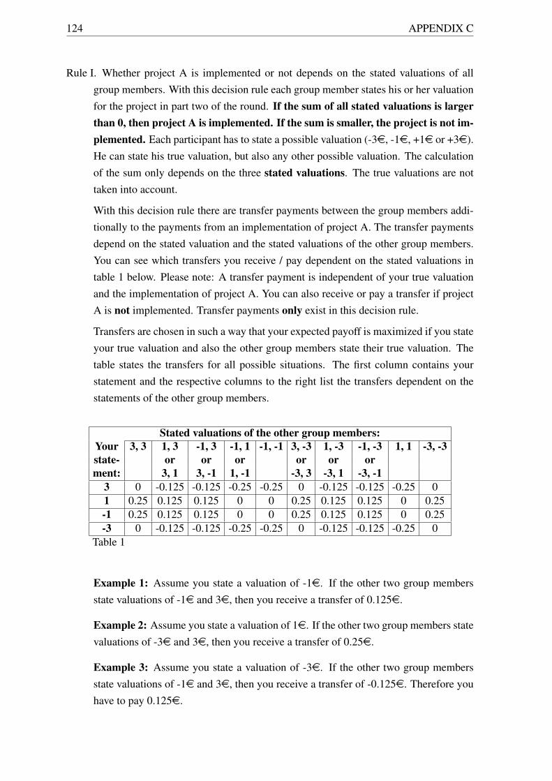
124 APPENDIX C

Rule I. Whether project A is implemented or not depends on the stated valuations of allgroup members. With this decision rule each group member states his or her valuationfor the project in part two of the round. If the sum of all stated valuations is largerthan 0, then project A is implemented. If the sum is smaller, the project is not im-plemented. Each participant has to state a possible valuation (-3e, -1e, +1e or +3e).He can state his true valuation, but also any other possible valuation. The calculationof the sum only depends on the three stated valuations. The true valuations are nottaken into account.

With this decision rule there are transfer payments between the group members addi-tionally to the payments from an implementation of project A. The transfer paymentsdepend on the stated valuation and the stated valuations of the other group members.You can see which transfers you receive / pay dependent on the stated valuations intable 1 below. Please note: A transfer payment is independent of your true valuationand the implementation of project A. You can also receive or pay a transfer if projectA is not implemented. Transfer payments only exist in this decision rule.

Transfers are chosen in such a way that your expected payoff is maximized if you stateyour true valuation and also the other group members state their true valuation. Thetable states the transfers for all possible situations. The first column contains yourstatement and the respective columns to the right list the transfers dependent on thestatements of the other group members.

Stated valuations of the other group members:Your 3, 3 1, 3 -1, 3 -1, 1 -1, -1 3, -3 1, -3 -1, -3 1, 1 -3, -3state- or or or or or orment: 3, 1 3, -1 1, -1 -3, 3 -3, 1 -3, -1

3 0 -0.125 -0.125 -0.25 -0.25 0 -0.125 -0.125 -0.25 01 0.25 0.125 0.125 0 0 0.25 0.125 0.125 0 0.25-1 0.25 0.125 0.125 0 0 0.25 0.125 0.125 0 0.25-3 0 -0.125 -0.125 -0.25 -0.25 0 -0.125 -0.125 -0.25 0

Table 1

Example 1: Assume you state a valuation of -1e. If the other two group membersstate valuations of -1e and 3e, then you receive a transfer of 0.125e.

Example 2: Assume you state a valuation of 1e. If the other two group members statevaluations of -3e and 3e, then you receive a transfer of 0.25e.

Example 3: Assume you state a valuation of -3e. If the other two group membersstate valuations of -1e and 3e, then you receive a transfer of -0.125e. Therefore youhave to pay 0.125e.

APPENDIX C 125

Example 4: Assume you state a valuation of 3e. If the other two group members statevaluations of -3e and -3e, then you receive a transfer of 0.

Please note that transfers payments are always made, independent of whether project A isimplemented or not. You receive / pay a transfer on top of the payments from project A.

Rule II. At least two group members have to vote for the implementation of project A. Inpart two all group members vote either for or against the implementation of project A.At least 2 group members have to vote for the implementation, otherwise project A isnot implemented (simple majority).

Rule III. Project A is never implemented. Group members do not make any further state-ments in part two. There is no voting and no valuations are stated.

Rule IV. The decision for or against implementation of project A depends on the result of acoin flip. There is no voting. If the coin flip results in HEADS, the project is imple-mented. If the result is TAILS, the project is not implemented. Both results, HEADSand TAILS, are equally likely. Therefore with rule IV. project A is implemented in50% of all cases and not implemented in the other 50%.

Please note that in decision rules I and II each participant has to state a valuation / vote. It isnot possible to abstain.

We now ask you to answer several understanding questions regarding the various decisionrules and your possible payments. Please answer these questions on the computer screen.After all participants have answered the seven understanding questions all participants willtake part in four practice rounds. In each round you will apply one of the four possibledecision rules (I.-IV.). In these rounds there is no choice between two rules, but the rule ispredetermined.

In these four rounds you are not in a group with two other participants. The computersimulates the decisions of your group members. The computer randomly choses between allavailable actions. E.g. with rule II the computer will vote “YES − implement project A” in50% of all cases and “NO − do not implement project A” in the other 50%.

These four rounds do not count towards your final profit. They are just meant to familiarizeyou with the four possible decision rules. After all participants have completed these fourrounds the actual experiment starts.

126 APPENDIX C

BibliographyAbeler, Johannes, Armin Falk, Lorenz Goette, and David Huffman (2011), “Reference

Points and Effort Provision”, American Economic Review, 101 (2), 470–92.

Acemoglu, Daron, Georgy Egorov, and Konstantin Sonin (2012), “Dynamics and Sta-bility of Constitutions, Coalitions, and Clubs”, American Economic Review, 102 (4),1446–1476.

Akerlof, George (1982), “Labor Contracts as Partial Gift Exchange”, The Quarterly Journal

of Economics, 97 (4), 543–569.

Akerlof, George and Janet Yellen (1990), “The Fair Wage-Effort Hypothesis and Unem-ployment”, The Quarterly Journal of Economics, 105 (2), 255–283.

Anderhub, Vital, Simon Gächter, and Manfred Königstein (2002), “Efficient Contract-ing and Fair Play in a Simple Principal-Agent Experiment”, Experimental Economics,5 (1), 5–27.

Arrow, Kenneth (1950), “A difficulty in the concept of social welfare”, The Journal of

Political Economy, 58 (4), 328–346.

Arrow, Kenneth (1979), “The property rights doctrine and demand revelation under incom-plete information”. Economics and Human Welfare. New York Academic Press, 23–39.

Balafoutas, Loukas, Rudolf Kerschbamer, and Matthias Sutter (2012), “Distributionalpreferences and competitive behavior”, Journal of Economic Behavior & Organization,83 (1), 125–135.

Barbera, Salvador and Matthew Jackson (2004), “Choosing how to choose: Self-stablemajority rules and constitutions”, The Quarterly Journal of Economics, 119 (3), 1011–1048.

Bartling, Björn, Ernst Fehr, Michel André Maréchal, and Daniel Schunk (2009), “Egal-itarianism and Competitiveness”, The American Economic Review, 99 (2), 93–98.

127

128 BIBLIOGRAPHY

Bernheim, Douglas (1984), “Rationalizable strategic behavior”, Econometrica: Journal of

the Econometric Society, 52 (4), 1007–1028.

Bierbrauer, Felix, Axel Ockenfels, Andreas Pollak, and Désirée Rückert (2014), “Ro-bust mechanism design and social preferences”, CESifo Working Paper Series, (No.4713).

Blanco, Mariana, Dirk Engelmann, Alexander Koch, and Hans-Theo Normann (2010),“Belief elicitation in experiments: is there a hedging problem?”, Experimental Eco-

nomics, 13 (4), 412–438.

Bull, Clive, Andrew Schotter, and Keith Weigelt (1987), “Tournaments and Piece Rates:An Experimental Study”, Journal of Political Economy, 95 (1), 1–33.

Camerer, Colin (2003), Behavioral Game Theory: Experiments in Strategic Interaction.Princeton University Press.

Camerer, Colin and Dan Lovallo (1999), “Overconfidence and Excess Entry: An Experi-mental Approach”, The American Economic Review, 89 (1), 306–318.

Cason, Timothy, William Masters, and Roman Sheremeta (2010), “Entry into winner-take-all and proportional-prize contests: An experimental study”, Journal of Public Eco-

nomics, 94 (9-10), 604–611.

Chatterjee, Kalyan (1982), “Incentive compatibility in bargaining under uncertainty”, The

Quarterly Journal of Economics, 97 (4), 717–726.

Costa-Gomes, Miguel, Vincent Crawford, and Bruno Broseta (2001), “Cognition andbehavior in normal-form games: An experimental study”, Econometrica, 69 (5), 1193–1235.

Costa-Gomes, Miguel and Georg Weizsäcker (2008), “Stated beliefs and play in normal-form games”, The Review of Economic Studies, 75 (3), 729–762.

Cramton, Peter, Robert Gibbons, and Paul Klemperer (1987), “Dissolving a partnershipefficiently”, Econometrica: Journal of the Econometric Society, 55 (3), 615–632.

Croson, Rachel (1999), “The disjunction effect and reason-based choice in games”, Orga-

nizational Behavior and Human Decision Processes, 80 (2), 118–133.

Croson, Rachel (2000), “Thinking like a game theorist: factors affecting the frequency ofequilibrium play”, Journal of Economic Behavior & Organization, 41 (3), 299–314.

d’Aspremont, Claude and Louis-Andre Gérard-Varet (1979), “Incentives and incom-plete information”, Journal of Public Economics, 11 (1), 25–45.

BIBLIOGRAPHY 129

Dohmen, Thomas and Armin Falk (2011), “Performance Pay and Multidimensional Sort-ing: Productivity, Preferences, and Gender”, American Economic Review, 101 (2), 556–90.

Dufwenberg, Martin and Uri Gneezy (2000), “Measuring beliefs in an experimental lostwallet game”, Games and Economic Behavior, 30 (2), 163–182.

Engelmann, Dirk and Hans Peter Grüner (2013), “Tailored Bayesian Mechanisms: Ex-perimental Evidence from Two-Stage Voting Games”, CEPR Discussion Paper, (No.9544).

Eriksson, Tor, Sabrina Teyssier, and Marie-Claire Villeval (2009), “Self-Selection andthe Efficiency of Tournaments”, Economic Inquiry, 47 (3), 530–548.

Falk, Armin and Michael Kosfeld (2006), “The Hidden Costs of Control”, The American

Economic Review, 96 (5), 1611–1630.

Fehr, Ernst and Armin Falk (1999), “Wage Rigidity in a Competitive Incomplete ContractMarket”, Journal of Political Economy, 107 (1), 106–134.

Fehr, Ernst, Simon Gächter, and Georg Kirchsteiger (1997), “Reciprocity as a ContractEnforcement Device: Experimental Evidence”, Econometrica, 65 (4), 833–860.

Fehr, Ernst, Georg Kirchsteiger, and Arno Riedl (1993), “Does Fairness Prevent MarketClearing? An Experimental Investigation”, The Quarterly Journal of Economics, 108(2), 437–459.

Fehr, Ernst, Georg Kirchsteiger, and Arno Riedl (1998), “Gift exchange and reciprocityin competitive experimental markets”, European Economic Review, 42 (1), 1–34.

Fehr, Ernst, Alexander Klein, and Klaus Schmidt (2007), “Fairness and Contract De-sign”, Econometrica, 75 (1), 121–154.

Fischbacher, Urs (2007), “z-Tree: Zurich toolbox for ready-made economic experiments”,Experimental Economics, 10 (2), 171–178.

Fischbacher, Urs and Simon Gächter (2010), “Social preferences, beliefs, and the dynam-ics of free riding in public goods experiments”, The American Economic Review, 100(1), 541–556.

Gächter, Simon and Elke Renner (2010), “The effects of (incentivized) belief elicitationin public goods experiments”, Experimental Economics, 13 (3), 364–377.

Gneezy, Uri and John List (2006), “Putting Behavioral Economics to Work: Testing forGift Exchange in Labor Markets Using Field Experiments”, Econometrica, 74 (5), 1365–1384.

130 BIBLIOGRAPHY

Green, Jerry and Nancy Stokey (1983), “A Comparison of Tournaments and Contracts”,Journal of Political Economy, 91 (3), 349–364.

Greiner, Ben (2015), “Subject pool recruitment procedures: organizing experiments withORSEE”, Journal of the Economic Science Association, 1 (1), 114–125.

Grüner, Hans Peter and Yukio Koriyama (2012), “Public goods, participation constraints,and democracy: A possibility theorem”, Games and Economic Behavior, 75 (1), 152–167.

Güth, Werner and Martin Hellwig (1986), “The private supply of a public good”, Journal

of Economics, 5, 121–159.

Güth, Werner and Martin Hellwig (1987), “Competition versus monopoly in the supplyof public goods”. Efficiency, Institutions and Economic Policy. Springer, 183–217.

Haruvy, Ernan, Yaron Lahav, and Charles Noussair (2007), “Traders’ expectations inasset markets: experimental evidence”, The American Economic Review, 97 (5), 1901–1920.

Holt, Charles and Susan Laury (2002), “Risk Aversion and Incentive Effects”, The Amer-

ican Economic Review, 92 (5), 1644–1655.

Holt, Charles and Angela Smith (2016), “Belief Elicitation with a Synchronized LotteryChoice Menu That Is Invariant to Risk Attitudes”, American Economic Journal: Mi-

croeconomics, 8 (1), 110–39.

Huck, Steffen and Georg Weizsäcker (2002), “Do players correctly estimate what othersdo?: Evidence of conservatism in beliefs”, Journal of Economic Behavior & Organiza-

tion, 47 (1), 71–85.

Kagel, John, Alvin Roth, and John Hey (1995), The Handbook of Experimental Eco-

nomics. Princeton University Press.

Lazear, Edward (2000), “The Power of Incentives”, The American Economic Review, 90(2), 410–414.

Lazear, Edward and Sherwin Rosen (1981), “Rank-Order Tournaments as Optimum La-bor Contracts”, Journal of Political Economy, 89 (5), 841–864.

Leuven, Edwin, Hessel Oosterbeek, Joep Sonnemans, and Bas van der Klaauw (2011),“Incentives versus Sorting in Tournaments: Evidence from a Field Experiment”, Journal

of Labor Economics, 29 (3), 637–658.

Lindner, Florian, Glenn Dutcher, and Dmitry Ryvkinx (2013), “Sorting and selectioneffects in tournament mechanisms: An experimental investigation”, mimeo.

BIBLIOGRAPHY 131

Mailath, George and Andrew Postlewaite (1990), “Asymmetric information bargainingproblems with many agents”, The Review of Economic Studies, 57 (3), 351–367.

Mehta, Cyrus and Joan Hilton (1993), “Exact power of conditional and unconditionaltests: going beyond the 2× 2 contingency table”, The American Statistician, 47 (2), 91–98.

Morgan, John, Henrik Orzen, and Martin Sefton (2012), “Endogenous entry in con-tests”, Economic Theory, 51 (2), 435–463.

Myerson, Roger and Mark Satterthwaite (1983), “Efficient mechanisms for bilateral trad-ing”, Journal of Economic Theory, 29 (2), 265–281.

Nalebuff, Barry and Joseph Stiglitz (1983), “Prizes and Incentives: Towards a GeneralTheory of Compensation and Competition”, The Bell Journal of Economics, 14 (1), 21–43.

Niederle, Muriel and Lise Vesterlund (2007), “Do Women Shy Away from Competition?Do Men Compete Too Much?”, The Quarterly Journal of Economics, 122 (3), 1067–1101.

Nyarko, Yaw and Andrew Schotter (2002), “An experimental study of belief learningusing elicited beliefs”, Econometrica, 70 (3), 971–1005.

Offerman, Theo, Joep Sonnemans, and Arthur Schram (1996), “Value orientations, ex-pectations and voluntary contributions in public goods”, The Economic Journal, 106(437), 817–845.

Pearce, David (1984), “Rationalizable strategic behavior and the problem of perfection”,Econometrica: Journal of the Econometric Society, 1029–1050.

Rey-Biel, Pedro (2009), “Equilibrium play and best response to (stated) beliefs in normalform games”, Games and Economic Behavior, 65 (2), 572–585.

Rutström, Elisabet and Nathaniel Wilcox (2009), “Stated beliefs versus inferred beliefs:A methodological inquiry and experimental test”, Games and Economic Behavior, 67(2), 616–632.

Schlag, Karl, James Tremewan, and Joel Van der Weele (2015), “A penny for yourthoughts: a survey of methods for eliciting beliefs”, Experimental Economics, 18 (3),457–490.

Schmitz, Patrick (2002), “Simple contracts, renegotiation under asymmetric information,and the hold-up problem”, European Economic Review, 46 (1), 169–188.

132 BIBLIOGRAPHY

Segal, Ilya and Michael Whinston (2011), “A simple status quo that ensures participation(with application to efficient bargaining)”, Theoretical Economics, 6 (1), 109–125.

Segal, Ilya and Michael Whinston (2014), “Property Rights and the Efficiency of Bargain-ing”, mimeo.

Stahl, Dale and Paul Wilson (1994), “Experimental evidence on players’ models of otherplayers”, Journal of Economic Behavior & Organization, 25 (3), 309–327.

Weber, Roberto (2003), “’Learning’ with no feedback in a competitive guessing game”,Games and Economic Behavior, 44 (1), 134–144.

Weizsäcker, Georg (2003), “Ignoring the rationality of others: evidence from experimentalnormal-form games”, Games and Economic Behavior, 44 (1), 145–171.

Wilcox, Nathaniel and Nick Feltovich (2000), “Thinking like a game theorist: Comment”,University of Houston Department of Economics working paper.

Zelmer, Jennifer (2003), “Linear public goods experiments: A meta-analysis”, Experimen-

tal Economics, 6 (3), 299–310.

Curriculum Vitae

2010 - 2016 Ph.D. student in EconomicsUniversity of Mannheim,Center for Doctoral Studies in Economics

2005 - 2010 University of Mannheim, Department of Economics07/2010 Diplom (M.Sc. equivalent) in Economics

2008 - 2009 UC Berkeley, Department of EconomicsVisiting Graduate Student

133

Essays in Experimental Economics

Documents

Transcript of Essays in Experimental Economics