Essays in Labor Economics and Applied Microeconomics

Purdue University Purdue University

Purdue e-Pubs Purdue e-Pubs

Open Access Dissertations Theses and Dissertations

8-2018

Essays in Labor Economics and Applied Microeconomics Essays in Labor Economics and Applied Microeconomics

Paul W. Thomas Purdue University

Follow this and additional works at: https://docs.lib.purdue.edu/open_access_dissertations

Recommended Citation Recommended Citation Thomas, Paul W., "Essays in Labor Economics and Applied Microeconomics" (2018). Open Access Dissertations. 2084. https://docs.lib.purdue.edu/open_access_dissertations/2084

This document has been made available through Purdue e-Pubs, a service of the Purdue University Libraries. Please contact [email protected] for additional information.

https://docs.lib.purdue.edu/

https://docs.lib.purdue.edu/open_access_dissertations

https://docs.lib.purdue.edu/etd

https://docs.lib.purdue.edu/open_access_dissertations?utm_source=docs.lib.purdue.edu%2Fopen_access_dissertations%2F2084&utm_medium=PDF&utm_campaign=PDFCoverPages

https://docs.lib.purdue.edu/open_access_dissertations/2084?utm_source=docs.lib.purdue.edu%2Fopen_access_dissertations%2F2084&utm_medium=PDF&utm_campaign=PDFCoverPages

ESSAYS IN LABOR ECONOMICS AND APPLIED MICROECONOMICS

A Dissertation

Submitted to the Faculty

of

Purdue University

by

Paul W. Thomas

In Partial Fulfillment of the

Requirements for the Degree

of

Doctor of Philosophy

August 2018

Purdue University

West Lafayette, Indiana

ii

THE PURDUE UNIVERSITY GRADUATE SCHOOL

STATEMENT OF DISSERTATION APPROVAL

Dr. Kevin J. Mumford, Chair

Department of Economics

Dr. John Barron


Dr. Tim Bond


Dr. Mohitosh Kejriwal


Approved by:

Dr. Brian Roberson

Director of Graduate Studies

iii

ACKNOWLEDGMENTS

The author would like to thank Kevin Mumford, John Barron, Tim Bond, Mohi-

tosh Kejriwal and the seminar participants at Purdue University for their comments

and suggestions. The author would like to give special thanks to Kevin Mumford for

all of his invaluable guidance and the time invested in helping me to succeed.

iv

TABLE OF CONTENTS

Page

LIST OF TABLES . . . . . . . . . . . . . . . . . . . . . . . . . . . . . . . . . . vi

LIST OF FIGURES

CHAPTER 1. CHILDHOOD FAMILY INCOME AND ADULT OUTCOMES:

. . . . . . . . . . . . . . . . . . . . . . . . . . . . . . . . . viii

ABSTRACT . . . . . . . . . . . . . . . . . . . . . . . . . . . . . . . . . . . . . ix

EVIDENCE FROM THE EITC . . . . . . . . . . . . . . . . . . . . . . . . . 1 1.1 Introduction . . . . . . . . . . . . . . . . . . . . . . . . . . . . . . . . . 1 1.2 Background on EITC . . . . . . . . . . . . . . . . . . . . . . . . . . . . 3 1.3 Related Literature . . . . . . . . . . . . . . . . . . . . . . . . . . . . . 5 1.4 Methodology . . . . . . . . . . . . . . . . . . . . . . . . . . . . . . . . 10 1.5 Theoretical Predictions Explored by the Empirical Model . . . . . . . . 12 1.6 Data . . . . . . . . . . . . . . . . . . . . . . . . . . . . . . . . . . . . . 15 1.7 Results . . . . . . . . . . . . . . . . . . . . . . . . . . . . . . . . . . . . 16 1.8 Conclusion . . . . . . . . . . . . . . . . . . . . . . . . . . . . . . . . . . 20 1.9 Figures and Tables . . . . . . . . . . . . . . . . . . . . . . . . . . . . . 22

CHAPTER 2. FERTILITY RESPONSE TO THE TAX TREATMENT OF CHILDREN . . . . . . . . . . . . . . . . . . . . . . . . . . . . . . . . . . . . 37 2.1 Introduction . . . . . . . . . . . . . . . . . . . . . . . . . . . . . . . . . 37 2.2 Data . . . . . . . . . . . . . . . . . . . . . . . . . . . . . . . . . . . . . 38 2.3 Estimation Strategy . . . . . . . . . . . . . . . . . . . . . . . . . . . . 40 2.4 Results . . . . . . . . . . . . . . . . . . . . . . . . . . . . . . . . . . . . 43 2.5 Conclusion . . . . . . . . . . . . . . . . . . . . . . . . . . . . . . . . . . 48 2.6 Figures and Tables . . . . . . . . . . . . . . . . . . . . . . . . . . . . . 49

APPENDIX A. CONTEMPORANEOUS OUTCOMES FOR NLSY SAMPLE . 61

APPENDIX B. SUBGROUP REGRESSIONS: ADDITIONAL OUTCOMES . . 63

APPENDIX C. SUMMARY STATISTICS BY DATASET . . . . . . . . . . . . 67

REFERENCES . . . . . . . . . . . . . . . . . . . . . . . . . . . . . . . . . . . . 68

v

LIST OF TABLES

Table Page

1.1 Sample Summary Statistics . . . . . . . . . . . . . . . . . . . . . . . . . . 26

1.2 Effect on High School Graduation: Maximum EITC Over Full Childhood . 27

1.3 Regressions for All Long-Run Outcomes: Maximum EITC Over Full Child-hood . . . . . . . . . . . . . . . . . . . . . . . . . . . . . . . . . . . . . . . 27

1.4 Regressions for All Long-Run Outcomes: Maximum EITC Over Age Ranges 28

1.5 Subgroup Regressions: High School Graduation/Earning a GED . . . . . . 29

1.6 Regressions for All Long-Run Outcomes: Divided Sample . . . . . . . . . . 30

1.7 Regressions for All Long-Run Outcomes: Matched Sample . . . . . . . . . 31

1.8 Regressions for All Long-Run Outcomes: Divided Sample, Female Indi-viduals . . . . . . . . . . . . . . . . . . . . . . . . . . . . . . . . . . . . . 32

1.9 Regressions for All Long-Run Outcomes: Divided Sample, Individuals With Highly Educated Parents . . . . . . . . . . . . . . . . . . . . . . . . 33

1.10 Regressions for All Long-Run Outcomes: Divided Sample, White Individ-uals . . . . . . . . . . . . . . . . . . . . . . . . . . . . . . . . . . . . . . . 34

1.11 Regressions for All Long-Run Outcomes: PSID Subsample Over NLSY Date Range . . . . . . . . . . . . . . . . . . . . . . . . . . . . . . . . . . . 35

2.1 Summary Statistics . . . . . . . . . . . . . . . . . . . . . . . . . . . . . . . 50

2.2 Change in Subsidy Example . . . . . . . . . . . . . . . . . . . . . . . . . . 51

2.3 Fertility Effects of Tax Subsidy Changes . . . . . . . . . . . . . . . . . . . 52

2.4 Fertility Effects of Tax Subsidy Changes by Income ($1,000’s) . . . . . . . 53

2.5 Heterogeneity of Fertility Effects by Income . . . . . . . . . . . . . . . . . 54

2.6 Heterogeneity of Fertility Effects by Income, Continued. . . . . . . . . . . 55

2.7 Time Period Heterogeneity of Fertility Effects . . . . . . . . . . . . . . . . 56

2.8 Placebo Test of Fertility Effects . . . . . . . . . . . . . . . . . . . . . . . . 57

2.9 Impulse Response of Fertility Effects . . . . . . . . . . . . . . . . . . . . . 58

2.10 Impulse Response of Contemporaneous Fertility Effects . . . . . . . . . . . 59

vi

Table Page

2.11 Fertility Effects by Income with Disaggregated Subsidy . . . . . . . . . . . 60

A.1 Regressions on Contemporaneous Outcomes . . . . . . . . . . . . . . . . . 61

B.1 Subgroup Regressions: At Least One Year of College . . . . . . . . . . . . 63

B.2 Subgroup Regressions: Four Year College Degree or More . . . . . . . . . . 64

B.3 Subgroup Regressions: Highest Grade Completed . . . . . . . . . . . . . . 65

B.4 Subgroup Regressions: Employment . . . . . . . . . . . . . . . . . . . . . . 65

B.5 Subgroup Regressions: Earnings . . . . . . . . . . . . . . . . . . . . . . . . 66

C.1 Sample Summary Statistics . . . . . . . . . . . . . . . . . . . . . . . . . . 67

vii

LIST OF FIGURES

Figure Page

1.1 EITC Sturctural Changes Over Time . . . . . . . . . . . . . . . . . . . . . 22

1.2 Federal EITC Parameters Over Time . . . . . . . . . . . . . . . . . . . . . 23

1.3 State EITC Sturctural Changes Over Time . . . . . . . . . . . . . . . . . . 25

2.1 Fertility Over Time . . . . . . . . . . . . . . . . . . . . . . . . . . . . . . . 49

2.2 Child Tax Subsidy Over Time . . . . . . . . . . . . . . . . . . . . . . . . . 49

viii

ABSTRACT

Thomas, Paul W. Ph.D., Purdue University, August 2018. Essays in Labor Economics and Applied Microeconomics. Major Professor: Kevin J. Mumford.

The first chapter of this dissertation is titled ”Childhood Family Income and Adult

Outcomes: Evidence from the EITC.” Many researchers have explored the impact

of family income on children by utilizing structural changes in the Earned Income

Tax Credit (EITC). However, most of this previous research focuses on childhood

outcomes, such as effects on the child’s performance in school or effects on health

and behavior. This paper is one of the few that estimates the effect of childhood

family income on adult outcomes. In order to overcome the confounding relationship

between childhood family income and future employment, this paper uses the struc-

tural changes made to the EITC, specifically the substantial changes made during

the 1980’s and 1990’s, as an exogenous income shock. The main covariate of interest,

maximum potential family EITC payments is constructed using the NBER TAXSIM

calculator. This chapter provides evidence that casts doubt on the previous findings

that the structural changes in the EITC, since it’s inception and through the early

2000’s, had a positive overall impact on long run educational and labor market out-

comes. Replicating the methodology used in Bastian and Michelmore (forthcoming)

on the combined NLSY and PSID sample produced overall effects that were much

smaller in magnitude than their analysis. In addition, these effects seem to be driven

by individuals in the PSID who are most likely to have unobserved characteristics that

would bias the estimates positively. However, there are similar coefficients estimated

for those in the 13 to 18 age range for those in the PSID and the NLSY. Thus, while

the analysis on the overall PSID sample did produce some consistency with Bastian

and Michelmore (forthcoming), the findings of positive effects for different subgroups

ix

and no effects for the subgroups in which they saw the largest responses call into

question the robustness of their analysis. Evidence is also presented that indicates

that the lack of significant effects in the NLSY is not due to differences in the years

spanned by the two data sets.

The second chapter of this dissertation is titled ”Fertility Response to the Tax

Treatment of Children.” This chapter uses variation in the child tax subsidy implicit

in US personal income taxation over time and across states to estimate the effect of

a decrease in the cost of raising a child on fertility. In a sample of 18,592 women age

20 to 43 from the Panel Study of Income Dynamics and the National Longitudinal

Survey of Youth (NLSY79) surveyed between 1968 and 2013, we estimate that the tax

subsidy for having a child does not seem to cause a significant fertility response, but

some subgroups of the US population do have a positive and economically significant

fertility response to the child tax subsidy. There are larger, statistically significant

fertility effects for low-income women, single women, and women in the earlier half of

our sample. The evidence suggests that not all child tax subsidy changes are equally

salient for these subgroups as the fertility response is driven by increases to the Earned

Income Tax Credit and not the value of the personal exemption or by increases to

the Child Tax Credit.

1

1. CHILDHOOD FAMILY INCOME AND ADULT OUTCOMES: EVIDENCE

FROM THE EITC

1.1 Introduction

The Earned Income Tax Credit (EITC) and the effects of the policy have been

the focus of numerous economic studies. The EITC provides a tax credit to families

with at least some earned income and is also available as a refund to qualifying families

with zero or negative tax liability. In almost all instances, EITC refunds are issued

as lump sum transfers after taxes have been filed and processed. While there are

lower benefits to single household heads without children, the primary focus of the

program has been to help families with children that meet the qualifications for the

credit. In 2015, a single filer in a childless household could receive a maximum credit

of $503, while a single-parent household with one child could receive up to $3,359.

This figure jumps to $5,548 for a single-parent household with two children. The IRS

has calculated that about 60% of all EITC dollars go to families with at least one

child.

Since the program began in 1975, the EITC has grown substantially and has

become the largest anti-poverty program in the US that is not contingent on age.

The EITC program has seen expansions1 in 1986, 1990, 1993, 2001, and 2009. Meyer

(2010) notes that in 2007, about 17% of taxpaying families (approximately 25 million

families) in the U.S. received EITC payments amounting to roughly $49.7 billion.

This moved approximately 4 million individuals over the poverty line (Meyer, 2010).

The EITC is also disproportionately responsible for tax audits relative to lost tax

revenue. Meyer (2010) notes that approximately half of all tax return audits were

focused on EITC claims, while the EITC only contributed about 3-4% to the tax gap.

1The credit itself was expanded regardless of whether or not an overall tax reduction or expansion occurred.

2

There has been a vast array of studies on the Earned Income Tax Credit (See

Meyer 2010 for a review of the literature), many of which have focused on the labor

market outcomes of the household heads that receive the credit. A large portion

of these studies explore the effect of the EITC on single mothers (Dickert, Houser,

Scholz, 1995; Essa and Liebman, 1996; Meyer and Rosenbaum, 2001; Hotz, Mullin,

Scholz, 2005;) utilizing an assortment of identification methods. Others studies are

concerned with married women’s response to changes in the credit (Eissa and Hoynes,

2004; Heim 2006).

Most of the research similar to this analysis has explored the impact of the EITC

or other tax credits on contemporaneous outcomes including test scores, high school

graduation rates, and college attendance. Chetty et al. (2011) and Chetty et al.

(2011b) estimate the effect of the EITC and Child Tax Credit on college attendance.

Michelmore (2013) utilizes state-level EITC expansions to estimate the impact on

educational attainment. That work finds modest effects on educational attainment.

Manoli and Turner (2014) investigate the effect of the EITC on high school seniors

in families with income close to a discontinuity in the EITC structure. Maxfield

(2013) also investigates the impact of the EITC on test scores and college going using

data from the NLSY. Using potential EITC exposure based on the individual’s state

of residence and number of children in the family in a given year, she finds that

the expansions did lead to improvement in standardized test scores as well as the

likelihood of graduating high school and attending college. However, she does not

investigate long-run labor market outcomes.

The main difference between this study and much of the previous work investi-

gating the impact of the EITC on children of recipient families is that this study

focuses on long-term outcomes rather than childhood health outcomes or childhood

educational achievement. The work most similar to this work is a forthcoming paper

by Bastian and Michelmore. Using data from 1968 to 2013 in the University of Michi-

gan’s Panel Study of Income Dynamics, they investigate the effects of the expansions

in federal and state EITC structures on long-term educational and labor market out-

3

comes. They find that increases in exposure from ages 13 to 18 are most influential

and that a $1000 increase in potential EITC received in this age range increases high

school graduation, graduating from college, the likelihood of being employed, and

earnings. This paper uses the methodology in Bastian and Michelmore and applies

it to both the Panel Study of Income Dynamics and the children with mothers in the

National Longitudinal Survey of Youth 1979 dataset.

This paper provides evidence that casts doubt on the previous findings that the

structural changes in the EITC, since it’s inception and through the early 2000’s,

had a positive overall impact on long run educational and labor market outcomes.

Replicating the methodology used in Bastian and Michelmore (forthcoming) on the

combined NLSY and PSID sample produced overall effects that were much smaller

in magnitude than their analysis. In addition, these effects seem to be driven by

individuals in the PSID who are most likely to have unobserved characteristics that






question the robustness of their analysis. Evidence is also presented that indicates

the lack of significant effects in the NLSY is not due to differences in the years spanned

by the two data sets.

1.2 Background on EITC

The initial version of the EITC was enacted in 1975 as part of a more general

effort by Congress to curb a recession that began a year prior. The policy was initially

put into action for eighteen months and provided a modest benefit to low-income,

working families with children. In 1978, the EITC became a permanent part of the

tax code and was no longer merely a temporary measure.

4

The EITC did not see any more major legislative changes until the Tax Reform

Act of 1986, but until that point, the real value of the credit had diminished due to

a lack of indexing in the structure of the initial policy. In order to bolster the credit

back to its initial value, this reform boosted the maximum available credit value so

that it was equal to the original maximum value in real terms. The credit was also

indexed to keep up with inflation so that the same problem was not incurred again.

The next reform to the EITC did not occur until the Omnibus Reconciliation Act of

1990, in which the changes to the policy were gradually implemented over the next

three years. Similar to the changes in 1986, the maximum credit was raised, the

phase-in rate increased and the phase-out rate was decreased. This reform also raised

the value of the maximum credit for families with two or more dependent children by

implementing a different benefit structure than that for families with only one child.

The most substantial reform to the EITC that is relevant to this analysis was the

Omnibus Reconciliation Act of 1993, which was gradually implemented from 1994 to

1996. The major changes were primarily targeted at families with children, although

in 1994, individuals that had some earned income in the qualifying range but who

had no children became eligible for a small credit. This act substantially raised the

rate of subsidization on the phase-in region of the EITC, both for families with only

one child (to 40% from 19.5%) and families with two or more children (to 34% from

18.5%). In addition, the phase-out rate was reduced significantly so that the families

with higher incomes relative to those in previous years would be eligible for the credit.

For example, a single filer with two or more children would still be eligible with an

earned income of about $28,000 in 1996 compared to just over $22,000 in 1992.

Figure 1 depicts the evolution of the EITC over this time horizon. For each year

depicted in Figure 1, there are three distinct portions of the EITC structure. Starting

from the origin and increasing earnings, the upward sloping segment is known as the

“phase-in” region. In this earnings range, the credit increases with every extra dollar

earned. In the flat segment, known as the “plateau region,” the credit is constant

throughout the earnings range. Finally, in the downward-sloping, “phase-out region,”

5

every additional dollar earned decreases the credit until earnings are too great and

the family is no longer eligible for the credit. From 1984 to 2014, the value of the

maximum federal credit to a married couple with three or more children increased

from $1,265 to $6,143 (2014 $s) and the maximum income in which this family needs

to fall below in order to be eligible for any credit expanded from $25,306 to $46,997

(2014 $s). Figure 2 details all of the federal EITC parameters from 1985 to 2014.

The various changes to the EITC not only increased the maximum credit and the

ending income eligible for the credit, but also decreased the phaseout rate. All of

these changes will provide valuable identifying variation in this analysis.

Along with federal implementation and reform to the EITC, many states have

implemented their own versions of the program. Rhode Island was the first state to

create their own EITC program and by 2001, fifteen other states had done so as well.

As of 2016, twenty-six states had established an EITC program to complement the

federal EITC, the majority of which are administered as a percentage of the federal

credit (26 out of 27) and are refundable (23 out of 26). Figure 3 presents how New

York’s and Wisconsin’s state EITC has changed from 1985 to 2014. Note that there

is not much difference in states that have no credit beyond the federal EITC and a

state that is always among the most generous with it’s own credit in Wisconsin at

the beginning of the period, but by 2014 the difference is greater than $2000. The

variation in differential state rates as well as the timing in states adopting their own

EITCs will add to the identifying variation caused by changes in the federal EITC.

In addition, states also increase, as well as occasionally decrease their supplemental

rates across time.

1.3 Related Literature

A large focus in research on the effects of the EITC has been the labor market

participation of recipient families, especially the response of the mothers in these

families. One result common in the literature is the lack of response to the negative

6

income and substitution effects on the “phase-out” region (Eissa and Hoynes, 2006;

Eissa and Leibman, 1996; Meyer, 2002; Meyer and Rosenbaum, 1999;). While theory

suggests that individuals in this section of the EITC structure should reduce their

hours of work, there is no evidence of any changes to working behavior. Meyer (2010)

notes that this could be due to an inability to adjust hours, measurement error in the

reporting of hours worked, or what he believes to be most likely true in that workers

do not have a solid understanding of marginal tax rates.

The EITC not only seeks to lift households out of poverty and encourage labor

participation but also aims to improve the lives of the children in low-income homes

by increasing social and economic mobility. How the EITC is being spent has also

been of interest to researchers who are curious if the expenditure patterns are in

line with the programs goals. Barrow and McGranahan (2000) and Goodman-Bacon

and Barrow (2008) find that it is common for families to spend the EITC refund on

durable goods, particularly vehicle and transportation based expenditures. Based on

survey data and tax filings from a sample of Chicago residents, Smeeding, Phillips,

and O’Connor (1999) seek to identify the main uses of EITC refunds and classify

them into two different categories: making ends meet and improving social mobility.

It is through these broad categories that the lives of children in these households could

be improved and in which there is potential for enhancing long-term outcomes. Uses

of the EITC that improve social mobility, such as moving to a neighborhood with

less crime or better schools may also lead to long-term labor market outcomes. By

being better able to make ends meet, households, especially parents, will experience

less stress. Additional resources may also improve educational outcomes directly by

allowing families to afford tutoring or other activities complementary to academic

success.

In one of the works most closely related to this one, Dahl and Lochner (2012) use

structural changes in the EITC to try to identify such positive effects. With mother-

child linked data from the NLSY and using an estimation strategy to instrument

for family income, they discover that there are moderate effects of family income on

7

childhood standardized math and verbal scores. Similarly, Milligan and Stabile (2010)

use data focusing on Canadian children, the National Longitudinal Study of Children

and Youth, to investigate the effect of increased family income on childhood outcomes.

Their study focuses on both the direct impact of extra resources and indirect channels,

particularly improved health outcomes of parents and children. The authors find

improvement in test scores, notably for boys from low-income backgrounds. These

effects are slightly larger in magnitude than the results of Dahl and Lochner (2012).

Milligan and Stabile also find gains in mental health for children in the sample,

especially in reducing aggression in girls.

From papers investigating consumption patterns stemming from tax rebates, there

is considerable evidence that liquidity constraints are key in determining who demon-

strates a substantial change in spending behavior in response to the rebates2 . In

examining the role of liquidity constraints for tax rebate recipients with credit card

debt, Agarwal, Liu, and Souleles (2007) show that recipients who are most likely to

be facing liquidity constraints exhibit the greatest increase in spending in response to

the rebate. Other papers in the literature which do not explicitly look at tax rebate

spending, but direct and indirect family income shocks, have also shown that impov-

erished children are most affected by these shocks. Loken, Mogstad, and Wiswall

(2010) use exogenous geographic variation in the increase in income due to the un-

earthing of a previously unknown reserve of oil in Norway to estimate the income

effect on children’s education and IQ scores. They find relatively large effects for

children from economically disadvantaged families, but these effects are significantly

lower for children from wealthier families. Similar in spirit to this paper, Dahl and

Lochner (2012) use changes in the structure of the EITC to estimate the income effect

on childhood test scores and find that improvements in scores are largest for children

from poor households. This paper also finds the strongest effects for individuals from

families that are economically disadvantaged throughout childhood. Families that are

only temporarily poor, that are relatively liquid, and that have the ability to smooth

2Bertrand, M. and Morse, A. (2009); Broda, C. and Parker, J. (2014); Johnson, D., Parker, J. and Souleles, N.(2006); Johnson, D., Parker, J. and Souleles, N. (2013); Souleles, N. (1999)

8

their consumption through borrowing will not have meaningful changes in economic

decisions due to income shocks caused by EITC expansions. On the other hand, we

would expect the largest effects of the EITC expansions for those from families that

remained impoverished throughout one’s childhood and who were most likely to be

constrained.

Most of the research similar to this analysis has explored the impact of the EITC

or other tax credits on contemporaneous outcomes including test scores, high school

graduation rates, and college attendance. Chetty et al. (2011) and Chetty et al.

(2011b) estimate the effect of the EITC and Child Tax Credit on college attendance.

They link student data to Internal Revenue Service records to see how the tax credit

expansions affected the student’s test scores. Since they could not directly link this

data to the students’ college attendance, the authors used a two-step approach to

obtain the estimates. First, they investigated how being randomly assigned higher

quality teachers led to improved test scores and increased college-going. Then assum-

ing that test score improvements from the tax credit expansions operate similarly,

they found that a $1000 in tax credits corresponds to a .3% increase in college atten-

dance. However, it may be the case the mechanisms behind the test score gains are

not equivalent for tax credit increases and having a better teacher. For example, the

tax credit expansions may have improved test scores due to enhancing the student’s

health or home environment whereas a “higher quality” teacher may be one that

dedicated more class time to material that would be present on the exams relative to

“lower quality” teachers.

Michelmore (2013) utilizes state-level EITC expansions to estimate the impact on

educational attainment. That work finds modest effects in educational attainment.

Specifically, individuals raised in households that likely qualified for the EITC at age

12 were 1% more likely to enroll in college by the age range of 18-23 for each additional

$1000 in the maximum EITC, as well as being .3% more likely to graduate with a

bachelors degree. Manoli and Turner (2014) investigate the effect of the EITC on high

school seniors in families wit income close to a discontinuity in the EITC structure.

9

From their difference-in-difference and regression discontinuity analyses, they find

that a $1000 increase in the credit increases college going for high school seniors by

approximately .4 to .7%. The results from this analysis may differ as the Manoli and

Turner results may not generalize across the entire family income distribution and

may only be pertinent to those with income near the EITC discontinuities. Maxfield

(2013) also investigates the impact of the EITC on test scores and college going using

data from the NLSY. Using potential EITC exposure based on the individual’s state

of residence and number of children in the family in a given year, she finds that

the expansions did lead to improvement in standardized test scores as well as a 2%

increase in earning a high school degree and a 1% increase in attending college per

$1000 increase in the credit. Maxfield does not examine long-term outcomes such as

college graduation, employment, or earnings.

The paper most similar to this work is a forthcoming paper by Bastian and Michel-

more. Using data from 1968 to 2013 in the University of Michigan’s Panel Study of

Income Dynamics, they investigate the effects of the expansions in federal and state

EITC structures on long-term educational and labor market outcomes. As in Max-

field (2013) and this work, Bastian and Michelmore (forthcoming) do not use actual

EITC exposure in order to avoid endogeneity concerns regarding family income and

labor force participation, but rather use the maximum potential EITC that the family

could have received based on the state of residence and number of dependent children

in a given year. They find that increases in exposure from ages 13 to 18 are most

influential and that a $1000 increase in potential EITC received in this age range

increases high school graduation by 1.3%, graduating from college by 4.2%, the like-

lihood of being employed by 1% and earnings by $2.2 percent. This paper uses the

methodology in Bastian and Michelmore and applies it to the same PSID sample in

addition to the children with mothers in the National Longitudinal Survey of Youth

1979 dataset. This paper provides evidence that casts doubt on the previous findings

that the structural changes in the EITC, since it’s inception and through the early

2000’s, had an overall positive impact on long run educational and labor market out-

10

comes. Replicating the methodology used in Bastian and Michelmore (forthcoming)

on the combined NLSY and PSID sample produced overall effects that were much

smaller in magnitude than their analysis. In addition, these effects seem to be driven

by individuals in the PSID who are most likely to have unobserved characteristics

that would bias the estimates positively. However, there are similar coefficients esti-

mated for those in the 13 to 18 age range for those in the PSID and the NLSY. Thus,

while the analysis on the overall PSID sample did produce some consistency with

Bastian and Michelmore (forthcoming), the findings of positive effects for different

subgroups and no effects for the subgroups in which they saw the largest responses

call into question the robustness of their analysis. Evidence is also presented that

indicates the lack of significant effects in the NLSY is not due to differences in the

years spanned by the two data sets.

1.4 Methodology

The following equation represents the regression specification of the paper:

Yi = βEIT Ci + γXi + λWs,t + σs + τt + �i

Here Yi is the outcome variable of interest: high school graduation by age 20,

college attendance by age 22, college completion by age 24, highest grade completed

by age 26, employment, and earnings. Employment and earnings are both the average

of any years observed between the ages of 22 and 27. Only those observed through age

26 are included and full time students are excluded from the labor market regressions.

The main covariate of interest, EIT Ci, is constructed using tax liability data from

the NBER TAXSIM online database. TAXSIM is a program that takes survey data

and uses key variables to calculate federal and state tax liability. The variables used

in this analysis are as follows: year, state, and number of dependent children. EIT Ci

takes on the maximum total EITC (federal and state combined) in each year based on

state and number of dependent children. Maximum potential EITC is then converted

into $1000’s for ease of interpretation. Using the maximum potential measure instead

11

of an imputed measure based also on family income, endogeneity concerns between

the family’s actual earnings and EITC receipt are avoided. Thus, identification in

the model is driven entirely by the state of residence, year, and number of dependent

children, and the EITC measure varies due to federal and state EITC expansions or

from a change of state of residence.3

Xi is a vector of control variables including indicators for female, Hispanic, black,

at least one parent completing high school, at least one parent completing some

college, ever-married parents, age, siblings at age 18 fixed effects, and cohort fixed

effects,as well as state and year interactions with female, black and Hispanic. τt

represents year fixed effects, σs represents state fixed effects.

Also included in the main specification are state by year economic and policy

controls including per-capita GPD, tax revenue, minimum wage, unemployment rate,

and the highest marginal income tax rate. These account for potential bias that would

occur if certain types of states were more generous with benefits such as the EITC

or if EITC expansions were correlated with economic fluctuations that would also

affect educational attainment and labor market decisions for the residents of those

states. State-specific quadratic time trends are also included in order to account for

other state qualities not controlled for by the model with the previously mentioned

state-by-year variables.

As in Bastian and Michelmore, a model is also used in which maximum EITC

is split into three age ranges, age 0 to 5, age 6 to 12 and age 13 to 18. All three

measures are simultaneously included as regressors in order to determine if there are

differential impacts on long-run outcomes depending on the at of the individual at the

time of the structural changes to the EITC. The next section outlines the theoretical

predictions of these differential effects.

3In the combined sample, there are relatively few individuals whose family moved to another state as only 2.6% do so in a given year. This corresponds to about 24% of the sample belonging to a family that ever changed states during one’s childhood. Results are robust to excluding these individuals from the analysis.

12

1.5 Theoretical Predictions Explored by the Empirical Model

The expansions of the federal and state EITC can lead impact long-run outcomes

through two main channels: the development of human capital and easing credit

constraints. If the building of human capital is the primary channel, one would expect

that early exposure to the EITC expansions would be the driving force in improving

outcomes. As was detailed earlier, expansions in the EITC have been found to increase

the labor force participation of single mothers. Hoynes and Patel (2015) found that

the primary way in which EITC expansions increase a family’s income is through

the additional income earned due to this increased labor force participation. Thus,

human capital development of the children of these families could be enhanced by

the improved home environment that these additional resources afford or through the

influence of having a working mother as a role model. However, the increased labor

force participation of the mother could also be detrimental to the child if the mother

ends up spending significantly less time with the child or the child is not in good care

while the mother is working. As a result, the overall prediction of exposure to the

EITC expansions in early years is not clear.

On the other hand, if the results of the analysis indicate that exposure in the later

years of adolescence is what is crucial in improving long-term outcomes, one would

attribute that to increasing a family’s financial liquidity as the individual is facing

the decision of whether or not to obtain additional schooling. It is also certainly

the case that these channels could both be working in tandem. Bastian and Michel-

more (forthcoming) found that the primary mechanism through which the EITC was

improving the outcomes of children of recipient families was through easing credit

constraints. The following model taken from Lochner and Monge-Naranjo (2011)

outlines the theory behind this mechanism.

The individual in this model faces two periods. The first period, t = 0 the

individual is in school and in the second, t = 1 the individual is working. The

individual’s utility is expressed as follows:

13

U = u(c0) + βu(c1) (1.1)

Consumption in each period is represented by ct, β > 0 is the discount factor, and

utility, u(·) is strictly increasing, concave, and satisfies the standard Inada conditions.

Endowed individual wealth is denoted by W ≥ 0 and innate ability is denoted by

a > 0, which includes all early investments made by the individual’s parents into

human capital development and other factors that could influence the choice to invest

in schooling. In the first period when the individual is obtaining schooling, individuals

invest in human capital h that increase earnings in second period when the individual

is working. Earnings are represented as y = w1af(h). For each additional unit of

h obtained, the individual does not receive wages, w0 ≥ and must pay tuition τ .

The cost of human capital is w1 and f(·) is strictly increasing and concave. In the

schooling period, individuals also choose a level of borrowing d with a gross interest

rate of R > 1. If an individual chooses to save, d < 0. Consumption in each period

is represented by the following two equations:

c0 = W + w0(1 − h) − τh + d (1.2)

c1 = w1af(h) − Rd (1.3)

If individuals do not face credit constraints, they maximize (1) subject to (2) and

(3). By equation the marginal return of human capital investment to the rate of return

R, human capital maximizes the present value of net earnings over the individual’s

lifetime:

w1af0[hU (a)]

R = (1.4) w0 + τ

Human capital investment for unconstrained individuals does not depend on one’s

wealth W and is strictly increasing in ability. Unconstrained individual’s choose the

14

optimal level of borrowing dU (a, W ) in order to smooth consumption over both periods

and dU (a, W ) is chosen so that the following Euler equation is satisfied:

u 0[W + w0 + dU (a, W ) − (w0 + τ)hU (a)] = βRu0[w1af [hU (a)] − RdU (a, W )] (1.5)

Implicitly from (5), borrowing rises as the return to human capital in the working

period, w1, increases. In addition, the level of borrowing when there are no credit

constraints is strictly increasing in ability and strictly decreasing in wealth. Those

with higher ability choose to borrow more because of greater expected lifetime earn-

ings, which leads to higher levels of consumption smoothing and because those with

higher ability want to invest in greater levels of human capital.

If an individual is credit constrained, then there is an upper bound on the amount

of debt that can be held in the first period such that d ≤ d̄ where 0 ≤ d̄ < ∞. ¯Note that dU (a, W ) = d implies that there is a minimum level of wealth under which

individuals are constrained and if individuals have wealth greater than this minimum

level, they will be unconstrained. When an individual does not have sufficient funds

to be unconstrained, they are not able to smooth consumption to the desired degree

¯and borrowing is at the limit d. For constrained individuals, the optimal level of

investment hχ satisfies the following Euler equation:

(w0 + τ )u 0[W + w0 + d̄− (w0 + τ)hχ(a)] = βRu0[w1af [hχ(a)] − Rd̄]w1afh

χ(a) (1.6)

For the purpose of this analysis, the most significant implication of this model is

that constrained individuals increase investment in human capital as wealth increases.

This is shown by implicitly differentiating (6).

Thus, the model predicts that the EITC expansions would increase investment in

schooling for individuals in families facing credit constraints and this would be sup-

ported by the empirical results if the most significant increases in schooling were due

15

to the EITC expansions that occurred in the years right before they needed to decide

if their child should pursue the next level of education. In this case, if a constrained

family is pushed over the minimum level of wealth by the EITC expansions to where

they are no longer constrained, we would expect their children to pursue higher levels

of education. This is especially relevant for the decision to attend college and if this

is the case, we would expect expansions during the latter years of childhood to be

most influential.

1.6 Data

The data used in this paper is constructed from two sources: the restricted

geocoded National Longitudinal Survey of Youth (NLSY79) spanning 1979-2014 and

the corresponding Child/Young Adult survey and the Panel Study of Income Dynam-

ics (PSID). The NLSY79 consists of approximately 13,000 young men and women that

were age 14 to 20 by December 31, 1978. Starting in 1986, the Child survey began

and includes the children born to the females of the NLSY79. The mothers of these

children and the children (when old enough) were surveyed every other year and when

the children reached age 15, they were transferred to the Young Adult survey in which

they were asked questions more in line with those in the NLSY79. Included in the

main sample are 1,183 children from the Child/Young adult sample of the NLSY and

3,433 individuals from the PSID.

Summary statistics for the overall sample are presented in Table 1. On average,

about half of the individuals in the sample tend to complete at least one year of college

and average earnings from age 22 to 27 about $30,000 (although highly variable as the

standard deviation is about two thirds the size of the mean). A fairly large percentage

of the individuals are from single parent households (19%)4 and in general, the parents

are slightly less educated than their children. The maximum potential EITC across

4These individuals are disproportionately from the NLSY subsample. For a comparison of all sum-mary statistics across the two datasets, refer to Appendix C.

16

all childhood years is about $54,000, and individuals tend to be exposed to larger

amounts as they age.

A disadvantage of using the NLSY is that it transitions from being an annual sur-

vey to biannual in 1994. In 1999, the PSID also transitioned from an annual survey to

a biannual survey. For the missing years in each survey, the number of children, state

of residence, family income, and marital status were imputed in order to calculate

the change in child tax subsidy for each individual in these years. Maximum EITC

exposure and family income have been imputed for missing years using the two adja-

cent survey years. No outcome variables (employment status, earnings, educational

attainment) were imputed.

1.7 Results

Table 2 presents the findings of the model using various controls over the

combined PSID and NLSY samples. Here the covariate of interest is the maximum

potential EITC over the individual’s entire childhood. For the most part, the EITC

expansions had no effect on the likelihood of graduating high school as the coefficient

estimates are very small in magnitude and not statistically different that zero. Only

the main regression specification of the model, as outlined in the Methodology section,

finds a positive coefficient. However, this effect is not statistically different than zero.

Table 3 presents the results of the main regression specification for all long-run

outcomes. Unlike Bastian and Michelmore (forthcoming), who find positive and sta-

tistically significant effects on attending college, graduating college, highest grade

completed, and employment, the model only shows a marginally significant effect of

the EITC expansions on an individual’s likelihood to graduate from high school and

there are no statistically significant effects on any of the other outcome variables.

However, the coefficient estimate of .001 is consistent with both Bastian and Michel-

more and Chetty (2001b), although slightly smaller in magnitude. A $1000 increase

17

in the total maximum potential EITC receipt from age 0 to age 18 corresponds with

a 0.1% increase in the likelihood of graduating from high school.

Table 4 contains the results of the model in which maximum EITC exposure has

been divided into age ranges, which is the preferred specification of the paper. Con-

sistent with the findings in Bastian and Michelmore (forthcoming), EITC expansions

that occurred in the years in which the individual was in high school have the strongest

effect on long-term outcomes. Specifically, a $1000 increase in potential maximum

EITC from age 13 to 18 correspond with a .8% increase in completing at least one

year of college, a 1% increase in completing college and completing an additional

0.038 years of education by age 26. Although there is a positive effect, the magni-

tudes of these coefficients are about two thirds of the size as those found by Bastian

and Michelmore, who also found positive and significant effects for graduating high

school, employment, and earnings. These results are consistent with the theoretical

predictions outlined in the model in Section 5 and are likely due to increased finan-

cial liquidity resulting from the increased credit, both directly and indirectly in terms

of additional income earned due to increased labor participation by the individual’s

mother. There is also a statistically significant increase in the likelihood of gradu-

ating from high school due to expansions during the age of 6 to 12, which is more

likely due to increased human capital development rather than the easing of credit

constraints. There is not a statistically significant effect on earnings, although the

estimates are quite noisy. In addition, there is a negative estimated effect for increase

potential EITC from age 6 to 12 on the likelihood of completing college and highest

grade completed. This may be due to a decrease in quality time the individual is

able to spend with his or her mother or due to a relative decrease in the care the

individual is receiving while the individual’s mother is working. These effects are sta-

tistically significant and the magnitudes are roughly equal to the of the positive effect

for the 13 to 18 age range, and are likely canceling out the positive benefits. This is

consistent with the finding in Table 3. The other negative coefficients, although not

statistically significant from zero, are almost entirely present for EITC exposure in

18

the earlier age ranges. Bastian and Michelmore who found that there was a decrease

in the time parents spent with their children due to the EITC expansions, although

their estimates were not statistically significant and were somewhat noisy.5

In Table 5, the sample is dividing into various subgroups and the effect of the

EITC expansions on the livelihood of graduating high school for the three age ranges

of exposure is presented. Groups are divided by race, gender, marital status of the

individual’s parents and by educational attainment of the parents. The low education

group are all those whose parents never completed at least some college education

and the high education subgroup are those with at least one parent who did complete

some college. Similar tables showing the effect on the other long term outcomes for

these subgroups are in Appendix B. The only positive and significant effects are for

EITC increase during the 6 to 12 age range for the Hispanic subgroup and for the

6 to 12 age range for the male individuals. In general, the positive and significant

effects of the EITC expansions across these tables are seen in the white, female, and

high educated parents subgroups. This is directly contrary to the finding of Bastian

and Michelmore (forthcoming) in which the subgroups who were more likely to be

credit constrained in their decision for further education demonstrated a consistently

positive, significant response (namely black individuals and those from a single parent

household).

Investigating the discrepancy see in the results of the analysis of the combined

sample and those previously found in the literature, the NLSY and PSID subjects

5Table A1 in Appendix A shows contemporaneous effects of the expansions in maximum potential EITC for the NLSY subsample. As in the considerable amount of previous research on the subject, increases in maximum EITC have a significant positive effect on the individual’s mother’s labor force participation, annual hours of work and the family’s earnings, which is represented here by total earnings from wages and salary plus the imputed EITC benefits given the family’s state of residence, number of children, marital status, and earnings in a given year. A $1000 increase in potential maximum EITC in a given year increases the likelihood of the mother being active in the labor force by about 8%, increases annual hours worked by the mother by 35.6 and family earnings by about $2,800. The increase in family earnings by almost three times the increase in maximum EITC is consistent with Hoynes and Patel (2015) who found that the primary way in which EITC expansions increase a family’s income is through the additional income earned due to this increased labor force participation. It is also important to note that imputed benefits for families only increase by about $60 per $1,000 increase in the maximum potential credit as most families in the sample are not actually eligible for the maximum credit in a given year.

19

are divided. As this paper is using the same methodology as Bastian and Michelmore

(forthcoming) and follows the data appendix of that paper when constructing the rel-

evant variables, the findings of their paper should be replicated when using only the

PSID subsample. Panel A of Table 6 gives the results for all long run outcomes using

the PSID subsample. While the positive and statistically significant coefficients for

completing at least one year of college and college completion are on par with Bastian

and Michelmore (Some College: 0.009 compared to 0.006; College Completion: 0.010

compared to 0.013), I do not find statistically significant results for high school grad-

uation, employment. or earnings. Also, the increase of 0.032 years in total education

due to a $1000 increase in maximum potential EITC is just under half the size of the

effect they found (0.081). There are no significant effects for the NLSY subsample,

although this may be due to the small sample sizes for many of the outcomes. It is

encouraging that the magnitudes for some college, college completion, and highest

grade completed are roughly the same as in the PSID sample. As seen in Table C1

in Appendix C, the observables for those in the PSID and those in the NLSY are

fairly different, particularly the number of individuals from single parent households.

Table 7 presents the results of the divided sample analysis when only using those on

the joint support of nearest neighbor matching in which ”treatment” is defined as

being part of the NLSY. As the estimates are very similar to those in Table 6, the

observable demographic differences between the samples are not worrisome.

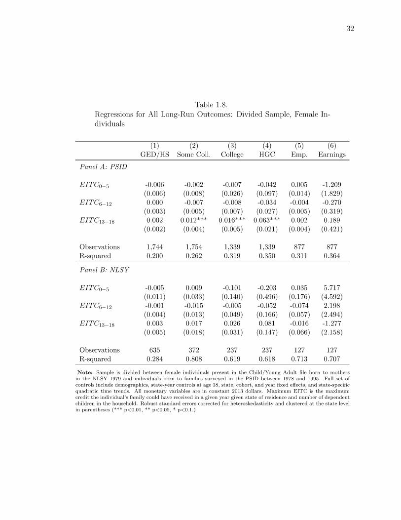
Tables 8-10 give the results of the same analysis performed on the subgroups that

most consistently had positive and significant effects on their long run outcomes,

specifically the female, white, and highly educated parents subgroups. There are

similarities in the effects across the two data sets, especially for the educational at-

tainment variables. Those in the PSID consistently show positive and significant

effects for EITC increases in the 13 to 18 age range on their level of education, while

the NLSY has similar but often insignificant coefficients for this variable on the same

educational outcomes. Thus, while the analysis on the overall PSID sample did pro-

duce some consistency with Bastian and Michelmore (forthcoming), the findings of

20

positive effects for completely different subgroups and no effects for the subgroups

in which they saw the largest responses call into question the robustness of their

analysis.

Lastly, one might be concerned that the difference in the time frames of the two

respective data sets are driving the lack of significant effects in the NLSY. While the

PSID subsample includes individuals born between 1969 and 1995, the earliest birth

year for the NLSY subsample is 1980. If the varying results between the two data sets

were do to the differing years present in each, we would expect that by excluding the

earlier years in the PSID that are not part of the NLSY, we should find no significant

effects. Table 11 shows the results of the main regression specification when run only

on those in the PSID who were born in 1980 or later so as to be consistent with the

NLSY time frame and the effects are almost identical to the earlier PSID results in

Table 6. Thus, the individuals from earlier years in the PSID are not driving the

effects. Thus, if there were more individuals present in the NLSY subsample, this

suggests we would likely find similar estimates,

1.8 Conclusion

This paper provides evidence that casts doubt on the previous findings that

the structural changes in the EITC, since it’s inception and through the early 2000’s,

had a positive overall impact on long run educational and labor market outcomes.

Replicating the methodology used in Bastian and Michelmore (forthcoming) on the

combined NLSY and PSID sample produced overall effects that were much smaller

in magnitude than their analysis. In addition, these effects seem to be driven by

individuals in the PSID who are most likely to have unobserved characteristics that





21


question the robustness of their analysis.

Exposure to different expansions due to differing time frames of the two data sets

do not seem to be driving this discrepancy. When using only the years present in

the NLSY for the PSID subjects, there is still evidence of significant positive effects

of the EITC expansions whereas if the effects were being driven by expansions not

experienced by the NLSY subjects, one would expect to see no significant effects.

Thus, it is up to future research to determine if there is indeed positive long term

educational and labor market effects for children whose families experienced EITC

expansions or if this is not as robust of an effect as was proposed in earlier work.

22

1.9 Figures and Tables

Figure 1.1. EITC Sturctural Changes Over Time

23

Figure 1.2. Federal EITC Parameters Over Time

25

Figure 1.3. State EITC Sturctural Changes Over Time

26

Table 1.1. Sample Summary Statistics

Full Sample

Obs. Mean Std. Dev.

Long-term Outcomes: HS Diploma or GED 4,616 0.92 0.28 Completed One or More Years of College 3,979 0.57 0.49 Bachelor’s Degree or Higher 2,914 0.32 0.47 Highest Grade Completed 2,914 13.92 1.94 Employed 2,052 0.87 0.24 Earnings ($1000s) 2,052 29.99 20.35

Demographics: Female 4,616 0.52 0.50 Black 4,616 0.39 0.49 Hispanic 4,616 0.06 0.24

Sibling at 18 4,616 1.038 1.12 Mother Ever Married 4,616 0.81 0.39 Parent Completed HS 4,616 0.91 0.29 Parent Completed Some College 4,616 0.50 0.50

EITC variables: EITC Maximum Age 0 to 5 ($1000s) 4,616 9.13 4.37 EITC Maximum Age 6 to 12 ($1000s) 4,616 20.49 10.97 EITC Maximum Age 13 to 18 ($1000s) 4,616 24.47 9.69 EITC Maximum Age 0 to 18 ($1000s) 4,616 54.10 22.64

Note: Sample contains a combination of individuals present in the Child/Young Adult file born to mothers in the NLSY 1979 and individuals born to families surveyed in the PSID between 1968 and 1995. Full set of controls include demographics, state-year controls at age 18, state, cohort, and year fixed effects, and state-specific quadratic time trends. All monetary variables are in constant 2013 dollars. Maximum EITC is the maximum credit the individual’s family could have received in a given year given state of residence and number of dependent children in the household.

27

Table 1.2. Effect on High School Graduation: Maximum EITC Over Full Child-hood

(1) (2) (3) (4) (5)

EIT C0−18 -0.000 0.000 0.000 0.000 0.001 (0.001) (0.001) (0.001) (0.001) (0.001)

Observations 4,616 4,616 4,616 4,616 4,616 R-squared 0.038 0.079 0.081 0.119 0.135 State, Cohort, & Year FEs X X X X X Demographics - X X X X State-Year Controls - - X X X Interaction Controls - - - X X State-Specific Time Trends Quadratic - - - - X

Note: Sample contains a combination of individuals present in the Child/Young Adult file born to mothers in the NLSY 1979 and individuals born to families surveyed in the PSID between 1968 and 1995. Full set of controls include demographics, state-year controls at age 18, state, cohort, and year fixed effects, and state-specific quadratic time trends. All monetary variables are in constant 2013 dollars. Maximum EITC is the maximum credit the individual’s family could have received in a given year given state of residence and number of dependent children in the household. Robust standard errors corrected for heteroskedasticity and clustered at the state level in parentheses (*** p<0.01, ** p<0.05, * p<0.1.)

Table 1.3. Regressions for All Long-Run Outcomes: Maximum EITC Over Full Childhood

(1) GED/HS

(2) Some Coll.

(3) College

(4) HGC

(5) Emp.

(6) Earnings

EIT C0−18 0.001 (0.001)

0.002 (0.001)

0.002 (0.002)

0.005 (0.009)

-0.001 (0.001)

-0.101 (0.135)

Observations R-squared

4,616 0.135

3,979 0.289

2,914 0.253

2,914 0.296

2,052 0.284

2,052 0.270


28

Table 1.4. Regressions for All Long-Run Outcomes: Maximum EITC Over Age Ranges

(1) GED/HS

(2) Some Coll.

(3) College

(4) HGC

(5) Emp.

(6) Earnings

EIT C0−5

EIT C6−12

EIT C13−18

-0.005 (0.006) 0.004** (0.002) -0.001 (0.002)

-0.001 (0.005) -0.005 (0.003) 0.008*** (0.002)

0.013 (0.014) -0.013* (0.007) 0.010** (0.004)

0.022 (0.052) -0.060** (0.028) 0.038** (0.016)

-0.000 (0.009) -0.004 (0.004) 0.001 (0.002)

-0.738 (0.456) -0.335 (0.231) 0.064 (0.163)


4,616 0.136

3,979 0.290

2,914 0.257

2,914 0.299

2,052 0.285

2,052 0.271


29

Table 1.5. Subgroup Regressions: High School Graduation/Earning a GED

(1)

Black

(2)

White

(3)

Female

(4)

Male

(5) Single Par.

(6) Low Ed. Par.

(7) High Ed. Par.

EIT C0−5

EIT C6−12

EIT C13−18

-0.007 (0.008) 0.004 (0.004) -0.003 (0.003)

-0.005 (0.007) 0.004 (0.003) 0.002 (0.002)

-0.007 (0.005) 0.001 (0.003) 0.002 (0.002)

-0.005 (0.009) 0.008** (0.003) -0.005 (0.003)

-0.030 (0.018) 0.003 (0.006) 0.003 (0.006)

-0.027 (0.039) 0.009 (0.016) 0.002 (0.014)

-0.003 (0.007) -0.000 (0.002) 0.001 (0.002)


1,787 0.191

2,553 0.127

2,379 0.160

2,237 0.184

877 0.371

412 0.661

2,313 0.200


30

Table 1.6. Regressions for All Long-Run Outcomes: Divided Sample

(1) GED/HS

(2) Some Coll.

(3) College

(4) HGC

(5) Emp.

(6) Earnings

Panel A: PSID

EIT C0−5

EIT C6−12

EIT C13−18

-0.005 (0.006) 0.004 (0.003) -0.001 (0.002)

-0.001 (0.006) -0.006* (0.003) 0.009*** (0.003)

0.014 (0.015) -0.014** (0.006) 0.010** (0.004)

0.027 (0.056) -0.062** (0.028) 0.032* (0.018)

0.002 (0.009) -0.003 (0.004) 0.002 (0.003)

-0.810 (0.522) -0.319 (0.219) 0.021 (0.201)


3,433 0.162 (5.264)

3,348 0.239 (9.467)

2,526 0.278 (12.554)

2,526 0.311 (49.724)

1,788 0.234 (5.850)

1,788 0.254

(553.266)

Panel B: NLSY

EIT C0−5

EIT C6−12

EIT C13−18

0.004 (0.009) 0.004 (0.004) -0.000 (0.006)

0.019 (0.015) -0.010 (0.007) 0.012 (0.010)

-0.029 (0.135) -0.008 (0.026) 0.017 (0.018)

0.067 (0.432) -0.080 (0.093) 0.050 (0.090)

-0.016 (0.127) -0.016 (0.019) -0.020 (0.019)

1.045 (3.910) 1.333 (1.432) -0.442 (1.060)


1,183 0.183

631 0.767

388 0.469

388 0.532

264 0.619

264 0.710

Note: Sample is divided between individuals present in the Child/Young Adult file born to mothers in the NLSY 1979 and individuals born to families surveyed in the PSID between 1978 and 1995. Full set of controls include demographics, state-year controls at age 18, state, cohort, and year fixed effects, and state-specific quadratic time trends. All monetary variables are in constant 2013 dollars. Maximum EITC is the maximum credit the individual’s family could have received in a given year given state of residence and number of dependent children in the household. Robust standard errors corrected for heteroskedasticity and clustered at the state level in parentheses (*** p<0.01, ** p<0.05, * p<0.1.)

31

Table 1.7. Regressions for All Long-Run Outcomes: Matched Sample

(1) GED/HS

(2) Some Coll.

(3) College

(4) HGC

(5) Emp.

(6) Earnings

Panel A: PSID

EIT C0−5

EIT C6−12

EIT C13−18

-0.002 (0.010) 0.002 (0.004) -0.002 (0.003)

0.006 (0.008) -0.012** (0.005) 0.017*** (0.005)

0.041 (0.028) -0.021** (0.009) 0.012** (0.005)

0.139 (0.107) -0.071* (0.038) 0.044** (0.019)

0.014 (0.009) -0.004 (0.006) 0.002 (0.003)

-0.875 (0.939) -0.419 (0.442) 0.082 (0.230)


1,980 0.236

2,039 0.269

1,582 0.330

1,582 0.361

1,129 0.318

1,129 0.325

Panel B: NLSY

EIT C0−5

EIT C6−12

EIT C13−18

0.004 (0.009) 0.004 (0.004) -0.000 (0.006)

0.019 (0.015) -0.010 (0.007) 0.012 (0.010)

-0.029 (0.135) -0.008 (0.026) 0.017 (0.018)

0.067 (0.432) -0.080 (0.093) 0.050 (0.090)

-0.016 (0.127) -0.016 (0.019) -0.020 (0.019)

1.045 (3.910) 1.333 (1.432) -0.442 (1.060)


1,183 0.183

631 0.767

388 0.469

388 0.532

264 0.619

264 0.710

Note: Sample is divided between individuals present in the Child/Young Adult file born to mothers in the NLSY 1979 and individuals born to families surveyed in the PSID between 1978 and 1995. Full set of controls include demographics, state-year controls at age 18, state, cohort, and year fixed effects, and state-specific quadratic time trends. This analysis includes individuals on the joint support of nearest neighbor matching without replacement based on all demographic and state-year economic controls. All monetary variables are in constant 2013 dollars. Maximum EITC is the maximum credit the individual’s family could have received in a given year given state of residence and number of dependent children in the household. Robust standard errors corrected for heteroskedasticity and clustered at the state level in parentheses (*** p<0.01, ** p<0.05, * p<0.1.)

32

Table 1.8. Regressions for All Long-Run Outcomes: Divided Sample, Female In-dividuals

(1) GED/HS

(2) Some Coll.

(3) College

(4) HGC

(5) Emp.

(6) Earnings

Panel A: PSID

EIT C0−5

EIT C6−12

EIT C13−18

-0.006 (0.006) 0.000 (0.003) 0.002 (0.002)

-0.002 (0.008) -0.007 (0.005) 0.012*** (0.004)

-0.007 (0.026) -0.008 (0.007) 0.016*** (0.005)

-0.042 (0.097) -0.034 (0.027) 0.063*** (0.021)

0.005 (0.014) -0.004 (0.005) 0.002 (0.004)

-1.209 (1.829) -0.270 (0.319) 0.189 (0.421)


1,744 0.200

1,754 0.262

1,339 0.319

1,339 0.350

877 0.311

877 0.364

Panel B: NLSY

EIT C0−5

EIT C6−12

EIT C13−18

-0.005 (0.011) -0.001 (0.004) 0.003 (0.005)

0.009 (0.033) -0.015 (0.013) 0.017 (0.018)

-0.101 (0.140) -0.005 (0.049) 0.026 (0.031)

-0.203 (0.496) -0.052 (0.166) 0.081 (0.147)

0.035 (0.176) -0.074 (0.057) -0.016 (0.066)

5.717 (4.592) 2.198 (2.494) -1.277 (2.158)


635 0.284

372 0.808

237 0.619

237 0.618

127 0.713

127 0.707

Note: Sample is divided between female individuals present in the Child/Young Adult file born to mothers in the NLSY 1979 and individuals born to families surveyed in the PSID between 1978 and 1995. Full set of controls include demographics, state-year controls at age 18, state, cohort, and year fixed effects, and state-specific quadratic time trends. All monetary variables are in constant 2013 dollars. Maximum EITC is the maximum credit the individual’s family could have received in a given year given state of residence and number of dependent children in the household. Robust standard errors corrected for heteroskedasticity and clustered at the state level in parentheses (*** p<0.01, ** p<0.05, * p<0.1.)

33

Table 1.9. Regressions for All Long-Run Outcomes: Divided Sample, Individuals With Highly Educated Parents

(1) GED/HS

(2) Some Coll.

(3) College

(4) HGC

(5) Emp.

(6) Earnings

Panel A: PSID

EIT C0−5

EIT C6−12

EIT C13−18

-0.003 (0.007) -0.001 (0.003) 0.001 (0.002)

-0.002 (0.010) -0.013** (0.006) 0.013** (0.005)

0.003 (0.033) -0.024** (0.011) 0.015* (0.008)

-0.036 (0.130) -0.092** (0.041) 0.055* (0.029)

-0.004 (0.015) -0.005 (0.007) 0.007* (0.004)

-1.920 (2.117) -0.678 (0.474) 0.278 (0.324)


1,732 0.248

1,721 0.238

1,284 0.323

1,284 0.328

915 0.380

915 0.357

Panel B: NLSY

EIT C0−5

EIT C6−12

EIT C13−18

0.003 (0.018) 0.003 (0.004) -0.005 (0.007)

0.013 (0.023) -0.008 (0.007) 0.014 (0.013)

-0.006 (0.324) 0.064 (0.083) -0.012 (0.076)

0.326 (1.390) 0.022 (0.383) 0.020 (0.352)

0.334 (0.406) 1.938 (2.425) -0.068 (0.145)

7.957 (18.726) 20.605 (107.019) -0.249 (4.347)


581 0.317

371 0.894

198 0.712

198 0.708

93 0.843

93 0.933

Note: Sample is divided between individuals present in the Child/Young Adult file born to mothers in the NLSY 1979 and individuals born to families surveyed in the PSID between 1978 and 1995 who had at least one parent complete a four year college degree or more. Full set of controls include demographics, state-year controls at age 18, state, cohort, and year fixed effects, and state-specific quadratic time trends. All monetary variables are in constant 2013 dollars. Maximum EITC is the maximum credit the individual’s family could have received in a given year given state of residence and number of dependent children in the household. Robust standard errors corrected for heteroskedasticity and clustered at the state level in parentheses (*** p<0.01, ** p<0.05, * p<0.1.)

34

Table 1.10. Regressions for All Long-Run Outcomes: Divided Sample, White Individuals

(1) GED/HS

(2) Some Coll.

(3) College

(4) HGC

(5) Emp.

(6) Earnings

Panel A: PSID

EIT C0−5

EIT C6−12

EIT C13−18

-0.005 (0.007) 0.006* (0.003) 0.002 (0.003)

-0.001 (0.010) -0.004 (0.006) 0.010** (0.004)

0.075** (0.035) -0.022* (0.012) 0.015** (0.007)

0.235* (0.132) -0.091* (0.048) 0.049* (0.027)

0.019 (0.013) -0.008* (0.005) 0.000 (0.003)

1.402 (1.642) -0.421 (0.483) 0.153 (0.263)


1,988 0.155

2,002 0.269

1,557 0.290

1,557 0.320

1,165 0.198

1,165 0.246

Panel B: NLSY

EIT C0−5

EIT C6−12

EIT C13−18

0.009 (0.013) 0.002 (0.006) 0.001 (0.007)

0.006 (0.018) -0.009 (0.009) 0.010 (0.018)

-0.063 (0.170) -0.058 (0.053) 0.063** (0.026)

-0.345 (0.501) -0.166 (0.157) 0.208** (0.083)

-0.067 (0.275) 0.014 (0.041) -0.008 (0.022)

5.284 (5.598) 5.273 (4.498) -2.404 (1.631)


565 0.320

310 0.892

175 0.677

175 0.719

115 0.699

115 0.866

Note: Sample is divided between white individuals present in the Child/Young Adult file born to mothers in the NLSY 1979 and individuals born to families surveyed in the PSID between 1978 and 1995. Full set of controls include demographics, state-year controls at age 18, state, cohort, and year fixed effects, and state-specific quadratic time trends. All monetary variables are in constant 2013 dollars. Maximum EITC is the maximum credit the individual’s family could have received in a given year given state of residence and number of dependent children in the household. Robust standard errors corrected for heteroskedasticity and clustered at the state level in parentheses (*** p<0.01, ** p<0.05, * p<0.1.)

35

Table 1.11. Regressions for All Long-Run Outcomes: PSID Subsample Over NLSY Date Range

(1) GED/HS

(2) Some Coll.

(3) College

(4) HGC

(5) Emp.

(6) Earnings

EIT C0−5

EIT C6−12

EIT C13−18

-0.009 (0.007) 0.004 (0.003) 0.000 (0.002)

-0.004 (0.007) -0.007* (0.004) 0.009*** (0.003)

-0.001 (0.018) -0.012* (0.007) 0.013** (0.005)

-0.035 (0.061) -0.062* (0.031) 0.039* (0.021)

-0.009 (0.009) -0.001 (0.005) 0.001 (0.004)

-0.884 (0.597) -0.120 (0.319) 0.082 (0.240)


1,925 0.184

1,941 0.283

1,265 0.326

1,265 0.351

879 0.305

879 0.349

Note: Sample contains a combination of individuals born to families surveyed in the PSID between who were born between 1980 and 1995. Full set of controls include demographics, state-year controls at age 18, state, cohort, and year fixed effects, and state-specific quadratic time trends. All monetary variables are in constant 2013 dollars. Maximum EITC is the maximum credit the individual’s family could have received in a given year given state of residence and number of dependent children in the household. Robust standard errors corrected for heteroskedasticity and clustered at the state level in parentheses (*** p<0.01, ** p<0.05, * p<0.1.)

36

2. FERTILITY RESPONSE TO THE TAX TREATMENT OF CHILDREN

2.1 Introduction

Since Becker (1960), many papers have explored the link between the cost of

raising a child and fertility. Classical economic theory suggests that as the cost of

raising a child increases, including the opportunity cost, the demand for children will

decrease. Alternatively, a reduction in the cost of raising a child from a government

subsidy to parents should increase the demand for children. However, there is only a

very small literature that attempts to estimate the magnitude of the fertility response

in the United States, with mixed findings.

As reviewed in Lopoo and Raissian (2012) there are many government programs

that give implicit child subsidies in the United States, despite not having an explicit

pro-natalist policy. Whittington, Alm, and Petters (1990) use child subsidy variation

from changes to the personal deduction in the personal income tax to estimate the

fertility elasticity and found very large and statistically significant effects.1 Crump,

Goda, and Mumford (2011) revisit this analysis by correcting model misspecification

and show that the long-run effect of child tax benefits in the U.S. on fertility is much

smaller, not statistically different than zero, and primarily operating through the

timing of births. Baughman and Dickert-Conlin(2003) find that the Earned Income

Tax Credit (EITC) expansions in the 1990s had no statistically significant effects on

fertility except for a small increase for married non-white women and a small decrease

for married white women who already have children.2

1They estimate that a $100 increase (in 2010 dollars) in the value of the subsidy would increase the general fertility rate by between 3 to 6 percent. Other papers use similar aggregate time-series data to estimate the effect of child tax benefits on fertility (e.g. Georgellis and Wall (1992), Zhang, Quan, and van Meerbergen (1994), Gauthier and Hatzius (1997), Huang (2002) and generally find a positive but small effect. 2There is a literature that exams the fertility response to child subsidies in other countries including Laroque and Salanie (2005), Milligan (2005), Parent and Wang (2007), Cohen, Dehejia, and Ro-

37

In this paper, we use state and federal personal income tax changes to identify

the fertility response to a change in the child subsidy. Our approach is to restrict the

variation in the child tax subsidy to change in the state or federal tax code, holding

all characteristics of the household fixed. Rather than focus on a single tax provision,

like the EITC or the personal deduction as in the prior literature, we use changes to

child tax subsidy resulting from changes in the overall tax structure. We calculate all

the ways in which state and federal tax codes treat taxpayers differently depending

on the number of children. This includes the EITC and personal deduction as in the

prior literature, but also includes many other deductions and credits including the

child tax credit and the additional child tax credit.

We find that the tax subsidy for having a child does not seem to cause a signifi-

cant fertility response, but some subgroups of the US population do have a positive

and economically significant fertility response to the child tax subsidy including low-

income women, single women, and women in the earlier half of our sample.

2.2 Data

We use a sample of women from two data sources: the Panel Study of Income

Dynamics (PSID) and the restricted geocoded National Longitudinal Survey of Youth

(NLSY79). The PSID is a longitudinal data set that began with a representative set

of households in 1968 and followed these households, their descendants, and refresher

samples. The NLSY79 spans 1979 to 2012 and consists of approximately 13,000 young

men and women that were age 14 to 20 by December 31, 1978. A disadvantage of

using the NLSY is that it transitions from being a annual survey to biannual in 1994.

In 1999, the PSID also transitioned from an annual survey to a biannual survey. For

the missing years in each survey, the number of children, state of residence, family

income, and marital status were imputed in order to calculate the change in child

tax subsidy for each individual in these years. Another limitation of the NLSY is

manov (2007) where the pro-natalist policy is generally explicit and thus not a good comparison for the U.S. experience.

38

that total taxable family income is not reported, but rather total earned income from

salary and wages is reported. In order to have consistency in our combined sample,

this income measure is used from both the NLSY and the PSID when computing the

change in child tax subsidy and as a demographic control variable. We restrict the

sample to women between the ages of 20 and 43. We remove teenage women because

they have a much lower likelihood of filing their taxes. Restricting the sample to

women age 44 or less is standard in the fertility literature as there are so few women

who give birth past the age of 44 due to biological factors. We also exclude women

aged 44 in from our sample as they were exhibiting fertility rates on par with women

in their twenties and were outliers as compared to the national rates for women of

that age. The results remain unchanged if these 37 women are not dropped from the

sample. In all, there are 207,470 observations and 18,592 individual women included

in the sample (5,819 from the NLSY and 12,773 from the PSID). An advantage of

these data sets is that they follow these women for many years, just over eleven

years on average per woman, and they allow us to observe births as well as provide

many years for which there are changes in the tax structure that affect their child tax

subsidies.

As shown in Table 1, the women included in this sample have a 16.3% chance of

having a child within two years of when they are observed in the data. Figure 1 plots

this variable for women in our sample over the time frame of our analysis. Fertility

for the women in our sample is somewhat volatile, tended to be higher for women in

the earlier half of our sample relative to the second half. The rate of births decreased

throughout the 1990’s for these women and started to rise again after 2000. The

average child tax subsidy for women in our sample is $929. Figure 2 illustrates how

this has changed for the women of our sample over time. Of particular note are the

significant increases in 1987 (tax year 1986) and 1999 (tax year 1998) mostly due to

the expansion of the Earned Income Tax Credit and the introduction of the Child Tax

Credit, respectively. Family income has been scaled by the CPI-U and converted into

constant 2013 dollars and on average women in the sample are in families that earn

39

about $42,000 annually. About 62 percent of the women in the data are married, 34

percent are black, and about 8% are Hispanic. The average woman has 1.6 children

and about 77 percent of the sample is participating in the labor force. Over half of

the women in the sample have at least some college education, and about a quarter

have a four year college degree or higher. From one year to the next, the mean change

in the child tax subsidy due to changes in the tax structure is approximately $16 for

the full sample and about $50 for low income women. However, it is possible for some

individuals to experience negative changes in the child tax subsidy while others in the

sample see changes that are substantially larger than the mean. The construction of

this variable is detailed in the following section.

2.3 Estimation Strategy

The following equation represents the main linear regression specification of the

paper:

Birthist = βΔT axSubsidy ∗ ist +γXist + τt + σs + θi + πZs,t + �ist (2.1)

Where Birthist is an indicator for having a child in the next two years. We do not look

for an immediate response to a child tax subsidy as it takes at least nine months to

observe a fertility change. The lag on this response is up to two years because family

units need time to respond to tax incentives, and most of the response would be from

observing the result of filing taxes for the previous tax year and the corresponding tax

returns. Xist is a vector of control variables including indicators for marital status,

Hispanic, black, level of education, religion, employment status, age fixed effects,

number of dependent children fixed effects, and a fifth degree polynomial in real family

income. Also included in Xist is the level of tax subsidy for period t − 1, referred to

as Tax Subsidy*, that was calculated using the individual’s observables from period

t in order to control for the level of the child tax subsidy that an individual with

these observable characteristics will receive. Both ΔTax Subsidy* and Tax Subsidy*

40

are in constant 2013 dollars. τt represents year dummy variables and σt represents

state dummy variables. θi are individual fixed effects that will control for any further

unaccounted for time-invariant individual characteristics.

The main covariate of interest is constructed using tax liability data from the

NBER TAXSIM calculator. TAXSIM calculates federal and state tax liability for

every woman in the sample using tax year, state, marital status, number of dependent

children, own wage, and spouse wages. We then increase the number of dependent

children by one for each woman in the sample and calculate what her tax liability

would be if she had an additional child. The difference between the two tax liabilities

in the same tax year define the child tax subsidy in that year.

These calculations are then repeated for the previous tax year, holding all indi-

vidual characteristics constant, including state, marital status, number of dependent

children, own wage, and spouse wage. In doing so, the only way for the tax liability

in the current year to be different from the tax liability in year t − 1 is if the state

or federal tax treatment of the individual changed. We once again calculate the tax

liability and child tax subsidy, this time for year t − 1.

The difference between the child tax subsidy in year t and the child tax subsidy

in year t − 1 (assuming year t characteristics) is what will henceforth be referred to as

the change in tax subsidy* (ΔTax Subsidy*) as this is not the observed value. Table

2 provides an example of these tax calculations. This example illustrates how the

main covariate of interest in this analysis, ΔTaxSubsidy*, is constructed and how it

differs from the observed ΔTaxSubsidy. When calculating ΔTaxSubsidy*, one must

first calculate the child tax subsidy in period t. The tax subsidy for t − 1 is then

also calculated using the individual’s characteristics from period t. ΔTaxSubsidy*

is the difference between these two values. Characteristics are fixed at t so that the

change in the subsidy is driven solely by structural changes in the tax code and we

avoid overstating changes due to individual choices that are endogenous to fertility

decisions. In equation (2), the coefficient β represents how the likelihood of having

41

a child within the next two years is associated with state or federal changes to the

child subsidy in the tax code.

The basis of our identification strategy for equation (2) is that changes in the

child tax subsidy from period t − 1 to t (holding individual characteristics fixed) are

conditionally exogenous to the individual woman’s choice to have a child within the

next two years. There are two main ways in which our identification strategy will fail.

Even after conditioning on the observable covariates in equation (2), fluctuations in

ΔTaxSubsidy* could be correlated with births in the next two years through means

other than structural changes in the tax code directly affecting the child tax subsidy.

The first is that we have not included flexible enough controls to account for the

correlations between the type of woman who is most likely to experience a change

in their child tax subsidy and their likelihood of giving birth. For example, our

data shows that the fewer dependent children a woman has the more likely she is to

experience a positive change in her child tax subsidy. Similarly, larger changes in the

child subsidy are more likely to be experienced by older women. However, even women

of the same age and number of children could likely have different fertility rates due

to other factors, such as marital status for instance. To account for these types of

relationships between the who is more or less likely to experience child tax subsidy

changes and the varying likelihoods of fertility, we also include all combinations of

interactions between our age, marital status, and number of children indicators in

the main specification of our model. Likewise, we also include interactions between

the indicators for black and Hispanic with the state and year fixed effects. Lastly,

to more flexibly control for factors associated with family income that could bias our

results, we include interactions between family income and all of our other covariates,

as well as interactions between family income squared and our covariates.

The second way in which our identification strategy can fail is if there are un-

accounted for state policies or characteristics that are correlated with both fertility

and changes in the child tax subsidy. For example, imagine women of a particular

state are more likely to have children for reasons not related to the child tax subsidy,

42

but this state is also more generous in it’s tax benefits to mothers. To account for

these types of relationships, we include state-specific quadratic time trends, Zs,t, in

our main specification as well.

We estimate our main specification on our full sample as well as check for het-

erogeneity in the effect across variety of sub-samples. We also run the specifica-

tion using a variant ΔTaxSubsidy* which serves as a placebo test. Additionally, we

look for evidence of timing effects as well as investigate a disaggregated measure of

ΔTaxSubsidy*. This analysis is detailed further in the following section.

2.4 Results

The results in Table 3 present the fertility effects of changes in the child tax subsidy

for the full sample, and Table 4 produces similar results by household income. Col-

umn (1) of Table 3 presents the results when only our demographic controls and state

and year fixed effects are included in the regression. Conditional on these controls,

a $1,000 increase in an individual’s child tax subsidy from t − 1 to t is associated

with a decrease in the likelihood of having a child within the next two years. A

negative coefficient does not have an intuitive interpretation in this case as there is

only a price effect influencing the individual’s decision to have a child. This sug-

gests further control variables are needed to account for omitted variable bias. The

coefficient decreases in magnitude as we include the interaction terms, specifically

interactions between our age, marital status, and number of children indicators as

well as interactions between the indicators for black and Hispanic with the state and

year fixed effects. Additionally, we include interactions between family income and

family income squared with all of the demographic and state-year controls. When we

also add mother fixed effects to the specification, the coefficient on ΔTaxSubsidy*

once again decreases in magnitude and is no longer statistically significant from zero.

This suggests that for the overall sample population, there is not a fertility response

to increasing the child tax subsidy. Note that we also include TaxSubsidy*, the level

43

of tax subsidy the individual would receive in t − 1 if they possessed their period t

characteristics. The negative coefficient in the first two columns suggests that those

who have larger child tax subsidies in the previous period are less likely to have a

child. However, these coefficients also diminish in the last two columns and are not

statistically different than zero.

Table 4 provides the results of our main specification on those of varying income

levels. Note that family income is the total labor income of the mother and spouse,

if married, and it has be scaled to constant 2013 dollars using the CPI-U. In column

(1), there is a very large, positive, and statistically significant fertility response to

changes in the child tax subsidy for mothers in families with $30,000 of income or

less. A $1,000 increase in the subsidy is associated with a 17.0% increase in the

baseline likelihood of having a child in the next two years of 0.159. This represents

an additional 14 births per 1,000 women per $1,000 increase and is a very large effect.

This is on par with the findings of Milligan (2005) who estimated that a $1,000

increase in child tax benefits was associated with an additional 11 births. Also of

note is the positive coefficient on TaxSubsidy* in column (1), which suggests that

those who have larger child tax subsidies in the previous period are more likely to

have a child. In contrast, columns (2) and (3) provide evidence that women in mid-

and high income families do not have a fertility response to changes in the child tax

subsidy.

Tables 5 and 6 illustrate further heterogeneity in the fertility response to changes in

the child tax subsidy. The specification used in all regressions presented in these two

tables is the main specification of the model and the same as that of Table 3, Column

(4). The response is not statistically significant from zero for the subsamples divided

by number of children, race, educational attainment, or age apart from a marginally

significant positive coefficient for women with no children. The results also indicate

that there is a significant positive response for single women and for women in the

1968 to 1990 range of our sample. The magnitudes of the coefficients for single

44

women and women in the 1980 to 1990 range are similar in their relationship to their

mean dependent variable values as was the case for low income women detailed above.

However, the marginal effect of a $1,000 increase for women in the 1968 to 1980 range

is extremely large. As we question that such an effect is reasonable, we conduct a

placebo test on this subsample, as well as the other subsamples with large, positive

fertility responses. This is detailed later in this section.

In contrast to the significant and positive coefficients for the two earlier date ranges

in our sample, the women in the 1990 to 2000 and 2000 to 2013 ranges do not exhibit

a fertility response to changes in the child subsidy that is significantly different from

zero. To investigate this further, we divide the sample roughly in half based on time

period: 1968 to 1990 as one group and 1991 to 2013 as the other. We use two date

ranges rather than the four used previously because we look into subsamples within

these ranges, specifically low income women and single women. These two groups were

chosen as they both showed a positive and statistically significant fertility response

in Table 5. In the top panel of Table 7, we find that low income women have a

positive fertility response that is slightly lower in the later date range but still large

and statistically significant. In the lower panel of Table 7, single women also have a

positive and significant fertility response in the early date range, but the magnitude

of this effect greatly decreases and is not significantly different from zero for women

in the 1991 to 2013 range. Thus, low income women are responsive throughout the

time frame of the analysis, but single women are no longer responding to the child

tax subsidy implicit in the tax structure.

In Table 8, we present the results of a placebo test run for the subgroups that

showed a positive and statistically significant fertility response. Here ΔTaxSubsidy*

is the difference in the child tax subsidy in period t + 3 and the subsidy in period

t + 4 using only individual characteristics from period t in both subsidy calculations.

Demographic controls still include total dependent children and the level of the child

tax subsidy in period t − 1 as well as dummy variables for age, income bins, race,

45

education, labor force participation, and religion. The reasoning behind this test is

that variation in the child tax subsidy due to structural tax changes from t + 3 to

t + 4 should not illicit a fertility response in t + 1 or t + 2. As seen in Table 8, only

single women and women in the 1968 to 1980 subgroups withstand this test as the

other two subgroups still demonstrate a positive and significant fertility response.

This suggests that the fertility response may be highly persistent over time or that

those who respond to changes in the child tax subsidy are likely to do so again in the

future in addition to being likely to experience similar changes to the subsidy.

Looking into the persistence of the fertility response over time even further, we run

our main specification and include four lagged terms of the change in the tax subsidy

as well. L“X”ΔTaxSubsidy* is the “X” year lagged value of ΔTaxSubsidy*. The

results of this exercise are presented in Table 9. All subgroups that showed a positive

and statistically significant fertility response in our previous analysis also demonstrate

a highly persistent effect, especially for variation in the child tax subsidy that has

occurred within the previous three tax years. The magnitude of the coefficients are

once again extremely large. The results here as well as those from our placebo analysis

seem to indicate that these estimates may be partly due to spurious correlation within

the data. Women may also be anticipating tax changes that have been announced

before being implemented or those that are rolled out gradually. To see if this is the

case, we repeat the impulse response analysis in Table 9 but change the dependent

variable to be an indicator for if the woman has a child in period t. The results

are presented in Table 10, and we see that there does not seem to be anticipation

for single mothers or in any time frame of the sample. However, women in low

income households do demonstrate a large, positive and statistically contemporaneous

response and the evidence suggests that they may even be anticipating changes in

the child tax subsidy up to three years in advance. This would most likely be for tax

law changes that have been announced but delayed in implementation or tax changes

that are gradually rolled out over time.

46

Lastly, Table 11 seeks to determine if there is a difference in response depending on

which component of the overall child tax subsidy was changed. To do so, we include

changes in the Earned Income Tax Credit (EITC) and the Child Tax Credit (CTC)

in the regression specification as well as their levels. These changes are calculated in

the same fashion as the overall change in the child tax subsidy in that we find the

increase of each credit due to an additional birth for period t and t − 1 and find the

difference between these two values holding the individual’s characteristics fixed at

those observed in period t. In this analysis, the coefficient for ΔTaxSubsidy* should

be interpreted as the fertility response to a $1000 increase in the tax subsidy that

is not being driven by changes in the earned income tax credit or child tax credit.

The coefficients on ΔEITCSubsidy* and ΔCTCSubsidy* represent the fertility effects

corresponding to the difference in all other changes and changes in the EITC and

CTC, respectively. Note that the change in the CTC and it’s level are not included

for columns (3) and (4) as the CTC was not implemented until the 1998 tax year.

Column (1) presents the results of this specification for the women in families with

$30,000 of annual income or less. As none of the coefficients are statistically different

from zero, there is seemingly no difference in fertility response for low income women

based on which component of the child subsidy is changed. However, the magnitudes

of the coefficients suggest that these women may be less responsive to changes in

the CTC relative to changes in all other parts of the subsidy (excluding the EITC).

However, for single women and for women across the date range of our sample, there

is a higher fertility response to increases in the EITC relative to the CTC and relative

to all other changes in the child tax subsidy as the coefficient for ΔEITCSubsidy* is

significantly larger than that for ΔTaxSubsidy* and ΔCTCSubsidy* for these sub-

groups.

47

2.5 Conclusion

Overall, the tax subsidy for having a child does not seem to have a significant

fertility response, but some subgroups of the US population do have a positive and

economically significant fertility response to the child tax subsidy. Specifically, low-

income women, single women, and women in the earlier half of our sample are most

responsive to the child tax subsidy. However, the effects for most of these subgroups

do not hold up to our placebo analysis. The evidence suggests that not all child

tax subsidy changes are equally salient for these subgroups as the fertility response

is driven by increases to the Earned Income Tax Credit and not the value of the

personal exemption or by increases to the Child Tax Credit.

48

2.6 Figures and Tables

Figure 2.1. Fertility Over Time

Figure 2.2. Child Tax Subsidy Over Time

49

Table 2.1. Summary Statistics

Mean Std. Dev.

Birth 0.163 0.369

Family Income 41,620 52,248

Tax Subsidy ($1000’s) 0.929 0.855

ΔTax Subsidy* ($1000’s) 0.016 0.176

Married 0.620 0.485

Labor Force Part. 0.766 0.423

No. Children 1.558 1.387

Black 0.335 0.472

Hispanic 0.077 0.266

High School 0.901 0.299

Some College 0.540 0.498

Bachelors+ 0.256 0.436

Age 20-24 0.171 0.376

Age 25-29 0.222 0.416

Age 30-34 0.237 0.425

Age 35-43 0.370 0.482

1968-1980 0.172 0.378

1981-1990 0.296 0.457

1991-2000 0.322 0.463

2001-2013 0.221 0.415

Observations 207,470

Note: Data used in the analysis is from Panel Study of Income Dynamics (PSID) and the restricted geocoded National Longitudinal Survey of Youth (NLSY79). The PSID is a longitudinal data set that began with a rep-resentative set of households in 1968 and followed these households, their descendants, and refresher samples. The NLSY79 spans 1979 to 2012 and consists of ap-proximately 13,000 young men and women that were age 14 to 20 by December 31, 1978. The sample is restricted to women between the ages of 20 and 43.

50

Table 2.2. Change in Subsidy Example

Observed Star

t − 1 t t − 1 t

Year 1997 1998 1997 1998

Income $25,000 $25,000 $25,000 $25,000

Dependent Children 1 2 2 2

Tax Liability $1397.89 -$836.38 $217.33 -$836.38

Tax Liability $217.33 -$1621.38 -$180.17 -$1621.38 (w/ one add. child)

Tax Subsidy $1180.56 $785 $397.50 $785

ΔTaxSubsidy -395.56 387.5

Note: The stylized example above illustrates how the main covariate of in-terest in this analysis, ΔTaxSubsidy*, is constructed and how it differs from the observed ΔTaxSubsidy. When calculating ΔTaxSubsidy*, one must first calculate the child tax subsidy in period t. Then the tax subsidy for t − 1 is then also calculated using the individual’s characteristics from period t. Thus, ΔTaxSubsidy* is the difference between these two values. Characteristics are fixed at t so that the change in the subsidy is driven solely by structural changes in the tax code and we avoid overstating changes due to individual choices that are endogenous to fertility decisions.

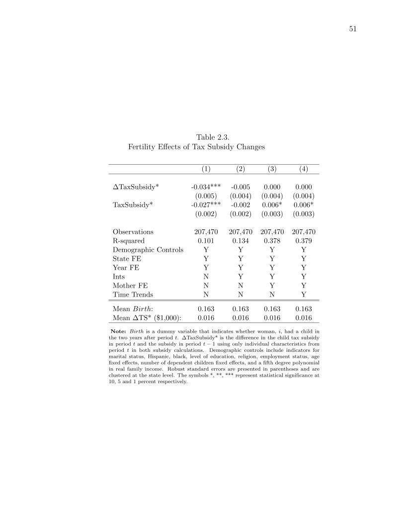
51

Table 2.3. Fertility Effects of Tax Subsidy Changes

(1) (2) (3) (4)

ΔTaxSubsidy* -0.034*** -0.005 0.000 0.000 (0.005) (0.004) (0.004) (0.004)

TaxSubsidy* -0.027*** -0.002 0.006* 0.006* (0.002) (0.002) (0.003) (0.003)

Observations 207,470 207,470 207,470 207,470 R-squared 0.101 0.134 0.378 0.379 Demographic Controls Y Y Y Y State FE Y Y Y Y Year FE Y Y Y Y Ints N Y Y Y Mother FE N N Y Y Time Trends N N N Y

Mean Birth: 0.163 0.163 0.163 0.163 Mean ΔTS* ($1,000): 0.016 0.016 0.016 0.016

Note: Birth is a dummy variable that indicates whether woman, i, had a child in the two years after period t. ΔTaxSubsidy* is the difference in the child tax subsidy in period t and the subsidy in period t − 1 using only individual characteristics from period t in both subsidy calculations. Demographic controls include indicators for marital status, Hispanic, black, level of education, religion, employment status, age fixed effects, number of dependent children fixed effects, and a fifth degree polynomial in real family income. Robust standard errors are presented in parentheses and are clustered at the state level. The symbols *, **, *** represent statistical significance at 10, 5 and 1 percent respectively.

52

Table 2.4. Fertility Effects of Tax Subsidy Changes by Income ($1,000’s)

(1) (2) (3) ≤ $30 $30 − $65 ≥ $65

ΔTaxSubsidy* 0.027*** 0.019* 0.008 (0.008) (0.010) (0.007)

TaxSubsidy* 0.020*** 0.004 0.004 (0.003) (0.007) (0.006)

Observations 75,715 66,377 65,378 R-squared 0.447 0.502 0.493 Demographic Controls Y Y Y State FE Y Y Y Year FE Y Y Y Ints Y Y Y Mother FE Y Y Y Time Trends Y Y Y

Mean Birth: 0.159 0.163 0.166 Mean ΔTS* ($1,000): 0.020 0.016 0.010

Note: Birth is a dummy variable that indicates whether woman, i, had a child in the two years after period t. ΔTaxSubsidy* is the difference in the child tax subsidy in period t and the subsidy in period t − 1 using only individual characteristics from period t in both subsidy calculations. Demographic controls include total dependent children and the level of the child tax subsidy in period t − 1 as well as dummy variables for age, income bins, race, education, labor force participation, and religion. Regressions also include mother fixed effects, state-specific quadratic time trends, and all interaction terms as described in the estimation strategy. Family income ($1000’s) has been scaled by the CPI-U and converted into constant 2013 dollars. The symbols *, **, *** represent statistical significance at 10, 5 and 1 percent respectively.

53

Table 2.5. Heterogeneity of Fertility Effects by Income

Birth Mean Birth Mean ΔTS* ($1,000)

Obs

Marital Status: Married

Single

-0.008 (0.007)

0.013*** (0.005)

0.118

0.190

0.025

0.010

128,655

78,815

Number of Children:

No Children

One Child

Two Children

Three or More Children

0.012** (0.006)

-0.010 (0.014)

-0.012 (0.008)

-0.003 (0.008)

0.087

0.250

0.117

0.097

0.030

0.022

0.010

-0.002

57,496

47,958

57,456

44,560

Race:

Black

Hispanic

White

Education:

0.006 (0.007)

-0.004 (0.015)

-0.003 (0.005)

0.156

0.166

0.166

0.015

0.026

0.015

69,482

15,935

122,053

High School

Some College

College or More

0.000 (0.008)

0.001 (0.008)

0.001 (0.006)

0.160

0.160

0.167

0.011

0.019

0.017

35,432

46,102

76,763

Note: All regressions include state, year, and mother fixed effects, demographic controls, and state-specific quadratic time trends. Birth is a dummy variable that indicates whether woman, i, had a child in the two years after period t. ΔTaxSubsidy* is the difference in the child tax subsidy in period t and the subsidy in period t − 1 using only individual characteristics from period t in both subsidy calculations. Demographic controls include total dependent children and the level of the child tax subsidy in period t − 1 as well as dummy variables for age, income bins, race, education, labor force participation, and religion. Regressions also include mother fixed effects, state-specific quadratic time trends, and all interaction terms as described in the estimation strategy. The symbols *, **, *** represent statistical significance at 10, 5 and 1 percent respectively.

54

Table 2.6. Heterogeneity of Fertility Effects by Income, Con-tinued.

Birth Mean Birth Mean ΔTS* ($1,000)

Obs

Age of Mother:

Age 20-24

Age 25-29

Age 30-34

Age 35-43

-0.013 (0.015)

-0.011 (0.010)

0.007 (0.009)

-0.011 (0.007)

0.258

0.237

0.154

0.067

-0.000

0.012

0.007

0.031

35,432

46,102

49,173

76,763

Year:

1968-1980

1980-1990

1990-2000

2000-2013

0.063*** (0.018)

0.015* (0.008)

-0.013 (0.010)

-0.006 (0.007)

0.196

0.200

0.135

0.128

-0.017

-0.004

0.048

0.023

35,714

61,445

64,515

45,796

Note: All regressions include state, year, and mother fixed effects, demographic con-trols, and state-specific quadratic time trends. Birth is a dummy variable that indicates whether woman, i, had a child in the two years after period t. ΔTaxSubsidy* is the difference in the child tax subsidy in period t and the subsidy in period t − 1 using only individual characteristics from period t in both subsidy calculations. Demographic controls include total dependent children and the level of the child tax subsidy in pe-riod t − 1 as well as dummy variables for age, income bins, race, education, labor force participation, and religion. Regressions also include mother fixed effects, state-specific quadratic time trends, and all interaction terms as described in the estimation strat-egy. The symbols *, **, *** represent statistical significance at 10, 5 and 1 percent respectively.

55

Table 2.7. Time Period Heterogeneity of Fertility Ef-fects

(1) (2) 1968-1990 1991-2013

Less Than $30,000 Family Inc. ΔTaxSubsidy* 0.043*** 0.034***

(0.016) (0.010) TaxSubsidy* 0.030*** 0.018***

(0.010) (0.005) Observations 36,802 38,913 R-squared 0.550 0.506 Mean Birth: 0.191 0.129 Mean ΔTS* ($1,000): 0.009 0.031

Single ΔTaxSubsidy* 0.032*** 0.005

(0.008) (0.008) TaxSubsidy* 0.020** 0.006*

(0.007) (0.003) Observations 32,706 46,109 R-squared 0.529 0.463 Mean Birth: 0.144 0.101 Mean ΔTS* ($1,000): 0.014 0.034

Used in each section: Demographic Controls Y Y State FE Y Y Year FE Y Y Ints Y Y Mother FE Y Y Time Trends Y Y

Note: All regressions include state, year, and mother fixed effects, demo-graphic controls, and state-specific quadratic time trends. Birth is a dummy variable that indicates whether woman, i, had a child in the two years after period t. ΔTaxSubsidy* is the difference in the child tax subsidy in period t and the subsidy in period t − 1 using only individual characteristics from period t in both subsidy calculations. Demographic controls include total dependent children and the level of the child tax subsidy in period t − 1 as well as dummy variables for age, income bins, race, education, labor force participation, and religion. Regressions also include mother fixed effects, state-specific quadratic time trends, and all interaction terms as described in the estimation strategy. The symbols *, **, *** represent statistical sig-nificance at 10, 5 and 1 percent respectively.

56

Table 2.8. Placebo Test of Fertility Effects

≤ $30k Single 1968-1980 1981-1990

ΔTaxSubsidy* 0.024** 0.009 -0.007 0.022** (0.010) (0.006) (0.014) (0.009)

Observations 75,715 78,815 65,378 61,445 Demographic Controls Y Y Y Y State FE Y Y Y Y Year FE Y Y Y Y Ints Y Y Y Y Mother FE Y Y Y Y Time Trends Y Y Y Y Mean Birth: 0.159 0.190 0.096 0.200 Mean ΔTS* ($1,000): 0.010 0.016 -0.017 -0.004

Note: All regressions include state, year, and mother fixed effects, demographic con-trols, and state-specific quadratic time trends. Birth is a dummy variable that indicates whether woman, i, had a child in the two years after period t. For this placebo analysis, ΔTaxSubsidy* is the difference in the child tax subsidy in period t + 3 and the subsidy in period t + 4 using only individual characteristics from period t in both subsidy cal-culations. Demographic controls include total dependent children and the level of the child tax subsidy in period t − 1 as well as dummy variables for age, income bins, race, education, labor force participation, and religion. Regressions also include mother fixed effects, state-specific quadratic time trends, and all interaction terms as described in the estimation strategy. The symbols *, **, *** represent statistical significance at 10, 5 and 1 percent respectively.

57

Table 2.9. Impulse Response of Fertility Effects

≤ $30k Single 1968-1980 1981-1990

ΔTaxSubsidy* 0.038*** 0.003 0.058** 0.055*** (0.011) (0.008) (0.025) (0.017)

L1ΔTaxSubsidy* 0.033** 0.018** 0.069* 0.058*** (0.013) (0.008) (0.035) (0.021)

L2ΔTaxSubsidy* 0.031** 0.016* 0.092*** 0.080*** (0.012) (0.010) (0.034) (0.027)

L3ΔTaxSubsidy* 0.017 0.007 0.029 0.021 (0.014) (0.007) (0.037) (0.035)

L4ΔTaxSubsidy* 0.007 0.007 0.036 0.038 (0.014) (0.006) (0.049) (0.034)

Observations 36,210 39,081 47,525 24,035 R-squared 0.456 0.420 0.555 0.555 Demographic Controls Y Y Y Y State FE Y Y Y Y Year FE Y Y Y Y Ints Y Y Y Y Mother FE Y Y Y Y Time Trends Y Y Y Y Mean Birth: 0.159 0.190 0.096 0.200 Mean ΔTS* ($1,000): 0.010 0.016 -0.017 -0.004

Note: Birth is a dummy variable that indicates whether woman, i, had a child in the two years after period t. ΔTaxSubsidy* is the difference in the child tax subsidy in period t and the subsidy in period t − 1 using only individual characteristics from period t in both subsidy calculations. L”X”ΔTaxSubsidy* is the ”X” year lagged value of ΔTaxSubsidy*. Demographic controls include total dependent children and the level of the child tax subsidy in period t − 4 as well as dummy variables for age, income bins, race, education, labor force participation, and religion. This regression also include the four year lagged level of TaxSubsidy*. Robust standard errors are presented in parentheses and are clustered at the state level. Regressions also include mother fixed effects, state-specific quadratic time trends, and all interaction terms as described in the estimation strategy. The symbols *, **, *** represent statistical significance at 10, 5 and 1 percent respectively.

58

Table 2.10. Impulse Response of Contemporaneous Fertility Effects

≤ $30k Single 1968-1980 1981-1990

ΔTaxSubsidy* 0.014** 0.008 -0.018 -0.003 (0.007) (0.000) (0.019) (0.012)

L1ΔTaxSubsidy* 0.038*** 0.017 0.012 -0.009 (0.010) (0.000) (0.021) (0.017)

L2ΔTaxSubsidy* 0.028*** 0.018 -0.035 -0.017 (0.010) (0.000) (0.022) (0.013)

L3ΔTaxSubsidy* 0.023** 0.020 -0.007 0.053 (0.009) (0.000) (0.024) (0.032)

L4ΔTaxSubsidy* 0.015 0.015 -0.055** 0.021 (0.010) (0.000) (0.023) (0.022)

Observations 43,468 50,241 17,296 30,663 R-squared 0.307 0.256 0.374 0.392 Demographic Controls Y Y Y Y State FE Y Y Y Y Year FE Y Y Y Y Ints Y Y Y Y Mother FE Y Y Y Y Time Trends Y Y Y Y Mean Birth: 0.063 0.044 0.083 0.082 Mean ΔTS* ($1,000): 0.018 0.022 -0.029 -0.023

Note: The dependent variable in this analysis is a dummy variable that indicates whether woman, i, had a child in period t. ΔTaxSubsidy* is the difference in the child tax sub-sidy in period t and the subsidy in period t − 1 using only individual characteristics from period t in both subsidy calculations. L”X”ΔTaxSubsidy* is the ”X” year lagged value of ΔTaxSubsidy*. Demographic controls include total dependent children and the level of the child tax subsidy in period t − 4 as well as dummy variables for age, income bins, race, education, labor force participation, and religion. This regression also include the four year lagged level of TaxSubsidy*. Robust standard errors are presented in parentheses and are clustered at the state level. Regressions also include mother fixed effects, state-specific quadratic time trends, and all interaction terms as described in the estimation strategy. The symbols *, **, *** represent statistical significance at 10, 5 and 1 percent respectively.

59

Table 2.11. Fertility Effects by Income with Disaggregated Subsidy

≤ $30k Single 1968-1980 1981-1990

ΔTaxSubsidy* 0.008 -0.001 0.020 -0.004 (0.015) (0.005) (0.022) (0.011)

ΔEITCSubsidyStar 0.017 0.029** 0.084** 0.058** (0.018) (0.011) (0.033) (0.023)

ΔCTCSubsidyStar -0.049 0.010 (0.038) (0.010)

TaxSubsidy* -0.006 0.002 -0.008 -0.001 (0.009) (0.004) (0.017) (0.011)

EITCSubsidy* 0.034** 0.034*** 0.092** 0.011 (0.013) (0.004) (0.038) (0.016)

CTCSubsidy* 0.026 0.040*** (0.019) (0.009)

Observations 75,715 78,815 65,378 61,445 Mean Birth: 0.159 0.190 0.096 0.200 Mean ΔTS* ($1,000): 0.010 0.016 -0.017 -0.004

Note: In this analysis, the coefficient for ΔTaxSubsidy* should be interpreted as the fertility response to a $1000 increase in the tax subsidy that is not being driven by changes in the earned income tax credit or child tax credit. The coefficients on ΔEITCSubsidy* and ΔCTCSubsidy* represent the fertility effects corresponding to the difference in all other changes and changes in the EITC and CTC, respectively. All regressions include state, year, and mother fixed effects, demographic controls, and state-specific quadratic time trends. Birth is a dummy variable that indicates whether woman, i, had a child in the two years after period t. ΔTaxSubsidy* is the difference in the child tax subsidy in period t and the subsidy in period t − 1 using only individual characteristics from period t in both subsidy calculations. Demographic controls include total dependent children and the level of the child tax subsidy in period t − 1 as well as dummy variables for age, income bins, race, education, labor force participation, and religion. Regressions also include mother fixed effects, state-specific quadratic time trends, and all interaction terms as described in the estimation strategy. The symbols *, **, *** represent statistical significance at 10, 5 and 1 percent respectively.

APPENDICES

60

A. CONTEMPORANEOUS OUTCOMES FOR NLSY SAMPLE

Table A.1. Regressions on Contemporaneous Outcomes

(1) (2) (3) (4) VARIABLES Mother Working Mother Hours Family Earnings EITC Benefits

MaxEITC 0.079*** 35.633*** 2.795*** 0.056*** (0.011) (12.618) (0.975) (18.682)

Observations 41,009 40,851 40,815 40,728 R-squared 0.120 0.131 0.097 0.181 Note: Sample contains individuals present in the Child/Young Adult file born to mothers in the NLSY 1979. Full set of controls include demographics, state-year controls at age 18, state, cohort, and year fixed effects, and state-specific quadratic time trends. All monetary variables are in constant 2013 dollars. Maximum EITC is the maximum credit the individual’s family could have received in a given year given state of residence and number of dependent children in the household. Robust standard errors corrected for heteroskedasticity and clustered at the state level in parentheses (*** p<0.01, ** p<0.05, * p<0.1.)

61

B. SUBGROUP REGRESSIONS: ADDITIONAL OUTCOMES

Table B.1. Subgroup Regressions: At Least One Year of College

(1)

Black

(2)

White

(3)

Female

(4)

Male

(5) Single Par.

(6) Low Ed. Par.

(7) High Ed. Par.

EIT C0−5

EIT C6−12

EIT C13−18

-0.004 (0.009) -0.004 (0.005) 0.005 (0.004)

-0.001 (0.009) -0.003 (0.005) 0.008** (0.003)

-0.002 (0.008) -0.006 (0.004) 0.011*** (0.004)

0.001 (0.010) -0.004 (0.005) 0.005 (0.003)

-0.026 (0.022) -0.008 (0.009) 0.019 (0.013)

0.006 (0.032) -0.013 (0.031) -0.008 (0.020)

0.000 (0.006) -0.005 (0.003) 0.008** (0.003)

Obs R-squared

1,522 0.266

2,312 0.326

2,126 0.321

1,853 0.328

574 0.707

337 0.766

3,642 0.291


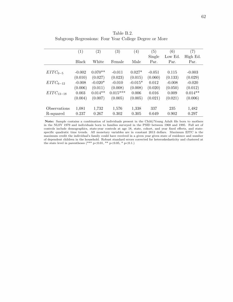
62

Table B.2. Subgroup Regressions: Four Year College Degree or More

(1) (2) (3) (4) (5) (6) (7) Single Low Ed. High Ed.

Black White Female Male Par. Par. Par.

EIT C0−5 -0.002 0.070** -0.011 0.027* -0.051 0.115 -0.003 (0.010) (0.027) (0.023) (0.015) (0.060) (0.133) (0.029)

EIT C6−12 -0.008 -0.020* -0.010 -0.015* 0.012 -0.008 -0.020 (0.006) (0.011) (0.008) (0.008) (0.020) (0.050) (0.012)

EIT C13−18 0.003 0.014** 0.015*** 0.006 0.016 0.009 0.014** (0.004) (0.007) (0.005) (0.005) (0.021) (0.021) (0.006)

Observations 1,081 1,732 1,576 1,338 337 235 1,482 R-squared 0.237 0.267 0.302 0.305 0.649 0.902 0.297


63

Table B.3. Subgroup Regressions: Highest Grade Completed

(1)

Black

(2)

White

(3)

Female

(4)

Male

(5) Single Par.

(6) Low Ed. Par.

(7) High Ed. Par.

EIT C0−5

EIT C6−12

EIT C13−18

-0.033 (0.040) -0.040 (0.029) 0.009 (0.022)

0.202* (0.105) -0.083* (0.045) 0.051* (0.026)

-0.073 (0.089) -0.041 (0.029) 0.068*** (0.019)

0.084 (0.065) -0.071 (0.044) 0.006 (0.022)

0.016 (0.304) -0.090 (0.078) 0.123 (0.077)

0.954 (0.562) -0.166 (0.256) -0.055 (0.127)

-0.054 (0.113) -0.087** (0.043) 0.052** (0.024)


1,081 0.283

1,732 0.309

1,576 0.337

1,338 0.349

337 0.687

235 0.893

1,482 0.308


Table B.4. Subgroup Regressions: Employment

(1)

Black

(2)

White

(3)

Female

(4)

Male

(5) Single Par.

(6) Low Ed. Par.

(7) High Ed. Par.

EIT C0−5

EIT C6−12

EIT C13−18

-0.006 (0.012) 0.001 (0.006) 0.001 (0.006)

0.009 (0.014) -0.008* (0.004) 0.001 (0.002)

0.010 (0.014) -0.005 (0.006) 0.001 (0.003)

-0.001 (0.010) -0.002 (0.006) -0.001 (0.004)

-0.116 (0.177) 0.020 (0.035) 0.037 (0.063)

-1.414*** (0.000) 0.709*** (0.000) -0.383*** (0.000)

0.005 (0.012) -0.007 (0.004) 0.005 (0.004)


705 0.291

1,280 0.219

1,004 0.345

1,048 0.352

210 0.807

188 0.997

1,008 0.407


64

Table B.5. Subgroup Regressions: Earnings

(1) (2) (3) (4) (5) (6) (7) Single Low Ed. High Ed.

Black White Female Male Par. Par. Par.

EIT C0−5 -1.63*** 1.00 -0.92 -0.56 2.49 14.09*** -1.13 (0.52) (1.42) (1.17) (1.11) (7.63) (0.00) (1.44)

EIT C6−12 -0.26 -0.29 -0.32 -0.05 0.39 -1.53*** -0.76* (0.26) (0.46) (0.27) (0.47) (2.35) (0.00) (0.41)

EIT C13−18 -0.19 0.22 0.21 -0.07 0.39 1.91*** 0.29 (0.39) (0.21) (0.36) (0.33) (2.50) (0.00) (0.33)

Observations 705 1,280 1,004 1,048 210 188 1,008 R-squared 0.33 0.25 0.38 0.30 0.84 1.00 0.36


65

C. SUMMARY STATISTICS BY DATASET

Table C.1. Sample Summary Statistics

PSID NLSY

Obs. Mean S.D. Obs. Mean S.D.

Long-term Outcomes: HS Diploma or GED 3,433 0.91 0.29 1,183 0.94 0.24 1+ Years of College 3,348 0.58 0.49 631 0.55 0.50 Bachelor’s Degree or Higher 2,526 0.31 0.46 388 0.39 0.49 Highest Grade Completed 2,526 13.83 1.90 388 14.49 2.09 Employed 1,788 0.89 0.22 264 0.70 0.33 Earnings ($1000s) 1,788 31.33 20.76 264 20.89 14.24

Demographics: Female 3,433 0.51 0.50 1,183 0.54 0.50 Black 3,433 0.43 0.50 1,183 0.31 0.46 Hispanic 3,433 0.005 0.07 1,183 0.22 0.41

Siblings at 18 3,433 1.22 1.26 1,183 2.09 1.09 Mother Ever Married 3,433 0.93 0.27 1,183 0.46 0.50 Parent Completed HS 3,433 0.91 0.29 1,183 0.91 0.28 Parent Completed Some College 3,433 0.50 0.50 1,183 0.49 0.50

EITC variables: EIT C0−5 ($1000s) 3,433 8.83 4.80 1,183 10.01 2.59 EIT C6−12 ($1000s) 3,433 19.03 11.17 1,183 24.75 9.12 EIT C13−18 ($1000s) 3,433 22.97 10.32 1,183 28.82 5.64 EIT C0−18 ($1000s) 3,433 50.83 24.04 1,183 63.58 14.20

Note: Sample contains a combination of individuals present in the Child/Young Adult file born to mothers in the NLSY 1979 and individuals born to families surveyed in the PSID between 1968 and 1995. Full set of controls include demographics, state-year controls at age 18, state, cohort, and year fixed effects, and state-specific quadratic time trends. All monetary variables are in constant 2013 dollars. Maximum EITC is the maximum credit the individual’s family could have received in a given year given state of residence and number of dependent children in the household.

REFERENCES

66

REFERENCES

[1] Agarwal, S., C. Liu, and N. Souleles, “The reaction of consumer spending and debt to tax rebates–evidence from consumer credit data.” No. w13694. National Bureau of Economic Research, (2007).

[2] Barrow, L. and L. McGranahan, “The Effects of the Earned Income Tax Credit on the Seasonality of Household Expenditures.” The American Economic Review, (2009), 418-423.

[3] Bastian, J., and K. Michelmore, “The Long-Term Impact of the Earned Income Tax Credit on Childrens Education and Employment Outcomes.” Journal of Labor Economics, (Forthcoming).

[4] Baughman, R. and S. Dickert-Conlin, “Did Expanding the EITC Promote Moth-erhood?” American Economic Review, (2003), 247-251.

[5] Becker, G. S., “An Economic Analysis of Fertility.” Demographic and Economic Change in Developed Countries., NBER (1960).

[6] Bertrand, M. and A. Morse, “What Do High-Interest Borrowers Do with Their Tax Rebate?” National Tax Journal, (2009), 1211-1243.

[7] Broda, C. and J. Parker, “The economic stimulus payments of 2008 and the aggregate demand for consumption.” Journal of Monetary Economics, (2014), S20-S36.

[8] Chetty, R., J. N. Friedman, N. Hilger, E. Saez, D. W. Schanzenbach, and D. Yagan, “How does your kindergarten classroom affect your earnings? Evidence from Project STAR.” The Quarterly Journal of Economics, (2011), 126(4), 1593-1660.

[9] Chetty, R., J. N. Friedman, and J. E. Rockoff, “The long-term impacts of teachers: Teacher value-added and student outcomes in adulthood.” National Bureau of Economic Research, (2011b), No. w17699.

[10] Cohen, A., R. Dehejia, and D. Romanov, “Do Financial Incentives Affect Fertil-ity?” National Bureau of Economic Research, (2007), Working Paper 13700.

[11] Crump, R., G. S. Goda, and K. J. Mumford, “Fertility and the Personal Exemp-tion: Comment,” American Economic Review, (2011), 1616-1628.

[12] Dahl, G. and L. Lochner, “The Impact of Family Income on Child Achieve-ment: Evidence from the Earned Income Tax Credit.” American Economic Re-view, (2012), 1927-1956.

[13] Dickert, S., S. Houser, and J. Scholz, “The Earned Income Tax Credit and Transfer Programs: A Study of Labor Market and Program Participation.” Tax Policy and the Economy, (1995), 1-50.

67

[14] Eissa, N. and H. Hoynes, “Taxes and the Labor Market Participation of Married Couples: The Earned Income Tax Credit.” Journal of Public Economics, (2004), 1931-1958.

[15] Eissa, N. and H. Hoynes, “Behavioral Responses To Taxes: Lessons from the EITC and Labor Supply.” Tax Policy and the Economy, (2006), 163-192.

[16] Eissa, N. and J. Liebman, “Labor Supply Response to the Earned Income Tax Credit.” Quarterly Journal of Economics, (1996), 605-637.

[17] Gauthier, A. H., and J. Hatzius, “Family Benefits and Fertility: An Econometric Analysis.” Population Studies, (1997), 295-306.

[18] Georgellis, Y., and H. J. Wall, “The Fertility Effect of Dependent Tax Exemp-tions: Estimates for the United States.” Applied Economics, (1992), 1139-1145.

[19] Goodman-Bacon, A. and L. McGranahan, “How Do EITC Recipients Spend Their Refunds.” Economic Perspectives, (2008), 17-32.

[20] Heim, B., “The Impact of the Earned Income Tax Credit on the Labor Supply of Married Couples: Structural Estimation and Labor Supply Interactions.” Working Paper

[21] Hotz, V., C. Mullin, and J. Scholz, “The Earned Income Tax Credit and the La-bor Market Participation of Families on Welfare.” Poverty Research News, (2001).

[22] Hotz, V. and J. Scholz, “The Earned Income Tax Credit.” Means-tested Transfer Programs in the United States, (2003).

[23] Hoynes, H. W., and A. J. Patel, “Effective policy for reducing inequality? The earned income tax credit and the distribution of income.” National Bureau of Economic Research, (2015), No. w21340.

[24] Huang, J. T., “Personal Tax Exemption: The Effect on Fertility in Taiwan.” Developing Economies, (2002), 32-48.

[25] Johnson, D., J. Parker, and N. Souleles, “Household Expenditure and the Income Tax Rebates of 2001.” The American Economic Review, (2006), 1589-1610.

[26] Johnson, D., J. Parker, and N. Souleles, “Consumer spending and the economic stimulus payments of 2008.” The American Economic Review, (2013), 2530-2553.

[27] Laroque, G., and B. Salanie, “Does Fertility Respond to Financial Incentives?” CEPR Discussion Paper, (2005), 5007.

[28] Lochner, L., and A. Monge-Naranjo, “Credit constraints in education.” (2011).

[29] Lopoo, L. M. and K. M. Raissian, “NaMarket Policies in the United States,” Journal of Policy Analysis and Management, (2012), 905-946.

[30] Manoli, D. S., and N. Turner, “Cash-on-hand and college enrollment: Evidence from population tax data and policy nonlinearities.” National Bureau of Economic Research., (2014), No. w19836.

68

[31] Maxfield, M., “The effects of the Earned Income Tax Credit on child achievement and long-term educational attainment.” Michigan State University Job Market Paper.

[32] Meyer, B., “Labor Supply at the Extensive and Intensive Margins: The EITC, Welfare, and Hours Worked.” American Economic Review Papers and Proceedings, (2002), 373-379.

[33] Meyer, B., “The U.S. Earned Income Tax Credit, its Effects, and Possible Re-forms.” Working paper//IFAU-Institute for Labour Market Policy Evaluation., (2008), No. 2008: 14.

[34] Meyer, B., “The Effects of the Earned Income Tax Credit and Recent Reforms.” Tax Policy and the Economy, (2010), 153-180.

[35] Meyer, B. and D. Rosenbaum, “Welfare, the Earned Income Tax Credit, and the Labor Supply of Single Mothers.” NBER Working Paper, (1999).

[36] Michelmore, K., “The Effect of Income on Educational Attainment: Evidence from State Earned Income Tax Credit Expansions.” SSRN Working Paper, (2013).

[37] Milligan, K., “Subsidizing the Stork: New Evidence on Tax Incentives and Fer-tility.” Review of Economics and Statistics, (2005), 539-555.

[38] Parent, D. and L. Wang, “Tax Incentives and Fertility in Canada: quantum vs tempo effects.” Canadian Journal of Economics, (2007), 371-400.

[39] Smeeding, T., K. Phillips, and M. O’Connor, “The Earned Income Tax Credit: Expectation, Knowledge, Use, and Economic and Social Mobility.” Center for Policy Research, (1999) Paper 147.

[40] Souleles, N., “The response of household consumption to income tax refunds.” American Economic Review, (1999), 947-958.

[41] Whittington, L. A., J. Alm, and H. E. Peters, “Fertility and the Personal Ex-emption: Implicit Pronatalist Policy in the United States.” American Economic Review, (1990), 545-556.

[42] Zhang, J., J. Quan, and P. van Meerbergen, “The Effect of Tax-Transfer Policies on Fertility in Canada, 1921-88.” The Journal of Human Resources, (1994), 181-201.

Essays in Labor Economics and Applied Microeconomics

Documents

Transcript of Essays in Labor Economics and Applied Microeconomics