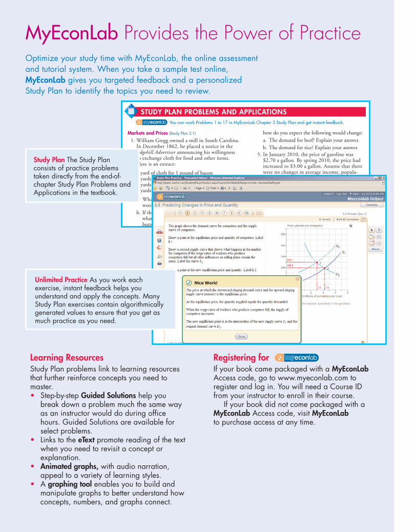
MyEconLab Provides the Power of PracticeOptimize your study time with MyEconLab, the online assessmentand tutorial system. When you take a sample test online,MyEconLab gives you targeted feedback and a personalizedStudy Plan to identify the topics you need to review.

Registering forIf your book came packaged with a MyEconLabAccess code, go to www.myeconlab.com toregister and log in. You will need a Course IDfrom your instructor to enroll in their course.

If your book did not come packaged with aMyEconLab Access code, visit MyEconLabto purchase access at any time.

Learning ResourcesStudy Plan problems link to learning resourcesthat further reinforce concepts you need tomaster.• Step-by-step Guided Solutions help you

break down a problem much the same wayas an instructor would do during officehours. Guided Solutions are available forselect problems.

• Links to the eText promote reading of the textwhen you need to revisit a concept orexplanation.

• Animated graphs, with audio narration,appeal to a variety of learning styles.

• A graphing tool enables you to build andmanipulate graphs to better understand howconcepts, numbers, and graphs connect.

how do you expect the following would change:a. The demand for beef? Explain your answer.b. The demand for rice? Explain your answer.

5. In January 2010, the price of gasoline was$2.70 a gallon. By spring 2010, the price hadincreased to $3.00 a gallon. Assume that therewere no changes in average income, popula-tion, or any other influence on buying plans.Explain how the rise in the price of gasolinewould affecta. The demand for gasoline.b. The quantity of gasoline demanded.

Supply (Study Plan 3.3)

6. In 2008, the price of corn increased by 35 per-

Markets and Prices (Study Plan 3.1)

1. William Gregg owned a mill in South Carolina.In December 1862, he placed a notice in theEdgehill Advertiser announcing his willingnessto exchange cloth for food and other items.Here is an extract:

1 yard of cloth for 1 pound of bacon2 yards of cloth for 1 pound of butter4 yards of cloth for 1 pound of wool8 yards of cloth for 1 bushel of salt

a. What is the relative price of butter in terms ofwool?

b. If the money price of bacon was 20¢ a pound,what do you predict was the money price ofbutter?

You can work Problems 1 to 17 in MyEconLab Chapter 3 Study Plan and get instant feedback.

STUDY PLAN PROBLEMS AND APPLICATIONS

Study Plan The Study Planconsists of practice problemstaken directly from the end-of-chapter Study Plan Problems andApplications in the textbook.

Unlimited Practice As you work eachexercise, instant feedback helps youunderstand and apply the concepts. ManyStudy Plan exercises contain algorithmicallygenerated values to ensure that you get asmuch practice as you need.

MICROECONOMICSTENTH EDITION

This page intentionally left blank

MICROECONOMICSTENTH EDITION

MICHAEL PARKINUniversity of Western Ontario

Editorial Director Sally Yagan

Editor in Chief Donna Battista

Senior Acquisitions Editor Adrienne D’Ambrosio

Development Editor Deepa Chungi

Managing Editor Nancy Fenton

Assistant Editor Jill Kolongowski

Photo Researcher Angel Chavez

Production Coordinator Alison Eusden

Director of Media Susan Schoenberg

Senior Media Producer Melissa Honig

Director of Marketing Patrice Jones

Executive Marketing Manager Lori DeShazo

Rights and Permissions Advisor Jill Dougan

Senior Manufacturing Buyer Carol Melville

Senior Media Buyer Ginny Michaud

Copyeditor Catherine Baum

Art Director and Cover Designer Jonathan Boylan

Technical Illustrator Richard Parkin

Text Design, Project Managementand Page Make-up Integra Software Services, Inc.

Cover Image: Medioimages/PhotoDisc/Getty Images

Photo credits appear on page C-1, which constitutes a continuation of the copyright page.

Copyright © 2012, 2010, 2008, 2005, 2003 Pearson Education, Inc. All rights reserved. No part of this publica-tion may be reproduced, stored in a retrieval system, or transmitted, in any form or by any means, electronic,mechanical, photocopying, recording, or otherwise, without the prior written permission of the publisher. Printedin the United States of America. For information on obtaining permission for use of material in this work, pleasesubmit a written request to Pearson Education, Inc., Rights and Contracts Department, 501 Boylston Street, Suite900, Boston, MA 02116, fax your request to 617-671-3447, or e-mail at http://www.pearsoned.com/legal/-permissions.htm.

Library of Congress Cataloging-in-Publication DataParkin, Michael, 1939–

Microeconomics/Michael Parkin. — 10th ed.p. cm.

Includes index.ISBN 978-0-13-139425-4 (alk. paper)1. Microeconomics. I. Title.

HB171.5.P313 2010330—dc22 2010045760

1 2 3 4 5 6 7 8 10—CRK—14 13 12 11 10

ISBN 10: 0-13-139425-8ISBN 13: 978-0-13-139425-4

TO ROBIN

This page intentionally left blank

vii

Michael Parkin is Professor Emeritus in the Department of Economics atthe University of Western Ontario, Canada. Professor Parkin has held facultyappointments at Brown University, the University of Manchester, the University ofEssex, and Bond University. He is a past president of the Canadian EconomicsAssociation and has served on the editorial boards of the American EconomicReview and the Journal of Monetary Economics and as managing editor of theCanadian Journal of Economics. Professor Parkin’s research on macroeconomics,monetary economics, and international economics has resulted in over 160publications in journals and edited volumes, including the American EconomicReview, the Journal of Political Economy, the Review of Economic Studies, theJournal of Monetary Economics, and the Journal of Money, Credit and Banking.He became most visible to the public with his work on inflation that discredited theuse of wage and price controls. Michael Parkin also spearheaded the movementtoward European monetary union. Professor Parkin is an experienced anddedicated teacher of introductory economics.

ABOUT THE AUTHOR

This page intentionally left blank

ix

PART ONEINTRODUCTION 1

CHAPTER 1 What Is Economics? 1CHAPTER 2 The Economic Problem 29

PART TWOHOW MARKETS WORK 55

CHAPTER 3 Demand and Supply 55CHAPTER 4 Elasticity 83CHAPTER 5 Efficiency and Equity 105CHAPTER 6 Government Actions in Markets 127CHAPTER 7 Global Markets in Action 151

PART THREEHOUSEHOLDS’ CHOICES 179

CHAPTER 8 Utility and Demand 179CHAPTER 9 Possibilities, Preferences, and Choices

203

PART FOUR FIRMS AND MARKETS 227

CHAPTER 10 Organizing Production 227CHAPTER 11 Output and Costs 251CHAPTER 12 Perfect Competition 273CHAPTER 13 Monopoly 299CHAPTER 14 Monopolistic Competition 323CHAPTER 15 Oligopoly 341

PART FIVEMARKET FAILURE AND GOVERNMENT 371

CHAPTER 16 Public Choices and Public Goods 371CHAPTER 17 Economics of the Environment 393

PART SIX FACTOR MARKETS, INEQUALITY, AND UNCERTAINTY 417

CHAPTER 18 Markets for Factors of Production 417CHAPTER 19 Economic Inequality 441CHAPTER 20 Uncertainty and Information 465

BRIEF CONTENTS

This page intentionally left blank

xi

Chapter 1

What is Economics

Chapter 2

The Economic Problem

Chapter 5

Efficiency and Equity

Chapter 4

Elasticity

Chapter 19

Economic Inequality

Chapter 8

Utility and Demand

Chapter 9

Possibilities,Preferences, and

Choices

Chapter 10

Organizing Production

Chapter 11

Output and Costs

Chapter 3

Demand and Supply

Start here ... … then jump toany of these …

… and jump to any of these afterdoing the pre-requisites indicated

Chapter 20

Uncertainty andInformation

Chapter 7

Global Marketsin Action

Chapter 6

Government Actionsin Markets

Chapter 16

Public Choicesand Public Goods

Chapter 17

Economics of theEnvironment

Chapter 12

Perfect Competition

Chapter 13

Monopoly

Chapter 14

MonopolisticCompetition

Chapter 15

Oligopoly

Chapter 18

Markets for Factorsof Production

Micro Flexibility

ALTERNATIVE PATHWAYS THROUGH THE CHAPTERS

This page intentionally left blank

xiii

TABLE OF CONTENTS

APPENDIX Graphs in Economics 13

Graphing Data 13Scatter Diagrams 14

Graphs Used in Economic Models 16Variables That Move in the Same Direction 16Variables That Move in Opposite Directions 17Variables That Have a Maximum or a

Minimum 18Variables That Are Unrelated 19

The Slope of a Relationship 20The Slope of a Straight Line 20The Slope of a Curved Line 21

Graphing Relationships Among More ThanTwo Variables 22

Ceteris Paribus 22When Other Things Change 23

MATHEMATICAL NOTEEquations of Straight Lines 24

PART ONEINTRODUCTION 1

CHAPTER 1 ◆ WHAT IS ECONOMICS? 1

Definition of Economics 2

Two Big Economic Questions 3What, How, and For Whom? 3Can the Pursuit of Self-Interest Promote the

Social Interest? 5

The Economic Way of Thinking 8A Choice Is a Tradeoff 8Making a Rational Choice 8Benefit: What You Gain 8Cost: What You Must Give Up 8How Much? Choosing at the Margin 9Choices Respond to Incentives 9

Economics as Social Science and Policy Tool 10

Economist as Social Scientist 10Economist as Policy Adviser 10

Summary (Key Points and Key Terms), Study PlanProblems and Applications, and Additional Problemsand Applications appear at the end of each chapter.

xiv Contents

PART TWOHOW MARKETS WORK 55

CHAPTER 3 ◆ DEMAND AND SUPPLY 55

Markets and Prices 56

Demand 57The Law of Demand 57Demand Curve and Demand Schedule 57A Change in Demand 58A Change in the Quantity Demanded Versus a

Change in Demand 60

Supply 62The Law of Supply 62Supply Curve and Supply Schedule 62A Change in Supply 63A Change in the Quantity Supplied Versus a

Change in Supply 64

Market Equilibrium 66Price as a Regulator 66Price Adjustments 67

Predicting Changes in Price and Quantity 68An Increase in Demand 68A Decrease in Demand 68An Increase in Supply 70A Decrease in Supply 70All the Possible Changes in Demand and

Supply 72

READING BETWEEN THE LINESDemand and Supply: The Price of Coffee 74

MATHEMATICAL NOTEDemand, Supply, and Equilibrium 76

CHAPTER 2 ◆ THE ECONOMIC PROBLEM 29

Production Possibilities and Opportunity Cost 30

Production Possibilities Frontier 30Production Efficiency 31Tradeoff Along the PPF 31Opportunity Cost 31

Using Resources Efficiently 33The PPF and Marginal Cost 33Preferences and Marginal Benefit 34Allocative Efficiency 35

Economic Growth 36The Cost of Economic Growth 36A Nation’s Economic Growth 37

Gains from Trade 38Comparative Advantage and Absolute

Advantage 38Achieving the Gains from Trade 39

Economic Coordination 41Firms 41Markets 42Property Rights 42Money 42Circular Flows Through Markets 42Coordinating Decisions 42

READING BETWEEN THE LINESThe Rising Opportunity Cost of Food 44

PART ONE WRAP-UP ◆

Understanding the Scope of EconomicsYour Economic Revolution 51

Talking withJagdish Bhagwati 52

Contents xv

CHAPTER 4 ◆ ELASTICITY 83

Price Elasticity of Demand 84Calculating Price Elasticity of Demand 85Inelastic and Elastic Demand 86Elasticity Along a Linear Demand Curve 87Total Revenue and Elasticity 88Your Expenditure and Your Elasticity 89The Factors That Influence the Elasticity of

Demand 89

More Elasticities of Demand 91Cross Elasticity of Demand 91Income Elasticity of Demand 92

Elasticity of Supply 94Calculating the Elasticity of Supply 94The Factors That Influence the Elasticity of

Supply 95

READING BETWEEN THE LINESThe Elasticities of Demand and Supply for

Tomatoes 98

CHAPTER 5 ◆ EFFICIENCY AND EQUITY 105

Resource Allocation Methods 106Market Price 106Command 106Majority Rule 106Contest 106First-Come, First-Served 106Lottery 107Personal Characteristics 107Force 107

Benefit, Cost, and Surplus 108Demand, Willingness to Pay, and Value 108Individual Demand and Market Demand 108Consumer Surplus 109Supply and Marginal Cost 109Supply, Cost, and Minimum Supply-Price 110Individual Supply and Market Supply 110Producer Surplus 111

Is the Competitive Market Efficient? 112Efficiency of Competitive Equilibrium 112Market Failure 113Sources of Market Failure 114Alternatives to the Market 115

Is the Competitive Market Fair? 116It’s Not Fair If the Result Isn’t Fair 116It’s Not Fair If the Rules Aren’t Fair 118Case Study: A Water Shortage in a Natural

Disaster 118

READING BETWEEN THE LINESIs the Global Market for Roses Efficient? 120

CHAPTER 6 ◆ GOVERNMENT ACTIONS IN MARKETS 127

A Housing Market With a Rent Ceiling 128A Housing Shortage 128Increased Search Activity 128A Black Market 128Inefficiency of a Rent Ceiling 129Are Rent Ceilings Fair? 130

A Labor Market With a Minimum Wage 131Minimum Wage Brings Unemployment 131Inefficiency of a Minimum Wage 131Is the Minimum Wage Fair? 132

Taxes 133Tax Incidence 133A Tax on Sellers 133A Tax on Buyers 134Equivalence of Tax on Buyers and Sellers 134Tax Incidence and Elasticity of Demand 135Tax Incidence and Elasticity of Supply 136Taxes and Efficiency 137Taxes and Fairness 138

Production Quotas and Subsidies 139Production Quotas 139Subsidies 140

Markets for Illegal Goods 142A Free Market for a Drug 142A Market for an Illegal Drug 142Legalizing and Taxing Drugs 143

READING BETWEEN THE LINESGovernment Actions in Labor Markets 144

CHAPTER 7 ◆ GLOBAL MARKETS IN ACTION151

How Global Markets Work 152International Trade Today 152What Drives International Trade? 152Why the United States Imports T-Shirts 153Why the United States Exports Airplanes 154

Winners, Losers, and the Net Gain from Trade 155

Gains and Losses from Imports 155Gains and Losses from Exports 156Gains for All 156

International Trade Restrictions 157Tariffs 157Import Quotas 160Other Import Barriers 162Export Subsidies 162

The Case Against Protection 163The Infant-Industry Argument 163The Dumping Argument 163Saves Jobs 164Allows Us to Compete with Cheap Foreign

Labor 164Penalizes Lax Environmental Standards 164Prevents Rich Countries from Exploiting

Developing Countries 165Offshore Outsourcing 165Avoiding Trade Wars 166Why Is International Trade Restricted? 166Compensating Losers 167

READING BETWEEN THE LINESA Tarriff on Tires 168

PART TWO WRAP-UP ◆

Understanding How Markets WorkThe Amazing Market 175

Talking withSusan Athey 176

xvi Contents

Contents xvii

PART THREEHOUSEHOLDS’ CHOICES 179

CHAPTER 8 ◆ UTILITY AND DEMAND 179

Consumption Choices 180Consumption Possibilities 180Preferences 181

Utility-Maximizing Choice 183A Spreadsheet Solution 183Choosing at the Margin 184The Power of Marginal Analysis 186Revealing Preferences 186

Predictions of Marginal Utility Theory 187A Fall in the Price of a Movie 187A Rise in the Price of Soda 189A Rise in Income 190The Paradox of Value 191Temperature: An Analogy 192

New Ways of Explaining Consumer Choices 194

Behavioral Economics 194Neuroeconomics 195Controversy 195

READING BETWEEN THE LINESA Paradox of Value: Paramedics and Hockey

Players 196

CHAPTER 9 ◆ POSSIBILITIES, PREFERENCES,AND CHOICES 203

Consumption Possibilities 204Budget Equation 205

Preferences and Indifference Curves 207Marginal Rate of Substitution 208Degree of Substitutability 209

Predicting Consumer Choices 210Best Affordable Choice 210A Change in Price 211A Change in Income 213Substitution Effect and Income Effect 214

READING BETWEEN THE LINESPaper Books Versus e-Books 216

PART THREE WRAP-UP ◆

Understanding Households’ ChoicesMaking the Most of Life 223

Talking withSteven D. Levitt 224

PART FOURFIRMS AND MARKETS 227

CHAPTER 10 ◆ ORGANIZINGPRODUCTION 227

The Firm and Its Economic Problem 228The Firm’s Goal 228Accounting Profit 228Economic Accounting 228A Firm’s Opportunity Cost of Production 228Economic Accounting: A Summary 229Decisions 229The Firm’s Constraints 230

Technological and Economic Efficiency 231Technological Efficiency 231Economic Efficiency 231

Information and Organization 233Command Systems 233Incentive Systems 233Mixing the Systems 233The Principal-Agent Problem 234Coping with the Principal-Agent Problem 234Types of Business Organization 234Pros and Cons of Different Types of Firms 235

Markets and the Competitive Environment 237Measures of Concentration 238Limitations of a Concentration Measure 240

Produce or Outsource? Firms and Markets 242Firm Coordination 242Market Coordination 242Why Firms? 242

READING BETWEEN THE LINESBattling for Markets in Internet Advertising 244

CHAPTER 11 ◆ OUTPUT AND COSTS 251

Decision Time Frames 252The Short Run 252The Long Run 252

Short-Run Technology Constraint 253Product Schedules 253Product Curves 253Total Product Curve 254Marginal Product Curve 254Average Product Curve 256

Short-Run Cost 257Total Cost 257Marginal Cost 258Average Cost 258Marginal Cost and Average Cost 258Why the Average Total Cost Curve Is

U-Shaped 258Cost Curves and Product Curves 260Shifts in the Cost Curves 260

Long-Run Cost 262The Production Function 262Short-Run Cost and Long-Run Cost 262The Long-Run Average Cost Curve 264Economies and Diseconomies of Scale 264

READING BETWEEN THE LINES Cutting the Cost of Producing Electricity 266

xviii Contents

Contents xix

CHAPTER 12 ◆ PERFECT COMPETITION 273

What Is Perfect Competition? 274How Perfect Competition Arises 274Price Takers 274Economic Profit and Revenue 274The Firm’s Decisions 275

The Firm’s Output Decision 276Marginal Analysis and the Supply Decision 277Temporary Shutdown Decision 278The Firm’s Supply Curve 279

Output, Price, and Profit in the Short Run 280Market Supply in the Short Run 280Short-Run Equilibrium 281A Change in Demand 281Profits and Losses in the Short Run 281Three Possible Short-Run Outcomes 282

Output, Price, and Profit in the Long Run 283Entry and Exit 283A Closer Look at Entry 284A Closer Look at Exit 284Long-Run Equilibrium 285

Changing Tastes and Advancing Technology 286

A Permanent Change in Demand 286External Economies and Diseconomies 287Technological Change 289

Competition and Efficiency 290Efficient Use of Resources 290Choices, Equilibrium, and Efficiency 290

READING BETWEEN THE LINESPerfect Competition in Corn 292

CHAPTER 13 ◆ MONOPOLY 299

Monopoly and How It Arises 300How Monopoly Arises 300Monopoly Price-Setting Strategies 301

A Single-Price Monopoly’s Output and Price Decision 302

Price and Marginal Revenue 302Marginal Revenue and Elasticity 303Price and Output Decision 304

Single-Price Monopoly and Competition Compared 306

Comparing Price and Output 306Efficiency Comparison 307Redistribution of Surpluses 308Rent Seeking 308Rent-Seeking Equilibrium 308

Price Discrimination 309Capturing Consumer Surplus 309Profiting by Price Discriminating 310Perfect Price Discrimination 311Efficiency and Rent Seeking with Price

Discrimination 312

Monopoly Regulation 313Efficient Regulation of a Natural Monopoly 313Second-Best Regulation of a Natural

Monopoly 314

READING BETWEEN THE LINESIs Google Misusing Monopoly Power? 316

CHAPTER 14 ◆ MONOPOLISTICCOMPETITION 323

What Is Monopolistic Competition? 324Large Number of Firms 324Product Differentiation 324Competing on Quality, Price, and Marketing

324Entry and Exit 325Examples of Monopolistic Competition 325

Price and Output in Monopolistic Competition 326

The Firm’s Short-Run Output and Price Decision 326

Profit Maximizing Might Be Loss Minimizing 326

Long-Run: Zero Economic Profit 327Monopolistic Competition and Perfect

Competition 328Is Monopolistic Competition Efficient? 329

Product Development and Marketing 330Innovation and Product Development 330Advertising 330Using Advertising to Signal Quality 332Brand Names 333Efficiency of Advertising and Brand Names 333

READING BETWEEN THE LINESProduct Differentiation and Entry in the Market

for Smart Phones 334

CHAPTER 15 ◆ OLIGOPOLY 341

What Is Oligopoly? 342Barriers to Entry 342Small Number of Firms 343Examples of Oligopoly 343

Oligopoly Games 344What Is a Game? 344The Prisoners’ Dilemma 344An Oligopoly Price-Fixing Game 346Other Oligopoly Games 350The Disappearing Invisible Hand 351A Game of Chicken 352

Repeated Games and Sequential Games 353

A Repeated Duopoly Game 353A Sequential Entry Game in a Contestable

Market 354

Antitrust Law 356The Antitrust Laws 356Price Fixing Always Illegal 357Three Antitrust Policy Debates 357Mergers and Acquisitions 359

READING BETWEEN THE LINESGillete and Schick in a Duopoly Game 360

PART FOUR WRAP-UP ◆

Understanding Firms and MarketsManaging Change and Limiting Market Power 367

Talking withThomas Hubbard 368

xx Contents

Contents xxi

PART FIVEMARKET FAILURE ANDGOVERNMENT 371

CHAPTER 16 ◆ PUBLIC CHOICES AND PUBLIC GOODS 371

Public Choices 372Why Governments Exist 372Public Choice and the Political Marketplace 372Political Equilibrium 373What is a Public Good? 374A Fourfold Classification 374Mixed Goods and Externalities 374Inefficiencies that Require Public Choices 376

Providing Public Goods 377The Free-Rider Problem 377Marginal Social Benefit from a Public

Good 377Marginal Social Cost of a Public Good 378Efficient Quantity of a Public Good 378Inefficient Private Provision 378Efficient Public Provision 378Inefficient Public Overprovision 380

Providing Mixed Goods with External Benefits 381

Private Benefits and Social Benefits 381Government Actions in the Market for a Mixed

Good with External Benefits 382Bureaucratic Inefficiency and Government

Failure 383Health-Care Services 384

READING BETWEEN THE LINESReforming Health Care 386

CHAPTER 17 ◆ ECONOMICS OF THEENVIRONMENT 393

Negative Externalities: Pollution 394Sources of Pollution 394Effects of Pollution 394Private Cost and Social Cost of Pollution 395Production and Pollution: How Much? 396Property Rights 396The Coase Theorem 397Government Actions in a Market with External

Costs 398

The Tragedy of the Commons 400Sustainable Use of a Renewable Resource 400The Overuse of a Common Resource 402Achieving an Efficient Outcome 403

READING BETWEEN THE LINESTax Versus Cap-and-Trade 406

PART FIVE WRAP-UP ◆

Understanding Market Failure andGovernment We, the People, … 413

Talking withCaroline M. Hoxby 414

PART SIXFACTOR MARKETS, INEQUALITY,AND UNCERTAINTY 417

CHAPTER 18 ◆ MARKETS FOR FACTORS OFPRODUCTION 417

The Anatomy of Factor Markets 418Markets for Labor Services 418Markets for Capital Services 418Markets for Land Services and Natural

Resources 418Entrepreneurship 418

The Demand for a Factor of Production 419Value of Marginal Product 419A Firm’s Demand for Labor 419A Firm’s Demand for Labor Curve 420Changes in a Firm’s Demand for Labor 421

Labor Markets 422A Competitive Labor Market 422A Labor Market with a Union 424Scale of the Union–Nonunion Wage

Gap 426Trends and Differences in Wage Rates 427

Capital and Natural Resource Markets 428Capital Rental Markets 428Land Rental Markets 428Nonrenewable Natural Resource Markets 429

READING BETWEEN THE LINESThe Labor Market in Action 432

MATHEMATICAL NOTE Present Value and Discounting 434

CHAPTER 19 ◆ ECONOMIC INEQUALITY 441

Economic Inequality in the United States 442The Distribution of Income 442The Income Lorenz Curve 443The Distribution of Wealth 444Wealth or Income? 444Annual or Lifetime Income and Wealth? 445Trends in Inequality 445Poverty 446

Inequality in the World Economy 448Income Distributions in Selected Countries 448Global Inequality and Its Trends 449

The Sources of Economic Inequality 450Human Capital 450Discrimination 452Contests Among Superstars 453Unequal Wealth 454

Income Redistribution 455Income Taxes 455Income Maintenance Programs 455Subsidized Services 455The Big Tradeoff 456

READING BETWEEN THE LINESTrends in Incomes of the Super Rich 458

xxii Contents

Contents xxiii

CHAPTER 20 ◆ UNCERTAINTY AND INFORMATION 465

Decisions in the Face of Uncertainty 466Expected Wealth 466Risk Aversion 466Utility of Wealth 466Expected Utility 467Making a Choice with Uncertainty 468

Buying and Selling Risk 469Insurance Markets 469A Graphical Analysis of Insurance 470Risk That Can’t Be Insured 471

Private Information 472Asymmetric Information: Examples and

Problems 472The Market for Used Cars 472The Market for Loans 475The Market for Insurance 476

Uncertainty, Information, and the Invisible Hand 477

Information as a Good 477Monopoly in Markets that Cope with

Uncertainty 477

READING BETWEEN THE LINESGrades as Signals 478

PART SIX WRAP-UP ◆

Understanding Factor Markets, Inequality, and UncertaintyFor Whom? 485

Talking withDavid Card 486

Glossary G-1Index I-1Credits C-1

This page intentionally left blank

The future is always uncertain. But at some times,and now is one such time, the range of possiblenear-future events is enormous. The major source ofthis great uncertainty is economic policy. There isuncertainty about the way in which internationaltrade policy will evolve as protectionism is returningto the political agenda. There is uncertainty aboutexchange rate policy as competitive devaluationrears its head. There is extraordinary uncertaintyabout monetary policy with the Fed having doubledthe quantity of bank reserves and continuing to cre-ate more money in an attempt to stimulate a flaggingeconomy. And there is uncertainty about fiscal policyas a trillion dollar deficit interacts with an aging pop-ulation to create a national debt time bomb.

Since the subprime mortgage crisis of August2007 moved economics from the business report tothe front page, justified fear has gripped producers,consumers, financial institutions, and governments.

Even the idea that the market is an efficient mecha-nism for allocating scarce resources came into questionas some political leaders trumpeted the end of capital-ism and the dawn of a new economic order in whichtighter regulation reigned in unfettered greed.

Rarely do teachers of economics have such a richfeast on which to draw. And rarely are the principlesof economics more surely needed to provide the solidfoundation on which to think about economic eventsand navigate the turbulence of economic life.

Although thinking like an economist can bring aclearer perspective to and deeper understanding oftoday’s events, students don’t find the economic wayof thinking easy or natural. Microeconomics seeks toput clarity and understanding in the grasp of the stu-dent through its careful and vivid exploration of thetension between self-interest and the social interest,the role and power of incentives—of opportunitycost and marginal benefit—and demonstrating thepossibility that markets supplemented by othermechanisms might allocate resources efficiently.

Parkin students begin to think about issues theway real economists do and learn how to explore dif-ficult policy problems and make more informed deci-sions in their own economic lives.

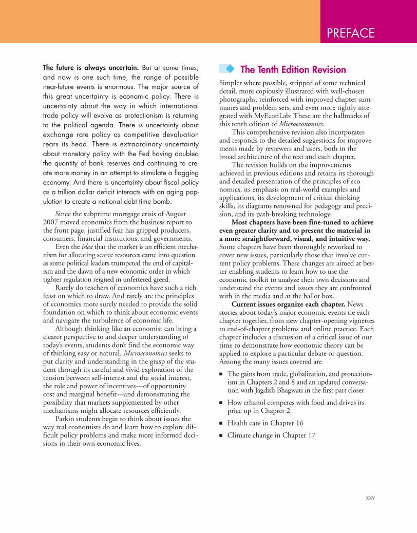
◆ The Tenth Edition RevisionSimpler where possible, stripped of some technicaldetail, more copiously illustrated with well-chosenphotographs, reinforced with improved chapter sum-maries and problem sets, and even more tightly inte-grated with MyEconLab: These are the hallmarks ofthis tenth edition of Microeconomics.

This comprehensive revision also incorporatesand responds to the detailed suggestions for improve-ments made by reviewers and users, both in thebroad architecture of the text and each chapter.

The revision builds on the improvementsachieved in previous editions and retains its thoroughand detailed presentation of the principles of eco-nomics, its emphasis on real-world examples andapplications, its development of critical thinkingskills, its diagrams renowned for pedagogy and preci-sion, and its path-breaking technology.

Most chapters have been fine-tuned to achieveeven greater clarity and to present the material ina more straightforward, visual, and intuitive way.Some chapters have been thoroughly reworked tocover new issues, particularly those that involve cur-rent policy problems. These changes are aimed at bet-ter enabling students to learn how to use theeconomic toolkit to analyze their own decisions andunderstand the events and issues they are confrontedwith in the media and at the ballot box.

Current issues organize each chapter. Newsstories about today’s major economic events tie eachchapter together, from new chapter-opening vignettesto end-of-chapter problems and online practice. Eachchapter includes a discussion of a critical issue of ourtime to demonstrate how economic theory can beapplied to explore a particular debate or question.Among the many issues covered are

■ The gains from trade, globalization, and protection-ism in Chapters 2 and 8 and an updated conversa-tion with Jagdish Bhagwati in the first part closer

■ How ethanol competes with food and drives itsprice up in Chapter 2

■ Health care in Chapter 16

■ Climate change in Chapter 17

xxv

PREFACE

■ The carbon tax debate in Chapter 17

■ Increasing inequality in the United States anddecreasing inequality across the nations in Chapter 18

■ Real-world examples and applications appear inthe body of each chapter and in the end-of-chapter problems and applications

A selection of questions that appear daily inMyEconLab in Economics in the News are also avail-able for assignment as homework, quizzes, or tests.

Highpoints of the RevisionIn addition to being thoroughly updated and revisedto include the topics and features just described, themicroeconomics chapters feature the following sevennotable changes:

1. What Is Economics? (Chapter 1): I have reworkedthe explanation of the economic way of thinkingaround six key ideas, all illustrated with student-relevant choices. The graphing appendix to thischapter has an increased focus on scatter diagramsand their interpretation and on understandingshifts of curves.

2. Utility and Demand (Chapter 8): This chapterhas a revised explanation of the marginal utilitymodel of consumer choice that now begins withthe budget line and consumption possibilities. Itthen returns to the budget line to explain andillustrate the utility-maximizing rule—equalizethe marginal utility per dollar for all goods. Thedramatic changes in the market for recordedmusic illustrate the theory in action.

3. Possibilities, Preferences, and Choices (Chapter9): Students find the analysis of the income effectand the substitution effect difficult and I havereworked this material to make the explanationclearer. I have omitted the work-leisure choicecoverage of earlier editions and given the chaptera student-friendly application to choices aboutmovies and DVDs.

4. Reorganized and expanded coverage of exter-nalities, public goods, and common resources(Chapters 16 and 17). These topics have beenreorganized to achieve an issues focus rather thana technical focus. Chapter 16 is about publicprovision of both public goods and mixed goodswith positive externalities; and Chapter 17 isabout overproduction of goods with negativeexternalities and overuse of common resources.

5. Public Goods and Public Choices (Chapter 16):This new chapter begins with an overview of pub-lic choice theory, a classification of goods andexternalities, and an identification of the marketfailures that give rise to public choices. The chapterthen goes on to explain the free-rider problem andthe underprovision of public goods, the bureau-cracy problem and overprovision, and the under-provision of mixed goods with external benefits,illustrated by education and health-care. The chap-ter explains how education and health care vouch-ers provide an effective way of achieving efficiencyin the provision of these two vital services, a viewreinforced in a box on Larry Kotlikoff ’s health-careplan and Caroline Hoxby’s part closer interview.

6. Economics and the Environment (Chapter 17):This new chapter brings all the environmentaldamage issues together by combining material onnegative externalities and common resources.Covering all this material in the same chapter(the previous editions split them between twochapters) enables their common solutions—property rights (Coase) or individual transferablequotas—to be explained and emphasized.

7. Economic Inequality (Chapter 19): This chapternow includes a section on inequality in the worldeconomy and compares U.S. inequality with thatin nations at the two extremes of equality andinequality. The new section also looks at the trendin global inequality. The discussion of the sourcesof inequality now includes an explanation of thesuperstar contest idea. This idea is used to explainEmmanuel Saez’s remarkable data on the incomeshare of the top one percent of Americans.

xxvi Preface

◆ Features to Enhance Teachingand Learning

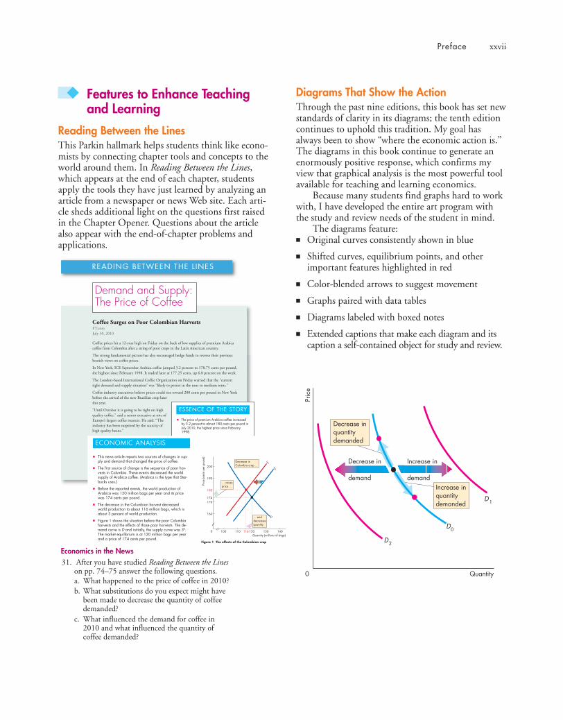
Reading Between the LinesThis Parkin hallmark helps students think like econo-mists by connecting chapter tools and concepts to theworld around them. In Reading Between the Lines,which appears at the end of each chapter, studentsapply the tools they have just learned by analyzing anarticle from a newspaper or news Web site. Each arti-cle sheds additional light on the questions first raisedin the Chapter Opener. Questions about the articlealso appear with the end-of-chapter problems andapplications.

Preface xxvii

Coffee Surges on Poor Colombian HarvestsFT.comJuly 30, 2010

Coffee prices hit a 12-year high on Friday on the back of low supplies of premium Arabicacoffee from Colombia after a string of poor crops in the Latin American country.

The strong fundamental picture has also encouraged hedge funds to reverse their previousbearish views on coffee prices.

In New York, ICE September Arabica coffee jumped 3.2 percent to 178.75 cents per pound,the highest since February 1998. It traded later at 177.25 cents, up 6.8 percent on the week.

The London-based International Coffee Organization on Friday warned that the “currenttight demand and supply situation” was “likely to persist in the near to medium term.”

Coffee industry executives believe prices could rise toward 200 cents per pound in New Yorkbefore the arrival of the new Brazilian crop laterthis year.

“Until October it is going to be tight on highquality coffee,” said a senior executive at one ofEurope’s largest coffee roasters. He said: “Theindustry has been surprised by the scarcity ofhigh quality beans.”

Colombia coffee production, key for supplies ofpremium beans, last year plunged to a 33-yearlow of 7.8m bags, each of 60kg, down nearly athird from 11.1m bags in 2008, tightening sup-plies worldwide. ...

Excerpted from “Coffee Surges on Poor Colombian Harvests” by JavierBlas. Financial Times, July 30, 2010. Reprinted with permission.

READING BETWEEN THE L INES

Demand and Supply: The Price of Coffee

The price of premium Arabica coffee increasedby 3.2 percent to almost 180 cents per pound inJuly 2010, the highest price since February1998.

A sequence of poor crops in Columbia cut theproduction of premium Arabica coffee to a 33-year low of 7.8 million 60 kilogram bags, downfrom 11.1 million bags in 2008.

The International Coffee Organization said thatthe “current tight demand and supply situation”was “likely to persist in the near to medium term.”

Coffee industry executives say prices mightapproach 200 cents per pound before the arrivalof the new Brazilian crop later this year.

Hedge funds previously expected the price of cof-fee to fall but now expect it to rise further.

ESSENCE OF THE STORY

D

S1

S0

Figure 1 The effects of the Columbian crop

Decrease inColumbia crop ...

Pric

e (c

ents

perp

ound

)

Quantity (millions of bags)0

160

110 116 130 140120

170174

180

190

200

100

... anddecreasesquantity

... raisesprice ...

ECONOMIC ANALYSIS

This news article reports two sources of changes in sup-ply and demand that changed the price of coffee.

The first source of change is the sequence of poor har-vests in Columbia. These events decreased the worldsupply of Arabica coffee. (Arabica is the type that Star-bucks uses.)

Before the reported events, the world production ofArabica was 120 million bags per year and its pricewas 174 cents per pound.

The decrease in the Columbian harvest decreasedworld production to about 116 million bags, which isabout 3 percent of world production.

Figure 1 shows the situation before the poor Columbiaharvests and the effects of those poor harvests. The de-mand curve is D and initially, the supply curve was S0.The market equilibrium is at 120 million bags per yearand a price of 174 cents per pound.

The poor Columbian harvests decreased supply andh l h f d l f d S1 ThEconomics in the News

31. After you have studied Reading Between the Lineson pp. 74–75 answer the following questions.a. What happened to the price of coffee in 2010?b. What substitutions do you expect might have

been made to decrease the quantity of coffeedemanded?

c. What influenced the demand for coffee in2010 and what influenced the quantity ofcoffee demanded?

Quantity

Pric

e

Decrease in

demand

D

D0

2

Increase in

demandIncrease inquantitydemanded

Decrease inquantitydemanded

0

D1

Diagrams That Show the ActionThrough the past nine editions, this book has set newstandards of clarity in its diagrams; the tenth editioncontinues to uphold this tradition. My goal hasalways been to show “where the economic action is.”The diagrams in this book continue to generate anenormously positive response, which confirms myview that graphical analysis is the most powerful toolavailable for teaching and learning economics.

Because many students find graphs hard to workwith, I have developed the entire art program withthe study and review needs of the student in mind.

The diagrams feature:■ Original curves consistently shown in blue

■ Shifted curves, equilibrium points, and otherimportant features highlighted in red

■ Color-blended arrows to suggest movement

■ Graphs paired with data tables

■ Diagrams labeled with boxed notes

■ Extended captions that make each diagram and itscaption a self-contained object for study and review.

Chapter OpenersEach chapter opens with a student-friendly vignettethat raises questions to motivate the student andfocus the chapter. This chapter-opening story iswoven into the main body of the chapter and isexplored in the Reading Between the Lines feature thatends each chapter.

Key TermsHighlighted terms simplify the student’s task oflearning the vocabulary of economics. Each high-lighted term appears in an end-of-chapter list with itspage number, in an end-of-book glossary with its pagenumber, boldfaced in the index, in MyEconLab, inthe interactive glossary, and in the Flash Cards.

In-Text Review QuizzesA review quiz at the end of each major sectionenables students to determine whether a topic needsfurther study before moving on. This feature includesa reference to the appropriate MyEconLab study planto help students further test their understanding.

End-of-Chapter Study MaterialEach chapter closes with a concise summary organ-ized by major topics, lists of key terms with page ref-erences, and problems and applications. Theselearning tools provide students with a summary forreview and exam preparation.

Economics in Action BoxesThis new feature uses boxes within the chapter toaddress current events and economic occurrences thathighlight and amplify the topics covered in the chap-ter. Instead of simply reporting the current events, thematerial in the boxes applies the event to an economicslesson, enabling students to see how economics plays apart in the world around them as they read throughthe chapter.

Some of the many issues covered in these boxesinclude the global market for crude oil, the bestaffordable choice of movies and DVDs, the cost ofselling a pair of shoes, how Apple doesn’t make theiPhone, the structural unemployment in Michigan,how loanable funds fuel a home price bubble, andthe size of the fiscal stimulus multipliers. A completelist can be found on the inside back cover.

xxviii Preface

Economics in ActionThe Global Market for Crude OilThe demand and supply model provides insights intoall competitive markets. Here, we’ll apply what you’velearned about the effects of an increase in demand tothe global market for crude oil.

Crude oil is like the life-blood of the global econ-omy. It is used to fuel our cars, airplanes, trains, andbuses, to generate electricity, and to produce a widerange of plastics. When the price of crude oil rises,the cost of transportation, power, and materials allincrease.

In 2001, the price of a barrel of oil was $20 (usingthe value of money in 2010). In 2008, before theglobal financial crisis ended a long period of eco-nomic expansion, the price peaked at $127 a barrel.

While the price of oil was rising, the quantity ofoil produced and consumed also increased. In 2001,the world produced 65 million barrels of oil a day. By2008, that quantity was 72 million barrels.

Who or what has been raising the price of oil? Is itthe action of greedy oil producers? Oil producersmight be greedy, and some of them might be bigenough to withhold supply and raise the price, but itwouldn’t be in their self-interest to do so. The higherprice would bring forth a greater quantity suppliedfrom other producers and the profit of the producerlimiting supply would fall.

Oil producers could try to cooperate and jointlywithhold supply. The Organization of PetroleumExporting Countries, OPEC, is such a group of pro-ducers. But OPEC doesn’t control the world supplyand its members’ self-interest is to produce the quanti-ties that give them the maximum attainable profit.

So even though the global oil market has some bigplayers, they don’t fix the price. Instead, the actionsof thousands of buyers and sellers and the forces ofdemand and supply determine the price of oil.

So how have demand and supply changed?Because both the price and the quantity have

increased, the demand for oil must have increased.Supply might have changed too, but here we’ll sup-pose that supply has remained the same.

The global demand for oil has increased for onemajor reason: World income has increased. Theincrease has been particularly large in the emergingeconomies of Brazil, China, and India. Increasedworld income has increased the demand for oil-usinggoods such as electricity, gasoline, and plastics, whichin turn has increased the demand for oil.

The figure illustrates the effects of the increase indemand on the global oil market. The supply of oilremained constant along supply curve S. The demandfor oil in 2001 was D2001, so in 2001 the price was$20 a barrel and the quantity was 65 million barrelsper day. The demand for oil increased and by 2008 ithad reached D2008. The price of oil increased to $127a barrel and the quantity increased to 72 million bar-rels a day. The increase in the quantity is an increasein the quantity supplied, not an increase in supply.

200

60 72 85

Pric

e (2

010

dolla

rs p

erba

rrel

)

Quantity (millions of barrels per day)65

127

20

40

0

60

80

100

140

160

180

80

S

D2001 D2008

Rise in globalincomes increasesthe demand for oil

The Global Market for Crude Oil

Price ofoil rises ...

… and quantityof oil suppliedincreases

Preface xxix

Supplemental ResourcesInstructor’s Manuals We have streamlined and reor-ganized the Instructor’s Manual to reflect the focusand intuition of the tenth edition. The Instructor’sManual for Microeconomics, written by Laura A.Wolff of Southern Illinois University Edwardsville,integrates the teaching and learning package andserves as a guide to all the supplements.

Each chapter contains

■ A chapter overview

■ A list of what’s new in the tenth edition

■ Ready-to-use lecture notes from each chapterenable a new user of Parkin to walk into a class-room armed to deliver a polished lecture. The lec-ture notes provide an outline of the chapter;concise statements of key material; alternativetables and figures; key terms and definitions; andboxes that highlight key concepts; provide aninteresting anecdote, or suggest how to handle adifficult idea; and additional discussion questions.The PowerPoint® lecture notes incorporate thechapter outlines and teaching suggestions.

Solutions Manual For ease of use and instructor ref-erence, a comprehensive solutions manual providesinstructors with solutions to the Review Quizzesand the end-of-chapter Problems and Applicationsas well as additional problems and the solutions tothese problems. Written by Mark Rush of theUniversity of Florida and reviewed for accuracy byJeannie Gillmore of the University of WesternOntario, the Solutions Manual is available in hardcopy and electronically on the Instructor’s ResourceCenter CD-ROM, in the Instructor’s Resourcessection of MyEconLab, and on the Instructor’sResource Center.

Test Item File Three separate Test Item Files withnearly 8,000 questions, provide multiple-choice,true/false, numerical, fill-in-the-blank, short-answer,and essay questions. Mark Rush reviewed and editedall existing questions to ensure their clarity and con-sistency with the tenth edition and incorporatednew questions into the thousands of existing Test

Interviews with EconomistsEach major part of the text closes with a summaryfeature that includes an interview with a leadingeconomist whose research and expertise correlates towhat the student has just learned. These interviewsexplore the background, education, and researchthese prominent economists have conducted, as wellas advice for those who want to continue the study ofeconomics. New to this tenth edition is ThomasHubbard of Northwestern University. I have alsoreturned to Jagdish Bhagwati, of ColumbiaUniversity and included his more recent thoughts onour rapidly changing economic times.

◆ For the InstructorThis book enables you to focus on the economic wayof thinking and choose your own course structure inyour principles course.

Focus on the Economic Way of ThinkingAs an instructor, you know how hard it is to encour-age a student to think like an economist. But that isyour goal. Consistent with this goal, the text focuseson and repeatedly uses the central ideas: choice;tradeoff; opportunity cost; the margin; incentives;the gains from voluntary exchange; the forces ofdemand, supply, and equilibrium; the pursuit of eco-nomic rent; the tension between self-interest and thesocial interest; and the scope and limitations of gov-ernment actions.

Flexible StructureYou have preferences for how you want to teach yourcourse. I have organized this book to enable you todo so. The flexibility chart on p. xi illustrates thebook’s flexibility. By following the arrows throughthe chart you can select the path that best fits yourpreference for course structure. Whether you want toteach a traditional course that blends theory and pol-icy, or one that takes a fast-track through either the-ory or policy issues, Microeconomics gives you thechoice.

Bank questions. The new questions, written bySvitlana Maksymenko of the University ofPittsburgh, James K. Self at the University ofIndiana, Bloomington, and Gary Hoover at theUniversity of Alabama follow the style and formatof the end-of-chapter text problems and provide theinstructor with a whole new set of testing opportu-nities and/or homework assignments. Additionally,end-of-part tests contain questions that cover all thechapters in the part and feature integrative ques-tions that span more than one chapter.

Computerized Testbanks Fully networkable, the testbanks are available for Windows® and Macintosh®.TestGen’s graphical interface enables instructors toview, edit, and add questions; transfer questions totests; and print different forms of tests. Tests can beformatted with varying fonts and styles, margins, andheaders and footers, as in any word-processing docu-ment. Search and sort features let the instructorquickly locate questions and arrange them in a pre-ferred order. QuizMaster, working with your school’scomputer network, automatically grades the exams,stores the results, and allows the instructor to view orprint a variety of reports.

PowerPoint Resources Robin Bade has developed afull-color Microsoft® PowerPoint LecturePresentation for each chapter that includes all the fig-ures and tables from the text, animated graphs, andspeaking notes. The lecture notes in the Instructor’sManual and the slide outlines are correlated, and thespeaking notes are based on the Instructor’s Manualteaching suggestions. A separate set of PowerPointfiles containing large-scale versions of all the text’sfigures (most of them animated) and tables (some ofwhich are animated) are also available. The presenta-tions can be used electronically in the classroom orcan be printed to create hard copy transparency mas-ters. This item is available for Macintosh andWindows.

Clicker-Ready PowerPoint Resources This editionfeatures the addition of clicker-ready PowerPointslides for the Personal Response System you use. Each

chapter of the text includes ten multiple-choice ques-tions that test important concepts. Instructors canassign these as in-class assignments or review quizzes.

Instructor’s Resource Center CD-ROM Fully compati-ble with Windows and Macintosh, this CD-ROMcontains electronic files of every instructor supple-ment for the tenth edition. Files included are:Microsoft® Word and Adobe® PDF files of theInstructor’s Manual, Test Item Files and SolutionsManual; PowerPoint resources; and theComputerized TestGen® Test Bank. Add this usefulresource to your exam copy bookbag, or locate yourlocal Pearson Education sales representative atwww.pearsonhighered.educator to request a copy.

Instructors can download supplements from asecure, instructor-only source via the Pearson HigherEducation Instructor Resource Center Web page(www.pearsonhighered.com/irc).

BlackBoard and WebCT BlackBoard and WebCTCourse Cartridges are available for download fromwww.pearsonhighered.com/irc. These standard course cartridges contain the Instructor’s Manual,Solutions Manual, TestGen Test Item Files, InstructorPowerPoints, Student Powerpoints and Student Data Files.

Study Guide The tenth edition Study Guide byMark Rush is carefully coordinated with the text,MyEconLab, and the Test Item Files. Each chapter ofthe Study Guide contains

■ Key concepts

■ Helpful hints

■ True/false/uncertain questions

■ Multiple-choice questions

■ Short-answer questions

■ Common questions or misconceptions that thestudent explains as if he or she were the teacher

■ Each part allows students to test their cumulativeunderstanding with questions that go across chap-ters and to work a sample midterm examination.

xxx Preface

MYECONLABMyEconLab’s powerful assessment and tutorial sys-tem works hand-in-hand with Microeconomics. Withcomprehensive homework, quiz, test, and tutorialoptions, instructors can manage all assessment needsin one program.

■ All of the Review Quiz questions and end-of-chapter Problems and Applications are assignableand automatically graded in MyEconLab.

■ Students can work all the Review Quiz questionsand end-of-chapter Study Plan Problems andApplications as part of the Study Plan inMyEconLab.

■ Instructors can assign the end-of-chapterAdditional Problems and Applications as auto-graded assignments. These Problems andApplications are not available to students inMyEconLab unless assigned by the instructor.

■ Many of the problems and applications are algo-rithmic, draw-graph, and numerical exercises.

■ Test Item File questions are available for assign-ment as homework.

■ The Custom Exercise Builder allows instructorsthe flexibility of creating their own problems forassignment.

■ The powerful Gradebook records each student’sperformance and time spent on Tests, the StudyPlan, and homework and generates reports by stu-dent or by chapter.

■ Economics in the News is a turn-key solution tobringing daily news into the classroom. Updateddaily during the academic year, I upload two rele-vant articles (one micro, one macro) and providelinks for further information and questions thatmay be assigned for homework or for classroomdiscussion.

■ A comprehensive suite of ABC news videos, whichaddress current topics such as education, energy,Federal Reserve policy, and business cycles, isavailable for classroom use. Video-specific exercisesare available for instructor assignment.

Robin Bade and I, assisted by Jeannie Gillmoreand Laurel Davies, author and oversee all of theMyEconLab content for Microeconomics. Our peerlessMyEconLab team has worked hard to ensure that it istightly integrated with the book’s content and vision. Amore detailed walk-through of the student benefitsand features of MyEconLab can be found on the insidefront cover. Visit www.myeconlab.com for more infor-mation and an online demonstration of instructor andstudent features.

Experiments in MyEconLabExperiments are a fun and engaging way to promoteactive learning and mastery of important economicconcepts. Pearson’s experiments program is flexibleand easy for instructors and students to use.

■ Single-player experiments allow your students toplay against virtual players from anywhere at any-time with an Internet connection.

■ Multiplayer experiments allow you to assign andmanage a real-time experiment with your class.

Pre-and post-questions for each experiment areavailable for assignment in MyEconLab.

Economics Videos and Assignable QuestionsFeaturing Economics videos featuringABC news enliven your course with short news clipsfeaturing real-world issues. These videos, available inMyEconLab, feature news footage and commentaryby economists. Questions and problems for eachvideo clip are available for assignment inMyEconLab.

Preface xxxi

◆ AcknowledgmentsI thank my current and former colleagues and friendsat the University of Western Ontario who have taughtme so much. They are Jim Davies, Jeremy Greenwood,Ig Horstmann, Peter Howitt, Greg Huffman, DavidLaidler, Phil Reny, Chris Robinson, John Whalley, andRon Wonnacott. I also thank Doug McTaggart andChristopher Findlay, co-authors of the Australian edi-tion, and Melanie Powell and Kent Matthews, coau-thors of the European edition. Suggestions arisingfrom their adaptations of earlier editions have beenhelpful to me in preparing this edition.

I thank the several thousand students whom Ihave been privileged to teach. The instant responsethat comes from the look of puzzlement or enlighten-ment has taught me how to teach economics.

It is a special joy to thank the many outstandingeditors, media specialists, and others at Addison-Wesleywho contributed to the concerted publishing effort thatbrought this edition to completion. Denise Clinton,Publisher of MyEconLab has played a major role in theevolution of this text since its third edition, and herinsights and ideas can still be found in this new edition.Donna Battista, Editor-in-Chief for Economics andFinance, is hugely inspiring and has provided overalldirection to the project. As ever, Adrienne D’Ambrosio,Senior Acquisitions Editor for Economics and mysponsoring editor, played a major role in shaping thisrevision and the many outstanding supplements thataccompany it. Adrienne brings intelligence and insightto her work and is the unchallengeable pre-eminenteconomics editor. Deepa Chungi, Development Editor,brought a fresh eye to the development process,obtained outstanding reviews from equally outstandingreviewers, digested and summarized the reviews, andmade many solid suggestions as she diligently workedthrough the drafts of this edition. Deepa also providedoutstanding photo research. Nancy Fenton, ManagingEditor, managed the entire production and designeffort with her usual skill, played a major role in envi-sioning and implementing the cover design, and copedfearlessly with a tight production schedule. SusanSchoenberg, Director of Media, directed the develop-ment of MyEconLab; Noel Lotz, Content Lead forMyEconLab, managed a complex and thorough review-ing process for the content of MyEconLab; and MelissaHonig, Senior Media Producer ensured that all ourmedia assets were correctly assembled. Lori Deshazo,Executive Marketing Manager, provided inspired mar-

keting strategy and direction. Catherine Baum pro-vided a careful, consistent, and intelligent copy edit andaccuracy check. Jonathan Boylan designed the coverand package and yet again surpassed the challenge ofensuring that we meet the highest design standards. JoeVetere provided endless technical help with the text andart files. Jill Kolongowski and Alison Eusden managedour immense supplements program. And HeatherJohnson with the other members of an outstandingeditorial and production team at Integra-Chicago keptthe project on track on an impossibly tight schedule. Ithank all of these wonderful people. It has been inspir-ing to work with them and to share in creating what Ibelieve is a truly outstanding educational tool.

I thank our talented tenth edition supplementsauthors and contributors—Luke Armstrong, JeannieGillmore, Laurel Davies, Gary Hoover, SvitlanaMaksymenko, Russ McCullough, Barbara Moore,Jim Self, and Laurie Wolff.

I especially thank Mark Rush, who yet againplayed a crucial role in creating another edition ofthis text and package. Mark has been a constantsource of good advice and good humor.

I thank the many exceptional reviewers who haveshared their insights through the various editions ofthis book. Their contribution has been invaluable.

I thank the people who work directly with me.Jeannie Gillmore provided outstanding research assis-tance on many topics, including the Reading Betweenthe Lines news articles. Richard Parkin created theelectronic art files and offered many ideas thatimproved the figures in this book. And Laurel Daviesmanaged an ever-growing and ever more complexMyEconLab database.

As with the previous editions, this one owes anenormous debt to Robin Bade. I dedicate this bookto her and again thank her for her work. I could nothave written this book without the tireless andunselfish help she has given me. My thanks to her areunbounded.

Classroom experience will test the value of thisbook. I would appreciate hearing from instructorsand students about how I can continue to improve itin future editions.

Michael ParkinLondon, Ontario, Canadamichael.parkin@uwo.ca

xxxii Preface

◆ ReviewersEric Abrams, Hawaii Pacific UniversityChristopher Adams, Federal Trade CommissionTajudeen Adenekan, Bronx Community CollegeSyed Ahmed, Cameron UniversityFrank Albritton, Seminole Community CollegeMilton Alderfer, Miami-Dade Community CollegeWilliam Aldridge, Shelton State Community CollegeDonald L. Alexander, Western Michigan UniversityTerence Alexander, Iowa State UniversityStuart Allen, University of North Carolina, GreensboroSam Allgood, University of Nebraska, LincolnNeil Alper, Northeastern UniversityAlan Anderson, Fordham UniversityLisa R. Anderson, College of William and MaryJeff Ankrom, Wittenberg UniversityFatma Antar, Manchester Community Technical CollegeKofi Apraku, University of North Carolina, AshevilleJohn Atkins, University of West FloridaMoshen Bahmani-Oskooee, University of Wisconsin,MilwaukeeDonald Balch, University of South CarolinaMehmet Balcilar, Wayne State UniversityPaul Ballantyne, University of ColoradoSue Bartlett, University of South FloridaJose Juan Bautista, Xavier University of LouisianaValerie R. Bencivenga, University of Texas, AustinBen Bernanke, Chairman of Federal ReserveRadha Bhattacharya, California State University, FullertonMargot Biery, Tarrant County College, SouthJohn Bittorowitz, Ball State UniversityDavid Black, University of ToledoKelly Blanchard, Purdue UniversityS. Brock Blomberg, Claremont McKenna CollegeWilliam T. Bogart, Case Western Reserve UniversityGiacomo Bonanno, University of California, DavisTan Khay Boon, Nanyard Technological UniversitySunne Brandmeyer, University of South FloridaAudie Brewton, Northeastern Illinois UniversityBaird Brock, Central Missouri State UniversityByron Brown, Michigan State UniversityJeffrey Buser, Columbus State Community CollegeAlison Butler, Florida International UniversityColleen Callahan, American UniversityTania Carbiener, Southern Methodist UniversityKevin Carey, American UniversityScott Carrell, University of California at DavisKathleen A. Carroll, University of Maryland, Baltimore CountyMichael Carter, University of Massachusetts, Lowell

Edward Castronova, California State University, FullertonFrancis Chan, Fullerton CollegeMing Chang, Dartmouth CollegeSubir Chakrabarti, Indiana University-Purdue UniversityJoni Charles, Texas State UniversityAdhip Chaudhuri, Georgetown UniversityGopal Chengalath, Texas Tech UniversityDaniel Christiansen, Albion CollegeKenneth Christianson, Binghamton UniversityJohn J. Clark, Community College of Allegheny County,

Allegheny CampusCindy Clement, University of MarylandMeredith Clement, Dartmouth CollegeMichael B. Cohn, U. S. Merchant Marine AcademyRobert Collinge, University of Texas, San AntonioCarol Condon, Kean UniversityDoug Conway, Mesa Community CollegeLarry Cook, University of ToledoBobby Corcoran, retired, Middle Tennessee State UniversityKevin Cotter, Wayne State UniversityJames Peery Cover, University of Alabama, TuscaloosaErik Craft, University of RichmondEleanor D. Craig, University of DelawareJim Craven, Clark CollegeJeremy Cripps, American University of KuwaitElizabeth Crowell, University of Michigan, DearbornStephen Cullenberg, University of California, RiversideDavid Culp, Slippery Rock UniversityNorman V. Cure, Macomb Community CollegeDan Dabney, University of Texas, AustinAndrew Dane, Angelo State UniversityJoseph Daniels, Marquette UniversityGregory DeFreitas, Hofstra UniversityDavid Denslow, University of FloridaShatakshee Dhongde, Rochester Institute of TechnologyMark Dickie, University of Central FloridaJames Dietz, California State University, FullertonCarol Dole, State University of West GeorgiaRonald Dorf, Inver Hills Community CollegeJohn Dorsey, University of Maryland, College ParkEric Drabkin, Hawaii Pacific UniversityAmrik Singh Dua, Mt. San Antonio CollegeThomas Duchesneau, University of Maine, OronoLucia Dunn, Ohio State UniversityDonald Dutkowsky, Syracuse UniversityJohn Edgren, Eastern Michigan UniversityDavid J. Eger, Alpena Community CollegeHarry Ellis, Jr., University of North TexasIbrahim Elsaify, Goldey-Beacom CollegeKenneth G. Elzinga, University of Virginia

Preface xxxiii

Patrick Emerson, Oregon State UniversityTisha Emerson, Baylor UniversityMonica Escaleras, Florida Atlantic UniversityAntonina Espiritu, Hawaii Pacific UniversityGwen Eudey, University of PennsylvaniaBarry Falk, Iowa State UniversityM. Fazeli, Hofstra UniversityPhilip Fincher, Louisiana Tech UniversityF. Firoozi, University of Texas, San AntonioNancy Folbre, University of Massachusetts, AmherstKenneth Fong, Temasek Polytechnic (Singapore)Steven Francis, Holy Cross CollegeDavid Franck, University of North Carolina, CharlotteMark Frank, Sam Houston State UniversityRoger Frantz, San Diego State UniversityMark Frascatore, Clarkson UniversityAlwyn Fraser, Atlantic Union CollegeMarc Fusaro, East Carolina UniversityJames Gale, Michigan Technological UniversitySusan Gale, New York UniversityRoy Gardner, Indiana UniversityEugene Gentzel, Pensacola Junior CollegeKirk Gifford, Brigham Young University, IdahoScott Gilbert, Southern Illinois University, CarbondaleAndrew Gill, California State University, FullertonRobert Giller, Virginia Polytechnic Institute and State UniversityRobert Gillette, University of KentuckyJames N. Giordano, Villanova UniversityMaria Giuili, Diablo CollegeSusan Glanz, St. John’s UniversityRobert Gordon, San Diego State UniversityRichard Gosselin, Houston Community CollegeJohn Graham, Rutgers UniversityJohn Griffen, Worcester Polytechnic InstituteWayne Grove, Syracuse UniversityRobert Guell, Indiana State UniversityWilliam Gunther, University of Southern MississippiJamie Haag, Pacific University, OregonGail Heyne Hafer, Lindenwood UniversityRik W. Hafer, Southern Illinois University, EdwardsvilleDaniel Hagen, Western Washington UniversityDavid R. Hakes, University of Northern IowaCraig Hakkio, Federal Reserve Bank, Kansas CityBridget Gleeson Hanna, Rochester Institute of TechnologyAnn Hansen, Westminster CollegeSeid Hassan, Murray State UniversityJonathan Haughton, Suffolk UniversityRandall Haydon, Wichita State UniversityDenise Hazlett, Whitman CollegeJulia Heath, University of Memphis

Jac Heckelman, Wake Forest UniversityJolien A. Helsel, Kent State UniversityJames Henderson, Baylor UniversityDoug Herman, Georgetown UniversityJill Boylston Herndon, University of FloridaGus Herring, Brookhaven CollegeJohn Herrmann, Rutgers UniversityJohn M. Hill, Delgado Community CollegeJonathan Hill, Florida International UniversityLewis Hill, Texas Tech UniversitySteve Hoagland, University of AkronTom Hoerger, Fellow, Research Triangle InstituteCalvin Hoerneman, Delta CollegeGeorge Hoffer, Virginia Commonwealth UniversityDennis L. Hoffman, Arizona State UniversityPaul Hohenberg, Rensselaer Polytechnic InstituteJim H. Holcomb, University of Texas, El PasoRobert Holland, Perdue UniversityHarry Holzer, Georgetown UniversityGary Hoover, University of AlabamaLinda Hooks, Washington and Lee UniversityJim Horner, Cameron UniversityDjehane Hosni, University of Central FloridaHarold Hotelling, Jr., Lawrence Technical UniversityCalvin Hoy, County College of MorrisIng-Wei Huang, Assumption University, ThailandJulie Hunsaker, Wayne State UniversityBeth Ingram, University of IowaJayvanth Ishwaran, Stephen F. Austin State UniversityMichael Jacobs, Lehman CollegeS. Hussain Ali Jafri, Tarleton State UniversityDennis Jansen, Texas A&M UniversityAndrea Jao, University of PennsylvaniaBarbara John, University of DaytonBarry Jones, Binghamton UniversityGarrett Jones, Southern Florida UniversityFrederick Jungman, Northwestern Oklahoma State UniversityPaul Junk, University of Minnesota, DuluthLeo Kahane, California State University, HaywardVeronica Kalich, Baldwin-Wallace CollegeJohn Kane, State University of New York, OswegoEungmin Kang, St. Cloud State UniversityArthur Kartman, San Diego State UniversityGurmit Kaur, Universiti Teknologi (Malaysia)Louise Keely, University of Wisconsin, MadisonManfred W. Keil, Claremont McKenna CollegeElizabeth Sawyer Kelly, University of Wisconsin, MadisonRose Kilburn, Modesto Junior CollegeAmanda King, Georgia Southern UniversityJohn King, Georgia Southern University

xxxiv Preface

Robert Kirk, Indiana University-Purdue University, IndianapolisNorman Kleinberg, City University of New York,

Baruch CollegeRobert Kleinhenz, California State University, FullertonJohn Krantz, University of UtahJoseph Kreitzer, University of St. ThomasPatricia Kuzyk, Washington State UniversityDavid Lages, Southwest Missouri State UniversityW. J. Lane, University of New OrleansLeonard Lardaro, University of Rhode IslandKathryn Larson, Elon CollegeLuther D. Lawson, University of North Carolina, WilmingtonElroy M. Leach, Chicago State UniversityJim Lee, Texas A & M, Corpus ChristiSang Lee, Southeastern Louisiana UniversityRobert Lemke, Florida International UniversityMary Lesser, Iona CollegeJay Levin, Wayne State UniversityArik Levinson, University of Wisconsin, MadisonTony Lima, California State University, HaywardWilliam Lord, University of Maryland, Baltimore CountyNancy Lutz, Virginia Polytechnic Institute and State UniversityBrian Lynch, Lakeland Community CollegeMurugappa Madhavan, San Diego State UniversityK. T. Magnusson, Salt Lake Community CollegeSvitlana Maksymenko, University of PittsburghMark Maier, Glendale Community CollegeJean Mangan, Staffordshire University Business SchoolDenton Marks, University of Wisconsin, WhitewaterMichael Marlow, California Polytechnic State UniversityAkbar Marvasti, University of HoustonWolfgang Mayer, University of CincinnatiJohn McArthur, Wofford CollegeAmy McCormick, Mary Baldwin CollegeRuss McCullough, Iowa State UniversityCatherine McDevitt, Central Michigan UniversityGerald McDougall, Wichita State UniversityStephen McGary, Brigham Young University-IdahoRichard D. McGrath, Armstrong Atlantic State UniversityRichard McIntyre, University of Rhode IslandJohn McLeod, Georgia Institute of TechnologyMark McLeod, Virginia Polytechnic Institute and

State UniversityB. Starr McMullen, Oregon State UniversityMary Ruth McRae, Appalachian State UniversityKimberly Merritt, Cameron UniversityCharles Meyer, Iowa State UniversityPeter Mieszkowski, Rice UniversityJohn Mijares, University of North Carolina, AshevilleRichard A. Miller, Wesleyan University

Judith W. Mills, Southern Connecticut State UniversityGlen Mitchell, Nassau Community CollegeJeannette C. Mitchell, Rochester Institute of TechnologyKhan Mohabbat, Northern Illinois UniversityBagher Modjtahedi, University of California, DavisShahruz Mohtadi, Suffolk UniversityW. Douglas Morgan, University of California, Santa BarbaraWilliam Morgan, University of WyomingJames Morley, Washington University in St. LouisWilliam Mosher, Clark UniversityJoanne Moss, San Francisco State UniversityNivedita Mukherji, Oakland UniversityFrancis Mummery, Fullerton CollegeEdward Murphy, Southwest Texas State UniversityKevin J. Murphy, Oakland UniversityKathryn Nantz, Fairfield UniversityWilliam S. Neilson, Texas A&M UniversityBart C. Nemmers, University of Nebraska, LincolnMelinda Nish, Orange Coast CollegeAnthony O’Brien, Lehigh UniversityNorman Obst, Michigan State UniversityConstantin Ogloblin, Georgia Southern UniversityNeal Olitsky, University of Massachusetts, DartmouthMary Olson, Tulane UniversityTerry Olson, Truman State UniversityJames B. O’Neill, University of DelawareFarley Ordovensky, University of the PacificZ. Edward O’Relley, North Dakota State UniversityDonald Oswald, California State University, BakersfieldJan Palmer, Ohio UniversityMichael Palumbo, Chief, Federal Reserve BoardChris Papageorgiou, Louisiana State UniversityG. Hossein Parandvash, Western Oregon State CollegeRandall Parker, East Carolina UniversityRobert Parks, Washington UniversityDavid Pate, St. John Fisher CollegeJames E. Payne, Illinois State UniversityDonald Pearson, Eastern Michigan UniversitySteven Peterson, University of IdahoMary Anne Pettit, Southern Illinois University, EdwardsvilleWilliam A. Phillips, University of Southern MaineDennis Placone, Clemson UniversityCharles Plot, California Institute of Technology, PasadenaMannie Poen, Houston Community CollegeKathleen Possai, Wayne State UniversityUlrika Praski-Stahlgren, University College in

Gavle-Sandviken, SwedenEdward Price, Oklahoma State UniversityRula Qalyoubi, University of Wisconsin, Eau ClaireK. A. Quartey, Talladega College

Preface xxxv

Herman Quirmbach, Iowa State UniversityJeffrey R. Racine, University of South FloridaRamkishen Rajan, George Mason UniversityPeter Rangazas, Indiana University-Purdue University, IndianapolisVaman Rao, Western Illinois UniversityLaura Razzolini, University of MississippiRob Rebelein, University of CincinnatiJ. David Reed, Bowling Green State UniversityRobert H. Renshaw, Northern Illinois UniversityJavier Reyes, University of ArkansasJeff Reynolds, Northern Illinois UniversityRupert Rhodd, Florida Atlantic UniversityW. Gregory Rhodus, Bentley CollegeJennifer Rice, Indiana University, BloomingtonJohn Robertson, Paducah Community CollegeMalcolm Robinson, University of North Carolina, GreensboroRichard Roehl, University of Michigan, DearbornCarol Rogers, Georgetown UniversityWilliam Rogers, University of Northern ColoradoThomas Romans, State University of New York, BuffaloDavid R. Ross, Bryn Mawr CollegeThomas Ross, Baldwin Wallace CollegeRobert J. Rossana, Wayne State UniversityJeffrey Rous, University of North TexasRochelle Ruffer, Youngstown State UniversityMark Rush, University of FloridaAllen R. Sanderson, University of ChicagoGary Santoni, Ball State UniversityJeffrey Sarbaum, University of North Carolina at Chapel HillJohn Saussy, Harrisburg Area Community CollegeDon Schlagenhauf, Florida State UniversityDavid Schlow, Pennsylvania State UniversityPaul Schmitt, St. Clair County Community CollegeJeremy Schwartz, Hampden-Sydney CollegeMartin Sefton, University of NottinghamJames Self, Indiana UniversityEsther-Mirjam Sent, University of Notre DameRod Shadbegian, University of Massachusetts, DartmouthNeil Sheflin, Rutgers UniversityGerald Shilling, Eastfield CollegeDorothy R. Siden, Salem State CollegeMark Siegler, California State University at SacramentoScott Simkins, North Carolina Agricultural and

Technical State UniversityJacek Siry, University of GeorgiaChuck Skoro, Boise State UniversityPhil Smith, DeKalb CollegeWilliam Doyle Smith, University of Texas, El Paso

Sarah Stafford, College of William and MaryRebecca Stein, University of PennsylvaniaFrank Steindl, Oklahoma State UniversityJeffrey Stewart, New York UniversityAllan Stone, Southwest Missouri State UniversityCourtenay Stone, Ball State UniversityPaul Storer, Western Washington UniversityRichard W. Stratton, University of AkronMark Strazicich, Ohio State University, NewarkMichael Stroup, Stephen F. Austin State UniversityRobert Stuart, Rutgers UniversityDella Lee Sue, Marist CollegeAbdulhamid Sukar, Cameron UniversityTerry Sutton, Southeast Missouri State UniversityGilbert Suzawa, University of Rhode IslandDavid Swaine, Andrews UniversityJason Taylor, Central Michigan UniversityMark Thoma, University of OregonJanet Thomas, Bentley CollegeKiril Tochkov, SUNY at BinghamtonKay Unger, University of MontanaAnthony Uremovic, Joliet Junior CollegeDavid Vaughn, City University, WashingtonDon Waldman, Colgate UniversityFrancis Wambalaba, Portland State UniversitySasiwimon Warunsiri, University of Colorado at BoulderRob Wassmer, California State University, SacramentoPaul A. Weinstein, University of Maryland, College ParkLee Weissert, St. Vincent CollegeRobert Whaples, Wake Forest UniversityDavid Wharton, Washington CollegeMark Wheeler, Western Michigan UniversityCharles H. Whiteman, University of IowaSandra Williamson, University of PittsburghBrenda Wilson, Brookhaven Community CollegeLarry Wimmer, Brigham Young UniversityMark Witte, Northwestern UniversityWillard E. Witte, Indiana UniversityMark Wohar, University of Nebraska, OmahaLaura Wolff, Southern Illinois University, EdwardsvilleCheonsik Woo, Vice President, Korea Development InstituteDouglas Wooley, Radford UniversityArthur G. Woolf, University of VermontJohn T. Young, Riverside Community CollegeMichael Youngblood, Rock Valley CollegePeter Zaleski, Villanova UniversityJason Zimmerman, South Dakota State UniversityDavid Zucker, Martha Stewart Living Omnimedia

xxxvi Preface

Supplements AuthorsSue Bartlett, University of South Florida

Kelly Blanchard, Purdue University

James Cobbe, Florida State University

Karen Gebhardt, Colorado State University

Jeannie Gillmore, University of Western Ontario

John Graham, Rutgers University

Jill Herndon, University of Florida

Gary Hoover, University of Alabama

Patricia Kuzyk, Washington State University

Sang Lee, Southeastern Louisiana University

Svitlana Maksymenko, University of Pittsburgh

Russ McCullough, Iowa State University

Barbara Moore, University of Central Florida

James Morley, Washington University in St. Louis

William Mosher, Clark University

Constantin Ogloblin, Georgia Southern University

Edward Price, Oklahoma State University

Mark Rush, University of Florida

James K. Self, University of Indiana, Bloomington

Michael Stroup, Stephen F. Austin State University

Della Lee Sue, Marist College

Nora Underwood, University of Central Florida

Laura A. Wolff, Southern Illinois University, Edwardsville

Preface xxxvii

This page intentionally left blank

PART ONE Introduction

You are studying economics at a time of extraordinary challenge and change.The United States, Europe, and Japan, the world’s richest nations, are still notfully recovered from a deep recession in which incomes shrank and millions ofjobs were lost. Brazil, China, India, and Russia, poorer nations with acombined population that dwarfs our own, are growing rapidly and playingever-greater roles in an expanding global economy.

The economic events of the past few years stand as a stark reminder that welive in a changing and sometimes turbulent world. New businesses are born and

old ones die. New jobs are created and old onesdisappear. Nations, businesses, and individuals must findways of coping with economic change.

Your life will be shaped by the challenges that youface and the opportunities that you create. But to face those challenges andseize the opportunities they present, you must understand the powerful forces atplay. The economics that you’re about to learn will become your most reliableguide. This chapter gets you started. It describes the questions that economiststry to answer and the ways in which they think as they search for the answers.

1

After studying this chapter, you will be able to:

� Define economics and distinguish betweenmicroeconomics and macroeconomics

� Explain the two big questions of economics� Explain the key ideas that define the economic way of

thinking� Explain how economists go about their work as social

scientists and policy advisers

WHAT IS ECONOMICS?1

2 CHAPTER 1 What Is Economics?

◆ Definition of EconomicsA fundamental fact dominates our lives: We wantmore than we can get. Our inability to get everythingwe want is called scarcity. Scarcity is universal. It con-fronts all living things. Even parrots face scarcity!

Because we can’t get everything we want, we mustmake choices. You can’t afford both a laptop and aniPhone, so you must choose which one to buy. Youcan’t spend tonight both studying for your next testand going to the movies, so again, you must choosewhich one to do. Governments can’t spend a tax dol-lar on both national defense and environmental pro-tection, so they must choose how to spend that dollar.

Your choices must somehow be made consistentwith the choices of others. If you choose to buy a lap-top, someone else must choose to sell it. Incentives rec-oncile choices. An incentive is a reward that encouragesan action or a penalty that discourages one. Prices actas incentives. If the price of a laptop is too high, morewill be offered for sale than people want to buy. And ifthe price is too low, fewer will be offered for sale thanpeople want to buy. But there is a price at whichchoices to buy and sell are consistent.

Economics is the social science that studies thechoices that individuals, businesses, governments,and entire societies make as they cope with scarcityand the incentives that influence and reconcile thosechoices.

The subject has two parts:

■ Microeconomics■ Macroeconomics

Microeconomics is the study of the choices that indi-viduals and businesses make, the way these choicesinteract in markets, and the influence of governments.Some examples of microeconomic questions are: Whyare people downloading more movies? How would atax on e-commerce affect eBay?

Macroeconomics is the study of the performance ofthe national economy and the global economy. Someexamples of macroeconomic questions are: Why isthe U.S. unemployment rate so high? Can theFederal Reserve make our economy expand by cut-ting interest rates?

Not only do I want a cracker—we all want a cracker!

© The New Yorker Collection 1985Frank Modell from cartoonbank.com. All Rights Reserved.

Think about the things that you want and thescarcity that you face. You want to live a long andhealthy life. You want to go to a good school, college,or university. You want to live in a well-equipped,spacious, and comfortable home. You want the latestsmart phone and a faster Internet connection foryour laptop or iPad. You want some sports and recre-ational gear—perhaps some new running shoes, or anew bike. And you want more time, much more thanis available, to go to class, do your homework, playsports and games, read novels, go to the movies, listento music, travel, and hang out with your friends.

What you can afford to buy is limited by yourincome and by the prices you must pay. And yourtime is limited by the fact that your day has 24 hours.

You want some other things that only govern-ments provide. You want to live in a peaceful andsecure world and safe neighborhood and enjoy thebenefits of clean air, lakes, and rivers.

What governments can afford is limited by thetaxes they collect. Taxes lower people’s incomes andcompete with the other things they want to buy.

What everyone can get—what society can get—islimited by the productive resources available. Theseresources are the gifts of nature, human labor andingenuity, and all the previously produced tools andequipment.

REVIEW QUIZ1 List some examples of the scarcity that you face.2 Find examples of scarcity in today’s headlines.3 Find an illustration of the distinction between

microeconomics and macroeconomics intoday’s headlines.

You can work these questions in Study Plan 1.1 and get instant feedback.

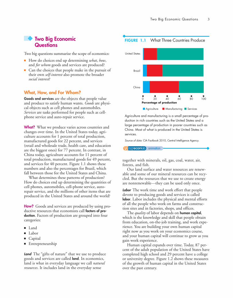
Two Big Economic Questions 3

◆ Two Big Economic Questions

Two big questions summarize the scope of economics:

■ How do choices end up determining what, how,and for whom goods and services are produced?

■ Can the choices that people make in the pursuit oftheir own self-interest also promote the broadersocial interest?

What, How, and For Whom?Goods and services are the objects that people valueand produce to satisfy human wants. Goods are physi-cal objects such as cell phones and automobiles.Services are tasks performed for people such as cell-phone service and auto-repair service.

What? What we produce varies across countries andchanges over time. In the United States today, agri-culture accounts for 1 percent of total production,manufactured goods for 22 percent, and services(retail and wholesale trade, health care, and educationare the biggest ones) for 77 percent. In contrast, inChina today, agriculture accounts for 11 percent oftotal production, manufactured goods for 49 percent,and services for 40 percent. Figure 1.1 shows thesenumbers and also the percentages for Brazil, whichfall between those for the United States and China.

What determines these patterns of production?How do choices end up determining the quantities ofcell phones, automobiles, cell-phone service, auto-repair service, and the millions of other items that areproduced in the United States and around the world?

How? Goods and services are produced by using pro-ductive resources that economists call factors of pro-duction. Factors of production are grouped into fourcategories:

■ Land■ Labor■ Capital■ Entrepreneurship

Land The “gifts of nature” that we use to producegoods and services are called land. In economics,land is what in everyday language we call naturalresources. It includes land in the everyday sense

together with minerals, oil, gas, coal, water, air,forests, and fish.

Our land surface and water resources are renew-able and some of our mineral resources can be recy-cled. But the resources that we use to create energyare nonrenewable—they can be used only once.

Labor The work time and work effort that peopledevote to producing goods and services is calledlabor. Labor includes the physical and mental effortsof all the people who work on farms and construc-tion sites and in factories, shops, and offices.

The quality of labor depends on human capital,which is the knowledge and skill that people obtainfrom education, on-the-job training, and work expe-rience. You are building your own human capitalright now as you work on your economics course,and your human capital will continue to grow as yougain work experience.

Human capital expands over time. Today, 87 per-cent of the adult population of the United States havecompleted high school and 29 percent have a collegeor university degree. Figure 1.2 shows these measuresof the growth of human capital in the United Statesover the past century.

100806040200Percentage of production

China

Agriculture Manufacturing Services

Brazil

United States

Agriculture and manufacturing is a small percentage of pro-duction in rich countries such as the United States and alarge percentage of production in poorer countries such asChina. Most of what is produced in the United States isservices.

Source of data: CIA Factbook 2010, Central Intelligence Agency.

FIGURE 1.1 What Three Countries Produce

animation

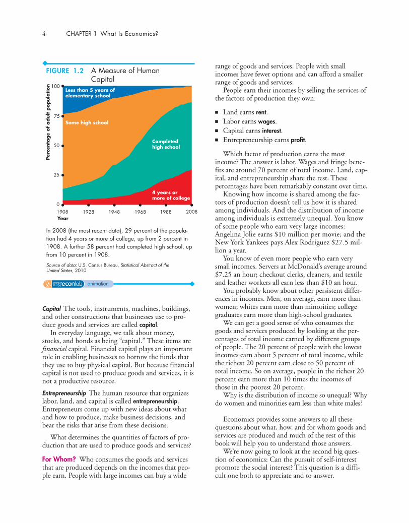
4 CHAPTER 1 What Is Economics?

Capital The tools, instruments, machines, buildings,and other constructions that businesses use to pro-duce goods and services are called capital.

In everyday language, we talk about money,stocks, and bonds as being “capital.” These items arefinancial capital. Financial capital plays an importantrole in enabling businesses to borrow the funds thatthey use to buy physical capital. But because financialcapital is not used to produce goods and services, it isnot a productive resource.

Entrepreneurship The human resource that organizeslabor, land, and capital is called entrepreneurship.Entrepreneurs come up with new ideas about whatand how to produce, make business decisions, andbear the risks that arise from these decisions.

What determines the quantities of factors of pro-duction that are used to produce goods and services?

For Whom? Who consumes the goods and servicesthat are produced depends on the incomes that peo-ple earn. People with large incomes can buy a wide

range of goods and services. People with smallincomes have fewer options and can afford a smallerrange of goods and services.

People earn their incomes by selling the services ofthe factors of production they own:

■ Land earns rent.■ Labor earns wages.■ Capital earns interest.■ Entrepreneurship earns profit.

Which factor of production earns the mostincome? The answer is labor. Wages and fringe bene-fits are around 70 percent of total income. Land, cap-ital, and entrepreneurship share the rest. Thesepercentages have been remarkably constant over time.

Knowing how income is shared among the fac-tors of production doesn’t tell us how it is sharedamong individuals. And the distribution of incomeamong individuals is extremely unequal. You knowof some people who earn very large incomes:Angelina Jolie earns $10 million per movie; and theNew York Yankees pays Alex Rodriguez $27.5 mil-lion a year.

You know of even more people who earn verysmall incomes. Servers at McDonald’s average around$7.25 an hour; checkout clerks, cleaners, and textileand leather workers all earn less than $10 an hour.

You probably know about other persistent differ-ences in incomes. Men, on average, earn more thanwomen; whites earn more than minorities; collegegraduates earn more than high-school graduates.

We can get a good sense of who consumes thegoods and services produced by looking at the per-centages of total income earned by different groupsof people. The 20 percent of people with the lowestincomes earn about 5 percent of total income, whilethe richest 20 percent earn close to 50 percent oftotal income. So on average, people in the richest 20percent earn more than 10 times the incomes ofthose in the poorest 20 percent.

Why is the distribution of income so unequal? Whydo women and minorities earn less than white males?

Economics provides some answers to all thesequestions about what, how, and for whom goods andservices are produced and much of the rest of thisbook will help you to understand those answers.

We’re now going to look at the second big ques-tion of economics: Can the pursuit of self-interestpromote the social interest? This question is a diffi-cult one both to appreciate and to answer.

Per

centa

ge

of

adult p

opula

tion

4 years ormore of college

Completedhigh school

Less than 5 years ofelementary school

Some high school

1908 19881928 1948 1968Year

2008

75

100

50

25

0

In 2008 (the most recent data), 29 percent of the popula-tion had 4 years or more of college, up from 2 percent in1908. A further 58 percent had completed high school, upfrom 10 percent in 1908.

Source of data: U.S. Census Bureau, Statistical Abstract of the United States, 2010.

FIGURE 1.2 A Measure of Human Capital

animation

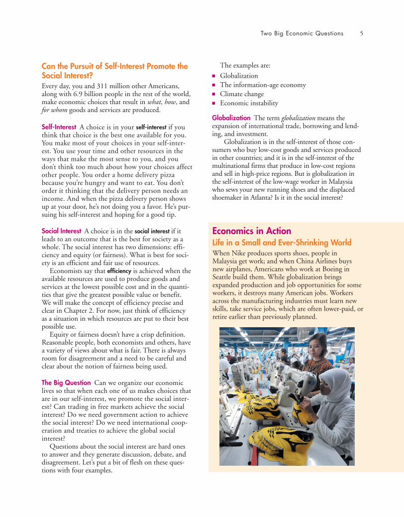
Two Big Economic Questions 5

Can the Pursuit of Self-Interest Promote theSocial Interest?Every day, you and 311 million other Americans,along with 6.9 billion people in the rest of the world,make economic choices that result in what, how, andfor whom goods and services are produced.

Self-Interest A choice is in your self-interest if youthink that choice is the best one available for you.You make most of your choices in your self-inter-est. You use your time and other resources in theways that make the most sense to you, and youdon’t think too much about how your choices affectother people. You order a home delivery pizzabecause you’re hungry and want to eat. You don’torder it thinking that the delivery person needs anincome. And when the pizza delivery person showsup at your door, he’s not doing you a favor. He’s pur-suing his self-interest and hoping for a good tip.

Social Interest A choice is in the social interest if itleads to an outcome that is the best for society as awhole. The social interest has two dimensions: effi-ciency and equity (or fairness). What is best for soci-ety is an efficient and fair use of resources.

Economists say that efficiency is achieved when theavailable resources are used to produce goods andservices at the lowest possible cost and in the quanti-ties that give the greatest possible value or benefit.We will make the concept of efficiency precise andclear in Chapter 2. For now, just think of efficiencyas a situation in which resources are put to their bestpossible use.

Equity or fairness doesn’t have a crisp definition.Reasonable people, both economists and others, havea variety of views about what is fair. There is alwaysroom for disagreement and a need to be careful andclear about the notion of fairness being used.

The Big Question Can we organize our economiclives so that when each one of us makes choices thatare in our self-interest, we promote the social inter-est? Can trading in free markets achieve the socialinterest? Do we need government action to achievethe social interest? Do we need international coop-eration and treaties to achieve the global socialinterest?

Questions about the social interest are hard onesto answer and they generate discussion, debate, anddisagreement. Let’s put a bit of flesh on these ques-tions with four examples.

The examples are:■ Globalization■ The information-age economy■ Climate change■ Economic instability

Globalization The term globalization means theexpansion of international trade, borrowing and lend-ing, and investment.

Globalization is in the self-interest of those con-sumers who buy low-cost goods and services producedin other countries; and it is in the self-interest of themultinational firms that produce in low-cost regionsand sell in high-price regions. But is globalization inthe self-interest of the low-wage worker in Malaysiawho sews your new running shoes and the displacedshoemaker in Atlanta? Is it in the social interest?

Economics in ActionLife in a Small and Ever-Shrinking WorldWhen Nike produces sports shoes, people inMalaysia get work; and when China Airlines buysnew airplanes, Americans who work at Boeing inSeattle build them. While globalization bringsexpanded production and job opportunities for someworkers, it destroys many American jobs. Workersacross the manufacturing industries must learn newskills, take service jobs, which are often lower-paid, orretire earlier than previously planned.

6 CHAPTER 1 What Is Economics?

The Information-Age Economy The technologicalchange of the past forty years has been called theInformation Revolution.

The information revolution has clearly servedyour self-interest: It has provided your cell phone,laptop, loads of handy applications, and the Internet.It has also served the self-interest of Bill Gates ofMicrosoft and Gordon Moore of Intel, both of whomhave seen their wealth soar.

But did the information revolution best serve thesocial interest? Did Microsoft produce the best possi-ble Windows operating system and sell it at a pricethat was in the social interest? Did Intel make theright quality of chips and sell them in the right quan-tities for the right prices? Or was the quality too lowand the price too high? Would the social interest havebeen better served if Microsoft and Intel had facedcompetition from other firms?

Climate Change Climate change is a huge politicalissue today. Every serious political leader is acutelyaware of the problem and of the popularity of havingproposals that might lower carbon emissions.

Every day, when you make self-interested choicesto use electricity and gasoline, you contribute to car-bon emissions; you leave your carbon footprint. Youcan lessen your carbon footprint by walking, riding abike, taking a cold shower, or planting a tree.

But can each one of us be relied upon to makedecisions that affect the Earth’s carbon-dioxide con-centration in the social interest? Must governmentschange the incentives we face so that our self-inter-ested choices are also in the social interest? How cangovernments change incentives? How can we encour-age the use of wind and solar power to replace theburning of fossil fuels that brings climate change?

Economics in ActionChips and WindowsGordon Moore, who founded the chip-maker Intel,and Bill Gates, a co-founder of Microsoft, held privi-leged positions in the Information Revolution.

For many years, Intel chips were the only avail-able chips and Windows was the only available oper-ating system for the original IBM PC and its clones.The PC and Apple’s Mac competed, but the PC hada huge market share.

An absence of competition gave Intel andMicrosoft the power and ability to sell their productsat prices far above the cost of production. If theprices of chips and Windows had been lower, manymore people would have been able to afford a com-puter and would have chosen to buy one.

Economics in ActionGreenhouse Gas EmissionsBurning fossil fuels to generate electricity and topower airplanes, automobiles, and trucks pours astaggering 28 billions tons—4 tons per person—ofcarbon dioxide into the atmosphere each year.

Two thirds of the world’s carbon emissionscomes from the United States, China, the EuropeanUnion, Russia, and India. The fastest growing emis-sions are coming from India and China.

The amount of global warming caused by eco-nomic activity and its effects are uncertain, but theemissions continue to grow and pose huge risks.

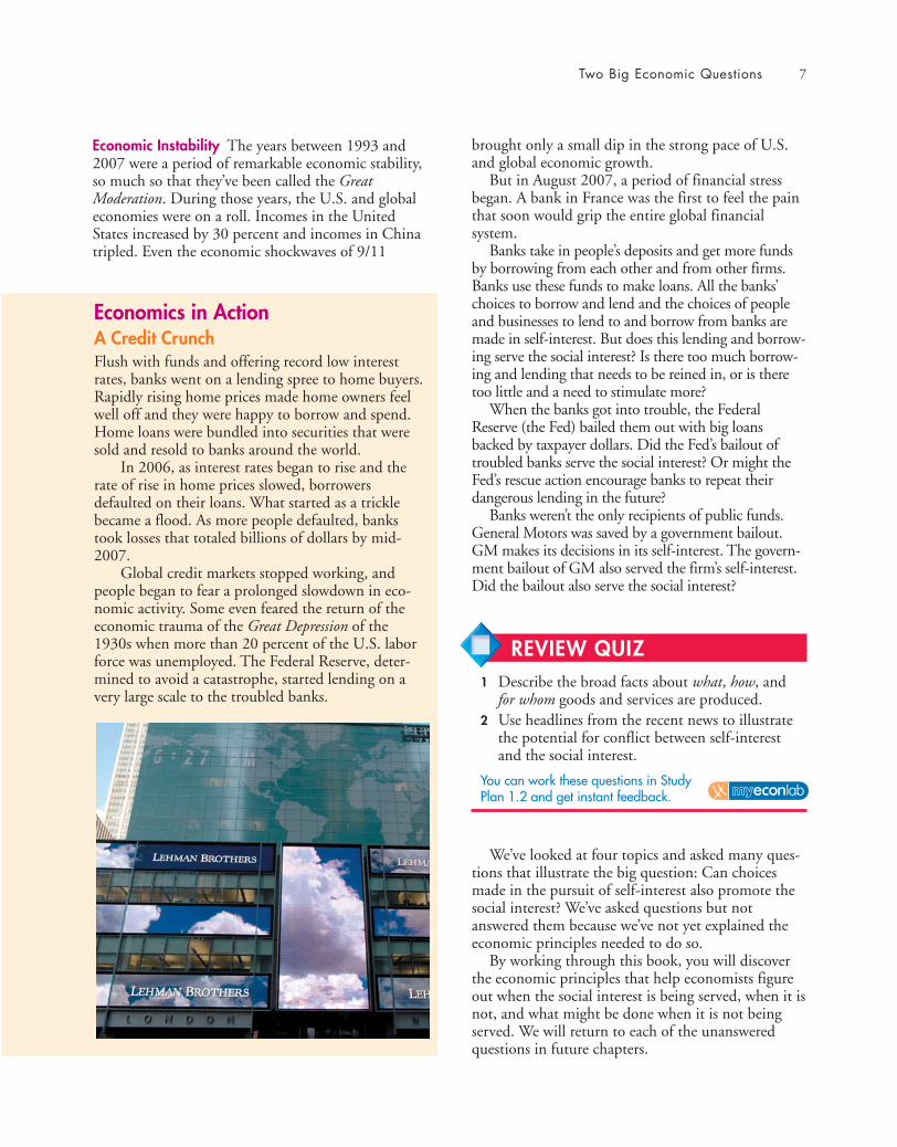
Two Big Economic Questions 7

Economic Instability The years between 1993 and2007 were a period of remarkable economic stability,so much so that they’ve been called the GreatModeration. During those years, the U.S. and globaleconomies were on a roll. Incomes in the UnitedStates increased by 30 percent and incomes in Chinatripled. Even the economic shockwaves of 9/11

We’ve looked at four topics and asked many ques-tions that illustrate the big question: Can choicesmade in the pursuit of self-interest also promote thesocial interest? We’ve asked questions but notanswered them because we’ve not yet explained theeconomic principles needed to do so.

By working through this book, you will discoverthe economic principles that help economists figureout when the social interest is being served, when it isnot, and what might be done when it is not beingserved. We will return to each of the unansweredquestions in future chapters.

Economics in ActionA Credit CrunchFlush with funds and offering record low interestrates, banks went on a lending spree to home buyers.Rapidly rising home prices made home owners feelwell off and they were happy to borrow and spend.Home loans were bundled into securities that weresold and resold to banks around the world.

In 2006, as interest rates began to rise and therate of rise in home prices slowed, borrowersdefaulted on their loans. What started as a tricklebecame a flood. As more people defaulted, bankstook losses that totaled billions of dollars by mid-2007.

Global credit markets stopped working, and people began to fear a prolonged slowdown in eco-nomic activity. Some even feared the return of theeconomic trauma of the Great Depression of the1930s when more than 20 percent of the U.S. laborforce was unemployed. The Federal Reserve, deter-mined to avoid a catastrophe, started lending on avery large scale to the troubled banks.

brought only a small dip in the strong pace of U.S.and global economic growth.

But in August 2007, a period of financial stressbegan. A bank in France was the first to feel the painthat soon would grip the entire global financialsystem.

Banks take in people’s deposits and get more fundsby borrowing from each other and from other firms.Banks use these funds to make loans. All the banks’choices to borrow and lend and the choices of peopleand businesses to lend to and borrow from banks aremade in self-interest. But does this lending and borrow-ing serve the social interest? Is there too much borrow-ing and lending that needs to be reined in, or is theretoo little and a need to stimulate more?

When the banks got into trouble, the FederalReserve (the Fed) bailed them out with big loansbacked by taxpayer dollars. Did the Fed’s bailout oftroubled banks serve the social interest? Or might theFed’s rescue action encourage banks to repeat their dangerous lending in the future?

Banks weren’t the only recipients of public funds.General Motors was saved by a government bailout.GM makes its decisions in its self-interest. The govern-ment bailout of GM also served the firm’s self-interest.Did the bailout also serve the social interest?

REVIEW QUIZ 1 Describe the broad facts about what, how, and

for whom goods and services are produced.2 Use headlines from the recent news to illustrate

the potential for conflict between self-interestand the social interest.

You can work these questions in Study Plan 1.2 and get instant feedback.

8 CHAPTER 1 What Is Economics?

◆ The Economic Wayof Thinking

The questions that economics tries to answer tell usabout the scope of economics, but they don’t tell ushow economists think and go about seeking answersto these questions. You’re now going to see how econ-omists go about their work.

We’re going to look at six key ideas that define theeconomic way of thinking. These ideas are■ A choice is a tradeoff.■ People make rational choices by comparing bene-

fits and costs.■ Benefit is what you gain from something.■ Cost is what you must give up to get something.■ Most choices are “how-much” choices made at the

margin.■ Choices respond to incentives.

A Choice Is a TradeoffBecause we face scarcity, we must make choices.And when we make a choice, we select from theavailable alternatives. For example, you can spendSaturday night studying for your next economicstest or having fun with your friends, but you can’tdo both of these activities at the same time. Youmust choose how much time to devote to each.Whatever choice you make, you could have chosensomething else.

You can think about your choices as tradeoffs. Atradeoff is an exchange—giving up one thing to getsomething else. When you choose how to spend yourSaturday night, you face a tradeoff between studyingand hanging out with your friends.

Making a Rational ChoiceEconomists view the choices that people make asrational. A rational choice is one that compares costsand benefits and achieves the greatest benefit overcost for the person making the choice.

Only the wants of the person making a choice arerelevant to determine its rationality. For example,you might like your coffee black and strong butyour friend prefers his milky and sweet. So it isrational for you to choose espresso and for yourfriend to choose cappuccino.

The idea of rational choice provides an answer tothe first question: What goods and services will be

produced and in what quantities? The answer isthose that people rationally choose to buy!

But how do people choose rationally? Why domore people choose an iPod rather than a Zune?Why has the U.S. government chosen to build aninterstate highway system and not an interstatehigh-speed railroad system? The answers turn oncomparing benefits and costs.

Benefit: What You GainThe benefit of something is the gain or pleasure that itbrings and is determined by preferences—by what aperson likes and dislikes and the intensity of those feel-ings. If you get a huge kick out of “Guitar Hero,” thatvideo game brings you a large benefit. And if you havelittle interest in listening to Yo Yo Ma playing a Vivaldicello concerto, that activity brings you a small benefit.

Some benefits are large and easy to identify, suchas the benefit that you get from being in school. Abig piece of that benefit is the goods and servicesthat you will be able to enjoy with the boost to yourearning power when you graduate. Some benefitsare small, such as the benefit you get from a slice ofpizza.

Economists measure benefit as the most that aperson is willing to give up to get something. You arewilling to give up a lot to be in school. But youwould give up only an iTunes download for a sliceof pizza.

Cost: What You Must Give UpThe opportunity cost of something is the highest-valued alternative that must be given up to get it.

To make the idea of opportunity cost concrete,think about your opportunity cost of being in school.It has two components: the things you can’t afford tobuy and the things you can’t do with your time.

Start with the things you can’t afford to buy. You’vespent all your income on tuition, residence fees, books,and a laptop. If you weren’t in school, you would havespent this money on tickets to ball games and moviesand all the other things that you enjoy. But that’s onlythe start of your opportunity cost. You’ve also given upthe opportunity to get a job. Suppose that the best jobyou could get if you weren’t in school is working atCitibank as a teller earning $25,000 a year. Anotherpart of your opportunity cost of being in school is allthe things that you could buy with the extra $25,000you would have.

The Economic Way of Thinking 9

As you well know, being a student eats up manyhours in class time, doing homework assignments,preparing for tests, and so on. To do all these schoolactivities, you must give up many hours of what wouldotherwise be leisure time spent with your friends.

So the opportunity cost of being in school is allthe good things that you can’t afford and don’t havethe spare time to enjoy. You might want to put adollar value on that cost or you might just list allthe items that make up the opportunity cost.

The examples of opportunity cost that we’ve justconsidered are all-or-nothing costs—you’re either inschool or not in school. Most situations are not likethis one. They involve choosing how much of anactivity to do.

How Much? Choosing at the MarginYou can allocate the next hour between studying andinstant messaging your friends, but the choice is not allor nothing. You must decide how many minutes toallocate to each activity. To make this decision, youcompare the benefit of a little bit more study time withits cost—you make your choice at the margin.

The benefit that arises from an increase in anactivity is called marginal benefit. For example, yourmarginal benefit from one more night of study beforea test is the boost it gives to your grade. Your mar-ginal benefit doesn’t include the grade you’re alreadyachieving without that extra night of work.

The opportunity cost of an increase in an activity iscalled marginal cost. For you, the marginal cost ofstudying one more night is the cost of not spendingthat night on your favorite leisure activity.

To make your decisions, you compare marginalbenefit and marginal cost. If the marginal benefitfrom an extra night of study exceeds its marginal cost,you study the extra night. If the marginal cost exceedsthe marginal benefit, you don’t study the extra night.

Choices Respond to IncentivesEconomists take human nature as given and viewpeople as acting in their self-interest. All people—you, other consumers, producers, politicians, andpublic servants—pursue their self-interest.

Self-interested actions are not necessarily selfishactions. You might decide to use your resources inways that bring pleasure to others as well as to your-self. But a self-interested act gets the most benefit foryou based on your view about benefit.

The central idea of economics is that we can pre-dict the self-interested choices that people make bylooking at the incentives they face. People undertakethose activities for which marginal benefit exceedsmarginal cost; and they reject options for whichmarginal cost exceeds marginal benefit.

For example, your economics instructor gives youa problem set and tells you these problems will be onthe next test. Your marginal benefit from workingthese problems is large, so you diligently work them.In contrast, your math instructor gives you a problemset on a topic that she says will never be on a test.You get little marginal benefit from working theseproblems, so you decide to skip most of them.

Economists see incentives as the key to reconcil-ing self-interest and social interest. When ourchoices are not in the social interest, it is because ofthe incentives we face. One of the challenges foreconomists is to figure out the incentives that resultin self-interested choices being in the social interest.

Economists emphasize the crucial role that institu-tions play in influencing the incentives that peopleface as they pursue their self-interest. Laws that pro-tect private property and markets that enable volun-tary exchange are the fundamental institutions. Youwill learn as you progress with your study of eco-nomics that where these institutions exist, self-inter-est can indeed promote the social interest.

REVIEW QUIZ1 Explain the idea of a tradeoff and think of three

tradeoffs that you have made today.2 Explain what economists mean by rational

choice and think of three choices that you’vemade today that are rational.

3 Explain why opportunity cost is the best for-gone alternative and provide examples of someopportunity costs that you have faced today.

4 Explain what it means to choose at the marginand illustrate with three choices at the marginthat you have made today.

5 Explain why choices respond to incentives andthink of three incentives to which you haveresponded today.

You can work these questions in Study Plan 1.3 and get instant feedback.

10 CHAPTER 1 What Is Economics?

◆ Economics as Social Science andPolicy Tool

Economics is both a social science and a toolkit foradvising on policy decisions.

Economist as Social ScientistAs social scientists, economists seek to discover howthe economic world works. In pursuit of this goal,like all scientists, economists distinguish betweenpositive and normative statements.

Positive Statements A positive statement is aboutwhat is. It says what is currently believed about theway the world operates. A positive statement mightbe right or wrong, but we can test it by checking itagainst the facts. “Our planet is warming because ofthe amount of coal that we’re burning” is a positivestatement. We can test whether it is right or wrong.

A central task of economists is to test positivestatements about how the economic world worksand to weed out those that are wrong. Economicsfirst got off the ground in the late 1700s, so it is ayoung science compared with, for example, physics,and much remains to be discovered.

Normative Statements A normative statement isabout what ought to be. It depends on values and can-not be tested. Policy goals are normative statements.For example, “We ought to cut our use of coal by 50percent” is a normative policy statement. You mayagree or disagree with it, but you can’t test it. Itdoesn’t assert a fact that can be checked.

Unscrambling Cause and Effect Economists are par-ticularly interested in positive statements aboutcause and effect. Are computers getting cheaperbecause people are buying them in greater quanti-ties? Or are people buying computers in greaterquantities because they are getting cheaper? Or issome third factor causing both the price of a com-puter to fall and the quantity of computers boughtto increase?

To answer such questions, economists create andtest economic models. An economic model is adescription of some aspect of the economic worldthat includes only those features that are needed forthe purpose at hand. For example, an economicmodel of a cell-phone network might include fea-tures such as the prices of calls, the number of cell-

phone users, and the volume of calls. But the modelwould ignore cell-phone colors and ringtones.

A model is tested by comparing its predictions withthe facts. But testing an economic model is difficultbecause we observe the outcomes of the simultaneouschange of many factors. To cope with this problem,economists look for natural experiments (situationsin the ordinary course of economic life in which theone factor of interest is different and other things areequal or similar); conduct statistical investigations tofind correlations; and perform economic experimentsby putting people in decision-making situations andvarying the influence of one factor at a time to dis-cover how they respond.

Economist as Policy AdviserEconomics is useful. It is a toolkit for advising gov-ernments and businesses and for making personaldecisions. Some of the most famous economists workpartly as policy advisers.

For example, Jagdish Bhagwati of ColumbiaUniversity, whom you will meet on pp. 52–54, hasadvised governments and international organizationson trade and economic development issues.

Christina Romer of the University of California,Berkeley, is on leave and serving as the chief eco-nomic adviser to President Barack Obama and headof the President’s Council of Economic Advisers.

All the policy questions on which economists pro-vide advice involve a blend of the positive and thenormative. Economics can’t help with the normativepart—the policy goal. But for a given goal, econom-ics provides a method of evaluating alternative solu-tions—comparing marginal benefits and marginalcosts and finding the solution that makes the best useof the available resources.

REVIEW QUIZ 1 Distinguish between a positive statement and a

normative statement and provide examples.2 What is a model? Can you think of a model

that you might use in your everyday life?3 How do economists try to disentangle cause

and effect?4 How is economics used as a policy tool?

You can work these questions in Study Plan 1.4 and get instant feedback.

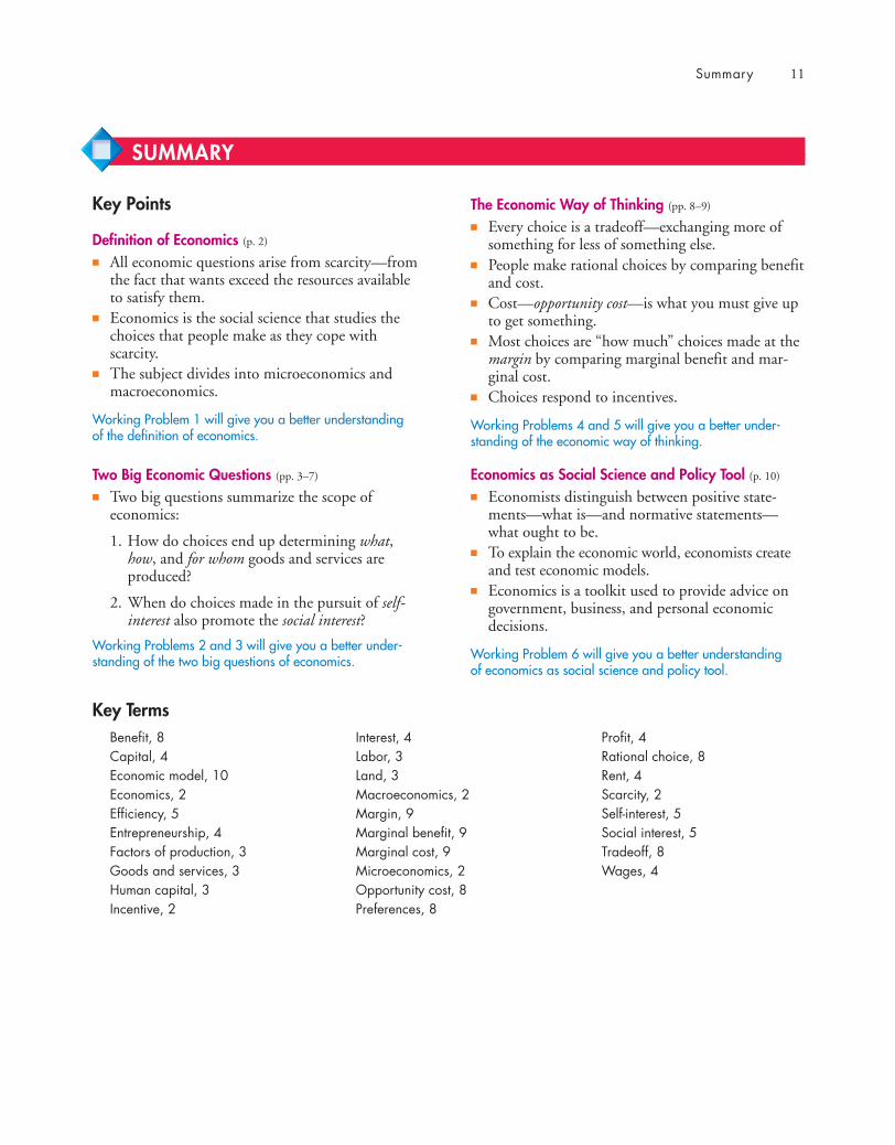
Summary 11

The Economic Way of Thinking (pp. 8–9)

■ Every choice is a tradeoff—exchanging more ofsomething for less of something else.

■ People make rational choices by comparing benefitand cost.

■ Cost—opportunity cost—is what you must give upto get something.

■ Most choices are “how much” choices made at themargin by comparing marginal benefit and mar-ginal cost.

■ Choices respond to incentives.

Working Problems 4 and 5 will give you a better under-standing of the economic way of thinking.

Economics as Social Science and Policy Tool (p. 10)

■ Economists distinguish between positive state-ments—what is—and normative statements—what ought to be.

■ To explain the economic world, economists createand test economic models.

■ Economics is a toolkit used to provide advice ongovernment, business, and personal economicdecisions.

Working Problem 6 will give you a better understandingof economics as social science and policy tool.

Key Points

Definition of Economics (p. 2)

■ All economic questions arise from scarcity—fromthe fact that wants exceed the resources availableto satisfy them.

■ Economics is the social science that studies thechoices that people make as they cope withscarcity.

■ The subject divides into microeconomics andmacroeconomics.

Working Problem 1 will give you a better understandingof the definition of economics.

Two Big Economic Questions (pp. 3–7)

■ Two big questions summarize the scope ofeconomics:

1. How do choices end up determining what,how, and for whom goods and services areproduced?

2. When do choices made in the pursuit of self-interest also promote the social interest?

Working Problems 2 and 3 will give you a better under-standing of the two big questions of economics.

SUMMARY

Key TermsBenefit, 8Capital, 4Economic model, 10Economics, 2Efficiency, 5Entrepreneurship, 4Factors of production, 3Goods and services, 3Human capital, 3Incentive, 2

Interest, 4Labor, 3Land, 3Macroeconomics, 2Margin, 9Marginal benefit, 9Marginal cost, 9Microeconomics, 2Opportunity cost, 8Preferences, 8

Profit, 4Rational choice, 8Rent, 4Scarcity, 2Self-interest, 5Social interest, 5Tradeoff, 8Wages, 4

12 CHAPTER 1 What Is Economics?

Definition of Economics (Study Plan1.1)

1. Apple Inc. decides to make iTunes freely availablein unlimited quantities.a. Does Apple’s decision change the incentives

that people face?b. Is Apple’s decision an example of a microeco-

nomic or a macroeconomic issue?

Two Big Economic Questions (Study Plan1.2)

2. Which of the following pairs does not match?a. Labor and wagesb. Land and rentc. Entrepreneurship and profitd. Capital and profit

3. Explain how the following news headlines con-cern self-interest and the social interest.a. Starbucks Expands in Chinab. McDonald’s Moves into Saladsc. Food Must Be Labeled with Nutrition Data

The Economic Way of Thinking (Study Plan1.3)

4. The night before an economics test, you decideto go to the movies instead of staying home andworking your MyEconLab Study Plan. You get

You can work Problems 1 to 6 in MyEconLab Chapter 1 Study Plan and get instant feedback.

STUDY PLAN PROBLEMS AND APPLICATIONS

50 percent on your test compared with the 70percent that you normally score.a. Did you face a tradeoff?b. What was the opportunity cost of your

evening at the movies?

5. Costs Soar for London OlympicsThe regeneration of East London, the site of the2012 Olympic Games, is set to add extra £1.5billion to taxpayers’ bill.

Source: The Times, London, July 6, 2006Is the cost of regenerating East London anopportunity cost of hosting the 2012 OlympicGames? Explain why or why not.

Economics as Social Science and Policy Tool (Study Plan1.4)

6. Which of the following statements is positive,which is normative, and which can be tested?a. The United States should cut its imports.b. China is the largest trading partner of the

United States.c. If the price of antiretroviral drugs increases,

HIV/AIDS sufferers will decrease their con-sumption of the drugs.

Definition of Economics7. Hundreds Line up for 5 p.m. Ticket Giveaway

By noon, hundreds of Eminem fans had lined upfor a chance to score free tickets to the concert.

Source: Detroit Free Press, May 18, 2009When Eminem gave away tickets, what was freeand what was scarce? Explain your answer.

Two Big Economic Questions8. How does the creation of a successful movie

influence what, how, and for whom goods andservices are produced?

9. How does a successful movie illustrate self-inter-ested choices that are also in the social interest?

The Economic Way of Thinking10. Before starring in Iron Man, Robert Downey Jr.

had appeared in 45 movies that grossed an aver-age of $5 million on the opening weekend. In

You can work these problems in MyEconLab if assigned by your instructor.

ADDITIONAL PROBLEMS AND APPLICATIONS

contrast, Iron Man grossed $102 million.a. How do you expect the success of Iron Man to

influence the opportunity cost of hiringRobert Downey Jr.?

b. How have the incentives for a movie producerto hire Robert Downey Jr. changed?

11. What might be an incentive for you to take aclass in summer school? List some of the benefitsand costs involved in your decision. Would yourchoice be rational?

Economics as Social Science and Policy Tool12. Look at today’s Wall Street Journal. What is the

leading economic news story? With which of thebig economic questions does it deal and whattradeoffs does it discuss or imply?

13. Provide two microeconomic statements and twomacroeconomic statements. Classify your state-ments as positive or normative. Explain why.

APPENDIX

Graphs in Economics

After studying this appendix,you will be able to:

� Make and interpret a scatter diagram� Identify linear and nonlinear relationships and

relationships that have a maximum and aminimum

� Define and calculate the slope of a line� Graph relationships among more than two

variables

◆ Graphing DataA graph represents a quantity as a distance on a line.In Fig. A1.1, a distance on the horizontal line repre-sents temperature, measured in degrees Fahrenheit. Amovement from left to right shows an increase intemperature. The point 0 represents zero degreesFahrenheit. To the right of 0, the temperature is posi-tive. To the left of 0 the temperature is negative (asindicated by the minus sign). A distance on the verti-cal line represents height, measured in thousands offeet. The point 0 represents sea level. Points above 0represent feet above sea level. Points below 0 repre-sent feet below sea level (indicated by a minus sign).

In Fig. A1.1, the two scale lines are perpendicularto each other and are called axes. The vertical line isthe y-axis, and the horizontal line is the x-axis. Eachaxis has a zero point, which is shared by the two axesand called the origin.

To make a two-variable graph, we need two piecesof information: the value of the variable x and thevalue of the variable y. For example, off the coast ofAlaska, the temperature is 32 degrees—the value of x.A fishing boat is located at 0 feet above sea level—thevalue of y. These two bits of information appear aspoint A in Fig. A1.1. A climber at the top of MountMcKinley on a cold day is 20,320 feet above sea levelin a zero-degree gale. These two pieces of informationappear as point B. On a warmer day, a climber mightbe at the peak of Mt. McKinley when the temperatureis 32 degrees, at point C.

We can draw two lines, called coordinates, frompoint C. One, called the x-coordinate, runs from C tothe vertical axis. This line is called “the x-coordinate”

because its length is the same as the value marked offon the x-axis. The other, called the y-coordinate, runsfrom C to the horizontal axis. This line is called “they-coordinate” because its length is the same as thevalue marked off on the y-axis.

We describe a point on a graph by the values ofits x-coordinate and its y-coordinate. For example, atpoint C, x is 32 degrees and y is 20,320 feet.

A graph like that in Fig. A1.1 can be made usingany quantitative data on two variables. The graph canshow just a few points, like Fig. A1.1, or manypoints. Before we look at graphs with many points,let’s reinforce what you’ve just learned by looking attwo graphs made with economic data.

Economists measure variables that describe what,how, and for whom goods and services are produced.These variables are quantities produced and prices.Figure A1.2 shows two examples of economic graphs.

Appendix: Graphs in Economics 13

y

x0

–5

–60 –30

5

90 120

10

15

20

25

Hei

ght (

thou

sand

s of

feet

)

Temperature (degrees F)

–10

30 60

CB

A

0ºF and20,320 ft

32ºF and20,320 ft

32ºF and0 ftOrigin

Negative Positive

Belo

w s

ea le

vel

Abo

ve s

ea le

vel

Graphs have axes that measure quantities as distances.Here, the horizontal axis (x-axis) measures temperature, andthe vertical axis (y-axis) measures height. Point A representsa fishing boat at sea level (0 on the y-axis) on a day whenthe temperature is 32ºF. Point B represents a climber at thetop of Mt. McKinley, 20,320 feet above sea level at atemperature of 0ºF. Point C represents a climber at the topof Mt. McKinley, 20,320 feet above sea level at a tempera-ture of 32ºF.

FIGURE A1.1 Making a Graph

animation

Figure A1.2(a) is a graph about iTunes song downloadsin January 2010. The x-axis measures the quantity ofsongs downloaded per day and the y-axis measures theprice of a song. Point A tells us what the quantity andprice were. You can “read” this graph as telling youthat in January 2010, 8.3 million songs a day weredownloaded at a price of 99¢ per song.

Figure A1.2(b) is a graph about iTunes song andalbum downloads in January 2010. The x-axis meas-ures the quantity of songs downloaded per day andthe y-axis measures the quantity of albums down-loaded per day. Point B tells us what these quantitieswere. You can “read” this graph as telling you that inJanuary 2010, 8.3 million songs a day and 0.4 mil-lion albums were downloaded.

The three graphs that you’ve just seen tell youhow to make a graph and how to read a data pointon a graph, but they don’t improve on the raw data.Graphs become interesting and revealing when theycontain a number of data points because then youcan visualize the data.

Economists create graphs based on the principlesin Figs. A1.1 and A1.2 to reveal, describe, and visual-ize the relationships among variables. We’re nowgoing to look at some examples. These graphs arecalled scatter diagrams.

Scatter DiagramsA scatter diagram is a graph that plots the value of onevariable against the value of another variable for anumber of different values of each variable. Such agraph reveals whether a relationship exists between

two variables and describes their relationship.The table in Fig. A1.3 shows some data on two

variables: the number of tickets sold at the box officeand the number of DVDs sold for eight of the mostpopular movies in 2009.

What is the relationship between these two vari-ables? Does a big box office success generate a largevolume of DVD sales? Or does a box office successmean that fewer DVDs are sold?

We can answer these questions by making a scatterdiagram. We do so by graphing the data in the table.In the graph in Fig. A1.3, each point shows the num-ber of box office tickets sold (the x variable) and thenumber of DVDs sold (the y variable) of one of themovies. There are eight movies, so there are eightpoints “scattered” within the graph.

The point labeled A tells us that Star Trek sold 34million tickets at the box office and 6 million DVDs.The points in the graph form a pattern, which revealsthat larger box office sales are associated with largerDVD sales. But the points also tell us that this associ-ation is weak. You can’t predict DVD sales with anyconfidence by knowing only the number of ticketssold at the box office.

Figure A1.4 shows two scatter diagrams of eco-nomic variables. Part (a) shows the relationshipbetween income and expenditure, on average, duringa ten-year period. Each point represents income andexpenditure in a given year. For example, point Ashows that in 2006, income was $31 thousand andexpenditure was $30 thousand. This graph shows thatas income increases, so does expenditure, and the rela-tionship is a close one.

14 CHAPTER 1 What Is Economics?

(b) iTunes downloads: songs and albums(a) iTunes downloads: quantity and price

0

0.2

0.6

0.8

1.0

0.4

Qua

ntity

(mill

ions

of a

lbum

s pe

r day

)

Quantity (millions of songs per day) Quantity (millions of songs per day)

Pric

e (c

ents

per s

ong)

5 8.3 10 15 5 8.3 10 150

150

99

50

A

B

8.3 millionsongs at 99cents per song

8.3 million songsand 0.4 millionalbums weredownloaded

The graph in part (a) tells us thatin January 2010, 8.3 millionsongs per day were downloadedfrom the iTunes store at a price of99 cents a song.

The graph in part (b) tells usthat in January 2010, 8.3 millionsongs per day and 0.4 millionalbums per day were downloadedfrom the iTunes store.

FIGURE A1.2 Two Graphs of Economic Data

animation

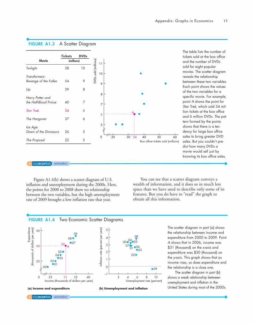
Figure A1.4(b) shows a scatter diagram of U.S.inflation and unemployment during the 2000s. Here,the points for 2000 to 2008 show no relationshipbetween the two variables, but the high unemploymentrate of 2009 brought a low inflation rate that year.

You can see that a scatter diagram conveys awealth of information, and it does so in much lessspace than we have used to describe only some of itsfeatures. But you do have to “read” the graph toobtain all this information.

Appendix: Graphs in Economics 15

0

5

20 30 34 5040 60

DVD

s so

ld (m

illio

ns)

6

7

8

9

10

11

A

Box office tickets sold (millions)

The table lists the number oftickets sold at the box officeand the number of DVDssold for eight popularmovies. The scatter diagramreveals the relationshipbetween these two variables.Each point shows the valuesof the two variables for aspecific movie. For example,point A shows the point forStar Trek, which sold 34 mil-lion tickets at the box officeand 6 million DVDs. The pat-tern formed by the pointsshows that there is a ten-dency for large box officesales to bring greater DVDsales. But you couldn’t pre-dict how many DVDs amovie would sell just byknowing its box office sales.

FIGURE A1.3 A Scatter Diagram

animation

Tickets DVDsMovie (millions)

Twilight 38 10

Transformers:Revenge of the Fallen 54 9

Up 39 8

Harry Potter andthe Half-Blood Prince 40 7

Star Trek 34 6

The Hangover 37 6

Ice Age:Dawn of the Dinosaurs 26 5

The Proposal 22 5

(b) Unemployment and inflation(a) Income and expenditure

–1

0

3

4

5

2

1

Infla

tion

rate

(per

cent

per

yea

r)

Income (thousands of dollars per year) Unemployment rate (percent)

Expe

nditu

re(th

ousa

nds

of d

olla

rs p

er y

ear)

25

00

00

01

01

02

0203

03

04

04

05

0506

0607

07

0808

09

09

31 35 40 2 4 6 8 100

35

25

30 A

The scatter diagram in part (a) showsthe relationship between income andexpenditure from 2000 to 2009. PointA shows that in 2006, income was$31 (thousand) on the x-axis andexpenditure was $30 (thousand) onthe y-axis. This graph shows that asincome rises, so does expenditure andthe relationship is a close one.

The scatter diagram in part (b)shows a weak relationship betweenunemployment and inflation in theUnited States during most of the 2000s.

FIGURE A1.4 Two Economic Scatter Diagrams

animation

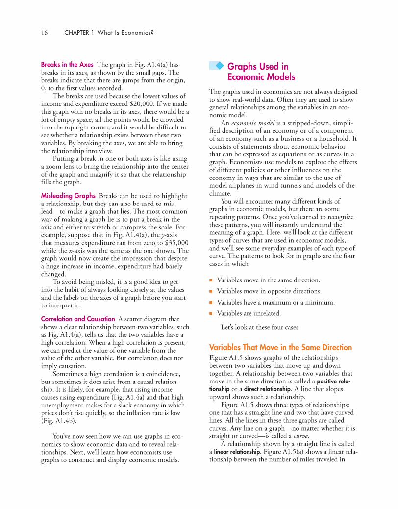
Breaks in the Axes The graph in Fig. A1.4(a) hasbreaks in its axes, as shown by the small gaps. Thebreaks indicate that there are jumps from the origin,0, to the first values recorded.

The breaks are used because the lowest values ofincome and expenditure exceed $20,000. If we madethis graph with no breaks in its axes, there would be alot of empty space, all the points would be crowdedinto the top right corner, and it would be difficult tosee whether a relationship exists between these twovariables. By breaking the axes, we are able to bringthe relationship into view.

Putting a break in one or both axes is like usinga zoom lens to bring the relationship into the centerof the graph and magnify it so that the relationshipfills the graph.

Misleading Graphs Breaks can be used to highlighta relationship, but they can also be used to mis-lead—to make a graph that lies. The most commonway of making a graph lie is to put a break in theaxis and either to stretch or compress the scale. Forexample, suppose that in Fig. A1.4(a), the y-axisthat measures expenditure ran from zero to $35,000while the x-axis was the same as the one shown. Thegraph would now create the impression that despitea huge increase in income, expenditure had barelychanged.

To avoid being misled, it is a good idea to getinto the habit of always looking closely at the valuesand the labels on the axes of a graph before you startto interpret it.

Correlation and Causation A scatter diagram thatshows a clear relationship between two variables, suchas Fig. A1.4(a), tells us that the two variables have ahigh correlation. When a high correlation is present,we can predict the value of one variable from thevalue of the other variable. But correlation does notimply causation.

Sometimes a high correlation is a coincidence,but sometimes it does arise from a causal relation-ship. It is likely, for example, that rising incomecauses rising expenditure (Fig. A1.4a) and that highunemployment makes for a slack economy in whichprices don’t rise quickly, so the inflation rate is low(Fig. A1.4b).

You’ve now seen how we can use graphs in eco-nomics to show economic data and to reveal rela-tionships. Next, we’ll learn how economists usegraphs to construct and display economic models.

◆ Graphs Used in Economic Models

The graphs used in economics are not always designedto show real-world data. Often they are used to showgeneral relationships among the variables in an eco-nomic model.

An economic model is a stripped-down, simpli-fied description of an economy or of a componentof an economy such as a business or a household. Itconsists of statements about economic behaviorthat can be expressed as equations or as curves in agraph. Economists use models to explore the effectsof different policies or other influences on theeconomy in ways that are similar to the use ofmodel airplanes in wind tunnels and models of theclimate.

You will encounter many different kinds ofgraphs in economic models, but there are somerepeating patterns. Once you’ve learned to recognizethese patterns, you will instantly understand themeaning of a graph. Here, we’ll look at the differenttypes of curves that are used in economic models,and we’ll see some everyday examples of each type ofcurve. The patterns to look for in graphs are the fourcases in which

■ Variables move in the same direction.

■ Variables move in opposite directions.

■ Variables have a maximum or a minimum.

■ Variables are unrelated.

Let’s look at these four cases.

Variables That Move in the Same DirectionFigure A1.5 shows graphs of the relationshipsbetween two variables that move up and downtogether. A relationship between two variables thatmove in the same direction is called a positive rela-tionship or a direct relationship. A line that slopesupward shows such a relationship.

Figure A1.5 shows three types of relationships:one that has a straight line and two that have curvedlines. All the lines in these three graphs are calledcurves. Any line on a graph—no matter whether it isstraight or curved—is called a curve.

A relationship shown by a straight line is calleda linear relationship. Figure A1.5(a) shows a linear rela-tionship between the number of miles traveled in

16 CHAPTER 1 What Is Economics?

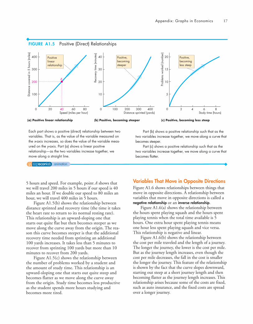
5 hours and speed. For example, point A shows thatwe will travel 200 miles in 5 hours if our speed is 40miles an hour. If we double our speed to 80 miles anhour, we will travel 400 miles in 5 hours.

Figure A1.5(b) shows the relationship betweendistance sprinted and recovery time (the time it takesthe heart rate to return to its normal resting rate).This relationship is an upward-sloping one thatstarts out quite flat but then becomes steeper as wemove along the curve away from the origin. The rea-son this curve becomes steeper is that the additionalrecovery time needed from sprinting an additional100 yards increases. It takes less than 5 minutes torecover from sprinting 100 yards but more than 10minutes to recover from 200 yards.

Figure A1.5(c) shows the relationship betweenthe number of problems worked by a student andthe amount of study time. This relationship is anupward-sloping one that starts out quite steep andbecomes flatter as we move along the curve awayfrom the origin. Study time becomes less productiveas the student spends more hours studying andbecomes more tired.

Variables That Move in Opposite DirectionsFigure A1.6 shows relationships between things thatmove in opposite directions. A relationship betweenvariables that move in opposite directions is called anegative relationship or an inverse relationship.

Figure A1.6(a) shows the relationship betweenthe hours spent playing squash and the hours spentplaying tennis when the total time available is 5hours. One extra hour spent playing tennis meansone hour less spent playing squash and vice versa.This relationship is negative and linear.

Figure A1.6(b) shows the relationship betweenthe cost per mile traveled and the length of a journey.The longer the journey, the lower is the cost per mile.But as the journey length increases, even though thecost per mile decreases, the fall in the cost is smallerthe longer the journey. This feature of the relationshipis shown by the fact that the curve slopes downward,starting out steep at a short journey length and thenbecoming flatter as the journey length increases. Thisrelationship arises because some of the costs are fixed,such as auto insurance, and the fixed costs are spreadover a longer journey.

Appendix: Graphs in Economics 17

0

100

200

300

400

20 40 60 80

Dis

tanc

e co

vere

d in

5 h

ours

(mile

s)

Speed (miles per hour)

(a) Positive linear relationship

0

10

20

30

40

100 200 300 400

Reco

very

tim

e (m

inut

es)

Distance sprinted (yards)

(b) Positive, becoming steeper

0

5

10

15

20

2 4 6 8

Prob

lem

s w

orke

d (n

umbe

r)

Study time (hours)

(c) Positive, becoming less steep

A

Positivelinearrelationship

Positive,becomingless steep

Positive,becomingsteeper

Each part shows a positive (direct) relationship between twovariables. That is, as the value of the variable measured onthe x-axis increases, so does the value of the variable meas-ured on the y-axis. Part (a) shows a linear positive relationship—as the two variables increase together, wemove along a straight line.

FIGURE A1.5 Positive (Direct) Relationships

animation

Part (b) shows a positive relationship such that as thetwo variables increase together, we move along a curve thatbecomes steeper.

Part (c) shows a positive relationship such that as thetwo variables increase together, we move along a curve thatbecomes flatter.

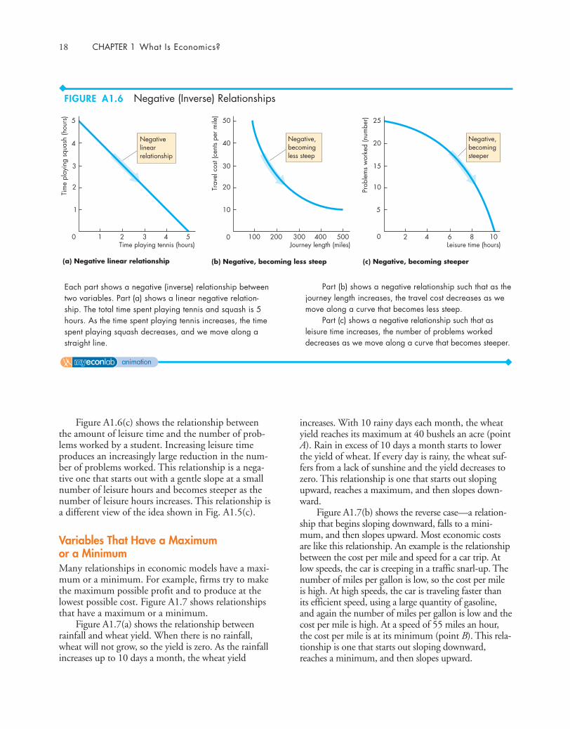
Figure A1.6(c) shows the relationship betweenthe amount of leisure time and the number of prob-lems worked by a student. Increasing leisure timeproduces an increasingly large reduction in the num-ber of problems worked. This relationship is a nega-tive one that starts out with a gentle slope at a smallnumber of leisure hours and becomes steeper as thenumber of leisure hours increases. This relationship isa different view of the idea shown in Fig. A1.5(c).

Variables That Have a Maximum or a MinimumMany relationships in economic models have a maxi-mum or a minimum. For example, firms try to makethe maximum possible profit and to produce at thelowest possible cost. Figure A1.7 shows relationshipsthat have a maximum or a minimum.

Figure A1.7(a) shows the relationship betweenrainfall and wheat yield. When there is no rainfall,wheat will not grow, so the yield is zero. As the rainfallincreases up to 10 days a month, the wheat yield

increases. With 10 rainy days each month, the wheatyield reaches its maximum at 40 bushels an acre (pointA). Rain in excess of 10 days a month starts to lowerthe yield of wheat. If every day is rainy, the wheat suf-fers from a lack of sunshine and the yield decreases tozero. This relationship is one that starts out slopingupward, reaches a maximum, and then slopes down-ward.

Figure A1.7(b) shows the reverse case—a relation-ship that begins sloping downward, falls to a mini-mum, and then slopes upward. Most economic costsare like this relationship. An example is the relationshipbetween the cost per mile and speed for a car trip. Atlow speeds, the car is creeping in a traffic snarl-up. Thenumber of miles per gallon is low, so the cost per mileis high. At high speeds, the car is traveling faster thanits efficient speed, using a large quantity of gasoline,and again the number of miles per gallon is low and thecost per mile is high. At a speed of 55 miles an hour,the cost per mile is at its minimum (point B). This rela-tionship is one that starts out sloping downward,reaches a minimum, and then slopes upward.

18 CHAPTER 1 What Is Economics?

0 1 2 3 5

Tim

e pl

ayin

g sq

uash

(hou

rs)

Time playing tennis (hours)

(a) Negative linear relationship

4

1

2

3

5

4

0 100 200 300 500

Trav

el c

ost (

cent

s pe

r mile

)

Journey length (miles)

(b) Negative, becoming less steep

400

10

20

30

50

40

0 2 4 6 10

Prob

lem

s w

orke

d (n

umbe

r)

Leisure time (hours)

(c) Negative, becoming steeper

8

5

10

15

25

20Negative,becomingsteeper

Negative,becomingless steep

Negativelinearrelationship

Each part shows a negative (inverse) relationship betweentwo variables. Part (a) shows a linear negative relation-ship. The total time spent playing tennis and squash is 5hours. As the time spent playing tennis increases, the timespent playing squash decreases, and we move along astraight line.

FIGURE A1.6 Negative (Inverse) Relationships

animation

Part (b) shows a negative relationship such that as thejourney length increases, the travel cost decreases as wemove along a curve that becomes less steep.

Part (c) shows a negative relationship such that asleisure time increases, the number of problems workeddecreases as we move along a curve that becomes steeper.

Variables That Are UnrelatedThere are many situations in which no matter whathappens to the value of one variable, the other vari-able remains constant. Sometimes we want to showthe independence between two variables in a graph,and Fig. A1.8 shows two ways of achieving this.

In describing the graphs in Fig. A1.5 through Fig.A1.7, we have talked about curves that slope upwardor slope downward, and curves that become less steepor steeper. Let’s spend a little time discussing exactlywhat we mean by slope and how we measure the slopeof a curve.

Appendix: Graphs in Economics 19

Increasingcost

Decreasingcost

40

0 5 10 15 20 25Rainfall (days per month)

(a) Relationship with a maximum

A

Maximumyield

Whe

at y

ield

(bus

hels

per a

cre)

15

0 15 35 95Speed (miles per hour)

(b) Relationship with a minimum

B

MinimumcostG

asol

ine

cost

(cen

ts pe

r mile

)

55 75

10

5

50

30

20

10

30

Increasingyield

Decreasingyield

Part (a) shows a relation-ship that has a maximumpoint, A. The curve slopesupward as it rises to itsmaximum point, is flat atits maximum, and thenslopes downward.

Part (b) shows a rela-tionship with a minimumpoint, B. The curve slopesdownward as it falls to itsminimum, is flat at its min-imum, and then slopesupward.

FIGURE A1.7 Maximum and Minimum Points

animation

100

75

50

25

0 20 40 60 80

Gra

de in

eco

nom

ics

(per

cent

)

Price of bananas (cents per pound)

(a) Unrelated: y constant

Unrelated:y constant

20

15

10

5

0 1 2 3 4

Rain

fall

in C

alifo

rnia

(day

s pe

r mon

th)

Output of French wine (billions of gallons)

(b) Unrelated: x constant

Unrelated:x constant

This figure shows howwe can graph two variablesthat are unrelated. In part(a), a student’s grade ineconomics is plotted at75 percent on the y-axisregardless of the price ofbananas on the x-axis. Thecurve is horizontal.

In part (b), the outputof the vineyards of Franceon the x-axis does not varywith the rainfall inCalifornia on the y-axis.The curve is vertical.

FIGURE A1.8 Variables That Are Unrelated

animation

◆ The Slope of a RelationshipWe can measure the influence of one variable onanother by the slope of the relationship. The slopeof a relationship is the change in the value of thevariable measured on the y-axis divided by thechange in the value of the variable measured on thex-axis. We use the Greek letter � (delta) to represent“change in.” Thus �y means the change in the valueof the variable measured on the y-axis, and �xmeans the change in the value of the variable meas-ured on the x-axis. Therefore the slope of the rela-tionship is

.Slope =¢y

¢x

If a large change in the variable measured onthe y-axis (�y) is associated with a small change inthe variable measured on the x-axis (�x), the slopeis large and the curve is steep. If a small change inthe variable measured on the y-axis (�y) is associ-ated with a large change in the variable measuredon the x-axis (�x), the slope is small and the curveis flat.

We can make the idea of slope clearer by doingsome calculations.

The Slope of a Straight LineThe slope of a straight line is the same regardless ofwhere on the line you calculate it. The slope of astraight line is constant. Let’s calculate the slope ofthe positive relationship in Fig. A1.9. In part (a),

20 CHAPTER 1 What Is Economics?

8

x

7

6

5

4

3

2

1

0

y

1 2 3 4 5 6 7 8

(a) Positive slope

8

x

7

6

5

4

3

2

1

0

y

1 2 3 4 5 6 7 8

Slope = – —34

(b) Negative slope

Slope = —34

To calculate the slope of a straight line, we divide the changein the value of the variable measured on the y-axis (�y ) bythe change in the value of the variable measured on the x-axis (�x) as we move along the line.

Part (a) shows the calculation of a positive slope. Whenx increases from 2 to 6, �x equals 4. That change in x

FIGURE A1.9 The Slope of a Straight Line

animation

brings about an increase in y from 3 to 6, so �y equals 3.The slope (�y/�x) equals 3/4.

Part (b) shows the calculation of a negative slope. Whenx increases from 2 to 6, �x equals 4. That increase in xbrings about a decrease in y from 6 to 3, so �y equals –3.The slope (�y/�x) equals –3/4.

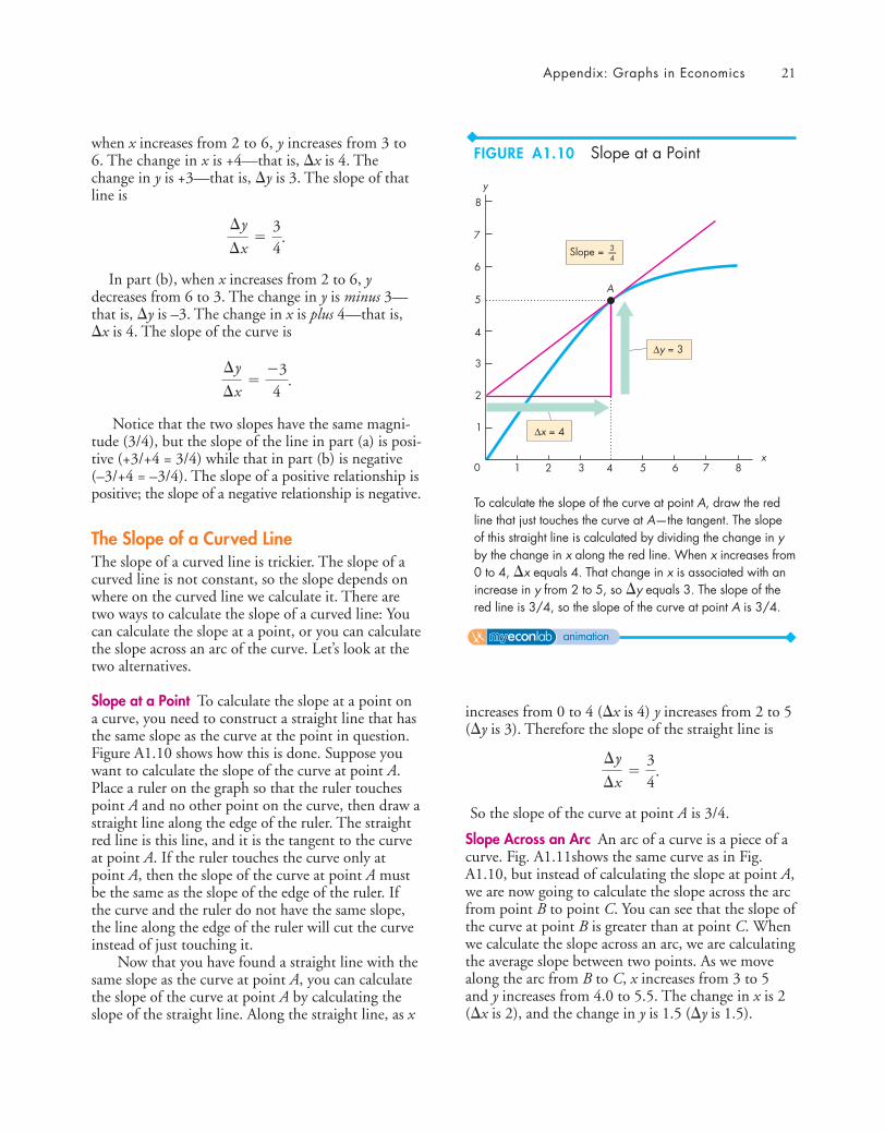
when x increases from 2 to 6, y increases from 3 to6. The change in x is +4—that is, �x is 4. Thechange in y is +3—that is, �y is 3. The slope of thatline is

In part (b), when x increases from 2 to 6, ydecreases from 6 to 3. The change in y is minus 3—that is, �y is –3. The change in x is plus 4—that is,�x is 4. The slope of the curve is

Notice that the two slopes have the same magni-tude (3/4), but the slope of the line in part (a) is posi-tive (+3/+4 = 3/4) while that in part (b) is negative(–3/+4 = –3/4). The slope of a positive relationship ispositive; the slope of a negative relationship is negative.

The Slope of a Curved LineThe slope of a curved line is trickier. The slope of acurved line is not constant, so the slope depends onwhere on the curved line we calculate it. There aretwo ways to calculate the slope of a curved line: Youcan calculate the slope at a point, or you can calculatethe slope across an arc of the curve. Let’s look at thetwo alternatives.

Slope at a Point To calculate the slope at a point ona curve, you need to construct a straight line that hasthe same slope as the curve at the point in question.Figure A1.10 shows how this is done. Suppose youwant to calculate the slope of the curve at point A.Place a ruler on the graph so that the ruler touchespoint A and no other point on the curve, then draw astraight line along the edge of the ruler. The straightred line is this line, and it is the tangent to the curveat point A. If the ruler touches the curve only atpoint A, then the slope of the curve at point A mustbe the same as the slope of the edge of the ruler. Ifthe curve and the ruler do not have the same slope,the line along the edge of the ruler will cut the curveinstead of just touching it.

Now that you have found a straight line with thesame slope as the curve at point A, you can calculatethe slope of the curve at point A by calculating theslope of the straight line. Along the straight line, as x

¢y

¢x=

-34

.

¢y

¢x=

3

4.

increases from 0 to 4 (�x is 4) y increases from 2 to 5(�y is 3). Therefore the slope of the straight line is

So the slope of the curve at point A is 3/4.

Slope Across an Arc An arc of a curve is a piece of acurve. Fig. A1.11shows the same curve as in Fig.A1.10, but instead of calculating the slope at point A,we are now going to calculate the slope across the arcfrom point B to point C. You can see that the slope ofthe curve at point B is greater than at point C. Whenwe calculate the slope across an arc, we are calculatingthe average slope between two points. As we movealong the arc from B to C, x increases from 3 to 5and y increases from 4.0 to 5.5. The change in x is 2(�x is 2), and the change in y is 1.5 (�y is 1.5).

¢y

¢x=

3

4.

Appendix: Graphs in Economics 21

0

4

5

6

8

7

3

2

1

4 5 6321 87

y

x

A

Slope = —34

To calculate the slope of the curve at point A, draw the redline that just touches the curve at A—the tangent. The slopeof this straight line is calculated by dividing the change in yby the change in x along the red line. When x increases from 0 to 4, �x equals 4. That change in x is associated with anincrease in y from 2 to 5, so �y equals 3. The slope of thered line is 3/4, so the slope of the curve at point A is 3/4.

FIGURE A1.10 Slope at a Point

animation

Therefore the slope is

So the slope of the curve across the arc BC is 3/4.This calculation gives us the slope of the curve

between points B and C. The actual slope calculatedis the slope of the straight line from B to C. Thisslope approximates the average slope of the curvealong the arc BC. In this particular example, theslope across the arc BC is identical to the slope of thecurve at point A, but the calculation of the slope of acurve does not always work out so neatly. You mighthave fun constructing some more examples and a fewcounter examples.

You now know how to make and interpret agraph. So far, we’ve limited our attention to graphs oftwo variables. We’re now going to learn how to graphmore than two variables.

¢y

¢x=

1.52

=34

.

◆ Graphing Relationships AmongMore Than Two Variables

We have seen that we can graph the relationshipbetween two variables as a point formed by the x-and y-coordinates in a two-dimensional graph. Youmight be thinking that although a two-dimensionalgraph is informative, most of the things in whichyou are likely to be interested involve relationshipsamong many variables, not just two. For example,the amount of ice cream consumed depends on theprice of ice cream and the temperature. If ice creamis expensive and the temperature is low, people eatmuch less ice cream than when ice cream is inex-pensive and the temperature is high. For any givenprice of ice cream, the quantity consumed varieswith the temperature; and for any given tempera-ture, the quantity of ice cream consumed varies withits price.

Figure A1.12 shows a relationship among threevariables. The table shows the number of gallons ofice cream consumed each day at two different tem-peratures and at a number of different prices of icecream. How can we graph these numbers?

To graph a relationship that involves more thantwo variables, we use the ceteris paribus assumption.

Ceteris ParibusCeteris paribus (often shortened to cet par) means “ifall other relevant things remain the same.” To isolatethe relationship of interest in a laboratory experi-ment, a scientist holds everything constant except forthe variable whose effect is being studied. Economistsuse the same method to graph a relationship that hasmore than two variables.

Figure A1.12 shows an example. There, you cansee what happens to the quantity of ice cream con-sumed when the price of ice cream varies but thetemperature is held constant.

The curve labeled 70°F shows the relationshipbetween ice cream consumption and the price of icecream if the temperature remains at 70°F. The num-bers used to plot that curve are those in the first twocolumns of the table. For example, if the tempera-ture is 70°F, 10 gallons are consumed when theprice is $2.75 a scoop and 18 gallons are consumedwhen the price is $2.25 a scoop.

The curve labeled 90°F shows the relationshipbetween ice cream consumption and the price ofice cream if the temperature remains at 90°F. The

22 CHAPTER 1 What Is Economics?

A

B

C

0

4.0

5.0

6.0

8.0

7.0

3.0

2.0

1.0

4 5 6321 87

y

x

5.5

Slope = — = —34

=1.5

1.52

To calculate the average slope of the curve along the arcBC, draw a straight line from point B to point C. The slopeof the line BC is calculated by dividing the change in y bythe change in x. In moving from B to C, the increase in x is2 (�x equals 2) and the change in y is 1.5 (�y equals 1.5).The slope of the line BC is 1.5 divided by 2, or 3/4. So theslope of the curve across the arc BC is 3/4.

FIGURE A1.11 Slope Across an Arc

animation

numbers used to plot that curve are those in thefirst and third columns of the table. For example, ifthe temperature is 90°F, 20 gallons are consumedwhen the price is $2.75 a scoop and 36 gallons areconsumed when the price is $2.25 a scoop.

When the price of ice cream changes but the tem-perature is constant, you can think of what happens inthe graph as a movement along one of the curves. At70°F there is a movement along the blue curve and at90°F there is a movement along the red curve.

When Other Things ChangeThe temperature is held constant along each of thecurves in Fig. A1.12, but in reality the temperature

changes. When that event occurs, you can think ofwhat happens in the graph as a shift of the curve.When the temperature rises from 70°F to 90°F, thecurve that shows the relationship between ice creamconsumption and the price of ice cream shifts right-ward from the blue curve to the red curve.

You will encounter these ideas of movementsalong and shifts of curves at many points in yourstudy of economics. Think carefully about whatyou’ve just learned and make up some examples (withassumed numbers) about other relationships.

With what you have learned about graphs, you canmove forward with your study of economics. There areno graphs in this book that are more complicated thanthose that have been explained in this appendix.

Appendix: Graphs in Economics 23

0

2.00

20 40 6010

Pric

e (d

olla

rs p

er s

coop

)

2.25

2.50

2.75

3.00

3.25

3.50

3.75

Ice cream consumption (gallons per day)

Price(dollars per scoop) 70ºF 90ºF

2.00

2.25

2.50

2.75

3.00

3.25

3.50

Ice cream consumption(gallons per day)

25

18

13

10

7

5

3

50

36

26

20

14

10

6

When temperaturerises, curve shiftsrightward

70ºF

90ºF

Ice cream consumption depends on its price and the temper-ature. The table tells us how many gallons of ice cream areconsumed each day at different prices and two differenttemperatures. For example, if the price is $2.75 a scoopand the temperature is 70ºF, 10 gallons of ice cream areconsumed.

To graph a relationship among three variables, thevalue of one variable is held constant. The graph shows therelationship between price and consumption when tempera-

FIGURE A1.12 Graphing a Relationship Among Three Variables

animation

ture is held constant. One curve holds temperature at 70ºFand the other holds it at 90ºF.

A change in the price of ice cream brings a movementalong one of the curves—along the blue curve at 70ºF andalong the red curve at 90ºF.

When the temperature rises from 70ºF to 90ºF, thecurve that shows the relationship between consumptionand price shifts rightward from the blue curve to the redcurve.

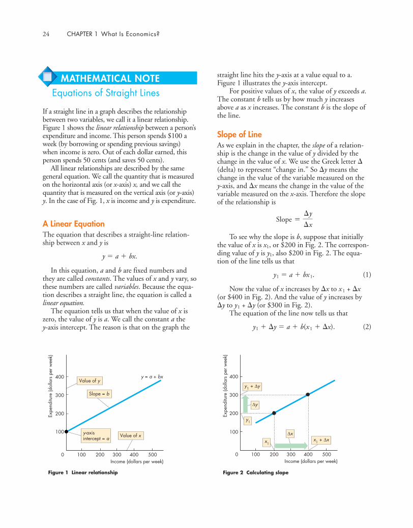
MATHEMATICAL NOTEEquations of Straight Lines

If a straight line in a graph describes the relationshipbetween two variables, we call it a linear relationship.Figure 1 shows the linear relationship between a person’sexpenditure and income. This person spends $100 aweek (by borrowing or spending previous savings)when income is zero. Out of each dollar earned, thisperson spends 50 cents (and saves 50 cents).

All linear relationships are described by the samegeneral equation. We call the quantity that is measuredon the horizontal axis (or x-axis) x, and we call thequantity that is measured on the vertical axis (or y-axis)y. In the case of Fig. 1, x is income and y is expenditure.

A Linear EquationThe equation that describes a straight-line relation-ship between x and y is

y � a � bx.

In this equation, a and b are fixed numbers andthey are called constants. The values of x and y vary, sothese numbers are called variables. Because the equa-tion describes a straight line, the equation is called alinear equation.

The equation tells us that when the value of x iszero, the value of y is a. We call the constant a they-axis intercept. The reason is that on the graph the

straight line hits the y-axis at a value equal to a.Figure 1 illustrates the y-axis intercept.

For positive values of x, the value of y exceeds a.The constant b tells us by how much y increasesabove a as x increases. The constant b is the slope ofthe line.

Slope of LineAs we explain in the chapter, the slope of a relation-ship is the change in the value of y divided by thechange in the value of x. We use the Greek letter �(delta) to represent “change in.” So �y means thechange in the value of the variable measured on the y-axis, and �x means the change in the value of thevariable measured on the x-axis. Therefore the slopeof the relationship is

To see why the slope is b, suppose that initiallythe value of x is x1, or $200 in Fig. 2. The correspon-ding value of y is y1, also $200 in Fig. 2. The equa-tion of the line tells us that

y1 � a � bx 1. (1)

Now the value of x increases by �x to x 1 + �x(or $400 in Fig. 2). And the value of y increases by�y to y1 + �y (or $300 in Fig. 2).

The equation of the line now tells us that

y1 � �y � a � b(x 1 � �x). (2)

Slope =¢y

¢x

24 CHAPTER 1 What Is Economics?

y = a + bxValue of y

Value of x

Slope = b

y-axisintercept = a

Figure 1 Linear relationship

Income (dollars per week)0

100

200

300

400

200100 300 400

Expe

nditu

re (d

olla

rs p

er w

eek)

500Income (dollars per week)

0

100

200

300

400

200100 300 400

Expe

nditu

re (d

olla

rs p

er w

eek)

x1

y1

500

Figure 2 Calculating slope

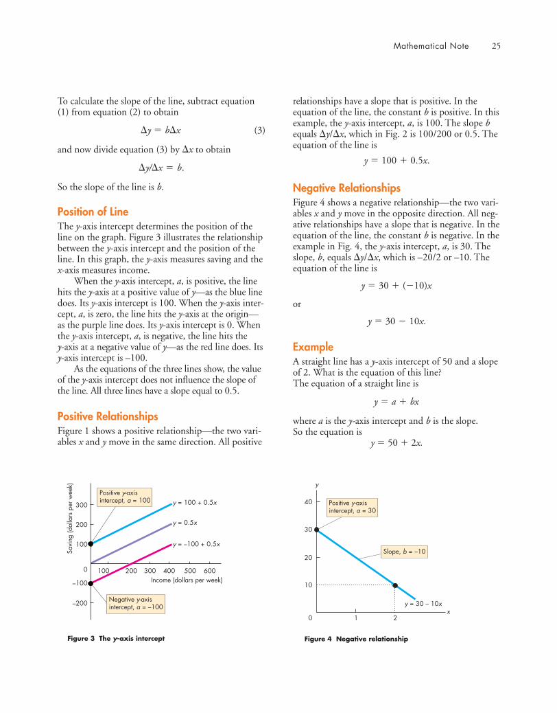
To calculate the slope of the line, subtract equation(1) from equation (2) to obtain

�y � b�x (3)

and now divide equation (3) by �x to obtain

�y/�x � b.

So the slope of the line is b.

Position of LineThe y-axis intercept determines the position of theline on the graph. Figure 3 illustrates the relationshipbetween the y-axis intercept and the position of theline. In this graph, the y-axis measures saving and thex-axis measures income.

When the y-axis intercept, a, is positive, the linehits the y-axis at a positive value of y—as the blue linedoes. Its y-axis intercept is 100. When the y-axis inter-cept, a, is zero, the line hits the y-axis at the origin—as the purple line does. Its y-axis intercept is 0. Whenthe y-axis intercept, a, is negative, the line hits the y-axis at a negative value of y—as the red line does. Itsy-axis intercept is –100.

As the equations of the three lines show, the valueof the y-axis intercept does not influence the slope ofthe line. All three lines have a slope equal to 0.5.

Positive RelationshipsFigure 1 shows a positive relationship—the two vari-ables x and y move in the same direction. All positive

relationships have a slope that is positive. In theequation of the line, the constant b is positive. In thisexample, the y-axis intercept, a, is 100. The slope bequals �y/�x, which in Fig. 2 is 100/200 or 0.5. Theequation of the line is

y � 100 � 0.5x.

Negative RelationshipsFigure 4 shows a negative relationship—the two vari-ables x and y move in the opposite direction. All neg-ative relationships have a slope that is negative. In theequation of the line, the constant b is negative. In theexample in Fig. 4, the y-axis intercept, a, is 30. Theslope, b, equals �y/�x, which is –20/2 or –10. Theequation of the line is

y � 30 � (�10)x

or

y � 30 � 10x.

ExampleA straight line has a y-axis intercept of 50 and a slopeof 2. What is the equation of this line?The equation of a straight line is

y � a � bx

where a is the y-axis intercept and b is the slope. So the equation is

y � 50 � 2x.

Mathematical Note 25

Income (dollars per week)

0

100

–100

–200

200

300

200100 300 400

Savi

ng (d

olla

rs p

er w

eek)

Positive y-axisintercept, a = 100

Negative y-axisintercept, a = –100

y = –100 + 0.5x

y = 0.5x

y = 100 + 0.5x

500 600

Figure 3 The y-axis intercept

x0

10

20

30

1 2

y

40

Figure 4 Negative relationship

Positive y-axisintercept, a = 30

Slope, b = –10

y = 30 – 10x

26 CHAPTER 1 What Is Economics?

SUMMARY

1 Explain how we “read” the three graphs in FigsA1.1 and A1.2.

2 Explain what scatter diagrams show and whywe use them.

3 Explain how we “read” the three scatter dia-grams in Figs A1.3 and A1.4.

4 Draw a graph to show the relationship betweentwo variables that move in the same direction.

5 Draw a graph to show the relationship betweentwo variables that move in opposite directions.

6 Draw a graph to show the relationship betweentwo variables that have a maximum and a mini-mum.

7 Which of the relationships in Questions 4 and5 is a positive relationship and which is a nega-tive relationship?

8 What are the two ways of calculating the slopeof a curved line?

9 How do we graph a relationship among morethan two variables?

10 Explain what change will bring a movementalong a curve.

11 Explain what change will bring a shift of acurve.

You can work these questions in Study Plan 1.A and get instant feedback.

REVIEW QUIZ

Key Points

Graphing Data (pp. 13–16)

■ A graph is made by plotting the values of two vari-ables x and y at a point that corresponds to theirvalues measured along the x-axis and the y-axis.

■ A scatter diagram is a graph that plots the values oftwo variables for a number of different values ofeach.

■ A scatter diagram shows the relationship betweenthe two variables. It shows whether they are posi-tively related, negatively related, or unrelated.

Graphs Used in Economic Models (pp. 16–19)

■ Graphs are used to show relationships among vari-ables in economic models.

■ Relationships can be positive (an upward-slopingcurve), negative (a downward-sloping curve), posi-tive and then negative (have a maximum point),negative and then positive (have a minimum point),or unrelated (a horizontal or vertical curve).

The Slope of a Relationship (pp. 20–22)

■ The slope of a relationship is calculated as thechange in the value of the variable measured onthe y-axis divided by the change in the value of thevariable measured on the x-axis—that is, �y/�x.

■ A straight line has a constant slope.■ A curved line has a varying slope. To calculate the

slope of a curved line, we calculate the slope at apoint or across an arc.

Graphing Relationships Among More Than TwoVariables (pp. 22–23)

■ To graph a relationship among more than twovariables, we hold constant the values of all thevariables except two.

■ We then plot the value of one of the variablesagainst the value of another.

■ A cet par change in the value of a variable on anaxis of a graph brings a movement along the curve.

■ A change in the value of a variable held constantalong the curve brings a shift of the curve.

Key TermsCeteris paribus, 22Direct relationship, 16Inverse relationship, 17

Linear relationship, 16Negative relationship, 17Positive relationship, 16

Scatter diagram, 14Slope, 20

Study Plan Problems and Applications 27

STUDY PLAN PROBLEMS AND APPLICATIONSYou can work Problems 1 to 11 in MyEconLab Chapter 1A Study Plan and get instant feedback.

Use the following spreadsheet to work Problems 1 to3. The spreadsheet provides data on the U.S. econ-omy: Column A is the year, column B is the inflationrate, column C is the interest rate, column D is thegrowth rate, and column E is the unemployment rate.

7. Calculate the slope of the following relationship.

Use the following relationship to work Problems 8 and 9.

8. Calculate the slope of the relationship at point Aand at point B.

9. Calculate the slope across the arc AB.

Use the following table to work Problems 10 and 11.The table gives the price of a balloon ride, the tem-perature, and the number of rides a day.

Balloon rides

Price(number per day)

(dollars per ride) 50ºF 70ºF 90ºF

5 32 40 5010 27 32 4015 18 27 32

10. Draw a graph to show the relationship betweenthe price and the number of rides, when the tem-perature is 70°F. Describe this relationship.

11. What happens in the graph in Problem 10 if thetemperature rises to 90°F?

10.0

2

6.0

8.0

4.0

0 4 6 8 10x

y

A

B1.5

10

6

8

4

0 4.0 8.0 12.0x

y

2

1

A B C D E

2

3

4

5

6

7

8

9

10

11

2.2

3.4

2.8

1.6

2.3

2.7

3.4

3.2

2.8

3.8

–0.4

1999

2000

2001

2002

2003

2004

2005

2006

2007

2008

2009

4.6

5.8

3.4

1.6

1.0

1.4

3.2

4.7

4.4

1.4

0.2

4.8

4.1

1.1

1.8

2.5

3.6

3.1

2.7

2.1

0.4

–2.4

4.2

4.0

4.7

5.8

6.0

5.5

5.1

4.6

4.6

5.8

9.3

1. Draw a scatter diagram of the inflation rate andthe interest rate. Describe the relationship.

2. Draw a scatter diagram of the growth rate andthe unemployment rate. Describe the relation-ship.

3. Draw a scatter diagram of the interest rate andthe unemployment rate. Describe the relation-ship.

Use the following news clip to work Problems 4 to 6.Clash of the Titans Tops Box Office With Sales of$61.2 Million:

RevenueTheaters (dollars

Movie (number) per theater)

Clash of the Titans 3,777 16,213Tyler Perry’s Why Did I 2,155 13,591Get MarriedHow To Train Your Dragon 4,060 7,145The Last Song 2,673 5,989

Source: Bloomberg.com, April 5, 2010

4. Draw a graph of the relationship between the rev-enue per theater on the y-axis and the number oftheaters on the x-axis. Describe the relationship.

5. Calculate the slope of the relationship between4,060 and 2,673 theaters.

6. Calculate the slope of the relationship between2,155 and 4,060 theaters.

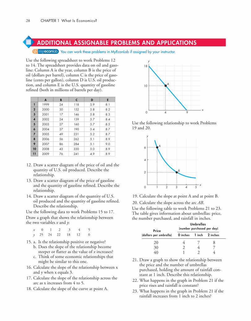
28 CHAPTER 1 What Is Economics?

ADDITIONAL ASSIGNABLE PROBLEMS AND APPLICATIONSYou can work these problems in MyEconLab if assigned by your instructor.

Use the following spreadsheet to work Problems 12to 14. The spreadsheet provides data on oil and gaso-line: Column A is the year, column B is the price ofoil (dollars per barrel), column C is the price of gaso-line (cents per gallon), column D is U.S. oil produc-tion, and column E is the U.S. quantity of gasolinerefined (both in millions of barrels per day).

12. Draw a scatter diagram of the price of oil and thequantity of U.S. oil produced. Describe therelationship.

13. Draw a scatter diagram of the price of gasolineand the quantity of gasoline refined. Describe therelationship.

14. Draw a scatter diagram of the quantity of U.S.oil produced and the quantity of gasoline refined.Describe the relationship.

Use the following data to work Problems 15 to 17.Draw a graph that shows the relationship betweenthe two variables x and y:

x 0 1 2 3 4 5y 25 24 22 18 12 0

15. a. Is the relationship positive or negative?b. Does the slope of the relationship become

steeper or flatter as the value of x increases?c. Think of some economic relationships that

might be similar to this one.16. Calculate the slope of the relationship between x

and y when x equals 3.17. Calculate the slope of the relationship across the

arc as x increases from 4 to 5.18. Calculate the slope of the curve at point A.

1A B C D E

2

3

4

5

6

7

8

9

10

11

24

30

17

24

27

37

49

56

86

43

76

1999

2000

2001

2002

2003

2004

2005

2006

2007

2008

2009

118

152

146

139

160

190

231

262

284

330

241

5.9

5.8

5.8

5.7

5.7

5.4

5.2

5.1

5.1

5.0

4.9

8.1

8.2

8.3

8.4

8.5

8.7

8.7

8.9

9.0

8.9

8.9

Use the following relationship to work Problems 19 and 20.

19. Calculate the slope at point A and at point B.

20. Calculate the slope across the arc AB.Use the following table to work Problems 21 to 23.The table gives information about umbrellas: price,the number purchased, and rainfall in inches.

Umbrellas

Price(number purchased per day)

(dollars per umbrella) 0 inches 1 inch 2 inches

20 4 7 830 2 4 740 1 2 4

21. Draw a graph to show the relationship betweenthe price and the number of umbrellaspurchased, holding the amount of rainfall con-stant at 1 inch. Describe this relationship.

22. What happens in the graph in Problem 21 if theprice rises and rainfall is constant?

23. What happens in the graph in Problem 21 if therainfall increases from 1 inch to 2 inches?

1

4

6

2

0 2 3 4 5x

y

A

B

18

4

10

0 9x

A

y

After studying this chapter, you will be able to:

� Define the production possibilities frontier and use it tocalculate opportunity cost

� Distinguish between production possibilities and preferences and describe an efficient allocation ofresources

� Explain how current production choices expand futureproduction possibilities

� Explain how specialization and trade expand production possibilities

� Describe the economic institutions that coordinatedecisions

2Why does food cost much more today than it did a few years ago? One

reason is that we now use part of our corn crop to produce ethanol, a cleanbiofuel substitute for gasoline. Another reason is that drought in some parts ofthe world has decreased global grain production. In this chapter, you will studyan economic model—the production possibilities frontier—and you will learnwhy ethanol production and drought have increased the cost of producingfood. You will also learn how to assess whether it is a good idea to increasecorn production to produce fuel; how we can expand our productionpossibilities; and how we gain by trading with others.

At the end of the chapter, in Reading Betweenthe Lines, we’ll apply what you’ve learned tounderstanding why ethanol production is raisingthe cost of food.

29

THE ECONOMIC PROBLEM

30 CHAPTER 2 The Economic Problem

◆ Production Possibilities and Opportunity Cost

Every working day, in mines, factories, shops, andoffices and on farms and construction sites across theUnited States, 138 million people produce a vastvariety of goods and services valued at $50 billion.But the quantities of goods and services that we canproduce are limited both by our available resourcesand by technology. And if we want to increase ourproduction of one good, we must decrease our pro-duction of something else—we face a tradeoff. Youare going to learn about the production possibilitiesfrontier, which describes the limit to what we canproduce and provides a neat way of thinking aboutand illustrating the idea of a tradeoff.

The production possibilities frontier (PPF ) is theboundary between those combinations of goods andservices that can be produced and those that cannot.To illustrate the PPF, we focus on two goods at atime and hold the quantities produced of all theother goods and services constant. That is, we look ata model economy in which everything remains thesame except for the production of the two goods weare considering.

Let’s look at the production possibilities frontierfor cola and pizza, which represent any pair of goodsor services.

Production Possibilities FrontierThe production possibilities frontier for cola and pizzashows the limits to the production of these twogoods, given the total resources and technology avail-able to produce them. Figure 2.1 shows this produc-tion possibilities frontier. The table lists somecombinations of the quantities of pizza and cola thatcan be produced in a month given the resourcesavailable. The figure graphs these combinations. Thex-axis shows the quantity of pizzas produced, and they-axis shows the quantity of cola produced.

The PPF illustrates scarcity because we cannotattain the points outside the frontier. These pointsdescribe wants that can’t be satisfied. We can produceat any point inside the PPF or on the PPF. Thesepoints are attainable. Suppose that in a typicalmonth, we produce 4 million pizzas and 5 millioncans of cola. Figure 2.1 shows this combination aspoint E and as possibility E in the table. The figure

Col

a (m

illio

ns o

f can

s)

5

10

15

0 1 2 3 4 5Pizzas (millions)

Attainable

Unattainable

PPF

AB

C

D

EZ

F

Pizzas ColaPossibility (millions) (millions of cans)

A 0 and 15

B 1 and 14

C 2 and 12

D 3 and 9

E 4 and 5

F 5 and 0

The table lists six production possibilities for cola and pizzas. Row A tells us that if we produce no pizzas, the maximum quantity of cola we can produce is 15 millioncans. Points A, B, C, D, E, and F in the figure represent therows of the table. The curve passing through these points isthe production possibilities frontier (PPF ).

The PPF separates the attainable from the unattainable.Production is possible at any point inside the orange areaor on the frontier. Points outside the frontier are unattain-able. Points inside the frontier, such as point Z, are inefficientbecause resources are wasted or misallocated. At suchpoints, it is possible to use the available resources to pro-duce more of either or both goods.

FIGURE 2.1 Production PossibilitiesFrontier

animation

Production Possibilities and Opportunity Cost 31

also shows other production possibilities. For exam-ple, we might stop producing pizza and move all thepeople who produce it into producing cola. Point Ain the figure and possibility A in the table show thiscase. The quantity of cola produced increases to 15million cans, and pizza production dries up.Alternatively, we might close the cola factories andswitch all the resources into producing pizza. In thissituation, we produce 5 million pizzas. Point F in thefigure and possibility F in the table show this case.

Production EfficiencyWe achieve production efficiency if we produce goodsand services at the lowest possible cost. This outcomeoccurs at all the points on the PPF. At points insidethe PPF, production is inefficient because we are giv-ing up more than necessary of one good to produce agiven quantity of the other good.

For example, at point Z in Fig. 2.1, we produce 3 million pizzas and 5 million cans of cola. But wehave enough resources to produce 3 million pizzas and9 million cans of cola. Our pizzas cost more cola thannecessary. We can get them for a lower cost. Onlywhen we produce on the PPF do we incur the lowestpossible cost of production.

Production is inefficient inside the PPF becauseresources are either unused or misallocated or both.

Resources are unused when they are idle but couldbe working. For example, we might leave some of thefactories idle or some workers unemployed.

Resources are misallocated when they are assignedto tasks for which they are not the best match. Forexample, we might assign skilled pizza chefs to workin a cola factory and skilled cola producers to work ina pizza shop. We could get more pizzas and more colafrom these same workers if we reassigned them to thetasks that more closely match their skills.

Tradeoff Along the PPFEvery choice along the PPF involves a tradeoff. On thePPF in Fig. 2.1, we trade off cola for pizzas.

Tradeoffs arise in every imaginable real-world situ-ation in which a choice must be made. At any givenpoint in time, we have a fixed amount of labor, land,capital, and entrepreneurship. By using our availabletechnologies, we can employ these resources to pro-duce goods and services, but we are limited in whatwe can produce. This limit defines a boundary

between what we can attain and what we cannotattain. This boundary is the real-world’s productionpossibilities frontier, and it defines the tradeoffs thatwe must make. On our real-world PPF, we can pro-duce more of any one good or service only if we pro-duce less of some other goods or services.

When doctors want to spend more on AIDS andcancer research, they face a tradeoff: more medicalresearch for less of some other things. When Congresswants to spend more on education and health care, itfaces a tradeoff: more education and health care forless national defense or less homeland security. Whenan environmental group argues for less logging, it issuggesting a tradeoff: greater conservation of endan-gered wildlife for less paper. When you want to studymore, you face a tradeoff: more study time for lessleisure or sleep.

All tradeoffs involve a cost—an opportunity cost.

Opportunity CostThe opportunity cost of an action is the highest-valuedalternative forgone. The PPF makes this idea preciseand enables us to calculate opportunity cost. Alongthe PPF, there are only two goods, so there is onlyone alternative forgone: some quantity of the othergood. Given our current resources and technology,we can produce more pizzas only if we produce lesscola. The opportunity cost of producing an addi-tional pizza is the cola we must forgo. Similarly, theopportunity cost of producing an additional can ofcola is the quantity of pizza we must forgo.

In Fig. 2.1, if we move from point C to point D,we get 1 million more pizzas but 3 million fewer cansof cola. The additional 1 million pizzas cost 3 millioncans of cola. One pizza costs 3 cans of cola.

We can also work out the opportunity cost of mov-ing in the opposite direction. In Fig. 2.1, if we movefrom point D to point C, the quantity of cola pro-duced increases by 3 million cans and the quantity ofpizzas produced decreases by 1 million. So if we choosepoint C over point D, the additional 3 million cans ofcola cost 1 million pizzas. One can of cola costs 1/3 ofa pizza.

Opportunity Cost Is a Ratio Opportunity cost isa ratio. It is the decrease in the quantity producedof one good divided by the increase in the quantityproduced of another good as we move along the pro-duction possibilities frontier.

32 CHAPTER 2 The Economic Problem

We’ve seen that what we can produce is limitedby the production possibilities frontier. We’ve alsoseen that production on the PPF is efficient. But wecan produce many different quantities on the PPF.How do we choose among them? How do we knowwhich point on the PPF is the best one?

Because opportunity cost is a ratio, the opportunitycost of producing an additional can of cola is equal tothe inverse of the opportunity cost of producing anadditional pizza. Check this proposition by returningto the calculations we’ve just worked through. Whenwe move along the PPF from C to D, the opportunitycost of a pizza is 3 cans of cola. The inverse of 3 is 1/3.If we decrease the production of pizza and increase theproduction of cola by moving from D to C, the oppor-tunity cost of a can of cola must be 1/3 of a pizza. Thatis exactly the number that we calculated for the movefrom D to C.

Increasing Opportunity Cost The opportunity cost ofa pizza increases as the quantity of pizzas producedincreases. The outward-bowed shape of the PPFreflects increasing opportunity cost. When we producea large quantity of cola and a small quantity of pizza—between points A and B in Fig. 2.1—the frontier has agentle slope. An increase in the quantity of pizzas costsa small decrease in the quantity of cola—the opportu-nity cost of a pizza is a small quantity of cola.

When we produce a large quantity of pizzas and asmall quantity of cola—between points E and F inFig. 2.1—the frontier is steep. A given increase in thequantity of pizzas costs a large decrease in the quantityof cola, so the opportunity cost of a pizza is a largequantity of cola.

The PPF is bowed outward because resources are notall equally productive in all activities. People with manyyears of experience working for PepsiCo are good atproducing cola but not very good at making pizzas. Soif we move some of these people from PepsiCo toDomino’s, we get a small increase in the quantity ofpizzas but a large decrease in the quantity of cola.

Similarly, people who have spent years working atDomino’s are good at producing pizzas, but they haveno idea how to produce cola. So if we move some ofthese people from Domino’s to PepsiCo, we get a smallincrease in the quantity of cola but a large decrease inthe quantity of pizzas. The more of either good we tryto produce, the less productive are the additionalresources we use to produce that good and the larger isthe opportunity cost of a unit of that good.

Economics in ActionIncreasing Opportunity Cost on the FarmSanders Wright, a homesick Mississippi native, isgrowing cotton in Iowa. The growing season is short,so his commercial success is unlikely. Cotton does notgrow well in Iowa, but corn does. A farm with irriga-tion can produce 300 bushels of corn per acre—twicethe U.S. average.

Ronnie Gerik, a Texas cotton farmer, has started togrow corn. Ronnie doesn’t have irrigation and insteadrelies on rainfall. That’s not a problem for cotton,which just needs a few soakings a season. But it’s a bigproblem for corn, which needs an inch of water aweek. Also, corn can’t take the heat like cotton, and ifthe temperature rises too much, Ronnie will be luckyto get 100 bushels an acre.

An Iowa corn farmer gives up almost no cotton toproduce his 300 bushels of corn per acre—corn has alow opportunity cost. But Ronnie Gerick gives up ahuge amount of cotton to produce his 100 bushels ofcorn per acre. By switching some land from cotton tocorn, Ronnie has increased the production of corn, butthe additional corn has a high opportunity cost.

“Deere worker makes ‘cotton pickin’ miracle happen,” WCFCourier.com;and “Farmers stampede to corn,” USA Today.

REVIEW QUIZ 1 How does the production possibilities frontier

illustrate scarcity?2 How does the production possibilities frontier

illustrate production efficiency?3 How does the production possibilities frontier

show that every choice involves a tradeoff?4 How does the production possibilities frontier

illustrate opportunity cost?5 Why is opportunity cost a ratio?6 Why does the PPF bow outward and what does

that imply about the relationship betweenopportunity cost and the quantity produced?

You can work these questions in Study Plan 2.1 and get instant feedback.

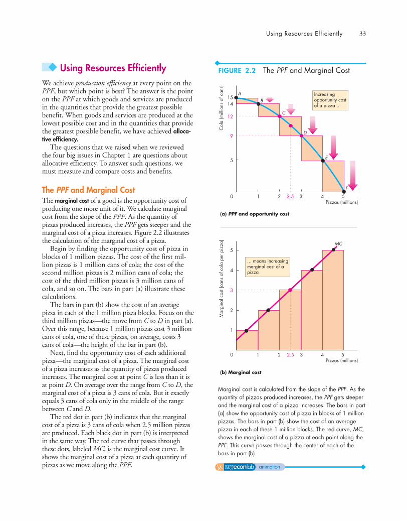
Using Resources Efficiently 33

◆ Using Resources Efficiently We achieve production efficiency at every point on thePPF, but which point is best? The answer is the pointon the PPF at which goods and services are producedin the quantities that provide the greatest possiblebenefit. When goods and services are produced at thelowest possible cost and in the quantities that providethe greatest possible benefit, we have achieved alloca-tive efficiency.

The questions that we raised when we reviewedthe four big issues in Chapter 1 are questions aboutallocative efficiency. To answer such questions, wemust measure and compare costs and benefits.

The PPF and Marginal CostThe marginal cost of a good is the opportunity cost ofproducing one more unit of it. We calculate marginalcost from the slope of the PPF. As the quantity ofpizzas produced increases, the PPF gets steeper and themarginal cost of a pizza increases. Figure 2.2 illustratesthe calculation of the marginal cost of a pizza.

Begin by finding the opportunity cost of pizza inblocks of 1 million pizzas. The cost of the first mil-lion pizzas is 1 million cans of cola; the cost of thesecond million pizzas is 2 million cans of cola; thecost of the third million pizzas is 3 million cans ofcola, and so on. The bars in part (a) illustrate thesecalculations.

The bars in part (b) show the cost of an averagepizza in each of the 1 million pizza blocks. Focus on thethird million pizzas—the move from C to D in part (a).Over this range, because 1 million pizzas cost 3 millioncans of cola, one of these pizzas, on average, costs 3cans of cola—the height of the bar in part (b).

Next, find the opportunity cost of each additionalpizza—the marginal cost of a pizza. The marginal costof a pizza increases as the quantity of pizzas producedincreases. The marginal cost at point C is less than it isat point D. On average over the range from C to D, themarginal cost of a pizza is 3 cans of cola. But it exactlyequals 3 cans of cola only in the middle of the rangebetween C and D.

The red dot in part (b) indicates that the marginalcost of a pizza is 3 cans of cola when 2.5 million pizzasare produced. Each black dot in part (b) is interpretedin the same way. The red curve that passes throughthese dots, labeled MC, is the marginal cost curve. Itshows the marginal cost of a pizza at each quantity ofpizzas as we move along the PPF.

5

9

12

1415

0 1 2 2.5 3 4 5

(a) PPF and opportunity cost

AB

C

D

E

MC

F

Increasingopportunity cost of a pizza ...

Mar

gina

l cos

t (ca

ns o

f col

a pe

r piz

za)

5

3

2

1

4

0 1 2 2.5 3 4 5

(b) Marginal cost

... means increasingmarginal cost of apizza

Col

a (m

illio

ns o

f can

s)

Pizzas (millions)

Pizzas (millions)

Marginal cost is calculated from the slope of the PPF. As thequantity of pizzas produced increases, the PPF gets steeperand the marginal cost of a pizza increases. The bars in part(a) show the opportunity cost of pizza in blocks of 1 millionpizzas. The bars in part (b) show the cost of an averagepizza in each of these 1 million blocks. The red curve, MC,shows the marginal cost of a pizza at each point along thePPF. This curve passes through the center of each of thebars in part (b).

FIGURE 2.2 The PPF and Marginal Cost

animation

34 CHAPTER 2 The Economic Problem

Will

ingn

ess

to p

ay (c

ans

of c

ola

per p

izza

)

1

2

3

4

5

0 1 2 3 4 5

MB

A

B

C

D

E

Decreasing marginalbenefit from a pizza

Pizzas (millions)

Preferences and Marginal BenefitThe marginal benefit from a good or service is thebenefit received from consuming one more unit of it.This benefit is subjective. It depends on people’spreferences—people’s likes and dislikes and the inten-sity of those feelings.

Marginal benefit and preferences stand in sharpcontrast to marginal cost and production possibilities.Preferences describe what people like and want andthe production possibilities describe the limits orconstraints on what is feasible.

We need a concrete way of illustrating preferencesthat parallels the way we illustrate the limits to pro-duction using the PPF.

The device that we use to illustrate preferences isthe marginal benefit curve, which is a curve that showsthe relationship between the marginal benefit from agood and the quantity consumed of that good. Notethat the marginal benefit curve is unrelated to the PPFand cannot be derived from it.

We measure the marginal benefit from a good orservice by the most that people are willing to pay foran additional unit of it. The idea is that you are will-ing to pay less for a good than it is worth to you butyou are not willing to pay more: The most you arewilling to pay for something is its marginal benefit.

It is a general principle that the more we have ofany good or service, the smaller is its marginal benefitand the less we are willing to pay for an additional unitof it. This tendency is so widespread and strong thatwe call it a principle—the principle of decreasing mar-ginal benefit.

The basic reason why marginal benefit decreases isthat we like variety. The more we consume of anyone good or service, the more we tire of it and wouldprefer to switch to something else.

Think about your willingness to pay for a pizza. Ifpizza is hard to come by and you can buy only a fewslices a year, you might be willing to pay a high priceto get an additional slice. But if pizza is all you’veeaten for the past few days, you are willing to payalmost nothing for another slice.

You’ve learned to think about cost as opportunitycost, not as a dollar cost. You can think about mar-ginal benefit and willingness to pay in the same way.The marginal benefit, measured by what you are will-ing to pay for something, is the quantity of othergoods and services that you are willing to forgo. Let’scontinue with the example of cola and pizza and illus-trate preferences this way.

Figure 2.3 illustrates preferences as the willingnessto pay for pizza in terms of cola. In row A, with 0.5million pizzas available, people are willing to pay 5cans of cola per pizza. As the quantity of pizzasincreases, the amount that people are willing to payfor a pizza falls. With 4.5 million pizzas available,people are willing to pay only 1 can of cola per pizza.

Let’s now use the concepts of marginal cost andmarginal benefit to describe allocative efficiency.

Pizzas Willingness to payPossibility (millions) (cans of cola per pizza)

A 0.5 5

B 1.5 4

C 2.5 3

D 3.5 2

E 4.5 1

The smaller the quantity of pizzas available, the more colapeople are willing to give up for an additional pizza. With0.5 million pizzas available, people are willing to pay 5 cansof cola per pizza. But with 4.5 million pizzas, people are will-ing to pay only 1 can of cola per pizza. Willingness to paymeasures marginal benefit. A universal feature of people’spreferences is that marginal benefit decreases.

FIGURE 2.3 Preferences and the MarginalBenefit Curve

animation

Using Resources Efficiently 35

Marginal cost exceedsmarginal benefit—producefewer pizzas

Mar

gina

l cos

t and

mar

gina

l ben

efit

(can

s of

col

a pe

r piz

za)

1

2

3

4

5

0 1.5 2.5 3.5 5

MB

MC

(b) Marginal benefit equals marginal cost

Too few pizzas

Too manypizzas

Point ofallocativeefficiency

Marginal benefit exceedsmarginal cost—producemore pizzas

Marginal benefitequals marginal cost—efficientquantity of pizzas

Pizzas (millions)

15

10

5

0 1.5 2.5 3.5 5

PPF

A

B

C

(a) On the PPF

Col

a (m

illio

ns o

f can

s)

Pizzas (millions)

You now understand the limits to productionand the conditions under which resources are usedefficiently. Your next task is to study the expansion ofproduction possibilities.

Allocative EfficiencyAt any point on the PPF, we cannot produce more ofone good without giving up some other good. At thebest point on the PPF, we cannot produce more ofone good without giving up some other good thatprovides greater benefit. We are producing at thepoint of allocative efficiency—the point on the PPFthat we prefer above all other points.

Suppose in Fig. 2.4, we produce 1.5 million pizzas.The marginal cost of a pizza is 2 cans of cola, and themarginal benefit from a pizza is 4 cans of cola.Because someone values an additional pizza morehighly than it costs to produce, we can get more valuefrom our resources by moving some of them out ofproducing cola and into producing pizza.

Now suppose we produce 3.5 million pizzas. Themarginal cost of a pizza is now 4 cans of cola, but themarginal benefit from a pizza is only 2 cans of cola.Because the additional pizza costs more to producethan anyone thinks it is worth, we can get more valuefrom our resources by moving some of them awayfrom producing pizza and into producing cola.

Suppose we produce 2.5 million pizzas. Marginalcost and marginal benefit are now equal at 3 cans ofcola. This allocation of resources between pizzas andcola is efficient. If more pizzas are produced, the for-gone cola is worth more than the additional pizzas. Iffewer pizzas are produced, the forgone pizzas areworth more than the additional cola.

The greater the quantity of pizzas produced, the smaller isthe marginal benefit (MB) from pizza—the less cola peopleare willing to give up to get an additional pizza. But thegreater the quantity of pizzas produced, the greater is themarginal cost (MC ) of a pizza—the more cola people mustgive up to get an additional pizza. When marginal benefitequals marginal cost, resources are being used efficiently.

FIGURE 2.4 Efficient Use of Resources

animation

REVIEW QUIZ1 What is marginal cost? How is it measured?2 What is marginal benefit? How is it measured?3 How does the marginal benefit from a good

change as the quantity produced of that goodincreases?

4 What is allocative efficiency and how does itrelate to the production possibilities frontier?

5 What conditions must be satisfied if resourcesare used efficiently?

You can work these questions in Study Plan 2.2 and get instant feedback.

36 CHAPTER 2 The Economic Problem

◆ Economic GrowthDuring the past 30 years, production per person inthe United States has doubled. The expansion ofproduction possibilities is called economic growth.Economic growth increases our standard of living, butit doesn’t overcome scarcity and avoid opportunitycost. To make our economy grow, we face a trade-off—the faster we make production grow, the greateris the opportunity cost of economic growth.

The Cost of Economic GrowthEconomic growth comes from technological changeand capital accumulation. Technological change is thedevelopment of new goods and of better ways of pro-ducing goods and services. Capital accumulation is thegrowth of capital resources, including human capital.

Technological change and capital accumulationhave vastly expanded our production possibilities. Wecan produce automobiles that provide us with moretransportation than was available when we had onlyhorses and carriages. We can produce satellites thatprovide global communications on a much larger scalethan that available with the earlier cable technology.But if we use our resources to develop new technolo-gies and produce capital, we must decrease our pro-duction of consumption goods and services. Newtechnologies and new capital have an opportunity cost.Let’s look at this opportunity cost.

Instead of studying the PPF of pizzas and cola,we’ll hold the quantity of cola produced constant andexamine the PPF for pizzas and pizza ovens. Figure2.5 shows this PPF as the blue curve PPF0. If wedevote no resources to producing pizza ovens, weproduce at point A. If we produce 3 million pizzas,we can produce 6 pizza ovens at point B. If we pro-duce no pizza, we can produce 10 ovens at point C.

The amount by which our production possibili-ties expand depends on the resources we devote totechnological change and capital accumulation. Ifwe devote no resources to this activity (point A),our PPF remains the blue curve PPF0 in Fig. 2.5. Ifwe cut the current pizza production and produce 6ovens (point B), then in the future, we’ll have morecapital and our PPF will rotate outward to the posi-tion shown by the red curve PPF1. The fewerresources we use for producing pizza and the moreresources we use for producing ovens, the greater isthe expansion of our future productionpossibilities.

Economic growth brings enormous benefits in theform of increased consumption in the future, but itis not free and it doesn’t abolish scarcity.

In Fig. 2.5, to make economic growth happen wemust use some resources to produce new ovens,which leaves fewer resources to produce pizzas. Tomove to B' in the future, we must move from A to Btoday. The opportunity cost of more pizzas in thefuture is fewer pizzas today. Also, on the new PPF, westill face a tradeoff and opportunity cost.

The ideas about economic growth that we haveexplored in the setting of the pizza industry alsoapply to nations. Hong Kong and the United Statesprovide a striking case study.

Pizz

a ov

ens

2

4

6

8

10

0 1 2 3 4 5 6 7

PPF0 PPF1

A A'

B

C

B'

Pizzas (millions)

PPF0 shows the limits to the production of pizzas and pizzaovens, with the production of all other goods and servicesremaining the same. If we devote no resources to producingpizza ovens and produce 5 million pizzas, our productionpossibilities will remain the same at PPF0. But if we decreasepizza production to 3 million and produce 6 ovens, at pointB, our production possibilities expand. After one period, thePPF rotates outward to PPF1 and we can produce at pointB', a point outside the original PPF0. We can rotate the PPFoutward, but we cannot avoid opportunity cost. The oppor-tunity cost of producing more pizzas in the future is fewerpizzas today.

FIGURE 2.5 Economic Growth

animation

Economic Growth 37

A Nation’s Economic GrowthThe experiences of the United States and Hong Kongmake a striking example of the effects of our choicesabout consumption and capital goods on the rate ofeconomic growth.

If a nation devotes all its factors of production toproducing consumption goods and services and noneto advancing technology and accumulating capital,its production possibilities in the future will be thesame as they are today.

To expand production possibilities in the future, anation must devote fewer resources to producing cur-rent consumption goods and services and someresources to accumulating capital and developing newtechnologies. As production possibilities expand,consumption in the future can increase. The decreasein today’s consumption is the opportunity cost oftomorrow’s increase in consumption.

Next, we’re going to study another way in whichwe expand our production possibilities—the amazingfact that both buyers and sellers gain from specializa-tion and trade.

AA

B

C

Consumption goods (per person)

Economic Growth in the United States and Hong Kong

0

D

Hong KongPPF in 2009

U.S. PPFin 2009

Hong KongPPF in 1969

U.S. PPFin 1969

Cap

ital g

oods

(per

per

son)Economics in Action

Hong Kong Catching Up to the United States In 1969, the production possibilities per person in theUnited States were more than four times those in HongKong (see the figure). The United States devotes onefifth of its resources to accumulating capital and in1969 was at point A on its PPF. Hong Kong devotesone third of its resources to accumulating capital and in1969, Hong Kong was at point A on its PPF.

Since 1969, both countries have experiencedeconomic growth, but because Hong Kong devotes abigger fraction of its resources to accumulating capital,its production possibilities have expanded more quickly.

By 2009, production possibilities per person inHong Kong had reached 94 percent of those in theUnited States. If Hong Kong continues to devotemore resources to accumulating capital than we do(at point B on its 2009 PPF ), it will continue togrow more rapidly. But if Hong Kong decreases capi-tal accumulation (moving to point D on its 2009PPF ), then its rate of economic growth will slow.

Hong Kong is typical of the fast-growing Asianeconomies, which include Taiwan, Thailand, SouthKorea, China, and India. Production possibilitiesexpand in these countries by between 5 and almost10 percent a year.

If such high economic growth rates are main-tained, these other Asian countries will continue toclose the gap between themselves and the UnitedStates, as Hong Kong is doing.

REVIEW QUIZ1 What generates economic growth?2 How does economic growth influence the

production possibilities frontier?3 What is the opportunity cost of economic growth?4 Why has Hong Kong experienced faster eco-

nomic growth than the United States?5 Does economic growth overcome scarcity?

You can work these questions in Study Plan 2.3 and get instant feedback.

TABLE 2.1 Liz’s Production Possibilities

38 CHAPTER 2 The Economic Problem

◆ Gains from TradePeople can produce for themselves all the goods andservices that they consume, or they can produce onegood or a few goods and trade with others. Producingonly one good or a few goods is called specialization.We are going to learn how people gain by specializingin the production of the good in which they have acomparative advantage and trading with others.

Comparative Advantage and AbsoluteAdvantageA person has a comparative advantage in an activity ifthat person can perform the activity at a lower oppor-tunity cost than anyone else. Differences in opportu-nity costs arise from differences in individual abilitiesand from differences in the characteristics of otherresources.

No one excels at everything. One person is an out-standing pitcher but a poor catcher; another person isa brilliant lawyer but a poor teacher. In almost allhuman endeavors, what one person does easily, some-one else finds difficult. The same applies to land andcapital. One plot of land is fertile but has no mineraldeposits; another plot of land has outstanding viewsbut is infertile. One machine has great precision butis difficult to operate; another is fast but often breaksdown.

Although no one excels at everything, some peo-ple excel and can outperform others in a large num-ber of activities—perhaps even in all activities. Aperson who is more productive than others has anabsolute advantage.

Absolute advantage involves comparing productiv-ities—production per hour—whereas comparativeadvantage involves comparing opportunity costs.

A person who has an absolute advantage does nothave a comparative advantage in every activity. JohnGrisham is a better lawyer and a better author of fast-paced thrillers than most people. He has an absoluteadvantage in these two activities. But compared toothers, he is a better writer than lawyer, so his com-parative advantage is in writing.

Because ability and resources vary from one per-son to another, people have different opportunitycosts of producing various goods. These differencesin opportunity cost are the source of comparativeadvantage.

Let’s explore the idea of comparative advantage bylooking at two smoothie bars: one operated by Lizand the other operated by Joe.

Liz’s Smoothie Bar Liz produces smoothies and sal-ads. In Liz’s high-tech bar, she can turn out either asmoothie or a salad every 2 minutes—see Table 2.1.If Liz spends all her time making smoothies, she canproduce 30 an hour. And if she spends all her timemaking salads, she can also produce 30 an hour. Ifshe splits her time equally between the two, she canproduce 15 smoothies and 15 salads an hour. Foreach additional smoothie Liz produces, she mustdecrease her production of salads by one, and foreach additional salad she produces, she must decreaseher production of smoothies by one. So

Liz’s opportunity cost of producing 1 smoothie is 1 salad,

and

Liz’s opportunity cost of producing 1 salad is 1 smoothie.

Liz’s customers buy smoothies and salads in equalquantities, so she splits her time equally between thetwo items and produces 15 smoothies and 15 saladsan hour.

Joe’s Smoothie Bar Joe also produces smoothies andsalads, but his bar is smaller than Liz’s. Also, Joe hasonly one blender, and it’s a slow, old machine. Even ifJoe uses all his resources to produce smoothies, hecan produce only 6 an hour—see Table 2.2. But Joeis good at making salads. If he uses all his resources tomake salads, he can produce 30 an hour.

Joe’s ability to make smoothies and salads is thesame regardless of how he splits an hour between thetwo tasks. He can make a salad in 2 minutes or asmoothie in 10 minutes. For each additional smoothie

Minutes to QuantityItem produce 1 per hour

Smoothies 2 30

Salads 2 30

TABLE 2.3 Liz and Joe Gain from Trade

Gains from Trade 39

(e) Gains from trade Liz Joe

Smoothies +5 +5

Salads +5 +5

Joe produces, he must decrease his production of sal-ads by 5. And for each additional salad he produces,he must decrease his production of smoothies by 1/5of a smoothie. So

Joe’s opportunity cost of producing 1 smoothie is 5 salads,

and

Joe’s opportunity cost of producing 1 salad is 1/5 of a smoothie.

Joe’s customers, like Liz’s, buy smoothies and saladsin equal quantities. So Joe spends 50 minutes of eachhour making smoothies and 10 minutes of each hourmaking salads. With this division of his time, Joeproduces 5 smoothies and 5 salads an hour.

Liz’s Comparative Advantage In which of the twoactivities does Liz have a comparative advantage?Recall that comparative advantage is a situation inwhich one person’s opportunity cost of producing agood is lower than another person’s opportunity costof producing that same good. Liz has a comparativeadvantage in producing smoothies. Her opportunitycost of a smoothie is 1 salad, whereas Joe’s opportu-nity cost of a smoothie is 5 salads.

Joe’s Comparative Advantage If Liz has a compara-tive advantage in producing smoothies, Joe must havea comparative advantage in producing salads. Joe’sopportunity cost of a salad is 1/5 of a smoothie,whereas Liz’s opportunity cost of a salad is 1 smoothie.

Achieving the Gains from TradeLiz and Joe run into each other one evening in a sin-gles bar. After a few minutes of getting acquainted, Liztells Joe about her amazing smoothie business. Heronly problem, she tells Joe, is that she would like toproduce more because potential customers leave whenher lines get too long.

Joe is hesitant to risk spoiling his chances by tellingLiz about his own struggling business, but he takes therisk. Joe explains to Liz that he spends 50 minutes ofevery hour making 5 smoothies and 10 minutes mak-ing 5 salads. Liz’s eyes pop. “Have I got a deal for you!”she exclaims.

Here’s the deal that Liz sketches on a paper napkin.Joe stops making smoothies and allocates all his timeto producing salads; Liz stops making salads and allo-cates all her time to producing smoothies. That is, theyboth specialize in producing the good in which theyhave a comparative advantage. Together they produce30 smoothies and 30 salads—see Table 2.3(b).

They then trade. Liz sells Joe 10 smoothies andJoe sells Liz 20 salads—the price of a smoothie is 2salads—see Table 2.3(c).

After the trade, Joe has 10 salads—the 30 he pro-duces minus the 20 he sells to Liz. He also has the 10smoothies that he buys from Liz. So Joe now hasincreased the quantities of smoothies and salads thathe can sell to his customers—see Table 2.3(d).

(b) Specialization Liz Joe

Smoothies 30 0

Salads 0 30

(c) Trade Liz Joe

Smoothies sell 10 buy 10

Salads buy 20 sell 20

(d) After trade Liz Joe

Smoothies 20 10

Salads 20 10

(a) Before trade Liz Joe

Smoothies 15 5

Salads 15 5

TABLE 2.2 Joe’s Production Possibilities

Minutes to QuantityItem produce 1 per hour

Smoothies 10 6

Salads 2 30

40 CHAPTER 2 The Economic Problem

Liz has 20 smoothies—the 30 she produces minusthe 10 she sells to Joe. She also has the 20 salads thatshe buys from Joe. Liz has increased the quantities ofsmoothies and salads that she can sell to her cus-tomers—see Table 2.3(d). Liz and Joe both gain 5smoothies and 5 salads an hour—see Table 2.3(e).

To illustrate her idea, Liz grabs a fresh napkin anddraws the graphs in Fig. 2.6. The blue PPF in part (a)shows Joe’s production possibilities. Before trade, he isproducing 5 smoothies and 5 salads an hour at point A.The blue PPF in part (b) shows Liz’s production possi-bilities. Before trade, she is producing 15 smoothiesand 15 salads an hour at point A.

Liz’s proposal is that they each specialize in produc-ing the good in which they have a comparative advan-tage. Joe produces 30 salads and no smoothies at pointB on his PPF. Liz produces 30 smoothies and no sal-ads at point B on her PPF.

Liz and Joe then trade smoothies and salads at aprice of 2 salads per smoothie or 1/2 a smoothie persalad. Joe gets smoothies for 2 salads each, which is lessthan the 5 salads it costs him to produce a smoothie.Liz gets salads for 1/2 a smoothie each, which is lessthan the 1 smoothie that it costs her to produce asalad.

With trade, Joe has 10 smoothies and 10 salads atpoint C—a gain of 5 smoothies and 5 salads. Joemoves to a point outside his PPF.

With trade, Liz has 20 smoothies and 20 salads atpoint C—a gain of 5 smoothies and 5 salads. Lizmoves to a point outside her PPF.

Despite Liz being more productive than Joe, bothof them gain from specializing—producing the goodin which they have a comparative advantage—andtrading.

(b) Liz(a) JoeSmoothies (per hour)

105 15 20 30250

Joe'sPPF

Sala

ds (p

er h

our)

10

5

15

20

25

30

A

A

C

Joe buys 10smoothiesfrom Liz

B

Trade line

5 15 20 25 30Smoothies (per hour)

100

Liz'sPPF

Sala

ds (p

er h

our)

10

5

15

20

25

30

Trade line

CLiz buys 20salads fromJoe

B

Initially, Joe produces at point A on his PPF in part (a), andLiz produces at point A on her PPF in part (b). Joe’s opportu-nity cost of producing a salad is less than Liz’s, so Joe has acomparative advantage in producing salads. Liz’s opportu-nity cost of producing a smoothie is less than Joe’s, so Lizhas a comparative advantage in producing smoothies.

If Joe specializes in making salads, he produces 30 sal-ads and no smoothies at point B on his PPF. If Liz specializes

in making smoothies, she produces 30 smoothies and no sal-ads at point B on her PPF. They exchange salads for smooth-ies along the red “Trade line.” Liz buys salads from Joe forless than her opportunity cost of producing them. Joe buyssmoothies from Liz for less than his opportunity cost of pro-ducing them. Each goes to point C—a point outside his orher PPF. With specialization and trade, Joe and Liz gain 5smoothies and 5 salads each with no extra resources.

FIGURE 2.6 The Gains from Trade

animation

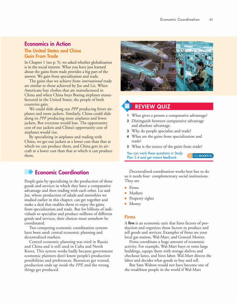
Economic Coordination 41

◆ Economic CoordinationPeople gain by specializing in the production of thosegoods and services in which they have a comparativeadvantage and then trading with each other. Liz andJoe, whose production of salads and smoothies westudied earlier in this chapter, can get together andmake a deal that enables them to enjoy the gainsfrom specialization and trade. But for billions of indi-viduals to specialize and produce millions of differentgoods and services, their choices must somehow becoordinated.

Two competing economic coordination systemshave been used: central economic planning anddecentralized markets.

Central economic planning was tried in Russiaand China and is still used in Cuba and NorthKorea. This system works badly because governmenteconomic planners don’t know people’s productionpossibilities and preferences. Resources get wasted,production ends up inside the PPF, and the wrongthings get produced.

Economics in ActionThe United States and ChinaGain From TradeIn Chapter 1 (see p. 5), we asked whether globalizationis in the social interest. What you have just learnedabout the gains from trade provides a big part of theanswer. We gain from specialization and trade.

The gains that we achieve from international tradeare similar to those achieved by Joe and Liz. WhenAmericans buy clothes that are manufactured inChina and when China buys Boeing airplanes manu-factured in the United States, the people of bothcountries gain.

We could slide along our PPF producing fewer air-planes and more jackets. Similarly, China could slidealong its PPF producing more airplanes and fewerjackets. But everyone would lose. The opportunitycost of our jackets and China’s opportunity cost ofairplanes would rise.

By specializing in airplanes and trading withChina, we get our jackets at a lower cost than that atwhich we can produce them, and China gets its air-craft at a lower cost than that at which it can producethem.

Decentralized coordination works best but to doso it needs four complementary social institutions.They are

■ Firms■ Markets■ Property rights■ Money

FirmsA firm is an economic unit that hires factors of pro-duction and organizes those factors to produce andsell goods and services. Examples of firms are yourlocal gas station, Wal-Mart, and General Motors.

Firms coordinate a huge amount of economicactivity. For example, Wal-Mart buys or rents largebuildings, equips them with storage shelves andcheckout lanes, and hires labor. Wal-Mart directs thelabor and decides what goods to buy and sell.

But Sam Walton would not have become one ofthe wealthiest people in the world if Wal-Mart

REVIEW QUIZ 1 What gives a person a comparative advantage?2 Distinguish between comparative advantage

and absolute advantage.3 Why do people specialize and trade?4 What are the gains from specialization and

trade?5 What is the source of the gains from trade?

You can work these questions in Study Plan 2.4 and get instant feedback.

42 CHAPTER 2 The Economic Problem

produced all the goods that it sells. He became richby specializing in providing retail services and buyingfrom other firms that specialize in producing goods(just as Liz and Joe did). This trade between firmstakes place in markets.

MarketsIn ordinary speech, the word market means a placewhere people buy and sell goods such as fish, meat,fruits, and vegetables. In economics, a market has amore general meaning. A market is any arrangementthat enables buyers and sellers to get information andto do business with each other. An example is themarket in which oil is bought and sold—the worldoil market. The world oil market is not a place. It isthe network of oil producers, oil users, wholesalers,and brokers who buy and sell oil. In the world oilmarket, decision makers do not meet physically. Theymake deals by telephone, fax, and direct computerlink.

Markets have evolved because they facilitate trade.Without organized markets, we would miss out on asubstantial part of the potential gains from trade.Enterprising individuals and firms, each pursuingtheir own self-interest, have profited from makingmarkets—standing ready to buy or sell the items inwhich they specialize. But markets can work onlywhen property rights exist.

Property RightsThe social arrangements that govern the ownership,use, and disposal of anything that people value arecalled property rights. Real property includes land andbuildings—the things we call property in ordinaryspeech—and durable goods such as plant and equip-ment. Financial property includes stocks and bondsand money in the bank. Intellectual property is theintangible product of creative effort. This type ofproperty includes books, music, computer programs,and inventions of all kinds and is protected by copy-rights and patents.

Where property rights are enforced, people havethe incentive to specialize and produce the goodsin which they have a comparative advantage.Where people can steal the production of others,resources are devoted not to production but toprotecting possessions. Without property rights,we would still be hunting and gathering like ourStone Age ancestors.

MoneyMoney is any commodity or token that is generallyacceptable as a means of payment. Liz and Joe didn’tuse money in the example above. They exchangedsalads and smoothies. In principle, trade in marketscan exchange any item for any other item. But youcan perhaps imagine how complicated life would beif we exchanged goods for other goods. The “inven-tion” of money makes trading in markets much moreefficient.

Circular Flows Through MarketsFigure 2.7 shows the flows that result from thechoices that households and firms make. Householdsspecialize and choose the quantities of labor, land,capital, and entrepreneurial services to sell or rent tofirms. Firms choose the quantities of factors of pro-duction to hire. These (red) flows go through thefactor markets. Households choose the quantities ofgoods and services to buy, and firms choose the quan-tities to produce. These (red) flows go through thegoods markets. Households receive incomes and makeexpenditures on goods and services (the green flows).

How do markets coordinate all these decisions?

Coordinating DecisionsMarkets coordinate decisions through price adjust-ments. To see how, think about your local marketfor hamburgers. Suppose that too few hamburgersare available and some people who want to buyhamburgers are not able to do so. To make buyingand selling plans the same, either more hamburgersmust be offered for sale or buyers must scale downtheir appetites (or both). A rise in the price of ahamburger produces this outcome. A higher priceencourages producers to offer more hamburgers forsale. It also encourages some people to change theirlunch plans. Fewer people buy hamburgers, andmore buy hot dogs. More hamburgers (and morehot dogs) are offered for sale.

Alternatively, suppose that more hamburgers areavailable than people want to buy. In this case, tomake the choices of buyers and sellers compatible,more hamburgers must be bought or fewer hamburg-ers must be offered for sale (or both). A fall in theprice of a hamburger achieves this outcome. A lowerprice encourages people to buy more hamburgers. Italso encourages firms to produce a smaller quantityof hamburgers.

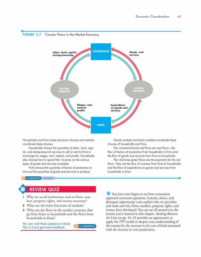
Economic Coordination 43

◆ You have now begun to see how economistsapproach economic questions. Scarcity, choice, anddivergent opportunity costs explain why we specializeand trade and why firms, markets, property rights, andmoney have developed. You can see all around you thelessons you’ve learned in this chapter. Reading Betweenthe Lines on pp. 44–45 provides an opportunity toapply the PPF model to deepen your understanding ofthe reasons for the increase in the cost of food associatedwith the increase in corn production.

Goods andservices

Wages, rent,interest,profits

Labor, land, capital, entrepreneurship

HOUSEHOLDS

FIRMS

Expenditureon goods andservices

FACTORMARKETS

GOODSMARKETS

Households and firms make economic choices and marketscoordinate these choices.

Households choose the quantities of labor, land, capi-tal, and entrepreneurial services to sell or rent to firms inexchange for wages, rent, interest, and profits. Householdsalso choose how to spend their incomes on the varioustypes of goods and services available.

Firms choose the quantities of factors of production tohire and the quantities of goods and services to produce.

Goods markets and factor markets coordinate thesechoices of households and firms.

The counterclockwise red flows are real flows—theflow of factors of production from households to firms andthe flow of goods and services from firms to households.

The clockwise green flows are the payments for the redflows. They are the flow of incomes from firms to householdsand the flow of expenditure on goods and services fromhouseholds to firms.

FIGURE 2.7 Circular Flows in the Market Economy

animation

REVIEW QUIZ 1 Why are social institutions such as firms, mar-

kets, property rights, and money necessary?2 What are the main functions of markets?3 What are the flows in the market economy that

go from firms to households and the flows fromhouseholds to firms?

You can work these questions in Study Plan 2.5 and get instant feedback.

44

READING BETWEEN THE L INES

The Rising OpportunityCost of Food

Fuel Choices, Food Crises, and Finger-Pointinghttp://www.nytimes.comApril 15, 2008

The idea of turning farms into fuel plants seemed, for a time, like one of the answers to highglobal oil prices and supply worries. That strategy seemed to reach a high point last yearwhen Congress mandated a fivefold increase in the use of biofuels.

But now a reaction is building against policies in the United States and Europe to promoteethanol and similar fuels, with political leaders from poor countries contending that these fuelsare driving up food prices and starving poor people. …

In some countries, the higher prices are leading to riots, political instability, and growingworries about feeding the poorest people. …

Many specialists in food policy consider government mandates for biofuels to be ill advised,agreeing that the diversion of crops like corn into fuel production has contributed to the higherprices. But other factors have played big roles, including droughts that have limited output andrapid global economic growth that has created higher demand for food.

That growth, much faster over the last four years than the historical norm, is lifting millions ofpeople out of destitution and giving them access to better diets. But farmers are having troublekeeping up with the surge in demand.

While there is agreement that the growth of biofuelshas contributed to higher food prices, the amount isdisputed. …

C. Ford Runge, an economist at the University ofMinnesota, said it is “extremely difficult to disentan-gle” the effect of biofuels on food costs. Nevertheless,he said there was little that could be done to mitigatethe effect of droughts and the growing appetite forprotein in developing countries.

“Ethanol is the one thing we can do something about,” hesaid. “It’s about the only lever we have to pull, but noneof the politicians have the courage to pull the lever.” …

From the New York Times, © April 15, 2008 The New York Times. All rights reserved.Used by permission and protected by the Copyright Laws of the United States. Theprinting, copying, redistribution, or retransmission of the Material without expresswritten permission is prohibited.

■ In 2007, Congress mandated a fivefold in-crease in the use of biofuels.

■ Political leaders in poor countries and special-ists in food policy say the biofuel mandate is illadvised and the diversion of corn into fuel pro-duction has raised the cost of food.

■ Drought that has limited corn production andglobal economic growth that has increased thedemand for protein have also raised the cost offood.

■ An economist at the University of Minnesotasays that while it is difficult to determine the ef-fect of biofuels on food costs, it is the only fac-tor under our control.

ESSENCE OF THE STORY

45

ECONOMIC ANALYSIS

Oth

er g

oods

and

ser

vice

s

0 350 400 420 500Corn (millions of metric tons)

In the rest of the world,the opportunity cost ofcorn increased because ...

450

… the area plantedincreased ...

… and the yieldper acre decreased PPF07

PPF

PPF08

Oth

er g

oods

and

ser

vice

sFigure 1 U.S. PPF

Figure 2 Rest of the World PPF

0 250 300 360 400Corn (millions of metric tons)

B

In the United States, theopportunity cost of cornincreased because thearea planted andproduction increasedA

■ Ethanol is made from corn in the United States, sobiofuel and food compete to use the same resources.

■ To produce more ethanol and meet the Congress’smandate, farmers increased the number of acresdevoted to corn production.

■ In 2008, the amount of land devoted to corn produc-tion increased by 20 percent in the United States andby 2 percent in the rest of the world.

■ Figure 1 shows the U.S. production possibilities fron-tier, PPF, for corn and other goods and services.

■ The increase in the production of corn is illustrated bya movement along the PPF in Fig. 1 from point A in2007 to point B in 2008.

■ In moving from point A to point B, the United Statesincurs a higher opportunity cost of producing corn, as the greater slope of the PPF at point B indicates.

■ In other regions of the world, despite the fact that moreland was devoted to corn production, the amount ofcorn produced didn’t change.

■ The reason is that droughts in South America and East-ern Europe lowered the crop yield per acre in thoseregions.

■ Figure 2 shows the rest of the world‘s PPF for corn andother goods and services in 2007 and 2008.

■ The increase in the amount of land devoted to produc-ing corn is illustrated by a movement along PPF07.

■ With a decrease in the crop yield, production possibili-ties decreased and the PPF rotated inward.

■ The rotation from PPF07 to PPF08 illustrates this decreasein production possibilities.

■ The opportunity cost of producing corn in the rest ofthe world increased for two reasons: the movementalong its PPF and the inward rotation of the PPF.

■ With a higher opportunity cost of producing corn, thecost of both biofuel and food increases.

46 CHAPTER 2 The Economic Problem

Economic Growth (pp. 36–37)

■ Economic growth, which is the expansion of pro-duction possibilities, results from capital accumu-lation and technological change.

■ The opportunity cost of economic growth isforgone current consumption.

■ The benefit of economic growth is increasedfuture consumption.

Working Problem 11 will give you a better understandingof economic growth.

Gains from Trade (pp. 38–41)

■ A person has a comparative advantage in pro-ducing a good if that person can produce thegood at a lower opportunity cost than everyoneelse.

■ People gain by specializing in the activity in whichthey have a comparative advantage and tradingwith others.

Working Problems 12 and 13 will give you a better under-standing of the gains from trade.

Economic Coordination (pp. 41–43)

■ Firms coordinate a large amount of economicactivity, but there is a limit to the efficient sizeof a firm.

■ Markets coordinate the economic choices ofpeople and firms.

■ Markets can work efficiently only when propertyrights exist.

■ Money makes trading in markets more efficient.

Working Problem 14 will give you a better understandingof economic coordination.

Key Points

Production Possibilities and Opportunity Cost (pp. 30–32)

■ The production possibilities frontier is the bound-ary between production levels that are attainableand those that are not attainable when all theavailable resources are used to their limit.

■ Production efficiency occurs at points on the pro-duction possibilities frontier.

■ Along the production possibilities frontier, theopportunity cost of producing more of one goodis the amount of the other good that must begiven up.

■ The opportunity cost of all goods increases as theproduction of the good increases.

Working Problems 1 to 3 will give you a better under-standing of production possibilities and opportunity cost.

Using Resources Efficiently (pp. 33–35)

■ Allocative efficiency occurs when goods and servicesare produced at the least possible cost and in thequantities that bring the greatest possible benefit.

■ The marginal cost of a good is the opportunitycost of producing one more unit of it.

■ The marginal benefit from a good is the benefitreceived from consuming one more unit of it andis measured by the willingness to pay for it.

■ The marginal benefit of a good decreases as theamount of the good available increases.

■ Resources are used efficiently when the marginalcost of each good is equal to its marginal benefit.

Working Problems 4 to 10 will give you a better under-standing of the efficient use of resources.

SUMMARY

Key TermsAbsolute advantage, 38Allocative efficiency, 33Capital accumulation, 36Comparative advantage, 38Economic growth, 36Firm, 41

Marginal benefit, 34Marginal benefit curve, 34Marginal cost, 33Market, 42Money, 42Opportunity cost, 31

Preferences, 34Production efficiency, 31Production possibilities frontier, 30Property rights, 42Technological change, 36

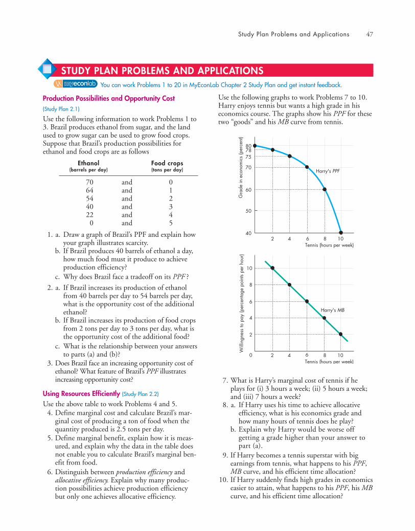
Study Plan Problems and Applications 47

Use the following graphs to work Problems 7 to 10.Harry enjoys tennis but wants a high grade in hiseconomics course. The graphs show his PPF for thesetwo “goods” and his MB curve from tennis.

7. What is Harry’s marginal cost of tennis if heplays for (i) 3 hours a week; (ii) 5 hours a week;and (iii) 7 hours a week?

8. a. If Harry uses his time to achieve allocativeefficiency, what is his economics grade andhow many hours of tennis does he play?

b. Explain why Harry would be worse offgetting a grade higher than your answer topart (a).

9. If Harry becomes a tennis superstar with bigearnings from tennis, what happens to his PPF,MB curve, and his efficient time allocation?

10. If Harry suddenly finds high grades in economicseasier to attain, what happens to his PPF, his MBcurve, and his efficient time allocation?

Production Possibilities and Opportunity Cost (Study Plan 2.1)

Use the following information to work Problems 1 to3. Brazil produces ethanol from sugar, and the landused to grow sugar can be used to grow food crops.Suppose that Brazil’s production possibilities forethanol and food crops are as follows

Ethanol Food crops(barrels per day) (tons per day)

70 and 064 and 154 and 240 and 322 and 40 and 5

1. a. Draw a graph of Brazil’s PPF and explain howyour graph illustrates scarcity.

b. If Brazil produces 40 barrels of ethanol a day,how much food must it produce to achieveproduction efficiency?

c. Why does Brazil face a tradeoff on its PPF ?

2. a. If Brazil increases its production of ethanolfrom 40 barrels per day to 54 barrels per day,what is the opportunity cost of the additionalethanol?

b. If Brazil increases its production of food cropsfrom 2 tons per day to 3 tons per day, what isthe opportunity cost of the additional food?

c. What is the relationship between your answersto parts (a) and (b)?

3. Does Brazil face an increasing opportunity cost ofethanol? What feature of Brazil’s PPF illustratesincreasing opportunity cost?

Using Resources Efficiently (Study Plan 2.2)

Use the above table to work Problems 4 and 5.4. Define marginal cost and calculate Brazil’s mar-

ginal cost of producing a ton of food when thequantity produced is 2.5 tons per day.

5. Define marginal benefit, explain how it is meas-ured, and explain why the data in the table doesnot enable you to calculate Brazil’s marginal ben-efit from food.

6. Distinguish between production efficiency andallocative efficiency. Explain why many produc-tion possibilities achieve production efficiencybut only one achieves allocative efficiency.

80

70

60

402 4 6 8

Gra

de in

eco

nom

ics

(per

cent

)Tennis (hours per week)

Harry's PPF

50

10

7578

10

8

6

4

2

0 2 4 6 8

Will

ingn

ess

to p

ay (p

erce

ntag

e po

ints

per h

our)

Tennis (hours per week)10

Harry's MB

You can work Problems 1 to 20 in MyEconLab Chapter 2 Study Plan and get instant feedback.

STUDY PLAN PROBLEMS AND APPLICATIONS

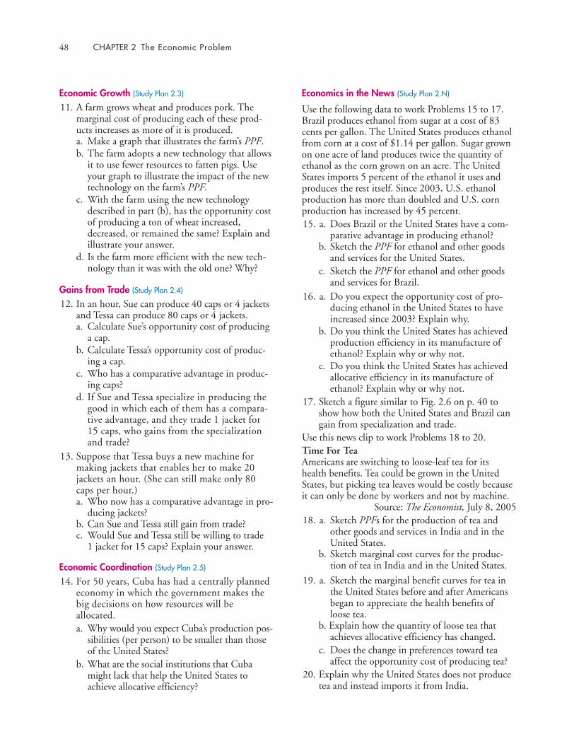
48 CHAPTER 2 The Economic Problem

Economic Growth (Study Plan 2.3)

11. A farm grows wheat and produces pork. Themarginal cost of producing each of these prod-ucts increases as more of it is produced.a. Make a graph that illustrates the farm’s PPF.b. The farm adopts a new technology that allows

it to use fewer resources to fatten pigs. Useyour graph to illustrate the impact of the newtechnology on the farm’s PPF.

c. With the farm using the new technologydescribed in part (b), has the opportunity costof producing a ton of wheat increased,decreased, or remained the same? Explain andillustrate your answer.

d. Is the farm more efficient with the new tech-nology than it was with the old one? Why?

Gains from Trade (Study Plan 2.4)

12. In an hour, Sue can produce 40 caps or 4 jacketsand Tessa can produce 80 caps or 4 jackets.a. Calculate Sue’s opportunity cost of producing

a cap.b. Calculate Tessa’s opportunity cost of produc-

ing a cap.c. Who has a comparative advantage in produc-

ing caps?d. If Sue and Tessa specialize in producing the

good in which each of them has a compara-tive advantage, and they trade 1 jacket for15 caps, who gains from the specializationand trade?

13. Suppose that Tessa buys a new machine formaking jackets that enables her to make 20jackets an hour. (She can still make only 80caps per hour.)a. Who now has a comparative advantage in pro-

ducing jackets?b. Can Sue and Tessa still gain from trade?c. Would Sue and Tessa still be willing to trade

1 jacket for 15 caps? Explain your answer.

Economic Coordination (Study Plan 2.5)

14. For 50 years, Cuba has had a centrally plannedeconomy in which the government makes thebig decisions on how resources will beallocated.a. Why would you expect Cuba’s production pos-

sibilities (per person) to be smaller than thoseof the United States?

b. What are the social institutions that Cubamight lack that help the United States toachieve allocative efficiency?

Economics in the News (Study Plan 2.N)

Use the following data to work Problems 15 to 17.Brazil produces ethanol from sugar at a cost of 83cents per gallon. The United States produces ethanolfrom corn at a cost of $1.14 per gallon. Sugar grownon one acre of land produces twice the quantity ofethanol as the corn grown on an acre. The UnitedStates imports 5 percent of the ethanol it uses andproduces the rest itself. Since 2003, U.S. ethanolproduction has more than doubled and U.S. cornproduction has increased by 45 percent.15. a. Does Brazil or the United States have a com-

parative advantage in producing ethanol?b. Sketch the PPF for ethanol and other goods

and services for the United States. c. Sketch the PPF for ethanol and other goods

and services for Brazil.16. a. Do you expect the opportunity cost of pro-

ducing ethanol in the United States to haveincreased since 2003? Explain why.

b. Do you think the United States has achievedproduction efficiency in its manufacture ofethanol? Explain why or why not.

c. Do you think the United States has achievedallocative efficiency in its manufacture ofethanol? Explain why or why not.

17. Sketch a figure similar to Fig. 2.6 on p. 40 toshow how both the United States and Brazil cangain from specialization and trade.

Use this news clip to work Problems 18 to 20.Time For TeaAmericans are switching to loose-leaf tea for itshealth benefits. Tea could be grown in the UnitedStates, but picking tea leaves would be costly becauseit can only be done by workers and not by machine.

Source: The Economist, July 8, 200518. a. Sketch PPFs for the production of tea and

other goods and services in India and in theUnited States.

b. Sketch marginal cost curves for the produc-tion of tea in India and in the United States.

19. a. Sketch the marginal benefit curves for tea inthe United States before and after Americansbegan to appreciate the health benefits ofloose tea.

b. Explain how the quantity of loose tea thatachieves allocative efficiency has changed.

c. Does the change in preferences toward teaaffect the opportunity cost of producing tea?

20. Explain why the United States does not producetea and instead imports it from India.

Additional Problems and Applications 49

Production Possibilities and Opportunity CostUse the following table to work Problems 21 to 22.Suppose that Yucatan’s production possibilities are

Food Sunscreen(pounds per month) (gallons per month)

300 and 0200 and 50100 and 100

0 and 150

21. a. Draw a graph of Yucatan’s PPF and explainhow your graph illustrates a tradeoff.

b. If Yucatan produces 150 pounds of food permonth, how much sunscreen must it produceif it achieves production efficiency?

c. What is Yucatan’s opportunity cost of produc-ing 1 pound of food?

d. What is Yucatan’s opportunity cost of produc-ing 1 gallon of sunscreen?

e. What is the relationship between your answersto parts (c) and (d)?

22. What feature of a PPF illustrates increasingopportunity cost? Explain why Yucatan’s opportu-nity cost does or does not increase.

Using Resources Efficiently23. In problem 21, what is the marginal cost of a

pound of food in Yucatan when the quantityproduced is 150 pounds per day? What is specialabout the marginal cost of food in Yucatan?

24. The table describes the preferences in Yucatan.Sunscreen Willingness to pay

(gallons per month) (pounds of food per gallon)

25 375 2

125 1

a. What is the marginal benefit from sunscreenand how is it measured?

b. Draw a graph of Yucatan’s marginal benefitfrom sunscreen.

Economic Growth25. Capital accumulation and technological change

bring economic growth, which means that thePPF keeps shifting outward: Production that wasunattainable yesterday becomes attainable today;production that is unattainable today will

become attainable tomorrow. Why doesn’t thisprocess of economic growth mean that scarcity isbeing defeated and will one day be gone?

Gains from TradeUse the following data to work Problems 26 and 27.Kim can produce 40 pies or 400 cakes an hour. Liamcan produce 100 pies or 200 cakes an hour.26. a. Calculate Kim’s opportunity cost of a pie and

Liam’s opportunity cost of a pie.b. If each spends 30 minutes of each hour pro-

ducing pies and 30 minutes producing cakes,how many pies and cakes does each produce?

c. Who has a comparative advantage in produc-ing pies? Who has a comparative advantage inproducing cakes?

27. a. Draw a graph of Kim’s PPF and Liam’s PPF.b. On your graph, show the point at which each

produces when they spend 30 minutes of eachhour producing pies and 30 minutes produc-ing cakes.

c. On your graph, show what Kim produces andwhat does Liam produces when they specialize.

d. When they specialize and trade, what are thetotal gains from trade?

e. If Kim and Liam share the total gains equally,what trade takes place between them?

Economic Coordination28. Indicate on a graph of the circular flows in the

market economy, the real and money flows inwhich the following items belong:a. You buy an iPad from the Apple Store.b. Apple Inc. pays the designers of the iPad.c. Apple Inc. decides to expand and rents an

adjacent building.d. You buy a new e-book from Amazon.e. Apple Inc. hires a student as an intern during

the summer.

Economics in the News29. After you have studied Reading Between the Lines

on pp. 44–45, answer the following questions.a. How has an Act of the United States Congress

increased U.S. production of corn?b. Why would you expect an increase in the

quantity of corn produced to raise the oppor-tunity cost of corn?

You can work these problems in MyEconLab if assigned by your instructor.

ADDITIONAL PROBLEMS AND APPLICATIONS

50 CHAPTER 2 The Economic Problem

c. Why did the cost of producing corn increasein the rest of the world?

d. Is it possible that the increased quantity ofcorn produced, despite the higher cost of pro-duction, moves the United States closer to al-locative efficiency?

30. Malaria Eradication Back on the TableIn response to the Gates Malaria Forum inOctober 2007, countries are debating the prosand cons of eradication. Dr. Arata Kochi of theWorld Health Organization believes that withenough money malaria cases could be cut by 90percent, but he believes that it would be veryexpensive to eliminate the remaining 10 percentof cases. He concluded that countries should notstrive to eradicate malaria.

Source: The New York Times, March 4, 2008a. Is Dr. Kochi talking about production

efficiency or allocative efficiency or both?b. Make a graph with the percentage of malaria

cases eliminated on the x-axis and the marginalcost and marginal benefit of driving downmalaria cases on the y-axis. On your graph: (i) Draw a marginal cost curve that is consis-

tent with Dr. Kochi’s opinion.(ii) Draw a marginal benefit curve that is

consistent with Dr. Kochi’s opinion.(iii) Identify the quantity of malaria eradicated

that achieves allocative efficiency.31. Lots of Little Screens

Inexpensive broadband access has created a gen-eration of television producers for whom theInternet is their native medium. As they redirectthe focus from TV to computers, cell phones,and iPods, the video market is developing into anopen digital network.

Source: The New York Times, December 2, 2007a. How has inexpensive broadband changed the

production possibilities of video entertain-ment and other goods and services?

b. Sketch a PPF for video entertainment andother goods and services before broadband.

c. Show how the arrival of inexpensive broad-band has changed the PPF.

d. Sketch a marginal benefit curve for videoentertainment.

e. Show how the new generation of TV producersfor whom the Internet is their native mediummight have changed the marginal benefit fromvideo entertainment.

f. Explain how the efficient quantity of videoentertainment has changed.

Use the following information to work Problems 32and 33.

Before the Civil War, the South traded with theNorth and with England. The South sold cotton andbought manufactured goods and food. During thewar, one of President Lincoln’s first actions was toblockade the ports and prevent this trade. The Southincreased its production of munitions and food.

32. In what did the South have a comparativeadvantage?

33. a. Draw a graph to illustrate production, con-sumption, and trade in the South before theCivil War.

b. Was the South consuming inside, on, or out-side its PPF ? Explain your answer.

c. Draw a graph to show the effects of the CivilWar on consumption and production in theSouth.

d. Did the Civil War change any opportunitycosts in the South? If so, did the opportunitycost of everything increase? Did the opportu-nity cost of any items decrease? Illustrate youranswer with appropriate graphs.

Use the following information to work Problems 34and 35.

He Shoots! He Scores! He Makes Movies!NBA All-star Baron Davis and his school friend,Cash Warren, premiered their first movie Made inAmerica at the Sundance Festival in January 2008.The movie, based on gang activity in South CentralLos Angeles, received good reviews.

Source: The New York Times, February 24, 200834. a. Does Baron Davis have an absolute advantage

in basketball and movie directing and is thisthe reason for his success in both activities?

b. Does Baron Davis have a comparative advan-tage in basketball or movie directing or bothand is this the reason for his success in bothactivities?

35. a. Sketch a PPF between playing basketball andproducing other goods and services for BaronDavis and for yourself.

b. How do you (and people like you) and BaronDavis (and people like him) gain from special-ization and trade?

51

Your Economic Revolution

PART ONE

out the wire, another straight-ens it, a third cuts it, a fourthpoints it, a fifth grinds it. Threespecialists make the head, anda fourth attaches it. Finally, thepin is polished and packaged.

But a large market isneeded to support the divisionof labor: One factory employing ten workers would need tosell more than 15 million pins a year to stay in business!

Three periods in human history stand out as ones of eco-nomic revolution. The first, the Agricultural Revolution,occurred 10,000 years ago. In what is today Iraq, peoplelearned to domesticate animals and plant crops. Peoplestopped roaming in search of food and settled in villages,towns, and cities where they specialized in the activities in which they had a com-parative advantage and developed markets in which to exchange their products.Wealth increased enormously.

You are studying economics at a time that future historians will call the InformationRevolution. Over the entire world, people are embracing new information tech-nologies and prospering on an unprecedented scale.

Economics was born during the Industrial Revolution, which began in Englandduring the 1760s. For the first time, people began to apply science and create newtechnologies for the manufacture of textiles and iron, to create steam engines, and toboost the output of farms.

During all three economic revolutions, many have prospered but many have beenleft behind. It is the range of human progress that poses the greatest question for eco-nomics and the one that Adam Smith addressed in the first work of economic sci-ence: What causes the differences in wealth among nations?

Many people had written about economics before AdamSmith, but he made economics a science. Born in 1723in Kirkcaldy, a small fishing town near Edinburgh, Scot-land, Smith was the only child of the town’s customs offi-cer. Lured from his professorship (he was a full professor at28) by a wealthy Scottish duke who gave him a pensionof £300 a year—ten times the average income at thattime—Smith devoted ten years to writing his masterpiece:An Inquiry into the Nature and Causes of the Wealthof Nations, published in 1776.

Why, Adam Smith asked , are some nations wealthywhile others are poor? He was pondering these questionsat the height of the Industrial Revolution, and he an-swered by emphasizing the role of the division of laborand free markets.

To illustrate his argument, Adam Smith described twopin factories. In the first, one person, using the hand toolsavailable in the 1770s, could make 20 pins a day. In theother, by using those same hand tools but breaking theprocess into a number of individually small operations inwhich people specialize—by the division of labor—ten peo-ple could make a staggering 48,000 pins a day. One draws

“It is not from thebenevolence of the butcher,the brewer, or the bakerthat we expect our dinner,but from their regard totheir own interest.”

ADAM SMITHThe Wealth of Nations

UNDERSTANDING THE SCOPE OF ECONOMICS

So growth in the pie seemed to be the principal (butnot the only) component of an anti-poverty strategy.To supplement growth’s good effects on the poor, theIndian plannerswere also dedi-cated to education,health, socialreforms, and landreforms. Also, theaccess of the low-est-income andsocially disadvan-taged groups to the growth process and its benefitswas to be improved in many ways, such as extensionof credit without collateral.

Today, this strategy has no rivals. Much empiricalwork shows that where growth has occurred, povertyhas lessened. It is nice to know that one’s basic takeon an issue of such central importance to humanity’swell-being has been borne out by experience!

You left India in 1968 to come to the United Statesand an academic job at MIT. Why?While the decision to emigrate often reflects personalfactors—and they were present in my case—the offerof a professorship from MIT certainly helped me

52

My main prescription was to“grow the pie” … Muchempirical work shows thatwhere growth has occurred,poverty has lessened.

TALKING WITH Jagdish Bhagwati

Professor Bhagwati, what attracted you to economics?When you come from India, where poverty hits theeye, it is easy to be attracted to economics, which canbe used to bring prosperity and create jobs to pull upthe poor into gainful employment.

I learned later that there are two broad types ofeconomist: those who treat the subject as an aridmathematical toy and those who see it as a serioussocial science.

If Cambridge, where I went as an undergraduate,had been interested in esoteric mathematical econom-ics, I would have opted for something else. But theCambridge economists from whom I learned—manyamong the greatest figures in the discipline—saw eco-nomics as a social science. I therefore saw the power ofeconomics as a tool to address India’s poverty and wasimmediately hooked.

Who had the greatest impact on you at Cambridge?Most of all, it was Harry Johnson, a young Canadianof immense energy and profound analytical gifts.Quite unlike the shy and reserved British dons,Johnson was friendly, effusive, and supportive of stu-dents who flocked around him. He would later moveto Chicago, where he became one of the most influ-ential members of the market-oriented Chicagoschool. Another was Joan Robinson, arguably theworld’s most impressive female economist.

When I left Cambridge for MIT, going from oneCambridge to the other, I was lucky to transitionfrom one phenomenal set of economists to another.At MIT, I learned much from future Nobel laureatesPaul Samuelson and Robert Solow. Both would laterbecome great friends and colleagues when I joinedthe MIT faculty in 1968.

After Cambridge and MIT, you went to Oxford andthen back to India. What did you do in India?I joined the Planning Commission in New Delhi,where my first big job was to find ways of raising thebottom 30 percent of India’s population out ofpoverty to a “minimum income” level.

And what did you prescribe?My main prescription was to “grow the pie.” Myresearch suggested that the share of the bottom 30percent of the pie did not seem to vary dramaticallywith differences in economic and political systems.

53

JAGDISH BHAGWATI is University Professor atColumbia University. Born in India in 1934, hestudied at Cambridge University in England, MIT,and Oxford University before returning to India.He returned to teach at MIT in 1968 and movedto Columbia in 1980. A prolific scholar, ProfessorBhagwati also writes in leading newspapers andmagazines throughout the world. He has beenmuch honored for both his scientific work and hisimpact on public policy. His greatest contributionsare in international trade but extend also to de-velopmental problems and the study of politicaleconomy.

Michael Parkin talked with Jagdish Bhagwatiabout his work and the progress that economistshave made in understanding the benefits of eco-nomic growth and international trade since thepioneering work of Adam Smith.

make up my mind. At the time, it was easily theworld’s most celebrated department. Serendipitously,the highest-ranked departments at MIT were not inengineering and the sciences but in linguistics (whichhad Noam Chomsky) and economics (which hadPaul Samuelson). Joining the MIT faculty was a dra-matic breakthrough: I felt stimulated each year byseveral fantastic students and by several of the world’smost creative economists.

We hear a lot in the popular press about fair trade andlevel playing fields. What’s the distinction between freetrade and fair trade? How can the playing field be un-level?Free trade simply means allowing no trade barriers suchas tariffs, subsidies, and quotas. Trade barriers makedomestic prices different from world prices for tradedgoods. When this happens, resources are not being usedefficiently. Basic economics from the time of AdamSmith tells us why free trade is good for us and whybarriers to trade harm us, though our understanding ofthis doctrine today is far more nuanced and profoundthan it was at its creation.

Fair trade, on the other hand, is almost always asneaky way of objecting to free trade. If your rivals arehard to compete with, you are not likely to get protec-

tion simply by saying that you cannot hack it. But ifyou say that your rival is an “unfair” trader, that is aneasier sell! As inter-national competi-tion has grownfiercer, cries of“unfair trade” havetherefore multi-plied. The lesser rogues among the protectionists askfor “free and fair trade,” whereas the worst ones ask for“fair, not free, trade.”

At the end of World War II, the General Agreementon Tariffs and Trade (GATT) was established andthere followed several rounds of multilateral trade ne-gotiations and reductions in barriers to trade. How doyou assess the contribution of GATT and its successor,the World Trade Organization (WTO)?The GATT has made a huge contribution by oversee-ing massive trade liberalization in industrial goodsamong the developed countries. GATT rules, which“bind” tariffs to negotiated ceilings, prevent the rais-ing of tariffs and have prevented tariff wars like thoseof the 1930s in which mutual and retaliatory tariffbarriers were raised, to the detriment of everyone.

The GATT was folded into the WTO at the endof the Uruguay Round of trade negotiations, and theWTO is institutionally stronger. For instance, it hasa binding dispute settlement mechanism, whereasthe GATT had no such teeth. It is also moreambitious in its scope, extending to new areas suchas the environment, intellectual property protection,and investment rules.

Running alongside the pursuit of multilateral freetrade has been the emergence of bilateral trade agree-ments such as NAFTA and the European Union(EU). How do you view the bilateral free trade areasin today’s world?Unfortunately, there has been an explosion of bilateralfree trade areas today. By some estimates, the ones inplace and others being plotted approach 400! Eachbilateral agreement gives preferential treatment to itstrading partner over others. Because there are now somany bilateral agreements, such as those between theUnited States and Israel and between the UnitedStates and Jordan, the result is a chaotic pattern of dif-ferent tariffs depending on where a product comesfrom. Also, “rules of origin” must be agreed upon to

Fair trade … is almostalways a sneaky way ofobjecting to free trade.

54

determine whether a product is, say, Jordanian orTaiwanese if Jordan qualifies for a preferential tariffbut Taiwan does not and Taiwanese inputs enter theJordanian manufacture of the product.

I have called the resulting crisscrossing of prefer-ences and rules of origin the “spaghetti bowl” problem.The world trading system is choking under these pro-liferating bilateral deals. Contrast this complexity withthe simplicity of a multilateral system with commontariffs for all WTO members.

We now have a world of uncoordinated andinefficient trade policies. The EU makes bilateral

free trade agreementswith different non-EU countries, so theUnited States followswith its own bilateralagreements; and withEurope and the

United States doing it, the Asian countries, longwedded to multilateralism, have now succumbed tothe mania.

Instead, if the United States had provided lead-ership by rewriting rules to make the signing ofsuch bilateral agreements extremely difficult, thisplague on the trading system today might well havebeen averted.

Is the “spaghetti bowl” problem getting better or worse?Unquestionably it is getting worse. Multilateralism isretreating and bilateralism is advancing. The 2010 G-20 meeting in Canada was a disappointment. Atthe insistence of the United States, a definite date forcompleting the Doha Round was dropped andinstead, unwittingly rubbing salt into the wound,President Barack Obama announced his administra-tion’s willingness to see the U.S.-South Korea freetrade agreement through. There are distressing recentreports that the U.S. Commerce Department isexploring ways to strengthen the bite of anti-dumping actions, which are now generally agreed tobe a form of discriminatory protectionism aimedselectively at successful exporting nations and firms.Equally distressing is Obama’s decision to sign a billthat raises fees on some temporary work visas inorder to pay for higher border-enforcement expendi-tures.Further, it was asserted that a tax on foreignworkers would reduce the numbers coming in and“taking jobs away” from U.S. citizens. Many support-

ers of the proposal claimed, incoherently, that itwould simultaneously discourage foreign workersfrom entering the United States and increase rev-enues.Obama’s surrender exemplified the doctrinethat one retreat often leads to another, with new lob-byists following in others’ footsteps. Perhaps the chiefmistake, as with recent “Buy American” provisions inU.S. legislation, was to allow the Employ AmericanWorkers Act (EAWA) to be folded into the stimulusbill. This act makes it harder for companies to getgovern-mental support to hire skilled immigrantswith H1(b) visas: They must first show that they havenot laid off or plan to lay off U.S. workers in similaroccupations. Whatever the shortcomings of suchmeasures in economic-policy terms, the visa-fee-enhancement provision is de facto discriminatory,and thus violates WTO rules against discriminationbetween domestic and foreign firms, or between for-eign firms from different WTO countries. While thevisa-fee legislation is what lawyers call “facially” non-discriminatory, its design confers an advantage onU.S. firms vis-à-vis foreign firms.Such acts of dis-crimination in trade policies find succor in the mediaand in some of America’s prominent think tanks. Forexample, in the wake of the vast misery brought byflooding to the people of Pakistan, the U.S. and othergovernments have risen to the occasion with emer-gency aid. But there have also been proposals to grantduty-free access to Pakistan’s exports. But this wouldbe discriminatory toward developing countries thatdo not have duty-free access, helping Pakistan at theirexpense.

What advice do you have for a student who is juststarting to study economics? Is economics a good sub-ject in which to major?I would say: enormously so. In particular, we econo-mists bring three unique insights to good policymaking.

First, economists look for second- and subse-quent-round effects of actions.

Second, we correctly emphasize that a policy can-not be judged without using a counterfactual. It is awitticism that an economist, when asked how herhusband was, said, “compared to what?”

Third, we uniquely and systematically bring theprinciple of social cost and social benefit to our policyanalysis.

We now have a world ofuncoordinated andinefficient trade policies.

55

PART TWO How Markets Work

After studying this chapter, you will be able to:

� Describe a competitive market and think about a price as an opportunity cost

� Explain the influences on demand� Explain the influences on supply� Explain how demand and supply determine prices

and quantities bought and sold� Use the demand and supply model to make

predictions about changes in prices and quantities

hat makes the price of oil double and the price of gasoline almost double injust one year? Will these prices keep on rising? Are the oil companies takingadvantage of people? This chapter enables you to answer these and similarquestions about prices—prices that rise, prices that fall, and prices thatfluctuate.

You already know that economics is about the choices people make to copewith scarcity and how those choices respond to incentives. Prices act asincentives. You’re going to see how people respond to prices and how pricesget determined by demand and supply. The demand and supply model that

you study in this chapter is the main tool of economics. Ithelps us to answer the big economic question: What, how,and for whom goods and services are produced?

At the end of the chapter, in Reading Between the Lines, we’ll apply themodel to the market for coffee and explain why its price increased sharply in2010 and why it was expected to rise again.

DEMAND AND SUPPLY

W

3

56 CHAPTER 3 Demand and Supply

Let’s begin our study of demand and supply,starting with demand.

◆ Markets and PricesWhen you need a new pair of running shoes, want abagel and a latte, plan to upgrade your cell phone, orneed to fly home for Thanksgiving, you must find aplace where people sell those items or offer those ser-vices. The place in which you find them is a market.You learned in Chapter 2 (p. 42) that a market is anyarrangement that enables buyers and sellers to getinformation and to do business with each other.

A market has two sides: buyers and sellers. Thereare markets for goods such as apples and hiking boots,for services such as haircuts and tennis lessons, for fac-tors of production such as computer programmers andearthmovers, and for other manufactured inputs suchas memory chips and auto parts. There are also mar-kets for money such as Japanese yen and for financialsecurities such as Yahoo! stock. Only our imaginationlimits what can be traded in markets.

Some markets are physical places where buyers andsellers meet and where an auctioneer or a brokerhelps to determine the prices. Examples of this typeof market are the New York Stock Exchange and thewholesale fish, meat, and produce markets.

Some markets are groups of people spread aroundthe world who never meet and know little about eachother but are connected through the Internet or by tele-phone and fax. Examples are the e-commerce marketsand the currency markets.

But most markets are unorganized collections ofbuyers and sellers. You do most of your trading inthis type of market. An example is the market forbasketball shoes. The buyers in this $3 billion-a-yearmarket are the 45 million Americans who play bas-ketball (or who want to make a fashion statement).The sellers are the tens of thousands of retail sportsequipment and footwear stores. Each buyer can visitseveral different stores, and each seller knows that thebuyer has a choice of stores.

Markets vary in the intensity of competition thatbuyers and sellers face. In this chapter, we’re going tostudy a competitive market—a market that has manybuyers and many sellers, so no single buyer or sellercan influence the price.

Producers offer items for sale only if the price ishigh enough to cover their opportunity cost. Andconsumers respond to changing opportunity cost byseeking cheaper alternatives to expensive items.

We are going to study how people respond toprices and the forces that determine prices. But to

pursue these tasks, we need to understand the rela-tionship between a price and an opportunity cost.

In everyday life, the price of an object is the num-ber of dollars that must be given up in exchange for it.Economists refer to this price as the money price.

The opportunity cost of an action is the highest-valued alternative forgone. If, when you buy a cup ofcoffee, the highest-valued thing you forgo is somegum, then the opportunity cost of the coffee is thequantity of gum forgone. We can calculate the quan-tity of gum forgone from the money prices of thecoffee and the gum.

If the money price of coffee is $1 a cup and themoney price of gum is 50¢ a pack, then the opportu-nity cost of one cup of coffee is two packs of gum. Tocalculate this opportunity cost, we divide the price ofa cup of coffee by the price of a pack of gum and findthe ratio of one price to the other. The ratio of oneprice to another is called a relative price, and a relativeprice is an opportunity cost.

We can express the relative price of coffee in termsof gum or any other good. The normal way ofexpressing a relative price is in terms of a “basket” ofall goods and services. To calculate this relative price,we divide the money price of a good by the moneyprice of a “basket” of all goods (called a price index).The resulting relative price tells us the opportunitycost of the good in terms of how much of the “bas-ket” we must give up to buy it.

The demand and supply model that we are aboutto study determines relative prices, and the word“price” means relative price. When we predict that aprice will fall, we do not mean that its money pricewill fall—although it might. We mean that its relativeprice will fall. That is, its price will fall relative to theaverage price of other goods and services.

REVIEW QUIZ1 What is the distinction between a money price

and a relative price?2 Explain why a relative price is an opportunity cost.3 Think of examples of goods whose relative price

has risen or fallen by a large amount.You can work these questions in Study Plan 3.1 and get instant feedback.

◆ DemandIf you demand something, then you

1. Want it,2. Can afford it, and3. Plan to buy it.

Wants are the unlimited desires or wishes that peo-ple have for goods and services. How many timeshave you thought that you would like something “ifonly you could afford it” or “if it weren’t so expen-sive”? Scarcity guarantees that many—perhapsmost—of our wants will never be satisfied. Demandreflects a decision about which wants to satisfy.

The quantity demanded of a good or service is theamount that consumers plan to buy during a giventime period at a particular price. The quantitydemanded is not necessarily the same as the quantityactually bought. Sometimes the quantity demandedexceeds the amount of goods available, so the quan-tity bought is less than the quantity demanded.

The quantity demanded is measured as an amountper unit of time. For example, suppose that you buyone cup of coffee a day. The quantity of coffee thatyou demand can be expressed as 1 cup per day, 7cups per week, or 365 cups per year.

Many factors influence buying plans, and one ofthem is the price. We look first at the relationshipbetween the quantity demanded of a good and itsprice. To study this relationship, we keep all otherinfluences on buying plans the same and we ask:How, other things remaining the same, does thequantity demanded of a good change as its pricechanges?

The law of demand provides the answer.

The Law of DemandThe law of demand states

Other things remaining the same, the higher theprice of a good, the smaller is the quantitydemanded; and the lower the price of a good, thegreater is the quantity demanded.

Why does a higher price reduce the quantitydemanded? For two reasons:

■ Substitution effect■ Income effect

Substitution Effect When the price of a good rises,other things remaining the same, its relative price—its opportunity cost—rises. Although each good isunique, it has substitutes—other goods that can beused in its place. As the opportunity cost of a goodrises, the incentive to economize on its use andswitch to a substitute becomes stronger.

Income Effect When a price rises, other thingsremaining the same, the price rises relative to income.Faced with a higher price and an unchanged income,people cannot afford to buy all the things they previ-ously bought. They must decrease the quantitiesdemanded of at least some goods and services.Normally, the good whose price has increased will beone of the goods that people buy less of.

To see the substitution effect and the income effectat work, think about the effects of a change in theprice of an energy bar. Several different goods aresubstitutes for an energy bar. For example, an energydrink could be consumed instead of an energy bar.

Suppose that an energy bar initially sells for $3 andthen its price falls to $1.50. People now substituteenergy bars for energy drinks—the substitution effect.And with a budget that now has some slack from thelower price of an energy bar, people buy even moreenergy bars—the income effect. The quantity of energybars demanded increases for these two reasons.

Now suppose that an energy bar initially sells for$3 and then the price doubles to $6. People now buyfewer energy bars and more energy drinks—the sub-stitution effect. And faced with a tighter budget, peo-ple buy even fewer energy bars—the income effect.The quantity of energy bars demanded decreases forthese two reasons.

Demand Curve and Demand ScheduleYou are now about to study one of the two most usedcurves in economics: the demand curve. You are alsogoing to encounter one of the most critical distinc-tions: the distinction between demand and quantitydemanded.

The term demand refers to the entire relationshipbetween the price of a good and the quantitydemanded of that good. Demand is illustrated by thedemand curve and the demand schedule. The termquantity demanded refers to a point on a demandcurve—the quantity demanded at a particular price.

Demand 57

Figure 3.1 shows the demand curve for energybars. A demand curve shows the relationship betweenthe quantity demanded of a good and its price whenall other influences on consumers’ planned purchasesremain the same.

The table in Fig. 3.1 is the demand schedule forenergy bars. A demand schedule lists the quantitiesdemanded at each price when all the other influenceson consumers’ planned purchases remain the same.For example, if the price of a bar is 50¢, the quantitydemanded is 22 million a week. If the price is $2.50,the quantity demanded is 5 million a week. Theother rows of the table show the quantities demandedat prices of $1.00, $1.50, and $2.00.

We graph the demand schedule as a demand curvewith the quantity demanded on the x-axis and theprice on the y-axis. The points on the demand curvelabeled A through E correspond to the rows of thedemand schedule. For example, point A on the graphshows a quantity demanded of 22 million energy barsa week at a price of 50¢ a bar.

Willingness and Ability to Pay Another way of look-ing at the demand curve is as a willingness-and-abil-ity-to-pay curve. The willingness and ability to pay isa measure of marginal benefit.

If a small quantity is available, the highest pricethat someone is willing and able to pay for one moreunit is high. But as the quantity available increases,the marginal benefit of each additional unit falls andthe highest price that someone is willing and able topay also falls along the demand curve.

In Fig. 3.1, if only 5 million energy bars are avail-able each week, the highest price that someone iswilling to pay for the 5 millionth bar is $2.50. But if22 million energy bars are available each week, some-one is willing to pay 50¢ for the last bar bought.

A Change in DemandWhen any factor that influences buying plans changes,other than the price of the good, there is a change indemand. Figure 3.2 illustrates an increase in demand.When demand increases, the demand curve shifts right-ward and the quantity demanded at each price is greater.For example, at $2.50 a bar, the quantity demanded onthe original (blue) demand curve is 5 million energybars a week. On the new (red) demand curve, at $2.50 abar, the quantity demanded is 15 million bars a week.Look closely at the numbers in the table and check thatthe quantity demanded at each price is greater.

58 CHAPTER 3 Demand and Supply

3.00

5 15 20 25

Pric

e (d

olla

rs p

er b

ar)

Quantity demanded (millions of bars per week)

Demand forenergy bars

10

E

D

C

B

A

2.50

2.00

1.50

1.00

0.50

0

The table shows a demand schedule for energy bars. At aprice of 50¢ a bar, 22 million bars a week are demanded;at a price of $1.50 a bar, 10 million bars a week aredemanded. The demand curve shows the relationshipbetween quantity demanded and price, other things remain-ing the same. The demand curve slopes downward: As theprice falls, the quantity demanded increases.

The demand curve can be read in two ways. For agiven price, the demand curve tells us the quantity thatpeople plan to buy. For example, at a price of $1.50 abar, people plan to buy 10 million bars a week. For agiven quantity, the demand curve tells us the maximumprice that consumers are willing and able to pay for thelast bar available. For example, the maximum price thatconsumers will pay for the 15 millionth bar is $1.00.

Quantity demandedPrice (millions of bars

(dollars per bar) per week)

A 0.50 22

B 1.00 15

C 1.50 10

D 2.00 7

E 2.50 5

FIGURE 3.1 The Demand Curve

animation

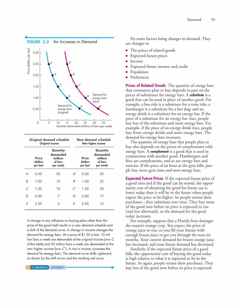
Six main factors bring changes in demand. Theyare changes in

■ The prices of related goods■ Expected future prices■ Income■ Expected future income and credit■ Population■ Preferences

Prices of Related Goods The quantity of energy barsthat consumers plan to buy depends in part on theprices of substitutes for energy bars. A substitute is agood that can be used in place of another good. Forexample, a bus ride is a substitute for a train ride; ahamburger is a substitute for a hot dog; and anenergy drink is a substitute for an energy bar. If theprice of a substitute for an energy bar rises, peoplebuy less of the substitute and more energy bars. Forexample, if the price of an energy drink rises, peoplebuy fewer energy drinks and more energy bars. Thedemand for energy bars increases.

The quantity of energy bars that people plan tobuy also depends on the prices of complements withenergy bars. A complement is a good that is used inconjunction with another good. Hamburgers andfries are complements, and so are energy bars andexercise. If the price of an hour at the gym falls, peo-ple buy more gym time and more energy bars.

Expected Future Prices If the expected future price ofa good rises and if the good can be stored, the oppor-tunity cost of obtaining the good for future use islower today than it will be in the future when peopleexpect the price to be higher. So people retime theirpurchases—they substitute over time. They buy moreof the good now before its price is expected to rise(and less afterward), so the demand for the goodtoday increases.

For example, suppose that a Florida frost damagesthe season’s orange crop. You expect the price oforange juice to rise, so you fill your freezer withenough frozen juice to get you through the next sixmonths. Your current demand for frozen orange juicehas increased, and your future demand has decreased.

Similarly, if the expected future price of a goodfalls, the opportunity cost of buying the good todayis high relative to what it is expected to be in thefuture. So again, people retime their purchases. Theybuy less of the good now before its price is expected

Demand 59

3.00

5 15 20 35

Pric

e (d

olla

rs p

er b

ar)

Quantity demanded (millions of bars per week)

Demand forenergy bars(original)

Demand forenergy bars(new)

10

E

D

C

B

A

2.50

2.00

1.50

1.00

0.50

0 3025

E'

D'

C'

B'

A'

Original demand schedule New demand scheduleOriginal income New higher income

Quantity Quantitydemanded demanded

Price (millions Price (millions(dollars of bars (dollars of barsper bar) per week) per bar) per week)

A 0.50 22 A' 0.50 32

B 1.00 15 B' 1.00 25

C 1.50 10 C' 1.50 20

D 2.00 7 D' 2.00 17

E 2.50 5 E' 2.50 15

A change in any influence on buying plans other than theprice of the good itself results in a new demand schedule anda shift of the demand curve. A change in income changes thedemand for energy bars. At a price of $1.50 a bar, 10 mil-lion bars a week are demanded at the original income (row Cof the table) and 20 million bars a week are demanded at thenew higher income (row C'). A rise in income increases thedemand for energy bars. The demand curve shifts rightward,as shown by the shift arrow and the resulting red curve.

FIGURE 3.2 An Increase in Demand

animation

Preferences Demand depends on preferences.Preferences determine the value that people place oneach good and service. Preferences depend on suchthings as the weather, information, and fashion. Forexample, greater health and fitness awareness hasshifted preferences in favor of energy bars, so thedemand for energy bars has increased.

Table 3.1 summarizes the influences on demandand the direction of those influences.

A Change in the Quantity Demanded Versus a Change in DemandChanges in the influences on buying plans bringeither a change in the quantity demanded or achange in demand. Equivalently, they bring either amovement along the demand curve or a shift of thedemand curve. The distinction between a change in

60 CHAPTER 3 Demand and Supply

to fall, so the demand for the good decreases todayand increases in the future.

Computer prices are constantly falling, and thisfact poses a dilemma. Will you buy a new computernow, in time for the start of the school year, or willyou wait until the price has fallen some more? Becausepeople expect computer prices to keep falling, the cur-rent demand for computers is less (and the futuredemand is greater) than it otherwise would be.

Income Consumers’ income influences demand.When income increases, consumers buy more of mostgoods; and when income decreases, consumers buyless of most goods. Although an increase in incomeleads to an increase in the demand for most goods, itdoes not lead to an increase in the demand for allgoods. A normal good is one for which demandincreases as income increases. An inferior good is onefor which demand decreases as income increases. Asincomes increase, the demand for air travel (a normalgood) increases and the demand for long-distance bustrips (an inferior good) decreases.

Expected Future Income and Credit When expectedfuture income increases or credit becomes easier toget, demand for the good might increase now. Forexample, a salesperson gets the news that she willreceive a big bonus at the end of the year, so she goesinto debt and buys a new car right now, rather thanwait until she receives the bonus.

Population Demand also depends on the size and theage structure of the population. The larger the popu-lation, the greater is the demand for all goods andservices; the smaller the population, the smaller is thedemand for all goods and services.

For example, the demand for parking spaces ormovies or just about anything that you can imagineis much greater in New York City (population 7.5million) than it is in Boise, Idaho (population150,000).

Also, the larger the proportion of the populationin a given age group, the greater is the demand forthe goods and services used by that age group.

For example, during the 1990s, a decrease in thecollege-age population decreased the demand for col-lege places. During those same years, the number ofAmericans aged 85 years and over increased by morethan 1 million. As a result, the demand for nursinghome services increased.

TABLE 3.1 The Demand for Energy Bars

The Law of Demand

The quantity of energy bars demanded

Decreases if: Increases if:

■ The price of an energy bar rises

■ The price of an energy bar falls

■ The price of a substitute falls

■ The price of acomplement rises

■ The expected futureprice of an energy barfalls

■ Income falls*

■ Expected future income falls or creditbecomes harder to get*

■ The population decreases

■ The price of a substitute rises

■ The price of acomplement falls

■ The expected futureprice of an energy barrises

■ Income rises*

■ Expected future income rises or creditbecomes easier to get*

■ The population increases

Changes in Demand

The demand for energy bars

Decreases if: Increases if:

*An energy bar is a normal good.

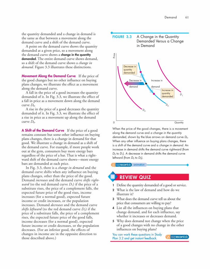
the quantity demanded and a change in demand isthe same as that between a movement along thedemand curve and a shift of the demand curve.

A point on the demand curve shows the quantitydemanded at a given price, so a movement alongthe demand curve shows a change in the quantitydemanded. The entire demand curve shows demand,so a shift of the demand curve shows a change indemand. Figure 3.3 illustrates these distinctions.

Movement Along the Demand Curve If the price ofthe good changes but no other influence on buyingplans changes, we illustrate the effect as a movementalong the demand curve.

A fall in the price of a good increases the quantitydemanded of it. In Fig. 3.3, we illustrate the effect ofa fall in price as a movement down along the demandcurve D0.

A rise in the price of a good decreases the quantitydemanded of it. In Fig. 3.3, we illustrate the effect ofa rise in price as a movement up along the demandcurve D0.

A Shift of the Demand Curve If the price of a goodremains constant but some other influence on buyingplans changes, there is a change in demand for thatgood. We illustrate a change in demand as a shift ofthe demand curve. For example, if more people workout at the gym, consumers buy more energy barsregardless of the price of a bar. That is what a right-ward shift of the demand curve shows—more energybars are demanded at each price.

In Fig. 3.3, there is a change in demand and thedemand curve shifts when any influence on buyingplans changes, other than the price of the good.Demand increases and the demand curve shifts right-ward (to the red demand curve D1) if the price of asubstitute rises, the price of a complement falls, theexpected future price of the good rises, incomeincreases (for a normal good), expected futureincome or credit increases, or the populationincreases. Demand decreases and the demand curveshifts leftward (to the red demand curve D2) if theprice of a substitute falls, the price of a complementrises, the expected future price of the good falls,income decreases (for a normal good), expectedfuture income or credit decreases, or the populationdecreases. (For an inferior good, the effects ofchanges in income are in the opposite direction tothose described above.)

Demand 61

Quantity

Pric

e

Decrease in

demand

D

D0

2

Increase in

demandIncrease inquantitydemanded

Decrease inquantitydemanded

0

D1

When the price of the good changes, there is a movementalong the demand curve and a change in the quantitydemanded, shown by the blue arrows on demand curve D0.When any other influence on buying plans changes, thereis a shift of the demand curve and a change in demand. Anincrease in demand shifts the demand curve rightward (fromD0 to D1). A decrease in demand shifts the demand curveleftward (from D0 to D2).

FIGURE 3.3 A Change in the QuantityDemanded Versus a Change in Demand

animation

REVIEW QUIZ1 Define the quantity demanded of a good or service.2 What is the law of demand and how do we

illustrate it?3 What does the demand curve tell us about the

price that consumers are willing to pay?4 List all the influences on buying plans that

change demand, and for each influence, saywhether it increases or decreases demand.

5 Why does demand not change when the priceof a good changes with no change in the otherinfluences on buying plans?

You can work these questions in Study Plan 3.2 and get instant feedback.

◆ SupplyIf a firm supplies a good or service, the firm

1. Has the resources and technology to produce it,2. Can profit from producing it, and3. Plans to produce it and sell it.

A supply is more than just having the resources andthe technology to produce something. Resources andtechnology are the constraints that limit what ispossible.

Many useful things can be produced, but they arenot produced unless it is profitable to do so. Supplyreflects a decision about which technologically feasi-ble items to produce.

The quantity supplied of a good or service is theamount that producers plan to sell during a giventime period at a particular price. The quantity sup-plied is not necessarily the same amount as thequantity actually sold. Sometimes the quantity sup-plied is greater than the quantity demanded, so thequantity sold is less than the quantity supplied.

Like the quantity demanded, the quantity sup-plied is measured as an amount per unit of time. Forexample, suppose that GM produces 1,000 cars aday. The quantity of cars supplied by GM can beexpressed as 1,000 a day, 7,000 a week, or 365,000 ayear. Without the time dimension, we cannot tellwhether a particular quantity is large or small.

Many factors influence selling plans, and againone of them is the price of the good. We look firstat the relationship between the quantity supplied ofa good and its price. Just as we did when we studieddemand, to isolate the relationship between thequantity supplied of a good and its price, we keepall other influences on selling plans the same andask: How does the quantity supplied of a goodchange as its price changes when other thingsremain the same?

The law of supply provides the answer.

The Law of SupplyThe law of supply states:

Other things remaining the same, the higher theprice of a good, the greater is the quantity supplied;and the lower the price of a good, the smaller is thequantity supplied.

Why does a higher price increase the quantity sup-plied? It is because marginal cost increases. As thequantity produced of any good increases, the mar-ginal cost of producing the good increases. (SeeChapter 2, p. 33 to review marginal cost.)

It is never worth producing a good if the pricereceived for the good does not at least cover the mar-ginal cost of producing it. When the price of a goodrises, other things remaining the same, producers arewilling to incur a higher marginal cost, so theyincrease production. The higher price brings forth anincrease in the quantity supplied.

Let’s now illustrate the law of supply with a supplycurve and a supply schedule.

Supply Curve and Supply ScheduleYou are now going to study the second of the twomost used curves in economics: the supply curve.You’re also going to learn about the critical distinc-tion between supply and quantity supplied.

The term supply refers to the entire relationshipbetween the price of a good and the quantity sup-plied of it. Supply is illustrated by the supply curveand the supply schedule. The term quantity suppliedrefers to a point on a supply curve—the quantitysupplied at a particular price.

Figure 3.4 shows the supply curve of energy bars. Asupply curve shows the relationship between the quan-tity supplied of a good and its price when all otherinfluences on producers’ planned sales remain the same.The supply curve is a graph of a supply schedule.

The table in Fig. 3.4 sets out the supply schedulefor energy bars. A supply schedule lists the quantitiessupplied at each price when all the other influences onproducers’ planned sales remain the same. For exam-ple, if the price of an energy bar is 50¢, the quantitysupplied is zero—in row A of the table. If the price ofan energy bar is $1.00, the quantity supplied is 6 mil-lion energy bars a week—in row B. The other rows ofthe table show the quantities supplied at prices of$1.50, $2.00, and $2.50.

To make a supply curve, we graph the quantitysupplied on the x-axis and the price on the y-axis.The points on the supply curve labeled A through Ecorrespond to the rows of the supply schedule. Forexample, point A on the graph shows a quantity sup-plied of zero at a price of 50¢ an energy bar. Point Eshows a quantity supplied of 15 million bars at $2.50an energy bar.

62 CHAPTER 3 Demand and Supply

Minimum Supply Price The supply curve can beinterpreted as a minimum-supply-price curve—acurve that shows the lowest price at which someone iswilling to sell. This lowest price is the marginal cost.

If a small quantity is produced, the lowest price atwhich someone is willing to sell one more unit is low.But as the quantity produced increases, the marginalcost of each additional unit rises, so the lowest priceat which someone is willing to sell an additional unitrises along the supply curve.

In Fig. 3.4, if 15 million bars are produced eachweek, the lowest price at which someone is willing tosell the 15 millionth bar is $2.50. But if 10 millionbars are produced each week, someone is willing toaccept $1.50 for the last bar produced.

A Change in SupplyWhen any factor that influences selling plans otherthan the price of the good changes, there is a changein supply. Six main factors bring changes in supply.They are changes in

■ The prices of factors of production■ The prices of related goods produced■ Expected future prices■ The number of suppliers■ Technology■ The state of nature

Prices of Factors of Production The prices of the fac-tors of production used to produce a good influenceits supply. To see this influence, think about the sup-ply curve as a minimum-supply-price curve. If theprice of a factor of production rises, the lowest pricethat a producer is willing to accept for that goodrises, so supply decreases. For example, during 2008,as the price of jet fuel increased, the supply of airtravel decreased. Similarly, a rise in the minimumwage decreases the supply of hamburgers.

Prices of Related Goods Produced The prices ofrelated goods that firms produce influence supply. Forexample, if the price of energy gel rises, firms switchproduction from bars to gel. The supply of energy barsdecreases. Energy bars and energy gel are substitutes inproduction—goods that can be produced by using thesame resources. If the price of beef rises, the supply ofcowhide increases. Beef and cowhide are complements inproduction—goods that must be produced together.

Supply 63

3.00

5 15 20 25

Pric

e (d

olla

rs p

er b

ar)

Quantity supplied (millions of bars per week)

Supply ofenergy bars

10

E

D

C

B

A

2.50

2.00

1.50

1.00

0.50

0

Price Quantity supplied(dollars per bar) (millions of bars per week)

A 0.50 0

B 1.00 6

C 1.50 10

D 2.00 13

E 2.50 15

The table shows the supply schedule of energy bars. Forexample, at a price of $1.00, 6 million bars a week aresupplied; at a price of $2.50, 15 million bars a week aresupplied. The supply curve shows the relationship betweenthe quantity supplied and the price, other things remainingthe same. The supply curve slopes upward: As the price ofa good increases, the quantity supplied increases.

A supply curve can be read in two ways. For a givenprice, the supply curve tells us the quantity that producersplan to sell at that price. For example, at a price of $1.50a bar, producers are planning to sell 10 million bars aweek. For a given quantity, the supply curve tells us theminimum price at which producers are willing to sell onemore bar. For example, if 15 million bars are producedeach week, the lowest price at which a producer is willingto sell the 15 millionth bar is $2.50.

FIGURE 3.4 The Supply Curve

animation

Expected Future Prices If the expected future price ofa good rises, the return from selling the good in thefuture increases and is higher than it is today. So sup-ply decreases today and increases in the future.

The Number of Suppliers The larger the number offirms that produce a good, the greater is the supply ofthe good. As new firms enter an industry, the supplyin that industry increases. As firms leave an industry,the supply in that industry decreases.

Technology The term “technology” is used broadly tomean the way that factors of production are used toproduce a good. A technology change occurs when anew method is discovered that lowers the cost of pro-ducing a good. For example, new methods used inthe factories that produce computer chips have low-ered the cost and increased the supply of chips.

The State of Nature The state of nature includes allthe natural forces that influence production. Itincludes the state of the weather and, more broadly,the natural environment. Good weather can increasethe supply of many agricultural products and badweather can decrease their supply. Extreme naturalevents such as earthquakes, tornadoes, and hurricanescan also influence supply.

Figure 3.5 illustrates an increase in supply. Whensupply increases, the supply curve shifts rightward andthe quantity supplied at each price is larger. For exam-ple, at $1.00 per bar, on the original (blue) supplycurve, the quantity supplied is 6 million bars a week.On the new (red) supply curve, the quantity suppliedis 15 million bars a week. Look closely at the numbersin the table in Fig. 3.5 and check that the quantitysupplied is larger at each price.

Table 3.2 summarizes the influences on supplyand the directions of those influences.

A Change in the Quantity Supplied Versus a Change in SupplyChanges in the influences on selling plans bringeither a change in the quantity supplied or a changein supply. Equivalently, they bring either a movementalong the supply curve or a shift of the supply curve.

A point on the supply curve shows the quantitysupplied at a given price. A movement along thesupply curve shows a change in the quantity supplied.The entire supply curve shows supply. A shift of thesupply curve shows a change in supply.

64 CHAPTER 3 Demand and Supply

3.00

5 15 20 35

Pric

e (d

olla

rs p

er b

ar)

Quantity supplied (millions of bars per week)

Supply ofenergy bars(original)

Supply ofenergy bars(new)

10

E

D

C

B

A

2.50

2.00

1.50

1.00

0.50

0 3025

E'

D'

C'

B'

A'

Original supply schedule New supply scheduleOld technology New technology

Quantity Quantitysupplied supplied

Price (millions Price (millions(dollars of bars (dollars of barsper bar) per week) per bar) per week)

A 0.50 0 A' 0.50 7

B 1.00 6 B' 1.00 15

C 1.50 10 C' 1.50 20

D 2.00 13 D' 2.00 25

E 2.50 15 E' 2.50 27

A change in any influence on selling plans other than theprice of the good itself results in a new supply schedule anda shift of the supply curve. For example, a new, cost-savingtechnology for producing energy bars changes the supplyof energy bars. At a price of $1.50 a bar, 10 million barsa week are supplied when producers use the old technology(row C of the table) and 20 million energy bars a week aresupplied when producers use the new technology (row C').An advance in technology increases the supply of energybars. The supply curve shifts rightward, as shown by theshift arrow and the resulting red curve.

FIGURE 3.5 An Increase in Supply

animation

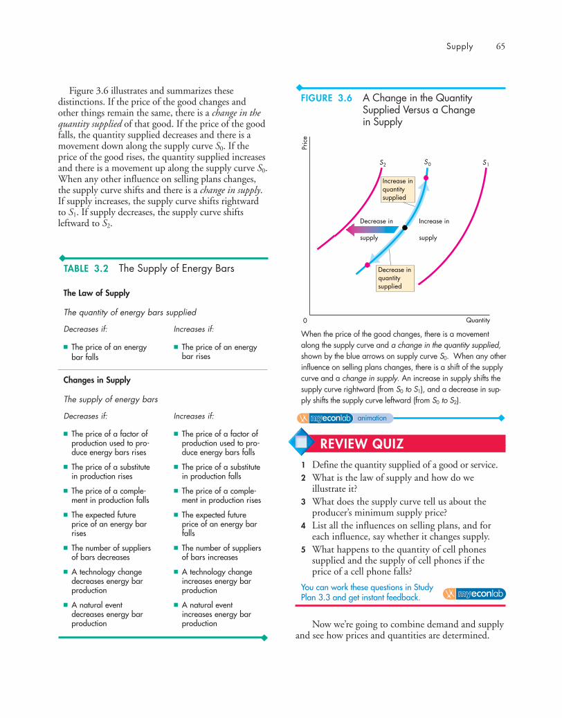
Figure 3.6 illustrates and summarizes thesedistinctions. If the price of the good changes andother things remain the same, there is a change in thequantity supplied of that good. If the price of the goodfalls, the quantity supplied decreases and there is amovement down along the supply curve S0. If theprice of the good rises, the quantity supplied increasesand there is a movement up along the supply curve S0.When any other influence on selling plans changes,the supply curve shifts and there is a change in supply.If supply increases, the supply curve shifts rightwardto S1. If supply decreases, the supply curve shiftsleftward to S2.

Now we’re going to combine demand and supplyand see how prices and quantities are determined.

Supply 65

Quantity

Pric

e

Decrease in

supply

Increase in

supply

0

Decrease inquantitysupplied

Increase inquantitysupplied

S2 S0 S1

When the price of the good changes, there is a movementalong the supply curve and a change in the quantity supplied,shown by the blue arrows on supply curve S0. When any otherinfluence on selling plans changes, there is a shift of the supplycurve and a change in supply. An increase in supply shifts thesupply curve rightward (from S0 to S1), and a decrease in sup-ply shifts the supply curve leftward (from S0 to S2).

FIGURE 3.6 A Change in the QuantitySupplied Versus a Changein Supply

animation

REVIEW QUIZ1 Define the quantity supplied of a good or service.2 What is the law of supply and how do we

illustrate it?3 What does the supply curve tell us about the

producer’s minimum supply price?4 List all the influences on selling plans, and for

each influence, say whether it changes supply.5 What happens to the quantity of cell phones

supplied and the supply of cell phones if theprice of a cell phone falls?

You can work these questions in Study Plan 3.3 and get instant feedback.

TABLE 3.2 The Supply of Energy Bars

The Law of Supply

The quantity of energy bars supplied

Decreases if: Increases if:

■ The price of an energybar falls

■ The price of an energybar rises

■ The price of a factor ofproduction used to pro-duce energy bars rises

■ The price of a substitutein production rises

■ The price of a comple-ment in production falls

■ The expected futureprice of an energy barrises

■ The number of suppliersof bars decreases

■ A technology changedecreases energy barproduction

■ A natural eventdecreases energy barproduction

■ The price of a factor ofproduction used to pro-duce energy bars falls

■ The price of a substitutein production falls

■ The price of a comple-ment in production rises

■ The expected futureprice of an energy barfalls

■ The number of suppliersof bars increases

■ A technology changeincreases energy barproduction

■ A natural eventincreases energy barproduction

Changes in Supply

The supply of energy bars

Decreases if: Increases if:

◆ Market EquilibriumWe have seen that when the price of a good rises, thequantity demanded decreases and the quantity sup-plied increases. We are now going to see how the priceadjusts to coordinate buying plans and selling plansand achieve an equilibrium in the market.

An equilibrium is a situation in which opposingforces balance each other. Equilibrium in a marketoccurs when the price balances buying plans and sell-ing plans. The equilibrium price is the price at whichthe quantity demanded equals the quantity supplied.The equilibrium quantity is the quantity bought andsold at the equilibrium price. A market moves towardits equilibrium because

■ Price regulates buying and selling plans.■ Price adjusts when plans don’t match.

Price as a RegulatorThe price of a good regulates the quantitiesdemanded and supplied. If the price is too high, thequantity supplied exceeds the quantity demanded. Ifthe price is too low, the quantity demanded exceedsthe quantity supplied. There is one price at which thequantity demanded equals the quantity supplied.Let’s work out what that price is.

Figure 3.7 shows the market for energy bars. Thetable shows the demand schedule (from Fig. 3.1) andthe supply schedule (from Fig. 3.4). If the price is50¢ a bar, the quantity demanded is 22 million bars aweek but no bars are supplied. There is a shortage of22 million bars a week. The final column of the tableshows this shortage. At a price of $1.00 a bar, there isstill a shortage but only of 9 million bars a week.

If the price is $2.50 a bar, the quantity supplied is15 million bars a week but the quantity demanded isonly 5 million. There is a surplus of 10 million bars aweek.

The one price at which there is neither a shortagenor a surplus is $1.50 a bar. At that price, the quan-tity demanded equals the quantity supplied: 10 mil-lion bars a week. The equilibrium price is $1.50 abar, and the equilibrium quantity is 10 million bars aweek.

Figure 3.7 shows that the demand curve and thesupply curve intersect at the equilibrium price of $1.50a bar. At each price above $1.50 a bar, there is a surplusof bars. For example, at $2.00 a bar, the surplus is 6

66 CHAPTER 3 Demand and Supply

3.00

0 5 15 20 25Pr

ice

(dol

lars

per

bar

)Quantity (millions of bars per week)

Demand forenergy bars

10

2.50

2.00

1.50

1.00

0.50

Supply ofenergy bars

Equilibrium

Surplus of 6 million barsat $2.00 a bar

Shortage of 9 million barsat $1.00 a bar

PriceQuantity Quantity Shortage (–)

(dollarsdemanded supplied or surplus (+)

per bar) (millions of bars per week)

0.50 22 0 –22

1.00 15 6 –9

1.50 10 10 0

2.00 7 13 +6

2.50 5 15 +10

The table lists the quantity demanded and the quantity sup-plied as well as the shortage or surplus of bars at eachprice. If the price is $1.00 a bar, 15 million bars a weekare demanded and 6 million bars are supplied. There is ashortage of 9 million bars a week, and the price rises.

If the price is $2.00 a bar, 7 million bars a week aredemanded and 13 million bars are supplied. There is a sur-plus of 6 million bars a week, and the price falls.

If the price is $1.50 a bar, 10 million bars a week aredemanded and 10 million bars are supplied. There is neithera shortage nor a surplus, and the price does not change. Theprice at which the quantity demanded equals the quantity sup-plied is the equilibrium price, and 10 million bars a week isthe equilibrium quantity.

FIGURE 3.7 Equilibrium

animation

million bars a week, as shown by the blue arrow. Ateach price below $1.50 a bar, there is a shortage of bars.For example, at $1.00 a bar, the shortage is 9 millionbars a week, as shown by the red arrow.

Price AdjustmentsYou’ve seen that if the price is below equilibrium,there is a shortage and that if the price is above equi-librium, there is a surplus. But can we count on theprice to change and eliminate a shortage or a surplus?We can, because such price changes are beneficial toboth buyers and sellers. Let’s see why the pricechanges when there is a shortage or a surplus.

A Shortage Forces the Price Up Suppose the price ofan energy bar is $1. Consumers plan to buy 15 millionbars a week, and producers plan to sell 6 million bars aweek. Consumers can’t force producers to sell morethan they plan, so the quantity that is actually offeredfor sale is 6 million bars a week. In this situation, pow-erful forces operate to increase the price and move ittoward the equilibrium price. Some producers, notic-ing lines of unsatisfied consumers, raise the price.Some producers increase their output. As producerspush the price up, the price rises toward its equilib-rium. The rising price reduces the shortage because itdecreases the quantity demanded and increases thequantity supplied. When the price has increased to thepoint at which there is no longer a shortage, the forcesmoving the price stop operating and the price comesto rest at its equilibrium.

A Surplus Forces the Price Down Suppose the priceof a bar is $2. Producers plan to sell 13 million bars aweek, and consumers plan to buy 7 million bars aweek. Producers cannot force consumers to buy morethan they plan, so the quantity that is actually boughtis 7 million bars a week. In this situation, powerfulforces operate to lower the price and move it towardthe equilibrium price. Some producers, unable to sellthe quantities of energy bars they planned to sell, cuttheir prices. In addition, some producers scale backproduction. As producers cut the price, the price fallstoward its equilibrium. The falling price decreases thesurplus because it increases the quantity demandedand decreases the quantity supplied. When the pricehas fallen to the point at which there is no longer asurplus, the forces moving the price stop operatingand the price comes to rest at its equilibrium.

The Best Deal Available for Buyers and SellersWhen the price is below equilibrium, it is forcedupward. Why don’t buyers resist the increase andrefuse to buy at the higher price? The answer isbecause they value the good more highly than its cur-rent price and they can’t satisfy their demand at thecurrent price. In some markets—for example, themarkets that operate on eBay—the buyers mighteven be the ones who force the price up by offeringto pay a higher price.

When the price is above equilibrium, it is biddownward. Why don’t sellers resist this decrease andrefuse to sell at the lower price? The answer is becausetheir minimum supply price is below the currentprice and they cannot sell all they would like to at thecurrent price. Sellers willingly lower the price to gainmarket share.

At the price at which the quantity demanded andthe quantity supplied are equal, neither buyers norsellers can do business at a better price. Buyers pay thehighest price they are willing to pay for the last unitbought, and sellers receive the lowest price at whichthey are willing to supply the last unit sold.

When people freely make offers to buy and selland when demanders try to buy at the lowest possibleprice and suppliers try to sell at the highest possibleprice, the price at which trade takes place is the equi-librium price—the price at which the quantitydemanded equals the quantity supplied. The pricecoordinates the plans of buyers and sellers, and noone has an incentive to change it.

Market Equilibrium 67

REVIEW QUIZ 1 What is the equilibrium price of a good or service?2 Over what range of prices does a shortage arise?

What happens to the price when there is ashortage?

3 Over what range of prices does a surplus arise?What happens to the price when there is asurplus?

4 Why is the price at which the quantitydemanded equals the quantity supplied theequilibrium price?

5 Why is the equilibrium price the best dealavailable for both buyers and sellers?

You can work these questions in Study Plan 3.4 and get instant feedback.

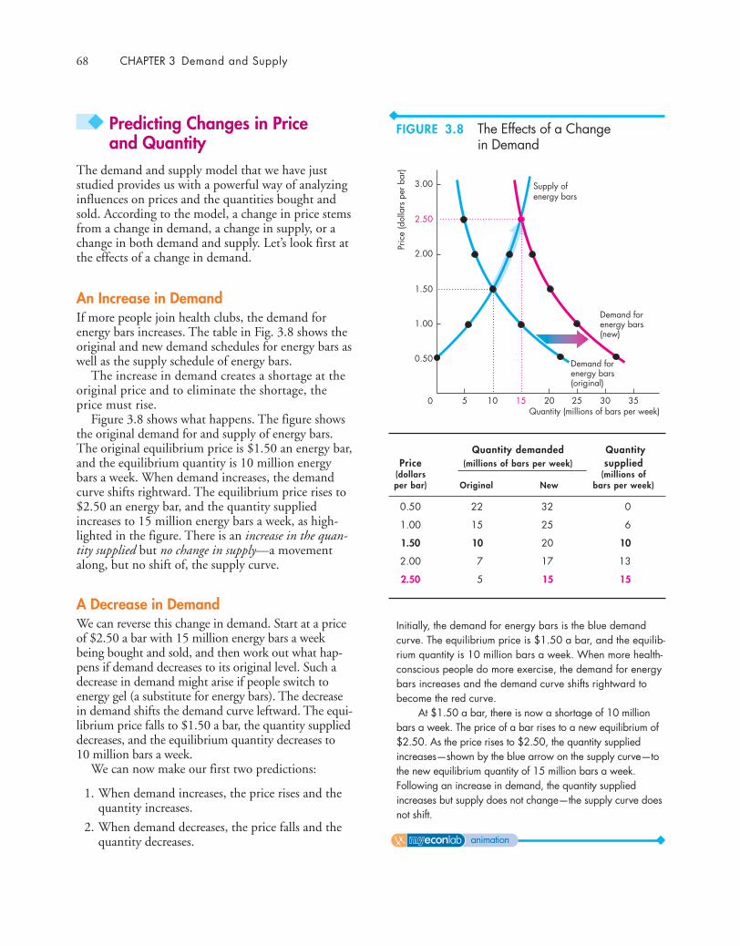
◆ Predicting Changes in Price and Quantity

The demand and supply model that we have juststudied provides us with a powerful way of analyzinginfluences on prices and the quantities bought andsold. According to the model, a change in price stemsfrom a change in demand, a change in supply, or achange in both demand and supply. Let’s look first atthe effects of a change in demand.

An Increase in DemandIf more people join health clubs, the demand forenergy bars increases. The table in Fig. 3.8 shows theoriginal and new demand schedules for energy bars aswell as the supply schedule of energy bars.

The increase in demand creates a shortage at theoriginal price and to eliminate the shortage, theprice must rise.

Figure 3.8 shows what happens. The figure showsthe original demand for and supply of energy bars.The original equilibrium price is $1.50 an energy bar,and the equilibrium quantity is 10 million energybars a week. When demand increases, the demandcurve shifts rightward. The equilibrium price rises to$2.50 an energy bar, and the quantity suppliedincreases to 15 million energy bars a week, as high-lighted in the figure. There is an increase in the quan-tity supplied but no change in supply—a movementalong, but no shift of, the supply curve.

A Decrease in DemandWe can reverse this change in demand. Start at a priceof $2.50 a bar with 15 million energy bars a weekbeing bought and sold, and then work out what hap-pens if demand decreases to its original level. Such adecrease in demand might arise if people switch toenergy gel (a substitute for energy bars). The decreasein demand shifts the demand curve leftward. The equi-librium price falls to $1.50 a bar, the quantity supplieddecreases, and the equilibrium quantity decreases to10 million bars a week.

We can now make our first two predictions:

1. When demand increases, the price rises and thequantity increases.

2. When demand decreases, the price falls and thequantity decreases.

68 CHAPTER 3 Demand and Supply

3.00

5 15 20 35Pr

ice

(dol

lars

per

bar

)Quantity (millions of bars per week)

Supply ofenergy bars

10

2.50

2.00

1.50

1.00

0.50

0 3025

Demand forenergy bars(original)

Demand forenergy bars(new)

Quantity demanded QuantityPrice (millions of bars per week) supplied

(dollars (millions ofper bar) Original New bars per week)

0.50 22 32 0

1.00 15 25 6

1.50 10 20 10

2.00 7 17 13

2.50 5 15 15

Initially, the demand for energy bars is the blue demandcurve. The equilibrium price is $1.50 a bar, and the equilib-rium quantity is 10 million bars a week. When more health-conscious people do more exercise, the demand for energybars increases and the demand curve shifts rightward tobecome the red curve.

At $1.50 a bar, there is now a shortage of 10 millionbars a week. The price of a bar rises to a new equilibrium of$2.50. As the price rises to $2.50, the quantity suppliedincreases—shown by the blue arrow on the supply curve—tothe new equilibrium quantity of 15 million bars a week.Following an increase in demand, the quantity suppliedincreases but supply does not change—the supply curve doesnot shift.

FIGURE 3.8 The Effects of a Changein Demand

animation

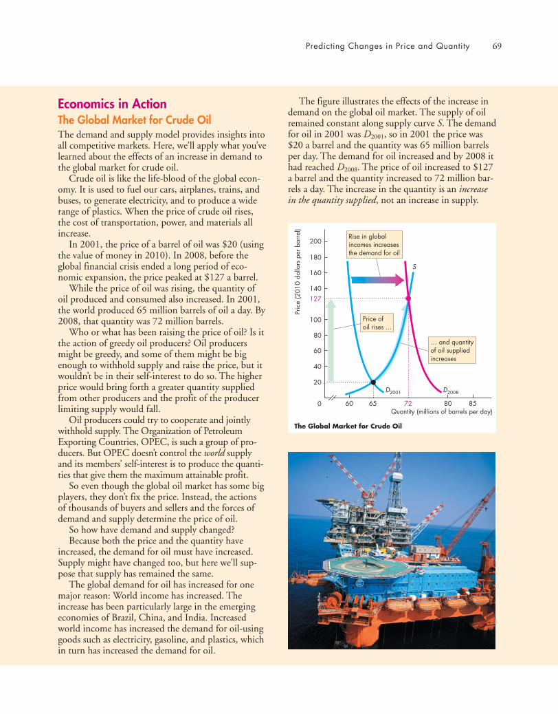
Predicting Changes in Price and Quantity 69

Economics in ActionThe Global Market for Crude OilThe demand and supply model provides insights intoall competitive markets. Here, we’ll apply what you’velearned about the effects of an increase in demand tothe global market for crude oil.

Crude oil is like the life-blood of the global econ-omy. It is used to fuel our cars, airplanes, trains, andbuses, to generate electricity, and to produce a widerange of plastics. When the price of crude oil rises,the cost of transportation, power, and materials allincrease.

In 2001, the price of a barrel of oil was $20 (usingthe value of money in 2010). In 2008, before theglobal financial crisis ended a long period of eco-nomic expansion, the price peaked at $127 a barrel.

While the price of oil was rising, the quantity ofoil produced and consumed also increased. In 2001,the world produced 65 million barrels of oil a day. By2008, that quantity was 72 million barrels.

Who or what has been raising the price of oil? Is itthe action of greedy oil producers? Oil producersmight be greedy, and some of them might be bigenough to withhold supply and raise the price, but itwouldn’t be in their self-interest to do so. The higherprice would bring forth a greater quantity suppliedfrom other producers and the profit of the producerlimiting supply would fall.

Oil producers could try to cooperate and jointlywithhold supply. The Organization of PetroleumExporting Countries, OPEC, is such a group of pro-ducers. But OPEC doesn’t control the world supplyand its members’ self-interest is to produce the quanti-ties that give them the maximum attainable profit.

So even though the global oil market has some bigplayers, they don’t fix the price. Instead, the actionsof thousands of buyers and sellers and the forces ofdemand and supply determine the price of oil.

So how have demand and supply changed?Because both the price and the quantity have

increased, the demand for oil must have increased.Supply might have changed too, but here we’ll sup-pose that supply has remained the same.

The global demand for oil has increased for onemajor reason: World income has increased. Theincrease has been particularly large in the emergingeconomies of Brazil, China, and India. Increasedworld income has increased the demand for oil-usinggoods such as electricity, gasoline, and plastics, whichin turn has increased the demand for oil.

The figure illustrates the effects of the increase indemand on the global oil market. The supply of oilremained constant along supply curve S. The demandfor oil in 2001 was D2001, so in 2001 the price was$20 a barrel and the quantity was 65 million barrelsper day. The demand for oil increased and by 2008 ithad reached D2008. The price of oil increased to $127a barrel and the quantity increased to 72 million bar-rels a day. The increase in the quantity is an increasein the quantity supplied, not an increase in supply.

200

60 72 85

Pric

e (2

010

dolla

rs p

er b

arre

l)

Quantity (millions of barrels per day)65

127

20

40

0

60

80

100

140

160

180

80

S

D2001 D2008

Rise in globalincomes increasesthe demand for oil

The Global Market for Crude Oil

Price ofoil rises ...

… and quantityof oil suppliedincreases

70 CHAPTER 3 Demand and Supply

An Increase in SupplyWhen Nestlé (the producer of PowerBar) and otherenergy bar producers switch to a new cost-savingtechnology, the supply of energy bars increases.Figure 3.9 shows the new supply schedule (the sameone that was shown in Fig. 3.5). What are the newequilibrium price and quantity? The price falls to$1.00 a bar, and the quantity increases to 15 millionbars a week. You can see why by looking at the quan-tities demanded and supplied at the old price of$1.50 a bar. The new quantity supplied at that priceis 20 million bars a week, and there is a surplus. Theprice falls. Only when the price is $1.00 a bar doesthe quantity supplied equal the quantity demanded.

Figure 3.9 illustrates the effect of an increase insupply. It shows the demand curve for energy barsand the original and new supply curves. The initialequilibrium price is $1.50 a bar, and the equilib-rium quantity is 10 million bars a week. When sup-ply increases, the supply curve shifts rightward. Theequilibrium price falls to $1.00 a bar, and the quan-tity demanded increases to 15 million bars a week,highlighted in the figure. There is an increase in thequantity demanded but no change in demand—amovement along, but no shift of, the demand curve.

A Decrease in SupplyStart out at a price of $1.00 a bar with 15 millionbars a week being bought and sold. Then supposethat the cost of labor or raw materials rises and thesupply of energy bars decreases. The decrease in sup-ply shifts the supply curve leftward. The equilibriumprice rises to $1.50 a bar, the quantity demandeddecreases, and the equilibrium quantity decreases to10 million bars a week.

We can now make two more predictions:

1. When supply increases, the price falls and thequantity increases.

2. When supply decreases, the price rises and thequantity decreases.

You’ve now seen what happens to the price and thequantity when either demand or supply changes whilethe other one remains unchanged. In real markets,both demand and supply can change together. Whenthis happens, to predict the changes in price andquantity, we must combine the effects that you’ve justseen. That is your final task in this chapter.

3.00

5 15 20 35Pr

ice

(dol

lars

per

bar

)Quantity (millions of bars per week)

Supply ofenergy bars(original)

Demand forenergy bars

Supply ofenergy bars(new)

10

2.50

2.00

1.50

1.00

0.50

0 3025

QuantityPrice demanded Quantity supplied

(dollars (millions of bars (millions of bars per week)

per bar) per week) Original New

0.50 22 0 7

1.00 15 6 15

1.50 10 10 20

2.00 7 13 25

2.50 5 15 27

Initially, the supply of energy bars is shown by the blue sup-ply curve. The equilibrium price is $1.50 a bar, and theequilibrium quantity is 10 million bars a week. When thenew cost-saving technology is adopted, the supply ofenergy bars increases and the supply curve shifts rightwardto become the red curve.

At $1.50 a bar, there is now a surplus of 10 millionbars a week. The price of an energy bar falls to a new equi-librium of $1.00 a bar. As the price falls to $1.00, thequantity demanded increases—shown by the blue arrow onthe demand curve—to the new equilibrium quantity of 15million bars a week. Following an increase in supply, thequantity demanded increases but demand does notchange—the demand curve does not shift.

FIGURE 3.9 The Effects of a Changein Supply

animation

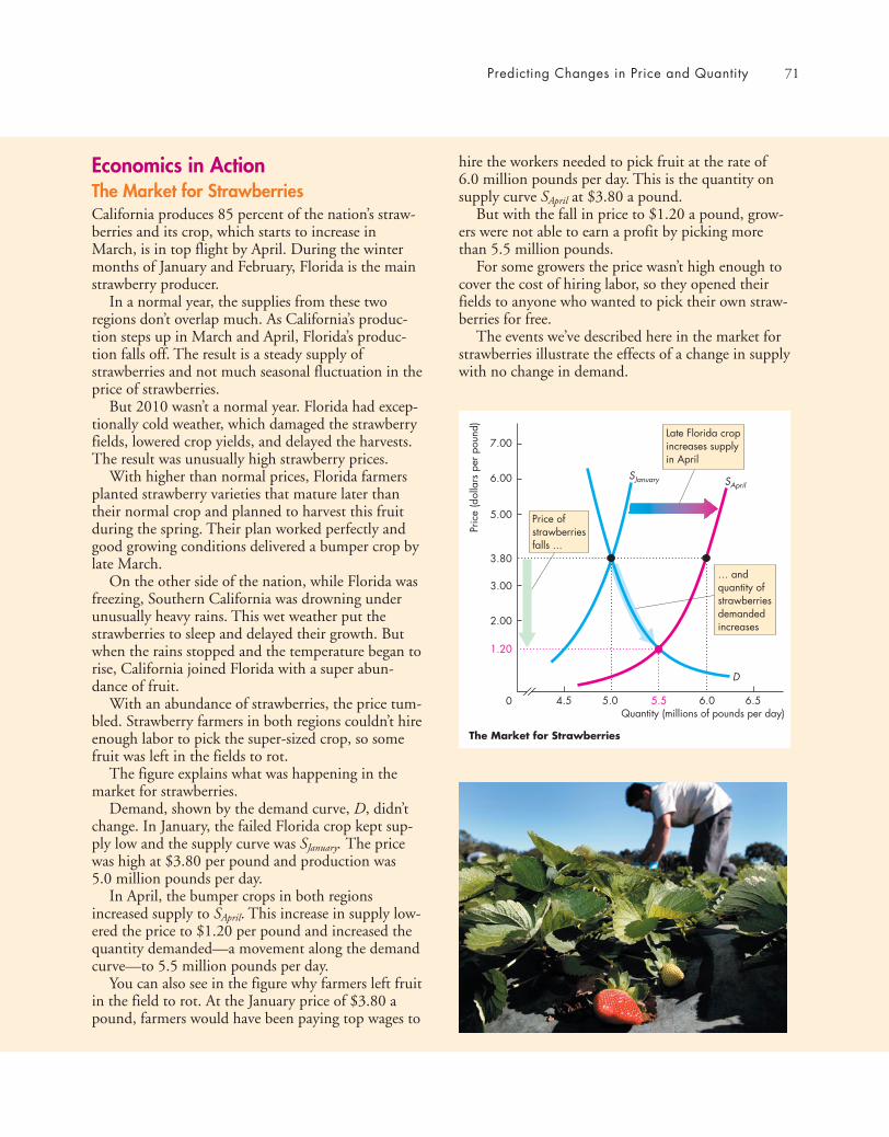
Economics in ActionThe Market for StrawberriesCalifornia produces 85 percent of the nation’s straw-berries and its crop, which starts to increase inMarch, is in top flight by April. During the wintermonths of January and February, Florida is the mainstrawberry producer.

In a normal year, the supplies from these tworegions don’t overlap much. As California’s produc-tion steps up in March and April, Florida’s produc-tion falls off. The result is a steady supply ofstrawberries and not much seasonal fluctuation in theprice of strawberries.

But 2010 wasn’t a normal year. Florida had excep-tionally cold weather, which damaged the strawberryfields, lowered crop yields, and delayed the harvests.The result was unusually high strawberry prices.

With higher than normal prices, Florida farmersplanted strawberry varieties that mature later thantheir normal crop and planned to harvest this fruitduring the spring. Their plan worked perfectly andgood growing conditions delivered a bumper crop bylate March.

On the other side of the nation, while Florida wasfreezing, Southern California was drowning underunusually heavy rains. This wet weather put thestrawberries to sleep and delayed their growth. Butwhen the rains stopped and the temperature began torise, California joined Florida with a super abun-dance of fruit.

With an abundance of strawberries, the price tum-bled. Strawberry farmers in both regions couldn’t hireenough labor to pick the super-sized crop, so somefruit was left in the fields to rot.

The figure explains what was happening in themarket for strawberries.

Demand, shown by the demand curve, D, didn’tchange. In January, the failed Florida crop kept sup-ply low and the supply curve was SJanuary. The pricewas high at $3.80 per pound and production was 5.0 million pounds per day.

In April, the bumper crops in both regionsincreased supply to SApril. This increase in supply low-ered the price to $1.20 per pound and increased thequantity demanded—a movement along the demandcurve—to 5.5 million pounds per day.

You can also see in the figure why farmers left fruitin the field to rot. At the January price of $3.80 apound, farmers would have been paying top wages to

hire the workers needed to pick fruit at the rate of6.0 million pounds per day. This is the quantity onsupply curve SApril at $3.80 a pound.

But with the fall in price to $1.20 a pound, grow-ers were not able to earn a profit by picking morethan 5.5 million pounds.

For some growers the price wasn’t high enough tocover the cost of hiring labor, so they opened theirfields to anyone who wanted to pick their own straw-berries for free.

The events we’ve described here in the market forstrawberries illustrate the effects of a change in supplywith no change in demand.

Predicting Changes in Price and Quantity 71

7.00

5.5 6.5

Pric

e (d

olla

rs p

er p

ound

)

Quantity (millions of pounds per day)5.0

1.20

2.00

3.80

0

6.00

3.00

5.00

6.04.5

D

SJanuary SApril

Price ofstrawberriesfalls ...

Late Florida cropincreases supplyin April

The Market for Strawberries

… andquantity ofstrawberriesdemandedincreases

Decrease in Both Demand and Supply Figure 3.10(i)shows the case in which demand and supply bothdecrease. For the same reasons as those we’ve justreviewed, when both demand and supply decrease,the quantity decreases, and again the direction of theprice change is uncertain.

Decrease in Demand and Increase in Supply You’veseen that a decrease in demand lowers the price anddecreases the quantity. And you’ve seen that anincrease in supply lowers the price and increases thequantity. Fig. 3.10(f ) combines these two changes.Both the decrease in demand and the increase in sup-ply lower the price, so the price falls. But a decreasein demand decreases the quantity and an increase insupply increases the quantity, so we can’t predict thedirection in which the quantity will change unless weknow the magnitudes of the changes in demand andsupply. In the example in Fig. 3.10(f ), the quantitydoes not change. But notice that if demand decreasesby slightly more than the amount shown in the fig-ure, the quantity will decrease; if supply increases byslightly more than the amount shown in the figure,the quantity will increase.

Increase in Demand and Decrease in Supply Figure3.10(h) shows the case in which demand increasesand supply decreases. Now, the price rises, and againthe direction of the quantity change is uncertain.

All the Possible Changes in Demand and SupplyFigure 3.10 brings together and summarizes theeffects of all the possible changes in demand and sup-ply. With what you’ve learned about the effects of achange in either demand or supply, you can predictwhat happens if both demand and supply changetogether. Let’s begin by reviewing what you alreadyknow.

Change in Demand with No Change in Supply Thefirst row of Fig. 3.10, parts (a), (b), and (c), summa-rizes the effects of a change in demand with nochange in supply. In part (a), with no change ineither demand or supply, neither the price nor thequantity changes. With an increase in demand andno change in supply in part (b), both the price andquantity increase. And with a decrease in demandand no change in supply in part (c), both the priceand the quantity decrease.

Change in Supply with No Change in Demand Thefirst column of Fig. 3.10, parts (a), (d), and (g),summarizes the effects of a change in supply withno change in demand. With an increase in supplyand no change in demand in part (d), the price fallsand quantity increases. And with a decrease in sup-ply and no change in demand in part (g), the pricerises and the quantity decreases.

Increase in Both Demand and Supply You’ve seenthat an increase in demand raises the price andincreases the quantity. And you’ve seen that anincrease in supply lowers the price and increases thequantity. Fig. 3.10(e) combines these two changes.Because either an increase in demand or an increasein supply increases the quantity, the quantity alsoincreases when both demand and supply increase.But the effect on the price is uncertain. An increasein demand raises the price and an increase in supplylowers the price, so we can’t say whether the pricewill rise or fall when both demand and supplyincrease. We need to know the magnitudes of thechanges in demand and supply to predict the effectson price. In the example in Fig. 3.10(e), the pricedoes not change. But notice that if demandincreases by slightly more than the amount shownin the figure, the price will rise. And if supplyincreases by slightly more than the amount shownin the figure, the price will fall.

◆ To complete your study of demand and supply,take a look at Reading Between the Lines on pp.74–75, which explains why the price of coffeeincreased in 2010. Try to get into the habit of usingthe demand and supply model to understand themovements in prices in your everyday life.

REVIEW QUIZ What is the effect on the price and quantity ofMP3 players (such as the iPod) if

1 The price of a PC falls or the price of an MP3download rises? (Draw the diagrams!)

2 More firms produce MP3 players or electronicsworkers’ wages rise? (Draw the diagrams!)

3 Any two of the events in questions 1 and 2occur together? (Draw the diagrams!)

You can work these questions in Study Plan 3.5 and get instant feedback.

72 CHAPTER 3 Demand and Supply

Predicting Changes in Price and Quantity 73

Demand

3.00

0 5 15 20

Pric

e (d

olla

rs p

er b

ar)

Quantity (millions of bars)10

2.50

2.00

1.50

1.00

0.50

Demand

3.00

0 5 15 20

Pric

e (d

olla

rs p

er b

ar)

Quantity (millions of bars)10

2.50

2.00

1.50

1.00

0.50

(d) Increase in supply (e) Increase in both demand and supply (f) Decrease in demand; increase in supply

(g) Decrease in supply (i) Decrease in both demand and supply(h) Increase in demand; decrease in supply

Demand(original)

Demand(new)

Supply(new)

Supply(original)

Demand(original)

Demand(new)

Supply(new)

Supply(original)

Demand(new)

Demand(original)

Supply(original)

Supply(new)

Demand(new)

Demand(original)

3.00

0 5 15 20

Pric

e (d

olla

rs p

er b

ar)

Quantity (millions of bars)10

2.50

2.00

1.50

1.00

0.50

Supply(new)

Supply(original)3.00

0 15 20

Pric

e (d

olla

rs p

er b

ar)

Quantity (millions of bars)10

2.50

2.00

1.50

1.00

0.50

Supply(new)

Supply(original)

3.00

0 5 15 20

Pric

e (d

olla

rs p

er b

ar)

Quantity (millions of bars)10

2.50

2.00

1.50

1.00

0.50

3.00

0 5 15 20

Pric

e (d

olla

rs p

er b

ar)

Quantity (millions of bars)10

2.50

2.00

1.50

1.00

0.50

Supply(new)

Supply(original)

Demand

Supply3.00

0 5 15 20

Pric

e (d

olla

rs p

er b

ar)

Quantity (millions of bars)

(a) No change in demand or supply

10

2.50

2.00

1.50

1.00

0.50

(c) Decrease in demand(b) Increase in demand

Equilibrium

Supply3.00

0 5 15 20

Pric

e (d

olla

rs p

er b

ar)

Quantity (millions of bars)10

2.50

2.00

1.50

1.00

0.50

Demand(new)

Demand(original)

Supply3.00

0 6 15 20

Pric

e (d

olla

rs p

er b

ar)

Quantity (millions of bars)10

2.50

2.00

1.50

1.00

0.50Demand(new)

Demand(original)

?

?

?

?

?

?

? ?

FIGURE 3.10 The Effects of All the Possible Changes in Demand and Supply

animation

74

Coffee Surges on Poor Colombian HarvestsFT.comJuly 30, 2010

Coffee prices hit a 12-year high on Friday on the back of low supplies of premium Arabicacoffee from Colombia after a string of poor crops in the Latin American country.

The strong fundamental picture has also encouraged hedge funds to reverse their previousbearish views on coffee prices.

In New York, ICE September Arabica coffee jumped 3.2 percent to 178.75 cents per pound,the highest since February 1998. It traded later at 177.25 cents, up 6.8 percent on the week.

The London-based International Coffee Organization on Friday warned that the “currenttight demand and supply situation” was “likely to persist in the near to medium term.”

Coffee industry executives believe prices could rise toward 200 cents per pound in New Yorkbefore the arrival of the new Brazilian crop laterthis year.

“Until October it is going to be tight on highquality coffee,” said a senior executive at one ofEurope’s largest coffee roasters. He said: “Theindustry has been surprised by the scarcity ofhigh quality beans.”

Colombia coffee production, key for supplies ofpremium beans, last year plunged to a 33-yearlow of 7.8m bags, each of 60kg, down nearly athird from 11.1m bags in 2008, tightening sup-plies worldwide. ...

Excerpted from “Coffee Surges on Poor Colombian Harvests” by JavierBlas. Financial Times, July 30, 2010. Reprinted with permission.

READING BETWEEN THE L INES

Demand and Supply: The Price of Coffee

■ The price of premium Arabica coffee increasedby 3.2 percent to almost 180 cents per pound inJuly 2010, the highest price since February1998.

■ A sequence of poor crops in Columbia cut theproduction of premium Arabica coffee to a 33-year low of 7.8 million 60 kilogram bags, downfrom 11.1 million bags in 2008.

■ The International Coffee Organization said thatthe “current tight demand and supply situation”was “likely to persist in the near to medium term.”

■ Coffee industry executives say prices mightapproach 200 cents per pound before the arrivalof the new Brazilian crop later this year.

■ Hedge funds previously expected the price of cof-fee to fall but now expect it to rise further.

ESSENCE OF THE STORY

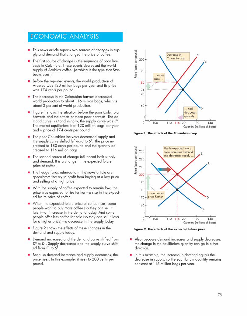
75

Figure 2 The effects of the expected future price

D

S1

S0

Figure 1 The effects of the Columbian crop

Decrease inColumbia crop ...

Pric

e (c

ents

per p

ound

)

Quantity (millions of bags)0

160

110 116 130 140120

170174

180

190

200

100

... anddecreasesquantity

... raisesprice ...

D0

D1

S1

S0

Rise in expected futureprice increases demandand decreases supply ...

Pric

e (c

ents

per p

ound

)

Quantity (millions of bags)0

160

110 116 130 140120

170

180

190

200

210

220

230

100

... and raisesprice further

ECONOMIC ANALYSIS

■ This news article reports two sources of changes in sup-ply and demand that changed the price of coffee.

■ The first source of change is the sequence of poor har-vests in Columbia. These events decreased the worldsupply of Arabica coffee. (Arabica is the type that Star-bucks uses.)

■ Before the reported events, the world production ofArabica was 120 million bags per year and its pricewas 174 cents per pound.

■ The decrease in the Columbian harvest decreasedworld production to about 116 million bags, which isabout 3 percent of world production.

■ Figure 1 shows the situation before the poor Columbiaharvests and the effects of those poor harvests. The de-mand curve is D and initially, the supply curve was S0.The market equilibrium is at 120 million bags per yearand a price of 174 cents per pound.

■ The poor Columbian harvests decreased supply andthe supply curve shifted leftward to S1. The price in-creased to 180 cents per pound and the quantity de-creased to 116 million bags.

■ The second source of change influenced both supplyand demand. It is a change in the expected futureprice of coffee.

■ The hedge funds referred to in the news article arespeculators that try to profit from buying at a low priceand selling at a high price.

■ With the supply of coffee expected to remain low, theprice was expected to rise further—a rise in the expect-ed future price of coffee.

■ When the expected future price of coffee rises, somepeople want to buy more coffee (so they can sell itlater)—an increase in the demand today. And somepeople offer less coffee for sale (so they can sell it laterfor a higher price)—a decrease in the supply today.

■ Figure 2 shows the effects of these changes in thedemand and supply today.

■ Demand increased and the demand curve shifted fromD0 to D1. Supply decreased and the supply curve shift-ed from S1 to S2.

■ Because demand increases and supply decreases, theprice rises. In this example, it rises to 200 cents perpound.

■ Also, because demand increases and supply decreases,the change in the equilibrium quantity can go in eitherdirection.

■ In this example, the increase in demand equals thedecrease in supply, so the equilibrium quantity remainsconstant at 116 million bags per year.

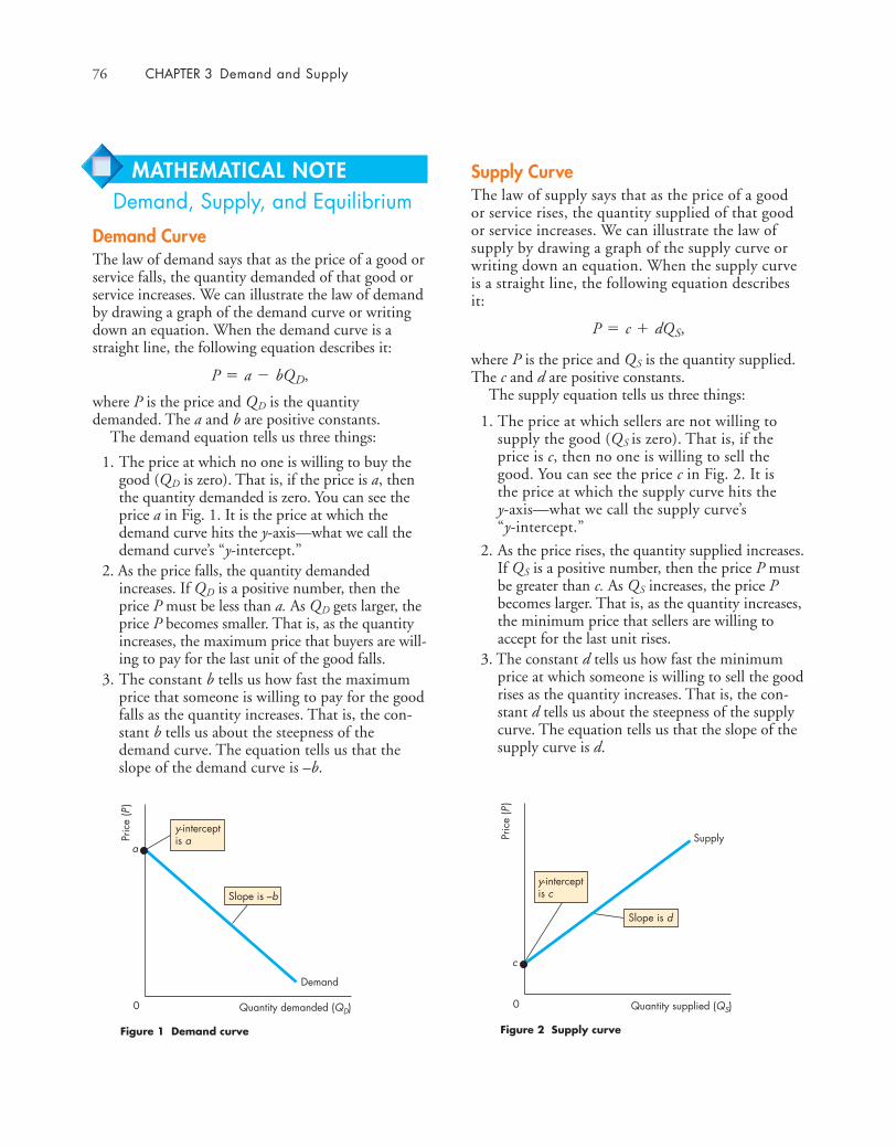
76 CHAPTER 3 Demand and Supply

MATHEMATICAL NOTEDemand, Supply, and Equilibrium

Demand CurveThe law of demand says that as the price of a good orservice falls, the quantity demanded of that good orservice increases. We can illustrate the law of demandby drawing a graph of the demand curve or writingdown an equation. When the demand curve is astraight line, the following equation describes it:

where P is the price and QD is the quantitydemanded. The a and b are positive constants.

The demand equation tells us three things:

1. The price at which no one is willing to buy thegood (QD is zero). That is, if the price is a, thenthe quantity demanded is zero. You can see theprice a in Fig. 1. It is the price at which thedemand curve hits the y-axis—what we call thedemand curve’s “y-intercept.”

2. As the price falls, the quantity demandedincreases. If QD is a positive number, then theprice P must be less than a. As QD gets larger, theprice P becomes smaller. That is, as the quantityincreases, the maximum price that buyers are will-ing to pay for the last unit of the good falls.

3. The constant b tells us how fast the maximumprice that someone is willing to pay for the goodfalls as the quantity increases. That is, the con-stant b tells us about the steepness of thedemand curve. The equation tells us that theslope of the demand curve is –b.

Quantity demanded (QD)0

Pric

e (P

)

a

Demand

y-interceptis a

Slope is –b

Figure 1 Demand curve

P = a - bQD,

Supply CurveThe law of supply says that as the price of a goodor service rises, the quantity supplied of that goodor service increases. We can illustrate the law ofsupply by drawing a graph of the supply curve orwriting down an equation. When the supply curveis a straight line, the following equation describesit:

where P is the price and QS is the quantity supplied.The c and d are positive constants.

The supply equation tells us three things:

1. The price at which sellers are not willing tosupply the good (QS is zero). That is, if theprice is c, then no one is willing to sell thegood. You can see the price c in Fig. 2. It is the price at which the supply curve hits the y-axis—what we call the supply curve’s “y-intercept.”

2. As the price rises, the quantity supplied increases.If QS is a positive number, then the price P mustbe greater than c. As QS increases, the price Pbecomes larger. That is, as the quantity increases,the minimum price that sellers are willing toaccept for the last unit rises.

3. The constant d tells us how fast the minimumprice at which someone is willing to sell the goodrises as the quantity increases. That is, the con-stant d tells us about the steepness of the supplycurve. The equation tells us that the slope of thesupply curve is d.

P = c + dQS,

Quantity supplied (QS)0

Pric

e (P

)

c

Supply

Slope is d

Figure 2 Supply curve

y-interceptis c

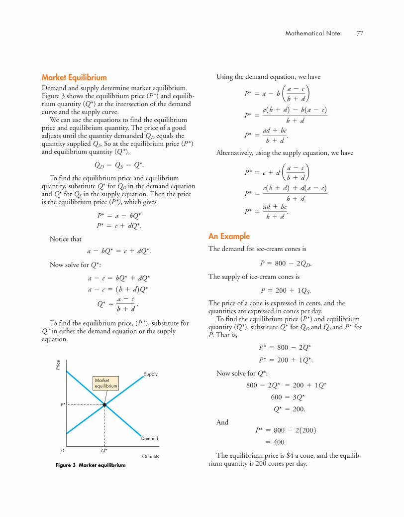
Market EquilibriumDemand and supply determine market equilibrium.Figure 3 shows the equilibrium price (P*) and equilib-rium quantity (Q*) at the intersection of the demandcurve and the supply curve.

We can use the equations to find the equilibriumprice and equilibrium quantity. The price of a goodadjusts until the quantity demanded QD equals thequantity supplied QS. So at the equilibrium price (P* )and equilibrium quantity (Q* ),

To find the equilibrium price and equilibriumquantity, substitute Q* for QD in the demand equationand Q* for QS in the supply equation. Then the priceis the equilibrium price (P*), which gives

Notice that

Now solve for Q*:

To find the equilibrium price, (P* ), substitute forQ* in either the demand equation or the supplyequation.

Quantity0

Pric

e

P*

Q*

Demand

SupplyMarketequilibrium

Figure 3 Market equilibrium

Q* =a - cb + d

.

a - c = 1b + d2Q*

a - c = bQ* + dQ*

a - bQ* = c + dQ*.

P* = c + dQ*.P* = a - bQ*

QD = QS = Q*.

Using the demand equation, we have

Alternatively, using the supply equation, we have

An ExampleThe demand for ice-cream cones is

The supply of ice-cream cones is

The price of a cone is expressed in cents, and thequantities are expressed in cones per day.

To find the equilibrium price (P*) and equilibriumquantity (Q*), substitute Q* for QD and QS and P* forP. That is,

Now solve for Q*:

And

The equilibrium price is $4 a cone, and the equilib-rium quantity is 200 cones per day.

= 400.

P* = 800 - 212002Q* = 200.

600 = 3Q*

800 - 2Q* = 200 + 1Q*

P* = 200 + 1Q*.

P* = 800 - 2Q*

P = 200 + 1QS.

P = 800 - 2QD.

P* =ad + bcb + d

.

P* =c1b + d2 + d1a - c2

b + d

P * = c + d a a - cb + d

b

P* =ad + bcb + d

.

P* =a1b + d2 - b1a - c2

b + d

P* = a - b a a - cb + d

b

Mathematical Note 77

■ Supply depends on the prices of factors of produc-tion used to produce a good, the prices of relatedgoods produced, expected future prices, the num-ber of suppliers, technology, and the state ofnature.

Working Problems 6 to 9 will give you a better under-standing of supply.

Market Equilibrium (pp. 66–67)

■ At the equilibrium price, the quantity demandedequals the quantity supplied.

■ At any price above the equilibrium price, there is asurplus and the price falls.

■ At any price below the equilibrium price, there is ashortage and the price rises.

Working Problems 10 and 11 will give you a better under-standing of market equilibrium

Predicting Changes in Price and Quantity (pp. 68–73)

■ An increase in demand brings a rise in the priceand an increase in the quantity supplied. Adecrease in demand brings a fall in the price and adecrease in the quantity supplied.

■ An increase in supply brings a fall in the price andan increase in the quantity demanded. A decreasein supply brings a rise in the price and a decreasein the quantity demanded.

■ An increase in demand and an increase in supply bringan increased quantity but an uncertain price change.An increase in demand and a decrease in supply bringa higher price but an uncertain change in quantity.

Working Problems 12 and 13 will give you a better under-standing of predicting changes in price and quantity.

78 CHAPTER 3 Demand and Supply

Key Points

Markets and Prices (p. 56)

■ A competitive market is one that has so many buy-ers and sellers that no single buyer or seller caninfluence the price.

■ Opportunity cost is a relative price.■ Demand and supply determine relative prices.

Working Problem 1 will give you a better understandingof markets and prices.

Demand (pp. 57–61)

■ Demand is the relationship between the quantitydemanded of a good and its price when all otherinfluences on buying plans remain the same.

■ The higher the price of a good, other thingsremaining the same, the smaller is the quantitydemanded—the law of demand.

■ Demand depends on the prices of related goods (sub-stitutes and complements), expected future prices,income, expected future income and credit, the pop-ulation, and preferences.

Working Problems 2 to 5 will give you a better under-standing of demand.

Supply (pp. 62–65)

■ Supply is the relationship between the quantitysupplied of a good and its price when all otherinfluences on selling plans remain the same.

■ The higher the price of a good, other thingsremaining the same, the greater is the quantitysupplied—the law of supply.

SUMMARY

Key TermsChange in demand, 58Change in supply, 63Change in the quantity

demanded, 61Change in the quantity supplied, 64Competitive market, 56Complement, 59Demand, 57

Demand curve, 58Equilibrium price, 66Equilibrium quantity, 66Inferior good, 60Law of demand, 57Law of supply, 62Money price, 56Normal good, 60

Quantity demanded, 57Quantity supplied, 62Relative price, 56Substitute, 59Supply, 62Supply curve, 62

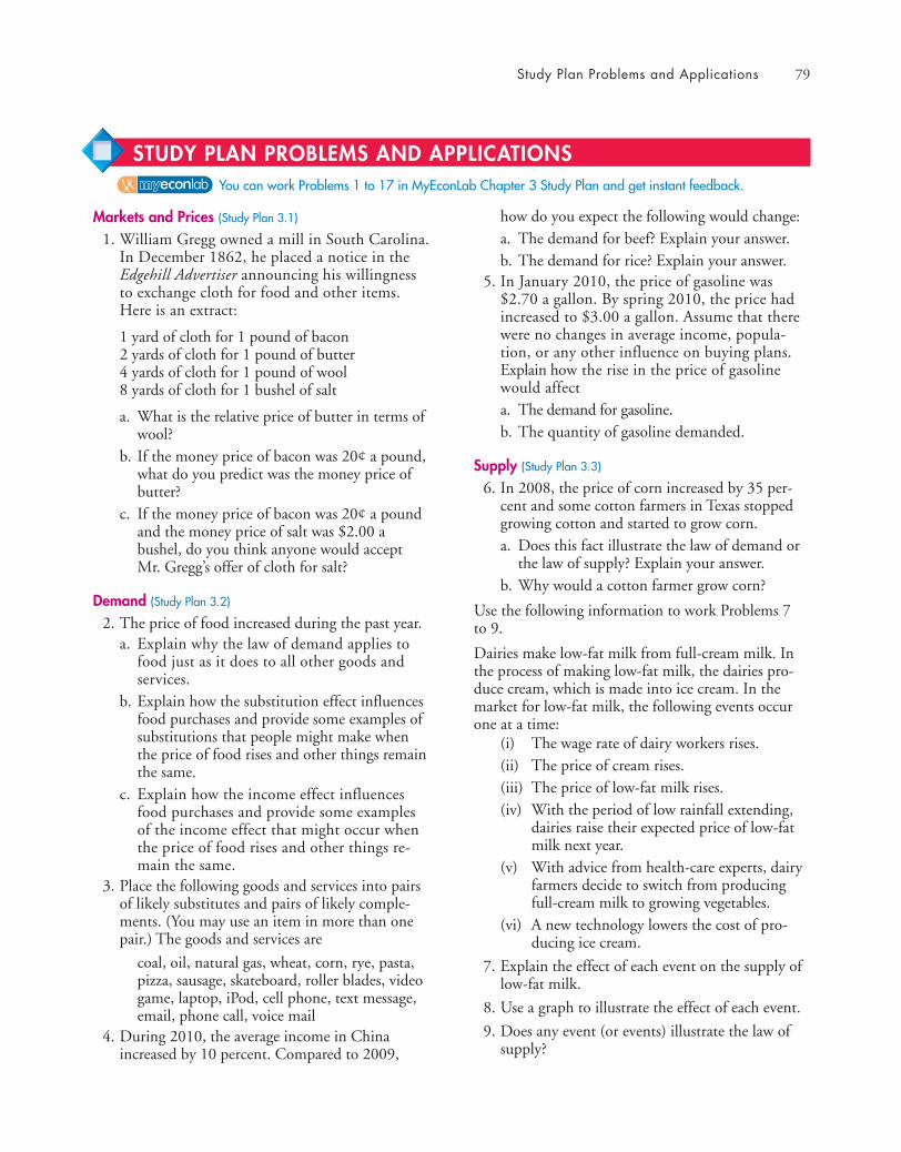
how do you expect the following would change:a. The demand for beef? Explain your answer.b. The demand for rice? Explain your answer.

5. In January 2010, the price of gasoline was$2.70 a gallon. By spring 2010, the price hadincreased to $3.00 a gallon. Assume that therewere no changes in average income, popula-tion, or any other influence on buying plans.Explain how the rise in the price of gasolinewould affecta. The demand for gasoline.b. The quantity of gasoline demanded.

Supply (Study Plan 3.3)

6. In 2008, the price of corn increased by 35 per-cent and some cotton farmers in Texas stoppedgrowing cotton and started to grow corn.a. Does this fact illustrate the law of demand or

the law of supply? Explain your answer.b. Why would a cotton farmer grow corn?

Use the following information to work Problems 7 to 9.

Dairies make low-fat milk from full-cream milk. Inthe process of making low-fat milk, the dairies pro-duce cream, which is made into ice cream. In themarket for low-fat milk, the following events occurone at a time:

(i) The wage rate of dairy workers rises.(ii) The price of cream rises.(iii) The price of low-fat milk rises.(iv) With the period of low rainfall extending,

dairies raise their expected price of low-fatmilk next year.

(v) With advice from health-care experts, dairyfarmers decide to switch from producingfull-cream milk to growing vegetables.

(vi) A new technology lowers the cost of pro-ducing ice cream.

7. Explain the effect of each event on the supply oflow-fat milk.

8. Use a graph to illustrate the effect of each event.

9. Does any event (or events) illustrate the law ofsupply?

Study Plan Problems and Applications 79

Markets and Prices (Study Plan 3.1)

1. William Gregg owned a mill in South Carolina.In December 1862, he placed a notice in theEdgehill Advertiser announcing his willingnessto exchange cloth for food and other items.Here is an extract:

1 yard of cloth for 1 pound of bacon2 yards of cloth for 1 pound of butter4 yards of cloth for 1 pound of wool8 yards of cloth for 1 bushel of salt

a. What is the relative price of butter in terms ofwool?

b. If the money price of bacon was 20¢ a pound,what do you predict was the money price ofbutter?

c. If the money price of bacon was 20¢ a poundand the money price of salt was $2.00 abushel, do you think anyone would acceptMr. Gregg’s offer of cloth for salt?

Demand (Study Plan 3.2)

2. The price of food increased during the past year.a. Explain why the law of demand applies to

food just as it does to all other goods andservices.

b. Explain how the substitution effect influencesfood purchases and provide some examples ofsubstitutions that people might make whenthe price of food rises and other things remainthe same.

c. Explain how the income effect influencesfood purchases and provide some examplesof the income effect that might occur whenthe price of food rises and other things re-main the same.

3. Place the following goods and services into pairsof likely substitutes and pairs of likely comple-ments. (You may use an item in more than onepair.) The goods and services are

coal, oil, natural gas, wheat, corn, rye, pasta,pizza, sausage, skateboard, roller blades, videogame, laptop, iPod, cell phone, text message,email, phone call, voice mail

4. During 2010, the average income in Chinaincreased by 10 percent. Compared to 2009,

You can work Problems 1 to 17 in MyEconLab Chapter 3 Study Plan and get instant feedback.

STUDY PLAN PROBLEMS AND APPLICATIONS

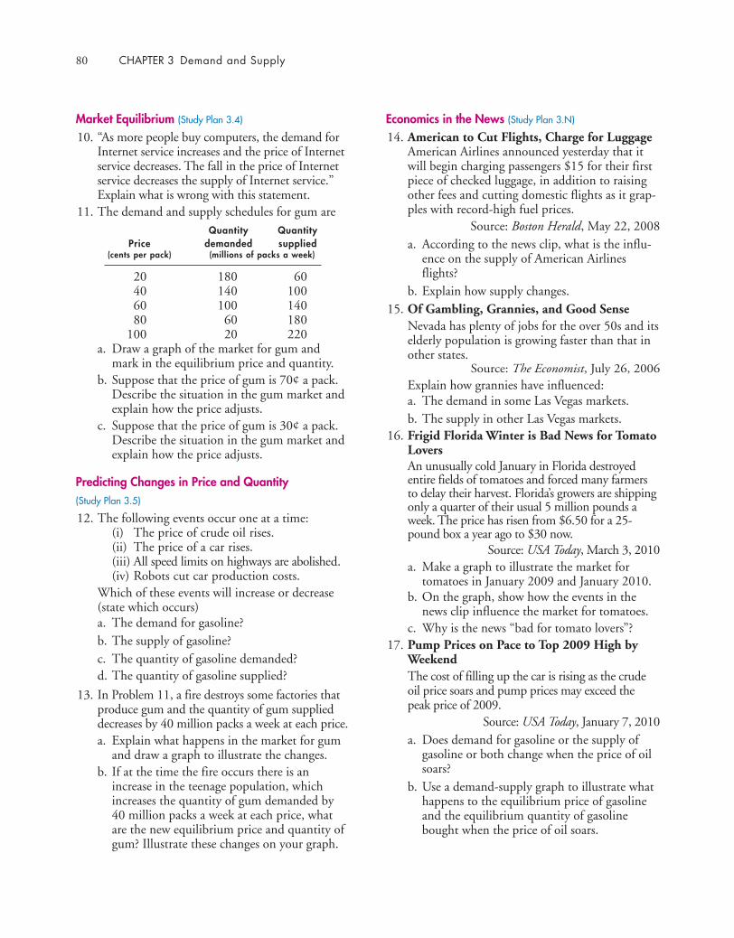
Market Equilibrium (Study Plan 3.4)

10. “As more people buy computers, the demand forInternet service increases and the price of Internetservice decreases. The fall in the price of Internetservice decreases the supply of Internet service.”Explain what is wrong with this statement.

11. The demand and supply schedules for gum areQuantity Quantity

Price demanded supplied(cents per pack) (millions of packs a week)

20 180 6040 140 10060 100 14080 60 180

100 20 220a. Draw a graph of the market for gum and

mark in the equilibrium price and quantity.b. Suppose that the price of gum is 70¢ a pack.

Describe the situation in the gum market andexplain how the price adjusts.

c. Suppose that the price of gum is 30¢ a pack.Describe the situation in the gum market andexplain how the price adjusts.

Predicting Changes in Price and Quantity (Study Plan 3.5)

12. The following events occur one at a time:(i) The price of crude oil rises.(ii) The price of a car rises.(iii) All speed limits on highways are abolished.(iv) Robots cut car production costs.

Which of these events will increase or decrease(state which occurs)a. The demand for gasoline?b. The supply of gasoline?c. The quantity of gasoline demanded?d. The quantity of gasoline supplied?

13. In Problem 11, a fire destroys some factories thatproduce gum and the quantity of gum supplieddecreases by 40 million packs a week at each price.a. Explain what happens in the market for gum

and draw a graph to illustrate the changes.b. If at the time the fire occurs there is an

increase in the teenage population, whichincreases the quantity of gum demanded by40 million packs a week at each price, whatare the new equilibrium price and quantity ofgum? Illustrate these changes on your graph.

80 CHAPTER 3 Demand and Supply

Economics in the News (Study Plan 3.N)

14. American to Cut Flights, Charge for LuggageAmerican Airlines announced yesterday that itwill begin charging passengers $15 for their firstpiece of checked luggage, in addition to raisingother fees and cutting domestic flights as it grap-ples with record-high fuel prices.

Source: Boston Herald, May 22, 2008a. According to the news clip, what is the influ-

ence on the supply of American Airlinesflights?

b. Explain how supply changes.15. Of Gambling, Grannies, and Good Sense

Nevada has plenty of jobs for the over 50s and itselderly population is growing faster than that inother states.

Source: The Economist, July 26, 2006 Explain how grannies have influenced: a. The demand in some Las Vegas markets.b. The supply in other Las Vegas markets.

16. Frigid Florida Winter is Bad News for TomatoLovers An unusually cold January in Florida destroyedentire fields of tomatoes and forced many farmersto delay their harvest. Florida’s growers are shippingonly a quarter of their usual 5 million pounds aweek. The price has risen from $6.50 for a 25-pound box a year ago to $30 now.

Source: USA Today, March 3, 2010a. Make a graph to illustrate the market for

tomatoes in January 2009 and January 2010.b. On the graph, show how the events in the

news clip influence the market for tomatoes.c. Why is the news “bad for tomato lovers”?

17. Pump Prices on Pace to Top 2009 High byWeekendThe cost of filling up the car is rising as the crudeoil price soars and pump prices may exceed thepeak price of 2009.

Source: USA Today, January 7, 2010a. Does demand for gasoline or the supply of

gasoline or both change when the price of oilsoars?

b. Use a demand-supply graph to illustrate whathappens to the equilibrium price of gasolineand the equilibrium quantity of gasolinebought when the price of oil soars.

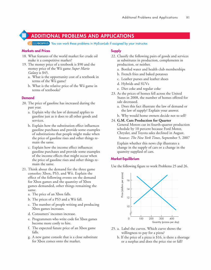
Markets and Prices18. What features of the world market for crude oil

make it a competitive market?19. The money price of a textbook is $90 and the

money price of the Wii game Super MarioGalaxy is $45.a. What is the opportunity cost of a textbook in

terms of the Wii game?b. What is the relative price of the Wii game in

terms of textbooks?

Demand20. The price of gasoline has increased during the

past year.a. Explain why the law of demand applies to

gasoline just as it does to all other goods andservices.

b. Explain how the substitution effect influencesgasoline purchases and provide some examplesof substitutions that people might make whenthe price of gasoline rises and other things re-main the same.

c. Explain how the income effect influencesgasoline purchases and provide some examplesof the income effects that might occur whenthe price of gasoline rises and other things re-main the same.

21. Think about the demand for the three gameconsoles: Xbox, PS3, and Wii. Explain theeffect of the following events on the demandfor Xbox games and the quantity of Xboxgames demanded, other things remaining thesame.a. The price of an Xbox falls.b. The prices of a PS3 and a Wii fall.c. The number of people writing and producing

Xbox games increases.d. Consumers’ incomes increase.e. Programmers who write code for Xbox games

become more costly to hire.f. The expected future price of an Xbox game

falls.g. A new game console that is a close substitute

for Xbox comes onto the market.

Supply22. Classify the following pairs of goods and services

as substitutes in production, complements inproduction, or neither.a. Bottled water and health club membershipsb. French fries and baked potatoesc. Leather purses and leather shoesd. Hybrids and SUVse. Diet coke and regular coke

23. As the prices of homes fell across the UnitedStates in 2008, the number of homes offered forsale decreased.a. Does this fact illustrate the law of demand or

the law of supply? Explain your answer.b. Why would home owners decide not to sell?

24. G.M. Cuts Production for QuarterGeneral Motors cut its fourth-quarter productionschedule by 10 percent because Ford Motor,Chrysler, and Toyota sales declined in August. Source: The New York Times, September 5, 2007

Explain whether this news clip illustrates achange in the supply of cars or a change in thequantity supplied of cars.

Market Equilibrium

Use the following figure to work Problems 25 and 26.

25. a. Label the curves. Which curve shows the willingness to pay for a pizza?

b. If the price of a pizza is $16, is there a shortageor a surplus and does the price rise or fall?

10

12

14

Quantity (pizzas per day)0 100 200 300 400

16

Pric

e (d

olla

rs p

er p

izza

)

Additonal Problems and Applications 81

You can work these problems in MyEconLab if assigned by your instructor.

ADDITIONAL PROBLEMS AND APPLICATIONS

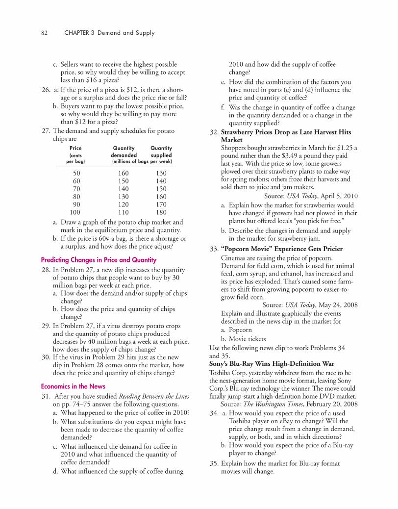
c. Sellers want to receive the highest possibleprice, so why would they be willing to acceptless than $16 a pizza?

26. a. If the price of a pizza is $12, is there a short-age or a surplus and does the price rise or fall?

b. Buyers want to pay the lowest possible price,so why would they be willing to pay morethan $12 for a pizza?

27. The demand and supply schedules for potatochips are

Price Quantity Quantity(cents demanded supplied

per bag) (millions of bags per week)

50 160 13060 150 14070 140 15080 130 16090 120 170

100 110 180a. Draw a graph of the potato chip market and

mark in the equilibrium price and quantity.b. If the price is 60¢ a bag, is there a shortage or

a surplus, and how does the price adjust?

Predicting Changes in Price and Quantity28. In Problem 27, a new dip increases the quantity

of potato chips that people want to buy by 30million bags per week at each price.a. How does the demand and/or supply of chips

change?b. How does the price and quantity of chips

change?29. In Problem 27, if a virus destroys potato crops

and the quantity of potato chips produceddecreases by 40 million bags a week at each price,how does the supply of chips change?

30. If the virus in Problem 29 hits just as the newdip in Problem 28 comes onto the market, howdoes the price and quantity of chips change?

Economics in the News31. After you have studied Reading Between the Lines

on pp. 74–75 answer the following questions.a. What happened to the price of coffee in 2010?b. What substitutions do you expect might have

been made to decrease the quantity of coffeedemanded?

c. What influenced the demand for coffee in2010 and what influenced the quantity ofcoffee demanded?

d. What influenced the supply of coffee during

2010 and how did the supply of coffeechange?

e. How did the combination of the factors youhave noted in parts (c) and (d) influence theprice and quantity of coffee?

f. Was the change in quantity of coffee a changein the quantity demanded or a change in thequantity supplied?

32. Strawberry Prices Drop as Late Harvest HitsMarketShoppers bought strawberries in March for $1.25 apound rather than the $3.49 a pound they paidlast year. With the price so low, some growersplowed over their strawberry plants to make wayfor spring melons; others froze their harvests andsold them to juice and jam makers.

Source: USA Today, April 5, 2010a. Explain how the market for strawberries would

have changed if growers had not plowed in theirplants but offered locals “you pick for free.”

b. Describe the changes in demand and supplyin the market for strawberry jam.

33. “Popcorn Movie” Experience Gets PricierCinemas are raising the price of popcorn.Demand for field corn, which is used for animalfeed, corn syrup, and ethanol, has increased andits price has exploded. That’s caused some farm-ers to shift from growing popcorn to easier-to-grow field corn.

Source: USA Today, May 24, 2008Explain and illustrate graphically the eventsdescribed in the news clip in the market fora. Popcorn b. Movie tickets

Use the following news clip to work Problems 34 and 35.Sony’s Blu-Ray Wins High-Definition WarToshiba Corp. yesterday withdrew from the race to bethe next-generation home movie format, leaving SonyCorp.’s Blu-ray technology the winner. The move couldfinally jump-start a high-definition home DVD market.

Source: The Washington Times, February 20, 200834. a. How would you expect the price of a used

Toshiba player on eBay to change? Will theprice change result from a change in demand,supply, or both, and in which directions?

b. How would you expect the price of a Blu-rayplayer to change?

35. Explain how the market for Blu-ray formatmovies will change.

82 CHAPTER 3 Demand and Supply

After studying this chapter, you will be able to:� Define, calculate, and explain the factors that influence

the price elasticity of demand� Define, calculate, and explain the factors that influence

the cross elasticity of demand and the income elasticityof demand

� Define, calculate, and explain the factors that influencethe elasticity of supply

4What do you do when the price of gasoline soars to $3 a gallon? If you’re

like most people, you complain a lot but keep on filling your tank and spendingmore on gas. Would you react the same way to a rise in the price of tomatoes?In the winter of 2010, a prolonged Florida frost wiped out most of the state’stomato crop, driving the price of tomatoes to almost five times its normal level.If faced with this price rise, do you keep buying the same quantity of tomatoes,or do you find less costly substitutes?

How can we compare the effects of price changes on buying plans fordifferent goods such as gasoline and tomatoes?

This chapter introduces you to elasticity: a tool that addresses thequantitative questions like the ones you’ve just considered and enables us tocompare the sensitivity of the quantity demanded to a change in priceregardless of the units in which the good is measured.

At the end of the chapter, in Reading Between the Lines, we’ll use theconcepts of the elasticity of demand and the elasticity of supply to explain whatwas happening in the market for fresh winter tomatoes from Florida during thesevere winter of 2010. But we’ll begin by explaining elasticity in anotherfamiliar setting: the market for pizza.

83

ELASTICITY

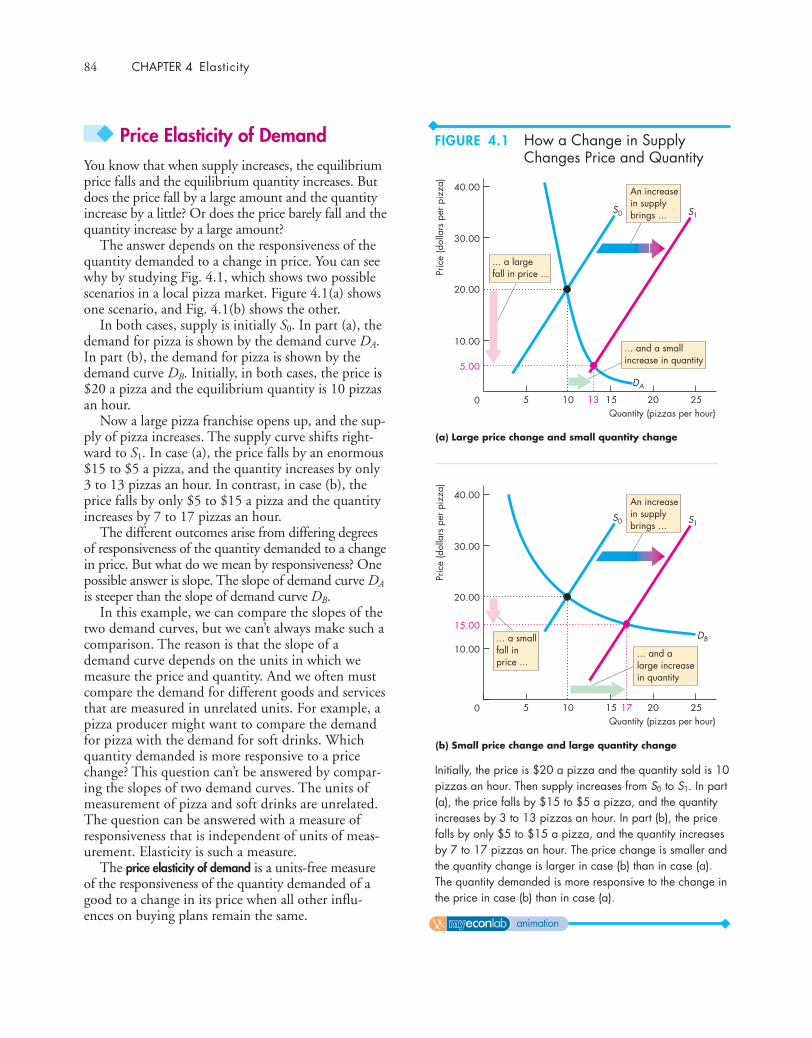
84 CHAPTER 4 Elasticity

◆ Price Elasticity of DemandYou know that when supply increases, the equilibriumprice falls and the equilibrium quantity increases. Butdoes the price fall by a large amount and the quantityincrease by a little? Or does the price barely fall and thequantity increase by a large amount?

The answer depends on the responsiveness of thequantity demanded to a change in price. You can seewhy by studying Fig. 4.1, which shows two possiblescenarios in a local pizza market. Figure 4.1(a) showsone scenario, and Fig. 4.1(b) shows the other.

In both cases, supply is initially S0. In part (a), thedemand for pizza is shown by the demand curve DA.In part (b), the demand for pizza is shown by thedemand curve DB. Initially, in both cases, the price is$20 a pizza and the equilibrium quantity is 10 pizzasan hour.

Now a large pizza franchise opens up, and the sup-ply of pizza increases. The supply curve shifts right-ward to S1. In case (a), the price falls by an enormous$15 to $5 a pizza, and the quantity increases by only3 to 13 pizzas an hour. In contrast, in case (b), theprice falls by only $5 to $15 a pizza and the quantityincreases by 7 to 17 pizzas an hour.

The different outcomes arise from differing degreesof responsiveness of the quantity demanded to a changein price. But what do we mean by responsiveness? Onepossible answer is slope. The slope of demand curve DA

is steeper than the slope of demand curve DB.In this example, we can compare the slopes of the

two demand curves, but we can’t always make such acomparison. The reason is that the slope of ademand curve depends on the units in which wemeasure the price and quantity. And we often mustcompare the demand for different goods and servicesthat are measured in unrelated units. For example, apizza producer might want to compare the demandfor pizza with the demand for soft drinks. Whichquantity demanded is more responsive to a pricechange? This question can’t be answered by compar-ing the slopes of two demand curves. The units ofmeasurement of pizza and soft drinks are unrelated.The question can be answered with a measure ofresponsiveness that is independent of units of meas-urement. Elasticity is such a measure.

The price elasticity of demand is a units-free measureof the responsiveness of the quantity demanded of agood to a change in its price when all other influ-ences on buying plans remain the same.

An increasein supplybrings ...

... a largefall in price ...

13 2520151050

10.00

20.00

30.00

5.00

40.00

S0 S1

DA

(a) Large price change and small quantity changePr

ice

(dol

lars

per

pizz

a)

Quantity (pizzas per hour)

(b) Small price change and large quantity change

... and a smallincrease in quantity

An increasein supplybrings ...

... a smallfall inprice ...

17 2520151050

10.00

20.00

30.00

15.00

40.00

S0 S1

DB

Pric

e (d

olla

rs p

erpi

zza)

Quantity (pizzas per hour)

... and a large increase in quantity

Initially, the price is $20 a pizza and the quantity sold is 10pizzas an hour. Then supply increases from S0 to S1. In part(a), the price falls by $15 to $5 a pizza, and the quantityincreases by 3 to 13 pizzas an hour. In part (b), the pricefalls by only $5 to $15 a pizza, and the quantity increasesby 7 to 17 pizzas an hour. The price change is smaller andthe quantity change is larger in case (b) than in case (a).The quantity demanded is more responsive to the change inthe price in case (b) than in case (a).

FIGURE 4.1 How a Change in SupplyChanges Price and Quantity

animation

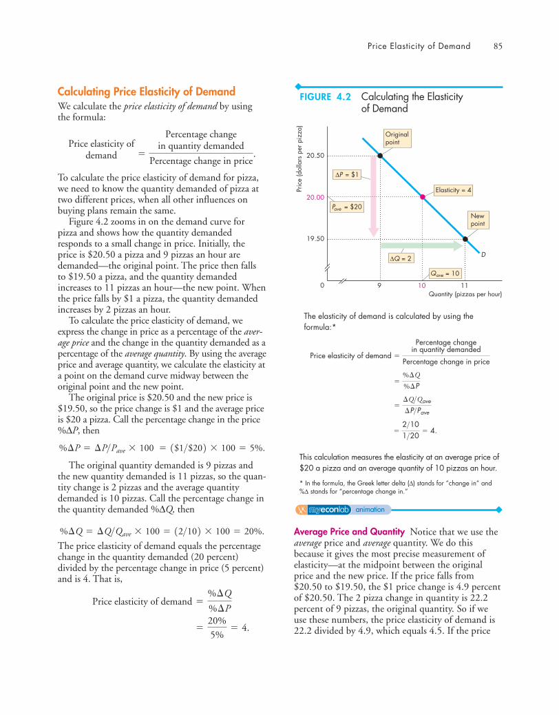
Price Elasticity of Demand 85

Calculating Price Elasticity of DemandWe calculate the price elasticity of demand by usingthe formula:

To calculate the price elasticity of demand for pizza,we need to know the quantity demanded of pizza attwo different prices, when all other influences onbuying plans remain the same.

Figure 4.2 zooms in on the demand curve forpizza and shows how the quantity demandedresponds to a small change in price. Initially, theprice is $20.50 a pizza and 9 pizzas an hour aredemanded—the original point. The price then fallsto $19.50 a pizza, and the quantity demandedincreases to 11 pizzas an hour—the new point. Whenthe price falls by $1 a pizza, the quantity demandedincreases by 2 pizzas an hour.

To calculate the price elasticity of demand, weexpress the change in price as a percentage of the aver-age price and the change in the quantity demanded as apercentage of the average quantity. By using the averageprice and average quantity, we calculate the elasticity ata point on the demand curve midway between theoriginal point and the new point.

The original price is $20.50 and the new price is$19.50, so the price change is $1 and the average priceis $20 a pizza. Call the percentage change in the price%ΔP, then

The original quantity demanded is 9 pizzas andthe new quantity demanded is 11 pizzas, so the quan-tity change is 2 pizzas and the average quantitydemanded is 10 pizzas. Call the percentage change inthe quantity demanded %ΔQ, then

The price elasticity of demand equals the percentagechange in the quantity demanded (20 percent)divided by the percentage change in price (5 percent)and is 4. That is,

=20%

5%= 4.

Price elasticity of demand =%¢Q

%¢P

%¢Q = ¢Q>Qave * 100 = 12>102 * 100 = 20%.

%¢P = ¢P>Pave * 100 = 1$1>$202 * 100 = 5%.

Price elasticity ofdemand �

Percentage changein quantity demanded

Percentage change in price.

Average Price and Quantity Notice that we use theaverage price and average quantity. We do thisbecause it gives the most precise measurement ofelasticity—at the midpoint between the originalprice and the new price. If the price falls from$20.50 to $19.50, the $1 price change is 4.9 percentof $20.50. The 2 pizza change in quantity is 22.2percent of 9 pizzas, the original quantity. So if weuse these numbers, the price elasticity of demand is22.2 divided by 4.9, which equals 4.5. If the price

10

Pric

e (d

olla

rs p

er p

izza

)Quantity (pizzas per hour)

20.50

0 119

19.50

20.00Elasticity = 4

Qave

Pave

= $1

Originalpoint

Newpoint

D

= $20

= 10

The elasticity of demand is calculated by using theformula:*

=2>101>20

= 4.

=¢Q>Qave

¢P>Pave

=%¢Q

%¢P

Price elasticity of demand =

Percentage changein quantity demanded

Percentage change in price

This calculation measures the elasticity at an average price of$20 a pizza and an average quantity of 10 pizzas an hour.

* In the formula, the Greek letter delta (Δ) stands for “change in” and%Δ stands for “percentage change in.”

FIGURE 4.2 Calculating the Elasticityof Demand

animation

86 CHAPTER 4 Elasticity

rises from $19.50 to $20.50, the $1 price change is5.1 percent of $19.50. The 2 pizza change in quan-tity is 18.2 percent of 11 pizzas, the original quan-tity. So if we use these numbers, the price elasticityof demand is 18.2 divided by 5.1, which equals 3.6.

By using percentages of the average price and aver-age quantity, we get the same value for the elasticityregardless of whether the price falls from $20.50 to$19.50 or rises from $19.50 to $20.50.

Percentages and Proportions Elasticity is the ratio oftwo percentage changes, so when we divide one per-centage change by another, the 100s cancel. A percent-age change is a proportionate change multiplied by 100.The proportionate change in price is ΔP/Pave, and theproportionate change in quantity demanded isΔQ/Qave. So if we divide ΔQ/Qave by ΔP/Pave we get thesame answer as we get by using percentage changes.

A Units-Free Measure Now that you’ve calculated aprice elasticity of demand, you can see why it is aunits-free measure. Elasticity is a units-free measurebecause the percentage change in each variable isindependent of the units in which the variable ismeasured. The ratio of the two percentages is a num-ber without units.

Minus Sign and Elasticity When the price of a goodrises, the quantity demanded decreases. Because a posi-tive change in price brings a negative change in thequantity demanded, the price elasticity of demand is

a negative number. But it is the magnitude, orabsolute value, of the price elasticity of demand thattells us how responsive the quantity demanded is. Soto compare price elasticities of demand, we use themagnitude of the elasticity and ignore the minus sign.

Inelastic and Elastic DemandFigure 4.3 shows three demand curves that coverthe entire range of possible elasticities of demand.In Fig. 4.3(a), the quantity demanded is constantregardless of the price. If the quantity demandedremains constant when the price changes, then theprice elasticity of demand is zero and the good is saidto have a perfectly inelastic demand. One good that hasa very low price elasticity of demand (perhaps zeroover some price range) is insulin. Insulin is of suchimportance to some diabetics that if the price rises orfalls, they do not change the quantity they buy.

If the percentage change in the quantity demandedequals the percentage change in the price, then theprice elasticity equals 1 and the good is said to have aunit elastic demand. The demand in Fig. 4.3(b) is anexample of a unit elastic demand.

Between the cases shown in Fig. 4.3(a) and Fig.4.3(b) is the general case in which the percentagechange in the quantity demanded is less than thepercentage change in the price. In this case, the priceelasticity of demand is between zero and 1 and thegood is said to have an inelastic demand. Food andshelter are examples of goods with inelastic demand.

Pric

e

D2

0 Quantity

(b) Unit elastic demand

Pric

e D1

0 Quantity

(a) Perfectly inelastic demand

Pric

e

D3

0 Quantity

(c) Perfectly elastic demand

12

1 2 3

6

12

6

12

6

Elasticity = 0 Elasticity = 1 Elasticity =

Each demand illustrated here has a constant elasticity. Thedemand curve in part (a) illustrates the demand for a goodthat has a zero elasticity of demand. The demand curve in

FIGURE 4.3 Inelastic and Elastic Demand

animation

part (b) illustrates the demand for a good with a unit elastic-ity of demand. And the demand curve in part (c) illustratesthe demand for a good with an infinite elasticity of demand.

Price Elasticity of Demand 87

If the quantity demanded changes by an infinitelylarge percentage in response to a tiny price change,then the price elasticity of demand is infinity and thegood is said to have a perfectly elastic demand. Figure4.3(c) shows a perfectly elastic demand. An exampleof a good that has a very high elasticity of demand(almost infinite) is a soft drink from two campusmachines located side by side. If the two machinesoffer the same soft drinks for the same price, somepeople buy from one machine and some from theother. But if one machine’s price is higher than theother’s, by even a small amount, no one buys fromthe machine with the higher price. Drinks from thetwo machines are perfect substitutes. The demandfor a good that has a perfect substitute is perfectlyelastic.

Between the cases in Fig. 4.3(b) and Fig. 4.3(c)is the general case in which the percentage change inthe quantity demanded exceeds the percentage changein price. In this case, the price elasticity of demand isgreater than 1 and the good is said to have an elasticdemand. Automobiles and furniture are examples ofgoods that have elastic demand.

Elasticity Along a Linear Demand CurveElasticity and slope are not the same. A linear demandcurve has a constant slope but a varying elasticity. Let’ssee why.

The demand curve in Fig. 4.4 is linear. A $5 fall inthe price brings an increase of 10 pizzas an hour nomatter what the initial price and quantity.

Let’s now calculate some elasticities along thisdemand curve.

At the midpoint of the demand curve, the price is$12.50 and the quantity is 25 pizzas per hour. Whenthe price falls from $15 to $10 a pizza the quantitydemanded increases from 20 to 30 pizzas an hour andthe average price and average quantity are at the mid-point of the demand curve. So

That is, at the midpoint of a linear demand curve,the price elasticity of demand is one.

At prices above the midpoint, demand is elastic.For example, when the price falls from $25 to $15 apizza, the quantity demanded increases from zero to

= 1.

Price elasticity of demand =10/25

5/12.25

20 pizzas an hour. The average price is $20 a pizza,and the average quantity is 10 pizzas. So

That is, the price elasticity of demand at an averageprice of $20 a pizza is 4.

At prices below the midpoint, demand is inelastic.For example, when the price falls from $10 a pizza tozero, the quantity demanded increases from 30 to 50pizzas an hour. The average price is now $5 and theaverage quantity is 40 pizzas an hour. So

That is, the price elasticity of demand at an averageprice of $5 a pizza is 1/4.

= 1>4.

Price elasticity of demand =20>40

10>5

= 4.

=20>10

10>20

Price elasticity of demand =¢Q>Qave

¢P>Pave

10 25

Pric

e (d

olla

rs p

er p

izza

)

Quantity (pizzas per hour)

10.00

0

5.00

50

Inelastic

Elasticity = 4

Elasticity =

Elastic

15.00

12.50

20.00

25.00

Elasticity = 1

20 30 40

14/

On a linear demand curve, demand is unit elastic at themidpoint (elasticity is 1), elastic above the midpoint, andinelastic below the midpoint.

FIGURE 4.4 Elasticity Along a LinearDemand Curve

animation

88 CHAPTER 4 Elasticity

Total Revenue and ElasticityThe total revenue from the sale of a good equals theprice of the good multiplied by the quantity sold.When a price changes, total revenue also changes.But a cut in the price does not always decrease totalrevenue. The change in total revenue depends on theelasticity of demand in the following way:

■ If demand is elastic, a 1 percent price cut increasesthe quantity sold by more than 1 percent and totalrevenue increases.

■ If demand is inelastic, a 1 percent price cutincreases the quantity sold by less than 1 percentand total revenue decreases.

■ If demand is unit elastic, a 1 percent price cutincreases the quantity sold by 1 percent and totalrevenue does not change.

In Fig. 4.5(a), over the price range from $25 to$12.50, demand is elastic. Over the price range from$12.50 to zero, demand is inelastic. At a price of$12.50, demand is unit elastic.

Figure 4.5(b) shows total revenue. At a price of$25, the quantity sold is zero, so total revenueis zero. At a price of zero, the quantity demandedis 50 pizzas an hour and total revenue is again zero.A price cut in the elastic range brings an increase intotal revenue—the percentage increase in the quan-tity demanded is greater than the percentagedecrease in price. A price cut in the inelastic rangebrings a decrease in total revenue—the percentageincrease in the quantity demanded is less than thepercentage decrease in price. At unit elasticity, totalrevenue is at a maximum.

Figure 4.5 shows how we can use this relation-ship between elasticity and total revenue to esti-mate elasticity using the total revenue test. Thetotal revenue test is a method of estimating the priceelasticity of demand by observing the change intotal revenue that results from a change in theprice, when all other influences on the quantitysold remain the same.

■ If a price cut increases total revenue, demand iselastic.

■ If a price cut decreases total revenue, demand isinelastic.

■ If a price cut leaves total revenue unchanged,demand is unit elastic.

200.00

350.00

0

50.00

100.00

150.00

250.00

312.50

(b) Total revenue

Elasticdemand

Tota

l rev

enue

(dol

lars

)

Quantity (pizzas per hour)

25 500

5.00

10.00

15.00

20.00

25.00

12.50

Unitelastic

Inelasticdemand

25 50

(a) DemandPr

ice

(dol

lars

per

piz

za)

Quantity (pizzas per hour)

Maximumtotal revenue

When demandis elastic, aprice cutincreasestotal revenue

When demandis inelastic, aprice cutdecreasestotal revenue

When demand is elastic, in the price range from $25 to$12.50, a decrease in price (part a) brings an increase intotal revenue (part b). When demand is inelastic, in theprice range from $12.50 to zero, a decrease in price (parta) brings a decrease in total revenue (part b). Whendemand is unit elastic, at a price of $12.50 (part a), totalrevenue is at a maximum (part b).

FIGURE 4.5 Elasticity and Total Revenue

animation

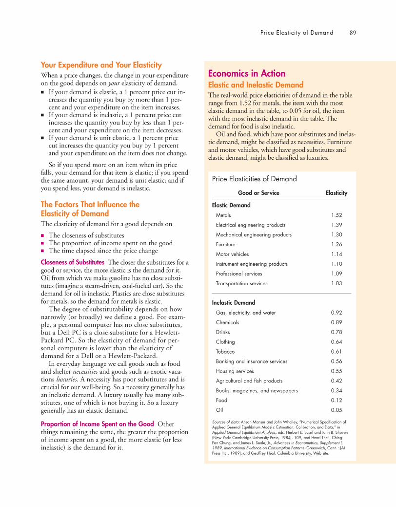
Price Elasticity of Demand 89

Your Expenditure and Your ElasticityWhen a price changes, the change in your expenditureon the good depends on your elasticity of demand.■ If your demand is elastic, a 1 percent price cut in-

creases the quantity you buy by more than 1 per-cent and your expenditure on the item increases.

■ If your demand is inelastic, a 1 percent price cutincreases the quantity you buy by less than 1 per-cent and your expenditure on the item decreases.

■ If your demand is unit elastic, a 1 percent pricecut increases the quantity you buy by 1 percentand your expenditure on the item does not change.

So if you spend more on an item when its pricefalls, your demand for that item is elastic; if you spendthe same amount, your demand is unit elastic; and ifyou spend less, your demand is inelastic.

The Factors That Influence the Elasticity of DemandThe elasticity of demand for a good depends on

■ The closeness of substitutes■ The proportion of income spent on the good■ The time elapsed since the price change

Closeness of Substitutes The closer the substitutes for agood or service, the more elastic is the demand for it.Oil from which we make gasoline has no close substi-tutes (imagine a steam-driven, coal-fueled car). So thedemand for oil is inelastic. Plastics are close substitutesfor metals, so the demand for metals is elastic.

The degree of substitutability depends on hownarrowly (or broadly) we define a good. For exam-ple, a personal computer has no close substitutes,but a Dell PC is a close substitute for a Hewlett-Packard PC. So the elasticity of demand for per-sonal computers is lower than the elasticity ofdemand for a Dell or a Hewlett-Packard.

In everyday language we call goods such as foodand shelter necessities and goods such as exotic vaca-tions luxuries. A necessity has poor substitutes and iscrucial for our well-being. So a necessity generally hasan inelastic demand. A luxury usually has many sub-stitutes, one of which is not buying it. So a luxurygenerally has an elastic demand.

Proportion of Income Spent on the Good Otherthings remaining the same, the greater the proportionof income spent on a good, the more elastic (or lessinelastic) is the demand for it.

Economics in ActionElastic and Inelastic DemandThe real-world price elasticities of demand in the tablerange from 1.52 for metals, the item with the mostelastic demand in the table, to 0.05 for oil, the itemwith the most inelastic demand in the table. Thedemand for food is also inelastic.

Oil and food, which have poor substitutes and inelas-tic demand, might be classified as necessities. Furnitureand motor vehicles, which have good substitutes andelastic demand, might be classified as luxuries.

Price Elasticities of Demand

Good or Service Elasticity

Elastic Demand

Metals 1.52

Electrical engineering products 1.39

Mechanical engineering products 1.30

Furniture 1.26

Motor vehicles 1.14

Instrument engineering products 1.10

Professional services 1.09

Transportation services 1.03

Inelastic Demand

Gas, electricity, and water 0.92

Chemicals 0.89

Drinks 0.78

Clothing 0.64

Tobacco 0.61

Banking and insurance services 0.56

Housing services 0.55

Agricultural and fish products 0.42

Books, magazines, and newspapers 0.34

Food 0.12

Oil 0.05

Sources of data: Ahsan Mansur and John Whalley, “Numerical Specification ofApplied General Equilibrium Models: Estimation, Calibration, and Data,” inApplied General Equilibrium Analysis, eds. Herbert E. Scarf and John B. Shoven(New York: Cambridge University Press, 1984), 109, and Henri Theil, Ching-Fan Chung, and James L. Seale, Jr., Advances in Econometrics, Supplement I,1989, International Evidence on Consumption Patterns (Greenwich, Conn.: JAIPress Inc., 1989), and Geoffrey Heal, Columbia University, Web site.

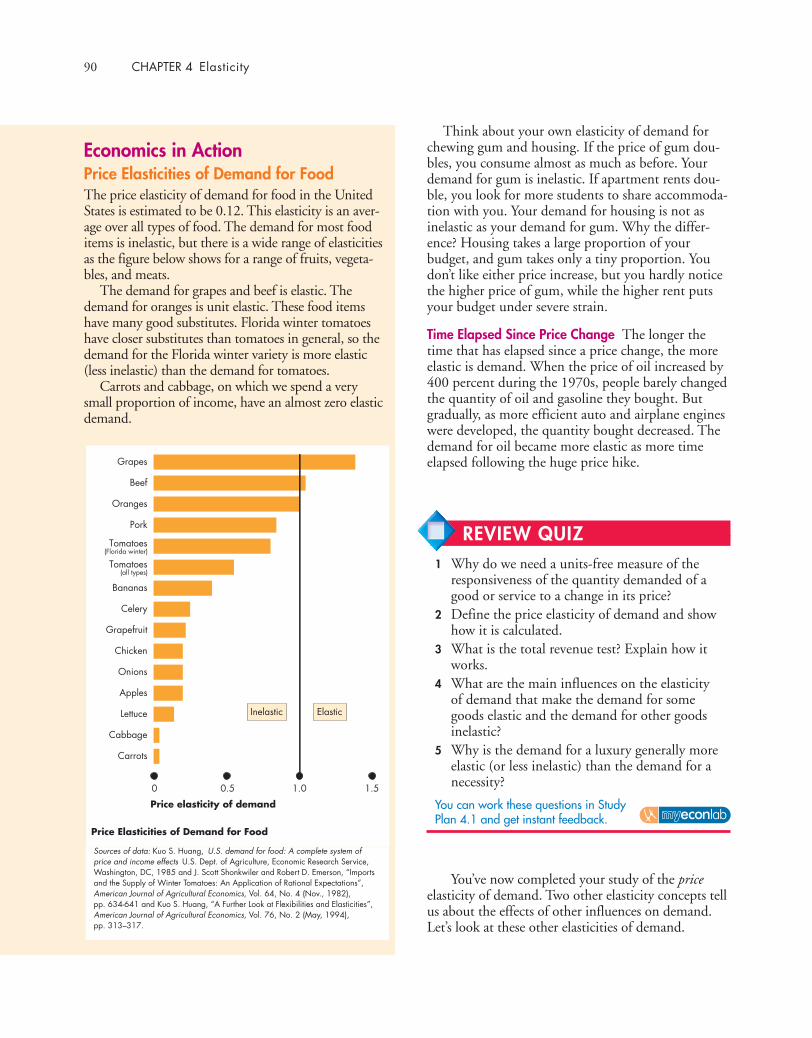
90 CHAPTER 4 Elasticity

You’ve now completed your study of the priceelasticity of demand. Two other elasticity concepts tellus about the effects of other influences on demand.Let’s look at these other elasticities of demand.

Think about your own elasticity of demand forchewing gum and housing. If the price of gum dou-bles, you consume almost as much as before. Yourdemand for gum is inelastic. If apartment rents dou-ble, you look for more students to share accommoda-tion with you. Your demand for housing is not asinelastic as your demand for gum. Why the differ-ence? Housing takes a large proportion of yourbudget, and gum takes only a tiny proportion. Youdon’t like either price increase, but you hardly noticethe higher price of gum, while the higher rent putsyour budget under severe strain.

Time Elapsed Since Price Change The longer thetime that has elapsed since a price change, the moreelastic is demand. When the price of oil increased by400 percent during the 1970s, people barely changedthe quantity of oil and gasoline they bought. Butgradually, as more efficient auto and airplane engineswere developed, the quantity bought decreased. Thedemand for oil became more elastic as more timeelapsed following the huge price hike.

0 0.5 1.0 1.5

Grapes

Beef

Oranges

Pork

Bananas

Celery

Grapefruit

Chicken

Onions

Apples

Lettuce

Cabbage

Carrots

Price elasticity of demand

Price Elasticities of Demand for Food

(Florida winter)

(all types)

Tomatoes

Tomatoes

ElasticInelastic

Economics in ActionPrice Elasticities of Demand for FoodThe price elasticity of demand for food in the UnitedStates is estimated to be 0.12. This elasticity is an aver-age over all types of food. The demand for most fooditems is inelastic, but there is a wide range of elasticitiesas the figure below shows for a range of fruits, vegeta-bles, and meats.

The demand for grapes and beef is elastic. Thedemand for oranges is unit elastic. These food itemshave many good substitutes. Florida winter tomatoeshave closer substitutes than tomatoes in general, so thedemand for the Florida winter variety is more elastic(less inelastic) than the demand for tomatoes.

Carrots and cabbage, on which we spend a verysmall proportion of income, have an almost zero elasticdemand.

Sources of data: Kuo S. Huang, U.S. demand for food: A complete system ofprice and income effects U.S. Dept. of Agriculture, Economic Research Service,Washington, DC, 1985 and J. Scott Shonkwiler and Robert D. Emerson, “Importsand the Supply of Winter Tomatoes: An Application of Rational Expectations”,American Journal of Agricultural Economics, Vol. 64, No. 4 (Nov., 1982), pp. 634-641 and Kuo S. Huang, “A Further Look at Flexibilities and Elasticities”,American Journal of Agricultural Economics, Vol. 76, No. 2 (May, 1994), pp. 313–317.

REVIEW QUIZ 1 Why do we need a units-free measure of the

responsiveness of the quantity demanded of agood or service to a change in its price?

2 Define the price elasticity of demand and showhow it is calculated.

3 What is the total revenue test? Explain how itworks.

4 What are the main influences on the elasticityof demand that make the demand for somegoods elastic and the demand for other goodsinelastic?

5 Why is the demand for a luxury generally moreelastic (or less inelastic) than the demand for anecessity?

You can work these questions in Study Plan 4.1 and get instant feedback.

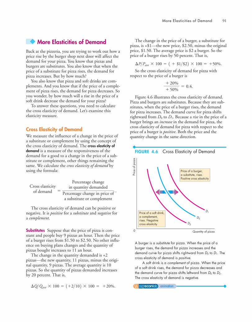
More Elasticities of Demand 91

◆ More Elasticities of DemandBack at the pizzeria, you are trying to work out how aprice rise by the burger shop next door will affect thedemand for your pizza. You know that pizzas andburgers are substitutes. You also know that when theprice of a substitute for pizza rises, the demand forpizza increases. But by how much?

You also know that pizza and soft drinks are com-plements. And you know that if the price of a comple-ment of pizza rises, the demand for pizza decreases. Soyou wonder, by how much will a rise in the price of asoft drink decrease the demand for your pizza?

To answer these questions, you need to calculatethe cross elasticity of demand. Let’s examine thiselasticity measure.

Cross Elasticity of DemandWe measure the influence of a change in the price ofa substitute or complement by using the concept ofthe cross elasticity of demand. The cross elasticity ofdemand is a measure of the responsiveness of thedemand for a good to a change in the price of a sub-stitute or complement, other things remaining thesame. We calculate the cross elasticity of demand byusing the formula:

The cross elasticity of demand can be positive ornegative. It is positive for a substitute and negative fora complement.

Substitutes Suppose that the price of pizza is con-stant and people buy 9 pizzas an hour. Then the priceof a burger rises from $1.50 to $2.50. No other influ-ence on buying plans changes and the quantity ofpizzas bought increases to 11 an hour.

The change in the quantity demanded is +2pizzas—the new quantity, 11 pizzas, minus the origi-nal quantity, 9 pizzas. The average quantity is 10pizzas. So the quantity of pizzas demanded increasesby 20 percent. That is,

.¢Q>Qave * 100 = 1+2>102 * 100 = + 20%

Cross elasticityof demand �

Percentage changein quantity demanded

Percentage change in price ofa substitute or complement

.

The change in the price of a burger, a substitute forpizza, is +$1—the new price, $2.50, minus the originalprice, $1.50. The average price is $2 a burger. So theprice of a burger rises by 50 percent. That is,

.

So the cross elasticity of demand for pizza withrespect to the price of a burger is

Figure 4.6 illustrates the cross elasticity of demand.Pizza and burgers are substitutes. Because they are sub-stitutes, when the price of a burger rises, the demandfor pizza increases. The demand curve for pizza shiftsrightward from D0 to D1. Because a rise in the price of aburger brings an increase in the demand for pizza, thecross elasticity of demand for pizza with respect to theprice of a burger is positive. Both the price and thequantity change in the same direction.

+ 20%

+ 50%= 0.4.

¢P>Pave * 100 = 1 + $1>$22 * 100 = +50%

Pric

e of

piz

za

Quantity of pizza0

D0

D1

D2

Price of a soft drink, a complement,rises. Negativecross elasticity

Price of a burger,a substitute, rises.Positive cross elasticity

A burger is a substitute for pizza. When the price of aburger rises, the demand for pizza increases and thedemand curve for pizza shifts rightward from D0 to D1. Thecross elasticity of demand is positive.

A soft drink is a complement of pizza. When the priceof a soft drink rises, the demand for pizza decreases andthe demand curve for pizza shifts leftward from D0 to D2.The cross elasticity of demand is negative.

FIGURE 4.6 Cross Elasticity of Demand

animation

92 CHAPTER 4 Elasticity

Complements Now suppose that the price of pizza isconstant and 11 pizzas an hour are bought. Then theprice of a soft drink rises from $1.50 to $2.50. Noother influence on buying plans changes and thequantity of pizzas bought falls to 9 an hour.

The change in the quantity demanded is theopposite of what we’ve just calculated: The quantityof pizzas demanded decreases by 20 percent (–20%).

The change in the price of a soft drink, acomplement of pizza, is the same as the percentagechange in the price of a burger that we’ve just calcu-lated. The price rises by 50 percent (�50%). So thecross elasticity of demand for pizza with respect tothe price of a soft drink is

Because pizza and soft drinks are complements,when the price of a soft drink rises, the demand forpizza decreases. The demand curve for pizza shiftsleftward from D0 to D2. Because a rise in the price ofa soft drink brings a decrease in the demand for pizza,the cross elasticity of demand for pizza with respectto the price of a soft drink is negative. The price andquantity change in opposite directions.

The magnitude of the cross elasticity of demanddetermines how far the demand curve shifts. Thelarger the cross elasticity (absolute value), the greateris the change in demand and the larger is the shift inthe demand curve.

If two items are close substitutes, such as twobrands of spring water, the cross elasticity is large. Iftwo items are close complements, such as movies andpopcorn, the cross elasticity is large.

If two items are somewhat unrelated to each other,such as newspapers and orange juice, the cross elastic-ity is small—perhaps even zero.

Income Elasticity of DemandSuppose the economy is expanding and people areenjoying rising incomes. This prosperity brings anincrease in the demand for most types of goods andservices. But by how much will the demand for pizzaincrease? The answer depends on the income elasticityof demand, which is a measure of the responsivenessof the demand for a good or service to a change inincome, other things remaining the same.

-20%

+ 50%= -0.4.

The income elasticity of demand is calculated byusing the formula:

Income elasticities of demand can be positive ornegative and they fall into three interesting ranges:

■ Greater than 1 (normal good, income elastic)■ Positive and less than 1 (normal good, income

inelastic)■ Negative (inferior good)

Income Elastic Demand Suppose that the price ofpizza is constant and 9 pizzas an hour are bought.Then incomes rise from $975 to $1,025 a week. Noother influence on buying plans changes and thequantity of pizzas sold increases to 11 an hour.

The change in the quantity demanded is +2 pizzas.The average quantity is 10 pizzas, so the quantitydemanded increases by 20 percent. The change inincome is +$50 and the average income is $1,000, soincomes increase by 5 percent. The income elasticityof demand for pizza is

The demand for pizza is income elastic. The per-centage increase in the quantity of pizza demandedexceeds the percentage increase in income. When thedemand for a good is income elastic, the percentage ofincome spent on that good increases as income increases.

Income Inelastic Demand If the income elasticity ofdemand is positive but less than 1, demand is incomeinelastic. The percentage increase in the quantitydemanded is positive but less than the percentageincrease in income. When the demand for a good isincome inelastic, the percentage of income spent on thatgood decreases as income increases.

Inferior Goods If the income elasticity of demand isnegative, the good is an inferior good. The quantitydemanded of an inferior good and the amount spenton it decrease when income increases. Goods in thiscategory include small motorcycles, potatoes, andrice. Low-income consumers buy most of thesegoods.

20%

5%= 4.

Income elasticityof demand �

Percentage changein quantity demanded

Percentage change in income.

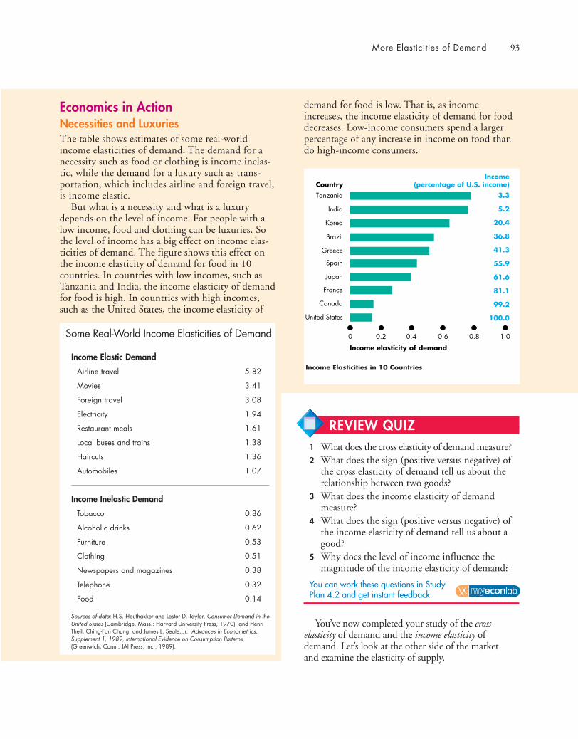
More Elasticities of Demand 93

You’ve now completed your study of the crosselasticity of demand and the income elasticity ofdemand. Let’s look at the other side of the marketand examine the elasticity of supply.

Economics in ActionNecessities and LuxuriesThe table shows estimates of some real-worldincome elasticities of demand. The demand for anecessity such as food or clothing is income inelas-tic, while the demand for a luxury such as trans-portation, which includes airline and foreign travel,is income elastic.

But what is a necessity and what is a luxurydepends on the level of income. For people with alow income, food and clothing can be luxuries. Sothe level of income has a big effect on income elas-ticities of demand. The figure shows this effect onthe income elasticity of demand for food in 10countries. In countries with low incomes, such asTanzania and India, the income elasticity of demandfor food is high. In countries with high incomes,such as the United States, the income elasticity of

0 0.2 0.4 0.6 0.8 1.0

Tanzania

India

Korea

Brazil

Greece

Spain

Japan

France

Canada

United States

Income elasticity of demand

Country3.3

5.2

20.4

36.8

41.3

55.9

61.6

81.1

99.2

100.0

Income(percentage of U.S. income)

Income Elasticities in 10 Countries

Some Real-World Income Elasticities of Demand

Income Elastic Demand

Airline travel 5.82

Movies 3.41

Foreign travel 3.08

Electricity 1.94

Restaurant meals 1.61

Local buses and trains 1.38

Haircuts 1.36

Automobiles 1.07

Income Inelastic Demand

Tobacco 0.86

Alcoholic drinks 0.62

Furniture 0.53

Clothing 0.51

Newspapers and magazines 0.38

Telephone 0.32

Food 0.14

Sources of data: H.S. Houthakker and Lester D. Taylor, Consumer Demand in theUnited States (Cambridge, Mass.: Harvard University Press, 1970), and HenriTheil, Ching-Fan Chung, and James L. Seale, Jr., Advances in Econometrics,Supplement 1, 1989, International Evidence on Consumption Patterns(Greenwich, Conn.: JAI Press, Inc., 1989).

demand for food is low. That is, as incomeincreases, the income elasticity of demand for fooddecreases. Low-income consumers spend a largerpercentage of any increase in income on food thando high-income consumers.

REVIEW QUIZ 1 What does the cross elasticity of demand measure?2 What does the sign (positive versus negative) of

the cross elasticity of demand tell us about therelationship between two goods?

3 What does the income elasticity of demandmeasure?

4 What does the sign (positive versus negative) ofthe income elasticity of demand tell us about agood?

5 Why does the level of income influence themagnitude of the income elasticity of demand?

You can work these questions in Study Plan 4.2 and get instant feedback.

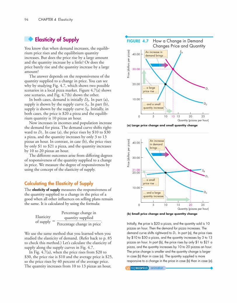
94 CHAPTER 4 Elasticity

◆ Elasticity of SupplyYou know that when demand increases, the equilib-rium price rises and the equilibrium quantityincreases. But does the price rise by a large amountand the quantity increase by a little? Or does theprice barely rise and the quantity increase by a largeamount?

The answer depends on the responsiveness of thequantity supplied to a change in price. You can seewhy by studying Fig. 4.7, which shows two possiblescenarios in a local pizza market. Figure 4.7(a) showsone scenario, and Fig. 4.7(b) shows the other.

In both cases, demand is initially D0. In part (a),supply is shown by the supply curve SA. In part (b),supply is shown by the supply curve SB. Initially, inboth cases, the price is $20 a pizza and the equilib-rium quantity is 10 pizzas an hour.

Now increases in incomes and population increasethe demand for pizza. The demand curve shifts right-ward to D1. In case (a), the price rises by $10 to $30a pizza, and the quantity increases by only 3 to 13pizzas an hour. In contrast, in case (b), the price risesby only $1 to $21 a pizza, and the quantity increasesby 10 to 20 pizzas an hour.

The different outcomes arise from differing degreesof responsiveness of the quantity supplied to a changein price. We measure the degree of responsiveness byusing the concept of the elasticity of supply.

Calculating the Elasticity of SupplyThe elasticity of supply measures the responsiveness ofthe quantity supplied to a change in the price of agood when all other influences on selling plans remainthe same. It is calculated by using the formula:

We use the same method that you learned when youstudied the elasticity of demand. (Refer back to p. 85to check this method.) Let’s calculate the elasticity ofsupply along the supply curves in Fig. 4.7.

In Fig. 4.7(a), when the price rises from $20 to$30, the price rise is $10 and the average price is $25,so the price rises by 40 percent of the average price.The quantity increases from 10 to 13 pizzas an hour,

Elasticityof supply �

Percentage change inquantity supplied

Percentage change in price.

2015 25105

An increase in demand brings ...

... a largeprice rise ...

... and a smallquantity increase

13 2520151050

10.00

20.00

30.00

40.00

D1

SA

D0

(a) Large price change and small quantity changePr

ice

(dol

lars

per

pizz

a)

Quantity (pizzas per hour)

An increasein demandbrings ...

... a smallprice rise ...

... and a largequantity increase

0

10.00

20.0021.00

30.00

40.00

D1

SB

D0

(b) Small price change and large quantity change

Pric

e (d

olla

rs p

erpi

zza)

Quantity (pizzas per hour)

Initially, the price is $20 a pizza, and the quantity sold is 10pizzas an hour. Then the demand for pizza increases. Thedemand curve shifts rightward to D1. In part (a), the price risesby $10 to $30 a pizza, and the quantity increases by 3 to 13pizzas an hour. In part (b), the price rises by only $1 to $21 apizza, and the quantity increases by 10 to 20 pizzas an hour.The price change is smaller and the quantity change is largerin case (b) than in case (a). The quantity supplied is moreresponsive to a change in the price in case (b) than in case (a).

FIGURE 4.7 How a Change in DemandChanges Price and Quantity

animation

Elasticity of Supply 95

so the increase is 3 pizzas, the average quantity is 11.5pizzas an hour, and the quantity increases by 26 per-cent. The elasticity of supply is equal to 26 percentdivided by 40 percent, which equals 0.65.

In Fig. 4.7(b), when the price rises from $20 to$21, the price rise is $1 and the average price is$20.50, so the price rises by 4.9 percent of the aver-age price. The quantity increases from 10 to 20 pizzasan hour, so the increase is 10 pizzas, the averagequantity is 15 pizzas, and the quantity increases by67 percent. The elasticity of supply is equal to 67percent divided by 4.9 percent, which equals 13.67.

Figure 4.8 shows the range of elasticities of supply.If the quantity supplied is fixed regardless of theprice, the supply curve is vertical and the elasticity ofsupply is zero. Supply is perfectly inelastic. This caseis shown in Fig. 4.8(a). A special intermediate caseoccurs when the percentage change in price equalsthe percentage change in quantity. Supply is thenunit elastic. This case is shown in Fig. 4.8(b). Nomatter how steep the supply curve is, if it is linearand passes through the origin, supply is unit elastic.If there is a price at which sellers are willing to offerany quantity for sale, the supply curve is horizontaland the elasticity of supply is infinite. Supply is per-fectly elastic. This case is shown in Fig. 4.8(c).

The Factors That Influence the Elasticity of SupplyThe elasticity of supply of a good depends on

■ Resource substitution possibilities■ Time frame for the supply decision

Resource Substitution Possibilities Some goods andservices can be produced only by using unique orrare productive resources. These items have a low,perhaps even a zero, elasticity of supply. Othergoods and services can be produced by using com-monly available resources that could be allocated toa wide variety of alternative tasks. Such items have ahigh elasticity of supply.

A Van Gogh painting is an example of a good witha vertical supply curve and a zero elasticity of supply.At the other extreme, wheat can be grown on landthat is almost equally good for growing corn, so it isjust as easy to grow wheat as corn. The opportunitycost of wheat in terms of forgone corn is almost con-stant. As a result, the supply curve of wheat is almosthorizontal and its elasticity of supply is very large.Similarly, when a good is produced in many differentcountries (for example, sugar and beef ), the supply ofthe good is highly elastic.

Pric

e

S2A

0 Quantity

(b) Unit elastic supply

Pric

e

S2B

S1

0 Quantity

(a) Perfectly inelastic supply

Pric

e

S3

0 Quantity

(c) Perfectly elastic supply

Elasticity ofsupply = 0 Elasticity of

supply = 1

Elasticity ofsupply =

Each supply illustrated here has a constant elasticity. Thesupply curve in part (a) illustrates the supply of a good thathas a zero elasticity of supply. The supply curve in part (b)illustrates the supply of a good with a unit elasticity of

supply. All linear supply curves that pass through the originillustrate supplies that are unit elastic. The supply curve inpart (c) illustrates the supply of a good with an infinite elas-ticity of supply.

FIGURE 4.8 Inelastic and Elastic Supply

animation

96 CHAPTER 4 Elasticity

The supply of most goods and services liesbetween these two extremes. The quantity producedcan be increased but only by incurring a higher cost.If a higher price is offered, the quantity suppliedincreases. Such goods and services have an elasticityof supply between zero and infinity.

Time Frame for the Supply Decision To study theinfluence of the amount of time elapsed since a pricechange, we distinguish three time frames of supply:

■ Momentary supply■ Short-run supply■ Long-run supply

Momentary Supply When the price of a good changes,the immediate response of the quantity supplied isdetermined by the momentary supply of that good.

Some goods, such as fruits and vegetables, have aperfectly inelastic momentary supply—a verticalsupply curve. The quantities supplied depend oncrop-planting decisions made earlier. In the case oforanges, for example, planting decisions have to bemade many years in advance of the crop beingavailable. Momentary supply is perfectly inelasticbecause, on a given day, no matter what the price oforanges, producers cannot change their output.They have picked, packed, and shipped their cropto market, and the quantity available for that day isfixed.

In contrast, some goods have a perfectly elasticmomentary supply. Long-distance phone calls are anexample. When many people simultaneously make acall, there is a big surge in the demand for telephonecables, computer switching, and satellite time. Thequantity supplied increases, but the price remainsconstant. Long-distance carriers monitor fluctuationsin demand and reroute calls to ensure that the quan-tity supplied equals the quantity demanded withoutchanging the price.

Short-Run Supply The response of the quantity sup-plied to a price change when only some of the possi-ble adjustments to production can be made isdetermined by short-run supply. Most goods have aninelastic short-run supply. To increase output in theshort run, firms must work their labor force overtimeand perhaps hire additional workers. To decreasetheir output in the short run, firms either lay offworkers or reduce their hours of work. With the pas-sage of time, firms can make more adjustments, per-

haps training additional workers or buying additionaltools and other equipment.

For the orange grower, if the price of oranges falls,some pickers can be laid off and oranges left on thetrees to rot. Or if the price of oranges rises, thegrower can use more fertilizer and improved irriga-tion to increase the yields of their existing trees.

But an orange grower can’t change the number oftrees producing oranges in the short run.

Long-Run Supply The response of the quantity suppliedto a price change after all the technologically possibleways of adjusting supply have been exploited is deter-mined by long-run supply. For most goods and services,long-run supply is elastic and perhaps perfectly elastic.

For the orange grower, the long run is the time ittakes new tree plantings to grow to full maturity—about 15 years. In some cases, the long-run adjustmentoccurs only after a completely new production planthas been built and workers have been trained to oper-ate it—typically a process that might take several years.

◆ You have now learned about the elasticities ofdemand and supply. Table 4.1 summarizes all the elastic-ities that you’ve met in this chapter. In the next chapter,we study the efficiency of competitive markets. But firststudy Reading Between the Lines on pp. 98–99, whichputs the elasticity of demand to work and looks at themarket for winter tomatoes.

REVIEW QUIZ 1 Why do we need a units-free measure of the

responsiveness of the quantity supplied of agood or service to a change in its price?

2 Define the elasticity of supply and show how itis calculated.

3 What are the main influences on the elasticityof supply that make the supply of some goodselastic and the supply of other goods inelastic?

4 Provide examples of goods or services whose elas-ticities of supply are (a) zero, (b) greater than zerobut less than infinity, and (c) infinity.

5 How does the time frame over which a supplydecision is made influence the elasticity ofsupply? Explain your answer.

You can work these questions in Study Plan 4.3 and get instant feedback.

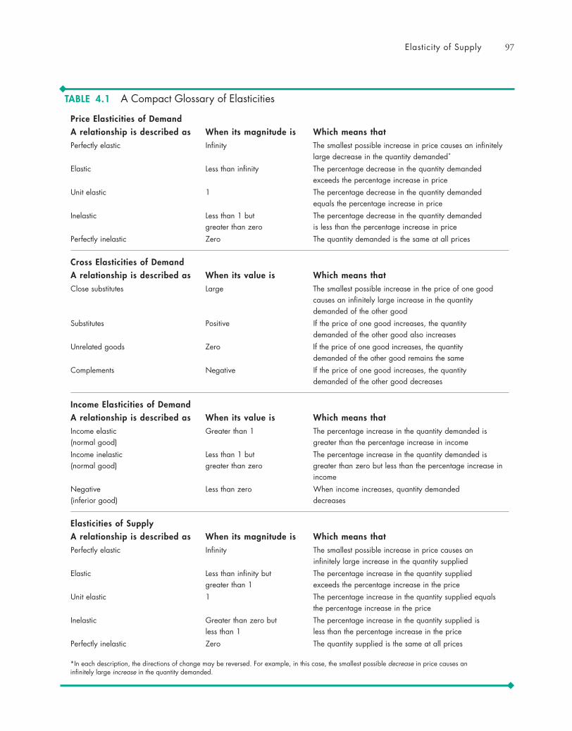
Elasticity of Supply 97

Price Elasticities of DemandA relationship is described as When its magnitude is Which means thatPerfectly elastic Infinity The smallest possible increase in price causes an infinitely

large decrease in the quantity demanded*

Elastic Less than infinity The percentage decrease in the quantity demandedexceeds the percentage increase in price

Unit elastic 1 The percentage decrease in the quantity demanded equals the percentage increase in price

Inelastic Less than 1 but The percentage decrease in the quantity demanded greater than zero is less than the percentage increase in price

Perfectly inelastic Zero The quantity demanded is the same at all prices

Cross Elasticities of DemandA relationship is described as When its value is Which means thatClose substitutes Large The smallest possible increase in the price of one good

causes an infinitely large increase in the quantity demanded of the other good

Substitutes Positive If the price of one good increases, the quantity demanded of the other good also increases

Unrelated goods Zero If the price of one good increases, the quantity demanded of the other good remains the same

Complements Negative If the price of one good increases, the quantity demanded of the other good decreases

Income Elasticities of DemandA relationship is described as When its value is Which means thatIncome elastic Greater than 1 The percentage increase in the quantity demanded is (normal good) greater than the percentage increase in income

Income inelastic Less than 1 but The percentage increase in the quantity demanded is (normal good) greater than zero greater than zero but less than the percentage increase in

income

Negative Less than zero When income increases, quantity demanded (inferior good) decreases

Elasticities of SupplyA relationship is described as When its magnitude is Which means thatPerfectly elastic Infinity The smallest possible increase in price causes an

infinitely large increase in the quantity supplied

Elastic Less than infinity but The percentage increase in the quantity supplied greater than 1 exceeds the percentage increase in the price

Unit elastic 1 The percentage increase in the quantity supplied equals the percentage increase in the price

Inelastic Greater than zero but The percentage increase in the quantity supplied is less than 1 less than the percentage increase in the price

Perfectly inelastic Zero The quantity supplied is the same at all prices

TABLE 4.1 A Compact Glossary of Elasticities

*In each description, the directions of change may be reversed. For example, in this case, the smallest possible decrease in price causes aninfinitely large increase in the quantity demanded.

98

READING BETWEEN THE L INES

Frigid Florida Winter Is Bad News for Tomato LoversUSA TodayMarch 5, 2010

ST. PETERSBURG, Fla. - A frigid Florida winter is taking its toll on your sandwich. TheSunshine State is the main U.S. source for fresh winter tomatoes, and its growers lost some70 percent of their crop during January’s prolonged cold snap. …

The average wholesale price for a 25-pound box of tomatoes is now $30, up from $6.50 ayear ago. Florida’s growers would normally ship about 25 million pounds of tomatoes a week;right now, they’re shipping less than a quarter of that, according to Reggie Brown of theFlorida Tomato Grower’s Exchange, a tomato farmer cooperative in Maitland. …

And because high demand has driven up domestic prices, many wholesalers are buying fromMexico instead.

“We’re obviously losing market share to Mexico,and there’s always a price to pay to get thecustomer to get back into the Florida market,”Brown said.

Florida is the only place where tomatoes aregrown on a large scale in the United States dur-ing winter. California doesn’t grow them untillater in the year, and much of that state’s crop isused for processed foods, such as ketchup,sauce, and juice. Other states grow tomatoes ingreenhouses year-round, but Florida’s wintertomato crop is by far the largest. …

Some Wendy’s restaurants posted signs sayingtomatoes would only be provided upon requestbecause of limited availability. …

Used with permission of The Associated Press. Copyright © 2010. All rights reserved.

■ Florida is the main U.S. source for fresh wintertomatoes.

■ California tomatoes come to market later in theyear and are mainly used for ketchup, sauce,and juice.

■ Other states grow tomatoes in greenhousesyear-round.

■ In January 2010, a prolonged cold snapwiped out 70 percent of the Florida crop.

■ The average wholesale price for a 25-poundbox of tomatoes rose from $6.50 in January2009 to $30 in January 2010.

■ The quantity of tomatoes shipped decreasedfrom a normal 25 million pounds per week toless than a quarter of that quantity.

■ “High demand has driven up prices” andwholesalers are buying from Mexico.

■ Some restaurants provided tomatoes only onrequest.

ESSENCE OF THE STORY

The Elasticities of Demandand Supply for Tomatoes

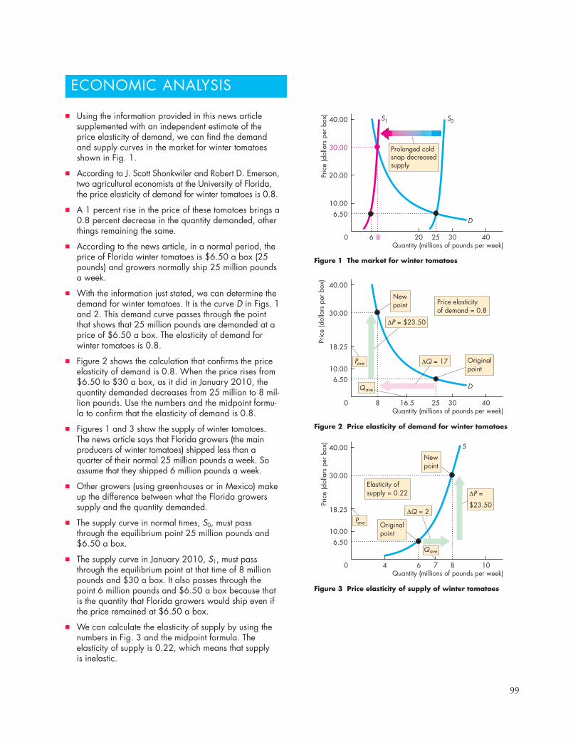
99

ECONOMIC ANALYSIS

Figure 3 Price elasticity of supply of winter tomatoes

Price elasticityof demand = 0.8

Elasticity ofsupply = 0.22

Newpoint

Newpoint

Originalpoint

Originalpoint

Figure 2 Price elasticity of demand for winter tomatoes

Pric

e (d

olla

rs p

erbo

x)

D

S1 S0

Prolonged coldsnap decreasedsupply

Figure 1 The market for winter tomatoes

Quantity (millions of pounds per week)403020 256 8

40.00

30.00

20.00

10.006.50

0

Pric

e (d

olla

rs p

erbo

x) S

Quantity (millions of pounds per week)10864

40.00

30.00

10.006.50

70

Pric

e (d

olla

rs p

erbo

x)

D

Quantity (millions of pounds per week)403016.5 258

40.00

30.00

18.25

10.006.50

18.25

0

Qave

Pave

Qave

Pave

■ Using the information provided in this news articlesupplemented with an independent estimate of theprice elasticity of demand, we can find the demandand supply curves in the market for winter tomatoesshown in Fig. 1.

■ According to J. Scott Shonkwiler and Robert D. Emerson,two agricultural economists at the University of Florida,the price elasticity of demand for winter tomatoes is 0.8.

■ A 1 percent rise in the price of these tomatoes brings a0.8 percent decrease in the quantity demanded, otherthings remaining the same.

■ According to the news article, in a normal period, theprice of Florida winter tomatoes is $6.50 a box (25pounds) and growers normally ship 25 million poundsa week.

■ With the information just stated, we can determine thedemand for winter tomatoes. It is the curve D in Figs. 1and 2. This demand curve passes through the pointthat shows that 25 million pounds are demanded at aprice of $6.50 a box. The elasticity of demand forwinter tomatoes is 0.8.

■ Figure 2 shows the calculation that confirms the priceelasticity of demand is 0.8. When the price rises from$6.50 to $30 a box, as it did in January 2010, thequantity demanded decreases from 25 million to 8 mil-lion pounds. Use the numbers and the midpoint formu-la to confirm that the elasticity of demand is 0.8.

■ Figures 1 and 3 show the supply of winter tomatoes.The news article says that Florida growers (the mainproducers of winter tomatoes) shipped less than aquarter of their normal 25 million pounds a week. Soassume that they shipped 6 million pounds a week.

■ Other growers (using greenhouses or in Mexico) makeup the difference between what the Florida growerssupply and the quantity demanded.

■ The supply curve in normal times, S0, must passthrough the equilibrium point 25 million pounds and$6.50 a box.

■ The supply curve in January 2010, S1, must passthrough the equilibrium point at that time of 8 millionpounds and $30 a box. It also passes through thepoint 6 million pounds and $6.50 a box because thatis the quantity that Florida growers would ship even ifthe price remained at $6.50 a box.

■ We can calculate the elasticity of supply by using thenumbers in Fig. 3 and the midpoint formula. Theelasticity of supply is 0.22, which means that supply is inelastic.

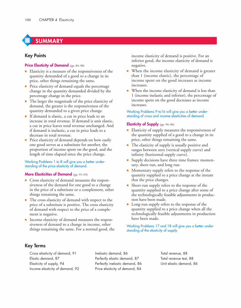
100 CHAPTER 4 Elasticity

income elasticity of demand is positive. For aninferior good, the income elasticity of demand isnegative.

■ When the income elasticity of demand is greaterthan 1 (income elastic), the percentage ofincome spent on the good increases as incomeincreases.

■ When the income elasticity of demand is less than1 (income inelastic and inferior), the percentage ofincome spent on the good decreases as incomeincreases.

Working Problems 9 to16 will give you a better under-standing of cross and income elasticities of demand.

Elasticity of Supply (pp. 94–96)

■ Elasticity of supply measures the responsiveness ofthe quantity supplied of a good to a change in itsprice, other things remaining the same.

■ The elasticity of supply is usually positive andranges between zero (vertical supply curve) andinfinity (horizontal supply curve).

■ Supply decisions have three time frames: momen-tary, short run, and long run.

■ Momentary supply refers to the response of thequantity supplied to a price change at the instantthat the price changes.

■ Short-run supply refers to the response of thequantity supplied to a price change after some ofthe technologically feasible adjustments in produc-tion have been made.

■ Long-run supply refers to the response of thequantity supplied to a price change when all thetechnologically feasible adjustments in productionhave been made.

Working Problems 17 and 18 will give you a better under-standing of the elasticity of supply.

Key Points

Price Elasticity of Demand (pp. 84–90)

■ Elasticity is a measure of the responsiveness of thequantity demanded of a good to a change in itsprice, other things remaining the same.

■ Price elasticity of demand equals the percentagechange in the quantity demanded divided by thepercentage change in the price.

■ The larger the magnitude of the price elasticity ofdemand, the greater is the responsiveness of thequantity demanded to a given price change.

■ If demand is elastic, a cut in price leads to anincrease in total revenue. If demand is unit elastic,a cut in price leaves total revenue unchanged. Andif demand is inelastic, a cut in price leads to adecrease in total revenue.

■ Price elasticity of demand depends on how easilyone good serves as a substitute for another, theproportion of income spent on the good, and thelength of time elapsed since the price change.

Working Problems 1 to 8 will give you a better under-standing of the price elasticity of demand.

More Elasticities of Demand (pp. 91–93)

■ Cross elasticity of demand measures the respon-siveness of the demand for one good to a changein the price of a substitute or a complement, otherthings remaining the same.

■ The cross elasticity of demand with respect to theprice of a substitute is positive. The cross elasticityof demand with respect to the price of a comple-ment is negative.

■ Income elasticity of demand measures the respon-siveness of demand to a change in income, otherthings remaining the same. For a normal good, the

SUMMARY

Cross elasticity of demand, 91Elastic demand, 87Elasticity of supply, 94Income elasticity of demand, 92

Inelastic demand, 86Perfectly elastic demand, 87Perfectly inelastic demand, 86Price elasticity of demand, 84

Total revenue, 88Total revenue test, 88Unit elastic demand, 86

Key Terms

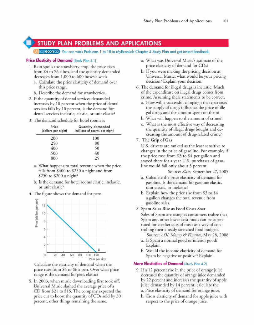
Study Plan Problems and Applications 101

a. What was Universal Music’s estimate of theprice elasticity of demand for CDs?

b. If you were making the pricing decision atUniversal Music, what would be your pricingdecision? Explain your decision.

6. The demand for illegal drugs is inelastic. Muchof the expenditure on illegal drugs comes fromcrime. Assuming these statements to be correct,a. How will a successful campaign that decreases

the supply of drugs influence the price of ille-gal drugs and the amount spent on them?

b. What will happen to the amount of crime?c. What is the most effective way of decreasing

the quantity of illegal drugs bought and de-creasing the amount of drug-related crime?

7. The Grip of GasU.S. drivers are ranked as the least sensitive tochanges in the price of gasoline. For example, ifthe price rose from $3 to $4 per gallon andstayed there for a year U.S. purchases of gaso-line would fall only about 5 percent.

Source: Slate, September 27, 2005a. Calculate the price elasticity of demand for

gasoline. Is the demand for gasoline elastic,unit elastic, or inelastic?

b. Explain how the price rise from $3 to $4a gallon changes the total revenue fromgasoline sales.

8. Spam Sales Rise as Food Costs SoarSales of Spam are rising as consumers realize thatSpam and other lower-cost foods can be substi-tuted for costlier cuts of meat as a way of con-trolling their already stretched food budgets.

Source: AOL Money & Finance, May 28, 2008a. Is Spam a normal good or inferior good?

Explain.b. Would the income elasticity of demand for

Spam be negative or positive? Explain.

More Elasticities of Demand (Study Plan 4.2)

9. If a 12 percent rise in the price of orange juicedecreases the quantity of orange juice demandedby 22 percent and increases the quantity of applejuice demanded by 14 percent, calculate thea. Price elasticity of demand for orange juice.b. Cross elasticity of demand for apple juice with

respect to the price of orange juice.

Price Elasticity of Demand (Study Plan 4.1)

1. Rain spoils the strawberry crop, the price risesfrom $4 to $6 a box, and the quantity demandeddecreases from 1,000 to 600 boxes a week.a. Calculate the price elasticity of demand over

this price range.b. Describe the demand for strawberries.

2. If the quantity of dental services demandedincreases by 10 percent when the price of dentalservices falls by 10 percent, is the demand fordental services inelastic, elastic, or unit elastic?

3. The demand schedule for hotel rooms isPrice Quantity demanded

(dollars per night) (millions of rooms per night)

200 100250 80400 50500 40800 25

a. What happens to total revenue when the pricefalls from $400 to $250 a night and from$250 to $200 a night?

b. Is the demand for hotel rooms elastic, inelastic,or unit elastic?

4. The figure shows the demand for pens.

Calculate the elasticity of demand when theprice rises from $4 to $6 a pen. Over what pricerange is the demand for pens elastic?

5. In 2003, when music downloading first took off,Universal Music slashed the average price of aCD from $21 to $15. The company expected theprice cut to boost the quantity of CDs sold by 30percent, other things remaining the same.

You can work Problems 1 to 18 in MyEconLab Chapter 4 Study Plan and get instant feedback.

STUDY PLAN PROBLEMS AND APPLICATIONS

10

4

6

8

200 40 60 80

Pric

e (d

olla

rs p

er p

en)

Pens per day

2

100 120

12

D

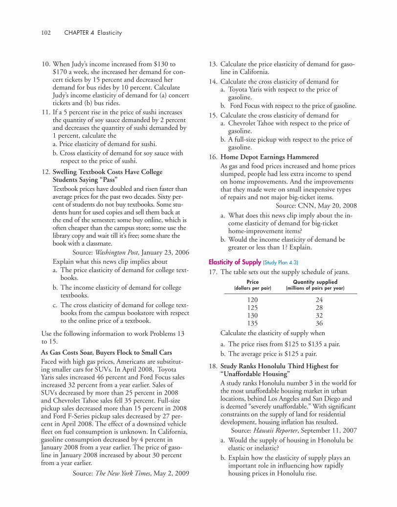
102 CHAPTER 4 Elasticity

10. When Judy’s income increased from $130 to$170 a week, she increased her demand for con-cert tickets by 15 percent and decreased herdemand for bus rides by 10 percent. CalculateJudy’s income elasticity of demand for (a) concerttickets and (b) bus rides.

11. If a 5 percent rise in the price of sushi increasesthe quantity of soy sauce demanded by 2 percentand decreases the quantity of sushi demanded by1 percent, calculate thea. Price elasticity of demand for sushi.b. Cross elasticity of demand for soy sauce with

respect to the price of sushi.

12. Swelling Textbook Costs Have CollegeStudents Saying “Pass”Textbook prices have doubled and risen faster thanaverage prices for the past two decades. Sixty per-cent of students do not buy textbooks. Some stu-dents hunt for used copies and sell them back atthe end of the semester; some buy online, which isoften cheaper than the campus store; some use thelibrary copy and wait till it’s free; some share thebook with a classmate.

Source: Washington Post, January 23, 2006Explain what this news clip implies abouta. The price elasticity of demand for college text-

books.b. The income elasticity of demand for college

textbooks.c. The cross elasticity of demand for college text-

books from the campus bookstore with respectto the online price of a textbook.

Use the following information to work Problems 13to 15.

As Gas Costs Soar, Buyers Flock to Small CarsFaced with high gas prices, Americans are substitut-ing smaller cars for SUVs. In April 2008, ToyotaYaris sales increased 46 percent and Ford Focus salesincreased 32 percent from a year earlier. Sales ofSUVs decreased by more than 25 percent in 2008and Chevrolet Tahoe sales fell 35 percent. Full-sizepickup sales decreased more than 15 percent in 2008and Ford F-Series pickup sales decreased by 27 per-cent in April 2008. The effect of a downsized vehiclefleet on fuel consumption is unknown. In California,gasoline consumption decreased by 4 percent inJanuary 2008 from a year earlier. The price of gaso-line in January 2008 increased by about 30 percentfrom a year earlier.

Source: The New York Times, May 2, 2009

13. Calculate the price elasticity of demand for gaso-line in California.

14. Calculate the cross elasticity of demand for a. Toyota Yaris with respect to the price of

gasoline.b. Ford Focus with respect to the price of gasoline.

15. Calculate the cross elasticity of demand for a. Chevrolet Tahoe with respect to the price of

gasoline.b. A full-size pickup with respect to the price of

gasoline.16. Home Depot Earnings Hammered

As gas and food prices increased and home pricesslumped, people had less extra income to spendon home improvements. And the improvementsthat they made were on small inexpensive typesof repairs and not major big-ticket items.

Source: CNN, May 20, 2008a. What does this news clip imply about the in-

come elasticity of demand for big-tickethome-improvement items?

b. Would the income elasticity of demand begreater or less than 1? Explain.

Elasticity of Supply (Study Plan 4.3)

17. The table sets out the supply schedule of jeans.Price Quantity supplied

(dollars per pair) (millions of pairs per year)

120 24125 28130 32135 36

Calculate the elasticity of supply when

a. The price rises from $125 to $135 a pair.b. The average price is $125 a pair.

18. Study Ranks Honolulu Third Highest for“Unaffordable Housing”A study ranks Honolulu number 3 in the world forthe most unaffordable housing market in urbanlocations, behind Los Angeles and San Diego andis deemed “severely unaffordable.” With significantconstraints on the supply of land for residentialdevelopment, housing inflation has resulted.

Source: Hawaii Reporter, September 11, 2007a. Would the supply of housing in Honolulu be

elastic or inelastic?b. Explain how the elasticity of supply plays an

important role in influencing how rapidlyhousing prices in Honolulu rise.

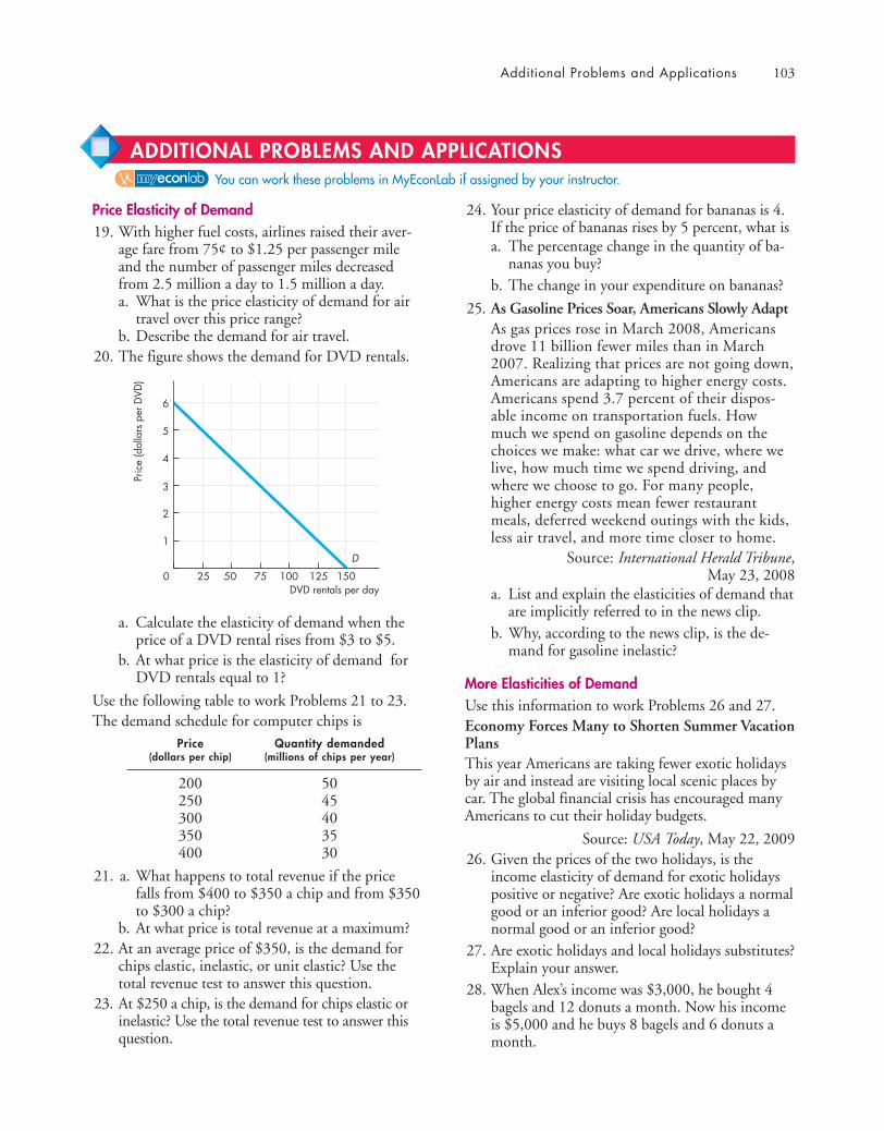
Additional Problems and Applications 103

Price Elasticity of Demand19. With higher fuel costs, airlines raised their aver-

age fare from 75¢ to $1.25 per passenger mileand the number of passenger miles decreasedfrom 2.5 million a day to 1.5 million a day.a. What is the price elasticity of demand for air

travel over this price range?b. Describe the demand for air travel.

20. The figure shows the demand for DVD rentals.

a. Calculate the elasticity of demand when theprice of a DVD rental rises from $3 to $5.

b. At what price is the elasticity of demand forDVD rentals equal to 1?

Use the following table to work Problems 21 to 23.The demand schedule for computer chips is

Price Quantity demanded(dollars per chip) (millions of chips per year)

200 50250 45300 40350 35400 30

21. a. What happens to total revenue if the pricefalls from $400 to $350 a chip and from $350to $300 a chip?

b. At what price is total revenue at a maximum?22. At an average price of $350, is the demand for

chips elastic, inelastic, or unit elastic? Use thetotal revenue test to answer this question.

23. At $250 a chip, is the demand for chips elastic orinelastic? Use the total revenue test to answer thisquestion.

5

2

3

4

250 50 75 100

Pric

e (d

olla

rs p

er D

VD)

DVD rentals per day

1

125 150

6

D

24. Your price elasticity of demand for bananas is 4.If the price of bananas rises by 5 percent, what isa. The percentage change in the quantity of ba-

nanas you buy?b. The change in your expenditure on bananas?

25. As Gasoline Prices Soar, Americans Slowly AdaptAs gas prices rose in March 2008, Americansdrove 11 billion fewer miles than in March2007. Realizing that prices are not going down,Americans are adapting to higher energy costs.Americans spend 3.7 percent of their dispos-able income on transportation fuels. Howmuch we spend on gasoline depends on thechoices we make: what car we drive, where welive, how much time we spend driving, andwhere we choose to go. For many people,higher energy costs mean fewer restaurantmeals, deferred weekend outings with the kids,less air travel, and more time closer to home.

Source: International Herald Tribune,May 23, 2008

a. List and explain the elasticities of demand thatare implicitly referred to in the news clip.

b. Why, according to the news clip, is the de-mand for gasoline inelastic?

More Elasticities of DemandUse this information to work Problems 26 and 27.Economy Forces Many to Shorten Summer VacationPlansThis year Americans are taking fewer exotic holidaysby air and instead are visiting local scenic places bycar. The global financial crisis has encouraged manyAmericans to cut their holiday budgets.

Source: USA Today, May 22, 200926. Given the prices of the two holidays, is the

income elasticity of demand for exotic holidayspositive or negative? Are exotic holidays a normalgood or an inferior good? Are local holidays anormal good or an inferior good?

27. Are exotic holidays and local holidays substitutes?Explain your answer.

28. When Alex’s income was $3,000, he bought 4bagels and 12 donuts a month. Now his incomeis $5,000 and he buys 8 bagels and 6 donuts amonth.

You can work these problems in MyEconLab if assigned by your instructor.

ADDITIONAL PROBLEMS AND APPLICATIONS

104 CHAPTER 4 Elasticity

Calculate Alex’s income elasticity of demand for a. Bagels.b. Donuts.

29. Wal-Mart’s Recession-Time Pet ProjectDuring the recession, Wal-Mart moved its petfood and supplies to in front of its other fast-growing business, baby products. Retail expertspoint out that kids and pets tend to be fairlyrecession-resistant businesses—even in a reces-sion, dogs will be fed and kids will get their toys.

Source: CNN, May 13, 2008a. What does this news clip imply about the in-

come elasticity of demand for pet food andbaby products?

b. Would the income elasticity of demand begreater or less than 1? Explain.

30. If a 5 percent fall in the price of chocolate sauceincreases the quantity of chocolate saucedemanded by 10 percent and increases the quan-tity of ice cream demanded by 15 percent, calcu-late thea. Price elasticity of demand for chocolate sauce.b. Cross elasticity of demand for ice cream with

respect to the price of chocolate sauce.31. Netflix to Offer Online Movie Viewing

Online movie rental service Netflix has intro-duced a new feature to allow customers to watchmovies and television series on their personalcomputers. Netflix competes with video rentalretailer Blockbuster, which added an onlinerental service to the in-store rental service.

Source: CNN, January 16, 2007 a. How will online movie viewing influence the

price elasticity of demand for in-store movierentals?

b. Would the cross elasticity of demand for on-line movies and in-store movie rentals be neg-ative or positive? Explain.

c. Would the cross elasticity of demand for on-line movies with respect to high-speed Inter-net service be negative or positive? Explain.

32. To Love, Honor, and Save MoneyIn a survey of caterers and event planners, nearlyhalf of them said that they were seeing declinesin wedding spending in response to the eco-nomic slowdown; 12% even reported weddingcancellations because of financial concerns.

Source: Time, June 2, 2008a. Based upon this news clip, are wedding events

a normal good or inferior good? Explain.

b. Are wedding events more a necessity or a lux-ury? Would the income elasticity of demandbe greater than 1, less than 1, or equal to 1?Explain.

Elasticity of Supply33. The supply schedule of long-distance phone calls

isPrice Quantity supplied

(cents per minute) (millions of minutes per day)

10 20020 40030 60040 800

Calculate the elasticity of supply when a. The price falls from 40¢ to 30¢ a minute.b. The average price is 20¢ a minute.

34. Weak Coal Prices Hit China’s Third-LargestCoal MinerThe chairman of Yanzhou Coal Mining reportedthat the recession had decreased the demand forcoal, with its sales falling by 11.9 percent to 7.92million tons from 8.99 million tons a year earlier,despite a 10.6 percent cut in the price.

Source: Dow Jones, April 27, 2009Calculate the price elasticity of supply of coal. Isthe supply of coal elastic or inelastic?

Economics in the News35. After you have studied Reading Between the Lines

on pp. 98–99 answer the following questions.a. Which demand is more price elastic and why:

tomatoes in general or Florida winter tomatoes?b. When cold weather destroyed the Florida crop

and more tomatoes came from Mexico andgreenhouses, what happened to the supply oftomatoes and the quantity of tomatoes sup-plied?

c. The news article says the “High demand hasdriven up prices and wholesalers are buyingfrom Mexico.” What does this statementmean? Did demand increase? Did it decrease?Is the news article correct?

d. Reggie Brown says “We’re obviously losingmarket share to Mexico, and there’s always aprice to pay to get the customer to get backinto the Florida market.” What does he meanand what does that imply about the elasticityof demand for Florida tomatoes when theprice rises and when the price falls?

After studying this chapter, you will be able to:� Describe the alternative methods of allocating scarce

resources� Explain the connection between demand and marginal

benefit and define consumer surplus; and explain theconnection between supply and marginal cost anddefine producer surplus

� Explain the conditions under which markets areefficient and inefficient

� Explain the main ideas about fairness and evaluateclaims that markets result in unfair outcomes

E

105

very time you decide to buy something, whether it’s an everyday pizza or aValentine’s Day rose, you express your view about how scarce resources shouldbe used and you make choices in your self-interest. A pizza cook one block awayand a Columbian rose grower 2,500 miles away make their self-interestedchoices about what to produce. Markets coordinate these self-interested choices.But do markets do a good job? Do they allocate resources between pizza androses, and everything else, efficiently?

The market economy generates huge income inequality: You can afford to buya pizza or give a rose, but they might be unaffordable luxuries for a pizza cook

and a Columbian rose grower who supply them. Is thissituation fair?

Efficiency and fairness (or equity) are the twodimensions of the social interest. So our central question in this chapter is: Domarkets operate in the social interest?

You will learn how economists approach and answer this question by studyinga model market for pizza. At the end of the chapter, in Reading Between theLines, we return to the global market in which roses are traded and see whetherthis market allocates resources efficiently.

EFFICIENCY AND EQUITY

5

106 CHAPTER 5 Efficiency and Equity

◆ Resource Allocation MethodsThe goal of this chapter is to evaluate the ability ofmarkets to allocate resources efficiently and fairly. Butto see whether the market does a good job, we mustcompare it with its alternatives. Resources are scarce,so they must be allocated somehow. Trading in mar-kets is just one of several alternative methods.

Resources might be allocated by

■ Market price■ Command■ Majority rule■ Contest■ First-come, first-served■ Lottery■ Personal characteristics■ Force

Let’s briefly examine each method.

Market PriceWhen a market price allocates a scarce resource, thepeople who are willing and able to pay that price getthe resource. Two kinds of people decide not to paythe market price: those who can afford to pay butchoose not to buy and those who are too poor andsimply can’t afford to buy.

For many goods and services, distinguishingbetween those who choose not to buy and those whocan’t afford to buy doesn’t matter. But for a few items,it does matter. For example, poor people can’t affordto pay school fees and doctors’ fees. Because poorpeople can’t afford items that most people consider tobe essential, these items are usually allocated by oneof the other methods.

CommandA command system allocates resources by the order(command) of someone in authority. In the U.S.economy, the command system is used extensivelyinside firms and government departments. For exam-ple, if you have a job, most likely someone tells youwhat to do. Your labor is allocated to specific tasks bya command.

A command system works well in organizations inwhich the lines of authority and responsibility areclear and it is easy to monitor the activities being per-

formed. But a command system works badly whenthe range of activities to be monitored is large andwhen it is easy for people to fool those in authority.North Korea uses a command system and it works sobadly that it even fails to deliver an adequate supplyof food.

Majority RuleMajority rule allocates resources in the way that amajority of voters choose. Societies use majority rule toelect representative governments that make some of thebiggest decisions. For example, majority rule decidesthe tax rates that end up allocating scarce resourcesbetween private use and public use. And majority ruledecides how tax dollars are allocated among competinguses such as education and health care.

Majority rule works well when the decisionsbeing made affect large numbers of people and self-interest must be suppressed to use resources mosteffectively.

ContestA contest allocates resources to a winner (or a groupof winners). Sporting events use this method. AndyRoddick competes with other tennis professionals,and the winner gets the biggest payoff. But contestsare more general than those in a sports arena, thoughwe don’t normally call them contests. For example,Bill Gates won a contest to provide the world’s per-sonal computer operating system.

Contests do a good job when the efforts of the“players” are hard to monitor and reward directly.When a manager offers everyone in the company theopportunity to win a big prize, people are motivatedto work hard and try to become the winner. Only afew people end up with a big prize, but many peoplework harder in the process of trying to win. The totaloutput produced by the workers is much greater thanit would be without the contest.

First-Come, First-ServedA first-come, first-served method allocates resourcesto those who are first in line. Many casual restau-rants won’t accept reservations. They use first-come,first-served to allocate their scarce tables. Highwayspace is allocated in this way too: The first to arriveat the on-ramp gets the road space. If too many

Resource Allocation Methods 107

vehicles enter the highway, the speed slows and peo-ple wait in line for some space to become available.

First-come, first-served works best when, as in theabove examples, a scarce resource can serve just oneuser at a time in a sequence. By serving the user whoarrives first, this method minimizes the time spentwaiting for the resource to become free.

LotteryLotteries allocate resources to those who pick thewinning number, draw the lucky cards, or come uplucky on some other gaming system. State lotteriesand casinos reallocate millions of dollars worth ofgoods and services every year.

But lotteries are more widespread than jackpotsand roulette wheels in casinos. They are used to allo-cate landing slots to airlines at some airports, placesin the New York and Boston marathons, and havebeen used to allocate fishing rights and the electro-magnetic spectrum used by cell phones.

Lotteries work best when there is no effective wayto distinguish among potential users of a scarceresource.

Personal CharacteristicsWhen resources are allocated on the basis of per-sonal characteristics, people with the “right” charac-teristics get the resources. Some of the resources thatmatter most to you are allocated in this way. Forexample, you will choose a marriage partner on thebasis of personal characteristics. But this methodcan also be used in unacceptable ways. Allocatingthe best jobs to white, Anglo-Saxon males and dis-criminating against visible minorities and women isan example.

ForceForce plays a crucial role, for both good and ill, inallocating scarce resources. Let’s start with the ill.

War, the use of military force by one nationagainst another, has played an enormous role histori-cally in allocating resources. The economicsupremacy of European settlers in the Americas andAustralia owes much to the use of this method.

Theft, the taking of the property of others withouttheir consent, also plays a large role. Both large-scaleorganized crime and small-scale petty crime collec-tively allocate billions of dollars worth of resourcesannually.

But force plays a crucial positive role in allocatingresources. It provides the state with an effectivemethod of transferring wealth from the rich to thepoor, and it provides the legal framework in whichvoluntary exchange in markets takes place.

A legal system is the foundation on which ourmarket economy functions. Without courts toenforce contracts, it would not be possible to dobusiness. But the courts could not enforce contractswithout the ability to apply force if necessary. Thestate provides the ultimate force that enables thecourts to do their work.

More broadly, the force of the state is essential touphold the principle of the rule of law. This principleis the bedrock of civilized economic (and social andpolitical) life. With the rule of law upheld, peoplecan go about their daily economic lives with theassurance that their property will be protected—thatthey can sue for violations against their property (andbe sued if they violate the property of others).

Free from the burden of protecting their prop-erty and confident in the knowledge that those withwhom they trade will honor their agreements, people can get on with focusing on the activity inwhich they have a comparative advantage and trad-ing for mutual gain.

In the next sections, we’re going to see how a mar-ket can achieve an efficient use of resources, examinethe obstacles to efficiency, and see how sometimes analternative method might improve on the market.After looking at efficiency, we’ll turn our attention tothe more difficult issue of fairness.

REVIEW QUIZ1 Why do we need methods of allocating scarce

resources?2 Describe the alternative methods of allocating

scarce resources.3 Provide an example of each allocation method

that illustrates when it works well.4 Provide an example of each allocation method

that illustrates when it works badly.

You can work these questions in Study Plan 5.1 and get instant feedback.

108 CHAPTER 5 Efficiency and Equity

◆ Benefit, Cost, and SurplusResources are allocated efficiently and in the socialinterest when they are used in the ways that peoplevalue most highly. You saw in Chapter 2 that thisoutcome occurs when the quantities produced areat the point on the PPF at which marginal benefitequals marginal cost (see pp. 33–35). We’re nowgoing to see whether competitive markets producethe efficient quantities.

We begin on the demand side of a market.

Demand, Willingness to Pay, and ValueIn everyday life, we talk about “getting value formoney.” When we use this expression, we are distin-guishing between value and price. Value is what weget, and price is what we pay.

The value of one more unit of a good or service isits marginal benefit. We measure marginal benefit bythe maximum price that is willingly paid for anotherunit of the good or service. But willingness to paydetermines demand. A demand curve is a marginalbenefit curve.

In Fig. 5.1(a), Lisa is willing to pay $1 for the30th slice of pizza and $1 is her marginal benefitfrom that slice. In Fig. 5.1(b), Nick is willing to pay$1 for the 10th slice of pizza and $1 is his marginalbenefit from that slice. But at what quantity is themarket willing to pay $1 for the marginal slice? Theanswer is provided by the market demand curve.

Individual Demand and Market DemandThe relationship between the price of a good and thequantity demanded by one person is called individ-ual demand. And the relationship between the priceof a good and the quantity demanded by all buyers iscalled market demand.

The market demand curve is the horizontal sum of theindividual demand curves and is formed by adding thequantities demanded by all the individuals at each price.

Figure 5.1(c) illustrates the market demand forpizza if Lisa and Nick are the only people in the mar-ket. Lisa’s demand curve in part (a) and Nick’sdemand curve in part (b) sum horizontally to themarket demand curve in part (c).

(a) Lisa's demand

3.00

2.00

1.00

0 20 3010 5040

2.50

1.50

0.50

Pric

e (d

olla

rs p

er s

lice

of p

izza

)

Lisa's D = MB

(b) Nick's demand (c) Market demand

Quantity (slices per month)

30 slices

Lisa is willingto pay $1 forthe 30th slice

3.00

2.00

1.00

0 20 3010 5040

2.50

1.50

0.50

Pric

e (d

olla

rs p

er s

lice

of p

izza

)

Nick's D = MB

Quantity (slices per month)

Nick is willingto pay $1 forthe 10th slice

3.00

2.00

1.00

0 20 3010 7050 6040

2.50

1.50

0.50

Pric

e (d

olla

rs p

er s

lice

of p

izza

)

Market D = MSB

Quantity (slices per month)

Society is willingto pay $1 for the40th slice

30 + 10 = 40 slices10 slices

At a price of $1 a slice, the quantity demanded by Lisa is 30slices and the quantity demanded by Nick is 10 slices, so thequantity demanded by the market is 40 slices. Lisa’s demand

curve in part (a) and Nick’s demand curve in part (b) sumhorizontally to the market demand curve in part (c). The mar-ket demand curve is the marginal social benefit (MSB) curve.

FIGURE 5.1 Individual Demand, Market Demand, and Marginal Social Benefit

animation

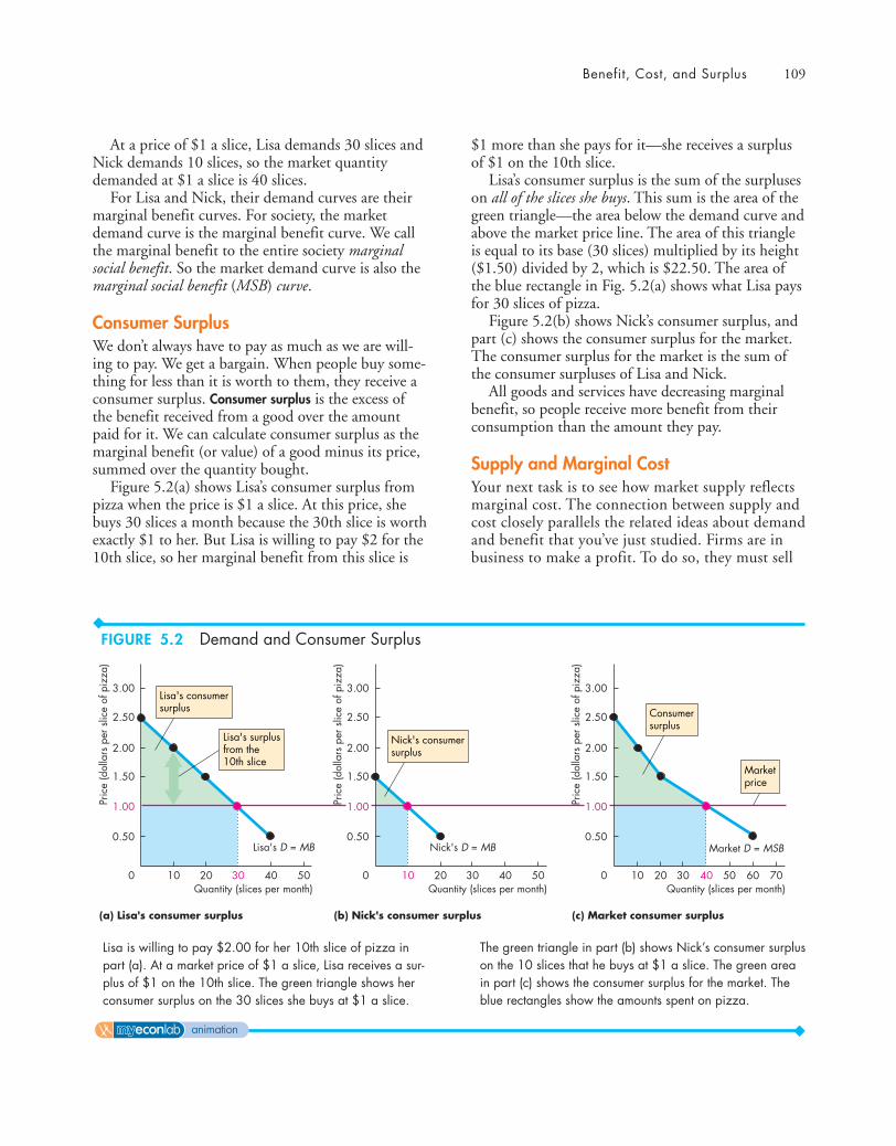
Benefit, Cost, and Surplus 109

$1 more than she pays for it—she receives a surplusof $1 on the 10th slice.

Lisa’s consumer surplus is the sum of the surpluseson all of the slices she buys. This sum is the area of thegreen triangle—the area below the demand curve andabove the market price line. The area of this triangleis equal to its base (30 slices) multiplied by its height($1.50) divided by 2, which is $22.50. The area ofthe blue rectangle in Fig. 5.2(a) shows what Lisa paysfor 30 slices of pizza.

Figure 5.2(b) shows Nick’s consumer surplus, andpart (c) shows the consumer surplus for the market.The consumer surplus for the market is the sum ofthe consumer surpluses of Lisa and Nick.

All goods and services have decreasing marginalbenefit, so people receive more benefit from theirconsumption than the amount they pay.

Supply and Marginal CostYour next task is to see how market supply reflectsmarginal cost. The connection between supply andcost closely parallels the related ideas about demandand benefit that you’ve just studied. Firms are inbusiness to make a profit. To do so, they must sell

At a price of $1 a slice, Lisa demands 30 slices andNick demands 10 slices, so the market quantitydemanded at $1 a slice is 40 slices.

For Lisa and Nick, their demand curves are theirmarginal benefit curves. For society, the marketdemand curve is the marginal benefit curve. We callthe marginal benefit to the entire society marginalsocial benefit. So the market demand curve is also themarginal social benefit (MSB) curve.

Consumer SurplusWe don’t always have to pay as much as we are will-ing to pay. We get a bargain. When people buy some-thing for less than it is worth to them, they receive aconsumer surplus. Consumer surplus is the excess ofthe benefit received from a good over the amountpaid for it. We can calculate consumer surplus as themarginal benefit (or value) of a good minus its price,summed over the quantity bought.

Figure 5.2(a) shows Lisa’s consumer surplus frompizza when the price is $1 a slice. At this price, shebuys 30 slices a month because the 30th slice is worthexactly $1 to her. But Lisa is willing to pay $2 for the10th slice, so her marginal benefit from this slice is

(a) Lisa's consumer surplus

3.00

2.00

1.00

0 20 3010 5040

2.50

1.50

0.50

Pric

e (d

olla

rs p

er s

lice

of p

izza

)

Lisa's D = MB

(b) Nick's consumer surplus (c) Market consumer surplus

Quantity (slices per month)

Lisa's consumersurplus

3.00

2.00

0 20 3010 5040

2.50

1.50

0.50

Pric

e (d

olla

rs p

er s

lice

of p

izza

)

Nick's D = MB

Quantity (slices per month)

3.00

2.00

0 20 3010 7050 6040

2.50

1.50

0.50

Pric

e (d

olla

rs p

er s

lice

of p

izza

)

Market D = MSB

Quantity (slices per month)

Marketprice

1.00 1.00

Lisa's surplusfrom the10th slice

Nick's consumersurplus

Consumersurplus

Lisa is willing to pay $2.00 for her 10th slice of pizza inpart (a). At a market price of $1 a slice, Lisa receives a sur-plus of $1 on the 10th slice. The green triangle shows herconsumer surplus on the 30 slices she buys at $1 a slice.

The green triangle in part (b) shows Nick’s consumer surpluson the 10 slices that he buys at $1 a slice. The green areain part (c) shows the consumer surplus for the market. Theblue rectangles show the amounts spent on pizza.

FIGURE 5.2 Demand and Consumer Surplus

animation

110 CHAPTER 5 Efficiency and Equity

their output for a price that exceeds the cost of pro-duction. Let’s investigate the relationship betweencost and price.

Supply, Cost, and Minimum Supply-PriceFirms make a profit when they receive more from thesale of a good or service than the cost of producing it.Just as consumers distinguish between value andprice, so producers distinguish between cost and price.Cost is what a firm gives up when it produces a goodor service and price is what a firm receives when itsells the good or service.

The cost of producing one more unit of a good orservice is its marginal cost. Marginal cost is the mini-mum price that producers must receive to inducethem to offer one more unit of a good or service forsale. But the minimum supply-price determines sup-ply. A supply curve is a marginal cost curve.

In Fig. 5.3(a), Max is willing to produce the100th pizza for $15, his marginal cost of that pizza.In Fig. 5.3(b), Mario is willing to produce the 50thpizza for $15, his marginal cost of that pizza.

What quantity is this market willing to producefor $15 a pizza? The answer is provided by themarket supply curve.

Individual Supply and Market SupplyThe relationship between the price of a good and thequantity supplied by one producer is called individ-ual supply. And the relationship between the price ofa good and the quantity supplied by all producers iscalled market supply.

The market supply curve is the horizontal sum of the individual supply curves and is formed by adding the quantities supplied by all the producers at each price.

Figure 5.3(c) illustrates the market supply of piz-zas if Max and Mario are the only producers. Max’ssupply curve in part (a) and Mario’s supply curve inpart (b) sum horizontally to the market supplycurve in part (c).

At a price of $15 a pizza, Max supplies 100 pizzasand Mario supplies 50 pizzas, so the quantity sup-plied by the market at $15 a pizza is 150 pizzas.

For Max and Mario, their supply curves are theirmarginal cost curves. For society, the market supplycurve is the marginal cost curve. We call the soci-ety’s marginal cost marginal social cost. So the mar-ket supply curve is also the marginal social cost(MSC ) curve.

(a) Max's supply

30.00

20.00

10.00

0 100 15050 250200

25.00

15.00

5.00

Pric

e (d

olla

rs p

er p

izza

)

Max's S = MC

(b) Mario's supply (c) Market supply

Quantity (pizzas per month)

100 pizzas

Max is willingto supply the 100thpizza for $15

30.00

20.00

10.00

0 100 15050 250200

25.00

15.00

5.00

Pric

e (d

olla

rs p

er p

izza

)

Mario's S = MC

Quantity (pizzas per month)

50 pizzas

Mario is willingto supply the 50thpizza for $15

30.00

20.00

10.00

0 15050 250 350

25.00

15.00

5.00

Pric

e (d

olla

rs p

er p

izza

)

Market S = MSC

Quantity (pizzas per month)

100 + 50 = 150 pizzas

Society is willingto supply the 150thpizza for $15

At a price of $15 a pizza, the quantity supplied by Max is100 pizzas and the quantity supplied by Mario is 50 pizzas,so the quantity supplied by the market is 150 pizzas. Max’s

supply curve in part (a) and Mario’s supply curve in part (b)sum horizontally to the market supply curve in part (c). Themarket supply curve is the marginal social cost (MSC) curve.

FIGURE 5.3 Individual Supply, Market Supply, and Marginal Social Cost

animation

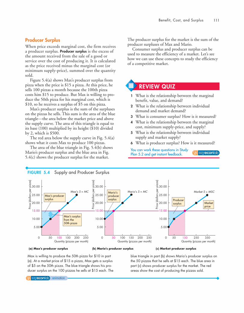
Benefit, Cost, and Surplus 111

Producer SurplusWhen price exceeds marginal cost, the firm receivesa producer surplus. Producer surplus is the excess ofthe amount received from the sale of a good orservice over the cost of producing it. It is calculatedas the price received minus the marginal cost (orminimum supply-price), summed over the quantitysold.

Figure 5.4(a) shows Max’s producer surplus frompizza when the price is $15 a pizza. At this price, hesells 100 pizzas a month because the 100th pizzacosts him $15 to produce. But Max is willing to pro-duce the 50th pizza for his marginal cost, which is$10, so he receives a surplus of $5 on this pizza.

Max’s producer surplus is the sum of the surpluseson the pizzas he sells. This sum is the area of the bluetriangle—the area below the market price and abovethe supply curve. The area of this triangle is equal toits base (100) multiplied by its height ($10) dividedby 2, which is $500.

The red area below the supply curve in Fig. 5.4(a)shows what it costs Max to produce 100 pizzas.

The area of the blue triangle in Fig. 5.4(b) showsMario’s producer surplus and the blue area in Fig.5.4(c) shows the producer surplus for the market.

(a) Max's producer surplus

30.00

20.00

10.00

0 100 15050 250200

25.00

15.00

5.00

Pric

e (d

olla

rs p

er p

izza

)

Max's S = MC

(b) Mario's producer surplus (c) Market producer surplus

Quantity (pizzas per month)

Max's surplusfrom the50th pizza

Max's producersurplus

Mario'sproducersurplus

30.00

20.00

10.00

0 100 15050 250200

25.00

15.00

5.00

Pric

e (d

olla

rs p

er p

izza

)

Mario's S = MC

Quantity (pizzas per month)

30.00

20.00

10.00

0 15050 250 350

25.00

15.00

5.00

Pric

e (d

olla

rs p

er p

izza

)

Market S = MSC

Quantity (pizzas per month)

Producersurplus Market

price

Max is willing to produce the 50th pizza for $10 in part(a). At a market price of $15 a pizza, Max gets a surplusof $5 on the 50th pizza. The blue triangle shows his pro-ducer surplus on the 100 pizzas he sells at $15 each. The

blue triangle in part (b) shows Mario’s producer surplus onthe 50 pizzas that he sells at $15 each. The blue area inpart (c) shows producer surplus for the market. The redareas show the cost of producing the pizzas sold.

The producer surplus for the market is the sum of theproducer surpluses of Max and Mario.

Consumer surplus and producer surplus can beused to measure the efficiency of a market. Let’s seehow we can use these concepts to study the efficiencyof a competitive market.

REVIEW QUIZ1 What is the relationship between the marginal

benefit, value, and demand?2 What is the relationship between individual

demand and market demand?3 What is consumer surplus? How is it measured?4 What is the relationship between the marginal

cost, minimum supply-price, and supply?5 What is the relationship between individual

supply and market supply?6 What is producer surplus? How is it measured?

You can work these questions in Study Plan 5.2 and get instant feedback.

FIGURE 5.4 Supply and Producer Surplus

animation

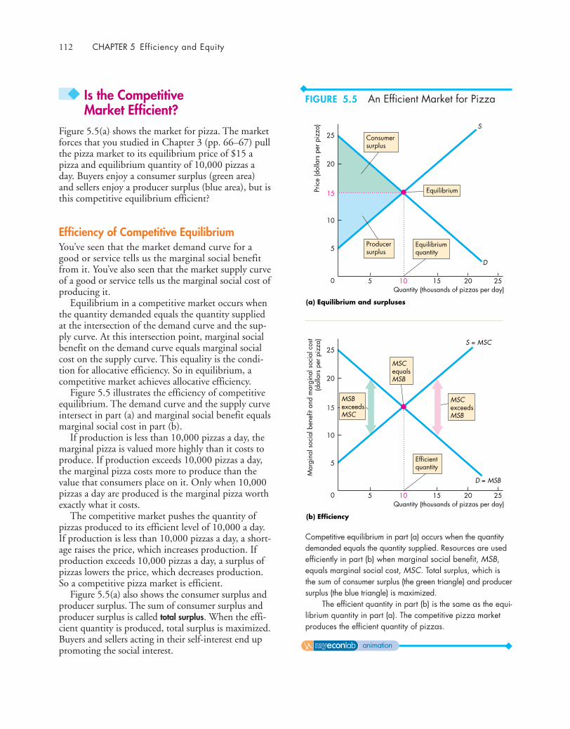
112 CHAPTER 5 Efficiency and Equity

◆ Is the Competitive Market Efficient?

Figure 5.5(a) shows the market for pizza. The marketforces that you studied in Chapter 3 (pp. 66–67) pullthe pizza market to its equilibrium price of $15 apizza and equilibrium quantity of 10,000 pizzas aday. Buyers enjoy a consumer surplus (green area)and sellers enjoy a producer surplus (blue area), but isthis competitive equilibrium efficient?

Efficiency of Competitive EquilibriumYou’ve seen that the market demand curve for agood or service tells us the marginal social benefitfrom it. You’ve also seen that the market supply curveof a good or service tells us the marginal social cost ofproducing it.

Equilibrium in a competitive market occurs whenthe quantity demanded equals the quantity suppliedat the intersection of the demand curve and the sup-ply curve. At this intersection point, marginal socialbenefit on the demand curve equals marginal socialcost on the supply curve. This equality is the condi-tion for allocative efficiency. So in equilibrium, acompetitive market achieves allocative efficiency.

Figure 5.5 illustrates the efficiency of competitiveequilibrium. The demand curve and the supply curveintersect in part (a) and marginal social benefit equalsmarginal social cost in part (b).

If production is less than 10,000 pizzas a day, themarginal pizza is valued more highly than it costs toproduce. If production exceeds 10,000 pizzas a day,the marginal pizza costs more to produce than thevalue that consumers place on it. Only when 10,000pizzas a day are produced is the marginal pizza worthexactly what it costs.

The competitive market pushes the quantity ofpizzas produced to its efficient level of 10,000 a day.If production is less than 10,000 pizzas a day, a short-age raises the price, which increases production. Ifproduction exceeds 10,000 pizzas a day, a surplus ofpizzas lowers the price, which decreases production.So a competitive pizza market is efficient.

Figure 5.5(a) also shows the consumer surplus andproducer surplus. The sum of consumer surplus andproducer surplus is called total surplus. When the effi-cient quantity is produced, total surplus is maximized.Buyers and sellers acting in their self-interest end uppromoting the social interest.

(a) Equilibrium and surpluses

(b) Efficiency

Pric

e (d

olla

rs p

er p

izza

)

Quantity (thousands of pizzas per day)5 10 15

20

25

15

10

0

5

20 25

S

D

Consumersurplus

Producersurplus

Equilibriumquantity

Equilibrium

Mar

gina

l soc

ial b

enef

it an

d m

argi

nal s

ocia

l cos

t(d

olla

rs p

er p

izza

)

Quantity (thousands of pizzas per day)5 10 15

20

25

15

10

0

5

20 25

S = MSC

D = MSB

MSCexceedsMSB

MSCequalsMSB

Efficientquantity

MSBexceedsMSC

Competitive equilibrium in part (a) occurs when the quantitydemanded equals the quantity supplied. Resources are usedefficiently in part (b) when marginal social benefit, MSB,equals marginal social cost, MSC. Total surplus, which isthe sum of consumer surplus (the green triangle) and producersurplus (the blue triangle) is maximized.

The efficient quantity in part (b) is the same as the equi-librium quantity in part (a). The competitive pizza marketproduces the efficient quantity of pizzas.

FIGURE 5.5 An Efficient Market for Pizza

animation

Is the Competitive Market Efficient? 113

Economics in ActionThe Invisible HandWriting in his Wealth of Nations in 1776, AdamSmith was the first to suggest that competitive mar-kets send resources to the uses in which they have thehighest value (see p. 51). Smith believed that eachparticipant in a competitive market is “led by aninvisible hand to promote an end [the efficient use ofresources] which was no part of his intention.”

You can see the invisible hand at work in the car-toon and in the world today.

Umbrella for Sale The cold drinks vendor has colddrinks and shade and he has a marginal cost and aminimum supply-price of each. The reader on thepark bench has a marginal benefit and willingness topay for each. The reader’s marginal benefit fromshade exceeds the vendor’s marginal cost; but thevendor’s marginal cost of a cold drink exceeds thereader’s marginal benefit. They trade the umbrella.The vendor gets a producer surplus from selling theshade for more than its marginal cost, and the readergets a consumer surplus from buying the shade forless than its marginal benefit. Both are better off andthe umbrella has moved to its highest-valued use.

The Invisible Hand at Work Today The market econ-omy relentlessly performs the activity illustrated inthe cartoon to achieve an efficient allocation ofresources.

A Florida frost cuts the supply of tomatoes. Withfewer tomatoes available, the marginal social benefitincreases. A shortage of tomatoes raises their price, sothe market allocates the smaller quantity available tothe people who value them most highly.

A new technology cuts the cost of producing asmart phone. With a lower production cost, the supplyof smart phones increases and the price of a smart

Market FailureMarkets do not always achieve an efficient outcome.We call a situation in which a market delivers an inef-ficient outcome one of market failure. Market failurecan occur because too little of an item is produced(underproduction) or too much is produced (over-production). We’ll describe these two market failureoutcomes and then see why they arise.

© The New Yorker Collection 1985 Mike Twohy from cartoonbank.com.All Rights Reserved.

phone falls. The lower price encourages an increase inthe quantity demanded of this now less-costly tool.The marginal social benefit from a smart phone isbrought to equality with its marginal social cost.

Underproduction In Fig. 5.6(a), the quantity of pizzasproduced is 5,000 a day. At this quantity, consumers arewilling to pay $20 for a pizza that costs only $10 to pro-duce. By producing only 5,000 pizzas a day, total surplusis smaller than its maximum possible level. The quantityproduced is inefficient—there is underproduction.

We measure the scale of inefficiency by deadweightloss, which is the decrease in total surplus that results

114 CHAPTER 5 Efficiency and Equity

from an inefficient level of production. The gray tri-angle in Fig. 5.6(a) shows the deadweight loss.

Overproduction In Fig. 5.6(b), the quantity of pizzasproduced is 15,000 a day. At this quantity, consumersare willing to pay only $10 for a pizza that costs $20to produce. By producing the 15,000th pizza, $10 ofresources are wasted. Again, the gray triangle showsthe deadweight loss, which reduces the total surplusto less than its maximum.

Inefficient production creates a deadweight lossthat is borne by the entire society: It is a social loss.

Sources of Market FailureObstacles to efficiency that bring market failure andcreate deadweight losses are

■ Price and quantity regulations■ Taxes and subsidies■ Externalities■ Public goods and common resources■ Monopoly■ High transactions costs

Price and Quantity Regulations Price regulations thatput a cap on the rent a landlord is permitted to chargeand laws that require employers to pay a minimumwage sometimes block the price adjustments that bal-ance the quantity demanded and the quantity suppliedand lead to underproduction. Quantity regulations thatlimit the amount that a farm is permitted to producealso lead to underproduction.

Taxes and Subsidies Taxes increase the prices paid by buyers and lower the prices received by sellers. Sotaxes decrease the quantity produced and lead tounderproduction. Subsidies, which are payments bythe government to producers, decrease the prices paidby buyers and increase the prices received by sellers.So subsidies increase the quantity produced and leadto overproduction.

Externalities An externality is a cost or a benefit thataffects someone other than the seller or the buyer. Anexternal cost arises when an electric utility burns coaland emits carbon dioxide. The utility doesn’t considerthe cost of climate change when it decides how muchpower to produce. The result is overproduction. Anexternal benefit arises when an apartment ownerinstalls a smoke detector and decreases her neighbor’s

(a) Underproduction

(b) Overproduction

Pric

e (d

olla

rs p

er p

izza

)

Quantity (thousands of pizzas per day)5 10 15

20

25

15

10

0

5

20 25

S

D

Deadweightloss

Pric

e (d

olla

rs p

er p

izza

)

Quantity (thousands of pizzas per day)5 10 15

20

25

15

10

0

5

20 25

S

D

Deadweightloss

If 5,000 pizzas a day are produced, in part (a), total surplus(the sum of the green and blue areas) is smaller than its maxi-mum by the amount of the deadweight loss (the gray trian-gle). At all quantities below 10,000 pizzas a day, the benefitfrom one more pizza exceeds its cost.

If 15,000 pizzas a day are produced, in part (b), totalsurplus is also smaller than its maximum by the amount of thedeadweight loss. At all quantities in excess of 10,000 pizzasa day, the cost of one more pizza exceeds its benefit.

FIGURE 5.6 Underproduction andOverproduction

animation

Is the Competitive Market Efficient? 115

Alternatives to the MarketWhen a market is inefficient, can one of the alterna-tive nonmarket methods that we described at thebeginning of this chapter do a better job? Sometimesit can.

Often, majority rule might be used in an attempt toimprove the allocation of resources. But majority rulehas its own shortcomings. A group that pursues theself-interest of its members can become the majority.For example, a price or quantity regulation that createsinefficiency is almost always the result of a self-inter-ested group becoming the majority and imposing costson the minority. Also, with majority rule, votes must betranslated into actions by bureaucrats who have theirown agendas based on their self-interest.

Managers in firms issue commands and avoid thetransactions costs that they would incur if they wentto a market every time they needed a job done.

First-come, first-served works best in some situa-tions. Think about the scene at a busy ATM. Insteadof waiting in line people might trade places at a “mar-ket” price. But someone would need to ensure thattrades were honored. At a busy ATM, first-come,first-served is the most efficient arrangement.

There is no one efficient mechanism that allocatesall resources efficiently. But markets, when supple-mented by other mechanisms such as majority rule,command systems, and first-come, first-served, do anamazingly good job.

Is an efficient allocation of resources also a fairallocation? Does the competitive market provide peo-ple with fair incomes for their work? Do peoplealways pay a fair price for the things they buy? Don’twe need the government to step into some competi-tive markets to prevent the price from rising too highor falling too low? Let’s now study these questions.

fire risk. She doesn’t consider the benefit to herneighbor when she decides how many detectors toinstall. The result is underproduction.

Public Goods and Common Resources A public goodis a good or service that is consumed simultaneouslyby everyone even if they don’t pay for it. Nationaldefense is an example. Competitive markets wouldunderproduce national defense because it is in eachperson’s interest to free ride on everyone else and avoidpaying for her or his share of such a good.

A common resource is owned by no one but is avail-able to be used by everyone. Atlantic salmon is anexample. It is in everyone’s self-interest to ignore thecosts they impose on others when they decide howmuch of a common resource to use. The result is thatthe resource is overused.

Monopoly A monopoly is a firm that is the soleprovider of a good or service. Local water supplyand cable television are supplied by firms that aremonopolies. The monopoly’s self-interest is tomaximize its profit. Because the monopoly has nocompetitors, it can set the price to achieve its self-interested goal. To achieve its goal, a monopolyproduces too little and charges too high a price. Itleads to underproduction.

High Transactions Costs When you go to Starbucks,you pay for more than the coffee. You pay your shareof the cost of the barrista’s time, the espresso maker,and the decor. When you buy your first apartment,you will pay for more than the apartment. You willbuy the services of a realtor and a lawyer. Economistscall the costs of the services that enable a market tobring buyers and sellers together transactions costs.

It is costly to operate any market so to use marketprice to allocate resources, it must be worth bearingthe transactions costs. Some markets are too costly tooperate. For example, it is too costly to operate amarket in time slots on a local tennis court. Insteadof a market, the court uses first-come, first-served:You hang around until the court becomes vacant and“pay” with your waiting time. When transactionscosts are high, the market might underproduce.

You now know the conditions under whichresource allocation is efficient. You’ve seen how acompetitive market can be efficient, and you’ve seensome obstacles to efficiency. Can alternative alloca-tion methods improve on the market?

REVIEW QUIZ1 Do competitive markets use resources effi-

ciently? Explain why or why not.2 What is deadweight loss and under what condi-

tions does it occur?3 What are the obstacles to achieving an efficient

allocation of resources in the market economy?

You can work these questions in Study Plan 5.3 and get instant feedback.

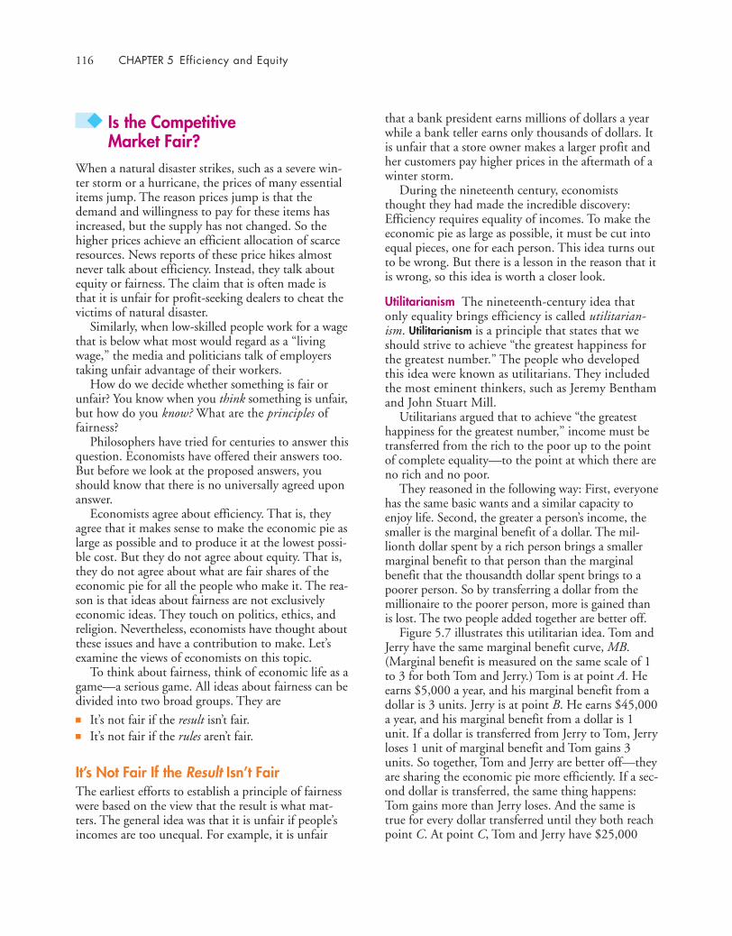
116 CHAPTER 5 Efficiency and Equity

◆ Is the Competitive Market Fair?

When a natural disaster strikes, such as a severe win-ter storm or a hurricane, the prices of many essentialitems jump. The reason prices jump is that thedemand and willingness to pay for these items hasincreased, but the supply has not changed. So thehigher prices achieve an efficient allocation of scarceresources. News reports of these price hikes almostnever talk about efficiency. Instead, they talk aboutequity or fairness. The claim that is often made isthat it is unfair for profit-seeking dealers to cheat thevictims of natural disaster.

Similarly, when low-skilled people work for a wagethat is below what most would regard as a “livingwage,” the media and politicians talk of employerstaking unfair advantage of their workers.

How do we decide whether something is fair orunfair? You know when you think something is unfair,but how do you know? What are the principles offairness?

Philosophers have tried for centuries to answer thisquestion. Economists have offered their answers too.But before we look at the proposed answers, youshould know that there is no universally agreed uponanswer.

Economists agree about efficiency. That is, theyagree that it makes sense to make the economic pie aslarge as possible and to produce it at the lowest possi-ble cost. But they do not agree about equity. That is,they do not agree about what are fair shares of theeconomic pie for all the people who make it. The rea-son is that ideas about fairness are not exclusivelyeconomic ideas. They touch on politics, ethics, andreligion. Nevertheless, economists have thought aboutthese issues and have a contribution to make. Let’sexamine the views of economists on this topic.

To think about fairness, think of economic life as agame—a serious game. All ideas about fairness can bedivided into two broad groups. They are■ It’s not fair if the result isn’t fair.■ It’s not fair if the rules aren’t fair.

It’s Not Fair If the Result Isn’t FairThe earliest efforts to establish a principle of fairnesswere based on the view that the result is what mat-ters. The general idea was that it is unfair if people’sincomes are too unequal. For example, it is unfair

that a bank president earns millions of dollars a yearwhile a bank teller earns only thousands of dollars. Itis unfair that a store owner makes a larger profit andher customers pay higher prices in the aftermath of awinter storm.

During the nineteenth century, economiststhought they had made the incredible discovery:Efficiency requires equality of incomes. To make theeconomic pie as large as possible, it must be cut intoequal pieces, one for each person. This idea turns outto be wrong. But there is a lesson in the reason that itis wrong, so this idea is worth a closer look.

Utilitarianism The nineteenth-century idea thatonly equality brings efficiency is called utilitarian-ism. Utilitarianism is a principle that states that weshould strive to achieve “the greatest happiness forthe greatest number.” The people who developedthis idea were known as utilitarians. They includedthe most eminent thinkers, such as Jeremy Benthamand John Stuart Mill.

Utilitarians argued that to achieve “the greatesthappiness for the greatest number,” income must betransferred from the rich to the poor up to the pointof complete equality—to the point at which there areno rich and no poor.

They reasoned in the following way: First, everyonehas the same basic wants and a similar capacity toenjoy life. Second, the greater a person’s income, thesmaller is the marginal benefit of a dollar. The mil-lionth dollar spent by a rich person brings a smallermarginal benefit to that person than the marginalbenefit that the thousandth dollar spent brings to apoorer person. So by transferring a dollar from themillionaire to the poorer person, more is gained thanis lost. The two people added together are better off.

Figure 5.7 illustrates this utilitarian idea. Tom andJerry have the same marginal benefit curve, MB.(Marginal benefit is measured on the same scale of 1to 3 for both Tom and Jerry.) Tom is at point A. Heearns $5,000 a year, and his marginal benefit from adollar is 3 units. Jerry is at point B. He earns $45,000a year, and his marginal benefit from a dollar is 1unit. If a dollar is transferred from Jerry to Tom, Jerryloses 1 unit of marginal benefit and Tom gains 3units. So together, Tom and Jerry are better off—theyare sharing the economic pie more efficiently. If a sec-ond dollar is transferred, the same thing happens:Tom gains more than Jerry loses. And the same istrue for every dollar transferred until they both reachpoint C. At point C, Tom and Jerry have $25,000

Is the Competitive Market Fair? 117

each and a marginal benefit of 2 units. Now they aresharing the economic pie in the most efficient way. Itbrings the greatest happiness to Tom and Jerry.

The Big Tradeoff One big problem with the utilitar-ian ideal of complete equality is that it ignores thecosts of making income transfers. Recognizing thecosts of making income transfers leads to what iscalled the big tradeoff, which is a tradeoff betweenefficiency and fairness.

The big tradeoff is based on the following facts.Income can be transferred from people with highincomes to people with low incomes only by taxingthe high incomes. Taxing people’s income fromemployment makes them work less. It results in thequantity of labor being less than the efficient quan-tity. Taxing people’s income from capital makes themsave less. It results in the quantity of capital being lessthan the efficient quantity. With smaller quantities ofboth labor and capital, the quantity of goods andservices produced is less than the efficient quantity.The economic pie shrinks.

The tradeoff is between the size of the economicpie and the degree of equality with which it is shared.The greater the amount of income redistributionthrough income taxes, the greater is the inefficiency—the smaller is the economic pie.

There is a second source of inefficiency. A dollartaken from a rich person does not end up as a dollar inthe hands of a poorer person. Some of the dollar isspent on administration of the tax and transfer system.The cost of tax-collecting agencies, such as the InternalRevenue Service (IRS), and welfare-administering agen-cies, such as the Centers for Medicare and Medicaid,must be paid with some of the taxes collected. Also,taxpayers hire accountants, auditors, and lawyers tohelp them ensure that they pay the correct amount oftaxes. These activities use skilled labor and capitalresources that could otherwise be used to producegoods and services that people value.

When all these costs are taken into account, takinga dollar from a rich person does not give a dollar to apoor person. It is possible that with high taxes, peo-ple with low incomes might end up being worse off.Suppose, for example, that highly taxed entrepreneursdecide to work less hard and shut down some of theirbusinesses. Low-income workers get fired and mustseek other, perhaps even lower-paid, work.

Today, because of the big tradeoff, no one says thatfairness requires equality of incomes.

Make the Poorest as Well Off as Possible A newsolution to the big-tradeoff problem was proposed byphilosopher John Rawls in a classic book entitled ATheory of Justice, published in 1971. Rawls says that,taking all the costs of income transfers into account,the fair distribution of the economic pie is the onethat makes the poorest person as well off as possible.The incomes of rich people should be taxed, and afterpaying the costs of administering the tax and transfersystem, what is left should be transferred to the poor.But the taxes must not be so high that they make theeconomic pie shrink to the point at which the poorestperson ends up with a smaller piece. A bigger share ofa smaller pie can be less than a smaller share of a big-ger pie. The goal is to make the piece enjoyed by thepoorest person as big as possible. Most likely, thispiece will not be an equal share.

The “fair results” idea requires a change in theresults after the game is over. Some economists saythat these changes are themselves unfair and proposea different way of thinking about fairness.

Maximumtotalbenefit

Mar

gina

l ben

efit

(uni

ts)

5 25 45Income (thousands of dollars)

2

0

1

3

MB

A

B

C

Tom

Jerry

Tom earns $5,000 and has 3 units of marginal benefit atpoint A. Jerry earns $45,000 and has 1 unit of marginalbenefit at point B. If income is transferred from Jerry to Tom,Jerry’s loss is less than Tom’s gain. Only when each of themhas $25,000 and 2 units of marginal benefit (at point C )can the sum of their total benefit increase no further.

FIGURE 5.7 Utilitarian Fairness

animation

118 CHAPTER 5 Efficiency and Equity

It’s Not Fair If the Rules Aren’t FairThe idea that it’s not fair if the rules aren’t fair isbased on a fundamental principle that seems to behardwired into the human brain: the symmetry prin-ciple. The symmetry principle is the requirement thatpeople in similar situations be treated similarly. It isthe moral principle that lies at the center of all thebig religions and that says, in some form or other,“Behave toward other people in the way you expectthem to behave toward you.”

In economic life, this principle translates intoequality of opportunity. But equality of opportunityto do what? This question is answered by the philoso-pher Robert Nozick in a book entitled Anarchy, State,and Utopia, published in 1974.

Nozick argues that the idea of fairness as an out-come or result cannot work and that fairness must bebased on the fairness of the rules. He suggests thatfairness obeys two rules:

1. The state must enforce laws that establish andprotect private property.

2. Private property may be transferred from oneperson to another only by voluntary exchange.

The first rule says that everything that is valuablemust be owned by individuals and that the statemust ensure that theft is prevented. The second rulesays that the only legitimate way a person canacquire property is to buy it in exchange for some-thing else that the person owns. If these rules, whichare the only fair rules, are followed, then the resultis fair. It doesn’t matter how unequally the eco-nomic pie is shared, provided that the pie is madeby people, each one of whom voluntarily providesservices in exchange for the share of the pie offeredin compensation.

These rules satisfy the symmetry principle. If theserules are not followed, the symmetry principle is bro-ken. You can see these facts by imagining a world inwhich the laws are not followed.

First, suppose that some resources or goods arenot owned. They are common property. Theneveryone is free to participate in a grab to use them.The strongest will prevail. But when the strongestprevails, the strongest effectively owns the resourcesor goods in question and prevents others fromenjoying them.

Second, suppose that we do not insist on voluntaryexchange for transferring ownership of resources fromone person to another. The alternative is involuntarytransfer. In simple language, the alternative is theft.

Both of these situations violate the symmetry prin-ciple. Only the strong acquire what they want. Theweak end up with only the resources and goods thatthe strong don’t want.

In a majority-rule political system, the strong arethose in the majority or those with enough resourcesto influence opinion and achieve a majority.

In contrast, if the two rules of fairness are fol-lowed, everyone, strong and weak, is treated in asimilar way. All individuals are free to use theirresources and human skills to create things that arevalued by themselves and others and to exchangethe fruits of their efforts with all others. This set ofarrangements is the only one that obeys the symme-try principle.

Fairness and Efficiency If private property rights areenforced and if voluntary exchange takes place in acompetitive market, resources will be allocated effi-ciently if there are no

1. Price and quantity regulations2. Taxes and subsidies3. Externalities4. Public goods and common resources5. Monopolies6. High transactions costs

And according to the Nozick rules, the resultingdistribution of income and wealth will be fair. Let’sstudy an example to check the claim that if resourcesare allocated efficiently, they are also allocated fairly.

Case Study: A Water Shortage in a Natural DisasterAn earthquake has broken the pipes that deliverdrinking water to a city. Bottled water is available,but there is no tap water. What is the fair way to allo-cate the bottled water?

Market Price Suppose that if the water is allocated bymarket price, the price jumps to $8 a bottle—fivetimes its normal price. At this price, the people whoown water can make a large profit by selling it.People who are willing and able to pay $8 a bottle getthe water. And because most people can’t afford the$8 price, they end up either without water or con-suming just a few drops a day.

You can see that the water is being used efficiently.There is a fixed amount available, some people arewilling to pay $8 to get a bottle, and the water goes

Is the Competitive Market Fair? 119

to those people. The people who own and sell waterreceive a large producer surplus and total surplus ismaximized.

In the rules view, the outcome is fair. No one isdenied the water they are willing to pay for. In theresults view, the outcome would most likely beregarded as unfair. The lucky owners of water make akilling, and the poorest end up the thirstiest.

Nonmarket Methods Suppose that by a majorityvote, the citizens decide that the government will buyall the water, pay for it with a tax, and use one of thenonmarket methods to allocate the water to the citi-zens. The possibilities now are

Command Someone decides who is the most deserv-ing and needy. Perhaps everyone is given an equalshare. Or perhaps government officials and their fam-ilies end up with most of the water.

Contest Bottles of water are prizes that go to thosewho are best at a particular contest.

First-come, first-served Water goes to the first off themark or to those who place the lowest value on theirtime and can afford to wait in line.

Lottery Water goes to those in luck.

Personal characteristics Water goes to those with the“right” characteristics. Perhaps the old, the young, orpregnant women get the water.

Except by chance, none of these methods deliversan allocation of water that is either fair or efficient. Itis unfair in the rules view because the distributioninvolves involuntary transfers of resources among cit-izens. It is unfair in the results view because the poor-est don’t end up being made as well off as possible.

The allocation is inefficient for two reasons. First,resources have been used to operate the allocationscheme. Second, some people are willing to pay formore water than the quantity they have been allo-cated and others have been allocated more water thanthey are willing to pay for.

The second source of inefficiency can be over-come if, after the nonmarket allocation, people arepermitted to trade water at its market price. Thosewho value the water they have at less than the mar-ket price sell, and people who are willing to pay themarket price to obtain more water buy. Those whovalue the water most highly are the ones whoconsume it.

Market Price with Taxes Another approach is to allo-cate the scarce water using the market price but thento alter the redistribution of buying power by taxingthe sellers and providing benefits to the poor.

Suppose water owners are taxed on each bottlesold and the revenue from these taxes is given to thepoorest people. People are then free, starting fromthis new distribution of buying power, to trade waterat the market price.

Because the owners of water are taxed on whatthey sell, they have a weaker incentive to offer waterfor sale and the supply decreases. The equilibriumprice rises to more than $8 a bottle. There is now adeadweight loss in the market for water—similar tothe loss that arises from underproduction on pp.113–114. (We study the effects of a tax and show itsinefficiency in Chapter 6 on pp. 133–138.)

So the tax is inefficient. In the rules view, the tax isalso unfair because it forces the owners of water tomake a transfer to others. In the results view, the out-come might be regarded as being fair.

This brief case study illustrates the complexity ofideas about fairness. Economists have a clear criterionof efficiency but no comparably clear criterion of fair-ness. Most economists regard Nozick as being tooextreme and want a fair tax system, but there is noconsensus about what a fair tax system looks like.

◆ You’ve now studied efficiency and equity (fair-ness), the two biggest issues that run through thewhole of economics. Reading Between the Lines on pp.120–121 looks at an example of an efficient market inour economy today. At many points throughout thisbook—and in your life—you will return to and usethe ideas you’ve learned in this chapter. We start inthe next chapter where we study some sources ofinefficiency and unfairness.

REVIEW QUIZ1 What are the two big approaches to thinking

about fairness?2 What is the utilitarian idea of fairness and what

is wrong with it?3 Explain the big tradeoff. What idea of fairness

has been developed to deal with it?4 What is the idea of fairness based on fair rules?

You can work these questions in Study Plan 5.4 and get instant feedback.

120

READING BETWEEN THE L INES

More Ash Fallout: 10 Million Roses Ruinedhttp://www.cbsnews.comApril 19, 2010

NAIROBI, Kenya—Daniel Oyier has been eating only once a day since an ash-belching vol-cano more than 5,000 miles away caused him to be laid off from his $4-a-day job packingred roses and white lilies for export to Paris and Amsterdam.

Some 5,000 day laborers in Kenya have been without work since the ash cloud from Icelandshut down air traffic across Europe, showing how one event can have drastic consequences indistant lands in today’s global economy. …

Kenya has thrown away 10 million flowers—mostly roses—since the volcano eruption. …

The world’s biggest flower auction in the Dutch town of Aalsmeer saw a drop of 15 percentin flowers sold on Monday as a result of flight disruptions from the volcanic ash cloud. …

Farmers have been forced to find alternative routes to get their products to market—even at aloss. They flew 1,000 metric tons of flowers to Spain on Monday, from where it would betransported by road to Paris and Amsterdam. …

Other flower-growing regions have seen salesfall because of the eruption. …

Willem Verhoogt [a South African exporter saidhis firm was] … supposed to export 11,000pounds of fresh cut flowers mainly to Europe,and to the United States via flights throughEurope.

“All together, it could be between 10 to 15 tonsthat won’t go in the end,” he said. “We’ve ad-vised farmers not to pick flowers anymore.”

Used with permission of The Associated Press. Copyright © 2010. Allrights reserved. The Associated Press contributed to this report.

■ In April 2010, the global fresh flower marketwas disrupted by the ash cloud from an erupt-ing volcano in Iceland that shut down Europe‘sair traffic.

■ Many of the world’s flowers are traded at auc-tion in the Dutch town of Aalsmeer, which sawa drop of 15 percent in the quantity of flowerssold.

■ 5,000 workers in Kenya who pick and packflowers were without work.

■ Kenya’s flower growers threw away 10 millionflowers—mostly roses.

■ South African flower growers were preventedfrom shipping as much as 15 tons of fresh cutflowers to Europe and the United States.

■ Some farmers found alternative but more costlyroutes to get their flowers to market.

ESSENCE OF THE STORY

Is the Global Market forRoses Efficient?

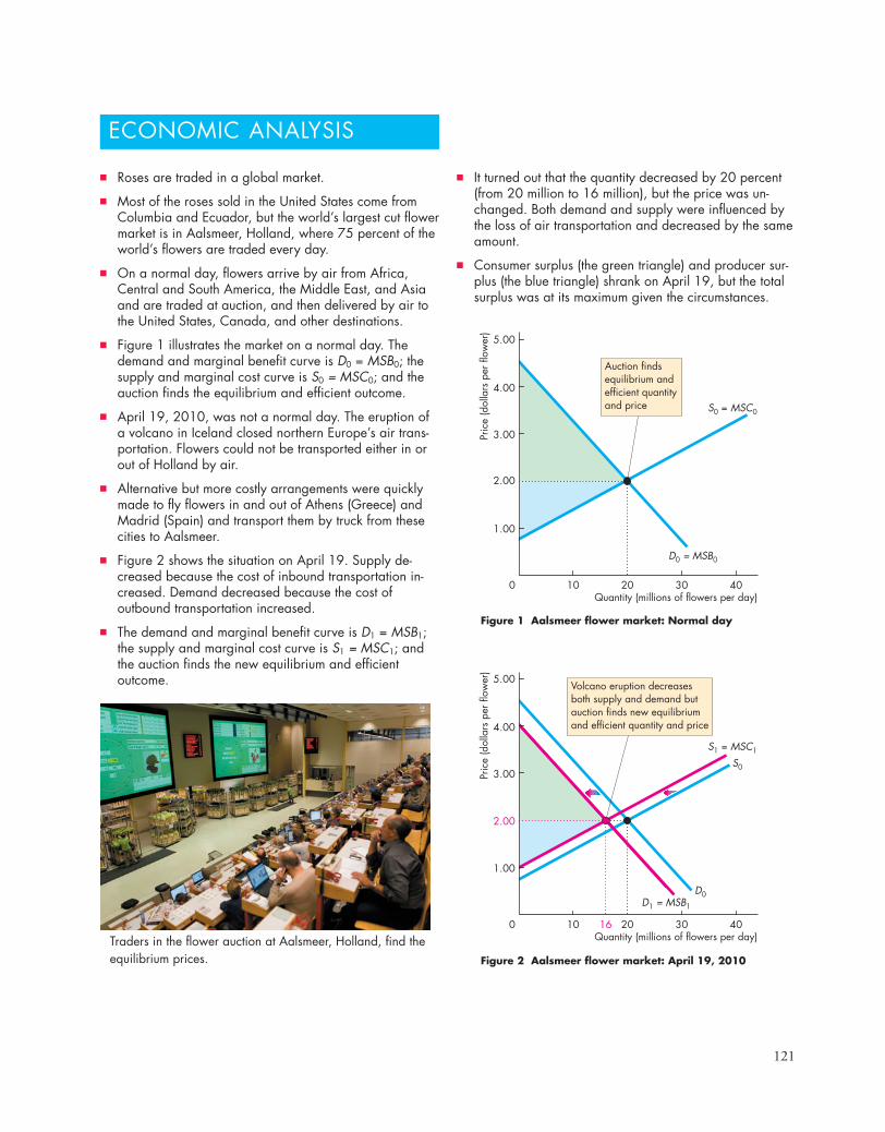
121

ECONOMIC ANALYSIS

Figure 2 Aalsmeer flower market: April 19, 2010

Figure 1 Aalsmeer flower market: Normal day

Pric

e (d

olla

rs p

er fl

ower

)

Quantity (millions of flowers per day)0

D0 = MSB0

S0

S1 = MSC1

D0D1 = MSB1

Auction findsequilibrium andefficient quantityand price

Volcano eruption decreasesboth supply and demand butauction finds new equilibriumand efficient quantity and price

20

1.00

10 30 40

2.00

3.00

4.00

5.00

S0 = MSC0

Pric

e (d

olla

rs p

er fl

ower

)

Quantity (millions of flowers per day)0 2016

1.00

10 30 40

2.00

3.00

4.00

5.00

■ Roses are traded in a global market.

■ Most of the roses sold in the United States come fromColumbia and Ecuador, but the world’s largest cut flowermarket is in Aalsmeer, Holland, where 75 percent of theworld’s flowers are traded every day.

■ On a normal day, flowers arrive by air from Africa,Central and South America, the Middle East, and Asiaand are traded at auction, and then delivered by air tothe United States, Canada, and other destinations.

■ Figure 1 illustrates the market on a normal day. Thedemand and marginal benefit curve is D0 = MSB0; thesupply and marginal cost curve is S0 = MSC0; and theauction finds the equilibrium and efficient outcome.

■ April 19, 2010, was not a normal day. The eruption ofa volcano in Iceland closed northern Europe’s air trans-portation. Flowers could not be transported either in orout of Holland by air.

■ Alternative but more costly arrangements were quicklymade to fly flowers in and out of Athens (Greece) andMadrid (Spain) and transport them by truck from thesecities to Aalsmeer.

■ Figure 2 shows the situation on April 19. Supply de-creased because the cost of inbound transportation in-creased. Demand decreased because the cost ofoutbound transportation increased.

■ The demand and marginal benefit curve is D1 = MSB1;the supply and marginal cost curve is S1 = MSC1; andthe auction finds the new equilibrium and efficientoutcome.

Traders in the flower auction at Aalsmeer, Holland, find theequilibrium prices.

■ It turned out that the quantity decreased by 20 percent(from 20 million to 16 million), but the price was un-changed. Both demand and supply were influenced bythe loss of air transportation and decreased by the sameamount.

■ Consumer surplus (the green triangle) and producer sur-plus (the blue triangle) shrank on April 19, but the totalsurplus was at its maximum given the circumstances.

122 CHAPTER 5 Efficiency and Equity

■ Producer surplus is the excess of the amountreceived from the sale of a good or service over thecost of producing it.

Working Study Plan Problems 3 to 10 will give you abetter understanding of benefit, cost, and surplus.

Is the Competitive Market Efficient? (pp. 112–115)

■ In a competitive equilibrium, marginal social ben-efit equals marginal social cost and resource alloca-tion is efficient.

■ Buyers and sellers acting in their self-interest endup promoting the social interest.

■ Total surplus, consumer surplus plus producer sur-plus, is maximized.

■ Producing less than or more than the efficientquantity creates deadweight loss.

■ Price and quantity regulations; taxes and subsidies;externalities; public goods and common resources;monopoly; and high transactions costs can lead tomarket failure.

Working Study Plan Problems 11 to 13 will give you a betterunderstanding of the efficiency of competitive markets.

Is the Competitive Market Fair? (pp. 116–119)

■ Ideas about fairness can be divided into twogroups: fair results and fair rules.

■ Fair-results ideas require income transfers from therich to the poor.

■ Fair-rules ideas require property rights and volun-tary exchange.

Working Study Plan Problems 14 and 15 will give you abetter understanding of the fairness of competitive markets.

Key Points

Resource Allocation Methods (pp. 106–107)

■ Because resources are scarce, some mechanismmust allocate them.

■ The alternative allocation methods are market price;command; majority rule; contest; first-come, first-served; lottery; personal characteristics; and force.

Working Study Plan Problems 1 and 2 will give you abetter understanding of resource allocation methods.

Benefit, Cost, and Surplus (pp. 108–111)

■ The maximum price willingly paid is marginalbenefit, so a demand curve is also a marginal bene-fit curve.

■ The market demand curve is the horizontal sum ofthe individual demand curves and is the marginalsocial benefit curve.

■ Value is what people are willing to pay; price iswhat people must pay.

■ Consumer surplus is the excess of the benefitreceived from a good or service over the amountpaid for it.

■ The minimum supply-price is marginal cost, so asupply curve is also a marginal cost curve.

■ The market supply curve is the horizontal sum ofthe individual supply curves and is the marginalsocial cost curve.

■ Cost is what producers pay; price is what produc-ers receive.

Key TermsBig tradeoff, 117Command system, 106Consumer surplus, 109Deadweight loss, 113

Market failure, 113Producer surplus, 111Symmetry principle, 118Total surplus, 112

Transactions costs, 115Utilitarianism, 116

SUMMARY

Study Plan Problems and Applications 123

b. What is the market consumer surplus whenthe price is $4 a mile?

Use the following table to work Problems 6 to 8.The table gives the supply schedules of hot air bal-loon rides for the only sellers in the market, Xavier,Yasmin, and Zack.

PriceQuantity supplied

(dollars per(rides per week)

ride) Xavier Yasmin Zack

100 30 25 2090 25 20 1580 20 15 1070 15 10 560 10 5 050 5 0 040 0 0 0

6. a. Construct the market supply schedule.b. What are the minimum prices that Xavier,

Yasmin, and Zack are willing to accept tosupply 20 rides? Why?

7. a. What is the marginal social cost when the totalnumber of rides is 30?

b. What is the marginal cost for each supplierwhen the total number of rides is 30 and howmany rides does each of the firms supply?

8. When the price is $70 a ride,a. What is each firm’s producer surplus?b. What is the market producer surplus?

Use the following news clip to work Problems 9 and 10.eBay Saves Billions for BiddersIf you think you would save money by bidding oneBay auctions, you would likely be right. TwoMaryland researchers calculated the differencebetween the actual purchase price paid for auctionitems and the top price bidders stated they were will-ing to pay. They found that the difference averaged atleast $4 per auction.

Source: InformationWeek, January 28, 20089. What method is used to allocate goods on eBay?

How does the allocation method used by eBayauctions influence consumer surplus?

10. a. Can an eBay auction give the seller a surplus?

Resource Allocation Methods (Study Plan 5.1)

Use the following information to work Problems 1and 2.At Chez Panisse, the restaurant in Berkeley that iscredited with having created California cuisine, reser-vations are essential. At Mandarin Dynasty, a restau-rant near the University of California San Diego,reservations are recommended. At Eli Cannon’s, arestaurant in Middletown, Connecticut, reservationsare not accepted.

1. a. Describe the method of allocating scarce table resources at these three restaurants.

b. Why do you think restaurants have differentreservations policies?

2. Why do you think restaurants don’t use the mar-ket price to allocate their tables?

Benefit, Cost, and Surplus (Study Plan 5.2)

Use the following table to work Problems 3 to 5. The table gives the demand schedules for train travelfor the only buyers in the market, Ann, Beth, and Cy.

PriceQuantity demanded

(dollars per(miles)

mile) Ann Beth Cy

3 30 25 204 25 20 155 20 15 106 15 10 57 10 5 08 5 0 09 0 0 0

3. a. Construct the market demand schedule.b. What are the maximum price that Ann, Beth,

and Cy are willing to pay to travel 20 miles?Why?

4. a. What is the marginal social benefit when thetotal distance travelled is 60 miles?

b. What is the marginal private benefit for eachperson when they travel a total distance of 60miles and how many miles does each of thepeople travel?

5. a. What is each traveler’s consumer surplus whenthe price is $4 a mile?

You can work Problems 1 to 17 in MyEconLab Chapter 5 Study Plan and get instant feedback.

STUDY PLAN PROBLEMS AND APPLICATIONS

124 CHAPTER 5 Efficiency and Equity

b. On a graph show the consumer surplus andproducer surplus from an eBay auction.

Is the Competitive Market Efficient? (Study Plan 5.3)

11. The figure illustrates the competitive market forcell phones.

a. What are the equilibrium price andequilibrium quantity of cell phones?

b. Shade in and label the consumer surplus atthe competitive equilibrium.

c. Shade in and label the producer surplus at thecompetitive equilibrium.

d. Calculate total surplus at the competitiveequilibrium.

e. Is the competitive market for cell phonesefficient?

12. The table gives the demand and supply schedulesfor sunscreen.

Quantity QuantityPrice demanded supplied

(dollars per bottle) (bottles per day)

0 400 05 300 100

10 200 20015 100 30020 0 400

Sunscreen factories are required to limit produc-tion to 100 bottles a day.a. What is the maximum price that consumers

are willing to pay for the 100th bottle?b. What is the minimum price that producers

are willing to accept for the 100th bottle?c. Describe the situation in this market.

13. Explain why each restaurant in Problem 1 mightbe using an efficient allocation method.

500 100 150 200

Pric

e (d

olla

rs p

er c

ell p

hone

)

Quantity (cell phones per month)

15.00

30.00

45.00

60.00

S

D

Is the Competitive Market Fair? (Study Plan 5.4)

14. Explain why the allocation method used by eachrestaurant in Problem 1 is fair or not fair.

15. In Problem 12, how can the 100 bottles availablebe allocated to beach-goers? Which possible meth-ods would be fair and which would be unfair?

Economics in the News (Study Plan 5.N)

16. The World’s Largest Tulip and Flower MarketEvery day 20 million tulips, roses, and other cutflowers are auctioned at the Dutch market calledThe Bloemenveiling. Each day 55,000 Dutch auc-tions take place, matching buyers and sellers.

Source: Tulip-Bulbs.comA Dutch auction is one in which the auctioneerstarts by announcing the highest price. If no oneoffers to buy the flowers, the auctioneer lowersthe price until a buyer is found.a. What method is used to allocate flowers at the

Bloemenveiling?b. How does a Dutch flower auction influence

consumer surplus and producer surplus?c. Are the flower auctions at the Bloemenveiling

efficient?

17. Wii Sells Out Across JapanAfter a two-month TV-ad blitz for Wii in Japan,demand was expected to be much higher than supply.Yodobashi Camera was selling Wii games on a first-come, first-served basis. Eager customers showed upearly and those who tried to join the line after 6 or 7a.m. were turned away—many rushed off to thesmaller stores that were holding raffles to decide whogot a Wii.

Source: Gamespot News, December 1, 2006a. Why was the quantity demanded of Wii ex-

pected to exceed the quantity supplied?b. Did Nintendo produce the efficient quantity

of Wii? Explain.c. Can you think of reasons why Nintendo might

want to underproduce and leave the marketwith fewer Wii than people want to buy?

d. What are the two methods of resource allocation described in the news clip? Is either method of allocating Wii efficient?

e. What do you think some of the people whomanaged to buy a Wii did with it?

f. Explain which is the fairer method of allocat-ing the Wii: the market price or the twomethods described in the news clip.

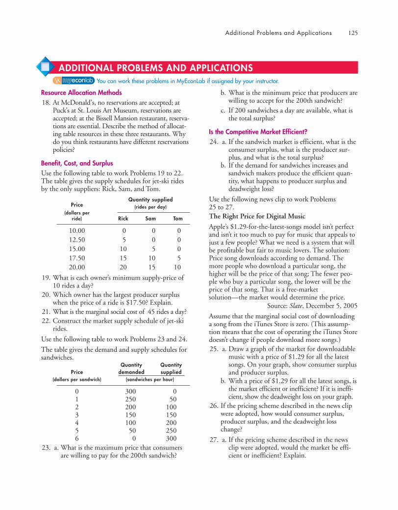
Additional Problems and Applications 125

Resource Allocation Methods18. At McDonald’s, no reservations are accepted; at

Puck’s at St. Louis Art Museum, reservations areaccepted; at the Bissell Mansion restaurant, reserva-tions are essential. Describe the method of allocat-ing table resources in these three restaurants. Whydo you think restaurants have different reservationspolicies?

Benefit, Cost, and SurplusUse the following table to work Problems 19 to 22.The table gives the supply schedules for jet-ski ridesby the only suppliers: Rick, Sam, and Tom.

PriceQuantity supplied

(dollars per(rides per day)

ride) Rick Sam Tom

10.00 0 0 012.50 5 0 015.00 10 5 017.50 15 10 520.00 20 15 10

19. What is each owner’s minimum supply-price of10 rides a day?

20. Which owner has the largest producer surpluswhen the price of a ride is $17.50? Explain.

21. What is the marginal social cost of 45 rides a day?22. Construct the market supply schedule of jet-ski

rides.

Use the following table to work Problems 23 and 24.

The table gives the demand and supply schedules forsandwiches.

Quantity QuantityPrice demanded supplied

(dollars per sandwich) (sandwiches per hour)

0 300 01 250 502 200 1003 150 1504 100 2005 50 2506 0 300

23. a. What is the maximum price that consumersare willing to pay for the 200th sandwich?

b. What is the minimum price that producers arewilling to accept for the 200th sandwich?

c. If 200 sandwiches a day are available, what isthe total surplus?

Is the Competitive Market Efficient?24. a. If the sandwich market is efficient, what is the

consumer surplus, what is the producer sur-plus, and what is the total surplus?

b. If the demand for sandwiches increases andsandwich makers produce the efficient quan-tity, what happens to producer surplus anddeadweight loss?

Use the following news clip to work Problems 25 to 27.The Right Price for Digital Music

Apple’s $1.29-for-the-latest-songs model isn’t perfectand isn’t it too much to pay for music that appeals tojust a few people? What we need is a system that willbe profitable but fair to music lovers. The solution:Price song downloads according to demand. Themore people who download a particular song, thehigher will be the price of that song; The fewer peo-ple who buy a particular song, the lower will be theprice of that song. That is a free-marketsolution—the market would determine the price.

Source: Slate, December 5, 2005

Assume that the marginal social cost of downloadinga song from the iTunes Store is zero. (This assump-tion means that the cost of operating the iTunes Storedoesn’t change if people download more songs.)25. a. Draw a graph of the market for downloadable

music with a price of $1.29 for all the latestsongs. On your graph, show consumer surplusand producer surplus.

b. With a price of $1.29 for all the latest songs, isthe market efficient or inefficient? If it is ineffi-cient, show the deadweight loss on your graph.

26. If the pricing scheme described in the news clipwere adopted, how would consumer surplus,producer surplus, and the deadweight losschange?

27. a. If the pricing scheme described in the newsclip were adopted, would the market be effi-cient or inefficient? Explain.

You can work these problems in MyEconLab if assigned by your instructor.

ADDITIONAL PROBLEMS AND APPLICATIONS

126 CHAPTER 5 Efficiency and Equity

b. Is the pricing scheme described in the newsclip a “free-market solution”? Explain.

Is the Competitive Market Fair?28. The winner of the men’s and women’s tennis

singles at the U.S. Open is paid twice as much asthe runner-up, but it takes two players to have asingles final. Is the compensation arrangementfair?

Economics in the News

29. After you have studied Reading Between the Lineson pp. 120–121 answer the following questions.a. What is the method used to allocate the

world’s cut flowers?b. Who benefits from this method of resource

allocation: buyers, sellers, or both? Explainyour answer using the ideas of marginal socialbenefit, marginal social cost, consumer sur-plus, and producer surplus.

c. On April 19, 2010, when the equilibriumquantity of cut flowers decreased by 20 per-cent, why was the outcome still efficient? Whywas there not underproduction and a dead-weight loss?

d. If the government of Holland placed a limit of15 million a day on the quantity of flowerstraded at Aalsmeer, would there be underpro-duction and a deadweight loss created?Explain your answer.

Use the following news clip to work Problems 30 and 31.Fight over Water Rates; Escondido Farmers SayIncrease would Put Them out of BusinessAgricultural users of water pay less than residentialand business users. Since 1993, water rates haveincreased by more than 90 percent for residential cus-tomers and by only 50 percent for agricultural users.Source:The San Diego Union-Tribune, June 14, 2006

30. a. Do you think that the allocation of waterbetween agricultural and residential users islikely to be efficient? Explain your answer.

b. If agricultural users paid a higher price, wouldthe allocation of resources be more efficient?

c. If agricultural users paid a higher price, whatwould happen to consumer surplus and pro-ducer surplus from water?

31. Is the difference in price paid by agricultural andresidential users fair?

32. MYTH: Price-Gouging Is BadMississippi cracked down on gougers afterHurricane Katrina. John Shepperson was one ofthe “gougers” authorities arrested. Sheppersonlives in Kentucky and he watched news reportsabout Katrina and learned that people desper-ately needed things. Shepperson thought hecould help and make some money, too, so hebought 19 generators. He rented a U-Haul anddrove 600 miles to an area of Mississippi that wasleft without power. He offered to sell his genera-tors for twice what he had paid for them, andpeople were eager to buy. Police confiscated hisgenerators, though, and Shepperson was jailedfor four days for price-gouging.

Source: ABC News, May 12, 2006a. Explain how the invisible hand (Shepperson)

actually reduced deadweight loss in the marketfor generators following Katrina.

b. Evaluate the “fairness” of Shepperson’s actions.Use the following information to work Problems 33and 34.Only 1 percent of the world supply of water is fit forhuman consumption. Some places have more waterthan they can use; some could use much more thanthey have. The 1 percent available would be sufficientif only it were in the right place.33. a. What is the major problem in achieving an

efficient use of the world’s water?b. If there were a global market in water, like

there is in oil, how do you think the marketwould be organized?

c. Would a free world market in water achieve anefficient use of the world’s water resources?Explain why or why not.

34. Would a free world market in water achieve a fairuse of the world’s water resources? Explain whyor why not and be clear about the concept offairness that you are using.

35. “Two Buck Chuck” Wine Cult“Two Buck Chuck,” is a cheap, good wine. Aftera year flooding the West Coast market, it is stillbeing sold by the case to wine lovers. An over-abundance of grapes has made the wine cheap tobottle—about 5 million cases so far.

Source: CBS, June 2, 2003How has “Two Buck Chuck” influenced the con-sumer surplus from wine, the producer surplusfor its producer, and the producer surplus for theproducers of other wines?

n New York City, where the average weekly wage rate is $1,000, it costs$3,500 a month to rent an average two-bedroom apartment. Can governmentscap rents to help renters live in affordable housing? Or instead, can governmentsmake housing more affordable by raising incomes with minimum wage laws?

Taxes put the hand of government in almost every pocket and market. Youprobably think that you pay more than your fair share of taxes. But whoactually pays and who benefits when a tax is cut: buyers or sellers?

In markets for farm products, governments intervene with the opposite of atax: a subsidy. Sometimes, governments limit thequantities that farms may produce. Do subsidies andproduction limits help to make markets efficient?

Some people break the law to evade price andwage regulations and taxes and trade in an “underground” economy. How domarkets work in the underground economy? In Reading Between the Lines at theend of this chapter, we apply what you’ve learned to the market for low-skilledlabor in California and see how governments must be careful to avoidunderground markets.

GOVERNMENT ACTIONS

After studying this chapter, you will be able to:

� Explain how rent ceilings create housing shortages andinefficiency

� Explain how minimum wage laws create unemploymentand inefficiency

� Explain the effects of a tax� Explain the effects of production quotas and subsidies

on production, costs, and prices� Explain how markets for illegal goods work

6I

IN MARKETS

127

128 CHAPTER 6 Government Actions in Markets

◆ A Housing Market with a Rent Ceiling

We spend more of our income on housing than onany other good or service, so it isn’t surprising thatrents can be a political issue. When rents are high, orwhen they jump by a large amount, renters mightlobby the government for limits on rents.

A government regulation that makes it illegal tocharge a price higher than a specified level is called aprice ceiling or price cap.

The effects of a price ceiling on a market dependcrucially on whether the ceiling is imposed at a levelthat is above or below the equilibrium price.

A price ceiling set above the equilibrium price hasno effect. The reason is that the price ceiling doesnot constrain the market forces. The force of thelaw and the market forces are not in conflict. But aprice ceiling below the equilibrium price has power-ful effects on a market. The reason is that the priceceiling attempts to prevent the price from regulat-ing the quantities demanded and supplied. Theforce of the law and the market forces are inconflict.

When a price ceiling is applied to a housing mar-ket, it is called a rent ceiling. A rent ceiling set belowthe equilibrium rent creates

■ A housing shortage■ Increased search activity■ A black market

A Housing ShortageAt the equilibrium price, the quantity demandedequals the quantity supplied. In a housing market,when the rent is at the equilibrium level, the quantityof housing supplied equals the quantity of housingdemanded and there is neither a shortage nor a sur-plus of housing.

But at a rent set below the equilibrium rent, thequantity of housing demanded exceeds the quantityof housing supplied—there is a shortage. So if a rentceiling is set below the equilibrium rent, there will bea shortage of housing.

When there is a shortage, the quantity available isthe quantity supplied and somehow, this quantitymust be allocated among the frustrated demanders.One way in which this allocation occurs is throughincreased search activity.

Increased Search ActivityThe time spent looking for someone with whom todo business is called search activity. We spend sometime in search activity almost every time we make apurchase. When you’re shopping for the latest hotnew cell phone, and you know four stores thatstock it, how do you find which store has the bestdeal? You spend a few minutes on the Internet,checking out the various prices. In some markets,such as the housing market, people spend a lot oftime checking the alternatives available before mak-ing a choice.

When a price is regulated and there is a shortage,search activity increases. In the case of a rent-con-trolled housing market, frustrated would-be rentersscan the newspapers, not only for housing ads butalso for death notices! Any information aboutnewly available housing is useful, and apartmentseekers race to be first on the scene when news of apossible supplier breaks.

The opportunity cost of a good is equal not only toits price but also to the value of the search time spentfinding the good. So the opportunity cost of housingis equal to the rent (a regulated price) plus the timeand other resources spent searching for the restrictedquantity available. Search activity is costly. It usestime and other resources, such as phone calls, auto-mobiles, and gasoline that could have been used inother productive ways.

A rent ceiling controls only the rent portion of thecost of housing. The cost of increased search activitymight end up making the full cost of housing higherthan it would be without a rent ceiling.

A Black MarketA rent ceiling also encourages illegal trading in ablack market, an illegal market in which the equilib-rium price exceeds the price ceiling. Black marketsoccur in rent-controlled housing and many othermarkets. For example, scalpers run black markets intickets for big sporting events and rock concerts.

When a rent ceiling is in force, frustrated rentersand landlords constantly seek ways of increasingrents. One common way is for a new tenant to pay ahigh price for worthless fittings, such as charging$2,000 for threadbare drapes. Another is for the ten-ant to pay an exorbitant price for new locks andkeys—called “key money.”

The level of a black market rent depends onhow tightly the rent ceiling is enforced. With loose

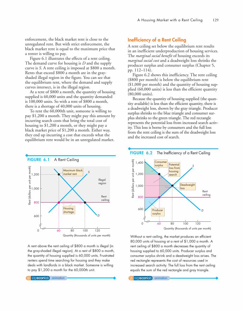
A Housing Market with a Rent Ceiling 129

enforcement, the black market rent is close to theunregulated rent. But with strict enforcement, theblack market rent is equal to the maximum price thata renter is willing to pay.

Figure 6.1 illustrates the effects of a rent ceiling.The demand curve for housing is D and the supplycurve is S. A rent ceiling is imposed at $800 a month.Rents that exceed $800 a month are in the gray-shaded illegal region in the figure. You can see thatthe equilibrium rent, where the demand and supplycurves intersect, is in the illegal region.

At a rent of $800 a month, the quantity of housingsupplied is 60,000 units and the quantity demandedis 100,000 units. So with a rent of $800 a month,there is a shortage of 40,000 units of housing.

To rent the 60,000th unit, someone is willing topay $1,200 a month. They might pay this amount byincurring search costs that bring the total cost ofhousing to $1,200 a month, or they might pay ablack market price of $1,200 a month. Either way,they end up incurring a cost that exceeds what theequilibrium rent would be in an unregulated market.

Inefficiency of a Rent CeilingA rent ceiling set below the equilibrium rent resultsin an inefficient underproduction of housing services.The marginal social benefit of housing exceeds itsmarginal social cost and a deadweight loss shrinks theproducer surplus and consumer surplus (Chapter 5,pp. 112–114).

Figure 6.2 shows this inefficiency. The rent ceiling($800 per month) is below the equilibrium rent($1,000 per month) and the quantity of housing sup-plied (60,000 units) is less than the efficient quantity(80,000 units).

Because the quantity of housing supplied (the quan-tity available) is less than the efficient quantity, there isa deadweight loss, shown by the gray triangle. Producersurplus shrinks to the blue triangle and consumer sur-plus shrinks to the green triangle. The red rectanglerepresents the potential loss from increased search activ-ity. This loss is borne by consumers and the full lossfrom the rent ceiling is the sum of the deadweight lossand the increased cost of search.

Housingshortage

Maximum black market rent1,200

80 100 120

Rent

(dol

lars

per

uni

t per

mon

th)

Quantity (thousands of units per month)

800

1,000

0

600

S

D

60

Rentceiling

Illegalregion

1,200

Rent

(dol

lars

per

uni

t per

mon

th)

Quantity (thousands of units per month)

800

1,000

0

600

S

D

Rentceiling

1,400

80 100 12060

Consumersurplus Potential

loss fromhousingsearch

Deadweightloss

Producersurplus

A rent above the rent ceiling of $800 a month is illegal (inthe gray-shaded illegal region). At a rent of $800 a month,the quantity of housing supplied is 60,000 units. Frustratedrenters spend time searching for housing and they makedeals with landlords in a black market. Someone is willingto pay $1,200 a month for the 60,000th unit.

Without a rent ceiling, the market produces an efficient80,000 units of housing at a rent of $1,000 a month. Arent ceiling of $800 a month decreases the quantity ofhousing supplied to 60,000 units. Producer surplus andconsumer surplus shrink and a deadweight loss arises. Thered rectangle represents the cost of resources used inincreased search activity. The full loss from the rent ceilingequals the sum of the red rectangle and gray triangle.

FIGURE 6.1 A Rent Ceiling

animation

FIGURE 6.2 The Inefficiency of a Rent Ceiling

animation

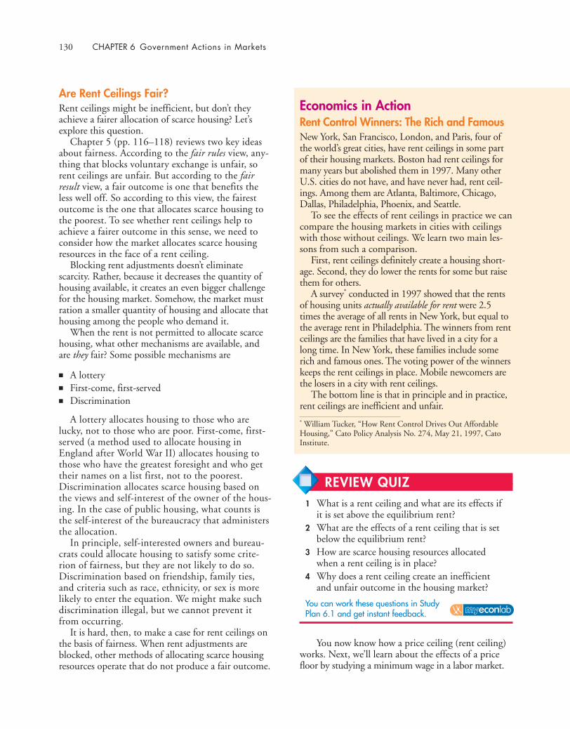
130 CHAPTER 6 Government Actions in Markets

Are Rent Ceilings Fair?Rent ceilings might be inefficient, but don’t theyachieve a fairer allocation of scarce housing? Let’sexplore this question.

Chapter 5 (pp. 116–118) reviews two key ideasabout fairness. According to the fair rules view, any-thing that blocks voluntary exchange is unfair, sorent ceilings are unfair. But according to the fairresult view, a fair outcome is one that benefits theless well off. So according to this view, the fairestoutcome is the one that allocates scarce housing tothe poorest. To see whether rent ceilings help toachieve a fairer outcome in this sense, we need toconsider how the market allocates scarce housingresources in the face of a rent ceiling.

Blocking rent adjustments doesn’t eliminatescarcity. Rather, because it decreases the quantity ofhousing available, it creates an even bigger challengefor the housing market. Somehow, the market mustration a smaller quantity of housing and allocate thathousing among the people who demand it.

When the rent is not permitted to allocate scarcehousing, what other mechanisms are available, andare they fair? Some possible mechanisms are

■ A lottery■ First-come, first-served■ Discrimination

A lottery allocates housing to those who arelucky, not to those who are poor. First-come, first-served (a method used to allocate housing inEngland after World War II) allocates housing tothose who have the greatest foresight and who gettheir names on a list first, not to the poorest.Discrimination allocates scarce housing based onthe views and self-interest of the owner of the hous-ing. In the case of public housing, what counts isthe self-interest of the bureaucracy that administersthe allocation.

In principle, self-interested owners and bureau-crats could allocate housing to satisfy some crite-rion of fairness, but they are not likely to do so.Discrimination based on friendship, family ties,and criteria such as race, ethnicity, or sex is morelikely to enter the equation. We might make suchdiscrimination illegal, but we cannot prevent itfrom occurring.

It is hard, then, to make a case for rent ceilings onthe basis of fairness. When rent adjustments areblocked, other methods of allocating scarce housingresources operate that do not produce a fair outcome.

You now know how a price ceiling (rent ceiling)works. Next, we’ll learn about the effects of a pricefloor by studying a minimum wage in a labor market.

Economics in ActionRent Control Winners: The Rich and FamousNew York, San Francisco, London, and Paris, four ofthe world’s great cities, have rent ceilings in some partof their housing markets. Boston had rent ceilings formany years but abolished them in 1997. Many otherU.S. cities do not have, and have never had, rent ceil-ings. Among them are Atlanta, Baltimore, Chicago,Dallas, Philadelphia, Phoenix, and Seattle.

To see the effects of rent ceilings in practice we cancompare the housing markets in cities with ceilingswith those without ceilings. We learn two main les-sons from such a comparison.

First, rent ceilings definitely create a housing short-age. Second, they do lower the rents for some but raisethem for others.

A survey* conducted in 1997 showed that the rentsof housing units actually available for rent were 2.5times the average of all rents in New York, but equal tothe average rent in Philadelphia. The winners from rentceilings are the families that have lived in a city for along time. In New York, these families include somerich and famous ones. The voting power of the winnerskeeps the rent ceilings in place. Mobile newcomers arethe losers in a city with rent ceilings.

The bottom line is that in principle and in practice,rent ceilings are inefficient and unfair.

REVIEW QUIZ1 What is a rent ceiling and what are its effects if

it is set above the equilibrium rent?2 What are the effects of a rent ceiling that is set

below the equilibrium rent?3 How are scarce housing resources allocated

when a rent ceiling is in place?4 Why does a rent ceiling create an inefficient

and unfair outcome in the housing market?

You can work these questions in Study Plan 6.1 and get instant feedback.

* William Tucker, “How Rent Control Drives Out AffordableHousing,” Cato Policy Analysis No. 274, May 21, 1997, CatoInstitute.

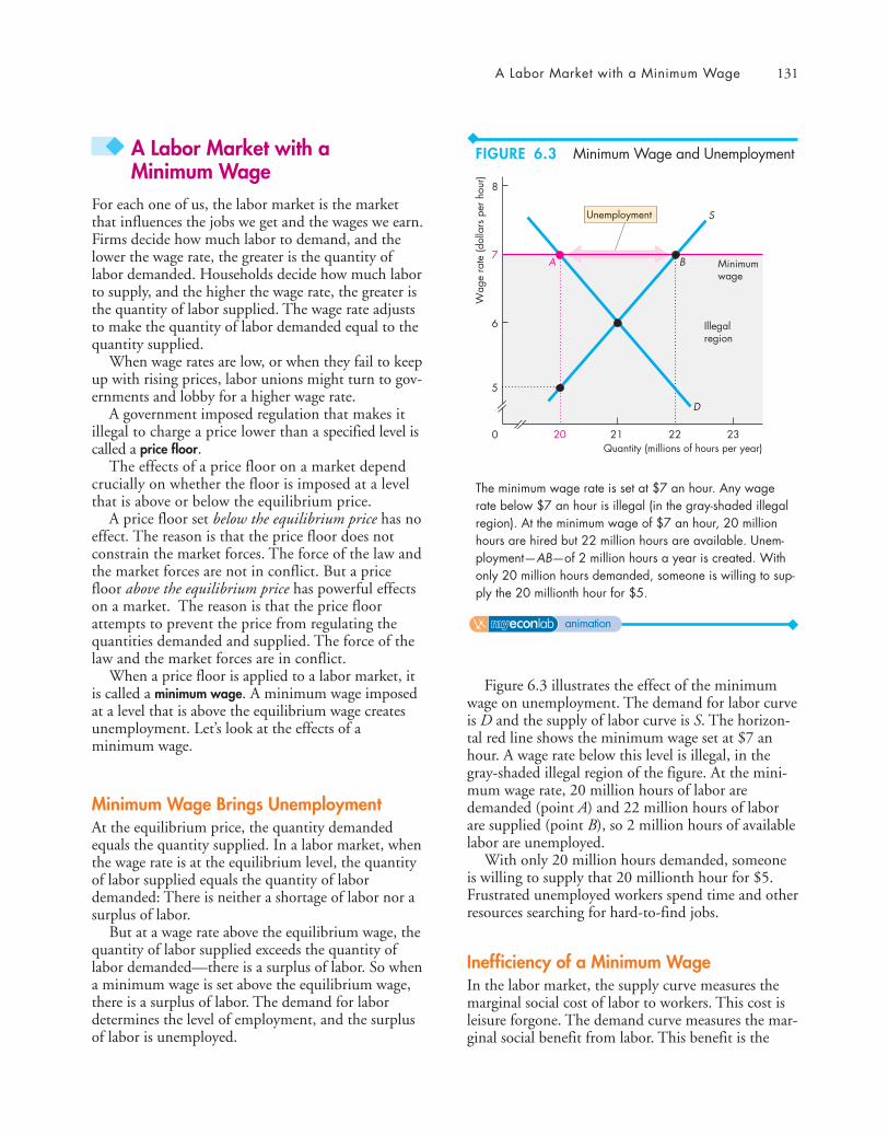
A Labor Market with a Minimum Wage 131

◆ A Labor Market with a Minimum Wage

For each one of us, the labor market is the marketthat influences the jobs we get and the wages we earn.Firms decide how much labor to demand, and thelower the wage rate, the greater is the quantity oflabor demanded. Households decide how much laborto supply, and the higher the wage rate, the greater isthe quantity of labor supplied. The wage rate adjuststo make the quantity of labor demanded equal to thequantity supplied.

When wage rates are low, or when they fail to keepup with rising prices, labor unions might turn to gov-ernments and lobby for a higher wage rate.

A government imposed regulation that makes itillegal to charge a price lower than a specified level iscalled a price floor.

The effects of a price floor on a market dependcrucially on whether the floor is imposed at a levelthat is above or below the equilibrium price.

A price floor set below the equilibrium price has noeffect. The reason is that the price floor does notconstrain the market forces. The force of the law andthe market forces are not in conflict. But a pricefloor above the equilibrium price has powerful effectson a market. The reason is that the price floorattempts to prevent the price from regulating thequantities demanded and supplied. The force of thelaw and the market forces are in conflict.

When a price floor is applied to a labor market, itis called a minimum wage. A minimum wage imposedat a level that is above the equilibrium wage createsunemployment. Let’s look at the effects of aminimum wage.

Minimum Wage Brings UnemploymentAt the equilibrium price, the quantity demandedequals the quantity supplied. In a labor market, whenthe wage rate is at the equilibrium level, the quantityof labor supplied equals the quantity of labordemanded: There is neither a shortage of labor nor asurplus of labor.

But at a wage rate above the equilibrium wage, thequantity of labor supplied exceeds the quantity oflabor demanded—there is a surplus of labor. So whena minimum wage is set above the equilibrium wage,there is a surplus of labor. The demand for labordetermines the level of employment, and the surplusof labor is unemployed.

Figure 6.3 illustrates the effect of the minimumwage on unemployment. The demand for labor curveis D and the supply of labor curve is S. The horizon-tal red line shows the minimum wage set at $7 anhour. A wage rate below this level is illegal, in thegray-shaded illegal region of the figure. At the mini-mum wage rate, 20 million hours of labor aredemanded (point A) and 22 million hours of laborare supplied (point B), so 2 million hours of availablelabor are unemployed.

With only 20 million hours demanded, someoneis willing to supply that 20 millionth hour for $5.Frustrated unemployed workers spend time and otherresources searching for hard-to-find jobs.

Inefficiency of a Minimum WageIn the labor market, the supply curve measures themarginal social cost of labor to workers. This cost isleisure forgone. The demand curve measures the mar-ginal social benefit from labor. This benefit is the

20 21 22 230

5

6

7

S

D

Quantity (millions of hours per year)

Wag

e ra

te (d

olla

rs p

er h

our)

Unemployment

A B Minimumwage

8

Illegalregion

The minimum wage rate is set at $7 an hour. Any wagerate below $7 an hour is illegal (in the gray-shaded illegalregion). At the minimum wage of $7 an hour, 20 millionhours are hired but 22 million hours are available. Unem-ployment—AB—of 2 million hours a year is created. Withonly 20 million hours demanded, someone is willing to sup-ply the 20 millionth hour for $5.

FIGURE 6.3 Minimum Wage and Unemployment

animation

132 CHAPTER 6 Government Actions in Markets

value of the goods and services produced. An unregu-lated labor market allocates the economy’s scarcelabor resources to the jobs in which they are valuedmost highly. The market is efficient.

The minimum wage frustrates the market mecha-nism and results in unemployment and increased jobsearch. At the quantity of labor employed, the mar-ginal social benefit of labor exceeds its marginal socialcost and a deadweight loss shrinks the firms’ surplusand the workers’ surplus.

Figure 6.4 shows this inefficiency. The minimumwage ($7 an hour) is above the equilibrium wage ($6an hour) and the quantity of labor demanded andemployed (20 million hours) is less than the efficientquantity (21 million hours).

Because the quantity of labor employed is less thanthe efficient quantity, there is a deadweight loss, shownby the gray triangle. The firms’ surplus shrinks to theblue triangle and the workers’ surplus shrinks to thegreen triangle. The red rectangle shows the potentialloss from increased job search, which is borne byworkers. The full loss from the minimum wage is thesum of the deadweight loss and the increased cost ofjob search.

Is the Minimum Wage Fair?The minimum wage is unfair on both views of fair-ness: It delivers an unfair result and imposes an unfairrule.

The result is unfair because only those people whohave jobs and keep them benefit from the minimumwage. The unemployed end up worse off than theywould be with no minimum wage. Some of thosewho search for jobs and find them end up worse offbecause of the increased cost of job search they incur.Also those who find jobs aren’t always the least welloff. When the wage rate doesn’t allocate labor, othermechanisms determine who finds a job. One suchmechanism is discrimination, which is yet anothersource of unfairness.

The minimum wage imposes an unfair rulebecause it blocks voluntary exchange. Firms are will-ing to hire more labor and people are willing to workmore, but they are not permitted by the minimumwage law to do so.

19 20 21 22 23 240

3

4

5

9

6

7

8

Minimumwage

S

D

Quantity (millions of hours per year)

Wag

e ra

te (d

olla

rs p

er h

our)

Workers'surplus

Potentialloss fromjob search

Firms'surplus

Deadweightloss

Economics in ActionUnscrambling Cause and Effect of theMinimum WageIn the United States, the federal government’s FairLabor Standards Act sets the minimum wage, whichhas fluctuated between 35 percent and 50 percent ofthe average wage, and in 2010 was $7.25 an hour.Most states have minimum wages that exceed thefederal minimum.

Does the minimum wage result in unemployment,and if so, how much unemployment does it create?The consensus answer is that a 10 percent rise in theminimum wage decreases teenage employment bybetween 1 and 3 percent.

This consensus answer has been challenged byDavid Card of the University of California atBerkeley (see pp. 484–486) and Alan Krueger ofPrinceton University.

Card and Krueger say that increases in the mini-mum wage have increased teenage employment anddecreased unemployment.

From their study of minimum wages in California,New Jersey, and Texas, Card and Krueger say that theemployment rate of low-income workers increased fol-lowing an increase in the minimum wage. They arguethat a higher wage increases employment by makingworkers become more conscientious and productive

A minimum wage decreases employment. Firms’ surplus (bluearea) and workers’ surplus (green area) shrink and a dead-weight loss (gray area) arises. Job search increases and thered area shows the loss from this activity.

FIGURE 6.4 The Inefficiency of a Minimum Wage

animation

Taxes 133

◆ TaxesEverything you earn and almost everything you buyis taxed. Income taxes and Social Security taxes arededucted from your earnings and sales taxes areadded to the bill when you buy something.Employers also pay a Social Security tax for theirworkers, and producers of tobacco products, alco-holic drinks, and gasoline pay a tax every time theysell something.

Who really pays these taxes? Because the incometax and Social Security tax are deducted from yourpay, and the sales tax is added to the prices that youpay, isn’t it obvious that you pay these taxes? Andisn’t it equally obvious that your employer pays theemployer’s contribution to the Social Security taxand that tobacco producers pay the tax oncigarettes?

You’re going to discover that it isn’t obvious whoreally pays a tax and that lawmakers don’t make thatdecision. We begin with a definition of tax incidence.

Tax IncidenceTax incidence is the division of the burden of a taxbetween buyers and sellers. When the governmentimposes a tax on the sale of a good*, the price paidby buyers might rise by the full amount of the tax,by a lesser amount, or not at all. If the price paidby buyers rises by the full amount of the tax, thenthe burden of the tax falls entirely on buyers—thebuyers pay the tax. If the price paid by buyers risesby a lesser amount than the tax, then the burden ofthe tax falls partly on buyers and partly on sellers.And if the price paid by buyers doesn’t change atall, then the burden of the tax falls entirely onsellers.

Tax incidence does not depend on the tax law. Thelaw might impose a tax on sellers or on buyers, butthe outcome is the same in either case. To see why,let’s look at the tax on cigarettes in New York City.

A Tax on SellersOn July 1, 2002, Mayor Bloomberg put a tax of$1.50 a pack on cigarettes sold in New York City. Towork out the effects of this tax on the sellers of ciga-rettes, we begin by examining the effects on demandand supply in the market for cigarettes.

* These propositions also apply to services and factors of production(land, labor, capital).

and less likely to quit, which lowers unproductive laborturnover. They also argue that a higher wage rate makesmanagers seek ways to increase labor productivity.

Most economists are skeptical about Card andKrueger’s argument. Why, economists ask, don’t firmsfreely pay wage rates above the equilibrium wage toencourage more productive work habits? Also, theypoint to other explanations for the employmentresponses that Card and Krueger found.

According to Daniel Hamermesh of the Universityof Texas at Austin, Card and Krueger got the timingwrong. Hamermesh says that firms cut employmentbefore the minimum wage is increased in anticipationof the increase. If he is correct, looking for the effectsof an increase after it has occurred misses its maineffects.

Finis Welch of Texas A&M University and KevinMurphy of the University of Chicago say the employ-ment effects that Card and Krueger found are causedby regional differences in economic growth, not bychanges in the minimum wage.

One effect of the minimum wage is an increase inthe quantity of labor supplied. If this effect occurs, itmight show up as an increase in the number of peo-ple who quit school to look for work before complet-ing high school. Some economists say that thisresponse does occur.

Next we’re going to study a more widespread gov-ernment action in markets: taxes. We’ll see how taxeschange prices and quantities. You will discover thesurprising fact that while the government can imposea tax, it can’t decide who will pay the tax! You willalso see that a tax creates a deadweight loss.

REVIEW QUIZ1 What is a minimum wage and what are its

effects if it is set above the equilibrium wage?2 What are the effects of a minimum wage set

below the equilibrium wage?3 Explain how scarce jobs are allocated when a

minimum wage is in place.4 Explain why a minimum wage creates an ineffi-

cient allocation of labor resources.5 Explain why a minimum wage is unfair.

You can work these questions in Study Plan 6.2 and get instant feedback.

134 CHAPTER 6 Government Actions in Markets

In Fig. 6.5, the demand curve is D, and the supplycurve is S. With no tax, the equilibrium price is $3 perpack and 350 million packs a year are bought and sold.

A tax on sellers is like an increase in cost, so itdecreases supply. To determine the position of thenew supply curve, we add the tax to the minimumprice that sellers are willing to accept for eachquantity sold. You can see that without the tax,sellers are willing to offer 350 million packs a yearfor $3 a pack. So with a $1.50 tax, they will offer350 million packs a year only if the price is $4.50 apack. The supply curve shifts to the red curvelabeled S + tax on sellers.

Equilibrium occurs where the new supply curveintersects the demand curve at 325 million packs ayear. The price paid by buyers rises by $1 to $4 apack. And the price received by sellers falls by 50¢ to$2.50 a pack. So buyers pay $1 of the tax and sellerspay the other 50¢.

A Tax on BuyersSuppose that instead of taxing sellers, New York Citytaxes cigarette buyers $1.50 a pack.

A tax on buyers lowers the amount they are will-ing to pay sellers, so it decreases demand and shiftsthe demand curve leftward. To determine the posi-tion of this new demand curve, we subtract the taxfrom the maximum price that buyers are willing topay for each quantity bought. You can see, in Fig.6.6, that without the tax, buyers are willing to buy350 million packs a year for $3 a pack. So with a$1.50 tax, they are willing to buy 350 millionpacks a year only if the price including the tax is $3a pack, which means that they’re willing to pay sell-ers only $1.50 a pack. The demand curve shifts tobecome the red curve labeled D – tax on buyers.

Equilibrium occurs where the new demand curveintersects the supply curve at a quantity of 325 mil-lion packs a year. The price received by sellers is$2.50 a pack, and the price paid by buyers is $4.

Equivalence of Tax on Buyers and SellersYou can see that the tax on buyers in Fig. 6.6 has thesame effects as the tax on sellers in Fig. 6.5. In bothcases, the equilibrium quantity decreases to 325 mil-lion packs a year, the price paid by buyers rises to $4a pack, and the price received by sellers falls to $2.50a pack. Buyers pay $1 of the $1.50 tax, and sellerspay the other 50¢ of the tax.

Can We Share the Burden Equally? Suppose thatMayor Bloomberg wants the burden of the cigarettetax to fall equally on buyers and sellers and declaresthat a 75¢ tax be imposed on each. Is the burden ofthe tax then shared equally?

You can see that it is not. The tax is still $1.50 apack. You’ve seen that the tax has the same effectregardless of whether it is imposed on sellers or buy-ers. So imposing half the tax on sellers and half onbuyers is like an average of the two cases you’ve justexamined. (Draw the demand-supply graph andwork out what happens in this case. The demandcurve shifts downward by 75¢ and the supply curveshifts upward by 75¢. The new equilibrium quantityis still 325 million packs a year. Buyers pay $4 a pack,of which 75¢ is tax. Sellers receive $3.25 from buy-ers, but pay a 75¢ tax, so sellers net $2.50 a pack.)

When a transaction is taxed, there are two prices:the price paid by buyers, which includes the tax; andthe price received by sellers, which excludes the tax.

325300275 350 375 400 425 4500

1.00

2.00

3.00

2.50

4.00

4.50

5.00S

D

Quantity (millions of packs per year)

Pric

e (d

olla

rs p

er p

ack)

S + tax on sellers

$1.50 tax

Price paidby buyers

Price receivedby sellers

Price with no tax

With no tax, 350 million packs a year are bought and sold at$3 a pack. A tax on sellers of $1.50 a pack shifts the supplycurve from S to S + tax on sellers. The equilibrium quantitydecreases to 325 million packs a year, the price paid by buy-ers rises to $4 a pack, and the price received by sellers fallsto $2.50 a pack. The tax raises the price paid by buyers byless than the tax and lowers the price received by sellers, sobuyers and sellers share the burden of the tax.

FIGURE 6.5 A Tax on Sellers

animation

Taxes 135

Buyers respond to the price that includes the tax andsellers respond to the price that excludes the tax.

A tax is like a wedge between the price buyers payand the price sellers receive. The size of the wedgedetermines the effects of the tax, not the side of themarket on which the government imposes the tax.

The Social Security Tax The Social Security tax is anexample of a tax that Congress imposes equally onboth buyers and sellers. But the principles you’ve justlearned apply to this tax too. The market for labor,not Congress, decides how the burden of the SocialSecurity tax is divided between firms and workers.

In the New York City cigarette tax example, buyersbear twice the burden of the tax borne by sellers. Inspecial cases, either buyers or sellers bear the entireburden. The division of the burden of a tax betweenbuyers and sellers depends on the elasticities ofdemand and supply, as you will now see.

325300275 350 375 400 4250

1.00

2.00

3.00

2.50

4.00

1.50

5.00

S

D

Quantity (millions of packs per year)

Pric

e (d

olla

rs p

er p

ack)

D – tax on buyers

$1.50 tax

Price paidby buyers

Price receivedby sellers

Price with no tax

250

1000

2.00

2.20 S

D

Quantity (thousands of doses per day)

Pric

e (d

olla

rs p

er d

ose) S + tax

Buyers payentire tax

Tax Incidence and Elasticity of DemandThe division of the tax between buyers and sellersdepends in part on the elasticity of demand. Thereare two extreme cases:

■ Perfectly inelastic demand—buyers pay.■ Perfectly elastic demand—sellers pay.

Perfectly Inelastic Demand Figure 6.7 shows themarket for insulin, a vital daily medication for thosewith diabetes. Demand is perfectly inelastic at100,000 doses a day, regardless of the price, as shownby the vertical demand curve D. That is, a diabeticwould sacrifice all other goods and services ratherthan not consume the insulin dose that providesgood health. The supply curve of insulin is S. Withno tax, the price is $2 a dose and the quantity is100,000 doses a day.

If insulin is taxed at 20¢ a dose, we must add thetax to the minimum price at which drug companiesare willing to sell insulin. The result is the new supplycurve S + tax. The price rises to $2.20 a dose, but thequantity does not change. Buyers pay the entire taxof 20¢ a dose.

With no tax, 350 million packs a year are bought and sold at$3 a pack. A tax on buyers of $1.50 a pack shifts thedemand curve from D to D – tax on buyers. The equilibriumquantity decreases to 325 million packs a year, the price paidby buyers rises to $4 a pack, and the price received by sellersfalls to $2.50 a pack. The tax raises the price paid by buyersby less than the tax and lowers the price received by sellers,so buyers and sellers share the burden of the tax.

In this market for insulin, demand is perfectly inelastic. Withno tax, the price is $2 a dose and the quantity is 100,000doses a day. A tax of 20¢ a dose shifts the supply curve to S + tax. The price rises to $2.20 a dose, but the quantitybought does not change. Buyers pay the entire tax.

FIGURE 6.6 A Tax on Buyers

animationFIGURE 6.7 Tax with Perfectly Inelastic Demand

animation

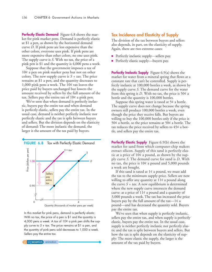
136 CHAPTER 6 Government Actions in Markets

Tax Incidence and Elasticity of SupplyThe division of the tax between buyers and sellersalso depends, in part, on the elasticity of supply.Again, there are two extreme cases:

■ Perfectly inelastic supply—sellers pay.■ Perfectly elastic supply—buyers pay.

Perfectly Inelastic Supply Figure 6.9(a) shows themarket for water from a mineral spring that flows at aconstant rate that can’t be controlled. Supply is per-fectly inelastic at 100,000 bottles a week, as shown bythe supply curve S. The demand curve for the waterfrom this spring is D. With no tax, the price is 50¢ abottle and the quantity is 100,000 bottles.

Suppose this spring water is taxed at 5¢ a bottle.The supply curve does not change because the springowners still produce 100,000 bottles a week, eventhough the price they receive falls. But buyers arewilling to buy the 100,000 bottles only if the price is50¢ a bottle, so the price remains at 50¢ a bottle. Thetax reduces the price received by sellers to 45¢ a bot-tle, and sellers pay the entire tax.

Perfectly Elastic Supply Figure 6.9(b) shows themarket for sand from which computer-chip makersextract silicon. Supply of this sand is perfectly elas-tic at a price of 10¢ a pound, as shown by the sup-ply curve S. The demand curve for sand is D. Withno tax, the price is 10¢ a pound and 5,000 poundsa week are bought.

If this sand is taxed at 1¢ a pound, we must addthe tax to the minimum supply-price. Sellers are nowwilling to offer any quantity at 11¢ a pound alongthe curve S + tax. A new equilibrium is determinedwhere the new supply curve intersects the demandcurve: at a price of 11¢ a pound and a quantity of3,000 pounds a week. The tax has increased the pricebuyers pay by the full amount of the tax—1¢ apound—and has decreased the quantity sold. Buyerspay the entire tax.

We’ve seen that when supply is perfectly inelastic,sellers pay the entire tax, and when supply is perfectlyelastic, buyers pay the entire tax. In the usual case,supply is neither perfectly inelastic nor perfectly elas-tic and the tax is split between buyers and sellers. Buthow the tax is split depends on the elasticity of sup-ply: The more elastic the supply, the larger is theamount of the tax paid by buyers.

1 40

0.90

1.00

Quantity (thousands of marker pens per week)

Pric

e (d

olla

rs p

er p

en)

D

SS + tax

Sellerspayentiretax

Perfectly Elastic Demand Figure 6.8 shows the mar-ket for pink marker pens. Demand is perfectly elasticat $1 a pen, as shown by the horizontal demandcurve D. If pink pens are less expensive than theother colors, everyone uses pink. If pink pens aremore expensive than other colors, no one uses pink.The supply curve is S. With no tax, the price of apink pen is $1 and the quantity is 4,000 pens a week.

Suppose that the government imposes a tax of10¢ a pen on pink marker pens but not on othercolors. The new supply curve is S + tax. The priceremains at $1 a pen, and the quantity decreases to1,000 pink pens a week. The 10¢ tax leaves theprice paid by buyers unchanged but lowers theamount received by sellers by the full amount of thetax. Sellers pay the entire tax of 10¢ a pink pen.

We’ve seen that when demand is perfectly inelas-tic, buyers pay the entire tax and when demandis perfectly elastic, sellers pay the entire tax. In theusual case, demand is neither perfectly inelastic norperfectly elastic and the tax is split between buyersand sellers. But the division depends on the elasticityof demand: The more inelastic the demand, thelarger is the amount of the tax paid by buyers.

In this market for pink pens, demand is perfectly elastic.With no tax, the price of a pen is $1 and the quantity is4,000 pens a week. A tax of 10¢ a pink pen shifts the sup-ply curve to S + tax. The price remains at $1 a pen, andthe quantity of pink pens sold decreases to 1,000 a week.Sellers pay the entire tax.

FIGURE 6.8 Tax with Perfectly Elastic Demand

animation

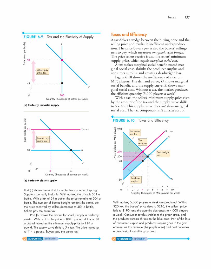
Taxes 137

Taxes and EfficiencyA tax drives a wedge between the buying price and theselling price and results in inefficient underproduc-tion. The price buyers pay is also the buyers’ willing-ness to pay, which measures marginal social benefit.The price sellers receive is also the sellers’ minimumsupply-price, which equals marginal social cost.

A tax makes marginal social benefit exceed mar-ginal social cost, shrinks the producer surplus andconsumer surplus, and creates a deadweight loss.

Figure 6.10 shows the inefficiency of a tax onMP3 players. The demand curve, D, shows marginalsocial benefit, and the supply curve, S, shows mar-ginal social cost. Without a tax, the market producesthe efficient quantity (5,000 players a week).

With a tax, the sellers’ minimum supply-price risesby the amount of the tax and the supply curve shiftsto S + tax. This supply curve does not show marginalsocial cost. The tax component isn’t a social cost of

1000

45

50

S

D

Quantity (thousands of bottles per week)

Pric

e (c

ents

per b

ottle

)

(a) Perfectly inelastic supply

Sellers payentire tax

3 50

10

11

Quantity (thousands of pounds per week)

Pric

e (c

ents

per p

ound

)

(b) Perfectly elastic supply

D

S

S + tax

Buyers payentire tax

4 5 6321 7 8 9 100

S + tax

S

D

Quantity (thousands of MP3 players per week)

Pric

e (d

olla

rs p

er M

P3 p

laye

r)

150

200

190

210

260Consumersurplus

Taxrevenue

Producersurplus

Deadweightloss

Part (a) shows the market for water from a mineral spring.Supply is perfectly inelastic. With no tax, the price is 50¢ abottle. With a tax of 5¢ a bottle, the price remains at 50¢ abottle. The number of bottles bought remains the same, butthe price received by sellers decreases to 45¢ a bottle.Sellers pay the entire tax.

Part (b) shows the market for sand. Supply is perfectlyelastic. With no tax, the price is 10¢ a pound. A tax of 1¢a pound increases the minimum supply-price to 11¢ apound. The supply curve shifts to S + tax. The price increasesto 11¢ a pound. Buyers pay the entire tax.

With no tax, 5,000 players a week are produced. With a$20 tax, the buyers’ price rises to $210, the sellers’ pricefalls to $190, and the quantity decreases to 4,000 playersa week. Consumer surplus shrinks to the green area, andthe producer surplus shrinks to the blue area. Part of the lossof consumer surplus and producer surplus goes to the gov-ernment as tax revenue (the purple area) and part becomesa deadweight loss (the gray area).

FIGURE 6.9 Tax and the Elasticity of Supply

animation

FIGURE 6.10 Taxes and Efficiency

animation

138 CHAPTER 6 Government Actions in Markets

Economics in ActionWorkers and Consumers Pay the Most TaxBecause the elasticity of the supply of labor is low andthe elasticity of demand for labor is high, workers paymost of the personal income taxes and most of theSocial Security taxes. Because the elasticities of demandfor alcohol, tobacco, and gasoline are low and the elas-ticities of supply are high, the burden of these taxes(excise taxes) falls more heavily on buyers than on sellers.

production. It is a transfer of resources to the govern-ment. At the new equilibrium quantity (4,000 play-ers a week), both consumer surplus and producersurplus shrink. Part of each surplus goes to the gov-ernment in tax revenue—the purple area; partbecomes a deadweight loss—the gray area.

Only in the extreme cases of perfectly inelasticdemand and perfectly inelastic supply does a tax notchange the quantity bought and sold so that no dead-weight loss arises.

Taxes and FairnessWe’ve examined the incidence and the efficiency oftaxes. But when political leaders debate tax issues, itis fairness, not incidence and efficiency, that gets themost attention. Democrats complain that Republicantax cuts are unfair because they give the benefits oflower taxes to the rich. Republicans counter that it isfair that the rich get most of the tax cuts because theypay most of the taxes. No easy answers are availableto the questions about the fairness of taxes.

Economists have proposed two conflicting princi-ples of fairness to apply to a tax system:

■ The benefits principle■ The ability-to-pay principle

The Benefits Principle The benefits principle is theproposition that people should pay taxes equal to thebenefits they receive from the services provided bygovernment. This arrangement is fair because itmeans that those who benefit most pay the mosttaxes. It makes tax payments and the consumption ofgovernment-provided services similar to private con-sumption expenditures.

The benefits principle can justify high fuel taxes topay for freeways, high taxes on alcoholic beveragesand tobacco products to pay for public health-careservices, and high rates of income tax on highincomes to pay for the benefits from law and orderand from living in a secure environment, from whichthe rich might benefit more than the poor.

The Ability-to-Pay Principle The ability-to-pay princi-ple is the proposition that people should pay taxesaccording to how easily they can bear the burden ofthe tax. A rich person can more easily bear the bur-den than a poor person can, so the ability-to-payprinciple can reinforce the benefits principle to justifyhigh rates of income tax on high incomes.

Your next task is to study production quotas andsubsidies, tools that are used to influence the marketsfor farm products.

0 10 20 30 5040

Personal income taxes

Social Security taxes

Corporation income taxes

Other taxes

Excise taxes

Tax receipts (percentage of total)

U.S. Taxes

Source of data: Budget of the United States Government, Fiscal Year2011, Historical Tables, Table 2.2.

REVIEW QUIZ 1 How does the elasticity of demand influence

the incidence of a tax, the tax revenue, and thedeadweight loss?

2 How does the elasticity of supply influence theincidence of a tax, the quantity bought, the taxrevenue, and the deadweight loss?

3 Why is a tax inefficient?4 When would a tax be efficient?5 What are the two principles of fairness that are

applied to tax systems?

You can work these questions in Study Plan 6.3 and get instant feedback.

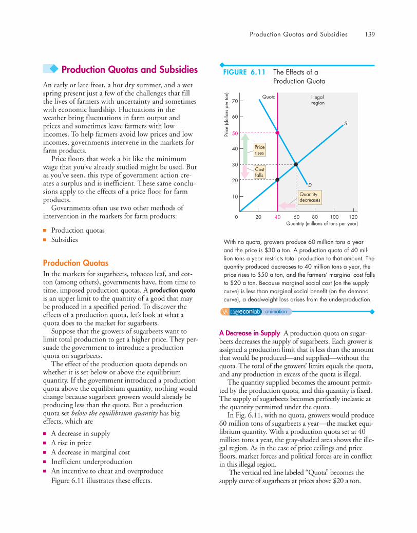
Production Quotas and Subsidies 139

◆ Production Quotas and SubsidiesAn early or late frost, a hot dry summer, and a wetspring present just a few of the challenges that fillthe lives of farmers with uncertainty and sometimeswith economic hardship. Fluctuations in theweather bring fluctuations in farm output andprices and sometimes leave farmers with lowincomes. To help farmers avoid low prices and lowincomes, governments intervene in the markets forfarm products.

Price floors that work a bit like the minimumwage that you’ve already studied might be used. Butas you’ve seen, this type of government action cre-ates a surplus and is inefficient. These same conclu-sions apply to the effects of a price floor for farmproducts.

Governments often use two other methods ofintervention in the markets for farm products:

■ Production quotas■ Subsidies

Production QuotasIn the markets for sugarbeets, tobacco leaf, and cot-ton (among others), governments have, from time totime, imposed production quotas. A production quotais an upper limit to the quantity of a good that maybe produced in a specified period. To discover theeffects of a production quota, let’s look at what aquota does to the market for sugarbeets.

Suppose that the growers of sugarbeets want tolimit total production to get a higher price. They per-suade the government to introduce a productionquota on sugarbeets.

The effect of the production quota depends onwhether it is set below or above the equilibriumquantity. If the government introduced a productionquota above the equilibrium quantity, nothing wouldchange because sugarbeet growers would already beproducing less than the quota. But a productionquota set below the equilibrium quantity has bigeffects, which are

■ A decrease in supply■ A rise in price■ A decrease in marginal cost■ Inefficient underproduction■ An incentive to cheat and overproduce

Figure 6.11 illustrates these effects.

A Decrease in Supply A production quota on sugar-beets decreases the supply of sugarbeets. Each grower isassigned a production limit that is less than the amountthat would be produced—and supplied—without thequota. The total of the growers’ limits equals the quota,and any production in excess of the quota is illegal.

The quantity supplied becomes the amount permit-ted by the production quota, and this quantity is fixed.The supply of sugarbeets becomes perfectly inelastic atthe quantity permitted under the quota.

In Fig. 6.11, with no quota, growers would produce60 million tons of sugarbeets a year—the market equi-librium quantity. With a production quota set at 40million tons a year, the gray-shaded area shows the ille-gal region. As in the case of price ceilings and pricefloors, market forces and political forces are in conflictin this illegal region.

The vertical red line labeled “Quota” becomes thesupply curve of sugarbeets at prices above $20 a ton.

20 40 60 80 100 1200

10

20

30

70

40

50

60S

D

Quantity (millions of tons per year)Pr

ice

(dol

lars

per

ton) Quota Illegal

region

Quantitydecreases

Pricerises

Costfalls

With no quota, growers produce 60 million tons a yearand the price is $30 a ton. A production quota of 40 mil-lion tons a year restricts total production to that amount. Thequantity produced decreases to 40 million tons a year, theprice rises to $50 a ton, and the farmers’ marginal cost fallsto $20 a ton. Because marginal social cost (on the supplycurve) is less than marginal social benefit (on the demandcurve), a deadweight loss arises from the underproduction.

FIGURE 6.11 The Effects of aProduction Quota

animation

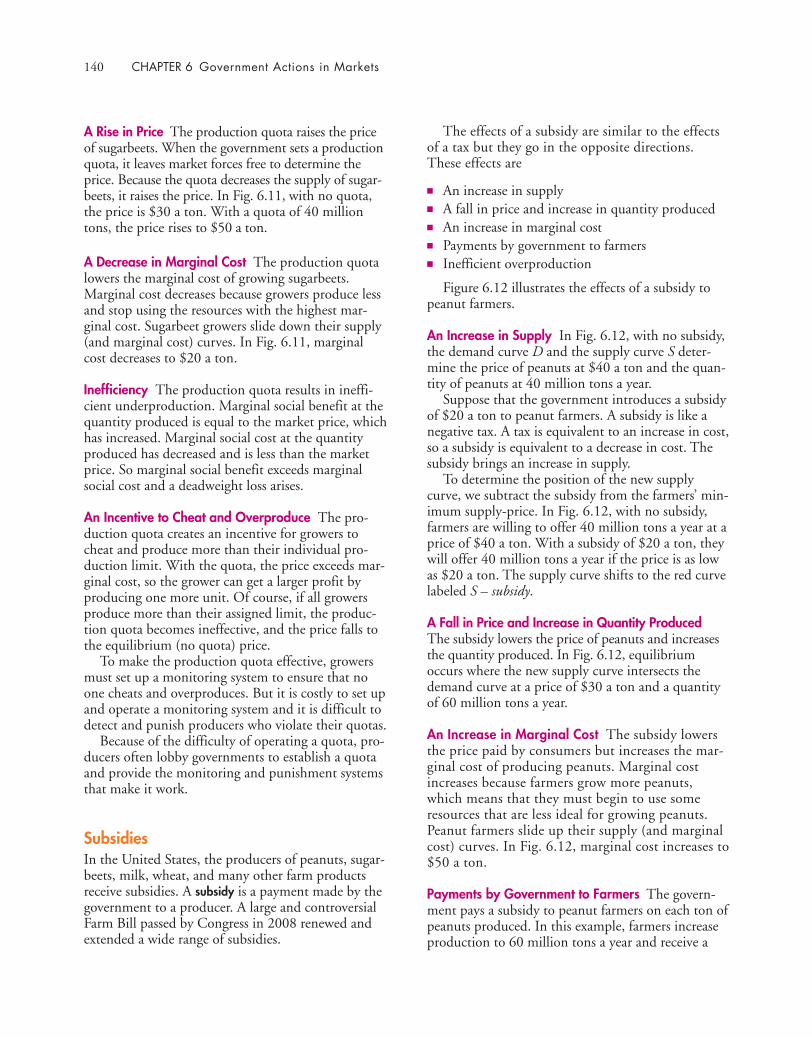
140 CHAPTER 6 Government Actions in Markets

The effects of a subsidy are similar to the effectsof a tax but they go in the opposite directions.These effects are

■ An increase in supply■ A fall in price and increase in quantity produced■ An increase in marginal cost■ Payments by government to farmers■ Inefficient overproduction

Figure 6.12 illustrates the effects of a subsidy topeanut farmers.

An Increase in Supply In Fig. 6.12, with no subsidy,the demand curve D and the supply curve S deter-mine the price of peanuts at $40 a ton and the quan-tity of peanuts at 40 million tons a year.

Suppose that the government introduces a subsidyof $20 a ton to peanut farmers. A subsidy is like anegative tax. A tax is equivalent to an increase in cost,so a subsidy is equivalent to a decrease in cost. Thesubsidy brings an increase in supply.

To determine the position of the new supplycurve, we subtract the subsidy from the farmers’ min-imum supply-price. In Fig. 6.12, with no subsidy,farmers are willing to offer 40 million tons a year at aprice of $40 a ton. With a subsidy of $20 a ton, theywill offer 40 million tons a year if the price is as lowas $20 a ton. The supply curve shifts to the red curvelabeled S – subsidy.

A Fall in Price and Increase in Quantity ProducedThe subsidy lowers the price of peanuts and increasesthe quantity produced. In Fig. 6.12, equilibriumoccurs where the new supply curve intersects thedemand curve at a price of $30 a ton and a quantityof 60 million tons a year.

An Increase in Marginal Cost The subsidy lowersthe price paid by consumers but increases the mar-ginal cost of producing peanuts. Marginal costincreases because farmers grow more peanuts,which means that they must begin to use someresources that are less ideal for growing peanuts.Peanut farmers slide up their supply (and marginalcost) curves. In Fig. 6.12, marginal cost increases to$50 a ton.

Payments by Government to Farmers The govern-ment pays a subsidy to peanut farmers on each ton ofpeanuts produced. In this example, farmers increaseproduction to 60 million tons a year and receive a

A Rise in Price The production quota raises the priceof sugarbeets. When the government sets a productionquota, it leaves market forces free to determine theprice. Because the quota decreases the supply of sugar-beets, it raises the price. In Fig. 6.11, with no quota,the price is $30 a ton. With a quota of 40 milliontons, the price rises to $50 a ton.

A Decrease in Marginal Cost The production quotalowers the marginal cost of growing sugarbeets.Marginal cost decreases because growers produce lessand stop using the resources with the highest mar-ginal cost. Sugarbeet growers slide down their supply(and marginal cost) curves. In Fig. 6.11, marginalcost decreases to $20 a ton.

Inefficiency The production quota results in ineffi-cient underproduction. Marginal social benefit at thequantity produced is equal to the market price, whichhas increased. Marginal social cost at the quantityproduced has decreased and is less than the marketprice. So marginal social benefit exceeds marginalsocial cost and a deadweight loss arises.

An Incentive to Cheat and Overproduce The pro-duction quota creates an incentive for growers tocheat and produce more than their individual pro-duction limit. With the quota, the price exceeds mar-ginal cost, so the grower can get a larger profit byproducing one more unit. Of course, if all growersproduce more than their assigned limit, the produc-tion quota becomes ineffective, and the price falls tothe equilibrium (no quota) price.

To make the production quota effective, growersmust set up a monitoring system to ensure that noone cheats and overproduces. But it is costly to set upand operate a monitoring system and it is difficult todetect and punish producers who violate their quotas.

Because of the difficulty of operating a quota, pro-ducers often lobby governments to establish a quotaand provide the monitoring and punishment systemsthat make it work.

SubsidiesIn the United States, the producers of peanuts, sugar-beets, milk, wheat, and many other farm productsreceive subsidies. A subsidy is a payment made by thegovernment to a producer. A large and controversialFarm Bill passed by Congress in 2008 renewed andextended a wide range of subsidies.

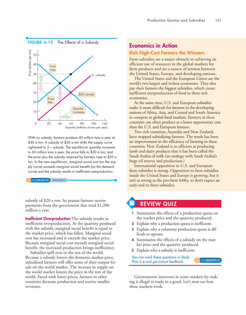
Production Quotas and Subsidies 141

subsidy of $20 a ton. So peanut farmers receivepayments from the government that total $1,200million a year.

Inefficient Overproduction The subsidy results ininefficient overproduction. At the quantity producedwith the subsidy, marginal social benefit is equal tothe market price, which has fallen. Marginal socialcost has increased and it exceeds the market price.Because marginal social cost exceeds marginal socialbenefit, the increased production brings inefficiency.

Subsidies spill over to the rest of the world.Because a subsidy lowers the domestic market price,subsidized farmers will offer some of their output forsale on the world market. The increase in supply onthe world market lowers the price in the rest of theworld. Faced with lower prices, farmers in othercountries decrease production and receive smallerrevenues.

20 40 60 80 100 1200

10

20

30

70

40

50

60

S

D

S – subsidy

Quantity (millions of tons per year)

Pric

e (d

olla

rs p

er to

n)

$20 subsidy

Quantityincreases

Costrises

Pricefalls

Economics in ActionRich High-Cost Farmers the WinnersFarm subsidies are a major obstacle to achieving anefficient use of resources in the global markets forfarm products and are a source of tension betweenthe United States, Europe, and developing nations.

The United States and the European Union are theworld’s two largest and richest economies. They alsopay their farmers the biggest subsidies, which createinefficient overproduction of food in these richeconomies.

At the same time, U.S. and European subsidiesmake it more difficult for farmers in the developingnations of Africa, Asia, and Central and South Americato compete in global food markets. Farmers in thesecountries can often produce at a lower opportunity costthan the U.S. and European farmers.

Two rich countries, Australia and New Zealand,have stopped subsidizing farmers. The result has beenan improvement in the efficiency of farming in thesecountries. New Zealand is so efficient at producinglamb and dairy products that it has been called theSaudi Arabia of milk (an analogy with Saudi Arabia’shuge oil reserve and production.)

International opposition to U.S. and Europeanfarm subsidies is strong. Opposition to farm subsidiesinside the United States and Europe is growing, but itisn’t as strong as the pro-farm lobby, so don’t expect anearly end to these subsidies.

Governments intervene in some markets by mak-ing it illegal to trade in a good. Let’s now see howthese markets work.

With no subsidy, farmers produce 40 million tons a year at$40 a ton. A subsidy of $20 a ton shifts the supply curverightward to S – subsidy. The equilibrium quantity increasesto 60 million tons a year, the price falls to $30 a ton, andthe price plus the subsidy received by farmers rises to $50 aton. In the new equilibrium, marginal social cost (on the sup-ply curve) exceeds marginal social benefit (on the demandcurve) and the subsidy results in inefficient overproduction.

REVIEW QUIZ 1 Summarize the effects of a production quota on

the market price and the quantity produced.2 Explain why a production quota is inefficient.3 Explain why a voluntary production quota is dif-

ficult to operate.4 Summarize the effects of a subsidy on the mar-

ket price and the quantity produced.5 Explain why a subsidy is inefficient.

You can work these questions in Study Plan 6.4 and get instant feedback.

FIGURE 6.12 The Effects of a Subsidy

animation

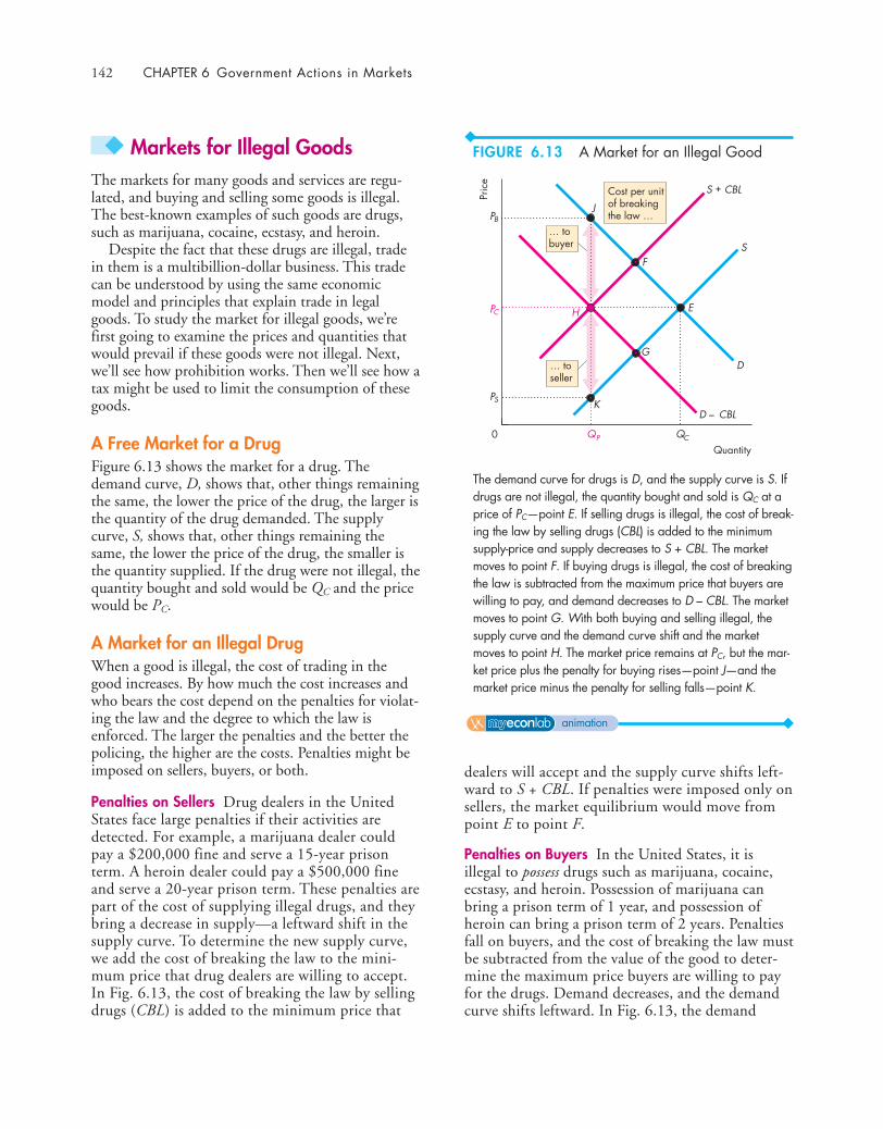
142 CHAPTER 6 Government Actions in Markets

dealers will accept and the supply curve shifts left-ward to S + CBL. If penalties were imposed only onsellers, the market equilibrium would move frompoint E to point F.

Penalties on Buyers In the United States, it isillegal to possess drugs such as marijuana, cocaine,ecstasy, and heroin. Possession of marijuana canbring a prison term of 1 year, and possession ofheroin can bring a prison term of 2 years. Penaltiesfall on buyers, and the cost of breaking the law mustbe subtracted from the value of the good to deter-mine the maximum price buyers are willing to payfor the drugs. Demand decreases, and the demandcurve shifts leftward. In Fig. 6.13, the demand

◆ Markets for Illegal GoodsThe markets for many goods and services are regu-lated, and buying and selling some goods is illegal.The best-known examples of such goods are drugs,such as marijuana, cocaine, ecstasy, and heroin.

Despite the fact that these drugs are illegal, tradein them is a multibillion-dollar business. This tradecan be understood by using the same economicmodel and principles that explain trade in legalgoods. To study the market for illegal goods, we’refirst going to examine the prices and quantities thatwould prevail if these goods were not illegal. Next,we’ll see how prohibition works. Then we’ll see how atax might be used to limit the consumption of thesegoods.

A Free Market for a DrugFigure 6.13 shows the market for a drug. Thedemand curve, D, shows that, other things remainingthe same, the lower the price of the drug, the larger isthe quantity of the drug demanded. The supplycurve, S, shows that, other things remaining thesame, the lower the price of the drug, the smaller isthe quantity supplied. If the drug were not illegal, thequantity bought and sold would be QC and the pricewould be PC.

A Market for an Illegal DrugWhen a good is illegal, the cost of trading in thegood increases. By how much the cost increases andwho bears the cost depend on the penalties for violat-ing the law and the degree to which the law isenforced. The larger the penalties and the better thepolicing, the higher are the costs. Penalties might beimposed on sellers, buyers, or both.

Penalties on Sellers Drug dealers in the UnitedStates face large penalties if their activities aredetected. For example, a marijuana dealer couldpay a $200,000 fine and serve a 15-year prisonterm. A heroin dealer could pay a $500,000 fineand serve a 20-year prison term. These penalties arepart of the cost of supplying illegal drugs, and theybring a decrease in supply—a leftward shift in thesupply curve. To determine the new supply curve,we add the cost of breaking the law to the mini-mum price that drug dealers are willing to accept.In Fig. 6.13, the cost of breaking the law by sellingdrugs (CBL) is added to the minimum price that

Q0

P

S

D

Quantity

Pric

e

QP C

C

PB

PS

J

K

EH

D – CBL

… tobuyer

… toseller

Cost per unitof breaking the law …

S + CBL

G

F

The demand curve for drugs is D, and the supply curve is S. Ifdrugs are not illegal, the quantity bought and sold is QC at aprice of PC—point E. If selling drugs is illegal, the cost of break-ing the law by selling drugs (CBL) is added to the minimumsupply-price and supply decreases to S + CBL. The marketmoves to point F. If buying drugs is illegal, the cost of breakingthe law is subtracted from the maximum price that buyers arewilling to pay, and demand decreases to D – CBL. The marketmoves to point G. With both buying and selling illegal, thesupply curve and the demand curve shift and the marketmoves to point H. The market price remains at PC, but the mar-ket price plus the penalty for buying rises—point J—and themarket price minus the penalty for selling falls—point K.

FIGURE 6.13 A Market for an Illegal Good

animation

Markets for Illegal Goods 143

curve shifts to D – CBL. If penalties were imposedonly on buyers, the market equilibrium would movefrom point E to point G.

Penalties on Both Sellers and Buyers If penalties areimposed on both sellers and buyers, both supply anddemand decrease and both the supply curve and thedemand curve shift. In Fig. 6.13, the costs of break-ing the law are the same for both buyers and sellers,so both curves shift leftward by the same amount.The market equilibrium moves to point H. The mar-ket price remains at the competitive market price PC,but the quantity bought decreases to Q P. Buyers payPC plus the cost of breaking the law, which equals PB.Sellers receive PC minus the cost of breaking the law,which equals PS.

The larger the penalties and the greater thedegree of law enforcement, the larger is the decreasein demand and/or supply. If the penalties are heav-ier on sellers, the supply curve shifts farther than thedemand curve and the market price rises above PC.If the penalties are heavier on buyers, the demandcurve shifts farther than the supply curve and themarket price falls below PC. In the United States,the penalties on sellers are larger than those on buy-ers, so the quantity of drugs traded decreases andthe market price increases compared with a freemarket.

With high enough penalties and effective lawenforcement, it is possible to decrease demand and/orsupply to the point at which the quantity bought iszero. But in reality, such an outcome is unusual. Itdoes not happen in the United States in the case ofillegal drugs. The key reason is the high cost of lawenforcement and insufficient resources for the policeto achieve effective enforcement. Because of this situ-ation, some people suggest that drugs (and other ille-gal goods) should be legalized and sold openly butalso taxed at a high rate in the same way that legaldrugs such as alcohol are taxed. How would such anarrangement work?

Legalizing and Taxing DrugsFrom your study of the effects of taxes, it is easy to seethat the quantity bought of a drug could be decreased ifthe drug was legalized and taxed. Imposing a suffi-ciently high tax could decrease the supply, raise theprice, and achieve the same decrease in the quantitybought as does a prohibition on drugs. The govern-ment would collect a large tax revenue.

Illegal Trading to Evade the Tax It is likely that anextremely high tax rate would be needed to cut thequantity of drugs bought to the level prevailing witha prohibition. It is also likely that many drug dealersand consumers would try to cover up their activitiesto evade the tax. If they did act in this way, theywould face the cost of breaking the law—the tax law.If the penalty for tax law violation is as severe and aseffectively policed as drug-dealing laws, the analysiswe’ve already conducted applies also to this case. Thequantity of drugs bought would depend on thepenalties for law breaking and on the way in whichthe penalties are assigned to buyers and sellers.

Taxes Versus Prohibition: Some Pros and ConsWhich is more effective: prohibition or taxes? In favorof taxes and against prohibition is the fact that the taxrevenue can be used to make law enforcement moreeffective. It can also be used to run a more effectiveeducation campaign against illegal drug use. In favorof prohibition and against taxes is the fact that prohi-bition sends a signal that might influence preferences,decreasing the demand for illegal drugs. Also, somepeople intensely dislike the idea of the governmentprofiting from trade in harmful substances.

◆ You now know how to use the demand and supplymodel to predict prices, to study government actions inmarkets, and to study the sources and costs of ineffi-ciency. In Reading Between the Lines on pp. 144–145,you will see how to apply what you’ve learned to themarket for low-skilled labor in California and see somepitfalls of government intervention in this market.

REVIEW QUIZ 1 How does the imposition of a penalty for sell-

ing an illegal drug influence demand, supply,price, and the quantity of the drug consumed?

2 How does the imposition of a penalty for pos-sessing an illegal drug influence demand, supply,price, and the quantity of the drug consumed?

3 How does the imposition of a penalty for sell-ing or possessing an illegal drug influencedemand, supply, price, and the quantity of thedrug consumed?

4 Is there any case for legalizing drugs?

You can work these questions in Study Plan 6.5 and get instant feedback.

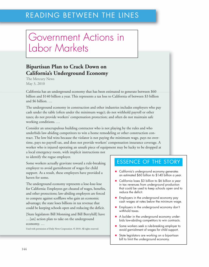
144

READING BETWEEN THE L INES

Bipartisan Plan to Crack Down onCalifornia’s Underground EconomyThe Mercury NewsMay 3, 2010

California has an underground economy that has been estimated to generate between $60billion and $140 billion a year. This represents a tax loss to California of between $3 billionand $6 billion. …

The underground economy in construction and other industries includes employers who paycash under the table (often under the minimum wage); do not withhold payroll or othertaxes; do not provide workers’ compensation protection; and often do not maintain safeworking conditions. …

Consider an unscrupulous building contractor who is not playing by the rules and whounderbids law-abiding competitors to win a home remodeling or other construction con-tract. The low bid wins because the violator is not paying the minimum wage, pays no over-time, pays no payroll tax, and does not provide workers’ compensation insurance coverage. Aworker who is injured operating an unsafe piece of equipment may be lucky to be dropped ata local emergency room, with implicit instructions notto identify the rogue employer.

Some workers actually gravitate toward a rule-breakingemployer to avoid garnishment of wages for childsupport. As a result, these employers have provided ahaven for some.

The underground economy represents a lose-lose-losefor California: Employees get cheated of wages, benefits,and other protections; law-abiding employers are forcedto compete against scofflaws who gain an economicadvantage; the state loses billions in tax revenue thatcould be keeping schools open and reducing the deficit.

[State legislators Bill Monning and Bill Berryhill] have…[an] action plan to take on the undergroundeconomy. …Used with permission of Daily News Corporation. © 2010. All rights reserved.

■ California’s underground economy generatesan estimated $60 billion to $140 billion a year.

■ California loses $3 billion to $6 billion a yearin tax revenues from underground productionthat could be used to keep schools open and toreduce the deficit.

■ Employers in the underground economy paycash wages at rates below the minimum wage.

■ Employers in the underground economy don’twithhold taxes.

■ A builder in the underground economy under-bids law-abiding competitors to win contracts.

■ Some workers seek a rule-breaking employer toavoid garnishment of wages for child support.

■ State legislators are working on a bipartisanbill to limit the underground economy.

ESSENCE OF THE STORY

Government Actions inLabor Markets

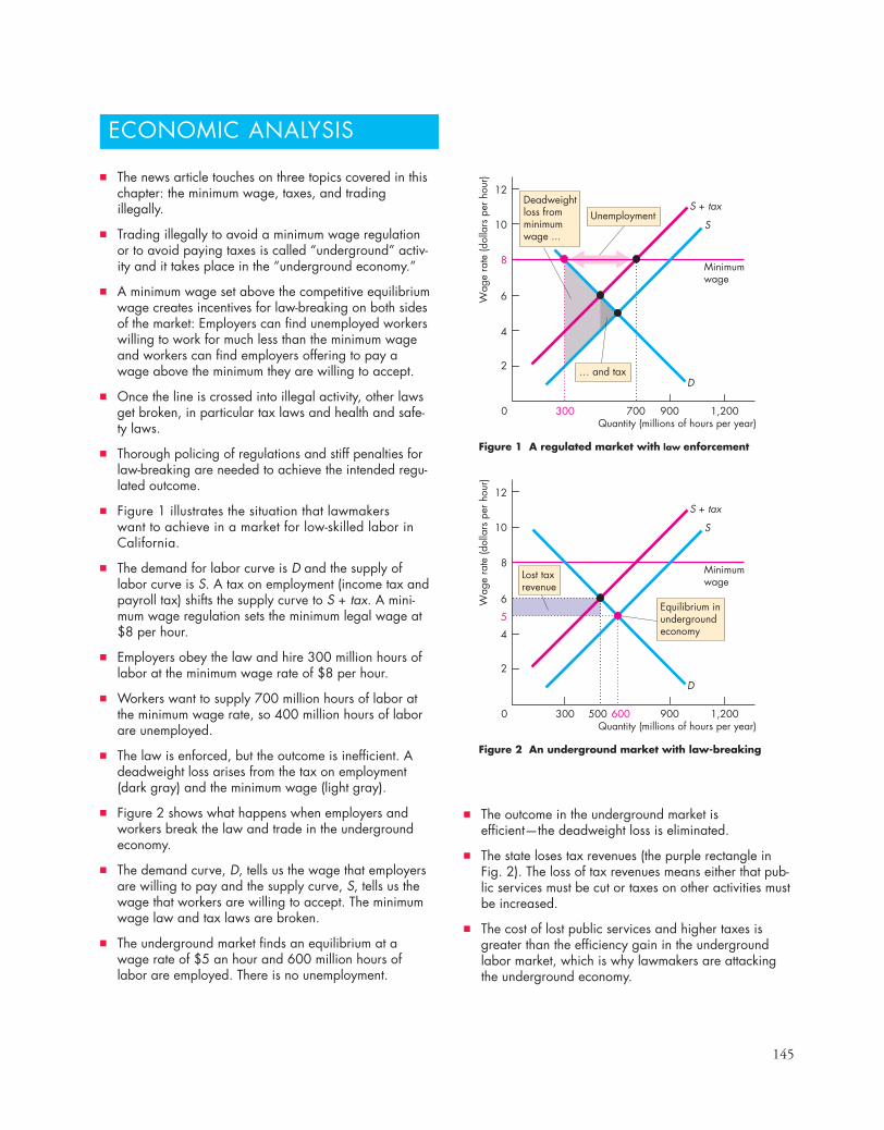
145

ECONOMIC ANALYSIS

Wag

e ra

te (d

olla

rs p

er h

our)

Quantity (millions of hours per year)900700300 1,200

2

12

8

10

4

6

0

D

S

S + tax

Minimumwage

UnemploymentDeadweightloss fromminimumwage ...

Lost taxrevenue

Equilibrium inundergroundeconomy

Figure 1 A regulated market with law enforcement

… and tax

Wag

e ra

te (d

olla

rs p

er h

our)

Quantity (millions of hours per year)900600300 500 1,200

2

12

8

10

4

6

5

0

D

S

S + tax

Minimumwage

Figure 2 An underground market with law-breaking

■ The news article touches on three topics covered in thischapter: the minimum wage, taxes, and tradingillegally.

■ Trading illegally to avoid a minimum wage regulationor to avoid paying taxes is called “underground” activ-ity and it takes place in the “underground economy.”

■ A minimum wage set above the competitive equilibriumwage creates incentives for law-breaking on both sidesof the market: Employers can find unemployed workerswilling to work for much less than the minimum wageand workers can find employers offering to pay awage above the minimum they are willing to accept.

■ Once the line is crossed into illegal activity, other lawsget broken, in particular tax laws and health and safe-ty laws.

■ Thorough policing of regulations and stiff penalties forlaw-breaking are needed to achieve the intended regu-lated outcome.

■ Figure 1 illustrates the situation that lawmakers want to achieve in a market for low-skilled labor inCalifornia.

■ The demand for labor curve is D and the supply oflabor curve is S. A tax on employment (income tax andpayroll tax) shifts the supply curve to S + tax. A mini-mum wage regulation sets the minimum legal wage at$8 per hour.

■ Employers obey the law and hire 300 million hours oflabor at the minimum wage rate of $8 per hour.

■ Workers want to supply 700 million hours of labor atthe minimum wage rate, so 400 million hours of laborare unemployed.

■ The law is enforced, but the outcome is inefficient. Adeadweight loss arises from the tax on employment(dark gray) and the minimum wage (light gray).

■ Figure 2 shows what happens when employers andworkers break the law and trade in the undergroundeconomy.

■ The demand curve, D, tells us the wage that employersare willing to pay and the supply curve, S, tells us thewage that workers are willing to accept. The minimumwage law and tax laws are broken.

■ The underground market finds an equilibrium at awage rate of $5 an hour and 600 million hours oflabor are employed. There is no unemployment.

■ The outcome in the underground market isefficient—the deadweight loss is eliminated.

■ The state loses tax revenues (the purple rectangle inFig. 2). The loss of tax revenues means either that pub-lic services must be cut or taxes on other activities mustbe increased.

■ The cost of lost public services and higher taxes isgreater than the efficiency gain in the undergroundlabor market, which is why lawmakers are attackingthe underground economy.

146 CHAPTER 6 Government Actions in Markets

■ The less elastic the demand or the more elastic thesupply, the larger is the share of the tax paid bybuyers.

■ If demand is perfectly elastic or supply is perfectlyinelastic, sellers pay the entire tax. And if demandis perfectly inelastic or supply is perfectly elastic,buyers pay the entire tax.

Working Problems 13 to 15 will give you a better under-standing of taxes.

Production Quotas and Subsidies (pp. 139–141)

■ A production quota leads to inefficient underpro-duction, which raises the price.

■ A subsidy is like a negative tax. It lowers the price,increases the cost of production, and leads to inef-ficient overproduction.

Working Problems 16 and 17 will give you a better under-standing of production quotas and subsidies.

Markets for Illegal Goods (pp. 142–143)

■ Penalties on sellers increase the cost of selling thegood and decrease the supply of the good.

■ Penalties on buyers decrease their willingness topay and decrease the demand for the good.

■ Penalties on buyers and sellers decrease the quan-tity of the good, raise the price buyers pay, andlower the price sellers receive.

■ Legalizing and taxing can achieve the same out-come as penalties on buyers and sellers.

Working Problem 18 will give you a better understandingof markets for illegal goods.

Key Points

A Housing Market with a Rent Ceiling (pp. 128–130)

■ A rent ceiling that is set above the equilibrium renthas no effect.

■ A rent ceiling that is set below the equilibriumrent creates a housing shortage, increased searchactivity, and a black market.

■ A rent ceiling that is set below the equilibriumrent is inefficient and unfair.

Working Problems 1 to 6 will give you a better under-standing of a housing market with a rent ceiling.

A Labor Market with a Minimum Wage (pp. 131–133)

■ A minimum wage set below the equilibrium wagerate has no effect.

■ A minimum wage set above the equilibrium wagerate creates unemployment and increases theamount of time people spend searching for a job.

■ A minimum wage set above the equilibrium wagerate is inefficient, unfair, and hits low-skilledyoung people hardest.

Working Problems 7 to 12 will give you a better under-standing of a labor market with a minimum wage.

Taxes (pp. 133–138)

■ A tax raises the price paid by buyers, but usuallyby less than the tax.

■ The elasticity of demand and the elasticity of supplydetermine the share of a tax paid by buyers and sellers.

SUMMARY

Key TermsBlack market, 128Minimum wage, 131Price cap, 128Price ceiling, 128

Price floor, 131Production quota, 139Rent ceiling, 128Search activity, 128

Subsidy, 140Tax incidence, 133

Study Plan Problems and Applications 147

5. Draw a graph to illustrate the effects of a priceceiling set below the equilibrium price in themarket for gasoline.

6. Explain the various ways in which a price ceilingon gasoline that is set below the equilibriumprice would make buyers and sellers of gasolinebetter off or worse off. What would happen tototal surplus and deadweight loss in this market?

A Labor Market with a Minimum Wage (Study Plan 6.2)

Use the following data to work Problems 7 to 9.The table gives the demand and supply schedules ofteenage labor.

Wage rate Quantity Quantity(dollars demanded supplied

per hour) (hours per month)

4 3,000 1,0005 2,500 1,5006 2,000 2,0007 1,500 2,5008 1,000 3,000

7. Calculate the equilibrium wage rate, the numberof hours worked, and the quantity of unemploy-ment.

8. If a minimum wage for teenagers is set at $5 anhour, how many hours do they work and howmany hours of teenage labor are unemployed?

9. If a minimum wage for teenagers is set at $7 anhour, a. How many hours do teenagers work and how

many hours are unemployed?b. Demand for teenage labor increases by 500

hours a month. What is the wage rate paid toteenagers and how many hours of teenagelabor are unemployed?

Use the following news clip to work Problems 10 to 12.India Steps Up Pressure for Minimum Wage for ItsWorkers in the GulfOil-rich countries in the [Persian] Gulf, already con-fronted by strong labor protests, are facing renewedpressure from India to pay minimum wages forunskilled workers. With five million immigrantworkers in the region, India is trying to win betterconditions for their citizens.

Source: International Herald Tribune,March 27, 2008

A Housing Market with a Rent Ceiling (Study Plan 6.1)

Use the following graph of the market for rentalhousing in Townsville to work Problems 1 and 2.

1. a. What are the equilibrium rent and equilib-rium quantity of rental housing?

b. If a rent ceiling is set at $600 a month, what isthe quantity of housing rented and what is theshortage of housing?

2. If a rent ceiling is set at $300 a month, what isthe quantity of housing rented, the shortage ofhousing, and the maximum price that someone iswilling to pay for the last unit of housing avail-able?

Use the following news clip to work Problems 3 to 6.Capping Gasoline PricesAs gasoline prices rise, many people are calling forprice caps, but price caps generate a distorted reflec-tion of reality, which leads buyers and suppliers to actin ways inconsistent with the price cap. By maskingreality, price caps only make matters worse.

Source: Pittsburgh Tribune-Review,September 12, 2005

Suppose that a price ceiling is set below the equilib-rium price of gasoline.

3. How does the price cap influence the quantity ofgasoline supplied and the quantity demanded?

4. How does the price cap influence a. The quantity of gasoline sold and the shortage

or surplus of gasoline?b. The maximum price that someone is willing

to pay for the last gallon of gasoline availableon a black market?

100 20 30 40

Rent

(dol

lars

per

mon

th)

Quantity (thousands)

600

450

300

150

S

D

You can work Problems 1 to 18 in MyEconLab Chapter 6 Study Plan and get instant feedback.

STUDY PLAN PROBLEMS AND APPLICATIONS

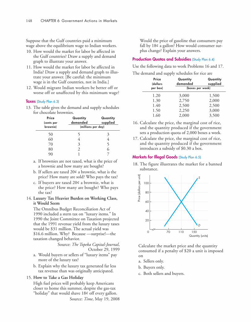
148 CHAPTER 6 Government Actions in Markets

Suppose that the Gulf countries paid a minimumwage above the equilibrium wage to Indian workers.10. How would the market for labor be affected in

the Gulf countries? Draw a supply and demandgraph to illustrate your answer.

11. How would the market for labor be affected inIndia? Draw a supply and demand graph to illus-trate your answer. [Be careful: the minimumwage is in the Gulf countries, not in India.]

12. Would migrant Indian workers be better off orworse off or unaffected by this minimum wage?

Taxes (Study Plan 6.3)

13. The table gives the demand and supply schedulesfor chocolate brownies.

Price Quantity Quantity(cents per demanded suppliedbrownie) (millions per day)

50 5 360 4 470 3 580 2 690 1 7

a. If brownies are not taxed, what is the price ofa brownie and how many are bought?

b. If sellers are taxed 20¢ a brownie, what is theprice? How many are sold? Who pays the tax?

c. If buyers are taxed 20¢ a brownie, what isthe price? How many are bought? Who paysthe tax?

14. Luxury Tax Heavier Burden on Working Class,it Would SeemThe Omnibus Budget Reconciliation Act of1990 included a stern tax on “luxury items.” In1990 the Joint Committee on Taxation projectedthat the 1991 revenue yield from the luxury taxeswould be $31 million. The actual yield was$16.6 million. Why? Because —surprise!—thetaxation changed behavior.

Source: The Topeka Capital-Journal,October 29, 1999

a. Would buyers or sellers of “luxury items” paymore of the luxury tax?

b. Explain why the luxury tax generated far lesstax revenue than was originally anticipated.

15. How to Take a Gas HolidayHigh fuel prices will probably keep Americanscloser to home this summer, despite the gas-tax“holiday” that would shave 18¢ off every gallon.

Source: Time, May 19, 2008

700 110 150

Pric

e (d

olla

rs p

er u

nit)

Quantity (units)

20

60

40

80

100

S

D

Would the price of gasoline that consumers payfall by 18¢ a gallon? How would consumer sur-plus change? Explain your answers.

Production Quotas and Subsidies (Study Plan 6.4)

Use the following data to work Problems 16 and 17.

The demand and supply schedules for rice arePrice Quantity Quantity

(dollars demanded suppliedper box) (boxes per week)

1.20 3,000 1,5001.30 2,750 2,0001.40 2,500 2,5001.50 2,250 3,0001.60 2,000 3,500

16. Calculate the price, the marginal cost of rice,and the quantity produced if the governmentsets a production quota of 2,000 boxes a week.

17. Calculate the price, the marginal cost of rice,and the quantity produced if the governmentintroduces a subsidy of $0.30 a box.

Markets for Illegal Goods (Study Plan 6.5)

18. The figure illustrates the market for a bannedsubstance.

Calculate the market price and the quantityconsumed if a penalty of $20 a unit is imposedona. Sellers only.b. Buyers only.c. Both sellers and buyers.

Additional Problems and Applications 149

A Housing Market with a Rent Ceiling Use this news clip to work Problems 19 and 20.Despite Protests, Rent Board Sets 7.25% IncreaseNew York’s Rent Guidelines Board voted for a rentincrease of up to 7.25 percent over the next twoyears on rent-stabilized apartments. A surveyreported that last year costs for the owners of rent-stabilized buildings rose by 7.8 percent. In additionthere is growing concern about the ability of themiddle class to afford to live in New York City.

Source: The New York Times, June 28, 200619. a. If rents for rent-stabilized apartments do

not increase, how do you think the market for rental units in New York City will develop?

b. Are rent ceilings in New York City helpful tothe middle class? Why or why not?

20. a. Explain the effect of the increase in the rentceiling on the quantity of rent-stabilizedapartments.

b. Why is rent stabilization a source of conflictbetween renters and owners of apartments?

A Labor Market with a Minimum WageUse the following news clip to work Problems 21 and 22.

House Passes Increase in Minimum Wage to $7.25The rise in the federal minimum wage will boost thewages of the lowest-paid U.S. workers from $5.15 to$7.25 an hour. Republican leaders, backed by small-business and restaurant groups, argued that the higherminimum wage would cripple the economy, so itmust be accompanied by tax cuts for small businesses.

Source: The Washington Post, January 11, 200721. On a graph of the market for low-skilled labor,

show the effect of the increase in the minimumwage on the quantity of labor employed.

22. Explain the effects of the higher minimum wageon the workers’ surplus and the firms’ surplus.Does the labor market become more efficient orless efficient? Explain.

Taxes23. Use the news clip in Problem 21.

a. Would a cut in the tax on small business prof-its offset the effect of the higher minimumwage on employment? Explain.

b. Would a cut in the Social Security tax that smallbusinesses pay offset the effect of the higherminimum wage on employment? Explain.

24. The demand and supply schedules for tulips arePrice Quantity Quantity

(dollars demanded suppliedper bunch) (bunches per week)

10 100 4012 90 6014 80 8016 70 10018 60 120

a. If tulips are not taxed, what is the price andhow many bunches are bought?

b. If tulips are taxed $6 a bunch, what are theprice and quantity bought? Who pays the tax?

25. Cigarette Taxes, Black Markets, and Crime:Lessons from New York’s 50-Year Losing BattleNew York City has the highest cigarette taxes inthe country. During the four months followingthe recent tax hike, sales of taxed cigarettes inthe city fell by more than 50 percent as con-sumers turned to the city's bustling black mar-ket. The thriving illegal market for cigaretteshas diverted billions of dollars from legitimatebusinesses and governments to criminals.

Source: Cato Institute, February 6, 2003a. How has the market for cigarettes in New York

City responded to the high cigarette taxes? b. How does the emergence of a black market

impact the elasticity of demand in a legalmarket?

c. Why might an increase in the tax rate actuallycause a decrease in the tax revenue?

Production Quotas and SubsidiesUse the following news clip to work Problems 26 to 28.

Congress Passes Farm Bill, Defies BushCongress sent the White House a huge $290 billion-election-year farm bill which contained $40 billion forfarm subsidies and almost $30 billion to farmers to idletheir land. Bush has threatened to veto the bill, saying itis irresponsible and too generous to wealthy corporatefarmers in a time of record crop prices.

Source: CNN, May 15, 2008

You can work these problems in MyEconLab if assigned by your instructor.

ADDITIONAL PROBLEMS AND APPLICATIONS

150 CHAPTER 6 Government Actions in Markets

26. a. Why does the federal government subsidizefarmers?

b. Explain how a subsidy paid to cotton farmersaffects the price of cotton and the marginalcost of producing it.

27. Explain how a subsidy paid to cotton farmersaffects the consumer surplus and the producersurplus from cotton. Does the subsidy make thecotton market more efficient or less efficient?Explain.

28. a. How would a payment to cotton farmers toidle their land influence the supply of cotton?

b. How would a payment to cotton farmers toidle their land affect the consumer surplus andthe producer surplus from cotton? Explain.

Markets for Illegal Goods

29. The table gives the demand and supply schedulesfor an illegal drug.

Price Quantity Quantity(dollars per demanded supplied

unit) (units per day)

50 500 30060 400 40070 300 50080 200 60090 100 700

a. If there are no penalties on buying or sellingthe drug, what is the price and how manyunits are consumed?

b. If the penalty on sellers is $20 a unit, what arethe price and quantity consumed?

c. If the penalty on buyers is $20 a unit, whatare the price and quantity consumed?

Economics in the News30. After you have studied Reading Between the Lines

on pp. 144–145 answer the following questions.a. In what ways do employers break laws in the

underground labor market described in thenews article?

b. How does a tax on labor change the equilib-rium level of employment and the wage ratepaid by employers?

c. How does a minimum wage law make taxevasion more likely to occur?

d. How can the minimum wage law and tax lawbe enforced more effectively?

e. Use the analysis of a market for an illegal good (on pp. 142–143) to explain how stiffer

penalties would change the quantity of labortraded and change the wage rate in the under-ground economy.

Use the following news clip to work Problems 31 to 33.Coal Shortage at China PlantsChinese power plants have run short of coal, anunintended effect of government-mandated pricecontrols designed to shield the public from risingglobal energy costs. Beijing has also frozen retailprices of gasoline and diesel. That helped farmers andthe urban poor, but it has spurred sales of gas-guz-zling luxury cars and propelled double-digit annualgrowth in fuel consumption. At the same time, oilrefiners are suffering heavy losses and some have beguncutting production, causing fuel shortages.

Source: CNN, May 20, 200831. a. Are China’s price controls described in the

news clip price floors or price ceilings?b. Explain how China’s price controls have creat-

ed shortages or surpluses in the markets forcoal, gasoline, and diesel.

c. Illustrate your answer to part (b) graphicallyby using the supply and demand model.

32. Explain how China’s price controls have changedconsumer surplus, producer surplus, total sur-plus, and the deadweight loss in the markets forcoal, gasoline, and diesel.

33. Show on a graph the change in consumer sur-plus, producer surplus, total surplus, and thedeadweight loss in the markets for coal, gasoline,and diesel.

34. On December 31, 1776, Rhode Island estab-lished wage controls to limit wages to 70¢ a dayfor carpenters and 42¢ a day for tailors.a. Are these wage controls a price ceiling or a price

floor? Why might they have been introduced?b. If these wage controls are effective, would you

expect to see a surplus or a shortage of carpen-ters and tailors?

35. Drivers Feel the Pinch as Diesel Hits $4 aGallon“The high price of gasoline is hurting our econ-omy,” said Mark Kirsch, a trucker, who organ-ized a rally in Washington. “It’s hurting middle-class people.”

Source: The Washington Post, April 29, 2008Explain to truck drivers why a cap on the price ofgasoline would hurt middle-class people morethan the high price of gasoline hurts.

After studying this chapter, you will be able to:

� Explain how markets work with international trade� Identify the gains from international trade and its

winners and losers� Explain the effects of international trade barriers� Explain and evaluate arguments used to justify

restricting international trade

7iPods, Wii games, and Nike shoes are just three of the items you might buythat are not produced in the United States. In fact, most of the goods that youbuy are produced abroad, often in Asia, and transported here in containerships and FedEx cargo jets. And it’s not just goods produced abroad that youbuy—it is services too. When you make a technical support call, most likelyyou’ll be talking with someone in India, or to a voice recognition system thatwas programmed in India. Satellites or fiber cables will carry your conversationalong with huge amounts of other voice messages, video images, and data.

All these activities are part of the globalization process that is having aprofound effect on our lives. Globalizationis controversial and generates heateddebate. Many Americans want to know

how we can compete with people whose wages are a fraction of our own.Why do we go to such lengths to trade and communicate with others in

faraway places? You will find some answers in this chapter. And in ReadingBetween the Lines at the end of the chapter, you can apply what you’velearned and examine the effects of a tariff that the Obama government has puton tires imported from China.

GLOBAL MARKETS IN ACTION

151

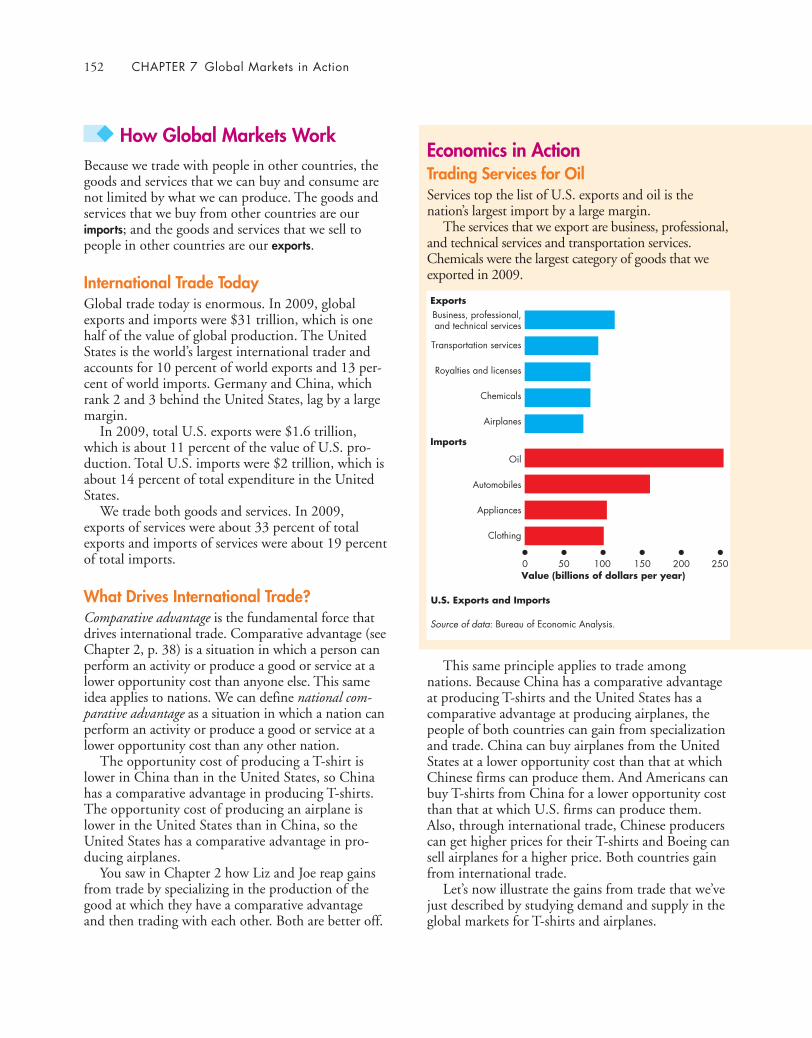
152 CHAPTER 7 Global Markets in Action

◆ How Global Markets WorkBecause we trade with people in other countries, thegoods and services that we can buy and consume arenot limited by what we can produce. The goods andservices that we buy from other countries are ourimports; and the goods and services that we sell topeople in other countries are our exports.

International Trade TodayGlobal trade today is enormous. In 2009, globalexports and imports were $31 trillion, which is onehalf of the value of global production. The UnitedStates is the world’s largest international trader andaccounts for 10 percent of world exports and 13 per-cent of world imports. Germany and China, whichrank 2 and 3 behind the United States, lag by a largemargin.

In 2009, total U.S. exports were $1.6 trillion,which is about 11 percent of the value of U.S. pro-duction. Total U.S. imports were $2 trillion, which isabout 14 percent of total expenditure in the UnitedStates.

We trade both goods and services. In 2009,exports of services were about 33 percent of totalexports and imports of services were about 19 percentof total imports.

What Drives International Trade?Comparative advantage is the fundamental force thatdrives international trade. Comparative advantage (seeChapter 2, p. 38) is a situation in which a person canperform an activity or produce a good or service at alower opportunity cost than anyone else. This sameidea applies to nations. We can define national com-parative advantage as a situation in which a nation canperform an activity or produce a good or service at alower opportunity cost than any other nation.

The opportunity cost of producing a T-shirt islower in China than in the United States, so Chinahas a comparative advantage in producing T-shirts.The opportunity cost of producing an airplane islower in the United States than in China, so theUnited States has a comparative advantage in pro-ducing airplanes.

You saw in Chapter 2 how Liz and Joe reap gainsfrom trade by specializing in the production of thegood at which they have a comparative advantageand then trading with each other. Both are better off.

This same principle applies to trade amongnations. Because China has a comparative advantageat producing T-shirts and the United States has acomparative advantage at producing airplanes, thepeople of both countries can gain from specializationand trade. China can buy airplanes from the UnitedStates at a lower opportunity cost than that at whichChinese firms can produce them. And Americans canbuy T-shirts from China for a lower opportunity costthan that at which U.S. firms can produce them.Also, through international trade, Chinese producerscan get higher prices for their T-shirts and Boeing cansell airplanes for a higher price. Both countries gainfrom international trade.

Let’s now illustrate the gains from trade that we’vejust described by studying demand and supply in theglobal markets for T-shirts and airplanes.

Economics in ActionTrading Services for OilServices top the list of U.S. exports and oil is thenation’s largest import by a large margin.

The services that we export are business, professional,and technical services and transportation services.Chemicals were the largest category of goods that weexported in 2009.

0 50 250100 150 200

Transportation services

Royalties and licenses

Chemicals

Airplanes

Business, professional,and technical services

Oil

Automobiles

Appliances

Clothing

Value (billions of dollars per year)

Exports

Imports

U.S. Exports and Imports

Source of data: Bureau of Economic Analysis.

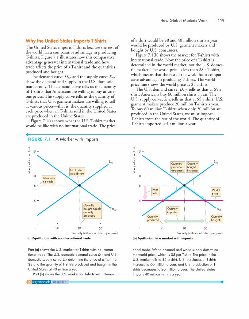
How Global Markets Work 153

Why the United States Imports T-ShirtsThe United States imports T-shirts because the rest ofthe world has a comparative advantage in producingT-shirts. Figure 7.1 illustrates how this comparativeadvantage generates international trade and howtrade affects the price of a T-shirt and the quantitiesproduced and bought.

The demand curve DUS and the supply curve SUS

show the demand and supply in the U.S. domesticmarket only. The demand curve tells us the quantityof T-shirts that Americans are willing to buy at vari-ous prices. The supply curve tells us the quantity ofT-shirts that U.S. garment makers are willing to sellat various prices—that is, the quantity supplied ateach price when all T-shirts sold in the United Statesare produced in the United States.

Figure 7.1(a) shows what the U.S. T-shirt marketwould be like with no international trade. The price

of a shirt would be $8 and 40 million shirts a yearwould be produced by U.S. garment makers andbought by U.S. consumers.

Figure 7.1(b) shows the market for T-shirts withinternational trade. Now the price of a T-shirt isdetermined in the world market, not the U.S. domes-tic market. The world price is less than $8 a T-shirt,which means that the rest of the world has a compar-ative advantage in producing T-shirts. The worldprice line shows the world price at $5 a shirt.

The U.S. demand curve, DUS, tells us that at $5 ashirt, Americans buy 60 million shirts a year. TheU.S. supply curve, SUS, tells us that at $5 a shirt, U.S.garment makers produce 20 million T-shirts a year.To buy 60 million T-shirts when only 20 million areproduced in the United States, we must import T-shirts from the rest of the world. The quantity of T-shirts imported is 40 million a year.

Pric

e (d

olla

rs p

er T

-shirt

)

200 40 60

15

5

DUS

SUS

(b) Equilibrium in a market with imports

8

10

Quantity (millions of T-shirts per year)

(a) Equilibrium with no international trade

Price withno trade

Quantitybought equalsquantityproduced

No tradeequilibrium Pr

ice

(dol

lars

per

T-sh

irt)

200 40 60

15

5

DUS

SUS

8

10

Quantity (millions of T-shirts per year)

Pricefalls

Quantityproduceddecreases

Quantityproduced

Quantityimported

Quantitybought

Quantityboughtincreases

Worldprice

Part (a) shows the U.S. market for T-shirts with no interna-tional trade. The U.S. domestic demand curve DUS and U.S.domestic supply curve SUS determine the price of a T-shirt at$8 and the quantity of T- shirts produced and bought in theUnited States at 40 million a year.

Part (b) shows the U.S. market for T-shirts with interna-

tional trade. World demand and world supply determinethe world price, which is $5 per T-shirt. The price in theU.S. market falls to $5 a shirt. U.S. purchases of T-shirtsincrease to 60 million a year, and U.S. production of T-shirts decreases to 20 million a year. The United Statesimports 40 million T-shirts a year.

FIGURE 7.1 A Market with Imports

animation

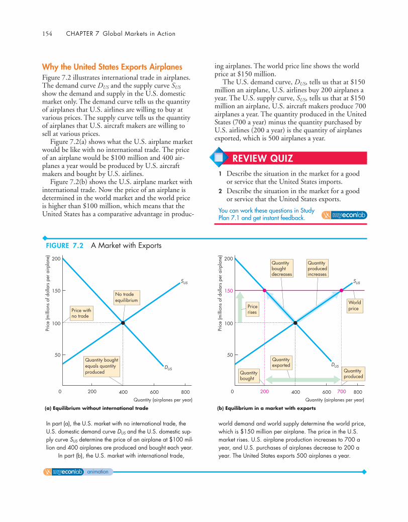
154 CHAPTER 7 Global Markets in Action

Why the United States Exports AirplanesFigure 7.2 illustrates international trade in airplanes.The demand curve DUS and the supply curve SUS

show the demand and supply in the U.S. domesticmarket only. The demand curve tells us the quantityof airplanes that U.S. airlines are willing to buy atvarious prices. The supply curve tells us the quantityof airplanes that U.S. aircraft makers are willing tosell at various prices.

Figure 7.2(a) shows what the U.S. airplane marketwould be like with no international trade. The priceof an airplane would be $100 million and 400 air-planes a year would be produced by U.S. aircraftmakers and bought by U.S. airlines.

Figure 7.2(b) shows the U.S. airplane market withinternational trade. Now the price of an airplane isdetermined in the world market and the world priceis higher than $100 million, which means that theUnited States has a comparative advantage in produc-

ing airplanes. The world price line shows the worldprice at $150 million.

The U.S. demand curve, DUS, tells us that at $150million an airplane, U.S. airlines buy 200 airplanes ayear. The U.S. supply curve, SUS, tells us that at $150million an airplane, U.S. aircraft makers produce 700airplanes a year. The quantity produced in the UnitedStates (700 a year) minus the quantity purchased byU.S. airlines (200 a year) is the quantity of airplanesexported, which is 500 airplanes a year.

Pric

e (m

illio

ns o

f dol

lars

per

airp

lane

)

2000 400 600 800

150

50

DUS

SUS

100

200

Price withno trade

Pricerises

Quantityexported

Quantityproduced

Quantitybought

Quantityproducedincreases

Quantityboughtdecreases

(a) Equilibrium without international trade (b) Equilibrium in a market with exports

Quantity (airplanes per year)

Quantity boughtequals quantityproduced

No tradeequilibrium

Pric

e (m

illio

ns o

f dol

lars

per

airp

lane

)

200 7000 400 600 800

150

50

DUS

SUS

100

200

Quantity (airplanes per year)

Worldprice

In part (a), the U.S. market with no international trade, theU.S. domestic demand curve DUS and the U.S. domestic sup-ply curve SUS determine the price of an airplane at $100 mil-lion and 400 airplanes are produced and bought each year.

In part (b), the U.S. market with international trade,

world demand and world supply determine the world price,which is $150 million per airplane. The price in the U.S.market rises. U.S. airplane production increases to 700 ayear, and U.S. purchases of airplanes decrease to 200 ayear. The United States exports 500 airplanes a year.

REVIEW QUIZ1 Describe the situation in the market for a good

or service that the United States imports.2 Describe the situation in the market for a good

or service that the United States exports.

You can work these questions in Study Plan 7.1 and get instant feedback.

FIGURE 7.2 A Market with Exports

animation

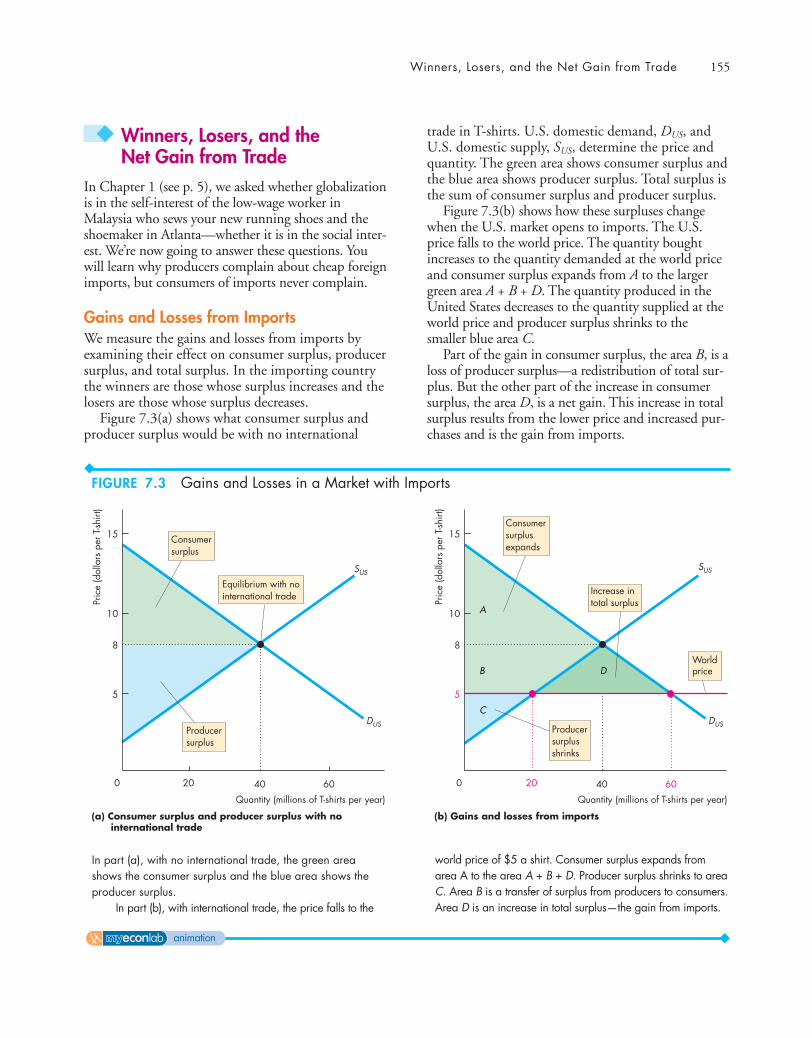
Winners, Losers, and the Net Gain from Trade 155

◆ Winners, Losers, and theNet Gain from Trade

In Chapter 1 (see p. 5), we asked whether globalizationis in the self-interest of the low-wage worker inMalaysia who sews your new running shoes and theshoemaker in Atlanta—whether it is in the social inter-est. We’re now going to answer these questions. Youwill learn why producers complain about cheap foreignimports, but consumers of imports never complain.

Gains and Losses from ImportsWe measure the gains and losses from imports byexamining their effect on consumer surplus, producersurplus, and total surplus. In the importing countrythe winners are those whose surplus increases and thelosers are those whose surplus decreases.

Figure 7.3(a) shows what consumer surplus andproducer surplus would be with no international

trade in T-shirts. U.S. domestic demand, DUS, andU.S. domestic supply, SUS, determine the price andquantity. The green area shows consumer surplus andthe blue area shows producer surplus. Total surplus isthe sum of consumer surplus and producer surplus.

Figure 7.3(b) shows how these surpluses changewhen the U.S. market opens to imports. The U.S.price falls to the world price. The quantity boughtincreases to the quantity demanded at the world priceand consumer surplus expands from A to the largergreen area A + B + D. The quantity produced in theUnited States decreases to the quantity supplied at theworld price and producer surplus shrinks to thesmaller blue area C.

Part of the gain in consumer surplus, the area B, is aloss of producer surplus—a redistribution of total sur-plus. But the other part of the increase in consumersurplus, the area D, is a net gain. This increase in totalsurplus results from the lower price and increased pur-chases and is the gain from imports.

Pric

e (d

olla

rs p

er T

-shirt

)

200 40 60

15

5

DUS

SUS

8

10

Quantity (millions of T-shirts per year)

Pric

e (d

olla

rs p

er T

-shirt

)

200 40 60

15

5

DUS

SUS

8

10

Quantity (millions of T-shirts per year)

Worldprice

(a) Consumer surplus and producer surplus with no international trade

(b) Gains and losses from imports

Equilibrium with nointernational trade

Consumersurplus

Producersurplus

Producersurplusshrinks

Increase intotal surplus

Consumersurplusexpands

A

B D

C

In part (a), with no international trade, the green areashows the consumer surplus and the blue area shows theproducer surplus.

In part (b), with international trade, the price falls to the

world price of $5 a shirt. Consumer surplus expands fromarea A to the area A + B + D. Producer surplus shrinks to areaC. Area B is a transfer of surplus from producers to consumers.Area D is an increase in total surplus—the gain from imports.

FIGURE 7.3 Gains and Losses in a Market with Imports

animation

156 CHAPTER 7 Global Markets in Action

Gains and Losses from ExportsWe measure the gains and losses from exports just likewe measured those from imports, by their effect onconsumer surplus, producer surplus, and total surplus.

Figure 7.4(a) shows the situation with no interna-tional trade. Domestic demand, DUS, and domesticsupply, SUS, determine the price and quantity, the con-sumer surplus, and the producer surplus.

Figure 7.4(b) shows how the consumer surplusand producer surplus change when the good isexported. The price rises to the world price. Thequantity bought decreases to the quantity demandedat the world price and the consumer surplus shrinksto the green area A. The quantity produced increasesto the quantity supplied at the world price and theproducer surplus expands to the blue area B + C + D.

Part of the gain in producer surplus, the area B, is aloss in consumer surplus—a redistribution of the totalsurplus. But the other part of the increase in producersurplus, the area D, is a net gain. This increase in total

surplus results from the higher price and increased pro-duction and is the gain from exports.

Gains for AllYou’ve seen that both imports and exports bringgains. Because one country’s exports are other coun-tries’ imports, international trade brings gain for allcountries. International trade is a win-win game.

Pric

e (m

illio

ns o

f dol

lars

per

airp

lane

)

2000 400 600 800

150

50

DUS

SUS

100

200

Quantity (airplanes per year)

Pric

e (m

illio

ns o

f dol

lars

per

airp

lane

)

200 7000 400 600 800

150

50

DUS

SUS

100

200

Quantity (airplanes per year)

Worldprice

A

B D

C

(a) Consumer surplus and producer surplus with no international trade

(b) Gains and losses from exports

Equilibrium with nointernational trade

Consumersurplus

Producersurplus

Producersurplusexpands

Consumersurplus shrinks

Increase intotal surplus

In part (a), the U.S. market with no international trade, thegreen area shows the consumer surplus and the blue areashows the producer surplus. In part (b), the U.S. market withinternational trade, the price rises to the world price.

Consumer surplus shrinks to area A. Producer surplusexpands from area C to the area B + C + D. Area B is atransfer of surplus from consumers to producers. Area D isan increase in total surplus—the gain from exports.

REVIEW QUIZ1 How is the gain from imports distributed

between consumers and domestic producers?2 How is the gain from exports distributed

between consumers and domestic producers?3 Why is the net gain from international trade

positive?

You can work these questions in Study Plan 7.2 and get instant feedback.

FIGURE 7.4 Gains and Losses in a Market with Exports

animation

International Trade Restrictions 157

Tariffs raise revenue for governments and serve theself-interest of people who earn their incomes inimport-competing industries. But as you will see,restrictions on free international trade decrease thegains from trade and are not in the social interest.

The Effects of a Tariff To see the effects of a tariff,let’s return to the example in which the United Statesimports T-shirts. With free trade, the T-shirts areimported and sold at the world price. Then, underpressure from U.S. garment makers, the U.S. govern-ment imposes a tariff on imported T-shirts. Buyers ofT-shirts must now pay the world price plus the tariff.Several consequences follow and Fig. 7.5 illustratesthem.

Figure 7.5(a) shows the situation with freeinternational trade. The United States produces 20million T-shirts a year and imports 40 million a yearat the world price of $5 a shirt. Figure 7.5(b) showswhat happens with a tariff set at $2 per T-shirt.

◆ International Trade RestrictionsGovernments use four sets of tools to influence inter-national trade and protect domestic industries fromforeign competition. They are

■ Tariffs■ Import quotas■ Other import barriers■ Export subsidies

TariffsA tariff is a tax on a good that is imposed by theimporting country when an imported good crosses its international boundary. For example, the govern-ment of India imposes a 100 percent tariff on wineimported from California. So when an Indianimports a $10 bottle of Californian wine, he pays the Indian government a $10 import duty.

(b) Market with tariff(a) Free trade

Pric

e (d

olla

rs p

er T

-shirt

)

20 35 450 60

15

5

DUS

SUS

7

10

Quantity (millions of T-shirts per year)

Worldprice

Pric

e (d

olla

rs p

er T

-shirt

)

200 40 60

15

5

DUS

SUS

8

10

Quantity (millions of T-shirts per year)

Worldprice Tariff

Importswith freetrade

Importswith tariff

Tariffrevenue

World priceplus tariff

The world price of a T-shirt is $5. With free trade in part(a), Americans buy 60 million T-shirts a year. U.S. gar-ment makers produce 20 million T-shirts a year and theUnited States imports 40 million a year.

With a tariff of $2 per T-shirt in part (b), the price in

the U.S. market rises to $7 a T-shirt. U.S. productionincreases, U.S. purchases decrease, and the quantityimported decreases. The U.S. government collects a tariffrevenue of $2 on each T-shirt imported, which is shown bythe purple rectangle.

FIGURE 7.5 The Effects of a Tariff

animation

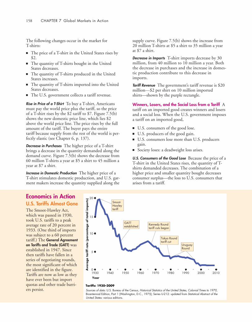
158 CHAPTER 7 Global Markets in Action

The following changes occur in the market for T-shirts:

■ The price of a T-shirt in the United States rises by$2.

■ The quantity of T-shirts bought in the UnitedStates decreases.

■ The quantity of T-shirts produced in the UnitedStates increases.

■ The quantity of T-shirts imported into the UnitedStates decreases.

■ The U.S. government collects a tariff revenue.

Rise in Price of a T-Shirt To buy a T-shirt, Americansmust pay the world price plus the tariff, so the priceof a T-shirt rises by the $2 tariff to $7. Figure 7.5(b)shows the new domestic price line, which lies $2above the world price line. The price rises by the fullamount of the tariff. The buyer pays the entire tariff because supply from the rest of the world is per-fectly elastic (see Chapter 6, p. 137).

Decrease in Purchases The higher price of a T-shirtbrings a decrease in the quantity demanded along thedemand curve. Figure 7.5(b) shows the decrease from60 million T-shirts a year at $5 a shirt to 45 million ayear at $7 a shirt.

Increase in Domestic Production The higher price of aT-shirt stimulates domestic production, and U.S. gar-ment makers increase the quantity supplied along the

supply curve. Figure 7.5(b) shows the increase from20 million T-shirts at $5 a shirt to 35 million a yearat $7 a shirt.

Decrease in Imports T-shirt imports decrease by 30million, from 40 million to 10 million a year. Boththe decrease in purchases and the increase in domes-tic production contribute to this decrease inimports.

Tariff Revenue The government’s tariff revenue is $20million—$2 per shirt on 10 million importedshirts—shown by the purple rectangle.

Winners, Losers, and the Social Loss from a Tariff Atariff on an imported good creates winners and losersand a social loss. When the U.S. government imposesa tariff on an imported good,

■ U.S. consumers of the good lose.■ U.S. producers of the good gain.■ U.S. consumers lose more than U.S. producers

gain.■ Society loses: a deadweight loss arises.

U.S. Consumers of the Good Lose Because the price of aT-shirt in the United States rises, the quantity of T-shirts demanded decreases. The combination of ahigher price and smaller quantity bought decreasesconsumer surplus—the loss to U.S. consumers thatarises from a tariff.

Smoot-Hawleytariff

GATTestablished Kennedy Round

tariff cuts began

Tokyo Roundtariff cut

UruguayRound

Year

Ave

rage

tari

ff r

ate

(per

centa

ge

of

tota

l im

port

s)

0

5

10

15

20

1990198019701960195019401930 20102000

Tariffs: 1930–2009

Economics in ActionU.S. Tariffs Almost GoneThe Smoot-Hawley Act,which was passed in 1930,took U.S. tariffs to a peakaverage rate of 20 percent in1933. (One third of importswas subject to a 60 percenttariff.) The General Agreementon Tariffs and Trade (GATT) wasestablished in 1947. Sincethen tariffs have fallen in aseries of negotiating rounds,the most significant of whichare identified in the figure.Tariffs are now as low as theyhave ever been but importquotas and other trade barri-ers persist. Sources of data: U.S. Bureau of the Census, Historical Statistics of the United States, Colonial Times to 1970,

Bicentennial Edition, Part 1 (Washington, D.C., 1975); Series U-212: updated from Statistical Abstract of the United States: various editions.

International Trade Restrictions 159

Pric

e (d

olla

rs p

er T

-shirt

)

200 60

15

5

7

DUS

SUS

10

Quantity (millions of T-shirts per year)

Worldprice

(a) Free trade (b) Market with tariff

B EC D

A

Pric

e (d

olla

rs p

er T

-shirt

)

200 40 60

15

5

DUS

SUS

40

10

Quantity (millions of T-shirts per year)

Worldprice

Producersurplus

Gain fromfree trade

Consumersurplus

Importswith freetrade

Tariff

Importswith tariff

Tariffrevenue

Deadweightloss from tariff

Consumersurplusshrinks

Producersurplusexpands

World priceplus tariff

The world price of a T-shirt is $5. In part (a), with free trade,the United States imports 40 million T-shirts. Consumer surplus,producer surplus, and the gains from free trade are as largeas possible.

In part (b), a tariff of $2 per T-shirt raises the U.S. price

of a T-shirt to $7. The quantity imported decreases.Consumer surplus shrinks by the areas B, C, D, and E.Producer surplus expands by area B. The government’s tariffrevenue is area D, and the tariff creates a deadweight lossequal to the area C + E.

FIGURE 7.6 The Winners and Losers from a Tariff

U.S. Producers of the Good Gain Because the price ofan imported T-shirt rises by the amount of the tariff,U.S. T-shirt producers are now able to sell their T-shirts for the world price plus the tariff. At the higherprice, the quantity of T-shirts supplied by U.S. pro-ducers increases. The combination of a higher priceand larger quantity produced increases producer sur-plus—the gain to U.S. producers from the tariff.

U.S. Consumers Lose More Than U.S. Producers GainConsumer surplus decreases for four reasons: Somebecomes producer surplus, some is lost in a highercost of production (domestic producers have highercosts than foreign producers), some is lost becauseimports decrease, and some goes to the governmentas tariff revenue. Figure 7.6 shows these sources oflost consumer surplus.

Figure 7.6(a) shows the consumer surplus and pro-ducer surplus with free international trade in T-shirts.Figure 7.6(b) shows the consumer surplus and pro-ducer surplus with a $2 tariff on imported T-shirts.By comparing Fig. 7.6(b) with Fig. 7.6(a), you cansee how a tariff changes these surpluses.

Consumer surplus—the green area—shrinks forfour reasons. First, the higher price transfers surplusfrom consumers to producers. The blue area Brepresents this loss (and gain of producer surplus).Second, domestic production costs more thanimports. The supply curve SUS shows the higher costof production and the gray area C shows this loss ofconsumer surplus. Third, some of the consumersurplus is transferred to the government. The purplearea D shows this loss (and gain of governmentrevenue). Fourth, some of the consumer surplus islost because imports decrease. The gray area Eshows this loss.

Society Loses: A Deadweight Loss Arises Some of theloss of consumer surplus is transferred to producersand some is transferred to the government and spenton government programs that people value. But theincrease in production cost and the loss fromdecreased imports is transferred to no one: It is asocial loss—a deadweight loss. The gray areas labeledC and E represent this deadweight loss. Total surplusdecreases by the area C + E.

animation

160 CHAPTER 7 Global Markets in Action

Figure 7.7(a) shows the situation with free inter-national trade. Figure 7.7(b) shows what happenswith an import quota of 10 million T-shirts a year.The U.S. supply curve of T-shirts becomes thedomestic supply curve, SUS, plus the quantity thatthe import quota permits. So the supply curvebecomes SUS + quota. The price of a T-shirt rises to$7, the quantity of T-shirts bought in the UnitedStates decreases to 45 million a year, the quantity ofT-shirts produced in the United States increases to35 million a year, and the quantity of T-shirtsimported into the United States decreases to thequota quantity of 10 million a year. All the effectsof this quota are identical to the effects of a $2 pershirt tariff, as you can check in Fig. 7.5(b).

Winners, Losers, and the Social Loss from an Import Quota An import quota creates winners andlosers that are similar to those of a tariff but with aninteresting difference.

Import QuotasWe now look at the second tool for restricting trade:import quotas. An import quota is a restriction thatlimits the maximum quantity of a good that may beimported in a given period.

Most countries impose import quotas on a widerange of items. The United States imposes them onfood products such as sugar and bananas and manu-factured goods such as textiles and paper.

Import quotas enable the government to satisfythe self-interest of the people who earn their incomesin the import-competing industries. But you will dis-cover that like a tariff, an import quota decreases thegains from trade and is not in the social interest.

The Effects of an Import Quota The effects of animport quota are similar to those of a tariff. The pricerises, the quantity bought decreases, and the quantityproduced in the United States increases. Figure 7.7illustrates the effects.

(b) Market with import quota(a) Free trade

Pric

e (d

olla

rs p

er T

-shirt

)

20 35 450 60

15

5

DUS

SUS

SUS + quota

7

10

Quantity (millions of T-shirts per year)

Pric

e (d

olla

rs p

er T

-shirt

)

200 40 8060

15

5

DUS

SUS

10

Quantity (millions of T-shirts per year)

Worldprice

Worldprice

Importswith freetrade

Importswith quota

Price withquota

Quota

80

With free international trade, in part (a), Americans buy 60million T-shirts at the world price. The United States produces20 million T-shirts and imports 40 million a year. With animport quota of 10 million T-shirts a year, in part (b),

the supply of T-shirts in the United States is shown by thecurve SUS + quota. The price in the United States rises to $7 a T-shirt. U.S. production increases, U.S. purchasesdecrease, and the quantity of T-shirts imported decreases.

FIGURE 7.7 The Effects of an Import Quota

animation

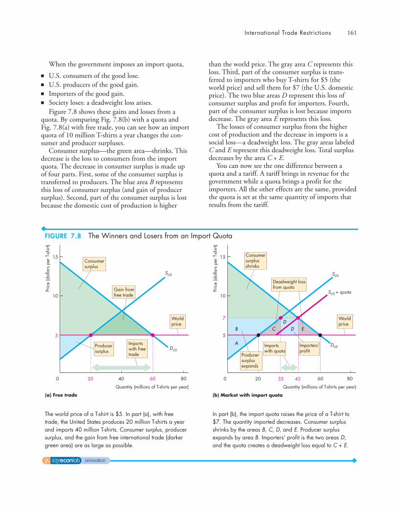
International Trade Restrictions 161

than the world price. The gray area C represents thisloss. Third, part of the consumer surplus is trans-ferred to importers who buy T-shirts for $5 (theworld price) and sell them for $7 (the U.S. domesticprice). The two blue areas D represent this loss ofconsumer surplus and profit for importers. Fourth,part of the consumer surplus is lost because importsdecrease. The gray area E represents this loss.

The losses of consumer surplus from the highercost of production and the decrease in imports is asocial loss—a deadweight loss. The gray areas labeledC and E represent this deadweight loss. Total surplusdecreases by the area C + E.

You can now see the one difference between aquota and a tariff. A tariff brings in revenue for thegovernment while a quota brings a profit for theimporters. All the other effects are the same, providedthe quota is set at the same quantity of imports thatresults from the tariff.

When the government imposes an import quota,

■ U.S. consumers of the good lose.■ U.S. producers of the good gain.■ Importers of the good gain.■ Society loses: a deadweight loss arises.

Figure 7.8 shows these gains and losses from aquota. By comparing Fig. 7.8(b) with a quota andFig. 7.8(a) with free trade, you can see how an importquota of 10 million T-shirts a year changes the con-sumer and producer surpluses.

Consumer surplus—the green area—shrinks. Thisdecrease is the loss to consumers from the importquota. The decrease in consumer surplus is made upof four parts. First, some of the consumer surplus istransferred to producers. The blue area B representsthis loss of consumer surplus (and gain of producersurplus). Second, part of the consumer surplus is lostbecause the domestic cost of production is higher

(b) Market with import quota(a) Free trade

Pric

e (d

olla

rs p

er T

-shirt

)

20 35 450 60

15

5

DUS

SUS

SUS + quota

7

10

Quantity (millions of T-shirts per year)

Pric

e (d

olla

rs p

er T

-shirt

)

200 40 8060

15

5

DUS

SUS

10

Quantity (millions of T-shirts per year)

Worldprice

Worldprice

Importswith quota

Producersurplusexpands

80

B EC DD

A Importers’profit

Imports with freetrade

Deadweight lossfrom quota

Consumersurplusshrinks

Producersurplus

Gain fromfree trade

Consumersurplus

The world price of a T-shirt is $5. In part (a), with freetrade, the United States produces 20 million T-shirts a yearand imports 40 million T-shirts. Consumer surplus, producersurplus, and the gain from free international trade (darkergreen area) are as large as possible.

In part (b), the import quota raises the price of a T-shirt to$7. The quantity imported decreases. Consumer surplusshrinks by the areas B, C, D, and E. Producer surplusexpands by area B. Importers’ profit is the two areas D,and the quota creates a deadweight loss equal to C + E.

FIGURE 7.8 The Winners and Losers from an Import Quota

animation

162 CHAPTER 7 Global Markets in Action

Other Import BarriersTwo sets of policies that influence imports are

■ Health, safety, and regulation barriers■ Voluntary export restraints

Health, Safety, and Regulation Barriers Thousandsof detailed health, safety, and other regulationsrestrict international trade. For example, U.S. foodimports are examined by the Food and DrugAdministration to determine whether the food is“pure, wholesome, safe to eat, and produced undersanitary conditions.” The discovery of BSE (mad cowdisease) in just one U.S. cow in 2003 was enough toclose down international trade in U.S. beef. TheEuropean Union bans imports of most geneticallymodified foods, such as U.S.-produced soybeans.Although regulations of the type we’ve just describedare not designed to limit international trade, theyhave that effect.

Voluntary Export Restraints A voluntary exportrestraint is like a quota allocated to a foreignexporter of a good. This type of trade barrier isn’tcommon. It was initially used during the 1980swhen Japan voluntarily limited its exports of carparts to the United States.

Export SubsidiesA subsidy is a payment by the government to a pro-ducer. You studied the effects of a subsidy on thequantity produced and the price of a subsidized farmproduct in Chapter 6, pp. 140–141.

An export subsidy is a payment by the governmentto the producer of an exported good. Export subsi-dies are illegal under a number of international agree-ments, including the North American Free TradeAgreement (NAFTA), and the rules of the WorldTrade Organization (WTO).

Although export subsidies are illegal, the subsidiesthat the U.S. and European Union governments payto farmers end up increasing domestic production,some of which gets exported. These exports of subsi-dized farm products make it harder for producers inother countries, notably in Africa and Central andSouth America, to compete in global markets. Exportsubsidies bring gains to domestic producers, but theyresult in inefficient underproduction in the rest of theworld and create a deadweight loss.

Economics in ActionSelf-Interest Beats the Social InterestThe World Trade Organization (WTO) is an interna-tional body established by the world’s major tradingnations for the purpose of supervising internationaltrade and lowering the barriers to trade.

In 2001, at a meeting of trade ministers from all theWTO member-countries held in Doha, Qatar, anagreement was made to begin negotiations to lower tar-iff barriers and quotas that restrict international trade infarm products and services. These negotiations arecalled the Doha Development Agenda or the Doha Round.

In the period since 2001, thousands of hours ofconferences in Cancún in 2003, Geneva in 2004, andHong Kong in 2005, and ongoing meetings at WTOheadquarters in Geneva, costing millions of taxpay-ers’ dollars, have made disappointing progress.

Rich nations, led by the United States, the EuropeanUnion, and Japan, want greater access to the markets ofdeveloping nations in exchange for allowing thosenations greater access to the markets of the rich world,especially those for farm products.

Developing nations, led by Brazil, China, India, andSouth Africa, want access to the markets of farm prod-ucts of the rich world, but they also want to protecttheir infant industries.

With two incompatible positions, these negotiationsare stalled and show no signs of a breakthrough. Theself-interests of rich nations and developing nations arepreventing the achievement of the social interest.

REVIEW QUIZ 1 What are the tools that a country can use to

restrict international trade?2 Explain the effects of a tariff on domestic pro-

duction, the quantity bought, and the price.3 Explain who gains and who loses from a tariff

and why the losses exceed the gains.4 Explain the effects of an import quota on

domestic production, consumption, and price.5 Explain who gains and who loses from an import

quota and why the losses exceed the gains.

You can work these questions in Study Plan 7.3 and get instant feedback.

The Case Against Protection 163

◆ The Case Against ProtectionFor as long as nations and international trade haveexisted, people have debated whether a country isbetter off with free international trade or with protec-tion from foreign competition. The debate continues,but for most economists, a verdict has been deliveredand is the one you have just seen. Free trade pro-motes prosperity for all countries; protection is ineffi-cient. We’ve seen the most powerful case for freetrade—it brings gains for consumers that exceed anylosses incurred by producers, so there is a net gain forsociety.

But there is a broader range of issues in the freetrade versus protection debate. Let’s review theseissues.

Two classical arguments for restricting interna-tional trade are

■ The infant-industry argument■ The dumping argument

The Infant-Industry ArgumentThe infant-industry argument for protection is that it isnecessary to protect a new industry to enable it togrow into a mature industry that can compete inworld markets. The argument is based on the ideathat comparative advantage changes or is dynamicand that on-the-job experience—learning-by-doing—is an important source of changes in compar-ative advantage. The fact that learning-by-doing canchange comparative advantage doesn’t justify protect-ing an infant industry.

First, the infant-industry argument is not valid ifthe benefits of learning-by-doing accrue only to thefirms in the infant industry. The reason is that thesefirms will anticipate and reap the benefits of learning-by-doing without the additional incentive of protec-tion from foreign competition.

For example, there are huge productivity gainsfrom learning-by-doing in the manufacture of air-craft, but these gains benefit Boeing and other air-craft producers. Because the people making thedecisions are the ones who benefit, they take the futuregains into account when they decide on the scale oftheir activities. No benefits accrue to firms in otherindustries or other parts of the economy, so there is noneed for government assistance to achieve an efficientoutcome.

Second, even if the case is made for protecting aninfant industry, it is more efficient to do so by givingthe firms in the industry a subsidy, which is financedout of taxes. Such a subsidy would encourage theindustry to mature and to compete with efficientworld producers and keep the price faced by con-sumers at the world price.

The Dumping ArgumentDumping occurs when a foreign firm sells its exportsat a lower price than its cost of production.Dumping might be used by a firm that wants togain a global monopoly. In this case, the foreignfirm sells its output at a price below its cost to drivedomestic firms out of business. When the domesticfirms have gone, the foreign firm takes advantage ofits monopoly position and charges a higher price forits product. Dumping is illegal under the rules ofthe WTO and is usually regarded as a justificationfor temporary tariffs, which are called countervailingduties.

But there are powerful reasons to resist thedumping argument for protection. First, it is virtu-ally impossible to detect dumping because it is hardto determine a firm’s costs. As a result, the test fordumping is whether a firm’s export price is below itsdomestic price. But this test is a weak one because itcan be rational for a firm to charge a low price in amarket in which the quantity demanded is highlysensitive to price and a higher price in a market inwhich demand is less price-sensitive.

Second, it is hard to think of a good that is producedby a global monopoly. So even if all the domestic firmsin some industry were driven out of business, it wouldalways be possible to find alternative foreign sources ofsupply and to buy the good at a price determined in acompetitive market.

Third, if a good or service were a truly globalmonopoly, the best way of dealing with it would beby regulation—just as in the case of domesticmonopolies (see Chapter 13, pp. 313–315). Suchregulation would require international cooperation.

The two arguments for protection that we’ve justexamined have an element of credibility. The coun-terarguments are in general stronger, however, sothese arguments do not make the case for protec-tion. But they are not the only arguments that youmight encounter. There are many other new argu-ments against globalization and for protection.

164 CHAPTER 7 Global Markets in Action

unit of output is $2. If a Mexican auto assemblyworker earns $3 an hour and produces 1 unit of out-put an hour, the average labor cost of a unit of outputis $3. Other things remaining the same, the higher aworker’s productivity, the higher is the worker’s wagerate. High-wage workers have high productivity; low-wage workers have low productivity.

Although high-wage U.S. workers are more pro-ductive, on average, than low-wage Mexican work-ers, there are differences across industries. U.S. laboris relatively more productive in some activities thanin others. For example, the productivity of U.S.workers in producing movies, financial services, andcustomized computer chips is relatively higher thantheir productivity in the production of metals andsome standardized machine parts. The activities inwhich U.S. workers are relatively more productivethan their Mexican counterparts are those in whichthe United States has a comparative advantage. Byengaging in free trade, increasing our productionand exports of the goods and services in which wehave a comparative advantage, and decreasing ourproduction and increasing our imports of the goodsand services in which our trading partners have acomparative advantage, we can make ourselves andthe citizens of other countries better off.

Penalizes Lax Environmental StandardsAnother argument for protection is that many poorercountries, such as China and Mexico, do not have thesame environmental policies that we have and,because they are willing to pollute and we are not, wecannot compete with them without tariffs. So ifpoorer countries want free trade with the richer and“greener” countries, they must raise their environ-mental standards.

This argument for protection is weak. First, a poorcountry cannot afford to be as concerned about itsenvironmental standard as a rich country can. Today,some of the worst pollution of air and water is foundin China, Mexico, and the former communist coun-tries of Eastern Europe. But only a few decades ago,London and Los Angeles topped the pollution leaguechart. The best hope for cleaner air in Beijing andMexico City is rapid income growth. And free tradecontributes to that growth. As incomes in developingcountries grow, they will have the means to match theirdesires to improve their environment. Second, a poorcountry may have a comparative advantage at doing“dirty” work, which helps it to raise its income and at

The most common ones are that protection

■ Saves jobs■ Allows us to compete with cheap foreign labor■ Penalizes lax environmental standards■ Prevents rich countries from exploiting developing

countries

Saves JobsFirst, free trade does cost some jobs, but it also createsother jobs. It brings about a global rationalization oflabor and allocates labor resources to their highest-valued activities. International trade in textiles hascost tens of thousands of jobs in the United States astextile mills and other factories closed. But tens ofthousands of jobs have been created in other countriesas textile mills opened. And tens of thousands of U.S.workers got better-paying jobs than as textile workersbecause U.S. export industries expanded and creatednew jobs. More jobs have been created thandestroyed.

Although protection does save particular jobs, itdoes so at a high cost. For example, until 2005, U.S.textile jobs were protected by an international agree-ment called the Multifiber Arrangement. The U.S.International Trade Commission (ITC) has esti-mated that because of import quotas, 72,000 jobsexisted in the textile industry that would otherwisehave disappeared and that the annual clothingexpenditure in the United States was $15.9 billion($160 per family) higher than it would have beenwith free trade. Equivalently, the ITC estimated thateach textile job saved cost $221,000 a year.

Imports don’t only destroy jobs. They create jobsfor retailers that sell imported goods and for firmsthat service those goods. Imports also create jobs bycreating income in the rest of the world, some ofwhich is spent on U.S.-made goods and services.

Allows Us to Compete with Cheap Foreign LaborWith the removal of tariffs on trade between theUnited States and Mexico, people said we would heara “giant sucking sound” as jobs rushed to Mexico.Let’s see what’s wrong with this view.

The labor cost of a unit of output equals the wagerate divided by labor productivity. For example, if aU.S. autoworker earns $30 an hour and produces 15 units of output an hour, the average labor cost of a

The Case Against Protection 165

the same time enables the global economy to achievehigher environmental standards than would otherwisebe possible.

Prevents Rich Countries from ExploitingDeveloping CountriesAnother argument for protection is that internationaltrade must be restricted to prevent the people of therich industrial world from exploiting the poorer peo-ple of the developing countries and forcing them towork for slave wages.

Child labor and near-slave labor are serious prob-lems that are rightly condemned. But by trading withpoor countries, we increase the demand for the goodsthat these countries produce and, more significantly,we increase the demand for their labor. When thedemand for labor in developing countries increases,the wage rate also increases. So, rather than exploitingpeople in developing countries, trade can improvetheir opportunities and increase their incomes.

The arguments for protection that we’ve reviewedleave free-trade unscathed. But a new phenomenon isat work in our economy: offshore outsourcing. Surely weneed protection from this new source of foreign com-petition. Let’s investigate.

Offshore OutsourcingCitibank, the Bank of America, Apple, Nike, Wal-Mart: What do these U.S. icons have in common?They all send jobs that could be done in America toChina, India, Thailand, or even Canada—they areoffshoring. What exactly is offshoring?

What Is Offshoring? A firm in the United States canobtain the goods and services that it sells in any of fourways:

1. Hire American labor and produce in America. 2. Hire foreign labor and produce in other countries.3. Buy finished goods, components, or services

from other firms in the United States.4. Buy finished goods, components, or services

from other firms in other countries.

Activities 3 and 4 are outsourcing, and activities 2and 4 are offshoring. Activity 4 is offshore outsourcing.Notice that offshoring includes activities that takeplace inside U.S. firms. If a U.S. firm opens its ownfacilities in another country, then it is offshoring.

Offshoring has been going on for hundreds of years,but it expanded rapidly and became a source of con-cern during the 1990s as many U.S. firms movedinformation technology services and general officeservices such as finance, accounting, and humanresources management overseas.

Why Did Offshoring of Services Boom During the1990s? The gains from specialization and trade thatyou saw in the previous section must be large enoughto make it worth incurring the costs of communica-tion and transportation. If the cost of producing a T-shirt in China isn’t lower than the cost of producingthe T-shirt in the United States by more than the costof transporting the shirt from China to America, thenit is more efficient to produce shirts in the UnitedStates and avoid the transportation costs.

The same considerations apply to trade in services.If services are to be produced offshore, then the costof delivering those services must be low enough toleave the buyer with an overall lower cost. Before the1990s, the cost of communicating across largedistances was too high to make the offshoring ofbusiness services efficient. But during the 1990s,when satellites, fiber-optic cables, and computers cutthe cost of a phone call between America and Indiato less than a dollar an hour, a huge base of offshoreresources became competitive with similar resourcesin the United States.

What Are the Benefits of Offshoring? Offshoringbrings gains from trade identical to those of any othertype of trade. We could easily change the names ofthe items traded from T-shirts and airplanes (theexamples in the previous sections of this chapter) tobanking services and call center services (or any otherpair of services). An American bank might exportbanking services to Indian firms, and Indians mightprovide call center services to U.S. firms. This type oftrade would benefit both Americans and Indians pro-vided the United States has a comparative advantagein banking services and India has a comparativeadvantage in call center services.

Comparative advantages like these emerged duringthe 1990s. India has the world’s largest educatedEnglish-speaking population and is located in a timezone half a day ahead of the U.S. east coast and mid-way between Asia and Europe, which facilitates 24/7operations. When the cost of communicating with aworker in India was several dollars a minute, as it was

166 CHAPTER 7 Global Markets in Action

Avoiding Trade WarsWe have reviewed the arguments commonly heard infavor of protection and the counterarguments againstit. There is one counterargument to protection that isgeneral and quite overwhelming: Protection invitesretaliation and can trigger a trade war.

The best example of a trade war occurred duringthe Great Depression of the 1930s when the UnitedStates introduced the Smoot-Hawley tariff. Countryafter country retaliated with its own tariff, and in ashort period, world trade had almost disappeared.The costs to all countries were large and led to arenewed international resolve to avoid such self-defeating moves in the future. The costs also led tothe creation of GATT and are the impetus behindcurrent attempts to liberalize trade.

Why Is International Trade Restricted?Why, despite all the arguments against protection, istrade restricted? There are two key reasons:

■ Tariff revenue■ Rent seeking

Tariff Revenue Government revenue is costly to col-lect. In developed countries such as the UnitedStates, a well-organized tax collection system is inplace that can generate billions of dollars of incometax and sales tax revenues. This tax collection systemis made possible by the fact that most economictransactions are done by firms that must keep prop-erly audited financial records. Without such records,revenue collection agencies (the Internal RevenueService in the United States) would be severely ham-pered in their work. Even with audited financialaccounts, some potential tax revenue is lost.Nonetheless, for industrialized countries, theincome tax and sales taxes are the major sources ofrevenue and tariffs play a very small role.

But governments in developing countries have adifficult time collecting taxes from their citizens.Much economic activity takes place in an informaleconomy with few financial records, so only a smallamount of revenue is collected from income taxesand sales taxes. The one area in which economictransactions are well recorded and audited is inter-national trade. So this activity is an attractive basefor tax collection in these countries and is usedmuch more extensively than it is in developedcountries.

before the 1990s, tapping these vast resources was justtoo costly. But at today’s cost of a long-distance tele-phone call or Internet connection, resources in Indiacan be used to produce services in the United States ata lower cost than those services can be produced byusing resources located in the United States. And withthe incomes that Indians earn from exporting services,some of the services (and goods) that Indians buy areproduced in the United States.

Why Is Offshoring a Concern? Despite the gain fromspecialization and trade that offshoring brings, manypeople believe that it also brings costs that eat up thegains. Why?

A major reason is that offshoring is taking jobs inservices. The loss of manufacturing jobs to othercountries has been going on for decades, but the U.S.service sector has always expanded by enough to createnew jobs to replace the lost manufacturing jobs. Nowthat service jobs are also going overseas, the fear is thatthere will not be enough jobs for Americans. This fearis misplaced.

Some service jobs are going overseas, while othersare expanding at home. The United States importscall center services, but it exports education, healthcare, legal, financial, and a host of other types ofservices. Jobs in these sectors are expanding and willcontinue to expand.

The exact number of jobs that have moved tolower-cost offshore locations is not known, and esti-mates vary. But even the highest estimate is a tinynumber compared to the normal rate of job creation.

Winners and Losers Gains from trade do not bringgains for every single person. Americans, on average,gain from offshore outsourcing, but some people lose.The losers are those who have invested in the humancapital to do a specific job that has now gone offshore.

Unemployment benefits provide short-term tempo-rary relief for these displaced workers. But the long-term solution requires retraining and the acquisition ofnew skills.

Beyond providing short-term relief through unem-ployment benefits, there is a large role for governmentin the provision of education and training to enablethe labor force of the twenty-first century to be capableof ongoing learning and rapid retooling to take on newjobs that today we can’t foresee.

Schools, colleges, and universities will expand andget better at doing their jobs of producing a highlyeducated and flexible labor force.

The Case Against Protection 167

Rent Seeking Rent seeking is the major reason whyinternational trade is restricted. Rent seeking is lob-bying for special treatment by the government tocreate economic profit or to divert consumer sur-plus or producer surplus away from others. Freetrade increases consumption possibilities on average,but not everyone shares in the gain and some peopleeven lose. Free trade brings benefits to some andimposes costs on others, with total benefits exceed-ing total costs. The uneven distribution of costs andbenefits is the principal obstacle to achieving moreliberal international trade.

Returning to the example of trade in T-shirts andairplanes, the benefits from free trade accrue to all theproducers of airplanes and to those producers of T-shirts that do not bear the costs of adjusting to asmaller garment industry. These costs are transitioncosts, not permanent costs. The costs of moving tofree trade are borne by the garment producers andtheir employees who must become producers of othergoods and services in which the United States has acomparative advantage.

The number of winners from free trade is large,but because the gains are spread thinly over a largenumber of people, the gain per person is small. Thewinners could organize and become a political forcelobbying for free trade. But political activity is costly.It uses time and other scarce resources and the gainsper person are too small to make the cost of politicalactivity worth bearing.

In contrast, the number of losers from free trade issmall, but the loss per person is large. Because theloss per person is large, the people who lose are will-ing to incur considerable expense to lobby againstfree trade.

Both the winners and losers weigh benefits andcosts. Those who gain from free trade weigh the ben-efits it brings against the cost of achieving it. Thosewho lose from free trade and gain from protectionweigh the benefit of protection against the cost ofmaintaining it. The protectionists undertake a largerquantity of political lobbying than the free traders.

Compensating LosersIf, in total, the gains from free international tradeexceed the losses, why don’t those who gain compen-sate those who lose so that everyone is in favor of freetrade?

Some compensation does take place. WhenCongress approved the North American Free Trade

Agreement (NAFTA) with Canada and Mexico, it setup a $56 million fund to support and retrain workerswho lost their jobs as a result of the new trade agree-ment. During NAFTA’s first six months, only 5,000workers applied for benefits under this scheme. Thelosers from international trade are also compensatedindirectly through the normal unemployment com-pensation arrangements. But only limited attempts aremade to compensate those who lose.

The main reason why full compensation is notattempted is that the costs of identifying all the losersand estimating the value of their losses would beenormous. Also, it would never be clear whether aperson who has fallen on hard times is sufferingbecause of free trade or for other reasons that mightbe largely under her or his control. Furthermore,some people who look like losers at one point in timemight, in fact, end up gaining. The young autoworkerwho loses his job in Michigan and becomes a com-puter assembly worker in Minneapolis might resentthe loss of work and the need to move. But a yearlater, looking back on events, he counts himselffortunate.

Because we do not, in general, compensate the los-ers from free international trade, protectionism is apopular and permanent feature of our national eco-nomic and political life.

◆ We end this chapter on global markets in actionin Reading Between the Lines on pp. 168–169, wherewe apply what you’ve learned by looking at the effectsof a U.S. tariff on imports of tires from China.

REVIEW QUIZ1 What are the infant industry and dumping

arguments for protection? Are they correct?2 Can protection save jobs and the environment

and prevent workers in developing countriesfrom being exploited?

3 What is offshore outsourcing? Who benefitsfrom it and who loses?

4 What are the main reasons for imposing a tariff?5 Why don’t the winners from free trade win the

political argument?

You can work these questions in Study Plan 7.4 and get instant feedback.

168

READING BETWEEN THE L INES

China: Tire Trade Penalties Will Hurt Relations with U.S.USATodaySeptember 12, 2009

WASHINGTON—President Obama’s decision to impose trade penalties on Chinese tireshas infuriated Beijing. …

The federal trade panel recommended a 55% tariff in the first year, 45% in the secondyear, and 35% in the third year. Obama settled on 35% the first year, 30% in the second,and 25% in the third, [White House Press Secretary Robert] Gibbs said.

“For trade to work for everybody, it has to be based on fairness and rules. We’re simplyenforcing those rules and would expect the Chinese to understand those rules,” Gibbs said.…

The steelworkers union … says more than 5,000 tire workers have lost jobs since 2004, asChinese tires overwhelmed the U.S. market.

The U.S. trade representative’s office said four tire plants closed in 2006 and 2007 andthree more are closing this year. During thattime, just one new plant opened. U.S. importsof Chinese tires more than tripled from 2004to 2008 and China’s market share in the Unit-ed States went from 4.7% of tires purchasedin 2004 to 16.7% in 2008, the office said. …

China said the tariffs do not square with thefacts, … citing a 2.2% increase in 2008 from2007, and a 16% fall in exports in the first halfof 2009 compared with the first half of 2008.

The new tariffs, on top of an existing 4% tar-iff on all tire imports, take effect Sept. 26. …

Used with permission of The Associated Press. Copyright © 2010. AllRights Reserved.

■ The United States is imposing a tariff on tiresimported from China of 35 percent in 2009and falling after two years to 25 percent.

■ The steelworkers union says that more than5,000 U.S. tire workers have lost jobs since2004.

■ Four U.S. tire plants closed in 2006 and 2007and three were closing in 2009.

■ Between 2004 and 2008, U.S. imports ofChinese tires more than tripled and China’sshare of the U.S. tire market increased from4.7 percent of tires purchased in 2004 to 16.7 percent in 2008.

■ China said that the rate of increase in 2008was 2.2 percent and in the first half of 2009its tire exports to the United States fell by 16percent compared with the first half of 2008.

ESSENCE OF THE STORY

A Tariff on Tires

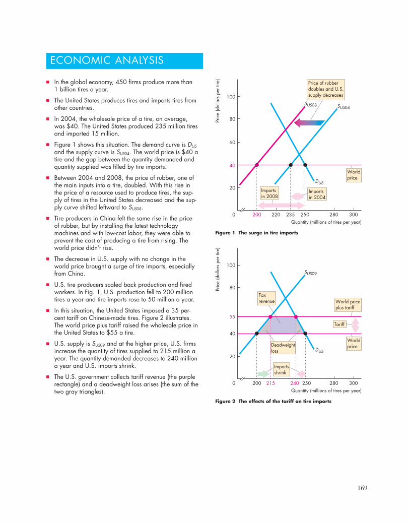
169

ECONOMIC ANALYSIS

Figure 1 The surge in tire imports

Pric

e (d

olla

rs p

er ti

re)

Quantity (millions of tires per year)0

20DUS

SUS08 SUS04

Price of rubberdoubles and U.S.supply decreases

Importsin 2008

Importsin 2004

Worldprice

40

60

80

100

300220 235 280200 250

Figure 2 The effects of the tariff on tire imports

Pric

e (d

olla

rs p

er ti

re)

Quantity (millions of tires per year)0

20DUS

SUS09

Importsshrink

Tariff

Worldprice

World priceplus tariff

Taxrevenue

Deadweightloss

55

40

80

100

300215 240 280250200

■ In the global economy, 450 firms produce more than 1 billion tires a year.

■ The United States produces tires and imports tires fromother countries.

■ In 2004, the wholesale price of a tire, on average,was $40. The United States produced 235 million tiresand imported 15 million.

■ Figure 1 shows this situation. The demand curve is DUS

and the supply curve is SUS04. The world price is $40 atire and the gap between the quantity demanded andquantity supplied was filled by tire imports.

■ Between 2004 and 2008, the price of rubber, one ofthe main inputs into a tire, doubled. With this rise inthe price of a resource used to produce tires, the sup-ply of tires in the United States decreased and the sup-ply curve shifted leftward to SUS08.

■ Tire producers in China felt the same rise in the priceof rubber, but by installing the latest technology machines and with low-cost labor, they were able toprevent the cost of producing a tire from rising. Theworld price didn’t rise.

■ The decrease in U.S. supply with no change in theworld price brought a surge of tire imports, especiallyfrom China.

■ U.S. tire producers scaled back production and firedworkers. In Fig. 1, U.S. production fell to 200 milliontires a year and tire imports rose to 50 million a year.

■ In this situation, the United States imposed a 35 per-cent tariff on Chinese-made tires. Figure 2 illustrates.The world price plus tariff raised the wholesale price inthe United States to $55 a tire.

■ U.S. supply is SUS09 and at the higher price, U.S. firmsincrease the quantity of tires supplied to 215 million ayear. The quantity demanded decreases to 240 milliona year and U.S. imports shrink.

■ The U.S. government collects tariff revenue (the purplerectangle) and a deadweight loss arises (the sum of thetwo gray triangles).

170 CHAPTER 7 Global Markets in Action

International Trade Restrictions (pp. 157–162)

■ Countries restrict international trade by imposingtariffs, import quotas, and other import barriers.

■ Trade restrictions raise the domestic price ofimported goods, lower the quantity imported,decrease consumer surplus, increase producer sur-plus, and create a deadweight loss.

Working Problems 9 to 20 will give you a better under-standing of international trade restrictions.

The Case Against Protection (pp. 163–167)

■ Arguments that protection is necessary for infantindustries and to prevent dumping are weak.

■ Arguments that protection saves jobs, allows usto compete with cheap foreign labor, is neededto penalize lax environmental standards, andprevents exploitation of developing countries areflawed.

■ Offshore outsourcing is just a new way ofreaping gains from trade and does not justifyprotection.

■ Trade restrictions are popular because protectionbrings a small loss per person to a large number ofpeople and a large gain per person to a small num-ber of people. Those who gain have a strongerpolitical voice than those who lose and it is toocostly to identify and compensate losers.

Working Problem 21 will give you a better understandingof the case against protection.

Key Points

How Global Markets Work (pp. 152–154)

■ Comparative advantage drives international trade.■ If the world price of a good is lower than the

domestic price, the rest of the world has a compar-ative advantage in producing that good and thedomestic country gains by producing less, con-suming more, and importing the good.

■ If the world price of a good is higher than thedomestic price, the domestic country has a compara-tive advantage in producing that good and gains byproducing more, consuming less, and exporting thegood.

Working Problems 1 to 6 will give you a better under-standing of how global markets work.

Winners, Losers, and the Net Gain from Trade (pp. 155–156)

■ Compared to a no-trade situation, in a marketwith imports, consumer surplus is larger, producersurplus is smaller, and total surplus is larger withfree international trade.

■ Compared to a no-trade situation, in a marketwith exports, consumer surplus is smaller, pro-ducer surplus is larger, and total surplus is largerwith free international trade.

Working Problems 7 and 8 will give you a better under-standing of winners, losers, and the net gains from trade.

SUMMARY

Key TermsDoha Development Agenda (Doha Round), 162

Dumping, 163Exports, 152General Agreement on Tariffs and Trade (GATT), 159

Import quota, 160Imports, 152Infant-industry argument, 163Offshore outsourcing, 165Offshoring, 165Outsourcing, 165

Rent seeking, 167Tariff, 157World Trade Organization

(WTO), 162

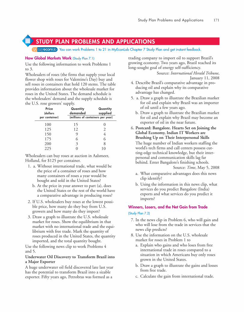
Study Plan Problems and Applications 171

trading company to import oil to support Brazil’sgrowing economy. Two years ago, Brazil reached itslong-sought goal of energy self-sufficiency.

Source: International Herald Tribune,January 11, 2008

4. Describe Brazil’s comparative advantage in pro-ducing oil and explain why its comparativeadvantage has changed.

5. a. Draw a graph to illustrate the Brazilian marketfor oil and explain why Brazil was an importerof oil until a few years ago.

b. Draw a graph to illustrate the Brazilian marketfor oil and explain why Brazil may become anexporter of oil in the near future.

6. Postcard: Bangalore. Hearts Set on Joining theGlobal Economy, Indian IT Workers areBrushing Up on Their Interpersonal SkillsThe huge number of Indian workers staffing theworld’s tech firms and call centers possess cut-ting-edge technical knowledge, but their inter-personal and communication skills lag farbehind. Enter Bangalore’s finishing schools.

Source: Time, May 5, 2008a. What comparative advantages does this news

clip identify?b. Using the information in this news clip, what

services do you predict Bangalore (India)exports and what services do you predict itimports?

Winners, Losers, and the Net Gain from Trade (Study Plan 7.2)

7. In the news clip in Problem 6, who will gain andwho will lose from the trade in services that thenews clip predicts?

8. Use the information on the U.S. wholesalemarket for roses in Problem 1 toa. Explain who gains and who loses from free

international trade in roses compared to asituation in which Americans buy only rosesgrown in the United States.

b. Draw a graph to illustrate the gains and lossesfrom free trade.

c. Calculate the gain from international trade.

How Global Markets Work (Study Plan 7.1)

Use the following information to work Problems 1 to 3. Wholesalers of roses (the firms that supply your localflower shop with roses for Valentine’s Day) buy andsell roses in containers that hold 120 stems. The tableprovides information about the wholesale market forroses in the United States. The demand schedule isthe wholesalers’ demand and the supply schedule isthe U.S. rose growers’ supply.

Price Quantity Quantity(dollars demanded supplied

per container) (millions of containers per year)

100 15 0125 12 2150 9 4175 6 6200 3 8225 0 10

Wholesalers can buy roses at auction in Aalsmeer,Holland, for $125 per container.

1. a. Without international trade, what would bethe price of a container of roses and howmany containers of roses a year would bebought and sold in the United States?

b. At the price in your answer to part (a), doesthe United States or the rest of the world havea comparative advantage in producing roses?

2. If U.S. wholesalers buy roses at the lowest possi-ble price, how many do they buy from U.S.growers and how many do they import?

3. Draw a graph to illustrate the U.S. wholesalemarket for roses. Show the equilibrium in thatmarket with no international trade and the equi-librium with free trade. Mark the quantity ofroses produced in the United States, the quantityimported, and the total quantity bought.

Use the following news clip to work Problems 4 and 5.Underwater Oil Discovery to Transform Brazil intoa Major ExporterA huge underwater oil field discovered late last yearhas the potential to transform Brazil into a sizableexporter. Fifty years ago, Petrobras was formed as a

You can work Problems 1 to 21 in MyEconLab Chapter 7 Study Plan and get instant feedback.

STUDY PLAN PROBLEMS AND APPLICATIONS

172 CHAPTER 7 Global Markets in Action

International Trade Restrictions (Study Plan 7.3)

Use the following news clip to work Problems 9 and 10.Steel Tariffs Appear to Have Backfired on BushPresident Bush set aside his free-trade principles lastyear and imposed heavy tariffs on imported steel tohelp out struggling mills in Pennsylvania and WestVirginia. Some economists say the tariffs may havecost more jobs than they saved, by driving up costsfor automakers and other steel users.

Source: The Washington Post, September 19, 2003

9. a. Explain how a high tariff on steel imports canhelp domestic steel producers.

b. Explain how a high tariff on steel imports canharm steel users.

10. Draw a graph of the U.S. market for steel toshow how a high tariff on steel imports

i. Helps U.S. steel producers.ii. Harms U.S. steel users.

iii. Creates a deadweight loss.Use the information on the U.S. wholesale marketfor roses in Problem 1 to work Problems 11 to 16.11. If the United States puts a tariff of $25 per con-

tainer on imports of roses, what happens to theU.S. price of roses, the quantity of roses bought,the quantity produced in the United States, andthe quantity imported?

12. Who gains and who loses from this tariff?13. Draw a graph to illustrate the gains and losses

from the tariff and on the graph identify thegains and losses, the tariff revenue, and the dead-weight loss.

14. If the United States puts an import quota onroses of 5 million containers, what happens tothe U.S. price of roses, the quantity of rosesbought, the quantity produced in the UnitedStates, and the quantity imported?

15. Who gains and who loses from this quota?16. Draw a graph to illustrate the gains and losses

from the import quota and on the graph identifythe gains and losses, the importers’ profit, andthe deadweight loss.

Use the following news clip to work Problems 17 and 18.Car Sales Go Up as Prices TumbleCar affordability in Australia is now at its best in 20years, fueling a surge in sales as prices tumble. In2000, Australia cut the tariff to 15 percent and onJanuary 1, 2005, it cut the tariff to 10 percent.

Source: Courier Mail, February 26, 2005

17. Explain who gains and who loses from the lowertariff on imported cars.

18. Draw a graph to show how the price of a car, the quantity of cars bought, the quantity of carsproduced in Australia, and the quantity of carsimported into Australia changed.

Use the following news clip to work Problems 19 and 20.Why the World Can’t Afford FoodAs [food] stocks dwindled, some countries placedexport restrictions on food to protect their own sup-plies. This in turn drove up prices, punishing coun-tries—especially poor ones—that depend on importsfor much of their food.

Time, May 19, 2008

19. a. What are the benefits to a country fromimporting food?

b. What costs might arise from relying on im-ported food?

20. If a country restricts food exports, what effectdoes this restriction have in that country on theprice of food, the quantity of food it produces,the quantity of food it consumes, and the quan-tity of food it exports?

The Case Against Protection (Study Plan 7.4)

21. Chinese Tire Maker Rejects U.S. Charge ofDefectsU.S. regulators ordered the recall of more than450,000 faulty tires. The Chinese producer ofthe tires disputed the allegations and hinted thatthe recall might be an effort by foreign competi-tors to hamper Chinese exports to the UnitedStates. Mounting scrutiny of Chinese-madegoods has become a source of new trade frictionsbetween the United States and China and fueledworries among regulators, corporations, and con-sumers about the risks associated with manyproducts imported from China.

Source: International Herald Tribune,June 26, 2007

a. What does the information in the news clipimply about the comparative advantage ofproducing tires in the United States andChina?

b. Could product quality be a valid argumentagainst free trade?

c. How would the product-quality argumentagainst free trade be open to abuse by domes-tic producers of the imported good?

Additional Problems and Applications 173

How Global Markets Work22. Suppose that the world price of sugar is 10 cents a

pound, the United States does not trade interna-tionally, and the equilibrium price of sugar in theUnited States is 20 cents a pound. The UnitedStates then begins to trade internationally.a. How does the price of sugar in the United

States change?b. Do U.S. consumers buy more or less sugar?c. Do U.S. sugar growers produce more or less

sugar?d. Does the United States export or import sugar

and why?23. Suppose that the world price of steel is $100 a

ton, India does not trade internationally, and theequilibrium price of steel in India is $60 a ton.India then begins to trade internationally.a. How does the price of steel in India change?b. How does the quantity of steel produced in

India change?c. How does the quantity of steel bought by

India change?d. Does India export or import steel and why?

24. A semiconductor is a key component in your lap-top, cell phone, and iPod. The table providesinformation about the market for semiconduc-tors in the United States.

Price Quantity Quantity(dollars demanded suppliedper unit) (billions of units per year)

10 25 012 20 2014 15 4016 10 6018 5 8020 0 100

Producers of semiconductors can get $18 a uniton the world market.a. With no international trade, what would be

the price of a semiconductor and how manysemiconductors a year would be bought andsold in the United States?

b. Does the United States have a comparative ad-vantage in producing semiconductors?

25. Act Now, Eat LaterThe hunger crisis in poor countries has its rootsin U.S. and European policies of subsidizing thediversion of food crops to produce biofuels likecorn-based ethanol. That is, doling out subsidiesto put the world’s dinner into the gas tank.

Source: Time, May 5, 2008a. What is the effect on the world price of corn

of the increased use of corn to produceethanol in the United States and Europe?

b. How does the change in the world price ofcorn affect the quantity of corn produced in apoor developing country with a comparativeadvantage in producing corn, the quantity itconsumes, and the quantity that it either ex-ports or imports?

Winners, Losers, and the Net Gain from Trade

26. Use the news clip in Problem 25. Draw a graphof the market for corn in a poor developingcountry to show the changes in consumer sur-plus, producer surplus, and deadweight loss.

Use the following news clip to work Problems 27 and 28.South Korea to Resume U.S. Beef ImportsSouth Korea will reopen its market to most U.S. beef.South Korea banned imports of U.S. beef in 2003amid concerns over a case of mad cow disease in theUnited States. The ban closed what was then thethird-largest market for U.S. beef exporters.

Source: CNN, May 29, 200827. a. Explain how South Korea’s import ban on

U.S. beef affected beef producers and con-sumers in South Korea.

b. Draw a graph of the market for beef in SouthKorea to illustrate your answer to part (a).Identify the changes in consumer surplus,producer surplus, and deadweight loss.

28. a. Assuming that South Korea is the onlyimporter of U.S. beef, explain how SouthKorea’s import ban on U.S. beef affected beefproducers and consumers in the United States.

b. Draw a graph of the market for beef in theUnited States to illustrate your answer to part(a). Identify the changes in consumer surplus,producer surplus, and deadweight loss.

These problems can be worked in MyEconLab if assigned by your instructor.

ADDITIONAL PROBLEMS AND APPLICATIONS

174 CHAPTER 7 Global Markets in Action

International Trade RestrictionsUse the following information to work Problems 29to 31.Before 1995, trade between the United States andMexico was subject to tariffs. In 1995, Mexico joinedNAFTA and all U.S. and Mexican tariffs have gradu-ally been removed.29. Explain how the price that U.S. consumers pay for

goods from Mexico and the quantity of U.S.imports from Mexico have changed. Who are thewinners and who are the losers from this free trade?

30. Explain how the quantity of U.S. exports toMexico and the U.S. government’s tariff revenuefrom trade with Mexico have changed.

31. Suppose that in 2008, tomato growers in Floridalobby the U.S. government to impose an importquota on Mexican tomatoes. Explain who in theUnited States would gain and who would losefrom such a quota.

Use the following information to work Problems 32and 33.Suppose that in response to huge job losses in theU.S. textile industry, Congress imposes a 100 percenttariff on imports of textiles from China. 32. Explain how the tariff on textiles will change the

price that U.S. buyers pay for textiles, the quan-tity of textiles imported, and the quantity of tex-tiles produced in the United States.

33. Explain how the U.S. and Chinese gains fromtrade will change. Who in the United States willlose and who will gain?

Use the following information to work Problems 34and 35.With free trade between Australia and the UnitedStates, Australia would export beef to the UnitedStates. But the United States imposes an importquota on Australian beef.34. Explain how this quota influences the price that

U.S. consumers pay for beef, the quantity of beefproduced in the United States, and the U.S. andthe Australian gains from trade.

35. Explain who in the United States gains from thequota on beef imports and who loses.

The Case Against Protection36. Trading Up

The cost of protecting jobs in uncompetitive sec-tors through tariffs is high: Saving a job in the

sugar industry costs American consumers$826,000 in higher prices a year; saving a dairyindustry job costs $685,000 per year; and savinga job in the manufacturing of women’s handbagscosts $263,000.

Source: The New York Times, June 26, 2006a. What are the arguments for saving the jobs

mentioned in this news clip?b. Explain why these arguments are faulty.c. Is there any merit to saving these jobs?

Economics in the News 37. After you have studied Reading Between the Lines

on pp. 168–169, answer the following questions.a. What events put U.S. tire producers under

pressure and caused some to go out of business?b. Explain how a tariff on tire imports changes

domestic production, consumption, and im-ports of tires.

c. Illustrate your answer to part (b) with anappropriate graphical analysis.

d. Explain how a tariff on tire imports changesconsumer surplus and producer surplus.

e. Explain the four sources of loss of consumersurplus that result from a tariff on tire imports.

f. Illustrate your answer to part (e) with anappropriate graphical analysis.

38. Aid May Grow for Laid-Off Workers

Expansion of the Trade Adjustment Assistance(TAA) program would improve the social safetynet for the 21st century, as advances permit moreindustries to take advantage of cheap foreignlabor—even for skilled, white-collar work. Byproviding special compensation to more of glob-alization’s losers and retraining them for stablejobs at home, an expanded program could beginto ease the resentment and insecurity arisingfrom the new economy.

Source: The Washington Post, July 23, 2007a. Why does the United States engage in interna-

tional trade if it causes U.S. workers to losetheir jobs?

b. Explain how an expansion of the TAA pro-gram will make it easier for the United Statesto move toward freer international trade.

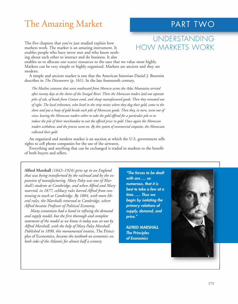
175

The Amazing Market

The five chapters that you’ve just studied explain howmarkets work. The market is an amazing instrument. Itenables people who have never met and who know noth-ing about each other to interact and do business. It alsoenables us to allocate our scarce resources to the uses that we value most highly.Markets can be very simple or highly organized. Markets are ancient and they aremodern.

A simple and ancient market is one that the American historian Daniel J. Boorstindescribes in The Discoverers (p. 161). In the late fourteenth century,

The Muslim caravans that went southward from Morocco across the Atlas Mountains arrivedafter twenty days at the shores of the Senegal River. There the Moroccan traders laid out separatepiles of salt, of beads from Ceutan coral, and cheap manufactured goods. Then they retreated outof sight. The local tribesmen, who lived in the strip mines where they dug their gold, came to theshore and put a heap of gold beside each pile of Moroccan goods. Then they, in turn, went out ofview, leaving the Moroccan traders either to take the gold offered for a particular pile or toreduce the pile of their merchandise to suit the offered price in gold. Once again the Moroccantraders withdrew, and the process went on. By this system of commercial etiquette, the Moroccanscollected their gold.

An organized and modern market is an auction at which the U.S. government sellsrights to cell phone companies for the use of the airwaves.

Everything and anything that can be exchanged is traded in markets to the benefitof both buyers and sellers.

PART TWO

UNDERSTANDING HOW MARKETS WORK

Alfred Marshall (1842–1924) grew up in an Englandthat was being transformed by the railroad and by the ex-pansion of manufacturing. Mary Paley was one of Mar-shall’s students at Cambridge, and when Alfred and Marymarried, in 1877, celibacy rules barred Alfred from con-tinuing to teach at Cambridge. By 1884, with more lib-eral rules, the Marshalls returned to Cambridge, whereAlfred became Professor of Political Economy.

Many economists had a hand in refining the demandand supply model, but the first thorough and completestatement of the model as we know it today was set out byAlfred Marshall, with the help of Mary Paley Marshall.Published in 1890, this monumental treatise, The Princi-ples of Economics, became the textbook on economics onboth sides of the Atlantic for almost half a century.

“The forces to be dealtwith are . . . sonumerous, that it isbest to take a few at atime .. . . Thus webegin by isolating theprimary relations ofsupply, demand, andprice.”

ALFRED MARSHALLThe Principles of Economics

176

opportunity to outbid the previous high bidder.There are also different ways to use bids received bythe auctioneer to determine the price. Create an newscreamer: Both revenue and efficiency are affected byauction design.The seller may consider revenue,though governments are often most concerned aboutefficient allocation.

Both revenue and efficiency are affected by auc-tion design. One key question the seller must consid-er is how the design will affect the participation ofbidders, as this will determine how competitive bid-ding will be as well as whether the object gets to thepotential bidder who values the item the most.

What must the designer of an auction-based market-place take into account?An example of an auction-based marketplace is eBay,where the market designer sets the rules for buyersand sellers to interact.

When you design an auction-based marketplace,you have a whole new set of concerns. The buyersand sellers themselves are independent agents, each

TALKING WITH Susan Athey

What sparked your interest in economics?I was studying mathematics and computer science, butI felt that the subjects were not as relevant as I wouldlike.

I discovered economics through a research as-sistantship with a professor who was working onauctions. I had a summer job working for a firmthat sold computers to the government throughauctions. Eventually my professor, Bob Marshall,wrote two articles on the topic and testified beforeCongress to help reform the system for governmentprocurement of computers. That really inspired meand showed me the power of economic ideas tochange the world and to make things work more ef-ficiently.

This original inspiration has remained and continuesto drive much of your research. Can you explain howeconomists study auctions?The study of the design of markets and auction-based marketplaces requires you to use all of the dif-ferent tools that economics offers.

An auction is a well-defined game. You can writedown the rules of the game and a formal theoreticalmodel does a great job capturing the real problemthat the players face. And theories do an excellent jobpredicting behavior.

Buyers have a valuation for an object that is pri-vate information. They do not know the valuationsof other bidders, and sometimes they don’t evenknow their own valuation. For example, if they’rebuying oil rights, there may be uncertainty abouthow much oil there is in the ground. In that case, in-formation about the amount of oil available is dis-persed among the bidders, because each bidder hasdone their own survey. The bidders face a strategicproblem of bidding, and they face an informationalproblem of trying to draw inferences about how valu-able the object will be if they win.

Bidders need to recognize that their bid onlymatters when they win the auction, and they onlywin when they bid the most. The knowledge thatthey were the most optimistic of all the competitorsshould cause them to revise their beliefs.

From the seller’s perspective, there are choicesabout how an auction is designed—auctions can usesealed bidding, where the seller receives bids and thenopens them at a pre-determined time, or alternativelybidding may be interactive, where each bidder has an

177

Does auction theory enable us to predict the differ-ences in the outcomes of an open ascending-bidEnglish auction and a sealed-bid auction?Sure. In some of my research, I compared open ascend-ing auctions and pay-your-bid, sealed-bid auctions. Ishowed how the choice of auction format can make abig difference when you have small bidders biddingagainst larger,stronger bidderswho usually (butnot always) havehigher valuations.

In an open as-cending auction, itis hard for a smallweaker bidder toever win, because a stronger bidder can see their bids,respond to them, and outbid them.

But in a pay-your-bid, sealed-bid auction, biddersshade their bids—they bid less than their value, assur-ing themselves of some profit if they win—and a largebidder doesn’t have the opportunity to see and respondto an unusually high bid from a weak bidder. Strongbidders realize that their competition is weak, and theyshade their bids a lot—they bid a lot less than theirvalue. That gives a small bidder the opportunity to beaggressive and outbid a larger bidder, even if it has alower value. So what that does is encourage entry ofsmall bidders. I found empirically that this entry effectwas important and it helps sealed-bid auctions generatelarger revenue than open ascending-bid auctions.

Does a sealed-bid auction always generate more revenue,other things equal, than an open ascending-bid auction?Only if you have asymmetric bidders—strong largebidders and weaker small bidders—and even then theeffect is ambiguous. It’s an empirical question, but ittends to be true. We also showed that sealed-bid auc-tions can do a better job of deterring collusion. Thereare theoretical reasons to suggest that sealed bid auc-tions are more difficult to collude at than open as-cending auctions, since at open ascending auctions,bidders can detect an opponent who is bidding high-er than an agreement specifies and then respond tothat. We found empirically in U.S. Forest Servicetimber auctions that the gap between sealed-bid auc-tions and ascending auctions was even greater thanwhat a competitive model would predict, suggestingthat some collusion may be at work.

acting in their own interest. The design is a two-stepprocess: you need to design an auction that is goingto achieve an efficient allocation; and you need to de-sign both the auction and the overall structure of themarketplace to attract participation.

In the case of eBay, the platform itself choosesthe possible auction formats: auctions take place overtime and bidders have the opportunity to outbid thestanding high bidder during that time. The platformalso allows sellers to use the “buy it now” option. Theplatform also makes certain tools and services avail-able, such as the ability to search for items in variousways, track auctions, provide feedback, and monitorreputation. The sellers can select the level of the re-serve price, whether they want to have a secret reserveprice, how long the auction will last, whether to use“buy it now,” what time of day the auction closes,how much information to provide, how many pic-tures they post.

These are all factors that impact participation ofbidders and the revenue the seller will receive. Thesuccess of the platform hinges on both buyers andsellers choosing to participate.

Sealed-bid auctions can do a better job of deterringcollusion ... and generatelarger revenue

SUSAN ATHEY is Professor of Economics at Har-vard University. Born in 1970 in Boston and grow-ing up in Rockville, Maryland, she completed highschool in three years, wrapped up three majors—ineconomics, mathematics, and computer science—atDuke University at 20, completed her Ph.D. at Stan-ford University at 24, and was voted tenure at MITand Stanford at 29. After teaching at MIT for sixyears and Stanford for five years, she moved toHarvard in 2006. Among her many honors andawards, the most prestigious is the John Bates ClarkMedal given to the best economist under 40. Sheis the first woman to receive this award.

Professor Athey’s research is broad both inscope and style. A government that wants to auctionnatural resources will turn to her fundamental dis-coveries (and possibly consult with her) before de-ciding how to organize the auction. An economistwho wants to test a theory using a large data setwill use her work on statistics and econometrics.

Michael Parkin talked with Susan Athey abouther research, the progress that economists havemade in understanding and designing markets, andher advice to students.

178

What is the connection between auctions and thesupply and demand model? The basic laws of supply and demand can be seen inevidence in a market like eBay. The more sellers thatare selling similar products, the lower the prices theycan expect to achieve. Similarly the more buyers thereare demanding those objects, the higher the pricesthe sellers can achieve.

An important thing for an auction marketplace isto attract a good balance of buyers and sellers so thatboth the buyers and the sellers find it more profitable

to transact in thatmarketplace ratherthan using someother mechanism.From a seller’s per-spective, the morebidders there are onthe platform, the

greater the demand and the higher the prices. Andfrom the buyer’s perspective, the more sellers thereare on the platform, the greater the supply and thelower the prices.

Can we think of this thought experiment you just de-scribed as discovering demand and supply curves?Exactly. When you study supply and demand curves,you wave your hands about how the prices actuallyget set. In different kinds of market settings, the actu-al mechanisms for setting prices are different. Oneway of setting prices is through auctions. But we tendto use auctions in settings where there are unique ob-jects, so there isn’t just one market price for the thingyou are selling. If you were selling something thathad lots of market substitutes, you can think of therebeing a market price in which this object can trans-act. An auction is a way to find a market price forsomething where there might not be a fixed market.

Can we think of an auction as a mechanism for find-ing the equilibrium price and quantity?Exactly. We can think of the whole collection of auc-tions on eBay as being a mechanism to discover amarket clearing price, and individual items might sell

a little higher or a little lower but over all we believethat the prices on eBay auctions will represent mar-ket-clearing (equilibrium) prices.

Is economics a good subject in which to major? Whatsubjects work well as complements with economics?Of course I think economics is a fabulous major andI am passionate about it. I think it’s a discipline thattrains you to think rigorously. And if you applyyourself you’ll finish an economics major with amore disciplined mind than when you started.Whether you go into the business world or academ-ics, you’ll be able to confront and think in a logicaland structured way about whether a policy makessense, a business model makes sense, or an industrystructure is likely to be sustainable. You should lookfor that in an undergraduate major. You should notbe looking to just absorb facts, but you should belooking to train your mind and to think in a waythat you will be able to apply to the rest of yourcareer. I think that economics combines well withstatistics and mathematics or with more policy-oriented disciplines.

Do you have anything special to say to women whomight be making a career choice? Why is economics agood field for a woman?On the academic side, economics is a fairly objectivefield, where the best ideas win, so it’s a level playingfield. Academics is not very family friendly beforeyou get tenured and extremely family friendly after.Within academics or outside of it, there are a widerange of fairly high-paying jobs that still allow someautonomy over your schedule and that have a deeperand more compelling meaning. For both men andwomen, if you choose to have a family, you reevaluateyour career choices, and the tradeoff between timeand money changes. And you’re more likely to stickwith and excel in a career if you find some meaningin it. So economics combines some of the advantagesof having a strong job market and opportunities tohave a large enough salary to pay for child care, andmakes it economically worthwhile to stay in the workforce, without sacrificing the sense of the greatergood.

The basic laws of supplyand demand can be seenin evidence in a marketlike eBay.

PART THREE Households’ Choices

After studying this chapter, you will be able to:

� Explain the limits to consumption and describepreferences using the concept of utility

� Explain the marginal utility theory of consumer choice� Use marginal utility theory to predict the effects of

changes in prices and incomes and to explain theparadox of value

� Describe some new ways of explaining consumerchoices

8You want Ke$ha’s album Animal. Will you buy the CD version from Amazon

for $11.88, or will you download it from the iTunes store for $7.99? Somepeople choose a physical CD, others a download. What determines our choicesas buyers of recorded music? Also, how much better off are we because we candownload an album for less than $10 and some songs for less than $1?

You know that diamonds are expensive and water is cheap. Doesn‘t thatseem odd? Why do we place a higher value on useless diamonds than onessential-to-life water? You can think of many other examples of this paradox.For example, paramedics who save peoples lives get paid a tiny fraction of

what a National Hockey League player earns. Do we reallyplace less value on the people who take care of the injuredand the sick than we place on those who provide us with

entertaining hockey games?The theory of consumer choice that you’re going to study in this chapter

answers questions like the ones we’ve just posed and Reading Between theLines at the end of the chapter looks at the paramedic and hockey playerparadox of value.

UTILITY AND DEMAND

179

180 CHAPTER 8 Utility and Demand

◆ Consumption ChoicesThe choices that you make as a buyer of goods andservices—your consumption choices—are influencedby many factors. We can summarize them under twobroad headings:

■ Consumption possibilities■ Preferences

Consumption PossibilitiesYour consumption possibilities are all the things thatyou can afford to buy. You can afford many differentcombinations of goods and services, but they are alllimited by your income and by the prices that youmust pay. For example, you might decide to spend abig part of your income on a gym membership andpersonal trainer and little on movies and music, oryou might spend lots on movies and music and usethe free gym at school.

The easiest way to describe consumption possibili-ties is to consider a model consumer who buys onlytwo items. That’s what we’ll now do. We’ll study theconsumption possibilities of Lisa, who buys onlymovies and soda.

A Consumer’s Budget Line Consumption possibilitiesare limited by income and by the prices of movies andsoda. When Lisa spends all her income, she reachesthe limits to her consumption possibilities. Wedescribe this limit with a budget line, which marks theboundary between those combinations of goods andservices that a household can afford to buy and thosethat it cannot afford.

Figure 8.1 illustrates Lisa’s consumption possibili-ties of movies and soda and her budget line. Lisa hasan income of $40 a month, the price of a movie is $8,and the price of soda is $4 a case. Rows A through Fin the table show six possible ways of allocating $40 tothese two goods. For example, in row A Lisa buys 10cases of soda and sees no movies; in row F she sees 5movies and buys no soda; and in row C she sees 2movies and buys 6 cases of soda.

Points A through F in the graph illustrate the possi-bilities presented in the table, and the line passingthrough these points is Lisa’s budget line.

The budget line constrains choices: It marks theboundary between what is affordable and unafford-able. Lisa can afford all the points on the budget lineand inside it. Points outside the line are unaffordable.

Changes in Consumption Possibilities Consumptionpossibilities change when income or prices change. Arise in income shifts the budget line outward butleaves its slope unchanged. A change in a pricechanges the slope of the line1. Our goal is to predictthe effects of such changes on consumption choices.To do so, we must determine the choice a consumermakes. The budget line shows what is possible; prefer-ences determine which possibility is chosen. We’llnow describe a consumer’s preferences.

Soda

(cas

es p

er m

onth

)

10

8

6

4

2

0 1 2 3 4 5Movies (per month)

Affordable

Unaffordable

A

B

C

D

E

F

Budget line

IncomeMoviesSoda

$40$8 each$4 a case

The graph and the table show six possible ways in whichLisa can allocate $40 to movies and soda. In row C and atpoint C, she sees 2 movies and buys 6 cases of soda. Theline AF is Lisa’s budget line and is a boundary betweenwhat she can afford and what she cannot afford. Herchoices must lie along the line AF or inside the orange area.

Movies SodaExpenditure Expenditure

Possibility Quantity (dollars) Cases (dollars)

A 0 0 10 40

B 1 8 8 32

C 2 16 6 24

D 3 24 4 16

E 4 32 2 8

F 5 40 0 0

1 Chapter 9 explains an alternative model of consumer choiceand pp. 203–204 provides some detail on how changes in incomeand prices change the budget line.

FIGURE 8.1 Lisa’s Budget Line

animation

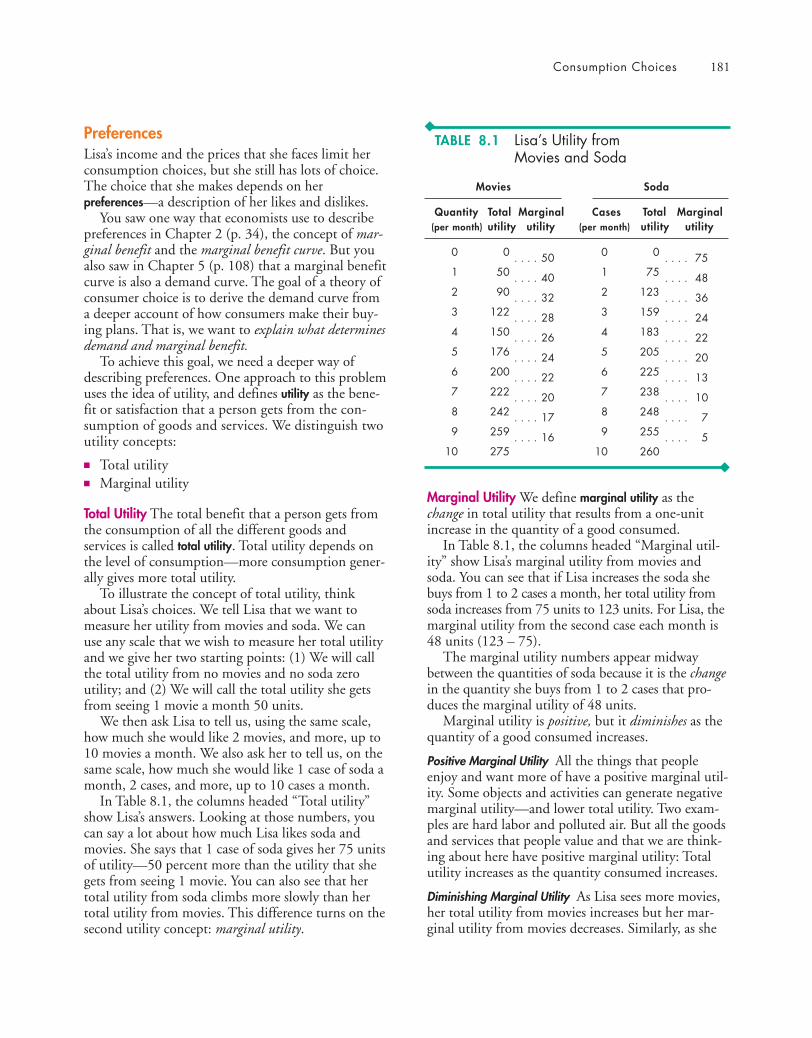
Consumption Choices 181

Movies Soda

Quantity Total Marginal Cases Total Marginal(per month) utility utility (per month) utility utility

PreferencesLisa’s income and the prices that she faces limit herconsumption choices, but she still has lots of choice.The choice that she makes depends on herpreferences—a description of her likes and dislikes.

You saw one way that economists use to describepreferences in Chapter 2 (p. 34), the concept of mar-ginal benefit and the marginal benefit curve. But youalso saw in Chapter 5 (p. 108) that a marginal benefitcurve is also a demand curve. The goal of a theory ofconsumer choice is to derive the demand curve froma deeper account of how consumers make their buy-ing plans. That is, we want to explain what determinesdemand and marginal benefit.

To achieve this goal, we need a deeper way ofdescribing preferences. One approach to this problemuses the idea of utility, and defines utility as the bene-fit or satisfaction that a person gets from the con-sumption of goods and services. We distinguish twoutility concepts:

■ Total utility■ Marginal utility

Total Utility The total benefit that a person gets fromthe consumption of all the different goods andservices is called total utility. Total utility depends onthe level of consumption—more consumption gener-ally gives more total utility.

To illustrate the concept of total utility, thinkabout Lisa’s choices. We tell Lisa that we want tomeasure her utility from movies and soda. We canuse any scale that we wish to measure her total utilityand we give her two starting points: (1) We will callthe total utility from no movies and no soda zeroutility; and (2) We will call the total utility she getsfrom seeing 1 movie a month 50 units.

We then ask Lisa to tell us, using the same scale,how much she would like 2 movies, and more, up to10 movies a month. We also ask her to tell us, on thesame scale, how much she would like 1 case of soda amonth, 2 cases, and more, up to 10 cases a month.

In Table 8.1, the columns headed “Total utility”show Lisa’s answers. Looking at those numbers, youcan say a lot about how much Lisa likes soda andmovies. She says that 1 case of soda gives her 75 unitsof utility—50 percent more than the utility that shegets from seeing 1 movie. You can also see that hertotal utility from soda climbs more slowly than hertotal utility from movies. This difference turns on thesecond utility concept: marginal utility.

Marginal Utility We define marginal utility as thechange in total utility that results from a one-unitincrease in the quantity of a good consumed.

In Table 8.1, the columns headed “Marginal util-ity” show Lisa’s marginal utility from movies andsoda. You can see that if Lisa increases the soda shebuys from 1 to 2 cases a month, her total utility fromsoda increases from 75 units to 123 units. For Lisa, themarginal utility from the second case each month is48 units (123 – 75).

The marginal utility numbers appear midwaybetween the quantities of soda because it is the changein the quantity she buys from 1 to 2 cases that pro-duces the marginal utility of 48 units.

Marginal utility is positive, but it diminishes as thequantity of a good consumed increases.

Positive Marginal Utility All the things that peopleenjoy and want more of have a positive marginal util-ity. Some objects and activities can generate negativemarginal utility—and lower total utility. Two exam-ples are hard labor and polluted air. But all the goodsand services that people value and that we are think-ing about here have positive marginal utility: Totalutility increases as the quantity consumed increases.

Diminishing Marginal Utility As Lisa sees more movies,her total utility from movies increases but her mar-ginal utility from movies decreases. Similarly, as she

0 0 . . . . 501 50 . . . . 402 90 . . . . 323 122 . . . . 284 150 . . . . 265 176 . . . . 246 200 . . . . 227 222 . . . . 208 242 . . . . 179 259 . . . . 16

10 275

0 0 . . . . 751 75 . . . . 482 123 . . . . 363 159 . . . . 244 183 . . . . 225 205 . . . . 206 225 . . . . 137 238 . . . . 108 248 . . . . 79 255 . . . . 5

10 260

TABLE 8.1 Lisa’s Utility from Movies and Soda

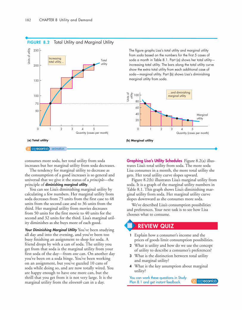
182 CHAPTER 8 Utility and Demand

The figure graphs Lisa’s total utility and marginal utilityfrom soda based on the numbers for the first 5 cases ofsoda a month in Table 8.1. Part (a) shows her total utility—increasing total utility. The bars along the total utility curveshow the extra total utility from each additional case ofsoda—marginal utility. Part (b) shows Lisa’s diminishingmarginal utility from soda.

consumes more soda, her total utility from sodaincreases but her marginal utility from soda decreases.

The tendency for marginal utility to decrease asthe consumption of a good increases is so general anduniversal that we give it the status of a principle—theprinciple of diminishing marginal utility.

You can see Lisa’s diminishing marginal utility bycalculating a few numbers. Her marginal utility fromsoda decreases from 75 units from the first case to 48units from the second case and to 36 units from thethird. Her marginal utility from movies decreasesfrom 50 units for the first movie to 40 units for thesecond and 32 units for the third. Lisa’s marginal util-ity diminishes as she buys more of each good.

Your Diminishing Marginal Utility You’ve been studyingall day and into the evening, and you’ve been toobusy finishing an assignment to shop for soda. Afriend drops by with a can of soda. The utility youget from that soda is the marginal utility from yourfirst soda of the day—from one can. On another dayyou’ve been on a soda binge. You’ve been workingon an assignment, but you’ve guzzled 10 cans ofsoda while doing so, and are now totally wired. Youare happy enough to have one more can, but thethrill that you get from it is not very large. It is themarginal utility from the eleventh can in a day.

2 3 4 5

250

200

150

0 1 0 1 2 3 4 5

40

20

Uni

ts of

utili

tyQuantity (cases per month)

Marginalutility

(b) Marginal utility

Uni

ts of

util

ity

Quantity (cases per month)

Totalutility

(a) Total utility

…and diminishingmarginal utility

Increasingtotal utility…

60

80

100100

75

50

Graphing Lisa’s Utility Schedules Figure 8.2(a) illus-trates Lisa’s total utility from soda. The more sodaLisa consumes in a month, the more total utility shegets. Her total utility curve slopes upward.

Figure 8.2(b) illustrates Lisa’s marginal utility fromsoda. It is a graph of the marginal utility numbers inTable 8.1. This graph shows Lisa’s diminishing mar-ginal utility from soda. Her marginal utility curveslopes downward as she consumes more soda.

We’ve described Lisa’s consumption possibilitiesand preferences. Your next task is to see how Lisachooses what to consume.

FIGURE 8.2 Total Utility and Marginal Utility

REVIEW QUIZ1 Explain how a consumer’s income and the

prices of goods limit consumption possibilities.2 What is utility and how do we use the concept

of utility to describe a consumer’s preferences?3 What is the distinction between total utility

and marginal utility?4 What is the key assumption about marginal

utility?

You can work these questions in Study Plan 8.1 and get instant feedback.

animation

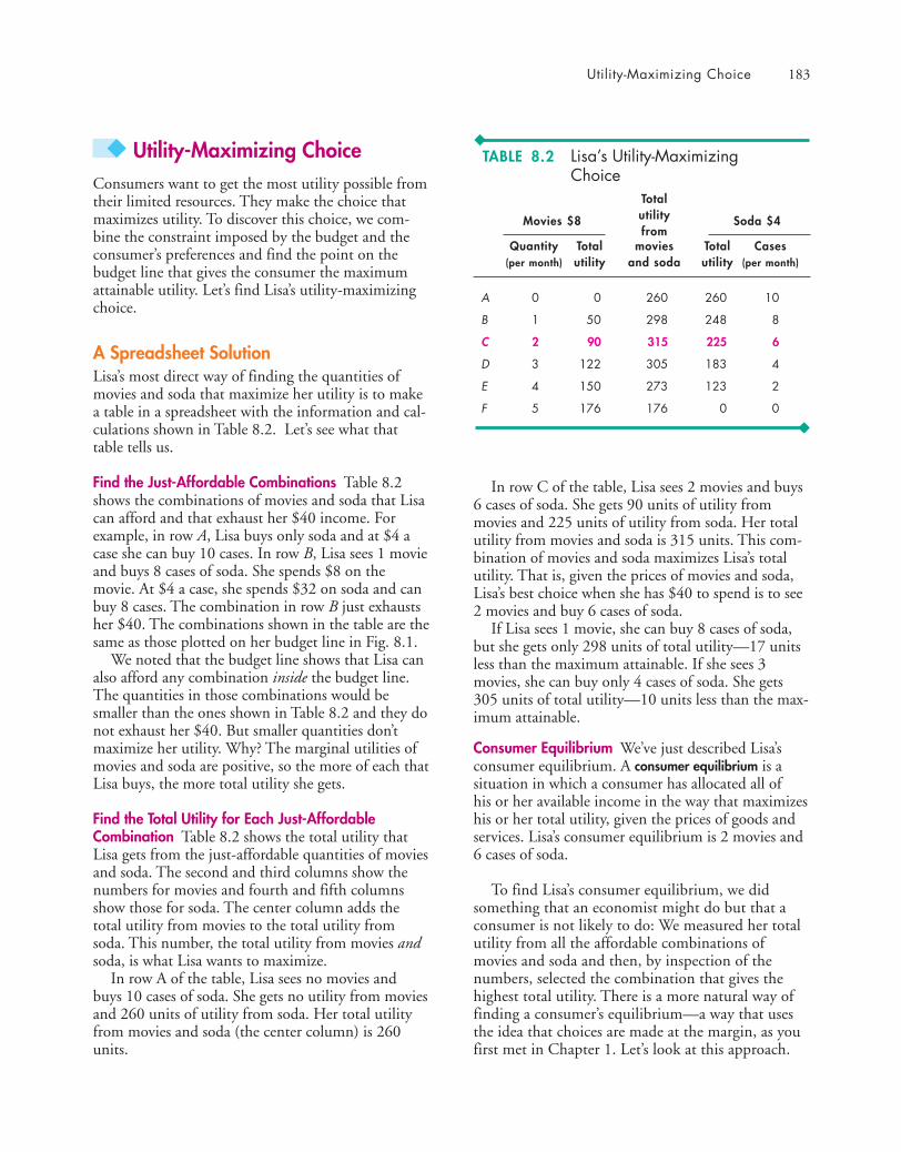
Utility-Maximizing Choice 183

◆ Utility-Maximizing ChoiceConsumers want to get the most utility possible fromtheir limited resources. They make the choice thatmaximizes utility. To discover this choice, we com-bine the constraint imposed by the budget and theconsumer’s preferences and find the point on thebudget line that gives the consumer the maximumattainable utility. Let’s find Lisa’s utility-maximizingchoice.

A Spreadsheet SolutionLisa’s most direct way of finding the quantities ofmovies and soda that maximize her utility is to makea table in a spreadsheet with the information and cal-culations shown in Table 8.2. Let’s see what thattable tells us.

Find the Just-Affordable Combinations Table 8.2shows the combinations of movies and soda that Lisacan afford and that exhaust her $40 income. Forexample, in row A, Lisa buys only soda and at $4 acase she can buy 10 cases. In row B, Lisa sees 1 movieand buys 8 cases of soda. She spends $8 on themovie. At $4 a case, she spends $32 on soda and canbuy 8 cases. The combination in row B just exhaustsher $40. The combinations shown in the table are thesame as those plotted on her budget line in Fig. 8.1.

We noted that the budget line shows that Lisa canalso afford any combination inside the budget line.The quantities in those combinations would besmaller than the ones shown in Table 8.2 and they donot exhaust her $40. But smaller quantities don’tmaximize her utility. Why? The marginal utilities ofmovies and soda are positive, so the more of each thatLisa buys, the more total utility she gets.

Find the Total Utility for Each Just-AffordableCombination Table 8.2 shows the total utility thatLisa gets from the just-affordable quantities of moviesand soda. The second and third columns show thenumbers for movies and fourth and fifth columnsshow those for soda. The center column adds thetotal utility from movies to the total utility fromsoda. This number, the total utility from movies andsoda, is what Lisa wants to maximize.

In row A of the table, Lisa sees no movies andbuys 10 cases of soda. She gets no utility from moviesand 260 units of utility from soda. Her total utilityfrom movies and soda (the center column) is 260units.

In row C of the table, Lisa sees 2 movies and buys6 cases of soda. She gets 90 units of utility frommovies and 225 units of utility from soda. Her totalutility from movies and soda is 315 units. This com-bination of movies and soda maximizes Lisa’s totalutility. That is, given the prices of movies and soda,Lisa’s best choice when she has $40 to spend is to see2 movies and buy 6 cases of soda.

If Lisa sees 1 movie, she can buy 8 cases of soda,but she gets only 298 units of total utility—17 unitsless than the maximum attainable. If she sees 3movies, she can buy only 4 cases of soda. She gets305 units of total utility—10 units less than the max-imum attainable.

Consumer Equilibrium We’ve just described Lisa’sconsumer equilibrium. A consumer equilibrium is asituation in which a consumer has allocated all of his or her available income in the way that maximizeshis or her total utility, given the prices of goods andservices. Lisa’s consumer equilibrium is 2 movies and6 cases of soda.

To find Lisa’s consumer equilibrium, we didsomething that an economist might do but that aconsumer is not likely to do: We measured her totalutility from all the affordable combinations ofmovies and soda and then, by inspection of thenumbers, selected the combination that gives thehighest total utility. There is a more natural way offinding a consumer’s equilibrium—a way that usesthe idea that choices are made at the margin, as youfirst met in Chapter 1. Let’s look at this approach.

TABLE 8.2 Lisa’s Utility-MaximizingChoice

TotalutilityMovies $8from

Soda $4

Quantity Total movies Total Cases(per month) utility and soda utility (per month)

A 0 0 260 260 10

B 1 50 298 248 8

C 2 90 315 225 6

D 3 122 305 183 4

E 4 150 273 123 2

F 5 176 176 0 0

184 CHAPTER 8 Utility and Demand

Choosing at the MarginWhen you go shopping you don’t do utility calcula-tions. But you do decide how to allocate your budget,and you do so in a way that you think is best for you.If you could make yourself better off by spending afew more dollars on an extra unit of one item and thesame number of dollars less on something else, youwould make that change. So, when you’ve allocatedyour budget in the best possible way, you can’t makeyourself better off by spending more on one item andless on others.

Marginal Utility per Dollar Economists interpretyour best possible choice by using the idea of mar-ginal utility per dollar. Marginal utility is the increasein total utility that results from consuming one moreunit of a good. Marginal utility per dollar is the mar-ginal utility from a good that results from spendingone more dollar on it.

The distinction between these two marginal con-cepts is clearest for a good that is infinitely divisible,such as gasoline. You can buy gasoline by the smallestfraction of a gallon and literally choose to spend onemore or one less dollar at the pump. The increase intotal utility that results from spending one more dol-lar at the pump is the marginal utility per dollar fromgasoline. When you buy a movie ticket or a case ofsoda, you must spend your dollars in bigger lumps.To buy our marginal movie ticket or case of soda, youmust spend the price of one unit and your total util-ity increases by the marginal utility from that item.So to calculate the marginal utility per dollar formovies (or soda), we must divide marginal utilityfrom the good by its price.

Call the marginal utility from movies MUM andthe price of a movie PM. Then the marginal utility perdollar from movies is

MUM/PM.

Call the marginal utility from soda MUS and theprice of a case of soda PS. Then the marginal utilityper dollar from soda is

MUS/PS.

By comparing the marginal utility per dollar fromall the goods that a person buys, we can determinewhether the budget has been allocated in the waythat maximizes total utility.

Let’s see how we use the marginal utility per dollarto define a utility-maximizing rule.

Utility-Maximizing Rule A consumer’s total utility ismaximized by following the rule:

■ Spend all the available income■ Equalize the marginal utility per dollar for all

goods

Spend All the Available Income Because more consump-tion brings more utility, only those choices thatexhaust income can maximize utility. For Lisa, com-binations of movies and soda that leave her withmoney to spend don’t give her as much total utility asthose that exhaust her $40 per month income.

Equalize the Marginal Utility per Dollar The basic ideabehind this rule is to move dollars from good A togood B if doing so increases the utility from good Aby more than it decreases the utility from good B.Such a utility-increasing move is possible if the mar-ginal utility per dollar from good A exceeds thatfrom good B.

But buying more of good A decreases its marginalutility. And buying less of good B increases its mar-ginal utility. So by moving dollars from good A togood B, total utility rises, but the gap between themarginal utilities per dollar gets smaller.

As long as the gap exists—as long as the marginalutility per dollar from good A exceeds that from goodB—total utility can be increased by spending moreon A and less on B. But when enough dollars havebeen moved from B to A to make the two marginalutilities per dollar equal, total utility cannot beincreased further. Total utility is maximized.

Lisa’s Marginal Calculation Let’s apply the basicidea to Lisa. To calculate Lisa’s marginal utility perdollar, we divide her marginal utility numbers foreach quantity of each good by the price of thegood. The table in Fig. 8.3 shows these calculationsfor Lisa, and the graph illustrates the situation onLisa’s budget line. The rows of the table are three ofher affordable combinations of movies and soda.

Too Much Soda and Too Few Movies In row B, Lisa sees1 movie a month and consumes 8 cases of soda amonth. Her marginal utility from seeing 1 movie amonth is 50 units. Because the price of a movie is $8,Lisa’s marginal utility per dollar from movies is 50units divided by $8, or 6.25 units of utility per dollar.

Lisa’s marginal utility from soda when she con-sumes 8 cases of soda a month is 10 units. Becausethe price of soda is $4 a case, Lisa’s marginal utility

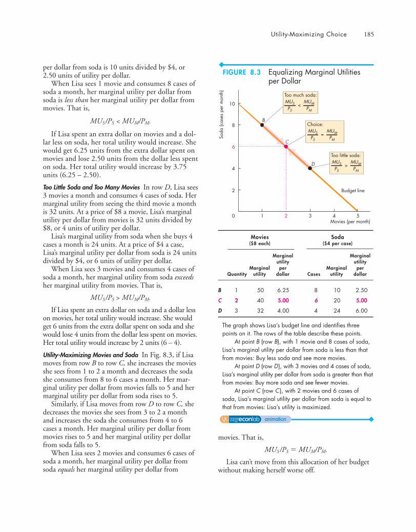
Utility-Maximizing Choice 185

Soda

(cas

es p

er m

onth

)

10

8

6

4

2

0 1 2 3 4 5Movies (per month)

B

C

D

Too much soda:

<MUSPS

MUMPM

Too little soda:

>MUSPS

MUMPM

Choice:

=MUSPS

MUMPM

Budget line

per dollar from soda is 10 units divided by $4, or2.50 units of utility per dollar.

When Lisa sees 1 movie and consumes 8 cases ofsoda a month, her marginal utility per dollar fromsoda is less than her marginal utility per dollar frommovies. That is,

MUS /PS < MUM/PM.

If Lisa spent an extra dollar on movies and a dol-lar less on soda, her total utility would increase. Shewould get 6.25 units from the extra dollar spent onmovies and lose 2.50 units from the dollar less spenton soda. Her total utility would increase by 3.75units (6.25 – 2.50).

Too Little Soda and Too Many Movies In row D, Lisa sees3 movies a month and consumes 4 cases of soda. Hermarginal utility from seeing the third movie a monthis 32 units. At a price of $8 a movie, Lisa’s marginalutility per dollar from movies is 32 units divided by$8, or 4 units of utility per dollar.

Lisa’s marginal utility from soda when she buys 4cases a month is 24 units. At a price of $4 a case,Lisa’s marginal utility per dollar from soda is 24 unitsdivided by $4, or 6 units of utility per dollar.

When Lisa sees 3 movies and consumes 4 cases ofsoda a month, her marginal utility from soda exceedsher marginal utility from movies. That is,

MUS /PS > MUM/PM.

If Lisa spent an extra dollar on soda and a dollar lesson movies, her total utility would increase. She wouldget 6 units from the extra dollar spent on soda and shewould lose 4 units from the dollar less spent on movies.Her total utility would increase by 2 units (6 – 4).

Utility-Maximizing Movies and Soda In Fig. 8.3, if Lisamoves from row B to row C, she increases the moviesshe sees from 1 to 2 a month and decreases the sodashe consumes from 8 to 6 cases a month. Her mar-ginal utility per dollar from movies falls to 5 and hermarginal utility per dollar from soda rises to 5.

Similarly, if Lisa moves from row D to row C, shedecreases the movies she sees from 3 to 2 a monthand increases the soda she consumes from 4 to 6cases a month. Her marginal utility per dollar frommovies rises to 5 and her marginal utility per dollarfrom soda falls to 5.

When Lisa sees 2 movies and consumes 6 cases ofsoda a month, her marginal utility per dollar fromsoda equals her marginal utility per dollar from

Movies Soda ($8 each) ($4 per case)

Marginal Marginalutility utility

Marginal per Marginal perQuantity utility dollar Cases utility dollar

B 1 50 6.25 8 10 2.50

C 2 40 5.00 6 20 5.00

D 3 32 4.00 4 24 6.00

The graph shows Lisa’s budget line and identifies threepoints on it. The rows of the table describe these points.

At point B (row B), with 1 movie and 8 cases of soda,Lisa’s marginal utility per dollar from soda is less than thatfrom movies: Buy less soda and see more movies.

At point D (row D), with 3 movies and 4 cases of soda,Lisa’s marginal utility per dollar from soda is greater than thatfrom movies: Buy more soda and see fewer movies.

At point C (row C), with 2 movies and 6 cases ofsoda, Lisa’s marginal utility per dollar from soda is equal tothat from movies: Lisa’s utility is maximized.

movies. That is,

MUS /PS � MUM/PM.

Lisa can’t move from this allocation of her budgetwithout making herself worse off.

FIGURE 8.3 Equalizing Marginal Utilities per Dollar

animation

186 CHAPTER 8 Utility and Demand

Multiply both sides of this equation by the price ofsoda, PS, to obtain

MUS � MUM � (PS/PM).

This equation says that the marginal utility fromsoda, MUS, is equal to the marginal utility frommovies, MUM, multiplied by the ratio of the price ofsoda, PS, to the price of a movie, PM.

The ratio PS /PM is the relative price of soda interms of movies: It is the number of movies that mustbe forgone to get 1 case of soda. It is also the oppor-tunity cost of soda. (See Chapter 2, p. 31 andChapter 3, p. 56.)

For Lisa, when PM = $8 and PS = $4 we observethat in a month she goes to the movies twice andbuys 6 cases of soda. So we know that her MUS from6 cases of soda equals her MUM from 2 movies multi-plied by $4/$8 or 0.5. That is, for Lisa, the marginalutility from 6 cases of soda equals one-half of themarginal utility from 2 movies.

If we observe the choices that Lisa makes at moreprices, we can find more rows in her utility schedule.By her choices, Lisa reveals her preferences.

Units of Utility Don’t Matter Lisa’s marginal utilityfrom 2 movies is a half of her marginal utility from 6cases of soda. So if the marginal utility from the sec-ond movie is 40 units, then the marginal utility fromthe sixth case of soda is 20 units. But if we call themarginal utility from the second movie 50 units,then the marginal utility from the sixth case of soda is25 units. The units of utility are arbitrary.

The Power of Marginal AnalysisThe method we’ve just used to find Lisa’s utility-maxi-mizing choice of movies and soda is an example of thepower of marginal analysis. Lisa doesn’t need a com-puter and a spreadsheet program to maximize utility.She can achieve this goal by comparing the marginalgain from having more of one good with the marginalloss from having less of another good.

The rule that she follows is simple: If the marginalutility per dollar from movies exceeds the marginalutility per dollar from soda, see more movies and buyless soda; if the marginal utility per dollar from sodaexceeds the marginal utility per dollar from movies,buy more soda and see fewer movies.

More generally, if the marginal gain from anaction exceeds the marginal loss, take the action. Youwill meet this principle time and again in your studyof economics, and you will find yourself using itwhen you make your own economic choices, espe-cially when you must make big decisions.

Revealing PreferencesWhen we introduced the idea of utility, we arbitrarilychose 50 units as Lisa’s total utility from 1 movie, andwe pretended that we asked Lisa to tell us how manyunits of utility she got from different quantities ofsoda and movies.

You’re now about to discover that we don’t need toask Lisa to tell us her preferences. We can figure themout for ourselves by observing what she buys atvarious prices.

Also, the units in which we measure Lisa’s prefer-ences don’t matter. Any arbitrary units will work. Inthis respect, utility is like temperature. Predictionsabout the freezing point of water don’t depend onthe temperature scale; and predictions about ahousehold’s consumption choice don’t depend onthe units of utility.

Lisa’s Preferences In maximizing total utility bymaking the marginal utility per dollar equal for allgoods, the units in which utility is measured do notmatter.

You’ve seen that when Lisa maximizes her totalutility, her marginal utility per dollar from soda,MUS /PS, equals her marginal utility per dollar frommovies, MUM/PM. That is,

MUS /PS � MUM/PM.You now understand the marginal utility theory of

consumer choices. Your next task is to see what thetheory predicts.

REVIEW QUIZ1 Why does a consumer spend the entire budget?2 What is the marginal utility per dollar and how

is it calculated?3 What two conditions are met when a consumer

is maximizing utility?4 Explain why equalizing the marginal utility per

dollar for all goods maximizes utility.

You can work these questions in Study Plan 8.2 and get instant feedback.

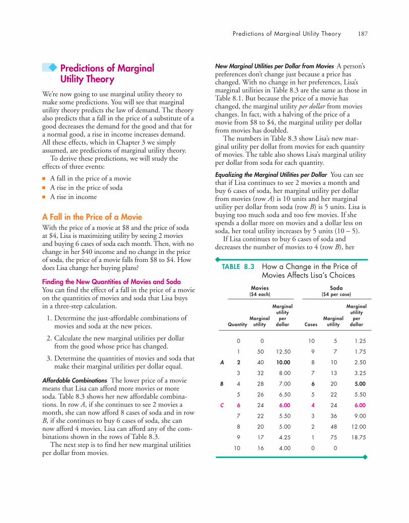
Predictions of Marginal Utility Theory 187

◆ Predictions of MarginalUtility Theory

We’re now going to use marginal utility theory tomake some predictions. You will see that marginalutility theory predicts the law of demand. The theoryalso predicts that a fall in the price of a substitute of agood decreases the demand for the good and that fora normal good, a rise in income increases demand.All these effects, which in Chapter 3 we simplyassumed, are predictions of marginal utility theory.

To derive these predictions, we will study theeffects of three events:

■ A fall in the price of a movie■ A rise in the price of soda■ A rise in income

A Fall in the Price of a MovieWith the price of a movie at $8 and the price of sodaat $4, Lisa is maximizing utility by seeing 2 moviesand buying 6 cases of soda each month. Then, with nochange in her $40 income and no change in the priceof soda, the price of a movie falls from $8 to $4. Howdoes Lisa change her buying plans?

Finding the New Quantities of Movies and SodaYou can find the effect of a fall in the price of a movieon the quantities of movies and soda that Lisa buysin a three-step calculation.

1. Determine the just-affordable combinations ofmovies and soda at the new prices.

2. Calculate the new marginal utilities per dollarfrom the good whose price has changed.

3. Determine the quantities of movies and soda thatmake their marginal utilities per dollar equal.

Affordable Combinations The lower price of a moviemeans that Lisa can afford more movies or moresoda. Table 8.3 shows her new affordable combina-tions. In row A, if she continues to see 2 movies amonth, she can now afford 8 cases of soda and in rowB, if she continues to buy 6 cases of soda, she cannow afford 4 movies. Lisa can afford any of the com-binations shown in the rows of Table 8.3.

The next step is to find her new marginal utilitiesper dollar from movies.

New Marginal Utilities per Dollar from Movies A person’spreferences don’t change just because a price haschanged. With no change in her preferences, Lisa’smarginal utilities in Table 8.3 are the same as those inTable 8.1. But because the price of a movie haschanged, the marginal utility per dollar from movieschanges. In fact, with a halving of the price of amovie from $8 to $4, the marginal utility per dollarfrom movies has doubled.

The numbers in Table 8.3 show Lisa’s new mar-ginal utility per dollar from movies for each quantityof movies. The table also shows Lisa’s marginal utilityper dollar from soda for each quantity.

Equalizing the Marginal Utilities per Dollar You can seethat if Lisa continues to see 2 movies a month andbuy 6 cases of soda, her marginal utility per dollarfrom movies (row A) is 10 units and her marginalutility per dollar from soda (row B) is 5 units. Lisa isbuying too much soda and too few movies. If shespends a dollar more on movies and a dollar less onsoda, her total utility increases by 5 units (10 – 5).

If Lisa continues to buy 6 cases of soda anddecreases the number of movies to 4 (row B), her

Movies Soda ($4 each) ($4 per case)

Marginal Marginalutility utility

Marginal per Marginal perQuantity utility dollar Cases utility dollar

0 0 10 5 1.25

1 50 12.50 9 7 1.75

A 2 40 10.00 8 10 2.50

3 32 8.00 7 13 3.25

B 4 28 7.00 6 20 5.00

5 26 6.50 5 22 5.50

C 6 24 6.00 4 24 6.00

7 22 5.50 3 36 9.00

8 20 5.00 2 48 12.00

9 17 4.25 1 75 18.75

10 16 4.00 0 0

TABLE 8.3 How a Change in the Price of Movies Affects Lisa’s Choices

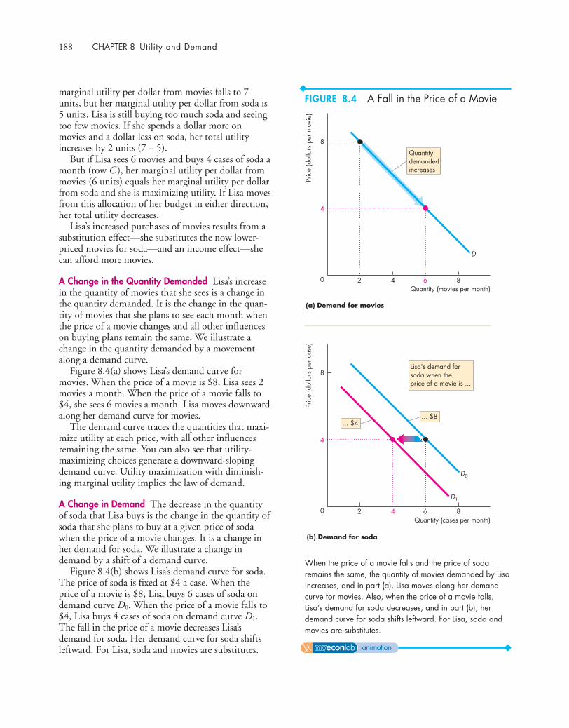
188 CHAPTER 8 Utility and Demand

marginal utility per dollar from movies falls to 7units, but her marginal utility per dollar from soda is5 units. Lisa is still buying too much soda and seeingtoo few movies. If she spends a dollar more onmovies and a dollar less on soda, her total utilityincreases by 2 units (7 – 5).

But if Lisa sees 6 movies and buys 4 cases of soda amonth (row C ), her marginal utility per dollar frommovies (6 units) equals her marginal utility per dollarfrom soda and she is maximizing utility. If Lisa movesfrom this allocation of her budget in either direction,her total utility decreases.

Lisa’s increased purchases of movies results from asubstitution effect—she substitutes the now lower-priced movies for soda—and an income effect—shecan afford more movies.

A Change in the Quantity Demanded Lisa’s increasein the quantity of movies that she sees is a change inthe quantity demanded. It is the change in the quan-tity of movies that she plans to see each month whenthe price of a movie changes and all other influenceson buying plans remain the same. We illustrate achange in the quantity demanded by a movementalong a demand curve.

Figure 8.4(a) shows Lisa’s demand curve formovies. When the price of a movie is $8, Lisa sees 2movies a month. When the price of a movie falls to$4, she sees 6 movies a month. Lisa moves downwardalong her demand curve for movies.

The demand curve traces the quantities that maxi-mize utility at each price, with all other influencesremaining the same. You can also see that utility-maximizing choices generate a downward-slopingdemand curve. Utility maximization with diminish-ing marginal utility implies the law of demand.

A Change in Demand The decrease in the quantityof soda that Lisa buys is the change in the quantity ofsoda that she plans to buy at a given price of sodawhen the price of a movie changes. It is a change inher demand for soda. We illustrate a change indemand by a shift of a demand curve.

Figure 8.4(b) shows Lisa’s demand curve for soda.The price of soda is fixed at $4 a case. When theprice of a movie is $8, Lisa buys 6 cases of soda ondemand curve D0. When the price of a movie falls to$4, Lisa buys 4 cases of soda on demand curve D1.The fall in the price of a movie decreases Lisa’sdemand for soda. Her demand curve for soda shiftsleftward. For Lisa, soda and movies are substitutes.

2 4 8

Pric

e (d

olla

rs p

er m

ovie

)Pr

ice

(dol

lars

per

cas

e)

Quantity (movies per month)

8

4

0 6

(a) Demand for movies

D

D0

(b) Demand for soda

Lisa's demand forsoda when theprice of a movie is ...

... $4... $8

Quantitydemandedincreases

D1

2 4 8Quantity (cases per month)

8

4

0 6

When the price of a movie falls and the price of sodaremains the same, the quantity of movies demanded by Lisaincreases, and in part (a), Lisa moves along her demandcurve for movies. Also, when the price of a movie falls,Lisa’s demand for soda decreases, and in part (b), herdemand curve for soda shifts leftward. For Lisa, soda andmovies are substitutes.

FIGURE 8.4 A Fall in the Price of a Movie

animation

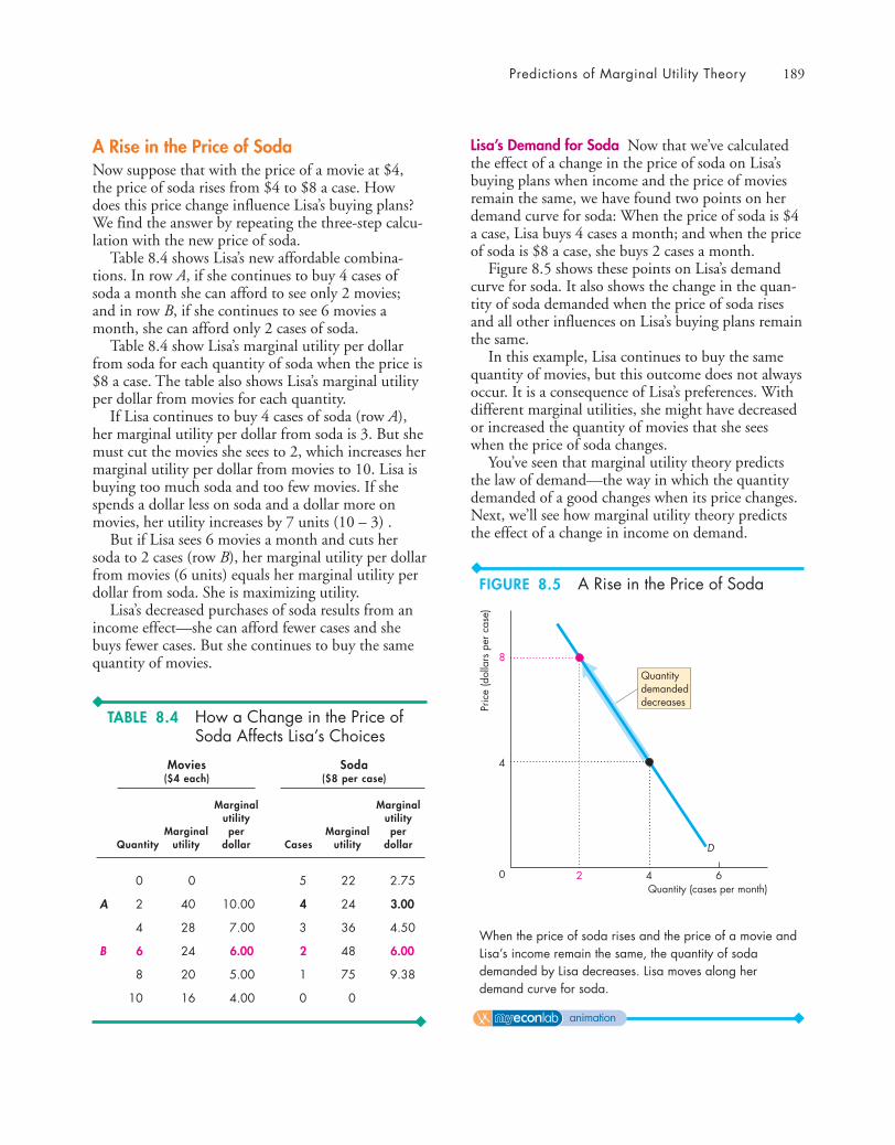
Predictions of Marginal Utility Theory 189

A Rise in the Price of Soda Now suppose that with the price of a movie at $4,the price of soda rises from $4 to $8 a case. Howdoes this price change influence Lisa’s buying plans?We find the answer by repeating the three-step calcu-lation with the new price of soda.

Table 8.4 shows Lisa’s new affordable combina-tions. In row A, if she continues to buy 4 cases ofsoda a month she can afford to see only 2 movies;and in row B, if she continues to see 6 movies amonth, she can afford only 2 cases of soda.

Table 8.4 show Lisa’s marginal utility per dollarfrom soda for each quantity of soda when the price is$8 a case. The table also shows Lisa’s marginal utilityper dollar from movies for each quantity.

If Lisa continues to buy 4 cases of soda (row A),her marginal utility per dollar from soda is 3. But shemust cut the movies she sees to 2, which increases hermarginal utility per dollar from movies to 10. Lisa isbuying too much soda and too few movies. If shespends a dollar less on soda and a dollar more onmovies, her utility increases by 7 units (10 – 3) .

But if Lisa sees 6 movies a month and cuts hersoda to 2 cases (row B), her marginal utility per dollarfrom movies (6 units) equals her marginal utility perdollar from soda. She is maximizing utility.

Lisa’s decreased purchases of soda results from anincome effect—she can afford fewer cases and shebuys fewer cases. But she continues to buy the samequantity of movies.

2 4

Pric

e (d

olla

rs p

er c

ase)

Quantity (cases per month)

8

4

0 6

D

Quantitydemandeddecreases

When the price of soda rises and the price of a movie andLisa’s income remain the same, the quantity of sodademanded by Lisa decreases. Lisa moves along herdemand curve for soda.

Lisa’s Demand for Soda Now that we’ve calculatedthe effect of a change in the price of soda on Lisa’sbuying plans when income and the price of moviesremain the same, we have found two points on herdemand curve for soda: When the price of soda is $4a case, Lisa buys 4 cases a month; and when the priceof soda is $8 a case, she buys 2 cases a month.

Figure 8.5 shows these points on Lisa’s demandcurve for soda. It also shows the change in the quan-tity of soda demanded when the price of soda risesand all other influences on Lisa’s buying plans remainthe same.

In this example, Lisa continues to buy the samequantity of movies, but this outcome does not alwaysoccur. It is a consequence of Lisa’s preferences. Withdifferent marginal utilities, she might have decreasedor increased the quantity of movies that she seeswhen the price of soda changes.

You’ve seen that marginal utility theory predictsthe law of demand—the way in which the quantitydemanded of a good changes when its price changes.Next, we’ll see how marginal utility theory predictsthe effect of a change in income on demand.

Movies Soda ($4 each) ($8 per case)

Marginal Marginalutility utility

Marginal per Marginal perQuantity utility dollar Cases utility dollar

0 0 5 22 2.75

A 2 40 10.00 4 24 3.00

4 28 7.00 3 36 4.50

B 6 24 6.00 2 48 6.00

8 20 5.00 1 75 9.38

10 16 4.00 0 0

FIGURE 8.5 A Rise in the Price of Soda

TABLE 8.4 How a Change in the Price of Soda Affects Lisa’s Choices

animation

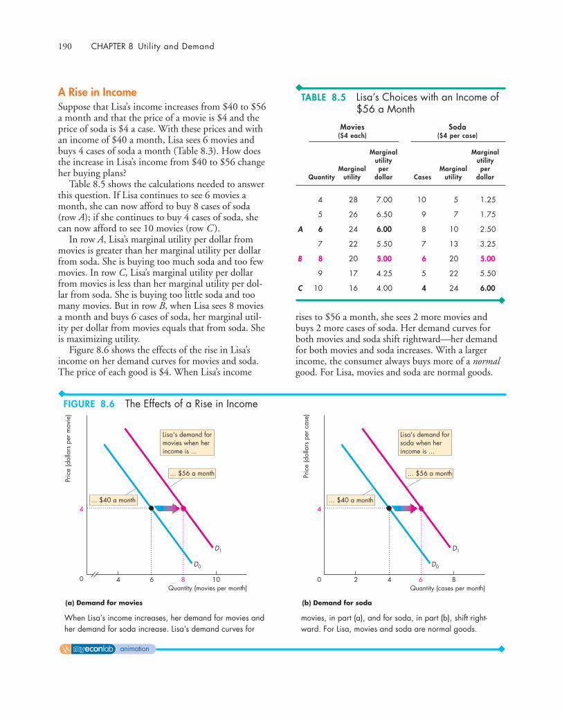
190 CHAPTER 8 Utility and Demand

rises to $56 a month, she sees 2 more movies andbuys 2 more cases of soda. Her demand curves forboth movies and soda shift rightward—her demandfor both movies and soda increases. With a largerincome, the consumer always buys more of a normalgood. For Lisa, movies and soda are normal goods.

A Rise in IncomeSuppose that Lisa’s income increases from $40 to $56a month and that the price of a movie is $4 and theprice of soda is $4 a case. With these prices and withan income of $40 a month, Lisa sees 6 movies andbuys 4 cases of soda a month (Table 8.3). How doesthe increase in Lisa’s income from $40 to $56 changeher buying plans?

Table 8.5 shows the calculations needed to answerthis question. If Lisa continues to see 6 movies amonth, she can now afford to buy 8 cases of soda(row A); if she continues to buy 4 cases of soda, shecan now afford to see 10 movies (row C ).

In row A, Lisa’s marginal utility per dollar frommovies is greater than her marginal utility per dollarfrom soda. She is buying too much soda and too fewmovies. In row C, Lisa’s marginal utility per dollarfrom movies is less than her marginal utility per dol-lar from soda. She is buying too little soda and toomany movies. But in row B, when Lisa sees 8 moviesa month and buys 6 cases of soda, her marginal util-ity per dollar from movies equals that from soda. Sheis maximizing utility.

Figure 8.6 shows the effects of the rise in Lisa’sincome on her demand curves for movies and soda.The price of each good is $4. When Lisa’s income

Movies Soda ($4 each) ($4 per case)

Marginal Marginalutility utility

Marginal per Marginal perQuantity utility dollar Cases utility dollar

4 28 7.00 10 5 1.25

5 26 6.50 9 7 1.75

A 6 24 6.00 8 10 2.50

7 22 5.50 7 13 3.25

B 8 20 5.00 6 20 5.00

9 17 4.25 5 22 5.50

C 10 16 4.00 4 24 6.00

... $40 a month

... $56 a month

4 8 10

Pric

e (d

olla

rs p

er m

ovie

)

Pric

e (d

olla

rs p

er c

ase)

Quantity (movies per month)

4

0 6

(b) Demand for soda(a) Demand for movies

Lisa's demand formovies when herincome is ...

Quantity (cases per month)

D0

D1

... $40 a month

... $56 a month

2 6 8

4

0 4

Lisa's demand forsoda when herincome is ...

D0

D1

When Lisa’s income increases, her demand for movies andher demand for soda increase. Lisa’s demand curves for

movies, in part (a), and for soda, in part (b), shift right-ward. For Lisa, movies and soda are normal goods.

TABLE 8.5 Lisa’s Choices with an Income of$56 a Month

FIGURE 8.6 The Effects of a Rise in Income

animation

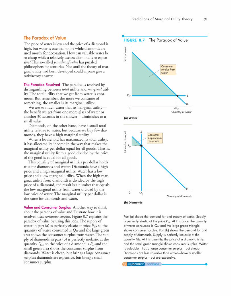
Predictions of Marginal Utility Theory 191

The Paradox of ValueThe price of water is low and the price of a diamond ishigh, but water is essential to life while diamonds areused mostly for decoration. How can valuable water beso cheap while a relatively useless diamond is so expen-sive? This so-called paradox of value has puzzledphilosophers for centuries. Not until the theory of mar-ginal utility had been developed could anyone give asatisfactory answer.

The Paradox Resolved The paradox is resolved bydistinguishing between total utility and marginal util-ity. The total utility that we get from water is enor-mous. But remember, the more we consume ofsomething, the smaller is its marginal utility.

We use so much water that its marginal utility—the benefit we get from one more glass of water oranother 30 seconds in the shower—diminishes to asmall value.

Diamonds, on the other hand, have a small totalutility relative to water, but because we buy few dia-monds, they have a high marginal utility.

When a household has maximized its total utility,it has allocated its income in the way that makes themarginal utility per dollar equal for all goods. That is,the marginal utility from a good divided by the priceof the good is equal for all goods.

This equality of marginal utilities per dollar holdstrue for diamonds and water: Diamonds have a highprice and a high marginal utility. Water has a lowprice and a low marginal utility. When the high mar-ginal utility from diamonds is divided by the highprice of a diamond, the result is a number that equalsthe low marginal utility from water divided by thelow price of water. The marginal utility per dollar isthe same for diamonds and water.

Value and Consumer Surplus Another way to thinkabout the paradox of value and illustrate how it isresolved uses consumer surplus. Figure 8.7 explains theparadox of value by using this idea. The supply ofwater in part (a) is perfectly elastic at price PW, so thequantity of water consumed is QW and the large greenarea shows the consumer surplus from water. The sup-ply of diamonds in part (b) is perfectly inelastic at thequantity QD, so the price of a diamond is PD and thesmall green area shows the consumer surplus fromdiamonds. Water is cheap, but brings a large consumersurplus; diamonds are expensive, but bring a smallconsumer surplus.

Pric

e of

wat

er

Quantity of water

PW

QW

S

D0

(a) Water

Pric

e of

a d

iam

ond

Quantity of diamonds

PD

QD

S

D0

(b) Diamonds

Consumersurplus fromwater

Consumersurplus fromdiamonds

Part (a) shows the demand for and supply of water. Supplyis perfectly elastic at the price PW. At this price, the quantityof water consumed is QW and the large green triangleshows consumer surplus. Part (b) shows the demand for andsupply of diamonds. Supply is perfectly inelastic at thequantity QD. At this quantity, the price of a diamond is PD

and the small green triangle shows consumer surplus. Wateris valuable—has a large consumer surplus—but cheap.Diamonds are less valuable than water—have a smallerconsumer surplus—but are expensive.

FIGURE 8.7 The Paradox of Value

animation

192 CHAPTER 8 Utility and Demand

Economics in ActionMaximizing Utility from Recorded MusicIn 2007, Americans spent $10 billion on recordedmusic, down from $14 billion in 2000. But the com-bined quantity of discs and downloads boughtincreased from 1 billion in 2000 to 1.8 billion in2007 and the average price of a unit of recordedmusic fell from $14 to $5.50.

The average price fell because the mix of formatsbought changed dramatically. In 2000, we bought940 million CDs; in 2007, we bought only 500million CDs and downloaded 1.2 billion music files.

Figure 1 shows the longer history of the changingformats of recorded music.

The music that we buy isn’t just one good—it isseveral goods. Singles and albums are different goods;downloads and discs are different goods; and down-loads to a computer and downloads to a cell phoneare different goods. There are five major categoriesand the table shows the quantities of each that webought in 2007 (excluding DVDs and cassettes).

Singles AlbumsFormat (millions in 2007)

Disc 3 500Download 800 40Mobile 400 –

Source of data: Recording Industry Association of America.

Most people buy all their music in digital form,but many still buy physical CDs and some peoplebuy both downloads and CDs.

We get utility from the singles and albums that webuy, and the more songs and albums we have, themore utility we get. But our marginal utility fromsongs and albums decreases as the quantity that weown increases.

We also get utility from convenience. A song thatwe can buy with a mouse click and play with the spinof a wheel is more convenient both to buy and to usethan a song on a CD. The convenience of songsdownloaded over the Internet means that, song forsong, we get more utility from a song downloadedthan we get from a song on a physical CD.

But most albums are still played at home on a CDplayer. So for most people, a physical CD is a moreconvenient medium for delivering an album. Albumfor album, people on average get more utility from aCD than from a download.

Temperature: An AnalogyUtility is similar to temperature—both are abstractconcepts. You can’t observe temperature. You canobserve water turning to steam if it is hot enough orturning to ice if it is cold enough. You can also con-struct an instrument—a thermometer—that can helpyou to predict when such changes will occur. We callthe scale on the thermometer temperature and we callthe units of temperature degrees. But like the units ofutility, these degree units are arbitrary. We can useCelsius units or Fahrenheit units or some other units.

The concept of utility helps us to make predic-tions about consumption choices in much the sameway that the concept of temperature helps us to makepredictions about physical phenomena.

Admittedly, marginal utility theory does notenable us to predict how buying plans change withthe same precision that a thermometer enables us topredict when water will turn to ice or steam. But thetheory provides important insights into buying plansand has some powerful implications. It helps us tounderstand why people buy more of a good or servicewhen its price falls and why people buy more of mostgoods when their incomes increase. It also resolvesthe paradox of value.

We’re going to end this chapter by looking at somenew ways of studying individual economic choicesand consumer behavior.

REVIEW QUIZ1 When the price of a good falls and the prices of

other goods and a consumer’s income remainthe same, explain what happens to the con-sumption of the good whose price has fallenand to the consumption of other goods.

2 Elaborate on your answer to the previous ques-tion by using demand curves. For which gooddoes demand change and for which good doesthe quantity demanded change?

3 If a consumer’s income increases and if allgoods are normal goods, explain how the quan-tity bought of each good changes.

4 What is the paradox of value and how is theparadox resolved?

5 What are the similarities between utility andtemperature?

You can work these questions in Study Plan 8.3 and get instant feedback.

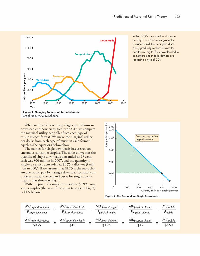
Predictions of Marginal Utility Theory 193

When we decide how many singles and albums todownload and how many to buy on CD, we comparethe marginal utility per dollar from each type ofmusic in each format. We make the marginal utilityper dollar from each type of music in each formatequal, as the equations below show.

The market for single downloads has created anenormous consumer surplus. The table shows that thequantity of single downloads demanded at 99 centseach was 800 million in 2007, and the quantity ofsingles on a disc demanded at $4.75 a disc was 3 mil-lion in 2007. If we assume that $4.75 is the most thatanyone would pay for a single download (probably anunderestimate), the demand curve for single down-loads is that shown in Fig. 2.

With the price of a single download at $0.99, con-sumer surplus (the area of the green triangle in Fig. 2)is $1.5 billion.

Year

Figure 1 Changing Formats of Recorded Music

CassettesVinyl discs

Compact discs

Downloads

Units

(mill

ions

per

yea

r)

0

200

400

600

1,200

2005200019951990198519801975 2010

800

1,000

600400200 800

Pric

e (d

olla

rs p

er s

ingl

e)

Quantity (millions of singles per year)

Figure 2 The Demand for Single Downloads

4.00

3.00

5.004.75

2.00

0.99

0 1,000

D

Consumer surplus fromsingle downloads

In the 1970s, recorded music cameon vinyl discs. Cassettes graduallyreplaced vinyl, then compact discs(CDs) gradually replaced cassettes,and today, digital files downloaded tocomputers and mobile devices arereplacing physical CDs.

Graph from www.swivel.com.

MUsingle downloads

Psingle downloads

MUsingle downloads

$0.99

MUalbum downloads

Palbum downloads

MUalbum downloads

$10=

=

=

=MUphysical singles

Pphysical singles

MUphysical singles

$4.75

MUphysical albums

Pphysical albums

MUphysical albums

$15 =

=

=

=MUmobile

Pmobile

MUmobile

$2.50

194 CHAPTER 8 Utility and Demand

◆ New Ways of ExplainingConsumer Choices

When William Stanley Jevons developed marginalutility theory in the 1860s, he would have loved tolook inside people’s brains and “see” their utility. Buthe believed that the human brain was the ultimateblack box that could never be observed directly. ForJevons, and for most economists today, the purposeof marginal utility theory is to explain our actions,not what goes on inside our brains.

Economics has developed over the past 150 yearswith little help from and paying little attention toadvances being made in psychology. Both economicsand psychology seek to explain human behavior, butthey have developed different ways of attacking thechallenge.

A few researchers have paid attention to the poten-tial payoff from exploring economic problems byusing the tools of psychology. These researchers, someeconomists and some psychologists, think that mar-ginal utility theory is based on a view of how peoplemake choices that attributes too much to reason andrationality. They propose an alternative approachbased on the methods of psychology.

Other researchers, some economists and someneuroscientists, are using new tools to look inside thehuman brain and open up Jevons’ “black box.”

This section provides a very brief introduction tothese new and exciting areas of economics. We’llexplore the two related research agendas:

■ Behavioral economics■ Neuroeconomics

Behavioral EconomicsBehavioral economics studies the ways in which limits on the human brain’s ability to compute andimplement rational decisions influences economicbehavior—both the decisions that people make andthe consequences of those decisions for the way mar-kets work.

Behavioral economics starts with observed behav-ior. It looks for anomalies—choices that do not seemto be rational. It then tries to account for the anom-alies by using ideas developed by psychologists thatemphasize features of the human brain that limitrational choice.

In behavioral economics, instead of being rationalutility maximizers, people are assumed to have threeimpediments that prevent rational choice: boundedrationality, bounded willpower, and bounded self-interest.

Bounded Rationality Bounded rationality is rational-ity that is limited by the computing power of thehuman brain. We can’t always work out the rationalchoice.

For Lisa, choosing between movies and soda, itseems unlikely that she would have much trouble fig-uring out what to buy. But toss Lisa some uncertaintyand the task becomes harder. She’s read the reviews of“Ironman 2” on Fandango, but does she really wantto see that movie? How much marginal utility will itgive her? Faced with uncertainty, people might userules of thumb, listen to the views of others, andmake decisions based on gut instinct rather than onrational calculation.

Bounded Willpower Bounded willpower is the less-than-perfect willpower that prevents us from makinga decision that we know, at the time of implementingthe decision, we will later regret.

Lisa might be feeling particularly thirsty when shepasses a soda vending machine. Under Lisa’s rationalutility-maximizing plan, she buys her soda at the dis-count store, where she gets it for the lowest possibleprice. Lisa has already bought her soda for thismonth, but it is at home. Spending $1 on a can nowmeans giving up a movie later this month.

Lisa’s rational choice is to ignore the temporarythirst and stick to her plan. But she might not possessthe willpower to do so—sometimes she will andsometimes she won’t.

Bounded Self-Interest Bounded self-interest is thelimited self-interest that results in sometimes sup-pressing our own interests to help others.

A hurricane hits the Florida coast and Lisa, feelingsorry for the victims, donates $10 to a fund-raiser.She now has only $30 to spend on movies and sodathis month. The quantities that she buys are not,according to her utility schedule, the ones that maxi-mize her utility.

The main applications of behavioral economics arein two areas: finance, where uncertainty is a key fac-tor in decision making, and savings, where the future

New Ways of Explaining Consumer Choices 195

is a key factor. But one behavior observed by behav-ioral economists is more general and might affectyour choices. It is called the endowment effect.

The Endowment Effect The endowment effect is thetendency for people to value something more highlysimply because they own it. If you have allocatedyour income to maximize utility, then the price youwould be willing to accept to give up something thatyou own (for example, your coffee mug) should bethe same as the price you are willing to pay for anidentical one.

In experiments, students seem to display theendowment effect: The price they are willing to payfor a coffee mug that is identical to the one they ownis less than the price they would be willing to acceptto give up the coffee mug that they own. Behavioraleconomists say that this behavior contradicts mar-ginal utility theory.

NeuroeconomicsNeuroeconomics is the study of the activity of thehuman brain when a person makes an economicdecision. The discipline uses the observational toolsand ideas of neuroscience to obtain a better under-standing of economic decisions.

Neuroeconomics is an experimental discipline. Inan experiment, a person makes an economic decisionand the electrical or chemical activity of the person’sbrain is observed and recorded using the same type ofequipment that neurosurgeons use to diagnose braindisorders.

The observations provide information aboutwhich regions of the brain are active at differentpoints in the process of making an economicdecision.

Observations show that some economic decisionsgenerate activity in the area of the brain (called theprefrontal cortex) where we store memories, analyzedata, and anticipate the consequences of ouractions. If people make rational utility-maximizingdecisions, it is in this region of the brain that thedecision occurs.

But observations also show that some economicdecisions generate activity in the region of the brain(called the hippocampus) where we store memories ofanxiety and fear. Decisions that are influenced byactivity in this part of the brain might not be rationaland be driven by fear or panic.

Neuroeconomists are also able to observe theamount of a brain hormone (called dopamine), thequantity of which increases in response to pleasurableevents and decreases in response to disappointingevents. These observations might one day enable neu-roeconomists to actually measure utility and shine abright light inside what was once believed to be theultimate black box.

ControversyThe new ways of studying consumer choice thatwe’ve briefly described here are being used morewidely to study business decisions and decisions infinancial markets, and this type of research is surelygoing to become more popular.

But behavioral economics and neuroeconomicsgenerate controversy. Most economists hold the viewof Jevons that the goal of economics is to explain thedecisions that we observe people making and not toexplain what goes on inside people’s heads.

Most economists would prefer to probe apparentanomalies more deeply and figure out why they arenot anomalies after all.

Economists also point to the power of marginal util-ity theory and its ability to explain consumer choiceand demand as well as resolve the paradox of value.

◆ You have now completed your study of the mar-ginal utility theory and some new ideas about howpeople make economic choices. You can see marginalutility theory in action once again in ReadingBetween the Lines on pp. 196–197, where it is usedto explain why paramedics who save people’s livesearn so much less than hockey players who merelyprovide entertainment.

REVIEW QUIZ1 Define behavioral economics.2 What are the three limitations on human ration-

ality that behavioral economics emphasizes?3 Define neuroeconomics.4 What do behavioral economics and neuroeco-

nomics seek to achieve?

You can work these questions in Study Plan 8.4 and get instant feedback.

196

READING BETWEEN THE L INES

Salaries, Strong Recruitment Ease Area Paramedic ShortageThe Washington PostApril 4, 2008

To curb a critical shortage, fire departments across the Washington region have pursued para-medics like star athletes in recent years, enticing them with signing bonuses, handsomesalaries and the promise of fast-track career paths.

Montgomery County hired a marketing expert and launched a national recruiting drive,reaching out in particular to women and minorities. Fairfax County offered top startingsalaries, now totaling about $57,000—as much as 50 percent higher than some other localjurisdictions, though Fairfax paramedics generally work longer hours. ...

Excerpted from “Salaries, Strong Recruitment Ease Area Paramedic Shortage” by William McCaffrey. The Washington Post, April 4, 2008.

Ducks Give Perry $26.6 Million DealThe Daily News of Los AngelesJuly 2, 2008

The Ducks’ first free-agent signing might also be their last, their biggest and their most expected.

Within the first hour of the NHL’s free agency period, Corey Perry signed a five-year, $26.625million contract that will keep the 23-year-old in Anaheim until 2013. Both parties had ex-pressed an interest in completing the deal for several months but it wasn’t possible until Tues-day, when the Ducks had enough room for long-term contracts under the salary cap.

“I really wanted to stay in Anaheim,” Perry said. “It’s home now and I didn’t want to leavehere. It’s a great place to play hockey and it just shows how well the organization is run.”

Including an $8 million signing bonus spread over its duration, the contract will pay Perry$4.5 million in 2008–09, then $6.5 million, $5.375million, $5.375 million, and $4.875 million, respec-tively, over the final four years. ...

Reprinted with permission from the San Bernadino Sun.■ In Washington, the starting salary for a para-

medic is $57,000 per year.

■ Corey Perry has a 5-year contract with the Ana-heim Ducks that will earn him $26.6 million.

ESSENCE OF THE STORIES

A Paradox of Value: Paramedics and Hockey Players

197

ECONOMIC ANALYSIS

Figure 2 The value of hockey players

Figure 1 The value of paramedicsW

age

rate

(tho

usan

ds o

f dol

lars

per

yea

r)

Quantity (thousands of paramedics)0

27

200100

50

SP

DP

Consumer surplus= $3 billion

40

10

20

Wag

e ra

te (m

illio

ns o

f dol

lars

per

yea

r)

Quantity (hockey players)0

4.0

750 1,500

8.0

6.0

SH

DH

Consumer surplus= $1.5 billion

2.0

57

■ If resources are used efficiently, the marginal utility perdollar from the services of a paramedic, MUP/PP, equalsthe marginal utility per dollar from the services of ahockey player, MUH/PH. That is,

■ A paramedic in Washington earns $57,000 a year,but the national average paramedic wage is $27,000a year.

■ Corey Perry earns $26.6 million over 5 years, or$5.32 million a year on average.

■ If we put these numbers into the above formula, we get

Equivalently,

■ Is the marginal utility from Corey Perry’s services really197 times that from the paramedic’s services?

■ The answer is no. A paramedic might serve about 8people a day, or perhaps 2,000 in a year; a hockeyplayer like Corey Perry serves millions of people ayear.

■ If a paramedic serves 2,000 people a year, then theprice of a paramedic’s service per customer served is$27,000/2,000, which equals $13.50.

■ If Corey Perry serves 1,000,000 people a year, thenthe price of Corey Perry’s service per customer servedis $5,320,000/1,000,000, which equals $5.32.

■ Using these prices of the services per customer, a para-medic is worth 2.5 times as much as a hockeyplayer—the marginal utility from the services of a para-medic is 2.5 times that from a hockey player.

■ Figure 1 shows the market for paramedics. The equilibri-um quantity is 200,000 workers, and the average wagerate is $27,000 a year.

■ Figure 2 shows the market for professional hockey play-ers. The equilibrium quantity is 750 players and the aver-age wage rate is $2,000,000 a year. (Corey Perryearns more than the average player.)

MUH

MUP= 197.

MUP

$27,000=

MUH

$5,320,000.

MUP

PP=

MUH

PH.

■ Not only is the marginal utility from a paramedicgreater than that from a hockey player, but paramedicsalso create a greater consumer surplus.

198 CHAPTER 8 Utility and Demand

higher the price of a good, the smaller is the quan-tity demanded of that good.

■ Marginal utility theory also predicts that, otherthings remaining the same, an increase in theconsumer’s income increases the demand for anormal good.

■ Marginal utility theory resolves the paradox ofvalue.

■ Total value is total utility or consumer surplus. Butprice is related to marginal utility.

■ Water, which we consume in large amounts, has ahigh total utility and a large consumer surplus, butthe price of water is low and the marginal utilityfrom water is low.

■ Diamonds, which we buy in small quantities, havea low total utility and a small consumer surplus,but the price of a diamond is high and the mar-ginal utility from diamonds is high.

Working Problems 12 to 21 will give you a better under-standing of the predictions of marginal utility theory.

New Ways of Explaining Consumer Choices (pp. 194–195)

■ Behavioral economics studies limits on the abilityof the human brain to compute and implementrational decisions.

■ Bounded rationality, bounded willpower, andbounded self-interest are believed to explain somechoices.

■ Neuroeconomics uses the ideas and tools of neuro-science to study the effects of economic events andchoices inside the human brain.

Working Problems 22 and 23 will give you a better under-standing of the new ways of explaining consumer choices.

Key Points

Consumption Choices (pp. 180–182)

■ A household’s consumption choices are deter-mined by its consumption possibilities and prefer-ences.

■ A budget line defines a household’s consumptionpossibilities.

■ A household’s preferences can be described by autility schedule that lists the total utility and mar-ginal utility derived from various quantities ofgoods and services consumed.

■ The principle of diminishing marginal utilityis that the marginal utility from a good or servicedecreases as consumption of the good or serviceincreases.

Working Problems 1 to 5 will give you a better under-standing of consumption choices.

Utility-Maximizing Choice (pp. 183–186)

■ A consumer’s objective is to maximize total utility.■ Total utility is maximized when all the available

income is spent and when the marginal utility perdollar from all goods is equal.

■ If the marginal utility per dollar for good Aexceeds that for good B, total utility increases ifthe quantity purchased of good A increases andthe quantity purchased of good B decreases.

Working Problems 6 to 11 will give you a better under-standing of a consumer’s utility-maximizing choice.

Predictions of Marginal Utility Theory (pp. 187–193)

■ Marginal utility theory predicts the law of demand.That is, other things remaining the same, the

SUMMARY

Key TermsBehavioral economics, 194Budget line, 180Consumer equilibrium, 183Diminishing marginal utility, 182

Marginal utility, 181Marginal utility per dollar, 184Neuroeconomics, 195Preferences, 181

Total utility, 181Utility, 181

Study Plan Problems and Applications 199

7. In your table in Problem 6, add two columns andlist Max’s marginal utility per dollar from wind-surfing and from snorkeling.

8. a. How many hours does Max windsurf and howmany hours does he snorkel to maximize hisutility?

b. If Max spent a dollar more on windsurfingand a dollar less on snorkeling than in part(a), by how much would his total utilitychange?

c. If Max spent a dollar less on windsurfing anda dollar more on snorkeling than in part (a),by how much would his total utility change?

9. Explain why, if Max equalized the marginalutility per hour from windsurfing and fromsnorkeling, he would not maximize his utility.

10. Schools Get a Lesson in Lunch Line EconomicsSharp rises in the cost of milk, grain, and freshfruits and vegetables are hitting cafeterias acrossthe country, forcing cash-strapped schools toraise prices or serve more economical dishes.For example, Fairfax schools serve oranges—14¢ each—instead of grapes, which are 25¢ aserving.

Source: The Washington Post, April 14, 2008

Assume that a Fairfax school has a $14 daily fruitbudget.a. How many oranges a day can the school

afford to serve if it serves no grapes? Howmany servings of grapes can the school affordeach day if it serves no oranges?

b. If the school provides 50 oranges a day andmaximizes utility, how many servings ofgrapes does it provide? If the marginal utilityfrom an orange is 14 units, what is the mar-ginal utility from a serving of grapes?

11. Can Money Buy Happiness?Whoever said money can’t buy happiness isn’tspending it right. There must be some connec-tion, but once your basic human needs are met,does more money buy more happiness? Anincrease in income from $20,000 a year to$50,000 makes you twice as likely to be happy,but the payoff from more than $90,000 is slight.

Source: CNN, July 18, 2006

Consumption Choices (Study Plan 8.1)

Jerry has $12 a week to spend on yogurt and maga-zines. The price of yogurt is $2, and the price of amagazine is $4.

1. List the combinations of yogurt and magazinesthat Jerry can afford. Draw a graph of Jerry’sbudget line with the quantity of magazines plottedon the x-axis.

2. Describe how Jerry’s consumption possibilitieschange if, other things remaining the same, (i) theprice of a magazine falls and (ii) Jerry’s incomeincreases.

Use the following data to work Problems 3 to 9.Max enjoys windsurfing and snorkeling. Max has $35 aday to spend, and he can spend as much time as helikes on his leisure pursuits. The price of renting equip-ment for windsurfing is $10 an hour and for snorkelingis $5 an hour. The table shows the total utility Max getsfrom each activity.

Total TotalHours utility from utility from

per day windsurfing snorkeling

1 120 402 220 763 300 1064 360 1285 396 1406 412 1507 422 158

3. Calculate Max’s marginal utility from windsurf-ing at each number of hours per day. Does Max’smarginal utility from windsurfing obey the prin-ciple of diminishing marginal utility?

4. Calculate Max’s marginal utility from snorkelingat each number of hours per day. Does Max’smarginal utility from snorkeling obey the princi-ple of diminishing marginal utility?

5. Which does Max enjoy more: his 6th hour ofwindsurfing or his 6th hour of snorkeling?

Utility-Maximizing Choice (Study Plan 8.2)

6. Make a table that shows the various combinationsof hours spent windsurfing and snorkeling thatMax can afford.

You can work Problems 1 to 23 in MyEconLab Chapter 8 Study Plan and get instant feedback.

STUDY PLAN PROBLEMS AND APPLICATIONS

200 CHAPTER 8 Utility and Demand

a. What does the fundamental assumption ofmarginal utility theory suggest about the con-nection between money and happiness?

b. Explain why this news clip is consistent withmarginal utility theory.

Predictions of Marginal Utility Theory(Study Plan 8.3)

Use the data in Problem 3 to work Problems 12 to 16.12. Max is offered a special deal: The price of renting

windsurfing equipment is cut to $5 an hour.How many hours does Max spend windsurfingand how many hours does he spend snorkeling?

13. Draw Max’s demand curve for rented windsurf-ing equipment. Over the price range from $5 to$10 an hour, is Max’s demand for windsurfingequipment elastic or inelastic?

14. How does Max’s demand for snorkeling equip-ment change when the price of windsurfingequipment falls? What is Max’s cross elasticity ofdemand for snorkeling with respect to the priceof windsurfing? Are windsurfing and snorkelingsubstitutes or complements for Max?

15. If Max’s income increases from $35 to $55 a day,how does his demand for rented windsurfingequipment change? Is windsurfing a normal goodor an inferior good for Max? Explain.

16. If Max’s income increases from $35 to $55 a day,how does his demand for rented snorkelingequipment change? Is snorkeling a normal goodor an inferior good for Max? Explain.

Use the following news clip to work Problems 17 and 18.Compared to Other Liquids, Gasoline is CheapIn 2008, when gasoline hit $4 a gallon, motoristscomplained, but they didn’t complain about $1.59for a 20-oz Gatorade and $18 for 16 mL of HP ink.

Source: The New York Times, May 27, 2008

The prices per gallon are $10.17 for Gatorade and$4,294.58 for printer ink.17. a. What does marginal utility theory predict

about the marginal utility per dollar fromgasoline, Gatorade, and printer ink?

b. What do the prices per gallon tell you about themarginal utility from a gallon of gasoline,Gatorade, and printer ink?

18. a. What do the prices per unit reported in thenews clip tell you about the marginal utilityfrom a gallon of gasoline, a 20-oz bottle ofGatorade, and a cartridge of printer ink?

b. How can the paradox of value be used to ex-plain why the fluids listed in the news clipmight be less valuable than gasoline, yet farmore expensive?

Use the following news clip to work Problems 19 to 21.Exclusive Status: It’s in The Bag; $52,500 Purses.24 Worldwide. 1 in Washington.Forget your Coach purse. Put away your Kate Spade.Even Hermes’s famous Birkin bag seems positivelydiscount. The Louis Vuitton Tribute Patchwork isthis summer’s ultimate status bag, ringing in at$52,500, and the company is offering only five forsale in North America and 24 worldwide.

Source: The Washington Post, August 21, 2007

19. Use marginal utility theory to explain the factsreported in the news clip.

20. If Louis Vuitton offered 500 Tribute Patchworkbags in North America and 2,400 worldwide,what do you predict would happen to the pricethat buyers would be willing to pay and whatwould happen to the consumer surplus?

21. If the Tribute Patchwork bag is copied and thou-sands are sold illegally, what do you predictwould happen to the price that buyers would bewilling to pay for a genuine bag and what wouldhappen to the consumer surplus?

New Ways of Explaining Consumer Choices (Study Plan 8.4)

Use the following news clip to work Problems 22 and 23.Eating Away the Innings in Baseball’s Cheap SeatsBaseball and gluttony, two of America’s favorite pas-times, are merging and taking hold at Major LeagueBaseball stadiums: all-you-can-eat seats. Some fanstry to “set personal records” during their first game inthe section, but by their second or third time in suchseats they eat normally, just as they would at a game.

Source: USA Today, March 6, 200822. a. What conflict might exist between utility-

maximization and setting “personal records”for eating?

b. What does the fact that fans eat less at subse-quent games indicate about the marginal utili-ty from ballpark food as the quantityconsumed increases?

23. a. How can setting personal records for eating bereconciled with marginal utility theory?

b. Which ideas of behavioral economics are con-sistent with the information in the news clip?

Additional Problems and Applications 201

Consumption Choices24. Tim buys 2 pizzas and sees 1 movie a week when he

has $16 to spend. The price of a movie ticket is $8,and the price of a pizza is $4. Draw Tim’s budgetline. If the price of a movie ticket falls to $4, describehow Tim’s consumption possibilities change.

Use the following information to work Problems 25to 32.Cindy has $70 a month to spend, and she can spend asmuch time as she likes playing golf and tennis. Theprice of an hour of golf is $10, and the price of anhour of tennis is $5. The table shows Cindy’s marginalutility from each sport.

Marginal MarginalHours utility from utility from

per month golf tennis

1 80 402 60 363 40 304 30 105 20 56 10 27 6 1

25. Make a table that shows Cindy’s affordable combi-nations of hours playing golf and tennis. If Cindyincreases her expenditure to $100, describe howher consumption possibilities change.

Utility-Maximizing Choice26. a. When Cindy has $70 to spend on golf and

tennis, how many hours of golf and howmany hours of tennis does she play to maxi-mize her utility?

b. Compared to part (a), if Cindy spent a dollarmore on golf and a dollar less on tennis, byhow much would her total utility change?

c. Compared to part (a), if Cindy spent a dollarless on golf and a dollar more on tennis, byhow much would her total utility change?

27. Explain why, if Cindy equalized the marginalutility per hour of golf and tennis, she would notmaximize her utility.

Predictions of Marginal Utility Theory28. Cindy’s tennis club raises its price of an hour of

tennis to $10. The price of golf remains at $10

an hour and Cindy continues to spend $70 ontennis and golf.a. List the combinations of hours spent playing

golf and tennis that Cindy can now afford.b. Along with the combinations in part (a), list

Cindy’s marginal utility per dollar from golfand from tennis.

c. How many hours does Cindy now spend play-ing golf and how many hours does she spendplaying tennis?

29. Use your answers to Problems 26a and 28 to drawCindy’s demand curve for tennis. Over the pricerange of $5 to $10 an hour of tennis, is Cindy’sdemand for tennis elastic or inelastic?

30. Use your answers to Problems 26a and 28 toexplain how Cindy’s demand for golf changedwhen the price of an hour of tennis increased.What is Cindy’s cross elasticity of demand forgolf with respect to the price of tennis? Are ten-nis and golf substitutes or complements forCindy?

31. Cindy loses her math tutoring job and theamount she has to spend on golf and tennis fallsto $35 a month. How does Cindy’s demand forgolf change? For Cindy, is golf a normal good oran inferior good? Is tennis a normal good or aninferior good?

32. Cindy takes a Club Med vacation, the cost ofwhich includes unlimited sports activities. Withno extra charge for golf and tennis, Cindy allo-cates a total of 4 hours a day to these activities.a. How many hours does Cindy play golf and

how many hours does she play tennis? b. What is Cindy’s marginal utility from golf and

from tennis?c. Why does Cindy equalize the marginal utili-

ties rather than the marginal utility per dollarfrom golf and from tennis?

33. Blu-Ray Format Expected to Dominate, butWhen?Blu-ray stomped HD DVD to become the stan-dard format for high-definition movie discs, butyears may pass before it can claim victory overthe good old DVD. The people who bought$2,000, 40-inch TVs are the ones that will leadthe charge. Everyone else will come along when

These problems are available in MyEconLab if assigned by your instructor.

ADDITIONAL PROBLEMS AND APPLICATIONS

202 CHAPTER 8 Utility and Demand

the price falls. Blu-ray machine prices are nowstarting to drop and Wal-Mart Stores Inc. beganstocking a $298 Magnavox model. That’s cheaperthan most alternatives, but a hefty price hikefrom a typical $50 DVD player.

Source: CNN, June 2, 2008a. What does marginal utility theory predict

about the marginal utility from a MagnavoxBlu-ray machine compared to the marginalutility from a typical DVD player?

b. What will have to happen to the marginalutility from a Blu-ray machine before it is ableto “claim victory over the good old DVD”?

34. Ben spends $50 a year on 2 bunches of flowersand $50 a year on 10,000 gallons of tap water.Ben is maximizing utility and his marginal utilityfrom water is 0.5 unit per gallon.a. Are flowers or water more valuable to Ben?b. Explain how Ben’s expenditure on flowers and

water illustrates the paradox of value.

New Ways of Explaining Consumer ChoicesUse the following news clip to work Problems 35 to 37.Putting a Price on Human LifeResearchers at Stanford and the University ofPennsylvania estimated that a healthy human life isworth about $129,000. Using Medicare records ontreatment costs for kidney dialysis as a benchmark,the authors tried to pinpoint the threshold beyondwhich ensuring another “quality” year of life was nolonger financially worthwhile. The study comes amiddebate over whether Medicare should start rationinghealth care on the basis of cost effectiveness.

Source: Time, June 9, 200835. Why might Medicare ration health care accord-

ing to treatment that is “financially worthwhile”as opposed to providing as much treatment as isneeded by a patient, regardless of costs?

36. What conflict might exist between a person’s val-uation of his or her own life and the rest of soci-ety’s valuation of that person’s life?

37. How does the potential conflict between self-interest and the social interest complicate setting afinancial threshold for Medicare treatments?

Economics in the News38. After you have studied Reading Between the Lines

(pp. 196–197) answer the following questions.a. If a wave of natural disasters put paramedics

in the news and a large number of people de-cide to try to get jobs as paramedics, how does

(i) The marginal utility of the services of aparamedic change?

(ii) Consumer surplus in the market for theservices of paramedics change?

b. If television advertising revenues during hock-ey games double, how does (i) The marginal utility of the services of a

hockey player change?(ii) Consumer surplus in the market for the

services of hockey players change?39. Five Signs You Have Too Much Money

When a bottle of water costs $38, it’s hard notto agree that bottled water is a fool’s drink. Thedrink of choice among image-conscious statusseekers and high-end tee-totalers in L.A. is BlingH2O. It’s not the water that accounts for thecost of the $38, but the “limited edition” bottledecked out in Swarovski crystals.

Source: CNN, January 17, 2006a. Assuming that the price of a bottle of Bling

H2O is $38 in all the major U.S. cities, whatmight its popularity in Los Angeles revealabout consumers’ incomes or preferences inLos Angeles relative to other U.S. cities?

b. Why might the marginal utility from a bottleof Bling H2O decrease more rapidly than themarginal utility from ordinary bottled water?

Use the following news clip to work Problems 40 and 41.How to Buy Happiness. CheapAt any given point in time, the rich tend to be a bithappier than the poor, but across-the-board increasesin living standards don’t seem to make people hap-pier. The average American’s income has grown about80% since 1972, but the percentage describing them-selves as “very happy” (roughly a third) has barelychanged over the years. As living standards increase,most of us respond by raising our own standards:Things that once seemed luxuries now are necessities.As a result, we’re working harder than ever to buystuff that satisfies us less and less.

Source: CNN, October 1, 200440. According to the news clip, how do widespread

increases in living standards influence total utility? 41. a. What does the news clip imply about how the

total utility from consumption changes overtime?

b. What does the news clip imply about how themarginal utility from consumption changesover time?

After studying this chapter, you will be able to:

� Describe a household’s budget line and show how itchanges when prices or income change

� Use indifference curves to map preferences and explainthe principle of diminishing marginal rate of substitution

� Predict the effects of changes in prices and income onconsumption choices

9You buy your music online and play it on an iPod. And as the prices of a music

download and an iPod have tumbled, the volume of downloads and sales ofiPods have skyrocketed.

The price of a DVD rental has also fallen and we’re renting ever more ofthem. But we’re also going to movie theaters in ever-greater numbers. Why arewe going to the movies more when it is so cheap and easy to rent a DVD?

The price of electronic books—e-books—and electronic readers such asAmazon’s Kindle are also falling. But most students continue to buy printedtextbooks and in the entire $24-billion book market, e-books contribute only

1.3 percent of the total revenue.Why have downloading music and

watching movies on DVD become so popularwhile downloading e-books has made only a tiny inroad into the overall marketfor books?

In this chapter, we’re going to study a model of choice that answersquestions like the ones just posed. We’ll use this model to explain the choiceswe make about movies, and at the end of the chapter in Reading Between theLines, to explain why e-books are only slowly replacing printed books.

POSSIBILITIES, PREFERENCES, AND CHOICES

203

204 CHAPTER 9 Possibilities, Preferences, and Choices

◆ Consumption PossibilitiesConsumption choices are limited by income and byprices. A household has a given amount of income tospend and cannot influence the prices of the goodsand services it buys. A household’s budget linedescribes the limits to its consumption choices.

Let’s look at Lisa’s budget line.* Lisa has an incomeof $40 a month to spend. She buys two goods:movies and soda. The price of a movie is $8, and theprice of soda is $4 a case.

Figure 9.1 shows alternative combinations ofmovies and soda that Lisa can afford. In row A, shesees no movies and buys 10 cases of soda. In row F,she sees 5 movies and buys no soda. Both of thesecombinations of movies and soda exhaust the $40available. Check that the combination of moviesand soda in each of the other rows also exhaustsLisa’s $40 of income. The numbers in the table andthe points A through F in the graph describe Lisa’sconsumption possibilities.

Divisible and Indivisible Goods Some goods—called divisible goods—can be bought in any quan-tity desired. Examples are gasoline and electricity.We can best understand household choice if wesuppose that all goods and services are divisible. Forexample, Lisa can see half a movie a month onaverage by seeing one movie every two months.When we think of goods as being divisible, theconsumption possibilities are not only the points Athrough F shown in Fig. 9.1, but also all the inter-mediate points that form the line running from Ato F. This line is Lisa’s budget line.

Affordable and Unaffordable Quantities Lisa’sbudget line is a constraint on her choices. It marksthe boundary between what is affordable and what isunaffordable. She can afford any point on the lineand inside it. She cannot afford any point outside theline. The constraint on her consumption depends onthe prices and her income, and the constraintchanges when the price of a good or her incomechanges. To see how, we use a budget equation.

10

1

Soda

(cas

es p

er m

onth

)

Movies (per month)

6

8

4

0

2

A

2 3 4 5

B

C

D

E

F

Budget line

Unaffordable

Affordable

IncomeMoviesSoda

$40$8 each$4 a case

Lisa’s budget line shows the boundary between what shecan and cannot afford. The rows of the table list Lisa’saffordable combinations of movies and soda when herincome is $40, the price of soda is $4 a case, and theprice of a movie is $8. For example, row A tells us that Lisaspends all of her $40 income when she buys 10 cases ofsoda and sees no movies. The figure graphs Lisa’s budgetline. Points A through F in the graph represent the rows ofthe table. For divisible goods, the budget line is the continu-ous line AF. To calculate the equation for Lisa’s budget line,start with expenditure equal to income:

Divide by $4 to obtain

Subtract 2QM from both sides to obtain

QS = 10 - 2QM.

QS + 2QM = 10.

$4QS + $8QM = $40.

Consumption Movies Sodapossibility (per month) (cases per month)

A 0 10

B 1 8

C 2 6

D 3 4

E 4 2

F 5 0

* If you have studied Chapter 8 on marginal utility theory, youhave already met Lisa. This tale of her thirst for soda and zeal formovies will sound familiar to you—up to a point. In this chapter,we’re going to explore her budget line in more detail and use adifferent method for representing preferences—one that does notrequire the idea of utility.

FIGURE 9.1 The Budget Line

animation

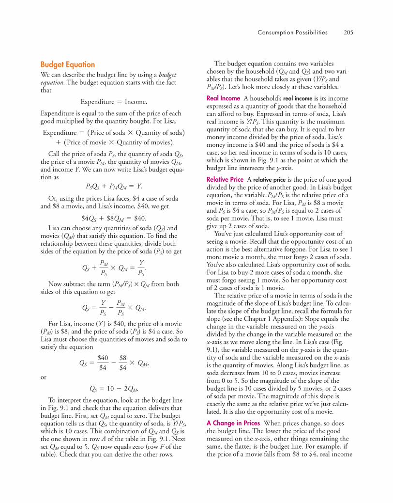
Consumption Possibilities 205

Budget EquationWe can describe the budget line by using a budgetequation. The budget equation starts with the factthat

Expenditure is equal to the sum of the price of eachgood multiplied by the quantity bought. For Lisa,

Call the price of soda PS, the quantity of soda QS,the price of a movie PM, the quantity of movies QM,and income Y. We can now write Lisa’s budget equa-tion as

Or, using the prices Lisa faces, $4 a case of sodaand $8 a movie, and Lisa’s income, $40, we get

Lisa can choose any quantities of soda (QS) andmovies (QM) that satisfy this equation. To find therelationship between these quantities, divide bothsides of the equation by the price of soda (PS) to get

Now subtract the term (PM/PS) × QM from bothsides of this equation to get

For Lisa, income (Y ) is $40, the price of a movie(PM) is $8, and the price of soda (PS) is $4 a case. SoLisa must choose the quantities of movies and soda tosatisfy the equation

or

To interpret the equation, look at the budget linein Fig. 9.1 and check that the equation delivers thatbudget line. First, set QM equal to zero. The budgetequation tells us that QS, the quantity of soda, is Y/PS,which is 10 cases. This combination of QM and QS isthe one shown in row A of the table in Fig. 9.1. Nextset QM equal to 5. QS now equals zero (row F of thetable). Check that you can derive the other rows.

QS � 10 � 2QM.

QS =$40$4

-$8$4

* QM,

QS �YPS

�PM

PS� QM.

QS �PM

PS� QM �

YPS

.

$4QS + $8QM = $40.

PSQS � PMQM � Y.

+ 1Price of movie * Quantity of movies2.Expenditure = 1Price of soda * Quantity of soda2

Expenditure = Income.

The budget equation contains two variableschosen by the household (QM and QS) and two vari-ables that the household takes as given (Y/PS andPM/PS). Let’s look more closely at these variables.

Real Income A household’s real income is its incomeexpressed as a quantity of goods that the householdcan afford to buy. Expressed in terms of soda, Lisa’sreal income is Y/PS. This quantity is the maximumquantity of soda that she can buy. It is equal to hermoney income divided by the price of soda. Lisa’smoney income is $40 and the price of soda is $4 acase, so her real income in terms of soda is 10 cases,which is shown in Fig. 9.1 as the point at which thebudget line intersects the y-axis.

Relative Price A relative price is the price of one gooddivided by the price of another good. In Lisa’s budgetequation, the variable PM/PS is the relative price of amovie in terms of soda. For Lisa, PM is $8 a movieand PS is $4 a case, so PM/PS is equal to 2 cases ofsoda per movie. That is, to see 1 movie, Lisa mustgive up 2 cases of soda.

You’ve just calculated Lisa’s opportunity cost ofseeing a movie. Recall that the opportunity cost of anaction is the best alternative forgone. For Lisa to see 1more movie a month, she must forgo 2 cases of soda.You’ve also calculated Lisa’s opportunity cost of soda.For Lisa to buy 2 more cases of soda a month, shemust forgo seeing 1 movie. So her opportunity costof 2 cases of soda is 1 movie.

The relative price of a movie in terms of soda is themagnitude of the slope of Lisa’s budget line. To calcu-late the slope of the budget line, recall the formula forslope (see the Chapter 1 Appendix): Slope equals thechange in the variable measured on the y-axisdivided by the change in the variable measured on thex-axis as we move along the line. In Lisa’s case (Fig.9.1), the variable measured on the y-axis is the quan-tity of soda and the variable measured on the x-axisis the quantity of movies. Along Lisa’s budget line, assoda decreases from 10 to 0 cases, movies increasefrom 0 to 5. So the magnitude of the slope of thebudget line is 10 cases divided by 5 movies, or 2 casesof soda per movie. The magnitude of this slope isexactly the same as the relative price we’ve just calcu-lated. It is also the opportunity cost of a movie.

A Change in Prices When prices change, so doesthe budget line. The lower the price of the goodmeasured on the x-axis, other things remaining thesame, the flatter is the budget line. For example, ifthe price of a movie falls from $8 to $4, real income

206 CHAPTER 9 Possibilities, Preferences, and Choices

We’ve studied the limits to what a householdcan consume. Let’s now learn how we can describepreferences and make a map that contains a lot ofinformation about a household’s preferences.

in terms of soda does not change but the relativeprice of a movie falls. The budget line rotates out-ward and becomes flatter, as Fig. 9.2(a) illustrates.The higher the price of the good measured on the x-axis, other things remaining the same, the steeper isthe budget line. For example, if the price of a movierises from $8 to $16, the relative price of a movieincreases. The budget line rotates inward andbecomes steeper, as Fig. 9.2(a) illustrates.

A Change in Income A change in money incomechanges real income but does not change the relativeprice. The budget line shifts, but its slope does notchange. An increase in money income increases realincome and shifts the budget line rightward. Adecrease in money income decreases real income andshifts the budget line leftward.

Figure 9.2(b) shows the effect of a change inmoney income on Lisa’s budget line. The initialbudget line when Lisa’s income is $40 is the same asin Fig. 9.1. The new budget line shows how muchLisa can buy if her income falls to $20 a month. Thetwo budget lines have the same slope because the rel-ative price is the same. The new budget line is closerto the origin because Lisa’s real income has decreased.

10

Soda

(cas

es p

er m

onth

)

Movies (per month)

9

4

0 8 106

(a) A change in price

6

2

7 942 3 51

Price of a movie is …

F

(b) A change in income

A

7

8

5

3

1 ... $4... $8... $16

10

Soda

(cas

es p

er m

onth

)

Movies (per month)

8

4

0

6

2

42 3 51

Income$20

7

9

5

3

1

Income$40

F

A

In part (a), the price of a movie changes. A fall in the pricefrom $8 to $4 rotates the budget line outward and makes itflatter. A rise in the price from $8 to $16 rotates the budgetline inward and makes it steeper.

In part (b), income falls from $40 to $20 while theprices of movies and soda remain the same. The budgetline shifts leftward, but its slope does not change.

FIGURE 9.2 Changes in Prices and Income

REVIEW QUIZ1 What does a household’s budget line show?2 How does the relative price and a household’s

real income influence its budget line?3 If a household has an income of $40 and buys

only bus rides at $2 each and magazines at $4each, what is the equation of the household’sbudget line?

4 If the price of one good changes, what happensto the relative price and the slope of the house-hold’s budget line?

5 If a household’s money income changes andprices do not change, what happens to thehousehold’s real income and budget line?

You can work these questions in Study Plan 9.1 and get instant feedback.

animation

Preferences and Indifference Curves 207

◆ Preferences and Indifference Curves

You are going to discover a very cool idea: that ofdrawing a map of a person’s preferences. A preferencemap is based on the intuitively appealing idea thatpeople can sort all the possible combinations ofgoods into three groups: preferred, not preferred, andindifferent. To make this idea more concrete, let’s askLisa to tell us how she ranks various combinations ofmovies and soda.

Figure 9.3 shows part of Lisa’s answer. She tells usthat she currently sees 2 movies and buys 6 cases ofsoda a month at point C. She then lists all the combi-nations of movies and soda that she says are just asacceptable to her as her current situation. When weplot these combinations of movies and soda, we getthe green curve in Fig. 9.3(a). This curve is the keyelement in a preference map and is called an indiffer-ence curve.

An indifference curve is a line that shows combina-tions of goods among which a consumer isindifferent. The indifference curve in Fig. 9.3(a) tellsus that Lisa is just as happy to see 2 movies and buy 6cases of soda a month at point C as she is to have thecombination of movies and soda at point G or at anyother point along the curve.

Lisa also says that she prefers all the combinationsof movies and soda above the indifference curve inFig. 9.3(a)—the yellow area—to those on the indif-ference curve. And she prefers any combination onthe indifference curve to any combination in the grayarea below the indifference curve.

The indifference curve in Fig. 9.3(a) is just one ofa whole family of such curves. This indifference curveappears again in Fig. 9.3(b), labeled I1. The curveslabeled I0 and I2 are two other indifference curves.Lisa prefers any point on indifference curve I2 to anypoint on indifference curve I1, and she prefers anypoint on I1 to any point on I0. We refer to I2 as beinga higher indifference curve than I1 and I1 as beinghigher than I0.

A preference map is a series of indifference curvesthat resemble the contour lines on a map. By lookingat the shape of the contour lines on a map, we candraw conclusions about the terrain. Similarly, by look-ing at the shape of the indifference curves, we candraw conclusions about a person’s preferences.

Let’s learn how to “read” a preference map.

10

2Movies (per month)

6

8

4

0

2

4 8 106

Preferred

G

CSoda

(cas

es p

er m

onth

)

Notpreferred

Indifferencecurve

10

2

Soda

(cas

es p

er m

onth

)

Movies (per month)

(a) An indifference curve

(b) Lisa's preference map

6

8

4

0

2

4 6 8 10I 0

2

C

G I

I1

J

Part (a) shows one of Lisa’s indifference curves. She is indif-ferent between point C (with 2 movies and 6 cases of soda)and all other points on the green indifference curve, such asG. She prefers points above the indifference curve (in theyellow area) to points on it, and she prefers points on theindifference curve to points below it (in the gray area).Part (b) shows three of the indifference curves—I0, I1, andI2—in Lisa’s preference map. She prefers point J to point Cor G, and she prefers all the points on I2 to those on I1.

FIGURE 9.3 A Preference Map

animation

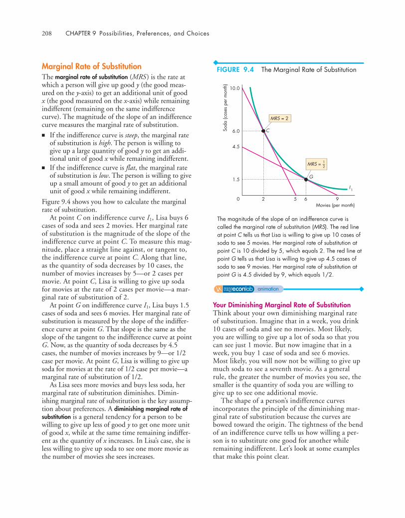
208 CHAPTER 9 Possibilities, Preferences, and Choices

Marginal Rate of SubstitutionThe marginal rate of substitution (MRS ) is the rate atwhich a person will give up good y (the good meas-ured on the y-axis) to get an additional unit of goodx (the good measured on the x-axis) while remainingindifferent (remaining on the same indifferencecurve). The magnitude of the slope of an indifferencecurve measures the marginal rate of substitution.■ If the indifference curve is steep, the marginal rate

of substitution is high. The person is willing togive up a large quantity of good y to get an addi-tional unit of good x while remaining indifferent.

■ If the indifference curve is flat, the marginal rateof substitution is low. The person is willing to giveup a small amount of good y to get an additionalunit of good x while remaining indifferent.

Figure 9.4 shows you how to calculate the marginalrate of substitution.

At point C on indifference curve I1, Lisa buys 6cases of soda and sees 2 movies. Her marginal rateof substitution is the magnitude of the slope of theindifference curve at point C. To measure this mag-nitude, place a straight line against, or tangent to,the indifference curve at point C. Along that line,as the quantity of soda decreases by 10 cases, thenumber of movies increases by 5—or 2 cases permovie. At point C, Lisa is willing to give up sodafor movies at the rate of 2 cases per movie—a mar-ginal rate of substitution of 2.

At point G on indifference curve I1, Lisa buys 1.5cases of soda and sees 6 movies. Her marginal rate ofsubstitution is measured by the slope of the indiffer-ence curve at point G. That slope is the same as theslope of the tangent to the indifference curve at pointG. Now, as the quantity of soda decreases by 4.5cases, the number of movies increases by 9—or 1/2case per movie. At point G, Lisa is willing to give upsoda for movies at the rate of 1/2 case per movie—amarginal rate of substitution of 1/2.

As Lisa sees more movies and buys less soda, hermarginal rate of substitution diminishes. Dimin-ishing marginal rate of substitution is the key assump-tion about preferences. A diminishing marginal rate ofsubstitution is a general tendency for a person to bewilling to give up less of good y to get one more unitof good x, while at the same time remaining indiffer-ent as the quantity of x increases. In Lisa’s case, she isless willing to give up soda to see one more movie asthe number of movies she sees increases.

Your Diminishing Marginal Rate of SubstitutionThink about your own diminishing marginal rateof substitution. Imagine that in a week, you drink10 cases of soda and see no movies. Most likely,you are willing to give up a lot of soda so that youcan see just 1 movie. But now imagine that in aweek, you buy 1 case of soda and see 6 movies.Most likely, you will now not be willing to give upmuch soda to see a seventh movie. As a generalrule, the greater the number of movies you see, thesmaller is the quantity of soda you are willing togive up to see one additional movie.

The shape of a person’s indifference curvesincorporates the principle of the diminishing mar-ginal rate of substitution because the curves arebowed toward the origin. The tightness of the bendof an indifference curve tells us how willing a per-son is to substitute one good for another whileremaining indifferent. Let’s look at some examplesthat make this point clear.

= 2

10.0

2

Soda

(cas

es p

er m

onth

)

Movies (per month)

6.0

4.5

0 5 96

I1

C

G

MRS = –12

MRS

1.5

The magnitude of the slope of an indifference curve iscalled the marginal rate of substitution (MRS). The red lineat point C tells us that Lisa is willing to give up 10 cases ofsoda to see 5 movies. Her marginal rate of substitution atpoint C is 10 divided by 5, which equals 2. The red line atpoint G tells us that Lisa is willing to give up 4.5 cases ofsoda to see 9 movies. Her marginal rate of substitution atpoint G is 4.5 divided by 9, which equals 1/2.

FIGURE 9.4 The Marginal Rate of Substitution

animation

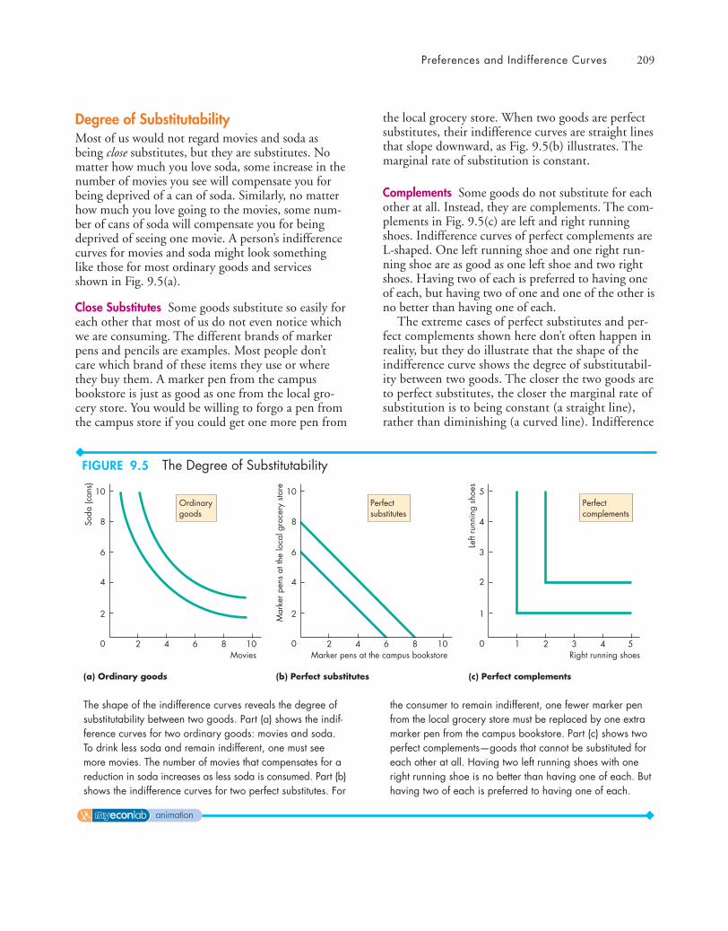
Preferences and Indifference Curves 209

Degree of SubstitutabilityMost of us would not regard movies and soda asbeing close substitutes, but they are substitutes. Nomatter how much you love soda, some increase in thenumber of movies you see will compensate you forbeing deprived of a can of soda. Similarly, no matterhow much you love going to the movies, some num-ber of cans of soda will compensate you for beingdeprived of seeing one movie. A person’s indifferencecurves for movies and soda might look somethinglike those for most ordinary goods and servicesshown in Fig. 9.5(a).

Close Substitutes Some goods substitute so easily foreach other that most of us do not even notice whichwe are consuming. The different brands of markerpens and pencils are examples. Most people don’tcare which brand of these items they use or wherethey buy them. A marker pen from the campusbookstore is just as good as one from the local gro-cery store. You would be willing to forgo a pen fromthe campus store if you could get one more pen from

the local grocery store. When two goods are perfectsubstitutes, their indifference curves are straight linesthat slope downward, as Fig. 9.5(b) illustrates. Themarginal rate of substitution is constant.

Complements Some goods do not substitute for eachother at all. Instead, they are complements. The com-plements in Fig. 9.5(c) are left and right runningshoes. Indifference curves of perfect complements areL-shaped. One left running shoe and one right run-ning shoe are as good as one left shoe and two rightshoes. Having two of each is preferred to having oneof each, but having two of one and one of the other isno better than having one of each.

The extreme cases of perfect substitutes and per-fect complements shown here don’t often happen inreality, but they do illustrate that the shape of theindifference curve shows the degree of substitutabil-ity between two goods. The closer the two goods areto perfect substitutes, the closer the marginal rate ofsubstitution is to being constant (a straight line),rather than diminishing (a curved line). Indifference

10

2

Soda

(can

s)

Movies

6

8

4

0

2

4 8 106

(a) Ordinary goods

10

2

Mar

ker p

ens

at th

e lo

cal g

roce

ry s

tore

Marker pens at the campus bookstore

6

8

4

0

2

4 8 106

(b) Perfect substitutes

5

1

Left

runn

ing

shoe

s

Right running shoes

3

4

2

0

1

2 4 53

(c) Perfect complements

Ordinarygoods

Perfectsubstitutes

Perfectcomplements

The shape of the indifference curves reveals the degree ofsubstitutability between two goods. Part (a) shows the indif-ference curves for two ordinary goods: movies and soda.To drink less soda and remain indifferent, one must seemore movies. The number of movies that compensates for areduction in soda increases as less soda is consumed. Part (b)shows the indifference curves for two perfect substitutes. For

the consumer to remain indifferent, one fewer marker penfrom the local grocery store must be replaced by one extramarker pen from the campus bookstore. Part (c) shows twoperfect complements—goods that cannot be substituted foreach other at all. Having two left running shoes with oneright running shoe is no better than having one of each. Buthaving two of each is preferred to having one of each.

FIGURE 9.5 The Degree of Substitutability

animation

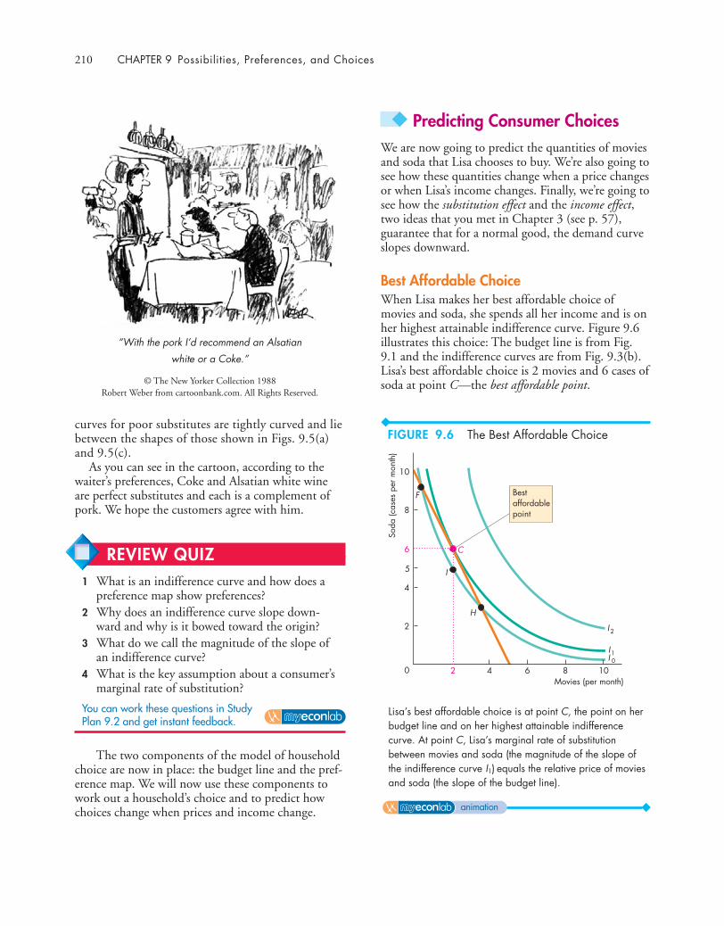
210 CHAPTER 9 Possibilities, Preferences, and Choices

The two components of the model of householdchoice are now in place: the budget line and the pref-erence map. We will now use these components towork out a household’s choice and to predict howchoices change when prices and income change.

curves for poor substitutes are tightly curved and liebetween the shapes of those shown in Figs. 9.5(a)and 9.5(c).

As you can see in the cartoon, according to thewaiter’s preferences, Coke and Alsatian white wineare perfect substitutes and each is a complement ofpork. We hope the customers agree with him.

◆ Predicting Consumer ChoicesWe are now going to predict the quantities of moviesand soda that Lisa chooses to buy. We’re also going tosee how these quantities change when a price changesor when Lisa’s income changes. Finally, we’re going tosee how the substitution effect and the income effect,two ideas that you met in Chapter 3 (see p. 57),guarantee that for a normal good, the demand curveslopes downward.

Best Affordable ChoiceWhen Lisa makes her best affordable choice ofmovies and soda, she spends all her income and is onher highest attainable indifference curve. Figure 9.6illustrates this choice: The budget line is from Fig.9.1 and the indifference curves are from Fig. 9.3(b).Lisa’s best affordable choice is 2 movies and 6 cases ofsoda at point C—the best affordable point.

“With the pork I’d recommend an Alsatian

white or a Coke.”

© The New Yorker Collection 1988Robert Weber from cartoonbank.com. All Rights Reserved.

10

2

Soda

(cas

es p

er m

onth

)

Movies (per month)

6

8

4

5

0

2

4 6 8 10

I

F

C

H

Bestaffordablepoint

II10

2I

Lisa’s best affordable choice is at point C, the point on herbudget line and on her highest attainable indifferencecurve. At point C, Lisa’s marginal rate of substitutionbetween movies and soda (the magnitude of the slope ofthe indifference curve I1) equals the relative price of moviesand soda (the slope of the budget line).

REVIEW QUIZ1 What is an indifference curve and how does a

preference map show preferences?2 Why does an indifference curve slope down-

ward and why is it bowed toward the origin?3 What do we call the magnitude of the slope of

an indifference curve?4 What is the key assumption about a consumer’s

marginal rate of substitution?

You can work these questions in Study Plan 9.2 and get instant feedback.

FIGURE 9.6 The Best Affordable Choice

animation

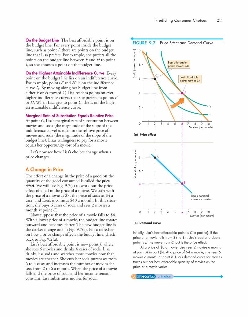
Predicting Consumer Choices 211

On the Budget Line The best affordable point is onthe budget line. For every point inside the budgetline, such as point I, there are points on the budgetline that Lisa prefers. For example, she prefers all thepoints on the budget line between F and H to pointI, so she chooses a point on the budget line.

On the Highest Attainable Indifference Curve Everypoint on the budget line lies on an indifference curve.For example, points F and H lie on the indifferencecurve I0. By moving along her budget line fromeither F or H toward C, Lisa reaches points on ever-higher indifference curves that she prefers to points For H. When Lisa gets to point C, she is on the high-est attainable indifference curve.

Marginal Rate of Substitution Equals Relative PriceAt point C, Lisa’s marginal rate of substitution betweenmovies and soda (the magnitude of the slope of theindifference curve) is equal to the relative price ofmovies and soda (the magnitude of the slope of thebudget line). Lisa’s willingness to pay for a movieequals her opportunity cost of a movie.

Let’s now see how Lisa’s choices change when aprice changes.

A Change in PriceThe effect of a change in the price of a good on thequantity of the good consumed is called the priceeffect. We will use Fig. 9.7(a) to work out the priceeffect of a fall in the price of a movie. We start withthe price of a movie at $8, the price of soda at $4 acase, and Lisa’s income at $40 a month. In this situa-tion, she buys 6 cases of soda and sees 2 movies amonth at point C.

Now suppose that the price of a movie falls to $4.With a lower price of a movie, the budget line rotatesoutward and becomes flatter. The new budget line isthe darker orange one in Fig. 9.7(a). For a refresheron how a price change affects the budget line, checkback to Fig. 9.2(a).

Lisa’s best affordable point is now point J, whereshe sees 6 movies and drinks 4 cases of soda. Lisadrinks less soda and watches more movies now thatmovies are cheaper. She cuts her soda purchases from6 to 4 cases and increases the number of movies shesees from 2 to 6 a month. When the price of a moviefalls and the price of soda and her income remainconstant, Lisa substitutes movies for soda.

0Movies (per month)

Soda

(cas

es p

er m

onth

)

1

2

4

6

8

10

3 7 8 9 10

C

0Movies (per month)

Pric

e (d

olla

rs p

er m

ovie

)

1

4

8

2 3 4 5 6 7 8 9 10

A

B

J

2

(b) Demand curve

Lisa’s demandcurve for movies

2 5

Best affordablepoint: movies $8

Best affordablepoint: movies $4

(a) Price effect

6

I1

4 6

2I

Initially, Lisa’s best affordable point is C in part (a). If theprice of a movie falls from $8 to $4, Lisa’s best affordablepoint is J. The move from C to J is the price effect.

At a price of $8 a movie, Lisa sees 2 movies a month,at point A in part (b). At a price of $4 a movie, she sees 6movies a month, at point B. Lisa’s demand curve for moviestraces out her best affordable quantity of movies as theprice of a movie varies.

FIGURE 9.7 Price Effect and Demand Curve

animation

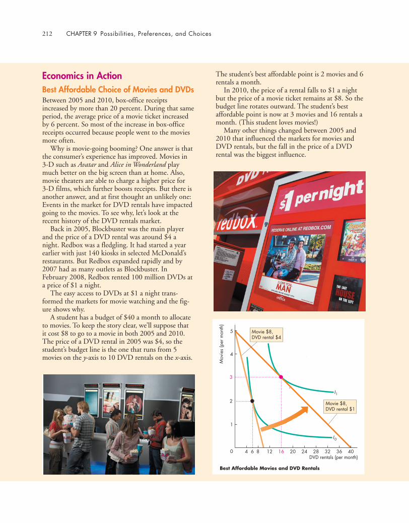
212 CHAPTER 9 Possibilities, Preferences, and Choices

Economics in ActionBest Affordable Choice of Movies and DVDsBetween 2005 and 2010, box-office receiptsincreased by more than 20 percent. During that sameperiod, the average price of a movie ticket increasedby 6 percent. So most of the increase in box-officereceipts occurred because people went to the moviesmore often.

Why is movie-going booming? One answer is thatthe consumer’s experience has improved. Movies in3-D such as Avatar and Alice in Wonderland playmuch better on the big screen than at home. Also,movie theaters are able to charge a higher price for3-D films, which further boosts receipts. But there isanother answer, and at first thought an unlikely one:Events in the market for DVD rentals have impactedgoing to the movies. To see why, let’s look at therecent history of the DVD rentals market.

Back in 2005, Blockbuster was the main playerand the price of a DVD rental was around $4 anight. Redbox was a fledgling. It had started a yearearlier with just 140 kiosks in selected McDonald’srestaurants. But Redbox expanded rapidly and by2007 had as many outlets as Blockbuster. InFebruary 2008, Redbox rented 100 million DVDs ata price of $1 a night.

The easy access to DVDs at $1 a night trans-formed the markets for movie watching and the fig-ure shows why.

A student has a budget of $40 a month to allocateto movies. To keep the story clear, we’ll suppose thatit cost $8 to go to a movie in both 2005 and 2010.The price of a DVD rental in 2005 was $4, so thestudent’s budget line is the one that runs from 5movies on the y-axis to 10 DVD rentals on the x-axis.

The student’s best affordable point is 2 movies and 6rentals a month.

In 2010, the price of a rental falls to $1 a nightbut the price of a movie ticket remains at $8. So thebudget line rotates outward. The student’s bestaffordable point is now at 3 movies and 16 rentals amonth. (This student loves movies!)

Many other things changed between 2005 and2010 that influenced the markets for movies andDVD rentals, but the fall in the price of a DVDrental was the biggest influence.

0DVD rentals (per month)

Mov

ies

(per

mon

th)

4

1

2

3

4

5

86 12 16 20 24 28 32 36 40

Movie $8,DVD rental $4

Movie $8,DVD rental $1

I0

1I

Best Affordable Movies and DVD Rentals

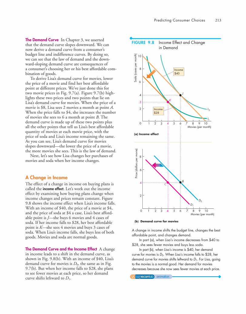
Predicting Consumer Choices 213

The Demand Curve In Chapter 3, we assertedthat the demand curve slopes downward. We cannow derive a demand curve from a consumer’sbudget line and indifference curves. By doing so,we can see that the law of demand and the down-ward-sloping demand curve are consequences ofa consumer’s choosing her or his best affordable com-bination of goods.

To derive Lisa’s demand curve for movies, lowerthe price of a movie and find her best affordablepoint at different prices. We’ve just done this fortwo movie prices in Fig. 9.7(a). Figure 9.7(b) high-lights these two prices and two points that lie onLisa’s demand curve for movies. When the price of amovie is $8, Lisa sees 2 movies a month at point A.When the price falls to $4, she increases the numberof movies she sees to 6 a month at point B. Thedemand curve is made up of these two points plusall the other points that tell us Lisa’s best affordablequantity of movies at each movie price, with theprice of soda and Lisa’s income remaining the same.As you can see, Lisa’s demand curve for moviesslopes downward—the lower the price of a movie,the more movies she sees. This is the law of demand.

Next, let’s see how Lisa changes her purchases ofmovies and soda when her income changes.

A Change in IncomeThe effect of a change in income on buying plans iscalled the income effect. Let’s work out the incomeeffect by examining how buying plans change whenincome changes and prices remain constant. Figure9.8 shows the income effect when Lisa’s income falls.With an income of $40, the price of a movie at $4,and the price of soda at $4 a case, Lisa’s best afford-able point is J—she buys 6 movies and 4 cases ofsoda. If her income falls to $28, her best affordablepoint is K—she sees 4 movies and buys 3 cases ofsoda. When Lisa’s income falls, she buys less of bothgoods. Movies and soda are normal goods.

The Demand Curve and the Income Effect A changein income leads to a shift in the demand curve, asshown in Fig. 9.8(b). With an income of $40, Lisa’sdemand curve for movies is D0, the same as in Fig.9.7(b). But when her income falls to $28, she plansto see fewer movies at each price, so her demandcurve shifts leftward to D1.

10

Soda

(cas

es p

er m

onth

)

Movies (per month)

3

8

4

0

2

4 6

(a) Income effect

5 8 1091 7

6

2 3

Income$40

0Movies (per month)

Pric

e (d

olla

rs p

er m

ovie

)

1

4

8

2 3 4 5 6 7 8 9 10

B

J

C

K

2

(b) Demand curve for movies

6

D1

D0

Income$28

1

2I

I

A change in income shifts the budget line, changes the bestaffordable point, and changes demand.

In part (a), when Lisa’s income decreases from $40 to$28, she sees fewer movies and buys less soda.

In part (b), when Lisa’s income is $40, her demandcurve for movies is D0. When Lisa’s income falls to $28, herdemand curve for movies shifts leftward to D1. For Lisa, goingto the movies is a normal good. Her demand for moviesdecreases because she now sees fewer movies at each price.

FIGURE 9.8 Income Effect and Changein Demand

animation

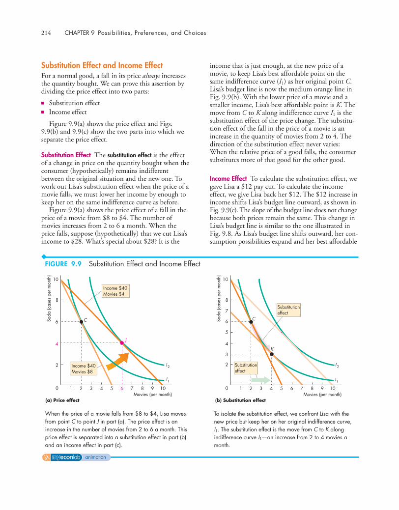
214 CHAPTER 9 Possibilities, Preferences, and Choices

income that is just enough, at the new price of amovie, to keep Lisa’s best affordable point on thesame indifference curve (I1) as her original point C.Lisa’s budget line is now the medium orange line inFig. 9.9(b). With the lower price of a movie and asmaller income, Lisa’s best affordable point is K. Themove from C to K along indifference curve I1 is thesubstitution effect of the price change. The substitu-tion effect of the fall in the price of a movie is anincrease in the quantity of movies from 2 to 4. Thedirection of the substitution effect never varies:When the relative price of a good falls, the consumersubstitutes more of that good for the other good.

Income Effect To calculate the substitution effect, wegave Lisa a $12 pay cut. To calculate the incomeeffect, we give Lisa back her $12. The $12 increase inincome shifts Lisa’s budget line outward, as shown inFig. 9.9(c). The slope of the budget line does not changebecause both prices remain the same. This change inLisa’s budget line is similar to the one illustrated inFig. 9.8. As Lisa’s budget line shifts outward, her con-sumption possibilities expand and her best affordable

Substitution Effect and Income EffectFor a normal good, a fall in its price always increasesthe quantity bought. We can prove this assertion bydividing the price effect into two parts:

■ Substitution effect■ Income effect

Figure 9.9(a) shows the price effect and Figs.9.9(b) and 9.9(c) show the two parts into which weseparate the price effect.

Substitution Effect The substitution effect is the effectof a change in price on the quantity bought when theconsumer (hypothetically) remains indifferentbetween the original situation and the new one. Towork out Lisa’s substitution effect when the price of amovie falls, we must lower her income by enough tokeep her on the same indifference curve as before.

Figure 9.9(a) shows the price effect of a fall in theprice of a movie from $8 to $4. The number ofmovies increases from 2 to 6 a month. When theprice falls, suppose (hypothetically) that we cut Lisa’sincome to $28. What’s special about $28? It is the

2I

10

Soda

(cas

es p

er m

onth

)

Movies (per month)(a) Price effect

4

8

0

2

4 6

C

52 3 8 1091 7

6

Income $40Movies $4

Income $40Movies $8

I1

10

Soda

(cas

es p

er m

onth

)

Movies (per month)(b) Substitution effect

4

8

7

5

3

0

2

4 6

C

K

52 3 8 1091 7

6

Substitutioneffect

Substitutioneffect

J

2I

I1

When the price of a movie falls from $8 to $4, Lisa movesfrom point C to point J in part (a). The price effect is anincrease in the number of movies from 2 to 6 a month. Thisprice effect is separated into a substitution effect in part (b)and an income effect in part (c).

To isolate the substitution effect, we confront Lisa with thenew price but keep her on her original indifference curve,I1. The substitution effect is the move from C to K alongindifference curve I1—an increase from 2 to 4 movies amonth.

FIGURE 9.9 Substitution Effect and Income Effect

animation

Predicting Consumer Choices 215

If the negative income effect is smaller than the pos-itive substitution effect, a fall in price increases thequantity bought and the demand curve still slopesdownward like that for a normal good. But thedemand for an inferior good might be less elastic thanthat for a normal good.

If the negative income effect exceeds the positivesubstitution effect, a fall in the price decreases thequantity bought and the demand curve slopes upward.This case does not appear to occur in the real world.

You can apply the indifference curve model thatyou’ve studied in this chapter to explain the changesin the way we buy recorded music, see movies, andmake all our other consumption choices. We allocateour budgets to make our best affordable choices.Changes in prices and incomes change our bestaffordable choices and change consumption patterns.

point becomes J on indifference curve I2. The movefrom K to J is the income effect of the price change.

As Lisa’s income increases, she sees more movies.For Lisa, a movie is a normal good. For a normalgood, the income effect reinforces the substitutioneffect. Because the two effects work in the same direc-tion, we can be sure that the demand curve slopesdownward. But some goods are inferior goods. Whatcan we say about the demand for an inferior good?

Inferior Goods Recall that an inferior good is a goodfor which demand decreases when income increases. Foran inferior good, the income effect is negative, whichmeans that a lower price does not inevitably lead to anincrease in the quantity demanded. The substitutioneffect of a fall in the price increases the quantitydemanded, but the negative income effect works in theopposite direction and offsets the substitution effect tosome degree. The key question is to what degree.

If the negative income effect equals the positive sub-stitution effect, a fall in price leaves the quantitybought the same. When a fall in price leaves the quan-tity demanded unchanged, the demand curve is verti-cal and demand is perfectly inelastic.

2I

I1

10

Soda

(cas

es p

er m

onth

)

Movies (per month)(c) Income effect

4

8

7

5

3

0

2

4 6

K

52 3 8 1091 7

6Incomeeffect

J

To isolate the income effect, we confront Lisa with the newprice of movies but increase her income so that she canmove from the original indifference curve, I1, to the newone, I2. The income effect is the move from K to J—anincrease from 4 to 6 movies a month.

◆ Reading Between the Lines on pp. 216–217 showsyou how the theory of household choice explains whye-books are taking off, and how people chose whetherto buy their books in electronic or paper format.

In the chapters that follow, we study the choicesthat firms make in their pursuit of profit and howthose choices determine the supply of goods andservices and the demand for productive resources.

REVIEW QUIZ1 When a consumer chooses the combination

of goods and services to buy, what is she or hetrying to achieve?

2 Explain the conditions that are met when aconsumer has found the best affordable combi-nation of goods to buy. (Use the terms budgetline, marginal rate of substitution, and relativeprice in your explanation.)

3 If the price of a normal good falls, what hap-pens to the quantity demanded of that good?

4 Into what two effects can we divide the effectof a price change?

5 For a normal good, does the income effectreinforce the substitution effect or does it partlyoffset the substitution effect?

You can work these questions in Study Plan 9.3 and get instant feedback.

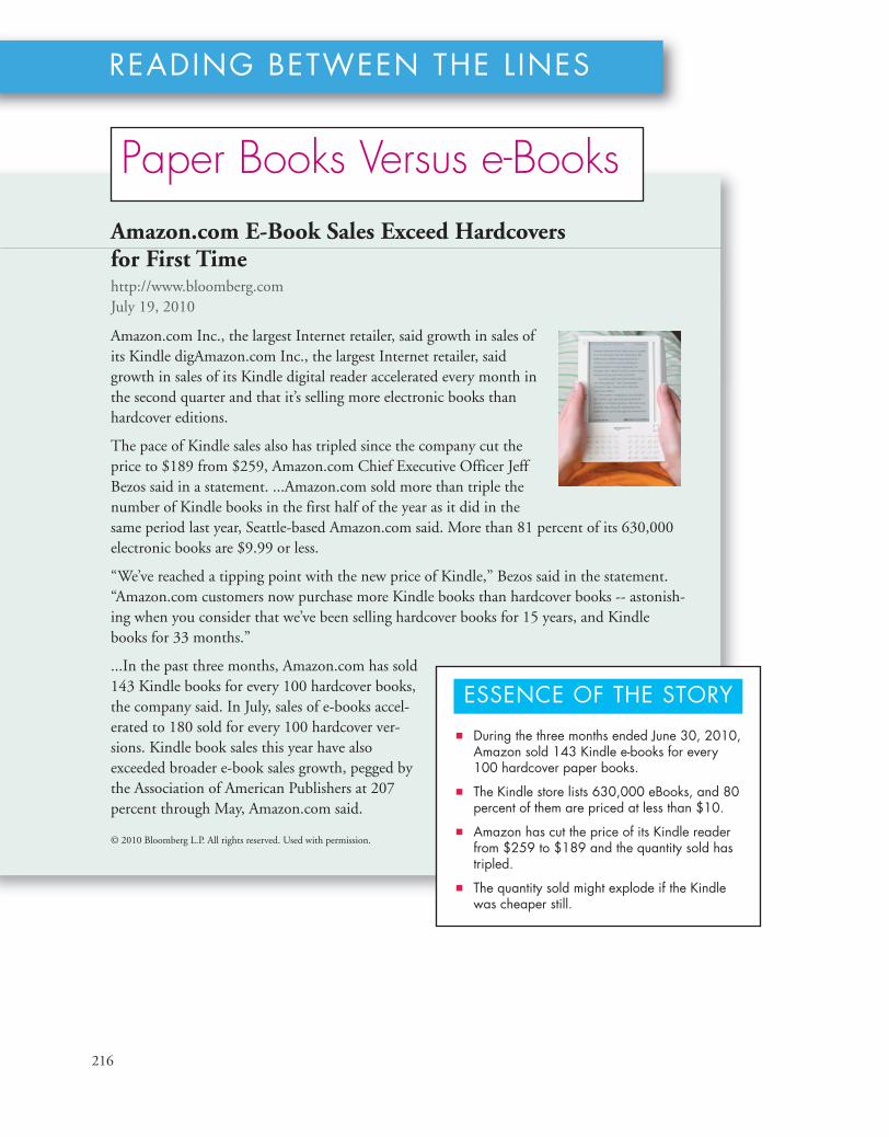
READING BETWEEN THE L INES

Amazon.com E-Book Sales Exceed Hardcovers for First Time http://www.bloomberg.com July 19, 2010

Amazon.com Inc., the largest Internet retailer, said growth in sales ofits Kindle digAmazon.com Inc., the largest Internet retailer, saidgrowth in sales of its Kindle digital reader accelerated every month inthe second quarter and that it’s selling more electronic books thanhardcover editions.

The pace of Kindle sales also has tripled since the company cut theprice to $189 from $259, Amazon.com Chief Executive Officer JeffBezos said in a statement. ...Amazon.com sold more than triple thenumber of Kindle books in the first half of the year as it did in thesame period last year, Seattle-based Amazon.com said. More than 81 percent of its 630,000electronic books are $9.99 or less.

“We’ve reached a tipping point with the new price of Kindle,” Bezos said in the statement.“Amazon.com customers now purchase more Kindle books than hardcover books -- astonish-ing when you consider that we’ve been selling hardcover books for 15 years, and Kindlebooks for 33 months.”

...In the past three months, Amazon.com has sold143 Kindle books for every 100 hardcover books,the company said. In July, sales of e-books accel-erated to 180 sold for every 100 hardcover ver-sions. Kindle book sales this year have alsoexceeded broader e-book sales growth, pegged bythe Association of American Publishers at 207percent through May, Amazon.com said.

© 2010 Bloomberg L.P. All rights reserved. Used with permission.

■ During the three months ended June 30, 2010,Amazon sold 143 Kindle e-books for every100 hardcover paper books.

■ The Kindle store lists 630,000 eBooks, and 80percent of them are priced at less than $10.

■ Amazon has cut the price of its Kindle readerfrom $259 to $189 and the quantity sold hastripled.

■ The quantity sold might explode if the Kindlewas cheaper still.

ESSENCE OF THE STORY

Paper Books Versus e-Books

216

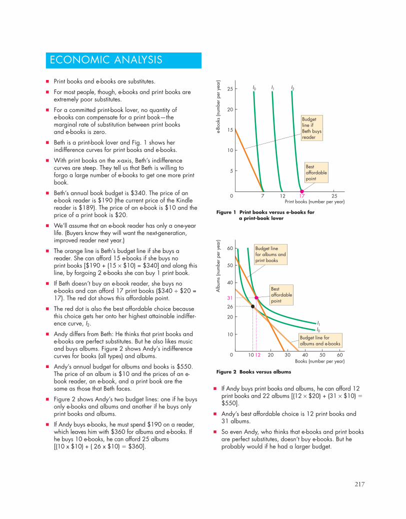
217

ECONOMIC ANALYSIS

Figure 2 Books versus albums

Figure 1 Print books versus e-books fora print-book lover

e-Bo

oks

(num

ber p

er y

ear)

Print books (number per year)0

I0

I0I1

I1 I2

Bestaffordablepoint

Budgetline if Beth buysreader

Bestaffordablepoint

Budget linefor albums andprint books

25

20

15

10

5

Alb

ums

(num

ber p

er y

ear)

Books (number per year)0

60

50

40

20

10

31

26

3010 20 40 5012 60

2517127

Budget line foralbums and e-books

■ If Andy buys print books and albums, he can afford 12print books and 22 albums [(12 × $20) + (31 × $10) �$550].

■ Andy’s best affordable choice is 12 print books and31 albums.

■ So even Andy, who thinks that e-books and print booksare perfect substitutes, doesn’t buy e-books. But heprobably would if he had a larger budget.

■ Print books and e-books are substitutes.

■ For most people, though, e-books and print books areextremely poor substitutes.

■ For a committed print-book lover, no quantity of e-books can compensate for a print book—the marginal rate of substitution between print books and e-books is zero.

■ Beth is a print-book lover and Fig. 1 shows herindifference curves for print books and e-books.

■ With print books on the x-axis, Beth’s indifferencecurves are steep. They tell us that Beth is willing toforgo a large number of e-books to get one more printbook.

■ Beth’s annual book budget is $340. The price of an e-book reader is $190 (the current price of the Kindlereader is $189). The price of an e-book is $10 and theprice of a print book is $20.

■ We’ll assume that an e-book reader has only a one-yearlife. (Buyers know they will want the next-generation,improved reader next year.)

■ The orange line is Beth’s budget line if she buys areader. She can afford 15 e-books if she buys no print books [$190 + (15 × $10) = $340] and along thisline, by forgoing 2 e-books she can buy 1 print book.

■ If Beth doesn’t buy an e-book reader, she buys no e-books and can afford 17 print books ($340 ÷ $20 =17). The red dot shows this affordable point.

■ The red dot is also the best affordable choice becausethis choice gets her onto her highest attainable indiffer-ence curve, I2.

■ Andy differs from Beth: He thinks that print books ande-books are perfect substitutes. But he also likes musicand buys albums. Figure 2 shows Andy’s indifferencecurves for books (all types) and albums.

■ Andy’s annual budget for albums and books is $550.The price of an album is $10 and the prices of an e-book reader, an e-book, and a print book are thesame as those that Beth faces.

■ Figure 2 shows Andy’s two budget lines: one if he buysonly e-books and albums and another if he buys onlyprint books and albums.

■ If Andy buys e-books, he must spend $190 on a reader,which leaves him with $360 for albums and e-books. Ifhe buys 10 e-books, he can afford 25 albums [(10 x $10) + ( 26 x $10) � $360].

218 CHAPTER 9 Possibilities, Preferences, and Choices

decreases and consumption of the good measuredon the x-axis increases.

Working Problems 11 to 15 will give you a better under-standing of preferences and indifference curves.

Predicting Consumer Choices (pp. 210–215)

■ A household consumes at its best affordablepoint. This point is on the budget line and onthe highest attainable indifference curve and has a marginal rate of substitution equal to relative price.

■ The effect of a price change (the price effect)can be divided into a substitution effect and anincome effect.

■ The substitution effect is the effect of a change inprice on the quantity bought when the consumer(hypothetically) remains indifferent between theoriginal choice and the new choice.

■ The substitution effect always results in anincrease in consumption of the good whose rela-tive price has fallen.

■ The income effect is the effect of a change inincome on consumption.

■ For a normal good, the income effect reinforcesthe substitution effect. For an inferior good, theincome effect works in the opposite direction tothe substitution effect.

Working Problems 16 to 20 will give you a better under-standing of predicting consumer choices.

Key Points

Consumption Possibilities (pp. 204–206)

■ The budget line is the boundary between what ahousehold can and cannot afford, given its incomeand the prices of goods.

■ The point at which the budget line intersects they-axis is the household’s real income in terms ofthe good measured on that axis.

■ The magnitude of the slope of the budget line isthe relative price of the good measured on the x-axis in terms of the good measured on the y-axis.

■ A change in the price of one good changes theslope of the budget line. A change in income shiftsthe budget line but does not change its slope.

Working Problems 1 to 10 will give you a better under-standing of consumption possibilities.

Preferences and Indifference Curves (pp. 207–210)

■ A consumer’s preferences can be represented byindifference curves. The consumer is indifferentamong all the combinations of goods that lie onan indifference curve.

■ A consumer prefers any point above an indiffer-ence curve to any point on it and prefers any pointon an indifference curve to any point below it.

■ The magnitude of the slope of an indifferencecurve is called the marginal rate of substitution.

■ The marginal rate of substitution diminishes asconsumption of the good measured on the y-axis

SUMMARY

Key TermsBudget line, 204Diminishing marginal rate of substitution, 208

Income effect, 213

Indifference curve, 207Marginal rate of substitution, 208Price effect, 211Real income, 205

Relative price, 205Substitution effect, 214

Study Plan Problems and Applications 219

Preferences and Indifference Curves (Study Plan 9.2)

11. Draw figures that show your indifference curvesfor the following pairs of goods:■ Right gloves and left gloves■ Coca-Cola and Pepsi■ Tylenol and acetaminophen (the generic form

of Tylenol)■ Desktop computers and laptop computers■ Strawberries and ice cream

For each pair, are the goods perfect substitutes,perfect complements, substitutes, complements, orunrelated?12. Discuss the shape of the indifference curve for

each of the following pairs of goods:■ Orange juice and smoothies■ Baseballs and baseball bats■ Left running shoe and right running shoe■ Eyeglasses and contact lenses

Explain the relationship between the shape of theindifference curve and the marginal rate of substitu-tion as the quantities of the two goods change.Use the following news clip to work Problems 13 and 14.

The Year in MedicineSudafed, used by allergy sufferers, contains as the activeingredient pseudoephedrine, which is widely used tomake home-made methamphetamine. Allergy suffererslooking to buy Sudafed, must now show photo ID, andsign a logbook. The most common alternative,phenylephrine, isn’t as effective as pseudoephedrine.

Source:Time, December 4, 2006

13. Sketch an indifference curve for Sudafed andphenylephrine that is consistent with this newsclip. On your graph, identify combinations thatallergy sufferers prefer, do not prefer, and areindifferent among.

14. Explain how the marginal rate of substitutionchanges as an allergy sufferer increases the con-sumption of Sudafed.

Use the following news clip to work Problems 15 and 16.

Consumption Possibilities (Study Plan 9.1)

Use the following information to work Problems 1 to 4.

Sara’s income is $12 a week. The price of popcorn is $3a bag, and the price of a smoothie is $3.

1. Calculate Sara’s real income in terms ofsmoothies. Calculate her real income in terms ofpopcorn.

2. What is the relative price of smoothies in termsof popcorn? What is the opportunity cost of asmoothie?

3. Calculate the equation for Sara’s budget line(with bags of popcorn on the left side).

4. Draw a graph of Sara’s budget line with the quan-tity of smoothies on the x-axis. What is the slopeof Sara’s budget line? What determines its value?

Use the following information to work Problems 5 to 8.

Sara’s income falls from $12 to $9 a week, while theprice of popcorn is unchanged at $3 a bag and theprice of a smoothie is unchanged at $3.

5. What is the effect of the fall in Sara’s income onher real income in terms of smoothies?

6. What is the effect of the fall in Sara’s income onher real income in terms of popcorn?

7. What is the effect of the fall in Sara’s income onthe relative price of a smoothie in terms of pop-corn?

8. What is the slope of Sara’s new budget line if it isdrawn with smoothies on the x-axis?

Use the following information to work Problems 9 and 10.

Sara’s income is $12 a week. The price of popcornrises from $3 to $6 a bag, and the price of a smoothieis unchanged at $3.

9. What is the effect of the rise in the price of pop-corn on Sara’s real income in terms of smoothiesand her real income in terms of popcorn?

10. What is the effect of the rise in the price of pop-corn on the relative price of a smoothie in terms ofpopcorn? What is the slope of Sara’s new budgetline if it is drawn with smoothies on the x-axis?

You can work Problems 1 to 22 in MyEconLab Chapter 9 Study Plan and get instant feedback.

STUDY PLAN PROBLEMS AND APPLICATIONS

220 CHAPTER 9 Possibilities, Preferences, and Choices

Gas Prices to Stunt Memorial Day TravelWith high gas prices, 12% of the people surveyedsay that they have cancelled their Memorial Dayroad trip and 11% will take a shorter trip nearhome. That may save consumers some money, but itwill also likely hurt service stations, which will sellless gas and fewer snacks and hurt roadside hotels,which will have fewer rooms used and serve fewercasual meals.

Source: MarketWatch, May 22, 2008

15. Describe the degree of substitutability betweenMemorial Day trips and other trip-related goodsand services and sketch a consumer’s preferencemap that illustrates your description.

Predicting Consumer Choices (Study Plan 9.3)

16. a. Sketch a consumer’s preference map betweenMemorial Day trips and other goods andservices. Draw a consumer’s budget line priorto the rise in the price of gasoline and markthe consumer’s best affordable point.

b. On your graph, show how the best affordablepoint changes when the price of gasoline rises.

Use the following information to work Problems 17and 18.

Pam has chosen her best affordable combination ofcookies and granola bars. She spends all of her weeklyincome on 30 cookies at $1 each and 5 granola barsat $2 each. Next week, people expect the price of acookie to fall to 50¢ and the price of a granola bar torise to $5.

17. a. Will Pam be able to buy and want to buy 30cookies and 5 granola bars next week?

b. Which situation does Pam prefer: cookies at$1 and granola bars at $2 or cookies at 50¢and granola bars at $5?

18. a. If Pam changes how she spends her weeklyincome, will she buy more or fewer cookiesand more or fewer granola bars?

b. When the prices change next week, will therebe an income effect, a substitution effect, orboth at work?

Use the following information to work Problems 19and 20.

Boom Time For “Gently Used” ClothesMost retailers are blaming the economy for theirpoor sales, but one store chain that sells used name-brand children’s clothes, toys, and furniture is boldly

declaring that an economic downturn can actually bea boon for its business. Last year, the company tookin $20 million in sales, up 5% from the previousyear. Sales are already up 5% this year.

Source: CNN, April 17, 2008

19. a. According to the news clip, is used clothing anormal good or an inferior good?

b. If the price of used clothing falls and incomeremains the same, explain how the quantity ofused clothing bought changes.

c. If the price of used clothing falls and incomeremains the same, describe the substitutioneffect and the income effect that occur.

20. a. Use a graph to illustrate a family’s indifferencecurves for used clothing and other goods andservices.

b. In your graph in part (a), draw two budgetlines to show the effect of a fall in income onthe quantity of used clothing purchased.

Economics in the News (Study Plan 9.N)

Use the following information to work Problems 21and 22.Gas Prices Send Surge of Travelers to Mass TransitWith the price of gas approaching $4 a gallon, morecommuters are abandoning their cars and taking thetrain or bus. It’s very clear that a significant portionof the increase in transit use is directly caused by peo-ple who are looking for alternatives to paying $3.50 agallon for gas. Some cities with long-established pub-lic transit systems, like New York and Boston, haveseen increases in ridership of 5 percent, but thebiggest surges—of 10 to 15 percent over last year—are occurring in many metropolitan areas in theSouthwest where the driving culture is strongest andbus and rail lines are more limited.

Source: The New York Times, May 10, 2008

21. a. Sketch a graph of a preference map and abudget line to illustrate the best affordablecombination of gasoline and public transit.

b. On your graph in part (a), show the effect of arise in the price of gasoline on the quantitiesof gasoline and public transit services pur-chased.

22. If the gas price rise has been similar in all regions,compare the marginal rates of substitution in theNortheast and the Southwest. Explain how youhave inferred the different marginal rates of sub-stitution from the information in the news clip.

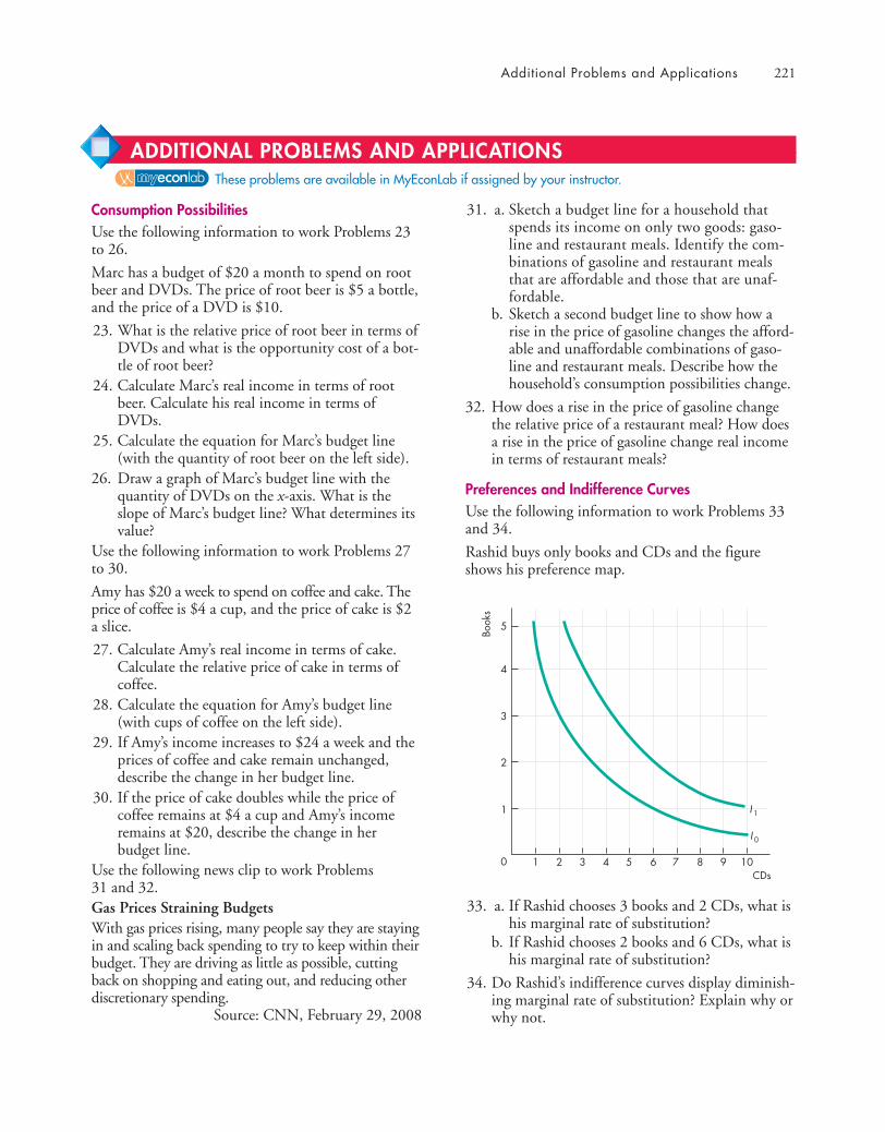
Additional Problems and Applications 221

Consumption PossibilitiesUse the following information to work Problems 23to 26.

Marc has a budget of $20 a month to spend on rootbeer and DVDs. The price of root beer is $5 a bottle,and the price of a DVD is $10.

23. What is the relative price of root beer in terms ofDVDs and what is the opportunity cost of a bot-tle of root beer?

24. Calculate Marc’s real income in terms of rootbeer. Calculate his real income in terms ofDVDs.

25. Calculate the equation for Marc’s budget line(with the quantity of root beer on the left side).

26. Draw a graph of Marc’s budget line with thequantity of DVDs on the x-axis. What is theslope of Marc’s budget line? What determines itsvalue?

Use the following information to work Problems 27to 30.

Amy has $20 a week to spend on coffee and cake. Theprice of coffee is $4 a cup, and the price of cake is $2a slice.

27. Calculate Amy’s real income in terms of cake.Calculate the relative price of cake in terms ofcoffee.

28. Calculate the equation for Amy’s budget line(with cups of coffee on the left side).

29. If Amy’s income increases to $24 a week and theprices of coffee and cake remain unchanged,describe the change in her budget line.

30. If the price of cake doubles while the price ofcoffee remains at $4 a cup and Amy’s incomeremains at $20, describe the change in herbudget line.

Use the following news clip to work Problems 31 and 32.Gas Prices Straining BudgetsWith gas prices rising, many people say they are stayingin and scaling back spending to try to keep within theirbudget. They are driving as little as possible, cuttingback on shopping and eating out, and reducing otherdiscretionary spending.

Source: CNN, February 29, 2008

31. a. Sketch a budget line for a household thatspends its income on only two goods: gaso-line and restaurant meals. Identify the com-binations of gasoline and restaurant mealsthat are affordable and those that are unaf-fordable.

b. Sketch a second budget line to show how arise in the price of gasoline changes the afford-able and unaffordable combinations of gaso-line and restaurant meals. Describe how thehousehold’s consumption possibilities change.

32. How does a rise in the price of gasoline changethe relative price of a restaurant meal? How doesa rise in the price of gasoline change real incomein terms of restaurant meals?

Preferences and Indifference CurvesUse the following information to work Problems 33and 34.

Rashid buys only books and CDs and the figureshows his preference map.

33. a. If Rashid chooses 3 books and 2 CDs, what ishis marginal rate of substitution?

b. If Rashid chooses 2 books and 6 CDs, what ishis marginal rate of substitution?

34. Do Rashid’s indifference curves display diminish-ing marginal rate of substitution? Explain why orwhy not.

CDs0 108 9

Book

s

7654321

5

4

3

2

1

I 0

I 1

These problems are available in MyEconLab if assigned by your instructor.

ADDITIONAL PROBLEMS AND APPLICATIONS

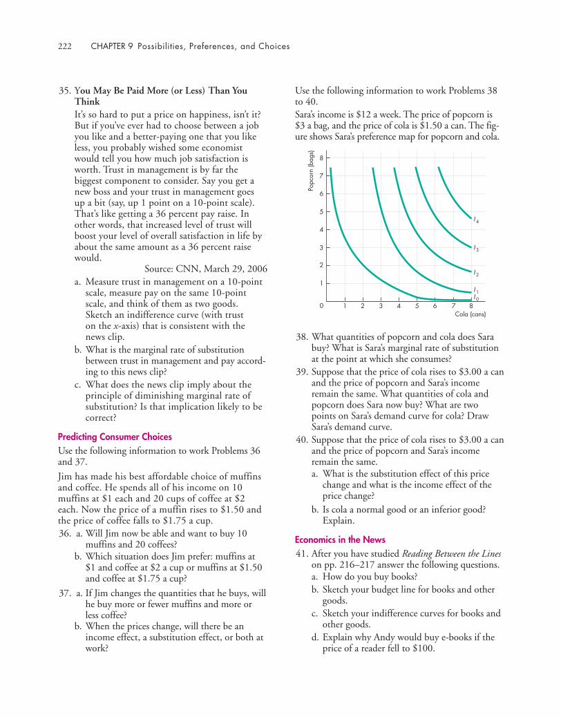
222 CHAPTER 9 Possibilities, Preferences, and Choices

35. You May Be Paid More (or Less) Than YouThinkIt’s so hard to put a price on happiness, isn’t it?But if you’ve ever had to choose between a jobyou like and a better-paying one that you likeless, you probably wished some economistwould tell you how much job satisfaction isworth. Trust in management is by far thebiggest component to consider. Say you get anew boss and your trust in management goes up a bit (say, up 1 point on a 10-point scale).That’s like getting a 36 percent pay raise. Inother words, that increased level of trust willboost your level of overall satisfaction in life byabout the same amount as a 36 percent raisewould.

Source: CNN, March 29, 2006a. Measure trust in management on a 10-point

scale, measure pay on the same 10-pointscale, and think of them as two goods.Sketch an indifference curve (with trust on the x-axis) that is consistent with the news clip.

b. What is the marginal rate of substitutionbetween trust in management and pay accord-ing to this news clip?

c. What does the news clip imply about theprinciple of diminishing marginal rate ofsubstitution? Is that implication likely to becorrect?

Predicting Consumer ChoicesUse the following information to work Problems 36and 37.

Jim has made his best affordable choice of muffinsand coffee. He spends all of his income on 10muffins at $1 each and 20 cups of coffee at $2each. Now the price of a muffin rises to $1.50 andthe price of coffee falls to $1.75 a cup.36. a. Will Jim now be able and want to buy 10

muffins and 20 coffees?b. Which situation does Jim prefer: muffins at

$1 and coffee at $2 a cup or muffins at $1.50and coffee at $1.75 a cup?

37. a. If Jim changes the quantities that he buys, willhe buy more or fewer muffins and more orless coffee?

b. When the prices change, will there be anincome effect, a substitution effect, or both atwork?

Use the following information to work Problems 38to 40.Sara’s income is $12 a week. The price of popcorn is$3 a bag, and the price of cola is $1.50 a can. The fig-ure shows Sara’s preference map for popcorn and cola.

38. What quantities of popcorn and cola does Sarabuy? What is Sara’s marginal rate of substitutionat the point at which she consumes?

39. Suppose that the price of cola rises to $3.00 a canand the price of popcorn and Sara’s incomeremain the same. What quantities of cola andpopcorn does Sara now buy? What are twopoints on Sara’s demand curve for cola? DrawSara’s demand curve.

40. Suppose that the price of cola rises to $3.00 a canand the price of popcorn and Sara’s incomeremain the same. a. What is the substitution effect of this price

change and what is the income effect of theprice change?

b. Is cola a normal good or an inferior good?Explain.

Economics in the News41. After you have studied Reading Between the Lines

on pp. 216–217 answer the following questions.a. How do you buy books?b. Sketch your budget line for books and other

goods.c. Sketch your indifference curves for books and

other goods.d. Explain why Andy would buy e-books if the

price of a reader fell to $100.

8

Cola (cans)0 8

Popc

orn

(bag

s)7654321

7

6

5

4

3

2

1

I 0

I 1

I 2

I 3

I 4

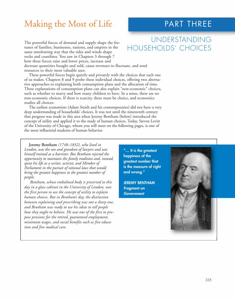
Jeremy Bentham (1748–1832), who lived inLondon, was the son and grandson of lawyers and washimself trained as a barrister. But Bentham rejected theopportunity to maintain the family tradition and, instead,spent his life as a writer, activist, and Member ofParliament in the pursuit of rational laws that wouldbring the greatest happiness to the greatest number ofpeople.

Bentham, whose embalmed body is preserved to thisday in a glass cabinet in the University of London, wasthe first person to use the concept of utility to explainhuman choices. But in Bentham’s day, the distinctionbetween explaining and prescribing was not a sharp one,and Bentham was ready to use his ideas to tell peoplehow they ought to behave. He was one of the first to pro-pose pensions for the retired, guaranteed employment,minimum wages, and social benefits such as free educa-tion and free medical care.

223

Making the Most of Life

The powerful forces of demand and supply shape the for-tunes of families, businesses, nations, and empires in thesame unrelenting way that the tides and winds shaperocks and coastlines. You saw in Chapters 3 through 7how these forces raise and lower prices, increase anddecrease quantities bought and sold, cause revenues to fluctuate, and sendresources to their most valuable uses.

These powerful forces begin quietly and privately with the choices that each oneof us makes. Chapters 8 and 9 probe these individual choices, offering two alterna-tive approaches to explaining both consumption plans and the allocation of time.These explanations of consumption plans can also explain “non-economic” choices,such as whether to marry and how many children to have. In a sense, there are nonon-economic choices. If there is scarcity, there must be choice, and economicsstudies all choices.

The earliest economists (Adam Smith and his contemporaries) did not have a verydeep understanding of households’ choices. It was not until the nineteenth centurythat progress was made in this area when Jeremy Bentham (below) introduced theconcept of utility and applied it to the study of human choices. Today, Steven Levittof the University of Chicago, whom you will meet on the following pages, is one ofthe most influential students of human behavior.

PART THREE

UNDERSTANDINGHOUSEHOLDS’ CHOICES

“... It is the greatesthappiness of thegreatest number thatis the measure of rightand wrong.”

JEREMY BENTHAMFragment onGovernment

224

clearly. The topics you apply these tools to are unlim-ited. That is why Ithink economicshas been so power-ful. If you under-stand economicsand use the toolswisely, you will bea better businessperson, doctor, public servant, parent.

What is the economic model of crime, and how does ithelp to design better ways of dealing with criminalactivity? Can you illustrate by talking a bit aboutyour work on the behavior of auto thieves? The economic model of crime argues that people havea choice of either working for a wage in the legal sectoror earning money from illegal activity. The model care-fully lays out the set of costs associated with being acriminal (e.g., forgone wages and being punished) andbenefits (e.g., the loot) associated with crime and ana-

I think of economics as beingprimarily about a way oflooking at the world and a setof tools for thinking clearly.

TALKING WITH Steven D. Levitt

Why did you become an economist?As a freshman in college, I took introductory eco-nomics. All the ideas made perfect sense to me—itwas the way I naturally thought. My friends werebefuddled. I thought, “This is the field for me!”

The idea of rational choice made at the margin lies atthe heart of economics. Would you say that your workgenerally supports that idea or challenges it? Can youprovide some examples?I don’t like the word “rational” in this context. I thinkeconomists model agents as being rational just for con-venience. What really matters is whether peoplerespond to incentives. My work very much supportsthe idea that humans in all types of circumstancesrespond strongly to incentives. I’ve seen it with drugdealers, auto thieves, sumo wrestlers, real estate agents,and elementary school teachers, just to name a fewexamples.

Can you elaborate? What are the incentives to whichdrug dealers respond? And does an understanding ofthese responses tell us anything about how public poli-cy might influence drug use?The incentives people face differ depending on theirparticular circumstances. Drug dealers, for instance,want to make money, but they also want to avoidbeing arrested or even killed. In the data we have ondrug sellers, we see that when the drug trade is morelucrative, dealers are willing to take greater risks ofarrest to carve out a share of the market. On the otherhand, they also do their best to minimize their risks.For example, crack sellers used to carry the crack withthem. When laws were passed imposing stiff penaltieson anyone caught with anything more than a minimalamount of crack, drug dealers responded by storingthe crack somewhere else, and retrieving only theamount being sold to the current client. Sumowrestlers, on the other hand, care mostly about theirofficial ranking. Sometimes matches occur where onewrestler has more to lose or gain than the otherwrestler. We find that sumo wrestlers make corruptdeals to make sure the wrestler who needs the win isthe one who actually wins.

Why is an economist interested in crime and cheating?I think of economics as being primarily about a way oflooking at the world and a set of tools for thinking

225

police. If you just look at different cities, the placeswith the most police also have the most crime, but itis not becausepolice cause crime,it is because crimecauses police to behired.

To figure out acausal impact ofpolice on crime,you would like todo a randomizedexperiment whereyou added a lot of police at random to some citiesand took them away in other cities. That is some-thing you cannot really do in real life. So instead, theeconomist has to look for “natural experiments” toanswer the question.

I used the timing of mayoral elections. It turns outthat mayors hire a lot of police before elections to “looktough on crime.” If elections do not otherwise affectcrime, then the election is kind of like a randomizingdevice that puts more police in some cities every oncein a while. Indeed, I found that crime goes down in theyear following elections once the police hired are upand running. It is indirect evidence, but it is an exam-ple of how economists use their toolbox to handle diffi-cult questions.

Your work shows that legalized abortion leads to lesscrime. Can you explain how you reach that conclu-sion? Can you also explain its implications for thepro-life, pro-choice debate?The theory is simple: Unwanted children have hardlives (including being much more likely to be crimi-nals); after legalized abortion, there are fewerunwanted children. Therefore, there should be lesscrime (with a 15–20 year lag while the babies growup and reach high-crime ages).

We looked at what happened to crime 15–20years after Roe v. Wade, in states with high and lowabortion rates and in states that legalized abortion afew years earlier than the rest of the country. Wecould even look at people born immediately before orafter abortion became legal.

All the evidence pointed the same way: Crimefell a lot because abortion was legalized.

Our results, however, don’t have large implica-tions for the abortion debate. If abortion is murder,

lyzes how a maximizing individual will choose whetherto commit crimes and how much crime to commit.One reason the model is useful is because it lays outthe various ways in which public policy might influ-ence crime rates. For instance, we can increase theprobability of a criminal getting caught or make theprison sentence longer for those who are caught. Thegovernment might also try to intervene in the labormarket to make legal work more attractive—forinstance, with a minimum wage.

What is the problem in figuring out whether more po-lice leads to less crime? How did you find the answer?We think that when you add more police, crime willfall because the cost of being a criminal goes upbecause of increased detection. From a public policyperspective, understanding how much crime falls inresponse to police is an important question. In prac-tice, it is hard to answer this question because wedon’t randomly hire police. Rather, where crime isbad, there is greater demand for police and thus more

If you just look at differentcities, the places with themost police also have themost crime, but it is notbecause police cause crime,it is because crime causespolice to be hired.

STEVEN D. LEVITT is Alvin H. Baum Professor ofEconomics at the University of Chicago. Born inMinneapolis, he was an undergraduate at Harvardand a graduate student at MIT. Among his manyhonors, he was recently awarded the John BatesClark Medal, given to the best economist under 40.

Professor Levitt has studied an astonishingly widerange of human choices and their outcomes. He hasexamined the effects of policing on crime, shownthat real estate agents get a higher price when theysell their own homes than when they sell other peo-ple’s, devised a test to detect cheating teachers, andstudied the choices of drug dealers and gang mem-bers. Much of this research has been popularized inFreakonomics (Steven D. Levitt and Stephen J. Dub-ner, HarperCollins, 2005). What unifies this appar-ently diverse body of research is the use of naturalexperiments. Professor Levitt has an incredible abili-ty to find just the right set of events and the data theevents have generated to enable him to isolate the ef-fect he’s looking for.

Michael Parkin talked with Steven Levitt abouthis career and the progress that economists havemade in understanding how people respond to in-centives in all aspects of life.

226

as pro-life advocates argue, then the changes in crimewe see are trivial in comparison. If a woman simplyhas the right to control her body, as pro-choice advo-cates argue, then our estimates about crime are like-wise irrelevant.

Our results have more to say about unwanted-ness: There are big benefits to making sure that chil-dren who are brought into the world are wantedand well cared for, through either birth control,adoption, abortion, or parental education.

Terrorism is on every-one’s minds these days.And presumably, ter-rorists respond to in-centives. Have youthought about how we

might be able to use the insights of economics to betterunderstand and perhaps even combat terrorism?Terrorism is an unusually difficult question to tacklethrough incentives. The religious terrorists we aremost worried about are willing to give up their livesto carry out terrorist acts. So the only punishmentwe can really offer is preventing them from commit-ting the act by catching them beforehand or maybe

minimizing the damage they can do. Unlike typicalcriminals, the threat of punishing them after thefact will not help deter the crime. Luckily, evenamong extremists, there are not many people willingto give their lives for a cause.

Can a student learn how to use natural experimentsor do you have a gift that is hard to teach?I don’t think I have such a gift. Most people who aregood at something are good because they haveworked hard and practiced. That is certainly truewith me.

For a while, I just walked around and every timeI observed anything in the world I asked myself, “Isthat a natural experiment?” Every once in a while Istumbled onto one because I was on the lookout.

What else can a student who wants to become a natu-ral experimenting economist or broader social scientistdo to better prepare for that career?I would say that the best thing students can do is to tryto really apply what they are learning to their lives,rather than just memorizing for an exam and quicklyforgetting. If you are passionate about economics (oranything else for that matter), you are way ahead ofothers who are just trying to get by.

. . . every time I observedanything in the world Iasked myself, “Is that anatural experiment?”

PART FOUR Firms and Markets

After studying this chapter, you will be able to:

� Explain what a firm is and describe the economicproblem that all firms face

� Distinguish between technological efficiency andeconomic efficiency

� Define and explain the principal–agent problem anddescribe how different types of business organizationscope with this problem

� Describe and distinguish between different types ofmarkets in which firms operate

� Explain why markets coordinate some economicactivities and why firms coordinate others

I n the fall of 1990, a British scientist named Tim Berners-Lee invented theWorld Wide Web. This remarkable idea paved the way for the creation ofthousands of profitable businesses that include Facebook and Twitter, Apple,Microsoft, Google, and Yahoo!.

Some of these successful dot.com firms sell goods and others sell services. Butmany firms, especially those that you can name, don’t make the things they sell:They buy them from other firms. For example, Apple doesn’t make the iPhone.Intel makes its memory chip and Foxconn, a firm in Taiwan, assembles its

components. Why doesn’t Apple make the iPhone? How do firmsdecide what to make themselves and what to buy from other firms?

How do Facebook, Twitter, Apple, Microsoft, Google, Intel,Foxconn, and the millions of other firms make their businessdecisions?

In this chapter, you are going to learn about firms and the choicesthey make. In Reading Between the Lines at the end of the chapter, we’ll applysome of what you’ve learned and look at some of the choices made byFacebook and Yahoo in the Internet advertising game.

ORGANIZINGPRODUCTION

10227

228 CHAPTER 10 Organizing Production

◆ The Firm and Its Economic Problem

The 20 million firms in the United States differ insize and in the scope of what they do, but they allperform the same basic economic functions. Eachfirm is an institution that hires factors of productionand organizes those factors to produce and sell goodsand services. Our goal is to predict firms’ behavior.To do so, we need to know a firm’s goal and the con-straints it faces. We start with the goal.

The Firm’s GoalWhen economists ask entrepreneurs what they aretrying to achieve, they get many different answers.Some talk about making a high-quality product,others about business growth, others about marketshare, others about the job satisfaction of their work-force, and an increasing number today talk aboutsocial and environmental responsibility. All of thesegoals are pursued by firms, but they are not the fun-damental goal: They are the means to that goal.

A firm’s goal is to maximize profit. A firm thatdoes not seek to maximize profit is either eliminated ortaken over by a firm that does seek that goal.

What is the profit that a firm seeks to maximize?To answer this question, we’ll look at CampusSweaters, Inc., a small producer of knitted sweatersowned and operated by Cindy.

Accounting ProfitIn 2010, Campus Sweaters received $400,000 for thesweaters it sold and paid out $80,000 for wool,$20,000 for utilities, $120,000 for wages, $5,000 forthe lease of a computer, and $5,000 in interest on abank loan. These expenses total $230,000, so thefirm had a cash surplus of $170,000.

To measure the profit of Campus Sweaters,Cindy’s accountant subtracted $20,000 for thedepreciation of buildings and knitting machinesfrom the $170,000 cash surplus. Depreciation is thefall in the value of a firm’s capital. To calculatedepreciation, accountants use Internal RevenueService rules based on standards established by theFinancial Accounting Standards Board. Using theserules, Cindy’s accountant calculated that CampusSweaters made a profit of $150,000 in 2010.

Economic AccountingAccountants measure a firm’s profit to ensure that thefirm pays the correct amount of income tax and toshow its investors how their funds are being used.

Economists measure a firm’s profit to enable them topredict the firm’s decisions, and the goal of these deci-sions is to maximize economic profit. Economic profit isequal to total revenue minus total cost, with total costmeasured as the opportunity cost of production.

A Firm’s Opportunity Cost of ProductionThe opportunity cost of any action is the highest-valued alternative forgone. The opportunity cost of pro-duction is the value of the best alternative use of theresources that a firm uses in production.

A firm’s opportunity cost of production is the valueof real alternatives forgone. We express opportunitycost in money units so that we can compare and addup the value of the alternatives forgone.

A firm’s opportunity cost of production is the sumof the cost of using resources

■ Bought in the market■ Owned by the firm■ Supplied by the firm’s owner

Resources Bought in the Market A firm incurs anopportunity cost when it buys resources in the mar-ket. The amount spent on these resources is anopportunity cost of production because the firmcould have bought different resources to producesome other good or service. For Campus Sweaters,the resources bought in the market are wool, utilities,labor, a leased computer, and a bank loan. The$230,000 spent on these items in 2010 could havebeen spent on something else, so it is an opportunitycost of producing sweaters.

Resources Owned by the Firm A firm incurs anopportunity cost when it uses its own capital. Thecost of using capital owned by the firm is an oppor-tunity cost of production because the firm could sellthe capital that it owns and rent capital fromanother firm. When a firm uses its own capital, itimplicitly rents it from itself. In this case, the firm’sopportunity cost of using the capital it owns iscalled the implicit rental rate of capital. The implicitrental rate of capital has two components: economicdepreciation and forgone interest.

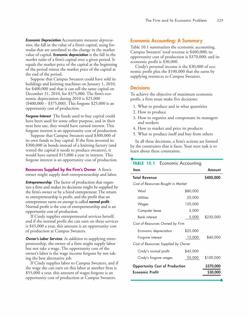
The Firm and Its Economic Problem 229

Economic Depreciation Accountants measure deprecia-tion, the fall in the value of a firm’s capital, using for-mulas that are unrelated to the change in the marketvalue of capital. Economic depreciation is the fall in themarket value of a firm’s capital over a given period. Itequals the market price of the capital at the beginningof the period minus the market price of the capital atthe end of the period.

Suppose that Campus Sweaters could have sold itsbuildings and knitting machines on January 1, 2010,for $400,000 and that it can sell the same capital onDecember 31, 2010, for $375,000. The firm’s eco-nomic depreciation during 2010 is $25,000($400,000 – $375,000). This forgone $25,000 is anopportunity cost of production.

Forgone Interest The funds used to buy capital couldhave been used for some other purpose, and in theirnext best use, they would have earned interest. Thisforgone interest is an opportunity cost of production.

Suppose that Campus Sweaters used $300,000 ofits own funds to buy capital. If the firm invested its$300,000 in bonds instead of a knitting factory (andrented the capital it needs to produce sweaters), itwould have earned $15,000 a year in interest. Thisforgone interest is an opportunity cost of production.

Resources Supplied by the Firm’s Owner A firm’sowner might supply both entrepreneurship and labor.

Entrepreneurship The factor of production that organ-izes a firm and makes its decisions might be supplied bythe firm’s owner or by a hired entrepreneur. The returnto entrepreneurship is profit, and the profit that anentrepreneur earns on average is called normal profit.Normal profit is the cost of entrepreneurship and is anopportunity cost of production.

If Cindy supplies entrepreneurial services herself,and if the normal profit she can earn on these servicesis $45,000 a year, this amount is an opportunity costof production at Campus Sweaters.

Owner’s Labor Services In addition to supplying entre-preneurship, the owner of a firm might supply laborbut not take a wage. The opportunity cost of theowner’s labor is the wage income forgone by not tak-ing the best alternative job.

If Cindy supplies labor to Campus Sweaters, and ifthe wage she can earn on this labor at another firm is$55,000 a year, this amount of wages forgone is anopportunity cost of production at Campus Sweaters.

Economic Accounting: A SummaryTable 10.1 summarizes the economic accounting.Campus Sweaters’ total revenue is $400,000; itsopportunity cost of production is $370,000; and itseconomic profit is $30,000.

Cindy’s personal income is the $30,000 of eco-nomic profit plus the $100,000 that she earns bysupplying resources to Campus Sweaters.

DecisionsTo achieve the objective of maximum economicprofit, a firm must make five decisions:

1. What to produce and in what quantities2. How to produce3. How to organize and compensate its managers

and workers4. How to market and price its products5. What to produce itself and buy from others

In all these decisions, a firm’s actions are limitedby the constraints that it faces. Your next task is tolearn about these constraints.

Item Amount

Total Revenue $400,000

Cost of Resources Bought in Market

Wool $80,000

Utilities 20,000

Wages 120,000

Computer lease 5,000

Bank interest 5,000 $230,000

Cost of Resources Owned by Firm

Economic depreciation $25,000

Forgone interest 15,000 $40,000

Cost of Resources Supplied by Owner

Cindy’s normal profit $45,000

Cindy’s forgone wages 55,000 $100,000

Opportunity Cost of Production $370,000

Economic Profit $30,000

TABLE 10.1 Economic Accounting

230 CHAPTER 10 Organizing Production

The Firm’s ConstraintsThree features of a firm’s environment limit the maxi-mum economic profit it can make. They are

■ Technology constraints■ Information constraints■ Market constraints

Technology Constraints Economists define technol-ogy broadly. A technology is any method of producinga good or service. Technology includes the detaileddesigns of machines and the layout of the workplace.It includes the organization of the firm. For example,the shopping mall is one technology for producingretail services. It is a different technology from thecatalog store, which in turn is different from thedowntown store.

It might seem surprising that a firm’s profit is lim-ited by technology because it seems that technologicaladvances are constantly increasing profit opportuni-ties. Almost every day, we learn about some newtechnological advance that amazes us. With comput-ers that speak and recognize our own speech and carsthat can find the address we need in a city we’venever visited, we can accomplish more than ever.

Technology advances over time. But at each pointin time, to produce more output and gain more rev-enue, a firm must hire more resources and incurgreater costs. The increase in profit that a firm canachieve is limited by the technology available. Forexample, by using its current plant and workforce,Ford can produce some maximum number of carsper day. To produce more cars per day, Ford musthire more resources, which increases its costs and lim-its the increase in profit that it can make by sellingthe additional cars.

Information Constraints We never possess all theinformation we would like to have to make decisions.We lack information about both the future and thepresent. For example, suppose you plan to buy a newcomputer. When should you buy it? The answerdepends on how the price is going to change in thefuture. Where should you buy it? The answer dependson the prices at hundreds of different computer stores.To get the best deal, you must compare the qualityand prices in every store. But the opportunity cost ofthis comparison exceeds the cost of the computer!

A firm is constrained by limited information aboutthe quality and efforts of its workforce, the current

and future buying plans of its customers, and theplans of its competitors. Workers might make too lit-tle effort, customers might switch to competing sup-pliers, and a competitor might enter the market andtake some of the firm’s business.

To address these problems, firms create incentivesto boost workers’ efforts even when no one is moni-toring them; conduct market research to lower uncer-tainty about customers’ buying plans, and “spy” oneach other to anticipate competitive challenges. Butthese efforts don’t eliminate incomplete informationand uncertainty, which limit the economic profit thata firm can make.

Market Constraints The quantity each firm can selland the price it can obtain are constrained by its cus-tomers’ willingness to pay and by the prices and mar-keting efforts of other firms. Similarly, the resourcesthat a firm can buy and the prices it must pay forthem are limited by the willingness of people to workfor and invest in the firm. Firms spend billions ofdollars a year marketing and selling their products.Some of the most creative minds strive to find theright message that will produce a knockout televisionadvertisement. Market constraints and the expendi-tures firms make to overcome them limit the profit afirm can make.

In the rest of this chapter and in Chapters 11through 14, we study the choices that firms make.You’re going to learn how we can predict a firm’sdecisions as those that maximize profit given the con-straints the firm faces. We begin by taking a closerlook at a firm’s technology constraints.

REVIEW QUIZ1 What is a firm’s fundamental goal and what

happens if the firm doesn’t pursue this goal?2 Why do accountants and economists calculate a

firm’s cost and profit in different ways?3 What are the items that make opportunity cost

differ from the accountant’s measure of cost?4 Why is normal profit an opportunity cost?5 What are the constraints that a firm faces? How

does each constraint limit the firm’s profit?

You can work these questions in Study Plan 10.1 and get instant feedback.

Technological and Economic Efficiency 231

◆ Technological and Economic Efficiency

Microsoft employs a large workforce, and mostMicrosoft workers possess a large amount of humancapital. But the firm uses a small amount of physicalcapital. In contrast, a coal-mining company employsa huge amount of mining equipment (physical capi-tal) and almost no labor. Why? The answer lies in theconcept of efficiency. There are two concepts of pro-duction efficiency: technological efficiency and eco-nomic efficiency. Technological efficiency occurs whenthe firm produces a given output by using the leastamount of inputs. Economic efficiency occurs when thefirm produces a given output at the least cost. Let’sexplore the two concepts of efficiency by studying anexample.

Suppose that there are four alternative techniquesfor making TVs:

A. Robot production. One person monitors the entirecomputer-driven process.

B. Production line. Workers specialize in a small partof the job as the emerging TV passes them on aproduction line.

C. Hand-tool production. A single worker uses a fewhand tools to make a TV.

D. Bench production. Workers specialize in a smallpart of the job but walk from bench to bench toperform their tasks.

Table 10.2 sets out the amounts of labor and capi-tal required by each of these four methods to make10 TVs a day.

Which of these alternative methods are technolog-ically efficient?

Technological EfficiencyRecall that technological efficiency occurs whenthe firm produces a given output by using the leastamount of inputs. Look at the numbers in the tableand notice that method A uses the most capital andthe least labor. Method C uses the most labor and theleast capital. Method B and method D lie betweenthe two extremes. They use less capital and morelabor than method A and less labor but more capitalthan method C.

Compare methods B and D. Method D requires100 workers and 10 units of capital to produce 10

TVs. Those same 10 TVs can be produced bymethod B with 10 workers and the same 10 units ofcapital. Because method D uses the same amount ofcapital and more labor than method B, method D isnot technologically efficient.

Are any of the other methods not technologicallyefficient? The answer is no. Each of the other meth-ods is technologically efficient. Method A uses morecapital but less labor than method B, and method Cuses more labor but less capital than method B.

Which of the methods are economically efficient?

Economic EfficiencyRecall that economic efficiency occurs when the firmproduces a given output at the least cost.

Method D, which is technologically inefficient,is also economically inefficient. It uses the sameamount of capital as method B but 10 times as muchlabor, so it costs more. A technologically inefficientmethod is never economically efficient.

One of the three technologically efficient methodsis economically efficient. The other two are economi-cally inefficient. But which method is economicallyefficient depends on factor prices.

In Table 10.3(a), the wage rate is $75 per dayand the rental rate of capital is $250 per day. Bystudying Table 10.3(a), you can see that method Bhas the lowest cost and is the economically effi-cient method.

In Table 10.3(b), the wage rate is $150 a day andthe rental rate of capital is $1 a day. Looking at Table10.3(b), you can see that method A has the lowestcost and is the economically efficient method. In thiscase, capital is so cheap relative to labor that the

Quantities of inputs

Method Labor Capital

A Robot production 1 1,000

B Production line 10 10

C Hand-tool production 1,000 1

D Bench production 100 10

TABLE 10.2 Four Ways of Making 10 TVs a Day

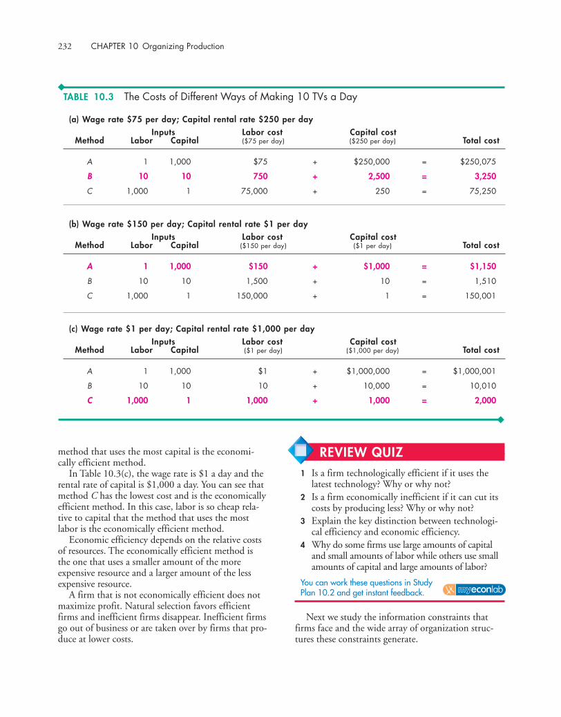
232 CHAPTER 10 Organizing Production

Next we study the information constraints thatfirms face and the wide array of organization struc-tures these constraints generate.

method that uses the most capital is the economi-cally efficient method.

In Table 10.3(c), the wage rate is $1 a day and therental rate of capital is $1,000 a day. You can see thatmethod C has the lowest cost and is the economicallyefficient method. In this case, labor is so cheap rela-tive to capital that the method that uses the mostlabor is the economically efficient method.

Economic efficiency depends on the relative costsof resources. The economically efficient method isthe one that uses a smaller amount of the moreexpensive resource and a larger amount of the lessexpensive resource.

A firm that is not economically efficient does notmaximize profit. Natural selection favors efficientfirms and inefficient firms disappear. Inefficient firmsgo out of business or are taken over by firms that pro-duce at lower costs.

(a) Wage rate $75 per day; Capital rental rate $250 per dayInputs Labor cost Capital cost

Method Labor Capital ($75 per day) ($250 per day) Total cost

A 1 1,000 $75 + $250,000 = $250,075

B 10 10 750 + 2,500 = 3,250

C 1,000 1 75,000 + 250 = 75,250

(b) Wage rate $150 per day; Capital rental rate $1 per dayInputs Labor cost Capital cost

Method Labor Capital ($150 per day) ($1 per day) Total cost

A 1 1,000 $150 + $1,000 = $1,150

B 10 10 1,500 + 10 = 1,510

C 1,000 1 150,000 + 1 = 150,001

(c) Wage rate $1 per day; Capital rental rate $1,000 per dayInputs Labor cost Capital cost

Method Labor Capital ($1 per day) ($1,000 per day) Total cost

A 1 1,000 $1 + $1,000,000 = $1,000,001

B 10 10 10 + 10,000 = 10,010

C 1,000 1 1,000 + 1,000 = 2,000

TABLE 10.3 The Costs of Different Ways of Making 10 TVs a Day

REVIEW QUIZ 1 Is a firm technologically efficient if it uses the

latest technology? Why or why not?2 Is a firm economically inefficient if it can cut its

costs by producing less? Why or why not?3 Explain the key distinction between technologi-

cal efficiency and economic efficiency.4 Why do some firms use large amounts of capital

and small amounts of labor while others use smallamounts of capital and large amounts of labor?

You can work these questions in Study Plan 10.2 and get instant feedback.

Information and Organization 233

◆ Information and OrganizationEach firm organizes the production of goods andservices by combining and coordinating the produc-tive resources it hires. But there is variety across firmsin how they organize production. Firms use a mixtureof two systems:

■ Command systems■ Incentive systems

Command SystemsA command system is a method of organizingproduction that uses a managerial hierarchy.Commands pass downward through the hierarchy,and information passes upward. Managers spendmost of their time collecting and processing infor-mation about the performance of the people undertheir control and making decisions about what com-mands to issue and how best to get those commandsimplemented.

The military uses the purest form of commandsystem. A commander-in-chief (in the United States,the President) makes the big decisions about strategicgoals. Beneath this highest level, generals organizetheir military resources. Beneath the generals, succes-sively lower ranks organize smaller and smaller unitsbut pay attention to ever-increasing degrees of detail.At the bottom of the managerial hierarchy are thepeople who operate weapons systems.

Command systems in firms are not as rigid as thosein the military, but they share some similar features. Achief executive officer (CEO) sits at the top of a firm’scommand system. Senior executives who report toand receive commands from the CEO specialize inmanaging production, marketing, finance, personnel,and perhaps other aspects of the firm’s operations.Beneath these senior managers might be several tiersof middle management ranks that stretch downwardto the managers who supervise the day-to-day opera-tions of the business. Beneath these managers are thepeople who operate the firm’s machines and whomake and sell the firm’s goods and services.

Small firms have one or two layers of managers,while large firms have several layers. As productionprocesses have become ever more complex, manage-ment ranks have swollen. Today, more people havemanagement jobs than ever before, even though theinformation revolution of the 1990s slowed thegrowth of management. In some industries, the

information revolution reduced the number of lay-ers of managers and brought a shakeout of middlemanagers.

Managers make enormous efforts to be wellinformed. They try hard to make good decisions andissue commands that end up using resources effi-ciently. But managers always have incomplete infor-mation about what is happening in the divisions ofthe firm for which they are responsible. For this rea-son, firms use incentive systems as well as commandsystems to organize production.

Incentive SystemsAn incentive system is a method of organizing produc-tion that uses a market-like mechanism inside thefirm. Instead of issuing commands, senior managerscreate compensation schemes to induce workers toperform in ways that maximize the firm’s profit.

Selling organizations use incentive systems mostextensively. Sales representatives who spend most oftheir working time alone and unsupervised areinduced to work hard by being paid a small salaryand a large performance-related bonus.

But incentive systems operate at all levels in afirm. The compensation plan of a CEO includes ashare in the firm’s profit, and factory floor workerssometimes receive compensation based on the quan-tity they produce.

Mixing the SystemsFirms use a mixture of commands and incentives,and they choose the mixture that maximizes profit.Firms use commands when it is easy to monitor per-formance or when a small deviation from an idealperformance is very costly. They use incentives whenit is either not possible to monitor performance ortoo costly to be worth doing.

For example, PepsiCo can easily monitor the per-formance of workers on a production line. If one per-son works too slowly, the entire line slows, so aproduction line is organized with a command system.

In contrast, it is costly to monitor a CEO. Forexample, what does Steve Jobs, the CEO of AppleInc., contribute to Apple’s success? This question can’tbe answered with certainty, yet Apple’s stockholdershave to put someone in charge of the business andprovide that person with an incentive to maximizestockholders’ returns. The performance of Apple

234 CHAPTER 10 Organizing Production

illustrates a general problem, known as the princi-pal–agent problem.

The Principal–Agent ProblemThe principal–agent problem is the problem of devisingcompensation rules that induce an agent to act in thebest interest of a principal. For example, the stockhold-ers of Texaco are principals, and the firm’s managers areagents. The stockholders (the principals) must inducethe managers (agents) to act in the stockholders’ bestinterest. Similarly, Steve Jobs (a principal) must inducethe designers who are working on the next generationiPhone (agents) to work efficiently.

Agents, whether they are managers or workers, pur-sue their own goals and often impose costs on a prin-cipal. For example, the goal of stockholders ofCiticorp (principals) is to maximize the firm’s profit—its true profit, not some fictitious paper profit. Butthe firm’s profit depends on the actions of its man-agers (agents), and they have their own goals. Perhapsa bank manager takes a customer to a ball game onthe pretense that she is building customer loyalty,when in fact she is simply enjoying on-the-job leisure.This same manager is also a principal, and her tellersare agents. The manager wants the tellers to workhard and attract new customers so that she can meether operating targets. But the workers enjoy conversa-tions with each other and take on-the-job leisure.Nonetheless, the firm constantly strives to find waysof improving performance and increasing profits.

Coping with the Principal–Agent ProblemIssuing commands does not address the principal–agentproblem. In most firms, the shareholders can’t monitorthe managers and often the managers can’t monitorthe workers. Each principal must create incentivesthat induce each agent to work in the interests of theprincipal. Three ways of attempting to cope with theprincipal–agent problem are

■ Ownership■ Incentive pay■ Long-term contracts

Ownership By assigning ownership (or part-ownership) of a business to managers or workers, itis sometimes possible to induce a job performancethat increases a firm’s profits. Part-ownership isquite common for senior managers but less com-

mon for workers. When United Airlines was run-ning into problems a few years ago, it made most ofits employees owners of the company.

Incentive Pay Incentive pay—pay related to per-formance—is very common. Incentives are based ona variety of performance criteria such as profits, pro-duction, or sales targets. Promoting an employee forgood performance is another example of the use ofincentive pay.

Long-Term Contracts Long-term contracts tie thelong-term fortunes of managers and workers (agents)to the success of the principal(s)—the owner(s) of thefirm. For example, a multiyear employment contractfor a CEO encourages that person to take a long-term view and devise strategies that achieve maxi-mum profit over a sustained period.

These three ways of coping with the principal–agentproblem give rise to different types of business organi-zation. Each type of business organization is a differentresponse to the principal–agent problem. Each typeuses a different combination of ownership, incentives,and long-term contracts. Let’s look at the main types ofbusiness organization.

Types of Business OrganizationThe three main types of business organization are

■ Proprietorship■ Partnership■ Corporation

Proprietorship A proprietorship is a firm with a singleowner—a proprietor—who has unlimited liability.Unlimited liability is the legal responsibility for all thedebts of a firm up to an amount equal to the entirewealth of the owner. If a proprietorship cannot payits debts, those to whom the firm owes money canclaim the personal property of the owner. Businessesof some farmers, computer programmers, and artistsare examples of proprietorships.

The proprietor makes management decisions,receives the firm’s profits, and is responsible for its losses.Profits from a proprietorship are taxed at the same rateas other sources of the proprietor’s personal income.

Partnership A partnership is a firm with two or moreowners who have unlimited liability. Partners mustagree on an appropriate management structure and

Information and Organization 235

on how to divide the firm’s profits among them-selves. The profits of a partnership are taxed as thepersonal income of the owners, but each partner islegally liable for all the debts of the partnership (limited only by the wealth of that individualpartner). Liability for the full debts of the partnershipis called joint unlimited liability. Most law firms arepartnerships.

Corporation A corporation is a firm owned by oneor more limited liability stockholders. Limited lia-bility means that the owners have legal liability onlyfor the value of their initial investment. This limi-tation of liability means that if the corporationbecomes bankrupt, its owners are not required touse their personal wealth to pay the corporation’sdebts.

Corporations’ profits are taxed independently ofstockholders’ incomes. Stockholders pay a capital

gains tax on the profit they earn when they sell astock for a higher price than they paid for it.Corporate stocks generate capital gains when acorporation retains some of its profit and reinvests itin profitable activities. So retained earnings are taxedtwice because the capital gains they generate aretaxed. Dividend payments are also taxed but at alower rate than other sources of income.

Pros and Cons of Different Types of FirmsThe different types of business organization arisefrom firms trying to cope with the principal–agentproblem. Each type has advantages in particular situ-ations and because of its special advantages, each typecontinues to exist. Each type of business organizationalso has disadvantages.

Table 10.4 summarizes these and other pros andcons of the different types of firms.

Type of Firm Pros Cons

Proprietorship ■ Easy to set up■ Simple decision making■ Profits taxed only once as

owner’s income

Partnership ■ Easy to set up■ Diversified decision making■ Can survive withdrawal of

partner■ Profits taxed only once as

owners’ incomes

Corporation ■ Owners have limited liability■ Large-scale, low-cost capital

available■ Professional management not

restricted by ability of owners■ Perpetual life■ Long-term labor contracts cut

labor costs

■ Bad decisions not checked; no need for consensus

■ Owner’s entire wealth at risk■ Firm dies with owner■ Cost of capital and labor is high relative to that

of a corporation

■ Achieving consensus may be slow and expensive■ Owners’ entire wealth at risk■ Withdrawal of partner may create capital

shortage■ Cost of capital and labor is high relative to that of a

corporation

■ Complex management structure can make decisionsslow and expensive

■ Retained profits taxed twice: as company profit and as stockholders’ capital gains

TABLE 10.4 The Pros and Cons of Different Types of Firms

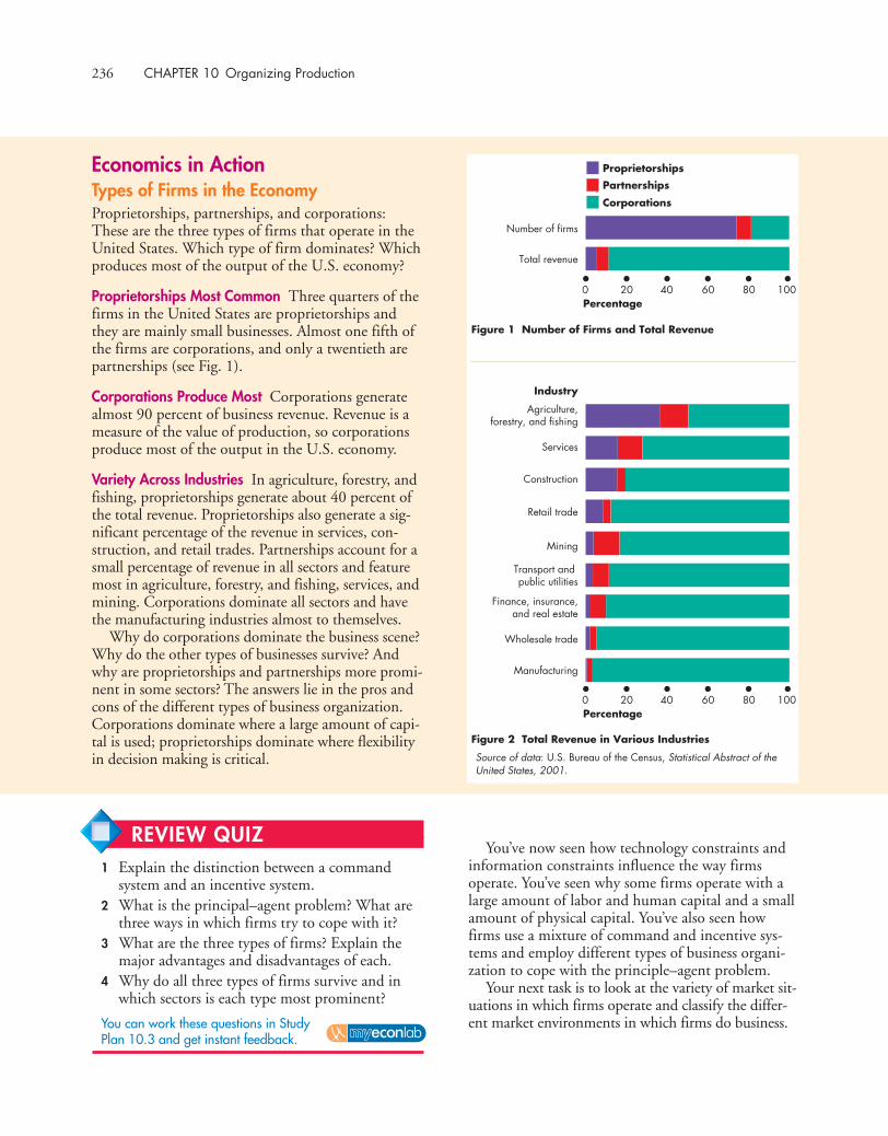
236 CHAPTER 10 Organizing Production

Economics in ActionTypes of Firms in the EconomyProprietorships, partnerships, and corporations:These are the three types of firms that operate in theUnited States. Which type of firm dominates? Whichproduces most of the output of the U.S. economy?

Proprietorships Most Common Three quarters of thefirms in the United States are proprietorships andthey are mainly small businesses. Almost one fifth ofthe firms are corporations, and only a twentieth arepartnerships (see Fig. 1).

Corporations Produce Most Corporations generatealmost 90 percent of business revenue. Revenue is ameasure of the value of production, so corporationsproduce most of the output in the U.S. economy.

Variety Across Industries In agriculture, forestry, andfishing, proprietorships generate about 40 percent ofthe total revenue. Proprietorships also generate a sig-nificant percentage of the revenue in services, con-struction, and retail trades. Partnerships account for asmall percentage of revenue in all sectors and featuremost in agriculture, forestry, and fishing, services, andmining. Corporations dominate all sectors and havethe manufacturing industries almost to themselves.

Why do corporations dominate the business scene?Why do the other types of businesses survive? Andwhy are proprietorships and partnerships more promi-nent in some sectors? The answers lie in the pros andcons of the different types of business organization.Corporations dominate where a large amount of capi-tal is used; proprietorships dominate where flexibilityin decision making is critical.

0 20 40 60 80 100

0 20 40 60 80 100Percentage

Percentage

Proprietorships

Partnerships

Corporations

Number of firms

Total revenue

Mining

Agriculture,forestry, and fishing

Industry

Services

Construction

Retail trade

Transport and public utilities

Finance, insurance,and real estate

Wholesale trade

Manufacturing

Figure 1 Number of Firms and Total Revenue

Figure 2 Total Revenue in Various Industries

You’ve now seen how technology constraints andinformation constraints influence the way firmsoperate. You’ve seen why some firms operate with alarge amount of labor and human capital and a smallamount of physical capital. You’ve also seen howfirms use a mixture of command and incentive sys-tems and employ different types of business organi-zation to cope with the principle–agent problem.

Your next task is to look at the variety of market sit-uations in which firms operate and classify the differ-ent market environments in which firms do business.

Source of data: U.S. Bureau of the Census, Statistical Abstract of theUnited States, 2001.

REVIEW QUIZ 1 Explain the distinction between a command

system and an incentive system.2 What is the principal–agent problem? What are

three ways in which firms try to cope with it?3 What are the three types of firms? Explain the

major advantages and disadvantages of each.4 Why do all three types of firms survive and in

which sectors is each type most prominent?

You can work these questions in Study Plan 10.3 and get instant feedback.

Markets and the Competitive Environment 237

◆ Markets and the Competitive Environment

The markets in which firms operate vary a great deal.Some are highly competitive, and profits in thesemarkets are hard to come by. Some appear to bealmost free from competition, and firms in thesemarkets earn large profits. Some markets are domi-nated by fierce advertising campaigns in which eachfirm seeks to persuade buyers that it has the bestproducts. And some markets display the character ofa strategic game.

Economists identify four market types:

1. Perfect competition2. Monopolistic competition3. Oligopoly4. Monopoly

Perfect competition arises when there are manyfirms, each selling an identical product, many buyers,and no restrictions on the entry of new firms into theindustry. The many firms and buyers are all wellinformed about the prices of the products of eachfirm in the industry. The worldwide markets forcorn, rice, and other grain crops are examples of per-fect competition.

Monopolistic competition is a market structure inwhich a large number of firms compete by making sim-ilar but slightly different products. Making a product

slightly different from the product of a competing firmis called product differentiation. Product differentiationgives a firm in monopolistic competition an element ofmarket power. The firm is the sole producer of the par-ticular version of the good in question. For example, inthe market for pizzas, hundreds of firms make theirown version of the perfect pizza. Each of these firms isthe sole producer of a particular brand. Differentiatedproducts are not necessarily different products. Whatmatters is that consumers perceive them to be different.For example, different brands of potato chips andketchup might be almost identical but be perceived byconsumers to be different.

Oligopoly is a market structure in which a smallnumber of firms compete. Computer software, air-plane manufacture, and international air transportationare examples of oligopolistic industries. Oligopoliesmight produce almost identical products, such as thecolas produced by Coke and Pepsi. Or they mightproduce differentiated products such as Boeing andAirbus aircraft.

Monopoly arises when there is one firm, which pro-duces a good or service that has no close substitutes andin which the firm is protected by a barrier preventingthe entry of new firms. In some places, the phone, gas,electricity, cable television, and water suppliers are localmonopolies—monopolies restricted to a given location.Microsoft Corporation, the software developer that cre-ated Windows and Vista, is an example of a globalmonopoly.

238 CHAPTER 10 Organizing Production

Perfect competition is the most extreme form ofcompetition. Monopoly is the most extreme absenceof competition. The other two market types fallbetween these extremes.

Many factors must be taken into account to deter-mine which market structure describes a particularreal-world market. One of these factors is the extentto which a small number of firms dominates the mar-ket. To measure this feature of markets, economistsuse indexes called measures of concentration. Let’slook at these measures.

Measures of ConcentrationEconomists use two measures of concentration:

■ The four-firm concentration ratio■ The Herfindahl-Hirschman Index

The Four-Firm Concentration Ratio The four-firm con-centration ratio is the percentage of the value of salesaccounted for by the four largest firms in an industry.The range of the concentration ratio is from almostzero for perfect competition to 100 percent formonopoly. This ratio is the main measure used toassess market structure.

Table 10.5 shows two calculations of the four-firmconcentration ratio: one for tire makers and one for

printers. In this example, 14 firms produce tires. Thelargest four have 80 percent of the sales, so the four-firm concentration ratio is 80 percent. In the printingindustry, with 1,004 firms, the largest four firms haveonly 0.5 percent of the sales, so the four-firm concen-tration ratio is 0.5 percent.

A low concentration ratio indicates a high degreeof competition, and a high concentration ratio indi-cates an absence of competition. A monopoly has aconcentration ratio of 100 percent—the largest (andonly) firm has 100 percent of the sales. A four-firmconcentration ratio that exceeds 60 percent isregarded as an indication of a market that is highlyconcentrated and dominated by a few firms in an oli-gopoly. A ratio of less than 60 percent is regarded asan indication of a competitive market.

The Herfindahl-Hirschman Index The Herfindahl-Hirschman Index—also called the HHI—is the squareof the percentage market share of each firm summedover the largest 50 firms (or summed over all thefirms if there are fewer than 50) in a market. Forexample, if there are four firms in a market and themarket shares of the firms are 50 percent, 25 percent,15 percent, and 10 percent, the Herfindahl-Hirschman Index is

HHI � 502 � 252 � 152 � 102 � 3,450.

TABLE 10.5 Calculating the Four-Firm Concentration Ratio

Tire makers Printers

Sales SalesFirm (millions of dollars) Firm (millions of dollars)

Top, Inc. 200 Fran’s 2.5

ABC, Inc. 250 Ned’s 2.0

Big, Inc. 150 Tom’s 1.8

XYZ, Inc. 100 Jill’s 1.7

Largest 4 firms 700 Largest 4 firms 8.0

Other 10 firms 175 Other 1,000 firms 1,592.0

Industry 875 Industry 1,600.0

Four-firm concentration ratios:

Tire makers: Printers: 8

1,600� 100 � 0.5 percent

700875

� 100 � 80 percent

Markets and the Competitive Environment 239

In perfect competition, the HHI is small. For exam-ple, if each of the largest 50 firms in an industry has amarket share of 0.1 percent, then the HHI is 0.12 � 50 � 0.5. In a monopoly, the HHI is 10,000.The firm has 100 percent of the market: 1002 � 10,000.

The HHI became a popular measure of the degreeof competition during the 1980s, when the JusticeDepartment used it to classify markets. A market in

Chewing gum

Industry

Household laundry equip.

Light bulbs

Breakfast cereal

Motor vehicles

Macaroni and spaghetti

Chocolate products

Pet food

Cookies and crackers

Computers

Soft drinks

Pharmaceuticals

Ice cream

Newspapers

Milk

Men‘s and boy‘s clothing

Women‘s clothing

Concrete blocks and bricks

Commercial printing

0 20 40 60 80 100

Four-firm concentration ratio (percentage)

..

2855

..

2253

2676

2237

2188

1229

1169

680

537

341

241

293

181

198

61

30

22

Herfindahl-Hirschman Index

Concentration Measures in the United States

Economics in ActionConcentration in the U.S. EconomyThe U.S. Department of Commerce calculates andpublishes data showing concentration ratios and theHHI for each industry in the United States. The barsin the figure show the four-firm concentration ratioand the number at the end of each bar is the HHI.

Chewing gum is one of the most concentratedindustries. William Wrigley Jr. Company of Chicagoemploys 16,000 people and sells $5 billion worth ofgum a year. It does have some competitors but theyhave a very small market share.

Household laundry equipment, light bulbs, break-fast cereal, and motor vehicles are highly concen-trated industries. They are oligopolies.

Pet food, cookies and crackers, computers, andsoft drinks are moderately concentrated industries.They are examples of monopolistic competition.

Ice cream, milk, clothing, concrete blocks andbricks, and commercial printing industries have lowconcentration measures and are highly competitive.

Concentration measures are useful indicators ofthe degree of competition in a market, but they mustbe supplemented by other information to determinethe structure of the market.

Newspapers and automobiles are examples of howthe concentration measures give a misleading readingof the degree of competition. Most newspapers arelocal. They serve a single city or even smaller area. Sodespite the low concentration measure, newspapersare concentrated in their own local areas.Automobiles are traded internationally and foreigncars are freely imported into the United States.Despite the high U.S. concentration measure, theautomobile industry is competitive.

which the HHI is less than 1,000 is regarded as beingcompetitive. A market in which the HHI lies between1,000 and 1,800 is regarded as being moderately com-petitive. But a market in which the HHI exceeds 1,800is regarded as being uncompetitive. The JusticeDepartment scrutinizes any merger of firms in a mar-ket in which the HHI exceeds 1,000 and is likely tochallenge a merger if the HHI exceeds 1,800.

Source of data: Concentration Ratios in Manufacturing, (Washington,D.C.: U.S. Department of Commerce,1996).

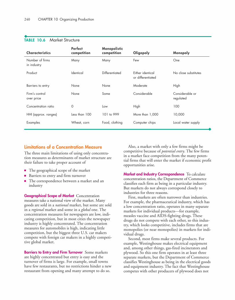
240 CHAPTER 10 Organizing Production

Limitations of a Concentration MeasureThe three main limitations of using only concentra-tion measures as determinants of market structure aretheir failure to take proper account of

■ The geographical scope of the market■ Barriers to entry and firm turnover■ The correspondence between a market and an

industry

Geographical Scope of Market Concentrationmeasures take a national view of the market. Manygoods are sold in a national market, but some are soldin a regional market and some in a global one. Theconcentration measures for newspapers are low, indi-cating competition, but in most cities the newspaperindustry is highly concentrated. The concentrationmeasures for automobiles is high, indicating littlecompetition, but the biggest three U.S. car makerscompete with foreign car makers in a highly competi-tive global market.

Barriers to Entry and Firm Turnover Some marketsare highly concentrated but entry is easy and theturnover of firms is large. For example, small townshave few restaurants, but no restrictions hinder a newrestaurant from opening and many attempt to do so.

Also, a market with only a few firms might becompetitive because of potential entry. The few firmsin a market face competition from the many poten-tial firms that will enter the market if economic profitopportunities arise.

Market and Industry Correspondence To calculateconcentration ratios, the Department of Commerceclassifies each firm as being in a particular industry.But markets do not always correspond closely toindustries for three reasons.

First, markets are often narrower than industries.For example, the pharmaceutical industry, which hasa low concentration ratio, operates in many separatemarkets for individual products—for example,measles vaccine and AIDS-fighting drugs. Thesedrugs do not compete with each other, so this indus-try, which looks competitive, includes firms that aremonopolies (or near monopolies) in markets for indi-vidual drugs.

Second, most firms make several products. Forexample, Westinghouse makes electrical equipmentand, among other things, gas-fired incinerators andplywood. So this one firm operates in at least threeseparate markets, but the Department of Commerceclassifies Westinghouse as being in the electrical goodsand equipment industry. The fact that Westinghousecompetes with other producers of plywood does not

TABLE 10.6 Market Structure

Perfect MonopolisticCharacteristics competition competition Oligopoly Monopoly

Number of firms Many Many Few Onein industry

Product Identical Differentiated Either identical No close substitutesor differentiated

Barriers to entry None None Moderate High

Firm’s control None Some Considerable Considerable or over price regulated

Concentration ratio 0 Low High 100

HHI (approx. ranges) Less than 100 101 to 999 More than 1,000 10,000

Examples Wheat, corn Food, clothing Computer chips Local water supply

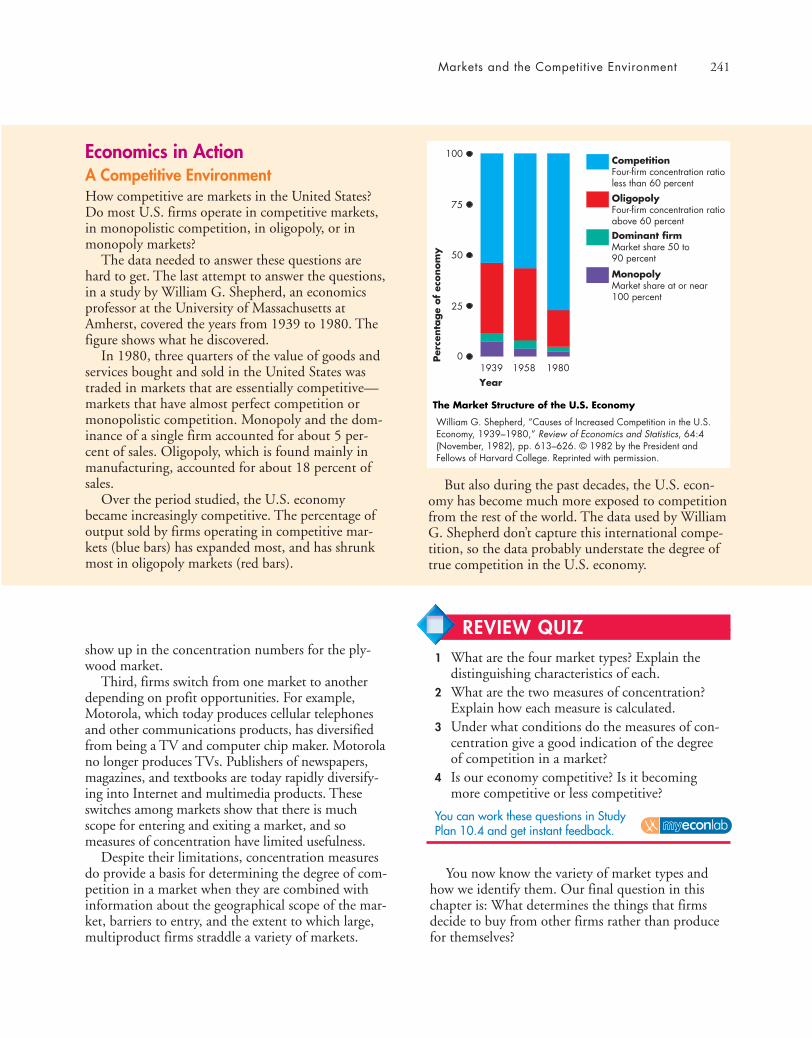
Markets and the Competitive Environment 241

You now know the variety of market types andhow we identify them. Our final question in thischapter is: What determines the things that firmsdecide to buy from other firms rather than producefor themselves?

show up in the concentration numbers for the ply-wood market.

Third, firms switch from one market to anotherdepending on profit opportunities. For example,Motorola, which today produces cellular telephonesand other communications products, has diversifiedfrom being a TV and computer chip maker. Motorolano longer produces TVs. Publishers of newspapers,magazines, and textbooks are today rapidly diversify-ing into Internet and multimedia products. Theseswitches among markets show that there is muchscope for entering and exiting a market, and someasures of concentration have limited usefulness.

Despite their limitations, concentration measuresdo provide a basis for determining the degree of com-petition in a market when they are combined withinformation about the geographical scope of the mar-ket, barriers to entry, and the extent to which large,multiproduct firms straddle a variety of markets.

0

25

50

75

100

Per

centa

ge

of

econom

y

1939 1958 1980Year

CompetitionFour-firm concentration ratioless than 60 percent

OligopolyFour-firm concentration ratioabove 60 percentDominant firmMarket share 50 to 90 percent

MonopolyMarket share at or near100 percent

The Market Structure of the U.S. Economy

Economics in ActionA Competitive EnvironmentHow competitive are markets in the United States?Do most U.S. firms operate in competitive markets,in monopolistic competition, in oligopoly, or inmonopoly markets?

The data needed to answer these questions arehard to get. The last attempt to answer the questions,in a study by William G. Shepherd, an economicsprofessor at the University of Massachusetts atAmherst, covered the years from 1939 to 1980. Thefigure shows what he discovered.

In 1980, three quarters of the value of goods andservices bought and sold in the United States wastraded in markets that are essentially competitive—markets that have almost perfect competition ormonopolistic competition. Monopoly and the dom-inance of a single firm accounted for about 5 per-cent of sales. Oligopoly, which is found mainly inmanufacturing, accounted for about 18 percent ofsales.

Over the period studied, the U.S. economybecame increasingly competitive. The percentage ofoutput sold by firms operating in competitive mar-kets (blue bars) has expanded most, and has shrunkmost in oligopoly markets (red bars).

William G. Shepherd, “Causes of Increased Competition in the U.S.Economy, 1939–1980,” Review of Economics and Statistics, 64:4(November, 1982), pp. 613–626. © 1982 by the President andFellows of Harvard College. Reprinted with permission.

But also during the past decades, the U.S. econ-omy has become much more exposed to competitionfrom the rest of the world. The data used by WilliamG. Shepherd don’t capture this international compe-tition, so the data probably understate the degree oftrue competition in the U.S. economy.

REVIEW QUIZ 1 What are the four market types? Explain the

distinguishing characteristics of each.2 What are the two measures of concentration?

Explain how each measure is calculated.3 Under what conditions do the measures of con-

centration give a good indication of the degreeof competition in a market?

4 Is our economy competitive? Is it becomingmore competitive or less competitive?

You can work these questions in Study Plan 10.4 and get instant feedback.

242 CHAPTER 10 Organizing Production

◆ Produce or Outsource?Firms and Markets

To produce a good or service, even a simple one suchas a shirt, factors of production must be hired andtheir activities coordinated. To produce a good ascomplicated as an iPhone, an enormous range ofspecialist factors of production must be coordinated.

Factors of production can be coordinated either byfirms or markets. We’ll describe these two ways oforganizing production and then see why firms play acrucial role in achieving an efficient use of resources.

Firm CoordinationFirms hire labor, capital, and land, and by using amixture of command systems and incentive systems(see p. 233) organize and coordinate their activities toproduce goods and services.

Firm coordination occurs when you take your car tothe garage for an oil change, brake check, and service.The garage owner hires a mechanic and tools andcoordinates all the activities that get your car serviced.Firms also coordinate the production of cornflakes,golf clubs, and a host of other items.

Market CoordinationMarkets coordinate production by adjusting pricesand making the decisions of buyers and sellers offactors of production and components consistent.Markets can coordinate production.

Market coordination occurs to produce a rock con-cert. A promoter books a stadium, rents some stageequipment, hires some audio and video recordingengineers and technicians, engages some rockgroups, a superstar, a publicity agent, and a ticketagent. The promoter sells tickets to thousands ofrock fans, audio rights to a recording company, and video and broadcasting rights to a television network. All these transactions take place in marketsthat coordinate this huge variety of factors ofproduction.

Outsourcing, buying parts or products from otherfirms, is another example of market coordination.Dell outsources the production of all the componentsof its computers. Automakers outsource the produc-tion of windshields, windows, transmission systems,engines, tires, and many other auto parts. Appleoutsources the entire production of iPods andiPhones.

Why Firms?What determines whether a firm or a market coordi-nates a particular set of activities? How does a firmdecide whether to buy an item from another firm ormanufacture it itself? The answer is cost. Takingaccount of the opportunity cost of time as well as thecosts of the other inputs, a firm uses the method thatcosts least. In other words, it uses the economicallyefficient method.

If a task can be performed at a lower cost by mar-kets than by a firm, markets will do the job, and anyattempt to set up a firm to replace such market activ-ity will be doomed to failure.

Firms coordinate economic activity when a taskcan be performed more efficiently by a firm than bymarkets. In such a situation, it is profitable to set upa firm. Firms are often more efficient than markets ascoordinators of economic activity because they canachieve

■ Lower transactions costs■ Economies of scale■ Economies of scope■ Economies of team production

Transactions Costs Firms eliminate transactions costs.Transactions costs are the costs that arise from findingsomeone with whom to do business, of reaching anagreement about the price and other aspects of theexchange, and of ensuring that the terms of the agree-ment are fulfilled. Market transactions require buyersand sellers to get together and to negotiate the termsand conditions of their trading. Sometimes, lawyershave to be hired to draw up contracts. A broken con-tract leads to still more expense. A firm can lower suchtransactions costs by reducing the number of individ-ual transactions undertaken.

Imagine getting your car fixed using market coor-dination. You hire a mechanic to diagnose the prob-lems and make a list of the parts and tools needed tofix them. You buy the parts from several dealers, rentthe tools from ABC Rentals, hire an auto mechanic,return the tools, and pay your bills. You can avoid allthese transactions and the time they cost you by let-ting your local garage fix the car.

Economies of Scale When the cost of producing aunit of a good falls as its output rate increases,economies of scale exist. An automaker experienceseconomies of scale because as the scale of productionincreases, the firm can use cost-saving equipment and

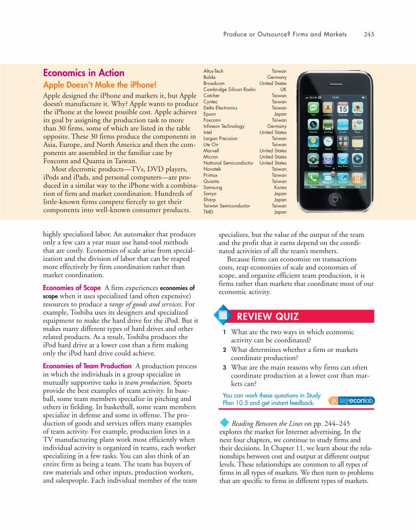
Produce or Outsource? Firms and Markets 243

highly specialized labor. An automaker that producesonly a few cars a year must use hand-tool methodsthat are costly. Economies of scale arise from special-ization and the division of labor that can be reapedmore effectively by firm coordination rather thanmarket coordination.

Economies of Scope A firm experiences economies ofscope when it uses specialized (and often expensive)resources to produce a range of goods and services. Forexample, Toshiba uses its designers and specializedequipment to make the hard drive for the iPod. But itmakes many different types of hard drives and otherrelated products. As a result, Toshiba produces theiPod hard drive at a lower cost than a firm makingonly the iPod hard drive could achieve.

Economies of Team Production A production processin which the individuals in a group specialize inmutually supportive tasks is team production. Sportsprovide the best examples of team activity. In base-ball, some team members specialize in pitching andothers in fielding. In basketball, some team membersspecialize in defense and some in offense. The pro-duction of goods and services offers many examplesof team activity. For example, production lines in aTV manufacturing plant work most efficiently whenindividual activity is organized in teams, each workerspecializing in a few tasks. You can also think of anentire firm as being a team. The team has buyers ofraw materials and other inputs, production workers,and salespeople. Each individual member of the team

specializes, but the value of the output of the teamand the profit that it earns depend on the coordi-nated activities of all the team’s members.

Because firms can economize on transactionscosts, reap economies of scale and economies ofscope, and organize efficient team production, it isfirms rather than markets that coordinate most of oureconomic activity.

◆ Reading Between the Lines on pp. 244–245explores the market for Internet advertising. In thenext four chapters, we continue to study firms andtheir decisions. In Chapter 11, we learn about the rela-tionships between cost and output at different outputlevels. These relationships are common to all types offirms in all types of markets. We then turn to problemsthat are specific to firms in different types of markets.

Economics in ActionApple Doesn’t Make the iPhone!Apple designed the iPhone and markets it, but Appledoesn’t manufacture it. Why? Apple wants to producethe iPhone at the lowest possible cost. Apple achievesits goal by assigning the production task to morethan 30 firms, some of which are listed in the tableopposite. These 30 firms produce the components inAsia, Europe, and North America and then the com-ponents are assembled in the familiar case byFoxconn and Quanta in Taiwan.

Most electronic products—TVs, DVD players,iPods and iPads, and personal computers—are pro-duced in a similar way to the iPhone with a combina-tion of firm and market coordination. Hundreds oflittle-known firms compete fiercely to get theircomponents into well-known consumer products.

Altus-Tech TaiwanBalda GermanyBroadcom United StatesCambridge Silicon Radio UKCatcher TaiwanCyntec TaiwanDelta Electronics TaiwanEpson JapanFoxconn TaiwanInfineon Technology GermanyIntel United StatesLargan Precision TaiwanLite On TaiwanMarvell United StatesMicron United StatesNational Semiconductor United StatesNovatek TaiwanPrimax TaiwanQuanta TaiwanSamsung KoreaSanyo JapanSharp JapanTaiwan Semiconductor TaiwanTMD Japan

REVIEW QUIZ 1 What are the two ways in which economic

activity can be coordinated?2 What determines whether a firm or markets

coordinate production?3 What are the main reasons why firms can often

coordinate production at a lower cost than mar-kets can?

You can work these questions in Study Plan 10.5 and get instant feedback.

244

READING BETWEEN THE L INES

Facebook Makes Gains in Web Adshttp://online.wsj.comMay 12, 2010

Facebook Inc. is catching up to rivals Yahoo Inc. and Microsoft Corp. in selling display ads.

In the first quarter, Facebook pulled ahead of Yahoo for the first time and delivered morebanner ads to its U.S. users than any other Web publisher, according to market-research firmcomScore Inc. ...

By revenue, Facebook has a long way to go to catch up to its more established rivals. Thesocial-networking site earned more than $500 million in revenue in 2009 and is forecastingrevenue of more than $1 billion in 2010, according to people familiar with the matter. Yahooearned $6.5 billion in revenue in 2009, mostly from advertising. ...

Nielsen Co., another measurement firm, found that Facebook’s share of the U.S. display-admarket grew to 20% in April 2010, up from 2% in April 2009. Nielsen still shows Yahoo inthe lead, with 34% of all display ads in April2010, compared with 35% in April 2009. ...

Facebook’s rise could help fuel an already re-bounding online-advertising market, whichshrank during the recession. Display ads haverecently shown strong growth as budgets havereturned and technology companies have devel-oped new ways to measure the effectiveness ofgraphical ads. Overall display impressions grewto 1.1 trillion in the first quarter of 2010, upfrom 944 billion in the first quarter of 2009,according to comScore.

Wall Street Journal, excerpted from “Facebook Makes Gains in Web Ads”by Jessica E. Vascellaro. Copyright 2010 by Dow Jones & Company, Inc.Reproduced with permission of Dow Jones & Company, Inc. via CopyrightClearance Center.

■ Facebook is catching up to rivals in sellingdisplay ads and according to comScoreFacebook sold more ads than Yahoo in the first quarter of 2010.

■ Facebook’s total revenue was more than $500million in 2009 and is forecast to exceed $1billion in 2010.

■ Yahoo’s total revenue, mostly from advertising,was $6.5 billion in 2009.

■ Nielsen says that Facebook’s share of U.S.display-ads grew from 2 percent to 20 percentin the year to April 2010 while Yahoo’s shrankslightly from 35 percent to 34 percent in thesame period.

■ Display ads are growing because technologycompanies have developed new ways tomeasure the effectiveness of graphical ads.

ESSENCE OF THE STORY

Battling for Markets inInternet Advertising

245

ECONOMIC ANALYSIS

■ Like all firms, Facebook and Yahoo aim to maximizeprofit.

■ Facebook provides social networking services andYahoo provides an Internet search service.

■ Facebook and Yahoo face constraints imposed by themarket and technology.

■ People who use social networks and search enginesdemand these services, and Facebook and Yahoo sup-ply them.

■ MySpace is Facebook’s biggest competitor andWikipedia lists 189 other social networking sites.

■ Google is Yahoo’s largest competitor but another 58search engines compete for attention.

■ The equilibrium price of social-networking services andsearch engine services to their users is zero.

■ But social networks and Internet search providers enjoyeconomies of scope: They produce advertising servicesas well as their other service.

■ To generate revenue and profit, social networks and In-ternet search providers sell advertising services.

■ To attract advertising revenue, a social network orsearch site must be able to offer the advertiser accessto a large potential customer base and target the peo-ple most likely to buy the advertised product or service.

■ Facebook and Yahoo are attractive to advertisers be-cause they are able to deliver both of these features: hun-dreds of millions of users, identified by their interests andlikely buying patterns.

■ To maximize the use of their services, Facebook andYahoo offer a variety of enticements to users.

■ One enticement is the quality of the primary service: social networking or search. Facebook innovates tomake its social networking services better than those ofMySpace; and Yahoo tries to make its search technologyas good as those of Google.

■ Another enticement is a variety of related attractions.Yahoo’s photo-sharing service is an example.

■ Facebook aims to attract even more users and to offer ad-vertisers the most effective return on the marketing dollar.

■ Although Facebook has seen explosive growth inusers, Fig. 1 shows that it is not generating revenues

on the scale of the leading search engines. (No dataare available for Facebook profit.)

■ Figures 1 and 2 show that Yahoo is not maintaining itsposition in the market for Internet search.

■ The data shown in Figs 1 and 2 suggest that Internetsearch is a more effective tool for generating revenueand profit than social networking.

■ The data also suggest that Google’s expansion istightening the market constraint that Yahoo faces.

Figure 1 Total revenue comparison

20010

2003 2005 20092007Year

Tota

l rev

enue

(bill

ions

of

dolla

rs p

er y

ear)

Google

Yahoo

Facebook

5

10

15

20

25

Figure 2 Profit comparison

20010

2003 2005 20092007Year

Pro

fit

(bill

ions

of

dolla

rs p

er y

ear) Google

Yahoo

2

4

6

8

10

246 CHAPTER 10 Organizing Production

form in ways that are consistent with the firms’goals.

■ Proprietorships, partnerships, and corporations useownership, incentive pay, and long-term contractsto cope with the principal–agent problem.

Working Problems 5 to 8 will give you a better under-standing of information and organization.

Markets and the Competitive Environment (pp. 237–241)

■ In perfect competition, many sellers offer an iden-tical product to many buyers and entry is free.

■ In monopolistic competition, many sellers offerslightly different products to many buyers andentry is free.

■ In oligopoly, a small number of sellers competeand barriers to entry limit the number of firms.

■ In monopoly, one firm produces an item that has noclose substitutes and the firm is protected by a bar-rier to entry that prevents the entry of competitors.

Working Problems 9 and 10 will give you a better under-standing of markets and the competitive environment.

Produce or Outsource? Firms and Markets (pp. 242–243)

■ Firms coordinate economic activities when theycan perform a task more efficiently—at lowercost—than markets can.

■ Firms economize on transactions costs and achievethe benefits of economies of scale, economies ofscope, and economies of team production.

Working Problems 11 and 12 will give you a better under-standing of firms and markets.

Key Points

The Firm and Its Economic Problem (pp. 228–230)

■ Firms hire and organize factors of production toproduce and sell goods and services.

■ A firm’s goal is to maximize economic profit,which is total revenue minus total cost measuredas the opportunity cost of production.

■ A firm’s opportunity cost of production is the sumof the cost of resources bought in the market,using the firm’s own resources, and resources sup-plied by the firm’s owner.

■ Normal profit is the opportunity cost of entrepre-neurship and is part of the firm’s opportunity cost.

■ Technology, information, and markets limit theeconomic profit that a firm can make.

Working Problems 1 and 2 will give you a better under-standing of the firm and its economic problem.

Technological and Economic Efficiency (pp. 231–232)

■ A method of production is technologically effi-cient when a firm uses the least amount of inputsto produce a given output.

■ A method of production is economically efficientwhen the cost of producing a given output is aslow as possible.

Working Problems 3 and 4 will give you a better under-standing of technological and economic efficiency.

Information and Organization (pp. 233–236)

■ Firms use a combination of command systems andincentive systems to organize production.

■ Faced with incomplete information and uncer-tainty, firms induce managers and workers to per-

SUMMARY

Key Terms

Command system, 233Economic depreciation, 229Economic efficiency, 231Economic profit, 228Economies of scale, 242Economies of scope, 243Firm, 228

Four-firm concentration ratio, 238Herfindahl-Hirschman Index, 238Implicit rental rate, 228Incentive system, 233Monopolistic competition, 237Monopoly, 237Normal profit, 229

Oligopoly, 237Perfect competition, 237Principal–agent problem, 234Product differentiation, 237Technological efficiency, 231Technology, 230Transactions costs, 242

Study Plan Problems and Applications 247

hourly wage rate and the implicit rental rate ofcapital are as follows:(i) Wage rate $1, rental rate $100?(ii) Wage rate $5, rental rate $50?(iii) Wage rate $50, rental rate $5?

4. John Deere’s Farm TeamDeere opened up the Pune [India] center in2001. Deere’s move was unexpected: Deere isknown for its heavy-duty farm equipment andbig construction gear whereas many of India’s300 million farmers still use oxen-pulled plows.

Source: Fortune, April 14, 2008a. Why do many Indian farmers still use oxen-

pulled plows? Are they efficient or inefficient?Explain.

b. How might making John Deere farm equip-ment available to Indian farmers change thetechnology constraint they face?

Information and Organization (Study Plan 10.3)

5. Here It Is. Now, You Design It!The idea is that the most successful companies nolonger invent new products and services on theirown. They create them along with their cus-tomers, and they do it in a way that produces aunique experience for each customer. The impor-tant corollary is that no company owns enoughresources—or can possibly own enough—to fur-nish unique experiences for each customer, socompanies must organize a constantly shiftingglobal web of suppliers and partners to do the job.

Source: Fortune, May 26, 2008 a. Describe this method of organizing and coor-

dinating production: Does it use a commandsystem or incentive system?

b. How does this method of organizing and co-ordinating production help firms achievelower costs?

6. Rewarding FailureOver the past 25 years CEO pay has risen fasterthan corporate profits, economic growth, or aver-age wages. A more sensible alternative to the cur-rent compensation system would require CEOsto own a lot of company stock. If the stock isgiven to the boss, his salary and bonus should bedocked to reflect its value. As for bonuses, they

The Firm and Its Economic Problem (Study Plan 10.1)

1. One year ago, Jack and Jill set up a vinegar-bot-tling firm (called JJVB). Use the following infor-mation to calculate JJVB’s opportunity cost ofproduction during its first year of operation:■ Jack and Jill put $50,000 of their own money

into the firm.■ They bought equipment for $30,000.■ They hired one employee to help them for an

annual wage of $20,000.■ Jack gave up his previous job, at which he

earned $30,000, and spent all his time work-ing for JJVB.

■ Jill kept her old job, which paid $30 an hour,but gave up 10 hours of leisure each week (for50 weeks) to work for JJVB.

■ JJVB bought $10,000 of goods and servicesfrom other firms.

■ The market value of the equipment at the endof the year was $28,000.

■ Jack and Jill have a $100,000 home loan onwhich they pay interest of 6 percent a year.

2. Joe, who has no skills, no job experience, and noalternative employment, runs a shoeshine standat the airport. Operators of other shoeshinestands earn $10,000 a year. Joe pays rent to theairport of $2,000 a year, and his total revenuefrom shining shoes is $15,000 a year. Joe spent$1,000 on a chair, polish, and brushes, using hiscredit card to buy them. The interest on a creditcard balance is 20 percent a year. At the end ofthe year, Joe was offered $500 for his businessand all its equipment. Calculate Joe’s opportunitycost of production and his economic profit.

Technological and Economic Efficiency (Study Plan 10.2)

3. Alternative ways of laundering 100 shirts areLabor Capital

Method (hours) (machines)

A 1 10B 5 8C 20 4D 50 1

a. Which methods are technologically efficient?b. Which method is economically efficient if the

You can work Problems 1 to 13 in MyEconLab Chapter 10 Study Plan and get instant feedback.

STUDY PLAN PROBLEMS AND APPLICATIONS

248 CHAPTER 10 Organizing Production

should be based on improving a company’s cashearnings relative to its cost of capital, not to moreeasily manipulated measures like earnings pershare. Bonuses should not be capped, but theyshould be unavailable to the CEO for someperiod of years.

Source: Fortune, April 28, 2008a. What is the economic problem that CEO

compensation schemes are designed to solve?b. How do the proposed changes to CEO com-

pensation outlined in the news clip addressthe problem you described in part (a)?

Use the following news clip to work Problems 7 and 8.Steps to Creating a Super StartupStarting a business is a complicated and risky task.Just two-thirds of new small businesses survive atleast two years, and only 44 percent survive at leastfour years. Most entrepreneurs start their businessesby dipping into their savings, borrowing from thefamily, and using the founder’s credit cards. Getting abank loan is tough unless you have assets—and thatoften means using your home as collateral.

Source: CNN, October 18, 20077. When starting a business, what are the risks and

potential rewards identified in the news clip thatare associated with a proprietorship?

8. How might (i) a partnership and (ii) a corpora-tion help to overcome the risks identified in thenews clip?

Markets and the Competitive Environment (Study Plan 10.4)

9. Sales of the firms in the tattoo industry areSales

Firm (dollars per year)

Bright Spots 450Freckles 325Love Galore 250Native Birds 200Other 15 firms 800

Calculate the four-firm concentration ratio. What isthe structure of the tattoo industry?10. GameStop Racks Up the Points

No retailer has more cachet among gamers thanGameStop. For now, only Wal-Mart has a largermarket share—21.3% last year. GameStop’s sharewas 21.1% last year, and may well overtake Wal-Mart this year. But if new women gamers prefershopping at Target to GameStop, Wal-Mart andTarget might erode GameStop’s market share.

Source: Fortune, June 9, 2008

a. According to the news clip, what is the struc-ture of the U.S. retail video-game market?

b. Estimate a range for the four-firm concentra-tion ratio and the HHI for the game marketin the United States based on the informationprovided in this news clip.

Produce or Outsource? Firms and Markets(Study Plan 10.5)

11. American automakers buy auto parts from inde-pendent suppliers rather than produce the partsthemselves. In the 1980s, Chrysler got about 70percent of its auto parts from independent suppli-ers, while Ford got about 60 percent and GeneralMotors got 25 percent. A decade earlier, the pro-portions were 50 percent at Chrysler, 5 percent atFord, and 20 percent at General Motors.Source: The Cato Institute Policy Analysis, 1987a. Why did American automakers decide to out-

source most of their parts production?b. Explain why independent producers of auto

parts are more efficient than the automakers.12. Federal Express enters into contracts with inde-

pendent truck operators who offer FedEx serviceand who are rewarded by the volume of packagesthey carry. Why doesn’t FedEx buy more trucksand hire more drivers? What incentive problemsmight arise from this arrangement?

Economics in the News (Study Plan 10.N)

13. Lego, the Danish toymaker, incurred economiclosses in 2003 and 2004. Lego faced competi-tion from low-cost copiers of its products and afall in demand. In 2004, to restore profits, Legofired 3,500 of its 8,000 workers; closed factoriesin Switzerland and the United States; openedfactories in Eastern Europe and Mexico; andintroduced performance-based pay for its man-agers. Lego returned to profit in 2005.

Based on Picking Up the Pieces,The Economist, October 28, 2006

a. Describe the problems that Lego faced in2003 and 2004, using the concepts of thethree types of constraints that all firms face.

b. Which of the actions that Lego took to re-store profits addressed an inefficiency? Howdid Lego seek to achieve economic efficiency?

c. Which of Lego’s actions addressed an infor-mation and organization problem? How didLego change the way in which it coped withthe principal–agent problem?

d. In what type of market does Lego operate?

Additional Problems and Applications 249

These problems are available in MyEconLab if assigned by your instructor.

ADDITIONAL PROBLEMS AND APPLICATIONS

The Firm and Its Economic ProblemUse the following information to work Problems 14and 15.Lee is a computer programmer who earned $35,000in 2009. But on January 1, 2010, Lee opened a bodyboard manufacturing business. At the end of the firstyear of operation, he submitted the following infor-mation to his accountant:

■ He stopped renting out his cottage for $3,500a year and used it as his factory. The marketvalue of the cottage increased from $70,000 to$71,000.

■ He spent $50,000 on materials, phone, etc.■ He leased machines for $10,000 a year.■ He paid $15,000 in wages.■ He used $10,000 from his savings account,

which earns 5 percent a year interest.■ He borrowed $40,000 at 10 percent a year.■ He sold $160,000 worth of body boards.■ Normal profit is $25,000 a year.

14. Calculate Lee’s opportunity cost of productionand his economic profit.

15. Lee’s accountant recorded the depreciation on hiscottage during 2010 as $7,000. According to theaccountant, what profit did Lee make?

16. In 2009, Toni taught music and earned $20,000.She also earned $4,000 by renting out her base-ment. On January 1, 2010, she quit teaching,stopped renting out her basement, and began touse it as the office for her new Web site designbusiness. She took $2,000 from her savingsaccount to buy a computer. During 2010, she paid$1,500 for the lease of a Web server and $1,750 forhigh-speed Internet service. She received a totalrevenue from Web site designing of $45,000 andearned interest at 5 percent a year on her savingsaccount balance. Normal profit is $55,000 a year.At the end of 2010, Toni could have sold her com-puter for $500. Calculate Toni’s opportunity costof production and her economic profit in 2010.

17. The Colvin Interview: ChryslerThe key driver of profitability will be that thefocus of the company isn’t on profitability. Ourfocus is on the customer. If we can find a way togive customers what they want better than any-body else, then what can stop us?

Source: Fortune, April 14, 2008

a. In spite of what Chrysler’s vice chairman andco-president claims, why is Chrysler’s focus ac-tually on profitability?

b. What would happen to Chrysler if it didn’tfocus on maximizing profit, but instead fo-cused its production and pricing decisions to“give customers what they want”?

18. Must WatchesStocks too volatile? Bonds too boring? Then tryan alternative investment—one you can wear onyour wrist. … [The] typical return on a watchover five to ten years is roughly 10%. [Onecould] do better in an index fund, but … whatother investment is so wearable?

Source: Fortune, April 14, 2008a. What is the cost of buying a watch?b. What is the opportunity cost of owning a

watch?c. Does owning a watch create an economic

profit opportunity?

Technological and Economic EfficiencyUse the following information to work Problems 19and 20.Four methods of completing a tax return and thetime taken by each method are: with a PC, 1 hour;with a pocket calculator, 12 hours; with a pocket cal-culator and paper and pencil, 12 hours; and with apencil and paper, 16 hours. The PC and its softwarecost $1,000, the pocket calculator costs $10, and thepencil and paper cost $1.19. Which, if any, of the methods is technologically

efficient?20. Which method is economically efficient if the

wage rate is(i) $5 an hour?(ii) $50 an hour?(iii) $500 an hour?

21. A Medical SensationHospitals are buying da Vinci surgical robots.Surgeons, sitting comfortably at a da Vinci con-sole, can use various robotic attachments to per-form even the most complex procedures.

Source: Fortune, April 28, 2008a. Assume that performing a surgery with a sur-

gical robot requires fewer surgeons and nurses.

250 CHAPTER 10 Organizing Production

Is using the surgical robot technologicallyefficient?

b. What additional information would you needto be able to say that switching to surgical ro-bots is economically efficient for a hospital?

Information and Organization22. Wal-Mart has more than 3,700 stores, more than

one million employees, and total revenues of closeto a quarter of a trillion dollars in the UnitedStates alone. Sarah Frey-Talley runs the family-owned Frey Farms in Illinois and supplies Wal-Mart with pumpkins and other fresh produce.a. How does Wal-Mart coordinate its activities?

Is it likely to use mainly a command system oralso to use incentive systems? Explain.

b. How do you think Sarah Frey-Talley coordi-nates the activities of Frey Farms? Is she likelyto use mainly a command system or also touse incentive systems? Explain.

c. Describe, compare, and contrast theprincipal–agent problems faced by Wal-Martand Frey Farms. How might these firms copewith their principal–agent problems?

23. Where Does Google Go Next?Google gives its engineers one day a week towork on whatever project they want. A couple ofcolleagues did what many of the young geniusesdo at Google: They came up with a cool idea. AtGoogle, you often end up with a laissez-fairemess instead of resource allocation.

Source: Fortune, May 26, 2008 a. Describe Google’s method of organizing pro-

duction with their software engineers.b. What are the potential gains and opportunity

costs associated with this method?

Markets and the Competitive Environment24. Market shares of chocolate makers are

Market shareFirm (percent)

Mayfair, Inc. 15Bond, Inc. 10Magic, Inc. 20All Natural, Inc. 15Truffles, Inc. 25Gold, Inc. 15

a. Calculate the Herfindahl-Hirschman Index.b. What is the structure of the chocolate

industry?

Produce or Outsource? Firms and MarketsUse the following information to work Problems 25to 27.Two leading design firms, Astro Studios of SanFrancisco and Hers Experimental Design Laboratory,Inc. of Osaka, Japan, worked with Microsoft to designthe Xbox 360 video game console. IBM, ATI, and SiSdesigned the Xbox 360’s hardware. Three firms—Flextronics, Wistron, and Celestica—manufacture theXbox 360 at their plants in China and Taiwan.25. Describe the roles of market coordination and

coordination by firms in the design, manufac-ture, and marketing of the Xbox 360.

26. a. Why do you think Microsoft works with alarge number of other firms, rather than per-forming all the required tasks itself?

b. What are the roles of transactions costs,economies of scale, economies of scope, andeconomies of team production in the design,manufacture, and marketing of the Xbox?

27. Why do you think the Xbox is designed in theUnited States and Japan but built in China?

Economics in the News28. After you have studied Reading Between the Lines

on pp. 244–245 answer the following questions.a. What products do Facebook and Yahoo sell?b. In what types of markets do Facebook and

Yahoo compete?c. How do social networks and Internet search

providers generate revenue?d. What is special about social networking sites

that make them attractive to advertisers?e. What is special about Internet search

providers that make them attractive to adver-tisers?

f. What technological changes might increasethe profitability of social networks and Inter-net search providers?

29. Long Reviled, Merit Pay Gains Among TeachersSchool districts in many states experiment withplans that compensate teachers partly based onclassroom performance, rather than their yearson the job and coursework completed. Workingwith mentors to improve their instruction andgetting bonuses for raising student achievementencourages efforts to raise teaching quality.

Source: The New York Times, June 18, 2007How does “merit pay” attempt to cope with theprincipal–agent problem in public education?

After studying this chapter, you will be able to:

� Distinguish between the short run and the long run� Explain the relationship between a firm’s output and

labor employed in the short run� Explain the relationship between a firm’s output and

costs in the short run and derive a firm’s short-run cost curves

� Explain the relationship between a firm’s output andcosts in the long run and derive a firm’s long-runaverage cost curve

What does a big electricity supplier in Pennsylvania, PennPower, and CampusSweaters, a small (fictional) producer of knitwear have in common? Like everyfirm, they must decide how much to produce, how many people to employ, andhow much and what type of capital equipment to use. How do firms makethese decisions?

PennPower and the other electric utilities in the United States face a demandfor electricity that fluctuates across the day and that fluctuates from day to daydepending on the temperature. How do electric utilities cope with thesedemand fluctuations?

We are going to answer these questions in this chapter.To explain the basic ideas as clearly as possible, we focus on

the economic decisions of Campus Sweaters, Inc. Studying theway this firm copes with its economic problems will give us a clear view of theproblems faced by all firms. We’ll then apply what we learn in this chapter to thereal-world costs of producing cars and electricity. In Reading Between the Lines,we’ll look at the effects of a new generation of ‘smart’ meters that encourage usersto even out electricity consumption across the day.

OUTPUT AND COSTS

11251

252 CHAPTER 11 Output and Costs

◆ Decision Time FramesPeople who operate firms make many decisions, andall of their decisions are aimed at achieving one over-riding goal: maximum attainable profit. But not alldecisions are equally critical. Some decisions are bigones. Once made, they are costly (or impossible) toreverse. If such a decision turns out to be incorrect, itmight lead to the failure of the firm. Other decisionsare small. They are easily changed. If one of thesedecisions turns out to be incorrect, the firm canchange its actions and survive.

The biggest decision that an entrepreneur makes isin what industry to establish a firm. For most entre-preneurs, their background knowledge and interestsdrive this decision. But the decision also depends onprofit prospects—on the expectation that total rev-enue will exceed total cost.

Cindy has already decided to set up CampusSweaters. She has also decided the most effectivemethod of organizing the firm. But she has notdecided the quantity to produce, the factors of pro-duction to hire, or the price to charge for sweaters.

Decisions about the quantity to produce and theprice to charge depend on the type of market inwhich the firm operates. Perfect competition,monopolistic competition, oligopoly, and monopolyall confront the firm with their own special problems.Decisions about how to produce a given output donot depend on the type of market in which the firmoperates. All types of firms in all types of marketsmake similar decisions about how to produce.

The actions that a firm can take to influence therelationship between output and cost depend on howsoon the firm wants to act. A firm that plans tochange its output rate tomorrow has fewer optionsthan one that plans to change its output rate sixmonths or six years from now.

To study the relationship between a firm’s outputdecision and its costs, we distinguish between twodecision time frames:■ The short run■ The long run

The Short RunThe short run is a time frame in which the quantity ofat least one factor of production is fixed. For mostfirms, capital, land, and entrepreneurship are fixed fac-tors of production and labor is the variable factor of

production. We call the fixed factors of production thefirm’s plant : In the short run, a firm’s plant is fixed.

For Campus Sweaters, the fixed plant is its factorybuilding and its knitting machines. For an electricpower utility, the fixed plant is its buildings, genera-tors, computers, and control systems.

To increase output in the short run, a firm mustincrease the quantity of a variable factor of production,which is usually labor. So to produce more output,Campus Sweaters must hire more labor and operate itsknitting machines for more hours a day. Similarly, anelectric power utility must hire more labor and operateits generators for more hours a day.

Short-run decisions are easily reversed. The firmcan increase or decrease its output in the short run byincreasing or decreasing the amount of labor it hires.

The Long RunThe long run is a time frame in which the quantities ofall factors of production can be varied. That is, the longrun is a period in which the firm can change its plant.

To increase output in the long run, a firm canchange its plant as well as the quantity of labor it hires.Campus Sweaters can decide whether to install moreknitting machines, use a new type of machine, reorgan-ize its management, or hire more labor. Long-run deci-sions are not easily reversed. Once a plant decision ismade, the firm usually must live with it for sometime. To emphasize this fact, we call the past expendi-ture on a plant that has no resale value a sunk cost. Asunk cost is irrelevant to the firm’s current decisions.The only costs that influence its current decisions arethe short-run cost of changing its labor inputs andthe long-run cost of changing its plant.

We’re going to study costs in the short run and thelong run. We begin with the short run and describe afirm’s technology constraint.

REVIEW QUIZ1 Distinguish between the short run and the long

run.2 Why is a sunk cost irrelevant to a firm’s current

decisions?

You can work these questions in Study Plan 11.1 and get instant feedback.

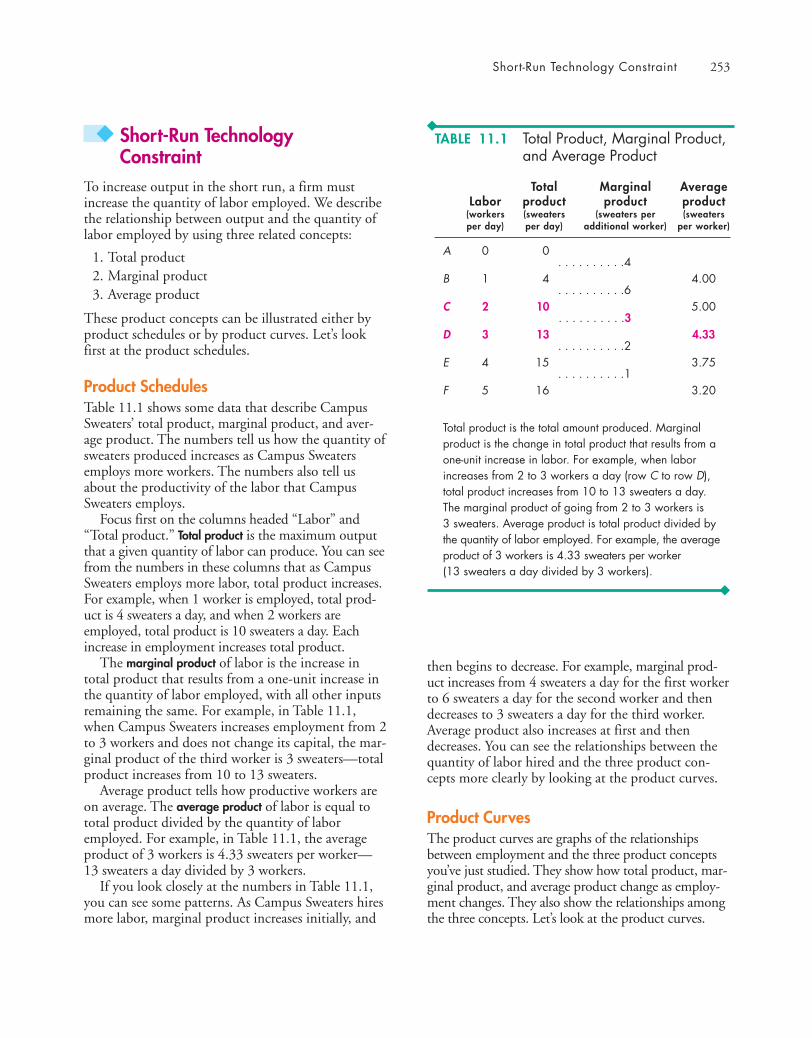
Short-Run Technology Constraint 253

◆ Short-Run Technology Constraint

To increase output in the short run, a firm mustincrease the quantity of labor employed. We describethe relationship between output and the quantity oflabor employed by using three related concepts:

1. Total product2. Marginal product3. Average product

These product concepts can be illustrated either byproduct schedules or by product curves. Let’s lookfirst at the product schedules.

Product SchedulesTable 11.1 shows some data that describe CampusSweaters’ total product, marginal product, and aver-age product. The numbers tell us how the quantity ofsweaters produced increases as Campus Sweatersemploys more workers. The numbers also tell usabout the productivity of the labor that CampusSweaters employs.

Focus first on the columns headed “Labor” and“Total product.” Total product is the maximum outputthat a given quantity of labor can produce. You can seefrom the numbers in these columns that as CampusSweaters employs more labor, total product increases.For example, when 1 worker is employed, total prod-uct is 4 sweaters a day, and when 2 workers areemployed, total product is 10 sweaters a day. Eachincrease in employment increases total product.

The marginal product of labor is the increase intotal product that results from a one-unit increase inthe quantity of labor employed, with all other inputsremaining the same. For example, in Table 11.1,when Campus Sweaters increases employment from 2to 3 workers and does not change its capital, the mar-ginal product of the third worker is 3 sweaters—totalproduct increases from 10 to 13 sweaters.

Average product tells how productive workers areon average. The average product of labor is equal tototal product divided by the quantity of laboremployed. For example, in Table 11.1, the averageproduct of 3 workers is 4.33 sweaters per worker—13 sweaters a day divided by 3 workers.

If you look closely at the numbers in Table 11.1,you can see some patterns. As Campus Sweaters hiresmore labor, marginal product increases initially, and

then begins to decrease. For example, marginal prod-uct increases from 4 sweaters a day for the first workerto 6 sweaters a day for the second worker and thendecreases to 3 sweaters a day for the third worker.Average product also increases at first and thendecreases. You can see the relationships between thequantity of labor hired and the three product con-cepts more clearly by looking at the product curves.

Product CurvesThe product curves are graphs of the relationshipsbetween employment and the three product conceptsyou’ve just studied. They show how total product, mar-ginal product, and average product change as employ-ment changes. They also show the relationships amongthe three concepts. Let’s look at the product curves.

TABLE 11.1 Total Product, Marginal Product,and Average Product

Total Marginal AverageLabor product product product

(workers (sweaters (sweaters per (sweatersper day) per day) additional worker) per worker)

A 0 0 . . . . . . . . . .4

B 1 4 . . . . . . . . . .6

4.00

C 2 10 . . . . . . . . . .3

5.00

D 3 13 . . . . . . . . . .2

4.33

E 4 15 . . . . . . . . . .1

3.75

F 5 16 3.20

Total product is the total amount produced. Marginalproduct is the change in total product that results from aone-unit increase in labor. For example, when laborincreases from 2 to 3 workers a day (row C to row D),total product increases from 10 to 13 sweaters a day.The marginal product of going from 2 to 3 workers is 3 sweaters. Average product is total product divided bythe quantity of labor employed. For example, the averageproduct of 3 workers is 4.33 sweaters per worker (13 sweaters a day divided by 3 workers).

254 CHAPTER 11 Output and Costs

Total Product CurveFigure 11.1 shows Campus Sweaters’ total productcurve, TP, which is a graph of the total productschedule. Points A through F correspond to rows Athrough F in Table 11.1. To graph the entire totalproduct curve, we vary labor by hours rather thanwhole days.

Notice the shape of the total product curve. Asemployment increases from zero to 1 worker a day,the curve becomes steeper. Then, as employmentincreases to 3, 4, and 5 workers a day, the curvebecomes less steep.

The total product curve is similar to the produc-tion possibilities frontier (explained in Chapter 2). Itseparates the attainable output levels from those thatare unattainable. All the points that lie above thecurve are unattainable. Points that lie below the curve,in the orange area, are attainable, but they are ineffi-cient—they use more labor than is necessary to pro-duce a given output. Only the points on the totalproduct curve are technologically efficient.

Marginal Product CurveFigure 11.2 shows Campus Sweaters’ marginal prod-uct of labor. Part (a) reproduces the total productcurve from Fig. 11.1 and part (b) shows the marginalproduct curve, MP.

In part (a), the orange bars illustrate the marginalproduct of labor. The height of a bar measures mar-ginal product. Marginal product is also measured bythe slope of the total product curve. Recall that theslope of a curve is the change in the value of the vari-able measured on the y-axis—output—divided by thechange in the variable measured on the x-axis—labor—as we move along the curve. A one-unitincrease in labor, from 2 to 3 workers, increases out-put from 10 to 13 sweaters, so the slope from pointC to point D is 3 sweaters per additional worker, thesame as the marginal product we’ve just calculated.

Again varying the amount of labor in the smallestunits possible, we can draw the marginal productcurve shown in Fig. 11.2(b). The height of this curvemeasures the slope of the total product curve at apoint. Part (a) shows that an increase in employmentfrom 2 to 3 workers increases output from 10 to 13sweaters (an increase of 3). The increase in output of3 sweaters appears on the y-axis of part (b) as themarginal product of going from 2 to 3 workers. Weplot that marginal product at the midpoint between2 and 3 workers. Notice that the marginal productshown in Fig. 11.2(b) reaches a peak at 1.5 workers,and at that point, marginal product is 6 sweaters peradditional worker. The peak occurs at 1.5 workersbecause the total product curve is steepest whenemployment increases from 1 worker to 2 workers.

The total product and marginal product curvesdiffer across firms and types of goods. GM’s productcurves are different from those of PennPower, whosecurves in turn are different from those of CampusSweaters. But the shapes of the product curves aresimilar because almost every production process hastwo features:

■ Increasing marginal returns initially■ Diminishing marginal returns eventually

Increasing Marginal Returns Increasing marginalreturns occur when the marginal product of an addi-tional worker exceeds the marginal product of theprevious worker. Increasing marginal returns arisefrom increased specialization and division of labor inthe production process.

15

1

Out

put (

swea

ters

per

day

)

Labor (workers per day)

10

5

0 2 3 4 5

C

A

B

D

EF

TP

Attainable

Unattainable

The total product curve, TP, is based on the data in Table11.1. The total product curve shows how the quantity ofsweaters produced changes as the quantity of laboremployed changes. For example, 2 workers can produce10 sweaters a day (point C ). Points A through F on thecurve correspond to the rows of Table 11.1. The total prod-uct curve separates attainable outputs from unattainable out-puts. Points below the TP curve are inefficient.

FIGURE 11.1 Total Product Curve

animation

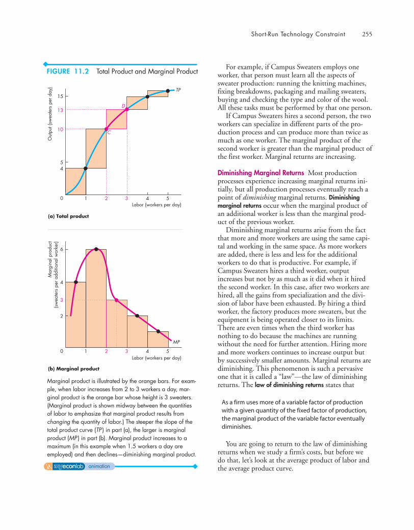
Short-Run Technology Constraint 255

For example, if Campus Sweaters employs oneworker, that person must learn all the aspects ofsweater production: running the knitting machines,fixing breakdowns, packaging and mailing sweaters,buying and checking the type and color of the wool.All these tasks must be performed by that one person.

If Campus Sweaters hires a second person, the twoworkers can specialize in different parts of the pro-duction process and can produce more than twice asmuch as one worker. The marginal product of thesecond worker is greater than the marginal product ofthe first worker. Marginal returns are increasing.

Diminishing Marginal Returns Most productionprocesses experience increasing marginal returns ini-tially, but all production processes eventually reach apoint of diminishing marginal returns. Diminishingmarginal returns occur when the marginal product ofan additional worker is less than the marginal prod-uct of the previous worker.

Diminishing marginal returns arise from the factthat more and more workers are using the same capi-tal and working in the same space. As more workersare added, there is less and less for the additionalworkers to do that is productive. For example, ifCampus Sweaters hires a third worker, outputincreases but not by as much as it did when it hiredthe second worker. In this case, after two workers arehired, all the gains from specialization and the divi-sion of labor have been exhausted. By hiring a thirdworker, the factory produces more sweaters, but theequipment is being operated closer to its limits.There are even times when the third worker hasnothing to do because the machines are runningwithout the need for further attention. Hiring moreand more workers continues to increase output butby successively smaller amounts. Marginal returns arediminishing. This phenomenon is such a pervasiveone that it is called a “law”—the law of diminishingreturns. The law of diminishing returns states that

As a firm uses more of a variable factor of productionwith a given quantity of the fixed factor of production,the marginal product of the variable factor eventuallydiminishes.

You are going to return to the law of diminishingreturns when we study a firm’s costs, but before wedo that, let’s look at the average product of labor andthe average product curve.

15

1

Out

put (

swea

ters

per

day

)

Labor (workers per day)

10

5

0 2 3 4 5

C

TP

(a) Total product

4

6

1

Mar

gina

l pro

duct

(sw

eate

rs p

er a

dditi

onal

wor

ker)

4

2

0 2 3 4 5

(b) Marginal product

MP

Labor (workers per day)

D13

3

Marginal product is illustrated by the orange bars. For exam-ple, when labor increases from 2 to 3 workers a day, mar-ginal product is the orange bar whose height is 3 sweaters.(Marginal product is shown midway between the quantitiesof labor to emphasize that marginal product results fromchanging the quantity of labor.) The steeper the slope of thetotal product curve (TP ) in part (a), the larger is marginalproduct (MP ) in part (b). Marginal product increases to amaximum (in this example when 1.5 workers a day areemployed) and then declines—diminishing marginal product.

FIGURE 11.2 Total Product and Marginal Product

animation

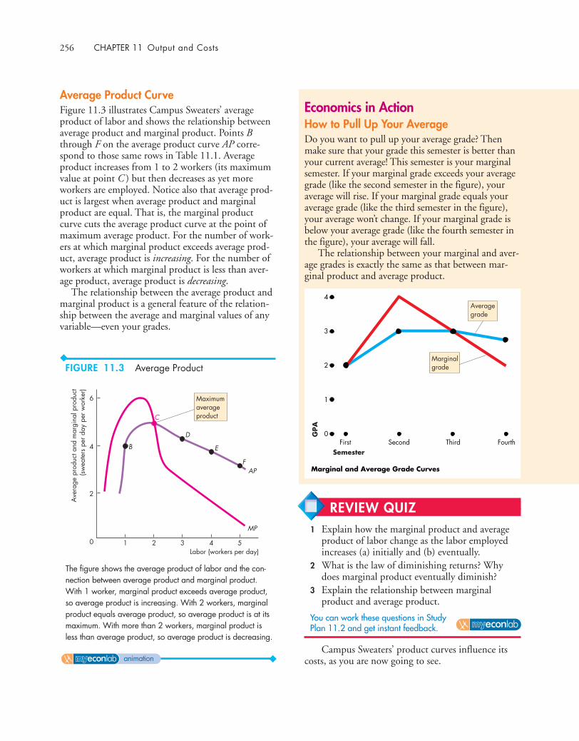
256 CHAPTER 11 Output and Costs

Campus Sweaters’ product curves influence itscosts, as you are now going to see.

Average Product CurveFigure 11.3 illustrates Campus Sweaters’ averageproduct of labor and shows the relationship betweenaverage product and marginal product. Points Bthrough F on the average product curve AP corre-spond to those same rows in Table 11.1. Averageproduct increases from 1 to 2 workers (its maximumvalue at point C ) but then decreases as yet moreworkers are employed. Notice also that average prod-uct is largest when average product and marginalproduct are equal. That is, the marginal productcurve cuts the average product curve at the point ofmaximum average product. For the number of work-ers at which marginal product exceeds average prod-uct, average product is increasing. For the number ofworkers at which marginal product is less than aver-age product, average product is decreasing.

The relationship between the average product andmarginal product is a general feature of the relation-ship between the average and marginal values of anyvariable—even your grades.

Economics in ActionHow to Pull Up Your AverageDo you want to pull up your average grade? Thenmake sure that your grade this semester is better thanyour current average! This semester is your marginalsemester. If your marginal grade exceeds your averagegrade (like the second semester in the figure), youraverage will rise. If your marginal grade equals youraverage grade (like the third semester in the figure),your average won’t change. If your marginal grade isbelow your average grade (like the fourth semester inthe figure), your average will fall.

The relationship between your marginal and aver-age grades is exactly the same as that between mar-ginal product and average product.

6

1

Ave

rage

pro

duct

and

mar

gina

l pro

duct

(sw

eate

rs p

er d

ay p

er w

orke

r)

Labor (workers per day)

4

2

0 2 3 4 5

B

D

C

E

FAP

Maximumaverageproduct

MP

0First Second Third Fourth

Semester

GPA

1

2

3

4Averagegrade

Marginalgrade

Marginal and Average Grade Curves

The figure shows the average product of labor and the con-nection between average product and marginal product.With 1 worker, marginal product exceeds average product,so average product is increasing. With 2 workers, marginalproduct equals average product, so average product is at itsmaximum. With more than 2 workers, marginal product isless than average product, so average product is decreasing.

FIGURE 11.3 Average Product

REVIEW QUIZ1 Explain how the marginal product and average

product of labor change as the labor employedincreases (a) initially and (b) eventually.

2 What is the law of diminishing returns? Whydoes marginal product eventually diminish?

3 Explain the relationship between marginalproduct and average product.

You can work these questions in Study Plan 11.2 and get instant feedback.

animation

Short-Run Cost 257

◆ Short-Run CostTo produce more output in the short run, a firm mustemploy more labor, which means that it must increaseits costs. We describe the relationship between outputand cost by using three cost concepts:

■ Total cost■ Marginal cost■ Average cost

Total CostA firm’s total cost (TC ) is the cost of all the factors ofproduction it uses. We separate total cost into totalfixed cost and total variable cost.

Total fixed cost (TFC ) is the cost of the firm’s fixedfactors. For Campus Sweaters, total fixed costincludes the cost of renting knitting machines andnormal profit, which is the opportunity cost ofCindy’s entrepreneurship (see Chapter 10, p. 229).The quantities of fixed factors don’t change as out-put changes, so total fixed cost is the same at alloutputs.

Total variable cost (TVC ) is the cost of the firm’svariable factors. For Campus Sweaters, labor is thevariable factor, so this component of cost is its wagebill. Total variable cost changes as output changes.

Total cost is the sum of total fixed cost and totalvariable cost. That is,

The table in Fig. 11.4 shows total costs. CampusSweaters rents one knitting machine for $25 a day, soits TFC is $25. To produce sweaters, the firm hireslabor, which costs $25 a day. TVC is the number ofworkers multiplied by $25. For example, to produce13 sweaters a day, in row D, the firm hires 3 workersand TVC is $75. TC is the sum of TFC and TVC, soto produce 13 sweaters a day, TC is $100. Check thecalculations in the other rows of the table.

Figure 11.4 shows Campus Sweaters’ total costcurves, which graph total cost against output. Thegreen TFC curve is horizontal because total fixedcost ($25 a day) does not change when outputchanges. The purple TVC curve and the blue TCcurve both slope upward because to increase output,more labor must be employed, which increases totalvariable cost. Total fixed cost equals the vertical dis-tance between the TVC and TC curves.

Let’s now look at a firm’s marginal cost.

TC = TFC + TVC.

150

Cos

t (do

llars

per

day

)

Output (sweaters per day)

100

50

75

0 5 10 1513

TC

TVC

TFC

TC = TFC + TVC

Total Totalfixed variable Total

Labor Outputcost cost cost

(workers (sweaters(TFC) (TVC) (TC)

per day) per day) (dollars per day)

A 0 0 25 0 25

B 1 4 25 25 50

C 2 10 25 50 75

D 3 13 25 75 100

E 4 15 25 100 125

F 5 16 25 125 150

Campus Sweaters rents a knitting machine for $25 a day,so this cost is the firm’s total fixed cost. The firm hires work-ers at a wage rate of $25 a day, and this cost is its totalvariable cost. For example, in row D, Campus Sweatersemploys 3 workers and its total variable cost is 3 × $25,which equals $75. Total cost is the sum of total fixed costand total variable cost. For example, when CampusSweaters employs 3 workers, total cost is $100—total fixedcost of $25 plus total variable cost of $75.

The graph shows Campus Sweaters’ total cost curves.Total fixed cost is constant—the TFC curve is a horizontalline. Total variable cost increases as output increases, sothe TVC curve and the TC curve increase as outputincreases. The vertical distance between the TC curve andthe TVC curve equals total fixed cost, as illustrated by thetwo arrows.

FIGURE 11.4 Total Cost Curves

animation

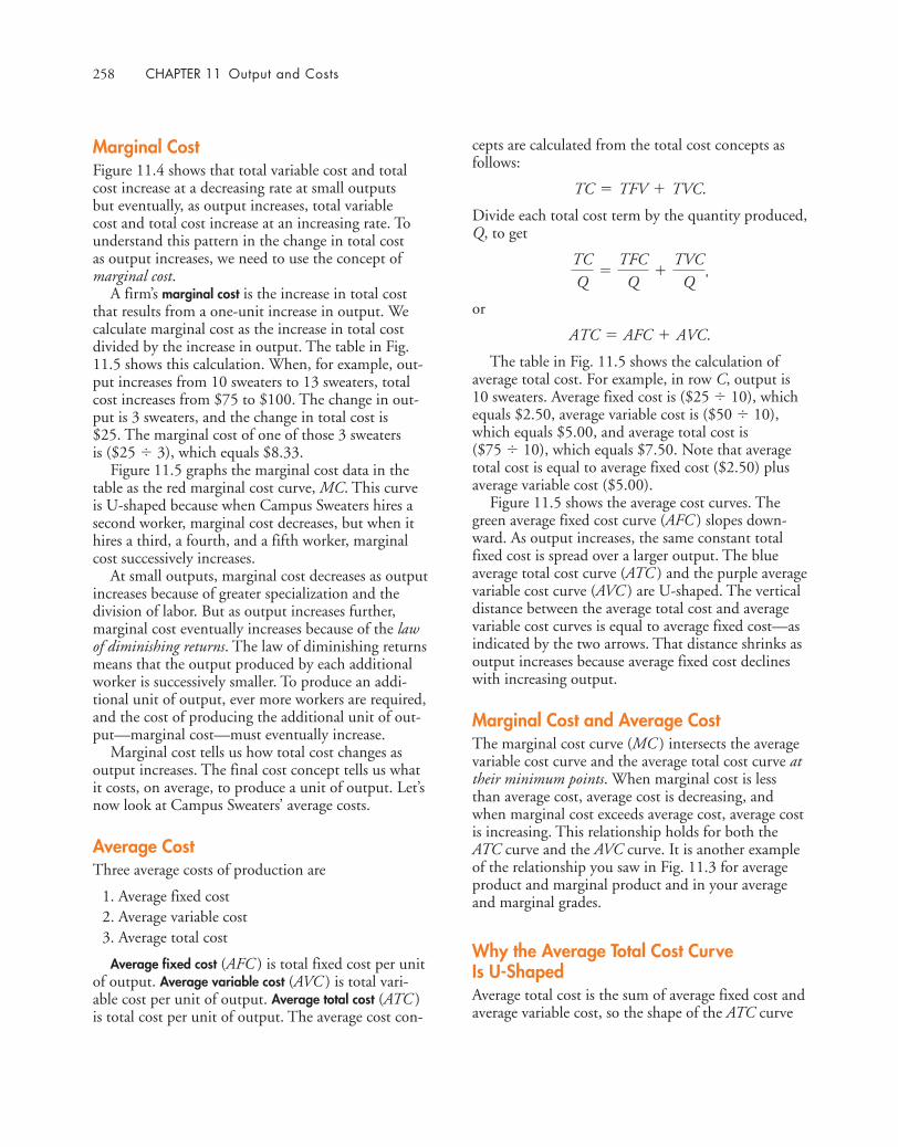
258 CHAPTER 11 Output and Costs

Marginal CostFigure 11.4 shows that total variable cost and totalcost increase at a decreasing rate at small outputs but eventually, as output increases, total variable cost and total cost increase at an increasing rate. Tounderstand this pattern in the change in total cost as output increases, we need to use the concept ofmarginal cost.

A firm’s marginal cost is the increase in total costthat results from a one-unit increase in output. Wecalculate marginal cost as the increase in total costdivided by the increase in output. The table in Fig.11.5 shows this calculation. When, for example, out-put increases from 10 sweaters to 13 sweaters, totalcost increases from $75 to $100. The change in out-put is 3 sweaters, and the change in total cost is$25. The marginal cost of one of those 3 sweatersis ($25 � 3), which equals $8.33.

Figure 11.5 graphs the marginal cost data in thetable as the red marginal cost curve, MC. This curveis U-shaped because when Campus Sweaters hires asecond worker, marginal cost decreases, but when ithires a third, a fourth, and a fifth worker, marginalcost successively increases.

At small outputs, marginal cost decreases as outputincreases because of greater specialization and thedivision of labor. But as output increases further,marginal cost eventually increases because of the lawof diminishing returns. The law of diminishing returnsmeans that the output produced by each additionalworker is successively smaller. To produce an addi-tional unit of output, ever more workers are required,and the cost of producing the additional unit of out-put—marginal cost—must eventually increase.

Marginal cost tells us how total cost changes asoutput increases. The final cost concept tells us whatit costs, on average, to produce a unit of output. Let’snow look at Campus Sweaters’ average costs.

Average CostThree average costs of production are

1. Average fixed cost2. Average variable cost3. Average total cost

Average fixed cost (AFC ) is total fixed cost per unitof output. Average variable cost (AVC ) is total vari-able cost per unit of output. Average total cost (ATC )is total cost per unit of output. The average cost con-

cepts are calculated from the total cost concepts asfollows:

Divide each total cost term by the quantity produced,Q, to get

,

or

The table in Fig. 11.5 shows the calculation ofaverage total cost. For example, in row C, output is10 sweaters. Average fixed cost is ($25 � 10), whichequals $2.50, average variable cost is ($50 � 10),which equals $5.00, and average total cost is ($75 � 10), which equals $7.50. Note that averagetotal cost is equal to average fixed cost ($2.50) plusaverage variable cost ($5.00).

Figure 11.5 shows the average cost curves. Thegreen average fixed cost curve (AFC ) slopes down-ward. As output increases, the same constant totalfixed cost is spread over a larger output. The blueaverage total cost curve (ATC ) and the purple averagevariable cost curve (AVC ) are U-shaped. The verticaldistance between the average total cost and averagevariable cost curves is equal to average fixed cost—asindicated by the two arrows. That distance shrinks asoutput increases because average fixed cost declineswith increasing output.

Marginal Cost and Average CostThe marginal cost curve (MC ) intersects the averagevariable cost curve and the average total cost curve attheir minimum points. When marginal cost is lessthan average cost, average cost is decreasing, andwhen marginal cost exceeds average cost, average costis increasing. This relationship holds for both theATC curve and the AVC curve. It is another exampleof the relationship you saw in Fig. 11.3 for averageproduct and marginal product and in your averageand marginal grades.

Why the Average Total Cost Curve Is U-ShapedAverage total cost is the sum of average fixed cost andaverage variable cost, so the shape of the ATC curve

ATC = AFC + AVC.

TCQ

=TFC

Q+

TVCQ

TC = TFV + TVC.

Short-Run Cost 259

combines the shapes of the AFC and AVC curves.The U shape of the ATC curve arises from the influ-ence of two opposing forces:

1. Spreading total fixed cost over a larger output2. Eventually diminishing returns

When output increases, the firm spreads its totalfixed cost over a larger output and so its averagefixed cost decreases—its AFC curve slopesdownward.

Diminishing returns means that as outputincreases, ever-larger amounts of labor are needed toproduce an additional unit of output. So as outputincreases, average variable cost decreases initially but

eventually increases, and the AVC curve slopesupward. The AVC curve is U shaped.

The shape of the ATC curve combines these twoeffects. Initially, as output increases, both average fixedcost and average variable cost decrease, so average totalcost decreases. The ATC curve slopes downward.

But as output increases further and diminishingreturns set in, average variable cost starts to increase.With average fixed cost decreasing more quickly thanaverage variable cost is increasing, the ATC curvecontinues to slope downward. Eventually, averagevariable cost starts to increase more quickly thanaverage fixed cost decreases, so average total coststarts to increase. The ATC curve slopes upward.

15

Cos

t (do

llars

per

sw

eate

r)

Output (sweaters per day)

10

5

0 5 10 15

MC

ATC

AFC

AVC

ATC = AFC + AVC

Marginal cost is calculated as the change in total cost dividedby the change in output. When output increases from 4 to 10sweaters, an increase of 6 sweaters, total cost increases by$25. Marginal cost is $25 ÷ 6, which is $4.17.

Each average cost concept is calculated by dividing therelated total cost by output. When 10 sweaters are produced,AFC is $2.50 ($25 ÷ 10), AVC is $5 ($50 ÷ 10), and ATC is$7.50 ($75 ÷ 10).

The graph shows that the MC curve is U-shaped andintersects the AVC curve and the ATC curve at their minimumpoints. The average fixed cost curve (AFC) is downward slop-ing. The ATC curve and AVC curve are U-shaped. The verticaldistance between the ATC curve and the AVC curve is equal toaverage fixed cost, as illustrated by the two arrows.

Total Total Marginal Average Average Averagefixed variable Total cost fixed variable total

Labor Output cost cost cost (MC) cost cost cost

(workers (sweaters (TFC) (TVC) (TC) (dollars per (AFC) (AVC) (ATC)

per day) per day) (dollars per day) additional sweater) (dollars per sweater)

A 0 0 25 0 25 . . . . . . . 6.25

— — —

B 1 4 25 25 50 . . . . . . . 4.17

6.25 6.25 12.50

C 2 10 25 50 75 . . . . . . . 8.33

2.50 5.00 7.50

D 3 13 25 75 100 . . . . . . .12.50

1.92 5.77 7.69

E 4 15 25 100 125 . . . . . . .25.00

1.67 6.67 8.33

F 5 16 25 125 150 1.56 7.81 9.38

FIGURE 11.5 Marginal Cost and Average Costs

animation

260 CHAPTER 11 Output and Costs

Cost Curves and Product CurvesThe technology that a firm uses determines its costs.Figure 11.6 shows the links between the firm’s prod-uct curves and its cost curves. The upper graph showsthe average product curve, AP, and the marginalproduct curve, MP—like those in Fig. 11.3. Thelower graph shows the average variable cost curve,AVC, and the marginal cost curve, MC—like those inFig. 11.5.

As labor increases up to 1.5 workers a day (uppergraph), output increases to 6.5 sweaters a day (lowergraph). Marginal product and average product riseand marginal cost and average variable cost fall. Atthe point of maximum marginal product, marginalcost is at a minimum.

As labor increases from 1.5 workers to 2 workers aday, (upper graph) output increases from 6.5 sweatersto 10 sweaters a day (lower graph). Marginal productfalls and marginal cost rises, but average product con-tinues to rise and average variable cost continues tofall. At the point of maximum average product, aver-age variable cost is at a minimum. As labor increasesfurther, output increases. Average product diminishesand average variable cost increases.

Shifts in the Cost CurvesThe position of a firm’s short-run cost curves dependson two factors:

■ Technology■ Prices of factors of production

Technology A technological change that increasesproductivity increases the marginal product and aver-age product of labor. With a better technology, thesame factors of production can produce more output,so the technological advance lowers the costs of pro-duction and shifts the cost curves downward.

For example, advances in robot production tech-niques have increased productivity in the automobileindustry. As a result, the product curves of Chrysler,Ford, and GM have shifted upward and their costcurves have shifted downward. But the relationshipsbetween their product curves and cost curves havenot changed. The curves are still linked in the wayshown in Fig. 11.6.

Often, as in the case of robots producing cars, atechnological advance results in a firm using more cap-ital, a fixed factor, and less labor, a variable factor.

Ave

rage

pro

duct

and

mar

gina

l pro

duct

Labor

Rising MP andfalling MC:rising AP andfalling AVC

1.5 2.00

2

4

6

6.5 100

3

6

9

12

Falling MP andrising MC:falling AP andrising AVC

Falling MP andrising MC:rising AP andfalling AVC

Maximum MP andMinimum MC

Maximum AP andMinimum AVC

Output

MP

AP

MC

AVC

Cos

t (do

llars

per

uni

t)

A firm’s MP curve is linked to its MC curve. If, as the firmincreases its labor from 0 to 1.5 workers a day, the firm’smarginal product rises, its marginal cost falls. If marginalproduct is at a maximum, marginal cost is at a minimum. If,as the firm hires more labor, its marginal product dimin-ishes, its marginal cost rises.

A firm’s AP curve is linked to its AVC curve. If, as thefirm increases its labor to 2 workers a day, its averageproduct rises, its average variable cost falls. If averageproduct is at a maximum, average variable cost is at a mini-mum. If, as the firm hires more labor, its average productdiminishes, its average variable cost rises.

FIGURE 11.6 Product Curves and Cost Curves

animation

Short-Run Cost 261

Another example is the use of ATMs by banks to dis-pense cash. ATMs, which are fixed capital, havereplaced tellers, which are variable labor. Such a tech-nological change decreases total cost but increases fixedcosts and decreases variable cost. This change in themix of fixed cost and variable cost means that at smalloutputs, average total cost might increase, while atlarge outputs, average total cost decreases.

Prices of Factors of Production An increase in theprice of a factor of production increases the firm’scosts and shifts its cost curves. How the curves shiftdepends on which factor price changes.

An increase in rent or some other component offixed cost shifts the TFC and AFC curves upward andshifts the TC curve upward but leaves the AVC andTVC curves and the MC curve unchanged. Forexample, if the interest expense paid by a truckingcompany increases, the fixed cost of transportationservices increases.

An increase in wages, gasoline, or another compo-nent of variable cost shifts the TVC and AVC curvesupward and shifts the MC curve upward but leavesthe AFC and TFC curves unchanged. For example, if

truck drivers’ wages or the price of gasoline increases,the variable cost and marginal cost of transportationservices increase.

You’ve now completed your study of short-runcosts. All the concepts that you’ve met are summa-rized in a compact glossary in Table 11.2.

TABLE 11.2 A Compact Glossary of Costs

Term Symbol Definition Equation

Fixed cost Cost that is independent of the output level;cost of a fixed factor of production

Variable cost Cost that varies with the output level; costof a variable factor of production

Total fixed cost TFC Cost of the fixed factors of production

Total variable cost TVC Cost of the variable factors of production

Total cost TC Cost of all factors of production TC = TFC + TVC

Output (total product) TP Total quantity produced (output Q)

Marginal cost MC Change in total cost resulting from a one- MC = ΔTC ÷ ΔQunit increase in total product

Average fixed cost AFC Total fixed cost per unit of output AFC = TFC ÷ Q

Average variable cost AVC Total variable cost per unit of output AVC = TVC ÷ Q

Average total cost ATC Total cost per unit of output ATC = AFC + AVC

REVIEW QUIZ 1 What relationships do a firm’s short-run cost

curves show?2 How does marginal cost change as output

increases (a) initially and (b) eventually?3 What does the law of diminishing returns

imply for the shape of the marginal cost curve?4 What is the shape of the AFC curve and why

does it have this shape?5 What are the shapes of the AVC curve and the

ATC curve and why do they have these shapes?

You can work these questions in Study Plan 11.3 and get instant feedback.

262 CHAPTER 11 Output and Costs

◆ Long-Run CostWe are now going to study the firm’s long-run costs.In the long run, a firm can vary both the quantity oflabor and the quantity of capital, so in the long run,all the firm’s costs are variable.

The behavior of long-run cost depends on thefirm’s production function, which is the relationshipbetween the maximum output attainable and thequantities of both labor and capital.

The Production FunctionTable 11.3 shows Campus Sweaters’ productionfunction. The table lists total product schedules forfour different quantities of capital. The quantity ofcapital identifies the plant size. The numbers forplant 1 are for a factory with 1 knitting machine—the case we’ve just studied. The other three plantshave 2, 3, and 4 machines. If Campus Sweaters usesplant 2 with 2 knitting machines, the variousamounts of labor can produce the outputs shown inthe second column of the table. The other two columnsshow the outputs of yet larger quantities of capital.Each column of the table could be graphed as a totalproduct curve for each plant.

Diminishing Returns Diminishing returns occur witheach of the four plant sizes as the quantity of laborincreases. You can check that fact by calculating themarginal product of labor in each of the plants with2, 3, and 4 machines. With each plant size, as thefirm increases the quantity of labor employed, themarginal product of labor (eventually) diminishes.

Diminishing Marginal Product of CapitalDiminishing returns also occur with each quantityof labor as the quantity of capital increases. You cancheck that fact by calculating the marginal productof capital at a given quantity of labor. The marginalproduct of capital is the change in total productdivided by the change in capital when the quantityof labor is constant—equivalently, the change inoutput resulting from a one-unit increase in thequantity of capital. For example, if CampusSweaters has 3 workers and increases its capitalfrom 1 machine to 2 machines, output increasesfrom 13 to 18 sweaters a day. The marginal productof the second machine is 5 sweaters a day. IfCampus Sweaters continues to employ 3 workers

and increases the number of machines from 2 to 3,output increases from 18 to 22 sweaters a day. Themarginal product of the third machine is 4 sweatersa day, down from 5 sweaters a day for the secondmachine.

Let’s now see what the production functionimplies for long-run costs.

Short-Run Cost and Long-Run CostAs before, Campus Sweaters can hire workers for $25a day and rent knitting machines for $25 a day.Using these factor prices and the data in Table 11.3,we can calculate the average total cost and graph theATC curves for factories with 1, 2, 3, and 4 knittingmachines. We’ve already studied the costs of a factorywith 1 machine in Figs. 11.4 and 11.5. In Fig. 11.7,the average total cost curve for that case is ATC1.Figure 11.7 also shows the average total cost curve fora factory with 2 machines, ATC2, with 3 machines,ATC3, and with 4 machines, ATC4.

You can see, in Fig. 11.7, that the plant size has abig effect on the firm’s average total cost.

TABLE 11.3 The Production Function

Output

Labor(sweaters per day)

(workers per day) Plant 1 Plant 2 Plant 3 Plant 4

1 4 10 13 15

2 10 15 18 20

3 13 18 22 24

4 15 20 24 26

5 16 21 25 27

Knitting machines 1 2 3 4(number)

The table shows the total product data for four quantitiesof capital (plant sizes). The greater the plant size, thelarger is the output produced by any given quantity oflabor. For a given plant size, the marginal product oflabor diminishes as more labor is employed. For a givenquantity of labor, the marginal product of capital dimin-ishes as the quantity of capital used increases.

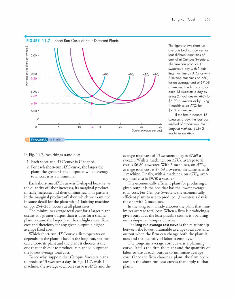
Long-Run Cost 263

In Fig. 11.7, two things stand out:

1. Each short-run ATC curve is U-shaped.2. For each short-run ATC curve, the larger the

plant, the greater is the output at which averagetotal cost is at a minimum.

Each short-run ATC curve is U-shaped because, asthe quantity of labor increases, its marginal productinitially increases and then diminishes. This patternin the marginal product of labor, which we examinedin some detail for the plant with 1 knitting machineon pp. 254–255, occurs at all plant sizes.

The minimum average total cost for a larger plantoccurs at a greater output than it does for a smallerplant because the larger plant has a higher total fixedcost and therefore, for any given output, a higheraverage fixed cost.

Which short-run ATC curve a firm operates ondepends on the plant it has. In the long run, the firmcan choose its plant and the plant it chooses is theone that enables it to produce its planned output atthe lowest average total cost.

To see why, suppose that Campus Sweaters plansto produce 13 sweaters a day. In Fig. 11.7, with 1machine, the average total cost curve is ATC1 and the

average total cost of 13 sweaters a day is $7.69 asweater. With 2 machines, on ATC2, average totalcost is $6.80 a sweater. With 3 machines, on ATC3,average total cost is $7.69 a sweater, the same as with1 machine. Finally, with 4 machines, on ATC4, aver-age total cost is $9.50 a sweater.

The economically efficient plant for producing agiven output is the one that has the lowest averagetotal cost. For Campus Sweaters, the economicallyefficient plant to use to produce 13 sweaters a day isthe one with 2 machines.

In the long run, Cindy chooses the plant that min-imizes average total cost. When a firm is producing agiven output at the least possible cost, it is operatingon its long-run average cost curve.

The long-run average cost curve is the relationshipbetween the lowest attainable average total cost andoutput when the firm can change both the plant ituses and the quantity of labor it employs.

The long-run average cost curve is a planningcurve. It tells the firm the plant and the quantity oflabor to use at each output to minimize averagecost. Once the firm chooses a plant, the firm oper-ates on the short-run cost curves that apply to thatplant.

12.00

Ave

rage

cos

t (do

llars

per

sw

eate

r)

10.00

8.00

6.00

6.80

7.69

9.50

0 5 10 15 20 25 3013Output (sweaters per day)

ATC1 ATC2 ATC3 ATC4

The figure shows short-runaverage total cost curves forfour different quantities ofcapital at Campus Sweaters.The firm can produce 13sweaters a day with 1 knit-ting machine on ATC1 or with3 knitting machines on ATC3

for an average cost of $7.69a sweater. The firm can pro-duce 13 sweaters a day byusing 2 machines on ATC2 for$6.80 a sweater or by using4 machines on ATC4 for$9.50 a sweater.

If the firm produces 13sweaters a day, the least-costmethod of production, thelong-run method, is with 2machines on ATC2.

FIGURE 11.7 Short-Run Costs of Four Different Plants

animation

264 CHAPTER 11 Output and Costs

The Long-Run Average Cost CurveFigure 11.8 shows how a long-run average cost curveis derived. The long-run average cost curve LRACconsists of pieces of the four short-run ATC curves.For outputs up to 10 sweaters a day, average total costis the lowest on ATC1. For outputs between 10 and18 sweaters a day, average total cost is the lowest onATC2. For outputs between 18 and 24 sweaters a day,average total cost is the lowest on ATC3. And for out-puts in excess of 24 sweaters a day, average total costis the lowest on ATC4. The piece of each ATC curvewith the lowest average total cost is highlighted indark blue in Fig. 11.8. This dark blue scallop-shapedcurve made up of the pieces of the four ATC curves isthe LRAC curve.

Economies and Diseconomies of ScaleEconomies of scale are features of a firm’s technologythat make average total cost fall as output increases.When economies of scale are present, the LRAC curveslopes downward. In Fig. 11.8, Campus Sweaters haseconomies of scale for outputs up to 15 sweaters a day.

Greater specialization of both labor and capital isthe main source of economies of scale. For example, if

12.00

Ave

rage

cos

t (do

llars

per

sw

eate

r)

10.00

8.00

6.00

0 5 10 15 20 25 30Output (sweaters per day)

18

Minimumefficientscale

24

curveLRAC

Economies of scale Diseconomies of scale

ATC1 ATC2 ATC3 ATC4

Least-cost plant is 1 Least-cost plant is 2 Least-cost plant is 3 Least-cost plant is 4

The long-run average costcurve traces the lowest attain-able ATC when both laborand capital change. Thegreen arrows highlight theoutput range over which eachplant achieves the lowestATC. Within each range, tochange the quantity pro-duced, the firm changes thequantity of labor it employs.

Along the LRAC curve,economies of scale occur ifaverage cost falls as outputincreases; diseconomies ofscale occur if average costrises as output increases.Minimum efficient scale is theoutput at which average costis lowest, 15 sweaters a day.

GM produces 100 cars a week, each worker must per-form many different tasks and the capital must be gen-eral-purpose machines and tools. But if GM produces10,000 cars a week, each worker specializes in a smallnumber of tasks, uses task-specific tools, and becomeshighly proficient.

Diseconomies of scale are features of a firm’s tech-nology that make average total cost rise as outputincreases. When diseconomies of scale are present,the LRAC curve slopes upward. In Fig. 11.8,Campus Sweaters experiences diseconomies of scaleat outputs greater than 15 sweaters a day.

The challenge of managing a large enterprise is themain source of diseconomies of scale.

Constant returns to scale are features of a firm’s tech-nology that keep average total cost constant as outputincreases. When constant returns to scale are present,the LRAC curve is horizontal.

Economies of Scale at Campus Sweaters Theeconomies of scale and diseconomies of scale atCampus Sweaters arise from the firm’s productionfunction in Table 11.3. With 1 machine and 1worker, the firm produces 4 sweaters a day. With 2machines and 2 workers, total cost doubles but out-

FIGURE 11.8 Long-Run Average Cost Curve

animation

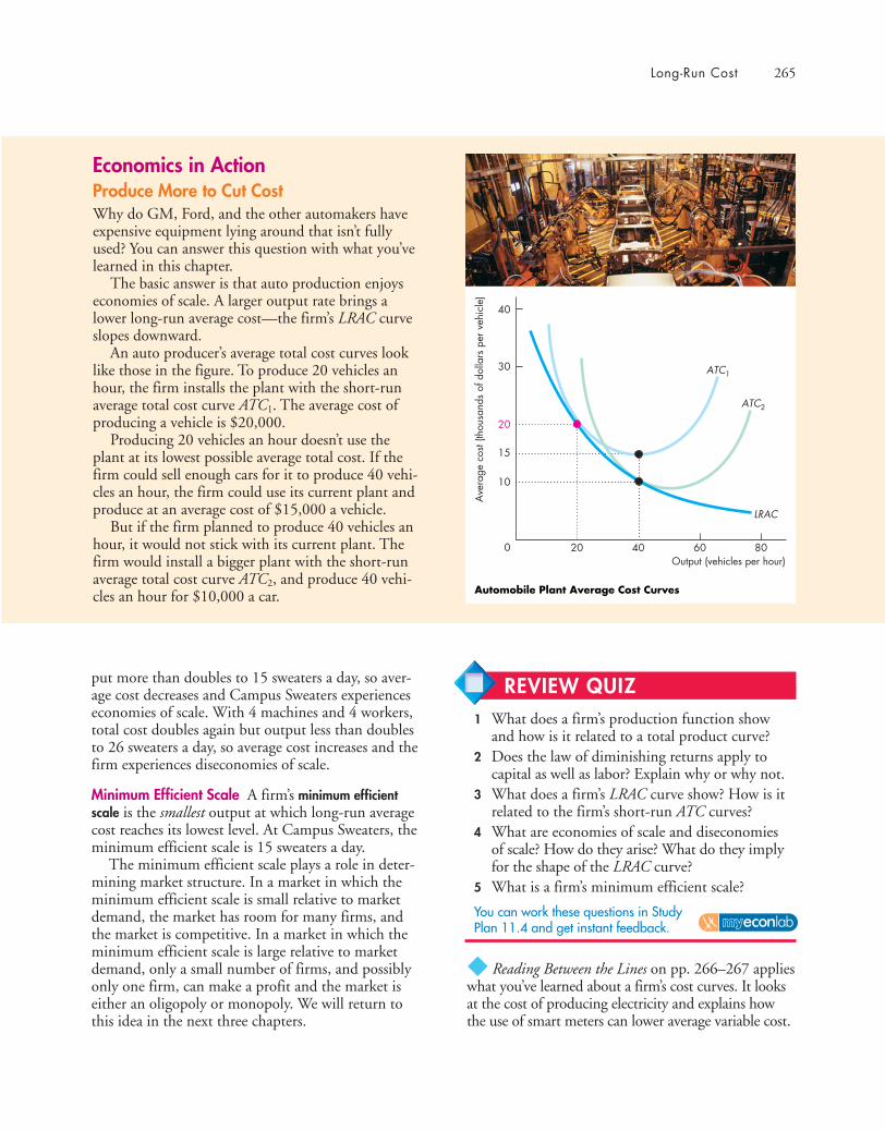
Long-Run Cost 265

put more than doubles to 15 sweaters a day, so aver-age cost decreases and Campus Sweaters experienceseconomies of scale. With 4 machines and 4 workers,total cost doubles again but output less than doublesto 26 sweaters a day, so average cost increases and thefirm experiences diseconomies of scale.

Minimum Efficient Scale A firm’s minimum efficientscale is the smallest output at which long-run averagecost reaches its lowest level. At Campus Sweaters, theminimum efficient scale is 15 sweaters a day.

The minimum efficient scale plays a role in deter-mining market structure. In a market in which theminimum efficient scale is small relative to marketdemand, the market has room for many firms, andthe market is competitive. In a market in which theminimum efficient scale is large relative to marketdemand, only a small number of firms, and possiblyonly one firm, can make a profit and the market iseither an oligopoly or monopoly. We will return tothis idea in the next three chapters.

◆ Reading Between the Lines on pp. 266–267 applieswhat you’ve learned about a firm’s cost curves. It looksat the cost of producing electricity and explains howthe use of smart meters can lower average variable cost.

Economics in ActionProduce More to Cut CostWhy do GM, Ford, and the other automakers haveexpensive equipment lying around that isn’t fullyused? You can answer this question with what you’velearned in this chapter.

The basic answer is that auto production enjoyseconomies of scale. A larger output rate brings alower long-run average cost—the firm’s LRAC curveslopes downward.

An auto producer’s average total cost curves looklike those in the figure. To produce 20 vehicles anhour, the firm installs the plant with the short-runaverage total cost curve ATC1. The average cost ofproducing a vehicle is $20,000.

Producing 20 vehicles an hour doesn’t use theplant at its lowest possible average total cost. If thefirm could sell enough cars for it to produce 40 vehi-cles an hour, the firm could use its current plant andproduce at an average cost of $15,000 a vehicle.

But if the firm planned to produce 40 vehicles anhour, it would not stick with its current plant. Thefirm would install a bigger plant with the short-runaverage total cost curve ATC2, and produce 40 vehi-cles an hour for $10,000 a car.

LRAC

Ave

rage

cos

t (th

ousa

nds

of d

olla

rs p

er v

ehic

le)

Output (vehicles per hour)0

10

20

40

30

15

20 40 60 80

ATC1

ATC2

Automobile Plant Average Cost Curves

REVIEW QUIZ1 What does a firm’s production function show

and how is it related to a total product curve?2 Does the law of diminishing returns apply to

capital as well as labor? Explain why or why not.3 What does a firm’s LRAC curve show? How is it

related to the firm’s short-run ATC curves?4 What are economies of scale and diseconomies

of scale? How do they arise? What do they implyfor the shape of the LRAC curve?

5 What is a firm’s minimum efficient scale?

You can work these questions in Study Plan 11.4 and get instant feedback.

266

READING BETWEEN THE L INES

Here Come the “Smart” Metershttp://www.wsj.comMay 21, 2010

One of modern life’s most durable features—fixed-price electricity—is slowly being pushed tothe sidelines, a creeping change that will influence such things as what time millions of Ameri-cans cook dinner and what appliances they buy.

Driving the change is the rollout of so-called smart meters, which can transmit data on howmuch power is being used at any given time. That gives utilities the ability to charge more forelectricity at peak times and less during lulls. Spreading out electricity consumption moreevenly across the day leads to more efficient use of power plants and lower emissions. ...

The new system uses digital meters to charge prices thatvary during the day.

Though fewer than 10 percent of U.S. homes have smartmeters now, the Department of Energy is funding effortsthat will boost that number to nearly a third by 2015.The majority of homes in California and Texas, the twomost populous states, will have smart meters by 2013.

Smart meters lie at the heart of efforts to get Americansto use less electricity. Power generation accounts forabout 40 percent of greenhouse-gas emissions in theUnited States. A 2009 federal study found that smartmeters could help cut peak electricity use by 20 percent.

In California, power plants totaling 30,000 to 35,000megawatts of capacity are needed on a typical day. But50,000 megawatts or more are needed on hot days.That forces generators to turn on their least efficientand most polluting plants to meet demand. In NewYork, average demand is 42 percent less than peak-timedemand. Flatten peak use, experts say, and system costsdrop, as does pollution. ...

Wall Street Journal, excerpted from “Here Come the ‘Smart’ Meters: ‘Smart' MetersKnow When You’re Cooking, Cleaning; How About Dinner at 4?” by Rebecca Smith.Copyright 2010 by Dow Jones & Company, Inc. Reproduced with permission of DowJones & Company, Inc. via Copyright Clearance Center.

■ Fixed-price electricity is being replaced bytime-of-day pricing.

■ Smart meters make it possible for utilities tocharge more for electricity at peak times andless at off-peak times.

■ Fewer than 10 percent of U.S. homes hadsmart meters in 2010, but the majority ofhomes in California and Texas will have themby 2013 and almost a third of all U.S. homeswill have them by 2015.

■ Time-of-day pricing makes electricityconsumption more even across the day.

■ A 2009 federal study found that smart meterscould help cut peak electricity use by 20percent.

■ Making electricity consumption more evenacross the day lowers the cost of electricitygeneration.

■ In California, power plants produce 30,000 to 35,000 megawatts on a typical day and50,000 megawatts or more on a hot day.

■ In New York, average production is 42 percentless than peak-time production.

ESSENCE OF THE STORY

Cutting the Cost ofProducing Electricity

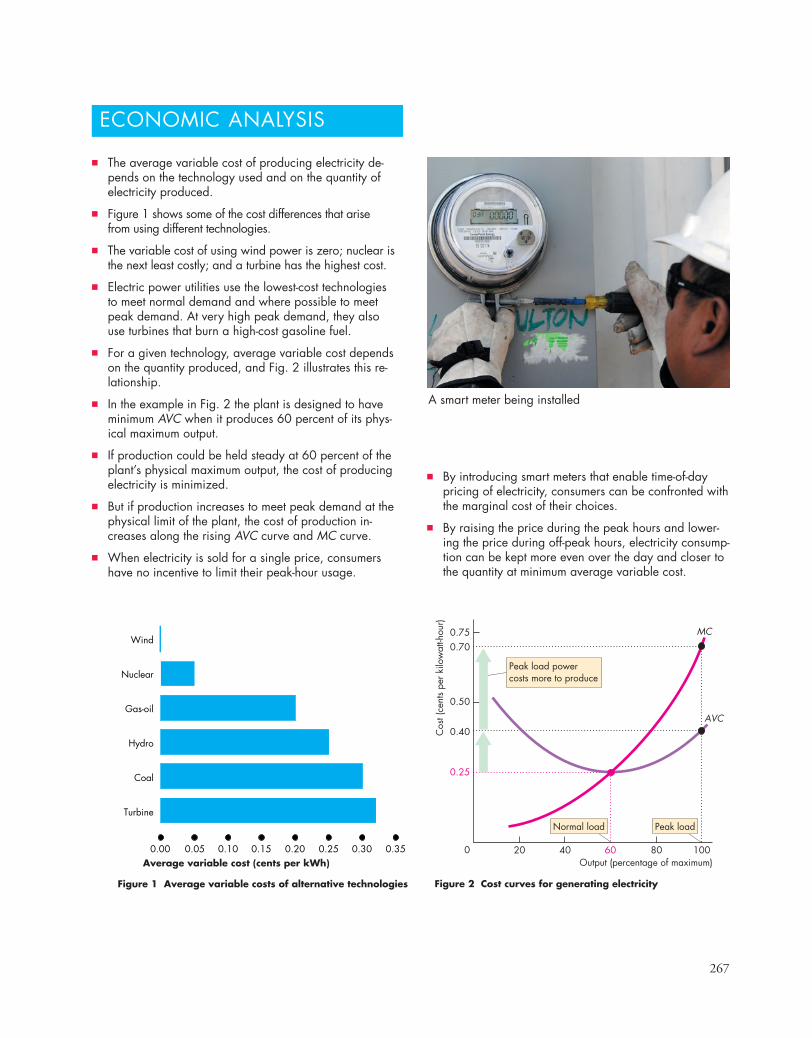
267

ECONOMIC ANALYSIS

■ By introducing smart meters that enable time-of-daypricing of electricity, consumers can be confronted withthe marginal cost of their choices.

■ By raising the price during the peak hours and lower-ing the price during off-peak hours, electricity consump-tion can be kept more even over the day and closer tothe quantity at minimum average variable cost.

Figure 1 Average variable costs of alternative technologies

0.00

Wind

Nuclear

Gas-oil

Hydro

Coal

Turbine

0.05 0.10 0.15 0.20 0.350.300.25Average variable cost (cents per kWh)

AVC

MC

Figure 2 Cost curves for generating electricity

Cos

t (ce

nts

per k

ilow

att-h

our)

Output (percentage of maximum)0

0.75

0.50

0.40

0.70

0.25

20 40 60 10080

Peak load powercosts more to produce

Normal load Peak load

■ The average variable cost of producing electricity de-pends on the technology used and on the quantity ofelectricity produced.

■ Figure 1 shows some of the cost differences that arisefrom using different technologies.

■ The variable cost of using wind power is zero; nuclear isthe next least costly; and a turbine has the highest cost.

■ Electric power utilities use the lowest-cost technologiesto meet normal demand and where possible to meetpeak demand. At very high peak demand, they alsouse turbines that burn a high-cost gasoline fuel.

■ For a given technology, average variable cost dependson the quantity produced, and Fig. 2 illustrates this re-lationship.

■ In the example in Fig. 2 the plant is designed to haveminimum AVC when it produces 60 percent of its phys-ical maximum output.

■ If production could be held steady at 60 percent of theplant’s physical maximum output, the cost of producingelectricity is minimized.

■ But if production increases to meet peak demand at thephysical limit of the plant, the cost of production in-creases along the rising AVC curve and MC curve.

■ When electricity is sold for a single price, consumershave no incentive to limit their peak-hour usage.

A smart meter being installed

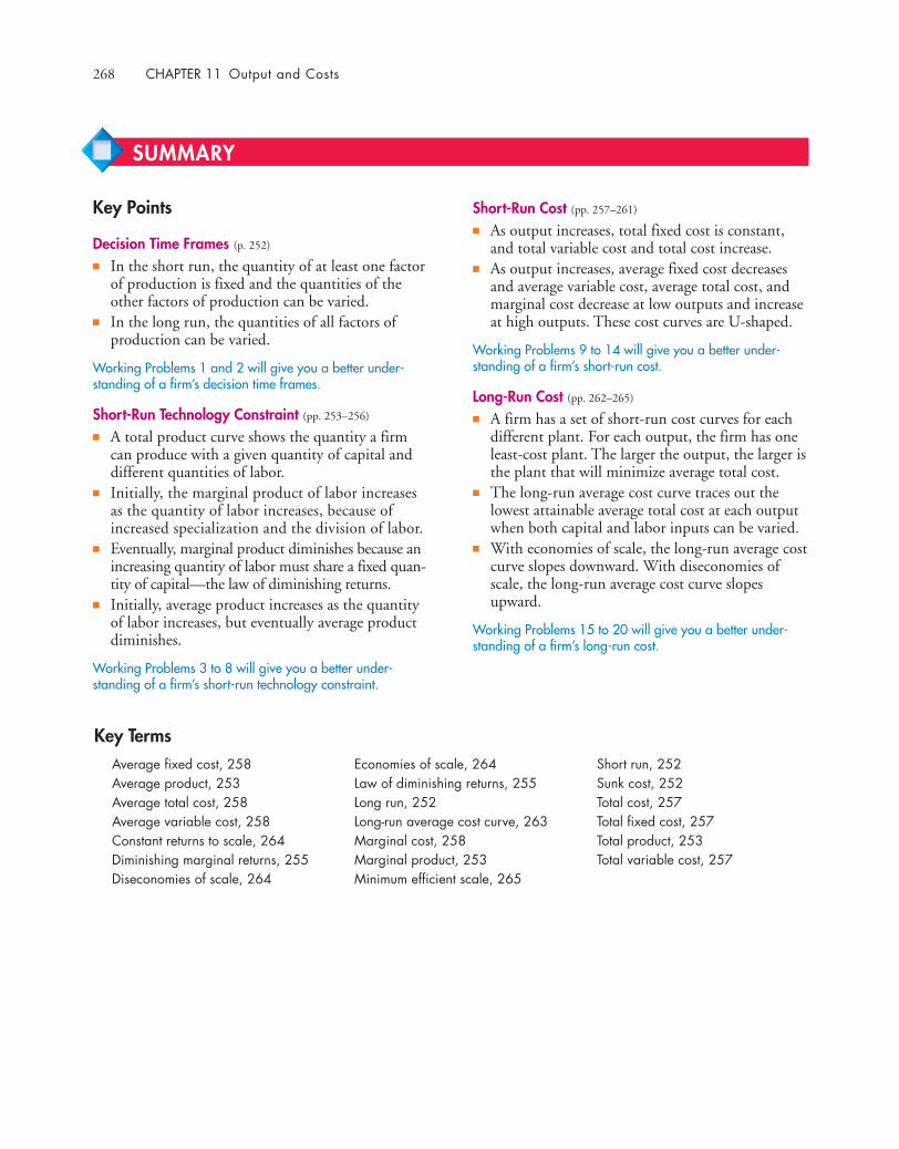
268 CHAPTER 11 Output and Costs

Short-Run Cost (pp. 257–261)

■ As output increases, total fixed cost is constant,and total variable cost and total cost increase.

■ As output increases, average fixed cost decreasesand average variable cost, average total cost, andmarginal cost decrease at low outputs and increaseat high outputs. These cost curves are U-shaped.

Working Problems 9 to 14 will give you a better under-standing of a firm’s short-run cost.

Long-Run Cost (pp. 262–265)

■ A firm has a set of short-run cost curves for eachdifferent plant. For each output, the firm has oneleast-cost plant. The larger the output, the larger isthe plant that will minimize average total cost.

■ The long-run average cost curve traces out thelowest attainable average total cost at each outputwhen both capital and labor inputs can be varied.

■ With economies of scale, the long-run average costcurve slopes downward. With diseconomies ofscale, the long-run average cost curve slopesupward.

Working Problems 15 to 20 will give you a better under-standing of a firm’s long-run cost.

Key Points

Decision Time Frames (p. 252)

■ In the short run, the quantity of at least one factorof production is fixed and the quantities of theother factors of production can be varied.

■ In the long run, the quantities of all factors ofproduction can be varied.

Working Problems 1 and 2 will give you a better under-standing of a firm’s decision time frames.

Short-Run Technology Constraint (pp. 253–256)

■ A total product curve shows the quantity a firmcan produce with a given quantity of capital anddifferent quantities of labor.

■ Initially, the marginal product of labor increasesas the quantity of labor increases, because ofincreased specialization and the division of labor.

■ Eventually, marginal product diminishes because anincreasing quantity of labor must share a fixed quan-tity of capital—the law of diminishing returns.

■ Initially, average product increases as the quantityof labor increases, but eventually average productdiminishes.

Working Problems 3 to 8 will give you a better under-standing of a firm’s short-run technology constraint.

SUMMARY

Key TermsAverage fixed cost, 258Average product, 253Average total cost, 258Average variable cost, 258Constant returns to scale, 264Diminishing marginal returns, 255Diseconomies of scale, 264

Economies of scale, 264Law of diminishing returns, 255Long run, 252Long-run average cost curve, 263Marginal cost, 258Marginal product, 253Minimum efficient scale, 265

Short run, 252Sunk cost, 252Total cost, 257Total fixed cost, 257Total product, 253Total variable cost, 257

Study Plan Problems and Applications 269

6. a. Over what output range does Sue’s Surfboardsenjoy the benefits of increased specializationand division of labor?

b. Over what output range does the firm experi-ence diminishing marginal product of labor?

c. Over what output range does the firm experi-ence an increasing average product of laborbut a diminishing marginal product of labor?

7. Explain how it is possible for a firm to experiencesimultaneously an increasing average product buta diminishing marginal product.

8. Business Boot CampAt a footwear company called Caboots, sales rosefrom $160,000 in 2000 to $2.3 million in 2006,but in 2007 sales dipped to $1.5 million. Joeyand Priscilla Sanchez, who run Caboots, blamethe decline partly on a flood that damaged thefirm’s office and sapped morale.

Source: CNN, April 23, 2008If the Sanchezes are correct in their assumptionsand the prices of footwear didn’t change

a. Explain the effect of the flood on the totalproduct curve and marginal product curve atCaboots.

b. Draw a graph to show the effect of the floodon the total product curve and marginal prod-uct curve at Caboots.

Short-Run Cost (Study Plan 11.3)

Use the following data to work Problems 9 to 13.

Sue’s Surfboards, in Problem 3, hires workers at $500a week and its total fixed cost is $1,000 a week.

9. Calculate total cost, total variable cost, and totalfixed cost of each output in the table. Plot thesepoints and sketch the short-run total cost curvespassing through them.

10. Calculate average total cost, average fixed cost,average variable cost, and marginal cost of eachoutput in the table. Plot these points and sketchthe short-run average and marginal cost curvespassing through them.

11. Illustrate the connection between Sue’s AP, MP,AVC, and MC curves in graphs like those in Fig.11.6.

Decision Time Frames (Study Plan 11.1)

1. Which of the following news items involves ashort-run decision and which involves a long-rundecision? Explain.January 31, 2008: Starbucks will open 75 morestores abroad than originally predicted, for a totalof 975.February 25, 2008: For three hours on Tuesday,Starbucks will shut down every single one of its7,100 stores so that baristas can receive arefresher course.June 2, 2008: Starbucks replaces baristas withvending machines.July 18, 2008: Starbucks is closing 616 stores bythe end of March.

2. Maryland Farmers Turn from Tobacco to FlowersMaryland tobacco farmers will be subsidized ifthey switch from growing tobacco to growingcrops such as flowers and organic vegetables.

Source: The New York Times, February 25, 2001a. How does offering farmers a payment to exit

tobacco growing influence the opportunitycost of growing tobacco?

b. What is the opportunity cost of using theequipment owned by a tobacco farmer?

Short-Run Technology Constraint (Study Plan 11.2)

Use the following table to work Problems 3 to 7.The table sets out Sue’s Surfboards’ total productschedule.

Labor Output(workers per week) (surfboards per week)

1 302 703 1204 1605 1906 2107 220

3. Draw the total product curve.4. Calculate the average product of labor and draw

the average product curve.5. Calculate the marginal product of labor and

draw the marginal product curve.

You can work Problems 1 to 21 in MyEconLab Chapter 11 Study Plan and get instant feedback.

STUDY PLAN PROBLEMS AND APPLICATIONS

270 CHAPTER 11 Output and Costs

12. Sue’s Surfboards rents a factory building. If therent is increased by $200 a week and other thingsremain the same, how do Sue’s Surfboards’ short-run average cost curves and marginal cost curvechange?

13. Workers at Sue’s Surfboards negotiate a wageincrease of $100 a week for each worker. If otherthings remain the same, explain how Sue’sSurfboards’ short-run average cost curves andmarginal cost curve change.

14. Grain Prices Go the Way of the Oil PriceEvery morning millions of Americans confrontthe latest trend in commodities markets at theirkitchen table. Rising prices for crops have begunto drive up the cost of breakfast.

Source: The Economist, July 21, 2007Explain how the rising price of crops affects theaverage total cost and marginal cost of producingbreakfast cereals.

Long-Run Cost (Study Plan 11.4)

Use the table in Problem 3 and the following infor-mation to work Problems 15 and 16.Sue’s Surfboards buys a second plant and the outputproduced by each worker increases by 50 percent.The total fixed cost of operating each plant is $1,000a week. Each worker is paid $500 a week.15. Calculate the average total cost of producing 180

and 240 surfboards a week when Sue’s Surfboardsoperates two plants. Graph these points andsketch the ATC curve.

16. a. To produce 180 surfboards a week, is it effi-cient to operate one or two plants?

b. To produce 160 surfboards a week, is it effi-cient for Sue’s to operate one or two plants?

Use the following table to work Problems 17 to 20.The table shows the production function of Jackie’sCanoe Rides.

Labor Output (rides per day)

(workers per day) Plant 1 Plant 2 Plant 3 Plant 4

10 20 40 55 6520 40 60 75 8530 65 75 90 10040 75 85 100 110

Canoes 10 20 30 40

Jackie’s pays $100 a day for each canoe it rentsand $50 a day for each canoe operator it hires.

17. Graph the ATC curves for Plant 1 and Plant 2.Explain why these ATC curves differ.

18. Graph the ATC curves for Plant 3 and Plant 4.Explain why these ATC curves differ.

19. a. On Jackie’s LRAC curve, what is the averagecost of producing 40, 75, and 85 rides a week?

b. What is Jackie’s minimum efficient scale?

20. a. Explain how Jackie’s uses its LRAC curve todecide how many canoes to rent.

b. Does Jackie’s production function featureeconomies of scale or diseconomies of scale?

Economics in the News (Study Plan 11.N)

21. Airlines Seek Out New Ways to Save on Fuel asCosts SoarThe financial pain of higher fuel prices is particu-larly acute for airlines because it is their singlebiggest expense. Airlines pump about 7,000 gal-lons into a Boeing 737 and about 60,000 gallonsinto the bigger 747 jet. Each generation of aircraftis more efficient: An Airbus A330 long-range jetuses 38 percent less fuel than the DC-10 itreplaced, while the Airbus A319 medium-rangejet is 27 percent more efficient than the DC-9 itreplaced.

Source: The New York Times, June 11, 2008a. Is the price of fuel a fixed cost or a variable

cost for an airline?b. Explain how an increase in the price of fuel

changes an airline’s total costs, average costs,and marginal cost.

c. Draw a graph to show the effects of an in-crease in the price of fuel on an airline’s TFC,TVC, AFC, AVC, and MC curves.

d. Explain how a technological advance thatmakes an airplane engine more fuel efficientchanges an airline’s total product, marginalproduct, and average product.

e. Draw a graph to illustrate the effects of amore fuel-efficient aircraft on an airline’s TP,MP, and AP curves.

f. Explain how a technological advance thatmakes an airplane engine more fuel efficientchanges an airline’s average variable cost, mar-ginal cost, and average total cost.

g. Draw a graph to illustrate how a technologicaladvance that makes an airplane engine morefuel efficient changes an airline’s AVC, MC,and ATC curves.

Additional Problems and Applications 271

These problems are available in MyEconLab if assigned by your instructor.

ADDITIONAL PROBLEMS AND APPLICATIONS

Decision Time Frames22. A Bakery on the Rise

Some 500 customers a day line up to buy Avalon’sbreads, scones, muffins, and coffee. Staffing andmanagement are worries. Avalon now employs 35and plans to hire 15 more. Its payroll will climb by30 percent to 40 percent. The new CEO has exe-cuted an ambitious agenda that includes the moveto a larger space, which will increase the rent from$3,500 to $10,000 a month.

Source: CNN, March 24, 2008a. Which of Avalon’s decisions described in the

news clip is a short-run decision and which isa long-run decision?

b. Why is Avalon’s long-run decision riskier thanits short-run decision?

23. The Sunk-Cost FallacyYou have good tickets to a basketball game anhour’s drive away. There’s a blizzard raging out-side, and the game is being televised. You can sitwarm and safe at home and watch it on TV, oryou can bundle up, dig out your car, and go tothe game. What do you do?

Source: Slate, September 9, 2005a. What type of cost is your expenditure on tickets?b. Why is the cost of the ticket irrelevant to your

current decision about whether to stay athome or go to the game?

Short-Run Technology Constraint24. Terri runs a rose farm. One worker produces

1,000 roses a week; hiring a second worker dou-bles her total product; hiring a third worker dou-bles her output again; hiring a fourth workerincreased her total product but by only 1,000roses. Construct Terri’s marginal product andaverage product schedules. Over what range ofworkers do marginal returns increase?

Short-Run Cost25. Use the events described in the news clip in

Problem 22. By how much will Avalon’s short-run decision increase its total variable cost? Byhow much will Avalon’s long-run decisionincrease its monthly total fixed cost? SketchAvalon’s short-run ATC curve before and afterthe events described in the news clip.

26. Coffee King Starbucks Raises Its PricesStarbucks is raising its prices because the whole-sale price of milk has risen 70 percent and there’sa lot of milk in Starbucks lattes.

Source: USA Today, July 24, 2007Is milk a fixed factor of production or a variablefactor of production? Describe how the increasein the price of milk changes Starbucks’ short-runcost curves.

27. Bill’s Bakery has a fire and Bill loses some of hiscost data. The bits of paper that he recovers afterthe fire provide the information in the followingtable (all the cost numbers are dollars).

TP AFC AVC ATC MC

10 120 100 22080

20 A B 15090

30 40 90 130130

40 30 C DE

50 24 108 132

Bill asks you to come to his rescue and providethe missing data in the five spaces identified asA, B, C, D, and E.

Use the following table to work Problems 28 and 29.ProPainters hires students at $250 a week to painthouses. It leases equipment at $500 a week. Thetable sets out its total product schedule.

Labor Output(students) (houses painted per week)

1 22 53 94 125 146 15

28. If ProPainters paints 12 houses a week, calculate itstotal cost, average total cost, and marginal cost. Atwhat output is average total cost a minimum?

29. Explain why the gap between ProPainters’ totalcost and total variable cost is the same no matterhow many houses are painted.

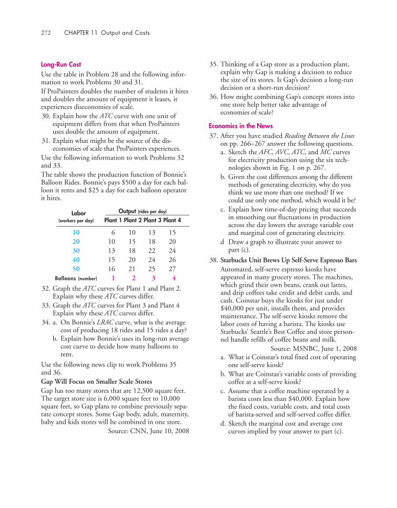
272 CHAPTER 11 Output and Costs

Long-Run Cost Use the table in Problem 28 and the following infor-mation to work Problems 30 and 31.If ProPainters doubles the number of students it hiresand doubles the amount of equipment it leases, itexperiences diseconomies of scale.30. Explain how the ATC curve with one unit of

equipment differs from that when ProPaintersuses double the amount of equipment.

31. Explain what might be the source of the dis-economies of scale that ProPainters experiences.

Use the following information to work Problems 32and 33.The table shows the production function of Bonnie’sBalloon Rides. Bonnie’s pays $500 a day for each bal-loon it rents and $25 a day for each balloon operatorit hires.

Labor Output (rides per day)

(workers per day) Plant 1 Plant 2 Plant 3 Plant 4

10 6 10 13 1520 10 15 18 2030 13 18 22 2440 15 20 24 2650 16 21 25 27

Balloons (number) 1 2 3 4

32. Graph the ATC curves for Plant 1 and Plant 2.Explain why these ATC curves differ.

33. Graph the ATC curves for Plant 3 and Plant 4Explain why these ATC curves differ.

34. a. On Bonnie’s LRAC curve, what is the averagecost of producing 18 rides and 15 rides a day?

b. Explain how Bonnie’s uses its long-run averagecost curve to decide how many balloons torent.

Use the following news clip to work Problems 35 and 36.Gap Will Focus on Smaller Scale StoresGap has too many stores that are 12,500 square feet.The target store size is 6,000 square feet to 10,000square feet, so Gap plans to combine previously sepa-rate concept stores. Some Gap body, adult, maternity,baby and kids stores will be combined in one store.

Source: CNN, June 10, 2008

35. Thinking of a Gap store as a production plant,explain why Gap is making a decision to reducethe size of its stores. Is Gap’s decision a long-rundecision or a short-run decision?

36. How might combining Gap’s concept stores intoone store help better take advantage ofeconomies of scale?

Economics in the News37. After you have studied Reading Between the Lines

on pp. 266–267 answer the following questions.a. Sketch the AFC, AVC, ATC, and MC curves

for electricity production using the six tech-nologies shown in Fig. 1 on p. 267.

b. Given the cost differences among the differentmethods of generating electricity, why do youthink we use more than one method? If wecould use only one method, which would it be?

c. Explain how time-of-day pricing that succeedsin smoothing out fluctuations in productionacross the day lowers the average variable costand marginal cost of generating electricity.

d Draw a graph to illustrate your answer to part (c).

38. Starbucks Unit Brews Up Self-Serve Espresso BarsAutomated, self-serve espresso kiosks haveappeared in many grocery stores. The machines,which grind their own beans, crank out lattes,and drip coffees take credit and debit cards, andcash. Coinstar buys the kiosks for just under$40,000 per unit, installs them, and providesmaintenance. The self-serve kiosks remove thelabor costs of having a barista. The kiosks useStarbucks’ Seattle’s Best Coffee and store person-nel handle refills of coffee beans and milk.

Source: MSNBC, June 1, 2008a. What is Coinstar’s total fixed cost of operating

one self-serve kiosk? b. What are Coinstar’s variable costs of providing

coffee at a self-serve kiosk?c. Assume that a coffee machine operated by a

barista costs less than $40,000. Explain howthe fixed costs, variable costs, and total costsof barista-served and self-served coffee differ.

d. Sketch the marginal cost and average costcurves implied by your answer to part (c).

After studying this chapter, you will be able to:

� Define perfect competition� Explain how a firm makes its output decision and why it

sometimes shuts down temporarily and lays off its workers� Explain how price and output are determined in a

perfectly competitive market� Explain why firms enter and leave a competitive

market and the consequences of entry and exit� Predict the effects of a change in demand and of a

technological advance� Explain why perfect competition is efficient

A n Iowa corn farmer must make many decisions, but figuring out the price tocharge for his corn is not one of them. Corn farmers must accept the pricedetermined by supply and demand. The producers of most crops—among themwheat, rice, soybean, sugarbeet, and coffee—must also accept the prices thatmarkets determine.

During the booming economic conditions of 2006 and 2007, crop pricesand production soared. Then, following the global financial crisis of 2008prices sagged, but for many crops production kept rising.

What are the forces that brought these changes in prices and production inthe world’s markets for farm products?

We’re going to answer this question by studyingcompetitive markets and building a model of a market in

which competition is as fierce and extreme as possible. We call this situationperfect competition.

In Reading Between the Lines at the end of the chapter, we’ll apply themodel to the global market for corn and see how changes in demand andfortunate weather bring changes in prices and quantities produced in this keyglobal agricultural market.

PERFECT COMPETITION

12273

274 CHAPTER 12 Perfect Competition

◆ What Is Perfect Competition?The firms that you study in this chapter face the forceof raw competition. We call this extreme form of com-petition perfect competition. Perfect competition is amarket in which

■ Many firms sell identical products to many buyers.■ There are no restrictions on entry into the market.■ Established firms have no advantage over new ones.■ Sellers and buyers are well informed about prices.

Farming, fishing, wood pulping and paper milling,the manufacture of paper cups and shopping bags,grocery and fresh flower retailing, photo finishing,lawn services, plumbing, painting, dry cleaning, andlaundry services are all examples of highly competi-tive industries.

How Perfect Competition ArisesPerfect competition arises if the minimum efficientscale of a single producer is small relative to the mar-ket demand for the good or service. In this situation,there is room in the market for many firms. A firm’sminimum efficient scale is the smallest output atwhich long-run average cost reaches its lowest level.(See Chapter 11, p. 265.)

In perfect competition, each firm produces a goodthat has no unique characteristics, so consumers don’tcare which firm’s good they buy.

Price TakersFirms in perfect competition are price takers. A pricetaker is a firm that cannot influence the market pricebecause its production is an insignificant part of thetotal market.

Imagine that you are a wheat farmer in Kansas. Youhave a thousand acres planted—which sounds like alot. But compared to the millions of acres in Colorado,Oklahoma, Texas, Nebraska, and the Dakotas, as wellas the millions more in Canada, Argentina, Australia,and Ukraine, your thousand acres are a drop in theocean. Nothing makes your wheat any better than anyother farmer’s, and all the buyers of wheat know theprice at which they can do business.

If the market price of wheat is $4 a bushel, thenthat is the highest price you can get for your wheat.Ask for $4.10 and no one will buy from you. Offer itfor $3.90 and you’ll be sold out in a flash and havegiven away 10¢ a bushel. You take the market price.

Economic Profit and RevenueA firm’s goal is to maximize economic profit, which isequal to total revenue minus total cost. Total cost isthe opportunity cost of production, which includesnormal profit. (See Chapter 10, p. 228.)

A firm’s total revenue equals the price of its outputmultiplied by the number of units of output sold(price × quantity). Marginal revenue is the change intotal revenue that results from a one-unit increase inthe quantity sold. Marginal revenue is calculated bydividing the change in total revenue by the change inthe quantity sold.

Figure 12.1 illustrates these revenue concepts. Inpart (a), the market demand curve, D, and marketsupply curve, S, determine the market price. Themarket price is $25 a sweater. Campus Sweaters isjust one of many producers of sweaters, so the best itcan do is to sell its sweaters for $25 each.

Total Revenue Total revenue is equal to the pricemultiplied by the quantity sold. In the table in Fig.12.1, if Campus Sweaters sells 9 sweaters, its totalrevenue is $225 (9 × $25).

Figure 12.1(b) shows the firm’s total revenue curve(TR), which graphs the relationship between totalrevenue and the quantity sold. At point A on the TRcurve, the firm sells 9 sweaters and has a total revenueof $225. Because each additional sweater sold bringsin a constant amount—$25—the total revenue curveis an upward-sloping straight line.

Marginal Revenue Marginal revenue is the change intotal revenue that results from a one-unit increase inquantity sold. In the table in Fig. 12.1, when thequantity sold increases from 8 to 9 sweaters, total rev-enue increases from $200 to $225, so marginal rev-enue is $25 a sweater.

Because the firm in perfect competition is a pricetaker, the change in total revenue that results from aone-unit increase in the quantity sold equals the mar-ket price. In perfect competition, the firm’s marginalrevenue equals the market price. Figure 12.1(c) showsthe firm’s marginal revenue curve (MR) as the hori-zontal line at the market price.

Demand for the Firm’s Product The firm can sell anyquantity it chooses at the market price. So thedemand curve for the firm’s product is a horizontalline at the market price, the same as the firm’s mar-ginal revenue curve.

What Is Perfect Competition? 275

A horizontal demand curve illustrates a perfectlyelastic demand, so the demand for the firm’s productis perfectly elastic. A sweater from Campus Sweatersis a perfect substitute for a sweater from any other fac-tory. But the market demand for sweaters is not per-fectly elastic: Its elasticity depends on the substitut-ability of sweaters for other goods and services.

The Firm’s DecisionsThe goal of the competitive firm is to maximize eco-nomic profit, given the constraints it faces. Toachieve its goal, a firm must decide

1. How to produce at minimum cost2. What quantity to produce3. Whether to enter or exit a marketYou’ve already seen how a firm makes the first

decision. It does so by operating with the plant thatminimizes long-run average cost—by being on its

long-run average cost curve. We’ll now see how thefirm makes the other two decisions. We start by look-ing at the firm’s output decision.

9

Pric

e (d

olla

rs p

er s

wea

ter)

Quantity (thousands ofsweaters per day)

25

50

0 20

S

9 20

(a) Sweater market

DTo

tal r

even

ue (d

olla

rs p

er d

ay)

Quantity (sweaters per day)

225

0

TR

(b) Campus Sweaters' total revenue

A

Marketdemandcurve

20

Pric

e (d

olla

rs p

er s

wea

ter)

Quantity (sweaters per day)

25

0 10

MR

(c) Campus Sweaters' marginal revenue

Demand forCampussweaters

50

Quantity Price Marginalsold (P) Total revenue(Q) (dollars revenue (MR = ΔTR/ΔQ)

(sweaters per (TR = P × Q) (dollars perper day) sweater) (dollars) additional sweater)

8 25 200 . . . . . . . 25

9 25 225 . . . . . . . 25

10 25 250 . . . . . . .

In part (a), market demand and market supply determinethe market price (and quantity). Part (b) shows the firm’stotal revenue curve (TR). Point A corresponds to the secondrow of the table—Campus Sweaters sells 9 sweaters at $25a sweater, so total revenue is $225. Part (c) shows thefirm’s marginal revenue curve (MR). This curve is also thedemand curve for the firm’s sweaters. The demand forsweaters from Campus Sweaters is perfectly elastic at themarket price of $25 a sweater.

REVIEW QUIZ1 Why is a firm in perfect competition a price taker?2 In perfect competition, what is the relationship

between the demand for the firm’s output andthe market demand?

3 In perfect competition, why is a firm’s marginalrevenue curve also the demand curve for thefirm’s output?

4 What decisions must a firm make to maximizeprofit?

You can work these questions in Study Plan 12.1 and get instant feedback.

FIGURE 12.1 Demand, Price, and Revenue in Perfect Competition

animation

276 CHAPTER 12 Perfect Competition

◆ The Firm’s Output DecisionA firm’s cost curves (total cost, average cost, and marginal cost) describe the relationship between itsoutput and costs (see pp. 257–261). And a firm’s revenue curves (total revenue and marginal revenue)describe the relationship between its output and revenue (p. 275). From the firm’s cost curves and revenue curves, we can find the output that maximizesthe firm’s economic profit.

Figure 12.2 shows how to do this for CampusSweaters. The table lists the firm’s total revenue andtotal cost at different outputs, and part (a) of the fig-ure shows the firm’s total revenue curve, TR, andtotal cost curve, TC. These curves are graphs of num-bers in the first three columns of the table.

Economic profit equals total revenue minus totalcost. The fourth column of the table in Fig. 12.2shows the economic profit made by CampusSweaters, and part (b) of the figure graphs thesenumbers as its economic profit curve, EP.

Campus Sweaters maximizes its economic profitby producing 9 sweaters a day: Total revenue is $225,total cost is $183, and economic profit is $42. Noother output rate achieves a larger profit.

At outputs of less than 4 sweaters and more than12 sweaters a day, the Campus Sweaters would incuran economic loss. At either 4 or 12 sweaters a day,the Campus Sweaters would make zero economicprofit, called a break-even point.

The table lists Campus Sweaters’ total revenue, total cost, andeconomic profit. Part (a) graphs the total revenue and totalcost curves and part (b) graphs economic profit.

Campus Sweaters makes maximum economic profit, $42a day ($225 – $183), when it produces 9 sweaters a day. Atoutputs of 4 sweaters and 12 sweaters a day, CampusSweaters makes zero economic profit—these are break-evenpoints. At outputs less than 4 sweaters and greater than 12sweaters a day, Campus Sweaters incurs an economic loss.

300

9

Tota

l rev

enue

and

tota

l cos

t (do

llars

per

day

)

225

100

0 4

TR

(a) Revenue and cost

183

12

TC

20

9

Econ

omic

pro

fit (d

olla

rs p

er d

ay)

Quantity(sweatersper day)

42

–20

–40

4

(b) Economic profit and loss

012

EP

Profit-maximizingquantity

Quantity (sweaters per day)

Economicprofit = TR – TC

Economicprofit

Economicloss

Economicloss

Economicloss

FIGURE 12.2 Total Revenue, Total Cost, and Economic Profit

animation

Quantity Total Total Economic(Q) revenue cost profit

(sweaters (TR) (TC ) (TR – TC )per day) (dollars) (dollars) (dollars)

0 0 22 –22

1 25 45 –20

2 50 66 –16

3 75 85 –10

4 100 100 0

5 125 114 11

6 150 126 24

7 175 141 34

8 200 160 40

9 225 183 42

10 250 210 40

11 275 245 30

12 300 300 0

13 325 360 –35

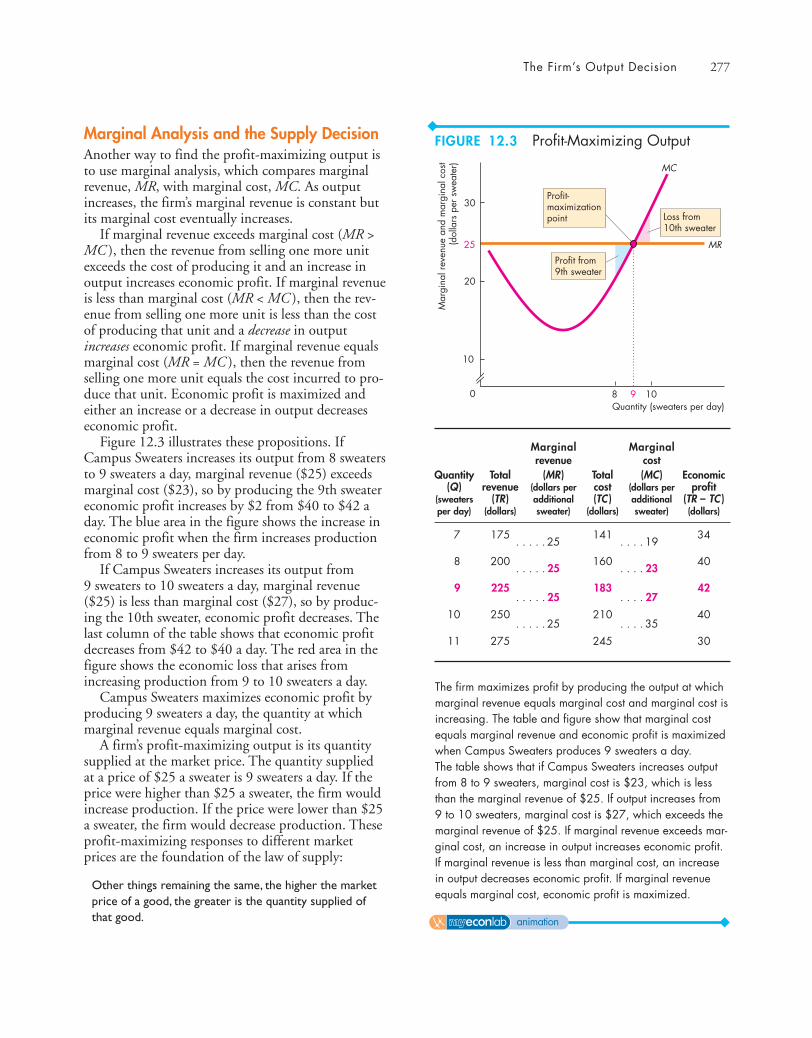
The Firm’s Output Decision 277

Marginal Analysis and the Supply DecisionAnother way to find the profit-maximizing output isto use marginal analysis, which compares marginalrevenue, MR, with marginal cost, MC. As outputincreases, the firm’s marginal revenue is constant butits marginal cost eventually increases.

If marginal revenue exceeds marginal cost (MR >MC ), then the revenue from selling one more unitexceeds the cost of producing it and an increase inoutput increases economic profit. If marginal revenueis less than marginal cost (MR < MC ), then the rev-enue from selling one more unit is less than the costof producing that unit and a decrease in outputincreases economic profit. If marginal revenue equalsmarginal cost (MR = MC ), then the revenue fromselling one more unit equals the cost incurred to pro-duce that unit. Economic profit is maximized andeither an increase or a decrease in output decreaseseconomic profit.

Figure 12.3 illustrates these propositions. IfCampus Sweaters increases its output from 8 sweatersto 9 sweaters a day, marginal revenue ($25) exceedsmarginal cost ($23), so by producing the 9th sweatereconomic profit increases by $2 from $40 to $42 aday. The blue area in the figure shows the increase ineconomic profit when the firm increases productionfrom 8 to 9 sweaters per day.

If Campus Sweaters increases its output from 9 sweaters to 10 sweaters a day, marginal revenue($25) is less than marginal cost ($27), so by produc-ing the 10th sweater, economic profit decreases. Thelast column of the table shows that economic profitdecreases from $42 to $40 a day. The red area in thefigure shows the economic loss that arises fromincreasing production from 9 to 10 sweaters a day.

Campus Sweaters maximizes economic profit byproducing 9 sweaters a day, the quantity at whichmarginal revenue equals marginal cost.

A firm’s profit-maximizing output is its quantitysupplied at the market price. The quantity suppliedat a price of $25 a sweater is 9 sweaters a day. If theprice were higher than $25 a sweater, the firm wouldincrease production. If the price were lower than $25a sweater, the firm would decrease production. Theseprofit-maximizing responses to different marketprices are the foundation of the law of supply:

Other things remaining the same, the higher the marketprice of a good, the greater is the quantity supplied ofthat good.

30

9

Mar

gina

l rev

enue

and

mar

gina

l cos

t(d

olla

rs p

er s

wea

ter)

25

20

10

10

Loss from10th sweater

Quantity (sweaters per day)80

Profit-maximizationpoint

Profit from9th sweater

MC

MR

The firm maximizes profit by producing the output at whichmarginal revenue equals marginal cost and marginal cost isincreasing. The table and figure show that marginal costequals marginal revenue and economic profit is maximizedwhen Campus Sweaters produces 9 sweaters a day. The table shows that if Campus Sweaters increases outputfrom 8 to 9 sweaters, marginal cost is $23, which is lessthan the marginal revenue of $25. If output increases from9 to 10 sweaters, marginal cost is $27, which exceeds themarginal revenue of $25. If marginal revenue exceeds mar-ginal cost, an increase in output increases economic profit.If marginal revenue is less than marginal cost, an increasein output decreases economic profit. If marginal revenueequals marginal cost, economic profit is maximized.

Marginal Marginalrevenue cost

Quantity Total (MR) Total (MC) Economic(Q) revenue (dollars per cost (dollars per profit

(sweaters (TR) additional (TC ) additional (TR – TC )per day) (dollars) sweater) (dollars) sweater) (dollars)

7 175 . . . . . 25

141 . . . . 19

34

8 200 . . . . . 25

160 . . . . 23

40

9 225 . . . . . 25

183 . . . . 27

42

10 250 . . . . . 25

210 . . . . 35

40

11 275 245 30

FIGURE 12.3 Profit-Maximizing Output

animation

278 CHAPTER 12 Perfect Competition

Temporary Shutdown DecisionYou’ve seen that a firm maximizes profit by produc-ing the quantity at which marginal revenue (price)equals marginal cost. But suppose that at this quan-tity, price is less than average total cost. In this case,the firm incurs an economic loss. Maximum profit isa loss (a minimum loss). What does the firm do?

If the firm expects the loss to be permanent, itgoes out of business. But if it expects the loss to betemporary, the firm must decide whether to shutdown temporarily and produce no output, or to keepproducing. To make this decision, the firm comparesthe loss from shutting down with the loss from pro-ducing and takes the action that minimizes its loss.

Loss Comparisons A firm’s economic loss equals totalfixed cost, TFC, plus total variable cost minus totalrevenue. Total variable cost equals average variablecost, AVC, multiplied by the quantity produced, Q,and total revenue equals price, P, multiplied by thequantity Q. So

Economic loss = TFC + (AVC – P) × Q.

If the firm shuts down, it produces no output (Q = 0). The firm has no variable costs and no rev-enue but it must pay its fixed costs, so its economicloss equals total fixed cost.

If the firm produces, then in addition to its fixedcosts, it incurs variable costs. But it also receives rev-enue. Its economic loss equals total fixed cost—theloss when shut down—plus total variable cost minustotal revenue. If total variable cost exceeds total rev-enue, this loss exceeds total fixed cost and the firmshuts down. Equivalently, if average variable costexceeds price, this loss exceeds total fixed cost and thefirm shuts down.

The Shutdown Point A firm’s shutdown point is theprice and quantity at which it is indifferent betweenproducing and shutting down. The shutdown pointoccurs at the price and the quantity at which aver-age variable cost is a minimum. At the shutdownpoint, the firm is minimizing its loss and its lossequals total fixed cost. If the price falls below mini-mum average variable cost, the firm shuts downtemporarily and continues to incur a loss equal tototal fixed cost. At prices above minimum averagevariable cost but below average total cost, the firmproduces the loss-minimizing output and incurs aloss, but a loss that is less than total fixed cost.

7

Pric

e (d

olla

rs p

er s

wea

ter)

17.00

20.14

25.00

15.00

30.00

13104

Shutdownpoint

Quantity (sweaters per day)0

MR

ATC

AVC

MC

The shutdown point is at minimum average variable cost. Ata price below minimum average variable cost, the firmshuts down and produces no output. At a price equal tominimum average variable cost, the firm is indifferentbetween shutting down and producing no output or produc-ing the output at minimum average variable cost. Eitherway, the firm minimizes its economic loss and incurs a lossequal to total fixed cost.

Figure 12.4 illustrates the firm’s shutdown deci-sion and the shutdown point that we’ve justdescribed for Campus Sweaters.

The firm’s average variable cost curve is AVC andthe marginal cost curve is MC. Average variable costhas a minimum of $17 a sweater when output is 7sweaters a day. The MC curve intersects the AVCcurve at its minimum. (We explained this relation-ship between marginal cost and average cost inChapter 11; see pp. 258–259.)

The figure shows the marginal revenue curve MRwhen the price is $17 a sweater, a price equal to min-imum average variable cost.

Marginal revenue equals marginal cost at 7sweaters a day, so this quantity maximizes economicprofit (minimizes economic loss). The ATC curveshows that the firm’s average total cost of producing7 sweaters a day is $20.14 a sweater. The firm incursa loss equal to $3.14 a sweater on 7 sweaters a day, soits loss is $22 a day, which equals total fixed cost.

FIGURE 12.4 The Shutdown Decision

animation

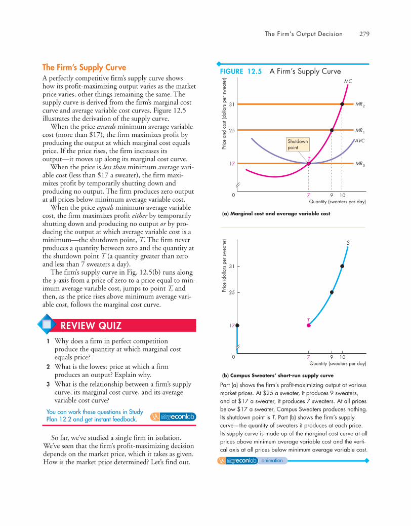
The Firm’s Output Decision 279

The Firm’s Supply CurveA perfectly competitive firm’s supply curve showshow its profit-maximizing output varies as the marketprice varies, other things remaining the same. Thesupply curve is derived from the firm’s marginal costcurve and average variable cost curves. Figure 12.5illustrates the derivation of the supply curve.

When the price exceeds minimum average variablecost (more than $17), the firm maximizes profit byproducing the output at which marginal cost equalsprice. If the price rises, the firm increases itsoutput—it moves up along its marginal cost curve.

When the price is less than minimum average vari-able cost (less than $17 a sweater), the firm maxi-mizes profit by temporarily shutting down andproducing no output. The firm produces zero outputat all prices below minimum average variable cost.

When the price equals minimum average variablecost, the firm maximizes profit either by temporarilyshutting down and producing no output or by pro-ducing the output at which average variable cost is aminimum—the shutdown point, T. The firm neverproduces a quantity between zero and the quantity atthe shutdown point T (a quantity greater than zeroand less than 7 sweaters a day).

The firm’s supply curve in Fig. 12.5(b) runs alongthe y-axis from a price of zero to a price equal to min-imum average variable cost, jumps to point T, andthen, as the price rises above minimum average vari-able cost, follows the marginal cost curve.

31

9

Pric

e an

d co

st (d

olla

rs p

er s

wea

ter)

25

17

10Quantity (sweaters per day)

0

(a) Marginal cost and average variable cost

7

MC

MR2

MR1

MR0

AVCShutdownpoint

T

31

9

Pric

e (d

olla

rs p

er s

wea

ter)

25

17

10Quantity (sweaters per day)

0

(b) Campus Sweaters’ short-run supply curve

7

T

S

Part (a) shows the firm’s profit-maximizing output at variousmarket prices. At $25 a sweater, it produces 9 sweaters,and at $17 a sweater, it produces 7 sweaters. At all pricesbelow $17 a sweater, Campus Sweaters produces nothing.Its shutdown point is T. Part (b) shows the firm’s supplycurve—the quantity of sweaters it produces at each price.Its supply curve is made up of the marginal cost curve at allprices above minimum average variable cost and the verti-cal axis at all prices below minimum average variable cost.

So far, we’ve studied a single firm in isolation.We’ve seen that the firm’s profit-maximizing decisiondepends on the market price, which it takes as given.How is the market price determined? Let’s find out.

REVIEW QUIZ 1 Why does a firm in perfect competition

produce the quantity at which marginal costequals price?

2 What is the lowest price at which a firm produces an output? Explain why.

3 What is the relationship between a firm’s supplycurve, its marginal cost curve, and its averagevariable cost curve?

You can work these questions in Study Plan 12.2 and get instant feedback.

FIGURE 12.5 A Firm’s Supply Curve

animation

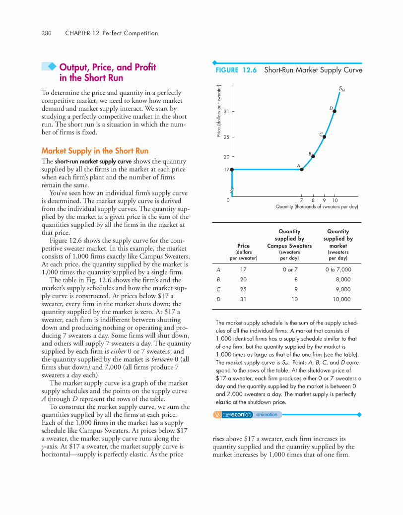
280 CHAPTER 12 Perfect Competition

◆ Output, Price, and Profitin the Short Run

To determine the price and quantity in a perfectlycompetitive market, we need to know how marketdemand and market supply interact. We start bystudying a perfectly competitive market in the shortrun. The short run is a situation in which the num-ber of firms is fixed.

Market Supply in the Short RunThe short-run market supply curve shows the quantitysupplied by all the firms in the market at each pricewhen each firm’s plant and the number of firmsremain the same.

You’ve seen how an individual firm’s supply curveis determined. The market supply curve is derivedfrom the individual supply curves. The quantity sup-plied by the market at a given price is the sum of thequantities supplied by all the firms in the market atthat price.

Figure 12.6 shows the supply curve for the com-petitive sweater market. In this example, the marketconsists of 1,000 firms exactly like Campus Sweaters.At each price, the quantity supplied by the market is1,000 times the quantity supplied by a single firm.

The table in Fig. 12.6 shows the firm’s and themarket’s supply schedules and how the market sup-ply curve is constructed. At prices below $17 asweater, every firm in the market shuts down; thequantity supplied by the market is zero. At $17 asweater, each firm is indifferent between shuttingdown and producing nothing or operating and pro-ducing 7 sweaters a day. Some firms will shut down,and others will supply 7 sweaters a day. The quantitysupplied by each firm is either 0 or 7 sweaters, andthe quantity supplied by the market is between 0 (allfirms shut down) and 7,000 (all firms produce 7sweaters a day each).

The market supply curve is a graph of the marketsupply schedules and the points on the supply curveA through D represent the rows of the table.

To construct the market supply curve, we sum thequantities supplied by all the firms at each price.Each of the 1,000 firms in the market has a supplyschedule like Campus Sweaters. At prices below $17a sweater, the market supply curve runs along the y-axis. At $17 a sweater, the market supply curve ishorizontal—supply is perfectly elastic. As the price

SM

D

C

B

A

31

9

Pric

e (d

olla

rs p

er s

wea

ter)

25

17

10Quantity (thousands of sweaters per day)

0 7 8

20

The market supply schedule is the sum of the supply sched-ules of all the individual firms. A market that consists of1,000 identical firms has a supply schedule similar to thatof one firm, but the quantity supplied by the market is1,000 times as large as that of the one firm (see the table).The market supply curve is SM. Points A, B, C, and D corre-spond to the rows of the table. At the shutdown price of$17 a sweater, each firm produces either 0 or 7 sweaters aday and the quantity supplied by the market is between 0and 7,000 sweaters a day. The market supply is perfectlyelastic at the shutdown price.

Quantity Quantity supplied by supplied by

Price Campus Sweaters market(dollars (sweaters (sweaters

per sweater) per day) per day)

A 17 0 or 7 0 to 7,000

B 20 8 8,000

C 25 9 9,000

D 31 10 10,000

rises above $17 a sweater, each firm increases itsquantity supplied and the quantity supplied by themarket increases by 1,000 times that of one firm.

FIGURE 12.6 Short-Run Market Supply Curve

animation

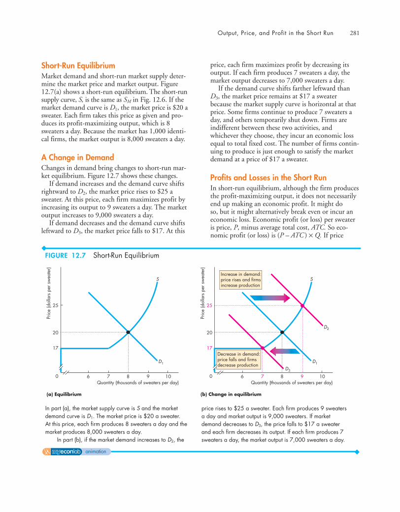
Output, Price, and Profit in the Short Run 281

Short-Run EquilibriumMarket demand and short-run market supply deter-mine the market price and market output. Figure12.7(a) shows a short-run equilibrium. The short-runsupply curve, S, is the same as SM in Fig. 12.6. If themarket demand curve is D1, the market price is $20 asweater. Each firm takes this price as given and pro-duces its profit-maximizing output, which is 8sweaters a day. Because the market has 1,000 identi-cal firms, the market output is 8,000 sweaters a day.

A Change in DemandChanges in demand bring changes to short-run mar-ket equilibrium. Figure 12.7 shows these changes.

If demand increases and the demand curve shiftsrightward to D2, the market price rises to $25 asweater. At this price, each firm maximizes profit byincreasing its output to 9 sweaters a day. The marketoutput increases to 9,000 sweaters a day.

If demand decreases and the demand curve shiftsleftward to D3, the market price falls to $17. At this

price, each firm maximizes profit by decreasing itsoutput. If each firm produces 7 sweaters a day, themarket output decreases to 7,000 sweaters a day.

If the demand curve shifts farther leftward thanD3, the market price remains at $17 a sweaterbecause the market supply curve is horizontal at thatprice. Some firms continue to produce 7 sweaters aday, and others temporarily shut down. Firms areindifferent between these two activities, andwhichever they choose, they incur an economic lossequal to total fixed cost. The number of firms contin-uing to produce is just enough to satisfy the marketdemand at a price of $17 a sweater.

Profits and Losses in the Short RunIn short-run equilibrium, although the firm producesthe profit-maximizing output, it does not necessarilyend up making an economic profit. It might doso, but it might alternatively break even or incur aneconomic loss. Economic profit (or loss) per sweateris price, P, minus average total cost, ATC. So eco-nomic profit (or loss) is (P – ATC ) × Q. If price

(a) Equilibrium

10

Pric

e (d

olla

rs p

er s

wea

ter)

9Quantity (thousands of sweaters per day)

0 876

S

D1

D3

D220

17

25

(b) Change in equilibrium

Increase in demand: price rises and firms increase production

Decrease in demand: price falls and firms decrease production

10

Pric

e (d

olla

rs p

er s

wea

ter)

9Quantity (thousands of sweaters per day)

0 876

S

D1

20

17

25

In part (a), the market supply curve is S and the marketdemand curve is D1. The market price is $20 a sweater. At this price, each firm produces 8 sweaters a day and themarket produces 8,000 sweaters a day.

In part (b), if the market demand increases to D2, the

price rises to $25 a sweater. Each firm produces 9 sweatersa day and market output is 9,000 sweaters. If marketdemand decreases to D3, the price falls to $17 a sweaterand each firm decreases its output. If each firm produces 7sweaters a day, the market output is 7,000 sweaters a day.

FIGURE 12.7 Short-Run Equilibrium

animation

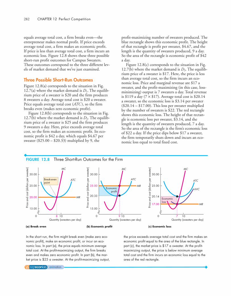
282 CHAPTER 12 Perfect Competition

equals average total cost, a firm breaks even—theentrepreneur makes normal profit. If price exceedsaverage total cost, a firm makes an economic profit.If price is less than average total cost, a firm incurs aneconomic loss. Figure 12.8 shows these three possibleshort-run profit outcomes for Campus Sweaters.These outcomes correspond to the three different lev-els of market demand that we’ve just examined.

Three Possible Short-Run OutcomesFigure 12.8(a) corresponds to the situation in Fig.12.7(a) where the market demand is D1. The equilib-rium price of a sweater is $20 and the firm produces8 sweaters a day. Average total cost is $20 a sweater.Price equals average total cost (ATC ), so the firmbreaks even (makes zero economic profit).

Figure 12.8(b) corresponds to the situation in Fig.12.7(b) where the market demand is D2. The equilib-rium price of a sweater is $25 and the firm produces9 sweaters a day. Here, price exceeds average totalcost, so the firm makes an economic profit. Its eco-nomic profit is $42 a day, which equals $4.67 persweater ($25.00 – $20.33) multiplied by 9, the

profit-maximizing number of sweaters produced. Theblue rectangle shows this economic profit. The heightof that rectangle is profit per sweater, $4.67, and thelength is the quantity of sweaters produced, 9 a day.So the area of the rectangle is economic profit of $42a day.

Figure 12.8(c) corresponds to the situation in Fig.12.7(b) where the market demand is D3. The equilib-rium price of a sweater is $17. Here, the price is lessthan average total cost, so the firm incurs an eco-nomic loss. Price and marginal revenue are $17 asweater, and the profit-maximizing (in this case, loss-minimizing) output is 7 sweaters a day. Total revenueis $119 a day (7 × $17). Average total cost is $20.14a sweater, so the economic loss is $3.14 per sweater($20.14 – $17.00). This loss per sweater multipliedby the number of sweaters is $22. The red rectangleshows this economic loss. The height of that rectan-gle is economic loss per sweater, $3.14, and thelength is the quantity of sweaters produced, 7 a day.So the area of the rectangle is the firm’s economic lossof $22 a day. If the price dips below $17 a sweater,the firm temporarily shuts down and incurs an eco-nomic loss equal to total fixed cost.

9

Pric

e an

d co

st (d

olla

rs p

er s

wea

ter)

Quantity (sweaters per day)

25.00

0 10

(b) Economic profit

30.00

20.33

15.00

MR

Pric

e an

d co

st (d

olla

rs p

er s

wea

ter)

Quantity (sweaters per day)

25.00

0 10

ATC

(a) Break even

MC

30.00

20.00

15.00

Economicprofit

8 7

Pric

e an

d co

st (d

olla

rs p

er s

wea

ter)

Quantity (sweaters per day)

25.00

0 10

ATC

(c) Economic loss

MC

30.00

20.14

MR

Economicloss

17.00

Break-evenpoint

ATC

MC

MR

AVC

In the short run, the firm might break even (make zero eco-nomic profit), make an economic profit, or incur an eco-nomic loss. In part (a), the price equals minimum averagetotal cost. At the profit-maximizing output, the firm breakseven and makes zero economic profit. In part (b), the mar-ket price is $25 a sweater. At the profit-maximizing output,

the price exceeds average total cost and the firm makes aneconomic profit equal to the area of the blue rectangle. Inpart (c), the market price is $17 a sweater. At the profit-maximizing output, the price is below minimum averagetotal cost and the firm incurs an economic loss equal to thearea of the red rectangle.

FIGURE 12.8 Three Short-Run Outcomes for the Firm

animation

Output, Price, and Profit in the Long Run 283

◆ Output, Price, and Profitin the Long Run

In short-run equilibrium, a firm might make an eco-nomic profit, incur an economic loss, or break even.Although each of these three situations is a short-runequilibrium, only one of them is a long-run equilib-rium. The reason is that in the long run, firms canenter or exit the market.

Entry and ExitEntry occurs in a market when new firms come intothe market and the number of firms increases. Exitoccurs when existing firms leave a market and thenumber of firms decreases.

Firms respond to economic profit and economicloss by either entering or exiting a market. New firmsenter a market in which existing firms are making aneconomic profit. Firms exit a market in which theyare incurring an economic loss. Temporary economicprofit and temporary economic loss don’t trigger entryand exit. It’s the prospect of persistent economic profitor loss that triggers entry and exit.

Entry and exit change the market supply, whichinfluences the market price, the quantity produced byeach firm, and its economic profit (or loss).

If firms enter a market, supply increases and themarket supply curve shifts rightward. The increase insupply lowers the market price and eventually elimi-nates economic profit. When economic profit reacheszero, entry stops.

If firms exit a market, supply decreases and themarket supply curve shifts leftward. The market pricerises and economic loss decreases. Eventually, eco-nomic loss is eliminated and exit stops.

To summarize:

■ New firms enter a market in which existing firmsare making an economic profit.

■ As new firms enter a market, the market price fallsand the economic profit of each firm decreases.

■ Firms exit a market in which they are incurring aneconomic loss.

■ As firms leave a market, the market price rises andthe economic loss incurred by the remaining firmsdecreases.

■ Entry and exit stop when firms make zero economicprofit.

Economics in ActionProduction Cutback and TemporaryShutdownThe high price of gasoline and anxiety about unem-ployment and future incomes brought a decrease inthe demand for luxury goods including high-endmotorcycles such as Harley-Davidsons.

Harley-Davidson’s profit-maximizing response tothe decrease in demand was to cut production andlay off workers. Some of the production cuts and lay-offs were temporary and some were permanent.

Harley-Davidson’s bike production plant in YorkCounty, Pennsylvania, was temporarily shut down inthe summer of 2008 because total revenue was insuf-ficient to cover total variable cost.

The firm also permanently cut its workforce by300 people. This permanent cut was like that atCampus Sweaters when the market demand forsweaters decreased from D1 to D3 in Fig. 12.7(b).

REVIEW QUIZ1 How do we derive the short-run market supply

curve in perfect competition?2 In perfect competition, when market demand

increases, explain how the price of the good andthe output and profit of each firm changes inthe short run.

3 In perfect competition, when market demanddecreases, explain how the price of the goodand the output and profit of each firm changesin the short run.

You can work these questions in Study Plan 12.3 and get instant feedback.

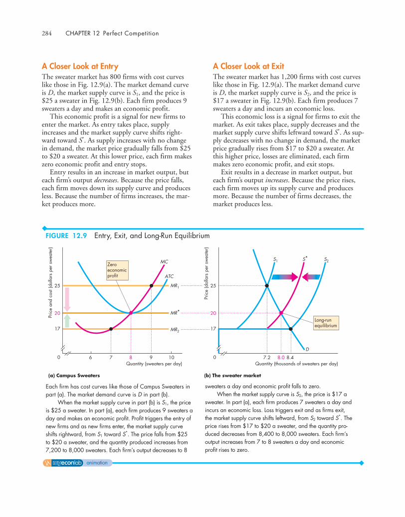
284 CHAPTER 12 Perfect Competition

A Closer Look at EntryThe sweater market has 800 firms with cost curveslike those in Fig. 12.9(a). The market demand curveis D, the market supply curve is S1, and the price is$25 a sweater in Fig. 12.9(b). Each firm produces 9sweaters a day and makes an economic profit.

This economic profit is a signal for new firms toenter the market. As entry takes place, supplyincreases and the market supply curve shifts right-ward toward S*. As supply increases with no changein demand, the market price gradually falls from $25to $20 a sweater. At this lower price, each firm makeszero economic profit and entry stops.

Entry results in an increase in market output, buteach firm’s output decreases. Because the price falls,each firm moves down its supply curve and producesless. Because the number of firms increases, the mar-ket produces more.

A Closer Look at ExitThe sweater market has 1,200 firms with cost curveslike those in Fig. 12.9(a). The market demand curveis D, the market supply curve is S2, and the price is$17 a sweater in Fig. 12.9(b). Each firm produces 7sweaters a day and incurs an economic loss.

This economic loss is a signal for firms to exit themarket. As exit takes place, supply decreases and themarket supply curve shifts leftward toward S*. As sup-ply decreases with no change in demand, the marketprice gradually rises from $17 to $20 a sweater. Atthis higher price, losses are eliminated, each firmmakes zero economic profit, and exit stops.

Exit results in a decrease in market output, buteach firm’s output increases. Because the price rises,each firm moves up its supply curve and producesmore. Because the number of firms decreases, themarket produces less.

(a) Campus Sweaters

Pric

e (d

olla

rs p

er s

wea

ter)

8.4Quantity (thousands of sweaters per day)

0 8.07.2

S*S1

MR1

MR*

MR2

S2

D

20

17

25

(b) The sweater market

Long-runequilibrium

10

Pric

e an

d co

st (d

olla

rs p

er s

wea

ter)

9Quantity (sweaters per day)

0 876

MC

ATC

20

17

25

Zeroeconomicprofit

Each firm has cost curves like those of Campus Sweaters inpart (a). The market demand curve is D in part (b).

When the market supply curve in part (b) is S1, the priceis $25 a sweater. In part (a), each firm produces 9 sweaters aday and makes an economic profit. Profit triggers the entry ofnew firms and as new firms enter, the market supply curveshifts rightward, from S1 toward S*. The price falls from $25to $20 a sweater, and the quantity produced increases from7,200 to 8,000 sweaters. Each firm’s output decreases to 8

sweaters a day and economic profit falls to zero.When the market supply curve is S2, the price is $17 a

sweater. In part (a), each firm produces 7 sweaters a day andincurs an economic loss. Loss triggers exit and as firms exit,the market supply curve shifts leftward, from S2 toward S*. Theprice rises from $17 to $20 a sweater, and the quantity pro-duced decreases from 8,400 to 8,000 sweaters. Each firm’soutput increases from 7 to 8 sweaters a day and economicprofit rises to zero.

FIGURE 12.9 Entry, Exit, and Long-Run Equilibrium

animation

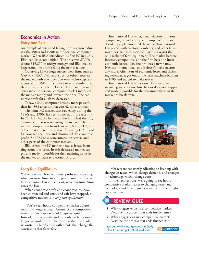
Output, Price, and Profit in the Long Run 285

Long-Run EquilibriumYou’ve now seen how economic profit induces entry,which in turn eliminates the profit. You’ve also seenhow economic loss induces exit, which in turn elimi-nates the loss.

When economic profit and economic loss havebeen eliminated and entry and exit have stopped, acompetitive market is in long-run equilibrium.

You’ve seen how a competitive market adjuststoward its long-run equilibrium. But a competitivemarket is rarely in a state of long-run equilibrium.Instead, it is constantly and restlessly evolving towardlong-run equilibrium. The reason is that the marketis constantly bombarded with events that change theconstraints that firms face.

Markets are constantly adjusting to keep up withchanges in tastes, which change demand, and changesin technology, which change costs.

In the next sections, we’re going to see how acompetitive market reacts to changing tastes andtechnology and how it guides resources to their high-est-valued use.

Economics in ActionEntry and ExitAn example of entry and falling prices occurred dur-ing the 1980s and 1990s in the personal computermarket. When IBM introduced its first PC in 1981,IBM had little competition. The price was $7,000(about $16,850 in today’s money) and IBM made alarge economic profit selling the new machine.

Observing IBM’s huge success, new firms such asGateway, NEC, Dell, and a host of others enteredthe market with machines that were technologicallyidentical to IBM’s. In fact, they were so similar thatthey came to be called “clones.” The massive wave ofentry into the personal computer market increasedthe market supply and lowered the price. The eco-nomic profit for all firms decreased.

Today, a $400 computer is vastly more powerfulthan its 1981 ancestor that cost 42 times as much.

The same PC market that saw entry during the1980s and 1990s has seen some exit more recently.In 2001, IBM, the firm that first launched the PC,announced that it was exiting the market. Theintense competition from Gateway, NEC, Dell, andothers that entered the market following IBM’s leadhas lowered the price and eliminated the economicprofit. So IBM now concentrates on servers andother parts of the computer market.

IBM exited the PC market because it was incur-ring economic losses. Its exit decreased market sup-ply and made it possible for the remaining firms inthe market to make zero economic profit.

International Harvester, a manufacturer of farmequipment, provides another example of exit. Fordecades, people associated the name “InternationalHarvester” with tractors, combines, and other farmmachines. But International Harvester wasn’t theonly maker of farm equipment. The market becameintensely competitive, and the firm began to incureconomic losses. Now the firm has a new name,Navistar International, and it doesn’t make tractorsany more. After years of economic losses and shrink-ing revenues, it got out of the farm-machine businessin 1985 and started to make trucks.

International Harvester exited because it wasincurring an economic loss. Its exit decreased supplyand made it possible for the remaining firms in themarket to break even.

REVIEW QUIZ1 What triggers entry in a competitive market?

Describe the process that ends further entry.2 What triggers exit in a competitive market?

Describe the process that ends further exit.

You can work these questions in Study Plan 12.4 and get instant feedback.

286 CHAPTER 12 Perfect Competition

◆ Changing Tastes and Advancing Technology

Increased awareness of the health hazards of smokinghas decreased the demand for tobacco products. Thedevelopment of inexpensive automobile and airtransportation during the 1990s decreased thedemand for long-distance trains and buses. Solid-state electronics has decreased the demand for TVand radio repair. The development of good-qualityinexpensive clothing has decreased the demand forsewing machines. What happens in a competitivemarket when there is a permanent decrease in thedemand for its product?

Microwave food preparation has increased thedemand for paper, glass, and plastic cooking utensilsand for plastic wrap. The Internet has increased thedemand for personal computers and the widespreaduse of computers has increased the demand for high-speed connections and music downloads. What hap-pens in a competitive market when the demand forits output increases?

Advances in technology are constantly loweringthe costs of production. New biotechnologies havedramatically lowered the costs of producing manyfood and pharmaceutical products. New electronictechnologies have lowered the cost of producing justabout every good and service. What happens in acompetitive market for a good when technologicalchange lowers its production costs?

Let’s use the theory of perfect competition toanswer these questions.

A Permanent Change in DemandFigure 12.10(a) shows a competitive market that ini-tially is in long-run equilibrium. The demand curveis D0, the supply curve is S0, the market price is P0,and market output is Q0. Figure 12.10(b) shows asingle firm in this initial long-run equilibrium. Thefirm produces q0 and makes zero economic profit.

Now suppose that demand decreases and thedemand curve shifts leftward to D1, as shown in Fig.12.10(a). The market price falls to P1, and the quan-tity supplied by the market decreases from Q0 to Q1

as the market moves down along its short-run supplycurve S0. Figure 12.10(b) shows the situation facing afirm. The market price is now below the firm’s mini-mum average total cost, so the firm incurs an eco-

nomic loss. But to minimize its loss, the firm adjustsits output to keep marginal cost equal to price. At aprice of P1, each firm produces an output of q1.

The market is now in short-run equilibrium butnot long-run equilibrium. It is in short-run equilib-rium because each firm is maximizing profit; it is notin long-run equilibrium because each firm is incur-ring an economic loss—its average total cost exceedsthe price.

The economic loss is a signal for some firms toexit the market. As they do so, short-run market sup-ply decreases and the market supply curve graduallyshifts leftward. As market supply decreases, the pricerises. At each higher price, a firm’s profit-maximizingoutput is greater, so the firms remaining in the mar-ket increase their output as the price rises. Each firmmoves up along its marginal cost or supply curve inFig. 12.10(b). That is, as some firms exit the market,market output decreases but the output of the firmsthat remain in the market increases.

Eventually, enough firms have exited the marketfor the market supply curve to have shifted to S1 inFig. 12.10(a). The market price has returned to itsoriginal level, P0. At this price, the firms remaining inthe market produce q0, the same quantity that theyproduced before the decrease in demand. Becausefirms are now making zero economic profit, no firmhas an incentive to enter or exit the market. The mar-ket supply curve remains at S1, and market output isQ2. The market is again in long-run equilibrium.

The difference between the initial long-run equi-librium and the final long-run equilibrium is thenumber of firms in the market. A permanent decreasein demand has decreased the number of firms. Eachfirm remaining in the market produces the same out-put in the new long-run equilibrium as it did initiallyand makes zero economic profit. In the process ofmoving from the initial equilibrium to the new one,firms incur economic losses.

We’ve just worked out how a competitive marketresponds to a permanent decrease in demand. A per-manent increase in demand triggers a similarresponse, except in the opposite direction. Theincrease in demand brings a higher price, economicprofit, and entry. Entry increases market supply andeventually lowers the price to its original level andeconomic profit to zero.

The demand for Internet service increased perma-nently during the 1990s and huge profit opportuni-ties arose in this market. The result was a massive rate

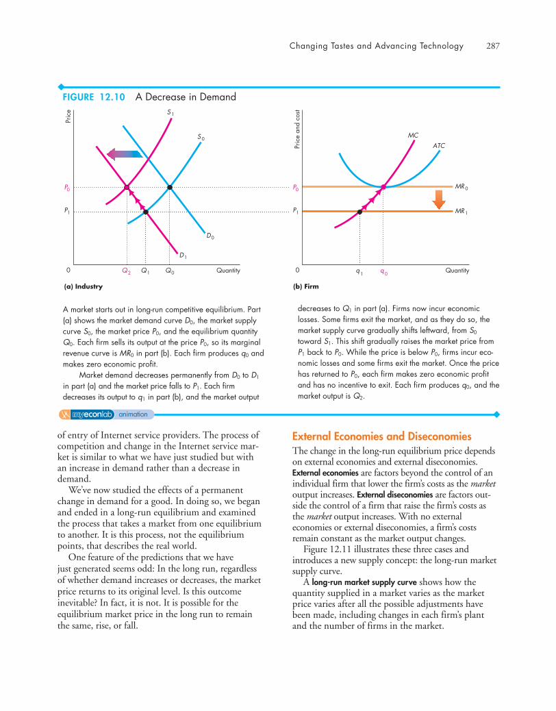
Changing Tastes and Advancing Technology 287

of entry of Internet service providers. The process ofcompetition and change in the Internet service mar-ket is similar to what we have just studied but withan increase in demand rather than a decrease indemand.

We’ve now studied the effects of a permanentchange in demand for a good. In doing so, we beganand ended in a long-run equilibrium and examinedthe process that takes a market from one equilibriumto another. It is this process, not the equilibriumpoints, that describes the real world.

One feature of the predictions that we have just generated seems odd: In the long run, regardlessof whether demand increases or decreases, the marketprice returns to its original level. Is this outcomeinevitable? In fact, it is not. It is possible for theequilibrium market price in the long run to remainthe same, rise, or fall.

External Economies and DiseconomiesThe change in the long-run equilibrium price dependson external economies and external diseconomies.External economies are factors beyond the control of anindividual firm that lower the firm’s costs as the marketoutput increases. External diseconomies are factors out-side the control of a firm that raise the firm’s costs asthe market output increases. With no externaleconomies or external diseconomies, a firm’s costsremain constant as the market output changes.

Figure 12.11 illustrates these three cases andintroduces a new supply concept: the long-run marketsupply curve.

A long-run market supply curve shows how thequantity supplied in a market varies as the marketprice varies after all the possible adjustments havebeen made, including changes in each firm’s plantand the number of firms in the market.

Pric

e

Quantity0

P

S 1

D1

S 0

(a) Industry

0

P1

D0

Q1 Q0

Pric

e an

d co

st

Quantity0

P 0

MC

(b) Firm

0

P1

q1

q0

ATC

MR

1MR

Q2

A market starts out in long-run competitive equilibrium. Part(a) shows the market demand curve D0, the market supplycurve S0, the market price P0, and the equilibrium quantityQ0. Each firm sells its output at the price P0, so its marginalrevenue curve is MR0 in part (b). Each firm produces q0 andmakes zero economic profit.

Market demand decreases permanently from D0 to D1

in part (a) and the market price falls to P1. Each firmdecreases its output to q1 in part (b), and the market output

decreases to Q1 in part (a). Firms now incur economiclosses. Some firms exit the market, and as they do so, themarket supply curve gradually shifts leftward, from S0

toward S1. This shift gradually raises the market price fromP1 back to P0. While the price is below P0, firms incur eco-nomic losses and some firms exit the market. Once the pricehas returned to P0, each firm makes zero economic profitand has no incentive to exit. Each firm produces q0, and themarket output is Q2.

FIGURE 12.10 A Decrease in Demand

animation

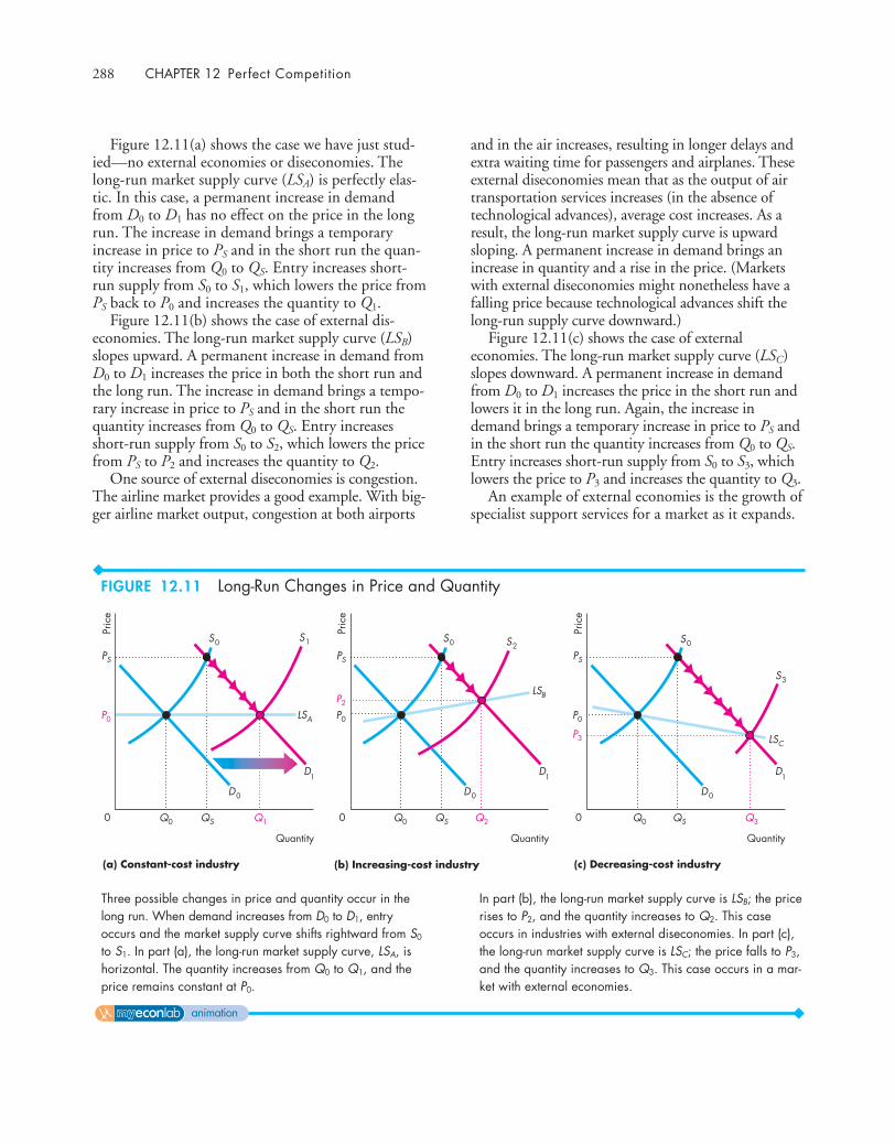
288 CHAPTER 12 Perfect Competition

Figure 12.11(a) shows the case we have just stud-ied—no external economies or diseconomies. Thelong-run market supply curve (LSA) is perfectly elas-tic. In this case, a permanent increase in demandfrom D0 to D1 has no effect on the price in the longrun. The increase in demand brings a temporaryincrease in price to PS and in the short run the quan-tity increases from Q0 to QS. Entry increases short-run supply from S0 to S1, which lowers the price fromPS back to P0 and increases the quantity to Q1.

Figure 12.11(b) shows the case of external dis-economies. The long-run market supply curve (LSB)slopes upward. A permanent increase in demand fromD0 to D1 increases the price in both the short run andthe long run. The increase in demand brings a tempo-rary increase in price to PS and in the short run thequantity increases from Q0 to QS. Entry increasesshort-run supply from S0 to S2, which lowers the pricefrom PS to P2 and increases the quantity to Q2.

One source of external diseconomies is congestion.The airline market provides a good example. With big-ger airline market output, congestion at both airports

and in the air increases, resulting in longer delays andextra waiting time for passengers and airplanes. Theseexternal diseconomies mean that as the output of airtransportation services increases (in the absence oftechnological advances), average cost increases. As aresult, the long-run market supply curve is upwardsloping. A permanent increase in demand brings anincrease in quantity and a rise in the price. (Marketswith external diseconomies might nonetheless have afalling price because technological advances shift thelong-run supply curve downward.)

Figure 12.11(c) shows the case of externaleconomies. The long-run market supply curve (LSC)slopes downward. A permanent increase in demandfrom D0 to D1 increases the price in the short run andlowers it in the long run. Again, the increase indemand brings a temporary increase in price to PS andin the short run the quantity increases from Q0 to QS.Entry increases short-run supply from S0 to S3, whichlowers the price to P3 and increases the quantity to Q3.

An example of external economies is the growth ofspecialist support services for a market as it expands.

D0 D0 D0

Pric

e

Quantity

0

P0

D1

S0

(a) Constant-cost industry

Q0 Q1

S1

LSA

(b) Increasing-cost industry (c) Decreasing-cost industry

PS

QS

Pric

e

Quantity

0

P0

D1

S0

P2

Q0 Q2

S2

LSB

PS

QS

Pric

e

Quantity

0

P0

D1

S0

P3

Q0 Q3

S3

LSC

PS

QS

Three possible changes in price and quantity occur in thelong run. When demand increases from D0 to D1, entryoccurs and the market supply curve shifts rightward from S0

to S1. In part (a), the long-run market supply curve, LSA, ishorizontal. The quantity increases from Q0 to Q1, and theprice remains constant at P0.

In part (b), the long-run market supply curve is LSB; the pricerises to P2, and the quantity increases to Q2. This caseoccurs in industries with external diseconomies. In part (c),the long-run market supply curve is LSC; the price falls to P3,and the quantity increases to Q3. This case occurs in a mar-ket with external economies.

FIGURE 12.11 Long-Run Changes in Price and Quantity

animation

Changing Tastes and Advancing Technology 289

As farm output increased in the nineteenth and earlytwentieth centuries, the services available to farmersexpanded. New firms specialized in the developmentand marketing of farm machinery and fertilizers. As aresult, average farm costs decreased. Farms enjoyedthe benefits of external economies. As a consequence,as the demand for farm products increased, the out-put increased but the price fell.

Over the long term, the prices of many goods andservices have fallen, not because of external economiesbut because of technological change. Let’s now studythis influence on a competitive market.

Technological ChangeIndustries are constantly discovering lower-cost tech-niques of production. Most cost-saving productiontechniques cannot be implemented, however, with-out investing in new plant and equipment. As a con-sequence, it takes time for a technological advance tospread through a market. Some firms whose plantsare on the verge of being replaced will be quick toadopt the new technology, while other firms whoseplants have recently been replaced will continue tooperate with an old technology until they can nolonger cover their average variable cost. Once aver-age variable cost cannot be covered, a firm will scrapeven a relatively new plant (embodying an old tech-nology) in favor of a plant with a new technology.

New technology allows firms to produce at a lowercost. As a result, as firms adopt a new technology,their cost curves shift downward. With lower costs,firms are willing to supply a given quantity at a lowerprice or, equivalently, they are willing to supply alarger quantity at a given price. In other words, mar-ket supply increases, and the market supply curveshifts rightward. With a given demand, the quantityproduced increases and the price falls.

Two forces are at work in a market undergoingtechnological change. Firms that adopt the new tech-nology make an economic profit, so there is entry bynew-technology firms. Firms that stick with the oldtechnology incur economic losses. They either exitthe market or switch to the new technology.

As old-technology firms disappear and new-tech-nology firms enter, the price falls and the quantityproduced increases. Eventually, the market arrives at along-run equilibrium in which all the firms use thenew technology and make a zero economic profit.Because in the long run competition eliminateseconomic profit, technological change brings only

temporary gains to producers. But the lower pricesand better products that technological advances bringare permanent gains for consumers.

The process that we’ve just described is one inwhich some firms experience economic profits andothers experience economic losses. It is a period ofdynamic change in a market. Some firms do well,and others do badly. Often, the process has a geo-graphical dimension—the expanding new-technologyfirms bring prosperity to what was once the boon-docks, and traditional industrial regions decline.Sometimes, the new-technology firms are in a foreigncountry, while the old-technology firms are in thedomestic economy. The information revolution ofthe 1990s produced many examples of changes likethese. Commercial banking, which was traditionallyconcentrated in New York, San Francisco, and otherlarge cities now flourishes in Charlotte, NorthCarolina, which has become the nation’s numberthree commercial banking city. Television shows andmovies, traditionally made in Los Angeles and NewYork, are now made in large numbers in Orlando.

Technological advances are not confined to theinformation and entertainment industries. Even foodproduction is undergoing a major technologicalchange because of genetic engineering.

We’ve seen how a competitive market operates inthe short run and the long run, but is a competitivemarket efficient?

REVIEW QUIZ 1 Describe the course of events in a competitive

market following a permanent decrease indemand. What happens to output, price, andeconomic profit in the short run and in thelong run?

2 Describe the course of events in a competitivemarket following a permanent increase indemand. What happens to output, price, and eco-nomic profit in the short run and in the long run?

3 Describe the course of events in a competitivemarket following the adoption of a new tech-nology. What happens to output, price, andeconomic profit in the short run and in thelong run?

You can work these questions in Study Plan 12.5 and get instant feedback.

290 CHAPTER 12 Perfect Competition

◆ Competition and EfficiencyA competitive market can achieve an efficient use ofresources. You first studied efficiency in Chapter 2.Then in Chapter 5, using only the concepts ofdemand, supply, consumer surplus, and producersurplus, you saw how a competitive market achievesefficiency. Now that you have learned what liesbehind the demand and supply curves of a competi-tive market, you can gain a deeper understanding ofthe efficiency of a competitive market.

Efficient Use of ResourcesRecall that resource use is efficient when we producethe goods and services that people value most highly(see Chapter 2, pp. 33–35, and Chapter 5, p. 108). Ifsomeone can become better off without anyone elsebecoming worse off, resources are not being used effi-ciently. For example, suppose we produce a computerthat no one wants and no one will ever use and, atthe same time, some people are clamoring for morevideo games. If we produce fewer computers andreallocate the unused resources to produce morevideo games, some people will become better off andno one will be worse off. So the initial resource allo-cation was inefficient.

In the more technical language that you havelearned, resource use is efficient when marginal socialbenefit equals marginal social cost. In the computerand video games example, the marginal social benefitof a video game exceeds its marginal social cost; themarginal social cost of a computer exceeds its mar-ginal social benefit. So by producing fewer computersand more video games, we move resources toward ahigher-valued use.

Choices, Equilibrium, and EfficiencyWe can use what you have learned about the decisionsmade by consumers and competitive firms and marketequilibrium to describe an efficient use of resources.

Choices Consumers allocate their budgets to get themost value possible out of them. We derive a con-sumer’s demand curve by finding how the bestbudget allocation changes as the price of a goodchanges. So consumers get the most value out of theirresources at all points along their demand curves. Ifthe people who consume a good or service are the

only ones who benefit from it, then the marketdemand curve measures the benefit to the entire soci-ety and is the marginal social benefit curve.

Competitive firms produce the quantity that maxi-mizes profit. We derive the firm’s supply curve by find-ing the profit-maximizing quantity at each price. Sofirms get the most value out of their resources at allpoints along their supply curves. If the firms that pro-duce a good or service bear all the costs of producingit, then the market supply curve measures the marginalcost to the entire society and the market supply curveis the marginal social cost curve.

Equilibrium and Efficiency Resources are used effi-ciently when marginal social benefit equals marginalsocial cost. Competitive equilibrium achieves thisefficient outcome because, with no externalities, priceequals marginal social benefit for consumers, andprice equals marginal social cost for producers.

The gains from trade are the sum of consumer sur-plus and producer surplus. The gains from trade forconsumers are measured by consumer surplus, which isthe area below the demand curve and above the pricepaid. (See Chapter 5, p. 109.) The gains from tradefor producers are measured by producer surplus, whichis the area above the supply curve and below the pricereceived. (See Chapter 5, p. 111.) The total gainsfrom trade equals total surplus —the sum of con-sumer surplus and producer surplus. When the mar-ket for a good or service is in equilibrium, the gainsfrom trade are maximized.

Illustrating an Efficient Allocation Figure 12.12 illus-trates the efficiency of perfect competition in long-run equilibrium. Part (a) shows the individual firm,and part (b) shows the market. The equilibrium mar-ket price is P*. At that price, each firm makes zeroeconomic profit and each firm has the plant thatenables it to produce at the lowest possible averagetotal cost. Consumers are as well off as possiblebecause the good cannot be produced at a lower costand the price equals that least possible cost.

In part (b), consumers get the most out of theirresources at all points on the market demand curve, D = MSB. Consumer surplus is the green area.Producers get the most out of their resources at allpoints on the market supply curve, S = MSC.Producer surplus is the blue area. Resources are usedefficiently at the quantity Q* and price P*. At thispoint, marginal social benefit equals marginal social

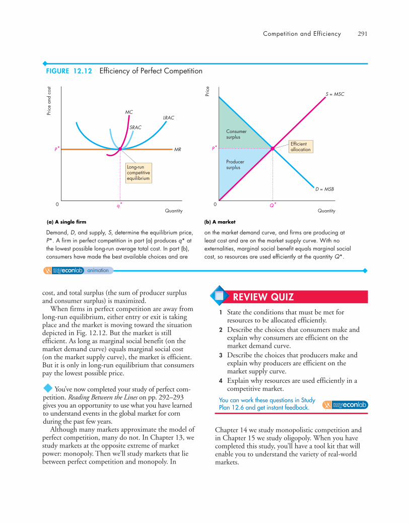
Competition and Efficiency 291

cost, and total surplus (the sum of producer surplusand consumer surplus) is maximized.

When firms in perfect competition are away fromlong-run equilibrium, either entry or exit is takingplace and the market is moving toward the situationdepicted in Fig. 12.12. But the market is stillefficient. As long as marginal social benefit (on themarket demand curve) equals marginal social cost(on the market supply curve), the market is efficient.But it is only in long-run equilibrium that consumerspay the lowest possible price.

◆ You’ve now completed your study of perfect com-petition. Reading Between the Lines on pp. 292–293gives you an opportunity to use what you have learnedto understand events in the global market for cornduring the past few years.

Although many markets approximate the model ofperfect competition, many do not. In Chapter 13, westudy markets at the opposite extreme of marketpower: monopoly. Then we’ll study markets that liebetween perfect competition and monopoly. In

Chapter 14 we study monopolistic competition andin Chapter 15 we study oligopoly. When you havecompleted this study, you’ll have a tool kit that willenable you to understand the variety of real-worldmarkets.

(a) A single firm (b) A market

Pric

e00

S = MSC

P*P*

Q*q*

D = MSB

Efficientallocation

Consumersurplus

Producersurplus

Pric

e an

d co

st

Quantity Quantity

LRAC

MR

Long-runcompetitiveequilibrium

MC

SRAC

Demand, D, and supply, S, determine the equilibrium price,P*. A firm in perfect competition in part (a) produces q* atthe lowest possible long-run average total cost. In part (b),consumers have made the best available choices and are

on the market demand curve, and firms are producing atleast cost and are on the market supply curve. With noexternalities, marginal social benefit equals marginal socialcost, so resources are used efficiently at the quantity Q*.

FIGURE 12.12 Efficiency of Perfect Competition

animation

REVIEW QUIZ1 State the conditions that must be met for

resources to be allocated efficiently.2 Describe the choices that consumers make and

explain why consumers are efficient on themarket demand curve.

3 Describe the choices that producers make andexplain why producers are efficient on themarket supply curve.

4 Explain why resources are used efficiently in acompetitive market.

You can work these questions in Study Plan 12.6 and get instant feedback.

292

READING BETWEEN THE L INES

Bumper Harvests Bring Stabilityhttp://www.ft.comJune 1, 2010

There is no better fertilizer than high prices, the old farming adage goes. Trends in agricul-ture appear to be proving this resoundingly true.

The spike in prices that caused the first global food crisis in 30 years in 2007–08 has led tolarge increases in production of foods such as corn and wheat. Farmers have responded tohigher prices. ...

The U.S. Department of Agriculture said ...“Higher prices, and thus expanded acreage, incombination with favorable weather, have helped production expand sharply.”

Global corn production will hit 835m metric tons in the 2010–11 season, its highest everlevel, the USDA forecasts. ... That is likely to lead to a period of relatively stable prices. ...

While prices for the main food and feed grain crops—corn, wheat, and soybeans—are likelyto remain steady and low in the next year or so, that does not mean a repeat of the food crisisis impossible. ...

One argument against that view holds thattechnological gains in response to the crisishave boosted productivity, making farmersmore able to deal with increasing consumption.

Some crops, such as corn, saw record yields inthe 2009–10 season and the USDA is predict-ing high yields for next year as well.

But analysts ascribe the gains in productivitymore to fortunate weather conditions than arevolution in farming technology. ...

Copyright 2010 The Financial Times. Reprinted with permission. Furtherreproduction prohibited.

■ In 2010–11, global corn production will reachits highest ever level at 835 million metric tons.

■ High prices in 2007–08 led to large increasesin the acreage of corn and wheat.

■ Favorable weather also helped to increaseproduction of these crops.

■ Prices for corn, wheat, and soybeans will likelyremain low next year, but a future price risemight occur.

■ A revolution in farming technology wouldincrease production without raising costs andprices.

■ The current gain in productivity is most likelythe result of fortunate weather and likely to betemporary.

ESSENCE OF THE STORY

Perfect Competition in Corn

293

ECONOMIC ANALYSIS

Figure 2 A corn farmer

MC0

ATC0

MC1

ATC1

MR0

MR1

Figure 1 The market for corn

Pric

e an

d co

st (2

010

dolla

rs p

er m

etric

ton)

Quantity (metric tons)0

200

500

400

310

230

7,500 8,3508,000 9,5009,000

D

Pric

e (2

010

dolla

rs p

er m

etric

ton)

Quantity (millions of metric tons)0

200

500

400

310

230

750 835800 950900

S0S1

■ In 2009 and 2010, good weather conditions in-creased the supply of corn. By 2010–11, the supplycurve had shifted rightward to S1. The price fell to$230 per metric ton and production increased to 835million metric tons.

■ Back on the farm in Fig. 2, the lower price decreasedmarginal revenue and the MR curve shifted downwardto MR1.

■ But the fortunate weather increased farm productivityand lowered the cost of producing corn. The averagetotal cost curve shifted downward to ATC1 and themarginal cost curve shifted downward to MC1.

■ The combination of the lower price and lower costsmight leave the farm with an economic profit. In Fig. 2we’re assuming that the farm again made zero eco-nomic profit.

■ If farms did make a positive (or negative) economicprofit, entry (or exit) would eventually return them to azero economic profit position like that shown in Fig. 2.

■ The global market for corn is competitive and themodel of perfect competition shows how that marketworks.

■ During 2006 through 2008, increases in demandbrought a rising price and an increase in the quantityof corn supplied.

■ In 2009 and 2010, good weather conditions broughtan increase in the supply of corn and the quantity ofcorn increased further but its price fell.

■ Figure 1 illustrates these events in the market for cornand Fig. 2 their effects on an individual farm.

■ From 2006 through 2008, the supply curve of cornwas S0 in Fig. 1. The demand for corn increased andby 2008, the demand curve was D. The price of cornin 2008 was $310 per metric ton and 800 million met-ric tons were produced.

■ In 2008, the farm faced a marginal revenue curve MR0

and had average total cost curve ATC0 and marginalcost curve MC0 in Fig. 2.

■ The farm maximized profit by producing 8,000 metrictons and (we will assume) made zero economic profit.

294 CHAPTER 12 Perfect Competition

Output, Price, and Profit in the Long Run(pp. 283–285)

■ Economic profit induces entry and economic lossinduces exit.

■ Entry increases supply and lowers price and profit.Exit decreases supply and raises price and profit.

■ In long-run equilibrium, economic profit is zero.There is no entry or exit.

Working Problems 10 and 11 will give you a better under-standing of output, price, and profit in the long run.

Changing Tastes and Advancing Technology (pp. 286–289)

■ A permanent decrease in demand leads to asmaller market output and a smaller number offirms. A permanent increase in demand leads to alarger market output and a larger number of firms.

■ The long-run effect of a change in demand on pricedepends on whether there are external economies(the price falls) or external diseconomies (the pricerises) or neither (the price remains constant).

■ New technologies increase supply and in the longrun lower the price and increase the quantity.

Working Problems 12 to 16 will give you a better under-standing of changing tastes and advancing technologies.

Competition and Efficiency (pp. 290–291)

■ Resources are used efficiently when we producegoods and services in the quantities that peoplevalue most highly.

■ Perfect competition achieves an efficient alloca-tion. In long-run equilibrium, consumers pay thelowest possible price and marginal social benefitequals marginal social cost.

Working Problems 17 and 18 will give you a better under-standing of competition and efficiency.

Key Points

What Is Perfect Competition? (pp. 274–275)

■ In perfect competition, many firms sell identicalproducts to many buyers; there are no restrictionson entry; sellers and buyers are well informedabout prices.

■ A perfectly competitive firm is a price taker.■ A perfectly competitive firm’s marginal revenue

always equals the market price.

Working Problems 1 to 3 will give you a better under-standing of perfect competition.

The Firm’s Output Decision (pp. 276–279)

■ The firm produces the output at which marginalrevenue (price) equals marginal cost.

■ In short-run equilibrium, a firm can make an eco-nomic profit, incur an economic loss, or break even.

■ If price is less than minimum average variable cost,the firm temporarily shuts down.

■ At prices below minimum average variable cost, afirm’s supply curve runs along the y-axis; at pricesabove minimum average variable cost, a firm’s sup-ply curve is its marginal cost curve.

Working Problems 4 to 7 will give you a better under-standing of a firm’s output decision.

Output, Price, and Profit in the Short Run(pp. 280–283)

■ The market supply curve shows the sum of thequantities supplied by each firm at each price.

■ Market demand and market supply determineprice.

■ A firm might make a positive economic profit, azero economic profit, or incur an economic loss.

Working Problems 8 and 9 will give you a better under-standing of output, price, and profit in the short run.

SUMMARY

Key TermsExternal diseconomies, 287External economies, 287Long-run market supply curve, 287

Marginal revenue, 274Perfect competition, 274Price taker, 274

Short-run market supply curve, 280Shutdown point, 278Total revenue, 274

Study Plan Problems and Applications 295

Price Quantity demanded(dollars per box) (thousands of boxes per week)

3.65 5005.20 4506.80 4008.40 350

10.00 30011.60 25013.20 200

Each producer of paper has the following costswhen it uses its least-cost plant:

Output Marginal costAverage Average

(boxes (dollars pervariable cost total cost

per week) additional box) (dollars per box)

200 6.40 7.80 12.80250 7.00 7.00 11.00300 7.65 7.10 10.43350 8.40 7.20 10.06400 10.00 7.50 10.00450 12.40 8.00 10.22500 20.70 9.00 11.00

a. What is the market price of paper?b. What is the market’s output?c. What is the output produced by each firm?d. What is the economic profit made or economic

loss incurred by each firm?

Output, Price, and Profit in the Short Run (Study Plan 12.3)

8. In Problem 7, as more and more computer usersread documents online rather than print them,the market demand for paper decreases and inthe short run the demand schedule becomes

Price Quantity demanded(dollars (thousands of boxesper box) per week)

2.95 5004.13 4505.30 4006.48 3507.65 3008.83 250

10.00 20011.18 150

What Is Perfect Competition? (Study Plan 12.1)

Use the following information to work Problems 1to 3.Lin’s makes fortune cookies that are identical tothose made by dozens of other firms, and there isfree entry in the fortune cookie market. Buyers andsellers are well informed about prices.

1. In what type of market does Lin’s operate? Whatdetermines the price of fortune cookies and whatdetermines Lin’s marginal revenue from fortunecookies?

2. a. If fortune cookies sell for $10 a box and Lin’soffers its cookies for sale at $10.50 a box, howmany boxes does it sell?

b. If fortune cookies sell for $10 a box and Lin’soffers its cookies for sale at $9.50 a box, howmany boxes does it sell?

3. What is the elasticity of demand for Lin’s fortunecookies and how does it differ from the elasticityof the market demand for fortune cookies?

The Firm’s Output Decision (Study Plan 12.2)

Use the following table to work Problems 4 to 6.Pat’s Pizza Kitchen is a price taker. Its costs are

Output Total cost(pizzas per hour) (dollars per hour)

0 101 212 303 414 545 69

4. Calculate Pat’s profit-maximizing output andeconomic profit if the market price is

(i) $14 a pizza.(ii) $12 a pizza.(iii) $10 a pizza.

5. What is Pat’s shutdown point and what is Pat’seconomic profit if it shuts down temporarily?

6. Derive Pat’s supply curve.7. The market for paper is perfectly competitive

and there are 1,000 firms that produce paper.The table sets out the market demand schedulefor paper.

You can work Problems 1 to 18 in MyEconLab Chapter 12 Study Plan and get instant feedback.

STUDY PLAN PROBLEMS AND APPLICATIONS

296 CHAPTER 12 Perfect Competition

If each firm producing paper has the costs set outin Problem 7, what is the market price and the eco-nomic profit or loss of each firm in the short run?

9. Fuel Prices Could Squeeze Cheap FlightsAirlines are having difficulty keeping prices low,especially as fuel prices keep rising. Airlines haveraised fares to make up for the fuel costs.American Airlines increased its fuel surcharge by$20 a roundtrip, which Delta, United Airlines,and Continental matched.

Source: CNN, June 12, 2008a. Explain how an increase in fuel prices might

cause an airline to change its output (numberof flights) in the short run.

b. Draw a graph to show the increase in fuelprices on an airline’s output in the short run.

c. Explain why an airline might incur an eco-nomic loss in the short run as fuel prices rise.

Output, Price, and Profit in the Long Run (Study Plan 12.4)

10. The pizza market is perfectly competitive, and allpizza producers have the same costs as Pat’s PizzaKitchen in Problem 4. a. At what price will some firms exit the pizza

market in the long run?b. At what price will firms enter the pizza market

in the long run?

11. In Problem 7, in the long run,a. Do firms have an incentive to enter or exit the

paper market? b. If firms do enter or exit the market, explain

how the economic profit or loss of the remain-ing paper producers will change.

c. What is the long-run equilibrium marketprice and the quantity of paper produced?What is the number of firms in the market?

Changing Tastes and Advancing Technology (Study Plan 12.5)

12. If in the long run, the market demand for paperremains the same as in Problem 8,a. What is the long-run equilibrium price of

paper, the market output, and the economicprofit or loss of each firm?

b. Does this market experience external economies,external diseconomies, or constant cost? Illus-trate by drawing the long-run supply curve.

Use the following news clip to work Problems 13and 14.Coors Brewing Expanding PlantCoors Brewing Co. of Golden will expand itsVirginia packaging plant at a cost of $24 million.The addition will accommodate a new productionline, which will bottle beer faster. Coors Brewingemploys 470 people at its Virginia plant. Theexpanded packaging line will add another eight jobs.

Source: Denver Business Journal, January 6, 200613. a. How will Coors’ expansion change its mar-

ginal cost curve and short-run supply curve?b. What does this expansion decision imply

about the point on Coors’ LRAC curve atwhich the firm was before the expansion?

14. a. If other breweries follow the lead of Coors,what will happen to the market price of beer?

b. How will the adjustment that you have de-scribed in part (a) influence the economicprofit of Coors and other beer producers?

15. Explain and illustrate graphically how the grow-ing world population is influencing the worldmarket for wheat and a representative individualwheat farmer.

16. Explain and illustrate graphically how the diaperservice market has been affected by the decreasein the North American birth rate and the devel-opment of disposable diapers.

Competition and Efficiency (Study Plan 12.6)

17. In a perfectly competitive market in long-runequilibrium, can consumer surplus be increased?Can producer surplus be increased? Can a con-sumer become better off by making a substitu-tion away from this market?

18. Never Pay Retail AgainNot only has scouring the Web for the bestpossible price become standard protocol beforebuying a big-ticket item, but more consumers areemploying creative strategies for scoring hotdeals. Comparison shopping, haggling and swap-ping discount codes are all becoming mainstreammarks of savvy shoppers. Online shoppers cancheck a comparison service like Price Grabberbefore making a purchase.

Source: CNN, May 30, 2008a. Explain the effect of the Internet on the de-

gree of competition in the market.b. Explain how the Internet influences market

efficiency.

Additional Problems and Applications 297

What Is Perfect Competition?

Use the following news clip to work Problems 19 to 21.Money in the TankTwo gas stations stand on opposite sides of the road:Rutter’s Farm Store and Sheetz gas station. Rutter’sdoesn’t even have to look across the highway to knowwhen Sheetz changes its price for a gallon of gas. WhenSheetz raises the price, Rutter’s pumps are busy. WhenSheetz lowers prices, there’s not a car in sight. Both gasstations survive but each has no control over the price.

Source: The Mining Journal, May 24, 200819. In what type of market do these gas stations

operate? What determines the price of gasolineand the marginal revenue from gasoline?

20. Describe the elasticity of demand that each ofthese gas stations faces.

21. Why does each of these gas stations have so littlecontrol over the price of the gasoline it sells?

The Firm’s Output Decision22. The figure shows the costs of Quick Copy, one of

many copy shops near campus.

If the market price of copying is 10¢ a page,calculate Quick Copy’sa. Profit-maximizing output.b. Economic profit.

23. The market for smoothies is perfectly competitive.The following table sets out the market demandschedule.

Price Quantity demanded(dollars per smoothie) (smoothies per hour)

1.90 1,0002.00 9502.20 8002.91 7004.25 5505.25 4005.50 300

Each of the 100 producers of smoothies has thefollowing costs when it uses its least-cost plant:

Output Marginal costAverage Average

(smoothies (dollars pervariable cost total cost

per hour) additional smoothie) (dollars per smoothie)

3 2.50 4.00 7.334 2.20 3.53 6.035 1.90 3.24 5.246 2.00 3.00 4.677 2.91 2.91 4.348 4.25 3.00 4.259 8.00 3.33 4.44

a. What is the market price of a smoothie?b. What is the market quantity of smoothies?c. How many smoothies does each firm sell?d. What is the economic profit made or econom-

ic loss incurred by each firm?

24. Cadillac Plant Shuts Down Temporarily, FutureUncertainDelta Truss in Cadillac [Michigan] is shuttingdown and temporarily discontinuing truss pro-duction. Workers fear this temporary shutdownwill become permanent, but the firm announcedthat it anticipates that production will resumewhen the spring business begins.

Source: 9&10 News, February 18, 2008

a. Explain how the shutdown decision will affectDelta Truss’ TFC, TVC, and TC.

b. Under what conditions would this shutdowndecision maximize Delta Truss’ economicprofit (or minimize its loss)?

c. Under what conditions will Delta Truss startproducing again?

You can work these problems in MyEconLab if assigned by your instructor.

ADDITIONAL PROBLEMS AND APPLICATIONS

8

6

4

0 20 40 60 80

Cos

t (ce

nts

per

page

)

Quantity (pages per hour)

2

100

10

12 MC ATC

298 CHAPTER 12 Perfect Competition

Output, Price, and Profit in the Short Run25. Big Drops in Prices for Crops Make It Tough

Down on the FarmGrain prices have fallen roughly 50 percent fromearlier this year. With better-than-expected cropyields, world grain production this year will rise 5percent from 2007 to a record high.

Source: USA Today, October 23, 2008Why did grain prices fall in 2008? Draw a graphto show that short-run effect on an individualfarmer’s economic profit.

Output, Price, and Profit in the Long Run26. In Problem 23, do firms enter or exit the market

in the long run? What is the market price andthe equilibrium quantity in the long run?

27. In Problem 24, under what conditions will DeltaTruss exit the market?

28. Exxon Mobil Selling All Its Retail Gas StationsExxon Mobil is not alone among Big Oil exitingthe retail gas business, a market where profitshave gotten tougher as crude oil prices haverisen. Gas station owners say they’re struggling toturn a profit because while wholesale gasolineprices have risen sharply, they’ve been unable toraise pump prices fast enough to keep pace.

Source: Houston Chronicle, June 12, 2008a. Is Exxon Mobil making a shutdown or exit

decision in the retail gasoline market?b. Under what conditions will this decision max-

imize Exxon Mobil’s economic profit?c. How might Exxon Mobil’s decision affect the

economic profit of other gasoline retailers?

Changing Tastes and Advancing Technology29. Another DVD Format, but It’s Cheaper

New Medium Enterprises claims the quality ofits new system, HD VMD, is equal to Blu-ray’sbut it costs only $199—cheaper than the $300cost of a Blu-ray player. Chairman of the Blu-rayDisc Association says New Medium will failbecause it believes that Blu-ray technology willalways be more expensive. But mass productionwill cut the cost of a Blu-ray player to $90.

Source: The New York Times, March 10, 2008a. Explain how technological change in Blu-ray

production might support the prediction oflower prices in the long run. Illustrate your ex-planation with a graph.

b. Even if Blu-ray prices do drop to $90 in thelong run, why might the HD VMD still endup being less expensive at that time?

Competition and Efficiency

30. In a perfectly competitive market, each firmmaximizes its profit by choosing only the quan-tity to produce. Regardless of whether the firmmakes an economic profit or incurs an economicloss, the short-run equilibrium is efficient. Is thestatement true? Explain why or why not.

Economics in the News31. After you have studied Reading Between the Lines

on pp. 292–293 answer the following questions.a. What are the features of the global market for

corn that make it competitive?b. If the increase in production during 2009 and

2010 was due entirely to good weather, whatwill happen to the price and quantity pro-duced when normal weather returns?

c. What will happen to an individual farmer’smarginal revenue, marginal cost, average totalcost, and economic profit if the events in part(b) occur?

d. If the increase in production during 2009 and2010 was due mainly to a revolution in farmtechnology, what will happen to the price andquantity produced when normal weatherreturns?

32. Cell Phone Sales Hit 1 Billion MarkMore than 1.15 billion mobile phones were soldworldwide in 2007, a 16 percent increase in ayear. Emerging markets, especially China andIndia, provided much of the growth as manypeople bought their first phone. CarolinaMilanesi, research director for mobile devices atGartner, reported that in mature markets, such asJapan and Western Europe, consumers’ appetitefor feature-laden phones was met with new mod-els packed with TV tuners, global positioningsatellite functions, touch screens, and cameras.

Source: CNET News, February 27, 2008a. Explain the effects of the increase in global de-

mand for cell phones on the market for cellphones and on an individual cell-phone pro-ducer in the short run.

b. Draw a graph to illustrate your explanation inpart (a).

c. Explain the long-run effects of the increase inglobal demand for cell phones on the marketfor cell phones.

d. What factors will determine whether the priceof cell phones will rise, fall, or stay the same inthe new long-run equilibrium?

After studying this chapter, you will be able to:

� Explain how monopoly arises and distinguish between single-price monopoly and price-discriminating monopoly

� Explain how a single-price monopoly determines its output and price

� Compare the performance and efficiency ofsingle-price monopoly and competition

� Explain how price discrimination increases profit� Explain how monopoly regulation influences output,

price, economic profit, and efficiency

13M icrosoft, Google, and eBay are dominant players in the markets they serve.

Because most PCs use Windows, programmers write most applications for thisoperating system, which attracts more users. Because most Web searchers useGoogle, most advertisers use it too, which attracts more searchers. Becausemost online auction buyers use eBay, most online sellers do too, which attractsmore buyers. Each of these firms benefits from a phenomenon called a networkexternality, which makes it hard for other firms to break into their markets.

Microsoft, Google, and eBay are obviously not like firms in perfectcompetition. How does their behavior compare with perfectly competitivefirms? Do they charge prices that are too high and that damage the interests ofconsumers? What benefits do they bring?

In this chapter, we study markets in which the firm can influence the price.We also compare the performance of the firm in such a market with that in acompetitive market and examine whether monopoly is as efficient ascompetition. In Reading Between the Lines at the end of the chapter, we’ll lookat a claim by Consumer Watchdog, a California consumer protectionorganization, that Google abuses its market power and should be scrutinizedby the Justice Department using the antitrust laws.

MONOPOLY

299

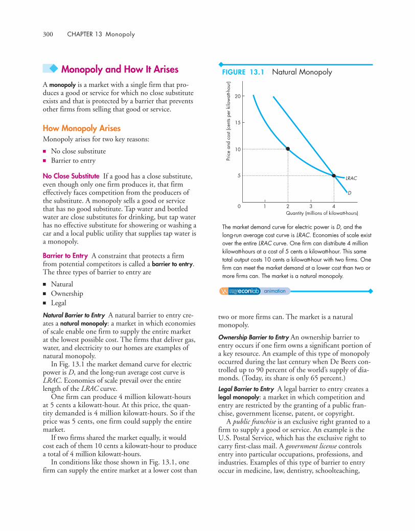
300 CHAPTER 13 Monopoly

◆ Monopoly and How It ArisesA monopoly is a market with a single firm that pro-duces a good or service for which no close substituteexists and that is protected by a barrier that preventsother firms from selling that good or service.

How Monopoly ArisesMonopoly arises for two key reasons:

■ No close substitute■ Barrier to entry

No Close Substitute If a good has a close substitute,even though only one firm produces it, that firmeffectively faces competition from the producers ofthe substitute. A monopoly sells a good or servicethat has no good substitute. Tap water and bottledwater are close substitutes for drinking, but tap waterhas no effective substitute for showering or washing acar and a local public utility that supplies tap water isa monopoly.

Barrier to Entry A constraint that protects a firmfrom potential competitors is called a barrier to entry.The three types of barrier to entry are

■ Natural■ Ownership■ Legal

Natural Barrier to Entry A natural barrier to entry cre-ates a natural monopoly: a market in which economiesof scale enable one firm to supply the entire marketat the lowest possible cost. The firms that deliver gas,water, and electricity to our homes are examples ofnatural monopoly.

In Fig. 13.1 the market demand curve for electricpower is D, and the long-run average cost curve isLRAC. Economies of scale prevail over the entirelength of the LRAC curve.

One firm can produce 4 million kilowatt-hoursat 5 cents a kilowatt-hour. At this price, the quan-tity demanded is 4 million kilowatt-hours. So if theprice was 5 cents, one firm could supply the entiremarket.

If two firms shared the market equally, it wouldcost each of them 10 cents a kilowatt-hour to producea total of 4 million kilowatt-hours.

In conditions like those shown in Fig. 13.1, onefirm can supply the entire market at a lower cost than

two or more firms can. The market is a naturalmonopoly.

Ownership Barrier to Entry An ownership barrier toentry occurs if one firm owns a significant portion ofa key resource. An example of this type of monopolyoccurred during the last century when De Beers con-trolled up to 90 percent of the world’s supply of dia-monds. (Today, its share is only 65 percent.)

Legal Barrier to Entry A legal barrier to entry creates alegal monopoly: a market in which competition andentry are restricted by the granting of a public fran-chise, government license, patent, or copyright.

A public franchise is an exclusive right granted to afirm to supply a good or service. An example is theU.S. Postal Service, which has the exclusive right tocarry first-class mail. A government license controlsentry into particular occupations, professions, andindustries. Examples of this type of barrier to entryoccur in medicine, law, dentistry, schoolteaching,

0

Pric

e an

d co

st (c

ents

per k

ilow

att-h

our)

Quantity (millions of kilowatt-hours)

D

LRAC

1 2 3 4

5

10

15

20

The market demand curve for electric power is D, and thelong-run average cost curve is LRAC. Economies of scale existover the entire LRAC curve. One firm can distribute 4 millionkilowatt-hours at a cost of 5 cents a kilowatt-hour. This sametotal output costs 10 cents a kilowatt-hour with two firms. Onefirm can meet the market demand at a lower cost than two ormore firms can. The market is a natural monopoly.

FIGURE 13.1 Natural Monopoly

animation

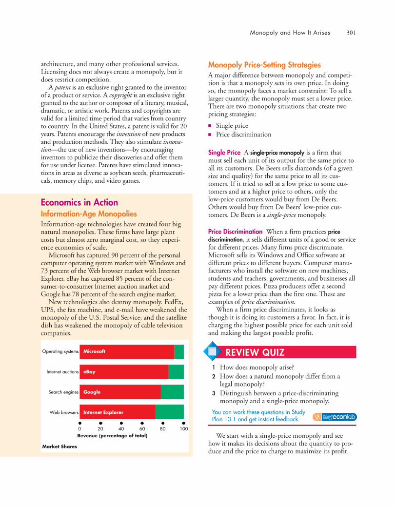
Monopoly and How It Arises 301

architecture, and many other professional services.Licensing does not always create a monopoly, but itdoes restrict competition.

A patent is an exclusive right granted to the inventorof a product or service. A copyright is an exclusive rightgranted to the author or composer of a literary, musical,dramatic, or artistic work. Patents and copyrights arevalid for a limited time period that varies from countryto country. In the United States, a patent is valid for 20years. Patents encourage the invention of new productsand production methods. They also stimulate innova-tion—the use of new inventions—by encouraginginventors to publicize their discoveries and offer themfor use under license. Patents have stimulated innova-tions in areas as diverse as soybean seeds, pharmaceuti-cals, memory chips, and video games.

Monopoly Price-Setting StrategiesA major difference between monopoly and competi-tion is that a monopoly sets its own price. In doingso, the monopoly faces a market constraint: To sell alarger quantity, the monopoly must set a lower price.There are two monopoly situations that create twopricing strategies:

■ Single price■ Price discrimination

Single Price A single-price monopoly is a firm thatmust sell each unit of its output for the same price toall its customers. De Beers sells diamonds (of a givensize and quality) for the same price to all its cus-tomers. If it tried to sell at a low price to some cus-tomers and at a higher price to others, only thelow-price customers would buy from De Beers.Others would buy from De Beers’ low-price cus-tomers. De Beers is a single-price monopoly.

Price Discrimination When a firm practices pricediscrimination, it sells different units of a good or servicefor different prices. Many firms price discriminate.Microsoft sells its Windows and Office software atdifferent prices to different buyers. Computer manu-facturers who install the software on new machines,students and teachers, governments, and businesses allpay different prices. Pizza producers offer a secondpizza for a lower price than the first one. These areexamples of price discrimination.

When a firm price discriminates, it looks asthough it is doing its customers a favor. In fact, it ischarging the highest possible price for each unit soldand making the largest possible profit.

We start with a single-price monopoly and seehow it makes its decisions about the quantity to pro-duce and the price to charge to maximize its profit.

Economics in ActionInformation-Age MonopoliesInformation-age technologies have created four bignatural monopolies. These firms have large plantcosts but almost zero marginal cost, so they experi-ence economies of scale.

Microsoft has captured 90 percent of the personalcomputer operating system market with Windows and73 percent of the Web browser market with InternetExplorer. eBay has captured 85 percent of the con-sumer-to-consumer Internet auction market andGoogle has 78 percent of the search engine market.

New technologies also destroy monopoly. FedEx,UPS, the fax machine, and e-mail have weakened themonopoly of the U.S. Postal Service; and the satellitedish has weakened the monopoly of cable televisioncompanies.

0 20 40 60 80 100

Operating systems

Internet auctions

Search engines

Web browsers

Revenue (percentage of total)

Microsoft

eBay

Google

Internet Explorer

Market Shares

REVIEW QUIZ1 How does monopoly arise?2 How does a natural monopoly differ from a

legal monopoly?3 Distinguish between a price-discriminating

monopoly and a single-price monopoly.

You can work these questions in Study Plan 13.1 and get instant feedback.

302 CHAPTER 13 Monopoly

◆ A Single-Price Monopoly’s Output and Price Decision

To understand how a single-price monopoly makesits output and price decision, we must first study thelink between price and marginal revenue.

Price and Marginal RevenueBecause in a monopoly there is only one firm, thedemand curve facing the firm is the market demandcurve. Let’s look at Bobbie’s Barbershop, the sole sup-plier of haircuts in Cairo, Nebraska. The table in Fig.13.2 shows the market demand schedule. At a price of$20, Bobbie sells no haircuts. The lower the price, themore haircuts per hour she can sell. For example, at$12, consumers demand 4 haircuts per hour (row E).

Total revenue (TR) is the price (P) multiplied bythe quantity sold (Q). For example, in row D, Bobbiesells 3 haircuts at $14 each, so total revenue is $42.Marginal revenue (MR) is the change in total revenue(ΔTR) resulting from a one-unit increase in the quan-tity sold. For example, if the price falls from $16 (rowC ) to $14 (row D), the quantity sold increases from 2to 3 haircuts. Total revenue increases from $32 to$42, so the change in total revenue is $10. Becausethe quantity sold increases by 1 haircut, marginal rev-enue equals the change in total revenue and is $10.Marginal revenue is placed between the two rows toemphasize that marginal revenue relates to the changein the quantity sold.

Figure 13.2 shows the market demand curve andmarginal revenue curve (MR) and also illustrates thecalculation we’ve just made. Notice that at eachlevel of output, marginal revenue is less thanprice—the marginal revenue curve lies below thedemand curve. Why is marginal revenue less thanprice? It is because when the price is lowered to sellone more unit, two opposing forces affect total rev-enue. The lower price results in a revenue loss, andthe increased quantity sold results in a revenue gain.For example, at a price of $16, Bobbie sells 2 hair-cuts (point C ). If she lowers the price to $14, shesells 3 haircuts and has a revenue gain of $14 on thethird haircut. But she now receives only $14 on thefirst two haircuts—$2 less than before. As a result,she loses $4 of revenue on the first 2 haircuts. Tocalculate marginal revenue, she must deduct thisamount from the revenue gain of $14. So her mar-ginal revenue is $10, which is less than the price.

0 2 3

20

Quantity (haircuts per hour)

Pric

e an

d m

argi

nal r

even

ue

16

14

10

(dol

lars

per

hai

rcut

)

Total revenue loss $4

Total revenue gain $14

C

D

Marginal revenue $10

MR Demand

The table shows the demand schedule. Total revenue (TR) isprice multiplied by quantity sold. For example, in row C,the price is $16 a haircut, Bobbie sells 2 haircuts, and totalrevenue is $32. Marginal revenue (MR) is the change intotal revenue that results from a one-unit increase in thequantity sold. For example, when the price falls from $16 to$14 a haircut, the quantity sold increases from 2 to 3, anincrease of 1 haircut, and total revenue increases by $10.Marginal revenue is $10. The demand curve and the mar-ginal revenue curve, MR, are based on the numbers in thetable and illustrate the calculation of marginal revenuewhen the price falls from $16 to $14 a haircut.

Quantity MarginalPrice demanded Total revenue(P ) (Q ) revenue (MR = ΔTR/ΔQ )

(dollars per (haircuts (TR = P × Q ) (dollars perhaircut) per hour) (dollars) haircut)

A 20 0 0 . . . . . . . . . . .18

B 18 1 18 . . . . . . . . . . .14

C 16 2 32 . . . . . . . . . . .10

D 14 3 42 . . . . . . . . . . . 6

E 12 4 48 . . . . . . . . . . . 2

F 10 5 50

FIGURE 13.2 Demand and Marginal Revenue

animation

A Single-Price Monopoly’s Output and Price Decision 303

In part (a), the demand curve is D and the marginal revenuecurve is MR. In part (b), the total revenue curve is TR. Overthe range 0 to 5 haircuts an hour, a price cut increases totalrevenue, so marginal revenue is positive—as shown by theblue bars. Demand is elastic. Over the range 5 to 10 haircutsan hour, a price cut decreases total revenue, so marginal rev-enue is negative—as shown by the red bars. Demand isinelastic. At 5 haircuts an hour, total revenue is maximizedand marginal revenue is zero. Demand is unit elastic.

Marginal Revenue and ElasticityA single-price monopoly’s marginal revenue is relatedto the elasticity of demand for its good. The demandfor a good can be elastic (the elasticity is greater than1), inelastic (the elasticity is less than 1), or unit elas-tic (the elasticity is equal to 1). Demand is elastic if a1 percent fall in the price brings a greater than 1 per-cent increase in the quantity demanded. Demand isinelastic if a 1 percent fall in the price brings a lessthan 1 percent increase in the quantity demanded.Demand is unit elastic if a 1 percent fall in the pricebrings a 1 percent increase in the quantity demanded.(See Chapter 4, pp. 84–86.)

If demand is elastic, a fall in the price brings anincrease in total revenue—the revenue gain from theincrease in quantity sold outweighs the revenue lossfrom the lower price—and marginal revenue ispositive. If demand is inelastic, a fall in the pricebrings a decrease in total revenue—the revenue gainfrom the increase in quantity sold is outweighed bythe revenue loss from the lower price—and mar-ginal revenue is negative. If demand is unit elastic,total revenue does not change—the revenue gainfrom the increase in the quantity sold offsets therevenue loss from the lower price—and marginalrevenue is zero. (See Chapter 4, p. 88.)

Figure 13.3 illustrates the relationship betweenmarginal revenue, total revenue, and elasticity. As theprice gradually falls from $20 to $10 a haircut, thequantity demanded increases from 0 to 5 haircuts anhour. Over this output range, marginal revenue ispositive in part (a), total revenue increases in part (b),and the demand for haircuts is elastic. As the pricefalls from $10 to $0 a haircut, the quantity of hair-cuts demanded increases from 5 to 10 an hour. Overthis output range, marginal revenue is negative inpart (a), total revenue decreases in part (b), and thedemand for haircuts is inelastic. When the price is$10 a haircut, marginal revenue is zero in part (a),total revenue is at a maximum in part (b), and thedemand for haircuts is unit elastic.

In Monopoly, Demand Is Always Elastic The rela-tionship between marginal revenue and elasticity ofdemand that you’ve just discovered implies that aprofit-maximizing monopoly never produces an out-put in the inelastic range of the market demandcurve. If it did so, it could charge a higher price, pro-duce a smaller quantity, and increase its profit. Let’snow look at a monopoly’s price and output decision.

0

10

Quantity(haircutsper hour)

Pric

e an

d m

argi

nal r

even

ue

20

(dol

lars

per

hai

rcut

)

Maximumtotal revenue

D

5

–20

(a) Demand and marginal revenue curvesTo

tal r

even

ue (d

olla

rs p

er h

our)

40

30

20

10

0

50

5 10

–10

Zeromarginalrevenue

Quantity(haircutsper hour)

TR

(b) Total revenue curve

MR

Elastic

Unit elastic

Inelastic

10

FIGURE 13.3 Marginal Revenue and Elasticity

animation

304 CHAPTER 13 Monopoly

Price Quantity Total Marginal Total Marginal(P ) demanded revenue revenue cost cost Profit

(dollars (Q ) (TR = P × Q ) (MR = ΔTR/ΔQ ) (TC ) (MC = ΔTC/ΔQ ) (TR – TC )per haircut) (haircuts per hour) (dollars) (dollars per haircut) (dollars) (dollars per haircut) (dollars)

20 0 0 . . . . . . . . . . . . 18

20 . . . . . . . . . . . 1

–20

18 1 18 . . . . . . . . . . . . 14

21 . . . . . . . . . . . 3

–3

16 2 32 . . . . . . . . . . . . 10

24 . . . . . . . . . . . 6

+8

14 3 42 . . . . . . . . . . . . 6

30 . . . . . . . . . . . 10

+12

12 4 48 . . . . . . . . . . . . 2

40 . . . . . . . . . . . 15

+8

10 5 50 55 –5

Price and Output DecisionA monopoly sets its price and output at the levelsthat maximize economic profit. To determine thisprice and output level, we need to study the behaviorof both cost and revenue as output varies. A monop-oly faces the same types of technology and cost con-straints as a competitive firm, so its costs (total cost,average cost, and marginal cost) behave just like thoseof a firm in perfect competition. And a monopoly’srevenues (total revenue, price, and marginal revenue)behave in the way we’ve just described.

Table 13.1 provides information about Bobbie’scosts, revenues, and economic profit, and Fig. 13.4shows the same information graphically.

Maximizing Economic Profit You can see in Table13.1 and Fig. 13.4(a) that total cost (TC ) and totalrevenue (TR) both rise as output increases, but TCrises at an increasing rate and TR rises at a decreasingrate. Economic profit, which equals TR minus TC,increases at small output levels, reaches a maximum,and then decreases. The maximum profit ($12)occurs when Bobbie sells 3 haircuts for $14 each. Ifshe sells 2 haircuts for $16 each or 4 haircuts for $12each, her economic profit will be only $8.

Marginal Revenue Equals Marginal Cost You can seeBobbie’s marginal revenue (MR) and marginal cost(MC ) in Table 13.1 and Fig. 13.4(b).

When Bobbie increases output from 2 to 3 haircuts,MR is $10 and MC is $6. MR exceeds MC by $4 andBobbie’s profit increases by that amount. If Bobbieincreases output yet further, from 3 to 4 haircuts, MRis $6 and MC is $10. In this case, MC exceeds MR by$4, so profit decreases by that amount. When MRexceeds MC, profit increases if output increases. WhenMC exceeds MR, profit increases if output decreases.When MC equals MR, profit is maximized.

Figure 13.4(b) shows the maximum profit as price(on the demand curve D) minus average total cost(on the ATC curve) multiplied by the quantity pro-duced—the blue rectangle.

Maximum Price the Market Will Bear Unlike a firmin perfect competition, a monopoly influences theprice of what it sells. But a monopoly doesn’t set theprice at the maximum possible price. At the maxi-mum possible price, the firm would be able to sellonly one unit of output, which in general is less thanthe profit-maximizing quantity. Rather, a monopolyproduces the profit-maximizing quantity and sellsthat quantity for the highest price it can get.

This table gives the information needed to find the profit-maxi-mizing output and price. Total revenue (TR) equals price multi-plied by the quantity sold. Profit equals total revenue minus total

cost (TC). Profit is maximized when 3 haircuts are sold at aprice of $14 each. Total revenue is $42, total cost is $30, andeconomic profit is $12 ($42 � $30).

TABLE 13.1 A Monopoly’s Output and Price Decision

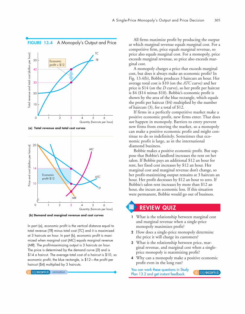
A Single-Price Monopoly’s Output and Price Decision 305

All firms maximize profit by producing the outputat which marginal revenue equals marginal cost. For acompetitive firm, price equals marginal revenue, soprice also equals marginal cost. For a monopoly, priceexceeds marginal revenue, so price also exceeds mar-ginal cost.

A monopoly charges a price that exceeds marginalcost, but does it always make an economic profit? InFig. 13.4(b), Bobbie produces 3 haircuts an hour. Heraverage total cost is $10 (on the ATC curve) and herprice is $14 (on the D curve), so her profit per haircutis $4 ($14 minus $10). Bobbie’s economic profit isshown by the area of the blue rectangle, which equalsthe profit per haircut ($4) multiplied by the numberof haircuts (3), for a total of $12.

If firms in a perfectly competitive market make apositive economic profit, new firms enter. That doesnot happen in monopoly. Barriers to entry preventnew firms from entering the market, so a monopolycan make a positive economic profit and might con-tinue to do so indefinitely. Sometimes that eco-nomic profit is large, as in the internationaldiamond business.

Bobbie makes a positive economic profit. But sup-pose that Bobbie’s landlord increases the rent on hersalon. If Bobbie pays an additional $12 an hour forrent, her fixed cost increases by $12 an hour. Hermarginal cost and marginal revenue don’t change, soher profit-maximizing output remains at 3 haircuts anhour. Her profit decreases by $12 an hour to zero. IfBobbie’s salon rent increases by more than $12 anhour, she incurs an economic loss. If this situationwere permanent, Bobbie would go out of business.

Tota

l rev

enue

and

tota

l cos

t (do

llars

per

hou

r)

50

42

30

10

TC

Economicprofit = $12

TR

30Quantity (haircuts per hour)

42 51

20

5

6

6Quantity (haircuts per hour)

20

14

Pric

e an

d co

st (d

olla

rs p

er h

airc

ut)

D

MR

30

MC

ATC

(b) Demand and marginal revenue and cost curves

421

10

Economicprofit $12

(a) Total revenue and total cost curves

In part (a), economic profit is the vertical distance equal tototal revenue (TR) minus total cost (TC) and it is maximizedat 3 haircuts an hour. In part (b), economic profit is maxi-mized when marginal cost (MC) equals marginal revenue(MR). The profit-maximizing output is 3 haircuts an hour.The price is determined by the demand curve (D) and is$14 a haircut. The average total cost of a haircut is $10, soeconomic profit, the blue rectangle, is $12—the profit perhaircut ($4) multiplied by 3 haircuts.

FIGURE 13.4 A Monopoly’s Output and Price

animation

REVIEW QUIZ 1 What is the relationship between marginal cost

and marginal revenue when a single-pricemonopoly maximizes profit?

2 How does a single-price monopoly determinethe price it will charge its customers?

3 What is the relationship between price, mar-ginal revenue, and marginal cost when a single-price monopoly is maximizing profit?

4 Why can a monopoly make a positive economicprofit even in the long run?

You can work these questions in Study Plan 13.2 and get instant feedback.

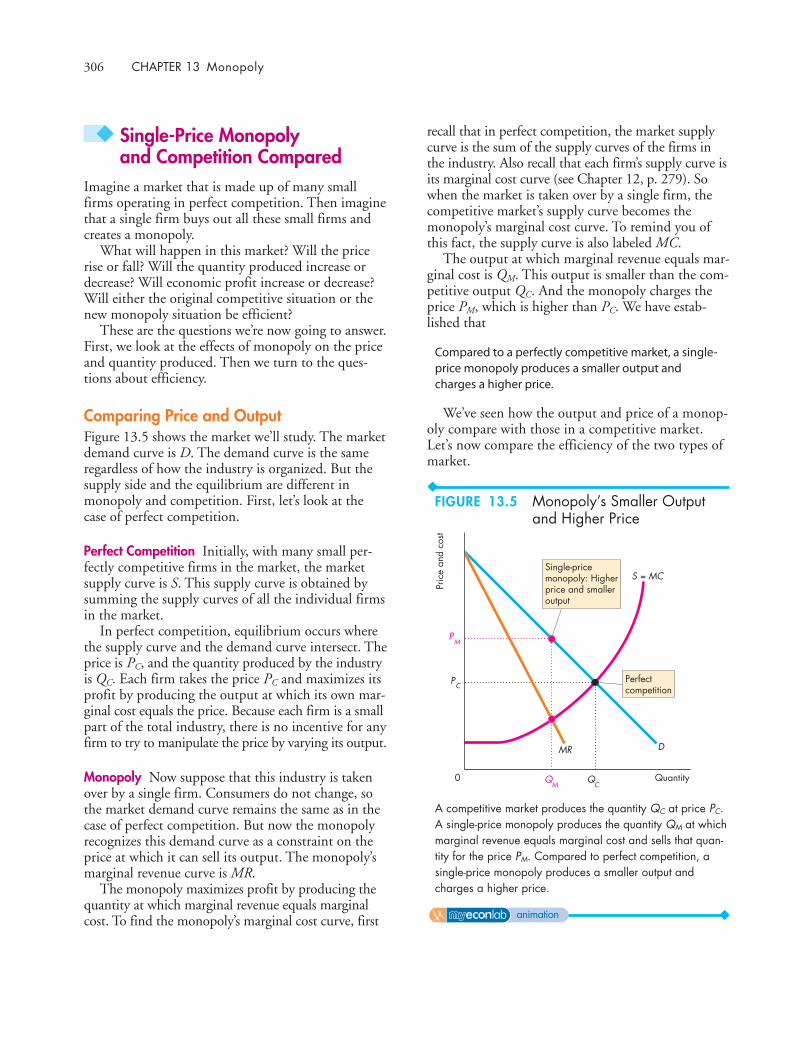
306 CHAPTER 13 Monopoly

◆ Single-Price Monopoly and Competition Compared

Imagine a market that is made up of many smallfirms operating in perfect competition. Then imaginethat a single firm buys out all these small firms andcreates a monopoly.

What will happen in this market? Will the pricerise or fall? Will the quantity produced increase ordecrease? Will economic profit increase or decrease?Will either the original competitive situation or thenew monopoly situation be efficient?

These are the questions we’re now going to answer.First, we look at the effects of monopoly on the priceand quantity produced. Then we turn to the ques-tions about efficiency.

Comparing Price and OutputFigure 13.5 shows the market we’ll study. The marketdemand curve is D. The demand curve is the sameregardless of how the industry is organized. But thesupply side and the equilibrium are different inmonopoly and competition. First, let’s look at thecase of perfect competition.

Perfect Competition Initially, with many small per-fectly competitive firms in the market, the marketsupply curve is S. This supply curve is obtained bysumming the supply curves of all the individual firmsin the market.

In perfect competition, equilibrium occurs wherethe supply curve and the demand curve intersect. Theprice is PC, and the quantity produced by the industryis QC. Each firm takes the price PC and maximizes itsprofit by producing the output at which its own mar-ginal cost equals the price. Because each firm is a smallpart of the total industry, there is no incentive for anyfirm to try to manipulate the price by varying its output.

Monopoly Now suppose that this industry is takenover by a single firm. Consumers do not change, sothe market demand curve remains the same as in thecase of perfect competition. But now the monopolyrecognizes this demand curve as a constraint on theprice at which it can sell its output. The monopoly’smarginal revenue curve is MR.

The monopoly maximizes profit by producing thequantity at which marginal revenue equals marginalcost. To find the monopoly’s marginal cost curve, first

recall that in perfect competition, the market supplycurve is the sum of the supply curves of the firms inthe industry. Also recall that each firm’s supply curve isits marginal cost curve (see Chapter 12, p. 279). Sowhen the market is taken over by a single firm, thecompetitive market’s supply curve becomes themonopoly’s marginal cost curve. To remind you ofthis fact, the supply curve is also labeled MC.

The output at which marginal revenue equals mar-ginal cost is QM. This output is smaller than the com-petitive output QC. And the monopoly charges theprice PM, which is higher than PC. We have estab-lished that

Compared to a perfectly competitive market, a single-price monopoly produces a smaller output andcharges a higher price.

We’ve seen how the output and price of a monop-oly compare with those in a competitive market.Let’s now compare the efficiency of the two types ofmarket.

0

CP

MP

Pric

e an

d co

st

Quantity

MR D

S = MCSingle-pricemonopoly: Higher price and smaller output

Perfectcompetition

MQ

CQ

A competitive market produces the quantity QC at price PC.A single-price monopoly produces the quantity QM at whichmarginal revenue equals marginal cost and sells that quan-tity for the price PM. Compared to perfect competition, asingle-price monopoly produces a smaller output andcharges a higher price.

FIGURE 13.5 Monopoly’s Smaller Outputand Higher Price

animation

Single-Price Monopoly and Competition Compared 307

Efficiency ComparisonPerfect competition (with no externalities) is efficient.Figure 13.6(a) illustrates the efficiency of perfect com-petition and serves as a benchmark against which tomeasure the inefficiency of monopoly. Along thedemand curve and marginal social benefit curve (D =MSB), consumers are efficient. Along the supply curveand marginal social cost curve (S = MSC ), producersare efficient. In competitive equilibrium, the price isPC, the quantity is QC, and marginal social benefitequals marginal social cost.

Consumer surplus is the green triangle under thedemand curve and above the equilibrium price (seeChapter 5, p. 109). Producer surplus is the blue areaabove the supply curve and below the equilibriumprice (see Chapter 5, p. 111). Total surplus (con-sumer surplus and producer surplus) is maximized.

Also, in long-run competitive equilibrium, entryand exit ensure that each firm produces its output atthe minimum possible long-run average cost.

To summarize: At the competitive equilibrium,marginal social benefit equals marginal social cost;total surplus is maximized; firms produce at the low-est possible long-run average cost; and resource use isefficient.

Figure 13.6(b) illustrates the inefficiency ofmonopoly and the sources of that inefficiency. Amonopoly produces QM and sells its output for PM.The smaller output and higher price drive a wedgebetween marginal social benefit and marginal socialcost and create a deadweight loss. The gray triangleshows the deadweight loss and its magnitude is ameasure of the inefficiency of monopoly.

Consumer surplus shrinks for two reasons. First,consumers lose by having to pay more for the good.This loss to consumers is a gain for monopoly andincreases the producer surplus. Second, consumerslose by getting less of the good, and this loss is part ofthe deadweight loss.

Although the monopoly gains from a higher price,it loses some producer surplus because it produces asmaller output. That loss is another part of the dead-weight loss.

A monopoly produces a smaller output than per-fect competition and faces no competition, so it doesnot produce at the lowest possible long-run averagecost. As a result, monopoly damages the consumerinterest in three ways: A monopoly produces less,increases the cost of production, and raises the priceby more than the increased cost of production.

0

(b) Monopoly

CP

MP

Quantity

MR

MSC

S = MSC

MQ

CQ

0

(a) Perfect competition

CP

Pric

e an

d co

stPr

ice

and

cost

Quantity

D = MSB

D = MSB

Consumersurplus

Producersurplus

Efficientquantity

Consumersurplus

Deadweightloss

Producersurplus

CQ

In perfect competition in part (a), output is QC and the priceis PC. Marginal social benefit (MSB) equals marginal socialcost (MSC); total surplus, the sum of consumer surplus (thegreen triangle) and producer surplus (the blue area), is max-imized; and in the long run, firms produce at the lowest pos-sible average cost. Monopoly in part (b) produces QM andraises the price to PM. Consumer surplus shrinks, the monop-oly gains, and a deadweight loss (the gray triangle) arises.

FIGURE 13.6 Inefficiency of Monopoly

animation

308 CHAPTER 13 Monopoly

Redistribution of SurplusesYou’ve seen that monopoly is inefficient because mar-ginal social benefit exceeds marginal social cost andthere is deadweight loss—a social loss. But monopolyalso brings a redistribution of surpluses.

Some of the lost consumer surplus goes to themonopoly. In Fig. 13.6, the monopoly takes the dif-ference between the higher price, PM, and the com-petitive price, PC , on the quantity sold, QM. So themonopoly takes that part of the consumer surplus.This portion of the loss of consumer surplus is not aloss to society. It is redistribution from consumers tothe monopoly producer.

Rent SeekingYou’ve seen that monopoly creates a deadweight lossand is inefficient. But the social cost of monopolycan exceed the deadweight loss because of an activitycalled rent seeking. Any surplus—consumer surplus,producer surplus, or economic profit—is called eco-nomic rent. The pursuit of wealth by capturing eco-nomic rent is called rent seeking.

You’ve seen that a monopoly makes its economicprofit by diverting part of consumer surplus toitself—by converting consumer surplus into eco-nomic profit. So the pursuit of economic profit by amonopoly is rent seeking. It is the attempt to captureconsumer surplus.

Rent seekers pursue their goals in two main ways.They might

■ Buy a monopoly■ Create a monopoly

Buy a Monopoly To rent seek by buying a monop-oly, a person searches for a monopoly that is for saleat a lower price than the monopoly’s economic profit.Trading of taxicab licenses is an example of this typeof rent seeking. In some cities, taxicabs are regulated.The city restricts both the fares and the number oftaxis that can operate so that operating a taxi resultsin economic profit. A person who wants to operate ataxi must buy a license from someone who alreadyhas one. People rationally devote time and effort toseeking out profitable monopoly businesses to buy. Inthe process, they use up scarce resources that couldotherwise have been used to produce goods andservices. The value of this lost production is part ofthe social cost of monopoly. The amount paid for a

monopoly is not a social cost because the payment isjust a transfer of an existing producer surplus fromthe buyer to the seller.

Create a Monopoly Rent seeking by creating amonopoly is mainly a political activity. It takes theform of lobbying and trying to influence the politicalprocess. Such influence might be sought by makingcampaign contributions in exchange for legislativesupport or by indirectly seeking to influence politicaloutcomes through publicity in the media or moredirect contacts with politicians and bureaucrats. Anexample of a monopoly created in this way is the gov-ernment-imposed restrictions on the quantities of tex-tiles that may be imported into the United States.Another is a regulation that limits the number oforanges that may be sold in the United States. Theseare regulations that restrict output and increase price.

This type of rent seeking is a costly activity thatuses up scarce resources. Taken together, firms spendbillions of dollars lobbying Congress, state legislators,and local officials in the pursuit of licenses and lawsthat create barriers to entry and establish a monopoly.

Rent-Seeking EquilibriumBarriers to entry create monopoly. But there is nobarrier to entry into rent seeking. Rent seeking is likeperfect competition. If an economic profit is avail-able, a new rent seeker will try to get some of it. Andcompetition among rent seekers pushes up the pricethat must be paid for a monopoly, to the point atwhich the rent seeker makes zero economic profit byoperating the monopoly. For example, competitionfor the right to operate a taxi in New York City leadsto a price of more than $100,000 for a taxi license,which is sufficiently high to eliminate the economicprofit made by a taxi operator.

Figure 13.7 shows a rent-seeking equilibrium. Thecost of rent seeking is a fixed cost that must be addedto a monopoly’s other costs. Rent seeking and rent-seeking costs increase to the point at which no eco-nomic profit is made. The average total cost curve,which includes the fixed cost of rent seeking, shiftsupward until it just touches the demand curve.Economic profit is zero. It has been lost in rent seeking.

Consumer surplus is unaffected, but the dead-weight loss from monopoly is larger. The deadweightloss now includes the original deadweight loss trian-gle plus the lost producer surplus, shown by theenlarged gray area in Fig. 13.7.

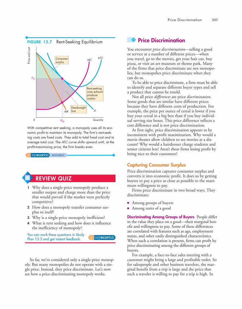
Price Discrimination 309

So far, we’ve considered only a single-price monop-oly. But many monopolies do not operate with a sin-gle price. Instead, they price discriminate. Let’s nowsee how a price-discriminating monopoly works.

◆ Price DiscriminationYou encounter price discrimination—selling a good or service at a number of different prices—when you travel, go to the movies, get your hair cut, buypizza, or visit an art museum or theme park. Many of the firms that price discriminate are not monopo-lies, but monopolies price discriminate when theycan do so.

To be able to price discriminate, a firm must be ableto identify and separate different buyer types and sella product that cannot be resold.

Not all price differences are price discrimination.Some goods that are similar have different pricesbecause they have different costs of production. Forexample, the price per ounce of cereal is lower if youbuy your cereal in a big box than if you buy individ-ual serving size boxes. This price difference reflects acost difference and is not price discrimination.

At first sight, price discrimination appears to beinconsistent with profit maximization. Why would amovie theater allow children to see movies at a dis-count? Why would a hairdresser charge students andsenior citizens less? Aren’t these firms losing profit bybeing nice to their customers?

Capturing Consumer SurplusPrice discrimination captures consumer surplus andconverts it into economic profit. It does so by gettingbuyers to pay a price as close as possible to the maxi-mum willingness to pay.

Firms price discriminate in two broad ways. Theydiscriminate:

■ Among groups of buyers■ Among units of a good

Discriminating Among Groups of Buyers People differin the value they place on a good—their marginal ben-efit and willingness to pay. Some of these differencesare correlated with features such as age, employmentstatus, and other easily distinguished characteristics.When such a correlation is present, firms can profit byprice discriminating among the different groups ofbuyers.

For example, a face-to-face sales meeting with acustomer might bring a large and profitable order. Sofor salespeople and other business travelers, the mar-ginal benefit from a trip is large and the price thatsuch a traveler is willing to pay for a trip is high. In

0

PM

Pric

e an

d co

st

Quantity

MR D

MCATC

QM

Consumersurplus

Deadweightloss

Rent-seekingcosts exhaustproducersurplus

With competitive rent seeking, a monopoly uses all its eco-nomic profit to maintain its monopoly. The firm’s rent-seek-ing costs are fixed costs. They add to total fixed cost and toaverage total cost. The ATC curve shifts upward until, at theprofit-maximizing price, the firm breaks even.

FIGURE 13.7 Rent-Seeking Equilibrium

animation

REVIEW QUIZ 1 Why does a single-price monopoly produce a

smaller output and charge more than the pricethat would prevail if the market were perfectlycompetitive?

2 How does a monopoly transfer consumer sur-plus to itself?

3 Why is a single-price monopoly inefficient?4 What is rent seeking and how does it influence

the inefficiency of monopoly?

You can work these questions in Study Plan 13.3 and get instant feedback.

310 CHAPTER 13 Monopoly

contrast, for a vacation traveler, any of several differ-ent trips and even no vacation trip are options. So forvacation travelers, the marginal benefit of a trip issmall and the price that such a traveler is willing topay for a trip is low. Because business travelers arewilling to pay more than vacation travelers are, it ispossible for an airline to profit by price discriminat-ing between these two groups.

Discriminating Among Units of a Good Everyoneexperiences diminishing marginal benefit and has adownward-sloping demand curve. For this reason, ifall the units of the good are sold for a single price,buyers end up with a consumer surplus equal to thevalue they get from each unit of the good minus theprice paid for it.

A firm that price discriminates by charging a buyerone price for a single item and a lower price for a sec-ond or third item can capture some of the consumersurplus. Buy one pizza and get a second one free (orfor a low price) is an example of this type of price dis-crimination.

(Note that some discounts for bulk arise fromlower costs of production for greater bulk. In thesecases, such discounts are not price discrimination.)

Let’s see how price discriminating increases eco-nomic profit.

Profiting by Price DiscriminatingGlobal Airlines has a monopoly on an exotic route.Figure 13.8 shows the market demand curve (D) fortravel on this route. It also shows Global Airline’smarginal revenue curve (MR), marginal cost curve(MC ), and average total cost curve (ATC ).

As a single-price monopoly, Global maximizesprofit by producing the quantity at which MR equalsMC, which is 8,000 trips a year, and charging $1,200per trip. At this quantity, average total cost is $600per trip, economic profit is $600 a trip, and Global’seconomic profit is $4.8 million a year, shown by theblue rectangle. Global’s customers enjoy a consumersurplus shown by the green triangle.

Global is struck by the fact that many of its cus-tomers are business travelers, and it suspects they arewilling to pay more than $1,200 a trip. Global doessome market research, which reveals that some busi-ness travelers are willing to pay as much as $1,800 atrip. Also, these customers frequently change theirtravel plans at the last minute. Another group ofbusiness travelers is willing to pay $1,600. These

customers know a week ahead when they will travel,and they never want to stay over a weekend. Yetanother group would pay up to $1,400. These travel-ers know two weeks ahead when they will travel andalso don’t want to stay away over a weekend.

Global announces a new fare schedule: no restric-tions, $1,800; 7-day advance purchase, nonrefund-able, $1,600; 14-day advance purchase,nonrefundable, $1,400; 14-day advance purchase,must stay over a weekend, $1,200.

Figure 13.9 shows the outcome with this new farestructure and also shows why Global is pleased withits new fares. It sells 2,000 seats at each of its fourprices. Global’s economic profit increases by the darkblue steps. Its economic profit is now its original $4.8million a year plus an additional $2.4 million fromits new higher fares. Consumer surplus shrinks to thesum of the smaller green areas.

Pric

e an

d co

st (d

olla

rs p

er tr

ip)

Trips (thousands per year)0

D

1085 15 20

1,200

2,100

1,800

1,500

900

600

300

MR

MCATC

Consumersurplus

Economicprofit

$4.8million

Global Airlines has a monopoly on an air route. The marketdemand curve is D. Global Airline’s marginal revenue curveis MR, its marginal cost curve is MC, and its average totalcost curve is ATC. As a single-price monopoly, Global maxi-mizes profit by selling 8,000 trips a year at $1,200 a trip. Itsprofit is $4.8 million a year—the blue rectangle. Global’scustomers enjoy a consumer surplus—the green triangle.

FIGURE 13.8 A Single Price of Air Travel

animation

Price Discrimination 311

Perfect Price DiscriminationPerfect price discrimination occurs if a firm is able to selleach unit of output for the highest price anyone iswilling to pay for it. In such a case, the entire con-sumer surplus is eliminated and captured by the pro-ducer. To practice perfect price discrimination, a firmmust be creative and come up with a host of pricesand special conditions, each one of which appeals toa tiny segment of the market.

With perfect price discrimination, something spe-cial happens to marginal revenue—the marketdemand curve becomes the marginal revenue curve.The reason is that when the price is cut to sell a largerquantity, the firm sells only the marginal unit at thelower price. All the other units continue to be sold forthe highest price that each buyer is willing to pay. Sofor the perfect price discriminator, marginal revenueequals price and the demand curve becomes the mar-ginal revenue curve.

With marginal revenue equal to price, Global canobtain even greater profit by increasing output up tothe point at which price (and marginal revenue) isequal to marginal cost.

So Global seeks new travelers who will not pay asmuch as $1,200 a trip but who will pay more thanmarginal cost. Global offers a variety of vacation spe-cials at different low fares that appeal only to newtravelers. Existing customers continue to pay thehigher fares. With all these fares and specials, Globalincreases sales, extracts the entire consumer surplus,and maximizes economic profit.

Figure 13.10 shows the outcome with perfect pricediscrimination. The fares paid by the original travel-ers extract the entire consumer surplus from thisgroup. The new fares between $900 and $1,200attract 3,000 additional travelers and take their entireconsumer surplus also. Global now makes an eco-nomic profit of more than $9 million.

Pric

e an

d co

st (d

olla

rs p

er tr

ip)

Trips (thousands per year)0

D

1082 4 6 15 20

1,200

2,100

1,800

1,400

1,600

900

600

300

MCATCIncreased economic

profit from pricediscrimination

Global revises its fare structure: no restrictions at $1,800, 7-day advance purchase at $1,600, 14-day advance purchaseat $1,400, and must stay over a weekend at $1,200. Globalsells 2,000 trips at each of its four new fares. Its economicprofit increases by $2.4 million a year to $7.2 million a year,which is shown by the original blue rectangle plus the darkblue steps. Global’s customers’ consumer surplus shrinks.

Pric

e an

d co

st (d

olla

rs p

er tr

ip)

Trips (thousands per year)0

D = MR

1185 15 20

1,200

2,100

1,800

1,500

900

600

300

MCATCIncrease in economic

profit from perfectprice discrimination

Increasein output

Dozens of fares discriminate among many different types ofbusiness traveler, and many new low fares with restrictionsappeal to vacation travelers. With perfect price discrimina-tion, the market demand curve becomes Global’s marginalrevenue curve. Economic profit is maximized when the lowestprice equals marginal cost. Global sells 11,000 trips andmakes an economic profit of more than $9 million a year.

FIGURE 13.9 Price Discrimination

animation

animation

FIGURE 13.10 Perfect Price Discrimination

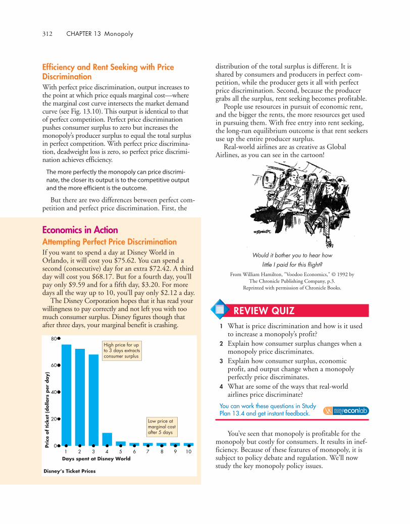
Economics in ActionAttempting Perfect Price DiscriminationIf you want to spend a day at Disney World inOrlando, it will cost you $75.62. You can spend asecond (consecutive) day for an extra $72.42. A thirdday will cost you $68.17. But for a fourth day, you’llpay only $9.59 and for a fifth day, $3.20. For moredays all the way up to 10, you’ll pay only $2.12 a day.

The Disney Corporation hopes that it has read yourwillingness to pay correctly and not left you with toomuch consumer surplus. Disney figures though thatafter three days, your marginal benefit is crashing.

1 2 3 4 5 6 7 8 9 10

80

60

40

20

0

Days spent at Disney World

Pri

ce o

f tick

et (

dolla

rs p

er d

ay)

High price for upto 3 days extractsconsumer surplus

Low price atmarginal costafter 5 days

Disney’s Ticket Prices

312 CHAPTER 13 Monopoly

distribution of the total surplus is different. It isshared by consumers and producers in perfect com-petition, while the producer gets it all with perfectprice discrimination. Second, because the producergrabs all the surplus, rent seeking becomes profitable.

People use resources in pursuit of economic rent,and the bigger the rents, the more resources get usedin pursuing them. With free entry into rent seeking,the long-run equilibrium outcome is that rent seekersuse up the entire producer surplus.

Real-world airlines are as creative as GlobalAirlines, as you can see in the cartoon!

Efficiency and Rent Seeking with PriceDiscriminationWith perfect price discrimination, output increases tothe point at which price equals marginal cost—wherethe marginal cost curve intersects the market demandcurve (see Fig. 13.10). This output is identical to thatof perfect competition. Perfect price discriminationpushes consumer surplus to zero but increases themonopoly’s producer surplus to equal the total surplusin perfect competition. With perfect price discrimina-tion, deadweight loss is zero, so perfect price discrimi-nation achieves efficiency.

The more perfectly the monopoly can price discrimi-nate, the closer its output is to the competitive outputand the more efficient is the outcome.

But there are two differences between perfect com-petition and perfect price discrimination. First, the

Would it bother you to hear how

little I paid for this flight?

From William Hamilton, "Voodoo Economics," © 1992 by The Chronicle Publishing Company, p.3.

Reprinted with permission of Chronicle Books.

You’ve seen that monopoly is profitable for themonopoly but costly for consumers. It results in inef-ficiency. Because of these features of monopoly, it issubject to policy debate and regulation. We’ll nowstudy the key monopoly policy issues.

REVIEW QUIZ 1 What is price discrimination and how is it used

to increase a monopoly’s profit?2 Explain how consumer surplus changes when a

monopoly price discriminates.3 Explain how consumer surplus, economic

profit, and output change when a monopolyperfectly price discriminates.

4 What are some of the ways that real-worldairlines price discriminate?

You can work these questions in Study Plan 13.4 and get instant feedback.

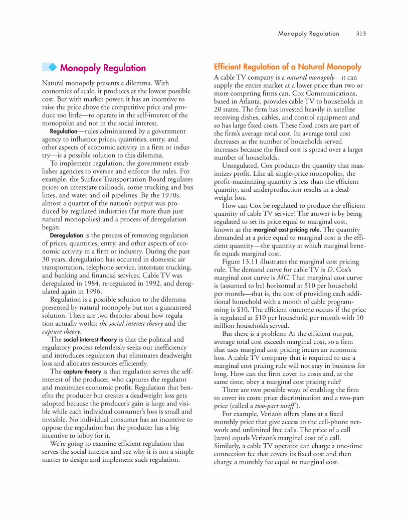
Monopoly Regulation 313

◆ Monopoly RegulationNatural monopoly presents a dilemma. Witheconomies of scale, it produces at the lowest possiblecost. But with market power, it has an incentive toraise the price above the competitive price and pro-duce too little—to operate in the self-interest of themonopolist and not in the social interest.

Regulation—rules administered by a governmentagency to influence prices, quantities, entry, andother aspects of economic activity in a firm or indus-try—is a possible solution to this dilemma.

To implement regulation, the government estab-lishes agencies to oversee and enforce the rules. Forexample, the Surface Transportation Board regulatesprices on interstate railroads, some trucking and buslines, and water and oil pipelines. By the 1970s,almost a quarter of the nation’s output was pro-duced by regulated industries (far more than justnatural monopolies) and a process of deregulationbegan.

Deregulation is the process of removing regulationof prices, quantities, entry, and other aspects of eco-nomic activity in a firm or industry. During the past30 years, deregulation has occurred in domestic airtransportation, telephone service, interstate trucking,and banking and financial services. Cable TV wasderegulated in 1984, re-regulated in 1992, and dereg-ulated again in 1996.

Regulation is a possible solution to the dilemmapresented by natural monopoly but not a guaranteedsolution. There are two theories about how regula-tion actually works: the social interest theory and thecapture theory.

The social interest theory is that the political andregulatory process relentlessly seeks out inefficiencyand introduces regulation that eliminates deadweightloss and allocates resources efficiently.

The capture theory is that regulation serves the self-interest of the producer, who captures the regulatorand maximizes economic profit. Regulation that ben-efits the producer but creates a deadweight loss getsadopted because the producer’s gain is large and visi-ble while each individual consumer’s loss is small andinvisible. No individual consumer has an incentive tooppose the regulation but the producer has a bigincentive to lobby for it.

We’re going to examine efficient regulation thatserves the social interest and see why it is not a simplematter to design and implement such regulation.

Efficient Regulation of a Natural MonopolyA cable TV company is a natural monopoly—it cansupply the entire market at a lower price than two ormore competing firms can. Cox Communications,based in Atlanta, provides cable TV to households in20 states. The firm has invested heavily in satellitereceiving dishes, cables, and control equipment andso has large fixed costs. These fixed costs are part ofthe firm’s average total cost. Its average total costdecreases as the number of households servedincreases because the fixed cost is spread over a largernumber of households.

Unregulated, Cox produces the quantity that max-imizes profit. Like all single-price monopolies, theprofit-maximizing quantity is less than the efficientquantity, and underproduction results in a dead-weight loss.

How can Cox be regulated to produce the efficientquantity of cable TV service? The answer is by beingregulated to set its price equal to marginal cost,known as the marginal cost pricing rule. The quantitydemanded at a price equal to marginal cost is the effi-cient quantity—the quantity at which marginal bene-fit equals marginal cost.

Figure 13.11 illustrates the marginal cost pricingrule. The demand curve for cable TV is D. Cox’smarginal cost curve is MC. That marginal cost curveis (assumed to be) horizontal at $10 per householdper month—that is, the cost of providing each addi-tional household with a month of cable program-ming is $10. The efficient outcome occurs if the priceis regulated at $10 per household per month with 10million households served.

But there is a problem: At the efficient output,average total cost exceeds marginal cost, so a firmthat uses marginal cost pricing incurs an economicloss. A cable TV company that is required to use amarginal cost pricing rule will not stay in business forlong. How can the firm cover its costs and, at thesame time, obey a marginal cost pricing rule?

There are two possible ways of enabling the firmto cover its costs: price discrimination and a two-partprice (called a two-part tariff ).

For example, Verizon offers plans at a fixedmonthly price that give access to the cell-phone net-work and unlimited free calls. The price of a call(zero) equals Verizon’s marginal cost of a call.Similarly, a cable TV operator can charge a one-timeconnection fee that covers its fixed cost and thencharge a monthly fee equal to marginal cost.

314 CHAPTER 13 Monopoly

Second-Best Regulation of a NaturalMonopolyA natural monopoly cannot always be regulated toachieve an efficient outcome. Two possible ways ofenabling a regulated monopoly to avoid an economicloss are

■ Average cost pricing■ Government subsidy

Average Cost Pricing The average cost pricing rulesets price equal to average total cost. With this rulethe firm produces the quantity at which the average

total cost curve cuts the demand curve. This ruleresults in the firm making zero economic profit—breaking even. But because for a natural monopolyaverage total cost exceeds marginal cost, the quantityproduced is less than the efficient quantity and adeadweight loss arises.

Figure 13.11 illustrates the average cost pricingrule. The price is $30 a month and 8 million house-holds get cable TV.

Government Subsidy A government subsidy is adirect payment to the firm equal to its economic loss.To pay a subsidy, the government must raise the rev-enue by taxing some other activity. You saw inChapter 6 that taxes themselves generate deadweightloss.

And the Second-Best Is ... Which is the betteroption, average cost pricing or marginal cost pricingwith a government subsidy? The answer depends onthe relative magnitudes of the two deadweight losses.Average cost pricing generates a deadweight loss inthe market served by the natural monopoly. A sub-sidy generates deadweight losses in the markets forthe items that are taxed to pay for the subsidy. Thesmaller deadweight loss is the second-best solution toregulating a natural monopoly. Making this calcula-tion in practice is too difficult and average cost pric-ing is generally preferred to a subsidy.

Implementing average cost pricing presents theregulator with a challenge because it is not possible tobe sure what a firm’s costs are. So regulators use oneof two practical rules:

■ Rate of return regulation■ Price cap regulation

Rate of Return Regulation Under rate of return regu-lation, a firm must justify its price by showing thatits return on capital doesn’t exceed a specified targetrate. This type of regulation can end up serving theself-interest of the firm rather than the social inter-est. The firm’s managers have an incentive to inflatecosts by spending on items such as private jets, freebaseball tickets (disguised as public relationsexpenses), and lavish entertainment. Managers alsohave an incentive to use more capital than the effi-cient amount. The rate of return on capital is regu-lated but not the total return on capital, and thegreater the amount of capital, the greater is the totalreturn.

Pric

e an

d co

st (d

olla

rs p

er h

ouse

hold

)

Quantity (millions of households)0

DMRMC

LRAC

85 10

60

40

30

10

Profitmaximizing

Marginalcost pricing

Averagecost pricing

110

A natural monopoly cable TV supplier faces the demandcurve D. The firm’s marginal cost is constant at $10 perhousehold per month, as shown by the curve labeled MC.The long-run average cost curve is LRAC.

Unregulated, as a profit-maximizer, the firm serves 5million households at a price of $60 a month. An efficientmarginal cost pricing rule sets the price at $10 a month.The monopoly serves 10 million households and incurs aneconomic loss. A second-best average cost pricing rule setsthe price at $30 a month. The monopoly serves 8 millionhouseholds and earns zero economic profit.

FIGURE 13.11 Regulating a Natural Monopoly

animation

Monopoly Regulation 315

Price Cap Regulation For the reason that we’ve justexamined, rate of return regulation is increasinglybeing replaced by price cap regulation. A price capregulation is a price ceiling—a rule that specifies thehighest price the firm is permitted to set. This type ofregulation gives a firm an incentive to operate effi-ciently and keep costs under control. Price cap regu-lation has become common for the electricity andtelecommunications industries and is replacing rateof return regulation.

To see how a price cap works, let’s suppose that thecable TV operator is subject to this type of regula-tion. Figure 13.12 shows that without regulation, thefirm maximizes profit by serving 5 million house-holds and charging a price of $60 a month. If a pricecap is set at $30 a month, the firm is permitted to sell

any quantity it chooses at that price or at a lowerprice. At 5 million households, the firm now incursan economic loss. It can decrease the loss by increas-ing output to 8 million households. To increase out-put above 8 million households, the firm would haveto lower the price and again it would incur a loss. Sothe profit-maximizing quantity is 8 million house-holds—the same as with average cost pricing.

Notice that a price cap lowers the price andincreases output. This outcome is in sharp contrast tothe effect of a price ceiling in a competitive marketthat you studied in Chapter 6 (pp. 128–130). Thereason is that in a monopoly, the unregulated equilib-rium output is less than the competitive equilibriumoutput, and the price cap regulation replicates theconditions of a competitive market.

In Fig. 13.12, the price cap delivers average costpricing. In practice, the regulator might set the captoo high. For this reason, price cap regulation is oftencombined with earnings sharing regulation—a regula-tion that requires firms to make refunds to customerswhen profits rise above a target level.

Pric

e an

d co

st (d

olla

rs p

er h

ouse

hold

)

Quantity (millions of households)0

DMRMC

LRAC

85

60

30

10

Profit-maximizingoutcome

Pricecap

Price capoutcome

110

Price capregulationlowers price ...

... andincreasesoutput

A natural monopoly cable TV supplier faces the demandcurve D. The firm’s marginal cost is constant at $10 perhousehold per month, as shown by the curve labeled MC.The long-run average cost curve is LRAC.

Unregulated, the firm serves 5 million households at aprice of $60 a month. A price cap sets the maximum priceat $30 a month. The firm has an incentive to minimize costand serve the quantity of households that demand service atthe price cap. The price cap regulation lowers the price andincreases the quantity.

◆ You’ve now completed your study of monopoly.Reading Between the Lines on pp. 316–317 looks atGoogle’s dominant position in the market for Internetsearch advertising.

In the next chapter, we study markets that liebetween the extremes of perfect competition andmonopoly and that blend elements of the two.

FIGURE 13.12 Price Cap Regulation

animation

REVIEW QUIZ 1 What is the pricing rule that achieves an effi-

cient outcome for a regulated monopoly? Whatis the problem with this rule?

2 What is the average cost pricing rule? Why is itnot an efficient way of regulating monopoly?

3 What is a price cap? Why might it be a moreeffective way of regulating monopoly than rateof return regulation?

4 Compare the consumer surplus, producer sur-plus, and deadweight loss that arise from aver-age cost pricing with those that arise fromprofit-maximization pricing and marginal costpricing.

You can work these questions in Study Plan 13.5 and get instant feedback.

316

READING BETWEEN THE L INES

Data Show Google Abuses Search Role, Group Contendshttp://www.sfgate.comJune 3, 2010

Consumer Watchdog continues to push its case that Google Inc.’s behavior necessitates an-titrust scrutiny, releasing a report Wednesday that alleges that the company is abusing itsdominance in online search to direct users to its own services.

The study, which will be sent to U.S. and European antitrust regulators, cites online trafficdata that the Santa Monica group claims shows the Mountain View Internet giant seizedlarge portions of market share in areas like online maps, video and comparison shoppingafter its search engine began highlighting links to its products in results.

Google called the report’s methodology and premise flawed and said its practices are designedto benefit users.

“Our goal is to give users the info they’re seeking as quickly as possible,” a spokesman said in astatement. “Sometimes that means showing a map, a streaming audio link, or an answer to aquestion at the top of the page if we think that’s what users want. We strive to deliver what wethink is the most relevant result from a varietyof content types, and if we’re not giving usersthe information they want then other sources ofinformation are always one click away.”

Google doubled its market share in onlinevideo to nearly 80 percent since 2007, the yearin which the company began returning high orprominent links to videos from its YouTubesubsidiary in search results, according to thereport by Consumer Watchdog’s Inside Googleproject.

…

San Francisco Chronicle by James Temple. Copyright 2010 by San FranciscoChronicle. Reproduced with permission of San Francisco Chronicle viaCopyright Clearance Center.

■ Consumer Watchdog says that Google shouldbe scrutinized by U.S. and European antitrustregulators because it is abusing its dominantposition in online search by directing users toits own services.

■ The claim is that Google has grown a largemarket share in online maps, video, and com-parison shopping because its search enginehighlights links to these products in searchresults.

■ Google says its goal is to give users theinformation they are seeking, in the formatrequired, as quickly as possible.

■ Google’s market share in online video hasdoubled to nearly 80 percent since 2007when it began returning links to YouTubevideos.

ESSENCE OF THE STORY

Is Google MissingMonopoly Power?

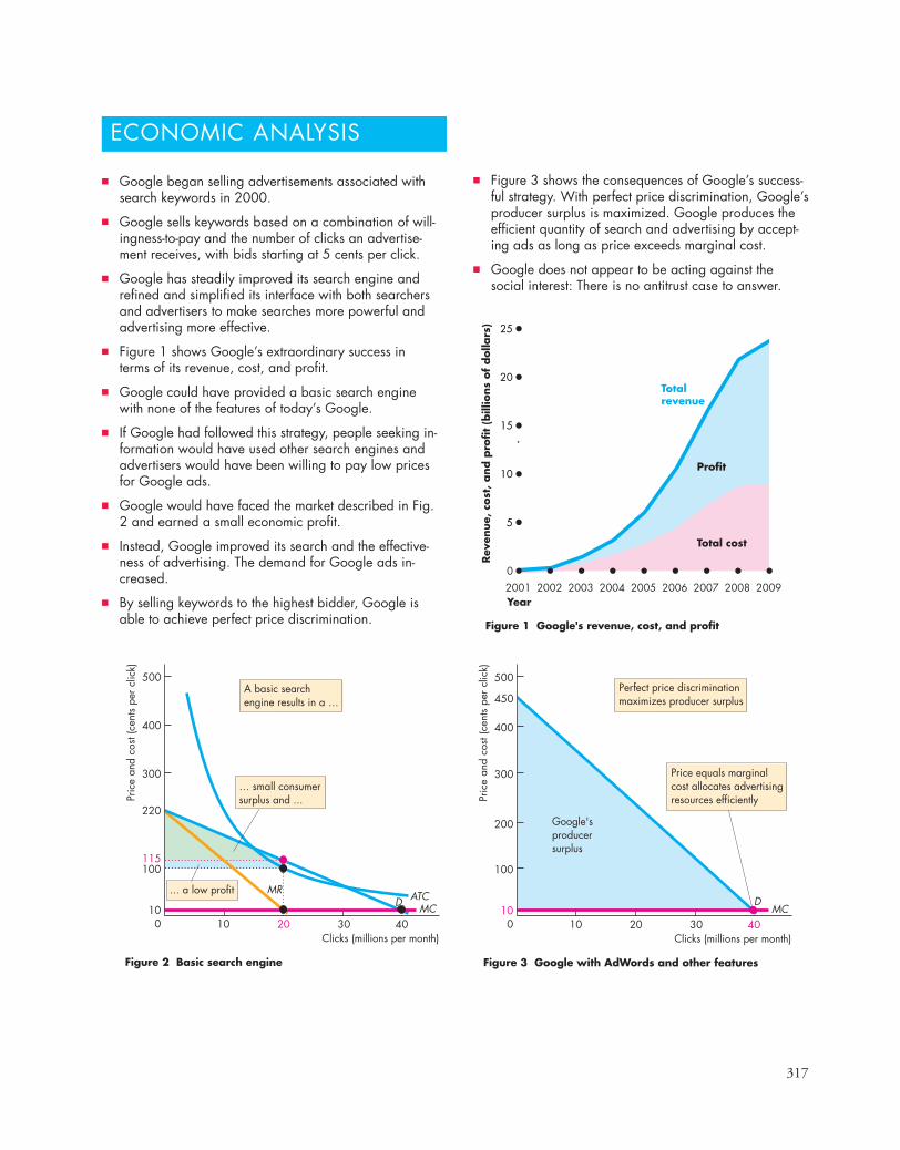
317

ECONOMIC ANALYSIS

■ Figure 3 shows the consequences of Google’s success-ful strategy. With perfect price discrimination, Google’sproducer surplus is maximized. Google produces theefficient quantity of search and advertising by accept-ing ads as long as price exceeds marginal cost.

■ Google does not appear to be acting against thesocial interest: There is no antitrust case to answer.

■ Google began selling advertisements associated withsearch keywords in 2000.

■ Google sells keywords based on a combination of will-ingness-to-pay and the number of clicks an advertise-ment receives, with bids starting at 5 cents per click.

■ Google has steadily improved its search engine andrefined and simplified its interface with both searchersand advertisers to make searches more powerful andadvertising more effective.

■ Figure 1 shows Google’s extraordinary success interms of its revenue, cost, and profit.

■ Google could have provided a basic search enginewith none of the features of today’s Google.

■ If Google had followed this strategy, people seeking in-formation would have used other search engines andadvertisers would have been willing to pay low pricesfor Google ads.

■ Google would have faced the market described in Fig.2 and earned a small economic profit.

■ Instead, Google improved its search and the effective-ness of advertising. The demand for Google ads in-creased.

■ By selling keywords to the highest bidder, Google isable to achieve perfect price discrimination.

Figure 3 Google with AdWords and other features

DMR

MC

Figure 2 Basic search engine

Pric

e an

d co

st (c

ents

per

clic

k)

Clicks (millions per month)0

115

500

400

300

100

1010 20 30 40

220

... a low profitD

MC

Pric

e an

d co

st (c

ents

per

clic

k)

Clicks (millions per month)0

500

300

100

1010 20 30 40

200

400

ATC

Price equals marginalcost allocates advertisingresources efficiently

450A basic searchengine results in a …

Perfect price discriminationmaximizes producer surplus

Google'sproducersurplus

… small consumersurplus and ...

Figure 1 Google's revenue, cost, and profit

Rev

enue,

cost

, and p

rofi

t (b

illio

ns

of

dolla

rs)

2001Year

Totalrevenue

Profit

Total cost

2002 2003 2004 2005 2006 2007 2008 2009

25

20

15

10

5

0

318 CHAPTER 13 Monopoly

■ The total loss that arises from monopoly equalsthe deadweight loss plus the cost of the resourcesdevoted to rent seeking.

Working Problems 10 to 12 will give you a better under-standing of the comparison of single-price monopoly andperfect competition.

Price Discrimination (pp. 309–312)

■ Price discrimination converts consumer surplusinto economic profit.

■ Perfect price discrimination extracts the entireconsumer surplus; each unit is sold for the maxi-mum price that each consumer is willing to pay;the quantity produced is the efficient quantity.

■ Rent seeking with perfect price discriminationmight eliminate the entire consumer surplus andproducer surplus.

Working Problems 13 to 16 will give you a better under-standing of price discrimination.

Monopoly Regulation (pp. 313–315)

■ Monopoly regulation might serve the social inter-est or the interest of the monopoly (the monopolycaptures the regulator).

■ Price equal to marginal cost achieves efficiency butresults in economic loss.

■ Price equal to average cost enables the firm tocover its cost but is inefficient.

■ Rate of return regulation creates incentives forinefficient production and inflated cost.

■ Price cap regulation with earnings sharing regula-tion can achieve a more efficient outcome thanrate of return regulation.

Working Problems 17 to 19 will give you a better under-standing of monopoly regulation.

Key Points

Monopoly and How It Arises (pp. 300–301)

■ A monopoly is a market with a single supplier of agood or service that has no close substitutes and inwhich barriers to entry prevent competition.

■ Barriers to entry may be legal (public franchise,license, patent, copyright), firm owns control ofa resource, or natural (created by economies ofscale).

■ A monopoly might be able to price discriminatewhen there is no resale possibility.

■ Where resale is possible, a firm charges one price.

Working Problems 1 to 4 will give you a better under-standing of monopoly and how it arises.

A Single-Price Monopoly’s Output and Price Decision(pp. 302–305)

■ A monopoly’s demand curve is the market demandcurve and a single-price monopoly’s marginal rev-enue is less than price.

■ A monopoly maximizes profit by producing theoutput at which marginal revenue equals marginalcost and by charging the maximum price that con-sumers are willing to pay for that output.

Working Problems 5 to 9 will give you a better under-standing of a single-price monopoly’s output and price.

Single-Price Monopoly and Competition Compared(pp. 306–309)

■ A single-price monopoly charges a higher priceand produces a smaller quantity than a perfectlycompetitive market.

■ A single-price monopoly restricts output and cre-ates a deadweight loss.

SUMMARY

Key TermsAverage cost pricing rule, 314Barrier to entry, 300Capture theory, 313Deregulation, 313Economic rent, 308Legal monopoly, 300

Marginal cost pricing rule, 313Monopoly, 300Natural monopoly, 300Perfect price discrimination, 311Price cap regulation, 315Price discrimination, 301

Rate of return regulation, 314Regulation, 313Rent seeking, 308Single-price monopoly, 301Social interest theory, 313

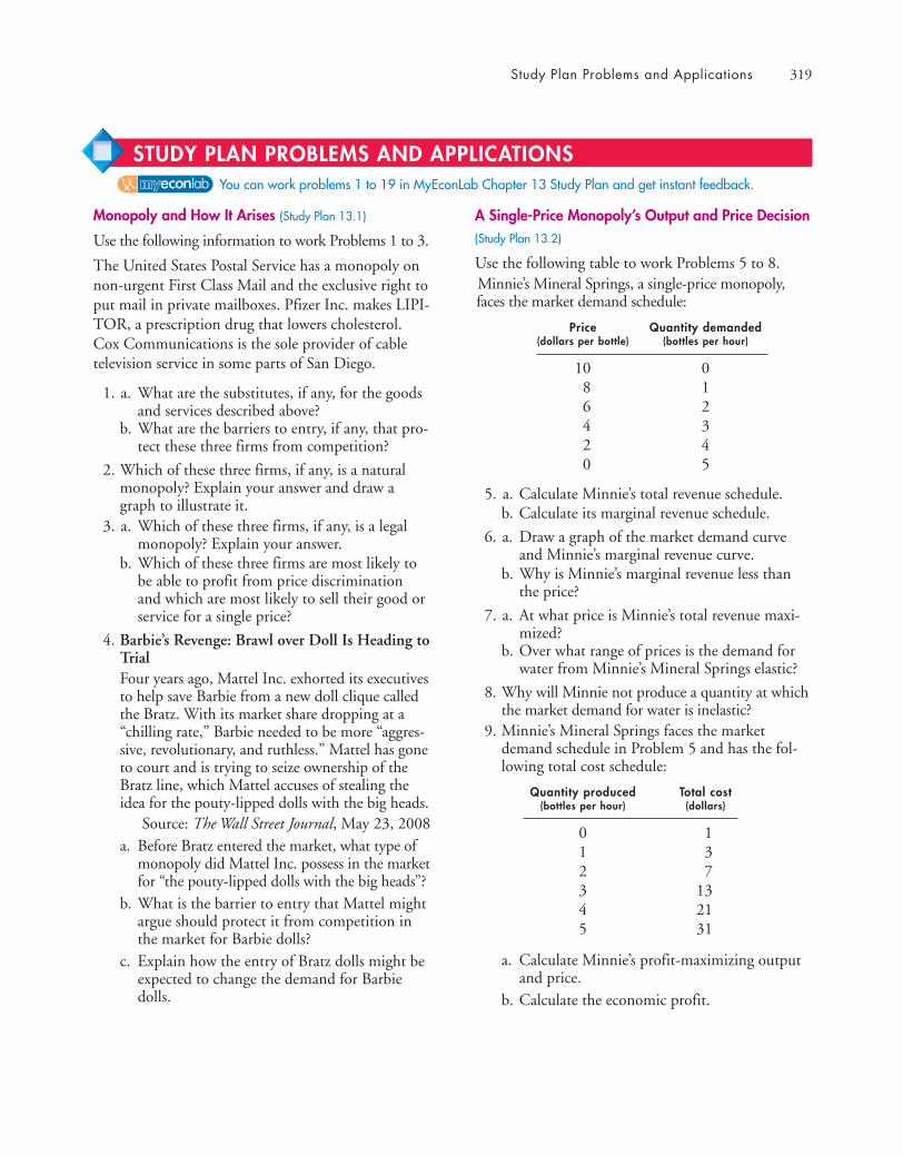
Study Plan Problems and Applications 319

A Single-Price Monopoly’s Output and Price Decision(Study Plan 13.2)

Use the following table to work Problems 5 to 8.Minnie’s Mineral Springs, a single-price monopoly,faces the market demand schedule:

Price Quantity demanded(dollars per bottle) (bottles per hour)

10 08 16 24 32 40 5

5. a. Calculate Minnie’s total revenue schedule.b. Calculate its marginal revenue schedule.

6. a. Draw a graph of the market demand curveand Minnie’s marginal revenue curve.

b. Why is Minnie’s marginal revenue less thanthe price?

7. a. At what price is Minnie’s total revenue maxi-mized?

b. Over what range of prices is the demand forwater from Minnie’s Mineral Springs elastic?

8. Why will Minnie not produce a quantity at whichthe market demand for water is inelastic?

9. Minnie’s Mineral Springs faces the marketdemand schedule in Problem 5 and has the fol-lowing total cost schedule:

Quantity produced Total cost(bottles per hour) (dollars)

0 11 32 73 134 215 31

a. Calculate Minnie’s profit-maximizing outputand price.

b. Calculate the economic profit.

Monopoly and How It Arises (Study Plan 13.1)

Use the following information to work Problems 1 to 3.

The United States Postal Service has a monopoly onnon-urgent First Class Mail and the exclusive right toput mail in private mailboxes. Pfizer Inc. makes LIPI-TOR, a prescription drug that lowers cholesterol.Cox Communications is the sole provider of cabletelevision service in some parts of San Diego.

1. a. What are the substitutes, if any, for the goodsand services described above?

b. What are the barriers to entry, if any, that pro-tect these three firms from competition?

2. Which of these three firms, if any, is a naturalmonopoly? Explain your answer and draw agraph to illustrate it.

3. a. Which of these three firms, if any, is a legalmonopoly? Explain your answer.

b. Which of these three firms are most likely tobe able to profit from price discriminationand which are most likely to sell their good orservice for a single price?

4. Barbie’s Revenge: Brawl over Doll Is Heading toTrialFour years ago, Mattel Inc. exhorted its executivesto help save Barbie from a new doll clique calledthe Bratz. With its market share dropping at a“chilling rate,” Barbie needed to be more “aggres-sive, revolutionary, and ruthless.” Mattel has goneto court and is trying to seize ownership of theBratz line, which Mattel accuses of stealing theidea for the pouty-lipped dolls with the big heads.

Source: The Wall Street Journal, May 23, 2008a. Before Bratz entered the market, what type of

monopoly did Mattel Inc. possess in the marketfor “the pouty-lipped dolls with the big heads”?

b. What is the barrier to entry that Mattel mightargue should protect it from competition inthe market for Barbie dolls?

c. Explain how the entry of Bratz dolls might beexpected to change the demand for Barbiedolls.

You can work problems 1 to 19 in MyEconLab Chapter 13 Study Plan and get instant feedback.

STUDY PLAN PROBLEMS AND APPLICATIONS

320 CHAPTER 13 Monopoly

Single-Price Monopoly and Competition Compared(Study Plan 13.3)

Use the following news clip to work Problems 10 to 12.Zoloft Faces Patent ExpirationPfizer’s antidepressant Zoloft, with $3.3 billion in2005 sales, loses patent protection on June 30. Whena brand name drug loses its patent, both the price ofthe drug and the dollar value of its sales each tend todrop 80 percent over the next year, as competitionopens to a host of generic drugmakers. The real win-ners are the patients and the insurers, who pay muchlower prices. The Food and Drug Administrationinsists that generics work identically to brand-names.

Source: CNN, June 15, 2006

10. a. Assume that Pfizer has a monopoly in theantidepressant market and that Pfizer cannotprice discriminate. Use a graph to illustrate themarket price and quantity of Zoloft sold.

b. On your graph, identify consumer surplus,producer surplus, and deadweight loss.

11. How might you justify protecting Pfizer fromcompetition with a legal barrier to entry?

12. a. Explain how the market for an antidepressantdrug changes when a patent expires.

b. Draw a graph to illustrate how the expirationof the Zoloft patent will change the price andquantity in the market for antidepressants.

c. Explain how consumer surplus, producersurplus, and deadweight loss change with theexpiration of the Zoloft patent.

Price Discrimination (Study Plan 13.4)

Use the following news clip to work Problems 13 and 14.The Saturday-Night Stay Requirement Is on ItsFinal ApproachThe Saturday-night stay—the requirement that air-lines instituted to ensure that business travelers payan outrageous airfare if he or she wants to go homefor the weekend—has gone the way of the dodo bird.Experts agree that low-fare carriers, such asSouthwest, are the primary reason major airlines areadopting more consumer-friendly fare structures,which include the elimination of the Saturday-nightstay, the introduction of one-way and walk-up fares,and the general restructuring of fares.

Source: Los Angeles Times, August 15, 2004

13. Explain why the opportunity for price discrimi-nation exists for air travel. How does an airlineprofit from price discrimination?

14. Describe the change in price discrimination inthe market for air travel when discount airlinesentered the market and explain the effect of dis-count airlines on the price and the quantity ofair travel.

Use the following information to work Problems 15and 16.

La Bella Pizza can produce a pizza for a marginal cost of $2. Its standard price is $15 a pizza. It offers a second pizza for $5. It also distributes coupons that give a $5 rebate on a standard-priced pizza.15. How can La Bella Pizza make a larger economic

profit with this range of prices than it could if itsold every pizza for $15? Use a graph to illustrateyour answer.

16. How might La Bella Pizza make even more eco-nomic profit? Would La Bella Pizza then be moreefficient than it would be if it charged $15 foreach pizza?

Monopoly Regulation (Study Plan 13.5)

Use the following information to work Problems 17 to 19.The figure shows a situation similar to that ofCalypso U.S. Pipeline, a firm that operates a natural gas distribution system in the United States.Calypso is a natural monopoly that cannot price discriminate.

What quantity will Calypso produce, what price willit charge, what is the total surplus, and what is thedeadweight loss if Calypso is17. An unregulated profit-maximizing firm?18. Regulated to make zero economic profit?19. Regulated to be efficient?

4

0 1 2 3 4

Pric

e an

d co

st (c

ents

per c

ubic

foot

)

Quantity (millions of cubic feet per day)

2

5

6

8

10

D

MC

LRAC

Additional Problems and Applications 321

Monopoly and How It Arises

Use the following list, which gives some informationabout seven firms, to answer Problems 20 and 21.

■ Coca-Cola cuts its price below that of Pepsi-Cola in an attempt to increase its market share.

■ A single firm, protected by a barrier to entry,produces a personal service that has no closesubstitutes.

■ A barrier to entry exists, but the good hassome close substitutes.

■ A firm offers discounts to students and seniors.■ A firm can sell any quantity it chooses at the

going price.■ The government issues Nike an exclusive

license to produce golf balls.■ A firm experiences economies of scale even

when it produces the quantity that meets theentire market demand.

20. In which of the seven cases might monopoly arise?21. Which of the seven cases are natural monopolies

and which are legal monopolies? Which can pricediscriminate, which cannot, and why?

A Single-Price Monopoly’s Output and Price DecisionUse the following information to work Problems 22 to 26.Hot Air Balloon Rides is a single-price monopoly.Columns 1 and 2 of the table set out the marketdemand schedule and columns 2 and 3 set out thetotal cost schedule:

Price Quantity demanded Total cost(dollars (rides) (dollarsper ride) per month) per month)

220 0 80200 1 160180 2 260160 3 380140 4 520120 5 680

22. Construct Hot Air’s total revenue and marginalrevenue schedules.

23. Draw a graph of the market demand curve andHot Air’s marginal revenue curve.

24. Find Hot Air’s profit-maximizing output andprice and calculate the firm’s economic profit.

25. If the government imposes a tax on Hot Air’sprofit, how do its output and price change?

26. If instead of taxing Hot Air’s profit, the govern-ment imposes a sales tax on balloon rides of $30a ride, what are the new profit-maximizing quan-tity, price, and economic profit?

27. The figure illustrates the situation facing thepublisher of the only newspaper containing localnews in an isolated community.

a. On the graph, mark the profit-maximizingquantity and price and the publisher’s totalrevenue per day.

b. At the price charged, is the demand for thisnewspaper elastic or inelastic? Why?

Single-Price Monopoly and Competition Compared28. Show on the graph in Problem 27 the consumer

surplus from newspapers and the deadweight losscreated by the monopoly. Explain why this mar-ket might encourage rent seeking.

29. If the newspaper market in Problem 27 were per-fectly competitive, what would be the quantity,price, consumer surplus, and producer surplus?Mark each on the graph.

30. Telecoms Look to Grow by AcquisitionMultibillion-dollar telecommunications mergersshow how global cellular powerhouses are scout-ing for growth in emerging economies while con-solidating in their own, crowded backyards.France Télécom offered to buy TeliaSonera, aSwedish-Finnish telecommunications operator, but

40

0 100 200 300 400

Pric

e an

d co

st (c

ents

per n

ewsp

aper

)

Quantity (newspapers per day)

20

500

60

80

100

D

MC

You can work these problems in MyEconLab if assigned by your instructor.

ADDITIONAL PROBLEMS AND APPLICATIONS

322 CHAPTER 13 Monopoly

within hours, TeliaSonera rejected the offer as toolow. Analysts said higher bids—either from FranceTélécom or others—could persuade TeliaSonera toaccept a deal. In the United States, VerizonWireless agreed to buy Alltel for $28.1 billion—adeal that would make the company the biggestmobile phone operator in the United States. Acombination of France Télécom and TeliaSonerawould create the world’s fourth-largest mobileoperator, smaller only than China Mobile,Vodafone, and Telefónica of Spain.

Source: International Herald Tribune,June 5, 2008

a. Explain the rent-seeking behavior of globaltelecommunications companies.

b. Explain how mergers may affect the efficiencyof the telecommunications market.

Price Discrimination31. AT&T Moves Away from Unlimited-Data

Pricing AT&T said it will eliminate its $30 unlimiteddata plan as the crush of data use from theiPhone has hurt call quality. AT&T is introduc-ing new plans costing $15 a month for 200megabytes of data traffic or $25 a month for 2gigabytes. AT&T says those who exceed 2 giga-bytes of usage will pay $10 a month for eachadditional gigabyte. AT&T hopes that theseplans will attract more customers.

Source: The Wall Street Journal, June 2, 2010a. Explain why AT&T’s new plans might be

price discrimination. b. Draw a graph to illustrate the original plan

and the new plans.

Monopoly Regulation32. iSurrender

Getting your hands on a new iPhone means sign-ing a two-year AT&T contract. Some markets,because of the costs of being a player, tendtoward either a single firm or a small number offirms. Everyone hoped the wireless market wouldbe different. A telephone monopoly has been thenorm for most of American telecommunicationhistory, except for what may turn out to havebeen a brief experimental period from 1984through 2012 or so. It may be that telephonemonopolies in America are a national tradition.

Source: Slate, June 10, 2008

a. How does AT&T being the exclusive providerof wireless service for the iPhone influence thewireless telecommunication market?

b. Explain why the wireless market may “tendtoward either a single firm or a small numberof firms.” Why might this justify allowing aregulated monopoly to exist in this market?

Economics in the News33. After you have studied Reading Between the Lines

on pp. 316 – 317 answer the following questions.a. Why does Consumer Watchdog say that

Google needs to be investigated? Do youagree? Explain why or why not.

b. Explain why it would be inefficient to regulateGoogle to make it charge the same price perkeyword click to all advertisers.

c. Explain why selling keywords to the highestbidder can lead to an efficient allocation ofadvertising resources.

34. F.C.C. Planning Rules to Open Cable MarketThe Federal Communications Commission(F.C.C.) is setting new regulations to open thecable television market to independent program-mers and rival video services. The new rules willmake it easier for small independent program-mers to lease access to cable channels and the sizeof the nation’s largest cable companies will becapped at 30 percent of the market.

Source: The New York Times,November 10, 2007

a. What barriers to entry exist in the cable televi-sion market?

b. Are high cable prices evidence of monopolypower?

c. Draw a graph to illustrate the effects of theF.C.C.’s new regulations on the price, quan-tity, total surplus, and deadweight loss.

35. Antitrust Inquiry Launched into IntelIntel, the world’s largest chipmaker, holds 80 per-cent of the microprocessor market. AdvancedMicro Devices complains that Intel stifles com-petition, but Intel says that the 42.4 percent fallin prices between 2000 and 2007 shows that thisindustry is fiercely competitive.

Source: The Washington Post, June 7, 2008a. Is Intel a monopoly in the chip market?b. Evaluate the argument made by Intel that the

fall in prices “shows that this industry isfiercely competitive.”

he online shoe store shoebuy.com lists athletic shoes made by 56 differentproducers in 40 different categories and priced between $25 and $850.Shoebuy offers 1,401 different types of athletic shoes for women and 1,757different types for men. Because there are many different types of athletic shoes,the market for them isn’t perfectly competitive. Athletic shoe producerscompete, but each has a monopoly on its own special kind of shoe.

Most of the things that you buy are like athletic shoes—they come in manydifferent types. Pizza and cell phones are two more striking examples.

The model of monopolistic competition that is explained in this chapterhelps us to understand the competition that we see every day in the marketsfor athletic shoes, pizza, cell phones, and for most other consumer goodsand services.

This chapter blends the models in the two preceding chapters on perfectcompetition and monopoly sto create the model of monopolistic competition. Toget the most out of this chapter, you will have studied the two preceding ones.

Reading Between the Lines, at the end of this chapter, applies themonopolistic competition model to the market for smart phones and the entry ofother firms in that market following the success of the Apple iPhone.

After studying this chapter, you will be able to:

� Define and identify monopolistic competition� Explain how a firm in monopolistic competition

determines its price and output in the short run and the long run

� Explain why advertising costs are high and why firms use brand names in a monopolistically competitive industry

T

MONOPOLISTICCOMPETITION

14323

324 CHAPTER 14 Monopolistic Competition

◆ What Is MonopolisticCompetition?

You have studied perfect competition, in which alarge number of firms produce at the lowest possi-ble cost, make zero economic profit, and are effi-cient. You’ve also studied monopoly, in which asingle firm restricts output, produces at a highercost and price than in perfect competition, and isinefficient.

Most real-world markets are competitive but notperfectly competitive, because firms in these marketshave some power to set their prices, as monopolies do.We call this type of market monopolistic competition.

Monopolistic competition is a market structure inwhich

■ A large number of firms compete.■ Each firm produces a differentiated product.■ Firms compete on product quality, price, and

marketing.■ Firms are free to enter and exit the industry.

Large Number of FirmsIn monopolistic competition, as in perfect competi-tion, the industry consists of a large number of firms.The presence of a large number of firms has threeimplications for the firms in the industry.

Small Market Share In monopolistic competition,each firm supplies a small part of the total industryoutput. Consequently, each firm has only limitedpower to influence the price of its product. Eachfirm’s price can deviate from the average price ofother firms by only a relatively small amount.

Ignore Other Firms A firm in monopolistic competi-tion must be sensitive to the average market price ofthe product, but the firm does not pay attention toany one individual competitor. Because all the firmsare relatively small, no one firm can dictate marketconditions, and so no one firm’s actions directly affectthe actions of the other firms.

Collusion Impossible Firms in monopolistic compe-tition would like to be able to conspire to fix ahigher price—called collusion. But because thenumber of firms in monopolistic competition islarge, coordination is difficult and collusion is notpossible.

Product DifferentiationA firm practices product differentiation if it makes a prod-uct that is slightly different from the products of com-peting firms. A differentiated product is one that is aclose substitute but not a perfect substitute for theproducts of the other firms. Some people are willing topay more for one variety of the product, so when itsprice rises, the quantity demanded of that varietydecreases, but it does not (necessarily) decrease to zero.For example, Adidas, Asics, Diadora, Etonic, Fila, NewBalance, Nike, Puma, and Reebok all make differenti-ated running shoes. If the price of Adidas runningshoes rises and the prices of the other shoes remainconstant, Adidas sells fewer shoes and the other pro-ducers sell more. But Adidas shoes don’t disappearunless the price rises by a large enough amount.

Competing on Quality, Price,and MarketingProduct differentiation enables a firm to competewith other firms in three areas: product quality, price,and marketing.

Quality The quality of a product is the physicalattributes that make it different from the products ofother firms. Quality includes design, reliability, theservice provided to the buyer, and the buyer’s ease ofaccess to the product. Quality lies on a spectrum thatruns from high to low. Some firms—such as DellComputer Corp.—offer high-quality products. Theyare well designed and reliable, and the customerreceives quick and efficient service. Other firms offera lower-quality product that is poorly designed, thatmight not work perfectly, and that is not supportedby effective customer service.

Price Because of product differentiation, a firm inmonopolistic competition faces a downward-slopingdemand curve. So, like a monopoly, the firm can setboth its price and its output. But there is a tradeoffbetween the product’s quality and price. A firm thatmakes a high-quality product can charge a higher pricethan a firm that makes a low-quality product.

Marketing Because of product differentiation, a firmin monopolistic competition must market its prod-uct. Marketing takes two main forms: advertisingand packaging. A firm that produces a high-quality

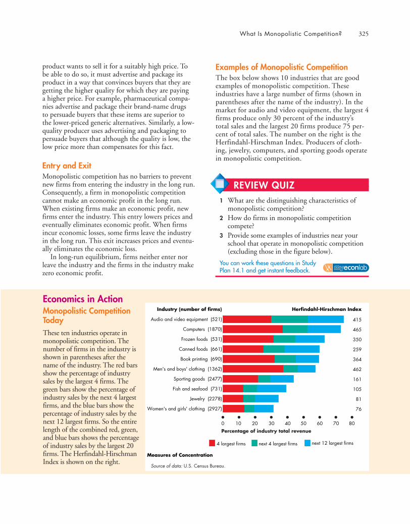
What Is Monopolistic Competition? 325

product wants to sell it for a suitably high price. Tobe able to do so, it must advertise and package itsproduct in a way that convinces buyers that they aregetting the higher quality for which they are payinga higher price. For example, pharmaceutical compa-nies advertise and package their brand-name drugsto persuade buyers that these items are superior tothe lower-priced generic alternatives. Similarly, a low-quality producer uses advertising and packaging topersuade buyers that although the quality is low, thelow price more than compensates for this fact.

Entry and ExitMonopolistic competition has no barriers to preventnew firms from entering the industry in the long run.Consequently, a firm in monopolistic competitioncannot make an economic profit in the long run.When existing firms make an economic profit, newfirms enter the industry. This entry lowers prices andeventually eliminates economic profit. When firmsincur economic losses, some firms leave the industryin the long run. This exit increases prices and eventu-ally eliminates the economic loss.

In long-run equilibrium, firms neither enter norleave the industry and the firms in the industry makezero economic profit.

Examples of Monopolistic CompetitionThe box below shows 10 industries that are goodexamples of monopolistic competition. Theseindustries have a large number of firms (shown inparentheses after the name of the industry). In themarket for audio and video equipment, the largest 4firms produce only 30 percent of the industry’stotal sales and the largest 20 firms produce 75 per-cent of total sales. The number on the right is theHerfindahl-Hirschman Index. Producers of cloth-ing, jewelry, computers, and sporting goods operatein monopolistic competition.

Economics in ActionMonopolistic CompetitionToday These ten industries operate inmonopolistic competition. Thenumber of firms in the industry isshown in parentheses after thename of the industry. The red barsshow the percentage of industrysales by the largest 4 firms. Thegreen bars show the percentage ofindustry sales by the next 4 largestfirms, and the blue bars show thepercentage of industry sales by thenext 12 largest firms. So the entirelength of the combined red, green,and blue bars shows the percentageof industry sales by the largest 20firms. The Herfindahl-HirschmanIndex is shown on the right.

0 10 40 5020 30 8060 70

Audio and video equipment (521)

Computers (1870)

Frozen foods (531)

Canned foods (661)

Book printing (690)

Men's and boys' clothing (1362)

Sporting goods (2477)

Fish and seafood (731)

Jewelry (2278)

Women's and girls' clothing (2927)

415

465

350

259

364

462

161

105

81

76

Herfindahl-Hirschman IndexIndustry (number of firms)

Percentage of industry total revenue

4 largest firms next 4 largest firms next 12 largest firms

Measures of Concentration

Source of data: U.S. Census Bureau.

REVIEW QUIZ1 What are the distinguishing characteristics of

monopolistic competition?2 How do firms in monopolistic competition

compete?3 Provide some examples of industries near your

school that operate in monopolistic competition(excluding those in the figure below).

You can work these questions in Study Plan 14.1 and get instant feedback.

326 CHAPTER 14 Monopolistic Competition

◆ Price and Output in Monopolistic Competition

Suppose you’ve been hired by VF Corporation, thefirm that owns Nautica Clothing Corporation, tomanage the production and marketing of Nauticajackets. Think about the decisions that you must makeat Nautica. First, you must decide on the design andquality of jackets and on your marketing program.Second, you must decide on the quantity of jackets toproduce and the price at which to sell them.

We’ll suppose that Nautica has already made itsdecisions about design, quality, and marketing andnow we’ll concentrate on the output and pricingdecision. We’ll study quality and marketing decisionsin the next section.

For a given quality of jackets and marketing activity,Nautica faces given costs and market conditions. Givenits costs and the demand for its jackets, how doesNautica decide the quantity of jackets to produce andthe price at which to sell them?

The Firm’s Short-Run Output and PriceDecisionIn the short run, a firm in monopolistic competitionmakes its output and price decision just like a monop-oly firm does. Figure 14.1 illustrates this decision forNautica jackets.

The demand curve for Nautica jackets is D. Thisdemand curve tells us the quantity of Nautica jacketsdemanded at each price, given the prices of other jack-ets. It is not the demand curve for jackets in general.

The MR curve shows the marginal revenue curveassociated with the demand curve for Nautica jackets.It is derived just like the marginal revenue curve of asingle-price monopoly that you studied in Chapter13.

The ATC curve and the MC curve show the aver-age total cost and the marginal cost of producingNautica jackets.

Nautica’s goal is to maximize its economic profit.To do so, it produces the output at which marginalrevenue equals marginal cost. In Fig. 14.1, this out-put is 125 jackets a day. Nautica charges the pricethat buyers are willing to pay for this quantity, whichis determined by the demand curve. This price is $75per jacket. When Nautica produces 125 jackets a day,its average total cost is $25 per jacket and it makes aneconomic profit of $6,250 a day ($50 per jacket mul-

tiplied by 125 jackets a day). The blue rectangleshows Nautica’s economic profit.

Profit Maximizing Might Be Loss MinimizingFigure 14.1 shows that Nautica is making a large eco-nomic profit. But such an outcome is not inevitable. Afirm might face a level of demand for its product that istoo low for it to make an economic profit.

Excite@Home was such a firm. Offering high-speed Internet service over the same cable that pro-vides television, Excite@Home hoped to capture alarge share of the Internet portal market in competi-tion with AOL, MSN, and a host of other providers.

Figure 14.2 illustrates the situation facingExcite@Home in 2001. The demand curve for itsportal service is D, the marginal revenue curve is MR,the average total cost curve is ATC, and the marginalcost curve is MC. Excite@Home maximized profit—

0 50 100 150125 200 250

Pric

e an

d co

st (d

olla

rs p

er N

autic

a ja

cket

)Quantity (Nautica jackets per day)

MR

D

MC

ATC

75

50

25

150

125

100

Profit-maximizingquantity

Economicprofit

Marginal revenue= marginal cost

Price greaterthan averagetotal cost

Nautica maximizes profit by producing the quantity atwhich marginal revenue equals marginal cost,125 jackets aday, and charging the price of $75 a jacket. This priceexceeds the average total cost of $25 a jacket, so the firmmakes an economic profit of $50 a jacket. The blue rectan-gle illustrates economic profit, which equals $6,250 a day($50 a jacket multiplied by 125 jackets a day).

FIGURE 14.1 Economic Profit in the Short Run

animation

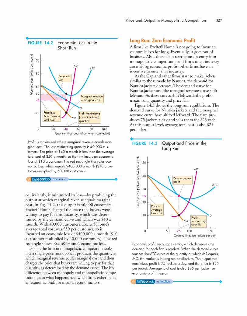
Price and Output in Monopolistic Competition 327

equivalently, it minimized its loss—by producing theoutput at which marginal revenue equals marginalcost. In Fig. 14.2, this output is 40,000 customers.Excite@Home charged the price that buyers werewilling to pay for this quantity, which was deter-mined by the demand curve and which was $40 amonth. With 40,000 customers, Excite@Home’saverage total cost was $50 per customer, so itincurred an economic loss of $400,000 a month ($10a customer multiplied by 40,000 customers). The redrectangle shows Excite@Home’s economic loss.

So far, the firm in monopolistic competition lookslike a single-price monopoly. It produces the quantity atwhich marginal revenue equals marginal cost and thencharges the price that buyers are willing to pay for thatquantity, as determined by the demand curve. The keydifference between monopoly and monopolistic compe-tition lies in what happens next when firms either makean economic profit or incur an economic loss.

Long Run: Zero Economic ProfitA firm like Excite@Home is not going to incur aneconomic loss for long. Eventually, it goes out ofbusiness. Also, there is no restriction on entry intomonopolistic competition, so if firms in an industryare making economic profit, other firms have anincentive to enter that industry.

As the Gap and other firms start to make jacketssimilar to those made by Nautica, the demand forNautica jackets decreases. The demand curve forNautica jackets and the marginal revenue curve shiftleftward. As these curves shift leftward, the profit-maximizing quantity and price fall.

Figure 14.3 shows the long-run equilibrium. Thedemand curve for Nautica jackets and the marginalrevenue curve have shifted leftward. The firm pro-duces 75 jackets a day and sells them for $25 each.At this output level, average total cost is also $25per jacket.

Pric

e an

d co

st (d

olla

rs p

er m

onth

)

Quantity (thousands of customers connected)

Price lessthan averagetotal cost

0

MR

D

MCATC

60

50

40

20

100

80

40 6020 10080

Profit-maximizing(loss-minimizing)quantity

Economicloss

Marginal revenue= marginal cost

Profit is maximized where marginal revenue equals mar-ginal cost. The loss-minimizing quantity is 40,000 cus-tomers. The price of $40 a month is less than the averagetotal cost of $50 a month, so the firm incurs an economicloss of $10 a customer. The red rectangle illustrates eco-nomic loss, which equals $400,000 a month ($10 a cus-tomer multiplied by 40,000 customers).

Pric

e an

d co

st (d

olla

rs p

er N

autic

a ja

cket

)

Quantity (Nautica jackets per day)

Price =Averagetotal cost

0

MR

D

MC

ATC30

20

25

10

50

40

75 10050 150

Profit-maximizingquantity

Zero economicprofit

Economic profit encourages entry, which decreases thedemand for each firm’s product. When the demand curvetouches the ATC curve at the quantity at which MR equalsMC, the market is in long-run equilibrium. The output thatmaximizes profit is 75 jackets a day, and the price is $25per jacket. Average total cost is also $25 per jacket, soeconomic profit is zero.

FIGURE 14.2 Economic Loss in the Short Run

animation

animation

FIGURE 14.3 Output and Price in the Long Run

328 CHAPTER 14 Monopolistic Competition

So Nautica is making zero economic profit on itsjackets. When all the firms in the industry are mak-ing zero economic profit, there is no incentive fornew firms to enter.

If demand is so low relative to costs that firmsincur economic losses, exit will occur. As firms leavean industry, the demand for the products of theremaining firms increases and their demand curvesshift rightward. The exit process ends when all thefirms in the industry are making zero economic profit.

Monopolistic Competition and PerfectCompetitionFigure 14.4 compares monopolistic competition andperfect competition and highlights two key differ-ences between them:

■ Excess capacity■ Markup

Excess Capacity A firm has excess capacity if it pro-duces below its efficient scale, which is the quantity atwhich average total cost is a minimum—the quantityat the bottom of the U-shaped ATC curve. In Fig.14.4, the efficient scale is 100 jackets a day. Nauticain part (a) produces 75 Nautica jackets a day and hasexcess capacity of 25 jackets a day. But if all jackets arealike and are produced by firms in perfect competi-tion, each firm in part (b) produces 100 jackets a day,which is the efficient scale. Average total cost is thelowest possible only in perfect competition.

You can see the excess capacity in monopolisticcompetition all around you. Family restaurants(except for the truly outstanding ones) almost alwayshave some empty tables. You can always get a pizzadelivered in less than 30 minutes. It is rare that everypump at a gas station is in use with customers wait-ing in line. There are always many real estate agentsready to help find or sell a home. These industries areexamples of monopolistic competition. The firms

Markup

Price

Marginalcost Excess

capacityEfficientscale

Quantity =Efficient scale

Price = Marginal cost

0 25 50 75 100 125 150

Pric

e an

d co

st (d

olla

rs p

er N

autic

a ja

cket

)

Quantity (Nautica jackets per day)

(a) Monopolistic competition

MR

D

MC

ATC

40

25

30

20

10

(b) Perfect competition

50

0 25 50 75 100 125 150

Pric

e an

d co

st (d

olla

rs p

er ja

cket

)

Quantity (jackets per day)

D = MR

MC

ATC

40

23

30

20

10

50

The efficient scale is 100 jackets a day. In monopolistic com-petition in the long run, because the firm faces a downward-sloping demand curve for its product, the quantity produced isless than the efficient scale and the firm has excess capacity.Price exceeds marginal cost by the amount of the markup.

In contrast, because in perfect competition the demand foreach firm’s product is perfectly elastic, the quantity pro-duced in the long run equals the efficient scale and priceequals marginal cost. The firm produces at the least possi-ble cost and there is no markup.

FIGURE 14.4 Excess Capacity and Markup

animation

Price and Output in Monopolistic Competition 329

have excess capacity. They could sell more by cuttingtheir prices, but they would then incur losses.

Markup A firm’s markup is the amount by whichprice exceeds marginal cost. Figure 14.4(a) showsNautica’s markup. In perfect competition, pricealways equals marginal cost and there is no markup.Figure 14.4(b) shows this case. In monopolistic com-petition, buyers pay a higher price than in perfectcompetition and also pay more than marginal cost.

Is Monopolistic Competition Efficient?Resources are used efficiently when marginal socialbenefit equals marginal social cost. Price equals mar-ginal social benefit and the firm’s marginal cost equalsmarginal social cost (assuming there are no externalbenefits or costs). So if the price of a Nautica jacketexceeds the marginal cost of producing it, the quan-tity of Nautica jackets produced is less than the effi-cient quantity. And you’ve just seen that in long-runequilibrium in monopolistic competition, price doesexceed marginal cost. So is the quantity produced inmonopolistic competition less than the efficientquantity?

Making the Relevant Comparison Two economistsmeet in the street, and one asks the other, “How isyour husband?” The quick reply is “Compared towhat?” This bit of economic wit illustrates a keypoint: Before we can conclude that something needsfixing, we must check out the available alternatives.

The markup that drives a gap between price andmarginal cost in monopolistic competition arisesfrom product differentiation. It is because Nauticajackets are not quite the same as jackets from BananaRepublic, CK, Diesel, DKNY, Earl Jackets, Gap,Levi’s, Ralph Lauren, or any of the other dozens ofproducers of jackets that the demand for Nauticajackets is not perfectly elastic. The only way in whichthe demand for jackets from Nautica might be per-fectly elastic is if there is only one kind of jacket andall firms make it. In this situation, Nautica jackets areindistinguishable from all other jackets. They don’teven have identifying labels.

If there was only one kind of jacket, the total ben-efit of jackets would almost certainly be less than it iswith variety. People value variety—not only becauseit enables each person to select what he or she likesbest but also because it provides an external benefit.Most of us enjoy seeing variety in the choices of oth-

ers. Contrast a scene from the China of the 1960s,when everyone wore a Mao tunic, with the China oftoday, where everyone wears the clothes of their ownchoosing. Or contrast a scene from the Germany ofthe 1930s, when almost everyone who could afford acar owned a first-generation Volkswagen Beetle, withthe world of today with its enormous variety of stylesand types of automobiles.

If people value variety, why don’t we see infinitevariety? The answer is that variety is costly. Each dif-ferent variety of any product must be designed, andthen customers must be informed about it. These ini-tial costs of design and marketing—called setupcosts—mean that some varieties that are too close toothers already available are just not worth creating.

The Bottom Line Product variety is both valued andcostly. The efficient degree of product variety is theone for which the marginal social benefit of productvariety equals its marginal social cost. The loss thatarises because the quantity produced is less than theefficient quantity is offset by the gain that arises fromhaving a greater degree of product variety. So com-pared to the alternative—product uniformity—monopolistic competition might be efficient.

You’ve seen how the firm in monopolistic com-petition determines its output and price in both theshort run and the long run when it produces a givenproduct and undertakes a given marketing effort. Buthow does the firm choose its product quality andmarketing effort? We’ll now study these decisions.

REVIEW QUIZ1 How does a firm in monopolistic competition

decide how much to produce and at what priceto offer its product for sale?

2 Why can a firm in monopolistic competitionmake an economic profit only in the short run?

3 Why do firms in monopolistic competitionoperate with excess capacity?

4 Why is there a price markup over marginal costin monopolistic competition?

5 Is monopolistic competition efficient?

You can work these questions in Study Plan 14.2 and get instant feedback.

330 CHAPTER 14 Monopolistic Competition

◆ Product Development and Marketing

When Nautica made its price and output decisionthat we’ve just studied, it had already made its prod-uct quality and marketing decisions. We’re now goingto look at these decisions and see how they influencethe firm’s output, price, and economic profit.

Innovation and Product DevelopmentThe prospect of new firms entering the industry keepsfirms in monopolistic competition on their toes! Toenjoy economic profits, they must continually seekways of keeping one step ahead of imitators—otherfirms who imitate the success of profitable firms.

One major way of trying to maintain economicprofit is for a firm to seek out new products thatwill provide it with a competitive edge, even if onlytemporarily. A firm that introduces a new and dif-ferentiated product faces a demand that is less elas-tic and is able to increase its price and make aneconomic profit. Eventually, imitators will makeclose substitutes for the innovative product andcompete away the economic profit arising from aninitial advantage. So to restore economic profit, thefirm must again innovate.

Profit-Maximizing Product Innovation The decisionto innovate and develop a new or improved productis based on the same type of profit-maximizing calcu-lation that you’ve already studied.

Innovation and product development are costlyactivities, but they also bring in additional revenues.The firm must balance the cost and revenue at themargin.

The marginal dollar spent on developing a newor improved product is the marginal cost of productdevelopment. The marginal dollar that the new orimproved product earns for the firm is the marginalrevenue of product development. At a low level ofproduct development, the marginal revenue from abetter product exceeds the marginal cost. At a highlevel of product development, the marginal cost of abetter product exceeds the marginal revenue.

When the marginal cost and marginal revenue ofproduct development are equal, the firm is under-taking the profit-maximizing amount of productdevelopment.

Efficiency and Product Innovation Is the profit-maxi-mizing amount of product innovation also the effi-cient amount? Efficiency is achieved if the marginalsocial benefit of a new and improved product equalsits marginal social cost.

The marginal social benefit of an innovation is theincrease in price that consumers are willing to pay forit. The marginal social cost is the amount that thefirm must pay to make the innovation. Profit is maxi-mized when marginal revenue equals marginal cost.But in monopolistic competition, marginal revenue isless than price, so product innovation is probably notpushed to its efficient level.

Monopolistic competition brings many productinnovations that cost little to implement and arepurely cosmetic, such as new and improved packag-ing or a new scent in laundry powder. And evenwhen there is a genuine improved product, it is neveras good as what the consumer is willing to pay for.For example, “The Legend of Zelda: TwilightPrincess” is regarded as an almost perfect and verycool game, but users complain that it isn’t quite per-fect. It is a game whose features generate a marginalrevenue equal to the marginal cost of creating them.

AdvertisingA firm with a differentiated product needs to ensurethat its customers know how its product is differentfrom the competition. A firm also might attempt tocreate a consumer perception that its product is dif-ferent from its competitors, even when that differ-ence is small. Firms use advertising and packaging toachieve this goal.

Advertising Expenditures Firms in monopolisticcompetition incur huge costs to ensure that buyersappreciate and value the differences between theirown products and those of their competitors. So alarge proportion of the price that we pay for a goodcovers the cost of selling it, and this proportion isincreasing. Advertising in newspapers and magazinesand on radio, television, and the Internet is the mainselling cost. But it is not the only one. Selling costsinclude the cost of shopping malls that look likemovie sets, glossy catalogs and brochures, and thesalaries, airfares, and hotel bills of salespeople.

Advertising expenditures affect the profits of firmsin two ways: They increase costs, and they changedemand. Let’s look at these effects.

Product Development and Marketing 331

Selling Costs and Total Cost Selling costs are fixedcosts and they increase the firm’s total cost. So likethe fixed cost of producing a good, advertising costsper unit decrease as the quantity produced increases.

Figure 14.5 shows how selling costs change a firm’saverage total cost. The blue curve shows the averagetotal cost of production. The red curve shows the firm’saverage total cost of production plus advertising. Theheight of the red area between the two curves shows theaverage fixed cost of advertising. The total cost of adver-tising is fixed. But the average cost of advertisingdecreases as output increases.

Figure 14.5 shows that if advertising increases thequantity sold by a large enough amount, it can loweraverage total cost. For example, if the quantity soldincreases from 25 jackets a day with no advertising to100 jackets a day with advertising, average total costfalls from $60 to $40 a jacket. The reason is thatalthough the total fixed cost has increased, the greaterfixed cost is spread over a greater output, so averagetotal cost decreases.

Average total costwith no advertising

Average total costwith advertising

Advertisingcost

0 5025 100 150 200 250

100

80

40

60

20

Cos

t (do

llars

per

Nau

tica

jack

et)

Quantity (Nautica jackets per day)

By increasing thequantity bought,advertising canlower averagetotal cost

Selling costs such as the cost of advertising are fixed costs.When added to the average total cost of production, sellingcosts increase average total cost by a greater amount atsmall outputs than at large outputs. If advertising enablessales to increase from 25 jackets a day to 100 jackets aday, average total cost falls from $60 to $40 a jacket.

Economics in ActionThe Cost of Selling a Pair of ShoesWhen you buy a pair of running shoes that cost you$70, you’re paying $9 for the materials from whichthe shoes are made, $2.75 for the services of theMalaysian worker who made the shoes, and $5.25 forthe production and transportation services of a man-ufacturing firm in Asia and a shipping company.These numbers total $17. You pay $3 to the U.S.government in import duty. So we’ve now accountedfor a total of $20. Where did the other $50 go? It isthe cost of advertising, retailing, and other sales anddistribution services.

The selling costs associated with running shoesare not unusual. Almost everything that you buyincludes a selling cost component that exceeds onehalf of the total cost. Your clothing, food, electronicitems, DVDs, magazines, and even your textbookscost more to sell than they cost to manufacture.

Advertising costs are only a part, and often a smallpart, of total selling costs. For example, Nike spendsabout $4 on advertising per pair of running shoessold.

For the U.S. economy as a whole, there are some20,000 advertising agencies, which employ more than200,000 people and have sales of $45 billion. Thesenumbers are only part of the total cost of advertisingbecause firms have their own internal advertisingdepartments, the costs of which we can only guess.

But the biggest part of selling costs is not the costof advertising. It is the cost of retailing services. Theretailer’s selling costs (and economic profit) are oftenas much as 50 percent of the price you pay.

Rawmaterials$9

Productioncosts$8

Importduty$3

Sellingcosts$50

FIGURE 14.5 Selling Costs and Total Cost

animation

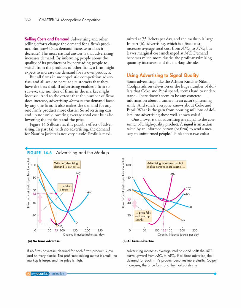
332 CHAPTER 14 Monopolistic Competition

Selling Costs and Demand Advertising and otherselling efforts change the demand for a firm’s prod-uct. But how? Does demand increase or does itdecrease? The most natural answer is that advertisingincreases demand. By informing people about thequality of its products or by persuading people toswitch from the products of other firms, a firm mightexpect to increase the demand for its own products.

But all firms in monopolistic competition adver-tise, and all seek to persuade customers that theyhave the best deal. If advertising enables a firm tosurvive, the number of firms in the market mightincrease. And to the extent that the number of firmsdoes increase, advertising decreases the demand facedby any one firm. It also makes the demand for anyone firm’s product more elastic. So advertising canend up not only lowering average total cost but alsolowering the markup and the price.

Figure 14.6 illustrates this possible effect of adver-tising. In part (a), with no advertising, the demandfor Nautica jackets is not very elastic. Profit is maxi-

mized at 75 jackets per day, and the markup is large.In part (b), advertising, which is a fixed cost,increases average total cost from ATC0 to ATC1 butleaves marginal cost unchanged at MC. Demandbecomes much more elastic, the profit-maximizingquantity increases, and the markup shrinks.

Using Advertising to Signal QualitySome advertising, like the Ashton Kutcher NikonCoolpix ads on television or the huge number of dol-lars that Coke and Pepsi spend, seems hard to under-stand. There doesn’t seem to be any concreteinformation about a camera in an actor’s glisteningsmile. And surely everyone knows about Coke andPepsi. What is the gain from pouring millions of dol-lars into advertising these well-known colas?

One answer is that advertising is a signal to the con-sumer of a high-quality product. A signal is an actiontaken by an informed person (or firm) to send a mes-sage to uninformed people. Think about two colas:

(a) No firms advertise (b) All firms advertise

0 50 10075 150 200 250

Pric

e an

d co

st (d

olla

rs p

er N

autic

a ja

cket

)

Quantity (Nautica jackets per day)

MRD

MC

ATC

80

5560

40

20

100With no advertising,demand is low but ...

… markupis large

0 50 100 125 150 200 250

Pric

e an

d co

st (d

olla

rs p

er N

autic

a ja

cket

)

Quantity (Nautica jackets per day)

MR

D

MC

ATC0

ATC1

80

45

60

40

20

100Advertising increases cost butmakes demand more elastic, ...

… price fallsand markupshrinks

If no firms advertise, demand for each firm’s product is lowand not very elastic. The profit-maximizing output is small, themarkup is large, and the price is high.

Advertising increases average total cost and shifts the ATCcurve upward from ATC0 to ATC1. If all firms advertise, thedemand for each firm’s product becomes more elastic. Outputincreases, the price falls, and the markup shrinks.

FIGURE 14.6 Advertising and the Markup

animation

Product Development and Marketing 333

Coke and Oke. Oke knows that its cola is not verygood and that its taste varies a lot depending on whichcheap batch of unsold cola it happens to buy eachweek. So Oke knows that while it could get a lot ofpeople to try Oke by advertising, they would all quicklydiscover what a poor product it is and switch back tothe cola they bought before. Coke, in contrast, knowsthat its product has a high-quality consistent taste andthat once consumers have tried it, there is a goodchance they’ll never drink anything else. On the basisof this reasoning, Oke doesn’t advertise but Coke does.And Coke spends a lot of money to make a big splash.

Cola drinkers who see Coke’s splashy ads know thatthe firm would not spend so much money advertisingif its product were not truly good. So consumers rea-son that Coke is indeed a really good product. Theflashy expensive ad has signaled that Coke is reallygood without saying anything about Coke.

Notice that if advertising is a signal, it doesn’t needany specific product information. It just needs to beexpensive and hard to miss. That’s what a lot of adver-tising looks like. So the signaling theory of advertisingpredicts much of the advertising that we see.

Brand NamesMany firms create and spend a lot of money promot-ing a brand name. Why? What benefit does a brandname bring to justify the sometimes high cost ofestablishing it?

The basic answer is that a brand name providesinformation to consumers about the quality of aproduct, and is an incentive to the producer toachieve a high and consistent quality standard.

To see how a brand name helps the consumer,think about how you use brand names to get infor-mation about quality. You’re on a road trip, and it istime to find a place to spend the night. You see road-side advertisements for Holiday Inn, Joe’s Motel, andAnnie’s Driver’s Stop. You know about Holiday Innbecause you’ve stayed in it before. You’ve also seentheir advertisements and know what to expect. Youhave no information at all about Joe’s and Annie’s.They might be better than the lodgings you do knowabout, but without that knowledge, you’re not goingto try them. You use the brand name as informationand stay at Holiday Inn.

This same story explains why a brand name pro-vides an incentive to achieve high and consistent qual-ity. Because no one would know whether Joe’s andAnnie’s were offering a high standard of service, they

have no incentive to do so. But equally, because every-one expects a given standard of service from HolidayInn, a failure to meet a customer’s expectation wouldalmost surely lose that customer to a competitor. SoHoliday Inn has a strong incentive to deliver what itpromises in the advertising that creates its brand name.

Efficiency of Advertising and Brand NamesTo the extent that advertising and brand names pro-vide consumers with information about the precisenature of product differences and about productquality, they benefit the consumer and enable a betterproduct choice to be made. But the opportunity costof the additional information must be weighedagainst the gain to the consumer.

The final verdict on the efficiency of monopolisticcompetition is ambiguous. In some cases, the gainsfrom extra product variety unquestionably offset theselling costs and the extra cost arising from excesscapacity. The tremendous varieties of books and mag-azines, clothing, food, and drinks are examples ofsuch gains. It is less easy to see the gains from beingable to buy a brand-name drug that has a chemicalcomposition identical to that of a generic alternative,but many people do willingly pay more for thebrand-name alternative.

◆ Monopolistic competition is one of the mostcommon market structures that you encounter inyour daily life. Reading Between the Lines on pp.334–335 applies the model of monopolistic competi-tion to the market for smart phones and shows whyyou can expect continual innovation and the intro-duction of new phones from Apple and other pro-ducers of smart phones.

REVIEW QUIZ 1 How, other than by adjusting price, do firms in

monopolistic competition compete?2 Why might product innovation and development

be efficient and why might it be inefficient?3 How do selling costs influence a firm’s cost

curves and its average total cost?4 How does advertising influence demand?5 Are advertising and brand names efficient?

You can work these questions in Study Plan 14.3 and get instant feedback.

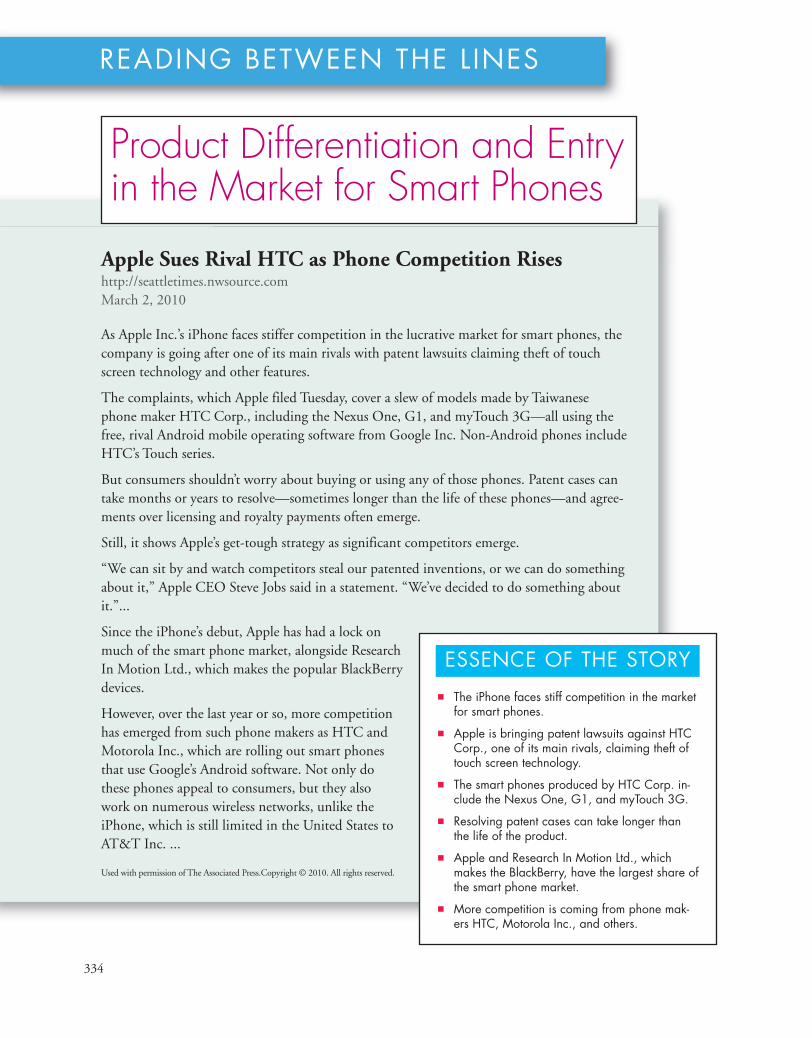
334

READING BETWEEN THE L INES

Apple Sues Rival HTC as Phone Competition Riseshttp://seattletimes.nwsource.comMarch 2, 2010

As Apple Inc.’s iPhone faces stiffer competition in the lucrative market for smart phones, thecompany is going after one of its main rivals with patent lawsuits claiming theft of touchscreen technology and other features.

The complaints, which Apple filed Tuesday, cover a slew of models made by Taiwanesephone maker HTC Corp., including the Nexus One, G1, and myTouch 3G—all using thefree, rival Android mobile operating software from Google Inc. Non-Android phones includeHTC’s Touch series.

But consumers shouldn’t worry about buying or using any of those phones. Patent cases cantake months or years to resolve—sometimes longer than the life of these phones—and agree-ments over licensing and royalty payments often emerge.

Still, it shows Apple’s get-tough strategy as significant competitors emerge.

“We can sit by and watch competitors steal our patented inventions, or we can do somethingabout it,” Apple CEO Steve Jobs said in a statement. “We’ve decided to do something aboutit.”...

Since the iPhone’s debut, Apple has had a lock onmuch of the smart phone market, alongside ResearchIn Motion Ltd., which makes the popular BlackBerrydevices.

However, over the last year or so, more competitionhas emerged from such phone makers as HTC andMotorola Inc., which are rolling out smart phonesthat use Google’s Android software. Not only dothese phones appeal to consumers, but they alsowork on numerous wireless networks, unlike theiPhone, which is still limited in the United States toAT&T Inc. ...

Used with permission of The Associated Press.Copyright © 2010. All rights reserved.

■ The iPhone faces stiff competition in the marketfor smart phones.

■ Apple is bringing patent lawsuits against HTCCorp., one of its main rivals, claiming theft oftouch screen technology.

■ The smart phones produced by HTC Corp. in-clude the Nexus One, G1, and myTouch 3G.

■ Resolving patent cases can take longer thanthe life of the product.

■ Apple and Research In Motion Ltd., whichmakes the BlackBerry, have the largest share ofthe smart phone market.

■ More competition is coming from phone mak-ers HTC, Motorola Inc., and others.

ESSENCE OF THE STORY

Product Differentiation and Entryin the Market for Smart Phones

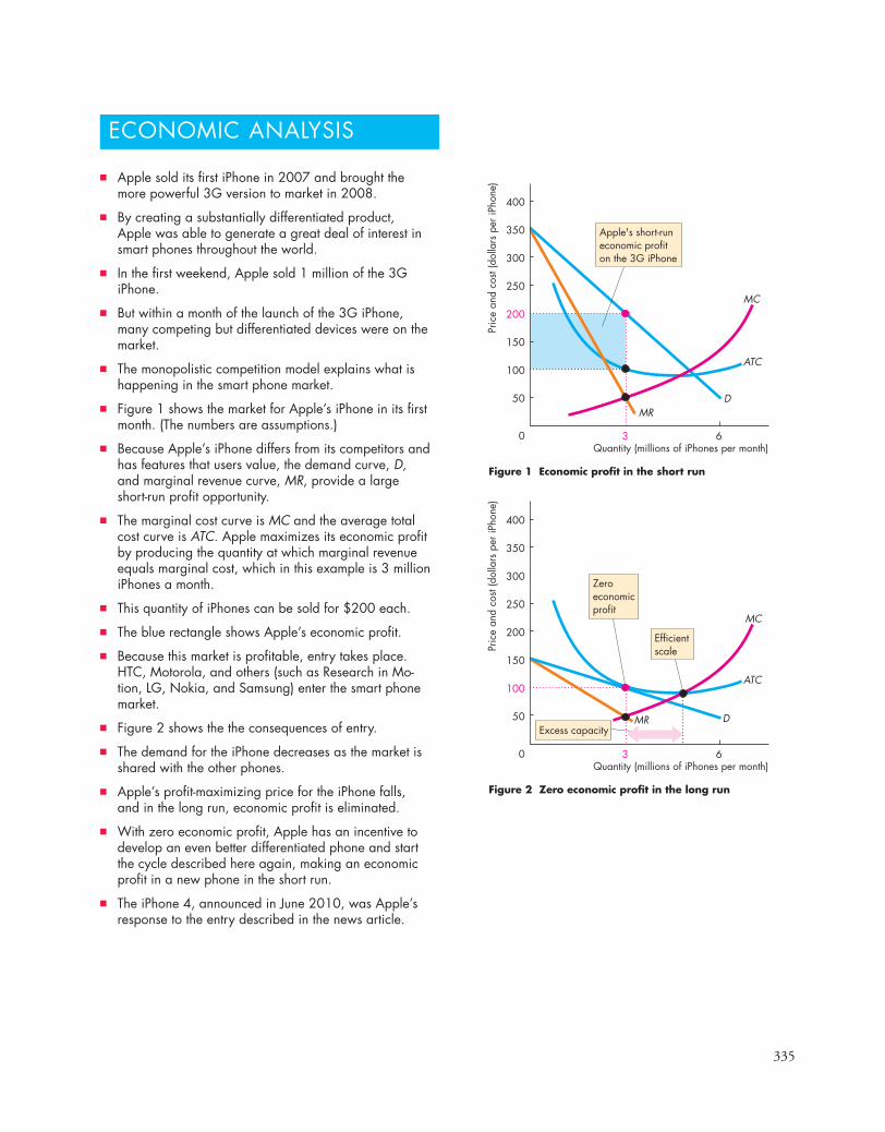
335

ECONOMIC ANALYSIS

Figure 1 Economic profit in the short run

Pric

e an

d co

st (d

olla

rs p

er iP

hone

)

Quantity (millions of iPhones per month)0

DMR

Apple's short-runeconomic profiton the 3G iPhone

50

100

150

200

250

300

350

400

63

MC

ATC

ATC

MC

Figure 2 Zero economic profit in the long run

Pric

e an

d co

st (d

olla

rs p

er iP

hone

)

Quantity (millions of iPhones per month)0

DMRExcess capacity

Efficientscale

Zeroeconomicprofit

50

100

150

200

250

300

350

400

63

■ Apple sold its first iPhone in 2007 and brought themore powerful 3G version to market in 2008.

■ By creating a substantially differentiated product,Apple was able to generate a great deal of interest insmart phones throughout the world.

■ In the first weekend, Apple sold 1 million of the 3GiPhone.

■ But within a month of the launch of the 3G iPhone,many competing but differentiated devices were on themarket.

■ The monopolistic competition model explains what ishappening in the smart phone market.

■ Figure 1 shows the market for Apple’s iPhone in its firstmonth. (The numbers are assumptions.)

■ Because Apple’s iPhone differs from its competitors andhas features that users value, the demand curve, D,and marginal revenue curve, MR, provide a largeshort-run profit opportunity.

■ The marginal cost curve is MC and the average totalcost curve is ATC. Apple maximizes its economic profitby producing the quantity at which marginal revenueequals marginal cost, which in this example is 3 millioniPhones a month.

■ This quantity of iPhones can be sold for $200 each.

■ The blue rectangle shows Apple’s economic profit.

■ Because this market is profitable, entry takes place.HTC, Motorola, and others (such as Research in Mo-tion, LG, Nokia, and Samsung) enter the smart phonemarket.

■ Figure 2 shows the the consequences of entry.

■ The demand for the iPhone decreases as the market isshared with the other phones.

■ Apple’s profit-maximizing price for the iPhone falls,and in the long run, economic profit is eliminated.

■ With zero economic profit, Apple has an incentive todevelop an even better differentiated phone and startthe cycle described here again, making an economicprofit in a new phone in the short run.

■ The iPhone 4, announced in June 2010, was Apple’sresponse to the entry described in the news article.

336 CHAPTER 14 Monopolistic Competition

Product Development and Marketing (pp. 330–333)

■ Firms in monopolistic competition innovate anddevelop new products.

■ Advertising expenditures increase total cost, butaverage total cost might fall if the quantity soldincreases by enough.

■ Advertising expenditures might increase demand,but demand might decrease if competitionincreases.

■ Whether monopolistic competition is inefficientdepends on the value we place on product variety.

Working Problems 13 to 18 will give you a better under-standing of product development and marketing.

Key Points

What Is Monopolistic Competition? (pp. 324–325)

■ Monopolistic competition occurs when a largenumber of firms compete with each other onproduct quality, price, and marketing.

Working Problems 1 and 2 will give you a better under-standing of what monopolistic competition is.

Price and Output in Monopolistic Competition (pp. 326–329)

■ Each firm in monopolistic competition faces adownward-sloping demand curve and producesthe profit-maximizing quantity.

■ Entry and exit result in zero economic profit andexcess capacity in long-run equilibrium.

Working Problems 3 to 12 will give you a better under-standing of price and output in monopolistic competition.

SUMMARY

Key TermsEfficient scale, 328Excess capacity, 328

Markup, 329Monopolistic competition, 324

Product differentiation, 324Signal, 332

Study Plan Problems and Applications 337

Use the following figure, which shows the situationfacing a producer of running shoes, to work Problems5 to 10.

5. What quantity does the firm produce, what pricedoes it charge, and what is its economic profit oreconomic loss?

6. In the long run, how does the number of firmsproducing running shoes change?

7. In the long run, how does the price of runningshoes and the quantity the firm produces change?What happens to the market output?

8. Does the firm have excess capacity in the longrun? If the firm has excess capacity in the longrun, why doesn’t it decrease its capacity?

9. In the long run, compare the price of a pair ofrunning shoes and the marginal cost of produc-ing the pair.

10. Is the market for running shoes efficient or inef-ficient in the long run? Explain your answer.

11. Wake Up and Smell the CoffeeEvery change that Starbucks made over the pastfew years—automated espresso machines, pre-ground coffee, drive-throughs, fewer soft chairsand less carpeting—was made for a reason: tosmooth operations or boost sales. Those mayhave been the right choices at the time, buttogether they ultimately diluted the coffee-cen-tric experience. By 2008, Starbucks experienced adrop in traffic as customers complained that inpursuing rapid growth, the company has strayedtoo far from its roots. Starbucks will once againgrind beans in its stores for drip coffee, give free

Pric

e an

d co

st (d

olla

rs p

er p

air)

Quantity (pairs of running shoes per week)0

D

MCATC

MR

60

80

100

100

40

20

50 150 200 250

What Is Monopolistic Competition? (Study Plan 14.1)

1. Which of the following items are sold by firms in monopolistic competition? Explain your selections.■ Cable television service ■ Wheat■ Athletic shoes ■ Soda ■ Toothbrushes ■ Ready-mix concrete

2. The four-firm concentration ratio for audioequipment makers is 30 and for electric lampmakers it is 89. The HHI for audio equipmentmakers it is 415 and for electric lamp makers it is 2,850. Which of these markets is an exampleof monopolistic competition?

Price and Output in Monopolistic Competition(Study Plan 14.2)

Use the following information to work Problems 3and 4.Sara is a dot.com entrepreneur who has established aWeb site at which people can design and buy sweat-shirts. Sara pays $1,000 a week for her Web serverand Internet connection. The sweatshirts that hercustomers design are made to order by another firm,and Sara pays this firm $20 a sweatshirt. Sara has noother costs. The table sets out the demand schedulefor Sara’s sweatshirts.

Price Quantity demanded(dollars per sweatshirt) (sweatshirts per week)

0 10020 8040 6060 4080 20

100 0

3. Calculate Sara’s profit-maximizing output, price,and economic profit.

4. a. Do you expect other firms to enter the Websweatshirt business and compete with Sara?

b. What happens to the demand for Sara’s sweat-shirts in the long run? What happens to Sara’seconomic profit in the long run?

You can work Problems 1 to 19 in MyEconLab Chapter 14 Study Plan and get instant feedback.

STUDY PLAN PROBLEMS AND APPLICATIONS

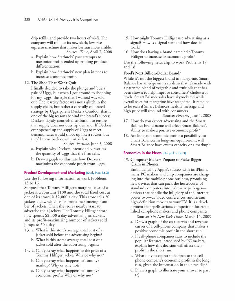
338 CHAPTER 14 Monopolistic Competition

drip refills, and provide two hours of wi-fi. Thecompany will roll out its new sleek, low-riseespresso machine that makes baristas more visible.

Source: Time, April 7, 2008a. Explain how Starbucks’ past attempts to

maximize profits ended up eroding productdifferentiation.

b. Explain how Starbucks’ new plan intends toincrease economic profit.

12. The Shoe That Won’t QuitI finally decided to take the plunge and buy apair of Uggs, but when I got around to shoppingfor my Uggs, the style that I wanted was soldout. The scarcity factor was not a glitch in thesupply chain, but rather a carefully calibratedstrategy by Ugg’s parent Deckers Outdoor that isone of the big reasons behind the brand’s success.Deckers tightly controls distribution to ensurethat supply does not outstrip demand. If Deckersever opened up the supply of Uggs to meetdemand, sales would shoot up like a rocket, butthey’d come back down just as fast.

Source: Fortune, June 5, 2008a. Explain why Deckers intentionally restricts

the quantity of Uggs that the firm sells.b. Draw a graph to illustrate how Deckers

maximizes the economic profit from Uggs.

Product Development and Marketing (Study Plan 14.3)

Use the following information to work Problems13 to 16.Suppose that Tommy Hilfiger’s marginal cost of ajacket is a constant $100 and the total fixed cost atone of its stores is $2,000 a day. This store sells 20jackets a day, which is its profit-maximizing num-ber of jackets. Then the stores nearby start toadvertise their jackets. The Tommy Hilfiger storenow spends $2,000 a day advertising its jackets,and its profit-maximizing number of jackets soldjumps to 50 a day.13. a. What is this store’s average total cost of a

jacket sold before the advertising begins?b. What is this store’s average total cost of a

jacket sold after the advertising begins?

14. a. Can you say what happens to the price of aTommy Hilfiger jacket? Why or why not?

b. Can you say what happens to Tommy’smarkup? Why or why not?

c. Can you say what happens to Tommy’seconomic profit? Why or why not?

15. How might Tommy Hilfiger use advertising as asignal? How is a signal sent and how does itwork?

16. How does having a brand name help TommyHilfiger to increase its economic profit?

Use the following news clip to work Problems 17and 18.

Food’s Next Billion-Dollar Brand?While it’s not the biggest brand in margarine, SmartBalance has an edge on its rivals in that it’s made witha patented blend of vegetable and fruit oils that hasbeen shown to help improve consumers’ cholesterollevels. Smart Balance sales have skyrocketed whileoverall sales for margarine have stagnated. It remainsto be seen if Smart Balance’s healthy message andhigh price will resound with consumers.

Source: Fortune, June 4, 200817. How do you expect advertising and the Smart

Balance brand name will affect Smart Balance’sability to make a positive economic profit?

18. Are long-run economic profits a possibility forSmart Balance? In long-run equilibrium, willSmart Balance have excess capacity or a markup?

Economics in the News (Study Plan 14.N)

19. Computer Makers Prepare to Stake BiggerClaim in PhonesEmboldened by Apple’s success with its iPhone,many PC makers and chip companies are charg-ing into the mobile-phone business, promisingnew devices that can pack the horsepower ofstandard computers into palm-size packages—devices that handle the full glory of the Internet,power two-way video conferences, and streamhigh-definition movies to your TV. It is a devel-opment that spells serious competition for estab-lished cell-phone makers and phone companies.

Source: The New York Times, March 15, 2009a. Draw a graph of the cost curves and revenue

curves of a cell-phone company that makes apositive economic profit in the short run.

b. If cell-phone companies start to include thepopular features introduced by PC makers,explain how this decision will affect theirprofit in the short run.

c. What do you expect to happen to the cell-phone company’s economic profit in the longrun, given the information in the news clip?

d. Draw a graph to illustrate your answer to part(c).

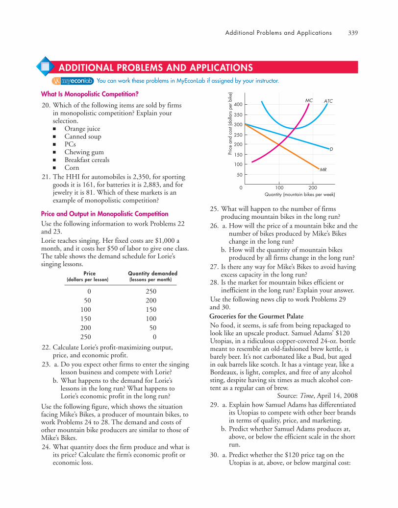
Additional Problems and Applications 339

What Is Monopolistic Competition?

20. Which of the following items are sold by firms in monopolistic competition? Explain your selection.■ Orange juice■ Canned soup■ PCs■ Chewing gum■ Breakfast cereals■ Corn

21. The HHI for automobiles is 2,350, for sportinggoods it is 161, for batteries it is 2,883, and forjewelry it is 81. Which of these markets is anexample of monopolistic competition?

Price and Output in Monopolistic CompetitionUse the following information to work Problems 22and 23.Lorie teaches singing. Her fixed costs are $1,000 amonth, and it costs her $50 of labor to give one class.The table shows the demand schedule for Lorie’ssinging lessons.

Price Quantity demanded(dollars per lesson) (lessons per month)

0 25050 200

100 150150 100200 50250 0

22. Calculate Lorie’s profit-maximizing output,price, and economic profit.

23. a. Do you expect other firms to enter the singinglesson business and compete with Lorie?

b. What happens to the demand for Lorie’slessons in the long run? What happens toLorie’s economic profit in the long run?

Use the following figure, which shows the situationfacing Mike’s Bikes, a producer of mountain bikes, towork Problems 24 to 28. The demand and costs ofother mountain bike producers are similar to those ofMike’s Bikes.24. What quantity does the firm produce and what is

its price? Calculate the firm’s economic profit oreconomic loss.

25. What will happen to the number of firmsproducing mountain bikes in the long run?

26. a. How will the price of a mountain bike and thenumber of bikes produced by Mike’s Bikeschange in the long run?

b. How will the quantity of mountain bikesproduced by all firms change in the long run?

27. Is there any way for Mike’s Bikes to avoid havingexcess capacity in the long run?

28. Is the market for mountain bikes efficient orinefficient in the long run? Explain your answer.

Use the following news clip to work Problems 29and 30.Groceries for the Gourmet PalateNo food, it seems, is safe from being repackaged tolook like an upscale product. Samuel Adams’ $120Utopias, in a ridiculous copper-covered 24-oz. bottlemeant to resemble an old-fashioned brew kettle, isbarely beer. It’s not carbonated like a Bud, but agedin oak barrels like scotch. It has a vintage year, like aBordeaux, is light, complex, and free of any alcoholsting, despite having six times as much alcohol con-tent as a regular can of brew.

Source: Time, April 14, 200829. a. Explain how Samuel Adams has differentiated

its Utopias to compete with other beer brandsin terms of quality, price, and marketing.

b. Predict whether Samuel Adams produces at,above, or below the efficient scale in the shortrun.

30. a. Predict whether the $120 price tag on theUtopias is at, above, or below marginal cost:

Pric

e an

d co

st (d

olla

rs p

er b

ike)

Quantity (mountain bikes per week)0

D

MC ATC

MR

300

400

100

200

100

250

350

150

50

200

You can work these problems in MyEconLab if assigned by your instructor.

ADDITIONAL PROBLEMS AND APPLICATIONS

340 CHAPTER 14 Monopolistic Competition

(i) In the short run.(ii) In the long run.

b. Do you think that Samuel Adams Utopiasmakes the market for beer inefficient?

Use the following news clip to work Problems 31 and 32.Swinging for Female GolfersOne of the hottest areas of innovation is in clubs forwomen, who now make up nearly a quarter of the 24 million golfers in the United States. Callaway andNike, two of the leading golf-equipment manufactur-ers, recently released new clubs designed specificallyfor women.

Source: Time, April 21, 200831. a. How are Callaway and Nike attempting to

maintain economic profit?b. Draw a graph to illustrate the cost curves and

revenue curves of Callaway or Nike in themarket for golf clubs for women.

c. Show on your graph in part (b) the short-runeconomic profit.

32. a. Explain why the economic profit thatCallaway and Nike make on golf clubs forwomen is likely to be temporary.

b. Draw a graph to illustrate the cost curves andrevenue curves of Callaway or Nike in themarket for golf clubs for women in the longrun. Mark the firm’s excess capacity.

Product Development and MarketingUse the following information to work Problems 33 to 35.Bianca bakes delicious cookies. Her total fixed cost is$40 a day, and her average variable cost is $1 a bag.Few people know about Bianca’s Cookies, and she ismaximizing her profit by selling 10 bags a day for $5a bag. Bianca thinks that if she spends $50 a day onadvertising, she can increase her market share and sell25 bags a day for $5 a bag.33. If Bianca’s advertising works as she expects, can

she increase her economic profit by advertising?34. If Bianca advertises, will her average total cost

increase or decrease at the quantity produced?35. If Bianca advertises, will she continue to sell her

cookies for $5 a bag or will she change her price?Use the following news clip to work Problems 36 and 37.A Thirst for More ChampagneChampagne exports have tripled in the past 20 years.That poses a problem for northern France, where thebubbly hails from—not enough grapes. So French

authorities have unveiled a plan to extend the officialChampagne grape-growing zone to cover 40 new vil-lages. This revision has provoked debate. The changewill take several years to become effective. In themeantime the vineyard owners whose land values willjump markedly if the changes are finalized certainlyhave reason to raise a glass.

Source: Fortune, May 12, 200836. a. Why is France so strict about designating the

vineyards that can use the Champagne label?b. Explain who most likely opposes this plan.

37. Assuming that vineyards in these 40 villages areproducing the same quality of grapes with orwithout this plan, why will their land values“jump markedly” if this plan is approved?

38. Under Armour’s Big Step UpUnder Armour, the red-hot athletic-apparelbrand, has joined Nike, Adidas, and NewBalance as a major player in the market for ath-letic footwear. Under Armour plans to revive thelong-dead cross-training category. But will youngathletes really spend $100 for a cross trainingshoe to lift weights in?

Source: Time, May 26, 2008What factors influence Under Armour’s ability tomake an economic profit in the cross-trainingshoe market?

Economics in the News39. After you have studied Reading Between the Lines

on pp. 334–335 answer the following questions.a. Describe the cost curves (MC and ATC) and

the marginal revenue and demand curves forthe iPhone when Apple first introduced it.

b. How do you think the creation of the iPhoneinfluenced the demand for older generationcell phones?

c. Explain the effects of the introduction of the3G iPhone on HTC and other firms in themarket for smart phones.

d. Draw a graph to illustrate your answer to part (c).

e. Explain the effect on Apple of the decisions byBlackBerry and HTC to bring their own smartphones to market.

f. Draw a graph to illustrate your answer to part (e).

g. Do you think the smart phone market isefficient? Explain your answer.

h. Do you predict that producers of smart phoneshave excess capacity? Explain your answer.

After studying this chapter, you will be able to:

� Define and identify oligopoly� Use game theory to explain how price and output are

determined in oligopoly� Use game theory to explain other strategic decisions� Describe the antitrust laws that regulate oligopoly

15The chip in your laptop was made by either Intel or Advanced Micro Devices;

the battery in your TV remote is most likely a Duracell or Energizer; if you use ahigh-tech razor, it is either a Gillette or a Schick; and if you take a long-distance trip by air, you will fly in an airplane made by either Boeing or theEuropean firm Airbus. In the markets for computer chips, batteries, high-techrazors, and big airplanes, two producers compete for market share in thepursuit of maximum profit. Many other markets have only a small number offirms. Among them are the markets for light bulbs, breakfast cereals, and majorappliances.

How does a market work when only a handful of firms compete? Is themarket efficient like perfect competition with the firms operating in the socialinterest? Or is the market inefficient like monopoly with the firms restrictingoutput to increase profit?

To answer these questions, we need to understand the models of oligopoly.These models use game theory, which the chapter explains.

At the end of the chapter, in Reading Between the Lines, we’ll look at the marketfor high-tech razors and see the game that Gillette and Schick are playing in theirbattle for market shares and maximum profit.

OLIGOPOLY

341

342 CHAPTER 15 Oligopoly

◆ What Is Oligopoly?Oligopoly, like monopolistic competition, liesbetween perfect competition and monopoly. Thefirms in oligopoly might produce an identical prod-uct and compete only on price, or they might pro-duce a differentiated product and compete on price,product quality, and marketing. Oligopoly is a marketstructure in which■ Natural or legal barriers prevent the entry of new

firms.■ A small number of firms compete.

Barriers to EntryNatural or legal barriers to entry can create oligopoly.You saw in Chapter 13 how economies of scale anddemand form a natural barrier to entry that can cre-ate a natural monopoly. These same factors can createa natural oligopoly.

Figure 15.1 illustrates two natural oligopolies. Thedemand curve, D (in both parts of the figure), showsthe demand for taxi rides in a town. If the average

total cost curve of a taxi company is ATC1 in part (a),the market is a natural duopoly—an oligopoly marketwith two firms. You can probably see some examplesof duopoly where you live. Some cities have only twotaxi companies, two car rental firms, two copy cen-ters, or two college bookstores.

The lowest price at which the firm would remainin business is $10 a ride. At that price, the quantityof rides demanded is 60 a day, the quantity that canbe provided by just two firms. There is no room inthis market for three firms. But if there were only onefirm, it would make an economic profit and a secondfirm would enter to take some of the business andeconomic profit.

If the average total cost curve of a taxi company isATC2 in part (b), the efficient scale of one firm is 20 ridesa day. This market is large enough for three firms.

A legal oligopoly arises when a legal barrier to entryprotects the small number of firms in a market. A citymight license two taxi firms or two bus companies, forexample, even though the combination of demand andeconomies of scale leaves room for more than two firms.

(a) Natural duopoly

Quantity (rides per day)

Lowestpossibleprice =minimumATC

Efficientscale of one firm

Two firmscan meetdemand

(b) Natural oligopoly with three firms

0 6030 90

Pric

e an

d co

st (d

olla

rs p

er ri

de)

D

ATC1

20

10

15

5

25

Quantity (rides per day)

Efficientscale of one firm

0 604020 80

Pric

e an

d co

st (d

olla

rs p

er ri

de)

D

ATC2

20

10

15

5

25

Three firmscan meetdemand

The lowest possible price is $10 a ride, which is the minimumaverage total cost. When a firm produces 30 rides a day, theefficient scale, two firms can satisfy the market demand. Thisnatural oligopoly has two firms—a natural duopoly.

When the efficient scale of one firm is 20 rides per day,three firms can satisfy the market demand at the lowestpossible price. This natural oligopoly has three firms.

FIGURE 15.1 Natural Oligopoly

animation

What Is Oligopoly? 343

Economics in ActionOligopoly TodayThese markets are oligopolies.Although in some of them, the num-ber of firms (in parentheses) is large,the share of the market held by the 4largest firms (the red bars) is close to100 percent.

The most concentratedmarkets—cigarettes, glass bottles andjars, washing machines and dryers,and batteries, are dominated by justone or two firms.

If you want to buy a battery foryour TV remote or toothbrush, you’llfind it hard to avoid buying a Duracellor an Energizer.

Small Number of FirmsBecause barriers to entry exist, oligopoly consists of asmall number of firms, each of which has a largeshare of the market. Such firms are interdependent,and they face a temptation to cooperate to increasetheir joint economic profit.

Interdependence With a small number of firms in amarket, each firm’s actions influence the profits of allthe other firms. When Penny Stafford opened her cof-fee shop in Bellevue, Washington, a nearby Starbuckscoffee shop took a hit. Within days, Starbucks beganto attract Penny’s customers with enticing offers andlower prices. Starbucks survived but Penny eventuallywent out of business. Penny Stafford and Starbuckswere interdependent.

Temptation to Cooperate When a small number offirms share a market, they can increase their profitsby forming a cartel and acting like a monopoly. Acartel is a group of firms acting together—collud-ing—to limit output, raise price, and increase eco-nomic profit. Cartels are illegal, but they do operatein some markets. But for reasons that you’ll discoverin this chapter, cartels tend to break down.

Examples of OligopolyThe box below shows some examples of oligopoly.The dividing line between oligopoly and monopolis-tic competition is hard to pin down. As a practicalmatter, we identify oligopoly by looking at concen-tration ratios, the Herfindahl-Hirschman Index, andinformation about the geographical scope of themarket and barriers to entry. The HHI that dividesoligopoly from monopolistic competition is generallytaken to be 1,000. An HHI below 1,000 is usually anexample of monopolistic competition, and a marketin which the HHI exceeds 1,000 is usually an exam-ple of oligopoly.

0 20 80 10040 60Percentage of industry total revenue

Cigarettes (9)

Glass bottles and jars (11)

Washing machines and dryers (10)

Batteries (35)

Light bulbs (54)

Breakfast cereals (48)

House slippers (22)

Automobiles (173)

Chocolate (152)

Motorcycles (373)

–

2,960

2,870

2,883

2,849

2,446

2,053

2,350

2,567

2,037

Herfindahl-Hirschman Index

Measures of Concentration

Industry (number of firms)

4 largest firms next 4 largest firms next 12 largest firms

Source of data: U.S. Census Bureau.

REVIEW QUIZ1 What are the two distinguishing characteristics

of oligopoly?2 Why are firms in oligopoly interdependent?3 Why do firms in oligopoly face a temptation to

collude?4 Can you think of some examples of oligopolies

that you buy from?

You can work these questions in Study Plan 15.1 and get instant feedback.

344 CHAPTER 15 Oligopoly

◆ Oligopoly GamesEconomists think about oligopoly as a game betweentwo or a few players, and to study oligopoly marketsthey use game theory. Game theory is a set of tools forstudying strategic behavior—behavior that takes intoaccount the expected behavior of others and therecognition of mutual interdependence. Game theorywas invented by John von Neumann in 1937 andextended by von Neumann and Oskar Morgensternin 1944 (p. 367). Today, it is one of the majorresearch fields in economics.

Game theory seeks to understand oligopoly as wellas other forms of economic, political, social, and evenbiological rivalries by using a method of analysis specifi-cally designed to understand games of all types, includ-ing the familiar games of everyday life (see Talking withThomas Hubbard on pp. 368–370). To lay the founda-tion for studying oligopoly games, we first think aboutthe features that all games share.

What Is a Game?What is a game? At first thought, the question seemssilly. After all, there are many different games. Thereare ball games and parlor games, games of chance andgames of skill. But what is it about all these differentactivities that makes them games? What do all thesegames have in common? All games share four com-mon features:■ Rules■ Strategies■ Payoffs■ Outcome

We’re going to look at these features of games byplaying at a game called “the prisoners’ dilemma.”The prisoners’ dilemma game displays the essentialfeatures of many games, including oligopoly games,and it gives a good illustration of how game theoryworks and generates predictions.

The Prisoners’ DilemmaArt and Bob have been caught red-handed stealing acar. Facing airtight cases, they will receive a sentenceof two years each for their crime. During his inter-views with the two prisoners, the district attorneybegins to suspect that he has stumbled on the twopeople who were responsible for a multimillion-dollarbank robbery some months earlier. But this is just a

suspicion. He has no evidence on which he can con-vict them of the greater crime unless he can get themto confess. But how can he extract a confession? Theanswer is by making the prisoners play a game. Thedistrict attorney makes the prisoners play the follow-ing game.

Rules Each prisoner (player) is placed in a separateroom and cannot communicate with the otherprisoner. Each is told that he is suspected of havingcarried out the bank robbery and that

If both of them confess to the larger crime, each willreceive a sentence of 3 years for both crimes.

If he alone confesses and his accomplice does not, hewill receive only a 1-year sentence while his accom-plice will receive a 10-year sentence.

Strategies In game theory, strategies are all the possi-ble actions of each player. Art and Bob each have twopossible actions:

1. Confess to the bank robbery.2. Deny having committed the bank robbery.

Because there are two players, each with two strate-gies, there are four possible outcomes:

1. Both confess.2. Both deny.3. Art confesses and Bob denies.4. Bob confesses and Art denies.

Payoffs Each prisoner can work out his payoff ineach of these situations, and we can tabulate the fourpossible payoffs for each of the prisoners in what iscalled a payoff matrix for the game. A payoff matrix isa table that shows the payoffs for every possibleaction by each player for every possible action byeach other player.

Table 15.1 shows a payoff matrix for Art and Bob.The squares show the payoffs for each prisoner—thered triangle in each square shows Art’s and the bluetriangle shows Bob’s. If both prisoners confess (topleft), each gets a prison term of 3 years. If Bob con-fesses but Art denies (top right), Art gets a 10-yearsentence and Bob gets a 1-year sentence. If Art con-fesses and Bob denies (bottom left), Art gets a 1-yearsentence and Bob gets a 10-year sentence. Finally, ifboth of them deny (bottom right), neither can beconvicted of the bank robbery charge but both aresentenced for the car theft—a 2-year sentence.

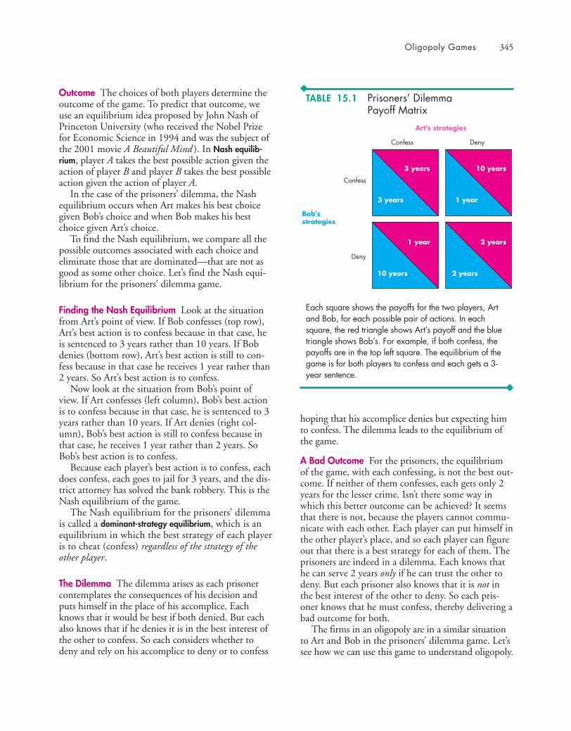
Oligopoly Games 345

Outcome The choices of both players determine theoutcome of the game. To predict that outcome, weuse an equilibrium idea proposed by John Nash ofPrinceton University (who received the Nobel Prizefor Economic Science in 1994 and was the subject ofthe 2001 movie A Beautiful Mind ). In Nash equilib-rium, player A takes the best possible action given theaction of player B and player B takes the best possibleaction given the action of player A.

In the case of the prisoners’ dilemma, the Nashequilibrium occurs when Art makes his best choicegiven Bob’s choice and when Bob makes his bestchoice given Art’s choice.

To find the Nash equilibrium, we compare all thepossible outcomes associated with each choice andeliminate those that are dominated—that are not asgood as some other choice. Let’s find the Nash equi-librium for the prisoners’ dilemma game.

Finding the Nash Equilibrium Look at the situationfrom Art’s point of view. If Bob confesses (top row),Art’s best action is to confess because in that case, heis sentenced to 3 years rather than 10 years. If Bobdenies (bottom row), Art’s best action is still to con-fess because in that case he receives 1 year rather than2 years. So Art’s best action is to confess.

Now look at the situation from Bob’s point ofview. If Art confesses (left column), Bob’s best actionis to confess because in that case, he is sentenced to 3years rather than 10 years. If Art denies (right col-umn), Bob’s best action is still to confess because inthat case, he receives 1 year rather than 2 years. SoBob’s best action is to confess.

Because each player’s best action is to confess, eachdoes confess, each goes to jail for 3 years, and the dis-trict attorney has solved the bank robbery. This is theNash equilibrium of the game.

The Nash equilibrium for the prisoners’ dilemmais called a dominant-strategy equilibrium, which is anequilibrium in which the best strategy of each playeris to cheat (confess) regardless of the strategy of theother player.

The Dilemma The dilemma arises as each prisonercontemplates the consequences of his decision andputs himself in the place of his accomplice. Eachknows that it would be best if both denied. But eachalso knows that if he denies it is in the best interest ofthe other to confess. So each considers whether todeny and rely on his accomplice to deny or to confess

hoping that his accomplice denies but expecting himto confess. The dilemma leads to the equilibrium ofthe game.

A Bad Outcome For the prisoners, the equilibriumof the game, with each confessing, is not the best out-come. If neither of them confesses, each gets only 2years for the lesser crime. Isn’t there some way inwhich this better outcome can be achieved? It seemsthat there is not, because the players cannot commu-nicate with each other. Each player can put himself inthe other player’s place, and so each player can figureout that there is a best strategy for each of them. Theprisoners are indeed in a dilemma. Each knows thathe can serve 2 years only if he can trust the other todeny. But each prisoner also knows that it is not inthe best interest of the other to deny. So each pris-oner knows that he must confess, thereby delivering abad outcome for both.

The firms in an oligopoly are in a similar situationto Art and Bob in the prisoners’ dilemma game. Let’ssee how we can use this game to understand oligopoly.

Each square shows the payoffs for the two players, Artand Bob, for each possible pair of actions. In eachsquare, the red triangle shows Art’s payoff and the bluetriangle shows Bob’s. For example, if both confess, thepayoffs are in the top left square. The equilibrium of thegame is for both players to confess and each gets a 3-year sentence.

Bob'sstrategies

Art's strategies

Confess

Confess

Deny

Deny

10 years

1 year

3 years

3 years

2 years

2 years

1 year

10 years

TABLE 15.1 Prisoners’ Dilemma Payoff Matrix

346 CHAPTER 15 Oligopoly

An Oligopoly Price-Fixing GameWe can use game theory and a game like the prison-ers’ dilemma to understand price fixing, price wars,and other aspects of the behavior of firms in oligop-oly. We’ll begin with a price-fixing game.

To understand price fixing, we’re going to studythe special case of duopoly—an oligopoly with twofirms. Duopoly is easier to study than oligopoly withthree or more firms, and it captures the essence of alloligopoly situations. Somehow, the two firms mustshare the market. And how they share it depends onthe actions of each. We’re going to describe the costsof the two firms and the market demand for the itemthey produce. We’re then going to see how game the-ory helps us to predict the prices charged and thequantities produced by the two firms in a duopoly.

Cost and Demand Conditions Two firms, Trick andGear, produce switchgears. They have identical costs.Figure 15.2(a) shows their average total cost curve(ATC ) and marginal cost curve (MC ). Figure 15.2(b)shows the market demand curve for switchgears (D).The two firms produce identical switchgears, so onefirm’s switchgear is a perfect substitute for the other’s,and the market price of each firm’s product is identi-cal. The quantity demanded depends on that price—the higher the price, the smaller is the quantitydemanded.

This industry is a natural duopoly. Two firms canproduce this good at a lower cost than either one firmor three firms can. For each firm, average total cost isat its minimum when production is 3,000 units aweek. When price equals minimum average totalcost, the total quantity demanded is 6,000 units aweek, and two firms can just produce that quantity.

Collusion We’ll suppose that Trick and Gear enterinto a collusive agreement. A collusive agreement is anagreement between two (or more) producers to forma cartel to restrict output, raise the price, and increaseprofits. Such an agreement is illegal in the UnitedStates and is undertaken in secret. The strategies thatfirms in a cartel can pursue are to

■ Comply■ Cheat

A firm that complies carries out the agreement. A firmthat cheats breaks the agreement to its own benefitand to the cost of the other firm.

Because each firm has two strategies, there are fourpossible combinations of actions for the firms:

1. Both firms comply.2. Both firms cheat.3. Trick complies and Gear cheats.4. Gear complies and Trick cheats.

MinimumATC

ATC

D

MC

Quantity (thousands of switchgears per week)

0

(b) Industry

Pric

e an

d co

st(th

ousa

nds

of d

olla

rs p

er u

nit)

Quantity (thousands of switchgears per week)

0

(a) Individual firm

10 10

4

6

Pric

e (th

ousa

nds

of d

olla

rs p

er u

nit)

6

1 532 41 5 73 62

The average total cost curve for each firmis ATC, and the marginal cost curve isMC (part a). Minimum average total costis $6,000 a unit, and it occurs at a pro-duction of 3,000 units a week.

Part (b) shows the market demandcurve. At a price of $6,000, the quantitydemanded is 6,000 units per week. Thetwo firms can produce this output at thelowest possible average cost. If the mar-ket had one firm, it would be profitablefor another to enter. If the market hadthree firms, one would exit. There is roomfor only two firms in this industry. It is anatural duopoly.

FIGURE 15.2 Costs and Demand

animation

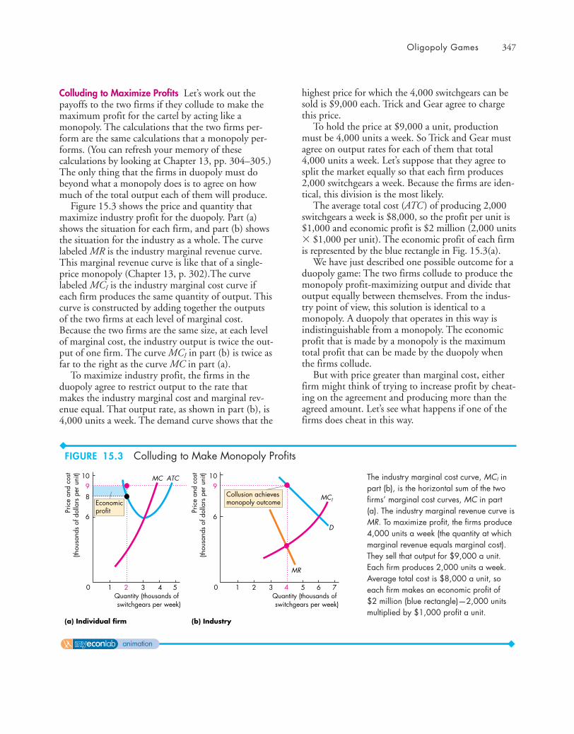
Oligopoly Games 347

Colluding to Maximize Profits Let’s work out thepayoffs to the two firms if they collude to make themaximum profit for the cartel by acting like amonopoly. The calculations that the two firms per-form are the same calculations that a monopoly per-forms. (You can refresh your memory of thesecalculations by looking at Chapter 13, pp. 304–305.)The only thing that the firms in duopoly must dobeyond what a monopoly does is to agree on howmuch of the total output each of them will produce.

Figure 15.3 shows the price and quantity thatmaximize industry profit for the duopoly. Part (a)shows the situation for each firm, and part (b) showsthe situation for the industry as a whole. The curvelabeled MR is the industry marginal revenue curve.This marginal revenue curve is like that of a single-price monopoly (Chapter 13, p. 302).The curvelabeled MCI is the industry marginal cost curve ifeach firm produces the same quantity of output. Thiscurve is constructed by adding together the outputsof the two firms at each level of marginal cost.Because the two firms are the same size, at each levelof marginal cost, the industry output is twice the out-put of one firm. The curve MCI in part (b) is twice asfar to the right as the curve MC in part (a).

To maximize industry profit, the firms in theduopoly agree to restrict output to the rate thatmakes the industry marginal cost and marginal rev-enue equal. That output rate, as shown in part (b), is4,000 units a week. The demand curve shows that the

highest price for which the 4,000 switchgears can besold is $9,000 each. Trick and Gear agree to chargethis price.

To hold the price at $9,000 a unit, productionmust be 4,000 units a week. So Trick and Gear mustagree on output rates for each of them that total4,000 units a week. Let’s suppose that they agree tosplit the market equally so that each firm produces2,000 switchgears a week. Because the firms are iden-tical, this division is the most likely.

The average total cost (ATC ) of producing 2,000switchgears a week is $8,000, so the profit per unit is$1,000 and economic profit is $2 million (2,000 units� $1,000 per unit). The economic profit of each firmis represented by the blue rectangle in Fig. 15.3(a).

We have just described one possible outcome for aduopoly game: The two firms collude to produce themonopoly profit-maximizing output and divide thatoutput equally between themselves. From the indus-try point of view, this solution is identical to amonopoly. A duopoly that operates in this way isindistinguishable from a monopoly. The economicprofit that is made by a monopoly is the maximumtotal profit that can be made by the duopoly whenthe firms collude.

But with price greater than marginal cost, eitherfirm might think of trying to increase profit by cheat-ing on the agreement and producing more than theagreed amount. Let’s see what happens if one of thefirms does cheat in this way.

Collusion achievesmonopoly outcome

MCI

MR

Economicprofit

ATC

D

MC

Quantity (thousands of switchgears per week)

0

(b) Industry

Pric

e an

d co

st(th

ousa

nds

of d

olla

rs p

er u

nit)

Quantity (thousands of switchgears per week)

0

(a) Individual firm

10

4

6

89

10

6

9

Pric

e an

d co

st(th

ousa

nds

of d

olla

rs p

er u

nit)

1 532 41 5 73 62

The industry marginal cost curve, MCI inpart (b), is the horizontal sum of the twofirms’ marginal cost curves, MC in part(a). The industry marginal revenue curve isMR. To maximize profit, the firms produce4,000 units a week (the quantity at whichmarginal revenue equals marginal cost).They sell that output for $9,000 a unit.Each firm produces 2,000 units a week.Average total cost is $8,000 a unit, soeach firm makes an economic profit of$2 million (blue rectangle)—2,000 unitsmultiplied by $1,000 profit a unit.

FIGURE 15.3 Colluding to Make Monopoly Profits

animation

348 CHAPTER 15 Oligopoly

One Firm Cheats on a Collusive Agreement To setthe stage for cheating on their agreement, Trick con-vinces Gear that demand has decreased and that itcannot sell 2,000 units a week. Trick tells Gear that itplans to cut its price so that it can sell the agreed2,000 units each week. Because the two firms pro-duce an identical product, Gear matches Trick’s pricecut but still produces only 2,000 units a week.

In fact, there has been no decrease in demand.Trick plans to increase output, which it knows willlower the price, and Trick wants to ensure that Gear’soutput remains at the agreed level.

Figure 15.4 illustrates the consequences of Trick’scheating. Part (a) shows Gear (the complier); part (b)shows Trick (the cheat); and part (c) shows the indus-try as a whole. Suppose that Trick increases output to3,000 units a week. If Gear sticks to the agreement toproduce only 2,000 units a week, total output is now5,000 a week, and given demand in part (c), the pricefalls to $7,500 a unit.

Gear continues to produce 2,000 units a week at acost of $8,000 a unit and incurs a loss of $500 a unit,or $1 million a week. This economic loss is shown bythe red rectangle in part (a). Trick produces 3,000units a week at a cost of $6,000 a unit. With a price

of $7,500, Trick makes a profit of $1,500 a unit andtherefore an economic profit of $4.5 million. Thiseconomic profit is the blue rectangle in part (b).

We’ve now described a second possible outcome forthe duopoly game: One of the firms cheats on the col-lusive agreement. In this case, the industry output islarger than the monopoly output and the industryprice is lower than the monopoly price. The total eco-nomic profit made by the industry is also smaller thanthe monopoly’s economic profit. Trick (the cheat)makes an economic profit of $4.5 million, and Gear(the complier) incurs an economic loss of $1 million.The industry makes an economic profit of $3.5 mil-lion. This industry profit is $0.5 million less than theeconomic profit that a monopoly would make, but itis distributed unevenly. Trick makes a bigger economicprofit than it would under the collusive agreement,while Gear incurs an economic loss.

A similar outcome would arise if Gear cheated andTrick complied with the agreement. The industryprofit and price would be the same, but in this case,Gear (the cheat) would make an economic profit of$4.5 million and Trick (the complier) would incur aneconomic loss of $1 million.

Let’s next see what happens if both firms cheat.

ATC

Quantity (thousands of switchgears per week)

0

(c) Industry

D

Quantity (thousands of switchgears per week)

0

(b) Cheat

10.0

4

7.5

1 5 6 732

6.0

Quantity (thousands of switchgears per week)

0

(a) Complier

10.0

4

7.5

1 532 41 532

8.0

Complier'soutput

Cheat'soutput

ATC

Economicprofit

Economicloss

Pric

e an

d co

st(th

ousa

nds

of d

olla

rs p

er u

nit)

Pric

e an

d co

st(th

ousa

nds

of d

olla

rs p

er u

nit) 10.0

7.5

Pric

e (th

ousa

nds

of d

olla

rs p

er u

nit)

One firm, shown in part (a), complies with the agreementand produces 2,000 units. The other firm, shown in part (b),cheats on the agreement and increases its output to 3,000units a week. Given the market demand curve, shown inpart (c), and with a total production of 5,000 units a week,

the price falls to $7,500 a unit. At this price, the complier inpart (a) incurs an economic loss of $1 million ($500 per unit� 2,000 units), shown by the red rectangle. In part (b), thecheat makes an economic profit of $4.5 million ($1,500 perunit � 3,000 units), shown by the blue rectangle.

FIGURE 15.4 One Firm Cheats

animation

Oligopoly Games 349

Both Firms Cheat Suppose that both firms cheat andthat each firm behaves like the cheating firm that wehave just analyzed. Each tells the other that it isunable to sell its output at the going price and that itplans to cut its price. But because both firms cheat,each will propose a successively lower price. As long asprice exceeds marginal cost, each firm has an incentiveto increase its production—to cheat. Only when priceequals marginal cost is there no further incentive tocheat. This situation arises when the price has reached$6,000. At this price, marginal cost equals price. Also,price equals minimum average total cost. At a priceless than $6,000, each firm incurs an economic loss.At a price of $6,000, each firm covers all its costs and makes zero economic profit. Also, at a price of$6,000, each firm wants to produce 3,000 units aweek, so the industry output is 6,000 units a week.Given the demand conditions, 6,000 units can be soldat a price of $6,000 each.

Figure 15.5 illustrates the situation just described.Each firm, in part (a), produces 3,000 units a week,and its average total cost is a minimum ($6,000 perunit). The market as a whole, in part (b), operates atthe point at which the market demand curve (D)intersects the industry marginal cost curve (MCI).Each firm has lowered its price and increased its out-put to try to gain an advantage over the other firm.Each has pushed this process as far as it can withoutincurring an economic loss.

We have now described a third possible outcomeof this duopoly game: Both firms cheat. If both firms

cheat on the collusive agreement, the output of eachfirm is 3,000 units a week and the price is $6,000 aunit. Each firm makes zero economic profit.

The Payoff Matrix Now that we have described thestrategies and payoffs in the duopoly game, we cansummarize the strategies and the payoffs in the formof the game’s payoff matrix. Then we can find theNash equilibrium.

Table 15.2 sets out the payoff matrix for thisgame. It is constructed in the same way as the payoffmatrix for the prisoners’ dilemma in Table 15.1. Thesquares show the payoffs for the two firms—Gearand Trick. In this case, the payoffs are profits. (Forthe prisoners’ dilemma, the payoffs were losses.)

The table shows that if both firms cheat (top left),they achieve the perfectly competitive outcome—each firm makes zero economic profit. If both firmscomply (bottom right), the industry makes themonopoly profit and each firm makes an economicprofit of $2 million. The top right and bottom leftsquares show the payoff if one firm cheats while theother complies. The firm that cheats makes an eco-nomic profit of $4.5 million, and the one that com-plies incurs a loss of $1 million.

Nash Equilibrium in the Duopolists’ Dilemma Theduopolists have a dilemma like the prisoners’dilemma. Do they comply or cheat? To answer thisquestion, we must find the Nash equilibrium.

Both firms cheatingachieves competitiveoutcome

MCIATC

D

MC

Quantity (thousands of switchgears per week)

0

(b) Industry

Quantity (thousands of switchgears per week)

0

(a) Individual firm

10

4

6

1 532 41 5 6 732

Pric

e an

d co

st(th

ousa

nds

of d

olla

rs p

er u

nit) 10

6

Pric

e an

d co

st(th

ousa

nds

of d

olla

rs p

er u

nit) If both firms cheat by increasing production,

the collusive agreement collapses. The limitto the collapse is the competitive equilib-rium. Neither firm will cut its price below$6,000 (minimum average total cost)because to do so will result in losses. In part(a), each firm produces 3,000 units a weekat an average total cost of $6,000. In part(b), with a total production of 6,000 units,the price falls to $6,000. Each firm nowmakes zero economic profit. This outputand price are the ones that would prevail ina competitive industry.

FIGURE 15.5 Both Firms Cheat

animation

350 CHAPTER 15 Oligopoly

Look at things from Gear’s point of view. Gearreasons as follows: Suppose that Trick cheats. If Icomply, I will incur an economic loss of $1 million.If I also cheat, I will make zero economic profit. Zerois better than minus $1 million, so I’m better off if Icheat. Now suppose Trick complies. If I cheat, I willmake an economic profit of $4.5 million, and if Icomply, I will make an economic profit of $2 mil-lion. A $4.5 million profit is better than a $2 millionprofit, so I’m better off if I cheat. So regardless ofwhether Trick cheats or complies, it pays Gear tocheat. Cheating is Gear’s best strategy.

Trick comes to the same conclusion as Gearbecause the two firms face an identical situation. Soboth firms cheat. The Nash equilibrium of the duop-oly game is that both firms cheat. And although theindustry has only two firms, they charge the sameprice and produce the same quantity as those in acompetitive industry. Also, as in perfect competition,each firm makes zero economic profit.

This conclusion is not general and will not alwaysarise. We’ll see why not by looking first at some othergames that are like the prisoners’ dilemma. Then we’llbroaden the types of games we consider.

Other Oligopoly GamesFirms in oligopoly must decide whether to mountexpensive advertising campaigns; whether to modifytheir product; whether to make their product morereliable and more durable; whether to price discrimi-nate and, if so, among which groups of customersand to what degree; whether to undertake a largeresearch and development (R&D) effort aimed atlowering production costs; and whether to enter orleave an industry.

All of these choices can be analyzed as games thatare similar to the one that we’ve just studied. Let’slook at one example: an R&D game.

Trick'sstrategies

Gear's strategies

Cheat

Cheat

Comply

Comply

–$1.0m

+$4.5m

$0

$0

+$2m

+$2m

+$4.5m

–$1.0m Economics in ActionAn R&D Game in the Market for DiapersDisposable diapers have been around for a bit morethan 40 years. Procter & Gamble (which has a 40percent market share with Pampers) and Kimberly-Clark (which has a 33 percent market share withHuggies) have always been the market leaders.

When the disposable diaper was first introduced,it had to be cost-effective in competition withreusable, laundered diapers. A costly research anddevelopment effort resulted in the development ofmachines that could make disposable diapers at a lowenough cost to achieve that initial competitive edge.But new firms tried to get into the business and takemarket share away from the two industry leaders, andthe industry leaders themselves battled each other tomaintain or increase their own market shares.

During the early 1990s, Kimberly-Clark was the firstto introduce Velcro closures. And in 1996, Procter &Gamble was the first to introduce “breathable” diapers.

The key to success in this industry (as in any other)is to design a product that people value highly relativeto the cost of producing it. The firm that creates themost highly valued product and also develops theleast-cost technology for producing it gains a competi-tive edge, undercutting the rest of the market, increas-ing its market share, and increasing its profit.

But the R&D that must be undertaken to improveproduct quality and cut cost is itself costly. So thecost of R&D must be deducted from the profitresulting from the increased market share that lowercosts achieve. If no firm does R&D, every firm canbe better off, but if one firm initiates the R&Dactivity, all must follow.

Each square shows the payoffs from a pair of actions.For example, if both firms comply with the collusiveagreement, the payoffs are recorded in the bottomright square. The red triangle shows Gear’s payoff,and the blue triangle shows Trick’s. In Nash equilib-rium, both firms cheat.

TABLE 15.2 Duopoly Payoff Matrix

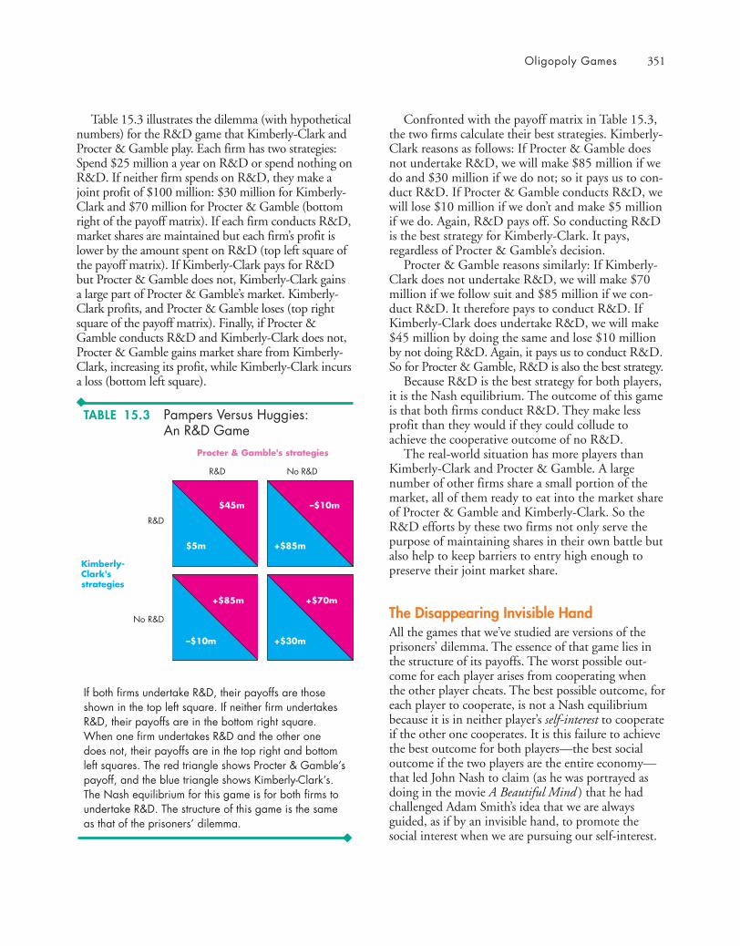
Oligopoly Games 351

Table 15.3 illustrates the dilemma (with hypotheticalnumbers) for the R&D game that Kimberly-Clark andProcter & Gamble play. Each firm has two strategies:Spend $25 million a year on R&D or spend nothing onR&D. If neither firm spends on R&D, they make ajoint profit of $100 million: $30 million for Kimberly-Clark and $70 million for Procter & Gamble (bottomright of the payoff matrix). If each firm conducts R&D,market shares are maintained but each firm’s profit islower by the amount spent on R&D (top left square ofthe payoff matrix). If Kimberly-Clark pays for R&Dbut Procter & Gamble does not, Kimberly-Clark gainsa large part of Procter & Gamble’s market. Kimberly-Clark profits, and Procter & Gamble loses (top rightsquare of the payoff matrix). Finally, if Procter &Gamble conducts R&D and Kimberly-Clark does not,Procter & Gamble gains market share from Kimberly-Clark, increasing its profit, while Kimberly-Clark incursa loss (bottom left square).

Confronted with the payoff matrix in Table 15.3,the two firms calculate their best strategies. Kimberly-Clark reasons as follows: If Procter & Gamble doesnot undertake R&D, we will make $85 million if wedo and $30 million if we do not; so it pays us to con-duct R&D. If Procter & Gamble conducts R&D, wewill lose $10 million if we don’t and make $5 millionif we do. Again, R&D pays off. So conducting R&Dis the best strategy for Kimberly-Clark. It pays,regardless of Procter & Gamble’s decision.

Procter & Gamble reasons similarly: If Kimberly-Clark does not undertake R&D, we will make $70million if we follow suit and $85 million if we con-duct R&D. It therefore pays to conduct R&D. IfKimberly-Clark does undertake R&D, we will make$45 million by doing the same and lose $10 millionby not doing R&D. Again, it pays us to conduct R&D.So for Procter & Gamble, R&D is also the best strategy.

Because R&D is the best strategy for both players,it is the Nash equilibrium. The outcome of this gameis that both firms conduct R&D. They make lessprofit than they would if they could collude toachieve the cooperative outcome of no R&D.

The real-world situation has more players thanKimberly-Clark and Procter & Gamble. A largenumber of other firms share a small portion of themarket, all of them ready to eat into the market shareof Procter & Gamble and Kimberly-Clark. So theR&D efforts by these two firms not only serve thepurpose of maintaining shares in their own battle butalso help to keep barriers to entry high enough topreserve their joint market share.

The Disappearing Invisible HandAll the games that we’ve studied are versions of theprisoners’ dilemma. The essence of that game lies inthe structure of its payoffs. The worst possible out-come for each player arises from cooperating whenthe other player cheats. The best possible outcome, foreach player to cooperate, is not a Nash equilibriumbecause it is in neither player’s self-interest to cooperateif the other one cooperates. It is this failure to achievethe best outcome for both players—the best socialoutcome if the two players are the entire economy—that led John Nash to claim (as he was portrayed asdoing in the movie A Beautiful Mind ) that he hadchallenged Adam Smith’s idea that we are alwaysguided, as if by an invisible hand, to promote thesocial interest when we are pursuing our self-interest.

Kimberly-Clark'sstrategies

Procter & Gamble's strategies

R&D

R&D

No R&D

No R&D

–$10m

+$85m

$45m

$5m

+$70m

+$30m

+$85m

–$10m

If both firms undertake R&D, their payoffs are thoseshown in the top left square. If neither firm undertakesR&D, their payoffs are in the bottom right square.When one firm undertakes R&D and the other onedoes not, their payoffs are in the top right and bottomleft squares. The red triangle shows Procter & Gamble’spayoff, and the blue triangle shows Kimberly-Clark’s.The Nash equilibrium for this game is for both firms toundertake R&D. The structure of this game is the sameas that of the prisoners’ dilemma.

TABLE 15.3 Pampers Versus Huggies: An R&D Game

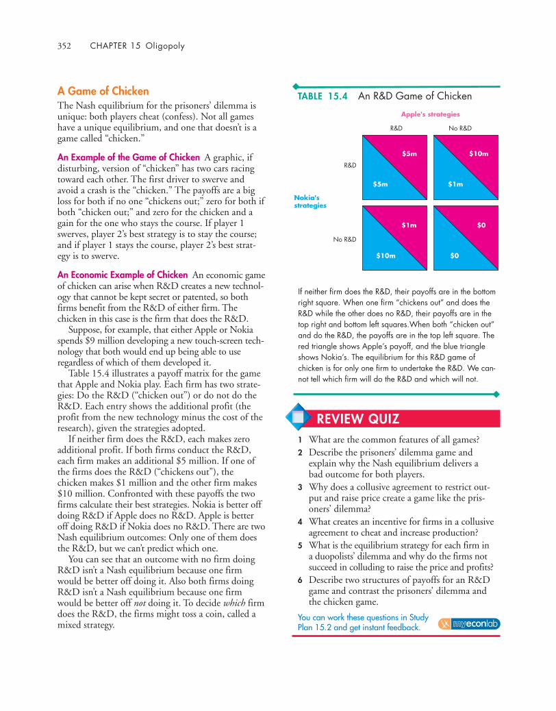
352 CHAPTER 15 Oligopoly

A Game of ChickenThe Nash equilibrium for the prisoners’ dilemma isunique: both players cheat (confess). Not all gameshave a unique equilibrium, and one that doesn’t is agame called “chicken.”

An Example of the Game of Chicken A graphic, ifdisturbing, version of “chicken” has two cars racingtoward each other. The first driver to swerve andavoid a crash is the “chicken.” The payoffs are a bigloss for both if no one “chickens out;” zero for both ifboth “chicken out;” and zero for the chicken and again for the one who stays the course. If player 1swerves, player 2’s best strategy is to stay the course;and if player 1 stays the course, player 2’s best strat-egy is to swerve.

An Economic Example of Chicken An economic gameof chicken can arise when R&D creates a new technol-ogy that cannot be kept secret or patented, so bothfirms benefit from the R&D of either firm. Thechicken in this case is the firm that does the R&D.

Suppose, for example, that either Apple or Nokiaspends $9 million developing a new touch-screen tech-nology that both would end up being able to useregardless of which of them developed it.

Table 15.4 illustrates a payoff matrix for the gamethat Apple and Nokia play. Each firm has two strate-gies: Do the R&D (“chicken out”) or do not do theR&D. Each entry shows the additional profit (theprofit from the new technology minus the cost of theresearch), given the strategies adopted.

If neither firm does the R&D, each makes zeroadditional profit. If both firms conduct the R&D,each firm makes an additional $5 million. If one ofthe firms does the R&D (“chickens out”), thechicken makes $1 million and the other firm makes$10 million. Confronted with these payoffs the twofirms calculate their best strategies. Nokia is better offdoing R&D if Apple does no R&D. Apple is betteroff doing R&D if Nokia does no R&D. There are twoNash equilibrium outcomes: Only one of them doesthe R&D, but we can’t predict which one.

You can see that an outcome with no firm doingR&D isn’t a Nash equilibrium because one firmwould be better off doing it. Also both firms doingR&D isn’t a Nash equilibrium because one firmwould be better off not doing it. To decide which firmdoes the R&D, the firms might toss a coin, called amixed strategy.

If neither firm does the R&D, their payoffs are in the bottomright square. When one firm “chickens out” and does theR&D while the other does no R&D, their payoffs are in thetop right and bottom left squares.When both “chicken out”and do the R&D, the payoffs are in the top left square. Thered triangle shows Apple’s payoff, and the blue triangleshows Nokia’s. The equilibrium for this R&D game ofchicken is for only one firm to undertake the R&D. We can-not tell which firm will do the R&D and which will not.

Nokia'sstrategies

Apple's strategies

R&D

R&D

No R&D

No R&D

$10m

$1m

$5m

$5m

$0

$0

$1m

$10m

TABLE 15.4 An R&D Game of Chicken

REVIEW QUIZ1 What are the common features of all games?2 Describe the prisoners’ dilemma game and

explain why the Nash equilibrium delivers abad outcome for both players.

3 Why does a collusive agreement to restrict out-put and raise price create a game like the pris-oners’ dilemma?

4 What creates an incentive for firms in a collusiveagreement to cheat and increase production?

5 What is the equilibrium strategy for each firm ina duopolists’ dilemma and why do the firms notsucceed in colluding to raise the price and profits?

6 Describe two structures of payoffs for an R&Dgame and contrast the prisoners’ dilemma andthe chicken game.

You can work these questions in Study Plan 15.2 and get instant feedback.

Repeated Games and Sequential Games 353

◆ Repeated Games and Sequential Games

The games that we’ve studied are played just once. Incontrast, many real-world games are played repeat-edly. This feature of games turns out to enable real-world duopolists to cooperate, collude, and make amonopoly profit.

Another feature of the games that we’ve studied isthat the players move simultaneously. But in manyreal-world situations, one player moves first and thenthe other moves—the play is sequential rather thansimultaneous. This feature of real-world games cre-ates a large number of possible outcomes.

We’re now going to examine these two aspects ofstrategic decision-making.

A Repeated Duopoly GameIf two firms play a game repeatedly, one firm has theopportunity to penalize the other for previous “bad”behavior. If Gear cheats this week, perhaps Trick willcheat next week. Before Gear cheats this week, won’tit consider the possibility that Trick will cheat nextweek? What is the equilibrium of this game?

Actually, there is more than one possibility. One isthe Nash equilibrium that we have just analyzed. Bothplayers cheat, and each makes zero economic profitforever. In such a situation, it will never pay one ofthe players to start complying unilaterally because todo so would result in a loss for that player and a profitfor the other. But a cooperative equilibrium in whichthe players make and share the monopoly profit ispossible.

A cooperative equilibrium might occur if cheatingis punished. There are two extremes of punishment.The smallest penalty is called “tit for tat.” A tit-for-tatstrategy is one in which a player cooperates in the cur-rent period if the other player cooperated in the pre-vious period, but cheats in the current period if theother player cheated in the previous period. The mostsevere form of punishment is called a trigger strategy.A trigger strategy is one in which a player cooperates ifthe other player cooperates but plays the Nash equi-librium strategy forever thereafter if the other playercheats.

In the duopoly game between Gear and Trick, atit-for-tat strategy keeps both players cooperating andmaking monopoly profits. Let’s see why with an example.

Table 15.5 shows the economic profit that Trickand Gear will make over a number of periods undertwo alternative sequences of events: colluding andcheating with a tit-for-tat response by the other firm.

If both firms stick to the collusive agreement inperiod 1, each makes an economic profit of $2 mil-lion. Suppose that Trick contemplates cheating inperiod 1. The cheating produces a quick $4.5 millioneconomic profit and inflicts a $1 million economicloss on Gear. But a cheat in period 1 produces aresponse from Gear in period 2. If Trick wants to getback into a profit-making situation, it must return tothe agreement in period 2 even though it knows thatGear will punish it for cheating in period 1. So inperiod 2, Gear punishes Trick and Trick cooperates.Gear now makes an economic profit of $4.5 million,and Trick incurs an economic loss of $1 million.Adding up the profits over two periods of play, Trickwould have made more profit by cooperating—$4million compared with $3.5 million.

What is true for Trick is also true for Gear. Becauseeach firm makes a larger profit by sticking with thecollusive agreement, both firms do so and themonopoly price, quantity, and profit prevail.

In reality, whether a cartel works like a one-playgame or a repeated game depends primarily on the

Cheat with Collude tit-for-tat

Trick’s Gear’s Trick’s Gear’sPeriod profit profit profit profitof play (millions of dollars) (millions of dollars)

1 2 2 4.5 –1.0

2 2 2 –1.0 4.5

3 2 2 2.0 2.0

4 . . . .

If duopolists repeatedly collude, each makes a profit of$2 million per period of play. If one player cheats inperiod 1, the other player plays a tit-for-tat strategyand cheats in period 2. The profit from cheating canbe made for only one period and must be paid for inthe next period by incurring a loss. Over two periodsof play, the best that a duopolist can achieve by cheat-ing is a profit of $3.5 million, compared to an eco-nomic profit of $4 million by colluding.

TABLE 15.5 Cheating with Punishment

354 CHAPTER 15 Oligopoly

number of players and the ease of detecting and pun-ishing cheating. The larger the number of players, theharder it is to maintain a cartel.

Games and Price Wars A repeated duopoly gamecan help us understand real-world behavior and, inparticular, price wars. Some price wars can be inter-preted as the implementation of a tit-for-tat strategy.But the game is a bit more complicated than the onewe’ve looked at because the players are uncertainabout the demand for the product.

Playing a tit-for-tat strategy, firms have an incen-tive to stick to the monopoly price. But fluctuationsin demand lead to fluctuations in the monopolyprice, and sometimes, when the price changes, itmight seem to one of the firms that the price hasfallen because the other has cheated. In this case, aprice war will break out. The price war will end onlywhen each firm is satisfied that the other is ready tocooperate again. There will be cycles of price warsand the restoration of collusive agreements.Fluctuations in the world price of oil might be inter-preted in this way.

Some price wars arise from the entry of a smallnumber of firms into an industry that had previ-ously been a monopoly. Although the industry has asmall number of firms, the firms are in a prisoners’dilemma and they cannot impose effective penaltiesfor price cutting. The behavior of prices and outputsin the computer chip industry during 1995 and1996 can be explained in this way. Until 1995, themarket for Pentium chips for IBM-compatible com-puters was dominated by one firm, Intel Corpora-tion, which was able to make maximum economicprofit by producing the quantity of chips at whichmarginal cost equaled marginal revenue. The priceof Intel’s chips was set to ensure that the quantitydemanded equaled the quantity produced. Then in1995 and 1996, with the entry of a small number ofnew firms, the industry became an oligopoly. If thefirms had maintained Intel’s price and shared themarket, together they could have made economicprofits equal to Intel’s profit. But the firms were in aprisoners’ dilemma, so prices fell toward the competi-tive level.

Let’s now study a sequential game. There are manysuch games, and the one we’ll examine is among thesimplest. It has an interesting implication and it willgive you the flavor of this type of game. The sequen-tial game that we’ll study is an entry game in a con-testable market.

A Sequential Entry Game in a Contestable MarketIf two firms play a sequential game, one firm makes adecision at the first stage of the game and the othermakes a decision at the second stage.

We’re going to study a sequential game in acontestable market—a market in which firms can enterand leave so easily that firms in the market face com-petition from potential entrants. Examples of con-testable markets are routes served by airlines and bybarge companies that operate on the major water-ways. These markets are contestable because firmscould enter if an opportunity for economic profitarose and could exit with no penalty if the opportu-nity for economic profit disappeared.

If the Herfindahl-Hirschman Index (p. 238) isused to determine the degree of competition, a con-testable market appears to be uncompetitive. But acontestable market can behave as if it were perfectlycompetitive. To see why, let’s look at an entry gamefor a contestable air route.

A Contestable Air Route Agile Air is the only firmoperating on a particular route. Demand and costconditions are such that there is room for only oneairline to operate. Wanabe Inc. is another airline thatcould offer services on the route.

We describe the structure of a sequential game byusing a game tree like that in Fig. 15.6. At the firststage, Agile Air must set a price. Once the price is setand advertised, Agile can’t change it. That is, once set,Agile’s price is fixed and Agile can’t react to Wanabe’sentry decision. Agile can set its price at either themonopoly level or the competitive level.

At the second stage, Wanabe must decide whetherto enter or to stay out. Customers have no loyalty(there are no frequent-flyer programs) and they buyfrom the lowest-price firm. So if Wanabe enters, it setsa price just below Agile’s and takes all the business.

Figure 15.6 shows the payoffs from the variousdecisions (Agile’s in the red triangles and Wanabe’s inthe blue triangles).

To decide on its price, Agile’s CEO reasons asfollows: Suppose that Agile sets the monopoly price.If Wanabe enters, it earns 90 (think of all payoffnumbers as thousands of dollars). If Wanabe staysout, it earns nothing. So Wanabe will enter. In thiscase Agile will lose 50.

Now suppose that Agile sets the competitive price.If Wanabe stays out, it earns nothing, and if it enters,

Repeated Games and Sequential Games 355

it loses 10, so Wanabe will stay out. In this case, Agilewill make zero economic profit.

Agile’s best strategy is to set its price at the com-petitive level and make zero economic profit. Theoption of earning 100 by setting the monopoly pricewith Wanabe staying out is not available to Agile. IfAgile sets the monopoly price, Wanabe enters, under-cuts Agile, and takes all the business.

In this example, Agile sets its price at the com-petitive level and makes zero economic profit. A lesscostly strategy, called limit pricing, sets the price atthe highest level that inflicts a loss on the entrant.Any loss is big enough to deter entry, so it is notalways necessary to set the price as low as the com-petitive price. In the example of Agile and Wanabe,at the competitive price, Wanabe incurs a loss of 10if it enters. A smaller loss would still keep Wanabeout.

This game is interesting because it points to thepossibility of a monopoly behaving like a competitiveindustry and serving the social interest without regu-lation. But the result is not general and depends onone crucial feature of the setup of the game: At thesecond stage, Agile is locked in to the price set at thefirst stage.

If Agile could change its price in the second stage,it would want to set the monopoly price if Wanabestayed out—100 with the monopoly price beats zerowith the competitive price. But Wanabe can figure outwhat Agile would do, so the price set at the first stage

has no effect on Wanabe. Agile sets the monopolyprice and Wanabe might either stay out or enter.

We’ve looked at two of the many possible repeatedand sequential games, and you’ve seen how thesetypes of games can provide insights into the complexforces that determine prices and profits.

90

–50

0

100

–10

–50

0

0

Monopoly price

Enter

Stay out

Enter

Stay out

Competitive price

Agile

First stage Second stage Payoffs

Wanabe

Wanabe

If Agile sets the monopoly price, Wanabe makes 90 (thou-sand dollars) by entering and earns nothing by staying out.So if Agile sets the monopoly price, Wanabe enters.

If Agile sets the competitive price, Wanabe earns noth-ing if it stays out and incurs a loss if it enters. So if Agilesets the competitive price, Wanabe stays out.

So far, we’ve studied oligopoly with unregulatedmarket power. Firms like Trick and Gear are free tocollude to maximize their profit with no concern forthe consumer or the law.

But when firms collude to achieve the monopolyoutcome, they also have the same effects on efficiencyand the social interest as monopoly. Profit is made atthe expense of consumer surplus and a deadweightloss arises. Your next task is to see how U.S. antitrustlaw limits market power.

FIGURE 15.6 Agile Versus Wanabe: A Sequential Entry Game in a Contestable Market

animation

REVIEW QUIZ1 If a prisoners’ dilemma game is played repeatedly,

what punishment strategies might the playersemploy and how does playing the game repeat-edly change the equilibrium?

2 If a market is contestable, how does the equilib-rium differ from that of a monopoly?

You can work these questions in Study Plan 15.3 and get instant feedback.

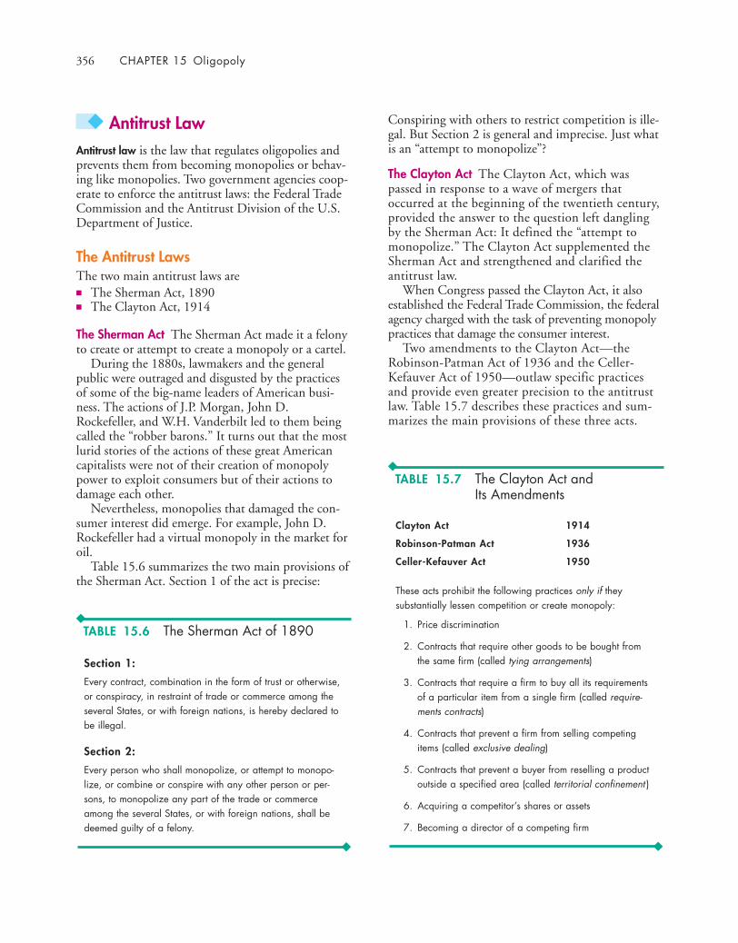
356 CHAPTER 15 Oligopoly

◆ Antitrust LawAntitrust law is the law that regulates oligopolies andprevents them from becoming monopolies or behav-ing like monopolies. Two government agencies coop-erate to enforce the antitrust laws: the Federal TradeCommission and the Antitrust Division of the U.S.Department of Justice.

The Antitrust LawsThe two main antitrust laws are■ The Sherman Act, 1890■ The Clayton Act, 1914

The Sherman Act The Sherman Act made it a felonyto create or attempt to create a monopoly or a cartel.

During the 1880s, lawmakers and the generalpublic were outraged and disgusted by the practicesof some of the big-name leaders of American busi-ness. The actions of J.P. Morgan, John D.Rockefeller, and W.H. Vanderbilt led to them beingcalled the “robber barons.” It turns out that the mostlurid stories of the actions of these great Americancapitalists were not of their creation of monopolypower to exploit consumers but of their actions todamage each other.

Nevertheless, monopolies that damaged the con-sumer interest did emerge. For example, John D.Rockefeller had a virtual monopoly in the market foroil.

Table 15.6 summarizes the two main provisions ofthe Sherman Act. Section 1 of the act is precise:

Conspiring with others to restrict competition is ille-gal. But Section 2 is general and imprecise. Just whatis an “attempt to monopolize”?

The Clayton Act The Clayton Act, which waspassed in response to a wave of mergers thatoccurred at the beginning of the twentieth century,provided the answer to the question left danglingby the Sherman Act: It defined the “attempt tomonopolize.” The Clayton Act supplemented theSherman Act and strengthened and clarified theantitrust law.

When Congress passed the Clayton Act, it alsoestablished the Federal Trade Commission, the federalagency charged with the task of preventing monopolypractices that damage the consumer interest.

Two amendments to the Clayton Act—theRobinson-Patman Act of 1936 and the Celler-Kefauver Act of 1950—outlaw specific practicesand provide even greater precision to the antitrustlaw. Table 15.7 describes these practices and sum-marizes the main provisions of these three acts.

Section 1:

Every contract, combination in the form of trust or otherwise,or conspiracy, in restraint of trade or commerce among theseveral States, or with foreign nations, is hereby declared tobe illegal.

Section 2:

Every person who shall monopolize, or attempt to monopo-lize, or combine or conspire with any other person or per-sons, to monopolize any part of the trade or commerceamong the several States, or with foreign nations, shall bedeemed guilty of a felony.

Clayton Act 1914

Robinson-Patman Act 1936

Celler-Kefauver Act 1950

These acts prohibit the following practices only if theysubstantially lessen competition or create monopoly:

1. Price discrimination

2. Contracts that require other goods to be bought fromthe same firm (called tying arrangements)

3. Contracts that require a firm to buy all its requirementsof a particular item from a single firm (called require-ments contracts)

4. Contracts that prevent a firm from selling competingitems (called exclusive dealing)

5. Contracts that prevent a buyer from reselling a productoutside a specified area (called territorial confinement )

6. Acquiring a competitor’s shares or assets

7. Becoming a director of a competing firm

TABLE 15.6 The Sherman Act of 1890

TABLE 15.7 The Clayton Act andIts Amendments

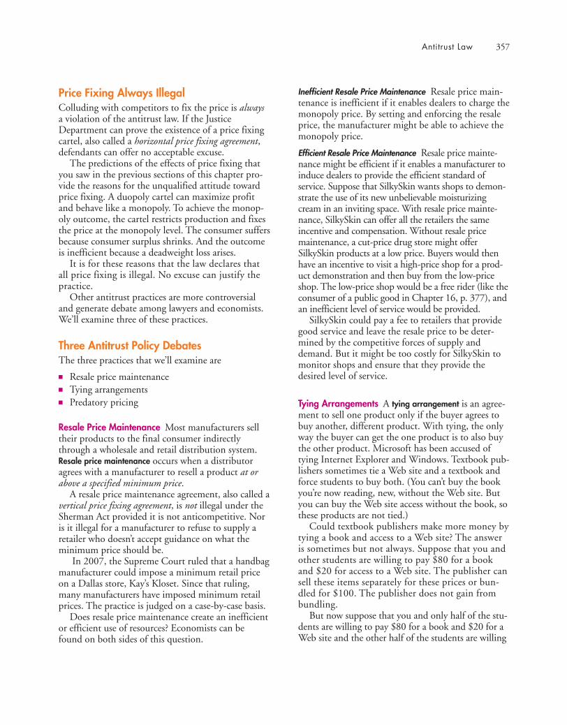
Antitrust Law 357

Price Fixing Always IllegalColluding with competitors to fix the price is alwaysa violation of the antitrust law. If the JusticeDepartment can prove the existence of a price fixingcartel, also called a horizontal price fixing agreement,defendants can offer no acceptable excuse.

The predictions of the effects of price fixing thatyou saw in the previous sections of this chapter pro-vide the reasons for the unqualified attitude towardprice fixing. A duopoly cartel can maximize profitand behave like a monopoly. To achieve the monop-oly outcome, the cartel restricts production and fixesthe price at the monopoly level. The consumer suffersbecause consumer surplus shrinks. And the outcomeis inefficient because a deadweight loss arises.

It is for these reasons that the law declares thatall price fixing is illegal. No excuse can justify thepractice.

Other antitrust practices are more controversialand generate debate among lawyers and economists.We’ll examine three of these practices.

Three Antitrust Policy DebatesThe three practices that we’ll examine are

■ Resale price maintenance■ Tying arrangements■ Predatory pricing

Resale Price Maintenance Most manufacturers selltheir products to the final consumer indirectlythrough a wholesale and retail distribution system.Resale price maintenance occurs when a distributoragrees with a manufacturer to resell a product at orabove a specified minimum price.

A resale price maintenance agreement, also called avertical price fixing agreement, is not illegal under theSherman Act provided it is not anticompetitive. Noris it illegal for a manufacturer to refuse to supply aretailer who doesn’t accept guidance on what theminimum price should be.

In 2007, the Supreme Court ruled that a handbagmanufacturer could impose a minimum retail priceon a Dallas store, Kay’s Kloset. Since that ruling,many manufacturers have imposed minimum retailprices. The practice is judged on a case-by-case basis.

Does resale price maintenance create an inefficientor efficient use of resources? Economists can befound on both sides of this question.

Inefficient Resale Price Maintenance Resale price main-tenance is inefficient if it enables dealers to charge themonopoly price. By setting and enforcing the resaleprice, the manufacturer might be able to achieve themonopoly price.

Efficient Resale Price Maintenance Resale price mainte-nance might be efficient if it enables a manufacturer toinduce dealers to provide the efficient standard ofservice. Suppose that SilkySkin wants shops to demon-strate the use of its new unbelievable moisturizingcream in an inviting space. With resale price mainte-nance, SilkySkin can offer all the retailers the sameincentive and compensation. Without resale pricemaintenance, a cut-price drug store might offerSilkySkin products at a low price. Buyers would thenhave an incentive to visit a high-price shop for a prod-uct demonstration and then buy from the low-priceshop. The low-price shop would be a free rider (like theconsumer of a public good in Chapter 16, p. 377), andan inefficient level of service would be provided.

SilkySkin could pay a fee to retailers that providegood service and leave the resale price to be deter-mined by the competitive forces of supply anddemand. But it might be too costly for SilkySkin tomonitor shops and ensure that they provide thedesired level of service.

Tying Arrangements A tying arrangement is an agree-ment to sell one product only if the buyer agrees tobuy another, different product. With tying, the onlyway the buyer can get the one product is to also buythe other product. Microsoft has been accused oftying Internet Explorer and Windows. Textbook pub-lishers sometimes tie a Web site and a textbook andforce students to buy both. (You can’t buy the bookyou’re now reading, new, without the Web site. Butyou can buy the Web site access without the book, sothese products are not tied.)

Could textbook publishers make more money bytying a book and access to a Web site? The answeris sometimes but not always. Suppose that you andother students are willing to pay $80 for a bookand $20 for access to a Web site. The publisher cansell these items separately for these prices or bun-dled for $100. The publisher does not gain frombundling.

But now suppose that you and only half of the stu-dents are willing to pay $80 for a book and $20 for aWeb site and the other half of the students are willing

358 CHAPTER 15 Oligopoly

to pay $80 for a Web site and $20 for a book. Now ifthe two items are sold separately, the publisher cancharge $80 for the book and $80 for the Web site.Half the students buy the book but not the Web site,and the other half buy the Web site but not the book.But if the book and Web site are bundled for $100,everyone buys the bundle and the publisher makes anextra $20 per student. In this case, bundling hasenabled the publisher to price discriminate.

There is no simple, clear-cut test of whether a firmis engaging in tying or whether, by doing so, it hasincreased its market power and profit and createdinefficiency.

Predatory Pricing Predatory pricing is setting a lowprice to drive competitors out of business with theintention of setting a monopoly price when the com-

petition has gone. John D. Rockefeller’s Standard OilCompany was the first to be accused of this practice inthe 1890s, and it has been claimed often in antitrustcases since then. Predatory pricing is an attempt to cre-ate a monopoly and as such it is illegal under Section 2of the Sherman Act.

It is easy to see that predatory pricing is an idea, nota reality. Economists are skeptical that predatory pric-ing occurs. They point out that a firm that cuts itsprice below the profit-maximizing level loses duringthe low-price period. Even if it succeeds in driving itscompetitors out of business, new competitors willenter as soon as the price is increased, so any potentialgain from a monopoly position is temporary. A highand certain loss is a poor exchange for a temporary anduncertain gain. No case of predatory pricing has beendefinitively found.

only a competing operating system but also an entirerange of supporting applications as well.

When Microsoft entered the Web browser marketwith its Internet Explorer, it offered the browser for azero price. This price was viewed as predatory pricing.Microsoft integrated Internet Explorer with Windowsso that anyone who uses this operating system wouldnot need a separate browser such as NetscapeNavigator. Microsoft’s competitors claimed that thispractice was an illegal tying arrangement.

Microsoft’s Response Microsoft challenged all theseclaims. It said that Windows was vulnerable to com-petition from other operating systems such as Linuxand Apple’s Mac OS and that there was a permanentthreat of competition from new entrants.

Microsoft claimed that integrating Internet Explorerwith Windows provided a single, unified product ofgreater consumer value like a refrigerator with a chilledwater dispenser or an automobile with a CD player.

The Outcome The court agreed that Microsoft was inviolation of the Sherman Act and ordered that it bebroken into two firms: an operating systems producerand an applications producer. Microsoft successfullyappealed this order. In the final judgment, though,Microsoft was ordered to disclose to other softwaredevelopers details of how its operating system works,so that they could compete effectively againstMicrosoft. In the summer of 2002, Microsoft beganto comply with this order.

Economics in ActionThe United States Versus MicrosoftIn 1998, the Antitrust Division of the U.S. Depart-ment of Justice along with the Departments of Justiceof a number of states charged Microsoft, the world’slargest producer of software for personal computers,with violations of both sections of the Sherman Act.

A 78-day trial followed that pitched two promi-nent MIT economics professors against each other,Franklin Fisher for the government and RichardSchmalensee for Microsoft.

The Case Against Microsoft The claims againstMicrosoft were that it

■ Possessed monopoly power■ Used predatory pricing and tying arrangements■ Used other anticompetitive practices

It was claimed that with 80 percent of the marketfor PC operating systems, Microsoft had excessivemonopoly power. This monopoly power arose fromtwo barriers to entry: economies of scale and networkeconomies. Microsoft’s average total cost falls as pro-duction increases (economies of scale) because thefixed cost of developing an operating system such asWindows is large while the marginal cost of produc-ing one copy of Windows is small. Further, as thenumber of Windows users increases, the range ofWindows applications expands (network economies),so a potential competitor would need to produce not

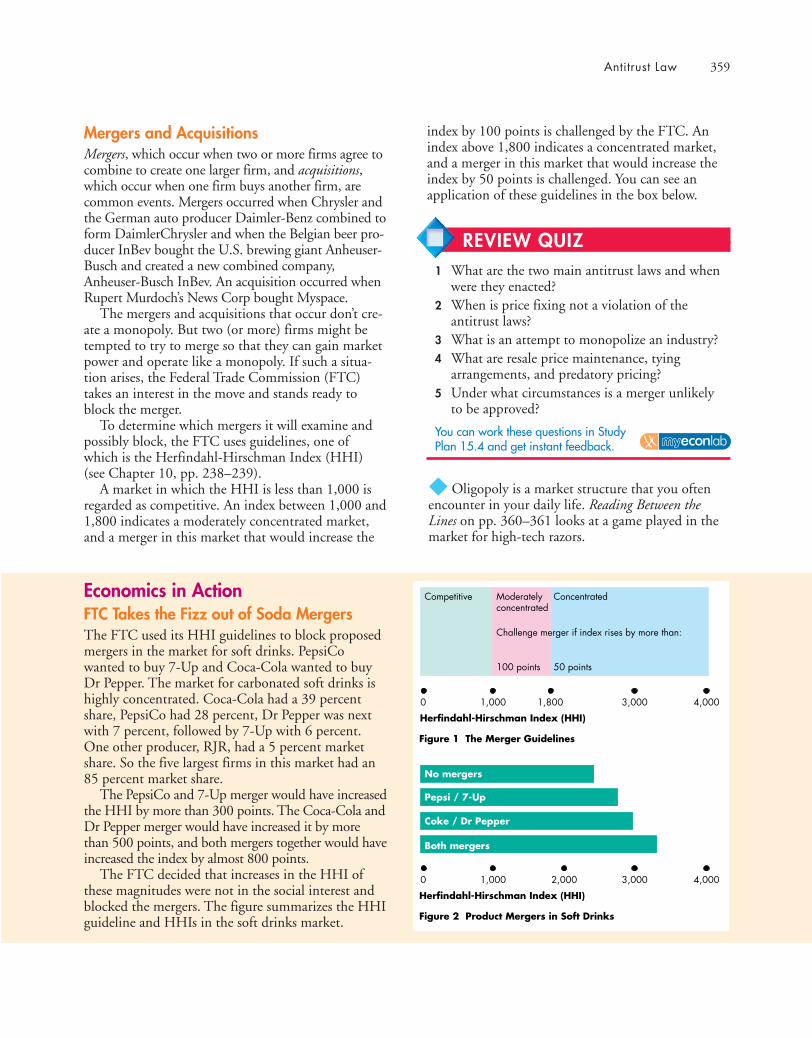
Antitrust Law 359

Mergers and AcquisitionsMergers, which occur when two or more firms agree tocombine to create one larger firm, and acquisitions,which occur when one firm buys another firm, arecommon events. Mergers occurred when Chrysler andthe German auto producer Daimler-Benz combined toform DaimlerChrysler and when the Belgian beer pro-ducer InBev bought the U.S. brewing giant Anheuser-Busch and created a new combined company,Anheuser-Busch InBev. An acquisition occurred whenRupert Murdoch’s News Corp bought Myspace.

The mergers and acquisitions that occur don’t cre-ate a monopoly. But two (or more) firms might betempted to try to merge so that they can gain marketpower and operate like a monopoly. If such a situa-tion arises, the Federal Trade Commission (FTC)takes an interest in the move and stands ready toblock the merger.

To determine which mergers it will examine andpossibly block, the FTC uses guidelines, one ofwhich is the Herfindahl-Hirschman Index (HHI)(see Chapter 10, pp. 238–239).

A market in which the HHI is less than 1,000 isregarded as competitive. An index between 1,000 and1,800 indicates a moderately concentrated market,and a merger in this market that would increase the

◆ Oligopoly is a market structure that you oftenencounter in your daily life. Reading Between theLines on pp. 360–361 looks at a game played in themarket for high-tech razors.

Economics in ActionFTC Takes the Fizz out of Soda MergersThe FTC used its HHI guidelines to block proposedmergers in the market for soft drinks. PepsiCowanted to buy 7-Up and Coca-Cola wanted to buyDr Pepper. The market for carbonated soft drinks ishighly concentrated. Coca-Cola had a 39 percentshare, PepsiCo had 28 percent, Dr Pepper was nextwith 7 percent, followed by 7-Up with 6 percent.One other producer, RJR, had a 5 percent marketshare. So the five largest firms in this market had an85 percent market share.

The PepsiCo and 7-Up merger would have increasedthe HHI by more than 300 points. The Coca-Cola andDr Pepper merger would have increased it by morethan 500 points, and both mergers together would haveincreased the index by almost 800 points.

The FTC decided that increases in the HHI ofthese magnitudes were not in the social interest andblocked the mergers. The figure summarizes the HHIguideline and HHIs in the soft drinks market.

index by 100 points is challenged by the FTC. Anindex above 1,800 indicates a concentrated market,and a merger in this market that would increase theindex by 50 points is challenged. You can see anapplication of these guidelines in the box below.

0 1,000 2,000 3,000 4,000

Both mergers

Coke / Dr Pepper

Pepsi / 7-Up

No mergers

Figure 2 Product Mergers in Soft Drinks

Herfindahl-Hirschman Index (HHI)

0 1,000 1,800 3,000 4,000

Figure 1 The Merger Guidelines

Herfindahl-Hirschman Index (HHI)

Moderatelyconcentrated

Concentrated

Challenge merger if index rises by more than:

100 points 50 points

Competitive

REVIEW QUIZ1 What are the two main antitrust laws and when

were they enacted?2 When is price fixing not a violation of the

antitrust laws?3 What is an attempt to monopolize an industry?4 What are resale price maintenance, tying

arrangements, and predatory pricing?5 Under what circumstances is a merger unlikely

to be approved?

You can work these questions in Study Plan 15.4 and get instant feedback.

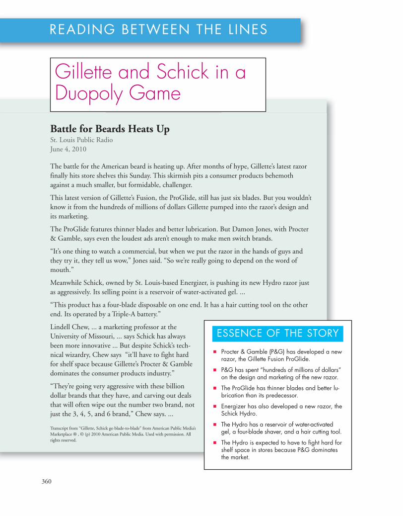
360

READING BETWEEN THE L INES

Battle for Beards Heats UpSt. Louis Public RadioJune 4, 2010

The battle for the American beard is heating up. After months of hype, Gillette’s latest razorfinally hits store shelves this Sunday. This skirmish pits a consumer products behemothagainst a much smaller, but formidable, challenger.

This latest version of Gillette’s Fusion, the ProGlide, still has just six blades. But you wouldn’tknow it from the hundreds of millions of dollars Gillette pumped into the razor’s design andits marketing.

The ProGlide features thinner blades and better lubrication. But Damon Jones, with Procter& Gamble, says even the loudest ads aren’t enough to make men switch brands.

“It’s one thing to watch a commercial, but when we put the razor in the hands of guys andthey try it, they tell us wow,” Jones said. “So we’re really going to depend on the word ofmouth.”

Meanwhile Schick, owned by St. Louis-based Energizer, is pushing its new Hydro razor justas aggressively. Its selling point is a reservoir of water-activated gel. ...

“This product has a four-blade disposable on one end. It has a hair cutting tool on the otherend. Its operated by a Triple-A battery.”

Lindell Chew, ... a marketing professor at theUniversity of Missouri, ... says Schick has alwaysbeen more innovative ... But despite Schick’s tech-nical wizardry, Chew says “it’ll have to fight hardfor shelf space because Gillette’s Procter & Gambledominates the consumer products industry.”

“They’re going very aggressive with these billiondollar brands that they have, and carving out dealsthat will often wipe out the number two brand, notjust the 3, 4, 5, and 6 brand,” Chew says. ...

Transcript from “Gillette, Schick go blade-to-blade” from American Public Media’sMarketplace ® , © (p) 2010 American Public Media. Used with permission. Allrights reserved.

■ Procter & Gamble (P&G) has developed a newrazor, the Gillette Fusion ProGlide.

■ P&G has spent “hundreds of millions of dollars”on the design and marketing of the new razor.

■ The ProGlide has thinner blades and better lu-brication than its predecessor.

■ Energizer has also developed a new razor, theSchick Hydro.

■ The Hydro has a reservoir of water-activatedgel, a four-blade shaver, and a hair cutting tool.

■ The Hydro is expected to have to fight hard forshelf space in stores because P&G dominatesthe market.

ESSENCE OF THE STORY

Gillette and Schick in aDuopoly Game

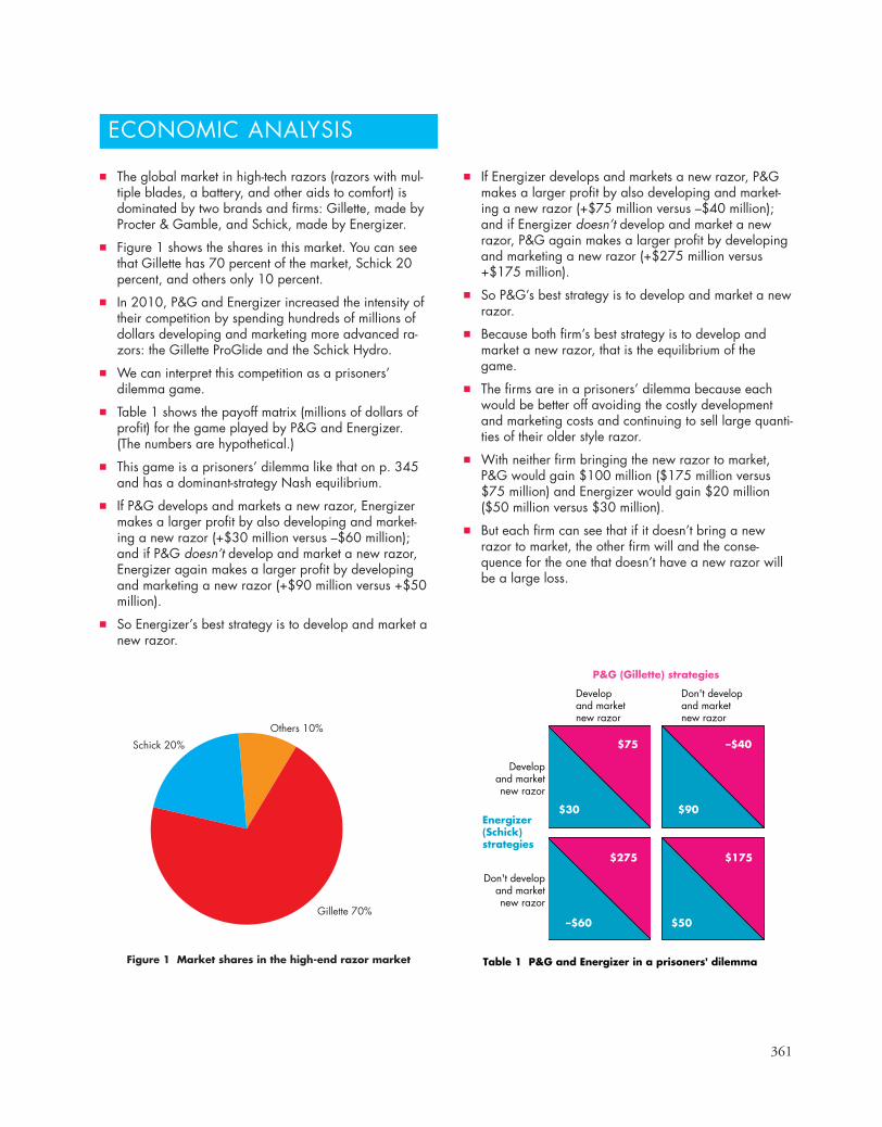
361

ECONOMIC ANALYSIS

Table 1 P&G and Energizer in a prisoners' dilemma

Energizer(Schick)strategies

P&G (Gillette) strategies

Developand marketnew razor

Developand marketnew razor

Don't developand marketnew razor

Don't developand marketnew razor

–$40

$90

$75

$30

$175

$50

$275

–$60Gillette 70%

Schick 20%

Others 10%

Figure 1 Market shares in the high-end razor market

■ If Energizer develops and markets a new razor, P&Gmakes a larger profit by also developing and market-ing a new razor (+$75 million versus –$40 million);and if Energizer doesn’t develop and market a newrazor, P&G again makes a larger profit by developingand marketing a new razor (+$275 million versus+$175 million).

■ So P&G’s best strategy is to develop and market a newrazor.

■ Because both firm’s best strategy is to develop andmarket a new razor, that is the equilibrium of thegame.

■ The firms are in a prisoners’ dilemma because eachwould be better off avoiding the costly developmentand marketing costs and continuing to sell large quanti-ties of their older style razor.

■ With neither firm bringing the new razor to market,P&G would gain $100 million ($175 million versus$75 million) and Energizer would gain $20 million($50 million versus $30 million).

■ But each firm can see that if it doesn’t bring a newrazor to market, the other firm will and the conse-quence for the one that doesn’t have a new razor willbe a large loss.

■ The global market in high-tech razors (razors with mul-tiple blades, a battery, and other aids to comfort) isdominated by two brands and firms: Gillette, made byProcter & Gamble, and Schick, made by Energizer.

■ Figure 1 shows the shares in this market. You can seethat Gillette has 70 percent of the market, Schick 20percent, and others only 10 percent.

■ In 2010, P&G and Energizer increased the intensity oftheir competition by spending hundreds of millions ofdollars developing and marketing more advanced ra-zors: the Gillette ProGlide and the Schick Hydro.

■ We can interpret this competition as a prisoners’dilemma game.

■ Table 1 shows the payoff matrix (millions of dollars ofprofit) for the game played by P&G and Energizer.(The numbers are hypothetical.)

■ This game is a prisoners’ dilemma like that on p. 345and has a dominant-strategy Nash equilibrium.

■ If P&G develops and markets a new razor, Energizermakes a larger profit by also developing and market-ing a new razor (+$30 million versus –$60 million);and if P&G doesn’t develop and market a new razor,Energizer again makes a larger profit by developingand marketing a new razor (+$90 million versus +$50million).

■ So Energizer’s best strategy is to develop and market anew razor.

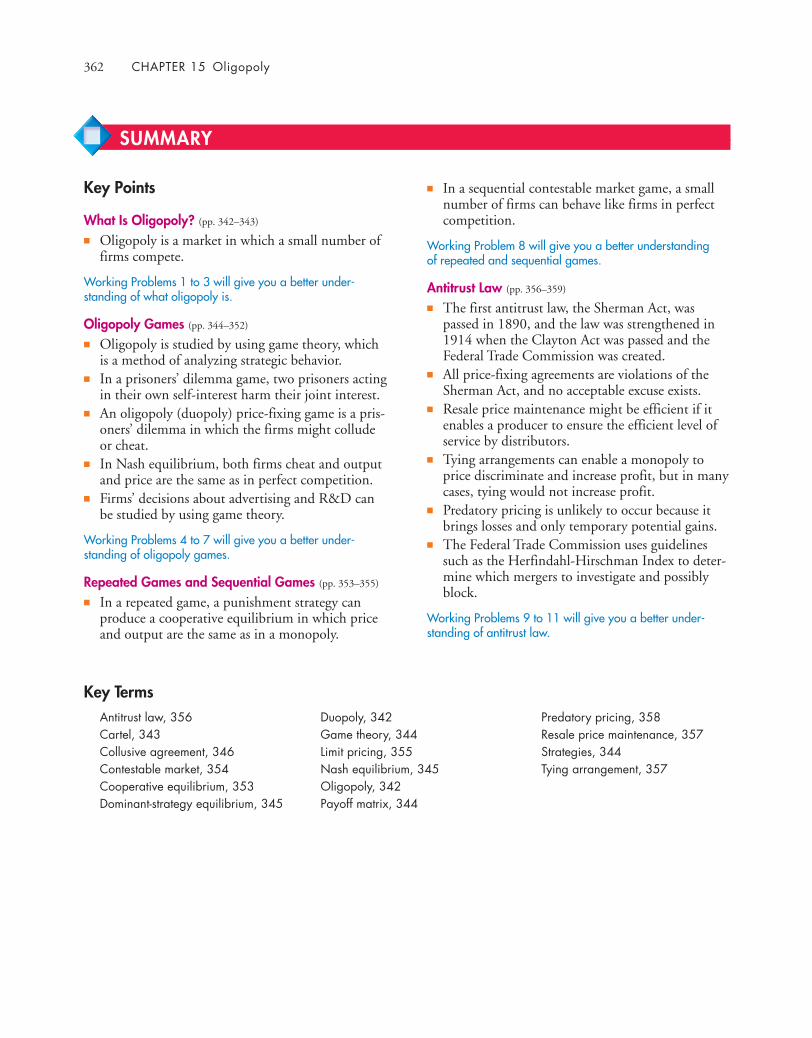
362 CHAPTER 15 Oligopoly

■ In a sequential contestable market game, a smallnumber of firms can behave like firms in perfectcompetition.

Working Problem 8 will give you a better understandingof repeated and sequential games.

Antitrust Law (pp. 356–359)

■ The first antitrust law, the Sherman Act, waspassed in 1890, and the law was strengthened in1914 when the Clayton Act was passed and theFederal Trade Commission was created.

■ All price-fixing agreements are violations of theSherman Act, and no acceptable excuse exists.

■ Resale price maintenance might be efficient if itenables a producer to ensure the efficient level ofservice by distributors.

■ Tying arrangements can enable a monopoly toprice discriminate and increase profit, but in manycases, tying would not increase profit.

■ Predatory pricing is unlikely to occur because itbrings losses and only temporary potential gains.

■ The Federal Trade Commission uses guidelinessuch as the Herfindahl-Hirschman Index to deter-mine which mergers to investigate and possiblyblock.

Working Problems 9 to 11 will give you a better under-standing of antitrust law.

Key Points

What Is Oligopoly? (pp. 342–343)

■ Oligopoly is a market in which a small number offirms compete.

Working Problems 1 to 3 will give you a better under-standing of what oligopoly is.

Oligopoly Games (pp. 344–352)

■ Oligopoly is studied by using game theory, whichis a method of analyzing strategic behavior.

■ In a prisoners’ dilemma game, two prisoners actingin their own self-interest harm their joint interest.

■ An oligopoly (duopoly) price-fixing game is a pris-oners’ dilemma in which the firms might colludeor cheat.

■ In Nash equilibrium, both firms cheat and outputand price are the same as in perfect competition.

■ Firms’ decisions about advertising and R&D canbe studied by using game theory.

Working Problems 4 to 7 will give you a better under-standing of oligopoly games.

Repeated Games and Sequential Games (pp. 353–355)

■ In a repeated game, a punishment strategy canproduce a cooperative equilibrium in which priceand output are the same as in a monopoly.

SUMMARY

Key TermsAntitrust law, 356Cartel, 343Collusive agreement, 346Contestable market, 354Cooperative equilibrium, 353Dominant-strategy equilibrium, 345

Duopoly, 342Game theory, 344Limit pricing, 355Nash equilibrium, 345Oligopoly, 342Payoff matrix, 344

Predatory pricing, 358Resale price maintenance, 357Strategies, 344Tying arrangement, 357

Study Plan Problems and Applications 363

a. Describe the strategies and payoffs of thisgame.

b. Construct the payoff matrix.c. What is the equilibrium of this game?d. Compare this game to the prisoners’ dilemma.

Are the two games similar or different?Explain.

Use the following information to work Problems 5and 6.Soapy Inc. and Suddies Inc. are the only producers ofsoap powder. They collude and agree to share themarket equally. If neither firm cheats on the agree-ment, each makes $1 million profit. If either firmcheats, the cheat makes a profit of $1.5 million, whilethe complier incurs a loss of $0.5 million. If bothcheat, they break even. Neither firm can monitor theother’s actions.

5. a.What are the strategies in this game?b. Construct the payoff matrix for this game.

6 a.What is the equilibrium of this game if it isplayed only once?

b. Is the equilibrium a dominant-strategy equi-librium? Explain.

7. The World’s Largest AirlineOn May 3, 2010, United Airlines andContinental Airlines announced a $3 billionmerger that would create the world’s biggestairline. The deal was completed in a remarkablyshort three weeks, and would give the airlines themuscle to fend off low-cost rivals at home and totake on foreign carriers abroad. For consumers,the merger could eventually result in higherprices although the new company does notintend to raise fares. One of the rationales forairline mergers is to cut capacity.

Source: The New York Times, June 7, 2010a. Explain how this airline merger might increase

air travel prices.b. Explain how this airline merger might lower

air travel production costs.c. Explain how cost savings arising from a cut in

capacity might get passed on to travelers andmight boost producers’ profits. Which do youpredict will happen from this airline mergerand why?

What Is Oligopoly? (Study Plan 15.1)

1. Two firms make most of the chips that power aPC: Intel and Advanced Micro Devices. Whatmakes the market for PC chips a duopoly?Sketch the market demand curve and cost curvesthat describe the situation in this market andthat prevent other firms from entering.

2. Sparks Fly for EnergizerEnergizer is gaining market share against com-petitor Duracell and its profit is rising despite thesharp rise in the price of zinc, a key battery ingre-dient.

Source: www.businessweek.com, August 2007In what type of market are batteries sold? Explainyour answer.

3. Oil CityIn the late 1990s, Reliance spent $6 billion tobuild a world-class oil refinery at Jamnagar,India. Now Reliance is more than doubling thesize of the facility, which will make it the world’sbiggest producer of gasoline —1.2 million gal-lons of gasoline per day, or about 5% of globalcapacity. Reliance plans to sell the gasoline in theUnited States and Europe where it’s too expen-sive and politically difficult to build new refiner-ies. The bulked-up Jamnagar will be able to movethe market and Singapore traders expect a dropin fuel prices as soon as it’s going at full steam.

Source: Fortune, April 28, 2008

a. Explain why the news clip claims that theglobal market for gasoline is not perfectlycompetitive.

b. What barriers to entry might limit competi-tion in this market and give a firm such as Re-liance power to influence the market price?

Oligopoly Games (Study Plan 15.2)

4. Consider a game with two players who cannotcommunicate, and in which each player is askeda question. The players can answer the questionhonestly or lie. If both answer honestly, eachreceives $100. If one player answers honestly andthe other lies, the liar receives $500 and the hon-est player gets nothing. If both lie, then eachreceives $50.

You can work Problems 1 to 12 in MyEconLab Chapter 15 Study Plan and get instant feedback.

STUDY PLAN PROBLEMS AND APPLICATIONS

364 CHAPTER 15 Oligopoly

Repeated Games and Sequential Games(Study Plan 15.3)

8. If Soapy Inc. and Suddies Inc., repeatedly playthe duopoly game that has the payoffs describedin Problem 5, on each round of play:a. What now are the strategies that each firm

might adopt?b. Can the firms adopt a strategy that gives the

game a cooperative equilibrium?c. Would one firm still be tempted to cheat in a

cooperative equilibrium? Explain your answer.

Antitrust Law (Study Plan 15.4)

9. Price Cuts Seen for Apple’s New iPhoneAT&T plans to sell the new iPhone for $200.The lower-priced phone would give AT&T anattractive weapon to win new subscribers.AT&T’s revenue is an average of $95 a monthfrom each iPhone customer, nearly twice theaverage of its conventional cell phone user.AT&T has a revenue-sharing agreement withApple that requires it to give Apple 25% of itsiPhone customers’ monthly payments. AT&T offers a $200 subsidy to customers wholock into the carrier for two years. It’s a smallinvestment for AT&T for a large return. Aftergiving Apple its cut of the revenue, AT&Treceives between $70 and $75 a month periPhone user, totaling more than $1,700 over thelife of the two-year contract.

Source: Fortune, June 2, 2008a. How does this arrangement between AT&T

and Apple regarding the iPhone affect compe-tition in the market for cell-phone service?

b. Does the iPhone arrangement between AT&Tand Apple violate U.S. antitrust laws? Explain.

10. Congress Examines Giant Airline MergerCongress examined a proposed merger betweenDelta Airlines and Northwest Airlines that woulddiscourage competition, reduce service, andresult in higher fares. Delta claims that themerger would not limit competition because thecarriers primarily serve different geographicregions. Witnesses scheduled to testify before theHouse Subcommittee were likely to focus onwhether the merger would result in lower airfaresor reduced competition.

Source: CNN, May 14, 2008

Explain the guidelines that the Federal TradeCommission uses to evaluate mergers and why itmight permit or block this merger.

11. AT&T’s New Pricing Takes Smartphones to theMassesAT&T, the second largest U.S. wireless carrierand only operator offering the iPhone, plans toattract average consumers to sign up for dataservice by cutting its prices: A $15 a month planfor 200 megabytes of data; $25 a month plan for2 gigabytes of data. Verizon Wireless, the largestU.S. wireless operator, wouldn’t comment onAT&T’s new pricing plans. But if history is anyindication, it won’t take long before Verizon,operator of the HTC Incredible, a smartphonethat looks very similar to an iPhone, begins offer-ing tiered data service.

Source: Cnet News, June 3, 2010a. Describe the basis of the competition between

AT&T and Verizon.b. Is AT&T likely to be using predatory pricing?c. If a price war develops in the market for data

services, who benefits most?

Economics in the News (Study Plan 15.N)

12. Starbucks Sued for Trying to Sink CompetitionPenny Stafford, owner of the Seattle-based BelviCoffee and Tea Exchange Inc. filed the lawsuit,which contends that Starbucks exploited itsmonopoly power. Starbucks used predatorypractices such as offering to pay leases thatexceeded market value if the building ownerwould refuse to allow competitors into the samebuilding; having its employees offer free coffeesamples in front of her store to lure away cus-tomers; and offering to buy out competitors atbelow-market prices and threatening to opennearby stores if the offer is rejected.

Source: CNN, September 26, 2006a. Explain how Starbucks is alleged to have vio-

lated U.S. antitrust laws in Seattle.b. Explain why it is unlikely that Starbucks

might use predatory pricing to permanentlydrive out competition.

c. What information would you need that is notprovided in the news clip to decide whetherStarbucks had practiced predatory pricing?

d. Sketch the situation facing Belvi Coffee andTea Exchange Inc. when the firm closed.

Additional Problems and Applications 365

What Is Oligopoly?

13. An Energy Drink with a Monster of a StockThe $5.7 billion energy-drink category, in whichMonster holds the No. 2 position behind indus-try leader Red Bull, has slowed down as copycatbrands jostle for shelf space. Over the past fiveyears Red Bull’s market share in dollar terms hasgone from 91 percent to well under 50 percentand much of that loss has been Monster’s gain.

Source: Fortune, December 25, 2006a. Describe the structure of the energy-drink

market. How has that structure changed overthe past few years?

b. If Monster and Red Bull formed a cartel, howwould the price charged for energy drinks andthe profits made change?

Oligopoly GamesUse the following information to work Problems 14and 15Bud and Wise are the only two producers of aniseedbeer, a New Age product designed to displace rootbeer. Bud and Wise are trying to figure out how muchof this new beer to produce. They know: (i) If they both limit production to 10,000 gallons aday, they will make the maximum attainable jointprofit of $200,000 a day—$100,000 a day each. (ii) If either firm produces 20,000 gallons a day whilethe other produces 10,000 a day, the one that pro-duces 20,000 gallons will make an economic profit of$150,000 and the other one will incur an economicloss of $50,000. (iii) If both increase production to 20,000 gallons aday, each firm will make zero economic profit.14. Construct a payoff matrix for the game that Bud

and Wise must play.15. Find the Nash equilibrium of the game that Bud

and Wise play.16. Asian Rice Exporters to Discuss Cartel

The rice-exporting nations Thailand, Cambodia,Laos, and Myanmar planned to discuss a pro-posal by Thailand, the world’s largest riceexporter, that they form a cartel. Ahead of themeeting, the countries said that the purpose ofthe rice cartel would be to contribute to ensuringfood stability, not just in an individual countrybut also to address food shortages in the region

and the world. The cartel will not hoard rice andraise prices when there are shortages. The Philippines says that it is a bad idea. It willcreate an oligopoly, and the cartel could price thegrain out of reach for millions of people.

Source: CNN, May 6, 2008a. Assuming the rice-exporting nations become a

profit-maximizing colluding oligopoly, explainhow they would influence the global marketfor rice and the world price of rice.

b. Assuming the rice-exporting nations become aprofit-maximizing colluding oligopoly, draw agraph to illustrate their influence on the globalmarket for rice.

c. Even in the absence of international antitrustlaws, why might it be difficult for this cartel tosuccessfully collude? Use the ideas of gametheory to explain.

17. Suppose that Mozilla and Microsoft each developtheir own versions of an amazing new Webbrowser that allows advertisers to target con-sumers with great precision. Also, the newbrowser is easier and more fun to use than exist-ing browsers. Each firm is trying to decidewhether to sell the browser or to give it away.What are the likely benefits from each action?Which action is likely to occur?

18. Why do Coca-Cola and PepsiCo spend hugeamounts on advertising? Do they benefit? Doesthe consumer benefit? Explain your answer byconstructing a game to illustrate the choicesCoca-Cola and PepsiCo make.

Use the following information to work Problems 19and 20.Microsoft with Xbox 360, Nintendo with Wii, andSony with PlayStation 3 are slugging it out in themarket for the latest generation of video game con-soles. Xbox 360 was the first to market; Wii has thelowest price; PS3 uses the most advanced technologyand has the highest price.19. a. Thinking of the competition among these

firms in the market for consoles as a game,describe the firms’ strategies concerningdesign, marketing, and price.

b. What, based on the information provided,turned out to be the equilibrium of the game?

20. Can you think of reasons why the three consolesare so different?

You can work these problems in MyEconLab if assigned by your instructor.

ADDITIONAL PROBLEMS AND APPLICATIONS

366 CHAPTER 15 Oligopoly

Repeated Games and Sequential Games21. If Bud and Wise in Problem 15 play the game

repeatedly, what is the equilibrium of the game?22. Agile Airlines’ profit on a route on which it has a

monopoly is $10 million a year. Wanabe Airlinesis considering entering the market and operatingon this route. Agile warns Wanabe to stay outand threatens to cut the price so that if Wanabeenters it will make no profit. Wanabe determinesthat the payoff matrix for the game in which it isengaged with Agile is shown in the table.

Does Wanabe believe Agile’s assertion? DoesWanabe enter or not? Explain.

23. Oil Trading Probe May Uncover ManipulationAmid soaring oil prices the Commodity FuturesTrade Commission (CFTC) is looking intomanipulation of the oil market—withholding oilin an attempt to drive prices higher. The CFTChas found such evidence in the past and it’s likely itwill find evidence again. But it is unlikely that asingle player acting alone would be able to run theprice up from $90 to $135.

Source: CNN, May 30, 2008What type of market does the news clip implybest describes the U.S. oil market?

Antitrust LawUse the following news clip to work Problems 24 and 25.Gadgets for Sale … or NotHow come the prices of some gadgets, like the iPod,are the same no matter where you shop? No, theanswer isn’t that Apple illegally manages prices. Inreality, Apple uses an accepted retail strategy calledminimum advertised price to discourage resellersfrom discounting. The minimum advertised price(MAP) is the absolute lowest price of a product thatresellers can advertise. MAP is usually enforcedthrough marketing subsidies offered by a manufac-turer to its resellers that keep the price at or above the

MAP. Stable prices are important to the companythat is both a manufacturer and a retailer. If Appleresellers advertised the iPod below cost, they couldsqueeze the Apple Stores out of their own markets.The downside to the price stability is that by limitinghow low sellers can go, MAP keeps prices artificiallyhigh (or at least higher than they might otherwise bewith unfettered price competition).

Source: Slate, December 22, 200624. a. Describe the practice of resale price mainte-

nance that violates the Sherman Act.b. Describe the MAP strategy used by iPod and

explain how it differs from a resale price main-tenance agreement that would violate theSherman Act.

25. Why might the MAP strategy be against thesocial interest and benefit only the producer?

Economics in the News26. After you have studied Reading Between the Lines

on pp. 360–361 answer the following questions.a. What are the strategies of P&G and Energizer

in the market for high-tech razors?b. Why, according to the news article, would

Energizer have a hard time competing withP&G?

c. Why wouldn’t Energizer stick with its oldrazor and leave P&G to incur the cost ofdeveloping and marketing a new one on itsown?

d. Could Energizer do something that wouldmake the Schick Hydro the market leader?Would that action maximize Energizer’sprofit?

27. Boeing and Airbus Predict Asian Sales Surge Airlines in the Asia-Pacific region are emerging asthe biggest customers for aircraft makers Boeingand Airbus. The two firms predict that over thenext 20 years, more than 8,000 planes worth upto $1.2 trillion will be sold there.

Source: BBC News, February 3, 2010a. In what type of market are big airplanes sold? b. Thinking of competition between Boeing and

Airbus as a game, what are the strategies andthe payoffs?

c. Set out a hypothetical payoff matrix for thegame you’ve described in part (b). What is theequilibrium of the game?

d. Do you think the market for big airplanes isefficient? Explain and illustrate your answer.

Wanabe

Agile

Enter

High price

Don't enter

Low price

1

0

7

5

5

0

10

0

367

Managing Change andLimiting Market PowerOur economy is constantly changing. Every year, newgoods appear and old ones disappear. New firms are born,and old ones die. This process of change is initiated andmanaged by firms operating in markets.

When a new product appears, just one or two firms sell it: Apple and IBM werethe only producers of personal computers; Microsoft was (and almost still is) the onlyproducer of the PC operating system; Intel was the only producer of the PC chip.These firms had enormous power to determine the quantity to produce and the priceof their products.

In many markets, entry eventually brings competition. Even with just two rivals,the industry changes its face in a dramatic way. Strategic interdependence is capable ofleading to an outcome like perfect competition.

With the continued arrival of new firms in an industry, the market becomes com-petitive. But in most markets, the competition isn’t perfect: it becomes monopolisticcompetition with each firm selling its own differentiated product.

Often, an industry that is competitive becomes less so as the bigger and more suc-cessful firms in the industry begin to swallow up the smaller firms, either by drivingthem out of business or by acquiring their assets. Through this process, an industrymight return to oligopoly or even monopoly. You can see such a movement in theauto and banking industries today.

By studying firms and markets, we gain a deeper understanding of the forces thatallocate resources and begin to see the invisible hand at work.

PART FOUR

UNDERSTANDING FIRMS AND MARKETS

John von Neumann was one of the great minds of thetwentieth century. Born in Budapest, Hungary, in 1903,Johnny, as he was known, showed early mathematicalbrilliance. He was 25 when he published the article thatchanged the social sciences and began a flood of researchon game theory—a flood that has not subsided. In thatarticle, von Neumann proved that in a zero-sum game(such as sharing a pie), there exists a best strategy for eachplayer.

Von Neumann did more than invent game theory: Healso invented and built the first practical computer, and heworked on the Manhattan Project, which developed theatomic bomb during World War II.

Von Neumann believed that the social sciences wouldprogress only if they used their own mathematical tools,not those of the physical sciences.

“Real life consists ofbluffing, of little tacticsof deception, of askingyourself what is theother man going tothink I mean to do.”

JOHN VONNEUMANN,told to JacobBronowski (in a Londontaxi) and reported inThe Ascent of Man

368

TALKING WITH Thomas Hubbard

My dissertation was about the expert servicesmarket. Famous examples of these are doctors andlawyers, but I looked at auto repair guys. In thesemarkets, doctors know more than their patientsabout the patient’s condition; lawyers know morethan their clientsabout the client’scondition. A lotof people havetried to studythese markets inthese contexts—especially themedical context.Well, coming out of my experience at the Council ofEconomic Advisers, I was exposed to a lower-browexpert service market—the market for auto emissionsinspection.

The basic economic issues for auto repair arepretty similar to the set of issues that doctors face. Butdata on auto repairers are far superior to data onphysicians’ services. When you investigate a specificexpert services question with lots of good data you candiscover how the organizational structure of firms and

Professor Hubbard, why did you decide to become aneconomist and what attracted you to the empiricalstudy of firms and markets? And why your special in-terest in the role of information?I became an economist a little bit by accident. Myfirst job coming out of undergrad was in an eco-nomic consulting firm. I’d never considered doing aPh.D. in economics before then. I didn’t know anyPh.D.s growing up. I don’t come from an academicbackground. But working with Ph.D. economists, Inoticed that they were doing some pretty interestingthings. They were looking at anti-competitive prac-tices and regulatory stuff associated with the televi-sion and casino industries. What I saw when doingthis work made me think that an academic job wouldbe even better. I figured I’d go to graduate school tothink about all of these interesting things.

When I went to graduate school I got interestedin industrial organization. Now I did take a side trip.After doing my first year of graduate school, I took ayear off. I spent it on the President’s Council ofEconomic Advisers. That was loads of fun because itreminded me about what I like most about econom-ics—applying it to understanding real world prob-lems. A typical first-year Ph.D. program doesn’t giveyou that sense. You are learning a lot of method andtechnique. But being thrust into a world where youhave to skilfully use Econ concepts has you veryquickly using them and applying them to real worldpolicy discussions. I worked on the policy discussionsurrounding environmental issues and that lead tomy dissertation.

Some economists who specialize in the study of firmsand markets focus on theory and in particular gametheory. Others, like you, have an empirical, data-driven approach. How do you see these two ways ofstudying, and seeking to understand, how firms andmarkets work?I don’t think my approach is all that data driven. It’sproblem driven. I think the core of economics is the-ory, not data. I think what I try to do is to be astrong consumer of theory, at least the theory that isrelevant to the problems that I’m interested in. WhatI try to do with respect to my research is to find a cir-cumstance where the theory is a good fit for the dataand the data are a good fit for the theory. Both aregood fits for the general question at hand.

The core of economics istheory, not data. I try to be aconsumer ... of the theory thatis relevant to the problemsthat I’m interested in

369

that thinking about whether to do something inter-nally or to outsource it, a very useful starting point isto make the decision on a transaction-by-transactionbasis.

Most firms probably don’t think at that level ofdetail. But still it’s the right starting point because itgets you to think about the useful fact that activitieshave to be performed and they have to be performedeither internally or externally. The way I like to thinkabout it is to boil it down to the theory of marketsand incentives.

Markets provide strong incentives but not neces-sarily good incen-tives. So when yououtsource some-thing, you rely on amarket mechanismrather than onsomething within a firm that is less than a marketmechanism. By outsourcing, you expose people to astrong market incentive. Now that can be good, and itis good most of the time. Strong market incentives getpeople to do things that the market rewards. Marketrewards are generally quite valuable, but in some cir-cumstances what the market rewards isn’t what thebuyer would want to reward. So there’s a tradeoff.Strong incentives are sometimes good and sometimesbad. Therefore, keeping things inside the firm pro-vides a weaker incentive. Sometimes that is good.

Can you provide an example?Think about McDonald’s. McDonald’s is not onefirm. It is many firms because a lot of the outlets areowned and managed by franchisees and some areowned and managed internally by McDonald’s.

McDonald’s thinks about whether to run one ofits restaurants itself or franchise it out. One thingthat it has in mind is if it franchises it out, then thefranchisor is going to be exposed to very strong mar-ket incentives. Now under some circumstances this isgreat. The franchisee treats the business as if he ownsit. So the good part about it is the franchisee workshard to try to develop his business.

But there is a flip side to the franchisee treatingthe business as his own that can be harmful for thechain. For example, a franchisee might want to installa menu item that is locally popular but not globallyaccepted. Or putting this item on the menu mightcause logistical problems elsewhere. There could be

THOMAS HUBBARD is the John L. and Helen KelloggDistinguished Professor of Management and Strate-gy at the Kellogg School of Management, North-western University and a research fellow at theNational Bureau of Economic Research.

Professor Hubbard is an empirical economist.His work is driven by data. The central problems thatunify much of his work are the limits to informationand the fact that information is costly to obtain.Professor Hubbard studies the ways in which infor-mation problems influence the organization of firms;the extent to which firms make or buy what they sell;and the structure and performance of markets.

His work appears in the leading journals suchas the American Economic Review, the QuarterlyJournal of Economics, and the Rand Journal of Eco-nomics. He is a co-editor of the Journal of Industri-al Economics.

Michael Parkin talked with Thomas Hubbardabout his research and what we learn from it aboutthe choices that firms make and their implicationsfor market structure and performance.

the information environment affect the economicoutcome. Doing things like that appeals to me.

Same way with trucking: I wrote a whole mass ofpapers about trucking. I was interested in the organi-zation of firms and the organizational tradeoffs in thecontext of trucking happen to be manifested in veryeasy-to-understand and obvious ways. And you couldget extremely good data, essentially close to the levelof individual transactions.

Some people are good at creating theory and weneed that work. But as I see it, good problem-driveneconomics needs three things: understanding the the-ory, understanding the institutional structure and evi-dence at hand, and integrating theory withinstitutional structure and data. It’s fascinating whenyou can triangulate.

You have made important contributions to our un-derstanding of the factors that determine whether afirm will make or buy. Can you summarize what youwe know about this question?If there is one thing that Coase (Ronald Coase, see p.413) taught us about the boundaries of the firm, it is

Markets provide strongincentives but not necessarilygood incentives.

370

externalities in other words. So a restaurant owned bya franchisee might not be the best option eventhough it provides good incentives in one dimension.Therefore, you might bring it inside and own theplace yourself.

You’ve used the construction of the interstate highwaysystem as a natural experiment through which to studythe structure of the market for gasoline. Can you de-scribe the question you posed and what you discovered?The question is really pretty simple: How does anindustry respond to an anticipated increase indemand? And how does this response differ depend-ing on whether demand is in the same place—newdemanders have the same preferences as older deman-ders did—or is in a different place—new demandershave different preferences than what the existingdemanders have?

So I got thinking about this question and real-ized that the construction of the interstate highwaysprovided a way of addressing it. The U.S. interstatehighway system, an enormous public works project,was built slowly and steadily over the course of 20years. Sometimes a new interstate highway would beclose and parallel to an existing road and sometimesit would be several miles away from the road itreplaced. So when a new highway was opened, it dideither one or two things: When it was close by, itincreased demand; when it was far away, it bothincreased demand and shifted demand spatially.

If the new highway was parallel to an existing road,it increased the volume of traffic along the route andincreased the demand for gasoline in the corridor inwhich the highway was built. But when a new highwaywas some miles distant from the route it replaced, itshifted demand as well as increasing demand.

The unique thing about this research is we knowexactly when a new highway opened, so we know theexact day that demand changed. We also know howmany gas stations there were in that area and the timeand the distribution of those gas stations. We canwatch this over time. We can do this not just for onetown. We can do this for hundreds of places as thehighways developed over time.

So what we found is that the timing and the mar-gin of the adjustment differed depending on whetherthe new highway was close to or far away from the oldhighway. When the highway was close, all the adjust-ment in demand was in larger firms, larger service sta-tions. You didn’t see any new service stations. You just

saw bigger service stations. And when the new highwaywas far away, you saw the adjustment to be in moreservice stations. So if you are a business person you’rethinking about changes in demand and if entry oppor-tunities occur when new demand comes, will they tendto occur when the new demanders have differentdemands than the existing ones?

As far as timing goes we saw something a littlesurprising. When the highway was opened near theexisting route, you see that the adjustment takes placebefore the highway even opened. When I said thatyou saw larger gas stations once the highway isopened close to the old route, you saw this starting tohappen two to three years before the highway actuallyopened. By the time the highway opened, most of theadjustments had already taken place.

But when the highway was opened far from theexisting road, the opposite was true—all the actionhappened after the highway opened.

You’ve given us a wonderful glimpse into the fascinat-ing research of a problem-driven economist who cre-atively finds rich data. Let’s end with your advice to astudent who is just starting to study economics. Whatmakes it a good subject in which to major?Watch what I do, not what I say! When I took my firsteconomics course in my freshman year my reaction toit was “Wow, this explains everything.” I took anundergraduate micro course. Just seeing supply curvesand demand curves was wonderful. I thought econom-ics explained things in ways that other disciplines didn’tdo. And the truth isalthough I’m a specialistin industrial organizationand we’ve been talkingabout game theory and soon and so forth, thepower of introductorymicro is astounding. Inmost of the economic questions that I encounter out-side of my role as a researcher, essentially I’m deployingundergraduate introductory microeconomics but at areal high level. So understanding microeconomicsextremely deeply is going to be useful to anybody thatworks for a living. You always have to deal with yourdemanders. You always have to deal with prices andcompetition. You’ll take your first course and you’llhave some ability to use these tools. But understandingat some extraordinary deep level takes a career to doreally well, but the returns are always positive.

... understandingmicroeconomics isuseful to anybody thatworks for a living.

PART FIVE Market Failure and Government

Fighting a California wildfire, screening passengers at an airport, providinggood schools and colleges, defending the nation’s borders and interestsaround the globe, policing neighborhoods and highways, operating courts anda legal system: Governments are involved in all these activities. But why? Whydoes government provide some goods and services and not others? Why don’twe leave it to private firms to provide and sell all goods and services? Dogovernments overprovide or underprovide—provide too much or too little?These are the questions we study in this chapter.

We begin by classifying goods and services and explaining the economictheory of why and how governments intervene in markets, oreven replace them. We apply this theory to the provision ofpublic services. Two such public services are education andhealth care. You will see how the political marketplace providesthese services.

In Reading Between the Lines at the end of the chapter, welook at some of the strengths and weaknesses of the 2010 Affordable Care Act.

PUBLIC CHOICESAND PUBLIC GOODS

16

After studying this chapter, you will be able to:

� Explain why some choices are public choices andhow these choices are made in the political market-place

� Explain how the free-rider problem arises and howthe quantity of public goods is determined

� Explain why mixed goods with external benefits leadto inefficient underproduction and how public produc-tion, subsidies, and vouchers can achieve allocativeefficiency

371

372 Chapter 16 Public Choices and Public Goods

When market failure occurs, too many of somethings and too few of some other things are pro-duced. Choices made in the pursuit of self-interesthave not served the social interest. By reallocatingresources, it is possible to make some people betteroff while making no one worse off.

The market economy also delivers a distributionof income and wealth that most people regard asunfair. Equity requires some redistribution.

Replacing markets with government resource-allocation decisions is no simple matter. Just as therecan be market failure, there can also be governmentfailure. Government failure is a situation in whichgovernment actions lead to inefficiency—to eitherunderprovision or overprovision.

Government failure can arise because governmentis made up of many individuals, each with theirown economic objectives. Public choices are theoutcome of the choices made by these individuals.To analyse these choices, economists have developeda public choice theory of the political marketplace.

Public Choice and the Political MarketplaceFour groups of decision makers, shown in Fig. 16.1,interact in the political marketplace. They are

■ Voters■ Firms■ Politicians■ Bureaucrats

Voters Voters evaluate politicians’ policy proposals,benefit from public goods and services, and paysome of the taxes. In the economic model of publicchoice, voters support the politicians whose policyproposals make them better off and express theirdemand for public goods and services by voting,helping in political campaigns, lobbying, and mak-ing campaign contributions.

Firms Firms also evaluate politicians’ policy propos-als, benefit from public goods and services, and paysome of the taxes. Although firms don’t vote, theydo make campaign contributions and are a majorsource of funds for political parties. Firms alsoengage in lobbying activity to persuade politiciansto propose policies that benefit them.

Politicians Politicians are the elected persons in thefederal, state, and local governments—from thePresident of the United States to the Superintendent

◆ Public ChoicesAll economic choices are made by individuals, butsome choices are private and some are public. A pri-vate choice is a decision that has consequences foronly the person making it. Decisions to buy(demand) or to sell (supply) goods and services incompetitive markets are examples of private choices.At the market equilibrium price, these choices areconsistent and one person’s decision to buy or sell alittle bit more or a little bit less has an imperceptibleeffect on the outcome.

A public choice is a decision that has consequencesfor many people and perhaps for an entire society.Decisions by political leaders and senior public ser-vants about price and quantity regulations, taxes,international trade policy, and government spendingare examples of public choices.

You studied the consequences of some publicchoices in Chapter 6 where you saw how price ceil-ings and price floors prevent voluntary exchangeseven though marginal social benefit exceeds mar-ginal social cost; you also saw how taxes drive awedge between marginal social benefit and marginalsocial cost. In Chapter 7, you saw how tariffs andimport quotas restrict international trade. All ofthese public choices result in scarce resources beingused inefficiently—they create deadweight loss.

Why do governments do things that create ineffi-ciency? Aren’t they supposed to make things better?If governments make things worse, why do theyexist? Why aren’t the successful societies those thathave no government? The economic theory of gov-ernment explains both why governments exist andwhy they do a less-than-perfect job.

Why Governments ExistGovernments exist for three major reasons. First, theyestablish and maintain property rights. Second, theyprovide nonmarket mechanisms for allocating scarceresources. Third, they implement arrangements thatredistribute income and wealth.

Property rights are the fundamental foundationof the market economy. By establishing propertyrights and the legal system that enforces them, gov-ernments enable markets to function. In many situ-ations, markets function well and allocate scarceresources efficiently. But sometimes the marketresults in inefficiency—market failure (see Chapter5, pp. 114–115).

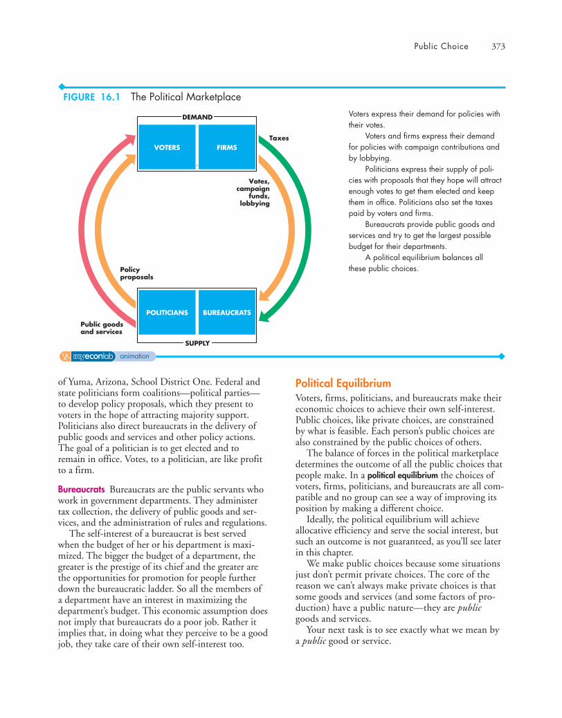
Public Choice 373

Political EquilibriumVoters, firms, politicians, and bureaucrats make theireconomic choices to achieve their own self-interest.Public choices, like private choices, are constrainedby what is feasible. Each person’s public choices arealso constrained by the public choices of others.

The balance of forces in the political marketplacedetermines the outcome of all the public choices thatpeople make. In a political equilibrium the choices ofvoters, firms, politicians, and bureaucrats are all com-patible and no group can see a way of improving itsposition by making a different choice.

Ideally, the political equilibrium will achieveallocative efficiency and serve the social interest, butsuch an outcome is not guaranteed, as you’ll see laterin this chapter.

We make public choices because some situationsjust don’t permit private choices. The core of thereason we can’t always make private choices is thatsome goods and services (and some factors of pro-duction) have a public nature—they are publicgoods and services.

Your next task is to see exactly what we mean bya public good or service.

Votes,campaign

funds,lobbying

Policyproposals

Public goodsand services

TaxesVOTERS FIRMS

POLITICIANS BUREAUCRATS

DEMAND

SUPPLY

Voters express their demand for policies withtheir votes.

Voters and firms express their demandfor policies with campaign contributions andby lobbying.

Politicians express their supply of poli-cies with proposals that they hope will attractenough votes to get them elected and keepthem in office. Politicians also set the taxespaid by voters and firms.

Bureaucrats provide public goods andservices and try to get the largest possiblebudget for their departments.

A political equilibrium balances allthese public choices.

of Yuma, Arizona, School District One. Federal andstate politicians form coalitions—political parties—to develop policy proposals, which they present tovoters in the hope of attracting majority support.Politicians also direct bureaucrats in the delivery ofpublic goods and services and other policy actions.The goal of a politician is to get elected and toremain in office. Votes, to a politician, are like profitto a firm.

Bureaucrats Bureaucrats are the public servants whowork in government departments. They administertax collection, the delivery of public goods and ser-vices, and the administration of rules and regulations.

The self-interest of a bureaucrat is best servedwhen the budget of her or his department is maxi-mized. The bigger the budget of a department, thegreater is the prestige of its chief and the greater arethe opportunities for promotion for people furtherdown the bureaucratic ladder. So all the members ofa department have an interest in maximizing thedepartment’s budget. This economic assumption doesnot imply that bureaucrats do a poor job. Rather itimplies that, in doing what they perceive to be a goodjob, they take care of their own self-interest too.

FIGURE 16.1 The Political Marketplace

animation

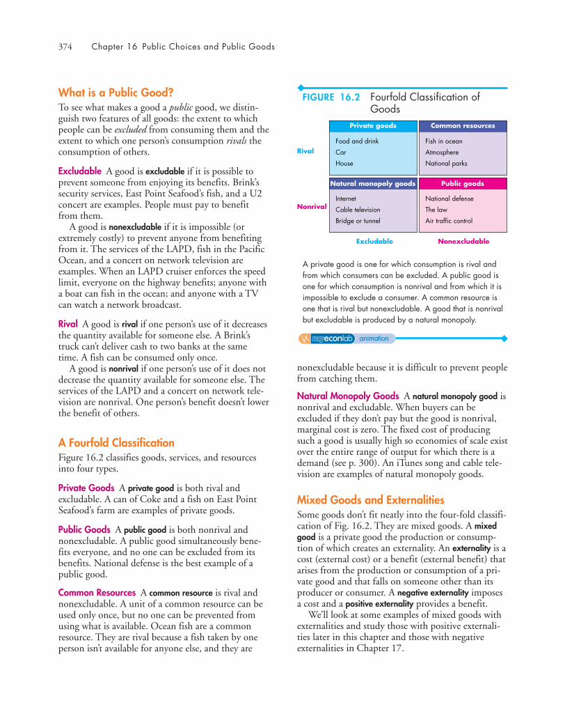
374 Chapter 16 Public Choices and Public Goods

nonexcludable because it is difficult to prevent peoplefrom catching them.

Natural Monopoly Goods A natural monopoly good isnonrival and excludable. When buyers can beexcluded if they don’t pay but the good is nonrival,marginal cost is zero. The fixed cost of producingsuch a good is usually high so economies of scale existover the entire range of output for which there is ademand (see p. 300). An iTunes song and cable tele-vision are examples of natural monopoly goods.

Mixed Goods and ExternalitiesSome goods don’t fit neatly into the four-fold classifi-cation of Fig. 16.2. They are mixed goods. A mixedgood is a private good the production or consump-tion of which creates an externality. An externality is acost (external cost) or a benefit (external benefit) thatarises from the production or consumption of a pri-vate good and that falls on someone other than itsproducer or consumer. A negative externality imposesa cost and a positive externality provides a benefit.

We’ll look at some examples of mixed goods withexternalities and study those with positive externali-ties later in this chapter and those with negativeexternalities in Chapter 17.

Nonrival

Rival

Excludable Nonexcludable

Private goods Common resources

Public goodsNatural monopoly goods

Fish in ocean

Atmosphere

National parks

Food and drink

Car

House

National defense

The law

Air traffic control

Internet

Cable television

Bridge or tunnel

A private good is one for which consumption is rival andfrom which consumers can be excluded. A public good isone for which consumption is nonrival and from which it isimpossible to exclude a consumer. A common resource isone that is rival but nonexcludable. A good that is nonrivalbut excludable is produced by a natural monopoly.

What is a Public Good?To see what makes a good a public good, we distin-guish two features of all goods: the extent to whichpeople can be excluded from consuming them and theextent to which one person’s consumption rivals theconsumption of others.

Excludable A good is excludable if it is possible toprevent someone from enjoying its benefits. Brink’ssecurity services, East Point Seafood’s fish, and a U2concert are examples. People must pay to benefitfrom them.

A good is nonexcludable if it is impossible (orextremely costly) to prevent anyone from benefitingfrom it. The services of the LAPD, fish in the PacificOcean, and a concert on network television areexamples. When an LAPD cruiser enforces the speedlimit, everyone on the highway benefits; anyone witha boat can fish in the ocean; and anyone with a TVcan watch a network broadcast.

Rival A good is rival if one person’s use of it decreasesthe quantity available for someone else. A Brink’struck can’t deliver cash to two banks at the sametime. A fish can be consumed only once.

A good is nonrival if one person’s use of it does notdecrease the quantity available for someone else. Theservices of the LAPD and a concert on network tele-vision are nonrival. One person’s benefit doesn’t lowerthe benefit of others.

A Fourfold ClassificationFigure 16.2 classifies goods, services, and resourcesinto four types.

Private Goods A private good is both rival andexcludable. A can of Coke and a fish on East PointSeafood’s farm are examples of private goods.

Public Goods A public good is both nonrival andnonexcludable. A public good simultaneously bene-fits everyone, and no one can be excluded from itsbenefits. National defense is the best example of apublic good.

Common Resources A common resource is rival andnonexcludable. A unit of a common resource can beused only once, but no one can be prevented fromusing what is available. Ocean fish are a commonresource. They are rival because a fish taken by oneperson isn’t available for anyone else, and they are

FIGURE 16.2 Fourfold Classification ofGoods

animation

Public Choices 375

Economics in ActionIs a Lighthouse a Public Good?Built on Little Brewster Island in 1716 to guide shipsinto and out of the Boston Harbor, Boston Lighthousewas the first light station in North America.

For two centuries, economists used the lighthouse asan example of a public good. No one can be preventedfrom seeing its warning light—nonexcludable—and oneperson seeing its light doesn’t prevent someone elsefrom doing so too—nonrival.

Ronald Coase, who won the 1991 Nobel Prize forideas he first developed when he was an undergradu-ate at the London School of Economics, discoveredthat before the nineteenth century, lighthouses inEngland were built and operated by private corpora-tions that earned profits by charging tolls on shipsdocking at nearby ports. A ship that refused to paythe lighthouse toll was excluded from the port.

So the benefit arising from the services of a light-house is excludable. Because the services provided by alighthouse are nonrival but excludable, a lighthouse isan example of a natural monopoly good and not apublic good.

Your education is another example of a mixedgood with external benefits. If all education wasorganized by private schools and universities, thosenot willing or able to pay would be excluded, andone person’s place in a class would rival another’s. Soeducation is a private good.

But your being educated brings benefits to others.It brings benefits to your friends who enjoy yoursharp, educated wit and it brings benefits to the com-munity in which you live because well-educated people with a strong sense of fellowship and responsi-bility toward others make good neighbors. Theseexternal benefits are like a public good. You can’tselectively decide who benefits from your goodneighborliness and one person’s enjoyment of yourgood behavior doesn’t rival someone else’s. So educa-tion is a mixed good with an external benefit.

Mixed Goods with External Costs Mixed goods withexternal costs have become a huge political issue inrecent years. The main ones are electricity and trans-portation (road, rail, and air) produced by burninghydrocarbon fuels—coal, oil, and natural gas.

Mixed Goods with External Benefits Two of thethings that have the greatest impact on your welfare,your education and health care, are mixed goods withexternal benefits.

Think about a flu vaccination. It is excludablebecause it would be possible to sell vaccinations andexclude those not willing to pay from benefiting fromthem. A flu vaccination is also rival because provid-ing one person with a vaccination means one feweravailable for everyone else. A flu vaccination is a pri-vate good, but it creates an externality.

If you decide to get a flu vaccination, you benefitfrom a lower risk of getting infected in the comingflu season. But if you avoid the flu, your neighborwho didn’t get vaccinated has a better chance ofavoiding it too. A flu vaccination brings a benefit toothers, so it is a mixed good with an external benefit.

The external benefit of a flu vaccination is like apublic good. It is nonexcludable because everyonewith whom you come into contact benefits. You can’tselectively benefit only your friends! And it is non-rival—protecting one person from the flu does notdiminish the protection for others.

376 Chapter 16 Public Choices and Public Goods

external costs because their producers and consumersdon’t take the external costs into account when theymake their own choices.

Conserve Common Resources Because no one can beexcluded from enjoying the benefits of a commonresource, no one has an incentive to pay for theirshare of it or to conserve it for future enjoyment.

If boat owners are left to catch as much SouthernBluefin tuna as they wish, the stock will deplete andeventually the species will vanish. The market econ-omy would overproduce tuna while stocks lasted andthen underproduce as stocks ran out.

This problem, called the tragedy of the commons,requires public choices to limit the overuse and even-tual destruction of common resources.

Regulate Natural Monopoly When people can beexcluded from enjoying the benefits of a good if theydon’t pay for it, and when the good is nonrival, themarginal cost of producing it is zero. A naturalmonopoly can produce such a good at the lowestcost. But as Chapter 13 explains, when one firmserves a market, that firm maximizes profit by pro-ducing too little of the good.

You studied the regulation of natural monopoly inChapter 13. This chapter and the next one study theother two public choices that must be made. In thischapter, we’ll focus on the underprovision of publicgoods and mixed goods with external benefits.Chapter 17 studies mixed goods with external costsand conserving common resources.

Electricity and transportation are excludable andrival—they are private goods. But when you use elec-tricity or travel by car, bus, train, or airplane, carbondioxide and other chemicals pour into the atmos-phere. This consequence of consuming a private goodcreates an external cost and is a public bad. (A “bad”is the opposite of a good.) No one can be excludedfrom bearing the external cost and one person’s dis-comfort doesn’t rival another’s. Electricity and trans-portation are mixed goods with external costs.

Other private goods that generate external costsinclude logging and the clearing of forests, whichdestroy the habitat of wildlife and influence theamount of carbon dioxide in the atmosphere; smok-ing cigarettes in a confined space, which imposes ahealth risk on others; and driving under the influenceof alcohol, which increases the risk of accident andinjury for others.

Inefficiencies that Require Public ChoicesPublic goods, mixed goods, common resources, andnatural monopoly goods all create inefficiency prob-lems that require public choices. Public choices mustbe made to

■ Provide public goods and mixed goods■ Conserve common resources■ Regulate natural monopoly

Provide Public Goods and Mixed Goods Because noone can be excluded from enjoying the benefits of apublic good, no one has an incentive to pay for theirshare of it. Even people with a social conscience haveno incentive to pay because one person’s enjoymentof a public good doesn’t lower the enjoyment of others—it is nonrival.

If private firms tried to produce and sell publicgoods to consumers, they wouldn’t remain in busi-ness for very long. The market economy would fail todeliver the efficient quantity of those goods. Forexample, there would be too little national defense,police services and law enforcement, courts andjudges, storm-water and sewage disposal services.

Mixed goods pose a less extreme problem. Themarket economy would underprovide mixed goodswith external benefits because their producers andconsumers don’t take the external benefits intoaccount when they make their own choices. The mar-ket economy would overprovide mixed goods with

REVIEW QUIZ1 List three main reasons why governments exist.2 Describe the political marketplace. Who

demands, who supplies, and what is the politicalequilibrium?

3 Distinguish among public goods, private goods,common resources, natural monopoly goods,and mixed goods.

4 What are the problems that arise from publicgoods, common resources, natural monopolygoods, and mixed goods?

You can work these questions in Study Plan 16.1 and get instant feedback.

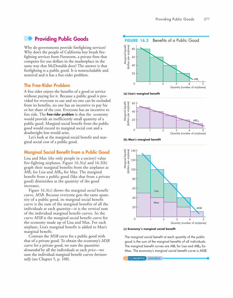
Providing Public Goods 377

1 2

Mar

gina

l ben

efit

(dol

lars

per

airp

lane

)

Quantity (number of airplanes)

80

60

0

20

MB

40

3 4L

5

1 2

Mar

gina

l ben

efit

(dol

lars

per

airp

lane

)

Quantity (number of airplanes)

60

0

20 MB

MSB

40

3 4

M

(b) Max's marginal benefit

(a) Lisa's marginal benefit

5

1 2

Mar

gina

l ben

efit

(dol

lars

per

airp

lane

)

Quantity (number of airplanes)

60

0

20

40

3 4

(c) Economy’s marginal social benefit

5

100

80

140

120

Lisa

Max

The marginal social benefit at each quantity of the publicgood is the sum of the marginal benefits of all individuals.The marginal benefit curves are MBL for Lisa and MBM forMax. The economy’s marginal social benefit curve is MSB.

◆ Providing Public GoodsWhy do governments provide firefighting services?Why don’t the people of California buy brush fire-fighting services from Firestorm, a private firm thatcompetes for our dollars in the marketplace in thesame way that McDonalds does? The answer is thatfirefighting is a public good. It is nonexcludable andnonrival and it has a free-rider problem.

The Free-Rider ProblemA free rider enjoys the benefits of a good or servicewithout paying for it. Because a public good is pro-vided for everyone to use and no one can be excludedfrom its benefits, no one has an incentive to pay hisor her share of the cost. Everyone has an incentive tofree ride. The free-rider problem is that the economywould provide an inefficiently small quantity of apublic good. Marginal social benefit from the publicgood would exceed its marginal social cost and adeadweight loss would arise.

Let’s look at the marginal social benefit and mar-ginal social cost of a public good.

Marginal Social Benefit from a Public GoodLisa and Max (the only people in a society) valuefire-fighting airplanes. Figure 16.3(a) and 16.3(b)graph their marginal benefits from the airplanes asMBL for Lisa and MBM for Max. The marginalbenefit from a public good (like that from a privategood) diminishes as the quantity of the goodincreases.

Figure 16.3(c) shows the marginal social benefitcurve, MSB. Because everyone gets the same quan-tity of a public good, its marginal social benefitcurve is the sum of the marginal benefits of all theindividuals at each quantity—it is the vertical sumof the individual marginal benefit curves. So thecurve MSB is the marginal social benefit curve forthe economy made up of Lisa and Max. For eachairplane, Lisa’s marginal benefit is added to Max’smarginal benefit.

Contrast the MSB curve for a public good withthat of a private good. To obtain the economy’s MSBcurve for a private good, we sum the quantitiesdemanded by all the individuals at each price—wesum the individual marginal benefit curves horizon-tally (see Chapter 5, p. 108).

FIGURE 16.3 Benefits of a Public Good

animation

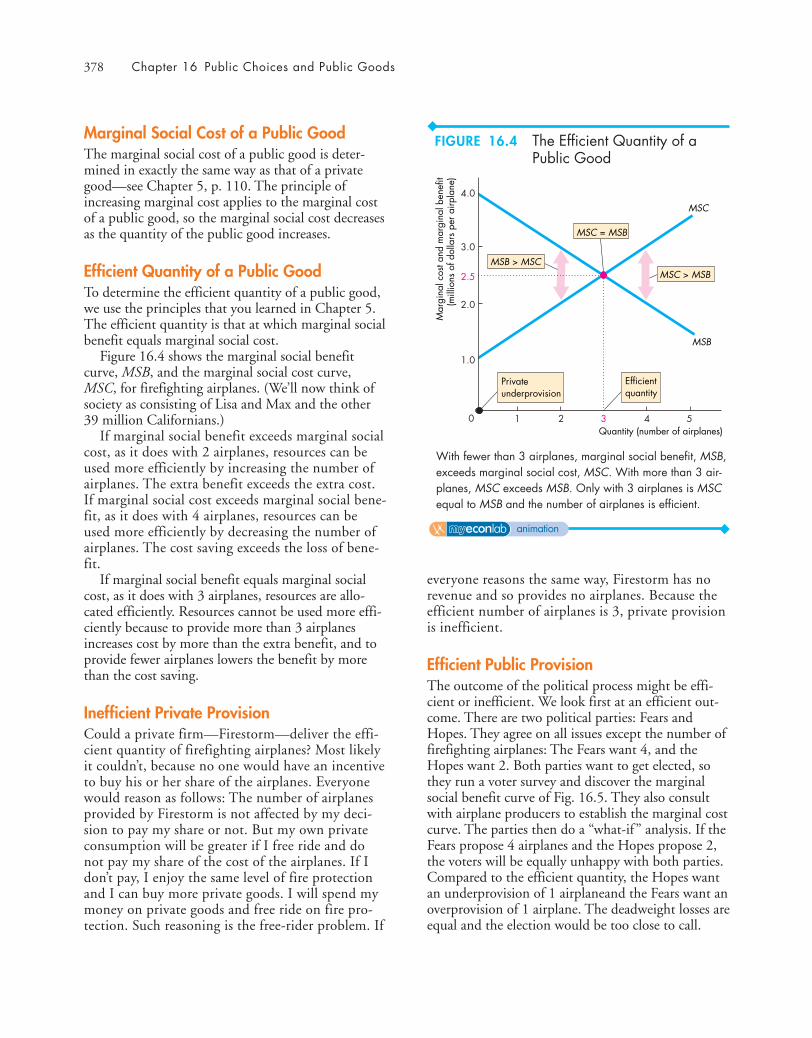
378 Chapter 16 Public Choices and Public Goods

MSC = MSB

MSB > MSCMSC > MSB

Efficientquantity

Privateunderprovision

0 53 421Quantity (number of airplanes)

MSB

MSC

2.0

1.0

2.5

3.0

4.0

Mar

gina

l cos

t and

mar

gina

l ben

efit

(mill

ions

of d

olla

rs p

er a

irpla

ne)

With fewer than 3 airplanes, marginal social benefit, MSB,exceeds marginal social cost, MSC. With more than 3 air-planes, MSC exceeds MSB. Only with 3 airplanes is MSCequal to MSB and the number of airplanes is efficient.

everyone reasons the same way, Firestorm has norevenue and so provides no airplanes. Because theefficient number of airplanes is 3, private provisionis inefficient.

Efficient Public ProvisionThe outcome of the political process might be effi-cient or inefficient. We look first at an efficient out-come. There are two political parties: Fears andHopes. They agree on all issues except the number offirefighting airplanes: The Fears want 4, and theHopes want 2. Both parties want to get elected, sothey run a voter survey and discover the marginalsocial benefit curve of Fig. 16.5. They also consultwith airplane producers to establish the marginal costcurve. The parties then do a “what-if ” analysis. If theFears propose 4 airplanes and the Hopes propose 2,the voters will be equally unhappy with both parties.Compared to the efficient quantity, the Hopes wantan underprovision of 1 airplaneand the Fears want anoverprovision of 1 airplane. The deadweight losses areequal and the election would be too close to call.

Marginal Social Cost of a Public GoodThe marginal social cost of a public good is deter-mined in exactly the same way as that of a privategood—see Chapter 5, p. 110. The principle ofincreasing marginal cost applies to the marginal costof a public good, so the marginal social cost decreasesas the quantity of the public good increases.

Efficient Quantity of a Public GoodTo determine the efficient quantity of a public good,we use the principles that you learned in Chapter 5.The efficient quantity is that at which marginal socialbenefit equals marginal social cost.

Figure 16.4 shows the marginal social benefitcurve, MSB, and the marginal social cost curve,MSC, for firefighting airplanes. (We’ll now think ofsociety as consisting of Lisa and Max and the other39 million Californians.)

If marginal social benefit exceeds marginal socialcost, as it does with 2 airplanes, resources can beused more efficiently by increasing the number ofairplanes. The extra benefit exceeds the extra cost.If marginal social cost exceeds marginal social bene-fit, as it does with 4 airplanes, resources can beused more efficiently by decreasing the number ofairplanes. The cost saving exceeds the loss of bene-fit.

If marginal social benefit equals marginal socialcost, as it does with 3 airplanes, resources are allo-cated efficiently. Resources cannot be used more effi-ciently because to provide more than 3 airplanesincreases cost by more than the extra benefit, and toprovide fewer airplanes lowers the benefit by morethan the cost saving.

Inefficient Private ProvisionCould a private firm—Firestorm—deliver the effi-cient quantity of firefighting airplanes? Most likelyit couldn’t, because no one would have an incentiveto buy his or her share of the airplanes. Everyonewould reason as follows: The number of airplanesprovided by Firestorm is not affected by my deci-sion to pay my share or not. But my own privateconsumption will be greater if I free ride and donot pay my share of the cost of the airplanes. If Idon’t pay, I enjoy the same level of fire protectionand I can buy more private goods. I will spend mymoney on private goods and free ride on fire pro-tection. Such reasoning is the free-rider problem. If

FIGURE 16.4 The Efficient Quantity of aPublic Good

animation

Providing Public Goods 379

Hopes'preference

Fears'preference

Efficientquantity

0 53 421Quantity (number of airplanes)

MSB

MSC

2.0

1.0

2.5

3.0

4.0

Mar

gina

l cos

t and

mar

gina

l ben

efit

(mill

ions

of d

olla

rs p

er a

irpla

ne)

The Hopes would like to provide 2 airplanes and the Fearswould like to provide 4 airplanes. The political outcome is 3airplanes because unless each party proposes 3 airplanes,the other party will beat it in an election.

Economics in ActionFighting California’s WildfiresDuring the 2009 wildfire season (July throughNovember), 63 fires burned across more than 500square miles of California. The two largest and dead-liest fires, Station Fire north of Los Angeles and LaBrea Fire in Santa Barbara County, together con-sumed almost 400 square miles of land.

Wildfires are natural and vital for the ecosystem,but some fires are started by human action, and someboth human-made and naturally occurring fires burnclose to where people live. So protection against wild-fires is a vital public good.

Fighting wildfires is an example of a public goodthat is provided by government and paid for with taxrevenues but produced by private firms.

Firestorm Wildfire Suppression Inc. is one suchfirm. Operating from Chico, CA, Firestorm hires andtrains firefighters and produces firefighting services tomaximize its profit. To achieve this goal, the firm mustproduce firefighting services at the lowest possible cost.

But if Firestorm (and its competitors) tried to selltheir services to each individual home owner in thewildfire regions of California, they wouldn’t getenough revenue to remain in business. There wouldbe a free-rider problem. The free-rider problem isavoided because the state of California and federalemergency services agencies buy the services ofFirestorm—government is the provider of this publicgood and Firestorm and others are the producers.

Contemplating this outcome, the Fears realize thatthey are too fearful to get elected. They figure that, ifthey scale back to 3 airplanes, they will win the elec-tion if the Hopes stick with 2. The Hopes reason in asimilar way and figure that, if they increase the num-ber of airplanes to 3, they can win the election if theFears propose 4.

So they both propose 3 airplanes. The voters areindifferent between the parties, and each partyreceives 50 percent of the vote. But regardless ofwhich party wins the election, 3 airplanes are pro-vided and this quantity is efficient. Competition inthe political place results in the efficient provision ofa public good.

The Principle of Minimum Differentiation Theprinciple of minimum differentiation is the tendency forcompetitors (including political parties) to makethemselves similar to appeal to the maximum num-ber of clients or voters. This principle describes thebehavior of political parties. It also explains why fast-food restaurants cluster in the same block. For exam-ple, if Dominoes opens a new pizza outlet, it is likelythat Pizza Hut will soon open nearby.

FIGURE 16.5 An Efficient Political Outcome

animation

380 CHAPTER 16 Public Choices and Public Goods

For the political process to deliver the efficientoutcome, voters must be well informed, evaluate thealternatives, and vote in the election. Political partiesmust be well informed about voter preferences. Asthe next section shows, we can’t expect to achieve thisoutcome.

Inefficient Public OverprovisionIf competition between two political parties is todeliver the efficient quantity of a public good,bureaucrats must cooperate and help to achieve thisoutcome. But bureaucrats might have a different ideaand end up frustrating rather than facilitating an effi-cient outcome. Their actions might bring governmentfailure.

Objective of Bureaucrats Bureaucrats want to maxi-mize their department’s budget because a biggerbudget brings greater status and more power. So theEmergency Services Department’s objective is tomaximize the budget for firefighting airplanes.

Figure 16.6 shows the outcome if the bureaucratsare successful in the pursuit of their goal. They mighttry to persuade the politicians that 3 airplanes costmore than the originally budgeted amount; or theymight press their position more strongly and arguefor more than 3 airplanes. In Fig. 16.6, theEmergency Services Department persuades the politi-cians to provide 4 airplanes.

Why don’t the politicians block the bureaucrats?Won’t overproviding airplanes cost future votes? Itwill if voters are well informed and know what is bestfor them. But voters might not be well informed, andwell-informed interest groups might enable thebureaucrats to achieve their objective and overcomethe objections of the politicians.

Rational Ignorance A principle of the economicanalysis of public choices is that it is rational for avoter to be ignorant about an issue unless that issuehas a perceptible effect on the voter’s economic wel-fare. Each voter knows that he or she can make virtu-ally no difference to the fire protection policy of thegovernment of California and that it would take anenormous amount of time and effort to become evenmoderately well informed about alternative fire-pro-tection technologies. Rationally uninformed votersenable bureaucrats and special interest groups tooverprovide public goods.

You’ve seen how the political marketplace providespublic goods and why it might overprovide them.Your next task is to see how the political marketplaceprovides mixed goods that bring external benefits.

Equilibriumoverprovision

Bureaucratsknow but votersrationally don'tknow thatMSC > MSB

Efficientquantity

0 53 421Quantity (number of airplanes)

MSB

MSC

2.0

1.0

2.5

3.0

4.0

Mar

gina

l cos

t and

mar

gina

l ben

efit

(mill

ions

of d

olla

rs p

er a

irpla

ne)

Deadweightloss

Well-informed bureaucrats want to maximize their budgetand rationally ignorant voters enable the bureaucrats to gosome way toward achieving their goal. A public goodmight be inefficiently overprovided with a deadweight loss.

FIGURE 16.6 Bureaucratic Overprovision

animation

REVIEW QUIZ1 What is the free-rider problem? Why do free

riders make the private provision of a publicgood inefficient?

2 Under what conditions will competition amongpoliticians for votes result in an efficient provi-sion of a public good?

3 How do rationally ignorant voters and budget-maximizing bureaucrats prevent the politicalmarketplace from delivering the efficient quan-tity of a public good?

4 Explain why public choices might lead to theoverprovision rather than the underprovision ofa public good.

You can work these questions in Study Plan 16.2 and get instant feedback.

Providing Mixed Goods with External Benefits 381

◆ Providing Mixed Goods withExternal Benefits

Most of the goods and services provided by govern-ments are mixed goods, not public goods. Two of thelargest mixed goods with external benefits are educa-tion and health care. We’re going to look at how gov-ernments operate in such s. We’re also going to lookat possible improvements on the current arrange-ments in these markets.

To keep our explanation clear, we’ll focus first onthe market for college education. We’ll then applythe lessons we learn to the market for health care.

We begin our study of the provision of mixedgoods by distinguishing between private benefitsand social benefits.

Private Benefits and Social BenefitsA private benefit is a benefit that the consumer of agood or service receives. For example, expanded jobopportunities and a higher income are private bene-fits of a college education.

Marginal benefit is the benefit from an additionalunit of a good or service. So marginal private benefit(MB) is the benefit that the consumer of a good orservice receives from an additional unit of it. Whenone additional student attends college, the benefitthat student receives is the marginal private benefitfrom college education.

The external benefit from a good or service isthe benefit that someone other than the consumer ofthe good or service receives. College graduates gener-ate many external benefits. On average, they are bet-ter citizens, have lower crime rates, and are moretolerant of the views of others. They enable the suc-cess of high quality newspapers and television chan-nels, music, theater, and other organized socialactivities that bring benefits to many other people.

A marginal external benefit is the benefit from anadditional unit of a good or service that people otherthan its consumer enjoy. The benefit that your friendsand neighbors get from your college education is themarginal external benefit of your college education.

Marginal social benefit (MSB) is the marginal bene-fit enjoyed by society—by the consumer of a good orservice (marginal private benefit) and by others (themarginal external benefit). That is,

MSB = MB + Marginal external benefit.

MSB

Pric

e (th

ousa

nds

of d

olla

rs p

er s

tude

nt p

er y

ear)

Quantity (millions of students per year)

50 10 20 25

40

30

25

10

MB

Marginalprivatebenefit

Marginalsocialbenefit

Marginalexternalbenefit

15

20

The MB curve shows the marginal private benefit enjoyedby the people who receive a college education. The MSBcurve shows the sum of marginal private benefit and mar-ginal external benefit. When 15 million students attend col-lege, the marginal private benefit is $10,000 per student,the marginal external benefit is $15,000 per student, andthe marginal social benefit is $25,000 per student.

Figure 16.7 shows an example of the relationshipbetween marginal private benefit, marginal externalbenefit, and marginal social benefit. The marginalbenefit curve, MB, describes the marginal privatebenefit enjoyed by the people who receive a collegeeducation. Marginal private benefit decreases as thenumber of students enrolled in college increases.

In the example in Fig. 16.7, when 15 million stu-dents enroll in college, the marginal external benefitis $15,000 per student per year . The marginal socialbenefit curve, MSB, is the sum of marginal privatebenefit and marginal external benefit at each numberof students. For example, when 15 million students ayear enroll in college, the marginal private benefit is$10,000 per student and the marginal external bene-fit is $15,000 per student, so the marginal social ben-efit is $25,000 per student.

When people make schooling decisions, they ignoreits external benefits and consider only its private bene-fits. So if education were provided by private schools

FIGURE 16.7 An External Benefit

animation

382 CHAPTER 16 Public Choices and Public Goods

MSB

Quantity (millions of students per year)

5 7.50 10 20 25

40

30

25

10

15

38

15

20

Inefficientmarketequilibrium

Pric

e an

d co

st (th

ousa

nds

of d

olla

rs p

er s

tude

nt p

er y

ear)

D = MB

S = MSC

Marginalsocial cost

Marginalsocialbenefit

Efficientquantity

Deadweightloss

Efficientequilibrium

The market demand curve is the marginal private benefitcurve, D = MB. The supply curve is the marginal social costcurve, S = MSC. Market equilibrium at a tuition of $15,000a year and 7.5 million students is inefficient because mar-ginal social benefit exceeds marginal social cost. The effi-cient quantity is 15 million students. A deadweight loss arises(gray triangle) because too few students enroll in college.

Paid bytaxpayer

MB

MSC

Paid bybuyer

Market priceat efficientquantity

MSB = MSC

MSB

Quantity (millions of students per year)

50 10 20 25

40

30

25

10

15

20

Pric

e an

d co

st (th

ousa

nds

of d

olla

rs p

er s

tude

nt p

er y

ear)

Efficientquantity

The efficient number of college students is 15 million, wheremarginal social benefit equals marginal social cost. With thedemand and marginal private benefit curve, D = MB, theprice at which the efficient number will enrol is $10,000 peryear. If students pay this price, the taxpayer must somehowpay the rest, which equals the marginal external cost at theefficient quantity—$15,000 per student per year.

Government Actions in the Market for aMixed Good with External BenefitsTo encourage more students to enroll in college —toachieve an efficient quantity of college education—students must be confronted with a lower marketprice and the taxpayer must somehow pay for thecosts not covered by what the student pays.

Figure 16.9 illustrates an efficient outcome. Withmarginal social cost curve MSC and marginal socialbenefit curve MSB, the efficient number of collegestudents is 15,000. The marginal private benefitcurve MB, tells us that 15,000 students will enrollonly if the tuition is $10,000 per year. But the mar-ginal social cost of 15,000 students is $25,000 peryear. To enable the marginal social cost to be paid,taxpayers must pay the balance of $15,000 per stu-dent per year.

that charged full-cost tuition, there would be too fewcollege graduates.

Figure 16.8 illustrates this private underprovision.The supply curve is the marginal social cost curve, S = MSC. The demand curve is the marginal privatebenefit curve, D = MB. Market equilibrium occursat a tuition of $15,000 per student per year and 7.5million students per year. At this equilibrium, themarginal social benefit of $38,000 per studentexceeds the marginal social cost by $23,000 per stu-dent. Too few students are enrolled in college. Theefficient number is 15 million per year, where mar-ginal social benefit equals marginal social cost. Thegray triangle shows the deadweight loss created.

To get closer to producing the efficient quantity ofa mixed good with an external benefit, we make pub-lic choices, through governments, to modify the mar-ket outcome.

FIGURE 16.8 Inefficiency with anExternal Benefit

animation animation

FIGURE 16.9 An Efficient Outcome with anExternal Benefit

Providing Mixed Goods with External Benefits 383

Efficient provision of college education occurs if thegovernment provides a voucher to each student with avalue equal to the marginal external benefit at the effi-cient number of students. In the example in Fig. 16.9,the efficient number of students is 15 million and thevoucher is valued at $15,000 per student. Each studentpays $10,000 tuition and gives the college a $15,000voucher. The colleges receive $25,000 per student,which equals their marginal cost.

Bureaucratic Inefficiency andGovernment FailureYou’ve seen three government actions that achieve anefficient provision of a mixed good with an externalbenefit. In each case, if the government estimates themarginal external benefit correctly and makes mar-ginal social benefit equal to marginal social cost, theoutcome is efficient.

Does the comparison that we’ve just made meanthat pubic provision, subsidized private provision,and vouchers are equivalent? It does not. And the rea-son lies in something that you’ve already encounteredin your study of public goods earlier in this chap-ter—the behavior of bureaucrats combined withrational ignorance that leads to government failure.

The Problem with Public Production Public colleges(and schools) are operated by a bureaucracy and aresubject to the same problems as the provision of pub-lic goods. If bureaucrats seek to maximize their budg-ets, the outcome might be inefficient.

But overprovision of colleges (and schools) doesn’tseem to be a problem. Just the opposite: People com-plain about underprovision—about inadequate publiccolleges and schools. The probable reason is thatthere is another type of bureaucratic budget maxi-mization: budget padding and waste.

Bureaucrats often incur costs that exceed the mini-mum efficient cost. They might hire more assistantsthan the number needed to do their work efficiently;give themselves sumptuous offices; get generousexpense allowances; build schools in the wrong placeswhere land costs are too high.

Economists have studied the possibility that edu-cation bureaucrats pad their budgets by comparingthe production costs of private and public collegesand schools. They have found that the costs per stu-dent of public schools are of the order of three timesthe costs of comparable private schools (see TalkingWith Carolyn Hoxby on pp. 414– 416.)

Four devices that governments can use to achieve amore efficient allocation of resources in the presenceof external benefits are

■ Public production■ Private subsidies■ Vouchers

Public Production With public production, a good orservice is produced by a public authority that receivesits revenue from the government. The education ser-vices produced by state universities and colleges andpublic schools are examples of public production.

In the example in Fig. 16.9, efficient public pro-duction occurs if public colleges receive funds fromgovernment equal to $15,000 per student per year,charge tuition of $10,000 per student per year, andenrol 15 million students.

Private Subsidies A subsidy is a payment that thegovernment makes to private producers. By makingthe subsidy depend on the level of output, the gov-ernment can induce private decision-makers to con-sider external benefits when they make their choices.

In the example in Fig. 16.9, efficient private provi-sion would occur if private colleges received a govern-ment subsidy of $15,000 per student per year. Thissubsidy reduces the colleges’ costs and would maketheir marginal cost equal to $10,000 per student atthe efficient quantity. Tuition of $10,000 wouldcover this cost, and the subsidy of $15,000 per stu-dent would cover the balance of the cost.

Vouchers A voucher is a token that the governmentprovides to households, which they can use to buyspecified goods or services. Food stamps are examplesof vouchers. The vouchers (food stamps) can be spentonly on food and are designed to improve the dietand health of extremely poor families.

School vouchers have been advocated as a meansof improving the quality of education and are used inWashington D.C. A school voucher allows parents tochoose the school their children will attend and touse the voucher to pay part of the cost. The schoolcashes the vouchers to pay its bills. A voucher couldbe provided to a college student in a similar way, andalthough technically not a voucher, a federal PellGrant has a similar effect.

Because vouchers can be spent only on a specifieditem, they increase the willingness to pay for that itemand so increase the demand for it.

384 CHAPTER 16 Public Choices and Public Goods

Economics in ActionDelivering Health Care EfficientlyAmericans spend 17 percent of income—$8,000 perperson per year—on health care, which is more thandouble the average of other rich countries. And thecost is projected to rise as the population ages andthe “baby boom” generation retires. Despite thisenormous expenditure, until the passage of the 2010Affordable Care Act, 47 million people had no healthinsurance and a further 25 million had too littleinsurance.

Of those who do have health insurance nearly 40million are covered by the government’s Medicareand Medicaid programs. These programs are in effectan open-ended commitment of public funds to thehealth care of the aged (Medicare) and those toopoor to buy private health care (Medicaid). In 2035,when those born in 1955 turn 80, benefits underthese programs will cost an estimated $50,000 perperson per year. Benefits on these programs alonewill cost more than 18 percent of the value of thenation’s total production.

You can see that health care in the United Statesfaces two problems: underprovision because privatechoices don’t value all the external benefits; and overexpenditure because private health-care producersdecide how much to produce and then collect feesfor their services from the government.

Health-Care ServicesHealth care is another example of a mixed good withexternal benefits. The external benefits from healthcare include avoiding infectious diseases, living andworking with healthy neighbors, and for many peo-ple, just living in a society in which poor, sick peoplehave access to affordable health care.

An additional problem arises in the case of healthcare: People with the biggest health problems are theelderly and the poor, who are least able to affordhealth care.

Because of its special features, no country justleaves the delivery of health care to the private marketeconomy. In almost all countries, health care is pro-vided at a zero price, or very low price, and doctorsand other health-care professionals and the hospitalsin which they work receive most (and in some casesall) their incomes from government.

Problems with Private Subsidies Subsidizing privateproducers might overcome some of the problems cre-ated by public production. A private producer has anincentive to produce at minimum cost and avoid thebudget padding of a bureaucratic producer. But twoproblems arise with private subsidies.

First, the subsidy budget must be allocated by abureau. A national, state, or local department of edu-cation must lobby for its own budget and allocatethis budget between school subsidies and its ownadministration costs. To the extent that the bureau-crats succeed in maximizing their own adminstrationbudget, they siphon off resources from schools and aproblem similar to that of public production arises.

Second, it is in the self-interest of subsidized pro-ducers to maximize their subsidy. These producersmight even spend some of the subsidy they receivelobbying for an even bigger one.

So neither public production nor subsidized pri-vate provision are likely to achieve an efficient alloca-tion of resources in the face of external benefits.

Are Vouchers the Solution? Vouchers have fouradvantages over the other two approaches:

1. Vouchers can be used with public production,private provision, or competition between thetwo.

2. Governments can set the value of vouchers andthe total voucher budget to overcome bureau-cratic overprovision and budget padding.

3. Vouchers spread the public contribution thinlyacross millions of consumers, so no one con-sumer has an interest in wasting part of the valuereceived in lobbying for overprovision.

4. By giving the buying power to the final con-sumer, producers must compete for business andprovide a high standard of service at the lowestattainable cost.

For these four reasons, vouchers are popular witheconomists. But they are controversial and opposedby most education administrators and teachers.

In The Economics of School Choice, a book editedby Caroline M. Hoxby, economists study the effect ofschool choice on student achievement and schoolproductivity and show how vouchers can be designedto achieve their goals while avoiding their potentialpitfalls. Caroline Hoxby is confident that she candesign a voucher that best achieves any educationaland school performance objective (see p. 416).

Providing Mixed Goods with External Benefits 385

1. Everyone is covered.2. Every American gets a health-plan voucher.3. Those with higher expected health-care costs

receive bigger vouchers.4. Can change health plan annually.5. Government defines basic policy each year.6. Basic policy covers drugs, home health care, and

nursing home care.7. Plans must cover basic policy.8. Plans compete for participants.9. Annual voucher budget is fixed as a percentage of

the value of total production.10. Medicare and employer-based health insurance

tax breaks are eliminated.

The Obama Affordable Care Act addresses thefirst of these problems by requiring everyone to beinsured and by creating a new Pre-ExistingCondition Insurance Plan financed partly by the gov-ernment.

But the act does little to address the problem ofover-expenditure, and this problem is extremely seri-ous. It is so serious that without massive change, thepresent open-ended health-care programs will bank-rupt the United States.

Other countries contain health-care costs bylimiting the budget and the number of physicians and hospital beds and by rationing services with longwait-times for treatment. This “solution” is inefficientbecause some people would be willing to pay morethan the cost (marginal benefit exceeds marginal cost)and it is unfair (some people are better at playing thesystem than others and are able to jump the line).

A more effective solution to both the problem ofcoverage and access and the problem of over-expen-diture has been suggested by Laurence Kotlikoff, aneconomics professor at Boston University. His pro-posal uses health-care vouchers to ensure universalcoverage and a cap on total expenditure. HisMedicare Part C for all is summarized in the ten-point plan in the next column.

This solution can deliver health care efficiently,distribute public funds among individuals based ontheir health status, and cap total expenditure.

In the United States, most health-care services areproduced by private doctors and hospitals thatreceive their incomes from both governments andprivate health insurance companies. The health insur-ance companies in turn receive their income fromemployers and individual contributors.

Economics in Action (above) describes some of thefeatures of health-care delivery in the United Statesand explains why it faces two serious problems, onlyone of which has been addressed by the AffordableCare Act of 2010.

Again, vouchers—health-care vouchers—are a crucial component of a program capable of achievingan efficient quantity and distribution of health-careservices across individuals.

◆ Reading Between the Lines on pp. 386–387 looksat the effects of the 2010 Act and some of the prob-lems that it brings.

REVIEW QUIZ1 What is special about education and health care

that makes them mixed goods with externalbenefits?

2 Why would the market economy produce toolittle education and health care?

3 How might public production, private subsi-dies, and vouchers achieve an efficient provisionof a mixed good with external benefits?

4 What are the key differences among public pro-duction, private subsidies, and vouchers?

5 Why do economists generally favor vouchersrather than public production or subsidies toachieve an efficient outcome?

You can work these questions in Study Plan 16.3 and get instant feedback.

Professor Laurence J. Kotlikoff of Boston University; author of The Healthcare Fix and creator of Medicare Part C for all.

386

READING BETWEEN THE L INES

Protective Net for All Residents; Q&A Legislation DetailsFinancial TimesMarch 22, 2010

What would the U.S. health-care bill do?

Offer or subsidise health-care coverage for 32m people, a tenth of the population, who areuninsured; mandate that every U.S. and legal resident receive minimal coverage.

Beginning in 2014, people who are out of work, self-employed, or working for companiesthat do not offer insurance could buy coverage from “health exchanges” in which private in-surers would offer different kinds of plans.

About 19m people would be eligible for financial subsidies to help pay for insurance. If indi-viduals refused to buy insurance coverage, they would be subject to a tax penalty.

How much would it cost and who is paying for it?

The non-partisan Congressional Budget Office estimates the bill would cost $940 billionover 10 years. This is expected to be paid for through tax on the wealthy and health-relatedindustries, including a tax on so-called “Cadillac” insurance plans that would raise $32 bil-lion over 10 years. The bill would also create a Medicare (the healthcare scheme for the elder-ly) commission that would have power toimpose steep cuts in payments. Individualsmaking more than $200,000 a year, or couplesmaking more than $250,000 a year, would payhigher taxes on Medicare and face a new 3.8percent tax on dividends, interest, and otherunearned income. The tax would take effect inJanuary 2013. The CBO estimates the health-care bill would reduce the U.S. deficit by $138billion over 10 years. ...

Copyright 2010 The Financial Times. Reprinted with permission. Furtherreproduction is prohibited.

■ Over the first ten years, health-care reform willcost $940 billion.

■ Coverage will expand to 32 million Americanwho are currently uninsured.

■ New taxes will pay for the plan and cut thebudget deficit.

■ Medicaid will expand to cover about 19 millionlow-income people.

■ Insurance companies will not be able to denycoverage for preexisting conditions.

■ Except for some low-income families, everyonewill be required to buy health insurance andwill face penalties if they refuse to do so.

ESSENCE OF THE STORY

Reforming Health Care

387

ECONOMIC ANALYSIS

Figure 1 Overprovision of Medicare and MedicaidPr

ice

and

cost

(thou

sand

s of

dol

lars

per

pat

ient

per

yea

r)

Quantity (millions of patients per year)0

MB

MSBMSC

MSB = MSC

10

5

15

20

25

30

40302010

Figure 2 Uncontrolled expenditure on Medicareand Medicaid

Efficientquantity

Quantitydemandedat zero price

Deadweightloss

Pric

e an

d co

st (th

ousa

nds

of d

olla

rs p

er p

atie

nt p

er y

ear)

Quantity (millions of patients per year)0

MB

MSC

10

5

15

20

25

30

40302010

Overexpenditure

Quantitydemandedat zero priceExpenditure

on efficientquantity

■ The quantity of health-care services provided byMedicare and Medicaid increases and the expenditureon these programs grows.

■ A health-care voucher program like that explained on pp. 384–385 is one way (and possibly the onlyeffective way) of achieving an efficient provision ofMedicare and Medicaid and of containing their cost.

■ Health care in the United States faces two problems:1) Underprovision because private choices leave toomany families and individuals without health insurance;2) Over expenditure on public programs because thegovernment pays for the quantity that patients demandand doctors supply.

■ The health-care reform of 2010 (the Patient Protectionand Affordable Care Act of 2010) addresses the firstproblem. It expands the scope of government provisionof health care by covering more families and individu-als and by improving the health-care insurance of thosealready covered. (The news article describes some ofthe details of the Act.)

■ The 2010 Act notes the problem of cost containmentbut does little to address the main source of overexpenditure: Medicare and Medicaid.

■ Medicare and Medicaid remain and Medicaid will beexpanded to cover more people.

■ Figure 1 shows how Medicare and Medicaid overpro-vide services to those covered by the programs. Thequantity is the quantity demanded by patients andsupplied by doctors at a zero (or almost zero) price.

■ Because the price is zero, marginal benefit, MB, isalso zero.

■ Doctors and hospitals negotiate fees with the govern-ment that equal marginal cost, which also equals mar-ginal social cost, MSC.

■ Marginal social cost, shown by the MSC curve,exceeds the (zero) marginal benefit. In this example,MSC is $25 at the quantity provided.

■ Medicare and Medicaid services would be providedefficiently if marginal social cost, MSC equalledmarginal social benefit, MSB.

■ With overprovision, a deadweight loss arises shownby the gray triangle.

■ Expenditure on Medicare and Medicaid equals the feeper unit of service multiplied by the quantity provided,and Fig. 2 illustrates this expenditure.

■ The white rectangle shows what expenditure would beon the efficient quantity. The purple area shows theover expenditure. Total expenditure is the sum of theseareas and equals $25 × 30 million.

■ As the population gets older and as treatment tech-niques become more sophisticated and more condi-tions can be treated, the MB curve shifts rightward.

388 CHAPTER 16 Public Choices and Public Goods

Key Points

Public Choices (pp. 372–376)

■ Governments establish and maintain propertyrights, provide nonmarket mechanisms for allo-cating scarce resources, and redistribute incomeand wealth.

■ Public choice theory explains how voters, firms,politicians, and bureaucrats interact in the politicalmarketplace and why government failure mightoccur.

■ A private good is a good or service that is rival andexcludable.

■ A public good is a good or service that is nonrivaland nonexcludable.

■ A mixed good is a private good that creates anexternal benefit or external cost.

Working Problems 1 to 6 will give you a better under-standing of public choices.

Providing Public Goods (pp. 377–380)

■ Because a public good is a good or service that isnonrival and nonexcludable, it creates a free-riderproblem: No one has an incentive to pay theirshare of the cost of providing a public good.

■ The efficient level of provision of a public good isthat at which marginal social benefit equals mar-ginal social cost.

SUMMARY

Key TermsCommon resource, 374Excludable, 374Externality, 374Free-rider problem, 377Government failure, 372Marginal external benefit, 381Marginal private benefit, 381Marginal social benefit, 381Mixed good, 374

Natural monopoly good, 374Negative externality, 374Nonexcludable, 374Nonrival, 374Political equilibrium, 373Postive externality, 374Principle of minimum differentiation, 379

Private good, 374

Public choice, 372Public good, 374Public production, 383Rival, 374Subsidy, 383Voucher, 383

■ Competition between political parties can lead tothe efficient scale of provision of a public good.

■ Bureaucrats who maximize their budgets andvoters who are rationally ignorant can lead to theinefficient overprovision of a public good—-government failure.

Working Problems 7 to 15 will give you a better under-standing of providing public goods.

Providing Mixed Goods with External Benefits (pp. 381–385)

■ Mixed goods provide external benefits—benefitsthat are received by people other than the con-sumer of a good or service.

■ Marginal social benefit equals marginal privatebenefit plus marginal external benefit.

■ External benefits arise from education and healthcare.

■ Vouchers provided to households can achieve amore efficient provision of education and healthcare than public production or subsidies to privateproducers.

Working Problems 16 to 20 will give you a better under-standing of providing mixed goods with external benefits.

Study Plan Problems and Applications 389

Public Choices (Study Plan 16.1)

1. Classify each of the following items as exclud-able, nonexcludable, rival, or nonrival.■ A Big Mac■ Brooklyn Bridge■ A view of the Statue of Liberty■ A tsunami warning system

2. Classify each of the following items as a publicgood, a private good, a natural monopoly good,or a common resource.■ Highway control services■ City sidewalks■ U.S. Postal Service■ FedEx courier service

3. Classify the following services for computer own-ers with an Internet connection as rival, nonrival,excludable, or nonexcludable:■ eBay■ A mouse■ A Twitter page■ MyEconLab Web site

4. Classify each of the following items as a publicgood, a private good, a mixed good, or a com-mon resource:■ Firefighting services■ A courtside seat at the U.S. Open (tennis)■ A well-stocked buffet that promises the most

bang for your buck■ The Mississippi River

5. Explain which of the following events creates anexternal benefit or an external cost:■ A huge noisy crowd gathers outside the lecture

room■ Your neighbor grows beautiful flowers on his

apartment deck.■ A fire alarm goes off accidently in the middle

of a lecture.■ Your instructor offers a free tutorial after class.

6. Wind Farm Off Cape Cod Clears HurdleThe nation’s first offshore wind farm with 130turbines will be built 5 miles off the coast. Windturbines are noisy, stand 440 feet tall, can be seenfrom the coast, and will produce power for 75percent of nearby homes.

Source: The New York Times, January 16, 2009List the externalities created by this wind farm.

You can work Problems 1 to 20 in MyEconLab Chapter 16 Study Plan and get instant feedback.

STUDY PLAN PROBLEMS AND APPLICATIONS

Providing Public Goods (Study Plan 16.2)

7. For each of the following goods, explain whetherthere is a free-rider problem. If there is no suchproblem, how is it avoided?■ July 4th fireworks display■ Interstate 81 in Virginia■ Wireless Internet access in hotels■ The public library in your city

8. The table sets out the marginal benefits that Terriand Sue receive from police officers on duty onthe college campus:

Police officers Marginal benefiton duty Terri Sue

(number per night) (dollars per police officer)

1 18 222 14 183 10 144 6 105 2 6

a. If the police officers are provided by the citygovernment, is the presence of the police on-campus a private good or a public good?

b. Suppose that Terri and Sue are the only stu-dents on the campus at night. Draw a graphto show the marginal social benefit from on-campus police officers on duty at night.

9. For each of the following goods and services,explain whether there is a free-rider problem. Ifthere is no such problem, how is it avoided?■ National hurricane warning system■ Ambulance service■ Road safety signs■ The U.S. Coast Guard

10. Vaccination DodgersDoctors struggle to eradicate polio worldwide,but one of the biggest problems is persuadingparents to vaccinate their children. Since the dis-covery of the vaccine, polio has been eliminatedfrom Europe and the law requires everyone to bevaccinated. People who refuse to be vaccinatedare “free riders.”

Source: USA Today, March 12, 2008

Explain why someone who has not opted out onmedical or religious grounds and refuses to bevaccinated is a “free rider.”

390 CHAPTER 16 Public Choices and Public Goods

Providing Mixed Goods with External Benefits(Study Plan 16.3)

Use the following figure, which shows the marginalprivate benefit from college education, to workProblems 16 to 19. The marginal cost of a collegeeducation is a constant $6,000 per student per year.The marginal external benefit from a college educa-tion is a constant $4,000 per student per year.

16. What is the efficient number of students? If allcolleges are private, how many people enroll incollege and what is the tuition?

17. If the government decides to provide public col-leges, what tuition will these colleges charge toachieve the efficient number of students? Howmuch will taxpayers have to pay?

18. If the government decides to subsidize privatecolleges, what subsidy will achieve the efficientnumber of college students?

19. If the government offers vouchers to those whoenroll at a college and no subsidy, what is thevalue of the voucher that will achieve the effi-cient number of students?

20. Tuition Hikes, not Loan Access, ShouldFrighten StudentsThe real danger during a recession is a hike intuition, not a cut in student loans. In past reces-sions, states have cut funding for colleges andincreased tuition. The Cato Institute says a betterpolicy would be for states to maintain the subsi-dies to colleges and increase their deficits.

Source: USA Today, October 22, 2008If government cuts the subsidy to colleges, whywill tuition rise and the number of studentsenrolled decrease? Why is it a better policy forgovernment to maintain the subsidy to colleges?

Pric

e an

d co

st (th

ousa

nds

of d

olla

rs)

Students (thousands per year)0 20 30 40 50 60

2

4

6

8

10

D = MB

Use the following figure to work Problems 11 to 13.The figure provides information about a waste dis-posal system that a city of 1 million people is consid-ering installing.

11. What is the efficient capacity of the waste dis-posal system? How much will each person haveto pay in taxes for the city to install the efficientcapacity?

12. What is the political equilibrium if voters arewell informed?

13. What is the political equilibrium if voters arerationally ignorant and bureaucrats achieve thehighest attainable budget?

Use the data on a mosquito control program in thefollowing table to work Problems 14 and 15.

Quantity Marginal Marginal(square miles social cost social benefit

sprayed per day) (thousands of dollars per day)

1 2 102 4 83 6 64 8 45 10 2

14. What quantity of spraying would a private mos-quito control program provide? What is the effi-cient quantity of spraying? In a single-issue elec-tion on the quantity of spraying, what quantitywould the winner of the election provide?

15. If the government sets up a Department ofMosquito Control and appoints a bureaucrat torun it, would mosquito spraying most likely beunderprovided, overprovided, or provided at theefficient quantity?

40

0 1 2 3 4Mar

gina

l soc

ial b

enef

it an

d m

argi

nal s

ocia

l cos

t(d

olla

rs p

er p

erso

n)

Capacity (millions of gallons per day)

20

5

60

80

100

MSB

MSC

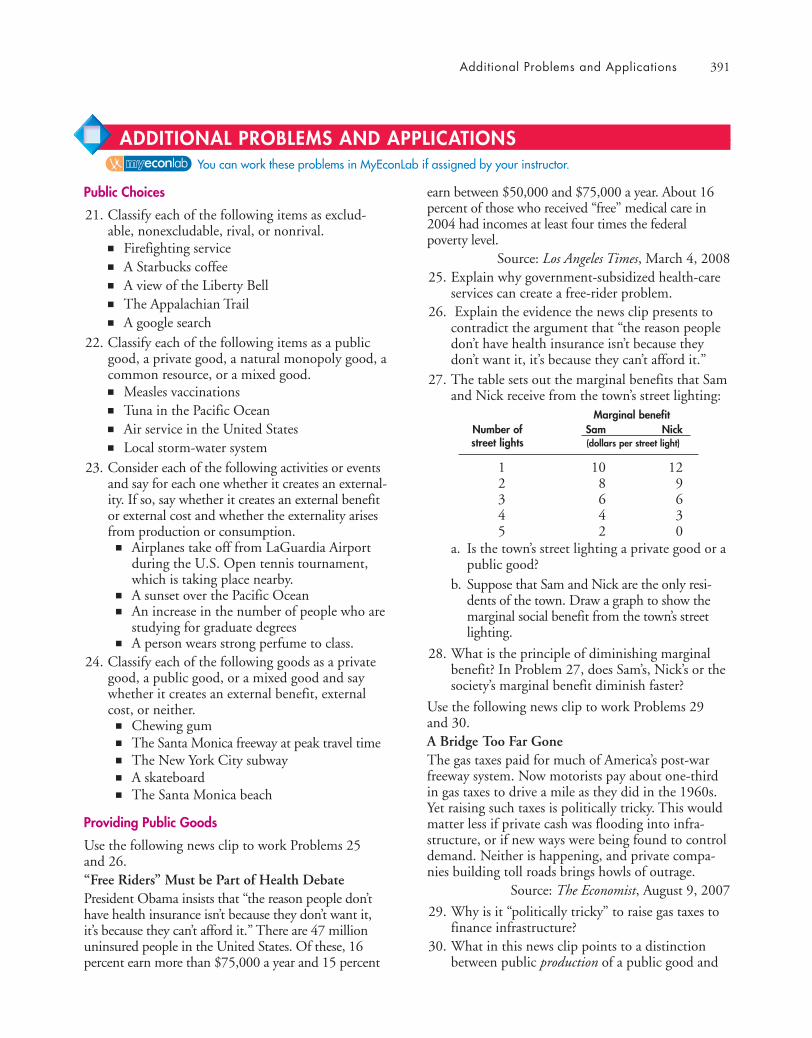
Additional Problems and Applications 391

Public Choices

21. Classify each of the following items as exclud-able, nonexcludable, rival, or nonrival.■ Firefighting service■ A Starbucks coffee■ A view of the Liberty Bell■ The Appalachian Trail■ A google search

22. Classify each of the following items as a publicgood, a private good, a natural monopoly good, acommon resource, or a mixed good.■ Measles vaccinations■ Tuna in the Pacific Ocean■ Air service in the United States■ Local storm-water system

23. Consider each of the following activities or eventsand say for each one whether it creates an external-ity. If so, say whether it creates an external benefitor external cost and whether the externality arisesfrom production or consumption.

■ Airplanes take off from LaGuardia Airportduring the U.S. Open tennis tournament,which is taking place nearby.

■ A sunset over the Pacific Ocean■ An increase in the number of people who are

studying for graduate degrees■ A person wears strong perfume to class.

24. Classify each of the following goods as a privategood, a public good, or a mixed good and saywhether it creates an external benefit, externalcost, or neither.

■ Chewing gum■ The Santa Monica freeway at peak travel time■ The New York City subway■ A skateboard■ The Santa Monica beach

Providing Public Goods

Use the following news clip to work Problems 25 and 26.“Free Riders” Must be Part of Health DebatePresident Obama insists that “the reason people don’thave health insurance isn’t because they don’t want it,it’s because they can’t afford it.” There are 47 millionuninsured people in the United States. Of these, 16percent earn more than $75,000 a year and 15 percent

earn between $50,000 and $75,000 a year. About 16percent of those who received “free” medical care in2004 had incomes at least four times the federalpoverty level.

Source: Los Angeles Times, March 4, 200825. Explain why government-subsidized health-care

services can create a free-rider problem.26. Explain the evidence the news clip presents to

contradict the argument that “the reason peopledon’t have health insurance isn’t because theydon’t want it, it’s because they can’t afford it.”

27. The table sets out the marginal benefits that Samand Nick receive from the town’s street lighting:

Marginal benefitNumber of Sam Nickstreet lights (dollars per street light)

1 10 122 8 93 6 64 4 35 2 0

a. Is the town’s street lighting a private good or apublic good?

b. Suppose that Sam and Nick are the only resi-dents of the town. Draw a graph to show themarginal social benefit from the town’s streetlighting.

28. What is the principle of diminishing marginalbenefit? In Problem 27, does Sam’s, Nick’s or thesociety’s marginal benefit diminish faster?

Use the following news clip to work Problems 29 and 30.A Bridge Too Far GoneThe gas taxes paid for much of America’s post-warfreeway system. Now motorists pay about one-thirdin gas taxes to drive a mile as they did in the 1960s.Yet raising such taxes is politically tricky. This wouldmatter less if private cash was flooding into infra-structure, or if new ways were being found to controldemand. Neither is happening, and private compa-nies building toll roads brings howls of outrage.

Source: The Economist, August 9, 2007

29. Why is it “politically tricky” to raise gas taxes tofinance infrastructure?

30. What in this news clip points to a distinctionbetween public production of a public good and

You can work these problems in MyEconLab if assigned by your instructor.

ADDITIONAL PROBLEMS AND APPLICATIONS

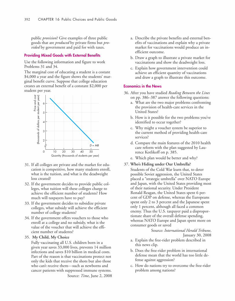
392 CHAPTER 16 Public Choices and Public Goods

public provision? Give examples of three publicgoods that are produced by private firms but pro-vided by government and paid for with taxes.

Providing Mixed Goods with External Benefits

Use the following information and figure to workProblems 31 and 34.The marginal cost of educating a student is a costant$4,000 a year and the figure shows the students’ mar-ginal benefit curve. Suppose that college educationcreates an external benefit of a constant $2,000 perstudent per year.

31. If all colleges are private and the market for edu-cation is competitive, how many students enroll,what is the tuition, and what is the deadweightloss created?

32. If the government decides to provide public col-leges, what tuition will these colleges charge toachieve the efficient number of students? Howmuch will taxpayers have to pay?

33. If the government decides to subsidize privatecolleges, what subsidy will achieve the efficientnumber of college students?

34. If the government offers vouchers to those whoenroll at a college and no subsidy, what is thevalue of the voucher that will achieve the effi-cient number of students?

35. My Child, My ChoiceFully vaccinating all U.S. children born in agiven year saves 33,000 lives, prevents 14 millioninfections and saves $10 billion in medical costs.Part of the reason is that vaccinations protect notonly the kids that receive the shots but also thosewho can’t receive them—such as newborns andcancer patients with suppressed immune systems.

Source: Time, June 2, 2008

Pric

e an

d co

st(th

ousa

nds

of d

olla

rs p

er s

tude

nt p

er y

ear)

Quantity (thousands of students per year)0 10 20 30 40 50

2

3

4

5

6

D = MB

a. Describe the private benefits and external ben-efits of vaccinations and explain why a privatemarket for vaccinations would produce an in-efficient outcome.

b. Draw a graph to illustrate a private market forvaccinations and show the deadweight loss.

c. Explain how government intervention couldachieve an efficient quantity of vaccinationsand draw a graph to illustrate this outcome.

Economics in the News

36. After you have studied Reading Between the Lineson pp. 386–387 answer the following questions:a. What are the two major problems confronting

the provision of health-care services in theUnited States?

b. How is it possible for the two problems you’veidentified to occur together?

c. Why might a voucher system be superior tothe current method of providing health-careservices?

d. Compare the main features of the 2010 healthcare reform with the plan suggested by Lau-rence Kotlikoff on p. 385.

e. Which plan would be better and why?

37. Who’s Hiding under Our Umbrella?Students of the Cold War learn that, to deterpossible Soviet aggression, the United Statesplaced a “strategic umbrella” over NATO Europeand Japan, with the United States providing mostof their national security. Under PresidentRonald Reagan, the United States spent 6 per-cent of GDP on defense, whereas the Europeansspent only 2 to 3 percent and the Japanese spentonly 1 percent, although all faced a commonenemy. Thus the U.S. taxpayer paid a dispropor-tionate share of the overall defense spending,whereas NATO Europe and Japan spent more onconsumer goods or saved

Source: International Herald Tribune,January 30, 2008

a. Explain the free-rider problem described inthis news clip.

b. Does the free-rider problem in internationaldefense mean that the world has too little de-fense against aggression?

c. How do nations try to overcome the free-riderproblem among nations?

After studying this chapter,you will be able to:

� Explain why external costs bring market failure and toomuch pollution and how property rights, pollution taxes,emission charges, and marketable permits mightachieve an efficient outcome

� Explain the tragedy of the commons and its possible solutions

We burn huge quantities of fossil fuels—coal, natural gas, and oil—thatcause acid rain and global warming. We dump toxic waste into rivers, lakes,and oceans. These environmental issues are simultaneously everybody’sproblem and nobody’s problem. How can we take account of the damage thatwe cause others every time we turn on our heating or air-conditioning systems?

More and more people with ever-increasing incomes demand ever-greaterquantities of most goods and services. One item that we demand more and moreof is fish grown wild in the ocean. The fish stocks of the world’s oceans are notowned by anyone. They are common resources and everyone is free to use

them. But we are overusing our fish stocks and bringing somespecies to extinction. Must the price of fish inevitably keeprising? What can be done to conserve the world’s fish stocks?

In this chapter, we study the problems that arise because many of ouractions impose costs on other people in ways that we do not take into account

when we make our own economic choices. We focus on two big issues—airpollution and overfishing. In Reading Between the Lines at the end of the chapter,we look at the effects of a carbon tax designed to lower carbon emissions andaddress global warming and climate change.

ENVIRONMENTECONOMICS OF THE

17393

394 CHAPTER 17 Economics of the Environment

◆ Negative Externality: PollutionCan each individual be relied upon to make decisionsthat influence the Earth’s carbon-dioxide concentra-tion in the social interest? Must governments changethe incentives we face so that our self-interestedchoices are also in the social interest? How can gov-ernments change incentives? These questions aboutclimate change that we posed in Chapter 1 (see p. 6)involve external costs and this chapter answers them.

This chapter also studies another environmentalproblem that requires public choices: the overuse andsometimes the depletion of renewable natural resources.

We first study the external costs of pollution andbegin with a quick review of the production activitiesthat pollute our environment.

Sources of PollutionEconomic activity pollutes air, water, and land, andthese individual areas of pollution interact throughthe ecosystem. The three biggest sources of pollutionare road transportation, electricity generation, andindustrial processes.

A common belief is that our advanced industrialeconomy is creating ever more pollution. But formany pollutants, in the rich countries that include

the United States, pollution is less serious today thatit was in earlier years (see Economics in Action belowfor a description of the trends in air pollution).

Effects of PollutionWhile the facts about the sources and trends in airpollution are not in doubt, there is disagreementabout the effects of air pollution. The least controver-sial is acid rain caused by sulphur dioxide and nitro-gen oxide emissions from coal- and oil-firedgenerators of power stations. Acid rain begins withair pollution, and it leads to water pollution anddamages vegetation.

More than 180 others airborne substances (sus-pended particulates) such as lead from leaded gaso-line have been identified, which in sufficiently largeconcentrations, are believed to cause cancer and otherlife-threatening conditions.

Many scientists believe that carbon dioxide emis-sions are a major cause of global warming and cli-mate change.

The effects of pollution mean that production andconsumption decisions impose costs that are nottaken fully into account when decisions are made.You are now going to see how economists analysethese decisions and solve the pollution problem.

–80

Highway vehicles Industrial processes Other fuel consumption

Percentage change: 1990 to 2008

Six Air Pollutants and their Economic Sources

–20–60 0–40

Lead

Carbonmonoxide

Volatile organiccompounds

Oxides ofnitrogen

Sulfurdioxide

Particulatematter

Source of data: Latest Findings on National Air Quality: Status and Trendsthrough 2008, United States Environmental Protection Agency,http://www.epa.gov/air/airtrends/2010/report/airpollution.pdf

Economics in ActionU.S. Air Pollution Trends: Cleaner and SaferThe figure shows the percentage changes in the con-centrations of six air pollutants between 1990 and2008 and their economic sources. All of these pollu-tants decreased.

These reductions in air pollution are more impres-sive when they are seen against the trends in eco-nomic activity. Between 1990 and 2008, totalproduction in the United States increased by 66 per-cent, vehicle miles traveled increased by 40 percent,and the population increased by 20 percent.

The Clean Air Act has brought regulations thatcut emissions of carbon monoxide, volatile organiccompounds, oxides of nitrogen, sulfur dioxide andparticulate matter to around a half of their 1990 lev-els. And economic actions that you will learn aboutin this chapter almost eliminated lead from highwaysand industrial processes.

Negative Externality: Pollution 395

Private Cost and Social Cost of PollutionTo study the economics of the external costs thatarise from pollution, we distinguish between the pri-vate cost and the social cost of production.

A private cost of production is a cost that is borneby the producer of a good or service. Marginal cost isthe cost of producing an additional unit of a good orservice. So marginal private cost (MC) is the cost ofproducing an additional unit of a good or service thatis borne by its producer.

An external cost is a cost of producing a good orservice that is not borne by the producer but borne byother people. A marginal external cost is the cost of pro-ducing an additional unit of a good or service that fallson people other than the producer.

Marginal social cost (MSC ) is the marginal costincurred by the producer and by everyone else onwhom the cost falls—by society. It is the sum of mar-ginal private cost and marginal external cost. That is,

We express costs in dollars, but we must alwaysremember that a cost is an opportunity cost—some-thing real, such as clean air or a clean river, is givenup to get something.

Valuing an External Cost Economists use marketprices to put a dollar value on the cost of pollution.For example, suppose that there are two similar rivers,one polluted and the other clean. Five hundred iden-tical homes are built along the side of each river. Thehomes on the clean river rent for $2,500 a month,and those on the polluted river rent for $1,500 amonth. If the pollution is the only detectable differ-ence between the two rivers and the two locations,the rent decrease of $1,000 per month is the cost ofthe pollution. With 500 homes on the polluted river,the external cost of pollution is $500,000 a month.

External Cost and Output Figure 17.1 shows anexample of the relationship between output and costin a chemical industry that pollutes. The marginalcost curve, MC, describes the marginal private costborne by the firms that produce the chemical.Marginal cost increases as the quantity of chemicalproduced increases.

If the firms dump waste into a river, they imposean external cost on other users of the river. We willassume that the marginal external cost increases withthe amount of the chemical produced.

MSC = MC + Marginal external cost.

The marginal social cost curve, MSC, is found byadding the marginal external cost to the marginal pri-vate cost. So a point on the MSC curve shows thesum of the marginal private cost of producing a givenoutput and marginal external cost created.

For example, when the chemical industry produces4,000 tons of chemical a month, its marginal privatecost is $100 a ton and the marginal external cost is$125 a ton, so the marginal social cost is $225 a ton.

In Fig. 17.1, when the quantity of chemicalproduced increases, the amount of pollution increasesand the external cost of pollution increases.

Figure 17.1 shows the relationship between thequantity of chemical produced and the cost of thepollution it creates, but it doesn’t tell us how muchpollution the chemical industry creates. That quantitydepends on the quantity of the chemical produced,which depends on supply and demand in the marketfor the chemical. We now look at that market.

Cos

t (do

llars

per

ton)

Quantity (thousands of tons of chemical per month)0 2 4 6

300

225

150

MSC

MC

Marginalexternalcost

Marginalprivate cost

Marginalsocial cost

75

100

The MC curve shows the marginal private cost borne by thefactories that produce a chemical. The MSC curve shows thesum of marginal private cost and marginal external cost.When output is 4,000 tons of chemical a month, marginalprivate cost is $100 a ton, marginal external cost is $125 aton, and marginal social cost is $225 a ton.

FIGURE 17.1 An External Cost

animation

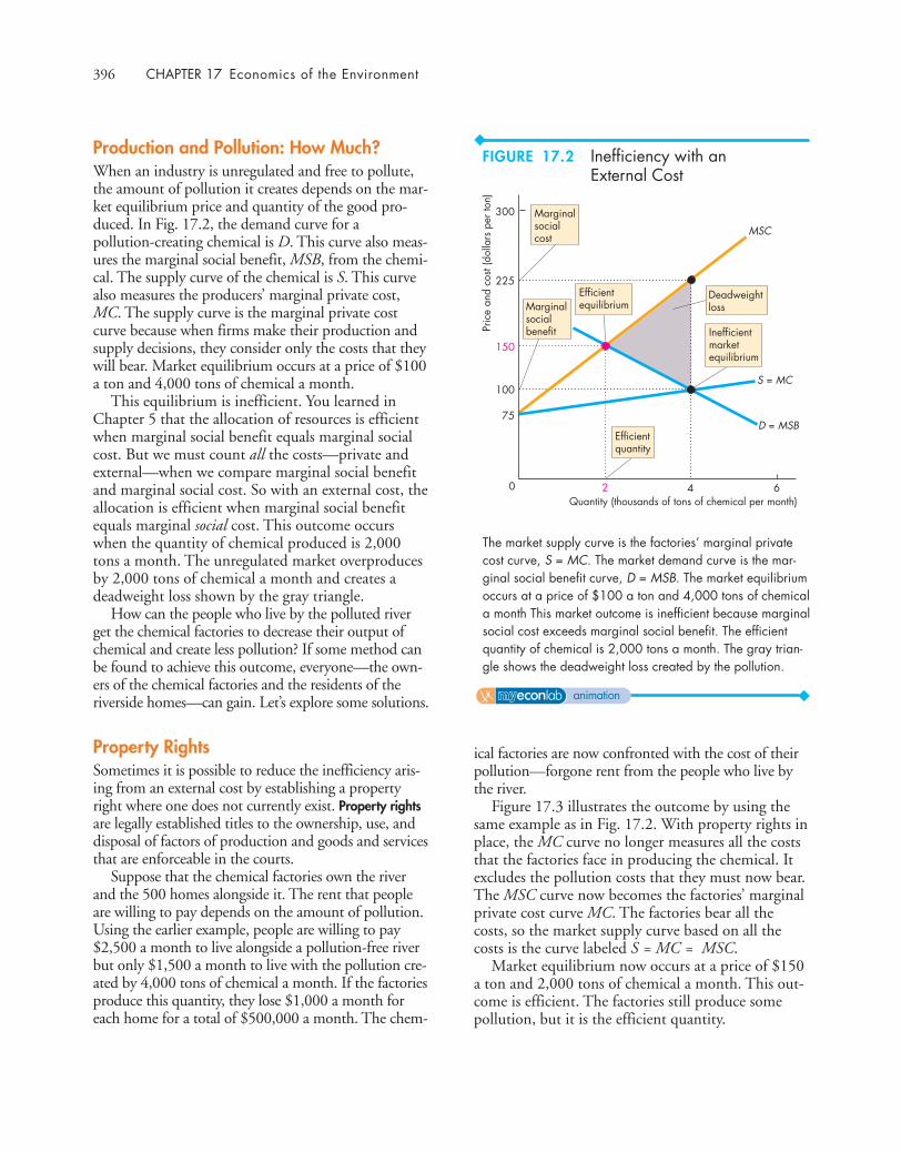
396 CHAPTER 17 Economics of the Environment

Production and Pollution: How Much?When an industry is unregulated and free to pollute,the amount of pollution it creates depends on the mar-ket equilibrium price and quantity of the good pro-duced. In Fig. 17.2, the demand curve for apollution-creating chemical is D. This curve also meas-ures the marginal social benefit, MSB, from the chemi-cal. The supply curve of the chemical is S. This curvealso measures the producers’ marginal private cost,MC. The supply curve is the marginal private costcurve because when firms make their production andsupply decisions, they consider only the costs that theywill bear. Market equilibrium occurs at a price of $100a ton and 4,000 tons of chemical a month.

This equilibrium is inefficient. You learned inChapter 5 that the allocation of resources is efficientwhen marginal social benefit equals marginal socialcost. But we must count all the costs—private andexternal—when we compare marginal social benefitand marginal social cost. So with an external cost, theallocation is efficient when marginal social benefitequals marginal social cost. This outcome occurswhen the quantity of chemical produced is 2,000tons a month. The unregulated market overproducesby 2,000 tons of chemical a month and creates adeadweight loss shown by the gray triangle.

How can the people who live by the polluted riverget the chemical factories to decrease their output ofchemical and create less pollution? If some method canbe found to achieve this outcome, everyone—the own-ers of the chemical factories and the residents of theriverside homes—can gain. Let’s explore some solutions.

Property RightsSometimes it is possible to reduce the inefficiency aris-ing from an external cost by establishing a propertyright where one does not currently exist. Property rightsare legally established titles to the ownership, use, anddisposal of factors of production and goods and servicesthat are enforceable in the courts.

Suppose that the chemical factories own the riverand the 500 homes alongside it. The rent that peopleare willing to pay depends on the amount of pollution.Using the earlier example, people are willing to pay$2,500 a month to live alongside a pollution-free riverbut only $1,500 a month to live with the pollution cre-ated by 4,000 tons of chemical a month. If the factoriesproduce this quantity, they lose $1,000 a month foreach home for a total of $500,000 a month. The chem-

Pric

e an

d co

st (d

olla

rs p

er to

n)

Quantity (thousands of tons of chemical per month)0 2 4 6

300

225

150

D = MSB

S = MC

MSC

Efficientequilibrium

Inefficientmarketequilibrium

Marginalsocialcost

75

100

DeadweightlossMarginal

socialbenefit

Efficientquantity

The market supply curve is the factories’ marginal privatecost curve, S = MC. The market demand curve is the mar-ginal social benefit curve, D = MSB. The market equilibriumoccurs at a price of $100 a ton and 4,000 tons of chemicala month This market outcome is inefficient because marginalsocial cost exceeds marginal social benefit. The efficientquantity of chemical is 2,000 tons a month. The gray trian-gle shows the deadweight loss created by the pollution.

ical factories are now confronted with the cost of theirpollution—forgone rent from the people who live bythe river.

Figure 17.3 illustrates the outcome by using thesame example as in Fig. 17.2. With property rights inplace, the MC curve no longer measures all the coststhat the factories face in producing the chemical. Itexcludes the pollution costs that they must now bear.The MSC curve now becomes the factories’ marginalprivate cost curve MC. The factories bear all thecosts, so the market supply curve based on all thecosts is the curve labeled S = MC = MSC.

Market equilibrium now occurs at a price of $150a ton and 2,000 tons of chemical a month. This out-come is efficient. The factories still produce somepollution, but it is the efficient quantity.

FIGURE 17.2 Inefficiency with anExternal Cost

animation

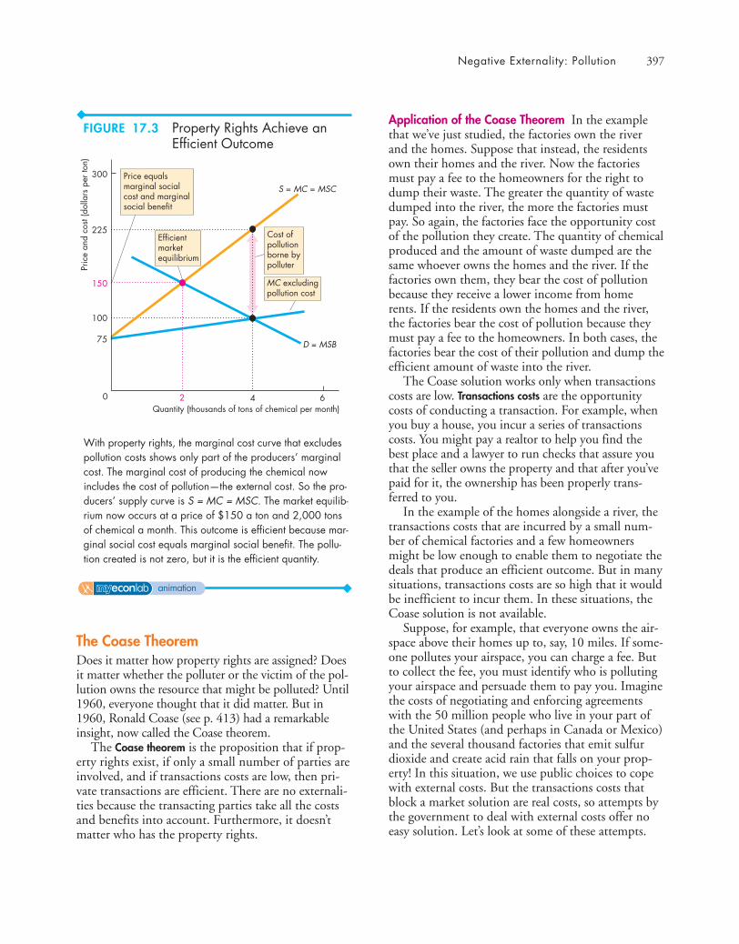
Negative Externality: Pollution 397

Application of the Coase Theorem In the examplethat we’ve just studied, the factories own the riverand the homes. Suppose that instead, the residentsown their homes and the river. Now the factoriesmust pay a fee to the homeowners for the right todump their waste. The greater the quantity of wastedumped into the river, the more the factories mustpay. So again, the factories face the opportunity costof the pollution they create. The quantity of chemicalproduced and the amount of waste dumped are thesame whoever owns the homes and the river. If thefactories own them, they bear the cost of pollutionbecause they receive a lower income from homerents. If the residents own the homes and the river,the factories bear the cost of pollution because theymust pay a fee to the homeowners. In both cases, thefactories bear the cost of their pollution and dump theefficient amount of waste into the river.

The Coase solution works only when transactionscosts are low. Transactions costs are the opportunitycosts of conducting a transaction. For example, whenyou buy a house, you incur a series of transactionscosts. You might pay a realtor to help you find thebest place and a lawyer to run checks that assure youthat the seller owns the property and that after you’vepaid for it, the ownership has been properly trans-ferred to you.

In the example of the homes alongside a river, thetransactions costs that are incurred by a small num-ber of chemical factories and a few homeownersmight be low enough to enable them to negotiate thedeals that produce an efficient outcome. But in manysituations, transactions costs are so high that it wouldbe inefficient to incur them. In these situations, theCoase solution is not available.

Suppose, for example, that everyone owns the air-space above their homes up to, say, 10 miles. If some-one pollutes your airspace, you can charge a fee. Butto collect the fee, you must identify who is pollutingyour airspace and persuade them to pay you. Imaginethe costs of negotiating and enforcing agreementswith the 50 million people who live in your part ofthe United States (and perhaps in Canada or Mexico)and the several thousand factories that emit sulfurdioxide and create acid rain that falls on your prop-erty! In this situation, we use public choices to copewith external costs. But the transactions costs thatblock a market solution are real costs, so attempts bythe government to deal with external costs offer noeasy solution. Let’s look at some of these attempts.

The Coase TheoremDoes it matter how property rights are assigned? Doesit matter whether the polluter or the victim of the pol-lution owns the resource that might be polluted? Until1960, everyone thought that it did matter. But in1960, Ronald Coase (see p. 413) had a remarkableinsight, now called the Coase theorem.

The Coase theorem is the proposition that if prop-erty rights exist, if only a small number of parties areinvolved, and if transactions costs are low, then pri-vate transactions are efficient. There are no externali-ties because the transacting parties take all the costsand benefits into account. Furthermore, it doesn’tmatter who has the property rights.

Pric

e an

d co

st (d

olla

rs p

er to

n)

Quantity (thousands of tons of chemical per month)0 2 4 6

300

225

150

D = MSB

S = MC = MSC

Cost ofpollutionborne bypolluter

Efficientmarketequilibrium

Price equalsmarginal socialcost and marginalsocial benefit

75

100

MC excludingpollution cost

With property rights, the marginal cost curve that excludespollution costs shows only part of the producers’ marginalcost. The marginal cost of producing the chemical nowincludes the cost of pollution—the external cost. So the pro-ducers’ supply curve is S = MC = MSC. The market equilib-rium now occurs at a price of $150 a ton and 2,000 tonsof chemical a month. This outcome is efficient because mar-ginal social cost equals marginal social benefit. The pollu-tion created is not zero, but it is the efficient quantity.

FIGURE 17.3 Property Rights Achieve anEfficient Outcome

animation

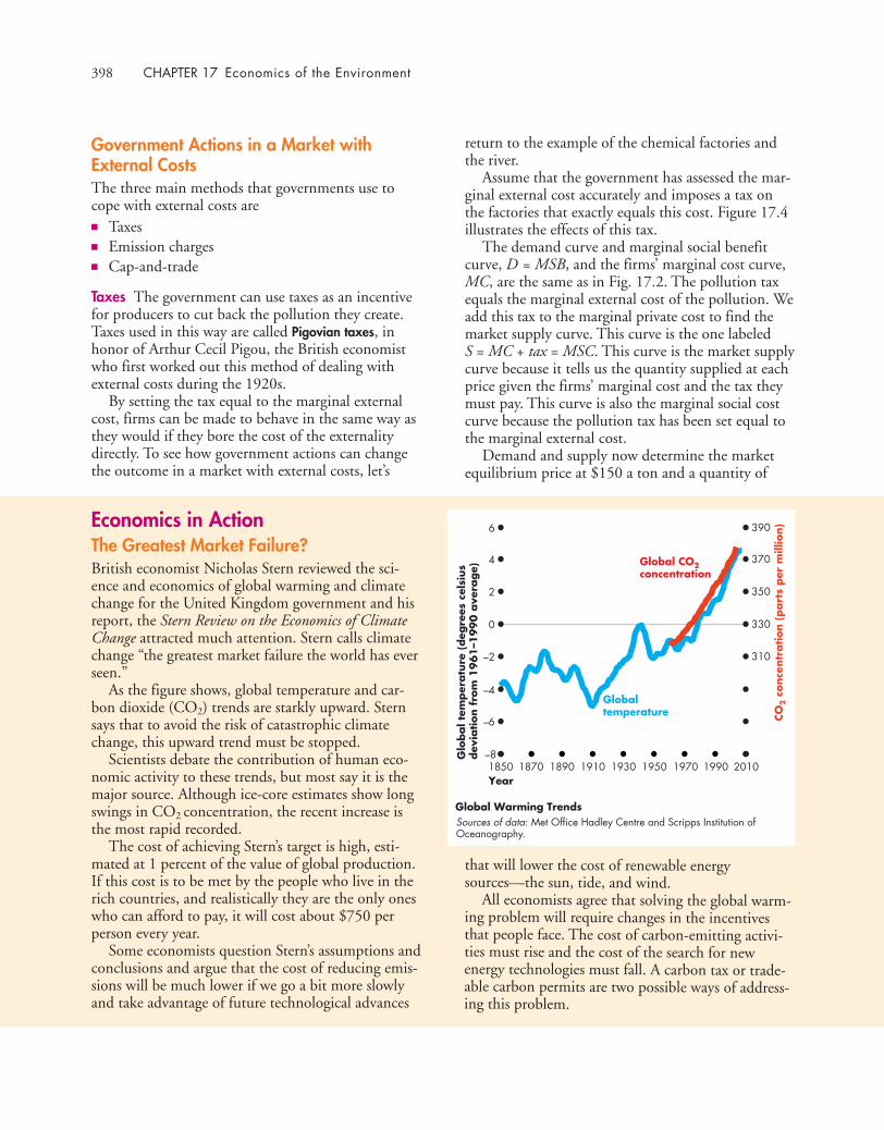
398 CHAPTER 17 Economics of the Environment

return to the example of the chemical factories andthe river.

Assume that the government has assessed the mar-ginal external cost accurately and imposes a tax onthe factories that exactly equals this cost. Figure 17.4illustrates the effects of this tax.

The demand curve and marginal social benefitcurve, D = MSB, and the firms’ marginal cost curve,MC, are the same as in Fig. 17.2. The pollution taxequals the marginal external cost of the pollution. Weadd this tax to the marginal private cost to find themarket supply curve. This curve is the one labeled S = MC + tax = MSC. This curve is the market supplycurve because it tells us the quantity supplied at eachprice given the firms’ marginal cost and the tax theymust pay. This curve is also the marginal social costcurve because the pollution tax has been set equal tothe marginal external cost.

Demand and supply now determine the marketequilibrium price at $150 a ton and a quantity of

Government Actions in a Market with External CostsThe three main methods that governments use tocope with external costs are■ Taxes■ Emission charges■ Cap-and-trade

Taxes The government can use taxes as an incentivefor producers to cut back the pollution they create.Taxes used in this way are called Pigovian taxes, inhonor of Arthur Cecil Pigou, the British economistwho first worked out this method of dealing withexternal costs during the 1920s.

By setting the tax equal to the marginal externalcost, firms can be made to behave in the same way asthey would if they bore the cost of the externalitydirectly. To see how government actions can changethe outcome in a market with external costs, let’s

Economics in ActionThe Greatest Market Failure?British economist Nicholas Stern reviewed the sci-ence and economics of global warming and climatechange for the United Kingdom government and hisreport, the Stern Review on the Economics of ClimateChange attracted much attention. Stern calls climatechange “the greatest market failure the world has everseen.”

As the figure shows, global temperature and car-bon dioxide (CO2) trends are starkly upward. Sternsays that to avoid the risk of catastrophic climatechange, this upward trend must be stopped.

Scientists debate the contribution of human eco-nomic activity to these trends, but most say it is themajor source. Although ice-core estimates show longswings in CO2 concentration, the recent increase isthe most rapid recorded.

The cost of achieving Stern’s target is high, esti-mated at 1 percent of the value of global production.If this cost is to be met by the people who live in therich countries, and realistically they are the only oneswho can afford to pay, it will cost about $750 perperson every year.

Some economists question Stern’s assumptions andconclusions and argue that the cost of reducing emis-sions will be much lower if we go a bit more slowlyand take advantage of future technological advances

Globaltemperature

Global CO2concentration

–8

–6

–4

0

6

1850

–2

2

4

330

390

310

350

370

Year1890 1970 20101990195019301870 1910

Glo

bal te

mper

atu

re (

deg

rees

cel

sius

dev

iation f

rom

1961–1

990 a

vera

ge)

CO

2 c

once

ntr

ation (

part

s per

mill

ion)

Global Warming Trends

that will lower the cost of renewable energysources—the sun, tide, and wind.

All economists agree that solving the global warm-ing problem will require changes in the incentivesthat people face. The cost of carbon-emitting activi-ties must rise and the cost of the search for newenergy technologies must fall. A carbon tax or trade-able carbon permits are two possible ways of address-ing this problem.

Sources of data: Met Office Hadley Centre and Scripps Institution ofOceanography.

Negative Externality: Pollution 399

2,000 tons of chemical a month. At this quantity ofchemical production, the marginal social cost is $150and the marginal social benefit is $150, so the out-come is efficient. The firms incur a marginal privatecost of $88 a ton and pay a tax of $62 a ton. Thegovernment collects tax revenue of $124,000 amonth.

Emission Charges Emission charges are an alternativeto a tax for confronting a polluter with the external costof pollution. The government sets a price per unit ofpollution. The more pollution a firm creates, the more itpays in emission charges. This method of dealing withpollution externalities has been used only modestly inthe United States but is common in Europe where, forexample, France, Germany, and the Netherlands makewater polluters pay a waste disposal charge.

To work out the emission charge that achieves effi-ciency, the government needs information about thepolluting industry that, in practice, is rarely available.

Cap-and-Trade Instead of taxing or imposing emis-sion charges on polluters, each potential pollutermight be assigned a permitted pollution limit. Eachfirm knows its own costs and its benefits from pollu-tion, and making pollution limits marketable is aclever way of using this private information that isunknown to the government. The government issueseach firm a permit to emit a certain amount of pollu-tion, and firms can trade these permits. Firms thathave a low marginal cost of reducing pollution selltheir permits, and firms that have a high marginal costof reducing pollution buy permits. The market in per-mits determines the price at which firms trade per-mits. Each firm buys or sells permits until its marginalcost of pollution equals the market price of a permit.

This method of dealing with pollution provides aneven stronger incentive than emission charges to findlower-polluting technologies because the price of a pol-lution permit rises as the demand for permits increases.

Trading in lead pollution permits became com-mon during the 1980s, and this marketable permitprogram enabled lead pollution to be virtually elim-inated in the United States (see p. 394). But thissuccess might not easily translate to other pollutantbecause most lead pollution came from gasoline,which was easy to monitor.

Pric

e an

d co

st (d

olla

rs p

er to

n)

Quantity (thousands of tons of chemical per month)0 2 4 6

300

225

150

88

D = MSB

S = MC + tax = MSC

MC

Pollutiontax

Efficientmarketequilibrium

Taxrevenue

Marginal socialcost and marginalsocial benefit

75

When the government imposes a pollution tax equal to themarginal external cost of pollution, the supply curvebecomes the marginal private cost curve, MC, plus thetax—the curve S = MC + tax. Market equilibrium occurs ata price of $150 a ton and a quantity of 2,000 tons ofchemical a month. This equilibrium is efficient because mar-ginal social cost equals marginal social benefit. The purplerectangle shows the government’s tax revenue.

Your next task is to study common resources andthe government actions that can bring efficient use.

FIGURE 17.4 A Pollution Tax to Achieve anEfficient Outcome

animationREVIEW QUIZ

1 What is the distinction between private costand social cost?

2 How do external costs prevent a competitivemarket from allocating resources efficiently?

3 How can external costs be eliminated by assign-ing property rights?

4 How do taxes help us to cope with externalcosts? At what level must a pollution tax be setto be efficient?

5 How do emission charges and marketablepollution permits work?

You can work these questions in Study Plan 17.1 and get instant feedback.

400 CHAPTER 17 Economics of the Environment

◆ The Tragedy of the CommonsOvergrazing the pastures around a village in MiddleAges England, and overfishing the cod stocks of theNorth Atlantic Ocean during the recent past aretragedies of the commons. The tragedy of the com-mons is the overuse of a common resource that ariseswhen its users have no incentive to conserve it anduse it sustainably.

To study the tragedy of the commons and its pos-sible remedies, we’ll focus on the recent and currenttragedy—overfishing and depleting the stock ofAtlantic cod. We begin by thinking about the sus-tainable use of a renewable resource.

Sustainable Use of a Renewable ResourceA renewable natural resource is one that replenishesitself by the birth and growth of new members of thepopulation. Fish, trees, and the fertile soil are allexamples of this type of resource.

Focusing on fish, the sustainable catch is the quan-tity that can be caught year after year without deplet-ing the stock. This quantity depends on the stock andin the interesting way illustrated in Fig. 17.6.

If the stock of fish is small, the quantity of new fishborn is also small, so the sustainable catch is small.

Economics in ActionThe Original Tragedy of the CommonsThe term “tragedy of the commons” comes from four-teenth-century England, where areas of rough grasslandsurrounded villages. The commons were open to alland used for grazing cows and sheep owned by thevillagers.

Because the commons were open to all, no one hadan incentive to ensure that the land was not over-grazed. The result was a severe overgrazing situation.Because the commons were overgrazed, the quantity ofcows and sheep that they could feed kept falling, thelonger the overgrazing continued.

During the sixteenth century, the price of woolincreased and England became a wool exporter to theworld. Sheep farming became profitable, and sheepowners wanted to gain more effective control of theland they used. So the commons were gradually pri-vatized and enclosed. Overgrazing ended, and landuse became more efficient.

100

50

150

200

250

300

0 3,000 6,000Cod stock (thousands of tons)

Susta

inab

le c

atch

(tho

usan

ds o

f ton

s pe

r yea

r) MaximumsustainablecatchOverfishing

depletesstock

As the stock of fish increases (on the x-axis), the sustainablecatch (on the y-axis) increases to a maximum. Beyond thatnumber, more fish must compete for food and the sustain-able catch falls.

If the catch exceeds the sustainable catch, the fish stockdiminishes.

FIGURE 17.5 Sustainable Catch

animation

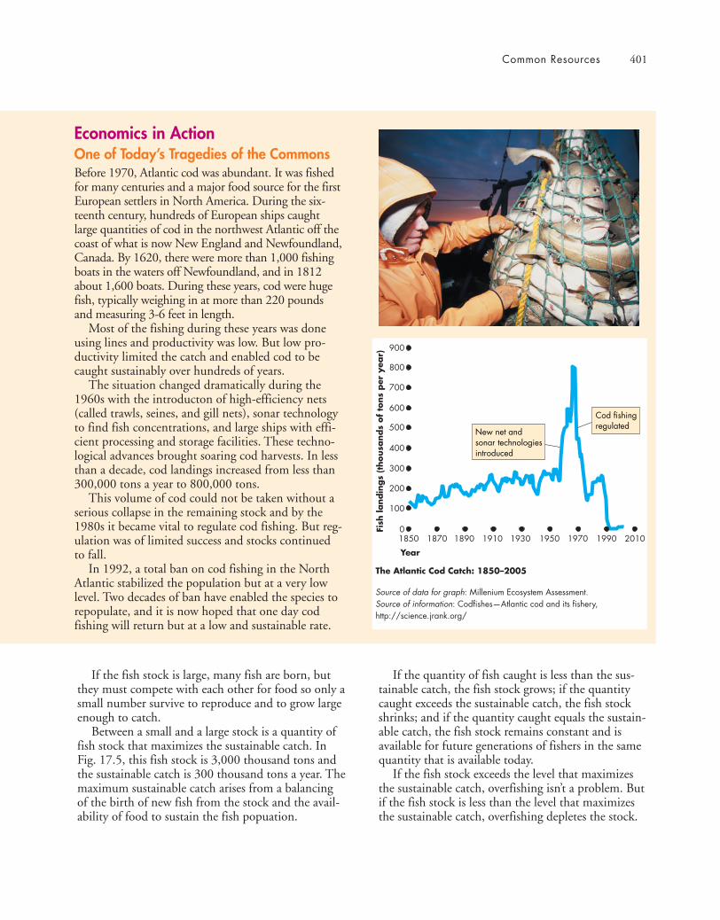
Common Resources 401

If the fish stock is large, many fish are born, butthey must compete with each other for food so only asmall number survive to reproduce and to grow largeenough to catch.

Between a small and a large stock is a quantity offish stock that maximizes the sustainable catch. InFig. 17.5, this fish stock is 3,000 thousand tons andthe sustainable catch is 300 thousand tons a year. Themaximum sustainable catch arises from a balancingof the birth of new fish from the stock and the avail-ability of food to sustain the fish popuation.

If the quantity of fish caught is less than the sus-tainable catch, the fish stock grows; if the quantitycaught exceeds the sustainable catch, the fish stockshrinks; and if the quantity caught equals the sustain-able catch, the fish stock remains constant and isavailable for future generations of fishers in the samequantity that is available today.

If the fish stock exceeds the level that maximizesthe sustainable catch, overfishing isn’t a problem. Butif the fish stock is less than the level that maximizesthe sustainable catch, overfishing depletes the stock.

Economics in ActionOne of Today’s Tragedies of the CommonsBefore 1970, Atlantic cod was abundant. It was fishedfor many centuries and a major food source for the firstEuropean settlers in North America. During the six-teenth century, hundreds of European ships caughtlarge quantities of cod in the northwest Atlantic off thecoast of what is now New England and Newfoundland,Canada. By 1620, there were more than 1,000 fishingboats in the waters off Newfoundland, and in 1812about 1,600 boats. During these years, cod were hugefish, typically weighing in at more than 220 poundsand measuring 3-6 feet in length.

Most of the fishing during these years was doneusing lines and productivity was low. But low pro-ductivity limited the catch and enabled cod to becaught sustainably over hundreds of years.

The situation changed dramatically during the1960s with the introducton of high-efficiency nets(called trawls, seines, and gill nets), sonar technologyto find fish concentrations, and large ships with effi-cient processing and storage facilities. These techno-logical advances brought soaring cod harvests. In lessthan a decade, cod landings increased from less than300,000 tons a year to 800,000 tons.

This volume of cod could not be taken without aserious collapse in the remaining stock and by the1980s it became vital to regulate cod fishing. But reg-ulation was of limited success and stocks continuedto fall.

In 1992, a total ban on cod fishing in the NorthAtlantic stabilized the population but at a very lowlevel. Two decades of ban have enabled the species torepopulate, and it is now hoped that one day codfishing will return but at a low and sustainable rate.

Year

The Atlantic Cod Catch: 1850–2005

Fish

landin

gs

(thousa

nds

of

tons

per

yea

r)

0

900

1870 1890 1910 1930 1950 1970 19901850 2010

800

700

600

500

400

300

200

100

Cod fishingregulated

New net andsonar technologiesintroduced

Source of data for graph: Millenium Ecosystem Assessment.Source of information: Codfishes—Atlantic cod and its fishery, http://science.jrank.org/

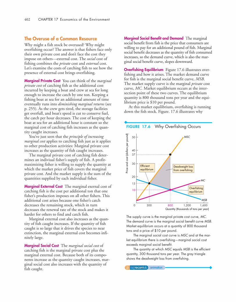
402 CHAPTER 17 Economics of the Environment

The Overuse of a Common ResourceWhy might a fish stock be overused? Why mightoverfishing occur? The answer is that fishers face onlytheir own private cost and don’t face the cost theyimpose on others—external cost. The social cost offishing combines the private cost and external cost.Let’s examine the costs of catching fish to see how thepresence of external cost brings overfishing.

Marginal Private Cost You can think of the marginalprivate cost of catching fish as the additional costincurred by keeping a boat and crew at sea for longenough to increase the catch by one ton. Keeping afishing boat at sea for an additional amount of timeeventually runs into diminishing marginal returns (seep. 255). As the crew gets tired, the storage facilitiesget overfull, and boat’s speed is cut to conserve fuel,the catch per hour decreases. The cost of keeping theboat at sea for an additional hour is constant so themarginal cost of catching fish increases as the quan-tity caught increases.

You’ve just seen that the principle of increasingmarginal cost applies to catching fish just as it appliesto other production activities: Marginal private costincreases as the quantity of fish caught increases.

The marginal private cost of catching fish deter-mines an indiviual fisher’s supply of fish. A profit-maximizing fisher is willing to supply the quantity atwhich the market price of fish covers the marginalprivate cost. And the market supply is the sum of thequantities supplied by each individual fisher.

Marginal External Cost The marginal exernal cost ofcatching fish is the cost per additional ton that onefisher’s production imposes on all other fishers. Thisadditional cost arises because one fisher’s catchdecreases the remaining stock, which in turndecreases the renewal rate of the stock and makes itharder for others to find and catch fish.

Marginal external cost also increases as the quan-tity of fish caught increases. If the quantity of fishcaught is so large that it drives the species to nearextinction, the marginal external cost becomes infi-nitely large.

Marginal Social Cost The marginal social cost ofcatching fish is the marginal private cost plus themarginal external cost. Because both of its compo-nents increase as the quantity caught increases, mar-ginal social cost also increases with the quantity offish caught.

Marginal Social Benefit and Demand The marginalsocial benefit from fish is the price that consumers arewilling to pay for an additional pound of fish. Marginalsocial benefit decreases as the quantity of fish consumedincreases, so the demand curve, which is also the mar-ginal social benefit curve, slopes downward.

Overfishing Equilibrium Figure 17.6 illustrates over-fishing and how it arises. The market demand curvefor fish is the marginal social benefit curve, MSB.The market supply curve is the marginal private costcurve, MC. Market equilibrium occurs at the inter-section point of these two curves. The equilibriumquantity is 800 thousand tons per year and the equi-librium price is $10 per pound.

At this market equilibrium, overfishing is runningdown the fish stock. Figure. 17.6 illustrates why

50

40

30

37

20

15

10

0 300 800 1,6001,200Quantity (thousands of tons per year)

Pric

e an

d co

st (d

olla

rs p

er p

ound

)

MSB

MC

MSC

Efficientequilibrium

Overfishingequilibrium

Deadweight lossfrom overfishing

The supply curve is the marginal private cost curve, MC.The demand curve is the marginal social benefit curve MSB.Market equilibrium occurs at a quantity of 800 thousandtons and a price of $10 per pound.

The marginal social cost curve is MSC and at the mar-ket equilibrium there is overfishing—marginal social costexceeds marginal social benefit.

The quantity at which MSC equals MSB is the efficientquantity, 300 thousand tons per year. The gray triangleshows the deadweight loss from overfishing.

FIGURE 17.6 Why Overfishing Occurs

animation

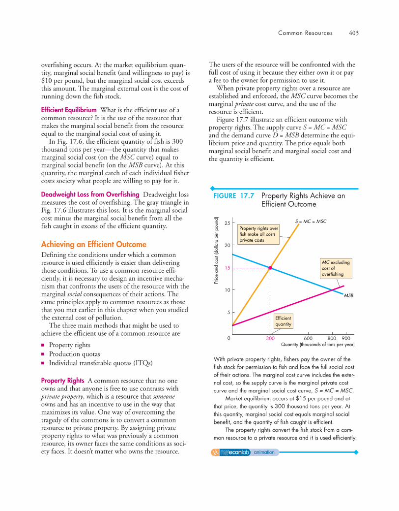
Common Resources 403

overfishing occurs. At the market equilibrium quan-tity, marginal social benefit (and willingness to pay) is$10 per pound, but the marginal social cost exceedsthis amount. The marginal external cost is the cost ofrunning down the fish stock.

Efficient Equilibrium What is the efficient use of acommon resource? It is the use of the resource thatmakes the marginal social benefit from the resourceequal to the marginal social cost of using it.

In Fig. 17.6, the efficient quantity of fish is 300thousand tons per year—the quantity that makesmarginal social cost (on the MSC curve) equal tomarginal social benefit (on the MSB curve). At thisquantity, the marginal catch of each individual fishercosts society what people are willing to pay for it.

Deadweight Loss from Overfishing Deadweight lossmeasures the cost of overfishing. The gray triangle inFig. 17.6 illustrates this loss. It is the marginal socialcost minus the marginal social benefit from all thefish caught in excess of the efficient quantity.

Achieving an Efficient OutcomeDefining the conditions under which a commonresource is used efficiently is easier than deliveringthose conditions. To use a common resource effi-ciently, it is necessary to design an incentive mecha-nism that confronts the users of the resource with themarginal social consequences of their actions. Thesame principles apply to common resources as thosethat you met earlier in this chapter when you studiedthe external cost of pollution.

The three main methods that might be used toachieve the efficient use of a common resource are

■ Property rights■ Production quotas■ Individual transferable quotas (ITQs)

Property Rights A common resource that no oneowns and that anyone is free to use contrasts withprivate property, which is a resource that someoneowns and has an incentive to use in the way thatmaximizes its value. One way of overcoming thetragedy of the commons is to convert a commonresource to private property. By assigning privateproperty rights to what was previously a commonresource, its owner faces the same conditions as soci-ety faces. It doesn’t matter who owns the resource.

25

20

15

10

5

0 300 900600Quantity (thousands of tons per year)

Pric

e an

d co

st (d

olla

rs p

er p

ound

)

800

MSB

S = MC = MSC

Efficientquantity

MC excludingcost ofoverfishing

Property rights overfish make all costsprivate costs

With private property rights, fishers pay the owner of thefish stock for permission to fish and face the full social costof their actions. The marginal cost curve includes the exter-nal cost, so the supply curve is the marginal private costcurve and the marginal social cost curve, S = MC = MSC.

Market equilibrium occurs at $15 per pound and atthat price, the quantity is 300 thousand tons per year. Atthis quantity, marginal social cost equals marginal socialbenefit, and the quantity of fish caught is efficient.

The property rights convert the fish stock from a com-mon resource to a private resource and it is used efficiently.

The users of the resource will be confronted with thefull cost of using it because they either own it or paya fee to the owner for permission to use it.

When private property rights over a resource areestablished and enforced, the MSC curve becomes themarginal private cost curve, and the use of theresource is efficient.

Figure 17.7 illustrate an efficient outcome withproperty rights. The supply curve S = MC = MSCand the demand curve D = MSB determine the equi-librium price and quantity. The price equals bothmarginal social benefit and marginal social cost andthe quantity is efficient.

FIGURE 17.7 Property Rights Achieve anEfficient Outcome

animation

404 CHAPTER 17 Economics of the Environment

The private property solution to the tragedy of thecommons is available in some cases. It was the solu-tion to the original tragedy of the commons inEngland’s Middle Ages. It is also a solution that hasbeen used to prevent overuse of the airwaves thatcarry cell-phone services. The right to use this space(called the frequency spectrum) has been auctionedby governments to the highest bidders. The owner ofeach part of the spectrum is the only one permittedto use it (or to license someone else to use it).

But assigning private property rights is not alwaysfeasible. It would be difficult, for example, to assignprivate property rights to the oceans. It would not beimpossible, but the cost of enforcing private propertyrights over thousands of square miles of ocean wouldbe high. It would be even more difficult to assign andprotect private property rights to the atmosphere.

In some cases, there is an emotional objection toassigning private property rights. Critics of it have amoral objection to someone owning a resource thatthey regard as public. In the absence of propertyrights, some form of government intervention isused, one of which is a production quota.

Production Quota A production quota is an upperlimit to the quantity of a good that may be pro-duced in a specified period. The quota is allocatedto individual producers, so each producer has itsown quota.

You studied the effects of a production quota inChapter 6 (pp. 139–140) and learned that a quota candrive a wedge between marginal social benefit andmarginal social cost and create deadweight loss. In thatearlier example, the market was efficient without aquota. But in the case of common resources, the mar-ket overuses the resource and produces an inefficientquantity. A production quota in this market brings amove toward a more efficient outcome.

Figure 17.8 shows a quota that achieves an effi-cient outcome. The quota limits the catch (produc-tion) to 300 thousand tons, the efficient quantity atwhich marginal social benefit, MSB, equals marginalsocial cost, MSC. If everyone sticks to their ownquota, the outcome is efficient. But implementing aproduction quota has two problems.

First, it is in every fisher’s self-interest to catchmore fish than the quantity permitted under thequota. The reason is that price exceeds marginal pri-vate cost, so by catching more fish, a fisher gets ahigher income. If enough fishers break the quota,overfishing and the tragedy of the commons remain.

Second, marginal cost is not, in general, the same forall producers—as we’re assuming here. Efficiencyrequires that the quota be allocated to the producerswith the lowest marginal cost. But bureaucrats whoallocate quotas do not have information about the mar-ginal cost of individual producers. Even if they tried toget this information, producers would have an incentiveto lie about their costs so as to get a bigger quota.

So where producers are difficult, or very costly, tomonitor or where marginal cost varies across producers,a production quota cannot achieve an efficient outcome.

Individual Transferable Quotas Where producers aredifficult to monitor or where marginal cost variesacross producers, a more sophisticated quota systemcan be effective. It is an individual transferable quota(ITQ), which is a production limit that is assigned toan individual who is then free to transfer (sell) thequota to someone else. A market in ITQs emergesand ITQs are traded at their market price.

The market price of an ITQ is the highest pricethat someone is willing to pay for one. That price is

25

20

15

10

5

0 300 900600Quantity (thousands of tons per year)

Pric

e an

d co

st (d

olla

rs p

er p

ound

)800

MSB

MC

MSCProductionquota

Efficientequilibrium

Profit onmarginalcatch ...

... is incentiveto over fish

A quota of 300 thousand tons that limits production to thisquantity, raises the price to $15 per pound, and lowersmarginal cost to $5 per pound. A fisher who cheats andproduces more that the alloted quota increases his profit by$10 per pound. If all (or most) fishers cheat, productionexceeds the quota and there is a return to overfishing.

FIGURE 17.8 A Production Quota to Use aCommon Resource Efficiently

animation

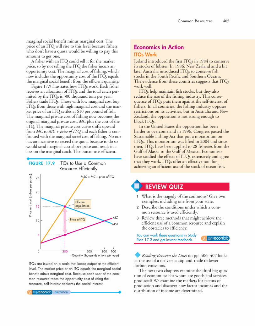
Common Resources 405

marginal social benefit minus marginal cost. Theprice of an ITQ will rise to this level because fisherswho don’t have a quota would be willing to pay thisamount to get one.

A fisher with an ITQ could sell it for the marketprice, so by not selling the ITQ the fisher incurs anopportunity cost. The marginal cost of fishing, whichnow includes the opportunity cost of the ITQ, equalsthe marginal social benefit from the efficient quantity.

Figure 17.9 illustrates how ITQs work. Each fisherreceives an allocation of ITQs and the total catch per-mited by the ITQs is 300 thousand tons per year.Fishers trade ITQs: Those with low marginal cost buyITQs from those with high marginal cost and the mar-ket price of an ITQ settles at $10 per pound of fish.The marginal private cost of fishing now becomes theoriginal marginal private cost, MC plus the cost of theITQ. The marginal private cost curve shifts upwardfrom MC to MC + price of ITQ and each fisher is con-fronted with the marginal social cost of fishing. No onehas an incentive to exceed the quota because to do sowould send marginal cost above price and result in aloss on the marginal catch. The outcome is efficient.

25

20

15

10

5

0 300 900600Quantity (thousands of tons per year)

Pric

e an

d co

st (d

olla

rs p

er p

ound

)

800

MSB

MC

MSC = MC + price of ITQ

Efficientequilibrium

Price of ITQ

ITQs are issued on a scale that keeps output at the efficientlevel. The market price of an ITQ equals the marginal socialbenefit minus marginal cost. Because each user of the com-mon resource faces the opportunity cost of using theresource, self-interest achieves the social interest.

◆ Reading Between the Lines on pp. 406–407 looksat the use of a tax versus cap-and-trade to lowercarbon emissions.

The next two chapters examine the third big ques-tion of economics: For whom are goods and servicesproduced? We examine the markets for factors ofproduction and discover how factor incomes and thedistribution of income are determined.

FIGURE 17.9 ITQs to Use a CommonResource Efficiently

animation

REVIEW QUIZ 1 What is the tragedy of the commons? Give two

examples, including one from your state.2 Describe the conditions under which a com-

mon resource is used efficiently.3 Review three methods that might achieve the

efficient use of a common resource and explainthe obstacles to efficiency.

You can work these questions in Study Plan 17.2 and get instant feedback.

Economics in ActionITQs WorkIceland introduced the first ITQs in 1984 to conserveits stocks of lobster. In 1986, New Zealand and a bitlater Australia introduced ITQs to conserve fishstocks in the South Pacific and Southern Oceans.The evidence from these countries suggests that ITQswork well.

ITQs help maintain fish stocks, but they alsoreduce the size of the fishing industry. This conse-quence of ITQs puts them against the self-interest offishers. In all countries, the fishing industry opposesrestrictions on its activities, but in Australia and NewZealand, the opposition is not strong enough toblock ITQs.

In the United States the opposition has beenharder to overcome and in 1996, Congress passed theSustainable Fishing Act that put a moratorium onITQs. This moratorium was lifted in 2004 and sincethen, ITQs have been applied to 28 fisheries from theGulf of Alaska to the Gulf of Mexico. Economistshave studied the effects of ITQs extensively and agreethat they work. ITQs offer an effective tool forachieving an efficient use of the stock of ocean fish.

406

READING BETWEEN THE L INES

Oil Spill Pushes Carbon Tax Back into Spotlighthttp://www.SFGate.com June 22, 2010

… Oil’s true cost also includes the well-known litany of other hidden burdens: militaryspending to protect Middle East oil, the $1 billion of U.S. wealth and jobs sent overseas eachday to buy oil, and pollution of all sorts, including carbon dioxide emissions. None of thesecosts is included in the price of the fossil fuels Americans use.

“There has to be a price, and a reward for moving to low-carbon fuels,” said Rep. Pete Stark,D-Fremont. Stark may be the only one in Congress who has the temerity to propose a directtax on carbon. …

Congress instead is considering cap-and-trade systems for carbon emissions that do the samething as a carbon tax, …

The leading Senate plan … would set an increas-ingly stricter limit on carbon emissions and auc-tion emissions permits. Revenue would go toalternative energy investments and utility rebatesto help low-income consumers burdened by risingenergy costs. …

Europeans pay $7 to $8 for a gallon of gas, mostlyin taxes, and “they still drive,” said Severin Boren-stein, co-director of the UC Energy Institute.“They use much less oil per capita than we do, butthey still use more than we need to get to.” …

Borenstein called for a big increase in federalfunding for basic research into alternatives.“When you take a realistic look at the economicside, without major technological breakthroughsat a much faster pace than we’ve seen over the lastcouple of decades, it doesn’t look very doable,” hesaid. …San Francisco Chronicle article by Carolyn Lochhead. Copyright 2010 by SanFrancisco Chronicle. Reproduced with permission of San Francisco Chronicle viaCopyright Clearance Center.

■ The cost of oil includes external costs that in-clude military spending to protect Middle Eastoil, pollution, and carbon dioxide emissions.

■ Representative Pete Stark, D-Fremont, says thatthere has to be a price, and a reward for mov-ing to low-carbon fuels, so he proposes a taxon carbon.

■ Congress is considering cap-and-trade systemsfor carbon emissions.

■ The leading Senate plan puts a limit on carbonemissions and auctions emissions permits.

■ Revenue from the sale of permits would be spenton developing clean alternative energy andutility rebates to help low-income consumers.

■ Europeans pay $7 to $8 for a gallon of gaso-line and use less than Americans but more thanthe required target.

■ Without a technological breakthrough to makeclean energy cheap, it will be hard to reach alow carbon emission target.

ESSENCE OF THE STORY

Tax Versus Cap-and-Trade

407

ECONOMIC ANALYSIS

Figure 1 Inelastic demand for gasoline

Pric

e (d

olla

rs p

er g

allo

n)

Gasoline consumption (gallons per person)0

DLR

5.00

7.50

10.00

2.50

800400350100

United Statesin 2010

Europein 2010

United States in 2010with European gas price

DSR

■ The news article lists some external costs of using oil.One of them, “sending jobs overseas,” isn’t such a cost.International trade brings gains for all, not externalcosts—see Chapter 7, pp. 155–156.

■ The price of gasoline might be raised to incude mar-ginal external cost with a carbon tax or a cap-and-trade carbon permit system.

■ The news article says that using either of these meas-ures would do little to curb gas consumption and Fig. 1 illustrates why.

■ In the short run, the demand for gasoline, DSR, isinelastic. If the U.S. gas price was raised to theEuropean level, gas consumption would decrease byvery little.

■ In the long run, the demand for gasoline, DLR, iselastic. Raising the U.S. gas price to the Europeanlevel might eventually cut U.S. consumption to theEuropean level.

■ Figure 2 illustrates how a technological breakthroughthat results in a low-cost clean fuel would work (sug-gests in the news article by Severin Borenstein).

■ Figure 2(a) shows the short-run effects. Taxing carbonemissions or putting a price on them raises the margin-al cost of gasoline to the marginal social cost, and thesupply curve becomes the MSC curve. The price ofgasoline rises, but the quantity consumed barelychanges. The government collects the revenue shownby the purple rectangle.

(a) In the short run

Figure 2 Short-run and long-run effects of tax and technological change

Pric

e an

d co

st (d

olla

rs p

er g

allo

n)

Gasoline consumption (gallons per person)0

MC

MSC

5.00

7.50

10.00

2.50

800350

Governmentrevenue

Carbon emissionstax or price

D0

(b) In the long run

Pric

e an

d co

st (d

olla

rs p

er g

allo

n)

Gasoline consumption (gallons per person)0

5.00

7.50

10.00

2.50

800350100

D0D1

MC

MSC

Carbonemissionsprice falls

Low-cost cleantechnology decreasesdemand for gasoline

■ Figure 2(b) shows the long-run effect when a newtechnology is developed.

■ The availablity of a low-cost clean fuel decreases thedemand for gasoline from D0 to D1. The price ofgasoline falls and the quantity consumed decreases.

■ In the new equilibrium, the price of gasoline islower, and so is the carbon tax or carbon price.

■ Technological change is a crucial source of eventuallycurbing carbon emissions.

408 CHAPTER 17 Economics of the Environment

The Tragedy of the Commons (pp. 400–405)

■ Common resources create a problem that is calledthe tragedy of the commons—no one has a privateincentive to conserve the resources and use themat an efficient rate.

■ A common resource is used to the point at whichthe marginal private benefit equals the marginalcost.

■ A common resource might be used efficiently bycreating a private property right, setting a quota,or issuing individual transferable quotas.

Working Problems 13 to 19 will give you a better under-standing of the tragedy of the commons.

Key Points

Negative Externality: Pollution (pp. 394–399)

■ A competitive market would produce too much ofa good that has external production costs.

■ External costs are costs of production that fall onpeople other than the producer of a good or ser-vice. Marginal social cost equals marginal privatecost plus marginal external cost.

■ Producers take account only of marginal privatecost and produce more than the efficient quantitywhen there is a marginal external cost.

■ Sometimes it is possible to overcome a negativeexternality by assigning a property right.

■ When property rights cannot be assigned, govern-ments might overcome externalities by using taxes,emission charges, or marketable permits.

Working Problems 1 to 12 will give you a better under-standing of the external costs of pollution.

SUMMARY

Key TermsCoase theorem, 397Individual transferable

quota (ITQ), 404Marginal external cost, 395

Marginal private cost, 395Marginal social cost, 395Pigovian taxes, 398Property rights, 396

Tragedy of the commons, 400Transactions costs, 397

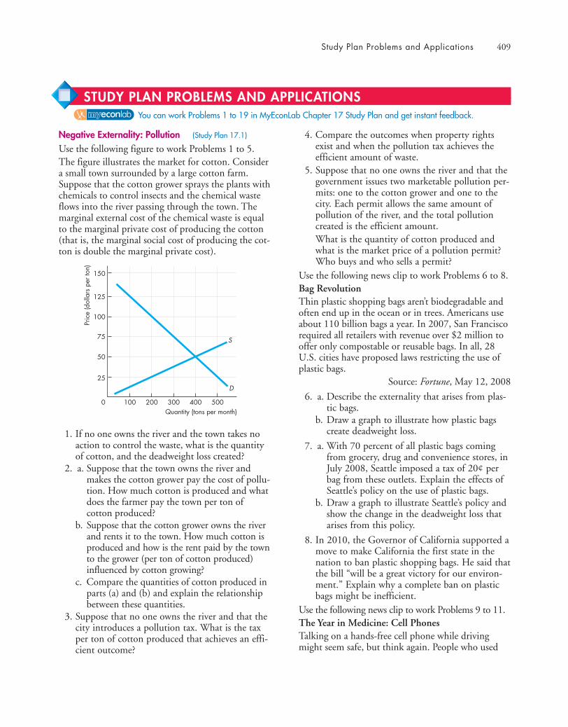
Study Plan Problems and Applications 409

You can work Problems 1 to 19 in MyEconLab Chapter 17 Study Plan and get instant feedback.

STUDY PLAN PROBLEMS AND APPLICATIONS

Negative Externality: Pollution (Study Plan 17.1)

Use the following figure to work Problems 1 to 5.The figure illustrates the market for cotton. Considera small town surrounded by a large cotton farm.Suppose that the cotton grower sprays the plants withchemicals to control insects and the chemical wasteflows into the river passing through the town. Themarginal external cost of the chemical waste is equalto the marginal private cost of producing the cotton(that is, the marginal social cost of producing the cot-ton is double the marginal private cost).

1. If no one owns the river and the town takes noaction to control the waste, what is the quantityof cotton, and the deadweight loss created?

2. a. Suppose that the town owns the river andmakes the cotton grower pay the cost of pollu-tion. How much cotton is produced and whatdoes the farmer pay the town per ton ofcotton produced?

b. Suppose that the cotton grower owns the riverand rents it to the town. How much cotton isproduced and how is the rent paid by the townto the grower (per ton of cotton produced)influenced by cotton growing?

c. Compare the quantities of cotton produced inparts (a) and (b) and explain the relationshipbetween these quantities.

3. Suppose that no one owns the river and that thecity introduces a pollution tax. What is the taxper ton of cotton produced that achieves an effi-cient outcome?

4. Compare the outcomes when property rightsexist and when the pollution tax achieves theefficient amount of waste.

5. Suppose that no one owns the river and that thegovernment issues two marketable pollution per-mits: one to the cotton grower and one to thecity. Each permit allows the same amount ofpollution of the river, and the total pollutioncreated is the efficient amount.What is the quantity of cotton produced andwhat is the market price of a pollution permit?Who buys and who sells a permit?

Use the following news clip to work Problems 6 to 8.Bag RevolutionThin plastic shopping bags aren’t biodegradable andoften end up in the ocean or in trees. Americans useabout 110 billion bags a year. In 2007, San Franciscorequired all retailers with revenue over $2 million tooffer only compostable or reusable bags. In all, 28U.S. cities have proposed laws restricting the use ofplastic bags.

Source: Fortune, May 12, 2008

6. a. Describe the externality that arises from plas-tic bags.

b. Draw a graph to illustrate how plastic bagscreate deadweight loss.

7. a. With 70 percent of all plastic bags comingfrom grocery, drug and convenience stores, inJuly 2008, Seattle imposed a tax of 20¢ perbag from these outlets. Explain the effects ofSeattle’s policy on the use of plastic bags.

b. Draw a graph to illustrate Seattle’s policy andshow the change in the deadweight loss thatarises from this policy.

8. In 2010, the Governor of California supported amove to make California the first state in thenation to ban plastic shopping bags. He said thatthe bill “will be a great victory for our environ-ment.” Explain why a complete ban on plasticbags might be inefficient.

Use the following news clip to work Problems 9 to 11.The Year in Medicine: Cell PhonesTalking on a hands-free cell phone while drivingmight seem safe, but think again. People who used

Pric

e (d

olla

rs p

er to

n)

Quantity (tons per month)0 100 200 300 400 500

25

50

75

100

125

150

D

S

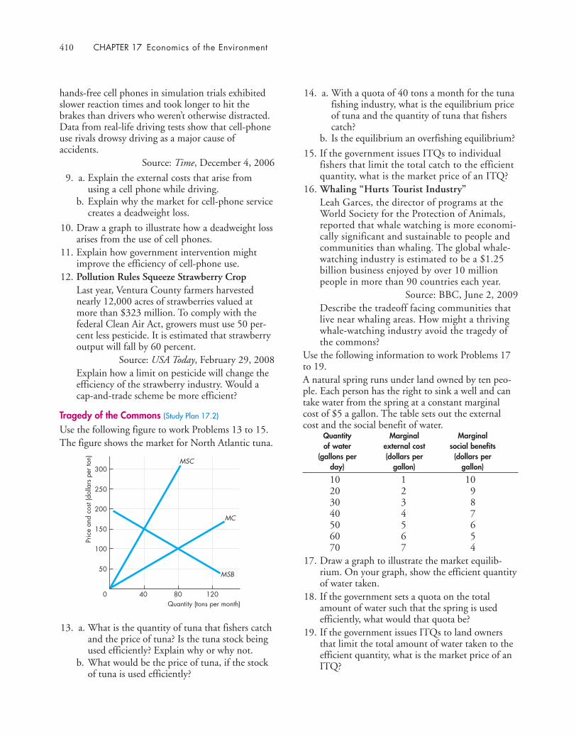
410 CHAPTER 17 Economics of the Environment

14. a. With a quota of 40 tons a month for the tunafishing industry, what is the equilibrium priceof tuna and the quantity of tuna that fisherscatch?

b. Is the equilibrium an overfishing equilibrium?

15. If the government issues ITQs to individualfishers that limit the total catch to the efficientquantity, what is the market price of an ITQ?

16. Whaling “Hurts Tourist Industry”Leah Garces, the director of programs at theWorld Society for the Protection of Animals,reported that whale watching is more economi-cally significant and sustainable to people andcommunities than whaling. The global whale-watching industry is estimated to be a $1.25billion business enjoyed by over 10 millionpeople in more than 90 countries each year.

Source: BBC, June 2, 2009Describe the tradeoff facing communities thatlive near whaling areas. How might a thrivingwhale-watching industry avoid the tragedy ofthe commons?

Use the following information to work Problems 17to 19.A natural spring runs under land owned by ten peo-ple. Each person has the right to sink a well and cantake water from the spring at a constant marginalcost of $5 a gallon. The table sets out the externalcost and the social benefit of water.

Quantity Marginal Marginalof water external cost social benefits

(gallons per (dollars per (dollars perday) gallon) gallon)

10 1 1020 2 930 3 840 4 750 5 660 6 570 7 4

17. Draw a graph to illustrate the market equilib-rium. On your graph, show the efficient quantityof water taken.

18. If the government sets a quota on the totalamount of water such that the spring is usedefficiently, what would that quota be?

19. If the government issues ITQs to land ownersthat limit the total amount of water taken to theefficient quantity, what is the market price of anITQ?

hands-free cell phones in simulation trials exhibitedslower reaction times and took longer to hit thebrakes than drivers who weren’t otherwise distracted.Data from real-life driving tests show that cell-phoneuse rivals drowsy driving as a major cause ofaccidents.

Source: Time, December 4, 2006

9. a. Explain the external costs that arise fromusing a cell phone while driving.

b. Explain why the market for cell-phone servicecreates a deadweight loss.

10. Draw a graph to illustrate how a deadweight lossarises from the use of cell phones.

11. Explain how government intervention mightimprove the efficiency of cell-phone use.

12. Pollution Rules Squeeze Strawberry CropLast year, Ventura County farmers harvestednearly 12,000 acres of strawberries valued atmore than $323 million. To comply with thefederal Clean Air Act, growers must use 50 per-cent less pesticide. It is estimated that strawberryoutput will fall by 60 percent.

Source: USA Today, February 29, 2008Explain how a limit on pesticide will change theefficiency of the strawberry industry. Would acap-and-trade scheme be more efficient?

Tragedy of the Commons (Study Plan 17.2)

Use the following figure to work Problems 13 to 15.The figure shows the market for North Atlantic tuna.

13. a. What is the quantity of tuna that fishers catchand the price of tuna? Is the tuna stock beingused efficiently? Explain why or why not.

b. What would be the price of tuna, if the stockof tuna is used efficiently?

Pric

e an

d co

st (d

olla

rs p

er to

n)

Quantity (tons per month)0 40 80 120

50

100

150

200

250

300

MSB

MC

MSC

Additional Problems and Applications 411

Negative Externality: Pollution20. Betty and Anna work at the same office in

Philadelphia. They both must attend a meetingin Pittsburgh, so they decide to drive to themeeting together. Betty is a cigarette smoker andher marginal benefit from smoking a package ofcigarettes a day is $40. Cigarettes are $6 a pack.Anna dislikes cigarette smoke, and her marginalbenefit from a smoke-free environment is $50 aday. What is the outcome ifa. Betty drives her car with Anna as a passenger?b. Anna drives her car with Betty as a passenger?

Use the following information and the figure, whichillustrates the market for a pesticide with no govern-ment intervention, to work Problems 21 to 24.When factories produce pesticide, they also createwaste, which they dump into a lake on the outskirtsof the town. The marginal external cost of the wasteis equal to the marginal private cost of producing thepesticide (that is, the marginal social cost of produc-ing the pesticide is double the marginal private cost).

21. What is the quantity of pesticide produced if noone owns the lake and what is the efficientquantity of pesticide?

22. If the residents of the town own the lake, what is the quantity of pesticide produced and howmuch do residents of the town charge thefactories to dump waste?

23. If the pesticide factories own the lake, howmuch pesticide is produced?

24. If no one owns the lake and the governmentlevies a pollution tax, what is the tax thatachieves the efficient outcome?

Use the following table to work Problems 25 to 27.

The first two columns of the table show the demandschedule for electricity from a coal burning utility;the second and third columns show the utility’s costof producing electricity. The marginal external costof the pollution created is equal to the marginalcost.

Price Quantity Marginal cost(cents per kilowatt) (kilowatts per day) (cents per kilowatt)

4 500 108 400 8

12 300 616 200 420 100 2

25. With no government action to control pollution,what is the quantity of electricity produced, theprice of electricity, and the marginal external costof the pollution generated?

26. With no government action to control pollution,what is the marginal social cost of the electricitygenerated and the deadweight loss created?

27. Suppose that the government levies a pollutiontax, such that the utility produces the efficientquantity. What is the price of electricity? What isthe tax levied, and the government’s tax revenueper day?

28. EPA Pushes to have Companies TrackGreenhouse GasesCongress plans to make large polluters, such asoil refiners and automobile manufacturers, andmakers of cement, aluminum, glass and paper,start tracking their emissions next year. TheEPA’s climate change division noted that this isan important step. A cap-and-trade scheme willbe introduced for factories that emit 90 percentof U.S. greenhouse gases.

Source: USA Today, March 11, 2009The monitoring cost of the scheme is expectedto be about $127 million a year. Who will bene-fit from the scheme? Who will bear the burdenof this scheme?

You can work these problems in MyEconLab if assigned by your instructor.

ADDITIONAL PROBLEMS AND APPLICATIONSPr

ice

(dol

lars

per

ton)

Quantity (tons per week)0 10 20 30 40 50

25

50

75

100

125

150

D

S

412 CHAPTER 17 Economics of the Environment

The Tragedy if the Commons

29. If hikers and other visitors were required to pay afee to use the Appalachian Trail,a. Would the use of this common resource be

more efficient?b. Would it be even more efficient if the most

popular spots along the trail had the highestprices?

c. Why do you think we don’t see more marketsolutions to the tragedy of the commons?

Use the following figure to work Problems 30 to 32.

A spring runs under a village. Everyone can sink awell on her or his land and take water from thespring. The figure shows the marginal social benefitfrom and the marginal cost of taking water.30. What is the quantity of water taken and what is

the private cost of the water taken?31. What is the efficient quantity of water taken and

the marginal social cost at the efficient quantity?32. If the village council sets a quota on the total

amount of water such that the spring is used effi-ciently, what would be the quota and the marketvalue of the water taken per day?

33. Polar Ice Cap Shrinks Further and ThinsWith the warming of the planet, the polar icecap is shrinking and the Arctic Sea is expanding.As the ice cap shrinks further, more and moreunderwater mineral resources will become acces-sible. Many countries are staking out territorialclaims to parts of the polar region.

Source: The Wall Street Journal, April 7, 2009Explain how ownership of these mineralresources will influence the amount of damagedone to the Arctic Sea and its wildlife.

Economics in the News

34. After you have studied Reading Between the Lineson pp. 406–407 answer the following questions:a. Why is it difficult to decrease carbon emis-

sions in the short run?b. Which holds the greater promise as a method

of lowering carbon emissions: actions that de-crease the demand for gasoline or actions thatdecrease the supply of gasoline? Explain.

c. Why might a carbon cap-and-trade programbe preferred to a carbon tax?

Use the following information to work Problems 35and 36.Where the Tuna RoamTo the first settlers, the Great Plains posed the sameproblem as the oceans today: a vast, open area wherethere seemed to be no way to protect animals. Butanimals thrived once the settlers divvied up the landand devised ways to protect their livestock. Today, theocean are much like an open range. Fishermen catchas much as they can this year, even if they are over-fishing. They figure any fish they don’t take for them-selves will just be taken by someone else.

Source: The New York Times, November 4, 200635. a. What are the similarities between the prob-

lems faced by the earliest settlers in the Westand today’s fishers?

b. Can the tragedy of the commons in the oceansbe eliminated in the same manner used by theearly settlers on the plains?

36. How can ITQs change the short-term outlook offishers to a long-term outlook?

37. Commuting More than Pain at Pump

Half of the respondents polled in 10 cities saidthat traffic congestion increased their stress levelsand cut their productivity. IBM has been devis-ing ways for cities to cut traffic congestion, suchas automated tolling, congestion pricing plansand real-time traffic modeling. Commuters wantmore options to work from home and improvedpublic transit.

Source: CNN, May 30, 2008a. Explain the problem of congested city streets

that results in inefficient usage. Draw a graphto illustrate the inefficient equilibrium.

b. How could government policies be used toachieve an efficient use of city streets?

Pric

e an

d co

st (c

ents

per g

allo

n)

Quantity (gallons per day)0 200 400 600 800

10

20

30

40

50

MSB

MC

MSC

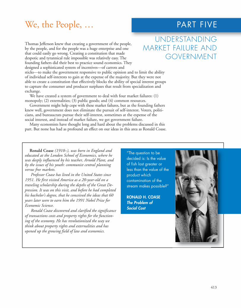
413

PART FIVE

Ronald Coase (1910–), was born in England andeducated at the London School of Economics, where hewas deeply influenced by his teacher, Arnold Plant, andby the issues of his youth: communist central planningversus free markets.

Professor Coase has lived in the United States since1951. He first visited America as a 20-year-old on atraveling scholarship during the depths of the Great De-pression. It was on this visit, and before he had completedhis bachelor’s degree, that he conceived the ideas that 60years later were to earn him the 1991 Nobel Prize forEconomic Science.

Ronald Coase discovered and clarified the significanceof transactions costs and property rights for the function-ing of the economy. He has revolutionized the way wethink about property rights and externalities and hasopened up the growing field of law and economics.

Thomas Jefferson knew that creating a government of the people,by the people, and for the people was a huge enterprise and onethat could easily go wrong. Creating a constitution that madedespotic and tyrannical rule impossible was relatively easy. Thefounding fathers did their best to practice sound economics. Theydesigned a sophisticated system of incentives—of carrots andsticks—to make the government responsive to public opinion and to limit the abilityof individual self-interests to gain at the expense of the majority. But they were notable to create a constitution that effectively blocks the ability of special interest groupsto capture the consumer and producer surpluses that result from specialization andexchange.

We have created a system of government to deal with four market failures: (1)monopoly; (2) externalities; (3) public goods; and (4) common resources.

Government might help cope with these market failures, but as the founding fathersknew well, government does not eliminate the pursuit of self-interest. Voters, politi-cians, and bureaucrats pursue their self-interest, sometimes at the expense of thesocial interest, and instead of market failure, we get government failure.

Many economists have thought long and hard about the problems discussed in thispart. But none has had as profound an effect on our ideas in this area as Ronald Coase.

We, the People, …

UNDERSTANDINGMARKET FAILURE AND

GOVERNMENT

“The question to bedecided is: Is the valueof fish lost greater orless than the value of theproduct whichcontamination of thestream makes possible?”

RONALD H. COASEThe Problem ofSocial Cost

414

TALKING WITH

the right incentives to do so. Society has a role infilling the gaps in the capital market; it fills this roleby public funding of elementary and secondary edu-cation, government guaranteed loans, college sav-ings programs, and so on. There is no particularreason, however, why government needs to actuallyrun schools; it can provide the funding withoutactually providing schooling.

In one of your papers, you posed the question: Doescompetition among public schools benefit students ortaxpayers? What are the issues, what was your answer,and how did you arrive at it?We are all familiar with the fact that families choosepublic schools when they choose where to live. Thistraditional form is by far the most pervasive form ofschool choice in the United States, and few parentswho exercise it would be willing to give it up. Yet,until quite recently, we did not know whether havingsuch traditional school choice was good for students(high achievement) or taxpayers (more efficientschools). It is important to know because some peo-ple in the United States, especially poor people wholive in central cities, are unable to exercise this form

Caroline M. Hoxby

Why did you decide to become an economist?I’ve wanted to be an economist from about the age of13. That was when I took my first class in economics(an interesting story in itself ) and discovered that allof the thoughts swimming around in my headbelonged to a “science” and there was an entire bodyof people who understood this science—a lot betterthan I did, anyway. I can still recall reading TheWealth of Nations for the first time; it was a revelation.

What drew you to study the economics of education?We all care about education, perhaps because it is thekey means by which opportunity is (or should be)extended to all in the United States. Also, nearlyeveryone now acknowledges that highly developedcountries like the United States rely increasingly oneducation as the engine of economic growth. Thus,one reason I was drawn to education is its impor-tance. However, what primarily drew me was thateducation issues were so clearly begging for economicanalysis and that there was so little of it. I try hard tounderstand educational institutions and problems,but I insist on bringing economic logic to bear oneducational issues.

Why is education different from fast food? Why don’twe just let people buy it from private firms that areregulated to maintain quality standards analogous tothe safety standards that the FDA imposes on fast-food producers?The thing that makes education different from fastfood is not that we cannot buy it from private insti-tutions that are regulated to maintain quality stan-dards. We do this all the time—think of privateschools and colleges. What makes education differ-ent is that it is (a) an investment, not consumption,and (b) the capital markets for financing the invest-ments work poorly when left on their own.Essentially, our country has an interest in every per-son investing optimally in his or her education. Tomake investments, however, people need funds thatallow them to attend good schools and take timeaway from work. Children don’t have these fundsand cannot arrange for loans that they may or maynot pay off decades later. Therefore, childrendepend on their families for funds, and families donot necessarily have the funds to invest optimally or

415

of school choice. Economists hypothesized that thislack of choice might be a reason why many childrenfrom poor, central city families receive such a defi-cient education, especially considering the dollarsspent in their schools (which spend significantlymore than the median school).

To investigate this hypothesis, I examined all ofthe metropolitan areas in the United States. Theyvary a great deal in the degree of traditional choiceavailable to parents. On one extreme, there is agroup of metropolitan areas with hundreds ofschool districts. On the other extreme, there is agroup of metropolitan areas with only one schooldistrict. Most are somewhere in between. A familyin a metropolitan area with one district may have noeasy way of “escaping” a badly run district adminis-tration. A family in a metropolitan area with hun-dreds of districts can choose among several districtsthat match well with its job location, housing pref-erences, and so on.

Looking across metropolitan areas with manydistricts (lots of potential competition from tradi-tional school choice) and few districts (little potentialcompetition), I found that areas with greater compe-tition had substantially higher student achievement

CAROLINE M. HOXBY is the Allie S. Freed Professorof Economics at Harvard University. Born in Cleve-land, Ohio, she was an undergraduate at Harvardand a graduate student at Oxford and MIT.

Professor Hoxby is a leading student of the eco-nomics of education. She has written many articleson this topic and has published books entitled TheEconomics of School Choice and College Choices(both University of Chicago Press, 2003 and 2004,respectively). She is Program Director of the Eco-nomics of Education Program at the National Bu-reau of Economic Research, serves on several othernational boards that study education issues, andhas advised or provided testimony to several statelegislatures and the United States Congress.

Michael Parkin talked with Caroline Hoxbyabout her work and the progress that economistshave made in understanding how the financing andthe provision of education influence the quality ofeducation and the equality of access to it.

for any given level of school spending. This suggeststhat schools are more efficient producers of achieve-ment when they face competition.

What do we know about the relative productivity ofpublic and private schools?It is somewhat difficult to say whether achievement ishigher at public or private schools in the UnitedStates. The best studies use randomly assigned privateschool scholarships, follow the same children overtime, or use “natural experiments” in which someareas accidentally end up with more private schoolsthan others. These studies tend to find that, for thesame student, private schools produce achievementthat is up to 10 percent higher. However, for under-standing which type of school is more productive, weactually do not need private schools to have higherachievement. For the sake of argument, let’s “call it adraw” on the achievement question.

In recent studies comparing achievement in pub-lic and private schools, the public schools spent anaverage of $9,662 per student and the private schoolsspent an average of $2,427 per student. These spend-ing numbers, combined with achievement that wewill call equal, suggest that the private schools were298 percent more productive. I would not claim thatthis number is precisely correct; we could think ofsome minor adjust-ments. But it is diffi-cult not to concludethat the privateschools are signifi-cantly more produc-tive. They produceequal achievement fora fraction of the cost.

What can economists say about the alternative meth-ods of financing education? Is there a voucher solutionthat could work?There is definitely a voucher solution that couldwork because vouchers are inherently an extremelyflexible policy. People often see the word “voucher”and think of, say, a $2000 voucher being given to asmall share of children. But this need not be so.Anything that we can do with public school financ-ing we can do better with a voucher because vouch-ers can be specific to a student, whereas the

Economists should say topolicy makers: “Tell meyour goals; I’ll design youa voucher.”

416

government can never ensure that funds get to anindividual student by giving those funds to his orher district.

Any well-designed voucher system will giveschools an incentive to compete. However, whendesigning vouchers, we can also build in remedies fora variety of educational problems. Vouchers can beused to ensure that disabled children get the fundingthey need and the program choices they need.Compared to current school finance programs, vouch-ers can do a better job of ensuring that low-incomefamilies have sufficient funds to invest in the child’seducation. Well-designed vouchers can encourageschools to make their student bodies socio-economi-cally diverse. Economists should say to policy makers:“Tell me your goals; I’ll design you a voucher.”

Is there a conflict between efficiency and equity in theprovision of quality education?To raise the public funds that allow all families toinvest optimally in their children’s education, we haveto have taxes. Taxes always create some deadweightloss, so we always create some inefficiency when weraise the funds we need to provide equitable educa-tional opportunities. However, if the funds are usedsuccessfully and actually induce people to make opti-mal investments in their education, we have elimi-nated much more inefficiency than the taxes created.Thus, in an ideal world, there need not be a conflictbetween efficiency and equity.

In the real world, public funds are often raisedwith taxes (creating deadweight loss) and then are notsuccessfully used. If we spend twice as much on pub-lic schools and do not have higher achievement toshow for it, then there are no efficiency gains to over-whelm the efficiency losses from taxation. In otherwords, to avoid a conflict between equity and effi-ciency, we must learn how to use public funds pro-ductively in education. This is what the economics ofeducation is all about.

What advice do you have for a student who is juststarting to study economics? Is economics a goodsubject in which to major? What other subjects go wellalongside it? And do you have anything special to sayto women who are making a career choice? What mustwe do to get more women involved in our subject?Students who are just starting to study economicsshould do two things. First, learn the tools even ifthey seem abstruse. Once you have mastered thetools, you will be able to “see the forest for the trees.”As long as you don’t master the tools, you will be inthe trees and will find it hard to think about eco-nomic problems. Second, think about economicproblems! The real world is a great moving textbookof economics, once you have the tools to analyze it.

Economics is a great subject in which to majorbecause it trains you for life, for many careers, andfor the thinking that you would need in a leadershipposition. I think that it is the best training for afuture career in business, the law, or policy making.Don’t forget nonprofits: every year, nonprofit organi-zations try to hire people with economics skills whoare also interested in charitable schemes.

Math and statistics courses are complementary toeconomics because they make it easier for a studentto master the tools quickly. Economics goes well withmany studies in the arts and sciences, too. It alldepends on what you want to use economics for. Ifyou want to do health policy making, take economicsalong with premedical courses. If you want to be apolicy maker in the performing arts, take economicsalong with music.

I wish that there were more women in econom-ics. Our field loses far too many talented minds. Also,women who need to understand economics for theircareers are sometimes without it. To aspiring womeneconomists, I can only say to hang in there. Mast-ering economics is empowering. You will never haveto worry about your opinion not being taken seri-ously if you are a good economist.

PART SIX Factor Markets, Inequality, and Uncertainty

After studying this chapter, you will be able to:

� Describe the anatomy of factor markets� Explain how the value of marginal product determines

the demand for a factor of production� Explain how wage rates and employment are deter-

mined and how labor unions influence labor markets� Explain how capital and land rental rates and natural

resource prices are determined

You know that wage rates vary a lot. A worker at McDonald’s earns $8 anhour. Demetrio Luna, who spends his days in a small container suspended fromthe top of Houston’s high-rise buildings cleaning windows, makes $12 an hour.Richard Seymour, who plays for the New England Patriots, collects a cool $25million a year. Some differences in earnings might seem surprising. For example,your college football coach earns much more than your economics professor.What determines the wages that people earn?

Wages are important, but just finding a job is even more important, especiallyin today’s tough labor markets. Factory jobs are vanishing as technological

change and foreign competition shrink manufacturing production inthe United States. But new job opportunities are opening in serviceindustries, and especially in health care where, in the next 10 years,jobs for more than 500,000 nurses will be created.

In this chapter, we study labor markets as well as markets forcapital and natural resources. You will learn how the prices andquantities of factors of production are determined. In ReadingBetween the Lines at the end of the chapter we look at the ever-

changing labor markets and how they constantly reallocate labor resources.

MARKETS FORFACTORS OFPRODUCTION

18417

418 CHAPTER 18 Markets for Factors of Production

◆ The Anatomy of Factor MarketsThe four factors of production are

■ Labor■ Capital■ Land (natural resources)■ Entrepreneurship

Let’s take a brief look at the anatomy of the mar-kets in which these factors of production are traded.

Markets for Labor ServicesLabor services are the physical and mental work effortthat people supply to produce goods and services. Alabor market is a collection of people and firms whotrade labor services. The price of labor services is thewage rate.

Some labor services are traded day by day. Theseservices are called casual labor. People who pick fruitand vegetables often just show up at a farm and takewhatever work is available that day. But most laborservices are traded on a contract, called a job.

Most labor markets have many buyers and manysellers and are competitive. In these labor markets,the wage rate is determined by supply and demand,just like the price is determined in any other compet-itive market.

In some labor markets, a labor union organizeslabor, which introduces an element of monopoly onthe supply-side of the labor market. In this type oflabor market, a bargaining process between the unionand the employer determines the wage rate.

We’ll study both competitive labor markets andlabor unions in this chapter.

Markets for Capital ServicesCapital consists of the tools, instruments, machines,buildings, and other constructions that have beenproduced in the past and that businesses now use toproduce goods and services. These physical objectsare themselves goods—capital goods. Capital goodsare traded in goods markets, just as bottled water andtoothpaste are. The price of a dump truck, a capitalgood, is determined by supply and demand in themarket for dump trucks. This market is not a marketfor capital services.

A market for capital services is a rental market—amarket in which the services of capital are hired.

An example of a market for capital services is thevehicle rental market in which Avis, Budget, Hertz,U-Haul, and many other firms offer automobiles andtrucks for hire. The price in a capital services marketis a rental rate.

Most capital services are not traded in a market.Instead, a firm buys capital and uses it itself. The ser-vices of the capital that a firm owns and operateshave an implicit price that arises from depreciationand interest costs (see Chapter 10, pp. 228–229).You can think of this price as the implicit rental rateof capital. Firms that buy capital and use it them-selves are implicitly renting the capital to themselves.

Markets for Land Services and NaturalResourcesLand consists of all the gifts of nature—naturalresources. The market for land as a factor of produc-tion is the market for the services of land—the use ofland. The price of the services of land is a rental rate.

Most natural resources, such as farm land, can beused repeatedly. But a few natural resources are non-renewable. Nonrenewable natural resources areresources that can be used only once. Examples areoil, natural gas, and coal. The prices of nonrenewablenatural resources are determined in global commoditymarkets and are called commodity prices.

EntrepreneurshipEntrepreneurial services are not traded in markets.Entrepreneurs receive the profit or bear the loss thatresults from their business decisions.

The rest of this chapter explores the influences onthe demand and supply of factors of production. Webegin by studying the demand for a factor ofproduction.

REVIEW QUIZ1 What are the factors of production and their

prices?2 What is the distinction between capital and the

services of capital?3 What is the distinction between the price of

capital equipment and the rental rate of capital?

You can work these questions in Study Plan 18.1 and get instant feedback.

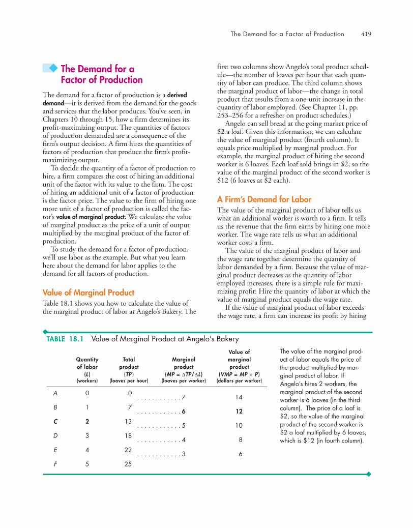
The Demand for a Factor of Production 419

◆ The Demand for a Factor of Production

The demand for a factor of production is a deriveddemand—it is derived from the demand for the goodsand services that the labor produces. You’ve seen, inChapters 10 through 15, how a firm determines itsprofit-maximizing output. The quantities of factorsof production demanded are a consequence of thefirm’s output decision. A firm hires the quantities offactors of production that produce the firm’s profit-maximizing output.

To decide the quantity of a factor of production tohire, a firm compares the cost of hiring an additionalunit of the factor with its value to the firm. The costof hiring an additional unit of a factor of productionis the factor price. The value to the firm of hiring onemore unit of a factor of production is called the fac-tor’s value of marginal product. We calculate the valueof marginal product as the price of a unit of outputmultiplied by the marginal product of the factor ofproduction.

To study the demand for a factor of production,we’ll use labor as the example. But what you learnhere about the demand for labor applies to thedemand for all factors of production.

Value of Marginal ProductTable 18.1 shows you how to calculate the value ofthe marginal product of labor at Angelo’s Bakery. The

first two columns show Angelo’s total product sched-ule—the number of loaves per hour that each quan-tity of labor can produce. The third column showsthe marginal product of labor—the change in totalproduct that results from a one-unit increase in thequantity of labor employed. (See Chapter 11, pp.253–256 for a refresher on product schedules.)

Angelo can sell bread at the going market price of$2 a loaf. Given this information, we can calculatethe value of marginal product (fourth column). Itequals price multiplied by marginal product. Forexample, the marginal product of hiring the secondworker is 6 loaves. Each loaf sold brings in $2, so thevalue of the marginal product of the second worker is$12 (6 loaves at $2 each).

A Firm’s Demand for LaborThe value of the marginal product of labor tells uswhat an additional worker is worth to a firm. It tellsus the revenue that the firm earns by hiring one moreworker. The wage rate tells us what an additionalworker costs a firm.

The value of the marginal product of labor andthe wage rate together determine the quantity oflabor demanded by a firm. Because the value of mar-ginal product decreases as the quantity of laboremployed increases, there is a simple rule for maxi-mizing profit: Hire the quantity of labor at which thevalue of marginal product equals the wage rate.

If the value of marginal product of labor exceedsthe wage rate, a firm can increase its profit by hiring

Value ofQuantity Total Marginal marginalof labor product product product

(L ) (TP ) (MP = ΔTP/ΔL ) (VMP = MP × P )(workers) (loaves per hour) (loaves per worker) (dollars per worker)

A 0 0 . . . . . . . . . . . . 7 14

B 1 7 . . . . . . . . . . . . 6 12

C 2 13 . . . . . . . . . . . . 5 10

D 3 18 . . . . . . . . . . . . 4 8

E 4 22 . . . . . . . . . . . . 3 6

F 5 25

The value of the marginal prod-uct of labor equals the price ofthe product multiplied by mar-ginal product of labor. IfAngelo’s hires 2 workers, themarginal product of the secondworker is 6 loaves (in the thirdcolumn). The price of a loaf is$2, so the value of the marginalproduct of the second worker is$2 a loaf multiplied by 6 loaves,which is $12 (in fourth column).

TABLE 18.1 Value of Marginal Product at Angelo’s Bakery

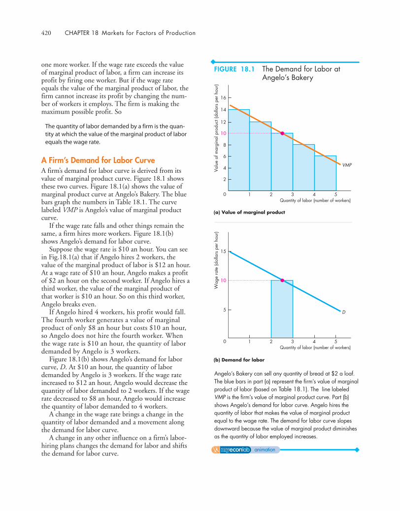
420 CHAPTER 18 Markets for Factors of Production

one more worker. If the wage rate exceeds the valueof marginal product of labor, a firm can increase itsprofit by firing one worker. But if the wage rateequals the value of the marginal product of labor, thefirm cannot increase its profit by changing the num-ber of workers it employs. The firm is making themaximum possible profit. So

The quantity of labor demanded by a firm is the quan-tity at which the value of the marginal product of laborequals the wage rate.

A Firm’s Demand for Labor CurveA firm’s demand for labor curve is derived from itsvalue of marginal product curve. Figure 18.1 showsthese two curves. Figure 18.1(a) shows the value ofmarginal product curve at Angelo’s Bakery. The bluebars graph the numbers in Table 18.1. The curvelabeled VMP is Angelo’s value of marginal productcurve.

If the wage rate falls and other things remain thesame, a firm hires more workers. Figure 18.1(b)shows Angelo’s demand for labor curve.

Suppose the wage rate is $10 an hour. You can seein Fig.18.1(a) that if Angelo hires 2 workers, thevalue of the marginal product of labor is $12 an hour.At a wage rate of $10 an hour, Angelo makes a profitof $2 an hour on the second worker. If Angelo hires athird worker, the value of the marginal product ofthat worker is $10 an hour. So on this third worker,Angelo breaks even.

If Angelo hired 4 workers, his profit would fall.The fourth worker generates a value of marginalproduct of only $8 an hour but costs $10 an hour,so Angelo does not hire the fourth worker. Whenthe wage rate is $10 an hour, the quantity of labordemanded by Angelo is 3 workers.

Figure 18.1(b) shows Angelo’s demand for laborcurve, D. At $10 an hour, the quantity of labordemanded by Angelo is 3 workers. If the wage rateincreased to $12 an hour, Angelo would decrease thequantity of labor demanded to 2 workers. If the wagerate decreased to $8 an hour, Angelo would increasethe quantity of labor demanded to 4 workers.

A change in the wage rate brings a change in thequantity of labor demanded and a movement alongthe demand for labor curve.

A change in any other influence on a firm’s labor-hiring plans changes the demand for labor and shiftsthe demand for labor curve.

(b) Demand for labor

Valu

e of

mar

gina

l pro

duct

(dol

lars

per

hou

r)

0

10

16

(a) Value of marginal product

14

6

4

2

8

12

VMP

Wag

e ra

te (d

olla

rs p

er h

our)

Quantity of labor (number of workers)0 1 2 3 4 5

Quantity of labor (number of workers)1 2 3 4 5

10

15

5 D

Angelo’s Bakery can sell any quantity of bread at $2 a loaf.The blue bars in part (a) represent the firm’s value of marginalproduct of labor (based on Table 18.1). The line labeledVMP is the firm’s value of marginal product curve. Part (b)shows Angelo’s demand for labor curve. Angelo hires thequantity of labor that makes the value of marginal productequal to the wage rate. The demand for labor curve slopesdownward because the value of marginal product diminishesas the quantity of labor employed increases.

FIGURE 18.1 The Demand for Labor atAngelo’s Bakery

animation

The Demand for a Factor of Production 421

Changes in a Firm’s Demand for LaborA firm’s demand for labor depends on

■ The price of the firm’s output■ The prices of other factors of production■ Technology

The Price of the Firm’s Output The higher the priceof a firm’s output, the greater is the firm’s demand forlabor. The price of output affects the demand forlabor through its influence on the value of marginalproduct of labor. A higher price for the firm’s outputincreases the value of the marginal product of labor.A change in the price of a firm’s output leads to ashift in the firm’s demand for labor curve. If the priceof the firm’s output increases, the demand for laborincreases and the demand for labor curve shiftsrightward.

For example, if the price of bread increased to $3 aloaf, the value of the marginal product of Angelo’sfourth worker would increase from $8 an hour to$12 an hour. At a wage rate of $10 an hour, Angelowould now hire 4 workers instead of 3.

The Prices of Other Factors of Production If the priceof using capital decreases relative to the wage rate, afirm substitutes capital for labor and increases thequantity of capital it uses. Usually, the demand forlabor will decrease when the price of using capitalfalls. For example, if the price of a bread-makingmachine falls, Angelo might decide to install onemachine and lay off a worker. But the demand forlabor could increase if the lower price of capital led toa sufficiently large increase in the scale of production.For example, with cheaper machines available,Angelo might install a machine and hire more laborto operate it. This type of factor substitution occursin the long run when the firm can change the size ofits plant.

Technology New technologies decrease the demandfor some types of labor and increase the demand forother types. For example, if a new automated bread-making machine becomes available, Angelo mightinstall one of these machines and fire most of hisworkforce—a decrease in the demand for bakeryworkers. But the firms that manufacture and serviceautomated bread-making machines hire more labor,so there is an increase in the demand for this type oflabor. An event similar to this one occurred duringthe 1990s when the introduction of electronic

telephone exchanges decreased the demand for tele-phone operators and increased the demand for com-puter programmers and electronics engineers.

Table 18.2 summarizes the influences on a firm’sdemand for labor.

The Law of Demand

(Movements along the demand curve for labor)

The quantity of labor demanded by a firm

Decreases if: Increases if:

■ The wage rate increases

■ The wage rate decreases

■ The price of the firm’soutput decreases

■ The price of a substitutefor labor falls

■ The price of a comple-ment of labor rises

■ A new technology ornew capital decreasesthe marginal product oflabor

■ The price of the firm’soutput increases

■ The price of a substitutefor labor rises

■ The price of a comple-ment of labor falls

■ A new technology ornew capital increasesthe marginal product oflabor

Changes in Demand

(Shifts in the demand curve for labor)

A firm’s demand for labor

Decreases if: Increases if:

TABLE 18.2 A Firm’s Demand for Labor

REVIEW QUIZ 1 What is the value of marginal product of labor?2 What is the relationship between the value of

marginal product of labor and the marginalproduct of labor?

3 How is the demand for labor derived from thevalue of marginal product of labor?

4 What are the influences on the demand forlabor?

You can work these questions in Study Plan 18.2 and get instant feedback.

422 CHAPTER 18 Markets for Factors of Production

Reservation Wage Rate Jill enjoys her leisure time,and she would be pleased if she didn’t have to spendher time working at Angelo’s Bakery. But Jill wantsto earn an income, and as long as she can earn awage rate of at least $5 an hour, she’s willing towork. This wage is called her reservation wage. Atany wage rate above her reservation wage, Jill sup-plies some labor.

The wage rate at Angelo’s is $10 an hour, and atthat wage rate, Jill chooses to work 30 hours aweek. At a wage rate of $10 an hour, Jill regardsthis use of her time as the best available. Figure18.2 illustrates.

Backward-Bending Labor Supply Curve If Jill wereoffered a wage rate between $5 and $10 an hour, shewould want to work fewer hours. If she were offereda wage rate above $10 an hour, she would want towork more hours, but only up to a point. If Jill could

◆ Labor MarketsLabor services are traded in many different labormarkets. Examples are markets for bakery workers,van drivers, crane operators, computer support spe-cialists, air traffic controllers, surgeons, and econo-mists. Some of these markets, such as the market forbakery workers, are local. They operate in a givenurban area. Some labor markets, such as the marketfor air traffic controllers, are national. Firms andworkers search across the nation for the right matchof worker and job. And some labor markets areglobal, such as the market for superstar hockey, bas-ketball, and soccer players.

We’ll look at a local market for bakery workers asan example. First, we’ll look at a competitive labormarket. Then, we’ll see how monopoly elements caninfluence a labor market.

A Competitive Labor MarketA competitive labor market is one in which manyfirms demand labor and many households supplylabor.

Market Demand for Labor Earlier in the chapter, yousaw how an individual firm decides how much laborto hire. The market demand for labor is derived fromthe demand for labor by individual firms. We deter-mine the market demand for labor by addingtogether the quantities of labor demanded by all thefirms in the market at each wage rate. (The marketdemand for a good or service is derived in a similarway—see Chapter 5, p. 109.)

Because each firm’s demand for labor curve slopesdownward, the market demand for labor curve alsoslopes downward.

The Market Supply of Labor The market supply oflabor is derived from the supply of labor decisionsmade by individual households.

Individual’s Labor Supply Decision People can allocatetheir time to two broad activities: labor supply andleisure. (Leisure is a catch-all term. It includes allactivities other than supplying labor.) For most peo-ple, leisure is more fun than work so to induce themto work they must be offered a wage.

Think about the labor supply decision of Jill, oneof the workers at Angelo’s Bakery. Let’s see how thewage rate influences the quantity of labor she is will-ing to supply.

Wag

e ra

te (d

olla

rs p

er h

our)

Quantity of labor (hours per week)0 10 20 30 40 50

30

5

35

25

20

15

10

S

Jill's maximumwork hours

Jill's reservation wage

Jill’s labor supply curve is S. Jill supplies no labor at wagerates below her reservation wage of $5 an hour. As thewage rate rises above $5 an hour, the quantity of labor thatJill supplies increases to a maximum of 40 hours a week at awage rate of $25 an hour. As the wage rate rises above$25 an hour, Jill supplies a decreasing quantity of labor: herlabor supply curve bends backward. The income effect onthe demand for leisure dominates the substitution effect.

FIGURE 18.2 Jill’s Labor Supply Curve

animation

Labor Markets 423

earn $25 an hour, she would be willing to work 40hours a week (and earn $1,000 a week). But at awage rate above $25 an hour, with the goods andservices that Jill can buy for $1,000, her prioritywould be a bit more leisure time. So if the wage rateincreased above $25 an hour, Jill would cut back onher work hours and take more leisure. Jill’s labor sup-ply curve eventually bends backward.

Jill’s labor supply decisions are influenced by asubstitution effect and an income effect.

Substitution Effect At wage rates below $25 an hour,the higher the wage rate Jill is offered, the greater isthe quantity of labor that she supplies. Jill’s wage rateis her opportunity cost of leisure. If she quits work anhour early to catch a movie, the cost of that extrahour of leisure is the wage rate that Jill forgoes. Thehigher the wage rate, the less willing Jill is to forgothe income and take the extra leisure time. This ten-dency for a higher wage rate to induce Jill to worklonger hours is a substitution effect.

Income Effect The higher Jill’s wage rate, the higher isher income. A higher income, other things remainingthe same, induces Jill to increase her demand formost goods and services. Leisure is one of thosegoods. Because an increase in income creates anincrease in the demand for leisure, it also creates adecrease in the quantity of labor supplied.

Market Supply Curve Jill’s supply curve shows thequantity of labor supplied by Jill as her wage ratechanges. Most people behave like Jill and have abackward bending labor supply curve, but they havedifferent reservation wage rates and wage rates atwhich their labor supply curves bend backward.

A market supply curve shows the quantity of laborsupplied by all households in a particular job market.It is found by adding together the quantities of laborsupplied by all households to a given job market ateach wage rate.

Also, along a supply curve in a particular job mar-ket, the wage rates available in other job marketsremain the same. For example, along the supplycurve of car-wash workers, the wage rates of car sales-people, mechanics, and all other labor are constant.

Despite the fact that an individual’s labor supplycurve eventually bends backward, the market supplycurve of labor slopes upward. The higher the wagerate for car-wash workers, the greater is the quantityof labor supplied in that labor market.

Let’s now look at labor market equilibrium.

Competitive Labor Market Equilibrium Labor marketequilibrium determines the wage rate and employ-ment. In Fig. 18.3, the market demand curve forbakery workers is D and the market supply curve ofbakery workers is S. The equilibrium wage rate is $10an hour, and the equilibrium quantity is 300 bakeryworkers. If the wage rate exceeded $10 an hour, therewould be a surplus of bakery workers. More peoplewould be looking for jobs in bakeries than firms werewilling to hire. In such a situation, the wage ratewould fall as firms found it easy to hire people at alower wage rate. If the wage rate were less than $10an hour, there would be a shortage of bakery workers.Firms would not be able to fill all the positions theyhad available. In this situation, the wage rate wouldrise as firms found it necessary to offer higher wagesto attract labor. Only at a wage rate of $10 an hourare there no forces operating to change the wage rate.

Equilibriumwage rate

Equilibrium quantityof bakery workers

Wag

e ra

te (d

olla

rs p

er h

our)

Quantity of labor (number of workers)0 100 200 300 400 500

20

15

5

10

S

D

A competitive labor market coordinates firms’ and house-holds’ plans. The market is in equilibrium—the quantity oflabor demanded equals the quantity supplied at a wage rateof $10 an hour when 300 workers are employed. If thewage rate exceeds $10 an hour, the quantity suppliedexceeds the quantity demanded and the wage rate will fall. Ifthe wage rate is below $10 an hour, the quantity demandedexceeds the quantity supplied and the wage rate will rise.

FIGURE 18.3 The Market forBakery Workers

animation

424 CHAPTER 18 Markets for Factors of Production

A Labor Market with a UnionA labor union is an organized group of workers thataims to increase the wage rate and influence other jobconditions. Let’s see what happens when a unionenters a competitive labor market.

Influences on Labor Supply One way of raising thewage rate is to decrease the supply of labor. In somelabor markets, a union can restrict supply by control-ling entry into apprenticeship programs or by influ-encing job qualification standards. Markets for skilledworkers, doctors, dentists, and lawyers are the easiestones to control in this way.

If there is an abundant supply of nonunion labor,a union can’t decrease supply. For example, in themarket for farm labor in southern California, theflow of nonunion labor from Mexico makes it diffi-cult for a union to control the supply.

On the demand side of the labor market, theunion faces a tradeoff: The demand for labor curveslopes downward, so restricting supply to raise thewage rate costs jobs. For this reason, unions also tryto influence the demand for union labor.

Influences on Labor Demand A union tries toincrease the demand for the labor of its members infour main ways:

1. Increasing the value of marginal product of itsmembers by organizing and sponsoring trainingschemes and apprenticeship programs, and byprofessional certification.

2. Lobbying for import restrictions and encouragingpeople to buy goods made by unionized workers.

3. Supporting minimum wage laws, which increasethe cost of employing low-skilled labor and leadfirms to substitute high-skilled union labor forlow-skilled nonunion labor.

4. Lobbying for restrictive immigration laws todecrease the supply of foreign workers.

Labor Market Equilibrium with a Union Figure 18.4illustrates what happens to the wage rate and employ-ment when a union successfully enters a competitivelabor market. With no union, the demand curve isDC, the supply curve is SC, the wage rate is $10 anhour, and 300 workers have jobs.

Now a union enters this labor market. First, lookat what happens if the union has sufficient controlover the supply of labor to be able to restrict supply

below its competitive level—to SU. If that is all theunion is able to do, employment falls to 200 workersand the wage rate rises to $15 an hour.

Suppose now that the union is also able to increasethe demand for labor to DU. The union can get aneven bigger increase in the wage rate and with asmaller fall in employment. By maintaining therestricted labor supply at SU, the union increases thewage rate to $20 an hour and achieves an employ-ment level of 250 workers.

Because a union restricts the supply of labor in themarket in which it operates, the union’s actions spillover into nonunion markets. Workers who can’t getunion jobs must look elsewhere for work. This actionincreases the supply of labor in nonunion marketsand lowers the wage rate in those markets. Thisspillover effect further widens the gap between unionand nonunion wages.

Wag

e ra

te (d

olla

rs p

er h

our)

Quantity of labor (number of workers)0 100 200 300250 400 500

20

25

15

5

10

600

SC

SU

DC

DU

Unionequilibrium

Union restrictssupply of labor

Competitiveequilibrium

Higher wagerate butfewer jobs

Union influencesdemand for labor

In a competitive labor market, the demand curve is DC andthe supply curve is SC. The wage rate is $10 an hour and300 workers are employed. If a union decreases the supplyof labor and the supply of labor curve shifts to SU, the wagerate rises to $15 an hour and employment decreases to200 workers. If the union can also increase the demand forlabor and shift the demand for labor curve to DU, the wagerate rises to $20 an hour and 250 workers are employed.

FIGURE 18.4 A Union Enters a CompetitiveLabor Market

animation

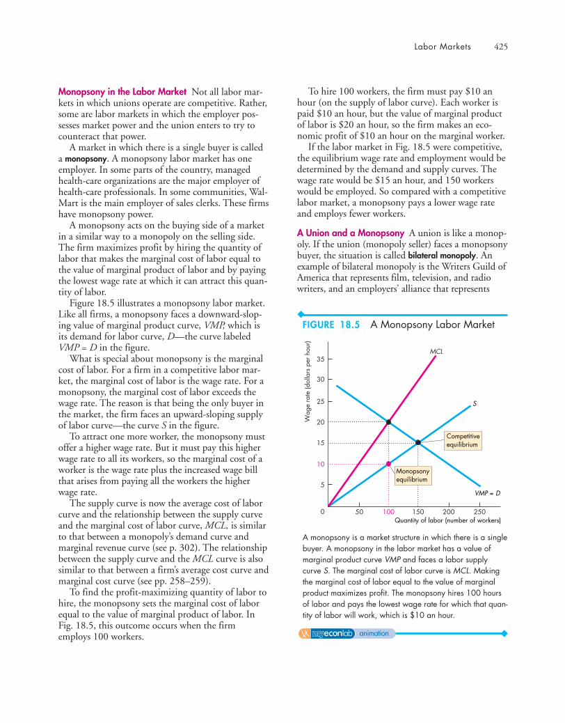
Labor Markets 425

Monopsony in the Labor Market Not all labor mar-kets in which unions operate are competitive. Rather,some are labor markets in which the employer pos-sesses market power and the union enters to try tocounteract that power.

A market in which there is a single buyer is calleda monopsony. A monopsony labor market has oneemployer. In some parts of the country, managedhealth-care organizations are the major employer ofhealth-care professionals. In some communities, Wal-Mart is the main employer of sales clerks. These firmshave monopsony power.

A monopsony acts on the buying side of a marketin a similar way to a monopoly on the selling side.The firm maximizes profit by hiring the quantity oflabor that makes the marginal cost of labor equal tothe value of marginal product of labor and by payingthe lowest wage rate at which it can attract this quan-tity of labor.

Figure 18.5 illustrates a monopsony labor market.Like all firms, a monopsony faces a downward-slop-ing value of marginal product curve, VMP, which isits demand for labor curve, D—the curve labeledVMP = D in the figure.

What is special about monopsony is the marginalcost of labor. For a firm in a competitive labor mar-ket, the marginal cost of labor is the wage rate. For amonopsony, the marginal cost of labor exceeds thewage rate. The reason is that being the only buyer inthe market, the firm faces an upward-sloping supplyof labor curve—the curve S in the figure.

To attract one more worker, the monopsony mustoffer a higher wage rate. But it must pay this higherwage rate to all its workers, so the marginal cost of aworker is the wage rate plus the increased wage billthat arises from paying all the workers the higherwage rate.

The supply curve is now the average cost of laborcurve and the relationship between the supply curveand the marginal cost of labor curve, MCL, is similarto that between a monopoly’s demand curve andmarginal revenue curve (see p. 302). The relationshipbetween the supply curve and the MCL curve is alsosimilar to that between a firm’s average cost curve andmarginal cost curve (see pp. 258–259).

To find the profit-maximizing quantity of labor tohire, the monopsony sets the marginal cost of laborequal to the value of marginal product of labor. InFig. 18.5, this outcome occurs when the firmemploys 100 workers.

To hire 100 workers, the firm must pay $10 anhour (on the supply of labor curve). Each worker ispaid $10 an hour, but the value of marginal productof labor is $20 an hour, so the firm makes an eco-nomic profit of $10 an hour on the marginal worker.

If the labor market in Fig. 18.5 were competitive,the equilibrium wage rate and employment would bedetermined by the demand and supply curves. Thewage rate would be $15 an hour, and 150 workerswould be employed. So compared with a competitivelabor market, a monopsony pays a lower wage rateand employs fewer workers.

A Union and a Monopsony A union is like a monop-oly. If the union (monopoly seller) faces a monopsonybuyer, the situation is called bilateral monopoly. Anexample of bilateral monopoly is the Writers Guild ofAmerica that represents film, television, and radiowriters, and an employers’ alliance that represents

Wag

e ra

te (d

olla

rs p

er h

our)

Quantity of labor (number of workers)0 50 100 150 200 250

30

5

35

25

20

15

10

MCL

S

VMP = D

Competitiveequilibrium

Monopsonyequilibrium

A monopsony is a market structure in which there is a singlebuyer. A monopsony in the labor market has a value ofmarginal product curve VMP and faces a labor supplycurve S. The marginal cost of labor curve is MCL. Makingthe marginal cost of labor equal to the value of marginalproduct maximizes profit. The monopsony hires 100 hoursof labor and pays the lowest wage rate for which that quan-tity of labor will work, which is $10 an hour.

FIGURE 18.5 A Monopsony Labor Market

animation

426 CHAPTER 18 Markets for Factors of Production

CBS, MGM, NBC, and other entertainment compa-nies. Every three years, the Writers Guild and theemployers’ alliance negotiate a pay deal.

In bilateral monopoly, the outcome is determinedby bargaining, which depends on the costs that eachparty can inflict on the other. The firm can shutdown temporarily and lock out its workers, and theworkers can shut down the firm by striking. Eachparty estimates the other’s strength and what it willlose if it does not agree to the other’s demands.

Usually, an agreement is reached without a strikeor a lockout. The threat is usually enough to bringthe bargaining parties to an agreement. When a strikeor lockout does occur, it is because one party has mis-judged the costs each party can inflict on the other.Such an event occurred in November 2007 when thewriters and entertainment producers failed to agreeon a compensation deal. A 100-day strike followedthat ended up costing the entertainment industry anestimated $2 billion.

In the example in Fig. 18.5, if the union andemployer are equally strong, and each party knowsthe strength of the other, they will agree to split thegap between $10 (the wage rate on the supply curve)and $20 (the wage rate on the demand curve) andagree to a wage rate of $15 an hour.

You’ve now seen that in a monopsony, a union canbargain for a higher wage rate without sacrificingjobs. A similar outcome can arise in a monopsonylabor market when a minimum wage law is enforced.Let’s look at the effect of a minimum wage.

Monopsony and the Minimum Wage In a competi-tive labor market, a minimum wage that exceeds theequilibrium wage decreases employment (see Chapter6, pp. 131–132). In a monopsony labor market, aminimum wage can increase both the wage rate andemployment. Let’s see how.

Figure 18.6 shows a monopsony labor marketwithout a union. The wage rate is $10 an hour and100 workers are employed.

A minimum wage law is passed that requiresemployers to pay at least $15 an hour. The monop-sony now faces a perfectly elastic supply of labor at$15 an hour up to 150 workers (along the mini-mum wage line). To hire more than 150 workers, awage rate above $15 an hour must be paid (alongthe supply curve). Because the wage rate is $15 anhour up to 150 workers, so is the marginal cost oflabor $15 an hour up to 150 workers. To maximizeprofit, the monopsony sets the marginal cost of

labor equal to the value of marginal product oflabor (on the demand curve). That is, the monop-sony hires 150 workers and pays $15 an hour. Theminimum wage law has succeeded in raising thewage rate and increasing the number of workersemployed.

Scale of the Union–Nonunion Wage GapYou’ve seen how a union can influence the wage rate,but how much of a difference to wage rates do unionsactually make? This question is difficult to answer. Tomeasure the difference in wages attributable tounions, economists have looked at the wages ofunionized and nonunionized workers who do similarwork and have similar skills.

The evidence based on these comparisons is thatthe union–nonunion wage gap lies between 10 and25 percent of the wage. For example, unionized air-line pilots earn about 25 percent more than non-union pilots with the same level of skill. In marketsthat have only a union wage rate, we might presumethat the wage rate is 10 to 25 percent higher than itwould be in the absence of a union.

Wag

e ra

te (d

olla

rs p

er h

our)

Quantity of labor (number of workers)0 50 100 150 200 250

30

5

35

25

20

15

10

MCL

S

VMP = D

Minimum wage

Increase inemployment

In a monopsony labor market, the wage rate is $10 anhour and 100 workers are hired. If a minimum wage lawincreases the wage rate to $15 an hour, the wage rate risesto this level and employment increases to 150 workers.

FIGURE 18.6 Minimum Wage Lawin Monopsony

animation

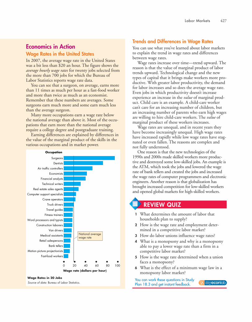
Labor Markets 427

Economics in ActionWage Rates in the United StatesIn 2007, the average wage rate in the United Stateswas a bit less than $20 an hour. The figure shows theaverage hourly wage rates for twenty jobs selected fromthe more than 700 jobs for which the Bureau ofLabor Statistics reports wage rate data.

You can see that a surgeon, on average, earns morethan 11 times as much per hour as a fast-food workerand more than twice as much as an economist.Remember that these numbers are averages. Somesurgeons earn much more and some earn much lessthan the average surgeon.

Many more occupations earn a wage rate belowthe national average than above it. Most of the occu-pations that earn more than the national averagerequire a college degree and postgraduate training.

Earning differences are explained by differences inthe value of the marginal product of the skills in thevarious occupations and in market power.

Trends and Differences in Wage RatesYou can use what you’ve learned about labor marketsto explain the trend in wage rates and differencesbetween wage rates.

Wage rates increase over time—trend upward. Thereason is that the value of marginal product of labortrends upward. Technological change and the newtypes of capital that it brings make workers more pro-ductive. With greater labor productivity, the demandfor labor increases and so does the average wage rate.Even jobs in which productivity doesn’t increaseexperience an increase in the value of marginal prod-uct. Child care is an example. A child-care workercan’t care for an increasing number of children, butan increasing number of parents who earn high wagesare willing to hire child-care workers. The value ofmarginal product of these workers increases.

Wage rates are unequal, and in recent years theyhave become increasingly unequal. High wage rateshave increased rapidly while low wage rates have stag-nated or even fallen. The reasons are complex andnot fully understood.

One reason is that the new technologies of the1990s and 2000s made skilled workers more produc-tive and destroyed some low-skilled jobs. An example isthe ATM, which took the jobs and lowered the wagerate of bank tellers and created the jobs and increasedthe wage rates of computer programmers and electronicengineers. Another reason is that globalization hasbrought increased competition for low-skilled workersand opened global markets for high-skilled workers.

0 4020 60 80

Wage rate (dollars per hour)

100

Surgeons

Dentists

Air traffic controllers

Economists

Financial analysts

Technical writers

Real estate sales agents

Computer support specialists

Crane operators

Truck drivers

Travel guides

Fitness trainers

Word processors and typists

Construction laborers

Van drivers

Medical assistants

Retail salespersons

Bank tellers

Motion picture projectionists

Fast-food workers

Occupation

National averagewage rate

Wage Rates in 20 Jobs

Source of data: Bureau of Labor Statistics.

REVIEW QUIZ1 What determines the amount of labor that

households plan to supply?2 How is the wage rate and employment deter-

mined in a competitive labor market?3 How do labor unions influence wage rates?4 What is a monopsony and why is a monopsony

able to pay a lower wage rate than a firm in acompetitive labor market?

5 How is the wage rate determined when a unionfaces a monopsony?

6 What is the effect of a minimum wage law in amonopsony labor market?

You can work these questions in Study Plan 18.3 and get instant feedback.

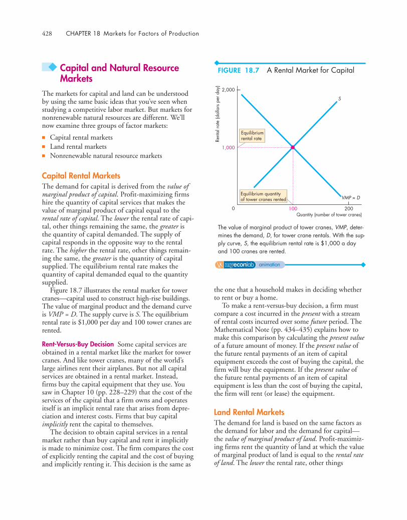
428 CHAPTER 18 Markets for Factors of Production

◆ Capital and Natural ResourceMarkets

The markets for capital and land can be understoodby using the same basic ideas that you’ve seen whenstudying a competitive labor market. But markets fornonrenewable natural resources are different. We’llnow examine three groups of factor markets:

■ Capital rental markets■ Land rental markets■ Nonrenewable natural resource markets

Capital Rental MarketsThe demand for capital is derived from the value ofmarginal product of capital. Profit-maximizing firmshire the quantity of capital services that makes thevalue of marginal product of capital equal to therental rate of capital. The lower the rental rate of capi-tal, other things remaining the same, the greater isthe quantity of capital demanded. The supply ofcapital responds in the opposite way to the rentalrate. The higher the rental rate, other things remain-ing the same, the greater is the quantity of capitalsupplied. The equilibrium rental rate makes thequantity of capital demanded equal to the quantitysupplied.

Figure 18.7 illustrates the rental market for towercranes—capital used to construct high-rise buildings.The value of marginal product and the demand curveis VMP = D. The supply curve is S. The equilibriumrental rate is $1,000 per day and 100 tower cranes arerented.

Rent-Versus-Buy Decision Some capital services areobtained in a rental market like the market for towercranes. And like tower cranes, many of the world’slarge airlines rent their airplanes. But not all capitalservices are obtained in a rental market. Instead,firms buy the capital equipment that they use. Yousaw in Chapter 10 (pp. 228–229) that the cost of theservices of the capital that a firm owns and operatesitself is an implicit rental rate that arises from depre-ciation and interest costs. Firms that buy capitalimplicitly rent the capital to themselves.

The decision to obtain capital services in a rentalmarket rather than buy capital and rent it implicitlyis made to minimize cost. The firm compares the costof explicitly renting the capital and the cost of buyingand implicitly renting it. This decision is the same as

the one that a household makes in deciding whetherto rent or buy a home.

To make a rent-versus-buy decision, a firm mustcompare a cost incurred in the present with a streamof rental costs incurred over some future period. TheMathematical Note (pp. 434–435) explains how tomake this comparison by calculating the present valueof a future amount of money. If the present value ofthe future rental payments of an item of capitalequipment exceeds the cost of buying the capital, thefirm will buy the equipment. If the present value ofthe future rental payments of an item of capitalequipment is less than the cost of buying the capital,the firm will rent (or lease) the equipment.

Land Rental MarketsThe demand for land is based on the same factors asthe demand for labor and the demand for capital—the value of marginal product of land. Profit-maximiz-ing firms rent the quantity of land at which the valueof marginal product of land is equal to the rental rateof land. The lower the rental rate, other things

Equilibriumrental rate

Equilibrium quantityof tower cranes rented

Rent

al ra

te (d

olla

rs p

er d

ay)

Quantity (number of tower cranes)0 100

2,000

1,000

200

S

VMP = D

The value of marginal product of tower cranes, VMP, deter-mines the demand, D, for tower crane rentals. With the sup-ply curve, S, the equilibrium rental rate is $1,000 a dayand 100 cranes are rented.

FIGURE 18.7 A Rental Market for Capital

animation

Capital and Natural Resource Markets 429

remaining the same, the greater is the quantity ofland demanded.

But the supply of land is special: Its quantity isfixed, so the quantity supplied cannot be changed bypeople’s decisions. The supply of each particularblock of land is perfectly inelastic.

The equilibrium rental rate makes the quantity ofland demanded equal to the quantity available.Figure 18.8 illustrates the market for a 10-acre blockof land on 42nd Street in New York City. The quan-tity supplied is fixed and the supply curve is S. Thevalue of marginal product and the demand curve isVMP = D. The equilibrium rental rate is $1,000 anacre per day.

The rental rate of land is high in New Yorkbecause the willingness to pay for the services pro-duced by that land is high, which in turn makes theVMP of land high. A Big Mac costs more atMcDonald’s on 42nd Street, New York, than atMcDonald’s on Jefferson Avenue, St. Louis, but notbecause the rental rate of land is higher in New York.The rental rate of land is higher in New York becauseof the greater willingness to pay for a Big Mac (andother goods and services) in New York.

Nonrenewable Natural Resource MarketsThe nonrenewable natural resources are oil, gas, andcoal. Burning one of these fuels converts it to energyand other by-products, and the used resource cannotbe re-used. The natural resources that we use to makemetals are also nonrenewable, but they can be usedagain, at some cost, by recycling them.

Oil, gas, and coal are traded in global commoditymarkets. The price of a given grade of crude oil is thesame in New York, London, and Singapore. Traders,linked by telephone and the Internet, operate thesemarkets around the clock every day of the year.

Demand and supply determine the prices and thequantities traded in these commodity markets. We’lllook at the influences on demand and supply by con-sidering the global market for crude oil.

The Demand for Oil The two key influences on thedemand for oil are

1. The value of marginal product of oil2. The expected future price of oil

The value of marginal product of oil is the funda-mental influence on demand. It works in exactly thesame way for a nonrenewable resource as it does forany other factor of production. The greater the quan-tity of oil used, the smaller is the value of marginalproduct of oil. Diminishing value of marginal prod-uct makes the demand curve slope downward. Thelower the price, the greater is the quantity demanded.

The higher the expected future price of oil, thegreater is the present demand for oil. The expectedfuture price is a speculative influence on demand.Oil in the ground and oil in storage tanks are inven-tories that can be held or sold. A trader might planto buy oil to hold now and to sell it later for aprofit. Instead of buying oil to hold and sell later,the trader could buy a bond and earn interest. Theinterest forgone is the opportunity cost of holdingthe oil. If the price of oil is expected to rise by a big-ger percentage than the interest rate, a trader willhold oil and incur the opportunity cost. In this case,the return from holding oil exceeds the return fromholding bonds.

The Supply of Oil The three key influences on thesupply of oil are

1. The known oil reserves2. The scale of current oil production facilities3. The expected future price of oil

Equilibriumrental rate

Rent

al ra

te (d

olla

rs p

er a

cre

per d

ay)

Land (acres)0 10

2,000

1,000

20

S

VMP = D

The value of marginal product of a 10-acre block, VMP,determines the rental demand, D, for this land. With thesupply curve, S, the block rents for $10,000 a day.

FIGURE 18.8 A Rental Market for Land

animation

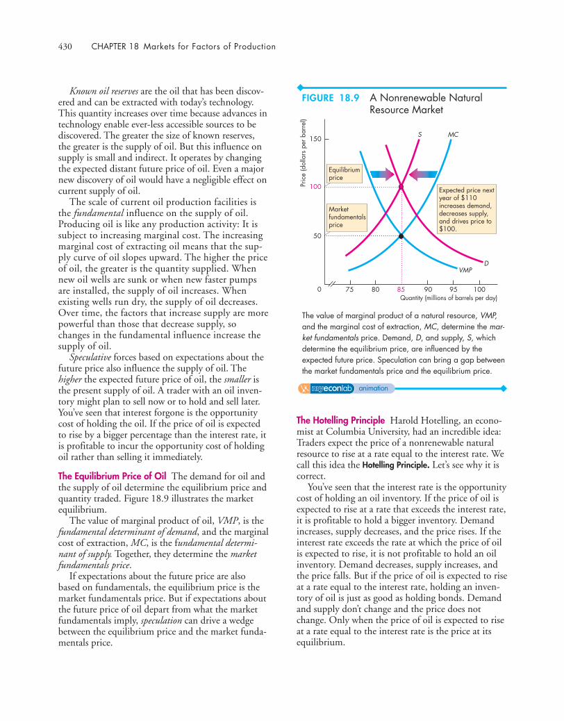
430 CHAPTER 18 Markets for Factors of Production

Known oil reserves are the oil that has been discov-ered and can be extracted with today’s technology.This quantity increases over time because advances intechnology enable ever-less accessible sources to bediscovered. The greater the size of known reserves,the greater is the supply of oil. But this influence onsupply is small and indirect. It operates by changingthe expected distant future price of oil. Even a majornew discovery of oil would have a negligible effect oncurrent supply of oil.

The scale of current oil production facilities isthe fundamental influence on the supply of oil.Producing oil is like any production activity: It issubject to increasing marginal cost. The increasingmarginal cost of extracting oil means that the sup-ply curve of oil slopes upward. The higher the priceof oil, the greater is the quantity supplied. Whennew oil wells are sunk or when new faster pumpsare installed, the supply of oil increases. Whenexisting wells run dry, the supply of oil decreases.Over time, the factors that increase supply are morepowerful than those that decrease supply, sochanges in the fundamental influence increase thesupply of oil.

Speculative forces based on expectations about thefuture price also influence the supply of oil. Thehigher the expected future price of oil, the smaller isthe present supply of oil. A trader with an oil inven-tory might plan to sell now or to hold and sell later.You’ve seen that interest forgone is the opportunitycost of holding the oil. If the price of oil is expectedto rise by a bigger percentage than the interest rate, itis profitable to incur the opportunity cost of holdingoil rather than selling it immediately.

The Equilibrium Price of Oil The demand for oil andthe supply of oil determine the equilibrium price andquantity traded. Figure 18.9 illustrates the marketequilibrium.

The value of marginal product of oil, VMP, is thefundamental determinant of demand, and the marginalcost of extraction, MC, is the fundamental determi-nant of supply. Together, they determine the marketfundamentals price.

If expectations about the future price are alsobased on fundamentals, the equilibrium price is themarket fundamentals price. But if expectations aboutthe future price of oil depart from what the marketfundamentals imply, speculation can drive a wedgebetween the equilibrium price and the market funda-mentals price.

The Hotelling Principle Harold Hotelling, an econo-mist at Columbia University, had an incredible idea:Traders expect the price of a nonrenewable naturalresource to rise at a rate equal to the interest rate. Wecall this idea the Hotelling Principle. Let’s see why it iscorrect.

You’ve seen that the interest rate is the opportunitycost of holding an oil inventory. If the price of oil isexpected to rise at a rate that exceeds the interest rate,it is profitable to hold a bigger inventory. Demandincreases, supply decreases, and the price rises. If theinterest rate exceeds the rate at which the price of oilis expected to rise, it is not profitable to hold an oilinventory. Demand decreases, supply increases, andthe price falls. But if the price of oil is expected to riseat a rate equal to the interest rate, holding an inven-tory of oil is just as good as holding bonds. Demandand supply don’t change and the price does notchange. Only when the price of oil is expected to riseat a rate equal to the interest rate is the price at itsequilibrium.

Pric

e (d

olla

rs p

er b

arre

l)Quantity (millions of barrels per day)

0 75 80 85 90 95

100

50

150

100

MCS

VMPD

Equilibriumprice

Marketfundamentalsprice

Expected price nextyear of $110increases demand,decreases supply,and drives price to$100.

The value of marginal product of a natural resource, VMP,and the marginal cost of extraction, MC, determine the mar-ket fundamentals price. Demand, D, and supply, S, whichdetermine the equilibrium price, are influenced by theexpected future price. Speculation can bring a gap betweenthe market fundamentals price and the equilibrium price.

FIGURE 18.9 A Nonrenewable NaturalResource Market

animation

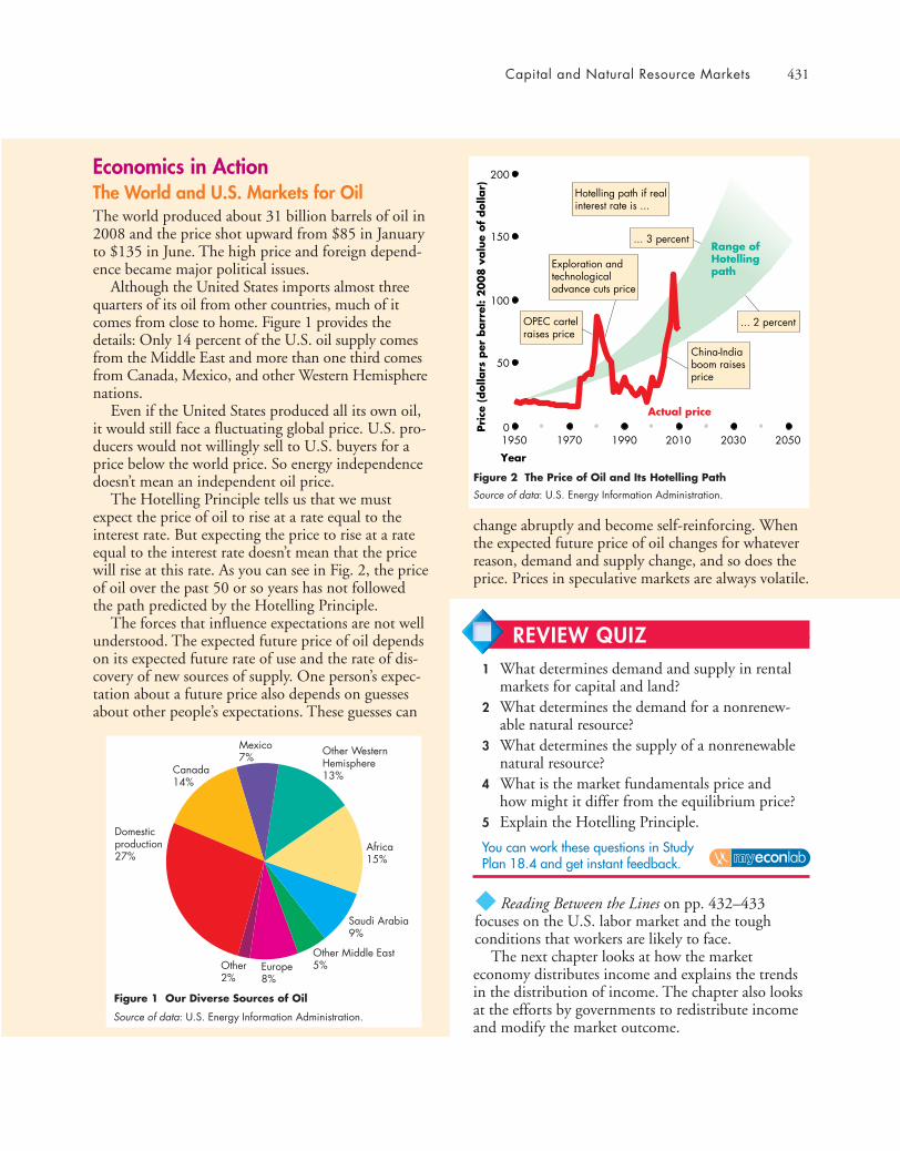
Capital and Natural Resource Markets 431

Economics in ActionThe World and U.S. Markets for OilThe world produced about 31 billion barrels of oil in2008 and the price shot upward from $85 in Januaryto $135 in June. The high price and foreign depend-ence became major political issues.

Although the United States imports almost threequarters of its oil from other countries, much of itcomes from close to home. Figure 1 provides thedetails: Only 14 percent of the U.S. oil supply comesfrom the Middle East and more than one third comesfrom Canada, Mexico, and other Western Hemispherenations.

Even if the United States produced all its own oil,it would still face a fluctuating global price. U.S. pro-ducers would not willingly sell to U.S. buyers for aprice below the world price. So energy independencedoesn’t mean an independent oil price.

The Hotelling Principle tells us that we mustexpect the price of oil to rise at a rate equal to theinterest rate. But expecting the price to rise at a rateequal to the interest rate doesn’t mean that the pricewill rise at this rate. As you can see in Fig. 2, the priceof oil over the past 50 or so years has not followedthe path predicted by the Hotelling Principle.

The forces that influence expectations are not wellunderstood. The expected future price of oil dependson its expected future rate of use and the rate of dis-covery of new sources of supply. One person’s expec-tation about a future price also depends on guessesabout other people’s expectations. These guesses can

◆ Reading Between the Lines on pp. 432–433focuses on the U.S. labor market and the toughconditions that workers are likely to face.

The next chapter looks at how the marketeconomy distributes income and explains the trendsin the distribution of income. The chapter also looksat the efforts by governments to redistribute incomeand modify the market outcome.

change abruptly and become self-reinforcing. Whenthe expected future price of oil changes for whateverreason, demand and supply change, and so does theprice. Prices in speculative markets are always volatile.

Year

Pri

ce (

dolla

rs p

er b

arr

el:

20

08

valu

e of

dolla

r)

Actual price

Range ofHotellingpath

0

50

200

100

150

20501950 1970 1990 2010 2030

OPEC cartelraises price

Hotelling path if realinterest rate is ...

... 3 percent

... 2 percent

Exploration andtechnologicaladvance cuts price

China-Indiaboom raisesprice

Figure 2 The Price of Oil and Its Hotelling Path

Saudi Arabia9%

Other WesternHemisphere13%

Other Middle East5%Other

2%

Mexico7%

Europe8%

Canada14%

Africa15%

Domesticproduction27%

Figure 1 Our Diverse Sources of Oil

Source of data: U.S. Energy Information Administration.

Source of data: U.S. Energy Information Administration.

REVIEW QUIZ1 What determines demand and supply in rental

markets for capital and land?2 What determines the demand for a nonrenew-

able natural resource?3 What determines the supply of a nonrenewable

natural resource?4 What is the market fundamentals price and

how might it differ from the equilibrium price?5 Explain the Hotelling Principle.

You can work these questions in Study Plan 18.4 and get instant feedback.

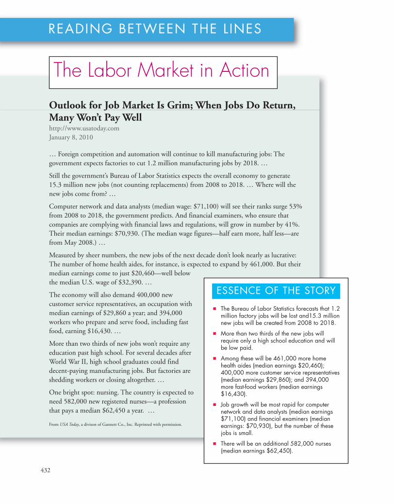
432

READING BETWEEN THE L INES

Outlook for Job Market Is Grim; When Jobs Do Return,Many Won’t Pay Wellhttp://www.usatoday.comJanuary 8, 2010

… Foreign competition and automation will continue to kill manufacturing jobs: Thegovernment expects factories to cut 1.2 million manufacturing jobs by 2018. …

Still the government’s Bureau of Labor Statistics expects the overall economy to generate 15.3 million new jobs (not counting replacements) from 2008 to 2018. … Where will thenew jobs come from? …

Computer network and data analysts (median wage: $71,100) will see their ranks surge 53%from 2008 to 2018, the government predicts. And financial examiners, who ensure thatcompanies are complying with financial laws and regulations, will grow in number by 41%.Their median earnings: $70,930. (The median wage figures—half earn more, half less—arefrom May 2008.) …

Measured by sheer numbers, the new jobs of the next decade don’t look nearly as lucrative:The number of home health aides, for instance, is expected to expand by 461,000. But theirmedian earnings come to just $20,460—well belowthe median U.S. wage of $32,390. …

The economy will also demand 400,000 newcustomer service representatives, an occupation withmedian earnings of $29,860 a year; and 394,000workers who prepare and serve food, including fastfood, earning $16,430. …

More than two thirds of new jobs won’t require anyeducation past high school. For several decades afterWorld War II, high school graduates could finddecent-paying manufacturing jobs. But factories areshedding workers or closing altogether. …

One bright spot: nursing. The country is expected toneed 582,000 new registered nurses—a professionthat pays a median $62,450 a year. …

From USA Today, a divison of Gannett Co., Inc. Reprinted with permission.

■ The Bureau of Labor Statistics forecasts that 1.2million factory jobs will be lost and15.3 millionnew jobs will be created from 2008 to 2018.

■ More than two thirds of the new jobs willrequire only a high school education and willbe low paid.

■ Among these will be 461,000 more homehealth aides (median earnings $20,460);400,000 more customer service representatives(median earnings $29,860); and 394,000more fast-food workers (median earnings$16,430).

■ Job growth will be most rapid for computernetwork and data analysts (median earnings$71,100) and financial examiners (medianearnings: $70,930), but the number of thesejobs is small.

■ There will be an additional 582,000 nurses(median earnings $62,450).

ESSENCE OF THE STORY

The Labor Market in Action

433

ECONOMIC ANALYSIS

Wag

e ra

te (d

olla

rs p

er y

ear)

Quantity (thousands of nurses)0 2,500 2,760 3,342

62,450

60,000

70,000

65,000

4,000

S08 S18

D18

D08

Equilibriumwage remainsconstant

Figure 2 The market for nurses when supply increases

Increase indemand Increase in

supply

582,000more nurses

Wag

e ra

te (d

olla

rs p

er y

ear)

Quantity (thousands of nurses)0 2,500 2,760 2,900 3,342

62,450

60,000

70,000

65,00066,000

4,000

S08

D18

D08

Increase in value ofmarginal product ofnurses increases thedemand for nurses ...

Equilibriumwage ratein 2008

Figure 1 The market for nurses with no change in supply

With no changein supply, wagerises

... by582,000

■ The labor markets are constantly in a state of change,reallocating the nation’s labor resources to their high-est-value employments.

■ The value of marginal product (VMP) of workers inservice industries is rising.

■ The VMP of nurses is rising because an aging popula-tion is increasing the demand for health care and tech-nological advances are making nurses more productive.

■ With an increase in VMP, the demand for nursesincreases.

■ Anticipating good job prospects in nursing, morecollege students and other young workers train asnurses, which increases the supply of nurses.

■ The combination of an increase in demand and anincrease in supply increases employment and theincrease is forecasted to be 582,000 nurses from2008 to 2018.

■ Nurses’ wages might rise, fall, or remain unchanged,depending on whether supply or demand increasesmore.

■ The figures illustrate the market for nurses in 2008 and2018. The 2008 demand curve, D08, and supplycurve, S08, determine the equilibrium number of nurses(2,760,000) and the equilibrium wage rate ($62,450per year).

■ By 2018, the demand for nurses will increase to D18.With no change in supply in Fig. 1, the wage raterises to $66,000 a year and employment increases to2,900,000.

■ But the anticipation of good job prospects increasessupply to S18 in Fig. 2. Employment increases by582,000 and the wage rate remains at its 2008 level(an assumption).

■ As the VMP of nurses is rising, the VMP of workers inmanufacturing industries is falling. Foreign competitionis cutting the prices of manufactured goods andautomation is making machines more productive thanfactory labor, decreasing their marginal product.

■ With a decrease in VMP, the demand for factoryworkers decreases.

■ Faced with the prospect of unemployment or workingfor a lower wage, young workers stop looking forfactory jobs and undertake training for service jobs,which decreases the supply of factory workers.

■ The combination of a decrease in demand and a de-crease in supply decreases factory employment and

the decrease is forecasted to be 1.2 million workersfrom 2008 to 2018.

■ The wages of factory workers might rise, fall, orremain unchanged, depending on whether supply ordemand decreases more.

■ Similar events are occurring in the markets for all typesof labor, some expanding like nurses and somecontracting like factory workers.

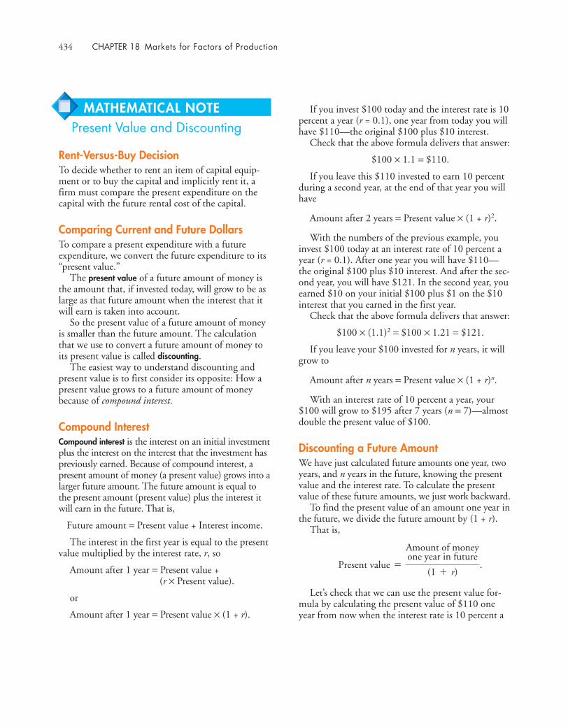
434 CHAPTER 18 Markets for Factors of Production

MATHEMATICAL NOTEPresent Value and Discounting

Rent-Versus-Buy DecisionTo decide whether to rent an item of capital equip-ment or to buy the capital and implicitly rent it, afirm must compare the present expenditure on thecapital with the future rental cost of the capital.

Comparing Current and Future DollarsTo compare a present expenditure with a futureexpenditure, we convert the future expenditure to its“present value.”

The present value of a future amount of money isthe amount that, if invested today, will grow to be aslarge as that future amount when the interest that itwill earn is taken into account.

So the present value of a future amount of moneyis smaller than the future amount. The calculationthat we use to convert a future amount of money toits present value is called discounting.

The easiest way to understand discounting andpresent value is to first consider its opposite: How apresent value grows to a future amount of moneybecause of compound interest.

Compound InterestCompound interest is the interest on an initial investmentplus the interest on the interest that the investment haspreviously earned. Because of compound interest, apresent amount of money (a present value) grows into alarger future amount. The future amount is equal tothe present amount (present value) plus the interest itwill earn in the future. That is,

Future amount = Present value + Interest income.

The interest in the first year is equal to the presentvalue multiplied by the interest rate, r, so

Amount after 1 year = Present value +(r × Present value).

or

Amount after 1 year = Present value × (1 + r).

If you invest $100 today and the interest rate is 10percent a year (r = 0.1), one year from today you willhave $110—the original $100 plus $10 interest.

Check that the above formula delivers that answer:

$100 × 1.1 = $110.

If you leave this $110 invested to earn 10 percentduring a second year, at the end of that year you willhave

Amount after 2 years = Present value × (1 + r)2.

With the numbers of the previous example, youinvest $100 today at an interest rate of 10 percent ayear (r = 0.1). After one year you will have $110—the original $100 plus $10 interest. And after the sec-ond year, you will have $121. In the second year, youearned $10 on your initial $100 plus $1 on the $10interest that you earned in the first year.

Check that the above formula delivers that answer:

$100 × (1.1)2 = $100 × 1.21 = $121.

If you leave your $100 invested for n years, it willgrow to

Amount after n years = Present value × (1 + r)n.

With an interest rate of 10 percent a year, your$100 will grow to $195 after 7 years (n = 7)—almostdouble the present value of $100.

Discounting a Future AmountWe have just calculated future amounts one year, twoyears, and n years in the future, knowing the presentvalue and the interest rate. To calculate the presentvalue of these future amounts, we just work backward.

To find the present value of an amount one year inthe future, we divide the future amount by (1 + r).

That is,

Let’s check that we can use the present value for-mula by calculating the present value of $110 oneyear from now when the interest rate is 10 percent a

Present value =

Amount of moneyone year in future

(1 + r).

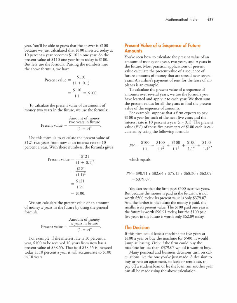
Mathematical Note 435

year. You’ll be able to guess that the answer is $100because we just calculated that $100 invested today at10 percent a year becomes $110 in one year. So thepresent value of $110 one year from today is $100.But let’s use the formula. Putting the numbers intothe above formula, we have

To calculate the present value of an amount ofmoney two years in the future, we use the formula:

Use this formula to calculate the present value of$121 two years from now at an interest rate of 10percent a year. With these numbers, the formula gives

We can calculate the present value of an amountof money n years in the future by using the generalformula

For example, if the interest rate is 10 percent ayear, $100 to be received 10 years from now has apresent value of $38.55. That is, if $38.55 is investedtoday at 10 percent a year it will accumulate to $100in 10 years.

Present value =

Amount of moneyn years in future

(1 + r)n .

= $100.

=$1211.21

=$121

(1.1)2

Present value =$121

(1 + 0.1)2

Present value =

Amount of moneytwo years in future

(1 + r)2 .

=$1101.1

= $100.

Present value =$110

(1 + 0.1)

Present Value of a Sequence of FutureAmountsYou’ve seen how to calculate the present value of anamount of money one year, two years, and n years inthe future. Most practical applications of presentvalue calculate the present value of a sequence offuture amounts of money that are spread over severalyears. An airline’s payment of rent for the lease of air-planes is an example.

To calculate the present value of a sequence ofamounts over several years, we use the formula youhave learned and apply it to each year. We then sumthe present values for all the years to find the presentvalue of the sequence of amounts.

For example, suppose that a firm expects to pay$100 a year for each of the next five years and theinterest rate is 10 percent a year (r = 0.1). The presentvalue (PV ) of these five payments of $100 each is cal-culated by using the following formula:

which equals

PV = $90.91 + $82.64 + $75.13 + $68.30 + $62.09= $379.07.

You can see that the firm pays $500 over five years.But because the money is paid in the future, it is notworth $500 today. Its present value is only $379.07.And the farther in the future the money is paid, thesmaller is its present value. The $100 paid one year inthe future is worth $90.91 today, but the $100 paidfive years in the future is worth only $62.09 today.

The DecisionIf this firm could lease a machine for five years at$100 a year or buy the machine for $500, it wouldjump at leasing. Only if the firm could buy themachine for less than $379.07 would it want to buy.

Many personal and business decisions turn on cal-culations like the one you’ve just made. A decision tobuy or rent an apartment, to lease or rent a car, topay off a student loan or let the loan run another yearcan all be made using the above calculation.

PV =$100

1.1+

$100

1.12 +$100

1.13 +$100

1.14 +$100

1.15 ,

436 CHAPTER 18 Markets for Factors of Production

■ Demand and supply determine the wage rate in acompetitive labor market.

■ A labor union can raise the wage rate by restrictingthe supply or increasing the demand for labor.

■ A monopsony can lower the wage rate below thecompetitive level.

■ A union or a minimum wage in a monopsonylabor market can raise the wage rate without a fallin employment.

Working Problems 9 to 11 will give you a better under-standing of labor markets.

Capital and Natural Resource Markets (pp. 428–431)

■ The value of marginal product of capital (andland) determines the demand for capital (andland).

■ Firms make a rent-versus-buy decision by choos-ing the option that minimizes cost.

■ The supply of land is inelastic and the demand forland determines the rental rate.

■ The demand for a nonrenewable natural resourcedepends on the value of marginal product and onthe expected future price.

■ The supply of a nonrenewable natural resourcedepends on the known reserves, the cost of extrac-tion, and the expected future price.

■ The price of nonrenewable natural resources candiffer from the market fundamentals price becauseof speculation based on expectations about thefuture price.

■ The price of a nonrenewable natural resource isexpected to rise at a rate equal to the interest rate.

Working Problems 12 to 17 will give you a better under-standing of capital and natural resource markets.

Key Points

The Anatomy of Factor Markets (p. 418)

■ The factor markets are: job markets for labor;rental markets (often implicit rental markets) forcapital and land; and global commodity marketsfor nonrenewable natural resources.

■ The services of entrepreneurs are not traded on afactor market.

Working Problem 1 will give you a better understandingof the anatomy of factor markets.

The Demand for a Factor of Production(pp. 419–421)

■ The value of marginal product determines thedemand for a factor of production.

■ The value of marginal product decreases as thequantity of the factor employed increases.

■ The firm employs the quantity of each factor ofproduction that makes the value of marginal prod-uct equal to the factor price.

Working Problems 2 to 8 will give you a better under-standing of the demand for a factor of production.

Labor Markets (pp. 422–427)

■ The value of marginal product of labor determinesthe demand for labor. A rise in the wage ratebrings a decrease in the quantity demanded.

■ The quantity of labor supplied depends on thewage rate. At low wage rates, a rise in the wage rateincreases the quantity supplied. Beyond a highenough wage rate, a rise in the wage rate decreasesthe quantity supplied—the supply curve eventu-ally bends backward.

Key TermsBilateral monopoly, 425Compound interest, 434Derived demand, 419Discounting, 434

Hotelling Principle, 430Job, 418Labor union, 424Monopsony, 425

Nonrenewable natural resources, 418

Present value, 434Value of marginal product, 419

SUMMARY

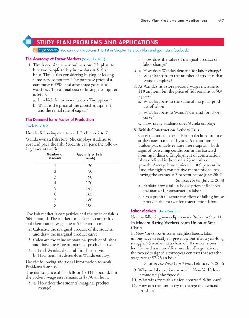
Study Plan Problems and Applications 437

b. How does the value of marginal product oflabor change?

6. a. How does Wanda’s demand for labor change?b. What happens to the number of students that

Wanda employs?7. At Wanda’s fish store packers’ wages increase to

$10 an hour, but the price of fish remains at 50¢a pound. a. What happens to the value of marginal prod-

uct of labor?b. What happens to Wanda’s demand for labor

curve?c. How many students does Wanda employ?

8. British Construction Activity FallsConstruction activity in Britain declined in Juneat the fastest rate in 11 years. A major homebuilder was unable to raise more capital—bothsigns of worsening conditions in the batteredhousing industry. Employment of constructionlabor declined in June after 23 months ofgrowth. Average house prices fell 0.9 percent inJune, the eighth consecutive month of declines,leaving the average 6.3 percent below June 2007.

Source: Forbes, July 2, 2008a. Explain how a fall in house prices influences

the market for construction labor.b. On a graph illustrate the effect of falling house

prices in the market for construction labor.

Labor Markets (Study Plan18.3)

Use the following news clip to work Problems 9 to 11.In Modern Rarity, Workers Form Union at SmallChainIn New York’s low-income neighborhoods, laborunions have virtually no presence. But after a year-longstruggle, 95 workers at a chain of 10 sneaker storeshave formed a union. After months of negotiations,the two sides signed a three-year contract that sets thewage rate at $7.25 an hour.

Source:The New York Times, February 5, 2006

9. Why are labor unions scarce in New York’s low-income neighborhoods?

10. Who wins from this union contract? Who loses?11. How can this union try to change the demand

for labor?

The Anatomy of Factor Markets (Study Plan18.1)

1. Tim is opening a new online store. He plans tohire two people to key in the data at $10 anhour. Tim is also considering buying or leasingsome new computers. The purchase price of acomputer is $900 and after three years it isworthless. The annual cost of leasing a computeris $450.a. In which factor markets does Tim operate?b. What is the price of the capital equipment

and the rental rate of capital?

The Demand for a Factor of Production (Study Plan18.2)

Use the following data to work Problems 2 to 7.Wanda owns a fish store. She employs students tosort and pack the fish. Students can pack the follow-ing amounts of fish:

Number of Quantity of fishstudents (pounds)

1 202 503 904 1205 1456 1657 1808 190

The fish market is competitive and the price of fish is50¢ a pound. The market for packers is competitiveand their market wage rate is $7.50 an hour.

2. Calculate the marginal product of the studentsand draw the marginal product curve.

3. Calculate the value of marginal product of laborand draw the value of marginal product curve.

4. a. Find Wanda’s demand for labor curve.b. How many students does Wanda employ?

Use the following additional information to workProblems 5 and 6.The market price of fish falls to 33.33¢ a pound, butthe packers’ wage rate remains at $7.50 an hour.

5. a. How does the students’ marginal productchange?

You can work Problems 1 to 18 in Chapter 18 Study Plan and get instant feedback.

STUDY PLAN PROBLEMS AND APPLICATIONS

438 CHAPTER 18 Markets for Factors of Production

Capital and Natural Resource Markets (Study Plan18.4)

12. Classify the following items as a nonrenewablenatural resource, a renewable natural resource, ornot a natural resource. Explain your answers.a. Trump Towerb. Lake Michiganc. Coal in a West Virginia coal mined. The Internete. Yosemite National Parkf. Power generated by wind turbines

13. Trump Group Selling Parcel For $1.8 BillionA consortium of Hong Kong investors andDonald J. Trump are selling a stretch of river-front land and three buildings on the UpperWest Side for about $1.8 billion in the largestresidential sale in city history. Mr. Trumpacquired the land for less than $100 million adecade ago during a real estate recession.

Source: The New York Times, June 1, 2005a. Why has the price of land on New York

City’s Upper West Side increased over the lastdecade? In your answer include a discussionof the demand for and supply of land.

b. Use a graph to show why the price of land onthe Upper West Side increased over the lastdecade.

c. Is the supply of land on the Upper West Sideperfectly inelastic?

14. In the news clip in Problem 8, a. Explain how a fall in house prices influences

the market for construction equipment leases.b. Draw a graph to illustrate the effect of a fall in

house prices in the market for constructionequipment leases.

Use the following news clip to work Problems 15 and 16.Fixing FarmingSolutions to the global food crisis will come fromgenetically engineered crops and large-scale farms.Demand for farm products will keep growing as thepopulation grows. But the supply of farmland is lim-ited and farms already use 55 percent of the habitableland. The solution is for farmers to become more pro-ductive—generating more output from fewer inputs.

Source: Fortune, May 22, 2008

15. a. Is farmland a renewable or nonrenewableresource?

b. Explain how the growing demand for farmproducts will affect the market for land anddraw a graph to illustrate your answer.

16. How might farmers meet the growing demandfor farm products without having to use a greaterquantity of farmland?

17. Copter CrisisHelicopters are in short supply these days. Youcould blame a rise in military spending, a jumpin disaster relief, even crowded airports pushingexecutives into private travel. But the fastestgrowth is coming from the offshore oil-and-gasindustry, where helicopters are the only way toferry crews to and from rigs and platforms.Hundred-dollar oil has pushed producers towork existing fields harder and to open newdeep-sea wells in Brazil, India, and Alaska. Thenumber of rigs and platforms has grown by 13%over the past decade. Oil companies are facing atwo-year backlog in orders for the Sikorsky S92,a favorite of the oil industry, and a 40% rise inprices for used models.

Source: Fortune, May 12, 2008a. Explain how high oil prices influence the

market for helicopter leases and services (such as the Sikorsky S92).

b. What happens to the value of marginal productof a helicopter as a firm leases or buys additionalhelicopters?

Mathematical Note (Study Plan 18.MN)

18. Keshia is opening a new bookkeeping service. Sheis considering buying or leasing some new laptopcomputers. The purchase price of a laptop is$1,500 and after three years it is worthless. Theannual lease rate is $550 per laptop. The value ofmarginal product of one laptop is $700 a year.The value of marginal product of a second laptopis $625 a year. The value of marginal product of athird laptop is $575 a year. And the value of mar-ginal product of a fourth laptop is $500 a year.a. How many laptops will Keshia lease or buy?b. If the interest rate is 4 percent a year, will

Keshia lease or buy her laptops?c. If the interest rate is 6 percent a year, will

Keshia lease or buy her laptops?

Additional Problems and Applications 439

The Anatomy of Factor Markets19. Venus is opening a tennis school. She plans to

hire a marketing graduate to promote the schooland an administrator at $20 an hour. Venus isalso considering buying or leasing a new tennisball machine. The purchase price of the machineis $1,000 and after three years it is worthless. Theannual cost of leasing the machine is $500.a. In which factor markets does Venus operate?b. What is the price of the capital equipment

and the rental rate of capital?

The Demand for a Factor of ProductionUse the following data to work Problems 20 to 23.Kaiser’s Ice Cream Parlor hires workers to producesmoothies. The market for smoothies is perfectlycompetitive, and the price of a smoothie is $4. Thelabor market is competitive, and the wage rate is $40a day. The table shows the workers’ total productschedule.

Number of Quantity producedworkers (smoothies per day)

1 72 213 334 435 516 55

20. Calculate the marginal product of hiring thefourth worker and the fourth worker’s value ofmarginal product.

21. How many workers will Kaiser’s hire to maximizeits profit and how many smoothies a day willKaiser’s produce?

22. If the price rises to $5 a smoothie, how manyworkers will Kaiser’s hire?

23. Kaiser’s installs a new soda fountain thatincreases the productivity of workers by 50 per-cent. If the price of a smoothie remains at $4 andthe wage rises to $48 a day, how many workersdoes Kaiser’s hire?

24. Detroit Oil Refinery Expansion ApprovedMarathon Oil Saturday started work on a $1.9billion expansion of its gasoline refinery in

Detroit. Marathon will employ 800 constructionworkers and add 135 permanent jobs to theexisting 480 workers at the refinery. Source: United Press International, June 21, 2008

a. Explain how rising gasoline prices influencethe market for refinery labor.

b. Draw a graph to illustrate the effects of risinggasoline prices on the market for refinerylabor.

Labor Markets

25. You May be Paid More (or Less) than YouThinkIt’s hard to put a price on happiness, but if you’veever had to choose between a job you like and abetter-paying one that you like less, you’d like toknow what job satisfaction is worth.John Helliwell and Haifang Huang (economistsat the University of British Columbia) have esti-mated four key factors influencing job satisfac-tion: Trust in management is like a 36 percentpay raise; a job with lots of variety is like a 21percent pay raise; a job that requires a high levelof skill is like a 19 percent pay raise; and a jobwith enough time to finish your work is like an11 percent pay raise.

Source: CNN, March 29, 2006a. How might the job characteristics described

here affect the supply of labor for differenttypes of jobs?

b. How might this influence on supply result indifferent wage rates that reflect the attractive-ness of a job’s characteristics?

Use the following news clip to work Problems 26 to 29.

The New War over Wal-MartToday, Wal-Mart employs more people—1.7 mil-lion—than any other private employer in the world.With size comes power: Wal-Mart’s prices are lowerand United Food and Commercial Workers Inter-national Union argues that Wal-Mart’s wages are alsolowers than its competitors. Last year, the workers at aCanadian outlet joined the union and Wal-Mart imme-diately closed the outlet. But does Wal-Mart behave

You can work these problems in MyEconLab if assigned by your instructor.

ADDITIONAL PROBLEMS AND APPLICATIONS

440 CHAPTER 18 Markets for Factors of Production

b. What could cause the price of natural gas tofall in the future?

32. New technology has allowed oil to be pumpedfrom much deeper offshore oil fields than before.For example, 28 deep ocean rigs operate in thedeep waters of the Gulf of Mexico.a. What effect do you think deep ocean sources

have had on the world oil price?b. Who will benefit from drilling for oil in the

Gulf of Mexico? Explain your answer.

33. Water is a natural resource that is plentiful inCanada but not plentiful in Arizona andsouthern California.a. If Canadians start to export bulk water to

Arizona and southern California, what do youpredict will be the effect on the price of bulkwater?

b. Will Canada eventually run out of water?c. Do you think the Hotelling Principle applies

to Canada’s water? Explain why or why not.

Economics in the News

34. After you have studied Reading Between the Lineson pp. 432–433 answer the following questions.a. Name some jobs for which future employ-

ment will expand and some for which it willshrink.

b. What are the influences on the demand forlabor that bring an increase in demand andwhat are the influences that bring a decreasein demand?

c. Why is an increase in the demand for nurseslikely to bring a similar increase in the supplyof nurses?

d. Draw a graph of the market for factory work-ers in 2008 and 2018. Show the effects of adecrease in the demand for factory workerswith no change in the supply on the employ-ment and wage rate of factory workers.

e. If the outcome you’ve shown in part (d)occurred, explain how the incentives faced byyoung workers just entering the labor forcewould be affected.

f. On your graph of the labor market in part (d), show how you would expect the supply offactory workers to change by 2018 and showyour predicted level of employment and wagerate of factory workers in 2018.

any worse than its competitors? When it comes to pay-roll, Wal-Mart’s median hourly wage tracks the nationalmedian wage for general merchandise retail jobs.

Source: The Atlantic, June 200626. a. Assuming that Wal-Mart has market power in

a labor market, explain how the firm coulduse that market power in setting wages.

b. Draw a graph to illustrate how Wal-Martmight use labor market power to set wages.

27. a. Explain how a union of Wal-Mart’s employeeswould attempt to counteract Wal-Mart’s wageoffers (a bilateral monopoly).

b. Explain the response by the Canadian Wal-Mart to the unionization of employees.

28. Based upon evidence presented in this article,does Wal-Mart function as a monopsony in labormarkets, or is the market for retail labor morecompetitive? Explain.

29. If the market for retail labor is competitive,explain the potential effect of a union on thewage rates. Draw a graph to illustrate youranswer.

Capital and Natural Resource Markets

Use the following news clip to work Problems 30 and 31.Gas Prices Create Land RushThere is a land rush going on across Pennsylvania,but buyers aren’t interested in the land itself. Buyersare interested in what lies beneath the earth’s sur-face—mineral rights to natural gas deposits. Recordhigh natural gas prices have already pushed updrilling activity across the state, but drilling compa-nies have discovered a new technology that willenable deep gas-bearing shale to be exploited.Development companies, drilling companies andspeculators have been crisscrossing the state, trying tolease mineral rights from landowners. The newdrilling techniques might recover about 10 percent ofthose reserves, and that would ring up at a value of$1 trillion.

Source: Erie Times-News, June 15, 200830. a. Is natural gas a renewable or nonrenewable

resource? Explain.b. Explain why the demand for land in Pennsyl-

vania has increased.

31. a. If companies are responding to the higherprices for natural gas by drilling right nowwherever they can, what does that imply abouttheir assumptions about the future price of nat-ural gas in relation to current interest rates?

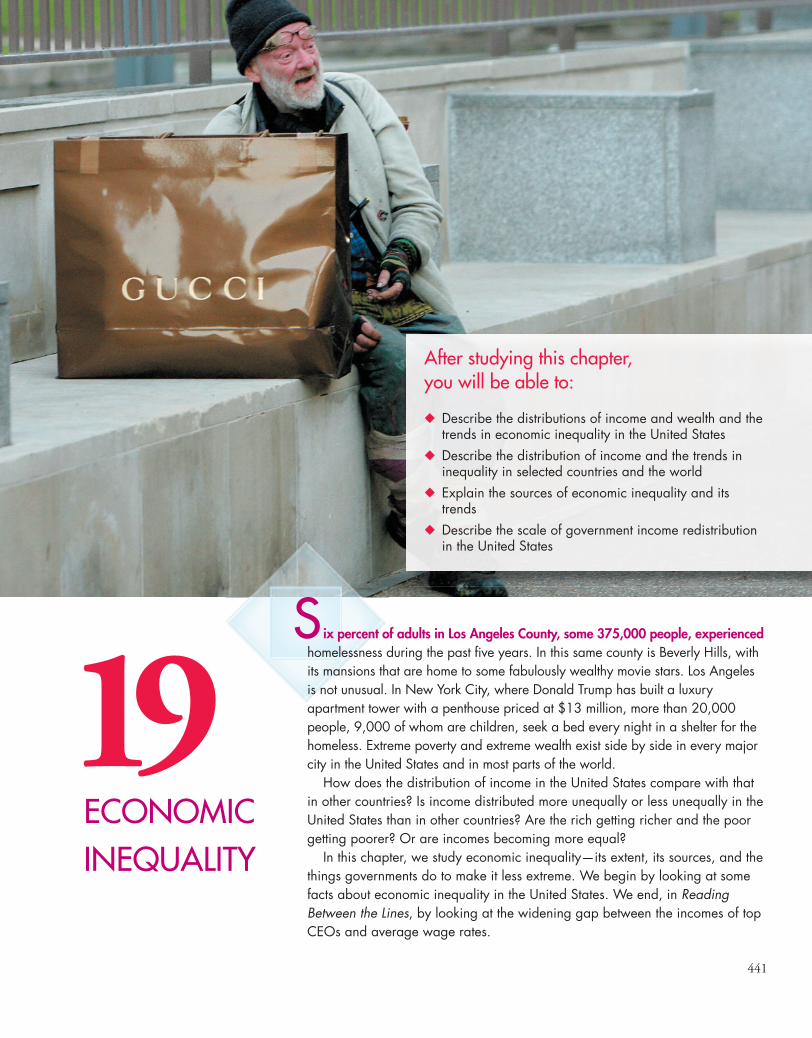
After studying this chapter, you will be able to:

� Describe the distributions of income and wealth and thetrends in economic inequality in the United States

� Describe the distribution of income and the trends ininequality in selected countries and the world

� Explain the sources of economic inequality and itstrends

� Describe the scale of government income redistributionin the United States

S ix percent of adults in Los Angeles County, some 375,000 people, experiencedhomelessness during the past five years. In this same county is Beverly Hills, withits mansions that are home to some fabulously wealthy movie stars. Los Angelesis not unusual. In New York City, where Donald Trump has built a luxuryapartment tower with a penthouse priced at $13 million, more than 20,000people, 9,000 of whom are children, seek a bed every night in a shelter for thehomeless. Extreme poverty and extreme wealth exist side by side in every majorcity in the United States and in most parts of the world.

How does the distribution of income in the United States compare with thatin other countries? Is income distributed more unequally or less unequally in theUnited States than in other countries? Are the rich getting richer and the poorgetting poorer? Or are incomes becoming more equal?

In this chapter, we study economic inequality—its extent, its sources, and thethings governments do to make it less extreme. We begin by looking at somefacts about economic inequality in the United States. We end, in ReadingBetween the Lines, by looking at the widening gap between the incomes of topCEOs and average wage rates.

ECONOMICINEQUALITY

19441

442 CHAPTER 19 Economic Inequality

◆ Economic Inequalityin the United States

The most commonly used measure of economicinequality is the distribution of annual income. TheCensus Bureau defines income as money income,which equals market income plus cash payments tohouseholds by government. Market income equalswages, interest, rent, and profit earned in factor mar-kets, before paying income taxes.

The Distribution of IncomeFigure 19.1 shows the distribution of annual incomeacross the 117.5 million households in the UnitedStates in 2009. Note that the x-axis measureshousehold income and the y-axis is percentage ofhouseholds.

The most common household income, called themode income, was received by the 6 percent of thehouseholds whose incomes fell between $20,000 and$25,000. The value of $22,000 marked on the figureis an estimate.

The middle level of household income in 2009,called the median income, was $49,777. Fifty percentof households have an income that exceeds themedian and fifty percent have an income below themedian.

The average household money income in 2009,called the mean income, was $67,976. This numberequals total household income, about $8 trillion,divided by the 117.5 million households.You can seein Fig. 19.1 that the mode is less than the medianand that the median is less than the mean. This fea-ture of the distribution of income tells us that thereare more households with low incomes than withhigh incomes. It also tells us that some of the highincomes are very high.

The income distribution in Fig. 19.1 is called apositively skewed distribution, which means that it hasa long tail of high values. This distribution contrastswith the bell that describes the distribution of peo-ple’s heights. In a bell-shaped distribution, the mean,median, and mode are all equal.

Another way of looking at the distribution ofincome is to measure the percentage of total incomereceived by each given percentage of households.Data are reported for five groups—called quintiles orfifth shares—each consisting of 20 percent of house-holds.

Figure 19.2 shows the distribution based on theseshares in 2009. The poorest 20 percent of householdsreceived 3.4 percent of total income; the secondpoorest 20 percent received 8.6 percent of totalincome; the middle 20 percent received 14.6 percentof total income; the next highest 20 percent received23.2 percent of total income; and the highest 20percent received 50.2 percent of total income.

The distribution of income in Fig. 19.1 and thequintile shares in Fig. 19.2 tell us that income is dis-tributed unequally. But we need a way of comparingthe distribution of income in different periods andusing different measures. A clever graphical toolcalled the Lorenz curve enables us to make such com-parisons.

Median (middle)income: $49,777

Mode (most common)income: $22,000

Perc

enta

ge o

f hou

seho

lds

Income (thousands of dollars per year)

Mean (average)income: $67,976

22 50 68 100 150 200 2500

7

6

5

4

3

2

1

The distribution of income is positively skewed. The mode(most common) income is less than the median (middle)income, which in turn is less than the mean (average)income. The distribution shown here ends at $250,000because data above that level are not available, but thedistribution goes up to several million dollars a year.

Source of data: U.S. Bureau of the Census, “Income, Poverty, and HealthInsurance Coverage in the United States: 2007,” Current PopulationReports, P-60-235, (Washington, DC: U.S. Government Printing Office,2008).

FIGURE 19.1 The Distribution of Income inthe United States in 2009

animation

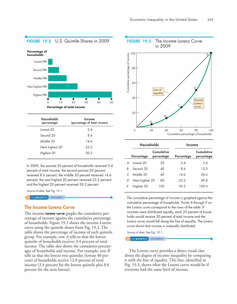
Economic Inequality in the United States 443

The Lorenz curve provides a direct visual clueabout the degree of income inequality by comparingit with the line of equality. This line, identified inFig. 19.3, shows what the Lorenz curve would be ifeveryone had the same level of income.

The Income Lorenz CurveThe income Lorenz curve graphs the cumulative per-centage of income against the cumulative percentageof households. Figure 19.3 shows the income Lorenzcurve using the quintile shares from Fig. 19.2. Thetable shows the percentage of income of each quintilegroup. For example, row A tells us that the lowestquintile of households receives 3.4 percent of totalincome. The table also shows the cumulative percent-ages of households and income. For example, row Btells us that the lowest two quintiles (lowest 40 per-cent) of households receive 12.0 percent of totalincome (3.4 percent for the lowest quintile plus 8.6percent for the next lowest).

Lowest fifth

Second fifth

Middle fifth

Next highest fifth

Highest fifth

0 10 20 30 40 50

Percentage of total income

Percentage ofhouseholds

In 2009, the poorest 20 percent of households received 3.4percent of total income; the second poorest 20 percentreceived 8.6 percent; the middle 20 percent received 14.6percent; the next highest 20 percent received 23.2 percent;and the highest 20 percent received 50.2 percent.

Source of data: See Fig. 19.1.

Households Income(percentage) (percentage of total income)

Lowest 20 3.4

Second 20 8.6

Middle 20 14.6

Next highest 20 23.2

Highest 20 50.2

Cumulative percentage of households

Cum

ulat

ive

perc

enta

ge o

f inc

ome

0

20

40

60

80

100

10080604020

A

B

C

D

E

IncomeLorenzcurve

Line ofequality

The cumulative percentage of income is graphed against thecumulative percentage of households. Points A through E onthe Lorenz curve correspond to the rows of the table. Ifincomes were distributed equally, each 20 percent of house-holds would receive 20 percent of total income and theLorenz curve would fall along the line of equality. The Lorenzcurve shows that income is unequally distributed.

Source of data: See Fig. 19.1.

Households Income

Cumulative CumulativePercentage percentage Percentage percentage

A Lowest 20 20 3.4 3.4

B Second 20 40 8.6 12.0

C Middle 20 60 14.6 26.6

D Next highest 20 80 23.2 49.8

E Highest 20 100 50.2 100.0

FIGURE 19.2 U.S. Quintile Shares in 2009

animation

animation

FIGURE 19.3 The Income Lorenz Curve in 2009

444 CHAPTER 19 Economic Inequality

Cumulative percentage of households

Cum

ulat

ive

perc

enta

ge o

f inc

ome

and

wea

lth0

20

40

60

80

100

10080604020

A

B

B'

C

C'

D

E '

D '

F '

G'

E

Income

Wealth

Line ofequality

A'

The cumulative percentage of wealth is graphed against thecumulative percentage of households. Points A' through G'on the Lorenz curve for wealth correspond to the rows of thetable. By comparing the Lorenz curves for income andwealth, we can see that wealth is distributed much moreunequally than is income.

Sources of data: For the income distribution data, see Fig. 19.1. The Wealth distribution data are from Edward N. Wolff, “RecentTrends in Wealth Ownership, 1938–1998,” Jerome Levy EconomicsInstitute Working Paper No. 300, April 2000.

Households Wealth

Cumulative CumulativePercentage percentage Percentage percentage

A' Lowest 40 40 0.2 0.2

B' Next 20 60 4.5 4.7

C' Next 20 80 11.9 16.6

D' Next 10 90 12.5 29.1

E' Next 5 95 11.5 40.6

F' Next 4 99 21.3 61.9

G' Highest 1 100 38.1 100.0

If income were distributed equally across all thehouseholds, each quintile would receive 20 percentof total income and the cumulative percentages ofincome received would equal the cumulative per-centages of households, so the Lorenz curve wouldbe the straight line labeled “Line of equality.”

The actual distribution of income shown by thecurve labeled “Income Lorenz curve” can be com-pared with the Line of equality. The closer theLorenz curve is to the line of equality, the moreequal is the distribution of income.

The Distribution of WealthThe distribution of wealth provides another way ofmeasuring economic inequality. A household’s wealth isthe value of the things that it owns at a point in time. Incontrast, income is the amount that the householdreceives over a given period of time.

Figure 19.4 shows the Lorenz curve for wealth inthe United States in 1998 (the most recent year forwhich we have wealth distribution data). The medianhousehold wealth in 1998 was $60,700. Wealth isextremely unequally distributed, and for this reason,the data are grouped by seven unequal groups ofhouseholds. The poorest 40 percent of householdsown only 0.2 percent of total wealth (row A' in thetable in Fig. 19.4). The richest 20 percent of house-holds own 83.4 percent of total wealth. Because thisgroup owns almost all the wealth, we need to breakthe group into smaller parts. That is what rows D'through G' do. The richest 1 percent of householdsin row G' own 38.1 percent of total wealth.

Figure 19.4 shows the income Lorenz curve (fromFig. 19.3) alongside the wealth Lorenz curve. You cansee that the Lorenz curve for wealth is much fartheraway from the line of equality than is the Lorenzcurve for income, which means that the distributionof wealth is much more unequal than the distributionof income.

Wealth or Income?We’ve seen that wealth is much more unequally dis-tributed than is income. Which distribution providesthe better description of the degree of inequality? Toanswer this question, we need to think about theconnection between wealth and income.

Wealth is a stock of assets, and income is theflow of earnings that results from the stock ofwealth. Suppose that a person owns assets worth

FIGURE 19.4 Lorenz Curves for Income andWealth

animation

Economic Inequality in the United States 445

$1 million—has a wealth of $1 million. If the rate ofreturn on assets is 5 percent a year, then this personreceives an income of $50,000 a year from thoseassets. We can describe this person’s economic condi-tion by using either the wealth of $1 million or theincome of $50,000. When the rate of return is 5 per-cent a year, $1 million of wealth equals $50,000 ofincome in perpetuity. Wealth and income are just dif-ferent ways of looking at the same thing.

But in Fig. 19.4, the distribution of wealth is moreunequal than the distribution of income. Why? It isbecause the wealth data do not include the value ofhuman capital, while the income data measureincome from all wealth, including human capital.

Think about Lee and Peter, two people with equalincome and equal wealth. Lee’s wealth is human capi-tal and his entire income is from employment. Peter’swealth is in the form of investments in stocks andbonds and his entire income is from these investments.

When a Census Bureau agent interviews Lee andPeter in a national income and wealth survey, theirincomes are recorded as being equal, but Lee’s wealthis recorded as zero, while Peter’s wealth is recorded asthe value of his investments. Peter looks vastly morewealthy than Lee in the survey data.

Because the national survey of wealth excludeshuman capital, the income distribution is a moreaccurate measure of economic inequality than thewealth distribution.

Annual or Lifetime Income and Wealth?A typical household’s income changes over its lifecycle. Income starts out low, grows to a peak when thehousehold’s workers reach retirement age, and thenfalls after retirement. Also, a typical household’s wealthchanges over time. Like income, it starts out low,grows to a peak at the point of retirement, and fallsafter retirement.

Think about three households with identical life-time incomes, one young, one middle-aged, and oneretired. The middle-aged household has the highestincome and wealth, the retired household has thelowest, and the young household falls in the middle.The distributions of annual income and wealth in agiven year are unequal, but the distributions of life-time income and wealth are equal.

The data on inequality share the bias that you’vejust seen. Inequality in annual income and wealthdata overstates lifetime inequality because householdsare at different stages in their life cycles.

Trends in InequalityTo see trends in the income distribution, we need ameasure that enables us to rank distributions on thescale of more equal and less equal. No perfect scaleexists, but one that is much used is called the Giniratio. The Gini ratio is based on the Lorenz curve andequals the ratio of the area between the line of equal-ity and the Lorenz curve to the entire area beneath theline of equality. The larger the Gini ratio, the greateris the degree of income inequality. If income is equallydistributed, the Lorenz curve is the same as the line ofequality, so the Gini ratio is zero. If one person has allthe income and everyone else has none, the Gini ratiois 1.

Figure 19.5 shows the U.S. Gini ratio from 1970to 2009. The figure shows breaks in the data in1992 and 2000 because in those years, the Census

Upward trendin inequality

1970 1980 1990 201020000.38

0.42

0.40

0.44

0.46

0.48

Year

Gin

i ratio

Changes indefinitionsbreak series

Measured by the Gini ratio, the distribution of income in theUnited States became more unequal from 1970 to 2009.The percentage of income earned by the richest householdsincreased through these years. Changes in definitions makethe numbers before and after 1992 and before and after2000 not comparable. Despite the breaks in the data, thetrends are still visible.

Source of data: See Fig. 19.1.

FIGURE 19.5 The U.S. Gini Ratio:1970–2009

animation

446 CHAPTER 19 Economic Inequality

Bureau changed its method of collecting the dataand definitions, so the numbers before and after thebreaks can’t be compared. Despite the breaks in theseries, the Gini ratio has clearly increased, whichmeans that on this measure, incomes have becomeless equal.

The major change is that the share of incomereceived by the richest households has increased. Youcan see in Economics in Action above how the incomeof the richest one percent has increased. No one knowsfor sure why this trend has occurred, but a possibilitythat we’ll explore in the next section is that technologi-cal change has increased the value of marginal productof high-skilled workers and decreased the value of mar-ginal product of low-skilled workers.

PovertyHouseholds at the low end of the income distribu-tion are so poor that they are considered to beliving in poverty. Poverty is a situation in which ahousehold’s income is too low to be able to buy thequantities of food, shelter, and clothing that aredeemed necessary. Poverty is a relative concept.Millions of people living in Africa and Asia surviveon incomes of less than $400 a year. In the UnitedStates, the poverty level is calculated each year bythe Social Security Administration. In 2009, thepoverty level for a four-person household was anincome of $21,756. In that year, 44 millionAmericans—14 percent of the population—lived in households that had incomes below the

Economics in ActionThe Rich Get Richer, but School Still PaysThe percentage of Americans who tell the Gallup pollthat wealth should be distributed more evenly hasbeen rising. In 2008, it reached 70 percent. A reasonmight be the trend in the incomes of the super rich.Emmanuel Saez, an economics professor at theUniversity of California, Berkeley, used tax returnsdata to get the numbers graphed in Fig. 1.

Year

Inco

me

of

top 1

per

cent

(per

centa

ge

of

tota

l inco

me)

6

9

18

12

15

20081928 1948 1968 1988

Globalization, theinformation revolution:rising inequality

World War IIand the "GreatCompression"

Figure 1 The Income Shares of the Top One Percent

Source of data: Adapted from Table II, “Income Inequality in the UnitedStates, 1913–1998” by Thomas Piketty and Emmanuel Saez. QuarterlyJournal of Economics, February 2003, Vol. 118, Issue 1. © The Presidentand Fellows of the Harvard College an MIT.

After decades of a falling share, starting in 1981,the share of income received by the richest one per-cent began a steady climb. By 2006 (the latest year inProfessor Saez’s database), the richest one percentwere earning 14.6 percent of the nation’s income.

Movie stars, sports stars, and the CEOs of large cor-porations are among the super rich. People whoscratch out a living doing seasonal work on farms earnthe lowest incomes. Aside from these extremes, whatare the characteristics of people who earn high incomesand people who earn low incomes? Figure 2 answersthis question. (The data are for 2009 but the pat-terns are persistent).

Education A postgraduate education is the main sourceof a high income. A person with a professional degree(such as a medical or law degree), earns (on average)$124,000—more than double the median income. Justcompleting high school raises a person’s income bymore than $14,000 a year; and getting a bachelor’sdegree adds another $36,000 a year. The averageincome of people who have not completed 9th grade is$22,000—less than half the median income.

Type of Household Married couples earn more, onthe average, than people who live alone. A marriedcouple earns about $72,000. In contrast, men wholive alone earn about $48,000, and women who livealone earn only $33,000.

Age of Householder Households with the oldest andyoungest householders have lower incomes than dothose with middle-aged householders. When the house-holder is aged between 45 and 54, household income

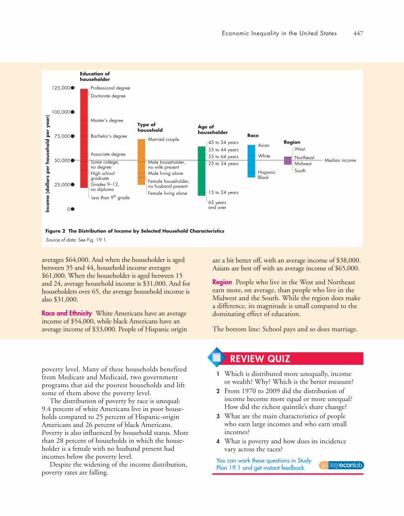
Economic Inequality in the United States 447

poverty level. Many of these households benefitedfrom Medicare and Medicaid, two governmentprograms that aid the poorest households and liftsome of them above the poverty level.

The distribution of poverty by race is unequal: 9.4 percent of white Americans live in poor house-holds compared to 25 percent of Hispanic-originAmericans and 26 percent of black Americans.Poverty is also influenced by household status. Morethan 28 percent of households in which the house-holder is a female with no husband present hadincomes below the poverty level.

Despite the widening of the income distribution,poverty rates are falling.

Some college, no degree

Education ofhouseholder

Figure 2 The Distribution of Income by Selected Household Characteristics

Type ofhousehold

Age ofhouseholder

RaceRegion

Median income

0

25,000

50,000

75,000

125,000

Inco

me

(dolla

rs p

er h

ouse

hold

per

yea

r)

100,000

Less than 9th grade

High schoolgraduateGrades 9–12,no diploma

Some college,no degree

Bachelor's degree

Associate degree

Master's degree

Professional degree

Doctorate degree

Married couple

Male living alone

Female householder,no husband presentFemale living alone

65 yearsand over

15 to 24 years

45 to 54 years35 to 44 years55 to 64 years25 to 34 years

Black

Asian

White

Hispanic

Midwest

West

Northeast

SouthSouthSouth

Male householder,no wife presentMale householder,no wife present

averages $64,000. And when the householder is agedbetween 35 and 44, household income averages$61,000. When the householder is aged between 15and 24, average household income is $31,000. And forhouseholders over 65, the average household income isalso $31,000.

Race and Ethnicity White Americans have an averageincome of $54,000, while black Americans have anaverage income of $33,000. People of Hispanic origin

are a bit better off, with an average income of $38,000.Asians are best off with an average income of $65,000.

Region People who live in the West and Northeastearn more, on average, than people who live in theMidwest and the South. While the region does makea difference, its magnitude is small compared to thedominating effect of education.

The bottom line: School pays and so does marriage.

Source of data: See Fig. 19.1.

REVIEW QUIZ1 Which is distributed more unequally, income

or wealth? Why? Which is the better measure?2 From 1970 to 2009 did the distribution of

income become more equal or more unequal?How did the richest quintile’s share change?

3 What are the main characteristics of peoplewho earn large incomes and who earn smallincomes?

4 What is poverty and how does its incidencevary across the races?

You can work these questions in Study Plan 19.1 and get instant feedback.

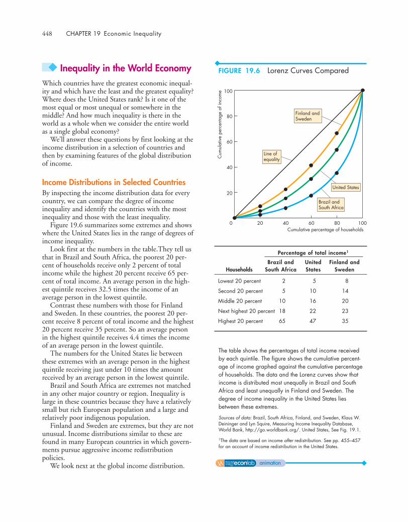
448 CHAPTER 19 Economic Inequality

◆ Inequality in the World EconomyWhich countries have the greatest economic inequal-ity and which have the least and the greatest equality?Where does the United States rank? Is it one of themost equal or most unequal or somewhere in themiddle? And how much inequality is there in theworld as a whole when we consider the entire worldas a single global economy?

We’ll answer these questions by first looking at theincome distribution in a selection of countries andthen by examining features of the global distributionof income.

Income Distributions in Selected CountriesBy inspecting the income distribution data for everycountry, we can compare the degree of incomeinequality and identify the countries with the mostinequality and those with the least inequality.

Figure 19.6 summarizes some extremes and showswhere the United States lies in the range of degrees ofincome inequality.

Look first at the numbers in the table.They tell usthat in Brazil and South Africa, the poorest 20 per-cent of households receive only 2 percent of totalincome while the highest 20 percent receive 65 per-cent of total income. An average person in the high-est quintile receives 32.5 times the income of anaverage person in the lowest quintile.

Contrast these numbers with those for Finlandand Sweden. In these countries, the poorest 20 per-cent receive 8 percent of total income and the highest20 percent receive 35 percent. So an average personin the highest quintile receives 4.4 times the incomeof an average person in the lowest quintile.

The numbers for the United States lie betweenthese extremes with an average person in the highestquintile receiving just under 10 times the amountreceived by an average person in the lowest quintile.

Brazil and South Africa are extremes not matchedin any other major country or region. Inequality islarge in these countries because they have a relativelysmall but rich European population and a large andrelatively poor indigenous population.

Finland and Sweden are extremes, but they are notunusual. Income distributions similar to these arefound in many European countries in which govern-ments pursue aggressive income redistributionpolicies.

We look next at the global income distribution.

Cumulative percentage of households

Cum

ulat

ive

perc

enta

ge o

f inc

ome

0

20

40

60

80

100

10080604020

Finland andSweden

United States

Brazil andSouth Africa

Line ofequality

The table shows the percentages of total income receivedby each quintile. The figure shows the cumulative percent-age of income graphed against the cumulative percentageof households. The data and the Lorenz curves show thatincome is distributed most unequally in Brazil and SouthAfrica and least unequally in Finland and Sweden. Thedegree of income inequality in the United States liesbetween these extremes.

Sources of data: Brazil, South Africa, Finland, and Sweden, Klaus W.Deininger and Lyn Squire, Measuring Income Inequality Database,World Bank, http://go.worldbank.org/. United States, See Fig. 19.1.

1The data are based on income after redistribution. See pp. 455–457for an account of income redistribution in the United States.

Percentage of total income1

Brazil and United Finland andHouseholds South Africa States Sweden

Lowest 20 percent 2 5 8

Second 20 percent 5 10 14

Middle 20 percent 10 16 20

Next highest 20 percent 18 22 23

Highest 20 percent 65 47 35

FIGURE 19.6 Lorenz Curves Compared

animation

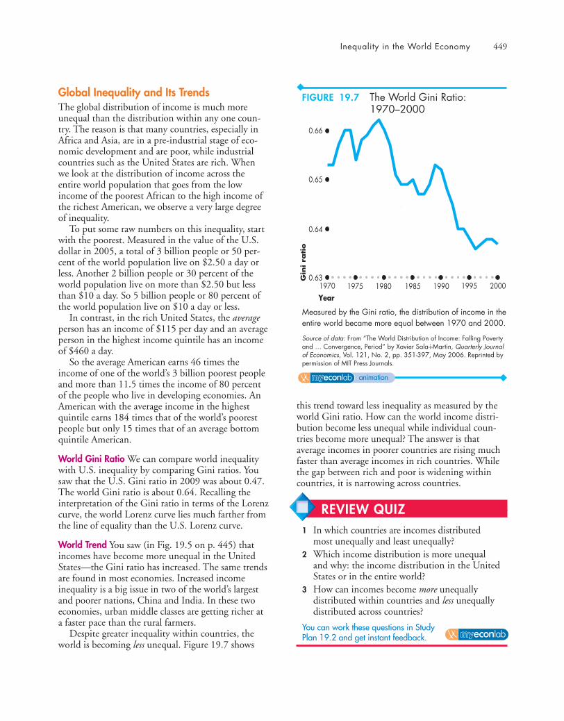
Inequality in the World Economy 449

Global Inequality and Its TrendsThe global distribution of income is much moreunequal than the distribution within any one coun-try. The reason is that many countries, especially inAfrica and Asia, are in a pre-industrial stage of eco-nomic development and are poor, while industrialcountries such as the United States are rich. When we look at the distribution of income across theentire world population that goes from the lowincome of the poorest African to the high income ofthe richest American, we observe a very large degreeof inequality.

To put some raw numbers on this inequality, startwith the poorest. Measured in the value of the U.S.dollar in 2005, a total of 3 billion people or 50 per-cent of the world population live on $2.50 a day orless. Another 2 billion people or 30 percent of theworld population live on more than $2.50 but lessthan $10 a day. So 5 billion people or 80 percent ofthe world population live on $10 a day or less.

In contrast, in the rich United States, the averageperson has an income of $115 per day and an averageperson in the highest income quintile has an incomeof $460 a day.

So the average American earns 46 times theincome of one of the world’s 3 billion poorest peopleand more than 11.5 times the income of 80 percentof the people who live in developing economies. AnAmerican with the average income in the highestquintile earns 184 times that of the world’s poorestpeople but only 15 times that of an average bottomquintile American.

World Gini Ratio We can compare world inequalitywith U.S. inequality by comparing Gini ratios. Yousaw that the U.S. Gini ratio in 2009 was about 0.47.The world Gini ratio is about 0.64. Recalling theinterpretation of the Gini ratio in terms of the Lorenzcurve, the world Lorenz curve lies much farther fromthe line of equality than the U.S. Lorenz curve.

World Trend You saw (in Fig. 19.5 on p. 445) thatincomes have become more unequal in the UnitedStates—the Gini ratio has increased. The same trendsare found in most economies. Increased incomeinequality is a big issue in two of the world’s largestand poorer nations, China and India. In these twoeconomies, urban middle classes are getting richer ata faster pace than the rural farmers.

Despite greater inequality within countries, theworld is becoming less unequal. Figure 19.7 shows

this trend toward less inequality as measured by theworld Gini ratio. How can the world income distri-bution become less unequal while individual coun-tries become more unequal? The answer is thataverage incomes in poorer countries are rising muchfaster than average incomes in rich countries. Whilethe gap between rich and poor is widening withincountries, it is narrowing across countries.

Measured by the Gini ratio, the distribution of income in theentire world became more equal between 1970 and 2000.

Source of data: From “The World Distribution of Income: Falling Povertyand … Convergence, Period” by Xavier Sala-i-Martin, Quarterly Journalof Economics, Vol. 121, No. 2, pp. 351-397, May 2006. Reprinted bypermission of MIT Press Journals.

1970 1975 1980 1985 1990 200019950.63

0.65

0.64

0.66

YearG

ini ra

tio

FIGURE 19.7 The World Gini Ratio:1970–2000

animation

REVIEW QUIZ 1 In which countries are incomes distributed

most unequally and least unequally?2 Which income distribution is more unequal

and why: the income distribution in the UnitedStates or in the entire world?

3 How can incomes become more unequallydistributed within countries and less unequallydistributed across countries?

You can work these questions in Study Plan 19.2 and get instant feedback.

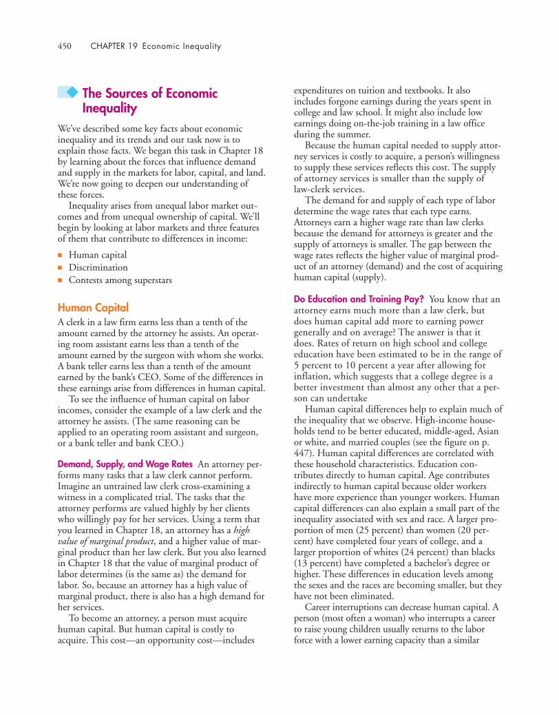
450 CHAPTER 19 Economic Inequality

◆ The Sources of EconomicInequality

We’ve described some key facts about economicinequality and its trends and our task now is toexplain those facts. We began this task in Chapter 18by learning about the forces that influence demandand supply in the markets for labor, capital, and land.We’re now going to deepen our understanding ofthese forces.

Inequality arises from unequal labor market out-comes and from unequal ownership of capital. We’llbegin by looking at labor markets and three featuresof them that contribute to differences in income:

■ Human capital■ Discrimination■ Contests among superstars

Human CapitalA clerk in a law firm earns less than a tenth of theamount earned by the attorney he assists. An operat-ing room assistant earns less than a tenth of theamount earned by the surgeon with whom she works.A bank teller earns less than a tenth of the amountearned by the bank’s CEO. Some of the differences inthese earnings arise from differences in human capital.

To see the influence of human capital on laborincomes, consider the example of a law clerk and theattorney he assists. (The same reasoning can beapplied to an operating room assistant and surgeon,or a bank teller and bank CEO.)

Demand, Supply, and Wage Rates An attorney per-forms many tasks that a law clerk cannot perform.Imagine an untrained law clerk cross-examining awitness in a complicated trial. The tasks that theattorney performs are valued highly by her clientswho willingly pay for her services. Using a term thatyou learned in Chapter 18, an attorney has a highvalue of marginal product, and a higher value of mar-ginal product than her law clerk. But you also learnedin Chapter 18 that the value of marginal product oflabor determines (is the same as) the demand forlabor. So, because an attorney has a high value ofmarginal product, there is also has a high demand forher services.

To become an attorney, a person must acquirehuman capital. But human capital is costly toacquire. This cost—an opportunity cost—includes

expenditures on tuition and textbooks. It alsoincludes forgone earnings during the years spent incollege and law school. It might also include lowearnings doing on-the-job training in a law officeduring the summer.

Because the human capital needed to supply attor-ney services is costly to acquire, a person’s willingnessto supply these services reflects this cost. The supplyof attorney services is smaller than the supply oflaw-clerk services.

The demand for and supply of each type of labordetermine the wage rates that each type earns.Attorneys earn a higher wage rate than law clerksbecause the demand for attorneys is greater and thesupply of attorneys is smaller. The gap between thewage rates reflects the higher value of marginal prod-uct of an attorney (demand) and the cost of acquiringhuman capital (supply).

Do Education and Training Pay? You know that anattorney earns much more than a law clerk, butdoes human capital add more to earning powergenerally and on average? The answer is that itdoes. Rates of return on high school and collegeeducation have been estimated to be in the range of5 percent to 10 percent a year after allowing forinflation, which suggests that a college degree is abetter investment than almost any other that a per-son can undertake

Human capital differences help to explain much ofthe inequality that we observe. High-income house-holds tend to be better educated, middle-aged, Asianor white, and married couples (see the figure on p.447). Human capital differences are correlated withthese household characteristics. Education con-tributes directly to human capital. Age contributesindirectly to human capital because older workershave more experience than younger workers. Humancapital differences can also explain a small part of theinequality associated with sex and race. A larger pro-portion of men (25 percent) than women (20 per-cent) have completed four years of college, and alarger proportion of whites (24 percent) than blacks(13 percent) have completed a bachelor’s degree orhigher. These differences in education levels amongthe sexes and the races are becoming smaller, but theyhave not been eliminated.

Career interruptions can decrease human capital. Aperson (most often a woman) who interrupts a careerto raise young children usually returns to the laborforce with a lower earning capacity than a similar

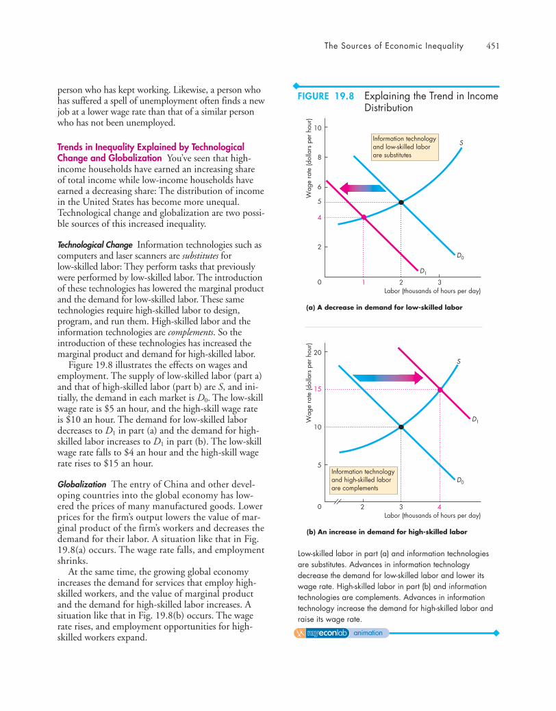
The Sources of Economic Inequality 451

person who has kept working. Likewise, a person whohas suffered a spell of unemployment often finds a newjob at a lower wage rate than that of a similar personwho has not been unemployed.

Trends in Inequality Explained by TechnologicalChange and Globalization You’ve seen that high-income households have earned an increasing shareof total income while low-income households haveearned a decreasing share: The distribution of incomein the United States has become more unequal.Technological change and globalization are two possi-ble sources of this increased inequality.

Technological Change Information technologies such ascomputers and laser scanners are substitutes forlow-skilled labor: They perform tasks that previouslywere performed by low-skilled labor. The introductionof these technologies has lowered the marginal productand the demand for low-skilled labor. These sametechnologies require high-skilled labor to design, program, and run them. High-skilled labor and theinformation technologies are complements. So theintroduction of these technologies has increased themarginal product and demand for high-skilled labor.

Figure 19.8 illustrates the effects on wages andemployment. The supply of low-skilled labor (part a)and that of high-skilled labor (part b) are S, and ini-tially, the demand in each market is D0. The low-skillwage rate is $5 an hour, and the high-skill wage rateis $10 an hour. The demand for low-skilled labordecreases to D1 in part (a) and the demand for high-skilled labor increases to D1 in part (b). The low-skillwage rate falls to $4 an hour and the high-skill wagerate rises to $15 an hour.

Globalization The entry of China and other devel-oping countries into the global economy has low-ered the prices of many manufactured goods. Lowerprices for the firm’s output lowers the value of mar-ginal product of the firm’s workers and decreases thedemand for their labor. A situation like that in Fig.19.8(a) occurs. The wage rate falls, and employmentshrinks.

At the same time, the growing global economyincreases the demand for services that employ high-skilled workers, and the value of marginal productand the demand for high-skilled labor increases. Asituation like that in Fig. 19.8(b) occurs. The wagerate rises, and employment opportunities for high-skilled workers expand.

Wag

e ra

te (d

olla

rs p

er h

our)

Labor (thousands of hours per day)0

10

8

6

5

2

4

1 2 3

D0

S

D1

(a) A decrease in demand for low-skilled labor

Information technologyand low-skilled laborare substitutes

(b) An increase in demand for high-skilled labor

Wag

e ra

te (d

olla

rs p

er h

our)

Labor (thousands of hours per day)0

20

10

5

15

432

D0

S

D1

Information technologyand high-skilled laborare complements

Low-skilled labor in part (a) and information technologiesare substitutes. Advances in information technologydecrease the demand for low-skilled labor and lower itswage rate. High-skilled labor in part (b) and informationtechnologies are complements. Advances in informationtechnology increase the demand for high-skilled labor andraise its wage rate.

FIGURE 19.8 Explaining the Trend in IncomeDistribution

animation

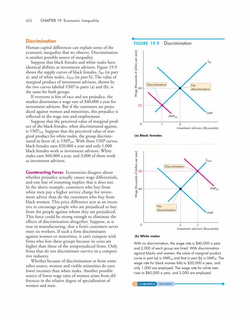
452 CHAPTER 19 Economic Inequality

DiscriminationHuman capital differences can explain some of theeconomic inequality that we observe. Discriminationis another possible source of inequality.

Suppose that black females and white males haveidentical abilities as investment advisors. Figure 19.9shows the supply curves of black females, SBF (in parta), and of white males, SWM (in part b). The value ofmarginal product of investment advisors, shown bythe two curves labeled VMP in parts (a) and (b), isthe same for both groups.

If everyone is free of race and sex prejudice, themarket determines a wage rate of $40,000 a year forinvestment advisors. But if the customers are preju-diced against women and minorities, this prejudice isreflected in the wage rate and employment.

Suppose that the perceived value of marginal prod-uct of the black females, when discriminated against,is VMPDA. Suppose that the perceived value of mar-ginal product for white males, the group discrimi-nated in favor of, is VMPDF. With these VMP curves,black females earn $20,000 a year and only 1,000black females work as investment advisors. Whitemales earn $60,000 a year, and 3,000 of them workas investment advisors.

Counteracting Forces Economists disagree aboutwhether prejudice actually causes wage differentials,and one line of reasoning implies that it does not.In the above example, customers who buy fromwhite men pay a higher service charge for invest-ment advice than do the customers who buy fromblack women. This price difference acts as an incen-tive to encourage people who are prejudiced to buyfrom the people against whom they are prejudiced.This force could be strong enough to eliminate theeffects of discrimination altogether. Suppose, as istrue in manufacturing, that a firm’s customers nevermeet its workers. If such a firm discriminatesagainst women or minorities, it can’t compete withfirms who hire these groups because its costs arehigher than those of the nonprejudiced firms. Onlyfirms that do not discriminate survive in a competi-tive industry.

Whether because of discrimination or from someother source, women and visible minorities do earnlower incomes than white males. Another possiblesource of lower wage rates of women arises from dif-ferences in the relative degree of specialization ofwomen and men.

Wag

e (th

ousa

nds

of d

olla

rs p

er y

ear)

Investment advisors (thousands)0

40

20

1 2

SBF

VMPVMPDA

(a) Black femalesW

age

(thou

sand

s of

dol

lars

per

yea

r)

Investment advisors (thousands)0

40

60

32

SWM

VMP

Nodiscrimination

VMPDF

Discrimination

Nodiscrimination

Discrimination

(b) White males

With no discrimination, the wage rate is $40,000 a yearand 2,000 of each group are hired. With discriminationagainst blacks and women, the value of marginal productcurve in part (a) is VMPDA and that in part (b) is VMPDF. Thewage rate for black women falls to $20,000 a year, andonly 1,000 are employed. The wage rate for white menrises to $60,000 a year, and 3,000 are employed.

FIGURE 19.9 Discrimination

animation

The Sources of Economic Inequality 453

Differences in the Degree of Specialization Couplesmust choose how to allocate their time betweenworking for a wage and doing jobs in the home, suchas cooking, cleaning, shopping, organizing vacations,and, most important, bearing and raising children.Let’s look at the choices of Bob and Sue.

Bob might specialize in earning an income andSue in taking care of the home. Or Sue might special-ize in earning an income and Bob in taking care ofthe home. Or both of them might earn an incomeand share home production jobs.

The allocation they choose depends on their pref-erences and on their earning potential. The choice ofan increasing number of households is for each per-son to diversify between earning an income anddoing some household chores. But in most house-holds, Bob will specialize in earning an income andSue will both earn an income and bear a larger shareof the task of running the home. With this alloca-tion, Bob will probably earn more than Sue. If Suedevotes time and effort to ensuring Bob’s mental andphysical well-being, the quality of Bob’s market laborwill be higher than it would be if he were diversified.If the roles were reversed, Sue would be able to sup-ply market labor that earns more than Bob’s.

To test whether the degree of specializationaccounts for earnings differences between the sexes,economists have compared the incomes of never-married men and women. They have found that, onthe average, with equal amounts of human capital,the wages of these two groups are the same.

Contests Among SuperstarsThe differences in income that arise from differencesin human capital are important and affect a largeproportion of the population. But human capital dif-ferences can’t account for some of the really largeincome differences.

The super rich—those in the top one percent ofthe income distribution whose income share has beenrising—earn vastly more than can be explained byhuman capital differences. What makes a personsuper rich?

A clue to the answer is provided by thinking aboutthe super rich in tennis and golf. What makes tennisplayers and golfers special is that their earningsdepend on where they finish in a tournament. WhenSerena Williams won the Wimbledon Championshipin 2010, she received £1,000,000 or $1,540,000. Therunner-up in this event, Russian Vera Zvonareva,

received £500,000. So Serena earned double theamount earned by Vera. And she earned 88 times theamount received by the players who lost in the firstround of the tournament.

It is true that Serena Williams has a lot of humancapital. She practices hard and long and is a remark-able athlete. But anyone who is good enough to getinto a tennis Grand Slam tournament is similarlywell equipped with human capital and has spent asimilar number of long hours in training and prac-tice. It isn’t human capital that explains the differ-ences in earnings. It is the tournament and the prizedifferences that accounts for the large differences inearnings.

But three questions jump out: First, why do wereward superstar tennis players (and golfers) withprizes for winning a contest? Second, why are theprizes so different? And third, do the principles thatapply on the tennis court (and golf course) applymore generally?

Why Prizes for a Contest? The answer to this ques-tion (which was noted in Chapter 5, see p. 106) isthat contests with prizes do a good job of allocatingscarce resources efficiently when the efforts of theparticipants are hard to monitor and reward directly.There is only one winner, but many people workhard in an attempt to be that person. So a great dealof diligent effort is induced by a contest.

Why Are Prizes So Different? The prizes need to besubstantially different to induce enough effort. If thewinner received 10 percent more than the runner up,the gain from being the winner would be insufficientto encourage anyone to work hard enough. Someonewould win but no one would put in much effort.Tennis matches would be boring, golf scores wouldbe high, and no one would be willing to pay to seethese sports. Big differences are necessary to induce abig enough effort to generate the quality of perform-ance that people are willing to pay to see.

Does the Principle Apply More Generally? Winner-takes-all isn’t confined to tennis and golf. Moviestars, superstars in baseball, basketball, football, andice hockey, and top corporate executives can all beviewed as participants in contests that decide thewinners. The prize for the winner is an income atleast double that of the runner up and many multi-ples of the incomes of those who drop out earlier inthe tournament.

454 CHAPTER 19 Economic Inequality

Do Contests Among Superstars Explain the Trend?Contests among superstars can explain large differ-ences in incomes. But can contests explain the trendtoward greater inequality with an increasing share oftotal income going to the super rich as shown on p. 445?

An idea first suggested by University of Chicagoeconomist Sherwin Rosen suggests that a winner-takes-all contest can explain the trend. The key isthat globalization has increased the market reach ofthe winner and increased the spread between thewinner and the runners-up.

Global television audiences now watch all theworld’s major sporting events and the total revenuegenerated by advertising spots during these events hasincreased. Competition among networks and cableand satellite television distributors has increased thefees that event organizers receive. And to attract thetop star performers, prize money has increased andthe winner gets the biggest share of the prize pot.

So the prizes in sports have become bigger and theshare of income going to the “winner” has increased.

A similar story can be told about superstars andthe super rich in business. As the cost of doing busi-ness on a global scale has fallen, more and more busi-nesses have become global in their reach. Not onlyare large multinational corporations sourcing theirinputs from far afield and selling in every country,they are also recruiting their top executives from aglobal talent pool. With a larger source of talent, anda larger total revenue, firms must make the“prize”—the reward for the top job—more attractiveto compete for the best managers.

We’ve examined some sources of inequality in thelabor market. Let’s now look at the way inequalityarises from unequal ownership of capital.

Unequal WealthYou’ve seen that wealth inequality—excluding humancapital—is much greater than income inequality.This greater wealth inequality arises from twosources: life-cycle saving patterns and transfers ofwealth from one generation to the next.

Life-Cycle Saving Patterns Over a family’s life cycle,wealth starts out at zero or perhaps less than zero. Astudent who has financed education all the waythrough graduate school might have lots of humancapital and an outstanding student loan of $60,000.This person has negative wealth. Gradually loans get

paid off and a retirement fund is accumulated. At thepoint of retiring from full-time work, the family hasmaximum wealth. Then, during its retirement years,the family spends its wealth. This life-cycle patternmeans that much of the wealth is owned by people intheir sixties.

Intergenerational Transfers Some households inheritwealth from the previous generation. Some save morethan enough on which to live during retirement andtransfer wealth to the next generation. But theseintergenerational transfers of wealth do not alwaysincrease wealth inequality. If a generation that has ahigh income saves a large part of that income andleaves wealth to a succeeding generation that has alower income, this transfer decreases the degree ofinequality. But one feature of intergenerational trans-fers of wealth leads to increased inequality: wealthconcentration through marriage.

Marriage and Wealth Concentration People tend tomarry within their own socioeconomic class—a phe-nomenon called assortative mating. In everyday lan-guage, “like attracts like.” Although there is a gooddeal of folklore that “opposites attract,” perhaps suchCinderella tales appeal to us because they are so rarein reality. Wealthy people seek wealthy partners.

Because of assortative mating, wealth becomesmore concentrated in a small number of families andthe distribution of wealth becomes more unequal.

Next, we’re going to see how taxes and govern-ment programs redistribute income and decrease thedegree of economic inequality.

REVIEW QUIZ 1 What role does human capital play in account-

ing for income inequality?2 What role might discrimination play in

accounting for income inequality?3 What role might contests among superstars play

in accounting for income inequality?4 How might technological change and globaliza-

tion explain trends in the distribution of income?5 Does inherited wealth make the distribution of

income less equal or more equal?

You can work these questions in Study Plan 19.3 and get instant feedback.

Income Redistribution 455

◆ Income RedistributionThe three main ways in which governments in theUnited States redistribute income are

■ Income taxes■ Income maintenance programs■ Subsidized services

Income TaxesIncome taxes may be progressive, regressive, or pro-portional. A progressive income tax is one that taxesincome at an average rate that increases as incomeincreases. A regressive income tax is one that taxesincome at an average rate that decreases as incomeincreases. A proportional income tax (also called a flat-rate income tax) is one that taxes income at a constantaverage rate, regardless of the level of income.

The income tax rates that apply in the UnitedStates are composed of two parts: federal and statetaxes. Some cities, such as New York City, also havean income tax. There is variety in the detailed taxarrangements in the individual states, but the taxsystem, at both the federal and state levels, is pro-gressive. The poorest working households receivemoney from the government through an earnedincome tax credit. Successively higher-incomehouseholds pay 10 percent, 15 percent, 25 percent,28 percent, 33 percent, and 35 percent of eachadditional dollar earned.

Income Maintenance ProgramsThree main types of programs redistribute income bymaking direct payments (in cash, services, or vouch-ers) to people in the lower part of the income distri-bution. They are

■ Social Security programs■ Unemployment compensation■ Welfare programs

Social Security Programs The main Social Securityprogram is OASDHI—Old Age, Survivors, Disability,and Health Insurance. Monthly cash payments toretired or disabled workers or their surviving spousesand children are paid for by compulsory payroll taxes on both employers and employees. In 2010,total Social Security expenditure was budgeted at

$736 billion, and the standard monthly SocialSecurity check for a married couple was a bit morethan $1,892 in 2010.

The other component of Social Security isMedicare, which provides hospital and health insur-ance for the elderly and disabled.

Unemployment Compensation To provide an incometo unemployed workers, every state has established anunemployment compensation program. Under theseprograms, a tax is paid that is based on the income ofeach covered worker and such a worker receives a ben-efit when he or she becomes unemployed. The detailsof the benefits vary from state to state.

Welfare Programs The purpose of welfare is to pro-vide incomes for people who do not qualify for SocialSecurity or unemployment compensation. They are

1. Supplementary Security Income (SSI) program,designed to help the neediest elderly, disabled,and blind people

2. Temporary Assistance for Needy Households(TANF) program, designed to help householdsthat have inadequate financial resources

3. Food Stamp program, designed to help the poor-est households obtain a basic diet

4. Medicaid, designed to cover the costs of medicalcare for households receiving help under the SSIand TANF programs

Subsidized ServicesA great deal of redistribution takes place in the UnitedStates through the provision of subsidized services—services provided by the government at prices belowthe cost of production. The taxpayers who consumethese goods and services receive a transfer in kindfrom the taxpayers who do not consume them. Thetwo most important areas in which this form of redis-tribution takes place are health care and education—both kindergarten through grade 12 and college anduniversity.

In 2010–2011, students enrolled in the Universityof California system paid annual tuition fees of$10,781. The cost of providing a year’s education atthe University of California was probably about$22,000. So households with a member enrolled inone of these institutions received a benefit from thegovernment of more than $11,000 a year.

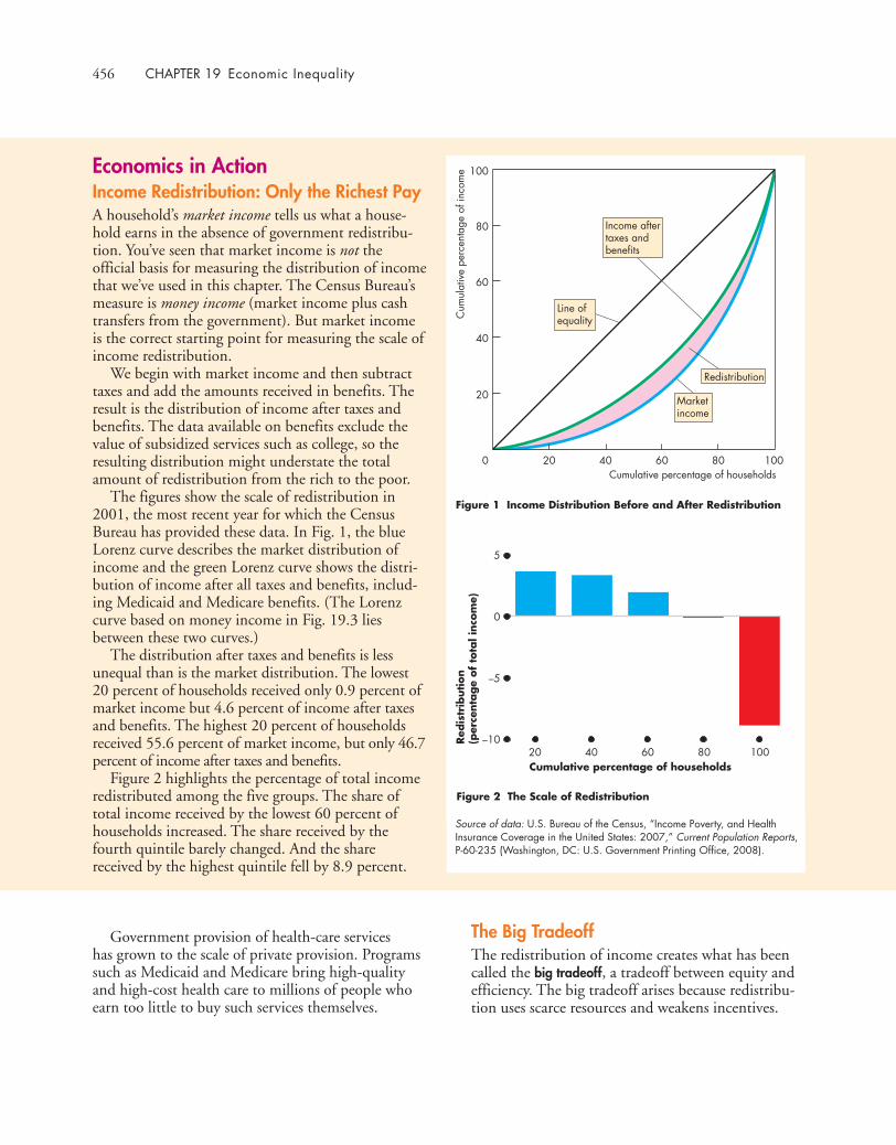
456 CHAPTER 19 Economic Inequality

Government provision of health-care serviceshas grown to the scale of private provision. Programssuch as Medicaid and Medicare bring high-qualityand high-cost health care to millions of people whoearn too little to buy such services themselves.

Figure 1 Income Distribution Before and After Redistribution

Figure 2 The Scale of Redistribution

Cumulative percentage of households

Cum

ulat

ive

perc

enta

ge o

f inc

ome

0

20

40

60

80

100

10080604020

10080604020–10

–5

0

5

Income aftertaxes andbenefits

Marketincome

Redistribution

Line ofequality

Cumulative percentage of households

Red

istr

ibution

(per

centa

ge

of

tota

l inco

me)

Source of data: U.S. Bureau of the Census, “Income Poverty, and HealthInsurance Coverage in the United States: 2007,” Current Population Reports,P-60-235 (Washington, DC: U.S. Government Printing Office, 2008).

Economics in ActionIncome Redistribution: Only the Richest PayA household’s market income tells us what a house-hold earns in the absence of government redistribu-tion. You’ve seen that market income is not theofficial basis for measuring the distribution of incomethat we’ve used in this chapter. The Census Bureau’smeasure is money income (market income plus cashtransfers from the government). But market incomeis the correct starting point for measuring the scale ofincome redistribution.

We begin with market income and then subtracttaxes and add the amounts received in benefits. Theresult is the distribution of income after taxes andbenefits. The data available on benefits exclude thevalue of subsidized services such as college, so theresulting distribution might understate the totalamount of redistribution from the rich to the poor.

The figures show the scale of redistribution in2001, the most recent year for which the CensusBureau has provided these data. In Fig. 1, the blueLorenz curve describes the market distribution ofincome and the green Lorenz curve shows the distri-bution of income after all taxes and benefits, includ-ing Medicaid and Medicare benefits. (The Lorenzcurve based on money income in Fig. 19.3 liesbetween these two curves.)

The distribution after taxes and benefits is lessunequal than is the market distribution. The lowest20 percent of households received only 0.9 percent ofmarket income but 4.6 percent of income after taxesand benefits. The highest 20 percent of householdsreceived 55.6 percent of market income, but only 46.7percent of income after taxes and benefits.

Figure 2 highlights the percentage of total incomeredistributed among the five groups. The share oftotal income received by the lowest 60 percent ofhouseholds increased. The share received by thefourth quintile barely changed. And the sharereceived by the highest quintile fell by 8.9 percent.

The Big TradeoffThe redistribution of income creates what has beencalled the big tradeoff, a tradeoff between equity andefficiency. The big tradeoff arises because redistribu-tion uses scarce resources and weakens incentives.

Income Redistribution 457

◆ We’ve examined economic inequality in theUnited States. We’ve seen how inequality arises andthat inequality has been increasing. Reading Betweenthe Lines on pp. 458–459 looks at the increasinginequality that began during the early 1980s andcontinues today.

The next chapter focuses on some problems forthe market economy that arise from uncertainty andincomplete information. But unlike the cases westudied in Chapters 16 and 17, this time the marketdoes a good job of coping with the problems.

A dollar collected from a rich person does nottranslate into a dollar received by a poor person.Some of it gets used up in the process of redistribu-tion. Tax-collecting agencies such as the InternalRevenue Service and welfare-administering agen-cies (as well as tax accountants and lawyers) useskilled labor, computers, and other scarce resourcesto do their work. The bigger the scale of redistribu-tion, the greater is the opportunity cost of adminis-tering it.

But the cost of collecting taxes and making welfarepayments is a small part of the total cost of redistri-bution. A bigger cost arises from the inefficiency(deadweight loss) of taxes and benefits. Greater equal-ity can be achieved only by taxing productive activi-ties such as work and saving. Taxing people’s incomefrom their work and saving lowers the after-taxincome they receive. This lower after-tax incomemakes them work and save less, which in turn resultsin smaller output and less consumption not only forthe rich who pay the taxes but also for the poor whoreceive the benefits.

It is not only taxpayers who face weaker incentivesto work. Benefit recipients also face weaker incen-tives. In fact, under the welfare arrangements thatprevailed before the 1996 reforms, the weakest incen-tives to work were those faced by households thatbenefited from welfare. When a welfare recipient gota job, benefits were withdrawn and eligibility for pro-grams such as Medicaid ended, so the household ineffect paid a tax of more than 100 percent on itsearnings. This arrangement locked poor householdsin a welfare trap.

So the agencies that determine the scale and meth-ods of income redistribution must pay close attentionto the incentive effects of taxes and benefits. Let’sclose this chapter by looking at one way in whichlawmakers are tackling the big tradeoff today.

A Major Welfare Challenge Young women who havenot completed high school, have a child (or chil-dren), live without a partner, and more likely areblack or Hispanic are among the poorest people inthe United States today. They and their childrenpresent a major welfare challenge.

First, their numbers are large. In 2009, there were14 million single-mother families. This number is 12percent of families. In 1997 (the most recent yearwith census data), single mothers were owed $26 bil-lion in child support. Of this amount, $10 billion was

not paid and 30 percent of the women received nosupport from their children’s fathers.

The long-term solution to the problem thesewomen face is education and job training—acquiringhuman capital. The short-term solutions are enforc-ing child support payments by absent fathers and for-mer spouses and providing welfare.

Welfare must be designed to minimize the disin-centive to pursue the long-term goal of becomingself-supporting. The current welfare program in theUnited States tries to walk this fine line.

Passed in 1996, the Personal Responsibility andWork Opportunities Reconciliation Act strengthenedthe Office of Child Support Enforcement andincreased the penalties for nonpayment of support.The act also created the Temporary Assistance forNeedy Households (TANF) program. TANF is ablock grant paid to the states, which administer pay-ments to individuals. It is not an open-ended entitle-ment program. An adult member of a household thatis receiving assistance must either work or performcommunity service, and there is a five-year limit forassistance.

REVIEW QUIZ 1 How do governments in the United States

redistribute income?2 Describe the scale of redistribution in the

United States.3 What is one of the major welfare challenges

today and how is it being tackled in the UnitedStates?

You can work these questions in Study Plan 19.4 and get instant feedback.

458

READING BETWEEN THE L INES

What Happened to All That Anger Over CEO Pay?http://www.csmonitor.comJuly 12, 2010

With last month’s sweeping financial reform bill, Congress has finally moved to tame runawayexecutive pay. Sort of.

It says shareholders must vote on a CEO’s pay package, though the vote is nonbinding. HasCongress thereby put an end to sky-high salaries in the executive suite?

“Totally ridiculous,” says Sam Pizzigati, an editor of a newsletter on income inequality put outby the liberal Institute for Policy Studies. Shareholder votes only rarely alter corporate decisions.

Given the political anger last year over the pay and bonuses of corporate officials, especiallythose on Wall Street and at American International Group, such tepid reform is surprising.President Obama expressed outrage in March 2009. His administration capped executive payat firms receiving bailout money.

That move and the recession had a small impact.In 2008, the CEOs of major U.S. firms were paidmore than 300 times the wage of the averageAmerican worker. Last year, they were paid justunder 300 times average pay, according to new re-search by Mr. Pizzigati. Now that most of thosefirms have paid back the government, they’re set-ting their own compensation levels again.

Those levels would astonish the bosses of top cor-porations in the late 1960s. Those CEOs got about30 times the average wage of U.S. workers.

Are today’s bosses 10 times more capable? Is therea shortage of able managers? Nope and nope, saysPizzigati. “There is more management talent todaythan ever before.” …

By David R. Francis. Reproduced with permission from the July 12, 2010 issue ofThe Christian Science Monitor (www.CSMonitor.com). © 2010 The ChristianScience Monitor.

■ Congress says shareholders must hold a non-binding vote on a CEO’s pay package.

■ Sam Pizzigati, editor of a liberal newsletter onincome inequality, says shareholder votes rarelyhave force.

■ The Obama Administration capped executivepay at firms receiving government bailoutmoney.

■ The Administration cap and the recession had asmall impact on CEO pay.

■ The CEOs of major U.S. firms were paid morethan 300 times the wage of the average Ameri-can worker in 2008 and just under 300 times in2009.

■ During the 1960s, CEOs got about 30 times theaverage wage of U.S. workers.

■ Sam Pizzigati says that today’s bosses are not10 times more capable than those of the 1960sand that there is more management talent avail-able today than ever before.

ESSENCE OF THE STORY

Trends in Incomes of theSuper Rich

459

ECONOMIC ANALYSIS

Figure 2 Bigger pyramid means bigger prizes for getting to top

Income share of top 0.01percent rises from less than1 percent to more than3 percent of total income

Figure 1 Income share of the top 0.01 percent

1965 1970 1975 1980 1985 1990 1995 2000 2005 2010

1960s 2008

0

2

1

3

4

Year

Share

of

tota

l inco

me

(per

cent)

■ The news article says that the incomes of top CEOshave increased from 30 times the average wage in the1960s to 300 times in 2008.

■ The facts about top CEO pay are correct and they arein line with broader changes in the incomes of thesuper rich.

■ Economists Thomas Piketty (of l’Ecole d’économie deParis—Paris School of Economics) and Emmanuel Saez(of U.C. Berkely) examined the tax returns of the superrich and found the trend shown in Fig. 1.

■ Figure 1 shows the income share (percentage of totalincome) received by the top 0.01 percent of the popu-lation.

■ The top 0.01 includes the top CEOs and in 2008 wasmade up of 15,246 families with incomes that exceed-ed $9,141,000.

■ The average family in the top 0.01 percent received296 times the income of the average family in the bot-tom quintile. This ratio was 27 in 1965. These ratiosare in line with the trend reported in the news article.

■ Sam Pizzigati is reported as saying that CEOs arepaid too much today and, with an abundance of talentaround, could and should be paid much less.

■ He is right that there is an abundance of talent. Global-ization has made the entire world the talent pool thatlarge corporations tap for their CEO spot.

■ But it is because of the abundance of talent that CEOpay has become so high.

■ You saw on p. 453 that we can view top CEOs as thewinners of a contest among potential superstars.

■ Contests induce high effort and productivity from man-agers at all levels as they compete for the top job.

■ How hard people compete (how productive they are)depends on the size of the prize and the probability ofwinning it.

■ You can think of the contest in terms of the pyramids inFig. 2. The talent pool is the base of the pyramid andthe contest delivers a winner who gets to the top.

■ When the talent pool is small, as it was in 1965, thechance of being the winner is large enough for a mod-erate prize to induce enough effort.

■ When the talent pool gets large, as it is today, thechance of being the winner is very small, so to inducethe same amount of effort, the prize is very large.

■ This superstar contest idea explains the direction ofchange—why top CEOs’ earnings have increased rela-tive to the average wage.

■ It also answers the question: Are today’s managers 10times as productive as their 1960s predecessors? Theanswer is no, they are not, but they are paid 10 timesas much (relative to the average) to maximize the pro-ductivity of the pool of potential CEOs.

Source of data: Figure 1, Emmanuel Saez, “Striking it Richer: TheEvolution of Top Incomes in the United States” Pathways, Winter 2008 issue.

460 CHAPTER 19 Economic Inequality

The Sources of Economic Inequality (pp. 450–454)

■ Inequality arises from differences in human capitaland from contests among superstars.

■ Trends in the distribution of human capital and inthe rewards to superstars that arise from technologi-cal change and globalization can explain some of thetrend in increased inequality.

■ Inequality might arise from discrimination.■ Inequality between men and women might arise

from differences in the degree of specialization.■ Intergenerational transfers of wealth lead to

increased inequality because people can’t inheritdebts and assortative mating tends to concentratewealth.

Working Problems 12 to 15 will give you a better under-standing of the sources of economic inequality.

Income Redistribution (pp. 455–457)

■ Governments redistribute income through pro-gressive income taxes, income maintenance pro-grams, and subsidized services.

■ Redistribution increases the share of total incomereceived by the lowest 60 percent of householdsand decreases the share of total income received bythe highest quintile. The share of the fourth quin-tile barely changes.

■ Because the redistribution of income weakensincentives, it creates a tradeoff between equity andefficiency.

■ Effective redistribution seeks to support the long-term solution to low income, which is educationand job training—acquiring human capital.

Working Problems 16 to 17 will give you a better under-standing of income redistribution.

Key Points

Economic Inequality in the United States (pp. 442–447)

■ In 2007, the mode money income was $13,000 ayear, the median money income was $50,233, andthe mean money income was $67,609.

■ The income distribution is positively skewed.■ In 2007, the poorest 20 percent of households

received 3.4 percent of total income and the wealthi-est 20 percent received 49.7 percent of total income.

■ Wealth is distributed more unequally than incomebecause the wealth data exclude the value ofhuman capital.

■ Since 1970, the distribution of income hasbecome more unequal.

■ Education, type of household, age of householder,and race all influence household income.

Working Problems 1 to 7 will give you a better under-standing of economic inequality in the United States.

Inequality in the World Economy (pp. 448–449)

■ Incomes are distributed most unequally in Braziland South Africa and least unequally in Finland,Sweden, and some other European economies.

■ The U.S. income distribution lies between theextremes.

■ The distribution of income across individuals in theglobal economy is much more unequal than in theUnited States.

■ The global income distribution has been gettingless unequal as rapid income growth in China andIndia has lifted millions from poverty.

Working Problems 8 to 11 will give you a better under-standing of economic inequality in the world economy.

Key TermsBig tradeoff, 456Gini ratio, 445Lorenz curve, 443Market income, 442

Money income, 442Poverty, 446Progressive income tax, 455Proportional income tax, 455

Regressive income tax, 455Wealth, 444

SUMMARY

Study Plan Problems and Applications 461

5. Why does excluding household subsidies lead toa misleading measurement of the percentage ofpeople actually living in poverty?

6. Why has the gap between high-income and low-income households grown in recent decades?

7. Census: Income Fell Sharply Last YearThe U.S. Census Bureau reported that in 2008the median household income fell 3.6%. Theshare of people living in poverty rose to 13.2% in2008 from 12.5% in 2007. Only households ledby people aged 65 or older enjoyed incomegains—a 1.2% increase.

Source: USA Today, September 11, 2009a. What does the information in this news report

tell you about changes in the distribution ofincome in 2008?

b. What additional information would you needto know how the changes described changedthe U.S. Lorenz curve?

Inequality in the World Economy (Study Plan19.2)

8. Incomes in China and India are a small fractionof incomes in the United States. But incomes inChina and India are growing at more than twicethe rate of those in the United States. a. Explain how economic inequality in China

and India is changing relative to that in theUnited States.

b. How is the world Lorenz curve and worldGini ratio changing?

Use the following table to work Problems 9 to 11.The table shows the money income shares in Canadaand the United Kingdom.

Canadian U.K.money income money income

Households (percent of total) (percent of total)

Lowest 20 percent 7 3Second 20 percent 13 5Middle 20 percent 18 14Next highest 20 percent 25 25Highest 20 percent 37 53

9. Create a table that shows the cumulative distri-bution of Canadian and U.K. incomes. Is thedistribution of income more unequal in Canadaor in the United Kingdom?

Economic Inequality in the United States (Study Plan19.1)

1. What is money income? Describe the distribu-tion of money income in the United States in2009.

2. The table shows money income shares in theUnited States in 1967.

Money incomeHouseholds (percent of total)

Lowest 20 percent 4.0Second 20 percent 10.8Middle 20 percent 17.3Next highest 20 percent 24.2Highest 20 percent 43.7

a. Draw a Lorenz curve for the United States in1967 and compare it with the Lorenz curve in2007 shown in Fig. 19.3 on p. 443.

b. Was U.S. money income distributed moreequally or less equally in 2007 than it was in1967?

Use the following news clip to work Problems 3 to 6.Household Incomes Rise but …As household income crept higher last year, morepeople in each household had to work becausemedian earnings for those working full-time year-round actually fell. As the poverty rate edged lower,the percent of Americans living below the povertyline slipped to 12.3 percent in 2006.

The poverty threshold is based on personal dataand not on the local cost of living, so the povertythreshold is the same in rural towns and large cities.Also it does not reflect the value of household subsi-dies such as food stamps, tax credits, and Medicaid,which are intended to alleviate the effects of poverty.Over the years, the gap between high-income and low-income households has grown, but income inequalityremained unchanged between 2005 and 2006.

Source: CNN, August 28, 2007

3. Why is the recent increase in median householdincome a misleading statistic when attempting tomeasure the change in economic inequality?

4. How does using set poverty thresholds that applyto the entire United States complicate theattempt to measure poverty?

You can work Problems 1 to 17 in MyEconLab Chapter 19 Study Plan and get instant feedback.

STUDY PLAN PROBLEMS AND APPLICATIONS

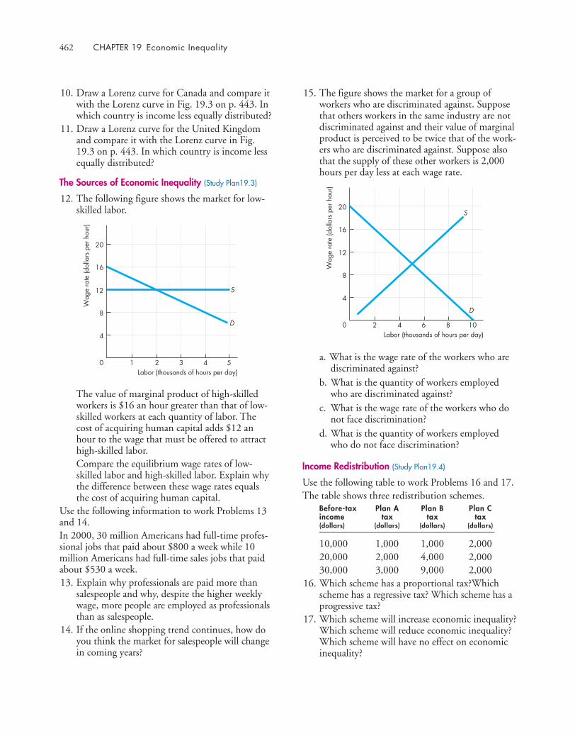
462 CHAPTER 19 Economic Inequality

10. Draw a Lorenz curve for Canada and compare itwith the Lorenz curve in Fig. 19.3 on p. 443. Inwhich country is income less equally distributed?

11. Draw a Lorenz curve for the United Kingdomand compare it with the Lorenz curve in Fig.19.3 on p. 443. In which country is income lessequally distributed?

The Sources of Economic Inequality (Study Plan19.3)

12. The following figure shows the market for low-skilled labor.

The value of marginal product of high-skilledworkers is $16 an hour greater than that of low-skilled workers at each quantity of labor. Thecost of acquiring human capital adds $12 anhour to the wage that must be offered to attracthigh-skilled labor. Compare the equilibrium wage rates of low-skilled labor and high-skilled labor. Explain whythe difference between these wage rates equalsthe cost of acquiring human capital.

Use the following information to work Problems 13and 14.In 2000, 30 million Americans had full-time profes-sional jobs that paid about $800 a week while 10million Americans had full-time sales jobs that paidabout $530 a week.13. Explain why professionals are paid more than

salespeople and why, despite the higher weeklywage, more people are employed as professionalsthan as salespeople.

14. If the online shopping trend continues, how doyou think the market for salespeople will changein coming years?

Wag

e ra

te (d

olla

rs p

er h

our)

Labor (thousands of hours per day)0

12

16

2

20

8

4

3 4 5 1

S

D

15. The figure shows the market for a group ofworkers who are discriminated against. Supposethat others workers in the same industry are notdiscriminated against and their value of marginalproduct is perceived to be twice that of the work-ers who are discriminated against. Suppose alsothat the supply of these other workers is 2,000hours per day less at each wage rate.

a. What is the wage rate of the workers who arediscriminated against?

b. What is the quantity of workers employedwho are discriminated against?

c. What is the wage rate of the workers who donot face discrimination?

d. What is the quantity of workers employedwho do not face discrimination?

Income Redistribution (Study Plan19.4)

Use the following table to work Problems 16 and 17.The table shows three redistribution schemes.

Before-tax Plan A Plan B Plan Cincome tax tax tax(dollars) (dollars) (dollars) (dollars)

10,000 1,000 1,000 2,00020,000 2,000 4,000 2,00030,000 3,000 9,000 2,000

16. Which scheme has a proportional tax?Whichscheme has a regressive tax? Which scheme has aprogressive tax?

17. Which scheme will increase economic inequality?Which scheme will reduce economic inequality?Which scheme will have no effect on economicinequality?

Wag

e ra

te (d

olla

rs p

er h

our)

Labor (thousands of hours per day)0

D

S

12

16

4

20

8

4

2 6 8 10

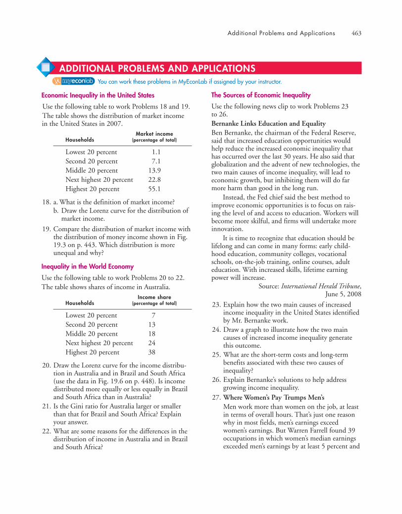
Additional Problems and Applications 463

Economic Inequality in the United States

Use the following table to work Problems 18 and 19.The table shows the distribution of market incomein the United States in 2007.

Market incomeHouseholds (percentage of total)

Lowest 20 percent 1.1Second 20 percent 7.1Middle 20 percent 13.9Next highest 20 percent 22.8Highest 20 percent 55.1

18. a. What is the definition of market income?b. Draw the Lorenz curve for the distribution of

market income.

19. Compare the distribution of market income withthe distribution of money income shown in Fig.19.3 on p. 443. Which distribution is moreunequal and why?

Inequality in the World Economy

Use the following table to work Problems 20 to 22.The table shows shares of income in Australia.

Income shareHouseholds (percentage of total)

Lowest 20 percent 7Second 20 percent 13Middle 20 percent 18Next highest 20 percent 24Highest 20 percent 38

20. Draw the Lorenz curve for the income distribu-tion in Australia and in Brazil and South Africa(use the data in Fig. 19.6 on p. 448). Is incomedistributed more equally or less equally in Braziland South Africa than in Australia?

21. Is the Gini ratio for Australia larger or smallerthan that for Brazil and South Africa? Explainyour answer.

22. What are some reasons for the differences in thedistribution of income in Australia and in Braziland South Africa?

The Sources of Economic Inequality

Use the following news clip to work Problems 23 to 26.Bernanke Links Education and EqualityBen Bernanke, the chairman of the Federal Reserve,said that increased education opportunities wouldhelp reduce the increased economic inequality thathas occurred over the last 30 years. He also said thatglobalization and the advent of new technologies, thetwo main causes of income inequality, will lead toeconomic growth, but inhibiting them will do farmore harm than good in the long run.

Instead, the Fed chief said the best method toimprove economic opportunities is to focus on rais-ing the level of and access to education. Workers willbecome more skilful, and firms will undertake moreinnovation.

It is time to recognize that education should belifelong and can come in many forms: early child-hood education, community colleges, vocationalschools, on-the-job training, online courses, adulteducation. With increased skills, lifetime earningpower will increase.

Source: International Herald Tribune,June 5, 2008

23. Explain how the two main causes of increasedincome inequality in the United States identifiedby Mr. Bernanke work.

24. Draw a graph to illustrate how the two maincauses of increased income inequality generatethis outcome.

25. What are the short-term costs and long-termbenefits associated with these two causes ofinequality?

26. Explain Bernanke’s solutions to help addressgrowing income inequality.

27. Where Women’s Pay Trumps Men’sMen work more than women on the job, at leastin terms of overall hours. That’s just one reasonwhy in most fields, men’s earnings exceedwomen’s earnings. But Warren Farrell found 39occupations in which women’s median earningsexceeded men’s earnings by at least 5 percent and

You can work these problems in MyEconLab if assigned by your instructor.

ADDITIONAL PROBLEMS AND APPLICATIONS

464 CHAPTER 19 Economic Inequality

in some cases by as much as 43 percent. In fieldslike engineering, a company may get one womanand seven men applying for a job. If the com-pany wants to hire the woman, it might have topay a premium to get her. Also, where womencan combine technical expertise with peopleskills—such as those required in sales and wherecustomers prefer dealing with a woman—that’slikely to contribute to a premium in pay.

Source: CNN, March 2, 2006a. Draw a graph to illustrate why discrimination

could result in female workers getting paidmore than male workers for some jobs.

b. Explain how market competition could poten-tially eliminate this wage differential.

c. If customers “prefer dealing with a woman” insome markets, how might that lead to a per-sistent wage differential between men andwomen?

Income Redistribution

28. Use the information provided in Problem 16 andin Fig. 19.3 on p. 443.a. What is the percentage of total income that

is redistributed from the highest incomegroup?

b. What percentages of total income are redis-tributed to the lower income groups?

29. Describe the effects of increasing the amount ofincome redistribution in the United States to thepoint at which the lowest income group receives15 percent of total income and the highestincome group receives 30 percent of totalincome.

Use the following news clip to work Problems 30and 31.The Tax Debate We Should be HavingA shrinking number of Americans are bearing aneven bigger share of the nation’s income tax burden.In 2005, the bottom 40 percent of Americans byincome had, in the aggregate, an effective tax ratethat’s negative: Their households received moremoney through the income tax system, largely fromthe earned income tax credit, than they paid. The top50% of taxpayers pay 97% of total income tax andthe top 10% of taxpayers pay 70%. The top 1% paidalmost 40% of all income tax, a proportion that hasjumped dramatically since 1986.Given the U.S. tax system, any tax cut must benefitthe rich, but in terms of the change in effective tax

rates: The bottom 50% got a much bigger tax cutunder the Bush tax cut than the top 1%. Did the dol-lar value of Bush’s tax cuts go mostly to the wealthy?Absolutely.

Source: Fortune, April 14, 200830. Explain why tax cuts in a progressive income tax

system are consistently criticized for favoring thewealthy.

31. How might the benefits of tax cuts “trickledown” to others whose taxes are not cut?

Economics in the News32. After you have studied Reading Between the Lines

on pp. 458–459 answer the following questions.a. What are the broad facts reported in the news

article about the gap in the incomes of CEOsand the average wage rate during the 1960sand in 2008?

b. What does Sam Pizzigati say should happen totop CEO pay?

c. How can the idea of a contest among poten-tial CEOs explain the trend in CEO pay?

d. If the contest among potential CEOs is thecorrect explanation for the trend in CEO pay,what would be the effects of a cap on CEOpay?

33. The Best and Worst College Degrees by SalaryBusiness administration is always a strong con-tender for honors as the most popular collegemajor. This is no surprise since students thinkbusiness is the way to make big bucks. But isbusiness administration really as lucrative as stu-dents and their parents believe? Nope.In a new survey by PayScale, Inc. of salaries bycollege degree, business administration didn’teven break into the list of the top 10 or 20 mostlucrative college degrees. A variety of engineeringmajors claim eight of the top 10 salary spots withchemical engineering ($65,700) winning bestfor starting salaries. Out of 75 undergrad collegemajors, business administration ($42,900) camein 35th, behind such degrees as occupationaltherapy ($61,300), information technology($49,400), and economics ($48,800).

Source: moneywatch.com, July 21, 2009a. Why do college graduates with different ma-

jors have drastically different starting salaries?b. Draw a graph of the labor markets for econom-

ics majors and business administration majorsto illustrate your explanation of the differencesin the starting salaries of these two groups.

After studying this chapter, you will be able to:

� Explain how people make decisions when they areuncertain about the consequences

� Explain how markets enable people to buy and sell risk� Explain how markets cope when buyers and sellers

have private information� Explain how the presence of uncertainty and incomplete

information influences the ability of markets to achievean efficient allocation of resources

L ife is like a lottery. You set up a summer business and work hard at it. Butwill you make enough income to keep you in school next year or will you getwiped out? How do people make a decision when they don’t know what itsconsequences will be?

As you drive across an intersection on a green light, you see a car on your leftthat’s still moving. Will it stop or will it run the red light? You buy insurance againstsuch a risk, and insurance companies gain from your business. Why are wewilling to buy insurance at prices that leave insurance companies with a gain?

Buying a new car—or a used car—is fun, but it’s also scary. You could getstuck with a lemon. Just about every complicated product you buycould be defective. How do car dealers and retailers induce us tobuy goods that might turn out to be lemons?

Although markets do a good job in helping people to use scarce resourcesefficiently, there are impediments to efficiency. Can markets lead to an efficientoutcome when there is uncertainty and incomplete information? In this chapter, weanswer questions such as these. And in Reading Between the Lines at the end ofthe chapter, you will see how accurate grading by high schools, colleges, anduniversities helps students get the right jobs and the problem that arises in jobmarkets if grades are inflated.

UNCERTAINTY AND

20INFORMATION

465

466 CHAPTER 20 Uncertainty and Information

◆ Decisions in the Faceof Uncertainty

Tania, a student, is trying to decide which of twosummer jobs to take. She can work as a housepainter and earn enough for her to save $2,000 bythe end of the summer. There is no uncertaintyabout the income from this job. If Tania takes it,she will definitely have $2,000 in her bank accountat the end of the summer. The other job, workingas a telemarketer selling subscriptions to a maga-zine, is risky. If Tania takes this job, her bank bal-ance at the end of the summer will depend on hersuccess at selling. She will earn enough to save$5,000 if she is successful but only $1,000 if sheturns out to be a poor salesperson. Tania has nevertried selling, so she doesn’t know how successfulshe’ll be. But some of her friends have done thisjob, and 50 percent of them do well and 50 percentdo poorly. Basing her expectations on this experi-ence, Tania thinks there is a 50 percent chance thatshe will earn $5,000 and a 50 percent chance thatshe will earn $1,000.

Tania is equally as happy to paint as she is to makephone calls. She cares only about the money. Whichjob does she prefer: the one that provides her with$2,000 for sure or the one that offers her a 50 per-cent chance of making $5,000 but a 50 percent riskof making only $1,000?

To answer this question, we need a way of com-paring the two outcomes. One comparison is theexpected wealth that each job creates.

Expected WealthExpected wealth is the money value of what a personexpects to own at a given point in time. An expecta-tion is an average calculated by using a formula thatweights each possible outcome with the probability(chance) that it will occur.

For Tania, the probability that she will have$5,000 is 0.5 (a 50 percent chance). The probabilitythat she will have $1,000 is also 0.5. Notice that theprobabilities sum to 1. Using these numbers, we cancalculate Tania’s expected wealth, EW, which is

EW = ($5,000 × 0.5) + ($1,000 × 0.5) = $3,000.

Notice that expected wealth decreases if the risk ofa poor outcome increases. For example, if Tania has a

20 percent chance of success (and 80 percent chanceof failure), her expected wealth falls to $1,800—

($5,000 × 0.2) + ($1,000 × 0.8) = $1,800.

Tania can now compare the expected wealth fromeach job—$3,000 for the risky job and $2,000 forthe non-risky job.

So does Tania prefer the risky job because it givesher a greater expected wealth? The answer is we don’tknow because we don’t know how much Tania dis-likes risk.

Risk AversionRisk aversion is the dislike of risk. Almost everyone isrisk averse but some more than others. In football,running is less risky than passing. Coach JohnHarbaugh of the Baltimore Ravens, who favors a cau-tious running game, is risk averse. Indianapolis quar-terback Peyton Manning, who favors a risky passinggame, is less risk averse. But almost everyone is riskaverse to some degree.

We can measure the degree of risk aversion by thecompensation needed to make a given amount of riskacceptable. Returning to Tania: If she needs to bepaid more than $1,000 to take on the risk arisingfrom the telemarketing job, she will choose the safepainting job and take the $2,000 non-risky income.But if she thinks that the extra $1,000 of expectedincome is enough to compensate her for the risk, shewill take the risky job.

To make this idea concrete, we need a way ofthinking about how a person values different levels ofwealth. The concept that we use is utility. We applythe same idea that explains how people make expen-diture decisions (see Chapter 8) to explain risk aver-sion and decisions in the face of risk.

Utility of WealthWealth (money in the bank and other assets of value)is like all good things. It yields utility. The morewealth a person has, the greater is that person’s totalutility. But each additional dollar of wealth brings adiminishing increment in total utility—the marginalutility of wealth diminishes as wealth increases.

Diminishing marginal utility of wealth means thatthe gain in utility from an increase in wealth issmaller than the loss in utility from an equal decreasein wealth. Stated differently, the pain from a loss isgreater than the pleasure from a gain of equal size.

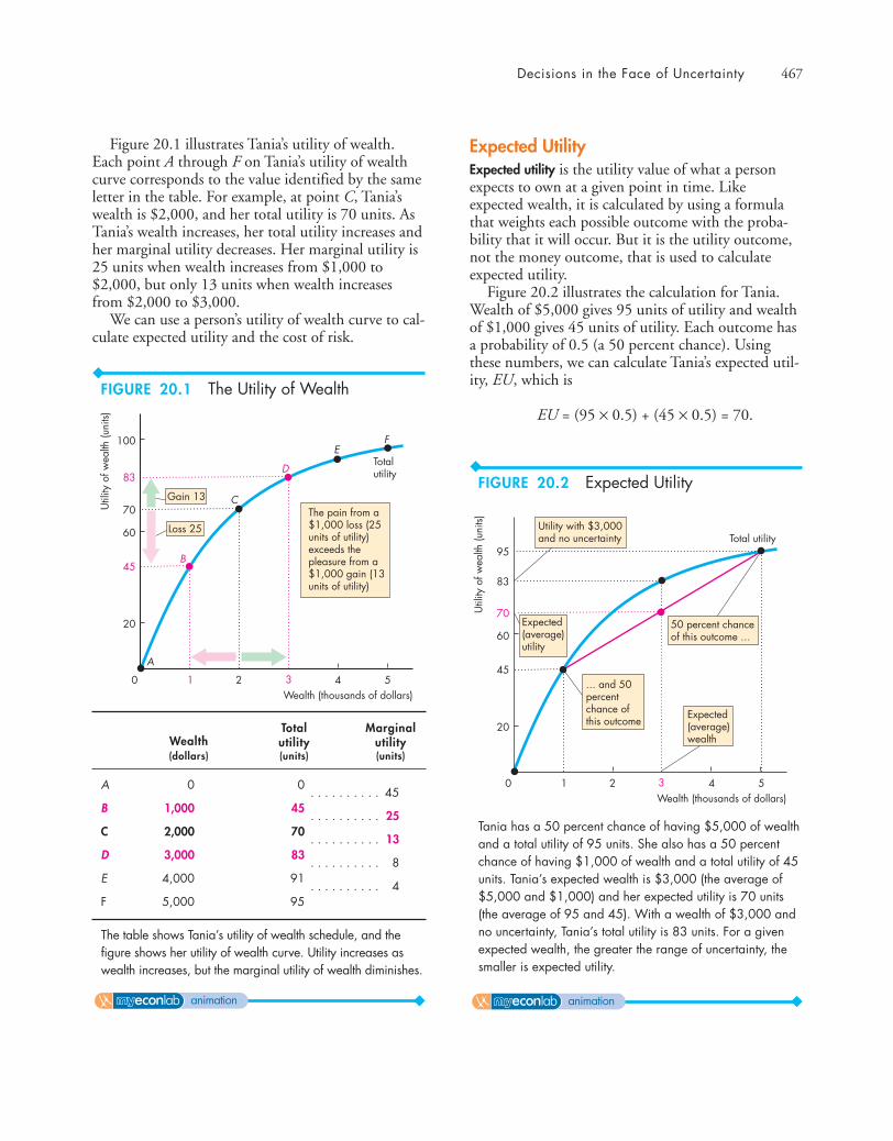
Decisions in the Face of Uncertainty 467

Figure 20.1 illustrates Tania’s utility of wealth.Each point A through F on Tania’s utility of wealthcurve corresponds to the value identified by the sameletter in the table. For example, at point C, Tania’swealth is $2,000, and her total utility is 70 units. AsTania’s wealth increases, her total utility increases andher marginal utility decreases. Her marginal utility is25 units when wealth increases from $1,000 to$2,000, but only 13 units when wealth increasesfrom $2,000 to $3,000.

We can use a person’s utility of wealth curve to cal-culate expected utility and the cost of risk.

Expected UtilityExpected utility is the utility value of what a personexpects to own at a given point in time. Likeexpected wealth, it is calculated by using a formulathat weights each possible outcome with the proba-bility that it will occur. But it is the utility outcome,not the money outcome, that is used to calculateexpected utility.

Figure 20.2 illustrates the calculation for Tania.Wealth of $5,000 gives 95 units of utility and wealthof $1,000 gives 45 units of utility. Each outcome hasa probability of 0.5 (a 50 percent chance). Usingthese numbers, we can calculate Tania’s expected util-ity, EU, which is

EU = (95 × 0.5) + (45 × 0.5) = 70.

The table shows Tania’s utility of wealth schedule, and thefigure shows her utility of wealth curve. Utility increases aswealth increases, but the marginal utility of wealth diminishes.

Wealth (thousands of dollars)3

20

45

60

70

83

95

0 2 4 51

Util

ity o

f wea

lth (u

nits)

Total utility

50 percent chanceof this outcome ...

... and 50percentchance ofthis outcome

Expected(average)wealth

Expected(average)utility

Utility with $3,000and no uncertainty

Tania has a 50 percent chance of having $5,000 of wealthand a total utility of 95 units. She also has a 50 percentchance of having $1,000 of wealth and a total utility of 45units. Tania’s expected wealth is $3,000 (the average of$5,000 and $1,000) and her expected utility is 70 units(the average of 95 and 45). With a wealth of $3,000 andno uncertainty, Tania’s total utility is 83 units. For a givenexpected wealth, the greater the range of uncertainty, thesmaller is expected utility.

Wealth (thousands of dollars)3

20

45

60

70

83

100

0 2 4 51

Util

ity o

f wea

lth (u

nits)

Totalutility

C

B

D

EF

A

The pain from a$1,000 loss (25units of utility)exceeds thepleasure from a$1,000 gain (13units of utility)

Loss 25

Gain 13

Total MarginalWealth utility utility(dollars) (units) (units)

A 0 0 . . . . . . . . . . 45

B 1,000 45 . . . . . . . . . . 25

C 2,000 70 . . . . . . . . . . 13

D 3,000 83 . . . . . . . . . . 8

E 4,000 91 . . . . . . . . . . 4

F 5,000 95

FIGURE 20.1 The Utility of Wealth

animation animation

FIGURE 20.2 Expected Utility

468 CHAPTER 20 Uncertainty and Information

Expected utility decreases if the risk of a poor out-come increases. For example, if Tania has a 20 per-cent chance of success (and an 80 percent chance offailure), her expected utility is 55 units—

(95 × 0.2) + (45 × 0.8) = 55.Notice how the range of uncertainty affects

expected utility. Figure 20.2 shows that with $3,000of wealth and no uncertainty, total utility is 83 units.But with the same expected wealth and Tania’s uncer-tainty—a 50 percent chance of having $5,000 and a50 percent chance of having $1,000—expected util-ity is only 70 units. Tania’s uncertainty lowers herexpected utility by 13 units.

Expected utility combines expected wealth andrisk into a single index.

Making a Choice with UncertaintyFaced with uncertainty, a person chooses the actionthat maximizes expected utility. To select the job thatgives her the maximum expected utility, Tania must:

1. Calculate the expected utility from the risky tele-marketing job

2. Calculate the expected utility from the safe paint-ing job

3. Compare the two expected utilitiesFigure 20.3 illustrates the calculations. You’ve just

seen that the risky telemarketing job gives Tania anexpected utility of 70 units. The safe painting jobalso gives Tania a utility of 70. That is, the total util-ity of $2,000 with no risk is 70 units. So with eitherjob, Tania has an expected utility of 70 units. She isindifferent between these two jobs.

If Tania had only a 20 percent chance of successand an 80 percent chance of failure in the telemarket-ing job, her expected utility would be 55 (calculatedabove). In this case, she would take the painting joband get 70 units of utility. But if the probabilitieswere reversed and she had an 80 percent chance ofsuccess and only a 20 percent chance of failure in thetelemarketing job, her expected utility would be 85units—(95 × 0.8) + (45 × 0.2) = 85. In this case, shewould take the risky telemarketing job.

We can calculate the cost of risk by comparing theexpected wealth in a given risky situation with thewealth that gives the same total utility but no risk.Using this principle, we can find Tania’s cost of bear-ing the risk that arises from the telemarketing job.That cost, highlighted in Figure 20.3, is $1,000.

You’ve now seen how a person makes a risky deci-sion. In the next section, we’ll see how marketsenable people to reduce the risks they face.

Wealth (thousands of dollars)3

45

70

95

0 2 4 51

Util

ity o

f wea

lth (u

nits)

Total utility

Cost of risk,$1,000

Expectedwealth

Expectedutility

With a 50 percent chance of having $5,000 of wealth anda 50 percent chance of having $1,000 of wealth, Tania’sexpected wealth is $3,000 and her expected utility is 70units. Tania would have the same 70 units of total utility withwealth of $2,000 and no risk, so Tania’s cost of bearing thisrisk is $1,000. Tania is indifferent between the job that pays$2,000 with no risk and the job that offers an equal chanceof $5,000 and $1,000.

FIGURE 20.3 Choice Under Uncertainty

animation

REVIEW QUIZ1 What is the distinction between expected

wealth and expected utility?2 How does the concept of utility of wealth

capture the idea that pain of loss exceeds thepleasure of gain?

3 What do people try to achieve when they makea decision under uncertainty?

4 How is the cost of the risk calculated whenmaking a decision with an uncertain outcome?

You can work these questions in Study Plan 20.1 and get instant feedback.

Buying and Selling Risk 469

◆ Buying and Selling RiskYou’ve seen at many points in your study of marketshow both buyers and sellers gain from trade. Buyersgain because they value what they buy more highlythan the price they must pay—they receive a con-sumer surplus. And sellers gain because they face coststhat are less than the price at which they can sell—they receive a producer surplus.

Just as buyers and sellers gain from trading goodsand services, so they can also gain by trading risk. Butrisk is a bad, not a good. The good that is traded isrisk avoidance. A buyer of risk avoidance can gainbecause the value of avoiding risk is greater than theprice that must be paid to someone else to get themto bear the risk. The seller of risk avoidance faces alower cost of risk than the price that people are will-ing to pay to avoid the risk.

We’re going to put some flesh on the bare bones ofthis brief account of how people can gain from trad-ing risk by looking at insurance markets.

Insurance MarketsInsurance plays a huge role in our economic lives.We’ll explain

■ How insurance reduces risk■ Why people buy insurance■ How insurance companies earn a profit

How Insurance Reduces Risk Insurance reduces therisk that people face by sharing or pooling the risks.When people buy insurance against the risk of anunwanted event, they pay an insurance company apremium. If the unwanted event occurs, the insur-ance company pays out the amount of the insuredloss.

Think about auto collision insurance. The proba-bility that any one person will have a serious autoaccident is small. But a person who does have an autoaccident incurs a large loss. For a large population,the probability of one person having an accident isthe proportion of the population that has an acci-dent. But this proportion is known, so the probabil-ity of an accident occurring and the total cost ofaccidents can be predicted. An insurance companycan pool the risks of a large population and enableeveryone to share the costs. It does so by collectingpremiums from everyone and paying out benefits to

those who suffer a loss. An insurance company thatremains in business collects at least as much in premi-ums as it pays out in benefits.

Why People Buy Insurance People buy insuranceand insurance companies earn a profit by sellinginsurance because people are risk averse. To see whypeople buy insurance and why it is profitable, let’sconsider an example. Dan owns a car worth $10,000,and that is his only wealth. There is a 10 percentchance that Dan will have a serious accident thatmakes his car worth nothing. So there is a 90 percentchance that Dan’s wealth will remain at $10,000 anda 10 percent chance that his wealth will be zero.Dan’s expected wealth is $9,000—($10,000 × 0.9) +($0 × 0.1).

Dan is risk averse (just like Tania in the previousexample). Because Dan is risk averse, he will be betteroff by buying insurance to avoid the risk that hefaces, if the insurance premium isn’t too high.

Without knowing some details about just howrisk averse Dan is, we don’t know the most that hewould be willing to pay to avoid this risk. But we doknow that he would pay more than $1,000. If Dandid pay $1,000 to avoid the risk, he would have$9,000 of wealth and face no uncertainty about hiswealth. If he does not have an accident, his wealth isthe $10,000 value of his car minus the $1,000 hepays the insurance company. If he does lose his car,the insurance company pays him $10,000, so he stillhas $9,000. Being risk averse, Dan’s expected utilityfrom $9,000 with no risk is greater than his expectedutility from an expected $9,000 with risk. So Danwould be willing to pay more than $1,000 to avoidthis risk.

How Insurance Companies Earn a Profit For theinsurance company, $1,000 is the minimum amountat which it would be willing to insure Dan and otherpeople like him. With say 50,000 customers all likeDan, 5,000 customers (50,000 × 0.1) lose their carsand 45,000 don’t. Premiums of $1,000 give theinsurance company a total revenue of $50,000,000.With 5,000 claims of $10,000, the insurance com-pany pays out $50,000,000. So a premium of $1,000enables the insurance company to break even (makezero economic profit) on this business.

But Dan (and everyone else) is willing to pay morethan $1,000, so insurance is a profitable business andthere is a gain from trading risk.

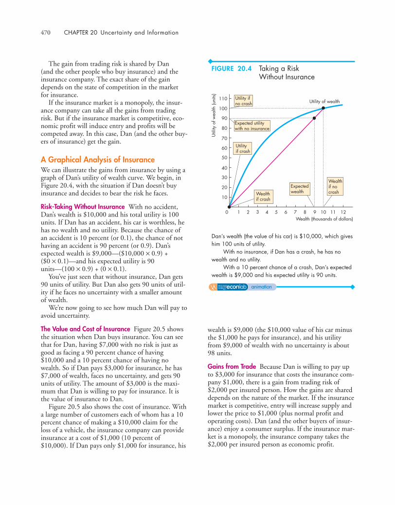
470 CHAPTER 20 Uncertainty and Information

The gain from trading risk is shared by Dan (and the other people who buy insurance) and theinsurance company. The exact share of the gaindepends on the state of competition in the market for insurance.

If the insurance market is a monopoly, the insur-ance company can take all the gains from tradingrisk. But if the insurance market is competitive, eco-nomic profit will induce entry and profits will becompeted away. In this case, Dan (and the other buy-ers of insurance) get the gain.

A Graphical Analysis of InsuranceWe can illustrate the gains from insurance by using agraph of Dan’s utility of wealth curve. We begin, inFigure 20.4, with the situation if Dan doesn’t buyinsurance and decides to bear the risk he faces.

Risk-Taking Without Insurance With no accident,Dan’s wealth is $10,000 and his total utility is 100units. If Dan has an accident, his car is worthless, hehas no wealth and no utility. Because the chance ofan accident is 10 percent (or 0.1), the chance of nothaving an accident is 90 percent (or 0.9). Dan’sexpected wealth is $9,000—($10,000 × 0.9) + ($0 × 0.1)—and his expected utility is 90units—(100 × 0.9) + (0 × 0.1).

You’ve just seen that without insurance, Dan gets90 units of utility. But Dan also gets 90 units of util-ity if he faces no uncertainty with a smaller amountof wealth.

We’re now going to see how much Dan will pay toavoid uncertainty.

The Value and Cost of Insurance Figure 20.5 showsthe situation when Dan buys insurance. You can seethat for Dan, having $7,000 with no risk is just asgood as facing a 90 percent chance of having$10,000 and a 10 percent chance of having nowealth. So if Dan pays $3,000 for insurance, he has$7,000 of wealth, faces no uncertainty, and gets 90units of utility. The amount of $3,000 is the maxi-mum that Dan is willing to pay for insurance. It isthe value of insurance to Dan.

Figure 20.5 also shows the cost of insurance. Witha large number of customers each of whom has a 10percent chance of making a $10,000 claim for theloss of a vehicle, the insurance company can provideinsurance at a cost of $1,000 (10 percent of$10,000). If Dan pays only $1,000 for insurance, his

wealth is $9,000 (the $10,000 value of his car minusthe $1,000 he pays for insurance), and his utilityfrom $9,000 of wealth with no uncertainty is about98 units.

Gains from Trade Because Dan is willing to pay upto $3,000 for insurance that costs the insurance com-pany $1,000, there is a gain from trading risk of$2,000 per insured person. How the gains are shareddepends on the nature of the market. If the insurancemarket is competitive, entry will increase supply andlower the price to $1,000 (plus normal profit andoperating costs). Dan (and the other buyers of insur-ance) enjoy a consumer surplus. If the insurance mar-ket is a monopoly, the insurance company takes the$2,000 per insured person as economic profit.

Wealth (thousands of dollars)3

60

50

40

30

20

10

70

100

90

80

110

0 2 4 5 6 7 8 9 10 11 121U

tility

of w

ealth

(uni

ts)

Utility of wealth

Wealthif nocrash

ExpectedwealthWealth

if crash

Expected utilitywith no insurance

Utility ifno crash

Utilityif crash

Dan’s wealth (the value of his car) is $10,000, which giveshim 100 units of utility.

With no insurance, if Dan has a crash, he has nowealth and no utility.

With a 10 percent chance of a crash, Dan’s expectedwealth is $9,000 and his expected utility is 90 units.

FIGURE 20.4 Taking a RiskWithout Insurance

animation

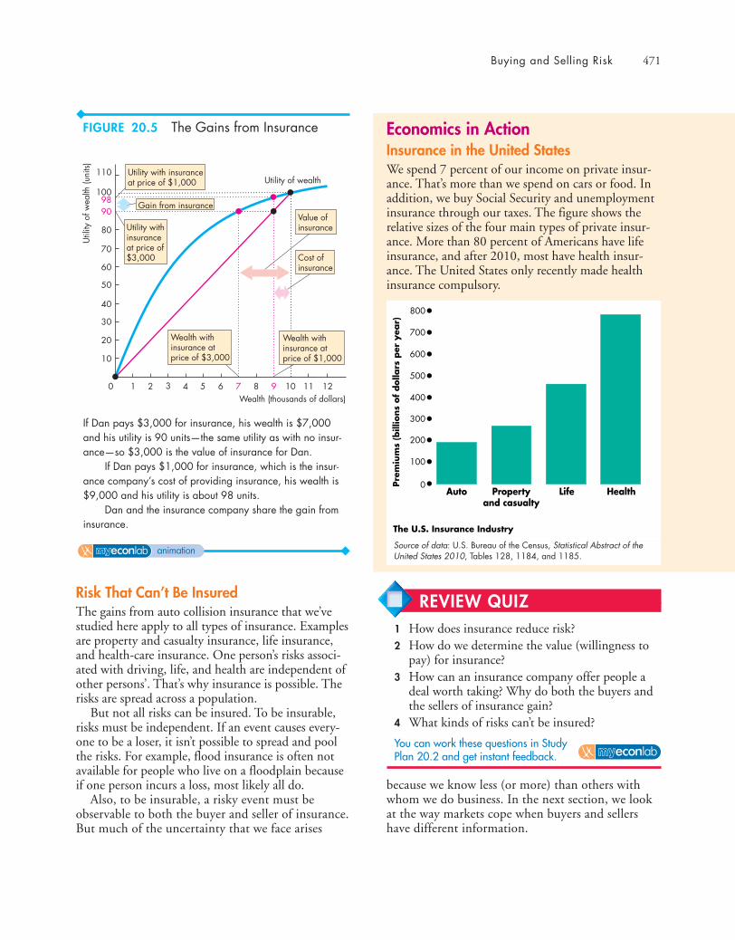
Buying and Selling Risk 471

Economics in ActionInsurance in the United StatesWe spend 7 percent of our income on private insur-ance. That’s more than we spend on cars or food. Inaddition, we buy Social Security and unemploymentinsurance through our taxes. The figure shows therelative sizes of the four main types of private insur-ance. More than 80 percent of Americans have lifeinsurance, and after 2010, most have health insur-ance. The United States only recently made healthinsurance compulsory.

Risk That Can’t Be InsuredThe gains from auto collision insurance that we’vestudied here apply to all types of insurance. Examplesare property and casualty insurance, life insurance,and health-care insurance. One person’s risks associ-ated with driving, life, and health are independent ofother persons’. That’s why insurance is possible. Therisks are spread across a population.

But not all risks can be insured. To be insurable,risks must be independent. If an event causes every-one to be a loser, it isn’t possible to spread and poolthe risks. For example, flood insurance is often notavailable for people who live on a floodplain becauseif one person incurs a loss, most likely all do.

Also, to be insurable, a risky event must beobservable to both the buyer and seller of insurance.But much of the uncertainty that we face arises

0

100

200

300

400

500

600

700

800

Pre

miu

ms

(bill

ions

of

dolla

rs p

er y

ear)

Life HealthPropertyand casualty

Auto

The U.S. Insurance Industry

Source of data: U.S. Bureau of the Census, Statistical Abstract of theUnited States 2010, Tables 128, 1184, and 1185.

Wealth (thousands of dollars)3

60

50

40

30

20

10

70

100

9098

80

110

0 2 4 5 6 7 8 9 10 11 121

Util

ity o

f wea

lth (u

nits)

Utility of wealth

Wealth withinsurance atprice of $1,000

Wealth withinsurance atprice of $3,000

Utility with insuranceat price of $1,000

Utility withinsuranceat price of$3,000

Gain from insuranceValue ofinsurance

Cost ofinsurance

If Dan pays $3,000 for insurance, his wealth is $7,000and his utility is 90 units—the same utility as with no insur-ance—so $3,000 is the value of insurance for Dan.

If Dan pays $1,000 for insurance, which is the insur-ance company’s cost of providing insurance, his wealth is$9,000 and his utility is about 98 units.

Dan and the insurance company share the gain frominsurance.

because we know less (or more) than others withwhom we do business. In the next section, we lookat the way markets cope when buyers and sellershave different information.

FIGURE 20.5 The Gains from Insurance

animation

REVIEW QUIZ1 How does insurance reduce risk?2 How do we determine the value (willingness to

pay) for insurance?3 How can an insurance company offer people a

deal worth taking? Why do both the buyers andthe sellers of insurance gain?

4 What kinds of risks can’t be insured?

You can work these questions in Study Plan 20.2 and get instant feedback.

472 CHAPTER 20 Uncertainty and Information

◆ Private InformationIn all the markets that you’ve studied so far, the buy-ers and the sellers are well informed about the good,service, or factor of production being traded. But insome markets, either the buyers or the sellers—usu-ally the sellers—are better informed about the valueof the item being traded than the person on the otherside of the market. Information about the value ofthe item being traded that is possessed by only buyersor sellers is called private information. And a market inwhich the buyers or sellers have private informationhas asymmetric information.

Asymmetric Information: Examples andProblemsAsymmetric information affects many of your owneconomic transactions. One example is your knowl-edge about your driving skills and temperament.You know much more than your auto insurancecompany does about how carefully and defensivelyyou drive—about your personal risk of having anaccident that would cause the insurance company topay a claim. Another example is your knowledgeabout your work effort. You know more than youremployer about how hard you are willing to work.Yet another example is your knowledge about thequality of your car. You know whether it’s a lemon,but the person to whom you are about to sell it doesnot know and can’t find out until after he or she hasbought it.

Asymmetric information creates two problems:

■ Adverse selection■ Moral hazard

Adverse Selection Adverse selection is the tendencyfor people to enter into agreements in which they canuse their private information to their own advantageand to the disadvantage of the uninformed party.

For example, if Jackie offers her salespeople a fixedwage, she will attract lazy salespeople. Hardworkingsalespeople will prefer not to work for Jackie becausethey can earn more by working for someone whopays by results. The fixed-wage contract adverselyselects those with private information (knowledgeabout their work habits) who can use that knowledgeto their own advantage and to the disadvantage of theother party.

Moral Hazard Moral hazard is the tendency for peo-ple with private information, after entering into anagreement, to use that information for their own ben-efit and at the cost of the less-informed party.For example, Jackie hires Mitch as a salesperson andpays him a fixed wage regardless of how much hesells. Mitch faces a moral hazard. He has an incentiveto put in the least possible effort, benefiting himselfand lowering Jackie’s profits. For this reason, sales-people are usually paid by a formula that makes theirincome higher, the greater is the volume (or value) oftheir sales.

A variety of devices have evolved that enable mar-kets to function in the face of moral hazard andadverse selection. We’ve just seen one, the use ofincentive payments for salespeople. We’re going tolook at how three markets cope with adverse selectionand moral hazard. They are

■ The market for used cars■ The market for loans■ The market for insurance

The Market for Used CarsWhen a person buys a car, it might turn out to be alemon. If the car is a lemon, it is worth less to thebuyer than if it has no defects. Does the used carmarket have two prices reflecting these two values—alow price for lemons and a higher price for cars with-out defects? It turns out that it does. But it needssome help to do so and to overcome what is calledthe lemon problem—the problem that in a market inwhich it is not possible to distinguish reliable prod-ucts from lemons, there are too many lemons and toofew reliable products traded.

To see how the used car market overcomes thelemon problem, we’ll first look at a used car marketthat has a lemon problem.

The Lemon Problem in a Used Car MarketTo explain the lemon problem as clearly as possible,we’ll assume that there are only two kinds of cars:defective cars—lemons—and cars without defectsthat we’ll call good cars. Whether or not a car is alemon is private information that is available only tothe current owner. The buyer of a used car can’t tellwhether he is buying a lemon until after he hasbought the car and learned as much about it as itscurrent owner knows.

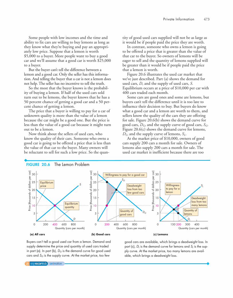
Private Information 473

Some people with low incomes and the time andability to fix cars are willing to buy lemons as long asthey know what they’re buying and pay an appropri-ately low price. Suppose that a lemon is worth$5,000 to a buyer. More people want to buy a goodcar and we’ll assume that a good car is worth $25,000to a buyer.

But the buyer can’t tell the difference between alemon and a good car. Only the seller has this informa-tion. And telling the buyer that a car is not a lemon doesnot help. The seller has no incentive to tell the truth.

So the most that the buyer knows is the probabil-ity of buying a lemon. If half of the used cars soldturn out to be lemons, the buyer knows that he has a50 percent chance of getting a good car and a 50 per-cent chance of getting a lemon.

The price that a buyer is willing to pay for a car ofunknown quality is more than the value of a lemonbecause the car might be a good one. But the price isless than the value of a good car because it might turnout to be a lemon.

Now think about the sellers of used cars, whoknow the quality of their cars. Someone who owns agood car is going to be offered a price that is less thanthe value of that car to the buyer. Many owners willbe reluctant to sell for such a low price. So the quan-

tity of good used cars supplied will not be as large asit would be if people paid the price they are worth.

In contrast, someone who owns a lemon is goingto be offered a price that is greater than the value ofthat car to the buyer. So owners of lemons will beeager to sell and the quantity of lemons supplied willbe greater than it would be if people paid the pricethat a lemon is worth.

Figure 20.6 illustrates the used car market thatwe’ve just described. Part (a) shows the demand forused cars, D, and the supply of used cars, S.Equilibrium occurs at a price of $10,000 per car with400 cars traded each month.

Some cars are good ones and some are lemons, butbuyers can’t tell the difference until it is too late toinfluence their decision to buy. But buyers do knowwhat a good car and a lemon are worth to them, andsellers know the quality of the cars they are offeringfor sale. Figure 20.6(b) shows the demand curve forgood cars, DG, and the supply curve of good cars, SG.Figure 20.6(c) shows the demand curve for lemons,DL, and the supply curve of lemons, SL.

At the market price of $10,000, owners of goodcars supply 200 cars a month for sale. Owners oflemons also supply 200 cars a month for sale. Theused car market is inefficient because there are too

Equilibriumprice

(a) All cars

Pric

e (th

ousa

nds

of d

olla

rs p

er c

ar)

Quantity (cars per month)0 200 400 600 800

S

D

(c) Lemons (b) Good cars

5

10

15

20

25

30

Equilibriumquantity

Deadweightloss from toofew good cars

Pric

e (th

ousa

nds

of d

olla

rs p

er c

ar)

Quantity (cars per month)0 200 400 600 800

SG

DG5

10

15

20

25

30

Pric

e (th

ousa

nds

of d

olla

rs p

er c

ar)

Quantity (cars per month)0 200150 300 400

SL

DL

5

10

15

20

25

30

Deadweightloss from toomany lemons

Willingness to pay for a good car

Quantity ofgood cars

Quantity oflemons

Willingnessto pay for alemon

Buyers can’t tell a good used car from a lemon. Demand andsupply determine the price and quantity of used cars tradedin part (a). In part (b), DG is the demand curve for good usedcars and SG is the supply curve. At the market price, too few

good cars are available, which brings a deadweight loss. Inpart (c), DL is the demand curve for lemons and SL is the sup-ply curve. At the market price, too many lemons are avail-able, which brings a deadweight loss.

FIGURE 20.6 The Lemon Problem

animation

474 CHAPTER 20 Uncertainty and Information

many lemons and not enough good cars. Figure 20.6makes this inefficiency clear by using the concept ofdeadweight loss (see Chapter 5, pp. 115–116).

At the quantity of good cars supplied, buyers arewilling to pay $25,000 for a good car. They are will-ing to pay more than a good car is worth to its cur-rent owner for all good cars up to 400 cars a month.The gray triangle shows the deadweight loss thatresults from there being too few good used cars.

At the quantity of lemons supplied, buyers arewilling to pay $5,000 for a lemon. They are willingto pay less than a lemon is worth to its current ownerfor all lemons above 150 cars a month. The gray tri-angle shows the deadweight loss that results fromthere being too many lemons.

You can see adverse selection in this used car marketbecause there is a greater incentive to offer a lemonfor sale. You can also see moral hazard because theowner of a lemon has little incentive to take goodcare of the car, so it is likely to become an even worselemon. The market for used cars is not working well.Too many lemons and too few good used cars aretraded.

A Used Car Market with Dealers’ WarrantiesHow can used car dealers convince buyers that a carisn’t a lemon? The answer is by giving a guarantee inthe form of a warranty. By providing warranties onlyon good cars, dealers signal which cars are good onesand which are lemons.

Signaling occurs when an informed person takesactions that send information to uninformed persons.The grades and degrees that a university awards stu-dents are signals. They inform potential (unin-formed) employers about the ability of the peoplethey are considering hiring.

In the market for used cars, dealers send signals bygiving warranties on the used cars they offer for sale.The message in the signal is that the dealer agrees topay the costs of repairing the car if it turns out tohave a defect.

Buyers believe the signal because the cost of send-ing a false signal is high. A dealer who gives a war-ranty on a lemon ends up bearing a high cost ofrepairs—and gains a bad reputation. A dealer whogives a warranty only on good cars has no repair costsand a reputation that gets better and better. It pays

(a) Good cars

Pric

e (d

olla

rs p

er c

ar)

Quantity (cars per month)600

5,000

10,000

15,000

20,000

25,000

0 400 800200

(b) Lemons

D

S

Price of agood car

Efficient outcomein the market forgood used cars

Pric

e (d

olla

rs p

er c

ar)

Quantity (cars per month)600

5,0006,667

15,000

20,000

25,000

0 400 800150

D

S

Quantity oflemons

Price of a lemon

Efficient outcome inthe market for lemons

Quantity ofgood cars

10,000

With dealers’ warranties as signals, the equilibrium price ofa good used car is $20,000 and 400 cars are traded. Themarket for good used cars is efficient. Because the signal

enables buyers to spot a lemon, the price of a lemon is$6,667 and 150 lemons are traded. The market for lemonsis efficient.

FIGURE 20.7 Warranties Make the Used Car Market Efficient

animation

Private Information 475

dealers to send an accurate signal, and it is rationalfor buyers to believe the signal.

So a car with a warranty is a good car; a car with-out a warranty is a lemon. Warranties solve the lemonproblem and enable the used car market to functionefficiently with two prices: one for lemons and onefor good cars.

Figure 20.7 illustrates this outcome. In part (a) thedemand for and supply of good cars determine theprice of a good car. In part (b), the demand for andsupply of lemons determine the price of a lemon.Both markets are efficient.

Pooling Equilibrium and Separating EquilibriumYou’ve seen two outcomes in the market for usedcars. Without warranties, there is only one messagevisible to the buyer: All cars look the same. So thereis one price regardless of whether the car is a good caror a lemon. We call the equilibrium in a market whenonly one message is available and an uninformed per-son cannot determine quality a pooling equilibrium.

But in a used car market with warranties, there aretwo messages. Good cars have warranties and lemonsdon’t. So there are two car prices for the two types ofcars. We call the equilibrium in a market when sig-naling provides full information to a previously unin-formed person a separating equilibrium.

The Market for LoansWhen you buy a tank of gasoline and swipe your creditcard, you are taking a loan from the bank that issuedyour card. You demand and your bank supplies a loan.Have you noticed the interest rate on an unpaid creditcard balance? In 2007, it ranged between 7 percent ayear and 36 percent a year. Why are these interest ratesso high? And why is there such a huge range?

The answer is that when banks make loans, theyface the risk that the loan will not be repaid. The riskthat a borrower, also known as a creditor, might notrepay a loan is called credit risk or default risk. Forcredit card borrowing, the credit risk is high and itvaries among borrowers. The highest-risk borrowerspay the highest interest rate.

Interest rates and the price of credit risk are deter-mined in the market for loans. The lower the interestrate, the greater is the quantity of loans demandedand for a given level of credit risk, the higher theinterest rate, the greater is the quantity of loans sup-plied. Demand and supply determine the interest rateand the price of credit risk.

If lenders were unable to charge different interestrates to reflect different degrees of credit risk, therewould be a pooling equilibrium and an inefficientloans market.

Inefficient Pooling Equilibrium To see why a poolingequilibrium would be inefficient, suppose that bankscan’t identify the individual credit risk of their bor-rowers: they have no way of knowing how likely it isthat a given loan will be repaid. In this situation,every borrower pays the same interest rate and themarket is in a pooling equilibrium.

If all borrowers pay the same interest rate, themarket for loans has the same problem as the usedcar market. Low-risk customers borrow less than theywould if they were offered the low interest rateappropriate for their low credit risk. High-risk cus-tomers borrow more than they would if they facedthe high interest rate appropriate for their high creditrisk. So banks face an adverse selection problem. Toomany borrowers are high risk and too few are lowrisk.

Signaling and Screening in the Market for LoansLenders don’t know how likely it is that a given loanwill be repaid, but the borrower does know. Low-riskborrowers have an incentive to signal their risk byproviding lenders with relevant information. Signalsmight include information about the length of time aperson has been in the current job or has lived at thecurrent address, home ownership, marital status, age,and business record.

High-risk borrowers might be identified simplyas those who have failed to signal low risk. Theseborrowers have an incentive to mislead lenders; andlenders have an incentive to induce high-risk bor-rowers to reveal their risk level. Inducing aninformed party to reveal private information iscalled screening.

By not lending to people who refuse to reveal rele-vant information, banks are able to screen as well asreceive signals that help them to separate their bor-rowers into a number of credit-risk categories. Iflenders succeed, the market for loans comes to a sepa-rating equilibrium with a high interest rate for high-risk borrowers and a low interest rate for low-riskborrowers. Signaling and screening in the market forloans works like warranties in the used car marketand avoids the deadweight loss of a poolingequilibrium.

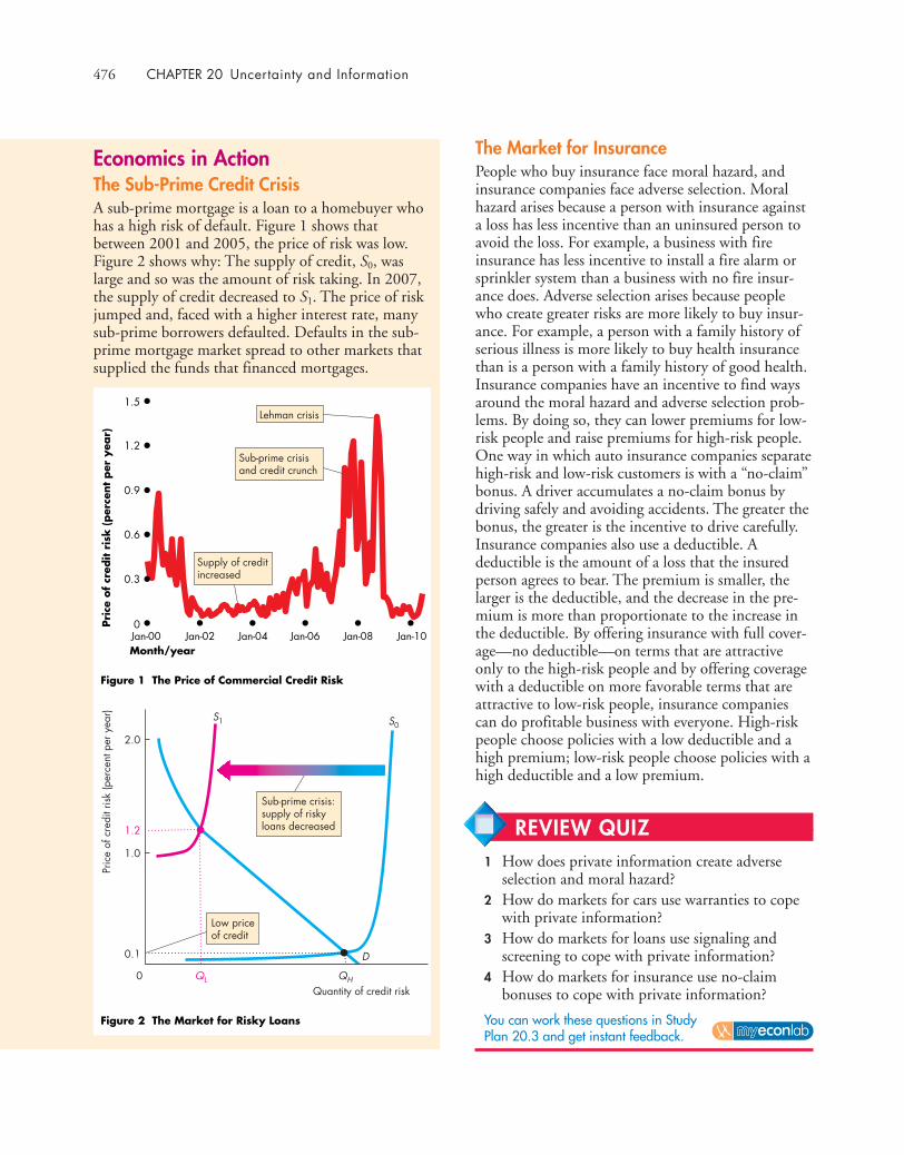
476 CHAPTER 20 Uncertainty and Information

The Market for InsurancePeople who buy insurance face moral hazard, andinsurance companies face adverse selection. Moralhazard arises because a person with insurance againsta loss has less incentive than an uninsured person toavoid the loss. For example, a business with fireinsurance has less incentive to install a fire alarm orsprinkler system than a business with no fire insur-ance does. Adverse selection arises because peoplewho create greater risks are more likely to buy insur-ance. For example, a person with a family history ofserious illness is more likely to buy health insurancethan is a person with a family history of good health.Insurance companies have an incentive to find waysaround the moral hazard and adverse selection prob-lems. By doing so, they can lower premiums for low-risk people and raise premiums for high-risk people.One way in which auto insurance companies separatehigh-risk and low-risk customers is with a “no-claim”bonus. A driver accumulates a no-claim bonus bydriving safely and avoiding accidents. The greater thebonus, the greater is the incentive to drive carefully.Insurance companies also use a deductible. Adeductible is the amount of a loss that the insuredperson agrees to bear. The premium is smaller, thelarger is the deductible, and the decrease in the pre-mium is more than proportionate to the increase inthe deductible. By offering insurance with full cover-age—no deductible—on terms that are attractiveonly to the high-risk people and by offering coveragewith a deductible on more favorable terms that areattractive to low-risk people, insurance companiescan do profitable business with everyone. High-riskpeople choose policies with a low deductible and ahigh premium; low-risk people choose policies with ahigh deductible and a low premium.

Economics in ActionThe Sub-Prime Credit CrisisA sub-prime mortgage is a loan to a homebuyer whohas a high risk of default. Figure 1 shows thatbetween 2001 and 2005, the price of risk was low.Figure 2 shows why: The supply of credit, S0, waslarge and so was the amount of risk taking. In 2007,the supply of credit decreased to S1. The price of riskjumped and, faced with a higher interest rate, manysub-prime borrowers defaulted. Defaults in the sub-prime mortgage market spread to other markets thatsupplied the funds that financed mortgages.

Figure 2 The Market for Risky Loans

Figure 1 The Price of Commercial Credit Risk

0

1.5

1.2

0.9

0.6

0.3

Jan-00 Jan-02 Jan-04 Jan-06 Jan-08 Jan-10

Pri

ce o

f cr

edit r

isk

(per

cent

per

yea

r)

Month/year

Pric

e of

cre

dit r

isk

(per

cent

per

yea

r)

Quantity of credit risk

1.0

0.1

1.2

2.0

0 QL QH

S1 S0

D

Sub-prime crisis:supply of riskyloans decreased

Supply of creditincreased

Sub-prime crisisand credit crunch

Lehman crisis

Low priceof credit

REVIEW QUIZ1 How does private information create adverse

selection and moral hazard?2 How do markets for cars use warranties to cope

with private information?3 How do markets for loans use signaling and

screening to cope with private information?4 How do markets for insurance use no-claim

bonuses to cope with private information?

You can work these questions in Study Plan 20.3 and get instant feedback.

Uncertainty, Information, and the Invisible Hand 477

◆ Uncertainty, Information,and the Invisible Hand

A recurring theme throughout microeconomics is thebig question: When do choices made in the pursuit ofself-interest also promote the social interest? When doesthe invisible hand work well and when does it fail us?You’ve learned about the concept of efficiency, a majorcomponent of what we mean by the social interest.And you’ve seen that while competitive markets gen-erally do a good job in helping to achieve efficiency,impediments such as monopoly and the absence ofwell-defined property rights can prevent the attain-ment of an efficient use of resources.

How do uncertainty and incomplete informationaffect the ability of self-interested choices to lead to asocial interest outcome? Are these features of eco-nomic life another reason why markets fail and whysome type of government intervention is required toachieve efficiency?

These are hard questions, and there are no defini-tive answers. But there are some useful things that wecan say about the effects of uncertainty and a lack ofcomplete information on the efficiency of resourceuse. We’ll begin our brief review of this issue bythinking about information as just another good.

Information as a GoodMore information is generally useful, and less uncer-tainty about the future is generally useful. Thinkabout information as one of the goods that we wantmore of.

The most basic lesson about efficiency that youlearned in Chapter 2 can be applied to information.Along our production possibilities frontier, we face atradeoff between information and all other goods andservices. Information, like everything else, can beproduced at an increasing opportunity cost—anincreasing marginal cost. For example, we could getmore accurate weather forecasts, but only at increas-ing marginal cost, as we increased the amount ofinformation that we gather from the atmosphere andthe amount of money that we spend on supercom-puters to process the data.

The principle of decreasing marginal benefit alsoapplies to information. More information is valuable,but the more you know, the less you value anotherincrement of information. For example, knowingthat it will rain tomorrow is valuable information.

Knowing the amount of rain to within an inch iseven more useful. But knowing the amount of rain towithin a millimeter probably isn’t worth much more.

Because the marginal cost of information isincreasing and the marginal benefit is decreasing,there is an efficient amount of information. It wouldbe inefficient to be overinformed.

In principle, competitive markets in informationmight deliver this efficient quantity. Whether theyactually do so is hard to determine.

Monopoly in Markets that Copewith UncertaintyThere are probably large economies of scale in pro-viding services that cope with uncertainty andincomplete information. The insurance industry, forexample, is highly concentrated. Where monopolyelements exist, exactly the same inefficiency issuesarise as occur in markets where uncertainty andincomplete information are not big issues. So it islikely that in some information markets, includinginsurance markets, there is underproduction arisingfrom the attempt to maximize monopoly profit.

◆ You’ve seen how people make decisions whenfaced with uncertainty and how markets work whenthere is asymmetric information. Reading Between theLines on pp. 478–479 looks at the way markets inhuman capital and labor use grades as signals thatsort students by ability so that employers can hire thetype of labor they seek. You’ll see why grade deflationcan be efficient and grade inflation is inefficient.Discriminating grades are in the social interest and inthe self-interest of universities and students.

REVIEW QUIZ 1 Thinking about information as a good, what

determines the information that people arewilling to pay for?

2 Why is it inefficient to be overinformed?3 Why are some of the markets that provide

information likely to be dominated bymonopolies?

You can work these questions in Study Plan 20.4 and get instant feedback.

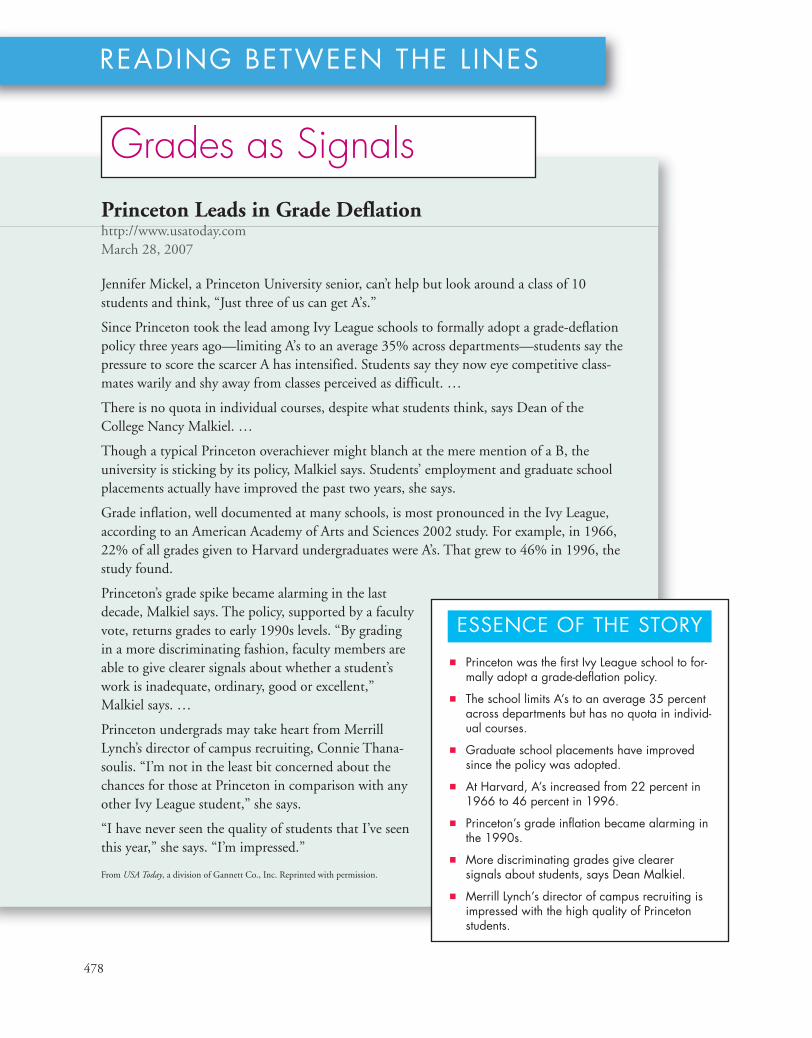
478

READING BETWEEN THE L INES

Princeton Leads in Grade Deflationhttp://www.usatoday.comMarch 28, 2007

Jennifer Mickel, a Princeton University senior, can’t help but look around a class of 10students and think, “Just three of us can get A’s.”

Since Princeton took the lead among Ivy League schools to formally adopt a grade-deflationpolicy three years ago—limiting A’s to an average 35% across departments—students say thepressure to score the scarcer A has intensified. Students say they now eye competitive class-mates warily and shy away from classes perceived as difficult. …

There is no quota in individual courses, despite what students think, says Dean of theCollege Nancy Malkiel. …

Though a typical Princeton overachiever might blanch at the mere mention of a B, theuniversity is sticking by its policy, Malkiel says. Students’ employment and graduate schoolplacements actually have improved the past two years, she says.

Grade inflation, well documented at many schools, is most pronounced in the Ivy League,according to an American Academy of Arts and Sciences 2002 study. For example, in 1966,22% of all grades given to Harvard undergraduates were A’s. That grew to 46% in 1996, thestudy found.

Princeton’s grade spike became alarming in the lastdecade, Malkiel says. The policy, supported by a facultyvote, returns grades to early 1990s levels. “By gradingin a more discriminating fashion, faculty members areable to give clearer signals about whether a student’swork is inadequate, ordinary, good or excellent,”Malkiel says. …

Princeton undergrads may take heart from MerrillLynch’s director of campus recruiting, Connie Thana-soulis. “I’m not in the least bit concerned about thechances for those at Princeton in comparison with anyother Ivy League student,” she says.

“I have never seen the quality of students that I’ve seenthis year,” she says. “I’m impressed.”

From USA Today, a division of Gannett Co., Inc. Reprinted with permission.

■ Princeton was the first Ivy League school to for-mally adopt a grade-deflation policy.

■ The school limits A’s to an average 35 percentacross departments but has no quota in individ-ual courses.

■ Graduate school placements have improvedsince the policy was adopted.

■ At Harvard, A’s increased from 22 percent in1966 to 46 percent in 1996.

■ Princeton’s grade inflation became alarming inthe 1990s.

■ More discriminating grades give clearersignals about students, says Dean Malkiel.

■ Merrill Lynch’s director of campus recruiting isimpressed with the high quality of Princetonstudents.

ESSENCE OF THE STORY

Grades as Signals

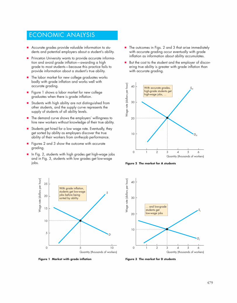
479

ECONOMIC ANALYSIS

Figure 1 Market with grade inflation

0 5 10

25

20

15

10

5

S

D

SL

DL

Wag

e ra

te (d

olla

rs p

er h

our)

Wag

e ra

te (d

olla

rs p

er h

our)

Quantity (thousands of workers)Quantity (thousands of workers)

Figure 3 The market for D students

0 1 2 3 4 6

40

30

20

10

5

SH

DH

Wag

e ra

te (d

olla

rs p

er h

our)

Quantity (thousands of workers)

Figure 2 The market for A students

0 1 2 3 4 6

40

30

20

10

5

With accurate grades,high-grade students gethigh-wage jobs, ...

With grade inflation,students get low-wagejobs before beingsorted by ability

… and low-gradestudents getlow-wage jobs

■ The outcomes in Figs. 2 and 3 that arise immediatelywith accurate grading occur eventually with gradeinflation as information about ability accumulates.

■ But the cost to the student and the employer of discov-ering true ability is greater with grade inflation thanwith accurate grading.

■ Accurate grades provide valuable information to stu-dents and potential employers about a student’s ability.

■ Princeton University wants to provide accurate informa-tion and avoid grade inflation—awarding a highgrade to most students—because this practice fails toprovide information about a student’s true ability.

■ The labor market for new college graduates worksbadly with grade inflation and works well withaccurate grading.

■ Figure 1 shows a labor market for new collegegraduates when there is grade inflation.

■ Students with high ability are not distinguished fromother students, and the supply curve represents thesupply of students of all ability levels.

■ The demand curve shows the employers’ willingness tohire new workers without knowledge of their true ability.

■ Students get hired for a low wage rate. Eventually, theyget sorted by ability as employers discover the trueability of their workers from on-the-job performance.

■ Figures 2 and 3 show the outcome with accurategrading.

■ In Fig. 2, students with high grades get high-wage jobsand in Fig. 3, students with low grades get low-wagejobs.

480 CHAPTER 20 Uncertainty and Information

Key Points

Decisions in the Face of Uncertainty (pp. 466–468)

■ To make a rational choice under uncertainty, peo-ple choose the action that maximizes the expectedutility of wealth.

■ A decreasing marginal utility of wealth makespeople risk averse. A sure outcome with a givenexpected wealth is preferred to a risky outcomewith the same expected wealth—risk is costly.

■ The cost of risk is found by comparing theexpected wealth in a given risky situation with thewealth that gives the same utility but with no risk.

Working Problems 1 to 3 will give you a better under-standing of decisions in the face of uncertainty.

Buying and Selling Risk (pp. 469–471)

■ People trade risk in markets for insurance.■ By pooling risks, insurance companies can reduce the

risks people face (from insured activities) at a lowercost than the value placed on the lower risk.

Working Problems 4 to 6 will give you a better under-standing of buying and selling risk.

Private Information (pp. 472–476)

■ Asymmetric information creates adverse selectionand moral hazard problems.

■ When it is not possible to distinguish good-qualityproducts from lemons, too many lemons and toofew good-quality products are traded in a poolingequilibrium.

■ Signaling can overcome the lemon problem.■ In the market for used cars, warranties signal good

cars and enable an efficient separating equilibrium.■ Private information about credit risk is overcome

by using signals and screening based on personalcharacteristics.

■ Private information about risk in insurance mar-kets is overcome by using the no-claim bonus anddeductibles.

Working Problems 7 to 11 will give you a better under-standing of private information.

Uncertainty, Information, and the Invisible Hand (p. 477)

■ Less uncertainty and more information can beviewed as a good that has increasing marginal costand decreasing marginal benefit.

■ Competitive information markets might be effi-cient, but economies of scale might bring inefficientunderproduction of information and insurance.

Working Problems 12 and 13 will give you a better under-standing of uncertainty, information, and the invisiblehand.

SUMMARY

Key TermsAdverse selection, 472Asymmetric information, 472Credit risk or default risk, 475Expected utility, 467Expected wealth, 466

Lemon problem, 472Moral hazard, 472Pooling equilibrium, 475Private information, 472Risk aversion, 466

Screening, 475Separating equilibrium, 475Signaling, 474

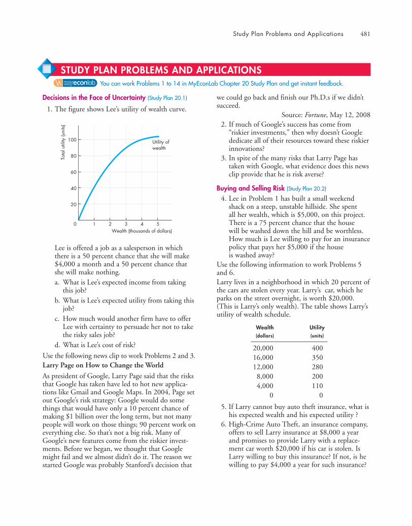
Study Plan Problems and Applications 481

Decisions in the Face of Uncertainty (Study Plan 20.1)

1. The figure shows Lee’s utility of wealth curve.

Lee is offered a job as a salesperson in whichthere is a 50 percent chance that she will make$4,000 a month and a 50 percent chance thatshe will make nothing.a. What is Lee’s expected income from taking

this job? b. What is Lee’s expected utility from taking this

job?c. How much would another firm have to offer

Lee with certainty to persuade her not to takethe risky sales job?

d. What is Lee’s cost of risk?

Use the following news clip to work Problems 2 and 3.Larry Page on How to Change the World

As president of Google, Larry Page said that the risksthat Google has taken have led to hot new applica-tions like Gmail and Google Maps. In 2004, Page setout Google’s risk strategy: Google would do somethings that would have only a 10 percent chance ofmaking $1 billion over the long term, but not manypeople will work on those things; 90 percent work oneverything else. So that’s not a big risk. Many ofGoogle’s new features come from the riskier invest-ments. Before we began, we thought that Googlemight fail and we almost didn’t do it. The reason westarted Google was probably Stanford’s decision that

Tota

l util

ity (u

nits)

Wealth (thousands of dollars)0 1 2 3 4 5

20

40

60

80

100 Utility ofwealth

we could go back and finish our Ph.D.s if we didn’tsucceed.

Source: Fortune, May 12, 20082. If much of Google’s success has come from

“riskier investments,” then why doesn’t Googlededicate all of their resources toward these riskierinnovations?

3. In spite of the many risks that Larry Page hastaken with Google, what evidence does this newsclip provide that he is risk averse?

Buying and Selling Risk (Study Plan 20.2)

4. Lee in Problem 1 has built a small weekendshack on a steep, unstable hillside. She spentall her wealth, which is $5,000, on this project.There is a 75 percent chance that the housewill be washed down the hill and be worthless.How much is Lee willing to pay for an insurancepolicy that pays her $5,000 if the houseis washed away?

Use the following information to work Problems 5and 6.Larry lives in a neighborhood in which 20 percent ofthe cars are stolen every year. Larry’s car, which heparks on the street overnight, is worth $20,000.(This is Larry’s only wealth). The table shows Larry’sutility of wealth schedule.

Wealth Utility(dollars) (units)

20,000 40016,000 35012,000 2808,000 2004,000 110

0 0

5. If Larry cannot buy auto theft insurance, what ishis expected wealth and his expected utility ?

6. High-Crime Auto Theft, an insurance company,offers to sell Larry insurance at $8,000 a yearand promises to provide Larry with a replace-ment car worth $20,000 if his car is stolen. IsLarry willing to buy this insurance? If not, is hewilling to pay $4,000 a year for such insurance?

You can work Problems 1 to 14 in MyEconLab Chapter 20 Study Plan and get instant feedback.

STUDY PLAN PROBLEMS AND APPLICATIONS

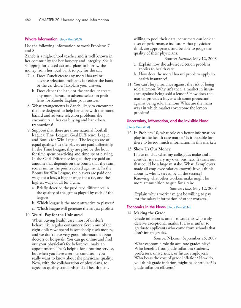
482 CHAPTER 20 Uncertainty and Information

Private Information (Study Plan 20.3)

Use the following information to work Problems 7and 8.Zaneb is a high-school teacher and is well known inher community for her honesty and integrity. She isshopping for a used car and plans to borrow themoney from her local bank to pay for the car.

7. a. Does Zaneb create any moral hazard oradverse selection problems for either the bankor the car dealer? Explain your answer.

b. Does either the bank or the car dealer createany moral hazard or adverse selection prob-lems for Zaneb? Explain your answer.

8. What arrangements is Zaneb likely to encounterthat are designed to help her cope with the moralhazard and adverse selection problems sheencounters in her car buying and bank loantransactions?

9. Suppose that there are three national footballleagues: Time League, Goal Difference League,and Bonus for Win League. The leagues are ofequal quality, but the players are paid differently.In the Time League, they are paid by the hourfor time spent practicing and time spent playing.In the Goal Difference league, they are paid anamount that depends on the points that the teamscores minus the points scored against it. In theBonus for Win League, the players are paid onewage for a loss, a higher wage for a tie, and thehighest wage of all for a win.a. Briefly describe the predicted differences in

the quality of the games played by each of theleagues.

b. Which league is the most attractive to players?c. Which league will generate the largest profits?

10. We All Pay for the UninsuredWhen buying health care, most of us don’tbehave like regular consumers: Seven out of theeight dollars we spend is somebody else’s money,and we don’t have very good information aboutdoctors or hospitals. You can go online and findout your physician’s fee before you make anappointment. That’s helpful for a routine service,but when you have a serious condition, youreally want to know about the physican’s quality.Now, with the collaboration of physicians, toagree on quality standards and all health plans

willing to pool their data, consumers can look ata set of performance indicators that physiciansthink are appropriate, and be able to judge thequality of their physicians.

Source: Fortune, May 12, 2008a. Explain how the adverse selection problem

applies to health care.b. How does the moral hazard problem apply to

health insurance?11. You can’t buy insurance against the risk of being

sold a lemon. Why isn’t there a market in insur-ance against being sold a lemon? How does themarket provide a buyer with some protectionagainst being sold a lemon? What are the mainways in which markets overcome the lemonproblem?

Uncertainty, Information, and the Invisible Hand(Study Plan 20.4)

12. In Problem 10, what role can better informationplay in the health care market? Is it possible forthere to be too much information in this market?

13. Show Us Our MoneyI have no clue what my colleagues make and Iconsider my salary my own business. It turns outthat could be a huge mistake. What if employersmade all employee salaries known? If you thinkabout it, who is served by all the secrecy?Knowing what other workers make might bemore ammunition to gun for a raise.

Source:Time, May 12, 2008Explain why a worker might be willing to payfor the salary information of other workers.

Economics in the News (Study Plan 20.N)

14. Making the GradeGrade inflation is unfair to students who trulydeserve exceptional marks. It also is unfair tograduate applicants who come from schools thatdon’t inflate grades.

Source: NJ.com, September 25, 2007What economic role do accurate grades play?Who benefits from grade inflation: students,professors, universities, or future employers?Who bears the cost of grade inflation? How doyou think grade inflation might be controlled? Isgrade inflation efficient?

Additional Problems and Applications 483

Decisions in the Face of Uncertainty

Use the following table, which shows Jimmy’s andZenda’s utility of wealth schedules, to work Problems15 to 17.

Wealth Jimmy’s utility Zenda’s utility

0 0 0100 200 512200 300 640300 350 672400 375 678500 387 681600 393 683700 396 684

15. What are Jimmy’s and Zenda’s expected utilitiesfrom a bet that gives them a 50 percent chance ofhaving a wealth of $600 and a 50 percent chanceof having nothing?

16. a. Calculate Jimmy’s and Zenda’s marginal utilityof wealth schedules.

b. Who is more risk averse, Jimmy or Zenda?How do you know?

17. Suppose that Jimmy and Zenda each have $400and are offered a business investment opportu-nity that involves committing the entire $400 tothe project. The project could return $600 (aprofit of $200) with a probability of 0.85 or$200 (a loss of $200) with a probability of 0.15.Who goes for the project and who hangs on tothe initial $400?

Use the following information to work Problems 18to 20.Two students, Jim and Kim, are offered summerjobs managing a student house-painting business.There is a 50 percent chance that either of themwill be successful and end up with $21,000 ofwealth to get them through the next school year.But there is also a 50 percent chance that eitherwill end up with only $3,000 of wealth. Each couldtake a completely safe but back-breaking job pick-ing fruit that would leave them with a guaranteed$9,000 at the end of the summer. The table in thenext column shows Jim’s and Kim’s utility of wealthschedules.

Wealth Jim’s utility Kim’s utility

0 0 03,000 100 2006,000 200 3509,000 298 475

12,000 391 56015,000 491 62018,000 586 66021,000 680 680

18. Does anyone take the painting job? If so, whotakes it and why? Does anyone take the job pick-ing fruit? If so, who takes it and why?

19. In Problem 18, what is each student’s maximizedexpected utility? Who has the larger expectedwealth? Who ends up with the larger wealth atthe end of the summer?

20. In Problem 18, if one of the students takes therisky job, how much more would the fruit-pick-ing job have needed to pay to attract that student?

Buying and Selling Risk

Use the following table, which shows Chris’s utility ofwealth schedule, to work Problems 21 and 22.Chris’s wealth is $5,000 and it consists entirely of hershare in a risky ice cream business. If the summer iscold, the business will fail, and she will have nowealth. Where Chris lives there is a 50 percentchance each year that the summer will be cold.

Wealth Utility

(dollars) (units)

5,000 1504,000 1403,000 1202,000 901,000 50

0 021. If Chris cannot buy cold summer insurance,

what is her expected wealth and what is herexpected utility?

22. Business Loss Recovery, an insurance company, iswilling to sell Chris cold summer insurance at aprice of $3,000 a year and promises to pay her

You can work these problems in MyEconLab if assigned by your instructor.

ADDITIONAL PROBLEMS AND APPLICATIONS

484 CHAPTER 20 Uncertainty and Information

$5,000 if the summer is cold and the businessfails. Is Chris willing to buy this loss insurance? Ifshe is, is she willing to pay $4,000 a year for it?

Private InformationUse the following information to work Problems 23to 25.Larry has a good car that he wants to sell; Harry has alemon that he wants to sell. Each knows what type ofcar he is selling. You are looking at used cars and planto buy one.

23. If both Larry and Harry are offering their cars forsale at the same price, from whom would youmost want to buy, Larry or Harry, and why?

24. If you made an offer of the same price to Larryand Harry, who would sell to you and why?Describe the adverse selection problem that arisesif you offer the same price to Larry and Harry.

25. How can Larry signal that he is selling a good carso that you are willing to pay Larry the price thathe knows his car is worth, and a higher pricethan what you are willing to offer Harry?

26. Pam is a safe driver and Fran is a reckless driver.Each knows what type of driver she is, but noone else knows. What might an automobileinsurance company do to get Pam to signal thatshe is a safe driver so that it can offer her insur-ance at a lower premium than it offers to Fran?

27. Why do you think it is not possible to buy insur-ance against having to put up with a low-paying,miserable job? Explain why a market in insuranceof this type would be valuable to workers butunprofitable for an insurance provider and sowould not work.

Uncertainty, Information, and the Invisible HandUse the following news clip to work Problems 28 and 29.

Why We Worry About the Things We Shouldn’t …and Ignore the Things We ShouldWe pride ourselves on being the only species thatunderstands the concept of risk, yet we have a con-founding habit of worrying about mere possibilitieswhile ignoring probabilities, building barricadesagainst perceived dangers while leaving ourselvesexposed to real ones: 20% of all adults still smoke;nearly 20% of drivers and more than 30% of back-seat passengers don’t use seat belts; two thirds of us

are overweight or obese. We dash across the streetagainst the light and build our homes in hurricane-prone areas—and when they’re demolished by astorm, we rebuild in the same spot.

Source: Time, December 4, 200628. Explain how “worrying about mere possibilities

while ignoring probabilities” can result in peoplemaking decisions that not only fail to satisfysocial interest, but also fail to satisfy self-interest.

29. How can information be used to improve peo-ple’s decision making?

Economics in the News30. After you have studied Reading Between the Lines

on pp. 478–479 answer the following questions.a. What information do accurate grades provide

that grade inflation hides?b. If grade inflation became widespread in high

schools, colleges, and universities, what newarrangements do you predict would emerge to provide better information about studentability?

c. Do you think grade inflation is in anyone’sself-interest? Explain who benefits and howthey benefit from grade inflation.

d. How do you think grade inflation might becontrolled?

31. Are You Paid What You’re Worth?How do you know if your pay adequately reflectsyour contributions to your employer’s profits? Inmany instances, you don’t. Your employer hasmore and better information than you do abouthow your salary and bonus compare to others inyour field, to others in your office, and relative tothe company’s profits in any given year. You cannarrow the information gap a bit if you’re willingto buy salary reports from compensation sources.For example, at $200, a quick-call salary reportfrom Economic Research Institute will offer youcompensation data for your position based onyour years of experience, your industry and theplace where your company is located.

Source: CNN, April 3, 2006a. Explain the role that asymmetric information

can play in worker wages.b. What adverse selection problem exists if a firm

offers lower wages to existing workers?c. What will determine how much a worker

should actually pay for a detailed salary report?

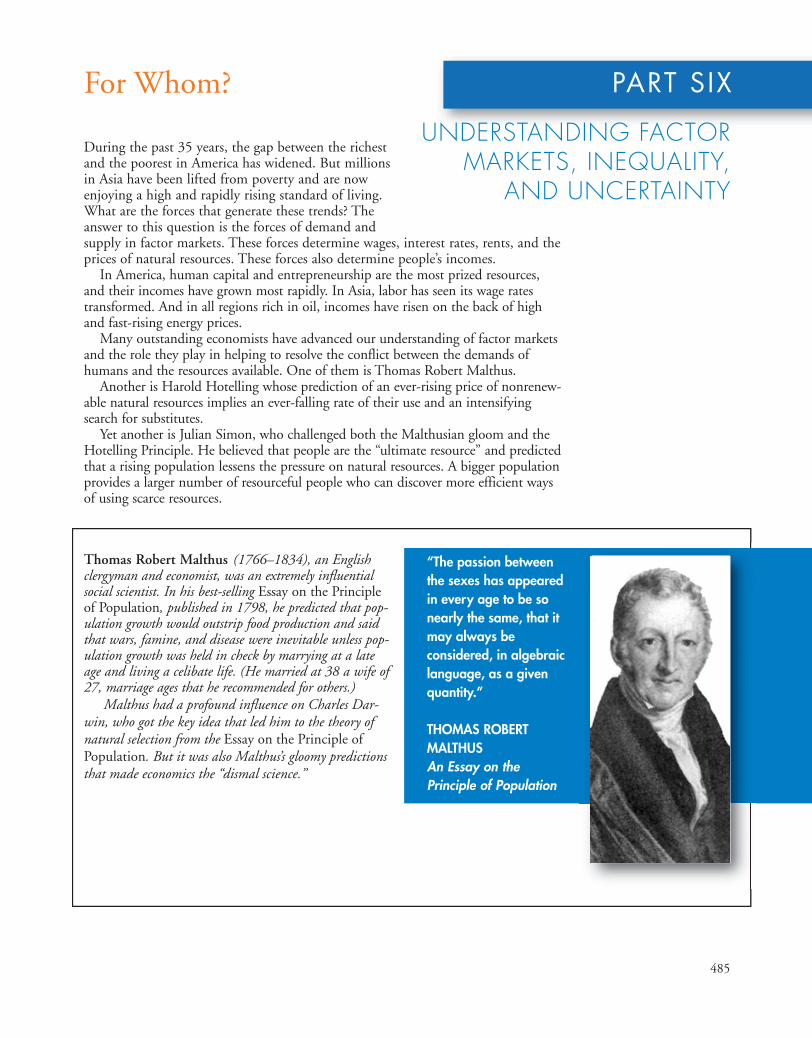
Thomas Robert Malthus (1766–1834), an Englishclergyman and economist, was an extremely influentialsocial scientist. In his best-selling Essay on the Principleof Population, published in 1798, he predicted that pop-ulation growth would outstrip food production and saidthat wars, famine, and disease were inevitable unless pop-ulation growth was held in check by marrying at a lateage and living a celibate life. (He married at 38 a wife of27, marriage ages that he recommended for others.)

Malthus had a profound influence on Charles Dar-win, who got the key idea that led him to the theory ofnatural selection from the Essay on the Principle ofPopulation. But it was also Malthus’s gloomy predictionsthat made economics the “dismal science.”

485

For Whom?

During the past 35 years, the gap between the richestand the poorest in America has widened. But millionsin Asia have been lifted from poverty and are nowenjoying a high and rapidly rising standard of living.What are the forces that generate these trends? Theanswer to this question is the forces of demand andsupply in factor markets. These forces determine wages, interest rates, rents, and theprices of natural resources. These forces also determine people’s incomes.

In America, human capital and entrepreneurship are the most prized resources,and their incomes have grown most rapidly. In Asia, labor has seen its wage ratestransformed. And in all regions rich in oil, incomes have risen on the back of highand fast-rising energy prices.

Many outstanding economists have advanced our understanding of factor marketsand the role they play in helping to resolve the conflict between the demands ofhumans and the resources available. One of them is Thomas Robert Malthus.

Another is Harold Hotelling whose prediction of an ever-rising price of nonrenew-able natural resources implies an ever-falling rate of their use and an intensifyingsearch for substitutes.

Yet another is Julian Simon, who challenged both the Malthusian gloom and theHotelling Principle. He believed that people are the “ultimate resource” and predictedthat a rising population lessens the pressure on natural resources. A bigger populationprovides a larger number of resourceful people who can discover more efficient waysof using scarce resources.

PART SIX

UNDERSTANDING FACTORMARKETS, INEQUALITY,

AND UNCERTAINTY

“The passion betweenthe sexes has appearedin every age to be sonearly the same, that itmay always beconsidered, in algebraiclanguage, as a givenquantity.”

THOMAS ROBERTMALTHUSAn Essay on thePrinciple of Population

486

single parents in the treatment group of SSP, we caninfer that the financial incentives of SSP caused peo-ple to work more.

Most often, we don’t have an experiment. We seea group of people who are subject to some “treat-ment” (such as a higher minimum wage) and we tryto construct a comparison group by finding someother group similar to the treatment group who tellus what the treatment group would have looked likein the absence of treatment. If we can’t find a com-pelling comparison group, we have to be cautious.

In your book on the minimum wage with AlanKrueger, you reported that an increase in the minimumwage increased employment—the opposite of the con-ventional wisdom. How did you reach that conclusion?

TALKING WITH David Card

Professor Card, what attracted you to economics? When I went to university I had no intention of study-ing economics: I was planning to be a physics major. Iwas helping a friend with her problem set and startedreading the supply and demand section of the textbook.I was impressed with how well the model seemed todescribe the paradox that a bumper crop can be bad forfarmers. I read most of the book over the next few days.The next year, I signed up as an economics major.

Almost all your work is grounded in data. You are an em-pirical economist. How do you go about your work, wheredo your data come from, and how do you use data? The data I use come from many different sources. Ihave collected my own data from surveys; transcribeddata from historical sources and government publica-tions; and used computerized data files based onrecords from Censuses and surveys in the UnitedStates, Canada, Britain, and other countries.

An economist can do three things with data. Thefirst is to develop simple statistics on basic questionssuch as “What fraction of families live in poverty?” Forthis, one needs to understand how the data were col-lected and processed and how the questions were asked.For example, the poverty rate depends on how youdefine a “family.” If a single mother and her child livewith the mother’s parents, the income of the motherand the grandparents is counted as “family income.”

The second thing economists do with data isdevelop descriptive comparisons. For example, I havecompared the wage differences between male andfemale workers. Again, the details are important. Forexample, the male-female wage differential is muchbigger if you look at annual earnings than at earningsper hour, because women work fewer hours per year.

Once you’ve established some simple facts, youstart to get ideas for possible explanations. You can alsorule out a lot of other ideas.

The third and most difficult thing that empiricaleconomists try to do is infer a causal relationship. Inrare instances, we have a true experiment in which arandom subgroup of volunteers is enrolled in a “treat-ment group” and the remainder become the “controlgroup.” The Self Sufficiency Program (SSP)—anexperimental welfare reform demonstration inCanada—was conducted this way. Because of randomassignment, we know that the treatment and controlgroups would have looked very similar in the absenceof the treatment. Thus when we see a difference inbehavior, such as the higher level of work activity by

487

DAVID CARD is Class of 1950 Professor ofEconomics and Director of the Center for LaborEconomics at the University of California, Berkeley,and Faculty Research Associate at the NationalBureau of Economic Research.

Born in Canada, Professor Card obtained hisB.A. at Queen’s University, Kingston, Ontario, in1977 and his Ph.D. at Princeton University in 1983.He has received many honors, the most notable ofwhich is the American Economic Association’s JohnBates Clark Prize, awarded to the best economistunder 40.

Professor Card’s research on labor markets andthe effects of public policies on earnings, jobs, andthe distribution of income has produced around 150articles and several books. His most recent book (co-edited with Alan Auerbach and John Quigley) isPoverty, the Distribution of Income, and Public Poli-cy (New York: Russell Sage Foundation, 2006). Anearlier book (co-authored with Alan B. Krueger),Myth and Measurement: The New Economics of theMinimum Wage (Princeton, NJ: Princeton Universi-ty Press, 1995), made a big splash and upset oneof the most fundamental beliefs about the effects ofminimum wages.

Michael Parkin talked with David Card abouthis work and the progress that economists havemade in understanding how public policies can in-fluence the distribution of income and economicwell-being.

We studied several instances where minimum wageswere raised in one place but not in another. Forexample, when we found out that the New Jersey leg-islature had recently voted to raise the minimumwage, we set up a survey of fast-food restaurants inNew Jersey and in nearby parts of Pennsylvania. We

surveyed the storesa few monthsbefore the NewJersey minimumwent up and thenagain one year

later, after the minimum had been raised. The first-round survey found that conditions were very similarin the two states. In the second round, we found thatalthough wages were now higher in New Jersey,employment was also slightly higher. It was very

important to have the first-round survey to bench-mark any differences that existed prior to the rise inthe minimum. Thus, we argued that any differentialchanges in New Jersey relative to Pennsylvania fromthe first round to the second round were most plausi-bly due to the minimum wage.

How did you explain what you found? We argued that many employers in New Jersey beforethe rise in the minimum were operating with vacan-cies and would have liked to hire more workers butcould not do so without raising their wages. In thissituation, an increase in the minimum wage cancause some employers to hire more and others to hireless. On average, the net effect on employment canbe small. What we saw was a rise in wages and areduction in vacancies in New Jersey, coupled with asmall gain in employment.

You’ve examined just about every labor market policy.Let’s talk about welfare payments to single mothers:How do they influence labor market decisions? The Self Sufficiency Program welfare demonstrationin Canada tested an earnings subsidy as an alternativeto conventional welfare payments. The problem withconventional welfare is that recipients have no incen-tive to work: If they earn $1, their payments arereduced by $1. That led Milton Friedman in the early1950s to advocate an alternative “negative incometax” program, such as SSP, in which recipients whoearn more only lose a fraction of their benefits (in thecase of SSP, 50 cents per dollar earned). The resultsshowed that this alternative system encourages singleparents to work more.

Immigration has been big news in recent years. Canyou describe your work on this issue and your findings? My research has tried to understand whether thearrival of low-skilled immigrants hurts the labor mar-ket opportunities for less-skilled natives. One of mypapers studies the effect of the Mariel Boatlift, whichoccurred in 1980 following a political uprising thatled Fidel Castro to declare that people who wanted toleave Cuba were free to exit from the port of Mariel.Within days, a flotilla of small boats from the UnitedStates began transporting people to Miami, and150,000 people eventually left. Over one half stayedin Miami, creating a huge “shock” to the supply of

The most difficult thing thatempirical economists try to dois infer a causal relationship.

488

low-skilled labor. I studied the effect by looking atwages and unemployment rates for various groups inMiami and in a set of comparison cities that had verysimilar wage and employment trends in the previousdecade. I found that the influx of the boatlift had nodiscernible effect on wages or unemployment ofother workers in Miami. My later work has con-firmed that the Miami story seems to hold in mostother cities. Cities can absorb big inflows of low-skilled immigrants with remarkably little negative

impact on natives.

The distribution ofincome has becomeincreasingly unequal.Do we know why? There are manysources. Familyincomes have become

more unequal in part because of a rise in familieswith two very high-wage earners. These families havepulled away from the rest, creating a widening distri-bution. The very richest families, whose incomes areabove the 95th or 99th percentile of the income dis-tribution, earn an increasingly large share of nationalincome. The trends in income for this group accountfor most of the rise in inequality we have seen in thelast 10 years.

Unfortunately, it is very hard to study this groupbecause they represent such a small fraction of fami-lies, and they are often under-reported on surveys.The best available data, from tax returns, don’t tell usmuch about the sources of this group’s success,though it seems to be due to labor market earningsrather than to previous investments or family wealth.

There is a large literature on wage inequalityamong the larger “middle” of the population: peoplewho earn up to $150,000 per year, for example.Wage inequality for men in this group rose verysharply in the early 1980s in the United States, rose a

little more between 1985 and 1990, and was fairlystable (or even decreasing) in the 1990s. Some of therise in the 1980s was due to decreases in unioniza-tion, and some was due to the changing effects of theminimum wage, which fell in real terms in the early1980s, and then gained in the early to mid-1990s.

Some researchers ascribe the rest of the trend inwage inequality to the spread of computers andincreasing demands for highly skilled workers. Othersblame international trade and, most recently, immi-gration. Those explanations are hard to evaluatebecause we don’t really see the forces of new technol-ogy or trade that affect any particular worker. Onething we do know is that wage inequality trends werequite different in many other countries. Canada, forinstance, had relatively modest rises in inequality inthe 1980s.

What advice do you have for someone who is just be-ginning to study economics? What other subjects doyou think work well alongside economics? Do youhave some reading suggestions? The part of economics that most interests me is thebehavior of people in their everyday life. People con-stantly have to answer questions such as: Should I getmore education? How much should I save? Should Isend my children to the local public school? It’sextremely important to see how these questions areanswered by different people: people from poorerfamilies or other countries or who had to make verydifferent choices. Take any opportunity to find outwhat life is like for other people. You can learn a lotfrom reading novels, spending a year abroad, or tak-ing classes in sociology or history. The best econo-mists are observant and thoughtful social scientists.My other piece of advice is study mathematics. Themore mathematics training you have, the more easilyyou can understand what economists are doing.Newton invented calculus to study the motion ofplanets, but economics benefits from the same tools.

... find out what life is likefor other people. ... Thebest economists areobservant and thoughtfulsocial scientists.

G-1

GLOSSARY

Absolute advantage A person has anabsolute advantage if that person ismore productive than another person.(p. 38)Adverse selection The tendency forpeople to enter into agreements inwhich that can use their private infor-mation to their own advantage and tothe disadvantage of the uninformedparty. (p. 472)Allocative efficiency A situation inwhich goods and services are pro-duced at the lowest possible cost andin the quantities that provide thegreatest possible benefit. We cannotproduce more of any good withoutgiving up some of another good thatwe value more highly. (p. 33)Antitrust law A law that regulatesoligopolies and prevents them frombecoming monopolies or behavinglike monopolies. (p. 356)Asymmetric information A marketin which buyers and sellers have pri-vate information. (p. 472)Average cost pricing rule A rule thatsets price to cover cost including nor-mal profit, which means setting theprice equal to average total cost. (p. 314)Average fixed cost Total fixed costper unit of output. (p. 258)Average product The average prod-uct of a factor of production. It equalstotal product divided by the quantityof the factor employed. (p. 253)Average total cost Total cost per unitof output. (p. 258)Average variable cost Total variablecost per unit of output. (p. 258)

Barrier to entry A natural or legalconstraint that protects a firm frompotential competitors. (p. 300)Behavioral economics A study of theways in which limits on the humanbrain’s ability to compute and imple-ment rational decisions influenceseconomic behavior—both the deci-sions that people make and the conse-quences of those decisions for the waymarkets work. (p. 194)Benefit The benefit of something isthe gain or pleasure that it brings andis determined by preferences. (p. 8)

Big tradeoff The tradeoff betweenequality and efficiency. (pp. 117, 456)Bilateral monopoly A situation inwhich a monopoly seller faces amonopsony buyer. (p. 425)Black market An illegal market inwhich the price exceeds the legallyimposed price ceiling. (p. 128)Budget line The limit to a house-hold’s consumption choices. It marksthe boundary between those combina-tions of goods and services that ahousehold can afford to buy and thosethat it cannot afford. (pp. 180, 204)

Capital The tools, equipment, build-ings, and other constructions thatbusinesses use to produce goods andservices. (p. 4)Capital accumulation The growth ofcapital resources, including humancapital. (p. 36)Capture theory A theory that regula-tion serves the self-interest of the pro-ducer, who captures the regulator andmaximizes economic profit. (p. 313)Cartel A group of firms actingtogether—colluding— to limit out-put, raise the price, and increase eco-nomic profit. (p. 343)Ceteris paribus Other things beingequal—all other relevant thingsremaining the same. (p. 22)Change in demand A change inbuyers’ plans that occurs when someinfluence on those plans other thanthe price of the good changes. It isillustrated by a shift of the demandcurve. (p. 58)

Change in supply A change in sell-er’s plans that occurs when someinfluence on those plans other thanthe price of the good changes. It isillustrated by a shift of the supplycurve. (p. 63)

Change in the quantity demandedA change in buyers’ plans that occurswhen the price of a good changes butall other influences on buyers’ plansremain unchanged. It is illustrated bya movement along the demand curve.(p. 61)

Change in the quantity supplied Achange in sellers’ plans that occurswhen the price of a good changes but

all other influences on sellers’ plansremain unchanged. It is illustrated bya movement along the supply curve.(p. 64)

Coase theorem The proposition thatif property rights exist, if only a smallnumber of parties are involved, andtransactions costs are low, then privatetransactions are efficient. (p. 397)

Collusive agreement An agreementbetween two (or more) producers toform a cartel to restrict output, raisethe price, and increase profits. (p. 346)Command system A method of allo-cating resources by the order (com-mand) of someone in authority. In afirm a managerial hierarchy organizesproduction. (pp. 106, 233)Common resource A resource that isrival and nonexcludable. (p. 374)Comparative advantage A person orcountry has a comparative advantagein an activity if that person or countrycan perform the activity at a loweropportunity cost than anyone else orany other country. (p. 38)Competitive market A market thathas many buyers and many sellers, sono single buyer or seller can influencethe price. (p. 56)Complement A good that is used inconjunction with another good. (p. 59)Compound interest The interest onan initial investment plus the intereston the interest that the investment haspreviously earned. (p. 434)

Constant returns to scale Features ofa firm’s technology that lead to con-stant long-run average cost as outputincreases. When constant returns toscale are present, the LRAC curve ishorizontal. (p. 264)Consumer equilibrium A situationin which a consumer has allocated allhis or her available income in the waythat, given the prices of goods andservices, maximizes his or her totalutility. (p. 183)Consumer surplus The excess of thebenefit received from a good over theamount paid for it. It is calculated asthe marginal benefit (or value) of agood minus its price, summed overthe quantity bought. (p. 109)

G-2 Glossary

Contestable market A market inwhich firms can enter and leave soeasily that firms in the market facecompetition from potential entrants.(p. 354)Cooperative equilibrium The out-come of a game in which the playersmake and share the monopoly profit.(p. 353)Credit risk The risk that a borrower,also known as a creditor, might notrepay a loan. (p. 475)

Cross elasticity of demand Theresponsiveness of the demand for agood to a change in the price of a sub-stitute or complement, other thingsremaining the same. It is calculated asthe percentage change in the quantitydemanded of the good divided by thepercentage change in the price of thesubstitute or complement. (p. 91)

Deadweight loss A measure of ineffi-ciency. It is equal to the decrease intotal surplus that results from an inef-ficient level of production. (p. 113)

Default risk The risk that a borrow-er, also known as a creditor, might notrepay a loan. (p. 475)Demand The entire relationshipbetween the price of the good and thequantity demanded of it when allother influences on buyers’ plansremain the same. It is illustrated by ademand curve and described by ademand schedule. (p. 57)

Demand curve A curve that showsthe relationship between the quantitydemanded of a good and its pricewhen all other influences on con-sumers’ planned purchases remain thesame. (p. 58)

Deregulation The process of remov-ing regulation of prices, quantities,entry, and other aspects of economicactivity in a firm or industry. (p. 313)

Derived demand Demand for a fac-tor of production—it is derived fromthe demand for the goods and servicesproduced by that factor. (p. 419)Diminishing marginal rate of sub-stitution The general tendency for aperson to be willing to give up less ofgood y to get one more unit of goodx, while at the same time remainingindifferent as the quantity of good xincreases. (p. 208)

Diminishing marginal returns Thetendency for the marginal product ofan additional unit of a factor of pro-duction to be less than the marginalproduct of the previous unit of thefactor. (p. 255)Diminishing marginal utility Thetendency for marginal utility todecrease as the quantity consumed ofa good increases. (p. 182)Direct relationship A relationshipbetween two variables that move inthe same direction. (p. 16)

Discounting The calculation we useto convert a future amount of moneyto its present value. (p. 434)

Diseconomies of scale Features of afirm’s technology that make averagetotal cost rise as output increases—theLRAC curve slopes upward.(p. 264)Doha Development Agenda (DohaRound) Negotiations held in Doha,Qatar, to lower tariff barriers and quo-tas that restrict international trade infarm products and services. (p. 162) Dominant strategy equilibrium Anequilibrium in which the best strategyfor each player is to cheat regardless ofthe strategy of the other player. (p. 345)Dumping The sale by a foreign firmof exports at a lower price than thecost of production. (p. 163)Duopoly A market structure inwhich two producers of a good orservice compete. (p. 342)

Economic depreciation The fall inthe market value of a firm’s capitalover a given period. (p. 229)Economic efficiency A situation thatoccurs when the firm produces a givenoutput at the least cost. (p. 231)Economic growth The expansion ofproduction possibilities. (p. 36)Economic model A description ofsome aspect of the economic worldthat includes only those features ofthe world that are needed for the pur-pose at hand. (p. 10)Economic profit A firm’s total rev-enue minus its total cost, with totalcost measured as the opportunity costof production. (p. 228)Economic rent Any surplus—con-sumer surplus, producer surplus oreconomic profit. (p. 308)

Economics The social science thatstudies the choices that individuals,businesses, governments, and entiresocieties make as they cope withscarcity and the incentives that influ-ence and reconcile those choices. (p. 2)

Economies of scale Features of afirm’s technology that make averagetotal cost fall as output increases—theLRAC curve slopes downward. (pp. 242, 264)

Economies of scope Decreases inaverage total cost that occur when afirm uses specialized resources to pro-duce a range of goods and services. (p. 243)

Efficiency A situation in which theavailable resources are used to producegoods and services at the lowest possi-ble cost and in quantities that give thegreatest value or benefit. (p. 5)

Efficient scale The quantity at whichaverage total cost is a minimum—thequantity at the bottom of the U-shaped ATC curve. (p. 328)

Elastic demand Demand with aprice elasticity greater than 1; otherthings remaining the same, the per-centage change in the quantitydemanded exceeds the percentagechange in price. (p. 87)

Elasticity of supply The responsive-ness of the quantity supplied of agood to a change in its price, otherthings remaining the same. (p. 94)

Entrepreneurship The humanresource that organizes the other threefactors of production: labor, land, andcapital. (p. 4)

Equilibrium price The price atwhich the quantity demanded equalsthe quantity supplied. (p. 66)

Equilibrium quantity The quantitybought and sold at the equilibriumprice. (p. 66)

Excess capacity A firm has excesscapacity if it produces below its effi-cient scale. (p. 328)

Excludable A good or service or aresource is excludable if it is possibleto prevent someone from enjoying thebenefit of it. (p. 374)

Expected utility The utility value ofwhat a person expects to own at agiven point in time. (p. 467)

G-2 Glossary

Glossary G-3

Expected wealth The money value ofwhat a person expects to own at agiven point in time. (p. 466)

Exports The goods and services thatwe sell to people in other countries.(p. 152)

External diseconomies Factors out-side the control of a firm that raise thefirm’s costs as the market outputincreases. (p. 287)

External economies Factors beyondthe control of a firm that lower thefirm’s costs as the market outputincreases. (p. 287)

Externality A cost (external cost) or abenefit (external benefit) that arisesfrom production or consumption of aprivate good and that falls on some-one other than its producer or con-sumer. (p. 374)

Factors of production The produc-tive resources used to produce goodsand services. (p. 3)Firm An economic unit that hiresfactors of production and organizesthose factors to produce and sellgoods and services. (pp. 41, 228)Four-firm concentration ratio Ameasure of market power that is cal-culated as the percentage of the valueof sales accounted for by the fourlargest firms in an industry. (p. 238)

Free-rider problem The problemthat the market would provide aninefficiently small quantity of a publicgood. (p. 377)

Game theory A set of tools forstudying strategic behavior—behaviorthat takes into account the expectedbehavior of others and the recognitionof mutual interdependence. (p. 344)

General Agreement on Tariffs andTrade (GATT) An internationalagreement signed in 1947 to reducetariffs on international trade. (p. 159)

Gini ratio The ratio of the areabetween the line of equality and theLorenz curve to the entire areabeneath the line of equality. (p. 445)

Goods and services The objects thatpeople value and produce to satisfyhuman wants. (p. 3)

Government failure A situation inwhich government actions lead toinefficiency—to either underprovisionor overprovision. (p. 372)

Herfindahl–Hirschman Index Ameasure of market power that is cal-culated as the square of the marketshare of each firm (as a percentage)summed over the largest 50 firms (orover all firms if there are fewer than50) in a market. (p. 238)Hotelling Principle The idea thattraders expect the price of a nonre-newable natural resource to rise at arate equal to the interest rate. (p. 430)

Human capital The knowledge andskill that people obtain from educa-tion, on-the-job training, and workexperience. (p. 3)

Implicit rental rate The firm’sopportunity cost of using its own cap-ital. (p. 228)Import quota A restriction that lim-its the maximum quantity of a goodthat may be imported in a given peri-od. (p. 160)Imports The goods and services thatwe buy from people in other coun-tries. (p. 152)

Incentive A reward that encouragesan action or a penalty that discouragesone. (p. 2)

Incentive system A method oforganizing production that uses amarket-like mechanism inside thefirm. (p. 233)

Income effect The effect of a changein income on buying plans, otherthings remaining the same. (p. 213)

Income elasticity of demand Theresponsiveness of demand to a changein income, other things remaining thesame. It is calculated as the percentagechange in the quantity demandeddivided by the percentage change inincome. (p. 92)

Indifference curve A line that showscombinations of goods among whicha consumer is indifferent. (p. 207)

Individual transferable quota (ITQ)A production limit that is assigned toan individual who is free to transfer(sell) the quota to someone else. (p. 404)

Inelastic demand A demand with aprice elasticity between 0 and 1; thepercentage change in the quantitydemanded is less than the percentagechange in price. (p. 86)

Infant-industry argument The argu-ment that it is necessary to protect anew industry to enable it to grow intoa mature industry that can compete inworld markets. (p. 163)

Inferior good A good for whichdemand decreases as income increases.(p. 60)

Intellectual property rights Propertyrights for discoveries owned by thecreators of knowledge. (p. 385)

Interest The income that capitalearns. (p. 4)

Inverse relationship A relationshipbetween variables that move in oppo-site directions. (p. 17)

Job A contract for the trade of laborservices. (p. 418)

Labor The work time and workeffort that people devote to producinggoods and services. (p. 3)Labor union An organized group ofworkers that aims to increase the wagerate and influence other job condi-tions. (p. 424)Land The “gifts of nature” that weuse to produce goods and services. (p. 3)Law of demand Other thingsremaining the same, the higher theprice of a good, the smaller is thequantity demanded of it; the lowerthe price of a good, the larger is thequantity demanded of it. (p. 57)Law of diminishing returns As a firmuses more of a variable factor of pro-duction with a given quantity of thefixed factor of production, the marginalproduct of the variable factor of pro-duction eventually diminishes. (p. 255)Law of supply Other things remain-ing the same, the higher the price of agood, the greater is the quantity sup-plied of it. (p. 62)Legal monopoly A market in whichcompetition and entry are restrictedby the granting of a public franchise,government license, patent, or copy-right. (p. 300)

Glossary G-3

G-4 Glossary

Lemon problem The problem thatin a market in which it is not possibleto distinguish reliable products fromlemons, there are too many lemonsand too few reliable products traded.(p. 472)Limit pricing The practice of settingthe price at the highest level thatinflicts a loss on an entrant. (p. 355)Linear relationship A relationshipbetween two variables that is illustrat-ed by a straight line. (p. 16)Long run The time frame in whichthe quantities of all factors of produc-tion can be varied. (p. 252)Long-run average cost curve Therelationship between the lowest attain-able average total cost and outputwhen the firm can change both theplant it uses and the quantity of laborit employs. (p. 263)Long-run market supply curve Acurve that shows how the quantitysupplied in a market varies as the mar-ket price varies after all the possibleadjustments have been made, includ-ing changes in each firm’s plant andthe number of firms in the market. (p. 287)Lorenz curve A curve that graphs thecumulative percentage of income orwealth against the cumulative percent-age of households. (p. 443)

Macroeconomics The study of theperformance of the national economyand the global economy. (p. 2)Margin When a choice is made bycomparing a little more of somethingwith its cost, the choice is made at themargin. (p. 9)Marginal benefit The benefit that aperson receives from consuming onemore unit of a good or service. It ismeasured as the maximum amountthat a person is willing to pay for onemore unit of the good or service. (pp. 9, 34)Marginal benefit curve A curve thatshows the relationship between themarginal benefit of a good and thequantity of that good consumed. (p. 34)Marginal cost The opportunity cost ofproducing one more unit of a good orservice. It is the best alternative for-gone. It is calculated as the increase in

total cost divided by the increase inoutput. (pp. 9, 33, 258)

Marginal cost pricing rule A rulethat sets the price of a good or serviceequal to the marginal cost of produc-ing it. (p. 313)

Marginal external benefit The bene-fit from an additional unit of a goodor service that people other than theconsumer enjoy. (p. 381)

Marginal external cost The cost ofproducing an additional unit of agood or service that falls on peopleother than the producer. (p. 395)

Marginal private benefit The bene-fit from an additional unit of a goodor service that the consumer of thatgood or service receives. (p. 381)

Marginal private cost The cost ofproducing an additional unit of agood or service that is borne by theproducer of that good or service. (p. 395)

Marginal product The increase intotal product that results from a one-unit increase in the variable input,with all other inputs remaining thesame. It is calculated as the increase intotal product divided by the increasein the variable input employed, whenthe quantities of all other inputsremain the same. (p. 253)

Marginal rate of substitution Therate at which a person will give upgood y (the good measured on the y-axis) to get an additional unit of goodx (the good measured on the x-axis)while at the same time remainingindifferent (remaining on the sameindifference curve) as the quantity ofx increases. (p. 208)

Marginal revenue The change intotal revenue that results from a one-unit increase in the quantity sold. It iscalculated as the change in total rev-enue divided by the change in quanti-ty sold. (p. 274)

Marginal social benefit The margin-al benefit enjoyed by society—by theconsumer of a good or service (mar-ginal private benefit) plus the margin-al benefit enjoyed by others (marginalexternal benefit). (p. 381)

Marginal social cost The marginalcost incurred by the producer and byeveryone else on whom the costfalls—by society. It is the sum of mar-

ginal private cost and marginal exter-nal cost. (p. 395)Marginal utility The change in totalutility resulting from a one-unitincrease in the quantity of a goodconsumed. (p. 181)Marginal utility per dollar Themarginal utility from a good thatresults from spending one more dollaron it. It is calculated as the marginalutility from the good divided by itsprice. (p. 184)Market Any arrangement thatenables buyers and sellers to get infor-mation and to do business with eachother. (p. 42)Market failure A situation in whicha market delivers an inefficient out-come. (p. 113)Market income The wages, interest,rent, and profit earned in factor mar-kets and before paying income taxes.(p. 442)Markup The amount by which thefirm’s price exceeds its marginal cost.(p. 329)Microeconomics The study of thechoices that individuals and businessesmake, the way these choices interactin markets, and the influence of gov-ernments. (p. 2)Minimum efficient scale The small-est quantity of output at which thelong-run average cost reaches its low-est level. (p. 265)Minimum wage A regulation thatmakes the hiring of labor below aspecified wage rate illegal. The lowestwage at which a firm may legally hirelabor. (p. 131)Mixed good A private good the pro-duction or consumption of which cre-ates an externality. (p. 374)Money Any commodity or tokenthat is generally acceptable as themeans of payment. (p. 42)Money income Market income pluscash payments to households by thegovernment. (p. 442)Money price The number of dollarsthat must be given up in exchange fora good or service. (p. 56)Monopolistic competition A marketstructure in which a large number offirms make similar but slightly differ-ent products and compete on product

Glossary G-5

quality, price, and marketin, and firmsare free to enter or exit the market.(pp. 237, 324)Monopoly A market structure inwhich there is one firm, which pro-duces a good or service that has noclose substitutes and in which thefirm is protected from competition bya barrier preventing the entry of newfirms. (pp. 237, 300)Monopsony A market in which thereis a single buyer. (p. 425)Moral hazard A tendency for peoplewith private information, after enteringinto an agreement, to use that informa-tion for their own benefit and at thecost of the less-informed party. (p. 472)

Nash equilibrium The outcome of agame that occurs when player A takesthe best possible action given theaction of player B and player B takesthe best possible action given theaction of player A. (p. 345)Natural monopoly A market inwhich economies of scale enable onefirm to supply the entire market at thelowest possible cost. (p. 300)Natural monopoly good A goodthat is nonrival and excludable. Whenbuyers can be excluded if they don’tpay but the good is nonrival, marginalcost is zero. (p. 374)Negative externality An externalitythat arises from either production orconsumption and that imposes anexternal cost. (p. 374)Negative relationship A relationshipbetween variables that move in oppo-site directions. (p. 17)Neuroeconomics The study of theactivity of the human brain when aperson makes an economic decision.(p. 195)Nonexcludable A good or service ora resource is nonexcludable if it isimpossible (or extremely costly) toprevent someone from enjoying itsbenefits. (p. 374)Nonrenewable natural resourcesNatural resources that can be usedonly once. (p. 418)Nonrival A good or service or aresource is nonrival if its use by oneperson does not decrease the quantityavailable for someone else. (p. 374)

Normal good A good for whichdemand increases as income increases.(p. 60)Normal profit The return to entre-preneurship is normal profit and it isthe profit that an entrepreneur earnson average. (p. 229)

Offshore outsourcing A U.S. firmbuys finished goods, components, orservices from other firms in othercountries. (p. 165)Offshoring A U.S. firm hires foreignlabor and produces in a foreign coun-try or a U.S. firm buys finished goods,components, or services from firms inother countries. (p. 165)Oligopoly A market structure inwhich a small number of firms com-pete. (pp. 237, 342)Opportunity cost The highest-val-ued alternative that we must give upto get something. (pp. 8, 31)Outsourcing A U.S. firm buys fin-ished goods, components, or servicesfrom other firms in the United Statesor from firms in other countries. (p. 165)

Payoff matrix A table that shows thepayoffs for every possible action byeach player for every possible actionby each other player. (p. 344)

Perfect competition A market inwhich there are many firms each sellingan identical product; there are manybuyers; there are no restrictions onentry into the industry; firms in theindustry have no advantage over poten-tial new entrants; and firms and buyersare well informed about the price ofeach firm’s product. (pp. 237, 274)

Perfectly elastic demand Demandwith an infinite price elasticity; thequantity demanded changes by aninfinitely large percentage in responseto a tiny price change. (p. 87)

Perfectly inelastic demand Demandwith a price elasticity of zero; thequantity demanded remains constantwhen the price changes. (p. 86)

Perfect price discrimination Pricediscrimination that occurs when afirm sells each unit of output for thehighest price that anyone is willing topay for it. The firm extracts the entireconsumer surplus. (p. 311)

Pigovian taxes Taxes that are used asan incentive for producers to cut backon an activity that creates an externalcost. (p. 398)

Political equilibrium The situationin which the choices of voters, firms,politicans, and bureaucrats are allcompatible and no group can see away of improving its position by mak-ing a different choice. (p. 373)

Pooling equilibrium The equilibriumin a market when only one message isavailable and an uninformed personcannot determine quality. (p. 475)

Positive externality An externalitythat arises from either production orconsumption and that creates anexternal benefit. (p. 374)Positive relationship A relationshipbetween two variables that move inthe same direction. (p. 16)

Poverty A state in which a house-hold’s income is too low to be able tobuy the quantities of food, shelter,and clothing that are deemed neces-sary. (p. 446)

Predatory pricing Setting a low priceto drive competitors out of businesswith the intention of setting amonopoly price when the competitionhas gone. (p. 358)

Preferences A description of a per-son’s likes and dislikes and the intensi-ty of those feelings. (pp. 8, 34, 181)

Present value The amount of moneythat, if invested today, will grow to beas large as a given future amountwhen the interest that it will earn istaken into account. (p. 434)

Price cap A regulation that makes itillegal to charge a price higher than aspecified level. (p. 128)

Price cap regulation A rule thatspecifies the highest price that thefirm is permitted to set—a price ceil-ing. (p. 315)

Price ceiling A regulation that makesit illegal to charge a price higher thana specified level. (p. 128)

Price discrimination The practice ofselling different units of a good orservice for different prices. (p. 301)

Price effect The effect of a change inthe price of a good on the quantity ofthe good consumed, other thingsremaining the same. (p. 211)

G-6 Glossary

Price elasticity of demand A units-free measure of the responsiveness ofthe quantity demanded of a good to achange in its price, when all otherinfluences on buyers’ plans remain thesame. (p. 84)Price floor A regulation that makes itillegal to trade at a price lower than aspecified level. (p. 131)Price taker A firm that cannot influ-ence the price of the good or service itproduces. (p. 274)Principal–agent problem The prob-lem of devising compensation rulesthat induce an agent to act in the bestinterest of a principal. (p. 234)Principle of minimum differentia-tion The tendency for competitors tomake themselves similar to appeal tothe maximum number of clients orvoters. (p. 379)Private good A good or service thatis both rival and excludable. (p. 374)Private information Informationabout the value of an item being trad-ed that is possessed by only buyers orsellers. (p. 472)

Producer surplus The excess of theamount received from the sale of agood or service over the cost of pro-ducing it. It is calculated as the priceof a good minus the marginal cost (orminimum supply-price), summed overthe quantity sold. (p. 111)

Product differentiation Making aproduct slightly different from theproduct of a competing firm. (pp. 237, 324)

Production efficiency A situation inwhich goods and services are producedat the lowest possible cost. (p. 31)

Production possibilities frontierThe boundary between the combina-tions of goods and services that can beproduced and the combinations thatcannot. (p. 30)

Production quota An upper limit tothe quantity of a good that may beproduced in a specified period. (p. 139)Profit The income earned by entre-preneurship. (p. 4)Progressive income tax A tax onincome at an average rate that increas-es with the level of income. (p. 455)

Property rights The social arrange-ments that govern the ownership, use,and disposal of anything that peoplevalue.Property rights are enforceablein the courts. (pp. 42, 396)Proportional income tax A tax onincome at a constant average rate,regardless of the level of income. (p. 455)Public choice A decision that hasconsequences for many people andperhaps for the entire society. (p. 372)Public good A good or service that isboth nonrival and nonexcludable. Itcan be consumed simultaneously byeveryone and from which no one canbe excluded from enjoying its benefits.(p. 374)Public production The productionof a good or service by a publicauthority that receives its revenuefrom the government. (p. 383)

Quantity demanded The amount ofa good or service that consumers planto buy during a given time period at aparticular price. (p. 57)Quantity supplied The amount of agood or service that producers plan tosell during a given time period at aparticular price. (p. 62)

Rate of return regulation A regula-tion that requires the firm to justify itsprice by showing that its return oncapital doesn’t exceed a specified targetrate. (p. 314)Rational choice A choice that com-pares costs and benefits and achievesthe greatest benefit over cost for theperson making the choice. (p. 8)Real income A household’s incomeexpressed as a quantity of goods thatthe household can afford to buy. (p. 205)Regressive income tax A tax onincome at an average rate that decreas-es with the level of income. (p. 455)Regulation Rules administered by agovernment agency to influenceprices, quantities, entry, and otheraspects of economic activity in a firmor industry. (p. 313)

Relative price The ratio of the price ofone good or service to the price of

another good or service. A relative priceis an opportunity cost. (pp. 56, 205)

Rent The income that land earns. (p. 4)

Rent ceiling A regulation that makesit illegal to charge a rent higher than aspecified level. (p. 128)

Rent seeking The lobbying for spe-cial treatment by the government tocreate economic profit or to divertconsumer surplus or producer surplusaway from others. The pursuit ofwealth by capturing economic rent.(pp. 167, 308)

Resale price maintenance An agree-ment between a distributor and a man-ufacturer to resell a product at or abovea specified minimum price. (p. 357)

Risk aversion The dislike of risk. (p. 466)

Rival A good, service, or a resource isrival if its use by one person decreasesthe quantity available for someoneelse. (p. 374)

Scarcity Our inability to satisfy allour wants. (p. 2)

Scatter diagram A graph that plotsthe value of one variable against thevalue of another variable for a numberof different values of each variable. (p. 14)

Screening Inducing an informed partyto reveal private information. (p. 475)

Search activity The time spent look-ing for someone with whom to dobusiness. (p. 128)

Self-interest The choices that youthink are the best ones available foryou are choices made in your self-interest. (p. 5)

Separating equilibrium The equilib-rium in a market when signaling pro-vides full information to a previouslyuninformed person. (p. 475)

Short run The time frame in whichthe quantity of at least one factor ofproduction is fixed and the quantitiesof the other factors can be varied. Thefixed factor is usually capital—that is,the firm uses a given plant. (p. 252)

Short-run market supply curve Acurve that shows the quantity sup-

Glossary G-7

plied in a market at each price wheneach firm’s plant and the number offirms remain the same. (p. 280)Shutdown point The price and quan-tity at which the firm is indifferentbetween producing the profit-maximiz-ing output and shutting down tem-porarily. The shutdown point occurs atthe price and the quantity at whichaverage variable cost is a minimum. (p. 278)

Signal An action taken by an informedperson (or firm) to send a message touninformed people. (p. 332)Signaling A situation in which aninformed person takes actions thatsend information to uninformed per-sons. (p. 474)Single-price monopoly A monopolythat must sell each unit of its outputfor the same price to all its customers.(p. 301)Slope The change in the value of thevariable measured on the y-axis dividedby the change in the value of the vari-able measured on the x-axis. (p. 20)Social interest Choices that are thebest ones for society as a whole. (p. 5)Social interest theory A theory thatthe political and regulatory processrelentlessly seeks out inefficiency andintroduces regulation that eliminatesdeadweight loss and allocatesresources efficiently. (p. 313)Strategies All the possible actions ofeach player in a game. (p. 344)

Subsidy A payment made by the gov-ernment to a producer. (pp. 140, 383)

Substitute A good that can be usedin place of another good. (p. 59)

Substitution effect The effect of achange in price of a good or serviceon the quantity bought when the con-sumer (hypothetically) remains indif-ferent between the original and thenew consumption situations—that is,the consumer remains on the sameindifference curve. (p. 214)Sunk cost The past expenditure on aplant that has no resale value. (p. 252)Supply The entire relationshipbetween the price of a good and thequantity supplied of it when all otherinfluences on producers’ planned salesremain the same. It is described by a

supply schedule and illustrated by asupply curve. (p. 62)Supply curve A curve that shows therelationship between the quantity sup-plied of a good and its price when allother influences on producers’planned sales remain the same. (p. 62)Symmetry principle A requirementthat people in similar situations betreated similarly. (p. 118)

Tariff A tax that is imposed by theimporting country when an importedgood crosses its international bound-ary. (p. 157)Tax incidence The division of theburden of the tax between the buyerand the seller. (p. 133)Technological change The develop-ment of new goods and of better waysof producing goods and services. (p. 36)Technological efficiency A situationthat occurs when the firm produces agiven output by using the leastamount of inputs. (p. 231)Technology Any method of produc-ing a good or service. (p. 230)Total cost The cost of all the produc-tive resources that a firm uses. (p. 257)Total fixed cost The cost of thefirm’s fixed inputs. (p. 257)Total product The maximum outputthat a given quantity of labor can pro-duce. (p. 253)Total revenue The value of a firm’ssales. It is calculated as the price of thegood multiplied by the quantity sold.(pp. 88, 274)Total revenue test A method of esti-mating the price elasticity of demandby observing the change in total rev-enue that results from a change in theprice, when all other influences on thequantity sold remain the same. (p. 88)Total surplus The sum of consumersurplus and producer surplus. (p. 112)Total utility The total benefit that aperson gets from the consumption ofall the different goods and services. (p. 181)Total variable cost The cost of allthe firm’s variable inputs. (p. 257)Tradeoff A constraint that involvesgiving up one thing to get somethingelse. (p. 8)

Tragedy of the commons Theabsence of incentives to prevent theoveruse and depletion of a commonlyowned resource. (p. 400)Transactions costs The opportunitycosts of making trades in a market.The costs that arise from findingsomeone with whom to do business,of reaching an agreement about theprice and other aspects of theexchange, and of ensuring that theterms of the agreement are fulfilled.(pp. 115, 242, 397)Tying arrangement An agreement tosell one product only if the buyeragrees to buy another, different prod-uct. (p. 357)

Unit elastic demand Demand with aprice elasticity of 1; the percentagechange in the quantity demandedequals the percentage change in price.(p. 86)Utilitarianism A principle that statesthat we should strive to achieve “thegreatest happiness for the greatestnumber of people.” (p. 116)Utility The benefit or satisfactionthat a person gets from the consump-tion of goods and services. (p. 181)

Value of marginal product The valueto the firm of hiring one more unit of afactor of prodeuction. It is calculated asthe price of a unit of output multipliedby the marginal product of the factor ofproduction. (p. 419)Voucher A token that the govern-ment provides to households, whichthey can use to buy specified goodsand services. (p. 383)

Wages The income that labor earns.(p. 4)Wealth The value of all the thingsthat people own—the market value oftheir assets—at a point in time. (p. 444)World Trade Organization (WTO)An international organization thatplaces greater obligations on its mem-ber countries to observe the GATTrules. (p. 162)

This page intentionally left blank

I-1

INDEX

Ability-to-pay principle, 138Abortion, 225–226Absolute advantage, 38Acid rain, 393Acquisitions, 359Adidas, 324Advanced Micro Devices, 341Adverse selection, 472, 475Advertising

brand names, 333efficiency of, 333Internet (Reading Between the Lines),

244–245in monopolistic competition, 330,

332–333quality signaled by, 332–333signaling with, 332–333, 474, 475

Affordable Care Act of 2010, 371,384–385

Agricultural revolution, 51Agriculture

Farm Bill, 140production, 3

AIG. See American International GroupAirbus, 341Airline industry, 154Airplanes, 154Air pollution, 394Allocative efficiency, 33, 35, 290–291Amazon.com, 216–217American Academy of Arts and Sciences,

478American International Group (AIG), 458Anarchy, State, and Utopia (Nozick), 118Android, 334Anheuser-Busch InBev, 359Antitrust Division, U.S. Department of

Justice, 356, 358Antitrust law, 356, 356–359

Clayton Act, 356Sherman Act, of 1890, 356

AOL, 326Apple, 6, 165, 227, 243, 321, 334–335,

352, 358, 367The Ascent of Man (Bronowski), 367Asic, 324Asymmetric information, 472Athey, Susan, 176–178Atlantic cod, 401Auerback, Alan, 487Average cost, 258Average cost pricing rule, 314Average fixed cost (AFC), 258Average price and quantity, 85–86Average product, 253Average product curve, 256Average total cost (ATC), 258Average total cost curve, 258–259Average variable cost (AVC), 258

Baltimore Ravens, 466Banana Republic, 329Bank of America, 165Barriers to entry, 240, 300, 301, 342A Beautiful Mind (film), 345, 351Behavioral economics, 194Benefit, 8, 108

Benefits principle, 138Bentham, Jeremy, 116, 223Berners-Lee, Tim, 227Best affordable choice, 210–211Best affordable point, 210–211Bhagwati, Jagdish, 10, 52–53Big tradeoff, 117, 456, 456–457Bilateral monopoly, 425, 425–426BlackBerry, 334Black market, 128, 128–129Bloomberg, Michael, 133BLS. See Bureau of Labor StatisticsBoeing, 341Books, paper v. e-books (Reading Between

the Lines), 216–217Boorstin, Daniel J., 175Borenstein, Severin, 406Bounded rationality, 194Bounded self-interest, 194–195Bounded willpower, 194Brand names, 333Bronowski, Jacob, 367BSE. See Mad cow diseaseBudget equation, 205–206Budget line, 180, 204, 211Bureaucratic inefficiency, 383–384Bureaucrats, 373, 380Bureau of Labor Statistics (BLS), 432Business organization, 234–235

Cable television, 313, 314California’s underground economy,

144–145California’s underground economy

(Reading Between the Lines),144–145

Cap-and-trade, 399, 406–407Capital, 3–4, 4, 262, 418. See also

Human capitalCapital accumulation, 36Capital rental markets, 428Capital services, 418Capture theory, 313Carbon emissions, 6, 394, 398, 399Card, David, 132–133, 486–488Cartel, 343, 357Castro, Fidel, 487Casual labor, 418Causal relationships, 486Causation, 26Cause and effect, 10, 132–133CBS, 426Celler-Kefauver Act, 356Cell phones, 313, 334–335Central bank, 368CEO pay (Reading Between the Lines),

458–459Ceteris paribus, 22Change in demand, 58, 58–59, 68

permanent, 286–287quantity demanded change v., 60–61

Change in price, 90, 205–206Change in quantity demanded, 60–61, 61Change in quantity supplied, 64Change in supply, 63, 63–64Cheating, 140, 224Chew, Lindell, 360

Chinaeconomic inequality and, 451tire trade penalties (Reading Between

the Lines), 168–169trade with, 41, 151, 152

China Airlines, 5Choices, 3–4

best affordable, 210–211competition, efficiency and, 290consumer, 194–195fuel, 44–45at margin, 9predicting consumer, 210–211, 213–215public, 371, 372–373, 376public choice theory, 372, 405rational, 8with uncertainty, 468

Chomsky, Noam, 53Chrysler, 359Circular flow, through markets, 42, 43Citibank, 165Citicorp, 234CK, 329Clayton Act, 356Clean Air Act, 394Climate change, 6Close substitute, 89, 209, 300Coase, Ronald, 369, 375, 397, 413Coase theorem, 397Coca-Cola, 332–333, 359Cod fishing, 401Coffee prices (Reading Between the Lines),

74–75College Choices (Hoxby), 415Collusion, 346–348. See also Price fixingCollusive agreement, 346, 348Columbia University, 10, 52–53Command system, 106, 233Commodity markets, 418Commodity prices, 418Common resources, 115, 374

conserving, 376efficient use of, 403–405overfishing equilibrium, 402–403overuse of, 402–403sustainable production, 400–401tragedy of the commons, 376, 400,

401–405Comparative advantage, 38, 38–39,

152–153, 164in international trade, 152national, 152

Compensation, unemployment, 455Competition. See also Monopolistic com-

petition; Perfect competitioncompared to single-price monopoly,

306–309efficiency and, 290–291, 307efficient use of resources and, 289markets and, 237–241between schools, 414–415single-price monopoly compared to,

306–309Competitive equilibrium, 112Competitive market, 56, 241

efficiency, 112–115fairness, 116–119

Complement, 59, 209–210Compound interest, 434Concentration measures, 238, 240–241,

454Constant returns to scale, 264Constraints, 230. See also Short-run tech-

nology constraintsConsumer choices, 194–195

predicting, 210–211, 213–215Consumer equilibrium, 183Consumer surplus, 109, 191, 307, 469,

470capturing, 309–310

Consumer Watchdog, 299, 316–317Consumption, 180–182Contest, 106Contestable market, 354, 355Contests among superstars, 453–454Contracts, long-term, 234Cooperative equilibrium, 353Coordinating decisions, 42Copyright, 301Corn, 271, 292–293Corporation, 235Correlation, 26Correspondence, markets and industry,

240–241Cost curves, 276

average total, 258–259long-run average, 263, 264, 300prices of factors of production, 261technology factor, 260–261

Costs, 108. See also Marginal cost;Marginal external cost; Marginalprivate cost; Marginal social cost;specific cost

long-run, 262–265minimum efficient, 383output and, 395private, 395selling, and demand, 331–332short-run, 257–261sunk, 252total, 257, 331transaction, 115, 242, 397

Counterveiling duties, 163Cox Communications, 313Credit

crunch, 7expected future, 60sub-prime crisis, 476

Credit risk, 475Criminal activity, and economics,

224–226Cross elasticity of demand, 91, 91–92, 97Crude oil, 69, 429–430

DaimlerChrysler, 359Darwin, Charles, 485Data, 486Deadweight loss, 113

efficiency comparison and, 307monopoly and, 307from overfishing, 403redistribution of income and, 457rent ceiling and, 129tariffs and, 158in underproduction, 113–114

Decisionscoordinating, 42in face of uncertainty, 466–468output, 276–279, 302–305rent-v.-buy, 428shutdown, 278temporary shutdown, 278, 283time frames for, 252

Decreasing marginal benefit, 34, 477Default risk, 475Dell, 242, 285, 324Demand, 57, 108. See also Change in

demand; Change in quantitydemanded; Demand curve;Inelastic demand; Law of demand;Perfectly elastic demand; Perfectlyinelastic demand; Unit elasticdemand

all possible changes in, 72–73behavioral economics, 194consumer choices, 194–195controversy, 195costs, 331–332cross elasticity of, 91–92, 97decrease in, 68derived, 419elastic, 86–87, 89, 303for factors of production,

419–422increase in, 59, 68individual, 108–109labor, 419–421, 424markets and prices, 108–109neuroeconomics, 195oil, 429for oil, 429in perfect competition, 328–329permanent changes in, 286–287prices of related goods, 59selling costs and, 332speculative influence on, 429unit elastic, 86, 303willingness to pay and value, 58

Demand curve, 57–58, 58, 76, 213elasticity along linear, 87income effect and, 213for labor, 420movement along, 61shift of, 61

Demand for labor, 419–420changes in, 421population and, 60

Demand schedule, 57–58Department of Commerce, U.S., 239Department of Energy, U.S., 266Depreciation, 228, 229Deregulation, 313Derived demand, 419Diadora, 324Diesel, 329Diminishing marginal rate of substitu-

tion, 208Diminishing marginal returns, 255Diminishing marginal utility, 181–182,

182Direct relationships, 16, 17Discounting, 434The Discoverers (Boorstin), 175

Discriminationeconomic inequality resulting from,

452–453among groups of buyers, 309–310perfect price, 311, 312among units of a good, 310

Diseconomies of scale, 264Disney, 312Divisible goods, 204DKNY, 329Doha Development Agenda, 162Doha, Qatar, 162Doha Round, 162Dominant-strategy equilibrium, 345Domino’s, 32Dopamine, 195dot.com, 227Dr Pepper, 359Drugs. See also Food and Drug

Administrationillegal, 142–143legalizing and taxing, 143

Dubner, Stephen J., 225Dumping argument, 163Duopoly, 342

price-fixing game explaining, 346–350razors (Reading Between the Lines),

360–361repeated game for, 353–354

Earl Jackets, 329Earnings sharing regulation, 315East Point Seafood, 374eBay, 177–178, 299, 301Economics, 2, 8, 10

behavioral, 194choices in, 3–4criminal activity and, 224–226definition, 2of education, 414graphs in, 13–24scope of, 8as social science, 10studying, 416way of thinking, 6–9

Economic accounting, 228Economic coordination, 41–43Economic depreciation, 229Economic efficiency, 231, 231–232Economic growth, 36–37Economic inequality

CEO pay (Reading Between the Lines),458–459

contest among superstars concept,453–454

discrimination, 452–453distribution of income, 442, 443distribution of wealth, 444education/training and, 450–451global, 448–449globalization and, 451human capital contributing to,

450–451income Lorenz curve, 443–444income or wealth, 444–445income redistribution, 455–457life cycle of income and wealth, 454poverty, 446–447

I-2 Index

sources of, 450–454technology and, 451trends, 445–446, 449unequal wealth, 454wealth and, 444–445in world economy, 448–449

Economic instability, 7Economic loss, 282Economic model, 10, 16–19Economic profit, 228

in long run, 327–328maximizing, 274, 304perfect competition and, 274–275in short run, 282, 326–327

Economic rent, 308Economic revolution, 51–54The Economics of School Choice (Hoxby),

415Economies of scale, 242, 242–243, 264,

265Economies of scope, 243Economies of team production, 243Education

competition between schools, 414–415economic inequality and, 450–451economics of, 414efficiency v. equity in, 416fast food v., 414financing of, 415–416as mixed good, 381–384public v. private schools, 415subsidies and, 383wealth relating to, 446

Efficiency, 5, 105, 118. See alsoBureaucratic inefficiency; Economicefficiency

of advertising/brand names, 333allocative, 33, 35, 290–291in common resources, 403–405competition and, 290–291, 307of competitive equilibrium, 112of competitive market, 112–115equilibrium and, 290equity v., in education, 416of health care delivery, 384of monopolistic competition, 329of political outcome, 378–380with price discrimination, 312of private provision, 378product innovation and, 330production, 31of public provision, 378–380of resource allocation methods, 106of resources, 33–35rose market (Reading Between the

Lines), 120–121taxes and, 137–138technological, 231, 254

Efficient scale, 265, 328E Ink, 216Elastic demand, 86–87, 87, 89, 303Elasticities of demand and supply for

tomatoes (Reading Between theLines), 98–100

Elasticity, 83. See also Elasticity ofdemand; Elasticity of supply;Income elasticity of demand

compact glossary of, 97

of demand and supply for tomatoes,98–99

expenditures and, 89along linear demand curve, 87marginal revenue and, 303minus sign and, 86total revenue and, 88

Elasticity of demandcross, 91–92, 97factors influencing, 89income, 92, 97in monopoly, 303price, 84–90, 97taxes and, 135–136

Elasticity of supply, 94, 94–96, 97taxes and, 136–137

Electrical production, 266–267Electronic book readers, 216Emission charges, 394, 398, 399Endowment effect, 195Energizer, 360Entrepreneurship, 4, 229, 418, 485Environment. See also Pollution

acid rain, 393air pollution, 394carbon emissions, 394, 398, 399climate change, 6fossil fuels, 6, 435global warming, 393greenhouse gas, 6Mexico’s policy on, 164natural disaster water shortage study,

118–119sustainable production, 400–401water pollution, 394

Environmental standards, 164–165Equality of opportunity, 118Equations

budget, 205–206linear, 24of straight lines, 24–25

Equilibrium, 66competitive, 112consumer, 183cooperative, 353dominant strategy, 345efficiency and, 290in labor markets, 423, 424long run, 285market, 66–67, 77Nash, 345, 349–352overfishing, 402–403political, 373, 405pooling, 475price, 430price of oil, 430prices, 430quantity, 66rent-seeking, 308, 309separating, 475short-run, 281

Equilibrium price, 66Equilibrium quantity, 66Equity, 105Essay on the Principle of Population

(Malthus), 485Etonic, 324Excess capacity, 328

Excite@Home, 326–327Excludable, 374, 375Expected utility, 467–468Expected wealth, 466Expenditures, 89Exploitation, of developing countries,

165Exports, 152

airplanes, from U.S., 154gains and losses from, 156subsidy, 162trade gains and losses, 156voluntary restraint on, 162

External benefit, 374–375, 381–385External cost

government action and, 398–399inefficiency with, 396marginal, 395, 402mixed good with, 375–376output and, 395pollution, 394–399valuing, 395

External diseconomies, 287, 287–289External economies, 287, 287–289Externalities, 114, 374

benefits, private/social, 381–382Coase theorem, 397copyright, 301government actions regarding,

398–399negative production, 300, 394, 398patents, 301Pigovian taxes, 398pollution, 394–399property rights, 396, 397, 403–404public provision, 378–380subsidies, 114, 139, 140–141, 162,

314, 383, 384vouchers, 383, 384, 415–416

Facebook, 227, 244–245Facebook (Reading Between the Lines),

244–245Factor markets

anatomy of, 418for capital services, 418entrepreneurship, 418for land services and natural resources,

418uncertainty, inequality, and, 485

Factors of production, 3, 63, 261, 418

cost curves and, 261demand for, 419–422prices of, 63

Fair Labor Standards Act, 132Fairness, 105, 118

competitive market, 116–119of minimum wage, 132taxes and, 138

Fair trade, 53Farm Bill, 140Farmer subsidies, 140–141Farm machines, 285FDA. See Food and Drug AdministrationFederal Trade Commission (FTC), 356, 359FedEx, 301Fertilizers, 292

Index I-3

I-4 Index

Fila, 324Financial Accounting Standards Board,

228Firestorm Wildfire Suppression, 378, 379Firms, 41–42, 228

accounting profit, 228constraints, 230coordination, 242decisions of, 275economic profit, 228information constraints of, 230labor demand of, 419–421market constraints of, 230monopolistic competition in, 324output decisions of, 276–279principal-agent problem, 234short-run technology constraint of,

252–256supply curve of, 279technological change and, 289technological constraints of, 230time frames for decisions, 252turnover, 240

First-come, first-served, resource allocationby, 106–107

Flu vaccination, 375Food, 90, 414Food and Drug Administration (FDA),

414Food Stamps, 455Force, 107Ford, 265Foreign labor, 164Forgone interest, 229Fossil fuels, 6, 435Four-firm concentration ratio, 238Freakonomics (Levitt and Dubner), 225Free market, for drugs, 142Free-rider problem, 377Free trade, 53Fresh flower market, 120–121Friedman, Milton, 487FTC. See Federal Trade CommissionFuture amounts

discounting, 434–435present value of sequence of, 435

Future prices, expectation, 59–60

Gameschicken, 352price-fixing, 346–350price wars and, 354prisoner’s dilemma, 344–345R&D, 350–351repeated, 353–354sequential entry, 354–355

Game theory, 344, 367Gap, 327, 329Gates, Bill, 6Gateway, 285GATT. See General Agreement on Tariffs

and TradeGeneral Agreement on Tariffs and Trade

(GATT), 53, 159General Motors (GM), 41, 62, 251, 265Gerik, Ronnie, 32Gibbs, Robert, 168Gillette, 341, 360–361

Gini Ratio, 445, 446, 449Globalization, 5–6, 41

economic inequality and, 451Global markets, 151–178. See also

International tradefor crude oil, 69dumping argument, 163economic inequality, 448–449, 451exploitation in, 165foreign labor, 164net gain from trade, 155–156oil, 431

Global warming, 393GM. See General MotorsGoods and resources. See also Common

resourcesclassification of, 374excludable, 374information as, 477natural monopolies, 374private goods, 374public goods, 374–380rival/nonrival, 374

Goods and services, 3Google, 227, 244–245, 299, 316–317,

334Google (Reading Between the Lines),

316–317Government. See also Taxes

actions in markets, 127external costs and, 398–399illegal goods markets, 142–143license, 300–301mixed goods and, 381–385production quotas, 404reasons for existence, 372rent ceilings, 128–130subsidy, 314

Government action in labor markets(Reading Between the Lines),144–145

Government failure, 371, 380,383–384

Grades, as Signals (Reading Between theLines), 478–479

Graphseconomic, 13–24of economic data, 14in economic models, 16–19equations of straight lines, 24–25making, 13–14misleading, 16more than two variables, 22–23Scatter diagrams, 14–15

Great Depression, 7Great Moderation, 7Greenhouse gas, 6

Hamermesh, Daniel, 133Harbaugh, Jim, 466Harley-Davidson, 283Harvard University, 177, 478Health care, 455

efficient delivery of, 384as mixed good, 384–385reforming, 386–387

Health Care Financing Administration,117

Herfindahl-Hirschman Index (HHI),238, 239

mergers, 359in monopolistic competition, 325oligopolies, 343

HHI. See Herfindahl-Hirschman IndexHoliday Inn, 333Hong Kong, 37Hotelling, Harold, 485Hotelling Principle, 430, 431, 485Housing market, 128–130Housing shortage, 128Hoxby, Caroline M., 414–416HTC, 334–335Hubbard, Thomas, 368–370Human capital, 3–4, 36, 485

demand/supply/wage rates, 450economic inequality explained by,

450–451education/training and, 450–451globalization and, 451technological change and, 451

Human nature, incentive, 9

IBM, 285, 354, 367Ignorance, rational, 380Illegal goods markets, 142–143Immigration, 487–488Implicit rental rate, 228Imports, 152

barriers, 162gains and losses from, 155–156

Import quota, 109, 160, 160–161, 191,307, 309–310, 469, 470

InBev, 359Incentive, 2, 9

to cheating, 140, 224human nature, institutions and, 9to overproduction, 140pay, 234

Incentive system, 140, 233Income, 60. See also Poverty; Real income;

Wealthchange in, 206distribution of, 442, 443, 446–448,

449, 488economic inequality, 444–445elastic demand, 92expected future, 60inelastic demand, 92maintenance programs, 455market, 422, 456money, 442, 456proportion spent on good, 89redistribution, 455–457rise in, 190taxes and proportional, 455U.S. distribution of, 442, 443,

446–447wealth v., 444–445

Income effect, 57, 210, 213, 423Income elasticity of demand, 92, 97Income Lorenz curve, 443–444Income tax

progressive, 455proportional, 455regressive, 455

Indifference curves, 207, 207–210

Index I-5

Individual demand, 108–109Individual supply, 110Individual transferable quotas (ITQs),

404–405Indivisible goods, 204Inefficiency

bureaucratic, 383–384with external cost, 396of minimum wage, 131–132of monopoly, 307overproduction, 141of pooling equilibrium, 475of private provision, 378production, 31public choice requiring, 376of public overprovision, 380

Inelastic demand, 86, 86–87, 89, 303Inequality. See also Economic inequality

in income distribution, 445–446, 488uncertainty, factor markets and, 485wage, 488

Infant-industry argument, 163Inferior goods, 60, 92, 215Inflation, 15, 368Information. See also Private information

constraints, 230as good, 477technology, 451uncertainty and, 477

Information-age economy, 6Information-age monopoly, 301Information Revolution, 6, 51Innovation

in monopolistic competition, 330patents and, 301

Inside Google, 316Institute for Policy Studies, 458Insurance

companies, 469–470markets, 476reducing risk with, 469

Intel, 6, 227, 341, 354Interest, 4. See also Bounded self-interest;

Social-interest; Social interest theorycompound, 434forgone, 229social-, 477

Interest rate, credit risk and, 475Intergenerational transfers, 454Internal Revenue Service (IRS), 228, 457International Harvester, 285International trade, 41, 152

comparative advantage in, 152driving force of, 152protection in, 163–167restrictions, 157–162, 166U.S. airplane export, 154

International Trade Commission (ITC),164

Internet advertising market battles(Reading Between the Lines),244–245

Invention, 301Inverse relationships, 17–18Invisible hand, 113, 351, 477iPhone, 243, 321, 334–335IRS. See Internal Revenue ServiceITC. See International Trade Commission

ITQs. See Individual transferable quotasiTunes, 14, 374Ivy League, 478

Jefferson, Thomas, 413Jevons, William Stanley, 194Jobs, 164, 418Jobs, Steve, 334Johnson, Harry, 52Jolie, Angelina, 4Jones, Damon, 360Justice Department, Antitrust Division,

356, 358

Kay’s Kloset, 357Ke$ha, 179Kimberly-Clark, 350–351Kindle (electronic book reader), 216Kotlikoff, Laurence, 385Krueger, Alan, 132–133, 486, 487Kutcher, Ashton, 332

Labor, 3, 485casual, 418demand, 419–421, 424foreign, 164services, 229, 418supply influences, 424

Labor markets, 144–145competitive, 422–423equilibrium, 423, 424minimum wage, 131–133monopsony in, 425–426supply curve for, 423with union, 424–426union-nonunion wage gap, 426wage rates trends in, 427

Labor union, 424Land, 3, 418, 428–429Land rental markets, 428–429Land services, 418LAPD, 374Law of demand, 57Law of diminishing returns, 255, 258Law of supply, 62Learning-by-doing, 163Legal barrier to entry, 300–301Legal monopoly, 300–301“The Legend of Zelda; Twilight Princess,”

330Lemon problem, 472–474Levi’s, 329Levitt, Steven, 224–226Life-cycle saving patterns, 454Lighthouses, 375Limit pricing, 355Linear equations, 24Linear relationships, 16Loan markets, 475, 476Long run, 252, 283–285Long-run average cost curve, 263, 264,

300Long-run cost, 262–265Long-run equilibrium, 285Long-run market supply curve,

287–288Long-run supply, 96Long-term contracts, 234

Lorenz curve, 442, 443–444, 445, 448,456

Losses, 155–156comparisons of, 278economic, 282minimizing, 326–327short-run, 281–282

Lottery, resource allocation by, 107Luna, Demetrio, 417Luxuries, 93

Macroeconomics, 2Mad cow disease (BSE), 162Majority rule, resource allocation by, 106Malkeil, Nancy, 478Malthusian theory, 485Malthus, Thomas Robert, 485Manning, Peyton, 466Manufacturing production, 3Margin, 9, 184Marginal analysis, 186, 277Marginal benefit, 9, 381

decreasing, 34, 477demand and, 58preferences and, 34–35

Marginal cost, 109–110, 139, 140, 258increase, 62PPF and, 33supply and, 63

Marginal cost of labor curve (MCL), 425

Marginal cost pricing rule, 313Marginal external benefit, 381Marginal external cost, 395, 402Marginal private benefit (MB), 381Marginal private cost (MC), 395,

402Marginal product, 253

value of, 419, 433Marginal product curve, 254–255Marginal product of capital, 262Marginal rate of substitution (MRS),

208, 211Marginal revenue, 274

elasticity and, 303price and, 302

Marginal social benefit (MSB), 381common resources and, 402–403of innovation, 330of public good, 377

Marginal social cost (MSC), 110, 378,395, 402

Marginal utility, 181Marginal utility per dollar, 184Marginal utility theory, 187–192Mariel Boatlift, 487Markets, 42. See also Factor markets

alternatives, 115black, 128–129circular flows through, 42, 43commodity, 418competitive, 56, 241competitive environments and,

237–241constraints, 230contestable, 354, 355coordination, 242efficiency of competitive, 112–115

I-6 Index

Markets (continued)entry/exit from, 283–285geographical scope of, 240housing, 128–130illegal goods, 142–143loan, 475, 476political, 372–373prices and, 56understanding, 175

Marketable permits, 399Market demand, 108–109Market equilibrium, 66–67, 77Market failure, 113, 113–114, 372, 398,

413Market income, 442, 456Marketing, in monopolistic competition,

324–325, 330–333Market power, 367Market price, resource allocation by, 106Market supply, 110Market supply curve, 423

long-run, 287–288short-run, 280

Markup, 329Marriage, wealth concentration and, 454Marshall, Alfred, 175Marshall, Bob, 176Marshall, Mary Paley, 175Massachusetts Institute of Technology

(MIT), 52–53, 216Math, studying, 368McDonald’s, 4, 369Measures of concentration, 238–241Medicaid, 384, 386–387, 455, 456Medicare, 384, 385, 386–387, 455, 456Medicare Part C for all (Kotlikoff ), 385Mergers and acquisitions, 359Merrill Lynch, 478Mexico, 164. See also North American

Free Trade AgreementMGM, 426Mickel, Jennifer, 478Microeconomics, 2Microsoft, 6, 227, 244, 299, 301, 358,

367Mill, John Stuart, 116, 375Minimum differentiation, 378–379Minimum efficient cost, 383Minimum efficient scale, 265Minimum wage, 131, 131–133

cause and effect of, 132–133employment increased by, 486–487fairness of, 132inefficiency of, 131–132monopsony and, 426unemployment brought by, 131

Minus sign and elasticity, 86MIT. See Massachusetts Institute of

TechnologyMixed good, 374, 375–376

with external benefits, 374–375,381–385

with external costs, 375–376government and, 381–385providing, 376, 381–385

Momentary supply, 96Money, 42Money income, 442, 456

Money price, 56Monopolistic competition, 237, 240,

324, 367advertising in, 330, 332–333efficiency of, 329entry and exit in, 325examples of, 325firms in, 324innovation in, 330marketing in, 324–325, 330–333output in, 326–329perfect competition compared with,

328–329price and output in, 306price in, 324, 326–329product development, 330–333product differentiation, 324product quality in, 324

Monopoly, 115, 237, 237–238, 240,300. See also Natural monopoly;Oligopoly; Single-price monopoly

antitrust law and, 356–359bilateral, 425–426buying a, 308creating, 308deadweight loss and, 307elasticity of demand in, 303inefficiency of, 307information-age, 301legal, 300–301natural, 300, 313–315, 342, 374, 376output and price decision, 302–305price and output comparison, 306price discrimination, 309–312price-setting strategies, 301reasons for, 300–301regulation, 313–315, 376single-price, 301–309uncertainty and, 477

Monopsony, 425, 425–426Moore, Gordon, 6Moral hazard, 472Morgan, J. P., 356Morgenstern, Oskar, 344Motorola, 334Movies, and DVDs, 212MSN, 326Multifiber Arrangement, 164Murdoch, Rupert, 359Murphy, Kevin, 133Music industry, 192–193MySpace, 359

NAFTA. See North American Free TradeAgreement

Nash equilibrium, 345, 349–350, 351,352

Nash, John, 345, 351National comparative advantage, 152Natural barrier to entry, 300Natural disaster water shortage study,

118–119Natural experiment, 24–25Natural monopoly, 300, 342

goods and resources in, 374regulation of, 313, 314–315, 376

Natural monopoly good, 374Natural oligopoly, 342

Natural resourcesnonrenewable, 418renewable, 400–401

Nautica, 326–329Navistar International, 285NBC, 426NEC, 285Necessities, 93Negative production externalities, 300,

394, 398Negative relationships, 17–18, 25Nestlé, 70Netscape, 358Neuroeconomics, 195New Balance, 324News Corp, 359Newsom, Darin, 74–75New York Yankees, 4Nexus One, 334Nike, 5, 165, 324Nikon, 332Nokia, 352Nonexcludable, 374, 375Nonrenewable natural resources, 418,

429–430Nonrival, 374Normal good, 60Normal profit, 229Normative statements, 10North American Free Trade Agreement

(NAFTA), 53, 162, 167Nozick, Robert, 118Nursing, 432–433

OASDHI. See Old Age, Survivors,Disability, and Health Insurance

Obama, Barack, 10, 151, 168, 458Office of Child Support Enforcement,

457Offshore outsourcing, 165Offshoring, 165, 165–166Oil

crude, 69, 429–430demand, 429equilibrium price of, 430supply, 429–430trade and, 152world and U.S. markets for, 431

Old Age, Survivors, Disability, and HealthInsurance (OASDHI), 455

Oligopoly, 237, 240, 342antitrust law, 356examples of, 343game theory, 344–352Nash equilibrium, 345, 349–350, 351,

352price-fixing game, 346–350repeated games, 353–354sequential games, 354–355

OPEC. See Organization of PetroleumExporting Countries

Opportunity cost, 8–9, 31, 128, 228increasing, 32of production, 228–229production possibilities and, 30–32as ratio, 31–32relative price as, 56, 205wage rate and, 423

Index I-7

Organization of Petroleum ExportingCountries (OPEC), 69

Origin, 13Output

costs and, 395decisions, 276–279, 302–305external cost and, 395firms and price of, 276–279firms decisions, 276–279in monopolistic competition, 306,

326–329in perfect competition, 280–285, 306perfect competition and, 276–279,

283–285, 306price compared to, 306, 326–328profit-maximizing, 326–327short-run technology constraint,

280–282time frame decisions, 252

Output decisions, supply curve, 279Outsourcing, 165Overfishing, 401, 402–403Overgrazing, 400Overproduction, 114

incentive to, 140inefficient, 141

Overprovision, 380, 383, 384Overuse of common resource, 402–403Ownership

as barrier to entry, 300principal-agent problem relating to,

234Oyier, Daniel, 120

Paperbooks v. e-books (Reading Betweenthe Lines), 216–217

Paramedics and hockey players (ReadingBetween the Lines), 196–197

Partnership, 234–236Patents, 301Patient Protection and Affordable Care Act.

See Affordable Care Act of 2010Pay. See also Ability-to-pay principle

CEO (Reading Between the Lines),458–459

incentive, 234willingness and ability to, 58

Payoff matrix, 344, 345, 349–350Payroll taxes, 386Pay, willingness and ability to, 58Pell Grant, 383PennPower, 251PepsiCo, 359Percentages and proportions, 86Perfect competition, 237, 240, 274

advancing technology and changingtastes, 286–289

of corn (Reading Between the Lines),292–293

economic profit and revenue in,274–275

efficiency of, 290–291, 307marginal analysis, 277monopolistic competition compared

with, 328–329output decisions of firm, 276–279output, price, and profit in long run,

283–285

price and output comparison, 306price takers in, 274short run output, price and profit,

280–282temporary shutdown decision, 278

Perfect competition of corn (ReadingBetween the Lines), 292–293

Perfectly elastic demand, 87, 136Perfectly elastic supply, 136–137Perfectly inelastic demand, 86, 135Perfectly inelastic supply, 136Perfect price discrimination, 311, 312Permits, marketable, 399Perry, Corey, 196–197Personal characteristics, resource allocation

by, 107Personal Responsibility and Work

Opportunities Reconciliation Act,457

Pigou, Arthur Cecil, 398Pigovian taxes, 398Pizzigati, Sam, 458, 459Political equilibrium, 373, 405Political marketplace, 372–373Political outcomes, efficient, 378–380Pollution

air, 394effects of, 394as external cost, 394–399as negative production externalities,

300, 394, 398production and, 396sources of, 394tax, 398–399trading permits for, 399trends in, 394water, 394

Pooling equilibrium, 475Population, 60, 485Position of line, 25Positive marginal utility, 181Positive relationships, 16, 17, 25Positive statements, 10Postal Service, U.S., 300, 301Potential entry, 240Poverty, 446–447PowerBar, 70Predatory pricing, 358Pre-Existing Condition Insurance Plan, 385Preferences, 8, 60, 181, 186

indifference curves and, 207–210marginal benefits and, 34–35

Premium, 469Present value, 434

rent-v.-buy decision and, 428of sequence of future amounts, 435

Prices. See also Single-price monopolyadjustments, 67average, quantity and, 85–86best deal available, 67change in, 90, 205–206commodity, 418demand and, 59, 108–109elasticity of demand and, 84–90, 97equilibrium, 66, 430expectation of future, 59–60of factors of production, cost curves

and, 63, 261

firms’ output decision and, 276–279of gasoline (Reading Between the Lines),

74–75limit, 355long run and, 283–285maintaining resale, 357marginal revenue and, 302markets and, 56, 106money, 56in monopolistic competition, 306,

324, 326–329monopoly output decision and,

302–306monopoly strategies for, 301of oil, 430output compared to, 306, 326–328perfect competition and, 280–285,

306predatory, 358predicting changes in, 68, 70, 72as regulator, 66–67relative, 56, 205resource allocation by, 56, 106short run and, 280–282single-price monopoly decisions for,

302–305supply and, 63, 64, 110time since change in, 90

Price cap regulation, 128, 315Price discrimination, 301

consumer surplus capture, 309–310efficiency and rent seeking with, 312monopoly and, 309–312perfect, 311, 312profiting by, 310

Price effect, 211Price elasticity of demand, 84, 84–90,

97calculating, 85–86for food, 90

Price fixing, 346–350, 357Price floor, 131Price regulations, 114Price takers, 274Price wars, 354Princeton University, 132, 478–479Principal-agent problem, 234Principle of decreasing marginal benefit,

34, 477Principle of minimum differentiation,

379–380The Principles of Economics (Marshall, A.),

175Prisoner’s dilemma, 344–345Private benefits, 381–382Private cost, 395Private good, 374Private information, 472

asymmetric information, 472insurance market, 476loan market, 475used car market, 472–475

Private property, 403–404Private provision, 378Private schools, public schools v., 415Private subsidy, 384Proctor & Gamble, 350–351, 360Producer surplus, 111, 307, 469

I-8 Index

Product curves, 252–256, 260Product development, 330–333Product differentiation, 237, 324,

334–335Product differentiation (Reading Between

the Lines), 334–335Production. See also Factors of production

under, 113–114agriculture, 3efficiency of, 31electrical, 266–267factors of, 418, 419–422government quotas, 404incentive systems, 140inefficient, 31manufacturing, 3opportunity cost of, 228–229over, 114, 140, 141pollution and, 396possibilities for, opportunity cost and,

30–32principal-agent problem, 234public, 383quotas, 139–140, 404sustainable, 400–401team, 243technological change and, 289technological efficiency and, 231, 254

Production cutbacks, 283Production efficiency, 31Production possibilities frontier (PPF),

30, 254marginal cost and, 33tradeoffs, 30–31

Production possibilities, opportunity costand, 30–32

Production quotas, 139, 139–140, 404Product schedules, 253Profits, 4

accounting, 228colluding to maximize, 347long run, 327–328loss minimizing and, 326–327normal, 229output for maximizing, 326–327perfect competition and, 274–275,

280–285price discrimination influencing, 310product innovation and maximizing,

330short-run, 281–282

Progressive income tax, 455Prohibition, 143Property, private, 403–404Property rights, 42, 396, 397, 403–404Proportional income tax, 455Proprietorship, 234–236Protection, argument against, 163–167Public choice, 371

inefficiencies that require, 376political marketplace and, 372–373theory, 372, 405

Public franchise, 300Public goods, 115, 374

efficient quantity of, 378excludable, 375lighthouses as, 375marginal social benefit from, 377

marginal social cost of, 378providing, 376, 377–380rival, 374

Public overprovision, 380Public production, 383Public provision, 378–380Public schools

competition between, 414–415private schools v., 415

Puma, 324

Qatar, 162Quantity

average, price and, 85–86efficient, of public good, 378equilibrium, 66regulations, 114

Quantity demanded, 57change in, 60–61

Quantity supplied, 62, 64Quigley, John, 487Quotas

import, 109, 160, 160–161, 191, 307,309–310, 469, 470

ITQs, 404–405production, 139–140, 404

Ralph Lauren, 329Rate of return regulation, 314Rational choice, 8Rational ignorance, 380Rawls, John, 117Razors (Reading Between the Lines),

360–361R&D. See Research and developmentReading Between the Lines

California’s underground economy,144–145

CEO pay, 458–459China tire trade penalties, 168–169coffee prices, 74–75elasticities of demand and supply for

tomatoes, 98–100Facebook, 244–245fuel choices, food crises, and finger-

pointing, 44–45Google, 316–317government action in labor markets,

144–145Internet advertising market battles,

244–245paperbooks v. e-books, 216–217paramedics and hockey players,

196–197perfect competition of corn, 292–293product differentiation, 334–335razors, 360–361rose market efficiency, 120–121smart meters, 266–267Web Ads, 244–245

Real income, 205Redistribution

income, 455–457of surplus, 308

Reebok, 324Regressive income tax, 455Regulation, 313. See also Deregulation

earnings sharing, 315

monopoly, 313–315, 376of natural monopoly, 313, 314–315,

376price cap, 128, 315rate of return, 314

Relative price, 56, 205Renewable natural resources, 400–401Rent, 4capital, 428economic, 308land, 428–429Rental markets, 418, 428–429Rental rate, 228, 418Rent ceiling, 128, 128–130Rent seeking, 167, 308equilibrium, 308, 309with price discrimination, 312Rent-v.-buy decision, 428, 434Repeated duopoly game, 353–354Resale price maintenance, 357Research and development (R&D), games,

350–351Research in Motion, 334–335Reservation wage, 422Resources, 228. See also Common

resources; Goods and resources;Natural resources; Renewable natu-ral resources

allocation methods, 106–107competition and efficient use of, 289efficient use of, 33–35

Riskbuying and selling, 469–471credit, 475decisions in face of, 466–468default, 475insurance markets, 476trading, 470

Risk aversion, 466Rival, 374Robinson, Joan, 52Robinson-Patman Act, 356Rockefeller, John D., 356, 358Rodriguez, Alex, 4Romer, Christina, 10Rose market efficiency (Reading Between

the Lines), 120–121Rosen, Sherwin, 454Runge, C. Ford, 44

Saez, Emmanuel, 446, 459Samuelson, Paul, 53Scarcity, 2Scatter diagrams, 14, 14–15Schick, 341, 360–361Screening, 475Search activity, 128Self-interest, 5–7, 477bounded, 194–195Self-interested actions, 9Self Sufficiency Program (SSP), 486, 487Selling costs, 331–332Separating equilibrium, 475Sequential entry games, 354–3557-Up, 359Seymour, Richard, 417Shephard, William G., 241Sherman Act, of 1890, 356, 357, 358

Shoebuy.com, 321Shoes, 321, 324, 331Shortages, 67

housing, 128Water, case study, 118–119

Short run, 252costs, 257–261equilibrium, 281output, price, and profit, 280–282possible outcomes, 282profits and losses in, 281–282supply, 96

Short-run market supply curve, 280Short-run technology constraints,

253–256average product curve, 255marginal product curve, 253–254product curves, 252product schedules, 252total product curve, 253

Shutdown decision, 278, 283Shutdown point, 278Signal, 332

grades as, 478–479Signaling, with advertising, 332–333,

474, 475Simon, Julian, 485Single-price monopoly, 301

competition compared to, 306–309output and price decision, 302–305

Slope, 20across arc, 21–22of curved line, 21–22of line, 24–24at point, 21of relationship, 20of straight line, 20–21

Smart meters (Reading Between the Lines),266–267

Smart phones. See Cell phones; specificphone

Smith, Adam, 51, 113, 223, 351, 414Smoot-Hawley Act, 159Social benefits, 381–382. See also Marginal

Social benefitSocial-interest, 5–7, 477Social interest theory, 313Social networking, 244–245Social Security, 455, 471Social Security tax, 133, 135Sony Reader, 216Specialization, 453SSI. See Supplementary Security InsuranceSSP. See Self Sufficiency ProgramStandard Oil, 358Starbucks, 343Stark, Pete, 406State of nature, 64Stern, Nicholas, 398Stern Review on the Economics of

Climate Change (Stern), 398Straight line equations, 24–25Strategic interdependence, 367Strategies, 301, 344, 345Strawberries, 71Structure and Change in Economic

History (North), 370Sub-prime credit crisis, 476

Subsidies, 114, 139, 140–141, 141, 162,383

education and, 383exports, 162to farmers, 140–141government, 314private, 384

Subsidized services, 455–456Substitutability, degree of, 209–210Substitute, 59close, 89, 209, 300Substitution effect, 57, 210, 214, 423Sunk cost, 252Supplementary Security Insurance (SSI),

455Supply, 62. See also Law of supply

all possible changes in, 72–73change in, 64–65, 70decision time-frame, 252decrease in, 70, 139–140expected future prices, 64increase in, 64, 70, 140of land, 429marginal analysis and, decision for, 277marginal cost and, 109–110minimum price and cost, 110number of suppliers, 64of oil, 429–430perfectly elastic, 136perfectly inelastic, 136prices of factors of production, 63prices of related goods produced, 63schedule, 62short-run, 96state of nature, 64technology, 64

Supply curve, 62, 63, 76for labor markets, 423in output decisions, 279short-run market, 280Surplus, 67, 108consumer, 109, 191, 307, 309–310,

469, 470producer, 111, 307, 469redistribution of, 308total, 112

Sustainable Fishing Act, 405Sustainable production, 400–401Symmetry principle, 118

Talking withCaroline M. Hoxby, 414–416David Card, 486–488Jagdish Bhagwati, 52–54Steven D. Levitt, 224–226Susan Athey, 176–178Thomas Hubbard, 368–370

TANF. See Temporary Assistance forNeedy Households

Tariffs, 157deadweight loss, 158effects of, 158revenue, 166social loss from, 159t-shirt, 157–158two-part, 313Taxes, 114, 133–138on buyers, 134, 135

cap-and-trade v., 406–407on drugs, 143efficiency and, 137–138elasticity of demand and, 135–136elasticity of supply and, 136–137equivalence of, on buyers and sellers,

134–135fairness and, 138payroll, 386with perfectly elastic demand, 136with perfectly inelastic demand, 135Pigovian, 398pollution and, 398–399progressive income, 455prohibition v., 143proportional income, 455regressive income, 455on sellers, 133–134Social Security, 133, 135tax incidence, 133workers and consumers paying most,

138Tax incidence, 133Team production, economies of, 243Technology, 64, 230

advancing, 286–289change in, 289constraints, 230cost curves and, 260–261economic inequality and, 451information-age, 6, 301labor demand and, 421short-run constraint of, 253–256

Technological change, 36Technological efficiency, 231, 254Telvent DTN, 74Temperature analogy, 192Temporary Assistance for Needy

Households (TANF), 455, 457Temporary shutdown decision, 278, 283Terrorism, 226Texas A&M University, 133Thanasoulis, Connie, 478A Theory of Justice (Rawls), 117Time elapsed since price change, 90Tire trade penalties, 168–169Tomatoes, 98–99Total cost (TC), 257, 331Total fixed cost (TFC), 257Total product, 253Total product curve, 254Total revenue, 88, 274, 302Total surplus, 112Total utility, 181Total variable cost (TVC), 257Trade. See also Cap-and-trade; Fair trade;

International tradewith China, 41, 151, 152gains and losses from exports, 156gains and losses from imports, 155–156gains from, 38, 39–40net gain from, 155–156protection in, 163–167in risk, 470of services for oil, 152

Tradeoff, 8big, 117, 456–457along PPF, 30–31

Index I-9

Trade wars, avoiding, 166Tragedy of the commons, 376, 400,

401–405Transaction costs, 115, 242, 397Trump, Donald, 441T-shirts, 152, 153, 157–158, 165Twitter, 227Two-part tariff, 313Tying arrangement, 357–358

U2, 374UC Energy Institute, 406Uncertainty

buying and selling risk, 469–471choice with, 468decisions in face of, 466–468expected utility, 467–468expected wealth, 466factor markets, inequality, and, 485information, invisible hand, and,

477insurance markets, 476monopoly and, 477risk aversion, 466utility of wealth, 466–467

Underproduction, 113–114Underprovision, 383, 384Unemployment

compensation, 455minimum wage bringing, 131

Unequal wealth, 454Union–nonunion wage gap, 426Unions, 424–426United States (U.S.). See also Great

Depressionairplane exports in, 154air pollution trends in, 394China tire trade penalties, 168–169distribution of Income, 442, 443,

446–447economic growth in, 37inflation in, 15Justice Department, 356, 358oil markets in, 431

rich getting richer in, 441trade in, 41t-shirt import in, 152, 153t-shirt tariffs in, 157–158

United States v. Microsoft, 358Unit elastic demand, 86, 303Units-free measure, 86University of California, Berkeley, 10, 132University of Chicago, 133, 223, 225,

241University of Texas, Austin, 133Unlimited liability, 234–236UPS, 301U.S. See United StatesU.S. Department of Agriculture (USDA),

292U.S. interstate system, 370Used car market, 472–475Utilitarianism, 116, 116–117Utility, 181, 466

choosing at margin, 184expected, 467–468marginal, 181, 184, 187–192maximizing, 183–186risk aversion and, 466temperature analogy, 192total, 181

Utility of wealth, 466–467

Vaccinations, 375Value, 108paradox of, 191Value of marginal product, 419, 433Vanderbilt, W. H., 356Variables

having maximum and minimumpoints, 18–19

more than two, 22–23moving in opposite direction, 17moving in same direction, 16–17unrelated, 19

Verizon, 313VF Corporation, 326Voluntary export restraint, 162

von Neumann, John, 344, 367Voucher, 383, 384, 415–416

Wages, 4, 450. See also Minimum wageinequality in, 488rates, 423, 427, 485union-nonunion gap in, 426

Wal-Mart, 41, 165Warranties, 474–475Water pollution, 394Water shortage, case study, 118–119Wealth, 444, 466

distribution of, 444economic inequality, 444–445education relating to, 446expected, 466income v., 444–445intergenerational transfers of, 454marriage and, 454unequal, 454utility of, 466–467

Wealth of Nations (Smith), 51, 113, 414Web Ads (Reading Between the Lines),

244–245Web browsers, 358Welch, Finis, 133Welfare, 455, 457Wendy’s, 98Westinghouse, 240Williams, Serena, 453William Wrigley Jr. Company, 239Wimbledon, 453World Trade Organization (WTO), 54,

162World Wide Web, 227Wright, Sanders, 32Writers Guild of America, 425–426WTO. See World Trade Organization

Yahoo!, 227, 244YouTube, 316

Zvonareva, Vera, 453

I-10 Index

C-1

PHOTO CREDITS

Michael Parkin (page iv) John Tamblyn

College campus (page 1) Image Source/Getty Images

Parrot cartoon (page 2) Copyright © 1985 The New YorkerCollection/Frank Modell from cartoonbank.com. All RightsReserved.

Sneaker factory (page 5) Adek Berry/Getty Images

Intel Chip (page 6) Imagebroker/Alamy

Pollution (page 6) Digital Vision

Lehman Brothers (page 7) Kurt Brady/Alamy

Corn (page 29) MNPhoto/Alamy

Ethanol gasoline pump (page 29) Alex Farnsworth/TheImage Works

Boeing (page 41) Randy Duchaine/Alamy

Clothing factory (page 41) INSADCO Photography/Alamy

Smith (page 51) Bettmann/Corbis

Bhagwati (page 52) Michael Parkin

Gas prices (page 55) Justin Sullivan/Staff/Getty Images

Oil drill (page 69) Alberto Incrocci/Getty Images

Strawberry picking (page 71) Chris O'Meara/AP Images

Rotting tomato plants (page 83) Chris O'Meara/AP Images

Rose (page 105) Corbis Super RF/Alamy

Hot dog stand cartoon (page 113) Copyright © 1988 TheNew Yorker Collection/Mike Twohy fromcartoonbank.com. All Rights Reserved.

Flower traders (page 121) Picture Contact/Alamy

Ted Kennedy (page 127) Win McNamee/Staff/Getty Images

FedEx planes (page 151) Oliver Berg/DPA/Corbis

Marshall (page 175) Stock Montage

Athey (page 176) Photo courtesy of Susan Athey

Ke$ha album (page 179) Photo courtesy of Deepa Chungi

e-reader (page 203) Chris Hackett/Getty Images

Wine cartoon (page 210) Copyright © 1988 The NewYorker Collection/Robert Weber from cartoonbank.com.All Rights Reserved.

Redbox (page 212) Justin Sullivan/Getty Images

Theater foyer (page 212) Corbis

Sony reader (page 216) Newscom

Bentham (page 223) Bettmann/Corbis

Levitt (page 224) Photo courtesy of Steven D. Levitt

Computer server room (page 227) Jetta Productions/Dana Neely/Blend Images/Corbis

Pizza (page 237) Michael Newman/PhotoEdit Inc.

Corn fields (page 237) Robert Glusic/Getty Images

Comcast (page 237) George Widman/AP Images

Boeing (page 237) Alastair Miller/Bloomberg News/Landov

iPhone (page 243) Oliver Leedham/Alamy

Electric plant (page 251) Jonutis/Shutterstock

Auto plant (page 265) Glowimages/Getty Images

Smart meter (page 267) Pat Sullivan/AP Images

Corn harvest (page 273) Woudew/Shutterstock

Motorcycle (page 283) Rena Schild/Shutterstock

Woman on Computer (page 285) Digital Vision/Getty Images

Tractor (page 285) Elena Elisseeva/Shutterstock

Google campus (page 299) Paul Sakuma/AP Images

Airline cartoon (page 312) William Hamilton

Sneaker display (page 323) Vario Images GmbH & Co.KG/Alamy

Computer store display (page 341) Paul Sakuma/AP Images

von Neumann (page 367) Topham/The Image Works

Hubbard (page 368) Photo Courtesy of EvanstonPhotographic Studios Inc.

Firefighters (page 371) Patti McConville/Getty Images

Lighthouse (page 275) Kenneth C. Zirkel/Getty Images\

Forest fire (page 379) Code Red/Getty Images

Kotlikoff (page 385) Kalman Zabarsky/ Boston University

The Healthcare Fox (page 385) The Healthcare Fix:Universal Insurance for All Americans by Laurence J.Kotlikoff, published by The MIT Press.

Pollution (page 393) Charlie Waite/Getty Images

Tragedy of the Commons (page 400) River Valley withSwineherd; Hamlet Beyond (ca 1600), Marten Ryckaert. Oilon panel. Private collection/Christie's Images/BridgemanArt Library

Cod (page 401) Jeff Rotman/Getty Images

Coase (page 413) David Joel Photography

Hoxby (page 414) Caroline M. Hoxby/E.S. Lee

Nurse (page 417) Dana Neely/Getty Images

Homeless man (page 441) Getty Images, Inc. - AgenceFrance Presse

Lemon car (page 465) iStockphoto

Malthus (page 485) Bettmann/Corbis

Card (page 486) David Card/Photo courtesy of StuartSchwartz

This page intentionally left blank

Abel/Bernanke/CroushoreMacroeconomics*

Bade/ParkinFoundations of Economics*

Berck/HelfandThe Economics of theEnvironment

Bierman/FernandezGame Theory withEconomic Applications

BlanchardMacroeconomics*

Blau/Ferber/WinklerThe Economics of Women,Men and Work

Boardman/Greenberg/Vining/ WeimerCost-Benefit Analysis

BoyerPrinciples of TransportationEconomics

BransonMacroeconomic Theory and Policy

Brock/AdamsThe Structure of AmericanIndustry

BrucePublic Finance and theAmerican Economy

Carlton/PerloffModern IndustrialOrganization

Case/Fair/OsterPrinciples of Economics*

Caves/Frankel/JonesWorld Trade and Payments:An Introduction

ChapmanEnvironmental Economics:Theory, Application, andPolicy

Cooter/UlenLaw & Economics

DownsAn Economic Theory ofDemocracy

Ehrenberg/SmithModern Labor Economics

Ekelund/Ressler/TollisonEconomics*

FarnhamEconomics for Managers

Folland/Goodman/StanoThe Economics of Healthand Health Care

FortSports Economics

FroyenMacroeconomics

FusfeldThe Age of the Economist

GerberInternational Economics*

GordonMacroeconomics*

GreeneEconometric Analysis

GregoryEssentials of Economics

Gregory/StuartRussian and SovietEconomic Performance and Structure

Hartwick/OlewilerThe Economics of NaturalResource Use

Heilbroner/MilbergThe Making of theEconomic Society

Heyne/Boettke/PrychitkoThe Economic Way ofThinking

Hoffman/AverettWomen and the Economy:Family, Work, and Pay

HoltMarkets, Games andStrategic Behavior

Hubbard/O’BrienEconomics*Money and Banking*

Hughes/CainAmerican Economic History

Husted/MelvinInternational Economics

Jehle/RenyAdvanced MicroeconomicTheory

Johnson-LansA Health Economics Primer

Keat/YoungManagerial Economics

KleinMathematical Methods forEconomics

Krugman/Obstfeld/MelitzInternational Economics:Theory & Policy*

LaidlerThe Demand for Money

Leeds/von AllmenThe Economics of Sports

Leeds/von Allmen/SchimingEconomics*

Lipsey/Ragan/StorerEconomics*

LynnEconomic Development:Theory and Practice for aDivided World

MillerEconomics Today*Understanding ModernEconomics

Miller/BenjaminThe Economics of MacroIssues

Miller/Benjamin/NorthThe Economics of PublicIssues

Mills/HamiltonUrban Economics

MishkinThe Economics of Money,Banking, and FinancialMarkets*The Economics of Money,Banking, and FinancialMarkets, Business SchoolEdition*Macroeconomics: Policy and Practice*

MurrayEconometrics: A ModernIntroduction

NafzigerThe Economics ofDeveloping Countries

O’Sullivan/Sheffrin/PerezEconomics: Principles,Applications and Tools*

ParkinEconomics*

PerloffMicroeconomics*Microeconomics: Theory andApplications with Calculus*

Perman/Common/McGilvray/Ma

Natural Resources andEnvironmental Economics

PhelpsHealth Economics

Pindyck/RubinfeldMicroeconomics*

The Pearson Series in Economics

Riddell/Shackelford/Stamos/SchneiderEconomics: A Tool forCritically UnderstandingSociety

Ritter/Silber/UdellPrinciples of Money,Banking & FinancialMarkets*

RobertsThe Choice: A Fable of FreeTrade and Protection

RohlfIntroduction to EconomicReasoning

Ruffin/GregoryPrinciples of Economics

SargentRational Expectations andInflation

Sawyer/SprinkleInternational Economics

SchererIndustry Structure, Strategy,and Public Policy

SchillerThe Economics of Povertyand Discrimination

ShermanMarket Regulation

SilberbergPrinciples ofMicroeconomics

Stock/WatsonIntroduction to EconometricsIntroduction toEconometrics, Brief Edition

StudenmundUsing Econometrics: APractical Guide

Tietenberg/LewisEnvironmental andNatural Resource EconomicsEnvironmental Economicsand Policy

Todaro/SmithEconomic Development

WaldmanMicroeconomics

Waldman/JensenIndustrial Organization:Theory and Practice

WeilEconomic Growth

WilliamsonMacroeconomics

* denotes titles Log onto www.myeconlab.com to learn more

This page intentionally left blank

READING BETWEEN THE L INES

Reading Between the Lines, which appears at the end of each chapter, helps students think likeeconomists by connecting chapter tools and concepts to the world around them.

2 Fuel Choices, Food Crises, and Finger-Pointing 44

3 Coffee Surges on Poor Colombian Harvests 74

4 Frigid Florida Winter Is Bad News for Tomato Lovers 98

5 More Ash Fallout: 10 Million Roses Ruined 120

6 Bipartisan Plan to Crack Down on California’s Underground Economy 144

7 China: Tire Trade Penalties Will Hurt Relations with U.S. 168

8 Salaries, Strong Recruitment Ease Area Paramedic Shortage 196

Ducks Give Perry $26.6 Million Deal 196

9 Amazon.com E-Book Sales Exceed Hardcovers for First Time 216

10 Facebook Makes Gains in Web Ads 244

11 Here Come the “Smart” Meters 266

12 Bumper Harvests Bring Stability 292

13 Data Show Google Abuses Search Role, Group Contends 316

14 Apple Sues Rival HTC as Phone Competition Rises 334

15 Battle for Beards Heats Up 360

16 Protective Net for All Residents; Q&A Legislation Details 386

17 Oil Spill Pushes Carbon Tax Back into Spotlight 406

18 Outlook for Job Market Is Grim; When Jobs Do Return, Many Won’t Pay Well 432

19 What Happened to All That Anger Over CEO Pay? 458

20 Princeton Leads in Grade Deflation 478

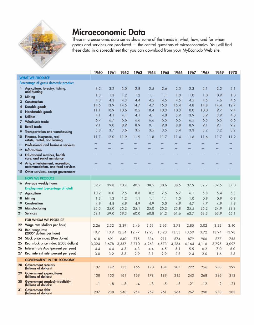
1960 1961 1962 1963 1964 1965 1966 1967 1968 1969 1970WHAT WE PRODUCE Percentage of gross domestic product

1 Agriculture, forestry, fishing, and hunting

2 Mining3 Construction4 Durable goods5 Nondurable goods6 Utilities7 Wholesale trade8 Retail trade9 Transportation and warehousing

10 Finance, insurance, real estate, rental, and leasing

11 Professional and business services12 Information13 Educational services, health

care, and social assistance14 Arts, entertainment, recreation,

accommodation, and food services15 Other services, except government

HOW WE PRODUCE16 Average weekly hours

Employment (percentage of total)17 Agriculture18 Mining19 Construction20 Manufacturing21 Services

FOR WHOM WE PRODUCE22 Wage rate (dollars per hour)23 Real wage rate

(2005º dollars per hour)24 Stock price index (Dow Jones)25 Real stock price index (2005 dollars)26 Interest rate Aaa (percent per year)27 Real interest rate (percent per year)

GOVERNMENT IN THE ECONOMY28 Government receipts

(billions of dollars)29 Government expenditures

(billions of dollars)30 Government surplus(+)/deficit(–)

(billions of dollars)31 Government debt

(billions of dollars)

3.2 3.2 3.0 2.8 2.5 2.6 2.5 2.3 2.1 2.2 2.1

1.3 1.3 1.2 1.2 1.1 1.1 1.0 1.0 1.0 0.9 1.04.3 4.3 4.3 4.4 4.5 4.5 4.5 4.5 4.5 4.6 4.6

14.6 13.9 14.5 14.7 14.7 15.3 15.4 14.8 14.8 14.4 12.711.1 10.9 10.6 10.5 10.4 10.3 10.3 10.0 10.0 9.7 9.4

4.1 4.1 4.1 4.1 4.1 4.0 3.9 3.9 3.9 3.9 4.06.7 6.7 6.6 6.6 6.6 6.5 6.5 6.5 6.5 6.5 6.69.1 9.0 8.9 8.9 9.1 9.0 8.8 8.9 9.1 9.1 9.23.8 3.7 3.6 3.5 3.5 3.5 3.4 3.3 3.2 3.2 3.2

11.7 12.0 11.9 11.9 11.8 11.7 11.4 11.6 11.6 11.7 11.9

— — — — — — — — — — —— — — — — — — — — — —

— — — — — — — — — — —

— — — — — — — — — — —

— — — — — — — — — — —

39.7 39.8 40.4 40.5 38.5 38.6 38.5 37.9 37.7 37.5 37.0

10.2 10.0 9.5 8.8 8.2 7.5 6.7 6.1 5.8 5.4 5.3

1.3 1.2 1.2 1.1 1.1 1.1 1.0 1.0 0.9 0.9 0.94.9 4.8 4.9 4.9 4.9 5.0 4.9 4.7 4.7 4.9 4.9

25.5 25.0 25.2 25.1 25.0 25.2 25.8 25.5 25.2 24.9 23.858.1 59.0 59.3 60.0 60.8 61.2 61.6 62.7 63.3 63.9 65.1

2.26 2.32 2.39 2.46 2.53 2.63 2.73 2.85 3.02 3.22 3.40

10.7 10.9 12.54 12.77 12.93 13.20 13.33 13.50 13.72 13.94 13.98

618 691 640 715 834 911 874 879 906 877 7533,324 3,678 3,357 3,710 4,263 4,573 4,264 4,164 4,116 3,795 3,097

4.4 4.4 4.3 4.3 4.4 4.5 5.1 5.5 6.2 7.0 8.03.0 3.2 3.3 2.9 3.1 2.9 2.3 2.4 2.0 1.6 2.3

137 142 153 165 170 184 207 222 256 288 292

138 150 161 169 178 189 215 243 268 286 313

–1 –8 –8 –4 –8 –5 –8 –21 –12 2 –21

237 238 248 254 257 261 264 267 290 278 283

Microeconomic DataThese microeconomic data series show some of the trends in what, how, and for whomgoods and services are produced — the central questions of microeconomics. You will findthese data in a spreadsheet that you can download from your MyEconLab Web site.

1971 1972 1973 1974 1975 1976 1977 1978 1979 1980 1981 1982 1983

2.1 2.3 3.2 2.8 2.7 2.3 2.0 2.1 2.2 1.8 2.0 1.8 1.3

1.0 1.0 1.0 1.4 1.5 1.4 1.6 1.5 1.7 2.4 2.9 2.5 1.94.7 4.7 4.8 4.7 4.3 4.4 4.4 4.6 4.7 4.4 3.9 3.7 3.7

12.4 12.7 13.0 12.3 11.5 12.1 12.5 12.7 12.3 11.3 11.0 10.0 9.89.1 8.9 8.7 8.8 8.8 8.9 8.8 8.6 8.6 8.5 8.5 8.2 7.84.0 4.0 3.9 3.8 4.1 4.1 4.1 4.1 3.8 4.0 4.1 4.5 4.46.5 6.6 6.6 6.9 6.9 6.6 6.5 6.6 6.6 6.5 6.4 6.3 6.19.2 9.1 9.0 8.7 8.9 9.0 9.0 8.9 8.6 8.3 8.2 8.3 8.53.2 3.3 3.3 3.3 3.0 3.2 3.2 3.2 3.2 3.1 2.9 2.7 2.7

12.1 12.0 11.7 11.8 12.0 11.7 11.8 11.9 11.8 12.3 12.5 13.1 13.4

— — — — — — — — — — — — —— — — — — — — — — — — — —

— — — — — — — — — — — — —

— — — — — — — — — — — — —

— — — — — — — — — — — — —

36.8 36.9 36.9 36.4 36.0 36.1 35.9 35.8 35.6 35.2 35.2 34.7 34.9

5.1 5.0 4.9 4.8 4.7 4.5 4.2 4.1 3.8 3.7 3.5 3.5 3.30.9 0.9 0.9 0.9 1.0 1.0 1.0 1.0 1.1 1.1 1.2 1.3 1.15.0 5.1 5.2 5.0 4.5 4.4 4.6 4.8 4.9 4.7 4.5 4.3 4.4

22.8 22.7 23.0 22.5 20.9 21.1 21.1 20.9 20.8 19.9 19.7 18.7 18.366.1 66.3 66.1 66.9 68.9 69.0 69.1 69.2 69.5 70.5 71.0 72.2 73.0

3.63 3.90 4.14 4.43 4.73 5.06 5.44 5.87 6.33 6.84 7.43 7.86 8.19

14.22 14.64 14.73 14.45 14.09 14.26 14.41 14.53 14.46 14.32 14.23 14.18 14.22

885 951 924 759 802 975 895 820 844 891 933 884 1,1903,465 3,569 3,287 2,476 2,391 2,747 2,370 2,030 1,930 1,867 1,786 1,596 2,066

7.4 7.2 7.4 8.6 8.8 8.4 8.0 8.7 9.6 11.9 14.2 13.8 12.03.0 4.0 1.2 –2.5 –0.3 2.7 1.5 1.1 –1.7 –1.6 3.9 7.6 8.8

309 354 397 438 448 513 576 653 736 807 927 949 1,008

340 370 400 453 533 573 620 682 760 879 996 1,106 1,206

–31 –16 –3 –15 –85 –61 –44 –29 –24 –73 –70 –158 –198

303 322 341 344 395 477 549 607 640 712 789 925 1,137

1984 1985 1986 1987 1988 1989 1990 1991 1992 1993 1994WHAT WE PRODUCE Percentage of gross domestic product

1 Agriculture, forestry, fishing, and hunting

2 Mining3 Construction4 Durable goods5 Nondurable goods6 Utilities7 Wholesale trade8 Retail trade9 Transportation and warehousing

10 Finance, insurance, real estate, rental, and leasing

11 Professional and business services12 Information13 Educational services, health

care, and social assistance14 Arts, entertainment, recreation,

accommodation, and food services15 Other services, except government

HOW WE PRODUCE16 Average weekly hours

Employment (percentage of total)17 Agriculture18 Mining19 Construction20 Manufacturing21 Services

FOR WHOM WE PRODUCE22 Wage rate (dollars per hour)23 Real wage rate

(2005 dollars per hour)24 Stock price index (Dow Jones)25 Real stock price index (2005 dollars)26 Interest rate Aaa (percent per year)27 Real interest rate (percent per year)

GOVERNMENT IN THE ECONOMY28 Government receipts

(billions of dollars)29 Government expenditures

(billions of dollars)30 Government surplus(+)/deficit(–)

(billions of dollars)31 Government debt

(billions of dollars)

1.6 1.5 1.4 1.7 1.6 1.7 1.7 1.5 1.6 1.4 1.5

1.8 1.5 1.0 1.5 1.4 1.4 1.5 1.3 1.1 1.1 1.03.9 4.1 4.4 4.6 4.6 4.5 4.3 3.8 3.7 3.7 3.9

10.3 9.8 9.5 10.2 10.2 9.9 9.4 9.0 8.9 8.9 9.27.4 7.2 6.6 6.9 7.0 7.0 7.0 6.9 6.8 6.7 6.74.3 4.2 4.1 2.6 2.4 2.5 2.5 2.5 2.5 2.5 2.56.3 6.2 6.1 6.0 6.2 6.2 6.0 6.0 6.0 6.0 6.38.6 8.7 8.7 7.4 7.2 7.1 6.9 6.8 6.8 6.9 7.02.8 2.7 2.7 3.2 3.2 3.0 2.9 3.0 2.9 3.0 3.1

13.4 13.6 14.0 17.7 17.8 17.8 18.0 18.4 18.6 18.6 18.4

— — — 8.7 9.1 9.4 9.8 9.7 9.9 9.9 9.9— — — 3.9 3.8 3.8 3.9 3.9 4.0 4.1 4.2

— — — 6.0 6.1 6.3 6.7 7.1 7.3 7.3 7.2

— — — 3.2 3.3 3.3 3.4 3.4 3.4 3.4 3.3

— — — 2.4 2.4 2.4 2.5 2.4 2.4 2.5 2.4

35.1 34.9 34.7 34.7 34.6 34.5 34.3 34.1 34.2 34.3 34.5

3.0 2.7 2.6 2.6 2.5 2.4 2.3 2.3 2.3 2.1 2.21.0 1.0 0.8 0.7 0.7 0.7 0.7 0.7 0.6 0.6 0.64.6 4.8 4.8 4.9 4.8 4.8 4.7 4.3 4.1 4.2 4.4

18.4 17.8 17.2 16.8 16.6 16.3 15.8 15.4 15.1 14.8 14.672.9 73.8 74.6 75.0 75.4 75.9 76.6 77.3 77.9 78.3 78.3

8.48 8.73 8.92 9.13 9.43 9.80 10.01 10.32 10.57 10.83 11.12

14.19 14.18 14.17 14.10 14.08 14.10 13.86 13.80 13.81 13.84 13.92

1,178 1,328 1,793 2,276 2,061 2,509 2,679 2,929 3,284 3,522 3,7941,972 2,157 2,849 3,514 3,076 3,609 3,710 3,918 4,291 4,503 4,75012.7 11.4 9.0 9.4 9.7 9.3 9.3 8.8 8.1 7.2 8.08.4 7.8 7.2 5.7 5.6 4.4 3.9 4.6 5.1 4.2 5.4

1,121 1,222 1,299 1,414 1,513 1,639 1,724 1,774 1,860 1,963 2,109

1,308 1,434 1,534 1,617 1,695 1,816 1,970 2,069 2,225 2,292 2,361

–187 –212 –234 –203 –182 –177 –246 –295 –366 –329 –252

1,307 1,507 1,741 1,890 2,052 2,191 2,412 2,689 3,000 3,248 3,433

Microeconomic DataThese microeconomic data series show some of the trends in what, how, and for whomgoods and services are produced — the central questions of microeconomics. You will findthese data in a spreadsheet that you can download from your MyEconLab Web site.

2008 20091995 1996 1997 1998 1999 2000 2001 2002 2003 2004 2005 2006 2007

1.3 1.5 1.3 1.2 1.0 1.0 1.0 0.9 1.0 1.2 1.0 1.0 1.2 1.1 1.0

1.0 1.1 1.1 0.9 0.9 1.2 1.2 1.0 1.3 1.5 1.8 2.0 2.0 2.1 1.63.9 4.0 4.1 4.3 4.4 4.4 4.6 4.6 4.5 4.6 4.9 4.8 4.1 4.4 4.19.2 9.0 9.1 9.2 8.9 8.8 7.7 7.4 7.0 6.9 6.8 6.7 6.7 6.4 5.96.8 6.4 6.3 6.1 6.0 5.7 5.6 5.5 5.4 5.3 5.2 5.1 5.0 5.2 5.12.5 2.3 2.2 2.1 2.0 1.9 2.0 2.0 2.0 2.1 2.0 2.1 2.1 1.8 1.96.2 6.3 6.3 6.2 6.2 6.0 6.0 5.9 5.8 5.9 5.8 5.8 5.8 5.7 5.67.0 7.0 6.9 6.8 6.9 6.7 6.8 6.9 6.9 6.6 6.5 6.4 6.4 6.0 5.93.1 3.0 3.1 3.1 3.1 3.1 2.9 2.9 2.9 2.9 2.9 2.9 2.9 2.8 2.8

18.7 18.8 19.2 19.3 19.4 19.7 20.3 20.5 20.5 20.4 20.5 20.9 20.7 21.1 21.4

10.0 10.4 10.8 11.2 11.5 11.6 11.5 11.4 11.4 11.5 11.7 11.8 12.2 12.1 12.14.2 4.3 4.2 4.4 4.7 4.7 4.7 4.6 4.5 4.5 4.6 4.5 4.7 4.3 4.4

7.2 7.1 6.9 6.9 6.8 6.9 7.3 7.6 7.8 7.8 7.7 7.7 7.9 7.9 8.3

3.4 3.4 3.5 3.5 3.5 3.6 3.6 3.6 3.6 3.7 3.6 3.6 3.7 3.8 3.8

2.4 2.4 2.4 2.4 2.3 2.3 2.4 2.4 2.4 2.3 2.3 2.3 2.3 2.5 2.5

34.3 34.3 34.5 34.5 34.3 34.3 34.0 33.9 33.7 33.7 33.8 33.9 34.6 34.5 33.9

2.2 2.0 2.0 1.8 1.7 1.6 1.6 1.6 1.6 1.5 1.5 1.4 1.3 1.3 1.30.5 0.5 0.5 0.5 0.5 0.4 0.5 0.4 0.4 0.4 0.5 0.5 0.5 0.6 0.54.4 4.5 4.6 4.8 5.0 5.1 5.1 5.1 5.1 5.2 5.4 5.6 5.5 5.2 4.5

14.4 14.1 13.9 13.7 13.2 12.9 12.3 11.5 11.0 10.7 10.5 10.3 10.0 9.7 9.078.5 78.8 79.0 79.2 79.6 80.0 80.6 81.4 81.9 82.1 82.2 82.3 82.7 83.3 84.6

11.43 12.03 12.49 13.00 13.47 14.02 14.54 14.97 15.37 15.69 16.13 16.76 17.43 18.08 18.60

14.02 14.48 14.77 15.20 15.52 15.82 16.04 16.25 16.33 16.21 16.13 16.23 16.40 16.65 16.97

4,494 5,743 7,441 8,626 10,465 10,735 10,189 9,226 8,994 10,317 10,548 11,409 13,170 11,253 8,8765,511 6,912 8,800 10,087 12,061 12,110 11,240 10,016 9,557 10,662 10,548 11,049 12,390 10,360 8,098

7.6 7.4 7.3 6.5 7.0 7.6 7.1 6.5 5.7 5.6 5.2 5.6 5.6 5.6 5.34.8 4.4 5.0 5.0 4.8 4.3 4.2 4.9 3.4 3.0 1.9 2.4 2.7 1.8 5.7

2,233 2,399 2,579 2,757 2,932 3,168 3,156 3,001 3,071 3,296 3,692 4,028 4,229 4,108 3,752

2,465 2,570 2,645 2,719 2,853 3,022 3,221 3,423 3,625 3,827 4,110 4,320 4,637 5,020 5,345

–232 –171 –66 38 79 147 –65 –422 –553 –531 –418 –292 –408 –912 –1,593

3,604 3,734 3,772 3,721 3,632 3,410 3,320 3,540 3,913 4,296 4,592 4,829 5,035 5,803 7,545

1 Life in a small and ever-shrinking world 5Chips and windows 6Greenhouse gas emissions 6A credit crunch 7

2 Increasing opportunity cost on the farm 32Hong Kong catching up to the United States 37The United States and China gain from trade 41

3 The global market for crude oil 69The market for strawberries 71

4 Elastic and inelastic demand 89The elasticities of demand for food 90Necessities and luxuries 93

5 The invisible hand 113

6 Rent control winners: The rich and famous 130Unscrambling cause and effect of the minimum

wage 132Workers and consumers pay the most tax 138Rich high-cost farmers the winners 141

7 Trading services for oil 152U.S. tariffs almost gone 158Self-interest beats the social interest 162

8 Maximizing utility from recorded music 192

9 Best affordable choice of movies and DVDs 212

10 Types of firms in the economy 236Concentration in the U.S. economy 239A competitive environment 241Apple doesn’t make the iPhone 243

Economics in ActionEconomics in Action boxes apply economic theory to current events to illustrate the importance of economicforces in the world around us.

11 How to pull up your average 256Produce more to cut cost 265

12 Production cutback and temporary shutdown 283

Entry and exit 285

13 Information-age monopolies 301Attempting perfect price discrimination 312

14 Monopolistic competition today 325The cost of selling a pair of shoes 331

15 Oligopoly today 343An R & D game in the market for diapers 350The United States versus Microsoft 358FTC takes the fizz out of soda mergers 359

16 Is a lighthouse a public good? 375Fighting California’s wildfires 379Delivering health care efficiently 384

17 U.S. air pollution trends: Cleaner and safer 394The greatest market failure? 398The original tragedy of the commons 400One of today’s tragedies of the commons 401ITQs work 40

18 Wage rates in the United States 427The world and U.S. markets for oil 431

19 The rich get richer, but school still pays 446Income redistribution: Only the richest pay 456

20 Insurance in the United States 471The sub-prime credit crisis 476