Essays in Household Finance and Housing Economics

University of Pennsylvania University of Pennsylvania

ScholarlyCommons ScholarlyCommons

Publicly Accessible Penn Dissertations

2013

Essays in Household Finance and Housing Economics Essays in Household Finance and Housing Economics

Cindy Katherine Soo University of Pennsylvania, [email protected]

Follow this and additional works at: https://repository.upenn.edu/edissertations

Part of the Economics Commons, and the Finance and Financial Management Commons

Recommended Citation Recommended Citation Soo, Cindy Katherine, "Essays in Household Finance and Housing Economics" (2013). Publicly Accessible Penn Dissertations. 702. https://repository.upenn.edu/edissertations/702

This paper is posted at ScholarlyCommons. https://repository.upenn.edu/edissertations/702 For more information, please contact [email protected].

https://repository.upenn.edu/

https://repository.upenn.edu/edissertations

https://repository.upenn.edu/edissertations?utm_source=repository.upenn.edu%2Fedissertations%2F702&utm_medium=PDF&utm_campaign=PDFCoverPages

http://network.bepress.com/hgg/discipline/340?utm_source=repository.upenn.edu%2Fedissertations%2F702&utm_medium=PDF&utm_campaign=PDFCoverPages

http://network.bepress.com/hgg/discipline/631?utm_source=repository.upenn.edu%2Fedissertations%2F702&utm_medium=PDF&utm_campaign=PDFCoverPages

https://repository.upenn.edu/edissertations/702?utm_source=repository.upenn.edu%2Fedissertations%2F702&utm_medium=PDF&utm_campaign=PDFCoverPages

https://repository.upenn.edu/edissertations/702

mailto:[email protected]

Essays in Household Finance and Housing Economics Essays in Household Finance and Housing Economics

Abstract Abstract With the wake of the United States financial crisis in 2008, policymakers and academics have begun to reevaluate the nature and impact of household financial decisions. While standard economic theory assumes individuals are fully rational, the devastation of the crisis suggests households may be subject to systematic biases that can have significant effects on the economy. Chapter 1 asks whether consumer sentiment has an impact on asset prices, particularly during the boom and bust of housing prices that instigated the most recent financial crisis. Empirically identifying a link between sentiment and prices is challenging, however, as measures of investor beliefs are difficult to construct. This paper develops the first measures of sentiment across local housing markets by quantifying the tone in local housing newspaper articles. The sentiment index forecasts both the boom and bust of housing prices by more than two years, and can predict over 70 percent of the variation in national housing prices above and beyond economic fundamentals. Chapter 2 then asks whether households can time the own versus rent decision successfully and generate profitable savings. Using 29 years of historical data, this essay creates robust measures of the costs of owning and renting and evaluates whether owning or renting was less expensive ex-post across 39 metropolitan areas in the United States. We find that households can potentially time their homeownership profitably and can save as much as 50 percent of annual rent costs using a few simple trading rules. Chapter 3 addresses whether the lack of household financial literacy has significant consequences for household wealth. We find that an overwhelming majority of households lack basic financial skills and that financial literacy appears to have a significant effect on wealth above and beyond other observed factors. Our results suggest that improving financial literacy could have large positive effects on wealth accumulation.

Degree Type Degree Type Dissertation

Degree Name Degree Name Doctor of Philosophy (PhD)

Graduate Group Graduate Group Applied Economics

First Advisor First Advisor Olivia S. Mitchell

Keywords Keywords financial literacy, household finance, housing, real estate finance, sentiment, textual analysis

Subject Categories Subject Categories Economics | Finance and Financial Management

This dissertation is available at ScholarlyCommons: https://repository.upenn.edu/edissertations/702

https://repository.upenn.edu/edissertations/702

!

!!

ESSAYS IN HOUSEHOLD FINANCE AND HOUSING ECONOMICS

Cindy K. Soo

A DISSERTATION

in

Applied Economics

For the Graduate Group in Managerial Science and Applied Economics

Presented to the Faculties of the University of Pennsylvania

in

Partial Fulfillment of the Requirements for the

Degree of Doctor of Philosophy

2013

Supervisor of Dissertation

_________________________

Olivia S. Mitchell, Professor of Business Economics and Public Policy

Graduate Group Chairperson

_________________________

Eric Bradlow, Professor of Marketing Statistics and Education

Dissertation Committee

Olivia S. Mitchell, Professor of Business Economics and Public Policy

Joseph Gyourko, Professor of Real Estate, Finance, Business Economics and Public Policy

Todd Sinai, Associate Professor of Real Estate, Business Economics and Public Policy

Fernando Ferreira, Associate Professor of Real Estate, Business Economics and Public Policy

!

!ii!

To Mom and Dad,

who have provided me with incredible support and love.

!

iii!!

ACKNOWLEDGMENT

I am deeply indebted to my advisors Fernando Ferreira, Joe Gyourko, Olivia Mitchell, Michael

Roberts, and Todd Sinai for their encouragement and guidance. I am very grateful to the faculty

and my classmates of the Wharton Applied Economics and Finance PhD program for their helpful

suggestions and feedback. Finally, I owe a deep heartfelt thanks to my family and friends for their

unconditional support.

!

!iv!

ABSTRACT

ESSAYS IN HOUSEHOLD FINANCE AND HOUSING ECONOMICS

Cindy K. Soo

Olivia S. Mitchell

With the wake of the United States financial crisis in 2008, policymakers and academics have

begun to reevaluate the nature and impact of household financial decisions. While standard

economic theory assumes individuals are fully rational, the devastation of the crisis suggests

households may be subject to systematic biases that can have significant effects on the

economy. Chapter 1 asks whether consumer sentiment has an impact on asset prices,

particularly during the boom and bust of housing prices that instigated the most recent financial

crisis. Empirically identifying a link between sentiment and prices is challenging, however, as

measures of investor beliefs are difficult to construct. This paper develops the first measures of

sentiment across local housing markets by quantifying the tone in local housing newspaper

articles. The sentiment index forecasts both the boom and bust of housing prices by more than

two years, and can predict over 70 percent of the variation in national housing prices above and

beyond economic fundamentals. Chapter 2 then asks whether households can time the own

versus rent decision successfully and generate profitable savings. Using 29 years of historical

data, this essay creates robust measures of the costs of owning and renting and evaluates

whether owning or renting was less expensive ex-post across 39 metropolitan areas in the United

States. We find that households can potentially time their homeownership profitably and can save

as much as 50 percent of annual rent costs using a few simple trading rules. Chapter 3

addresses whether the lack of household financial literacy has significant consequences for

household wealth. We find that an overwhelming majority of households lack basic financial skills

and that financial literacy appears to have a significant effect on wealth above and beyond other

observed factors. Our results suggest that improving financial literacy could have large positive

effects on wealth accumulation.

!

!v!

TABLE OF CONTENTS

ACKNOWLEDGEMENT…………………………………………………………………….....iii

ABSTRACT……………………………………………………………………………………...iv

LIST OF TABLES……………………………………………………………………………….vi

LIST OF FIGURES……………………………………………………………………………..vii

CHAPTER 1……………………………………………………………………………………...1

CHAPTER 2…………………………………………………………………………………….66

CHAPTER 3…………………………………………………………………………………...123

!

!vi!

LIST OF TABLES

CHAPTER 1: “Quantifying Animal Spirits: News and Sentiment in the Housing Market”

Table 1: Descriptive Statistics for Newspaper Housing Articles Table 2: Sample Positive Words and Word Counts Table 3: Summary Statistics – Sentiment, Prices, Volume and Fundamentals Table 4: Sentiment Predicts National House Price Appreciation Table 5: Sentiment Predicts City House Price Appreciation (Panel) Table 6: Sentiment Predicts City House Prices Beyond Subprime Lending Trends Table 7: Sentiment Predicts the Volume of Housing Transactions Table 8: Explanatory Power of Observed Fundamentals Pre- and Post-2000 Table 9: Is Sentiment Driven By News Stories on Unobserved Fundamentals? Table 10: Correlation of Weekend Instrument with Friday News Releases Table 11: Weekend and Narrative Instruments for Sentiment, First-Stage Table 12: Predicting Price Growth Using Positive Sentiment, IV Result Table A.1: Comparing Effect Of Alternative Sentiment Indices

CHAPTER 2: “Timing the Housing Market”

Table 1. Summary Statistics Of Relative Costs Of Owning V. Renting Table 2. Predicting Binary Rent v. Own Decision, 1-year horizon Table 3. Forecasting the 1-Year Horizon Own versus Rent Decision Table 4. Annual Savings from Least Costly Benchmark (% of CR), 1980-2009, 1-Year Table 5. Transaction Cost Per Rent-Own Switch Before Eliminate Savings, 1980-2009 Table 6. Predicting the 5-Year and 10-Year Horizon Own versus Rent Decision Table 7. Forecasting the 5-Year and 10-Year Horizon Table 8. Average Annual Savings from Least Costly Benchmark, 5-Year Horizon Table 9. Average Annual Savings from Least Costly Benchmark with 10-Year Horizon Table 10. Probability Owning is Cheaper by Income Tier, 1-Year horizon Table 10. Average Annual Savings from Least Costly Benchmark with 1-Year Horizon, Lowest Income Tier Appendix Table 1. Predicting Continuous CO-CR, 1-year horizon Appendix Table 2. Predicting Binary Rent v. Own Decision, 1-year horizon, IV Results Appendix Table 3. Predicting Binary Rent v. Own Decision, 1-year horizon, 2 Bedroom Appendix Table 4. Forecasting the 1-Year Horizon Own versus Rent Decision 2 Bedroom Appendix Table 5. Annual Savings from Least Costly Benchmark (% of CR), 1-Year, 2 Bedroom

CHAPTER 3: “FINANCIAL LITERACY, SCHOOLING, AND WEALTH ACCUMULATION”

Table 1. Summary Statistics for Dependent Variables. Table 2. Summary Statistics for Right-Side Variables and Candidate Instruments Table 3. Financial Literacy Questions: Percent Correct and PRIDIT Weighting Scheme Table 4. OLS Models of Wealth and Pension Density: PRIDIT Alone, Schooling Alone, and Both, Plus Interactions Table 5. IV Models of Wealth and Pension Density: PRIDIT Alone, Schooling Alone, and Both, Plus Interactions Table 6. Predicted Change in Measured Outcomes for Correct Answer to Financial Literacy Question Appendix A: Complete Set of OLS Coefficient Estimates for Table 4 Appendix B: Complete Set of IV Estimates for Table 5

!

!vii!

LIST OF FIGURES !CHAPTER 1: “Quantifying Animal Spirits: News and Sentiment in the Housing Market”

Figure 1: Composite-20 Housing Sentiment and Case-Shiller Home Price Index Figure 2: Housing Sentiment and Case-Shiller Home Price Indexes by City Figure 3: Random Sentiment Placebo Test Figure 4: Validating Sentiment Against Surveys of Housing Market Confidence Figure 5: Predicting House Price Growth with Sentiment Index v. Fundamentals Figure 6: Composite-20 Housing Sentiment Index and Transaction Volume Figure A.1: Housing Sentiment Index and Housing Prices, By City

CHAPTER 2: “Timing the Housing Market”

Figure 1. Actual v. Predicted Cost of Owning Minus Cost of Renting Figure 2. Actual v. Predicted Cost of Owning Minus Cost of Renting by City Figure 3. Cost of Owning Minus Cost of Renting, 1980-2009

CHAPTER 1

QUANTIFYING ANIMAL SPIRITS:

NEWS MEDIA AND SENTIMENT IN THE HOUSING MARKET⇤

Cindy K. Soo

The Wharton School, University of Pennsylvania

Abstract

Sentiment or “animal spirits” has long been posited as an important determinant of asset prices,but measures of sentiment are difficult to construct and often confounded by asset fundamentals.This paper provides a first empirical test of the role of sentiment in the run-up and crash ofhousing prices that instigated the great financial crisis of 2008. I develop the first measures ofsentiment across local housing markets by quantifying the positive and negative tone of housingnews in local newspaper articles. I find that my housing sentiment index forecasts the boomand bust pattern of house prices at a two year lead, and can predict over 70 percent of thevariation in aggregate house price growth. Consistent with theories of investor sentiment, I findthat my sentiment index not only predicts price variation but also patterns in trading volume.Estimated effects of sentiment are robust to an extensive list of observed controls includinglagged fundamentals, lagged price growth, subprime lending patterns, and news content overtypically unobserved variables. To address potential bias from latent fundamentals, I developinstruments from a subset of weekend and narrative articles that newspapers use to cater tosentiment but are plausibly exogenous to news on fundamentals. Estimates remain robust toinstrumental variable estimation, suggesting bias from unobserved fundamentals is minimal.

⇤I am deeply indebted to my advisors Fernando Ferreira, Joe Gyourko, Olivia Mitchell, Michael Roberts, and ToddSinai for their continual encouragement and guidance. I am very grateful to Nick Barberis, Mark Duggan, Alex Edmans,Alex Gelber, Joao Gomes, Todd Gormley, Vincent Glode, Daniel Gottlieb, Philipp Illeditsch, Raimond Maurer, GregNini, Christian Opp, David Musto, Devin Pope, Nikolai Roussanov, Robert Stambaugh, Robert Shiller, Kent Smetters,Luke Taylor, Jeremy Tobacman, Maisy Wong, Yu Yuan and numerous participants in the 2011 Whitebox Graduate Stu-dent Conference, the 2011 TransAtlantic Doctoral Conference, the Wharton MicroFinance Brown Bag, and the WhartonApplied Economics Seminar for their helpful suggestions and comments. I owe special thanks to Eugene Soltes andKumar Kesavan, and greatly appreciate the constant support from my classmates in the Wharton Applied Economics andFinance PhD program. I gratefully acknowledge support from the Connie K. Duckworth Fellowship, the Bradley Foun-dation, the S.S. Huebner Foundation, and the Pension Research Council/Boettner Center for Pensions and RetirementResearch. All errors are my own. © 2012, Soo. All rights reserved.

1

1 Introduction

Sentiment, broadly defined as the psychology behind investor beliefs, has long been posited

as an important determinant of asset price variation (Keynes (1936); Shiller (1990); Kothari and

Shanken (1997); Baker and Wurgler (2002); Shiller (2005)). However, identifying an empirical

link between sentiment and prices presents two major challenges. First, beliefs are by definition

unobservable and therefore not straightforward to quantify. Second, it is difficult to separate effects

of sentiment from underlying economic fundamentals. If fundamentals jointly determine sentiment

and asset prices, then an empirical correlation between a proxy for sentiment and prices may reflect

effects from latent fundamentals rather than the role of sentiment (Baker and Wurgler (2006)).

The goal of this paper is to quantify the role of investor sentiment in asset price formation and

address both of these challenges in novel ways. I use the run-up and crash of U.S. housing prices

from 2000 to 2011 as my laboratory to examine the role of sentiment. This is an important and

useful setting for several reasons. First, housing is a significant sector of the economy. Over two-

thirds of U.S households own a home and invest the majority of their portfolio in real estate (Tracy

et al. (1999); Nakajima (2005)). The housing crash also greatly impacted the financial sector, as

banks and financial institutions held significant investments in mortgage-backed securities and other

housing related assets. Second, the housing market provides greater power for identifying potential

effects of sentiment. Unlike the stock market, which is dominated by large institutional investors,

housing is primarily traded by individual buyers who are likely more subject to sentiment. Finally,

the recent housing cycle is an important setting to examine the effect of sentiment because standard

economic explanations for the housing boom have so far been difficult to reconcile empirically.

Observed fundamentals that accounted for nearly 70 percent of the variation in national house price

growth from 1987 to 2000, explain less than 10 percent of the variation from 2000 to 2011 (Lai and

Van Order (2010)). While there was much discussion of the potential role of sentiment, empirical

evidence of this theory has been limited and largely anecdotal.

This paper provides the first measures and empirical test of sentiment in the housing market. I

measure sentiment by capturing the qualitative tone of housing news from local newspapers. Specif-

ically, I calculate the difference between the share of positive and negative words across newspaper

2

articles each month. I construct sentiment indices corresponding to each of the 20 city markets cov-

ered by the Case-Shiller home price index. This methodology builds on work from Tetlock (2007)

and a growing number of studies that construct proxies for sentiment in the stock market with me-

dia coverage. This strategy is also motivated by literature on asset price bubbles that claims the

media reflects sentiment through an incentive to cater to readers’ preferences over a particular asset

(Kindleberger (1978); Galbraith (1990); Shiller (2005)). I present a simple theoretical model that

formalizes these arguments and illustrates how news media may relate to sentiment.

I find that my sentiment index forecasts the boom and bust trend of housing prices by more

than a two year lead. Figure 1 shows that aggregate sentiment increases rapidly and peaks in 2004,

well before the peak of national house prices in mid-2006. This pattern is also evident across cities.

Cities that experienced dramatic rises and declines in house prices are preceded by similar cycles

in sentiment, whereas cities with milder price changes are led by more subdued sentiment growth.

Furthermore, I find that my sentiment measure can explain over 70 percent additional variation in

national house price movements above and beyond observed fundamentals. This is significant as

prior studies have found standard fundamental determinants to account for only a limited fraction

of house price variation after 2000.1 Nonetheless, interpreting these effects as sentiment is limited

without a validation of media sentiment as a reflection of investor beliefs.

External validations of sentiment proxies are naturally difficult to provide since investor be-

liefs are unobservable (Baker et al. (2012a)). In this paper, I validate my measure of sentiment by

comparing it with surveys of investor expectations in the housing market. I find that my sentiment

measure is highly correlated with housing market confidence indexes from the Survey of Consumers

and the National Association of Home Builders. In particular, home buyer survey confidence also

peaks in 2004, reflecting similar timing to trends in my composite index. Case et al. (2012) im-

plement annual surveys of home buyer expectations and similarly find that long term expectations

peak in 2004, well ahead of house prices. These surveys are otherwise limited in frequency and

geographic scope, but reaffirm the overall time-varying trends in my sentiment indices.1For example, Glaeser et al. (2010) find that lower real interest rates can explain only one-fifth of the rise in house

prices from 1996 to 2006. He et al. (2012) examine the role of liquidity in the housing boom, and find that their modelcan account for approximately one-fifth of house price run up from 1996 to 2006.

3

Still, all of these measures may potentially capture variation in fundamentals. I first address

this by controlling for an exhaustive sequence of fundamental determinants of house prices. I find

that the predictive power of sentiment on house prices not only remains robust in significance, but

also in magnitude. The stability of the estimates suggests that bias from unobservable factors is less

likely. I find that estimates also remain stable to the inclusion of additional controls for subprime

lending trends. While not considered a typical housing fundamental, subprime credit exhibited

unprecedented expansion with the growth of house prices in many cities (Mian and Sufi (2009);

Demyanyk and Van Hemert (2011); Goetzmann et al. (2012)). The richness of my news dataset also

allows me to control for the content of news articles directly. News may report on harder-to-quantify

fundamentals that I do not observe. Thus, I control for the share of positive minus negative words

in any article that directly mentions a fundamental in its text and find that this does not affect my

results. Furthermore, I find that sentiment not only predicts house price variation but also patterns in

transaction volume. This result is consistent with existing theories and empirical studies of investor

sentiment (Odean (1998, 1999); Scheinkman and Xiong (2003); Barber and Odean (2000, 2008)).

Interestingly, sentiment leads volume first and is followed by prices another year later. This evidence

supports a hypothesis that search frictions in the housing market likely induce lags between changes

in sentiment, housing transactions, and prices.

While these results are highly suggestive, the positive association between my sentiment in-

dex and house prices may still be driven by latent fundamentals. I present two candidate instruments

for sentiment by isolating a subset of housing news articles that cater to reader sentiment but are

plausibly exogenous to news on fundamentals. The first is my measure of sentiment calculated only

over housing articles published over the weekend. Weekend articles tend to cater to readers who

have preferences for lighter content, and are arguably exogenous to news on fundamentals since

official press releases on economic data can only occur on a weekday. The second proposed instru-

ment is my measure of sentiment calculated only over narrative housing news articles. Narratives

cater to sentiment through a human interest appeal, and are plausibly exogenous to fundamentals

because they consist of anecdotal stories rather than actual information. Of course, the validity of

these instruments relies on the assumption that information on fundamentals is not being reported

4

on or somehow related through these subset of news articles. I acknowledge and test for a number of

possible violations of this assumption, and find that results are consistent with the exclusion restric-

tion. Given this, I show that the predictive power of sentiment remains robust both in significance

and magnitude even after instrumenting for sentiment.

This paper provides evidence that sentiment may have a significant effect on house prices,

and challenges standard explanations of the housing boom and bust that rely solely on fundamentals.

The results of this paper suggest that if a fundamental drove house prices during this period, then

it would also have had to drive expectations at a two year lead to prices both nationally and across

cities. Furthermore, to be consistent with the empirical data, this fundamental would fail to explain

prices from 1987 to 2000 but suddenly begin to drive expectations and prices differently from 2000

to 2011. This paper does not advocate that fundamentals did not play any role, but that the evidence

suggests sentiment played an economically important role as well.

These findings complement a number of empirical studies that attempt to quantify sentiment

and provide evidence for its effect on asset prices (Edmans et al. (2007); Baker and Wurgler (2006,

2007); Baker et al. (2012a); Baker and Stein (2004); Greenwood and Nagel (2009); Barber et al.

(2009); Brown and Cliff (2005)). At the same time, the evidence in this paper relates to a large body

of work that explores determinants and consequences of the last housing boom and bust (Pisko-

rski et al. (2010); Avery and Brevoort (2010); Haughwout et al. (2011); Bhutta (2009); Bayer et al.

(2011); Glaeser et al. (2008); Gerardi et al. (2008); Ho and Pennington-Cross (2008)). This paper

also generally relates to a larger literature that explores housing price dynamics and more specif-

ically to studies that explore the role of expectations in the housing market (Genesove and Mayer

(2001); Piazzesi and Schneider (2009); Goetzmann et al. (2012); Arce and López-Salido (2011);

Burnside et al. (2011); Favilukis et al. (2010)). Finally, this paper contributes to research that links

media coverage to trading activity and shows that media sentiment can be used to predict asset prices

beyond stock market applications (Tetlock (2007); Tetlock et al. (2008); Tetlock (2011); Antweiler

and Frank (2004); Barber and Loeffler (1993); Dougal et al. (2012); Dyck and Zingales (2003);

Engelberg (2008); Engelberg and Parsons (2011); Garcia (2012); Gurun and Butler (2012)).

Section 2 presents a model that describes the relationship between news, sentiment, and

5

prices. Section 3 describes how I construct my database of newspaper articles and set of observed

fundamentals. Section 4 details how the sentiment index is calculated. Section 5 and 6 present the

main empirical and instrumental variable results respectively. Section 7 concludes and discusses

potential avenues for future work.

2 Theoretical Motivation

In this section, I present a simple theoretical framework that illustrates the potential relationship

between the news media, investor sentiment, and housing prices. I specifically measure sentiment

with news because prominent literature on bubbles and panics commonly stress that the news media

has an important relationship with investor beliefs (Kindleberger (1978); Galbraith (1990); Shiller

(2005)). They argue that newspapers have a demand-side incentive to cater to reader preferences,

and will spin news according to readers’ opinion over assets they own. Economic models of media

slant make similar arguments in the context of readers’ political preferences. Mullainathan and

Shleifer (2005) and Gentzkow and Shapiro (2006) assume that readers have a disutility for news that

is inconsistent with their beliefs, citing psychology literature that show people have a tendency to

favor information that confirms their priors.2 Indeed, Gentzkow and Shapiro (2010) find empirical

evidence that readers have a preference for news consistent with their beliefs and news outlets

respond accordingly. This framework adapts models of investor sentiment (De Long et al. (1990a);

Copeland (1976); Hong and Stein (1999)) and models of media slant (Gentzkow and Shapiro (2010);

Mullainathan and Shleifer (2005)) to show how news relates to investor sentiment and asset prices.

Agents: I assume there are two types of agents in the economy: fully rational traders and imperfectly

rational optimists that have a preference for news that confirms their priors. Agents are otherwise

identical in utility maximization and risk aversion parameters. In each period t, the fraction of

optimistic traders are present in the economy each period at measure µt , and fully rational agents are

present in the economy at measure (1�µt). All agents have constant absolute risk aversion where g

denotes the common coefficient of risk aversion. Thus, the allocation to the risky asset is unaffected

by the accumulation of wealth. For simplicity, I assume there is no consumption decision, no labor2This tendency is called confirmatory bias in the psychology literature (Lord (1979); Yariv (2002)).

6

supply decision, and no bequest. The resources agents have to invest are completely exogenous. In

each period, agents choose an optimal allocation of housing, Xt , to maximize the following:

maxHt

E[�e�2gWt+1 ]

subject to the budget constraint:

Wt+1 =Wt(1+ r f (1� t))+Xt [Pt+1 +Dt+1 �Pt(d t +mt +(1� t t)(1+ r f +p t)]

where Wt represents wealth in period t. Agents allocate wealth between a risk-free asset that guar-

antees a risk-free rate of r f > 0 each period and a risky asset of housing that pays dividends, Dt ,

in the form of housing services each period. Housing is in supply quantity Qt each period, and the

risk-free asset is in perfectly elastic supply. The price of housing stock is denoted by Pt . I assume

housing depreciates at rate dt , requires maintenance and repairs at a fraction of house value mt ,

and incurs property tax liabilities at rate pt . Furthermore, all investors must pay a marginal income

tax of tt , but may deduct property taxes from taxable income and otherwise borrow or lend at the

risk-free rate r f . This represents the user cost of housing as formalized by Poterba (1984). For ease

of notation going forward, let wt = dt +mt +(1� tt)(1+ r f +pt).

Maximizing expected utility over Xt yields the following optimal demand function for hous-

ing:3

Xt =EPt+1 +Dt+1 �Ptw t

2gEs

2Pt+1

. (1)

Since this is just a linear demand function, for simplicity let the above be represented by:4

Xt = at �wPt (2)3With normally distributed returns, maximizing the above is the same as maximizing mean-variance utility. I rewrite

the agents problem such that they maximize the following expected utility each period: EU = E[Wt+1]� gs

2Wt+1

=

Wt(1+ r f )(1� tt)+Xt [EtPt+1 +Dt+1 �wtPt ]�XtgEts2Pt+1

, where s

2Wt+1

is the one-period ahead variance of wealth ands

2Pt+1 is the one period ahead variance of price. This follows the set up in De Long et al. (1990a).

4

where a = EPt+1+Dt+12gEs

2Pt+1

and w = wt2gEs

2Pt+1

.

7

Rational traders demand housing according to equation (1), but I assume optimists overestimate the

expected price of housing relative to rational traders by an additional positive parameter q .5 Thus

relative to rational traders, optimists shift their demand curves upward by an additional q .

XOptt = at +q �wPt (3)

Newspapers: I also assume that optimistic investors have a preference for news that confirms their

positive beliefs. Gentzkow and Shapiro (2007) model this preference by assuming readers have a

quadratic disutility for news that conflicts with their priors, and derive an equation for newspaper

readership approximately equal to a � (Sn � Si)2 where a is a constant, Snt is slant reported by

newspaper n, and Sit is the overall level of sentiment in city i and period t. In this framework, the

overall level of sentiment in the economy is equal to the fraction of optimists, µt , multiplied by

their level of optimism, q . Thus, Sit = µtq , and the optimal level of news slant that maximizes a

newspaper’s readership is equal to:

S⇤nt = Sit = µtq (4)

Thus news slant, or the sentiment in news, directly reflects the overall level of reader sentiment.

Equilibrium Price: Given the presence of µt optimists and (1�µt) rational traders, equilibrium is

characterized by setting demand equal to supply, (1�µt)(a �wPt)+µt(a+q �wPt) = Qt . Thus

the equilibrium price equals:

Pt =(at +µtq �Qt)

w

(5)

Equation 5 reveals that investor sentiment has a positive association with prices ( dPt)dµ t q

> 0 ). Using

equation 4, we can rewrite equation 5 in terms of news sentiment:

Pt =(at +S⇤nt �Qt)

w

(6)

Then the price change from t to t +1 can be expressed by:5Conversely, this framework could also apply to a set of pessimists who underestimate the expected price of housing

by a negative parameter q .

8

4Pt+1 =1w

[(4at+1)+(4S⇤nt+1)� (4Qt+1)] (7)

where 4Pt+1 = Pt+1 �Pt . Thus Equation (7) predicts that changes in news sentiment (4S⇤nt+1) are

positively associated with changes in prices (Pt+1). Positive fundamentals such as dividends, Dt ,

will also drive prices up, while increasing costs and housing stock will have dampening effect on

prices. If there are no optimists in the market (µt = 0) or sentiment remains unchanged, then prices

will equal Pt =(a�Qt)

w

and are only moved by changes in fundamentals and rational expectations in

a, b , and Qt .

Examining the effect of sentiment in the housing market allows me to analyze not only the

time-varying effects of sentiment but also the cross-sectional effect of sentiment across different

local housing markets. Let 4Pit = Pit �Pit�1 be the change in prices in city i and 4Pjt represent the

changing prices in city j. The difference in house price changes across cities can be written as:

4Pit �4Pjt =1w

[(4ait �4a jt)+(4S⇤i,nt �4S⇤j,nt)� (4Qit �4Q jt)] (8)

Equation 8 shows that if the price increase from t �1 to t is greater in city i than in city j, then this

is due to either a greater increase in components in 4ait or in investor sentiment (proxied by news

sentiment 4S⇤i,nt).

Trading Volume. Increasing sentiment driven by the rising demand from optimists in the econ-

omy has further implications for trading volume in each housing market. Suppose the fraction of

optimists increases from t to t + 1 such that µt+1 > µt . Trading volume, Vt+1, is then equal to the

additional demand for housing from the fraction of optimists period to period:6

Vt+1 = µt+1XOptt+1 �µtX

Optt

=1w

(Snt+1 �Snt)(a �Q) (9)

Equation 9 illustrates that as sentiment increases, trading volume will be pushed upward. The

greater the demand from optimists is relative to the previous period, the greater the volume of6I assume that a and Q stay constant here to make the effect of sentiment clear.

9

trades. This framework predicts that positive changes in sentiment should lead to increases in trading

volume.

Lagged Effect. The above framework assumes that news only reflects investor sentiment. However,

Shiller (2005) argues that news media can simultaneously fuel sentiment if readers misperceive

optimism in the news for real information about fundamentals the housing market. Housing, in

particular, is a widely held household investment by individual buyers. Thus the average housing

investor is likely less financially sophisticated than the typical stock market investor. Survey evi-

dence shows that a majority of Americans do suffer from surprisingly low levels of financial literacy

(Lusardi and Mitchell (2007a,b)). Even more sophisticated investors may find it difficult to process

quantitative data on market fundamentals. Indeed, Engelberg (2008) provides empirical evidence

from earnings announcements that qualitative information on positive fundamentals is especially

difficult to process. News slant can make it difficult for readers to separate true information from

sentiment, and can subsequently affect trading behaviors. Empirical studies on political media slant

show that the media has been able to shift public opinion and voting behavior (DellaVigna and Ka-

plan (2007); Gerber et al. (2009)). Engelberg and Parsons (2011) show that different local media

coverage of the stock market drives different trading outcomes across markets. If this is the case,

then news sentiment in period t can also drive investor sentiment in future periods, µt+1q , and prices

would be positively associated with both contemporaneous and lagged values of news sentiment,

Sntand Snt�k.

Furthermore, this framework also assumes that transactions in the housing market are imme-

diate and costless. The transaction process of buying a home is by no means immediate, and the

search process for a home can actually take several months. Thus there can be several lags between

a change in sentiment and its effect on prices, and potentially no contemporaneous effect at all.

If news slant does feed sentiment, then this can also take some time to diffuse and spread across

investors.7 Thus I consider the effect of both contemporaneous and lagged effects of sentiment in

my empirical estimations.7Hong and Stein (1999)model a gradual diffusion of news where only a fraction of traders receive innovations about

dividends in each period.

10

3 Data Description

3.1 Newspaper Articles

My approach to measuring sentiment requires the text of newspaper articles covering the housing

market. My source for news articles is Factiva.com, a comprehensive online database of newspa-

pers.8 Factiva categorizes its articles by subject, and provides a code that identifies articles that

discuss local real estate markets. This code is determined by a propriety algorithm that remains

objective across all newspapers and years. This subject code covers new and existing home sales,

housing affordability indices, and housing price indices as well as supply side indicators on housing

starts, building permits, housing approvals, and construction spending. Routine real estate property

listings are not included. Wire-service articles are also generally excluded, as syndicated stories

cannot be redistributed and typically do not appear in the Factiva database. This exclusion is ac-

tually preferable to capturing the local sentiment unique to each city. Wire-service articles are

typically those that cover topics of more general national interest, supplied to local newspapers by

large media companies such as the Associated Press. Excluding such articles ensures each city’s

sentiment measure is only based on news articles written by local staff writers. To that end, I also

exclude any additional republished or duplicate news stories from other news outlets.9

I download all newspaper articles covering the housing market between January 2000 and

August 2011 from the major newspaper publication in each of the following 20 cities: Atlanta,

Boston, Charlotte, Chicago, Cleveland, Dallas, Denver, Detroit, Las Vegas, Los Angeles, Miami,

Minneapolis, New York, Phoenix, Portland, San Francisco, San Diego, Seattle, Tampa, and Wash-

ington, D.C. I retrieve a total of 19,620 articles.

I then apply a second automated script to parse information from each article. I not only

extract the text of the articles, but also useful information on the the date, headline, author, section,

and copyright. My database contains each individual word of an article with its corresponding date,8Other similar newspaper databases are Lexis Nexis and NewsBank. Factiva.com arguably has the most comprehen-

sive coverage.9I do not, however, exclude stories that are written by local staff writers but may comment on the housing market of

other cities. While an article may comment on other cities, publication of these articles may be in response to a localinterest in reading housing news. In a follow up paper, I provide evidence that suggests news mentions of other cities is amechanism through which a contagion of sentiment is spread.

11

word position, author, and originating newspaper. My final dataset consists of a total 15,295,393

words. I then implement a final script that produces counts of positive and negative words and total

words across housing articles by city and month.

Table 1 summarizes some descriptive statistics on the collected articles by city. Most cities

have one major newspaper that dominates the news market, with the exception of Boston, Detroit,

and Los Angeles, which have two. Some Associated Press articles remain in the sample, but make

up less than 6 percent of the collected articles. Approximately 20 percent of the articles are found

in the front or “A” section of the newspapers. Additionally, 20 percent are found in a special real

estate section. Furthermore, over 30 percent of the articles are published in local news or regional

editions of the newspaper. Otherwise, the majority of articles are reported in a general news or

business section.

3.2 Housing Fundamentals and Additional Variables

The goal of this paper is to identify an effect of sentiment on house prices. However if housing

market fundamentals also affect my news sentiment proxy, then estimating an effect of sentiment

on house prices will suffer from omitted variable bias. In particular, a positive shock to fundamentals

may simultaneously drive both sentiment and prices upward, biasing coefficient estimates upward.

Thus, controlling for these fundamentals is key to identification. Since the true model of house

prices is unknown, I apply a “kitchen sink” approach and assemble as many housing market inputs

and ouputs that may account for the variation in house prices.

Rents. The “fundamental value” of an asset typically refers to its present discounted value

of future cash flow. As noted in Section 2, the model assumes housing pays dividends in the form

of rental services. I acquire measures of monthly rents from two sources: REIS and the Bureau of

Labor Statistics (BLS). REIS provides average asking rents on rental units with common character-

istics with single family homes. REIS reports monthly data on actual rental values which I normalize

to match price indexes (100=January 2000). I also obtain residential rents from the Consumer Price

Index Housing Survey implemented by the BLS. The BLS reports rents of primary residences as a

part of the shelter component of the consumer price index. I include the BLS measure of rents as a

12

robustness check and report the results using REIS rental indices.

Supply. I measure changes in housing supply using data on building permits and housing

starts for the U.S. Census Bureau. Housing starts are the total new privately owned housing units

started each month. Building permits are those authorized for new privately owned housing units in

each city. I also include a measure of supply elasticity developed by Saiz (2010) with the Wharton

Residential Land Use Regulatory Index (WRLURI) created by Gyourko et al. (2008).

Employment and Unemployment. A number of models highlight the importance of labor

market variables on housing demand (Roback (1982); Rosen (1979); Nakajima (2011); Mankiw

and Weil (1989)). I attain monthly employment levels and local unemployment rates by city from

the BLS. I also test various measures of employment such as civilian labor force, or employment

rates by particular sector, age, and industry.

Population and Income. I attain measures of income and population growth by city from

the Bureau of Economic Analysis (BEA). I also use income data on loan applicants from the Home

Mortgage Disclosure Act (HMDA). HMDA requires lending institutions file reports on all mortgage

applications, and thus provides an exceptional profile of the pool of potential home buyers.

Interest Rates. A large focus of the debate over the housing crisis has been on the role of low

real interest rates and availability of easy credit. Theory shows that low interest rates should lead

to increased housing demand and higher prices (Himmelberg et al. (2005); Mayer and Sinai (2009);

Taylor (2009)). I include measures of both real and nominal interest rates relevant to home buyers.

I use the national 30-year conventional mortgage rate from the Federal Reserve Board. Following

Himmelberg et al. (2005), I calculate real interest rates by subtracting the Livingston Survey 10-

year expected inflation rate from the 10-year Treasury bond rate. The standard user cost formula of

housing suggests a 10-year rate, rather than a short-term rate, is more sensible when approximating

the duration of mortgages. I also include measures of the the 10-year treasury bill rate and the

6-month London Interbank Offered Rate (LIBOR).

Subprime Lending and Leverage. Studies also hypothesize that the availability of credit

should boost housing demand and prices are likely more sensitive in cities where homeowners

are highly leveraged (Stein (1995); Lamont and Stein (1999)). Thus, I attain loan-to-value ratios

13

come from a comprehensive new micro dataset provided by DataQuick10, an industry data provider

(Ferreira et al. (2010)). DataQuick provides detailed transaction level data on over 23 million arms

length housing transaction from 1993 to 2009. Loan-to-value ratios include the total amount of

mortgage debt including not only the primary but also any debt up to three loans taken to finance

the home. This dataset covers transactions cover 16 cities in my sample. I also use the percent of

subprime mortgages as calculated by Ferreira and Gyourko (2012). The share of subprime loans in a

city is the share of loans issued by any of the top twenty subprime lenders ranked by the publication

Inside Mortgage Finance.

Housing Prices and Volume. I measure home prices for each city from 2000 to 2011

with monthly indexes calculated by Standard & Poor’s/Case-Shiller home price index. I use their

composite-20 home price index to measure aggregate prices. The S&P/Case-Shiller price indices

estimate price changes with repeat sales to control for the changing quality of houses being sold

through time. The overall average price index over all twenty cities is 147.3, with the highest,

280.9, occurring in Miami December 2006 and the lowest hitting 67.68 in Detroit the March of

2010. The Case-Shiller Composite 20 index aggregates prices of all 20 major metropolitan areas

into composite index and has a slightly higher mean of 157.2 with less variance over time. As a

further robustness check, I also test quarterly home price indices calculated by the Federal Housing

Finance Agency (FHFA). Since DataQuick covers transaction level data across cities, I also calcu-

late the volume of transactions as an additional dependent variable. This dataset covers transactions

for most of cities in my sample and is available monthly.

4 Measuring Sentiment in the News

4.1 Textual Analysis of News Articles

I capture news sentiment through a textual analysis of newspaper articles. Textual analysis is a

increasingly popular methodology used to quantify the tone and sentiment in financial documents.11

For example, a number of finance and accounting studies have applied textual analysis techniques10Data provided by DataQuick Information Systems, Inc. www.dataquick.com.11Alternative labels for textual analysis are content analysis, natural language processing, or information retrieval.

14

to capture the tone of earnings announcements, investor chat rooms, corporate 10-K reports, IPO

prospectuses, and newspaper articles (Engelberg (2008); Antweiler and Frank (2004); Li (2006);

Loughran and Mcdonald (2011); Tetlock (2007); Jegadeesh and Wu (2011); Hanley and Hoberg

(2010); Kothari et al. (2009); Feldman and Segal (2008); Henry (2008)). Many of these papers

have linked the sentiment of these documents to outcomes such as firm earnings, stock returns, and

trading volume. Tetlock (2007), one of the most well known of these papers, quantifies the negative

tone of the popular Wall Street Journal newspaper column “Abreast the Market.” His results support

the tone of news as as robust proxy for stock market sentiment.

I apply the most standard methodology employed by this literature, which quantifies the

raw frequency of positive and negative words in a text. These papers typically identify words as

positive or negative based on an external word list. External word lists are preferred because they are

predetermined and less vulnerable to subjectivity from the author. A number of previous papers start

with general positive or negative word lists provided by Harvard IV-4 Psychological Dictionary.

Existing studies have found, however, that these general tonal lists can contain irrelevant words and

lead to noisy measures (Tetlock et al. (2008)). For example, Engelberg (2008) points out words

on the general Harvard positive list such as company or shares have limited relevance in capturing

positive tone and can unintentionally capture other effects in finance applications. Indeed, several

papers have specifically found limited use for the general Harvard positive list (Tetlock (2007);

Engelberg (2008); Kothari et al. (2009)). A recent study by Loughran and Mcdonald (2011) shows

that the noise introduced by the general Harvard negative word list can also be substantial and argues

that word lists should be discipline-specific to reduce measurement error.

To balance these concerns, I still use a predetermined list from the Harvard IV-4 dictionary

to reduce subjectivity, but choose one that specifically reflects how the media spins excitement over

asset markets. Shiller (2008) asserts that “the media weave stories around price movements, and

when those movements are upward, the media tend to embellish and legitimize ’new era’ stories

with extra attention and detail.” He argues that the media employs superlatives that emphasize price

increases and upward movements. For example, a news article may describe markets as “skyrock-

eting,” “soaring,” “booming” or “heating up.” For this reason, I use the Harvard IV-4 lists Increase

15

and Rise, words associated with increasing outlook and rising movement.12 Nonetheless, these lists

still include a few words such as people and renaissance that are clearly irrelevant and would result

in obvious misclassifications. I manually remove these words, but simultaneously expand the re-

maining words with their dictionary synonyms.13 For example, skyrocket is a synonym of soar, but

not included in the original Harvard lists. I exclude synonyms that correspond to an alternative def-

inition of the original word. Following Loughran and Mcdonald (2011), I also expand the list with

inflections and tenses that retain the original meaning of each word. Thus counts for the root word

skyrocket, for example, also include skyrockets, skyrocketed, and skyrocketing. The original Harvard

IV-4 lists include 136 words and the expanded list, including inflections and synonyms, contains 403

words. Table 2 reports a sample of positive words and their corresponding word counts. I repeat the

above process to create negative word lists using the converse Harvard IV-4 lists Decrease and Fall.

4.2 Calculating the Sentiment Index

Using an automated script, I generate counts of positive words by city and month. I calculate the

fraction of positive words in city i and month t by simply dividing the number of positive words by

the total number of words each month. The share of positive words is represented by:

Posit =#positivewords

#totalwords it(10)

An alternative method is to calculate the share of positive words in each individual article and then

average across articles; I try both methods and they do not make a difference in values. To be

conservative, I focus my analysis and report my results based on the leading text of an article. An

article may intend to express a negative tone with the first half of its text, but contain a number

of positive words in the latter half. Thus, tabulating word counts over the full text can potentially

overestimate the share of positive words. Nevertheless, the share of positive words based on the full

text of the articles is highly correlated with the share based on the leading text.

Still, positive words in a text may be simultaneously surrounded by a number of negative12These lists can be found at http://www.wjh.harvard.edu/⇠inquirer/Increas.html and

http://www.wjh.harvard.edu/⇠inquirer/rise.html.13My dictionary source for synonyms is Rogets 21st Century Thesaurus, 3rd Edition.

16

words. I address this issue by subtracting the share of negative words from the share of positive

words. I define the fraction of negative words by the analogous expression:

Negit =#negativewords

#totalwords it(11)

and define the housing news sentiment index by:

Sit = Posit �Negit (12)

where i and t denote the city and month respectively. I additionally adjust both negative and positive

word counts for negation using the terms: no, not, none, neither, never, nobody. I consider a word

negated if it is preceded within five words by one of these negation terms.14 Finally, I apply a

backwards 3-month moving average to smooth the series and reduce noise.15 The window for

each reporting month is based on data for that month and the preceding two months. This mirrors

the same 3-month moving average used to calculate the S&P/Case-Shiller home price indices. In

addition, I apply the same normalized weights used to create the Case-Shiller Composite-20 home

price index to create an analogous Composite-20 housing sentiment index.

I create a number of alternate versions of the baseline index sentiment index for robustness.

For example, I calculate a version of the index that uses the full, rather than just the leading, text

of the articles. I also construct a version that accounts for not only the tone of news, but also the

frequency of housing articles published each month. Loughran and Mcdonald (2011) also suggest a

“term-weighted” index that adjusts for the commonality and frequency of a word across documents.

I find that the results remain robust to these alternative versions. Details on alternate versions and

their correlations with the baseline index are available in the 7.14Loughran and Mcdonald (2011) apply the same strategy except with a preceding word distance of three words.

Textual analysis studies in the computer science field use a preceding distance of five words, so I opt for the widerwindow.

15Baker et al. (2012b)suggest a 36-month backward moving average to smooth a monthly series of an economic policyuncertainty index.

17

4.3 Validating Sentiment Index Patterns

Figure 3 plots my composite-20 housing news sentiment index with the Case-Shiller composite-20

housing price index across time. My housing news sentiment index exhibits a striking boom and

bust pattern, and appears to forecast the rise and fall of aggregate housing prices by more than

two years. My sentiment index peaks in January 2004, while the housing price index peaks 30

months (2.5 years) later in July 2006. This aggregate pattern is driven by similar patterns across in

individual cities. Figure 2 plots individual sentiment indexes across time for a sample of six cities.

As in the composite index, cities such as Las Vegas and Phoenix that experienced large swings

in house prices were preceded by similar swings in news sentiment. Conversely, cities with more

moderate increases in housing prices such as Atlanta and Minneapolis, do not appear to have clear

trending patterns in news sentiment. Plots for all cities are available in Figure A.1.

One concern might be that these patterns reflect some coincidental manifestation of text

across newspaper articles. While Figure 2 shows that the pattern of sentiment varies across cities,

it is possible that the boom and bust pattern of words is common across all subjects and not neces-

sarily specific to housing. To address this issue, I collect a random sample of articles that cover any

subject or topic. I then compute a “random” sentiment index using the same methodology I used

to create my housing sentiment index. If my index really reflects sentiment in the housing market,

then we would not expect to see the same pattern arise from a random set of news articles. Figure

3 reveals that the random index is a relatively flat line, and does not exhibit any discernible trend.

This suggests that the sentiment index is at least specific to housing news.

Validating the sentiment index as a proxy for investor beliefs is naturally more challenging.

By definition, beliefs are unobservable, but there exist some surveys that ask investors about the

housing market. Existing survey measures are limited in frequency or geographic variation, but

can be used to validate overall trends in my composite sentiment index. The Survey of Consumers

(SOC) run by the University of Michigan and Reuters surveys a nationally representative sample

of 500 individuals each month on their attitudes toward personal finances, business conditions, and

buying conditions. One of these questions refers to the buying conditions in the housing market.

Specifically, the SOC asks consumers, “Generally speaking, do you think now is a good or bad time

18

to buy a house?” Respondents answer “yes,” “no,” or “do not know.” Figure 4 plots the percentage

of respondents that answered “yes” across time. This simple question on home buyer confidence

reveals a strikingly similar pattern to my composite-20 housing sentiment index. The percentage of

positive home buyers also peaks well before housing prices, by more than a two year lead. Surveyed

home buyer confidence actually appears to lead housing news sentiment slightly, from two to six

months. This lead is consistent with a theory that news sentiment responds to consumer sentiment

in the market. Interestingly, the increase in survey confidence is also followed by a similar increase

in news sentiment in 2008. Both of the increases occur before the temporary rebound of the housing

market in 2009, but fall again afterwards.

Case and Shiller (2003) implement even more detailed surveys of home buyer behaviors and

provide more detailed perspective on investor expectations. They directly ask respondents how

much they expect their house price to grow over the next ten years. Answers in 2003 revealed

astonishingly high expectations; with respondents expecting prices to rise an average of 11 to 13

percent annually. Case et al. (2012) recently updated these surveys each year from 2003 to 2012.

Their survey covers just four suburban areas, but the similarity in timing of sentiment across the

same cities in my dataset is significant. They find that long-term expectations of home buyers also

peak in 2004, the same time as my sentiment index.

Panel B in Figure 4 further plots my sentiment index with an index of home builder confi-

dence constructed by the National Association of Home Builders (NAHB). The NAHB implements

a monthly survey of their members, asking builders and developers to rate the current market con-

ditions of the sale of new homes, the prospective market conditions in the next 6 months, and the

expected volume of new home buyers. The NAHB index weights these answers into one index to

represent an aggregate builders’ opinion of housing market conditions. Figure 4 shows that builder

confidence index in the housing market declined significantly at similar timing to my sentiment in-

dex. Builder confidence peaks in 2005, suggesting a slight lag to home buyer confidence. My senti-

ment index highly correlates with survey measures of housing market confidence in both trends and

timing, suggesting that news sentiment does reflect investor beliefs over the housing market. Still,

both survey and news sentiment may still be driven by changes in fundamentals. I address effects

19

from both observed and unobserved fundamentals in the following sections.

5 Does Sentiment Reflect Changes in Observed Fundamentals?

5.1 Sentiment Effects on House Price Growth

In this section I test the empirical predictions of the effect of sentiment on prices in Section 2 and

analyze whether the results reflect variation in observed fundamentals. I first test the predicted effect

of sentiment on prices across time using the composite index. I approximate Equation 7 with the

following estimating equation:

Dpt = a0 +K

Âk=0

bkLkDsnt + gDxt +dm +nt (13)

where a lowercase letter represents a log operator (pt = lnPt) and D denotes the first difference such

that Dpt = lnPt � lnPt�1. Lk is a lag operator such that lags LkDsnt = lnSn,t�k � lnSn,t�k�1. Vector

xt controls for changes in observable fundamentals that drive housing prices over time. House price

growth may generally coincide with increased home buying in particular seasons of the year (such

as the summer), so I include a set of monthly fixed effects, dm, to control for price changes due to

seasonality. I assume the error term nt is heteroskedastic across time and serially correlated, and

calculate Newey and West (1987) standard errors that are robust to heteroskedasticity and auto-

correlation up to twelve lags.

Taking log differences provides a convenient approximation of growth period, but also ad-

dresses concerns of nonstationarity. Serial correlation in house prices have been well documented

(Case and Shiller (1989, 1990)). Estimates will still be consistent if prices and sentiment are serially

correlated, as long as this correlation weakens over time.16 However if both prices and sentiment

are nonstationary and contain unit roots, then a regression of Equation 8 could result in a signifi-

cant estimate of sentiment even if the series are completely unrelated. First differencing also has

an additional benefit of removing any linear time trend in price levels. For estimates to be consis-16In other words, to ensure that prices and sentiment are stationary and weakly dependent, weak dependence is gener-

ally defined as occurring when the correlation between observations xt and xt+h of a series approaches zero “sufficientlyquickly” as h ! •.

20

tent, I also impose an assumption that the error term nt is uncorrelated with fundamentals and both

contemporaneous and lagged values of news sentiment. Making this assumption is useful because

it does not require that the error term be independent from future values of news sentiment. This is

important because it does not rule out feedback from prices onto future values of news sentiment. In

particular, newspapers may put a positive spin on news by emphasizing certain past price increases

over others.

The effect of sentiment on prices is captured by the coefficients bk. Each individual coefficient

bk represents the effect of the one-time change in sentiment growth in period t�k on the equilibrium

price growth in time t. Conceptually, the lagged coefficients bk represent the lagged adjustment path

of prices to sentiment.17 As noted in the last section, Figures 1 reveals that composite sentiment

peaks in 2004, suggesting a lag structure of nearly three years. Ultimately, I am interested in the

accumulated effect of sentiment on prices, represented by the sum of the coefficients, ÂKk=0 bk For

ease of notation going forward, let b = ÂKk=0 bk.

Table 4 tests the the hypothesis that b > 0 against the null that Ho : b = 0. If news sentiment

simply reflects price movements or information about fundamentals that is already in prices, then b

will not be significantly different than zero. Column (1) estimates equation 13 without any control

variables. The first row reports the total accumulated effect of sentiment, b , on the current t monthly

growth in prices. The subsequent rows groups the summed lagged effect of sentiment by years.

The estimated coefficient describes the proportional relationship between the percentage change

in lagged sentiment and prices. An estimated coefficient equal to one would indicate that monthly

price and lagged sentiment growth have a one-to-one relationship. Estimates show that a one percent

appreciation in the sum of lagged sentiment is associated with a monthly price appreciation of

approximately 0.8 percentage points. This is significant relative to the mean of monthly housing

price appreciation across this period of 25 basis points.

Nonetheless, the estimated effect of sentiment may still be due to changes in fundamentals.

For example, if news sentiment reports on a fundamental not yet incorporated into prices, then b

17It is important to note that all estimations rely on assumptions over a particular lag structure on the data. I select thisstructure using a number of standard model selection criteria, but each has its acknowledged benefits and drawbacks. Inaddition, the lag structure restricts my estimation sample period. Since my measures for sentiment being in January 2000,my estimation evaluates prices beginning in 2003.

21

may still be greater than zero but biased upwards. To address this concern, columns (1) through (6)

add an increasing number of fundamental controls to the specification. I add each of the fundamental

controls sequentially to test the stability of b . Column (2) controls for rental growth, column (3)

adds variables for real interest rates and 30-year mortgage rates, and column (4) adds housing supply

variables including new housing starts and building permits. Column (5) controls for additional

labor market variables for employment, unemployment, and changing labor force, while column (6)

includes controls for changing population and income. I do not present the individual coefficients

for each control variable as they are not the primary interest of my analysis, but the coefficients are

either generally in the right direction or not significantly different than zero. Estimates of b remains

remarkably robust with the inclusion of each additional control and decline neither in significance

nor magnitude. As argued by a number of previous studies, the stability of my estimates to the

sequential addition of controls suggests bias from unobserved factors is less likely (Altonji et al.

(2005); Angrist and Krueger (1999)).

Figure 5 plots the predicted prices first using only fundamentals, and then using sentiment.

The plot shows that sentiment growth is able to fit both the boom and subsequent bust of prices.

In contrast, fundamentals explain a portion of the boom, but are not able to fit the subsequent bust

in prices. Consistent with prior studies, observed fundamentals are not able to explain much of

the variation in prices on their own. The adjusted R2 from running a regression with fundamental

controls only is 0.10.18 Adding in lagged sentiment explains an additional 75 percent of the variation

in price growth, increasing the R2 to 0.85. From 2004 to 2006, aggregate housing prices increased

by 33 percent. Observed fundamental controls account for approximately 9 percentage points, while

sentiment explains an additional 24 percentage points.

Column (7) adds in monthly fixed effects to control for any seasonal variation in housing

prices. The magnitude of b actually increases by 10 basis points. Alternatively, the effect of senti-

ment could simply be capturing a linear time trend in house price changes. Column (8) shows that

controlling for a simple linear time trend does reduce the magnitude of b somewhat, but estimates18However, these same fundamentals were able to explain a significant variation in prices historically. As detailed in

the next section, running a regression with the same fundamentals prior to this period (from 1987 to 2000) results in anadjusted R2 of 0.69.

22

remain positive and significant. Further examination reveals that the coefficient estimate on the lin-

ear time trend (not shown) is negative, fitting the bust of the housing prices rather than the boom.

Sentiment still largely accounts for the run-up in aggregate house prices.

Column (9) applies a specification that includes lagged measures of fundamentals. Search

frictions in the housing market could also potentially affect the immediate effect of fundamentals

(Wheaton (1990); Stein (1995); Krainer (2001)). Not all lags can be included due to high collinear-

ity among fundamentals, but I select as many lags as possible with the same model selection criteria

used to select the lag structure of sentiment. The effect of sentiment again remains positive, signif-

icant, and robust in magnitude. Column (10) reveals that the only variable able to drive down the

magnitude of b are lagged measures of the price growth itself. This is not surprising as the pre-

dictability of house prices has been well documented (Case and Shiller (1989); Cutler et al. (1990)).

Still, coefficient estimates of sentiment growth remain positive. In the following panel estimation,

the predictive effect of sentiment remains both positive and significant beyond lagged price growth.

Still, estimations in Table 4 are limited to a small number of observations (N = 94) and only

accounts for variation in aggregate price growth. Table 5 utilizes the full panel dataset and tests

whether sentiment has an effect on prices across cities. I estimate this effect with the following

regressions:

4pit = a0 +bLkDsn,it + gDxit +dm + ci +nit (14)

where i denotes each city. In some specifications I also control for unobserved heterogeneity across

cities with city dummies, ci. I assume errors are heteroskedastic across time and serially correlated

within city, and cluster Newey and West (1987) standard errors by city assuming auto-correlation

up to twelve lags. The number of observations between Columns (1) and (2) of Table 5 vary slightly

since I do not have rental data for Las Vegas, but I do include Vegas when I estimate the effect of

sentiment without controlling for fundamentals. Also, rental data is only available through October

2009 for most of cities. Column 1 has more observations since my sentiment indexes are available

through August 2011. Some newspapers do have gaps in coverage by Factiva at various points in

time, and thus are missing sentiment measures for those months.

Column (1) estimates regression 14 without any additional controls. Estimates of b are even

23

larger in magnitude than in the aggregate specification, with an estimated coefficient for b of 1.12.

Adding in fundamentals sequentially between columns (1) and (2) does not change the magnitude

or significance of the results, and including all fundamentals actually increases the total effect of

sentiment slightly to 1.22. The robustness of this estimates confirms the stability of b from the

composite estimation, and further reduces concerns of that bias from unobserved fundamentals.

Column (3) of Table 5 adds city fixed effects to the specification. Trading behavior in different

markets may have particular characteristics that affect the differences in house price movements

across different cities. Some cities may have inherently higher or lower house price levels (for

example, New York may have high house prices due to particular characteristics of its location,

financial center, etc.) that corresponds to innately optimistic newspapers. Transforming prices

into growth terms normalizes fixed differences in house price levels across cities. Nonetheless,

some markets also may also have coincidentally higher house price and news sentiment changes.

Including city fixed effects removes any differences in house price appreciation due to time-invariant

unobservable characteristics. The estimated effect of sentiment actually increases in magnitude after

controlling for city fixed effects. This suggests that a large part of the predicted effect of sentiment

can be attributed to its effect on price growth across time.

Columns (4) and (5) add month and year fixed effects. Adding just month fixed effects

does not affect the results, estimates do not appear to be driven by seasonality. Including both

month and year fixed effects drops the estimated coefficient by about half the magnitude. This drop

in magnitude reflects the common trends in price growth across markets. The most recent boom

of housing markets was notable because it was appeared to be a coordinated movement across

many markets. Nonetheless, even with month and year dummies, the sentiment index still has a

positive and significant predictive effect on price appreciation both statistically and economically.

The coefficient implies that a one percent increase in accumulated sentiment growth predicts a 0.6

percentage change in price growth (monthly). This is still large compared to the average monthly

house price growth of 16 basis points across cities during this period. Column (6) alternatively

controls for a linear time trend, which drives down the magnitude slightly from column (4). As in

the aggregate estimates, the coefficient on the linear time trend is negative, fitting the bust of prices

24

in many places but not the boom.

In column (7), I add lagged fundamentals and find that the magnitude of the effect declines

slightly to 0.87, but is still positive and economically significant. Column (8) of Table 5 sepa-

rately tests whether sentiment has any predictive effect from price growth above and beyond lagged

prices. While the b drops to 30 basis points, the estimated effect of sentiment remains positive and

significant. As in the aggregate specification, most of the explanatory power of lagged price growth

comes from the first few lags (Dpt�1). Lagged prices beyond the preceding year do not have much

predictive power for future prices, whereas sentiment growth leads prices by more than two years.

Estimating over the whole sample period conceals whether the results are driven by the boom

or bust period housing prices, or both. In columns (9) and (10), I split the sample and estimates

the effect of sentiment on prices separately for each time period. Column (9) estimates equation 14

with data before July 2006, and Column (10) runs the regression with data July 2006 and afterwards.

Concurrent with plots in Panel B of Figure 4, I find that sentiment predicts both the boom and bust

of housing prices across cities. Estimated effects are positive, significant, and large in magnitude,

while the magnitude of b is slightly larger for the bust than the boom. This is consistent with the

observation that not all cities experienced a rise in housing prices, but a majority experienced a

subsequent bust.

5.1.1 Subprime Conditions

One concern for the results in Table 4 and 5 is that estimates could instead reflect a spurious cor-

relation between news and the rise in the availability of credit and subprime lending patterns. The

extraordinary rise in house prices from 2000-2005 was also accompanied by an unprecedented ex-

pansion of mortgage credit, particularly in the subprime market (Mian and Sufi (2009); Glaeser

et al. (2010)). Easing lending standards and rising approval rates opened homebuying to a new set

of consumers, which potentially allowed a new group of homebuyers to shift aggregate demand and

drive up house price growth (Keys et al. (2010, 2012); Mian et al. (2010)).19 Mian and Sufi (2009)19Other papers that explore subprime lending explanations and the role of mortgage securitization in the housing crisis

are Bajari et al. (2008); Danis and Pennington-Cross (2008); Demyanyk and Van Hemert (2011); Gerardi et al. (2008);Goetzmann et al. (2012); Mayer and Pence (2008); Mayer et al. (2010); Haughwout and Tracy (2009) Adelino et al.(2009); Campbell et al. (2011); Foote et al. (2008); Mayer et al. (2009); Mian and Sufi (2009); Mian et al. (2010);

25

show that lending to subprime zip codes grew rapidly from 2002 to 2005, and sharply fell as house

prices declined. Thus if news simply documents the rise and fall in subprime lending, then not

controlling for these patterns may misrepresent the effect of b .

I address this possibility by including additional controls for credit and subprime lending in

Table 7. Column (1) in Table 7 adds controls for the changes in the six-month London Interbank

Offered Rate (LIBOR). Estimations in Tables 4 and 5 already include changes in overall the real

interest rate and 30-year mortgage rate, but many adjustable-rate subprime mortgages were set at

an initial fixed rate for the first two years and then indexed to changes in the LIBOR six-month

rate (Mayer et al. (2009); Gerardi et al. (2008)). Column (1) includes the full set of controls from

column (5) in Table 5, including fundamentals, lagged fundamentals, month and city fixed effects.

Including changes in the 6-month LIBOR rate has no effect on the results, and the estimated effect of

sentiment is still positive and significant. The estimate also remains robust in magnitude compared

to estimates in column (5), Table 5.

Column (2) additionally controls for the fraction of subprime mortgages and average loan-

to-value ration in each city. I do not have measures for subprime lending and applicant income for

Atlanta, Charlotte, Dallas, and Minneapolis. Thus, regressions in columns (2)-(5) only include data

from 16 cities. Additionally, measures of subprime lending, loan-to-value, and applicant income

are only available through 2008. Thus, estimations in columns 2-5 are limited to five years of data

(2003-2008), and restricted to observations where both data on subprime lending and sentiment

indexes are available. Nonetheless including trends of subprime lending and loan-to-value ratios

does not significantly change the results. The estimated effect of sentiment on price growth declines

slightly, but by less than 5 basis points. In column (5), I include additional measures of income,

but specific to those reported by mortgage applicants. The effect of sentiment is again remarkably

robust. b decreases slightly by 5 basis points, but remains positive and significant in magnitude.

Only including additional lags of the subprime variables reduces estimates of b more substantially,

but estimated effect of sentiment remains economically significant.

Piskorski et al. (2010).

26

5.2 Sentiment Effects on Housing Trading Volume

Existing theories of sentiment also links sentiment to trading volume (Harrison and Kreps (1978);

De Long et al. (1990b)). For example, Baker and Stein (2004) reason that when limits to arbitrage

are very costly, optimistic investors are more likely to trade and drive up volume. Scheinkman and

Xiong (2003) and Odean (1998) make related arguments based on overconfident investors. The

model similarly provides testable empirical predictions for housing sentiment and trading volume.

Equations 9 suggests a relationship between changes in sentiment and trading volume levels. Thus,

I estimate the effect of sentiment on trading volume in the housing market with the following spec-

ification:

vit = j0 +kLkDsn,it +Dxit +dm + ci +xit (15)

where vit represents the de-trended log volume of housing transactions in each month t . I measure

trading volume in de-trended log levels to address concerns of nonstationarity in levels of volume

in the housing market. I follow a de-trending methodology applied to volume in Campbell et al.

(1993). I also control for all observed fundamentals, quarterly fixed effects, and city fixed effects,

and lagged fundamentals. As in equation 13, k represents the sum of coefficients for all lags of

sentiment.

Figure 6 plots the composite-20 housing sentiment index and volume of housing transactions

over time. I construct a composite measure of transaction volume by aggregating the number of

transactions in each city and weighting each measure with the normalized weights used to calculate

the composite-20 Case-Shiller home price index. Figure 6 shows that sentiment not only forecasts

the pattern in prices, but also foreshadows a rise and fall in volume. Interestingly, volume appears

to peak before prices. The plot shows that volume begins to drop at the end of 2005, while prices

do not begin to decline until July 2006. Sentiment thus still precedes volume by approximately a

18 months (1.5 years). This pattern provides a potential explanation for the long lead in sentiment

to prices. Figure 6 suggests that sentiment moves first and leads to housing transactions in the

following year, and this increased trading activity shows up in housing prices another year later.

Table 7 presents the results for regression 15. I select a model that includes K = 18 lags i.e.

27

a year and six months. Note that my volume data ends in July 2009 so that my sample period is

shorter than in my estimations for prices. Columns (1)-(3) estimate the effect of sentiment on the

composite-20 measure of transaction volume, and Columns (4)-(6) estimates over the panel dataset

across cities. Consistent with predictions in Equation 9, the growth in sentiment has a positive

association with increases in transaction volume levels. Columns (1) and (4) runs the regression

with any additional controls. Sentiment growth has a positive and significant accumulated effect on

trading volume both in the composite and panel data. Specifically, a one percent increase across

monthly lags of sentiment growth leads to a 4.7 and 3.5 percent increase in the volume of housing

transactions in the composite and panel regressions respectively.

As in our regressions above, a primary concern is that this positive effect instead reflects pos-

itive changes from fundamentals. Thus, Columns (2)-(3) and (5)-(6) include the same set of housing

fundamentals used to explain housing prices as well as month and city fixed effects. In the compos-

ite regressions, the estimated coefficient for k remains robust to the inclusion of fundamentals in xit ,

and further increases in magnitude after controlling for month fixed effects. In the panel regressions,

including fundamentals, lagged fundamentals, month, city fixed effects reduces the magnitude of

the k in the panel regressions, but the effect of sentiment growth on volume remains positive and

significant. Column (6) shows that a one percent positive appreciation in lagged sentiment leads to

a 1.6 percent increase in transaction volume after controlling for lagged fundamentals. This is still

well above the mean of detrended log volume (-.02). These results are consistent with empirical ev-

idence that connects investor sentiment to trading volume (Barber and Odean (2000, 2008); Odean

(1999)). The correlation between volume and prices has also been previously documented in the

housing market (Stein (1995)). Genesove and Mayer (1997) provide empirical evidence that behav-

ioral biases such as loss aversion might explain positive price-volume correlations in the housing

market.

6 Does Sentiment Reflect Changes in Unobserved Fundamentals?

The previous section shows that sentiment, proxied by the tone of news, has a predictive effect for

house price growth and transaction volume above and beyond a number of observed housing fun-

28

damentals. In this section I address whether this effect instead reflects effects from unobserved fun-

damentals. As noted in the previous section, the robustness of the estimates to the inclusion of each

additional control is already strongly suggestive that bias from unobservables is less likely. Further-

more, the lead in sentiment growth to prices suggests that prices move in response to sentiment and

not the reverse. One might be worried that these indexes actually overlap since Case-Shiller home

price index is reported using housing transactions from previous months. However news sentiment

leads prices by more than two years, and the Case-Shiller home price index is calculated over trans-

actions from the current month and the previous two months. Even if there is some further delay in

reported transactions, news sentiment peaks at such a significant year lead that it very unlikely due

to some mechanical delay in the reporting of prices. Still, prediction does not eliminate the possibil-

ity that news is reporting information on unobserved fundamentals not yet incorporated into prices.

Search frictions in the housing market could delay the effect of both sentiment and fundamentals on

price growth.

If the housing sentiment index is affected by unobserved fundamentals, estimates of senti-

ment in Tables 4 and 5 may be potentially biased. The extent of this bias depends on whether xit

includes the key set of fundamentals that drive house price growth. If only minor fundamentals are

missing, then estimates may still be biased but only minimally. I can assess whether my observed

vector xit appears to miss any important housing fundamentals by testing whether it explains prices

well during periods where sentiment is not suspected to be a factor. Table 8 splits the sample into

two periods, pre- and post-2000, and estimates the effect on prices with fundamentals alone. If xit

sufficiently controls for important determinants of housing prices, then these variables should ex-

plain changes in price growth during the “pre-bubble” period, i.e. before 2000. The adjusted R2 in

column 1 shows that fundamentals explain almost 70 percent of the variation in composite housing

prices before January 2000. I use the composite-10 price index since the composite-20 index is

only available starting in 2000. Similar to the composite-20 index, the Case-Shiller Composite-10

home price index is a weighted average of ten major U.S. cities., which includes Boston, Chicago,

Denver, Las Vegas, Los Angeles, Miami, New York, San Diego, San Francisco, and Washington,

D.C. In contrast, the same fundamentals explain very little of the change in prices after 2000 with

29

an adjusted R2 equal to only 0.092. Columns 3 and 4 similarly show that fundamentals have greater

explanatory power for housing prices across cities prior to 2000. Local fundamentals do explain at

least 23 percent of the variation in prices after 2000, but are able to explain 1.55 times more prior

to 2000. Fundamentals are more significant in cities that did not experience rapid growth in prices.

These results suggest that if that my news sentiment index is affected by articles on unobserved

fundamentals, then bias from these variables are at least minimal.

Still, the housing sentiment index may be contaminated by news reports on unobserved fun-

damentals. I exploit the richness of my data to isolate any articles that discuss housing fundamentals

and partial out their effect directly. I identify any article that mentions words related to housing fun-

damentals using stem words such as “unemployment”, “mortgage rates”, or “taxes.” Tetlock et al.

(2008) employ a similar strategy to identify news articles that discuss firm fundamentals. The ad-

vantage of this strategy is that I can identify articles that discuss fundamentals that I both observe

and do not observe. I then directly control for fraction of the positive minus negative words in these

news stories that mention fundamentals in my estimations. If information on fundamentals from

these articles subsequently drive prices, then controlling for words in these articles should drive

down the significance and magnitude of the results in Section 5.

Table 9 show that the estimated effects of sentiment on price growth remain robust to control-

ling for news content over fundamentals. I create individual measures of these “media fundamen-

tals” and evaluate their effect on prices separately. I control for all lags of these measures as well as

all observed controls. Columns (1) through (7) adds a control for articles discussing each housing

fundamental to test the stability of b . Column (2) shows that the estimate drops after controlling for

news articles discussing credit conditions, but the remains stable with the addition of remaining me-

dia fundamentals. Column 2 reports an estimated coefficient for the accumulated effect of sentiment

approximately equal to 0.5, an almost one-to-two proportional relationship between lagged senti-

ment changes and monthly price growth. The estimated effect of positive news sentiment remains

significant, positive, and large in magnitude.

30

6.1 Weekend and Narrative News Content

Results in Section 5 show that sentiment predicts price growth at a significant lead of more than two

years, and estimated effects remain highly robust to the sequential addition of observed controls.

The observed set of fundamentals explains a significant amount of variation in price growth prior to

2000, suggesting it is unlikely effects are due to a key omitted fundamental after 2000. In addition,

the estimated effect does not appear to be driven by articles that discuss fundamentals in its text. To

narrow the identifying variation further, I isolate two subsamples of the news articles that cater to

reader sentiment but are less likely to be affected by information on fundamentals.

The first set I isolate are those articles that are published on the weekend. Weekend articles

are likely correlated with sentiment because it must cater to readers who prefer content lighter in

nature. Indeed, research on newspaper readership shows that lighter readers are concentrated on the

weekend. The Readership Institute of Northwestern University conducted a survey of 37,000 news-

paper readers in 2000 and found that readership is highest on Friday, Saturday and Sunday, driven

by the greater proportion of “light” readers on the weekend. Light readers are those who spend

fewer than 16 minutes reading the newspaper a week, whereas heavy readers pay attention to the

news every day. Furthermore, the survey reports that these readers appear to be light readers of all

news alternatives, including television news, magazines, and internet websites.20 Thus these readers

are more likely to be those who are more subject to sentiment and demand articles that cater to their

preferences. This is consistent with why Saturday and Sunday editions of newspapers typically in-

clude additional sections, such as entertainment and sports, in order to draw readers who are more

subject to sentiment. At the same time, weekend news articles are less likely to reflect information

on fundamentals as market news tends to be reported during the business week. Furthermore, any

press releases on fundamentals data can only occur on a working weekday. Thus, news stories on

the weekend are more likely to be exogenous to official news reports on fundamentals. Because my

dataset includes the exact date of each story, I am able to identify the exact day of the week each

article is published. Thus, I create a weekend instrument that only analyzes the tone of articles that

occur on Friday, Saturday, and Sunday.20Survey reports can be found at http://www.readership.org/reports.asp

31

Examining a smaller subset of articles allows me to run further falsification tests on the as-

sumption that they are less likely to reflect news on fundamentals. For example, one concern might

be that news releases on fundamentals are increasingly released on Friday and then reported over

the weekend. If this is the case than the increase of positive or negative words on the weekend may

be the result of increasing news releases concentrated at the end of the week. To test this possibility,

I compile a dataset of of all the press release dates on various housing fundamentals. Specifically, I

organize the schedule of press releases from the Bureau of Labor Statistics (BLS) and regional data

from the Census. Table 10 reports the correlation of the weekend instrument with the percentage

of news reports released on Friday. The first row reports the correlation of all BLS news releases

and the subsequent rows reports the correlation with regional and employment releases. Column 2

reveals that the correlation with each are very low, suggesting the weekend instrument is not simply

reporting news occurring on Friday. The last two rows examine the correlation with Census releases

on new residential construction and sales. The weekend instrument is also uncorrelated with the

percentage of these releases occurring on Friday.

Another concern might be that news on fundamentals are reported during the working week,

but then summarized over the weekend. One way to address this issue is to control for the pattern of

positive and negative words that occur during the weekday. If weekday articles contain information

on fundamentals, then controlling for this content should address concerns that weekend content is

actually a proxy or response to weekday information. I control for the fraction of positive minus

negative words in weekday articles in both the first stage regressions Table 11 and instrumental

variable (IV) results in 12. A captured effect of sentiment is then narrowed to the differential

variation between weekend and weekday news.

I create an additional instrument that from the narrative articles in my sample. A narrative

article refers to one that narrates a story or account of events around particular individuals. Narra-

tive writing is also a particular writing strategy through which newspapers can reflect sentiment and

capture readers’ attention. The Readership Institute Survey reports that readers have high preference

for “people-centered news” or articles about local ordinary people. The study particularly encour-

ages newspapers to increase readership through this “approach to story-writing” and finds that it is

32

how a story is written that matters more for reader satisfaction. At the same time, narrative articles

contain anecdotal stories, but tend to offer no actual data or news on fundamentals in the market.

The above narrative expresses an obvious optimistic view over the housing market, but contains no

actual news on any particular fundamentals. Thus, trends in news slant across narrative articles are

correlated with sentiment but plausibly exogenous from any actual news on fundamentals.

I identify narrative articles by locating those that discuss individual people. I isolate any

article that includes a name from name lists from the Social Security Administration (SSA) and

the Census. The Social Security publishes a list of the 200 most popular first names of the 2000s.

I create a list of last names with the top 1000 most frequently occurring surnames in the 2000

census. I then define an article as narrative if it discusses any of these names in its first paragraph. I

exclude any articles that match a quoted statement by an individual in case these are cited statements

from various experts. I then analyze the share of positive and negative words in just the identified

“narrative” articles in my sample.

I then use share of positive and negative words over the smaller sample of weekend and

narrative articles as instruments for my overall measure of sentiment. These instruments are only

valid if they are sufficiently correlated with the housing sentiment index. I directly test the first-stage

relevance between sentiment and each of my instruments with the following first-stage regression:

4sn,it = a0 +l4zit +h4xit +dm + ci +uit (16)

where z represents the log of the candidate instrument. Columns 1 and 2 in Table 11 confirms that

changes in both the weekend and narrative instruments are positively and significantly correlated

with positive news sentiment. I test the strength of both instruments and report the F-statistics in

bold at the bottom of Table 11. The weekend instrument is stronger than the narrative instrument,

but both instruments have more than sufficient strength, with F-statistics well above the benchmark

of 10.

Table 12 presents the second-stage results of instrumenting for positive news sentiment. Col-

umn (1) presents the original ordinary least squares estimates with all controls from estimating

Equation 14. Columns (2) and (3) reports the results instrumenting for sentiment using the weekend

33

and narrative index respectively. The estimated effect for sentiment on price growth remains pos-

itive, significant, and robust in magnitude. Instrumenting sentiment with the weekend instrument

actually increases the magnitude of the estimated effect of sentiment on price growth substantially.

While our main concern is addressing upward bias, noise from sentiment measures likely biases

standard ordinary least squares estimates downward. Estimates remain robust in magnitude after

instrumenting with the narrative index, though do not increase.

7 Conclusion

This paper presents evidence that sentiment has a significant effect on housing prices, particularly

during the boom and bust from 2000 to 2011. While there has been much discussion and interest in

the role of mass psychology or “animal spirits” in the most recent housing crisis, empirical support

for this argument has been limited due to the lack of sentiment measures for the housing market.

This paper provides the first measures of sentiment across local housing markets by capturing the

tone of local housing news across 20 major city newspapers.

I find that sentiment forecasts the boom and bust of housing markets by a significant lead,

peaking two years before house prices began to decline in 2006. Results show that sentiment growth

is positively associated with future price growth, and is able to explain a significant amount of

variation in the price changes above and beyond fundamentals. In particular, the housing sentiment

index is able to explain an additional 70 percent of the variation in national house prices beyond

observed fundamentals. Further evidence suggests these estimates are unlikely driven by latent

fundamentals. Estimates are significantly robust to the inclusion of an exhaustive list of controls

and remain robust to a novel instrumental variable strategy.

The findings of this paper have several potential implications. The evidence suggests that

sentiment has an important effect on asset prices, and raises questions over how behavioral factors

interact in economic contexts. Expectations and fundamentals likely have a more complex rela-

tionship, for example, perhaps where individuals systematically overestimate a positive shock from

lower interest rates or increases in credit supply. Indeed, studies on financial literacy suggest that

many investors are not able to appropriately compound interest or account for inflation (Lusardi

34

and Mitchell (2007b)). Brunnermeier and Julliard (2008) find supportive evidence that particularly

links money illusion to the run-up in housing prices. Furthermore, the ability of news to forecast

price movements suggests measures of market sentiment may be useful indicators to monitor em-

pirically. The central finding of this paper, however, highlights that sentiment plays an important

role on aggregate economic outcomes and suggests it deserves greater attention in future work.

35

Bibliography

Adelino, M., Gerardi, K., and Willen, P. S. (2009). Why don’t lenders renegotiate more homemortgages? redefaults, self-cures, and securitization. Working Paper 2009-17, Federal ReserveBank of Atlanta.

Altonji, J., Elder, T., and Taber, C. (2005). Selection on observed and unobserved variables: As-sessing the effectiveness of catholic schools. Journal of Political Economy, 113(1):151–184.

Angrist, J. and Krueger, A. (1999). Empirical strategies in labor economics. Handbook of LaborEconomics, 3:1277–1366.

Antweiler, W. and Frank, M. Z. (2004). Is all that talk just noise? the information content of internetstock message boards. The Journal of Finance, 59(3):pp. 1259–1294.

Arce, Ó. and López-Salido, D. (2011). Housing bubbles. American Economic Journal: Macroeco-nomics, 3(1):212–41.

Avery, R. and Brevoort, K. (2010). The subprime crisis: How much did lender regulation matter.Technical report, Division of Research and Statistics. Board of Governors of the Federal ReserveSystem.

Bajari, P., Chu, C. S., and Park, M. (2008). An empirical model of subprime mortgage default from2000 to 2007. Working Paper 14625, National Bureau of Economic Research.

Baker, M. and Stein, J. C. (2004). Market liquidity as a sentiment indicator. Journal of FinancialMarkets, 7(3):271 – 299.

Baker, M. and Wurgler, J. (2002). The equity share in new issues and aggregate stock returns. TheJournal of Finance, 55(5):2219–2257.

Baker, M. and Wurgler, J. (2006). Investor sentiment and the cross-section of stock returns. TheJournal of Finance, 61(4):pp. 1645–1680.

Baker, M. and Wurgler, J. (2007). Investor sentiment in the stock market. The Journal of EconomicPerspectives, 21(2):pp. 129–151.

Baker, M., Wurgler, J., and Yuan, Y. (2012a). Global, local, and contagious investor sentiment.Journal of Financial Economics, 104(2):272 – 287.

Baker, S., Bloom, N., and Davis, S. (2012b). Measuring economic policy uncertainty. manuscript,Stanford University.

Barber, B. M. and Loeffler, D. (1993). The "dartboard" column: Second-hand information and pricepressure. The Journal of Financial and Quantitative Analysis, 28(2):pp. 273–284.

Barber, B. M. and Odean, T. (2000). Trading is hazardous to your wealth: The common stockinvestment performance of individual investors. The Journal of Finance, 55(2):pp. 773–806.

Barber, B. M. and Odean, T. (2008). All that glitters: The effect of attention and news on the buyingbehavior of individual and institutional investors. The Review of Financial Studies, 21(2):pp.785–818.

36

Barber, B. M., Odean, T., and Zhu, N. (2009). Do retail trades move markets? The Review ofFinancial Studies, 22(1):pp. 151–186.

Bayer, P., Geissler, C., and Roberts, J. W. (2011). Speculators and middlemen: The role of flippersin the housing market. Working Paper 16784, National Bureau of Economic Research.

Bhutta, N. (2009). Regression discontinuity estimates of the effects of the gse act of 1992. Technicalreport, Divisions of Research and Statistics and Monetary Affairs, Federal Reserve Board.

Brown, G. W. and Cliff, M. T. (2005). Investor sentiment and asset valuation. The Journal ofBusiness, 78(2):405–440.

Brunnermeier, M. and Julliard, C. (2008). Money illusion and housing frenzies. Review of FinancialStudies, 21(1):135–180.

Burnside, C., Eichenbaum, M., and Rebelo, S. (2011). Understanding booms and busts in housingmarkets. Working Paper 16734, National Bureau of Economic Research, Inc.

Campbell, J. Y., Giglio, S., and Pathak, P. (2011). Forced sales and house prices. The AmericanEconomic Review, 101(5):2108–31.

Campbell, J. Y., Grossman, S. J., and Wang, J. (1993). Trading volume and serial correlation instock returns. The Quarterly Journal of Economics, 108(4):pp. 905–939.

Case, K., Shiller, R., and Thompson, A. (2012). What have they been thinking? home buyerbehavior in hot and cold markets. Brookings Papers on Economic Activity.

Case, K. E. and Shiller, R. J. (1989). The efficiency of the market for single-family homes. TheAmerican Economic Review, 79(1):pp. 125–137.

Case, K. E. and Shiller, R. J. (1990). Forecasting prices and excess returns in the housing market.Real Estate Economics, 18(3):253–273.

Case, K. E. and Shiller, R. J. (2003). Is there a bubble in the housing market? Brookings Papers onEconomic Activity, 2003(2):pp. 299–342.

Copeland, T. E. (1976). A model of asset trading under the assumption of sequential informationarrival. The Journal of Finance, 31(4):pp. 1149–1168.

Cutler, D. M., Poterba, J. M., and Summers, L. H. (1990). Speculative dynamics and the role offeedback traders. The American Economic Review, 80(2):pp. 63–68.

Danis, M. A. and Pennington-Cross, A. (2008). The delinquency of subprime mortgages. Journalof Economics and Business, 60(1-2):67–90.

De Long, J. B., Shleifer, A., Summers, L. H., and Waldmann, R. J. (1990a). Noise trader risk infinancial markets. Journal of Political Economy, 98(4):pp. 703–738.

De Long, J. B., Shleifer, A., Summers, L. H., and Waldmann, R. J. (1990b). Positive feedbackinvestment strategies and destabilizing rational speculation. The Journal of Finance, 45(2).

37

DellaVigna, S. and Kaplan, E. (2007). The fox news effect: Media bias and voting. The QuarterlyJournal of Economics, 122(3):1187–1234.

Demyanyk, Y. and Van Hemert, O. (2011). Understanding the subprime mortgage crisis. Review ofFinancial Studies, 24(6):1848–1880.

Dougal, C., Engelberg, J., Garcia, D., and Parsons, C. A. (2012). Journalists and the stock market.Review of Financial Studies, 25(3):639–679.

Dyck, A. and Zingales, L. (2003). The bubble and the media. In Cornelius, P. K. and Kogut, B.,editors, Corporate Governance and Capital Flows in a Global Economy, pages 83–102. OxfordUniversity Press, New York, NY.

Edmans, A., Garcia, D., and Norli, A. (2007). Sports sentiment and stock returns. The Journal ofFinance, 62(4):1967–1998.

Engelberg, J. (2008). Costly information processing: Evidence from earnings announcements.

Engelberg, J. E. and Parsons, C. A. (2011). The causal impact of media in financial markets. TheJournal of Finance, 66(1):67–97.

Favilukis, J., Ludvigson, S. C., and Nieuwerburgh, S. V. (2010). The macroeconomic effects ofhousing wealth, housing finance, and limited risk-sharing in general equilibrium. Working Paper15988, National Bureau of Economic Research.

Feldman, Ronen, G. S. L. J. and Segal, B. (2008). The incremental information content of tonechange in management discussion and analysis. Technical report, SSRN Working Paper.

Ferreira, F. and Gyourko, J. (2012). Heterogeneity in neighborhood-level price growth in the unitedstates, 1993-2009. The American Economic Review, 102(3):134–40.

Ferreira, F., Gyourko, J., and Tracy, J. (2010). Housing busts and household mobility. Journal ofUrban Economics, 68(1):34–45.

Foote, C. L., Gerardi, K., and Willen, P. S. (2008). Negative equity and foreclosure: Theory andevidence. Journal of Urban Economics, 64(2):234–245.

Galbraith, J. (1990). A Short History of Financial Euphoria. Viking Press, New York.

Garcia, D. (2012). Sentiment during recessions. Journal of Finance, Forthcoming.

Genesove, D. and Mayer, C. (2001). Loss aversion and seller behavior: Evidence from the housingmarket. The Quarterly Journal of Economics, 116(4):pp. 1233–1260.

Genesove, D. and Mayer, C. J. (1997). Equity and time to sale in the real estate market. TheAmerican Economic Review, 87(3):pp. 255–269.

Gentzkow, M. and Shapiro, J. (2007). What drives media slant? evidence from us daily newspapers.Working Paper 12707, National Bureau of Economic Research.

Gentzkow, M. and Shapiro, J. M. (2006). Media bias and reputation. Journal of Political Economy,114(2):pp. 280–316.

38

Gentzkow, M. and Shapiro, J. M. (2010). What drives media slant? evidence from u.s. daily news-papers. Econometrica, 78(1):pp. 35–71.

Gerardi, K., Lehnert, A., Sherlund, S. M., and Willen, P. (2008). Making sense of the subprimecrisis. Brookings Papers on Economic Activity, 2008:pp. 69–145.

Gerber, A. S., Karlan, D., and Bergan, D. (2009). Does the media matter? a field experiment mea-suring the effect of newspapers on voting behavior and political opinions. American EconomicJournal: Applied Economics, 1(2):35–52.

Glaeser, E. L., Gottlieb, J. D., and Gyourko, J. (2010). Can cheap credit explain the housing boom?Working Paper 16230, National Bureau of Economic Research.

Glaeser, E. L., Gyourko, J., and Saiz, A. (2008). Housing supply and housing bubbles. Journal ofUrban Economics, 64(2):198 – 217.

Goetzmann, W., Peng, L., and Yen, J. (2012). The subprime crisis and house price appreciation.The Journal of Real Estate Finance and Economics, 44(1):36–66.

Greenwood, R. and Nagel, S. (2009). Inexperienced investors and bubbles. Journal of FinancialEconomics, 93(2):239–258.

Gurun, U. G. and Butler, A. W. (2012). Don’t believe the hype: Local media slant, local advertising,and firm value. The Journal of Finance, 67(2):561–598.

Gyourko, J. E., Saiz, A., and Summers, A. A. (2008). A new measure of the local regulatoryenvironment for housing markets: The wharton residential land use regulatory index. UrbanStudies, 45(3):693–729.

Hanley, K. W. and Hoberg, G. (2010). The information content of ipo prospectuses. The Review ofFinancial Studies, 23(7):pp. 2821–2864.

Harrison, J. and Kreps, D. (1978). Speculative investor behavior in a stock market with heteroge-neous expectations. The Quarterly Journal of Economics, 92(2):323–336.

Haughwout, A. F., Lee, D., Tracy, J. S., and Van der Klaauw, W. (2011). Real estate investors,the leverage cycle, and the housing market crisis. Working Paper 514, FRB of New York StaffReport.

Haughwout, Andrew F., O. E. and Tracy, J. S. (2009). Second chances: Subprime mortgage modi-fication and re-default. Technical Report 417, FRB of New York Staff Report.

He, C., Wright, R., and Zhu, Y. (2012). Housing and liquidity. In 2012 Meeting Papers, number 94.Society for Economic Dynamics.

Henry, E. (2008). Are investors influenced by how earnings press releases are written? Journal ofBusiness Communication, 45(4):363–407.

Himmelberg, C., Mayer, C., and Sinai, T. (2005). Assessing high house prices: Bubbles, fundamen-tals and misperceptions. The Journal of Economic Perspectives, 19(4):pp. 67–92.

39

Ho, G. and Pennington-Cross, A. (2008). Predatory lending laws and the cost of credit. Real EstateEconomics, 36(2):175–211.

Hong, H. and Stein, J. C. (1999). A unified theory of underreaction, momentum trading, and over-reaction in asset markets. The Journal of Finance, 54(6):pp. 2143–2184.

Jegadeesh, N. and Wu, D. (2011). Word power: A new approach for content analysis. Technicalreport, AFA 2012 Chicago Meetings Paper.

Keynes, J. (1936). The General Theory of Employment, Interest and Money. Macmillan, London.

Keys, B. J., Mukherjee, T., Seru, A., and Vig, V. (2010). Did securitization lead to lax screening?evidence from subprime loans. The Quarterly Journal of Economics, 125(1):pp. 307–362.

Keys, B. J., Seru, A., and Vig, V. (2012). Lender screening and the role of securitization: Evidencefrom prime and subprime mortgage markets. Review of Financial Studies, 25(7):2071–2108.

Kindleberger, C. P. (1978). Manias, Panics, and Crashes: A History of Financial Crises. JohnWiley and Sons, Inc., first edition.

Kothari, S., Li, X., and Short, J. (2009). The effect of disclosures by management, analysts, andbusiness press on cost of capital, return volatility, and analyst forecasts: A study using contentanalysis. The Accounting Review, 84(5):1639–1670.

Kothari, S. and Shanken, J. (1997). Book-to-market, dividend yield, and expected market returns:A time-series analysis. Journal of Financial Economics, 44(2):169–203.

Krainer, J. (2001). A theory of liquidity in residential real estate markets. Journal of Urban Eco-nomics, 49(1):32 – 53.

Lai, R. N. and Van Order, R. A. (2010). Momentum and house price growth in the united states:Anatomy of a bubble. Real Estate Economics, 38(4):753–773.

Lamont, O. and Stein, J. C. (1999). Leverage and house-price dynamics in u.s. cities. The RANDJournal of Economics, 30(3):pp. 498–514.

Li, F. (2006). Do stock market investors understand the risk sentiment of corporate annual reports?

Lord, Charles G.; Ross, L. L. M. R. (1979). Biased assimilation and attitude polarization: Theeffects of prior theories on subsequently considered evidence. Journal of Personality and SocialPsychology, 37(11):2098–2109.

Loughran, T. and Mcdonald, B. (2011). When is a liability not a liability? textual analysis, dictio-naries, and 10-ks. Journal of Finance, 66(1):35–65.

Lusardi, A. and Mitchell, O. S. (2007a). Baby boomer retirement security: The roles of planning,financial literacy, and housing wealth. Journal of Monetary Economics, 54(1):205–224.

Lusardi, A. and Mitchell, O. S. (2007b). Financial literacy and retirement preparedness: Evidenceand implications for financial education. Business Economics, 42(1):35–44.

40

Mankiw, N. and Weil, D. N. (1989). The baby boom, the baby bust, and the housing market.Regional Science and Urban Economics, 19(2):235 – 258.

Mayer, C., Johnson, K. W., and Faltin-Traeger, O. (2010). Issuer credit quality and the price of assetbacked securities. The American Economic Review, 100(2):pp. 501–5.

Mayer, C. and Pence, K. (2008). Subprime mortgages: What, where and to whom? TechnicalReport 2008-29, Finance and Economics Discussion Series, Divisions of Research & Statisticsand Monetary Affairs, Federal Reserve Board, Washington, D.C.

Mayer, C., Pence, K., and Sherlund, S. M. (2009). The rise in mortgage defaults. Journal ofEconomic Perspectives, 23(1):27–50.

Mayer, C. and Sinai, T. (2009). U.S. House Price Dynamics and Behavioral Finance, chapter 5.Federal Reserve Bank of Boston, Boston, MA.

Mian, A. and Sufi, A. (2009). The consequences of mortgage credit expansion: Evidence from theu.s. mortgage default crisis. The Quarterly Journal of Economics, 124(4):pp. 1449–1496.

Mian, A., Sufi, A., and Trebbi, F. (2010). The political economy of the us mortgage default crisis.American Economic Review, 100(5):1967–98.

Mullainathan, S. and Shleifer, A. (2005). The market for news. The American Economic Review,95(4):pp. 1031–1053.

Nakajima, M. (2005). Rising earnings instability, portfolio choice, and housing prices.

Nakajima, M. (2011). Understanding house-price dynamics. Business Review, (Q2):20–28.

Newey, W. K. and West, K. D. (1987). A simple, positive semi-definite, heteroskedasticity andautocorrelation consistent covariance matrix. Econometrica, 55(3):pp. 703–708.

Odean, T. (1998). Volume, volatility, price, and profit when all traders are above average. TheJournal of Finance, 53(6):pp. 1887–1934.

Odean, T. (1999). Do investors trade too much? The American Economic Review, 89(5):pp. 1279–1298.

Piazzesi, M. and Schneider, M. (2009). Momentum traders in the housing market: Survey evidenceand a search model. The American Economic Review, pages pp. 406–11.

Piskorski, T., Seru, A., and Vig, V. (2010). Securitization and distressed loan renegotiation: Evi-dence from the subprime mortgage crisis. Journal of Financial Economics, 97(3):369 – 397.

Poterba, J. M. (1984). Tax subsidies to owner-occupied housing: An asset market approach. TheQuarterly Journal of Economics, 99(4):729–52.

Roback, J. (1982). Wages, rents, and the quality of life. Journal of Political Economy, 90(6):pp.1257–1278.

Rosen, S. (1979). Wage-based indexes of urban quality of life. In Mieszkowski, P. and Straszheim,M., editors, In Current Issues in Urban Economics. Johns Hopkins Univerity Press, Baltimore.

41

Saiz, A. (2010). The geographic determinants of housing supply. The Quarterly Journal of Eco-nomics, 125(3):1253–1296.

Scheinkman, J. A. and Xiong, W. (2003). Overconfidence and speculative bubbles. Journal ofPolitical Economy, 111(6):pp. 1183–1220.

Shiller, R. J. (1990). Speculative prices and popular models. The Journal of Economic Perspectives,4(2):pp. 55–65.

Shiller, R. J. (2005). Irrational Exuberance. Princeton University Press, Princeton, NJ, 2nd edition.

Shiller, R. J. (2008). The Subprime Solution. Princeton University Press, Princeton, NJ.

Stein, J. C. (1995). Prices and trading volume in the housing market: A model with down-paymenteffects. The Quarterly Journal of Economics, 110(2):379–406.

Taylor, J. B. (2009). Getting Off Track: How Government Actions and Interventions Caused, Pro-longed, and Worsened the Financial Crisis. Hoover Institution Press, Stanford.

Tetlock, P. C. (2007). Giving content to investor sentiment: The role of media in the stock market.The Journal of Finance, 62(3):pp. 1139–1168.

Tetlock, P. C. (2011). All the news that’s fit to reprint: Do investors react to stale information? TheReview of Financial Studies, 24(5):pp. 1481–1512.

Tetlock, P. C., Saar-Tsechansky, M., and Macskassy, S. (2008). More than words: Quantifyinglanguage to measure firms’ fundamentals. The Journal of Finance, 63(3):pp. 1437–1467.

Tracy, J., Schneider, H., and Chan, S. (1999). Are stocks overtaking real estate in household port-folios? Current Issues in Economics and Finance.

Wheaton, W. C. (1990). Vacancy, search, and prices in a housing market matching model. Journalof Political Economy, 98(6):pp. 1270–1292.

Yariv, L. (2002). I’ll see it when i believe it: A simple model of cognitive consistency. CowlesFoundation Discussion Paper No. 1352.

42

Appendix

A.1 Sentiment Index Robustness and Alternate Versions

Leading v. Full Text. The primary sentiment index used in this paper is the share of positive

minus negative words calculated over the leading text of housing articles each city-month. I create

a number of alternate versions of the baseline sentiment index for robustness. Table A.1 compares

the effect of sentiment on house price growth using different versions of the housing sentiment

index. Column (1) first presents the results using the baseline index, Posit �Negit . Column (2)

similarly applies the share of positive minus negative words, but calculated using the full text of

housing articles. Using the full rather than the leading text has no significant effect on the results, in

precision or magnitude. The bottom panel of Table A.1 reports the correlations of each alternative

with the baseline index, and shows that the full text version of the index is highly correlated with

the baseline.

News Intensity. Excitement over the housing market may be evident in not only the tone of

news articles, but also by how many articles cover the housing market each month. A newspaper

can cater to reader sentiment through both the slant and frequency of its housing news articles. Thus

to capture this dimension, I interact the baseline index with the share of housing articles published

by a newspaper each month. Specifically, this version can be represented by:

(Posit �Negit)⇤# Housing Articles

# Total Articles it

The share of housing articles is equal to the number of housing articles divided by the total number

of news articles (in any subject) in city i and month t. Column (3) shows that this version also has

no effect on the results, and is highly correlated with the baseline.

Positive v. Negative Index. Another informative robustness check is to separate the effect of

positive and negative words. If the baseline index is appropriately capturing sentiment, we might

expect the growth in the share of positive words to have a positive association with prices while the

share of negative words should have a negative association with house prices. Indeed, columns (4)

43

and (6) shows that the effect of just positive words is positive while negative words has an opposing

negative effect. The baseline index has a greater predictive effect for house prices than just positive

or negative words alone, but both still have a significant effect on house price growth individually.

Term Weighted Index. Loughran and Mcdonald (2011) also propose an index that weights

each word in an article using the term-weighting formula:

wk j =1+ logt fi j

1+ log(a)log(

Nd fi

)

where N represents the total number of articles in the sample, d fi, the number of articles containing

at least one occurrence of the ith word, t fi j the raw count of the ith word in the jth document, and

a the total number of positive words in the article. The first term accounts for the frequency of

the term within each article but also applies a log transformation to attenuate the impact of high

frequency words. For example, the word soar may appear 32,000 times in our sample while the

word skyrocket only appears 10 times, but this does not mean soar is necessarily 3200 times more

important than the word skyrocket. The second term measures the importance of the term across

documents by dividing the total number of documents in the sample by the number of documents

containing the particular term. Thus the word soar will receive a high weight based on the first term,

but if it is a common word that appears in more than 90 percent of articles, then the second term

will decrease the first term by more than 90 percent. I apply this weighting formula to the share

of positive words and test to see this has a significant effect on the results in Column (5) of Table

A.1. The results show that term-weighted share of positive words has an almost identical impact on

house price growth as the non-weighted positive index.

44

FIGURE 1: COMPOSITE-20 HOUSING SENTIMENT AND CASE-SHILLER HOME PRICE INDEX

Note: This figure plots the composite-20 sentiment index and the composite-20 Case-Shiller housing priceindex. Lines are smoothed for seasonal variation and noise with a 6-month backward and forward movingaverage. Housing prices and sentiment are calculated using a 3-month backward moving average in empiricalestimations.

45

FIGURE 2: HOUSING SENTIMENT AND CASE-SHILLER HOME PRICE INDEXES BY CITY

Note: Figure 2 plots the housing sentiment index and housing price indexes for individual cities. Lines aresmoothed for seasonal variation and noise with a 6-month backward and forward moving average. Housingprices and sentiment are calculated using a 3-month backward moving average in empirical estimations.

46

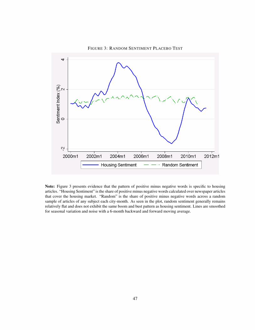
FIGURE 3: RANDOM SENTIMENT PLACEBO TEST

Note: Figure 3 presents evidence that the pattern of positive minus negative words is specific to housingarticles. “Housing Sentiment” is the share of positive minus negative words calculated over newspaper articlesthat cover the housing market. “Random” is the share of positive minus negative words across a randomsample of articles of any subject each city-month. As seen in the plot, random sentiment generally remainsrelatively flat and does not exhibit the same boom and bust pattern as housing sentiment. Lines are smoothedfor seasonal variation and noise with a 6-month backward and forward moving average.

47

FIGURE 4: VALIDATING SENTIMENT AGAINST SURVEYS OF HOUSING MARKET CONFIDENCE

Panel A. Housing Sentiment Index and Survey of Consumers Home Buyer Confidence

Panel B. Housing Sentiment Index and National Association of Home Builders Confidence Index

Note: Panel A plots the composite-20 housing sentiment index with a national survey of home buyer confidence. TheSurvey of Consumers surveys a nationally representative sample of 500 consumers and asks whether they think it is agood time to buy a home. Consumers answer “Yes/No/Don’t Know.” The green dashed line represents the percentageof those surveyed who answered “Yes.” Panel B plots the composite housing sentiment index with a national surveyof members of home builder confidence. The National Association Home Builders asks members of their associationeach month to rate the current market conditions of the sale of new homes, the prospective market conditions in thenext 6 months, and the expected volume of new home buyers. The NAHB index weights these answers into one indexto represent an aggregate builders’ opinion of housing market conditions. The timing the sentiment index coincideswith survey measures of confidence, suggesting that it is reflecting investor beliefs over the housing market. Lines aresmoothed for seasonal variation and noise with a 6-month backward and forward moving average.

48

FIGURE 5: PREDICTING HOUSE PRICE GROWTH WITH SENTIMENT INDEX V. FUNDAMENTALS

Note: Figure 7 plots observed composite-20 prices and predicted prices. The dashed line represents prices predicted withcontemporaneous. fundamentals alone. The solid line plots prices predicted with positive sentiment only. The pictureillustrates that sentiment can explain a significant variation in prices. More importantly, sentiment fits the prediction tothe timing of the boom and bust, whereas fundamentals only predict a linear projection of prices.

49

FIGURE 6: COMPOSITE-20 HOUSING SENTIMENT INDEX AND TRANSACTION VOLUME

Note: Figure 8 plots a composite-20 volume of housing transactions and my housing sentiment index. Datafor transaction volume comes from DataQuick. I calculate a composite-20 measure of volume using the sameweights used to create the Case-Shiller Composite-20 Home price Index. Lines are smoothed for seasonalvariation and noise with a 6-month backward and forward moving average.

50

TABLE 1: DESCRIPTIVE STATISTICS FOR NEWSPAPER HOUSING ARTICLES

Newspaper Publication # Articles AP A-section Real Estate Local General

All Cities 19,620 6% 19% 20% 28% 45%

Atlanta The Atlanta Journal-Constitution 647 0 24 13 29 60

Boston Boston Herald/Boston Globe 966 3 23 15 24 43

Charlotte The Observer 556 14 23 28 17 33

Chicago Chicago Tribune 1,965 8 79 66 13 27

Cleveland The Plain Dealer 303 1 18 13 20 62

DC The Washington Post 1,171 6 13 38 27 24

Dallas The Dallas Morning News 1,294 0 3 0 74 22

Denver The Denver Post 432 1 13 0 11 83

Detroit Detroit News/Detroit Free Press 624 5 48 23 10 55

LA LA Times/LA Daily News 3,579 5 17 14 18 69

Las Vegas Las Vegas Review-Journal 588 0 15 0 4 92

Miami The Miami Herald 678 7 27 11 14 51

Minneapolis Star Tribune 625 1 17 20 1 79

NYC New York Times 1,372 4 19 33 17 42

Phoenix The Arizona Republic 1,921 0 19 5 52 29

Portland The Oregonian 509 2 18 16 35 42

San Diego The San Diego Union-Tribune 1,086 7 14 26 16 52

San Francisco The San Francisco Chronicle 530 0 27 8 8 81

Seattle The Seattle Times 398 29 25 36 5 59

Tampa Tampa Tribune 376 0 30 2 43 41

Note: Table 1 lists each city, its corresponding newspaper, and descriptive statistics for my sample of housing newsarticles. My source for housing news articles is Factiva.com, which provides a subject code to identify articles that coverhousing market news. My sample covers articles from January 2000 to August 2011. “AP” lists the percent of articles thatare credited to the Associated Press. “A-section” refers to the percent of articles located in the front or “A” section of thenewspaper. “Real Estate” is the percent of articles that were published in a special real estate section of the newspaper.“Local News” refers to those articles listed in the metropolitan or any specific regional news section of the newspaper.Most of the articles are found in a general news or business news section of the newspaper. It is possible for one articleto show up in more than one category. For example, if an article is in the real estate section of the regional edition of thenewspaper than it would show up in both columns 6 and 7. Thus, the percents will not necessarily add up to 100 percentfor each city.

51

TABLE 2: SAMPLE POSITIVE WORDS AND WORD COUNTS

word % of Total PosWord Count Freq.BOOM 3.24 959BOOST 1.17 348BRIGHT 0.36 106EXCEED 0.33 98EXTEND 0.52 154GOOD 2.29 678GREAT 0.69 203HEAT 3.1 917HOPE 0.69 205JUMP 2.67 790LEAP 0.49 145POSITIVE 0.3 89SHOOT 0.44 130SIZZLE 0.48 143SKYROCKET 0.34 101SOAR 2.23 660SPIKE 0.32 96SPRINGING 0.49 145STRONG 2.4 711SURGE 1.91 565

Note: This base list of positive words are from the word lists Increas and Rise word lists in the Harvard IV-4 PsychologicalDictionary. I use these lists to maintain the objectivity of a predetermined list, but also reflect how the media spinsexcitement over asset markets. Shiller (2008) in particular argues that the media expresses a positive slant throughsuperlatives that emphasize price increases and upward movements. I then expand the original word list with synonyms,alternate tenses, and inflections. I also eliminate obvious misclassifications. The original Harvard list consisted of 136words while the extended Inc-NEW list contains 403 words. This table presents a sample of words and their correspondingword counts.

52

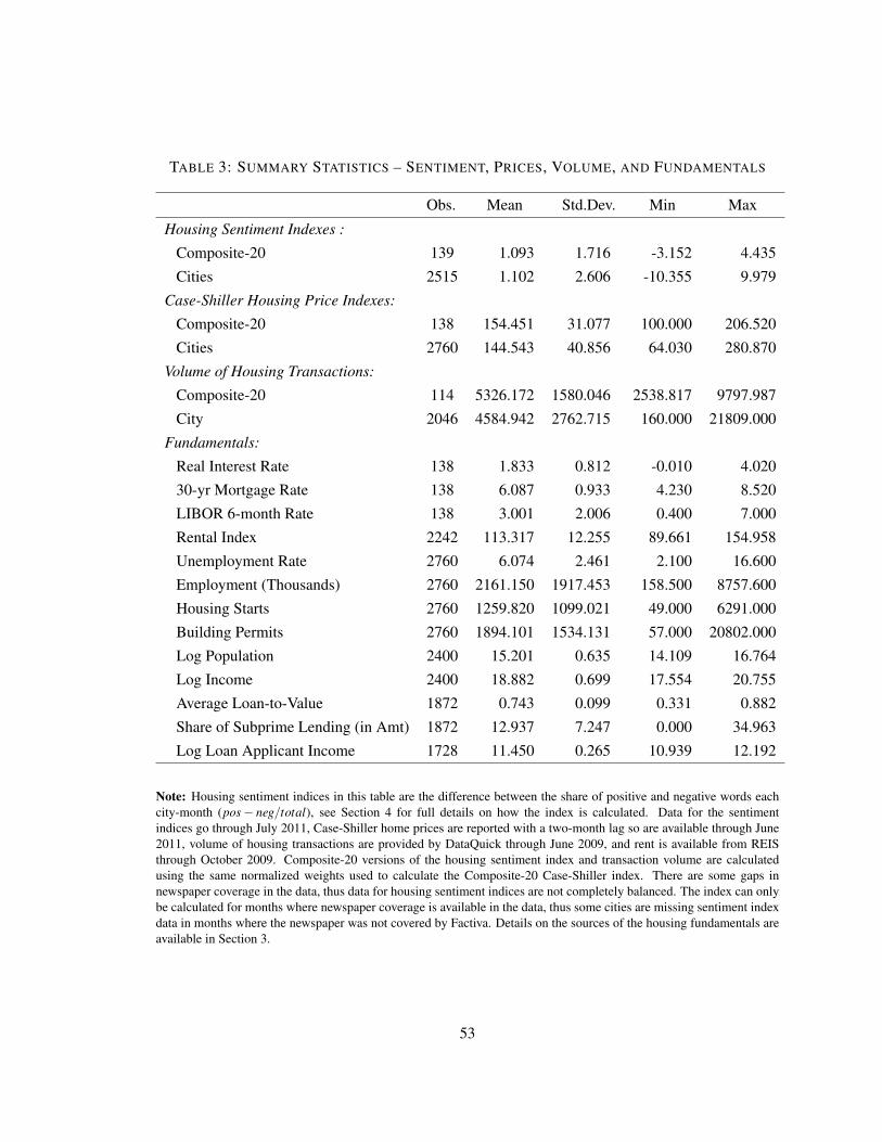
TABLE 3: SUMMARY STATISTICS – SENTIMENT, PRICES, VOLUME, AND FUNDAMENTALS

Obs. Mean Std.Dev. Min MaxHousing Sentiment Indexes :

Composite-20 139 1.093 1.716 -3.152 4.435Cities 2515 1.102 2.606 -10.355 9.979

Case-Shiller Housing Price Indexes:Composite-20 138 154.451 31.077 100.000 206.520Cities 2760 144.543 40.856 64.030 280.870

Volume of Housing Transactions:Composite-20 114 5326.172 1580.046 2538.817 9797.987City 2046 4584.942 2762.715 160.000 21809.000

Fundamentals:Real Interest Rate 138 1.833 0.812 -0.010 4.02030-yr Mortgage Rate 138 6.087 0.933 4.230 8.520LIBOR 6-month Rate 138 3.001 2.006 0.400 7.000Rental Index 2242 113.317 12.255 89.661 154.958Unemployment Rate 2760 6.074 2.461 2.100 16.600Employment (Thousands) 2760 2161.150 1917.453 158.500 8757.600Housing Starts 2760 1259.820 1099.021 49.000 6291.000Building Permits 2760 1894.101 1534.131 57.000 20802.000Log Population 2400 15.201 0.635 14.109 16.764Log Income 2400 18.882 0.699 17.554 20.755Average Loan-to-Value 1872 0.743 0.099 0.331 0.882Share of Subprime Lending (in Amt) 1872 12.937 7.247 0.000 34.963Log Loan Applicant Income 1728 11.450 0.265 10.939 12.192

Note: Housing sentiment indices in this table are the difference between the share of positive and negative words eachcity-month (pos � neg/total), see Section 4 for full details on how the index is calculated. Data for the sentimentindices go through July 2011, Case-Shiller home prices are reported with a two-month lag so are available through June2011, volume of housing transactions are provided by DataQuick through June 2009, and rent is available from REISthrough October 2009. Composite-20 versions of the housing sentiment index and transaction volume are calculatedusing the same normalized weights used to calculate the Composite-20 Case-Shiller index. There are some gaps innewspaper coverage in the data, thus data for housing sentiment indices are not completely balanced. The index can onlybe calculated for months where newspaper coverage is available in the data, thus some cities are missing sentiment indexdata in months where the newspaper was not covered by Factiva. Details on the sources of the housing fundamentals areavailable in Section 3.

53

TAB

LE

4:SE

NT

IME

NT

PRE

DIC

TS

NA

TIO

NA

LH

OU

SEPR

ICE

APP

RE

CIA

TIO

N

(1)

(2)

(3)

(4)

(5)

(6)

(7)

(8)

(9)

(10)

Sum

ofLa

gged

Sent

imen

t0.

756*

**0.

763*

**0.

760*

**0.

760*

**0.

760*

**0.

763*

**0.

838*

**0.

696*

**0.

932*

**0.

120

(0.0

80)

(0.0

76)

(0.0

74)

(0.0

77)

(0.0

79)

(0.0

78)

(0.1

25)

(0.1

63)

(0.2

06)

(0.0

73)

Year

1La

gs(L

1+...+

L12)

0.21

3***

0.18

4***

0.18

9***

0.18

9***

0.18

6***

0.18

5***

0.19

3***

0.16

9***

0.27

3***

0.02

1

(0.0

18)

(0.0

26)

(0.0

25)

(0.0

26)

(0.0

24)

(0.0

25)

(0.0

29)

(0.0

39)

(0.0

71)

(0.0

21)

Year

2La

gs(L

13+...+

L24)

0.10

1***

0.08

7***

0.08

9***

0.08

9***

0.08

8***

0.08

7***

0.09

5***

0.10

0***

0.16

4***

0.01

2

(0.0

30)

(0.0

27)

(0.0

24)

(0.0

24)

(0.0

23)

(0.0

24)

(0.0

25)

(0.0

28)

(0.0

42)

(0.0

11)

Year

3La

gs(L

25+...+

L43)

0.44

2***

0.49

3***

0.48

2***

0.48

2***

0.48

6***

0.49

1***

0.55

0***

0.42

7***

0.49

5**

0.08

7

(0.0

51)

(0.0

49)

(0.0

51)

(0.0

53)

(0.0

56)

(0.0

58)

(0.1

03)

(0.1

39)

(0.1

76)

(0.0

52)

Ren

ts.

XX

XX

XX

XX

XIn

tere

stR

ate

Varia

bles

..

XX

XX

XX

XX

Labo

rMar

ketV

aria

bles

..

.X

XX

XX

XX

Hou

sing

Supp

ly.

..

.X

XX

XX

XPo

pula

tion

and

Inco

me

..

..

.X

XX

XX

Mon

thFi

xed

Effe

cts

..

..

..

XX

XX

Line

arTi

me

Tren

d.

..

..

..

X.

.

Lagg

edFu

ndam

enta

ls.

..

..

..

.X

.

Lagg

edPr

ice

Gro

wth

..

..

..

..

.X

Obs

erva

tions

9494

9494

9494

9494

9494

Adj

uste

dR2

0.85

40.

863

0.86

60.

860.

858

0.85

20.

835

0.83

80.

841

0.97

4

Not

e:*

10%

sign

ifica

nce,

**5%

leve

l,**

*1%

leve

l.N

ewey

and

Wes

t(19

87)s

tand

ard

erro

rsth

atar

ero

bust

tohe

tero

sked

astic

ityan

dau

to-c

orre

latio

nup

to12

lags

are

inpa

rent

hese

s.Lk

deno

tes

the

lag

t�k.

Sum

ofLa

gged

Sent

imen

tsum

sall

the

coef

ficie

ntes

timat

esof

curr

enta

ndla

gged

sent

imen

tgro

wth

toge

ther

.The

row

sbel

owbr

eak

dow

nto

tals

umof

the

mon

thly

lags

ofse

ntim

ent

byla

gged

year

s.“Y

ear1

Lags

”eq

uals

the

sum

ofla

gged

sent

imen

tfro

mL1

toL12

,“Ye

ar2

Lags

”is

the

sum

ofla

gsL13

toL24

,“Ye

ar3

Lags

”is

the

sum

from

lags

L25to

L43..

The

corr

espo

ndin

gst

anda

rder

rors

fort

helin

earc

ombi

natio

nof

estim

ates

are

repo

rted

inpa

rent

hese

sbe

low

.The

lag

stru

ctur

eis

chos

enth

roug

ha

join

tF-te

st.A

dditi

onal

lags

afte

rL43

does

nota

ffec

tthe

resu

lts.

54

TAB

LE

5:SE

NT

IME

NT

PRE

DIC

TS

CIT

YH

OU

SEPR

ICE

APP

RE

CIA

TIO

N(P

AN

EL

)B

OO

MB

UST

(1)

(2)

(3)

(4)

(5)

(6)

(7)

(8)

(9)

(10)

Sum

ofLa

gged

Sent

imen

t1.

120*

**1.

223*

**1.

342*

**1.

276*

**0.

670*

**1.

015*

**0.

846*

**0.

266*

**0.

814*

**1.

035*

**

(0.1

20)

(0.1

31)

(0.1

27)

(0.1

25)

(0.1

70)

(0.1

71)

(0.1

44)

(0.0

48)

(0.3

09)

(0.1

53)

Year

1La

gs(L

1+...+

L12)

0.24

8***

0.28

2***

0.32

3***

0.29

4***

0.15

6***

0.25

7***

0.20

0***

0.06

8***

0.28

9***

0.20

6***

(0.0

34)

(0.0

42)

(0.0

39)

(0.0

37)

(0.0

35)

(0.0

39)

(0.0

41)

(0.0

13)

(0.0

85)

(0.0

36)

Year

2La

gs(L

13+...+

L24)

0.31

1***

0.44

0***

0.47

9***

0.46

2***

0.22

6***

0.36

6***

0.31

4***

0.09

3***

0.24

9**

0.37

1***

(0.0

41)

(0.0

50)

(0.0

48)

(0.0

47)

(0.0

58)

(0.0

65)

(0.0

51)

(0.0

18)

(0.1

12)

(0.0

56)

Year

3La

gs(L

25+...+

L43)

0.56

0***

0.50

1***

0.54

0***

0.52

1***

0.28

7***

0.39

2***

0.33

2***

0.10

5***

0.27

5*0.

458*

**

(0.0

65)

(0.0

83)

(0.0

70)

(0.0

69)

(0.0

98)

(0.0

89)

(0.0

85)

(0.0

24)

(0.1

44)

(0.0

83)

Fund

amen

tals

.X

XX

XX

XX

XX

City

Fixe

dEf

fect

s.

.X

XX

XX

XX

XM

onth

Fixe

dEf

fect

s.

..

XX

XX

XX

XYe

arFi

xed

Effe

cts

..

..

X.

..

..

Line

arTi

me

Tren

d.

..

..

X.

..

.

Lagg

edFu

ndam

enta

ls.

..

..

.X

..

.

Lagg

edPr

ice

Gro

wth

..

..

..

.X

..

Obs

erva

tions

1564

1106

1106

1106

1106

1106

1106

1106

399

707

Adj

uste

dR2

0.28

70.

466

0.51

70.

582

0.63

40.

589

0.66

90.

863

0.47

10.

576

Not

e:*

10%

sign

ifica

nce,

**5%

leve

l,**

*1%

leve

l.Th

ista

ble

estim

ates

the

effe

ctof

sent

imen

tacr

oss

citie

s.Th

enu

mbe

rofo

bser

vatio

nsde

clin

efr

omco

lum

ns(1

)to

(2)b

ecau

sefu

ndam

enta

lsar

eon

lyav

aila

ble

thro

ugh

2009

whi

lese

ntim

enti

ndic

esar

eav

aila

ble

thro

ugh

July

2011

.New

eyan

dW

est(

1987

)sta

ndar

der

rors

that

are

robu

stto

hete

rosk

edas

ticity

and

auto

-cor

rela

tion

upto

12la

gsar

ein

pare

nthe

ses.

Lkde

note

sth

ela

gt�

k.Su

mof

Lagg

edSe

ntim

ents

ums

allt

heco

effic

ient

estim

ates

ofcu

rren

tand

lagg

edse

ntim

entg

row

thto

geth

er.T

hero

ws

belo

wbr

eak

dow

nto

tal

sum

ofth

em

onth

lyla

gsof

sent

imen

tby

lagg

edye

ars.

“Yea

r1La

gs”

equa

lsth

esu

mof

lagg

edse

ntim

entf

rom

L1to

L12,“

Year

2La

gs”

isth

esu

mof

lags

L13to

L24,“

Year

3La

gs”

isth

esu

mfr

omla

gsL25

toL43

..Th

eco

rres

pond

ing

stan

dard

erro

rsfo

rthe

linea

rcom

bina

tion

ofes

timat

esar

ere

porte

din

pare

nthe

ses

belo

w.E

stim

ates

ofla

gged

logg

edse

ntim

entm

easu

reth

eim

pact

ofa

one

perc

enti

ncre

ase

inth

em

onth

lygr

owth

ofse

ntim

ento

nth

em

onth

lygr

owth

inpr

ices

i.e.m

onth

lyca

pita

lapp

reci

atio

non

hous

ing.

55

TABLE 6: SENTIMENT PREDICTS CITY HOUSE PRICES BEYOND SUBPRIME LENDING TRENDS

(1) (2) (3) (4) (5)

Sum of Lagged Sentiment 0.830*** 0.778*** 0.769*** 0.692*** 0.421***

(0.148) (0.162) (0.161) (0.154) (0.135)

Year 1 Lags (L1 + ...+L12) 0.193*** 0.213*** 0.212*** 0.224*** 0.144***

(0.043) (0.049) (0.049) (0.045) (0.035)

Year 2 Lags (L13 + ...+L24) 0.304*** 0.290*** 0.287*** 0.263*** 0.169***

(0.052) (0.057) (0.057) (0.051) (0.049)

Year 3 Lags (L25 + ...+L43) 0.333*** 0.275*** 0.270*** 0.204** 0.108

(0.088) (0.098) (0.097) (0.097) (0.08)

Month Fixed Effects X X X X XCity Fixed Effects X X X X XFundamentals X X X X XLagged Fundamentals X X X X XLIBOR 6-month rate X X X X X% Subprime Loans . X X X XLoan-To-Value . X X XLoan Applicant Income . . X XLagged Credit Variables . . . XObservations 1106 876 876 771 771

Adjusted R2 0.667 0.707 0.709 0.735 0.793

Note: * 10% significance, ** 5% level, *** 1% level. This table estimates the effect of sentiment across cities. The number ofobservations decline from columns (1) to (2) because data for % of subprime loans are only available for 16 cities in the sample andonly through September 2009, observations further decline because loan applicant income from the HMDA database are only availablethrough 2008.Newey and West (1987) standard errors that are robust to heteroskedasticity and auto-correlation up to 12 lags are inparentheses. Lk denotes the lag t � k. Sum of Lagged Sentiment sums all the coefficient estimates of current and lagged sentimentgrowth together. The rows below break down total sum of the monthly lags of sentiment by lagged years. “Year 1 Lags” equals thesum of lagged sentiment from L1 to L12, “Year 2 Lags” is the sum of lags L13 to L24, “Year 3 Lags” is the sum from lags L25 to L43..The corresponding standard errors for the linear combination of estimates are reported in parentheses below. The lag structure is chosenthrough a standard joint F-test. Including additional lags after L43 does not affect the results. Estimates of lagged logged sentimentmeasure the impact of a one percent increase in the monthly growth of sentiment on the monthly growth in prices i.e. monthly capitalappreciation on housing.

56

TABLE 7: SENTIMENT PREDICTS THE VOLUME OF HOUSING TRANSACTIONS

Composite Panel

(1) (2) (3) (4) (5) (6)

Sum of Lagged Sentiment 4.674*** 4.909*** 5.531*** 3.658*** 2.709*** 1.479**

(1.189) (1.337) (1.915) (0.678) (0.668) (0.594)

Year 1 Lags (L1 + ...+L12) 3.555*** 3.938*** 4.13** 2.957*** 2.355*** 1.381***

(0.890) (1.012) (1.681) (0.556) (0.532) (0.486)

Year 2 Lags (L13 + ...+L18) 1.119** 0.971 1.401 0.701*** 0.354* 0.098

(0.505) (0.874) (0.893) (0.208) (0.206) (0.153)

Rents . X X . X XInterest Rate Variables . X X . X XLabor Market Variables . X X . X XHousing Supply . X X . X XPopulation and Income . X X . X XMonth Fixed Effects . X X . X XCity Fixed Effects . . . . X XLagged Fundamentals . . X . . XObservations 96 96 96 1578 1481 1437

Adjusted R2 0.430 0.613 0.595 0.068 0.261 0.507

Note: * 10% significance, ** 5% level, *** 1% level. Newey-West standard errors that are robust to heteroskedasticity and auto-correlation up to 12 lags are in parentheses. This tables estimates the effect of sentiment on detrended log volume. I use detrended logvolume to address non stationarity concerns, and detrend volume following Campbell et al. (1993). Specifically, I subtract the one yearbackward moving average. Newey and West (1987) standard errors that are robust to heteroskedasticity and auto-correlation up to 12lags are in parentheses. Lk denotes the lag t � k. Sum of Lagged Sentiment sums all the coefficient estimates of current and laggedsentiment growth together. The rows below break down total sum of the monthly lags of sentiment by lagged years. “Year 1 Lags”equals the sum of lagged sentiment from L1 to L12, “Year 2 Lags” is the sum of lags L13 to L24, “Year 3 Lags” is the sum from lags L25

to L43.. The corresponding standard errors for the linear combination of estimates are reported in parentheses below. The lag structureis chosen through a standard joint F-test. Including additional lags after L43 does not affect the results. Estimates of lagged loggedsentiment measure the impact of a one percent increase in the monthly growth of sentiment on the monthly growth in prices i.e. monthlycapital appreciation on housing.

57

TABLE 8: EXPLANATORY POWER OF OBSERVED FUNDAMENTALS PRE- AND POST-2000

Composite-10 Panel

Pre-2000 Post-2000 Pre-2000 Post-2000

(1) (2) (4) (5)

Rents 1.424*** 0.373 0.840*** 0.365**

(0.166) (0.704) (0.110) (0.179)

Interest Rate Variables X X X XLabor Market Variables X X X XHousing Supply X X X XPopulation and Income X X X XMonth Fixed Effects X X X XCity Fixed Effects . . X XObservations 119 118 2136 2241

Adjusted R2 0.693 0.092 0.363 0.234

Note: * 10% significance, ** 5% level, *** 1% level. Newey-West standard errors that are robust to heteroskedasticity and auto-correlation up to 12 lags are in parentheses. Lk denotes the lag t � k. Sum of Lagged Sentiment sums all the coefficient estimates ofcurrent and lagged sentiment growth together. The corresponding standard errors for the linear combination of estimates are reportedin parentheses below. Estimates of lagged logged sentiment measure the impact of a one percent increase in the monthly growthof sentiment on the monthly growth in prices i.e. monthly capital appreciation on housing. This table shows that they key set offundamentals explain prices much better prior to the suspected bubble period, post-2000. For example, the R2 in column 1 shows thatthe key set of fundamentals is able to explain nearly 70 percent of the variation in aggregate price growth prior to 2000. After 2000,however, this same set of fundamentals explains very little of the variation in price growth with an adjusted R2 = 0.09. This suggeststhat the main set of results at least incorporate the key set of fundamentals that typically explain housing price growth, and that pricemovements post-2000 must be due to some other variable. Thus, sentiment estimates in the main results are less likely driven by biasfrom an unobserved fundamental.

58

TAB

LE

9:IS

SEN

TIM

EN

TD

RIV

EN

BY

NE

WS

STO

RIE

SO

NU

NO

BSE

RV

ED

FUN

DA

ME

NTA

LS?

Dep

Var:

Hou

sing

Pric

eG

row

th,t

=mon

thly

(1)

(2)

(3)

(4)

(5)

(6)

(7)

Sum

ofLa

gged

Sent

imen

t0.

826*

**0.

540*

*0.

636*

**0.

572*

**0.

589*

**0.

530*

*0.

581*

*

(0.1

48)

(0.2

12)

(0.2

08)

(0.2

1)(0

.215

)(0

.256

)(0

.279

)

Med

iaR

ents

XX

XX

XX

XM

edia

Cre

ditC

ondi

tions

.X

XX

XX

XM

edia

Labo

rMar

ketC

ondi

tions

..

XX

XX

XM

edia

Hou

sing

Supp

ly.

..

XX

XX

Med

iaU

serC

osts

..

..

XX

XM

edia

Dem

ogra

phic

s.

..

..

XX

Med

iaLo

calG

DP

&In

flatio

n.

..

..

.X

Mon

thFi

xed

Effe

cts

XX

XX

XX

XC

ityFi

xed

Effe

cts

XX

XX

XX

XFu

ndam

enta

lsX

XX

XX

XX

Lagg

edFu

ndam

enta

lsX

XX

XX

XX

Obs

erva

tions

1094

1094

1093

1093

1093

1093

1093

Adj

uste

dR2

0.67

80.

683

0.71

70.

717

0.71

70.

718

0.72

3

Not

e:*

10%

sign

ifica

nce,

**5%

leve

l,**

*1%

leve

l.N

ewey

-Wes

tsta

ndar

der

rors

that

are

robu

stto

hete

rosk

edas

ticity

and

auto

-cor

rela

tion

upto

12la

gsar

ein

pare

nthe

ses.

Sum

ofLa

gged

Sent

imen

tsum

sal

lthe

coef

ficie

ntes

timat

esof

curr

enta

ndla

gged

sent

imen

tgro

wth

toge

ther

.The

corr

espo

ndin

gst

anda

rder

rors

fort

helin

earc

ombi

natio

nof

estim

ates

are

repo

rted

inpa

rent

hese

sbel

ow.E

stim

ates

ofla

gged

logg

edse

ntim

entm

easu

reth

eim

pact

ofa

one

perc

enti

ncre

ase

inth

em

onth

lygr

owth

ofse

ntim

ento

nth

em

onth

lygr

owth

inpr

ices

i.e.

mon

thly

capi

tala

ppre

ciat

ion

onho

usin

g.Th

ista

ble

dire

ctly

cont

rols

forn

ews

cont

ento

verf

unda

men

tals

byid

entif

ying

any

new

sar

ticle

that

men

tions

apa

rticu

larf

unda

men

tali

nits

text

.The

varia

ble

“Med

iaR

ents

”,fo

rexa

mpl

e,is

the

shar

eof

posi

tive

min

usne

gativ

ew

ords

inan

yar

ticle

sth

atm

entio

nan

yw

ord

rela

ted

to“r

ents

”in

itste

xt.T

his

tabl

esh

ows

that

cont

rolli

ngfo

rarti

cles

that

men

tion

fund

amen

tals

has

min

imal

effe

cton

the

estim

ated

effe

ctof

sent

imen

ton

hous

epr

ices

.

59

TABLE 10: CORRELATION OF WEEKEND INSTRUMENT WITH FRIDAY NEWS RELEASES

% of Releases on Friday Correlation with Weekend Instrument

All BLS 0.07

Any Metro or Regional -0.01

County Employment -0.04

Regional Employment -0.05

Metro Area Employment 0.00

CPI -0.02

PPI 0.14

New Residential Construction -0.02

New Residential Sales -0.01

Note: This table test for a possible violation of the exclusion restriction for the weekend instrument. The validity ofthe weekend instrument relies on the assumption that no news on fundamentals is being released over the weekend.One possible violation of this assumption is that news is increasingly released on Friday and therefore reported overthe weekend. I put together a database of the schedule of economic data releases from the BLS and the Census. Thistable shows that the fraction released on Friday is uncorrelated with the share of positive minus negative words over theweekend. The first column lists the types of press releases, including all releases by the Bureau of Labor Statistics, anyrelease on metropolitan or regional specific fundamentals, release on employment, measures of inflation, and housingspecific fundamentals from the Census. The second column reports the simple correlation between the fraction of thesereleases that occur on Friday with the weekend instrument.

60

TABLE 11: WEEKEND AND NARRATIVE INSTRUMENTS FOR SENTIMENT, FIRST-STAGE

Dep Var: Sentiment Growth, t=monthly

Weekend Narrative

Instrument 0.458*** 0.208***

(0.100) (0.031)

Weekday News Tone X .

Rents X XInterest Rate Variables X XLabor Market Variables X XHousing Supply Variables X XPopulation and Income X XMonth Fixed Effects X XCity Fixed Effects X XLagged Fundamentals X XF-statistic 233.776 46.089Observations 1856 1856

Adjusted R2 0.663 0.108

Note: * 10% significance, ** 5% level, *** 1% level. Newey-West standard errors that are robust to heteroskedasticityand auto-correlation up to 12 lags are in parentheses. Sum of Lagged Sentiment sums all the coefficient estimates ofcurrent and lagged sentiment growth together. The corresponding standard errors for the linear combination of estimatesare reported in parentheses below. Estimates of lagged logged sentiment measure the impact of a one percent increasein the monthly growth of sentiment on the monthly growth in prices i.e. monthly capital appreciation on housing. Thistable reports the first-stage estimates of sentiment on the weekend and narrative instruments. The bottom panel reportsthe F-statistic for the instruments in bold to test for instrument strength. Both instruments are sufficiently relevant to thehousing sentiment index, with F-statistics well above the benchmark rule of 10.

61

TABLE 12: PREDICTING PRICE GROWTH USING POSITIVE SENTIMENT, IV RESULTS

OLS Weekend IV Narrative IV

(1) (2) (3)

Sum of Lagged Sentiment 0.837*** 1.247*** 0.805**

(0.096) (0.217) (0.382)

Year 1 Lags (L1+...+L12) 0.18*** 0.305 0.01

(0.035) (0.187) (0.304)

Year 2 Lags (L13+...+L24) 0.294*** 0.500*** 0.47**

(0.039) (0.153) (0.215)

Year 3 Lags (L25+...+L43) 0.363*** 0.441*** 0.326

(0.042) (0.091) (0.201)

Weekday News Tone . X .

Month Fixed Effects X X XCity Fixed Effects X X XFundamentals X X XLagged Fundamentals X X XObservations 1106 1106 1106

Adjusted R2 0.669 0.647 0.648

Note: * 10% significance, ** 5% level, *** 1% level. Newey-West standard errors that are robust to heteroskedasticityand auto-correlation up to 12 lags are in parentheses. Sum of Lagged Sentiment sums all the coefficient estimates ofcurrent and lagged sentiment growth together. The corresponding standard errors for the linear combination of estimatesare reported in parentheses below. Estimates of lagged logged sentiment measure the impact of a one percent increasein the monthly growth of sentiment on the monthly growth in prices i.e. monthly capital appreciation on housing. Thistable presents the original OLS estimates in column (1), and the instrumental variable estimates using the weekend andnarrative instruments in columns (2) and (3) respectively. The estimated effect of sentiment remains robust to bothinstrumental variable strategies, suggesting bias from unobserved factors in the original estimates are less likely.

62

TAB

LE

A.1

:C

OM

PAR

ING

EFF

EC

TO

FA

LTE

RN

AT

IVE

SEN

TIM

EN

TIN

DIC

ES

Dep

Var:

Hou

sing

Pric

eG

row

th,t

=mon

thly

(1)

(2)

(3)

(4)

(5)

(6)

Pos-

Neg

Pos-

Neg

Pos-

Neg

*Po

sitiv

ePo

sitiv

eN

egat

ive

(bas

elin

e)(fu

llte

xt)

%ho

usin

gar

ticle

s(te

rm-w

eigh

ted)

Sum

ofLa

gged

Sent

imen

t0.

846*

**0.

803*

**0.

802*

**0.

264*

**0.

277*

*-0

.349

***

(0.1

44)

(0.1

37)

(0.1

49)

(0.0

75)

(0.1

08)

(0.0

69)

Fund

amen

tals

XX

XX

XX

City

Fixe

dEf

fect

sX

XX

XX

XM

onth

Fixe

dEf

fect

sX

XX

XX

XLa

gged

Fund

amen

tals

XX

XX

XX

Cor

rela

tion

with

base

line

1.00

0.78

40.

655

0.67

40.

510

-0.6

66O

bser

vatio

ns11

0611

0611

0611

0611

0611

06A

djus

ted

R20.

669

0.69

40.

696

0.62

40.

615

0.66

2

Not

e:*

10%

sign

ifica

nce,

**5%

leve

l,**

*1%

leve

l.N

ewey

-Wes

tsta

ndar

der

rors

that

are

robu

stto

hete

rosk

edas

ticity

and

auto

-cor

rela

tion

upto

12la

gsar

ein

pare

nthe

ses.

Sum

ofLa

gged

Sent

imen

tsum

sal

lthe

coef

ficie

ntes

timat

esof

curr

enta

ndla

gged

sent

imen

tgro

wth

toge

ther

.The

corr

espo

ndin

gst

anda

rder

rors

fort

helin

earc

ombi

natio

nof

estim

ates

are

repo

rted

inpa

rent

hese

sbe

low

.Es

timat

esof

lagg

edlo

gged

sent

imen

tmea

sure

the

impa

ctof

aon

epe

rcen

tinc

reas

ein

the

mon

thly

grow

thof

sent

imen

ton

the

mon

thly

grow

thin

pric

esi.e

.m

onth

lyca

pita

lapp

reci

atio

non

hous

ing.

This

tabl

eco

mpa

res

the

effe

ctof

alte

rnat

eve

rsio

nsof

the

sent

imen

tind

exon

hous

epr

ices

and

show

stha

tres

ults

are

qual

itativ

ely

the

sam

e.“P

os-N

eg”

repr

esen

tsth

edi

ffer

ence

betw

een

the

shar

eof

posi

tive

and

nega

tive

wor

dsin

the

lead

ing

text

ofho

usin

gar

ticle

seac

hci

ty-m

onth

.Pos

-Neg

(full

text

)ist

hesa

me

inde

xca

lcul

ated

over

the

full

text

ofth

ear

ticle

s.C

olum

n(3

)add

sano

ther

dim

ensi

onof

sent

imen

tby

inte

ract

ing

the

base

line

inde

xw

ithth

efr

actio

nof

alln

ewsp

aper

artic

les

that

cove

rthe

hous

ing

mar

ket.

This

inde

xac

coun

tsfo

rbot

hth

eto

neof

new

spap

erar

ticle

san

dth

enu

mbe

rofa

rticl

espu

blis

hed

onho

usin

g.C

olum

ns(4

)-(6

)con

side

rsth

eef

fect

ofpo

sitiv

ean

dne

gativ

ese

ntim

ents

epar

atel

y.C

olum

n(4

)use

sju

stth

esh

are

ofpo

sitiv

ew

ords

.C

olum

n(5

)cal

cula

tes

a“t

erm

-wei

ghte

d”po

sitiv

ein

dex,

whi

chad

dw

eigh

tsfo

rth

eco

mm

onal

ityan

dfr

eque

ncy

ofa

wor

dac

ross

docu

men

ts(L

ough

ran

and

Mcd

onal

d(2

011)

).“N

egat

ive”

isth

esh

are

ofne

gativ

ew

ords

acro

ssar

ticle

sea

chm

onth

.

63

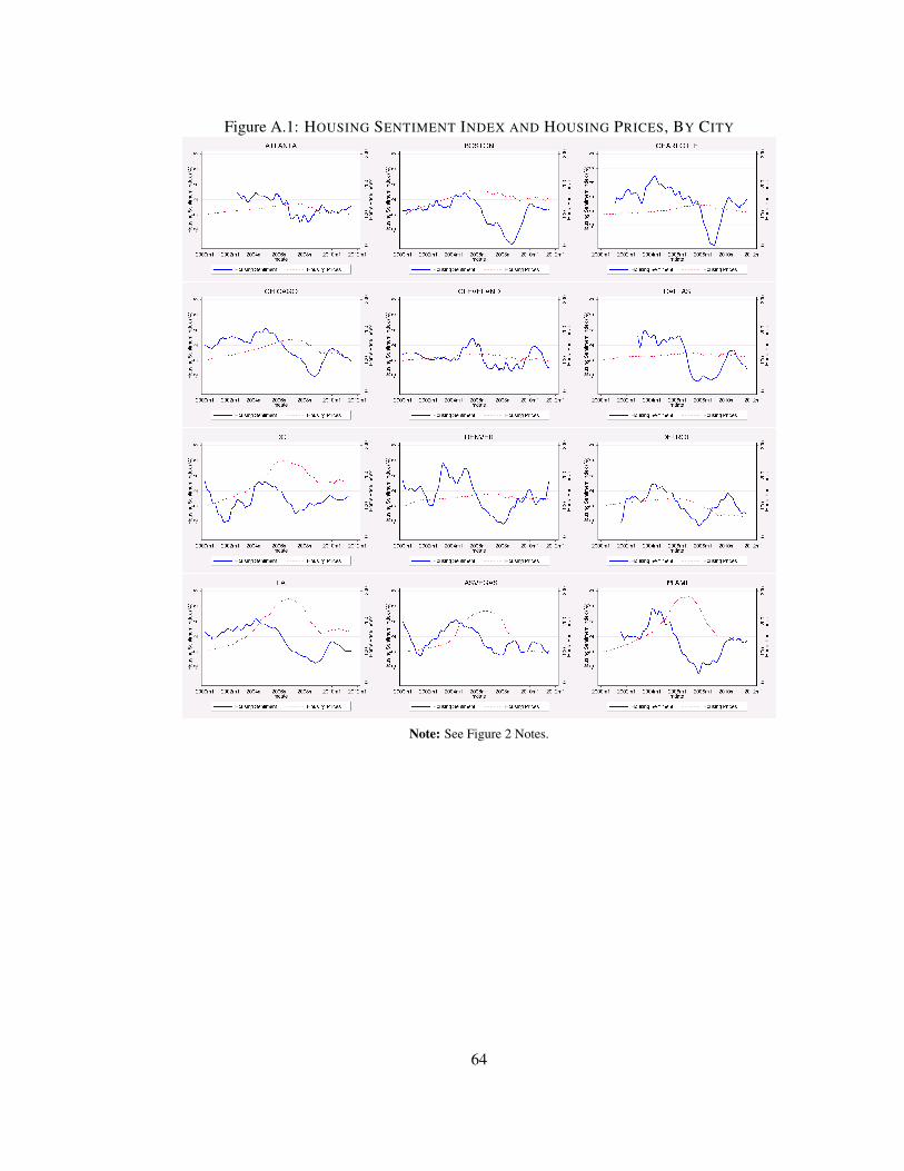
Figure A.1: HOUSING SENTIMENT INDEX AND HOUSING PRICES, BY CITY

Note: See Figure 2 Notes.

64

Figure A.1: HOUSING SENTIMENT INDEX AND HOUSING PRICES, BY CITY (CONT’D)

Note: See Figure 2 Notes.

65

66

CHAPTER 2

TIMING THE HOUSING MARKET*

Todd Sinai The Wharton School, University of Pennsylvania

Cindy K. Soo


Abstract

We create reliable measures of the cost of owning and the cost of renting that enable us to compare the level of rents and ownership costs across MSAs. We show that households can predict whether renting or owning will end up being less expensive ex post. This exercise is more robust than trying to predict house price changes or housing returns because much of that uncertainty is inframarginal in the optimal own/rent decision, which depends only on the which tenure mode is cheaper. We show that households can profitably time the home ownership decision. Using several simple trading rules, we estimate that households can save as much as 50 percent of annual rental costs over a five-year period by timing the decision of when to buy a home. The potential savings varies across cities.

! *Pengpeng Xiao provided outstanding research assistance. We are grateful to the participants in the Wharton Applied Economics Workshop for their helpful comments and to the Research Scholars Program at the Zell-Lurie Real Estate Center for financial support.

67

1 Introduction

Pioneering work by Case and Shiller (1989) has documented significant predictability in

the house price changes, such that a change in a given year predicts the same direction in the

following year. From an asset pricing perspective, this predictability suggests an opportunity for

investors to time the market and develop a profitable trading strategy. Despite the predictability

of the housing market, recent studies find that empirical forecasts of house prices lack sufficient

precision for investors arbitrage in practice (Glaeser and Gyourko, 2010). Still, the predictability

of housing prices may be useful for the average homebuyer. For the typical household investor,

the primary concern in facing the housing market is whether own versus rent. The average

household makes a decision of when to own or rent in order to obtain housing at the lowest

possible cost. Thus, timing the market for the household rests on the relative costs of owning

versus renting.

In this paper, we investigate whether the predictability of house price changes has any

relevance for the household decision to own versus rent. Since the total cost of housing depends

on the realization of the sale price of the house, predictability of house prices suggests that the

costs of owning may also be forecastable (Hendershott and Van Order 1987; Poterba 1984).

Nevertheless, the costs of rent may vary with the costs of owning such that the relative decision

to own versus rent is still difficult to predict. Furthermore Poterba (1984) shows that if the

housing market is in equilibrium, the marginal cost of owning should equal the cost of rent in

steady-state.

In order to reliably compare the costs of owning and renting, we first pin down the

relative level of rents and house prices. Using extensive sets of both proprietary and Census

household level data, we match housing and rental values across housing and buyer

characteristics including the number of bedrooms, age of structure, and income quartiles. With

that data, we estimate the relative cost of owning and renting across 39 different metropolitan

68

statistical areas (MSAs) from 1980 to 2009.

We document a significant amount of predictability in the binary decision for the

household to own versus rent relevant for the typical household. While theory suggests that the

costs of owning and renting should be equal in equilibrium, we find that the relative costs of

owning and renting are forecastable year to year. On average, if it is better to rent (own) in a

given year and city, it is better to rent (own) respectively the next year. Overall, in many cities

owning is generally cheaper than renting, though the difference in costs varies in magnitude

across locations.

We then develop several trading strategies for the binary own versus rent decision and

compare the expected savings of using these strategies against less sophisticated trading rules.

We find that a simple trading rule of choosing to own when it was cheaper to own in the

previous year saves 13 percent of annual rent relative to always owning. A household can

benefit even more relative to a simple strategy of always renting, saving more than 40 percent on

average. While the amount of savings from this rule varies across cities, it is consistently

positive. In some cities in the South, for example, it is almost always better to own than rent

such that switching based on the trading rule produces minimal gains. In other cities, particularly

those with more momentum in their house price changes, the savings from switching relative to

always owning is much larger. While a more sophisticated rule based on a regression model

performs better, it produces minimal savings above and beyond the simpler benchmark.

We further extend our analysis to a multi-year holding period. Prior literature often

focuses on the housing returns of a 1-year holding period, but the horizon for investing in a

home is likely much longer for many households. We find that the difference in the cost of

owning and renting is still predictable over longer horizons. For example, if it is better for an

investor with a horizon of five years to own in a given year, then it is still likely better for him to

own if he enters the market in the following year. We find that a first-time homebuyer gains the

69

most savings if she waits to buy until she observes that is cheaper to own in the previous year.

Otherwise, the she should continue to rent if it was cheaper to rent in the prior year. This simple

strategy can save as much as 50 percent of annual housing costs over a 5-year period.

In contrast to prior literature, we find that the tenure choice between owning and renting

may be profitably timed. In a number of cities – but far from all – the savings from switching

tenure mode following our trading rules is large enough to offset even sizeable transaction costs.

The key is that the relative costs of owning and renting are so persistent that households do not

need to change tenure mode very often to take advantage of them. Like Case and Shiller (1989),

we find that first-time homebuyers can save money by following a trading rule to decide whether

to defer home buying for a year. However, we also show that by making the own/rent decision

serially, a household that decides to continue to rent will have the option the following year to

continue to rent some more. In most cities, we find that simple strategy can approach the lowest

cost timing for buying a home.

Our paper also contributes to several literatures besides the study of housing market

efficiency. We find that rental and owner-occupied housing markets do not appear to be in

equilibrium (Diaz and Luengo-Prado 2008, Glaeser and Gyourko 2007, Verbrugge 2009). Our

work also has implications for the recent literature on housing risk that emphasizes the choice

between owning and renting (Han 2008, Sinai and Souleles 2005, Ortalo-Magne and Rady

2002).

The remainder of the paper is organized as follows: Section 2 details the methodology

and data used to calculate our measures of the cost of owning and cost of renting. Section 3

presents the main results based on the 1-year costs of investing or renting a home. Section 4

develops a profitable trading strategy based on these results. In section 5, we extend our analysis

across greater horizons. Section 6 analyzes our results across different tax brackets, and the final

section concludes.

70

2 Measuring the Cost of Owning and Renting

2.1 Rent to Price Ratios

To compare the relative costs of owning versus renting houses, we need estimates of the

levels of house prices and rents for an otherwise-equivalent residence. This presents several

empirical challenges. First, owned units and rental units may differ in physical and economic

characteristics, and it is rare for researchers to observe rents and prices for the same unit

(Glaeser and Gyourko, 2010). Second, commonly available house price indexes and rent

indexes report only the growth in normalized prices or rents. Instead, data that can match the

level of house price and rental values are only observed at occasional points in time.

Furthermore, if one uses a growth index to extrapolate prices or rents from one point in time to

another, the extrapolated levels of prices or rents will not match observed levels in the years

when they overlap.

A number of prior studies have employed varying strategies to match house prices and

rents for comparable residences and convert house price and rent indexes into levels, (Davis et

al. 2008; Meese and Wallace, 1994; Cutts et al. 2005; Gallin 2004; Crone et al. 2004; Smith and

Smith 2006). Our approach is to apply a wide variety of methods to obtain a distribution of

possible house price and rent series. We estimate owning and rental costs in each city and year

for each possible price and rent series. This approach enables us to construct a rough estimate of

the uncertainty around the relative costs of owning and renting that is due to measuring prices

and rents with error.1

!!!!!!!!!!!!!!!!!!!!!!!!!!!!!!!!!!!!!!!!!!!!!!!!!!!!!!!!1!Prior studies typically commit to one approach. Meese and Wallace (1994) and Cutts et al. (2005) derive a rent-price ratio for specific metro at one or two points in time. Other studies such as Gallin (2004) calculated a relative rent to price ratio using just growth rates of prices and rents while ignoring the level. Crone et al. (2004) uses the American Housing Survey to create a biennial estimate of the national rent-price ratio, though not by city. Davis et al. (2008) use a hedonic method to obtain predicted rents and housing values for a set of owners and renters respectively.!

71

To implement this approach, we extract household-level micro data on the level of

house values and rents values from the 1980, 1990, and 2000 U.S. Decennial Census. The

Census data consists of a nationally representative sample of five percent of U.S. households and

reports rents paid by renters, the market value of housing reported by owners, and household

income and demographic variables. These surveys also include detailed data on house

characteristics.2

Using this data, we impute rental values to homeowners and house values to renters. We

match rental and owner-occupied units based on the following characteristics: number of

bedrooms -- including one, two, and three and more bedroom units; age of structure – whether

built within the last 0-10 years, 11-20 years, 21-30 years, or 31 years or older; and buyer and

renter income quartiles. For homeowners, we impute the average rent of rental units in the same

cell. Similarly, we impute the average house price of owner-occupied homes to rental units in

the same cell. We construct cells based on the three categories alone and in combination, and

for each year separately, yielding 42 different imputations.

We also employ a hedonic method to calculate corresponding housing and rental values

based on housing characteristics. Specifically, we regress housing values on housing

characteristics and imputed predicted house values for the units rented by renters. Conversely,

we regress rental values on a set of housing characteristics and use the estimates to predict rents

for homeowners as in Davis et al. 2008. We do this separately for each Census year, for another

six imputations.

We obtain average annual rental values by MSA from a proprietary source, REIS.3

Using these values, we create three estimates of rent to price ratios: (a) using matched rental and

!!!!!!!!!!!!!!!!!!!!!!!!!!!!!!!!!!!!!!!!!!!!!!!!!!!!!!!!2!We drop any observations where the residence lacks complete plumbing, a kitchen, phone, or heat. We also exclude group quarters and non-family units. !3!For robustness, we also used rent values from the Bureau of Labor Statistics’ rent index and found little difference. !

72

housing values from the Census; (b) using REIS rental values and matched Census housing

prices; and using (c) REIS rents and a calculated REIS housing value based on the Census rent

to price ratio.4 We calculate these rent-to-price ratios in each given Census base year, and then

extrapolate the levels from each base year using normalized indices. We extrapolate house prices

using annual growth rates for 39 MSAs from the Federal Housing Finance Agency’s constant-

quality repeat sales index from 1980 to 2010. We calculate MSA-level rent growth rates using

annual rental values from REIS. In the end, we obtain over 200 different estimated rent to price

ratios per MSA per year, 1980-2009.

2.2 Cost of Owning and Cost of Renting

The annual cost of renting, !", is rent, !!, observed directly. The annual cost of owning,

however, must be calculated. Following prior literature, we apply the user cost formula to

estimate the annual cost of owning.5 Nonetheless in contrast to prior work, we are interested in

the realization of the user cost rather than the expectation. Thus we substitute actual house price

appreciation, !!!, into the traditional user cost formula in place of the expected capital gain,

![!!!]. Our estimate of the ex-post observed annual cost of owning is:

!" = !! 1 − !!"# !"# !! + 1 − !! 1 − !"# !! +!! + 1 − !!! !!

− 1 − !!" !!! !!!!!!!!!!!(1)!

where !! denotes the nominal interest rate, LTV is the loan-to-value ratio, !! is equal to the

property tax rate, and !! is the rate of maintenance and depreciation. Mortgage interest is tax-

deductible at rate !!"#, property taxes are deductible at rate !!!, dividend and interest income is

taxed at rate !!, and housing capital gains is taxed at the rate !!" .

!!!!!!!!!!!!!!!!!!!!!!!!!!!!!!!!!!!!!!!!!!!!!!!!!!!!!!!!4 i.e. Predicted REIS housing value = REIS rent * (Census Price/Census Rent) 5!For examples, see Hendershott and Slemrod (1983), Poterba (1984), Poterba and Sinai (2008).!

73

We do not observe a household’s actual mortgage rate, so we approximate the

household’s mortgage interest rate !! with the contemporaneous 30-year fixed mortgage rate

from the Federal Reserve Board. Glaeser, Gottlieb, and Gyourko (2012) emphasize that

households have a one-sided option to refinance to lower mortgage rates, which implies that our

average proxy mortgage rate will be higher than the true average mortgage rate, and our

calculations will err on the side of overestimating the cost of owning. The opportunity cost of

equity, !! 1 − !"# !!, is a latent variable. We follow the prior literature by assuming that a

household’s equivalent-risk alternative investment is to lend at the mortgage interest rate, !!.

Following Himmelberg, Mayer, and Sinai (2005), property tax rates are allowed to vary

by MSA using the estimates reported in Emrath (2002); and maintenance and depreciation are

assumed to total 2.5 percent per year as in Harding, Rosenthal, and Sirmans (2007). We assume

a loan-to-value ratio of 80 percent, the typical cutoff most lenders require to separate high versus

low risk borrowers and meet Fannie Mae and Freddie Mac underwriting guidelines.6

One significant difference between the user cost formula in equation (1) and that used in

Poterba (1984), Himmelberg, Mayer, and Sinai (2005), and others, is that we do not include a

risk premium for owning, usually denoted !. The prior literature typically assumes a risk

premium of 2.0 percent.7 However, recent work by Sinai and Souleles (2005, 2013) and

Paciorek and Sinai (2012) implies that when comparing owning with renting – rather than

considering owning in a vacuum – the net risk premium could be zero for households on the

margin of home buying and negative for inframarginal homeowners. Additionally, owning may

be more or less expensive than renting because of differences in risk, and so we seek to estimate

the cost difference rather than assume a risk premium.

!!!!!!!!!!!!!!!!!!!!!!!!!!!!!!!!!!!!!!!!!!!!!!!!!!!!!!!!6!Our results are not sensitive to this assumption since !!"# and !! are usually very close. We have replicated our analysis with LTV=0.69, the average for young households according to the 2004 Survey of Consumer Finances as reported in Poterba and Sinai (20YY), and LTV=0.387, which is the average for all households, and obtain very similar estimates. 7 See Campbell et al (2009) for estimates of a time-varying risk premium.!

74

Across longer horizons, we estimate the cost of owning using a more general formula:

!!!,!!! = !! −!!!!

Π!!!!!!!! (1 + !!)!+ !! +! !!

Π!!!!!! (1 + !!)!!!

!!!!!!!!!!!!!!!(2)!

!where !! = !"# 1 − !!"# !! + 1 − !"# 1 − !! !!. Similarly, the cost of renting from year t

to year t+k is equal to the sum of discounted rents from year t to t+k with values being

discounted starting year t+1. We calculate the annual cost of renting over longer horizons with

the following equation:

!!!,!!! =!!

Π!!!!!! (1 + (1 − !!)!!)!!!

!!!!!!!!!!!!!!!(3)!

For our baseline tables, we will set the income and deduction tax rates equal to the

national average federal income rate and state average state income tax rate as reported by the

National Bureau of Economic Research. We acknowledge income tax rates vary across

households within a housing market, and estimate the effects of varying the tax rate in Section 4.

We will assume that the tax rate on housing capital gains, !!" , is always zero.8

Following the discussion in Section 2.1, we do not estimate the rent, !!, or house price,

!!, with certainty. Instead, we observe !"!" = !"! + !!" and !"!" = !"! + !!" where the

error terms represent noise in the process of extrapolating from rent and house price growth to

the levels of those variables.

3 Predictability of Cost of Owning and Renting

We first estimate the relative costs of owning and renting assuming that a household is

agnostic about future costs. In such case, the fraction of the time in the past that owning turned

!!!!!!!!!!!!!!!!!!!!!!!!!!!!!!!!!!!!!!!!!!!!!!!!!!!!!!!!8!This is a common and reasonable assumption. For most of our sample period, married households enjoyed a capital gains tax exclusion of $500,000 ($250,000 for singles) on their primary residence. In the early to mid-1980s, the exclusion amount was lower and limited to older households. However, younger households could defer capital gains taxes by purchasing a more expensive house. In both cases, the effective tax rate typically was zero. In practice, the capital gains tax on housing collects little revenue. See Cunningham and Engelhardt (2008) and Shan (2011).

75

out to be less expensive than renting is the best predictor of whether owning will be less

expensive than renting in the future.

Using the rent and price series developed in Section 2, we calculate the distribution of

the difference between the costs of owning and renting for each of the sample 39 MSAs each

year.9 We treat each index as a separate observation; thus MSAs with less of a consensus across

estimation methods will exhibit more variance in their relative costs of owning versus renting

measures within a year.

The first column of Table 1 reports one statistic from the estimated distribution: the

probability that the cost of owning is less than the cost of renting (!" < !") across all measures

and years by city. Overall, owning a house ends up being less expensive than renting during our

sample period across all cities. Nevertheless, the odds vary considerably across MSAs. The

first row reports the average across all MSAs, with the average in any given city in subsequent

rows. The probability that the cost of owning was less than renting is about 65 percent across all

cities and never less than 50 percent in any individual MSA. Owning was particularly dominant

in Charlotte (it was cheaper 84 percent of the time), Atlanta (75 percent), and St. Louis (74

percent). It was least dominant in San Diego (51 percent), Seattle (53 percent), and Los Angeles

(55 percent).

In Table 1, we also report the estimated saving from owning a home versus renting. We

find that the average cost of owning over our sample period was less than the average rent across

all MSAs. The first row of column 2 shows that, averaged across all MSAs, it was nearly 30

percent cheaper per year to own rather than to rent.10 Ex-post savings from owning ranged from

!!!!!!!!!!!!!!!!!!!!!!!!!!!!!!!!!!!!!!!!!!!!!!!!!!!!!!!!9!We replicate all of our results restricting our rent and price series to 2 bedroom units, where rent and owned units have the most overlap. We find no significant difference in results. Comparable tables evaluating 2 bedroom units only are available in Appendix Tables 4-7.!10 Savings are expressed as a percentage of average annual rent.

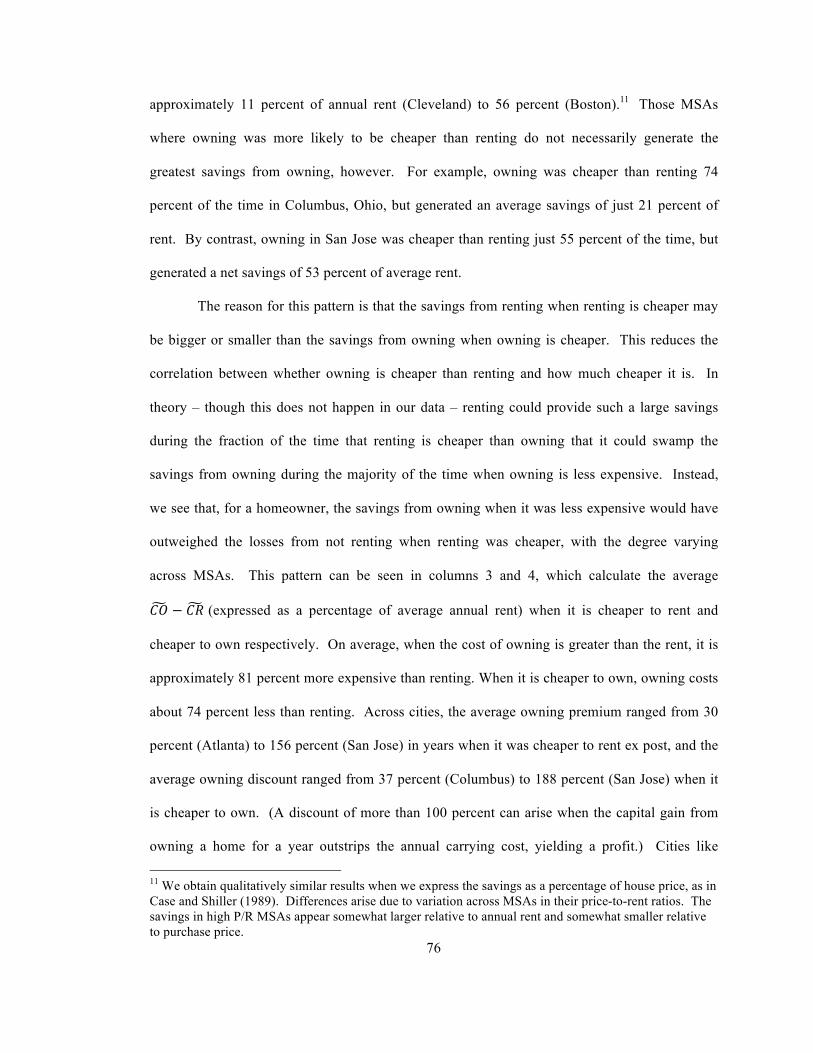
76

approximately 11 percent of annual rent (Cleveland) to 56 percent (Boston).11 Those MSAs

where owning was more likely to be cheaper than renting do not necessarily generate the

greatest savings from owning, however. For example, owning was cheaper than renting 74

percent of the time in Columbus, Ohio, but generated an average savings of just 21 percent of

rent. By contrast, owning in San Jose was cheaper than renting just 55 percent of the time, but

generated a net savings of 53 percent of average rent.

The reason for this pattern is that the savings from renting when renting is cheaper may

be bigger or smaller than the savings from owning when owning is cheaper. This reduces the

correlation between whether owning is cheaper than renting and how much cheaper it is. In

theory – though this does not happen in our data – renting could provide such a large savings

during the fraction of the time that renting is cheaper than owning that it could swamp the

savings from owning during the majority of the time when owning is less expensive. Instead,

we see that, for a homeowner, the savings from owning when it was less expensive would have

outweighed the losses from not renting when renting was cheaper, with the degree varying

across MSAs. This pattern can be seen in columns 3 and 4, which calculate the average

!" − !" (expressed as a percentage of average annual rent) when it is cheaper to rent and

cheaper to own respectively. On average, when the cost of owning is greater than the rent, it is

approximately 81 percent more expensive than renting. When it is cheaper to own, owning costs

about 74 percent less than renting. Across cities, the average owning premium ranged from 30

percent (Atlanta) to 156 percent (San Jose) in years when it was cheaper to rent ex post, and the

average owning discount ranged from 37 percent (Columbus) to 188 percent (San Jose) when it

is cheaper to own. (A discount of more than 100 percent can arise when the capital gain from

owning a home for a year outstrips the annual carrying cost, yielding a profit.) Cities like !!!!!!!!!!!!!!!!!!!!!!!!!!!!!!!!!!!!!!!!!!!!!!!!!!!!!!!!11 We obtain qualitatively similar results when we express the savings as a percentage of house price, as in Case and Shiller (1989). Differences arise due to variation across MSAs in their price-to-rent ratios. The savings in high P/R MSAs appear somewhat larger relative to annual rent and somewhat smaller relative to purchase price.!

77

Columbus had very similar savings from owning (37 percent) or renting (40 percent) when the

respective mode was cheaper. San Francisco, by contrast, had a larger gap between owning (186

percent savings) and renting (165 percent savings). In a handful of cities – Austin, Indianapolis,

and San Diego – the savings from renting in a year when renting was cheaper is much larger

than the savings from owning in the years when owning was cheaper, yet owning was still

cheaper on average because there were sufficiently few years where renting is the less expensive

mode.

Overall, the results in Table 1 suggest that a household that planned never to move – so

moving costs are not an issue – would save money, on average, in any MSA by always owning.

Nonetheless, the wide dispersion in some MSAs between the average savings from owning

when owning was cheaper, and the average savings from renting when renting was cheaper

suggests that if a household could predict which tenure would be less expensive it could save

money relative to always-owning or choosing its tenure mode randomly.

Predictability of house price changes suggests that the relative cost of owning and

renting might also be forecastable, since owning costs decline when house price growth is

greater. Indeed, a lengthy literature has found that house prices exhibit short-run momentum

and long-run mean reversion, (Glaeser and Gyourko 2010). Still, predictability of the relative

cost of owning and renting does not necessarily follow from predictability of house price

changes because rents also vary over time. A negative correlation between house price changes

and rent would make the relative cost of owning and renting less predictable than house prices

alone, but a positive correlation would make the relative cost more predictable.

In addition, the binary rent/own prediction is different than the continuous cost-of-

owning vs. rent forecast. In some ranges of the relative costs of owning and renting – say, when

owning is much more expensive than renting – errors in the forecast of the relative cost of

owning or renting would not affect which option is less expensive. In those ranges, when errors

78

in estimated owning or renting costs are inframarginal, predictions of whether owning or renting

is cheaper could be more robust than forecasts of the differences in cost. Conversely, when

renting and owning costs are close, small forecasting errors can induce large swings in the rent

versus own prediction.

Table 2 asks if, in a MSA in a particular year, owning is more or less expensive than

renting, does it have predictive power for whether owning or renting is cheaper the next year?

We estimate the following logit forecasting regression:

!(!" − !" > 0)!,! = !! + !!! !" − !" > 0 !,!!!! + !!!!!!!!!(4)

The function !(!" − !" > 0)!,! equals one if the annualized cost of owning exceeds rent in city

i and year t. The unit of observation is a city × year × price/rent estimation method. We cluster

the standard errors by city × year to account for the correlation across estimation methods.12

We find that, in all cities in our sample, the lagged relative-cost indicator is positively

correlated with the subsequent year’s indicator for whether renting is cheaper. That is, years

when renting is cheaper are more often than not followed by years when renting is cheaper.

Likewise, if owning is cheaper, it is more likely to be cheaper again the next year. The first

column of Table 2 pools the MSAs and controls for MSA fixed effects, thus using variation over

time and within-MSA to identify !!. The estimated logit coefficient of 2.4 (standard error of

0.11) corresponds to a 11 percent increase in the odds that owning will be more expensive than

renting if it was more expensive than renting the prior year. The second column adds year

dummies, so the identifying variation is due to changes in whether an MSA’s cost of owning is

above or below the rent for an equivalent property, after controlling for national changes in that

!!!!!!!!!!!!!!!!!!!!!!!!!!!!!!!!!!!!!!!!!!!!!!!!!!!!!!!!12 Since CO incorporates the change in house prices, measurement error in !!!! could potentially affect both the right- and left-hand-sides of the regression equation, inducing correlated measurement error. However, instrumenting for ! !" − !" > 0 !,!!!!with ! !" − !" > 0 !,!!!! had little effect on the estimates in columns 1 and 2 of Table 2. The MSA-specific coefficients in column 3 were affected more, but the qualitative results are the same. See Appendix Table 2.

79

relationship. The estimated logit coefficient, 2.5 (0.15), barely changes.13 The lagged indicator

variable !(!" − !" > 0)!,!!! contains the bulk of the MSA-level information, whether time-

varying or not.

The last column of Table 2 estimates a separate logit regression, and thus a separate !!,

for each MSA. This column shows that in all MSAs, the lagged indicator for whether renting

was cheaper than owning is positively correlated with renting being cheaper than owning the

subsequent year. The greatest persistence is in Detroit (3.9 with a standard error of 0.07), where

years when owning is above-average more expensive than renting are 50 percent more likely to

repeat. The lowest persistence is found in Baltimore (1.3 with a standard error of 0.05), and is

estimated to be just 3.7 percent.

One way to assess the quality of the model’s fit is to examine the percent of the time the

model correctly predicts the relative expense of owning versus renting. Results appear in Table

3, where each of the columns matches the corresponding specifications from Table 2. For the

binary decision to own or rent a home for one year, our results show that on average the forecast

is correct approximately 80 percent of the time and ranges from a high of 93 percent in San

Diego to a low of 73 percent in Phoenix.

The reason for the model’s fit can be seen in Figures 1 and 2. We estimate (!" −

!")!,! = !! + !! !" − !" !,!!!! + !!! and plot the actual ex post difference between the cost of

owning and the rent versus the cost difference predicted by the model, for the entire distribution

of cost of rent measures across all MSAs (in Figure 1) and selected cities (in Figure 2). Because

this model predicts the serial correlation in cost differences, larger positive gaps in the cost of

owning and renting are further to the northeast in the figures, whereas bigger negative gaps are

further to the southwest. For the country as a whole, as well as in the selected cities, there is a

!!!!!!!!!!!!!!!!!!!!!!!!!!!!!!!!!!!!!!!!!!!!!!!!!!!!!!!!13!Estimated coefficients on the MSA fixed effects are available from the authors, but are almost always statistically insignificant. !

80

reasonably strong positive relationship between the actual and predicted cost difference.

Nevertheless there is some noise, especially in a subset of cities. A perfect fit would lie along

the 45-degree line. Instead, the predictions deviate from that.

Households have an easier job, however, as reflected by the specification in equation

(6). They do not need to forecast how much more (or less) expensive owning might be than

renting, but rather they need only to predict whether owning will be more or less expensive than

renting. In Figures 1 and 2, when a point is in the top right or bottom left quadrants, the model

gets that prediction right. Only in the northwest and southeast quadrants is the forecast in error.

For example, in Figure 1, there is a point where the predicted cost of owning is only slightly less

than the cost of renting, but the ex post realization was that the actual cost of owning was much

less than rent. From the household’s perspective, though, the model got it exactly right: owning

was forecasted to be cheaper than renting and, in hindsight, it was. Accordingly, the

corresponding data point lies in the bottom-left quadrant.

There are a couple of factors that can make it more reliable to predict whether to own or

rent. In some cities, like Boston in Figure 2, the predicted relative costs of owning and renting

are close to the actual, especially in the region around the origin where accuracy is especially

important. In other cities, such as Philadelphia, owning tends to be cheaper most of the time, so

the forecast almost always prescribes owning, and therefore it almost always is right.

4 Trading Strategy

While observed differences in the cost of owning and renting are predictable year to

year, can households exploit this predictability to time the purchase of their homes? We estimate

the possible savings from using past information to influence future home buying/renting

decisions. We consider two approaches. First, we allow households to switch between owning

and renting as many times as they want. Naturally, the savings from switching to the lowest-

81

cost tenure mode will be offset – or, as prior research has typically found, overwhelmed – by the

transactions costs of switching.14 Second, we consider the savings possible when making just

one rent-to-own transition, so the transactions cost is essentially sunk. The primary decision that

typically falls into this category that of a first-time homebuyer determining whether to purchase

a house in the current year or rent for one more year. We will evaluate the potential savings

from optimizing that one-year decision in this section. It will turn out that a large benefit to

timing the rent/own decision is that continuing to rent for one more year extends the option to

rent again. We will show in the next section that the option to continue renting has been

valuable historically.

We consider a household who is indifferent between owning and renting outside of the

costs captured by our measures and has a one-year horizon for holding a home. We simulate

several possible tenure choice rules and evaluate them based on how close they are to the

lowest-possible-cost of housing, which comes from always correctly picking whether owning or

renting is cheaper. The difference in the costs is reported in Table 4 and is expressed as a

percentage of the average annual rent; a lower-cost strategy will exhibit a lower cost premium

over the optimal tenure choices.

We first simulate a simple trading rule: buy if the model reported in column 2 of Table 3

predicts a household should own, and otherwise rent. We label this the “regression-based trading

strategy” in Column 1 of Table 4. On average, over the 1980-2009 period, households would

have paid just 6 percent of annual rent per year more than the lowest-cost-option. The cost

premium varies across cities, ranging from just 1.6 percent in Atlanta to 17 percent in Houston.15

!!!!!!!!!!!!!!!!!!!!!!!!!!!!!!!!!!!!!!!!!!!!!!!!!!!!!!!!14!The institutional features of the real estate market can impose significant transaction costs. Given the heterogeneity in both property types and individual preferences, households often face high search frictions in buying a home (Wheaton, 1990; Stein, 1995; Krainer, 2001). Selling a home also typically involves hiring a broker and paying commission fees. Households also likely incur substantial pecuniary and non-pecuniary moving costs from switching from owning to renting.!15 This savings is based on in-sample fit of the prediction model. We obtain very similar results when we predict out-of-sample by repeatedly fitting the regression model over rolling 10-year periods, always

82

The savings from the regression-based trading strategy can be seen by comparing its

cost premium to a more naïve strategy, such as always owning (in column 3) or always renting

(in column 5). Both naïve strategies are on average more expensive than the regression-based

strategy in all cities. Across all MSAs, the cost premium for always owning averages almost 22

percent of annual rent and for always-renting the premium is almost 50 percent of annual rent.

(This result follows from Table 1, which showed that on average it was cheaper to own than rent

during this time period.) On average, then, the regression-based strategy saved more than 15

percent of rent annually vs. always owning and more than 40 percent of rent relative to always

renting. The magnitude of the difference varies by MSA; always-owning is fairly close in cost

to the optimal tenure choice in Atlanta and Charlotte, and so the regression-based strategy does

not do much better. However, always-owning is especially expensive in Boston, Fort

Lauderdale, Los Angeles, Palm Beach, Sacramento, and San Jose, so the regression-based

strategy provides especially large savings in those cities.

Since many households may not be able to generate own/rent forecasts from a logit

regression model, we consider an alternative strategy where a household simply chooses to own

if owning was cheaper than renting in the prior year, and otherwise chooses to rent. For most

cities, this simple strategy performs comparably to the more complex regression analysis. A

comparison of columns 7 and 1 shows that, on average across all MSAs, the regression-based

strategy saves just over 3 percent of rent more than the simple “last year” strategy. Only in a few

of the most volatile housing markets – Los Angeles, Miami, San Diego, San Francisco, San Jose,

and Tampa – does the regression-based strategy save considerably more than the simple “last-

year” strategy. In a handful of housing markets – Austin, Dallas, Houston, and Seattle – the last-

year strategy actually saved slightly more on average over the 1980-2009 period than the

regression-based strategy. !!!!!!!!!!!!!!!!!!!!!!!!!!!!!!!!!!!!!!!!!!!!!!!!!!!!!!!!!!!!!!!!!!!!!!!!!!!!!!!!!!!!!!!!!!!!!!!!!!!!!!!!!!!!!!!!!!!!!!!!!!!!!!!!!!!!!!!!!!!!!!!!!!!!!!!!!!!!!!!!!!!predicting the first post-sample year. However, this procedure limits our usable sample period, so we report use the in-sample prediction as our base case.

83

The even-numbered columns of Table 4 contain the standard deviations of the

corresponding savings estimates. Recall that there are two sources of error in our estimates:

Year-to-year variation from the average, and estimation of the levels of prices and rents. The

standard deviations reported in this table include both sources. Column 2, which corresponds to

the regression-based prediction, includes a third source of error: The prediction error from the

model in Equation 4. In the standard deviations reported in Table 4, we assume that !! from

Equation 4 is independent of the other errors listed above. The standard deviations in Table 4

reflect the certainty of the potential savings – trading strategies that are more consistently close

to lowest-possible-cost optimum will have the lowest standard deviations. Thus, it is

unsurprising that we find that the trading strategies and cities that are closest to the least-cost

optimum also generally exhibit the lowest standard deviations.

The reason why one can save money trading on the serial correlation in housing costs

may be seen in Figure 3, which plots the distribution of cost of owning minus cost of rent

measures for a sample of cities from 1980-2009. The shaded areas represent the saving from

renting, when the number is positive, or owning, when the number is negative. The optimal

tenure mode would be to rent when the shaded area is above the x-axis and own when it is

below. Deviations from that strategy pay the shaded area in the year of a “mistake.” For

example, the average cost of owning is less than the average cost of renting when the shaded

area below the x-axis is larger than the area above the x-axis.

The top panel shows that in cities such as Boston, Los Angeles, and New York, the

difference between the cost of owning and rent is volatile across the sample period. These cities

have experienced long periods where either renting or owning was less expensive, year after

year. During those periods, whether owning or renting was cheaper the prior year is a strong

predictor of owning or renting being cheaper the following year. Occasionally there is a regime

switch and the other tenure mode becomes less expensive, but the difference in the cost is

84

usually quite small in the transition period. That is, a city is unlikely to go from one year where

owning is significantly cheaper than renting to a subsequent year where owning is wildly more

expensive than renting. Hence while the decision rule of “rent if renting was cheaper than

owning last year” is wrong every so often, choosing the wrong tenure mode in that year is

unlikely to be a costly mistake. The saving in the meantime from profiting from the persistence

in relative own/rent costs easily outweighs the loss from being wrong once or twice a decade.

In other MSAs, !" − !" remains relatively stable over time. The bottom panel of

Figure 3 provides some examples, such as Chicago, Cleveland, and Denver. In fact in cities

such as Atlanta and Charlotte, it is almost always cheaper to own from 1980 to 2009. In these

cities, households almost never need to switch tenure mode to save money. However, the

differences in annual cost between owning and renting are very slight.

Of course, the savings from predicting whether renting or owning would be cheaper and

switching tenure mode to take advantage of cost differences comes at a cost – every move incurs

transaction costs. These costs include paying realtors, searching for a new residence, and the

pecuniary, time and psychic costs of moving. Indeed, the classic literature on the predictability

of house prices concludes that transaction costs in the housing market are too high to profitably

arbitrage house prices by buying and selling homes. However, the savings from arbitraging the

own-rent gap may be larger than the returns on trading on house prices alone. In addition, those

savings differ across cities, so a switching-tenure-mode strategy might make financial sense in

some cities but not in others.

We find that at reasonable levels of transaction costs, a switching tenure mode based on

the trading strategies described earlier, saves money on net relative to always-renting but not

relative to always-owning in most cities. For each of our trading strategies – the regression-

based strategy and the last-year strategy – we compute the break-even level of transaction costs

as a percentage of the price of the house. Specifically, we compute the savings from the trading

85

strategy over our sample period relative to a strategy of picking one tenure mode – renting or

owning – and never moving. We express the savings as a percent of house price and divide it by

the fraction of years that a household would have to move in order to implement the strategy.

We choose to express the savings in terms of a break-even level of transaction costs rather than

netting out an assumed rate of costs because transaction costs might vary across households.

However, a 10 percent transaction cost (6 percent realtor fees and 4 percent other costs) is a

commonly used threshold.

The results are reported in Table 5. The first two columns report the break-even level of

transaction costs that could be covered by the regression-based strategy and the latter two

columns correspond to the simple last-year strategy. In each pair of columns, the counterfactual

in the first column is a strategy of always owning and in the second column is always renting.

On average (the first row), the trading strategies save enough relative to always-owning that

transaction costs could be between 5 and 6 percent of the average house price. This is not

enough savings to cover even standard realtors’ fees (which are typically 6 percent of the

purchase price). However, relative to always-renting, a tenure mode-switching strategy saves

enough to cover transaction costs of 15 to 17 percent of house price on average, enough to cover

any reasonable assumption of transaction cost.16

The breakeven level of transaction cost varies across MSAs due to differences in the

efficacy of the trading strategies and the number of moves implementation would require. Even

relative to always owning, where an active strategy typically does save enough to cover

transaction costs, households in Detroit, Los Angeles, Sacramento, and San Diego could afford

double-digit trading costs and still come out ahead. Furthermore relative to always-renting,

!!!!!!!!!!!!!!!!!!!!!!!!!!!!!!!!!!!!!!!!!!!!!!!!!!!!!!!!16!Due to the momentum in house prices seen in Figure 3, the trading strategies do not require very many switches (the average number of switches is four to five over a 29 year sample period). Thus, households can afford higher transaction costs because they do not incur them very often. !

86

where forecasting usually provides a considerable benefit, it would still not be worthwhile for

typical households in Memphis, Nashville, and perhaps Seattle to bother switching.

5 Predictability by Horizon Thus far we have followed prior studies by focusing on the one-year cost of owning or

renting a home. Most households, however, intend to live in a home for longer than a year. Thus

this section extends our analyses the costs of owning and renting for longer horizons. Using the

formula detailed in equations 2 and 3, we first calculate the costs of owning and cost of renting a

home for five years (k=5) and ten years (k=10) across the variety of methodologies and property

types described in Section 2. We then estimate the predictability of the relative cost of owning

and renting over these longer horizons. Next, we extend our trading rule to multi-year horizons

and show that when owning was cheaper over the prior five- or ten-year period, it predicts that

owning is less expensive than renting over the subsequent period. Finally, we consider the case

of chaining together sequential one-year rent/own decisions for households with multiple-year

horizons.

Analogous to our analysis for the one-year costs, we perform the following logit

regression of the binary decision to own or rent for the five and ten year horizon:

!(!" − !")!,!! = !! + !!!(!" − !")!,!!!! + !!!!!!!!!(8)

where !(!" − !")!,!! is an indicator variable that equals 1 if the cost of owning exceeds the cost

of renting (!" − !" > 0) over the next k years in a given city i and starting year t, and 0

otherwise. For example, !(!" − !")!,!""#! = 0 means that it was cheaper for a household to

own from 1990 to 1995, rather than rent during that five-year period. We use the t-k lag of the

own/rent decision to predict the binary decision in current year t, since this is the most recent lag

over which a household would have information about costs at a k horizon. For example, if a

household with a five-year horizon was deciding whether to buy or rent in 1990, the most recent

87

observable costs for a five-year tenure would start in 1985. Thus !(!" − !")!,!!!! indicates

whether it was ex-post cheaper for the household to own or rent for the next k years starting in

year t-k.

Table 6 reports the estimated values of !! for horizons of both five and ten years.

Columns 1 and 2 perform the above binary regression for the five-year horizon, first on the

pooled sample with city effects, and then with both city and year fixed effects. Columns 3 and 4

implement the same respective specifications for the ten-year tenure horizon.17 Our results

reveals that pooled estimates are still on average significant at longer horizons, but at smaller

magnitudes than for the 1-year horizon. The magnitude of the coefficient estimate for the 5-year

horizon is a fifth of the estimate for the 1-year horizon (0.5 versus 2.5). The pooled estimate of

!! for the 10-year horizon is slightly greater in magnitude than the five-year at approximately

0.93, though still less than half of the one-year horizon estimate. The exponent of the ten-year

horizon estimate suggests that when it is cheaper to rent in the current year, it is likely to be

cheaper in the following year by odds of approximately 2.53 to 1. Nonetheless, it is important to

note that the forecasts for these longer horizons are estimated over smaller sample periods. Since

our sample period ends in 2009, the final observable costs of a five and ten-year tenure occur in

2004 and 1999 respectively.

Using the estimated coefficients from Table 5, we forecast whether it was better to own

or rent each year from 1980 given a five- and ten-year tenure horizon. We then compare the

actual versus predicted results and calculate how often the predicted binary decision was correct.

The binary prediction indicates whether a household with a five-year tenure horizon should start

owning or renting in a given city and year, and we consider a forecast to be “correct” if it was

indeed cheaper to own or rent throughout the next five years. Table 7 presents the share of years

the in-sample prediction correctly forecasts the binary decision to own or rent by city. Each

!!!!!!!!!!!!!!!!!!!!!!!!!!!!!!!!!!!!!!!!!!!!!!!!!!!!!!!!17!Though not shown, results are very similar if we exclude time and city fixed effects all together.!

88

column corresponds to the respective specifications from Table 5. Column 1 shows that on

average, from 1980 to 2004 the predicted decision from the pooled regression forecasts the own

or rent decision correctly 82 percent of the time for a household with a five-year horizon.

Column 3 shows that this predictability is even greater at the ten-year horizon, forecasting the

binary decision correctly 93 percent of the time. This is driven by the fact it is more often better

to own with a ten-year horizon. In some cities such as Atlanta, for example, it was cheaper to

rent less than 3 percent of the time across the observed sample period and distribution of cost

measures. Overall, the results show that if it was cheaper to own in a current year, it will be even

more likely be cheaper to own again in the following year for households with longer horizons.

We then use these predictions to simulate a simple trading rule: buy if the above results

indicate that it is cheaper to own for the next five (or ten) years, and otherwise rent. This trading

strategy assumes that a household would have to buy or rent throughout the entire residence

spell. As a performance benchmark, we estimate housing costs assuming that a household had

perfect foresight and perfectly timed its shift from renting to owning (or owning to renting). We

limit the household to just one switching of tenure mode to hold transactions costs essentially

constant. For example, for a household with a five-year horizon, it may be ex-post less

expensive to rent for the first two years of its tenure and then own a home for the remaining

three years. Thus, for each MSA and year of our sample period, we calculate the least expensive

tenure choice across our distribution of cost measures. We then use this option as a benchmark

to compare the performance of different trading strategies.

The first column of Table 8 indicates how close to the perfect-foresight optimum a

household with a five-year horizon could have gotten by using the regression-based tenure

choice criteria over the 1980-2009 period. On average, the difference in cost would have

equaled about six percent of annual rent. In many MSAs, the regression-based model was

within five percent of rent of the optimum strategy. In other MSAs, such as Austin and San

89

Antonio Texas, annual ownership costs under this rule exceeded the optimum by more than 16

percent of annual rent on average. For most cities, however, always-owning (column 3) or

always-renting (column 5), performs significantly worse: for example, the cost of always-

owning in Boston exceeded the optimal strategy each year by about 23 percent of annual rent.

Always-renting is worse, wasting about 52 percent of annual rent. Using the regression-based

strategy in Boston would have moved a household within seven percent of annual rent of the

perfect-foresight ideal.

Column 7 evaluates the “last year” strategy of owning over the next five years, if

owning was cheaper over the prior five years. In most cities, this strategy unsurprisingly

performed like the average of the always-own and always-rent approaches. Still, in a handful of

cities where owning was almost always dominant – Atlanta, Charlotte, Cincinnati, Columbus,

Kansas City, Sacramento, and Washington DC – this strategy did very well.

However, it may be unrealistic to think that a renter would commit to renting for 5

years. (Conversely, homeownership is generally an absorbing state.) Instead, a more realistic

trading rule is one that says a household should own if owning was less expensive the prior year,

and then continue to own for the remainder of its horizon. However, if renting is cheaper, the

household should rent for another year and then reevaluate. If owning turns out to have been

cheaper, the household should then own. But if not, it should rent again and reevaluate for

another year. In this way, the household ends up renting for its entire horizon only if renting

was cheaper than owning for each of the first k-1 years.

This strategy compares very favorably to the perfect-foresight ideal and almost always

does better than the regression-based strategy. Column 9 reports the average cost relative to

optimal timing as a percentage of average annual rent. On average, the year-at-a-time strategy

costs just five percent of annual rent more than the best-case housing cost. That is close to the

regression-based cost from column 1.

90

A large portion of the savings from this strategy comes from the option to delay the

switch from renting to owning for several years. That savings can be seen by comparing

columns 7 and 9. Column 7’s cost premium to the lowest-cost strategy assumes the household

commits upfront to either renting for 5 years or owning for 5 years. In column 9, the household

either owns for 5 years, or rents for one year and then reevaluates. The difference between the

two columns, then, is due to the option to have an intermediate number of years of renting before

entering into a home owning commitment. The savings is considerable – the average cost

premium in column 7 is more than three times as large as the one in column 9. Indeed, the year-

at-a-time strategy always is less expensive than the last-year strategy, and the greatest benefit

accrues in the cities with cyclical housing markets such as San Francisco or Boston, where the

commitment strategy does particularly poorly.

Table 9 evaluates the same trading strategies for households with a ten-year horizon. We

define the predicted strategy based on the results for the ten-year horizon in Table 6, and

similarly define the naïve strategy as owning if it was cheaper to own over the last ten years.

Results for the 10-year horizon are qualitatively the same as the 5-year horizon, but the savings

differences between trading strategies are wider in magnitude.

6 Effect of different tax rates

One of the more significant determinants of the relative cost of owning and renting is a

household’s tax bracket. From equations 2 and 3, holding the housing constant, rents do not

vary with a household’s tax rate but the annual cost of owning rises as the tax rate declines. This

implies that the difference between the cost of owning and rent is greater for low income, low

tax-rate households. The precise details of the U.S. tax treatment can be found in Poterba (1991)

and Poterba and Sinai (2008).

91

In Table 10, we expand our analysis to consider how the own/rent balance varies across

the income distribution. We obtain average tax rates on mortgage interest, property taxes, and

income at different points in each city’s income distribution. Using household-level micro data

from the 1980, 1990, 2000, and 2010 Decennial Censuses, we compute the average income of

households whose house values are between zero and 75 percent of the median house value in

their city (tier 1), 75-100 percent of the median house value (tier 2), 100-125 percent of the

median house value (tier 3), and more than 125 percent of the median house value (tier 4). It is

worth underscoring that tiers have different meanings in different cities. For example,

households in in San Francisco have higher average incomes than households in the same tier in

Columbus, Ohio. For each household, we obtain the family structure from the Census and

impute mortgage interest and opportunity cost of capital using the current 30-year mortgage

interest rate. We linearly interpolate the households’ characteristics incomes for each

intervening year and use the National Bureau of Economic Research’s TAXSIM tax model to

impute state and federal taxes.

Table 10 reports the probability that owning is cheaper than renting for five categories

of households: Four categories corresponding to each of the house value tiers, and one where we

assume zero tax rates. Households in the highest house value tier in each city generally will find

that owning is cheaper than renting (in column 5). However, it is a toss-up in Palm Beach and

renting is slightly cheaper on average in San Diego. By contrast, a household with zero tax

rates, and thus no tax subsidy to owner-occupied housing, would find that renting is less

expensive most of the time in most cities (in column 1). In Milwaukee, for example, in the

absence of taxes owning is cheaper than renting just one-third of the years between 1980 and

2009. (For the highest tier households there, owning is cheaper than renting nearly 68 percent of

the time.) In the exceptions -- Austin, Charlotte, Detroit, Houston, Kansas City, Memphis,

Miami, Nashville, Phoenix, Pittsburgh, San Antonio, and St. Louis – owning is cheaper than

92

renting barely more than 50 percent in the absence of taxes, except for San Antonio where it is

59 percent.

The intervening columns vary on whether owning has typically been cheaper than

renting or not, depending on the sensitivity of owning costs to the tax rate and on how the tax

rates change across tiers. In some cities, like Austin, owning is always more likely to be cheaper

than renting. In some, like Palm Beach, owning is typically more expensive in all tiers. Other

cities, like Baltimore, exhibit large differences between the lowest tier (owning is cheaper 41

percent of the time) and the highest tier (owning is cheaper 65 percent of the time). By contrast,

San Francisco ranges little, from 48 percent (lowest tier) to 54 percent (highest tier).

Whether owning or renting is cheaper on average due to taxes does not influence the

efficacy of the owning/renting strategy – it just changes the frequency of the time that owning or

renting are chosen. We have replicated Table 4 for the various income tiers and even in the

bottom tier, which is the most different from our baseline results, the savings from the last-year

and regression-based strategies are not affected much.18 On average across all MSAs, the last-

year strategy is just 7.9 percent of annual rent more expensive than the lowest-possible-cost

housing (versus 8.1 in Table 4) and the regression-based strategy is just 5.9 percent more

expensive. (The same as in Table 4.) We do see some differences across MSAs, but they are

slight and for every MSA where the trading strategy is slightly less efficient, there is another

where it is slightly more effective.

7 Conclusion

We examine 30 years of data from 39 metropolitan areas to see if households could

successfully time the housing market when deciding whether to own or rent their homes. We

find several home buying strategies that would have saved households money. First, simply

!!!!!!!!!!!!!!!!!!!!!!!!!!!!!!!!!!!!!!!!!!!!!!!!!!!!!!!!18 Savings for the lowest income tier can be found in Table 11.

93

choosing homeownership when in the previous year owning was cheaper than renting saves 13

percent of annual rent on average relative to always-owning and 40 percent on average relative

to always being a renter. The potential savings varies across cities, but it is always positive.

While we can improve upon this simple rule of thumb with a regression model to predict

whether to own or rent, in most cities the gains from the additional complexity are small.

This approach also extends to the first-time buyer with a multi-year holding period. If a

household is otherwise indifferent between renting and owning, it should buy if owning was

cheaper than renting the prior year. However, if it was not, it should rent another year. Not only

does that save the difference between rent and ownership costs for that year, it preserves the

option to keep renting. In other words, if the first-time homebuyer defers ownership for a year,

it can defer it again if conditions warrant. Indeed, we find that if renting is chosen, the

household should again evaluate whether to own or rent based on the relative cost in the prior

year. In this manner, a first-time homebuyer will not buy a house until owning is finally cheaper

than renting. We find that this option to keep renting is quite valuable and in many cities this

strategy approaches the lowest-possible cost timing for becoming an owner.

The intuition behind these results is straightforward. It is by now well-established that

house prices exhibit short-run persistence and long-run mean reversion. We find that statistical

pattern is not undone by corresponding changes in rent. From the perspective of a potential

homebuyer, this means that a year when owning is cheaper than renting tend to be followed by

another year when owning is cheaper than renting. Thus, owning being less expensive than

renting is a good signal to buy. When owning finally becomes more expensive than renting, it is

time to sell. However, due to the slow-changing nature of house prices, owning initially is not

much more expensive than renting, so the cost of getting the transition year wrong is low.

Finally, because owning typically is cheaper than renting for many years in a row, not many

94

moves are needed to arbitrage relative costs of owning and renting. Thus, even in the presence

of high moving costs, it can be worthwhile in some cities to switch tenure mode.

This analysis emphasizes the importance of persistence in house price growth and the

covariance of house price changes and rents in timing the home buying decision. Indeed, the

differences between our results and those in other papers are due to these factors. For example,

Glaeser and Gyourko (2010) conclude that waiting a year to own incurs considerable house price

risk because the purchase price of the next year’s housing is uncertain. However, they calibrate

their model assuming no persistence in house prices; that persistence dampens the exposure to

house price changes and increases the benefit from waiting a year. In the four cities in their

data, Case and Shiller (1989) exploit the serial correlation in house price changes and find a

benefit to waiting a year to buy if their model does not predict housing excess returns to be

positive. However, they do not consider the additional benefit from potentially renting for

multiple years.

In addition, we establish two empirical patterns that future research should try to

explain. First, housing markets do not seem to be in equilibrium either with rents and ownership

costs being equal ex post, or in the Poterba (1984) sense that expected annual housing costs

equal rents. It is hard to reconcile the fact that in many cities owning is typically cheaper than

renting, and the expected cost difference is positive, with an equilibrium that equates user cost

and rent (Verbrugge, 2008). Second, the degree and frequency to which expected user cost is

below rent varies across cities.

These patterns deserve investigation. Possible explanations include taxes – which we

find to have a big effect on the relative costs of owning and renting.19 Since tax rates are

heterogenous across the population, the tax rate of the marginal homebuyer may differ across

!!!!!!!!!!!!!!!!!!!!!!!!!!!!!!!!!!!!!!!!!!!!!!!!!!!!!!!!19 See also Diaz and Luengo-Prado (2008).

95

cities. Other possible explanations include differences in liquidity constraints, transaction costs,

and risk.

96

Bibliography Campbell, S., Davis, M., Gallin, J. and Martin, R. (2009). “What Moves Housing Markets: A

Variance Decomposition of the Rent-Price Ratio,” Journal of Urban Economics, 66: 90-102.

Case, K. and Shiller, R. (1989). “The Efficiency of the Market for Single-Family Homes,”

American Economic Review, 79: 125-137. Case, K. and Shiller, R. (1990). “Forecasting Prices and Excess Returns in the Housing Market,”

Real Estate Economics, 18: 253-273.

Case, K. and Shiller, R. (2003). “Is There a Bubble in the Housing Market?” Brookings Papers on Economic Activity, 299-342.

Case, K., Shiller, R. and Thompson, A. (2012). “What Have They Been Thinking? Home Buyer Behavior in Hot and Cold Markets.” Brookings Papers on Economic Activity, 265-298.

Crone, T., Nakamura, L., and Voith, R. (2004). “Hedonic Estimates of the Cost of Housing Services: Rental and Owner-Occupied Units,” Federal Reserve Bank of Philadelphia. Working Paper No. 04-22.

Cunningham, C. and Engelhardt, G. (2008). “Housing Capital-gains Taxation and Homeowner Mobility: Evidence from the Taxpayer Relief Act of 1997” Journal of Urban Economics, 63: 803-815.

Cutts, A., Green, R., and Chang, Y. (2005). “Did Changing Rents Explain Changing House

Prices During the 1990s?” George Washington University.

Davis, Morris A. and Heathcote, J. (2008). “The Rent-Price Ratio for the Aggregate Stock of Owner-Occupied Housing,” Review of Income and Wealth, 54: 279-284.

Davis, M. A., Lehnert, A., & Martin, R. F. (2008). The Rent‐Price Ratio for the Aggregate Stock of Owner‐Occupied Housing. Review of Income and Wealth, 54(2), 279-284.

Diaz, A. and Luengo-Prado, M. J. (2008). “On the User Cost and Homeownership,” Review of

Economic Dynamics, 11: 284-613. Emrath, P. (2002). “Property Taxes in the 2000 Census,” Housing Economics, December: 16-21. Gallin, J. (2004). “The Long-Run Relationship between House Prices and Rents,” Federal

Reserve Board Finance and Economics Discussion Series, No. 2004-50.

Glaeser, E. and Gyourko, J. (2007). “Arbitrage in Housing Markets,” NBER Working Paper 13704, December 2007.

Han, L. (2008). “The Effects of House Price Uncertainty on Housing Demand: Empirical Evidence from the U.S. Housing Markets,” Review of Financial Studies, 23(11): 3889-3928.

97

Harding, John P., Rosenthal, S., Sirmans, C.F. (2007). “Depreciation of Housing Capital,

Maintenance, and House Price Inflation: Estimates from a Repeat Sales Model,” Journal of Urban Economics, 61(2): 193-217.

Hendershott, P. H., and Slemrod, J. (1982). “Taxes and the User Cost of Capital for Owner‐Occupied Housing,” Real Estate Economics, 10(4), 375-393.

Hendershott, P. H., and Van Order, R. (1987). “Pricing Mortgages: an Interpretation of the

Models and Results,” Journal of Financial Services Research, 1(1), 19-55. Himmelberg, C., Mayer, C., and Sinai, T. (2005). “Assessing High House Prices: Bubbles,

Fundamentals and Misperceptions.” The Journal of Economic Perspectives, 19(4): 67–92.

Krainer, J. (2001). “A Theory of Liquidity in Residential Real Estate Markets,” Journal of Urban Economics, 49: 32-53.

Meese, R. and Wallace, N. (1994). “Testing the Present Value Relation for Housing Prices:

Should I Leave My House in San Francisco?” Journal of Urban Economics, 35(3), 245–66.

Ortalo-Magné, F., and Rady, S. (2002). “Tenure Choice and the Riskiness of Non-Housing Consumption.” Journal of Housing Economics, 11(3), 266-279.

Paciorek, A., and Sinai, T. (2012). “Does Home Owning Smooth the Variability of Future

Housing Consumption?” Journal of Urban Economics, 71(2), 244-257. Poterba, J. M. (1984). “Tax Subsidies to Owner-Occupied Housing: An Asset Market

Approach,” Quarterly Journal of Economics. 99: 729-52. Poterba, J. M. (1992). “Taxation and Housing: Old Questions, New Answers,” The American

Economic Review, 82(2), 237-242. Poterba, J. and Sinai, T. (2008). “Tax Expenditures for Owner-Occupied Housing: Deductions

for Property Taxes and Mortgage Interest and the Exclusion of Imputed Rental Income,” American Economic Review Papers and Proceedings, 96(2).

Poterba, J. and Sinai, T. (2011). “Revenue Costs and Incentive Effects of the Mortgage Interest

Deduction for Owner-Occupied Housing.” National Tax Journal, 65(2): 531-564. Shan, H., 2011. “The Effect of Capital Gains Taxation on Home Sales: Evidence from the

Taxpayer Relief Act of 1997,” Journal of Public Economics, 95: 177-188. Sinai, T., and Souleles, N. S. (2005). “Owner-occupied Housing as a Hedge Against Rent

Risk,” The Quarterly Journal of Economics, 120(2): 763-789. Sinai, T., and Souleles, N. S. (2013). “Can Owning a Home Hedge the Risk of Moving?” AEJ:

Economic Policy, Forthcoming.

98

Smith, G. and Smith, M. H. (2006). “Bubble, Bubble, Where's the Housing Bubble?” Brookings Papers on Economic Activity, 1-63.

Stein, J. C. (1995). “Prices and Trading Volume in the Housing Market: A Model with Down-

Payment Effects,” Quarterly Journal of Economics, 110: 379-406. Verbrugge, R. (2008). “The Puzzling Divergence of Rents and user Costs, 1980-2004,” Bureau

of Labor Statistics, Working Paper #422. Wheaton, W. C. (1990). “Vacancy, Search, and Prices in a Housing Market Matching Model,”

Journal of Political Economy, 98: 1270-1292.

99

TABLE 1. SUMMARY STATISTICS OF RELATIVE COSTS OF OWNING V. RENTING

Pr(CO>CR) Average CO-CR (as % of CR) Overall Overall if CO>CR if CO<CR

All MSAs 65.1 -29.2 81.3 -73.7 Atlanta 74.8 -31.0 29.5 -46.3 Austin 69.6 -21.8 106.3 -61.4 Baltimore 64.8 -38.6 59.7 -84.0 Boston 57.5 -56.1 115.1 -155.0 Charlotte 83.8 -40.0 31.7 -49.8 Chicago 63.0 -14.3 69.2 -54.7 Cincinnati 68.4 -14.2 52.0 -38.2 Cleveland 64.7 -11.8 55.0 -40.2 Columbus 74.2 -21.1 40.7 -37.2 Dallas 63.4 -11.3 58.9 -39.6 Denver 57.0 -20.0 61.7 -71.3 Detroit 67.0 -19.7 88.5 -60.7 Fort Lauderdale 64.0 -36.8 99.7 -92.6 Houston 67.2 -15.2 91.9 -54.2 Indianapolis 71.9 -21.4 38.9 -38.2 Kansas City 74.2 -28.0 56.2 -49.0 Los Angeles 54.7 -45.2 154.1 -184.3 Memphis 71.9 -20.2 68.1 -45.8 Miami 65.0 -34.8 98.6 -98.4 Milwaukee 68.5 -15.2 60.3 -43.4 Minneapolis 70.2 -30.2 57.9 -60.8 Nashville 68.5 -26.5 44.8 -54.2 New York 58.5 -52.7 115.6 -137.2 Orlando 67.8 -35.5 72.9 -74.1 Palm Beach 55.5 -28.0 87.3 -97.8 Philadelphia 64.2 -40.5 51.9 -80.9 Phoenix 66.2 -33.1 109.4 -91.7 Pittsburgh 75.1 -25.2 57.9 -46.4 Portland 60.8 -31.6 71.9 -93.7 Richmond 70.0 -36.1 34.3 -59.8 Sacramento 55.9 -29.2 155.7 -146.7 San Antonio 69.6 -24.3 91.7 -61.1 San Diego 50.6 -34.1 132.7 -176.5 San Francisco 55.9 -49.9 164.6 -185.7 San Jose 54.6 -53.4 155.0 -187.6 Seattle 52.8 -20.2 84.2 -107.7 St. Louis 73.6 -29.7 38.9 -48.7 Tampa 65.4 -35.7 69.5 -79.2 Washington, D.C. 59.7 -48.5 80.9 -118.7

Note: The cost of owning is denoted by “CO”, and the cost of renting “CR”. Pr(CO>CR) is the probability that the owning is cheaper than renting. “Overall" is the average CO-CR across all cost measures and years in a given city. Cost measures are calculated by equation (4), assuming a loan-to-value constant of 0.8 and national average federal and state income tax for all tax rates.

100

TABLE 2. PREDICTING BINARY RENT V. OWN DECISION, 1-YEAR HORIZON Coef/SE of I(CO-CR)t-1 (1) (2) (3)

All MSAs 2.38 2.52

!(0.11) (0.15)

Atlanta !

3.00

! (0.07)

Austin

2.18

(0.06)

Baltimore

1.25

(0.05)

Boston

2.73

(0.06)

Charlotte

2.56

(0.07)

Chicago

2.07

(0.05)

Cincinnati

3.52

(0.07)

Cleveland

3.07

(0.06)

Columbus

2.85

(0.06)

Dallas

3.15

(0.06)

Denver

3.73

(0.07)

Detroit

3.87

(0.07)

Fort Lauderdale

1.46

(0.05)

Houston

2.53

(0.06)

Indianapolis

2.36

(0.06)

Kansas City

2.58

(0.06)

Los Angeles

2.67

(0.06)

Memphis

1.77

! (0.06)

Miami

2.09

(0.05)

MSA Fixed Effects YES YES !!Time Fixed Effects

!YES

!Pseudo R2 0.22 0.39 !Obs 314496 314496 8064

Note: Dependent variable is I(CO-CR)t. Standard errors are clustered by MSA-year and in parentheses. Each unit of observation is for a given MSA, year, method, and type of home. Columns 1 and 2 perform pooled regressions with different specifications, while column 3 performs individual regressions by city.

101

TABLE 2. (CONT’D) PREDICTING BINARY RENT V. OWN DECISION, 1-YEAR HORIZON Coef/SE of (CO-CR)t-1 (1) (2) (3)

Milwaukee

2.98

(0.06)

Minneapolis

2.18

(0.06)

Nashville

1.83

(0.05)

New York

3.16

(0.06)

Orlando

2.04

(0.05)

Palm Beach

1.76

(0.05)

Philadelphia

1.68

(0.05)

Phoenix

1.66

(0.05)

Pittsburgh

1.45

(0.06)

Portland

3.15

(0.06)

Richmond

1.70

(0.05)

Sacramento

2.90

(0.06)

San Antonio

2.11

(0.05)

San Diego

3.48

(0.06)

San Francisco

2.10

(0.05)

San Jose

1.63

(0.05)

Seattle

2.72

(0.06)

St. Louis

3.32

(0.07)

Tampa

1.52

(0.05)

Washington, D.C.

2.18

! (0.05)


!YES

!Pseudo R2 0.22 0.39 !Obs 314496 314496 8064

Note: Dependent variable is I(CO-CR)t. Standard errors are clustered by MSA-year and in parentheses. Each unit of observation is for a given MSA, year, method, and type of home. Columns 1 and 2 perform pooled regressions with different specifications, while column 3 performs individual regressions by city.

102

TABLE 3. FORECASTING THE 1-YEAR HORIZON OWN VERSUS RENT DECISION % of Time Forecast is Correct (1) (2) (3)

All MSAs 78.7 82.5 78.8 Atlanta 84.9 87.6 84.9 Austin 77.6 76.9 77.6 Baltimore 67.6 74.6 67.6 Boston 79.7 86.9 79.7 Charlotte 85.9 84.8 85.9 Chicago 75.4 82.8 75.4 Cincinnati 86.8 90.3 86.8 Cleveland 83.5 85.8 83.5 Columbus 83.7 84.5 83.7 Dallas 83.5 79.0 83.5 Denver 86.5 87.4 86.5 Detroit 88.5 86.7 88.5 Fort Lauderdale 69.4 74.7 69.4 Houston 79.7 73.8 79.7 Indianapolis 79.6 80.6 79.6 Kansas City 82.5 84.0 82.5 Los Angeles 79.0 92.4 79.0 Memphis 75.7 78.4 75.7 Miami 75.5 79.8 75.5 Milwaukee 83.6 86.4 83.6 Minneapolis 78.5 80.8 78.5 Nashville 75.0 75.8 75.0 New York 83.2 89.5 83.2 Orlando 75.9 84.5 75.9 Palm Beach 70.8 79.7 70.8 Philadelphia 71.8 77.7 71.8 Phoenix 71.9 73.1 71.9 Pittsburgh 74.7 82.1 77.7 Portland 83.6 85.3 83.6 Richmond 74.4 82.9 74.4 Sacramento 81.1 83.0 81.1 San Antonio 76.8 76.9 76.8 San Diego 85.1 92.8 85.1 San Francisco 74.5 80.9 74.5 San Jose 69.4 85.7 69.4 Seattle 79.7 76.3 79.7 St. Louis 86.7 86.8 86.7 Tampa 71.2 79.8 71.2 Washington, D.C. 75.4 87.0 75.4 MSA Fixed Effects YES YES

!Time Fixed Effects !

YES !Obs 314496 314496 8064

Note: This table calculates the percent of the time the predicted binary rent v. own decision was “correct”, i.e. when it was actually better to own or rent. The columns correspond to the specifications in Table 2.

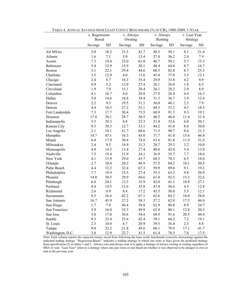
103

TABLE 4. ANNUAL SAVINGS FROM LEAST COSTLY BENCHMARK (% OF CR), 1980-2009, 1-YEAR

v. Regression-Based

v. Always Owning

v. Always Renting

v. Last-Year Strategy

Savings SD Savings SD Savings SD Savings SD

All MSAs 5.9 18.2 21.5 41.7 48.5 58.1 8.1 21.4 Atlanta 1.6 7.1 5.9 13.4 37.0 36.2 2.4 7.9 Austin 7.3 19.4 25.0 61.0 46.7 50.1 5.7 15.3 Baltimore 5.4 12.9 15.9 30.1 48.4 64.0 8.7 16.7 Boston 5.1 22.1 29.4 44.6 68.5 82.8 8.7 25.3 Charlotte 3.5 12.9 4.0 13.6 45.4 37.0 3.5 12.1 Chicago 2.4 8.7 18.3 35.4 29.9 33.8 4.2 9.9 Cincinnati 0.9 5.2 12.9 27.4 26.1 26.0 1.8 6.3 Cleveland 1.9 7.9 15.1 28.4 26.1 28.2 2.9 8.9 Columbus 4.1 16.7 8.0 20.8 27.9 26.4 4.4 16.3 Dallas 5.0 14.6 18.8 39.4 31.3 36.7 3.9 12.4 Denver 2.2 9.3 19.5 31.1 36.0 46.1 2.3 7.9 Detroit 4.4 18.5 27.2 53.1 49.3 53.3 4.3 18.5 Fort Lauderdale 7.3 17.7 30.4 73.5 68.9 91.3 9.3 19.1 Houston 17.0 38.1 28.7 50.5 46.5 46.6 11.4 31.4 Indianapolis 5.5 20.3 8.8 22.3 31.0 32.6 6.0 20.1 Kansas City 8.3 30.3 12.7 33.1 44.2 41.0 8.6 30.0 Los Angeles 2.1 10.1 41.7 68.6 71.5 90.7 8.4 21.3 Memphis 14.7 47.1 16.3 43.0 37.7 41.0 15.6 46.8 Miami 6.4 17.9 30.4 74.8 63.6 81.8 11.9 31.5 Milwaukee 2.4 9.5 14.9 31.3 28.7 29.3 3.2 10.0 Minneapolis 4.9 14.5 13.4 27.4 40.6 42.0 5.4 13.8 Nashville 7.5 19.4 11.9 24.1 36.9 35.7 7.7 18.6 New York 4.1 15.9 29.0 43.7 68.5 78.3 6.5 18.0 Orlando 2.7 10.0 20.2 49.9 57.5 84.2 10.1 30.5 Palm Beach 4.4 12.2 32.4 67.3 59.9 89.6 9.1 19.2 Philadelphia 7.7 19.9 15.5 27.4 55.5 63.3 9.8 20.9 Phoenix 14.0 30.5 29.9 60.6 61.0 92.5 15.5 32.6 Pittsburgh 6.8 24.1 13.3 35.9 42.0 41.1 10.9 27.1 Portland 4.4 14.5 21.6 35.8 47.0 56.6 4.5 12.8 Richmond 2.6 8.9 8.4 17.2 43.5 50.0 5.5 12.1 Sacramento 8.5 26.6 42.2 67.1 62.6 84.2 10.0 28.0 San Antonio 16.7 45.9 27.2 58.3 57.2 62.0 17.5 46.0 San Diego 1.7 7.9 40.4 58.8 62.9 80.8 8.9 24.7 San Francisco 5.9 16.0 35.3 49.9 62.8 80.1 12.8 30.3 San Jose 5.0 17.0 36.6 54.4 68.9 91.6 20.5 44.4 Seattle 9.3 23.4 25.6 42.4 39.1 66.2 7.2 19.1 St. Louis 2.3 10.0 8.7 20.9 39.5 36.4 2.3 8.8 Tampa 9.8 32.2 21.8 49.6 60.1 78.9 17.1 41.7 Washington, D.C. 3.8 12.9 22.7 41.5 61.4 78.5 7.8 17.5

Note: Each column reports the expected money saved from following the least costly benchmark (correctly forecasting) against the indicated trading strategy. "Regression-Based " indicates a trading strategy in which one rents or buys given the predicted strategy from specification (2) in tables 1 and 2. Always own and always rent is to apply a strategy of always owning or renting regardless of MSA or year. “Last-Year” refers to a strategy where one just owns or rent based on whether it was observed to be cheaper to own or rent in the previous year.

104

TABLE 5. TRANSACTION COST PER RENT-OWN SWITCH BEFORE ELIMINATE SAVINGS, 1980-2009 Transaction Cost Per Switch (as % of P)

Regression-Based v. Always Owning

Regression-Based v. Always Renting

Last-Year v. Always Owning

Last-Year v. Always Renting

All MSAs 5.8 16.9 4.7 14.8 Atlanta 1.8 14.8 1.8 17.6 Austin 9.6 21.2 7.0 14.6 Baltimore 3.1 12.3 1.6 8.8 Boston 11.5 27.9 7.5 20.2 Charlotte 0.2 21.1 0.2 25.5 Chicago 7.5 15.6 3.4 7.7 Cincinnati 6.4 16.6 5.0 13.7 Cleveland 6.7 15.9 4.2 10.5 Columbus 1.9 11.3 1.6 10.4 Dallas 5.8 10.6 6.7 11.9 Denver 10.1 19.0 9.8 18.4 Detroit 13.5 28.8 13.6 28.9 Fort Lauderdale 5.8 14.1 5.1 13.1 Houston 2.9 9.2 5.5 12.8 Indianapolis 1.7 11.8 1.1 8.4 Kansas City 0.6 13.6 0.5 15.1 Los Angeles 16.0 27.5 11.8 21.8 Memphis -0.8 7.9 -1.0 7.1 Miami 7.8 17.6 5.6 14.6 Milwaukee 5.9 13.7 4.8 11.5 Minneapolis 2.4 12.3 2.2 12.1 Nashville 0.3 8.5 0.3 9.5 New York 11.3 29.6 9.7 27.1 Orlando 6.1 18.5 3.1 14.1 Palm Beach 8.5 15.9 5.9 12.2 Philadelphia 2.5 14.7 1.5 11.7 Phoenix 4.2 11.7 3.8 11.3 Pittsburgh 0.7 25.3 -0.9 9.4 Portland 6.8 19.6 6.6 19.2 Richmond 2.1 17.4 0.6 11.5 Sacramento 8.5 13.5 12.6 20.5 San Antonio 4.1 15.7 3.1 12.4 San Diego 13.2 21.7 15.0 26.9 San Francisco 7.4 14.6 6.4 14.5 San Jose 12.5 24.2 3.9 11.1 Seattle 2.6 6.8 4.8 11.6 St. Louis 2.7 18.9 3.1 22.0 Tampa 3.8 18.2 0.8 11.0 Washington, D.C. 7.3 21.7 4.5 15.8

Note: Each column reports average transaction cost each rent/own switch would have to equal in order completely eliminate savings from the predicted strategy versus the more naïve strategy in each column.. "Predicted" indicates a trading strategy in which one rents or buys given the predicted strategy from specification (2) in tables 1 and 2. Always own and always rent is to apply a strategy of always owning or renting regardless of MSA or year. “Last-year” strategy is to buy or rent based on whether it was better to buy or rent in previous year.

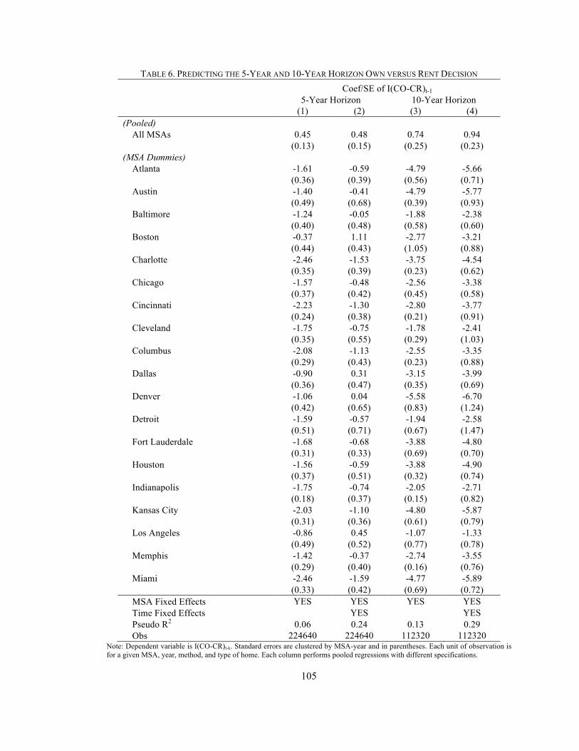
105

TABLE 6. PREDICTING THE 5-YEAR AND 10-YEAR HORIZON OWN VERSUS RENT DECISION Coef/SE of I(CO-CR)t-1

5-Year Horizon 10-Year Horizon

(1) (2) (3) (4) (Pooled)

All MSAs 0.45 0.48 0.74 0.94

!(0.13) (0.15) (0.25) (0.23)

(MSA Dummies) Atlanta -1.61 -0.59 -4.79 -5.66

(0.36) (0.39) (0.56) (0.71)

Austin -1.40 -0.41 -4.79 -5.77

(0.49) (0.68) (0.39) (0.93)

Baltimore -1.24 -0.05 -1.88 -2.38

(0.40) (0.48) (0.58) (0.60)

Boston -0.37 1.11 -2.77 -3.21

(0.44) (0.43) (1.05) (0.88)

Charlotte -2.46 -1.53 -3.75 -4.54

(0.35) (0.39) (0.23) (0.62)

Chicago -1.57 -0.48 -2.56 -3.38

(0.37) (0.42) (0.45) (0.58)

Cincinnati -2.23 -1.30 -2.80 -3.77

(0.24) (0.38) (0.21) (0.91)

Cleveland -1.75 -0.75 -1.78 -2.41

(0.35) (0.55) (0.29) (1.03)

Columbus -2.08 -1.13 -2.55 -3.35

(0.29) (0.43) (0.23) (0.88)

Dallas -0.90 0.31 -3.15 -3.99

(0.36) (0.47) (0.35) (0.69)

Denver -1.06 0.04 -5.58 -6.70

(0.42) (0.65) (0.83) (1.24)

Detroit -1.59 -0.57 -1.94 -2.58

(0.51) (0.71) (0.67) (1.47)

Fort Lauderdale -1.68 -0.68 -3.88 -4.80

(0.31) (0.33) (0.69) (0.70)

Houston -1.56 -0.59 -3.88 -4.90

(0.37) (0.51) (0.32) (0.74)

Indianapolis -1.75 -0.74 -2.05 -2.71

(0.18) (0.37) (0.15) (0.82)

Kansas City -2.03 -1.10 -4.80 -5.87

(0.31) (0.36) (0.61) (0.79)

Los Angeles -0.86 0.45 -1.07 -1.33

(0.49) (0.52) (0.77) (0.78)

Memphis -1.42 -0.37 -2.74 -3.55

(0.29) (0.40) (0.16) (0.76)

Miami -2.46 -1.59 -4.77 -5.89

(0.33) (0.42) (0.69) (0.72)

MSA Fixed Effects YES YES YES YES Time Fixed Effects

!YES

!YES

Pseudo R2 0.06 0.24 0.13 0.29 Obs 224640 224640 112320 112320

Note: Dependent variable is I(CO-CR)t-k. Standard errors are clustered by MSA-year and in parentheses. Each unit of observation is for a given MSA, year, method, and type of home. Each column performs pooled regressions with different specifications.

106

TABLE 6 (CONT'D). PREDICTING THE 5-YEAR AND 10-YEAR HORIZON OWN VERSUS RENT DECISION Coef/SE of I(CO-CR)t-1


(1) (2) (3) (4) (MSA Dummies)

Milwaukee -2.65 -1.77 -3.49 -4.59

(0.41) (0.54) (0.36) (0.97)

Minneapolis -1.82 -0.86 -7.55 -8.58

(0.40) (0.48) (0.65) (0.84)

Nashville -1.49 -0.46 -3.77 -4.68

(0.43) (0.53) (0.19) (0.74)

New York -0.52 0.90 -1.93 -2.29

(0.41) (0.41) (0.75) (0.67)

Orlando -1.47 -0.43 -3.56 -4.38

(0.29) (0.35) (0.50) (0.63)

Palm Beach -1.08 0.09 -3.21 -4.04

(0.32) (0.31) (0.66) (0.68)

Philadelphia -0.99 0.27 -1.64 -2.04

(0.41) (0.47) (0.59) (0.61)

Phoenix -1.32 -0.29 -5.41 -6.40

(0.45) (0.57) (0.69) (0.72)

Pittsburgh -2.19 -1.21 -2.19 -2.88

(0.22) (0.39) (0.15) (0.72)

Portland -3.16 -2.35 -6.11 -7.40

(0.46) (0.65) (0.68) (1.16)

Richmond -2.02 -1.02 -3.22 -4.05

(0.34) (0.36) (0.49) (0.60)

Sacramento -1.03 0.23 -1.52 -1.92

(0.52) (0.61) (0.68) (0.67)

San Antonio -1.49 -0.51 -3.76 -4.72

(0.45) (0.62) (0.27) (0.78)

San Diego -0.90 0.39 -1.99 -2.44

(0.50) (0.54) (0.83) (0.74)

San Francisco -0.91 0.36 -2.64 -3.19

(0.49) (0.49) (1.09) (0.96)

San Jose -1.18 0.01 -3.10 -3.73

(0.52) (0.54) (1.03) (0.89)

Seattle -1.77 -0.73 -2.75 -3.69

(0.57) (0.63) (0.41) (0.70)

St. Louis -1.77 -0.77 -3.76 -4.62

(0.32) (0.34) (0.45) (0.61)

Tampa -1.57 -0.56 -4.21 -5.08

!(0.32) (0.37) (0.55) (0.63)

Washington, D.C. -0.96 0.32 -1.87 -2.33

!(0.45) (0.52) (0.72) (0.66)

MSA Fixed Effects YES YES YES YES Time Fixed Effects

!YES

!YES

Pseudo R2 0.06 0.24 0.13 0.29 Obs 224640 224640 112320 112320

Note: Dependent variable is I(CO-CR)t-k. Standard errors are clustered by MSA-year and in parentheses. Each unit of observation is for a given MSA, year, method, and type of home. Each column performs pooled regressions with different specifications.

107

TABLE 7. FORECASTING THE 5-YEAR AND 10-YEAR HORIZON OWN VERSUS RENT DECISION % of Time Forecast is Correct


(1) (2) (3) (4) All MSAs 78.2 82.1 92.2 92.9 Atlanta 77.6 68.5 98.5 98.5 Austin 74.5 77.7 84.4 87.0 Baltimore 42.4 84.4 91.4 91.4 Boston 91.7 91.7 97.5 97.5 Charlotte 80.8 80.8 91.6 91.6 Chicago 89.2 89.2 92.8 92.8 Cincinnati 83.8 83.8 83.4 75.3 Cleveland 88.1 88.1 91.6 91.6 Columbus 66.0 70.5 92.4 92.4 Dallas 70.3 60.0 99.4 99.4 Denver 82.0 82.0 86.5 82.8 Detroit 82.0 83.0 97.1 97.1 Fort Lauderdale 79.3 77.3 96.5 96.5 Houston 83.9 83.9 86.6 85.7 Indianapolis 87.0 87.0 98.9 98.9 Kansas City 66.3 75.4 69.2 89.2 Los Angeles 78.2 80.6 91.7 91.7 Memphis 91.0 91.0 98.8 98.8 Miami 92.6 92.6 96.3 96.3 Milwaukee 84.6 84.6 99.9 99.9 Minneapolis 79.6 80.3 96.9 96.9 Nashville 58.3 90.3 82.5 88.4 New York 78.6 82.6 95.9 95.9 Orlando 70.3 87.3 93.8 93.8 Palm Beach 69.8 73.8 80.9 85.5 Philadelphia 75.8 81.3 99.3 99.3 Phoenix 88.9 88.9 88.3 86.4 Pittsburgh 95.3 95.3 99.7 99.7 Portland 87.0 87.0 95.3 95.3 Richmond 69.3 60.1 79.7 86.8 Sacramento 78.3 70.3 96.0 96.0 San Antonio 67.0 80.2 85.0 85.6 San Diego 67.6 91.8 91.7 91.7 San Francisco 73.7 87.1 95.1 95.1 San Jose 82.8 82.8 93.1 93.1 Seattle 84.1 84.1 97.0 97.0 St. Louis 80.6 82.7 97.9 97.9 Tampa 68.8 82.3 84.3 90.8 Washington, D.C. 80.6 81.8 97.9 95.0 MSA Fixed Effects YES YES YES YES Time Fixed Effects

YES

YES

Obs 224640 224640 112320 112320 Notes: See Table 3 notes.

108

TABLE 8. AVERAGE ANNUAL SAVINGS FROM LEAST COSTLY BENCHMARK, 5-YEAR HORIZON, 1980-2009 Annual Savings from Least Costly Tenure Choice (as % of CR)

v. Regression

-Based v. Always Owning

v. Always Renting


v. 1-Year Strategy

All MSAs 6.4 7.8 54.1 17.9 4.7 Atlanta 2.9 3.2 42.1 6.7 2.4 Austin 23.7 19.1 47.5 28.5 8.9 Baltimore 4.3 5.3 57.3 18.2 4.7 Boston 6.9 23.0 51.7 40.0 11.1 Charlotte 1.1 1.1 46.4 3.1 1.0 Chicago 2.4 2.4 32.7 11.0 2.3 Cincinnati 1.2 1.2 32.3 4.9 1.4 Cleveland 2.5 2.5 31.6 6.7 2.4 Columbus 1.4 1.4 31.7 2.9 1.3 Dallas 11.1 14.9 34.9 11.2 4.6 Denver 21.0 10.9 49.0 19.0 2.4 Detroit 7.8 7.8 58.1 19.1 5.7 Fort Lauderdale 3.0 3.3 82.2 6.3 3.8 Houston 8.6 7.9 50.3 9.8 2.7 Indianapolis 2.3 2.3 31.0 2.6 1.6 Kansas City 2.5 2.5 53.1 4.8 1.5 Los Angeles 16.1 23.0 84.7 53.2 11.2 Memphis 3.8 4.4 33.6 5.0 3.2 Miami 1.6 1.6 79.4 6.7 3.4 Milwaukee 0.8 0.8 36.3 6.4 1.1 Minneapolis 2.3 2.3 51.7 4.0 2.0 Nashville 5.1 5.4 36.2 12.6 3.7 New York 3.9 22.4 54.2 32.8 9.3 Orlando 3.3 4.2 66.6 5.4 2.6 Palm Beach 2.1 6.6 72.3 10.3 5.8 Philadelphia 7.9 9.0 53.7 19.2 4.7 Phoenix 6.2 8.1 65.7 12.2 5.4 Pittsburgh 1.7 1.7 43.5 4.3 2.9 Portland 2.1 2.1 63.7 22.2 2.0 Richmond 2.0 2.0 53.1 5.2 2.5 Sacramento 26.3 16.4 77.5 57.8 10.0 San Antonio 16.8 12.8 54.9 15.4 9.8 San Diego 11.5 18.4 80.2 56.3 10.5 San Francisco 7.2 17.4 68.2 55.9 9.9 San Jose 8.9 15.7 70.8 51.7 11.6 Seattle 5.3 5.3 48.1 29.0 4.8 St. Louis 2.7 2.7 42.6 4.1 1.3 Tampa 3.3 3.7 69.6 4.9 2.5 Washington, D.C. 5.2 9.4 69.6 28.5 6.3

Note: Each column reports the expected money saved if a household was able to follow the least costly tenure choice perfectly against the indicated trading strategy. "Regression-Based” indicates a trading strategy in which one rents or buys given the predicted strategy from specification (2) in Table 5. Always own and always rent is to apply a strategy of always owning or renting regardless of MSA or year. “1-year strategy” refers to a decision rule in which a household decides to start owning for the rest of the tenure choice horizon if the observed 1-year cost of owning was cheaper than the cost of rent in the previous year. If not, then the household will continue to rent until the 1-year costs indicate it was cheaper to own in the prior year.

109

TABLE 9. AVERAGE ANNUAL SAVINGS FROM LEAST COSTLY BENCHMARK WITH 10-YEAR HORIZON, 1980-2009

Annual Savings from Least Costly Tenure Choice (as % of CR)

v. Regression-

Based v. Always Owning

v. Always Renting


v. 1-Year Strategy

All MSAs 2.1 5.7 50.2 15.1 3.9 Atlanta 0.2 1.8 45.5 6.2 1.8 Austin 0.1 9.9 48.1 30.2 5.1 Baltimore 2.2 4.8 43.8 10.9 4.4 Boston 5.0 17.9 53.0 34.3 9.3 Charlotte 0.1 0.7 46.5 0.5 0.8 Chicago 0.9 1.6 28.1 1.8 1.7 Cincinnati 0.3 0.7 33.2 2.7 1.0 Cleveland 2.0 1.3 31.7 2.2 1.6 Columbus 0.4 0.8 32.7 1.0 0.9 Dallas 0.8 9.3 34.4 23.7 4.4 Denver 0.1 5.5 58.8 31.9 0.7 Detroit 2.2 2.1 59.8 4.1 2.4 Fort Lauderdale 0.7 2.2 74.1 18.1 3.0 Houston 0.5 4.5 48.5 24.7 3.2 Indianapolis 0.9 1.7 30.9 0.6 1.5 Kansas City 0.1 1.2 56.9 8.5 0.8 Los Angeles 8.7 21.9 62.9 43.5 13.0 Memphis 0.6 2.7 33.5 4.3 2.5 Miami 0.5 1.0 71.2 12.4 2.7 Milwaukee 0.2 0.3 35.5 3.2 0.6 Minneapolis 0.1 0.7 57.0 9.7 0.6 Nashville 0.3 3.0 36.2 5.1 2.6 New York 5.2 20.4 50.2 36.0 11.2 Orlando 0.7 3.2 58.1 18.0 2.3 Palm Beach 1.3 4.7 62.7 28.0 4.9 Philadelphia 2.6 7.3 40.3 13.4 5.3 Phoenix 0.2 4.2 62.4 28.2 3.1 Pittsburgh 1.0 1.3 40.1 0.9 2.0 Portland 0.3 1.4 61.4 8.9 1.2 Richmond 0.5 1.5 45.7 4.6 2.0 Sacramento 8.3 13.5 59.0 19.4 7.4 San Antonio 0.3 5.9 48.1 24.9 6.1 San Diego 10.3 17.3 71.0 33.3 9.8 San Francisco 9.0 16.6 64.3 27.1 9.7 San Jose 7.7 13.3 69.0 16.8 8.0 Seattle 2.2 3.1 38.4 3.4 3.7 St. Louis 0.2 1.6 42.4 4.5 1.2 Tampa 0.5 2.6 65.3 19.0 2.4 Washington, D.C. 4.1 9.0 56.4 20.8 6.8

Note: This table reports the same as Table 8 except for the 10-year horizon. Each column reports the expected money saved if a household was able to follow the least costly tenure choice perfectly against the indicated trading strategy.

110

TABLE 10. PROBABILITY OWNING IS CHEAPER BY INCOME TIER, 1-YEAR HORIZON PR(CO<CR)

Zero Tax Baseline

Low House Value Tier Tier 2 Tier 3 High House

Value Tier All MSAs 45.8 47.5 51.6 54.6 61.9 Atlanta 45.7 47.4 58.4 64.7 74.9 Austin 50.3 51.4 56.1 59.3 65.6 Baltimore 39.7 41.1 49.9 56.2 64.6 Boston 47.4 49.1 51.7 53.3 56.2 Charlotte 54.3 56.1 61.4 66.5 80.7 Chicago 38.7 40.2 47.1 54.5 62.8 Cincinnati 36.1 39.4 43.7 48.0 62.0 Cleveland 35.1 36.3 39.2 43.3 57.3 Columbus 35.9 37.5 42.3 48.8 65.2 Dallas 41.7 42.9 46.6 50.0 59.0 Denver 39.0 40.9 46.5 49.3 56.5 Detroit 51.1 52.1 55.1 57.6 64.5 Fort Lauderdale 49.9 50.5 52.2 54.0 59.8 Houston 56.9 57.6 57.8 58.8 62.6 Indianapolis 42.4 44.3 47.1 50.9 64.2 Kansas City 53.5 55.0 59.2 63.6 73.2 Los Angeles 45.9 47.4 49.1 50.4 53.2 Memphis 52.3 53.3 56.2 58.1 68.9 Miami 52.2 52.7 53.5 55.1 61.0 Milwaukee 33.7 35.8 48.4 57.3 67.7 Minneapolis 41.9 45.3 54.9 61.4 69.9 Nashville 53.3 54.3 56.5 58.3 64.2 New York 47.4 49.7 53.3 54.3 57.4 Orlando 48.0 48.8 52.3 54.4 62.2 Palm Beach 42.7 43.4 44.9 45.5 50.0 Philadelphia 47.2 48.1 51.5 54.4 61.9 Phoenix 51.7 54.1 57.9 59.8 65.2 Pittsburgh 53.0 54.4 55.0 56.5 64.9 Portland 45.4 46.6 52.0 52.8 58.4 Richmond 46.1 47.7 54.6 59.0 69.4 Sacramento 42.1 42.7 46.2 48.1 51.8 San Antonio 59.3 59.5 60.3 60.7 63.8 San Diego 45.4 46.1 48.0 48.6 49.6 San Francisco 43.2 47.6 50.7 52.0 53.8 San Jose 41.0 48.0 52.4 53.1 54.5 Seattle 38.6 39.2 43.4 47.1 51.5 St. Louis 50.2 51.6 55.4 59.5 70.2 Tampa 47.1 47.5 48.7 50.2 57.1 Washington, D.C. 40.7 46.5 54.3 55.8 58.2

Note: This table reports the probability owning is cheaper than renting by house value tiers. “Zero Tax Baseline” is the PR(CO<CR) assuming no taxes or deductions. “Low House Value Tier” corresponds to households with house values to 0.75*median house value or lower, Tier 2 households have house values between the low and the median, Tier 3 house values are between median and 1.25*median, and “High House Value Tier” are those above 1.25*median house value. We assume loan-to-value equals 0.8 in these calculations.

111

TABLE 11. AVERAGE ANNUAL SAVINGS FROM LEAST COSTLY BENCHMARK WITH 1-YEAR HORIZON, LOWEST INCOME TIER, 1980-2009


v. Predicted v. Always Owning

v. Always Renting


Savings SD Savings SD Savings SD Savings SD

All MSAs 5.9 17.8 35.8 52.8 31.6 49.1 7.9 21.6 Atlanta 1.4 6.8 20.2 26.7 18.1 27.6 2.8 9.9 Austin 11.4 23.4 36.2 68.4 29.1 41.9 8.3 17.6 Baltimore 2.6 10.4 32.3 40.9 31.3 56.4 5.9 15.9 Boston 6.5 22.0 41.1 52.8 53.3 72.0 8.6 22.8 Charlotte 3.8 12.5 15.5 27.9 21.8 29.0 4.0 11.6 Chicago 3.0 10.1 34.4 47.4 14.7 23.8 3.9 11.4 Cincinnati 2.0 7.5 30.2 43.7 8.9 16.0 2.4 7.8 Cleveland 4.1 11.9 34.1 45.2 8.9 17.1 4.7 12.4 Columbus 2.5 9.1 25.1 35.6 8.6 16.1 2.5 8.9 Dallas 3.5 11.7 33.2 48.0 17.5 28.8 2.7 10.5 Denver 2.5 9.1 34.1 41.8 21.0 35.6 1.7 7.8 Detroit 3.6 13.8 41.5 65.1 29.1 41.6 3.1 13.2 Fort Lauderdale 7.0 20.7 42.4 79.0 53.0 83.7 10.2 22.9 Houston 9.5 26.4 40.8 63.9 30.1 36.4 10.6 27.3 Indianapolis 5.3 21.1 21.9 34.8 13.7 22.7 6.4 21.6 Kansas City 4.1 20.6 24.8 45.8 24.5 32.1 4.0 20.6 Los Angeles 2.0 8.9 58.0 76.5 55.6 81.9 7.2 22.7 Memphis 12.2 39.8 27.0 53.7 21.8 32.6 12.3 39.8 Miami 9.5 22.5 42.4 80.7 47.9 75.4 15.9 36.1 Milwaukee 2.3 8.7 34.9 47.8 9.6 19.0 2.2 9.1 Minneapolis 2.0 8.5 28.3 38.8 21.1 31.9 3.6 11.6 Nashville 6.6 17.7 22.7 37.0 20.9 27.1 7.6 18.1 New York 6.7 21.7 43.5 55.4 50.1 65.4 7.9 23.0 Orlando 3.3 10.7 32.0 55.3 41.4 78.7 9.7 32.4 Palm Beach 4.7 14.7 46.7 72.5 46.3 82.6 9.9 23.1 Philadelphia 5.1 14.9 29.3 39.4 37.1 53.2 6.6 16.2 Phoenix 11.1 32.3 41.6 69.1 42.0 86.0 12.4 32.7 Pittsburgh 7.8 21.1 25.5 50.0 22.7 32.1 10.4 23.6 Portland 8.0 24.4 41.9 55.1 27.9 45.4 5.4 17.9 Richmond 4.1 12.1 24.1 32.2 25.8 42.6 5.2 12.5 Sacramento 9.4 25.5 62.9 76.3 45.7 73.4 10.9 33.7 San Antonio 22.9 57.4 38.6 68.7 39.4 50.8 23.3 57.4 San Diego 2.2 10.6 59.8 69.7 46.9 69.9 9.1 28.6 San Francisco 4.8 14.7 47.7 59.0 51.3 72.6 12.9 34.6 San Jose 9.4 24.9 48.9 63.3 56.2 85.7 23.5 50.0 Seattle 7.6 19.5 40.9 52.7 28.2 58.7 8.0 20.7 St. Louis 1.9 7.9 21.2 34.5 19.8 27.2 1.8 7.7 Tampa 8.7 27.7 34.7 56.8 44.7 70.9 12.9 32.9 Washington, D.C. 3.8 12.1 35.9 49.5 48.1 71.0 5.8 15.5

Note: Each column reports the expected money saved if a household was able to follow the least costly tenure choice perfectly against the indicated trading strategy, but only for the lowest income tier.

112

FIGURE 1. ACTUAL V. PREDICTED COST OF OWNING MINUS COST OF RENTING

Note: This figure plots the actual CO-CR against the predicted CO-CR across all MSAs and cost measures.

113

FIGURE 2. ACTUAL V. PREDICTED COST OF OWNING MINUS COST OF RENTING BY CITY

Note: This figure plots the actual CO-CR against the predicted CO-CR for a select sample of cities.

114

FIGURE 3. COST OF OWNING MINUS COST OF RENTING, 1980-2009

Note: This figure plots the average cost of owning minus cost of renting (CO-CR) for a 1-year horizon across a select sample of cities. The red dashed lined indicates where the cost of owning equals the cost of rent.

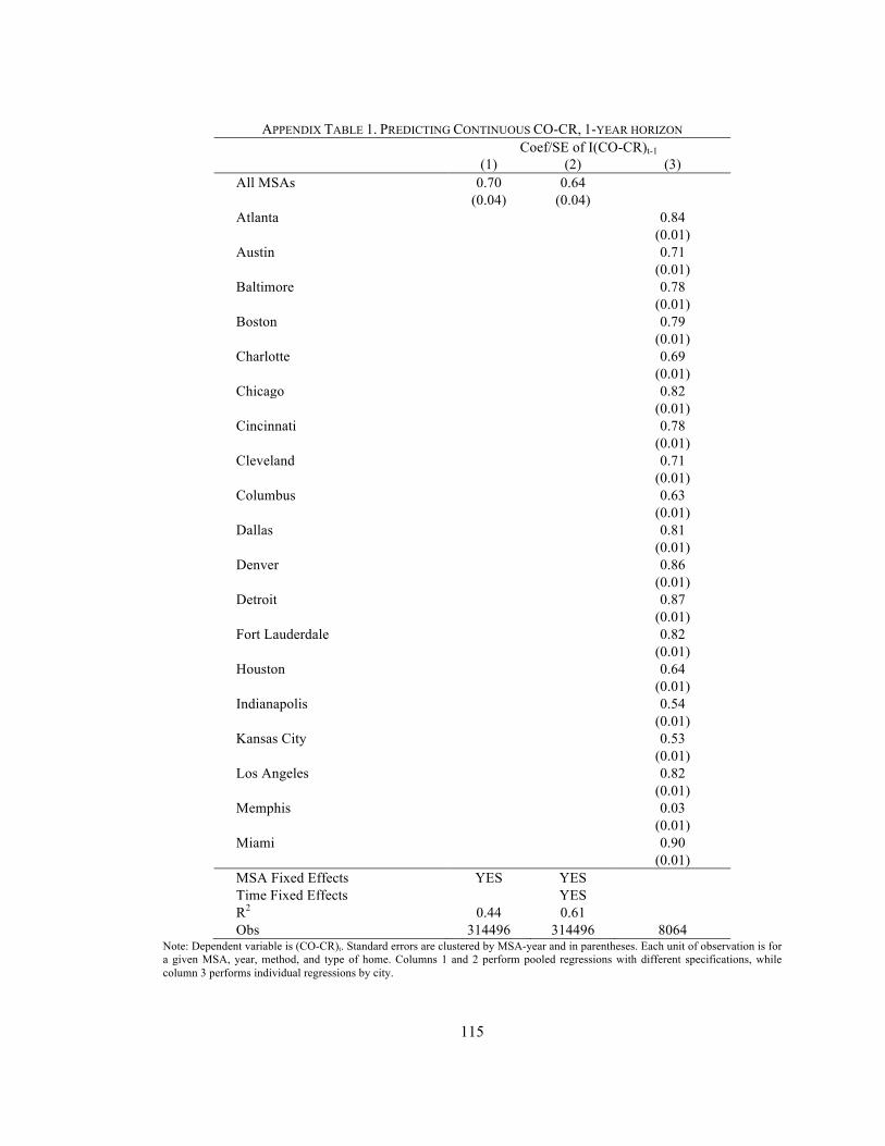
115

APPENDIX TABLE 1. PREDICTING CONTINUOUS CO-CR, 1-YEAR HORIZON

Coef/SE of I(CO-CR)t-1 (1) (2) (3)

All MSAs 0.70 0.64

!(0.04) (0.04)

Atlanta !

0.84

! (0.01)

Austin

0.71

(0.01)

Baltimore

0.78

(0.01)

Boston

0.79

(0.01)

Charlotte

0.69

(0.01)

Chicago

0.82

(0.01)

Cincinnati

0.78

(0.01)

Cleveland

0.71

(0.01)

Columbus

0.63

(0.01)

Dallas

0.81

(0.01)

Denver

0.86

(0.01)

Detroit

0.87

(0.01)

Fort Lauderdale

0.82

(0.01)

Houston

0.64

(0.01)

Indianapolis

0.54

(0.01)

Kansas City

0.53

(0.01)

Los Angeles

0.82

(0.01)

Memphis

0.03

! (0.01)

Miami

0.90

(0.01)


!YES

!R2 0.44 0.61 !Obs 314496 314496 8064

Note: Dependent variable is (CO-CR)t. Standard errors are clustered by MSA-year and in parentheses. Each unit of observation is for a given MSA, year, method, and type of home. Columns 1 and 2 perform pooled regressions with different specifications, while column 3 performs individual regressions by city.

116

APPENDIX TABLE 1 (CONT'D). PREDICTING CONTINUOUS CO-CR, 1-YEAR HORIZON

Coef/SE of (CO-CR)t-1 (1) (2) (3)

Milwaukee

0.67

(0.01)

Minneapolis

0.84

(0.01)

Nashville

0.45

(0.01)

New York

0.83

(0.01)

Orlando

0.72

(0.01)

Palm Beach

0.84

(0.01)

Philadelphia

0.70

(0.01)

Phoenix

0.53

(0.01)

Pittsburgh

0.40

(0.01)

Portland

0.76

(0.01)

Richmond

0.75

(0.01)

Sacramento

0.77

(0.01)

San Antonio

0.30

(0.01)

San Diego

0.82

(0.01)

San Francisco

0.66

(0.01)

San Jose

0.51

(0.01)

Seattle

0.45

(0.01)

St. Louis

0.81

(0.01)

Tampa

0.61

(0.01)

Washington, D.C.

0.79

! (0.01)


!YES

!R2 0.44 0.61 !Obs 314496 314496 8064

Note: Dependent variable is (CO-CR)t. Standard errors are clustered by MSA-year and in parentheses. Each unit of observation is for a given MSA, year, method, and type of home. Columns 1 and 2 perform pooled regressions with different specifications, while column 3 performs individual regressions by city.

117

APPENDIX TABLE 2. PREDICTING BINARY RENT V. OWN DECISION, 1-YEAR HORIZON, IV RESULTS


All MSAs 2.17 2.55

!(0.09) (0.11)

Atlanta !

1.72

! (0.07)

Austin

1.83

(0.05)

Baltimore

2.18

(0.03)

Boston

2.15

(0.04)

Charlotte

2.21

(0.08)

Chicago

2.14

(0.04)

Cincinnati

2.44

(0.05)

Cleveland

2.41

(0.04)

Columbus

2.50

(0.05)

Dallas

2.51

(0.04)

Denver

2.27

(0.05)

Detroit

2.53

(0.05)

Fort Lauderdale

2.24

(0.03)

Houston

2.66

(0.03)

Indianapolis

2.38

(0.05)

Kansas City

2.63

(0.05)

Los Angeles

1.52

(0.06)

Memphis

1.93

! (0.07)

Miami

2.11

(0.05)


!YES

!Pseudo R2 0.22 0.39 !Obs 314496 314496 8064

Note: Dependent variable is I(CO-CR)t. This table instrument I(CO-CR)t-1 with I(CO-CR)t-2. Standard errors are clustered by MSA-year and in parentheses. Each unit of observation is for a given MSA, year, method, and type of home. Columns 1 and 2 perform pooled regressions with different specifications, while column 3 performs individual regressions by city.

118

APPENDIX TABLE 2 (CONT’D). PREDICTING BINARY RENT V. OWN DECISION, 1-YEAR HORIZON, IV RESULTS


Milwaukee

2.29

(0.05)

Minneapolis

2.39

(0.05)

Nashville

1.86

(0.07)

New York

2.02

(0.05)

Orlando

1.82

(0.06)

Palm Beach

2.28

(0.02)

Philadelphia

2.28

(0.03)

Phoenix

2.36

(0.03)

Pittsburgh

2.04

(0.06)

Portland

2.04

(0.05)

Richmond

2.26

(0.03)

Sacramento

1.39

(0.06)

San Antonio

2.19

(0.04)

San Diego

1.36

(0.07)

San Francisco

1.77

(0.05)

San Jose

1.29

(0.08)

Seattle

1.43

(0.07)

St. Louis

1.57

(0.07)

Tampa

2.42

(0.02)

Washington, D.C.

1.94

! (0.05)


!YES

!Pseudo R2 0.22 0.39 !Obs 314496 314496 8064

Note: Dependent variable is I(CO-CR)t. This table instrument I(CO-CR)t-1 with I(CO-CR)t-2. Standard errors are clustered by MSA-year and in parentheses. Each unit of observation is for a given MSA, year, method, and type of home. Columns 1 and 2 perform pooled regressions with different specifications, while column 3 performs individual regressions by city.

119

APPENDIX TABLE 3. PREDICTING BINARY RENT V. OWN DECISION, 1-YEAR HORIZON, 2 BEDROOM Coef/SE of I(CO-CR)t-1 (1) (2) (3)

All MSAs 2.38 2.24

!(0.13) (0.18)

Atlanta !

2.57

! (0.19)

Austin

2.96

(0.13)

Baltimore

0.73

(0.11)

Boston

3.20

(0.12)

Charlotte

0.74

(0.44)

Chicago

2.43

(0.13)

Cincinnati

4.07

(0.17)

Cleveland

4.07

(0.16)

Columbus

2.35

(0.17)

Dallas

3.06

(0.14)

Denver

3.68

(0.13)

Detroit

3.39

(0.14)

Fort Lauderdale

1.63

(0.11)

Houston

3.06

(0.13)

Indianapolis

2.70

(0.18)

Kansas City

1.69

(0.18)

Los Angeles

2.45

(0.11)

Memphis

1.56

! (0.17)

Miami

2.72

(0.12)


!YES

!Pseudo R2 0.24 0.42 !Obs 81432 81432 2088

Note: The cost of owning is denoted by “CO”, and the cost of renting “CR”. Pr(CO>CR) is the probability that the owning is cheaper than renting. “Overall" is the average CO-CR across all cost measures and years in a given city. Cost measures are calculated by equation (4), assuming a loan-to-value constant of 0.8 and national average federal and state income tax for all tax rates. The calculations in this table are restricted to 2 bedroom units only.

120

APPENDIX TABLE 3 (CONT'D). PREDICTING BINARY RENT V. OWN DECISION, 1-YEAR HORIZON, 2 BEDROOM


Milwaukee

1.63

(0.14)

Minneapolis

1.80

(0.10)

Nashville

1.20

(0.11)

New York

1.62

(0.11)

Orlando

2.31

(0.18)

Palm Beach

3.07

(0.12)

Philadelphia

1.47

(0.19)

Phoenix

2.47

(0.11)

Pittsburgh

2.55

(0.12)

Portland

3.29

(0.12)

Richmond

2.12

(0.10)

Sacramento

1.75

(0.10)

San Antonio

2.44

(0.11)

San Diego

2.54

(0.18)

San Francisco

0.98

(0.13)

San Jose

1.91

(0.11)

Seattle

2.44

(0.11)

St. Louis

2.56

(0.18)

Tampa

0.98

(0.13)

Washington, D.C.

2.06

! (0.11)


!YES

!Pseudo R2 0.24 0.42 !Obs 81432 81432 2088

Note: Dependent variable is (CO-CR)t. Standard errors are clustered by MSA-year and in parentheses. Each unit of observation is for a given MSA, year, method, and type of home. Columns 1 and 2 perform pooled regressions with different specifications, while column 3 performs individual regressions by city. The calculations in this table are restricted to 2 bedroom units only.

121

APPENDIX TABLE 4. FORECASTING THE 1-YEAR HORIZON OWN VERSUS RENT DECISION, 2 BEDROOM

% of Time Forecast is Correct (1) (2) (3)

All MSAs 82.8 84.9 83.2 Atlanta 90.1 90.8 90.1 Austin 85.4 81.5 85.4 Baltimore 68.0 77.2 73.3 Boston 83.6 86.7 83.6 Charlotte 95.9 95.7 95.9 Chicago 82.3 88.9 82.3 Cincinnati 91.5 92.6 91.5 Cleveland 91.2 91.4 91.2 Columbus 88.8 88.8 88.8 Dallas 86.0 80.2 86.0 Denver 86.7 84.9 86.7 Detroit 87.7 89.9 87.7 Fort Lauderdale 73.9 76.0 73.9 Houston 84.5 67.7 84.5 Indianapolis 90.2 91.4 90.2 Kansas City 91.1 88.8 91.1 Los Angeles 77.4 91.5 77.4 Memphis 90.0 87.2 90.0 Miami 81.7 83.6 81.7 Milwaukee 86.0 86.5 86.0 Minneapolis 81.1 84.9 81.3 Nashville 80.5 78.1 82.7 New York 82.8 86.2 82.8 Orlando 80.8 87.8 82.5 Palm Beach 73.0 78.0 73.0 Philadelphia 71.5 80.3 73.1 Phoenix 72.8 73.9 72.8 Pittsburgh 92.5 92.2 92.5 Portland 83.6 85.4 83.6 Richmond 89.6 89.1 89.6 Sacramento 78.1 82.7 78.1 San Antonio 82.3 78.9 82.3 San Diego 83.9 92.6 83.9 San Francisco 74.9 80.7 74.9 San Jose 70.8 87.7 70.8 Seattle 78.1 76.3 78.1 St. Louis 90.3 89.8 90.3 Tampa 74.9 78.7 81.2 Washington, D.C. 74.3 87.0 74.3 MSA Fixed Effects YES YES

!Time Fixed Effects !

YES !Obs 81432 81432 2088

Note: This table calculates the percent of the time the predicted binary rent v. own decision was “correct”, i.e. when it was actually better to own or rent. The columns correspond to the specifications in Table 2. The calculations in this table are restricted to 2 bedroom units only.

122

APPENDIX TABLE 5. AVERAGE ANNUAL SAVINGS FROM LEAST COSTLY BENCHMARK WITH 1-YEAR HORIZON, 2 BEDROOM


v. Regression-Based

v. Always Owning

v. Always Renting


Savings SD Savings SD Savings SD Savings SD All MSAs 4.5 14.3 13.2 29.3 49.8 49.5 6.1 17.5 Atlanta 0.8 4.3 1.0 4.9 45.8 31.9 1.1 4.8 Austin 6.5 20.5 16.7 46.1 47.1 43.2 3.5 13.2 Baltimore 3.3 9.1 8.6 20.4 47.7 54.0 6.9 13.7 Boston 4.0 15.7 19.8 32.5 61.3 70.1 6.6 19.5 Charlotte 0.9 6.0 0.9 6.0 57.6 29.3 2.2 9.8 Chicago 1.3 6.6 11.0 25.0 31.8 30.0 3.0 9.4 Cincinnati 0.7 4.3 5.5 16.5 34.1 24.0 1.4 6.7 Cleveland 0.9 4.6 7.0 16.6 32.5 25.7 1.1 5.0 Columbus 3.0 12.3 2.8 12.0 37.0 23.3 3.1 12.4 Dallas 5.2 15.2 9.2 26.4 39.7 34.8 3.3 12.0 Denver 2.3 8.4 11.8 21.5 34.8 40.3 1.9 7.7 Detroit 4.2 18.7 15.4 35.0 56.7 49.2 5.0 19.5 Fort Lauderdale 5.0 12.8 20.3 56.6 64.8 75.5 6.3 15.6 Houston 20.7 37.6 17.6 33.9 51.8 42.4 8.9 27.9 Indianapolis 2.4 11.6 2.7 11.8 42.0 28.8 2.8 12.0 Kansas City 6.0 22.2 5.7 21.0 54.7 36.5 6.9 22.7 Los Angeles 1.8 8.5 31.1 53.6 60.5 74.5 6.9 17.4 Memphis 6.8 26.9 8.1 28.8 47.3 36.2 12.5 39.0 Miami 4.1 14.2 20.9 58.2 57.5 67.3 8.2 24.9 Milwaukee 2.6 9.6 8.0 20.6 34.0 26.8 2.9 10.4 Minneapolis 3.8 12.4 7.7 18.8 41.2 35.6 4.5 12.7 Nashville 5.4 16.5 4.6 13.1 42.8 32.6 5.2 16.2 New York 5.2 17.4 21.9 34.2 57.6 64.7 5.2 14.7 Orlando 1.9 7.9 11.0 36.0 61.9 70.2 7.3 23.0 Palm Beach 3.5 9.4 20.9 51.9 55.3 74.3 6.4 14.8 Philadelphia 5.8 16.7 7.1 15.7 56.5 55.3 8.7 18.9 Phoenix 11.3 23.9 21.0 46.1 55.5 75.4 13.5 27.7 Pittsburgh 2.2 10.7 5.7 21.4 54.9 36.1 6.4 23.9 Portland 3.0 10.7 13.6 25.5 43.9 48.6 3.7 11.3 Richmond 1.8 7.5 1.9 7.8 48.4 42.7 2.9 9.7 Sacramento 6.5 21.9 30.1 51.1 56.0 70.4 8.6 22.1 San Antonio 11.4 30.9 16.2 40.8 63.6 54.7 10.4 30.6 San Diego 1.1 5.6 29.0 45.2 54.5 67.5 7.0 19.7 San Francisco 4.3 11.5 26.8 39.0 52.5 65.6 10.1 24.0 San Jose 3.3 12.2 26.6 41.9 59.6 76.0 14.6 32.9 Seattle 6.7 18.5 16.5 31.5 36.0 55.5 5.5 15.1 St. Louis 2.4 10.4 2.3 9.5 49.0 31.1 2.5 10.5 Tampa 11.9 34.7 12.4 36.2 59.7 66.1 13.5 35.2 Washington, D.C. 2.0 8.5 14.4 30.8 56.2 66.0 6.6 15.5

Note: Each column reports the expected money saved from following the least costly benchmarket (correctly forecasting) against the indicated trading strategy. "Regression-Based " indicates a trading strategy in which one rents or buys given the predicted strategy from specification (2) in tables 1 and 2. Always own and always rent is to apply a strategy of always owning or renting regardless of MSA or year. “Last-Year” refers to a strategy where one just owns or rent based on whether it was observed to be cheaper to own or rent in the previous year. The calculations in this table are restricted to 2 bedroom units only.

123

CHAPTER 3

FINANCIAL LITERACY, SCHOOLING, AND WEALTH ACCUMULATION*

Jere R. Behrman University of Pennsylvania

Olivia S. Mitchell


Cindy K. Soo The Wharton School, University of Pennsylvania

David Bravo

Centro de Microdatos, Universidad Chile

Abstract

Financial literacy and schooling attainment have been linked to household wealth accumulation. Yet prior findings may be biased due to noisy measures of financial literacy and schooling, as well as unobserved factors such as ability, intelligence, and motivation that could enhance financial literacy and schooling but also directly affect wealth accumulation. Here we use a new household dataset and an instrumental variables approach to isolate the causal effects of financial literacy and schooling on wealth accumulation. While financial literacy and schooling attainment are both strongly positively associated with wealth outcomes in linear regression models, our approach reveals even stronger and larger effects of financial literacy on wealth. It also indicates no significant positive effects of schooling attainment conditional on financial literacy in a linear specification, but positive effects when interacted with financial literacy. Estimated impacts are substantial enough to suggest that investments in financial literacy could have large positive payoffs. *The authors acknowledge support provided by the TIAA-CREF Institute, the Pension Research Council and Boettner Center at the Wharton School of the University of Pennsylvania, and NIH/NIA grant AG023774-01(P.I. Petra Todd) on “Lifecycle health, work, aging, insurance and pensions in Chile.” They also thank Luc Arrondel, Alex Gelber, Jeremy Tobacman, Javiera Vasquez, and participants in the Wharton Applied Economics doctoral workshop as well as the 2010 LBS TransAtlantic Doctoral Conference for helpful comments, and Richard Derrig for sharing his PRIDIT code. Opinions and errors are solely those of the authors and not of the institutions providing funding for this study or with which the authors are affiliated. ©2010 Behrman, Mitchell, Soo, and Bravo. All rights reserved.

124

1 Introduction

Traditional economic theory posits that forward-looking individuals maximize expected

lifetime utility using economic information to accumulate and then decumulate wealth effectively

over their lifetimes. Yet survey evidence reveals that fewer than half of U.S. workers have even

attempted to estimate how much money they might need in retirement, and many older adults

face significant retirement saving shortfalls (Lusardi and Mitchell 2007a and b; Mitchell and

Moore 1998; Scholz, Seshadri, and Khitatrakun 2006). Numerous economic explanations for

these phenomena have been suggested including dispersion in discount rates, risk aversion, and

credit constraints, but the empirical literature exploring such factors thus far has been unable to

account for much of the observed differentials in wealth (Bernheim, Skinner, and Weinberg,

2001; Barsky, Juster, Kimball, and Shapiro, 1997).

The present study seeks to evaluate whether people who find it difficult to understand

their financial environment are also less likely to accumulate wealth. Specifically, we examine

the links between financial literacy, by which we mean the ability to process economic

information and make informed decisions about household finances, and wealth accumulation

and pension contributions. Previous studies have reported strong correlations between financial

literacy and asset accumulation as well as retirement planning.1 These findings have prompted

policymakers to support efforts to enhance household wealth accumulation and welfare through

increasing financial literacy. For instance, the U.S. President’s Advisory Council on Financial

Literacy recently stated that (PACFL, 2008, np): "While the crisis has many causes, it is

undeniable that financial illiteracy is one of the root causes... Sadly, far too many Americans do

not have the basic financial skills necessary to develop and maintain a budget, to understand 1 For instance, Hilgert, Hogarth, and Beverley (2003) show that more financially knowledgeable US respondents are also more likely to engage in a wide range of recommended financial practices; Lusardi and Mitchell (2007a, b) find that more financially literate elderly U.S. respondents are also more likely to plan, to succeed in planning, and to invest in complex assets; and Campbell (2006) reports that more educated Swedish households also diversify their portfolios more efficiently. Cole, Sampson, and Zia (2009) find that the financially more literate are more likely to have bank accounts in India and Indonesia.

125

credit, to understand investment vehicles, or to take advantage of our banking system. It is

essential to provide basic financial education that allows people to better navigate an economic

crisis such as this one.” Similarly, the Organization for Economic Cooperation and Development

(OECD nd) has recently launched a major initiative to “identify individuals who are most in need

of financial education and the best ways to improve that education.”

Despite these and other enthusiastic endorsements for programs to boost financial

literacy, questions have been raised about whether these associations reflect causality (Lusardi

and Mitchell, 2008, 2010). For example, individuals who fail to save also may be financially

illiterate due to some underlying and usually unobservable factor such as impatience, making it

difficult to assess whether boosting financial education would, in fact, enhance household wealth

accumulation. Moreover, in simple bivariate associations of financial literacy with wealth,

financial literacy might be proxying, in part, for other factors such as schooling attainment.

Empirical measures of financial literacy are also likely to have considerable measurement error

that, ceteris paribus, is likely to bias standard estimates of the impacts of financial literacy

towards zero. Instrumental variable (IV) estimates in principle can control for both the

unobserved variable and the random measurement error biases, and schooling attainment can be

included in the same specification to control for the possibility that financial literacy proxies for

schooling. To our knowledge, however, no studies have yet used IV methods to estimate the

impact of financial literacy and schooling attainment on wealth, as we do here.2

2 Some studies have looked at related issues using IV methods. For instance, Lusardi and Mitchell (2007a) test the possible causal effect of wealth on financial planning using changes in regional housing prices as an instrument for wealth, but they limit their study to older respondents in the U.S. Health and Retirement Study and do not consider the possible impact of financial literacy on wealth as we do in this study. Bernheim, Garrett, and Maki (2001), Cole and Shastry (2009), and Lusardi and Mitchell (2009) investigate how changes in U.S. schooling laws and state mandates requiring schools to offer financial literacy relate to financial market participation, but these studies do not focus on wealth accumulation as we do here. Ameriks, Caplin, and Leahy (2003) explore instruments for planning by U.S. respondents but they are silent on the role of financial literacy.

126

In what follows, we draw on a unique microeconomic dataset, the Chilean Social

Protection Survey, to explore how financial literacy and schooling attainment influence wealth.3

This dataset includes extensive information on household wealth as well as individual and

household characteristics for a representative sample of prime-age adults, permitting us to

evaluate the effects of financial literacy using a richer range of ages and schooling than heretofore

available.4 Using a set of plausibly exogenous instrumental variables that satisfy critical

diagnostic tests to isolate the causal effects of financial literacy and schooling attainment on

wealth, we show that both financial literacy and schooling attainment are positively associated

with wealth outcomes. Moreover, our IV estimates indicate even stronger effects of financial

literacy on wealth than suggested by OLS models, while the opposite is true for schooling in

linear specifications; interactive specifications imply that both schooling and financial literacy

have significant positive effects.

Our results are relevant for financial educational policy in that we find that improved

financial literacy can make a significant difference for financial behavior, even after controlling

for schooling. This rigorous analysis of the impact of financial literacy on wealth accumulation

should be useful in informing governments and their policy advisers around the world, as they

consider new initiatives for financial education.5

2 Empirical Framework

Several prior studies have shown that financial literacy and schooling are significantly

correlated with positive financial behavior, but few have controlled for (usually) unobserved

3 The Social Protection Survey is described at www.microdatos.cl/interior_areasMT.php?id_s=2&id_ss=2&id_proy=1 4 Ameriks et al. (2003) examine highly-educated TIAA-CREF survey participants; Lusardi and Mitchell (2007a) use Health and Retirement Study respondents over age 50. In contrast, the dataset we use below is a nationally representative sample of men age 24-65 and women age 24-60. 5 For instance the World Bank and the Russian Federation have recently announced a multi-million dollar, multi-year collaborative to improve financial literacy in low- and middle-income countries (see http://web.worldbank.org/WBSITE/EXTERNAL/TOPICS/EXTEDUCATION/0,,contentMDK:21936796~menuPK:2643854~pagePK:64020865~piPK:149114~theSitePK:282386,00.html)

127

factors such as risk aversion, self-esteem, innate ability, intelligence, and motivation that may

shape the relationship between financial literacy and financial behaviors.6 For this reason, it is

difficult to conclude, based on the scientific evidence, that improvements in financial literacy

actually enhance financial planning and saving, or whether, instead, wealth and financial literacy

are both the result of some other unobserved factors. For this reason, analyses that do not control

for such unobserved factors may be vulnerable to biases in the estimated effects of schooling and

financial literacy on financial wellbeing. Moreover, empirical indicators of schooling and

financial literacy are noisy measures, and as is well-known, random measurement error in right-

side variables tends to bias their coefficient estimates towards zero. Estimates of noise-to-signal

ratios for schooling attainment are often about 10 percent (Ashenfelter and Krueger 1994;

Behrman, Rosenzweig, and Taubman 1994), producing a bias towards zero of almost that

magnitude. Measures of financial literacy are likely subject to greater measurement errors, and

thus, greater biases. Instrumental variable estimates are one way to eliminate the attenuation bias

towards zero due to measurement error.

Our goal is to assess whether wealth accruals could be enhanced with greater financial

literacy and schooling. Suppose the true relationship between financial literacy, schooling, and

wealth could be described for the ith person as:

Wi =β0 +β1FLi +β2Si +β3FLi *Si +β4Ci +β5Ei + εi , (1)

where wealth Wi depends linearly on financial literacy FLi, schooling Si, their interaction FLi *Si,

other observed individual characteristics Ci, unobserved individual characteristics Ei, and

unobserved random shocks εi. We include in relation (1) both linear terms in FLi and Si and their

interaction. We include the interaction because it is possible that the effects of financial literacy

FL depend on the level of schooling Si and vice versa. This coefficient of this interaction term

6 Both Lusardi (2003) and Ameriks et al. (2003) use IV strategies, but they focus on financial planning rather than financial literacy.

128

may be positive if financial literacy FLi and schooling Si are complements and reinforce each

other or negative if they are substitutes in determination of wealth accumulation. Below we

consider three variants of relation (1):

(1a) only linear terms,7 (1b) both the linear and interaction terms, and (1c) only the interaction term.

Equation (1) posits that there are no other endogenous variables beyond financial literacy

and schooling that directly determine wealth. For example, the time one devotes to schoolwork

and how that time is divided between arithmetic and other topics might affect wealth, but our

assumption is that such effects are indirect via financial literacy and schooling. Likewise, there

could be other behavioral channels through which FLi and Si affect Wi. For instance, part of the

effects on wealth may work through choosing to contribute more to pensions, or by increasing

understanding of business news and market predictions. Estimating equation (1) does not

illuminate such possibilities, though formulations similar to equation (1) but using some saving

pathway as the dependent variable could illuminate the roles of FLi and Si in determining the

relevant mechanism. In what follows, we offer analysis of two such pathways, the density of

pension contributions and whether the individual attempted to calculate money needed for

retirement.

We further posit that financial literacy and schooling are determined by observed

personal characteristics Ci* (that may overlap with Ci), some factors in C* and Xi that affect

learning and schooling but do not directly affect Wi , unobserved individual characteristics Ei, and

error terms ui and vi:8

7 We also consider two sub-variants of the linear case with only financial literacy or only schooling. 8 We also could include another equation parallel to (2) and (3) for the interaction, but since the points made here for the case in which FLi and Si enter in equation (1a) only linearly carry over to the case with the interaction, we limit this discussion to the simpler case in which they only enter linearly. We have written equations (2) and (3) as if FLi and Si have the same determinants except for ui and vi, which are likely to be correlated (perhaps perfectly correlated). This is the usual setup in household models if decisions regarding FLi and Si are made at the same time – in principle, all concurrent decisions are made in

129

FLi =η0 +η1Ci* +η2Xi +η3Ei + ui (2)

Si =α0 +α1Ci* +α2Xi +α3Ei + vi (3)

In general, for consistent estimates of the coefficients of interest, ordinary least squares (OLS)

regression requires that the covariance between the disturbance terms in equations (1) and (2) and

(1) and (3) be zero: that is, there can be no unobserved factors that are correlated with financial

literacy or schooling but also affect the outcome of interest Wi. Nevertheless, the unobserved

individual factors vector Ei appears in the compound disturbance terms for all relations, implying

that OLS estimates are likely to suffer from omitted variable bias. The direction of the bias

depends on whether the true values of β5 and η3 (and similarly, of β5 and α3) have the same or the

opposite signs. For example, if the unobserved factor is ability that positively affects financial

literacy and also directly positively affects wealth, both β5 and η3 are positive and OLS estimates

of β1 are biased upward, overestimating the magnitude and significance of financial literacy as a

determinant of wealth. Conversely, if some unobserved factor such as innate caution produced

greater investment in financial literacy, but ceteris paribus reduced wealth due to too great

caution in investment behavior, OLS estimates of β1 are biased downward, underestimating the

magnitude and significance of financial literacy as a determinant of wealth accumulation. In

addition to the possibility of such omitted variable biases, financial literacy and schooling

measures are potentially subject to measurement error as noted above, which would tend to bias

OLS estimates towards zero.

A similar point holds with regard to estimates that include only FLi or only Si – one at at a

time – if the true relation is actually equation (1a) with both entering linearly.9 Equations (2) and

light of all the variables that determine household behaviors – though, of course, the coefficients could differ and some may not be significantly different from zero. If decisions are made at different times, the right-side determinants in equations (2) and (3) may differ; for example, some expectations that determine the earlier decision could be replaced by realized outcomes that occurred prior to the later decision. Our microeconomic dataset, like most, does not permit empirical representations of such possibilities. 9 Some other endogenous variable Yi might also be included in equation (1) but our maintained hypothesis for our estimates, as in other instrumental variable estimates, if that this is not the case.

130

(3) show that it is highly likely that FLi and Si are correlated because their determinants are

basically the same.10 Accordingly, if the true relation is equation (1a) with both FLi and Si entering

linearly but analysts include either FLi or Si, the coefficient estimate for the included variable is

biased because it is correlated with the excluded factor.

To handle this problem, we use an IV approach with robust standard errors to estimate

the three variants of equation (1) in light of (2) and (3), seeking to isolate the causal effects of

financial literacy and schooling, and to control for random measurement errors. Good

instruments are ones that are sufficiently correlated with financial literacy FLi and with schooling

Si, but that are independent of unobserved effects in equation (1) determining wealth. The Xi

vector and elements of the Ci* vector excluded from Ci in equations (2) and (3) refer to such

instruments. For the IV estimation, we begin by estimating the “first stage” determinants of

financial literacy and schooling in (2) and (3); next we use these estimates to predict financial

literacy and schooling and employ them in the “second stage” estimate of equation (1). Note that

with the above assumptions, predicted financial literacy and predicted schooling are independent

of the compound error term in (1). Therefore, if equation (1) is the true relation, the IV or two-

stage least squares procedure leads to consistent estimates of β1 and β2.

In what follows, we utilize a set of plausible instruments and diagnostic tests to determine

whether our instruments are (a) sufficiently strong (using F tests for excluded instruments,

Angrist-Pische multivariate F tests for excluded instruments, and the Kleibergen-Paap weak

identification tests), and (b) independent of the second-stage compound disturbance term (β4Ei +

εi) using the Hansen J statistic overidentification test.11 Our candidate instruments, on which we

10 It is possible but highly unlikely in such household models that the coefficients of the variables in equations (2) and (3) differ so that financial literacy and schooling are orthogonal. 11 There recently has been what Stock (2010) calls a “transformation” in econometric tools for making inferences, including development of some of the diagnostic tools that we use here(see Stock (2010) and the references therein). As is well-known, the J statistic only tests the overidentifying restrictions, not the exogeneity of all the first-stage instruments (e.g., Stock and Watson 2007, Wooldridge 2002). As also is well known (e.g. Wooldridge 2002), the failure to reject the null in overidentification tests may be because

131

elaborate below, include (1) age-related factors such as governmental policies and

macroeconomic conditions, (2) family background, and (3) personality traits. We find that many

of these candidates are good by conventional criteria. Nevertheless, some are insufficiently strong

predictors of the endogenous FLi and Si right-side variables, and some are not independent of the

second-stage disturbance term. Therefore, arguably, this latter group should be included as

controls in the second-stage relation (i.e., in the vector Ci in relation 1).

3 Data and Descriptive Statistics

Our primary data source is the Social Protection Survey (Encuesta de Protecion Social,

EPS) administered by us in collaboration with the Microdata Center of the University of Chile

(Arenas et al., 2008; Bravo et al. 2004, 2006, 2010). This survey is comparable to the U.S. Health

and Retirement Study (HRS) that provides a nationally-representative stratified random survey on

respondents over the age of 50, covering, inter alia, their wealth, schooling, financial literacy,

work history, childhood background, and selected personality traits. In contrast to the HRS,

however, the EPS covers all adults, not just respondents over age 50. In what follows, we limit

our attention to 13,054 prime-age respondents surveyed in 2006, namely men age 24-65 and

women age 24-60 (since in Chile the legal retirement age is 60 for women but 65 years for men).

As noted below, we also have linked these data to some information on policies, markets and

macroeconomic conditions at critical junctures in respondents’ lives.

Wealth and Pension Contribution Outcomes: Our outcomes of interest are components of net

wealth, drawing on four EPS measures summarized in Table 1 (wealth in US$2006):

• Pension wealth averages $38,600 or 54 percent of total net wealth, though with

considerable variance across respondents and about a quarter (25 percent) of

respondents have zero pension wealth. In 1981, the Chilean government terminated

the test has low power for detecting the endogeneity of some of the instruments. As discussed below, however, in our case, the overidentification test does have power to reject a number of candidate instruments.

132

the old insolvent pay-as-you-go retirement system and replaced it with a national,

mandatory defined-contribution scheme known as the AFP system (Mitchell, Todd,

and Bravo, 2008). This reform required all new formal sector employees to

contribute at least 10 percent of their salaries to one of several licensed defined

contribution pension funds.12 We believe that pension wealth is likely to be relatively

accurately reported in Chile because respondents receive annual statements from the

government summarizing their defined contribution pension system accruals.

• Net housing wealth averages $22,100 or 31 percent of total wealth, again with

considerable variance across respondents (though with a standard deviation only

about half as large as for pension wealth despite a greater range); about a quarter (26

percent) of respondents report none and 1 percent report negative net housing wealth.

We calculate net housing wealth based on self-reported data on market values (either

for sale or for rent) minus estimated mortgage debt. Our measure of housing wealth

is probably noisier than our measure of pension wealth and some of the other wealth

components.

• Other net wealth averages $10,600 or 15 percent of total net wealth, with greater

variance across respondents than either pension or housing wealth but again about a

quarter (25 percent) of respondents report zero and more (31 percent) report negative

values. We calculated other net wealth by summing self-reported business wealth,

agricultural assets, other real estate assets, and financial investments and subtracting

all forms of household debt. This other net wealth measure probably also is a noisier

than the measure of pension wealth.

• Total net wealth averages $71,500, with greater variance and greater range than the

other wealth measures just described. Total net wealth is the sum of the three

components above.

In addition to these wealth measures, we also explore two possible channels via which

financial literacy and schooling might affect particularly pension wealth. The first is the “density

of pension contributions.” This concept refers to the fraction of months each individual

contributed to the pension system, from age 18 to the survey date, and therefore is indicative of

12 Those who started working prior to 1980 could elect to join the new scheme or remain covered by the previous system.

133

how attached the worker is to the pension saving system. We derive this measure by tracking

respondent self-reports of the number of months they worked in covered jobs over time and

contributed to a pension fund, compared to the number of months when they could have

contributed. On average respondents report that they contributed to their pension almost half the

time they were eligible to do so, though there is again wide dispersion over the sample.13 About

10 percent of individuals contributed all of the available time, while 17 percent report they never

contributed. The second channel that we explore is a retirement planning indicator of whether the

individual has attempted to calculate the money he or she needs for retirement. The survey

question for this retirement planning variable is as follows:

• Have you attempted to calculate the money needed in order to retire? [yes/no]

We create a dummy indicator in which 1 indicates a yes response, and 0 represents a negative

response.

Explanatory Variables: Schooling and Financial Literacy: Our key explanatory variables are

schooling attainment and financial literacy. Schooling attainment is measured in a fairly

conventional manner (e.g., Bravo, Mukhopadhyay, and Todd 2010), with primary school

referring to grades 1-8, secondary school to grades 9-13, and post-secondary school to grades

beyond that, to a maximum of 20. The average schooling attainment in our sample (see Table 2)

is 10.4 grades, with a standard deviation of 3.9 grades. Only about one percent of the respondents

have no schooling, and about the same fraction has the maximum of 20 years.

Financial literacy is measured using a rich set of 12 questions. The first three ‘core’

questions cover basic economics and finance including an understanding of risk and simple

interest; the second more ‘sophisticated’ set of three pertains to more elaborate financial

concepts; and a third set of six covers knowledge of retirement system rules including the legal

retirement age and how to calculate AFP pension benefits.

13 Our density estimates conform to those reported in Arenas et al. (2008).

134

The “core” first three financial literacy queries were developed and implemented in the

HRS (Lusardi and Mitchell, 2007c); they have also been adopted by several other international

surveys. They are as follows:

• If the chance of catching an illness is 10 percent, how many people out of 1000 would get the illness?

• If 5 people share winning lottery tickets and the total prize is 2 Million pesos, how much would each receive?

• Assume that you have $100 in a savings account and the interest rate you earn on this money is 2 percent a year. If you keep this money in the account for 5 years, how much would you have after 5 years? [more than $120, exactly $120, less than $120]

The second more sophisticated set of three questions has also been fielded in a special HRS

module (Lusardi and Mitchell, 2009) intending to measure more complex concepts such as

compound interest, inflation, and risk diversification. The specific questions are:

• Assume that you have $200 in a savings account, and the interest rate that you earn on these savings is 10 percent a year. How much would you have in the account after 2 years? [exact number]

• Assume that you have $100 in a savings account and the interest rate that you earn on these savings is 1 percent a year. Inflation is 2 percent a year. After one year, if you withdraw the money from the savings account you could buy more/less/the same?

• T/F: Buying shares in one company is less risky than buying shares from many different companies with the same money.

The third set of questions is specific to the EPS, and it touches on some of the key aspects of the

Chilean retirement system focusing on the mandatory contribution rate, the legal retirement age

for women and men, how pension benefits are computed in the defined contribution system,

whether people are aware of the government’s welfare benefit for the elderly, and whether people

know they can contribute to the Voluntary Pension system even when they are not in covered-

sector jobs. The specific wording of these questions is:

• Do you know what percentage of income is (has been or would be) deducted monthly for pension system contributions? [yes/no]

• Do you know the legal retirement age for women? [60] • Do you know the legal retirement age for men? [65] • Do you know how to calculate pensions in the AFP? [yes, by balance of individual account

and other elements such as age of retirement]

135

• Do you know there is a minimum state guaranteed old age pension for people aged 65 and over? [yes/no]

• Have you heard of the Voluntary Pension Savings system introduced in 2002? [yes/no]

Table 3 lists all 12 financial literacy questions along with a summary of how the

individuals in our sample answered them. As is clear from Column 1, only half of the respondents

knew the correct answer to the core questions (1-3), and fewer knew the sophisticated financial

literacy questions (4-6). While people did score relatively well on the risk diversification

question, they could have been guessing as only a true/false response was required.14 Patterns are

more variable for questions regarding knowledge of pension system benefit rules and provisions:

most knew the legal retirement ages, but only about one-third knew the mandatory contribution

rates and only 10 percent could say how benefits are computed. About half the sample knew

about both the guaranteed minimum benefit and the Voluntary Savings plan.

Previous authors have measured financial literacy by selecting one or two key questions

and reporting whether respondents answered each one correctly (Lusardi and Mitchell, 2007a).

With such a rich set of financial literacy measures available in the EPS, however, it is inefficient

to limit ourselves to a question or two; instead, we seek to use all the information contained in the

dozen questions. A conventional way to aggregate responses would be to assign one point to each

question answered correctly and calculate an overall percentage correct score. Yet this approach

has the disadvantage of weighting each question equally and hence does not allow distinctions

among questions either in difficulty or information.

A more sophisticated approach to measuring financial literacy employs a weighted

scoring mechanism called PRIDIT, first designed to deal with difficult-to-observe outcomes

where indicator variables that proxy for the dependent variable are binary or categorical. For

example, Brockett et al. (2002) use the approach to assess insurance fraud, where investigators

use several indicator variables (such as whether an individual had time gaps between medical 14 This pattern is similar to that reported for India and higher than for Indonesia (Cole, Sampson, and Zia 2009).

136

treatments or experienced many hospital visits) to assess whether a given claim might be

fraudulent. PRIDIT has also been used in the health economics field to evaluate hospital care,

where indicators of quality are used to generate a ‘best’ or most informative quality index

(Lieberthal, 2008).

In what follows, we use the PRIDIT approach to develop financial literacy scores and

highlight which questions are the most informative indicators of financial literacy.15 This

approach involves a two-step weighting scheme, where the first step links each individual’s

responses on particular questions to others’ responses to the same question. One goal is to

determine which questions are more difficult – ones that few people answer correctly – and then

it gives more credit to particularly difficult questions that few people can answer correctly. A

simple aggregation would simply assign zero credit for an incorrect answer and a full point for

each correct answer; by contrast, PRIDIT applies a negative penalty for an incorrect answer and a

greater penalty for a question that more of the population answers correctly. As an example, a

small fraction of the sample answered question 4 correctly (Table 3, Column 1), so question 4 is

considered a difficult question. Consequently, answering question 4 correctly is assigned a greater

reward, while answering it incorrectly results in only a relatively small penalty. Unlike simple

integer scoring, this method captures the degree and direction to which an individual’s response

stands out relative to the population.

The second PRIDIT step applies a principal components analysis to take into account

correlations across questions.16 The resulting PRIDIT scores indicate how financially literate an

individual is in relation to the average population and to specific questions asked. Questions tend

to be informative, ceteris paribus, the less they are correlated with other questions. The bivariate

15 A related approach was implemented in Mitchell et al. (2008) in an analysis of pension switching patterns. 16 Specifically, we calculate the first principal component vector for each of the 12 questions and the eigenvalue of the first principal component. The eigenvector with the largest eigenvalue captures more of the variance in the data than any other eigenvector. Using these values, we then calculate a weight for each question that gives more weight to questions that are more informative on financial literacy.

137

correlations are suggestive though not conclusive in this regard, because correlations of the

answers to a question with a linear combination of the answers to other questions may differ from

the bivariate correlations. The bivariate correlations among the correct answers to the questions

vary considerably, from 0.04 (for the correlations between question 4 and questions 8, 9, and 11)

to 0.63 (for the correlation between questions 8 and 9). Also the mean correlations of each

question with the other 11 questions vary considerably, with those for questions 4 and 10 only

about half of those for questions 1, 2 and 12 (third column from right in Table 3). By this

criterion, in isolation, questions 4 and 10 seem to be relatively important. But this is not the only

criterion. Questions also tend to be more important on average, ceteris paribus, if the proportions

correct are closer to one half, rather than almost zero or almost one. The intuition for this is clear

by considering the extremes: questions for which the proportion correct is zero or one provide no

information because the answers are the same for everyone, whereas questions for which the

proportion correct is close to zero or close to one provide substantial information to distinguish

among those in the tails of the distribution. However, if the distribution of the underlying latent

variable for true financial literacy is normal, relatively few individuals will be in the tails of the

distribution, versus in the middle. By this criterion, questions 4 and 10 are relatively

unimportant, particularly in comparison to the three ‘core’ HRS questions (1-3) and questions 6,

11 and 12 (penultimate column in Table 3).

The last column of Table 3 reports PRIDIT weights for each question that are indicative

of how “informative” a given question is regarding the underlying latent financial literacy

variable, relative to other questions based on both criteria. The ‘core’ HRS financial literacy

questions receive the greatest weight compared to the other financial literacy questions included

in the EPS. Next most informative are the queries on pension system knowledge (e.g. question 7

“Do you know what percentage of income is deducted for monthly pension system

contributions?” and question 12 “Have you heard of the Voluntary Pension Savings system

138

introduced in 2002?”). Despite being most informative by the criterion of being least correlated

with other questions, question 4 “Assume that you have $200 in a savings account, and the

interest rate that you earn on these savings is 10 percent a year. How much would you have in the

account after 2 years?” and question 10 “Do you know how to calculate pensions in the AFP?”)

have the smallest PRIDIT weights because of the second criteria discussed in the previous

paragraph (i.e., proportions correct close to zero).

The PRIDIT score thus computed is highly correlated with a simple percentage correct

tally, and results using either type of aggregation are very similar. Nevertheless, we favor the

PRIDIT approach as it incorporates additional information about the relative difficulty of each

question and value-added of each question, and we use it in estimates presented below.

Control Variables. Demographic controls included in our specification for equation (1) include

Age in a quadratic form to account for the typical hump-shaped life-cycle pattern of wealth

accumulation. The mean age of our respondents is 43 years, with a standard deviation of 11

years. We also control on the variable Male, a dichotomous variable to allow for shifts on average

between wealth accumulations for men versus women. Just over half (52 percent) of our

respondents are male.

We do not include in the set of controls any variables likely to be determined in part by

schooling and financial literacy, and hence possibly affect wealth, such as marital status and

current residence.17 We do include as controls some of the candidate instruments that do not

satisfy the second condition for a good instrument, independence of the disturbance term in

equation (1), which are apparently correlated with factors that have direct effects on wealth

17 We adopt this approach because we are interested in the gross effect of schooling and financial literacy, not net of effects through such behaviors as marital status and current residence. Moreover, if we were to include such variables it would be necessary to treat them as endogenous, but it is difficult to increase the number of endogenous variables beyond the two on which we focus. For this reason, our approach thus assumes that these are among the channels through which schooling and financial literacy work to affect wealth. (Below we explore the robustness of our estimates to the inclusion of such factors in the second-stage estimates, but without treating them as behaviorally-determined.)

139

accumulation in addition to any effects that work through schooling and financial literacy. We

indicate which variables these are in our discussion of the results below.

Candidate First-Stage Instruments: As is generally the case, we cannot identify good instruments

a priori, only possible candidate instruments that might predict schooling and financial literacy

well, while not being correlated with the second-stage disturbance. Even experiments that directly

affect schooling and financial literacy might not be good instruments if they have weak effects on

schooling and financial literacy (and therefore do not satisfy the first condition), or if they affect

wealth directly through some other channel than schooling and financial literacy (and therefore

do not satisfy the second condition). In what follows, we consider as three broad sets of

candidate instruments: Age-dependent variables, Family Background factors, and Respondent

Personality traits. We describe each in turn.

For the Age-dependent variables, we include factors indicative of where the respondents

attended primary school as children, how old they were when an innovative national voucher

program was implemented by the government in 1981, what macroeconomic conditions were

when they were of an age to have been making marginal schooling and labor market entry

decisions, and what pension marketing practices prevailed when they were of an age to have

completed initial job searches and to have settled in more permanent positions. These four

variables are as follows:

− Primary School in Urban Area: In Chile, as in many countries, urban primary schools on

average tend to be better and have a wider range of options, which may lead to more

learning relevant for financial literacy and greater schooling attainment. Chile is a fairly

urban country and 81 percent of the respondents did attend primary school in urban areas.

− School Voucher Exposure (years of school age under voucher system): In 1981, the

Chilean government adopted a national school voucher system for primary and secondary

school. Anyone turning age 18 prior to 1981 therefore had no exposure, whereas younger

individuals had varying numbers of years of exposure to the new school voucher

program. We posit that this exogenous policy change may have had significant effects on

140

individual schooling attainment and financial literacy. At the same time, the introduction

of school vouchers could also have had direct effects on wealth accumulation through

increasing schooling quality, beyond direct effects on financial literacy and schooling

attainment. For instance, Bravo, Mukhopadhyay, and Todd (2010) report that this

schooling reform improved schooling quality and resulted in subsequent higher labor

market earnings for adults exposed to the voucher system when they were children. Our

respondents averaged 2.2 years of exposure to the voucher system when they were of

primary school age and 1.8 years of exposure to the voucher system when they were of

secondary school age, but with a fair amount of variance among respondents depending

on when they were born. In fact, a substantial majority of our respondents (73 percent)

had no exposure to the school voucher system at all due to having been older than age 18

at the time of the reform.

− Macroeconomic conditions around the time of the school-leaving/labor-market-entry

decision: It is also likely that the state of the macroeconomy around the age respondents

made school-leaving and labor market entry decisions influenced both their schooling

attainment and financial literacy. For this reason we control for the unemployment rate in

the Santiago metropolitan area at the time the individual was age 16, since these rates

(but not national rates) are available for a sufficiently long time period and a large

fraction of the population lives in the capital city.

− Pension marketing activities around end of early adult job search: We also posit that

AFP marketing agents and expenditures early in a respondent’s work life could increase

financial literacy, by enhancing awareness of wealth accumulation in general and of

pensions in particular. Accordingly, we measure the number of marketing agents and

AFP marking expenditures around the time the individual completed initial labor market

search and settled down in more permanent employment, around age 24. But such AFP

marketing activities might also have direct effects on wealth accumulation in addition to

indirect effects through financial literacy (or possibly schooling, though most respondents

completed their schooling prior to age 24), a pathway we test below. In fact, there was

substantial variation in the number of AFP marketing agents and marketing expenditures

across respondent birth cohorts; at the same time, almost 40 percent of respondents were

older than 24 before the AFP system was implemented, so for them marketing activities

around this age were zero.

141

We posit that these four conditions are unlikely to have been affected by conscious decisions by

either the respondents when they were young, or their families, to increase respondents'

subsequent wealth levels. That is, we assume that respondents’ parents did not move to urban

areas when the children were in primary school for reasons correlated with the respondents' later

wealth accumulations, and that neither the respondents nor their parents could affect national

schooling voucher policies, macroeconomic conditions, or AFP marketing. Nevertheless, some

of these variables might not satisfy the second condition for good instruments, as we note above

and test in the empirical work.

For the Family Background Variables, it is well-known that there are strong empirical

links between family background and schooling attainment, and family background is included

among instruments in some previous studies where schooling attainment is a right-side

explanatory variable.18 We argue that a similar association exists with financial literacy (though

there is no literature to date on the topic), and accordingly family background should meet the

first condition for a good financial literacy instrument as well. Nevertheless, it seems a priori

plausible that family background could also proxy for factors such as intergenerationally

correlated ability endowments via channels other than schooling and financial literacy that

directly affect wealth.19 Accordingly, we include indicators of family background in our set of

candidate instruments, but we test whether they satisfy the second condition for being good

instruments. The specific family background indicators we include are:

− Paternal and Material Schooling Attainment: These averaged 7.2 and 6.6 grades,

respectively, indicating considerable intergenerational increases in schooling attainment

given the respondents’ average of 10.4 grades of schooling completed.

18 See Hanushek and Welch (2006), as well as studies mentioned in the next note and the citations therein. 19 For example, studies of the impact of maternal schooling on child schooling find that significantly positive associations become much smaller or even reversed in sign if estimation techniques using twins data, adopted children, or policy changes are used to control for unobserved intergenerationally-correlated endowments such as ability (e.g., Behrman and Rosenzweig 2002, 2005; Black, Devereux, and Salvanes 2005; Plug, 2004).

142

− Poor Economic Background when Child: Some eight percent of respondents

characterized their childhood family economic background as poor.

− Respondent Worked when Under 15 Years of Age: Child labor generally is associated

with poorer family backgrounds; in our sample; 7 percent of respondents reported that

they had started to work when younger than 15 years of age.

Respondent Personality Traits are enduring individual characteristics that generally

reflect genetic endowments and earlier life experience rather than states that change over fairly

short time periods for adults. McCrae and Costa (1990), for example, report that both many

longitudinal studies following the same individuals over time and cross-sectional comparisons

across different age groups show a high degree of stability in personality traits during

adulthood.20 Heritability variance decompositions using twins data typically attribute half (and

sometimes much more) of the overall variance of personality traits to genetic variation, and the

remaining variance is mostly due to early life experience. 21 For this reason, we posit that some

personality traits observed in our data are relatively stable and may have significant effects on

schooling and financial literacy. Of course they may also have direct effects on wealth

accumulation in addition to indirect effects through schooling and financial literacy, and thus they

could violate the second condition for good instruments, something that we also test below. The

specific variables we use from the EPS are as follows:

20 For some other examples see Kahnemann (1999:14) who argues that, with respect to wellbeing or happiness, “each individual may be on a personal treadmill that tends to restore well-being to a predetermined setpoint after each change of circumstances.” Csikszentmihalyi and Jeremy (2003: 185–186) conclude that “chance events like personal tragedies, illness, or sudden strokes of good fortune may drastically affect the level of happiness, but apparently these effects do not last long.” And Costa et al. (1987: 54) report that “objective circumstances appear to be limited in the magnitude, scope, and particularly duration of their effects on psychological well-being, which, in the long run, is likely to reflect instead stable characteristics of the individual.” Easterlin (2005) reviews the psychological literature with respect to this “set-point theory” of happiness. 21Lykken and Tellegen (1996) report that variation in the well-being component of the Multidimensional Personality Questionnaire for twins in the Minnesota Twin Registry is primarily associated with genetic variation; that is, genetic effects account for up to 80 percent of the variance in happiness indicators obtained by averaging repeated measures of well-being. Moreover, socioeconomic status, schooling, family income, marital status, and religious commitment do not account for more than three percent of the variance in these averaged measures of well-being. In another example, Bouchard and McGue (2003) summarize the estimated heritabilities for the “Big Five” personality traits to be about one-half.

143

− Risk Aversion, referring to a respondent’s reluctance to accept a risky but possible more

rewarding alternative versus a choice with a more certain but lower expected payoff.

This is measured using a dichotomous variable for a positive answer for Alternative A to

the following question:22

Suppose that you, as the only source of household income, have to choose between the following two jobs. What alternative would you choose in [this] situation?

Alternative A. A fixed income job that is stable for life. Alternative B. A job where you have the same possibility of earning double or only three quarters of your income for the rest of your life.

By this measure almost two-thirds (65 percent) of our sample is risk averse.23

− Self Esteem is used by psychologists to refer to an individual’s overall evaluation of his

or her own worth (Mruk 2006). For empirical research, this is usually assessed with a

self-report inventory such as the Rosenberg Self-Esteem Scale that usually uses a 10-

question battery scored on a four-point response system that requires participants to

indicate their level of agreement with a series of statements about themselves. The 2006

EPS applied a version of the Rosenberg test as follows:

Finally, we ask about the level of agreement or disagreement with the following statements: [Scale: 1. Strongly Disagree, 2. Disagree, 3. Agree, 4. Strongly Agree] 1. I feel that I am a valuable person, at least with respect to others 2. I feel that I have a number of good qualities 3. I definitely tend to think that I am a failure 4. I can do things as well as other people 5. I do not feel that I have much to be proud of 6. I have a positive attitude about myself 7. All in all, I am happy with myself 8. I would like to have more self-respect 9. I sometimes feel useless 10. I sometimes feel that I am good for nothing.

In our analysis, we focus on a measure of positive self-esteem defined as the sum of the

answers to questions 1, 2, 4, 6 and 7, as well as a measure of negative self-esteem defined as the

sum of the answers to questions 3, 5, 8, 9 and 10.24 Both sums range from 1 to 20, with a mean

22 This is third question in a series of three alternative pairs, where the previous two indicate riskier options for Alternative B. 23 For other recent studies linking risk aversion and economic behavior, see Dohmen et al. (2010 a, b), Eckell et al. (2005); and Guiso et al. (2005, 2008). Borghans, Duckworth, Heckman and ter Weel (2008) provide another recent discussion about personality traits and economics. 24 We also considered a combined index defined as positive self-esteem – negative self-esteem, but the two separate indices have greater predictive power so we include them separately in our estimates.

144

for positive self-esteem of 16.1 and for negative self-esteem of 10.5. Each of the five respective

components in each sum is weighted equally, so we also investigate whether any of the

components has significantly different effects than the sums.

Finally we also include a vector of other respondent characteristics for robustness tests

in some alternative specifications. We do not include these in our basic estimates because many

could argue they are endogenous, including residence in the Santiago metropolitan area at the

time of the survey (38 percent), self-reported bad (6 percent) or good health (69 percent), being

never married (23 percent) or married at the time of the survey (66 percent), being a household

head (56 percent) or spouse of household head (24 percent) at the survey date.

4 Ordinary Least Squares Estimates

Since most prior studies have used ordinary least squares (OLS) models that did not treat

schooling and financial literacy as behaviorally determined or imprecisely measured due to

random measurement errors, we also begin with OLS estimates to describe the associations

among schooling, financial literacy, and the wealth, pension density and retirement planning

outcomes. Results appear in Table 4 (control variables are identical to those used later in IV

models so estimates can be compared across results).

Table 4 here

Panel I of Table 4 reports estimated coefficients for a specification that includes only the

PRIDIT index of financial literacy and excludes schooling (equation 1a-subvariant 1). Results

indicate that the PRIDIT index is positive and strongly statistically significant in all four wealth

equations, the density of pension contributions, and the probability of calculating the money

needed for retirement. Moreover, the estimates are quantitatively important, implying that a 0.2

standard deviation increase in the PRIDIT index (taken from Table 2) is associated with an

average $4,000 increase in net wealth, or almost 6 percent increase in mean net wealth. The

145

largest response is for pension wealth ($2,200), with other wealth ($1,000) and housing wealth

($800) less than half as large. A 0.2 standard deviation increase in PRIDIT is also associated

with an average increase of 1.4 percent in the density of pension contributions and 0.8 percent

increase in the probability of calculating the money needed for retirement.

Panel II of Table 4 provides coefficient estimates for an OLS specification that includes

schooling as an explanatory variable but excludes the PRIDIT financial literacy measure

(equation 1a-subvariant 2). Schooling coefficient estimates are positive and highly significant for

all four wealth measures, the density of pension contributions, and retirement planning. Moreover

they are substantial and even somewhat larger than the PRIDIT effects in that they imply that that

a 0.2 standard deviation increase in schooling (taken from Table 2) is associated with an average

$5,900 increase in net wealth, or 8.3 percent of mean net wealth. The largest component of this

overall wealth increment again is pension wealth ($3,000), with other wealth ($1,600) and

housing wealth ($1,300) taken together almost as large. A 0.2 standard deviation increase in

schooling is associated with an average increase of 1.4 percent in the density of pension

contributions and 0.6 percent increase in the probability of calculating money needed for

retirement.

Yet the PRIDIT financial literacy index and schooling are significantly positively

correlated (r=0.51), so their coefficients estimates are anticipated to change when both are

included in the same regression. Indeed this is the case, as is shown in Panel III of Table 4

(equation 1a), where the PRIDIT coefficient estimates drop by a quarter for the density of pension

contributions to two-thirds for housing wealth, with total wealth in between, dropping by half.

The schooling coefficient estimates also decline, though by less, around 10 percent for housing

wealth and 16 percent for total wealth. Consequently, one can conclude that including only one

of these two explanatory variables in OLS regressions produces larger estimates for each, than if

both are included. Nevertheless, when both are included, the associations remain significant and

146

fairly large in magnitude for both.

As noted in the discussion of equation (1), having only linear terms for schooling and

financial literacy is but one possible specification choice. Adding interactions between schooling

and the PRIDIT financial literacy index in addition to the linear terms alters the results somewhat

(Panel IV of Table 4, equation 1b). The linear schooling coefficient estimates remain about the

same magnitudes as without the interaction term, and they are estimated with greater precision.

Yet the linear PRIDIT coefficient estimates become negative and significant for three of the four

wealth outcomes (of course, the total association of PRIDIT with the wealth outcomes for any

schooling attainment must include the interaction with schooling attainment). For the density of

pension contributions, in contrast, the coefficient estimates of both the PRIDIT and the schooling

terms remain significantly positive and the coefficient estimates of the interaction is significantly

negative. For the retirement planning variable, the coefficient estimates on both the PRIDIT and

the schooling terms also remain significantly positive but the coefficient estimate of the

interaction is insignificant.

If the specification of the effects of financial literacy and schooling is limited to only the

PRIDIT-schooling interaction term (Panel V in Table 4, equation 1c), the coefficient estimates of

the interaction are positive, significant, and fairly substantial for all of the wealth outcomes and

for the density of pension contributions and retirement planning.

5 Instrumental Variable Estimates

As noted above, omitted variables and/or measurement error can bias measured OLS

coefficients, so next we turn to instrumental variable (IV) estimates using the candidate

instruments discussed above. Some of the candidate instruments – namely, years of exposure to

school vouchers when of school age, AFP marketing efforts, family background, and risk

aversion – do not appear to be independent of the second-stage disturbance term but do seem to

147

affect wealth accumulation and the density of contribution directly, in addition to indirect effects

through schooling and financial literacy. This result suggests that the Hansen J statistic has some

power in identifying problematic candidate instruments, and we include all these variables as

controls in results to follow (as well as in the OLS estimates discussed above). Our remaining

instruments, discussed at the end of this paragraph and listed in Appendix Table B, work quite

well. First, they predict both financial literacy and schooling well as is required by the first

condition for good instruments. For instance, when financial literacy and schooling enter linearly,

the F tests for excluded instruments respectively are 156.56 and 215.57 (prob > F = 0.0000 in

both cases), the Angrist-Pischke multivariate F test of excluded instruments respectively are

17.19 and 24.58 (prob > F = 0.0000 in both cases), and the Kleibergen-Paap Wald F weak

identification test statistic is 15.767, indicating between 5 percent and 10 percent maximal IV

relative bias according to the Stock-Yogo weak ID test critical values. Second, they are

independent of the second-stage disturbance term as required by the second condition for good

instruments. The Hansen J statistic for the overidentification test of all instruments’ p values are

from 0.26 to 0.92 for the linear specification in equation 1a (see Table 5), indicating that our

instruments are independent of the disturbance term in the second-stage relation.25 The patterns of

significant coefficient estimates are also plausible a priori: positive effects are recorded for

having had primary schooling in an urban area and positive self-esteem, and negative effects of

unemployment rates when age 16 and negative self-esteem (with some significant deviations

from equal weighting for some of the components of esteem).26 Interestingly, negative self-

esteem is a much more important predictor of both financial literacy and schooling than is

positive self-esteem.

25 The p values also are satisfactory for the specification with only the PRIDIT measure of financial literacy in Panel I of Table 5. For the specification with only schooling in Panel II of Table 5 the p values for four of the outcomes are below 0.011. However if the true relation is equation (1a), this relation is actually mis-specified because financial literacy is excluded, which could account for this result. 26 See Appendix B for a complete set of estimates.

148

When only the PRIDIT financial literacy index is included and instrumented (equation

1a-subvariant 1), the coefficient estimates are positive, significant, substantial, and twice to three

times larger than the OLS estimates presented earlier (compare Panel I of Table 5 with Panel I of

Table 4). When only schooling is included and instrumented (equation 1a-subvariant 2), the

coefficient estimates are positive, significant, substantial, and from 16-84 percent larger than the

comparable OLS estimates (Panel II of Table 5 versus Panel II of Table 4). But when we include

both the instrumented schooling and the PRIDIT financial literacy variables (equation 1a), the

schooling effects mostly become statistically insignificant and negative, whereas the PRIDIT

effects are positive, significant, substantial and much larger than the OLS results (compare Panel

III in Tables 4 and 5; the latter effects are 282-1775 percent larger for the PRIDIT variable) for all

of the dependent variables except retirement planning. The effect of financial literacy on

retirement planning is no longer statistically significant when we instrument both financial

literacy and schooling.

This pattern suggests that, if equation (1a) is the true model, OLS coefficient estimates

substantially understate the effect of financial literacy on wealth accumulation, due to random

measurement error and omitted variable bias. This may be due to omitted factors in the OLS

framework that are negatively associated with wealth accumulation but positively correlated with

financial literacy. For example, as noted above, over-cautious individuals who invest more in

financial literacy may be less successful in accumulating wealth.27 If the IV estimates can be

interpreted causally, as we argue is appropriate, these estimates mean that financial literacy is a

powerful determinant of wealth and pension contributions. Specifically, they imply that a 0.2

standard deviation increase in the PRIDIT financial literacy score could, on average, raise net

wealth by $13,800, broken down into about a $5,200 boost in pension wealth, a $1,600 rise in net

27 Another example of such positive selection is offered by Finkelstein and McGarry (2006) who show that long-term health care insurance buyers tend to be healthier, which they interpret to indicate that cautious people buy insurance and take good care of their health.

149

housing wealth, and a gain of $6,900 in other wealth. The same 0.2 standard deviation increase in

the PRIDIT financial literacy score would also boost the density of pension contributions by on

average of 3 percent and the probability of calculating retirement money by an average of .5

percent. In other words, increased financial literacy can have relatively large payoffs in wealth,

particularly pension and other wealth, and less so in terms of housing wealth.

Since the two sets of the HRS questions have also been introduced recently in other

international surveys, we assess the marginal impacts of correct responses of the individual

questions on each of the six outcomes of interest. Table 6 gives simulated impacts for the “core”

as well as the “sophisticated” HRS questions, based on the linear specification of 0.2 standard

deviation increases in correct responses to individual questions underlying the PRIDIT estimates.

The findings suggest that knowing the correct answers to the HRS ”core” questions has a

particularly strong impact. It is also of interest that schooling has only a small and insignificant

impact when both factors are instrumented. In other words, if the true model is equation (1a) for

these outcomes, mis-specifying the relation by leaving out financial literacy (as Table 5, Panel II)

leads to rather misleading estimates of the impact of schooling on household wealth

accumulations.28 Our preferred linear estimates (Table 5, Panel III) for these outcomes suggest

that it is financial literacy that actually counts, rather than increasing general schooling

attainment.29

Adding a PRIDIT-schooling interaction term in Panel IV of Table 5 (equation 1b) results

in coefficient estimates for the interaction terms that are positive for all wealth components

(though not for the density of pension contributions or retirement planning) and substantially

28As well as problems with the Hansen’s J-test for overidentifying restrictions that suggests that the second condition for good instruments is not satisfied, as noted above. 29 For other wealth, the schooling coefficient estimate is significant and fairly large but negative (which carries over at the 10% significance level for total wealth); this result is surprising and may be implausible. We conjecture that this negative schooling coefficient estimate may reflect some interaction with financial literacy that also probably underlies the relatively large coefficient estimate for financial literacy for this outcome.

150

more precisely estimated than the linear PRIDIT and schooling terms for three of the four wealth

components. Indeed the interactions are the only variables that have significantly nonzero

coefficient estimates for the wealth components at even the 0.10 level (and for total wealth at the

0.05 level), which suggests a specification that includes only the interaction between PRIDIT and

schooling (as in Panel V of Table 5, equation 1c). The diagnostics for such estimates are good:

the F test for excluded instruments30 is 109.74 (prob > F = 0.0000) and the Kleibergen-Paap rk

Wald F weak identification test statistic is 109.74, indicating substantially less than 5 percent

maximal IV relative bias according to the Stock-Yogo weak IV test critical values. With regard

to the second condition for good instruments, the Hansen J statistic for the overidentification test

of all instruments p values are from 0.39 to 0.95 for the wealth components (last row of Table 5),

suggesting that our instruments are independent of the disturbance term in the second-stage

relation.31 The root mean squared errors are somewhat smaller for the interactive specification in

Panel V (equation 1c) than for the linear specifications for other wealth and total wealth (Panel

III, equation 1b), but slightly larger for pension wealth, household wealth, the density of pension

contributions, and retirement planning.

These findings indicate that a case can be made to favor the interactive over the linear

specification for other wealth and total wealth, though the estimated effects for the interactive

specification are, in any case, substantial for the wealth components and similar to those for the

linear model in Panel III of Table 5 discussed above. They imply that a 0.2 standard deviation

increase PRIDIT in the interactive format would induce a $11,600 increase in total net wealth,

attributable to a $5,900 increase in pension wealth, a $3,600 increase in other wealth, and a

$2,100 increase in housing wealth. These are somewhat bigger than the implied effects the same

PRIDIT change in the linear model for pension wealth (13 percent bigger) and housing wealth

30 In the one endogenous variable case, this also is the Angrist-Pischke multivariate F test of excluded instruments. 31 For the density of contributions this test also is satisfactory with a probability of 0.21. For the financial planning indicator, however, it is less so with a probability of 0.06.

151

(by 28 percent), but substantially smaller for other wealth (48 percent smaller) and somewhat

smaller for total wealth (by 16 percent).32

Finally, we assess how robust our estimates are to specification changes (results available on

request). For example, given intergenerational correlations in schooling (significant correlations

of 0.34 with fathers, 0.38 with mothers), including parental schooling as a control in the second-

stage could change estimated impacts of respondent schooling attainment. Interestingly, we find

no substantial changes in our variables of interest. Similarly, it might be thought that including

the family background variables as second-stage controls could make a difference, but again there

are no substantial changes in results. Finally, we allow for the possibility that respondent

characteristics at the time of the survey, such as current urban residence, current health, marital

status, household head/spouse, could enter the second stage; again the relevant coefficient

estimates are robust.

6 Discussion and Implications

In this paper we use an instrumental variable approach to identify the impact of financial

literacy and schooling on wealth accumulation and pension contribution patterns. Prior studies

have linked financial literacy and schooling with positive financial outcomes, but they usually do

not control for unobserved factors that might shape both financial literacy and schooling, as well

as wealth outcomes, nor do they control for possible measurement error in financial literacy and

schooling. Using an IV approach (and conditional on our specification assumptions), we have

isolated the causal effects of financial literacy and schooling on wealth outcomes using plausibly

exogenous variation of instruments available in the Chilean Social Protection Survey. Results for

a nationally-representative sample of adults indicate that financial literacy and schooling

32 The interactive estimates seem more plausible for other wealth and possibly total net wealth, because the relatively large positive coefficient estimate for financial literacy in the linear case (Table 5, Panel III) may compensate for the substantial significantly negative coefficient estimate for schooling.

152

attainment are both positively and significantly correlated with wealth, pension contributions, and

retirement planning using OLS, while the IV estimates uncover an even stronger positive impact

of financial literacy. They also indicate no significant positive effects of schooling attainment,

conditional on financial literacy, in a linear specification, though the effect is positive when

interacted with financial literacy.

There are several implications of our findings. First, prior studies using OLS models to

estimate the effects of financial literacy and schooling are likely to be misleading due to

measurement error and unobserved factors. IV estimates indicate that financial literacy is at least

as important, if not more so, than schooling, in explaining variation in household wealth and

pension contributions. Second, our improved estimates of the impact of financial literacy are

economically meaningful and potentially quite important. Indeed, in our view they are substantial

enough to imply that investments in financial literacy could well have high payoffs. Third, our

estimates indicate that some components of financial literacy, such as the HRS ”core” questions,

are particularly important. This insight would not have been gained with the most representations

of financial literacy (e.g., percentage correct) used in the previous literature, Fourth, our paper

contributes to a growing body of research on the factors influencing peoples’ attachment to

financial markets. Households that build up more net wealth, particularly via the pension system,

may be better able to smooth consumption in retirement and thus enhance risk-sharing and

wellbeing in old age. Our finding that financial literacy enhances peoples’ likelihood of

contributing to their pension saving suggests that this is a valuable pathway by which improved

financial literacy can build household net wealth.

In future work we hope to evaluate in more detail the costs as well as the benefits of

enhancing financial literacy levels. Nevertheless, we view as very important the central finding of

this paper that individuals, firms, and governments can enhance household wealth and wellbeing

by investing in financial literacy.

153

Bibliography Ameriks, John, Caplin, A., and Leahy, J. (2003). “Wealth Accumulation and the Propensity to

Plan.” Quarterly Journal of Economics 68, 1007-1047. Arenas de Mesa, A., Bravo, D., Behrman, J. R., Mitchell, O.S., and Todd, P. E. (2008). “The

Chilean Pension Reform Turns 25: Lessons from the Social Protection Survey.” In Stephen Kay and Tapen Sinha. eds. Lessons from Pension Reform in the Americas, eds. Oxford: OUP 23-58.

Ashenfelter, O. and Krueger, A. (1994). "Estimates of the Economic Return to Schooling from a

New Sample of Twins," American Economic Review 84:5 (December), 1157-74. Barsky, R., Juster, T., Kimball, M., Shapiro, M., Bernheim, D., Skinner, J., and Weinberg, S.

(2001). “What Accounts for the Variation in Retirement Wealth among U.S. Households.” American Economic Review 91, 832-857.

Barsky, R., Juster, T., Kimball M., and Shapiro, M. (1997). “Preference Parameters and

Behavioral Heterogeneity: An Experimental Approach in the Health and Retirement Survey.” NBER Working Paper.

Behrman, J. R. and Rosenzweig, M. R. (2002). “Does Increasing Women’s Schooling Raise the

Schooling of the Next Generation?” American Economic Review 92:1(March), 323-334. Behrman, J. R. and Rosenzweig, M. R. (2005). “Does Increasing Women’s Schooling Raise the

Schooling of the Next Generation? – Reply” American Economic Review 95:5 (December), 1745-1751.

Behrman, J. R., Rosenzweig, M. R. and Taubman, P. (1994). “Endowments and the Allocation of

Schooling in the Family and in the Marriage Market: The Twins Experiment.” Journal of Political Economy 102:6 (December), 1131-1174.

Bernheim, D., Garrett, D., and Maki, D. (2001). “Education and Saving: The Long-term Effects

of High School Financial Curriculum Mandates”, Journal of Public Economics, 85, 435-565.

Bernheim, D., Skinner, J., and Weinberg, S. (2001). “What Accounts for the Variation in

Retirement Wealth among U.S. Households”, American Economic Review, 91(4), 832-857. Black, Sandra E., Paul J. Devereux, and Kjell G. Salvanes. 2005. “Why the Apple Doesn’t Fall

Far: Understanding Intergenerational Transmission of Human Capital,” American Economic Review 95:1 (March), 437-449.

Borghans, L., Duckworth, A.L., Heckman, J.J., and terWeel, B. (2008). The Economics and

Psychology of Personality Traits. Journal of Human Resources, 43(4), 972-1059. Bouchard T.J. Jr, and McGue, M. (2003). "Genetic and Environmental Influences on Human

Psychological Differences." Journal of Neurobiology, 54, 4-45

154

Bravo, D., Behrman, J., Mitchell, O. S., and Todd, P. (2004). Análisis y Principales Resultados: Primera Encuesta de Protección Social (Historia Laboral y Seguridad Social, 2002). www.proteccionsocial.cl/english/docs/AnalisisPrincipalesResultadosPrimeraEncuestaProteccionSocial.pdf

Bravo, D., Behrman, J., Mitchell, O. S., and Todd, P. (2006). Encuesta de Protección Social

2004: Presentación General y Principales Resultados. http://www.proteccionsocial.cl/ english/docs/Encuesta_Protección_Social%2020041.pdf

Bravo, D., Mukhopadhyay, S., and Todd, P. (2010). “How Universal School Vouchers Affect

Educational and Labor Market Outcomes: Evidence from Chile.” Quantitative Economics. Brockett, P., Derrig, R.A., Golden, L.L., Levine, A., Alpert., M. (2002). “Fraud Classification

Using Principal Component Analysis of RIDITs.” Journal of Risk and Insurance, 69, 341-371.

Campbell, J. (2006). “Household Finance,” Journal of Finance, 61, 1553-1604. Cole, S. and Shastry, G. (2009). “Smart Money: The Effect of Education, Cognitive Ability, and

Financial Literacy on Financial Market Participation.” HBS Working Paper 09-071. Cole, S., Sampson, T., and Zia, B. (2009). “Money or Knowledge?” HBS working paper 09-117. Costa, P. T., Zonderman, A. B., McCrae, R. R., Cornonihuntley, J., Locke, B. Z., and Barbano, H.

E. (1987). “Longitudinal analyses of psychological well-being in a national sample—Stability of mean levels,” Journal of Gerontology 42(1): 50–55.

Csikszentmihalyi, M. and H. Jeremy. (2003). “Happiness in Everyday Life: The Uses of

Experience Sampling,” Journal of Happiness 4(2): 185–189. Dohmen, T., Falk, A., Huffman, D., and Sunde, U. (2010a). “Are Risk Aversion and Impatience

Related to Cognitive Ability?” American Economic Review 100 (June): 1238–1260. Dohmen, T., Falk, A., Huffman, D., Sunde, U., Schupp, J. and Wagner, G. G. (2010b).

“Individual Risk Attitudes: New Evidence from a Large, Representative, Experimentally-Validated Survey.” Journal of the European Economic Association. (forthcoming).

Easterlin, R. A. (2005). “Is there an ‘Iron Law of Happiness?” Working paper, Department of

Economics, University of Southern California. Eckel, C., Johnson, C., and Montmarquette, C. (2005). “Saving Decisions of the Working Poor:

Short- and Long-Term Horizons.” In Research in Experimental Economics. Vol. 10: Field Experiments in Economics, ed. J. P. Carpenter, G. W. Harrison, and J. A. List, 219–60. Amsterdam: Elsevier.

Finkelstein, A. and McGarry, K. K. (2006). “Multiple Dimensions of Private Information:

Evidence from the Long-Term Care Insurance Market.” American Economic Review, (September) 96(4): 938–958.

155

Guiso, L., and Paiella, M. (2005). “The Role of Risk Aversion in Predicting Individual Behavior.” Bank of Italy Economic Working Paper No. 546.

Guiso, L., and Paiella, M. (2008). “Risk Aversion, Wealth, and Background Risk.” Journal of the

European Economic Association, 6(6): 1109–50. Hanushek, E. and Welch, F. (2006). The Handbook of the Economics of Education, Amsterdam:

Elsevier-North-Holland. Hilgert, M., Hogarth, J., and Beverley, S. (2003). “Household Financial Management: The Connection between Knowledge and Behavior.” Federal Reserve Bulletin Report #309-322. Kahneman, D. (1999). “Objective Well-being,” in D. Kahneman, E. Diener, and N. Schwarz

(eds.), Well-Being: Foundations of Hedonic Psychology. New York: Russell Sage Foundation, 3–25.

Lykken, D. T. and Tellegen, A. (1996). “Happiness is a Stochastic Phenomenon,” Psychological

Science 7(3): 186–189. Lusardi, A. (2003). “Planning and Saving for Retirement.” Working Paper, Dartmouth College. Lusardi, A., Mitchell, O. S., and Curto, V. (2010). “Financial Literacy among the Young:

Evidence and Implications for Consumer Policy.” Journal of Consumer Affairs. (44, 2): 358-380.

Lusardi, A. and Mitchell, O. S. (2007a). “Baby Boomer Retirement Security: The Roles of

Planning, Financial Literacy, and Housing Wealth.” Journal of Monetary Economics 54, 205-224.

Lusardi, A. and Mitchell, O. S. (2007b). “Financial Literacy and Retirement Planning: New

Evidence from the RAND American Life Panel.” NBER Working Paper. Lusardi, A. and Mitchell, O. S. (2007c). “Financial Literacy and Retirement Preparedness:

Evidence and Implications for Financial Education.” Business Economics 42, 35-44. Lusardi, A. and Mitchell, O. S. (2008). “Planning and Financial Literacy: How Do Women

Fare?” American Economic Review P&P, 98, 413-417. Lusardi, A. and Mitchell, O. S. (2009). “How Ordinary Consumers Make Complex Economic

Decisions: Financial Literacy and Retirement Readiness.” Cambridge, MA: NBER Working Paper.

McCrae, R. R. & Costa, P. T. (1990). Personality in Adulthood. New York: The Guildford Press. Mitchell, O. S. and Moore, J. (1998). “Can Americans Afford to Retire? New Evidence on

Retirement Saving Adequacy.” Journal of Risk and Insurance, 65 (3) December: 371-400.

156

Mitchell, O. S., Todd, P., and Bravo, D. (2008). “Learning from the Chilean Experience: The Determinants of Pension Switching.” In Annamaria Lusardi, Ed. Overcoming the Saving Slump: Making Financial Education and Saving Programs More Effective. University of Chicago Press, 301-323.

Mruk, C. (2006). Self-Esteem Research, Theory, and Practice: Toward a Positive Psychology of

Self-esteem (3rd ed.). New York: Springer OECD.Nd. “Financial Education.” Directorate for Financial and Enterprise Affairs.

www.oecd.org/department/0,3355,en_2649_15251491_1_1_1_1_1,00.html Plug, E. (2004). “Estimating the Effect of Mother's Schooling on Children's Schooling Using a

Sample of Adoptees,” American Economic Review 94:1 (March), 358-368. President’s Advisory Committee on Financial Literacy (PACFL). (2008). Annual Report to the

President: Executive Summary. www.ustreas.gov/offices/domestic-finance/financial-institution/fin-education/council/exec_sum.pdf

Scholz, J. K., Seshadri, A. and Khitatrakun, S. (2006). “Are Americans Saving 'Optimally' for

Retirement?” Journal of Political Economy, 114 (August), 607-643. Srivastava, S., John, O. P., Gosling, S. D., & Potter, J. (2003). “Development of Personality in

Early and Middle Adulthood: Set like Plaster or Persistent Change?” Journal of Personality and Social Psychology, 84, 1041-1053

Staiger, D. and Stock, J. H. (1997). "Instrumental Variables Regression with Weak Instruments."

Econometrica 65:3, 557-586. Stock, J. H. (2010). "The Other Transformation in Econometric Practice: Robust Tools for

Inference," Journal of Economic Perspectives 24:2 (Spring), 83-94. Stock, J. H. and Watson, M. W. (2007). Introduction to Econometrics, Boston, San Francisco,

New York: Peason-Addison Wesley. Wooldridge, J. M. (2002). Econometric Analysis of Cross Section and Panel Data, Cambridge,

MA: MIT Press.

157

TABLE 1. SUMMARY STATISTICS FOR DEPENDENT VARIABLES.

Mean St. Dev. Min. Max. Wealth components (2006 US$ 1000s)

Pension Wealth 38.6 87.3 0 1076.8

!Housing Wealth 22.1 43.7 -223 1395.8

!Other Wealth 10.9 123 -553.8 11572

!Total Wealth 71.5 166.1 -519.7 11985

Pension Density (%) 47.7 34.8 0 100 Calculated Retirement Money (%) 7.9 26.9 0 100

Note: Calculated from Chilean 2006 Social Protection Survey (EPS) on a sample of 13,054 respondents age 24-retirement age (60 for women, 65 for men) for whom key variables (including wealth outcomes, financial literacy, schooling) are available. See text.

158

TABLE 2. SUMMARY STATISTICS FOR RIGHT-SIDE VARIABLES AND CANDIDATE INSTRUMENTS. Mean St. Dev. Min. Max. Key Right-Side Variables ! ! ! !! ! Financial Literacy PRIDIT Score 0.6 7.7 -15.3 23.3 ! ! Schooling Attainment (Grades) 10.4 3.9 0 20 ! ! PRIDIT*Schooling Attainment 15 84.3 -259.5 466.4 Right-Side Demographic Controls ! ! ! !! ! Age (Years) 42.7 10.6 24 65 ! ! Male (%) 51.9 50 0 100 Candidate First-Stage Instruments ! ! ! !! I. Age-Related Variables ! ! ! !! ! Primary School Urban (%) 80.9 39.3 0 100 ! ! School Vouchers ! ! ! !! ! ! Primary Ages 2.2 3.2 0 8 ! ! ! Secondary Ages 1.8 1.9 0 4 ! ! ! Total 4 4.9 0 12 ! ! AFP Activities at Age 24 ! ! ! !! ! ! Number of Agents (10^3) 6.2 6.9 0 23.7 ! ! ! Marketing Expenditures (P10^9) 2.2 2.7 0 10.1 ! ! ! No AFP Activities (%) 39.2 48.8 0 100 ! ! Macroeconomy at Age 16 ! ! ! !! ! ! Unemployment Rate (%) 10.3 5.2 3 23.2 ! II. Family Background ! ! ! !! ! Father Schooling Attainment (Grades) 7.2 3.5 0 20 ! ! Mother Schooling Attainment (Grades) 6.6 3.4 0 20 ! ! Poor Economic Background (%) 8 27.1 0 100 ! ! Respondent Worked < 15 Y of Age (%) 6.9 25.4 0 100 ! III. Personality Traits ! ! ! !! ! Risk Aversion (%) 64.5 47.9 0 100 ! ! Positive Self Esteem (Sum) 16.1 2.5 5 20 ! ! ! Valuable Person 3.2 0.7 1 4 ! ! ! Number of Good Qualities 3.2 0.6 1 4 ! ! ! Can Do Well As Others 3.3 0.7 1 4 ! ! ! Positive Attitude about Self 3.2 0.7 1 4 ! ! ! Happy with Self 3.2 0.7 1 4 ! ! Negative Self Esteem (Sum) 10.5 2.6 5 20 ! ! ! Think I am a Failure 1.8 0.7 1 4 ! ! ! Not Much to be Proud of 2.1 0.9 1 4 ! ! ! Like More Self Respect 2.6 0.8 1 4 ! ! ! Sometimes Feel Useless 2.2 0.8 1 4 ! ! ! Feel Good for Nothing 1.9 0.8 1 4 Selected Current Characteristics ! ! ! !! ! Santiago Metropolitan Residence (%) 38.4 48.6 0 100 ! ! Health Bad (%) 6.4 24.5 0 100 ! ! Health Good (%) 68.7 46.4 0 100 ! ! Never Married (%) 22.8 41.9 0 100 ! ! Now Married (%) 65.7 47.5 0 100 ! ! Household Head (%) 55.5 49.7 0 100 ! ! Spouse of Household Head (%) 24.3 42.9 0 100

Note: For sample see Table 1.

159

TABLE 3. FINANCIAL LITERACY QUESTIONS: PERCENT CORRECT AND PRIDIT WEIGHTING SCHEME

Question Correct (%)

PRIDIT weights

Concepts of basic economics and finance Main HRS questions:

(1) If the chance of catching an illness is 10%, how many people out of 1000 would get the illness? 50% 0.64

(2) If 5 people share winning lottery tickets and the total prize is 2 Million pesos, how much would each receive? 44% 0.59

(3)

Assume that you have $100 in a savings account and the interest rate you earn on this money is 2% a year. If you keep this money in the account for 5 years, how much would you have after 5 years? [over $120, exactly $120, less than $120]

50% 0.59

Additional questions:

(4)

Assume that you have $200 in a savings account, and the interest rate that you earn on these savings is 10% a year. How much would you have in the account after 2 years? [exact number]

2% 0.29

(5)

Assume that you have $100 in a savings account and the interest rate that you earn on these savings is 1% a year. Inflation is 2% a year. After one year, if you withdraw the money from the savings account you could buy more/less/the same?

26% 0.42

(6) T/F: Buying shares in one company is less risky than buying shares from many different companies with the same money. 46% 0.44

Knowledge of benefit rules and institutions

(7) Do you knows what percentage of income is (has been or would be) deducted monthly for pension system contributions? [yes/no]

37% 0.54

(8) Do you know the legal retirement age for women? [60] 79% 0.44

(9) Do you know the legal retirement age for men? [65] 84% 0.41

(10) Do you know how to calculate pensions in the AFP? [yes, by balance of individual account and other elements such as age of retirement]

10% 0.37

(11) Do you know there is a minimum state guaranteed old age pension for people aged 65 and over? [yes/no] 53% 0.42

(12) Have you heard of the Voluntary Pension Savings system introduced in 2002? [yes/no] 55% 0.58

Note: For sample see Table 1. The PRIDIT financial literacy score is calculated using the 12 financial literacy questions in the 2006 EPS. Column 1 lists the % of people that answered the question correctly; Column 2 provides PRIDIT weights for each question (see text).

160

TABLE 4. OLS MODELS OF WEALTH AND PENSION DENSITY: PRIDIT ALONE, SCHOOLING ALONE, AND BOTH, PLUS INTERACTIONS

Components of Wealth

Pension Wealth

Housing

Wealth

Other Wealth

Total Net

Wealth

Pension Density

Calculated Retirement

Money

I. PRIDIT Index Alone

PRIDIT 1.46 0.49 0.62 2.57 0.91 0.51

t 12.48 8.43 5.82 14.24 25.24 14.72

II. Schooling Alone

Schooling 3.89 1.7 2.01 7.59 1.76 0.80

t 14.52 12.92 5.78 15.59 21.89 9.93 III. Both PRIDIT and Schooling PRIDIT 0.81 0.17 0.25 1.23 0.69 0.44

t 6.61 2.82 2.58 6.91 16.98 11.37

Schooling 3.07 1.53 1.75 6.35 1.06 0.36

t 10.75 11.13 4.87 12.46 11.78 4.07 IV. Linear and Interaction Effects

PRIDIT -0.32 -0.87 -1.17 -2.36 1.5 0.29

!t -1.02 -4.9 -2.74 -3.92 14.95 3.01

!Schooling 3.14 1.59 1.84 6.56 1.01 0.37

!t 10.75 11.62 4.83 12.4 11.22 4.09

!PRIDIT*Schooling 0.1 0.1 0.13 0.33 -0.07 0.01

!t 3.56 5.54 3.3 5.83 -8.89 1.56

V. Interaction Effect Alone PRIDIT*Schooling 0.13 0.05 0.07 0.25 0.06 0.04 !! t 11.13 8.69 5.18 12.48 19.77 12.99

Note: For sample size see Table 1. A complete set of coefficient estimates is provided in Appendix A. Pension density is included in the estimates as proportion between 0 and 1 but the coefficient estimate is multiplied by 100 in this table to be of the same magnitude as the other coefficient estimates. Other control variables include age, age squared, male, years of exposure to school vouchers when of school age, AFP marketing efforts, family background, and risk aversion. “t” refers to t-statistic.

161

TABLE 5. IV MODELS OF WEALTH AND PENSION DENSITY: PRIDIT ALONE, SCHOOLING ALONE, AND BOTH, PLUS INTERACTIONS


Pension Wealth

Housing Wealth

Other Wealth

Total Net

Wealth

Pension Density


Money


PRIDIT 3.23 1.14 1.83 6.2 1.88 0.62

z 9.18 7.46 4.47 10.31 15.15 5.58

Hansen J p 0.35 0.40 0.09 0.14 0.96 0.29

II. Schooling Alone

Schooling 5.55 1.98 2.66 10.18 3.23 1.12

z 9.12 7.28 4.01 10.23 14.22 5.68

Hansen J p 0.01 0.17 0.01 0.00 0.00 0.29 II. Both PRIDIT and Schooling

!PRIDIT 3.4 1.06 4.46 8.93 1.94 0.31

!z 3.23 1.9 3.64 4.77 4.92 0.90

!Schooling -0.34 0.14 -5.05 -5.25 -0.12 0.58

!z -0.18 0.14 -2.6 -1.68 -0.17 0.95

!! Hansen J p 0.26 0.30 0.82 0.34 0.92 0.26 IV. Linear and Interaction Effects PRIDIT -2.28 -1.51 0.28 -3.51 2.15 2.19

!z -0.67 -1.01 0.09 -0.65 1.83 1.97

!Schooling 2.44 1.4 -3.01 0.82 -0.23 -0.34

!z 0.99 1.24 -1.22 0.21 -0.25 -0.41

!PRIDIT*Schooling 0.44 0.2 0.33 0.97 -0.02 -0.15

!z 1.75 1.7 1.26 2.36 -0.19 -1.80

! Hansen J p 0.41 0.39 0.86 0.92 0.85 0.5 V. Interaction Effect Alone PRIDIT*Schooling 0.34 0.12 0.2 0.66 0.19 0.06

!z 9.03 7.3 4.35 9.91 14.25 5.01

!! Hansen J p 0.53 0.52 0.39 0.95 0.21 0.06 Notes: For sample size see Table 1. A complete set of coefficient estimates is provided in Appendix B. Pension density is included in the estimates as proportion between 0 and 1 but the coefficient estimate is multiplied by 100 in this table to be of the same magnitude as the other coefficient estimates. Other control variables include age, age squared, male, years of exposure to school vouchers when of school age, AFP marketing efforts, family background, and risk aversion. “z” refers to z-statistic; see text.

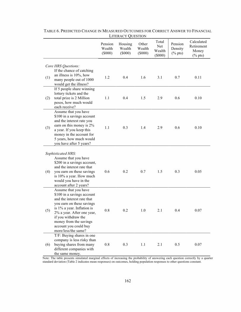
162

TABLE 6. PREDICTED CHANGE IN MEASURED OUTCOMES FOR CORRECT ANSWER TO FINANCIAL LITERACY QUESTION

Pension Wealth ($000)

Housing Wealth ($000)

Other Wealth ($000)

Total Net

Wealth ($000)

Pension Density (% pts)


Money (% pts)

Core HRS Questions:

(1)

If the chance of catching an illness is 10%, how many people out of 1000 would get the illness?

1.2 0.4 1.6 3.1 0.7 0.11

(2)

If 5 people share winning lottery tickets and the total prize is 2 Million pesos, how much would each receive?

1.1 0.4 1.5 2.9 0.6 0.10

(3)

Assume that you have $100 in a savings account and the interest rate you earn on this money is 2% a year. If you keep this money in the account for 5 years, how much would you have after 5 years?

1.1 0.3 1.4 2.9 0.6 0.10

Sophisticated HRS:

(4)

Assume that you have $200 in a savings account, and the interest rate that you earn on these savings is 10% a year. How much would you have in the account after 2 years?

0.6 0.2 0.7 1.5 0.3 0.05

(5)

Assume that you have $100 in a savings account and the interest rate that you earn on these savings is 1% a year. Inflation is 2% a year. After one year, if you withdraw the money from the savings account you could buy more/less/the same?

0.8 0.2 1.0 2.1 0.4 0.07

(6)

T/F: Buying shares in one company is less risky than buying shares from many different companies with the same money.

0.8 0.3 1.1 2.1 0.5 0.07

Note: The table presents simulated marginal effects of increasing the probability of answering each question correctly by a quarter standard deviation (Table 2 indicates mean responses) on outcomes, holding population responses to other questions constant.

163

APPENDIX A: COMPLETE SET OF OLS COEFFICIENT ESTIMATES FOR TABLE 4*


Pension Wealth

Housing Wealth

Other Wealth

Total Net

Wealth

Pension Density


Money I. PRIDIT Index Alone

PRIDIT 1.46 0.49 0.62 2.57 0.91 0.51

Male 15.74 -3.18 0.18 12.95 19.22 2.27

Age 4.63 -0.09 1.38 5.52 2.36 0.65

Age-squared -0.04 0.01 -0.01 -0.04 -0.02 0.00

Risk averse -3.99 -1.17 -3.43 -8.18 0.90 -0.14

Voucher exposure primary ages 0.55 0.27 0.38 1.15 0.98 0.02

Number of agents 0.00 0.00 0.00 0.00 0.00 0.00

No AFP activities 5.13 1.10 5.09 10.84 4.05 0.13

Mother schooling attainment 0.52 0.87 0.69 2.05 0.00 -0.03

Father schooling attainment 0.48 0.79 1.31 2.58 -0.15 0.03

Poor economic background -21.54 -1.14 0.76 -22.18 -36.35 -2.17

Worked when <15 years of age -4.84 -4.62 -7.20 -16.90 -5.33 0.08

Constant -90.09 3.46 -47.90 -127.14 -22.22 -11.80

II. Schooling Alone

Schooling 3.89 1.70 2.01 7.59 1.76 0.80

Male 19.70 -1.81 1.86 19.75 21.34 3.40

Age 4.02 -0.21 1.25 5.05 2.30 0.64

Age-squared -0.03 0.01 -0.01 -0.03 -0.02 0.00

Risk averse -2.29 -0.62 -2.79 -5.71 1.47 0.15


Number of agents 0.00 0.00 0.00 0.00 0.00 0.00


Mother schooling attainment -0.04 0.61 0.39 0.97 -0.18 -0.08


Poor economic background -19.68 0.30 2.31 -17.07 -36.27 -2.50

Worked when <15 years of age 0.62 -1.88 -4.04 -5.30 -3.22 0.87

Constant -121.33 -12.29 -66.67 -200.30 -41.48 -21.24 III. Both PRIDIT and Schooling

PRIDIT 0.81 0.17 0.25 1.23 0.69 0.44

Schooling 3.07 1.53 1.75 6.35 1.06 0.36

Male 18.02 -2.16 1.35 17.21 19.93 2.51

Age 3.97 -0.22 1.23 4.98 2.26 0.62

Age-squared -0.03 0.01 -0.01 -0.03 -0.02 0.00

Risk averse -2.62 -0.69 -2.89 -6.21 1.19 -0.03


Number of agents 0.00 0.00 0.00 0.00 0.00 0.00



Father schooling attainment 0.09 0.60 1.08 1.77 -0.28 -0.01


Worked when <15 years of age 0.39 -1.93 -4.11 -5.65 -3.42 0.73

Constant -109.59 -9.81 -63.05 -182.45 -31.53 -14.97 IV. Linear and Interaction Effects

PRIDIT -0.32 -0.87 -1.17 -2.36 1.50 0.29

!Schooling 3.14 1.59 1.84 6.56 1.01 0.37

!PRIDIT*Schooling 0.10 0.10 0.13 0.33 -0.07 0.01

!Male 17.98 -2.21 1.29 17.05 19.96 2.50

164

!Age 3.94 -0.25 1.19 4.88 2.28 0.62

!Age-squared -0.03 0.01 -0.01 -0.03 -0.02 0.00

!Risk averse -2.25 -0.35 -2.42 -5.02 0.92 0.02

!Voucher exposure primary ages 0.35 0.18 0.27 0.79 0.99 0.00

!Number of agents 0.00 0.00 0.00 0.00 0.00 0.00

!No AFP activities 4.13 0.92 4.93 9.97 3.68 0.07

!Mother schooling attainment -0.10 0.56 0.33 0.79 -0.16 -0.10

!Father schooling attainment 0.05 0.56 1.03 1.63 -0.24 -0.02

!Poor economic background -19.51 -0.54 1.16 -18.89 -34.18 -1.91

!Worked when <15 years of age 0.42 -1.90 -4.07 -5.54 -3.44 0.73

!Constant -109.92 -10.12 -63.48 -183.52 -31.28 -15.02

V. Interaction Effect Alone PRIDIT*Schooling 0.13 0.05 0.07 0.25 0.06 0.04 Male 15.97 -3.33 -0.04 12.60 19.59 2.32 Age 4.22 -0.11 1.35 5.45 2.38 0.65 Age-squared -0.04 0.01 -0.01 -0.04 -0.02 0.00 Risk averse -3.13 -1.00 -3.22 -7.35 1.10 0.01 Voucher exposure primary ages 0.47 0.25 0.35 1.06 1.00 0.01 Number of agents 0.00 0.00 0.00 0.00 0.00 0.00 No AFP activities 4.95 1.18 5.18 11.31 4.30 0.24 Mother schooling attainment 0.46 0.84 0.64 1.94 0.03 -0.03 Father schooling attainment 0.46 0.76 1.26 2.47 -0.10 0.03 Poor economic background -23.71 -1.58 0.26 -25.02 -37.96 -2.90 Worked when <15 years of age -5.33 -4.55 -7.07 -16.95 -5.81 -0.05 Constant -82.94 3.99 -47.08 -126.02 -23.91 -12.08

Note: *italics indicate significance at 5% level or better. See also Table 4.

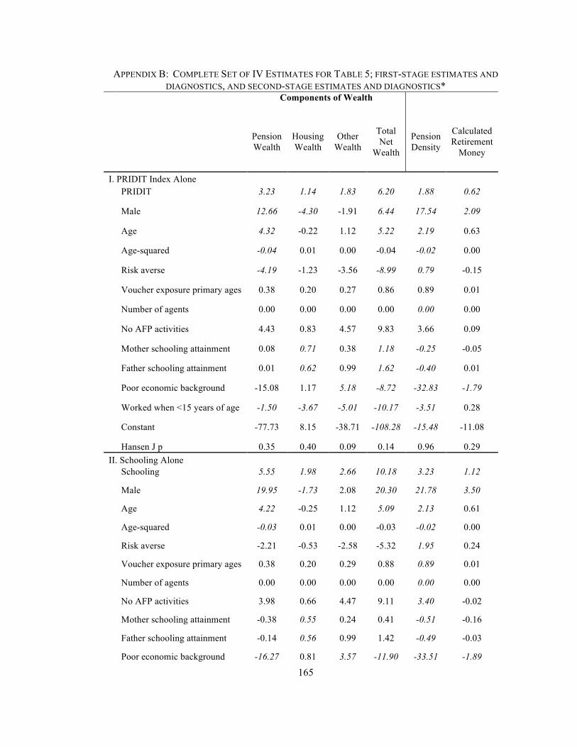
165

APPENDIX B: COMPLETE SET OF IV ESTIMATES FOR TABLE 5; FIRST-STAGE ESTIMATES AND DIAGNOSTICS, AND SECOND-STAGE ESTIMATES AND DIAGNOSTICS*


Pension Wealth

Housing Wealth

Other Wealth

Total Net

Wealth

Pension Density


Money


PRIDIT 3.23 1.14 1.83 6.20 1.88 0.62

Male 12.66 -4.30 -1.91 6.44 17.54 2.09

Age 4.32 -0.22 1.12 5.22 2.19 0.63

Age-squared -0.04 0.01 0.00 -0.04 -0.02 0.00

Risk averse -4.19 -1.23 -3.56 -8.99 0.79 -0.15


Number of agents 0.00 0.00 0.00 0.00 0.00 0.00


Mother schooling attainment 0.08 0.71 0.38 1.18 -0.25 -0.05




Constant -77.73 8.15 -38.71 -108.28 -15.48 -11.08

Hansen J p 0.35 0.40 0.09 0.14 0.96 0.29

II. Schooling Alone

Schooling 5.55 1.98 2.66 10.18 3.23 1.12

Male 19.95 -1.73 2.08 20.30 21.78 3.50

Age 4.22 -0.25 1.12 5.09 2.13 0.61

Age-squared -0.03 0.01 0.00 -0.03 -0.02 0.00

Risk averse -2.21 -0.53 -2.58 -5.32 1.95 0.24


Number of agents 0.00 0.00 0.00 0.00 0.00 0.00

No AFP activities 3.98 0.66 4.47 9.11 3.40 -0.02


Father schooling attainment -0.14 0.56 0.99 1.42 -0.49 -0.03


166

Worked when <15 years of age 4.51 -1.50 -2.67 0.34 0.00 1.57

Constant -140.83 -14.26 -70.93 -226.01 -52.21 -23.58

Hansen J p 0.01 0.17 0.01 0.00 0.00 0.29 III. Both PRIDIT and Schooling

PRIDIT 3.40 1.06 4.46 8.93 1.94 0.31

Schooling -0.34 0.14 -5.05 -5.25 -0.12 0.58

Male 12.25 -4.13 -8.01 0.11 17.39 2.79

Age 4.33 -0.22 1.26 5.36 2.19 0.62

Age-squared -0.04 0.01 -0.01 -0.04 -0.02 0.00

Risk averse -4.31 -1.18 -5.33 -10.83 0.75 0.05


Number of agents 0.00 0.00 0.00 0.00 0.00 0.00


Mother schooling attainment 0.11 0.70 0.88 1.69 -0.23 -0.11

Father schooling attainment 0.03 0.61 1.21 1.85 -0.40 -0.02



Constant -74.03 6.58 16.60 -50.84 -14.12 -17.47

Hansen J p 0.26 0.30 0.82 0.34 0.92 0.26

IV. Linear and Interaction Effects

PRIDIT -2.28 -1.51 0.28 -3.51 2.15 2.19

!Schooling 2.44 1.40 -3.01 0.82 -0.23 -0.34

!PRIDIT*Schooling 0.44 0.20 0.33 0.97 -0.02 -0.15

!Male 14.32 -3.19 -6.48 4.65 17.31 2.11

!Age 4.06 -0.34 1.06 4.79 2.20 0.70

!Age-squared -0.04 0.01 -0.01 -0.03 -0.02 -0.01

!Risk averse -1.91 -0.09 -3.57 -5.57 0.66 -0.75

!Voucher exposure primary ages 0.17 0.11 0.14 0.42 0.90 0.08

!Number of agents 0.00 0.00 0.00 0.00 0.00 0.00

!No AFP activities 4.88 1.01 5.42 11.30 3.66 -0.12

!Mother schooling attainment -0.44 0.45 0.47 0.48 -0.21 0.07

167

!Father schooling attainment -0.38 0.43 0.91 0.96 -0.38 0.12

!Poor economic background -18.83 -0.52 2.36 -17.00 -32.70 -0.54

!Worked when <15 years of age 2.09 -1.69 -8.14 -7.74 -3.80 -0.34

!Constant -99.93 -5.14 -2.47 -107.54 -13.18 -8.88

!Hansen J p 0.41 0.39 0.86 0.92 0.85 0.50

V. Interaction Effect Alone PRIDIT*Schooling 0.34 0.12 0.20 0.66 0.19 0.06

Male 11.71 -4.64 -2.67 4.40 17.11 2.03

Age 4.18 -0.26 1.01 4.93 2.12 0.62

Age-squared -0.04 0.01 0.00 -0.04 -0.02 0.00

Risk averse -3.11 -0.85 -2.92 -6.88 1.41 0.04

Voucher exposure primary ages 0.23 0.15 0.17 0.55 0.81 -0.01

Number of agents 0.00 0.00 0.00 0.00 0.00 0.00



Father schooling attainment -0.20 0.54 0.83 1.17 -0.51 -0.01



Constant -74.43 9.35 -35.96 -101.04 -14.03 -10.94

Hansen J p 0.53 0.52 0.39 0.95 0.21 0.06 Notes: also Table 4. Source: Authors’ computations.

168

APPENDIX B. FIRST STAGE ESTIMATES PRIDIT Index Schooling PRIDIT*Schooling

Male 1.77 -0.25 19.87 Age 0.07 0.09 1.22 Age-squared 0.00 0.00 -0.01 Risk averse 0.17 -0.25 -1.65 Voucher exposure primary ages -0.04 0.03 0.13 Number of agents 0.00 0.00 0.00 No AFP activities 0.04 0.18 -1.28 Mother schooling attainment 0.17 0.18 2.31 Father schooling attainment 0.19 0.13 2.50 Poor economic background -2.96 -1.51 -20.16 Worked when <15 years of age -1.41 -1.90 -15.13 Primary school urban 2.92 2.32 20.18 Unemployment rate at age 16 -6.21 -1.32 -58.02 Think I am a Failure 0.08 0.12 1.87 Can Do Well As Others 0.46 0.19 4.05 Positive Attitude about Self 0.28 0.16 1.91 Like More Self Respect 0.04 -0.14 -2.06 Postive Self Esteem (Sum) 0.10 0.01 1.36 Negative Self Esteem (Sum) -0.58 -0.24 -6.04 Constant -3.25 8.11 -31.71

F test stat: 156.56 215.57 109.72 Angrist-Pischke multivariate F stat:

III. Both PRIDIT and Schooling 17.19 24.58

IV. Linear and Interaction Effects 2.32 19.05 3.16 Kleibergen-Paap Wald F stat:

III. Both PRIDIT and Schooling 15.77

IV. Linear and Interaction Effects 9.43 Note: *italics indicate significance at 5% level or better Source: Authors’ computations.

Essays in Household Finance and Housing Economics

Documents

Transcript of Essays in Household Finance and Housing Economics