Essays on Personnel and Health Economics

by

Pieter De Vlieger

A dissertation submitted in partial fulfillmentof the requirements for the degree of

Doctor of Philosophy(Economics)

in The University of Michigan2020

Doctoral Committee:

Professor John Bound, Co-ChairAssistant Professor Sarah Miller, Co-ChairProfessor Ying FanProfessor Kevin Stange

Pieter De Vlieger

pdvl@umich.edu

ORCID ID 0000-0002-3149-5849

c© Pieter De Vlieger 2020

All Rights Reserved

For Tadeja

ii

ACKNOWLEDGEMENTS

While this dissertation carries my name, it is the product of several people and institutions

who provided support and guidance along the way.

I would like to thank my committee members John Bound, Sarah Miller, Ying Fan, and

Kevin Stange for their patience and commitment, and knowing when a push or support was

warranted. Their thoughtful comments and feedback have been instrumental in shaping this

dissertation.

Additionally, this dissertation in its current form would not have existed without the

support and data access provided by the Inter-Mutual Agency (IMA) and the National

Institute for Health and Disability Insurance (NIHDI/RIZIV) in Belgium. Koen Cornelis,

Birgit Gielen, and Johan Vanoverloop at IMA and Marc De Falleur and Joos Tielemans at

RIZIV in particular were instrumental in setting up this collaboration. Financial support

of The Ryoichi Sasakawa Young Leaders Fellowship Fund (SYLFF), the Rackham graduate

school at the University of Michigan, and the MITRE center at the Department of Economics

at the University of Michigan is greatly appreciated. Andras Avonts, Andre Decoster, Erik

Schokkaert, and Karla Vander Weyden provided crucial input in ensuring the administrative

details were processed in a timely fashion. Erik Schokkaert and Johan Vanoverloop provided

important institutional support and insights.

Similarly, I am grateful to the IAB in Germany for making available the Cross-Sectional

model of the Linked Employer-Employee Data (LIAB) (Version 3, Years 1993-2010) for the

research presented in the second chapter of this dissertation. Data access was provided via

on-site use at the Research Data Centre (FDZ) of the German Federal Employment Agency

iii

(BA) at the Institute for Employment Research (IAB) and subsequently remote data access.

Finally, I am grateful to Hinrich Eylers and Ashok Yadav at the University of Phoenix for

many discussions and for providing access to the data used for the analyses and research in

the third chapter of this dissertation.

I would also like to thank the many people at the University of Michigan and beyond

who provided thoughtful insights and comments. Especially Charlie Brown and Zach Brown

have played an important role in the final form of this dissertation. Thomas Buchmueller,

Kimberly Conlon, James Cooke, Sebastian Fleitas, Jeremy Fox, Tadeja Gracner, Andreas

Hagemann, Kyle Handley, Sara Heller, Daniela Hochfellner, Iris Kesternich, Gaurav Khanna,

Meera Mahadevan, Edward Norton, Erwin Ooghe, Aniko Ory, Yesim Orhun, Stephanie

Owen, Dhiren Patki, Johannes Schmieder, Erik Schokkaert, Andrew Simon, Jeff Smith, Jo-

hannes Spinnewijn, Mel Stephens, Katalin Springel, Brenden Timpe, Matthias Umkehrer,

and Frank Verboven provided insightful comments and suggestions. Finally, useful com-

ments by seminar participants at several seminars at the University of Michigan, Katholieke

Universiteit Leuven, IZA, the GSOEP User Workshop, and the IHEA conference have im-

proved the different chapters in this dissertation. Brian Jacob and Kevin Stange, who were

co-authors on one of the chapters in this dissertation, were great collaborators.

I also want to thank family members and friends for their support. My parents have

always been supportive of my various pursuits, and their curiosity and healthy skepticism

have transpired into this dissertation. The support of Dries, Veerle, Jan, Jonas, Pieter,

Greet, Bart, Victor, Celine, Ellis, Amber, and Lucas also needs acknowledging. The wise

words of Does and Joos deserve special mention.

Finally, I would like to especially thank Tadeja Gracner for her support and being there

every single step of the way z Gorickega v pir dvainstirideset.

iv

TABLE OF CONTENTS

DEDICATION . . . . . . . . . . . . . . . . . . . . . . . . . . . . . . . . . . . . . . ii

ACKNOWLEDGEMENTS . . . . . . . . . . . . . . . . . . . . . . . . . . . . . . iii

LIST OF FIGURES . . . . . . . . . . . . . . . . . . . . . . . . . . . . . . . . . . . viii

LIST OF TABLES . . . . . . . . . . . . . . . . . . . . . . . . . . . . . . . . . . . . x

LIST OF APPENDICES . . . . . . . . . . . . . . . . . . . . . . . . . . . . . . . . xii

ABSTRACT . . . . . . . . . . . . . . . . . . . . . . . . . . . . . . . . . . . . . . . xiii

CHAPTER

I. Quantifying Sources of Persistent Prescription Behavior: Evidencefrom Belgium . . . . . . . . . . . . . . . . . . . . . . . . . . . . . . . . . . 1

1.1 Introduction . . . . . . . . . . . . . . . . . . . . . . . . . . . . . . . 11.2 The Minimum Prescription Rate (MPR) . . . . . . . . . . . . . . . 10

1.2.1 Setting . . . . . . . . . . . . . . . . . . . . . . . . . . . . . 101.2.2 The Market for Physicians and Prescription Drugs . . . . 111.2.3 The Minimum Prescription Rate (MPR) . . . . . . . . . . 14

1.3 IMA Farmanet: Transaction-Level Prescription Data . . . . . . . . 151.3.1 Defining Starters and Patient Profiles . . . . . . . . . . . . 181.3.2 Sample Selection and Descriptive Statistics . . . . . . . . . 191.3.3 Descriptive Evidence on the MPR . . . . . . . . . . . . . . 20

1.4 Reduced Form Evidence on the introduction of MPR . . . . . . . . 211.4.1 Do Physicians Switch to Generics? . . . . . . . . . . . . . 221.4.2 Do Physicians Move Away from On-Patent Drugs? . . . . 251.4.3 Is Switching Longstanding Patients Costly for Health Out-

comes? . . . . . . . . . . . . . . . . . . . . . . . . . . . . 271.4.4 2SLS Results . . . . . . . . . . . . . . . . . . . . . . . . . . 281.4.5 Which Longstanding Patients are Costly to Switch? . . . . 311.4.6 Discussion of Reduced Form Results . . . . . . . . . . . . 33

1.5 A Structural Model of Prescription Behavior under the MPR Mandate 34

v

1.5.1 Set-up . . . . . . . . . . . . . . . . . . . . . . . . . . . . . 351.5.2 The physician’s prescription decision . . . . . . . . . . . . 351.5.3 The MPR Mandate . . . . . . . . . . . . . . . . . . . . . . 411.5.4 Identification and Estimation . . . . . . . . . . . . . . . . 44

1.6 Decomposition and Policy Counterfactuals . . . . . . . . . . . . . . 491.6.1 Decomposition . . . . . . . . . . . . . . . . . . . . . . . . . 491.6.2 Counterfactuals . . . . . . . . . . . . . . . . . . . . . . . . 50

1.7 Conclusion . . . . . . . . . . . . . . . . . . . . . . . . . . . . . . . . 53

II. Fairness Considerations in Wage Setting: Evidence from DomesticOutsourcing Events in Germany . . . . . . . . . . . . . . . . . . . . . . 75

2.1 Introduction . . . . . . . . . . . . . . . . . . . . . . . . . . . . . . . 752.2 Background . . . . . . . . . . . . . . . . . . . . . . . . . . . . . . . 782.3 Theoretical Framework . . . . . . . . . . . . . . . . . . . . . . . . . 79

2.3.1 Labor Supply . . . . . . . . . . . . . . . . . . . . . . . . . 802.3.2 Firm Problem . . . . . . . . . . . . . . . . . . . . . . . . . 812.3.3 Wage Setting . . . . . . . . . . . . . . . . . . . . . . . . . . 832.3.4 Assumptions on Fairness and Demand. . . . . . . . . . . . 842.3.5 Comparative Statics. . . . . . . . . . . . . . . . . . . . . . 84

2.4 Data and Institutional Setting . . . . . . . . . . . . . . . . . . . . . 862.4.1 Data . . . . . . . . . . . . . . . . . . . . . . . . . . . . . . 862.4.2 Institutional Setting . . . . . . . . . . . . . . . . . . . . . . 88

2.5 Domestic Outsourcing . . . . . . . . . . . . . . . . . . . . . . . . . 892.5.1 Measuring Domestic Outsourcing . . . . . . . . . . . . . . 892.5.2 Summary Statistics . . . . . . . . . . . . . . . . . . . . . . 91

2.6 Empirical Strategy and Results . . . . . . . . . . . . . . . . . . . . 922.6.1 Establishment-Level Outcomes and Structure . . . . . . . . 922.6.2 Worker-Level Results . . . . . . . . . . . . . . . . . . . . . 932.6.3 Importance of Change in Structure . . . . . . . . . . . . . 96

2.7 Robustness Checks . . . . . . . . . . . . . . . . . . . . . . . . . . . 972.8 Conclusion . . . . . . . . . . . . . . . . . . . . . . . . . . . . . . . . 98

III. Measuring Instructor Effectiveness in Higher Education . . . . . . . 109

3.1 Introduction . . . . . . . . . . . . . . . . . . . . . . . . . . . . . . . 1093.2 Prior Evidence and Institutional Context . . . . . . . . . . . . . . . 112

3.2.1 Prior Evidence . . . . . . . . . . . . . . . . . . . . . . . . . 1123.2.2 Context: College Algebra at The University of Phoenix . . 115

3.3 Data . . . . . . . . . . . . . . . . . . . . . . . . . . . . . . . . . . . 1193.3.1 Data Sources . . . . . . . . . . . . . . . . . . . . . . . . . . 1193.3.2 Sample Selection . . . . . . . . . . . . . . . . . . . . . . . . 1223.3.3 Descriptive Statistics . . . . . . . . . . . . . . . . . . . . . 124

3.4 Empirical Approach . . . . . . . . . . . . . . . . . . . . . . . . . . . 1253.4.1 Course and Instructor Assignment . . . . . . . . . . . . . . 126

vi

3.4.2 Outcomes . . . . . . . . . . . . . . . . . . . . . . . . . . . 1283.4.3 Cross-Campus Comparisons . . . . . . . . . . . . . . . . . 1303.4.4 Implementation . . . . . . . . . . . . . . . . . . . . . . . . 130

3.5 Results on Instructor Effectiveness . . . . . . . . . . . . . . . . . . . 1333.5.1 Main Results for Course Grades and Final Exam Scores . . 1333.5.2 Robustness of Grade and Test Score Outcomes . . . . . . . 1373.5.3 Student Evaluations and Other Outcomes . . . . . . . . . . 138

3.6 Does Effectiveness Correlate with Experience and Pay? . . . . . . . 1403.7 Conclusion and Discussion . . . . . . . . . . . . . . . . . . . . . . . 142

APPENDICES . . . . . . . . . . . . . . . . . . . . . . . . . . . . . . . . . . . . . . 158

BIBLIOGRAPHY . . . . . . . . . . . . . . . . . . . . . . . . . . . . . . . . . . . . 215

vii

LIST OF FIGURES

Figure

1.1 Example of Prescription Note in Belgium . . . . . . . . . . . . . . . . . . . 631.2 Differences between Brand Name and Generic Drugs . . . . . . . . . . . . . 641.3 Distribution of Physician Generic Prescription Rates in 2004 and 2006 . . . 651.4 Descriptive Graphs: Prescription and Switching Rate of Generics . . . . . . 661.5 Impact of the mandate on Starters and Longstanding Patients . . . . . . . 671.6 Prescription rate of On-Patent Drugs . . . . . . . . . . . . . . . . . . . . . 681.7 Estimated Physician Inertia Before and After Mandate . . . . . . . . . . . 691.8 Heterogeneous Effects in Switching of Longstanding Patients . . . . . . . . 701.9 Structurally Estimated Physician Bias Before and After Mandate . . . . . 711.10 Adoption Rate of Generics (over 5 years) . . . . . . . . . . . . . . . . . . . 721.11 Framework for Policy Simulations . . . . . . . . . . . . . . . . . . . . . . . 731.12 Policy Simulations . . . . . . . . . . . . . . . . . . . . . . . . . . . . . . . . 742.1 Incidence of Outsourcing . . . . . . . . . . . . . . . . . . . . . . . . . . . . 1032.2 Effect of outsourcing on establishment employment. . . . . . . . . . . . . . 1042.3 Effect of outsourcing on establishment Skill Ratio. . . . . . . . . . . . . . . 1052.4 Effect of outsourcing on wages of workers that stay. . . . . . . . . . . . . . 1062.5 Nonparametric specification . . . . . . . . . . . . . . . . . . . . . . . . . . 1072.6 Effect of outsourcing on establishment investments. . . . . . . . . . . . . . 1083.1 Relationship between Instructor Effectiveness (Grades) and Teaching Expe-

rience . . . . . . . . . . . . . . . . . . . . . . . . . . . . . . . . . . . . . . . 1563.2 Relationship between Instructor Effectiveness (Test Scores) and Teaching

Experience . . . . . . . . . . . . . . . . . . . . . . . . . . . . . . . . . . . . 157A.1 Stylized Facts: Overall Prescription Rate 2000-2010 . . . . . . . . . . . . . 160A.2 Descriptive Graphs: Prescription and Switching Rate of Generics . . . . . . 161A.3 Stylized Facts: Changes in Prices . . . . . . . . . . . . . . . . . . . . . . . 165A.4 Determination of Status Prescription Drug. . . . . . . . . . . . . . . . . . . 167A.5 Processing and collection flow of the data . . . . . . . . . . . . . . . . . . . 169A.6 Market for Product Groups in Belgium . . . . . . . . . . . . . . . . . . . . 174A.7 Dominance of Administration Method at Active Ingredient Level . . . . . . 175A.8 Dominance of Administration Method at Active Ingredient Level . . . . . . 175A.9 Definition of Starters and Longstanding Patients . . . . . . . . . . . . . . . 176

viii

A.10 Fraction of Product Group Prescription as a function of Baseline Prescrip-tion (in deciles) . . . . . . . . . . . . . . . . . . . . . . . . . . . . . . . . . 180

A.11 Within-Physician Correlations of Generic Prescription Rates across ProductGroups . . . . . . . . . . . . . . . . . . . . . . . . . . . . . . . . . . . . . . 181

A.12 Kernel Density of Generic Prescription Rate (Physician by Product GroupLevel) . . . . . . . . . . . . . . . . . . . . . . . . . . . . . . . . . . . . . . 183

A.13 Descriptive Graphs: Prescription and Switching Rate of Generics . . . . . . 185A.14 Physician Switching . . . . . . . . . . . . . . . . . . . . . . . . . . . . . . . 187A.15 Robustness Checks for Quality of Drugs Dispensed . . . . . . . . . . . . . . 190B.1 Firing Rate by Occupation . . . . . . . . . . . . . . . . . . . . . . . . . . . 206

ix

LIST OF TABLES

Table

1.1 Classification of ATCs into Product Groups . . . . . . . . . . . . . . . . . 551.2 Physician Descriptives. . . . . . . . . . . . . . . . . . . . . . . . . . . . . . 561.3 Summary Statistics for Patients and Precriptions . . . . . . . . . . . . . . 571.4 Split Sample Reduced Form Coefficients . . . . . . . . . . . . . . . . . . . 581.5 Dose-Response Models . . . . . . . . . . . . . . . . . . . . . . . . . . . . . 591.6 The effect of switching a patient on medication adherence . . . . . . . . . . 601.7 Pooled Chronic Drugs Reduced Form Results . . . . . . . . . . . . . . . . . 611.8 Structural Parameter Estimates . . . . . . . . . . . . . . . . . . . . . . . . 622.1 Summary Statistics for Establishments . . . . . . . . . . . . . . . . . . . . 1002.2 Summary Statistics for Workers Remaining in the Establishment . . . . . . 1012.3 Event Study coefficients Interacted with Change in Share Low over High Skill1023.1 Descriptive Statistics for Sections and Instructors (Full Sample) . . . . . . 1453.2 Descriptive Statistics for Students (Full Sample) . . . . . . . . . . . . . . . 1463.3 Randomization Check . . . . . . . . . . . . . . . . . . . . . . . . . . . . . . 1473.4 Main Course Grade and Test Score Outcomes . . . . . . . . . . . . . . . . 1483.5 Robustness to Having Same Instructor for MTH208 and MTH209, FTF

Sections . . . . . . . . . . . . . . . . . . . . . . . . . . . . . . . . . . . . . 1493.6 Robustness of Test Score Results to First-Stage Model (with Selection Shocks)1503.7 Robustness to Imputation Method . . . . . . . . . . . . . . . . . . . . . . . 1513.8 Relationship between Course Grade or Test Effect and Teaching Evaluation 1523.9 Instructor Effects for Alternative Outcomes . . . . . . . . . . . . . . . . . . 1533.10 Correlates of Instructor Effectiveness . . . . . . . . . . . . . . . . . . . . . 1543.11 Correlates of Instructor Salary . . . . . . . . . . . . . . . . . . . . . . . . . 155A.1 Balance of Patients . . . . . . . . . . . . . . . . . . . . . . . . . . . . . . . 179A.2 Robustness Checks Level of Fixed Effects . . . . . . . . . . . . . . . . . . . 184A.3 Robustness Checks Level of Fixed Effects . . . . . . . . . . . . . . . . . . . 187A.4 Robustness Checks Quality Dispensed Drugs . . . . . . . . . . . . . . . . . 189A.5 The effect of switching a patient on medication adherence . . . . . . . . . . 191A.6 Predicting Generic Switching Using Feature Selection Methods . . . . . . . 197B.1 Occupation Codes for different Business Service Occupations . . . . . . . . 203B.2 Industry Codes for different Business Service Industries . . . . . . . . . . . 204B.3 Descriptives of Employment . . . . . . . . . . . . . . . . . . . . . . . . . . 205

x

C.1 Descriptive Statistics for Sections and Instructors (Test Sample) . . . . . . 209C.2 Descriptive Statistics for Students (Test Score Sample) . . . . . . . . . . . 210C.3 How much switching is there between online and FTF campuses? . . . . . 211C.4 Correlation across Outcomes (Restricted to Test Sample) . . . . . . . . . . 212

xi

LIST OF APPENDICES

Appendix

A. Appendix to Quantifying Sources of Persistent Prescription Behavior: Evi-dence from Belgium . . . . . . . . . . . . . . . . . . . . . . . . . . . . . . . . 159

B. Appendix to Fairness Considerations in Wage Setting: Evidence from DomesticOutsourcing Events in Germany . . . . . . . . . . . . . . . . . . . . . . . . . 198

C. Appendix to Measuring Instructor Effectiveness in Higher Education . . . . . 208

xii

ABSTRACT

This dissertation examines the importance of incentive schemes or personnel policies in

three distinct labor markets.

The first essay answers the following question: How important are patient and physician-

specific factors in explaining persistent prescription behavior? A wide range of research has

suggested that prescription behavior is highly persistent and an important barrier to realizing

cost savings, but the sources of this persistence are not well understood. I quantify the

importance of physician and patient factors in physician prescription behavior by exploiting

a policy mandate in Belgium requiring physicians to prescribe a minimum percentage of

cheap drugs, using detailed administrative data on 24 million prescription drugs dispensed

to 152,000 patients. First, I show that physicians increase the prescription rate of generics

for first-time users of an active ingredient by 10 percentage points. They do so without

compromising on quality of dispensed drugs. Second, I find that first-time patients are more

likely to receive a generic than long-time patient are likely to be switched from a branded

to a generic drug, suggesting physicians consider the latter costly to switch. I find that

switching a patient indeed comes at a cost, measured in decreased medication adherence.

Building on this reduced form evidence, I develop and estimate a structural model. I use the

model estimates to simulate the entry of generics and find physician and patient factors are

about equally important in explaining the slow adoption of generics. Requiring pharmacists

to only dispense generics decreases welfare, unless patient considerations are decreased by

at least 60%.

In a second essay, I estimate the effect of domestic outsourcing events on wages of work-

ers remaining in outsourcing establishments. I use employer-employee linked data from

xiii

Germany that includes detailed administrative information on earnings, industry and oc-

cupation of employment. I exploit outsourcing event as my main source of identification

and find substantial effects on the wages of workers that stay: holding worker ability con-

stant, high skilled workers receive, on average, an immediate wage increase of about five log

points, while low skilled worker face a wage cut of about one log points. On average, wage

increases enjoyed by high skilled workers are positively correlated with changes in the skill

ratio within the establishment. I propose a new theoretical model of wage setting in which

fairness considerations generate spillover effects that are consistent with these two empirical

findings. Taken together, these results indicate fairness considerations may play a role in

wage setting.

In a third essay, co-authored with Kevin Stange and Brian Jacob, we investigate the

role of instructors in promoting student success. We explore this issue in the context of

the University of Phoenix, a large for-profit university that offers both online and in-person

courses in a wide array of fields and degree programs. We focus on instructors in the college

algebra course that is required for all BA degree program students. We find substantial

variation in student performance across instructors both in the current class and subsequent

classes. Variation is larger for in-person classes, but is still substantial for online courses.

Effectiveness grows modestly with course-specific teaching experience, but is unrelated to

pay. Our results suggest that personnel policies for recruiting, developing, motivating, and

retaining effective postsecondary instructors may be a key, yet underdeveloped, tool for

improving institutional productivity.

xiv

CHAPTER I

Quantifying Sources of Persistent Prescription

Behavior: Evidence from Belgium

1.1 Introduction

Physicians frequently prescribe costly treatments even when cheaper alternatives become

available or are recommended by clinical practice guidelines (Chandra, Cutler and Song,

2011). Policymakers who have tried to address this behavior to reduce health care costs

have achieved limited success: studies consistently show that physician behavior is highly

persistent and difficult to change.1 One example is the use of generic prescription drugs that

offer the same therapeutic value as their branded equivalents, but at a lower cost.2 “Generic

substitution,” moving patients from branded to equally effective generic prescription drugs,

could substantially reduce prescription drug costs – the fastest-growing segment of health

care spending worth $325 billion annually in the US and $1.2 trillion worldwide (CMS,

2015; IQVIA, 2019). Specifically, estimates suggest that generic substitution could save the

US 11% and EU more than 20% on overall prescription drug spending (Haas et al., 2005;

Carone, Schwierz and Xavier, 2012; Choudhry, Denberg and Qaseem, 2016). A large body

1Persistence refers to a tendency in prescribing behavior not explained by patient illness characteristics,demographics, or indicators of preferences (Phelps, 2000). Grimshaw et al. (2012), Ivers et al. (2012) andWilensky (2016) review policies.

2The active ingredient is the chemical in the compound producing the biological or chemical effect. Afterpatent expiration, generic manufacturers can enter the market and manufacture the same (and equallyeffective) active ingredient.

1

of research argues, however, that persistent prescribing behavior is an important barrier to

realizing these cost savings. Yet, the sources of this persistence are not well understood

(Hellerstein, 1998; Kesselheim, Avorn and Sarpatwari, 2016).

In this paper, I study the importance of physician and patient factors in the persistence

of physician prescribing decisions. On the one hand, physicians may prescribe the more

expensive drug because of their habits (Hellerstein, 1998), preferences (Shrank et al., 2011),

or financial incentives from physician dispensing or detailing (Iizuka, 2012; Grennan et al.,

2018). This is often referred to as partial altruism, as physicians only partially act in the

patient’s best interest (Ellis and McGuire, 1986). On the other hand, physicians may take

patients’ needs or preferences into account, and as such, resist switching between equally

effective drugs for patient-specific reasons. Patients exhibit brand loyalty (Sinkinson and

Starc, 2018) or rely on pill appearance in their medication regimen (Sarpatwari et al., 2019).

Changing a patient’s prescription may lead to confusion and worse medication adherence

(Kesselheim et al., 2014), possibly resulting in higher hospitalization rates and healthcare

costs (Sokol et al., 2005; Bosworth et al., 2011). In such cases, persistence in prescription

behavior may not be wasteful. Quantifying the relative importance of both provider and

patient factors in physician treatment decisions, along with understanding their welfare

effects, is critical for designing policy efforts aimed at containing healthcare costs while

maintaining the quality of care. Nevertheless, empirical evidence on this question is limited.

I quantify the relative importance of physician and patient factors in prescribing decisions

of primary care physicians (PCPs) in Belgium by exploiting a national policy mandating a

change in prescribing habits. The mandate required PCPs to prescribe a minimum percent-

age of cheap or generic drugs. It was announced in June 2005 and went into effect starting

2006. The minimum prescription rate was set to 27% for PCPs, up from an average pre-

scription rate of 18% in 2004. Physicians had to meet this quote over the course of a full

year, and the mandate was binding for almost all PCPs.3

3Non-compliance resulted in physicians having to justify their decisions before the Order of Physicians.See section 1.2.3.

2

The analysis in this paper is organized in two parts. As a first step, I present reduced

form evidence of physician and patient factors in PCPs’ prescribing decisions. I document

physicians’ tendency to prescribe brand name drugs without quality or therapeutic justifica-

tions to do so. I refer to this tendency as physician bias, but do not take a stand on whether

this bias is driven by habits, inattention, preferences or industry interactions. Additionally,

I show that changing a patient’s prescription drug decreases their medication adherence, and

that physicians take this behavior into account. Patients who are prescribed a drug for the

first time (“starters”) are therefore more likely to receive a generic than patients who were

using a brand name before (“longstanding patients”). I refer to this as patient considera-

tions. As a second step, I develop and estimate a structural model to quantify the relative

importance of both factors and to analyze counterfactual policies.

The Belgian healthcare market serves as a useful setting for several reasons. First, uni-

versal insurance alleviates concerns that physicians face uncertainty over differences in for-

mularies or insurance plans, and rules out the possibility that patients might choose different

plans (or none at all) in response to the policy mandate. This also simplifies modeling as-

sumptions. Second, direct-to-consumer-advertising (DTCA) is not allowed. As a result,

patients rarely request generics when they are prescribed a drug for the first time, and few

patients can differentiate between branded and generic versions of the same prescription

drug (Fraeyman et al., 2015).4 Changes in the demand for generics among starters therefore

capture physician bias. Third, physicians prescribe on product name and pharmaceutical

substitution is not allowed (i.e. pharmacists dispense as written).5 Detailed transaction

data from pharmacies, stored in a central database to operationalize reimbursements in the

healthcare system, therefore reflect physician prescribing behavior.

I draw rich and novel administrative data on 26 million dispensed prescription drugs

between 2004 and 2009 for 152,000 randomly selected patients from this central database

4Physicians and healthcare officials confirmed patients rarely request branded drugs during an initialvisit.

5See Section 1.2.2 for details on the absence of pharmaceutical substitution in Belgium at the time of thepolicy mandate.

3

to compute these patients’ prescription profiles. For a random subset of 300 distinct PCPs,

the dataset also records all 6 million prescriptions dispensed to their patients, which I use

to track their average prescription rate of generics over time across different patients and

prescription drugs. I merge this data with detailed drug characteristics, such as daily doses,

potency, and extended release version, based on the product’s unique barcode that is scanned

upon dispensing in the pharmacy. Finally, I link census demographic records using unique

patient and physician identifiers to precisely characterize the demographic profile of patients

and physicians.

Physicians exhibit bias, as they respond to the mandate by increasing the prescription

rate of generics without compromising on the quality of dispensed drugs. To isolate this

bias, I focus solely on prescriptions for starters. Starters are unlikely to request a branded

prescription drug, so limiting the analysis to these patients allows me to address concerns

of unobservable demand factors or costs related to switching between drugs. The mandate

increased the average prescription rate of generics for starters by about 10 percentage points,

up from a pre-mandate average of 35%. PCPs far from the threshold (“low prescribers”)

responded more. PCPs did not decrease the use of (possibly superior) on-patent prescription

drugs to comply with the mandate, with no discernible differences across high and low

prescribers.6 Assuming generic and branded versions of the same active ingredients are

equally effective, this is evidence of physician bias.7 I further strengthen this claim by

showing no changes in other quality characteristics of dispensed drugs, such as administration

method (e.g. pill or injection) or extended release formulation.

I show evidence of patient considerations by contrasting how PCPs respond to the man-

date for starters and longstanding patients. I find that PCPs increase the switching rate

for longstanding patients by about 1 to 2 percentage points, which is substantially lower

than the 10 percentage point increase for starters described above. These differences imply

6On-patent drugs face no generic competition and are typically newer, so may be superior to older drugswith competition.

7See Kesselheim et al. (2008) and (Choudhry, Denberg and Qaseem, 2016) for meta-analyses on the equalclinical effectiveness of generics.

4

that it is less costly for a patient who needs a new prescription to receive a generic than for

a longstanding patient to switch, and that PCPs take these costs into account. This lines

up with previous work that finds physicians differentiate between starters and longstanding

patients (Dickstein, 2011b; Sinkinson and Starc, 2018; Shapiro, 2018a; Feng, 2019).

Leveraging the quasi-experimental design of the mandate, I develop an instrumental

variables framework and show that switching a patient from a brand-name to generic version

of the same prescription drug indeed comes at a cost, measured with decreased medication

adherence. I instrument the endogenous decision to switch a longstanding patient with

exogenous variation in the timing of the mandate and whether the patient visits a low

prescriber. I find that a switch causally reduces medication adherence by about 30%, and

that a naive OLS estimate would understate the effect by a factor of two. A patient in my

sample refills their prescription, on average, every two months, so a change in prescription

drugs increases the time between refills by about three to four weeks. This decrease in

medication adherence is short-lived and does not generate persistent reductions in adherence,

suggesting an initiation cost to switching prescription drugs for longstanding patients. These

costs are likely driven by patient behavior, such as confusion or mistrust, and can therefore

be interpreted as an increase in “behavioral hazard” as defined by Baicker, Mullainathan

and Schwartzstein (2015).

I complement this IV approach with a complier analysis where I investigate which patient

observables predict an increase in switching probability in response to the policy mandate. I

use linear probability models and non-parametric machine learning methods. Patients using

an active ingredient for only 6 months are equally likely to be switched as those using it for

at least 1.5 years, i.e. evidence of lock-in effects. Furthermore, PCPs are unlikely to switch

older patients who take multiple prescription drugs. These results support the hypothesis

that patient behavior likely drives patient switching costs.

To quantify the relative importance of physician bias and patient considerations, and

understand the impact of counterfactual policies, I develop a structural choice model of

5

physician prescribing behavior. I first model the demand for generic drugs, and then model

how the policy mandate affects physician behavior. In my demand model, PCPs are decision-

makers maximizing transaction utility by choosing either a brand name or a generic drug.8

They take into account the patient’s copay but also derive (private) utility from prescribing

the brand-name drug, giving rise to physician bias. For longstanding patients, the PCP

observes the cost of changing a patient’s prescription drug. For chronic starters, I assume an

exclusion restriction imposing this switching cost is zero, motivated by the absence of patient

considerations for these patients and the inability of pharmaceutical companies to steer

demand through changes in DTCA.9 It is typically difficult to separately identify switching

costs from persistent preferences (such as physician bias); it is unclear whether the lack

of switching is due to high switching costs or strong persistent preferences.10 I identify

both sources of persistence separately by exploiting the exclusion restriction on starters,

along with the introduction of the policy mandate. I use a difference-in-difference type

argument to identify switching costs: the difference between the change in the generic share

for longstanding patients and starters identifies the switching cost. Additionally, the post-

policy share of generic drugs among starters identifies post-policy physician biases. Similarly,

pre-policy shares identify the pre-policy fixed effects.

I use the model to simulate the adoption of generics over a five-year period under three

different scenarios. In one scenario, only the copay differential and physician bias affect

PCPs’ prescription decisions; in a second scenario, only the copay differential and patient

considerations do. Finally, I simulate the adoption of generics in a scenario where the

copay differential, physician bias and patient considerations all drive prescription decisions.

Generics only achieve a market share of about 60% and 70% in scenarios one and two

respectively. The market share in the final scenario plateaus at about 50%. The outcomes

for scenario one and two are very similar, so physician bias and patient considerations seem

8This binary simplification is reasonable, as generic markets for a drug are typically dominated by oneor two manufacturers.

9See, for instance, Sinkinson and Starc (2018) who show DTCA may impact demand for starters.10See (Heckman, 1981) and (Torgovitsky, 2019) for more detailed discussions of these challenges.

6

to be almost equally important in the slow dissemination of generics in the prescription drug

market. The steady inflow of chronic starters, however, does decrease the importance of

patient considerations in the longer run.

Finally, I use the model estimates to simulate the introduction of a Mandatory Generic

Substitution (MGS) policy, in which pharmacies are required to dispense the generic drug

whenever possible – effectively overruling physician decisions. I assume that patient welfare

can be characterized by the copay sensitivity and switching costs in the transaction utility.11

I find that an MGS policy is predicted to decrease total insurance expenditures by 20%,

but that it also leads to a welfare loss in patient considerations. The weight the social

planner puts on patient considerations therefore guide whether an MGS policy increases

overall welfare. I use the Minimum Prescription Rate policy mandate to calculate that the

Belgian health care system is willing to accept a e1.5 increase in prescription drug costs for

a e1 decrease in patient considerations (or less). This welfare weight suggests that the MGS

for the Belgian health care system is welfare-decreasing. However, complementary policies

that reduce patient switching costs by at least 60% could make the introduction of an MGS

policy welfare-increasing.

These model simulations therefore suggest two take-aways for policy design. First, it

highlights important trade-offs in the continuity of care. Policymakers increasingly consider

policies that override physician decisions and pharmacies around the world regularly change

generic suppliers depending on the cost. My results suggest these policies might result in

costs for patients – especially since welfare losses are incurred on longstanding patients, who

typically represent the majority of patients. Second, combining such policies with attempts

to mitigate these negative effects (e.g. by making it easier to switch between prescription

drugs) could increase overall welfare, and is therefore a promising area for future research.

These concerns are particularly salient as chronic care accounts for about 75% of the overall

health care budget (CMS, 2018).

11In other words, patient welfare is the utility derived from the transaction taking out the physician bias.

7

The magnitude of this tradeoff in other healthcare markets, however, depends on how the

results in this study extrapolate to these markets. The unique setting in Belgium allows for

a transparent interpretation of how physician and patient factors interact, and what their

relative importance is. By minimizing and eliminating several important confounding factors,

I provide some of the first evidence that physicians take patient behavior and medication

adherence into account in their decisions, and show this factor is quantitatively important

(relative to physician biases). Nevertheless, healthcare markets where these confounding

factors are present will therefore face different tradeoffs, and the direction of these effects is

not always clear ex ante.12 Understanding these interactions is a promising area for future

research.

This paper adds to a rich literature on factors influencing physician prescribing behavior.

I suggest medication adherence and patient behavior as novel factors driving persistence of

prescription decisions that are not necessarily wasteful (Sokol et al., 2005; Chandra, Handel

and Schwartzstein, 2018). To the best of my knowledge, this is the first study to do so.

In contrast, researchers have studied other influencing factors such as physicians learning

about the (static) match quality between a patient and an active ingredient (Crawford and

Shum, 2005; Dickstein, 2011a), or the extent to which physicians act on (possibly perverse)

financial incentives – typically referred to as agency (Iizuka, 2012; Rischatsch, Trottmann

and Zweifel, 2013; Grennan et al., 2018). Other papers have considered the role of physician

habits (Hellerstein, 1998; Janakiraman et al., 2008; Emanuel et al., 2016), or direct-to-

consumer advertising of prescription drugs to patients (Sinkinson and Starc, 2018; Shapiro,

2018b). Furthermore, in contrast to other studies of medication adherence, the sample of

patients in this study is also remarkably representative.13

This paper also speaks to a broader literature on persistent physician behavior and treat-

ment choices (Phelps, 2000; Chandra, Cutler and Song, 2011). The clean identification of

12DTCA, for instance, may affect demand for, especially for starters (Sinkinson and Starc, 2018), and theperceived effectiveness of generics – and therefore medication adherence after a switch.

13Other studies typically rely on smaller samples from specific pharmacies, providers, or regions in the USor other countries (Glombiewski et al., 2012; Lam and Fresco, 2015).

8

patient switching costs in the presence of persistent physician bias addresses challenges sur-

veyed by Farrell and Klemperer (2007).14 Researchers’ inability to observe initial choices in

micro-level panel datasets confounds their ability to separately identify switching costs from

persistent preferences. I exploit rich micro-level panel data covering six years of prescrip-

tions over different prescription drugs, to observe active choices for starters before and after

the policy mandate, and contrast them to choices for longstanding patients. This allows

me to disentangle switching costs from persistent preferences, and quantify their relative

importance. Other studies rely on controlling for patient characteristics and stated prefer-

ences (Baicker et al., 2004; O’Hare et al., 2010), or exploiting moving Medicare beneficiaries

(Finkelstein, Gentzkow and Williams, 2016). To a lesser extent, my paper also provides a

view of health care services as credence goods – complex products or services sold on mar-

kets with information asymmetries between informed experts and uninformed buyers. I show

that one may overstate the extent to which expert advice is biased if patient face switching

costs (Darby and Karni, 1973). One may also interpret this as extending the literature on

consumers facing switching costs (Klemperer, 1995) to allow for these consumers to visit

biased experts.

This paper proceeds as follows. Section 1.2 presents the policy studied in this paper and

highlights several key features of the Belgian healthcare market. Section 1.3 presents the data

sources that are used, while section 1.4 presents the reduced form results. Section 1.5 presents

the structural model. Section 1.6 presents the decompositions and policy counterfactuals,

while section 1.7 concludes.

14Thus, this paper also relates to the literature separating persistent preferences from switching costssurveyed in this paper.

9

1.2 The Minimum Prescription Rate (MPR)

1.2.1 Setting

Belgium counts about 11 million inhabitants and 11,000 certified and active primary care

physicians, making its health care market comparable to Michigan, Pennsylvania, or Ohio.15

The healthcare system in Belgium is organized through a tightly regulated health insurance

market providing universal health insurance.16 Universal health coverage is achieved by

requiring every eligible person to acquire Mandatory Health Insurance (MHI) by enrolling

at one of several competing health insurance providers (called “sickness funds”) that are set

up as not-for-profit organizations.17

The National Institute for Health and Disability Insurance (NIHDI) specifies the services

that are covered in the standard MHI plan, and negotiates prices for these services. Prices

are set nationally, with certain well-defined demographic groups receiving “increased reim-

bursements,” which I will denote as IR patients in this paper.18 As a result, the plan is

homogenous across sickness funds, and competition is therefore mostly on service.19 Sick-

ness funds are reimbursed for their costs using risk-adjustment formulas similar in spirit to

15Belgian population statistics for 2011 and retrieved from ec.europa.eu/eurostat/data/database on11/2/2017. Healthcare statistics reported for 2005 and obtained from Roberfroid et al. (2008). Popu-lation and physician workforce statistics for Michigan, Pennsylvania, and Ohio retrieved from Center forWorkforce Studies (2013).

16The Belgian model is sometimes classified as a “social insurance” or “Bismarck” system, with similarsystems being used in Germany, the Netherlands, France, Japan and Switzerland (Reid, 2010).

17One is eligible if over 25 years of age, or if 25 years of age or younger but employed orreceiving unemployment insurance. People younger than 25 are insured through their parents.Source: https://www.vlaanderen.be/nl/gezin-welzijn-en-gezondheid/gezondheidszorg/ziekteverzekering, ac-cessed 01/27/2018. In 2016, there were 53 mutual funds that were grouped into five national associations,who have deep political and ideological roots. The five national associations are the Christian Mutalities,the Socialist Mutualities, the Liberal Mutualities, the Independent Sickness Funds, and the Neutral SicknessFunds. Entry (or exit) into the MHI market is not allowed.

18These demographic groups are orphans, persons with disabilities, widows, pensioners, or people onunemployment insurance. Prices for prescription drugs could in principle change every month, and can beconsulted online.

19Mutual funds can differentiate by including services that are not part of the standard MHI plan. Thissupplementary insurance has become more popular in recent decades, and this market is fully competitive– mutual funds and private insurers compete in a fully competitive market. As Schokkaert, Guillaume andVan de Voorde (2017) point out, supplementary insurance schemes are typically used for ambulatory services,not prescription drugs, and this therefore does not affect the design of this study.

10

Medicare reimbursements to offset the cost for non-selective contracting (Schokkaert, Guil-

laume and Van de Voorde, 2017).20 The system is financed through employer and employee

contributions (Grosse-Tebbe and Figueras, 2005).21

Taken together, the Belgian healthcare market provides a setting where patients do not

face insurance plan choices for prescription drugs and there is no outside option (as non-

insurance is not allowed). There are no economic incentives to prefer one sickness fund over

another, so switching between these funds is rare – about 1% of enrollees switch in any given

year (Schokkaert, Guillaume and Van de Voorde, 2017). Furthermore, physicians face no

uncertainty regarding the plan a certain patient is on or which prices they face, as patients

with higher reimbursement rates are typically easily identified by physicians (Farfan-Portet

et al., 2012).

1.2.2 The Market for Physicians and Prescription Drugs

Physicians. Enrollees are free to choose their primary care physician.22 Even though the

state enforces strict regulation on the insurance market and that products in the standard

MHI plan, there is a long tradition of physician autonomy in how they choose to treat their

patients. Physicians receive a flat fee for a visit, and if, during the course of this visit,

they decide to prescribe a certain drug (or set of drugs), this prescription is provided free

of charge.23 There are no direct financial incentives embedded in the health care system for

physicians to prescribe a generic (or a brand name) drug.

Prescription Filling. Figure 1.1 provides an example of a prescription. The bar code

20For a variety of reasons, including political ones, there are no direct steps to move towards selectivecontracting in the near future (Schokkaert, Guillaume and Van de Voorde, 2017).

21See Appendix A.1 for a short discussion and additional references.22In other words, there are no networks that differ across sickness funds as in the US. The profession

of physician is regulated through a licensing-type system for “Free Professions,” where there is a strongfocus on autonomous decision-making with little direct state involvement (see Appendix A.1.3). Unlicensedphysicians are not be reimbursed by the NIHDI.

23In most cases, patients pay the full amount and then use a pay slip to receive the reimbursement directlyfrom his or her mutual fund. Patients receiving higher reimbursements (if they are part of the well-definedat-risk groups discussed above) only pay the required copay and the physician directly bills their sicknessfund.

11

on top uniquely identifies the physician who prescribes the exact product to be dispensed

in the text box indicated by the number 5 on figure 1.1b. A physician will write down the

branded or generic name (with manufacturer), potency, size and number of packages.24 The

patient then takes this prescription to the pharmacy, where the pharmacist dispenses the

product exactly as prescribed by the physician.25. An electronic health insurance card that

is inserted into a chip reader identifies the patient and associated insurance plan. Patients

generally pay the full price, and the recover the reimbursement by handing the prescription

over to their mutual fund, along with a sticker that identifies the patient.26 Prescription

drugs are dispensed in the original packaging produced by the manufacturer, that can differ

across manufacturers (see Figure 1.2 for an example).

Prescription Drug Markets and Pricing. Within a market for an active ingredient,

almost all transactions (99%) make use of one single active ingredient, and the two largest

manufacturers capture about 85-90% of the market. Appendix A.2.3 describes this in larger

detail.

The Belgian healthcare system uses a reference pricing system (RPS) for prescription

drugs, introduced in 2001 (Farfan-Portet et al., 2012; Cornelis, 2013).27 An RPS consists of

a set of drug clusters and the reference prices that applies to these clusters. The clusters

are groups of prescription drugs that the policymaker considers to be equivalent, while the

reference price is the maximum price manufacturers can charge within a cluster. Belgium

has a “generic RPS” where all drugs with the exact same active ingredient form one cluster

(Vrijens et al., 2010; Farfan-Portet et al., 2012).

The reference price is based on a well-defined estimate of the production cost of the

24A program to prescribe active ingredients rather than product name was available during this period,but not used.

25Suggesting (or dispensing) an alternative but equivalent prescription drug was, in fact, illegal (Farfan-Portet et al., 2012). In practice, pharmacists may send patients to another pharmacy, or dispense a genericof a different make (e.g. Sandoz rather than Mylan) if the prescribed generic brand is not in stock.

26Exceptions are made for (typically expensive) drugs and patients on an IR plan, where only the copayis charged.

27RPSs are used in other countries, as discussed in Dylst, Vulto and Simoens (2012), Simoens (2012) andFarfan-Portet et al. (2012).

12

branded drug. If a branded prescription drug charges the reference price, it is considered

cheap. The NIHDI then also only covers the reimbursement based on this reference price

(i.e. they cover (1 − c) × P where c is the copay rate and P is the reference price). If

the branded drug charges more than the reference price, it is considered expensive and the

patient pays the remaining amount. While there some changes in the RPS in Belgium, the

copay differential between branded and generic prescription drugs remained largely constant

and the mandate did not affect tis gap, as is further detailed in Appendix A.1.5.

Prescription Drug Advertising and Detailing. Direct-to-consumer advertising

(DTCA) for prescription drugs is not allowed in Belgium (Rekenhof, 2013).28 As a re-

sult, patients typically cannot tell brand name and generic drugs apart and are unlikely

to request the branded version when they are prescribed a prescription drug for the very

first time (Fraeyman et al., 2015). Detailing, the process through which pharmaceutical

companies inform physicians about their products, is strictly regulated. Pharmaceutical

companies can disseminate scientific information through publications and visits of repre-

sentatives, but regulations require the content be sufficiently scientific. Similarly, conferences

to which physicians can be invited need to have sufficient scientific merit, and costs need to

“reasonable.”29

Take-away. Given the institutional features described above, the Belgian healthcare

market provides a setting where dispensed drugs closely reflect physician decisions. Further-

more, the generic market for a given active ingredient is typically dominated by one or two

manufacturers, indicating the choice between generics is not a first-order concern. Patients

are unlikely to request the brand name drug during an initial diagnosis and there are no

(direct) financial incentives for physicians to prescribe a generic or a brand-name drug. De-

tailing is allowed, but regulations limit the extent to which pharmaceutical companies can

respond to a policy requiring physicians to change their prescription practices.

28There are provisions for exceptions regarding campaigns of public interest (such as vaccination program).Advertising (non-prescription) over-the-counter drugs is legal.

29“Reasonable” as specified in the Royal Decree of 7 April 1995. In practice, such events are typically apresentation including scientific results, followed by a dinner or event.

13

1.2.3 The Minimum Prescription Rate (MPR)

Historically, the take-up of generics drugs in Belgium has been low, and expenditures on

prescription drugs rose at faster rates than healthcare expenditures during the 1990s and

early 2000s (Cornelis, 2013).30 Cheap drugs – brand name drugs that match the price of

generics – were also very uncommon. In fact, the market share of generics and cheap drugs,

measured in Defined Daily Dosage (DDD), was only about 12 and 15 percent respectively

in 2004.31

In response, the government and NIHDI announced the introduction of a Minimum Pre-

scription Rate (MPR) in 2005: physicians were required to prescribe a minimum percentage

of generic or cheap drugs, but were free in how to comply with this percentage. Physician

organizations resisted, as there was a strong tradition of independence in their decision-

making.32 At the same time, NIHDI was aware that abrupt changes to prescription behavior

could be detrimental to patient health and industry relations.33 After several weeks of dis-

cussion, this percentage was set at 27 percent for primary care physicians, and announced

at the end of June 2005, and went into effect starting in January 2006.34

Knowing the exact prescription rate throughout the year, however, is challenging for

physicians. They were not informed about their prescription rate in 2004 or 2005 before

30Drivers of cross-country differences in the adoption generic drugs are complex. See Costa-Font, McGuireand Varol (2014) and Wouters, Kanavos and McKee (2017) for a discussion. Important determinants include,but are not limited to, price regulation, the organization of the health care sector (e.g. the use of genericsubstitution at the pharmacy) and the cost differential between generics and brand-name drugs. However,Wouters, Kanavos and McKee (2017) point out that there are substantial methodological challenges inreliably calculating these differences across countries.

31DDD is a well-defined quantity measure used by the World Health Organization to capture a typicaldaily dose. While this quantity-measure is well-defined, physicians are not fully familiar are aware of itsmagnitude. See https://www.whocc.no/ddd/ for further information. Website accessed 01/31/2018.

32This tradition was, in part, reason for the relative freedom the mandate afforded physicians in how tocomply.

33Possible adverse effects on patients were a concern when discussing the threshold in the MPR: policy-makers I talked to specifically mentioned this as a reason to not set the threshold too high and why thresholdswere set by specialty.

34In practice, NIHDI had calculated the average share of cheap drugs by specialty in 2004 (in DDD),multiplied this number by 1.25, and set this number to be the MPR for the relevant specialty. Physiciansprescribing less than 200 packs of prescription drugs on an annual basis are precluded from the minimumthreshold. This exemption largely targeted older physicians that had effectively retired, but still prescribedsome prescription drugs for home and family use.

14

the mandate went into effect. There was no way for them to track it in real-time, and the

volume measure (DDD) was not typically used by physicians. The NIHDI, however, did

recognize the need to inform physicians and sent out reports with the 2005 prescription rate

in 2006. If a physician did not meet the MPR threshold, he or she was required to prepare

documentation and defend their prescription behavior in person to the Order of Physicians,

located in Brussels.35 Ultimately, the majority of physicians complied with the mandate,

and no physicians were ever called upon to defend her prescription behavior.36

This policy mandate therefore provides a unique opportunity to understand how physi-

cians make prescription decisions, how costly it is to adjust their prescription practices, and

whether these costs differ across different types of patients. Furthermore, this mandate also

provides a unique opportunity to try and evaluate whether switching longstanding patients

can actually results in worse health outcomes or not.

1.3 IMA Farmanet: Transaction-Level Prescription Data

I use two novel datasets drawn from Farmanet, a database maintained by the NIHDI

that links physicians and patients to prescription drugs dispensed in public pharmacies in

Belgium, and merge them to a rich set of physician and patient-level demographics and vital

statistics.37 At the transaction level, pharmacists scan the prescription bar code (containing

a unique physician identifier as shown in figure 1.1), and the product bar from the packag-

ing. Patients insert their health insurance card (containing a unique patient identifier) that

automatically calculates the copay based on the patients’ insurance plan. The patient and

35The Order of Physicians in Belgium can be compared to the American Medical Association, in that itdecides, among other things, the number of medical profession jobs that open up each year and continuingeducation for physicians. Physicians that are charged with misconduct or professional violations go through asimilar first step, therefore, these costs can be considered significant in terms of effort, stigma and reputation.In contrast to misconduct charges, however, it was not made clear what additional steps would be takenafter an unsatisfactory defense.

36They were, in part, helped by a substantial shift of brand name multisource drugs that matched thereference price and became cheap. However, these changes were difficult to anticipate.

37Figure A.5 provides a graphical overview, but see RIZIV/INAMI (2009) for a detailed discussion on datacollection and processing. Hospital pharmacies are excluded from this data source, as are drugs not eligiblefor reimbursement.

15

physician identifier are based on their National Registry Identification Number and there-

fore consistently track the same individual over time, and the data undergo extensive quality

review at different points in time.

NIHDI. The first dataset is provided by NIHDI and draws a 10% random sample of

physicians and provides their full transaction history from January 2004 through December

2009. Physician-level information includes anonymized identifiers, sex, age, year of degree,

and province of residence. NIHDI has collected these data on all prescription drug trans-

actions in pharmacies since January 2004. At the patient level, there is information on the

insurance plan, age, and sex of the patient, but no patient identifiers. Barcode identifiers

at the product level allow me to match hand-collected product-level information, including

dosage and strength of the drug, DDD of the transaction, brand and manufacturer name,

along with the exact active chemical element as denoted by the ATC (Anatomical Therapeu-

tic Chemical) Classification System.38 This dataset is primarily used for descriptive statistics

and to compute prices and determine when generic prescription drugs were introduced.

IMA. The second dataset is provided by the InterMutualistic Agency (IMA), a joint

research venture created by several mutual funds, that augments the Farmanet data described

above with patient identifiers that I use to merge on patient-specific zip code, demographics,

healthcare information and vital statistics.39 I randomly sample 300 physicians, select all

patients they see between January 2004 and December 2009 that are over 35 years old in

2006, and obtain the full transaction history of these patients.40

This sampling frame provides three distinct advantages. First, patient-specific anonymized

identifiers consistently track patients over time and across prescriptions, which is crucial to

38The ATC system classifies active ingredients of prescription drugs, and consists of five levels. At the mostdetailed level, drugs have the exact same active chemical ingredient. The fourth level suggests therapeuticequivalence.

39All mutual funds participate in this effort.40Therefore, the dataset contains both prescriptions written by physicians that are part of the 3% random

sample, and physicians that are not part of this random sample but were seen by the patients in question.This sampling frame was, in part, motivated by proportionality requirements put forward by the privacyreview that set forward a maximum number of patients that could be part of the study. The physicians inthe IMA dataset cannot be linked to the physicians in the NIHDI dataset.

16

identify patients that are prescribed a prescription drug for the first time and get a full

picture of patients’ prescription profile (e.g. the number of different prescription drugs a

patient is taking). Second, it allows me to describe detailed prescription profiles of patients

incorporating information from all prescriptions and visits, even when physicians are not

part of the original 3% random sample. Third, I can measure the impact on, among others,

healthcare expenditures or number of days the person was incapacitated for work, and can

take into account a rich set of demographics (such as whether the person is part of a one-

person household or receives welfare) or regional information using the NIS code (which is

roughly comparable to a US zip code).

Limitations. Both datasets, however, exhibit some limitations that are worth noting.

First, the data cover prescriptions that are filled and dispensed at pharmacies, not all that

are written. Therefore, the transaction data only provide a proxy of the actual prescription

behavior. Second, hospital pharmacies and drugs that are not covered by health insurance

are not included in the dataset. Third, while most patients are prescribed their first chronic

prescription drugs at older ages, the sampling frame does not include patients that are

prescribed chronic drugs at early ages (i.e. under 35 years old).41

Additional data. Finally, I hand-collect several additional datasets with detailed prod-

uct information at the product barcode level. A first dataset collects product details such

as ATC code, manufacturer, number of daily doses per pack, number of pills, strength of

the pill, and mode of administration. A second dataset was hand-collected and provides the

exact date of introduction of all prescription drugs in Belgium. This information is available

for prescription drugs with differences in dosage, method of administration, active chemical

and manufacturer. A third, and final dataset, differentiates between two types of generics:

“copies” and generics. The latter refers to standard generic prescription drugs, that differ

in inactive ingredients and are therefore tested rigorously before making it onto the market.

The former are exact copies of the brand name drugs, based on the specific manufacturing

41Given the age restriction, this study will not focus on anticonceptive prescription drugs.

17

process of the brand name manufacturer. As a result, they require less extensive testing and

documentation.

1.3.1 Defining Starters and Patient Profiles

I compute several measures that capture the disease and risk profile of the patient re-

ceiving a prescription. First, I define starters as patients that have been using an active

ingredient for 3 months or less, as patients typically refill their prescription drugs every 2

months (see below).42 Second, I compute a polypharmacy measure that counts the number

of prescription drugs the patient regularly takes.43

Third, I describe how well a patient follows the prescriptions of a physician by computing

an adherence measure. Specifically, I compute the ratio of the number of daily doses pre-

scribed in a transaction by the number of days between the current and the next prescription

fill, which is formally written out in equation 1.1, where j indexes the patient, p indexes the

active ingredient, and t indexes the prescription date.44

Adherencejpt =DDDjpt

Datejpt+1 −Datejpt(1.1)

An adherence measure below one suggests the patient does not follow the prescriptions as

ordered, where a measure of one reflects perfect adherence.45

42Figure A.9 in appendix A.2.4 discusses censoring issues when using this definition in the data: it isimpossible to distinguish between starters and longstanding patients in the first three months of the dataset.Therefore, I only employ this definition for starters after April 2004, and denote all transactions in the firstthree months of 2004 as written for longstanding patients.

43The specific measure is the number of different ATCs the patient takes in 2004. I restrict to activeingredients of which the patient picks up a minimum of 100 daily doses in 2004, and visits a pharmacy forthis specific prescription drug at least on three different dates in that year – this to exclude small one-timemedications that are not taken regularly. This polypharmacy measure is computed using prescriptions acrossall physicians (not only the core sample).

44I compute this difference in days at the patient by active ingredient level.45I correct for some outliers, and only compute this measure if there are at least (most) 7 (500) days

between filling. Adherence measures for patients who were prescribed large daily dosage amounts (over 200daily doses) were also set to missing.

18

1.3.2 Sample Selection and Descriptive Statistics

Sample Selection. The IMA dataset consists of 6,440,115 dispensed transactions that

are written by the core sample of 300 physicians for 152,589 patients that are at least 35

years old in 2006. The full dataset, containing other physicians these patients see, consists of

25,449,736 dispensed transactions and covers 44,872 physicians. Further details on sample

selection and statistics on merging are discussed in Appendix A.2.1. The NIHDI dataset

contains 42,398,960 transactions. The primary use of this dataset is to compute the full

price that is paid for a prescription drug to a pharmaceutical company, along with the copay

and the reimbursement. Details on sample selection are reported in Appendix A.2.2.

Descriptive Statistics. This section describes key features of patients and physicians in

the analysis sample. Table 1.2 compares the overall physician population in Belgium (column

one and two) to the physicians in the NIHDI dataset (column three and four) and the IMA

dataset (column five and six). Overall, physicians in the IMA and NIHDI datasets are

comparable and representative of the wider physician population.46 On average, physicians

in the baseline year (2004) are about 45 years old with about 20 years of experience. About

three out of four physicians in the sample is male. The baseline prescription rate of generics

is 12.2 percent, while it is 17.2 percent for cheap drugs.

Table 1.3 describes the IMA prescription dataset in 2004. The left panel covers all

dispensed prescription drugs, while the right panel focuses on active ingredients for which a

generic equivalent was available. Physicians prescribe an on-patent prescription drug (that

has no generic equivalent) about half of the time. Prescription drugs intended to treat

chronic conditions make up the bulk of transactions (about 75 to 80% for both off-patent

and on-patent prescriptions).47 A typical patient receiving a prescription drug is about 65

years of age and slightly more likely to be female. About one transaction in four is intended

46The total number of daily doses in the IMA sample is lower, as patients under 35 years old are notincluded.

47I determine whether an active ingredient is a chronic drug using the classification suggested by Huberet al. (2013).

19

for a patient on an increased reimbursement schedule, one transaction in seven is intended

for a starter. A prescription typically covers about 45 DDDs or approximately a 1.5 month

supply. Patients refill their prescriptions just over every month and a half. Adherence

therefore centers around 1, and a patient takes, on average, about 3.5 active ingredients on

a regular basis.48

Baseline Prescription Behavior of Physicians. Physicians exhibit variation in the

prescription rate of generics, as highlighted in Figure 1.3. As is often documented in the

literature, differences in patient characteristics or disease profiles do not explain this vari-

ation. Appendix A.3.1 documents these findings in more detail. Appendix A.3.1 also doc-

uments that a physician prescribing high levels of generics for one prescription drug does

not necessarily prescribe high rates of generics for another prescription drug. In fact, the

within-physician correlation of the prescription rate across prescription drugs is typically in

the 0.2-0.4 range.

1.3.3 Descriptive Evidence on the MPR

Figure 1.3 shows the (smoothed) distribution of prescription rates of generics in 2004

(before the announcement of the mandate) and in 2006 (after the introduction of the policy

mandate). It shows a clear shift towards a higher prescription rate of generics. Appendix

A.3.2 discusses the distribution of generic prescription rates in more detail, and shows that

physicians primarily increased the use of generic prescription drugs where they were prescrib-

ing low shares in 2004. Furthermore, Appendix A.3.1 also shows that the prescription rate of

generics was relatively stable between 2000 and 2004, with a sudden increase in 2005-2006.

In Figure 1.4, I investigate this further by zooming in on the fraction of generic drugs

prescribed to starters and the switching rate of brand name drugs to generic drugs for long-

48There are three reasons for the missing values in adherence measures. First, these are not computed forprescription drugs intended for non-chronic conditions. Second, the first time a chronic patient shows upin the data, no adherence measure can be computed, as the previous date cannot be observed in the data.Relatedly, the measure exhibits many outliers in the first three months, that are therefore excluded. Finally,there are additional restrictions described above.

20

standing patients.49 The upper panel shows the overall effect for starters (Figure 1.4a) and

longstanding patients (Figure 1.4b). In both graphs, the prescription rates are stable before

the announcement of the mandate and exhibit an increase after the mandate is announced.

The prescription rate for starters remains high after the mandate goes into effect, while the

rate of switching longstanding patients from brand name to generic goes up in response to

the mandate, and returns to its initial levels after about a year. Additionally, the switching

rate from generic to brand name drugs is stable for chronic longstanding patients, suggesting

that physicians did not decide to switch patients back from generic to brand name drugs

after the mandate was announced.

The lower panel of Figure 1.4 breaks these graphs down by physicians far from and close

to the threshold (I refer to these as “low” and “high” prescribers respectively). Specifically,

a low prescriber’s prescription rate of generics in 2004 was in the bottom quartile of the

distribution of generic prescription rates in 2004, while high prescribers had one in the top

quartile.50 The graphs display stable prescription and switching rates before the mandate is

announced, supporting the common trends among high and low prescribers. Furthermore,

they also display a narrowing of the gap between high and low prescribers.

1.4 Reduced Form Evidence on the introduction of MPR

The descriptive evidence above suggests that the mandate was effective in changing the

prescription behavior of physicians, but it is silent on whether this changed the quality of

drugs that were prescribed and why physicians might treat starters and chronic longstanding

patients differently. This section exploits the quasi-experimental variation of the mandate

and provides reduced form evidence on four key research questions that, taken together, help

to understand how important physician bias and patient considerations are.

49I again focus on the choice within active ingredients for which a generic is available before the mandateis announced.

50The physicians in the middle are therefore dropped.

21

1.4.1 Do Physicians Switch to Generics?

I estimate the treatment effect of the law on the fraction of generics prescribed for non-

chronic prescription drugs, chronic starters and chronic longstanding patients by running

the following regression.51

gijpt =T∑

τ=−T

βτ I{q(t)− q(t∗) = τ}+ δip + φXijpt + εijpt (1.2)

The outcome variable gijpt is an indicator that takes on value one if a generic is prescribed

by physician i for chemical p in period t for patient j, and value zero if not. I run these

regressions separately for non-chronic drugs, chronic starters, and chronic longstanding pa-

tients. The indicators I{q(t) − q(t∗) = τ} are quarter-level fixed effects that capture the

average prescription rate of generics just before and after the announcement of the mandate

in quarter q(t∗) (the third quarter of 2005). The coefficients on indicators βτ capture the

dynamic time path of the fraction of generics prescribed conditional on a set of controls

Xijpt and physician by chemical fixed effects δip. Allowing for physicians to exhibit different

biases across different prescription drugs makes sense, given the descriptive evidence of base-

line prescription behavior presented in section 1.3.3. As a full set quarter fixed effects are

perfectly collinear, I leave out indicator of the announcement month q(t∗) to normalize the

coefficients to the announcement of the mandate. The identifying assumption for this model

to capture the causal effect of the mandate and εipt to be an idiosyncratic error term, is that

there are no contemporaneous changes in prescribing behavior at the time of the policy that

are not caused by the policy. Standard errors are clustered at the physician level to allow

for arbitrary correlation across observations at the physician level.

I include the price differential between generic and multisource drugs and an indicator

variable for the gender of the patients. The price differential is the copay for a daily dose, and

is calculated at the active ingredient by month level.52 Additionally, I include an indicator

51The results for non-chronic drugs are included in appendix A.3.52Prices are typically set at the monthly level. I calculate the average price (defined as copay per daily

22

that takes on value one if the person is on an increased reimbursement plan and an interaction

between this indicator and the price differential to test for differences in price sensitivity

across these two different patient groups. I run these regressions separately for chronic

starters and longstanding patients.

The βτ coefficients from regression 1.2 along with their cluster-robust 95% confidence in-

tervals are shown in Figure 1.5. They suggest that the prescription rate of generics increased

by about 10 percentage points for chronic starters, but only by about 1 to 2 percentage points

for chronic longstanding patients. For chronic starters, the effect persists well beyond the

introduction of the mandate. The prescription rate of generics among longstanding chronic

patients, however, only increases by about one percentage point, an effect that only lasts for

about a year. The prescription rates are relatively stable before the announcement of the

mandate. There is some anticipation in the quarter before the exact mandate was announced,

likely the result from public discussions in the two months leading up to the mandate.53 I

also obtained additional aggregate pre-data from NIHDI that shows the prescribing behavior

was relatively stable before the policy mandate (see Appendix A.1.2).

These regression results suggest that the mandate resulted in physicians adjusting their

behavior towards prescribing a higher share of generics. The substantial difference in switch-

ing rates between the two types of patients, however, highlights that physicians consider

longstanding patients costlier to switch than chronic starters. This is consistent with other

recent studies investigating prescription behavior of physicians that find treatment decisions

for starters are more prone to respond to physician incentives (Sinkinson and Starc, 2018;

Feng, 2019).

Dose-Response Model. In order to exploit the variation in baseline prescription rates,

I use the distance to the mandated threshold to estimate dose-response models.54 I split

dose) by calculating the average across all products at the active ingredient level, following Iizuka (2012).53As noted before, it was clear about two or three months before the actual mandate was announced that

a minimum percentage would be mandated, even though the exact percentages were still being discussedbetween key stakeholders such as the NIHDI and the Order of Physicians.

54Difference-in-Difference models are not appropriate in this setting, as most physicians had prescriptionrates well below the threshold, leaving few control units. Furthermore, those physicians above the threshold

23

physicians into “high” and “low” prescribers based on their baseline prescription rate of

cheap drugs, and use the median as a cutoff (i.e. physician above the median are “high”

prescribers and vice versa). As before, physicians are indexed by i, patients by j, active

ingredients by p and time by t. Standard errors are clustered at the physician level.

gijpt = β1Postt + β2Postt ×Highi + δip + δm(t) + φXijpt + εijpt (1.3)

The results for these Dose-Response model are reported in table 1.5 and highlight that physi-

cians further from the threshold indeed respond by prescribing higher shares of generics for

patients, both for chronic starters and longstanding patients. Furthermore, most switching

among longstanding patients happens among physicians that are further from the threshold,

which will be a useful result that will be exploited below.

Robustness Checks. One possible concern is that patients respond to the mandate by

changing their physicians when these physicians start prescribing higher levels of generics.

I show in Appendix A.2 that such physician shopping is not a concern when examining the

data.

The empirical strategy in this section assumes physicians exhibit biases at the chemical

level, and considers patients as chronic starters when they switch the active ingredient they

use. In Appendix A.2, I show that the results are robust to including physician by therapeutic

fixed effects (rather than physician by chemical ones).55 Changes to the definition of starters

also do not substantively change the results. For instance, changing the 90-day window to 60

or 120 days does not change results, nor does defining chronic starters at the therapeutic level

rather than at the active ingredient level. I also exploit the physician response to non-chronic

prescription drugs as a robustness check, as prescription decisions for non-chronic drugs are

essentially very similar to those for starters. In appendix A.2, I confirm that the mandate

response is indeed very similar across both prescription types. I also show that allowing for

faced some uncertainty over their prescription rates for the reasons mentioned in section 1.2.3.55This is not surprising, as the vast majority of important prescription drug groups (e.g. statins or ACE

inhibitors) over the sample period are dominated by one single off-patent active ingredient.

24

flexible patient demographic controls does not alter the magnitude of the findings in this

section.

1.4.2 Do Physicians Move Away from On-Patent Drugs?

While the results above provide clear evidence that physicians switched to generic drugs

for chronic starters, this result alone does not provide conclusive evidence that physicians

exhibit bias. If the mandate induced physicians to switch from on-patent drugs to generic

off-patent drugs, patients are now less likely to receive newer treatments that are possibly

superior. If on-patent drugs are more effective or result in fewer side effects, the mandate

has then lowered patient welfare. In order to test whether the mandate caused physicians

to switch from on-patent drugs to generics, I use an empirical specification similar in spirit

to Equation 1.2. It tests whether physicians, when deciding on a therapeutic class of drugs

c (e.g. beta blockers or diuretics) were more likely to choose those active ingredients that

were on-patent or not.

OnPatentijct =∆∑

τ=−∆

βτ I{q(t)− q(t∗) = τ}+ δic + φXijct + εijct (1.4)

The variable OnPatentijct is an indicator that takes on value one if physician i prescribes

a on-patent drug for patient j at time t, and zero if not. The subscript c indexes the

therapeutic class, therefore the variation exploited is the choice for an on-patent or off-

patent active ingredient within a therapeutic class. The coefficients βτ in this regression

capture the dynamic time path of the fraction of multisource drugs prescribed conditional

on a set of controls Xijpt and physician by therapeutic class fixed effects δic. The vector of

controls includes the price differential between on-patent and off-patent active ingredients

and indicator for female patients. As before, standard errors are clustered at the physician

level.

The βτ coefficients along with their cluster-robust 95% confidence intervals are shown

25

in Figure 1.6a. First, I restrict the analysis to salient and important therapeutic classes

that are not part of the “Other” product category in table 1.1. The event study coefficients

suggest that the mandate had little effect on the prescription rate of on-patent prescription

drugs. If anything, it trended up slightly over the analysis period.

Second, I include therapeutic classes that fall under the “Other” product category, and

find suggestive evidence that some new (patented) prescription drugs entered the market in

2006 in lesser-used therapeutic classes, as I now document a small and sudden increase. One

might therefore worry that low prescribers – that were further from the threshold – did not

adopt these on-patent prescription drugs at the same rate as high prescribers. Therefore, I

run equation 1.4 separately for high and low prescribers. Figure 1.6b suggests that are no

discernible differences in how high and low prescribers adopt on-patent drugs: they both

exhibit a similar, increasing proclivity over time to prescribe on-patent drugs.

Robustness Checks. I provide additional evidence that physicians did not compromise

on the quality of dispensed drugs using a range of other product characteristics (discussed in

Appendix A.4). Physicians did not decrease their use of extended release versions, change the

administration method (which may interfere with how people absorb the active ingredient),

or adjust the potency of the prescription. Additionally, there is a subset of drugs that have

a Narrow Therapeutic Index, which means small changes in dosage or absorption can have

large effects on effectiveness or side effects. I again find no evidence that physicians responded

to the mandate on this margin. In other words, the quality of dispensed prescription drugs

was not affected by the introduction of the policy mandate. Allergies to inactive ingredients

(also known as excipients) can also not explain these results, as allergies to them are rare

and idiosyncratic.56

Taken together, these results suggest that the low initial prescription rates of generics in

56See Kelso (2014) and Page and Etherton-Beer (2017) for reviews. Recent research does suggest moreattention should be given to allergies and excipients as they are often not reported on prescription drugingredient lists. (Reker et al., 2019b). Additionally, given the low initial prescription rate of generics, themandate might have resulted in better patient matches to excipients, as patients now get a wider mix ofpossible prescription drugs.

26

2004 are driven by physician biases or habits. Physicians opted to not prescribe a generic

when choosing an off-patent drug, but rather prescribed the more expensive off-patent brand

name drug. They also did not compromise on a range of other product characteristics.

1.4.3 Is Switching Longstanding Patients Costly for Health Outcomes?

The results in section 1.4.1 illustrated that physicians consider it less costly to prescribe

a generic for a chronic starter, than to prescribe a generic for a longstanding patient who has

been using a brand name drug. This section leverages the quasi-experimental design of the

mandate to investigate whether switching a patient’s prescription drug comes at a health

cost. In order to asses the cost of switching a prescription drug, one could run the following

regression, where I use some outcome variable for patient j taking prescription drug p at

time t.

Outcomejpt = α + βSwitchjpt + εjpt (1.5)

However, results from estimating equation 1.5 using an OLS estimator will likely bias the

estimate of β, as the identifying assumption E[εjptSwitchjpt] = 0 is likely not met. Patients

that can cope with a switch more easily and are not as easily confused, exhibit a residual

error εjpt that is above (below) zero, and are more likely to be switched. If these determinants

are unobservable to the econometrician, this induces endogeneity and omitted variable bias

that understates the effect of switching on health outcomes.

The health outcome of interest in my specification is medication adherence, as measured

in equation 1.1, which measures how well a patient follows the treatment plan prescribed by

the physician. Changes in this measure are associated with substantial changes in the risk

of hospitalization and increased health care costs (Sokol et al., 2005). This outcome is also

a first order concern of physicians in the use of prescription drugs and correlational evidence

suggests that it is negatively impacted by switching (Kesselheim et al., 2014).

In order to estimate the causal effect of switching a patient’s prescription drugs on health

27

outcomes, I exploit the quasi-experimental variation induced by the mandate in an Instru-

mental Variables (IV) framework. In particular, I split the sample in physicians that are

close and far away from the threshold. As shown in the reduced form section, physicians far

from the threshold are more likely to switch longstanding patients from a brand-name drug

to a generic drug in response to the mandate. I then instrument the probability of being

switched using differences in the type of physician a patient sees (close or far away from the

threshold). As a result, the full estimating equation therefore can be written as

Adherencejpt = α + βSwitchjpt + δpt + γxjt + εjpt (1.6)

where the outcome of interest is medication adherence at time t for patient j taking pre-

scription drug p. Active ingredient by month fixed effects control for level differences across

active ingredients, and differences in the availability or use of boxes of different size over

time.57 A vector of patient-level observable characteristics xjt is also controlled for.

IV Assumptions. The three key assumptions I maintain for the IV estimation, are the

exclusion restriction, the relevance condition, and the monotonicity assumption. The latter

two are motivated by the reduced form evidence. The exclusion restriction imposes that

switching only affects medication adherence through the switch, and not through the type

of physician patients see, i.e. physicians closer to the threshold are not “better” at switching

their patients without affecting their medication adherence. This assumption is maintained

for the analysis, and investigated in the interpretation of the results.

1.4.4 2SLS Results

I estimate the Instrumenal Variable regressions using a 2 Stage Least Squares (2SLS)

and report the results in Table 1.6. The upper panel shows the results from the full sample

57The use of these fixed effects exploits cross-sectional variation in physicians that are close to or far fromthe threshold. Not controlling for idiosyncratic changes at the monthly level would easily overstate the effectof medication adherence, as the probability of switching (which is in the denominator of the Wald estimator)is relatively small (physicians typically switch longstanding patients at differential rates of about 1 to 2percentage points).

28

where I split up patients by whether their physician is in the top or bottom median of

prescribing generics in 2004. The lower panel shows the results from a sample where I split

up patients by whether their physician is in the top or bottom quarter of prescribing generics

in 2004 (and drop the middle). Employing the full analysis sample has the added value of

using more data and obtaining more precise estimates, whereas the restricted sample has

the added value of a starker contrast between high and low prescribers.

The first two columns of the upper panel report the coefficients on the switching indicator

from estimating equation 1.6 using an OLS estimator. The first column controls for patient

and product characteristics, while the second column controls for patient characteristics

and active ingredient by month fixed effects. The estimates are fairly similar across both

specifications. Focusing on the OLS coefficient in column 2, the coefficient estimate suggests

that a patient who normally refills their prescription every two months, will take about 2.5

months to refill their prescription after being switched.

Columns 3 and 4 provide IV estimates of equation 1.6 using 2SLS, and where I use two

strategies that exploit the quasi-experimental variation of the mandate to instrument for

whether a patient is switched or not. Column 3 interacts an indicator taking on value one if

the patient sees a physician far from or close to the threshold and indicator for quarters after

the mandate is announced. Column 4 interacts the physician type with a post indicator.

Both columns include an interaction between an indicator taking on value one when the

mandate is announced and zero if not, and an indicator indicating whether a patient was

prescribed a generic during the previous visit. The first stage F-tests are well above the

suggested critical values (Staiger and Stock, 1997). In order to ensure weak instruments are

detected, I follow Kleibergen and Paap (2006) and allow for arbitrary correlations at the

patient level and obtain a robust F test statistic.

The estimated coefficients using an IV strategy (Column 3 and 4) highlight that the

causal effect of switching is about -0.3, suggesting the causal effect of switching a patient’s

prescription drugs on their medication adherence is substantially more negative than the OLS

29

estimate that is biased upwards. This suggests that physicians target patients that are likely

to benefit (or, at least, suffer less negative consequences) from switching prescription drugs.

The coefficient magnitude suggests that a patient typically refilling every two months, would

take about three months to refill their prescription after being switched from one prescription

drug to another.

The estimated effects reported in column 3 and 4 are contemporaneous. Therefore, I

explore whether these effects persist by looking at the effect of switching on future medication

adherence. Overall, the estimates suggest that the negative effect of switching a patients’

prescription drugs is short-lived and does not persist in the future. Figure 1.7 provides a

graphical overview. The evidence therefore suggests that there is an initiation cost to moving

a patient to a new prescription drug.

These IV results warrant four short remarks. First, comparing OLS and IV estimates

suggest that physicians take the drop in medication adherence into account and seek out

patients that stand to benefit from a switch. Interpreting results through a Local Average

Treatment Effect framework suggests these results likely understate the Average Treatment

Effect.58 Second, the similarity of IV estimates across panels A and B supports the exclusion

restriction: high prescribers do not exhibit a comparative advantage in switching patients’

prescription drugs. As physicians play a limited role in how patients use their prescription

drugs at home, this is reasonable. This result is also useful in interpreting welfare effects

when considering counterfactual policies, as welfare effects do not depend on the type of

physician patients see.

Third, several factors impact medication adherence. Their lower cost makes it easier

for patients to follow their treatment plan, but switching may also result in mistrust and

confusion. I therefore estimate the net effect of switching on medication adherence. The

negative effect suggest that mistrust and confusion dominate, and is in line with other

research. Financial costs, while important, are not unlikely to be mentioned as an crucial

58Both the contemporaneous and the persistence effects may be understated, as the policy mandate mayresult in physicians paying more attention to adherence and a better follow-up with their patients.

30

reason for medication non-adherence in the EU.59 Finally, the results are consistent with

a change in actual adherence, with patients decreasing the number of pills they refill (and

take). Persistent side effects or quality differences fail to explain the short-lived effects. I also

address the concern that patients may have stockpiled pills in the past, and now use their

stock before refilling their new generic prescriptions. I show that the drop in medication

adherence does not depend on whether the patient was exhibited high or low medication

adherence before the mandate, with the details reported in Appendix A.3.6.

1.4.5 Which Longstanding Patients are Costly to Switch?

The results in section 1.4.3 show that switching a patient’s prescription drug decreases

medication adherence, and suggest that physicians take this behavior into account. In this

section, I investigate heterogeneity in which patients physicians decide to switch. In other

words, who are the compliers in this setting?

I start with a simple parametric regression that pools starters and longstanding patients.

In particular, I use the following regression framework

gijpt = α1Sjpt + α2Ljpt + β1Sjpt × Postt + β2Postt + δip + φXijpt + εijpt (1.7)

where, as before, i indexes the physician. Recall that gijpt indicates whether patient j

receives a generic for product p. Variable Sjpt is an indicator taking on value one if patient

j is a chronic starter for active ingredient j at time t, whereas Ljpt indicates longstanding

patients. Indicator Postt switches on once the mandate is announced.60 Thus, this regression

framework pools the split-sample regressions from Equation 1.2 and imposes a parametric

assumption on the treatment effect for starters and longstanding patients. Parameters α1

59Morgan and Lee (2017) provide cross-country survey evidence. In the EU, only 1.6 and 4% of patientsreport financial costs as reason for low medication adherence. While the copay gap between branded andgeneric drugs in the US is typically larger than in the EU, only 16.3% of US patients mention financial costsas a primary reason for non-adherence.

60In order to match the reduced form evidence from section 1.4.1 I set Postt to be one throughout forstarters, and Postt to switch on between months 18 and 36 for chronic longstanding (β2). For notationalsimplicity, however, I use Postt for both.

31

and α2 capture the average prescription rate of generics for starters and chronic longstanding

patients before the mandate is announced respectively, while parameters β1 and β2 capture

the increased prescription rate for generics after the mandate is announced for chronic starters

and longstanding patients respectively. Interacting the Postts × Ljpt indicator with various

patient-level demographics then provides evidence on which patients are more likely to be

switched after the mandate is announced. The parametric assumption, that assumes a level

shift for both starters and longstanding patients is supported by the reduced form evidence

in section 1.4.1. Standard errors are clustered at the patient level.

I primarily focus on three patient characteristics: the amount of time a longstanding

patient has been using a drug (“user experience”), the number of prescription drugs a pa-

tient is using (“polypharmacy”), and age. The first characteristic primarily tests whether

patients exhibit endogenous brand loyalty, as patients using a drug for a longer time might

be unwilling to switch.61 The second and third characteristic are expected to be predictive

of switching in response to the mandate if physicians worry about a decrease in medication

adherence.

The results of these regressions are reported in Table 1.7 and Figure 1.8. The results

suggest that compliers are mostly younger patients using few prescription drugs, as older

patients using multiple prescription drugs are less likely to be switched in response to the

mandate. I find evidence of immediate lock-in effects, but do not find evidence that user

experience predicts an increase in switching in response to the mandate among longstanding

patients. A more detailed discussion is also available in appendix A.3.7.

One concern with these results is that the parametric restrictions are driving the results.

I address this concern by relying on non-linear machine learning methods to see whether

these predictors also hold up when we allow for more flexible parametric restrictions. In

particular, I use regression tree and random forest models.62 Whereas the actual decision

61Bronnenberg, Dube and Gentzkow (2012) discuss endogenous brand loyalty. Exogenous brand loyalty isunlikely to play a major role in Belgium as DCTA for prescription drugs is not allowed and brand awarenessis low.

62LASSO regressions would be another feature selection model that could be used. However, LASSO

32

rules are difficult to back out from these models, both feature selection methods provide

estimates of how important the different variables are in predicting the outcome of interest.

The specific results are discussed in Appendix A.3.8, but confirm the results of the parametric

regressions.

Taken together, the results from the parametric regressions and feature selection methods

suggest that age and polypharmacy are important determinants of whether a physician

switches a patient’s prescription drugs or not. As a patient takes more prescription drugs, it

may be more difficult to keep track of which pill to take (e.g. because of changes in the look

of the pill). Older patients may be more easily confused when their prescription drugs are

switched and the appearance of their prescription drugs change. Duration of use (which may

indicate brand loyalty) seems to be less important. A parsimonious model may therefore

primarily focus on polypharmacy and age as important sources of heterogeneity in patient

considerations.

1.4.6 Discussion of Reduced Form Results

This section presented four key facts that suggest physician bias and patient considera-

tions are both important. On the one hand, physicians increase their generic prescription

rate for chronic starters without moving away from on-patent drugs or compromising the

quality of for these patients. Thus, physicians exhibit a bias towards prescribing brand name

drugs without therapeutic justification and physician bias plays a role.

On the other hand, the substantial difference in switching between chronic starters and

longstanding patients suggests physicians consider the latter costlier to switch. The change

in switching rates (in response to the mandate) is relatively lower for older patients using

multiple prescription drugs, which is suggestive evidence that the reluctance to switch long-

regressions typically still impose fairly strong linear assumptions and are useful in scenarios where a largenumber of features (or regressors) is available. In my specific scenario, I am particularly interested in non-linearities in the decision-making process of physicians. Furthermore, regression trees and random forests donot require me to bin the age and polypharmacy variables. As a result, the number of features (regressors)are therefore manageable, making regression trees and random forests an excellent model to use in my specificcontext.

33

standing patients is – at least in part – driven by risks of confusing patients and negative

interactions with other prescription drugs, rather than by brand loyalty. I complement this

suggestive evidence with causal estimates of the effect of switching on medication adherence,

where I document that switching a longstanding patient indeed seems to have (short-lived)

effects on medication adherence.

In order to quantify the importance of these two different sources of persistence, put a

monetary value on these switching costs, or analyze the welfare effects of introducing different

policies aimed at promoting the use of generics, it is necessary to set up a structural model

of prescription behavior that allow me to recover the key primitives of the model. I turn to

this in the next section.

1.5 A Structural Model of Prescription Behavior under the MPR

Mandate

This section develops a structural model of static prescription decisions by physicians

facing the MPR incentive scheme. I motivate the key modeling assumptions by relying on

the reduced form results and the institutional features of the Belgian healthcare market.

The goal of the model is to twofold: on the one hand, quantify the importance of patient

considerations, and, on the other hand, strip out these patient considerations to recover the

levels of bias before the introduction of the mandate. In a first step, I consider a discrete

choice model of a physician’s prescription behavior, building on the work of Hellerstein

(1998). In a second step, I model the introduction of the MPR, show how it creates a trade-

off for physicians between the cost of adjusting their own bias and the cost of switching a

patient, and highlight how the model allows me to map differences in prescription rates into

patient considerations. This can then be used to recover levels of physician bias before and

after the introduction of the mandate.

34

1.5.1 Set-up

The healthcare market consists of a set of physicians I, indexed by i, who prescribe

different prescription drugs indexed by p. During period t, each physician sees a set of

patients Jipt indexed by j. As is standard, I assume the physician is the decision maker.

This physician diagnoses what active ingredient a patient needs, and, if this active ingredient

is off-patent, then decides between a multisource or generic drug. I do not model the choice

for active ingredient, as the reduced form results highlighted that physicians did not adjust

their prescription rate of on-patent drugs: therefore, physicians faced costs to switch from

brand name drugs to generics within chemical, not across chemicals.63 For simplicity, I

consider the simple binary decision between a brand-name and generic drug, and do not

model product choice within generics.64 If physician i chooses a generic drug for patient j

at time t for a product group p, then the indicator gijpt takes on value 1, and 0 if not.

1.5.2 The physician’s prescription decision

1.5.2.1 Utility for Starters

As a starting point, I focus on the utility of a chronic starter, i.e. a patient who is

prescribed a prescription drug for the first time. Following other work in this literature, I

allow a physician to derive utility from prescribing a certain prescription drug (and term

this physician bias), and allow her to take into account patient utility (Hellerstein, 1998;

Dickstein, 2011a; Iizuka, 2012). At time t, physician i decides to prescribe a product p for

patient j, deciding between a branded and generic drug. As a result, I assume physician

63Nevertheless, the chemical choice is an important margin that has been studied in numerous papers:Crawford and Shum (2005) and Dickstein (2011a) provide models for how physicians would diagnose andlearn about patient-drug match across chemicals.

64Typically, multiple generic alternatives are available for an active ingredient, especially for the morestandard prescription drugs (such as beta blockers, ACE inhibitors, etc.). However, markets are mostlydominated by one or two manufacturers.

35

utility takes on the following form for brand-name (k = B) or generic drugs (k = G).

U(k) = −αj︸︷︷︸Copay

Sensitivity

× ckpt︸︷︷︸Copay

+ ξkip0︸︷︷︸Physician

Bias

+ εkijpt︸︷︷︸i.i.d.

shock

where k ∈ {B,G} (1.8)

I model patient utility as a linear function of the copay ckpt with the coefficient αj capturing

the price sensitivity of the physician. Motivated by the reduced form evidence, I allow the

price sensitivity to depend on patient characteristics.65

The term ξkip0 captures the utility physician i derives from one particular prescription

drug type (brand-name or generic) and is modeled in a reduced form way as is standard in

the literature (Hellerstein, 1998). If ξBip0 > ξGip0, physicians prefer to prescribe a brand-name

rather than a generic drug, resulting in a higher likelihood that the physician will prescribe

a brand-name drug even though a cheaper but equally effective product is available. This

creates agency issues analyzed by Hellerstein (1998) and Iizuka (2012). In line with the

reduced form section, I refer to ξip0 ≡ ξBip0 − ξGip0 > 0 as physician bias.66

I allow for idiosyncratic shocks εkijpt, such as person-specific idiosyncratic allergies to a

specific excipient or temporary shortages at the local pharmacy, to drive differential choices

holding copay and physician bias fixed.67 These idiosyncratic shocks follow the standard

type I Extreme-Value distribution.

65One can interpret αj as ω×α∗j where α∗j represents the patient’s “true” price sensitivity and ω representsthe weight a physician puts on the patient’s utility. If ω = 0, the physician does not take into account thepatient’s utility and is not altruistic, if γ → ∞, the physician only cares about the patient’s utility andis fully altruistic. Hellerstein (1998) and Dickstein (2011a) model it this way, but highlight identificationchallenges. As a result, I simply interpret αj as the price sensitivity of a physician to the price a patientpays.

66This utility differential could be the result of habits, detailing (or marketing to physician by represen-tatives) by pharmaceutical companies, preferences, or other underlying mechanisms that are not specificallymodeled here.

67While excipients are typically inactive ingredients for the majority of patients, certain people may haveallergic reactions to excipients such as peanut oil (Reker et al., 2019b).

36

1.5.2.2 Introducing Switching Costs

The reduced form evidence clearly demonstrated that PCPs take into account whether the

patient was previously prescribed a brand-name or prescription drug when making a decision

for a longstanding patient. I model these patient considerations as an instantaneous switching

cost the physician incurs upon moving a patient from a brand name to a generic drug CB→Gjpt

or upon moving a patient from a generic to a brand name drug CG→Bjpt .68 Such switching costs

can be the result of pushback from patients or the risk of decreasing medication adherence

when switching longstanding patients. As patient j’s status between chronic starter and

longstanding can change over time, these switching costs are index by j and t. While I allow

for this switching cost to depend on the type of drug a patient is switched to, the goal of

this study will be to estimate CB→Gjpt .69

I incorporate these patient considerations by describing the value function for physician

i making a prescription drug choice for patient j who needs a prescription drug in product

group p at time t, where the physician takes the previous choice k′ ∈ {B,G} for this patient

as a predetermined state variable. Physicians now do not only consider the instantaneous

utility U(G) and U(B), which depend on the vector of copay levels and physician bias, but

also the cost of switching a patient. I model switching costs to be additively linear. These

switching costs do not depend on i, maintaining the exclusion restriction assumed in section

1.4.3. This gives rise to the following expression for the value function V (k′; cpt, ξip0) where

the vectors cpt and ξip0 contain the copay levels and physician bias for both brand name and

68I model this cost as immediate, with no future costs paid. One could think of this as a Net PresentValue (NPV) of the flow of costs to be paid in the future. Again, an altruism parameter ω indicating theweight a physician assigns to patient welfare could be included. The same rationale I presented for the pricesensitivity parameter holds here.

69The switching cost CG→Bjpt cannot easily be uncovered using the mandate. However, testing the equalityof these costs is the topic of future work.

37

generic drugs.

V (k′; cpt, ξip0) = max{Utility Brand Name,Utility Generic} (1.9)

= max

−αjcBpt + ξBip0 + εBijpt︸ ︷︷ ︸U(B)

−CG→Bjpt × I{k′ = G}︸ ︷︷ ︸

Switching Cost

,

−αjcGpt + ξGip0 + εGijpt︸ ︷︷ ︸U(G)

−CB→Gjpt × I{k′ = B}︸ ︷︷ ︸

Switching Cost

It is now possible to write the probability physician i prescribes a generic for patient j and

prescription drug p at time t (i.e. gijpt = 1) as

P (gijpt = 1;gijpt−1, cpt, ξip0) = P (Utility Brand Name < Utility Generic) (1.10)

= P(−αjcBpt + ξBip0 + εBijpt − CG→B

jpt × gijpt−1

< −αjcGpt + ξGip0 + εGijpt − CB→Gjpt × (1− gijpt−1)

)= P

(− αj (cBpt − cGpt)︸ ︷︷ ︸

≡∆cpt

+ (ξBip0 − ξGip0)︸ ︷︷ ︸≡ξip0

−(CG→Bjpt + CB→G

jpt

)︸ ︷︷ ︸≡γ

gijpt−1 + CB→Gjpt +

εBijpt < εGijpt

)

= P

−αj∆cpt + γgijpt−t︸ ︷︷ ︸Observable

+ ξip0 + CB→Gjpt︸ ︷︷ ︸

Unobservable

< εGijpt − εBijpt︸ ︷︷ ︸∼ Logit

where gijpt−1 is an indicator equal to one if a generic was chosen during the previous visit

(and zero if not), ∆cpt ≡ cBpt − cGpt and εijpt ≡ εBijpt − εGijpt. I assume, for simplicity, that the

sum of the switching costs γ ≡(CB→Gjpt + CG→B

jpt

)is a constant, although I will discuss and

relax this assumption during the estimation of the model. The final line in equation 1.10

highlights that, if patient considerations are important, it is difficult to separately identify

the importance of physician bias (ξip0) from patient considerations (CB→Gjpt ): both terms are

unobservable to the econometrician, not idiosyncratic, and persistent over time.

38

1.5.2.3 Aggregation

Using the distributional assumption on εkijpt, the fraction of generics that physician i

prescribes for prescription drug p during period t, which I denote by sGipt can now be charac-

terized by aggregating the probabilities at the appropriate level.

sGipt(cpt, gipt−1, ξip0) =1

|Jipt|

|Jipt|∑j=1

1

1 + exp(−αj∆cpt + γgijpt−t + ξip0 + CB→G

jpt

) (1.11)

where gipt−1 is a vector containing the lagged choice for all |Jipt| patients that physician i

sees at time t for prescription drug p. Finally, these market shares also depend on physician

bias (ξip0) and the vector of copay levels (cpt).

1.5.2.4 Patient Considerations for Chronic Starters

I assume switching costs arise for longstanding patients, or, in other words, that patient

considerations do not factor into decisions for chronic starters, i.e. CG→Bjpt = CB→G

jpt = 0

for these patients. Three features of the Belgian healthcare market motivate why ex-ante

patient preferences are unlikely to play an important role in this specific setting. First,

the advertising ban for prescription drugs is strictly enforced. As a result, patients are

unlikely to know the name brand-name drug over the name of the generic drugs (Fraeyman

et al., 2015).70 Second, physicians typically make their prescription decision for the initial

choice at the time of diagnosis, making it difficult for the patient to assess whether the

prescription is written for the brand name drug or the generic equivalent at the time of

prescription.71 Third, even if some patients specifically request a brand-name drug at the

time of prescription, the model would capture physicians’ prescription decision as long as

70Furthermore, other European countries have similar bans on advertising for prescription drugs (onlyNew-Zealand and the United States allow direct-to-consumer advertising of prescription drugs). Healthcareprofessionals and researchers in Belgium indeed confirmed patients are not necessarily familiar with thenames of brand name prescription drugs before receiving their first prescriptions.

71If the patient decides to do so afterwards and request a switch to the brand-name drug, the physicianwould need to provide a new prescription which comes at a cost (a new physician visit). Again, this is rarein practice.

39

tastes (or distastes) for generics are distributed i.i.d. across physicians. This assumption is

reasonable in this setting, as the advertising ban rules out regional or temporal variation in

advertising that may drive such preferences (Sinkinson and Starc, 2018).72

Furthermore, I assume away (unobserved) quality differences between a brand name

drug and its generic equivalent. The active ingredient of a multisource and generic drug are

identical in terms of product quality, and several studies have documented no substantial

differences between the quality of generics and brand name drugs when used in controlled

environments (Kesselheim et al., 2008; Gagne et al., 2014). While it is possible that patients

are allergic to excipients (the inactive ingredients), such allergies are typically rare and

highly idiosyncratic between patients and can therefore not account for large average quality

differences (Kelso, 2014; Page and Etherton-Beer, 2018).73 Therefore, the difference between

ξBip0 and ξGip0 represent a physician’s bias towards brand-name drugs.74

1.5.2.5 Additional Modeling Assumptions

The model is parsimonious, yet leaves sufficient flexibility to capture physician bias and

patient considerations. Furthermore, much of the simplifying assumptions are motivated by

the institutional setting and empirical facts. Yet, some additional modeling decisions deserve

discussion.

Physician Myopia. Physicians are modeled as myopic in prices and only consider

current prices, similar to Handel (2013) and Polyakova (2016). Put differently, prices are

72It, for instance, allows patients to talk to each other about which drugs are brand-name and which aregenerics so chronic starters are aware of which type they are receiving at the time of the initial diagnosis, butdoes not allow for this to vary systematically across physicians with different prescription rates of generics.If such tastes are not distributed with a zero mean, this mean cannot be identified from the average levelof physician bias, and the assumption that patient considerations are zero for the initial choice amount to anormalization.

73Excipients are, among others, the binding agents and coating. Sometimes certain oils (such as peanutoils) or chemicals can cause allergies. Nevertheless, researchers nevertheless have recently started acknowl-edging a better understanding of these inactive ingredients would be useful (Reker et al., 2019a).

74Some recent concerns regarding the quality of generics being produced in China or India have beenraised in recent years. However, in the setting I study, production of prescription drugs was by and largelocated in Belgium. Additionally, brand name drugs also increasingly outsource their production to Indiaand China, so it’s unclear whether offshoring really affects the quality of generics as such, or affects thequality of prescription drugs overall.

40

assumed to follow an AR(1) process. Illanes (2016) studies inertia with forward-looking

patients in pension plan decisions in Chile, and finds that not including them may lead to

biased estimates. In this setting, the modeling assumption requires that beliefs about future

changes in the price differential between generics and brand name multisource drugs are not

systematically related differences in baseline physician bias – different beliefs about price

levels are therefore not necessarily problematic. Given a transparent pricing system that is

common knowledge, this assumption therefore seems reasonable.

Prescription Drug History. Similarly, I assume that conditioning on a patient’s pre-

vious prescription decision is sufficient to capture the choice between a generic and a mul-

tisource drug. Past trajectories with longer histories are often found to be quantitatively

important in papers that consider prescription decisions across different chemicals and active

ingredients, where the quality of treatment choices is not necessarily held constant (Craw-

ford and Shum, 2005; Dickstein, 2011a). However, bioequivalence between multisource and

generic drugs makes conditioning on a single previous choice a parsimonious and tractable

assumption.

1.5.3 The MPR Mandate

The section above sets up a parsimonious discrete choice model describing how physicians

choose between brand name and generic drugs when treating a patient and highlighted the

challenges in separately identifying physician bias from patient considerations. This section

models the introduction of the MPR mandate and shows how it introduces a clear tradeoff

for physicians between these two sources of persistence, and how the differences in switching

response across patients can be mapped into patient considerations.

41

1.5.3.1 The Minimum Prescription Rate

The fraction of brand-name drugs physician i will prescribe at time t can be written as

SGit (ct, git−1, ξi0) =1

P

P∑p=1

sGipt(cpt, gipt, zipt, ξip0) (1.12)

=1

P

P∑p=1

1

|Jipt|

|Jipt|∑j=1

1

1 + exp(−αj∆cpt + γgijpt−t + ξip0 + CB→G

jpt

) (1.13)

where p indexes the different drugs and ct, git−1 and ξi0 are the vectors containing the

variables cpt, gipt−1 and ξip0 across all prescription drugs.75 A physician can adjust her bias

ξip0 by some amount aip, incurring some adjustment cost c(aip).76 Denoting ai as the vector

containing all P adjustments aip for physician i, the problem a physician faces can be written

as

minai

P∑p=1

c(aip) (1.14)

such that SGi,2006(ct, git−1, ξi0 − ai) ≥ q + ν

The parameter q is the mandated minimum prescription rate (in this case 23%). As detailed

before, it is difficult for physicians to exactly hit this target. The mandate was specified in

DDD – a unit that is not exactly known by physicians – and PCPs can not monitor their

prescription rate throughout the year. Additionally, there was uncertainty about which

drugs were cheap and which drugs would change status from expensive to cheap. As a

result, physicians did not “bunch” on the mandate: the random variable ν captures this

uncertainty as a mean-zero forecasting error independently distributed.

75For simplicity, I abstract away from weighting the decisions by DDD.76I assume the cost of effort is independent across product group, ie. there are no spillovers across

prescription drugs. If bias is driven by not knowing the name of the generic chemicals, the physician stillneeds to look up the name for all separate generics. If a physician believes generics are less effective andwants to look up which ones are effective, this process again will require work for every separate prescriptiondrug.

42

1.5.3.2 Solution to adjusting physician bias

Before the mandate goes into effect, q = 0 and the constraint does not bind (as the

fraction of generics prescribed cannot be strictly negative). After the mandate goes into

effect, however, q = 0.23 > 0: the restriction binds and (most) PCPs need to exert effort

in order to meet the threshold. A PCP will then adjust her bias by solving a first order

condition for each product group

c′(a∗ip) =λ

P

1

|Jipt|∑j∈Jipt

f(−αj∆cpt + γgijpt−1 + ξip0 − a∗ip + ψzjpt) (1.15)

where f(.) is the logit pdf and λ is the shadow value of the constraint for the physician. This

shadow value will be higher for physicians that are far away from the threshold, and smaller

for physicians that are close to meeting the requirement. The effort exerted by physicians is

correlated, but only through the distance from the threshold.

1.5.3.3 The Post-Mandate probability of Prescribing a Generic

It is now possible to combine the demand model and the adjustment induced by the

mandate to describe the probability a generic is prescribed after the mandate is announced.

P (gijpt = 1; gijpt−1, cpt, ξip0−a∗ip) = P(−αj∆cpt + γgijpt−t + ξip0 − a∗ip + CB→G

jpt < εGijpt − εBijpt)

The unique adjustment of PCPs therefore eliminates the concern to directly model the ad-

justment using parametric assumptions on how physicians adjust their prescribing behavior

post-mandate. In contrast, physician bias can be backed out before and after the man-

date, and the difference between these two will then identify a∗ip. Additionally, this is also

crucial in estimating patient considerations after the mandate is announced. I turn to the

identification and estimation strategy in more detail in the following section.

43

1.5.4 Identification and Estimation

1.5.4.1 Parameterization

Building on the reduced form evidence presented in section 1.4.5, I model the switching

cost as a linear cost of patient characteristics CB→Gjpt = ψzjpt×Postt. I include the interaction

with a post-indicator, as these patient considerations can only be properly identified after

the announcement of the mandate.

In its simplest form, I assume a fixed cost for longstanding patients, i.e. zjpt is a single

variable LSjpt indicating whether a patient is longstanding (1) or not (0). However, I allow

for heterogeneity in switching costs by introducing age and polypharmacy bins.

Building on the reduced form evidence presented in section 1.4.1, I model the price

sensitivity αj of patient j as a function of whether the patient is longstanding (LSjpt = 1),

and whether the patient receives an increased reimbursement (IRjt = 1). In particular,

αj = α1 + α2LSjpt + α3IRjt + α4IRjt × LSjpt = αXCjpt (1.16)

The coefficient α1 here captures the price sensitivity of chronic starters, while α1+α2 captures

the price sensitivity of longstanding patients. Coefficients α3 and α4 capture the additional

price sensitivity for patients on an increased reimbursement plan.

I include a set of control variables. Motivated by the theoretical section, I include an

indicator whether the patient was prescribed a generic during the previous visit (gijpt−1).

However, I also include the vector of patient characteristics zjpt as these could introduce

omitted variable bias if not included in the structural regression. Finally, I also include an

indicator for whether the patient is on an increased reimbursement plan. As a result, the set

of control variables takes the form

βxijpt = γgijpt−1 + β1IRjt + β2zjpt (1.17)

44

1.5.4.2 Identification and Normalization

Motivated by the reduced form results, my model incorporates unobserved heterogeneity

of physicians (physician bias) and patient-level switching costs (patient considerations). A

large literature dating back to Heckman (1981) has discussed the challenges of disentangling

unobserved heterogeneity from switching costs.77. Farrell and Klemperer (2007) discuss

different specific empirical examples and highlight the challenge in finding micro-data where

initial choices can be compared to choices affected by switching costs.

In this specific setting, I therefore exploit the prescription behavior of physicians across

two sets of patients: chronic longstanding patients who are on branded drugs and chronic

starters. The former are affected by switching costs, the latter are not. Analyzing the pre-

scription behavior among chronic starters therefore identifies physician bias, while differences

in response across patients identify patient considerations.

Patient Considerations. Patient switching costs are identified by comparing the differ-

ence in response across chronic starters and longstanding patients using prescription drugs.

For simplicity, I abstract away from copay here to convey the key identification ideas.

P (ξip0 − a∗ip|Starter)− P (ξip0|Starter)︸ ︷︷ ︸Change in prescription rate

for chronic starters

−P (ξip0 − a∗ip|gijpt−1 = 0)− P (ξip0|gijpt−1 = 0)︸ ︷︷ ︸Change in prescription rate

for chronic longstanding patients

(1.18)

Maintaining the assumption that the bias a physician exhibits is the same across all patients,

the difference in the change of generics across chronic starters and chronic longstanding

patients is attributed to patient switching costs. It is possible to consider heterogeneity in

switching costs by considering how the change on the right hand side depends on patient

77See Torgovitsky (2019) for a recent discussion and advances in the non-parametric identification of statedependence in the presence of unobserved heterogeneity

45

characteristics zjpt as follows.

P (ξip0−a∗ip|Starters)−P (ξip0|Starter)︸ ︷︷ ︸Change in prescription rate

for chronic starters

−P (ξip0−a∗ip|gijpt−1 =0, zjpt)−P (ξip0|gijpt−1 =0, zjpt)︸ ︷︷ ︸Change in prescription rate

for chronic longstanding patients

(1.19)

Physician Bias. Physician bias – and the policy-induced change in effort – is identified

by comparing the prescription rate of physicians before and after the mandate for chronic

starters. As especially chronic starters are not impacted by switching costs, the bias terms

are primarily identified off of initial choices made for patients. Copay levels are uniform

across patients (conditional on whether they are receiving an increased reimbursement or

not) and temporal variation at the prescription drug level identifies the copay sensitivity.

Any residual proclivity of a physician to prescribe a generic or brand name drug then is set

to match the actual prescription rate of generics before and after the mandate.78

The levels of ξBip0 and ξGip0 are not identified. I therefore normalize ξGip0, the utility the

physician derives from prescribing a generic to a generic starter (for a certain prescription

drug), to be zero. The difference ξip0 is then identified as discussed above during the pre-

mandate period, while ξip0 − a∗ip is then identified during the post-mandate period.

1.5.4.3 Estimation

Collecting the theoretical results and the parameterization, I now turn to estimating the

parameters θ = {α, β, ψ} and physician biases {ξip0, ξip0− a∗ip} for all i, p. I model the biases

78It is important to note, however, that I do not make use of the contraction mapping proposed in Berry,Levinsohn and Pakes (1995) during the estimation.

46

(before and after the mandate) as Fixed Effects. The estimating equation reduces to

P (gijpt = 1; gijpt−1, cpt, ξip0, XCjpt, zjpt, xijpt) =

P

−α×XCjpt︸ ︷︷ ︸

αj

×∆cpt + ξip0︸︷︷︸Pre-Mandate

Bias

− a∗ip × Postt︸ ︷︷ ︸Post-Mandate

Adjustment

+ψzjpt × Postt︸ ︷︷ ︸Patient

Considerations

+ βxijpt︸ ︷︷ ︸Control

Variables

< εGijpt − εBijpt

In order to ensure there are sufficient observations to adequately estimate these fixed effects,

I focus on active ingredients where the number of patients is sufficiently large. In essence, I

focus on prescriptions for active ingredients that are in the main product group categories

posted in table 1.1 (i.e. I exclude ”Z: Other”) and where the physicians prescribed a strictly

positive share of generics both before and after the introduction of the mandate.79

I use two different ways to estimate this model. In the first method, I estimate a condi-

tional logistic regression using Maximum Likelihood to recover the parameters θ = {α, β, ψ}

and then use the contraction mapping proposed by Berry, Levinsohn and Pakes (1995) to

recover the bias before and after the announcement of the mandate. The bias terms I es-

timate are then essentially deviations from zero that match the predicted market shares

to the actual market shares, conditional on the parameters estimated in a first step using

Maximum Likelihood. In particular, given the vector of MLE estimates θ, the contraction

mapping solves the following moment condition.

SGijpt(cpt, gipt−1, θ; ξip0 − a∗ip × Postt) = sGipt (1.20)

In this moment condition, the right hand side sGipt is the empirical market share observed

in the data, before and after the announcement of the mandate. The left hand side is the

essentially the equation in 1.11, where the observable characteristics and the MLE parameters

79This induces some selection in the analysis sample. This is currently being worked out in greater detailin a follow-up study that focuses on the adjustment cost of physicians.

47

θ are used. This leaves the physician unobservables free to match the model-implied market

shares to match the empirical market shares.80

In a second approach, I directly estimate all parameters (including the Fixed Effects)

using Maximum Likelihood to complement and verify the estimates of the first estimation

method. This is computationally more intensive than conditional logistic regression. Never-

theless, the parameter estimates are highly similar across the different estimation methods.

The results presented in the next section (and used in the decomposition and counterfactual

analyses) draw from the second method. Additional details on the estimation and the two

different methods are discussed in the Appendix.

1.5.4.4 Results

The results of the structural estimation are posted in table 1.8. The estimated coefficients

line up with the reduced form evidence, lending credibility to the structural model. The

price elasticities suggest that physicians are price sensitive, especially for chronic starters.

Similar to the reduced form results, I find some evidence that they are more price sensitive

for patients on an increased reimbursement plan – especially for starters. The results also

suggest (as extensively documented in the reduced form evidence) that the previous choice

is highly predictive of the current choice of prescription drug.

When looking at the patient consideration parameters, Column 1 shows that longstanding

patients are more likely to be kept on a brand name drug after the mandate is announced.

Column 2 shows that patients with higher levels of polypharmacy are somewhat less likely

to be switched, even though the numbers are a bit smaller than in the linear probability

model results in section 1.4.5. Column 3 highlights that older patients are less likely to be

switched, somewhat more starkly than in the reduced form section. Including both measures

of polypharmacy and age, these results and interpretations persist.

Furthermore, it is possible to back out the physician biases before and after the mandate.

80I use a tolerance of 10e− 9 to match these market shares.

48

These results are shown graphically in figure 1.9. As expected, we find a decrease in physician

bias. Furthermore, the average decrease in bias is somewhat bigger than the parameter

estimate for patient considerations, in line with the empirical finding that longstanding

patients are likely to be switched, but in quite small numbers.

Using these structural parameters, I now turn to quantify the importance of physicians

and patients using a decomposition exercise, and analyze the hypothetical introduction of a

Mandatory Generic Substitution policy.

1.6 Decomposition and Policy Counterfactuals

1.6.1 Decomposition

Short-term. A simple decomposition of the treatment effect in the short term suggests

that patient considerations dominate the importance of physician bias: the overall treatment

effect is only about a third of the treatment effect on chronic starters. I use that about 1

in 7 prescriptions is written for starters and the approximate treatment effects recovered in

section 1.4 to show

∆SG = F S︸︷︷︸Fraction

Starters

∆P S︸ ︷︷ ︸TE

Starters

+ FL︸︷︷︸Fraction

LS

∆PL︸ ︷︷ ︸TE

LS

(1.21)

= ∆P S − FL(∆P S −∆PL

)≈ 10%− 0.86× (10%− 2%)

= 3.12%

Long-term. Nevertheless, as the composition of patients changes over time, and a steady

flow of starters arrives, the short term effect likely overstates the importance of patient

considerations and is unlikely equal to the long-term effect. In order to get a better sense

of these long-term effects, I perform the following decomposition exercise. I set prices at

49

the active ingredient level and physician bias to its 2004 levels (i.e. I set them to be ξip0).

I simulate the generic prescription rate assuming all drugs in the sample were on-patent

until 2004, and go off-patent in January 2005. I assume all patients return every quarter

to pick up a new prescription and have the model run for 5 years (or 20 quarters). It is

worth noting that this is the market share for prescription drugs where a generic alternative

is available: on-patent drugs are not included in this analysis. The predicted market shares

can be analyzed in four scenarios.

1. Only copay differentials in transaction utility

2. Copay differentials and physician bias in transaction utility

3. Copay differentials and patient considerations in transaction utility

4. Copay differentials, patient considerations, and physician bias in transaction utility

The resulting take-up rates of generics are posted as market shares over time in Figure 1.10.

Scenario 1 suggests a fast penetration rate of generics if only copay differentials matter,

with the market share stabilizing at about 90 percent after about 2 years (or 8 quarters).

Scenario 2 plateaus at about 60 percent, while scenario 3 leads to an adoption rate of about

70% after 5 years (but does not plateau to the same extent). It takes about 2 to 3 years for

physician bias to actually become more important than patient considerations in the slow

adoption rate of generics over time. If both physician bias and patient considerations matter,

the market share stabilizes at about 50 percent. Therefore, taking a longer term view on

the decomposition suggests that physician bias and patient considerations are about equally

important.

1.6.2 Counterfactuals

Given the reduced form results and the decomposition exercises posted above, it is reason-

able to analyze different policies that aim to reduce physician bias or reduce the importance

of patient considerations. One particular type of policy that has gained popularity is to

override physician authority by allowing or requiring pharmacies to dispense the cheaper

50

generic when a physician has failed to prescribe this cheaper option even when available.

Several variations on this policy are possible, but I will simulate the introduction of a strin-

gent Mandatory Generic Substitution (MGS) policy that forcefully requires the pharmacy to

overrule the physician decision and dispense the generic option with no possible exception.

Set-up and assumptions. As in the decomposition exercise, I set prices (copay differ-

entials and reimbursement amounts) and physician bias equal to their 2004 levels. Therefore,

these welfare analyses should be thought of as partial equilibrium exercises, as pharmaceu-

tical companies are likely to adjust their pricing strategies in response to such a policy.81 I

focus on the short-term introduction of a policy and select all longstanding patients that pick

up a prescription in 2004. Over the course of four quarters of 2005, I select the patients that

are chronic starters in that quarter. I assume, as before, that the patient comes back every

three months to pick up another prescription.82 Therefore, initial choices for longstanding

patients in January 2004 and the actual incoming starters over the year 2005 along with

physician bias levels are based on actual data and structural estimates, as shown in figure

1.11.

I make two important assumptions on the patient considerations estimated in the struc-

tural estimation. On the one hand, I assume that patient considerations are actual welfare

costs that a social planner would worry about (such as decreased medication adherence re-

sulting in lower productivity and higher healthcare expenditures) and that none of these

patient considerations are “wasteful” (resistance from patients that exhibit brand loyalty to-

wards the box they receive or a general unwillingness to be switched). While I can’t rule out

such “wasteful” considerations are at play, the IV estimates from section 1.4.3 suggest that

indeed these patient considerations indeed include important actual welfare considerations.

On the other hand, I assume that physicians perceive these costs correctly such that I can

81These strategies could include both on-patent brand name drugs and those with generic competition. Ileave this is a useful avenue for future research to consider.

82As in the decomposition, I therefore ignore the contemporaneous budgetary effect of switching on med-ication adherence. This will overstate the budget savings, as longstanding patients that are switched willpick up fewer prescription drugs in the months after being switched.

51

use the structural estimates are correct estimates of these welfare costs.

I assume the following social welfare objective where τ is the (relative) weight the so-

cial planner places on patient considerations over reimbursements. I use the compensating

variation as the welfare measuring capturing patient considerations. I assume that the so-

cial planner does not care about physician bias and considers it wasteful; it is therefore not

included as a part of patient welfare.83

WF = (1− τ)︸ ︷︷ ︸Budget Weight

J∑j=1

[P (gijpt = 1)×RIGpt + P (gijpt = 0)×RIBpt

]︸ ︷︷ ︸

Government Expenditure

+

τ︸︷︷︸Patient Health Weight

J∑j=1

− 1

αjln (1 + exp (−αj∆cpt + ψzjpt + βxijpt))︸ ︷︷ ︸

Compensating Variation Patient j

(1.22)

I run a model with 2004 prices and bias levels to calculate the baseline reimbursement rates

and patient welfare levels. I now turn to two alternative scenarios that I then compare to

this baseline scenario to see what the impact of such policies would be.

1.6.2.1 Mandatory Generic Substitution

I simulate the introduction of a mandatory generic substitution (MGS) policy, in which

pharmacies are (legally) required to dispense the generic drug when a brand name with the

same active ingredient is prescribed. Essentially, all starters that come in over the year

2005 are provided with a generic as initial choice, and the only welfare cost is incurred

by those longstanding patients that were previously using brand name drugs. Under these

assumptions, the healthcare system would stand to save 205 millione on their prescription

expenditures, or about a 9% overall decrease in prescription drug spending. Figure 1.12a

provides a graphical overview of the welfare effect of such a policy. The x axis analyzes

83In other words, the social planner maintains the assumption I use in this paper, namely that a brandedand generic version of the same active ingredient are therapeutically and clinically equivalent. These biasesdo not represent private information of the physician on the quality of one version over another.

52

the change in overall welfare for different welfare weights. The graph shows that, for a

healthcare system putting little weight on patient welfare, the policy would be welfare-

increasing. However, if the healthcare system values puts a weight of more than 0.7 on patient

welfare (comparable to valuing 1e in patient welfare at about 3e in reimbursements), the

policy is welfare-decreasing. In order to get some estimate of the welfare weight in Belgium,

I run a simulation of the MPR and find that the Belgian healthcare system employs a weight

on patient welfare of about 0.7.84

1.6.2.2 Focusing on physicians and Patients

As the Belgian healthcare system seems to put a large weight on patient welfare, it is

useful to consider under what circumstances the introduction of an MGS could be welfare-

increasing. I analyze different scenarios in which I decrease the importance of patient con-

siderations, and I find that combining an MGS with a decrease in patient considerations of

at least 60% would result in a welfare-increasing policy under a patient welfare weight of 0.7.

1.7 Conclusion

In this paper, I investigate physician and patient-specific factors in the demand for pre-

scription drugs that give rise to persistence. I do so by studying the impact of a national

mandate that required PCPs to adjust their prescribing behavior. In particular, I first focus

on the proclivity of physicians to prescribe a brand name drug when equally effective alterna-

tives are available, and whether they adjust this behavior in response to the mandate. I refer

to as physician bias. Second, I also investigate whether physicians switch different patient

types at different rates. I find that physicians switch chronic starters at much higher rates

than chronic longstanding patients, which indicates that physicians consider prescribing a

84One should not necessarily take this weight as the “true” welfare weight, as this is an analysis taking thecurrent copay structures as given. A more rigorous estimation of welfare weights should take into accountboth margins that are set by the social planner. However, this estimate does provide some guidance as towhere the weight is likely situated

53

generic to be less costly for a patient receiving a prescription drug for the first time, than

for a chronic longstanding patient to switch, and that they take these costs into considera-

tion. I refer to this as patient considerations. As these changes hold the active ingredient

constant, these costs may be behavioral in nature. I investigate this hypothesis in two steps.

I find physicians are particularly unlikely to switch older longstanding patients that take

multiple prescription drugs. Leveraging the quasi-experimental design of the policy, I find

that switching a patient’s prescription drug from a branded to a generic version of the same

active ingredient indeed comes at a health cost, measured by medication adherence.

Motivated by these reduced form results, I set out to quantify the relative importance of

physician bias and patient considerations. I simulate the patent expiration of brand name

drugs and the adoption of generics over a five year period under different scenarios, and find

that physician bias and patient considerations are about equally important. I then use the

model to simulate the introduction of a Mandatory Generic Substitution policy, in which

pharmacies only dispense the generic version of an active ingredient. I assume all physician

bias is wasteful (and therefore do not include in my welfare measure) and assume that the

perceived cost of switching a patient is fully driven by the risk of decreasing medication

adherence (and therefore fully include it in my welfare measure). I find that such policy

may decrease overall welfare. Taking active steps to mitigate patient considerations would,

however, increase overall welfare.

These results suggest that policymakers should carefully consider the effect of policies

that target physician behavior and reallocate patients between treatments if the way they

use care is subject to behavioral hazard. A better understanding of how patients use care,

and how this can be improved, is therefore an interesting area for future research.

54

Tab

le1.

1:C

lass

ifica

tion

ofA

TC

sin

toP

roduct

Gro

ups

Main

Chemical

2004

withGeneric

Market

ProductGroup

Equivalent

Share

ATCswithW

HO

Desc

riptionin

Brackets

Bra

nd

AT

C

1.DiabetesDrugs

Dia

mic

ron

A10B

B09

0.0

539

Any

AT

Cco

de

that

start

sw

ith

A10

(Dru

gs

use

din

dia

bet

es).

2.Diuretics

Flu

dex

C03B

A11

0.0

552

Any

AT

Cco

de

that

start

sw

ith

C03

(Diu

reti

cs).

Lasi

xC

03C

A01

3.BetaBlockers

Em

con

cor

C07A

B07

0.0

852

Any

AT

Cco

de

that

start

sw

ith

C07

(Bet

aB

lock

ing

Agen

ts).

4.Calcium

ChannelBlockers

Am

lor

C08C

A01

0.0

499

Any

AT

Cco

de

that

start

sw

ith

C08

(Calc

ium

Ch

an

nel

Blo

cker

s).

5.ACE

inhibitors

Zes

tril

C09A

A03

0.1

145

Any

AT

Cco

de

that

start

sw

ith

C09

(Agen

tsact

ing

on

the

ren

in-a

ngio

ten

sin

syst

em).

6.Statins

Zoco

rC

10A

A01

0.0

783

Any

AT

Cco

de

that

start

sw

ith

C10

(Lip

idm

od

ifyin

gagen

ts).

7.Antibiotics

Cla

moxyl

J01C

A04

0.0

250

Any

AT

Cco

de

that

start

sw

ith

J01

(Anti

bact

eria

lsfo

rsy

stem

icu

se).

J01C

R02

8.Antirheumatics

Volt

are

nM

01A

B05

0.0

445

Any

AT

Cco

de

that

start

sw

ith

M01

(Anti

-in

flam

mato

ryan

danti

rheu

mati

cp

rod

-u

cts)

.B

rufe

nM

01A

E01

9.Analeptics

Pro

zac

N06A

B03

0.0

588

Any

AT

Cco

de

that

start

sw

ith

N06

(Psy

choan

ale

pti

cs).

Cip

ram

ilN

06A

B04

10.Obst

ructiveAirway

Plu

mic

ort

R03B

A02

0.0

507

Any

AT

Cco

de

that

start

sw

ith

R03

(Dru

gs

for

ob

stru

ctiv

eair

way

dis

ease

s).

11.Other

0.2

625

Any

AT

Cco

de

that

start

sw

ith

A01

(Sto

mato

logic

al

pre

para

tion

s),

A03

(Dru

gs

for

fun

ctio

nal

gast

roin

test

inal

dis

ord

ers)

,A

04

(Anti

emet

ics

an

danti

nau

seants

),A

05

(Bile

an

dliver

ther

apy),

A06

(Dru

gs

for

con

stip

ati

on

),A

07

(Anti

dia

rrh

eals

,in

test

inal

anti

-in

flam

mato

ry/anti

-in

fect

ive

agen

ts),

A08

(Anti

ob

esit

yp

rep

ara

-ti

on

s,ex

clu

din

gdie

tp

rod

uct

s),

A09

(Dig

esti

ves

,in

clu

din

gen

zym

es),

A11

(Vi-

tam

ins)

,A

12

(Min

eral

Su

pp

lem

ents

),A

13

(Ton

ics)

,A

14

(An

ab

olic

agen

tsfo

rsy

stem

icu

se),

A15

(Ap

pet

ite

stim

ula

nts

),A

16

(Oth

eralim

enta

rytr

act

an

dm

etab

oli

smp

rod

uct

s),

B(B

lood

an

db

lood

form

ing

org

an

s),

C01

(Card

iac

ther

-apy),

C02

(Anti

hyp

erte

nsi

ves

),C

04

(Per

iph

eral

vaso

dilato

rs),

C05

(Vaso

pro

tec-

tives

),D

(Der

mato

logic

als

),H

(Syst

emic

horm

on

al

pre

para

tion

s,ex

clu

din

gse

xh

orm

on

esan

din

suli

ns)

,J02

(Anti

myco

tics

for

syst

emic

use

),J04

(Anti

myco

bac-

teri

als

),J05

(Anti

vir

als

for

syst

emic

use

),J06

(Im

mu

ne

sera

an

dim

mu

noglo

b-

ulin

s),

J07

(Vacc

ines

),L

(Anti

neo

pla

stic

an

dim

mu

nom

od

ula

tin

gagen

ts),

M02

(Top

ical

pro

du

cts

for

join

tan

dm

usc

ula

rp

ain

),M

03

(Mu

scle

rela

xants

),M

04

(Anti

gou

tp

rep

ara

tion

s),M

05

(Dru

gs

for

trea

tmen

tofb

on

ed

isea

ses)

,M

09

(Oth

erd

rugs

for

dis

ord

ers

of

the

mu

culo

-skel

etalsy

stem

),N

01

(An

esth

etic

s),

N02

(An

al-

ges

ics)

,N

03

(Anti

epilep

tics

),N

04

(Anti

-park

inso

nd

rugs)

,N

05

(Psy

chole

pti

cs),

N07

(Oth

ern

ervou

ssy

stem

dru

gs)

,P

(Anti

para

siti

cp

rod

uct

s,in

sect

icid

es,

an

dre

pel

lents

),R

01

(Nasa

lp

rep

ara

tion

s),

R02

(Th

roat

pre

para

tion

s),

R05

(Cou

gh

an

dco

ldp

rep

ara

tion

s),

R06

(Anti

his

tam

ines

for

syst

emic

use

),R

07

(Oth

erre

s-p

irato

rysy

stem

pro

du

cts)

,S

(Sen

sory

org

an

s),

V(V

ari

ou

s).

Excluded

0.0

541

Any

AT

Cco

de

that

start

sw

ith

A02

(Dru

gs

for

aci

dre

late

dd

isord

ers)

.0.0

675

Any

AT

Cco

de

that

start

sw

ith

G(G

enit

o-u

rin

ary

syst

eman

dse

xh

orm

on

es).

Note

s:M

arke

tsh

ares

mea

sure

dac

ross

all

physi

cian

s,u

sin

gD

DD

for

qu

anti

tym

easu

re.

Sou

rces

for

the

AT

Cn

am

esob

tain

edfr

om

htt

ps:

//w

ww

.wh

occ

.no/

atc

dd

din

dex

(acc

esse

d02/01/2018).

55

Table 1.2: Physician Descriptives.

Overall Sample NIHDI Sample IMA Sample

Mean SD Mean SD Mean SD(1) (2) (3) (4) (5) (6)

Age (in 2004) 46.839 10.824 47.371 10.787 44.343 10.110Experience (in 2004) 20.616 10.787 21.166 10.795 — —Female 0.288 0.453 0.258 0.438 0.153 0.361In Group Practice — — — — 0.160 0.367

Generic Prescription Rate — — 0.122 0.072 0.147 0.077(in 2004)

Cheap Prescription Rate 0.186 0.060 0.172 0.066 0.201 0.074(in 2004)

Total DDD (in 2004) 236,334 166,169 214,241 156,561 137,819 104,70310th percentile 38,349 34,233 16,57590th percentile 459,117 424,318 293,887

# Transactions (in 2004) 5,764 4,134 3,301 2,43510th percentile 1,016 48090th percentile 11,287 6,922

Number of Patients 249 14810th percentile 7490th percentile 448

Observations 10,800 1,065 300

Source: Tabulation of NIHDI and IMA Analyses Samples. The baseline generic prescription rateis calculated as the prescription rate of generics (at the physician level) in 2004.

56

Table 1.3: Summary Statistics for Patients and Precriptions

Full Sample Generic CompetitionMean SD N Mean SD N

(1) (2) (3) (4) (5) (6)

Off Patent 0.484 0.500 963,716Generic 0.107 0.304 963,716 0.221 0.407 466,843Cheap 0.151 0.358 963,716 0.309 0.462 466,843Chronic 0.774 0.419 963,716 0.789 0.408 466,843Branded Copay 0.281 0.324 466,840Generic Copay 0.150 0.208 397,920Copay Difference 0.133 0.179 397,917

Age (in 2004) 64.664 12.81 963,716 64.497 12.71 466,843Female 0.616 0.486 963,716 0.616 0.486 466,843Increased 0.283 0.450 963,716 0.263 0.440 466,843

Reimbursement

Starter 0.267 0.442 963,716 0.244 0.429 466,843Daily Dose (DDD) 41.767 38.927 963,716 44.772 39.629 466,843Polypharmacy 3.604 2.368 963,716 3.493 2.298 466,843Days Between Refill 52.882 44.343 617,888 55.243 45.018 303,349Adherence 1.043 0.798 424,838 1.040 0.796 242,350

Notes: Tabulation of IMA Analysis sample. All copay variables per DDD unit.

57

Table 1.4: Split Sample Reduced Form Coefficients

Chronic Starters LongstandingGeneric Generic Generic Generic

(1) (2) (3) (4)

Copay Differential 0.034** 0.117*** 0.005** 0.008***(0.016) (0.019) (0.002) (0.003)

Increased Reimbursement (IR) -0.013*** -0.012*** -0.004*** -0.004***(0.004) (0.004) (0.001) (0.001)

Copay Differential × IR 0.028* 0.042** 0.009** 0.012***(0.016) (0.017) (0.004) (0.003)

Female 0.002 0.000 0.000 0.000(0.003) (0.003) (0.001) (0.001)

Generict−1 0.876*** 0.901***(0.004) (0.004)

Mean Generic (Pre-Mandate) 0.310 0.310 0.023 0.023N 242,019 242,019 951,707 951,707N Clusters 300 300 300 300Physician × Chemical FE X XPhysician × Therapeutic FE X X

Notes: *** p < 0.01, ** p < 0.05, * p < 0.1. The outcomes for this regression are whethera physician prescribes a generic prescription drug. The independent variables included inthe regressions are discussed in section 1.4.1, and the estimates on the quarterly dummiesbefore and after the announcement of the mandate are shown graphically in Figure 1.5. Theanalysis sample restricts attention to cases where a generic is available. The first two columnsuse the sample of prescriptions dispensed for chronic starters, columns three through fourfocus on prescriptions for chronic longstanding patients. Controls not listed in the table aretwo indicators for Calcium Channel Blockers and Analeptics in the first 8 months of thesample, as generics were not yet available for these groups at this point. Regressions areweighted by DDD, while standard errors are clustered at the physician level.

58

Table 1.5: Dose-Response Models

Chronic Starters Chronic Longstanding

Top vs. BottomAbove 27%

vsTop vs. Bottom

Median Quart. Below 15% Median Quartile

Generic Generic Generic Generic Generic(1) (2) (3) (4) (5)

Post 0.105*** 0.110*** 0.118*** 0.018*** 0.020***(0.006) (0.008) (0.011) (0.002) (0.003)

Post × High -0.018* -0.032** -0.056** -0.008*** -0.013***(0.009) (0.015) (0.026) (0.003) (0.004)

Controls X X X X XPhysician by Chemical FE X X X X X

N Clusters 300 198 100 300 198N 221,588 130,582 59,034 951,707 565,276

Notes: *** p < 0.01, ** p < 0.05, * p < 0.1. The outcomes for this regression are whethera physician prescribes a generic prescription drug. The analysis sample restricts attention tocases where a generic is available. The first two columns use the sample of chronic starters,the final two columns chronic longstanding patients. Controls are the copay differential (atthe active ingredient level), an indicator that takes on value on if the patient is on a increasedreimbursement schedule, one indicator for female patients, and an interaction between patientson a increased reimbursement schedule and the copay differential. Regressions are weighted byDDD, while standard errors are clustered at the physician level.

59

Tab

le1.

6:T

he

effec

tof

swit

chin

ga

pat

ient

onm

edic

atio

nad

her

ence

OL

SO

LS

IVIV

IVIV

(1)

(2)

(3)

(4)

(5)

(6)

A:

Up

per/L

ow

er

Med

ian

(Fu

llS

am

ple

)

Dep

.V

ari

ab

leAdherencet

Adherencet+

1Adherencet+

2Adherencet+

3

Switch

-0.1

62***

-0.1

61***

-0.3

32***

-0.2

17***

-0.0

97

-0.0

52

(0.0

09)

(0.0

08)

(0.0

84)

(0.0

69)

(0.0

70)

(0.0

60)

Rob

ust

1st

Sta

ge

F-t

est

51.4

941.7

345.8

851.6

6M

ean

Ad

her

ence

1.0

40

1.0

40

1.0

40

1.0

40

1.0

40

1.0

40

Days

Bet

wee

nR

efill

55.2

43

55.2

43

55.2

43

55.2

43

55.2

43

55.2

43

N861,0

22

861,0

22

861,0

22

706,1

56

657,3

17

611,1

15

NC

lust

er298

298

298

295

294

293

Contr

ols

XX

XX

XX

Month×

AT

CF

EX

XX

XX

X

B:

Up

per/L

ow

er

Qu

arte

r(5

0%

Sam

ple

)

Dep

.V

ari

ab

leAdherencet

Adherencet+

1Adherencet+

2Adherencet+

3

Switch

-0.1

55***

-0.1

65***

-0.2

49**

-0.1

93*

0.0

07

0.0

60

(0.0

16)

(0.0

14)

(0.1

33)

(0.1

33)

(0.1

26)

(0.1

08)

Rob

ust

1st

Sta

ge

F-t

est

15.9

613.6

616.6

918.5

6M

ean

Ad

her

ence

1.0

40

1.0

40

1.0

40

1.0

40

1.0

40

1.0

40

Days

Bet

wee

nR

efill

55.2

43

55.2

43

55.2

43

55.2

43

55.2

43

55.2

43

N368,1

99

368,1

99

368,1

99

301,0

18

280,0

41

260,1

87

NC

lust

er148

148

148

145

144

144

Contr

ols

XX

XX

XX

Month×

AT

CF

EX

XX

XX

X

Note

s:**

*p<

0.0

1,**

p<

0.05

,*p<

0.1.

Inst

rum

ents

inco

lum

n3

thro

ugh

6are

Low

Prescriber×Post

an

dLagged

Choice×Post.

Pat

ient-

leve

lco

ntr

ols

are

gen

der

,w

het

her

the

pati

ent

rece

ives

an

incr

ease

dre

imb

urs

emen

t,an

dw

het

her

the

pat

ient

rece

ived

age

ner

icat

the

pre

vio

us

vis

it.

Base

lin

eco

ntr

ols

for

the

inst

rum

ents

(wh

eth

erth

ep

ati

ent

sees

ah

igh

orlo

wp

resc

rib

er,

and

lagg

edch

oic

ein

tera

cted

wit

hlo

wp

resc

rib

er)

are

als

oin

clu

ded

.M

onth

by

act

ive

ingre

die

nt

fixed

effec

tsar

ead

ded

toco

ntr

olfo

rid

iosy

ncr

ati

cti

me

shock

sto

over

all

ad

her

ence

.C

olu

mn

1als

oin

clu

des

contr

ols

for

the

cop

aydiff

eren

tial

bet

wee

nb

ran

dn

ame

an

dgen

eric

dru

gs.

Sta

nd

ard

erro

rsare

clu

ster

edat

the

physi

cian

leve

l.

60

Table 1.7: Pooled Chronic Drugs Reduced Form Results

Generic Generic Generic Generic Generic(1) (2) (3) (4) (5)

Starter × Post 0.111*** 0.091*** 0.091*** 0.092*** 0.092***(0.003) (0.003) (0.003) (0.003) (0.003)

Longstanding × Post 0.014*** 0.014*** 0.015***(0.001) (0.001) (0.001)

Longstanding × Post×Recent Longstanding -0.001

(First Prescription after 04/2004) (0.001)Age ∈ [35, 50) 0.014***

(0.003)Age ∈ [50, 60) 0.015***

(0.004)Age ∈ [60, 70) 0.012***

(0.003)Age ∈ [70, 80) 0.012***

(0.003)Age ∈ [80,∞) 0.010***

(0.003)Polypharmacy : 0 0.020***

(0.005)Polypharmacy : 1− 2 0.014***

(0.003)Polypharmacy : 3− 4 0.012***

(0.003)Polypharmacy : 5− 6 0.011***

(0.003)Polypharmacy : 7+ 0.010***

(0.003)LS × gijpt−1 0.839*** 0.803*** 0.803*** 0.803*** 0.803***

(0.002) (0.002) (0.002) (0.002) (0.002)

Controls X X X XPhysician by Chemical FE X X X X XN 1,1957,92 1,139,504 1,139,504 1,139,504 1,139,504N Clusters 59,572 58,890 58,890 58,890 58,890

Notes: *** p < 0.01, ** p < 0.05, * p < 0.1. The outcomes for this regression are whethera physician prescribes a generic prescription drug. The analysis sample restricts attention tochronic drugs and cases where a generic is available. Controls include the copay differential, thecopay differential interacted with an indicator for longstanding patients, patient on an increasedreimbursement plan, the copay differential interacted with an indicator for patients on an increasedreimbursement plan, an indicator for female patients, and two indicators for Calcium ChannelBlockers and Analeptics in the first 8 months of the sample, as generics were not yet available forthese groups at this point. Regressions are weighted by DDD, while standard errors are clusteredat the patient level.

61

Table 1.8: Structural Parameter Estimates

(1) (2) (3) (4)Coef. S.E. Coef. S.E. Coef. S.E. Coef. S.E.

Price Sensitivity∆ Copay -0.72 0.02 -0.74 0.02 -0.76 0.02 -0.77 0.02× Longstanding 0.54 0.03 0.60 0.03 0.63 0.03 0.67 0.03× Increased -0.16 0.03 -0.14 0.03 -0.07 0.03 -0.06 0.032

Reimbursement (IR)× IR × Longstanding 0.07 0.04 -0.01 0.04 -0.13 0.04 -0.18 0.04

ControlsFemale 0.04 0.00 0.04 0.00 0.03 0.00 0.03 0.00IR 0.05 0.00 0.05 0.00 0.04 0.00 0.04 0.00Longstanding 2.15 0.00 2.04 0.01 2.10 0.01 2.01 0.01g(t-1) -5.87 0.00 -5.87 0.00 -5.87 0.00 -5.87 0.00

Patient ConsiderationsLongstanding × Post 0.27 0.01 0.24 0.01 0.22 0.01 0.20 0.01× Polypharmacy (2-4 Drugs) 0.04 0.01 0.03 0.01× Polypharmacy (5-6 Drugs) 0.07 0.01 0.04 0.01× Polypharmacy (7+ Drugs) 0.04 0.01 0.01 0.01

× Age ∈ [60− 80) 0.06 0.01 0.06 0.01× Age ∈ [80−∞) 0.20 0.01 0.19 0.01

N 270,987 270,987 270,987 270,987Physician by Chemical FE X X X XBaseline Controls X X X

Notes: Coefficients and standard errors are estimated using the strategy discussed in section1.5.4.3. The model is estimated on a sample of chronic and non-chronic drugs, where baselineinformation (on generic use and polypharmacy) is available for chronic longstanding patients.Additionally, I introduce a dummy variable for prescription drugs with atc’s starting with C08and N06 in the first 8 months of 2004, since a generic was not yet available for these productgroups.

62

Figure 1.1: Example of Prescription Note in Belgium

(a) Blank Prescription Note (b) Prescription Note with Explanatory Codes

Notes: The left panel shows a simple blank prescription note as used in the Belgian healthcaremarket. On the right hand side, the numbers refer to the following explanations. 1: Barcode identifying the prescribing physician. 2: Box where prescribing physician writes heror his own name. 3: Box where prescribing physician writes down the name of the patient.4: Box reserved for patient vignette for administrative purposes. 5: Box where prescribingphysician details the name of the drug, the dosage, and the number of packs. Only one drugchemical per prescription is allowed. 6: Box for medical justification for using an brand nameprescription when a generic is available (introduced in 2013). 7: Box for an official stamp ofthe prescribing physicians. 8: Date of prescription. 9: Date when the prescription goes intoeffect (optional and used when prescription should be explicitly used after a certain date).10: Area where pharmacies with sufficient ICT infrastructure can print a pharmacy-specificbarcode.

63

Figure 1.2: Differences between Brand Name and Generic Drugs

(a) Brand Name Package (Zocor) (b) Generic Package (Brand: EuroGenerics)

(c) Brand Pill (Zocor 5 mg) (d) Generic Pill (Brand: Accord 5 mg)

Notes: Image from Zocor package retried from https://www.medibib.be/producten/zocor-40-mg-98-tabletten.

Image from Eurogenerics Simvastatine package retrieved from

https://www.multipharma.be/be fr/eurogenerics-simvastatine-eg-comp-pell-98-x-40mg-98-pc.html.

Image from Zocor pill retrieved from https://www.drugs.com/imprints/zocor-msd-726-431.html. Image from

generic pill retried from https://www.drugs.com/imprints/s1-22732.html. (all websites accessed 02/02/2018)

64

Figure 1.3: Distribution of Physician Generic Prescription Rates in 2004 and 2006

Notes: Kernel density of the (overall) prescription rate of generics at the physicianlevel (N=300) before and after the announcement of the Minimum Prescription Ratepolicy mandate.

65

Figure 1.4: Descriptive Graphs: Prescription and Switching Rate of Generics

(a) Chronic Starters: Overall

MandateAnnounced

MandateEffective

.25

.3.3

5.4

Frac

tion

of T

rans

actio

ns

Jan 2

004

Jul 2

004

Jan 2

005

Jul 2

005

Jan 2

006

Jul 2

006

Jan 2

007

Jul 2

007

Jan 2

008

Month

Chronic StartersFraction of Transactions for which Generic is Prescribed

(b) Longstanding Switching: Overall

MandateAnnounced

MandateEffective

0.0

1.0

2.0

3.0

4.0

5Pe

rcen

t of L

ongs

tand

ing

Patie

nts

Switc

hed

Jan 2

004

Jul 2

004

Jan 2

005

Jul 2

005

Jan 2

006

Jul 2

006

Jan 2

007

Jul 2

007

Jan 2

008

Month

Switching to Generic Switching to Brand Name

Switching Rates among Chronic Longstanding

(c) Chronic Starters: Top/Bottom Third

MandateAnnounced

MandateEffective

.1.2

.3.4

.5Pr

escr

iptio

n R

ate

amon

g C

hron

ic S

tarte

rs

Jan 2

004

Jul 2

004

Jan 2

005

Jul 2

005

Jan 2

006

Jul 2

006

Jan 2

007

Jul 2

007

Quarter

Physicians in Top Third Physicians in Bottom Third

Fraction of Transactions for which Generic is Prescribed

(d) Longstanding Switching: Top/BottomQuartile

MandateAnnounced

MandateEffective

0.0

1.0

2.0

3.0

4.0

5Fr

actio

n of

Tra

nsac

tions

Jan 2

004

Jul 2

004

Jan 2

005

Jul 2

005

Jan 2

006

Jul 2

006

Jan 2

007

Jul 2

007

Quarter

Physicians in Top Third Physicians in Bottom Third

Chronic LongstandingFraction of Transactions for which Generic is Prescribed

Notes: This data is a graph of the average prescription rate of generics for differenttypes of patients (chronic starters and longstanding). I show the overall prescriptionrate (upper panel) and averages across physicians that are in the top/bottom quartile(bottom panel). Overall, the figures display a sudden increase upon announcementof the mandate, with physicians far from the threshold responding more.

66

Figure 1.5: Impact of the mandate on Starters and Longstanding Patients

-.05

0.0

5.1

.15

Pres

crip

tion

Rat

e of

Gen

eric

s

-4 -2 0 2 4 6Time to Announcement (in Quarters)

Longstanding Starters

Event Study Coefficient for Chronic Drugs

Notes: The regression coefficients and details for these event study coefficients arediscussed in section 1.4.1 and table 1.4.

67

Figure 1.6: Prescription rate of On-Patent Drugs

(a) Overall

-.05

-.025

0.0

25.0

5Pr

escr

iptio

n Ra

te

-4 -2 0 2 4 6Time to Announcement (in Quarters)

All Classes Restricted Classes

Event Study Coefficient for On-Patent Drugs

(b) High/Low Prescribers

-.05

-.025

0.0

25.0

5Pr

escr

iptio

n Ra

te

-4 -2 0 2 4 6Time to Announcement (in Quarters)

High Prescribers Low Prescribers

Event Study Coefficient for On-Patent Drugs (Heterogeneity)

Notes: The regression coefficients and details for these event study coefficients arediscussed in section 1.4.2.

68

Figure 1.7: Estimated Physician Inertia Before and After Mandate

-0.6

-0.5

-0.4

-0.3

-0.2

-0.1

0

0.1

t t+1 t+2 t+3

Chan

ge in

Med

ica6

on A

dher

ence

(C

hang

e in

Ra6

o)

Timing

Effect of Prescrip6on Drug Change on Medica6on Adherence

Cluster-Robust1stStageF-Stat51.4941.7345.8851.66

ImpliedChangeMeanAdherence1month0.5months1week2.5days

OLS

IV

Notes: This graph shows the IV estimates reported in table 1.6 where t is the first time apatient refills their prescription drug after being switched from a branded to a generic versionof the same active ingredient. The OLS estimate is reported for time t. The Cluster-Robust1st Stage F-Statistic and implied change in mean medication adherence are reported belowthe graph. Additional details are discussed in Section 1.4.3.

69

Figure 1.8: Heterogeneous Effects in Switching of Longstanding Patients

0

0.005

0.01

0.015

0.02

0.025

0.03

Overall Old Recent 35-49 50-59 60-69 70-79 80+ 0 1-2 3-4 5-6 7+

Diff

eren

ce in

Sw

itchi

ng R

espo

nse

(P

erce

ntag

e Po

ints

)

User Experience Age Category Polypharmacy (# Drugs)

Differences in Switching Response across Longstanding PaRents

Notes: The estimates reported in this Figure are obtained with the empirical strategy dis-cussed in section 1.4.5 and the coefficient estimates are reported in table 1.7. Sample sizes,controls and clustering details are also found in this section and table.

70

Figure 1.9: Structurally Estimated Physician Bias Before and After Mandate

Notes: This figure shows the smoothed density of physician bias, before and after the man-date. The bias is scaled by the price sensitivity for chronic starters.

71

Figure 1.10: Adoption Rate of Generics (over 5 years)

Notes: This figure shows the adoption of generics upon patent expiration in the four scenariosdiscussed in section 1.6. The details of the implementation are discussed in section 1.6 andis based on the structural estimates obtained in the structural estimation.

72

Figure 1.11: Framework for Policy Simulations

2004 Jan-Mar05 Apr-Jun05 Jul-Sep05 Oct-Dec05

Frequence: DataProb(Gen): Model

PreviousChoice Data Model Model Model ModelBaseline,Prices Data Data Data Data Data

Starters

Starters

Starters

Starters

LS

LSLS

LSLS

73

Figure 1.12: Policy Simulations

(a) Mandatory Generic Substitution (MGS)

(b) MGS with Decreases in Patient Considerations

Notes: These two graphs show the welfare effect of introducing a Mandatory Generic Sub-stitution (MGS) policy in pharmacies (Figure 1.12a) and the welfare effects of combininga MGS policy with decreases in Patient considerations. Only scenarios with decreases of30 and 60% are reported. The welfare calculations depend on the welfare weight (x-axis),with the yellow vertical line denoting an estimate of the welfare weight of the Belgian healthinsurer.

74

CHAPTER II

Fairness Considerations in Wage Setting: Evidence

from Domestic Outsourcing Events in Germany

2.1 Introduction

The impact of fairness considerations in the labor market has been a topic of interest

in economics since the seminal paper by Akerlof and Yellen (1988).1 Ever since, empirical

evidence in economics has focused on how these considerations affect job satisfaction (Fehr

and Schmidt, 1999; Hamermesh, 2001; Card et al., 2012), job search effort (Card et al.,

2012), and labor supply decisions (Cohn et al., 2011; Breza, Kaur and Shamdasani, 2018).

It is unclear, however, to what extent employers and firms take these fairness considerations

into account when setting wages, and how this can affect labor market outcomes.

In this paper, I fill this gap by studying whether fairness considerations play a role in

wage setting. To do so, I investigate the effect of domestic outcourcing events on workers

that remain in establishments after these domestic outsourcing events occur.2 Domestic

outsourcing is generally defined as the decision of firms to buy local services (such as clean-

ing or security services) on the market, instead of producing them in-house. I study this

question in Germany, where I employ administrative earnings data with detailed occupation

and industry codes that links employers to their employees. Using these detailed industry

1This paper built on a rich tradition in psychology, sociology, and organizational behavior. Durkheim(1895) is considered one of the seminal studies in sociology, while Bicchieri and Muldoon (2011) provides arecent review of this literature.

2The definition of domestic outsourcing events in this paper is similar to that used in Goldschmidt andSchmieder (2015).

75

and occupation identifiers, I define domestic outsourcing events when employment in four

occupation categories at the establishment level drop to zero. I focus on occupations in

security, catering, cleaning, or logistics services.

The main empirical strategy in this paper exploits the timing of these domestic outsourc-

ing events in an event study framework: I compare establishment and worker-level outcomes

before and after these events. I find three main results. First, domestic outsourcing events

result in an immediate change in the skill ratio in the outsourcing establishment. This ratio

is stable both before and after the outsourcing events. On average, outsourcing establish-

ments become more high-skill intensive. Second, holding workers’ individual ability constant

– using worker-level fixed effects – I find that high skilled workers receive a wage increase of

about 5 log points, where low skilled workers face a wage cut of about 1 log point. These

changes are not accompanied by changes in investments – suggesting that changes in wages

are not explained by substitution or complementarity effects with new investments. Third,

these differences are more pronounced in smaller establishments, where workers are more

likely to interact with each other.

These empirical findings are consistent with a new theoretical model that describes the

outsourcing decision for an employer that faces fairness considerations acros skill groups in

the wage setting process.3 More specifically, low skilled workers care about the ratio of high

skill to low skill wages, and exert less effort when high skill wages increase relative to low skill

wages (ie. when this ratio increases). Employers, who produce goods using a CES production

function with imperfect substitution between low and high skilled workers, are constrained

in how they can set wages for their workers. Domestic outsourcing allows these employers

to not only save on the production of services that are being outsourced, but also to change

wage setting as the organizational set-up of the establishment is altered. As establishments

become more high skilled, they increase the wages of high skilled workers relative to low

3There are other theoretical ways to model fairness in the workplace. This model simply takes a stand ona specific type of fairness considerations where the relative wage gap between different skill groups matters,and does not discard other forms of fairness (such as “internal” fairness norms as in Akerlof and Yellen(1988)).

76

skilled workers. As a result, domestic outsourcing can increase within-establishment wage

inequality among workers who remain in outsourcing establishments.

Several studies have documented that rising assortativeness has been related to the in-

crease in wage inequality in several OECD countries – such as the United Kingdom (Faggio,

Salvanes and Van Reenen, 2010; Mueller, Ouimet and Simintzi, 2017), Germany (Card, Hein-

ing and Kline, 2013), Sweden (Hakanson, Lindqvist and Vlachos, 2015), Brazil (Helpman

et al., 2017), the United States (Song et al., 2019), and studied the role between domestic

outsourcing and increasing wage inequality across establishments. Building on the work

of Dube and Kaplan (2010), Goldschmidt and Schmieder (2015) look at how domestic out-

sourcing relates to the resorting of workers to different establishments. However, these papers

typically do not assess whether there is a role for domestic outsourcing in rising wage in-

equality within establishments or firms through how employers set wages in response to how

these events change the organizational nature of the firm or establishment.

This paper therefore makes two distinct contributions. First, it contributes to our under-

standing of how fairness considerations play a role in the labor market by looking at how it

affects the wage setting process in the labor market. As noted before, much of the previous

evidence has focused on how fairness considerations affect worker behavior – either in terms

of job satisfaction (Card et al., 2012), job search behavior (Card et al., 2012), or labor supply

(Breza, Kaur and Shamdasani, 2018). This paper is one of the first to examine how these

fairness considerations play out in how employer set wages and organize their production.

This channel also provides an additional motivation for employers to use domestic outsourc-

ing. Apart from the direct cost savings which have typically received most attention in

economics research (Dube and Kaplan, 2010; Goldschmidt and Schmieder, 2015), employers

can also readjust their wages for workers they decided not to outsource and affect their effort

levels.

The second contribution is that it analyzes the potential role of domestic outsourcing in

rising within-firm or within-establishment wage inequality. Whereas the increasing impor-

77

tance of assortativeness in the wage inequality has naturally led researchers to investigate

the reallocative effects of domestic outsourcing (Faggio, Salvanes and Van Reenen, 2010;

Card, Heining and Kline, 2013; Hakanson, Lindqvist and Vlachos, 2015; Mueller, Ouimet

and Simintzi, 2017; Helpman et al., 2017; Song et al., 2019), this paper highlights how do-

mestic outsourcing can change organizational workplace features that affect wage setting and

within-establishment or within-firm wage inequality.

The remainder of this paper proceeds as follows. Section 2.2 discusses the use of domestic

outsourcing in several labor markets over time and discusses how these relate to the research

questions in this paper. Section 2.3 presents the model, while section 2.4 discusses the data

and the setting of the German labor market. Section 2.5 presents how domestic outsourcing

is measured for the purposes of this paper and section 2.6 presents the results. Section 2.7

shows the results are robustness to various concerns, while Section 2.8 concludes.

2.2 Background

The increased use of domestic outsourcing services in recent decades has changed the

employment relationship in the labor market in important ways, as employers increasingly

rely on outside contractors rather than employed workers in the production process. Do-

mestic outsourcing is generally defined as the decision of firms to buy local services (such as

cleaning or security) on the market from other firms, instead of producing them in-house.

The GDP share of these services almost doubled from 7 to 12 percent between 1982 and

2009 (Yuskavage, Strassner and Medeiros, 2008), and about half of the workers used in the

production of manufacturing products are currently employed outside of the manufacturing

sector (Houseman, 2014).

Outsourcing firms typically pay higher wages than smaller firms that workers are being

outsourced to (Abraham, 1990; Dube and Kaplan, 2010; Goldschmidt and Schmieder, 2015).

In particular, recent evidence shows that the outsourced workers on average face substantial

wage losses of about 10 to 20 percent (Dube and Kaplan, 2010; Goldschmidt and Schmieder,

78

2015). This is consistent with the finding that high (low) wage workers are increasingly

sorted into high (low) wage firms (Card, Heining and Kline, 2013; Song et al., 2019). In fact,

the domestic outsourcing of cleaning, catering, security and logistics services alone explains

about 10 percent of the rise in wage inequality in Germany (Goldschmidt and Schmieder,

2015).

While these changes may result in changes in wages through how workers are allocated

across employers, it is unclear whether these domestic outsourcing events have impacts on

wages through how employers set wages in response to organizational changes. There has

been an active and longstanding interest in sociology, psychology and organizational behavior

into how workplace organization may drive wage setting. Nevertheless, empirical evidence in

economics has largely focused on how fairness considerations drive decisions on the worker

side.

Nevertheless, there is descriptive evidence on organizational features possibly playing a

role in explaining the rise in wage inequality. Several papers have documented that increasing

occupational and education concentration in production units are related to higher levels

of wage inequality (Kremer and Maskin, 1996; Handwerker and Spletzer, 2015; Hakanson,

Lindqvist and Vlachos, 2015). The underlying drivers of these empirical facts, however, are

not that well understood.

2.3 Theoretical Framework

In this section, I build a static model of domestic outsourcing decisions that allows for

fairness considerations to impact the on-the-job effort of workers (and hence their marginal

productivity). The model has an establishment choosing between two types of labor (high

skill and low skill) that each have their labor supply. I follow a recent literature that draws

on the IO literature on diversified products to model establishments that offer different wage

tuples because of differences in productivity across establishments (Card et al., 2016).

In a first step, I model establishments as cost-minimizers that offer wage tuples to high

79

and low skill workers as the result of underlying differences in productvitiy. The establish-

ment employs high and low skill workers both directly (in-house) and through purchasing

services on the market (outsourcing). For in-house labor, they face a static labor supply

as a result of these differences in wages. Workers observe the wages establishments set for

their skill group, but only discover the wages of other skill groups in this establishment

once employed.4 This has an effect on their productivity in the establishment through fair-

ness considerations: low-skill workers exert less effort on the job when the wage differential

between low-skill and high-skill workers is large.

2.3.1 Labor Supply

There are two types of worker on the labor market: high skilled workers (type 1) and

low skilled workers (type 2). A type s worker gets an indirect utility from working at an

establishment j that offers wage wjs that is given by

νijs = σwjs + εijs (2.1)

where εijs is some idiosyncratic error term that follows a type I extreme value distribution.

It is important to note here the worker does not necessarily observe the wages for other types

of workers. Each firm has some degree of market power as workers have some unobserved

taste shock. Conditional on wages, these taste shocks as assumed to be independent.5 If the

number of establishments J is sufficiently large, Card et al. (2016) show these logit choice

probabilities simplify to

P (νijs ≥ νiks ∀ k 6= j) ≈ λs exp(σwjs) (2.2)

4Alternatively, the decision for low-skill workers to work for an establishment depends solely on the wagelow-skill workers get, but their effort once hired depends on both the low-skill and high-skill wages.

5Compared to other labor markets, such as the United States, the majority of benefits in Germany iscaptured through wages. While company cars and other amenities do exist, important benefits such as401(k)’s are not used in Germany. As a result, the assumption that labor supply decisions can – in largepart – be characterized by wage levels and idiosyncratic shocks, is reasonable in this context.

80

where λs is some constant that is different across skill groups.6 Finally, the labor supply

function an establishment faces can then be written as

ln(Ljs(wjs)) = ln(Isλs) + σ ln(wjs) (2.3)

The assumption that the number of establishments is sufficiently large implies a partial

equilibrium framework where there are no strategic interactions between establishments.

Given that the fraction of firms deciding to outsourcing is low in any given year, this seems

like a reasonable assumption.

Additionally, market conditions allow establishment j to hire some high and low skill

labor on the market — Lj1 and Lj2 respectively. The extent to which the establishment uses

such services will depend on transaction costs, the availability of different services in local

market, and other environmental factors. For these reasons, the firm largely is assumed to

take these numbers as given.

2.3.2 Firm Problem

Firms are cost-minimizers that produce a final good using high and low skill labor and

need to set wages in order to meet the demand for their product. It is reasonable to allow for

low and high skill workers to be imperfect substitutes. Therefore, I model this production

function fj = f(Lj1(wj1), Lj2(wj2)) as a CES production function with two inputs. Following

Card et al. (2016), I allow for a productivity shifter Tj that differs across establishments and

captures differential technological innovations. A1 and A2 capture differential productivity

shifters across high and low skill workers.7

Following Akerlof and Yellen (1988) and Rees (1993), I assume high wage differentials

within the establishment can negatively affect the effort (and hence marginal product) of

6It is possible to distinguish for different labor supply elasticities σs for different skill groups. Since Iam not aware of any studies that highlight these elasticties are dramatically different across skill groups, Ichoose to simplify in this specific model.

7These three productivity shifters are not separately identified, but this notation may clarify how differenttechnological shocks may impact wages. Therefore, I opt to use this notation.

81

workers. Most research (see, e.g., Card et al. (2012) or Rees (1993)) has suggested that

fairness considerations mainly affect workers earning below the mean or the median within

the establishment.8 As low skill workers typically earn less than high skill workers, I assume

the productivity of both these workers is affected by large wage differentials, following the

empirical literature (Card et al., 2012). In particular, the productivity wedge can be written

as τ(wj1, wj2) where τ1(., .) < 0 and τ2(., .) > 0.9 The cost minimization problem when

producing the business service in-house can be written as

Vj(wj1, wj2) = minwj1,wj2

wj1Lj1(wj1) + wj2Lj2(wj2) + C(Lj1, Lj2) (2.4)

s. t. Tj{A1

[L1(wj1) + Lj1

]ρ+ A2

[τ(wj1, wj2)L2(wj2) + Lj2

]ρ} 1ρ ≥ Yj1 (2.5)

It is worth noting that in this context, differential skills are important for two reasons. On

the one hand, there are different productivity levels associated to workers of different skill.

On the other hand, they offer one way in which workers differ in wage levels, generating

fairness considerations. Other reference groups are possible, but using difference in skill

levels has the benefit it is a relatively clean and objective measure.

Firms or establishments will decide to outsource when new opportunities make it viable,

i.e. when there is a shock to or change in C(Lj1, Lj2). When the outsourcing environment

for an establishment changes in such a way that outsourcing becomes cheaper and outside

labor can be contracted, an establishment can alter its employment by increasing the level

of outside workers Lj1 and Lj2.

8In Card et al. (2012), the median is calculated at the department level, which could be thought of as anestablishment. What workers exactly see as their reference group is not something that is clearly laid out inthe fairness literature. Therefore, I assume the reference group of interest is the establishment.

9Here, τ1(w1, w2) is shorthand for ∂τ(w1,ws)∂w1

and τ2(w1, ws) is shorthand for ∂τ(w1,ws)∂ws

.

82

2.3.3 Wage Setting

In any one time period, the firm minimizes the objective function, leading to the following

first order conditions. I suppress the firm subscripts for brevity.

(1 + σ)L1−ρ1 =µTf 1−ρ

{A1

σ

w1

}︸ ︷︷ ︸

Without fairness

+µTf 1−ρ

{A2τ1(w1, w2)

[L2

L1

]ρ−1L2(w2)

L1(w1)

}︸ ︷︷ ︸

Fairness effect

(2.6)

(1 + σ)L1−ρ2 = µTf 1−ρ

{A2τ(w1, w2)

σ

w2

}︸ ︷︷ ︸

Without fairness

+µ1Tf1−ρ {A2τ2(w1, w2)}︸ ︷︷ ︸

Fairness effect

(2.7)

where µ is the Lagrange multipliers on the production constraint in equation 2.5. For

simplicity, L1 = L1(w1) + L1 and L2 = τ(w1, w2)L2(w2) + L2 represent the effective labor

units in terms of high and low skill labor. This can be thought of as the amount of work that

needs to be performed. There is perfect substitution between the actual work being done,

which is arguably a reasonable assumption for several outsourcing services, such as catering

workers, security guards, and cleaning workers.

In the absence of fairness considerations, τ(., .) = 1, τ1(., .) = 0 and τ2(., .) = 0. Therefore,

all fairness effects simply drop out, and we are left with the leading terms in all equations. If

τ1(., .) < 0 and τ2(., .) > 0 as assumed, the left hand side of equation 2.6 is driven downwards

compared to the scenario when there are no fairness considerations, while the right hand

side of equations 2.7 and 2.6 are driven up. Therefore, the effect of fairness considerations

predicts wage compression, a prediction that is often hypothesized as an effect of fairness

considerations (Bernhardt et al., 2016).

Furthermore, fairness considerations operate as a tax that is carried by high skill workers.

This follows from the assumption that workers are paid more (i.e. high skill workers) are

typically not affected by fairness considerations (Card et al., 2012). Establishments inter-

nalize this knowledge and therefore levy the tax on these high skill workers. However, this

model can easily be extended to a scenario where the morale of high skill workers is affected

83

and this decreases overall productivity at the establishment. This could be modeled by an

overall productivity wedge for the establishment. However, as long as low skill workers and

their morale are affected more by fairness considerations, the main intuitions of the model

go through.

Additionally, the labor composition of the establishment also determines the extent to

which fairness considerations affect the establishment. If the ratio of low to high skill workers

is high, fairness considerations are expected to depress the wage of high skill workers more,

as high skill workers need to carry a larger burden.

2.3.4 Assumptions on Fairness and Demand.

I follow Card et al. (2016) and assume firms face an inverse demand function of Pj =

P 0j (Yj1)−

1ε . Here, ε is a market wide-parameter.

In order to get more traction on the effect of fairness considerations, I assume some

structure on τ(w1, ws) =(wsw1

)awhere a > 0. If a = 0, there are no fairness effects.10 This

parameterization need not be a deep structural relationship, but can be thought of as a local

approximation of the effect of fairness considerations on the marginal productivity of low

skilled workers.

2.3.5 Comparative Statics.

When establishments decide to outsource, the wages that the establishment sets will

change. Denote the wages before outsourcing as {w1, w2}, whereas the wages after outsourc-

ing are {w′1, w′2}. Taking logs and substracting wages pre-outsourcing from post-outsourcing

10If a < 0 low skill workers become more productive as their wages is further away from high skill workers.This is not supported by any empirical work, therefore assuming a ≥ 0 seems relatively innocuous.

84

wages gives the following relationships11

ln

(w′1w1

)= (ρ− 1) ln

(L′1L1

)+ ln

(A1σ − A2a

(L′2L′1

)(L2(w′2)

L1(w′1)

)1+ aσ

ξa

)− (2.8)

ln

(A1σ − A2a

(L2

L1

)(L2(w2)

L1(w1)

)1+ aσ

ξa

)

ln

(w′2w2

)=

(ρ− 1)

1− aln

(L′2L2

)− a

1− aln

(w′1w1

)(2.9)

Under the assumption that “effective” labor units (i.e. L1 and L2) are constant, two key

predictions arise.

1. Wages of high skill and low skill workers move in opposite directions.

This prediction is derived from equation 2.9 in conjunction with the assumptions that

a > 0 and the effective labor units are constant.

2. High skill wages increase more when an employer becomes more skill in-

tensive

This prediction is derived from equation 2.8 and discussed in more detail in the ap-

pendix. Intuitively, however, it results from all terms within the brackets of the second

and third ln terms in equation 2.8 being constant, apart from the labor supply quan-

tities before and after the domestic outsourcing event.

The assumption that effective labor units are constant is a reasonable assumption where

services provided are relatively homogenous, easy to provide, and not part of the core business

of the establishment. Cleaning or catering services, for instance, is a task where the quantity

is relatively well defined and constant where it is reasonable to assume that the amount of

cleaning does not change after outsourcing.12

11I assume that the functional form of the production function f does not change over time. Additionally,

ξ in this context is a constant equal to ξ =(λ1I1λ2I2

)1/σ12For high skill outsourcing, this assumption may be less clearcut. One may expect the change in effective

labor units to be relatively important (and increasing) for high skill workers. Under this assumption, we arelikely to understate fairness considerations, as part of the wage increase for high skill workers does not onlyreflect this effect, but also the change in effective labor units after outsourcing.

85

2.4 Data and Institutional Setting

2.4.1 Data

The data used in this paper combines two data sources from Germany, both made avail-

able by the Institute for Employment Research or IAB.13 The first data source is the Be-

triebspanel or Establishment Survey, a representative and yearly survey of establishments in

Germany, stratified according to establishment size, industry and federal state. The survey

provides each establishment with a unique identifier that is matched to the establishment

identification number (EID) that links this survey data to administrative employment data.

The sample spans years 1993 through 2010 and consists of about 5,000 establishments at

the start of the sample and about 15,000 establishments at the end of the sample.14 The

topics of the survey include, but are not limited to, employment development, production

outcomes, investment decisions, unionization information and personnel structure.

The second data source is the Linked IAB or LIAB, a linked employer-employee dataset

that augments the Betriebspanel with detailed administrative information from the Ger-

man Social Security system for every employee in those establishments that are part of the

survey. This data is matched using the unique EID identifier. The Social Security system

combines data for all establishments and individuals into the Integrated Employment Bi-

ographies (IEB), that is built on the integrated notification procedure for health insurance,

unemployment insurance, and the statutory pension scheme. Employers have to notify the

social security agencies for all employees in a calendar year, using their administrative EID.

They provide information on the employment spell (the exact starting and end date of their

job), the total earnings, and education, occupation, trainee status, employment type (i.e.

13For completeness, IAB stands for Institut for Arbeitsmarkt- und Berufsforschung der Bundesagentur furArbeit. The data used in this study are also described in further detail in Alda, Bender and Gartner (2005)or Heining et al. (2013).

14More specifically, the survey samples about 5,000 establishments from West Germany from 1993 until1999 and about 10,000 establishments from West Germany from 2000 until 2010. The survey also samplesabout 5,000 establishments from East Germany from 1996 until 2010. Data past 2010 are not available yet,as the data reporting system underwent some changes. The IAB is working to make the post-2010 dataconsistent, and information until 2014 should be available soon.

86

part-time of full-time), and several demographics for each unique employee identifier.15 If the

employment spell lasts longer than one year, an annual report is set up and communicated

with social security agencies. In contrast to the IEB, the LIAB therefore does not cover the

universe of the German workforce, only those workers that are employed by establishments

sampled for the establishment surveys.

There are two models of the LIAB available, a cross-sectional model and a longitudinal

model. The cross-sectional model follows establishments and provides detailed information

of employment within all these establishments and only follows workers when they leave one

establishment for another that is surveyed. When the worker leaves for an establishment not

part of the survey, the workers is not in the cross-sectional LIAB any longer. In contrast, the

longitudinal model tracks fewer establishments, but follows workers even when they leave.

For the purposes of this paper, the cross-sectional model is used, as it maximizes the number

of establishments in the sample and provides detailed information to answer the research

questions of interest.

The EIDs are assigned by social security agencies on the basis of ownership, industry and

municipality. Hethey, Schmieder et al. (2010) discuss some important issues that arise when

using these EIDs. For instance, two manufacturing plants or restaurants owned by the same

firm, operating in the same authority district (Kreis) will receive one EID. A manufacturing

plant and a sales outlet that are run by one firm in the same Kreis, will receive two EIDs.

Additionally, new EIDs can be issued when establishments change ownership. One way in

which this could be important for my results is when an establishment breaks up in two

separate establishments, one “general industry” establishment and one “business service”

establishment, which would possibly lead to missing outsourcing events in the data. Mergers,

with subsequent outsourcing, could similarly bias my results. Another limitation of the data

is that there is top coding of the earnings information.

Appendix B.1 provides details on the data processing used in this paper. I restrict the

15This unique employee identifier is not only unique at the establishment level, but unique for Germany,as it is based on social security numbers.

87

sample to observations that have non-missing establishment and person identifiers and focus

on workers that are between 20 and 60 years old. In order to adjust for top coding, I use im-

putation techniques that follow other papers that made use of this data (Dustmann, Ludsteck

and Schonberg, 2009; Card, Heining and Kline, 2013; Goldschmidt and Schmieder, 2015).

The precise details are discussed in appendix B.1.2. After imputing, I drop observations

with daily earnings below 10 Deutsche Mark or euros.

For the skill variable, the schooling variable is split up in high and low skill workers. Low

skill workers include those workers that have finished middle or high school, with or without

a vocational degree. High skill workers have finished either technical university or college.

The effects within these skill groups are relatively similar when estimating the models at

more granular levels of skill, so this grouping makes does not mask heterogeneous effects

across the different skill levels within groups (e.g. those low skill workers with or without a

vocational degree).

2.4.2 Institutional Setting

Labor relations and wage setting in Germany differ substantially from the US setting.16

Collective bargaining agreements are typically set at the industry level and negotiated be-

tween the industry and labor unions. Establishments can either agree – covering all workers

automatically – or they can deviate from these agreements and set up an agreement at the

firm or establishment level that union representatives at the establishment agree with and

sign off on. Even in the absence of such agreement, establishments can opt out of agreements.

When doing so, they are required to pay their existing employees according to previous wage

agreements, but need not follow these agreements for new hires.17

Unionization is different from the collective bargaining agreement, as workers decide

16For more complete discussions, Dustmann et al. (2014) and Fitzenberger, Kohn and Lembcke (2013)provide a good overview

17Despite the apparent benefits of changing to firm-level agreements, Dustmann et al. (2014) show that theunion decline in Germany is primarily driven by firms going from industry level agreements to non-unionizedworkplaces.

88

individually to join the union. Workers that are covered by the industry or establishment

collective bargaining agreement are therefore not necessarily part of a union and vice versa.

Addtionally, when it comes to firing workers, Germany does not adhere to employment-at-

will which is common in the United States. There are specific laws protecting workers from

mass layoffs. There is an upper bound on the number of employees any one establishment

can fire within a 30-day period. Any layoffs above these thresholds need the authorization

of the employment office, also called the Agentur fur Arbeit. The last revision to this law

was passed in 2008, with, for example, an upper bound of 5 employees for establishments

employing 21 to 59 employees (see Kundigungsschutzgesetz, Section 17).

2.5 Domestic Outsourcing

2.5.1 Measuring Domestic Outsourcing

Several methods to measure domestic outsourcing or contracting out have been used in

the literature, and all methods require detailed industry and occupational information to do

so. Abraham (1990) compares both high and low wage occupation workers across “general”

industries and “business service” industries. Another strand of literature has focused on

low skilled occupations such as janitorial or security services. The reason to focus on these

occupations is twofold (Goldschmidt and Schmieder, 2015). First, these occupations are

easily measured in the data and represent tasks that are fairly consistent over time. Second,

the employment share of these occupations in the labor market has remained relatively

constant. The employment of other occupations, such as typists or accountants, exhibits

strong trends and changing job contents. Dube and Kaplan (2010) use a fixed effects strategy

for people moving from a general to a business service industry, acknowledging that different

types of workers may sort into different industries. Both of these studies can be performed

using CPS or similar data. Both Abraham (1990) and Dube and Kaplan (2010) find that,

using this definition, workers take a pay cut of about 10 to 20% when they are outsourced.

89

Linked employer-employee data provide other ways of measuring domestic outsourcing.

Similar to Dube and Kaplan (2010), Goldschmidt and Schmieder (2015) study catering,

cleaning, security and logistics (CCSL) occupations, but highlight the concern that the out-

sourcing decision in the previous definition is not necessarily exogenous from an individual’s

perspective, even when including worker fixed effects.18 Using the complete IEB covering all

German workers since 1975, they exploit the linked nature of their data, and identify events

where at least ten people leave one “general industry” establishment to then all show up at

a new “business service” establishment in the following year, something they coin on-site

outsourcing.19 They contrast this definition to the one used by Dube and Kaplan (2010) and

find similar results: workers take a pay cut of about 10 to 15% when they are outsourced.

Similar to Goldschmidt and Schmieder (2015), I exploit the linked character of my data

and focus on CCSL occupations, but define outsourcing events differently.20 I build on a set

of five descriptive facts, discussed in appendix B.2, to define outsourcing events at the estab-

lishment level rather than at the individual level. The first three panels of table B.3 describe

the stability of CCSL employment within establishments. First, simple establishment fixed

effects explain the majority of the variation in the employment level of these occupations.

Second, adding a AR(1) structure on the error component highlights that employment within

establishments is highly persistent, as the autocorrelation is close to one. Third, running

these regressions with employment shares rather than employment levels decreases the au-

tocorrelation coefficient considerably, indicating that the employment of these occupations

does not increase one-to-one with the size of the establishment. Fourth, the final panel of the

table highlights that, once the employment in these occupations drops to zero, it is highly

unlikely these occupations are insourced again. Finally, figure B.1 highlights that turnover

18See Gibbons and Katz (1992) for a more complete discussion.19The precise restrictions they impose are the following. At least 10 workers leave a “general industry”

establishment and show up at a new “business service” establishment in the following year; the “generalindustry” establishment does not close down in the following year; this worker flow represents at most 30%of the initial workforce at the originating establishment; and this establishment initially has at least 50full-time employees.

20I follow the codes used in Goldschmidt and Schmieder (2015). The precise occupational and industrycodes are presented in appendix B.2.1, tables B.1 and B.2.

90

rates are highly stable for these occupations.

Building on this set of facts, I define an outsourcing event at the establishment level as

follows. First, the employment in the relevant occupation drops to zero, after it was positive

in the year immediately before. Second, the establishment industry code does not switch

to a business service or temp industry identifier after the outsourcing event.21 Third, the

flow of workers that are outsourced, constitute no more than 30% of employment at the

moment of outsourcing. Fourth, and finally, the outsourcing establishment employs at least

20 people. Figure 2.1 shows the outsourcing rates (i.e. the fraction of establishments making

the decision to outsource) are relatively stable across the sample period and the fraction of

establishments that are outsourcing under this definition.22 Overall, the even spread of

outsourcing events across the sample period also mitigates concerns of general equilibrium

effect in local labor markets.23

2.5.2 Summary Statistics

Table 2.1 provides some key summary statistics for establishments. The upper panel

focuses on establishments the year before outsourcing, while the lower panel focuses on

establishments that have never outsourced. Overall, employers that are about to outsource

are large and pay slightly higher wages than establishments that do not outsource, consistent

with the findings of Goldschmidt and Schmieder (2015). Additionally, they are more likely

to be covered by a collective bargaining agreement and tend to have somewhat higher levels

of education and productivity, but lower shares of part-time workers.

Table 2.2 provides some summary statistics for workers that remain in outsourcing estab-

lishments in the upper panel, and summary statistics for workers that work in establishments

that never outsource in the lower panel. Overall, the workers are relatively similar in terms

21I follow the industry codes used by Goldschmidt and Schmieder (2015), with the slight difference that Idon’t have access to 5 digit industry codes.

22This graph possibly underestimates the extent to which establishments are outsourcing. Establishmentsthat decided to outsource prior to 1993 show up as non-outsourcing.

23In order to analyze these effects in more detail, access to the full underlying administrative data wouldbe necessary and is a useful area for future research.

91

of wages, education levels and demographics, such as age, gender, nationality and part-time

status. However, workers that stay in outsourcing establishments tend to have higher tenure.

2.6 Empirical Strategy and Results

2.6.1 Establishment-Level Outcomes and Structure

I examine the impact of outsourcing events on establishment outcomes using an event

study research design. Consider the following econometric model of outsourcing:

yjt =4∑

∆=−3

δ∆I{t− t∗j = ∆}+ γXjt + ξj + θt + εjt (2.10)

where yjt is the outcome variable for establishment j at time t. The event study specification

measures the dynamic time path of the outcome variable before and after the outsourcing

event (which occurs at time t∗j) conditional on a set of fixed effects (θt and ξj respectively)

and a set of time-varying establishment controls.24 The sample for these establishment-level

regressions includes all establishments with an employment size of at least 20 people the year

before the outsourcing event takes place.25 The identifying assumption is that the timing of

the outsourcing event is random, which can be tested for by verifying that δ∆ = 0 for ∆ < 0.

Figures 2.2a and 2.2b highlight the impact of outsourcing events on the stucture of

outsourcing establishments by showing the δ∆ coefficients with 95% cluster-robust confidence

intervals for estimating equation 2.10. Both establishment size (measured in number of

workers employed) and number of (distinct) occupations employed are relatively constant

before and after the outsourcing event, but exhibit and clear and sudden drop in the wake

of an outsourcing event. The drop in size and occupations at the establishment highlights

that the domestic outsourcing event based on CCSL occupations seems to coincide with

24There are some cases where an establishments outsources an occupation twice using the definition inthis paper. As a result, I focus solely on the first time an establishment outsources this occupation.

25Running the regressions on a restricted sample of firms that only decide to outsource provide similarresults in terms of magnitude and statistical and economic significance.

92

a large restructuring of the production process and organizational overhaul. Additionally,

the number of occupations decreases by almost 15 log points where total employment only

drops by about 10 log points. These numbers suggest that domestic outsourcing events

primarily lead to occupations that employ a (relatively) smaller number of workers within

the establishment are being purchased on the local labor market (rather than being produced

in-house).

Additionally, figure 2.3 shows the effects of domestic outsourcing events on the skill ratio

– defined as the number of high skill workers over the number of low skill workers – in

outsourcing establishments. On average, the skill ratio increases by about 5 percent. As

a result, outsourcing establishments typically become more intensive users of high skilled

labor, and outsourcing events result in a clear change in the organizational set-up of the

establishment. In the next section, I turn to investigating whether these organizational

changes affect the wages of workers employed in these outsourcing establishments. Whereas

the identifying assumptions do not seem to fully hold for the employment and occupation

regressions, the skill ratio is remarkably stable before and after the outsourcing event –

despite large changes in the number of workers and occupations highlighted in the previous

paragraph.

2.6.2 Worker-Level Results

I examine the impact of outsourcing events on worker outcomes using an event study

research design. Consider the following econometric model of outsourcing:

yij(i)t =4∑

∆=−3

δ∆I{t− t∗j(i) = ∆}+ γXij(i)t + ξi + θt + εij(i)t (2.11)

Here, yij(i)t is the log wages worker i earns working at establishment j in year t, while t∗j

is the year the outsourcing decision is made at establishment j, with employment for the

occupation of interest dropping to zero in t∗j + 1. θt represents a year fixed effect, while ξi

93

represents a worker fixed effect. Xij(i)t is a vector of time-varying controls.

The identifying assumption in these worker-level regression warrants a more detailed dis-

cussion. If the timing of the outsourcing event is random from the worker’s point of view,

any changes in wages are attributed to the outsourcing event. Worker fixed effects hold con-

stant the worker’s ability and productivity, so changes in wages do not reflect changes in the

pool of high or low skill workers. Nevertheless, one may be worried that workers strategically

move in (or are hired) just before the domestic outsourcing events occur. Therefore, I restrict

the sample to workers who have been at the establishment at least three years before the

outsourcing event. The sample here again includes all establishments with an employment

size of at least 20 people the year before the outsourcing event takes place.26 As before, I

focus only on the first domestic outsourcing event an establishment engages in.

Intuitively, the coefficients δ∆ represent the time path of log wages relative to the timing

of the outsourcing decision and conditional on the set of controls. One way to test the

identifying assumption is to verify that δ∆ = 0 for ∆ < 1. The estimation of equation

2.11 can be undertaken using standard panel data techniques, provided one of the indicators

I{t− t∗j = ∆} is normalized for some ∆, as the full set of indicators is perfectly collinear with

either the establishment or worker fixed effect. As is standard in this literature, I normalize

the indicator where ∆ = 0 to zero, as this is when the outsourcing decision is taken, so

post-decision coefficients can be interpreted as treatment effects.

An augmented version of equation 2.11 can be used to test for heterogeneity in the wage

setting process for the different skill groups. In particular, I test this hypothesis using the

following specification, where Educationi(e)t is an indicator variable that takes on value one

when individual j has education level e, and 0 if not. I collapse the results to three education

levels: middle or high school (with or without vocational degree), technical college and

26Running the regressions on a restricted sample of firms that only decide to outsource provide similarresults in terms of magnitude and statistical and economic significance.

94

college.27

yij(i)t =4∑

∆=−3

δ∆I{t− t∗j(i) = ∆}+2∑e=1

αe×Educationi(e)t× I{t > t∗j(i)}+γXij(i)t+ ξi+ θt+εjt

(2.12)

The skill interactions in this regression are identified off of changes in the wages of workers

that have a certain skill level, and move from the non-outsourcing into the outsourcing

period within this establishment, controlling for fixed worker unobservable characteristics.

Therefore, these are not changes at the establishment across skill groups that are possibly

driven by composition, but rather represent wage increases and wage cuts at the individual

level. The relative pay increase or decrease for other skill groups is then captured by the

αe coefficients. Finally, the αe are not identified for both education groups simultaneously,

so the low skill workers are chosen as the omitted category. This means that the event

study coefficients δ∆ show the time path of wages for low skill workers, and the α1 coefficient

capture the level shift for high skill workers in the aftermath of an outsourcing event. I

cluster standard errors at the establishment level.

Figure 2.4a graphically presents the effect of domestic outsourcing on the wages of workers

that remain in outsourcing establishment and shows the δ∆ coefficients with 95% cluster-

robust confidence intervals for estimating equation 2.11. On average, there is little to no

evidence of spillover effects of domestic outsourcing events on the average wages of workers

that remain in the establishment. Nevertheless, these results mask substantial heterogeneity

across skill groups. Figure 2.4b graphically represents the effects for different education

groups, showing the δ∆ coefficients with 95% cluster-robust confidence intervals, but now for

estimating equation 2.11. Where low skill workers face wage losses of about one to two log

point, high skill workers receive immediate wage increases of about five log points.

Both these effects are not only statistically significant, but also economically significant.

27Similar regressions that distinguish between all six levels of education find relatively similar effects formiddle school (with or without vocational) and high school (with or without vocational). Also technicalcollege and college exhibit similar patterns motivating the decision to collapse the education variable tothese levels.

95

Dustmann, Ludsteck and Schonberg (2009) provide a useful starting point to interpret the

magnitude of these effects. Using IAB data that also draw from the IEB files, they find

that wages at the 15th (85th) percentile of the wage distribution decreased (increased) by

about six (ten) percentage points from 1993 to 2010. The immediate effects of domestic

outsourcing on the wages of workers staying in establishments represent about a third to a

half of this increase. Domestic outsourcing events therefore lead to the same workers being

paid substantially different wages just before and after the outsourcing event.

These results, by and large, confirm the first prediction of the model – that in response to

an outsourcing event and a change in skill composition, the changes in wages for high and low

skill workers move in opposite directions. Finally, it is reasonable to combine medium and

high skill workers into one group, as the effect on these two groups is similar and statistically

indistinguishable.

2.6.3 Importance of Change in Structure

I augment equation 2.12 by pooling the medium and high skill workers into one group

(“High Skill”) and regress the change in wages on the change in the ratio of high to low

skill workers. This is an explicit test of the first comparative static – that wage increases for

high skill workers will be proportional to the change in the skill ratio. As this is essentially

an equilibrium relationship, these results should not be interpreted as a causal relationship.

However, there is no reason to find a correlation like this in the data if the underlying

mechanism is not related to fairness considerations. Table 2.3 presents the results from this

empirical appraoch. The first column shows the estimation results from running specifica-

tion 2.12, whereas the second column presents the relationship between the change in skill

intensity at the establishment and the changes in wages for low and high skill workers. The

third column presents the relationship between the change in skill intensity and the increase

in wages for high skill workers only. The results show a (marginally) significant relationship

between the change in skill intensity and both high and low skill wages. As wages for high

96

and low skill workers are expected to move in opposite directions, the different sign on the

coefficients is in line with the theoretical model. Finally, when just focusing on the high skill

workers, the results remain relatively similar. Overall, these results are in line with a model

where fairness considerations across skill groups matter.

2.7 Robustness Checks

One concern, in line with a large literature on skill-biased or task-biased technological

change (Bound and Johnson, 1992; Acemoglu and Autor, 2011), is that changes in investment

drive these changes in wages. For instance, if new technologies are complements for high

skill workers (or the tasks they perform) and substitutes for low skill workers (or the tasks

they perform), changes in investments may change the productivity shifters A1 and A2 in

the way that we observe in the data. In order to assess whether these changes may be driven

by changes in investment, I run regression 2.10 with the log of total investment expenditures

as an outcome. Figure 2.6 shows the result from this regression and plots the effects of

domestic outsourcing events on this establishment outcome. Overall, there is no evidence of

changes in investment levels, as levels are fairly stable across the event study window and not

statistically significant. As a result, there is no evidence of a sudden change in investments.28

A second concern is the parametric assumptions imposed in equation 2.12. Specifically,

the level shifter according to education level before and after the domestic outsourcing event

may mask changes that are not well described by a level shift. In order to allow for more

flexibility, I estimate the dynamice time path by education group non-parametrically before

and after the domestic outsourcing event (but maintain the group of high and medium skill

workers). More specifically, I use the following regression equation.

yij(i)t =4∑

∆=−3

δ∆I{t− t∗j(i) = ∆} ×2∑e=1

αe × Educationi(e)t + γXij(i)t + ξi + θt + εjt (2.13)

28Unfortunately, it is not possible to get a breakdown in investments into what is being invested in.

97

Figure 2.5 highlights that, with this flexible approach, the assumption of a level shift across

the different skill groups is reasonable, as wages for low skill workers seem to decrease more or

less immediately, while wages for high skill workers seem to increase more or less immediately.

The standard errors increase compared to the more parametric version, but the overall effects

of outsourcing on wages are clear. Furthermore, there are no pre-trends for either skill group,

strenghtening the identification assumption.

Finally, additional (omitted) robustness checks confirm that the results are not driven by

workers with imputed wages, or part-time workers.

2.8 Conclusion

This paper investigates the effects of domestic outsourcing events on workers that stay

in the outsourcing establishment. Most research so far has focused on what happens to

wages of those workers that get outsourced at the industry or establishment level. While

these studies find substantial wage losses for workers that are being outsourced (Dube and

Kaplan, 2010; Goldschmidt and Schmieder, 2015), this paper finds that outsourcing events

also have substantial effects on the wages of workers that stay in the establishment. These

findings indicate that employers set wages for workers that likely depend on the wages of

their coworkers. This finding is underpinned by additional findings, that show the wage

increase high skill workers receive in the aftermath of outsourcing events depends on the

extent to which the establishment becomes more skill intensive.

These empirical facts can be interpreted through a model that incorporates fairness con-

siderations into wage setting, allowing for wages of workers to depend on the wages of their

colleages. In particular, I model fairness considerations as affecting effort, as proposed by

Akerlof and Yellen (1988). The reference wage builds on empirical work (see, e.g. Rees

(1993); Card et al. (2012)) that fairness considerations primarily affect workers that are paid

less than their coworkers. I use skill groups to distinguish between high and low wage work-

ers in the establishment and postulate that effort of low skill workers depends on the wage

98

dispersion between low and high skill workers within the establishment.

The model predicts that wages for high skill workers will increase if more low than high

skill jobs are outsourced. Additionally, the wages of low skill workers will move in the

opposite direction: when the wages of high skill workers go up, those for low skill workers go

down and vice versa. Finally, the wage increase that high skill workers obtain is correlated

with the change in skill intensity at the establishment. If the ratio of high to low skill workers

increases after the outsourcing event, the wage increase for high skill is expected to be higher.

There are several interesting areas for future research. First, a better understanding

which occupations – both for high and low skill workers – are being outsourced is a feasible

and interesting avenue for future research. Second, there are several interesting other aspects

to fairness that might make for interesting future research. For instance, what is the effect of

fairness norms on labor market flows, search behavior, and productivity in the labor market

– especially in settings where flows across firms or effort on the job can be measured better.

Finally, a better understanding of how fairness norms are shaped (e.g. what is the relevant

reference group workers think about when deciding what is fair) would also be a fruitful area

for future research.

99

Table 2.1: Summary Statistics for Establishments

Outsourcing Category

Catering Cleaning Security Logistics

Year Before Outsourcing

Median log Daily Wage (e) 4.314 4.275 4.316 4.256(0.329) (0.332) (0.335) (0.358)

Middle/High School 0.158 0.137 0.160 0.127Middle/High School + Vocational 0.675 0.675 0.670 0.683Technical College / College 0.095 0.074 0.104 0.096Missing 0.072 0.104 0.087 0.093

Total Employment 508.9 270.1 344.9 212.0(1,158.0) (717.0) (532.4) (573.3)

CBA 0.793 0.665 0.750 0.675Missing 0.035 0.023 0.034 0.026

Part-Time 0.192 0.177 0.206 0.172

log per capita Profit 6.032 6.875 6.470 6.592(8.866) (8.031) (8.465) (8.231)

Missing 0.388 0.234 0.378 0.277

Observations 1,537 3,407 2,117 2,322

Not Outsourcing

Median log Wage 4.207 4.193 4.193 4.200(0.429) (0.443) (0.439) (0.441)

Middle/High School 0.129 0.130 0.131 0.132Middle/High School + Vocational 0.665 0.663 0.662 0.661Technical College / College 0.077 0.094 0.092 0.094Missing 0.113 0.112 0.116 0.113

Total Employment 179.8 182.7 184.0 196.3(827.6) (857.2) (877.6) (866.5)

CBA 0.566 0.560 0.560 0.570Missing 0.019 0.019 0.019 0.020

Part-Time 0.210 0.215 0.212 0.217

log per capita Profit 6.217 6.118 6.161 6.191(8.354) (8.408) (8.372) (8.363)

Missing 0.211 0.214 0.204 0.216

Observations 183,221 171,929 181,924 181,924

Notes: Mean of each variable with standard deviation in parentheses. Statistics are calculatedin year before outsourcing for outsourcing establishments and across all observations for estab-lishments that do not outsourced in the sample period. All columns exclude East Germanyprior to 1996.

100

Table 2.2: Summary Statistics for Workers Remaining in the Establishment

Outsourcing Category

Catering Cleaning Security Logistics

At Outsourcing

Mean log Daily Wage (e) 3.844 3.830 3.786 3.888(0.480) (0.472) (0.500) (0.535)

Age 41.750 41.729 41.478 42.158(10.019) (10.100) (10.156) (10.077)

Female 0.362 0.363 0.411 0.449Nongerman 0.068 0.067 0.079 0.048Part-Time 0.135 0.117 0.138 0.172

EducationMiddle/High School 0.165 0.175 0.181 0.133Middle/High School + Vocational 0.723 0.712 0.705 0.715Technical College / College 0.112 0.113 0.114 0.152Missing 0.029 0.036 0.056 0.050

Job Tenure 10.525 10.513 9.527 9.151(7.395) (7.547) (7.039) (7.331)

Establishment Tenure 11.379 11.395 10.241 9.975(7.493) (7.618) (7.123) (7.588)

Observations 253,448 311,844 259,916 135,484

Never Outsourced

Mean log Daily Wage (e) 3.897 3.915 3.900 3.897(0.569) (0.560) (0.569) (0.573)

Age 41.658 41.578 41.639 41.587(10.113) (10.105) (10.106) (10.141)

Female 0.369 0.361 0.372 0.387Nongerman 0.071 0.069 0.071 0.071Part-Time 0.141 0.132 0.142 0.146

EducationMiddle/High School 0.162 0.154 0.164 0.159Middle/High School + Vocational 0.706 0.714 0.705 0.706Technical College / College 0.132 0.132 0.131 0.135Missing 0.045 0.041 0.044 0.043

Job Tenure 9.819 9.852 9.929 9.877(7.432) (7.441) (7.478) (7.454)

Establishment Tenure 10.585 10.622 10.712 10.674(7.556) (7.565) (7.600) (7.579)

Observations 28,842,142 27,943,626 29,200,157 28,719,570

Notes: Mean of each variable with standard deviation in parentheses. The top panel reports statistics that are calculated for each typeof outsourcing separately, and covers workers that work in an establishment that outsources catering, cleaning, security or logistics(CCSL) services, but are not employed in the outsourced category. These statistics are reported the year before outsourcing. Thesecond panel reports statistics that are calculated for each type of outsourcing separately, and covers workers that are not employedin the occupation of interest or in the related business service industry. The sample covers workers that are between 20 and 60 yearsold, and whose log earnings are between 2 and 6.5 for both the top and the bottom panel. All columns exclude East Germany priorto 1996.

101

Table 2.3: Event Study coefficients Interacted with Change in Share Low over High Skill

Dependent Variable: ln(wij(i)t)

(1) (2) (3)

High Skill ×Outsourcing 0.0641∗∗∗

(.0084)

High Skill ×Outsourcing 0.0167∗ 0.0189∗

×∆SkillRatio (0.0100) (0.0106)

Low Skill ×Outsourcing -0.0058∗

×∆SkillRatio (0.0032)

I{t− t∗ < −5} -0.0044 0.0084 0.0085(0.0142) (0.0155) (0.0155)

I{t− t∗ = −5} -0.0033 0.0065 0.0065(0.0105) (0.0112) (0.0112)

I{t− t∗ = −4} -0.0050 0.0037 0.0037(0.0077) (0.0081) (0.0081)

I{t− t∗ = −3} -0.0129 -0.0051 -0.0050(0.0089) (0.0101) (0.0101)

I{t− t∗ = −2} -0.0085 -0.0034 -0.0033(0.0089) (0.0094) (0.0094)

I{t− t∗ = −1} -0.0113 -0.0094 -0.0094(0.0101) (0.0107) (0.0107)

I{t− t∗ = 1} -0.0125 -0.0054 -0.0107(0.0068) (0.0088) (0.0074)

I{t− t∗ = 2} -0.0198∗∗ -0.0142 -0.0196∗∗

(0.0083) (0.0097) (0.0084)I{t− t∗ = 3} -0.0247∗∗ -0.0208∗ -0.0262∗∗

(0.0099) (0.0114) (0.0103)I{t− t∗ = 4} -0.0228∗∗ -0.0210∗∗ -0.0263∗∗∗

(0.0091) (0.0103) (0.0092)I{t− t∗ = 5} -0.0232∗∗ -0.0222∗ -0.0276∗∗

(0.0113) (0.0125) (0.0115)I{t− t∗ > 6} -0.0312∗∗ -0.0336∗∗ -0.0388∗∗

(0.0147) (0.0165) (0.0158)

Notes: These coefficients provide event study coefficients for the different models where the outcomeof interest is the log of worker wages. The event study regression controls for sales, an indicator forwhether sales is missing, a second-order polynomial in (establishmet) tenure, and worker and year fixedeffects.

102

Figure 2.1: Incidence of Outsourcing

0.0

25.0

5.0

75.1

fract

ion

1995 2000 2005 2010Year

Catering CleaningSecurity LogisticsOverall

Establishments Deciding to Outsource

(a) Fraction of Establishments making Outsourcing Decision

0.0

5.1

.15

.2fra

ctio

n

1995 2000 2005 2010Year

Catering CleaningSecurity LogisticsOverall

Establishments Outsourcing

(b) Fraction of Establishments Outsourcing

Notes: The top panel shows the fraction of establishment that decide to engage in outsourcing, broken up

by relevant occupational category. The bottom panel shows the fraction of establishments that are currently

engaging in outsourcing. Source: author’s calculations.

103

Figure 2.2: Effect of outsourcing on establishment employment.

-.15

-.1-.0

50

.05

Log

Poin

ts

-3 -2 -1 0 1 2 3 4Years relative to Outsourcing Decision

Effect of Outsourcing on log(Employment)

(a) Effect on log(Employment) at outsourcing establishments

-.2-.1

5-.1

-.05

0Lo

g Po

ints

-3 -2 -1 0 1 2 3 4Years relative to Outsourcing Decision

Effect of Outsourcing log(Occupations)

(b) Effect on log(Occupations) at outsourcing establishments

Notes: These graphs plot event study coefficients where the outcome of interest is the log of the number

of employees (upper panel) and occupations (lower panel) in the establishment. The event study regression

controls for region, establishment and year fixed effects.

104

Figure 2.3: Effect of outsourcing on establishment Skill Ratio.

-.1-.0

50

.05

.1lo

g(sk

illrat

io)

-3 -2 -1 0 1 2 3 4Years relative to Outsourcing Decision

Effect of Outsourcing on Skill Ratio

Notes: This graph plots the event study coefficients where the outcome of interest is the log of the skill

ratio (number of high skill workers over number of low skill workers) in the establishment. The event study

regression controls for region, establishment and year fixed effects.

105

Figure 2.4: Effect of outsourcing on wages of workers that stay.

-.05

0.0

5Lo

g Da

ily W

age

-3 -2 -1 0 1 2 3 4Years relative to Outsourcing Decision

All Workers

Effect of Outsourcing on Wages of Remaining Workers

(a) Effect on wages at the establishments

-.05

-.025

0.0

25.0

5Lo

g Da

ily W

age

-3 -2 -1 0 1 2 3 4Years relative to Outsourcing Decision

Low Skill Medium Skill High Skill

Effect of Outsourcing on Wages of Remaining Workers

(b) Effect on wages at the establishments by skill group

Notes: These graphs plot event study coefficients where the outcome of interest is the log of worker wages,

with the upper panel using the regression specification 2.11 and the lower panel uses the regression speci-

fication 2.12. The event study regression controls for age, gender, education, and worker, region, and year

fixed effects.

106

Figure 2.5: Nonparametric specification

-.1-.0

50

.05

.1Lo

g Da

ily W

age

-3 -2 -1 0 1 2 3 4Years relative to Outsourcing Decision

Low Skill High Skill

Nonparametric SpecificationEffect of Outsourcing on Remaining Workers

Notes: These graphs plot event study coefficients where the outcome of interest is the log of worker wages

using the non-parametric regression equation 2.13. The event study regression controls for age, gender,

education, and worker, region, and year fixed effects.

107

Figure 2.6: Effect of outsourcing on establishment investments.

-.1-.0

50

.05

.1Lo

g In

vest

men

ts

-3 -2 -1 0 1 2 3 4Years relative to Outsourcing Decision

Effect of Outsourcing on Establishment Investments

Notes: This graph plots the event study coefficients where the outcome of interest is the log of investments at

the establishment level. The event study regression controls for region, establishment and year fixed effects,

and sets missing values for investment equal to zero, while controlling for a dummy variable that takes on

value 1 if the investment outcome is missing in that year and zero when not missing.

108

CHAPTER III

Measuring Instructor Effectiveness in Higher

Education

3.1 Introduction

Professors and instructors are a chief input into the higher education production process,

yet we know very little about their role in promoting student success. There is growing

evidence that teacher quality is an important determinant of student achievement in K12,

with some school districts identifying and rewarding teachers with high value-added. Yet

relatively little is known about the importance of or correlates of instructor effectiveness in

postsecondary education. Such information may be particularly important at the postsec-

ondary level, in which administrators often have substantial discretion to reallocate teaching

assignments not only within a specific class of instructors (e.g., tenured faculty), but across

instructor types (e.g., adjuncts vs. tenured faculty).

There are a number of challenges to measuring effectiveness in the context of higher

education. Unlike in K12, there are rarely standardized test scores to use as an outcome.

Furthermore, to the extent that college courses and majors intend to teach a very wide variety

of knowledge and skills, it is harder to imagine an appropriate outcome as a conceptual

matter. The issue of non-random student sorting across instructors is arguably more serious

in the context of higher education because students have a great deal of flexibility in the

choice classes and the timing of these classes. Finally, one might have serious concerns

about the attribution of a particular skill to a specific instructor given the degree to which

109

knowledge spills over across courses in college (e.g., the importance of calculus in intermediate

microeconomics or introductory physics, the value of English composition in a history classes

where the grade is based almost entirely on a term paper, etc.) For many reasons, the

challenge of evaluating college instructors is more akin to the problem of rating physicians

(Staiger, 2018).

This paper tackles these challenges to answer two main questions. First, is there variation

in instructor effectiveness in higher education? We examine this in a highly standardized

setting where one would expect minimal variation in what instructors actually do. Second,

how does effectiveness correlate with teaching experience and salary? This informs whether

teaching assignment and personnel policies could be used to increase effectiveness and insti-

tutional productivity. We examine these questions using detailed administrative data from

the University of Phoenix (UPX), the largest university in the world, which offers both online

and in-person courses in a wide array of fields and degree programs. We focus on instructors

in the college algebra course that is required for all students in BA degree programs and

that often is a roadblock to student attainment.

This context provides several advantages. Our sample includes more than two thousand

instructors over more than a decade in campuses all across the United States. This allows

us to generate extremely precise estimates, and to generalize to a much larger population

than has been the case in previous studies. Most students in these courses take a common,

standardized assessment that provides an objective outcome by which to measure instructor

effectiveness. And, as we describe below, student enrollment and course assignment is such

that we believe the issue of sorting is either non-existent (in the case of the online course)

or extremely small (in the case of face-to-face or FTF courses).

These institutional advantages possibly come at some cost, however, to generalizability.

The UPX does not match the “traditional” model of higher education, in which tenured

professors at selective institutions teach courses they develop themselves and have non-

instructional responsibilities (such as research). UPX is a for-profit institution with con-

110

tingent (i.e., non-tenured, mostly part-time) faculty that is focused solely on instruction,

and the courses are highly standardized, with centrally prepared curriculum materials and

assessments (both online and face-to-face sections). While our findings may not generalize

to all sectors of higher education, we believe they are relevant for the growing for-profit

sector and possibly less-selective 4-year and community colleges that also have many con-

tingent instructors. A limitation of prior research is that it focuses on selective non-profit

or public institutions, which are quite different from the non-selective or for-profit sectors.

It is in these settings with many contingent faculty and institutions whose primary purpose

is instruction (rather than, say, research) where productivity-driven personnel policies could

theoretically be adapted.

We find substantial variation in student performance across instructors. A 1 SD increase

in instructor quality is associated with 0.30 SD increase in grades in the current course and a

0.20 SD increase in grades in the subsequent course in the math sequence. Unlike some prior

work (Carrell and West, 2010), we find a positive correlation between instructor effectiveness

measured by current and subsequent course performance overall and for face-to-face courses.

The variation in instructor effectiveness is larger for in-person courses, but still substantial

for online courses. These broad patterns and magnitudes are robust to extensive controls

to address any possible non-random student sorting, using test scores that are less likely to

be under the control of instructors, and other specification checks. These magnitudes are

substantially larger than found in the K12 literature and in the Carrell and West (2010) study

of the Air Force Academy, but comparable to the recent estimates from DeVry University

(Bettinger et al., 2015). Furthermore, instructor effects on future course performance has

little correlation with student end-of-course evaluations, the primary metric through which

instructor effectiveness is currently judged.

Salary is primarily determined by tenure (time since hire), but is mostly uncorrelated with

measured effectiveness or course-specific teaching experience, both in the cross-section and

for individual teachers over time. However, effectiveness grows modestly with course-specific

111

teaching experience but is otherwise unrelated to time since hire. Given the disconnect

between pay and effectiveness, the performance differences we uncover translate directly

to differences in productivity from the University’s perspective. These large productivity

differences imply that personnel decisions and policies that attract, develop, allocate, moti-

vate, and retain faculty are a potentially important tool for improving student success and

productivity at the University of Phoenix. Our study institution – like almost all others –

measures faculty effectiveness through student end-of-course evaluations, despite only min-

imal correlation between evaluation scores and our measures of effectiveness. Thus current

practices are not doing a great job of identifying or supporting effective instructors. Though

policy-makers and practitioners have recently paid a lot of attention to the importance of

teachers in elementary and secondary school, there is surprisingly little attention paid to the

importance of instructors or instructor-related policies and practices at the postsecondary

level.

The remainder of this paper proceeds as follows. We discuss prior evidence on college

instructor effectiveness and our institutional context in Section 3.2. Section 3.3 introduces

our administrative data sources and our analysis sample. Section 3.4 presents our empirical

approach and examines the validity of our proposed method. Our main results quantifying

instructor effectiveness are presented in Section 3.5. Section 3.6 examines how instructor

effectiveness correlates with experience. Section 3.7 concludes by discussing the implications

of our work for institutional performance and productivity.

3.2 Prior Evidence and Institutional Context

3.2.1 Prior Evidence

There is substantial evidence that teacher quality is an important determinant of student

achievement in elementary and secondary education (Rockoff, 2004; Rivkin, Hanushek and

Kain, 2005; Rothstein, 2010; Chetty, Friedman and Rockoff, 2014). Many states and school

112

districts now incorporate measures of teacher effectiveness into personnel policies in order to

select and retain better teachers (Jackson, Rockoff and Staiger, 2014). Yet little is known

about instructor effectiveness in postsecondary education, in part due to difficulties with

outcome measurement and self-selection. Standardized assessments are rare and grading

subjectivity across professors makes outcome measurement difficult. In addition, students

often choose professors and courses, so it is difficult to separate instructors’ contribution to

student outcomes from student sorting. As a consequence of these two challenges, only a

handful of existing studies examine differences in professor effectiveness.

Several prior studies have found that the variance of college instructor effectiveness is

small compared to what has been estimated for elementary teachers. Focusing on large,

introductory courses at a Canadian research university, Hoffmann and Oreopoulos (2009b)

find the standard deviation of professor effectiveness in terms of course grades is no larger

than 0.08. Carrell and West (2010) examine students at the U.S. Air Force Academy, where

grading is standardized and students have no choice over coursework or instructors. They

find sizeable differences in student achievement across professors teaching the same courses,

roughly 0.05 SD, which is about half as large as in the K12 sector.

Interestingly, instructors that were better at improving contemporary performance re-

ceived higher teacher evaluations but were less successful at promoting “deep-learning,” as

indicated by student performance in subsequent courses. Braga, Paccagnella and Pellizzari

(2014) estimate teacher effects on both student academic achievement and labor market

outcomes at Bocconi University. They also find significant variation in teacher effectiveness,

roughly 0.05 SD both for academic and labor market outcomes. They find only a modest

correlation of instructor effectiveness in academic and labor market outcomes.

Two recent studies have concluded that instructors play a larger role in student success.

(Bettinger et al., 2015) examine instructor effectiveness using data from DeVry University,

a large for-profit institution in which the average student takes two-thirds of her courses

online. They find a variance of instructor effectiveness that is substantially larger than prior

113

studies in higher education. Specifically, they find that being taught by an instructor that is

1 SD more effective improves student course grades by about 0.18 to 0.24 SD. The estimated

variation is 15% lower when courses are online, even among instructors that teach in both

formats. Among instructors of economics, statistics, and computer science at an elite French

public university, Brodaty and Gurgand (2016) find that a 1 SD increase in teacher quality is

associated with a 0.14 or 0.25 SD increase in student test scores, depending on the subject.

A few studies have also examined whether specific professor characteristics correlate with

student success, though the results are quite mixed.1 Using institutional-level data from a

sample of U.S. universities, Ehrenberg and Zhang (2005) find a negative relationship be-

tween the use of adjuncts and student persistence, though they acknowledge that this could

be due to non-random sorting of students across schools. Hoffmann and Oreopoulos (2009b)

find no relationship between faculty rank (including adjuncts and tenure-track faculty) and

subsequent course enrollment. Two other studies find positive effects of adjuncts. Study-

ing course-taking among students in public four-year institutions in Ohio, Bettinger and

Long (2010) find adjuncts are more likely to induce students to take further courses in the

same subject. Using a sample of large, introductory courses taken by first-term students at

Northwestern University, Figlio, Schapiro and Soter (2015) find that adjuncts are positively

associated with subsequent course-taking in the subject as well as performance in these sub-

sequent courses. In their study of the U.S. Air Force Academy, Carrell and West (2010)

find that academic rank, teaching experience, and terminal degree are positively correlated

with follow-on course performance, though negatively related to contemporary student per-

formance.

There is also evidence that gender and racial match between students and instructors

influences students’ interest and performance (Bettinger and Long, 2005; Hoffmann and Ore-

opoulos, 2009a; Fairlie, Hoffmann and Oreopoulos, 2014). Finally, Hoffmann and Oreopoulos

(2009b) find that students’ subjective evaluations of professors are a much better predictor

1Much of this evidence is reviewed in Ehrenberg (2012).

114

of student academic performance than objective professor characteristics such as rank. This

echoes the finding of Jacob and Lefgren (2008) that elementary school principals can identify

effective teachers, but that observed teacher characteristics tend to explain little of teacher

effectiveness.

A limitation of this prior research is that it focuses largely on selective non-profit or

public institutions, which are quite different from the non-selective or for-profit sectors that

constitute a large and growing share of the postsecondary sector. It is in these settings with

many contingent faculty and institutions whose primary purpose is instruction (rather than,

say, research) where productivity-driven personnel policies could theoretically be adapted.

Students at these types of institutions also have lower rates of degree completion, so facili-

tating these students’ success is thus particularly important policy goal. The one prior study

examining a setting similar to ours (Bettinger et al’s 2015 study of Devry University) focuses

on differences in student performance between online and in-person formats, with very little

attention paid to instructors. The simultaneous consideration of multiple outcomes and how

the exploration of how effectiveness varies with salary and teaching experience is also novel

in the postsecondary literature.

3.2.2 Context: College Algebra at The University of Phoenix

We study teacher effectiveness in the context of the University of Phoenix, a large for-

profit university that offers both online and face-to-face (FTF) courses. UPX offers a range

of programs, including AA, BA and graduate degrees, while also offering a-la carte courses.

We focus on core mathematics courses, MTH208 and MTH209 (College Mathematics I and

II), which are a requirement for most BA programs. Below we describe these courses, the

process through which instructors are hired and evaluated, and the mechanism through

which students are allocated to instructors.2 As highlighted above, the context of both the

institution and the coursework does not translate to all sectors of higher education: the

2This description draws on numerous conversations between the research team and individuals at theUniversity of Phoenix.

115

faculty body is largely contingent and employed part-time and admissions is non-selective.

3.2.2.1 MTH208 and MTH209

BA-level courses at UPX are typically five weeks in duration and students take one

course at a time (sequentially), in contrast to the typical structure at most universities. The

MTH208 curriculum focuses on setting up algebraic equations and solving single and two-

variable linear equations and inequalities. Additionally, the coursework focuses on relating

equations to real-world applications, generating graphs, and the use of exponents. MTH209 is

considered a logical follow-up course, focusing on more complicated, non-linear equations and

functions. Students in our sample take MTH208 after completing about eight other courses,

so enrollment in the math course sequence does signify a higher level of commitment to

the degree program than students in the most entry-level courses. However, many students

struggle in these introductory math courses and they are regarded by UPX staff as an

important obstacle to obtaining a BA for many students.

Students can take these courses online or in-person. In the face-to-face sections, students

attend four hours of standard in-class lecture per week, typically held on a single day in

the evening. In addition, students are required to work with peers roughly four hours per

week on what is known as “learning team” modules. Students are then expected to spend

16 additional hours per week outside of class reading material, working on assignments and

studying for exams.3

Online courses are asynchronous, which means that a set of course materials is provided

through the online learning platform, and instructors provide guidance and feedback through

online discussion forums and redirect students to relevant materials when necessary. There is

no synchronous or face-to- face interaction with faculty in the traditional sense, but students

are required to actively participate in online discussions by substantively posting six to eight

times per week over three to four days. One instructor defined a substantive post as having

3There have been recent reductions in the use of learning team interactions in the past two years, butthese changes occurred after our analysis sample.

116

substantial math content:

Substantial math content means you are discussing math concepts and problems. A sub-

stantive math post will have at least one math problem in it. Simply talking “around” the

topic (such as, “I have trouble with the negative signs” or “I need to remember to switch the

signs when I divide by a negative coefficient”) will not be considered substantive. (Morris,

2016).

Online participation is the equivalent of the four hours of classes for the FTF sections.4

There are differences between the two course modes in terms of curriculum and grading

flexibility. Both courses have standardized course curricula, assignments, and tests that are

made available to the instructors. Grading for these components is performed automatically

through the course software. However, FTF instructors sometimes provide students with

their own learning tools, administer extra exams and homework, or add other components

that are not part of the standard curriculum. In contrast, online instructors mainly take

the course materials and software as given, and interaction with students for these teachers

is mainly limited to the online discussion forum. In both online and FTF courses, teachers

are able to choose the weights they assign to specific course components for the final grade.

As discussed below, for this reason we also use student performance on the final exam as an

outcome measure.

3.2.2.2 Hiring and Allocation of Instructors

The hiring and onboarding process of teachers is managed and controlled by a central

hiring committee that is hosted at the Phoenix, AZ campus, though much input comes from

local staff at ground campuses. First, this committee checks whether a new candidate has an

appropriate degree.5 Second, qualified candidates then go through a five-week standardized

4The posting requirements actually changed over time - for the majority of the time of the study, therequirement was four days a week, two substantive posts per day (i.e., eight posts). In the past several years,it went to six times per week, on at last three days (effectively, allowing for two single post days).

5For MTH208 sections, for instance, a minimum requirement might be having a master’s degree inmathematics, or a master’s degree in biology, engineering or similar coursework, along with a minimumnumber of credits in advanced mathematics courses and teaching experience in mathematics.

117

training course they need to pass. This includes a mock lecture for FTF instructors and a

mock online session for online instructors. Finally, an evaluator sits in on the first class or

follows the online course to ensure the instructor performs according to university standards.

Salaries are relatively fixed, but do vary somewhat with respect to degree and tenure.6 We

should note that the actual hiring process for instructors may deviate from this description

for certain campuses or in time periods when positions are particularly difficult to fill.

The allocation of instructors to classes is essentially random for online classes. About 60

MTH208 sections are started weekly and the roster is only made available to students two or

three days before the course starts, at which point students are typically enrolled. The only

way to sidestep these teacher assignments is by dropping the course altogether and enrolling

in a subsequent week. This differs from most settings in other higher education institutions,

where students have more discretion over what section to attend. For FTF sections, the

assignment works differently, since most campuses are too small to have different sections

concurrently and students may need to wait for a few months if they decide to take the next

MTH208 section at that campus. While this limits the ability of students to shop around

for a better teacher, the assignment of students to these sections is likely to be less random

than for online sections. For this reason, we rely on value-added models that control for a

host of student-specific characteristics that may correlate with both instructor and student

course performance.

3.2.2.3 Evaluation and Retention of Instructors

UPX has in place three main evaluation tools to keep track of the performance of in-

structors. First, instructors need to take a yearly refresher course on teaching methods,

and an evaluator will typically sit in or follow an online section every year to ensure the

quality of the instructor still meets the university’s requirements. Second, there is an in-

6For instance, all else equal, instructors with a Ph.D. can expect a higher salary than instructors witha master’s degree. Additionally, tenure in this context refers to the date of first hire at the Universityof Phoenix. Salary differences are larger among new instructors, and tend to diminish at higher levels ofexperience.

118

house data analytics team that tracks key performance parameters. These include average

response time to questions asked through the online platform, or indicators that students

in sections are systematically getting too high (or too low) overall grades. For instance, if

instructors consistently give every student in a section high grades, this will raise a flag, and

the validity of these grades will be verified. Finally, additional evaluations can be triggered

if students file complaints about instructor performance. If these evaluation channels show

the instructor has not met the standards of the university, the instructor receives a warning.

Instructors that have received a warning are followed up more closely in subsequent courses.

If the instructor performance does not improve, the university will not hire the person back

for subsequent courses.

3.3 Data

We investigate variation in instructor effectiveness using data drawn from administrative

UPX records. This section describes these records, the sample selection, and descriptive

statistics. While the data we analyze has very rich information about the experiences of

students and instructors while at the University of Phoenix, information on outside activities

is limited.

3.3.1 Data Sources

We analyze university administrative records covering all students and teachers who

have taken or taught MTH208 at least once between July 2000 and July 2014. The raw

data contains information on 2,343 instructors that taught 34,725 sections of MTH208 with

a total of 396,038 student-section observations. For all of these instructors and students,

we obtain the full teaching and course-taking history back to 2000.7 Our analysis spans 84

campuses (plus the online campus). There is typically one campus per city, but some larger

7The administrative records are not available before 2000 because of information infrastructure differences,leading to incomplete teaching and course-taking spells for professors and students respectively.

119

metropolitan areas have multiple physical locations (branches) at which courses are offered.8

3.3.1.1 Instructors

We draw on three information sources for instructor level characteristics. A first dataset

provides the full teaching history of instructors that have ever taught MTH208, covering

190,066 class sections. Information includes the campus and location of instruction, subject,

the number of credits, and start date and end date of the section.

For each instructor x section observation, we calculate the instructor’s teaching load for

the current year, as well as the number of sections he or she had taught in the past separately

for MTH208 and other courses. This allows us to construct a variety of different experience

measures, which we use in the analysis below. As the teaching history is censored before the

year 2000, we only calculate the cumulative experience profile for instructors hired in the

year 2000 or later.

The second dataset contains self-reported information on ethnicity and gender of the

instructor, along with complete information on the date of first hire, the type of employment

(full-time or part-time) and the zip code of residence.9 A unique instructor identifier allows

us to merge this information onto the MTH208 sections.10 A third dataset contains the

salary information for the instructor of each section, which can be merged onto the MTH208

sections using the unique section identifier.

3.3.1.2 Students

Student-level information combines four data sources: demographics, transcript, assess-

ment, and student end-of-course evaluations. The demographics dataset provides informa-

tion on the zip code of residence, gender, age of the student, program the student is enrolled

8There are more than 200 physical locations (branches) corresponding to these 84 campuses.9This instructor dataset also contains information on birth year and military affiliation, though these

variables have high non-response rates and are therefore not used for the analysis.10The instructor identifier is, in principle, unique. It is possible, however, that an instructor shows up

under two different identifiers if the instructor leaves the university and then returns after a long time. Whilethis is a possibility, UPX administrators considered this unlikely to be a pervasive issue in their records.

120

in, program start, and program end date.11 A unique student identifier number allows us to

merge this information onto the course-taking history of the student.

Transcript data contains complete course-taking history including the start and end date

of the section, campus of instruction, grade, and number of credits. Every section has

a unique section identifier that allows for matching students to instructors. Additionally,

student-level information includes course completion, course grade, earned credits, along

with a unique student identifier that allows for merging on the student demographics.

For sections from July 2010 to March 2014, or roughly 30 percent of the full sample, we

have detailed information on student performance separately by course assignment or assess-

ment, which includes everything from individual homework assignments to group exercises

to exams. We use this data to obtain a final exam score for each student when available.

Because the data does not have a single, clear code for final exam component across all

sections, and instructors have discretion to add additional final exam components, we use a

decision rule to identify the “best” exam score for each student based on the text description

of the assessment object. Approximately 11% of observations have a single score clearly tied

to the common computer-administered final assessment, 77% have a single assessment for

a final exam (but we cannot be certain it is from the standardized online system), and the

remainder have final exam assessments that are a little more ambiguous. Discussions with

UPX personnel indicated that the vast majority of instructors use the online standardized

assessment tool with no customization, but unfortunately this is not recorded in the admin-

istrative data. Nonetheless, results excluding this latter group are quite similar to analysis

with the full sample. Our approach is outlined in Appendix B.

While the analysis focuses on course grades and final test scores, it also considers future

performance measures, such as grades and cumulative grade point average earned in the 180

or 365 days following the MTH208 section of interest. Given the linear, one-by-one nature

11Similar to the instructor dataset, demographic data are self-reported. While information on gender andage is missing for less than 1% of the sample, information on ethnicity, veteran status, and transfer creditsexhibit much larger non-response rates and are therefore not used for the analysis.

121

of the coursework, these measures capture the effect instructors have on moving students

towards obtaining a final degree.

Finally, for sections taught between March 2010 and July 2014, we obtained student end-

of-course evaluations. Students are asked whether they would recommend the instructor on

a ten point scale. Recommendation scores of 8 or above are considered “good” and are the

primary form that the evaluations are used by the University of Phoenix administration.

We follow this practice and use a binary indicator for whether the recommendation score

is at least 8 as our primary evaluation measure. End of course evaluations are optional

for students so have a relatively low response rate. Only 37% of students provide a course

evaluation score for MTH208, which is less than half of the students that have a final exam

test score for MTH208. While non-random missing evaluations could create bias in our

estimates of teacher effectiveness, this bias is also present in the evaluations as used by the

institution. Our goal is to see how evaluations as currently used in practice correlate with

more objective measures of teacher effectiveness.

3.3.1.3 Census Data

In addition to the UPX administrative school records, we use several census data resources

to get additional variables capturing the characteristics of students’ residential neighbor-

hoods. In particular, we obtain the unemployment rate, median family income, the percent-

age of family below the poverty line, and the percentage with a bachelor degree or higher of

students’ home zip code, from the 2004-2007 five-year ACS files.

3.3.2 Sample Selection

Starting from the raw data, we apply several restrictions to obtain the primary analysis

sample. We restrict our analysis to the 33,200 MTH208 sections that started between Jan-

uary 2001 and July 2014. We then drop all students with missing data for final grade or

unusual grades (0.1% of students) as well as students who do not show up in the student

122

demographics file (0.3% of remaining students).12 We then drop all cancelled sections (0.02%

of the sections), sections with fewer than 5 enrolled students who had non-missing final grade

and did not withdraw from the course (11.4% of the remaining sections) and sections for

which the instructor is paid less than $300 (5.2% of remaining sections). We believe the

final two restrictions exclude sections that were not actual courses, but rather independent

studies of some sort. We also drop sections for which the instructor does not show up in the

teacher demographics file, which is 3.5% of the remaining sections.

To calculate instructor experience, we use an instructor-section panel that drops observa-

tions where there is no salary information (about 3% of sections), the section was cancelled

(0.04%), and with less than 5 students (21.7% of the remaining sections) or for which the

instructor is paid less than $300 (8.6% of the remaining sections). As above, these final two

restrictions are meant to exclude independent study type courses or other unusual courses

that may enter differently into the teacher human capital function.13 We then calculate sev-

eral experience measures based on this sample. We calculate measures of experience such as

number of courses taught in the previous calendar year and total cumulative experience in

MTH208 specifically and in other categories of classes. The complete cumulative experience

measures are only fully available for instructors that were hired after 2000, since the teaching

history is not available in prior years.

Finally, we drop data from nine campuses because none of the instructors we observe

in these campuses ever taught in another physical campus or online. As discuss below, in

order to separately identify campus and instructor fixed effects, each campus must have at

least one instructor that has taught in a different location. Fortunately, these nine campuses

represent only 2 percent of the remaining sections and 4 percent of remaining instructors.

12We keep students with grades A-F, I/A-I/F (incomplete A-F) or W (withdraw). Roughly 0.1% of scoresare missing or not A-F or I/A-I/F (incomplete), and we drop these. These grades include AU (audit), I(incomplete), IP, IX, OC, ON, P, QC and missing values.

13There are three instructors that are first employed part-time and then employed full-time. As the part-time spells are longer than the full-time spells, we use the part-time demographics only. This restrictiononly impacts the employment type and date of first hire, as the other demographics are the same for the twoemployment spells for all three instructors.

123

The final analysis sample consists of 339,844 students in 26,384 sections, taught by 2,243

unique instructors. The sub-sample for which final exam data is available includes 94,745

students in 7,232 MTH208 sections taught by 1,198 unique instructors. We calculate various

student characteristics from the transcript data, including cumulative grade point average

and cumulative credits earned prior to enrolling in MTH208, as well as future performance

measures. In the rare case of missing single student demographic variables, we set missing

to zero and include an indicator variable for missing.

3.3.3 Descriptive Statistics

We report key descriptive statistics for the final analysis sample, spanning January 2001 to

July 2014, in Table 3.1 and Table 3.2. We report these statistics for all sections, and for FTF

and online sections separately. Table 3.1 reports section and instructor characteristics for

the 26,384 MTH208 sections, while Table 3.2 reports student background characteristics and

student performance measures. About half of all sections are taught online, and instructors

are paid about $950 for teaching a course, regardless of the instruction mode.14 Instructors

are majority white and male and have been at the university just under five years.15 They

typically have taught more than 40 total course sections since joining the faculty, of which 15

were MTH208 and 10 were MTH209. Instructors teaching online sections tend to specialize

more in teaching MTH208 compared to their counterparts teaching FTF sections. Class size

is about 13 students and is slightly larger for FTF than online sections. Tables C.1 and C.2

in the appendix report descriptive statistics for the sample for which test scores are available

(July 2010 – March 2014). The test score sample is quite similar to the full sample, though

the instructors are typically more experienced.

Table 3.1 provides an overview of student characteristics and performance. The students

enrolled in these sections tend to be female, around 35 years old, and typically have taken 23

14The earnings measures are deflated using the national CPI. For each year, the CPI in April was used,with April 2001 as the base.

15Though omitted from the table, nearly 100% of instructors are part-time.

124

credits with a GPA of 3.35 prior to beginning MTH208. Students in online sections tend to

have earned somewhat fewer credits than their counterparts in FTF sections, and are more

likely to have taken MTH208 before. Most students, both in FTF and online sections, are

enrolled in a business or general studies program.

Students across both modes of instruction are equally likely to earn a grade of A (about

32%) or B (about 27%) and have similar final exam scores (70%) when available. Consistent

with prior work, online students are more likely to withdraw from and less likely to pass

MTH208 than students in FTF sections. In terms of student performance after taking

MTH208, we find that FTF students are more likely to go on and take MTH209.16 Students

earn about 10.5 credits in the six months following the MTH208 section, with a two-credit gap

between FTF and online students. Participation in end-of-course evaluations is similar across

formats, though FTF students generally report a greater level of instructor satisfaction.

3.4 Empirical Approach

Our main aim is to characterize the variation in student performance across instructors

teaching the same courses. Consider the standard “value-added” model of student achieve-

ment given in equation (3.1):

Yijkt = β1Xi + β2Zjkt + φt + δc + θk + eijkt (3.1)

where Yijkt is the outcome of student i in section j taught by instructor k during term t.

The set of parameters θk quantify the contribution of instructor k to the performance of

their students, above and beyond what could be predicted by observed characteristics of

the student (Xi), course section (Zjkt), campus(δk) or time period (φt). The variance of θk

across instructors measures the dispersion of instructor quality and is our primary parameter

of interest. We are particularly interested in how the distribution of θk varies across outcomes

16Conditional on taking MTH209, both online and FTF students typically take this class about a weekafter the MTH208 section.

125

and formats, and how effectiveness covaries across outcomes.

Estimation of the standard value-added model in (3.1) must confront three key issues.

First, non-random assignment of students to instructors or instructors to course sections

could bias value-added models. In the presence of non-random sorting, differences in perfor-

mance across sections could be driven by differences in student characteristics rather than

differences in instructor effectiveness per se. Second, outcomes should reflect student learning

rather than grading leniency or “teaching to the test” of instructors. Furthermore, missing

outcomes may bias instructor effects if follow-up information availability is not random.

Third, our ability to make performance comparisons between instructors across campuses

while also controlling for cross-campus differences in unobserved factors relies on the presence

of instructors that teach at multiple campuses. We address each of these in turn below.

3.4.1 Course and Instructor Assignment

In many education settings, we worry about non-random assignment of instructors to

sections (and students) creating bias in VA measures (Rothstein, 2009; Chetty, Friedman

and Rockoff, 2014). In general, we believe that there is relatively little scope for sorting

in our setting. Students do not know much about the instructor when they enroll, and

instructors are only assigned to specific sections about two days before the start of the

course for online sections. Students who have a strong preference with regard to instructor

can choose to drop the course once they learn the instructor’s identity, but this would mean

that they would likely have to wait until the start of the next session to take the course,

at which point they would be randomly assigned to a section again. According to UPX

administrators, there is no sorting at all in online courses, which is plausible given the very

limited interaction students with have with instructors in the initial meetings of the course.

UPX admits the possibility of some sorting in FTF courses, but believe this is likely minimal.

To explore the extent of sorting, we conduct two types of tests. First, we test whether

observable instructor characteristics correlate with the observable characteristics of students

126

in a section. To do so, we regress mean student characteristics on instructor characteristics,

where each observation is a course section.17 Table 3.3 reports the estimates from three

regression models which differ in terms of the type of fixed effects that are included. Once

we include campus fixed effects, there are very few systematic correlations between student

and instructor characteristics and any significant relationships are economically insignificant.

To take one example, consider incoming student GPA, which is the single biggest predictor of

student success in MTH208. Whether the instructor was hired in the last year is statistically

significantly related to incoming student GPA once campus fixed effects are included, yet

this difference is only 0.012 grade points, or 0.3% of the sample mean. Similar patterns are

seen for all other observable student and instructor characteristics we examine. Furthermore,

this pattern attenuates further when campus-year fixed effects are included. In results not

reported here, but available upon request, we continue to find no significant relationship

between instructor and student characteristics for subsamples limited to only online sections

and to sections with final exam scores.

In addition, we follow the procedure utilized by Carrell and West (2010) to test whether

the distribution of student characteristics across sections are similar to what you would

get from random assignment within campus and time. In a first step, we take the pool of

students in a campus-year cell, randomly draw sections of different sizes (based on the actual

distribution), and compute the statistic of interest for these random sections. Similar to test

1, the statistics of interest are average age, fraction male, average prior credits, and average

prior GPA. By construction, the resulting distribution of these section-level characteristics

is obtained under random assignment of students to sections. In a second step, we take

each actual section and compare the actual student average of each baseline characteristic to

the counterfactual distribution for the relevant campus-year combination by calculating the

p-value. For instance, we take a section, compute the average age, and compute the fraction

17An alternate approach would be to regress each student characteristic on a full set of course sectiondummies along with campus (or campus-year) fixed effects, and test whether the dummies are jointly equalto zero. This is equivalent to jointly testing the equality of the means of the characteristics across classsections.

127

of counterfactual sections with values smaller than the actual value. For each campus-year

combination, we therefore obtain a number of p-values equal to the number of sections held

at that campus-year combination. In a final step, we test for random assignment by testing

the null hypothesis that these p-values are uniformly distributed. Intuitively, we are equally

likely to draw any percentile under random assignment, which should result in these p-

values having a uniform distribution. If, for instance, we have systematic sorting of student

according to age, we would find we are more likely to find low and high percentiles, and the

p-values would not exhibit a uniform distribution.

Similar to Carrell and West (2010), we test the uniformity of these p-values using the

Chi-square goodness-of-fit test, and a Kolmogorov-Smirnov test with a 5% significance level.

We draw counterfactual distributions at the campus-year level, leading to 763 tests of the

null hypothesis of uniformity of the p-values. We find that the null hypothesis is rejected

in 56 cases using the Chi-square goodness-of-fit test, and in 51 cases using the Kolmogorov-

Smirnov test, which is about 6-7%. Given that the significance level of these tests was 5%, we

conclude that these tests do not reject the null hypothesis of random assignment of students

to sections for these specific observables.

3.4.2 Outcomes

Unlike the elementary and secondary setting in which teacher effectiveness has been

studied extensively using standardized test scores, appropriate outcomes are more difficult

to identify in the higher education context. Our unique setting, however, allows us to use

a standardized testing framework in a higher education institution. Following prior studies

in the literature, we examine not only contemporaneous course performance as measured

by students’ course grades, but also enrollment and performance (measured by grades) in

subsequent courses in the same subject.

An important limitation of grades as a measure of course performance is that they reflect,

at least in part, different grading practices. This may be particularly worrisome in the context

128

of FTF courses at UPX because many students have the same instructor for MTH208 and

MTH209. Thus lenient or subjective grading practices in 208 may be correlated with the

same practices in MTH209, meaning that the MTH209 grade is not an objective measure of

long-run learning from MTH208. For a subset of our sample, we are able to examine student

performance on the final examination for MTH208 and/or MTH209. It also is informative

to compare test-based measures to grade-based measures simply because the grade-based

measures are easier for the universities to implement. It is informative to know how far from

the more “objective” measures using course grades deviates. In order to maximize sample

coverage we first look at course grades and credits earned, but then also look at final exam

scores (for a smaller sample).

A practical challenge with both grade and test score outcomes is that they may not be

observed for students that do not persist to the final exam in MTH208 or who do not enroll

in MTH209. Our main analysis imputes values for these outcomes where missing, though we

also assess the consequences of this imputation. Our preferred method assumes that students

who chose not to enroll in MTH209 would have received a failing grade and those without

test scores would have received a score at the tenth percentile of the test score distribution

from their MTH208 class. Generally results are not sensitive to imputation method used.

We also look directly at the likelihood of enrolling in MTH209 or of having non-missing final

exam scores as outcomes.

Persistence is less susceptible to these concerns. Given that roughly one-quarter of the

sample either withdraw or fail MTH208, and an equal fraction fail to take MTH209 at any

point, it is interesting to look at whether students eventually take MTH209 as an outcome.

The number of credits accumulated in the six months following MTH208 is another outcome

we examine that is also less susceptible to instructor leniency and missing value concerns.

129

3.4.3 Cross-Campus Comparisons

A third challenge in estimating instructor effectiveness is that unobservable differences

between students across campuses may confound instructor differences. This is the rationale

for controlling for campus fixed effects in equation (3.1). But separately identifying campus

and instructor effects requires that a set of instructors teach in multiple campuses.18 For

example, if an instructor’s students do particularly well, it is impossible to say whether

this reflects the contribution of the instructor herself or unobserved campus phenomenon,

such as the campus-specific facilities or student peers. Observing instructors across multiple

campuses permits the separation of these two phenomenon and permit instructors across

campuses to be ranked on a common scale. This is analogous to the concern in studies

that attempt to simultaneously estimate firm and worker effects as well as the literature

that measures teacher value-added at the K12 level. Most prior work on postsecondary

instructors has focused on single campus locations and thus not confronted the cross-campus

comparison problem. The existence of the online courses, and the fact that a sizeable fraction

of instructors teach both online and at a physical campus, provides the “connectedness” that

allows us to separately identify campus and instructor effects. Appendix Table C.3 reports

the degree of “switching” that exists across campuses in our data. About 8 percent of the

exclusively FTF instructors teach in more than one campus, and about 21 percent of the

online instructors also teach at a FTF campus.

3.4.4 Implementation

We implement our analysis with a two-step procedure. In the first step, we first estimate

the standard value-added model in (3.1) with OLS including a host of student characteris-

tics, campus fixed effects, and instructor FEs (θk). Including θk’s as fixed effects permits

correlation between θk’s and x characteristics (including campus FEs), generating estimates

18Including fixed effects for each of the 200 physical locations requires instructors that teach at multiplelocations within each campus. Within-campus switching is more common than cross-campus switching, andthus location fixed effects are only slightly more challenging to implement than campus fixed effects.

130

of β1, β2, φt, and δc that are purged of any non-random sorting by instructors (Chetty,

Friedman and Rockoff, 2014). However, the estimated θk’s are noisy, so their variance would

be an inaccurate estimate of the true variance of the instructor effects. We then construct

mean section-level residuals for each outcome

Yjkt =∑i∈j

(Yijkt − β1Xi − β2Zjkt − φt − δc

)(3.2)

The section-level residuals Yjkt combine the instructor effects (θk) with any non-mean-

zero unobserved determinants of student performance at the student- or section-level. Our

fully-controlled first-stage model includes student characteristics (male, age, incoming GPA,

incoming credits, indicator for repeat MTH208, number of times taking MTH208, 12 program

dummies, years since started program), section averages of these individual characteristics,

student zip code characteristics (unemployment rate, median family income, percent of fam-

ilies below poverty line, percent of adults with BA degree in ZIP code, plus missing ZIP)

and total section enrollment. We control for aggregate temporal changes in unobserved stu-

dent characteristics or grading standards by including calendar year and month fixed effects.

Campus fixed effects control for any unobserved differences in student characteristics across

campuses. Since the campus includes several physical locations for very large metro areas,

as a robustness we replace campus fixed effects with effects for the specific physical location

at which the class is taught. Finally, we also examine models with various subsets of these

control variables and large sets of interactions between them.

In the second step, we use the mean residuals to estimate the variance of the instructor

effects θk as random effects with maximum likelihood.19 For a single outcome, not distin-

guishing by mode, the model is simply Yjkt = θk + ejkt. The error term ejkt includes any

section-specific shocks and also any non-mean-zero student-level unobserved characteristics,

19Second stage models are estimated with maximum likelihood using Stata’s mixed command. To ensurethat estimated variances are positive, this routine estimates the log of the standard deviation of randomeffects as the unknown parameter during maximization. Standard errors of this transformed parameter arecomputed using the inverse of the numerical Hessian, then converted back to standard deviation units.

131

both of which are assumed to be independent across instructors and time. Our preferred

approach stacks outcomes and lets effectiveness vary by outcome with an unrestricted co-

variance matrix. For instance, for two outcomes (o = grade in MTH208, grade in MTH209)

we estimate

Y ojkt = θM208

k (M208ojkt) + θM209k (M209ojkt) + eojkt (3.3)

where M208ojkt and M209ojkt are indicators for MTH208 and MTH209 outcomes, respec-

tively.20 The key parameters of interest are SD(θM208k ), SD(θM209

k ), and Corr(θM208k ,θM209

k ).

The benefit of stacking outcomes and estimating multiple outcomes simultaneously is that

the correlation across outcomes is estimated directly. As noted by Carrell and West (2010),

the estimate of Corr(θM208k ,θM209

k ) from (3.3) will be biased in the presence of shocks common

to all students in a given MTH208 section if those shocks have a positive correlation across

outcomes. For instance, groups of students that are high performing in MTH208 (relative

to that predicted by covariates) are also likely to do well in MTH209, independent of the

MTH208 instructors’ ability to influence MTH209 performance. For this reason, our pre-

ferred specification also includes section-specific shocks (random effects µM208jkt and µM209

jkt )

with an unrestricted covariance matrix.

Y ojkt = θM208

k (M208ojkt) + θM209k (M209ojkt) + eojkt (3.4)

The Corr(µM208ojkt ,µM209

ojkt ) captures any common shocks in MTH208 that carry over into MTH209

performance (regardless of instructor), such as unobserved student characteristics or similar-

ities of environment between the classes (such as the same peers). The distribution of θM208k

and θM209k is still estimated by systematic differences in student performance across sections

taught by the same instructor, but now the correlation between these two effects nets out

what would be expected simply due to the fact that individual students’ performance in the

20All models also include a constant and an indicator for one of the outcomes to adjust for mean differencesin residuals across outcomes, which is most relevant when we estimate the model separately by mode ofinstruction.

132

two courses are likely to be correlated. Note that since the instructor and section effects are

random effects (rather than fixed), their distributions are separately identified. Including

section-specific random effects has no bearing on the instructor effects, but does impact the

estimated correlation between contemporary and follow-up course effectiveness. Analogous

models are estimated separately by mode of instruction.

3.5 Results on Instructor Effectiveness

3.5.1 Main Results for Course Grades and Final Exam Scores

Table 3.4 reports our main estimates of the variances and correlations of MTH208 in-

structor effects for both grade and test score outcomes, overall and separately by mode of

instruction. This base model includes our full set of student and section controls in the first

stage, in addition to campus fixed effects. The odd columns report results without correlated

section effects.

For the full sample, a one-standard deviation increase in MTH208 instructor quality

is associated with a 0.30 and 0.20 standard deviation increase in student course grades in

MTH208 and MTH209, respectively. In course grade points, this is a little larger than one

grade step (going from a “B” to “B+”). Thus MTH208 instructors substantially affect

student achievement in both the introductory and follow-on math courses. These estimates

are statistically significant and quite a bit larger than effects found in prior research in

postsecondary (e.g. Carrell and West (2010)) and elementary schools (Kane, Rockoff and

Staiger, 2008). In Section 1.7, we return to the institutional and contextual differences

between our study and these that may explain these differences.

We also find that instructor effects in MTH208 and MTH209 are highly positively corre-

lated (correlation coefficient = 0.70). Including section-specific shocks that correlate across

outcomes reduces (to 0.60) but does not eliminate this positive correlation. This tells us that

MTH208 instructors that successfully raise student performance in MTH208 also raise per-

133

formance in follow-on courses. Thus we do not observe the same negative tradeoff between

contemporaneous student performance and “deep learning” highlighted by Carrell and West

(2010).

Columns (4) and (6) split the full sample by whether the MTH208 section was held at

a ground campus (face-to-face) or the online campus. Though slightly more than half of

sections are held at ground campuses, they make up three-quarters of the instructors in the

full sample. The assignment of students to online sections is de facto randomized, while

results from ground sections are more generalizable to non- selective two and four-year in-

stitutions and community colleges. Instructor quality is slightly more variable at ground

campuses than online (0.31 SD vs. 0.24 SD for MTH208), but with a much larger difference

by format when measuring follow-on course performance (0.24 SD vs. 0.04 SD). There are a

number of reasons that online instructors may have less variation in quality than face-to-face

instructors. First, ground instructors have more discretion over course delivery and are more

likely to modify the curriculum. Ground instructors also have more direct interaction with

students. Both of these factors may magnify differences in their effectiveness in a ground

setting. Second, personnel management is centralized for online sections, while many aspects

of hiring, evaluation, and instructor training are done by individual campuses for ground sec-

tions. Finally, since faculty are not randomly assigned to section formats (FTF vs. online),

variance differences across formats could reflect differences in instructor characteristics. For

instance, if teaching experience relates to effectiveness and ground campuses have a greater

variance of instructor experience, then this will be reflected in the variance of instructor

quality. Furthermore, if there is less non-random sorting of students to instructors (condi-

tional on our extensive control variables) in online sections than in ground sections, this will

inflate the estimated variance of instructors at ground campuses. Interestingly, instructor

quality in contemporaneous and follow-on course performance are more positively correlated

for face-to-face sections than for online sections, though estimates for the latter are quite

imprecise and not terribly robust across specifications.

134

Course grades are problematic as a measure of student achievement to the extent that

systematic differences across instructors reflect different grading policies or standards rather

than student learning. We address this by examining student performance on normalized

final course exams.21 Panel B of Table 3.4 restricts analysis to sections that start between

June 2010 and March 2014, for which we have such exam scores.22 For FTF sections, the

variance of instructor effects is actually larger when using final exam score rather than course

grades: 0.49 compared with 0.31. This is consistent with less effective teachers grading

more easily than more effective teachers. In contrast, in online sections, the variance of

instructor effects is smaller when using final exam score, consistent with less effective teachers

grading more harshly. Effectiveness is also highly positively correlated (correlation = 0.61)

between contemporaneous and follow-on course exam performance. The weak correlation

between contemporaneous and follow-on course performance for online MTH208 sections is

also observed with final exam scores (in fact the point estimate of the correlation is negative),

though it is imprecisely estimated and generally not robust (in magnitude or sign) across

alternative specifications.

One way to interpret the magnitudes is to compare them to outcome differences by

student characteristics. On the standardized final exam score, for instance, students that

are ten years older score 0.15 SD lower and a one grade-point difference in GPA coming into

the class is associated with a 0.46 SD difference in exam scores. So having an instructor

that is 1 SD more effective produces a test score change that is larger than the gap between

25 and 35 year-olds and comparable to the performance gap between students entering the

class with a 3.0 vs. a 2.0 GPA. So at least compared to these other factors which we know

are important – age and prior academic success – instructors seem to be a quite important

factor in student success.

21Since exams differ in maximum point values across sections and for MTH208 and MTH209, the outcomeis the fraction of points earned (out of the maximum). This fraction is then standardized to mean zero andstandard deviation one for the individuals with scores across the entire sample.

22Though not shown in the table, estimates for grade outcomes on the restricted sample of sections withexam scores are nearly identical to those for the full sample in Panel A. Thus any differences between PanelsA and B are due to the outcome differences, not the difference in sample.

135

One candidate explanation for the high positive correlation between instructor effects in

contemporaneous and follow-on courses in the FTF setting is that many students have the

same instructors for MTH208 and MTH209 at ground campuses. Fully 81% of students in

ground sections have the same instructor for MTH208 and MTH209, while fewer than 1%

of students taking MTH208 online do. This difference in the likelihood of having repeat

instructors could also possibly explain differences between online and face-to-face formats.

Having the same instructor for both courses could generate a positive correlation through

several different channels. First, instructor-specific grading practices or tendency to “teach-

to-the-test” that are similar in MTH208 and 209 will generate correlated performance across

classes that does not reflect true learning gains. Alternatively, instructors teaching both

courses may do a better job of preparing students for the follow-on course.

To examine this issue, Table 3.5 repeats our analysis on the subset of MTH208 face-to-

face sections where students have little chance of having the same instructor for MTH209.

We focus on situations where the instructor was not teaching any classes or MTH208 again

in the next three months and where few (<25%) or no students take MTH209 from the

same instructor. While instructor quality may influence some students’ choice of MTH209

instructor, it is unlikely to trump other considerations (such as schedule and timing) for

all students. Thus we view these subsamples as identifying situations where students had

little ability to have a repeat instructor for other reasons. Though the number of sections

is reduced considerably and the included instructors are disproportionately low-tenure, the

estimated instructor effects exhibit a similar variation as the full sample, both for course

grades and exam scores. The correlation between MTH208 and 209 instructor effects is

reduced substantially for grades and modestly for test scores, but remains positive and

significant for both, even with the most restricted sample.23

23These specifications all include correlated section shocks across outcomes, though they are not reported inthe table. Excluding section shocks makes the instructor effects more positively correlated across outcomes.

136

3.5.2 Robustness of Grade and Test Score Outcomes

Table 3.6 examines the robustness of our test score results to different first stage models.

Our preferred first-stage model includes numerous student characteristics, section averages

of these individual characteristics, total section enrollment, campus fixed effects, instructor

fixed effects, calendar year fixed effects, and month fixed effects. Even models with only time

controls (columns 1) exhibit patterns that are qualitatively similar to our base model, with

substantial instructor quality variation, particularly for face-to-face sections. In fact, the

extensive controls have little impact on estimates of instructor quality, suggesting minimal

systematic non-random sorting of students to instructors based on observed characteristics

(and possibly unobserved characteristics too). Even including incredibly flexible student-

level controls (5) or fixed effects for each physical location of the class (6) has minimal

impact on our estimates.24 The only consequential controls we include are campus fixed

effects when combined with instructor fixed effects, which increase the estimated variance

of instructor effects on MTH208 and MTH209 exam scores and reduce their correlation.

For online sections, estimates of instructor effects do not change at all across first stage

specifications, but the estimated correlation across current and future course outcomes is

not robust and very imprecisely estimated.

Table 3.7 addresses sample selection by assessing the robustness of our estimates to dif-

ferent ways of imputing missing outcomes, overall and separately by instructional mode. For

grade outcomes, estimated instructor effects are quite similar regardless of whether MTH209

grades are imputed if a student does not take MTH209. Our preferred method for test scores

assumes that students without test scores would have received a score at the tenth percentile

of the test score distribution from their MTH208 class. The results are generally quite sim-

ilar, qualitatively and quantitatively, across imputation methods (including no imputation

by only using test scores for the select sample of students with test scores). These results

suggest that the substantial differences across instructors and the positive (overall and for

24There are approximately 200 physical locations included in the sample, in contrast to the 75 campuses.

137

FTF sections) correlation across contemporary and follow-up course outcomes is not driven

by non-random selection of students into test score and follow-up course outcomes.

3.5.3 Student Evaluations and Other Outcomes

Though course grades and final exam performance are two objective measures of student

learning that can be used to assess instructor quality, end-of-course student evaluations are

the primary mechanism for assessing instructor quality at the University of Phoenix and

most other institutions. At UPX, end-of-course evaluations are optional; fewer than 50% of

students that have a MTH208 final exam score (our proxy for being engaged in the course

at the end of the class) also have a completed evaluation. Students are asked how much

they would recommend the instructor to another student, on a 1 to 10 scale. Scores equal

to 8 or above are considered “good” by the University and we adopt this convention as well,

constructing an indicator for whether the student rated the instructor at least an 8 on the 10

point scale. Table 3.8 presents estimates of model (4) with this evaluation score included pair-

wise along with four different learning outcomes. We also include section-specific shocks that

are permitted to correlate between learning and evaluation outcomes. The variance of these

section shocks captures section-to-section variability that is not explained by instructors.

We do not impute evaluation scores when missing, as our goal is to assess how well the

course evaluation system – as it is currently used – captures our more objective measures of

instructor effectiveness.25

As with learning outcomes, there is substantial variability across instructors: a one-

standard-deviation increase in instructor quality is associated with a 0.219 percentage point

increase in the fraction of student evaluations that are positive. This variability is smaller,

though still large, among online instructors and is also comparable to the section-to-section

variability (0.233). Interestingly, evaluation scores are most positively correlated with grades

25There is the additional complication that it is not entirely clear how missing evaluations should beimputed. In contrast, we are comfortable assuming that students with missing final exam scores (becausethey dropped out) are likely to have received low exam scores had they taken the exam.

138

in the current course, suggesting that instructors are rewarded (through higher evaluations)

for high course grades or that students experiencing temporary positive grade shocks at-

tribute this to their instructor. Correlations with subsequent course performance and test

scores is much weaker (and even negative for MTH209 test scores). Collectively this suggests

that end-of-course evaluations by students are unlikely to capture much of the variation in

instructor quality, especially for more distant or objective outcomes.

Table 3.9 presents estimates of instructor effects for several different outcomes, both for

the full sample and the restricted sample for which test scores are available. There is sub-

stantial instructor variability in students’ likelihood of taking MTH209 and in the number of

credits earned in the six months following MTH208. Both of these are important indicators

of students’ longer-term success at UPX. A one-standard-deviation increase in MTH208 in-

structor quality is associated with a five percentage point increase in the likelihood a student

enrolls in MTH209 (on a base of 76%), with the variability twice as large for face-to-face

MTH208 sections as it is for online ones. A similar increase in instructor quality is associ-

ated with a 0.13 SD increase in the number of credits earned in the six months following

MTH208, again with face-to-face instructors demonstrating more than twice as much vari-

ability as online sections. Total credits earned after MTH208 is an important outcome for

students and the university which is unlikely to be manipulated by individual instructors.

In Appendix Table C.4 we report correlations between predicted instructor effects measured

with these different outcomes for the test score sample, overall and separately by format.26

Most of the outcomes are positively correlated overall and for face-to-face sections. Interest-

ingly, value-added measured by likelihood of taking MTH209 after MTH208 is only weakly

correlated with value-added measured by final exam scores. Thus instructors that excel in

improving student test scores are unlikely to excel at getting their students to enroll in the

26These correlation matrices are formed by predicting the BLUP instructor effects for different outcomesone at a time and correlating these using section-level data. It would be more efficient to estimate all theeffects and the correlations simultaneously as we did for pairs of outcomes (e.g. grades in MTH208 andMTH209 in Table 3.4), but these models did not converge. Consequently, these models do not includesection-specific shocks that correlate across outcomes. Thus the correlations reported in Table C.4 differfrom those in Table 3.4. Correlations are quite similar for the full sample.

139

follow-up course.

3.6 Does Effectiveness Correlate with Experience and Pay?

Having demonstrated substantial variation in instructor effectiveness along several dimen-

sions of student success, particularly for face-to-face sections, we now consider how teaching

experience and pay correlates with effectiveness. Are more experienced instructors more

effective? Are more effective instructors paid more highly? While we do not attempt an ex-

haustive analysis of these questions, the answers have implications for whether instructional

resources are used productively and how overall effectiveness could be improved. Teaching

experience – both course-specific and general – may be an important factor in instructor

performance given results found in other contexts (e.g., Ost (2014); Papay and Kraft (2015);

Cook and Mansfield (2016)).

For this analysis, we focus on instructors hired since 2002 so that we can construct a

full history of courses taught across all courses and in MTH208 specifically, not censored by

data availability. This results in 18,409 sections (5,970 in the test score sample). Our main

approach is to regress section-level residuals Yjkt on observed instructor experience at the

time the section was taught:

Yjkt = f(ExpMTH208,t) + θk + ejkt (3.5)

Where f(.) is a flexible function of experience teaching MTH208. Our preferred model

includes instructor fixed effects, θk, isolating changes in effectiveness as individual instructors

gain experience. This model controls for selection into experience levels based on fixed

instructor characteristics, but does not control for time-varying factors related to experience

and effectiveness. For instance, if instructors tend to accumulate teaching experience when

other work commitments are slack, the experience effect may be confounded with any effects

of these other work commitments. We also include other dimensions of experience, such as

140

number of sections taught of MTH209 and other courses. Papay and Kraft (2015) discuss

the challenges in estimating (3.5) in the traditional K12 setting, given the near collinearity

between experience and calendar year for almost all teachers. Many of these issues are

not present in our setting, since the timing of when courses are taught and experience is

accumulated differs dramatically across instructors. The non-standard calendar of UPX

thus facilitates the separation of experience from time effects.

Figures 3.1 and 3.2 present estimates of (3.5) for a non-parametric version of f(.), regress-

ing section mean residuals on a full set of MTH208 experience dummies (capped at 20) along

with year, month, and (when noted) instructor fixed effects.27 Figure 3.1 depicts results for

course grade outcomes. Effectiveness increases very modestly the first few times instructors

teach MTH208, as measured by MTH208 and MTH209 course grades. Interestingly, includ-

ing instructor fixed effects stabilizes the effectiveness- experience profile, suggesting that less

effective instructors are more likely to select into having more MTH208 teaching experience.

Figure 3.2 repeats this analysis but for final exam test scores on the restricted test score

sample. Estimates are quite imprecise, but do suggest modest growth in MTH208 exam

scores as instructors gain experience. Improvement with experience is not as clear-cut for

MTH209 test score performance.

To gain precision, Table 3.10 presents estimates from parametric specifications for f(.),

while also including teaching experience in other courses and time since hire (in Panel C) .

We find that teaching MTH208 at least one time previously is associated with a 0.03 to 0.04

SD increase in effectiveness (measured by MTH208 grade), but that additional experience

improves this outcome very little. This holds even after controlling for additional experi-

ence in other subjects. Instructors’ experience impact on follow-on course grades is more

modest and gradual. Test score results are much less precise, but do suggest that instruc-

tor effectiveness increases with experience for final exams in contemporaneous courses and

(very modestly) in follow-on courses. We find that general experience in other subjects has

27Approximately one quarter of the sections are taught by instructors that have taught MTH208 morethan 20 times previously. Nine percent have not previously taught MTH208.

141

little association with effectiveness in MTH208 (not shown). Finally, we find no systematic

relationship between teaching experience and instructors’ impact on the number of credits

their students earn subsequent to MTH208. Whether the instructor was hired in the past

year and the number of years since first hire date has no association with most measures

of instructor effectiveness (after controlling for MTH208 experience), but is associated with

MTH208 test scores.

If pay was commensurate with effectiveness, then the substantial variation in measured

effectiveness across instructors would not necessarily translate to productivity or efficiency

differences (at least from the institution’s perspective). Our discussions with leaders at

University of Phoenix suggest that pay is not linked to classroom performance in any direct

way, but rather is tied primarily to tenure and experience. We directly examine correlates of

instructor salary quantitatively in Table 3.11. Consistent with this practice, effectiveness (as

measured by section-level mean residuals in MTH209 grades) is uncorrelated with pay, both

in the cross-section and within instructors over time.28 However, years since first hire is the

one consistent predictor of the salary instructors are paid for MTH208 courses. Instructors

receive approximately $44 more per course for each year of tenure (approximately 4% higher

pay) after fixed instructor differences are accounted for. Overall and course-specific teaching

experience have no association with instructor salary.

3.7 Conclusion and Discussion

In this study, we document substantial differences in effectiveness across instructors of

required college algebra at the University of Phoenix. A one-standard-deviation in instructor

quality is associated with a 0.20 SD increase in course grades and a 0.41 SD increase in final

exam scores in the follow-on course, as well as a 0.13 SD increase in the number of credits

earned within six months. Variation is much smaller for online sections, yet still measurable

28It is possible that noise in our estimates of section-specific effectiveness attenuates our estimate of therelationship between effectiveness and pay. We are currently examining this issue, though we note that afinding of no relationship is consistent with the institution’s stated pay policy.

142

and larger than that found in other contexts. Putting these magnitudes in context, having

an instructor that is 1 SD more effective produces a test score change that is larger than the

gap between 25 and 35 year-olds and comparable to the performance gap between students

entering the class with a 3.0 vs. a 2.0 GPA. Instructors are clearly an quite important factor

in student success.

It is worth considering what institutional factors may contribute to such large differences

across instructors, particularly in contrast to other settings. Prior work in postsecondary

has focused on selective and research-oriented public and non-profit universities, courses

taught by permanent or tenure-track faculty, institutions operating in a single geographic

location, and serving “traditional” students. Our setting focuses on a non-selective for-profit

institution where the teaching force is contingent and employed part-time, the student body

is diverse, the performance of the teaching force is solely based on teaching and instruction,

and courses and testing procedures are highly standardized. It is possible that instructors

are a more important factor in the success of “non-traditional” students or that there is more

variation in instructor quality among contingent and adjunct faculty than among permanent

or tenure-track faculty. The one prior study that finds instructor variation comparable to

ours (Bettinger et al., 2015) shares all of these traits with our study institution. Having

a better understanding of the importance of faculty at less selective institutions and in

settings where most faculty are contingent is important, as these institutions serve a very

large (and growing) share of postsecondary students in the U.S.. Finally, it is possible that

the fast course pace – five weeks – could magnify the consequences of behavioral differences

across instructors. A delay in providing student feedback – even just a few days – could be

devastating to students in a five-week course.

This substantial variation across instructors suggests potential to improve student and

institutional performance via changes in how faculty are hired, developed, motivated, and

retained. Institutions like UPX reflect the sector-wide trend towards contingent faculty (e.g.

adjuncts and lecturers), which aimed to save costs and create flexibility (Ehrenberg, 2012).

143

Debate about whether adjuncts are better or worse for instruction than permanent fac-

ulty obfuscates the feature that contingent arrangements create opportunities for improving

student performance via personnel policies that are not available when faculty are perma-

nent. However, instructor evaluation and compensation systems have not kept up with these

changes; our study institution has an evaluation system (student course evaluations) that

is similar to that at elite research universities and a salary schedule that varies only with

tenure and credentials. Of course the potential for improvement through changes in person-

nel policies – and how these policies should be designed – depends critically on the supply of

instructors available (e.g. Rothstein (2015)). Online and ground campuses likely face quite

different labor markets for instructors, the former drawing on instructors across the country,

suggesting that personnel policies should differ between them. Better understanding the

labor market for postsecondary faculty – particularly at less selective institutions – is an

important area for future attention.

Finally, we have focused on the role of individual faculty in promoting the success of

students. In fact, differences in instructor effectiveness is one potential explanation for

cross-institution differences in institutional performance and productivity that has yet to be

explored. Our study suggests it should.

144

Tab

le3.

1:D

escr

ipti

veSta

tist

ics

for

Sec

tion

san

dIn

stru

ctor

s(F

ull

Sam

ple

)

All

Sections

Face-to-F

aceSections

OnlineSections

n=

26,3

84

n=

13,7

91

n=

12,5

93

Mea

nS

td.

Dev

.M

ean

Std

.D

ev.

Mea

nS

td.

Dev

.

On

lin

ese

ctio

n0.4

77

0.4

99

0.0

00

0.0

00

1.0

00

0.0

00

Mal

e0.7

35

0.4

41

0.7

55

0.4

30

0.7

14

0.4

52

Wh

ite

0.6

49

0.4

77

0.6

33

0.4

82

0.6

64

0.4

72

Inst

ruct

orC

omp

ensa

tion

per

Sec

tion

($)

955.1

4181.6

1949.3

9211.4

5961.4

5141.8

6S

ecti

on-a

vera

gest

ud

ent

age

34.8

87

3.2

53

34.3

31

3.3

75

35.4

50

2.9

98

Sec

tion

-ave

rage

shar

em

ale

0.3

60

0.1

75

0.3

73

0.1

74

0.3

46

0.1

74

Sec

tion

-ave

rage

inco

min

gG

PA

3.3

48

0.2

26

3.3

37

0.2

43

3.3

59

0.2

05

Sec

tion

-ave

rage

inco

min

gcr

edit

s22.8

75

8.3

94

25.5

64

8.8

23

19.9

30

6.7

68

Sec

tion

-ave

rage

rep

eat

208

0.1

07

0.1

10

0.0

79

0.0

97

0.1

38

0.1

15

Sec

tion

-ave

rage

nu

mb

erti

mes

take

n20

81.1

12

0.1

28

1.0

86

0.1

12

1.1

40

0.1

39

Sec

tion

-ave

rage

tim

esi

nce

pro

gram

star

t(y

ears

)1.1

46

0.5

01

1.2

00

0.5

21

1.0

87

0.4

72

Sec

tion

enro

llm

ent

12.8

81

4.4

04

13.9

76

5.3

83

11.6

81

2.4

79

Yea

rssi

nce

firs

th

ire

4.7

83

4.2

81

5.0

05

4.8

11

4.5

39

3.5

97

Yea

rssi

nce

firs

th

ire>

10.8

30

0.3

76

0.8

04

0.3

97

0.8

58

0.3

49

Tot

alm

ath

208

sect

ion

sta

ugh

tp

rior

toth

isse

ctio

n15.3

10

16.7

92

11.0

38

13.1

32

19.9

88

18.9

75

Eve

rta

ugh

tM

TH

208

pri

orto

this

sect

ion

0.9

20

0.2

72

0.8

88

0.3

16

0.9

55

0.2

08

Tot

alse

ctio

ns

inst

ruct

orta

ugh

tp

rior

toth

isse

ctio

n43.2

13

51.8

54

46.5

0149

61.1

6311

39.6

1129

38.8

8616

Tot

alM

TH

209

sect

ion

sta

ugh

tp

rior

toth

isse

ctio

n9.8

71

12.9

15

10.6

90

13.1

70

8.9

75

12.5

69

Eve

rta

ugh

tM

TH

209

pri

orto

this

sect

ion

0.7

76

0.4

17

0.8

73

0.3

33

0.6

70

0.4

70

145

Table 3.2: Descriptive Statistics for Students (Full Sample)

Face-to-Face

All Sections Sections Online Sections

n=339,844 n=192,747 n=147,097

MeanStd.Dev.

MeanStd.Dev.

MeanStd.Dev.

Male 0.359 0.480 0.373 0.484 0.341 0.474Age 34.816 9.097 34.264 9.127 35.538 9.008Baseline GPA (0-4) 3.348 0.538 3.348 0.518 3.347 0.563Credits earned prior to start of Math 208 23.386 18.363 25.714 18.451 20.337 17.791Took Math 208 before 0.104 0.306 0.0772 0.267 0.140 0.347Number of times MTH 208 taken 1.109 0.385 1.084 0.325 1.142 0.448BS (general studies) 0.211 0.408 0.208 0.406 0.214 0.410BS in Nursing 0.0496 0.217 0.026 0.159 0.081 0.272BS in Accounting 0.003 0.057 0.002 0.045 0.005 0.069BS in Business 0.503 0.500 0.587 0.492 0.393 0.488BS in Criminal Justice Administration 0.035 0.183 0.047 0.213 0.018 0.133BS in Education 0.022 0.145 0.013 0.112 0.033 0.179BS in Health Administration 0.034 0.182 0.034 0.181 0.034 0.182BS in Human Services 0.033 0.179 0.023 0.150 0.046 0.210BS in Information Technology 0.028 0.166 0.027 0.162 0.030 0.172BS in Management 0.041 0.199 0.022 0.148 0.066 0.248Non-degree program 0.014 0.117 0.002 0.042 0.030 0.169BS in other Program 0.015 0.122 0.009 0.092 0.024 0.152Time since program start date (years) 1.160 1.399 1.203 1.334 1.105 1.478Grade in Math 208 2.457 1.395 2.534 1.333 2.355 1.467

A / A- 0.319 0.466 0.323 0.468 0.314 0.464B+ / B / B- 0.268 0.443 0.275 0.446 0.258 0.438C+ / C / C- 0.174 0.379 0.192 0.394 0.151 0.358D+ / D / D- 0.073 0.260 0.077 0.267 0.066 0.249F 0.045 0.207 0.038 0.191 0.054 0.226Withdrawn 0.122 0.327 0.095 0.293 0.156 0.363Passed Math 208 0.834 0.372 0.867 0.340 0.790 0.407

Math 208 Final exam score available 0.242 0.429 0.282 0.450 0.191 0.393Math 208 final exam % correct (if available) 0.708 0.241 0.697 0.246 0.729 0.230Took Math 209 0.755 0.430 0.824 0.380 0.664 0.472Grade in Math 209 (if took it) 2.620 1.246 2.714 1.160 2.464 1.363

A / A- 0.318 0.466 0.328 0.470 0.300 0.458B+ / B / B- 0.294 0.456 0.304 0.460 0.279 0.449C+ / C / C- 0.201 0.401 0.217 0.412 0.174 0.379D+ / D / D- 0.074 0.261 0.074 0.262 0.073 0.260F 0.032 0.176 0.021 0.145 0.049 0.215Withdrawn 0.068 0.251 0.046 0.209 0.104 0.305

Math 209 Final exam score available 0.200 0.400 0.249 0.433 0.136 0.342Math 209 final exam % correct (if available) 0.691 0.246 0.690 0.245 0.693 0.250Credits earned in following 6 months 10.461 5.315 11.401 5.053 9.230 5.397Have course evaluation 0.117 0.321 0.118 0.323 0.115 0.320Course evaluation: Recommend instructor 0.658 0.474 0.693 0.461 0.610 0.488

(if available)

146

Tab

le3.

3:R

andom

izat

ion

Chec

k

(1)

(2)

(3)

(4)

(5)

(6)

(7)

(8)

(9)

Pan

el

A.

Pan

el

B.

Pan

el

C.

Ou

tcom

e=

Average

Age

Ou

tcom

e=

Fracti

on

Male

Ou

tcom

e=

Fracti

on

Rep

eati

ng

mea

n=

34.8

9m

ean

=0.3

6m

ean

=0.1

1

Yea

rssi

nce

firs

th

ire

-0.0

15

0.0

09

0.0

02

0.0

01

-0.0

01**

-0.0

01

-0.0

00

0.0

00

0.0

00

(0.0

12)

(0.0

10)

(0.0

09)

(0.0

01)

(0.0

01)

(0.0

00)

(0.0

00)

(0.0

00)

(0.0

00)

Yea

rssi

nce

firs

th

ire>

10.2

53***

0.0

81

0.0

91

-0.0

02

0.0

08*

0.0

07*

0.0

11***

0.0

03

-0.0

01

(0.0

80)

(0.0

73)

(0.0

74)

(0.0

05)

(0.0

04)

(0.0

04)

(0.0

03)

(0.0

02)

(0.0

02)

Tota

lM

TH

208

sect

ion

sta

ught

0.0

17***

0.0

04**

-0.0

02

-0.0

01***

-0.0

00***

-0.0

00

0.0

01***

0.0

00

-0.0

00

pri

or

toth

isse

ctio

n(0

.002)

(0.0

02)

(0.0

02)

(0.0

00)

(0.0

00)

(0.0

00)

(0.0

00)

(0.0

00)

(0.0

00)

Ever

tau

ght

MT

H208

0.1

55*

-0.0

76

-0.0

33

0.0

03

0.0

06

0.0

03

0.0

25***

0.0

05*

0.0

08***

pri

or

toth

isse

ctio

n(0

.084)

(0.0

80)

(0.0

78)

(0.0

05)

(0.0

05)

(0.0

05)

(0.0

03)

(0.0

03)

(0.0

03)

Tota

lse

ctio

ns

inst

ruct

or

tau

ght

-0.0

01

-0.0

01

-0.0

00

9.6

0e-

05*

7.6

9e-

05**

0.0

00

-7.3

9e-

05***

-0.0

00

-0.0

00

pri

or

toth

isse

ctio

n(0

.001)

(0.0

01)

(0.0

01)

(0.0

00)

(0.0

00)

(0.0

00)

(0.0

00)

(0.0

00)

(0.0

00)

Tota

lM

TH

209

sect

ion

sta

ught

-0.0

05

-0.0

01

0.0

01

0.0

00

0.0

00

0.0

00*

-0.0

00

0.0

00

0.0

00

pri

or

toth

isse

ctio

n(0

.004)

(0.0

02)

(0.0

02)

(0.0

00)

(0.0

00)

(0.0

00)

(0.0

00)

(0.0

00)

(0.0

00)

Ever

tau

ght

MT

H209

-0.3

61***

0.0

281

0.0

141

-0.0

0352

-0.0

121***

-0.0

135***

-0.0

206***

0.0

0304

-0.0

00

pri

or

toth

isse

ctio

n(0

.073)

(0.0

64)

(0.0

61)

(0.0

04)

(0.0

04)

(0.0

04)

(0.0

02)

(0.0

02)

(0.0

02)

R-s

qu

are

d0.0

47

0.1

21

0.1

76

0.0

34

0.1

05

0.1

67

0.0

54

0.1

30.1

67

Pan

el

D.

Pan

el

E.

Pan

el

F.

Ou

tcom

e=

Average

Age

Ou

tcom

e=

Fracti

on

Male

Ou

tcom

e=

Fracti

on

Rep

eati

ng

mea

n=

34.8

9m

ean

=0.3

6m

ean

=0.1

1

Yea

rssi

nce

firs

th

ire

0.0

02**

-0.0

00

-0.0

00

0.0

87**

0.0

29

-0.0

07

0.0

65**

0.0

22

0.0

06

(0.0

01)

(0.0

01)

(0.0

00)

(0.0

42)

(0.0

26)

(0.0

15)

(0.0

25)

(0.0

15)

(0.0

12)

Yea

rssi

nce

firs

th

ire>

1-0

.017***

-0.0

12***

-0.0

01

0.1

74

0.5

93***

0.1

92

-0.2

78**

0.0

59

0.0

32

(0.0

05)

(0.0

04)

(0.0

04)

(0.2

34)

(0.1

92)

(0.1

43)

(0.1

35)

(0.1

05)

(0.0

87)

Tota

lM

TH

208

sect

ion

sta

ught

-0.0

00

0.0

00

0.0

00

-0.0

46***

0.0

24***

0.0

01

-0.0

12***

0.0

19***

0.0

05***

pri

or

toth

isse

ctio

n(0

.000)

(0.0

00)

(0.0

00)

(0.0

07)

(0.0

04)

(0.0

03)

(0.0

04)

(0.0

03)

(0.0

02)

Ever

tau

ght

MT

H208

0.0

02

0.0

00

-0.0

02

-1.5

5***

0.1

74

0.3

26**

-0.5

35***

0.0

04

0.2

69***

pri

or

toth

isse

ctio

n(0

.005)

(0.0

05)

(0.0

05)

(0.2

00)

(0.1

93)

(0.1

65)

(0.1

19)

(0.1

12)

(0.0

96)

Tota

lse

ctio

ns

inst

ruct

or

tau

ght

0.0

00

0.0

00

0.0

00

0.0

06*

-0.0

04*

-0.0

01

0.0

06**

-0.0

01

-0.0

00

pri

or

toth

isse

ctio

n(0

.000)

(0.0

00)

(0.0

00)

(0.0

03)

(0.0

02)

(0.0

01)

(0.0

02)

(0.0

01)

(0.0

01)

Tota

lM

TH

209

sect

ion

sta

ught

0.0

00

0.0

00

0.0

00

0.0

13

0.0

03

0.0

05

0.0

23***

0.0

16***

0.0

11***

pri

or

toth

isse

ctio

n(0

.000)

(0.0

00)

(0.0

00)

(0.0

11)

(0.0

07)

(0.0

04)

(0.0

07)

(0.0

04)

(0.0

03)

Ever

tau

ght

MT

H209

0.0

00

-0.0

02

0.0

03

1.8

90***

-0.0

93

-0.0

45

0.7

09***

-0.1

43

-0.0

67

pri

or

toth

isse

ctio

n(0

.004)

(0.0

04)

(0.0

04)

(0.1

91)

(0.1

65)

(0.1

12)

(0.1

17)

(0.1

04)

(0.0

63)

R-s

qu

are

d0.3

38

0.3

97

0.4

40

0.1

30

0.2

83

0.4

29

0.0

70

0.2

36

0.3

59

Ob

serv

ati

on

s23,2

98

23,2

98

23,2

98

23,2

98

23,2

98

23,2

98

23,2

98

23,2

98

23,2

98

FE

Non

eca

mp

us

cam

pu

s-yea

rN

on

eca

mp

us

cam

pu

s-yea

rN

on

eca

mp

us

cam

pu

s-yea

r

Note

s:E

ach

pan

el-c

olu

mn

isa

sep

arat

ere

gres

sion

of

sect

ion

-lev

elst

ud

ent

aver

age

chara

cter

isti

cs(o

rto

tal

sect

ion

enro

llm

ent)

on

inst

ruct

or

char

acte

rist

ics.

All

spec

ifica

tion

sal

soin

clud

eye

ar

an

dm

onth

fixed

effec

ts.

Rob

ust

stan

dard

erro

rscl

ust

ered

by

inst

ruct

or

inp

are

nth

esis

.

147

Tab

le3.

4:M

ain

Cou

rse

Gra

de

and

Tes

tSco

reO

utc

omes

FT

Fan

dO

nli

ne

Com

bin

ed

FT

FO

nly

On

lin

eO

nly

(1)

(2)

(3)

(4)

(5)

(6)

Pan

el

A.

Ou

tcom

e=

Sta

nd

ard

ized

Course

Grad

eF

ull

Sam

ple

Fu

llS

am

ple

Fu

llS

am

ple

Fu

llS

am

ple

Fu

llS

am

ple

Fu

llS

am

ple

Inst

ruct

or

Eff

ect

(no

sect

ion

shock

s)(s

ecti

on

shock

s)(n

ose

ctio

nsh

ock

s)(s

ecti

on

shock

s)(n

ose

ctio

nsh

ock

s)(s

ecti

on

shock

s)

SD

(MT

H208

effec

t)0.3

05

0.3

00

0.3

16

0.3

15

0.2

46

0.2

45

(0.0

06)

(0.0

06)

(0.0

07)

(0.0

07)

(0.0

08)

(0.0

08)

SD

(MT

H209

effec

t)0.2

01

0.1

95

0.2

50

0.2

43

0.0

41

0.0

39

(0.0

05)

(0.0

05)

(0.0

06)

(0.0

06)

(0.0

05)

(0.0

05)

Corr

(MT

H208,

MT

H209)

0.6

95

0.5

96

0.7

63

0.6

57

0.3

74

0.1

68

(0.0

17)

(0.0

20)

(0.0

17)

(0.0

20)

(0.0

87)

(0.0

95)

Sec

tion

Eff

ect

SD

(MT

H208

effec

t)0.2

87

0.2

80

0.2

96

(1.1

02)

(0.2

06)

(0.1

50)

SD

(MT

H209

effec

t)0.2

99

0.3

00

0.2

98

(1.0

58)

(0.1

92)

(0.1

49)

Corr

(MT

H208,

MT

H209)

0.4

25

0.4

78

0.3

64

(3.1

32)

(0.6

59)

(0.3

67)

Ob

serv

ati

on

s(s

ecti

on

s)26,3

84

26,3

84

13,7

91

13,7

91

12,5

93

12,5

93

Nu

mb

erof

Inst

ruct

ors

2,2

43

2,2

43

1,7

10

1,7

10

676

676

Pan

el

B.

Ou

tcom

e=

Sta

nd

ard

ized

Test

Score

Fu

llS

am

ple

Fu

llS

am

ple

Fu

llS

am

ple

Fu

llS

am

ple

Fu

llS

am

ple

Fu

llS

am

ple

Inst

ruct

or

Eff

ect

(no

sect

ion

shock

s)(s

ecti

on

shock

s)(n

ose

ctio

nsh

ock

s)(s

ecti

on

shock

s)(n

ose

ctio

nsh

ock

s)(s

ecti

on

shock

s)

SD

(MT

H208

effec

t)0.4

36

0.4

44

0.4

82

0.4

86

0.1

10

0.1

35

(0.0

12)

(0.0

12)

(0.0

14)

(0.0

14)

(0.0

14)

(0.0

12)

SD

(MT

H209

effec

t)0.4

25

0.4

08

0.4

90

0.4

81

0.1

00

0.0

47

(0.0

12)

(0.0

12)

(0.0

15)

(0.0

15)

(0.0

17)

(0.0

32)

Corr

(MT

H208,

MT

H209)

0.6

80

0.6

09

0.6

80

0.5

97

0.2

48

-0.0

66

(0.0

25)

(0.0

27)

(0.0

26)

(0.0

29)

(0.2

04)

(0.3

58)

Sec

tion

Eff

ect

SD

(MT

H208

effec

t)0.3

80

0.3

84

0.3

84

(0.6

05)

(0.8

28)

(0.0

07)

SD

(MT

H209

effec

t)0.4

78

0.4

39

0.5

47

(0.4

81)

(0.7

24)

(0.0

09)

Corr

(MT

H208,

MT

H209)

0.2

94

0.3

91

0.1

58

(0.7

63)

(1.4

89)

(0.0

23)

Ob

serv

ati

on

s(s

ecti

on

s)7,2

32

7,2

32

4,7

07

4,7

07

2,5

60

2,5

60

Nu

mb

erof

Inst

ruct

ors

1,1

98

1,1

98

938

938

292

292

Notes:

Random

eff

ects

models

are

est

imate

don

secti

on-l

evelre

siduals

.F

irst

stage

models

inclu

de

inst

ructo

r,cam

pus,

year,

and

month

fixed

eff

ects

inaddit

ion

toin

div

idualcontr

ols

,se

cti

on

avera

ge

contr

ols

,and

ZIP

code

contr

ols

.R

esi

duals

are

taken

wit

hre

spect

toall

these

vari

able

soth

er

than

inst

ructo

rfixed

eff

ects

.In

div

idual

contr

ols

inclu

de

male

,age,

incom

ing

GP

A,

incom

ing

cre

dit

s,in

dic

ato

rfo

rre

peat

MT

H208,

num

ber

of

tim

es

takin

gM

TH

208,

12

pro

gra

mdum

mie

s,years

since

start

ed

pro

gra

m.

Secti

on

avera

ge

contr

ols

inclu

de

secti

on

avera

ges

of

these

sam

echara

cte

rist

ics

plu

stto

tal

enro

llm

ent

inse

cti

on.

ZIP

contr

ols

inclu

de

the

unem

plo

ym

ent

rate

,m

edia

nfa

mily

incom

e,

perc

ent

of

fam

ilie

sb

elo

wp

overt

yline,

perc

ent

of

adult

sw

ith

BA

degre

ein

ZIP

code

from

2004-2

007

AC

S(p

lus

mis

sing

ZIP

).Stu

dents

who

did

not

enro

llin

MT

H209

were

ass

igned

azero

(failin

g)

and

students

that

did

not

poss

ess

ate

stsc

ore

for

208

or

209

were

ass

igned

the

10th

perc

enti

leof

the

test

score

from

their

208

secti

on.

Robust

standard

err

ors

clu

stere

dby

inst

ructo

rin

pare

nth

ese

s.A

llm

odels

inclu

de

full

contr

ols

infi

rst

stage,

impute

zero

MT

H209

gra

de

ifm

issi

ng,

impute

10th

pti

leof

test

score

sif

mis

sing.

148

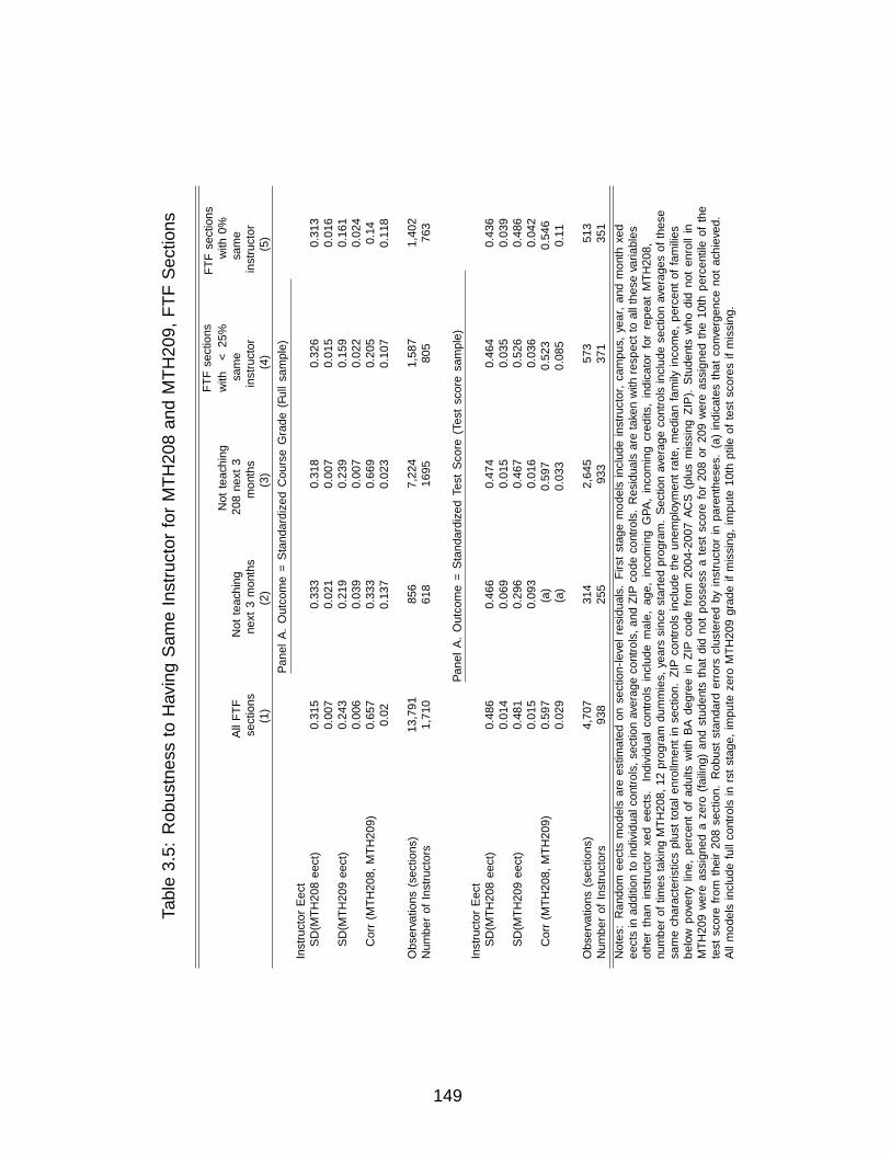
Tab

le3.

5:R

obust

nes

sto

Hav

ing

Sam

eIn

stru

ctor

for

MT

H20

8an

dM

TH

209,

FT

FSec

tion

s

FT

Fse

ctio

ns

FT

Fse

ctio

ns

Not

teach

ing

wit

h<

25%

wit

h0%

All

FT

FN

ot

teach

ing

208

nex

t3

sam

esa

me

sect

ion

sn

ext

3m

onth

sm

onth

sin

stru

ctor

inst

ruct

or

(1)

(2)

(3)

(4)

(5)

Pan

el

A.

Ou

tcom

e=

Sta

nd

ard

ized

Cou

rse

Grad

e(F

ull

sam

ple

)

Inst

ruct

or

Eff

ect

SD

(MT

H208

effec

t)0.3

15

0.3

33

0.3

18

0.3

26

0.3

13

0.0

07

0.0

21

0.0

07

0.0

15

0.0

16

SD

(MT

H209

effec

t)0.2

43

0.2

19

0.2

39

0.1

59

0.1

61

0.0

06

0.0

39

0.0

07

0.0

22

0.0

24

Corr

(MT

H208,

MT

H209)

0.6

57

0.3

33

0.6

69

0.2

05

0.1

40.0

20.1

37

0.0

23

0.1

07

0.1

18

Ob

serv

ati

on

s(s

ecti

on

s)13,7

91

856

7,2

24

1,5

87

1,4

02

Nu

mb

erof

Inst

ruct

ors

1,7

10

618

1695

805

763

Pan

el

A.

Ou

tcom

e=

Sta

nd

ard

ized

Test

Score

(Test

score

sam

ple

)

Inst

ruct

or

Eff

ect

SD

(MT

H208

effec

t)0.4

86

0.4

66

0.4

74

0.4

64

0.4

36

0.0

14

0.0

69

0.0

15

0.0

35

0.0

39

SD

(MT

H209

effec

t)0.4

81

0.2

96

0.4

67

0.5

26

0.4

86

0.0

15

0.0

93

0.0

16

0.0

36

0.0

42

Corr

(MT

H208,

MT

H209)

0.5

97

(a)

0.5

97

0.5

23

0.5

46

0.0

29

(a)

0.0

33

0.0

85

0.1

1

Ob

serv

ati

on

s(s

ecti

on

s)4,7

07

314

2,6

45

573

513

Nu

mb

erof

Inst

ruct

ors

938

255

933

371

351

Notes:

Ran

dom

effec

tsm

od

els

are

esti

mate

don

sect

ion

-lev

elre

sid

uals

.F

irst

stage

mod

els

incl

ud

ein

stru

ctor,

cam

pu

s,yea

r,an

dm

onth

fixed

effec

tsin

ad

dit

ion

toin

div

idu

al

contr

ols

,se

ctio

naver

age

contr

ols

,an

dZ

IPco

de

contr

ols

.R

esid

uals

are

taken

wit

hre

spec

tto

all

thes

evari

ab

les

oth

erth

an

inst

ruct

or

fixed

effec

ts.

Ind

ivid

ual

contr

ols

incl

ud

em

ale

,age,

inco

min

gG

PA

,in

com

ing

cred

its,

ind

icato

rfo

rre

pea

tM

TH

208,

num

ber

of

tim

esta

kin

gM

TH

208,

12

pro

gra

md

um

mie

s,yea

rssi

nce

start

edp

rogra

m.

Sec

tion

aver

age

contr

ols

incl

ud

ese

ctio

naver

ages

of

thes

esa

me

chara

cter

isti

csp

lust

tota

len

rollm

ent

inse

ctio

n.

ZIP

contr

ols

incl

ud

eth

eu

nem

plo

ym

ent

rate

,m

edia

nfa

mily

inco

me,

per

cent

of

fam

ilie

sb

elow

pover

tylin

e,p

erce

nt

of

ad

ult

sw

ith

BA

deg

ree

inZ

IPco

de

from

2004-2

007

AC

S(p

lus

mis

sin

gZ

IP).

Stu

den

tsw

ho

did

not

enro

llin

MT

H209

wer

eass

ign

eda

zero

(failin

g)

an

dst

ud

ents

that

did

not

poss

ess

ate

stsc

ore

for

208

or

209

wer

eass

ign

edth

e10th

per

centi

leof

the

test

score

from

thei

r208

sect

ion

.R

ob

ust

stan

dard

erro

rscl

ust

ered

by

inst

ruct

or

inp

are

nth

eses

.(a

)in

dic

ate

sth

at

conver

gen

cen

ot

ach

ieved

.A

llm

od

els

incl

ud

efu

llco

ntr

ols

infi

rst

stage,

imp

ute

zero

MT

H209

gra

de

ifm

issi

ng,

imp

ute

10th

pti

leof

test

score

sif

mis

sin

g.

149

Tab

le3.

6:R

obust

nes

sof

Tes

tSco

reR

esult

sto

Fir

st-S

tage

Model

(wit

hSel

ecti

onShock

s)

No

inst

ru

cto

rF

Ein

first

stage

Inst

ru

cto

rF

Ein

clu

ded

infi

rst

stage

(1)

(2)

(3)

(4)

(5)

(6)

(7)

(8)

(9)

(10)

(11)

(12)

Pan

el

A.

All

Secti

on

s(j

ust

test

score

sam

ple

),n

=7,2

32

secti

ons,

1,1

98

inst

ru

cto

rs

SD

(MT

H208

test

effec

t)0.2

93

0.2

63

0.2

85

0.2

66

0.2

66

0.2

48

0.2

94

0.4

42

0.2

87

0.4

44

0.4

40.4

25

(0.0

10)

(0.0

09)

(0.0

09)

(0.0

09)

(0.0

09)

(0.0

09)

(0.0

10)

(0.0

12)

(0.0

09)

(0.0

12)

(0.0

12)

(0.0

11)

SD

(MT

H209

test

effec

t)0.2

86

0.2

10.2

64

0.2

16

0.2

17

0.1

94

0.2

89

0.4

32

0.2

91

0.4

08

0.4

13

0.4

68

(0.0

10)

(0.0

10)

(0.0

10)

(0.0

10)

(0.0

10)

(0.0

09)

(0.0

10)

(0.0

13)

(0.0

10)

(0.0

12)

(0.0

12)

(0.0

13)

Corr

(MT

H208,

MT

H209)

0.7

25

0.8

54

0.7

99

0.8

65

0.8

64

0.8

62

0.7

22

0.6

16

0.7

54

0.6

09

0.6

19

0.6

17

(0.0

28)

(0.0

27)

(0.0

25)

(0.0

25)

(0.0

25)

(0.0

28)

(0.0

28)

(0.0

26)

(0.0

26)

(0.0

27)

(0.0

27)

(0.0

26)

Pan

el

B.

FT

FS

ecti

on

s(j

ust

test

score

sam

ple

)-

4,6

73

secti

on

s,935

inst

ru

cto

rs

SD

(MT

H208

test

effec

t)0.3

41

0.3

04

0.3

28

0.3

05

0.3

05

0.2

83

0.3

42

0.4

80

0.3

31

0.4

86

0.4

82

0.4

66

(0.0

12)

(0.0

11)

(0.0

11)

(0.0

11)

(0.0

11)

(0.0

11)

(0.0

12)

(0.0

14)

(0.0

11)

(0.0

14)

(0.0

14)

(0.0

14)

SD

(MT

H209

test

effec

t)0.2

93

0.2

59

0.2

93

0.2

63

0.2

64

0.2

36

0.2

94

0.5

07

0.2

96

0.4

81

0.4

87

0.5

46

(0.0

12)

(0.0

11)

(0.0

12)

(0.0

11)

(0.0

11)

(0.0

11)

(0.0

12)

(0.0

15)

(0.0

12)

(0.0

15)

(0.0

15)

(0.0

16)

Corr

(MT

H208,

MT

H209)

0.8

57

0.8

96

0.8

66

0.9

06

0.9

06

0.9

19

0.8

55

0.6

01

0.8

67

0.5

97

0.6

06

0.5

90

(0.0

23)

(0.0

23)

(0.0

22)

(0.0

22)

(0.0

22)

(0.0

23)

(0.0

23)

(0.0

29)

(0.0

22)

(0.0

29)

(0.0

28)

(0.0

28)

Pan

el

C.

On

lin

eS

ecti

on

s(j

ust

test

score

sam

ple

)-

2,5

59

secti

on

s,292

inst

ru

cto

rs

SD

(MT

H208

test

effec

t)0.1

35

0.1

35

0.1

35

0.1

35

0.1

35

0.1

35

0.1

35

0.1

35

0.1

35

0.1

35

0.1

35

0.1

35

(0.0

13)

(0.0

13)

(0.0

12)

(0.0

12)

(0.0

12)

(0.0

12)

(0.0

13)

(0.0

13)

(0.0

12)

(0.0

12)

(0.0

12)

(0.0

12)

SD

(MT

H209

test

effec

t)0.0

36

0.0

39

0.0

44

0.0

44

0.0

41

0.0

41

0.0

42

0.0

42

0.0

47

0.0

47

0.0

45

0.0

46

(0.0

42)

(0.0

39)

(0.0

34)

(0.0

34)

(0.0

36)

(0.0

36)

(0.0

37)

(0.0

36)

(0.0

32)

(0.0

32)

(0.0

33)

(0.0

33)

Corr

(MT

H208,

MT

H209)

-0.2

00

-0.1

72

-0.0

08

-0.0

82

-0.1

48

-0.1

42

-0.1

56

-0.1

57

-0.0

62

-0.0

66

-0.1

22

-0.1

21

(0.5

57)

(0.4

89)

(0.3

78)

(0.3

87)

(0.4

31)

(0.4

30)

(0.4

49)

(0.4

45)

(0.3

60)

(0.3

58)

(0.3

81)

(0.3

78)

Contr

ols

inF

irst

Sta

ge

Mod

el

ind

iv.

contr

ols

no

no

yes

yes

yes

yes

no

no

yes

yes

yes

yes

zip

contr

ols

no

no

yes

yes

yes

yes

no

no

yes

yes

yes

yes

sect

ion

avg

contr

ols

no

no

yes

yes

yes

yes

no

no

yes

yes

yes

yes

flex

ible

contr

ols

no

no

no

no

yes

yes

no

no

no

no

yes

yes

yea

rF

E,

month

FE

yes

yes

yes

yes

yes

yes

yes

yes

yes

yes

yes

yes

cam

pu

sF

En

oyes

no

yes

yes

no

no

yes

no

yes

yes

no

loca

tion

FE

no

no

no

no

no

yes

no

no

no

no

no

yes

Notes:

Ran

dom

effec

tsm

od

els

are

esti

mate

don

sect

ion

-lev

elre

sid

uals

.In

div

contr

ols

incl

ud

em

ale

,age,

inco

min

gG

PA

,in

com

ing

cred

its,

ind

icato

rfo

rre

pea

tM

TH

208,

nu

mb

erof

tim

esta

kin

gM

TH

208,

12

pro

gra

md

um

mie

s,yea

rssi

nce

start

edp

rogra

m.

Sec

tion

aver

age

contr

ols

incl

ud

ese

ctio

naver

ages

of

thes

esa

me

chara

cter

isti

csp

lust

tota

len

rollm

ent

inse

ctio

n.

ZIP

contr

ols

incl

ud

eth

eu

nem

plo

ym

ent

rate

,m

edia

nfa

mily

inco

me,

per

cent

of

fam

ilie

sb

elow

pover

tylin

e,p

erce

nt

of

ad

ult

sw

ith

BA

deg

ree

inZ

IPco

de

from

2004-2

007

AC

S(p

lus

mis

sin

gZ

IP).

Fle

xib

leco

ntr

ols

incl

ud

ep

rogra

m-s

pec

ific

cub

ics

inin

com

ing

GP

Aan

dcr

edit

s,cu

bic

inte

ract

ion

sb

etw

een

GP

Aan

dcr

edit

s,gen

der

-sp

ecifi

cage

cub

ic,

an

din

tera

ctio

ns

bet

wee

ngen

der

an

dG

PA

an

dcr

edit

s.S

tud

ents

wh

od

idn

ot

enro

llin

MT

H209

wer

eass

ign

eda

zero

(failin

g)

an

dst

ud

ents

that

did

not

poss

ess

ate

stsc

ore

for

208

or

209

wer

eass

ign

edth

e10th

per

centi

leof

the

test

score

from

thei

r208

sect

ion

.R

ob

ust

stan

dard

erro

rscl

ust

ered

by

inst

ruct

or

inp

are

nth

eses

.**

Ind

icate

sth

at

mod

elfa

iled

toco

nver

ge.

All

mod

els

incl

ud

ese

ctio

n-s

pec

ific

shock

san

dim

pu

teze

roM

TH

209

gra

de

ifm

issi

ng,

imp

ute

10th

pti

leof

test

score

ifm

issi

ng.

150

Tab

le3.

7:R

obust

nes

sto

Imputa

tion

Met

hod

Grad

eO

utc

om

es

Test

Score

Ou

tcom

es

Mis

sin

ggra

des

for

MT

H209

rep

lace

dw

ith

...

Mis

sin

ggra

des

for

MT

H209

rep

lace

dw

ith

...

Base

mod

el:

Mea

nfo

rp

10

for

p10

for

Mea

nof

Min

imu

mof

stu

den

tsw

ho

Base

mod

el:

cam

pu

s-yea

rst

ud

ents

stu

den

tsst

ud

ents

rece

ived

sam

eN

oS

etE

qu

al

toN

oof

MT

H208

from

MT

H208

from

MT

H208

from

MT

H208

gra

de

inM

TH

-

Imp

uta

tion

0(F

ailin

g)

Imp

uta

tion

sect

ion

sect

ion

sect

ion

sect

ion

208

sect

ion

(1)

(2)

(3)

(4)

(5)

(6)

(7)

(8)

Pan

el

A.

All

Secti

on

s

Inst

ruct

or

Eff

ect

SD

(MT

H208

effec

t)0.2

86

0.2

86

0.4

16

0.3

95

0.4

44

0.4

69

0.4

06

0.4

02

(0.0

08)

(0.0

08)

(0.0

11)

(0.0

10)

(0.0

12)

(0.0

12)

(0.0

11)

(0.0

10)

SD

(MT

H209

effec

t)0.2

44

0.2

05

0.3

94

0.3

43

0.4

08

0.4

95

0.3

79

0.3

74

(0.0

08)

(0.0

07)

(0.0

11)

(0.0

10)

(0.0

12)

(0.0

14)

(0.0

12)

(0.0

11)

Corr

(MT

H208,

MT

H209)

0.4

77

0.5

50

0.5

44

0.6

14

0.6

09

0.5

31

0.6

23

0.5

56

(0.0

34)

(0.0

30)

(0.0

28)

(0.0

25)

(0.0

27)

(0.0

28)

(0.0

27)

(0.0

27)

Pan

el

B.

FT

FO

nly

Inst

ruct

or

Eff

ect

SD

(MT

H208

effec

t)0.2

98

0.2

98

0.4

45

0.4

30

0.4

86

0.5

03

0.4

45

0.4

36

(0.0

09)

(0.0

09)

(0.0

13)

(0.0

13)

(0.0

14)

(0.0

15)

(0.0

13)

(0.0

13)

SD

(MT

H209

effec

t)0.2

88

0.2

39

0.4

57

0.3

92

0.4

81

0.5

72

0.4

47

0.4

3(0

.010)

(0.0

08)

(0.0

14)

(0.0

12)

(0.0

15)

(0.0

17)

(0.0

14)

(0.0

13)

Corr

(MT

H208,

MT

H209)

0.5

93

0.5

97

0.5

49

0.6

29

0.5

97

0.5

50.6

14

0.5

95

(0.0

33)

(0.0

32)

(0.0

31)

(0.0

28)

(0.0

29)

(0.0

31)

(0.0

29)

(0.0

29)

Pan

el

C.

On

lin

eO

nly

Inst

ruct

or

Eff

ect

SD

(MT

H208

effec

t)0.2

27

0.2

25

0.1

15

0.1

07

0.1

35

0.1

41

0.1

23

0.1

18

(a)

(0.0

12)

(0.0

09)

(0.0

09)

(0.0

12)

(0.0

10)

(0.0

12)

(0.0

09)

SD

(MT

H209

effec

t)0.0

47

0.0

28

0.0

34

0.0

10.0

47

0.0

54

0.0

48

0.0

23

(a)

(0.0

13)

(0.0

24)

(0.0

07)

(0.0

32)

(0.0

22)

(0.0

29)

(0.0

29)

Corr

(MT

H208,

MT

H209)

-10.3

65

-0.2

96

1-0

.066

0.1

72

-0.2

76

0.3

59

(a)

(0.2

34)

(0.4

03)

(a)

(0.3

58)

(0.2

35)

(0.3

82)

(0.5

26)

Notes:

Random

eff

ects

models

are

est

imate

don

secti

on-l

evelre

siduals

.F

irst

stage

models

inclu

de

inst

ructo

r,cam

pus,

year,

and

month

fixed

eff

ects

inaddit

ion

toin

div

idualcontr

ols

,se

cti

on

avera

ge

contr

ols

,and

ZIP

code

contr

ols

.R

esi

duals

are

taken

wit

hre

spect

toall

these

vari

able

soth

er

than

inst

ructo

rfi

xed

eff

ects

.In

div

idual

contr

ols

inclu

de

male

,age,

incom

ing

GP

A,

incom

ing

cre

dit

s,in

dic

ato

rfo

rre

peat

MT

H208,

num

ber

of

tim

es

takin

gM

TH

208,

12

pro

gra

mdum

mie

s,years

since

start

ed

pro

gra

m.

Secti

on

avera

ge

contr

ols

inclu

de

secti

on

avera

ges

of

these

sam

echara

cte

rist

ics

plu

stto

tal

enro

llm

ent

inse

cti

on.

ZIP

contr

ols

inclu

de

the

unem

plo

ym

ent

rate

,m

edia

nfa

mily

incom

e,

perc

ent

of

fam

ilie

sb

elo

wp

overt

yline,

perc

ent

of

adult

sw

ith

BA

degre

ein

ZIP

code

from

2004-2

007

AC

S(p

lus

mis

sing

ZIP

).R

obust

standard

err

ors

clu

stere

dby

inst

ructo

rin

pare

nth

ese

s.A

llm

odels

inclu

de

full

contr

ols

infi

rst

stage

and

inclu

de

secti

on-s

pecifi

csh

ocks.

(a)

indic

ate

sth

at

converg

ence

not

achie

ved.

151

Tab

le3.

8:R

elat

ionsh

ipb

etw

een

Cou

rse

Gra

de

orT

est

Eff

ect

and

Tea

chin

gE

valu

atio

n

FT

Fan

dO

nli

ne

FT

FO

nly

On

lin

eO

nly

Mea

sure

of

Stu

den

tL

earn

ing:

Mea

sure

of

Stu

den

tL

earn

ing:

Mea

sure

of

Stu

den

tL

earn

ing:

MT

H208

MT

H209

MT

H208

MT

H209

MT

H208

MT

H209

MT

H208

MT

H209

MT

H208

MT

H209

MT

H208

MT

H209

gra

de

gra

de

test

test

gra

de

gra

de

test

test

gra

de

gra

de

test

test

(1)

(2)

(3)

(4)

(5)

(6)

(7)

(8)

(9)

(10)

(11)

(12)

Inst

ruct

or

Eff

ect

SD

(lea

rnin

geff

ect)

0.2

86

0.2

05

0.4

44

0.4

10

0.2

99

0.2

40

0.4

87

0.4

84

0.2

27

0.0

28

0.1

37

0.0

48

(0.0

08)

(0.0

07)

(0.0

12)

(0.0

12)

(0.0

09)

(0.0

08)

(0.0

14)

(0.0

15)

(0.0

12)

(0.0

13)

(0.0

12)

(0.0

32)

SD

(eval

effec

t)0.2

19

0.2

19

0.2

19

0.2

19

0.2

40

0.2

39

0.2

40.2

40

0.1

40

0.1

41

0.1

41

0.1

41

(0.0

06)

(0.0

06)

(0.0

06)

(0.0

06)

(0.0

08)

(0.0

08)

(0.0

08)

(0.0

08)

(0.0

08)

(0.0

09)

(0.0

08)

(0.0

09)

Corr

(lea

rnin

g,

eval)

0.4

39

0.2

37

0.0

84

-0.0

84

0.3

90

0.2

23

0.0

59

-0.0

74

0.7

51

0.5

97

0.5

20

-0.6

05

(0.0

33)

(0.0

42)

(0.0

39)

(0.0

41)

(0.0

39)

(0.0

47)

(0.0

44)

(0.0

45)

(0.0

41)

(0.2

93)

(0.0

84)

(0.4

35)

Sec

tion

Eff

ect

SD

(lea

rnin

geff

ect)

0.2

71

0.2

79

0.3

99

0.4

90

0.2

78

0.2

91

0.4

00

0.4

50

0.2

57

0.2

62

0.3

99

0.5

55

(0.0

03)

(0.1

48)

(0.3

52)

(0.3

96)

(0.6

24)

(0.0

04)

(0.2

66)

(0.2

24)

(0.2

55)

(0.0

04)

(0.0

06)

(0.2

75)

SD

(eval

effec

t)0.2

33

0.2

33

0.2

19

0.2

13

0.2

46

0.2

46

0.2

32

0.2

28

0.2

10

0.2

17

0.2

00

0.1

91

(0.0

03)

(0.1

78)

(0.6

41)

(0.9

13)

(0.7

06)

(0.0

03)

(0.4

57)

(0.4

42)

(0.3

13)

(0.0

04)

(0.0

04)

(0.7

97)

Corr

(lea

rnin

g,

eval)

0.1

74

0.0

40

0.1

19

0.0

01

0.1

56

0.0

41

0.1

02

0.0

01

0.2

14

0.0

41

0.1

53

0.0

01

(0.0

15)

(0.0

54)

(0.4

52)

(0.0

17)

(0.7

99)

(0.0

19)

(0.2

7)

(0.0

21)

(0.5

34)

(0.0

23)

(0.0

24)

(0.0

26)

Ob

serv

ati

on

s(s

ecti

on

s)7,2

67

7,2

67

7,2

67

7,2

67

4,7

07

4,7

07

4,7

07

4,7

07

2,5

60

2,5

60

2,5

60

2,5

60

Nu

mb

erof

Inst

ruct

ors

1,2

01

1,2

01

1,2

01

1,2

01

938

938

938

938

292

292

292

292

Notes:

Random

eff

ects

models

are

est

imate

don

secti

on-l

evelre

siduals

.F

irst

stage

models

inclu

de

inst

ructo

r,cam

pus,

year,

and

month

fixed

eff

ects

inaddit

ion

toin

div

idualcontr

ols

,se

cti

on

avera

ge

contr

ols

,and

ZIP

code

contr

ols

.R

esi

duals

are

taken

wit

hre

spect

toall

these

vari

able

soth

er

than

inst

ructo

rfixed

eff

ects

.In

div

idual

contr

ols

inclu

de

male

,age,

incom

ing

GP

A,

incom

ing

cre

dit

s,in

dic

ato

rfo

rre

peat

MT

H208,

num

ber

of

tim

es

takin

gM

TH

208,

12

pro

gra

mdum

mie

s,years

since

start

ed

pro

gra

m.

Secti

on

avera

ge

contr

ols

inclu

de

secti

on

avera

ges

of

these

sam

echara

cte

rist

ics

plu

stto

tal

enro

llm

ent

inse

cti

on.

ZIP

contr

ols

inclu

de

the

unem

plo

ym

ent

rate

,m

edia

nfa

mily

incom

e,

perc

ent

of

fam

ilie

sb

elo

wp

overt

yline,

perc

ent

of

adult

sw

ith

BA

degre

ein

ZIP

code

from

2004-2

007

AC

S(p

lus

mis

sing

ZIP

).Stu

dents

who

did

not

enro

llin

MT

H209

were

ass

igned

azero

(failin

g)

and

students

that

did

not

poss

ess

ate

stsc

ore

for

208

or

209

were

ass

igned

the

10th

perc

enti

leof

the

test

score

from

their

208

secti

on.

Robust

standard

err

ors

clu

stere

dby

inst

ructo

rin

pare

nth

ese

s.A

llm

odels

inclu

de

full

contr

ols

infi

rst

stage,

impute

zero

MT

H209

gra

de

ifm

issi

ng,

impute

10th

pti

leof

test

score

ifm

issi

ng.

152

Table 3.9: Instructor Effects for Alternative Outcomes

Outcome

CreditsPass Take earned

MTH208 MTH209 6 months

Panel A. Full SampleSD (instructor effect) - overall 0.073 0.051 0.126(n = 26,384) (0.002) (0.002) (0.004)SD instructor effect - FTF 0.080 0.062 0.154(n = 13,791) (0.002) (0.002) (0.005)SD instructor effect - online 0.059 0.031 0.059(n = 12,593) (0.002) (0.002) (0.004)

Panel B. Test Score SampleSD (instructor effect) - overall 0.072 0.059 0.130(n = 7,267) (0.002) (0.003) (0.006)SD instructor effect - FTF 0.077 0.069 0.150(n = 4,707) (0.003) (0.003) (0.007)SD instructor effect - online 0.056 0.032 0.040( n = 2,560) (0.004) (0.004) (0.011)

Notes: Random effects models are estimated on section-level residuals. First stage modelsinclude instructor, campus, year, and month fixed effects in addition to individual controls,section average controls, and ZIP code controls. Residuals are taken with respect to all thesevariables other than instructor fixed effects. Individual controls include male, age, incomingGPA, incoming credits, indicator for repeat MTH208, number of times taking MTH208, 12program dummies, years since started program. Section average controls include sectionaverages of these same characteristics plust total enrollment in section. ZIP controls includethe unemployment rate, median family income, percent of families below poverty line, percentof adults with BA degree in ZIP code from 2004-2007 ACS (plus missing ZIP). Robuststandard errors clustered by instructor in parentheses. First stage model with full controls.

153

Table 3.10: Correlates of Instructor Effectiveness

Outcome: Section-level mean residual for

CreditsMTH208 MTH209 MTH208 MTH209 Earned

grade grade test test 6 months(1) (2) (3) (4) (5)

A. Linear, Only MTH208 Experience, Instructor FEs

Taught MTH208 previously 0.0384*** 0.006 0.069** 0.019 -0.016(0.011) (0.011) (0.034) (0.038) (0.010)

Times taught MTH208 0.000 0.000 -0.003 -0.003 0.001(0.001) (0.001) (0.004) (0.004) (0.001)

B. Piecewise, Only MTH208 Experience, Instructor FEs

Times taught MTH208 = 1 0.031*** -0.002 0.067* 0.020 0.000(0.012) (0.012) (0.036) (0.042) (0.012)

Times taught MTH208 = 2 to 5 0.041*** 0.008 0.078* 0.045 -0.020*(0.012) (0.012) (0.040) (0.044) (0.011)

Times taught MTH208 = 6 to 10 0.040*** 0.008 0.137** -0.001 -0.005(0.016) (0.015) (0.054) (0.056) (0.014)

Times taught MTH208 = 11 to15

0.041** 0.001 0.169** 0.043 -0.001

(0.020) (0.018) (0.066) (0.068) (0.017)Times taught MTH208 = 16 to20

0.040* -0.009 0.159** 0.077 0.017

(0.024) (0.020) (0.079) (0.081) (0.019)Times taught MTH208 > 20 0.035 -0.005 0.131 0.113 0.043*

(0.028) (0.023) (0.089) (0.096) (0.023)

C. Linear, Control for MTH209 experience, other math,non-math experience linearly, time since hire, Instructor FEs

Taught MTH208 previously 0.028** -0.005 0.059 -0.045 -0.025**(0.014) (0.013) (0.048) (0.055) (0.012)

Times taught MTH208 0.000 0.000 -0.008 -0.003 0.001(0.001) (0.001) (0.005) (0.005) (0.001)

Taught MTH209 previously 0.015 0.014 -0.014 0.081* 0.015(0.015) (0.013) (0.054) (0.049) (0.012)

Times taught MTH209 0.002 0.001 0.001 0.009** -0.000(0.001) (0.001) (0.005) (0.004) (0.001)

Years since first hire date 0.002 -0.005 0.019 0.038 0.023(0.016) (0.016) (0.048) (0.056) (0.016)

First hire more than one year ago 0.017 0.017 0.084*** -0.001 0.0014(0.012) (0.012) (0.032) (0.033) (0.011)

Notes: Section mean residuals are regressed on teaching experience, instructor fixed effects, and year and monthfixed effects. Sample restricted to 18,409 sections (5970 for test scores) taught by instructors hired since 2002. Firststage model include instructor, campus, year, and month fixed effects in addition to individual controls, sectionaverage controls, and ZIP code controls. Residuals are taken with respect to all these variables other than instructorfixed effects. Individual controls include male, age, incoming GPA, incoming credits, indicator for repeat MTH208,number of times taking MTH208, 12 program dummies, years since started program. Section average controlsinclude section averages of these same characteristics plust total enrollment in section. ZIP controls include theunemployment rate, median family income, percent of families below poverty line, percent of adults with BA degreein ZIP code from 2004-2007 ACS (plus missing ZIP). Students who did not enroll in MTH209 were assigned a zero(failing) and students that did not possess a test score for 208 or 209 were assigned the 10th percentile of the testscore from their 208 section. Robust standard errors clustered by instructor in parentheses. First stage model withfull controls. All sections, faculty hired since 2002.

154

Table 3.11: Correlates of Instructor Salary

Outcome: Total Salary Paid for MTH208 Section ($1,000)

(mean=1.077)

(1) (2) (3) (4) (5)

Section-level mean residual -0.005 0.003 0.006 0.007 0.006for MTH209 grade (0.006) (0.005) (0.005) (0.004) (0.004)

Years since first hire date 0.030*** 0.027*** 0.044*** 0.046***(0.001) (0.001) (0.004) (0.004)

First hire more than one year ago 0.010*** 0.008** 0.006 0.005(0.004) (0.004) (0.004) (0.004)

Total sections taught previously 0.001*** 0.000*** 0.000(0.000) (0.000) (0.000)

Taught MTH208 previously 0.002(0.004)

Times taught MTH208 -0.001**(0.000)

Times taught MTH209 0.000(0.000)

Times taught other math courses -0.000(0.000)

Times taught nonmath courses 0.000(0.000)

Constant 1.038 0.919 0.907 0.953 0.951(0.004) (0.007) (0.007) (0.013) (0.013)

R-squared 0.265 0.536 0.565 0.713 0.714Fixed effects None None Campus Instructor Instructor

Notes: Sample restricted to 18,080 sections taught by instructors hired since 2002.All specifications also includeyear and month fixed effects. Section-level residuals include the full set of individual and section controls andcampus fixed effects, imputing zero MTH209 grades for students that did not enroll. Robust standard errorsclustered by instructor in parentheses. All sections, faculty hired since 2002.

155

Fig

ure

3.1:

Rel

atio

nsh

ipb

etw

een

Inst

ruct

orE

ffec

tive

nes

s(G

rades

)an

dT

each

ing

Exp

erie

nce

Notes:

Dash

edlin

esd

enote

95%

CI

wit

hst

an

dard

erro

rscl

ust

ered

by

inst

ruct

or.

Sec

tion

mea

nre

sid

uals

are

regre

ssed

on

MT

H208

teach

ing

exp

erie

nce

(cap

ped

at

20),

inst

ruct

or

fixed

effec

ts(b

ott

om

row

),an

dyea

ran

dm

onth

fixed

effec

ts.

Sam

ple

rest

rict

edto

18,4

18

sect

ion

sta

ught

by

inst

ruct

ors

hir

edsi

nce

2002.

Fir

stst

age

mod

elin

clu

des

full

contr

ols

(see

text)

.

156

Fig

ure

3.2:

Rel

atio

nsh

ipb

etw

een

Inst

ruct

orE

ffec

tive

nes

s(T

est

Sco

res)

and

Tea

chin

gE

xp

erie

nce

Notes:

Dash

edlin

esd

enote

95%

CI

wit

hst

an

dard

erro

rscl

ust

ered

by

inst

ruct

or.

Sec

tion

mea

nre

sid

uals

are

regre

ssed

on

MT

H208

teach

ing

exp

erie

nce

(cap

ped

at

20),

inst

ruct

or

fixed

effec

ts(b

ott

om

row

),an

dyea

ran

dm

onth

fixed

effec

ts.

Sam

ple

rest

rict

edto

18,4

18

sect

ion

sta

ught

by

inst

ruct

ors

hir

edsi

nce

2002.

Fir

stst

age

mod

elin

clu

des

full

contr

ols

(see

text)

.

157

APPENDICES

158

APPENDIX A

Appendix to Quantifying Sources of Persistent

Prescription Behavior: Evidence from Belgium

A.1 Institutional Setting

A.1.1 The Belgian Healthcare Market

The health care market in Belgium is financed through a withheld tax (at a rate of

13.07%) which applies to gross wages. This tax is used for health, disability, and unemploy-

ment insurance. Additional funds to finance shortfalls are earmarked and financed through

specific taxes (e.g. tobacco taxes) or other financing means. The health care market is orga-

nized through a heavily regulated insurance market in which the Mandated Health Insurance

is sold.

A.1.2 The Minimum Prescription Rate (MPR)

This section provides some additional descriptive numbers on the introduction of the

MPR. Below is an overview of the average prescription rate of generics going back to 2004

which is based on data provided by the NIHDI in Belgium. The micro-data I employ is not

159

available going back to before 2004, but these data do provide some insight as to what the

impact of the MPR was.

Figure A.1: Stylized Facts: Overall Prescription Rate 2000-2010

0

0.05

0.1

0.15

0.2

0.25

2000 2001 2002 2003 2004 2005 2006 2007 2008 2009 2010

MarketS

hare

Frac,onofGenericsPrescribed(Volume)

ActualMarketShare

Fi;edMarketShare(2000-2004)

Notes: data used for this graph were provided by NIHDI, and plots the overal prescription rate of generics

between 2000 and 2010.

Overall, the graph suggests that there is a steady increase in the use of generics (for

instance, because of the arrival rate of generics as patents expire), but that this steady

increase was relatively stable before the introduction of the MPR.

Finally, I also show a graph similar to Figure 1.4 but dividing the data into physicians

in the top and bottom quartile of the baseline prescription rate of generics. Comparing

these numbers to Figure 1.4 shows that physicians further from the threshold (e.g. bottom

quartile) are much more likely to increase the prescription rate of generics in the wake of the

policy mandate.

160

Figure A.2: Descriptive Graphs: Prescription and Switching Rate of Generics

(a) Chronic Starters: Top/Bottom Median

MandateAnnounced

MandateEffective

.1.2

.3.4

.5Pr

escr

iptio

n R

ate

amon

g C

hron

ic S

tarte

rs

Jan 2

004

Jul 2

004

Jan 2

005

Jul 2

005

Jan 2

006

Jul 2

006

Jan 2

007

Jul 2

007

Quarter

Physicians above Median Physicians below Median

Fraction of Transactions for which Generic is Prescribed

(b) Longstanding Switching: Top/Bottom Me-dian

MandateAnnounced

MandateEffective

0.0

1.0

2.0

3.0

4.0

5Fr

actio

n of

Tra

nsac

tions

Jan 2

004

Jul 2

004

Jan 2

005

Jul 2

005

Jan 2

006

Jul 2

006

Jan 2

007

Jul 2

007

Quarter

Physicians above Median Physicians below Median

Chronic LongstandingFraction of Transactions for which Generic is Prescribed

Notes: This data is a graph of the average prescription rate of generics for different types of patients (chronic

starters and longstanding). I show the averages across physicians that are above/below the median (middle

panel). Overall, the figures display a sudden increase upon announcement of the mandate, with physicians

far from the threshold responding more.

A.1.3 Licensing of “Free Professions”

Practicing physicians in Belgium are subject to an employment regime of “free profes-

sions”, a regime that refers to non-merchant occupations that perform intellectual or non-

manual labor services both for a direct customer and the society as a whole. Other examples

of free professions include, among others, veteranarians, accountant, pharmacists, architects,

nurses. For a more complete discussion on exact status definitions, see 2005/36/EG Direc-

tory of the European Parliament and the European Council. People with a medical degree

might choose not to practice medicin and pursue other career paths that are not “free occu-

pations” in diverse sectors. A notable exception is practicing physicians that are affiliated

with universities and university hospitals: they are typically directly employed by the state

and are therefore in paid employment, although they do need to fulfill licensing require-

ments. These physicians are typically specialists and not primary care physicians.Access

to “free professions” is regulated through occupational licensing programs that operate in

161

similar ways to similar programs in other countries in the European Union or the United

States. Upon licensing, primary care physicians are typically self-employed in a solo-practice,

or self-employed in a cooperative group practice.

A.1.4 Prescription Filling and Processing

The central document in this process is the prescription written out by a physician (see

Figure 1.1 for an example). The bar code in the top left identifies the physician (who is

forced to order his prescription books at a central provider who prints the bar code). The

physician writes the specific product name in the field denoted by box 5 in Figure 1.1b.

The patient then takes this prescription to a pharmacist who provides the drug as written

on the prescription and scans the product barcode upon dispensing. Pharmacists in this

period were required to follow the physician’s prescription, although some changes to this

procedure have been made. The patient then inserts their electronic health insurance cards

(identifying their health insurance records) and pays for the prescription drug. Unless the

prescription drug is a particular drug (e.g. because of cost) or the patient is on an increased

reimbursement plan, the patient pays the full price. The patient then uses a “vignet” (akin

to a sticker with identifying information on the patient) which is then submitted to their

mutual fund who reimburses the patient.

Typically, a patient visits their physician to obtain a prescription. Prescriptions are valid

for three months from the date of prescription (which is posted in box 8 in Figure 1.1b).

It is possible for a physician to allow for this start date to be in the future, e.g. when

the physician wants to provide a prescription in February and June while not requiring the

patient to return. This future start date is denoted in box 9. However, physicians typically

prefer patients to come back for a visit when needing a new prescription, as they receive

only a fee for a visit (not for a prescription).

162

Prescriptions on INN (Active Ingredient)

There was a program that was introduced in 2005 at the time of the mandate that allowed

physicians to prescribe on INN (International Nonproprietary Names). However, the fraction

of prescription that used these was low (around 1-2%) and the take-up rate was the lowest

among primary care physicians, for whom it was well below 1%. This program has become

more popular in recent years though.

A.1.5 Pricing and Price changes

The Belgian healthcare system uses a reference pricing system (RPS) for prescription

drugs, detailed in further detail in Appendix A.1.5, which was introduced in 2001 (Farfan-

Portet et al., 2012; Cornelis, 2013).1 An RPS consists of two elements. The first element is

the set of clusters, or groups of prescription drugs that are considered equivalent from the

perspective of the policymaker. Belgium has a “generic RPS” or an “RPS at the molecular

level,” where all drugs that have the exact same active ingredient (i.e. are bio-equivalent)

form one cluster (Vrijens et al., 2010; Farfan-Portet et al., 2012).2

The second element is the Reference Price (RP ), which is the maximum price manufac-

turers of generic drugs can charge within a cluster.3 The RPS then fixes the reimbursement

within a cluster to be the RP multiplied by the copay rate. As a result, the insurer reim-

burses a fixed amount, regardless of the prescription decision. If a drug is priced above the

RP , the difference between the price and this fixed reimbursement is therefore fully borne by

the patient. Generics and branded drugs that charge the RP are considered “cheap”, while

1Similar systems are used in other countries. Dylst, Vulto and Simoens (2012), Simoens (2012) andFarfan-Portet et al. (2012) provide a more complete discussion on this system and differences across thecountries that have implemented such systems.

2In contrast, therapeutic equivalence – defined at the ATC4 level – only requires drugs to treat similarconditions. Bio-equivalence implies that brand-name simvastatin Zocor would be in a cluster with genericsimvastatins, but not atorvastatins (such as Lipitor or generic equivalents). All these drugs would be in thesame cluster when using therapeutic equivalence.

3This reference price is based on a well-defined estimate of the production cost of the brand-name mul-tisource drug.

163

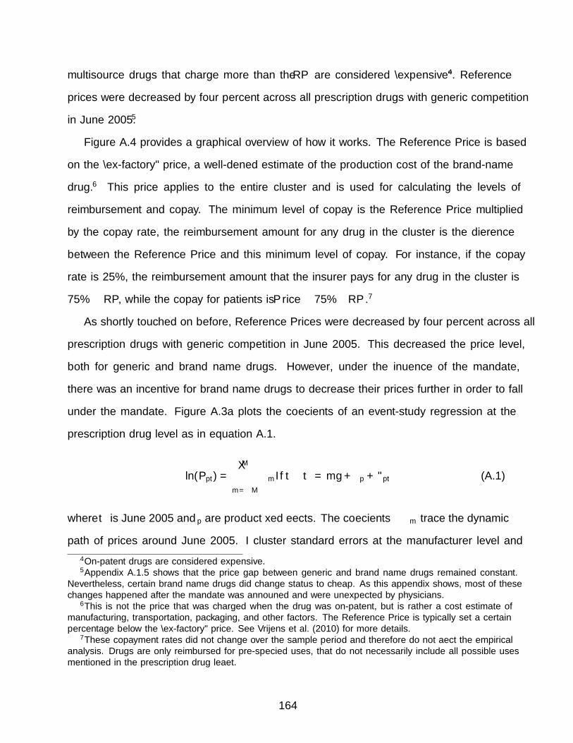
multisource drugs that charge more than the RP are considered “expensive”.4 Reference

prices were decreased by four percent across all prescription drugs with generic competition

in June 2005.5

Figure A.4 provides a graphical overview of how it works. The Reference Price is based

on the “ex-factory” price, a well-defined estimate of the production cost of the brand-name

drug.6 This price applies to the entire cluster and is used for calculating the levels of

reimbursement and copay. The minimum level of copay is the Reference Price multiplied

by the copay rate, the reimbursement amount for any drug in the cluster is the difference

between the Reference Price and this minimum level of copay. For instance, if the copay

rate is 25%, the reimbursement amount that the insurer pays for any drug in the cluster is

75% × RP, while the copay for patients is Price− 75%×RP .7

As shortly touched on before, Reference Prices were decreased by four percent across all

prescription drugs with generic competition in June 2005. This decreased the price level,

both for generic and brand name drugs. However, under the influence of the mandate,

there was an incentive for brand name drugs to decrease their prices further in order to fall

under the mandate. Figure A.3a plots the coefficients of an event-study regression at the

prescription drug level as in equation A.1.

ln(Ppt) =M∑

m=−M

βmI{t− t∗ = m}+ ξp + εpt (A.1)

where t∗ is June 2005 and ξp are product fixed effects. The coefficients βm trace the dynamic

path of prices around June 2005. I cluster standard errors at the manufacturer level and

4On-patent drugs are considered expensive.5Appendix A.1.5 shows that the price gap between generic and brand name drugs remained constant.

Nevertheless, certain brand name drugs did change status to cheap. As this appendix shows, most of thesechanges happened after the mandate was announed and were unexpected by physicians.

6This is not the price that was charged when the drug was on-patent, but is rather a cost estimate ofmanufacturing, transportation, packaging, and other factors. The Reference Price is typically set a certainpercentage below the “ex-factory” price. See Vrijens et al. (2010) for more details.

7These copayment rates did not change over the sample period and therefore do not affect the empiricalanalysis. Drugs are only reimbursed for pre-specified uses, that do not necessarily include all possible usesmentioned in the prescription drug leaflet.

164

set M to 10. On-patent drugs did not change prices. Overall, these results suggest that

the price gap between generic and brand name prescription drug remained fairly stable over

the study period. Nevertheless, the levels of copays and reimbursements have changed by

about four percent for generics and brand name drugs with generic competition. As a result,

the price gap between both drug groups is relatively stable. Figure A.3b shows the average

(smoothed) price gap between off-patent branded and generic prescription drugs, and we

indeed find that the average price gap does exhibit some variation, but is not strongly

affected by the introduction of the change in the Reference Pricing System.

Figure A.3: Stylized Facts: Changes in Prices

(a) Changes in Prices by Type of Drug

-.1-.0

50

.05

-10 -5 0 5 10timeline

On Patent Generic Brand Name

(b) Price Difference Brand Name and GenericDrugs

-.04-.02

0.02

-.04-.02

0.02

-.04-.02

0.02

0 20 40 60 80 0 20 40 60 80 0 20 40 60 80

A10: Diabetes Drugs C03: Diuretics C07: Beta Blockers

C08: Calcium Channel Blockers C09: ACE inhibitors C10: Statins

J01: Antibiotics M01: Antirheumatics N06: Analeptics

Log

Diff

eren

ce (i

n eu

ros)

group(year month)Graphs by Product Group

Notes: Figure A.3a shows the regression coefficients βm from regression equation A.1 for three distinct

product groups: on-patent drugs (unaffected), branded off-patent drugs, and generic drugs. Figure A.3b

shows the smoothed copay differential between branded off-patent and generic prescription drugs at the

product group level (as defined in table 1.1). These numbers are smoothed and show some variation over

tim, but no systematic change in the effect of the mandate.

The limited effect of the changes in the RP system are supported in Figure A.3b, that

plots the differential between the price of brand name and generic drugs for selected main

product groups. Most price changes at the product group level are within a two to four

percent change, and are therefore relatively small. This graph was computed as follows: the

average price of generic and brand name products is computed at the level of the active

165

ingredient. Then, to purge the data of level differences, I regress these price differences on

an active ingredient fixed effect and compute the average price differential for each product

group in each month. Figure A.3b presents the Lowess-smoothed version of these differences.

166

Figure A.4: Determination of Status Prescription Drug.

Cluster 1 Cluster 2 Cluster 3 ...

Reference Price Cluster 2 (RP2)

Status of Drugs in Cluster 2

Copay of Drugs in Cluster 2

Cluster Reimbursement on all Drugs:

(1− c)×RP2 where c is copay rate.

Price ≤ RP2 Price > RP2

Generic Drug

Brand Name Drug

Generic Not on Market

Cheap Expensive

Copay for Patient: Price - Cluster Reimbursement

167

A.2 Data

The flow of the data collection is shown graphically in Figure A.5. The source of the

data is the pharmacy, where the prescription and patient health care card are read and

provide information on the physician and patient identifier are recovered. The pharmacy

then sells the prescription drug and scans the product’s bar code upon dispensing. The

copay is directly identified (and stored) when the patient inserts their health care. As a

result, if a patient does not fill out the slip and recover the reimbursement, this is not in the

data.

After the prescription is read in at the pharmacy, the data are then uploaded and made

available to a billing service provider, who aggregates and delivers this data to the relevant

mutual fund on a quarterly basis.8 These data are heavily scrutinized and reviewed for

quality and accuracy at all steps in this process. For instance, certain checks on the copay

and reimbursement are made. The mutual funds receive the verified data and reimburse their

patients. As these mutual funds still need to reimburse, these mutual funds have access to

patient identifiers.

In a final step, these data are shared with the NIHDI, who use it for risk-adjustment for-

mulas and reimbursement of the mutual funds. While information is still at the patient-level,

mutual funds anonymize the data before sending them along to NIHDI as NIHDI in princi-

ple does not require knowledge of patients’ identities to reimburse mutual funds. Physician

identifiers still uniquely identify physicians for the NIHDI, as they use this information to

provide feedback reports to physicians and use this for general follow-up and control.

As noted in Figure A.5, the different mutual funds have also organized themselves to

create the InterMutualistic Agency (IMA) where patient identifiers are still available and

used for research purposes. As a result, this graph provides a clear overview of the data I

use (and the advantages of this data).

8The pharmacist can choose among licensed billing service providers that are approved by the NIHDI.

168

Fig

ure

A.5

:P

roce

ssin

gan

dco

llec

tion

flow

ofth

edat

a

Pharmacistre

adsinprescriptio

nAg

gregatesdataandcalculatesra

tes

Coverreimbu

rsem

entrates

Receiveanon

ymize

dpatie

ntdata

-con

tainsp

hysic

ianiden

tifier

Extensivequ

ality

review

Extensivequ

ality

review

Extensivequ

ality

review

Pharmacistre

adsinpatie

nt's

-che

cksd

uringeachprocessingstep

healthinsurancecard

Inpu

tforrisk-adjustedpaym

ents

-con

tainsp

atientiden

tifier

Pharmaciesc

hoosefrom

listof

-processespaymen

tplan

approved

billingservices(N

IHDI)

Pharmacistre

adsinprescriptio

ndrugbarcode

-con

tainsp

rodu

ctiden

tifier

Combine

patientdatawith

otherdata

Patie

ntpaysc

opay

-Pop

ulationdata,vita

lstatistics,…

PHAR

MAC

YBILLINGSERV

ICES

MUTU

ALFUNDS

NIHDI

INTERM

UTU

ALISTICAG

ENCY

(IMA)

169

A.2.1 Sample selection NIHDI.

I drop transactions for which a negative DDD is recorded, as this is indicative of data

error (10,860 observations or 0.025 percent of the sample). Additionally, I drop transactions

referring to prescription drugs that have ATC codes starting either with “A02” (acid reflux

medication) or “G” (mostly birth control pills), since administrative reporting for these

prescription drugs was not consistent throughout. However, results are robust to keeping

these groups in the sample. These transactions represent about 8.56 percent of the original

sample. I drop all transactions in 2009 (representing 7,000,844 observations or about 18

percent of the remaining sample) as an increase in the MPR was announced for 2010. Finally,

observations with negative prices (61 or 0.0001 percent of the remaining sample) are dropped.

The final sample consists of 31,775,509 transactions.

A.2.2 Sample selection IMA.

The IMA dataset consist of 25,449,736 transactions covering about 152,589 patients and

44,872 physicians, of which 300 physicians form the “core” sample for whom I have the full

transaction history for all patients over 35 years old. I drop transactions where the physician

prescribes a preparation made by a pharmacist rather than a manufactured prescription drug

(N=1,173,648 or 4.6%), prescription drugs for which no product information is available

(N=283,073 or 1.2%) and transactions for which the patient ID could not be linked to the

census information (N=9,728 or 0.04%). This yields 23,983,287 transactions, that reduces

to a sample of 6,440,115 when I focus on the core sample of 300 physicians.

For starters, I also exclude product groups for which a generic was not yet introduced.

This is primarily analeptics (ATC code N06) and Calcium Channel blockers (C08). They

both go off-patent in July 2004, and are then added in to the sample.

170

A.2.3 Market Descriptives.

I first use the NIHDI to provide an overview of several market characteristics. It is not

necessary to differentiate between chronic starters and longstanding patients in the sections

below, and – being a 10% random sample of physicians – the NIHDI dataset provides a better

overview of the market. Figure A.6 provides information about the market for prescription

drugs in Belgium over the sample period, with panel A.6a providing prescription shares of

the different product groups over time: the prescription shares of the main product groups

have stayed relatively constant over time. Panel A.6b displays the growth (measured in

DDD) of the different product groups, normalized to be one in the first month of the sample

period (January 2004). This picture higlights that there is a steady growth in some of the

product groups, and the MPR and other policy interventions do not seem to have altered

growth rates of prescription volume.

In a second step, I discuss the market for active ingredients. I first describe the extent

to which an active ingredient is dispensed in different administration methods. Figure A.7

describes this in larger detail. The histogram reports the number of administration meth-

ods (at the active ingredient level) on the horizontal axis, and reports the share of active

ingredients on the vertical axis. Taking a look at unweighted data, about 75% of products

have one single administration method, and about 20% have at most 2. As a result, most

products are dominated by a single administration method. When adjusting for the number

of daily doses that are being prescribed, this number becomes even more stark. About 99%

of active ingredients are then dominated by a single administration method. Those active

ingredients for which more than one administration method can be found is typically in the

Antirheumatics class (results not reported).

In a third step, I investigate the number of manufacturers that dominate the market

at the active ingredient level. The histogram in Figure A.8 shows the extent to which the

larger manufacturers dominate the (generic) market. The horizontal axis shows the rank

of the manufacturer according to market size (for the generic prescriptions being sold).

171

In other words, the leftmost bin reports the average market share for the largest generic

manufacturers. The number of manufacturers can be relatively large. There are some generic

markets with up to eleven competitors. However, the market is largely captured by the larger

manufacturers. Especially when weighing by quantity, the top two generic manufacturers

typically account for about 85 to 90% of the generic market.

A.2.4 Sample Selection and Definitions

In order to answer the research questions in this research paper, it is necessary to dis-

tinguish between, on the one hand, non-chronic and chronic drugs, and, on the other hand,

starters and longstanding patients. Figure A.9 shows how I do this. I start 6.5 million trans-

actions written by my core sample of 300 physicians (the 4.1 million refers to the sample

when restricting my sample to data points between 2004 and 2007). I divide the chronic and

non-chronic drugs as decribed in the main paper. I then define starters as those patients

who were prescribed their first prescription less than 90 days ago. I define starters at the

active ingredient level. To be more specific, a patient who switched from astorvastatin to

simvastatin is defined as a new patient. This is a reasonable defintion, as a central concern in

the paper is whether a patient may be confused when being switching at the active ingredient

level. However, the results are robust to changing this to the therapeutic level.

The figure clearly highlights the censoring problem I encounter in January 2004. There-

fore, I only start defining chronic starters starter 1 April 2004. All patient prescriptions

noted before this date are defined at chronic longstanding. I motivate this cut-off by looking

at the arrival rate of chronic starters, displayed in Figure A.9b. Changing the cut-off from

90 to 60 (or 120) days does not substantially affect the results in my papers (results not

displayed).

When a patient is prescribed an active ingredient more than 3 months ago, the patient

moves from the green field to the orange field. As a result, including longstanding patients

whose initial choice was affected by the mandate (the grey field in the figure) may lead to

172

a misinterpretation on the probability that a longstanding patient is switched. Therefore,

these observations are discarded from the sample. Finally, these issues do not arise when

looking at non-chronic drugs, therefore the full sample of these drugs can simply be retained.

173

Figure A.6: Market for Product Groups in Belgium

(a) Market share for product groups over time (measured in DDD).

Acid RefluxDiabetes DrugsDiureticsBeta BlockersCalcium Channel BlockersACE inhibitors

StatinsDermatologicalsAntibioticsAntirheumaticsAnalepticsObstructive Airway

Other

0.2

.4.6

.81

Mar

ket S

hare

Jan 2

004

Jun 2

004

Jan 2

005

Jun 2

005

Jan 2

006

Jun 2

006

Jan 2

007

Jun 2

007

Jan 2

008

Jun 2

008

Month

Market Share of Different Product Groups

(b) Index of Market demand for product groups over time (measured inDDD).

.51

1.5

2In

dex

Valu

e

Jan 2

004

Jun 2

004

Jan 2

005

Jun 2

005

Jan 2

006

Jun 2

006

Jan 2

007

Jun 2

007

Jan 2

008

Jun 2

008

Jan 2

009

Jun 2

009

Month

Acid Reflux Diabetes DrugsDiuretics Beta BlockersCalcium Channel Blockers ACE inhibitorsStatins DermatologicalsAntibiotics AntirheumaticsAnaleptics Obstructive AirwayOther

Market Growth of Different Product Groups

Notes: Author’s calculations from NIHDI data sample using product group definitions intable 1.1.

174

Figure A.7: Dominance of Administration Method at Active Ingredient Level

0.2

.4.6

.81

Frac

tion

of D

DD

1 2 3 4Number of Admin Methods (at Active Ingredient level)

Unweighted Weighted DDD

Dominance of Single Administration Method

Notes: Author’s calculations from NIHDI data sample

Figure A.8: Dominance of Administration Method at Active Ingredient Level

0.2

.4.6

Mar

ket S

hare

0 5 10Rank of Manufacturer (in Market Size)

Unweighted Weighted DDD

Dominance of Generic Manufacturer

Notes: Author’s calculations from NIHDI data sample

175

Figure A.9: Definition of Starters and Longstanding Patients

(a) Sampling Scheme

90days

N:1,393,540/908,165

July2005:Announcementof

theMandate

N:820,620/569,096

DISCARD

N:811,346/556,278 N:1,255,050/460,643

FirstScript≤90daysago FirstScript>90daysago

LONGSTANDING(STOCK) NON-CHRONIC

1April2004 N:2,159,559/1,648,128

STARTERSLONGSTANDING

(RECENT)

TRANSACTIONSN:6,440,115/4,142,310

CHRONIC NON-CHRONIC

N:5,046,575/3,234,145 N:1,393,540/908,165

(b) Distribution of First Day Since Prescribed Within Product Group

0

1000

2000

3000

4000

5000

6000

7000

8000

9000

10000

1/1/04 2/1/04 3/1/04 4/1/04 5/1/04 6/1/04 7/1/04 8/1/04 9/1/04 10/1/04 11/1/04 12/1/04

Distribu(onFirstDayPa(entwasPrescribedanyDrugwithinProductGroup(2004only)

176

A.3 Additional Descriptives and Reduced Form Evidence

A.3.1 Additional Descriptives

This section describes several key features of the prescription behavior of physicians

in 2004 (before the mandate was announced). The data reveal substantial variation in the

fraction of generics a physician prescribes, as highlighted in Figure 1.3. As often documented

in this literature, differences in patient characteristics or disease profiles do not explain this

variation in prescription behavior. Table A.1 statistically tests for differences in patient

composition across high and low prescribers and documents that there are no statistically

significant or economically meaningful differences in patient mix across these two physician

types.

It is possible that physicians face patients with similar demographics, but different disease

profiles. If the availability of generics differs across health conditions, the patient mix a

physician sees could explain differences in prescription behavior. In order to investigate this,

I group active ingredients into larger product groups that represent large, salient prescription

drug groups. Table 1.1 provides an overview. These are typically dominated by one or two

active ingredients for which a generic is available (e.g. amlodipine for Calcium Channel

Blockers). The aggregation therefore mostly has the advantage that it groups several smaller

active ingredients that are prescribed infrequently, while indicating the prescription behavior

of physicians across larger, more important active ingredients.

Figure A.10 plots the market share of different product groups (y axis) in relation to

the physicians baseline prescription ranking (x axis). The fraction of prescription drugs

physicians write within product groups are remarkably stable across this ranking. Differences

in the availability of generics across product groups are therefore unlikely to explain the

differences in prescription rates of generics.

In order to test whether physicians consistently prescribe brand name across different

active ingredients, I zoom in on the prescription behavior of physicians across different

177

product groups. For each physician, I compute the 2004 generic prescription rate within a

product group, and then investigate the correlation of these prescription rates across product

groups.9 A correlation coefficient close to one suggests that physicians whose prescription

rate of generics is above the average in one product group, are likely to prescribe above the

average prescription rate in the other product group. A correlation coefficient close to zero

suggests prescribing an above-average fraction of generics is not predictive of the physician’s

prescription behavior in the other product group. Figure A.11 reports this information

through a heatmap, where fields in the color yellow denote correlations closer to one, and

fields in the color dark blue denote correlations closer to zero (or negative). The correlation

coefficients across product groups are typically positive, and range from 0.2 to 0.4, with

some values up to 0.5. The overall picture that emerges is one where the prescription rate

of generics in one product group is somewhat predictive of the behavior in another group.

The correlations, however, are not suggestive of clear high-prescribing and low-prescribing

physicians.

9In order to focus on the choice between an off-patent brand name drug and a generic, I computethese correlations only for active ingredients where a generic was available. In particular, I focus on activeingredients for which generics were available before the announcement of the mandate percentage in June2005.

178

Table A.1: Balance of Patients

BaselineTop vs.Bottom

Top vs.Bottom

Fraction Median Quartile(1) (2) (3) (4) (5) (6)

Intercept 0.205*** 0.202*** 0.586*** 0.551*** 0.543*** 0.506***(0.005) (0.004) (0.051) (0.043) (0.064) (0.057)

Increased 0.001 0.001 -0.006 -0.006 -0.008 -0.008Reimbursement (0.002) (0.002) (0.014) (0.014) (0.018) (0.018)

Female -0.001 -0.001 -0.010 -0.010 -0.016 -0.016(0.001) (0.001) (0.009) (0.008) (0.011) (0.011)

Starter 0.001 0.001 0.006 0.005 0.011 0.011(0.002) (0.001) (0.013) (0.012) (0.017) (0.017)

Age (in 2004) 0.000 0.000 0.000(0.000) (0.001) (0.001)

Polypharmacy (in 2004) 0.000 -0.001 -0.002(0.000) (0.003) (0.004)

Age (in 2004)∈ [35, 50) 0.002 0.018 0.023

(0.003) (0.028) (0.036)∈ [50, 60) 0.000 0.006 -0.001

(0.002) (0.022) (0.029)∈ [60, 70) 0.002 0.009 0.017

(0.002) (0.018) (0.024)∈ [70, 80) 0.001 0.011 0.007

(0.002) (0.015) (0.019)Polypharmacy (in 2004)

0 0.001 0.025 0.006(0.003) (0.025) (0.034)

1− 2 0.000 0.005 0.004(0.003) (0.022) (0.029)

3− 4 -0.001 0.000 -0.007(0.002) (0.017) (0.024)

5− 6 -0.002 0.013 -0.011(0.002) (0.017) (0.023)

N 466,843 466,843 466,843 466,843 275,927 275,927N Clusters 300 300 300 300 300 300

Notes: *** p < 0.01, ** p < 0.05, * p < 0.1. The dependent variable for these regression isthe prescription of cheap drugs in 2004 (Columns 1 and 2), whether the physician is in thetop (1) or bottom (0) median of cheap prescribers in 2004 (Columns 3 and 4), and whetherthe physician is in the top (1) or bottom (0) quartile of cheap prescribers in 2004 (Columns 5and 6). The analysis sample restricts attention to cases where a generic is available. Standarderrors are clustered at the physician level.

179

Figure A.10: Fraction of Product Group Prescription as a function of Baseline Prescription(in deciles)

Diabetes DrugsDiuretics

Beta Blockers

Calcium Channel Blockers

ACE inhibitors

StatinsAntibioticsAntirheumaticsAnalepticsObstructive AirwayOther

0.2

.4.6

.81

Mar

ket S

hare

1 2 3 4 5Quintile of Baseline Prescription Rate

Prescription Profile Balance

Notes: This graph shows the prescription shares of 11 different product groups (as defined

in table 1.1 in order to aggregate active ingredients and facilitate interpretation). The x-axis

ranks physician by baseline prescription rate from lowest quintile (left) to highest quintile

(right). The figure shows that physicians at different quintiles have patients with similar

disease profiles.

180

Figure A.11: Within-Physician Correlations of Generic Prescription Rates across ProductGroups

Notes: This graph uses NIHDI data to calculate the prescription rate of generics for the

major active ingredients highlighted across 10 product groups (as shown in table 1.1). I then

compute the correlation of this prescription rate across product groups. A high and positive

correlation therefore indicates that a physician that prescribes a high share of generics is

also very likely to prescribe a high share of generics in other product groups. A near-zero

correlation suggests the prescription behavior of a physician for one product group is not

predictive of its behavior in another product group.

181

A.3.2 Distribution and Change in Prescription Rates

While the distribution before 2004 cannot be plotted, Appendix A.3.1 plots the average

prescription rate of generics and shows the prescription behavior of physicians is relatively

stable. Figure A.12 shows a smoothed histogram of the prescription rate of generics for

active ingredients for which a generic was available, both before and after the announcement

of the mandate. The prescription rates are computed at the physician by product group level

(as defined above), and weighted by daily doses. First, the histogram highlights that very

few physicians prescribe exclusively brand name or generic prescription drugs even within

product groups, but rather prescribe a mixture of both generics and brand name drugs

(both before and after the announcement of the mandate). Second, the histogram shows an

overall increase in the prescription rate of generics, with a particularly change at low generic

prescription rates; in line with the objectives of the mandate, there is a stark decrease in

physicians prescribing shares of generics within product groups below 20 percent.

182

Figure A.12: Kernel Density of Generic Prescription Rate (Physician by Product GroupLevel)

02

46

Perc

enta

ge

0 .2 .4 .6 .8 1Generic Prescription Rate

Before Announcement After Announcement

Density of Generic Prescription Rates

Notes: This graph uses IMA data and bins the average prescription rate of a physician by product group

combination, both before and after the announcement of the mandate. The “before” graph shows that

physicians tend to mix within product groups, and do not simply prescribe only generics or only brand name

drugs (5% of physician by product group combinations do prescribe a zero share). The “after” graph shows a

clear increase in the use of generics, particularly in the bottom, that pushes the histogram towards generics.

However, there is still no clear bunching on either extremes.

183

A.3.3 Robustness Checks

Non-Chronic Drugs and Flexible controls. Prescriptions for non-chronic drugs serve

as a reasonable robustness check for the physician response to chronic starters. Switching

costs do not apply to non-chronic drug users, and therefore physicians are likely to treat

these patients as chronic starters. The figures below indeed confirm that the response for

non-chronic drugs mirrors that of chronic starters. Additionally, including additional flexible

controls for demographics does not substantially change the results.

Physician Biases. The results below in Figure A.13 show that including physician by

therapeutic class essentially leads to the same results as those presented in the paper. Using

product group fixed effects, however, leads to estimates that are similar in direction, but are

somewhat different in magnitude. For completeness, the regression coefficients (excluding

the β coefficients) are list in table A.2.

Table A.2: Robustness Checks Level of Fixed Effects

Chronic Starters Chronic Longstanding(1) (2) (3) (4) (5) (6)

Copay Differential -0.034 0.117 -0.21 0.005 0.008 -0.004(0.016) (0.019) (0.018) (0.002) (0.003) (0.003)

Increased Reimbursement (IR) -0.013 -0.012 -0.011 -0.004 -0.004 -0.003(0.004) (0.004) (0.004) (0.001) (0.001) (0.001)

Copay Differential ×IR 0.028 0.042 -0.021 0.009 0.012 -0.001(0.016) (0.017) (0.018) (0.004) (0.003) (0.003)

Female 0.002 0 0.002 0 0 0(0.003) (0.003) (0.003) (0.001) (0.001) (0.001)

Generict−1 0.876 0.901 0.92(0.004) (0.004) (0.003)

N 242,019 242,019 242,019 951,707 951,707 951,707N Clusters 300 300 300 300 300 300Physician × Chemical FE X X X X X X

Notes: Coefficients are estimated using the strategy discussed in section 1.5.4.3.

184

Figure A.13: Descriptive Graphs: Prescription and Switching Rate of Generics

(a) Chronic Starters: Active Ingredient

-.05

0.0

5.1

.15

Pres

crip

tion

Rat

e of

Gen

eric

s

-4 -2 0 2 4 6Time to Announcement (in Quarters)

Active Ingredient by Physician Fixed EffectsEvent Study Coefficient for Chronic Drugs (Chronic Starters)

(b) Longstanding Switching: Active Ingredient

-.05

0.0

5.1

.15

Pres

crip

tion

Rat

e of

Gen

eric

s

-4 -2 0 2 4 6Time to Announcement (in Quarters)

Active Ingredient by Physician Fixed EffectsEvent Study Coefficient for Chronic Drugs (Chronic Longstanding)

(c) Chronic Starters: Therapeutic Class

-.05

0.0

5.1

.15

Pres

crip

tion

Rat

e of

Gen

eric

s

-4 -2 0 2 4 6Time to Announcement (in Quarters)

Therapeutic Class by Physician Fixed EffectsEvent Study Coefficient for Chronic Drugs (Chronic Starters)

(d) Longstanding Switching: Therapeutic Class

-.05

0.0

5.1

Pres

crip

tion

Rat

e of

Gen

eric

s

-4 -2 0 2 4 6Time to Announcement (in Quarters)

Therapeutic Class by Physician Fixed EffectsEvent Study Coefficient for Chronic Drugs (Chronic Longstanding)

(e) Chronic Starters: Product Group

-.05

0.0

5.1

Pres

crip

tion

Rat

e of

Gen

eric

s

-4 -2 0 2 4 6Time to Announcement (in Quarters)

Product Group by Physician Fixed EffectsEvent Study Coefficient for Chronic Drugs (Chronic Starters)

(f) Longstanding Switching: Product Group

-.05

0.0

5.1

Pres

crip

tion

Rat

e of

Gen

eric

s

-4 -2 0 2 4 6Time to Announcement (in Quarters)

Product Group by Physician Fixed EffectsEvent Study Coefficient for Chronic Drugs (Chronic Longstanding)

185

A.3.4 Physician Shopping

This section investigates whether patients respond to the mandate by “shopping” for

physicians who are willing to prescribe brand name drugs despite the mandate. As patients

take, on average, 3 to 4 chronic prescription drugs, it might actually be costly for them to

switch physicians when they are switched on one specific drug (as it risks changes in the

other drugs the patient takes). Additionally, patients tend to prioritize convenience when

choosing providers (e.g. distance). However, they might also consider provider personality or

practice style. Even though brand awareness is low and patients may not necessarily select

physicians they see according to the number of generics they prescribe, these prescription

patterns might be correlated with the physician’s personality traits that matter to patients.

As a result, this section investigates in more detail whether physician shopping is a concern.

Figure A.14 plots the probability that a patient sees a different physician from the one

they saw during their previous visit. Overall, there is a reasonably high amount of switching,

as patients regularly see a physician on call or when their regular physician is on holiday (with

clear bumps in the summer months). However, we see no evidence of physician shopping:

patients of high prescribers are not less likely to switch in the aftermath of the policy mandate

and vice versa. As a result, this does not point to evidence of physician shopping in response

to the mandate.

I also test this concern in a regression framework. If patients resort to physician shopping,

I expect to uncover two patterns in the data. First, longstanding patients who visit a low

prescriber are likely to switch. Second, starters are now more likely to look for a high

prescriber if they prefer receiving brand name drugs. As a result, we expect high prescribers

to see an increase in the fraction of starters after the policy mandate goes into effect –

especially since physicians primarily change their habits for starters.

The regression results in Table A.3 below show that there is no evidence of physician

shopping the data. Column 1 highlights that physician close to the threshold (above the

median of the 2004 generic prescription rate distribution) are not more likely to see starters

186

Figure A.14: Physician Switching

0

0.02

0.04

0.06

0.08

0.1

0.12

0.14

Apr-04

Jun-04

Aug-04

Oct-04

Dec-04

Feb-05

Apr-05

Jun-05

Aug-05

Oct-05

Dec-05

Feb-06

Apr-06

Jun-06

Aug-06

Oct-06

Dec-06

Feb-07

Apr-07

Jun-07

Aug-07

Oct-07

Dec-07

Percen

t

Month

ProbabilityofPaCentChangingPhysicianbetweenPrescripCons

LowPrescribers

HighPrescribers

Notes: This graph plots the probability (at the prescription level) that a patient’s current prescription is

written by a physician that did not write the patient’s previous prescription.

than physicians far from the theshold. Column 2 shows that longstanding patients visiting

physicians far from the threshold (as defined in Column 1) exhibit no increase in switching

physicians compared to those visiting physicians close to the threshold.

Table A.3: Robustness Checks Level of Fixed Effects

(1) (2)

Post×High 0.0056 0.0010(0.0057) (0.0007)

N 1,188,993 889,829N Clusters 300 300Physician × Chemical FE X X

Controls Post, HighPost, High,Generict−1

Notes: Column 1 reports the coefficients of a regression in which a binary indicator ofwhether the prescription was written for a starter is regressed on physician by chemicalfixed effects, a post indicator (taking on value 1 in months after June 2005), an indicatorfor whether the physician is a high prescriber or not, and an interaction between thesetwo indicators. Column 2 reports the coefficients of a regression in which a binaryindicator taking on value one if a patient sees a different physician between prescriptionsis regressed on the same two indicators and interaction used in the regression in Column1. Additionally, the lagged generic choice is also used as a control.

187

A.3.5 Robustness Checks to Quality of Dispensed Drugs

Some additional robustness checks regarding the quality of drugs being dispensed are

posted below. I use an empirical strategy that is similar in spirit to equation 1.2, but uses

several different outcomes. There are a couple of concerns beyond the use of on-patent drugs.

At the active ingredient level, manufacturers have introduced prescription drugs that release

the active ingredients in more gradual ways (also known as “extended release” formulations),

there may be differences in the potency of drugs that are being prescribed. Additionally,

changes in the administration method may matter as they may affect the extent, speed or

quality with which the active ingredient is absorbed. Finally, there is a certain class of drugs

for which small changes in dosis or small differences in how the body absorbs the active

ingredient can have severe consequences in effectiveness or side effects. These drugs are

typically referred to as Narrow Therapeutic Index drugs, with Warfarin being a particularly

famous example.

The graphs in Figure A.15 below show event study coefficients for four key outcome

variables for chronic starters. The graph in panel Figure A.15a shows that the prescription

rate of extended release formulations does not change over the sample period. The graph in

panel Figure A.15b shows that the potency of drugs was not affected by the announcement

or the introduction of the policy mandate. The graph in panel Figure A.15d shows active

ingredients are typically dominated by one single administration method, and, therefore,

changes in administration method are only a minimal worry. The graph in panel Figure

A.15c shows, similarly, that the use of NTI drugs was not substantially affected by the

introduction of the policy mandate. The coefficients are listed in table A.4.

A.3.6 Robustness Checks to Effect of Switching Prescription Drugs on Medi-

cation Adherence.

This section gathers some additional evidence on the effect of switching a patient’s pre-

scription drugs on his or her medication adherence. Table 1.6 collects several results that

188

Table A.4: Robustness Checks Quality Dispensed Drugs

Chronic Starters Chronic Longstanding(1) (2) (3) (4)

Copay Differential 0.007 0.015 0.007 0.015(0.007) (0.010) (0.007) (0.010)

Increased Reimbursement (IR) 0.001 -0.003 0.001 -0.003(0.001) (0.005) (0.001) (0.005)

Copay Differential ×IR -0.026 -0.001 -0.026 -0.001(0.010) (0.018) (0.010) (0.018)

Female -0.002 -0.035 -0.002 -0.035(0.001) (0.004) (0.001) (0.004)

N 242,019 242,019 242,019 242,019N Clusters 300 300 300 300Physician × Chemical FE X X X X

Notes: Coefficients are estimated using the strategy discussed in section 1.5.4.3.

strengthen the interpretation of the IV results discussed in the paper. I focus on the full

sample, exploiting differences between physicians with a baseline prescription rate above or

below the median of the distribution of baseline generic prescription rates.

Column 1 repeats the exercise of the Instrumental Variable strategy in the text, but

estimates the causal effect of switching on medication adherence before being switched. This

addresses the concern that the effect might be spurious, or that the switching is driven by a

change in medication adherence. As the results show, switching has no effect on pre-switch

adherence.

Another concern is that the medication adherence results are the result of patients that

have hoarded prescription drugs in the past. Patients may exhibit poor medication adherence

and therefore have multiple prescription drug doses at home. Upon being switched, they

first decide to use up this stock of prescription drugs before filling their generic prescription

drugs (either because they do not like the switch or suddenly realize they have a stock of

prescription drugs at home). This would imply that the use of prescription drugs does not

actually change, but that patients substitute to using a stock of prescription drugs they have

189

Figure A.15: Robustness Checks for Quality of Drugs Dispensed

(a) Extended Release drugs

-0.008

-0.006

-0.004

-0.002

0

0.002

0.004

0.006

0.008

-4 -3 -2 -1 0 1 2 3 4 5 6 7 8 9 10

Change(inlevels)

Quarter(rela>vetoAnnouncementMandate)

ExtendedRelease

(b) Potency Prescribed

(c) Narrow Therapeutic Index

0.2

.4.6

.81

Frac

tion

0 1NTI

Share of Prescriptions with Narrow Therapeutic Index (NTI)

(d) Change in Administration Method

-0.003-0.002-0.001

00.0010.0020.0030.0040.0050.0060.007

1 2 3 4 5 6 7 8 9 10 11 12 13 14

Percen

tagePoint

Quarter(Rela=vetoMandateAnnouncement)

ChangeinAdministra=onType

at home. While this results in a decrease in measured medication adherence, there is no

change in “actual” medication adherence.

Column 2 and 3 address this concern by splitting the data into patients that exhibited

high levels of medication adherence (Column 2) and patients that exhibited low levels of

medication adherence before the introduction of the mandate (Column 3). Patients that

exhibit low levels of medication adherence are likely to have stocks of prescription drugs lying

around at home, while those who exhibit high levels of medication adherence are unlikely to

have a large stock of prescription drugs at home. As a result, if hoarding is driving the IV

estimates, I expect to find that a change in prescription drugs primarily changes medication

adherence for patients exhibiting low levels of medication adherence.

Column 2 and 3 show that the point estimate of the effect of switching a patient’s

190

prescription drug is indeed somewhat larger for patients exhibiting a low level of medication

adherence, but that, by an large, the effect is fairly similar. These findings therefore suggest

that the evidence for hoarding as the primary driver of changes in medication adherence is

small.

Table A.5: The effect of switching a patient on medication adherence

IV IV IV

(1) (2) (3)

Dep. Variable Adherencet−1 Adherencet

Switch 0.020 -0.209* -0.266***(0.160) (0.112) (0.066)

Robust 1st Stage F-test

205.64 24.77 41.47

N 514,316 515,409 310,040N Cluster 293 294 296Controls X X XMonth × ATC FE X X X

Notes: *** p < 0.01, ** p < 0.05, * p < 0.1. Instruments in column 1through 3 are Low Prescriber×Post and Lagged Choice×Post. Patient-level controls are gender, whether the patient receives an increased reim-bursement, and whether the patient received a generic at the previousvisit. Baseline controls for the instruments (whether the patient sees ahigh or low prescriber, and lagged choice interacted with low prescriber)are also included. Month by active ingredient fixed effects are added tocontrol for idiosyncratic time shocks to overall adherence. Standard errorsare clustered at the patient level.

A.3.7 Robustness Checks to Patient Heterogeneity

The graphical results highlight that older patients using multiple prescription drugs are

less likely to be switched. As these are risk factors for confusion and possible drug-drug

interactions, these results line up with the results in Table 1.7.

Overall, Column 1 and 2 suggest the prescription rate increases by about 7 and 1.5

percentage points for chronic starters and longstanding patients respectively, similar to the

191

results documented in section 1.4.1. Interacting Ljpt×Postt with different demographic char-

acteristics of the patient provides a useful framework to investigate which patient observables

predict which longstanding patients are switched at higher or lower rates.

First, I investigate whether whether the duration of use is an important predictor of

longstanding patients being switched. One may, for instance, hypothesize that patients

exhibit brand loyalty to the specific prescription drug they use, especially since boxes in

Belgium differ across brand name and generic drugs. Column 3 in Table 1.7 provides the

results from a formal test of this hypothesis by comparing the switching rate of patients

that have been “longstanding” for only a couple of months to those that have been for at

least a year. In particular, I compare patients that started using prescription drugs in a

therapeutic class in the year between April 2004 and April 2005 (“recent longstanding”) and

patients that were using a prescription drug within a therapeutic class at least since April

2004 (“legacy longstanding”).10 The coefficient estimate on the interaction term suggest that

recent longstanding patients are indeed somewhat more likely to be switched than legacy

longstanding patients. However, the effect is rather small, especially comparing the effect

size between starters and longstanding patients. Therefore, the results suggest that there is

an immediate lock-in effect.

Second, I investigate whether this immediate lock-in effect could result from risks of

confusing patients or adverse interactions with other prescription drugs. Patients that take

multiple prescription drugs might experience negative interactions between different active

or inactive ingredients when a prescription drug is changed, or might get confused more

easily when one (or multiple) prescription drugs change appearance. Older patients might

also get confused more easily when prescription drugs change appearance, especially if it is

used to follow their treatment plan. In particular, I investigate whether a patient’s age or

10I use April 2005 as cut-off since these patients are “longstanding” by the time the mandate is announced.The April 2004 cut-off is a natural result of the censoring inherent in my dataset. This censoring makes itimpossible to contrast patients that have been longstanding for at least 2 years to those who have been atleast 3 years. However, the small differences between the longstanding patients of less than a year to thoseof more than a year alleviates those concerns substantially.

192

polypharmacy profile (ie. the number of prescription drugs the patient takes on a regular

basis) recorded in 2004 predict the probability of a longstanding patient being switched.

Columns 4 and 5 in Table 1.7 indeed uncover differences in switching rates that are consistent

with these hypotheses. Older patient cohorts are less likely to be switched compared to

younger patient cohorts: a longstanding patient in their forties or fifties in 2004 is about

50% more likely to be switched than a patient in their eighties in 2004. More strikingly,

patients that had no history of polypharmacy were about twice as likely to be switched than

a longstanding patient taking five or more drugs on a regular basis.

193

A.3.8 Machine Learning Algorithm

Equation A.2 provides a simple framework to think about how to predict the change in

switching from brand name drugs to generic drugs. The change in probability that patient

j is switched from a branded to a generic version of prescription drug p at time t is set up

as a function of patient characteristics xjpt, without imposing a predefined functional form

on f(.).

∆Switchjpt = f(xjpt) (A.2)

It is possible to parameterize this with functional forms, as I did in the previous section,

or to use more flexible feature selection or machine learning methods to see which variables

predict switching. I pursue the second strategy in this section. Details of regression tree and

random forest algorithms are provided in A.3.8.

Regression Tree. Regression trees use a single decision tree to predict who is switched,

but the statistics package made available by the data provider does not apply regression

trees on the change in an outcome variable. Therefore, I compute switching rates before and

after the mandate and bin these by age, gender polypharmacy, type of longstanding patient

(recent or long) and whether the patient is on an increased reimbursement scheme or not.

As this is now a continuous rather than a binary measure, it is necessary to use a regression

tree rather than a decision tree model.

Random Forest. Random Forests allow for the flexible approach of decision trees, but

minimize the risk of overfitting the data. They do so by allowing for multiple regression or

decision trees, and then average out over the different predictions to get a final prediction.

The upside of this method is that it is more robust, but the downside is there is no clear

deicision rule that can be backed out. I use the methodology proposed by Su et al (2009)

and Radcliffe and Surry (2011) to see how variable predict the change in the probability of

being switched in response to the mandate announcement.

The random forest algorithm builds on the Random Forest literature going back to

194

Breiman (2001). The uplift algorithm used in this paper builds on algorithms proposed

in Su et al. (2009) and Radcliffe and Surry (2011). In this algorithm, the training data

is used to both generate the trees and estimate the uplift inside the different leaves. This

differentiates this approach from the “honest” sampling approach as proposed in Athey and

Imbens (2016) and Athey et al. (2019). In this sampling approach, the training data is split

into a sample that generates the trees, and a separate sample where the uplift of different

leaves is estimated. This has the added value that confidence intervals on the uplift can be

computed, which is not possible with the algorithm proposed here. As the machine learning

algorithm in this paper is mostly a robustness check, the uplift algorithm is sufficient for

these purposes.

Once the trees have been generated, the selection of which decision rules to retain build

on the selection rule in Radcliffe and Surry (2011). In essence, at each possible split, the

following interaction regression is run.

Genericijpt = α + βPostt + γUpjpt + ηPostt × Upjpt (A.3)

In this regression Genericijpt is an indicator taking on value 1 if a generic is prescribed and

value 0 if not. The indicator Postt takes on value 1 after the mandate is announced, and

0 before. Finally, Upjpt is an indicator variable indicating that splits the observations at a

certain node (e.g. patients over 55 years old against those younger than 55 years old). These

splits were randomly created during the first step of the random forest, so the goal of these

regressions is to retain those splits where the predictive power of the split is sufficiently high.

As a result, those splits where the parameter η has a (absolute value of the) t-stat that is

sufficiently large will be retained. Further details regarding the specific outcomes in this

paper are to be added.

Table A.6 provides an overview of the results. Whereas the magnitudes of the numbers

are not comparable across methods, a higher number suggests a variable is more important

195

for predicting the outcome of interest. The results from both the regression tree and random

forests model confirm the more parametric results from the previous section. In particu-

lar, a patient’s polypharmacy levels and age are important features that predict whether a

physician will switch them from a brand name to a generic prescription drug. Whether the

patient is a recent switcher or not is not that important and carries about the same weight

as the gender of a patient, and is less important than whether a patient receives an increased

reimbursement rate.

196

Table A.6: Predicting Generic Switching Using Feature Selection Methods

(1) (2) (3)

∆ Generic Switch Generic SwitchRegression

TreeRandom Forest

Variable Importance (Higher is more Informative)

Polypharmacy 3.139 2,102 2,076Age 4.369 1,673 4,608Recent Switcher 1.952 686 649

Increased Reimburse-ment

1.533 725 918

Female 2.116 593 1,436Days Unemployed(2004)

1,366

Days Unable to work(2004)

706

Days Disabled (2004) 702

N 15,697 1,059,820 1,059,820

Notes: The results in column 1 of this table are based on binned regression tree methods,where variables are binned as described in section 1.4.5. The outcome in column 1 isthe change in the switching rate from brand name to generic drugs and the modelis a regression tree. Variable importance is measured using the outcome “VariableImportance” (higher is more predictive). The results in column 2 through 4 of thistable use the sample of prescription drugs dispensed for longstanding patients. Themodel is an random forest with uplift (Radcliffe and Surry, 2011). This model predictswhich characteristics predict a change in the outcome variable for some treatment,which in my setting is the announcement of the mandate (Postt = 1 or 0.). Variableimportance here is measured by the number of decisions rules over the different trees(higher is more predictive).

197

APPENDIX B

Appendix to Fairness Considerations in Wage Setting:

Evidence from Domestic Outsourcing Events in

Germany

B.1 Data Processing

B.1.1 Data Creation and Variable Construction

I draw on two main datasets. In a first step, I collect the relevant survey responses from

the Betriebspanel data files over the different years and save the yearly survey datasets. The

specific survey questions are discussed in subsection 3 of this appendix section. In a second

step, I read in establishment-level LIAB data for every year, with detailed information. I

drop observations for which there is a missing establishment or person identifier, and restrict

the sample to include only people ages 20 to 60 years old. At this point, I define part-

time workers and drop wages that fall above the top coding limit in any given year and

perform the data imputation method, discussed in subsection 2 of this appendix section.

After imputing these wages, I save a worker-level file with information on the employment

and demographics of the worker, and then collapse this file to an establishment-level file.

198

I merge the survey responses to these establishment level files. In a third step, I append

all the worker-level datasets and establishment level datasets in order to obtain the panel

structure. The establishment level dataset is used to define the outsourcing events, therefore

they contain information on total number of workers in the different occupations, and other

necessary variables that enable me to create outsourcing event indicators. Two variables

need special attention:

1. Education: Originally, the education variable takes on seven values: middle school

(1), middle school with a vocational degree (2), high school (3), high school with a vo-

cational degree (4), technical university (5), university (6), and missing (.z). I combine

middle school and high school (1 and 3) as the number of people with high school de-

grees was very small for certain outsourcing events, and overall in the workforce. This

was problematic both for data review of summary statistics and estimation purposes.

2. Part-time: The part-time indicator is based off of the stib variable. Workers are

coded as working part-time when this variable takes on value 8 or 9, as is the standard

when working with this data.

B.1.2 Imputation

As mentioned in the text, I follow standard imputation techniques closely, but not exactly:

I miss two variables that Card, Heining and Kline (2013) use in their imputation method.

The imputation algorithm is as follows. I first divide the age variable into 4 age bins (20-30

years; 31-40 year; 41-50 years; 51-60 years). I then run several tobit specifications within each

year for all year, gender, education group, part-time, and age bin combinations. This yields

23× 2× 7× 2× 4 = 2, 576 separate tobit models. The variable in the tobit models are: age,

the fraction of censored wages in the establishment of employment, an indicator whether the

establishment employs more than 10 people, an indicator whether the establishment is a one-

person establishment, the fraction of full-time workers at the establishment of employment

199

(along with a quadratic of this variable), and, finally, the mean of the uncensored wages

within the establishment of employment. I then impute wages building on the estimated

tobit model, and using a random uniform draw u for each censored observation. In particular,

I follow Card, Heining and Kline (2013) and drop censored values, imputing the upper tail

by setting it equal to yimp = X ′β + σΦ−1(k + u × (1 − k)) where yimp stands for imputed

value, X is the vector of observables associated with the observation, and σ represents the

estimated standard deviation of the tobit model. Φ−1 stands for the inverse normal, u is the

random uniform draw, k = Φ[(c−X ′β)/σ], and c is the value at which wages are censored.

200

B.2 Details on measuring domestic outsourcing

B.2.1 Industry and Occupation Codes

The occupation codes are consistent throughout the sample period. The industry codes

have 4 3-digit variables: the digit codes based on the 1973, 1993, 2003, or 2008 codes. Focus-

ing on the first three covers all workers, so I report the industry codes for these classifications

only. I code an establishment being part of a certain business service industry if either of

these industry variables takes on a relevant value. For instance, if an establishment is a

business service firm only under the 1973 classification code, but not for any of the other

classifications, I classify it as a business service establishment. The overview of the occupa-

tion codes can be found on the next page in table B.1, while the overview of the industry

codes can be found on the page after that, in table B.2. These largely follow Goldschmidt

and Schmieder (2015), but not fully, as I don’t have five-digit industry codes to my disposal.

B.2.2 Descriptive facts on outsourcing

The first three facts describe the stability of CCSL employment at the establishments

level, using a fixed effects regression where the employment for each occupation at the es-

tablishment level is regressed on a set of establishment fixed effects. Since the population

of interest here is establishments that employ these occupations, all establishments not em-

ploying the occupation of interest are dropped from the sample.1 The first panel of table

B.3 shows that simple establishment fixed effects explain the majority (about 90 to 95%)

of the variation in the employment level of these occupations. Since these numbers may be

hard to interpret, I impose an AR(1) structure on the error to test the persistent of em-

ployment, presented in the second panel of figure B.3. An autocorrelation coefficient close

to one provides evidence that employment within the establishment is highly persistent and

stable. As the second panel of table highlights, the autocorrelation for all occupations is

1Adding in the establishments that do not employ these occupations, or have outsourced these occupa-tions, would mechanically increase the persistence of employment of these occupations.

201

about 0.75, indicating the employment level is relatively stable. The third panel repeats

this exercise, but for employment shares rather than employment levels. While the fixed

effects still explain a majority of the variance, the estimated autocorrelation coefficients are

substantially lower. The finding that employment levels are more stable than employment

shares indicate that employment of these occupations does not increase one-to-one with the

size of the establishment. For instance, a manufacturing plant may need only one security

agent, regardless of whether it employs one hundred or two hundred workers.

Another way to consider the stability of these occupations is by considering the turnover

rates at the establishment level. Figure B.1 shows this graphically: they plot the turnover

rates at the establishment level with the share of the workforce leaving on the horizontal

axis, and the frequency on the vertical axis.2 As the pictures show, cleaning and security

jobs in particular seem to be very stable, but also catering and logistics show spikes around

zero. Finally, the bottom panel of table B.3 shows the rate at which establishments end up

rehiring the occupation after outsourcing, sometimes dubbed “insourcing”.3 For all CCSL

occupations, this probability is fairly small and hovers around 8%.

2As the object of interest here involves the stability of turnover rates before establishments engage inoutsourcing or contracting out, the outsourcing events are precluded from this sample. Including them wouldmechanically generate a spike at -1. The turnover rates are calculated for all establishments that either havepositive employment for the specific occupation or have not engaged in outsourcing of the occupation justyet. The rationale here is similar to that of the fixed effects regressions discussed above.

3In contrast to the four descriptive facts above, these probabilities are based on the sample of establish-ments that decided to outsource. Employment in the occupation of interest was positive at some point intime, but has fallen to zero due to outsourcing. I then compute the probability of seeing positive employmentin the relevant occupation any given year after outsourcing.

202

Tab

leB

.1:

Occ

upat

ion

Codes

for

diff

eren

tB

usi

nes

sSer

vic

eO

ccupat

ions

Category

Code

Description

(EN)

Cat

erin

g41

1K

och

e(C

ook

s)41

2F

erti

gger

ichte

-,O

bst

-,G

emu

seko

nse

rvie

rer,

-zu

ber

eite

r(R

ead

y-m

ade

mea

ls-,

fru

it-

and

vege

tab

le-p

roce

ssin

gm

ach

ine

oper

ato

rs)

911

Gast

wir

te,H

ote

llie

rs,G

asts

tatt

enka

ufl

eute

(Hot

elie

rs,in

nkee

per

s,re

stau

rate

urs

,an

dm

anag

emen

tas

sist

ants

inh

otel

san

dre

stau

rants

)91

2K

elln

er,

Ste

war

ds

(Wai

ters

,w

aitr

esse

s,st

ewar

ds,

stew

ard

esse

san

db

usp

erso

ns)

913

Ub

rige

Gas

teb

etre

uer

(Por

ters

,b

arte

nd

ers,

and

oth

erh

otel

and

rest

aura

nt

atte

nd

ants

)

Cle

anin

g92

3H

au

swir

tsch

aft

lich

eB

etre

uer

(Val

ets,

cham

ber

mai

ds,

and

oth

erh

ouse

keep

ing

atte

nd

ants

)93

3R

au

m-,

Hau

srat

rein

iger

(Dis

hw

ash

ers,

room

and

dom

esti

ccl

ean

ers)

934

Gla

s-,

Geb

aud

erei

nig

er(W

ind

ows,

fron

tage

san

db

uil

din

gcl

ean

ers)

936

Fah

rzeu

grei

nig

er,

-pfl

eger

(Car

was

her

s,veh

icle

clea

ner

s,ca

ran

dve

hic

leca

rers

)93

7M

asch

inen

-,B

ehalt

erre

inig

eru

nver

wan

dte

Ber

ufe

(Mac

hin

ery,

pla

nt,

tub

ean

dco

nta

iner

clea

ner

s)

Sec

uri

ty79

1W

erksc

hu

tzle

ute

,D

etek

tive

(Fac

tori

esse

curi

tyoffi

ces,

stor

e,h

otel

and

oth

erd

etec

tive

s)79

2W

atc

hp

erso

ns,

cust

od

ian

s,at

ten

dan

ts,

and

rela

ted

wor

kers

793

Pfo

rtn

er,

Hau

swart

e(D

oor

-,ga

teke

eper

s,an

dca

reta

kers

)

Logi

stic

s71

4K

raft

fah

rzeu

ghfu

hre

r(C

ar,

taxi,

bu

s,(h

eavy)

tru

ckan

dot

her

mot

orve

hic

led

river

s)74

1L

ager

ver

wal

ter,

Mag

azin

er(S

tock

sad

min

istr

ator

s,an

dcl

erks)

742

Tra

nsp

ort

ger

atef

uh

rer

(Lif

t,li

ftin

g-tr

uck

s,an

dot

her

mat

eria

lsh

and

lin

geq

uip

men

top

erat

ors)

743

Sta

uer

,M

obel

pack

er(L

ongs

hor

eman

,fu

rnit

ure

rem

over

s)74

4L

ager

-,T

ran

sport

arb

eite

r(S

tock

,lo

adin

g,an

dot

her

tran

spor

tw

orke

rs)

203

Tab

leB

.2:

Indust

ryC

odes

for

diff

eren

tB

usi

nes

sSer

vic

eIn

dust

ries

Category

Code

Year

Description

(EN)

Cate

rin

g703

197

3–19

93

Gas

t-u

nd

Sp

eise

wir

tsch

afte

n(R

esta

ura

nts

)553

199

3–20

03

Res

tau

rants

,C

afes

,E

isd

iele

nu

nd

Imb

ißh

alle

n(R

esta

ura

nts

)554

199

3–20

03

Son

stig

esG

asts

tatt

enge

wer

be

(Bar

s)555

199

3–20

03

Kanti

nen

un

dC

ater

er(C

ante

ens

and

cate

rin

g)553

200

3–20

10

Sp

eise

nge

pra

gte

Gas

tron

omie

(Res

tau

rants

)554

200

3–20

10

Get

ran

kege

pra

gte

Gas

tron

omie

(Bar

s)555

200

3–20

10

Kanti

nen

un

dC

ater

er(C

ante

ens

and

cate

rin

g)

Cle

an

ing

721

197

3–19

93

Rei

nig

un

gvon

Geb

aud

en,

Rau

men

,In

venta

r(I

nd

ust

rial

clea

nin

g)747

199

3–20

03

Rei

nig

un

gvon

Geb

aud

en,

Inven

tar

un

dV

erke

hrs

mit

teln

(In

du

stri

alcl

ean

ing)

747

200

3–20

10

Rei

nig

un

gvon

Geb

aud

en,

Inven

tar

un

dV

erke

hrs

mit

teln

(In

du

stri

alcl

ean

ing)

Sec

uri

ty861

197

3–19

93

Bew

achu

ng,

Au

fbew

ahru

ng,

Bot

end

ien

ste

(Sec

uri

tyan

dst

orag

eac

tivit

ies;

cou

rier

serv

ices

)746

199

3–20

03

Det

ekte

ien

un

dS

chu

tzd

ien

ste

(Inve

stig

atio

nan

dse

curi

tyac

tivit

ies)

746

200

3–20

10

Wac

h-

un

dS

ich

erh

eits

die

nst

eso

wie

Det

ekte

ien

(Inves

tiga

tion

and

secu

rity

acti

vit

ies)

Log

isti

cs651

197

3–19

93

Gu

terb

efor

der

un

gm

itK

raft

fah

rzeu

gen

(Car

riag

eof

good

sby

mot

orve

hic

les)

670

197

3–19

93

Sp

edit

ion

,L

ager

ei,

K”u

hlh

ause

r(F

orw

ardin

gag

enci

es,

stor

age

and

refr

iger

atin

gst

orag

eh

ouse

s)602

199

3–20

03

Son

stig

erL

and

ver

keh

r(O

ther

lan

dtr

ansp

ort)

631

199

3–20

03

Fra

chtu

msc

hla

gu

nd

Lag

erei

(Car

goh

and

ling

and

stor

age)

632

199

3–20

03

Son

stig

eH

ilfs

-u

nd

Neb

enta

tigk

eite

nfu

rd

enV

erke

hr

(Oth

ersu

pp

orti

ng

tran

spor

tac

tivi-

ties

)634

199

3–20

03

Sp

edit

ion

,so

nst

ige

Ver

keh

rsver

mit

tlu

ng

(Act

ivit

ies

ofot

her

tran

spor

tag

enci

es)

602

200

3–20

10

Son

stig

erL

and

ver

keh

r(O

ther

lan

dtr

ansp

ort)

631

200

3–20

10

Fra

chtu

msc

hla

gu

nd

Lag

erei

(Car

goh

and

ling

and

stor

age)

632

200

3–20

10

Son

stig

eH

ilfs

-u

nd

Neb

enta

tigk

eite

nfu

rd

enV

erke

hr

(Oth

ersu

pp

orti

ng

tran

spor

tac

tivi-

ties

)634

200

3–20

10

Sp

edit

ion

,so

nst

ige

Ver

keh

rsver

mit

tlu

ng

(Act

ivit

ies

ofot

her

tran

spor

tag

enci

es)

Tem

p865

197

3–19

93

Arb

eitn

ehm

eru

ber

lass

un

g(L

abou

rre

cru

itm

ent

and

pro

vis

ion

ofp

erso

nn

el)

745

199

3–20

03

Gew

erbsm

aßig

eV

erm

ittl

ung

un

dU

ber

lass

un

gvo

nA

rbei

tskra

ften

(Lab

our

recr

uit

men

tan

dp

rovis

ion

ofp

erso

nn

el)

745

200

3–20

10

Per

son

al-

un

dS

tell

enve

rmit

tlu

ng,

Ub

erla

ssu

ng

von

Arb

eits

kra

ften

(Lab

our

recr

uit

men

tan

dp

rovis

ion

ofp

erso

nn

el)

204

Table B.3: Descriptives of Employment

Outsourcing Category

Catering Cleaning Security Logistics

Variance Decomposition of Employment Levels

Variance % Variance % Variance % Variance %

Between 45.143 0.993 26.068 0.871 18.358 0.948 48.3750.905

Within 3.912 10.048 4.287 15.641

Variance Decomposition of Employment Levels with AR(1) Error

ρ 0.731 0.823 0.739 0.752

Variance % Variance % Variance % Variance %Between 54.466 0.997 28.068 0.956 22.205 0.982 54.565 0.955

Within 2.912 6.000 2.971 11.782

Variance Decomposition of Employment Shares with AR(1) Error

ρ 0.303 0.467 0.497 0.409

Variance % Variance % Variance % Variance %Between 0.110 0.930 0.085 0.879 0.053 0.899 0.119 0.925

Within 0.030 0.032 0.018 0.034

Probability of Insourcing after Outsourcing

P (Insource) 0.0615 0.0912 0.0807 0.0849

Notes: Panel one through three report a variance decomposition based on a regression ofemployment levels or shares on establishment fixed effects, where the estimation sample onlyincludes establishments with strictly positive employment in the occupation of interest. Thebetween variance is accounted for by differences between establishments, the within varianceis accounted for by differences within establishments. The percentage reports the fractionof variance that is explained between firms. Panel two through three additionally imposean AR(1) model on the error term and report a point estimate for the autocorrelationcoefficient. Standard errors are not reported yet, as Stata does not readily report these,but will be calculated for future versions of this paper. Panel four reports the probabilityof seeing positive employment in the occupation of interest in any given year, after theestablishment has outsourced this category according to my outsourcing measure.

205

Figure B.1: Firing Rate by Occupation0

.51

1.5

dens

ity

-1 -.5 0 .5 1Turnover rate in Catering Services

(a) Catering

02

46

810

dens

ity

-1 -.5 0 .5 1Turnover rate in Cleaning Services

(b) Cleaning

02

46

810

dens

ity

-1 -.5 0 .5 1Turnover rate in Security Services

(c) Security

0.5

11.

52

2.5

dens

ity

-1 -.5 0 .5 1Turnover rate in Logistics Services

(d) Logistics

Notes: Frequency graphs for the turnover rate in the different occupations of interest.The sample for which these turnover rates are calculated include only establishments withstrictly positive employment in the occupation of interest, and do not include the year whenthe employment in the relevant occupation drops to zero.

206

B.3 Proofs

I start from equations 2.8 and 2.9 which are given by

ln

(w′1w1

)= (ρ− 1) ln

(L′1L1

)+ ln

(A1σ − A2a

(L′2L′1

)(L2(w′2)

L1(w′1)

)1+ aσ

ξa

)− (B.1)

ln

(A1σ − A2a

(L2

L1

)(L2(w2)

L1(w1)

)1+ aσ

ξa

)

ln

(w′2w2

)=

(ρ− 1)

1− aln

(L′2L2

)− a

1− aln

(w′1w1

)(B.2)

Define the employment ratio of high skill to low skill workers as η = L2(w2)L1(w1)

and the

post-outsourcing skill ratio as η′. I first rewrite equation B.1 as4

ln

(w′1w1

)= (ρ− 1) ln

(L′1L1

)+ ln

(A1σ − A2a

(L′2L′1

)η′

1+ aσ ξa)−

ln

A1σ − A2a

(L2

L1

)η1+ a

σ ξa︸ ︷︷ ︸≡b(w2,w1)

Then maintaining the assumption on L′k and Lk for k ∈ {1, 2} and applying a first-orderTaylor approximation to this equation around η results in

ln

(w′1w1

)≈ ln

(A1σ − A2a

(L2

L1

)η1+ a

σ ξa)−

ln

(A1σ − A2a

(L2

L1

)η1+ a

σ ξa)

+

A2aξa

b(w2, w1)

L2

L1

η(w2, w1)aσ︸ ︷︷ ︸

>0

(η′ − η)

A more detailed and precise Taylor approximation could state this in terms of changesin wages, rather than in changes in the skill ratio, however this is left out of the

4The assumption that L1 = L′1 and L2 = L′2 allow to have b not depend on these magnitudes.

207

APPENDIX C

Appendix to Measuring Instructor Effectiveness in

Higher Education

C.1 Additional Tables

208

Tab

leC

.1:

Des

crip

tive

Sta

tist

ics

for

Sec

tion

san

dIn

stru

ctor

s(T

est

Sam

ple

)

All

Sections

Face-to-F

aceSections

OnlineSections

n=

7,2

67

n=

4,7

07

n=

2,5

60

Mea

nS

td.

Dev

.M

ean

Std

.D

ev.

Mea

nS

td.

Dev

.

On

lin

ese

ctio

n0.3

52

0.4

78

0.0

00

0.0

00

1.0

00

0.0

00

Mal

e0.6

83

0.4

65

0.6

99

0.4

59

0.6

56

0.4

75

Wh

ite

0.6

41

0.4

80

0.6

33

0.4

82

0.6

52

0.4

76

Sec

tion

-ave

rage

stu

den

tag

e34.3

67

3.3

55

33.6

97

3.4

78

35.5

98

2.7

15

Sec

tion

-ave

rage

shar

em

ale

0.3

81

0.1

79

0.4

12

0.1

91

0.3

23

0.1

37

Sec

tion

-ave

rage

inco

min

gG

PA

3.2

00

0.2

05

3.1

85

0.2

22

3.2

27

0.1

68

Sec

tion

-ave

rage

inco

min

gcr

edit

s24.5

29

7.1

51

25.2

00

7.7

67

23.2

95

5.6

49

Sec

tion

-ave

rage

rep

eat

208

0.1

12

0.1

06

0.0

91

0.1

01

0.1

52

0.1

03

Sec

tion

-ave

rage

nu

mb

erti

mes

take

n1.1

24

0.1

30

1.1

05

0.1

25

1.1

59

0.1

31

Sec

tion

-ave

rage

tim

esi

nce

pro

gram

star

t(y

ears

)1.2

32

0.5

18

1.1

96

0.5

10

1.2

97

0.5

25

Sec

tion

enro

llm

ent

13.0

38

4.2

84

12.7

02

5.1

59

13.6

55

1.6

00

Yea

rssi

nce

firs

th

ire

6.2

71

5.0

08

5.9

08

5.4

50

6.9

39

3.9

87

Yea

rssi

nce

firs

th

ire>

10.8

32

0.3

74

0.8

02

0.3

99

0.8

87

0.3

17

Tot

alm

ath

208

sect

ion

sta

ugh

tp

rior

toth

isse

ctio

n19.6

61

20.9

00

13.7

04

15.6

89

30.6

15

24.5

42

Eve

rta

ugh

tM

TH

208

pri

orto

this

sect

ion

0.9

37

0.2

44

0.9

11

0.2

85

0.9

84

0.1

26

Tot

alse

ctio

ns

inst

ruct

orta

ugh

tp

rior

toth

isse

ctio

n59.8

54

66.5

90

58.8

33

75.4

95

61.7

33

45.8

69

Tot

alM

TH

209

sect

ion

sta

ugh

tp

rior

toth

isse

ctio

n14.0

14

16.7

65

13.1

39

15.6

80

15.6

21

18.4

90

Eve

rta

ugh

tM

TH

209

pri

orto

this

sect

ion

0.8

05

0.3

96

0.8

96

0.3

06

0.6

39

0.4

80

209

Table C.2: Descriptive Statistics for Students (Test Score Sample)

Face-to-Face

All Sections Sections Online Sections

n=339,844 n=192,747 n=147,097

MeanStd.Dev.

MeanStd.Dev.

MeanStd.Dev.

Male 0.384 0.486 0.419 0.493 0.323 0.468Age 34.319 9.411 33.57 9.3 35.601 9.46Baseline GPA (0-4) 3.206 0.576 3.195 0.565 3.227 0.594Credits earned prior to start of Math 208 24.533 17.534 25.256 16.69 23.296 18.827Took Math 208 before 0.112 0.316 0.089 0.285 0.152 0.359Number of times MTH 208 taken 1.124 0.407 1.103 0.36 1.16 0.475BS (general studies) 0.164 0.371 0.159 0.366 0.173 0.378BS in Nursing 0.044 0.206 0.017 0.131 0.09 0.287BS in Accounting 0.009 0.094 0.005 0.071 0.015 0.123BS in Business 0.382 0.486 0.467 0.499 0.236 0.425BS in Criminal Justice Administration 0.1 0.3 0.124 0.33 0.058 0.234BS in Education 0.028 0.166 0.013 0.115 0.054 0.226BS in Health Administration 0.091 0.288 0.092 0.288 0.09 0.287BS in Human Services 0.044 0.204 0.036 0.186 0.057 0.232BS in Information Technology 0.043 0.203 0.046 0.21 0.038 0.191BS in Management 0.055 0.228 0.027 0.162 0.103 0.304Non-degree program 0.013 0.114 0.003 0.056 0.031 0.172BS in other Program 0.025 0.155 0.009 0.095 0.051 0.221Time since program start date (years) 1.234 1.596 1.197 1.425 1.297 1.85Grade in Math 208 2.385 1.361 2.405 1.324 2.352 1.422

A / A- 0.283 0.451 0.275 0.447 0.296 0.457B+ / B / B- 0.277 0.448 0.283 0.451 0.267 0.442C+ / C / C- 0.189 0.392 0.203 0.402 0.167 0.373D+ / D / D- 0.092 0.289 0.099 0.299 0.08 0.272F 0.052 0.221 0.05 0.217 0.055 0.227Withdrawn 0.106 0.308 0.09 0.286 0.135 0.342Passed Math 208 0.842 0.365 0.861 0.346 0.81 0.392

Math 208 Final exam score available 0.854 0.354 0.894 0.308 0.785 0.411Math 208 final exam % correct (if available) 0.707 0.241 0.696 0.246 0.728 0.23Took Math 209 0.779 0.415 0.833 0.373 0.686 0.464Grade in Math 209 (if took it) 2.467 1.249 2.524 1.187 2.347 1.361

A / A- 0.265 0.442 0.265 0.442 0.265 0.441B+ / B / B- 0.296 0.457 0.307 0.461 0.273 0.445C+ / C / C- 0.22 0.414 0.233 0.423 0.192 0.394D+ / D / D- 0.102 0.302 0.107 0.309 0.091 0.288F 0.04 0.195 0.031 0.174 0.057 0.232Withdrawn 0.067 0.25 0.049 0.215 0.105 0.306

Math 209 Final exam score available 0.67 0.47 0.758 0.428 0.518 0.5Math 209 final exam % correct (if available) 0.69 0.245 0.691 0.243 0.688 0.251Credits earned in following year 10.947 5.348 11.561 5.078 9.897 5.628Have course evaluation 0.369 0.483 0.342 0.474 0.416 0.493Course evaluation: Recommend instructor 0.661 0.473 0.694 0.461 0.614 0.487

210

Table C.3: How much switching is there between online and FTF campuses?

Total FTF campuses taught at

0 1 2 3 4 Total

Never online 0 1,498 110 10 1 1,619Taught online 534 126 14 3 0 677Total 534 1624 124 13 1 2,296

Notes: Number of MTH208 faculty by online and FTF participation.

211

Tab

leC

.4:

Cor

rela

tion

acro

ssO

utc

omes

(Res

tric

ted

toT

est

Sam

ple

)

All

secti

on

s,rest

ric

ted

tote

stan

devalu

ati

on

ssa

mp

le(N

=7,1

35

secti

on

s)

Tes

tT

est

Gra

de

Gra

de

Cre

dit

sP

ass

Take

Good

eval

MT

H208

MT

H209

MT

H208

MT

H209

earn

ed6m

oM

TH

208

MT

H209

MT

H208

Tes

tM

TH

208

1.0

00

Tes

tM

TH

209

0.5

74

1.0

00

Gra

de

MT

H208

0.5

29

0.2

71

1.0

00

Gra

de

MT

H209

0.3

04

0.3

05

0.5

06

1.0

00

Cre

dit

sea

rned

6m

o0.2

32

0.0

81

0.4

01

0.4

66

1.0

00

Pass

MT

H208

0.3

93

0.1

27

0.8

27

0.4

29

0.5

42

1.0

00

Take

MT

H209

0.1

27

0.0

14

0.3

85

0.6

28

0.5

15

0.5

14

1.0

00

Good

evalu

ati

on

inM

TH

208

0.1

09

-0.0

42

0.3

82

0.2

07

0.1

67

0.3

54

0.1

38

1.0

00

FT

Fse

cti

on

s,rest

ric

ted

tote

stan

devalu

ati

on

ssa

mp

le(N

=4,5

81

secti

on

s)

Tes

tT

est

Gra

de

Gra

de

Cre

dit

sP

ass

Take

Good

eval

MT

H208

MT

H209

MT

H208

MT

H209

earn

ed6m

oM

TH

208

MT

H209

MT

H208

Tes

tM

TH

208

1.0

00

Tes

tM

TH

209

0.6

13

1.0

00

Gra

de

MT

H208

0.5

36

0.3

49

1.0

00

Gra

de

MT

H209

0.3

38

0.3

07

0.5

98

1.0

00

Cre

dit

sea

rned

6m

o0.3

46

0.1

19

0.4

57

0.4

71

1.0

00

Pass

MT

H208

0.3

900

0.1

86

0.7

91

0.5

04

0.6

03

1.0

00

Take

MT

H209

0.0

97

0.0

26

0.3

36

0.6

40

0.5

09

0.4

89

1.0

00

Good

evalu

ati

on

inM

TH

208

0.0

74

-0.0

34

0.3

07

0.2

11

0.1

43

0.2

68

0.0

62

1.0

00

On

lin

ese

cti

on

s,rest

ric

ted

tote

stand

evalu

ati

on

ssa

mp

le(N

=2,5

54

secti

on

s)

Tes

tT

est

Gra

de

Gra

de

Cre

dit

sP

ass

Take

Good

eval

MT

H208

MT

H209

MT

H208

MT

H209

earn

ed6m

oM

TH

208

MT

H209

MT

H208

Tes

tM

TH

208

1.0

00

Tes

tM

TH

209

0.0

59

1.0

00

Gra

de

MT

H208

0.4

26

-0.2

99

1.0

00

Gra

de

MT

H209

0.2

27

0.2

97

0.1

84

1.0

00

Cre

dit

sea

rned

6m

o0.2

30

-0.0

64

0.5

44

0.5

58

1.0

00

Pass

MT

H208

0.3

85

-0.3

22

0.9

10

0.2

04

0.6

24

1.0

00

Take

MT

H209

0.2

82

-0.1

20

0.5

35

0.7

10

0.6

60

0.5

91

1.0

00

Good

evalu

ati

on

inM

TH

208

0.3

65

-0.1

53

0.6

58

0.1

85

0.3

49

0.6

33

0.4

23

1.0

00

Notes:

Ran

dom

effec

tsm

od

els

are

esti

mate

don

sect

ion

-lev

elre

sid

uals

on

eou

tcom

eat

ati

me.

Tab

les

show

pair

-wis

eco

rrel

ati

on

sb

etw

een

pre

dic

ted

BL

UP

sfo

rra

nd

om

inst

ruct

or

effec

tsfo

rea

chp

air

of

ou

tcom

es.

Fir

stst

age

mod

els

incl

ud

ein

stru

ctor,

cam

pu

s,yea

r,an

dm

onth

fixed

effec

tsin

ad

dit

ion

toin

div

idu

al

contr

ols

,se

ctio

naver

age

contr

ols

,an

dZ

IPco

de

contr

ols

.R

esid

uals

are

taken

wit

hre

spec

tto

all

thes

evari

ab

les

oth

erth

an

inst

ruct

or

fixed

effec

ts.

Ind

ivid

ual

contr

ols

incl

ud

em

ale

,age,

inco

min

gG

PA

,in

com

ing

cred

its,

ind

icato

rfo

rre

pea

tM

TH

208,

nu

mb

erof

tim

esta

kin

gM

TH

208,

12

pro

gra

md

um

mie

s,yea

rssi

nce

start

edp

rogra

m.

Sec

tion

aver

age

contr

ols

incl

ud

ese

ctio

naver

ages

of

thes

esa

me

chara

cter

isti

csp

lust

tota

len

rollm

ent

inse

ctio

n.

ZIP

contr

ols

incl

ud

eth

eu

nem

plo

ym

ent

rate

,m

edia

nfa

mily

inco

me,

per

cent

of

fam

ilie

sb

elow

pover

tylin

e,p

erce

nt

of

ad

ult

sw

ith

BA

deg

ree

inZ

IPco

de

from

2004-2

007

AC

S(p

lus

mis

sin

gZ

IP).

Stu

den

tsw

ho

did

not

enro

llin

MT

H209

wer

eass

ign

eda

zero

(failin

g)

an

dst

ud

ents

that

did

not

poss

ess

ate

stsc

ore

for

208

or

209

wer

eass

ign

edth

e10th

per

centi

leof

the

test

score

from

thei

r208

sect

ion

.R

ob

ust

stan

dard

erro

rscl

ust

ered

by

inst

ruct

or

inp

are

nth

eses

.A

llm

od

els

incl

ud

efu

llco

ntr

ols

infi

rst

stage,

imp

ute

zero

MT

H209

gra

de

ifm

issi

ng,

imp

ute

10th

pti

leof

test

score

ifm

issi

ng.

212

C.2 Final Exam Score Determination

For sections from July 2010 to March 2014, we have detailed information on student

performance separately by course assignment or assessment, which includes everything from

individual homework assignments to group exercises to exams. We use this data to obtain a

final exam score for each student when available. Because the data does not have a single,

clear code for final exam component across all sections, and instructors have discretion to

add additional final exam components, we use a decision rule to identify the “best” exam

score for each student based on the text description of the assessment object. Ideally, this

measure would capture computer-administered tests, since instructors do not have discretion

over these. We therefore define a quality measure, ranging from 1 (best) to 4 (worst),

that indicates how clean we believe the identification of these test scores to be. Once a

student in a certain section gets assigned a test score, it is marked and not considered in

later steps, so students get assigned a single quality measure and the assigned test score

is of the highest quality available Group 1 consists of the computer-administered common

assessments available to all UPX instructors. To identify these assessments, we flag strings

that contain words or phrases associated with the computer testing regime (e.g., “Aleks”,

“MyMathLab” or “MML”) as well as words or phrases indicating a final exam (e.g., “final

exam,” “final examination,” “final test”). If a student has an assessment that meets these

criteria, we use the score from this assessment as the student’s final exam score.1 Specifically,

we use the fraction of test items answered correctly as our measure of student performance.

Roughly 11% of student-sections in our test score subsample have a final exam score with

this highest level of quality, both for MTH208 and MTH209 test scores. Some students

have a single assessment with a word or phrase indicating a final exam (e.g., “final exam,”

1In extremely rare cases (less than 4 percent of the sample), students will have more than one assessmentthat meets these criteria, in which case we sum the attained and maximal score for these components, andcalculate the percentage score. This is, in part, because for many cases, there was no grade component thatcould be clearly identified as the test score (e.g. a student may have “Aleks final exam: part 1” and “Aleksfinal exam: part 2”). About 3.75% of these cases have two assessments that meet the criteria. The maximumnumber of components for a student is five.

213

“final examination,” “final test”), but no explicit indication that the exam was from the

standardized online system. If the assessment does not contain any additional words or

phrases indicating that the test was developed by the instructor (e.g., “in class,” “instructor

generated,” etc.), we are reasonably confident that it refers to the standardized online system.

Hence, we use this assessment score as the student’s final exam, but we consider these

assessments as Group 2 for the purpose of exam quality. Another 77 percent of student-

sections fall into this category for the MTH208 and MTH209 sections. The third group looks

at strings such as “test,” “quiz,” and “course exam.” While quizzes and tests may sometimes

refer to weekly refresher assessments, these strings identify final test scores reasonably well

after having considered decision rules 1 and 2. About 9% of the student-sections fall into this

category for both section types. The fourth and final group selects a grade component as a

final test score if the title includes both “class” and “final.” Another 2 percent of the sample

gets assigned a test score of this quality for both the MTH208 and MTH209 sections.

214

BIBLIOGRAPHY

215

BIBLIOGRAPHY

Abraham, Katharine G. 1990. “Restructuring the employment relationship: The growthof market-mediated work arrangements.” New developments in the labor market: Towarda new institutional paradigm, 85.

Acemoglu, Daron, and David Autor. 2011. “Skills, tasks and technologies: Implicationsfor employment and earnings.” In Handbook of labor economics. Vol. 4, 1043–1171. Elsevier.

Akerlof, George A, and Janet L Yellen. 1988. “Fairness and unemployment.” TheAmerican Economic Review, 78(2): 44–49.

Alda, Holger, Stefan Bender, and Hermann Gartner. 2005. “The linked employer-employee dataset of the IAB (LIAB).” IAB Discussion Paper.

Athey, Susan, and Guido Imbens. 2016. “Recursive partitioning for heterogeneous causaleffects.” Proceedings of the National Academy of Sciences, 113(27): 7353–7360.

Athey, Susan, Julie Tibshirani, Stefan Wager, et al. 2019. “Generalized randomforests.” The Annals of Statistics, 47(2): 1148–1178.

Baicker, Katherine, Amitabh Chandra, Jonathan S Skinner, and John EWennberg. 2004. “Who You Are And Where You Live: How Race And Geography Af-fect The Treatment Of Medicare Beneficiaries: There is no simple story that explains theregional patterns of racial disparities in health care.” Health affairs, 23(Suppl2): VAR–33.

Baicker, Katherine, Sendhil Mullainathan, and Joshua Schwartzstein. 2015. “Be-havioral hazard in health insurance.” The Quarterly Journal of Economics, 130(4): 1623–1667.

Bernhardt, Annette, Rosemary Batt, Susan N Houseman, and Eileen Appel-baum. 2016. “Domestic Outsourcing in the United States: A Research Agenda to AssessTrends and Effects on Job Quality.”

Berry, Steven, James Levinsohn, and Ariel Pakes. 1995. “Automobile prices in marketequilibrium.” Econometrica: Journal of the Econometric Society, 841–890.

Bettinger, Eric, Lindsay Fox, Susanna Loeb, and Eric Taylor. 2015. “Changing Dis-tributions: How Online College Classes Alter Student and Professor Performance. CEPAWorking Paper No. 15-10.” Stanford Center for Education Policy Analysis.

216

Bettinger, Eric P, and Bridget Terry Long. 2005. “Do faculty serve as role models? Theimpact of instructor gender on female students.” American Economic Review, 95(2): 152–157.

Bettinger, Eric P, and Bridget Terry Long. 2010. “Does cheaper mean better? Theimpact of using adjunct instructors on student outcomes.” The Review of Economics andStatistics, 92(3): 598–613.

Bicchieri, Cristina, and Ryan Muldoon. 2011. “Social norms.”

Bosworth, Hayden B, Bradi B Granger, Phil Mendys, Ralph Brindis, RebeccaBurkholder, Susan M Czajkowski, Jodi G Daniel, Inger Ekman, Michael Ho,Mimi Johnson, et al. 2011. “Medication adherence: a call for action.” American heartjournal, 162(3): 412–424.

Bound, John, and George Johnson. 1992. “Changes in the Structure of Wages in the1980’s: An Evaluation of Alternative Explanations.” The American Economic Review,82(3): 371–392.

Braga, Michela, Marco Paccagnella, and Michele Pellizzari. 2014. “The academicand labor market returns of university professors.” Bank of Italy Temi di Discussione(Working Paper) No, 981.

Breiman, Leo. 2001. “Random forests.” Machine learning, 45(1): 5–32.

Breza, Emily, Supreet Kaur, and Yogita Shamdasani. 2018. “The morale effects ofpay inequality.” The Quarterly Journal of Economics, 133(2): 611–663.

Brodaty, Thibault, and Marc Gurgand. 2016. “Good peers or good teachers? Evidencefrom a French University.” Economics of Education Review, 54: 62–78.

Bronnenberg, Bart J, Jean-Pierre H Dube, and Matthew Gentzkow. 2012. “Theevolution of brand preferences: Evidence from consumer migration.” American EconomicReview, 102(6): 2472–2508.

Card, David, Alexandre Mas, Enrico Moretti, and Emmanuel Saez. 2012. “In-equality at work: The effect of peer salaries on job satisfaction.” The American EconomicReview, 102(6): 2981–3003.

Card, David, Ana Rute Cardoso, Jorg Heining, and Patrick Kline. 2016. “Firmsand Labor Market Inequality: Evidence and Some Theory.”

Card, David, Jorg Heining, and Patrick Kline. 2013. “Workplace Heterogeneity andthe Rise of West German Wage Inequality.” Quarterly Journal of Economics, 128(3).

Carone, Giuseppe, Christoph Schwierz, and Ana Xavier. 2012. “Cost-containmentpolicies in public pharmaceutical spending in the EU.” Available at SSRN 2161803.

217

Carrell, Scott E, and James E West. 2010. “Does professor quality matter? Evi-dence from random assignment of students to professors.” Journal of Political Economy,118(3): 409–432.

Center for Workforce Studies. 2013. “State Physician Workforce Data Book.” AmericanAssociation of Medical Colleges.

Chandra, Amitabh, Benjamin Handel, and Joshua Schwartzstein. 2018. “Behav-ioral Economics and Health-Care Markets.”

Chandra, Amitabh, David Cutler, and Zirui Song. 2011. “Who ordered that? Theeconomics of treatment choices in medical care.” In Handbook of health economics. Vol. 2,397–432. Elsevier.

Chetty, Raj, John N Friedman, and Jonah E Rockoff. 2014. “Measuring the impactsof teachers I: Evaluating bias in teacher value-added estimates.” American Economic Re-view, 104(9): 2593–2632.

Choudhry, Niteesh K, Thomas D Denberg, and Amir Qaseem. 2016. “Improvingadherence to therapy and clinical outcomes while containing costs: opportunities from thegreater use of generic medications: best practice advice from the Clinical Guidelines Com-mittee of the American College of Physicians.” Annals of internal medicine, 164(1): 41–49.

CMS. 2015. “National Health Expenditures 2015 Highlights.”

CMS. 2018. “Speech: Remarks by CMS Administrator Seema Verma at the PharmacyQuality Alliance Annual Meeting.”

Cohn, Alain, Ernst Fehr, Benedikt Herrmann, and Frederic Schneider. 2011.“Social Comparison in the Workplace: Evidence from a Field Experiment.” Working paperseries/Department of Economics, , (07).

Cook, Jason B, and Richard K Mansfield. 2016. “Task-specific experience and task-specific talent: Decomposing the productivity of high school teachers.” Journal of PublicEconomics, 140: 51–72.

Cornelis, Koen. 2013. “Het geneesmiddelenbeleid inzake goedkopere geneesmiddelen inBelgie.” Federaal Kenniscentrum voor de Gezondheidszorg.

Costa-Font, Joan, Alistair McGuire, and Nebibe Varol. 2014. “Price regulation andrelative delays in generic drug adoption.” Journal of health economics, 38: 1–9.

Crawford, Gregory S, and Matthew Shum. 2005. “Uncertainty and learning in phar-maceutical demand.” Econometrica, 73(4): 1137–1173.

Darby, Michael R, and Edi Karni. 1973. “Free competition and the optimal amount offraud.” The Journal of law and economics, 16(1): 67–88.

Dickstein, Michael J. 2011a. “Efficient provision of experience goods: Evidence fromantidepressant choice.”

218

Dickstein, Michael J. 2011b. “Physician vs. patient incentives in prescription drug choice.”

Dube, Arindrajit, and Ethan Kaplan. 2010. “Does outsourcing reduce wages in thelow-wage service occupations? Evidence from janitors and guards.” Industrial & laborrelations review, 63(2): 287–306.

Durkheim, Emile. 1895. The rules of sociological method. Vol. 8.

Dustmann, Christian, Bernd Fitzenberger, Uta Schonberg, and Alexandra Spitz-Oener. 2014. “From sick man of Europe to economic superstar: Germany’s resurgenteconomy.” The Journal of Economic Perspectives, 28(1): 167–188.

Dustmann, Christian, Johannes Ludsteck, and Uta Schonberg. 2009. “Revisitingthe German Wage Structure.” The Quarterly Journal of Economics, 124(2): 843–881.

Dylst, Pieter, Arnold Vulto, and Steven Simoens. 2012. “Reference pricing systems inEurope: characteristics and consequences.” Generics Biosimilars Initiative J, 1: 127–31.

Ehrenberg, Ronald G. 2012. “American higher education in transition.” Journal of Eco-nomic Perspectives, 26(1): 193–216.

Ehrenberg, Ronald G, and Liang Zhang. 2005. “Do tenured and tenure-track facultymatter?” Journal of Human Resources, 40(3): 647–659.

Ellis, Randall P, and Thomas G McGuire. 1986. “Provider behavior under prospectivereimbursement: Cost sharing and supply.” Journal of health economics, 5(2): 129–151.

Emanuel, Ezekiel J, Peter A Ubel, Judd B Kessler, Gregg Meyer, Ralph WMuller, Amol S Navathe, Pankaj Patel, Robert Pearl, Meredith B Rosenthal,Lee Sacks, et al. 2016. “Using behavioral economics to design physician incentives thatdeliver high-value care.” Annals of internal medicine, 164(2): 114–119.

Faggio, Giulia, Kjell G Salvanes, and John Van Reenen. 2010. “The evolution ofinequality in productivity and wages: panel data evidence.” Industrial and CorporateChange, 19(6): 1919–1951.

Fairlie, Robert W, Florian Hoffmann, and Philip Oreopoulos. 2014. “A communitycollege instructor like me: Race and ethnicity interactions in the classroom.” AmericanEconomic Review, 104(8): 2567–91.

Farfan-Portet, Maria-Isabel, Carine Van de Voorde, France Vrijens, and RobertVander Stichele. 2012. “Patient socioeconomic determinants of the choice of genericversus brand name drugs in the context of a reference price system: evidence from Belgianprescription data.” The European Journal of Health Economics, 13(3): 301–313.

Farrell, Joseph, and Paul Klemperer. 2007. “Coordination and lock-in: Competitionwith switching costs and network effects.” Handbook of industrial organization, 3: 1967–2072.

219

Fehr, Ernst, and Klaus M Schmidt. 1999. “A theory of fairness, competition, andcooperation.” The quarterly journal of economics, 114(3): 817–868.

Feng, Josh. 2019. “History-Dependent Demand in Chronic Drug Markets: Evidence andImplications.” Available at SSRN 3316426.

Figlio, David N, Morton O Schapiro, and Kevin B Soter. 2015. “Are tenure trackprofessors better teachers?” Review of Economics and Statistics, 97(4): 715–724.

Finkelstein, Amy, Matthew Gentzkow, and Heidi Williams. 2016. “Sources of geo-graphic variation in health care: Evidence from patient migration.” The quarterly journalof economics, 131(4): 1681–1726.

Fitzenberger, Bernd, Karsten Kohn, and Alexander C Lembcke. 2013. “Union den-sity and varieties of coverage: the anatomy of union wage effects in Germany.” Industrial& Labor Relations Review, 66(1): 169–197.

Fraeyman, Jessica, Lies Peeters, Guido Van Hal, Philippe Beutels, Guido RYDe Meyer, and Hans De Loof. 2015. “Consumer choice between common generic andbrand medicines in a country with a small generic market.” Journal of managed care &specialty pharmacy, 21(4): 288–296.

Gagne, Joshua J, Niteesh Kumar Choudhry, Aaron Seth Kesselheim, Jen-nifer Milan Polinski, David Hutchins, Olga S Matlin, Troyen Anthony Bren-nan, Jerry Lewis Avorn, and William Shrank. 2014. “Comparative effectiveness ofgeneric and brand-name statins on patient outcomes.”

Gibbons, Robert, and Lawrence Katz. 1992. “Does unmeasured ability explain inter-industry wage differentials?” The Review of Economic Studies, 59(3): 515–535.

Glombiewski, Julia A, Yvonne Nestoriuc, Winfried Rief, Heide Glaesmer, andElmar Braehler. 2012. “Medication adherence in the general population.” PLoS One,7(12): e50537.

Goldschmidt, Deborah, and Johannes F Schmieder. 2015. “The Rise of DomesticOutsourcing and the Evolution of the German Wage Structure.” National Bureau of Eco-nomic Research.

Grennan, Matthew, Kyle Myers, Ashley Swanson, and Aaron Chatterji. 2018.“Physician-Industry Interactions: Persuasion and Welfare.” National Bureau of EconomicResearch Working Paper 24864.

Grimshaw, Jeremy M, Martin P Eccles, John N Lavis, Sophie J Hill, and Janet ESquires. 2012. “Knowledge translation of research findings.” Implementation science,7(1): 50.

Grosse-Tebbe, Susanne, and Josep Figueras. 2005. Snapshots of health systems.

220

Haas, Jennifer S, Kathryn A Phillips, Eric P Gerstenberger, and Andrew CSeger. 2005. “Potential savings from substituting generic drugs for brand-name drugs:medical expenditure panel survey, 1997–2000.” Annals of internal medicine, 142(11): 891–897.

Hakanson, Christina, Erik Lindqvist, and Jonas Vlachos. 2015. “Firms and skills:the evolution of worker sorting.” Stockholm University, Department of Economics.

Hamermesh, Daniel S. 2001. “The Changing Distribution of Job Satisfaction.” Journalof Human Resources, 36(1).

Handel, Benjamin R. 2013. “Adverse selection and inertia in health insurance markets:When nudging hurts.” American Economic Review, 103(7): 2643–82.

Handwerker, Elizabeth Weber, and James Spletzer. 2015. “The Role of Establish-ments and the Concentration of Occupations in Wage Inequality.” US Census BureauCenter for Economic Studies Paper No. CES-WP-15-26.

Heckman, James J. 1981. “Heterogeneity and state dependence.” In Studies in labormarkets. 91–140. University of Chicago Press.

Heining, Jorg, Theresa Scholz, Stefan Seth, et al. 2013. “Linked employer–employeedata from the IAB: LIAB cross-sectional model 2, 1993–2010 (LIAB QM2 9310).” FDZ-Datenreport, 2: 2013.

Hellerstein, Judith K. 1998. “The importance of the physician in the generic versus trade-name prescription decision.” The Rand journal of economics, 108–136.

Helpman, Elhanan, Oleg Itskhoki, Marc-Andreas Muendler, and Stephen J Red-ding. 2017. “Trade and inequality: From theory to estimation.” The Review of EconomicStudies, 84(1): 357–405.

Hethey, Tanja, Johannes F Schmieder, et al. 2010. “Using worker flows in the analysisof establishment turnover–Evidence from German administrative data.” FDZ Methoden-report, 6(en): 43.

Hoffmann, Florian, and Philip Oreopoulos. 2009a. “A professor like me the influenceof instructor gender on college achievement.” Journal of human resources, 44(2): 479–494.

Hoffmann, Florian, and Philip Oreopoulos. 2009b. “Professor qualities and studentachievement.” The Review of Economics and Statistics, 91(1): 83–92.

Houseman, Susan. 2014. “Trade, Competitiveness and Employment in the Global Econ-omy.” Employment Research, 21(1): 1.

Huber, Carola A, Thomas D Szucs, Roland Rapold, and Oliver Reich. 2013. “Iden-tifying patients with chronic conditions using pharmacy data in Switzerland: an updatedmapping approach to the classification of medications.” BMC public health, 13(1): 1030.

221

Iizuka, Toshiaki. 2012. “Physician agency and adoption of generic pharmaceuticals.” Amer-ican Economic Review, 102(6): 2826–58.

Illanes, Gaston. 2016. “Switching Costs in Pension Plan Choice.”

IQVIA. 2019. “The Global Use of Medicine in 2019 and Outlook to 2023.”

Ivers, Noah, Gro Jamtvedt, Signe Flottorp, Jane M Young, Jan Odgaard-Jensen,Simon D French, Mary Ann O’Brien, Marit Johansen, Jeremy Grimshaw, andAndrew D Oxman. 2012. “Audit and feedback: effects on professional practice andhealthcare outcomes.” Cochrane database of systematic reviews, , (6).

Jackson, C Kirabo, Jonah E Rockoff, and Douglas O Staiger. 2014. “Teacher effectsand teacher-related policies.” Annu. Rev. Econ., 6(1): 801–825.

Jacob, Brian A, and Lars Lefgren. 2008. “Can principals identify effective teachers?Evidence on subjective performance evaluation in education.” Journal of labor Economics,26(1): 101–136.

Janakiraman, Ramkumar, Shantanu Dutta, Catarina Sismeiro, and Philip Stern.2008. “Physicians’ persistence and its implications for their response to promotion ofprescription drugs.” Management Science, 54(6): 1080–1093.

Kane, Thomas J, Jonah E Rockoff, and Douglas O Staiger. 2008. “What doescertification tell us about teacher effectiveness? Evidence from New York City.” Economicsof Education review, 27(6): 615–631.

Kelso, John M. 2014. “Potential food allergens in medications.” Journal of Allergy andClinical Immunology, 133(6): 1509–1518.

Kesselheim, Aaron S, Alexander S Misono, Joy L Lee, Margaret R Stedman,M Alan Brookhart, Niteesh K Choudhry, and William H Shrank. 2008. “Clinicalequivalence of generic and brand-name drugs used in cardiovascular disease: a systematicreview and meta-analysis.” Jama, 300(21): 2514–2526.

Kesselheim, Aaron S, Jerry Avorn, and Ameet Sarpatwari. 2016. “The high costof prescription drugs in the United States: origins and prospects for reform.” Jama,316(8): 858–871.

Kesselheim, Aaron S, Katsiaryna Bykov, Jerry Avorn, Angela Tong, MichaelDoherty, and Niteesh K Choudhry. 2014. “Burden of changes in pill appearance forpatients receiving generic cardiovascular medications after myocardial infarction: cohortand nested case–control studies.” Annals of internal medicine, 161(2): 96–103.

Kleibergen, Frank, and Richard Paap. 2006. “Generalized reduced rank tests using thesingular value decomposition.” Journal of econometrics, 133(1): 97–126.

Klemperer, Paul. 1995. “Competition when consumers have switching costs: An overviewwith applications to industrial organization, macroeconomics, and international trade.”The review of economic studies, 62(4): 515–539.

222

Kremer, Michael, and Eric Maskin. 1996. “Wage inequality and segregation by skill.”National bureau of economic research.

Lam, Wai Yin, and Paula Fresco. 2015. “Medication adherence measures: an overview.”BioMed research international, 2015.

Morgan, Steven G, and Augustine Lee. 2017. “Cost-related non-adherence to prescribedmedicines among older adults: a cross-sectional analysis of a survey in 11 developed coun-tries.” BMJ open, 7(1): e014287.

Morris, Jolene. 2016. “University of Phoenix, Online Cam-pus Course Syllabus – Math 208 r3.” retrieved athttp://www.jolenemorris.com/mathematics/Math208/CM/Week0/math 208 syllabus.htmon October 26, 2016.

Mueller, Holger M, Paige P Ouimet, and Elena Simintzi. 2017. “Wage inequalityand firm growth.” American Economic Review, 107(5): 379–83.

Ost, Ben. 2014. “How do teachers improve? The relative importance of specific and generalhuman capital.” American Economic Journal: Applied Economics, 6(2): 127–51.

O’Hare, Ann M, Rudolph A Rodriguez, Susan M Hailpern, Eric B Larson, andManjula Kurella Tamura. 2010. “Regional variation in health care intensity and treat-ment practices for end-stage renal disease in older adults.” Jama, 304(2): 180–186.

Page, Amy, and Christopher Etherton-Beer. 2017. “Choosing a medication brand:Excipients, food intolerance and prescribing in older people.” Maturitas.

Page, Amy, and Christopher Etherton-Beer. 2018. “Choosing a medication brand:Excipients, food intolerance and prescribing in older people.” Maturitas, 107: 103–109.

Papay, John P, and Matthew A Kraft. 2015. “Productivity returns to experience in theteacher labor market: Methodological challenges and new evidence on long-term careerimprovement.” Journal of Public Economics, 130: 105–119.

Phelps, Charles E. 2000. “Information diffusion and best practice adoption.” In Handbookof health economics. Vol. 1, 223–264. Elsevier.

Polyakova, Maria. 2016. “Regulation of insurance with adverse selection and switchingcosts: Evidence from Medicare Part D.” American Economic Journal: Applied Economics,8(3): 165–95.

Radcliffe, Nicholas J, and Patrick D Surry. 2011. “Real-world uplift modelling withsignificance-based uplift trees.” White Paper TR-2011-1, Stochastic Solutions.

Rees, Albert. 1993. “The role of fairness in wage determination.” Journal of Labor Eco-nomics, 243–252.

Reid, T.R. 2010. The Healing of America: A Global Quest for Better, Cheaper, and FairerHealth Care. New York times bestseller, Penguin Books.

223

Rekenhof. 2013. “Terugbetaling van Geneesmiddelen: Performantie van het Overheidsbe-heer.”

Reker, Daniel, Steven M. Blum, Christoph Steiger, Kevin E. Anger, Jamie M.Sommer, John Fanikos, and Giovanni Traverso. 2019a. ““Inactive” ingredients inoral medications.” Science Translational Medicine, 11(483).

Reker, Daniel, Steven M Blum, Christoph Steiger, Kevin E Anger, Jamie MSommer, John Fanikos, and Giovanni Traverso. 2019b. ““Inactive” ingredients inoral medications.” Science translational medicine, 11(483): eaau6753.

Rischatsch, Maurus, Maria Trottmann, and Peter Zweifel. 2013. “Generic substi-tution, financial interests, and imperfect agency.” International Journal of Health CareFinance and Economics, 13(2): 115–138.

Rivkin, Steven G, Eric A Hanushek, and John F Kain. 2005. “Teachers, schools, andacademic achievement.” Econometrica, 73(2): 417–458.

RIZIV/INAMI. 2009. “Globaal analyseverslag over de inhoud van Farmanet – uniekspoor.”

Roberfroid, Dominique, Sabine Stordeur, Cecile Camberlin, Carine Van de Vo-orde, France Vrijens, and Christian Leonard. 2008. “Physician workforce supply inBelgium: current situation and challenges.” Federaal Kenniscentrum voor de Gezondhei-dszorg.

Rockoff, Jonah E. 2004. “The impact of individual teachers on student achievement:Evidence from panel data.” American economic review, 94(2): 247–252.

Rothstein, Jesse. 2009. “Student sorting and bias in value-added estimation: Selection onobservables and unobservables.” Education finance and policy, 4(4): 537–571.

Rothstein, Jesse. 2010. “Teacher quality in educational production: Tracking, decay, andstudent achievement.” The Quarterly Journal of Economics, 125(1): 175–214.

Rothstein, Jesse. 2015. “Teacher quality policy when supply matters.” American EconomicReview, 105(1): 100–130.

Sarpatwari, Ameet, Joshua J Gagne, Zhigang Lu, Eric G Campbell, Wendy JCarman, Cheryl L Enger, Sarah K Dutcher, Wenlei Jiang, and Aaron S Kessel-heim. 2019. “A Survey of Patients’ Perceptions of Pill Appearance and Responses toChanges in Appearance for Four Chronic Disease Medications.” Journal of general inter-nal medicine, 34(3): 420–428.

Schokkaert, Eric, Joeri Guillaume, and Carine Van de Voorde. 2017. “Risk ad-justment in Belgium: why and how to introduce socioeconomic variables in health planpayment.”

224

Shapiro, Bradley. 2018a. “Promoting wellness or waste? evidence from antidepressant ad-vertising.” Evidence from Antidepressant Advertising (December 29, 2018). Becker Fried-man Institute for Research in Economics Working Paper, , (2018-14).

Shapiro, Bradley T. 2018b. “Positive spillovers and free riding in advertising of prescriptionpharmaceuticals: The case of antidepressants.” Journal of political economy, 126(1): 381–437.

Shrank, William H, Joshua N Liberman, Michael A Fischer, Charmaine Girdish,Troyen A Brennan, and Niteesh K Choudhry. 2011. “Physician perceptions aboutgeneric drugs.” Annals of Pharmacotherapy, 45(1): 31–38.

Simoens, Steven. 2012. “A review of generic medicine pricing in Europe.” GaBI Journal,1(1): 8–12.

Sinkinson, Michael, and Amanda Starc. 2018. “Ask your doctor? Direct-to-consumeradvertising of pharmaceuticals.” The Review of Economic Studies.

Sokol, Michael C, Kimberly A McGuigan, Robert R Verbrugge, and Robert SEpstein. 2005. “Impact of medication adherence on hospitalization risk and healthcarecost.” Medical care, 521–530.

Song, Jae, David J Price, Fatih Guvenen, Nicholas Bloom, and Till Von Wachter.2019. “Firming up inequality.” The Quarterly journal of economics, 134(1): 1–50.

Staiger, Douglas. 2018. “What Healthcare Teaches Us About Measuring Productivity inHigher Education.” In Productivity in Higher Education. University of Chicago Press.

Staiger, Douglas, and James H Stock. 1997. “Instrumental Variables Regression withWeak Instruments.” Econometrica, 65(3): 557–586.

Su, Xiaogang, Chih-Ling Tsai, Hansheng Wang, David M Nickerson, and BogongLi. 2009. “Subgroup analysis via recursive partitioning.” Journal of Machine LearningResearch, 10(Feb): 141–158.

Torgovitsky, Alexander. 2019. “Nonparametric Inference on State Dependence in Un-employment.” University of Chicago, Becker Friedman Institute for Economics WorkingPaper, , (2019-11).

Vrijens, France, Carine Van de Voorde, Maria-Isabel Farfan-Portet, MaıteLe Pain, and Oliver Lohest. 2010. “The reference price system and socioeconomicdifferences in the use of low cost drugs.” Federaal Kenniscentrum voor de Gezondheid-szorg.

Wilensky, Gail. 2016. “Changing physician behavior is harder than we thought.” Jama,316(1): 21–22.

Wouters, Olivier J, Panos G Kanavos, and Martin McKee. 2017. “Comparing genericdrug markets in Europe and the United States: prices, volumes, and spending.” TheMilbank Quarterly, 95(3): 554–601.

225

Yuskavage, Robert E, Erich H Strassner, and Gabriel W Medeiros. 2008. “Out-sourcing and Imported Inputs in the US Economy: Insights from Integrated EconomicAccounts.”

226