Three Essays in Empirical Political Economics

Mustafa Kaba 

Abstract

This thesis is a collection of independent empirical essays in the field of political economy.

The first chapter investigates the electoral effects of a local public good provision, using

a local food subsidy program that took place in Turkey, 2019. Exploiting the variation in

the geographical distances of voters to the food subsidy program groceries, I establish three

results. First, the food subsidy program has a statistically significant positive effect on the

incumbent vote share. Second, the effects of the program are conditional on partisanship.

Although the effects of the incumbent vote share do not change across different partisan

groups, the effects on turnout are heterogeneous and countervailing across partisans of

incumbent and opposition party. Finally, I find that much of the electoral effects of the

program come from areas where voters are uniformly partisans of either party rather than

from areas with mixed partisan profiles.

The second chapter investigates the evolution of class distinctiveness in economic

preferences across countries and over time. To this end, I first develop a new measure of

class distinctiveness by using predictive modeling. I then estimate this new measure for 18

European countries for three points in time using micro-level survey data. After validating

the newly developed measure, I test whether the variation in the strength of class-based

voting can be explained by the class distinctiveness in economic preferences.

In the third chapter, co-authored with Nicole Stoelinga, we test whether hosting or

bidding on the Olympic games leads to an increase in the exports of the host and bidding

countries. Previous studies on this question provide mixed findings and typically suffer

from empirical problems such as selection bias. We re-evaluate the problem by applying a

synthetic control approach. Our results indicate that hosting or bidding on the Olympic

Games may affect exports positively or negatively depending on the countries’ initial

reputation in terms of trade.

To My Parents

Acknowledgements

I have come into contact with so many generous people who helped and supported me in

numerous ways during the course of my Ph.D study. First and foremost, I am extremely

grateful for having the chance to be a student of David K. Levine. His openness, valuation

of ideas, professionalism, and support for his students have been life-long lessons for me.

Furthermore, his feedback and input have always been very constructive, and help me stay on

track and motivated in all my research efforts. I consider myself very lucky to be in regular

contact with him for the last four years.

I am also extremely grateful to my second supervisor Arthur Schram, who has always

provided me with on-the-spot help. He has always been welcoming, paying attention, and

thinking together with me to improve my work. Without his sharp intellect and his to the point

solid feedback, none of my work would be in the same form as they are now. I feel truly sorry

for losing the chance of receiving his regular feedback on my work.

Similarly, a profound gratitude goes to Sule Alan, whom I have met at a relatively later

stage of my Ph.D study, however, who have been influential in shaping my academic interests

and have also inspired me in many different ways. I would also like to express my special

gratitude to my jury members Daniela Iorio and Cemal Eren Arbatlı for their availability and

valuable suggestions.

A special thank you should go to my wonderful friend Serkant, with whom we have thought

over numerous projects, both academic and also non-academic. We have been both friends

and colleagues for a long time, and without his companion, working would have been much

less fun and much less fruitful. Since we are almost there, I would also like to take this chance

to thank my wonderful friend Berkant. He has not only provided his invaluable skills and

assistance in programming, but has also been a great supportive friend. Gözde Çörekçioglu

has been a great mentor and friend to me for the last four years. Her generous comments were

among the most helpful. I cannot overstate the importance of the companion of Özge Demirci

neither.

Special thanks should go to my lovely friends whom I met in Florence: Daniele, David,

Flavia, and Giulia. They have not made this Ph.D. journey easier, they have been a second

family. It has been an amazing experience to know each one of them and to deeply know that

these are life-long friendships. I am also indebted to my good old friend Murat Barıs Kösalı

for his companion throughout all those years. I would also like to thank him –although we

disagree most of the time– for the discussions we had basically on everything. Similarly, I

would like to express my gratitude to another person that I have regular disagreements with,

Nihan, whom I have known only for two years but who have already been a unique and devoted

friend.

I am thankful to Nicole Stoelinga, who is the co-author of the third chapter of this thesis,

for her patience, support, and contributions. Special mention should also go to the members of

the Levine/Matozzi reading group from which I have greatly benefited. And I would also like

to express my gratitude to Julia Valero for helping me with the thesis preparation, and to Sarah

Simonsen, Rossella Corridori, Lucia Vigna, Thomas Bourke, Alessandro Barucci, Antonella,

and Loredana for all their great efforts to keep things working perfectly.

Lastly, I would like to express my ultimate gratitude to my family for all their love and

encouragement. My brother Emre has been both a great friend and consultant to me on various

domains. My mother, Hülya, and my father Necmettin, have been supporting me with great

faith from the very beginning. Their very presence have made this Ph.D. study possible. I

therefore dedicate this thesis to them.

Contents

1 The Differential Electoral Returns to a Local Food Subsidy Program 1

1.1 Introduction . . . . . . . . . . . . . . . . . . . . . . . . . . . . . . . . . . . 1

1.2 Empirical Setting . . . . . . . . . . . . . . . . . . . . . . . . . . . . . . . . 9

1.2.1 Institutional Background . . . . . . . . . . . . . . . . . . . . . . . . 10

1.2.2 The Food Subsidy Program: State-run Groceries . . . . . . . . . . . 11

1.3 Empirical Framework . . . . . . . . . . . . . . . . . . . . . . . . . . . . . . 13

1.3.1 Data . . . . . . . . . . . . . . . . . . . . . . . . . . . . . . . . . . . 14

1.3.2 Empirical Strategy . . . . . . . . . . . . . . . . . . . . . . . . . . . 15

1.4 Electoral Returns . . . . . . . . . . . . . . . . . . . . . . . . . . . . . . . . 20

1.4.1 Baseline Results . . . . . . . . . . . . . . . . . . . . . . . . . . . . . 20

1.4.2 Alternative Mechanisms . . . . . . . . . . . . . . . . . . . . . . . . 21

1.4.3 Placebo Test . . . . . . . . . . . . . . . . . . . . . . . . . . . . . . . 24

1.5 Partisan Conditioning . . . . . . . . . . . . . . . . . . . . . . . . . . . . . . 28

1.6 The Spatial Partisan Segregation . . . . . . . . . . . . . . . . . . . . . . . . 33

1.7 Robustness Analysis . . . . . . . . . . . . . . . . . . . . . . . . . . . . . . 37

1.8 Conclusion . . . . . . . . . . . . . . . . . . . . . . . . . . . . . . . . . . . 38

2 Class Distinctiveness & Class Voting 40

2.1 Introduction . . . . . . . . . . . . . . . . . . . . . . . . . . . . . . . . . . . 40

2.2 Data & Operationalization . . . . . . . . . . . . . . . . . . . . . . . . . . . 43

2.2.1 Micro-level Survey Data . . . . . . . . . . . . . . . . . . . . . . . . 44

2.2.2 Party Positions . . . . . . . . . . . . . . . . . . . . . . . . . . . . . 45

2.2.3 The Hypotheses . . . . . . . . . . . . . . . . . . . . . . . . . . . . . 47

2.3 Measuring Class Distinctiveness . . . . . . . . . . . . . . . . . . . . . . . . 48

2.4 Results . . . . . . . . . . . . . . . . . . . . . . . . . . . . . . . . . . . . . . 53

2.4.1 Validation of the Class Distinctiveness Measure . . . . . . . . . . . . 53

2.4.2 Blurring of Class Divisions? . . . . . . . . . . . . . . . . . . . . . . 57

2.4.3 Multilevel Modeling . . . . . . . . . . . . . . . . . . . . . . . . . . 60

2.5 Conclusion . . . . . . . . . . . . . . . . . . . . . . . . . . . . . . . . . . . 65

3 Escaping the Reputation Trap: revisiting the Olympic effect 67

3.1 Introduction . . . . . . . . . . . . . . . . . . . . . . . . . . . . . . . . . . . 67

3.2 Institutional background . . . . . . . . . . . . . . . . . . . . . . . . . . . . 70

3.3 Related Literature . . . . . . . . . . . . . . . . . . . . . . . . . . . . . . . . 70

3.4 Empirical Framework . . . . . . . . . . . . . . . . . . . . . . . . . . . . . . 72

3.4.1 Sample and Data . . . . . . . . . . . . . . . . . . . . . . . . . . . . 72

3.4.2 Empirical Strategy . . . . . . . . . . . . . . . . . . . . . . . . . . . 72

3.4.3 Donor pool . . . . . . . . . . . . . . . . . . . . . . . . . . . . . . . 74

3.4.4 Moment of treatment . . . . . . . . . . . . . . . . . . . . . . . . . . 75

3.5 Results . . . . . . . . . . . . . . . . . . . . . . . . . . . . . . . . . . . . . . 76

3.5.1 Country-level Analysis . . . . . . . . . . . . . . . . . . . . . . . . . 76

3.5.2 Results & Discussion . . . . . . . . . . . . . . . . . . . . . . . . . . 80

3.6 Conclusion . . . . . . . . . . . . . . . . . . . . . . . . . . . . . . . . . . . 82

References 83

A Appendix to Chapter 1 90

B Appendix to Chapter 2 104

C Appendix to Chapter 3 122

1The Differential Electoral Returns to a Local Food

Subsidy Program

1.1 Introduction

Since at least Ferejohn (1986), we have known that economic performance is among the best

predictors of voting behavior. However, much less understood is the mechanisms through

which economic performance affects voting behavior. Historically, survey-based empirical

studies of economic voting have largely concluded that voters assess the national economic

conditions –socio-tropic evaluations– rather than their own personal economic conditions

–pocketbook evaluations– (Lewis-Beck and Stegmaier (2007)). Recent works with better

empirical research designs, on the other hand, have started to generate evidence also for the

presence of pocketbook considerations in voting behavior (Elinder et al. (2015), Healy et al.

(2017)).1

The present paper focuses on the distinct mechanisms through which pocketbook con-

siderations affect voting behavior and elaborates on how partisanship affects the working of1There are many other studies that provide evidence for the electoral effects of distributive/government

spending such as conditional cash transfers, mean-tested programs, public good provisions, disaster reliefs, andvote-buying campaigns. See Manacorda et al. (2011), Kogan (2018), De la Calle and Orriols (2010), Adiguzelet al. (2019), Bechtel and Hainmueller (2011), Healy and Malhotra (2009), and Cantú (2019).

1

these mechanisms. To address these questions, I first study whether pocketbook considerations

have an effect on voting behavior. This is a difficult question to answer causally because it

requires, first, to identify the voters that benefit from the distributive transfer, and second to

know how voters would have behaved in the absence of distributive transfer. After I document

causal evidence for the pocketbook considerations in voting behavior, I then study the role of

vote-buying and turnout mechanisms in generating electoral benefits for the incumbent party,

and also how partisanship conditions the working of these two channels. Finally, I document

evidence on how spatial partisan segregation may affect the electoral returns tied to local public

goods.

Although the bulk of the empirical work on economic voting has concluded that socio-tropic

evaluations are the main driver of economic voting, evaluating personal economic experience is

easier for voters than evaluating how the national economy did (Healy et al. (2017)). Moreover,

pocketbook economic voting is based on the assumption that voters predominantly are the

maximizers of their own utilities, and hence, look at their own economic experience. In this

regard pocketbook considerations in voting share the same foundations as the theoretical

political economy literature (Ansolabehere et al. (2014)). I contribute empirical evidence for

the presence of pocketbook considerations by demonstrating the causal effect of a local public

good provision –a local food subsidy program– on voting behavior by using actual election

outcomes and the geographical accessability of voters to this local public good.

An important advantage of using geographical accessability is that it is based on the actual

geographical distance between voters and the local public good provided. Hence, it both truly

reflects the accessability of voters to the public good and also necessarily introduces a variation

in the likelihood of voters to benefit from the local public good, which is the main source of

variation in identifying the causal effect of local public good provision on voting behavior in

this study. Since I also work with polling station level and precise geographical location data,

I am able quantify the accessability of voters to the local public good at a very disaggregate

level, which is not always the case in the previous literature (Golden and Min (2013)).

The second question I address concerns the channels through which pocketbook considera-

tions affect voting behavior. The previous literature has identified two main channels through

which we see the effects of pocketbook considerations: vote-buying and turnout-buying. The

first one refers to vote shifts between parties mostly by swing voters (Stokes (2005)), whereas

2

the latter channel usually refers to the mobilization of core supporters to get out to vote

(Nichter (2008)). In this paper, I define vote-buying as the vote shifts between parties and

turnout-buying as the mobilization of core supporters or the demobilization of opposition

supporters to turn out. Although the vote-buying channel has been extensively studied, the

relationship between local public good provision and turnout has been relatively overlooked

(Weschle (2014), Tillman (2008), Blais (2006)).2 Using the variation in voters’ accessability

to a local public good, I provide estimates for the relative strength and direction of both the

vote-buying and turnout-buying channels.

These estimates provide us with the average treatment effects of the local public good

provision on voting behavior for the entire electorate. They, however, do not take into account

partisanship, which may introduce important heterogeneities in the way that the vote-buying

and turnout-buying mechanisms generate electoral effects.3 Although pocketbook consider-

ations assert that anyone who receives benefits from the incumbent party should have more

favorable views of the incumbent compared to people who do not receive benefits, partisanship

may still condition the turnout-buying channel in a way that failing to account for such condi-

tioning may result in biased estimates (Baysan (2019)). Since the majority of the previous work

on this topic has been arguing that distributive spending affects electoral outcomes by either

mobilizing core voter turnout or persuading swing/moderate voters or both, it is likely that

they fail to account for the heterogeneities introduced by partisanship on the turnout-buying

channel.

More specifically, whereas core supporters of an incumbent may mobilize thanks to a local

public good provision by the incumbent in order to maximize the re-election probability of it,

core supporters of the opposition –who benefit from the same public good– may turn out to vote

less compared to the opposition voters who do not benefit from the public good or benefit less

(Chen (2013)). The underlying reason is that the material benefits provided by the incumbent

can make core opposition voters have more favorable views of the incumbent and less eager to

2There are studies that document evidence for the turnout effects of distributive spending other than localpublic good provision. Chen (2013), for example, studies the electoral effects of a disaster relief transfer in the USand finds a positive relationship between the distributive transfers and turnout. Simonovits et al. (2019) reports apositive relationship, albeit, from a different kind of competition (from the elections for the Farm Service Agencyin the U.S.). Clinton and Sances (2018) also report a positive relationship for the case of Medicaid Expansion inthe U.S., whereas Soss (1999) reports a negative relationship for a means-tested program.

3We already know that political partisanship affects voters’ assessments of incumbent performance andnational economy, trust in government, etc. (Bartels (2002), Gerber and Huber (2009), Gerber and Huber (2010)).

3

overthrow it (abstention-buying).4 If this is the case, then failing to account for partisanship

leads us to incorrect estimates of the turnout-buying channel since the turnout-buying and

abstention-buying countervail each other.

Although different in geographical focus and studying a different type of distributive

spending, Chen (2013) also provides empirical evidence for the aforementioned theory of his.

The empirical evidence he documents comes from the U.S. context and from a study of disaster

relief policy of the government. The present paper corroborates the evidence provided by Chen

(2013) and lends further credibility to his theory. There are, however, important distinctions

between this study and that of Chen (2013).

First of all, a disaster relief policy stands mostly as a valence issue and is almost free from

any ideological bearings, whereas a food subsidy program –to fight food prices inflation– well-

resides in the realm of political discussion since it is a myopic, unconventional, and populist

policy that is just one of the several ways of combating inflation. Therefore, documenting

evidence for the electoral effects of this subsidy program, and for its partisan conditionings,

show us that politicians benefit electorally even when they deliver benefits to voters who

are ideologically opposed with a policy that is arguably ideological as well. This further

corroborates the importance of pocketbook considerations in voting.

Second, the disaster relief policy that is studied by Chen (2013) involves private transfers to

individuals who applied for the aid program. On the contrary, the local food subsidy program

studied hereby represents local public goods where people queue to buy subsidized food, and

thus, where the material benefits accrue to voters in the public sphere rather than through a

private transfer. This physical and spatial nature of the local public good studied here brings

about the possibility of interaction between different partisan groups and influencing each

other’s views toward the food subsidy program. Consequently, the spatial segregation of

different partisan groups in the catchment areas of the program comes into question as a factor

that may further condition the electoral effects.

Therefore, the third question this paper concerns whether the local spatial distribution of

different partisan groups condition the electoral effects of this food subsidy program. Although

it is a daunting empirical task to collect precise geographical information to explore such

conditioning, we however know that spatial externalities play a key role both in the allocation

4Chen (2013) provides a very detailed account of this reasoning that is also complemented by a formal model.

4

of distributive spending and in the electoral returns tied to distributive spending. The previous

works have documented evidence both for the effects of spatial ethnic segregation on the

targeting strategies of politicians when deciding the local public good provision (Alesina et al.

(1999), Easterly and Levine (1997), Ichino and Nathan (2013), Tajima et al. (2018), Ejdemyr

et al. (2018)), and also for the effects of spatial ethnic segregation on voting behavior (Kasara

(2013), Enos (2011), Cho et al. (2006)). To the best of my knowledge, however, the electoral

effects of spatial partisan segregation has not yet been studied empirically. In this paper, I

provide such evidence and discuss the underlying potential mechanisms.

Finally, although two studies differ substantively, both Chen (2013)’s study and the present

paper provide numbers for what percentage of GDP per capita is required to buy an additional

vote. These calculations offer additional insights on the effectiveness of distributive spending

in generating electoral gains.

To estimate the causal effect of the food subsidy program on voting behavior, I use actual

election outcomes at the polling station level, and exploit the quasi-random variation in

polling stations’ geographical proximity to the provided local public good. Data at the polling

station level is the most disaggregate level possible, while being also stable in terms of voter

assignment and geographical location. This allows me to mitigate the ecological inference

problem, a common concern in the previous literature.5

The results of this study indicate a robust and positive effect of the food subsidy program on

the incumbent vote share. Though small, the effect is comparable to the margin of victory of the

election. The effect of the program on turnout, on the other hand, is not statistically significant

unless partisanship is accounted for. These results are robust to alternative specifications of the

econometric model and present in different sub-samples of the data. I also run a placebo-in-

place test in the districts where the program was not implemented. This placebo test yields

null results and supports the causal interpretation of the effect of the food subsidy program on

voting behavior.

The separate analyses of core supporters of different parties and swing voters reveal

how partisanship conditions the effects of the food subsidy program on both the incumbent

5The ecological inference problem refers to the problem of inferring conclusions about individual-levelbehavior from more aggregate data. The essence of the problem is that there may exist many different individual-level relationships that generate the same observation at the aggregate-level. Using data as close as to individual-level, therefore, is one of the ways to mitigate this problem.

5

vote share and turnout, and paints a richer picture of heterogeneous electoral effects. More

specifically, I find that the program has a positive effect on the incumbent vote share for all

partisan groups and for swing voters. On the other hand, as hypothesized, the program increases

turnout in core incumbent constituencies, decreases it in core opposition constituencies, and

does not affect it in swing constituencies.

The findings for the turnout-buying channel imply that distinct partisan groups respond

differently to the very same program. The countervailing effects of the program on turnout

cancel each other out when partisanship is not taken into account. This, in turn, leads to an

underestimation of the turnout effect of the program.

Finally, I find that spatial segregation of partisan groups further conditions the electoral

effects of the food subsidy program. The results indicate that swing voters and especially core

opposition voters respond positively to the program more in segregated areas rather then areas

where partisans of different parties reside together.

The rest of the paper is organized as follows: Section 1.2 provides the empirical setting

where the program has taken place, and also details institutional background and the food

subsidy program. Section 1.3 describes the data and the empirical strategy. Section 3.5 presents

the results, alternative mechanisms, a placebo analysis. Sections 1.5 and 1.6 discusses how

partisanship conditions the electoral effects of the program. Section 1.7 provides the robustness

checks.

Related Literature

The present paper speaks to several strands of political economy literature. One of them is

the literature on economic voting, that is the phenomenon of voters rewarding or punishing

incumbents based on economic performance (Ferejohn (1986)). Studies of economic voting

are largely dominated by the conclusion that voters evaluate national economic performance

under the incumbent’s term when making their voting decisions rather than their personal

economic situation (Kinder and Kiewiet (1979), Kiewiet and Lewis-Beck (2011), Aytaç (2018)).

However, a reviving strand of the literature shows that pocketbook considerations also play an

important role in voting decision.

6

In this vein, using detailed individual data Healy et al. (2017) provide evidence for pock-

etbook considerations in voting from Sweden. Kogan (2018) uses the timing variation in a

means-tested national food stamp program in the US and provide evidence for pocketbook

considerations. In a more recent study, Vannutelli (2019) shows the effects of a means-tested

welfare program in Italy. The findings of the present paper corroborates the recent evidence on

pocketbook considerations in economic voting.

In a broader sense, this paper is related to the literature on political accountability. Golden

and Min (2013) classify the works in this literature into four strands based on the task each

strand of work deals with. These four different strands ask the questions: a) whether politicians

target swing or core constituencies (Dixit and Londregan (1996), Cox and McCubbins (1986)),

b) whether there is political favoritism of any type such as race, ethnicity, religion, etc., c)

whether the timing of distributive allocations is strategic (electoral business cycles; Tufte

(1978), Nordhaus (1975), Drazen and Eslava (2010)), and d) whether there are electoral returns

to distributive transfers, vote-buying campaigns, or public goods provided by incumbents

(Cantú (2019), Greene et al. (2017), De la Calle and Orriols (2010), Adiguzel et al. (2019),

Ortega and Penfold-Becerra (2008)). The present paper also contributes empirical evidence to

these literatures.

The previous literature on electoral returns to distributive transfers has largely focused on

the targeting strategies of political parties, and has left the question of whether electoral gains

accrue to distributive transfers –and if so, through what mechanisms– unanswered. Thanks to

the study by Cantú (2019), we know that a recent vote-buying campaign by a political party in

Mexico resulted in electoral gains. For the case of electoral returns to public good provision,

De la Calle and Orriols (2010) show that voters respond to the expansion of underground

transportation system in Madrid. Adiguzel et al. (2019) document another instance of electoral

returns to a public good provision when the incumbent party in Turkey increased the number

of family health care centers in Istanbul.

Ortega and Penfold-Becerra (2008), on the other hand, compare the electoral returns to

excludable and non-excludable goods in Venezuela. They report that no electoral gains accrue

to non-excludable transfers, but to exludable transfers through clientelism. In contrast, the

present paper contributes causal evidence for the electoral returns to a non-excludable good –a

food subsidy program.

7

The food subsidy program studied in this paper differs from previous vote-buying cam-

paigns. It is not purely a vote-buying campaign because the votes are cast in a secret ballot

and thus cannot be monitored by the politicians involved. The lack of a strategic targeting

mechanism in the implementation of food subsidy program also suggests that it differs from

standard vote-buying campaigns such as the one studied by Cantú (2019).

An important aspect of electoral returns to distributive transfers is the mechanisms through

which the electoral returns accrue. Previous studies identify the mechanism as vote-buying

when the party targets swing voters (Stokes (2005)), and turnout-buying when the party targets

loyal voters (Nichter (2008)). Building on such previous work, I empirically document the

existence of both mechanisms and their relative strengths over core and swing constituencies.

Although the previous work on the targeting strategies of politicians conclude that politicians

either target their core supporters or try to persuade swing voters, I show that opposition voters

are also responsive to spending by incumbents.

Finally, I contribute to the literature that focuses on the spatial nature of local public goods.

This literature has already documented evidence for the role of spatial ethnic segregation and

related externalities on the targeting of public goods by politicians and on the electoral effects

tied to these public goods (Alesina et al. (1999), Easterly and Levine (1997), Ichino and Nathan

(2013), Tajima et al. (2018), Ejdemyr et al. (2018), Kasara (2013), Enos (2011), Cho et al.

(2006)). The present paper documents evidence for the role of spatial partisan segregation in

the electoral effects of local public goods.

Finally, this paper is related to the literature on electoral business cycles. As Drazen and

Eslava (2010) show, incumbents try to change the composition of governments spending and

make it more voter-friendly in pre-election periods. Their empirical study shows an increase in

voter-friendly spending before the election and a subsequent positive response by voters. The

food subsidy program studied here also fits into this voter-friendly spending.

To sum up, the food subsidy program studied here, is a unique instance where the electoral

effects of a local public good and its partisan conditioning can be studied without a targeting

mechanism, and hence, without endogeneity concerns.6 The direct effect of food subsidy

6The presence of a targeting mechanism would introduce endogeneity to the relationship between theincumbent vote share and the allocation of the food subsidy program. This implies that, without furtherassumptions, we would not be able to infer whether the incumbent vote share increases in response to the program,or the program is located closer to the incumbent voters.

8

program on people’s pocketbooks, on the other hand, relates it to the reviving literature on

pocketbook considerations in economic voting, which I discuss above.

1.2 Empirical Setting

A food subsidy program that took place in Istanbul, Turkey, in 2019 provides an ideal setting to

study the questions outlined above. This program involved a number of state-run groceries in

the centers of Istanbul’s districts and provided subsidized food for everyone (Yackley (2019)).

Several reasons render this program suitable for the purposes of this study.

First, the program took place in March 2019 –two months before the mayoral elections–

when the food price inflation was at its historical peak of a 30% annual rate (compared to a

20% inflation in overall prices). In an economy where the food related spending constitutes a

quarter of the consumer basket (TurkStat 2019), a 30% inflation in food prices stands for a

severe adverse shock to people’s pocketbooks. For the very same reason, the high food prices

were a salient topic, especially in urban areas as the election approached.7

Second, the program did not involve a targeting mechanism such as targeting swing or core

supporters. A vast majority of Istanbul’s districts had the program implemented regardless of

their political orientation. This implies that, at least at the district level, the program allocation

was not clientelistically distorted by political favoritism or that it was not strategically targeted

to swing voters. The presence of a targeting strategy would be a major problem because it

brings endogeneity to the relationship between incumbent support and the allocation of the

local public good.

Third, the program took place between the two elections in 2018 and 2019. The relatively

short time between these elections strengthens the comparability of their outcomes and aids

in refuting alternative stories. Finally, the political context in which these two elections took

place was one of a highly polarized electorate and high partisanship. Hence, votes were frozen

within blocks with little possibility of shifting in between. (IstanPol Report, 2019).8

7A survey study by Aydin et al. (2019) provides supporting figures. The percentage of people, who reportedthe cost of living as the most important problem in Turkey, was 17.8 in the beginning of January 2019. It wasthe second most reported problem after unemployment. The previous version of the same study reports thatunemployment and cost of living were the third and fourth most reported problems in the previous year.

8The Turkish version of this report is available online here.

9

This particular context has two implications on our findings. First, the turnout-buying

channel should be at least as important as the vote-buying channel since vote shifts are expected

to be rare. And second, any evidence in favor of the vote-buying channel would be deemed as

strong evidence, since the electoral context is one that particularly limits this channel.

1.2.1 Institutional Background

In this paper I focus on two consecutive elections in Turkey: the presidential elections of 2018

and the mayoral elections of 2019 in Istanbul.9 Following the referendum on the constitutional

change in April 2018, the presidential election of June 2018 is the first presidential election in

Turkey. It is also the first election that allows parties to form alliances before the competition.

These alliances were formed in order to secure 50% of the votes to win presidency in the

first round, or to exceed the 10% threshold to enter the parliament. The then incumbent

president Recep Tayyip Erdogan of the Justice and Development Party (the AKP hereafter)

was re-running for the presidency under the new constitution after 16 years of ruling. To secure

50% of the votes in the first round, the AKP formed the so-called Cumhur Alliance with the

Nationalist Movement Party (the MHP) for the presidential elections of 2018. The presidency

was won by the Cumhur Alliance and its candidate Recep Tayyip Erdogan. His vote share in

Istanbul was just above 50%.

The Cumhur Alliance also participated in the mayoral elections of March 2019 in Istanbul,

and their candidate was the former prime minister Binali Yildirim from the AKP.10 The electoral

campaign by the Cumhur Alliance for mayoral elections in Istanbul, however, was excessively

–and perhaps exclusively– run by president Recep Tayyip Erdogan. Erdogan campaigned

himself in the large meetings on Istanbul squares, and by appearing in the television. In short,

the president used his own popularity among the electorate to ask for votes.

The main reason behind all these effort was to not lose the Metropolitan Municipality

of Istanbul, which is important due to its large municipal budget, high population, and huge

economic potential. Despite all the effort exerted by the popular president Erdogan, the

9The implications of comparing a presidential election to a mayoral election are discussed in detail in Section1.4.2.

10The incumbent party in Istanbul Metropolitan Municipality was the AKP before the mayoral election inMarch 2019.

10

Cumhur Alliance lost the Istanbul Metropolitan Municipality to the candidate of the major

opposition party in a very tight competition where the margin of victory was 0.25%.11

1.2.2 The Food Subsidy Program: State-run Groceries

The incumbent party’s response to high inflation in food prices was to launch state-run groceries

in big Turkish cities, including Istanbul in the beginning of February 2019 –approximately two

months before the mayoral elections (Bakıs and Acar (2019)). Figure 1.1 shows the timeline

of these events. The newly launched state-run groceries supplied subsidized food –mainly

vegetables but also legumes– under a campaign called “Fighting Inflation Altogether". I do not

discuss the reasons for the high inflation in food prices here, however, it is worthwhile to note

that the incumbent successfully blamed it on large food producers.

Figure 1.1 Timeline of events

The most comprehensive implementation of this food subsidy program took place in

Istanbul, with 52 groceries. The program was implemented by the Metropolitan Municipality

of Istanbul, which was held by the AKP then. While mobile food trucks were also used in other

cities, only fixed grocery trucks and tents were located in the central areas of Istanbul’s districts.

The groceries initially sold eight different vegetables that are very common and standard in

Turkish cuisine: cucumber, eggplant, onion, two kinds of paprika, potato, spinach, and tomato.

At a later stage chickpeas, lentils, and rice were also included in the groceries. In a single visit,

each individual was entitled to buy a maximum of 3 kg of vegetables and legumes in total.

Table 1.1 presents the prices of these products at the state-run groceries and at the Istanbul

wholesale food market. The prices at the latter are the averages of daily minimum prices for

every product over the first week of February 2019. According to these prices, the average

11Although it is not relevant for the purpose of this study, I feel obliged to point out that the mayoral electionsof 2019 in Istanbul was canceled –to be re-run in June 2019– due to alleged vote stealing by opposition partymembers. YThe official results of the March 2019 mayoral elections, however, were announced by the HigherElection Board before the cancellation.

11

Table 1.1 Food prices at the state-run gro-ceries and Istanbul wholesale food market

Prices (in Turkish Lira)

State-run Wholesalegroceries (min. prices)

Cucumber 4 4Eggplants 4.5 6.8Onion 2 3.16Paprika type-1 6 8.6Paprika type-2 6 10Potato 2 3.06Spinach 4 3.8Tomato 3 8

Note: All reported prices are per kg of product.The prices reported for the wholesale food mar-ket are the averages of the daily minimum per kgprice of each product for the first week of Febru-ary 2019.

discount rate at the state-run groceries is around 30%. However, note that the prices at the

wholesale food market are not the prices a typical consumer faces. Final consumers face higher

prices due to the intermediaries such as transporters, supermarkets, etc. In addition to this, I

use the daily minimum prices at the wholesale food markets. Considering these two points

together suggests that 30% is a conservative estimate of the discount rate. However, even this

30% discount is substantial when applied to already high food prices and when one considers

the 30% inflation in food prices.

Regarding the allocation of state-run groceries, 34 out of 39 districts of Istanbul had at

least one state-run grocery implemented prior to the mayoral elections. The remaining five

districts were excluded because they were mostly rural and had active agricultural production.

Within the districts, the groceries were located at central places such as main squares, or next

to municipality and other official buildings, or at the entrances of metro stations.

All the grocery locations were characterized by easy access through public transportation

or by foot, in areas that are highly populated during daytime, and with areas available for

queuing and storing the food products. Figure 1.2 shows the locations of state-run groceries

and the population of Istanbul at the neighborhood level.

12

Although the choice of grocery locations is obviously not random, given that central

locations are chosen due to logistic reasons such as reachability, population size, and storage

and queuing areas, I assume that the choice of locations is as-if random conditional on the

fact that central places are chosen. I discuss the validity of this assumption and the potential

threats to it in detail in Section 1.3.2. Section 1.4.2, on the other hand, discusses the alternative

mechanisms that this assumption may entail.

Figure 1.2 Population and the locations of program groceriesNote: The map shows Istanbul’s population at the neighborhood level and the locations of program groceries.The red triangles correspond to state-run groceries. The population size increases from light to dark blue. A fewobservations with larger population than 60000, are truncated to 60000. The map is trimmed from both the eastand the west for a fine-grained look. There were no state-run groceries in the truncated regions.

1.3 Empirical Framework

The following two subsections describe first the data sets used, and second the empirical

strategy that allows a causal interpretation of the estimated effect of the food subsidy program

on voting behavior.

13

1.3.1 Data

In order to estimate the effect of state-run groceries on voting behavior, I build a data set

by combining data from several sources. These include election outcomes at the polling

station level, precise geographical coordinates of the polling stations and those of the state-

run groceries. I supplement these data with administrative data on the demographic and

socio-economic characteristics of Istanbul’s neighborhoods.12

The main data set provides the election outcomes at the polling station level. I obtain these

data from the major opposition party (CHP–Cumhuriyet Halk Partisi) in Turkey. For both

elections this party has published the election results at the ballot box level on their website.

They have also reported the name of the polling stations to which the ballot boxes belong to. I

aggregate the ballot box level results to the polling station level, since the polling station is

the most disaggregate level that is also geographically meaningful and stable in terms of voter

assignment.13 This aggregation yields 1589 polling stations located in the Istanbul districts

where the program was implemented.

The main dependent variables of the analysis are the incumbent vote share and the turnout

rates at the polling station level. I operationalize these variables, respectively, as the number of

votes for the incumbent over the number of total votes, and the number of total votes over the

number of registered voters.

A second data set includes the geographical coordinates of the polling stations and state-run

groceries. Using the name of the polling stations, I retrieve the geographical coordinates of

each one from Google Maps. The locations of the state-run groceries were determined and

announced by the Metropolitan Municipality of Istanbul. I also geo-code the state-run groceries

via Google Maps based on the addresses given by the municipality.

The main variable of interest in this paper is the Distance between the polling stations

and the nearest state-run groceries. I compute this distance variable through the Google Maps

Distance Matrix API. The computed distances in km represent the traveling distance on a

weekday at noon, in walking mode, from a polling station to the nearest state-run grocery.14

12Neighborhoods are the smallest administrative units in Turkey, and are followed by districts and provinces.The province of Istanbul has 782 neighborhoods and 39 districts.

13The assignment of voters to polling stations depends on their proximity to the polling stations. Therefore, itis safe to assume that voters who live nearby vote in the same polling station.

14See Figure ?? for a distribution of the distance variable.

14

The treatment variables are based on this distance variable. The versions of the treatment

variable that I adopt are the continuous distance variable, its square root, and a discretized

version.

The third data set provides administrative data on the demographic and socio-economic

characteristics at the neighborhood level from MahallemIstanbul project.15 This project gathers

data from different administrative records for the neighborhoods of Istanbul.16 It, however,

covers only until 2017. In the analyses in the subsequent sections, I include population size,

female share of the population, average age, and the share of people with low education

from 2016. I include the level of house prices and rents from 2017 to proxy the economic

development level of the neighborhoods. Table A.2 shows the descriptive statistics of these

variables.

1.3.2 Empirical Strategy

The identification strategy in this paper is based on the variation in the accessibility of voters

to the state-run groceries operated under the food subsidy program. The accessibility of voters

to these groceries depends on their geographical distance to the nearest state-run grocery.

Therefore, I build the Treatment variable based on the Distance variable and operationalize its

three different versions.

First, I use the Distance variable itself as the treatment since this is the most straightforward

and assumption-free metric. The treatment effect, however, is unlikely to be linear. Going an

extra km further away from a state-run grocery is not likely to have much effect on the voting

behavior if one is already too far away from it. Therefore, the second version of the treatment

variable is the square root of the Distance variable, which accounts for the likely non-linear

functional form.

Third, I use a binary treatment variable that is also based on the Distance variable. This

binary treatment variable helps me both translate estimates of the effects into actual number

of votes, and also identify the geographical range of the catchment areas of the program. I

formally define this variabe as the following:

15Administrative data at the level of polling station, unfortunately, does not exist.16This is a joint data gathering project by the Metropolitan Municipality of Istanbul, its companies, the

governorship of Istanbul, several ministries, and some other government institutions. It is available online athttps://www.mahallemistanbul.com/.

15

Treatmenti =

1, if Distancei ≤ k km

0, if Distancei > k km

where Distancei is the distance of polling station i to the nearest state-run grocery.

Treatmenti is 1 when the polling station i falls within k km of any state-run grocery (treatment

group), or 0 otherwise (control group).

The catchment areas, on the other hand, refer to the areas where the food subsidy program

is effective on voting behavior, and are defined as a circle of k radius around each state-run

grocery. This is because the program groceries are local public goods with geographically

limited benefit areas (Ichino and Nathan (2013)). After I document that the program has

an effect on voting behavior through the first two versions of the treatment variable, I then

experiment with different binary treatment cut-off values (k). This experimentation suggests 2

km as the geographical range of the catchment areas.17 In other words, the polling stations in

the treatment group are the ones that fall in 2 km circles around the state-run groceries. The

catchment areas contain on average 15 polling stations, whose assigned voters can benefit from

the food subsidy program.

The main goal of the empirical analysis is to compare polling stations that have access to

the food subsidy program (treatment group) to those do not (control group). Such comparison

would yield causal estimates if the choice of grocery locations were random. We know, however,

that the choice of locations are not random but instead affected by logistic and geographic

factors such as the centrality of the location, the ease to reach it by public transportation, high

population, and storage and queuing area availability.

The second best method to establish causality is to ensure that the choice of grocery

locations is as-if random. If we could safely assume that the choice of grocery locations is

exogenous to the factors that can also affect voting behavior, we then would be confident about

the causality of the estimated effects. In order to show -albeit indirectly– to what extent this

assumption holds, I check the balance between the treatment and control groups on observable

variables that are likely to affect both election outcomes and the choice of grocery locations.

17In Appendix A, I explain in detail the analysis that suggests 2 km as the treatment cut-off value.

16

Table 1.2 reports the means of observable variables for treatment and control groups.

It suggests that the sample is well-balanced. The t-test comparisons shows that the only

statistically significant difference is that of average age variable. The magnitude of this

difference, however, is not large enough to have an impact on the results.

Yet, the t-test approach does not account for the district level variation. Therefore, alter-

natively in the last column of Table 1.2, I report the coefficients of binary treatment variable

(with a 2 km cut-off) from regressions of observable variables on binary treatment variable and

district fixed effects. For example, the regression for IncVote_prev is as follows:

IncV ote_previ = β ·BinaryTreatmenti +DistrictFE +µi.

The last column of Table 1.2 shows that, once the district level variation is accounted for,

none of the observable variables significantly differ between treatment and control groups. I

discuss the alternative mechanisms that the as-if random allocation assumption may entail in

Section 1.4.2.

In order to reduce the concerns about omitted variable biases to the minimum, I include

all observables as control variables in the subsequent analyses. Doing so, I hope, aids in

accounting for any pre-treatment difference in observables between the treatment and control

units (Duflo et al. (2007)).

A related important factor that further strengthens the causal interpretation of the estimated

effects is the very short time –nine months– between two elections of interest. These nine

months were characterized by high partisanhip, votes locked in blocks, and little room for vote

shifts between the vote blocks.18 Moreover, the most salient topic towards the latter election

was the high inflation food prices, along with no changes in other main policy areas.

Taking together, these characteristics of the context suggest that the first election provides

a useful control variable (or baseline measurement of the outcome) for the latter election. Very

high correlation (0.99) of incumbent vote shares between these two elections supports this

argument. Accordingly, in the subsequent analyses, the previous incumbent vote share explains

almost all the variation in the incumbent vote share in the latter election with a coefficient very

close to one (and with an R-squared of 0.99). Therefore, inclusion of the previous incumbent

18IstanPol Report, 2019. See Footnote 8.

17

vote share as a control variable especially helps us account for a great deal of pre-existing

differences between units, and hence, aids in refuting alternative stories that may cause changes

in voting behavior.

Finally, in order to estimate the effect of the food subsidy program on the incumbent vote

share and turnout rates, I use the following econometric specifications:

IncV otei = β0 +β1 ·Treatmenti +β2 ·Xj +β3 · IncV ote_previ (1.1)

+β4 ·Turnout_previ + ϵi,

Turnouti = α0 +α1 ·Treatmenti +α2 ·Xj +α3 · IncV ote_previ (1.2)

+α4 ·Turnout_previ +ui,

where IncV otei and IncV ote_previ correspond to the incumbent vote shares in 2019 and

2018 elections, whereas Turnouti and Turnout_previ correspond to the turnout rates in

2019 and 2018 elections. Xj is a vector of control variables at the neighborhood level, which

includes population size, female share of the population, share of people with low education,

average age, and the level of house prices and rents.

18

Table 1.2 Balance on observables

Variable Treatment Control Difference Treatment Coef.

Previous Inc. Vote 0.44 0.42 0.02 0.005Previous Turnout 0.76 0.77 -0.01 -0.03Population 0.27 0.28 -0.02 -0.023Share of Females 0.44 0.44 0.00 -0.013Average Age 29.83 28.51 1.32* 0.0398Share of Low-educated People 0.49 0.49 0.00 -0.037House Prices 3.56 3.55 0.01 -0.272House Rents 3.54 3.38 0.16 -0.196

No of Observations 785 804 1589

Note: The first two columns report the means of treatment and control groups. The third columns reportsthe difference in group means and its statistical significance. The last column shows the coefficients ofbinary treatment variable in regressions of each observable variable on binary treatment (with 2 km cut-off)and district fixed effects, with the standard errors clustered at the district level. Previous Inc. Vote indicatesthe vote share of the incumbent in the previous election. The observations are weighted by the number ofregistered voters at each polling station in 2018 presidential election. ∗p<0.1; ∗∗p<0.05; ∗∗∗p<0.01.

19

1.4 Electoral Returns

Below I first present evidence for the effect of the food subsidy program on voting behavior.

I then respectively discuss the alternative mechanisms, present a placebo test, show the

robustness of the reported results.

1.4.1 Baseline Results

In this subsection, I estimate the causal effect of the food subsidy program on the incumbent

vote share and turnout rate for the entire sample, using three different versions of the Treatment

variable. In all the subsequent analyses, I include district fixed effects and cluster the standard

errors at the district level. Moreover, to provide more accurate estimates of the effects, I weight

the observations by the number of registered voters at each polling station in 2018 presidential

election.

Table 1.3 shows the results of the baseline analysis. The first three models show the

effect of the food subsidy program on the incumbent vote share using the treatment variables,

respectively Distance, square root of the Distance, and binary treatment variable with a 2

km cut-off. The negative coefficients of the treatment variable in Models (1) and (2) indicate

that the incumbent vote share increases when the distance between polling stations and the

nearest state-run groceries decrease. These coefficients are small, yet they are comparable to

the margin of the second election. In order to translate these estimates into numbers of votes, I

turn to the models with the binary treatment variable.

Models (3) and (6) report the coefficients of the binary treatment variable with a 2 km

cut-off for the incumbent vote share and turnout, respectively. The positive and statistically

significant coefficient of the treatment variable in Model (3) indicates a positive effect of

state-run groceries on the incumbent vote share. This coefficient implies that being within 2

km of a state-run grocery increases the incumbent vote share by 0.4pp. This effect, although

small, is still larger than the 0.25pp margin of victory observed in the second election. In order

to compare the size of this effect with the margin of the election, I convert both percentages to

actual number of votes. The 0.4pp treatment effect on the treated group amounts to ∼16000

20

votes, whereas 0.25pp margin amounts to ∼21,000 votes. In short, the effect of the food

subsidy program turns out to be still comparable to the margin of the election.19

On the other hand, Models (4), (5), and (6) suggest that the program has no statistically

significant impact on turnout rates. As the next section shows, however, these null effects

are due to the heterogeneous effects of the food subsidy program on turnout conditional on

partisanship. Keeping this in mind, the baseline analysis concludes that the program affects

voter behavior through both the vote-buying and turnout-buying channels.

An interesting aspect of distributive transfers is the efficiency with which they generate

electoral gains. In this regard, Chen (2013) and Levitt and Snyder Jr (1997) both estimate that,

in the U.S., buying an additional vote requires a $14000 spending. Chen (2013)’s calculation is

for the disaster relief transfers in the U.S. in 2004. His estimate of $14000 translates into 32%

of the GDP per capita in 2004. My own calculations for the case of the food subsidy program

in Turkey in 2019 indicates that the spending required to buy an extra vote is 663.75 TL.20

This corresponds to 5.3% of GDP per capita of Turkey in 2019. Therefore, although the types

of the transfers and calculation methods are quite different, these numbers suggest that it is

cheaper to engage in vote-buying through distributive transfers in Turkey than it is in the US.

1.4.2 Alternative Mechanisms

A primary candidate for an alternative mechanism is related to the comparison of presidential

to mayoral elections. One can plausibly argue that voters’ perceptions, expectations, and

incentives differ substantially over these two types of elections. Nevertheless, for these

differences to constitute an alternative mechanism, they must also be correlated with the

distance to the nearest state-run grocery. Under only these circumstances, an alternative

mechanism stemming fro this distinction would provide a valid explanation for our results.

We know, however, that the mayoral elections of major cities such as Istanbul are perceived

no different than general elections in Turkey.21 The very high correlation (0.98) of the

incumbent vote share in 2014 mayoral and 2015 presidential elections in Istanbul supports

19The incumbent party lost the second election. The size of the effect in terms of actual votes provide an insighton how much additional spending on the program would have secured the electoral victory. According to theestimates, increasing the number of state-run groceries by a half would reverse the outcome of the second electionin favor of the incumbent.

20I discuss the calculation method and its assumptions in detail in Appendix A.21Kalaycıoglu (2014) documents this exclusively for the electorate of Turkey.

21

Table 1.3 Baseline Results

Dependent variable:

Incumbent Vote Turnout

(1) (2) (3) (4) (5) (6)

Distance −0.001∗∗ −0.0001(0.0003) (0.0002)√

Distance −0.003∗∗ −0.001(0.001) (0.001)

Treatment-2km 0.004∗∗∗ 0.001(0.001) (0.001)

Previous Inc. Vote 0.934∗∗∗ 0.934∗∗∗ 0.933∗∗∗ 0.009∗ 0.009∗ 0.009∗

(0.007) (0.007) (0.008) (0.005) (0.005) (0.005)Previous Turnout 0.008 0.010 0.010 1.059∗∗∗ 1.061∗∗∗ 1.060∗∗∗

(0.035) (0.035) (0.035) (0.034) (0.034) (0.034)

Neigh.-level controls Yes Yes Yes Yes Yes YesDistrict F.E. Yes Yes Yes Yes Yes Yes

Observations 1,575 1,575 1,575 1,575 1,575 1,575R2 0.987 0.987 0.988 0.797 0.797 0.797

Note: The reported results are from OLS estimations. Distance variable indicates the distance betweenpolling stations and nearest program groceries. Previous Inc. Vote indicates the vote share of the incumbentin the previous election. Treatment-2km indicates the binary treatment variable with 2 km cut-off. All regres-sions include control variables at the neighborhood-level: population, share of females, average age, share oflow educated people, house prices, and house rents. The standard errors are clustered at the district level.∗p<0.1; ∗∗p<0.05; ∗∗∗p<0.01.

this argument. The same argument has also been documented by Adiguzel et al. (2019) for

consecutive mayoral and general elections respectively in 2009 and 2011, and in 2014 and

2015 for Istanbul. Therefore, I see no reason for the comparison of these two different types of

elections to pose any threat on the credibility of the estimates.

On the other hand, this comparison brings important advantages to the research design

of this study. In particular, there are only nine months between these two elections, which

is much shorter compared to five years between any two elections of the same type. This

ensures that there are fewer new voters registering, and less inflow and outflow of voters to

and from polling stations. Moreover, the incumbent party entered both elections within the

same alliance. And finally, there were no major policy changes, such as concerning Kurdish or

refugee policies that could affect voting behavior.

A second candidate for an alternative mechanism relates to the center-periphery distinction

–or, urban-rural distinction– across polling stations. Since the state-run groceries are not

22

allocated randomly but to central places, the treatment variable is likely to be correlated

with being a central polling station as opposed to peripheral. Therefore, the center-periphery

distinction would be an effective alternative mechanism if voting behavior differs across central

and peripheral polling stations for reasons other than the state-run groceries. However, even if

this is the case, controlling for voting behavior –both the incumbent vote share and turnout– in

the previous election that is nine months ago should eliminate the effects of such differences.

Although unlikely, one remaining possibility for an alternative mechanism may be a factor

that affects the central and peripheral polling stations differentially in the two consecutive

elections, which is exactly what the food subsidy program does. The program affects only

the polling stations that are close enough in the latter election. It has no effect on the polling

stations in the first election simply because it did not exist at the time. The presence of such a

factor, other than the food subsidy program, would be a major threat for the causal identification

of the effect of the food subsidy program. Nevertheless, I find it difficult to come up with such

a factor given the very short time between these two elections.

Finally, although it does not eliminate this concern completely, I subset my entire sample

gradually to sub-samples of polling stations that are closer to central areas, and show that

the effect persists within each sub-sample. More specifically, I subset my sample to polling

stations within 10, 9, 8, 7, 6, and 5 km of state-run groceries. I then estimate Equation 2.1

separately on these sub-samples.

Figure 1.3 shows the estimated treatment effects in these sub-samples. The results indicate

that the estimated coefficient of the binary treatment does not change across sub-samples.

This finding, in turn, implies that a gradual shut down of the center-periphery channel does

not effect the estimated treatment effect. If the effective mechanism were a factor related

to the center-periphery distinction –other than the food subsidy program–, we then would

have expected that shutting down that channel would have affected the estimated treatment

coefficients. Figure 1.3 suggests that it is not the case.22

22The regression tables underlying Figure 1.3 are presented in Table A.4.

23

Figure 1.3 Alternative mechanism: center vs. peripheryNote: The figure shows the estimated treatment effects and their 95% confidence intervals in different sub-samplesof the data set based on the distance to nearest state-run groceries. The dependent variable is the incumbent voteshare. The cut-off for the binary treatment variable is chosen as 2 km. The results come from OLS estimationsthat include control variables at the neighborhood-level: population, share of females, average age, share of loweducated people, house prices, and house rents. The vertical dashed line corresponds to a treatment effect ofzero. The point estimates and confidence intervals in different colors correspond to the estimates in differentsub-samples of data set. <5 km, for example, denotes the sub-sample of polling stations within 5 km of thestate-run groceries. The confidence intervals are built based on the standard errors clustered at the district level.

1.4.3 Placebo Test

This subsection provides supporting evidence for the causal effect of the food subsidy program

on voting behavior through a placebo-in-place analysis. To do so, I repeat the baseline analysis

in the districts where the program has not been implemented. I treat these excluded districts as

if there were state-run groceries in their central squares although there were none. The basic

idea is that, if it was only the state-run groceries driving the effect, then we should not see any

significant effect of the placebo treatment on voting behavior in these excluded districts.

Since the food subsidy program took place in 34 out of 39 districts of Istanbul, the remaining

five districts provide a suitable sample for a placebo-in-place test. These remaining five districts

–Adalar, Arnavutkoy, Catalca, Silivri, and Sile– are the outer districts of Istanbul, and they

were excluded from the food subsidy program due to their active agricultural production.

24

Figure 1.4 shows the areas where the program has been implemented and not, at the

neighborhood level. Among the excluded districts, Adalar is a district that consists of several

islands. I exclude this district from the analysis due to its different transportation mode and

also difficulties in public transportation. The remaining four excluded districts constitute a

placebo sample of 198 observations.

In order to carry out the placebo-in-place test, I estimate Equation 2.1 and 1.2 on the placebo

sample with three different versions of the treatment variable as in the baseline analysis. In all

models, I include the district fixed effects and also cluster the standard errors at the district

level. The observations are weighted by the number of registered voters in 2018.

Table 1.4 presents the results of the placebo analysis. The six models that are reported

in this table are identical to the six models reported in Table 1.3. The first three columns in

the table shows the effects of the placebo treatment on the incumbent vote share when the

treatment variable is, respectively, the distance to the nearest placebo grocery, the square root

of this distance, and the binary treatment variable with a 2 km cut-off. The latter three models

show the effects of placebo treatment on the turnout rates with the same treatment variables.

In all models from (1) to (6), the coefficients of treatment variables turn out to be statistically

not different than zero. Since the treatment may have heterogeneous and countervailing effects

on turnout conditional on partisanship, Models (4)-(6) do not tell us much about the presence of

a placebo effect. Models (1)-(3), however, show that the placebo treatment has no statistically

significant effect on the incumbent vote share.

This finding is in contrast with the baseline results in Table 1.3. It therefore strengthens

the causal claim for the estimated effects. Moreover, this placebo-in-place analysis also

suggests the rejection of the alternative stories such as comparing elections of different types

or center-periphery distinction, which are also discussed in Section 1.4.2.

25

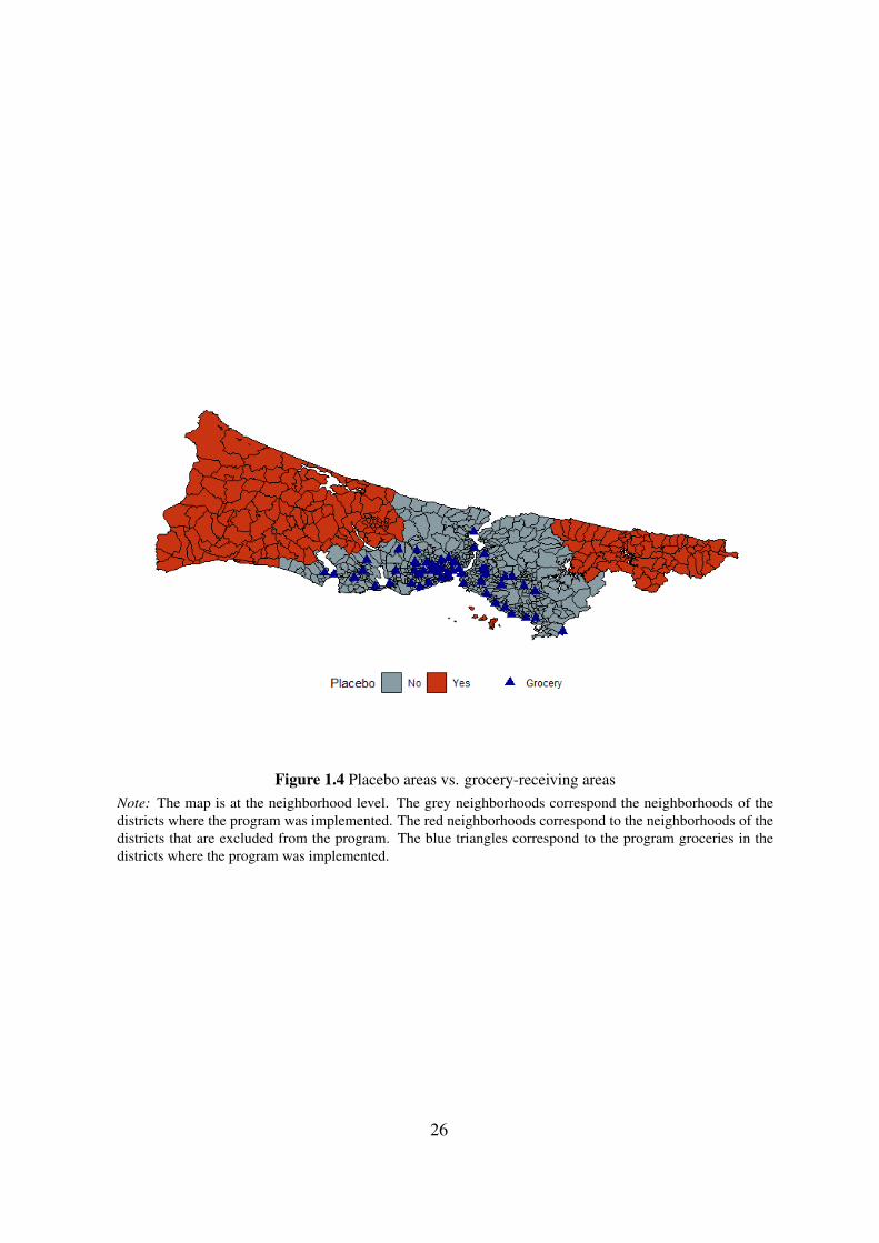
Figure 1.4 Placebo areas vs. grocery-receiving areasNote: The map is at the neighborhood level. The grey neighborhoods correspond the neighborhoods of thedistricts where the program was implemented. The red neighborhoods correspond to the neighborhoods of thedistricts that are excluded from the program. The blue triangles correspond to the program groceries in thedistricts where the program was implemented.

26

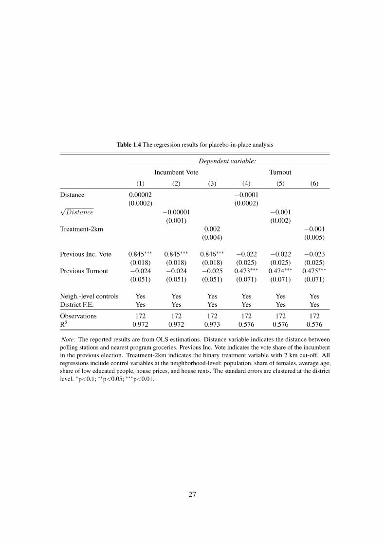
Table 1.4 The regression results for placebo-in-place analysis

Dependent variable:

Incumbent Vote Turnout

(1) (2) (3) (4) (5) (6)

Distance 0.00002 −0.0001(0.0002) (0.0002)√

Distance −0.00001 −0.001(0.001) (0.002)

Treatment-2km 0.002 −0.001(0.004) (0.005)

Previous Inc. Vote 0.845∗∗∗ 0.845∗∗∗ 0.846∗∗∗ −0.022 −0.022 −0.023(0.018) (0.018) (0.018) (0.025) (0.025) (0.025)

Previous Turnout −0.024 −0.024 −0.025 0.473∗∗∗ 0.474∗∗∗ 0.475∗∗∗

(0.051) (0.051) (0.051) (0.071) (0.071) (0.071)

Neigh.-level controls Yes Yes Yes Yes Yes YesDistrict F.E. Yes Yes Yes Yes Yes Yes

Observations 172 172 172 172 172 172R2 0.972 0.972 0.973 0.576 0.576 0.576

Note: The reported results are from OLS estimations. Distance variable indicates the distance betweenpolling stations and nearest program groceries. Previous Inc. Vote indicates the vote share of the incumbentin the previous election. Treatment-2km indicates the binary treatment variable with 2 km cut-off. Allregressions include control variables at the neighborhood-level: population, share of females, average age,share of low educated people, house prices, and house rents. The standard errors are clustered at the districtlevel. ∗p<0.1; ∗∗p<0.05; ∗∗∗p<0.01.

27

1.5 Partisan Conditioning

In this section I focus on the heterogeneous effects of the program conditional on partisanship.

All the estimates I have reported so far abstracted the analysis from the possibility of hetero-

geneous effects of the treatment conditional on partisanship. Yet, if the treatment affected

the incumbent vote share and turnout rates differentially conditional on partisanship, then

failing to account for this conditioning may obscure the important dynamics especially if the

mechanisms work in opposite directions for different partisan groups.

Accordingly, to investigate the heterogeneous effects of the treatment, I classify polling

stations into core incumbent, swing, and core opposition constituencies. This conceptualization

entails operationalization of core and swing voters at a level higher than the individual, based

on a margin of victory variable (Vaishnav and Sircar (2012)). Consequently, I define the

Margin of victory and Partisanship variables, for each polling station i based on the previous

election results as follows:

Margini = IncV ote_previ −OppV ote_previ

Partisanshipi =

Core Incumbent, if Margini ≥ 0.25

Swing, if −0.25 < Margini < 0.25

Core Opposition, if Margini ≤ −0.25

where OppV ote_previ correspond to the vote share of the main opposition party in the previous

election.

To estimate the heterogeneous effects of the treatment, I first sub-sample my data set based

on the Partisanshipi variable, which yields three data sets consisting of either only core

incumbent, or swing, or core opposition polling stations. I then estimate Equation (2.1) and

(1.2) separately on these three sub-samples, using the binary treatment variable with a 2 km

cut-off.

28

The results indicate that the effects of treatment on the incumbent vote share are heteroge-

neous over different types of constituencies, but are not countervailing. On the other hand, the

effect of treatment on turnout is positive in core incumbent constituencies, whereas negative in

core opposition constituencies. These effects cancel each other out and yield a null aggregate

effect on turnout when partisanship is not taken into account. Figure 1.5 reports the estimated

coefficients of treatment on both the incumbent vote share and turnout in three sub-samples of

the data set.23

In line with the baseline results, Part (a) in Figure 1.5 shows that the food subsidy program

affected the incumbent vote share positively in core incumbent and swing constituencies. The

treatment effect on the incumbent vote share in core opposition constituencies, although close

to the treatment effect in core incumbent constituencies in magnitude, has wider confidence

intervals.24 In sum, although the treatment has heterogeneous effects in terms of magnitude

over distinct partisan groups, these effects are not countervailing for the incumbent vote share.

Consequently, this implies that the estimates obtained from the baseline analysis give an

accurate estimate of the treatment effect on the incumbent vote share.

On the other hand, Part (b) in Figure 1.5 paints a very different picture for the effects

of treatment on turnout. First, we see that the treatment effect on turnout is negative and

statistically different than zero in core opposition constituencies. This indicates that in these

constituencies there is significant amount of turnout-buying, or to put it more accurately,

abstention-buying.25 Second, Part (b) also shows that the treatment did not affect turnout

in swing constituencies but it has a slightly positive significant effect on turnout in the core

incumbent sub-sample.

Taking these findings together, allowing heterogeneous effects of the treatment conditional

on partisanship yields a richer set of results that the baseline model cannot provide. In fact,

the baseline model obscures the effects of treatment on turnout by averaging the effect over

different partisan groups. The hereby reported countervailing effects are in line with Chen

23The regression tables underlying Figures 1.5 and 1.6 are presented in Table A.3.24The most likely reason for the wider confidence intervals is the relatively small number of polling stations

in core opposition sub-sample (296 polling stations) compared to the numbers of polling stations in other twosub-samples (588 polling stations in core opposition sub-sample, 691 polling stations in swing sub-sample).

25Abstention-buying –although named differently– is also reported in Adiguzel et al. (2019). They show that,when the walking time to the nearest family health center decreases in non-incumbent municipalities, turnoutrates decrease too. Nichter (2008) calls the suppression of opposition voters “negative vote buying", whereasChen (2013) calls it “abstention buying".

29

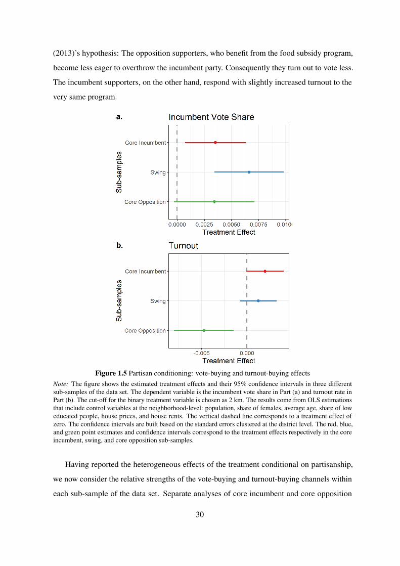
(2013)’s hypothesis: The opposition supporters, who benefit from the food subsidy program,

become less eager to overthrow the incumbent party. Consequently they turn out to vote less.

The incumbent supporters, on the other hand, respond with slightly increased turnout to the

very same program.

Figure 1.5 Partisan conditioning: vote-buying and turnout-buying effectsNote: The figure shows the estimated treatment effects and their 95% confidence intervals in three differentsub-samples of the data set. The dependent variable is the incumbent vote share in Part (a) and turnout rate inPart (b). The cut-off for the binary treatment variable is chosen as 2 km. The results come from OLS estimationsthat include control variables at the neighborhood-level: population, share of females, average age, share of loweducated people, house prices, and house rents. The vertical dashed line corresponds to a treatment effect ofzero. The confidence intervals are built based on the standard errors clustered at the district level. The red, blue,and green point estimates and confidence intervals correspond to the treatment effects respectively in the coreincumbent, swing, and core opposition sub-samples.

Having reported the heterogeneous effects of the treatment conditional on partisanship,

we now consider the relative strengths of the vote-buying and turnout-buying channels within

each sub-sample of the data set. Separate analyses of core incumbent and core opposition

30

constituencies allow us to identify the true turnout effects in each sample. This in turn facilitates

explaining how much of the change in the incumbent vote share can be attributed to the turnout-

or abstention-buying channel.26

In the swing constituencies, on the other hand, it is more difficult to obtain the true turnout

or abstention effect because both the turnout- and abstention-buying may be happening at

the same time and may cancel each other out. If this is the case, it implies that the estimated

turnout effect for the swing sub-sample is a conservative one. Moreover, we can expect to find

more vote switches in the swing sub-sample, which implies a stronger vote-buying channel.

Figure 1.6 shows the estimated coefficients of the treatment on the incumbent vote share

and turnout. Part (a) in Figure 1.6 shows that the strengths of the vote- and turnout-buying

channels are closer to each other in the core incumbent sub-sample than they are in the other

two sub-samples. This result in turn suggests that the increase in the incumbent vote share may

be mostly driven by the increase in turnout in the core incumbent sub-sample. In other words,

given that the core incumbent constituencies are composed of incumbent voters by definition,

the increase in the incumbent vote share indicates a mobilization of core supporters.

On the other hand, for the swing sub-sample, Part (b) in Figure 1.6 shows that the statisti-

cally significant channel is the vote-buying rather than the turnout channel. The reason for the

null effect on turnout may be countervailing effects of the treatment on turnout within the swing

sub-sample. Yet the greater discrepancy between the strengths of the vote-buying and turnout

channels in the swing sub-sample –compared to the discrepancy in the core incumbent and

core opposition sub-samples– can also be explained by the greater amount of vote switching in

the swing sub-sample.

Finally, Part (c) in Figure 1.6 shows that in the core opposition sub-sample, the effects of

treatment on the incumbent vote share and turnout are in opposite directions. This suggests

that, in core opposition constituencies, the increase in incumbent vote share is partly driven

by the decrease in the turnout rate of opposition supporters. This is, again, what I call

abstention-buying.

26Note that the separate analyses of core constituencies do not exclude the possibility of the incumbent sup-porters (in core incumbent constituencies) abstain or the opposition supporters (in core opposition constituencies)mobilize due to the food subsidy program. Yet these incidents are unlikely, and even if present, they would implya conservative estimate of the effect on turnout.

31

Figure 1.6 Partisan conditioning: vote-buying and turnout-buying effectsNote: The figure shows the estimated treatment effects and their 95% confidence intervals in three differentsub-samples of the data set. The dependent variables are the incumbent vote share and turnout. The cut-off for thebinary treatment variable is chosen as 2 km. Part (a) shows the treatment effects in the core incumbent sub-sample,Part (b) in the swing sub-sample, and Part (c) in the core opposition sub-sample. The results come from OLSestimations that include control variables at the neighborhood-level: population, share of females, average age,share of low educated people, house prices, and house rents. The vertical dashed line corresponds to a treatmenteffect of zero. The confidence intervals are built based on the standard errors clustered at the district level.The redand blue point estimates and confidence intervals correspond to the treatment effects on, respectively, incumbentvote share and turnout.

32

1.6 The Spatial Partisan Segregation

One aspect of local public goods that I have not touched upon so far is their spatial nature and

the consequent externalities (O’Keeffe-O’Donovan (2020)). The previous literature on the

spatial nature of local public goods have documented evidence for the effects of spatial ethnic

segregation on the targeting of such goods and on the electoral effects tied to them (Ichino et al.

(2018)). Yet, to the best of my knowledge, whether spatial partisan segregation conditions the

electoral returns of such goods have not been explored before.

Since local public goods such as the food subsidy program studied in this paper have

geographical catchment areas – within which the inhabitants have the opportunity to benefit

from the local public good –, it is difficult to target these goods to specific communities such as

co-partisans of the incumbent when the area includes partisans of different sides. These spatial

externalities, in turn, not only complicate and have implications on the allocation of these local

public goods, but they may also impact the electoral returns to the local public good provision.

In such catchment areas interactions between partisans of different groups, for example, can

have an effect on the electoral response. The food subsidy program studied here provides an

instance of such.

To explore this idea, I investigate whether the profile of partisan mix within catchment areas

influences the electoral returns to this local public good. To this end, I classify the catchment

areas of the program groceries into categories based on the average previous vote share of the

incumbent over polling stations within each catchment area. Note that this measure is at the

grocery level and a characteristic of the catchment area of a program grocery. Thus, it differs

from the measure of partisanship (Partisanshipi) at the polling station level. The first one,

an indicator of spatial partisan segregation, captures the effect of others’ partisanship on one’s

electoral response to the food subsidy program.

More specifically, I first calculate the weighted average of the previous incumbent vote

share over polling stations within each catchment area –weights being the number of voters

assigned to each polling station in 2018 presidential election. I denote this variable by

Catch_Inc. I then classify the catchment areas at the grocery level (g) into distinct groups

based on Catch_Inc as the following:

33

Catchment_areag =

Uniformly_Opposition, if Catch_Inci ≤ P25

Mixed, if P25 < Catch_Inci < P75

Uniformly_Incumbent, if Catch_Inci ≥ P75

where Pk means the k-th percentile of the Catch_Inci.

In order to test whether the partisan mix within the catchment area of a grocery impacts

the electoral returns, I interact the binary treatment variable with the Catchment_areag.

Accordingly, I estimate the following interaction models on core incumbent, swing, and core

opposition sub-samples:

IncV otei = β0 +β1 ·Treatmenti ∗Catchment_areag +β2 ·Xj (1.3)

+β3 · IncV ote_previ +β4 ·Turnout_previ + ϵi,

Turnouti = α0 +α1 ·Treatmenti ∗Catchment_areag +α2 ·Xj+ (1.4)

+α3 · IncV ote_previ +α4 ·Turnout_previ +ui.

Table 1.5 presents the results of the interaction models. These estimations, to a large extent,

are in line with the previous results, yet they help us further isolate the source of the reported

effects. In the core opposition sub-sample, for example, the treatment effect on the incumbent

vote share ceases to be statistically significant and instead the interaction of the treatment

with uniform opposition catchment area turns out to be statistically significant. This indicates

that treatment effect in core opposition sub-samples is exclusively coming from the polling

stations that are located in catchment areas which are uniformly composed of opposition voters.

The statistically significant treatment effect on turnout also disappears in the core opposition

sub-sample and does not appear in the interaction of treatment variable with uniform opposition

catchment area. Nevertheless, the coefficient of this interaction term has the same sign and is

34

also very similar in magnitude to the treatment effect on turnout that is reported in Part (b) in

Figure 1.5.

In the swing sub-sample, on the other hand, the treatment effect on the incumbent vote

share is stronger in uniform incumbent and uniform opposition catchment areas than it is

in the mixed catchment areas. The treatment effect on turnout is also more pronounced in

uniform catchment areas than it is in the mixed catchment areas. Finally, in the core incumbent

sub-sample, we see that the spatial partisan distribution does not play a role in the electoral

effects of the local food subsidy program.

These findings point out that, especially for swing and core opposition voters, catchment

areas that are uniformly composed of partisans of one side are more effective in generating

electoral returns. This, in turn, has important implications on the targeting strategies of

politicians when it comes to decide the allocation of local public goods. Although it is very

difficult two pin down the underlying mechanism behind, these results can be interpreted as an

outcome of the interaction between partisans of different sides. These interactions may have

the potential to further polarize the different partisan groups and lead them to have diverging

opinions on the local food subsidy program.27

Related to the interactions between different partisan groups, a potential mechanism

that can decrease the electoral returns in mixed catchment areas may be the fear of being

shamed and the resulting less usage of the program by swing and core opposition voters. These

mechanisms, however, are at best suggestive and it is not possible to document evidence in favor

of them without information on voting behavior at the individual level. Yet, the examination of

reasoning mechanisms of voters in their electoral response to a local public good provision, and

its partisan conditioning, can be taken up by future research as an interesting and promising

direction.

27Alesina et al. (2020) shows evidence of voters polarizing in response to the same factual information. Baysan(2019), on the other hand, documents an increase in polarization of voters in response to the same informationalcampaign in Turkey.

35

Table 1.5 Interaction of treatment variable with type of the catchment area in different sub-samples

Sub-sample: Core Incumbent Swing Core Opposition

Dependent variable: IncVote Turnout IncVote Turnout IncVote Turnout

(1) (2) (3) (4) (5) (6)

Treatment-2km 0.004∗ 0.001 0.004∗∗ 0.001 −0.001 −0.002(0.002) (0.002) (0.002) (0.001) (0.003) (0.003)

Treatment-2km × Catchment Area(Reference level: Mixed)

× Uniformly Incumbent 0.0002 0.002 0.008∗ 0.005∗

(0.003) (0.002) (0.005) (0.003)

× Uniformly Opposition −0.007 −0.008 0.007∗ −0.002 0.007∗ −0.005(0.007) (0.005) (0.004) (0.003) (0.004) (0.004)

Neigh.-level controls Yes Yes Yes Yes Yes YesDistrict F.E. Yes Yes Yes Yes Yes Yes

Observations 588 588 691 691 296 296R2 0.953 0.761 0.928 0.834 0.955 0.865

Note: The reported results are from OLS estimations. The dependent variables are the incumbent vote share and turnout. Catch-ment Area is at the grocery-level and is a categorical variable with three levels: Mixed, Uniformly Incumbent, and UniformlyOpposition. The reference level of this variable is Mixed. Treatment-2km variable indicates the binary treatment variable with 2km cut-off. The sub-samples are based on the polling station level previous incumbent vote share variable. All regressionscontrol for the polling-station level previous incumbent vote share and previous turnout, and also include control variables at theneighborhood-level: population, share of females, average age, share of low educated people, house prices, and house rents.The standard errors are clustered at the district level. ∗p<0.1; ∗∗p<0.05; ∗∗∗p<0.01.

36

1.7 Robustness Analysis

In this section I discuss the robustness of main results. In the first robustness test, I repeat the

partisan conditioning analysis with Distance variable and also with its square root, instead of

using the binary treatment variable. Figure A.3 and A.4 in the Appendix present the results of

these analyses.28 Although the estimated effects for both incumbent vote share and turnout

keep the ordinal ranking the same as in the previous analysis (see Figure 1.5), an important

difference with the previous analysis is that some of the estimated effects come closer to

zero. Nevertheless, this is most likely due to the uninformative –for our purposes– variation

in Distance variable. For example, once a voter is already too far away from the program

groceries, then going an extra kilometer further away should not make much of a difference

for her accessability to the program.

Indeed, taking the square root of Distance variable accounts for this non-linearity to some

extent and yields us estimates that are closer to what we obtain with binary treatment variable

(see Figure A.4). However, in overall, the distance variable and its square root are not good

measures of the accessability of voters to the program groceries, especially when the program

is expected to be effective within a very limited area.29

The second robustness test also concerns heterogeneous effects of the program conditional

on partisanship. The previous analysis have analyzed the heterogeneous effects by dividing our

data set to different sub-samples based on partisanship. Working with sub-samples however

implies smaller number of observations, and hence, less power to estimate the treatment effects.

Alternatively, I check whether the main results related to the heterogeneous effects replicate in

an alternative specification that makes use of interaction terms.

In this estimation, I interact the binary treatment variable with Partisanship variable. I

choose the Core Incumbent as the reference level of the categorical Partisanship variable. The

coefficients of treatment interaction terms with Swing and Core Opposition then correspond

28Notice that the sign of the treatment effects is the opposite of the treatment effects we report with binarytreatment. This is only because of the way binary treatment variable is constructed from continuous Distancevariable.

29The levels of statistical significance of the first three models in Table 1.3 also supports this argument. Thebinary treatment variable reaches the highest level of statistical significance whereas square root of distancecomes second, and distance variable itself comes third in terms of level of the statistical significance.

37

to their contrast with the reference level of Core Incumbent. Consequently, I estimate the

following two econometric specifications:

IncV otei = β0 +β1 ·Treatmenti ∗Partisanshipi +β2 ·Xj (1.5)

+β3 · IncV ote_previ +β4 ·Turnout_previ + ϵi,

Turnouti = α0 +α1 ·Treatmenti ∗Partisanshipi +α2 ·Xj+ (1.6)

+α3 · IncV ote_previ +α4 ·Turnout_previ +ui.

The results reported in Table A.5 indicate that the program has a significant positive effect

on the incumbent vote share with interaction terms turning out statistically insignificant. This

merely reflects the non-heterogeneous effects of treatment on incumbent vote share for different

partisan groups and is in line with the results of the previous analysis. Regarding the effects on

turnout, the results indicate that the program has a negative significant effect on turnout in core

opposition constituencies compared to core incumbent constituencies, which is also in line

with the findings of the previous analysis.

1.8 Conclusion

In this paper I study the electoral effects of a food subsidy program that aims to help people

in the wake of historically high food prices inflation. Using the variation in the accessability

of voters to the program groceries, I first estimate the causal effect of this program on voting

behavior. I then examine the distinct mechanisms through which we observe electoral effects

and also the factors that condition these effects.

The present paper makes several contributions to the literature. First, by showing that

the food subsidy program has a positive effect on the incumbent vote share, I contribute

causal evidence for the electoral effects of local public good provision by using a distinct

empirical strategy that allows me to quantify the accessability of voters to the local public

good in a precise manner. This finding can also be interpreted as a presence of pocketbook

considerations in voting behavior. Although pocketbook considerations in economic voting

38

fit the theoretical political economy literature better than socio-tropic considerations do, the

survey-based empirical literature has largely concluded that the predominant type of economic

voting is socio-tropic. Nevertheless, an emerging strand of work has recently started to

document evidence of pocketbook economic voting. The present paper contributes further

evidence to this reviving literature.

Second, as an important aspect of the economic voting, I examine the distinct mechanisms

through which we observe the electoral effects of local public good provision. The previous

literature have identified two such channels: the vote-buying and turnout-buying channels. The

previous literature, however, mostly focused on the vote-buying channel and overlooked the

turnout-buying. The second contribution of this paper is thus related to the turnout-buying

channel. I document that the vote-buying and turnout-buying channels co-exist, and that the

turnout channel is at least as important as the vote-buying channel.

Additionally, I show how partisanship conditions the working of vote-buying and turnout-

buying channels. By analyzing core incumbent, swing, and core opposition voters separately, I

show that the turnout effects are heterogeneous and countervailing. Averaging treatment effects

mask these conditional effects and lead us to underestimate the strength of turnout-buying

channel.

Lastly, I document how the spatial distribution of partisan groups may influence the

electoral effects of local public good provision. The previous literature have documented

evidence for the role of spatial ethnic segregation on the electoral effects of local public goods.

Yet, the role of spatial partisan segregation has not been explored. I contribute to this literature

by showing that most of the electoral responses to the local public good come from the uniform

areas in terms of partisanship rather than areas that are composed of partisans of different

sides.

To conclude, the food subsidy program failed in granting an electoral victory to the

incumbent party. It could however easily have changed the election outcome given that the

estimated effects are very close to the margin of victory. We learn from this program that

pocketbook considerations play an important role in economic voting. Moreover, we obtain

evidence in favor of the turnout channel being as important as the vote-buying channel in

generating electoral gains. Finally, we gain insights on how partisanship and the spatial

distribution of partisans may condition the effects of the program.

39

2Class Distinctiveness & Class Voting

2.1 Introduction

In the wake of rising extremism and unprecedented populist surge, the discussion of social

classes seems to have returned to the discussion of politics. One implication of this recent

trend is that it is now even more important to understand the relationship between classes

and vote choices of people. Accordingly, the recent political events such as Brexit, Donald

Trump’s victory in the 2016 US presidential election, and AfD’s recent entry into German

parliament have been argued to be related to class politics (Guiso et al. (2017)). Other research

suggests that the preferences of the working class has become better aligned with those of

far-right parties (Oesch and Rennwald (2018), Spies (2013)). These evidences suggest that the

classes still plays an important role in today’s politics. To this end, a useful concept to gauge

the relationship between social classes and vote choices of people has been the class voting.

Arzheimer et al. (2016) define class voting as the tendency of individuals in a given social

class to vote for a particular political party rather than the alternatives compared to voters in

other classes. Although much debated concepts due to problems in conceptualization and

measurement, both class and class voting have received substantial attention from the scholarly

world. Several studies have attempted to measure the changes in the class-vote relationship

40

over time (e.g., Evans (2000), Evans (1999)). More recent studies on class voting, on the

other hand, also focus on the mechanisms that cause variations in the extent of class voting

across countries and over time (Jansen et al. (2013), Evans and Tilley (2012a), Evans and

Tilley (2012b)). One of these mechanisms is the blurring class divisions in terms of economic

preferences as a driving force of the class voting. Nevertheless, although widely accepted, no

empirical evidence has yet been presented for neither the blurring of class divisions nor its

relationship with class voting. I, therefore, first develop a measure that captures the extent of

class divisions in economic preferences and test whether blurring of divisions has taken place.

Second, I demonstrate the statistical relationship between the class distinctiveness in economic

preferences and class voting.

The previous literature on class voting has put forward two main explanations for the

variations in class voting: supply side and demand side explanations. The supply side concerns

the range of political choices that are offered by political parties to voters. The main hypothesis

of this approach is that, if parties offer similar policies on the economic dimension, then

voters are less likely to base their voting decisions on their class memberships. The common

underlying assumption in these studies is the responsiveness of voters to party programs. This

implies the following: if voters are responsive to party programs but are not represented by

these programs in terms of economic policy preferences, this results in a weakened class voting.

Studies in this strand of literature commonly measure party polarization on the economic

dimension over time using the Manifesto Project or expert surveys. They test whether the

convergence or polarization in the economic dimension is associated with the strength of class

voting. Evans and Tilley (2012a), Evans and Tilley (2012b) provide evidence from Great

Britain in favor of this hypothesis. Evans and De Graaf (2013) study the same matter in a

cross-national perspective. In this article, I do not focus on this supply side argument, which is

already well-established.

The demand side approach, on the other hand, concerns the class structure of society

and political preferences of distinct classes. The main hypothesis here is that when the class

structure becomes more diffused, or in other words when classes become less distinct in terms

of their economic preferences, we should expect to observe that the voting choices are less

based on class membership. Throughout this paper, I use the term class distinctiveness to

refer to the extent to which once can distinguish between classes in terms of their economic

41

preferences. Therefore, the blurring of class divisions means a smaller value of the class

distinctiveness measure.

The hypothesis of blurring of class divisions is not new. Early studies such as Inglehart

and Rabier (1986) and Clark and Lipset (1991) have already announced the death of class as

being of interest in the study of electoral politics. The diffusion of class structure and blurring

of class divisions in economic preferences are usually thought to arise from the transition to

a post-industrial society with more educated people, higher living standards and more social

mobility (Arzheimer et al. (2016)). This hypothesis also appears in more recent studies, and

also has managed to make its way to the standard comparative politics textbook Citizen Politics

by Dalton (2013).

Although it has been put forward in several studies, to the best of my knowledge no

empirical evidence has yet been presented on either the blurring of class divisions or on the

nature of the relationship between class divisions and class voting. The only study that provides

evidence on this issue is Evans and Tilley (2017), who show that class distinctiveness is stable

over time for Britain. Along these lines, Evans and Tilley (2012a) point out this gap in the

literature: “Conclusions concerning the impact of blurring and fracturing of the class structure

on political choice have usually been inferred, retrospectively, from an observed decline in

class voting, rather than measured independently and then used to account for such declines.

[...] We did not, however, test directly whether a decline in the effects of class position on

values and preferences can account for a decline in the effect of class on party choice."

In this paper, I fill this gap in the class voting literature by studying whether changes in

class distinctiveness in terms of economic preferences can account for the variation in the

strength of class-vote linkage over time in a comparative perspective. Class distinctiveness

measure, however, is not readily available in standard survey data. For creating such a measure,

I adapt the empirical framework of Bertrand and Kamenica (2018) to my setting. They utilize

a simple idea from predictive modeling, which is to use the ability to infer a person’s true

cultural identity from her preferences as a measure of the extent to which one can distinguish

between cultural identities. I discuss the adaption of this method to current setting and its

execution in detail in Section 2.3.

The method I adopt does not only produce a measure that reflects the extent to which classes

are distinct from each other in terms of economic preferences, but also allows a comparison

42

of this measure across countries and over time. Moreover, the method is scale-able and can

also be implemented with any prediction model. Although I work with a limited number of

explanatory variables in this study, this can be increased in other settings. The scale-ability is a

powerful feature because it enables inferences otherwise impossible in settings where a large

number of explanatory variables are available.

In this study, I limit the preference space -in which the class divisions lie- to economic

preferences rather than using all sorts of political preferences mainly for two reasons.1 First,

in class voting literature, class is commonly defined based on occupation one holds and the

implications of occupation in terms of economic interests. It is then natural to expect that any

clustering of preferences within classes should primarily occur within the realm of economic

preferences. A second common practice in class voting literature is to use political parties’

economic left-right positioning rather than general left-right positions. This is because the left

and right are well-defined on the economic dimension, whereas general left-right positions

conflate the positions taken in the economic and cultural dimension by political parties.

The rest of the paper proceeds as follows: Section 2.2 introduces the data sets, the opera-

tionalizations of class variable and party positions, and finally hypotheses to be empirically

tested. Section 2.3 lays out the methodology for the computation of class distinctiveness

measure. Section 3.5 discusses the main results of the paper. Section 2.5 concludes.

2.2 Data & Operationalization

In this study I combine two different data sets. I first obtain individual level information on

occupation, economic policy preferences, party choices, and demographic status from the

The European Values Survey (EVS) data set, which is described in detail in the next section,

provides this information. Second I obtain the economic left-right positions of political parties

from the Manifesto Project, which is described in Section 2.2.2 below. I then match these two

data sets based on the reported party choice of individual in the EVS data set. The hypotheses

that are put to an empirical test are explained in Section 2.2.3.

1The other two sets of political preferences are grid and group dimensions as described by Kitschelt and Rehm(2014), corresponding to preferences related to governance and polity membership, respectively. Measuring theclass distinctiveness in terms of these two sets of preferences might be also interesting and promising in thestudy of class voting. It might especially shed some light on the evolution of the salience of different politicaldimensions, which is also closely related to class voting. It is, however, beyond the scope of this paper.

43

2.2.1 Micro-level Survey Data

The European Values Study (EVS) survey is one of the richest data sources for individual level

data on economic preferences, political attitudes and party choices. It covers a large number

of European countries and includes four waves that were carried out in years 1981-1983,

1990-1993, 1999-2001, and 2008-2010. This survey data also includes socio-economic and

demographic information of the respondents such as income, occupation, education, age, and

gender. I use the last three waves of the EVS due to the missingness of some key variables in

the 1981-1983 wave. The countries included in my sample are Austria, Belgium, Bulgaria,

Czech Republic, Germany, Denmark, Spain, France, Great Britain, Hungary, Ireland, Italy,

Netherlands, Poland, Portugal, Sweden, Slovenia, and Slovakia.

A major advantage of the EVS data is that it is a harmonized dataset. The same core

questions are asked in all countries and in all waves with the same wording.2 This enables

truthful comparisons between countries and across time, which is not always the case for survey

data sets, for example, when combining the national election studies of different countries

(Boxell et al. (2020)).

In particular, I include the following variables from the EVS to measure class distinctiveness

and the class-vote linkage: attitude towards government responsibility, choice over freedom or

equality, confidence in labour unions, party choice, occupation, age, gender, and education.

The party choice variable is the key variable that enables a connection between the EVS and

Manifesto Project data, which is the dataset containing political parties’ policy stances on a

number of issues. For each country in each wave in the sample, I match the individual EVS

data to the parties encoded in the Manifesto Project based on the party choice variable in the

EVS.

A second advantage of the EVS data set is that the occupation variable is encoded according

to the International Standard Classification of Occupations (ISCO), and hence it is convertible

to the Erikson-Goldthorpe class schema (EGP) (Erikson and Goldthorpe (1992), Ganzeboom

and Treiman (1996)). The EGP classification of the occupation is the dependent variable of the

analysis that deals with the measurement of class distinctiveness.

2The exact wording of the questions and response scales of the EVS variables are given in Appendix B.

44

The Erikson-Goldthorpe classification is constructed based on occupations and according

to the characteristics of occupations. It classifies occupations into social classes by considering

dimensions such as job security, level of earnings and the way they are earned, promotion

prospects, autonomy at work, and working conditions. Evans and Tilley (2017) note that the

EGP class schema has been “consistently shown to be related to differences in employment

conditions, job autonomy, income, and life-time expected earnings". The EGP has also been

adopted in the National Statistics Socio-economic Classification used in the U.K. Census (Rose

and Pevalin (2002)).

For statistical power concerns, I use the four-class version of the EGP in the same spirit as

Jansen et al. (2013) rather than the versions with larger number of classes.3 The four classes

I arrive at are the service class, the routine non-manual working class, the self-employed,

and the manual working class (or, just working class as a shorthand). The share of classes

within each country at each time point is given in the Appendix B.4 As an example, the typical

occupations in these four classes are as follows: Office managers, business professionals,

health professionals, legal professionals in the service class. Clerks, sales persons in the routine

non-manual working class. Small entrepreneurs, own account workers in the self-employed

class. Machine operators, craft workers in the manual working class.

2.2.2 Party Positions

I use the Manifesto Project data to retrieve the economic left-right positions of political parties.

The unit of observation in this data set is a political party, belonging to a specific country and

election year.

The Manifesto Project uses text analysis methods to derive the policy positions of political

parties from their election manifesto. Using this method party positions are generated for

more than 50 countries and from 1945 up to date. The data set includes a large number of

policy issue categories such as freedom and democracy, political system, economy, welfare,

and quality of life. The reported numbers for the variables in each category, however, are not

the positions of parties on these issues but the emphases that parties put on that issue in their

3The eleven-class full version of EGP and its conversion into a four-class version is provided in Appendix B.4The heterogeneity of classes in terms of their economic preferences and descriptive statistics of these variables

are also reported in the Appendix B.

45

Table 2.1 Variables from the Manifesto Project

Left Emphases Right Emphasesregulate capitalism free enterpriseeconomic planning economic incentivespro-protectionism anti-protectionism

social services expansion social services limitationeducation expansion economic orthodoxy: positive

nationalization labour groups: negativecontrolled economy

labour groups: positivecorporatism: positive

Keynesian demand management:positive

Marxist analysis: positivesocial justice

Note: The table shows the variables that are used in Bakker and Hobolt (2013) tocalculate economic left-right positions of political parties. Left emphases refer toleft-wing economic policy emphases as a share of total emphases in a party manifesto.Similarly, right emphases refer to right-wing economic policy emphases as a share oftotal emphases in a party manifesto.

manifesto. The Manifesto Project, therefore, does not provide a readily available measure of

economic left-right positions of parties.

In order to create such a measure, I choose the variables that have been identified as useful

in the calculation of positions on an economic dimension by Bakker and Hobolt (2013). This

implies calculating the ‘right’ and ‘left’ emphases of each party. The difference then is simply

the position of a party on the economic dimension. Left-emphases (right-emphases) of a party

therefore can be minimum zero if it does not mention left-wing (right-wing) economic issues

at all in its manifesto, and 1 if it only mentions left-wing (right-wing) economic issues. The

variables used for the calculation of party positions on the economic dimension are listed in

Table 2.1.

The emphases profiles of parties across countries may vary to a large extent due to country-

specific factors such as the party system. For example, it could be that in country A the

economic left-right positions of parties (the difference between right-emphases and left-

emphases) ranges from -1 to +1, whereas in country B it ranges from -0.5 to +0.5. These

positionings, however, do not necessarily mean that the party with -1 (+1) economic position

in country A is more left (right) than the party with -0.5 (+0.5) economic position. Such a

conclusion requires a more in-depth comparison of these two countries in many aspects. To

46

refrain from such hefty arguments and since our unit of observation is at the country-year

level, I opt for considering only the ranking of parties on economic dimension within a country

for a given year, but not relative to the positions of parties in other countries. Accordingly, I

standardize party positions within a country-year.

I finally match the Manifesto Project data set with the EVS data set by political party and

year. For each political party reported as a response to party choice variable in the EVS data

set, the closest election year available for that party in the Manifesto Project is chosen for

matching purposes.

2.2.3 The Hypotheses

In this study I test two main hypotheses. Both hypotheses have been put forward in previous

scholarship, however, have not been empirically tested. I first test whether blurring of class

divisions (in economic preferences) have taken place by using the relationship between class

membership of respondents and their economic preferences. I then measure the extent of class

voting by using the relationship between class membership of respondents and their party

choices. A graph of this operationalization is given in Figure 2.1 below.

Figure 2.1 The blurring of class divisions is measured by how good class membership predicts economicpreferences. The class voting is measured by the strength of statistical relationship between classmembership and class voting.

Accordingly, the first hypothesis concerns the development of distinctiveness of classes in

terms of their economic preferences over time:

47

H1: Classes have become less distinct in terms of their economic preferences over time.

This first hypothesis exclusively concerns the development of class distinctiveness over

time, and it is silent on the relationship between class distinctiveness and class voting. In order

to shed light on the nature of this relationship, I also test the following hypothesis:

H2: The strength of class voting is positively related to the class distinctiveness. In other

words; the more distinct the classes are, the stronger is class voting.

An alternative operating channel in Figure 2.1 may be the preference formation by political

parties. This would correspond to an arrow from party choice to economic preferences in

Figure 2.1. Nevertheless, recent works show that the core values –such as the economic

preferences studied in this paper– are either more stable or at least as stable as partisanship

(Evans and Neundorf (2018), Ansolabehere et al. (2008)).

2.3 Measuring Class Distinctiveness

The empirical strategy that is underlying the computation of a class distinctiveness measure

originates from the study of Gentzkow et al. (2018), where they examine the extent of parti-

sanship in the U.S. Congress. To derive such a measure, they use the texts of congressional

speeches from 1873 to 2016. They define the partisanship of a speech in a given session as

the predictability of the speaker’s party from a single utterance. This implies that if speakers

from different parties use more distinct phrases in their speeches, the predictability of party

membership increases and thus indicates a session with higher partisanship. A similar study,

by Peterson and Spirling (2018), exploits the same idea and derives a polarization index for

British politics using the speeches in the House of Commons.

An application by Bertrand and Kamenica (2018) is perhaps the most similar one to the

current study in terms of the way that the prediction accuracy is used as a substantial quantity

of interest. In that study, they simply predict an individual’s group membership within income

categories, education levels, gender, race, or political ideology; from either their media usage,

consumption patterns, time usage, or social attitudes. The main statistical apparatus here is

48

that the higher the predictability of group membership from –for example– media usage is, the

more distinct are the groups in their media usage.

In this study, I define class distinctiveness as the ease with which one can infer the class

membership of a respondent solely from his or her economic preferences. This amounts

to a classification problem with the dependent variable –class membership– being a binary

variable for measuring pairwise class distinctiveness and a categorical variable with four levels

for measuring overall class distinctiveness. The explanatory variables (predictors) are the

economic preferences that are listed in Section 2.2.1. To obtain pairwise and overall class

distinctiveness measures quantitatively, I use logistic and multinomial logistic regressions,

respectively for pairwise class distinctiveness and overal class distinctiveness. The following

specification is used in all predictions for each country in each wave:

Classi = α1 ·Govt_Respi +α2 ·Free_or_Eqi +α3 ·Conf_Unioni, (2.1)

where Classi is the class membership of individual i. Govt_Respi, Free_or_Eqi and

Conf_Unioni correspond to the economic preferences of individual i for, respectively,

government responsibility, the choice of freedom or equality, and confidence in labour unions.

Let us illustrate how the proposed method works with a simple example. Suppose that

we have three classes that are class A, B, and C, each with same number of people in our

hypothetical society at a given time. Suppose also, for illustration purposes, that there is only

one economic preference, which can take three values that are P1, P2, and P3. Let us first work

out the extreme cases. Suppose that each class is homogeneous in its economic preference

within itself and different than other classes. For example, everyone in class A favors P1,

everyone in class B favors P2, and everyone in class C favors P3. This is the case when class

distinctiveness is highest. Suppose now that we need to predict the class membership of a

person whose economic preference we already know. In this case, we would immediately tell

that this person is from class A if she favors P1, from class B if she favors P2, and from class

C if she favors P3. Accordingly our prediction accuracy rate would also be high, as is class

distinctiveness. This is the perfect predictability and highest class distinctiveness case.

49

On the other extreme, suppose that each class has the same composition of economic

preferences. For example; 20% of class A favors P1, 30% favors P2, and 50% favors P3.

Suppose that this is also true for class B and C. Let us try again to predict the class membership

of someone whose economic preference we already know. Notice that we do not have much

predictive ability in this case, since this person may be in any class with equal probabilities.

Therefore, our predictive performance would be as good as assigning people randomly into

classes. This is the case when class distinctiveness is lowest and prediction accuracy is very

close to performance of a random allocation. For all the other values of class distinctiveness

between its highest and lowest cases, the prediction accuracy rate takes values between the

perfect predictability and random assignment case.

To implement this idea, for each country in each wave, I first partition the data for a given

country-year randomly into training and testing sets such that the training set constitutes 70%

and the testing set constitutes the remaining 30% of the country-year sample. I then estimate

Eq.2.1 for every country-year in the data set with the training set data. The testing set data are

reserved for out-of-sample predictions. The class membership of the respondents in the testing

set data is predicted with the estimated models and compared to the true class membership of

these respondents. This process leaves us with both predicted and true class membership of the

respondents in the testing set data. The prediction accuracy is then defined as the percentage

of correctly classified respondents. This number represents “the ease with which one can infer

the class membership of a respondent solely from his or her economic preferences." In short,

the obtained prediction accuracy rates serve as the class distinctiveness measure. The higher

the predictability is, the higher is class distinctiveness.

I use multinomial logistic regression predictions to obtain the overall class distinctiveness

measure –that is how distinct the four classes are in terms of their economic preferences–,

whereas I use binary logistic regressions to obtain the pair-wise class distinctiveness measure

–that is how distinct a given class is from the working class in terms of economic preferences.

Note that the predictions could also be made by using more sophisticated prediction

algorithms such as regression tree or random forest. Indeed Bertrand and Kamenica (2018)

employ three different prediction algorithms and also use the ensemble of these to increase

the predictive performance. The more sophisticated prediction algorithms and their ensembles

result in better predictions in general (Varian (2014)). The level of prediction accuracy,

50

however, is not the quantity of interest per se in this study. What is of interest is the variation

in prediction accuracy rates across time and space. Consequently, this requires prediction

accuracy rates being comparable across waves and countries.

A problem, that might hinder such a comparison, one could think of is the changing

compositions of classes over time. For example, if a certain class becomes more populated

by female respondents over time and if female respondents are somehow characterized by

relatively left-wing economic preferences compared to males, this class will emerge as more

left over time. Importantly however, this change in the compositions of and (consequently) in

the preferences of classes is not something that I want to exclude or to control for, instead it is

a part of what I intend to capture. This is because the blurring of class divisions hypothesis

encompasses such changes in the composition of classes and consequently in their preferences.

Therefore, in the context of this study, the changing composition of classes does not pose a

threat for comparability.

A concern that might pose a threat for comparability, however, is the imbalanced nature of

the data. The classes in the country-year samples do not constitute equal shares of the sample

with severe imbalances in the number of observations belonging to each class. Moreover,

the sample sizes of country-year data also exhibit a variation between countries and across

time, posing another threat for the comparability of prediction accuracy rates. Consequently,

a country-year sample with more observations than others is more likely to yield different

prediction accuracy rates just because it is trained with more data. This should, of course, be

avoided to enable a truthful comparison.

To illustrate the impact of imbalance problem, suppose that we try to predict a binary

class variable with levels A and B with some predictors. Assume that the data set consists of

imbalanced classes: Class A has a very low proportion, say 10%, as compared to class B in the

sample. In such case, a classifier such as logistic regression might find it optimal to classify

everything into class B since doing so implies a 90% prediction accuracy and the classifier’s

job is to maximize the prediction accuracy. As a consequence, the model does actually a poor

job in predicting the class membership, yet, yields a high predictive accuracy rate. It classifies

all observations belonging to class A incorrectly to class B. Therefore, it cannot reflect the true

underlying class distinctiveness of the sample. Below I explain how I mitigate this imbalance

51

problem.

Imbalance Problem. There exists several ways of dealing with the imbalance problem

(Kuhn and Johnson (2013)). One of the simplest ways is to tune the model such that it optimizes

the prediction accuracy of the minority class that is called the sensitivity. This method uses

a different optimization criterion: it maximizes the prediction accuracy of the minority class

rather than the overall prediction accuracy. An alternative method is simply to change cutoffs

(for the class membership variable) so that the same prediction model results in different

prediction accuracy rates and sensitivity. This method does not change the prediction model

per se, but post-processes the already predicted values. Neither of them, however, ensures

the comparability of prediction accuracy rates across time and space, which is of crucial

importance for our purposes in this study. The variation in the sample sizes across countries

and years remains a problem for both methods.

A more convenient way of dealing with the imbalance problem for the purposes of this

study might be using case weights. This involves putting more weight on the observations

of minority class(es), for example, by duplicating some observations in the minority class.

Although this method solves the problem of class imbalance, the variation in the sample sizes

across countries and years is still a problem.

An alternative approach that solves both the imbalances in class size and also in sample

sizes of different country-year data is the re-sampling method. This entails either up-sampling

the minority class or down-sampling the majority class (or both at the same time). By using

up-sampling and down-sampling together, it is possible to balance both class sizes and sample

sizes of country-year data, both across time and space. Up-sampling does not increase the

information contained in the data but only puts more weight on the minority class (Chen et al.

(2004)). On the other hand, since we repeat the re-sampling process for a large number of

times, the effect of down-sampling on the representativeness is mitigated too.

Consequently, to balance class sizes I determine a class size k, which is same for each class.

This amounts to total sample size of 4 ∗ k for the multinomial logistic regressions and 2 ∗ k

for the logistic regressions with binary dependent variable. The re-sampling process entails

up-sampling of classes that have sample size smaller than k and down-sampling of classes

that have sample size larger than k. I choose the class size k = 100 (the average class size in

52

our sample is 300, 234, and 409, respectively for years 1990, 1999, and 2008).5 Note that the

sample sizes of country-years are also balanced by fixing the class sizes.

The sampling process of each class is repeated 500 times. Each round of draws from

classes constitutes a country-year sample. A logistic or multinomial logistic regression has

thus been estimated for each country-year sample for 500 times. The prediction accuracy

rates obtained from these regressions are averaged over the draws to obtain a final prediction

accuracy for each country-year. This procedure enables a meaningful comparison of prediction

accuracy rates across countries and over time since the class sizes and sample sizes no longer

idiosyncratically affect the prediction accuracy. A schema illustrating the re-sampling process

for the regressions with four classes is provided in Figure B.1. The re-sampling process for the

regressions with binary class variable is analogous to that.

2.4 Results

In what follows I first provide an empirical validation for the class distinctiveness measure that

is developed in the previous section. I them test the blurring of class division hypothesis and

its relationship with class voting.

2.4.1 Validation of the Class Distinctiveness Measure

Although similar measures have been developed for studying the evolution of cultural dif-

ferences between distinct groups (Bertrand and Kamenica (2018)), the class distinctiveness

measure used in this study is an innovative measure in the study of electoral politics. I therefore

find it useful to provide some evidence to demonstrate its validity.

To this end, although it is not the primary goal of this paper to explain cross-country

variations of class distinctiveness, I first provide some supporting evidence from the structure

of political competition across countries. This aims to ensure that the cross-country pattern

of class distinctiveness measure is in line with the established findings in electoral politics.

Second, I look at pairwise class distinctiveness and show that the class distinctiveness

measure reflects the expected differences between certain classes. Lastly, I argue that class5I, however, also experiment with k = 50 and 200 to show that the results are robust to class size choice. The

correlations between the results of these experiments are given in the Appendix B. The results with class sizesk = 50 and 200 are very similar to those with class size k = 100.

53

distinctiveness pattern over time for Great Britain runs parallel to the class differences trends

reported by Evans and Tilley (2017). These validation strategies are discussed in detail below.

Political cleavage structures. According to Rokkan, there are two revolutions that have

set the cleavage structure on which political competition takes place. The industrial revolution

has led to the emergence of an economic dimension, while the French Revolution has led to

nation-state building and the state-church conflict, and hence the emergence of a non-economic

cultural dimension. These are the main reasons why today’s political competition takes place

mostly on these two dimensions –economic and cultural. Manow et al. (2018) elaborate these

arguments in detail and link the historically rooted cleavage structures of political competition

to different types of welfare regimes by providing supporting empirical evidence.

The four types of welfare regimes described in Manow et al. (2018) are the northern, liberal

Anglo-Saxon, continental and southern types. The southern type is added to the well-known

Esping-Andersen welfare regime type classification (see Esping-Andersen (2013)) by Manow

et al. (2018). Among the European countries: Denmark, Finland, and Sweden belong to the

northern type; Ireland and the United Kingdom to the liberal Anglo-Saxon type; Austria,

Belgium, Germany, France, and the Netherlands to the continental type; finally Greece, Italy,

Portugal, and Spain belong to the southern type. Here I provide neither a comprehensive review

of the differences between these welfare regimes nor of the underlying reasons (for this, see,

Polk and Rovny (2016)). I, however, do provide some key features of these welfare regimes

that can be linked to the class distinctiveness in economic preferences.

First of all, the northern type of welfare regime have not experienced a church-state conflict.

The political competition therefore has been taking place mostly on the economic dimension

in countries belonging to this group, whereas the cultural dimension is less salient. Second, in

the continental type of welfare regime, the state-church conflict is more pronounced compared

to the northern type regime, leading both economic and cultural dimensions to be salient in the

political competition. Manow et al. (2018), however, notably states that, although belonging to

the continental type, “France resembles the southern type in many respects."

Third, the southern type of welfare regime is characterized by its relatively more salient

cultural dimension compared to the economic dimension, due to the historical state-church

54

conflict. Fourth, the Anglo-Saxon model has an economic dimension more salient than cultural

dimension.

To sum up, in the light of the evidence provided by Polk and Rovny (2016) and Manow

et al. (2018), we expect to see that political competition is oriented more towards economic

issues in the countries belonging to the northern type. We also expect to see that it is oriented

more towards cultural issues in the countries belonging to the southern type, and possibly

in France. This also implies that we should expect more class distinctiveness in northern

types -since class distinctiveness is defined in terms of economic preferences- and less class

distinctiveness in southern types.

Figure 2.2 shows the averages (over three points in time) of the class distinctiveness

measure for the countries whose welfare regime type we know thanks to Manow et al. (2018).

Although the class distinctiveness measure shows only limited variation across countries, they

are in line with expected pattern described above. Northern type countries such as Denmark

and Sweden show the highest class distinctiveness, whereas southern type countries such as

Portugal, Spain and Italy have the lowest class distinctiveness. Moreover France, although

classified as a continental type welfare regime, is very close to the southern type, as noted by

Polk and Rovny (2016).

The continental and liberal Anglo-Saxon type countries take positions in between, except

Ireland, which is the only country that does not fit the suggested pattern. One reason for the

observed pattern for Ireland may be the state-church conflict, since a large part of Ireland’s

population is Roman Catholic. Considering that the state-church conflict (and consequently

emergence of a salient cultural dimension) was more pronounced in countries where the

Catholic Church (instead of the Protestant churches) was more influential, the case of Ireland is

not very surprising (Manow (2008)). All in all, I believe that Figure 2.2 grants some credibility

to the class distinctiveness measure developed in the previous section.

Before moving to the next validation argument, let us make clear why the magnitudes of

class distinctiveness measure, in other words prediction accuracy rates, are so low. Figure 2.2

reports that prediction accuracy rates range between 28% and 35%. The main reason for low

prediction accuracy rates is that I include only a few variables (three variables that measure

economic preferences) as explanatory variables in the predictions.

55

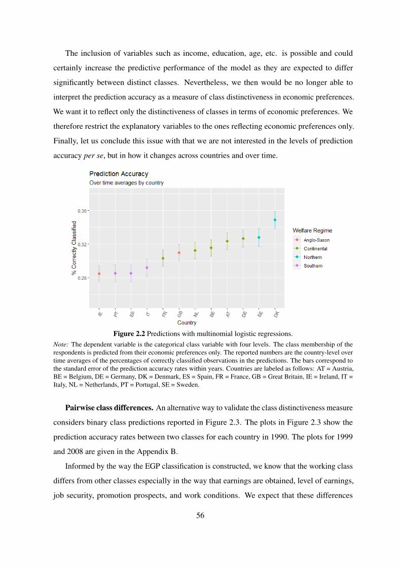
The inclusion of variables such as income, education, age, etc. is possible and could

certainly increase the predictive performance of the model as they are expected to differ

significantly between distinct classes. Nevertheless, we then would be no longer able to

interpret the prediction accuracy as a measure of class distinctiveness in economic preferences.

We want it to reflect only the distinctiveness of classes in terms of economic preferences. We

therefore restrict the explanatory variables to the ones reflecting economic preferences only.

Finally, let us conclude this issue with that we are not interested in the levels of prediction

accuracy per se, but in how it changes across countries and over time.

Figure 2.2 Predictions with multinomial logistic regressions.Note: The dependent variable is the categorical class variable with four levels. The class membership of therespondents is predicted from their economic preferences only. The reported numbers are the country-level overtime averages of the percentages of correctly classified observations in the predictions. The bars correspond tothe standard error of the prediction accuracy rates within years. Countries are labeled as follows: AT = Austria,BE = Belgium, DE = Germany, DK = Denmark, ES = Spain, FR = France, GB = Great Britain, IE = Ireland, IT =Italy, NL = Netherlands, PT = Portugal, SE = Sweden.

Pairwise class differences. An alternative way to validate the class distinctiveness measure

considers binary class predictions reported in Figure 2.3. The plots in Figure 2.3 show the

prediction accuracy rates between two classes for each country in 1990. The plots for 1999

and 2008 are given in the Appendix B.

Informed by the way the EGP classification is constructed, we know that the working class

differs from other classes especially in the way that earnings are obtained, level of earnings,

job security, promotion prospects, and work conditions. We expect that these differences

56

in the characteristics of occupations also reveal themselves as differences in the economic

preferences of these occupations. For example, working class people work in less secure jobs

and in worse working conditions with lower earnings and low promotion prospects.

The service class, on the other hand, has better terms in all these respects. The self-

employed are expected to have right-wing economic preferences (Arzheimer and Carter (2006),

Lubbers et al. (2002), Lubbers and Scheepers (2001)). Finally, the routine non-manual class is

expected to be more similar to the working class in terms of economic preferences than the

other two classes are. This is because the routine non-manual class constitutes the lower tail of

the middle class and actually it is also called “routine white collar workers" (Evans and Tilley

(2017)).

Figure 2.3 confirms these expectations. Part (a) and (c) indeed show higher prediction

accuracy rates on average, in other words higher class distinctiveness, compared to the Part (b),

which shows the relative class distinctiveness between the working class and the routine non-

manual class. We observe the same patterns in 1999 and 2008 (see the appendix). The means

of the prediction accuracy rates reported in Part (a), (b), and (c) in Figure 2.3 are, respectively,

0.59, 0.52 and 0.61. This indicates the relative similarity of the routine non-manual class to

the working class, as expected.6

Great Britain. Although there exists no cross-country evidence for the evolution of class

distinctiveness over time, Evans and Tilley (2017) provide some figures for Great Britain. They

use both the British Election Study (the BES) and the British Social Attitudes (the BSA) data

sets and study the time period between 1963-2015. According to the figures reported in this

study, the differences between classes in terms of economic preferences first decrease between

1990 and 1999, and then slightly increases between 1999 and 2008. This pattern is confirmed

in Figure 2.4, where the prediction accuracy rates for Great Britain are reported over time.

2.4.2 Blurring of Class Divisions?

The blurring of class divisions hypothesis asserts that classes have lost their distinctiveness due

to several reasons including the transition from an industrial society to a post-industrial one, a

rising quality of life and welfare, more social mobility, etc. Figure 2.5 shows the evolution of

6Similarly, the means of the prediction accuracy rates are 0.57, 0.53 and 0.58 for 1999; and 0.55, 0.51, 0.58for 2008.

57

Figure 2.3 Predictions with logistic regression.Note: The dependent variable is the binary class variable. Its levels are: (a) working class and service class,(b) working class and the routine non-manual class, (c) working class and self-employed. The class of therespondents is predicted from their economic preferences only. The reported numbers are the percentages ofcorrectly classified observations for year 1990 in the predictions. Countries are labeled as follows: AT = Austria,BE = Belgium, BG = Bulgaria, CZ = Czech Republic, DE = Germany, DK = Denmark, ES = Spain, FR = France,GB = Great Britain, HU = Hungary, IE = Ireland, IT = Italy, NL = Netherlands, PL = Poland, PT = Portugal, SE =Sweden, SI = Slovenia, SK = Slovakia.

prediction accuracy rates over time for each country in the sample. Eyeballing the plots reveals

that, first, there is clearly some evidence of decreasing class distinctiveness for countries such

as Bulgaria, Hungary, Poland, Portugal, and Slovakia. For the other countries in the sample,

however, there is a variation in class distinctiveness rather than a general trend of decline.

58

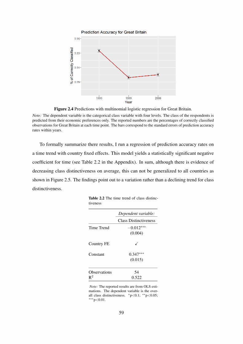
Figure 2.4 Predictions with multinomial logistic regression for Great Britain.Note: The dependent variable is the categorical class variable with four levels. The class of the respondents ispredicted from their economic preferences only. The reported numbers are the percentages of correctly classifiedobservations for Great Britain at each time point. The bars correspond to the standard errors of prediction accuracyrates within years.

To formally summarize there results, I run a regression of prediction accuracy rates on

a time trend with country fixed effects. This model yields a statistically significant negative

coefficient for time (see Table 2.2 in the Appendix). In sum, although there is evidence of

decreasing class distinctiveness on average, this can not be generalized to all countries as

shown in Figure 2.5. The findings point out to a variation rather than a declining trend for class

distinctiveness.

Table 2.2 The time trend of class distinc-tiveness

Dependent variable:

Class Distinctiveness

Time Trend −0.012∗∗∗

(0.004)

Country FE ✓

Constant 0.347∗∗∗

(0.015)

Observations 54R2 0.522

Note: The reported results are from OLS esti-mations. The dependent variable is the over-all class distinctiveness. ∗p<0.1; ∗∗p<0.05;∗∗∗p<0.01.

59

Figure 2.5 Predictions with multinomial logistic regression.Note: The dependent variable is the categorical class variable with four levels. The reported numbers are thepercentages of correctly classified observations in the testing set data. The bars correspond to the standard errorsof the prediction accuracy rates within years. Countries are labeled as follows: AT = Austria, BE = Belgium,BG = Bulgaria, CZ = Czech Republic, DE = Germany, DK = Denmark, ES = Spain, FR = France, GB = GreatBritain, HU = Hungary, IE = Ireland, IT = Italy, NL = Netherlands, PL = Poland, PT = Portugal, SE = Sweden, SI= Slovenia, SK = Slovakia.

2.4.3 Multilevel Modeling

In order to estimate the strength of class voting, I use multilevel/hierarchical modeling. These

models estimate a separate regression for each country-year sample by assuming a probability

distribution for the coefficients of these regressions. A multilevel model can be considered as a

generalization of the linear regression model with intercepts and/or slopes being allowed to

vary by group (Gelman and Hill (2006)).

60

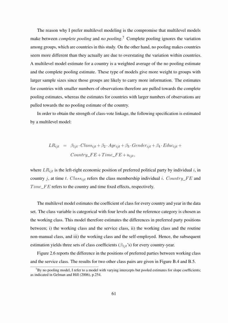
The reason why I prefer multilevel modeling is the compromise that multilevel models

make between complete pooling and no pooling.7 Complete pooling ignores the variation

among groups, which are countries in this study. On the other hand, no pooling makes countries

seem more different than they actually are due to overstating the variation within countries.

A multilevel model estimate for a country is a weighted average of the no pooling estimate

and the complete pooling estimate. These type of models give more weight to groups with

larger sample sizes since those groups are likely to carry more information. The estimates

for countries with smaller numbers of observations therefore are pulled towards the complete

pooling estimates, whereas the estimates for countries with larger numbers of observations are

pulled towards the no pooling estimate of the country.

In order to obtain the strength of class-vote linkage, the following specification is estimated

by a multilevel model:

LRijt = β1jt ·Classijt +β2 ·Ageijt +β3 ·Genderijt +β4 ·Educijt +

Country_FE +Time_FE +uijt,

where LRijt is the left-right economic position of preferred political party by individual i, in

country j, at time t. Classijt refers the class membership individual i. Country_FE and

Time_FE refers to the country and time fixed effects, respectively.

The multilevel model estimates the coefficient of class for every country and year in the data

set. The class variable is categorical with four levels and the reference category is chosen as

the working class. This model therefore estimates the differences in preferred party positions

between; i) the working class and the service class, ii) the working class and the routine

non-manual class, and iii) the working class and the self-employed. Hence, the subsequent

estimation yields three sets of class coefficients (β1jt’s) for every country-year.

Figure 2.6 reports the difference in the positions of preferred parties between working class

and the service class. The results for two other class pairs are given in Figure B.4 and B.5.

7By no pooling model, I refer to a model with varying intercepts but pooled estimates for slope coefficients;as indicated in Gelman and Hill (2006), p.254.

61

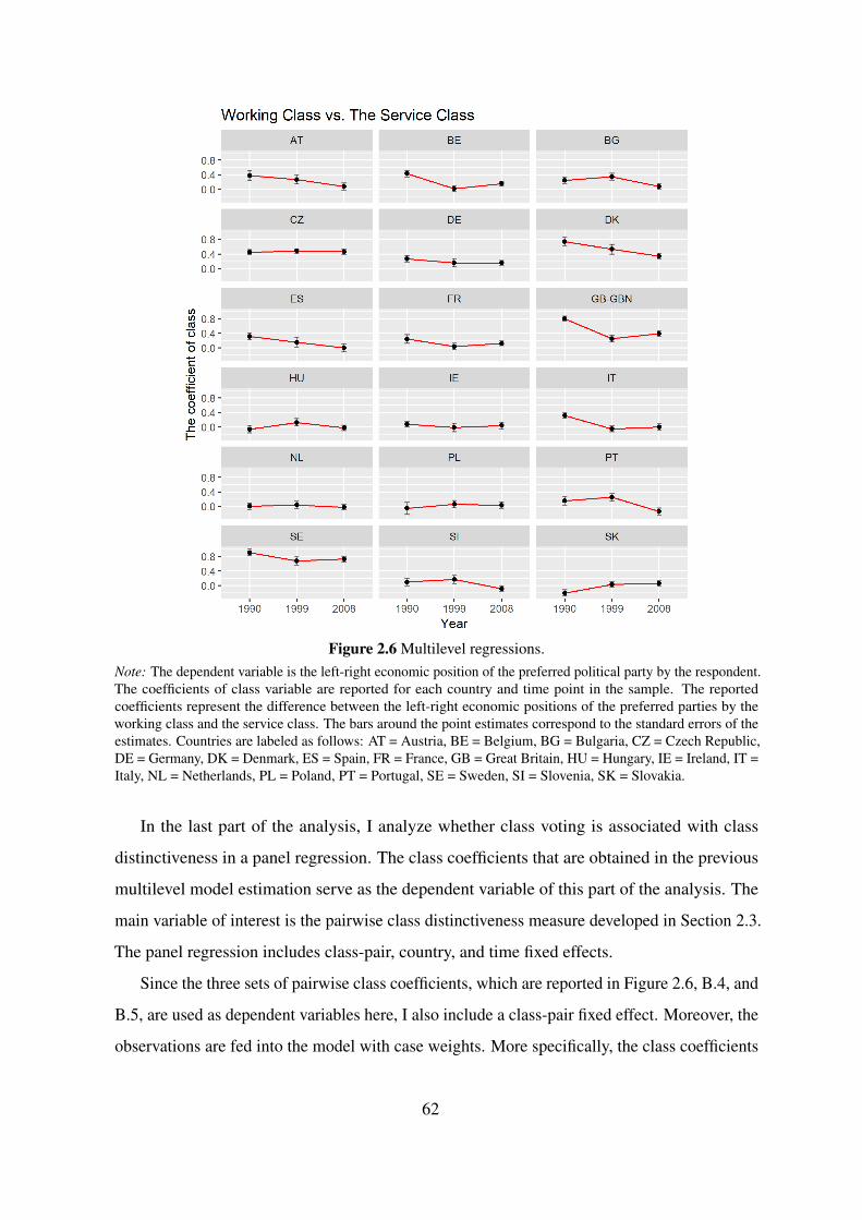
Figure 2.6 Multilevel regressions.Note: The dependent variable is the left-right economic position of the preferred political party by the respondent.The coefficients of class variable are reported for each country and time point in the sample. The reportedcoefficients represent the difference between the left-right economic positions of the preferred parties by theworking class and the service class. The bars around the point estimates correspond to the standard errors of theestimates. Countries are labeled as follows: AT = Austria, BE = Belgium, BG = Bulgaria, CZ = Czech Republic,DE = Germany, DK = Denmark, ES = Spain, FR = France, GB = Great Britain, HU = Hungary, IE = Ireland, IT =Italy, NL = Netherlands, PL = Poland, PT = Portugal, SE = Sweden, SI = Slovenia, SK = Slovakia.

In the last part of the analysis, I analyze whether class voting is associated with class

distinctiveness in a panel regression. The class coefficients that are obtained in the previous

multilevel model estimation serve as the dependent variable of this part of the analysis. The

main variable of interest is the pairwise class distinctiveness measure developed in Section 2.3.

The panel regression includes class-pair, country, and time fixed effects.

Since the three sets of pairwise class coefficients, which are reported in Figure 2.6, B.4, and

B.5, are used as dependent variables here, I also include a class-pair fixed effect. Moreover, the

observations are fed into the model with case weights. More specifically, the class coefficients

62

are assigned a case weight that is inversely proportional to their estimated standard deviations

in the multilevel analysis. This is to take into account the uncertainty of the estimated class

coefficients from the previous multilevel model. Finally, I estimate the following panel

regression:

Class_V otingkjt = γ ·Class_Distkjt +Class_pair_FE +Country_FE +

Time_FE +νkjt,

where k represents the class-pair: working class vs. service class, working class vs. routine

non-manual class, working class vs. self-employed. Class_V otingkjt is the coefficient of

class variable obtained in the previous multilevel model, for class pair k, in country j, at time t.

Class_pair_FE, Country_FE and Time_FE correspond to class pair, country, and time

fixed effects, respectively.

This specification is estimated with a panel regression. The results are summarized in Table

2.3. The first model in Table 2.3 is a panel regression of class voting on class distinctiveness

with only intercept and class-pair fixed effect. It yields a positive and significant coefficient for

class distinctiveness. This supports the second hypothesis that the higher class distinctiveness

is, the stronger is class voting. The second model adds country fixed effect to the first model.

The coefficient of interest is still positive and significant. Third model additionally includes

the time fixed effects. The coefficient of class distinctiveness is still positive and statistically

significant. In sum, these findings confirm our second hypothesis of a positive relationship

between class voting and class distinctiveness.

Cross-country regressions. After providing supporting evidence for the second hypothesis

with panel regressions, I also run cross-country regressions to check whether the same pattern

repeats itself in the absence of time trend. Two different models are estimated in these

regressions: (1) a model with only class-pair fixed effects, (2) a model with both class-pair and

country fixed effects. Table 2.4 summarizes the results for years 1990, 1999, and 2000.

Although the coefficients of class distinctiveness variables are positive in all models in

Table 2.4, they are statistically significant only for years 1999 and 2008. These findings

63

Table 2.3 Panel regressions of class voting on class distinctiveness

Dependent variable:

Strength of class voting

(1) (2) (3)

Class distinctiveness 1.924∗∗∗ 1.671∗∗∗ 1.417∗∗∗

(0.462) (0.357) (0.366)

Constant −0.890∗∗∗ −0.770∗∗∗ −0.579∗∗

(0.264) (0.213) (0.222)

Class-pair FE ✓ ✓ ✓

Country FE ✓ ✓

Time FE ✓

Observations 162 162 162R2 0.225 0.696 0.711

Note: The reported results are from panel regressions. The dependent vari-able is the strength of class voting, which are obtained from multilevel modelestimations. ∗p<0.1; ∗∗p<0.05; ∗∗∗p<0.01.

still partially support the hypothesis of a positive relationship between class voting and class

distinctiveness in a cross-country perspective without the time trend.

Table 2.4 The cross-country regressions of class voting on class distinctiveness

Dependent variable:

Class voting - 1990 Class voting - 1999 Class voting - 2008

(1) (2) (3) (4) (5) (6)

Class dist. 1.307 1.125 1.455∗∗ 1.049∗∗ 2.884∗∗∗ 1.631∗∗∗

(1.054) (0.717) (0.605) (0.397) (0.842) (0.581)

Class-pair FE ✓ ✓ ✓ ✓ ✓ ✓

Country FE ✓ ✓ ✓

Constant −0.490 −0.337 −0.634∗ −0.431∗ −1.454∗∗∗ −0.780∗∗

(0.628) (0.455) (0.348) (0.248) (0.465) (0.308)

Observations 54 54 54 54 54 54R2 0.161 0.875 0.244 0.903 0.269 0.882

Note: The reported results are from OLS estimations. The dependent variable is the strength of class voting,which are obtained from multilevel estimations. ∗p<0.1; ∗∗p<0.05; ∗∗∗p<0.01.

64

2.5 Conclusion

The recent literature on class voting has centered around the mechanisms that drive class voting.

This paper concerns one of the potential mechanisms: the blurring of class divisions. The

previous scholarship in political science, and also in sociology, has either announced the death

of class as an interesting concept in electoral politics or claimed that its explanatory power in

electoral politics has disappeared. Although this hypothesis is pronounced in several studies,

there has been no empirical evidence on the blurring of class divisions and its relationship with

class voting.

This paper addresses this specific question. By using the European Values Survey and

Manifesto Project data sets, class divisions are first operationalized as differences in economic

preferences between classes. The difference between classes then is transformed into a single

measure of class distinctiveness by predictive modeling. This transformation is based on the

simple idea that the predictability of class membership from economic preferences is itself an

indicator of class distinctiveness. Since the imbalance in class sizes and variation in the sample

sizes of country-year samples are likely to affect the predictive performance and threatens

comparability, I applied a re-sampling method to every country-year sample to balance the

data set in these two respects.

In order to validate the newly developed class distinctiveness measure, I provide supporting

evidence from the structure of political competition within countries, from expectations about

class distinctiveness given the way the EGP classification is constructed, and from the trend of

class differences in Great Britain. Based on this class distinctiveness measure, I then provide

evidence of declining class divisions over time. This declining trend however is pronounced

for some countries whereas some countries exhibit a variation rather than a general trend.

I then test the relationship between class distinctiveness and class voting. To obtain a

quantitative measure of the latter, I run regressions of left-right positions of preferred political

parties on class membership. A multilevel model is estimated for this purpose since it deals

with both within and between country variation. Having obtained both the class distinctiveness

and class voting measures, I then estimate panel and cross-country regressions of the strength

of class-vote linkage on the class distinctiveness measure. These regressions provide strong

evidence in favor of a positive relationship between class voting and class distinctiveness. In

65

overall, these findings point out that the class is still relevant and of interest for the study of

electoral politics.

A major caveat of this study might be the relatively low number of time points included in

the sample. This is due to the lack of data availability in the EVS. Another limitation comes

from the number of explanatory variables that are used for representing economic preferences.

We know that the larger the number of variables there are available on the same issue, the

more representative they are (Ansolabehere et al. (2008)). Due to missing variables in some

countries, hpwever, the number of variables related to economic preferences are limited to

three. An interesting direction for future research is replicating this type of an analysis for

other political dimensions such as the cultural dimension.

66

3Escaping the Reputation Trap: revisiting the Olympic

effect

3.1 Introduction

The main argument of the scholarly work on the Olympic effect is that hosting, and even

just bidding on, the Olympic Games leads to an increase in trade, exports, economic growth,

tourism and other positive outcomes. The competitive bidding process that countries enter

in the hopes of hosting the mega-event shows that many believe that the tremendous initial

costs will be compensated by both these economic and socio-cultural gains. Although a great

deal of attention has been paid to the so-called ‘Olympic effect’, previous research does not

provide one clear answer to the question whether there is a positive ‘Olympic effect’ on hosting

or bidding countries (Matheson, 2006). Moreover, it seems that the effects of hosting the

Olympics differ by country and are positive only under specific circumstances (Baade and

Matheson, 2016). In this paper, we first investigate the question of the presence of a positive

Olympic effect on exports using an empirical design that addresses the shortcomings of the

empirical methods adopted by previous studies. We then discuss one of the factors, namely

reputation, that might condition the Olympic effect.

67

More specifically, we re-estimate the effect of the Olympic games on exports using the

synthetic control method (SCM) of Abadie et al. (2010). Using this method we avoid the

common traps and problems that arise frequently in this specific strand of the literature –

selection bias, structurally different comparison units, choices regarding the timing of the

treatment (as also mentioned in, among others, Maennig and Richter (2012) and Bista (2017)).

By doing so, we hope, not only to give a causal interpretation (within the potential outcomes

framework) to the estimated effects, but also to shed some light on the mechanisms that drive

the effects. We therefore first contribute to the relevant literature by using a better suited

empirical method for the question at hand than the previous one. Furthermore, since our

analysis focuses on countries individually, we are able to provide more fine-grained evidence

regarding the presence of the Olympic effect, and also to test a specific mechanism, namely

the Olympic games being way out of the reputation trap, which is elaborated below.

Why would a country decide to bid on the Olympics if the outcome is so uncertain? One

explanation would be that the country wants to send a signal of economic liberalization and

trade openness to the world. This idea has been put forth by Rose and Spiegel (2011). We make

a modification to this idea and argue that such a signal would only be effective for countries

that want to go through a process of liberalization and increase their economic openness. The

immediate implication of is that developed countries with high trade levels and economic

openness (good-reputation countries) would not experience positive benefits of hosting (or

bidding on) the Olympics through signaling openness. On the other hand, countries who want

to endorse open trade (bad-reputation countries) would find it valuable to signal economic

liberalization and trade openness to the rest of the world.

The key difference therefore between our signaling mechanism and the one in Rose and

Spiegel (2011) is that our mechanism implies not all countries will experience the same positive

Olympic effect because not all countries have a reputation to gain from signaling openness.

This idea resonates well with the theory of Levine (2019), according to whom, a bad-reputation

player, who finds itself in a reputation trap, does not find it profitable to invest in a good

signal. One way to make this player to invest in the good signal is to subsidize the cost of the

investment regarding the good signal. However, the welfare analysis of his theory indicates

that the player is strictly better-off when it receives the amount of subsidy than investing it

in the good signal. Therefore, it is not very straightforward for a country to invest in a good

68

signal to tell the rest of the world that it is endorsing free trade. The model, however, points

to another possibility of escape: an outside agency may have an advantage over the player in

disseminating credible information to the outsiders and make the investment in the good signal

profitable for this bad-reputation player. The key outside agency in our setting is the Olympic

Games itself as is also proposed by Levine (2019).

For this very reason, if we consider the Olympic Games acting as such a signaling device,

lumping good-reputation venues with bad-reputation venues would not be the right way of

assessing the Olympic effect as is the practice in Rose and Spiegel (2011). In this paper, we

address this problem by creating a synthetic comparison unit for all countries who hosted or

bid on the Olympics. Doing so enables us to ensure that we are not comparing structurally

different units/countries.

We consider bidding on or hosting the Olympic games as a credible, costly signal to escape

the reputation trap. Note that only countries that have a reputation to gain will experience the

effect of the signal and escape the reputation trap, enjoying higher levels of trade or exports

with the rest of the world. Countries that already have a good reputation and enjoy its benefits

will experience a much smaller, if even positive, effect of hosting or bidding on the Olympics.

It might be that in this case the tremendous costs involved with the event do not out-weigh the

potential positive pay-offs. The results of Maennig and Richter (2012) hint at this, when they

show that using propensity score matching (and pairing OECD countries with arguably good

reputations) the positive significant effect of the Olympics disappears.

We hypothesize that the Olympic games might act as the costly and credible signal needed

to positively affect the host country’s reputation. By increasing their reputation, countries might

be able to increase trade levels, especially their exports. We test this hypothesis empirically and

estimate the effect of hosting and bidding on the Olympics on total export levels of countries

that arguably find themselves in a reputation trap. Our findings indicate that the Olympic effect

is indeed present for some countries but not for all. The reputation trap theory, on the other

hand, explains only a part of the story.

The rest of the paper is organized as follows: Section 3.2 provides the institutional back-

ground related to the host selection process of the Olympic Games. Section 3.3 summarizes

the previous related works. Section 3.4 describes our empirical strategy and data. Section 3.5

69

presents the results of our analyses, Section 3.5 presents a discussion of results, and finally,

Section 3.6 concludes.

3.2 Institutional background

Hosting the Olympics is the final stage of a process that spans multiple years. This process

starts at the invitation phase, where potential candidates are invited to Lausanne, in Switzerland,

to discuss their ideas and visions for the Olympic Games. They receive feedback, support

and assistance in developing these ideas into a formal application. This formal application is

the next stage of the candidature process. These formal applications are the first time most

countries, or cities, publicly announce that they plan on bidding on the Olympic Games. In this

paper, we refer to countries who have formally applied (i.e., completed this phase) as bidders.

The formal applications are submitted roughly two years before the Olympic Committee

makes the final decision on what country will be asked to host the Olympic Games. During

these two years, the bidders enter a process of fine-tuning their initial application with the help

of the Olympic Committee. In the final step of the process, the Evaluation Committee decides

each bidders’ ability to “deliver successful Games and assesses whether the Games would

leave a positive legacy that meets the individual needs and long-term development plans of the

respective city and region".1 The decision which country gets to host the Olympic Games is

made five to eight years prior to the Games.

3.3 Related Literature

The previous literature does not provide a straightforward conclusion as to whether hosting or

bidding on the Olympics has a positive effect on exports. For a full review of the literature on

the Olympic effect with respect to both short and long term and ex-ante and ex-post effects,

see Matheson (2006). Below, we will focus on the work done with respect to the long term,

ex-post effects of the Olympics on export levels.

Rose and Spiegel (2011) investigated the effect of hosting and bidding on the Olympic

Games on trade flows and were among the first to introduce the idea of considering hosting or

1Official information by the Olympics Committee: All about the candidature process, 2020.

70

bidding on the Olympic games as a signal of liberalization and openness to trade. The authors

found that both imports and exports increased, and that the effect of hosting the Summer

Olympics was especially strong.

Others have also found a positive effect of hosting the Olympics. Song (2010) estimates

the effect of hosting the Summer Olympics on exports and tourism, using a gravity model

following Rose and Spiegel (2011). Song (2010) takes an important step and estimates when,

first, the effect of the Olympics on exports starts, and second, how long they last. The findings

suggest that the effect on exports is slow but persistent. There is some evidence that the effect

starts a little before the Olympics, but this is not fully supported by all model specifications.

Finally, the positive effect holds for both Summer and Winter Olympics, though the latter has

a smaller effect on exports.

Additionally, Brückner and Pappa (2015) consider the effect of the Olympics and view the

bidding on the Olympics as a news shock. The shock takes place when the countries bid on

the Olympics, around nine to seven years before the actual event would take place. This news

shock results in significant increases in investment, consumption and output. Countries that go

on to host the Olympics experience another significant increase in these three areas five to two

years before the Games take place.

Not all studies find unambiguously positive results of hosting (or bidding on) the Olympic

Games. Considering the stock market and net exports, Veraros et al. (2004) find that the

announcement of winning the Olympic bid had a positive effect on the Athens’ stock market

but not on the Australian stock market.

Importantly, there seems to be evidence that the positive results found are sensitive to

the empirical method used. Contrary to estimating a gravity model using OLS, Bista (2017)

employs a Poisson pseudo-maximum likelihood (PPML) model and notes that this estimation

allows for heteroskedasticity that is prevalent in trade data. Using this set-up, Bista (2017)

finds no significant effect of hosting, or bidding on, the Summer Olympics on total export

levels.

Additionally, Maennig and Richter (2012) raise an important issue with respect to the

methodology of Rose and Spiegel (2011). The authors argue that comparing certain nations

with high levels of exports that have hosted the Olympics to all other nations (with lower

levels of exports and that did not host the Olympics) might imply a selection bias. Maennig

71

and Richter (2012) re-estimate the model of Rose and Spiegel (2011) using a matching and

treatment methodology and show that the positive, significant effect disappears.

3.4 Empirical Framework

3.4.1 Sample and Data

Our main data set in this study is the publicly available TRADHIST data set, which includes

trade information for an extensive list of countries and covers the period 1827-2014 (Fouquin

et al. (2016)).2 From this data set, we specifically use aggregate export levels, population

size, and the real GDP variables at the country level. For each country analysis we first subset

this data set to our period of interest, and second subset it to countries within a specific trade

agreement or economic community (such as GATT).

We complement this data set with the information of the host and bidder countries for the

post-war summer Olympic Games, which is reported in Table C.1 (Rose and Spiegel (2011)).

A binary variable, at the country-year level, that captures being the host or a bidder for an

Olympic Games constitutes the treatment in this study. In our analyses we consider individually

each treated country since the 1960 Olympic Games, except those for which the data are not

available. We also exclude countries who became a member of GATT/WTO during the study

period since it would confound the treatment effect. In the cases of countries bidding multiple

times consecutively, we only focus on the first bids.

3.4.2 Empirical Strategy

We estimate the effect of hosting and bidding on the Olympic games on total export levels

using the SCM.3 In short, the idea behind the method is that a weighted combination of various

control units (the group of control units is called the ‘donor pool’) is better suited to match the

pre-intervention trend of the treated unit than one control unit individually. The SCM offers

an objective and rigorous way of assigning weights to donor pool countries based on a set

of predictor variables. These predictor variables are chosen carefully in such a way that they

2The TRADHIST data set is available online.3We run our synthetic control applications with the ‘Synth’ package by Abadie et al. (2011), and our placebo

tests with the ‘SCtools’ package by Silva and DeWitt (2019), both in R.

72

predict the outcome variable as well as possible. The weighted combination of the control

units is referred to as the ‘synthetic control’. If the SCM is conducted correctly, this synthetic

control is identical to the treated unit in all aspects except that it did not undergo treatment

(in our case, treatment being the bidding on or hosting of the Olympics). We refer the reader

unfamiliar with this method to Abadie (2019); Abadie et al. (2010, 2015) where the method is

discussed in detail.

The literature review touched upon some potential empirical shortcomings of earlier

estimations of the Olympic effect. The SCM allows us to address these issues and causally

estimate the effect that hosting the Olympic Games has on exports, and thereby whether it is a

credible and effective signal that allows a country to escape the reputation trap.

An issue that arises in the previous literature is lumping good-reputation countries with

bad-reputation countries when assessing the Olympic effect. However, to test a reputational

mechanism for driving the Olympic effect, such an analysis is ill-suited. We address this

problem by applying our synthetic control method to individual countries and assess the effect

case by case for good-reputation and bad-reputation countries.

Another empirical shortcoming is caused by unobservable characteristics of the treatment

and control groups that drive the effect instead of the actual hosting of the Olympics. Rose and

Spiegel (2011) note this, but argue that the problem is avoided by comparing trade patterns

for countries that host the games to those that unsuccessfully bid for the games. Maennig and

Richter (2012) state that some estimations of the Olympic Effect suffer from selection bias with

respect to what countries are compared to each other: “We challenge the empirical findings of

Rose and Spiegel (2011) because they compare Olympic nations such as the United States,

Japan, Germany, Canada, Italy, Spain, and Australia, which have been among the leading

export nations for centuries, to all other nations (p 635-636)".

We mitigate this common pitfall of empirical research by the pre-treatment match between

our treated units and their synthetic controls. The quality of pre-treatment trajectory match in

synthetic control methods provides us the required credibility to claim that any discrepancy

in trends after the treatment is due to our treatment. We also mitigate the sample selection

problem thanks to the simple and explicit optimization problem underlying the synthetic

control methods. Moreover, since we perform a country by country analysis, we can carefully

73

distinguish between countries who need to costly and credibly signal to repair their reputation,

and countries that do not. Thereby we can precisely test our hypothesis.

Finally, the timing of the treatment is a difficult but crucial modeling choice for assessing

the Olympic effect. In regression-based methods, the coefficient of the treatment variable is

the average of the treatment effect for the entire post-treatment time period. It may occur that

the effect starts much later, and thereby biases the coefficient. Getting the timing right is a

difficult matter, given that the moment of the decision to award the Olympic Games varies, as

well as the fact that the effect might start sometime after the event took place or gets stronger

over time (this is shown to be the case by Song (2010)). It might also occur that the treatment

starts in different years in different countries.

The synthetic control method allows us to backdate the time of the treatment without losing

the causal interpretation of the estimated post-treatment difference between trends (Abadie,

2019). The backdating approach of SCMs frees us from making a difficult modeling choice,

that is, determining the exact timing of the treatment. It also frees us from having to specify an

identical treatment year for all the countries.

3.4.3 Donor pool

As noted by Maennig and Richter (2012), it is important to compare countries that are similar

to each other to avoid selection bias and thereby unreliable results. For this reason, a few words

on the construction of the donor pool for our analysis follows.

Since our outcome of interest is export levels, we consider GATT membership as an

important factor in determining the donor pool. Therefore, as recommended in Abadie (2019),

we restrict the donor pool (initially consisting of all countries that did not bid or host the

Olympics in the time-period considered) to countries that have a similar GATT-membership

status. This is in line with the recommendation of Abadie (2019) that any comparison units that

(might) have experienced large shocks that affect the outcome variable should be excluded.4 If

we would not do so, we would fail to control for the large impact that this membership has on

export levels.

4This is similar to donor pool restriction to OECD members in Abadie et al. (2015) who study the effects ofGerman Unification on West Germany GDP through a synthetic control method.

74

In addition, we exclude countries that hosted the Olympics or bid on the Olympics simulta-

neously with the treated country from the donor pool, and also the countries that hosted or bid

on the Olympics within the corresponding study period. This sample restriction ensures that

we compare treated units to non-treated units.

3.4.4 Moment of treatment

Equally important as selecting the units of our donor pool is determining the correct moment

of treatment. According to Abadie (2019), it is crucially important to align the timing of the

treatment, and thereby the pre-treatment period, with when the first effects of the (policy)

change or intervention take place. As the economy consists of forward-looking agents, the

anticipation of the event (in our case, the Olympics) taking place in the future can already have

an impact. This ensures that the full effect of the intervention can be estimated (Abadie, 2019).

Signs of this anticipation are found in the literature as it is often found that the effect starts a

few years prior to the Games taking place. Song (2010) found that the effect starts a few years

prior to hosting the Olympics. Brückner and Pappa (2015) also find that the effect starts prior

to the eventual hosting of the Olympics, and conclude that the effect starts nine to seven years

prior to the Games while it most significantly increases five to two years prior to the Games for

host countries. These timelines roughly coincide with the moment a country officially declares

its candidacy.

As we consider the bidding on the Olympics as a signal about the reputation of the country

(to lift itself out of the reputation trap), a straightforward assumption is that the effect will start

at the time of the announcement. This would suggest that the effect starts about seven to five

years prior to the year the Games take place. We show in our robustness tests that this is a

reliable and robust choice.

Choosing the Olympics host announcement year as the start of the treatment coincides with

backdating approach in SCMs. Since we start the Olympics treatment as early as possible (for

example, the host announcement year for the host countries), we actually allow the treatment

effects to start at anytime after the treatment starting year. This grants us some flexibility in

capturing the treatment effects. In our robustness checks, we replicate our results when the

treatment year is specified as two years before the host announcement year.

75

Moreover, the backdating approach ensures that any effect that emerges at any time after

the treatment starting year –even when various time periods show no treatment effects– can be

interpreted as the causal effect of the treatment (Abadie (2019)). This implies that we allow

our treated units to exhibit heterogeneity in when they start to experience the positive export

effects of the Olympic Games, and we see this as a substantial improvement over the empirical

designs of the previous studies.

3.5 Results

In what follows we first provide an example of our country-level analysis by focusing on South

Korea and the 1988 Olympics. We explain in detail the baseline specification, robustness

checks, and placebo-in-place tests. In all the analyses for other countries, unless otherwise

stated, our econometric specifications and other modeling choices regarding the baseline

analyses, robustness checks, and placebo-in-place tests are identical across countries.

Second, we present the results for all countries in our sample and provide a discussion of

these results.

3.5.1 Country-level Analysis

Our exampler for the country-level analysis is that of South Korea, who hosted the 1988

Olympic Games. In the baseline analysis, our dependent variable is total export and its

predictors for constructing the synthetic control are population size, real GDP, and total export

itself. All of these variables are standardized before applying the synthetic control method.

We start the treatment when the host of the Olympic Games has been announced (which is

1981 for the 1988 Olympics). We go back eight years before the announcement year so that

the optimization problem that generates the synthetic control has enough time to yield a good

pre-treatment match of trends. We then track the trends of our treated unit (South Korea in this

example) and its synthetic control for 15 years after the treatment started.

Figure 3.1 shows the results of our application of synthetic control method. The good

pre-treatment fit lends credibility to a causal interpretation of the observed differences between

the treated unit and its synthetic control after the treatment started. Figure 3.1 shows that, after

South Korea was announced as the host of the 1988 Olympics Games in 1981, a difference

76

starts to emerge between the export trends of South Korea and its synthetic control. This

difference corresponds to the effect of the Olympic Games on the exports of South Korea, and

it seems persistent throughout the 15 years after the treatment.

Figure 3.1 Baseline results for South Korea.Note: The plot summarizes the results of baseline analysis. It shows the total export levels of South Korea and itssynthetic control for the study period of interest. The black vertical line corresponds to the treatment year. Theblue line corresponds to the total exports of South Korea, and the red line corresponds to the total exports of thesynthetic control.

We conduct two robustness checks to our baseline results. We first take our treatment year

back to two years before the host announcement year, to 1979 in this example. This is the

backdating approach and it does not harm the causality of the estimated differences even if

the actual treatment starts later (Abadie (2019)). We still optimize over eight years before the

treatment and track the export trends for 15 years after the treatment. Figure 3.2 shows that,

even if the treatment starts in 1979, we still observe a difference in export levels between South

Korea and its synthetic control.

In our second robustness check, we construct our synthetic control with a single predictor,

which is the export level itself. The aim of this robustness analysis is to show that the pre-

treatment fit and the results in the baseline analysis are not an artifact of our choices regarding

the predictor variables. In this analysis we use the host announcement year as the treatment

starting year as in the baseline specification. Figure C.13 confirms that the baseline results are

not due to our selection of predictor variables.

77

Figure 3.2 Robustness-I for South Korea: treatment two years before host announcement.Note: The plot summarizes the results of robustness analysis. It shows the total export levels of South Korea andits synthetic control for the study period of interest. The black vertical line corresponds to the treatment year. Theblue line corresponds to the total exports of South Korea, and the red line corresponds to the total exports of thesynthetic control.

Figure 3.3 Robustness-II for South Korea: single predictor.Note: The plot summarizes the results of robustness analysis. It shows the total export levels of South Korea andits synthetic control for the study period of interest. The black vertical line corresponds to the treatment year. Theblue line corresponds to the total exports of South Korea, and the red line corresponds to the total exports of thesynthetic control.

Finally, we run placebo-in-place tests to further strengthen the causal interpretation of our

baseline results. In this analysis we rotate over all countries in our sample by choosing each

country as the treated unit, and construct a synthetic control for each one of them. Since our

sample in this subsection does not include any country that hosted or bid on the Olympics

(except our treated country of interest), we do not expect to see a positive difference between

78

the treated unit and its synthetic control in terms of export levels. If we happen to see such

positive differences for placebo countries, this then would cast a serious doubt on the credibility

of positive effects of the Olympic Games on exports.

Our modeling choices in constructing the synthetic control in this placebo-in-place analysis

are identical to the ones in our baseline analysis. Figure 3.4 presents the outcome gaps between

the treated units and their synthetic controls for each country in our sample. The placebo-

in-place analyses reported in Figure 3.4 confirm that our actual treated unit, South Korea

(represented by the bold black line), is the one that experiences the positive effects of the

Olympic Games distinctively more, compared to the our countries in our sample who did not

host or bid on the Olympics.

Figure 3.4 Placebo analysis for South Korea, 1988 Olympics.Note: The plot summarizes the results of placebo analysis. We apply synthetic control method to each country inour donor pool by rotating the treated unit -placebo treatment units. The trends correspond to the exports gapbetween treated units and its synthetic controls. The dashed line corresponds to the treatment year. The solidblack line corresponds to the exports gap between South Korea and its synthetic control. Gray lines correspond tothe exports gap of the placebo treatment units and their synthetic controls.

In overall, our results indicate that the Olympic Games has a positive effects on exports in

the case of South Korea as a host of the 1988 Olympic Games. We see this result as suggestive

evidence for the presence of a reputational mechanism since we consider South Korea as a

country who can receive benefits from signaling economic liberalisation and trade openness to

the rest of the world. In the next section, we replicate the above analyses for 12 other countries

who hosted or bid on the Olympics and discuss our findings. The baseline results regarding

these 12 countries are reported in the Appendix C.

79

3.5.2 Results & Discussion

Table 3.1 summarizes the results of 13 synthetic control method applications for countries who

hosted or bid on the Olympic Games and also their reputation measures regarding trade. The

‘Olympic effect’ column in Table 3.1 reports the standardized Olympic effect, which is the

10-year average of the gap between the exports of actual treated unit and its synthetic control

immediately after the treatment, divided by the total exports of the treated unit at the starting

year of the treatment. More formally, let T be the treatment year, XT,treated be the exports of

treated unit at time T , and Gapt be the difference between the exports of treated unit and its

synthetic control at time t. The standardized Olympic effect then is given by:

∑10i=1 GapT +i

XT,treated.

The last three columns of Table 3.1 presents the percentiles of countries in terms of three

different reputation measures. The first reputation measure is the trade openness, which is

the total share of exports and imports in GDP. The second reputations measure is the share of

exports in GDP. And finally, the third measure is the exports itself. The reputation percentile

indicates in which percentile a country is placed in terms of each reputation measure. Being

in kth percentile means that k% of the sample has a lower value in the respective reputation

measure than the country that is in the kth percentile.

The main finding of Table 3.1, which is in line with the results of Rose and Spiegel (2011),

is that both the host and bidder countries experience a positive Olympic effect, with the former

experiencing a much larger effect. The average standardized Olympic effect for host countries

is 0.68, whereas it is 0.15 for bidder countries. Nevertheless, these baseline results are not fully

supported and lent credibility by placebo-in-place analyses.5

Among 13 countries to which we apply our synthetic control method, we are able to

document a causal Olympic effect only for three countries: 1) France experiences an Olympic

effect of 0.77 by bidding on the 1968 Olympics, 2) South Korea, an Olympic effect of 0.97

by hosting the 1988 Olympics, and 3) Japan, an Olympic effect of 0.49 by bidding on the

1988 Olympics. The causal interpretation of these effects are supported by the corresponding

placebo-in-place analysis.

5The results of placebo-in-place analysis are reported in the Appendix C.

80

Table 3.1 Summary of the results

Reputation percentile:

Country Host/bid Olympics Treat.year Olympic effect X+MGDP

XGDP X

Austria bid 1964 1959 0.19 49 53 86Mexico host 1968 1963 0.46 9 16 85France bid 1968 1963 0.77 20 23 99Canada bid 1972 1966 0.12 40 48 98South Korea host 1988 1981 0.97 54 62 89Japan bid 1988 1981 0.49 12 25 99Spain host 1992 1986 0.60 13 24 92Netherlands bid 1992 1986 -0.20 82 82 96France bid 1992 1986 -0.04 27 35 99UK bid 1992 1986 -0.19 35 43 98Turkey bid 2000 1993 0.21 13 12 83South Africa bid 2004 1997 0.17 15 35 84Sweden bid 2004 1997 0.01 43 65 91

Note: The table summarizes the results of several synthetic control method applications. ‘Olympic effect’ columnshows the standardized Olympic effect, which is the 10-year average of the gap between the exports of actualtreated unit and its synthetic control immediately after the treatment, divided by the total exports of the treatedunit at the starting year of the treatment. The last three columns includes three different reputation measures.‘Reputation percentile’ indicates in which percentile a country is placed in a given reputation measure at the year ofthe treatment. Being in kth percentile means that k% of the sample has a lower value in the respective reputationmeasure than the country that is in the kth percentile. The first reputation measure is the trade openness, which isthe total share of export and imports in GDP. The second one is the share of exports in GDP. The third one is theexports itself. ‘X’, ‘M’, and ‘GDP’ correspond to respectively exports, imports, and gross domestic product.

Although we have some strong evidence for the Olympic effect for some countries, this

does not seem like a universal robust effect as it is argued by Rose and Spiegel (2011). A

careful country by country analysis suggests that, for most of the host and bidder countries of

Olympic Games, the Olympic effect is not present. On the other hand, though the placebo-in-

place tests do not fully support, our results seem partly resonate with the reputation trap theory

of Levine (2019), who predicts that a third party/outside agency (the Olympics in our case)

can help the bad reputation country credibly signal that it invests in good reputation.

Our results indicate that Mexico (1963), South Korea (1981), South Africa (1997) may

have experienced the positive Olympic effect as these countries had much to gain from a

credible signaling. On the contrary, the results indicate that the developed western economies

such as Netherlands (1986), France (1986), the U.K. (1986), and Sweden (1997) do not exhibit

a positive Olympic effect. Nevertheless, the results for Austria (1964) or Spain (1986) do not

accord well with the reputation trap theory.

81

In overall, although we think there are good reasons to expect a positive Olympic effect

for countries who are especially in need of credibly signaling to the rest of the world that they

invest in good reputation, the empirical evidence we generate hereby do not fully support the

presence of such an effect. We conclude by emphasizing the necessity of further research

that would explain why some countries enjoy a positive Olympic effect while others do not.

Reputation may still be one of the conditioning factors but our analysis suggests it is only part

of the story.

3.6 Conclusion

In this paper, we revisit the Olympic effect problem with a better-suited empirical tool: the

synthetic control method. Previous works on whether hosting or bidding on the Olympic Games

leads to increases in exports provide us with mixed findings. These empirical studies, however,

suffer from very typical empirical research problems such as the selection bias. Furthermore,

these studies make quite restrictive assumptions on the timing of the treatment. Neither they

take into account the case of multiple bidders, nor they separate the good reputation countries

from bad reputation ones.

We propose synthetic control method to overcome these problems. Several features of

synthetic control methods such as the pre-treatment matching, backdating approach, selection

of donor pool help us overcome the aforementioned problems and give a causal interpretation

to our estimates. We apply our method to each host or bidder country individually. We also

complement our baseline analysis with placebo-in-place analyses to strengthen the credibility

of the results.

Our findings indicate that although there is a positive Olympic effect for some countries, it

clearly does not apply to all hosts or bidders. A reputation trap theory is partly successful in

explaining why some countries experience a positive Olympic effect while others do not. We

however believe that further research is required to pin down the other mechanisms that play a

role in the trade effects of the Olympic Games.

82

References

Abadie, A. (2019). Using synthetic controls: Feasibility, data requirements, and methodologicalaspects. Journal of Economic Literature.

Abadie, A., Diamond, A., and Hainmueller, J. (2010). Synthetic control methods for compara-tive case studies: Estimating the effect of california’s tobacco control program. Journal ofthe American statistical Association, 105(490):493–505.

Abadie, A., Diamond, A., and Hainmueller, J. (2011). Synth: An r package for syntheticcontrol methods in comparative case studies. Journal of Statistical Software, 42(13).

Abadie, A., Diamond, A., and Hainmueller, J. (2015). Comparative politics and the syntheticcontrol method. American Journal of Political Science, 59(2):495–510.

Adiguzel, F. S., Cansunar, A., and Corekcioglu, G. (2019). Out of sight, out of mind? electoralresponses to proximity of health care.

Alesina, A., Baqir, R., and Easterly, W. (1999). Public goods and ethnic divisions. TheQuarterly journal of economics, 114(4):1243–1284.

Alesina, A., Miano, A., and Stantcheva, S. (2020). The polarization of reality. In AEA Papersand Proceedings, volume 110, pages 324–28.

Ansolabehere, S., Meredith, M., and Snowberg, E. (2014). Mecro-economic voting: Localinformation and micro-perceptions of the macro-economy. Economics & Politics, 26(3):380–410.

Ansolabehere, S., Rodden, J., and Snyder, J. M. (2008). The strength of issues: Using multiplemeasures to gauge preference stability, ideological constraint, and issue voting. AmericanPolitical Science Review, 102(2):215–232.

Arzheimer, K. and Carter, E. (2006). Political opportunity structures and right-wing extremistparty success. European Journal of Political Research, 45(3):419–443.

Arzheimer, K., Evans, J., and Lewis-Beck, M. S. (2016). The Sage handbook of electoralbehaviour. Sage.

Aydin, M., Celikpala, M., Dizdaroglu, C., Hawks, B. B., Guvenc, M., Karaoguz, E., andAkinci, B. A. (2019). Turkiye sosyal-siyasal egilimler arastirmasi-2018.

Aytaç, S. E. (2018). Relative economic performance and the incumbent vote: a reference pointtheory. The Journal of Politics, 80(1):16–29.

Baade, R. A. and Matheson, V. A. (2016). Going for the gold: The economics of the olympics.Journal of Economic Perspectives, 30(2):201–18.

Bakıs, O. and Acar, U. (2019). Tanzim satıs uygulaması enflasyonu düsürdü.

Bakker, R. and Hobolt, S. (2013). Measuring party positions. Political Choice Matters:Explaining the Strenght of Class and Religious Cleavages in Cross-National Perspective,pages 27–45.

83

Bartels, L. M. (2002). Beyond the running tally: Partisan bias in political perceptions. Politicalbehavior, 24(2):117–150.

Baysan, C. (2019). The polarizing effects of persuasive communication: Experimental evidencefrom turkey.

Bechtel, M. M. and Hainmueller, J. (2011). How lasting is voter gratitude? an analysis of theshort-and long-term electoral returns to beneficial policy. American Journal of PoliticalScience, 55(4):852–868.

Bertrand, M. and Kamenica, E. (2018). Coming apart? cultural distances in the united statesover time. Technical report, National Bureau of Economic Research.

Bista, R. (2017). Revisiting the olympic effect. Review of International Economics, 25(2):279–291.

Blais, A. (2006). What affects voter turnout? Annu. Rev. Polit. Sci., 9:111–125.

Boxell, L., Gentzkow, M., and Shapiro, J. M. (2020). Cross-country trends in affectivepolarization. Technical report, National Bureau of Economic Research.

Brückner, M. and Pappa, E. (2015). News shocks in the data: Olympic games and theirmacroeconomic effects. Journal of Money, Credit and Banking, 47(7):1339–1367.

Cantú, F. (2019). Groceries for votes: The electoral returns of vote buying. The Journal ofPolitics, 81(3):000–000.

Chen, C., Liaw, A., and Breiman, L. (2004). Using random forest to learn imbalanced data.University of California, Berkeley, 110:1–12.

Chen, J. (2013). Voter partisanship and the effect of distributive spending on political partici-pation. American Journal of Political Science, 57(1):200–217.

Cho, W. K. T., Gimpel, J. G., and Dyck, J. J. (2006). Residential concentration, politicalsocialization, and voter turnout. The Journal of Politics, 68(1):156–167.

Clark, T. N. and Lipset, S. M. (1991). Are social classes dying? International sociology,6(4):397–410.

Clinton, J. D. and Sances, M. W. (2018). The politics of policy: The initial mass political effectsof medicaid expansion in the states. American Political Science Review, 112(1):167–185.

Connelly, R., Gayle, V., and Lambert, P. S. (2016). A review of occupation-based social classi-fications for social survey research. Methodological Innovations, 9:2059799116638003.

Cox, G. W. and McCubbins, M. D. (1986). Electoral politics as a redistributive game. TheJournal of Politics, 48(2):370–389.

Dalton, R. J. (2013). Citizen politics: Public opinion and political parties in advancedindustrial democracies. Cq Press.

De la Calle, L. and Orriols, L. (2010). Explaining the electoral effects of public investments:The case of the expansion of the underground in madrid, 1995–2007. European Journal ofPolitical Research, 49(3):393–417.

84

Dixit, A. and Londregan, J. (1996). The determinants of success of special interests inredistributive politics. the Journal of Politics, 58(4):1132–1155.

Drazen, A. and Eslava, M. (2010). Electoral manipulation via voter-friendly spending: Theoryand evidence. Journal of development economics, 92(1):39–52.

Duflo, E., Glennerster, R., and Kremer, M. (2007). Using randomization in developmenteconomics research: A toolkit. Handbook of development economics, 4:3895–3962.

Easterly, W. and Levine, R. (1997). Africa’s growth tragedy: policies and ethnic divisions. Thequarterly journal of economics, 112(4):1203–1250.

Ejdemyr, S., Kramon, E., and Robinson, A. L. (2018). Segregation, ethnic favoritism, and thestrategic targeting of local public goods. Comparative Political Studies, 51(9):1111–1143.

Elinder, M., Jordahl, H., and Poutvaara, P. (2015). Promises, policies and pocketbook voting.European Economic Review, 75:177–194.

Enos, R. D. (2011). Racial threat: Field-experimental evidence that a proximate racial outgroupactivates political participation. January, 7:1–50.

Erikson, R. and Goldthorpe, J. H. (1992). The constant flux: A study of class mobility inindustrial societies. Oxford University Press, USA.

Esping-Andersen, G. (2013). The three worlds of welfare capitalism. John Wiley & Sons.

Evans, G. (1999). The end of class politics?: class voting in comparative context. OxfordUniversity Press.

Evans, G. (2000). The continued significance of class voting. Annual review of politicalscience, 3(1):401–417.

Evans, G. and De Graaf, N. D. (2013). Political choice matters: explaining the strength ofclass and religious cleavages in cross-national perspective. OUP Oxford.

Evans, G. and Neundorf, A. (2018). Core political values and the long-term shaping ofpartisanship. British Journal of Political Science, pages 1–19.

Evans, G. and Tilley, J. (2012a). The depoliticization of inequality and redistribution: Explain-ing the decline of class voting. The Journal of Politics, 74(4):963–976.

Evans, G. and Tilley, J. (2012b). How parties shape class politics: Explaining the decline ofthe class basis of party support. British journal of political science, 42(1):137–161.

Evans, G. and Tilley, J. (2017). The new politics of class: The political exclusion of the Britishworking class. Oxford University Press.

Ferejohn, J. (1986). Incumbent performance and electoral control. Public choice, pages 5–25.

Fouquin, M., Hugot, J., et al. (2016). Two centuries of bilateral trade and gravity data:1827-2014. Technical report, Universidad Javeriana-Bogotá.

Ganzeboom, H. B. and Treiman, D. J. (1996). Internationally comparable measures ofoccupational status for the 1988 international standard classification of occupations. Socialscience research, 25(3):201–239.

85

Gelman, A. and Hill, J. (2006). Data analysis using regression and multilevel/hierarchicalmodels. Cambridge university press.

Gentzkow, M., Shapiro, J. M., and Taddy, M. (2018). Measuring group differences in high-dimensional choices: Method and application to congressional speech. Technical report,Technical report Stanford University. URL: http://web. stanford. edu . . . .

Gerber, A. S. and Huber, G. A. (2009). Partisanship and economic behavior: Do partisandifferences in economic forecasts predict real economic behavior? American PoliticalScience Review, 103(3):407–426.

Gerber, A. S. and Huber, G. A. (2010). Partisanship, political control, and economic assess-ments. American Journal of Political Science, 54(1):153–173.

Golden, M. and Min, B. (2013). Distributive politics around the world. Annual Review ofPolitical Science, 16.

Greene, K., Aytaç, S. E., and Çarkoglu, A. (2017). Why even dominant parties can’t buy votes:Campaigns and vote buying in turkey’s 2015 general elections. Technical report, Workingpaper.

Guiso, L., Herrera, H., and Morelli, M. (2017). Demand and supply of populism.

Healy, A. and Malhotra, N. (2009). Myopic voters and natural disaster policy. AmericanPolitical Science Review, 103(3):387–406.

Healy, A. J., Persson, M., and Snowberg, E. (2017). Digging into the pocketbook: Evidence oneconomic voting from income registry data matched to a voter survey. American PoliticalScience Review, 111(4):771–785.

Ichino, N. and Nathan, N. L. (2013). Crossing the line: Local ethnic geography and voting inghana. American Political Science Review, 107(2):344–361.

Ichino, N., Williams, M., and Wibbels, E. (2018). The political geography of governmentprojects: Evidence from+/-40,000 projects in ghana.

Inglehart, R. and Rabier, J.-R. (1986). Political realignment in advanced industrial society:from class-based politics to quality-of-life politics. Government and Opposition, 21(4):456–479.

Jansen, G., Evans, G., and De Graaf, N. D. (2013). Class voting and left–right party positions:A comparative study of 15 western democracies, 1960–2005. Social science research,42(2):376–400.

Kalaycıoglu, E. (2014). Local elections and the turkish voter: looking for the determinants ofparty choice. South European Society and Politics, 19(4):583–600.

Kasara, K. (2013). Separate and suspicious: Local social and political context and ethnictolerance in kenya. the Journal of Politics, 75(4):921–936.

Kiewiet, D. R. and Lewis-Beck, M. S. (2011). No man is an island: self-interest, the publicinterest, and sociotropic voting. Critical Review, 23(3):303–319.

Kinder, D. R. and Kiewiet, D. R. (1979). Economic discontent and political behavior: Therole of personal grievances and collective economic judgments in congressional voting.American Journal of Political Science, pages 495–527.

86

Kitschelt, H. and Rehm, P. (2014). Occupations as a site of political preference formation.Comparative Political Studies, 47(12):1670–1706.

Kogan, V. (2018). Do welfare benefits pay electoral dividends? evidence from the food stampprogram rollout. Evidence from the Food Stamp Program Rollout (May 24, 2018).

Kuhn, M. and Johnson, K. (2013). Applied predictive modeling, volume 26. Springer.

Levine, D. K. (2019). The reputation trap. Technical report, David K. Levine.

Levitt, S. D. and Snyder Jr, J. M. (1997). The impact of federal spending on house electionoutcomes. Journal of political Economy, 105(1):30–53.

Lewis-Beck, M. S. and Stegmaier, M. (2007). Economic models of voting. In The Oxfordhandbook of political behavior.

Lubbers, M., Gijsberts, M., and Scheepers, P. (2002). Extreme right-wing voting in westerneurope. European Journal of Political Research, 41(3):345–378.

Lubbers, M. and Scheepers, P. (2001). Explaining the trend in extreme right-wing voting:Germany 1989–1998. European Sociological Review, 17(4):431–449.

Maennig, W. and Richter, F. (2012). Exports and olympic games: is there a signal effect?Journal of Sports Economics, 13(6):635–641.

Manacorda, M., Miguel, E., and Vigorito, A. (2011). Government transfers and politicalsupport. American Economic Journal: Applied Economics, 3(3):1–28.

Manow, P. (2008). Electoral rules, class coalitions and welfare state regimes, or how to explainesping-andersen with stein rokkan. Socio-Economic Review, 7(1):101–121.

Manow, P., Palier, B., and Schwander, H. (2018). Welfare Democracies and Party Politics:Explaining Electoral Dynamics in Times of Changing Welfare Capitalism. Oxford UniversityPress.

Matheson, V. (2006). Mega-events: The effect of the world’s biggest sporting events on local,regional, and national economies.

Nichter, S. (2008). Vote buying or turnout buying? machine politics and the secret ballot.American political science review, 102(1):19–31.

Nordhaus, W. D. (1975). The political business cycle. The review of economic studies,42(2):169–190.

Oesch, D. and Rennwald, L. (2018). Electoral competition in europe’s new tripolar politicalspace: Class voting for the left, centre-right and radical right. European Journal of PoliticalResearch.

O’Keeffe-O’Donovan, R. (2020). Water, spillovers, and free riding: Provision of local publicgoods in a spatial network. Available at SSRN 3172733.

Ortega, D. and Penfold-Becerra, M. (2008). Does clientelism work? electoral returns ofexcludable and non-excludable goods in chavez’s misiones programs in venezuela. In Paperapresentado em 2008 Meeting of the American Political Science Association, pages 28–31.

87

Peterson, A. and Spirling, A. (2018). Classification accuracy as a substantive quantity ofinterest: Measuring polarization in westminster systems. Political Analysis, 26(1):120–128.

Polk, J. and Rovny, J. (2016). Worlds of welfare and multidimensional party competition ineurope. Unpublished manuscript.

Rose, A. K. and Spiegel, M. M. (2011). The olympic effect. The Economic Journal,121(553):652–677.

Rose, D. and Pevalin, D. J. (2002). A researcher’s guide to the national statistics socio-economic classification. Sage.

Silva, B. C. and DeWitt, M. (2019). Sctools: Extensions for synthetic controls analysis.Technical report, https://cran.r-project.org/web/packages/SCtools/index.html.

Simonovits, G., Malhotra, N., Lee, R. Y., and Healy, A. (2019). The effect of distributivepolitics on electoral participation: Evidence from 70 million agricultural payments. PoliticalBehavior, pages 1–14.

Song, W. (2010). Impacts of olympics on exports and tourism. Journal of economic develop-ment, 35(4):93.

Soss, J. (1999). Lessons of welfare: Policy design, political learning, and political action.American Political Science Review, 93(2):363–380.

Spies, D. (2013). Explaining working-class support for extreme right parties: A party competi-tion approach. Acta Politica, 48(3):296–325.

Stokes, S. C. (2005). Perverse accountability: A formal model of machine politics withevidence from argentina. American political science review, 99(3):315–325.

Tajima, Y., Samphantharak, K., and Ostwald, K. (2018). Ethnic segregation and public goods:Evidence from indonesia. American Political Science Review, 112(3):637–653.

Tillman, E. R. (2008). Economic judgments, party choice, and voter abstention in cross-nationalperspective. Comparative Political Studies, 41(9):1290–1309.

Tufte, E. R. (1978). Political control of the economy. Princeton University Press.

Vaishnav, M. and Sircar, N. (2012). Core or swing? the role of electoral context in shapingpork barrel. Typescript. Department of Political Science, Columbia University.

Vannutelli, S. (2019). Fighting inequality or buying votes? the political economy of redistribu-tive transfers.

Varian, H. R. (2014). Big data: New tricks for econometrics. Journal of Economic Perspectives,28(2):3–28.

Veraros, N., Kasimati, E., and Dawson, P. (2004). The 2004 olympic games announcement andits effect on the athens and milan stock exchanges. Applied Economics Letters, 11(12):749–753.

Weschle, S. (2014). Two types of economic voting: How economic conditions jointly affectvote choice and turnout. Electoral Studies, 34:39–53.

88

Yackley, J. A. (2019). Grocery stores are at the line ofturkey’s latest political battle, accessed 20.08.2020. The Atlantic,https://www.theatlantic.com/international/archive/2019/03/erdogan-grocery-prices-turkey-economy-lira/585646/.

89

AAppendix to Chapter 1

The Choice of Treatment Cut-off

We expect the state-run groceries to be effective within a certain geographical range mainly for

two reasons. First, voters’ accessability to the food subsidy program groceries depends on their

geographical distance to the groceries and accessability is decreasing in distance to the nearest

grocery. Second, since transportation is costly, we expect that voters beyond a certain distance

will not benefit from the program. This in turn suggests a geographical range within which

the local food subsidy program is able to cater individuals. In this study, I operationalize this

geographical catchment area as catchment circles of radius k around the program groceries.

Radius k corresponds to the treatment cut-off value.

Note that before setting out to identify the geographical reach of program groceries, I have

shown that the program has a statistically significant effect on the incumbent vote shore by

using the continuous Distance variable and its square root as well (Section 1.3). In order to

decide the fine-grained geographical range of the program groceries, I estimate Equation 2.1

with a categorical treatment variable, which is defined as the following:

90

Treatmenti =

0-1km, if Distancei ≤ 1 km

1-2km, if 1 < Distancei ≤ 2 km

2-3km, if 2 < Distancei ≤ 3 km

3-4km, if 3 < Distancei ≤ 4 km

>4km, if 4 < Distancei.

Table A.1 reports the results of this regression. I specify the reference level for the categor-

ical treatment variable as the 0-1km. Therefore, the coefficients of other levels correspond to

the contrast of each level with the reference level 0-1km. We start with the assumption that

the polling stations, which have the reference level 0-1km, are in the treatment group since

they are the closest. The results in Table A.1 show that level 1-2km does not have a significant

effect on the dependent variable compared to the reference level 0-1km. However, the levels

2-3km, 3-4km, and >4km differs significantly and negatively from the reference level, in their

effects on the dependent variable. This suggests the treatment cut-off value as 2 km.

The reason that I decide the treatment cut-off value based on the incumbent vote share –but

not turnout rate– is the heterogeneous effects of treatment on turnout over different types of

constituencies. The effects of treatment on incumbent vote share, on the other hand, are not

countervailing over different types of constituencies.

Alternatively, I experiment with different treatment cut-off values. Figure A.1 shows the

estimated coefficients of treatment when the cut-off value is chosen as 1, 2, 3, or 4 km. The

model with treatment cut-off 1 km, for example, defines the treatment group as the polling

stations that fall within 1 km of any state-run grocery, and the remaining as the control group.

Figure A.1 reveals mainly two results. First, it shows that the geographical range of

the effect is greater than 1 km. The red estimate at the bottom, which is statistically not

different than zero, shows that either there is no treatment effect or it is washed away due to

the composition of treatment and control groups –i.e. due to the treated units in the control

group. Since we already know that the treatment has a statistically significant positive effect

91

from our baseline results (and also from some other models in Figure A.1), the red coefficient

shows us that the geographical range of the treatment is greater than 1 km.

Second, the comparison of the two coefficient estimates at the bottom indicates that the

geographical range of the effect extends to within 2 km of state-run groceries. The increase in

the magnitude of the treatment effect, and in its precision, shows the presence of treated units

within 1 to 2 km of state-run groceries. On the other hand, extending the treatment group to

within 3 and 4 km of state-run groceries decreases both the magnitude of the treatment effect

and its precision.

92

Table A.1 The choice of treatment cut-off value

Dependent variable:

Incumbent Vote

Treatment(Reference level: 0-1km)

1-2km 0.0003(0.002)

2-3km −0.003∗

(0.002)3-4km −0.004∗∗∗

(0.002)>4km −0.006∗∗

(0.003)

Previous Inc. Vote 0.932∗∗∗

(0.008)Previous Turnout 0.009

(0.035)

Neigh.-level controls YesDistrict F.E. Yes

Observations 1,575R2 0.988

Note: The reported results are from OLS estimations. Thedependent variable is the incumbent vote share. Previous Inc.Vote indicates the vote share of the incumbent in the previouselection. Treatment is a categorical variable with 5 levels: 0-1km, 1-2km, 2-3km, 3-4km, and >4km. The reference levelis chosen as 0-1km. All regressions include control variablesat the neighborhood-level: population, share of females, av-erage age, share of low educated people, house prices, andhouse rents. The standard errors are clustered at the districtlevel. ∗p<0.1; ∗∗p<0.05; ∗∗∗p<0.01.

93

Figure A.1 Treatment effects with different treatment cut-offsNote: The figure shows the estimated treatment effects and their 95% confidence intervals with different treatmentcut-off values. The dependent variable is the incumbent vote share. The results come from OLS estimationsthat include control variables at the neighborhood-level: population, share of females, average age, share of loweducated people, house prices, and house rents. The vertical dashed line corresponds to a treatment effect of zero.The confidence intervals are built based on the standard errors clustered at the district level. The red, blue, green,and purple point estimates and confidence intervals correspond to the estimates of treatment effects with differenttreatment cut-off values.

94

Cost of the Food Subsidy Program

In calculating the total net cost of the food subsidy program –from the day of onset to the

election day– I use the prices at the state-run groceries, daily prices at the Istanbul wholesale

food market, and the quantity of sales in the first day of the food subsidy program, as reported

by the Istanbul Metropolitan Municipality.

The first step to calculate total net cost of the program is to find how much loss (in Turkish

Lira, TL) the Metropolitan Municipality makes at each kg of product sold. I calculate the loss

per kg for every product that is covered in state-run groceries with the following steps: First,

for every product, I take the difference between the price at state-run groceries and the price

at the Istanbul wholesale food market for the first week of Feburary 2019 –the week before

state-run groceries started. To obtain the latter, I take the average of daily minimum prices at

the wholesale food market in the first week of February 2019. Note that using minimum prices

of the wholesale food market gives a conservative estimate for the loss per kg.

The second step is to multiply the loss per kg with the quantity sold in one day for each

product and report their sum as the total daily loss. The third step is to multiply the total daily

loss with the number of days from the day of onset of state-run groceries to the election day.

The resulting number is a conservative estimate of the total net cost of the program.

The calculation method described above requires several assumptions:

1. Loss for each product is constant over time, and is the difference between the price (per

kg) at the state-run groceries and price (per kg) at the Istanbul wholesale food market.

2. To obtain a conservative estimate of the cost of the program, I take the average of

daily minimum price for each product at the wholesale food market in the first week of

February 2019. I, however, give estimates of overall cost when the loss is halved and

when increased by 50% as well.

3. The quantity sold for each product is constant over time and same as the first day quantity,

which is reported by the metropolitan municipality.

4. Since I do not have prices for legumes at the wholesale food market, I cannot calculate

the loss per kg for these products in the same as I do for other products. Alternatively,

95

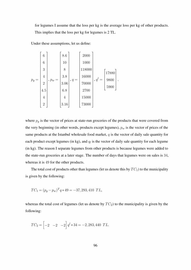
for legumes I assume that the loss per kg is the average loss per kg of other products.

This implies that the loss per kg for legumes is 2 TL.

Under these assumptions, let us define:

pg =

6

6

3

4

2

4.5

4

2

, pw =

8.6

10

8

3.8

3.06

6.8

4

3.16

, q =

2000

1000

118000

16000

70000

2700

15000

73000

, ql =

17880

9800

5900

,

where pg is the vector of prices at state-run groceries of the products that were covered from

the very beginning (in other words, products except legumes), pw is the vector of prices of the

same products at the Istanbul wholesale food market, q is the vector of daily sale quantity for

each product except legumes (in kg), and ql is the vector of daily sale quantity for each legume

(in kg). The reason I separate legumes from other products is because legumes were added to

the state-run groceries at a later stage. The number of days that legumes were on sales is 34,

whereas it is 49 for the other products.

The total cost of products other than legumes (let us denote this by TC1) to the municipality

is given by the following:

TC1 = (pg −pw)T q ∗49 = −37,293,410 TL,

whereas the total cost of legumes (let us denote by TC2) to the municipality is given by the

following:

TC2 =[−2 −2 −2

]ql ∗34 = −2,283,440 TL.

96

Therefore, the total cost of the program is given by:

TC = TC1 +TC2 = −39,576,850 TL.

In order to calculate how much spending is required to gain an additional vote, we divide

the absolute value of the total cost by the number of actual votes gained through the food

subsidy program. The latter is calculated in Section 1.4.1. Consequently, the cost of an

additional vote (c) is given by:

c = |T C|16521 = 39,576,850

16521 = 2395.548 TL.

Finally, we can calculate what percentage of the GDP per capita that the cost of an

additional vote (c) corresponds to. The GDP per capita of Turkey in 2019 is 45242,96 TL.

Dividing c by the GDP per capita of Turkey yields this percentage:

cGDP pc_T urkey = 2395.548

45242,96 = 5.29%.

Halving the loss (per kg of product) and increasing it by 50% yields respectively 2.65% and

7.94%. These percentages are still much smaller than those of the US, where Chen (2013)’s

calculation yields 32% as the percentage of GDP per capita required to buy an extra vote.

97

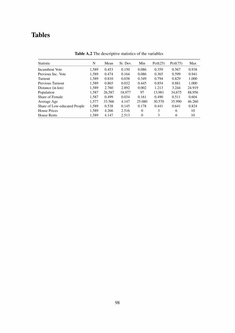
Tables

Table A.2 The descriptive statistics of the variables

Statistic N Mean St. Dev. Min Pctl(25) Pctl(75) Max

Incumbent Vote 1,589 0.453 0.150 0.086 0.359 0.567 0.938Previous Inc. Vote 1,589 0.474 0.164 0.086 0.365 0.599 0.941Turnout 1,589 0.810 0.038 0.349 0.794 0.829 1.000Previous Turnout 1,589 0.865 0.032 0.445 0.854 0.881 1.000Distance (in km) 1,589 2.760 2.892 0.002 1.213 3.244 24.919Population 1,587 26,587 18,977 97 13,981 34,675 88,956Share of Female 1,587 0.499 0.034 0.161 0.490 0.511 0.604Average Age 1,577 33.566 4.147 25.080 30.570 35.990 46.260Share of Low-educated People 1,589 0.538 0.145 0.178 0.441 0.641 0.824House Prices 1,589 4.266 2.516 0 3 6 10House Rents 1,589 4.147 2.513 0 3 6 10

98

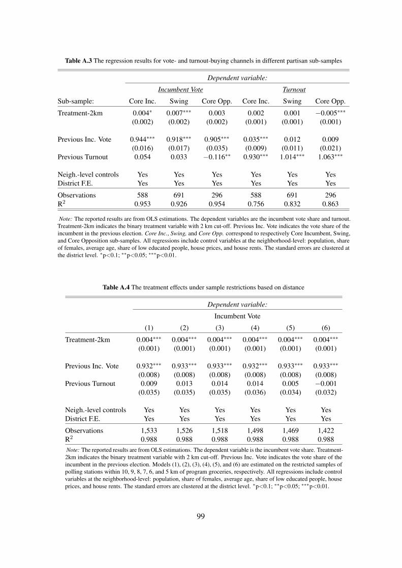
Table A.3 The regression results for vote- and turnout-buying channels in different partisan sub-samples

Dependent variable:

Incumbent Vote Turnout

Sub-sample: Core Inc. Swing Core Opp. Core Inc. Swing Core Opp.

Treatment-2km 0.004∗ 0.007∗∗∗ 0.003 0.002 0.001 −0.005∗∗∗

(0.002) (0.002) (0.002) (0.001) (0.001) (0.001)

Previous Inc. Vote 0.944∗∗∗ 0.918∗∗∗ 0.905∗∗∗ 0.035∗∗∗ 0.012 0.009(0.016) (0.017) (0.035) (0.009) (0.011) (0.021)

Previous Turnout 0.054 0.033 −0.116∗∗ 0.930∗∗∗ 1.014∗∗∗ 1.063∗∗∗

Neigh.-level controls Yes Yes Yes Yes Yes YesDistrict F.E. Yes Yes Yes Yes Yes Yes

Observations 588 691 296 588 691 296R2 0.953 0.926 0.954 0.756 0.832 0.863

Note: The reported results are from OLS estimations. The dependent variables are the incumbent vote share and turnout.Treatment-2km indicates the binary treatment variable with 2 km cut-off. Previous Inc. Vote indicates the vote share of theincumbent in the previous election. Core Inc., Swing, and Core Opp. correspond to respectively Core Incumbent, Swing,and Core Opposition sub-samples. All regressions include control variables at the neighborhood-level: population, shareof females, average age, share of low educated people, house prices, and house rents. The standard errors are clustered atthe district level. ∗p<0.1; ∗∗p<0.05; ∗∗∗p<0.01.

Table A.4 The treatment effects under sample restrictions based on distance

Dependent variable:

Incumbent Vote

(1) (2) (3) (4) (5) (6)

Treatment-2km 0.004∗∗∗ 0.004∗∗∗ 0.004∗∗∗ 0.004∗∗∗ 0.004∗∗∗ 0.004∗∗∗

(0.001) (0.001) (0.001) (0.001) (0.001) (0.001)

Previous Inc. Vote 0.932∗∗∗ 0.933∗∗∗ 0.933∗∗∗ 0.932∗∗∗ 0.933∗∗∗ 0.933∗∗∗

(0.008) (0.008) (0.008) (0.008) (0.008) (0.008)Previous Turnout 0.009 0.013 0.014 0.014 0.005 −0.001

(0.035) (0.035) (0.035) (0.036) (0.034) (0.032)

Neigh.-level controls Yes Yes Yes Yes Yes YesDistrict F.E. Yes Yes Yes Yes Yes Yes

Observations 1,533 1,526 1,518 1,498 1,469 1,422R2 0.988 0.988 0.988 0.988 0.988 0.988Note: The reported results are from OLS estimations. The dependent variable is the incumbent vote share. Treatment-2km indicates the binary treatment variable with 2 km cut-off. Previous Inc. Vote indicates the vote share of theincumbent in the previous election. Models (1), (2), (3), (4), (5), and (6) are estimated on the restricted samples ofpolling stations within 10, 9, 8, 7, 6, and 5 km of program groceries, respectively. All regressions include controlvariables at the neighborhood-level: population, share of females, average age, share of low educated people, houseprices, and house rents. The standard errors are clustered at the district level. ∗p<0.1; ∗∗p<0.05; ∗∗∗p<0.01.

99

Table A.5 Interaction of binary treatment variable with partisanship

Dependent variable:

Incumbent Vote Turnout

(1) (2)

Treatment-2km 0.004∗∗ 0.002(0.002) (0.001)

Treatment-2km × Partisanship(Reference level: Core Incumbent)

× Swing 0.002 0.0001(0.003) (0.002)

× Core Opposition −0.0003 −0.005∗∗∗

(0.003) (0.002)

Neigh.-level controls Yes YesDistrict F.E. Yes Yes

Observations 1,575 1,575R2 0.988 0.799

Note: The reported results are from OLS estimations. The dependent variables arethe incumbent vote share and turnout. Treatment-2km indicates the binary treat-ment variable with 2 km cut-off. Partisanship is a categorical variable with threelevels: Core Incumbent, Swing, and Core Opposition. The reference level is chosenas Core Incumbent. Previous Inc. Vote indicates the vote share of the incumbentin the previous election. The regressions control for polling station level previousincumbent vote share and previous turnout, and also include control variables at theneighborhood-level: population, share of females, average age, share of low educatedpeople, house prices, and house rents. The standard errors are clustered at the districtlevel. ∗p<0.1; ∗∗p<0.05; ∗∗∗p<0.01.

100

Figures

Figure A.2 Distribution of the distance variable

101

Figure A.3 Robustness test: partisan conditioning with continuous Distance variableNote: The figure shows the estimated treatment effects and their 95% confidence intervals in three differentsub-samples of the data set. The dependent variable is the incumbent vote share in Part (a) and turnout rate inPart (b). The treatment variable is the continuous Distance variable. The results come from OLS estimationsthat include control variables at the neighborhood-level: population, share of females, average age, share of loweducated people, house prices, and house rents. The vertical dashed line corresponds to a treatment effect ofzero. The confidence intervals are built based on the standard errors clustered at the district level. The red, blue,and green point estimates and confidence intervals correspond to the treatment effects respectively in the coreincumbent, swing, and core opposition sub-samples.

102

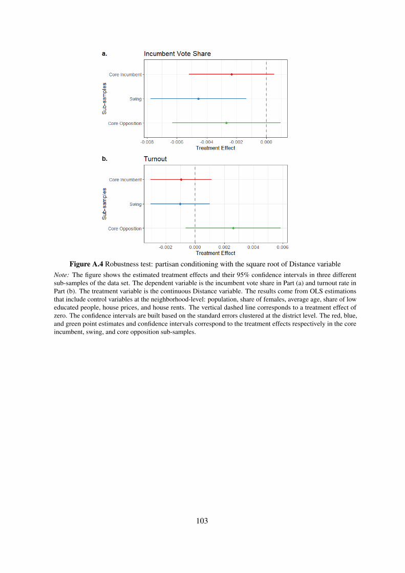
Figure A.4 Robustness test: partisan conditioning with the square root of Distance variableNote: The figure shows the estimated treatment effects and their 95% confidence intervals in three differentsub-samples of the data set. The dependent variable is the incumbent vote share in Part (a) and turnout rate inPart (b). The treatment variable is the continuous Distance variable. The results come from OLS estimationsthat include control variables at the neighborhood-level: population, share of females, average age, share of loweducated people, house prices, and house rents. The vertical dashed line corresponds to a treatment effect ofzero. The confidence intervals are built based on the standard errors clustered at the district level. The red, blue,and green point estimates and confidence intervals correspond to the treatment effects respectively in the coreincumbent, swing, and core opposition sub-samples.

103

BAppendix to Chapter 2

Class Heterogeneity

104

Table B.1 The share of classes within countries - 1990Country Service Routine Self-emp. Working

AT 0.02 0.50 0.13 0.34BE 0.05 0.33 0.15 0.47BG 0.19 0.18 0.03 0.60CZ 0.10 0.32 0.03 0.54DK 0.06 0.44 0.08 0.42FR 0.12 0.53 0.12 0.24DE 0.02 0.45 0.06 0.47HU 0.14 0.14 0.05 0.68IE 0.17 0.22 0.11 0.49IT 0.19 0.38 0.07 0.35NL 0.23 0.33 0.06 0.39PL 0.03 0.24 0.21 0.52PT 0.05 0.28 0.11 0.57SK 0.11 0.27 0.01 0.61SI 0.13 0.24 0.06 0.56ES 0.09 0.19 0.15 0.57SE 0.17 0.50 0.04 0.29GB 0.17 0.23 0.07 0.53

Note: The reported numbers are share of classes within countries.“Service" correspond to the service class, “Routine" to the the rou-tine non-manual class, “Self-emp." to the self-employed class, and“Working" to the working class. Countries are labeled as follows:AT = Austria, BE = Belgium, BG = Bulgaria, CZ = Czech Repub-lic, DE = Germany, DK = Denmark, ES = Spain, FR = France,GB = Great Britain, HU = Hungary, IE = Ireland, IT = Italy, NL= Netherlands, PL = Poland, PT = Portugal, SE = Sweden, SI =Slovenia, SK = Slovakia.

105

Table B.2 The share of classes within countries - 1999Country Service Routine Self-emp. Working

AT 0.04 0.48 0.11 0.36BE 0.14 0.50 0.06 0.30BG 0.30 0.09 0.06 0.54CZ 0.27 0.21 0.05 0.47DK 0.03 0.48 0.08 0.40FR 0.12 0.51 0.10 0.28DE 0.03 0.51 0.10 0.36HU 0.11 0.20 0.07 0.61IE 0.08 0.38 0.20 0.34IT 0.25 0.26 0.12 0.37NL 0.24 0.30 0.06 0.40PL 0.13 0.21 0.13 0.53PT 0.13 0.16 0.12 0.59SK 0.15 0.27 0.03 0.55SI 0.15 0.27 0.06 0.52ES 0.12 0.13 0.13 0.61SE 0.10 0.44 0.12 0.34GB 0.20 0.23 0.05 0.51

Note: The reported numbers are share of classes within countries.“Service" correspond to the service class, “Routine" to the the rou-tine non-manual class, “Self-emp." to the self-employed class, and“Working" to the working class. Countries are labeled as follows:AT = Austria, BE = Belgium, BG = Bulgaria, CZ = Czech Repub-lic, DE = Germany, DK = Denmark, ES = Spain, FR = France,GB = Great Britain, HU = Hungary, IE = Ireland, IT = Italy, NL= Netherlands, PL = Poland, PT = Portugal, SE = Sweden, SI =Slovenia, SK = Slovakia.

106

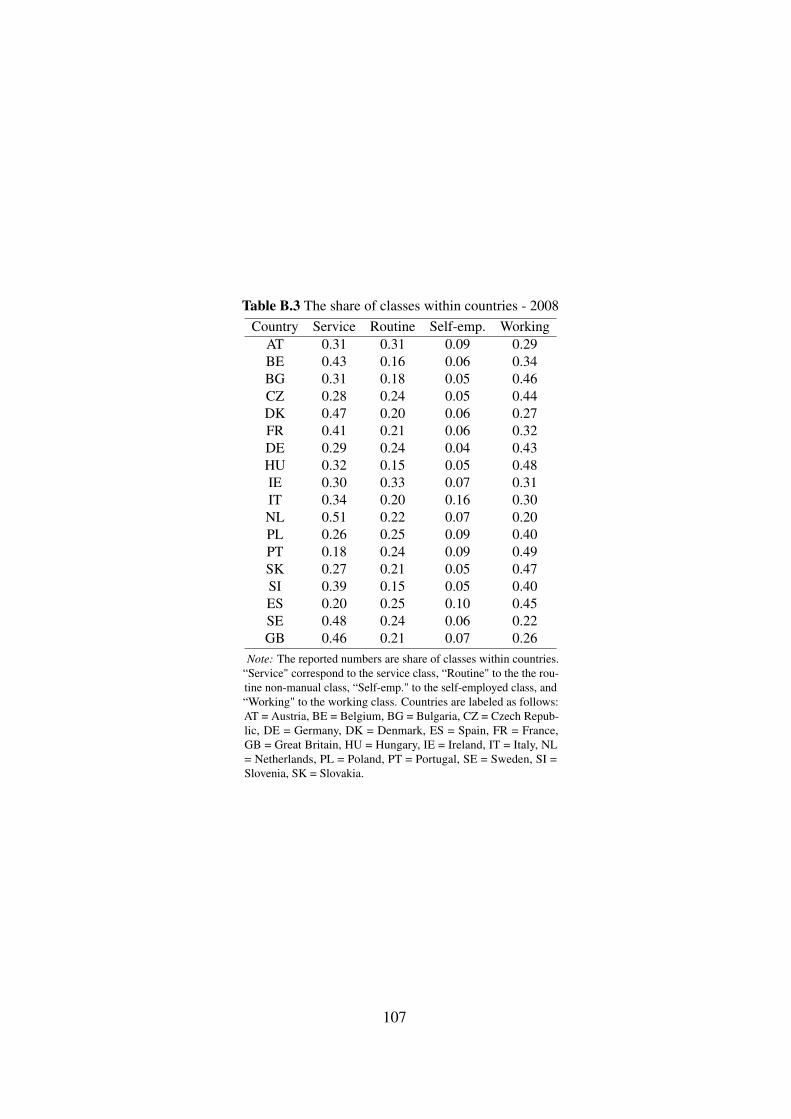
Table B.3 The share of classes within countries - 2008Country Service Routine Self-emp. Working

AT 0.31 0.31 0.09 0.29BE 0.43 0.16 0.06 0.34BG 0.31 0.18 0.05 0.46CZ 0.28 0.24 0.05 0.44DK 0.47 0.20 0.06 0.27FR 0.41 0.21 0.06 0.32DE 0.29 0.24 0.04 0.43HU 0.32 0.15 0.05 0.48IE 0.30 0.33 0.07 0.31IT 0.34 0.20 0.16 0.30NL 0.51 0.22 0.07 0.20PL 0.26 0.25 0.09 0.40PT 0.18 0.24 0.09 0.49SK 0.27 0.21 0.05 0.47SI 0.39 0.15 0.05 0.40ES 0.20 0.25 0.10 0.45SE 0.48 0.24 0.06 0.22GB 0.46 0.21 0.07 0.26

Note: The reported numbers are share of classes within countries.“Service" correspond to the service class, “Routine" to the the rou-tine non-manual class, “Self-emp." to the self-employed class, and“Working" to the working class. Countries are labeled as follows:AT = Austria, BE = Belgium, BG = Bulgaria, CZ = Czech Repub-lic, DE = Germany, DK = Denmark, ES = Spain, FR = France,GB = Great Britain, HU = Hungary, IE = Ireland, IT = Italy, NL= Netherlands, PL = Poland, PT = Portugal, SE = Sweden, SI =Slovenia, SK = Slovakia.

107

Table B.4 The standard deviations variables within classes - 1990

Country Variable Service Routine Self-emp. Working

AT Govt. Resp. 0.66 0.92 0.82 0.93AT Freedom or Eq. 0.94 0.98 0.96 1.04AT Conf. in Union 1.01 0.96 0.87 1.02BE Govt. Resp. 0.98 0.96 0.99 1.08BE Freedom or Eq. 0.86 1.00 0.99 1.01BE Conf. in Union 0.94 0.94 1.01 0.98BG Govt. Resp. 1.10 1.06 1.03 1.05BG Freedom or Eq. 1.00 1.00 0.73 0.99BG Conf. in Union 0.83 0.96 0.98 1.04CZ Govt. Resp. 0.84 0.98 1.03 1.04CZ Freedom or Eq. 0.87 0.99 0.87 1.02CZ Conf. in Union 0.81 0.94 1.05 1.01DK Govt. Resp. 0.77 0.84 0.76 0.88DK Freedom or Eq. 0.97 0.99 0.82 1.02DK Conf. in Union 1.03 0.91 0.98 1.03FR Govt. Resp. 0.79 0.92 0.82 0.97FR Freedom or Eq. 0.97 1.00 0.97 1.00FR Conf. in Union 1.02 1.02 1.10 1.09DE Govt. Resp. 0.95 0.98 0.93 1.07DE Freedom or Eq. 0.91 0.97 0.91 1.03DE Conf. in Union 0.99 0.94 0.82 1.00HU Govt. Resp. 1.02 1.04 1.07 1.02HU Freedom or Eq. 0.91 1.03 0.91 1.01HU Conf. in Union 0.89 1.12 0.79 1.11IE Govt. Resp. 0.87 1.01 0.88 1.09IE Freedom or Eq. 1.01 0.99 1.00 1.00IE Conf. in Union 0.97 0.93 0.94 1.06IT Govt. Resp. 0.98 1.07 1.06 1.15IT Freedom or Eq. 1.00 1.00 1.02 1.00IT Conf. in Union 0.94 0.98 0.98 1.08NL Govt. Resp. 0.74 0.76 0.72 0.88NL Freedom or Eq. 0.96 0.99 0.93 1.02NL Conf. in Union 0.81 0.89 1.01 1.02PL Govt. Resp. 0.92 0.88 1.12 1.06PL Freedom or Eq. 1.03 1.00 0.95 1.01PL Conf. in Union 1.17 1.00 1.02 1.05PT Govt. Resp. 0.76 1.09 1.10 1.10PT Freedom or Eq. 0.99 1.01 0.99 0.99PT Conf. in Union 0.80 0.91 0.98 1.00

108

The standard deviations of variables within classes - 1990 (continued)

Country Variable Service Routine Self-emp. Work.

SK Govt. Resp. 0.90 1.10 1.34 1.10SK Freedom or Eq. 0.93 1.01 0.81 1.00SK Conf. in Union 0.87 0.97 1.03 1.04SI Govt. Resp. 0.93 1.10 1.23 1.16SI Freedom or Eq. 0.95 1.01 1.01 0.98SI Conf. in Union 0.84 1.07 0.90 1.11ES Govt. Resp. 1.04 0.94 0.94 0.96ES Freedom or Eq. 0.98 0.97 0.98 1.02ES Conf. in Union 1.02 0.99 0.90 1.02SE Govt. Resp. 0.72 0.80 0.83 0.79SE Freedom or Eq. 0.82 1.01 0.82 1.06SE Conf. in Union 0.91 0.92 1.02 0.99

GB-GBN Govt. Resp. 0.98 0.94 0.89 1.01GB-GBN Freedom or Eq. 0.96 1.01 0.94 1.01GB-GBN Conf. in Union 0.88 0.96 0.84 1.10

Note: The reported numbers are the standard deviations of the economicpreferences variables within each class in each country. “Service" corre-spond to the service class, “Routine" to the the routine non-manual class,“Self-emp." to the self-employed class, and “Working" to the workingclass. Countries are labeled as follows: AT = Austria, BE = Belgium,BG = Bulgaria, CZ = Czech Republic, DE = Germany, DK = Denmark,ES = Spain, FR = France, GB = Great Britain, HU = Hungary, IE =Ireland, IT = Italy, NL = Netherlands, PL = Poland, PT = Portugal, SE =Sweden, SI = Slovenia, SK = Slovakia.

109

Table B.5 The standard deviations of variables within classes - 1999

Country Variable Service Routine Self-emp. Working

AT Govt. Resp. 0.96 0.91 0.84 1.01AT Freedom or Eq. 0.97 0.99 0.99 1.02AT Conf. in Union 0.82 0.90 0.94 1.00BE Govt. Resp. 1.00 0.92 1.00 1.06BE Freedom or Eq. 1.00 1.00 1.01 0.99BE Conf. in Union 0.97 0.99 1.01 1.09BG Govt. Resp. 0.97 0.98 1.05 1.07BG Freedom or Eq. 0.93 1.05 1.03 1.02BG Conf. in Union 1.00 0.99 0.91 0.92CZ Govt. Resp. 0.91 0.88 0.93 0.98CZ Freedom or Eq. 0.96 0.98 0.81 1.02CZ Conf. in Union 0.86 0.86 0.89 0.99DK Govt. Resp. 0.83 0.80 0.72 0.78DK Freedom or Eq. 0.93 0.98 0.93 1.04DK Conf. in Union 1.04 0.86 0.90 0.95FR Govt. Resp. 0.88 0.89 0.81 0.97FR Freedom or Eq. 0.95 1.00 1.00 1.00FR Conf. in Union 0.92 1.02 1.00 1.09DE Govt. Resp. 0.77 0.96 0.96 1.01DE Freedom or Eq. 0.71 1.02 0.91 0.99DE Conf. in Union 0.68 0.94 0.94 0.89HU Govt. Resp. 1.00 0.96 1.18 1.06HU Freedom or Eq. 0.93 1.01 0.95 0.98HU Conf. in Union 1.04 0.91 0.89 0.99IE Govt. Resp. 0.93 0.90 1.01 0.92IE Freedom or Eq. 1.01 1.00 1.00 1.00IE Conf. in Union 0.97 0.99 0.94 1.10IT Govt. Resp. 0.92 0.94 1.11 1.02IT Freedom or Eq. 0.98 0.99 1.02 1.01IT Conf. in Union 0.97 0.95 0.95 1.03NL Govt. Resp. 0.71 0.71 0.71 0.75NL Freedom or Eq. 0.99 0.99 0.99 1.02NL Conf. in Union 0.78 0.71 0.86 0.83PL Govt. Resp. 0.86 0.86 0.97 1.01PL Freedom or Eq. 0.95 1.01 1.00 1.00PL Conf. in Union 0.99 0.97 1.02 1.06PT Govt. Resp. 0.82 0.97 0.91 1.05PT Freedom or Eq. 0.99 0.96 1.02 1.01PT Conf. in Union 0.99 1.02 0.90 1.03

110

The standard deviations of variables within classes - 1999 (continued)

Country Variable Service Routine Self-emp. Working

SK Govt. Resp. 0.98 0.88 1.22 0.95SK Freedom or Eq. 0.89 0.96 1.07 1.04SK Conf. in Union 0.96 1.04 0.81 0.96SI Govt. Resp. 0.79 0.96 1.04 0.99SI Freedom or Eq. 0.96 1.00 0.90 0.97SI Conf. in Union 0.90 0.94 0.93 1.11ES Govt. Resp. 0.87 0.88 0.86 0.89ES Freedom or Eq. 0.99 0.99 1.02 1.01ES Conf. in Union 0.93 0.94 1.08 0.99SE Govt. Resp. 0.79 0.79 0.75 0.78SE Freedom or Eq. 0.94 0.98 0.91 1.05SE Conf. in Union 0.87 0.81 0.81 0.85

GB-GBN Govt. Resp. 0.88 0.92 0.92 0.86GB-GBN Freedom or Eq. 0.98 0.98 1.07 1.01GB-GBN Conf. in Union 0.92 0.94 0.94 0.97

Note: The reported numbers are the standard deviations of the economicpreferences variables within each class in each country. “Service" corre-spond to the service class, “Routine" to the the routine non-manual class,“Self-emp." to the self-employed class, and “Working" to the workingclass. Countries are labeled as follows: AT = Austria, BE = Belgium,BG = Bulgaria, CZ = Czech Republic, DE = Germany, DK = Denmark,ES = Spain, FR = France, GB = Great Britain, HU = Hungary, IE =Ireland, IT = Italy, NL = Netherlands, PL = Poland, PT = Portugal, SE =Sweden, SI = Slovenia, SK = Slovakia.

111

Table B.6 The standard deviations of variables within classes - 2008

Country Variable Service Routine Self-emp. Working

AT Govt. Resp. 0.89 0.94 0.89 1.01AT Freedom or Eq. 0.99 1.00 1.00 1.01AT Conf. in Union 0.92 0.96 0.86 0.99BE Govt. Resp. 0.80 0.84 0.92 0.95BE Freedom or Eq. 1.00 1.01 1.00 0.99BE Conf. in Union 0.92 0.85 1.02 1.02BG Govt. Resp. 1.05 1.07 1.11 1.12BG Freedom or Eq. 0.95 1.01 1.01 1.02BG Conf. in Union 0.82 0.88 0.87 0.92CZ Govt. Resp. 0.95 0.90 0.90 0.91CZ Freedom or Eq. 0.97 1.00 0.99 1.00CZ Conf. in Union 1.01 0.99 1.06 1.04DK Govt. Resp. 0.78 0.84 0.64 0.85DK Freedom or Eq. 0.96 1.02 0.97 1.02DK Conf. in Union 0.87 0.85 0.83 0.94FR Govt. Resp. 0.85 0.89 0.86 0.98FR Freedom or Eq. 1.01 0.97 1.00 1.00FR Conf. in Union 0.99 0.96 1.00 1.01DE Govt. Resp. 0.89 0.87 0.75 0.96DE Freedom or Eq. 1.00 1.00 0.94 0.99DE Conf. in Union 0.95 0.95 0.83 1.03HU Govt. Resp. 0.88 0.93 1.09 1.00HU Freedom or Eq. 0.99 1.00 0.98 1.00HU Conf. in Union 0.99 0.90 0.81 0.91IE Govt. Resp. 0.93 0.92 0.85 0.97IE Freedom or Eq. 1.00 1.00 0.97 1.01IE Conf. in Union 0.96 0.96 0.87 0.93IT Govt. Resp. 0.90 0.90 1.04 1.02IT Freedom or Eq. 0.99 1.00 1.01 1.00IT Conf. in Union 0.96 0.96 1.04 0.98NL Govt. Resp. 0.76 0.80 0.85 0.88NL Freedom or Eq. 0.98 1.02 0.94 1.02NL Conf. in Union 0.86 0.91 1.02 0.91PL Govt. Resp. 0.91 0.87 0.94 0.96PL Freedom or Eq. 1.00 1.00 0.98 1.01PL Conf. in Union 0.94 0.91 0.93 1.02PT Govt. Resp. 0.80 0.82 0.89 0.88PT Freedom or Eq. 1.02 1.00 1.00 0.99PT Conf. in Union 0.92 1.04 1.06 1.03

112

The standard deviations of variables within classes - 2008 (continued)

Country Variable Service Routine Self-emp. Working

SK Govt. Resp. 0.90 0.87 0.85 0.91SK Freedom or Eq. 0.97 1.01 0.96 1.01SK Conf. in Union 0.98 0.95 1.06 1.04SI Govt. Resp. 0.97 1.07 1.12 1.04SI Freedom or Eq. 0.93 1.02 1.03 1.02SI Conf. in Union 0.85 0.83 0.81 0.81ES Govt. Resp. 0.78 0.81 0.90 0.89ES Freedom or Eq. 0.99 1.00 0.97 1.01ES Conf. in Union 1.00 1.04 0.91 1.03SE Govt. Resp. 0.86 0.90 0.87 0.93SE Freedom or Eq. 0.96 1.02 1.01 1.02SE Conf. in Union 0.86 0.94 0.96 0.93

GB-GBN Govt. Resp. 0.85 0.81 0.85 0.89GB-GBN Freedom or Eq. 1.00 1.02 0.96 1.00GB-GBN Conf. in Union 0.89 0.92 0.86 1.06

Note: The reported numbers are the standard deviations of the economicpreferences variables within each class in each country. “Service" corre-spond to the service class, “Routine" to the the routine non-manual class,“Self-emp." to the self-employed class, and “Working" to the workingclass. Countries are labeled as follows: AT = Austria, BE = Belgium,BG = Bulgaria, CZ = Czech Republic, DE = Germany, DK = Denmark,ES = Spain, FR = France, GB = Great Britain, HU = Hungary, IE =Ireland, IT = Italy, NL = Netherlands, PL = Poland, PT = Portugal, SE =Sweden, SI = Slovenia, SK = Slovakia.

113

Question Wordings of the Variables from the EVS

• e037 - Government Responsibility: On this card you see a number of opposite views

on various issues. How would you place your views on this scale?

1: Individuals should take more responsibility for providing for themselves,

10: The state should take more responsibility to ensure that everybody is provided

for.

• e032 - Freedom or Equality: Which of these two statements comes closest to your

own opinion?

A) I find that both freedom and equality are important. But if I were to make up my

mind for/to choose one or the other, I would consider personal freedom more important,

that is, everyone can live in freedom and develop without hindrance.

B) Certainly both freedom and equality are important. But if I were to make up my

mind for/to choose one or the other, I would consider equality more important, that is

that nobody is underprivileged and that the social class differences are not so strong.

1: Agreement with Statement A, 2: Agreement with Statement B, 3: Neither.

• e69_05 - Confidence Labour Unions: Please look at this card and tell me, for each

item listed, how much confidence you have in them, is it a great deal, quite a lot, not

very much or non at all?

1: A great deal, 2: Quite a lot, 3: Not very much, 4: None at all.

• e179 - Which political party would you vote for?: First Choice: Response scales

change from country to country since it consists of the political parties.

114

EGP and Its Versions

The eleven-class original version of EGP class schema is coded into four-version according to

Connelly et al. (2016) and Jansen et al. (2013).

Classes in original EGP:

• I: Higher Controllers: higher grade professionals, administrators, officials; managers

of large industrial establishments.

• II: Lower Controllers: lower grade professionals; higher grade technicians; managers

in small industrial establishments; supervisors of non-manual employees.

• IIIa: Routine Non-manual: higher grade employees (administration and commerce).

• IIIb: Routine Lower Sales-Service: lower grade employees (sales and services).

• IVa+IVb: Self-employed: small proprietors, artisans with and without employees.

• IVc: Self-employed Farmer

• V: Manual Work Supervisors: foremen, supervisors of manual workers.

• VI: Skilled Worker

• VIIa: Unskilled Worker

• VIIb: Farm Worker

The class schema that is used in this study is a slightly different version of EGP class

schema in Jansen et al. (2013):

• 1. The service class: I + II.

• 2. The routine non-manual class: IIIa + IIIb.

• 3. The self-employed: IVa + IVb + IVc.

• 4. The manual working class: V + VI + VIIa + VIIb.

115

Robustness to Class Size Choice k

Table B.7 The correlations of prediction accuracy rates between different class size choices

Class pair:

Service vs. Work. Routine vs. Work. Self-emp vs. Work.

k = 50 vs. 100 0.98 0.95 0.94

k = 50 vs. 200 0.87 0.91 0.88

k = 100 vs. 200 1.00 0.96 0.96

Note: The reported numbers are the correlations between the prediction accuracy rates for differentclass choices, averaged over countries, for each class pair under different class size choices. “Ser-vice" stands for the service class, whereas “Routine" for the non-manual routine class, “Self-emp"for the self-employed class, and “Work." for the working class.

116

Re-sampling Process

Figure B.1 The resampling process that is used to balance class size and sample sizes of country-yeardata.

117

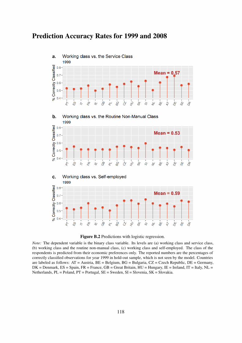
Prediction Accuracy Rates for 1999 and 2008

Figure B.2 Predictions with logistic regression.Note: The dependent variable is the binary class variable. Its levels are (a) working class and service class,(b) working class and the routine non-manual class, (c) working class and self-employed. The class of therespondents is predicted from their economic preferences only. The reported numbers are the percentages ofcorrectly classified observations for year 1999 in hold-out sample, which is not seen by the model. Countriesare labeled as follows: AT = Austria, BE = Belgium, BG = Bulgaria, CZ = Czech Republic, DE = Germany,DK = Denmark, ES = Spain, FR = France, GB = Great Britain, HU = Hungary, IE = Ireland, IT = Italy, NL =Netherlands, PL = Poland, PT = Portugal, SE = Sweden, SI = Slovenia, SK = Slovakia.

118

Figure B.3 Predictions with logistic regression.Note: The dependent variable is the binary class variable. Its levels are (a) working class and service class,(b) working class and the routine non-manual class, (c) working class and self-employed. The class of therespondents is predicted from their economic preferences only. The reported numbers are the percentages ofcorrectly classified observations for year 2008 in hold-out sample, which is not seen by the model. Countriesare labeled as follows: AT = Austria, BE = Belgium, BG = Bulgaria, CZ = Czech Republic, DE = Germany,DK = Denmark, ES = Spain, FR = France, GB = Great Britain, HU = Hungary, IE = Ireland, IT = Italy, NL =Netherlands, PL = Poland, PT = Portugal, SE = Sweden, SI = Slovenia, SK = Slovakia.

Additional Figures

119

Figure B.4 Multilevel regressions.Note: The dependent variable is the economic left-right position of the preferred political party by the respondent.The coefficients of class variable are reported for each country and time point in the sample. The reportedcoefficients represent the difference between the economic left-right positions of the preferred parties by workingclass and routine non-manual class. Countries are labeled as follows: AT = Austria, BE = Belgium, BG = Bulgaria,CZ = Czech Republic, DE = Germany, DK = Denmark, ES = Spain, FR = France, GB = Great Britain, HU =Hungary, IE = Ireland, IT = Italy, NL = Netherlands, PL = Poland, PT = Portugal, SE = Sweden, SI = Slovenia,SK = Slovakia.

120

Figure B.5 Multilevel regressions.Note: The dependent variable is the economic left-right position of the preferred political party by the respondent.The coefficients of class variable are reported for each country and time point in the sample. The reportedcoefficients represent the difference between the economic left-right positions of the preferred parties by workingclass and routine non-manual class. Countries are labeled as follows: AT = Austria, BE = Belgium, BG = Bulgaria,CZ = Czech Republic, DE = Germany, DK = Denmark, ES = Spain, FR = France, GB = Great Britain, HU =Hungary, IE = Ireland, IT = Italy, NL = Netherlands, PL = Poland, PT = Portugal, SE = Sweden, SI = Slovenia,SK = Slovakia.

121

CAppendix to Chapter 3

Tables

Table C.1 The host and bidders of post-war summer Olympic Games

Host Unsuccessful Bidders

1960 Rome, Italy Brussels, Budapest, Detroit, Lausanne, Mexico City, Tokyo1964 Tokyo, Japan Brussels, Detroit, Vienna1968 Mexico City, Mexico Buenos Aires, Detroit, Lyon1972 Munich, Germany Detroit, Madrid, Montreal1976 Montreal, Canada Los Angeles, Moscow1980 Moscow, USSR Los Angeles1984 Los Angeles, USA None1988 Seoul, Korea Nagoya1992 Barcelona, Spain Amsterdam, Belgrade, Birmingham, Brisbane, Paris1996 Atlanta, USA Athens, Belgrade, Manchester, Melbourne, Toronto2000 Sydney, Australia Beijing, Berlin, Istanbul, Manchester2004 Athens, Greece Buenos Aires, Cape Town, Rome, Stockholm2008 Beijing, China Istanbul, Osaka, Toronto, Paris

Source: Rose and Spiegel (2011).

122

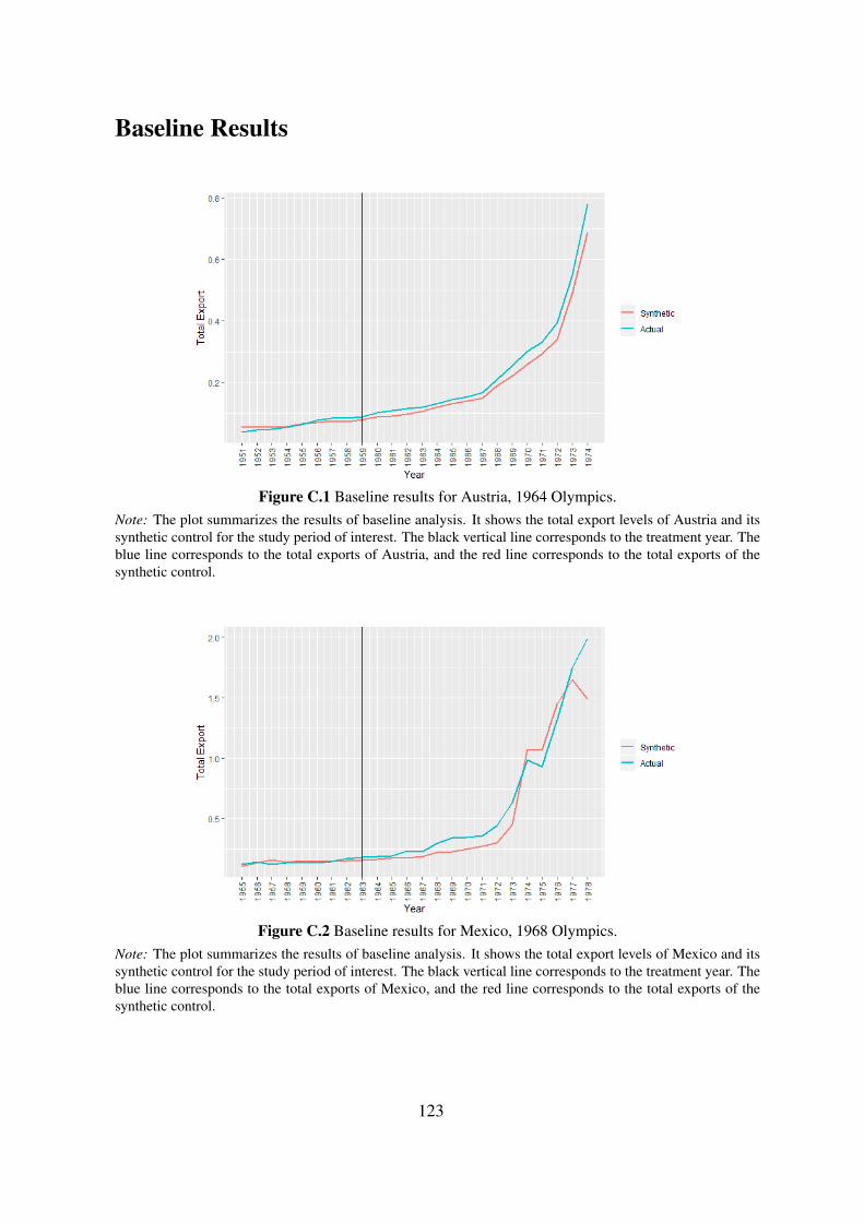
Baseline Results

Figure C.1 Baseline results for Austria, 1964 Olympics.Note: The plot summarizes the results of baseline analysis. It shows the total export levels of Austria and itssynthetic control for the study period of interest. The black vertical line corresponds to the treatment year. Theblue line corresponds to the total exports of Austria, and the red line corresponds to the total exports of thesynthetic control.

Figure C.2 Baseline results for Mexico, 1968 Olympics.Note: The plot summarizes the results of baseline analysis. It shows the total export levels of Mexico and itssynthetic control for the study period of interest. The black vertical line corresponds to the treatment year. Theblue line corresponds to the total exports of Mexico, and the red line corresponds to the total exports of thesynthetic control.

123

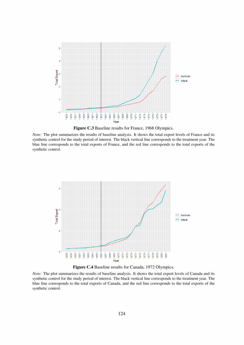
Figure C.3 Baseline results for France, 1968 Olympics.Note: The plot summarizes the results of baseline analysis. It shows the total export levels of France and itssynthetic control for the study period of interest. The black vertical line corresponds to the treatment year. Theblue line corresponds to the total exports of France, and the red line corresponds to the total exports of thesynthetic control.

Figure C.4 Baseline results for Canada, 1972 Olympics.Note: The plot summarizes the results of baseline analysis. It shows the total export levels of Canada and itssynthetic control for the study period of interest. The black vertical line corresponds to the treatment year. Theblue line corresponds to the total exports of Canada, and the red line corresponds to the total exports of thesynthetic control.

124

Figure C.5 Baseline results for Spain, 1992 Olympics.Note: The plot summarizes the results of baseline analysis. It shows the total export levels of Spain and itssynthetic control for the study period of interest. The black vertical line corresponds to the treatment year. Theblue line corresponds to the total exports of Spain, and the red line corresponds to the total exports of the syntheticcontrol.

Figure C.6 Baseline results for Netherlands, 1992 Olympics.Note: The plot summarizes the results of baseline analysis. It shows the total export levels of Netherlands and itssynthetic control for the study period of interest. The black vertical line corresponds to the treatment year. Theblue line corresponds to the total exports of Netherlands, and the red line corresponds to the total exports of thesynthetic control.

125

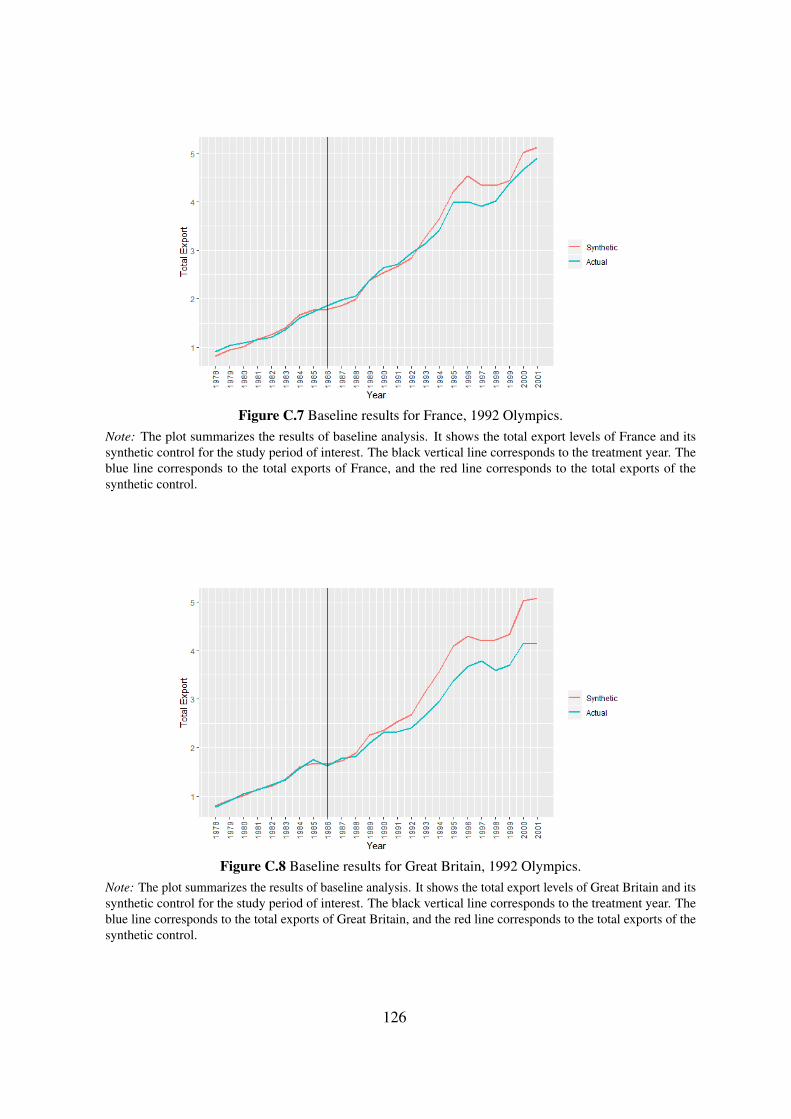
Figure C.7 Baseline results for France, 1992 Olympics.Note: The plot summarizes the results of baseline analysis. It shows the total export levels of France and itssynthetic control for the study period of interest. The black vertical line corresponds to the treatment year. Theblue line corresponds to the total exports of France, and the red line corresponds to the total exports of thesynthetic control.

Figure C.8 Baseline results for Great Britain, 1992 Olympics.Note: The plot summarizes the results of baseline analysis. It shows the total export levels of Great Britain and itssynthetic control for the study period of interest. The black vertical line corresponds to the treatment year. Theblue line corresponds to the total exports of Great Britain, and the red line corresponds to the total exports of thesynthetic control.

126

Figure C.9 Baseline results for Turkey, 2000 Olympics.Note: The plot summarizes the results of baseline analysis. It shows the total export levels of Turkey and itssynthetic control for the study period of interest. The black vertical line corresponds to the treatment year. Theblue line corresponds to the total exports of Turkey, and the red line corresponds to the total exports of thesynthetic control.

Figure C.10 Baseline results for South Africa, 2004 Olympics.Note: The plot summarizes the results of baseline analysis. It shows the total export levels of South Africa and itssynthetic control for the study period of interest. The black vertical line corresponds to the treatment year. Theblue line corresponds to the total exports of South Africa, and the red line corresponds to the total exports of thesynthetic control.

127

Figure C.11 Baseline results for Sweden, 2004 Olympics.Note: The plot summarizes the results of baseline analysis. It shows the total export levels of Sweden and itssynthetic control for the study period of interest. The black vertical line corresponds to the treatment year. Theblue line corresponds to the total exports of Sweden, and the red line corresponds to the total exports of thesynthetic control.

128

Robustness-I

Figure C.12 Robustness-I for Japan: backdating treatment 2 years, 1988 Olmypics.Note: The plot summarizes the results of robustness analysis. It shows the total export levels of Japan and itssynthetic control for the study period of interest. The black vertical line corresponds to the treatment year. Theblue line corresponds to the total exports of Japan, and the red line corresponds to the total exports of the syntheticcontrol.

129

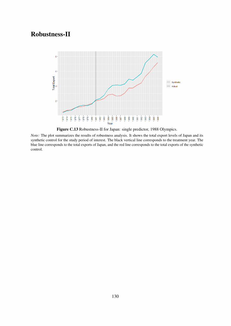
Robustness-II

Figure C.13 Robustness-II for Japan: single predictor, 1988 Olympics.Note: The plot summarizes the results of robustness analysis. It shows the total export levels of Japan and itssynthetic control for the study period of interest. The black vertical line corresponds to the treatment year. Theblue line corresponds to the total exports of Japan, and the red line corresponds to the total exports of the syntheticcontrol.

130

Placebo Analyses

Figure C.14 Placebo analysis for Austria, 1964 Olympics.Note: The plot summarizes the results of placebo analysis. We apply synthetic control method to each country inour donor pool by rotating the treated unit -placebo treatment units. The trends correspond to the exports gapbetween treated units and its synthetic controls. The dashed line corresponds to the treatment year. The solidblack line corresponds to the exports gap between Austria and its synthetic control. Gray lines correspond to theexports gap of the placebo treatment units and their synthetic controls.

Figure C.15 Placebo analysis for Mexico, 1968 Olympics.Note: The plot summarizes the results of placebo analysis. We apply synthetic control method to each country inour donor pool by rotating the treated unit -placebo treatment units. The trends correspond to the exports gapbetween treated units and its synthetic controls. The dashed line corresponds to the treatment year. The solidblack line corresponds to the exports gap between Mexico and its synthetic control. Gray lines correspond to theexports gap of the placebo treatment units and their synthetic controls.

131

Figure C.16 Placebo analysis for France, 1968 Olympics.Note: The plot summarizes the results of placebo analysis. We apply synthetic control method to each country inour donor pool by rotating the treated unit -placebo treatment units. The trends correspond to the exports gapbetween treated units and its synthetic controls. The dashed line corresponds to the treatment year. The solidblack line corresponds to the exports gap between France and its synthetic control. Gray lines correspond to theexports gap of the placebo treatment units and their synthetic controls.

Figure C.17 Placebo analysis for Canada, 1972 Olympics.Note: The plot summarizes the results of placebo analysis. We apply synthetic control method to each country inour donor pool by rotating the treated unit -placebo treatment units. The trends correspond to the exports gapbetween treated units and its synthetic controls. The dashed line corresponds to the treatment year. The solidblack line corresponds to the exports gap between Canada and its synthetic control. Gray lines correspond to theexports gap of the placebo treatment units and their synthetic controls.

132

Figure C.18 Placebo analysis for Japan, 1988 Olympics.Note: The plot summarizes the results of placebo analysis. We apply synthetic control method to each country inour donor pool by rotating the treated unit -placebo treatment units. The trends correspond to the exports gapbetween treated units and its synthetic controls. The dashed line corresponds to the treatment year. The solidblack line corresponds to the exports gap between Japan and its synthetic control. Gray lines correspond to theexports gap of the placebo treatment units and their synthetic controls.

Figure C.19 Placebo analysis for Netherlands, 1992 Olympics.Note: The plot summarizes the results of placebo analysis. We apply synthetic control method to each country inour donor pool by rotating the treated unit -placebo treatment units. The trends correspond to the exports gapbetween treated units and its synthetic controls. The dashed line corresponds to the treatment year. The solidblack line corresponds to the exports gap between Netherlands and its synthetic control. Gray lines correspond tothe exports gap of the placebo treatment units and their synthetic controls.

133

Figure C.20 Placebo analysis for France, 1992 Olympics.Note: The plot summarizes the results of placebo analysis. We apply synthetic control method to each country inour donor pool by rotating the treated unit -placebo treatment units. The trends correspond to the exports gapbetween treated units and its synthetic controls. The dashed line corresponds to the treatment year. The solidblack line corresponds to the exports gap between France and its synthetic control. Gray lines correspond to theexports gap of the placebo treatment units and their synthetic controls.

Figure C.21 Placebo analysis for Great Britain, 1992 Olympics.Note: The plot summarizes the results of placebo analysis. We apply synthetic control method to each country inour donor pool by rotating the treated unit -placebo treatment units. The trends correspond to the exports gapbetween treated units and its synthetic controls. The dashed line corresponds to the treatment year. The solidblack line corresponds to the exports gap between Great Britain and its synthetic control. Gray lines correspondto the exports gap of the placebo treatment units and their synthetic controls.

134

Figure C.22 Placebo analysis for Turkey, 2000 Olympics.Note: The plot summarizes the results of placebo analysis. We apply synthetic control method to each country inour donor pool by rotating the treated unit -placebo treatment units. The trends correspond to the exports gapbetween treated units and its synthetic controls. The dashed line corresponds to the treatment year. The solidblack line corresponds to the exports gap between Turkey and its synthetic control. Gray lines correspond to theexports gap of the placebo treatment units and their synthetic controls.

Figure C.23 Placebo analysis for South Africa, 2004 Olympics.Note: The plot summarizes the results of placebo analysis. We apply synthetic control method to each country inour donor pool by rotating the treated unit -placebo treatment units. The trends correspond to the exports gapbetween treated units and its synthetic controls. The dashed line corresponds to the treatment year. The solidblack line corresponds to the exports gap between South Africa and its synthetic control. Gray lines correspondto the exports gap of the placebo treatment units and their synthetic controls.

135

Figure C.24 Placebo analysis for Sweden, 2004 Olympics.Note: The plot summarizes the results of placebo analysis. We apply synthetic control method to each country inour donor pool by rotating the treated unit -placebo treatment units. The trends correspond to the exports gapbetween treated units and its synthetic controls. The dashed line corresponds to the treatment year. The solidblack line corresponds to the exports gap between Sweden and its synthetic control. Gray lines correspond to theexports gap of the placebo treatment units and their synthetic controls.

136