Essays on the Economics of Ethnolinguistic Differences

Andrew C. Dickens

A DISSERTATION

SUBMITTED TO THE FACULTY OF GRADUATE STUDIESIN PARTIAL FULFILLMENT OF THE REQUIREMENTS

for the degree

DOCTOR OF PHILOSOPHY

GRADUATE PROGRAM IN ECONOMICSYORK UNIVERSITY

TORONTO, ONTARIOAPRIL 2017

c© Andrew C. Dickens, 2017

Abstract

In this dissertation, I study the origins and economic consequences of ethnolinguistic differences.To quantify these differences, I construct a lexicostatistical measure of linguistic distance. I usethis measure to study two different outcomes: ethnic politics and cross-country idea flows. I thentake the economic importance of ethnolinguistic differences as given, and explore the geographicfoundation of these differences.

In chapter 1, I document evidence of ethnic favoritism in 35 sub-Saharan countries. I use lexi-costatistical distance to quantify the similarity between an ethnic group and the national leader’sethnic identity. I find that a one standard deviation increase in similarity yields a 2 percent in-crease in group-level GDP per capita. I then use the continuity of lexicostatistical similarity toshow that favoritism exists among groups that are not coethnic to the leader, where the mean ef-fect of non-coethnic similarity is one quarter the size of the coethnic effect. I relate these resultsto the literature on coalition building, and provide evidence that ethnicity is a guiding principlebehind high-level government appointments.

In chapter 2, I use book translations data to capture cross-country idea flows. It has beenconjectured that income gaps are smaller between ancestrally related countries because they com-municate more ideas. I provide empirical support for this link and a deeper understanding ofthe hypothesized mechanism: population differences do exhibit a negative relationship with thediffusion of ideas, with the caveat that this negative relationship operates across linguistic lines.After accounting for the linguistic distance between two countries, I find that dissimilar popula-tions communicate more ideas.

In chapter 3, I study the geographic origins of ethnolinguistic differences. I construct a noveldataset to examine the border regions of neighbouring ethnolinguistic groups, together with varia-tion in the set of potentially cultivatable crops at the onset of the Columbian Exchange, to estimatehow agricultural diversity impacts linguistic differences between neighbouring groups. I findthat ethnic groups separated across agriculturally diverse regions are more similar in languagethan groups separated across homogeneous agricultural regions. I propose that historical trade inagriculturally diverse regions is the mechanism by which group similarities are preserved.

ii

Dedication

To Meghan, for your steadfast encouragement and support throughout the years. You have mademy life better in more ways than I could ever articulate to you, and undoubtedly my work isbetter off as a result. Your daily inspiration is the footing upon which I have found my stride as aresearcher.

To my parents, Wenda and Greg, you have instilled in me an appreciation of knowledge.Thank you for believing in me, and always encouraging me to go after my dreams in life – aca-demic and otherwise. My education would not have been possible without the opportunities thatyou provided for me, and I am forever grateful that I am where I am today because of you.

To my sister, Claire, I have always admired your curiosity and enthusiasm. You have inspiredthese qualities in me, without which I would not have seen this dissertation through to comple-tion. You have always been my ally and I thank you for your unwavering support.

iii

Acknowledgements

I am indebted to my supervisor, Nippe Lagerlof, for his unwavering support of my ideas, for hisability to always push me towards my intellectual frontier, and for the countless hours of his timehe spent with me discussing my research. My dissertation would pale in comparison without hisinvaluable supervision, his contribution to my academic development and his friendship.

My development as a researcher would also not have been the same without the help of TassoAdamopoulos. Throughout many meetings over the course of my dissertation, he has offeredperspective and encouragement that has directly contributed to how I think about economic prob-lems. I am truly grateful for all the excellent advice Tasso has given me about my research andabout how to succeed as an economist.

I owe a huge thanks to Ben Sand for guiding me through the world of econometrics. My un-derstanding and appreciation of empirical methods would not be the same without Ben’s wealthof knowledge. In addition to his fantastic comments and suggestions about my work, Ben hasspent hours of his time helping me understand the answer to my many questions over the years.

Many other members of the department have contributed to my dissertation and provided anenvironment that was conducive to my academic development. A special thanks to Berta Esteve-Volart for reading and commenting on many drafts of my work, and for always providing excel-lent comments during or after one of my seminars. Other faculty members that have contributedto my dissertation and always given me their time, even though not on my committee, includeAhmet Akyol, Sam Bucovetsky, Avi Cohen, Wai-Ming Ho, Fernando Leibovici, Uros Petronijevic,Laura Salisbury and Andrey Stoyanov. And a big thanks to my classmate, Andrew Hencic, foralways hearing out my daily research problem on the subway ride home from campus.

An additional thanks to the many discussants and seminar participants that have contributedto my dissertation, in particular James Fenske for providing extensive comments on my job marketpaper. A special thanks also goes to Oded Galor for hosting my Visiting Research Fellowship atBrown University in 2015. My time at Brown was the most memorable experience of my graduatestudies, and I thank those that I met who contributed to my dissertation, including Greg Casey,Mario Carillo, Raphael Franck, Stelios Michalopoulos, Omer Ozak, Assaf Sarid and David Weil.

Last, but definitely not least, I am thankful for my friends who have made Toronto home forme. Having a group of friends who support and encourage me – away from work – has beeninstrumental to my productivity and focus over the past six years. This dissertation would not bethe same without them.

iv

Table of Contents

1 Ethnolinguistic Favoritism in African Politics 11.1 Introduction . . . . . . . . . . . . . . . . . . . . . . . . . . . . . . . . . . . . . . . . . . 11.2 Data . . . . . . . . . . . . . . . . . . . . . . . . . . . . . . . . . . . . . . . . . . . . . . . 7

1.2.1 Language Group Partitions . . . . . . . . . . . . . . . . . . . . . . . . . . . . . 71.2.2 Satellite Imagery of Night Light Luminosity . . . . . . . . . . . . . . . . . . . 81.2.3 Assignment of a Leader’s Ethnolinguistic Identity . . . . . . . . . . . . . . . . 81.2.4 Linguistic Similarity . . . . . . . . . . . . . . . . . . . . . . . . . . . . . . . . . 91.2.5 Patterns in the Data . . . . . . . . . . . . . . . . . . . . . . . . . . . . . . . . . . 12

1.3 Empirical Model . . . . . . . . . . . . . . . . . . . . . . . . . . . . . . . . . . . . . . . . 141.3.1 Identification of Linguistic Similarity . . . . . . . . . . . . . . . . . . . . . . . 15

1.4 Benchmark Results . . . . . . . . . . . . . . . . . . . . . . . . . . . . . . . . . . . . . . 161.4.1 What Drives Favoritism? . . . . . . . . . . . . . . . . . . . . . . . . . . . . . . 24

1.5 How Is Patronage Distributed? . . . . . . . . . . . . . . . . . . . . . . . . . . . . . . . 251.5.1 DHS Individual-Level Data . . . . . . . . . . . . . . . . . . . . . . . . . . . . . 281.5.2 Locational and Individual Similarity Estimates . . . . . . . . . . . . . . . . . . 29

1.6 Discussion: Coalition Building . . . . . . . . . . . . . . . . . . . . . . . . . . . . . . . 301.7 Concluding Remarks . . . . . . . . . . . . . . . . . . . . . . . . . . . . . . . . . . . . . 34

2 Population Relatedness and Cross-Country Idea Flows 362.1 Introduction . . . . . . . . . . . . . . . . . . . . . . . . . . . . . . . . . . . . . . . . . . 362.2 Data . . . . . . . . . . . . . . . . . . . . . . . . . . . . . . . . . . . . . . . . . . . . . . . 40

2.2.1 Measuring Language Distance . . . . . . . . . . . . . . . . . . . . . . . . . . . 402.2.2 Measuring Genetic Distance . . . . . . . . . . . . . . . . . . . . . . . . . . . . . 422.2.3 Book Translations as Idea Flows . . . . . . . . . . . . . . . . . . . . . . . . . . 42

2.3 Methodology and Empirical Results . . . . . . . . . . . . . . . . . . . . . . . . . . . . 452.3.1 Econometric Model . . . . . . . . . . . . . . . . . . . . . . . . . . . . . . . . . . 452.3.2 Unconditional Benchmark Results . . . . . . . . . . . . . . . . . . . . . . . . . 452.3.3 Conditional Benchmark Results . . . . . . . . . . . . . . . . . . . . . . . . . . 48

2.4 Robustness . . . . . . . . . . . . . . . . . . . . . . . . . . . . . . . . . . . . . . . . . . . 502.4.1 Testing the Home Country Assumption of Book Translations . . . . . . . . . 50

v

2.4.2 Human Capital . . . . . . . . . . . . . . . . . . . . . . . . . . . . . . . . . . . . 542.4.3 Existing Bilateral Relationships . . . . . . . . . . . . . . . . . . . . . . . . . . . 562.4.4 Check for Understated Standard Errors . . . . . . . . . . . . . . . . . . . . . . 572.4.5 Differences in Across Country Language Structure . . . . . . . . . . . . . . . 57

2.5 Distance Effects by Idea Types . . . . . . . . . . . . . . . . . . . . . . . . . . . . . . . . 602.6 Concluding Remarks . . . . . . . . . . . . . . . . . . . . . . . . . . . . . . . . . . . . . 61

3 Ecology, Trade and the Geographic Origins of Ethnolinguistic Differences 633.1 Introduction . . . . . . . . . . . . . . . . . . . . . . . . . . . . . . . . . . . . . . . . . . 633.2 The Columbian Exchange . . . . . . . . . . . . . . . . . . . . . . . . . . . . . . . . . . 663.3 Data . . . . . . . . . . . . . . . . . . . . . . . . . . . . . . . . . . . . . . . . . . . . . . . 66

3.3.1 Linguistic Distance . . . . . . . . . . . . . . . . . . . . . . . . . . . . . . . . . . 663.3.2 Independent Variables . . . . . . . . . . . . . . . . . . . . . . . . . . . . . . . . 673.3.3 Does Geography Delineate Ethnolinguistic Groups? . . . . . . . . . . . . . . . 69

3.4 Empirical Strategy and Estimates . . . . . . . . . . . . . . . . . . . . . . . . . . . . . . 703.4.1 Identification Strategy . . . . . . . . . . . . . . . . . . . . . . . . . . . . . . . . 703.4.2 Empirical Model and Results . . . . . . . . . . . . . . . . . . . . . . . . . . . . 70

3.5 Concluding Remarks . . . . . . . . . . . . . . . . . . . . . . . . . . . . . . . . . . . . . 77

Bibliography 80

A Language Appendix 89

B Chapter 1 Appendix 92

C Chapter 2 Appendix 119

D Chapter 3 Appendix 132

vi

List of Tables

1.1 Descriptive Statistics . . . . . . . . . . . . . . . . . . . . . . . . . . . . . . . . . . . . . 131.2 Means of Linguistic Similarity Above-Below Median Night Lights . . . . . . . . . . . 131.3 Benchmark Regressions Using Various Measures of Linguistic Similarity . . . . . . . 171.4 Horse Race Regressions: Contrasting the Different Measures of Linguistic Similarity 191.5 Testing for Anticipatory Effects: Estimates Using Leads and Lags . . . . . . . . . . . 211.6 Test for Migration Following Leadership Changes . . . . . . . . . . . . . . . . . . . . 231.7 Selection into Lexicostatistical Language Lists . . . . . . . . . . . . . . . . . . . . . . 241.8 The Dynamics of Ethnolinguistic Favoritism . . . . . . . . . . . . . . . . . . . . . . . 261.9 Benchmark Regressions with Heterogeneous Effects . . . . . . . . . . . . . . . . . . . 271.10 Individual-Level Regressions: Locational and Individual Similarity . . . . . . . . . . 31

2.1 Summary Statistics for Distance Measures . . . . . . . . . . . . . . . . . . . . . . . . . 462.2 Unconditional Benchmark Regressions . . . . . . . . . . . . . . . . . . . . . . . . . . . 472.3 Conditional Benchmark Regressions . . . . . . . . . . . . . . . . . . . . . . . . . . . . 492.4 Robustness Check for Problematic Original Languages of Translation . . . . . . . . . 512.5 Conditional Benchmark Regressions with Alternative Home Country Assignment . 532.6 Robustness Check: Human Capital and Education . . . . . . . . . . . . . . . . . . . . 552.7 Robustness Check: Unobserved Country-Pair Effects . . . . . . . . . . . . . . . . . . 562.8 Robustness Check for Understated Standard Errors . . . . . . . . . . . . . . . . . . . 582.9 Robustness Check for Differences in Across-Country Language Structure . . . . . . . 592.10 Distance Effects by Cultural and Economic Idea Types . . . . . . . . . . . . . . . . . . 61

3.1 Difference in Means: Language Pair Zone vs. Language Pair Buffer Zone . . . . . . . 713.2 Border-Level Regressions: Unconditional Caloric Suitability Index Benchmark Results 733.3 Border-Level Regressions: Conditional Caloric Suitability Index Benchmark Results 743.4 Border-Level Regressions: Native Population Sensitivity Analysis . . . . . . . . . . . 763.5 Border-Level Regressions: Overlapping and Multipart Polygon Sensitivity Analysis 78

B1 Language Groups Included in Regional-Level Analysis . . . . . . . . . . . . . . . . . 97B2 Language Groups Included in DHS Individual-Level Analysis . . . . . . . . . . . . . 98B3 Leaders Included in Regional-Level Analysis . . . . . . . . . . . . . . . . . . . . . . . 99B4 Leaders Included in DHS Individual-Level Analysis . . . . . . . . . . . . . . . . . . . 100

vii

B5 Countries Included in Regional- and Individual-Level Analysis . . . . . . . . . . . . 100B6 Summary Statistics – Regional-Level Dataset . . . . . . . . . . . . . . . . . . . . . . . 101B7 Summary Statistics – DHS Individual-Level Dataset . . . . . . . . . . . . . . . . . . . 102B8 Summary Statistics – Power Sharing Dataset . . . . . . . . . . . . . . . . . . . . . . . 102B9 Benchmark Regressions Using Various Combinations of Fixed Effects . . . . . . . . . 109B10 Robustness Check: Benchmark Regressions with Additional Control Variables . . . . 110B11 Robustness Check: Excluding Leaders with Ambiguous Ethnolinguistic Identities . 111B12 Robustness Check: Benchmark Regressions on a Balanced Panel . . . . . . . . . . . . 112B13 Robustness Check: Benchmark Regressions Weighted by Language Group Population113B14 Robustness Check: Benchmark Regressions with Alternative Dependent Variables . 114B15 Individual-Level Regressions: Locational and Individual Similarity . . . . . . . . . . 115B16 Individual-Level Regressions: Locational and Individual Similarity . . . . . . . . . . 116B17 Individual-Level Regressions: Baseline Covariates . . . . . . . . . . . . . . . . . . . . 117B18 Ethnic Favoritism and Coalition Power Sharing . . . . . . . . . . . . . . . . . . . . . . 118

C1 Benchmark Sample Summary Statistics . . . . . . . . . . . . . . . . . . . . . . . . . . 121C2 Commonly Translated Authors by Country . . . . . . . . . . . . . . . . . . . . . . . . 122C3 Language Pair Observations by Translating Country for the Benchmark Sample

(1979-2005) . . . . . . . . . . . . . . . . . . . . . . . . . . . . . . . . . . . . . . . . . . . 123C4 Observations by Translating Language for the Benchmark Sample (1979-2005) . . . . 124C5 Observations by Original Language for the Benchmark Sample (1979-2005) . . . . . 125C6 Conditional Benchmark Regressions with Cladistic Linguistic Distance . . . . . . . . 128C7 Sensitivity Analysis: Further Test of Home Country Assignment . . . . . . . . . . . . 129C8 Robustness Check for Dominant Subject of Translation . . . . . . . . . . . . . . . . . 130C9 Ethnologue Home Country vs. Synthetic Language Country Assignment . . . . . . . 131

D1 Summary Statistics – Full Sample . . . . . . . . . . . . . . . . . . . . . . . . . . . . . . 134D2 Summary Statistics – Sibling Sample . . . . . . . . . . . . . . . . . . . . . . . . . . . . 135D3 Robustness Check: Native Population Sensitivity Analysis . . . . . . . . . . . . . . . 136D4 Robustness Check: Overlapping and Multi-Part Polygon Sensitivity Analysis . . . . 137

viii

List of Figures

1.1 Change in Night Lights Intensity from 1993-1999 . . . . . . . . . . . . . . . . . . . . . 41.2 Language Groups . . . . . . . . . . . . . . . . . . . . . . . . . . . . . . . . . . . . . . . 71.3 Language Partitions . . . . . . . . . . . . . . . . . . . . . . . . . . . . . . . . . . . . . . 71.4 Lexicostatistical Similarities Among Sibling Language Pairs . . . . . . . . . . . . . . 111.5 Pre-Post Leadership Change . . . . . . . . . . . . . . . . . . . . . . . . . . . . . . . . . 121.6 DHS Clusters Across Waves in the Kuranko Language Group Partition . . . . . . . . 291.7 Ethnic Favoritism and Coalition Building . . . . . . . . . . . . . . . . . . . . . . . . . 33

2.1 Opposing Forces of Population Relatedness on the Flow of Ideas . . . . . . . . . . . 392.2 Benchmark Sample Observations by Country (1979-2005) . . . . . . . . . . . . . . . . 44

3.1 Phylogenetic Tree of Eritrean Languages . . . . . . . . . . . . . . . . . . . . . . . . . . 673.2 Example: Buffer Zone Unit of Observation . . . . . . . . . . . . . . . . . . . . . . . . 68

A1 Phylogenetic Tree of the Eight Major Eritrean Languages . . . . . . . . . . . . . . . . 91

ix

Chapter 1

Ethnolinguistic Favoritism in AfricanPolitics

1.1 Introduction

Understanding why global poverty is so concentrated in Africa remains one of the most crucialareas of inquiry in the social sciences. One long-standing explanation is that Africa’s high level ofethnic diversity is a major source of its underdevelopment and political instability (Easterly andLevine, 1997; Collier and Gunning, 1999; Posner, 2004; Alesina and La Ferrara, 2005, among oth-ers). Yet recent evidence documents that the source of underdevelopment is not ethnic diversityper se, but rather Africa’s high degree of inequality between ethnic groups (Alesina et al., 2016).This suggests that ethnic diversity is only an impediment to economic development when someethnicities prosper at the expense of others.

Ethnic inequality not only contributes to the under-provision of the overall level of publicresources (Baldwin and Huber, 2010), but it provokes discriminatory policies that advantage somegroups over others (Alesina et al., 2016). Discriminatory policies of this type are a form of ethnicfavoritism, which has been the subject of a few influential papers that document evidence of publicresource distribution across ethnic lines in Africa (Franck and Rainer, 2012; Burgess et al., 2015;Kramon and Posner, 2016). The provision of resources on the basis of ethnicity – rather than on aneed or marginal value basis – suggests that some ethnic groups are being systematically favoredover others. Hence, a better understanding of how ethnic patronage is distributed and to whomis important because it sheds light on the extent to which favoritism occurs and how some ethnicgroups benefit at the expense of others.

In this paper I revisit the study of ethnic favoritism with three contributions. My first contri-bution is a novel measure of linguistic similarity that quantifies the relative similarity of all ethnicgroups to the national leader in each country, not just groups that share an ethnicity with theleader (coethnics). Because linguistic similarity is measured on the unit interval it encompassesthe commonly used coethnic dummy variable, while extending measurement to all non-coethnic

1

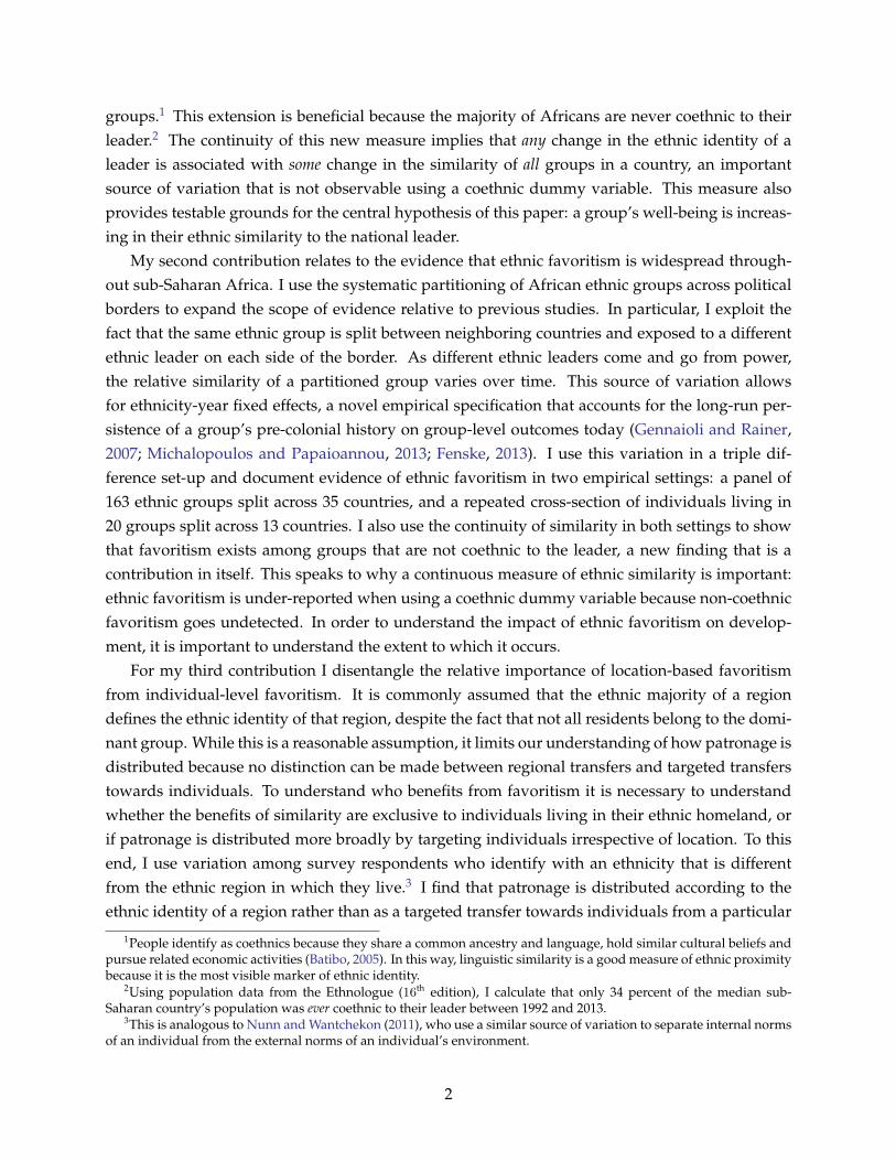
groups.1 This extension is beneficial because the majority of Africans are never coethnic to theirleader.2 The continuity of this new measure implies that any change in the ethnic identity of aleader is associated with some change in the similarity of all groups in a country, an importantsource of variation that is not observable using a coethnic dummy variable. This measure alsoprovides testable grounds for the central hypothesis of this paper: a group’s well-being is increas-ing in their ethnic similarity to the national leader.

My second contribution relates to the evidence that ethnic favoritism is widespread through-out sub-Saharan Africa. I use the systematic partitioning of African ethnic groups across politicalborders to expand the scope of evidence relative to previous studies. In particular, I exploit thefact that the same ethnic group is split between neighboring countries and exposed to a differentethnic leader on each side of the border. As different ethnic leaders come and go from power,the relative similarity of a partitioned group varies over time. This source of variation allowsfor ethnicity-year fixed effects, a novel empirical specification that accounts for the long-run per-sistence of a group’s pre-colonial history on group-level outcomes today (Gennaioli and Rainer,2007; Michalopoulos and Papaioannou, 2013; Fenske, 2013). I use this variation in a triple dif-ference set-up and document evidence of ethnic favoritism in two empirical settings: a panel of163 ethnic groups split across 35 countries, and a repeated cross-section of individuals living in20 groups split across 13 countries. I also use the continuity of similarity in both settings to showthat favoritism exists among groups that are not coethnic to the leader, a new finding that is acontribution in itself. This speaks to why a continuous measure of ethnic similarity is important:ethnic favoritism is under-reported when using a coethnic dummy variable because non-coethnicfavoritism goes undetected. In order to understand the impact of ethnic favoritism on develop-ment, it is important to understand the extent to which it occurs.

For my third contribution I disentangle the relative importance of location-based favoritismfrom individual-level favoritism. It is commonly assumed that the ethnic majority of a regiondefines the ethnic identity of that region, despite the fact that not all residents belong to the domi-nant group. While this is a reasonable assumption, it limits our understanding of how patronage isdistributed because no distinction can be made between regional transfers and targeted transferstowards individuals. To understand who benefits from favoritism it is necessary to understandwhether the benefits of similarity are exclusive to individuals living in their ethnic homeland, orif patronage is distributed more broadly by targeting individuals irrespective of location. To thisend, I use variation among survey respondents who identify with an ethnicity that is differentfrom the ethnic region in which they live.3 I find that patronage is distributed according to theethnic identity of a region rather than as a targeted transfer towards individuals from a particular

1People identify as coethnics because they share a common ancestry and language, hold similar cultural beliefs andpursue related economic activities (Batibo, 2005). In this way, linguistic similarity is a good measure of ethnic proximitybecause it is the most visible marker of ethnic identity.

2Using population data from the Ethnologue (16th edition), I calculate that only 34 percent of the median sub-Saharan country’s population was ever coethnic to their leader between 1992 and 2013.

3This is analogous to Nunn and Wantchekon (2011), who use a similar source of variation to separate internal normsof an individual from the external norms of an individual’s environment.

2

ethnic group.Throughout this empirical analysis I rely on the fact that the location of African borders are

quasi-random (Englebert et al., 2002; Michalopoulos and Papaioannou, 2014, 2016, among oth-ers). The historical formation of Africa’s borders began with the Berlin Conference of 1884-1885,where European powers divided up Africa with little regard for the spatial distribution of eth-nic homelands (Herbst, 2000). This disregard led to the arbitrary formation of national borders,which “did not reflect reality but helped create it” (Wesseling, 1996, p.364). One such reality wasthe partitioning of approximately 200 ethnic groups throughout Africa.

In the context of this study, the quasi-random nature of African border design generates ex-ogenous variation because the ethnic identity of a national leader varies across borders withinthe same partitioned group. Because an ethnic group shares a common ancestry, and is relativelyhomogeneous in terms of cultural and biological factors, the fraction of a partitioned group onone side of the border is a suitable counterfactual observation for the other fraction of that samegroup across the border. Using ethnic groups partitioned across African borders as a source ofexogenous variation is methodologically similar to Michalopoulos and Papaioannou (2014).

To exploit this within-group variation I use the 16th edition of the Ethnologue language map(Lewis, 2009). This map depicts the spatial distribution of ethnolinguistic homelands across theworld. I use these subnational groups as a spatial unit of observation in Africa. Because no incomedata exists at this level of observation, I proxy an ethnic group’s economic activity using annualsatellite images of night light luminosity for the time period 1992-2013. These luminosity data areavailable at a very fine spatial resolution, which I can use to construct a panel of economic activ-ity at the country-group level. Luminosity is frequently used as a measure of economic activitybecause of its strong empirical association with GDP per capita and other measures of living stan-dards (Henderson et al., 2012; Michalopoulos and Papaioannou, 2013, 2014; Alesina et al., 2016,among others). Hodler and Raschky (2014) first used luminosity in this way to study patterns ofregional favoritism.

Consider, as an example, the Jola-Fonyi language group partitioned across Gambia and Sene-gal. In 1993, both the Gambian and Senegalese Jola-Fonyi bear little resemblance to their respec-tive leaders. For several years little changed in Senegal as President Diouf’s reign continued. Onthe contrary, much changed for the Gambian Jola-Fonyi when Yahya Jammeh, a young officer inthe National Gambian Army, overthrew President Jawara in a 1994 military coup. Jammeh wasborn in Kanilai, a small village near the southern border of Gambia and home to the Jola-Fonyilanguage group. Jammeh took much pride in his birth region – a “place that gained prominenceovernight in Gambia” (Mwakikagile, 2010, p. 56). Jammeh repeatedly “feathered his nest” to suchan extent that the Jola-Fonyi region surrounding Kanilai is one of few rural areas in Gambia with“electricity, street lighting, paved roads and running water – not to mention its own zoo and gamepreserve, wrestling arena, bakery and luxury hotel with a swimming pool” (Wright, 2015, p. 219).

Figure 1.1 provides visual evidence of this phenomenon. The two panels represent the samesubsection of the Jola-Fonyi language group at two points in time, with the border dividing Gam-

3

Figure 1.1: Change in Night Lights Intensity from 1993-1999

This figure documents the change in night light activity in the partitioned Jola-Fonyi language group in Gambia (northof the border) and Senegal (south of the border) between 1993 and 1999. In 1994, Yahya Jammeh assumed power ofGambia and soon after started reallocating funds to the Jola-Fonyi. Within 5 years of presidency the Gambian Jola-Fonyi exhibit much greater economic activity in terms of night lights than the Senegalese Jola-Fonyi on the south sideof the border, whom had no change in leadership during this period.

bia to the north and Senegal to the south. While there is no visible night light activity on either sideof the border in 1993, there is a significant increase in lights on the Gambian side only 5 years afterJammeh assumed power. On the contrary, Diouf’s presidency continued throughout this entireperiod and there is no observable change in night light activity in Senegal just south of the border.This demonstrated change in Figure 1.1 is exactly the within-group variation that I use to estimatethe effect of similarity. In this case, the Senegalese Jola-Fonyi are the counterfactual observationfor the Gambian Jola-Fonyi, who are equally dissimilar in language to their incumbent leader in1993, and the effect of similarity on night light activity is estimated off of the change in linguisticsimilarity following Jammeh’s rise to power.

My benchmark results imply that a standard deviation increase in linguistic similarity (23 per-cent) yields a 7 percent increase in luminosity and a 2 percent increase in group-level GDP percapita. I also use the continuity of linguistic similarity to document evidence of non-coethnicfavoritism, where the mean non-coethnic effect is one quarter the coethnic premium. To the con-trary I find no evidence of anticipatory effects in the data or evidence migration in response toleadership changes. To be sure this result is not a consequence of my new measure of similarity Iconstruct two alternative measures: a standard binary measure of coethnicity and a discrete simi-larity measure of the ratio of shared nodes on the Ethnologue language tree. While these alterna-tive measures of similarity yield significant evidence of favoritism, my preferred lexicostatisticalmeasure of similarity is more precisely estimated and the only measure to maintain significance

4

in a series of horse race regressions.I also test for a variety of mechanisms, but find no systematic evidence of the usual channels

(e.g., democracy). However, I do find that my benchmark result is largely driven by leaders whohave held office longer than the sample median of nine years. This implies that one determinantof favoritism is leadership tenure.

Next I turn to individual-level data from the Demographic and Health Survey (DHS). I usesurvey cluster coordinates to pinpoint the location of individual respondents on the Ethnologuemap. Doing so allows me to construct a repeated cross-section of individuals living in partitionedethnic groups across DHS survey waves. Narrowing the focus to these individuals allows me toexploit the same variation I use in my benchmark estimates. As an outcome I use an individual-level measure of access to public resources and ownership of assets. I corroborate my benchmarkfindings with this individual-level data, including evidence of non-coethnic favoritism. I also es-tablish that patronage is distributed regionally and not as a targeted transfer towards individuals.

These findings speak to a sparse but growing body of evidence that ethnic favoritism is widespreadthroughout sub-Saharan Africa. Franck and Rainer (2012) use a panel of ethnic groups in 18 coun-tries to document evidence of favoritism throughout sub-Saharan Africa. What sets my paperapart from Franck and Rainer’s (2012) is that I construct a panel of partitioned ethnic groups, soI have a minimum of two country-group observations for any partitioned group in a year. Thisfeature of my data affords me ethnicity-year fixed effects. Because I can account for all observ-able and unobservable time-varying features of an ethnic group, I am able to rule out endogeneityconcerns associated with the impact of pre-colonial group characteristics on contemporary devel-opment (Gennaioli and Rainer, 2007; Michalopoulos and Papaioannou, 2013; Fenske, 2013).

More commonly researchers focus on a single patronage good in a single country. Kramonand Posner (2016) find that Kenyans whom are coethnic to their leader attain higher levels of edu-cation, while Burgess et al. (2015) find that Kenyan districts associated with the leader’s ethnicityreceive two times the investment in roads during periods of autocracy. At an even finer level,Marx et al. (2015) document evidence of ethnic favoritism in housing markets within a large slumoutside of Nairobi.

The rich micro-data these studies use provide clear evidence of ethnic favoritism and the chan-nels through which patronage is distributed. Yet generalizing these results is difficult because ofthe highly localized analyses these studies employ. To this end, I exploit the systematic partition-ing of ethnic groups in Africa to expand the scope of evidence to 35 sub-Saharan countries. In arelated manuscript, De Luca et al. (2015) document that ethnic favoritism is an axiom of politics ona global scale and not simply an African phenomenon. As this literature continues to grow, theselocalized studies coupled with the broader evidence of ethnic favoritism help to build consensusaround ethnic favoritism in Africa.4

4Yet consensus on ethnic favoritism if Africa has not been reached. Francois et al. (2015) document that leadersonly provide a small premium to their coethnics, and otherwise political power is proportional to group size in Africa.Kasara (2007) finds that leaders are more likely to extract taxes from their own ethnic group because they have a betterunderstanding of internal markets in their homeland.

5

The notion that ethnic favoritism drives discriminatory policies that disadvantage some groupsat the expense of others also relates this research to the literature on ethnic inequality and con-flict. Alesina et al. (2016) document that the negative correlation between ethnic inequality andeconomic development is a global phenomenon, though most pronounced in Africa. Income dif-ferences between a country’s ethnic groups can also impact the political process: ethnic inequalitymitigates public good provision (Baldwin and Huber, 2010), diminishes the quality of governance(Kyriacou, 2013), and provokes the “ethnification” of political parties (Huber and Suryanarayan,2014). At the heart of this literature is the long-standing instrumentalist view that conflict overscarce resources drives ethnic competition in Africa (Bates, 1974). Even the perception of ethnicfavoritism exacerbates already existing ethnic tensions (Bowles and Gintis, 2004), which itself canfurther incite ethnic conflict (Esteban and Ray, 2011; Esteban et al., 2012; Caselli and Coleman,2013).

I contribute to this line of research with evidence that regions, rather than individuals, tend tobe targeted, and that non-coethnic groups that are similar to the leader stand to gain from theirethnic proximity. The fact that similar but not identical ethnic regions benefit from patronagesuggests that ethnicity is more than just a marker of identity: similarity may create affinity orreduce coordination costs across related non-coethnic groups. This is consistent with the ideathat these broader ethnic connections may solve collective action problems (Miguel and Gugerty,2005) and bring about greater between-group trust (Habyarimana et al., 2009). The continuityof linguistic similarity captures these affinities that are otherwise unobservable with a coethnicdummy variable, thus highlighting one further benefit of this new measure.

This is also in line with the idea that leaders bring elites from outside of their ethnic groupinto the governing coalition in an effort to sustain power in the face of political instability (Joseph,1987; Francois et al., 2015). In the discussion section of this paper I provide evidence that leadersappoint similar but not identical ethnic elites to high-level government positions for this purpose.In doing so, non-coethnic groups gain coethnic representation in government, where representa-tives speak on their behalf and channel resources to them (Arriola, 2009). Although my focus isAfrica, this deeper understanding of where favoritism is expected to take place has implicationsfor distributive politics more broadly: it contributes to our knowledge of how targeted transferscan potentially magnify inequality between groups and thus is informative of a determining factorof comparative economic development

The rest of this paper is structured as follows. Section 1.2 describes how I identify languagegroup partitions and measure linguistic similarity. This section also documents patterns in thedata. Section 1.3 outlines the empirical model and identification strategy, and Section 1.4 reportsthe benchmark estimates and robustness checks. Section 1.5 disentangles the relative importanceof location-based favoritism from individual-level favoritism, and in Section 1.6 I link the findingsto the literature on ethnic favoritism and coalition building, and provide suggestive evidence thatnon-coethnic favoritism works through the appointment of elites from outside of the leader’sethnic group. Section 1.7 concludes.

6

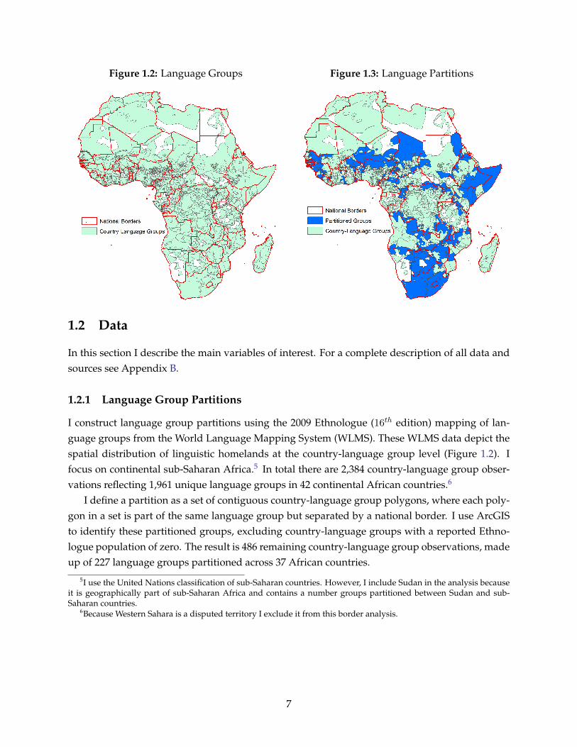
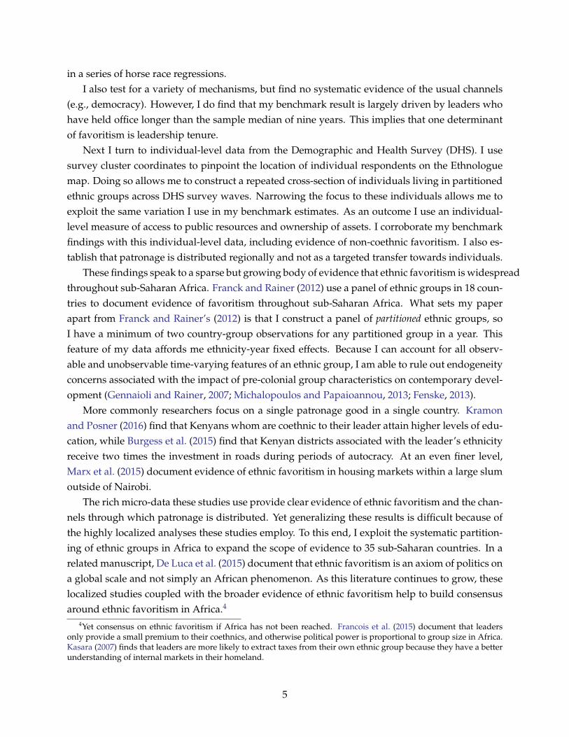
Figure 1.2: Language Groups Figure 1.3: Language Partitions

1.2 Data

In this section I describe the main variables of interest. For a complete description of all data andsources see Appendix B.

1.2.1 Language Group Partitions

I construct language group partitions using the 2009 Ethnologue (16th edition) mapping of lan-guage groups from the World Language Mapping System (WLMS). These WLMS data depict thespatial distribution of linguistic homelands at the country-language group level (Figure 1.2). Ifocus on continental sub-Saharan Africa.5 In total there are 2,384 country-language group obser-vations reflecting 1,961 unique language groups in 42 continental African countries.6

I define a partition as a set of contiguous country-language group polygons, where each poly-gon in a set is part of the same language group but separated by a national border. I use ArcGISto identify these partitioned groups, excluding country-language groups with a reported Ethno-logue population of zero. The result is 486 remaining country-language group observations, madeup of 227 language groups partitioned across 37 African countries.

5I use the United Nations classification of sub-Saharan countries. However, I include Sudan in the analysis becauseit is geographically part of sub-Saharan Africa and contains a number groups partitioned between Sudan and sub-Saharan countries.

6Because Western Sahara is a disputed territory I exclude it from this border analysis.

7

1.2.2 Satellite Imagery of Night Light Luminosity

Satellite imagery of night light luminosity come from the National Oceanic and Atmospheric Ad-ministration’s (NOAA) National Geophysical Data Center. Many others have used these databecause of two features: night lights data exhibit a strong empirical relationship with GDP percapita and other measures of living standards (Henderson et al., 2012), and because these data areavailable at a spatial resolution of 30-arc seconds (approximately 1 square kilometre).7 The fineresolution of these lights data facilitates a proxy measure of GDP per capita at any desired levelof spatial aggregation. Because I require a measure of economic activity at the country-languagegroup level – a level of aggregation where no official data on economic output exists – the avail-ability of these data is indispensable to this study.

The yearly composite of night light luminosity is constructed by NOAA using daily imagestaken from U.S. Department of Defense weather satellites that circle the earth 14 times a day. Thesesatellites observe every location on earth every night sometime between 20:30 and 22:00. Beforedistributing these data publicly, NOAA scientists remove observations contaminated by strongsources of natural light, e.g., the summer months when the sun sets late, light activity related tothe northern and southern lights, forest fires, etc. All daily images that pass this screening processare then averaged for the entire year producing a satellite-year dataset for the time period 1992 to2013. Light intensity receives a value of 0 to 63 at a resolution of 30-arc seconds. The result is ameasure of night light intensity that only reflects human (economic) activity.8

Using these data I construct a panel of average luminosity for each country-language grouppartition. I use the Africa Albers Equal Area Conic projection to minimize distortion across thearea dimension before calculating the average light luminosity of each country-language grouppolygon in each year.9 I follow Michalopoulos and Papaioannou (2013, 2014) and Hodler andRaschky (2014) in adding 0.01 to the log transformation of the lights data because roughly 40%of these data have a value of zero in the benchmark sample. Doing so helps correct for the non-normal nature of the data and preserves sample size, and allows for a (near) semi-elasticity inter-pretation of the benchmark empirical model.

1.2.3 Assignment of a Leader’s Ethnolinguistic Identity

There are 106 leaders to assign an ethnolinguistic identity for my sample of 35 countries between1992-2013. The challenge of mapping ethnicity to language is that, in some instances, a singleethnic group speaks many languages. Because African language groups are often resident ofwell-defined territories (Lewis, 2009), an ethnolinguistic identity is typically attached to a person’s

7Hodler and Raschky (2014) also show there is a strong empirical relationship between these night lights data andGDP at the subnational administrative region. Michalopoulos and Papaioannou (2014) further validate the use ofnight lights in Africa as a proxy measure of development with evidence that light intensity correlates strongly withindividual-level data on electrification, presence of sewage systems, access to piped water and education.

8Henderson et al. (2012, p. 998) provide a thorough introduction to the NOAA night lights data.9In some years data is available for two separate satellite, and in all such cases the correlation between the two is

greater than 99 percent in my sample. To remove choice on the matter I use an average of both.

8

birthplace (Batibo, 2005). As a first step towards assignment I locate the birthplace of a leader andcollect latitude and longitude coordinates for each birthplace from www.latlong.net. I project thesecoordinates onto the Ethnologue map of Africa to back out the language group associated witheach leader’s birthplace.10 I exclude leaders born abroad (4 leaders) since their ethnolinguisticgroup is not home to the country they govern.11 Second, I identify a leader’s ethnic identity usingdata from Dreher et al. (2015) and Francois et al. (2015), and in the few instances where neithersource reports the ethnicity of a leader I fill in the gap using a country’s Historical Dictionary.Finally, I take the following steps to assign a leader’s ethnolinguistic identity using these data:

Step 1: I compare the birthplace linguistic identity with the ethnic identity for each of the102 leaders. In 56.9 percent of the sample the name of the birth language and ethnic identity areequivalent (58 leaders). For these leaders the assignment is unambiguous.

Step 2: For the remaining sample of unmatched leaders, I check if the birthplace languageis a language spoken by the leader’s ethnic group. In 12.7 percent of the sample this is true (13leaders); I assign the birthplace language as the leader’s ethnolinguistic identity.

Step 3: For the remaining 30.4 percent of unmatched leaders (31 leaders), the birthplace iden-tity does not correspond to their ethnic identity. This is especially true for leaders born in a majorcity. For these leaders I drop the birthplace identity and map the ethnicity of a leader to a singlelanguage using the three-step assignment rule outlined in Appendix B.

1.2.4 Linguistic Similarity

Estimating linguistic similarity is difficult because languages can differ in a variety of ways, in-cluding vocabulary, pronunciation, grammar, syntax, phonetics and more. One common approachis to use a measure of the shared branches on a language tree as an approximation of linguisticsimilarity. Known as cladistic similarity, this measure was introduced to economists by Fearonand Laitin (1999), popularized by Fearon (2003) and has since become the convention.12 The ideabehind the cladistic approach is that two languages with a large number of shared nodes – andthus a recent splitting from a common ancestor – will be similar in terms of language becauseof their common ancestry. The data most commonly used is Fearon’s (2003) cladistic measure oflinguistic similarity, constructed using the Ethnologue’s phylogenetic language tree. A cladisticmeasure is attractive because linguistic similarity is easily computed for any language pair, sincelanguage trees exist for virtually all known world language families (Lewis, 2009). See AppendixA for a formal definition of this measure.

My preferred measure is a computerized lexicostatistical measure of linguistic similarity de-

10Because most leaders enter/exit office mid-year, I assign the incumbent leader as whomever is in power on De-cember 31st of the transition year. Hence, by assumption I drop any leader who exited office the same year she enteredoffice because she was neither in power the previous year or December 31st of the transition year.

11These leaders include Ian Khama (Botswana), Francois Bozize Yangouvonda (Central African Republic), NicephoreSoglo (Benin), and Rupiah Banda (Zambia).

12For example, Guiso et al. (2009); Spolaore and Wacziarg (2009); Desmet et al. (2012); Esteban et al. (2012) and Gomes(2014) all use a cladistic approach, among others.

9

veloped by the Automatic Similarity Judgement Program (ASJP).13 As a percentage estimate ofa language pair’s cognate words (i.e., words that share a common linguistic origin), the lexico-statistical method is a measure of the phonological similarity between two languages. Hence, alexicostatistical measure can be thought of as a proxy for the ancestral relationship between twogroups, or an implicit measure of the set of shared ancestral and cultural traits that are importantto group identity.

The ASJP Database (Version 16) consists of 4401 language lists, where each list contains thesame 40 implied meanings (i.e., words) for comparison across languages. The ASJP research teamhas transcribed these lists into a standardized orthography called ASJPcode, a phonetic ASCIIalphabet consisting of 34 consonants and 7 vowels. A standardized alphabet restricts variationacross languages to phonological differences. Meanings are then transcribed according to pro-nunciation before language differences are estimated.14

Then for each language pair of interest I run the Levenshtein distance algorithm on the re-spective language lists, which calculates the minimum number of edits necessary to translate thespelling of each word from one language to another. To correct for the fact that longer words willdemand more edits, each distance is divided by the length of the translated word. This normal-ization yields a percentage estimate of dissimilarity, which is measured across the unit interval.The average distance of a language pair is calculated by averaging across the distance estimatesof all 40 words. By this procedure I estimate the linguistic distance of a language pair vis-a-vis thevocabulary dimension.

A second normalization procedure is used to adjust for the accidental similarity of two lan-guages (Wichmann et al., 2010). This normalization accounts for similar ordering and frequencyof characters that are the result of chance and independent of a word’s meaning. Finally, I definethe lexicostatistical similarity of a language pair as one minus this normalized distance. For aformal definition of this measure, I direct to reader to Appendix A.

The main advantage of the lexicostatistical approach is that it measures similarity in a morecontinuous way than the cladistic approach. Because the lexicostatistical method explicitly iden-tifies the phonological differences of a language pair, there is far more observable variation in ameasure of lexicostatistical similarity than cladistic similarity. The cladistic approach is a coarsemeasure of similarity because data dispersion is limited to 15 unique values, the maximum num-ber of language family classifications in the Ethnologue.

To illustrate this point, consider language pairs that share a common parent language on theEthnologue language tree. Let these language pairs be known as siblings. All sibling pairs sharethe maximum number of tree nodes, and have no differences in cladistic similarity between them,but they do exhibit substantial variation in lexicostatistical similarity. To make this point clear,

13The lexicostatistical measure I use in this paper has been used to study factor flows in international trade (Is-phording and Otten, 2013), job satisfaction of linguistically distinct migrants (Bloemen, 2013), language acquisition ofmigrants (Isphording and Otten, 2014), and the role of language in the flow of ideas (Dickens, 2016b). See (Ginsburghand Weber, 2016) for a discussion of this and other measures of linguistic distance.

14For example, the French word for you is vous, and is encoded using ASJPcode as vu to reflect its pronunciation.

10

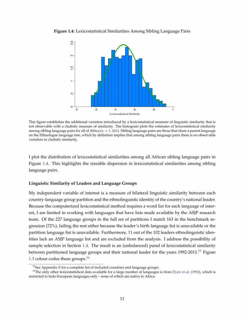
Figure 1.4: Lexicostatistical Similarities Among Sibling Language Pairs

0.5

11.5

22.5

0 .2 .4 .6 .8 1Lexicostatistical Similarity

This figure establishes the additional variation introduced by a lexicostatistical measure of linguistic similarity that isnot observable with a cladistic measure of similarity. The histogram plots the estimates of lexicostatistical similarityamong sibling language pairs for all of Africa (n = 1, 241). Sibling language pairs are those that share a parent languageon the Ethnologue language tree, which by definition implies that among sibling language pairs there is no observablevariation in cladistic similarity.

I plot the distribution of lexicostatistical similarities among all African sibling language pairs inFigure 1.4. This highlights the sizeable dispersion in lexicostatistical similarities among siblinglanguage pairs.

Linguistic Similarity of Leaders and Language Groups

My independent variable of interest is a measure of bilateral linguistic similarity between eachcountry-language group partition and the ethnolinguistic identity of the country’s national leader.Because the computerized lexicostatistical method requires a word list for each language of inter-est, I am limited to working with languages that have lists made available by the ASJP researchteam. Of the 227 language groups in the full set of partitions I match 163 in the benchmark re-gression (72%), failing the rest either because the leader’s birth language list is unavailable or thepartition language list is unavailable. Furthermore, 11 out of the 102 leaders ethnolinguistic iden-tities lack an ASJP language list and are excluded from the analysis. I address the possibility ofsample selection in Section 1.4. The result is an (unbalanced) panel of lexicostatistical similaritybetween partitioned language groups and their national leader for the years 1992-2013.15 Figure1.3 colour codes these groups.16

15See Appendix B for a complete list of included countries and language groups.16The only other lexicostatistical data available for a large number of languages is from Dyen et al. (1992), which is

restricted to Indo-European languages only – none of which are native to Africa.

11

Figure 1.5: Pre-Post Leadership Change

-.06-.04-.02

0.02

.04

.06

-4 -3 -2 -1 0 1 2 3 4Years Before-After Leader Change

Positive change in linguistic similarity to leader

Negative change in linguistic similarity to leader

(Net of country-year fixed effects)Average Night Light Intensity

This figure plots the before and after effects of a change in leadership on average night light luminosity. The greensolid line depicts luminosity in the 4 years leading up to a change in leadership and the 4 years following an increase inlinguistic similarity. The blue dashed line depicts the same for country-language groups that experienced a decrease insimilarity after a change in leadership. Average night light luminosity is the residual light variation net of country-yeareffects to account for different years of leadership change across countries.

1.2.5 Patterns in the Data

Table 1.1 reports descriptive statistics for the night lights and language data. For completeness, Ihave included a cladistic measure of similarity and a binary measure of coethnicity.17 The meanvalue of lexicostatistical linguistic similarity says that country-language groups are 19.3 percentsimilar to their national leader on average, and the mean value of cladistic similarity implies 40.9percent similarity. The mean value of coethnicity says that 4.7 percent of the benchmark sample iscoethnic to their national leader.18

In Table 1.2 I preview the empirical results by splitting the sample by the median value of nightlights and test for differences in average linguistic similarity. Panel A reports mean differences inthe benchmark sample for all three similarity measures. Take, for example, the mean differencein lexicostatistical similarity: language groups who emit night light above the median value areon average 10.4 percent more similar to their national leader than those below the median value.This difference is highly significant, with a reported p-value of 0.000. The same pattern is trueirrespective of the measure of linguistic similarity. These findings are consistent with my proposedhypothesis of ethnolinguistic favoritism, where language groups are better off the more similar

17I use the term coethnicity to be consistent with the literature, but a better name would be coethnolinguists since Idefine coethnicity equal to one when a leader’s ethnolinguistic identity is the same as a partitioned language group.

18Table B6 reports a complete set of descriptive statistics used throughout this analysis.

12

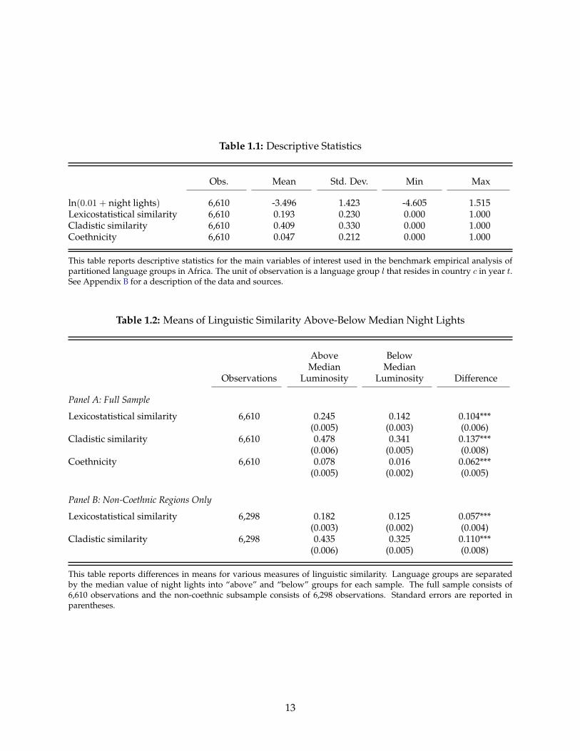
Table 1.1: Descriptive Statistics

Obs. Mean Std. Dev. Min Max

ln(0.01 + night lights) 6,610 -3.496 1.423 -4.605 1.515Lexicostatistical similarity 6,610 0.193 0.230 0.000 1.000Cladistic similarity 6,610 0.409 0.330 0.000 1.000Coethnicity 6,610 0.047 0.212 0.000 1.000

This table reports descriptive statistics for the main variables of interest used in the benchmark empirical analysis ofpartitioned language groups in Africa. The unit of observation is a language group l that resides in country c in year t.See Appendix B for a description of the data and sources.

Table 1.2: Means of Linguistic Similarity Above-Below Median Night Lights

Above BelowMedian Median

Observations Luminosity Luminosity Difference

Panel A: Full Sample

Lexicostatistical similarity 6,610 0.245 0.142 0.104***(0.005) (0.003) (0.006)

Cladistic similarity 6,610 0.478 0.341 0.137***(0.006) (0.005) (0.008)

Coethnicity 6,610 0.078 0.016 0.062***(0.005) (0.002) (0.005)

Panel B: Non-Coethnic Regions Only

Lexicostatistical similarity 6,298 0.182 0.125 0.057***(0.003) (0.002) (0.004)

Cladistic similarity 6,298 0.435 0.325 0.110***(0.006) (0.005) (0.008)

This table reports differences in means for various measures of linguistic similarity. Language groups are separatedby the median value of night lights into “above” and “below” groups for each sample. The full sample consists of6,610 observations and the non-coethnic subsample consists of 6,298 observations. Standard errors are reported inparentheses.

13

they are to their national leader.Panel B repeats this exercise in all non-coethnic sample observations. As stated in the introduc-

tion, if relative groups differences matter outside of coethnic relationships, then the data shouldtell me that similarity matters among non-coethnics. This is exactly what I find: the average sim-ilarity among non-coethnic language groups above and below the median night lights value issignificantly different than zero. While I reserve more conclusive statements for the regressionanalysis, this suggests that linguistic similarity provides significant variation that is unobservablein the conventional binary framework. Together these results show that night lights and linguisticsimilarity are positively related, or that on average a language group is increasingly better off themore linguistically similar they are to the birth language of their national leader. The significantpairwise correlation of 0.30 between light intensity and lexicostatistical similarity is also sugges-tive of this positive relationship (correlation not shown here).

I also plot average luminosity before and after a leadership change in Figure 1.5, separatinggroups who experience an increase in lexicostatistical similarity from those that experience a de-crease. I construct a “treatment” time scale that takes a value of 0 in the year of a leadershipchange, and plot the residual light variation net of country-year effects to account for differentyears of leadership changes. I plot these data for the 4 years leading up to a change and the 4years following. It is reassuring for identification that there is little observed change in night lightactivity in the years leading up to a change in leadership. Yet shortly after a leadership changethere is a noticeable increase in night lights in regions that experienced an increase in linguisticsimilarity to the leader (solid green line), and a large drop in average night lights in regions thatexperienced a decrease in similarity (dashed blue line). Hence, Figure 1.5 is a clean visualizationof favoritism across linguistic lines.19

1.3 Empirical Model

The main objective of this empirical analysis is to test the hypothesis that a language group that islinguistically similar to the ethnolinguistic identity of the national leader will be better off than agroup whose language is relatively more distant. To do this I use a triple difference-in-differencesestimator:

yc,l,t = γc,l + λc,t + θl,t + x′c,l,t Φ + βLSc,l,t−1 + εc,l,t. (1.1)

The dependent variable yc,l,t is the night lights measure of economic activity for languagegroup l in country c in year t. As the dependent variable I follow the literature and take theaforementioned log transformation of night lights such that yc,l,t ≡ ln (0.01 +NightLightsc,l,t).

19The number of observations used to calculate the average night lights in either group varies by years. The nature ofthe data presents two challenges in constructing a standard treatment time scale. First, in some instances there is morethan one leadership change in the shown 8-year interval. Second, and in consequence of the first point, two leadershipchanges over the 8-year interval do not always result in consistent positive or negative changes of similarity.

14

LSc,l,t−1, the variable of interest, measures the linguistic similarity between language groupl in country c and the ethnolinguistic identity of country c’s political leader in year t − 1. I laglinguistic similarity because of an expected delay between the decision to allocate public fundsto a region and the actual allocation of those goods (Hodler and Raschky, 2014), and an expecteddelay between the actual allocation of public funds and the resulting regional increase in nightlight production.

Xc,l,t is a vector of controls including the (logged) average of population density for eachcountry-language, and the (logged) geodesic distance between language group l and the languagegroup associated with the leader of country c.20 I also include a variety of geographic endowmentcontrols in xc,l,t: two indicator variables for the presence of oil and diamond reserves in boththe leader and language group regions, as well as the absolute difference in elevation, rugged-ness, precipitation, average temperature and the caloric suitability index (agricultural quality).These additional controls account for the possibility that national projects that are beneficial to theleader’s region because of a particular geographic characteristic might also benefit other regionsof similar character.21 γc,l are country-language group fixed effects, λc,t are country-year fixedeffects and θl,t are language-year fixed effects.22 In all specifications I adjust standard errors forclustering in country-language groups.23

1.3.1 Identification of Linguistic Similarity

In order to identify the effect of linguistic similarity it is necessary that the placement of nationalborders are not the result of local economic conditions or any factor that reflects the well-being ofa language group. Indeed, national borders are a historical by-product of the Scramble for Africa.The use of straight lines prevailed when drawing borders in Africa because the Berlin Confer-ence of 1884-85 legitimized claims of colonial sovereignty without pre-existing territorial occupa-tion, rendering knowledge of pre-colonial boundaries inconsequential (Englebert et al., 2002). Theresult was a reluctance by colonialists to respect traditional boundaries when drawing borders(Herbst, 2000). Evidence of this is still seen today, where group partitions do not correlate withgeography and natural resources (Michalopoulos and Papaioannou, 2016) and nearly 80% of allAfrican borders follow lines of latitude and longitude – an amount larger than any other continentin the world (Alesina et al., 2011).24

20Population density data comes from the Gridded Population of the World. Because population density data is onlyavailable in 5-year intervals (i.e., 1990, 1995, 2000, 2005 and 2010), I assume the density to be constant throughout theunobserved intermediate years.

21See Appendix B for more details on data definitions and sources.22In my benchmark sample γc,l represents 355 fixed effects, λc,t represents 691 fixed effects and θl,t represents 3044

fixed effects.23Given that the benchmark sample has only 35 countries, I choose not to adjust standard errors for two-dimensional

clustering within language groups and countries (Cameron et al., 2011). While the benchmark results are qualitativelysimilar when two-way clustering, I follow Kezdi’s (2004) rule of thumb that at least 50 clusters are needed for accurateinference.

24See Englebert et al. (2002) and Michalopoulos and Papaioannou (2014, 2016) for a detailed discussion on the arbi-trary design of African borders.

15

It is the arbitrary design of African political borders that forms the basis of my identificationstrategy. The ethnolinguistic identity of a national leader varies by country, so group partitioninggenerates exogenous within-group variation in terms of that group’s linguistic similarity to theirleader. This strategy is similar to Michalopoulos and Papaioannou (2014), though a key differ-ence is that I construct a panel of partitioned groups rather than a cross-section, so the relativesimilarity within a partitioned group also varies over time as new leaders come to power. This isinstrumental to identification: by including the three sets of fixed effects discussed in the previoussection, I absorb all the variation in the data with the exception of time-variation at the country-language group level. γc,l and λc,t respectively difference out time-invariant country-group trendsand country-time trends that are differentially affecting the same group on each side of the border.The inclusion of θl,t only allows for within-group time-variation that comes from changes in lead-ership. Hence, with my set-up in equation (1.1), I am estimating the effect of linguistic similarityoff of changes in the incoming leader’s ethnolinguistic identity.

In my benchmark sample this variation comes from 35 leadership changes: the within trans-formation of θl,t implies that a leadership change in one country varies the mean similarity of apartition in that country and all other fragments of that partition in neighbouring countries. Inother words, the relative similarity within a partitioned group varies with a leadership changeon either side of the border. This amounts to 485 unique relative similarities observed between1992-2013 in my data.

1.4 Benchmark Results

Table 1.3 reports nine different estimates: three versions of equation (1.1) for each of the threelinguistic similarity measures. For each measure of similarity, I report estimates (i) without anycovariates (columns 1-3), (ii) estimates that control for log population density and the loggedgeodesic distance between each partitioned group and the corresponding leader’s group (columns4-6), and (iii) the full set of covariates I outlined in Section 1.3 (columns 7-9). Hereafter I will referto columns 7-9 as my benchmark specification.25

Consistent with my hypothesis of ethnolinguistic favoritism, all nine coefficients are positiveand my preferred measure of lexicostatistical similarity is always statistically significant. Becausevariation is coming from changes in the ethnic identity of a leader, the interpretation of thesefindings is that a group’s well-being is increasing in their ethnic similarity to the leader. To giveeconomic meaning to these estimates, consider the benchmark estimate of lexicostatistical simi-larity in column 7. Using the rule of thumb that the estimated elasticity of GDP per capita withrespect to night lights is 0.3 (Henderson et al., 2012), the point estimate of 0.305 implies that a stan-dard deviation increase in linguistic similarity (23 percent change) yields a 2.1 percent increase inregional GDP per capita, an economically significant effect.26

25See Table B9 for various other combinations of fixed effects specifications.26The percentage change in GDP per capita ≈ percentage change in night lights × 0.3 = (β × ∆LSc,l,t−j) × 0.3 =

16

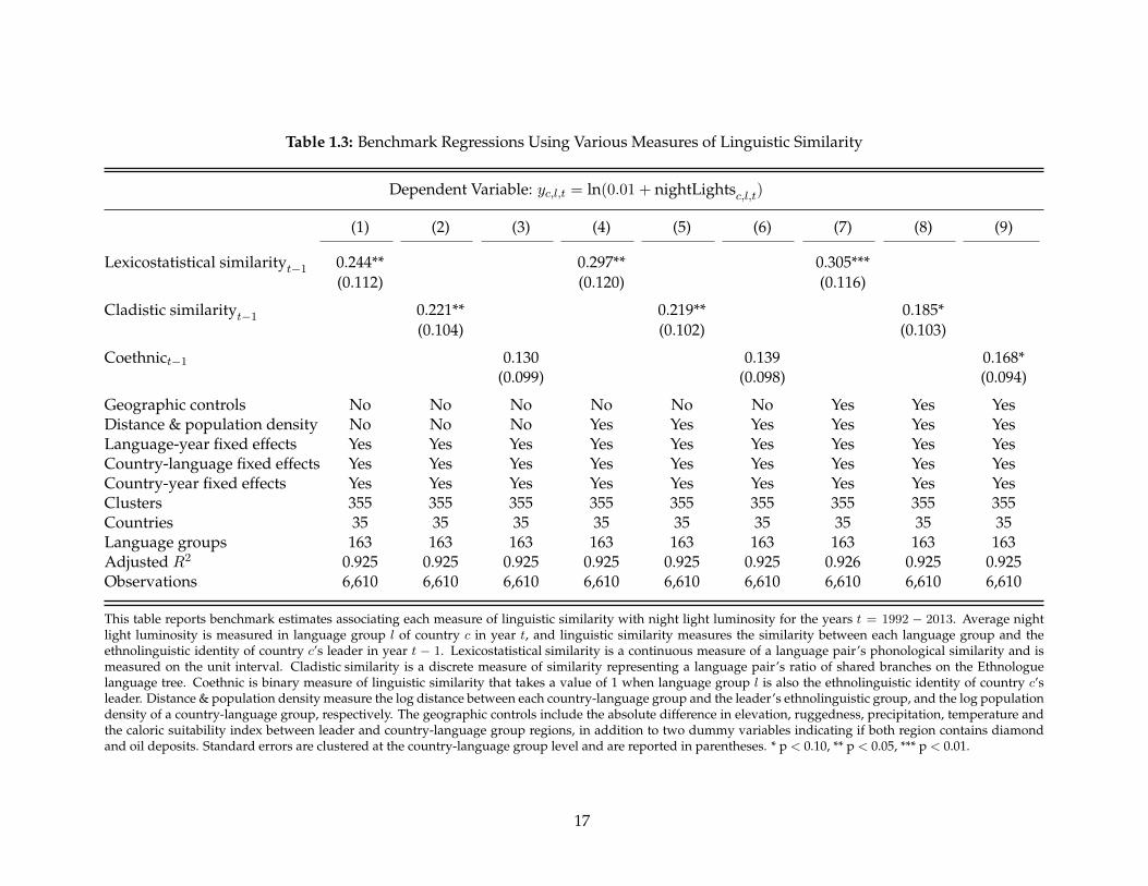
17

Table 1.3: Benchmark Regressions Using Various Measures of Linguistic Similarity

Dependent Variable: yc,l,t = ln(0.01 + nightLightsc,l,t)

(1) (2) (3) (4) (5) (6) (7) (8) (9)

Lexicostatistical similarityt−1 0.244** 0.297** 0.305***(0.112) (0.120) (0.116)

Cladistic similarityt−1 0.221** 0.219** 0.185*(0.104) (0.102) (0.103)

Coethnict−1 0.130 0.139 0.168*(0.099) (0.098) (0.094)

Geographic controls No No No No No No Yes Yes YesDistance & population density No No No Yes Yes Yes Yes Yes YesLanguage-year fixed effects Yes Yes Yes Yes Yes Yes Yes Yes YesCountry-language fixed effects Yes Yes Yes Yes Yes Yes Yes Yes YesCountry-year fixed effects Yes Yes Yes Yes Yes Yes Yes Yes YesClusters 355 355 355 355 355 355 355 355 355Countries 35 35 35 35 35 35 35 35 35Language groups 163 163 163 163 163 163 163 163 163Adjusted R2 0.925 0.925 0.925 0.925 0.925 0.925 0.926 0.925 0.925Observations 6,610 6,610 6,610 6,610 6,610 6,610 6,610 6,610 6,610

This table reports benchmark estimates associating each measure of linguistic similarity with night light luminosity for the years t = 1992 − 2013. Average nightlight luminosity is measured in language group l of country c in year t, and linguistic similarity measures the similarity between each language group and theethnolinguistic identity of country c’s leader in year t − 1. Lexicostatistical similarity is a continuous measure of a language pair’s phonological similarity and ismeasured on the unit interval. Cladistic similarity is a discrete measure of similarity representing a language pair’s ratio of shared branches on the Ethnologuelanguage tree. Coethnic is binary measure of linguistic similarity that takes a value of 1 when language group l is also the ethnolinguistic identity of country c’sleader. Distance & population density measure the log distance between each country-language group and the leader’s ethnolinguistic group, and the log populationdensity of a country-language group, respectively. The geographic controls include the absolute difference in elevation, ruggedness, precipitation, temperature andthe caloric suitability index between leader and country-language group regions, in addition to two dummy variables indicating if both region contains diamondand oil deposits. Standard errors are clustered at the country-language group level and are reported in parentheses. * p < 0.10, ** p < 0.05, *** p < 0.01.

I also provide estimates for cladistic similarity and coethnicity to see how these alternativemeasures compare to lexicostatistical similarity. For my benchmark estimates both coefficients arepositive and statistically significant, albeit only at the 10 percent level. Notice that in all iterationsof equation (1.1), the magnitude and precision of the estimate is monotonically increasing in themeasured continuity of linguistic similarity. This suggests that the observable variation amongnon-coethnic groups assists in identifying patterns of ethnic favoritism in Africa, and thus speaksthe virtue of the lexicostatistical measure.

In Table 1.4 I report estimates from a series of horse race regressions. With these estimatesI show that the lexicostatistical measure is better at identifying patterns of favoritism than thealternative measures of similarity. In columns 1-4, I report estimates for all possible pairings ofthe three measures of similarity. Because all three measures of similarity are highly correlatedwith each other, and for coethnic observations are equivalent, the effect of lexicostatistical andcladistic similarity are estimated off of the additional variation these measures provide amongnon-coethnics. In all pairings the additional lexicostatistical variation is estimated to be statisti-cally significant, despite the fact that the effect of coethnicity is not identifiable in these regressions.In column 3, cladistic similarity outperforms coethnicity in magnitude and precision, reaffirmingthe value of the addition variation it provides over a coethnic indicator, but is not estimated to besignificantly different than zero.

To disentangle the effect of coethnicity from the benefits of similarity among non-coethnics, Idefine non-coethnic lexicostatistical similarity as (1−coethnict−1)× lexicostatistical similarity, andequivalently for non-coethnic cladistic similarity. In other words, these non-coethnic similaritymeasures are equal to zero when the observed language group is coethnic to their national leader,and otherwise equivalent to the respective measure of similarity. Combined with the coethnicmeasure, I can exploit the same variation I identify off of in columns 2 and 3 but load the effect ofcoethnicity onto the coethnic dummy variable.

Because it is intuitive that a leader is more inclined to favor her coethnics, I expect to see astrong significant effect of coethnicity beyond the effect found among non-coethnic groups. In-deed, column 5 indicates that coethnics are most favored with an estimated increase of 0.260 inaverage night light luminosity. While there is still an observable benefit from similarity amongnon-coethnics, the magnitude of the effect is roughly one quarter the size of the coethnic effect onaverage. With a sample mean of 0.146, non-coethnic lexicostatistical similarity yields an averageincrease of 0.069 (= 0.146× 0.473) in night light luminosity.27

I repeat this exercise with non-coethnic cladistic similarity and report the estimates in column(6). Once again I find the corresponding estimate for cladistic similarity from column (3) but cannow identify the effect of coethnicity. The estimated coefficient for coethnicity is quite similarto the coethnic effect found in column (5), only now the additional variation coming from the

0.305 × 0.230 × 0.3 = 2.1%, assuming that ln(0.01 + nightLightsc,l,t

) ≈ ln(nightLightsc,l,t

).27By these estimates the threshold value of non-coethnic similarity is 0.550, above which would imply non-coethnics

are better off than coethnics. The likelihood of measurement error in linguistic similarity implies this is a rather “fuzzy”threshold, and with only 2 percent of the benchmark sample above this threshold I find this result to be reassuring.

18

19

Table 1.4: Horse Race Regressions: Contrasting the Different Measures of Linguistic Similarity

Dependent Variable: yc,l,t = ln(0.01 +NightLightsc,l,t)

(1) (2) (3) (4) (5) (6)

Lexicostatistical similarityt−1 0.345** 0.473** 0.591**(0.165) (0.227) (0.291)

Cladistic similarityt−1 -0.046 0.151 -0.102(0.146) (0.125) (0.150)

Coethnict−1 -0.213 0.080 -0.249 0.260** 0.230**(0.202) (0.114) (0.211) (0.106) (0.110)

Non-coethnic lexicostatistical similarityt−1 0.473**(0.227)

Non-coethnic cladistic similarityt−1 0.151(0.125)

Geographic controls Yes Yes Yes Yes Yes YesDistance & population density Yes Yes Yes Yes Yes YesLanguage-year fixed effects Yes Yes Yes Yes Yes YesCountry-language fixed effects Yes Yes Yes Yes Yes YesCountry-year fixed effects Yes Yes Yes Yes Yes YesClusters 355 355 355 355 355 355Countries 35 35 35 35 35 35Language groups 163 163 163 163 163 163Adjusted R2 0.926 0.926 0.925 0.926 0.926 0.925Observations 6,610 6,610 6,610 6,610 6,610 6,610

This table reports horse race regressions comparing each measure of linguistic similarity. Average night light luminosity is measured in language group l of coun-try c in year t, and linguistic similarity measures the similarity between each language group and the ethnolinguistic identity of country c’s leader in year t − 1.Lexicostatistical similarity is a continuous measure of a language pair’s phonological similarity and is measured on the unit interval. Cladistic similarity is a dis-crete measure of similarity representing a language pair’s ratio of shared branches on the Ethnologue language tree. Coethnic is binary measure of linguisticsimilarity that takes a value of 1 when language group l is also the ethnolinguistic identity of country c’s leader. Non-coethnic lexicostatistical similarity andNon-coethnic cladistic similarity are constructed by interacting a dummy variable for non-coethnicity with Lexicostatistical similarity and Cladistic similarity, re-spectively. All control variables are described in Table 1.3. Standard errors are clustered at the country-language group level and are reported in parentheses. * p <0.10, ** p < 0.05, *** p < 0.01.

cladistic measure is not enough to identify the effect of similarity among non-coethnic groups.

Taken together the results of Table 1.3 and Table 1.4 indicate that favoritism is most prominentamong coethnics but also to a lesser extent among non-coethnics. These results also indicate thata continuous measure of lexicostatistical similarity provides valuable information that is not ob-servable with a coethnic indicator variable. For the remainder of this section I proceed to test therobustness of the benchmark lexicostatistical estimate.

Anticipatory Effects

In this section I run of a series of tests of the identifying assumptions underlying my benchmarkestimates. Column (1) of Table 1.5 reproduces the benchmark estimate of lexicostatistical similarityfor comparison. In column (2) I show that the lagged measure of lexicostatistical similarity is notessential to my findings; contemporaneous lexicostatistical similarity is estimated to be positiveand significant at the 5 percent level.

In column (3) I report an estimate of lexicostatistical similarity measured in period t + 1. Inthis specification I’m estimating the effect of linguistic similarity off of the change in an incomingleader’s ethnolinguistic group in the period before that leader comes to power. Should there beany pre-trends in the incoming leader’s group, then this lead measure of lexicostatistical similarityshould be estimated significantly different than zero. I find no evidence of a pre-trend, which isreassuring for identification that the common trends assumption is satisfied. In column (4)-(6) Ireport estimates from horse race regressions between lead, contemporaneous and lagged lexico-statistical similarity. Again I find no evidence of a pre-trend in the lead variable. Together thesefindings confirm there are no anticipatory changes in night lights preceding a change in leader-ship, an observation consistent with Figure 1.5. Column (6) also indicates that lagged lexicostatis-tical similarity is a better predictor of favoritism than contemporaneous similarity, a finding thatsupports my decision to lag lexicostatistical similarity.

Next I re-estimate equation (1.1) with a lagged dependent variable. Identification rests on theassumption that leaders are not endogenously elected because of the economic success of theirethnolinguistic group prior to an election. I find no evidence of this as indicated by column (7)and (8). Lexicostatistical similarity is estimated to be positive and significant at the 5 percent level,albeit with a reduced magnitude. Hence, these results are reassuring that my benchmark estimatesare not an outcome of any pre-transition changes in economic activity in a leader’s ethnolinguisticgroup.

Migration

One additional concern with my identification strategy is cross-border migration. Suppose indi-viduals who live near the border become coethnics of the neighboring country’s leader. Theseindividuals may choose to migrate in response to this spatial disequilibrium of similarity. Whilethe cultural affinity of partitioned groups might ease the migration process, Oucho (2006) points

20

21

Table 1.5: Testing for Anticipatory Effects: Estimates Using Leads and Lags

Dependent Variable: yc,l,t = ln(0.01 +NightLightsc,l,t)

(1) (2) (3) (4) (5) (6) (7) (8)

Lexicostatistical similarityt−1 0.305*** 0.299*** 0.249** 0.170** 0.131**(0.116) (0.110) (0.101) (0.067) (0.062)

Lexicostatistical similarityt 0.495** 0.406** 0.242 0.214(0.204) (0.205) (0.183) (0.134)

Lexicostatistical similarityt+1 0.170 0.134 0.059 0.067 0.021(0.117) (0.107) (0.096) (0.096) (0.070)

Night lightst−1 0.521*** 0.506***(0.050) (0.055)

Geographic controls Yes Yes Yes Yes Yes Yes Yes YesDistance & population density Yes Yes Yes Yes Yes Yes Yes YesLanguage-year fixed effects Yes Yes Yes Yes Yes Yes Yes YesCountry-language fixed effects Yes Yes Yes Yes Yes Yes Yes YesCountry-year fixed effects Yes Yes Yes Yes Yes Yes Yes YesClusters 355 355 355 355 355 355 355 351Countries 35 35 35 35 35 35 35 35Language groups 163 163 163 163 163 163 163 161Adjusted R2 0.926 0.926 0.930 0.930 0.930 0.930 0.947 0.950Observations 6,610 6,474 6,121 6,121 6,084 6,084 6,315 5,785

This table reports a series of tests for anticipatory effects in the benchmark estimates. Average night light intensity is measured in language group l of country cin year t, and Lexicostatistical similarity is a continuous measure of language group l’s phonological similarity to the national leader and is measured on the unitinterval. The same log transformation of the dependent variable is used for the lagged value of night lights, i.e., ln(0.01 +NightLightsc,l,t−1). All control variablesare described in Table 1.3. Standard errors are clustered at the country-language group level and are reported in parentheses. * p < 0.10, ** p < 0.05, *** p < 0.01.

out that migration restrictions throughout sub-Saharan Africa make this unlikely in a formal ca-pacity, so this might only be an issue among undocumented migrants. Not only do undocumentedmigrants make up a small percentage of total migrants but those that do migrate tend to do so totrade and are temporary by definition (Oucho, 2006). To corroborate this anecdotal evidence, Ialso regress log population density on linguistic similarity in period t− 1 and report the estimatesin Table 1.6. If people are in fact migrating in response to leadership changes, I should observecorresponding changes in population density. These estimates also account for the possibility ofwithin-country migration. In all specifications, the various measures of similarity are insignifi-cant. Overall these estimates imply that changes in night lights within a partitioned group cannotbe explained by movements of people to regions that are similar to the leader in terms of ethno-linguistic identity.

Sample Selection

My inability to observe the lexicostatistical similarity of the 64 language groups without an ASJPlanguage list raises the question whether these unobserved groups are systematically differentthan those in my benchmark sample. To address this concern I test for mean differences in keyobservables and report these differences in Table 1.7.

First I show that there is no difference in the average night light luminosity between in- andout-of-sample partitioned language groups. I also show that there is no difference between thecladistic similarity of in- and out-of-sample groups. These two results are reassuring that bothsets of partitioned groups are comparable in terms of economic activity and proximity to theirleader.

To the contrary, I show that in-sample groups reside in countries that are, on average, moredemocratic, more competitive politically, have more constraints on the executive, and are moreopen and competitive in the recruitment of executives. Should there be an in-sample selectionbias, these institutional mean differences suggest that my estimates would be biased towards zero,given the evidence that a well-functioning democracy mitigates the extent of ethnic favoritism(Burgess et al., 2015) and regional favoritism (Hodler and Raschky, 2014)

Robustness Checks

I also show that the results are robust to a variety of specifications and estimators. I report anddiscuss each robustness check in Appendix B. In particular, I show that the results are similarwhen:

• I reproduce my benchmark estimates with additional controls for malaria and land suitabil-ity for agriculture. Because these data are only available at a 0.5 × 0.5 spatial resolution(approx. 111 km × 111 km), I exclude them from my benchmark estimates to avoid losingobservations where a pixel is larger than a language group partition (Table B10).

22

Table 1.6: Test for Migration Following Leadership Changes

Dependent Variable: ln(Population Densityc,l,t)

(1) (2) (3)

Lexicostatistical similarityt−1 0.001(0.019)

Cladistic similarityt−1 -0.027(0.031)

Coethnict−1 0.010(0.016)

Country-language fixed effects Yes Yes YesLanguage-year fixed effects Yes Yes YesCountry-year fixed effects Yes Yes YesClusters 355 355 355Countries 35 35 35Language groups 163 163 163Adjusted R2 0.999 0.999 0.999Observations 6,610 6,610 6,610

This table reports estimates associating population density with linguistics similarity as a test for changes in populationdensity following a change in a leader’s ethnolinguistic identity. Lexicostatistical similarity is a continuous measure of alanguage pair’s phonological similarity and is measured on the unit interval. Cladistic similarity is a discrete measureof similarity representing a language pair’s ratio of shared branches on the Ethnologue language tree. Coethnic isbinary measure of linguistic similarity that takes a value of 1 when language group l is also the ethnolinguistic identityof country c’s leader. Standard errors are clustered at the country-language group level and are reported in parentheses.* p < 0.10, ** p < 0.05, *** p < 0.01.

• I check that measurement error coming from ambiguous assignment of a leader’s ethno-linguistic identity does not explain my benchmark results, particularly the finding that fa-voritism exists among non-coethnics (Table B11).

• I reproduce my benchmark estimates on a balanced panel of 84 ethnolinguistic groups par-titioned across 23 countries (Table B12).

• I re-estimate equation (1.1) and weight the estimates by the Ethnologue population of eachlanguage group (Table B13). The idea here is to correct for possible heteroskedasticity: themeasure of night light intensity is an average within each country-language group, and it islikely to have more variance in places where the population is small.

• I also provide estimates with two alternative transformations of the night lights data to showthat my benchmark lexicostatistical estimate is not an outcome of the aforementioned logtransformation (Table B14).

23

Table 1.7: Selection into Lexicostatistical Language Lists

Partitioned Language Groups

Benchmark Out ofObservations Sample Mean Sample Mean Difference

ln(0.01 + night lights) 11,869 -3.487 -3.505 0.018(0.018) (0.022) (0.028)

Cladistic similarity 11,869 0.276 0.272 0.004(0.004) (0.004) (0.005)

Level of democracy (Polity2) 11,822 0.677 0.319 0.358***(0.059) (0.062) (0.086)

Political competition 10,854 6.180 5.940 0.239***(0.032) (0.033) (0.046)

Executive constraints 10,854 3.634 3.368 0.266***(0.022) (0.022) (0.032)

Openness of executive 10,854 2.756 2.556 0.200***recruitment (0.024) (0.028) (0.036)

Competitiveness of executive 10,854 1.283 1.208 0.075***recruitment (0.014) (0.015) (0.021)

This table tests for selection into the available language lists in the ASJP database. The full sample of partitionedlanguage groups are separated by those that I observe in my benchmark dataset and those that I do not because ofmissing ASJP language lists. Standard errors are reported in parentheses.

1.4.1 What Drives Favoritism?

In this section I test for heterogeneity across a variety of potential channels to better understandwhat drives favoritism. In Table 1.8 I study the dynamics of my benchmark findings by accountfor the possibility that the extent of favoritism is a function of the time a leader has held office. Incolumn 1, I report estimates of an augmented equation (1.1) that includes an interaction betweenlinguistic similarity and a count of the years a leader has held office. The interaction term enterspositive and statistically significant, indicating that favoritism is an increasing function of theyears a leader has held office.

I also construct a set of indicator variables at 5-year intervals to explore the non-linearitiesfurther. Column 2 reports these estimates. All coefficients are positive and the magnitude of effectis increasing in the length of tenure, however there is no significant effect associated with the firstfive leaders of leadership. Taken together, Table 1.8 indicates that the extent of ethnolinguisticfavoritism is an increasing function of a leader’s incumbency. In a continent where multi-decadepresidencies are not uncommon (e.g., Jose Eduardo dos Santos in Angola or Robert Mugabe inZimbabwe), it should come as no surprise that favoritism is so rampant.

I also check for heterogeneous effects across seven other measures: the level of democracy(Padro i Miquel, 2007; Burgess et al., 2015), language group Ethnologue population shares (Fran-

24

cois et al., 2015), distance to the capital from a group’s centroid (Michalopoulos and Papaioannou,2014), distance to the nearest coast from a group’s centroid (Nunn, 2008; Nunn and Wantchekon,2011), presence of an oil reserve and diamond mine within the territory of the country-languagegroup (Jensen and Wantchekon, 2004). Table 1.9 reports these estimates.

The analysis reveals little evidence of heterogeneity. One explanation for a lack of heterogene-ity is that these different channels are only relevant in some countries and do not generalize to the35-country sample I use here. Another possible explanation is that the rich set of fixed effects ineach regression absorb much of the important variation. For example, in column (1), I find thatdemocracy has a mitigating effect on the extent of observed favoritism, but this effect is not statis-tically significant. While the intuition is consistent with Burgess et al. (2015), the lack of precisionlikely comes from the fact that country-year fixed effects account for the level effect of democracy,and the residual variation is not significant enough to identify any meaningful effect. A similarexplanation applies to the remaining variables, where country-language fixed effects absorb thelevel effect for each because of the time invariance of these group-level measures.

However, there is some evidence of heterogeneity in terms of a diamond mine being presentwithin a country-language group. The negative coefficient implies favoritism is less prevalent inregions where diamond mines exist. On interpretation is that the presence of diamonds createswealth, and the resulting development may reduce the material importance of patronage to theregion. Yet the lack of heterogeneity in oil reserves does not corroborate this story, so I leave amore concrete analysis of why diamond mines might constrain favoritism to future research.

1.5 How Is Patronage Distributed?

In this section I develop a within-group set-up similar to the previous section using individual-level data from the Demographic and Health Survey (DHS). Exploiting the same source of varia-tion with different data serves as an additional robustness check of my benchmark analysis. TheDHS data also allows me to explore how patronage is distributed. In particular, I use data onan individual’s location and ethnolinguistic identity to construct two measures of lexicostatisticalsimilarity: locational and individual similarity. I define individual similarity as the lexicostatis-tical similarity of the leader to each respondent’s ethnolinguistic identity. To assign a locationallanguage I use the Ethnologue language map and individual location coordinates to determine thelanguage group associated with an individual’s location. I define locational similarity as the lexi-costatistical similarity of a leader to the respondent’s locational language. Because these measuresdo not always coincide, I can jointly estimate both channels to determine the relative importanceof being similar to the leader versus living in a location with an attached identity similar to theleader.

25

Table 1.8: The Dynamics of Ethnolinguistic Favoritism

Dependent Variable: yc,l,t = ln(0.01 + nightLightsc,l,t)

(1) (2)

Lexicostatistical similarityt−1 0.072(0.160)

Lexicostatistical similarityt−1 0.027*× Years in officet−1 (0.016)

Lexicostatistical similarityt−1 0.118× 1(Years in officet−1 ≤ 5) (0.129)

Lexicostatistical similarityt−1 0.325*× 1(5 < Years in officet−1 ≤ 10) (0.170)

Lexicostatistical similarityt−1 0.561***× 1(10 < Years in officet−1 ≤ 15) (0.197)

Lexicostatistical similarityt−1 0.555**× 1(15 < Years in officet−1 ≤ 20) (0.233)

Lexicostatistical similarityt−1 0.689**× 1(20 < Years in officet−1) (0.347)

Geographic controls Yes YesDistance & population density Yes YesLanguage-year fixed effects Yes YesCountry-language fixed effects Yes YesCountry-year fixed effects Yes YesClusters 355 355Countries 35 35Language groups 163 163Adjusted R2 0.926 0.926Observations 6,610 6,610

This table reports estimates of the dynamics of ethnolinguistic favoritism. The unit of observation is a language groupl in country c in the specified year. Average night light intensity is measured in language group l of country c inyear t, and Lexicostatistical similarity is a continuous measure of language group l’s phonological similarity to theethnolinguistic identity of the national leader. Current years in office is a count variable of the years the incumbentleader has been in power, and total years in office measures the total years the incumbent leader will remain in power.Quartile measures relate to current years in office. All control variables are described in Table 1.3. Standard errors areclustered at the country-language group level and are reported in parentheses. * p < 0.10, ** p < 0.05, *** p < 0.01.

26

27

Table 1.9: Benchmark Regressions with Heterogeneous Effects

Dependent Variable: yc,l,t = ln(0.01 +NightLightsc,l,t)

(1) (2) (3) (4) (5) (6)

Lexicostatistical similarityt−1 0.298** 0.407** 0.379** 0.327* 0.305*** 0.397***(0.127) (0.161) (0.174) (0.190) (0.116) (0.135)

Lexicostatistical similarityt−1 -0.005× Democracyt−1 (0.020)

Lexicostatistical similarityt−1 -0.610× Population share (0.533)

Lexicostatistical similarityt−1 -0.000× Distance to the capital (0.000)

Lexicostatistical similarityt−1 -0.000× Distance to the coast (0.000)

Lexicostatistical similarityt−1 0.232× Oil reserve (1.140)

Lexicostatistical similarityt−1 -0.336*× Diamond mine (0.190)

Language-year fixed effects Yes Yes Yes Yes Yes YesCountry-language fixed effects Yes Yes Yes Yes Yes YesCountry-year fixed effects Yes Yes Yes Yes Yes YesBaseline controls Yes Yes Yes Yes Yes YesClusters 355 355 355 355 355 355Countries 35 35 35 35 35 35Language groups 163 163 163 163 163 163Adjusted R2 0.927 0.926 0.926 0.926 0.926 0.926Observations 6,540 6,610 6,610 6,610 6,610 6,610

This table reports a series of tests for heterogeneous effects in the benchmark estimates. Average night light intensity is measured in language group l of countryc in year t, and lexicostatistical similarity is a continuous measure of language group l’s phonological similarity to the national leader and is measured on the unitinterval. All control variables are described in Table 1.3. Democracy is the polity2 score of democracy for the country in which a group resides, geodesic distancesare measured in kilometres from a group’s centroid to the capital city and the nearest coast, oil reserve and diamond mine represent indicators variables at the grouplevel. Standard errors are clustered at the country-language group level and are reported in parentheses. * p < 0.10, ** p < 0.05, *** p < 0.01.

1.5.1 DHS Individual-Level Data

I collect data from the Demographic and Health Surveys (DHS) for 13 African countries.28 Foreach country I pool both the male and female samples for each wave, and when separately pro-vided, I merge the wealth index dataset for that year. To replicate the same variation I use in mybenchmark estimates, I choose DHS countries and survey waves as follows:

(1) I identify all DHS country-waves that include latitude and longitude coordinates for eachsurvey cluster as well as information on a respondent’s home language and/or ethnic iden-tity.

(2) I identify all language groups that are partitioned across contiguous country pairs in theDHS database that also possess the necessary information noted in (1).

(3) For each partitioned language group identified in (2) I keep those that possess at least 2consecutive surveys from the same set of DHS waves.

Next I project the latitude and longitude coordinates for each survey cluster onto the Ethno-logue language map and back out the language group associated with that location.29 I assignthis language as the locational language for that cluster and construct a measure of locationalsimilarity as the lexicostatistical similarity of that region to the incumbent leader.

To measure individual similarity I use data on the language a respondent speaks at home,and when not available data on their ethnicity. I describe the mapping between ethnicity andlanguage in detail in Appendix B. I construct a measure of individual similarity as the lexicosta-tistical similarity between the home language of an individual and the ethnolinguistic identityof their national leader. To be consistent with my benchmark model, I measure locational andindividual linguistic similarity to the national leader in year t− 1.

The result is 33 DHS country-waves, 13 countries and 11 country pairs, with 20 partitioned lan-guage groups. Having at least 2 consecutive survey waves for each partitioned group allows for aset-up similar to my benchmark model, where within-group time variation comes from leadershipchanges across waves. One important difference from my benchmark set-up is that for 3 countriesI only observe a single partitioned language group, meaning that country-location-language fixedeffects are not applicable in this context.

Among the 56,455 respondents for whom I successfully match both locational and individuallanguages, I find that 55.9 percent reside in their ethnolinguistic homeland.30 This finding corrob-orates the implicit assumption made in the regional-level analysis that the majority of a languageregion’s inhabitants are native to that region. At the same time, having 44.1 percent of respondents

28See Appendix B for a list of countries and a detailed discussion of all DHS data.29In instances of overlapping language groups, I assign the largest group in terms of population30Nunn and Wantchekon (2011) also find that 55 percent of respondents in the 2005 Afrobarometer reside in their

ethnolinguistic homeland. The consistency across datasets is quite remarkable since only 7 out of the 13 countries usedin this paper overlap with the Afrobarometer data in Nunn and Wantchekon (2011).

28

Figure 1.6: DHS Clusters Across Waves in the Kuranko Language Group Partition

This figure documents the spatial distribution of DHS enumeration clusters in the partitioned Kuranko language groupin Sierra Leone (west of the border) and Guinea (east of the border). Variation between individual and locational lexi-costatistical similarity comes from the 40 percent of respondents who identify with an ethnolinguistic group differentthan the Kuranko.

be non-native to their location allows me to exploit variation in individual and location similarityto separately estimate the two effects off of leadership changes.31

Consider, as an example, the Kuranko language group partitioned across Guinea and SierraLeone. Figure 1.6 depicts the spatial distribution of Kuranko survey clusters by wave. For eachsurvey respondent living in one of these clusters I assign the Kuranko language as their locationallanguage, despite the fact that only 60.1 percent of respondents report Kuranko as their ethnolin-guistic identity. Among the remaining 39.9 percent of respondents in the Kuranko region thereare 9 other reported ethnolinguistic identities. Take the 117 Sierra Leoneans living in the Kurankoregion who identify as Themne – the ethnicity/language of president Ernest Bai Koroma. The in-clusion of individual similarity allows me to ask if Themne respondents benefit from coethnicity– and similarity more generally – irrespective of where they live.

1.5.2 Locational and Individual Similarity Estimates

I test the general importance of locational and individual similarity vis-a-vis changes in the DHSwealth index – a composite measure of cumulative living conditions for a household. The indexis constructed using data on a household ownership of assets (e.g., television, refrigerator, tele-phone, etc.) and access to public resources (e.g., water, electricity, sanitation facility, etc.). Sincevariation in linguistic similarity comes from leadership changes, a positive estimate for either mea-sure implies better access to public resources and more acquired assets because of an individual’s

31The use of non-natives in this way is methodologically similar to Nunn and Wantchekon (2011) and Michalopouloset al. (2016), who also use variation within non-native Africans to disentangle regional effects from individual-leveleffects.

29

similarity across the significant dimension.In every specification I include country-wave fixed effects, locational language-wave fixed

effects and individual language-wave fixed effects. As previously mentioned I do not includecountry-language fixed effects because in some instances I only observe a single language for acountry. Unlike estimating equation (1.1), I include individual language-wave fixed effects be-cause 45 percent of respondents’ home language is different than their locational language.

I report these estimates in Table 1.10. In column 1 the estimate for lexicostatistical locationalsimilarity is positive and significant at the 1 percent level. This point estimate of 0.540 is equivalentto 0.35 of a standard deviation increase in the wealth index. In column 2 I report the estimatefor individual similarity. While the estimate has the expected positive sign, the coefficient is notprecisely estimated. This suggests that changes in the individual-level wealth index are comingfrom transfers based on the ethnic identity of a region. Indeed, when I run a horse race between thetwo, I find that locational similarity is significantly different than zero while individual similarityremains insignificant. 32

Overall, these estimates indicate that favoritism operates through regional transfers, whichsuggests that favoritism is beneficial to all inhabits of a region regardless of their background.This finding is consistent with the evidence that Kenyan leaders invest twice as much in roads(Burgess et al., 2015), and disproportionately target school construction in their coethnic districts(Kramon and Posner, 2016). In a case study of Congo-Brazzaville, Franck and Rainer (2012) simi-larly find that ethnic divisions impact the patterns of regional school construction. However, thiscase study also points to anecdotal evidence of the individual-level channel, where coethnic indi-viduals benefit from preferential access to education and civil servant jobs irrespective of wherethey live. Kramon and Posner (2016) similarity posit the existence of this preferential access chan-nel. To the contrary, I find that an individual’s similarity to her leader does not afford her anyluxuries beyond the location effect.

Finally, to show that the locational mechanism is not only driven by the coethnic effect, Iseparately estimate locational coethnicity and non-coethnic locational similarity. I do this in thesame way I did in the regional-level analysis: I define non-coethnic locational similarity as (1 −coethnicity) × locational similarity. Column 4 of Table 1.10 reports this estimate. I find that boththe coethnic and non-coethnic effect are positive and strongly significant. These estimates sug-gest that the average level of non-coethnic locational similarity (0.164) yields an increase of 0.122(= 0.164× 0.742) in the wealth index – roughly one fourth the coethnic effect.

1.6 Discussion: Coalition Building

The results of this paper indicate that ethnic favoritism is widespread throughout Africa, and thatpatronage is distributed to both the ethnic region of the leader and to related but non-coethnicregions. But what mechanism drives these regional transfers? Why might we expect to see fa-

32See Appendix B for the unconditional estimates.

30

Table 1.10: Individual-Level Regressions: Locational and Individual Similarity

Dependent Variable: DHS Wealth Index

(1) (2) (3) (4)

Locational similarityt−1 0.540*** 0.541***(0.128) (0.128)

Individual similarityt−1 0.239 0.240(0.216) (0.216)

Locational coethnicityt−1 0.501***(0.133)

Non-coethnic locational similarityt−1 0.742***(0.148)

Individual controls Yes Yes Yes YesDistance controls Yes Yes Yes YesCountry-wave fixed effects Yes Yes Yes YesLocational language-wave fixed effects Yes Yes Yes YesIndividual language-wave fixed effects Yes Yes Yes YesClusters 88 88 88 88Countries 13 13 13 13Language groups 20 20 20 20Adjusted R2 0.605 0.605 0.605 0.605Observations 56,455 56,455 56,455 56,455

This table reports estimates that test for favoritism outside of coethnic language partitions. The unit of observation isan individual. The rural indicator is equal to 1 if a respondent lives in a rural location. The individual set of controlvariables include age, age squared, rural indicator variable, a gender indicator variable and an indicator for respondentsliving in the capital city. Distance to the coast and border are in kilometers. Standard errors are in parentheses andadjusted for clustering at the country-language-wave level. * p < 0.10, ** p < 0.05, *** p < 0.01.

voritism outside of the leader’s ethnic region?

I offer an explanation that relates to the literature on coalition building. Central to this litera-ture is the idea that leaders respond to political instability by co-opting elites from outside of theirethnic group into high-level government positions to pacify unrest and to maintain control of thestate (Joseph, 1987; Arriola, 2009; Francois et al., 2015). The fact that similar but not identical eth-nic regions benefits from patronage suggests that ethnicity is more than just a marker of identity:similarity may capture affinity between related non-coethnic groups. It is intuitive that the “close-ness” of a group to the leader would predict their share in the governing coalition for reasonsrelated to trust (Habyarimana et al., 2009), reduced costs of coordination (Miguel and Gugerty,

31

2005), clientelistic networks (Wantchekon, 2003) and more. Because leaders share power with eth-nic groups other than their own to make credible their promise of patronage (Arriola, 2009), anyevidence that leaders appoint closely related groups is an indication that coalition building is onemechanism underlying this paper’s findings.

An insightful paper by Francois et al. (2015) provides theoretical and empirical support forthe claim that ethnic group representation in the governing coalition is proportional to a group’sshare of the national population. The logic of this theory runs contrary to ethnic favoritism: theirproposed mechanism underlying coalition building is group size. Yet these authors still find that aleader’s ethnic group receives a premium in government appointments over and above the effectof group size. While it is beyond the scope of this paper to take a stance on the relative importanceof these channels, what is important is that they are not mutually exclusive to each other.

To shed light on this interesting area of research I document that the similarity of an ethnicgroup to the leader correlates with an ethnic group’s representation in government conditionalon group size. I use yearly data from Francois et al. (2015) on the share of an ethnic group’srepresentation in the governing coalition for 15 African countries between 1992 and 2004.33 Themajority of Ethnologue groups are defined as Others in Francois et al.’s (2015) data, which severelylimits the observable number of group partitions. Consequently, it is not possible to use the samesource of within-group variation employed elsewhere in this paper. Instead I use an identicalset-up to Francois et al. (2015), but augment their empirical model with an indicator variable forsimilar but not identical ethnic groups:

yc,e,t = α coethnicc,e,t + β similarc,e,t + f(

groupsizec,e)

+ δc + γt + εc,e,t. (1.2)

The outcome variable yc,e,t is ethnic group e’s share of cabinet positions in country c in year t.In addition to the usual coethnicc,e,t indicator variable, I include an indicator equal to one whena non-coethnic group’s linguistic similarity is greater than a defined threshold of “closeness” (i.e.,similarc,e,t). Francois et al. (2015) find that groupsizec,e – the population share of ethnic group e

in country c – is concave in its relationship with a group’s share of cabinet positions, so I includegroupsizec,e and its polynomial in all regressions. δc and γt capture unobserved time-invariantcountry effects and time trends. I follow Francois et al. (2015) and cluster standard errors at thecountry level.

I exploit a range of thresholds to let the data inform me of the relevant threshold of closeness.My preferred approach is to split the distribution of linguistic similarity for non-coethnics intodeciles. I assign the threshold for closeness as any non-coethnic observation with similarity to theleader that is equal to or greater than a defined decile of the distribution. Hence, these thresholdsare cumulative, where similarc,e,t is equal to one when a non-coethnic group’s linguistic similarityis equal to or greater than the decile cut-off.34

33See Appendix B for details on the construction of this dataset.34In Appendix B, I replicate Table III from Francois et al. (2015) and include the more general specification of lexico-

statistical similarity in place of coethnicity.

32

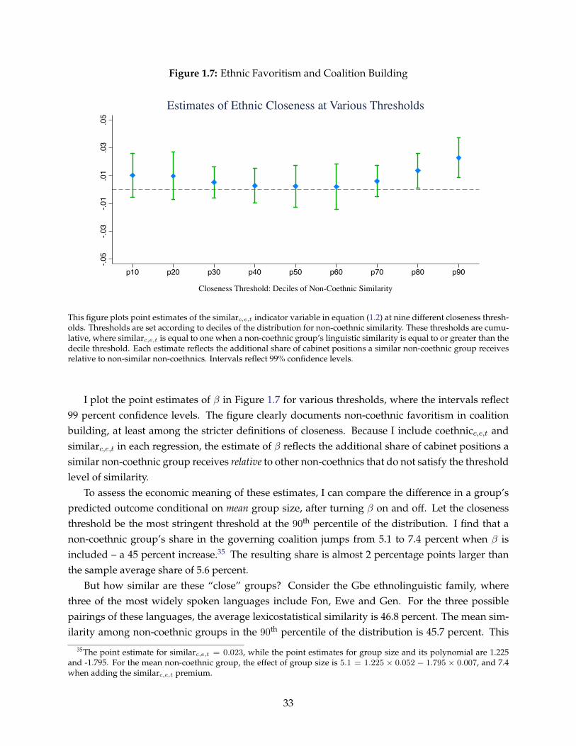
Figure 1.7: Ethnic Favoritism and Coalition Building

-.05

-.03

-.01

.01

.03

.05

p10 p20 p30 p40 p50 p60 p70 p80 p90

Closeness Threshold: Deciles of Non-Coethnic Similarity

Estimates of Ethnic Closeness at Various Thresholds

This figure plots point estimates of the similarc,e,t indicator variable in equation (1.2) at nine different closeness thresh-olds. Thresholds are set according to deciles of the distribution for non-coethnic similarity. These thresholds are cumu-lative, where similarc,e,t is equal to one when a non-coethnic group’s linguistic similarity is equal to or greater than thedecile threshold. Each estimate reflects the additional share of cabinet positions a similar non-coethnic group receivesrelative to non-similar non-coethnics. Intervals reflect 99% confidence levels.

I plot the point estimates of β in Figure 1.7 for various thresholds, where the intervals reflect99 percent confidence levels. The figure clearly documents non-coethnic favoritism in coalitionbuilding, at least among the stricter definitions of closeness. Because I include coethnicc,e,t andsimilarc,e,t in each regression, the estimate of β reflects the additional share of cabinet positions asimilar non-coethnic group receives relative to other non-coethnics that do not satisfy the thresholdlevel of similarity.

To assess the economic meaning of these estimates, I can compare the difference in a group’spredicted outcome conditional on mean group size, after turning β on and off. Let the closenessthreshold be the most stringent threshold at the 90th percentile of the distribution. I find that anon-coethnic group’s share in the governing coalition jumps from 5.1 to 7.4 percent when β isincluded – a 45 percent increase.35 The resulting share is almost 2 percentage points larger thanthe sample average share of 5.6 percent.

But how similar are these “close” groups? Consider the Gbe ethnolinguistic family, wherethree of the most widely spoken languages include Fon, Ewe and Gen. For the three possiblepairings of these languages, the average lexicostatistical similarity is 46.8 percent. The mean sim-ilarity among non-coethnic groups in the 90th percentile of the distribution is 45.7 percent. This

35The point estimate for similarc,e,t = 0.023, while the point estimates for group size and its polynomial are 1.225and -1.795. For the mean non-coethnic group, the effect of group size is 5.1 = 1.225 × 0.052 − 1.795 × 0.007, and 7.4when adding the similarc,e,t premium.

33

suggests that leaders appoint elites from outside of their immediate ethnic group that are part ofthe same family cluster. In other words, the affinity that similarity captures is reflective of theshared ancestry in a group’s larger ethnic network.

Overall, these findings suggest that leaders are inclined to make ethnicity-based decisionswhen appointing ministers from outside their own ethnic group. While the estimates of equa-tion (1.2) cannot necessarily be taken as causal, they are informative of the mechanism throughwhich public resources are allocated to non-coethnic regions. The tendency of ministers to redi-rect funds to their coethnics explains why non-coethnic groups with representation in governmentreceive patronage (Arriola, 2009).

1.7 Concluding Remarks

Ethnic favoritism is often thought to be endemic to African politics, yet the empirical basis for thisclaim is largely founded on single-country case studies. In this paper, I document evidence thatethnic favoritism is widespread throughout Africa using data for 35 sub-Saharan countries. I alsointroduce a novel measure of linguistic similarity that contributes to this literature in three ways:(i) it better predicts patterns of ethnic favoritism with added variation in measured similarity, (ii)the continuity of the measure enables the study of favoritism among groups that are not coethnicto the leader, and (iii) it informs our understanding of a new mechanism related to the ethnicaffinity between similar but non-coethnic groups. This deepens our understanding of the extent offavoritism – evidence of favoritism among non-coethnics normally goes undetected when usinga coethnic dummy variable. I also show that patronage tends to be distributed at a regional levelrather than as targeted transfers towards individuals. I interpret these results through the lensof coalition building and find that ethnicity is one of the guiding principles behind high-levelgovernment appointments.

These observations inform policy in a number of new ways. In particular, my findings areinformative of both the extent of favoritism and where it is expected to take place. This can beused for many purposes, one of which is to enhance monitoring of foreign aid. There is a growingbody of evidence that links the misuse of foreign aid to ethnic patronage in Africa (Briggs, 2014;Jablonski, 2014). Greater oversight is achieved through a deeper understanding of where patron-age is expected to flow. My findings suggest aid donors should not only worry about patronagedirected toward the leader’s ethnic group but also toward other related groups. The benefits ofoversight are evident when comparing the non-interference aid policy of China with conditionaltransfers from the World Bank. Dreher et al. (2015) find little evidence that World Bank aid is usedfor patronage purposes in contrast to the evidence that China’s non-interference policy engendersresource allocation across ethnic lines rather than on a basis of need.

More generally, my findings speak to the value of nation-building policies that promote di-versity in a Pan-Africanist tradition. Tanzania is a good example of a country that has stresseda sense of unity and shared history in its national policies. One nation-building tool of this type

34

that is particularly relevant to this paper is Tanzania’s national language policy (Miguel, 2004). Inthe mid-1960s, the Tanzanian government changed the official language of the country to Swahili.The extent to which Swahili is found in other countries and commonly used as a lingua francaspeaks to the ethnic neutrality of the language. Within only a few years of its implementation, theofficial status granted to Swahili was described as a “linguistic revolution” for its ability to helpshape a national consciousness that runs contrary to ethnic identity (Harries, 1969, p. 277). TheTanzania example is a model to be replicated elsewhere, given the evidence that ethnic favoritismis so widespread throughout Africa. This is not to imply that national language policies are theonly means to pacify existing ethnic tensions: the lesson here is that national policies must be de-signed to engender acceptance of diversity through unity. For example, education is an effectiveway to build a national culture that actively values diversity and differences in experience andbackground.

Lastly, the findings of this paper call for future work. The evidence that favoritism is not sim-ply a coethnic phenomenon demands a deeper understanding of what it means to be “close” tothe ruling ethnic group. The taxonomy of linguistic and ethnic clusters provide an opportunityto study this notion of closeness in the same vein as Desmet et al. (2012). Linking the extent offavoritism to the impact it has on ethnic inequality is an important next step in this line of re-search. The Tanzania example also suggests ethnic favoritism is not an unavoidable consequenceof a country’s high level of diversity, an observation that is consistent with the literature on ethnicinequality. Why then do we observe favoritism in some countries and not others? Geographicsegregation is linked to ethnic favoritism in Africa (Ejdemyr et al., 2014), while geographic en-dowments are linked to ethnic inequality (Alesina et al., 2016), which suggests an answer to thisquestion lies at the intersection of these two areas of research.

35

Chapter 2

Population Relatedness andCross-Country Idea Flows

2.1 Introduction

Recent research documents a link between the ancestral relationship of two countries and theircurrent difference in income (Spolaore and Wacziarg, 2009, 2013a). This link is interpreted as re-flecting an indirect causal effect: income gaps are smaller between related populations becausethey are more likely to communicate and adopt similar ideas. By this interpretation the proba-bility of an idea flowing between two countries is the indirect causal link, and this probability issmaller in more distant relationships. At the same time, dissimilarity could theoretically provideincentive for idea flows if a wider spectrum of non-overlapping traits increase the likelihood oftwo populations having complementary ideas. This notion of a diversity-driven incentive for ideaflows suggests a possible counterbalancing force to the lower probability of communication whentwo countries are ancestrally distant. This hypothesis is similar in spirit to the theory of Ashrafand Galor (2013) and Ashraf et al. (2014, 2015), who document empirical evidence of opposingforces of relatedness on income per capita within a country.

The purpose of this research is then two-fold: can the degree of relatedness between countriesexplain the cross-country flow of ideas, and if so, do we observe interplay between two opposingforces of population relatedness? I find that the degree of relatedness can explain these flows,and that measuring relatedness across linguistic and genetic dimensions yields robust empiricalevidence of two opposing forces on the cross-country flow of ideas.

I follow the literature in using genetic distance as a measure of population relatedness, and usedata on book translations to capture bilateral flows of information. Consistent with the suggestedmechanism of Spolaore and Wacziarg (2009), I find that unconditional genetic distance negativelycorrelates with book translations. However, after isolating variation in population differences spe-cific to language and geography, the residual variation indicates book translations are increasingin genetic distance. This is consistent with the proposed diversity-driven communication incen-

36

tive. The observed negative correlation of unconditional genetic distance captures a cost specificto language that I account for when linguistic distance is jointly estimated. The result is two mea-sures of relatedness capturing opposing forces: language differences impose a cost on idea flowswhile population differences yield a communication incentive.

I also find that linguistic distance reflects a stronger relationship with book translations (inabsolute terms) than genetic distance. This evidence reconciles my findings with the intuitionof Spolaore and Wacziarg (2009), where unconditional genetic distance is expected to exhibit anegative relationship with book translations. One reason genetic distance has received so muchattention in the literature is because it captures a variety of intergenerationally transmitted traits– notably language (Spolaore and Wacziarg, 2015). As a summary measure it is then intuitivethat unconditional genetic distance absorbs the overarching cost of language differences and neg-atively correlates with book translations. The stable and positive relationship between geneticdistance and book translations is observable only after separating out linguistic and geographicvariation from genetic distance.

Conversely the estimated coefficient for linguistic distance is stable in significance and mag-nitude with or without conditioning on genetic distance. The stability of the estimate has twoimplications: that linguistic distance is not a latent measure of genetic distance and that languageconstrains the flow of ideas.

Book translations are an appealing measure of idea flows since by definition they require abilateral exchange in terms of language and often location. This feature lends itself to bilateralcomparisons of population relatedness. The bilateral nature of book translations also makes themsuitable for study within a gravity model, the empirical model most frequently used in studies ofgenetic and linguistic differences. Book translations are also a recognized measure of internationalidea flows (Abramitzky and Sin, 2014), and satisfy the necessary properties of an idea because theyare non-rival and disembodied.1

But more than this a book can convey an idea or tell a story that reflects a different set ofvalues and cultural norms, or draw analogy as a form of commentary about the state of society.The breadth of ideas that a book can capture make translations an appealing measure of ideaflows because of a book’s capacity to influence human behaviour. Rodrik (2014) argues ideas arenot only relevant as technical innovations, but also shape our preferences and how we think theworld works, and at times “can unlock what otherwise might seem like the iron grip of vestedinterests” (p. 194). This behavioural influence of an idea resonates with a long history of booksand their influence over society.2

Using an empirical gravity model of translation flows, I estimate that a one standard deviationincrease in linguistic distance yields 12 percent fewer book translations. This distance is roughly

1A printed copy of a translated text is a rival good because my purchasing of that book inhibits another’s purchase ofit. But the translation itself is non-rival because my purchase of the book does not diminish the use of that translation forfuture copies of the book. This also implies a translation is disembodied in the sense that it is not physically containedas a tangible good.

2The empirical evidence that television affects social capital (Olken, 2009), fertility decisions (La Ferrara et al., 2012),and the status of women (Jensen and Oster, 2009) suggests books can also influence human behaviour.

37

equivalent to how much more Romanian differs from English than German. This result is highlysignificant and robust to a range of controls, including per capita income and population, politicalrights, and other covariates measuring bilateral differences in geography and colonial history.Estimates also hold in magnitude and significance when disaggregating the translation data byidea type, as well as including numerous measures of human capital and bilateral trade betweencountry pairs. For the benchmark estimate I flexibly control for country, time and language fixedeffects, and later show that the core linguistic distance result holds even when accounting forunobserved country-pair effects. The stability of the linguistic distance estimate in significanceand magnitude shows little evidence of a selection bias driving this benchmark result.

Similarly I estimate a significant and robust relationship between book translations and ge-netic distance. Only now the sign is reversed, where a one standard deviation increase in geneticdistance yields an 10 percent increase in book translations. This result is again robust to a rich setof controls and a variety of robustness checks.

To interpret these findings I argue relatedness affects both the costs and benefits of social in-teractions overall. On the one hand, the translatability of two languages is a crucial determinantof communication between countries. Translatability reflects the cost of capturing the originalmessage of a book in a translation – I use a computerized lexicostatistical measure of distanceto capture this cost. On the other hand, there is little overlap of traits and cultural norms whenancestral relationships are distant. This wider spectrum of separate traits increase the likelihoodof complementary ideas and therefore an incentive for communication exists when groups havemore to learn from each other, possibly driving the positive relationship between genetic distanceand book translations.

It is also intuitive that we observe this positive relationship through genealogical differences.By construction, genetic distance reflects a molecular clock that maps the time since two popula-tions shared a common ancestor (discussed further in section 2.2.2). Although linguistic distancereflects the time since two populations shared a common language, this does not necessarily cap-ture the same historical relationship. For example, the Magyar invaded Hungary in the ninthcentury, imposing their Uralic language on the conquered. To this day Hungarians exhibit a genedistribution similar to the rest of Central Europe, but continue to speak a Uralic language unlikethe Latin-based languages of their neighbours (Cavalli-Sforza, 2000). A similar pattern exists inmany regions of the transatlantic slave trade, where colonizers imposed their own language onthe colonized with little genetic mixing (Phillipson, 1992). Such historical events create a wedgebetween the co-evolution of language and genetics. In this sense genetic distance is a better sum-mary measure of the time since two populations separated, and thus the extent of dissimilar ideas,beliefs and cultural norms. Figure 2.1 depicts this argument schematically.

The principal contribution of this paper is the evidence that population relatedness confersboth social costs and benefits on the flow of ideas. Ashraf and Galor (2013) document a trade-off between the costs and benefits of diversity on productivity within a country.3 While I am

3Ashraf et al. (2014, 2015) also document a trade-off between the costs and benefits of genetic diversity on night light

38

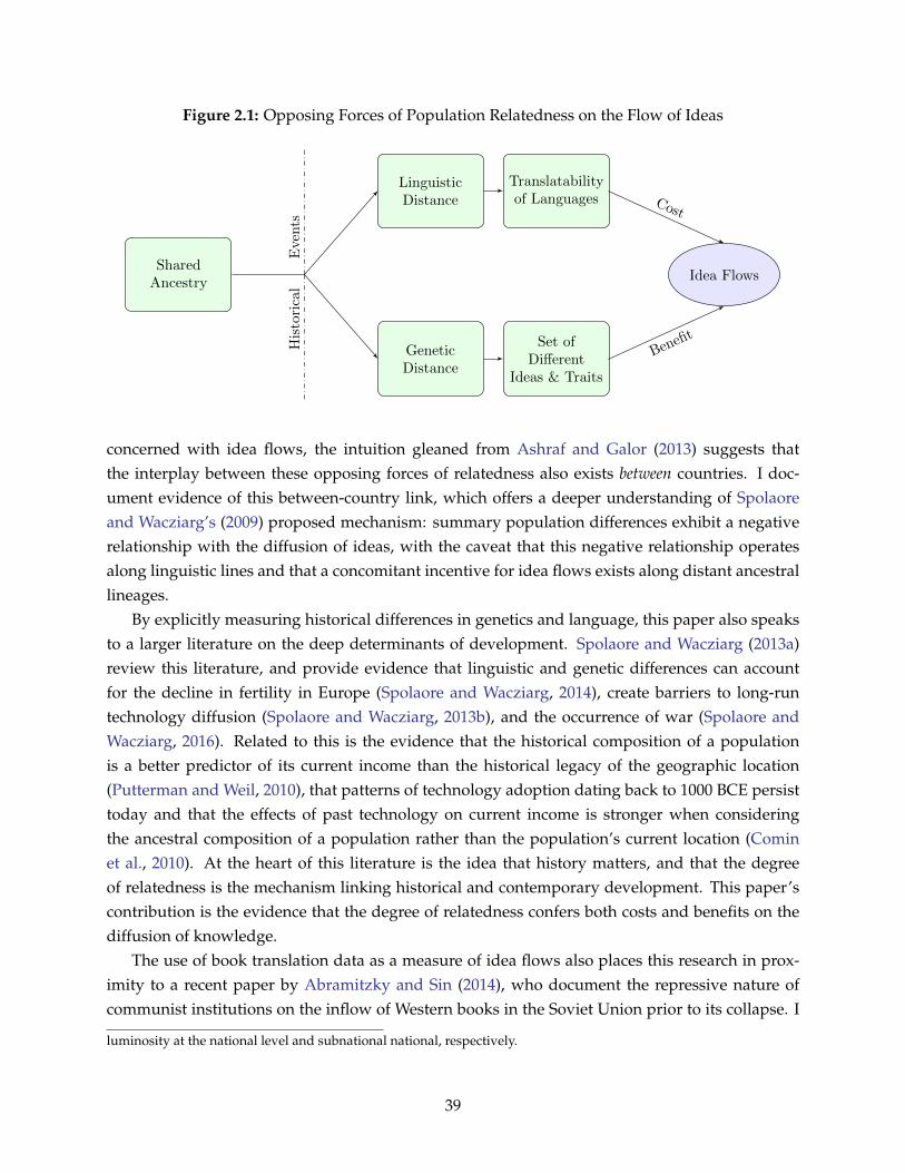
Figure 2.1: Opposing Forces of Population Relatedness on the Flow of Ideas

SharedAncestry

LinguisticDistance

Translatabilityof Languages

GeneticDistance

Set ofDifferent

Ideas & Traits

Idea Flows

Eve

nts

His

tori

cal

Cost

Benefit

concerned with idea flows, the intuition gleaned from Ashraf and Galor (2013) suggests thatthe interplay between these opposing forces of relatedness also exists between countries. I doc-ument evidence of this between-country link, which offers a deeper understanding of Spolaoreand Wacziarg’s (2009) proposed mechanism: summary population differences exhibit a negativerelationship with the diffusion of ideas, with the caveat that this negative relationship operatesalong linguistic lines and that a concomitant incentive for idea flows exists along distant ancestrallineages.

By explicitly measuring historical differences in genetics and language, this paper also speaksto a larger literature on the deep determinants of development. Spolaore and Wacziarg (2013a)review this literature, and provide evidence that linguistic and genetic differences can accountfor the decline in fertility in Europe (Spolaore and Wacziarg, 2014), create barriers to long-runtechnology diffusion (Spolaore and Wacziarg, 2013b), and the occurrence of war (Spolaore andWacziarg, 2016). Related to this is the evidence that the historical composition of a populationis a better predictor of its current income than the historical legacy of the geographic location(Putterman and Weil, 2010), that patterns of technology adoption dating back to 1000 BCE persisttoday and that the effects of past technology on current income is stronger when consideringthe ancestral composition of a population rather than the population’s current location (Cominet al., 2010). At the heart of this literature is the idea that history matters, and that the degreeof relatedness is the mechanism linking historical and contemporary development. This paper’scontribution is the evidence that the degree of relatedness confers both costs and benefits on thediffusion of knowledge.

The use of book translation data as a measure of idea flows also places this research in prox-imity to a recent paper by Abramitzky and Sin (2014), who document the repressive nature ofcommunist institutions on the inflow of Western books in the Soviet Union prior to its collapse. I

luminosity at the national level and subnational national, respectively.

39

account for the institutional environment of a country with a measure of political rights, but findthat the coefficient estimates of linguistic and genetic distance are unaltered in significance andmagnitude conditional on the extent of political rights. This suggests the influence of the institu-tional environment is only part of the story, and that the degree of relatedness is a contributingfactor to the bilateral flow of book translations across countries.

The rest of this paper is structured as follows. Section 2.2 describes the translation data anddetails the measurement strategy for the linguistic and genetic distance data. I outline the econo-metric model in section 2.3 and document the benchmark empirical finding. Section 2.4 tests therobustness of the benchmark result and section 2.5 extends the analysis by disaggregating thebook translation data by idea type. Section 2.6 concludes.

2.2 Data

This section outlines the data used to construct the main variables of interest. See Appendix C formore detailed variable definitions, summary statistics and data sources.

2.2.1 Measuring Language Distance

Measurement of linguistic differences is difficult because languages can differ in a variety of ways,including vocabulary, pronunciation, grammar, syntax, phonetics and more. To overcome thischallenge I isolate variation specific to vocabulary differences with a computerized lexicostatisti-cal approach. As a percentage estimate of cognate words in a language pair, the lexicostatisticalmethod measures how the passage of time diminishes the lexical similarity between two lan-guages.4 The recent splitting of two languages from a parent language implies a large number ofshared cognates or a small linguistic distance.

The computerized lexicostatistical method was developed as part of the Automatic SimilarityJudgement Program (ASJP), a project run by linguists at the Max Planck Institute for EvolutionaryAnthropology.5 To begin a list of 40 universal words (i.e., implied meanings) are compiled for eachlanguage to compare the lexical similarity of any language pair. Swadesh (1952) introduced thisidea of comparing a universal list of words. When a word is universal across world languages, itsimplied meaning, and therefore any estimate of linguistic distance, is independent of culture andgeography.6

Each word in each language is transcribed into a standardized orthography called ASJPcode,a phonetic ASCII alphabet consisting of 34 consonants and 7 vowels. A standardized alphabetrestricts variation across languages to phonological differences. Words are then transcribed ac-

4Two words are said to be cognate if they exist in separate languages but share a common linguistic origin. In otherwords they descend from the same historical parent language.

5http://asjp.clld.org6A recent paper by Holman et al. (2009) shows that the 40-item list employed here yields results at least as good as

those of the commonly used 100-item list propo1sed by Swadesh (1955). Specifically, the 40-item list is a refined versionof the 100-item list, deduced from rigorous testing for word stability across all languages.

40

cording to pronunciation before language distances are estimated. For example, the French wordfor you is vous, and is encoded using ASJPcode as vu to reflect its pronunciation.

I then take these word lists and run the Levenshtein distance algorithm to calculate the mini-mum number of edits needed to translate a word from one language into another. To correct forthe fact that longer words demand more edits, each distance is divided by the length of the trans-lated word. This normalization procedure yields a percentage estimate of dissimilarity. Averagingacross the 40-item list of words for each language pair yields an average lexicostatistical distancebetween two languages.

Following Wichmann et al. (2010), a second normalization procedure is used to adjust for theaccidental similarity of two languages. This normalization accounts for similar ordering and fre-quency of characters that are the result of chance and independent of a word’s meaning.

In instances where two languages have many accidental similarities in terms of ordering andfrequency of characters, the second normalization procedure can yield percentage estimates largerthan 100 percent. To account for this I divide each distance by the maximum distance, the resultof which is a measure of lexicostatistical linguistic distance measured across the unit interval. SeeAppendix A for a formal definition of this lexicostatistical language distance.7

Existing studies typically use data from Fearon (2003), a measure of cladistic language dis-tance. The cladistic measure is a ratio of shared branches between two languages on the languagetree, and distance is calculated as one minus this ratio. This measure is widespread in its usebecause cladistic distance is easily computed for any language pair, since language trees exist forvirtually all known world language families (Lewis, 2009).8

The main advantange of the lexicostatistical measure is that it is a continuous measure of lin-guistic distance and thus provides significant variation in distance estimates. The cladistic ap-proach is a coarse measure of distance because data dispersion is limited to 15 unique values, themaximum number of language family classifications on the Ethnologue langauge tree. ConverselyI match 72 unique lexicostatistical distances to my sample of book translations. This additionalvariation gives me a distribution of distances among language pairs that would otherwise exhibitno variation in cladistic distance. Dickens (2016a) uses this lexicostatistical measure to approx-imate the similarity of African ethnolinguistic groups to their national leaders, and empiricallyverifies the added precision it yields in estimation of ethnic favoritism over and above the cladis-tic measure.

7A number of other economists have used the data from Dyen et al. (1992) as an estimate of lexicostatistical linguisticdistances for the Indo-European family (Desmet et al., 2005, 2009, 2011; Ku and Zussman, 2010; Spolaore and Wacziarg,2009, 2014, 2016). But this data is restricted to 84 Indo-European languages and does not employ the computerizedapproach used here. The non-computerized approach calls for a trained linguist to work with each possible cognateone by one to make judgement of cognation among them. Such an approach relies on subjectively determined cognates,and is extremely labour intensive, thus inhibiting the number of language comparisons possible. Greenberg (1956)formally introduced this approach, and Dyen et al. (1992) provide a detailed discussion of the procedure.

8See Appendix A for a formal discussion of the cladistic approach.

41

2.2.2 Measuring Genetic Distance

Data on cross-country genetic distance comes from Spolaore and Wacziarg (2009), who collectedtheir data from Cavalli-Sforza et al. (1994). To quantify genetic distance, Cavalli-Sforza et al. (1994)collected data on population allele frequencies specific to a set of selectively neutral genes. Anallele is one of many different forms the same gene can assume, where different phenotypic traits(observable characteristics) develop out of different allele sets. Genes were chosen that are knownto be selectively neutral to ensure genetic variation across populations is the result of geneticdrift. The random nature of drift makes genetic differences simply a function of time. Comparingthe distribution of neutral allele frequencies effectively measures the time since two populationsshared a common ancestor, so genetic distance becomes a molecular clock.9

The Fst measure of genetic distance I use is based on an index of heterozygosity – the prob-ability that two randomly selected alleles at a given locus will be different in two populations.An allele distribution that is identical across two populations yields an Fst measure equal to zero,while the Fst index takes on an increasingly higher value the greater the variation in the allelefrequencies across two populations.

When constructing a measure of genetic distance at the country level it is problematic thatmany countries contain multiple ethnic sub-groups. To correct for this I adopt a genetic distancemeasure weighted by the population share of each sub-group in a country.10 This measures theexpected genetic distance between a randomly selected individual from each country. All reportedempirical results use this weighted measure versus one that calculates the distance between thedominant population in each country. However, the two measures are highly correlated and thecore empirical result is robust to this alternative measure.11

2.2.3 Book Translations as Idea Flows

I use a bibliographic database on book translations from around the world as a measure of inter-national idea flows. While book translations are not the only means to knowledge diffusion, theyare perhaps the most common form of transmitting written ideas between countries, making thema useful and quantifiable measure of idea flows. Abramitzky and Sin (2014) also use book trans-lations as a measure international idea flows to study the diffusion of information under differentinstitutional regimes.

One appealing feature of book translations is the breadth of ideas they capture. Rodrik (2014)argues that the influence of an idea extends beyond the technical innovation of a patent citation,

9Because genes are selectively neutral they are independent of natural selection, implying that all conclusions of thispaper do not speak to a hierarchy of genetic traits and should not be interpreted this way.

10For example, suppose country 1 has i = 1, . . . , I ethnic sub-groups and country 2 has j = 1, . . . , J ethnic sub-groups with corresponding population shares s1i and s2j . Letting dij be genetic distance between group i and j, thenthe weighted Fst genetic distance between country 1 and 2 is Fw

st =∑I

i=1

∑Jj=1(dij × s1i × s2j).

11Because the Fst genetic distance data has become more common in the economics literature, I have foregone somedetails in how the measure is constructed for the sake of brevity. I direct interested readers to Spolaore and Wacziarg(2009, p. 480) for a thoughtful and detailed discussion of the data.

42

and that economists should recognize a broader scope of ideas that may also influence humanbehaviour more generally.

Acknowledging the power and influence of books is at the heart of my measurement strategy.Technical ideas are not excluded from the book translation data, but unlike patent citations, thesedata also capture innovative activity outside the scope of technology. Innovative ideas includenew ways of thinking about societal norms, and how individual interests are defined and pursued.Leighton and Lopez (2013) argue the rules of society shape the incentive structures that we liveby, and that new ideas change these rules, which in turn provide new incentives and ultimatelyan influence over human behaviour.

History is replete with examples of the power of books and the influence of their ideas. Em-peror Qin Shi Huang famously consolidated the political philosophy of the Qin Dynasty in ancientChina, in part, with a wave of book burnings to destroy any writing that challenged his own phi-losophy. The ceremonial practice of book burning in Nazi Germany was an attempt to rid thecountry of political writings contrary to the agenda of the National Socialist party. Even more re-cently, Ayatollah Khomeini issued a fatwa demanding Salman Rushdie be put to death for writingThe Satanic Verses because it was disrespectful to the Muslim faith. The intolerance and feelings ofthreat that come from ideas in books speaks to their broader influence on society, politics and ourunderstanding of how the world works.

The influence of books is not only apparent in controversy, but also in their capacity to dissem-inate ideas. Israel (2009) argues that the transatlantic democratic revolutions of the late eighteenthcentury have an intellectual origin rooted in the ideas of the Enlightenment, which “persuadedmuch of the reading elite on either side of the Atlantic [. . .] that a general revolution in the prin-ciple and construction of governments is necessary” (p. 39). This wave of democratic revolutions,Israel argues, was propelled by the spread of pamphlets and books articulating these ideas. Thisexample also speaks to the economic importance of books in the long-run. Given the recent evi-dence that democracy causes growth (Acemoglu et al., 2014), by extension the intellectual originof democracy indirectly links the historical role of books to development patterns of today.

Measuring Book Translations

Translation data was collected from the Index Translationum (IT) database, an international bib-liographic archive of book translations hosted by the United Nations Educational, Scientific andCultural Organization (UNESCO). Since 1932, IT has compiled a detailed record of book trans-lations in print form, and more recently developed an online archive containing bibliographicinformation of translated books in UNESCO Member States since 1979. Legal deposit legislationstates that all publications of a book be submitted to the book repository of a country.12 Records ofbook translations are then submitted to IT by the national book repository. The systematic natureof the data collection process is a reassurance of the data’s accuracy.

12An in-depth report on legal deposit legislation was drafted by UNESCO in 2000, which provides a guideline ofhow this legislation is formed. See http://archive.ifla.org/VII/s1/gnl/legaldep1.htm.

43

Figure 2.2: Benchmark Sample Observations by Country (1979-2005)

I use data on 1,634,817 book translations that span 119 translating countries over the timeperiod 1979-2005. The panel is unbalanced because I do not observe the same translating country–language pairs in each year. Figure 2.2 depicts the spatial distribution of observations for thebenchmark sample of translating countries.13 While the majority of these translations are intothe dominant language of the translating country, many countries translate books into more thanone language. Each bibliographic entry contains information by subject, the translating countryand year, and the original and target languages of translation.14 Table C2 lists some of the mosttranslated authors within a random sample of countries, including the subject in which they havemost commonly published.

Because the translation data does not report the country in which a book was originally pub-lished, I assign a home country to each original translation language as stated in the Ethnologue.15

The benefit of this assignment rule is that it removes judgement and hence any personal bias inthe data construction. The drawback is that, in some cases, multiple countries share a commonofficial language so it is not clear the Ethnologue’s stated home country is always the correct one.For example, it is unlikely that all translations originating in English were originally published inthe United Kingdom as the Ethnologue assignment rule would suggest. In section 2.4.1 I performtwo tests of this assignment rule: I drop the most problematic languages in terms of home countryassignment and alternatively construct a home language “country” as an average of country char-acteristics weighted by population shares for each country in which an original language is found.In either case the benchmark result remains unaltered. Given the reassurance of this resoundingevidence I proceed with the Ethnologue assignment rule as a consistent method of home countryassignment for each original language of translation.

13See Table C3 in the appendix for a complete list of observations by translating country.14Subjects are classified according to the Universal Decimal Classification system, including [1] history, geography

and biography, [2] law, social sciences, and education, [3] literature, [4] philosophy and psychology, [5] religion andtheology, [6] natural and exact sciences, [7] applied sciences, [8] and arts, games, and sports.

15The Ethnologue is a comprehensive database cataloguing all of the world’s 7,097 known living languages.

44

2.3 Methodology and Empirical Results

2.3.1 Econometric Model

Given the bilateral nature of linguistic and genetic distance, I adopt an empirical model similarin spirit to the gravity equation. The basic theoretical gravity model implies that bilateral tradebetween two countries is a function of their economic size and a variety of costs to trade, notablygeographic distance. With this in mind, I develop a similar estimation strategy that tests howlinguistic and genetic distance affect bilateral translation flows. This basic relationship can bewritten as:

TRANSijlt = α0 + α1 LINGDISTijl + α2GENDISTij + α3GEODISTij

+ X′ijΓ + X′itΩ + X′jtΦ + γi + γj + γl + γt + εijlt (2.1)

where i indexes the translating country, j the original country (and language), l the target languageand t the time period.16 The dependent variable TRANS measures log translations, LINGDISTandGENDIST measure linguistic and genetic distance, andGEODIST measures the geographicdistance in 10,000 kilometre units. Xij is a vector of bilateral time-invariant measures of geogra-phy and colonial relations, while Xit and Xjt include time-varying measures of income, popula-tion and political rights in country i and j. A set of fixed effects is also included in each regression,capturing unobserved country effects, time effects and idiosyncratic target language effects. In allregressions I estimate robust standard errors clustered at the country-pair level.

Reverse causality is not a problem here unless one believes that the amount a country translateshas an effect on the distance between two languages or the genetic make-up of those populations.The implausibility of this comes from the fact that group differences are historically determinedlong before the time period of interest to this study. To account for the possibility of an omittedvariable bias I include a rich set of covariates and fixed effects. I control for a variety of standardmeasures of trade costs and a host of time-varying measures believed to influence book transla-tions. I also find that the benchmark estimates are robust to measures of time-varying bilateraltrade and human capital. Country fixed effects absorb any unobserved country-specific factorswhile time effects absorb year-specific shocks, and robustness checks confirm that unobserved,time-invariant factors specific to bilateral country pairs do not drive the empirical findings.

2.3.2 Unconditional Benchmark Results

In this section I investigate the basic empirical relationship between book translations and threemeasures of bilateral distance. In particular I investigate how linguistic and genetic distance cor-relate with book translations in various combinations and disentangle the role of geographic dis-tance.

16It is redundant to denote the original language since by assumption each original language is matched to an originalcountry as previously noted.

45

Table 2.1: Summary Statistics for Distance Measures

Simple Correlations

Log Linguistic Genetic GeographicTranslations Distance Distance Distance

Linguistc distance -0.11 1.00

Genetic distance -0.12 0.34 1.00

Geographic distance -0.12 0.24 0.45 1.00

Summary Statistics

Mean Std dev. Min Max

Log translations 1.23 1.59 0.00 8.98

Linguistic distance 0.86 0.12 0.18 1.00

Genetic distance 0.04 0.04 0.00 0.29

Geographic distance (10,000 km) 0.38 0.37 0.01 1.96

Note: 42,817 observations for correlations and all summary statistics.

Table 2.1 provides summary statistics for these measures. As expected, all three distance mea-sures are positively correlated with each other. Linguistic distance exhibits a positive correlationof 0.34 with genetic distance and 0.24 with geographic distance, and genetic and geographic dis-tance exhibit a positive correlation of 0.45. Book translations exhibit negative correlation with eachdistance measure, including -0.11, -0.12 and -0.12 with linguistic, genetic and geographic distance.No pairwise correlation between two distance measures is very large in magnitude, and yet all ex-hibit pairwise negative correlation with book translations, suggesting that each distance measuremay have a significant and differential effect on book translations.

Table 2.2 reports the unconditional estimates of the regression analysis. Columns (1) through(3) indicate that all measure of distance negatively correlate with book translations when sepa-rately estimated. The systematic negative relationship between each unconditional distance andbook translations is intuitively consistent with the interpretation of Spolaore and Wacziarg (2009).The estimate for linguistic distance is not only statistically significant but also economically mean-ingful: a standard deviation increase in linguistic distance implies an 18.6 percent decrease inbook translations (exp(0.12 × −1.72) − 1 = 0.186). The magnitude of this effect is greater thanthat of genetic distance, where the estimate in column (2) implies a standard deviation increase ingenetic distance yields a 11.9 percent decrease in book translations (exp(0.04×−3.17)−1 = 0.119).At the bottom of the table I provide standardized “beta” coefficients to simplify relative compar-isons. Column (1) indicates that a one standard deviation increase in linguistic distance accounts

46

Table 2.2: Unconditional Benchmark Regressions

Dependent variable: Log translations

(1) (2) (3) (4)

Linguistic distance -1.72*** -1.52***(0.26) (0.26)

Genetic distance -3.17*** 2.87***(1.05) (0.96)

Geographic distance -0.86*** -0.85***(0.14) (0.15)

Translating Language FE Yes Yes Yes YesTranslating Country FE Yes Yes Yes YesOriginal Country FE Yes Yes Yes YesYear FE Yes Yes Yes Yes

Observations 42,817 42,817 42,817 42,817Adjusted R2 0.27 0.26 0.27 0.28Country pair clusters 2112 2112 2112 2112

Standardized Coefficients (%)

Linguistic distance −12.7 - - −11.2Genetic distance - −8.3 - 7.5

Country-pair clustered robust standard errors in parentheses. * p < 0.10, ** p < 0.05, *** p < 0.01.

for 12.7 percent of a standard deviation decrease in log book translations, whereas column (2) in-dicates a one standard deviation increase in genetic distance accounts for 8.3 percent of a standarddeviation decrease in log book translations.

To explore the possibility of a differential effect of these two measures further I run a horse raceregression and report the estimates in column (4). The coefficient estimate for linguistic distanceis remarkably stable in magnitude and significance. This is reassuring that linguistic distanceis not a latent measure of genetic and geographic differences, but instead an accurate measureof summary language differences. The standardized coefficient for linguistic distance falls by 1.5percentage points from−12.7 in column (1) to−11.2 in column (4) after controlling for both geneticand geographic distance.

Conversely, after conditioning on both linguistic and geographic distance the correlative rela-tionship between genetic distance and book translations becomes positive. Yet despite this changein sign the estimate remains statistically significant at the 1 percent level. The standardized betacoefficient implies a one standard deviation increase in genetic distance accounts for 7.5 percentof a standard deviation increase in book translations. The sensitivity of the coefficient is alsosuggestive that genetic distance does in fact capture summary population differences, includinglinguistic and geographic differences.

The influence of geographic distance is also of a notable magnitude: Norway is expected to

47

translate over 3 percent more books originating in neighbouring Sweden than Finland based ongeographic distance alone, all else being equal. On a global scale the influence of geographicdistance can become quite large.

Taken together, the unconditional estimates of Table 2.2 nicely summarize the earlier discus-sion of the opposing forces of relatedness on idea flows. For book translations, linguistic distancereflects a cost that hinders interactions between linguistically distinct populations so that on av-erage a country can be expected to translate more books from a country that speaks a similarlanguage. Genetic distance has the opposite effect; a country can be expected to translate morebooks written by authors of distant genealogical ancestries. Hence the trade-off between a lowerprobability of book translation when two countries are linguistically distant and a diversity-drivenincentive for translation when two countries share distant ancestries.

2.3.3 Conditional Benchmark Results

When interpreting the core results of the previous section, one source of concern is that booktranslations are driven by time-varying country-specific factors unaccounted for by country fixedeffects. To be sure the results of the previous section are not confounded by an omitted variablebias, I test the robustness of the distance measures to a variety of covariates.17

Column (1) of Table 2.3 reproduces column (4) of Table 2.2 using the benchmark sample.18 Incolumn (2) I report estimates that include measures of log real GDP per capita and log populationfor both the translating and original country. Adding these time-varying measures leaves the stan-dardized value for linguistic distance unchanged and still maintains significance at the 1 percentlevel. The estimate of genetic distance also maintains statistical significance and is unchanged inmagnitude. Similarly, adding political rights has no observable effect on the magnitude and sig-nificance of both distances, as shown in column (3). Given that these covariates tend to changeat a slow pace this result isn’t surprising because country fixed effects absorb the majority of theobservable variation.

In column (4) I report estimates that include a measure of log bilateral trade. Bilateral tradeflows not only measure the extent of an economic partnership, but they also capture latent deter-minants of trade such as existing communication networks or the extent of bilateral trust betweencountries (Guiso et al., 2009). In this sense it is intuitive that a country pair that trades more wouldalso be more inclined to share ideas. Indeed, the coefficient estimate for bilateral trade indicatesan influence on book translations: a 10 percent increase in bilateral trade yields a 1.2 percentageincrease in book translations. This suggests that the extent of a bilateral trade relationship has asmall positive but significant influence on the level of book translations for a given country pair.At the same time the standardized coefficient for linguistic distance falls 2 percentage points inmagnitude when conditioning on trade, while the standardized coefficient for genetic distanceexhibits a slight increase.

17See Appendix C for data definitions and sources.18The benchmark sample differs because some covariates are not available for every country in each year.

48

Table 2.3: Conditional Benchmark Regressions

Dependent variable: Log translations

(1) (2) (3) (4) (5) (6)

Linguistic distance -1.55*** -1.55*** -1.54*** -1.27*** -1.24*** -1.13***(0.28) (0.28) (0.28) (0.28) (0.28) (0.28)

Genetic distance 3.21*** 3.19*** 3.19*** 3.32*** 3.28*** 2.40**(1.04) (1.04) (1.05) (1.03) (1.02) (1.05)

Geographic distance -0.85*** -0.85*** -0.85*** -0.57*** -0.55*** -1.37***(0.16) (0.16) (0.16) (0.16) (0.17) (0.46)

Log real GDP per capita -0.08 -0.07 -0.17** -0.18** -0.15**translating country (0.07) (0.07) (0.07) (0.07) (0.07)

Log real GDP per capita 0.11** 0.11** 0.03 0.02 0.04original country (0.05) (0.05) (0.05) (0.05) (0.05)

Log population 0.12 0.24 0.38** 0.39** 0.39**translating country (0.18) (0.17) (0.18) (0.18) (0.18)

Log population 0.09 0.12 0.26** 0.28** 0.30**original country (0.12) (0.12) (0.13) (0.13) (0.13)

Political rights -0.21** -0.21*** -0.21*** -0.22***translating country (0.09) (0.08) (0.08) (0.08)

Political rights -0.07 -0.04 -0.03 -0.04original country (0.08) (0.07) (0.07) (0.07)

Log bilateral trade 0.12*** 0.13*** 0.10***(0.02) (0.02) (0.02)

= 1 if ever in a -0.13 -0.11colonial relationship (0.14) (0.13)

= 1 for contiguity 0.14*(0.08)

Absolute difference in latitude -0.00(0.00)

Absolute difference in longitude 0.01**(0.00)

Translating Language FE Yes Yes Yes Yes Yes YesTranslating Country FE Yes Yes Yes Yes Yes YesOriginal Country FE Yes Yes Yes Yes Yes YesYear FE Yes Yes Yes Yes Yes Yes

Observations 39,275 39,275 39,275 39,275 39,275 39,275Adjusted R2 0.28 0.28 0.28 0.28 0.28 0.28Country pair clusters 1897 1897 1897 1897 1897 1897

Standardized Coefficients (%)

Linguistic distance −11.0 −11.0 −11.0 −9.0 −8.8 −8.0Genetic distance 8.4 8.4 8.4 8.7 8.6 6.3

Country-pair clustered robust standard errors in parentheses. * p < 0.10, ** p < 0.05, *** p < 0.01.

49

In column (5) I report estimates that include past and present colonial relationships betweencountry pairs, but this doesn’t alter the influence of linguistic or genetic distance in any substantialway.

To the contrary, when accounting for the spatial proximity of a country pair the influence ofgenetic distance falls by over 2 percentage points. The drop in magnitude of genetic distance isin consequence of adding longitudinal difference to the set of covariates, since genetically distantpopulations tend to be geographically distant as well. The positive and significant coefficient onabsolute difference in longitude in column (6) is interesting because it suggests ideas tend to flowbetween geographically distant countries across similar latitudes. The presence of a north-southfriction is consistent with the historical evidence that information tends to flow across east-westaxes (Diamond, 1997; Blouin, 2014). At the same time, contiguity suggests translations are morelikely between neighbouring countries. While these two results are contradictory on the surface,they are consistent with the idea of counterbalancing forces in idea flows that is at the heart of thispaper. The cost of translation is lower between neighbouring countries where languages tend to besimilar, and yet ideas flow between distant countries because the probability of a wider spectrumof traits and ideas provides incentive for communication.19

Hereafter I refer to the estimates in column (6) as my benchmark estimates. Using this specifi-cation to assess the magnitude of these estimates, first note that a standard deviation in linguisticdistance reduces the dependent variable by 0.124 log units, while a standard deviation in geneticdistance increases the dependent variable by 0.096 log units.20 This says that a standard devia-tion increase in linguistic distance reduces book translations by 11.7 percent (exp(−0.124) − 1 =

−0.117), while a standard deviation increase in genetic distance increases book translations by10.1 percent (exp(0.096)− 1 = 0.101).

2.4 Robustness

2.4.1 Testing the Home Country Assumption of Book Translations

A concern of the benchmark result is that the home country of a book translation is not known.This implies that genetic distance is measured with error. As an assignment rule I use the homecountry of a language as indicated in the Ethnologue database. However, this rule does not allowfor the original language of a book translation to be the same in more than one source country.

Problematic Languages

As a first test of the home country assumption I identify the most problematic languages andpurge them from my benchmark dataset. Using data from the Ethnologue I generate a list of lan-

19As further evidence of these conditional benchmark estimates, I reproduce the estimates of Table 2.3 in Table C6using a cladistic measure of linguistic distance. The opposing forces of linguistic and genetic distance hold even whenusing this alternative measure of linguistic distance.

20See Appendix Table C1 for a complete list of the benchmark sample summary statistics.

50

51

Table 2.4: Robustness Check for Problematic Original Languages of Translation

Dependent variable: Log translations

(1) (2) (3) (4) (5) (6) (7)

English Arabic French Mandarin Spanish Hindi All SixExcluding: Language Language Language Language Language Language Language

Translations Translations Translations Translations Translations Translations Translations

Linguistic distance -1.48*** -1.10*** -1.04*** -1.14*** -1.12*** -1.13*** -1.39***(0.25) (0.28) (0.27) (0.28) (0.28) (0.28) (0.24)

Genetic distance 2.02** 2.41** 1.96* 2.28** 2.45** 2.40** 1.44*(0.88) (1.04) (1.03) (1.05) (1.08) (1.05) (0.81)

Geographic distance -1.43*** -1.40*** -1.14** -1.35*** -1.29*** -1.37*** -1.06***(0.38) (0.46) (0.45) (0.48) (0.47) (0.46) (0.40)

Benchmark controls Yes Yes Yes Yes Yes Yes Yes

Target Language FE Yes Yes Yes Yes Yes Yes YesTarget Country FE Yes Yes Yes Yes Yes Yes YesOriginal Country FE Yes Yes Yes Yes Yes Yes YesYear FE Yes Yes Yes Yes Yes Yes Yes

Observations 34,292 38,032 36,198 38,342 37,727 39,021 27,238Adjusted R2 0.33 0.29 0.29 0.28 0.28 0.28 0.36Country pair clusters 1840 1833 1860 1880 1871 1892 1694

Standardized Coefficients (%)

Linguistic Distance −12.0 −7.8 −7.9 −8.1 −8.0 −8.0 −13.0Genetic Distance 5.9 6.3 5.3 5.8 6.5 6.3 4.5

This table reports estimates on various subsamples that exclude problematic languages in terms of ambiguous home country assignment. All regressionsinclude the benchmark set of control variables used in column (6) of Table 2.3. Country-pair clustered robust standard errors reported in parentheses. * p <0.10, ** p < 0.05, *** p < 0.01.

guages sorted by first-language speakers. The top five languages by number of speakers includeMandarin (1,197 million), Spanish (414 million), English (335 million), Hindi (260 million) andArabic (237 million). I also use the Ethnologue to generate a list of languages sorted by the numberof countries in which the language is spoken. The top five languages by this definition includeEnglish (99 countries), Arabic (60 countries), French (51 countries), Mandarin (33 countries) andSpanish (31 countries). Because these languages are spoken in so many countries they are prob-lematic in terms of assigning a single country to each language. It is no surprise these lists arealmost identical. The result is a list of six potentially problematic languages: English, Arabic,French, Mandarin, Spanish and Hindi. As a test of home country assignment I re-estimate thebenchmark model and systematically drop all books translated from a problematic language. Ta-ble 2.4 presents these results.

All estimates are statistically significant with the expected sign, and the majority are com-parable to the benchmark estimate in terms of magnitude. The first estimate that stands out isreported in column (1), where the magnitude of the linguistic distance estimate is quite sensitiveto the sample restricting English translations. This result is not surprising given that English is alingua franca for so many speakers of different first languages around the world. The ubiquity ofEnglish as a global language is evident in the fact that only one out of four users of the languageare native speakers (Crystal, 2003). Consider the comparable standardized beta of −8.0 percentfor linguistic distance in the full sample. The significant increase in this standardized coefficientto −12.0 percent suggests the negative effect of linguistic distance is quite a bit stronger whenabstracting from translations originating in English. This result is reassuring because it impliesthat the benchmark specification conservatively estimates the effect of linguistic distance when noconsideration is given to the importance of English as a global lingua franca.

The other estimate that differs considerably from the benchmark estimate is reported in col-umn (7), where I drop all translations originating in any of the six problematic languages. Thestandardized coefficient for linguistic distance jumps up to −13.0 percent, while the genetic dis-tance coefficient falls to 4.5 percent. As a test of the home country assignment this result is promis-ing because it says that, if anything, the assumption of a home country for the most problematiclanguages attenuates the benchmark linguistic distance estimate. While the coefficient for geneticdistance drops below the magnitude of the benchmark estimate, it remains robust to a 45 per-cent loss of observations relative to the benchmark sample. This provides further evidence that adiversity-driven incentive for idea flows exists between countries.

In the appendix I extend this test by systematically dropping every original language of atranslation with at least 100 observations in the benchmark sample. Table C7 reports these results.In every one of these 45 additional regressions, the coefficients of interest maintain the expectedsign and statistical significance at standard levels of confidence. While the cut-off of 100 observa-tions is arbitrary, the coefficient estimates converge to that of the benchmark estimates after thecut-off because the sample restrictions become so small.

52

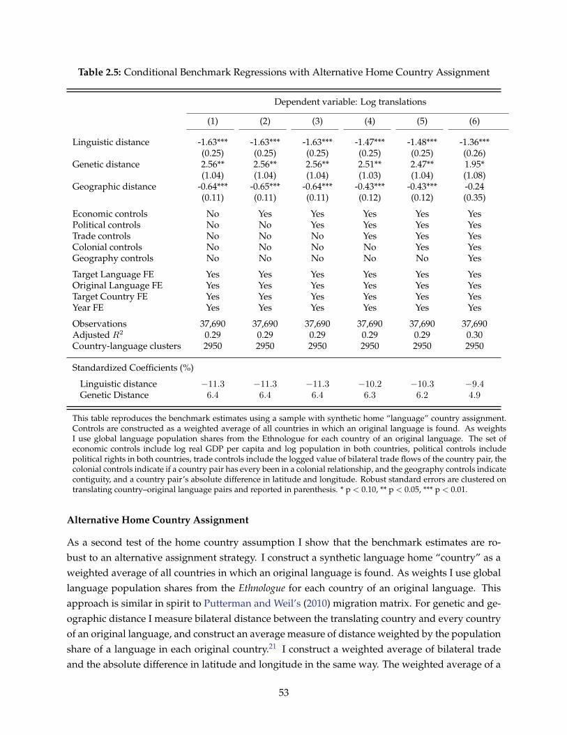
Table 2.5: Conditional Benchmark Regressions with Alternative Home Country Assignment

Dependent variable: Log translations

(1) (2) (3) (4) (5) (6)

Linguistic distance -1.63*** -1.63*** -1.63*** -1.47*** -1.48*** -1.36***(0.25) (0.25) (0.25) (0.25) (0.25) (0.26)

Genetic distance 2.56** 2.56** 2.56** 2.51** 2.47** 1.95*(1.04) (1.04) (1.04) (1.03) (1.04) (1.08)

Geographic distance -0.64*** -0.65*** -0.64*** -0.43*** -0.43*** -0.24(0.11) (0.11) (0.11) (0.12) (0.12) (0.35)

Economic controls No Yes Yes Yes Yes YesPolitical controls No No Yes Yes Yes YesTrade controls No No No Yes Yes YesColonial controls No No No No Yes YesGeography controls No No No No No Yes

Target Language FE Yes Yes Yes Yes Yes YesOriginal Language FE Yes Yes Yes Yes Yes YesTarget Country FE Yes Yes Yes Yes Yes YesYear FE Yes Yes Yes Yes Yes Yes

Observations 37,690 37,690 37,690 37,690 37,690 37,690Adjusted R2 0.29 0.29 0.29 0.29 0.29 0.30Country-language clusters 2950 2950 2950 2950 2950 2950

Standardized Coefficients (%)

Linguistic distance −11.3 −11.3 −11.3 −10.2 −10.3 −9.4Genetic Distance 6.4 6.4 6.4 6.3 6.2 4.9

This table reproduces the benchmark estimates using a sample with synthetic home “language” country assignment.Controls are constructed as a weighted average of all countries in which an original language is found. As weightsI use global language population shares from the Ethnologue for each country of an original language. The set ofeconomic controls include log real GDP per capita and log population in both countries, political controls includepolitical rights in both countries, trade controls include the logged value of bilateral trade flows of the country pair, thecolonial controls indicate if a country pair has every been in a colonial relationship, and the geography controls indicatecontiguity, and a country pair’s absolute difference in latitude and longitude. Robust standard errors are clustered ontranslating country–original language pairs and reported in parenthesis. * p < 0.10, ** p < 0.05, *** p < 0.01.

Alternative Home Country Assignment

As a second test of the home country assumption I show that the benchmark estimates are ro-bust to an alternative assignment strategy. I construct a synthetic language home “country” as aweighted average of all countries in which an original language is found. As weights I use globallanguage population shares from the Ethnologue for each country of an original language. Thisapproach is similar in spirit to Putterman and Weil’s (2010) migration matrix. For genetic and ge-ographic distance I measure bilateral distance between the translating country and every countryof an original language, and construct an average measure of distance weighted by the populationshare of a language in each original country.21 I construct a weighted average of bilateral tradeand the absolute difference in latitude and longitude in the same way. The weighted average of a

53

bilateral indicator variable becomes a percentage measure of the indicator for all possible countrypairs of the original language, and non-bilateral measures including real GDP, population and po-litical rights are a simple weighted average. Given the alternative structure of this data I replaceoriginal country fixed effects in equation (2.1) with original language fixed effects, and clusterstandard errors by translating country and original language pairs instead of country pairs.

The benefit of a synthetic language home “country” over the Ethnologue home country assign-ment is that all origin countries of a language are proportionally present in covariate calculations.By doing so I relax the assumption of a home country for each language. The drawback is that Icannot construct a weighted average with complete coverage of all groups because I lack country-level data for some countries of language origin. To account for languages with particularly poorcoverage I trim the bottom 5 percent of languages according to coverage.22 The average coverageof these trimmed languages is only 56 percent and range from 0 to 90 percent. The average cov-erage of the remaining languages is 99 percent with a median of 100 percent. This translates to asample of 37,960 observations out of the benchmark sample of 39,275 observation (96 percent).

I re-run the benchmark estimates of Table 2.3 using these population-weighted covariates andreport the results in Table 2.5. These home language “country” estimates are very similar to thebenchmark estimates, though the positive effect of genetic distance drops slightly in magnitude.The stability of the coefficient estimates indicates that the benchmark result is not a consequenceof the Ethnologue home country assignment rule. The fact that the opposing forces of linguisticand genetic distance are borne out of these alternative assignment estimates is quite reassuringgiven that the set of transformed covariates all exhibit a significant difference in means relative tothe comparable measures in the benchmark sample (Table C9). The similarity of these estimatesto the benchmark estimates ensure the Ethnologue assignment rule is a good approximation of abook translation’s country of origin.

2.4.2 Human Capital

A country’s decision to translate might also be influenced by its level of human capital, sinceeducated populations are more likely to have a high demand for book translations. Using datafrom Barro and Lee (2013), I measure human capital in the translating country in four ways: acountry’s average years of schooling attained, the percentage of the total population who havecompleted primary schooling, secondary schooling and tertiary schooling. Because these data areonly available in 5-year intervals I supplement it with data from the Penn World Tables version8.0. I use a yearly index of human capital per person, based on years of school (Barro and Lee,2013) and the returns to education (Psacharopoulos, 1994). Table 2.6 reports robustness checksusing these different measures of human capital.

Column (1) includes the Penn World Table human capital index, which I match to 99 percent of

21Linguistic distance is measured between the target and original language and thus measured independently of thehome country assumption.

22The results are also robust to both stricter and weaker restrictions on coverage.

54

Table 2.6: Robustness Check: Human Capital and Education

Dependent variable: Log translations

(1) (2) (3) (4) (5) (6)

Linguistic distance -1.14*** -0.95*** -0.95*** -0.96*** -0.95*** -0.96***(0.29) (0.31) (0.31) (0.31) (0.31) (0.31)

Genetic distance 2.38** 3.13*** 3.12*** 3.12*** 3.10*** 3.12***(1.05) (1.18) (1.18) (1.18) (1.18) (1.18)

Geographic distance -1.38*** -1.08** -1.09** -1.09** -1.08** -1.09**(0.46) (0.46) (0.46) (0.47) (0.47) (0.47)

Human capital index 0.13translating country (0.14)

Average years of schooling 0.06*translating country (0.03)

% of primary schooling -0.01* 0.00translating country (0.00) (0.00)

% of secondary schooling 0.01** 0.01*translating country (0.00) (0.00)

% of tertiary schooling 0.01 0.02translating country (0.01) (0.01)

Benchmark controls Yes Yes Yes Yes Yes Yes

Translating Language FE Yes Yes Yes Yes Yes YesTranslating Country FE Yes Yes Yes Yes Yes YesOriginal Country FE Yes Yes Yes Yes Yes YesYear FE Yes Yes Yes Yes Yes Yes

Observations 38,907 8,815 8,815 8,815 8,815 8,815Adjusted R2 0.28 0.26 0.26 0.26 0.26 0.26Country pair clusters 1809 1342 1342 1342 1342 1342

Standardized Coefficients (%)

Linguistic Distance −8.0 −6.8 −6.8 −6.8 −6.7 −6.8Genetic Distance 6.2 8.1 8.1 8.0 8.0 8.0

This table tests for selection on the human capital level of a translating country. All regressions include the bench-mark set of control variables used in column (6) of Table 2.3. Country-pair clustered robust standard errors reportedin parentheses. * p < 0.10, ** p < 0.05, *** p < 0.01.

55

Table 2.7: Robustness Check: Unobserved Country-Pair Effects

Dependent variable: Log translations

(1) (2) (3) (4)

Linguistic distance -0.86* -0.89* -0.88* -0.88*(0.47) (0.52) (0.52) (0.52)

Economic controls No No Yes YesPolitical controls No No Yes YesTrade controls No No No Yes

Translating Language FE Yes Yes Yes YesCountry Pair FE Yes Yes Yes YesYear FE Yes Yes Yes Yes

Observations 42,415 38,928 38,928 38,928Adjusted R2 0.36 0.35 0.35 0.35Country pair clusters 1711 1551 1551 1551

Standardized Coefficients (%)

Linguistic Distance −6.3 −6.3 −6.3 −6.3

This table tests for selection on time-invariant country-pair effects. Genetic and geographic distanceare time invariant across country-pair observations and therefore not estimable in this specification.The set of economic controls include log real GDP per capita and log population in both countries,political controls include political rights in both countries and the trade controls include the loggedvalue of bilateral trade flows of the country pair. Country-pair clustered robust standard errors re-ported in parentheses. * p < 0.10, ** p < 0.05, *** p < 0.01.

my benchmark sample. The translating country human capital index positively correlates to booktranslations as expected, but is estimated to be no different than zero. The linguistic and geneticdistance estimates are robust to the inclusion of human capital, and quantitatively equivalent tothe benchmark estimates. Columns (2) through (6) add each original Barro-Lee measure and againthe variables of interest are unaltered. In column (3) the human capital measure is estimated withthe wrong sign, but in all other cases the expected positive sign results. Overall these resultssuggest human capital cannot explain away the benchmark estimates.

2.4.3 Existing Bilateral Relationships

The most effective way to capture any relevant time-invariant feature of a country pair is to includecountry pair fixed effects. The major limitation of this approach is that it is no longer possible toexplicitly estimate genetic distance because country pair variation is time-invariant and adsorbedby the fixed effects estimator.23 Nonetheless I proceed to test the robustness of the benchmarklinguistic distance estimate.

23Although language distances are assumed to be constant over the sampled time period, country-pair fixed effectsdo not absorb language distance effects because each unit of observation is indexed by country-pair, year and the targetlanguage of translation – the latter of which isn’t constant for a country pair each year.

56

Table 2.7 reports the benchmark estimate with country pair fixed effects in place of individualcountry effects. Column (1) reports estimates where I forego any covariates in order to maxi-mize the sample. Linguistic distance is estimated to be significantly different from zero with theexpected sign and with a magnitude of influence similar to the benchmark estimate. I then in-crementally add the benchmark covariates that are not absorbed by the country-pair fixed effects.Overall the results are similar to the benchmark, albeit a little noiser and consequently less pre-cisely estimated. However, the robustness of the linguistic distance estimate to country-pair fixedeffects confirms that time-invariant country-pair variation cannot explain away the benchmarkestimate.

2.4.4 Check for Understated Standard Errors

Because linguistic and genetic distance are assumed to be constant over the sampled time period,standard errors may be understated due to repeated values of each distance measure for the samelanguage-country pair in the panel (Bertrand et al., 2004). To test for this I regress log translationson a set of year dummies and collapse the data by averaging over time the residual translationvariation. Similarly, all other time-variant independent variables are regressed on time dummiesand the residuals are collapsed by averaging over time. The benchmark specification is then re-estimated using this collapsed and time-averaged data. Results are reported in table 2.8.

Linguistic and genetic distance are again estimated significantly significant and have the ex-pected signs. The only feature of these results that is different from the benchmark estimate is thestandardized coefficient for genetic distance is greater in absolute magnitude than linguistic dis-tance. However, the main finding of the opposing forces of linguistic and genetic distance remainsunchanged.

2.4.5 Differences in Across Country Language Structure

One additional concern is that countries are structurally different in terms of language. For exam-ple, multilingual countries may translate more books because they are more linguistically diverse.Similarly, the colonial legacy of language is evident in the fact that many countries still use theircolonizer’s native language as a regional lingua franca. This may influence both the number ofbooks translated and specific languages that are commonly translated. A shared language be-tween two countries may also influence how much those two countries translate each other’swritings. In this section, I investigate further sample restrictions to be sure the benchmark resultsare not driven by country-level differences in language structure. Results are reported in Table2.9, where all estimates include a full set of controls.

Column (1) reports model estimates from a subsample of unilingual countries. The estimatedcoefficient for linguistic and genetic distance are consistent with the previous estimates in termsof significance and magnitude.

Next I investigate the influence of lingua francas within a translating country. Using data

57

Table 2.8: Robustness Check for Understated Standard Errors

Dependent variable: Time averaged log translations

(1) (2) (3) (4) (5) (6)

Linguistic distance -0.63*** -0.66*** -0.66*** -0.58*** -0.59*** -0.57***(0.16) (0.16) (0.16) (0.16) (0.16) (0.16)

Genetic distance 1.73*** 1.79*** 1.78*** 1.83*** 1.83*** 1.69***(0.47) (0.47) (0.47) (0.47) (0.47) (0.47)

Geographic distance -0.19*** -0.21*** -0.21*** -0.11 -0.12* -0.35**(0.06) (0.06) (0.06) (0.07) (0.07) (0.17)

Economic controls No Yes Yes Yes Yes YesPolitical controls No No Yes Yes Yes YesTrade controls No No No Yes Yes YesColonial controls No No No No Yes YesGeography controls No No No No No Yes

Target Language FE Yes Yes Yes Yes Yes YesOriginal Language FE Yes Yes Yes Yes Yes YesTarget Country FE Yes Yes Yes Yes Yes YesYear FE Yes Yes Yes Yes Yes Yes

Observations 7,084 7,084 7,084 7,084 7,084 7,084Adjusted R2 0.10 0.11 0.11 0.11 0.11 0.11Country pair clusters 1891 1891 1891 1891 1891 1891

Standardized Coefficients (%)

Linguistic Distance −7.9 −8.3 −8.2 −7.3 −7.3 −7.0Genetic Distance 9.2 9.5 9.4 9.7 9.7 8.9

The dependent variable is the residual of regressing log translations per capita on time dummies and averaged acrosstime. The set of economic controls include log real GDP per capita and log population in both countries, political con-trols include political rights in both countries, trade controls include the logged value of bilateral trade flows of thecountry pair, the colonial controls include a dummy variable indicating if a country pair has ever been in a colonialrelationship, and the geography controls include a set of indicators for contiguity and a country pair’s absolute differ-ence in latitude and longitude. Country-pair clustered robust standard errors reported in parentheses. * p < 0.10, ** p< 0.05, *** p < 0.01.

58

Table 2.9: Robustness Check for Differences in Across-Country Language Structure

Dependent variable: Log translations

(1) (2) (3) (4) (5)

Common CommonLingua Language Language All

Excluding: Multilingual Franca Countries Countries ExcludedCountries Translations (official) (> 9% pop.) Countries

Linguistic distance -1.18*** -1.10*** -1.43*** -1.41*** -1.37***(0.32) (0.28) (0.30) (0.31) (0.33)

Genetic distance 2.82** 2.43** 2.91*** 2.92*** 2.63**(1.13) (1.07) (1.07) (1.07) (1.13)

Geographic distance -1.26*** -1.27*** -1.44*** -1.23*** -1.39***(0.49) (0.45) (0.42) (0.42) (0.46)

Benchmark controls Yes Yes Yes Yes Yes

Translating Language FE Yes Yes Yes Yes YesTranslating Country FE Yes Yes Yes Yes YesOriginal Country FE Yes Yes Yes Yes YesYear FE Yes Yes Yes Yes Yes

Observations 32,588 37,628 34,481 33,589 28,279Adjusted R2 0.29 0.29 0.31 0.31 0.31Country pair clusters 1636 1840 1743 1707 1440

Standardized Coefficients (%)

Linguistic Distance −8.2 −7.8 −10.0 −9.8 −9.4Genetic Distance 7.3 6.3 7.3 7.4 6.5

This table reports estimates from various subsamples that exclude potentially problematic countries and translations.All regressions include the benchmark set of control variables used in column (6) of Table 2.3. Country-pair clusteredrobust standard errors reported in parentheses. * p < 0.10, ** p < 0.05, *** p < 0.01.

59

from Alesina et al. (2003), I identify all target languages that are considered to be a lingua francain the translating country and exclude those observations from the regression. The virtue of thisapproach is that a language will not always be considered a lingua franca in every country, only incases when it is commonly used by a significant portion of the population as a bridging language.Column (2) reports these estimates. Once again, after dropping all books translated into a linguafranca of the translating country, model estimates are qualitatively and quantitatively consistentwith the benchmark estimate.

In column (3) I drop all observations for country pairs that share a common official language,and in column (4) I drop all observations with at least 9 percent of the population in both countriesspeaking the same language. Again the benchmark result holds.

Column (5) is the most restrictive test, where I drop all translations including multilingualcountries, lingua franca translations and shared language countries (by either definition). Theresults conform with the benchmark, albeit with a slightly larger magnitude of influence in termsof linguistic distance. Despite this difference the same qualitative result holds.

2.5 Distance Effects by Idea Types

This section extends the analysis by investigating if the two opposing forces of relatedness existacross different idea types. I narrow the focus to two categories of idea type: economic ideasand cultural ideas. I define a book as having economic use value when it is scientific in nature,including translations pertaining to the applied sciences and natural sciences. Conversely I de-fine a book to have cultural use value when a translation pertains to the field of social science,philosophy, history, literature, religion or the arts.24

To preserve the sample size of the benchmark estimates I construct the dependent variablefor economic book translations as ln(1 + economic translations) and the dependent variable forcultural book translations as ln(1 + cultural translations). In other words, in instances where nobook translations of an economic idea type are observed, the dependent variable for economicideas equals zero where it would have otherwise taken a strictly positive value in the benchmarkestimates. The opposite is true for the measure of cultural book translations.

Table 2.10 reports estimates for each idea type. Consistent with the benchmark estimates, bothlinguistic and genetic distance are significantly estimated with the expected sign irrespective ofidea type. These results suggest the opposing forces of relatedness are still at play when disaggre-gating books by their economic and cultural use value.

More interesting is the fact that economic book translations are more responsive to geneticdifferences than cultural book translations, as indicated by the standardized betas. Ashraf andGalor (2013) establish that the positive effect of population diversity on income per capita resultsfrom a wider spectrum of traits found amongst a diverse group, which increases the likelihood

24I also separately drop observations for each subject of translation to test the sensitivity of the benchmark estimateto different idea types. The benchmark results are unaltered (see Appendix Table C8).

60

Table 2.10: Distance Effects by Cultural and Economic Idea Types

(1) (2) (3) (4)

Cultural Book Translations Economic Book Translations

Linguistic distance -1.19*** -0.86*** -1.04*** -0.77***(0.24) (0.24) (0.22) (0.21)

Genetic distance 2.69*** 1.93** 2.22*** 1.67**(0.88) (0.88) (0.77) (0.73)

Geographic distance -0.73*** -1.28*** -0.60*** -0.68**(0.13) (0.38) (0.08) (0.31)

Benchmark controls No Yes No Yes

Translating Language FE Yes Yes Yes YesTranslating Country FE Yes Yes Yes YesOriginal Country FE Yes Yes Yes YesYear FE Yes Yes Yes Yes

Observations 39,275 39,275 39,275 39,275Adjusted R2 0.26 0.27 0.25 0.26Country pair clusters 1897 1897 1897 1897

Standardized Coefficients (%)

Linguistic Distance −10.0 −7.3 −11.8 −8.7Genetic Distance 8.3 6.0 9.2 7.0

This table establishes that the two opposing forces of relatedness exist across different idea types. Cultural booktranslations are those from the field of philosophy, social sciences, history, literature, religion and the arts. Economicbook translations are those from the fields of natural and applied sciences. All regressions include the benchmarkset of control variables used in column (6) of Table 2.3. Country-pair clustered robust standard errors reported inparentheses. * p < 0.10, ** p < 0.05, *** p < 0.01.

of complementary traits and thus aggregate productivity. In the context of this paper, geneticallydistant groups likely possess a wider spectrum of traits than similar groups, which increases thelikelihood of complementary ideas and therefore an incentive for communication exists whengroups have more to learn from each other. Hence the incentive to translate economically relevantbooks is greater than culturally relevant books because the diversity-driven incentive for ideaflows is linked to aggregate productivity.

2.6 Concluding Remarks

This paper is motivated by the observation that linguistic and genetic distance can account forcontemporary cross-country income differences. One interpretation of this evidence is that thesedistance measures proxy as indices of population relatedness, and that cross-country communi-cation and adoption of ideas is more likely when two countries are closely related (Spolaore andWacziarg, 2009, 2013a). To test this interpretation I use data on book translations as a measureof international idea flows. I empirically establish that idea flows exhibit a trade-off between two

61

opposing forces of population relatedness: linguistic differences impose a cost on idea flows whilegenetic differences provide a communication incentive. This speaks to the evidence of two oppos-ing forces of relatedness found to exist within countries (Ashraf and Galor, 2013), and contributesto this literature with evidence that these opposing forces of relatedness also exist between coun-tries.

To reconcile this evidence with the interpretation of Spolaore and Wacziarg (2009) I also showthat linguistic distance reflects a stronger relationship with book translations (in absolute terms)than genetic distance. Similarly geographic distance reflects a large and robust negative rela-tionship with book translations. This suggests that when treating genetic distance as a summarymeasure of population differences, it should reflect a negative relationship with book translationsbecause of the latent linguistic and geographic variation captured by unconditional genetic dis-tance. This is indeed what I find, and that only after accounting for linguistic and geographicdistance do I observe a stable positive relationship between genetic distance and book transla-tions.

Taken together, this paper documents the importance of cross-country relatedness in the flowof ideas. Recognizing that the empirical evidence here speaks to book translations in only thelast few decades, I believe the core result is informative of a more general relationship betweenidea flows and population differences. This empirical finding is important because it suggestsone society’s exposure and interaction with new ideas is not only determined by the pool of othercountries that share similar histories, but also the type of shared history (e.g., linguistic or bio-logical). The importance of distinguishing between the type of shared history is evident in theopposing relationship linguistic and genetic distance exhibit with book translations. Hence, thebenefits of a more integrated global network of idea sharing may be achieved by overcoming lin-guistic barriers with directed education policy, and by improving incentives for the translation ofideas across borders.

62

Chapter 3

Ecology, Trade and the GeographicOrigins of Ethnolinguistic Differences

3.1 Introduction

An ethnic group is a social grouping of people that is rooted in the belief of shared ancestry.A basic feature of an ethnic group is some form of a cultural community, often manifested in acommon language, where a sense of solidarity within the community unites its members (Fearon,2003; Ahlerup and Olsson, 2012). Yet this cultural affinity can also form a rift between dissimilarethnic groups.

Ashraf and Galor (2013) provide evidence of a trade-off between the beneficial and detrimentaleffects of ethnic diversity at the national level, and corroborate this evidence at the subnationallevel (Ashraf et al., 2015). Ethnic diversity also explains cross-country differences in public policyand income (Easterly and Levine, 1997; Alesina et al., 2003), institutions (La Porta et al., 1999), theprevalence of conflict (Esteban et al., 2012) and more (see Alesina and La Ferrara (2005)). Relatedto this is the effect of ethnic or genetic distance between groups on cross-country income (Spolaoreand Wacziarg, 2009), conflict (Spolaore and Wacziarg, 2016), in addition to within-country patternsof ethnic favoritism (Dickens, 2016a), inequalities in child mortality rates (Gomes, 2014) and more(see Spolaore and Wacziarg (2013a)). If the historical determinants of ethnic group differences arenot well understood, then their lingering effects in the present may go unnoticed or be incorrectlyattributed to other channels of influence.

In this paper, I empirically examine the geographic origins of ethnic differences, and offeran economic interpretation as to why we observe these differences in similarity. This research ismotivated by a growing literature that aims to correctly identify the historical determinants ofgroup differences, and to understand the specific transmission mechanisms that account for thishistorical persistence (Nunn, 2013; Spolaore and Wacziarg, 2013a). It has been shown that culturalvalues and human capital skills are transmitted through migration (Putterman and Weil, 2010;Easterly and Levine, 2012), colonialism (Nunn, 2008; Nunn and Wantchekon, 2011), institutions

63

(Alesina and Giuliano, 2013) and more, but there is a scarcity of evidence that explains why ethnicdiversity and ethnic differences exist in the first place.

Michalopoulos (2012) shows that regions characterized by homogeneous land endowmentstend to be more homogeneous in ethnicity, and consequently less diverse today. The underly-ing mechanism is that homogeneous land endowments historically gave rise to the same set oflocation-specific skills among inhabitants of that region, resulting in the emergence of localizedethnicities. Ahlerup and Olsson (2012) also study the origins of ethnic diversity, and similarly findthat isolating geographic features tend to increase ethnic diversity, but they also show that ethnicdiversity is particularly pronounced in countries where humans settled relatively early.1

Yet this scarce but growing body of evidence on the origins of ethnic diversity only speaksto the why some regions are more diverse than others, and cannot speak to why some ethnicgroups are relatively more different than others. Hence, a subtle yet important question remainsunanswered: why are some ethnic groups more dissimilar from each other than others? Thisresearch constitutes the first attempt to fill this gap by shedding light on the geographic origins ofethnolinguistic distance.

I propose that trade is one factor driving this variation in ethnic distance between neighbour-ing groups. The incentive for farmers to specialize in crop production is larger in agriculturallydiverse regions, where trade results as a necessary outcome of specialization. This propositionspeaks to the work of Bates (1983), who posits a theory of state formation in agriculturally diverseregions. The crux of his argument is that trade was more profitable – and thus more frequent– across ecological boundaries because of the diversity of tradable agricultural goods.2 Becausegroups would historically trade by interacting and communicating with each other, the extent ofdrift is mitigated by frequent interaction. Hence, the resulting inter-group trade is the channelthrough which agricultural diversity mitigates cultural drift.

Implicit in Bates’ theory, is this idea that the agricultural diversity of a particular region is aproxy for the historical gains from trade in that region. In a related paper, Fenske (2014) usesagricultural diversity to approximate the historical gains from trade. Indeed, Bates (2010, p.21) re-iterates this point when discussing the historical development of agrarian societies: “The diversityof the ecosystem thus promotes diversity in production and, with it, exchange over space.”

To examine this empirically I study the geo-climatic conditions that separate neighbouringethnolinguistic groups. To do this I use GIS software to identify all neighbouring ethnolinguisticgroups around the world, and create a 100 km buffer zone around the border segment connectinga neighbouring ethnolinguistic pair (i.e., a 50 km zone that follows the border in each group). Imeasure the agricultural diversity of a buffer zone as the variation in potential agricultural output.Because these border zones delineate ethnolinguistic pairs that vary in their linguistic distance, Ican empirically test the effect of agricultural diversity on cultural drift as reflected by the similarity

1In a recent manuscript, Galor et al. (2016) find that regional variations in geographic characteristics explain cross-language variation in linguistic structures, in particular the presence of the future tense.

2In particular, Bates (1983) argues that state formation was a natural response to the uncertainty of trade in a worldwithout protected property rights. Fenske (2014) provides empirical evidence of this theory.

64

of language between neighbouring groups.The second part of my empirical strategy accounts for the fact that neighbouring ethnolinguis-

tic groups do not always descend from the same language family. In such instances the distancebetween two languages might simply reflect a different ancestry. As a solution to this problem Iuse the structure of language trees and narrow my focus to “sibling” ethnolinguistic pairs – thosethat descend from the same parent language. I define these pairs to be siblings because they sharean identical ancestral history, separated only at the most recent cleavage on the Ethnologue lan-guage tree. Narrowing the focus to sibling pairs implicitly accounts for all unobserved historicalcharacteristics of a language family that might plausibly affect the drift between two groups. Do-ing so thus disentangles the effects of shared ancestry from the effect of geo-climatic characteristicsthat I’m interested in.

The third part of my empirical strategy exploits the exogenous change in potential agriculturaldiversity that was the result of the Columbian Exchange – the widespread exchange of cropsbetween the Old and New World following Columbus’ encounter of the Americas in 1492 (Nunnand Qian, 2010). This unexpected change in the availability of agricultural goods provides a sourceof historical variation in a region’s potential output and thus agricultural diversity (Galor andOzak, 2016).

Consistent with my hypothesis, results indicate that greater agricultural diversity reduces thelinguistic distance between neighbouring groups. This evidence is consistent across the full sam-ple and the sibling sample. These results are robust to the inclusion of numerous geographic,climatic and disease environment control variables.

In addition to my main finding, I show that ruggedness and the prevalence of malaria in bor-der regions amplify the distance between groups, whereas a lake or river within the border regionbrings groups closer together. I also find that groups neighbouring across a north-south axis orien-tation tend to be more ethnically distant, which is consistent with Blouin (2014), who empiricallyverifies Diamond’s (1997) hypothesis that latitudinal differences reduced the historical flow ofinformation and thus communication between groups.

This research provides the first attempt to document the geographic origins of ethnolinguis-tic distance. My main finding and contribution is the empirical evidence that variations in pre-industrial agricultural diversity are at the root of existing cross-group variations in linguistic dif-ferences. Although I do not have georeferenced data on the historical gains from train, the pro-posed trade mechanism is consistent with the historical and anthropological evidence from Bates(1983). The corollary contribution is thus an empirical verification of Bates’s (1983) theory.

The rest of this paper is organized as follows. Section 3.2 summarizes the Columbian Exchangeand the expansion of available agricultural goods. Section 3.3 presents the data and how the bufferzones are constructed. Section 3.4 outlines the empirical model and identification strategy, andpresents the empirical results. Section 3.5 concludes.

65

3.2 The Columbian Exchange

The Columbian Exchange refers to the time period following the encounter of the Americas in1492 by Christopher Columbus. In particular the widespread exchange of crops, disease, ideas,populations and more between the Old and New World. Nunn and Qian (2010) summarize theexisting literature on the Columbian Exchange and provide insight into less-studied areas of theexchange.

This coming together of the continents introduced a new set of available crops for cultivationthat, in the context of this paper, provide an exogenous source of variation in potential agriculturaldiversity. Both the availability of new crops and the availability of unpopulated land suitable foragriculture in the New World had a substantial impact on the global supply of agricultural goods(Nunn and Qian, 2010).

The natural experiment associated with the Columbian Exchange is the unexpected change in atract of land’s potential output following the expansion of available agricultural goods. Galor andOzak (2016) use this source of variation to study the effect of agricultural returns on contemporarytime preference at the individual, regional and national level. Nunn and Qian (2011) also use timevariation coming from the Columbian Exchange with regional variation in suitability for potatocultivation to estimate the effect of the potatoes introduction to the Old World on population andurbanization rates.

3.3 Data

3.3.1 Linguistic Distance

As my outcome variable I use a computerized lexicostatistical measure of linguistic distance de-veloped by the Automatic Similarity Judgement Program. This lexicostatistical measure capturesthe phonological dissimilarity between two languages as an approximation of ethnic distance. SeeDickens (2016a) for a discussion of this measure and Appendix A for a formal discussion of theestimation procedure.

Lexicostatistical distance is indispensable to this paper. Economists often use the ratio ofshared branches on a language tree as a measure of proximity between languages – known asa cladistic distance.3 However, when analysing sibling pairs there is no variation in cladistic dis-tance because the two languages separated at the most recent cleavage on the Ethnologue languagetree. In other words, each sibling pair share an identical number of branches on a language tree.To the contrary, lexicostatistical distance explicitly measures dissimilarity between two languagesso there is no reason two separate sibling pairs should be identical in their distance.

Figure 3.1 makes this point clear. I’ve drawn the Ethnologue language tree for the 8 majorEritrea languages, and coloured coded sibling ethnolinguistic pairs. Each sibling pair share 5

3See Ginsburgh and Weber (2016) for a review of this literature.

66

Figure 3.1: Phylogenetic Tree of Eritrean Languages

Afro-Asiatic

Semetic

Cushitic

East

Saho-Afar

AfarSaho

Central

Northern

Bilen

North

Bedawiyet

South

Ethiopian

North

TigringaTigre

Nilo-Saharan

Eastern Sudanic

Eastern

NaraKunama

Level 0

Level 1

Level 2

Level 3

Level 4

Level 5

Level 6

This figure depicts the language tree for the 8 major languages of Eritrea. Among these 8 languages there are 2 languagepairs that share a parent language on the language tree. I’ve colour coded these sibling ethnolinguistic pairs: Tigre-Tigringa in green and Saho-Afar in blue.

out of the 6 branches – the maximum number of shared branches for two distinct languages.4

Because the ratio is always identical across sibling pairs, there is no observable variation amongthese pairs. To the contrary, the lexicostatistical estimate for the Tigre-Tigringa sibling pair is63.2 percent dissimilarity whereas the estimate for the Saho-Afar sibling pair is only 50.9 percentdissimilarity.

3.3.2 Independent Variables

Unit of Observation: Buffer Zones

I use the Ethnologue’s (16th edition) mapping of ethnolinguistic groups to construct 100 kilometrebuffer zones that follow the length of a border segment delineating each neighbouring ethno-linguistic pair.5 By construction these buffer zones provide a lens to examine the geography ofborder regions, extending 50 kilometres in every direction from each point on the border segmentdelineating a neighbouring pair. Throughout the empirical analysis, these buffer zones serve asmy unit of observation.6

Consider, as an example, the neighbouring Shona and Manyika groups in Zimbabwe. Panel(a) of Figure 3.2 depicts the spatial distribution of these ethnolinguistic groups, and the red line

4The Ethnologue world language tree contains 15 levels, which I abstract from here for simplicity.5I use the World Goode Homolosine projection because it is an equal-area projection that minimizes area distortion

in measurement.6I impose two size restrictions on a valid sample observation: each ethnolinguistic group’s total area must be at

least 100 square kilometres in size and must have a population of speakers greater than 100 people. However, bothrestrictions are innocuous and do not change the interpretation of the estimates in any way.

67

Figure 3.2: Example: Buffer Zone Unit of Observation

represents the segment of border delineating the Shone and Manyika. I then construct a Euclideanbuffer zone that extends 50 kilometres from every point on the border, resulting in a total bufferzone width of 100 kilometres. In effect, the buffer zone is a perimeter around the delineatingsegment of border that I use to measure different geographic characteristics contained within theenclosed region. Panel (b) exemplifies how I overlay the Shona-Manyika buffer zone onto rasterdata and measure different geographic characteristics within the buffer region.

Caloric Suitability Index and Agricultural Diversity

As a measure of agricultural diversity I use variation in the Caloric Suitability Index (CSI) of eachbuffer zone. Galor and Ozak (2016) introduce this novel measure of agricultural productivity –a standardized measure of productivity based on the agro-climatic determinants of the potentialcaloric output of each 5′ × 5′ grid cell on earth.7 Data for this measure comes from the GlobalAgro-Ecological Zones (GAEZ) project of the Food and Agriculture Organization (FAO).

Galor and Ozak (2016) use the FAO’s estimate of potential crop yield for the 48 available cropsunder low-level inputs and rain-fed agriculture to construct a composite measure of potentialoutput in each grid cell. To account for differences in the nutritional value of different crops, theyconvert the estimated potential output for each crop to reflect its potential caloric return. Theythen average across crops within each 5′ × 5′ grid cell to construct an average measure of caloricsuitability.

7http://ozak.github.io/Caloric-Suitability-Index/

68

When constructing this average measure, Galor and Ozak (2016) make an important distinc-tion between the caloric potential of a grid cell in the pre-1500 and post-1500 period. The differencebetween these two different measures reflects the change in potential caloric output that resultedfrom the expansion of agricultural goods during the Columbian Exchange.

To measure agricultural diversity, I overlay a map of the constructed buffer zones onto the CSIraster data, and calculate the standard deviation of both the pre-1500 and post-1500 CSI withineach buffer zone. I also calculate the average of the CSI within each buffer zone.

As an alternative measure of agricultural diversity, I use Ramankutty et al.’s (2002) Agricul-tural Suitability Index (ASI) data. Similar to my calculations with the CSI data, I use the standarddeviation of the ASI within a border region as a measure of agricultural diversity. However, theASI is not available for the pre-1500 period, so it is not possible to exploit the expansion of agri-cultural goods during the Columbian Exchange. See Galor and Ozak (2015) for a more detaileddiscussion of the additional advantages of the Caloric Suitability Index over Ramankutty et al.’s(2002) Agricultural Suitability Index.

Additional Geo-Climatic and Disease Environment Data

In addition to the data on agricultural productivity, I collect a variety of other geographic andclimatic data. Data on average temperature and precipitation come from the WorldClim – GlobalClimate Database. These datasets provide information on temperature and precipitation at a spa-tial resolution of 5′ × 5′. I use these raster data in an identical way to the CSI data; I calculate boththe mean and standard deviation of the data within each buffer zone.

I use elevation data from the National Oceanic and Atmospheric Adminstration (NOAA).These data are available at a 30-arc-second resolution. In addition to measuring the level of el-evation within each buffer zone, I calculate the standard deviation of elevation as a measure ofruggedness (Michalopoulos, 2012; Kitamura and Lagerlof, 2016).

I also construct dummy variables for the presence of a lake and river in the buffer zone. Thesedata come from georeferenced maps from Natural Earth, which I intersect with my map of bufferzones to indicate border regions with either a lake or river.

As a measure of the disease environment, I use the Malaria Ecology Index to construct a mea-sure of the average prevalence of malaria in a buffer zone. These data come from Kiszewski et al.(2004) and are available at a spatial resolution of 0.5 × 0.5.8

3.3.3 Does Geography Delineate Ethnolinguistic Groups?

Before proceeding to the empirical analysis, I check if there is something unique about the ge-ography of ethnolinguistic group border regions. Michalopoulos’ (2012) principal finding is thatethnolinguistic groups form across homogeneous geographic terrain. By extension this finding

8See Table D1 and Table D2 in the appendix for the full sample and sibling sample summary statistics.

69

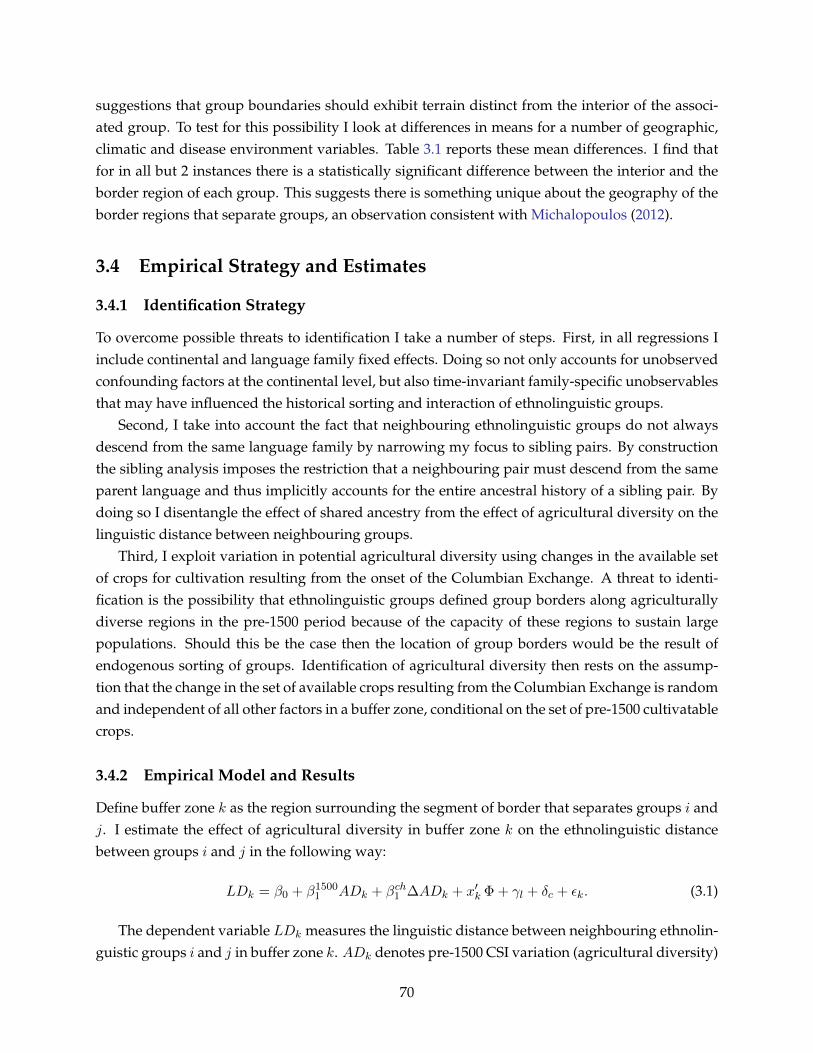
suggestions that group boundaries should exhibit terrain distinct from the interior of the associ-ated group. To test for this possibility I look at differences in means for a number of geographic,climatic and disease environment variables. Table 3.1 reports these mean differences. I find thatfor in all but 2 instances there is a statistically significant difference between the interior and theborder region of each group. This suggests there is something unique about the geography of theborder regions that separate groups, an observation consistent with Michalopoulos (2012).

3.4 Empirical Strategy and Estimates

3.4.1 Identification Strategy

To overcome possible threats to identification I take a number of steps. First, in all regressions Iinclude continental and language family fixed effects. Doing so not only accounts for unobservedconfounding factors at the continental level, but also time-invariant family-specific unobservablesthat may have influenced the historical sorting and interaction of ethnolinguistic groups.

Second, I take into account the fact that neighbouring ethnolinguistic groups do not alwaysdescend from the same language family by narrowing my focus to sibling pairs. By constructionthe sibling analysis imposes the restriction that a neighbouring pair must descend from the sameparent language and thus implicitly accounts for the entire ancestral history of a sibling pair. Bydoing so I disentangle the effect of shared ancestry from the effect of agricultural diversity on thelinguistic distance between neighbouring groups.

Third, I exploit variation in potential agricultural diversity using changes in the available setof crops for cultivation resulting from the onset of the Columbian Exchange. A threat to identi-fication is the possibility that ethnolinguistic groups defined group borders along agriculturallydiverse regions in the pre-1500 period because of the capacity of these regions to sustain largepopulations. Should this be the case then the location of group borders would be the result ofendogenous sorting of groups. Identification of agricultural diversity then rests on the assump-tion that the change in the set of available crops resulting from the Columbian Exchange is randomand independent of all other factors in a buffer zone, conditional on the set of pre-1500 cultivatablecrops.

3.4.2 Empirical Model and Results

Define buffer zone k as the region surrounding the segment of border that separates groups i andj. I estimate the effect of agricultural diversity in buffer zone k on the ethnolinguistic distancebetween groups i and j in the following way:

LDk = β0 + β15001 ADk + βch1 ∆ADk + x′k Φ + γl + δc + εk. (3.1)

The dependent variable LDk measures the linguistic distance between neighbouring ethnolin-guistic groups i and j in buffer zone k. ADk denotes pre-1500 CSI variation (agricultural diversity)

70

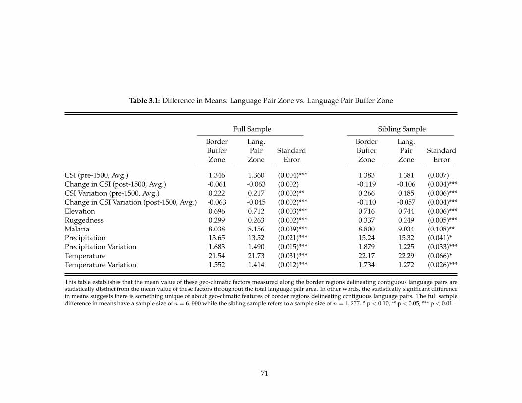
71

Table 3.1: Difference in Means: Language Pair Zone vs. Language Pair Buffer Zone

Full Sample Sibling Sample

Border Lang. Border Lang.Buffer Pair Standard Buffer Pair StandardZone Zone Error Zone Zone Error

CSI (pre-1500, Avg.) 1.346 1.360 (0.004)*** 1.383 1.381 (0.007)Change in CSI (post-1500, Avg.) -0.061 -0.063 (0.002) -0.119 -0.106 (0.004)***CSI Variation (pre-1500, Avg.) 0.222 0.217 (0.002)** 0.266 0.185 (0.006)***Change in CSI Variation (post-1500, Avg.) -0.063 -0.045 (0.002)*** -0.110 -0.057 (0.004)***Elevation 0.696 0.712 (0.003)*** 0.716 0.744 (0.006)***Ruggedness 0.299 0.263 (0.002)*** 0.337 0.249 (0.005)***Malaria 8.038 8.156 (0.039)*** 8.800 9.034 (0.108)**Precipitation 13.65 13.52 (0.021)*** 15.24 15.32 (0.041)*Precipitation Variation 1.683 1.490 (0.015)*** 1.879 1.225 (0.033)***Temperature 21.54 21.73 (0.031)*** 22.17 22.29 (0.066)*Temperature Variation 1.552 1.414 (0.012)*** 1.734 1.272 (0.026)***

This table establishes that the mean value of these geo-climatic factors measured along the border regions delineating contiguous language pairs arestatistically distinct from the mean value of these factors throughout the total language pair area. In other words, the statistically significant differencein means suggests there is something unique of about geo-climatic features of border regions delineating contiguous language pairs. The full sampledifference in means have a sample size of n = 6, 990 while the sibling sample refers to a sample size of n = 1, 277. * p < 0.10, ** p < 0.05, *** p < 0.01.

in buffer zone k, and ∆ADk denotes the change in CSI variation (change in agricultural diversity)following the onset of the Columbian Exchange. xk represents a vector of buffer zone geo-climaticcharacteristics,9 γl is a complete set of language family fixed effects for groups i and j, and γc is acomplete set of continental fixed effects associated with the buffer zone region k.

Unconditional Estimates

Table 3.2 presents the unconditional estimates of equation (3.1). Column 1 reports estimates forthe average value of pre-1500 CSI and the change in average CSI. Neither estimate is statisticallysignificant. However these measures reflect the average potential productivity on a region andnot the diversity.

Column 2 reports estimates for the pre-1500 variation in CSI and the change in that variationat the onset of the Columbian Exchange. These measures capture the agricultural diversity of abuffer zone. Both estimates enter with the expected negative sign and are statistically significantat the 1 percent level. This says that neighbouring groups are more similar in their language whenthe region delineating those groups exhibits greater diversity in potential agricultural output.

Column 3 includes both the potential productivity measures of column 1 and the potentialdiversity measures of column 2. Reassuringly, the estimates for pre-1500 CSI variation and thechange in CSI variation remain remarkably stable in magnitude and significance even when ac-counting for the average potential productivity of a buffer zone. The estimates in column 4 includecontinent fixed effects, and although the magnitude of the estimates drop, the effect remains sta-tistically significant at the 10 percent level.

Columns 5-8 report the analogue estimates of column 1-4 using a sample of sibling pairs. Theestimates in column 5 are almost twice that of the full sample estimates in column 1. For thechange the CSI the effect is now estimated to be significant at the 5 percent level. The estimatesin column 6 are similarly much larger in magnitude with little change in the estimated standarderror. However, as column 7 makes clear, the significant effect of the change in CSI goes awayonce CSI variation and the change in CSI variation are included the estimating equation.

All together the estimates of Table 3.2 suggestion two things: that ethnic groups separatedacross agriculturally diverse regions are more similar in language than groups separated acrosshomogeneous regions, and the precision of the estimates greatly improve after accounting for theancestral history of an ethnolinguistic pair with the sibling-level analysis.

Conditional Estimates

Table 3.3 reports the conditional estimates of equation (3.1) on the sibling-level sample. The es-timates are sorted in pairs, where an even-numbered column is identical to the previous odd-

9Including the pre-1500 potential crop yield and the change in that yield following the Columbian Exchange, themalaria suitability index, elevation, ruggedness, precipitation and precipitation variation, temperature and temperaturevariation, a dummy variable for the presence of a lake, a dummy variable for the presence of a river, the total area ofan ethnolinguistic pair, the latitudinal difference between group centroids, the longitudinal difference between groupcentroids, the interaction of the latitude and longitudinal differences, and variation in land suitability for agriculture.

72

73

Table 3.2: Border-Level Regressions: Unconditional Caloric Suitability Index Benchmark Results

Dependent Variable: Lexicostatistical Linguistic Distance ∈ (0, 1)

Full Sample Sibling Sample

(1) (2) (3) (4) (5) (6) (7) (8)

CSI (pre-1500) -0.007 -0.005 -0.007 -0.017 -0.017 -0.026*(0.007) (0.007) (0.008) (0.014) (0.014) (0.014)

Change in CSI (post-1500) -0.019 -0.010 0.009 -0.039** -0.007 0.004(0.013) (0.014) (0.016) (0.017) (0.018) (0.022)

CSI Variation (pre-1500) -0.067*** -0.065*** -0.059** -0.105*** -0.103*** -0.117***(0.023) (0.023) (0.024) (0.036) (0.036) (0.037)

Change in CSI Variation (post-1500) -0.113*** -0.105*** -0.076* -0.218*** -0.223*** -0.197***(0.036) (0.039) (0.041) (0.049) (0.052) (0.055)

Language Family FE Yes Yes Yes Yes Yes Yes Yes YesContinental FE No No No Yes No No No Yes

Language Cluster 1 2,713 2,713 2,713 2,713 942 942 942 942Language Cluster 2 1,769 1,769 1,769 1,769 851 851 851 851

Observations 6,990 6,990 6,990 6,990 1,277 1,277 1,277 1,277Adjusted R2 0.26 0.26 0.26 0.26 0.32 0.34 0.34 0.35

This table establishes the negative and statistically significant effect of the variation in caloric suitability on a language pair’s lexicostatistical linguistic distance. Theunit of observation is a 100 km buffer zone along the contiguous border segment of each language pair. Standard errors are double-clustered at the level of eachlanguage group and are reported in parentheses. * p < 0.10, ** p < 0.05, *** p < 0.01.

74

Table 3.3: Border-Level Regressions: Conditional Caloric Suitability Index Benchmark Results

Dependent Variable: Lexicostatistical Linguistic Distance ∈ (0, 1)

(1) (2) (3) (4) (5) (6) (7) (8)

CSI Variation (pre-1500) -0.103*** -0.117*** -0.167*** -0.185*** -0.169*** -0.195*** -0.173*** -0.199***(0.036) (0.037) (0.064) (0.063) (0.065) (0.064) (0.064) (0.063)

Change in CSI Variation (post-1500) -0.223*** -0.197*** -0.254*** -0.238*** -0.237*** -0.233*** -0.255*** -0.257***(0.052) (0.055) (0.066) (0.068) (0.066) (0.069) (0.065) (0.068)

CSI (pre-1500) -0.017 -0.026* -0.016 -0.029* -0.012 -0.026* -0.017 -0.029*(0.014) (0.014) (0.014) (0.015) (0.015) (0.015) (0.015) (0.016)

Change in CSI (post-1500) -0.007 0.004 -0.011 -0.006 -0.006 -0.007 -0.005 -0.008(0.018) (0.022) (0.019) (0.024) (0.019) (0.025) (0.019) (0.025)

Elevation 0.021 0.022 0.023 0.021 0.021 0.020(0.019) (0.019) (0.018) (0.018) (0.018) (0.018)

Ruggedness 0.198** 0.190** 0.193** 0.190** 0.175* 0.173*(0.096) (0.094) (0.096) (0.095) (0.096) (0.096)

Precipitation -0.000 -0.000 -0.001 -0.001 -0.001 -0.001(0.001) (0.001) (0.001) (0.001) (0.001) (0.001)

Precipitation Variation 0.002 0.001 0.003 0.003 0.002 0.002(0.005) (0.005) (0.005) (0.005) (0.005) (0.005)

Temperature 0.002 0.003* 0.002* 0.003** 0.003* 0.003**(0.002) (0.002) (0.001) (0.002) (0.001) (0.002)

Temperature Variation -0.029 -0.026 -0.029 -0.026 -0.026 -0.024(0.018) (0.018) (0.018) (0.018) (0.018) (0.018)

River -0.037*** -0.040*** -0.031*** -0.034*** -0.032*** -0.035***(0.012) (0.012) (0.011) (0.011) (0.011) (0.011)

Lake -0.051** -0.051** -0.051** -0.049** -0.050** -0.048**(0.022) (0.022) (0.022) (0.022) (0.022) (0.022)

Malaria 0.003*** 0.002* 0.002** 0.001 0.002* 0.001(0.001) (0.001) (0.001) (0.001) (0.001) (0.001)

Area of Language Pair (km2) -0.009 -0.008 -0.010 -0.008(0.006) (0.006) (0.006) (0.006)

Population of Language Pair -0.004 -0.005 -0.004 -0.005(0.004) (0.004) (0.004) (0.004)

Latitude Difference 0.011** 0.007 0.011** 0.007(0.005) (0.006) (0.005) (0.006)

Longitude Difference 0.006 0.005 0.006 0.005(0.004) (0.004) (0.004) (0.004)

Latitude × Longitude -0.000 -0.000 -0.000 -0.000(0.001) (0.000) (0.001) (0.001)

Land Suitability Variation 0.157** 0.138*(0.074) (0.074)

Language Family FE Yes Yes Yes Yes Yes Yes Yes YesContinental FE No Yes No Yes No Yes No Yes

Language Cluster 1 942 942 942 942 942 942 933 933Language Cluster 2 851 851 851 851 851 851 841 841

Observations 1,277 1,277 1,277 1,277 1,277 1,277 1,267 1,267Adjusted R2 0.34 0.35 0.37 0.38 0.38 0.39 0.39 0.39

This table establishes the negative and statistically significant effect of the variation in caloric suitability on a language pair’s lexicostatistical linguistic distance. Theunit of observation is a 100 km buffer zone along the contiguous border segment of each language pair. Standard errors are double-clustered at the level of eachlanguage group and are reported in parentheses. * p < 0.10, ** p < 0.05, *** p < 0.01.

numbered column but includes continental fixed effects. Overall it is clear that the estimates forCSI variation and change in CSI variation are quite robust to the inclusion of additional geo-climatic covariates, with or without continental fixed effects. In fact, adding these covariates in-creases the magnitude of the estimates. The estimates in column 8 imply that a one standard devi-ation increase in pre-1500 CSI variation reduced linguistic dissimilarity by 5.9 percentage points,while a one standard deviation increase in CSI variation in the post-1500 period reduced dissimi-larity by an additional 6.1 percentage points.

A number of other covariates yield interesting results. I find that rugged border regions tend toamplify linguistic differences between sibling pairs. When a region possess substantial variationin elevation, communication is more costly and contact between neighbouring groups is limited.Thus, groups separated across rugged terrain tend to be more dissimilar in language than groupsseparated across homogeneous terrain. This intensive margin result is complimentary to the ex-tensive margin evidence of Michalopoulos (2012), who finds that the number of ethnolinguisticgroups is decreasing in a region’s terrain ruggedness.

Another interesting result is the finding that the presence of a lake or river in a border regionsystematically limits the divergence of language between neighbouring groups. Lakes and riverswere historically focal points of commercial activity, and the resulting trade in these regions is apossible mechanism through which linguistic similarity is preserved.

To the contrary, I find greater dissimilarities between groups neighbouring across a north-south axis orientation. This is consistent with the evidence that latitudinal differences betweengroups reduced the historical flow of information and thus communication between groups (Di-amond, 1997; Blouin, 2014). I also find that the high prevalence of malaria in a border regionincreases the linguistic distance between neighbouring groups. However, both these results aresomewhat sensitive to the empirical specification, tending to fall short of statistical significant atconventional levels when including continental fixed effects.

Recent Migrations

In this paper, I propose a hypothesis that similar groups border agriculturally diverse areas be-cause they have always lived there and their similarity is the result of inter-group trade. However,since the onset of the Columbian Exchange there has been considerable migration of populationsacross the world that might have led to the arrival of these groups in their current location becauseof a region’s agricultural diversity. It’s feasible that interconnected groups migrate to neighbour-ing regions, in particular agriculturally diverse regions that have the capacity to support a largenumber of people. Should this be true then it’s not the case that agricultural diversity has anyeffect on the cultural similarity of the neighbouring groups.

To check for this I limit my sibling sample to pairs that reside in a country where a significantproportion of its population is native to that country. Data on the ancestral composition of acountry’s contemporary population comes from Putterman and Weil (2010). Table 3.4 reportsestimates for a variety of specifications, where at least 25, 50 or 75 of the population is native to the

75

76

Table 3.4: Border-Level Regressions: Native Population Sensitivity Analysis

Dependent Variable: Lexicostatistical Linguistic Distance ∈ (0, 1)

Sibling Sample Sibling Sample Sibling Sample& >25% Native Pop. & >50% Native Pop. & >75% Native Pop.

(1) (2) (3) (4) (5) (6)

CSI Variation (pre-1500) -0.121*** -0.200*** -0.121*** -0.212*** -0.132*** -0.252***(0.037) (0.065) (0.037) (0.065) (0.039) (0.070)

Change in CSI Variation (post-1500) -0.209*** -0.248*** -0.218*** -0.269*** -0.202*** -0.281***(0.055) (0.070) (0.055) (0.070) (0.057) (0.074)

Controls No Yes No Yes No Yes

Language Family FE Yes Yes Yes Yes Yes YesContinental FE Yes Yes Yes Yes Yes Yes

Language Cluster 1 915 915 886 886 767 767Language Cluster 2 826 826 795 795 693 693

Observations 1,241 1,241 1,202 1,202 1,036 1,036Adjusted R2 0.34 0.39 0.34 0.39 0.33 0.37

This table tests the sensitivity of the benchmark estimates by limiting the sibling sample to pairs that reside in a country where a significant portion of their populationis native to that country. Columns (1)-(2), (3)-(4) and (5)-(6) report estimates where at least 25, 50 and 75 percent of the population is native to the country of residence,respectively. Control variables are identical to those in columns (5) and (6) in Table 3.3. The unit of observation is a 100 km buffer zone along the contiguous bordersegment of each language pair. Standard errors are double-clustered at the level of each language group and are reported in parentheses. * p < 0.10, ** p < 0.05, ***p < 0.01.

country of residence. In all cases the variables of interest are remarkably consistent in magnitudeand significance. These estimates relieve any concern that the estimates are a spurious outcome ofgroup migration.10

Overlapping and Disjoint Ethnolinguistic Groups

The Ethnologue mapping of ethnolinguistic groups poses two problems for this empirical exercise:group territories sometimes overlap and group territories are sometimes spatially disjoint. In thecase of overlapping groups, this is problematic because a buffer zone will not be uniquely repre-sentative of the neighbouring pair. When a group is spatially disjoint (e.g., a single ethnolinguisticgroup occupies two non-adjacent regions within a country), each portion of the disjoint group willnot necessarily be adjacent to the same set of neighbouring groups.

To address these concerns, I drop overlapping groups and groups composed of (disjoint) multi-parts from the sibling sample and re-estimate equation (3.1). Table 3.5 reports these estimates.Whether I drop overlapping groups (columns 1 and 2), multi-part groups (columns 3 and 4) orboth (columns 5 and 6), the coefficients of interest remain statistically significant. Overall, theestimates in Table 3.5 imply that the main result of this paper is unaffected by the Ethnologue’smapping of groups.11

3.5 Concluding Remarks

This study takes the economic importance of ethnolinguistic distance as given, and goes a stepdeeper to explore the geographic foundation of these differences. I construct a novel georeferenceddataset to examine the border regions of neighbouring ethnolinguistic groups, together with varia-tion in the set of potentially cultivatable crops at the onset of the Columbian Exchange, to estimatehow agricultural diversity impacts linguistic differences between neighbouring groups. I find thatethnic groups separated across agriculturally diverse regions are more similar in language thangroups separated across homogeneous agricultural regions.

I offer an explanation that speaks to the work of Bates (1983, 2010), who argues that tradewas historically more profitable and thus more frequent in agriculturally diverse regions. Becausegroups would trade by interacting and communicating with each other, the extent to which theirtwo languages drift apart is mitigated by frequent interaction. Hence, the resulting inter-grouptrade is the channel through which agricultural diversity mitigates ethnolinguistic differences.

What does this result add to our understanding of the link between ethnolinguistic differencesand contemporary patterns of development? It implies that other findings that have been inter-preted as effects of ethnolinguistic distance might be rooted in geography. It also suggests that theexogeneity of ethnolinguistic distance in regression analysis should be questioned in the absenceof the appropriate geographic control variables.

10See Table D3 in the appendix for control variable coefficient estimates.11See Table D4 in the appendix for control variable coefficient estimates.

77

78

Table 3.5: Border-Level Regressions: Overlapping and Multipart Polygon Sensitivity Analysis

Dependent Variable: Lexicostatistical Linguistic Distance ∈ (0, 1)

Sibling Sample Sibling Sample Sibling SampleExcluding Excluding Excluding Overlapping

Overlapping Groups Multi-Part Groups & Multi-Part Groups

(1) (2) (3) (4) (5) (6)

CSI Variation (pre-1500) -0.100** -0.197*** -0.117*** -0.215** -0.136*** -0.205*(0.041) (0.073) (0.045) (0.086) (0.050) (0.106)

Change in CSI Variation (post-1500) -0.175*** -0.221*** -0.218*** -0.262*** -0.213*** -0.244**(0.061) (0.080) (0.071) (0.099) (0.076) (0.118)

Controls No Yes No Yes No Yes

Language Family FE Yes Yes Yes Yes Yes YesContinental FE Yes Yes Yes Yes Yes Yes

Language Cluster 1 744 744 587 587 492 492Language Cluster 2 666 666 539 539 453 453

Observations 988 988 763 763 632 632Adjusted R2 0.36 0.40 0.36 0.40 0.37 0.39

This table tests the sensitivity of the benchmark estimates by limiting the sibling sample to ethnolinguistic pairs that do not overlap with any other groups andare not composed of multi-part group polygons. Control variables are identical to those in columns (5) and (6) in Table 3.3. The unit of observation is a 100 kmbuffer zone along the contiguous border segment of each language pair. Standard errors are double-clustered at the level of each language group and are reported inparentheses. * p < 0.10, ** p < 0.05, *** p < 0.01.

On a more general level, these findings suggest that ethnolinguistic differences are potentiallylinked to a group’s level of state centralization in history. Fenske (2014) shows that the gainsfrom trade resulting from agricultural diversity predicts pre-colonial state centralization, a findingthat corroborates the theory of Bates (1983). Because of the long-run persistent effects of pre-colonial state centralization (Gennaioli and Rainer, 2007; Michalopoulos and Papaioannou, 2013),an interesting area of future research would be to document the possible role of the state in thediffusion of culture and language, and how this role interacts with the persistent effect of pre-colonial states on comparative economic development today.

79

Bibliography

Abramitzky, R. and Sin, I. (2014). Book Translations As Idea Flows: The Effects of the Collapseof Communism on the Diffusion of Knowledge. Journal of the European Economic Association,12(6):1453–1520.

Acemoglu, D., Naidu, S., Restrepo, P., and Robinson, J. A. (2014). Democracy Does Cause Growth.NBER Working Paper 20004.

Ahlerup, P. and Olsson, O. (2012). The Roots of Ethnic Diversity. Journal of Economic Growth,17(2):71–102.

Alesina, A., Devleeschauwer, A., Easterly, W., Kurlat, S., and Wacziarg, R. (2003). Fractionalization.Journal of Economic Growth, 8(2):155–194.

Alesina, A., Easterly, W., and Matuszeski, J. (2011). Artificial States. Journal of the European EconomicAssociation, 9(2):246–277.

Alesina, A. and Giuliano, P. (2013). Culture and Institutions. NBER Working Paper 19750.

Alesina, A. and La Ferrara, E. (2005). Ethnic Diversity and Economic Performance. Journal ofEconomic Literature, 43(3):762–800.

Alesina, A., Michalopoulos, S., and Papaioannou, E. (2016). Ethnic Inequality. Journal of PoliticalEconomy, 124(2):428–488.

Arriola, L. R. (2009). Patronage and Political Stability in Africa. Comparative Political Studies,42(10):1339–1362.

Ashraf, Q. and Galor, O. (2013). The “Out of Africa” Hypothesis, Human Genetic Diversity, andComparative Economic Development. American Economic Review, 103(1):1–46.

Ashraf, Q., Galor, O., and Klemp, M. (2014). The Out of Africa Hypothesis of Comparative Devel-opment Reflected by Nighttime Light Intensity. MRPA Working Paper 55634.

Ashraf, Q., Galor, O., and Klemp, M. (2015). Heterogeneity and Productivity. Brown University,mimeo.

80

Bakker, D., Brown, C. H., Brown, P., Egorov, D., Grant, A., Holman, E. W., Mailhammer, R., Muller,A., Velupillai, V., and Wichmann, S. (2009). Add Typology to Lexicostatistics: A CombinedApproach to Language Classification. Linguistic Typology, 13:167–179.

Baldwin, K. and Huber, J. D. (2010). Economic Versus Cultural Differences: Forms of Ethnic Di-versity and Public Goods Provision. American Political Science Review, 104(4):644–662.

Barbieri, K., Keshk, O. M. G., and Pollin, B. (2009). Trading Data: Evaluating our Assumptionsand Coding Rules. Conflict Management and Peace Science, 26(5):471–491.

Barro, R. and Lee, J.-W. (2013). A New Data Set of Education Attainment in the World, 1950-2010.Journal of Development Economics, 104(1):184–198.

Bates, R. H. (1974). Ethnic Competition and Modernization in Contemporary Africa. ComparativePolitical Studies, 6(4):457–484.

Bates, R. H. (1983). Essays on the Political Economy of Rural Africa. Cambridge University Press,Cambridge.

Bates, R. H. (2010). Prosperity and Violence: The Political Economy of Development. W. W. Norton &Company, New York.

Batibo, H. M. (2005). Language Decline and Death in Africa: Causes, Consequences and Challenges.Multilingual Matters, Tonawanda.

Bertrand, M., Duflo, E., and Mullainathan, S. (2004). How Much Should We Trust Differences-In-Differences Estimates? The Quarterly Journal of Economics, 119(1):249–275.

Bloemen, H. G. (2013). Language Proficiency of Migrants: The Relation with Job Satisfaction andMatching. IZA Discussion Paper 7366.

Blouin, A. (2014). Culture, Isolation, and the Diffusion of Knowledge: Evidence from the BantuExpansion. University of Toronto, mimeo.

Bowles, S. and Gintis, H. (2004). Persistent Parochialism: Trust and Exclusion in Ethnic Networks.Journal of Economic Behavior & Organization, 55:1–23.

Briggs, R. C. (2014). Aiding and Abetting: Project Aid and Ethnic Politics in Kenya. World Devel-opment, 64:194–205.

Burgess, R., Miguel, E., Jedwab, R., Morjaria, A., and Padro i Miquel, G. (2015). The Value ofDemocracy: Evidence from Road Building in Kenya. American Economic Review, 105(6):1817–1851.

Cameron, A. C., Gelbach, J. B., and Miller, D. L. (2011). Robust Inference With Multiway Cluster-ing. Journal of Business & Economic Statistics, 29(2):238–249.

81

Cameron, A. C. and Trivedi, P. K. (2005). Microeconometrics: Methods and Applications. CambridgeUniversity Press, New York.

Caselli, F. and Coleman, W. J. (2013). On the Theory of Ethnic Conflict. Journal of the EuropeanEconomic Association, 11(S1):161–192.

Cavalli-Sforza, L. (2000). Genes, Peoples, and Languages. North Point Press, New York.

Cavalli-Sforza, L. L., Menozzi, P., and Piazza, A. (1994). The History and Geography of Human Genes.Princeton University Press, Princeton.

Collier, P. and Gunning, J. W. (1999). Explaining African Economic Performance. Journal of Eco-nomic Literature, 37(1):64–111.

Comin, D., Easterly, W., and Gong, E. (2010). Was the Wealth of Nations Determined in 1000 BC?American Economic Journal: Macroeconomics, 2(3):65–97.

Crystal, D. (2003). English as a Global Language. Cambridge University Press, Cambridge.

De Luca, G., Hodler, R., Raschky, P. A., and Valsecchi, M. (2015). Ethnic Favoritism: An Axiom ofPolitics? CESifo Working Paper 5209, pages 1–35.

Desmet, K., Breton, M., Ortuno-Ortın, I., and Weber, S. (2011). The Stability and Breakup of Na-tions: A Quantitative Analysis. Journal of Economic Growth, 16(3):183–213.

Desmet, K., Ortuno-Ortın, I., and Wacziarg, R. (2012). The Political Economy of Linguistic Cleav-ages. Journal of Development Economics, 97(2):322–338.

Desmet, K., Ortuno-Ortın, I., and Wacziarg, R. (2015). Culture, Ethnicity and Diversity. NBERWorking Paper 20989.

Desmet, K., Ortuno-Ortın, I., and Weber, S. (2005). Peripheral Diversity and Redistribution. CEPRDiscussion Papers 5112.

Desmet, K., Ortuno-Ortın, I., and Weber, S. (2009). Linguistic Diversity and Redistribution. Journalof the European Economic Association, 7(6):1291–1318.

Diamond, J. (1997). Guns, Germs and Steel. W. W. Norton & Company, New York.

Dickens, A. (2016a). Ethnolinguistic Favoritism in African Politics. York University, mimeo, (Au-gust).

Dickens, A. (2016b). Population Relatedness and Cross-Country Idea Flows: Evidence from BookTranslations. York University, mimeo.

Dreher, A., Fuchs, A., Parks, B. C., Raschky, P. A., and Tierney, M. J. (2015). Aid on Demand:African Leaders and the Geography of China’s Foreign Assistance. CESifo Working Paper 5439.

82

Dyen, I., Kruskal, J. B., and Black, P. (1992). An Indoeuropean Classification: A LexicostatisticalExperiment. Transactions of the American Philosophical Society, 82(5):1–132.

Easterly, W. and Levine, R. (1997). Africa’s Growth Tragedy: Policies and Ethnic Divisions. TheQuarterly Journal of Economics, 112(4):1203–1250.

Easterly, W. and Levine, R. (2012). The European Origin of Economic Development. NBER WorkingPaper 18162.

Ejdemyr, S., Kramon, E., and Robinson, A. L. (2014). Segregation, Ethnic Favoritism, and theStrategic Targeting of Local Public Goods. Stanford University, mimeo.

Englebert, P., Tarango, S., and Carter, M. (2002). Dismemberment and Suffocation: A Contributionto the Debate on African Boundaries. Comparative Political Studies, 35(10):1093–1118.

Esteban, J., Mayoral, L., and Ray, D. (2012). Ethnicity and Conflict: An Empirical Study. AmericanEconomic Review, 102(4):1310–1342.

Esteban, J. and Ray, D. (2011). A Model on Ethnic Conflict. Journal of the European Economic Asso-ciation, 9(3):496–521.

Fearon, J. D. (2003). Ethnic and Cultural Diversity by Country. Journal of Economic Growth, 8(2):195–222.

Fearon, J. D. and Laitin, D. D. (1999). Weak States, Rough Terrain, and Large-Scale Ethnic ViolenceSince 1945. Paper presented at the 1999 Annual Meetings of the American Political Science Association.

Fenske, J. (2013). Does Land Abundance Explain African Institutions? The Economic Journal,123(573):1363–1390.

Fenske, J. (2014). Ecology, Trade, and States in Pre-Colonial Africa. Journal of the European EconomicAssociation, 12(3):612–640.

Franck, R. and Rainer, I. (2012). Does the Leader’s Ethnicity Matter? Ethnic Favoritism, Education,and Health in Sub-Saharan Africa. American Political Science Review, 106(2):294–325.

Francois, P., Rainer, I., and Trebbi, F. (2015). How Is Power Shared in Africa? Econometrica,83(2):465–503.

Galor, O. and Ozak, O. (2015). Land Productivity and Economic Development: Caloric Suitabilityvs . Agricultural Suitability. Brown University, mimeo, pages 1–30.

Galor, O. and Ozak, O. (2016). The Agricultural Origins of Time Preference. American EconomicReview, 106(10):3064–3103.

Galor, O., Ozak, O., and Sarid, A. (2016). Geographical Origins and Economic Consequences ofLanguage Structures. Brown University, mimeo.

83

Gennaioli, N. and Rainer, I. (2007). The Modern Impact of Precolonial Centralization in Africa.Journal of Economic Growth, 12(3):185–234.

Ginsburgh, V. A. and Weber, S. (2016). Linguistic Distances and Ethnolinguistic Fractionaliza-tion and Disenfranchisement Indices. In Ginsburgh, V. A. and Weber, S., editors, The PalgraveHandbook of Economics and Language, pages 137–173. Palgrave Macmillan UK, London.

Goemans, H. E., Gleditsch, K. S., and Chiozza, G. (2009). Introducting Archigos: A Data Set ofPolitical Leaders. Journal of Peace Research, 46(2):269–283.

Gomes, J. F. (2014). The Health Costs of Ethnic Distance: Evidence from Sub-Saharan Africa. pages1–48.

Greenberg, J. H. (1956). The Measurement of Linguistic Diversity. Language, 32(1):109–115.

Guiso, L., Sapienza, P., and Zingales, L. (2009). Cultural Biases in Economic Exchange? TheQuarterly Journal of Economics, 124(3):1095–1131.

Habyarimana, J., Humphreys, M., Posner, D. N., and Weinstein, J. M. (2009). Coethnicity andTrust. In Cook, K., Levi, M., and Hardin, R., editors, Whom Can We Trust?, pages 42–64. RussellSage Foundation, New York.

Harries, L. (1969). Language Policy in Tanzania. Journal of the International African Institute,39(3):275–280.

Henderson, J. V., Storeygard, A., and Weil, D. N. (2012). Measuring Economic Growth From OuterSpace. The American Economic Review, 102(2):994–1028.

Herbst, J. (2000). State and Power in Africa. Princeton University Press, Princeton.

Hodler, R. and Raschky, P. A. (2014). Regional Favoritism. The Quarterly Journal of Economics,129(2):995–1033.

Holman, E. W., Wichmann, S., Brown, C. H., Velupillai, V., Muller, A., and Bakker, D. (2009).Explorations in Automated Language Classification. Folia Linguistica, 42(3-4):331–354.

Huber, J. D. and Suryanarayan, P. (2014). Ethnic Inequality and the Ethnification of Political Par-ties: Evidence from India. Columbia University, mimeo.

Isphording, I. E. and Otten, S. (2013). The Costs of Babylon: Linguistic Distance in Applied Eco-nomics. Review of International Economics, 21(2):354–369.

Isphording, I. E. and Otten, S. (2014). Linguistic Barriers in the Destination Language Acquisitionof Immigrants. Journal of Economic Behavior and Organization, 105(5):30–50.

Israel, J. (2009). A Revolution of the Mind: Radical Enlightenment and the Intellectual Origins of ModernDemocracy. Princeton University Press, Princeton.

84

Jablonski, R. S. (2014). How Aid Targets Votes: The Impact of Electoral Incentives on Foreign AidDistribution. World Politics, 66(2):293–330.

Jensen, N. and Wantchekon, L. (2004). Resource Wealth and Political Regimes in Africa. Compara-tive Political Studies, 37(7):816–841.

Jensen, R. and Oster, E. (2009). The Power of TV: Cable Television and Women’s Status in India.The Quarterly Journal of Economics, 124(3):1057–1094.

Joseph, R. A. (1987). Democracy and Prebendalism in Nigeria. Cambridge University Press, Cam-bridge.

Kasara, K. (2007). Tax Me If You Can: Ethnic Geography, Democracy, and the Taxation of Agricul-ture in Africa. The American Political Science Review, 101(1):159–172.

Kezdi, G. (2004). Robust Standard Error Estimation in Fixed-Effects Panel Models. HungarianStatistical Review, 9:95–116.

Kiszewski, A., Mellinger, A., Spielman, A., Malaney, P., Sachs, S. E., and Sachs, J. (2004). A GlobalIndex Representing the Stability of Malaria Transmission. American Journal of Tropical Medicineand Hygiene, 70(5):486–498.

Kitamura, S. and Lagerlof, N.-P. (2016). Geography and State Fragmentation. York University,mimeo.

Kramon, E. and Posner, D. N. (2016). Ethnic Favoritism in Primary Education in Kenya. QuarterlyJournal of Political Science, 11(1):1–58.

Ku, H. and Zussman, A. (2010). Lingua franca: The role of English in international trade. Journalof Economic Behavior & Organization, 75(2):250–260.

Kyriacou, A. P. (2013). Ethnic Group Inequalities and Governance : Evidence from DevelopingCountries. Kyklos, 66(1):78–101.

La Ferrara, E., Chong, A., and Duryea, S. (2012). Soap Operas and Fertility: Evidence from Brazil.American Economic Journal: Applied Economics, 4(4):1–31.

La Porta, R., Lopez-de Silanes, F., Shleifer, A., and Vishny, R. (1999). The Quality of Government.Journal of Law, Economics, and Organization, 15(1):222–279.

Leighton, W. A. and Lopez, E. J. (2013). Madmen, Intellectuals, and Academic Scribblers: The EconomicEngine of Political Change. Stanford University Press, Redwood City.

Lewis, P. M. (2009). Ethnologue: Languages of the World. SIL International, Dallas, 16 edition.

Marx, B., Stoker, T. M., and Suri, T. (2015). There is No Free House: Ethnic Patronage in a KenyanSlum. MIT, mimeo.

85

Michalopoulos, S. (2012). The Origins of Ethnolinguistic Diversity. American Economic Review,102(4):1508–1539.

Michalopoulos, S. and Papaioannou, E. (2013). Pre-colonial Ethnic Institutions and ContemporaryAfrican Development. Econometrica, 81(1):113–152.

Michalopoulos, S. and Papaioannou, E. (2014). National Institutions and Subnational Develop-ment in Africa. The Quarterly Journal of Economics, 29(1):151–213.

Michalopoulos, S. and Papaioannou, E. (2016). The Long-Run Effects of the Scramble for Africa.American Economic Review, 106(7):1802–1848.

Michalopoulos, S., Putterman, L., and Weil, D. N. (2016). The Influence of Ancestral Lifeways onIndividual Economic Outcomes in Sub-Saharan Africa. NBER Working Paper 21907.

Miguel, E. (2004). Tribe or Nation?: Nation Building and Public Goods in Kenya versus Tanzania.World Politics, 56(3):327–362.

Miguel, E. and Gugerty, M. K. (2005). Ethnic Diversity, Social Sanctions and Public Goods inKenya. Journal of Public Economics, 89(11-12):2325–2368.

Mwakikagile, G. (2010). Ethnic Diversity and Integration in The Gambia: The Land, The People and TheCulture. Continental Press, Dar es Salaam.

Nunn, N. (2008). The Long-Term Effects of Africa’s Slave Trades. The Quarterly Journal of Economics,123(1):139–176.

Nunn, N. (2013). Historical Development. In Aghion, P. and Durlauf, S., editors, Handbook ofEconomic Growth, volume 2. North-Holland.

Nunn, N. and Qian, N. (2010). The Columbian Exchange: A History of Disease, Food, and Ideas.Journal of Economic Perspectives, 24(2):163–188.

Nunn, N. and Qian, N. (2011). The Potato’s Contribution to Population and Urbanization: Evi-dence From A Historical Experiment. The Quarterly Journal of Economics, 126(2):593–650.

Nunn, N. and Wantchekon, L. (2011). The Slave Trade and the Origins of Mistrust in Africa.American Economic Review, 101(7):3221–3252.

Olken, B. A. (2009). Do Television and Radio Destroy Social Capital? American Economic Journal:Applied Economics, 1(4):1–33.

Oucho, J. (2006). Cross-Border Migration and Regional Initiatives in Managing Migration inSouthern Africa. In Kok, P., Gelderblom, D., Oucho, J., and van Zyl, J., editors, Migration inSouth and Southern Africa: Dynamics and Determinants, pages 47–70. HSRC Press, Cape Town.

86

Padro i Miquel, G. (2007). The Control of Politicians in Divided Societies: The Politics of Fear. TheReview of Economic Studies, 74(2007):1259–1274.

Phillipson, R. (1992). Linguistic Imperialism. Oxford University Press, Oxford.

Posner, D. N. (2004). Measuring ethnic fractionalization in Africa. American Journal of PoliticalScience, 48(4):849–863.

Psacharopoulos, G. (1994). Returns to Investment in Education: A Global Update. World Develop-ment, 22(9):1325–1343.

Putterman, L. and Weil, D. N. (2010). Post-1500 Population Flows and the Long-Run Determinantsof Economic Growth and Inequality. The Quarterly Journal of Economics, 125(4):1627–1682.

Ramankutty, N., Foley, J. A., Norman, J., and McSweeney, K. (2002). A Global Distribution ofCultivable Lands: Current Patterns and Sensitivity to Possible Climate Changes. Global Ecologyand Biogeography, 11:377–392.

Rodrik, D. (2014). When Ideas Trump Interests: Preferences, Worldviews, and Policy Innovations.Journal of Economic Perspectives, 28(1):189–208.

Solon, G., Haider, S. J., and Wooldridge, J. (2015). What Are We Weighting For? Journal of HumanResources, 50(2):301–316.

Spolaore, E. and Wacziarg, R. (2009). The Diffusion of Development. The Quarterly Journal ofEconomics, 124(2):469–529.

Spolaore, E. and Wacziarg, R. (2013a). How Deep Are the Roots of Economic Development? Jour-nal of Economic Literature, 51(2):325–369.

Spolaore, E. and Wacziarg, R. (2013b). Long-Term Barriers to Economic Development. NBERWorking Paper 19361.

Spolaore, E. and Wacziarg, R. (2014). Fertility and Modernity. Tufts University Discussion PapersSeries 0779.

Spolaore, E. and Wacziarg, R. (2015). Ancestry, Langauge and Culture. NBER Working Paper 21242.

Spolaore, E. and Wacziarg, R. (2016). War and Relatedness. Review of Economics and Statistics,98(2):925–939.

Swadesh, M. (1952). Lexicostatistical Dating of Prehistoric Ethnic Contracts. Proceedings of theAmerican Philosophical Society, 96:121–137.

Swadesh, M. (1955). Towards Greater Accuracy in Lexicostatistic Dating. International Journal ofAmerican Linguistics, 21:121–137.

87

Wantchekon, L. (2003). Clientelism and Voting Behavior: Evidence from a Field Experiment inBenin. World Politics, 55(3):399–422.

Wesseling, H. (1996). Divide and Rule: The Partition of Africa, 1880-1914. Praeger, Westport.

Wichmann, S., Holman, E. W., Bakker, D., and Brown, C. H. (2010). Evaluating Linguistic DistanceMeasures. Physica A, 389(17):3632–3639.

Wichmann, S., Muller, A., Wett, A., Velupillai, V., Bischoffberger, J., Brown, C. H., Holman, E. W.,Sauppe, S., Molochieva, Z., Brown, P., Hammarstrom, H., Belyaev, O., List, J.-M., Bakker, D.,Egorov, D., Urban, M., Mailhammer, R., Carrizo, A., Dryer, M. S., Korovina, E., Beck, D., Geyer,H., Epps, P., Grant, A., and Valenzuela, P. (2013). The ASJP Database. Version 16.

Wright, D. R. (2015). The World and a Very Small Place in Africa: A History of Globalization in Niumi,The Gambia. Routledge, New York.

Young, A. (2013). Inequality, the Urban-Rural Gap, and Migration. Quarterly Journal of Economics,128(4):1727–1785.

88

Appendix A

Language Appendix

A.1 Computerized Lexicostatistical Linguistic Distance

The computerized approach to estimating lexicostatistical distances was developed as part of theAutomatic Similarity Judgement Program (ASJP), a project run by linguists at the Max Planck Insti-tute for Evolutionary Anthropology. To begin a list of 40 implied meanings (i.e., words) are com-piled for each language to compare the lexical similarity of any language pair. Swadesh (1952)first introduced the notion of a basic list of words believed to be universal across nearly all worldlanguages. When a word is universal across world languages, its implied meaning, and thereforeany estimate of linguistic distance, is independent of culture and geography. From here on I referto this 40-word list as a Swadesh list, as it is commonly called.1

For each language the 40 words are transcribed into a standardized orthography called ASJP-code, a phonetic ASCII alphabet consisting of 34 consonants and 7 vowels. A standardized al-phabet restricts variation across languages to phonological differences only. Meanings are thentranscribed according to pronunciation before language distances are estimated.

I use a variant of the Levenshtein distance algorithm, which in its simplest form calculatesthe minimum number of edits necessary to translate the spelling of a word from one language toanother. In particular, I use the normalized and divided Levenshtein distance estimator proposedby Bakker et al. (2009).2 DenoteLD(αi, βi) as the raw Levenshtein distance for word i of languagesα and β. Each word i comes from the aforementioned Swadesh list. Define the length of this listbe M , so 1 ≤ i ≤ M .3 The algorithm is run to calculate LD(αi, βi) for each word in the M -wordSwadesh list across each language pair. To correct for the fact that longer words will often demand

1A recent paper by Holman et al. (2009) shows that the 40-item list employed here, deduced from rigorous testing forword stability across all languages, yields results at least as good as those of the commonly used 100-item list proposedby Swadesh (1955).

2I use Taraka Rama’s (2013) Python program for string distance calculations.3Wichmann et al. (2010) point out that in some instances not every word on the 40-word list exists for a language,

but in all cases a minimum of 70 percent of the 40-word list exist.

89

more edits, the distance is normalized according to word length:

LDN(αi, βi) =LD(αi, βi)

L(αi, βi)(A.1)

where L(αi, βi) is the length of the longer of the two spellings αi and βi of word i. LDN(αi, βi)

is the normalized Levenshtein distance, which represents a percentage estimate of dissimilaritybetween languages α and β for word i. For each language pair, LDN(αi, βi) is calculated foreach word of the M -word Swadesh list. Then the average lexical distance for each language pairis calculated by averaging across all M words for those two languages. The average distancebetween two languages is then

LDN(α, β) =1

M

M∑i=1

LDN(αi, βi). (A.2)

A second normalization procedure is then adopted to account for phonological similarity thatis the result of coincidence. This adjustment is done to correct for accidental similarity in soundstructure of two languages that is unrelated to their historical relationship. The motivation for thisstep is that no prior assumptions need to be made about historical versus chance relationship. Toimplement this normalization the defined distance LDN(α, β) is divided by the global distancebetween two language. To see this, first denote the global distance between languages α and β as

GD(α, β) =1

M(M − 1)

M∑i 6=j

LD(αi, βj), (A.3)

where GD(α, β) is the global (average) distance between two languages excluding all word com-parisons of the same meaning. This estimates the similarity of languages α and β only in terms ofthe ordering and frequency of characters, and is independent of meaning. The second normaliza-tion procedure is then implemented by weighting equation (A.2) with equation (A.3) as follows:

LDND(α, β) =LDN(α, β)

GD(α, β). (A.4)

LDND(α, β) is the final measure of linguistic distance, referred to as the normalized and di-vided Levenshtein distance (LDND). This measure yields a percentage estimate of the languagedissimilarity between α and β. In instances where two languages have many accidental similar-ities in terms of ordering and frequency of characters, the second normalization procedure canyield percentage estimates larger than 100 percent by construction, so I divide LDND(α, β) by itsmaximum value to normalize the measure as a continuous [0, 1] variable. In Chapter 1, I transformthis measure of lexicostatistical distance into a measure of linguistic similarity as follows:

LS(α, β) = 1− LDND(α, β). (A.5)

90

A.2 Cladistic Similarity

To construct a measure cladistic similarity I calculate the number of shared branches betweenlanguage α and β on the Ethnologue language tree, denoted s(α, β). Let M be the maximumnumber of tree branches between any two languages. Cladistic similarity is constructed as follows:

CS(α, β) =

(s(α, β)

M

)δ, (A.6)

where δ is an arbitrarily assigned weight used to discount more recent linguistic cleavages relativeto deep cleavages. This weight is arbitrary because there is no consensus on the assumed valueof the weight. Fearon (2003) argues the true function is concave and assumes a value of δ = 0.5,which has since become the convention. Desmet et al. (2009) experiment with a range of valuesbetween δ ∈ [0.04, 0.10], but settle on a value of δ = 0.05. In all reported estimates I assume δ = 0.5,though the estimates are robust to alternative weighting assumptions.

One issue with calculating cladistic similarity is the asymmetrical nature of historical languagesplitting. Because the number of branches varies among language families and subfamilies, themaximum number of branches between any two languages is not constant. To overcome thischallenge I assume that all current languages are of equal distance from the proto-language atthe root of the Ethnologue language tree. I visualize this assumption in Figure A1, where I haveconstructed a phylogenetic language tree for the 8 distinct languages of Eritrea. The dashed linesrepresent this assumed historical relationship, so in all cases the contemporary Eritrean languagespossess an equal number of branches to the proto-language at Level 0. Although M = 6 in FigureA1, in the Ethnologue language tree the highest number of classifications for any language isM = 15, which I abstract from here for simplicity.

Figure A1: Phylogenetic Tree of the Eight Major Eritrean Languages

Afro-Asiatic

Semetic

Cushitic

East

Saho-Afar

AfarSaho

Central

Northern

Bilen

North

Bedawiyet

South

Ethiopian

North

TigringaTigre

Nilo-Saharan

Eastern Sudanic

Eastern

NaraKunama

Level 0

Level 1

Level 2

Level 3

Level 4

Level 5

Level 6

91

Appendix B

Chapter 1 Appendix

B.1 Data Descriptions, Sources and Summary Statistics

B.1.1 Regional-Level Data Description and Sources

Country-language groups: Geo-referenced country-language group data comes from the WorldLanguage Mapping System (WLMS). These data map information from each language in the Eth-nologue to the corresponding polygon. When calculating averages within these language grouppolygons, I use the Africa Albers Equal Area Conic projection.Source: http://www.worldgeodatasets.com/language/

Linguistic similarity: I construct two measures of linguistic similarity: lexicostatistical similarityfrom the Automatic Similarity Judgement Program (ASJP), and cladistic similarity using Ethno-logue data from the WLMS. I use these to measure the similarity between each language groupand the ethnolinguistic identity of that country’s national leader. I discuss how I assign a leader’sethnolinguistic identity in Section 1.2.3.Source: http://asjp.clld.org and http://www.worldgeodatasets.com/language/

Night lights: Night light intensity comes from the Defense Meteorological Satellite Program(DMSP). My measure of night lights is calculated by averaging across pixels that fall within eachWLMS country-language group polygon for each year the night light data is available (1992-2013).To minimize area distortions I use the Africa Albers Equal Area Conic projection. In some yearsdata is available for two separate satellites, and in all such cases the correlation between the twois greater than 99% in my sample. To remove choice on the matter I use an average of both. Thedependent variable used in the benchmark analysis is ln(0.01 + average night lights).Source: http://ngdc.noaa.gov/eog/dmsp/downloadV4composites.html

Population density: Population density is calculated by averaging across pixels that fall withineach country-language group polygon. To minimize area distortions I use the Africa Albers Equal

92

Area Conic projection. Data comes from the Gridded Population of the World, which is availablein 5-year intervals: 1990, 1995, 2000, 2005, 2010. For intermediate years I assume population den-sity is constant; e.g., the 1995 population density is assigned to years 1995-1999. Throughout theregression analysis I use log population density.Source: http://sedac.ciesin.columbia.edu/data/collection/gpw-v3

National leaders: I collected birthplace locations of all African leaders between 1991-2013. Namesof African leaders and years entered and exited office comes from the Archigos Database on Lead-ers 1875-2004 (Goemans et al., 2009), which I extended to 2011 using data from Dreher et al. (2015),and 2012-2013 using a country’s Historical Dictionary and other secondary sources.Source: http://www.rochester.edu/college/faculty/hgoemans/data.htm

National leader birthplace coordinates: Birthplace locations are confirmed using Wikipedia, andentered into www.latlong.com to collect latitude and longitude coordinates.Source: http://www.latlong.net

Years in office: To calculate each leader’s current years in office and total years in office I usethe entry and exit data described above.Source: Calculated using Stata.

Distance to leader’s birth region: Country-language group centroids calculated in ArcGIS, andthe distance between each centroid and the national leader’s birthplace coordinates is calculatedin Stata using the globdist command. Throughout the regression analysis I use log leader birth-place distance.Source: Calculated using ArcGIS and Stata.

Absolute difference in elevation: I collect elevation data from the National Geophysical DataCentre (NGDC) at the National Oceanic and Atmospheric Administration (NOAA). I measureaverage elevation of each partitioned language group and leader’s ethnolinguistic group. To min-imize area distortions I use the Africa Albers Equal Area Conic projection. I use Stata to calculatethe absolute difference between the two.Source: www.ngdc.noaa.gov/mgg/topo/globe.html

Absolute difference in ruggedness: As a measure of ruggedness I use the standard deviationof the NGDC elevation data. I use Stata to calculate the absolute difference between the two.Source: www.ngdc.noaa.gov/mgg/topo/globe.html

Absolute difference in precipitation: Precipitation data comes from the WorldClim – GlobalClimate Database. I measure average precipitation within each partitioned language group and

93

leader’s ethnolinguistic group using the Africa Albers Equal Area Conic projection. I use Stata tocalculate the absolute difference between the two.Source: http://www.worldclim.org/current

Absolute difference in temperature: Temperature data comes from the WorldClim – Global Cli-mate Database. I measure the average temperature within each partitioned language group andleader’s ethnolinguistic group using the Africa Albers Equal Area Conic projection. I use Stata tocalculate the absolute difference between the two.Source: http://www.worldclim.org/current

Absolute difference in caloric suitability index: I sourced the caloric suitability index (CSI) datafrom Galor and Ozak (2016). CSI is a measure of agricultural productivity that reflects the caloricpotential in a grid cell. It’s based on the Global Agro-Ecological Zones (GAEZ) project of the Foodand Agriculture Organization (FAO). A variety of related measures are available: in the reportedestimates I use the pre-1500 average CSI measure that includes cells with zero productivity. Theresults are not sensitive to which measure I use. I measure average CSI within each partitionedlanguage group and leader’s ethnolinguistic group using the Africa Albers Equal Area Conic pro-jection. I use Stata to calculate the absolute difference between the two.Source: http://omerozak.com/csi

Oil reserve: I construct an indicator variable equal to one if an oil field is found in both the par-titioned language group and leader’s ethnolinguistic group. Version 1.2 of the Petroleum Datasetcontains geo-referenced point data indicating the presence of on-shore oil and gas deposits fromaround the world.Source: https://www.prio.org/Data/Geographical-and-Resource-Datasets/Petroleum-Dataset/

Diamond reserve: I construct an indicator variable equal to one if a known diamond depositis found in both the partitioned language group and leader’s ethnolinguistic group. Version 1.2 ofthe Petroleum Dataset contains geo-referenced point data indicating the presence of on-shore oiland gas deposits from around the world.Source: https://www.prio.org/Data/Geographical-and-Resource-Datasets/Diamond-Resources/

B.1.2 Individual-Level Data Description and Sources

Unless otherwise stated, all individual-level data comes from the Demographic and Health Sur-veys (DHS). Source: http://dhsprogram.com/

Individual linguistic similarity: To assign an individual a home language I assign the reportedlanguage a respondent speaks at home when this data is available (59 percent availability). Forsurveys when this data isn’t available or the reported language is “other”, I map the respondent’s

94

home language from their reported ethnicity. To do this I use the following assignment rule:

1. Direct match: the DHS ethnicity name is the same as an Ethnologue language name for therespondent’s country of residence.

2. Alternative name: the unmatched DHS ethnicity is an unambiguous alternative name for alanguage in the Ethnologue or Glottolog database.

3. Macrolanguage: if the ethnicity corresponds to a macrolanguage in the Ethnologue, then Iassign the most populated sub-language of that macrolanguage.

4. Population size: if the unmatched ethnicity maps to numerous languages, I choose the lan-guage with the largest Ethnologue population.

I also cross-reference the Wikipedia page for each ethnic group to corroborate that the assignedlanguage maps into the reported ethnicity. Then using the same data on leaders as in the regional-analysis, I match the lexicostatistical similarity of the respondent’s home language to the leader’sethnolinguistic identity.Source: http://asjp.clld.org

Locational linguistic similarity: I project DHS cluster latitude and longitude coordinates ontothe Ethnologue language map and assign the associated language as the regional language groupto that respondent. In instances of overlapping language groups, I assign the largest group interms of population. Then using the same data on leaders as in the regional-analysis, I match thelexicostatistical similarity of the respondent’s home language to the leader’s ethnolinguistic iden-tity.Source: http://asjp.clld.org

Wealth Index: I use the quantile DHS wealth index. The quantile index is derived from a com-posite measure of a household’s assets (e.g., television, refrigerator, telephone, etc.) and access topublic resources (e.g., water, electricity, sanitation facility, etc.), in addition to data indicating if ahousehold owns agricultural land and if they employ a domestic servant. Principal componentanalysis is used to construct the original index, then respondents are order by score and sortedinto quintiles. Read the DHS Comparative Report: The DHS Wealth Index for more details.

Age: Age of respondent at the time of survey.

Gender: An indicator variable equal to one if a respondent is female.

Rural: An indicator variable for rural locations.

Education: The 10 education fixed effects are from question 90.

95

Religion: The 18 fixed effects for the religion of a respondent come from question 91.

Distance to the capital: I use the World Cities layer available on the ArcGIS website, which in-cludes latitude-longitude coordinates and indicators for capital cities. I calculate language groupcentroids coordinates using ArcGIS, and measure the geodesic distance between the two points inStata using the globdist command.Source: http://www.arcgis.com/home/

Distance to the coast: I use the coastline shapefile from Natural Earth, calculate the nearest coast-line from a language groups centroid using the Near tool in ArcGIS. I measure the geodesic dis-tance between the two points in Stata using the globdist command.Source: http://www.naturalearthdata.com/downloads/10m-physical-vectors/10m-coastline/

Distance to the border: I use country boundaries from the Digital Chart of the World (5th edition)that’s complimentary to the Ethnologue data from the WLMS, and calculate the nearest borderfrom a language groups centroid using the Near tool in ArcGIS. I measure the geodesic distancebetween the two points in Stata using the globdist command.Source: http://www.worldgeodatasets.com/language/

96

B.1.3 Summary Statistics and Additional Details

Table B1: Language Groups Included in Regional-Level Analysis

Sample Language Groups

Regional-LevelAnalysis

Acholi, Adamawa Fulfulde, Adele, Afade, Afrikaans, Alur, Anuak,Anufo, Anyin, Baatonum, Badyara, Baka, Bari, Bata, Bayot, Bedawiyet,Bemba, Berta, Bissa, Boko, Bokyi, Bomwali, Borana-Arsi-Guji Oromo,Buduma, Central Kanuri, Chadian Arabic, Chidigo, Cokwe, Daasanach,Dan, Dazaga, Dendi, Dholuo, Diriku, Ditammari, Ejagham, Ewe, Fur,Gbanziri, Gidar, Glavda, Gola, Gourmanchema, Gude, Gumuz, Hausa,Herero, Holu, Jola-Fonyi, Juhoan, Jukun Takum, Jula, Kaba, Kacipo-Balesi, Kako, Kakwa, Kalanga, Kaliko, Kaonde, Kasem, Khwe, Kikongo,Kisikongo, Kiswahili, Komo, Konkomba, Koromfe, Kuhane, Kunama,Kunda, Kuo, Kuranko, Kusaal, Kwangali, Kxauein, Langbashe, Lozi, Lug-bara, Lunda, Lutos, Luvale, Maasai, Madi, Makonde, Mambwe-Lungu,Mandinka, Mandjak, Manga Kanuri, Mann, Manyika, Masana, Mashi,Mbandja, Mbay, Mbukushu, Mende, Monzombo, Moore, Mpiemo, Mun-dang, Mundu, Musey, Musgu, Nalu, Naro, Ndali, Ndau, Ngangam, Ng-baka Mabo, Ninkare, Northern Kissi, Northwest Gbaya, Nsenga, Ntcham,Nuer, Nyakyusa-Ngonde, Nyanja, Nzakambay, Nzanyi, Nzema, Oshi-wambo, Pana, Peve, Pokoot, Psikye, Pulaar, Pular, Runga, Rwanda, Saho,Shona, Shuwa Arabic, Somali, Soninke, Southern Birifor, Southern Kisi,Southern Sotho, Susu, Swati, Taabwa, Talinga-Bwisi, Tamajaq, Tedaga,Teso, Tigrigna, Tonga, Tswana, Tumbuka, Tupuri, Vai, Venda, Wandala,Western Maninkakan, Xhosa, Xoo, Yaka, Yaka, Yalunka, Yao, Yeyi, Za-ghawa, Zande, Zarma, Zemba, Zulu

97

Table B2: Language Groups Included in DHS Individual-Level Analysis

Sample Language Groups

Individual-LevelAnalysis (Loca-tional)

Alur, Bemba, Borana, Kaonde, Kasem, Kisi (Southern), Kissi (North-ern), Kuhane, Kuranko, Lamba, Lugbara, Lunda, Maninkakan (Western),Mann, Oromo (Borana-Arsi-Guji), Pular, Somali, Soninke, Susu, Taabwa,Teso

Individual-LevelAnalysis (Individ-ual)

Afar, Amharic, Aushi, Bamanankan, Bandi, Bemba, Berta, Bissa,Bobo Madare (Southern), Bwile, Cokwe, Dagaare (Southern), Dagbani,Dan, Dholuo, Ekegusii, Farefare, Ganda, Gedeo, Gikuyu, Gola, Gour-manchema, Gwere, Hadiyya, Harari, Hausa, Ila, Jola-Fonyi, Kamba,Kambaata, Kaonde, Kigiryama, Kipsigis, Kisi (Southern), Kissi (North-ern), Kono, Koongo, Kpelle (Guinea), Kpelle (Liberia), Krio, Kuhane,Kunda, Kuranko, Lala-Bisa, Lamba, Lendu, Lenje, Limba (East), Lozi,Luba-Kasai, Lugbara, Lunda, Luvale, Maasai, Madi, Mambwe-Lungu,Mandinka, Maninkakan (Kita), Mann, Mbunda, Mende, Moore, Ngombe,Nkoya, Nsenga, Nyanja, Oromo (Borana-Arsi-Guji), Oromo (West Cen-tral), Oyda, Pulaar, Pular, Rendille, Samburu, Sebat Bet Gurage, Senoufo(Mamara), Serer-Sine, Sherbro, Sidamo, Soli, Somali, Songhay (Koyra Chi-ini), Soninke, Susu, Swahili, Taabwa, Tamasheq, Teso, Themne, Tigrigna,Tonga, Tumbuka, Turkana, Wolaytta, Wolof

98

Table B3: Leaders Included in Regional-Level Analysis

Sample Leaders

Regional-LevelAnalysis

Angola: Jose Eduardo dos Santos; Benin: Thomas Yayi Boni, Mathieu Kerekou;Botswana: Quett Masire, Festus Mogae; Burkina Faso: Blaise Compaore;Cameroon: Paul Biya; Central African Republic: Ange-Felix Patasse, Andre-Dieudonne Kolingba; Chad: Idriss Deby; Congo: Pascal Lissouba, Denis Sas-sou Nguesso; Cote d’Ivoire: Konan Bedie, Laurent Gbagbo, Robert Gueı, FelixHouphouet-Boigny, Alassane Ouattara; DRC: Joseph Kabila, Laurent-Desire Ka-bila, Mobutu Sese Seko; Eritrea: Isaias Afewerki; Ethiopia: Hailemariam Desalegn,Meles Zenawi; Gambia: Yahya Jammeh, Dawda Jawara; Ghana: John Evans Atta-Mills, John Agyekum Kufuor, John Dramani Mahama, Jerry Rawlings; Guinea:Moussa Dadis Camara, Alpha Conde, Lansana Conte, Sekouba Konate; Guinea-Bissau: Kumba Iala, Manuel Serifo Nhamadjo, Henrique Periera Rosa, Malam Ba-cai Sanhe, Joao Bernardo Vieira; Kenya: Daniel arap Moi; Mwai Kibaki; Lesotho:Elias Phisoana Ramaema, Ntsu Mokhehle, Pakalithal Mosisili, Tom Thabane;Liberia: Gyude Bryant, Ruth Perry, Wilton G. S. Sankawulo, Ellen Johnson Sir-leaf, Charles Taylor; Malawi: Hastings Kamuzu Banda, Joyce Banda, Bakili Muluzi,Bungu wa Mutharika; Mali: Alpha Oumar Konare, Amadou Toumani Toure, Dion-counda Traore; Mozambique: Armando Guebuza, Joaquim Chissano; Namibia:Sam Nujoma, Hifikepunye Pohamba; Niger: Mahamadou Issoufou, Ibrahim BareMaınassara, Mahamane Ousmane, Ali Saibou, Mamadou Tandja; Nigeria: SaniAbacha, Abdulsalami Abubakar, Goodluck Jonathan, Olusegun Obasanjo, UmaruMusa Yar’Adua; Senegal: Abdou Diouf, Macky Sall, Abdoulaye Wade; SierraLeone: Ahmad Tejan Kabbah, Ernest Bai Koroma, Johnny Paul Koroma, Valen-tine Strasser; Somalia: Abdullahi Yusuf Ahmed, Sharif Sheikh Ahmed, AbdiqasimSalad Hassan, Hassan Sheikh Mohamud, Ali Mahdi Muhammad; South Africa:Frederik Willem de Klerk, Nelson Mandela, Thabo Mbeki, Jacob Zuma; Sudan:Omar Hassan Ahmad al-Bashir; Tanzania: Jakaya Kikwete, Benjamin Mkapa, AliHassan Mwinyi; Togo: Gnassingbe Eyadema, Faure Gnassingbe; Uganda: Yow-eri Museveni; Zambia: Frederick Chiluba, Levy Mwanawasa, Michael Sata; Zim-babwe: Robert Mugabe

99

Table B4: Leaders Included in DHS Individual-Level Analysis

Sample Leaders

Individual-Level Burkina Faso: Blaise CompaoreAnalysis Democratic Republic of Congo: Joseph Kabila

Ethiopia: Meles ZenawiGhana: Jerry Rawlings; John Agyekum KufuorGuinea: Alpha Conde; Lansana ConteKenya: Mwai KibakiLiberia: Ellen Johnson SirleafMali: Alpha Oumar Konare; Amadou Toumani ToureNamibia: Hifikepunye PohambaSenegal: Abdou Diouf; Abdoulaye WadeSierra Leone: Ernest Bai KoromaUganda: Yoweri MuseveniZambia: Levy Mwanawasa; Michael Sata

Table B5: Countries Included in Regional- and Individual-Level Analysis

Sample Countries

Regional-Level Analy-sis

Angola, Benin, Botswana, Burkina Faso, Cameroon, Central AfricanRepublic, Chad, Congo, Cote d’Ivoire, Democratic Republic of Congo,Eritrea, Ethiopia, Gambia, Ghana, Guinea, Guinea-Bissau, Kenya,Lesotho, Liberia, Malawi, Mali, Mozambique, Namibia, Niger, Nige-ria, Senegal, Sierra Leone, Somalia, South Africa, Sudan, Tanzania,Togo, Uganda, Zambia, Zimbabwe

Individual-Level Anal-ysis

Burkina Faso, Democratic Republic of Congo, Ethiopia, Ghana,Guinea, Kenya, Liberia, Mali, Namibia, Senegal, Sierra Leone,Uganda, Zambia

100

Table B6: Summary Statistics – Regional-Level Dataset

Mean Std dev. Min Max N

Night lightst 0.123 0.387 0.000 4.540 6,610ln(0.01 + night lightst) -3.487 1.427 -4.605 1.515 6,610ln(0.01 + night lightst−1) -3.507 1.415 -4.605 1.515 6,315√

night lightst 0.187 0.297 0.000 2.131 6,610ln(night lightst) -3.370 2.049 -10.60 1.513 4,069Lexicostatistical similarityt−1 0.193 0.230 0.000 1.000 6,610Cladistic similarityt−1 0.409 0.330 0.000 1.000 6,610Coethnicityt−1 0.047 0.212 0.000 1.000 6,610Non-coethnic cladistic similarityt−1 0.362 0.313 0.000 0.966 6,610Non-coethnic lexicostatistical similarityt−1 0.146 0.148 0.000 0.960 6,610Lexicostatistical similarityt+1 0.194 0.230 0.000 1.00 6228Current years in officet−1 11.44 8.680 1.000 38.00 6,610Total years in officet−1 18.50 10.19 1.000 38.00 6,610Log distance (km) to leader’s groupt−1 5.844 1.485 0.000 7.419 6,610Log population densityt 2.886 1.529 -2.169 6.116 6,610Absolute difference in elevationt 250.5 296.1 0.000 2,021 6,610Absolute difference in ruggednesst 101.5 105.5 0.000 542.4 6,610Absolute difference in precipitationt 30.20 28.90 0.00 230.7 6,610Absolute difference in mean temperaturet 16.81 17.09 0.000 120.2 6,610Absolute difference in caloric suitability indext 298.0 310.1 0.000 1711 6,610Oil reserve in both leader and language groupt 0.018 0.131 0.000 1.000 6,610Diamond mine in both leader and language groupt 0.079 0.269 0.000 1.000 6,610Absolute difference in malaria suitabilityt 4.951 5.635 0.000 29.30 5,111Absolute difference in land suitabilityt 0.178 0.184 0 0.777 5111Democracyt−1 0.435 4.877 -9.000 9.000 6,573Language group population share 0.045 0.113 0 0.851 6610Distance (km) to capital city 559.7 397.7 26.58 1922 6,610Distance (km) to the coast 677.9 408.4 10.52 1743 6,610

101

Table B7: Summary Statistics – DHS Individual-Level Dataset

Mean Std Dev. Min Max N

Wealth index 2.974 1.468 1.000 5.000 56,455Locational similarity 0.350 0.380 0.025 1.000 56,455Individual similarity 0.363 0.387 0.021 1.000 56,455Age 29.36 10.51 15.00 78.00 56,455Female indicator 0.663 0.473 0.000 1.000 56,455Rural indicator 0.635 0.482 0.000 1.000 56,455Education 4.721 1.520 1.000 6.000 56,455Religion 4.912 2.032 1.000 8.000 56,455Log distance to the coast (km) 6.059 0.910 1.654 7.238 56,455Log distance to the border (km) 4.948 0.887 0.920 6.801 56,455Log distance to the capital (km) 5.676 0.727 2.070 7.548 56,455

Table B8: Summary Statistics – Power Sharing Dataset

Mean Std dev. Min Max N

Share of cabinet positionst 0.056 0.078 0.000 0.471 2,539Share of top cabinet positionst 0.057 0.108 0.000 0.643 2,539Share of low cabinet positionst 0.055 0.078 0.000 0.450 2,539Coethnicityt 0.077 0.266 0.000 1.000 2,539Lexicostatistical similarityt 0.196 0.267 0.000 1.000 2,539Non-coethnic lexicostatistical similarityt 0.114 0.122 0.000 0.659 2,539Ethnic group population sharet 0.057 0.065 0.005 0.390 2,539

102

B.2 Mapping Ethnicity to Language

There is mostly agreement between ethnographers that language is a suitable marker of ethnicityin Africa (Batibo, 2005; Desmet et al., 2015). The challenge of mapping ethnicity to language isthat, in some instances, a single ethnic group speaks many languages. In such instances it’s notobvious what language is the appropriate language to match to a leader’s ethnicity. As a solutionto this problem I use the following three-step assignment rule to construct a mapping betweenethnicity and language in Africa.

Step 1: For each ethnic group, I refer to the Ethnologue list of languages for the country to whichthey belong. If a language name is identical to the ethnic name then I assign the correspond-ing language to that ethnicity.

Step 2: If there is no language name identical to the ethnicity then I check the alternate names for alanguage. If an ethnic name matches an alternate language name, I assign the correspondinglanguage to that ethnicity.

Step 3: If a set of potential language matches still exist, I assign the largest language group (in termsof population) to the ethnic group.

103

B.3 Supplementary Materials

This section presents results referenced but not presented in the main body of the paper.

B.3.1 Various Fixed Effects Specifications

Table B9 reports 27 different estimates: 9 versions of equation (1.1) for each of the 3 linguisticsimilarity measures. Columns 1-3 report between-group estimates with country-year fixed effects,the estimates in columns 4-6 add country-language fixed effects, and columns 7-9 report estimatesfor the triple-difference estimator. For each set of three regressions I report estimates (i) withoutany covariates, (ii) estimates that only control for log population density and the logged geodesicdistance between each partitioned group and the corresponding leader’s group, and (iii) the fullset of covariates I outlined in Section 1.3.

Consistent with my hypothesis of ethnolinguistic favoritism, all 27 coefficients are positiveand the majority are statistically significant. In all cases my preferred measure of lexicostatisticalsimilarity is significant with the exception of column 4, where lexicostatistical similarity has a re-ported p-value of 0.127. However, in this instance, the estimator lacks language-year fixed effectsand thus does not exploit the counterfactual comparison of the same language group on the otherside of the border.

Indeed, the addition of language-year fixed effects in 7-9 adds considerable precision to theestimates relative to columns 4-6. The allowance of a within-group estimator that comes fromhaving a panel of partitioned language groups substantially improves my ability to identify eth-nolinguistic favoritism.

I also provide estimates for cladistic similarity and coethnicity to see how these alternativemeasures compare to lexicostatistical similarity. For my benchmark estimates both coefficients arepositive and statistically significant, albeit only at the 10 percent level. Not only does the esti-mated coefficient monotonically increase in the measured continuity of linguistic similarity, butlexicostatistical similarity is also more precisely estimated than both alternative measures. Thissuggests that the observable variation among non-coethnic groups assists in identifying patternsof ethnic favoritism in Africa.

B.3.2 Additional Controls

In this section I reproduce the benchmark estimates with two additional control variables: theMalaria Ecology Index (Kiszewski et al., 2004) and the Agricultural Suitability Index (Ramankuttyet al., 2002). The trouble with these data is that in a number of instances a single raster cell coversan area larger than a country-language group partition because these data are only available at aspatial resolution of 0.5 × 0.5 (approximately 111 km × 111 km). These partitions are droppedfrom group average calculations, resulting in a sample 61.5 percent of the benchmark sample size.

Table B10 reports these subsample estimates that include the additional control variables. Foreach of the three measures of similarity I report estimates that include the absolute difference in the

104

Malaria Ecology Index, the absolute difference in the Agricultural Suitability Index and estimatesthat include both measures, in addition to benchmark set of controls. The results are unchangedby including these controls.

B.3.3 Measurement Error

When an unambiguous assignment of a leader’s ethnolinguistic identity cannot be made, I as-sign the group with the largest population among the set of potential matches. The finding thatfavoritism exists among groups that are not coethnic to the leader might be driven by the mea-surement error introduced by this approach.

In this section I report estimates on a subsample of my benchmark dataset that excludes the4 leaders I could not unambiguously match.1 Table B11 reports these results. Overall little ischanged from my benchmark estimates, with the exception that coethnicity is no longer signif-icant at standard levels of confidence. However, lexicostatistical similarity is roust to these ex-cluded leaders, and most importantly, column (4) of Table B11 makes clear that the significance ofnon-coethnic similarity is not a consequence of the possible measurement error introduced whenassigning an ethnolinguistic identity to the aforementioned leaders.

B.3.4 Balanced Panel

In this section I test the robustness of the benchmark estimates using a balanced panel of country-language groups between 1992 and 2013. My benchmark panel was unbalanced because of miss-ing data on language lists used to estimate lexciostatistical similarity. This is problematic if theselists are missing for non-random reasons (Cameron and Trivedi, 2005). To check this I limit theanalysis to a balanced sample of 84 language groups partitioned across 23 countries. Table B12reports these estimates.

In all 27 reported regressions the measure of linguistic similarity takes the expected positivesign positive. For my preferred measure of lexicostatistical similarity the coefficients are statis-tically significant in all but one regression. The magnitudes of the estimates are also relativelysimilar to my benchmark estimates. To the contrary cladistic similarity seems to be quite sensitiveto this subsample and in only significant in a single instance. The coethnic results are similar tothose in Table 1.3.

B.3.5 Weighted Regressions

In this section I test for heteroskedasticity in my benchmark estimates by weighting regressionsby the Ethnologue population of each language group. The idea is that the measure of night lightintensity is an average within each country-language group, and it is likely to have more variancein places where the population is small (Solon et al., 2015). Table B13 reports these estimates.

1Mobutu Sese Seko (DRC), Joseph Kabila (DRC), Laurent-Desire Kabila (DRC) and Goodluck Jonathan (Nigeria).

105

The lexicostatistical estimates are less sensitive to weighting than the cladistic and coethnicestimates. While a few lexicostatistical estimates lose their significance in columns (4)-(6), theseestimates do not exploit language-year fixed effects, and hence are not identified off the exogenouswithin-group variation. In my benchmark specification in column (9), the effect of lexicostatisticalsimilarity is significant at the 5 percent level and very similar to the benchmark estimate in termsof magnitude.

B.3.6 Alternative Night Light Transformations

The log transformation used throughout the regional analysis is without a doubt arbitrary. The useof this transformation has become the convention when using these night lights data so I followthe literature in my chose to add 0.01 to the log transformation. Nonetheless, I experiment withtwo alternative transformations in Table B14.

In columns (1)-(3) I report estimates where the dependent variable is defined as the squareroot of the raw night lights data. In columns (4)-(6) I log the night lights data without adding aconstant. The latter results in a substantial loss of observations due to the fact that 40 percent ofthe observations exhibit zero night light activity. Because I must observe a partitioned group onboth sides of the border for any year, I lose nearly 60 percent of my benchmark sample using thislog transformation.

I find that the lexicostatistical estimate is robust to both transformations, while the cladistic isonly robust to the square root transformation. Coethnicity remains positive but loses its statisticalsignificance is both instances.

B.3.7 DHS Additional Tables

Table B17 reports 15 estimates: 5 separate specifications for both locational and individual similar-ity, and the same five specifications for the joint similarity estimates. In all specifications I adjuststandard errors for clustering in country-wave-locational-language areas.

The top panel reports estimates for locational similarity. In column (1) the coefficient takesthe expected positive sign, but is insignificant because the standard error is estimated to be quitelarge. However, in this specification I do not account for any individual characteristics, includingwhether a respondent lives in a rural location. Young (2013) shows that the urban-rural incomegap accounts for 40 percent of mean country inequality in a sample of 65 DHS countries. Incolumn (2) I report an estimate that includes a rural indicator variable. Indeed, the inclusionof this indicator substantially improves the precision of estimation, where locational similarityis now significant at the 1 percent level. In column (3) I add a set of individual controls.2 Themagnitude of locational similarity increases slightly and maintains its strong significant effect onindividual wealth. In Table B17 I add each individual control variable one at a time. While I

2The set of individual controls include age, age squared, a female indicator, a rural indicator, a capital city indicator,5 education fixed effects and 7 religion fixed effects. See Appendix B for variable definitions.

106

account for capital city effects with an indicator variable, I also account for additional spatialeffects in columns (4) and (5) by separately adding the geodesic distance to the nearest coast andborder.3

The middle panel of Table B15 reports estimates for individual similarity. While all coefficientstake the expected positive sign, only a single estimate of individual similarity is statistically signif-icant. When I do not control for any covariates the effect of individual similarity is very preciselyestimated. To the contrary, the effect goes away once I account for respondents living in rurallocations. The same is true when including the full set of controls.

Next I jointly estimate both channels using the aforementioned variation among individualsnon-native to the region in which they reside. The results are consistent with the rest of the tableand reported in the bottom panel of Table B15. In column (1) the estimate for individual similarityoutperforms locational similarity when no individual characteristics are accounted for, howeverthe reverse is true in columns (2)-(5) as covariates are incrementally added – in particular the ruralindicator.

To show that the locational mechanism is not only driven by the coethnic effect, I separatelyestimate locational coethnicity and non-coethnic locational similarity. I do this in the same way Idid in the regional-level analysis: I define non-coethnic locational similarity as (1− coethnicity)×locational similarity. Table B16 reports these estimates. While non-coethnic locational similarityis estimated to be no different than zero in the most basic regression, once again after the base-line set of controls are added both the coethnic and non-coethnic effect are positive and stronglysignificant. Using the more conservative estimates of column (5), this suggests that the averagelevel of non-coethnic locational similarity (0.164) yields an increase of 0.094 (= 0.164 × 0.573) inthe wealth index – roughly one fourth the coethnic effect.

Finally, I also report the DHS estimates for locational similarity and include each baselinecovariate one at a time. The idea here is to highlight the relative importance of controlling for theurban-rural inequality gap when using the DHS wealth index (Young, 2013). Table B17 reportsthese estimates.

Indeed I find that the precision of the locational similarity estimate is substantially improvedby including an indicator variable for respondents living in rural regions. While many of theother covariates are themselves positive, no other variable have such a large confounding effecton locational similarity in its absence.

3I include distances separately because language areas tend to be fairly small, so location clusters in a partition areusually very close together and distance measures are highly collinear.

107

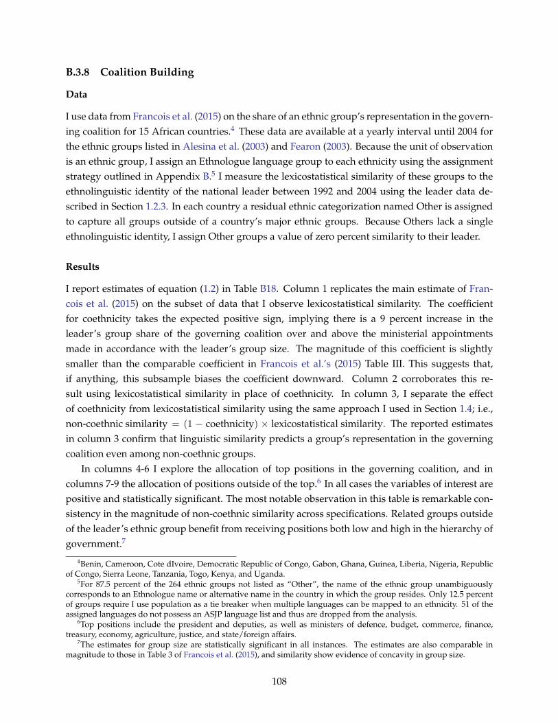
B.3.8 Coalition Building

Data

I use data from Francois et al. (2015) on the share of an ethnic group’s representation in the govern-ing coalition for 15 African countries.4 These data are available at a yearly interval until 2004 forthe ethnic groups listed in Alesina et al. (2003) and Fearon (2003). Because the unit of observationis an ethnic group, I assign an Ethnologue language group to each ethnicity using the assignmentstrategy outlined in Appendix B.5 I measure the lexicostatistical similarity of these groups to theethnolinguistic identity of the national leader between 1992 and 2004 using the leader data de-scribed in Section 1.2.3. In each country a residual ethnic categorization named Other is assignedto capture all groups outside of a country’s major ethnic groups. Because Others lack a singleethnolinguistic identity, I assign Other groups a value of zero percent similarity to their leader.

Results

I report estimates of equation (1.2) in Table B18. Column 1 replicates the main estimate of Fran-cois et al. (2015) on the subset of data that I observe lexicostatistical similarity. The coefficientfor coethnicity takes the expected positive sign, implying there is a 9 percent increase in theleader’s group share of the governing coalition over and above the ministerial appointmentsmade in accordance with the leader’s group size. The magnitude of this coefficient is slightlysmaller than the comparable coefficient in Francois et al.’s (2015) Table III. This suggests that,if anything, this subsample biases the coefficient downward. Column 2 corroborates this re-sult using lexicostatistical similarity in place of coethnicity. In column 3, I separate the effectof coethnicity from lexicostatistical similarity using the same approach I used in Section 1.4; i.e.,non-coethnic similarity = (1 − coethnicity) × lexicostatistical similarity. The reported estimatesin column 3 confirm that linguistic similarity predicts a group’s representation in the governingcoalition even among non-coethnic groups.

In columns 4-6 I explore the allocation of top positions in the governing coalition, and incolumns 7-9 the allocation of positions outside of the top.6 In all cases the variables of interest arepositive and statistically significant. The most notable observation in this table is remarkable con-sistency in the magnitude of non-coethnic similarity across specifications. Related groups outsideof the leader’s ethnic group benefit from receiving positions both low and high in the hierarchy ofgovernment.7

4Benin, Cameroon, Cote dIvoire, Democratic Republic of Congo, Gabon, Ghana, Guinea, Liberia, Nigeria, Republicof Congo, Sierra Leone, Tanzania, Togo, Kenya, and Uganda.

5For 87.5 percent of the 264 ethnic groups not listed as “Other”, the name of the ethnic group unambiguouslycorresponds to an Ethnologue name or alternative name in the country in which the group resides. Only 12.5 percentof groups require I use population as a tie breaker when multiple languages can be mapped to an ethnicity. 51 of theassigned languages do not possess an ASJP language list and thus are dropped from the analysis.

6Top positions include the president and deputies, as well as ministers of defence, budget, commerce, finance,treasury, economy, agriculture, justice, and state/foreign affairs.

7The estimates for group size are statistically significant in all instances. The estimates are also comparable inmagnitude to those in Table 3 of Francois et al. (2015), and similarity show evidence of concavity in group size.

108

109

Table B9: Benchmark Regressions Using Various Combinations of Fixed Effects

Dependent Variable: yc,l,t = ln(0.01 + nightLightsc,l,t)

(1) (2) (3) (4) (5) (6) (7) (8) (9)

Lexicostatistical similarityt−1 1.292*** 0.806*** 0.936*** 0.115 0.200** 0.213** 0.244** 0.297** 0.305***(0.255) (0.306) (0.318) (0.075) (0.087) (0.088) (0.112) (0.120) (0.116)

Adjusted R2 0.342 0.428 0.452 0.921 0.921 0.922 0.925 0.925 0.926

Cladistic similarityt−1 0.835*** 0.488** 0.446** 0.044 0.065 0.058 0.221** 0.219** 0.185*(0.199) (0.205) (0.203) (0.064) (0.066) (0.068) (0.104) (0.102) (0.103)

Adjusted R2 0.331 0.428 0.449 0.921 0.921 0.921 0.925 0.925 0.925

Coethnict−1 1.058*** 0.386 0.648** 0.092 0.193** 0.202** 0.130 0.139 0.168*(0.244) (0.325) (0.314) (0.064) (0.084) (0.082) (0.099) (0.098) (0.094)

Adjusted R2 0.332 0.423 0.447 0.921 0.921 0.922 0.925 0.925 0.925

Geographic controls No No Yes No No Yes No No YesDistance & population density No Yes Yes No Yes Yes No Yes YesLanguage-year fixed effects No No No No No No Yes Yes YesCountry-language fixed effects No No No Yes Yes Yes Yes Yes YesCountry-year fixed effects Yes Yes Yes Yes Yes Yes Yes Yes YesClusters 355 355 355 355 355 355 355 355 355Countries 35 35 35 35 35 35 35 35 35Language groups 163 163 163 163 163 163 163 163 163Observations 6,610 6,610 6,610 6,610 6,610 6,610 6,610 6,610 6,610

This table reports benchmark estimates associating each measure of linguistic similarity with night light luminosity for the years t = 1992 − 2013. Average nightlight luminosity is measured in language group l of country c in year t, and linguistic similarity measures the similarity between each language group and theethnolinguistic identity of country c’s leader in year t − 1. Lexicostatistical similarity is a continuous measure of a language pair’s phonological similarity and ismeasured on the unit interval. Cladistic similarity is a discrete measure of similarity representing a language pair’s ratio of shared branches on the Ethnologuelanguage tree. Coethnic is binary measure of linguistic similarity that takes a value of 1 when language group l is also the ethnolinguistic identity of country c’sleader. Distance & population density measure the log distance between each country-language group and the leader’s ethnolinguistic group, and the log populationdensity of a country-language group, respectively. The geographic controls include the absolute difference in elevation, ruggedness, precipitation, temperature andthe caloric suitability index between leader and country-language group regions, in addition to two dummy variables indicating if either region contains diamondand oil deposits. Standard errors are clustered at the country-language group level and are reported in parentheses. * p < 0.10, ** p < 0.05, *** p < 0.01.

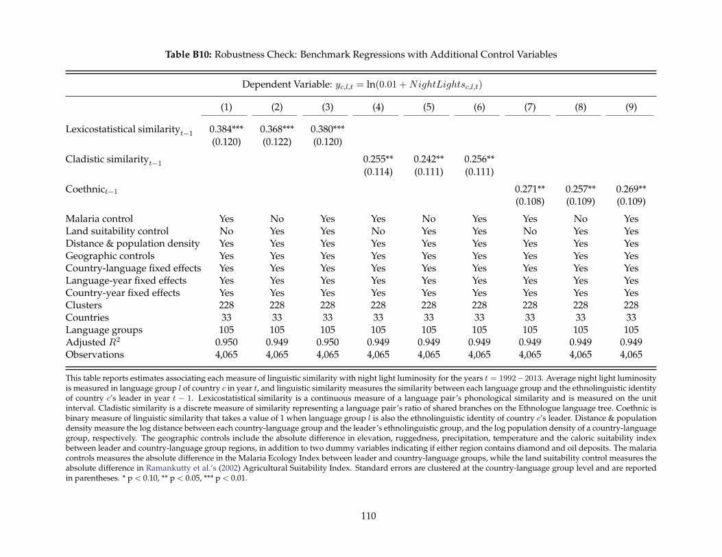
110

Table B10: Robustness Check: Benchmark Regressions with Additional Control Variables

Dependent Variable: yc,l,t = ln(0.01 +NightLightsc,l,t)

(1) (2) (3) (4) (5) (6) (7) (8) (9)

Lexicostatistical similarityt−1 0.384*** 0.368*** 0.380***(0.120) (0.122) (0.120)

Cladistic similarityt−1 0.255** 0.242** 0.256**(0.114) (0.111) (0.111)

Coethnict−1 0.271** 0.257** 0.269**(0.108) (0.109) (0.109)

Malaria control Yes No Yes Yes No Yes Yes No YesLand suitability control No Yes Yes No Yes Yes No Yes YesDistance & population density Yes Yes Yes Yes Yes Yes Yes Yes YesGeographic controls Yes Yes Yes Yes Yes Yes Yes Yes YesCountry-language fixed effects Yes Yes Yes Yes Yes Yes Yes Yes YesLanguage-year fixed effects Yes Yes Yes Yes Yes Yes Yes Yes YesCountry-year fixed effects Yes Yes Yes Yes Yes Yes Yes Yes YesClusters 228 228 228 228 228 228 228 228 228Countries 33 33 33 33 33 33 33 33 33Language groups 105 105 105 105 105 105 105 105 105Adjusted R2 0.950 0.949 0.950 0.949 0.949 0.949 0.949 0.949 0.949Observations 4,065 4,065 4,065 4,065 4,065 4,065 4,065 4,065 4,065

This table reports estimates associating each measure of linguistic similarity with night light luminosity for the years t = 1992−2013. Average night light luminosityis measured in language group l of country c in year t, and linguistic similarity measures the similarity between each language group and the ethnolinguistic identityof country c’s leader in year t − 1. Lexicostatistical similarity is a continuous measure of a language pair’s phonological similarity and is measured on the unitinterval. Cladistic similarity is a discrete measure of similarity representing a language pair’s ratio of shared branches on the Ethnologue language tree. Coethnic isbinary measure of linguistic similarity that takes a value of 1 when language group l is also the ethnolinguistic identity of country c’s leader. Distance & populationdensity measure the log distance between each country-language group and the leader’s ethnolinguistic group, and the log population density of a country-languagegroup, respectively. The geographic controls include the absolute difference in elevation, ruggedness, precipitation, temperature and the caloric suitability indexbetween leader and country-language group regions, in addition to two dummy variables indicating if either region contains diamond and oil deposits. The malariacontrols measures the absolute difference in the Malaria Ecology Index between leader and country-language groups, while the land suitability control measures theabsolute difference in Ramankutty et al.’s (2002) Agricultural Suitability Index. Standard errors are clustered at the country-language group level and are reportedin parentheses. * p < 0.10, ** p < 0.05, *** p < 0.01.

111

Table B11: Robustness Check: Excluding Leaders with Ambiguous Ethnolinguistic Identities

Dependent Variable: yc,l,t = ln(0.01 +NightLightsc,l,t)

(1) (2) (3) (4) (5)

Lexicostatistical similarityt−1 0.278**(0.116)

Cladistic similarityt−1 0.199*(0.108)

Coethnicityt−1 0.145 0.229** 0.218*(0.095) (0.104) (0.112)

Non-coethnic lexicostatistical similarityt−1 0.480**(0.237)

Non-coethnic cladistic similarityt−1 0.185(0.130)

Geographic controls Yes Yes Yes Yes YesDistance & population density Yes Yes Yes Yes YesLanguage-year fixed effects Yes Yes Yes Yes YesCountry-language fixed effects Yes Yes Yes Yes YesCountry-year fixed effects Yes Yes Yes Yes YesClusters 314 314 314 314 314Countries 34 34 34 34 34Language groups 144 144 144 144 144Adjusted R2 0.922 0.922 0.922 0.922 0.922Observations 5,745 5,745 5,745 5,745 5,745

This table reports estimates from a subsample that excludes all ambiguous leadership assignments. Because these problematic assignments introduce measurementerror, excluding them from the analysis ensures that the results are not a consequence of measurement. Average night light intensity is measured in language groupl of country c in year t, and Lexicostatistical similarity is a continuous measure of language group l’s phonological similarity to the national leader and is measuredon the unit interval. The same log transformation of the dependent variable is used for the lagged value of night lights, i.e., ln(0.01 +NightLightsc,l,t−1). All controlvariables are described in Table 1.3. Standard errors are clustered at the country-language group level and are reported in parentheses. * p < 0.10, ** p < 0.05, *** p< 0.01.

112

Table B12: Robustness Check: Benchmark Regressions on a Balanced Panel

Dependent Variable: yc,l,t = ln(0.01 + nightLightsc,l,t)

(1) (2) (3) (4) (5) (6) (7) (8) (9)

Lexicostatistical similarityt−1 0.500** 0.563** 0.542***(0.200) (0.222) (0.206)

Cladistic similarityt−1 0.491** 0.460* 0.407*(0.231) (0.238) (0.238)

Coethnict−1 0.328 0.337 0.338*(0.198) (0.209) (0.185)

Baseline controls Yes Yes Yes Yes Yes Yes Yes Yes YesLanguage-year fixed effects Yes Yes Yes Yes Yes Yes Yes Yes YesCountry-language fixed effects Yes Yes Yes Yes Yes Yes Yes Yes YesCountry-year fixed effects Yes Yes Yes Yes Yes Yes Yes Yes YesClusters 177 177 177 177 177 177 177 177 177Countries 23 23 23 23 23 23 23 23 23Language groups 84 84 84 84 84 84 84 84 84Adjusted R2 0.921 0.921 0.921 0.921 0.920 0.921 0.920 0.920 0.921Observations 3,894 3,894 3,894 3,894 3,894 3,894 3,894 3,894 3,894

This table reproduces benchmark estimates on a balanced subset of the panel dataset. Average night light luminosity is measured in language group l of countryc in year t, and linguistic similarity measures the similarity between each language group and the ethnolinguistic identity of country c’s leader in year t − 1.Lexicostatistical similarity is a continuous measure of a language pair’s phonological similarity and is measured on the unit interval. Cladistic similarity is a discretemeasure of similarity representing a language pair’s ratio of shared branches on the Ethnologue language tree. Coethnic is binary measure of linguistic similaritythat takes a value of 1 when language group l is also the ethnolinguistic identity of country c’s leader. All control variables are described in Table 1.3. Standard errorsare clustered at the country-language group level and are reported in parentheses. * p < 0.10, ** p < 0.05, *** p < 0.01.

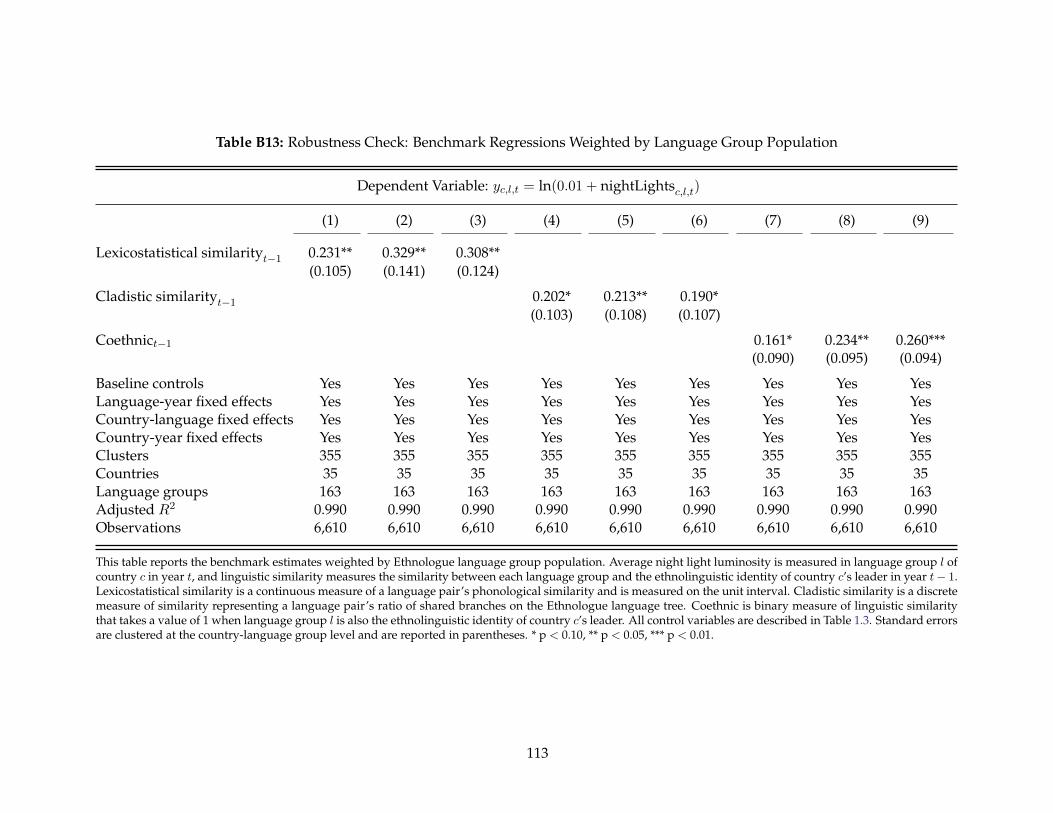
113

Table B13: Robustness Check: Benchmark Regressions Weighted by Language Group Population

Dependent Variable: yc,l,t = ln(0.01 + nightLightsc,l,t)

(1) (2) (3) (4) (5) (6) (7) (8) (9)

Lexicostatistical similarityt−1 0.231** 0.329** 0.308**(0.105) (0.141) (0.124)

Cladistic similarityt−1 0.202* 0.213** 0.190*(0.103) (0.108) (0.107)

Coethnict−1 0.161* 0.234** 0.260***(0.090) (0.095) (0.094)

Baseline controls Yes Yes Yes Yes Yes Yes Yes Yes YesLanguage-year fixed effects Yes Yes Yes Yes Yes Yes Yes Yes YesCountry-language fixed effects Yes Yes Yes Yes Yes Yes Yes Yes YesCountry-year fixed effects Yes Yes Yes Yes Yes Yes Yes Yes YesClusters 355 355 355 355 355 355 355 355 355Countries 35 35 35 35 35 35 35 35 35Language groups 163 163 163 163 163 163 163 163 163Adjusted R2 0.990 0.990 0.990 0.990 0.990 0.990 0.990 0.990 0.990Observations 6,610 6,610 6,610 6,610 6,610 6,610 6,610 6,610 6,610

This table reports the benchmark estimates weighted by Ethnologue language group population. Average night light luminosity is measured in language group l ofcountry c in year t, and linguistic similarity measures the similarity between each language group and the ethnolinguistic identity of country c’s leader in year t− 1.Lexicostatistical similarity is a continuous measure of a language pair’s phonological similarity and is measured on the unit interval. Cladistic similarity is a discretemeasure of similarity representing a language pair’s ratio of shared branches on the Ethnologue language tree. Coethnic is binary measure of linguistic similaritythat takes a value of 1 when language group l is also the ethnolinguistic identity of country c’s leader. All control variables are described in Table 1.3. Standard errorsare clustered at the country-language group level and are reported in parentheses. * p < 0.10, ** p < 0.05, *** p < 0.01.

114

Table B14: Robustness Check: Benchmark Regressions with Alternative Dependent Variables

√NightLightsc,l,t ln(NightLightsc,l,t)

(1) (2) (3) (4) (5) (6)

Lexicostatistical similarityt−1 0.038** 0.396**(0.018) (0.191)

Cladistic similarityt−1 0.029* 0.189(0.016) (0.163)

Coethnict−1 0.012 0.258*(0.014) (0.138)

Geographic controls Yes Yes Yes Yes Yes YesDistance & population density Yes Yes Yes Yes Yes YesLanguage-year fixed effects Yes Yes Yes Yes Yes YesCountry-language fixed effects Yes Yes Yes Yes Yes YesCountry-year fixed effects Yes Yes Yes Yes Yes YesClusters 355 355 355 214 214 214Countries 35 35 35 33 33 33Language groups 164 164 164 98 98 98Adjusted R2 0.952 0.952 0.952 0.935 0.935 0.935Observations 6,610 6,610 6,610 2,921 2,921 2,921

This table tests the robustness of the dependent variable using two alternative transformations: a square root of the raw night lights data (√

NightLightsc,l,t

) and

the natural log of the raw night lights data without a constant term (ln(NightLightsc,l,t)). Average night light luminosity is measured in language group l ofcountry c in year t, and linguistic similarity measures the similarity between each language group and the ethnolinguistic identity of country c’s leader in year t− 1.Lexicostatistical similarity is a continuous measure of a language pair’s phonological similarity and is measured on the unit interval. Cladistic similarity is a discretemeasure of similarity representing a language pair’s ratio of shared branches on the Ethnologue language tree. Coethnic is binary measure of linguistic similaritythat takes a value of 1 when language group l is also the ethnolinguistic identity of country c’s leader. All control variables are described in Table 1.3. Standard errorsare clustered at the country-language group level and are reported in parentheses. * p < 0.10, ** p < 0.05, *** p < 0.01.

115

Table B15: Individual-Level Regressions: Locational and Individual Similarity

Dependent Variable: DHS Wealth Index

(1) (2) (3) (4) (5)

Locational similarityt−1 0.594 0.463*** 0.479*** 0.643*** 0.365**(0.613) (0.152) (0.119) (0.153) (0.140)

Adjusted R2 0.312 0.574 0.603 0.603 0.604

Individual similarityt−1 1.260*** 0.123 0.211 0.228 0.219(0.359) (0.220) (0.219) (0.219) (0.215)

Adjusted R2 0.313 0.574 0.602 0.603 0.604

Locational similarityt−1 0.592 0.463*** 0.479*** 0.643*** 0.364**(0.613) (0.153) (0.119) (0.153) (0.140)

Individual similarityt−1 1.259*** 0.122 0.211 0.230 0.218(0.359) (0.220) (0.219) (0.219) (0.215)

Adjusted R2 0.313 0.574 0.603 0.603 0.604

Rural indicator No Yes Yes Yes YesIndividual controls No No Yes Yes YesDistance to border No No No Yes NoDistance to coast No No No No YesCountry-wave fixed effects Yes Yes Yes Yes YesLocational language-wave fixed effects Yes Yes Yes Yes YesIndividual language-wave fixed effects Yes Yes Yes Yes YesClusters 88 88 88 88 88Countries 13 13 13 13 13Language groups 20 20 20 20 20Observations 56,455 56,455 56,455 56,455 56,455

This table provides estimates for two channels: the effect of individual and locational similarity on the DHS wealth index. The unit of observation is an individual.The rural indicator is equal to 1 if a respondent lives in a rural location. The individual set of control variables include age, age squared, a gender indicator variable,an indicator for respondents living in the capital city, 5 education fixed effects and 7 religion fixed effects. Distance to the coast and border are in kilometers. Standarderrors are in parentheses and adjusted for clustering at the country-language-wave level. * p < 0.10, ** p < 0.05, *** p < 0.01.

Table B16: Individual-Level Regressions: Locational and Individual Similarity

Dependent Variable: DHS Wealth Index

(1) (2) (3) (4) (5)

Locational coethnicityt−1 0.838* 0.485*** 0.437*** 0.324** 0.601***(0.430) (0.139) (0.116) (0.134) (0.160)

Non-coethnic locational similarityt−1 -0.692 0.348* 0.697*** 0.573*** 0.854***(0.556) (0.205) (0.148) (0.167) (0.173)

Rural indicator No Yes Yes Yes YesIndividual controls No No Yes Yes YesDistance to coast No No No Yes NoDistance to border No No No No YesCountry-wave fixed effects Yes Yes Yes Yes YesLocational language-wave fixed effects Yes Yes Yes Yes YesIndividual language-wave fixed effects Yes Yes Yes Yes YesClusters 88 88 88 88 88Countries 13 13 13 13 13Language groups 20 20 20 20 20Adjusted R2 0.314 0.574 0.603 0.604 0.603Observations 56,455 56,455 56,455 56,455 56,455

This table reports estimates that test for favoritism outside of coethnic language partitions. The unit of observation isan individual. The rural indicator is equal to 1 if a respondent lives in a rural location. The individual set of controlvariables include age, age squared, a gender indicator variable and an indicator for respondents living in the capitalcity. Distance to the coast and border are in kilometers. Standard errors are in parentheses and adjusted for clusteringat the country-language-wave level. * p < 0.10, ** p < 0.05, *** p < 0.01.

116

117

Table B17: Individual-Level Regressions: Baseline Covariates

Dependent Variable: DHS Wealth Index

(1) (2) (3) (4) (5) (6) (7) (8) (9)

Locational similarityt−1 0.585 0.594 0.463*** 0.636 0.490 1.024* 0.518 0.608 0.479***(0.604) (0.613) (0.152) (0.398) (0.637) (0.592) (0.587) (0.399) (0.119)

Age -0.021*** -0.008(0.005) (0.006)

Age squared 0.000*** 0.000(0.000) (0.000)

Female indicator -0.010 0.112***(0.013) (0.013)

Rural indicator -1.846*** -1.606***(0.072) (0.079)

Capital city indicator 1.502*** 0.238***(0.053) (0.053)

Distance to the coast -0.001(0.000)

Distance to the border -0.001*(0.001)

Religion FE No No No No No No Yes No YesEducation FE No No No No No No No Yes YesCountry-wave FE Yes Yes Yes Yes Yes Yes Yes Yes YesLocation-language-wave FE Yes Yes Yes Yes Yes Yes Yes Yes YesIndividual-language-wave FE Yes Yes Yes Yes Yes Yes Yes Yes YesClusters 88 88 88 88 88 88 88 88 88Countries 13 13 13 13 13 13 13 13 13Language groups 20 20 20 20 20 20 20 20 20Adjusted R2 0.316 0.312 0.574 0.342 0.314 0.317 0.317 0.416 0.603Observations 56,455 56,455 56,455 56,455 56,455 56,455 56,455 56,455 56,455

This table establishes the impact of each baseline covariate used in Section 1.5. The unit of observation is an individual. Standard errors are in parentheses andadjusted for clustering at the country-language-wave level. * p < 0.10, ** p < 0.05, *** p < 0.01.

118

Table B18: Ethnic Favoritism and Coalition Power Sharing

Share of cabinet positions Share of top cabinet positions Share of low cabinet positions

(1) (2) (3) (4) (5) (6) (7) (8) (9)

Coethnicityt 0.093*** 0.100*** 0.179*** 0.185*** 0.050*** 0.057***(0.012) (0.013) (0.019) (0.020) (0.013) (0.014)

Lexicostatistical similarityt 0.095*** 0.172*** 0.057***(0.013) (0.021) (0.013)

Non-coethnic similarityt 0.047** 0.047* 0.048**(0.018) (0.022) (0.019)

Group size controls Yes Yes Yes Yes Yes Yes Yes Yes YesYear fixed effects Yes Yes Yes Yes Yes Yes Yes Yes YesCountry fixed effects Yes Yes Yes Yes Yes Yes Yes Yes YesCountries 15 15 15 15 15 15 15 15 15Ethnic groups 187 187 187 187 187 187 187 187 187Adjusted R2 0.665 0.664 0.668 0.539 0.521 0.541 0.544 0.549 0.548Observations 2,539 2,539 2,539 2,539 2,539 2,539 2,539 2,539 2,539

This table establishes that linguistic similarity predicts an ethnic group’s share in the governing coalition of a country. The unit of observation is an ethnic group.The dependent variable in columns (1)-(3) is the share of cabinet positions of an ethnic group in the governing coalition, whereas in columns (4)-(6) and (7)-(9) thedependent variable measures the cabinet share of top positions and low positions. The group size controls include a time-invariant measure of an ethnic group’sshare of the national population and its polynomial. Standard errors are in parentheses and adjusted for clustering at the country level. * p < 0.10, ** p < 0.05, *** p< 0.01.

Appendix C

Chapter 2 Appendix

C.1 Variable Definitions, Summary Statistics and Data Sources

C.1.1 Data and Sources

Book translations: The total number of translated books in a country for a given year. The dataused here is from the time period 1979-2005, and comes from the Index Translationum, an onlinebibliographic archive hosted by UNESCO.Source: http://www.unesco.org/culture/xtrans/

Lexicostatistical linguistic distance: This computerized lexicostatistical linguistic distance mea-sures the phonetic similarity between two languages. See Appendix A for a formal discussion ofhow this data is estimated. I source the language lists used to estimate linguistic distance fromthe Automated Similarity Judgement Program (ASJP) to estimate language distances (Wichmannet al., 2013).Source: http://asjp.clld.org/

Cladistic linguistic distance: I construct the cladistic measure according to the details above inAppendix A. I use the Ethnologue language tree, sourced from World Language Mapping System.Source: http://www.worldgeodatasets.com/language/

Genetic distance: An index of heterozygosity, the probability that two randomly selected alle-les at a given locus will be different in two populations. Genetic distance is used as a proxy forthe degree of common ancestry between two populations. This data was originally constructedby Cavalli-Sforza et al. (1994), and was sourced from Spolaore and Wacziarg (2009).Source: http://www.anderson.ucla.edu/faculty_pages/romain.wacziarg/downloads/genetic_distance.zip

Geographic distance: Geodesic distance between the most populated cities in a country pair,

119

measured per 100 kilometres. This data comes from a data set compiled by researchers at Centred’Etudes Prospectives et d’Informations Internationales (CEPII).Source: http://www.cepii.fr/cepii/en/welcome.asp

Real GDP: Purchasing power parity converted expenditure-side real GDP at chained purchas-ing power parity rates (in mil. 2005 US dollars) from the Penn World Tables version 8.0.Source: http://www.rug.nl/research/ggdc/data/pwt/pwt-8.0

Population: Total population in thousands from the Penn World Tables version 8.0.Source: http://www.rug.nl/research/ggdc/data/pwt/pwt-8.0

Political rights: Freedom House Political Rights Index with an original range of 1 through 7,normalized as a 0-1 variable.Source: http://www.freedomhouse.org/report-types/freedom-world#.U1f1lV5bTwI

Colonial history indicator: Colonial history data was sources from the CEPII. I use an dummyvariable indicating if a country pair has ever been in a colonial relationship.Source: http://www.cepii.fr/cepii/en/welcome.asp

Other geography data: All other geography data was also sourced from the CEPII. Measure oflatitude and longitude differences were constructed using individual country measures and tak-ing the absolute value of the difference between each for a country pair. A dummy variable wasalso collected indicating contiguity of a country pair.Source: http://www.cepii.fr/cepii/en/welcome.asp

Shared common language indicators: Indicator variables specifying (i) if country pairs share acommon language and (ii) if at least 9 percent of the population in both countries speak the samelanguage were also sourced from the CEPII.Source: http://www.cepii.fr/cepii/en/welcome.asp

Bilateral trade shares: Measures the logged average value of bilateral trade for a country pairin constant US dollars. To construct this variable I average imports from i to j and imports fromj to i in current US dollars, deflate this value by the American CPI for all urban consumers (1982-1984 = 100; taken from http://www.bls.gov/data/#prices), and take the log of this averagedvalue. The trade data was sourced from Barbieri et al. (2009).Source: http://www.correlatesofwar.org/COW2%20Data/Trade/Trade.html

Human capital: The cross-country 5-year panel of education attainment for the total populationaged 15 and over is from Barro and Lee (2013). Measures used include (i) the average years of

120

schooling attained, (ii) the percentage of complete primary schooling attained, (iii) the percentageof complete secondary schooling attained, and (iv) the percentage of complete tertiary schoolingattained.Source: http://www.barrolee.com

Human capital index: The index of human capital per person is based on years of schooling(Barro and Lee, 2013) and returns to education (Psacharopoulos, 1994), and is sourced from thePenn World Tables version 8.0.Source: http://www.rug.nl/research/ggdc/data/pwt/pwt-8.0

C.1.2 Summary Statistics

Table C1: Benchmark Sample Summary Statistics

Mean Std. Dev. Min. Max. N

Log book translations 1.26 1.61 0.00 8.98 39,275Log economic book translations 0.42 1.01 0.00 7.70 39,275Log cultural book translations 1.59 1.36 0.00 8.85 39,275Linguistic distance 0.86 0.11 0.27 1.00 39,275Linguistic distance (cladistic) 0.96 0.08 0.26 1.00 39,275Genetic distance 0.04 0.04 0.00 0.29 39,275Geographic distance (10,000 km) 0.39 0.38 0.01 1.96 39,275Log real GDP translating country 12.75 1.68 6.17 16.37 39,275Log real GDP original country 12.97 1.41 5.56 16.26 39,275Log real GDP original country (weighted) 13.22 1.56 7.12 16.22 37,976Log population translating country 3.19 1.62 -1.86 7.16 39,275Log population original country 3.47 1.51 -1.88 7.16 39,275Log population original country (weighted) 4.13 1.84 -1.86 8.08 37,976Political rights translating country 0.13 0.24 0.00 0.86 39,275Political rights original country 0.17 0.28 0.00 0.86 39,275Political rights original country (weighted) 0.17 0.26 0.00 0.86 37,976Log bilateral trade 5.88 2.37 -5.91 11.66 39,275Log bilateral trade (weighted) 5.97 2.31 -5.87 11.66 37,549= 1 if ever in colonial relationship 0.10 0.30 0.00 1.00 39,275= 1 if ever in colonial relationship (weighted) 0.08 0.23 0.00 1.00 35,737= 1 if contiguous 0.13 0.33 0.00 1.00 39,275= 1 if contiguous (weighted) 0.11 0.30 0.00 1.00 35,737Absolute difference in latitude 14.94 17.76 0.00 104.2 39,275Absolute difference in latitude (weighted) 16.14 18.39 0.00 104.2 37,976Absolute difference in longitude 41.23 44.06 0.07 238.92 39,275Absolute difference in longitude (weighted) 46.25 46.44 0.02 248.73 37,976Human capital index translating country 2.60 0.45 1.08 3.54 38,908Average years of schooling translating country 8.40 2.23 0.62 12.75 8,903% of primary schooling translating country 22.58 11.76 0.69 55.63 8,903% of secondary schooling translating country 21.39 13.92 0.48 69.75 8,903% of tertiary schooling translating country 8.10 4.73 0.14 26.36 8,903

121

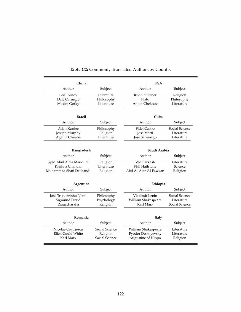
Table C2: Commonly Translated Authors by Country

China USAAuthor Subject Author Subject

Leo Tolstoy Literature Rudolf Steiner ReligionDale Carnegie Philosophy Plato PhilosophyMaxim Gorky Literature Anton Chekhov Literature

Brazil CubaAuthor Subject Author Subject

Allan Kardec Philosophy Fidel Castro Social ScienceJoseph Murphy Religion Jose Marti LiteratureAgatha Christie Literature Jose Saramago Literature

Bangladesh Saudi ArabiaAuthor Subject Author Subject

Syed Abul A’ala Maududi Religion Ved Parkash LiteratureKrishna Chandar Literature Phil Hailstone Science

Muhammad Shafi Deobandi Religion Abd Al-Aziz Al-Fawzan Religion

Argentina EthiopiaAuthor Subject Author Subject

Jose Trigueirinho Netto Philosophy Vladimir Lenin Social ScienceSigmund Freud Psychology William Shakespeare LiteratureRamacharaka Religion Karl Marx Social Science

Romania ItalyAuthor Subject Author Subject

Nicolae Ceausescu Social Science William Shakespeare LiteratureEllen Gould White Religion Fyodor Dostoyevsky Literature

Karl Marx Social Science Augustine of Hippo Religion

122

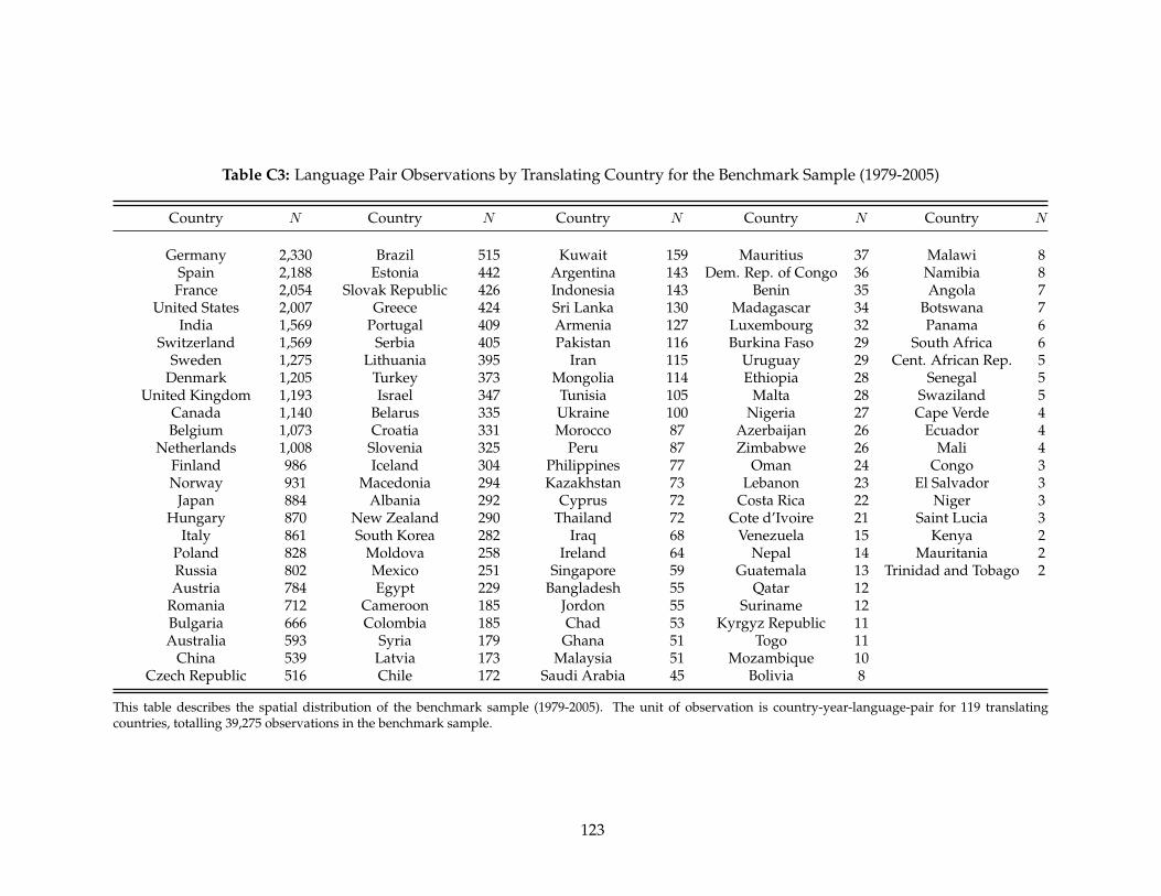
123

Table C3: Language Pair Observations by Translating Country for the Benchmark Sample (1979-2005)

Country N Country N Country N Country N Country N

Germany 2,330 Brazil 515 Kuwait 159 Mauritius 37 Malawi 8Spain 2,188 Estonia 442 Argentina 143 Dem. Rep. of Congo 36 Namibia 8France 2,054 Slovak Republic 426 Indonesia 143 Benin 35 Angola 7

United States 2,007 Greece 424 Sri Lanka 130 Madagascar 34 Botswana 7India 1,569 Portugal 409 Armenia 127 Luxembourg 32 Panama 6

Switzerland 1,569 Serbia 405 Pakistan 116 Burkina Faso 29 South Africa 6Sweden 1,275 Lithuania 395 Iran 115 Uruguay 29 Cent. African Rep. 5

Denmark 1,205 Turkey 373 Mongolia 114 Ethiopia 28 Senegal 5United Kingdom 1,193 Israel 347 Tunisia 105 Malta 28 Swaziland 5

Canada 1,140 Belarus 335 Ukraine 100 Nigeria 27 Cape Verde 4Belgium 1,073 Croatia 331 Morocco 87 Azerbaijan 26 Ecuador 4

Netherlands 1,008 Slovenia 325 Peru 87 Zimbabwe 26 Mali 4Finland 986 Iceland 304 Philippines 77 Oman 24 Congo 3Norway 931 Macedonia 294 Kazakhstan 73 Lebanon 23 El Salvador 3

Japan 884 Albania 292 Cyprus 72 Costa Rica 22 Niger 3Hungary 870 New Zealand 290 Thailand 72 Cote d’Ivoire 21 Saint Lucia 3

Italy 861 South Korea 282 Iraq 68 Venezuela 15 Kenya 2Poland 828 Moldova 258 Ireland 64 Nepal 14 Mauritania 2Russia 802 Mexico 251 Singapore 59 Guatemala 13 Trinidad and Tobago 2Austria 784 Egypt 229 Bangladesh 55 Qatar 12

Romania 712 Cameroon 185 Jordon 55 Suriname 12Bulgaria 666 Colombia 185 Chad 53 Kyrgyz Republic 11Australia 593 Syria 179 Ghana 51 Togo 11

China 539 Latvia 173 Malaysia 51 Mozambique 10Czech Republic 516 Chile 172 Saudi Arabia 45 Bolivia 8

This table describes the spatial distribution of the benchmark sample (1979-2005). The unit of observation is country-year-language-pair for 119 translatingcountries, totalling 39,275 observations in the benchmark sample.

124

Table C4: Observations by Translating Language for the Benchmark Sample (1979-2005)

Translating Translating Translating Translating Translating Translating TranslatingLanguage N Language N Language N Language N Language N Language N Language N

English 5,538 Latvian 213 Tagalog 33 Waama 11 Mari 7 Hdi 5 Biali 3German 3,099 Urdu 208 Irish 30 Aragonese 10 Morisyen 7 Jula 5 Fijian 3French 3,054 Latin 175 Northern Saami 29 Bissa 10 Pitjantjatjara 7 Kabiye 5 Igbo 3Spanish 2,297 Mongolian (Halh) 175 Maltese 28 Kera 10 Somrai 7 Karachay-Balkar 5 Kabardian 3Dutch 1,370 Malayalam 169 Maori 28 Koonzime 10 Tuva 7 Karelian 5 Moksha 3Italian 1,242 Persian (Iranian) 168 Western Frisian 26 Lamnso 10 Arabic (Chadian) 6 Kekchi 5 St. Lucian Creole 3

Russian 1,057 Galacian 167 Kalaallisut 26 Yoruba 10 Blaan, Sarangani 6 Kenga 5 Sranan 3Portuguese 1,014 Idonesian 163 Occitan 25 Hausa 9 Bosnian 6 Kituba 5 Suri 3

Swedish 1,005 Tamil 151 Tatar 25 Kom 9 Chuvash 6 Koorete 5 Udmurt 3Arabic 968 Armenian 150 Georgian 24 Kuo 9 Corsican 6 Koromfe 5 Veps 3

Japanese 934 Ukrainian 142 Kasem 24 Ladino 9 Fon 6 Manobo, Cotabato 5 Aramaic 2Hungarian 926 Belarusan 126 Uzbek 21 Northern Ndebele 9 Haitian 6 Naro 5 Buriat 2Norwegian 891 Sinhala 117 Samoan 20 Niuean 9 Kabyle 6 Ngangam 5 Chukchi 2

Polish 870 Vietnamese 111 Sanskrit 20 Ossetian 9 Kalagan 6 Carpathian Romani 5 Coptic 2Romanian 794 Esperanto 109 Central Tibetan 20 Plautdietsch 9 Limbum 6 Syriac 5 Cornish 2

Danish 793 Kazakh 109 Kako 19 Chichewa 8 Luba-Lulua 6 Turkmen 5 Dargwa 2Finnish 753 Assamese 106 Tongan 18 Chipewyan 8 Mampruli 6 Vengo 5 Even 2

Bulgarian 683 Oriya 93 Amharic 16 Daba 8 Mapun 6 Warlpiri 5 Frisian 2Czech 602 Breton 85 Luxembourgeois 16 Dangaleat 8 Nafaanra 6 Aghem 4 Guadeloupean Creole 2

Catalan 488 Marathi 84 Tigrigna 16 Gaelic 8 Nepali 6 Aja 4 Guarani 2Greek 488 Kannada 77 Tokelauan 16 Hawaiian 8 Noone 6 Bamanankan 4 Jingpho 2

Mandarin 455 Gujarati 76 Cree 15 Khmer 8 Ojibwa 6 Old Church Slavic 4 Kara-Kalpak 2Turkish 437 Faroese 75 Kyrgyz 15 Konkomba 8 Roviana 6 Djeebbana 4 Maithili 2

Albanian 369 Thai 75 Mofu-Gudur 15 Lao 8 Sisaala, Tumulung 6 Hmong 4 Navajo 2Estonian 359 Telugu 73 Rarotongan 15 Lingala 8 Swati 6 Komi-Zyrian 4 Ndonga 2Hebrew 356 Uyghur 69 Scots 15 Mundani 8 Tboli 6 Kongo 4 Nogai 2

Lithuanian 356 Inuktitut 65 Swahili 15 Nateni 8 Yakut 6 Kriol 4 Reunion Creole 2Croatian 352 Welsh 60 Tajiki 15 Newari 8 Zulgo-Gemzek 6 Mukulu 4 Southern Saami 2Korean 330 Malay 56 Swabian 14 Parkwa 8 Akoose 5 Balkan Romani 4 Southern Sotho 2Slovene 321 Serbo-Croatian 49 Kankanaey 13 Yamba 8 Anyin 5 Macedo Romanian 4 Tahitian 2Slovak 314 German (Swiss) 45 Farefare 12 Afrikaans 7 Bafut 5 Inari Saami 4 Tai Hongjin 2Serbian 309 Kurdish 44 Tikar 12 Bashkir 7 Chumburung 5 Lule Saami 4 Tamazight 2

Icelandic 296 Panjabi 43 Gude 11 Fuliiru 7 Dakota 5 Sokoro 4 Tok Pisin 2Macedonian 240 Asturian 42 Karang 11 Gbaya-Bossangoa 7 Dan 5 Tswana 4

Bengali 234 Azerbaijani 37 Ngbaka 11 Kalinga 7 Gagauz 5 Wolof 4Hindi 230 Yiddish 37 Shona 11 Kenyang 7 Gikyode 5 Adyghe 3

Basque 213 Malagasy 33 Somali 11 Mambila 7 Hanga 5 Avar 3

This table reports the benchmark sample by translating language (1979-2005). The unit of observation is country-year-language-pair for 119 translating countries, totalling 39,275observations in the benchmark sample.

125

Table C5: Observations by Original Language for the Benchmark Sample (1979-2005)

Original Original Original Original Original OriginalLanguage N Language N Language N Language N Language N Language N

English 4,958 Korean 282 Mongolian (Halh) 59 Ladino 17 Friulian 6 Shona 4French 3,066 Albanian 264 Malay 54 Lao 17 Guarani 6 Abkhazian 3

German 2,770 Hindi 254 Telugu 54 Uzbek 17 Lingala 6 Asturian 3Greek 2,349 Croatian 252 Galacian 52 Zulu 17 Yucatan Maya 6 Chechen 3

Spanish 1,544 Vietnamese 204 Quiche 51 Bamanankan 16 Huautla Mazatec 6 Chukchi 3Dutch 1,255 Slovene 195 Marathi 50 Geez 16 Southern Sotho 6 Erzya 3Arabic 1,241 Pali 186 Belarusan 49 Maltese 16 Udmurt 6 Northern Frisian 3

Swedish 1,214 Slovak 176 Inuktitut 45 Avestan 14 Cree 5 Ganda 3Russian 1,115 Estonian 163 Malayalam 43 Dakota 14 Hopi 5 Hmong 3Danish 1,066 Indonesian 160 Amharic 42 Oriya 14 Igbo 5 Kabardian-Cherkess 3

Portuguese 1,063 Syriac 155 Swahili 41 Tagalog 14 Kalaallisut 5 Kongo 3Japanese 1,053 Panjabi 139 Nepali 40 Javanese 13 Komi-Zyrian 5 Maori 3Hebrew 1,009 Irish 138 Faroese 39 Turkmen 13 Manchu 5 St. Lucian Creole 3Polish 991 Arabic (Egyptian) 136 Breton 35 Western Frisian 11 Moksha 5 Zarma 3

Mandarin 933 Ukrainian 130 Gaelic 34 Gikuyu 11 Morisyen 5 Arabic (Moroccan) 2Norwegian 902 Aramaic 127 Gujarati 33 Tajiki 11 Plautdietsch 5 Avar 2Hungarian 776 Afrikaans 126 Azerbaijani 29 Wolof 11 Lule Saami 5 Chagatai 2

Persian (Iranian) 655 Lithuanian 115 Old Church Slavic 24 Carib 10 Sranan 5 Fang 2Finnish 640 Coptic 110 Northern Saami 24 Uyghur 9 Cornish 4 Kalmyk 2

Romanian 599 Thai 109 Kazakh 23 Cheyenne 8 Corsican 4 Khanty 2Turkish 571 Latvian 104 Tamazight 22 Evenki 8 Duala 4 Koryak 2Sanskrit 519 Armenian 92 Kyrgyz 21 Hausa 8 Komi-Permyak 4 Lak 2Bengali 493 Tamil 88 Sorbian 21 Sinte Romani 8 Luxembourgeois 4 Mansi 2Czech 490 Kurdish 85 German (Swiss) 20 Tatar 8 Mari 4 Mapudungun 2

Bulgarian 399 Occitan 83 Scots 20 Assamese 7 Moore 4 North Ndebele 2Tibetan 388 Welsh 82 Tamasheq 19 Chuvash 7 Navajo 4 Ossetian 2Yiddish 378 Basque 78 Kannada 18 Kashmiri 7 Nenets 4 Rwanda 2

Icelandic 368 Macedonian 74 Malagasy 18 Vlax Romani 7 Ojibwa 4 Seraiki 2Urdu 334 Esperanto 68 Sinhala 18 Akan 6 Carpathian Romani 4 Tuva 2

Catalan 327 Georgian 59 Yoruba 18 Ewe 6 Macedo Romanian 4

This table reports the benchmark sample by translating language (1979-2005). The unit of observation is country-year-language-pair for 119 translatingcountries, totalling 39,275 observations in the benchmark sample.

C.2 Supplementary Materials

C.2.1 Alternative Measure of Linguistic Distance

In this section I reproduce the table of benchmark estimates using a cladistic measure of linguisticdistance. I construct this measure of cladistic distance as outlined in Appendix A, which is mea-sured as one minus the ratio of shared branches on the Ethnologue language tree. I assume theweighting scheme of Fearon (2003), where the ratio of shared tree branches is square rooted to dis-count more recent linguistic cleavages relative to deep cleavages. Because the number of branchesvaries among language familes and subfamilies, the maximum number of branches between anytwo languages is not constant. To overcome this obstacle I assume that all current languages are ofequal distance from the proto-language at the root of the Ethnologue language tree. This assump-tion is equivalent to the assumption Desmet et al. (2012) use when constructing cladistic distances(see Figure A1).

Table C6 reports the benchmark estimates using this alternative measure. The two oppos-ing forces of relatedness are borne out of this alternative data and estimated to be significantlydifferent than zero. The effect of the cladistic measure of linguistic distance is smaller than thecomparable lexicostatistical measure used in the benchmark estimate. This finding is consistentwith the evidence in Dickens (2016a), where the added variation of the lexicostatistical measureyields added percision in estimation. Nonetheless, the basic finding of this paper is robust toalternative measures of linguistic distance.

C.2.2 Further Test of the Home Country Assumption

In this section I extend the analysis of section 2.4.1 and systematically dropping every originallanguage of a translation with at least 100 observations in the benchmark sample. The idea hereis to ensure that the benchmark results cannot be explained away by any one original languagedue to the ambiguity of the home country assignment rule. Table C7 reports these estimates andshows no evidence that any one language can explain away the benchmark result.

C.2.3 Dominant Book Subject?

A potential concern is that the interplay between linguistic and genetic distance observed in thebenchmark estimate is the result of a strong statistical association with one field of study in theaggregate translation data. Regression analysis using total translations as the dependent variablemay hide the fact that certain idea types are strongly influenced by distance while others are not.If so, then excluding book translations from the dependent variable that belong to some outliersubject would yield estimates of linguistic and genetic distance substantially different from thebaseline.

To test this I re-estimate the preferred specification and drop all translations belonging to eachsubject area one at a time. The results are presented in Table C8. Coefficient estimates should

126

be interpreted relative to the benchmark estimate; i.e., small deviations from the benchmark esti-mate imply the excluded subject of translation is not influential over and above the average effect,whereas large deviations indicate subject areas that are particularly influential in the benchmarkresult.

The first observation about Table C8 is that no one subject area is driving the core result of thisstudy – the standardized coefficient for linguistic distance range from −7.8 to −8.5 percent, andfrom 5.6 to 7.2 percent for genetic distance. It is reassuring that the benchmark estimate of −8.0

percent for linguistic distance and 6.3 percent for genetic distance tend towards the lower bound ofthis range of coefficients. Second, both genetic and linguistic distance are precisely estimated in allregressions at standard levels of confidence. These two observations suggest the baseline resultsof section 2.3.3 cannot be explained by a single outlier subject that is particularly responsive toeither linguistic or genetic distance.

127

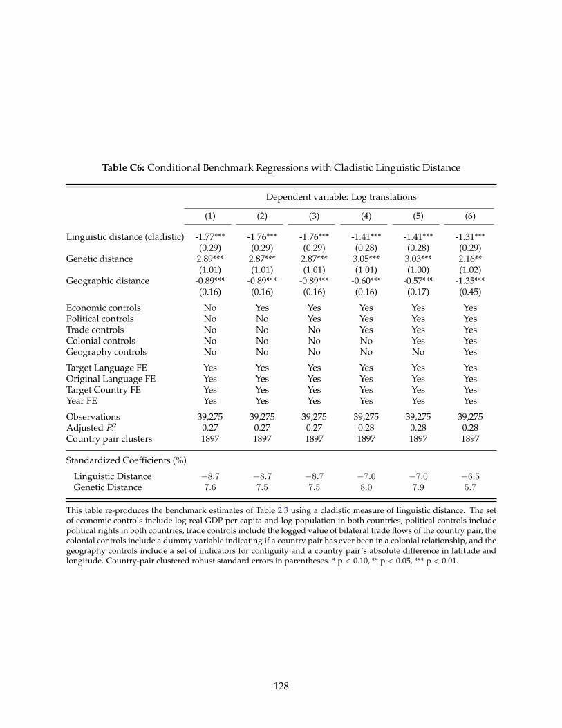
Table C6: Conditional Benchmark Regressions with Cladistic Linguistic Distance

Dependent variable: Log translations

(1) (2) (3) (4) (5) (6)

Linguistic distance (cladistic) -1.77*** -1.76*** -1.76*** -1.41*** -1.41*** -1.31***(0.29) (0.29) (0.29) (0.28) (0.28) (0.29)

Genetic distance 2.89*** 2.87*** 2.87*** 3.05*** 3.03*** 2.16**(1.01) (1.01) (1.01) (1.01) (1.00) (1.02)

Geographic distance -0.89*** -0.89*** -0.89*** -0.60*** -0.57*** -1.35***(0.16) (0.16) (0.16) (0.16) (0.17) (0.45)

Economic controls No Yes Yes Yes Yes YesPolitical controls No No Yes Yes Yes YesTrade controls No No No Yes Yes YesColonial controls No No No No Yes YesGeography controls No No No No No Yes

Target Language FE Yes Yes Yes Yes Yes YesOriginal Language FE Yes Yes Yes Yes Yes YesTarget Country FE Yes Yes Yes Yes Yes YesYear FE Yes Yes Yes Yes Yes Yes

Observations 39,275 39,275 39,275 39,275 39,275 39,275Adjusted R2 0.27 0.27 0.27 0.28 0.28 0.28Country pair clusters 1897 1897 1897 1897 1897 1897

Standardized Coefficients (%)

Linguistic Distance −8.7 −8.7 −8.7 −7.0 −7.0 −6.5Genetic Distance 7.6 7.5 7.5 8.0 7.9 5.7

This table re-produces the benchmark estimates of Table 2.3 using a cladistic measure of linguistic distance. The setof economic controls include log real GDP per capita and log population in both countries, political controls includepolitical rights in both countries, trade controls include the logged value of bilateral trade flows of the country pair, thecolonial controls include a dummy variable indicating if a country pair has ever been in a colonial relationship, and thegeography controls include a set of indicators for contiguity and a country pair’s absolute difference in latitude andlongitude. Country-pair clustered robust standard errors in parentheses. * p < 0.10, ** p < 0.05, *** p < 0.01.

128

Table C7: Sensitivity Analysis: Further Test of Home Country Assignment

Language Linguistic GeneticDropped Distance Distance N

German -1.29*** 2.15** 36,498(0.28) (1.04)

Greek -1.12*** 2.77** 36,920(0.28) (1.10)

Dutch -1.03*** 2.42** 38,020(0.28) (1.06)

Swedish -1.06*** 2.36** 38,060(0.29) (1.06)

Russian -1.11*** 2.27** 38,158(0.29) (1.06)

Danish -1.08*** 2.44** 38,205(0.29) (1.06)

Portuguese -1.12*** 2.54** 38,211(0.29) (1.08)

Japanese -1.10*** 2.08** 38,221(0.28) (1.02)

Hebrew -1.14*** 2.39** 38,261(0.28) (1.06)

Polish -1.15*** 2.60** 38,284(0.29) (1.06)

Norwegian -1.05*** 2.44** 38,373(0.29) (1.06)

Hungarian -1.14*** 2.40** 38,499(0.28) (1.16)

Persian (Iranian) -1.11*** 2.41** 38,620(0.28) (1.04)

Finnish -1.11*** 3.03*** 38,634(0.28) (1.07)

Romanian -1.17*** 2.46** 38,675(0.29) (1.05)

Turkish -1.12*** 2.29** 38,704(0.28) (1.05)

Sanskrit -1.13*** 2.40** 38,756(0.28) (1.04)

Bengali -1.10*** 2.27** 38,782(0.29) (1.05)

Czech -1.11*** 2.39** 38,785(0.29) (1.05)

Bulgarian -1.13*** 2.39** 38,876(0.29) (1.05)

Tibetan -1.13*** 2.27** 38,887(0.28) (1.07)

Yiddish -1.12*** 2.41** 38,897(0.29) (1.05)

Icelandic -1.11*** 2.44** 38,907(0.29) (1.05)

Language Linguistic GeneticDropped Distance Distance N

Urdu -1.11*** 2.37** 38,941(0.29) (1.05)

Catalan -1.13*** 2.43** 38,948(0.29) (1.06)

Korean -1.12*** 2.63** 38,993(0.28) (1.09)

Albanian -1.12*** 2.37** 39,011(0.29) (1.05)

Croatian -1.13*** 2.38** 39,023(0.29) (1.05)

Vietnamese -1.13*** 2.44** 39,071(0.29) (1.05)

Slovene -1.15*** 2.41** 39,080(0.29) (1.05)

Pali -1.13*** 2.39** 39,089(0.28) (1.05)

Slovak -1.12*** 2.40** 39,099(0.29) (1.05)

Estonian -1.12*** 2.48** 39,112(0.28) (1.06)

Indonesian -1.13*** 2.37** 39,115(0.28) (1.05)

Syriac -1.12*** 2.38** 39,120(0.28) (1.05)

Panjabi -1.12*** 2.38** 39,136(0.28) (1.05)

Irish -1.13*** 2.41** 39,137(0.28) (1.05)

Arabic (Egyptian) -1.13*** 2.40** 39,139(0.28) (1.05)

Ukrainian -1.15*** 2.45** 39,145(0.28) (1.05)

Aramaic -1.12*** 2.41** 39,148(0.28) (1.05)

Afrikaans -1.11*** 2.46** 39,149(0.28) (1.05)

Lithuanian -1.12*** 2.41** 39,160(0.28) (1.06)

Coptic -1.13*** 2.40** 39,165(0.28) (1.05)

Thai -1.13*** 2.35** 39,166(0.28) (1.05)

Latvian -1.13*** 2.41** 39,171(0.28) (1.05)

This table tests the assignment of the home country of a language by systematically dropping each original language of a booktranslation with a 100 or more observations. The robustness of the results to this test suggests the benchmark result is not driven bythe assumption of the original country of a translation. All regressions include the benchmark set of control variables used in column(6) of Table 2.3. All regressions also include individual country, year and target language fixed effects. Country-pair clustered robuststandard errors reported in parentheses. * p < 0.10, ** p < 0.05, *** p < 0.01.

129

130

Table C8: Robustness Check for Dominant Subject of Translation

Dependent variable: Log translations

(1) (2) (3) (4) (5) (6) (7) (8)

Social Applied NaturalExcluding: Arts History Literature Philosophy Religion Science Science Science

Linguistic distance -1.09*** -1.13*** -1.12*** -1.11*** -1.08*** -1.18*** -1.13*** -1.11***(0.28) (0.28) (0.34) (0.28) (0.28) (0.28) (0.27) (0.28)

Genetic distance 2.33** 2.48** 2.47* 2.13** 2.39** 2.78*** 2.43** 2.47**(1.07) (1.03) (1.29) (1.04) (1.09) (1.03) (1.02) (1.06)

Geographic distance -1.34*** -1.32*** -1.54*** -1.42*** -1.36*** -1.44*** -1.33*** -1.33***(0.45) (0.46) (0.53) (0.45) (0.46) (0.45) (0.45) (0.45)

Benchmark controls Yes Yes Yes Yes Yes Yes Yes Yes

Target Language FE Yes Yes Yes Yes Yes Yes Yes YesOriginal Language FE Yes Yes Yes Yes Yes Yes Yes YesTarget Country FE Yes Yes Yes Yes Yes Yes Yes YesYear FE Yes Yes Yes Yes Yes Yes Yes Yes

Observations 38,405 37,661 26,488 38,610 35,471 37,717 38,374 38,987Adjusted R2 0.29 0.30 0.31 0.29 0.30 0.30 0.29 0.28Country pair clusters 1887 1873 1505 1885 1805 1852 1884 1893

Standardized Coefficients (%)

Linguistic Distance −7.8 −8.1 −8.2 −8.0 −7.8 −8.5 −8.2 −8.0Genetic Distance 6.1 6.5 6.6 5.6 6.2 7.2 6.4 6.5

This table reports estimates on various subsamples that exclude each subject classification in the data one by one. All regressions include thebenchmark set of control variables used in column (6) of Table 2.3. Country-pair clustered robust standard errors reported in parentheses. * p <0.10, ** p < 0.05, *** p < 0.01.

Table C9: Ethnologue Home Country vs. Synthetic Language Country Assignment

EthnologueHome Country

SyntheticLanguageCountry

Mean Mean Difference Observations

Genetic distance 0.041 0.045 -0.004*** 35,732(0.000) (0.000) (0.000)

Geographic distance 0.390 0.455 -0.066*** 35,737(0.002) (0.002) (0.001)

Log real GDP 12.989 13.222 -0.233*** 37,976(0.007) (0.008) (0.003)

Log population 3.457 4.133 -0.675*** 37,976(0.008) (0.009) (0.007)

Political rights 0.163 0.171 -0.008*** 37,976(0.001) (0.001) (0.000)

Log bilateral trade 5.932 5.972 -0.041*** 37,549(0.012) (0.012) (0.003)

Colonial relationship 0.093 0.075 0.017*** 35,737(0.002) (0.001) (0.001)

Contiguity 0.116 0.112 0.004*** 35,737(0.002) (0.002) (0.001)

Abs. difference in latitude 14.751 16.142 -1.391*** 37,976(0.091) (0.094) (0.054)

Abs. difference in longitude 40.893 46.247 -5.354*** 37,976(0.226) (0.238) (0.095)

This table establishes the mean difference in covariates between the alternate home country assignment rules of abook translation.

131

Appendix D

Chapter 3 Appendix

D.1 Data Description and Sources

Ethnolinguistic groups: Georeferenced group data comes from the World Language MappingSystem (WLMS). These data map information from each ethnolinguistic group in the Ethnologueto the corresponding polygon. When constructing buffer zones are group borders, I use Goode’shomolosine map projection.Source: http://www.worldgeodatasets.com/language/

Caloric suitability index: I sourced the caloric suitability index (CSI) data from Galor and Ozak(2016). CSI is a measure of agricultural productivity that reflects the caloric potential in a gridcell. It’s based on the Global Agro-Ecological Zones (GAEZ) project of the Food and AgricultureOrganization (FAO). A variety of related measures are available: in the reported estimates I useboth the pre-1500 and post-1500 average CSI measure that includes cells with zero productivity. Imeasure average CSI within each buffer zone using Goode’s homolosine map projection to mini-mize area distortions. I use Stata to calculate the the post-1500 change in CSI .Source: http://omerozak.com/csi

Agricultural suitability index: I sourced the agricultural suitability index (ASI) data from Ra-mankutty et al. (2002). ASI is an index of the suitability of land for agriculture, which measuresthe fraction of each 0.5× 0.5 grid cell that is suitable for agriculture. I measure average ASI withineach buffer zone using Goode’s homolosine map projection to minimize area distortions.Source: https://goo.gl/pPNxLVi

Absolute difference in elevation: I collect elevation data from the National Geophysical DataCentre (NGDC) at the National Oceanic and Atmospheric Administration (NOAA). I measure av-erage elevation of each buffer zone using Goode’s homolosine map projection.Source: www.ngdc.noaa.gov/mgg/topo/globe.html

132

Ruggedness: As a measure of ruggedness I use the standard deviation of the NGDC elevationdata. I use Goode’s homolosine map projection.Source: www.ngdc.noaa.gov/mgg/topo/globe.html

Precipitation: Precipitation data comes from the WorldClim – Global Climate Database. I mea-sure average precipitation within each buffer zone using Goode’s homolosine map projection tominimize area distortions.Source: http://www.worldclim.org/current

Temperature: Temperature data comes from the WorldClim – Global Climate Database. I mea-sure the average temperature within each buffer zone using Goode’s homolosine map projectionto minimize area distortions.Source: http://www.worldclim.org/current

Malaria Ecology Index: I sourced the Malaria Ecology Index data from Kiszewski et al. (2004).The index measures the prevalence of malaria for each 0.5 × 0.5 grid cell on earth. I construct ameasure of the average prevalence of malaria with each buffer zone using Goode’s homolosinemap projection.Source: https://sites.google.com/site/gordoncmccord//datasets

Lakes and Rivers: Georeferenced data on lakes and rivers from around the world come fromNatural Earth. I use the Equidistant Cylindrical projection in ArcGIS, and identify buffer zonesthat intersect with a river or lake. I use Stata to construct two indicator variables: one indicatorwhen a lake intersect the buffer zone and another when a river intersects the buffer zone.Source: http://www.naturalearthdata.com/downloads/10m-physical-vectors/

Area of language pair: Total area of neighbouring ethnolinguistic group polygons, measured inkilometres squared.Source: Calculated using ArcGIS.

Population of language pair: Ethnolinguistic group population comes from the WLMS Ethno-logue database. Population of language pair is the sum of both groups population.Source: Calculated using Stata.

Latitude and Longitude difference: Latitude and longitude coordinates for an ethnolinguisticgroup correspond to the group’s centroid. Differences are calculated by taking the absolute differ-ence of a neighbouring pair centroids.Source: Calculated using ArcGIS and Stata.

133

D.2 Supplementary Material

Table D1 reports summary statistics for the full sample dataset and Table D2 reports summarystatistics for the sibling sample dataset. Table D3 is a replication of Table 3.4, but includes thecoefficient estimates for all control variables. Similarly, Table D4 is a replication of Table 3.5 thatincludes all coefficient estimates.

Table D1: Summary Statistics – Full Sample

Mean Std dev. Min Max N

Linguistic distance 0.727 0.180 0.003 0.945 6,990CSI variation (pre-1500) 0.222 0.265 0.000 1.616 6,990Change in CSI variation (post-1500) -0.063 0.181 -0.977 0.321 6,990CSI (pre-1500) 1.346 0.706 0.000 4.939 6,990Change in CSI (post-1500) -0.061 0.572 -2.136 1.361 6,990Malaria 8.238 8.923 0.000 36.29 6,990Ruggedness 0.299 0.292 0.000 1.934 6,990Elevation 0.696 0.662 -0.022 4.929 6,990Precipitation 13.65 7.964 0.000 50.67 6,990Precipitation variation 1.683 1.846 0.000 19.65 6,990Temperature 21.54 6.917 -12.29 29.49 6,990Temperature variation 1.552 1.502 0.000 10.09 6,990River 0.612 0.487 0.000 1.000 6,990Lake 0.096 0.295 0.000 1.000 6,990Area of language pair (km2) 10.05 2.384 5.353 16.00 6,990Population of language pair 13.00 3.18 5.298 20.64 6,990Latitude difference 1.505 2.515 0.000 30.34 6,990Longitude difference 2.151 7.201 0.000 340.3 6,990Land suitability variation 0.091 0.077 0.000 0.469 6,966

134

Table D2: Summary Statistics – Sibling Sample

Mean Std dev. Min Max N

Linguistic distance 0.514 0.175 0.003 0.913 1,277CSI variation (pre-1500) 0.266 0.298 0.000 1.373 1,277Change in CSI variation (post-1500) -0.11 0.239 -0.977 0.220 1,277CSI (pre-1500) 1.383 0.702 0.000 4.598 1,277Change in CSI (post-1500) -0.119 0.643 -2.064 1.335 1,277Malaria 8.822 8.847 0.000 35.62 1,277Ruggedness 0.337 0.311 0.000 1.897 1,277Elevation 0.716 0.662 0.000 4.929 1,277Precipitation 15.24 8.306 0.000 48.68 1,277Precipitation variation 1.879 1.841 0.000 16.69 1,277Temperature 22.17 5.902 -6.977 29.21 1,277Temperature variation 1.734 1.596 0.000 9.981 1,277River 0.524 0.500 0.000 1.000 1,277Lake 0.081 0.272 0.000 1.000 1,277Area of language pair (km2) 8.694 1.892 5.376 15.97 1,277Population of language pair 11.33 2.664 5.298 20.64 1,277Latitude difference 0.642 1.12 0.000 15.23 1,277Longitude difference 0.734 2.261 0.000 51.60 1,277Land suitability variation 0.082 0.073 0.000 0.434 1,267

135

Table D3: Robustness Check: Native Population Sensitivity Analysis

Dependent Variable: Lexicostatistical Linguistic Distance ∈ (0, 1)

& >25% & >50% & >75%Native Pop. Native Pop. Native Pop.

(1) (2) (3) (4) (5) (6)

CSI Variation (pre-1500) -0.121*** -0.200*** -0.121*** -0.212*** -0.132*** -0.252***(0.037) (0.065) (0.037) (0.065) (0.039) (0.070)

Change in CSI Variation (post-1500) -0.209*** -0.248*** -0.218*** -0.269*** -0.202*** -0.281***(0.055) (0.070) (0.055) (0.070) (0.057) (0.074)

CSI (pre-1500) -0.025 -0.023 -0.023 -0.014 -0.008 -0.008(0.015) (0.016) (0.015) (0.016) (0.016) (0.017)

Change in CSI (post-1500) -0.001 -0.012 -0.004 -0.016 0.001 -0.008(0.024) (0.026) (0.023) (0.026) (0.024) (0.027)

Malaria 0.001 0.002 0.002(0.001) (0.001) (0.001)

Ruggedness 0.195** 0.188* 0.185(0.096) (0.097) (0.128)

Elevation 0.023 0.025 0.030(0.019) (0.019) (0.021)

Precipitation -0.001 -0.001 -0.001(0.001) (0.001) (0.002)

Precipitation Variation 0.003 0.004 0.008(0.005) (0.005) (0.006)

Temperature 0.003** 0.003** 0.003(0.002) (0.002) (0.002)

Temperature Variation -0.028 -0.026 -0.027(0.018) (0.018) (0.023)

River -0.036*** -0.035*** -0.045***(0.011) (0.011) (0.013)

Lake -0.054** -0.056** -0.057**(0.022) (0.022) (0.027)

Area of Language Pair (km2) -0.009 -0.009 -0.005(0.006) (0.006) (0.007)

Population of Language Pair -0.004 -0.003 -0.005(0.004) (0.004) (0.005)

Latitude Difference 0.007 0.007 0.005(0.006) (0.006) (0.006)

Longitude Difference 0.005 0.004 0.002(0.004) (0.003) (0.003)

Latitude × Longitude -0.000 0.000 0.000(0.000) (0.000) (0.000)

Language Family FE Yes Yes Yes Yes Yes YesContinental FE Yes Yes Yes Yes Yes Yes

Language Cluster 1 915 915 886 886 767 767Language Cluster 2 826 826 795 795 693 693

Observations 1,241 1,241 1,202 1,202 1,036 1,036Adjusted R2 0.34 0.39 0.34 0.39 0.33 0.37

This table tests the sensitivity of the benchmark estimates by limiting the sibling sample to pairs that reside in a countrywhere a significant portion of their population is native to that country. Columns (1)-(2), (3)-(4) and (5)-(6) reportestimates where at least 25, 50 and 75 percent of the population is native to the country of residence, respectively. Theunit of observation is a 100 km buffer zone along the contiguous border segment of each language pair. Standard errorsare double-clustered at the level of each language group and are reported in parentheses. * p < 0.10, ** p < 0.05, *** p< 0.01.

136

Table D4: Robustness Check: Overlapping and Multi-Part Polygon Sensitivity Analysis

Dependent Variable: Lexicostatistical Linguistic Distance ∈ (0, 1)

Excluding Excluding Excluding OverlappingOverlapping Groups Multi-Part Groups & Multi-Part Groups

(1) (2) (3) (4) (5) (6)

CSI Variation (pre-1500) -0.100** -0.197*** -0.117*** -0.215** -0.136*** -0.205*(0.041) (0.073) (0.045) (0.086) (0.050) (0.106)

Change in CSI Variation (post-1500) -0.175*** -0.221*** -0.218*** -0.262*** -0.213*** -0.244**(0.061) (0.080) (0.071) (0.099) (0.076) (0.118)

CSI (pre-1500) -0.022 -0.023 -0.034 -0.036* -0.024 -0.027(0.019) (0.020) (0.021) (0.022) (0.027) (0.030)

Change in CSI (post-1500) -0.000 -0.018 -0.011 -0.019 -0.009 -0.019(0.027) (0.030) (0.033) (0.036) (0.038) (0.041)

Malaria 0.002 0.001 0.002(0.001) (0.002) (0.002)

Ruggedness 0.184* 0.163 0.150(0.108) (0.116) (0.123)

Elevation 0.020 0.039 0.041(0.024) (0.024) (0.042)

Precipitation -0.003* -0.001 -0.002(0.002) (0.002) (0.002)

Precipitation Variation 0.006 0.000 0.001(0.006) (0.007) (0.008)

Temperature 0.003 0.007** 0.008(0.002) (0.003) (0.006)

Temperature Variation -0.023 -0.015 -0.015(0.020) (0.022) (0.024)

River -0.032** -0.014 -0.013(0.013) (0.015) (0.017)

Lake -0.041 -0.027 -0.023(0.025) (0.030) (0.036)

Area of Language Pair (km2) -0.003 -0.003 -0.005(0.007) (0.010) (0.012)

Population of Language Pair -0.008 -0.009 -0.004(0.005) (0.007) (0.008)

Latitude Difference -0.003 -0.027 -0.014(0.008) (0.023) (0.033)

Longitude Difference 0.003 -0.021 -0.027(0.004) (0.023) (0.036)

Latitude × Longitude 0.000 0.012 0.015(0.000) (0.010) (0.023)

Language Family FE Yes Yes Yes Yes Yes YesContinental FE Yes Yes Yes Yes Yes Yes

Language Cluster 1 744 744 587 587 492 492Language Cluster 2 666 666 539 539 453 453

Observations 988 988 763 763 632 632Adjusted R2 0.36 0.40 0.36 0.40 0.37 0.39

This table tests the sensitivity of the benchmark estimates by limiting the sibling sample to ethnolinguistic pairs thatdo not overlap with any other groups and are not composed of multi-part group polygons. The unit of observation isa 100 km buffer zone along the contiguous border segment of each language pair. Standard errors are double-clusteredat the level of each language group and are reported in parentheses. * p < 0.10, ** p < 0.05, *** p < 0.01.

137