Essays on the Economics of Public Sector Recruitment in India

CitationMangal, Kunal. 2021. Essays on the Economics of Public Sector Recruitment in India. Doctoral dissertation, Harvard University Graduate School of Arts and Sciences.

Permanent linkhttps://nrs.harvard.edu/URN-3:HUL.INSTREPOS:37368484

Terms of UseThis article was downloaded from Harvard University’s DASH repository, and is made available under the terms and conditions applicable to Other Posted Material, as set forth at http://nrs.harvard.edu/urn-3:HUL.InstRepos:dash.current.terms-of-use#LAA

Share Your StoryThe Harvard community has made this article openly available.Please share how this access benefits you. Submit a story .

Accessibility

Essays on the Economics of Public SectorRecruitment in India

A dissertation presented

by

Kunal Mangal

to

The Department of Public Policy

in partial fulfillment of the requirements

for the degree of

Doctor of Philosophy

in the subject of

Public Policy

Harvard University

Cambridge, Massachusetts

April 2021

© 2021 Kunal Mangal

All rights reserved.

Dissertation Advisors:Professor Asim KhwajaProfessor Emily Breza

Author :Kunal Mangal

Essays on the Economics of Public Sector Recruitment in India

Abstract

This dissertation compiles three essays that study how the institution of exam-based

civil service recruitment in India interacts with the rest of the labor market. In the first

chapter, I ask whether the intense competition for civil service jobs affects aggregate labor

supply. To answer this question, I study the impact of a civil service hiring freeze in the state

of Tamil Nadu. I find that candidates responded by spending more time studying, not less.

A decade after the hiring freeze was lifted, the cohorts that were most impacted also have

lower earnings, suggesting that participation in the exam process did not build human capital.

Finally, I provide evidence that structural features of the testing environment—such as how

well candidates are able to forecast their own performance, and the underlying returns to study

effort—help explain the observed response. In the second chapter, I use a structural model to

estimate how much candidates must value civil service jobs in order to rationalize their exam

preparation behavior. Based on data I collected from candidates in Pune, Maharashtra, I

estimate total compensation to be worth several times the nominal wage, which suggests that

candidates derive most of their value from non-wage amenities. Finally, in the last chapter,

Niharika Singh and I study why women remain underrepresented in civil service posts. Using

data from Tamil Nadu, we show that test re-taking is a key constraint for women: successful

candidates require multiple attempts, but women—particularly those that score well on initial

attempts—are less likely to retake the exam than men. We provide suggestive evidence that

the pressure to get married constrains high-ability women from making more attempts.

iii

Contents

Abstract . . . . . . . . . . . . . . . . . . . . . . . . . . . . . . . . . . . . . . . . . . iiiAcknowledgments . . . . . . . . . . . . . . . . . . . . . . . . . . . . . . . . . . . . . xi

1 Chasing Government Jobs: How Aggregate Labor Supply Responds toPublic Sector Hiring Policy in India 11.1 Introduction . . . . . . . . . . . . . . . . . . . . . . . . . . . . . . . . . . . . . 11.2 Setting . . . . . . . . . . . . . . . . . . . . . . . . . . . . . . . . . . . . . . . . 6

1.2.1 The Competitive Examination System . . . . . . . . . . . . . . . . . . 61.2.2 The Hiring Freeze . . . . . . . . . . . . . . . . . . . . . . . . . . . . . 8

1.3 Short-Run Impacts of the Hiring Freeze . . . . . . . . . . . . . . . . . . . . . 101.3.1 Changes in Labor Supply . . . . . . . . . . . . . . . . . . . . . . . . . 101.3.2 Linking Unemployment to Exam Preparation . . . . . . . . . . . . . . 24

1.4 Long-run Effects of the Hiring Freeze . . . . . . . . . . . . . . . . . . . . . . . 281.4.1 Data . . . . . . . . . . . . . . . . . . . . . . . . . . . . . . . . . . . . . 281.4.2 Empirical Strategy . . . . . . . . . . . . . . . . . . . . . . . . . . . . . 291.4.3 Results . . . . . . . . . . . . . . . . . . . . . . . . . . . . . . . . . . . 30

1.5 Mechanisms . . . . . . . . . . . . . . . . . . . . . . . . . . . . . . . . . . . . . 321.5.1 Why might candidates be willing to study for longer? . . . . . . . . . 331.5.2 Why not work until the hiring freeze is over? . . . . . . . . . . . . . . 43

1.6 Conclusion . . . . . . . . . . . . . . . . . . . . . . . . . . . . . . . . . . . . . 45

2 How much is a government job in India worth? 472.1 Introduction . . . . . . . . . . . . . . . . . . . . . . . . . . . . . . . . . . . . . 472.2 A Model of Exam Preparation . . . . . . . . . . . . . . . . . . . . . . . . . . 50

2.2.1 Set-Up . . . . . . . . . . . . . . . . . . . . . . . . . . . . . . . . . . . . 502.2.2 Optimal Stopping . . . . . . . . . . . . . . . . . . . . . . . . . . . . . 51

2.3 The Peth Area Library Survey . . . . . . . . . . . . . . . . . . . . . . . . . . 532.3.1 Setting . . . . . . . . . . . . . . . . . . . . . . . . . . . . . . . . . . . 532.3.2 Sampling . . . . . . . . . . . . . . . . . . . . . . . . . . . . . . . . . . 542.3.3 Defining the Analysis Sample . . . . . . . . . . . . . . . . . . . . . . . 562.3.4 Measurement of Model Parameters . . . . . . . . . . . . . . . . . . . . 57

iv

2.3.5 Assessing the Validity of the Model . . . . . . . . . . . . . . . . . . . . 602.4 Structural Estimation . . . . . . . . . . . . . . . . . . . . . . . . . . . . . . . 60

2.4.1 Estimation Strategy . . . . . . . . . . . . . . . . . . . . . . . . . . . . 602.4.2 Results . . . . . . . . . . . . . . . . . . . . . . . . . . . . . . . . . . . 642.4.3 Robustness . . . . . . . . . . . . . . . . . . . . . . . . . . . . . . . . . 66

2.5 Alternative Explanations . . . . . . . . . . . . . . . . . . . . . . . . . . . . . . 692.5.1 Are candidates misinformed about the salary? . . . . . . . . . . . . . . 692.5.2 Do candidates derive value from the search process? . . . . . . . . . . 70

2.6 Conclusion . . . . . . . . . . . . . . . . . . . . . . . . . . . . . . . . . . . . . 71

3 The Underrepresentation of Women in Competitive Careers: Evidencefrom the Indian Civil Service 733.1 Introduction . . . . . . . . . . . . . . . . . . . . . . . . . . . . . . . . . . . . . 733.2 Context and Data . . . . . . . . . . . . . . . . . . . . . . . . . . . . . . . . . 77

3.2.1 Civil service recruitment in Tamil Nadu . . . . . . . . . . . . . . . . . 773.2.2 Data sources . . . . . . . . . . . . . . . . . . . . . . . . . . . . . . . . 793.2.3 How under-represented are women? . . . . . . . . . . . . . . . . . . . 79

3.3 The Recruitment Pipeline . . . . . . . . . . . . . . . . . . . . . . . . . . . . . 803.3.1 Defining first-time applicants . . . . . . . . . . . . . . . . . . . . . . . 813.3.2 Gender differences in application rates . . . . . . . . . . . . . . . . . . 813.3.3 Gender differences in exam performance across attempts . . . . . . . . 843.3.4 Gender differences in re-application behavior . . . . . . . . . . . . . . 88

3.4 Does Marriage Pressure Contribute to the Gender Gap? . . . . . . . . . . . . 923.4.1 Empirical Strategy . . . . . . . . . . . . . . . . . . . . . . . . . . . . . 943.4.2 Application rates . . . . . . . . . . . . . . . . . . . . . . . . . . . . . . 943.4.3 Exam performance . . . . . . . . . . . . . . . . . . . . . . . . . . . . . 963.4.4 Re-application . . . . . . . . . . . . . . . . . . . . . . . . . . . . . . . 97

3.5 Concluding Remarks . . . . . . . . . . . . . . . . . . . . . . . . . . . . . . . . 99

References 101

Appendix A Supplementary Materials to Chapter 1 105A.1 Additional Figures and Tables . . . . . . . . . . . . . . . . . . . . . . . . . . . 105A.2 Estimating the Direct Demand Effect . . . . . . . . . . . . . . . . . . . . . . 121A.3 Measurement Error in Age in the CMIE . . . . . . . . . . . . . . . . . . . . . 124A.4 Additional Discussion on Mechanisms . . . . . . . . . . . . . . . . . . . . . . 130

v

Appendix B Supplementary Materials to Chapter 2 133B.1 Theory Appendix . . . . . . . . . . . . . . . . . . . . . . . . . . . . . . . . . . 133B.2 Additional Figures and Tables . . . . . . . . . . . . . . . . . . . . . . . . . . . 136

Appendix C Supplementary Materials to Chapter 3 140C.1 Additional Figures and Tables . . . . . . . . . . . . . . . . . . . . . . . . . . . 140

vi

List of Tables

1.1 Application Intensity in Tamil Nadu . . . . . . . . . . . . . . . . . . . . . . . 71.2 Short-Run Impacts of the Hiring Freeze on Male College Graduates . . . . . . 211.3 Shifts in the Average Application Rate Over Time . . . . . . . . . . . . . . . 261.4 Long-run Impacts of the Hiring Freeze on Labor Market Earnings . . . . . . . 311.5 Estimating the Convexity of the Returns to Additional Attempts . . . . . . . 45

2.1 Summary Statistics . . . . . . . . . . . . . . . . . . . . . . . . . . . . . . . . . 582.2 Reduced Form Correlations . . . . . . . . . . . . . . . . . . . . . . . . . . . . 622.3 Estimates of the Value of a Government Job . . . . . . . . . . . . . . . . . . . 652.4 Maharashtra Tehsildar Salary Calculation . . . . . . . . . . . . . . . . . . . . 66

3.1 How underrpresented are women in the Tamil Nadu civil service? . . . . . . . 803.2 Gender differences among applicants . . . . . . . . . . . . . . . . . . . . . . . 823.3 Gender differences in exam performance across attempts . . . . . . . . . . . . 883.4 Gender differences in reapplication rates, first time applicants . . . . . . . . . 913.5 Gender differences in exam scores among candidates who drop out . . . . . . 923.6 Heterogeneity in application rates by exposure to marriage pressure . . . . . 953.7 Heterogeneity in exam performance by exposure to marriage pressure . . . . 963.8 Heterogeneity in re-application rates by exposure to marriage pressure . . . . 983.9 Heterogeneity in who drops out by exposure to marriage pressure . . . . . . . 99

A.1 Sample Size in Tamil Nadu Cohorts by Education Level, National Sample Survey113A.2 Coverage Rate of 95% Confidence Intervals for Main Specification . . . . . . . 114A.3 Tamil Nadu vs. the Rest of India Before the Hiring Freeze . . . . . . . . . . . 115A.4 College Completion Rates Across Cohorts by Sex . . . . . . . . . . . . . . . . 115A.5 Short-Run Impacts of the Hiring Freeze, Comparison States Restricted to South

India . . . . . . . . . . . . . . . . . . . . . . . . . . . . . . . . . . . . . . . . . 116A.6 Short-Run Impacts of the Hiring Freeze, Comparison States Restricted to Large

States . . . . . . . . . . . . . . . . . . . . . . . . . . . . . . . . . . . . . . . . 117A.7 Short-Run Impacts of the Hiring Freeze, Dropping Caste and Religion Controls 118A.8 Short-Run Impacts of the Hiring Freeze on Wages . . . . . . . . . . . . . . . 119

vii

A.9 Candidates with no prior experience with the exam have more positively biasedbeliefs about exam performance . . . . . . . . . . . . . . . . . . . . . . . . . . 120

B.1 Peth Area Survey Response Rates . . . . . . . . . . . . . . . . . . . . . . . . 139

C.1 How competitive are TNPSC exams? . . . . . . . . . . . . . . . . . . . . . . . 141

viii

List of Figures

1.1 Available Vacancies Fall Dramatically During the Hiring Freeze . . . . . . . . 91.2 What Fraction of Eligible Men Apply for Posts through TNPSC? . . . . . . . 141.3 Empirical Strategy . . . . . . . . . . . . . . . . . . . . . . . . . . . . . . . . . 151.4 Unadjusted Difference-in-Differences Estimates of Short-Run Impacts on Labor

Supply . . . . . . . . . . . . . . . . . . . . . . . . . . . . . . . . . . . . . . . . 191.5 The Application Rate Increases During the Hiring Freeze . . . . . . . . . . . 271.6 Candidates are over-optimistic about exam performance, especially on early

attempts . . . . . . . . . . . . . . . . . . . . . . . . . . . . . . . . . . . . . . . 361.7 Extracting the Luck Component of the Test Score . . . . . . . . . . . . . . . 411.8 Candidates base re-application decisions on past test scores . . . . . . . . . . 42

2.1 An illustration of the optimal stopping model . . . . . . . . . . . . . . . . . . 522.2 Distribution of the preferred dropout age . . . . . . . . . . . . . . . . . . . . 612.3 Sensitivity of the Estimated Lower Bound on w′ . . . . . . . . . . . . . . . . 672.3 Sensitivity of the Estimated Lower Bound on w′ (continued) . . . . . . . . . . 68

3.1 Gender differences in application rates . . . . . . . . . . . . . . . . . . . . . . 833.2 Distribution of test scores by gender . . . . . . . . . . . . . . . . . . . . . . . 853.3 Test performance of top-scoring candidates by gender . . . . . . . . . . . . . 873.4 Gender differences in re-application rates among first-time applicants . . . . . 903.5 Number of prior attempts made by successful candidates . . . . . . . . . . . . 93

A.1 Indian Youth Career Aspirations . . . . . . . . . . . . . . . . . . . . . . . . . 105A.2 Hiring Outside of TNPSC is Relatively Unaffected . . . . . . . . . . . . . . . 106A.3 Outliers in Outcomes Measured Before the Hiring Freeze . . . . . . . . . . . . 107A.4 Employment status is correlated between the college-educated and ineligible

samples across states and years . . . . . . . . . . . . . . . . . . . . . . . . . . 108A.5 Estimates of the Short-Run Impact of the Hiring Freeze are not Sensitive to

the Choice of Comparison States . . . . . . . . . . . . . . . . . . . . . . . . . 109A.6 Comparison of the GDP Growth Rate in Tamil Nadu and the Rest of India . 110A.7 Assessing the Fit of the IRT Model . . . . . . . . . . . . . . . . . . . . . . . . 111

ix

A.8 Most candidates drop out after their first attempts . . . . . . . . . . . . . . . 112A.9 Fraction of vacancies accruing to each cohort . . . . . . . . . . . . . . . . . . 122A.10 Average change in age between waves . . . . . . . . . . . . . . . . . . . . . . . 125A.11 Average change in age between waves . . . . . . . . . . . . . . . . . . . . . . . 126A.12 Average change in age between waves . . . . . . . . . . . . . . . . . . . . . . . 127A.13 Average change in age between waves . . . . . . . . . . . . . . . . . . . . . . . 128

B.1 A Map of the Peth Area, Pune . . . . . . . . . . . . . . . . . . . . . . . . . . 136B.2 A test of bias in the preferred dropout age . . . . . . . . . . . . . . . . . . . . 137B.3 Age of retirement for male college graduates in Maharashtra . . . . . . . . . . 138

C.1 Marriage rates for men and women are correlated within districts . . . . . . . 140

x

Acknowledgments

What a journey. This is by far the most difficult task I have undertaken, far more difficult

than I realized it would be. So I do not exaggerate when I say that I would not be standing

here now at the finish line if it were not for the encouragement, support, advice, criticism,

faith, and effort of many, many people.

I would like to start by thanking the people who provided me with the values I needed

to make it through. My dad encouraged me to remain curious, to love learning for its own

sake, and to be sincere in my effort. My mom made sure I understood that the purpose of

knowledge is never to burnish one’s status or ego, but rather to find ways to be useful to

others. These values helped me identify a set of research questions I truly care about, and

provided me with the motivation to want to answer these questions to the best of my ability.

I am grateful for my advisors for shepherding me through the process. There are, it seems,

an infinite number of bad ideas lurking out there, and my advisors did their best to prevent

me from falling prey to them. I thank Asim Khwaja for believing in my potential and for

pushing me to live up to it. Emily Breza showed up just when I really needed her. At a time

when it seemed like all my projects were mired in problems, her kindness and compassion

gave me the confidence to persevere. And, finally, Rohini Pande provided sharp feedback that

forced me to become a more careful thinker.

I am also grateful to the professors who made major contributions to my thinking even

though they were not on my committee. When I first got started on research, Rob Townsend

supplied me with the early encouragement I needed to start writing models and to value my

own research agenda. Tauhid Rahman did me the valuable service of exhorting me to learn to

appreciate the perspective of the people that I was studying. Michael Boozer helped me find

my voice.

I am deeply indebted to my “shadow" advising committee, the peer group that I was

fortunate to find that helped me make it through my day-to-day challenges. Megan has been

a constant source of friendship and support. Frina, MD, and Shweta all helped keep my spirits

up and think through solutions when I ran into problems during the regular check-ins we

xi

tried to maintain. Long conversations with Abe, Asad, Sharan, Niha, Nikkil, Utkarsh, and

Sagar helped me vent and clarified my thinking. Perdie Stillwell has always done her best

to help and that’s what counts. And Holly, Isabel, Blake, and Layane all sat through many

iterations of my presentations over the years and helped my ideas mature. Towards the end of

the process, Augustin Bergeron provided extensive comments on the first chapter that greatly

improved the presentation of the results.

Niha in particular deserves a special shoutout. The collaboration that we started together

in my final year was one of the best things that happened to me in the PhD. I have probably

learned more in that one year than in all of my other years combined. All of the chapters in

this dissertation have benefited from conversations with her. I look forward to many more

years of learning to come.

I expected the PhD to be an intellectual challenge. But it turns out that the hardest

part was dealing with the emotions that arose along the way. I am forever grateful to Nikita,

gunda extraordinaire, who helped me learn to process the doubt and anxiety and anger and

frustration that cropped up, sometimes bearing the brunt of these emotions. I am a better

researcher—and, more importantly, a more whole and happier person—because of her patience

and kindness.

None of the research in this dissertation would be possible without the extensive support

of scores of people in India. One of the privileges of working on this dissertation has been the

opportunity to travel the country extensively and connect with people I would not have met

otherwise. I’m floored by how willing people are to give of themselves to this research agenda.

Tamil Nadu. The first and third chapter would not have been possible without the support

of S. Nagarajan and K. Nanthakumar of the Tamil Nadu government. Despite facing every

possible professional incentive to ignore me, they chose not to. I have learned a lot from them

from that choice alone. Moreover, every conversation with them often yielded some insight

into the mechanics of public administration that I had not otherwise appreciated. There is a

wide, wide gap between the theory and practice of public administration, and I am grateful

to Nagarajan and Nanthakumar for making me aware of just how wide this gap is.

xii

I am also deeply grateful to Nashima, Augusta and Usha of the R&D Section of TNPSC

for the hospitality that they showed me, and for bearing the cost of the institutional changes

required to make this research possible. And I am grateful to Suraj for stepping in and

supporting this work when I was not able to be in Chennai myself.

Maharashtra. Dr. Anand Patil, Vaishali Patil, Mahesh Bade, and Ram were angel investors

in this project. At a time when I just had an outline of an idea, they were all willing to

spend hours with me planning, arranging resources and contacts, and troubleshooting. Their

contributions made all the difference. Rajesh Belhekar, Kranti Mane, and Deepak Palhal all

provided sincere research assistance. I am grateful to mamaji and mamiji for hosting me in

Pune, making their apartment feel like a second home. I thank Rujuta for her friendship, and

for introducing me to Pagdandi while I was there.

Bihar. I am grateful to Ujjwal Kumar for dedicated research assistance in Patna, to Anna

Ranjan for giving me the full tour of Purnea, and to Chinmaya Kumar for hosting me during

my travels.

Finally, I would like to thank the hundreds of candidates who opened up their world to

me and entrusted me with their story.

xiii

To everyone who has struggled to find a decent job

xiv

Chapter 1

Chasing Government Jobs: How

Aggregate Labor Supply Responds

to Public Sector Hiring Policy in

India

1.1 Introduction

Government employees in developing countries tend to enjoy substantial rents: not only are

wages typically higher than what comparable workers would earn in the private sector, but

these jobs also come with many valuable and rare amenities, such as lifetime job security.1

What costs do these rents impose on the rest of the economy? A key concern is that rents

could induce losses orders of magnitude larger than the fiscal costs, due to behavioral responses.

Many countries have been particularly sensitive to the possibility that the competition for

rents will lead to the selection of less qualified candidates, either due to patronage or bribery,

and have responded by implementing rigid systems of civil service exams, in which selection

1Finan et al. (2017) show that public sector wage premia decline with GDP per capita. Wage premia likelyunderstate the ex-post rents that government employees enjoy because of the amenities.

1

is based on objective, transparent criteria.

Although competitive exams usually succeed in minimizing political interference in the

selection process,2 economists have long been concerned that they do not fully mitigate the

costs of rent-seeking behavior. In particular, one worries that the prospect of a lucrative

government job encourages individuals to divert time away from productive activity towards

unproductive preparation for the selection exam.3 However, it is unclear whether enough

candidates respond in this way to affect the aggregate economy;4 and it is possible that the

effect may even be positive, if studying for the exam builds general human capital.5 Thus, it

is still an open question whether rent-seeking through competitive exams imposes meaningful

social costs.

In this paper, I provide, to my knowledge, the first empirical evidence on how the

competition for rents through the competitive exam system affects the rest of the economy. I

address three related questions: First, do rents in the public sector affect individuals’ labor

supply decisions? Second, are investments in exam preparation productive in the labor

market, or are they mostly unproductive signaling costs? And finally, what factors affect how

individuals respond to the availability of rents?

To answer these questions, I study the labor market impact of a partial hiring freeze in

the state of Tamil Nadu in India. India is a country where rents in public sector employment

are particularly large, and where competitive exams are commonplace.6 In 2001, while staring

2For example, Colonnelli et al. (2020) show that connections generally matter for selection into the Brazilianbureaucracy, but not for positions that are filled via competitive exam.

3This exact concern has found mention in the literature from Krueger (1974) to, more recently, Muralidharan(2015) and Banerjee and Duflo (2019). There are other potential costs which I do not address in this paper.For example, another strand of the literature discusses how these rents could starve the private sector oftalented individuals, which would in turn affect aggregate productivity and investment (Murphy et al., 1991;Geromichalos and Kospentaris, 2020).

4A competitive exam is a tournament, and tournament theory predicts that only candidates on the marginsof selection should be responsive to the prize amount (Lazear and Rosen, 1981).

5An increase in general human capital is just one potential social benefit of exam preparation. For example,learning about how government works (which is a commonly found on the syllabus of these exams) mightcreate more engaged citizens, who have a stronger belief in democratic ideals or who are better able to advocatefor themselves and others. This paper will not be able to speak to those considerations.

6In the sample of 32 countries that Finan et al. (2017) include in their cross-country comparison, India

2

down a fiscal crisis, the Government of Tamil Nadu suspended hiring for most civil service

posts for an indefinite period of time. The hiring freeze was ultimately lifted in 2006. Although

civil service hiring fell by 85% during this period, because these jobs constitute a small share

of the overall government hiring, the hiring freeze had a negligible impact on aggregate labor

demand.7 Thus, how the labor market equilibrium shifted during the hiring freeze tells us

how labor supply responded, which in turn helps us better understand the nature of the

competition for rents in the civil service.

My analysis draws on data from nationally-representative household surveys, government

reports that I digitized, and newly available application and testing data from the government

agency that conducts civil service examinations in Tamil Nadu. I focus on college graduates,

who are empirically the demographic group most likely to apply for civil service positions. To

identify the impact of the hiring freeze, my main results use a difference-in-differences design

that compares: i) Tamil Nadu with the rest of India; and ii) exposed cohorts to unexposed

cohorts. For identification, I rely on the fact that the college graduation rates of men remain

stable across cohorts. Unfortunately, because the same is not true of women, I restrict the

sample to men.8

First, I show that aggregate labor supply does in fact respond to the availability of

government jobs. Using data from the National Sample Survey, I find that men who were

expected to graduate from college during the hiring freeze are 30% more likely to be unemployed

in their 20s than men in cohorts whose labor market trajectories were measured before the

start of the hiring freeze. The increase in unemployment corresponds to a nearly equal decrease

in employment rates.

Why are fresh college graduates more unemployed? The most likely answer is that

has the largest (unadjusted) public sector wage premium, both in absolute terms, and relative to its GDPper capita. Consistent with government employees enjoying rents, surveys of representative samples of Indianyouth consistently find that about two-thirds prefer government employment to either private sector jobs orself-employment (see Appendix Figure A.1). Among the rural college-educated youth population, the preferencefor government jobs stands at over 80% (Kumar, 2019).

7See Appendix A.2 for details.

8Women are well-represented among civil service exam applicants in Tamil Nadu. Between 2012 and 2016,women represented 49% of all applicants in competitive exams for state-level jobs in Tamil Nadu.

3

candidates spent extra time preparing for the competitive exam. During the hiring freeze,

the application rate for civil service exams skyrocketed to 10-20 times its normal rate. It is

unlikely, then, that college graduates responded to the hiring freeze by seeking employment in

the private sector instead.

If college graduates spent more time preparing for the exam, did they build general

human capital in the process? My next set of results suggest that the answer is no. If exam

preparation builds general human capital, we should expect to see higher labor market earnings

in the long-run among cohorts that spent more time preparing. To test this hypothesis, I use

data from the Consumer Pyramids Household Survey, which measures labor market earnings

about a decade after the hiring freeze ended. I find that, if anything, earnings declined among

those cohorts that spent more time in unemployment.

Lastly, I try to understand why candidates responded the way they did. I focus on how

the testing environment shapes the incentives for applicants in a way that helps explain

their response. There are at least two aspects to the response that we observe that are

puzzling. First, it is unclear why candidates were willing to spend more time studying when

the probability of obtaining a civil service job declined (at least in the short run). Second,

given that the hiring freeze did not have a definite end date, it is unclear why candidates did

not take up private sector jobs until the uncertainty was resolved.

To answer the first question, I propose that candidates are generally over-optimistic about

their own probability of selection, and only revise their beliefs downwards through the process

of making attempts. I provide suggestive evidence to support this hypothesis. I first show

that candidates are generally over-optimistic about their exam performance, drawing on an

incentivized prediction task I conducted with 88 civil service aspirants in Maharashtra, a state

with a similar civil service examination system as the one in Tamil Nadu. Next, using civil

service exam application and testing data from between 2012 and 2016 in Tamil Nadu, I show

that candidates respond to prior test scores when deciding whether to make re-application

decisions. A key empirical challenge in estimating this relationship is that re-application

decisions may be endogenous to ability. I therefore draw from Item Response Theory, a branch

4

of psychometrics, to construct an instrument. The instrument isolate the “luck" component

of the test score from variation in ability. Consistent with candidates learning about ability, I

show that this luck component predicts re-application decisions. Under some assumptions,

the effect of past test scores on re-application decisions is large enough to account for the

increase in unemployment that we observe in response to the hiring freeze.

Next, I turn to why candidates may choose not to wait to resume studying until the hiring

freeze is over. One reason this might be the case is if the returns to exam preparation are

convex in the amount of time spent studying. In that case, candidates who start to prepare

early can “out-run" candidates who prepare later, inducing an incentive to start as early as

possible. I then use the application and testing data from Tamil Nadu to provide empirical

evidence that the returns to additional attempts are in fact convex.

This paper contributes to several distinct strands of the literature. First, it helps us

understand why unemployment is high among college graduates in a developing country

setting. On average, college graduates are relatively more likely to be unemployed in poorer

countries (Feng et al., 2018), but why this is so is not well understood. Previous literature has

largely focused on frictions within the private sector labor market (Abebe et al., 2018; Banerjee

and Chiplunkar, 2018). In this paper, I provide evidence for an alternative mechanism that

explains why: the unemployed are searching for government jobs.

This paper also has implications for understanding optimal public sector hiring policy.

Motivated by a focus on improving service delivery, much of the existing literature has focused

on the effects of these policies on the set of people that are ultimately selected (Dal Bó et al.,

2013; Ashraf et al., 2014, 2020). By contrast, this paper redirects focus towards the vast

majority of candidates who apply but are not selected. In a context where this population is

large—such as in India—the effect on this latter population appears to be large enough that

is worth considering this population explicitly when designing hiring policy.

More broadly, this paper helps us understand how workers respond to demand shocks

within highly desirable and salient sectors of the economy. When these shocks occur, incumbent

workers face a choice between doubling down, or cutting their losses. In the United States,

5

evidence from the manufacturing sector (a desirable and salient sector for less-educated men)

suggests that men tend to double down (Autor et al., 2014). In this paper, I provide evidence

from a different context for a similar pattern of responses.

These results suggest that public sector hiring policy in India has the potential to affect

the entire labor market. This represents both an opportunity and a challenge: hiring policy is

a relatively unexplored policy lever for combating unemployment in this context, but that

also means that the chance that hiring policy decisions have unintended consequences in the

economy are also relatively high.

This paper proceeds as follows. Section 1.2 describes the competitive exam system in

India and provides details about the hiring freeze policy. Section 1.3 presents evidence on

the short-run labor supply impacts of the hiring freeze. Section 1.4 presents evidence on

the long-run impact of the hiring freeze on earnings. Section 1.5 discusses how the testing

environment influences candidates’ response to the hiring freeze. Section 1.6 concludes.

1.2 Setting

1.2.1 The Competitive Examination System

In India, most administrative positions—such as clerk, typist, and section officer—are filled

through a system of competitive exams.9 All competitive exams include a multiple choice test.

For more skilled positions, the exam may also include an essay component and/or an oral

interview. The exam typically covers a wide range of academic subjects, including history,

geography, mathematics and logical reasoning, languages, and science. The government

conducts a single set of exams for batches of vacancies with similar job descriptions and

required qualifications. After the results are tabulated, candidates then choose their preferred

posting according to their exam rank.10

9The government also conducts exams for specialized positions, such as surgeons, scientists, statisticians,and university lecturers.

10In general, the exam process has enough integrity (especially in Tamil Nadu) that cheating is rare. Incases where cheating is detected it is usually punished severely. For example, in Tamil Nadu 99 candidates werecaught in a cheating scandal in January 2020 and were subsequently banned from applying for government

6

Government jobs advertised through competitive exams have eligibility requirements. In

Tamil Nadu, all posts require candidates to be at least 18 years of age and have a minimum of

a 10th standard education. Unlike other states, Tamil Nadu does not have upper age limits for

most applicants, and candidates can make an unlimited number of attempts. In addition to

10th standard, some posts require require college degrees and/or degrees in specific fields. For

recruitments completed between 1995 and 2010, 43% of posts and 25% of vacancies required

a college degree.

These exams are heavily over-subscribed. Table 1.1 highlights a typical example from

Tamil Nadu for a recruitment advertised in 1999, a few years before the hiring freeze was

implemented. In this case, the Tamil Nadu government notified 310 vacancies through its

Group 4 examination, which recruits for the most junior category of clerical workers. It

received 405,927 applications. Relative to the entire eligible population ages 18-40, this

corresponds to an application rate of about 5.6%. Because the application rate for state-level

government jobs is so high, it is plausible that changes in candidate behavior could be reflected

in aggregate labor market outcomes.

Table 1.1: Application Intensity in Tamil Nadu

Group 4 Recruitment Notified in 1999

Vacancies 310

Applications Received 405,927

Application to Vacancy Ratio 1,309

Eligible Population (18-40) 7,169,276

Share of eligible population applying 5.6%

Notes: This table summarizes statistics for a particular recruitment conducted by the Tamil Nadu PublicService Commission (TNPSC). All data sourced from TNPSC except data on the eligible population,which is calculated from the 2001 Indian Census. The eligible population refers to the total number ofTamil Nadu residents with at least a 10th standard education between the ages of 18-40.

jobs for life (Rajan, 2020).

7

1.2.2 The Hiring Freeze

In November 2001, the Government of Tamil Nadu publicly announced that it would suspend

recruitment for “non-essential" posts for an indefinite period of time. Doctors, police, and

teachers were explicitly exempted from the hiring freeze. This meant that the freeze applied

mostly to administrative posts. In case a department wanted to make an exception to the

hiring freeze, it had to submit a proposal to a panel of senior bureaucrats for approval.11 This

policy was ultimately rescinded in July 2006.12

According to the World Bank, the proximate cause of the hiring freeze appears to be a

fiscal crisis, triggered by a set of pay raises that the Government implemented in the late

1990s (Bank, 2004). Although other states experienced fiscal crises around the same time,

to the best of my knowledge they did not implement a hiring freeze.13 I therefore use the

set of states excluding Tamil Nadu as a control group in the empirical analysis. I test the

sensitivity of the results to the choice of states included in the control group. To the extent

that other states also implemented hiring freezes at the same time, I expect the estimated

effects to be attenuated.

At the time of the hiring freeze, there were three government agencies in Tamil Nadu

responsible for recruitment: the Tamil Nadu Public Service Commission (which recruited

both administrative and medical posts); the Tamil Nadu Uniformed Services Board (which

recruited police); and the Tamil Nadu Teacher Recruitment Board (which recruited primary

and secondary teachers).14 Because the hiring freeze exempted teachers, doctors, and police,

the effect of hiring freeze thus fell entirely on recruitments conducted by the Tamil Nadu

11Specifically, proposals were vetted by a committee consisting of the Chief Secretary, the Finance Secretary,and the Secretary (Personnel and Administrative Reforms).

12The hiring freeze was announced in Tamil Nadu Government Order 212/2001. The freeze was lifted inGovernment Order 91/2006.

13To make this determination precisely, I would need to collect information from each of the state governments.These requests for information are often denied on the grounds that they would require too much time of thedepartment’s staff.

14In 2012, the Tamil Nadu Government established the Tamil Nadu Medical Recruitment Board, whichtook over responsibilities of recruiting medical staff from TNPSC.

8

Public Service Commission (TNPSC, hereafter). In Appendix Figure A.2, I present evidence

that recruitment in the exempt positions continued as usual.

Over the course of the five years of the hiring freeze, the Government made few exceptions.

There were only 15 exams conducted during the entire course of the hiring freeze at TNPSC

(of which 6 were for medical personnel), as opposed to an average of 28 per year when TNPSC

was fully functional. As a result, as we see in Figure 1.1, the number of available vacancies

advertised by TNPSC fell by approximately 85% during the hiring freeze. After the hiring

freeze was lifted, the number of vacancies notified returned to roughly the same level it was

at before the hiring freeze was announced.

Figure 1.1: Available Vacancies Fall Dramatically During the Hiring Freeze

Notes: Data sourced from the Annual Reports of the Tamil Nadu Public Service Commission, 1995to 2010. The figure plots the total number of vacancies advertised for the given fiscal year. Red linesmark the beginning and end of the hiring freeze. The Y-axis is in log scale.

The number of vacancies that were abolished due to the freeze was small relative to the

overall size of the labor force. A back-of-the-envelope calculation suggests that the hiring

freeze caused the most exposed cohorts of male college graduates to lose about 600 fewer

9

vacancies over five years. Meanwhile, these same cohorts have a population of about 100,000.

So even if the hiring freeze caused a one-to-one loss in employment (which is dubious, since

family business is common), at most only about 0.6% the cohort’s employment should be

affected. Even accounting for the large wage premium, the drop in average earnings due

to the aggregate demand shock is on the order of 0.4% of cohort-average earnings. (See

Appendix A.2 for the details of these calculations). I therefore treat the direct demand effect

of the hiring freeze (i.e. the reduction in labor demand due to less government hiring) as

negligible, and ascribe any observable shifts in labor market equilibrium to an endogenous

supply response.

1.3 Short-Run Impacts of the Hiring Freeze

In this section, I assess whether and by how much the hiring freeze affected aggregate labor

market outcomes both during and in the years immediately following the hiring freeze.

1.3.1 Changes in Labor Supply

Data

For this analysis, I use data from the National Sample Survey (NSS), a nationally representative

household survey conducted by the Government of India. I combine all rounds of the NSS

conducted between 1994 and 2010 that included a module on employment. This includes two

rounds conducted before the hiring freeze; three rounds conducted during the hiring freeze;

and two rounds conducted after the end of the hiring freeze.15 By stacking these individual

rounds, I obtain a data set of repeated cross-sections.

My key outcome variable is employment status. I consider three categories: employed,

unemployed, and out of labor force. These variables are constructed using the NSS’s Usual

Principal Status definition. Household members’ Usual Principal Status is the activity in

15Specifically, I use data from the 50th, 55th, 60th, 61st, 62nd, 64th, and 66th rounds. These surveys wereconducted during the following months, respectively: July 1993 - June 1994; July 1999 - June 2000; January2004 - June 2004; July 2004 - June 2005; July 2005 - June 2006; July 2007 - June 2008; and July 2009 - June2010. For simplicity, I refer to each round by the year in which it was completed.

10

which they spent the majority of their time over the year prior to the date of the survey. In

accordance with the NSS definition, I consider individuals to be employed if their principal

status included any form of own-account work, salaried work, or casual labor. Individuals

are marked as unemployed if they were “available" for work but not working.16 Relevant to

this setting, individuals who are enrolled in school are considered unemployed if they would

consider leaving in order to take up an available job opportunity (NSS Handbook). This

means that individuals who continue to collect degrees while they prepare for government

exams—as documented in Jeffrey (2010)—would be marked as unemployed. Being out of the

labor force is the residual category among those who are neither employed nor unemployed.

Unless otherwise noted, I adjust all estimates according to the sampling weights provided

with the data. I normalize weights so that observations have equal weight across rounds

relative to each other.17

Empirical Strategy

The key empirical challenge is to estimate how labor market outcomes would evolve in Tamil

Nadu in the absence of the hiring freeze. To construct this counterfactual, I use a difference-

in-differences (DD) design that compares Tamil Nadu with the rest of India, and compares

more affected cohorts with less affected cohorts.18

Who is likely to be affected by the hiring freeze? The hiring freeze policy will likely only

affect a specific segment of Tamil Nadu’s labor market. In general, Indian states require that

candidates who appear for competitive examinations have at least a 10th standard education.

In the year 2000, the year before the hiring freeze was first implemented, this requirement

excluded about 70% of the population between the ages of 18 to 40 in Tamil Nadu. Moreover,

16Note that this definition does not include explicit criteria for active search.

17That is: if wir are NSS-provided weights for individual i in round r, and there are Nr observations inround r, then the weights I use are: Nr ∗ wir

/∑rwir.

18Throughout the analysis, I include observations from Puducherry in Tamil Nadu. Puducherry is a smallfederally-administrated enclave entirely surrounded by Tamil Nadu, which shares the same language as TamilNadu, and which does not have a Public Service Commission of its own. Residents of Puducherry commonlyapply for positions through the Tamil Nadu Public Service Commission.

11

as we will see, application rates are very heterogeneous within the eligible population. For

these reasons, even though the total number of applicants is large, the share of the overall

population of Tamil Nadu that would have been actively making application decisions during

the hiring freeze is likely to be relatively small. The NSS unfortunately does not provide me

with enough statistical power to measure the impact at an aggregate level. I therefore need to

zoom in on the segment of the population that is most likely to consider applying during the

hiring freeze.

To estimate how application rates vary across demographic groups, I use administrative

data from the Tamil Nadu Public Service Commission for exams conducted between 2012 and

2014, and Census data from 2011. I estimate the application rate by dividing counts of the

average number of applications received by age by the population estimate from the Census.

The results of this calculation are presented in Figure 1.2. Note that application rates vary

widely by age and education. Application rates are highest among college graduates around

age 21, which is the year right after a typical student completes an undergraduate degree.19

Based on the observed variation in application rates, we should expect the largest effect

for cohorts that turned 21 during the hiring freeze. That is because this group was most likely

to make application decisions under usual conditions. This is my primary “treatment" group

of interest. It is possible that cohorts that were older than 21 at the time the hiring freeze was

announced were affected. However, we would also expect smaller effects sizes for this group

relative to the group that graduated from college, since many individuals from the former

group would have exited exam preparation already.

Sample Restrictions. I restrict the sample in three ways: 1) I restrict the sample to men.

This is because, as we will see in Section 1.3.1, college graduation rates for women shift after

the hiring freeze, which makes it difficult to disentangle the impact of the hiring freeze from

violations of the parallel trends assumption. 2) I restrict the sample to individuals between

the ages of 21 to 27 at the time the survey was completed, thereby focusing on the sample

19A typical undergraduate degree starts at age 18 and lasts 3 years, which makes a typical fresh graduate 21years old.

12

that is most likely to apply for government jobs.20 3) I further restrict the sample to cohorts

who were between the ages of 17 to 30 in the year 2001. The lower bound corresponds to the

youngest individuals who are expected to have graduated from college before the end of the

hiring freeze.21

Regression Specification. Figure 1.3 summarizes the variation that I use. In each survey

year, I plot the cohorts that are included in the sample after implementing the restrictions

described in the preceding paragraph. I define cohorts by their age in 2001, the year in which

the hiring freeze was announced.22 The comparison group includes all individuals whose

outcomes were measured before the start of the hiring freeze. The treatment group includes all

observations measured after the implementation of the hiring freeze belonging to individuals

who were expected to complete college before the end of the hiring freeze. Throughout, I use

age 21 as the expected age of college graduation. The treatment group therefore includes

seven cohorts, i.e. those between the ages of 17 to 24 in 2001.23 I divide the treatment group

into two groups: 1) those who are expected to have graduated from college during the hiring

freeze (i.e. age 17-21 in 2001); and 2) those who are expected to have already graduated from

college before the hiring freeze (i.e. age 22 to 24 in 2001). My empirical strategy compares

each of these groups to the comparison group in Tamil Nadu and to its counterpart in the

rest of India.

20For most rounds, the NSS was conducted over the course of a year. Assuming that birthdays are roughlyuniformly distributed, this means that about half of the sample will have aged another year during the courseof the survey. I can break the tie either way. I choose to break it by adding one to the reported age for eachindividual in the sample.

21There is no conceptual reason to include the upper bound. Its primary purpose is to exclude the cohortthat was age 31 in 2001, which is a severe outlier relative to all the other cohorts in the sample (see AppendixFigure A.3). All the results hold if the cohorts older than 31 are included in the sample as well.

22Specifically, I compute [Age in 2001] = [Age] + (2001− [NSS Round Completion Year]).

23Given the sample restrictions and the timing of the NSS rounds, cohorts that were older than 24 of age in2001 were only surveyed before the hiring freeze was announced.

13

Figure 1.2: What Fraction of Eligible Men Apply for Posts through TNPSC?

Data: 1) Administrative data from the Tamil Nadu Public Service Commission for the exams conductedaccording to the following notifications: 2012/14; 2012/26; 2013/09; and 2014/07; and 2) the 2011Census of India.Notes: I use the date of birth included in the application to calculate each candidate’s age on the lastdate to apply for the exam. I then divide the number of applications in each age/education bin withan estimate of the corresponding population size in Tamil Nadu from the 2011 Census. Applicationsfrom outside of Tamil Nadu are a negligible share of the overall application pool. The Census reportspopulation estimates by educational attainment according to age ranges, e.g. 20-24, 25-29, and so on.I divide the total reported population level by the size of the age bin, and then compute a three-yearmoving average to obtain a smoothed population series by age. The graph plots the average applicationrate across the four exams included in the sample.

14

Figure1.3:

EmpiricalS

trategy

Notes:Figure

illustrates

theem

piricalstrategyused

inSection1.3.

15

I implement these comparisons using the following regression specification:

yi = β1[TNs(i) ×Duringc(i) × Freezet(i)] + β2[TNs(i) ×Beforec(i) × Freezet(i)]

+ ζTNs(i) + γc(i) + δFreezet(i) + Γ′Xi + εi (1.1)

Because the data consists of repeated cross-sections, each observation is a unique individual.

Cohorts c(i) are indexed according to their age in 2001. TNs(i) is an indicator for whether state

s is Tamil Nadu. Duringc(i) and Beforec(i) are indicators for whether cohorts were expected

to graduate either during or before the hiring freeze, respectively. That is, Duringc(i) =

1 [17 ≤ c(i) ≤ 21] and Beforec(i) = 1 [c(i) ≥ 22]. Freezet(i) is an indicator for whether

the individual was surveyed in a year t(i) after the hiring freeze was implemented, i.e.

Freezet(i) = 1 [t(i) ≥ 2001]. Finally, the vector Xi includes a set of control variables, including:

1) dummy variables for the individual’s age at the time of the survey, interacted with TNs(i);

and 2) caste and religion dummies.24

The primary coefficients of interest are β1 and β2. These parameters identify the impact of

the hiring freeze under a parallel trends assumption. Before the hiring freeze was announced,

Tamil Nadu and the rest of India had similar average rates of unemployment and employment

within the analysis sample (see Appendix Table A.3). The parallel trends assumption requires

that Tamil Nadu and the rest of India would continue to have similar average outcomes in

this sample across time if not for the hiring freeze.

To assess the validity of the parallel trends assumption it is standard practice to compare

trends before the implementation of the policy change. Unfortunately, the paucity of data

before the hiring freeze does not allow me to estimate pre-trends with enough precision for

this test to be informative.25 Instead, I implement an alternative over-identification test made

available by the institutional context. Recall, individuals with less than a 10th standard

education are not eligible to apply for government jobs through competitive exams (henceforth,

24Both caste and religion are coded in groups of three. Caste is either ST, SC, or Other. Religion is eitherHindu, Muslim, or Other.

25The sample sizes in state x cohort cells are often less than a hundred observations, especially for oldercohorts. See Appendix Table A.1.

16

I refer to this group as the ineligible sample). Therefore, if the rest of India serves as a valid

counterfactual, we should expect β1 = β2 = 0 when the specification in equation (1.1) is run on

the ineligible sample.26 As with the pre-trends test, this test is neither necessary nor sufficient

for valid identification in the college-educated sample. However, because employment status

tends to be correlated between the two samples across years and states (see Appendix Figure

A.4), it is plausible that shocks to employment status are common across both samples, and

hence this test should be informative.

I also explicitly compare the coefficients from the college sample with the coefficients from

the ineligible sample using a triple difference design. The full estimating equation for this

specification is:

yi = Collegei×[β1[TNs(i)×Duringc(i)×Freezet(i)] +β2[TNs(i)×Beforec(i)×Freezet(i)]

+ γc(i),1 + δ1Freezet(i) + Γ′1Xi + α

]+[η1[TNs(i) ×Duringc(i) × Freezet(i)] + η2[TNs(i) ×Beforec(i) × Freezet(i)]

+ γc(i),0 + δ0Freezet(i) + Γ′0Xi

]+ εi (1.2)

Across both specifications, I cluster standard errors at the state-by-cohort level.27 In doing

so, I treat clustering as a design correction that accounts for the fact that the treatment (i.e.

exposure to the hiring freeze) varied across cohorts within Tamil Nadu (Abadie et al., 2017).

Since cohorts are tracked across multiple survey rounds, state-by-cohort clusters will also

capture serial correlation in error terms across years.28 Although the total number of clusters

is large, traditional clustered standard errors are still too small because the number of clusters

corresponding to the coefficients of interest is also small (Donald and Lang, 2007; MacKinnon

26This assumes that general equilibrium effects on the ineligible sample are negligible.

27Several states split during this time period. I ignore these splits when assigning observations to states,maintaining consistent state definitions across the 8 rounds of the NSS.

28This approach is standard in the literature on the effects of graduating during a recession, which alsofeatures shocks that vary in intensity across states and cohorts (Kahn, 2010; Oreopoulos et al., 2012; Schwandtand Von Wachter, 2019).

17

and Webb, 2018). I therefore report confidence intervals using the wild bootstrap procedure

outlined in Cameron et al. (2008). My own simulations indicate that these confidence intervals

are likely to have nearly the correct coverage rate in this setting.29

The validity of restricting to the analysis to a sample of college graduates depends on

whether college graduation rates moved in parallel in Tamil Nadu and the rest of India. In

Appendix Table A.4, I assess whether this is the case. For men, I observe no statistically

significant changes in college completion after the hiring freeze. By contrast, I see a large

increase for women. It is unclear whether this shift reflects a violation of the parallel trends

assumption or is an endogenous outcome of the hiring freeze.30 To simplify the analysis, I

therefore restrict the analysis to men.

Results

I begin by presenting the DD results for each treatment cohort using unadjusted cell means.

Although these estimates are imprecise, they allow us to more transparently assess the

underlying variation that informs the estimates from the parametric specifications. To compute

these estimates, I first compute unweighted averages of unemployment and employment by

state x cohort x year cells. For each treatment cohort, I compute a simple DD estimate by

subtracting the Tamil Nadu mean from the simple average of the remaining states, and then

comparing that difference with the comparison group.31

The results of this exercise are presented in Figure 1.4. Note that unemployment is

consistently higher (and employment consistently lower) among all cohorts that were expected

29I construct the simulation as follows. For each of 500 iterations, I replace the dependent variable with aset of random 0/1 draws that are i.i.d. across observations. I then tabulate the fraction of confidence intervalsthat include zero. The results are reported in Appendix Table A.2.

30One reason why we might expect to see a parallel trends violation for women in particular is that thisperiod coincided with a large expansion in the set of available respectable work opportunities (especially businessprocess outsourcing work), which both affected educational attainment and were not uniformly available acrossIndian states (Jensen, 2012).

31In more precise terms: Let s index states, c index cohorts, t ∈ {0, 1} be an indicator for whether outcomeswere measured after the hiring freeze, and TNs be an indicator for Tamil Nadu. Then for each outcome y, Ipresent estimates of:

(E[y | c, t = 1, TNs = 1

]− E

[y | t = 0, TNs = 1

])−(E[y | c, t = 1, TNs = 0

]− E

[y | t =

0, TNs = 0]).

18

Figure 1.4: Unadjusted Difference-in-Differences Estimates of Short-Run Impacts on Labor Supply

(a) Unemployment

(b) Employment

Data: National Sample Survey, 1994 to 2010.Notes: Sample restricted to college-educated men between the ages of 21 to 27 at the time of the survey.For each cohort whose outcomes were measured after the implementation of the hiring freeze, I computea simple difference-in-differences estimate. I first compute unweighted average outcomes by state xcohort x year cells. Let s index states, c index cohorts, t ∈ {0, 1} be an indicator for whether outcomeswere measured after the hiring freeze, and TNs be an indicator for Tamil Nadu. Then for each outcomey, I present estimates of:

(E[y | c, t = 1, TNs = 1

]− E

[y | t = 0, TNs = 1

])−(E[y | c, t = 1, TNs =

0]− E

[y | t = 0, TNs = 0

]).

19

to graduate from college during the hiring freeze. Meanwhile, among cohorts that we expect

to have already graduated, the estimates tend to hover around zero. The consistency of the

estimates across these two groups of cohorts suggets that it is unlikely that estimates of β1

and β2 in equation (1.1) are driven by individual cohorts.

Panel A of Table 1.2 summarizes the estimates for equation (1.1). The coefficients in

Column (1) indicate that, after the implementation of the hiring freeze, unemployment among

cohorts that were expected to graduate from college during the hiring freeze increased by a

statistically significant 6.2 percentage points relative to the rest of India (95% CI: 0.4 - 11.9 p.p.).

This corresponds to a 6.2/20.7 = 30% increase in the likelihood of unemployment. Meanwhile,

we observe opposite-signed and statistically insignificant effects on cohorts that were already

expected to have graduated. These coefficients capture the average shift in cohorts’ labor

market trajectory between the ages of 21 and 27. The increase in unemployment could therefore

reflect both an intensive margin effect (i.e. individuals spending more time in unemployment)

and an extensive margin effect (i.e. more people ever experiencing unemployment). In

Columns (2) and (3) we see that the increase in unemployment is almost entirely accounted

for by a decline in employment. Changes in labor force participation are negligible.

Panel B re-estimates equation (1.1) on the ineligible sample. For all three outcome

variables, the coefficients are small and statistically insignificant. The null effect indicates

that, in the ineligible sample, men tended to follow the same early career trajectories during

the hiring freeze as their predecessors did prior to the hiring freeze. This provides some

reassurance that the parallel trends assumption is reasonable for men in this context.

Finally, in Panel C, I present estimates from the triple difference specification in equation

(1.2), which effectively estimates the difference between the coefficients of Panels A and B.

Since the coefficients in Panel B are all close to zero, the point estimates in Panel C are very

similar to those in Panel A. The confidence intervals are also nearly identical.

Robustness

I probe the robustness of these results in three ways:

20

Table 1.2: Short-Run Impacts of the Hiring Freeze on Male College Graduates

(1) (2) (3)Unemployed Employed Out of labor force

Panel A: Diff-in-diff estimates, college sample

TN × Age 17-21 in 2001, Post-freeze (β1) 0.065∗∗ -0.063∗ -0.002[0.010, 0.127] [-0.125, 0.004] [-0.088, 0.074]

TN × Age 22-24 in 2001, Post-freeze (β2) -0.035 0.071 -0.036[-0.206, 0.078] [-0.072, 0.263] [-0.168, 0.096]

Mean, reference group in TN 0.211 0.491 0.298Observations 19,299 19,299 19,299

Panel B: Diff-in-diff estimates, ineligible sample

TN × Age 17-21 in 2001, Post-freeze (β1) -0.001 0.005 -0.004[-0.020, 0.018] [-0.029, 0.035] [-0.026, 0.022]

TN × Age 22-24 in 2001, Post-freeze (β2) -0.004 0.006 -0.002[-0.030, 0.021] [-0.025, 0.039] [-0.045, 0.034]

Mean, reference group in TN 0.033 0.930 0.037Observations 90,284 90,284 90,284

Panel C: Triple difference estimates

β1 − β1 0.066∗∗ -0.068∗ 0.002[0.009, 0.135] [-0.148, 0.014] [-0.092, 0.081]

β2 − β2 -0.032 0.065 -0.034[-0.189, 0.090] [-0.069, 0.231] [-0.149, 0.106]

Observations 109,583 109,583 109,583

Data: National Sample Survey, 1994 to 2010.Notes: Panel A presents difference-in-differences estimates of the impact of the hiring freeze onemployment status for the main sample of interest. This sample is: 1) men; 2) who are collegegraduates; 3) between the ages of 21 to 27 at the time of the survey; and 4) who were between theages of 17 to 30 in 2001. Coefficients correspond to β1 and β2 from equation (1.1) in the main text.Panel B presents an over-identification test of the parallel trends assumption, estimating equation (1.1)on the sample of individuals ineligible for government jobs, i.e. those with less than a 10th standardeducation. Panel C presents triple difference estimates, differencing the coefficients from Panels A andB. 95% confidence intervals in brackets, computed via wild bootstrap with 999 replications, clustered bystate x cohort level. ∗ p < 0.1, ∗∗ p < 0.05, ∗∗∗ p < 0.01

21

Choice of comparison group. I test whether the results in Table 1.2 are sensitive to the

choice of states to include in the comparison group. I try several variations. In Appendix A.5

I use only the states that neighbor Tamil Nadu in the comparison group (namely Karnataka,

Kerala, and undivided Andhra Pradesh). In Appendix Table A.6, I only use other large states,

which I define as those with at least 500 observations per state in the sample of male college

graduates.32 In both cases, the point estimates of β1 remain very similar. As we would expect,

the confidence intervals are tighter when I use more comparison states.

This lack of sensitivity to the choice of comparison states generalizes: I find that on average

I obtain the same estimate of β1 when I use a random subset of states in the comparison group.

That is, if I randomly sample 10 states from the set of comparison states and re-estimate

equation (1.1), the mean of this distribution nearly coincides with the estimates of β1 reported

in Table 1.2 (see Appendix Figure A.5). This is exactly what we would expect if states

experience common shocks across time and state-specific trends are largely absent in this

context.

Specification. I probe robustness to dropping the caste and religion controls. In case the

types of individual completing college responded to the hiring freeze policy, these controls may

no longer be exogenous. These results are presented in Appendix Table A.7. The estimates

remain similar.

Alternative interpretations. So far, I have interpreted the estimates in Table 1.2 as

reflecting shifts in labor supply. Here, I consider alternative interpretations of these coefficients.

In particular, one might be concerned about the direct effects of the conditions that

precipitated the hiring freeze in the first place. As discussed in Section 1.2, the Tamil Nadu

government appears to have implemented the hiring freeze because it faced a fiscal crisis. In

2001, the same year as the implementation of the hiring freeze, Tamil Nadu experienced a

drop in GDP growth relative to the rest of the country (see Appendix Figure A.6). This fact

32The states included in this sample are: undivided Andhra Pradesh, Bihar, Gujarat, Karnataka, Kerala,undivided Madhya Pradesh, Maharashtra, Odisha, Punjab, Rajasthan, Uttar Pradesh (including Uttarakhand),and West Bengal.

22

raises the possibility that the increase in unemployment is a result of the more well-understood

cost of graduating during a recession (Kahn, 2010; Oreopoulos et al., 2012; Schwandt and

Von Wachter, 2019). Furthermore, the labor market may be affected by contemporaneous

changes in service delivery or budget re-allocations.

The triple difference specification addresses these concerns to some extent: in general, it

is hard to conceive of a mechanism in which macroeconomic shocks only affect the cohorts of

college graduates most likely to apply for government jobs during the hiring freeze. Still, it is

possible that demand shocks for less educated individuals are not reflected in employment

status, since their labor supply tends to be less elastic (Jayachandran, 2006).

To aid in distinguishing between demand- and supply-based interpretations of the data, I

study the impacts on earnings. Consider a simple supply and demand model of the aggregate

labor market, in which both curves have finite elasticity. If the increase in unemployment

reflects a reduction an aggregate labor supply, then we would expect to observe an increase

in average wages among the remaining participants in the labor market. Conversely, if the

increase in unemployment reflects a drop in aggregate labor demand, then see a decrease in

wages.

To assess how wages responded to the hiring freeze, I use earnings data in the NSS.

Household members report the number of days employed in the week prior to the survey,

and their earnings in each day. I compute average wages by dividing weekly earnings by the

number of days worked in the week. I use the same specification from the main analysis (i.e.

equation (1.1)), with the sample restricted to male college graduates who reported any days

of employment. Appendix Table A.8 summarizes these results. Members of the cohorts age

17 to 21 in 2001 who chose to stay in the labor market had higher earnings. This evidence,

combined with the evidence on employment status, is consistent with aggregate labor supply

falling after the implementation of the hiring freeze.

23

1.3.2 Linking Unemployment to Exam Preparation

After the implementation of the hiring freeze, the cohorts that were most likely to be affected

spent more time unemployed. Why is this the case? In this section, I present evidence

that the most likely account is that they spent more time preparing full-time for the exam.

Unfortunately, in India there are no existing datasets that directly measure exam preparation

during this time period. However, if exam preparation did increase, then we should observe

an increase in the application rate during the hiring freeze.33 Recall that not all recruitments

were frozen during the hiring freeze. I can therefore test whether recruitments conducted

during the hiring freeze received more or less applications than similar recruitments conducted

before the hiring freeze.

Data

I digitized all the annual reports of the Tamil Nadu Public Service Commission that were

published between 1995 and 2010. These reports provide statistics for all recruitments

completed during the report year.34

In the report, vacancies are classified into “state" and “subordinate" positions. The former

include the highest level positions for which TNPSC conducts examinations. It turns out

that the only state-level recruitments conducted by TNPSC during the hiring freeze were for

specialized legal and medical positions (such as judge, surgeon, and veterinarian), which were

exempt under the hiring freeze (and thus these applicants should be unaffected). Therefore I

focus the analysis on the sample of subordinate positions, which reflects 57% of posts and

75% of vacancies in this period.

33Of course, it is possible that candidates appear for the exam without preparing. But, as we will see, thefact that tougher exams receive fewer applications suggests that candidates tend to consider their preparednesswhen deciding whether to apply.

34On average, it takes 475 days between the date of last application and the date when the result isannounced. The maximum observed in the sample is 2998 days.

24

Empirical Strategy

I compare recruitments conducted during the hiring freeze against those with similar number

of vacancies before the hiring freeze. The regression I estimate takes the following form:

log yi = α+ β1freezet(i) + β2aftert(i) + γ log(vacancies)i + εi (1.3)

where i indexes recruitments, and t(i) measures the year in which recruitment i was notified.

The outcome of interest is application intensity, for which I observe two distinct measures: 1)

the number of applications received; and 2) the number of candidates who appeared for the

exam. The variable freezet(i) is a dummy for whether the last date to apply occurred while

the hiring freeze was still in effect, and aftert(i) is a dummy for whether the last date to apply

occurred after the freeze was lifted. The variable vacanciesi tracks the number of vacancies

advertised in the recruitment. Recruitments with fewer vacancies are typically those for more

senior positions, which involve more difficult exams. Controlling for the number of advertised

vacancies therefore proxies for a range of different features of the advertised position.

The coefficients β1 and β2 identify the impact of the hiring freeze under the assumption

that recruitments conducted before the hiring freeze are valid counterfactuals. To assess

the validity of this assumption, I explicitly check for trends by estimating the following

specification:

log yi = αt(i) + γ log(vacancies)i + εi (1.4)

The parameter of interest in this specification is αt(i). In the absence of meaningful pre-trends,

we should expect to see roughly constant values of of αt(i) before the hiring freeze, and a

sharp change in αt(i) during the hiring freeze.

Results

Figure 1.5a provides an approximate visual illustration of the regression in equation (1.3),

using applications received as an outcome variable. There were four recruitments conducted

during the hiring freeze. Those recruitments are labeled with the year in which the recruitment

was conducted. Relative to the number of advertised vacancies, the number of applications

25

received is much higher than usual. Table 1.3 summarizes estimates of the magnitude of this

difference. The estimates indicate that applications increased by 301 log points during the

hiring freeze; that is equivalent to a 20-fold increase in the usual application rate. The effect

on the number of candidates that actually appeared for the exam is even larger.

Table 1.3: Shifts in the Average Application Rate Over Time

(1) (2)Log Applications Log Attended Exam

During Hiring Freeze (β1) 3.01∗∗∗ 3.61∗∗∗(0.33) (0.33)

After Hiring Freeze (β2) 1.28∗∗∗ 1.73∗∗∗(0.26) (0.27)

Log Vacancies 0.97∗∗∗ 0.98∗∗∗(0.06) (0.06)

p-value: β1 = β2 0.000 0.000Observations 181 181

Data: Annual Reports of the Tamil Nadu Public Service Commission, 1995-2010.Notes: The unit of observations is a recruitment that was notified and completed between 1995 and2010. The sample excludes posts classified as “state" level. Recruitments are dated according to theyear in which applications were last accepted. Recruitments were marked as occuring during (after) thehiring freeze if the last date to apply occurred during (after) the freeze. Columns present coefficientestimates of equation (1.3) from the main text. Robust standard errors in parentheses. ∗ p < 0.1, ∗∗p < 0.05, ∗∗∗ p < 0.01

The increase in the application rate during the hiring freeze is not part of a long-run trend.

After the hiring freeze, the vacancy-application curve falls, but it does not entirely return to

the same level it was at before the hiring freeze. The point estimate (β2) suggests that the

number of candidates appearing for exams is still 173 log points higher than the period before

the hiring freeze. Still, this is meaningfully smaller than the application level observed during

the hiring freeze: a test of the equality of the β1 and β2 coefficients rejects at the 1% level.

In Figure 1.5b, I plot year-by-year estimates of the change in the hiring freeze using

equation (1.4), which confirms that the increase in the application rate during the hiring

freeze is not continuous with pre-trends.

26

Figure 1.5: The Application Rate Increases During the Hiring Freeze

(a) Aggregate effect

(b) Year-by-year effects

Data: Annual Reports of the Tamil Nadu Public Service Commission, 1995-2010.Notes: The unit of observations is a recruitment that was notified and completed between 1995 and2010. The sample excludes posts classified as “state" level. Recruitments are dated according to theyear in which applications were last accepted. Recruitments were marked as occuring during the hiringfreeze if the last date to apply occurred during the freeze. Panel A: For each recruitment published inthe report, the figure plots the log of the applications received against the log of the vacancies advertised.Panel B: plots the αt coefficients from equation (1.4), where 1995 is the base year.

27

1.4 Long-run Effects of the Hiring Freeze

In this section, I assess whether the hiring freeze had an impact on the earnings of cohorts

between 2014-2019, about a decade after the end of the hiring freeze.

1.4.1 Data

I use the Centre for Monitoring the Indian Economy’s Consumer Pyramids Household Survey

(CMIE-CPHS). This survey follows a nationally-representative panel of approximately 160,000

households every four months, starting in January 2014. I use all waves of data collected

between January 2014 and December 2019.

In each wave, households report earnings for the previous four months.35 My primary

outcome is labor market earnings, which includes, wages, overtime, bonuses, and income from

self-employment.36 The CMIE-CPHS reports nominal income figures. I deflate all reported

income values to their 2014 values using annual inflation rates reported by the World Bank.

As in Section 1.3, I identify cohorts by their age in 2001.37 I correct for measurement

error in the observed age using an imputation procedure detailed in Appendix A.3. I weight

all estimates using the sampling weights provided by CMIE.

35In the first wave (January to April 2014), respondents reported income for months that extended into2013. I drop observations that reflect income from 2013.

36The CMIE-CPHS documentation provides the following details on how this variable is constructed:

This is the income earned by each working member of the household in the form of wages. Thisis the salary earned at the end of a month by the salaried people in India. If a businessman takesa salary from the business, it is included here as wages. A salaried person may earn a salary fromhis employers and may also work as a home-based worker (for example, by giving tuitions). Insuch cases, the income earned from home-based work is also added into wages. Wages can be paidat the end of a month, a week, a fortnight or any other frequency. All of these are added into amonthly salary appropriately during the capture of data. Wages includes over-time paymentsreceived. Wages also includes bribes. If an employee is given a part of his/her income in the formof food or other goods, the value of these is included in wages with a corresponding entry in theexpenses of the respective item head. If rent expenses are reimbursed by the employer, then it isincluded in wages. A corresponding entry in expenses is be made only if such an expense is made.

37Specifically, I compute [Age in 2001] = floor([Age]− [Months between Survey Date and Jan 2001]/12).

28

1.4.2 Empirical Strategy

I adapt the cohort-based approach from Section 1.3 to study the impact on long run outcomes.

As in Section 1.3, I restrict the main analysis to male college graduates between the ages of 17

to 30 in 2001.38 The main difference is that I do not observe outcomes measured before the

hiring freeze. To accommodate, I will treat the cohorts age 27 to 30 in 2001 as the comparison

group, assuming they are relatively unaffected by the hiring freeze. This is consistent with

the evidence from Section 1.3 that older cohorts appear to be unaffected by the hiring freeze.

I estimate the following difference-in-differences specification:39

yit = β1[TNs(it) × 1(17 ≤ cit ≤ 21)

]+ β2

[TNs(it) × 1(22 ≤ cit ≤ 26)

]+ ζTNs(it) + γc(it) + αt + εit (1.5)

where yit is the outcome for individual i measured in month t. Note that while all the variation

in exposure to the hiring freeze is across individuals, the panel structure allows us to measure

individual outcomes more precisely. Cohorts are indexed according to their age in 2001. The

group of cohorts 1(17 ≤ ci ≤ 21) is intended to capture individuals expected to graduate from

college during the hiring freeze; the group 1(22 ≤ ci ≤ 26) captures the individuals expected

to graduate from college before the hiring freeze.

To assess the parallel trends assumption, I run the same specification on the ineligible

sample, i.e. men with less than a 10th standard education. I also use this sample as part of a

triple difference specification that compares the difference-in-differences coefficients between

38Education is measured independently in each wave of the survey. Due to measurement error, the measurededucation of individuals sometimes fluctuates. I assign individuals the maximum modal observed educationlevel.

39Compared to equation (1.1), this specification drops the age-specific dummies. That is because thesecoefficients would largely be collinear with the cohort effects, both because the CMIE-CPHS is a panel andbecause there are no outcomes measured before the implementation of the hiring freeze.

29

the college and ineligible samples:

yit = Collegei ×[β1[TNs(it) × 1(17 ≤ cit ≤ 21)

]+ β2

[TNs(it) × 1(22 ≤ cit ≤ 26)

]+ ζ1TNs(it) + γc(it),1 + αt,1

]+[η1[TNs(it) × 1(17 ≤ cit ≤ 21)

]+ η2

[TNs(it) × 1(22 ≤ cit ≤ 26)

]+ ζ0TNs(it) + γc(it),0 + αt,0

]+ εit (1.6)

As before, for both specifications I cluster errors at the state x cohort level and report

95% confidence intervals using the wild bootstrap.

1.4.3 Results

The same cohorts of men who spend more time in unemployment in the short run appear to

have lower labor market earnings in the long run. This result is summarized in Table 1.4. I

am unable to detect effects on average earnings with any precision (Column (1)). However, if

I find suggestive evidence that affected men are less likely to appear in the top of the earnings

distribution. I find suggestive evidence that men who were 17 to 21 in 2001 are 6 percentage

points more likely to earn less than Rs. 20,000 per month in 2014 INR (95% CI: -0.004 -

0.129). Note that Rs. 20,000 corresponds to the 75th percentile of the earnings distribution

in the rest of India for this cohort.

Reassuringly, we do not see any of these same impacts for the ineligible sample (see Panel

B), or for cohorts who were already expected to have graduated from college before the hiring

freeze. The triple difference estimates suggest that the effects on the college sample are not

driven by common shocks.

Taken seriously, the estimates in Column (2) imply a large drop in earnings. Recall, the

evidence in Section 1.3 suggests that about 6% of the population that graduated during the

hiring freeze spent an average of an extra year in unemployment. Assuming no impact on the

remaining population, these estimates imply that a single additional year of studying caused

all individuals studying for the exam to drop below the Rs. 20K threshold. It is unlikely

30

Table 1.4: Long-run Impacts of the Hiring Freeze on Labor Market Earnings

(1) (2) (3) (4)

Log Earnings Earnings < 20K Share of HHIncome

Log HHIncome

Panel A: Diff-in-diff estimates, college sample

TN × Age 17-21 in 2001 (β1) -0.020 0.062∗ -0.054∗∗∗ 0.063[-0.153, 0.121] [-0.012, 0.133] [-0.090, -0.018] [-0.131, 0.284]

TN × Age 22-26 in 2001 (β2) 0.049 0.006 -0.012 0.050[-0.078, 0.184] [-0.090, 0.100] [-0.068, 0.047] [-0.149, 0.264]

Mean, reference group in TN 9.761 0.589 0.718 10.101Unique individuals 50,742 53,472 52,924 52,924Observations 677,974 752,592 744,298 744,298

Panel B: Diff-in-diff estimates, ineligible sample

TN × Age 17-21 in 2001 (β1) 0.029 -0.002 -0.010 0.032[-0.043, 0.097] [-0.012, 0.006] [-0.036, 0.016] [-0.036, 0.094]

TN × Age 22-26 in 2001 (β2) 0.038 0.001 0.006 0.030[-0.025, 0.103] [-0.009, 0.010] [-0.019, 0.033] [-0.039, 0.100]

Mean, reference group in TN 8.945 0.978 0.601 9.472Unique individuals 106,571 114,606 112,872 112,872Observations 1,586,145 1,763,558 1,734,713 1,734,713

Panel C: Triple difference estimates

β1 − β1 -0.048 0.065∗ -0.044∗ 0.031[-0.176, 0.087] [-0.013, 0.134] [-0.088, 0.007] [-0.152, 0.221]

β2 − β2 0.011 0.006 -0.019 0.020[-0.118, 0.139] [-0.087, 0.100] [-0.083, 0.042] [-0.167, 0.231]

Unique individuals 157,313 168,078 165,796 165,796Observations 2,264,119 2,516,150 2,479,011 2,479,011

Data: CMIE-Consumer Pyramids Household Survey, 2014-2019.Notes: Sample restricted to: 1) men; 2) between the ages of 17 to 30 in 2001. Panels A and B reportestimates from equation (1.5) from the main text, where cohorts ages 27 to 30 are the reference category.Panel A uses the sample of college graduates; Panel B uses the ineligible sample, i.e. those with lessthan a 10th standard education. Panel C reports estimates from equation (1.6). Earnings reportedin real 2014 INR. Earnings include all labor market earnings, including self-employment income andin-kind income. Household income includes both labor market earnings, and earnings from assets andtransfers. 95% confidence intervals in brackets constructed via wild bootstrap with 999 replications,clustered at the state x cohort level. ∗ p < 0.1, ∗∗ p < 0.05, ∗∗∗ p < 0.01

31

that we can account for this effect just based on the returns to labor market experience,

when Mincer regressions suggest that those returns are on the order of 3% per year. One

possible explanation is that affected men remain less attached to the workforce and more

reliant on family for financial support. Jeffrey (2010) documents how men who prepare for

government jobs tend to delay household formation, which could increase financial dependence

in the long-run. The evidence in Columns (3) and (4) hints at that story: Although there

is no indication of a shift in household income (Column (4)), affected mens’ earnings are a

smaller share of total household income (Column (3)). Further work is needed to assess this

hypothesis more robustly.

1.5 Mechanisms

The results so far suggest that college graduates increased the amount of time they spent

preparing for the exam in response to the hiring freeze. There are two aspects of this response

that are puzzling.

First, why would candidates be willing to study longer because of a hiring freeze? As we

will see in this section, during normal testing years, almost all candidates in Tamil Nadu drop

out voluntarily. This suggests that time spent preparing for the exam is costly, and that these

costs bind. For some reason, the hiring freeze made candidates more willing to incur the costs

associated with additional exam preparation. What factors explain why those additional costs

were more worthwhile after the hiring freeze than they were before?

Second, why did candidates not take up employment until the hiring freeze was over?

Recall, the hiring freeze policy did not include an end date when it was announced. This

meant that there was substantial uncertainty over how long the hiring freeze would last.

Candidates who continued to study during the hiring freeze ran the risk that their investments

would have a lower return than they expected.40 What prevented candidates from waiting to

make these investment decisions until after the uncertainty was resolved?

40This would happen if, for example, the hiring freeze lasted longer than expected, or if the number ofvacancies announced after the end of the freeze was lower than expected.

32

In this section, I propose several plausible answers based on the ways in which structural

features of the testing environment—namely, the kind of information that candidates have

about their own probability of selection, and the underlying returns to studying—shape

candidates’ incentives. I then put together a collage of evidence to demonstrate the plausibility

of the proposed hypotheses.

This discussion is meant to be suggestive, and does not rule out alternative mechanisms.

In Appendix A.4, I outline a broader set of hypotheses that are consistent with the observed

response. However, without detailed data on what candidates believed or were doing during

the hiring freeze, it is difficult to assess many of these alternative hypotheses. One of the key

advantages of focusing on the testing environment is that I can study the implications of the

incentives it generates without relying on data that are necessarily from the same population

as the one that experienced the hiring freeze.

1.5.1 Why might candidates be willing to study for longer?

One reason why candidates might be willing to study for longer is if they are generally

over-optimistic about their chances of success, and they only revise their beliefs downwards

after making unsuccessful attempts. Because the hiring freeze reduced the number of prior

attempts that candidates had a chance to make before deciding whether to persist, they were

more likely to make these decisions on the basis of over-optimistic beliefs. This, in turn, made

candidates more willing to spend extra time on the exam track.

Implicit in this model of behavior are the following two testable hypotheses:

• Hypothesis 1 : Most candidates are over-optimistic about their exam performance,

especially in early attempts

• Hypothesis 2 : Re-application decisions are responsive to prior test scores.

I provide empirical evidence for each of these hypotheses in turn.

33

Candidates are over-optimistic about exam performance

Data. I use data from a survey of candidates preparing for the Maharashtra state civil service

exam. Across India, state civil service exams ask similar types of questions, so candidates from

Maharashtra should be able to forecast their own performance about as well as candidates

from Tamil Nadu.41

The survey was conducted in September 2019. The sample consists of 88 candidates who

were currently preparing for the state civil service exam in the city of Pune, Maharashtra.

To target candidates who were preparing full time, I conducted the survey in three separate

libraries in the city that are well-known to host a high-proportion of candidates preparing full

time for state civil service exams.

As a part of the survey, respondents were asked to predict their score before they took a

practice test. The practice test followed the same format as one of the most popular civil

service exams conducted in Maharashtra.42 This prediction was incentivized, following an

adaption of the “crossover" mechanism used in Mobius et al. (2011). Respondents were asked

whether they would prefer to obtain a reward of 200 INR via either a coin flip or if their score

was higher than some threshold X.43 The maximum possible score on the exam is 100 points,

so X varied from 5 to 95 by 5. After the test was completed, I randomly selected one of the

observed choices to determine whether respondents received the reward.44 As discussed in

Mobius et al. (2011), under a wide range of utility functions, the point at which respondents

switch from preferring to bet on their score to betting on a coin flip identifies the median of

the respondent’s prior distribution of their test performance.45 I use this switching point as

41If anything, the candidates in Maharashtra are likely to have better information than candidates preparingduring the hiring freeze, since the market for practice tests and coaching classes has expanded dramaticallysince the early 2000s.

42Namely, the practice test replicates the format of the Maharashtra Public Service Commission’s “GroupB" preliminary exam.

43This is a large reward. Respondents reported receiving on average Rs. 184 per day from home to supporttheir living expenses while they were studying.

44The rewards were delivered to respondents within an hour of completing the practice test.

45In case a respondent did not naturally provide a switch point in their responses, the task was explained to

34

my measure of the respondent’s prediction.46 I measure the bias of the prediction as follows:

Bias = (y − y), where y is the realized test score and y is the prediction.

Before they made their prediction, respondents were provided with information that helped

them calibrate the difficulty of the exam they were about to take. Specifically, they were

told that a separate group of candidates had already taken the same practice test, and they

were told what the average score was in this calibration sample was. Respondents were also

told the number of participants in this “calibration sample" and how well this group had

performed on various civil service exams conducted in the past year.

The survey also asked respondents to report their history with either the Maharashtra state

civil service exams or the Union Public Service Commission exam.47 I measure the number

of prior years spent preparing as the number of years in which the respondent appeared for

either a state exam or the UPSC exam. Because I only ask about exams since 2015, this

variable is censored at 4.

Results. Figure 1.6a plots a scatter plot of the predicted score against the realized score.

Note that almost all values are above the 45 degree line, which is consistent with respondents

having positively biased beliefs about their performance.

The bias appears to diminish with prior experience. In Figure 1.6b, we see that respondents

who have taken at least one prior test have less biased beliefs than candidates without any

prior exam experience. The variation in the amount of prior experience is not exogenous, so

it possible that factors that vary with experience also affect bias. However, controlling for

variables that plausibly affect both experience and bias does not attenuate the relationship

(see Appendix Table A.9).

that respondent again.

46Because there is a gap of 5 points each alternative, I do not observe the point at which respondents switchexactly. I therefore take the midpoint between the X value at which the respondent last prefers betting on hisscore and the value of X at which they prefer as a measure of the switch point.

47The latter is an exam for more prestigious central government exams. Some candidates who prepare forthe state service exams simultaneously prepare for these posts as well. In this sample, about 23% have given aUPSC exam.

35

Figure 1.6: Candidates are over-optimistic about exam performance, especially on early attempts

(a) Predicted vs. Realized Test Scores

(b) Bias vs. prior experience

Data: Survey data from Pune, Maharashtra.Notes: Respondents were asked to predict their performance on a practice test right before they tookit. The prediction was done in an incentivized manner. See Section 1.5.1 of the main text for moredetails on how this prediction was elicited. The top figure shows the discrepancy between the predictionand the realized test score. The red line plots the 45 degree line. The bottom figure shows average bias(i.e. predicted score - realized score) depending on the number of prior years in which the respondentparticipated in a civil service exam. Error bars show 95% confidence intervals under the assumptionthat errors are independent across respondents.

36

Discussion. Why are candidates over-optimistic in the first place? For reasons that Lazear

(2016) cites, we should not expect this phenomenon to be unique to civil service exam

preparation: as long as individuals observe their relative ability across occupations imperfectly,

then sorting effects imply that on average people have positively biased beliefs about their

ability in their chosen occupation. The more difficult it is for candidates to predict their

performance on civil service exams, the stronger this effect should be. A key prediction of

the Lazear model is that the bias should be largest for individuals at the beginning of their

career, and diminish with experience. The evidence presented above is consistent with these

predictions.

Candidates respond to prior test scores

Data. I use data on applications and test scores from the Tamil Nadu Public Service

Commission. I observe the universe of general-skill civil service exams that were scheduled

between 2012 and 2016.48 For each of these exams, I observe the universe of applicants. In

total, there were the 16 exams conducted during this period.

The estimation strategy relies on linking candidates across attempts. To do so, I match

candidates using a combination of name, parents’ names, and date of birth.49 Overall, this

method works very well: less than 0.1% of applications are marked as duplicates. I drop

the handful of duplicates from the dataset. Because applications are official documents, it is

costly for candidates to make mistakes in either spelling names or writing an incorrect date of

birth. Therefore these fields tend to be consistent across time for the same candidate.50

Empirical Strategy. To estimate the causal effect of prior test scores on re-application

48TNPSC also conducts exams for a wide variety of government positions that require specialized degrees,such as Chemist, or Geologist. Posts that require specialized skills attract far fewer applicants. During thisperiod, the median notification for a general skill post attracted about 640,000 applicants, while the mediannotification for specialized skills attracted about 2500 applicants.

49To protect the identity of the candidates, TNPSC anonymized all names. In order to match names, Itherefore compared a set of numeric IDs across examinations.

50To the extent that candidates are mismatched across attempts, the effects that we observe should beattenuated.

37

decisions, an ideal experiment would look something like the following. Imagine if, after all

candidates completed their test, the scores that were reported back to them were perturbed

by some random amount, unbeknownst to them. In that case, we would be able to compare

two candidates who actually obtained the same actual test score, but who observed different

signals based on the random perturbation. This way, two otherwise identical candidates would

obtain different signals, and we can directly compare their responses.

The key idea behind my empirical strategy is that the measurement error that is inherent in

standardized tests allows us to approximate this ideal experiment. In general, two candidates

with the same ability will obtain different test scores due to luck. Using insights from Item

Response Theory, a branch of the psychometrics literature, I can isolate the “luck component"

of the test score from variation due to ability. This residual variation approximates a random

shock that causes two otherwise identical candidates to observe different test scores. As long

as candidates do not know their true ability, they should react to the variation induced by

luck.

Estimating Luck. The total number of correct responses on a test does not necessarily

incorporate all the available information. We may be able to obtain more precise estimates of

ability by accounting for which candidates answer which questions correctly. This is because

not all test questions discriminate to the same degree. A test question’s discrimination is the

rate at which higher ability candidates are more likely to answer the question correctly. A

question with low discrimination is one in which high ability candidates are guessing about

the correct answer nearly as much as low ability candidates.

I use a three-parameter logistic model to estimate the ability of each candidate. For each

candidate, I observe xij ∈ {0, 1}, a matrix that tracks whether each candidate i answered

question j correctly. According to the model, the probability of a correct answer is given by:

Pr(xij = 1|θi, aj , bj , cj) = cj + (1− cj)[

exp(aj(θi − bj))1 + exp(aj(θi − bj))

](1.7)

where θi is the individual’s ability, aj reflects the discrimination coefficient, bj captures the

difficulty of the question, and cj captures the probability of guessing the question correctly.

38

Assuming that responses across questions are independent, we can estimate the model

parameters by maximizing the following likelihood function:

L(X) =∏i

∏j

Pr(xij = 1|θi, aj , bj , cj) (1.8)

Because of the high dimensionality of the parameter space and a lack of a closed form solution,

the estimates are obtained using an Expectation Maximization algorithm.51

A key output of the model is the score residual. For each candidate, the model generates

an estimate θi of his ability. It also generates estimates of the question-specific parameters

(aj , bj , cj). Using these estimated parameters, I can use the model to generate a predicted

score, T =∑j Pr(xij = 1|θi, aj , bj , cj). Let us call T − T the score residual. This will be my

measure of the “luck component" of the test score.

Interpreting the residual as a measure of luck depends critically on whether the model is

correctly specified. To assess the fit of the model, in Appendix Figure A.7 I plot the average

score residual against estimated ability. If the model is well-specified, then the average residual

should be zero across the distribution of ability. We see that the model tends to fit the data

reasonably well for ability estimates between -2 and 1, but the fit deteriorates towards the

extremes of the distribution. Thus, unless noted otherwise, in all of the subsequent analysis I

restrict the sample to candidates with estimated ability in between -2 and 1, where the fit is

better.

Because the Item Response Theory model uses more information than the total correct

responses, it produces ability estimates that are not perfectly correlated with the total test

score. In Figure 1.7a, I plot test scores against the estimated ability parameters for a particular

exam from 2013, the 2013/09 Group 4 exam. The variation in actual test scores among

candidates with the same estimated ability generates variation in the score residual. In Figure

1.7b, I plot the histogram of the score residual in this sample. Note that distribution is wide:

candidates with the same ability can experience fluctuations in test scores of up to 30 points

51This algorithm is implemented in the mirt package. The documentation for this package is available inChalmers et al. (2012).

39

in either direction, out of a total of 300 possible points. About 9.6% of the total variance in

test scores can be accounted for by variance in the score residual.

Estimating how candidates respond to variation in test scores. I estimate an OLS regression

of the following form:52

appliedi,t = α+ βresiduali,0 + f(θi) + εi (1.9)

where appliedi,t is an indicator for whether candidate i applied for exam t, and residuali,0 is

the score residual calculated from a baseline exam. For this analysis I use the 2013/09 Group

4 exam as the baseline exam. I control flexibly for the effect of ability, f(θ), by splitting the

distribution of ability into ventiles and including a dummy for each bin in the regression.53 I

assume the errors terms are independent across candidates. Identification of β depends on a

conditional independence assumption: εi should be independent of residuali,0, conditional on

θi.

To match the population that I study in Sections 1.3 and 1.4, I restrict the sample male,

college graduates, who were younger than 30 at the time of the baseline exam, and who

had minimal prior testing experience (which I proxy by dropping individuals who made any

application in 2012).

Results. Figure 1.8 summarizes the main result. It presents estimates of β from equation

(1.9) for each of the 11 exams that were conducted after the baseline exam. We see two

patterns that are consistent with the hypothesis that candidates learn from past experience.

First, we see large positive coefficients for the exams that were conducted shortly after the

baseline exam. This tells us that candidates with higher than expected test scores were more

likely to re-apply in the future. Second, we see that the effect of the information shock from

the baseline exam decays over time. For exams conducted more than a year after the baseline

52Note that because percentile rank vary linearly with the rank residual, this specification produces identicalestimates as one that instruments percentile rank with the residual.

53To increase the security of the exam, there are several different versions of the exams that are administeredat the same time. Each version has the same set of questions but presents them in a different order. The abilityparameters are estimated within the set of candidates that take a given version of the test. The specificationtherefore also interacts the ability ventile with the exam group ID.

40

Figure 1.7: Extracting the Luck Component of the Test Score

(a) Correlation between IRT ability and test scores

(b) Distribution of the score residual

Data: Administrative data from the Tamil Nadu Public Service Commission, 2013/09 exam.Notes: IRT Ability is a measure of ability that accounts for the specific questions that candidatesanswered correctly. The ability parameter is estimated using the model described in Equation 1.7 of themain text. Figure a) plots a scatter plot; the blue line plots a local linear regression. Figure b) plotsthe score residual. This is the difference between the candidate’s actual score and the predicted scoreaccording to the model. In both cases, the sample is restricted to individuals where the fit of the IRTmodel is reasonably good, which is for individuals with an estimated ability greater than -2 and lessthan 1.

41

exam, the effect of the information shock is close to zero. This also makes sense. As candidates

gain additional experience, prior information should become less relevant.

Figure 1.8: Candidates base re-application decisions on past test scores

Data: Administrative data from the Tamil Nadu Public Service Commission.Notes: The figure plots the impact of score variation in the baseline exam (the 2013 Group 4 exam)on subsequent exam-taking. The x-axis plots the years between a particular exam and the baselineexam (which is the 2013 Group 4 exam). The y-axis plots the estimate of the β coefficient from theregression specified in equation (1.9). This is a regression of a dummy of whether the candidate appliedfor a particular exam and the rank residual on the baseline exam. The error bars plot 95% confidenceintervals.

Discussion. A back-of-the-envelope calculation suggests that the marginal effect of lower-

than-expected test scores is not quite enough to explain the increase in unemployment that

we saw in Section 1.3.54 However, this marginal effect holds constant being unsuccessful on

54The population for which we observed the largest impact of the hiring freeze was male recent collegegraduates. According to the 2001 Census, there were 240,512 male college graduates between the ages of 20to 24 in the population of Tamil Nadu. Meanwhile, there were 405,927 applicants in the last large groupexam conducted before the hiring freeze (see Table 1.1), of which current application data suggests that 12%

42

the exam in the first place, which may have a direct effect in its own right. For example,

candidates who are unsuccessful may get demoralized, or have a harder time convincing their

family to continue to support their studies. Indeed, the fact that about 60% candidates drop

out permanently after what is likely their first year of attempting the exam (see Appendix

Figure A.8) suggests that re-application after a single failed attempt is particularly costly.55

If we assume that the observational drop-out rate is causal—that is, that the hiring freeze

causes 60% of candidates to persist instead of dropping out—then it is possible to reasonably

account for the unemployment effect of the hiring freeze.56

1.5.2 Why not work until the hiring freeze is over?

One of the main reasons why we might expect to see employment rates increase during the

hiring freeze is that candidates had the option of studying again after the hiring freeze was

lifted. This is true even if they remained over-optimistic about their probability of success.

The fact that most candidates choose to remain unemployed during the hiring freeze suggests

that interrupting exam preparation is costly. One reason that might be the case is if the

returns to exam preparation are convex. In that case, candidates who drop out would not be

able to easily catch up with those who kept studying during the hiring freeze. This generates

a strategic incentive for candidates to keep studying.57

belong to this demographic. On average candidates score 70 points below the passing cutoff mark. If weassume that all candidates have very naive priors and believe they would score at the cutoff prior to takingthe test, then the test score shock is 70 points. The estimates imply that an information shock of 70 pointswould have decreased persistence by 0.00164× 70 = 11.5%. In other words, the absence of this informationshock might have increased persistence by 11.5%. This would only lead to an increase in the fraction of thepopulation applying of about (240, 512× 12%× 11.5%) / 405, 927 = 2.3%. Since not all candidates who applyare unemployed, the effect on unemployment is likely smaller.

55Because TNPSC does not track attempts directly, I proxy for the first attempt by restricting attention toa sub-sample: i) between the ages of 20-22 at the time of the attempt; that ii) did not take appear for anyexam prior to the first observed exam.

56Continuing from Footnote 54, an increase in persistence of 60% implies that the effect on the fractionof the population applying would be about (240, 512× 12%× 60%) / 405, 927 = 12.2%. It is unknown whatfraction of applicants prepare full time, but if that number is close to 50% (which is plausible for this particulardemographic) then the overall effect on unemployment would be about 6%.

57A formal model of this logic is provided in Appendix A.4.

43

The returns to exam preparation are convex

Data. I continue using application and test score data from TNPSC, with some of the same

sample restrictions: I limit the analysis to individuals with i) with college degrees; ii) who

participated in the 2013/09 Group 4 exam (which I again use as the baseline exam); and

iii) who have an estimated ability measure θi between -2 and 1 (see Section 1.5.1 for more

details). A key difference is that I no longer restrict the sample to men or those without prior

test-taking experience. This is done to increase the sample size, which maximizes statistical

power for the non-linear IV that I rely on to estimate the returns to exam preparation.

Empirical Strategy. The goal is to estimate how the amount of time spent preparing for

civil service exams affects the probability of success. Ideally, I would use a direct measure

of the amount of time spent studying for the civil service exam. However, in the absence of

direct measures I proxy for study time using attempts. This proxy is reasonable if either: i)

candidates study for a fixed amount before each test; or ii) candidates study continuously but

the exams are roughly evenly spaced.

The instrumental variable strategy that I use in Section 1.5.1 also provides a first stage

for estimating the convexity of the returns to exam preparation. The instrument introduces

random variation in the number of subsequent attempts that candidates make. I can then

use this variation to estimate how test scores and the probability of success depend on the

number of attempts made.

I estimate a two-stage least squares regression. The second-stage specification is:

selectioni,1 = β0 + β1attemptsi,1 + β2attempts2i,1 + f(θi) + εi (1.10)

where selectioni,1 is an indicator for whether the candidate was successful in any of the three

exams that were notified after the baseline exam.58 The dependent variable, attemptsi,1,

measures the number of attempts made on the three exams that were notified after the

58Multiple selection is uncommon. Of the 1,679 candidates in the sample selected in these three exams,91% were selected only once.

44

baseline exam. The fitted values for this regression come from:

attemptsi,1 = γ0 + γ1residuali,0 + γ2residual2i,0 + g(θi) + νi (1.11)

attempts2i,1 = δ + δ1residuali,0 + δ2residual

2i,0 + h(θi) + ηi (1.12)

The parameters of interest are β1 and β2, which are just identified.

Results. Table 1.5 presents the results. Column (1) presents coefficients for the OLS estimate

of equation (1.10); column (2) presents the IV estimates. In both cases, the coefficient on

(Additional Attempts)2 is positive, consistent with the returns to additional attempts being

convex.

Table 1.5: Estimating the Convexity of the Returns to Additional Attempts

(1) (2)

Additional Attempts −0.0044∗∗∗ −0.32∗∗∗(0.0003) (0.07)

(Additional Attempts)2 0.0031∗∗∗ 0.12∗∗∗(0.0001) (0.02)

Specification OLS IVKleibergen-Paap F - 18.2Controls None Estimated AbilityObservations 518, 256 518, 256

Data: Tamil Nadu Public Service Commission Administrative Data, 2013-2014.Notes: The sample consists of candidates who: 1) appeared for the 2013 Group 4 exam; 2) are collegegraduates; and 3) whose estimated ability is between -2 and 1 (see Section 1.5.1 for more details). Thedependent variable is whether the candidate was successful in any of the three exams that were notifiedfollowing the 2013 Group 4 exam. “Additional Attempts" measures the number of additional attemptsmade in the same time period. In the second column, I instrument for the endogenous variables usingthe score residual. See equation (1.10) for the specification. ∗ p < 0.1, ∗∗ p < 0.05, ∗∗∗ p < 0.01

1.6 Conclusion

The public sector hiring freeze that the government of Tamil Nadu enacted between 2001

and 2006 had far-reaching consequences for the labor market. Cohorts that graduated from

college during the hiring freeze spent substantially more time unemployed. The extra time

45

spent in unemployment among college graduates appears to reflect increased investments in

exam preparation. A decade after the end of the hiring freeze, these same cohorts have lower

earnings.

These findings suggest that, in the current environment, reductions in government hiring

can have substantial adverse affects. As long as candidates face strong incentives to continue

studying, a regular and timely testing policy may help reduce the unemployment rate on

the margin.59 The importance of the convexity of the returns to exam preparation invites

us to consider ways to “de-convexify" the selection process. One possible mechanism would

be to randomly select among candidates who clear a certain minimum threshold, instead of

selecting candidates based on their rank order in each exam.

The implications of these findings for public sector wages is not obvious. Although in

theory reducing the size of the prize would, in theory, reduce the incentive to prepare as

intensely, doing so may also reduce the caliber of applicants (Dal Bó et al., 2013), or affect

morale within the civil service (Mas, 2006), which would then affect service delivery. These

costs are uncertain, and may offset any potential gains from reducing rent-seeking.

59Delays in the testing process are very common at the state level, especially in states like Uttar Pradeshand Bihar that also tend to have high levels of unemployment.

46

Chapter 2

How much is a government job in

India worth?

2.1 Introduction

How much is a government job worth? The answer to this question is an important parameter

that determines which people seek these jobs, how much they invest in obtaining them, and

how much effort they expend once employed. But for developing countries in particular, a

complete answer to this fundamental question remains elusive. This is because in developing

countries government jobs typically offer amenities that are hard to price and which may

represent an important component of total compensation. For example, government employees

in developing countries typically obtain lifetime job security, have ready access to bribe

payments, and enjoy very salient prestige.1 It is an open question whether the value of these

amenities competes with the wage premium itself.

The absence of even order-of-magnitude estimates of the value of public sector job amenities

limits the conversation on public sector compensation. Because wages are the most visible

component of total compensation, most work on public sector compensation has focused on

1For example, in India recently selected government officers have told me that they become celebrities intheir home district after selection. People switch from using the informal version of you (tum) to the formalversion (aap).

47

wages.2 But if amenities are a large component of total compensation, we may be ignoring

the part of compensation that is most responsible for allocating individuals and effort.

The standard method to value job amenities is to use variation in the characteristics of jobs

within a candidate’s choice set (Stern, 2004; Mas and Pallais, 2017). But in India, the context

for this study, such comparisons are difficult to obtain. For most credible candidates for

government jobs, wages in the public sector are often far beyond what they could realistically

expect to obtain in the private sector. It is therefore unlikely that we would be able to observe

or induce a choice set in which a private sector offer competes with a public sector offer.

This paper therefore develops an alternative strategy for valuing government jobs. I make

use of the fact that in India government jobs are allocated through a system of highly structured

system of competitive exams. In a typical exam, the government receives approximately several

thousand applications for each vacancy. In order to remain competitive, many candidates

spend years studying full time. I infer how much candidates value government jobs from

the amount of time they are willing to spend studying for these exams. By imposing some

parametric structure on a model of exam preparation, I can price this time in monetary terms.

To estimate the model, I collected data from a sample of 120 candidates preparing for

civil service exams in Pune, a city in western India in the state of Maharashtra. I targeted

the survey to a neighborhood of the city in which candidates from all over the state come

to study. This is therefore a population of highly motivated applicants. My sample consists

of individuals for state-level civil service exams, known as the Maharashtra Public Service

Commission (MPSC) exams.3

I first provide evidence for the relevance of the model in this context. I focus my analysis

on men, for whom the assumption of maximizing expected lifetime income is more realistic.

The model makes predictions about how the exogenous parameters should correlate with

dropout age. I provide evidence that these correlations appear in the analysis sample.

2See Finan et al. (2017) for a survey of this literature.

3The Maharashtra Public Service Commission is the state agency responsible for conducting civil serviceexams for state-level posts.

48

Next, I use the model to infer the value of a government job. I use three estimators, each

of which imposes different restrictions and assumptions on the data and the data generating

process. The estimates indicate that, in this sample, candidates value a government job at

least Rs. 4.25 lakh per month.4 By comparison, the annuity value of the nominal salary of

a Tehsildar—one of the highest paying jobs offered through these exams—is about Rs. 0.81

lakhs per month.5 This suggests that amenity value of a government job is at least 81% of

total compensation.

I consider two alternative explanations for why individuals may appear to have a high

value for government jobs. First, I consider the possibility that candidates are misinformed

about the salary structure. Second, I consider whether candidates derive process utility from

the process of studying for a government job, which encourages them to participate above

and beyond the instrumental value of obtaining a government job. I find that neither of these

hypotheses can account for the large implied amenity value of government jobs.

Conceptually, this paper builds on a long literature in labor economics that uses queues

for particular employment opportunities as evidence of rents (Krueger, 1988; Holzer et al.,

1991). This paper takes that insight one step further to price the value of those rents. For the

private sector, estimating the value of rents from queuing behavior would require taking a

perhaps unjustifiably specific stand on the structure of jobseekers’ search behavior across firms.

However, in this context, because the exam process is already highly structured, modeling

this behavior is more feasible.

This paper proceeds as follows. Section 2.2 presents a model of exam preparation. Section

2.3 describes the survey data that will be used to estimate this model. Section 2.4 presents the

estimation strategy and the results. Section 2.5 discusses alternative explanations for the high

observed value of government jobs. Section 2.6 concludes with a discussion of the implications

of a large amenity value of government jobs for personnel policy and future research.

4Throughout, I measure monetary values in lakhs, which corresponds to units of 100,000. This is a naturalunit of account for wages in India.

5The annuity value calculation takes into account the fact that government salaries are scheduled to increaseby 3% per year of service.

49

2.2 A Model of Exam Preparation

I model exam preparation as an optimal stopping problem. The model incorporates specific

features of the context. Candidates maximize their expected lifetime earnings over a finite

horizon. In each period, candidates decide whether to prepare for the exam or not. If yes,

then they obtain a government job with some probability. If not, then they take their outside

option in the private sector. A key prediction of this model is that for each candidate there

should be an age at which they drop out of exam preparation and take up their outside

option in the private sector. This dropout age is monotonically increasing in the value of a

government job. I infer the value of government jobs from the unobserved model parameter

that rationalizes the observed dropout behavior.

2.2.1 Set-Up

In each year t, the agent decides whether to study for a government job. If yes, then the agent

is unemployed. If not, then he takes his outside offer in the private sector, which yields an

annual income of w. Consistent with the context, I treat search costs for the private sector

jobs as negligible, so agents do not need to spend time searching to obtain it.

Candidates that are studying obtain a government job in the next period with a probability

p. The government job is worth w′ per year. This term incorporates both the wage and

amenity values of a government job, which are defined relative to the outside option. While

studying, the agent receives income b through transfers from family members. Agents have a

finite horizon T and discount the future at rate β.

The agent’s search problem can be summarized with the following value functions. For

t = 0, 1, 2, . . . , T − 1:

Gt = u(w′) +βmax{Gt+1, Pt+1, Ut+1} (2.1)

Pt = u(w) +βmax{Pt+1, Ut+1} (2.2)

Ut = u(b) +β[pGt+1 + (1− p) max{Pt+1, Ut+1}

](2.3)

50

where Gt is the value of working in a government job at time t, Pt is the value of working in a

private sector job, and Ut is the value of preparing for the government job exam.

In the final period, the value of each state is just the flow value, i.e. GT = u(w′), PT = u(w),

and UT = u(b).

2.2.2 Optimal Stopping

This model only has meaningful content when w′ > w > b. If w < b then a candidate would

never give up preparing. If w′ < w then a candidate would never prepare for a government

job in the first place. But when w′ > w > b the model set up an interesting optimal stopping

rule:

Proposition 1. Someone who starts unemployed will eventually take private sector work

if not employed by the government, i.e. if U1 > P1, then Pt > Ut for some t. Furthermore,

taking private employment is an absorbing state, i.e. Pt > Ut =⇒ Pt+s > Ut+s for all s.

Proof. See Appendix.

Thus, for someone starting from unemployment, the optimal path is to keep trying for a

government job, and if that doesn’t work out, to switch to a private job at some time t∗ for

the remainder of the career. I will refer to t∗ as the dropout age.

Figure 2.1 provides intuition for the dropout rule. The figure plots the value of unemploy-

ment and the private sector job. Both are declining in time because of the finite time horizon.

However, the value of unemployment declines faster than the value of a private sector job.

This is because the more time one spends in unemployment, the less time there is available to

enjoy the government job even if one is successful in obtaining it. Consequently, there is some

point at which the value functions cross. This crossing point is the dropout age.

The dropout age can be expressed a function of the model parameters. It is the value t∗

at which the value of a private job just equals the value of unemployment.

51

Figure 2.1: An illustration of the optimal stopping model

Notes: The figure plots the value functions for Ut (exam preparation) and Pt (private job) from themodel for a specific set of model parameters: b = 3000, w = 8000, w′ = 30000, p = 0.085, β = 0.9.The figure is meant to illustrate the optimal stopping rule: at t = 6, the value of exam preparation nolonger exceeds the value of a private job. The value functions only cross once.

52

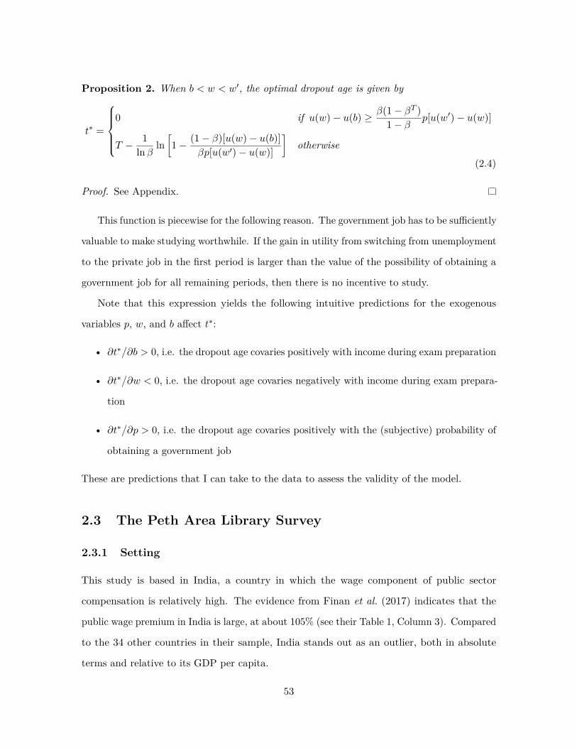
Proposition 2. When b < w < w′, the optimal dropout age is given by

t∗ =

0 if u(w)− u(b) ≥ β(1− βT )

1− β p[u(w′)− u(w)]

T − 1ln β ln

[1− (1− β)[u(w)− u(b)]

βp[u(w′)− u(w)]

]otherwise

(2.4)

Proof. See Appendix.

This function is piecewise for the following reason. The government job has to be sufficiently

valuable to make studying worthwhile. If the gain in utility from switching from unemployment

to the private job in the first period is larger than the value of the possibility of obtaining a

government job for all remaining periods, then there is no incentive to study.

Note that this expression yields the following intuitive predictions for the exogenous

variables p, w, and b affect t∗:

• ∂t∗/∂b > 0, i.e. the dropout age covaries positively with income during exam preparation

• ∂t∗/∂w < 0, i.e. the dropout age covaries negatively with income during exam prepara-

tion

• ∂t∗/∂p > 0, i.e. the dropout age covaries positively with the (subjective) probability of

obtaining a government job

These are predictions that I can take to the data to assess the validity of the model.

2.3 The Peth Area Library Survey

2.3.1 Setting

This study is based in India, a country in which the wage component of public sector

compensation is relatively high. The evidence from Finan et al. (2017) indicates that the

public wage premium in India is large, at about 105% (see their Table 1, Column 3). Compared

to the 34 other countries in their sample, India stands out as an outlier, both in absolute

terms and relative to its GDP per capita.

53

This paper uses data from a survey I fielded in the city of Pune. Within the state of

Maharashtra, Pune is well-known as a hub for preparation for government job exams. Students

from all over the state migrate to Pune to study. In particular, the 411030 zip code—known as

the Peth Area—is the epicenter of exam preparation. Appendix Figure B.1 includes a map of

this area. This zip code has a high concentration of both candidates preparing for competitive

exams and businesses that cater to their needs, including book shops, photo copiers (which

maintain ready catalogs of practice tests and study materials), coaching classes, libraries,

canteens and hostels.

Most government job aspirants in the Peth Area prepare for state-level civil service jobs.

These exams for these jobs are conducted by the Maharashtra Public Service Commission

(MPSC), a state-level government agency. In a typical year, candidates participate in 1-3

exams, and there are about 1500 applicants for each available vacancy.6 It is commonly

understood that many candidates who give the test do not prepare nearly as intensely as

candidates in the Peth Area. We should therefore expect selection rates in this group to be

much higher on average.

2.3.2 Sampling

I conducted the survey with a random sample of candidates preparing for state-level government

jobs in libraries in the Peth Area. Libraries serve as the primary sampling unit. These libraries

are private business that offer candidates a quiet space to study for a fee. Libraries are in

high demand because out-of-town students generally do not find their rooms conducive to

studying.

Before sampling libraries, a research assistant and I first conducted a census of all libraries

in the Peth Area. This was done by physically traversing the entire zip code and verifying

the presence of each library in person.7 In each library that we spotted, we collected data on

6For example, in the 2016 State Service Exam, there were 191,536 applicants and 135 were ultimatelyselected.

7Even still, it is possible that we may have missed some libraries. To increase the coverage of the census, wedeveloped an online app that allowed members of the public (in particular MPSC students) to suggest a library

54

the following items: the size of the library (measured in terms of the approximate number

of desks available); the fee structure; and the availability of amenities. The census yielded a

total of 166 libraries in the Peth Area.

To sample libraries, we drew a stratified random sample from the census. After dropping

six libraries that had restrictions on the types of students that could join, we divided the

remaining 160 into 6 groups based on their size and their monthly fee. To construct these six

bins, I took the Cartesian product of three bins for size (dividing the marginal distribution by

terciles) and two bins for fees (dividing the marignal distribution by the median). Within

each strata, I created a random re-sampling ordering list. I also randomly varied the order in

which we visited libraries from each strata.

Finally, I sampled students within libraries. Sampled students then received a paper

survey form. Those who agreed to participate in the survey filled out the form and returned

it to a research assistant, who then verified answers and answered follow-up questions in case

of confusion. The sampling strategy was designed in a way that allowed the research assistant

sufficient time to attend to each sampled student, while also accounting for the fact that the

population in the library is constantly moving, as students enter and leave throughout the

day. To account for the possibility that the population of students varies across the day, I

stratified the sample by time. For each library, I divided the day into 7-16 time slots in which

we would conduct a session, ranging from 9:30am to 6:00pm to account for the changing

composition of students over the course of the day. The research assistant divided the set

of available desks in the library into roughly equal sized groups. Each group of desks was

then randomly matched to a time slot. We allowed for gaps in the survey schedule to ensure

that the probability that a time slot was selected was independent of the library size. At

the designed time, the research assistant would visit the section and provide a copy of the

survey to all students who were: 1) present in the desk at the start of the session; and 2)

currently preparing for a state-level government job. In case a student sat down at a desk in

that was missing from our list. The website indicated that students would receive a compensation for eachlibrary that they found that wasn’t on our list. We proceeded only after we stopped receiving new suggestions.

55

that section after the start of the session, that student would be excluded from the sample.

Appendix Table B.1 summarizes details of the response rate at each of the six libraries

included in the survey. The survey was conducted between February 11th, 2020 and March

12th, 2020. The response rate fell dramatically in the last library because the onset of the

Covid-19 pandemic caused most students to return to their hometown.

2.3.3 Defining the Analysis Sample

Throughout the analysis, I restrict the analysis to men. In a patriarchal society that prioritizes

marriage over careers for women, it is unclear whether a model based on maximizing earning

potential would be appropriate for women. In principle, this is a testable hypothesis. For

example, I can test whether the reduced form relationships that the model predicts hold for

women as well as for men. Unfortunately, given the small sample of women, I do not have

enough statistical power to run this test. I therefore drop women from the sample based on

this a priori assumption about the context.

There are two distinct samples that I use for this analysis. The full sample uses the set of

observations who have non-missing values for all the variables used in the structural analysis.

Next, the restricted sample further restricts the sample to the observations for whom the

anticipated dropout age data is available. Due to an error in survey implementation, this

variable is not available for individuals in the first two libraries that were surveyed.8 On the

whole, the full sample and restricted sample report similar averages for a wide range of survey

responses (see Table 2.1), which suggests that these samples are comparable.

Throughout the analysis, I present standard errors that do not adjust for clustering. As

discussed in Abadie et al. (2017), these standard errors are valid for inferences about the

population of students that attend the specific libraries that appear in my sample, but they

are not correct for inferences about the population of MPSC students in the Peth Area as a

whole. With only 4-6 clusters, clustered standard errors will largely be uninformative; this

8In the first two libraries, respondents mistakenly thought that the question asked about the maximumallowable age instead of their own personal preference. In subsequent surveys, we explicitly clarified themeaning of the question with respondents.

56

study is thus not well suited to say much about the overall population of MPSC students in

the Peth Area as a whole. However, since students in the Peth Area are already a highly

selected group within the population of MPSC students, the thrust of the conclusions of

this study does not meaningfully change if we treat the students who study at the sampled

libraries as the population of interest.

2.3.4 Measurement of Model Parameters

The survey captures variables that proxy for five main parameters that relate to the model: 1)

b, the level of consumption that candidates have while preparing for the exam; 2) w, earnings

in the outside option; 3) p, the probability of success; and 4) t, the candidate’s current age;

and 5) t∗, the age at which the candidate drops out. Summary statistics for each of these

parameters is included in Table 2.1.

I measure b by asking respondents to report the amount of income they receive from home

every month. On average, candidates receive Rs. 8,000 per month. Almost all candidates are

supported by their family. I asked candidates to report separately their monthly expenditure

across a range of standard categories. On average, the transfers from home total to 97% of

total expenses. It is therefore fairly costly for candidates to come to Pune to study. Candidates

have told me that what makes it worthwhile is that they are able to see how well prepared

the competition is, which motivates them to study further.

I measure w by asking respondents to estimate their annual earnings in their outside

option. This was done by first asking candidates to consider the specific career they would

choose if they were to drop out of exam preparation right away. We then asked candidates

to consider the income they expect to earn in a typical month in that career. We ask this

question over two different time horizons—within 1 year of starting and within 10 years of

starting—to account for the possibility that some careers have lower initial earnings by higher

lifetime earnings. Consistent with the model’s assumption of minimal search effort in the

outside option, we see that most candidates (about 75%) anticipate that their outside option

is either farming or business.

57

Table 2.1: Summary Statistics

Full Sample Restricted Sample

Mean Std. Dev. N Mean Std. Dev. N

Persistence

Age 24.775 2.701 148 24.623 2.650 85

Preferred Dropout Age – – – 26.736 3.346 87

Demographic Characteristics

From Pune District (0/1) 0.032 0.176 157 0.022 0.147 91

Caste Group: General Category (0/1) 0.172 0.379 157 0.176 0.383 91

Caste Group : SC / ST (0/1) 0.108 0.312 157 0.121 0.328 91

Work Experience

Currently working (0/1) 0.006 0.080 157 0.011 0.105 91

Ever worked (0/1) 0.134 0.341 157 0.143 0.352 91

Alternative Occupation

Alt. Occ.: Business (0/1) 0.554 0.499 157 0.582 0.496 91

Alt. Occ.: Farming (0/1) 0.299 0.459 157 0.330 0.473 91

Alt. Occ.: Wage Employment (0/1) 0.229 0.422 157 0.231 0.424 91

Expected monthly income in alt. occ.after 1 year of experience (Lakh Rs.) 0.469 0.457 131 0.443 0.407 77

Expected monthly income in alt. occ.after 10 years of experience (Lakh Rs.) 3.089 10.965 124 2.650 8.307 73

Income Support

Total Monthly Expenses (Lakh Rs.) 0.082 0.017 157 0.086 0.018 91

Monthly transfer from home (Lakh Rs.) 0.078 0.019 153 0.080 0.018 88

Subjective BeliefsSubjective yearly pass probability 0.059 0.077 126 0.065 0.085 78

Expected monthly income as a Tehsildarafter 1 year of experience (Lakh Rs.) 0.920 1.621 140 0.961 1.847 82

Expected monthly income as a Tehsildarafter 10 years of experience (Lakh Rs.) 2.717 10.105 135 3.531 12.975 79

Notes: This table presents summary statistics from the Peth Area survey. The sample consists of maleMPSC candidates studying in libraries located in the 411030 zip code of Pune. The restricted sample isrestricted to the survey rounds in which the question on the preferred dropout age was asked correctly.

58

I measure p by asking candidates to provide subjective estimates of the average probability

of success for candidates in the Peth Area. For the purposes of estimating the value of a

government job, what matters is the subjective probability and not the objective probability

of success. To elicit these beliefs, we told candidates that about 12,000 students study for the

MPSC in the Peth Area, and we asked them to estimate how many of them they expect to be

successful in any given year.9 The respondent’s subjective assessment of p is the recorded

response divided by 12,000. In a few cases, respondents provide values greater than 50%.

This appears due to misunderstanding the question, and we therefore remove these responses

from the analysis.

I measure t, the respondent’s current age, by asking for their date of birth. Because I

know the date of the survey and the date of birth, I can estimate age with a high degree of

precision.

Finally, I measure t∗ by asking respondents to report the maximum age at which they

would be willing to prepare for the exam. As mentioned above, this outcome is only available

in the restricted sample. Note that this a preference parameter, and not a belief. Candidates

may drop out sooner than their preferred dropout age due to constraints (e.g. because of a

shock to household income), but if the self-reported data are reliable then they should stay

no longer than the observed dropout age.

How reliable are the self-reported preferred dropout ages? The main threats to reliability

are that: 1) candidates may not be truthful in their reports (e.g. because they are embarrassed

about stating their true preferences); and 2) candidates may not be time-consistent in their

preferences. One test of reliability is that we should not see more candidates studying at a

given age then the number of candidates who expect to study that long. In other words, the

value of the cumulative distribution function (CDF) of the current age should never be larger

than the value of the CDF of the preferred dropout age. This consistency check holds in the

data (see Appendix Figure B.2).

9The figure of 12,000 candidates studying in the Peth Area is based on the library census. For each librarywe estimated the total capacity and then multiplied the total observe capacity across all libraries by the averageattendance rate at 9am, when attendance typically was the highest.

59

There is substantial variation in the preferred dropout age (see Figure 2.2). At the 10th

percentile, respondents report not being willing to continue studying past age 22, or just one

to two years after completing college. At the 90th percentile, respondent report being willing

to study until age 31. The model helps us understand this variation.

2.3.5 Assessing the Validity of the Model

The validity of the parameter estimates depend on how well the optimal stopping model

outlined in Section 2.2 describes candidates’ search behavior. In this section, I assess whether

the assumptions of the model fit the men studying for MPSC jobs in the Peth Area.

To do so, I test whether the reduced form correlations that the model predicts also show

up in the data. Table 2.2 presents the correlations between the preferred dropout age and

measures of the main model parameters. All specifications include reservation category fixed

effects. The parameters correlate with the preferred dropout age in the expected way. In

Column (1) we see a weak with transfers from home. In Column (2), we see a negative

correlation with expected outside earnings. In Column (3), we see a positive correlation

between with the candidate’s subjective assessment of the pass probability. If we combine all

the predictors together, we see in Column (4) that the coefficients maintain the correct sign.

These correlations suggest that male candidates are in fact thinking about their persistence

decisions in a way that is aligned with the model.

2.4 Structural Estimation

2.4.1 Estimation Strategy

I suppose that agents are risk averse with a Bernoulii utility of u(c) = ln(c). This assumption

accords with the available evidence on risk aversion in labor supply (Chetty, 2006). I test the

sensitivity of this assumption by setting u(c) = (c1−η − 1)/(1− η) and perturbing η around a

neighborhood of 1.

I supply two constants to the model. First, I fix the discount rate β using the prevailing

60

Figure 2.2: Distribution of the preferred dropout age

(a) Histogram

(b) Survival curve

Notes: Panels A plots a histogram of the preferred dropout age. Panel B plots a Kaplan-Meier estimateof the survival curve. The red bands show 95% confidence intervals.

61

Table 2.2: Reduced Form Correlations

(1) (2) (3) (4)

ln b 1.756 1.190(1.418) (1.684)

lnw -0.862∗ -1.000∗∗(0.450) (0.398)

Subjective p 8.925∗ 9.074∗(5.026) (5.015)

Current age 0.663∗∗ 0.653∗∗ 0.713∗∗ 0.660∗∗(0.126) (0.118) (0.108) (0.104)

Reservation FE X X X XObservations 79 71 73 63

Notes: Table presents correlations between the preferred dropout age (the dependent variable) and theexogenous model parameters. All specifications include fixed effects for the respondent’s reservationcategory. Heteroskedasticity-robust standard errors in parentheses. ∗ p < 0.1, ∗∗ p < 0.05, ∗∗∗ p < 0.01

interest rate. The State Bank of India provided interest rates of 6.8% for one year deposits at

the time of the survey.10 I therefore fix the discount factor at 1/(1 + 0.068) ≈ 0.936. Second,

I assume that candidates’ last anticipated working year T is at age 60. This is both the

standard mandatory retirement age for government employees and the age at which male

college graduates in Maharashtra typically retire.11

In the absence of an obviously superior method of estimating the model, I apply three

distinct approaches, which impose different kinds of assumptions on the data and the data

generating process. To the extent that these approaches yield similar results, they should

help us triangulate the underlying parameter of interest: the money equivalent value of a

government job.

Estimator 1: Moment Inequality. The first approach, which imposes the weakest

assumptions, uses a partial identification strategy. This approach addresses the concern that

10Data obtained from the SBI website: https://sbi.co.in/web/interest-rates/interest-rates/deposit-rates

11Using data from the CMIE Consumer Households Pyramids Survey, I verify this assumption empirically.See Appendix Figure B.3.

62

I do not observe the dropout age. However, by virtue of appearing in the sample, I know that

candidates’ dropout age is at least as large as their current age.

According to the model, candidate i persists as long as the value of unemployment Ut

exceeds the value of obtaining a private sector job Pt. This is true as long as age ti satisfies:

u(wi)− u(bi)u(w′)− u(wi)

≤ pi[β(1− βT−ti)

1− β

](2.5)

Suppose I assume that all unobserved heterogeneity is due to unobserved variation in pi,

i.e. pi = p+ εi where E[εi] = 0. In that case, by rearranging this inequality and taking the

expectation of both sides I obtain the following moment inequality:

E

[u(wi)− u(bi)u(w′)− u(wi)

· 1− ββ(1− βT−ti) − p

]≤ 0 (2.6)

Since the left hand side is strictly decreasing in w′ for w′ > wi, the moment inequality identifies

a lower bound on the value of w′ that is consistent with the data.

Estimator 2: GMM. I can point identify w′ by replacing the inequality in equation

(2.6) with an equality at the preferred dropout age.12 The validity of this estimate requires

stronger assumptions, namely that candidates are time-consistent and report their preferences

truthfully.

Estimator 3: Maximum likelihood. Alternatively, I can assume that all individuals

have the same subjective probability of selection, but value the government job differently. In

particular, I suppose that lnw′i ∼ N(µ, σ2), and that all individuals have the same subjective

probability of selection p. I then estimate the parameters of the distribution of lnw′i via

maximum likelihood. This model implies that a particular function of the data zi is normally

distributed. Therefore, the maximum likelihood estimate admits the following closed-form

12In theory, this method would still estimate a lower bound if the government imposed maximum ageeligibility requirement was binding. However, this does not appear to occur in the data. Only a handful ofcandidates report an preferred dropout age at the age limit.

63

expressions:

µ = 1n

n∑i=1

zi (2.7)

σ2 = 1n

n∑i=1

(zi − µ)2 (2.8)

where in the case of log utility zi is given by:13

zi = u(wi)− u(bi)φ(T, t∗i ) · p

+ u(wi) (2.9)

Here, φ(T, ti) =[β(1− βT−ti)

] /(1− β). Because w′i is lognormally distributed, I estimate

E[w′i] with exp(µ+ 12 σ

2), and I estimate the median of w′i with exp(µ). As is well known, the

maximum likelihood estimator of σ2 is biased downwards, but it has lower mean square error

than the unbiased estimator n/(n− 1)σ2.

Inference. For all three estimation strategies, I use a bootstrap procedure to calculate

confidence intervals. All standard errors calculations are based on 1000 repetitions. I report

95% confidence intervals that are given by the range between the 2.5th percentile to the 97.5th

percentile of the bootstrap distribution.

2.4.2 Results

Table 2.3 summarizes the results. Across all three estimation approaches, I consistently

estimate a very high valuation of government jobs. In the full sample, the partial identification

approach yields a lower bound of Rs. 5.491 lakh per month [95% CI: 3.402-11.072]. This

estimate falls when I focus on the restricted sample, which likely reflects normal sampling

variation. As we saw in Table 2.1, the preferred dropout age is not much higher than candidates’

current age. Accordingly, the point-identified estimate of the value of a government job is not

much higher than the lower bound in the same sample (4.333 vs. 4.251).

13For more general CRRA utility functions, one can show that

zi = 11− η ln

[(1− η)

(u(wi)− u(bi)φ(T, t∗i ) · p + u(wi)

)+ 1]

64

Tab

le2.3:

Estim

ates

oftheVa

lueof

aGovernm

entJo

b

Estim

ator

Source

ofun

observed

heterogene

ityPa

rameter

Parameter

Estim

ate

(Rs.

Lakh

s/mon

th)

1-M

omentinequa

lity

Prob

ability

ofselection

Lower

boun

don

w′

5.49

14.25

1[3.402

,11.07

2][2.310

,9.918

]

2-G

MM

Prob

ability

ofselection

w′

–4.33

3–

[2.404

,10.27

7]

3-M

LEVa

lueof

governmentjob

µ–

0.68

5[0.001

,1.671

]

σ2

–3.47

8[2.195

,5.854

]

E[w′ i]

–11

.289

[3.291

,88.29

5]

Med

ianw′ i

–1.98

4[1.001

,5.320

]

Sample

Full

Restricted

N12

070

Notes:Ta

blepresents

estim

ates

usingthreediffe

rent

estim

ationstrategies.Fo

reach

estim

ate,

Iprovide95%

confi

denceintervalsbasedon

1000

bootstrapsamples

inbrackets.The

confi

denceintervalsdo

notadjust

forclustering.The

restricted

sampleexclud

esindividu

alswith

amissing

valueof

thepreferreddropou

tage.

65

Table 2.4: Maharashtra Tehsildar Salary Calculation

As of 2019

Government Policy

Salary Group Pay Band 3 with Grade Pay 5000

Starting Pay Rs. 55,100 per month

Annual Growth Rate 3%

Retirement Age 60

Model Parameters

Annual discount factor 0.936

Value calculations

Total NPV, starting from age 20 Rs. 14,242,460

Annuity equivalent Rs. 81,429 per month

Notes: These calculations are based on the Maharashtra 7th Pay Commission pay matrix and policies.

How does these estimates compare to the nominal salary? In Table 2.4, I present a

calculation of the nominal salary of a Tehsildar, one of the highest-paid posts recruited

through MPSC competitive exams. To account for the fact that government salaries increase

every year, I convert the net present value of the income stream into the equivalent annuity.

This requires fixing a discount factor, for which I use the same value I used to estimate the

model. This calculation yields an annuity value of a Tehsildar post of about 0.81 lakh INR

per month. I assume that the gap between the nominal salary and the private valuation

reflects the amenity value of government jobs. This implies that at least 81% of the value of a

government job is due to unobserved amenities.

2.4.3 Robustness

I assess the robustness of these findings to local perturbations of key features of model

parameters and the data. For each of these robustness checks, I focus on the estimate with

minimal requirements of the data, i.e. the lower bound estimate on w′ using the full sample.

66

The results are summarized in Figure 2.3.

Figure 2.3: Sensitivity of the Estimated Lower Bound on w′

67

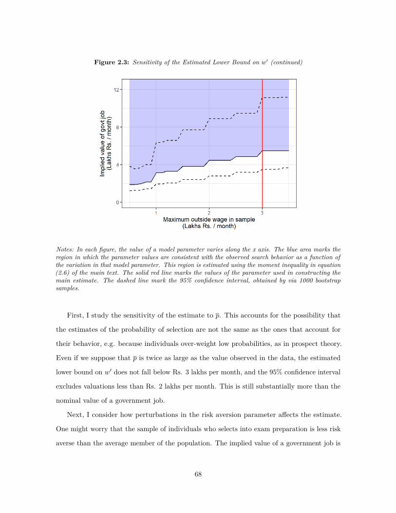
Figure 2.3: Sensitivity of the Estimated Lower Bound on w′ (continued)

Notes: In each figure, the value of a model parameter varies along the x axis. The blue area marks theregion in which the parameter values are consistent with the observed search behavior as a function ofthe variation in that model parameter. This region is estimated using the moment inequality in equation(2.6) of the main text. The solid red line marks the values of the parameter used in constructing themain estimate. The dashed line mark the 95% confidence interval, obtained by via 1000 bootstrapsamples.

First, I study the sensitivity of the estimate to p. This accounts for the possibility that

the estimates of the probability of selection are not the same as the ones that account for

their behavior, e.g. because individuals over-weight low probabilities, as in prospect theory.

Even if we suppose that p is twice as large as the value observed in the data, the estimated

lower bound on w′ does not fall below Rs. 3 lakhs per month, and the 95% confidence interval

excludes valuations less than Rs. 2 lakhs per month. This is still substantially more than the

nominal value of a government job.

Next, I consider how perturbations in the risk aversion parameter affects the estimate.

One might worry that the sample of individuals who selects into exam preparation is less risk

averse than the average member of the population. The implied value of a government job is

68

declines as the risk aversion coefficient also declines. But even with a 20% reduction (from 1

to 0.8), the estimate still stays above Rs. 3.5 lakhs per month.

Finally, I consider how the estimate falls when I exclude individuals with the highest

reported outside wage offers from the sample. The model implies a single common value of

a government job across all candidates. To fit the data, the model may place substantial

weight on ensuring that the estimate falls above these values. The figure shows that indeed

the estimated lower bound on w′ is sensitive to excluding these observations. However, even

when individuals who anticipate an outside option of more than 1 lakh INR per month are

excluded, the estimated lower bound on w′ remains above 3 lakh INR per month.

2.5 Alternative Explanations

Thus far, I have interpreted the high monthly wage that rationalizes search behavior as

reflecting a high amenity value of government jobs. In this section, I consider two alternative

explanations for the high estimated value of government jobs: 1) that candidates are mis-

informed about the nominal wage in government jobs; and 2) that candidates derive value

from the search process itself. I conclude that neither of these alternative explanations are

compelling in this context.

2.5.1 Are candidates misinformed about the salary?

Candidates may persist in studying simply because they overestimate the salary offered in

government jobs. It it not unreasonable to believe this to be the case. Information about the

wage offered in government jobs is not necessarily easy to obtain. The notifications advertising

government jobs generally do not list the nominal monthly wage. Instead, it lists the “pay

band." One then needs to look up the nominal wage in a table that the government continually

revises.

To assess beliefs about wages, I include a question in the survey that asks respondents to

69

guess the monthly wage of a Tehsildar after 1 year of experience.14 In general, candidates

tend to have accurate beliefs about the initial salary. The median belief is 0.60 lakh INR per

month, which is close to the true value of 0.55 lakh INR per month. Moreoever, about 64%

of respondents guessed within 0.2 lakh of the true value, and 90% of individuals provided

an estimate of less than 1 lakh INR per month. The average estimate (as seen in Table

2.1) is much higher than the median because a few individuals provide very large estimates.

But there is no evidence to suggest that individuals systematically entertain beliefs about

compensation that are out of line with the official salary.

2.5.2 Do candidates derive value from the search process?

So far, I have assumed that the government job is the only state that has unobserved amenities.

However, it is possible that candidates derive value from the search process itself, independent

of the instrumental value of obtaining a government job. Candidates may value delaying

starting work, living in Pune, or the lifestyle of being a student. In that case, exam preparation

is not as costly as I have supposed, in which case we can rationalize the search behavior with

a lower value for government jobs.

One way to address this concern within the scope of the model is to multiply the observed

values of bi by some constant α > 1. This does not affect the conclusions substantially. The

estimated lower bound on w′ still remains above 3 lakh per month, even if I set α = 2.

I also provide direct experimental evidence that the amenity value of exam preparation is

not so large as to encourage candidates to continue preparing for its own sake. If candidates

did in fact have these non-instrumental motivations, then we would expect to see that they

would still express a preference to persist even as the probability of passing vanishes. This

logic can be expressed formally as follows. Suppose candidates persist in period t as long as

ptw′t + bt > wt where pt is the probability of success, w′t is the value of a government job, bt is

the value of searching, and wt is the value of the outside option. As long as bt < wt, then

14As reported in Table 2.1, I also asked candidates about their salary beliefs after 10 years of experience.However, it is difficult to assess the correctness of these beliefs, since the true value also incorporate uncertaintyabout interim government policy changes.

70

there is some value of pt below which candidates will prefer to drop out.

To test whether this is the case, I constructed a vignette experiment in which I asked a

convenience sample of 50 MPSC candidates in the Peth Area whether they would recommend

a hypothetical friend to take the test next year, given their score history over the past

three attempts. In each iteration of the survey, I randomly varied the score history of the

hypothetical friend.15

I ensured that the hypothetical friend described came from the same district as the

respondent and had the same gender. This was done to maximize the likelihood that the

respondents’ recommendation reflects how they would make the same decision for themselves.

Respondents were able to provide one of three recommendations: A) Continue preparing for

the MPSC only; B) Prepare for the MPSC, but also prepare a backup option; and C) Focus

on an alternative career. I treat responses of either A or B as a recommendation to persist.

Figure ?? plots the fraction of individuals recommending that the friend drop-out as a

function of the average distance to the preliminary exam cutoff score across the three scores

showed in the vignette.16 If individuals had strong non-instrumental reasons for studying, we

would expect the fraction of candidates recommending dropping out to plateau at some value

less than 1. This does not appear to be the case.

2.6 Conclusion

The value of a government job in India far exceeds the nominal wage, indicating that amenities

comprise a large share total compensation. This finding has several important implications

for personnel policy in developing countries and for future research.

First, the results of this paper imply that policymakers and researchers should think

15The score in the 2016 X2016 is randomly chosen from the set {10, 30, 50}. I then generate scores for 2017and 2018 using the following AR process: Xt = 0.33X2016 + 0.67Xt−1 + εt where εt ∼ N(0, σ = 4.5). Thisgenerates a set of realistic scores that have a fixed mean but vary in trajectory. The exam has two stages. Ifthe randomly generated score crosses the cutoff, then I randomly generate a main score exam from a uniformdistribution between 30 and 50.

16Note that clearing the preliminary cutoff score only allows one to progress to the next stage of the exam,at which points the odds against selection are still substantial.

71

more holistically about the types of incentives available in the public sector other than salary.

Research on personnel policy, particularly in developing countries, has largely focused on

manipulating the salary component of earnings. The estimates from this paper suggest that

this work leaves much of the available variation for incentive provision off the table. A recent

exception in this literature is Khan et al. (2019), who study the effects of a performance-based

transfers scheme on tax collection. These authors motivate this scheme by pointing out that

governments are often constrained in providing financial incentives. However, to the extent that

government employees derive most of the value of employment from non-financial amenities,

even an unconstrained government may prefer to provide incentives through amenities rather

than through wages.

An interesting question for future work is the extent to which the amenity value of these

jobs depends on the wage. For example, one may imagine that the prestige and insurance

value of government employment depend on the salary component. This question has bearing

on whether we would expect the re-application rates to decrease if the salary were reduced.

It would also be valuable to unpack the components of this large amenity value. If this

value reflects access to bribes or abuse of power, then these estimates are cause for concern.

If, instead, the value hinges more on the insurance value of a government job, then these

estimates suggest a dire need for policy that supports income security. In this way, learning

about the civil service recruitment process may provide a window into the economy as a

whole.

72

Chapter 3

The Underrepresentation of Women

in Competitive Careers: Evidence

from the Indian Civil Service†

3.1 Introduction

Entry into prestigious, high-paying jobs often depends on succeeding in some kind of tourna-

ment. These are often the same jobs in which women are under-represented. For example,

women are less likely to be elected to political office (Bhalotra et al., 2018); they are less

likely to win promotions within corporate firms (Bertrand and Hallock, 2001; Bertrand, 2018;

Ganguli et al., 2021); and they are less likely to obtain senior positions within government

(Sabharwal, 2015).

What prevents women from competing effectively for these jobs? To the extent that

women are constrained from competing to the best of their ability, the under-representation

of women may limit economic growth (Hsieh et al., 2019). But evidence on this question from

developing countries is especially scarce, even as rising female educational attainment makes

this question increasingly salient.

†Co-authored with Niharika Singh

73

In this paper, we study the causes of the under-representation of women in the Indian civil

service. This question serves as a window into understanding the barriers that prevent educated

women in India from competing in the labor market. Moreover, the under-representation of

women in the civil service is puzzling in its own right. Selection is determined by a competitive

exam, and the syllabus of these exams cover similar material to what most students cover in

high school. But even though women tend to outperform men on school-leaving exams, they

tend to lag behind in civil service selection.1

Our analysis focuses on candidates applying for posts within the Tamil Nadu state

bureaucracy. Tamil Nadu is one of several states in India that has sought to address the

long-standing gender imbalance by implementing reservations for women. These quotas remain

binding. Excluding posts covered by the quota, only 1 woman is selected for every 3.5 men.

Our analysis aims to document the underlying causes of this selection gap.

We draw on administrative data from the Tamil Nadu Public Service Commission (TNPSC),

the agency responsible for conducting civil service exams for state-level posts. We observe

application data for the universe of recruitments notified between 2012 and 2016, and test

score data for recruitments notified between 2013 and 2016.

Almost all candidates are allowed an unlimited number of attempts.2 As a result, aggregate

gender differences are a result of both differences in initial selection and performance, and

differences in how candidates’ selection and performance evolves over the course of repeat

attempts. Our analysis separates these margins by looking at how gender differences vary

with prior exam experience. Although TNPSC does not track the number of attempts directly,

we are able to construct a useful proxy. Throughout this paper, first-time applicants will refer

to individuals who were: a) between the ages of 20 to 21 at the time of application; and b)

did not appear for any TNPSC exam in the prior year.

We begin by documenting three facts about how men and women fare in the recruitment

1For example, in the 2019 CBSE 12th standard board exam, the pass rate for women was 9 percentagepoints higher than that of men. In the same exam about 15 of the top 23 highest scoring students were women.(We inferred students’ gender from their first name.)

2The maximum age eligiblity criteria apply to fewer than 1% of applicants.

74

pipeline for a civil service job in our setting.

First, we document that, in contrast to the final selection outcomes, the application

pool shows minimal to no gender gaps in test-taking. Women account for 65% of first-time

applicants and 52% of the overall applicant pool. This tells us that gender gaps are not

pervasive throughout the recruitment pipeline, but rather appear at a later stage in the

recruitment process.

Second, we show that there is a reversal in the relative performance of men and women

across attempts. In the first attempt, women tend to outperform men, both on average and

among the top-scoring candidates. However, because very few first time applicants score well

enough to meet the selection cutoff, the initial performance advantage does not meaningfully

affect the overall rate of selection. By the third year of applying, women score less than men,

especially at the top of the distribution. Accordingly, the relative selection rate also reverses.

Third, we show that the dynamic selection of applicants across attempts contributes to

the gender gap. Among first-time applicants, women are much less likely to re-apply, even

conditional on having the same test score as men. Moreover, the women who drop out tend

to have higher scores on their first attempt than men. This is an important source of leakage

in the recruitment pipeline. That is because it is rare for first-time applicants to succeed: in a

typical recruitment, fewer than 10% are able to do so.

What factors explains these patterns? In this paper, we consider whether social pressure

for women to marry young prevents them from making as many attempts as men.3

We provide a preliminary test of this hypothesis using variation in the early marriage

rate across districts in Tamil Nadu. We expect to see more marriage pressure for women in

districts where women tend to get married at earlier ages. Consistent with marriage pressure

constraining women, we find that women born in districts with a higher early marriage rate

are less likely to re-apply. Moreover, we see that in these districts the women who dropout

3In theory, it is also possible that men and women have different preferences or beliefs. For example, menand women may differ in their their taste for competition Niederle and Vesterlund 2007; Niederle et al. 2013;their tolerance for risk (Eckel and Grossman, 2008); or they may respond differently to information aboutability (Owen, 2020).

75

tend to be higher ability. By contrast, men from districts with high marriage rates are more

likely to re-apply. We consider this to be suggestive evidence in favor of the marriage pressure

hypothesis.4

This paper contributes to the literature on the constraints that prevent women in South

Asia from fully participating in the labor market. Although it is well-known that female

labor force participation in India is low (Fletcher et al., 2017), the constraints faced by

relatively elite women in this context are less well documented. Previous work has shown that

women’s participation in the economy is hindered by many factors, including a lack of access

to transport (Martinez et al., 2020), harassment and violence (Siddique, 2018; Chakraborty

et al., 2018), and norms around family and childcare (Reed, 2020). This paper extends this

literature by providing evidence for how a cultural norm that prioritizes women’s marriage

over their careers also shapes women’s labor market trajectories.

We also contribute to literature documenting how the structure of the recruitment process

itself can determine outcomes for women. Abraham and Stein (2018) shows that women

applicants may hold themselves to higher standards during the application process and

experimentally changing the language of job postings helps close the gender skills gap in

applications. Similarly, Roussille (2020) shows that changing the default option of specifying

desired salary on an online job platform from an empty field to a pre-filled field with the

median salary for similar candidates eliminates the gender ask gap, without affecting hiring

outcomes. In this paper, we show that the length of the recruitment process is also a margin

that can contribute to gender differences in recruitment outcomes. This disadvantage appears

to be especially pronounced in settings where women face differential pressure to marry early.

This paper proceeds as follows. Section 3.2 provides details on civil service recruitment in

Tamil Nadu and the data that we use to study it. Section 3.3 follows applicants through the

recruitment pipeline to identify the stage of the application process where women drop out.

Section 3.4 provides suggestive evidence that marriage norms constrain women’s application

4In particular, we are not able to rule out the presence of gender-specific unobservables that are correlatedwith marriage rates and that influence re-application decisions independent of marriage pressure.

76

decisions. Section 3.5 concludes.

3.2 Context and Data

3.2.1 Civil service recruitment in Tamil Nadu

This paper focuses on candidates who apply for civil service posts through the Tamil Nadu

Public Service Commmission (TNPSC). TNPSC is the agency within the Government of

Tamil Nadu that is responsible for conducting exams for state-level positions. These positions

occupy the junior levels of the state bureaucracy, and report to officers recruited through the

central government. TNPSC posts are open to all Indian citizens. But because the exam

includes questions on the Tamil language, the Commission sees very few applicants from

outside Tamil Nadu or Puducherry.

TNPSC conducts exams for groups of vacancies at a time. Vacancies are grouped so that

they have similar educational qualification requirements and occupy a similar rank within

the state government. Our analysis focuses on the group recruitments that require a college

degree. The college-level positions are classified into three distinct ranks. Group 1 posts

correspond to the highest ranking posts recruited by the Government of Tamil Nadu, followed

by Group 2, and Group 2A. Individuals with any college-level degree are eligible to participate

in these exams.5

The recruitment process begins with a public notification of an exam. TNPSC then allows

for about 1 month for candidates to apply online. In a typical year, TNPSC will notify

between 1-3 recruitments for college-level civil service posts.

Candidates do not apply to specific vacancies. Instead, once the candidates’ final ranks are

calculated, TNPSC allocates candidates to vacancies through a serial dictatorship mechanism.

In rank order, candidates select from the set of remaining vacancies that are available to them

based on their qualifications and reservation quota.

The selection process depends on the exam group. For posts advertised at the Group

5Not all applicants will qualify for all posts, since some positions require specific qualifications (e.g. a lawdegree or a typing certificate).

77

2A level, TNPSC conducts a single multiple choice examination, and candidates are ranked

simply based on their performance in that exam.6 The examination covers a wide range of

subjects, including

For Group 1 and Group 2 posts, TNPSC follows a multi-stage process. In the first stage,

TNPSC conducts a multiple choice exam. The top-scoring candidates in this preliminary

round are then invited to take the “main" examination, which consists of a series of open-ended

responses. Each exam is scored at least two independent reviewers.7 Finally, the top-scoring

candidates in the main examination are invited for an interview conducted at TNPSC’s office

in Chennai. Interview scores are constrained to five letter grades, each of which provides a

fixed number of points to the total score. Candidates’ final rank is calculated based on a

combination of the main exam score plus the interview marks.

For the vast majority of candidates, there are no restrictions on the number of attempts

that can be made or the maximum age at which one can apply. TNPSC does stipulate

a maximum age requirement for individuals who do not belong to one their caste-based

reservation groups, but in a typical recruitment fewer than 1% of applicants fall in this

category.

TNPSC includes a quota for female candidates in all recruitments. Women are eligible

to compete for seats both in the “general" category as well as in their quota. Seats are

first filled within the general category. Therefore, the female quota sets a floor on women’s

representation but does not impose a ceiling. The number of seats that are allocated to the

female quota is determined before applications are received.

TNPSC exams are very competitive. On average, TNPSC receives about 390 applications

for each vacancy it advertises.8 To stay competitive, many candidates find it worthwhile

to prepare for these exams full time for several years. It is unknown precisely how many

6Ties are broken based on educational qualifications, age, and, if necessary, the alphabetical order of thecandidates’ names.

7In case of a large discrepancy between the two reviews, the exam is sent to a third reviewer.

8Appendix Table C.1 summarizes the number of applicants at each stage of the process for the recruitmentsfor which data are available.

78

candidates engage in this behavior, but it is enough that changes in civil service hiring policy

can affect the aggregate unemployment rate (see Chapter 1).

3.2.2 Data sources

This paper draws primarily on application and testing data from TNPSC. We observe

application data for the universe of civil service exams that were notified between 2012 and

2016. For exams that were notified between 2013 and 2016, we also observe test scores at

each stage of the process, whether the candidate was selected, and if so, under which quota

(if any).9

The data allow candidates to be linked across attempts using a combination of name,

parents’ name, and date of birth.10 This method reliably identifies unique individuals within

exams. Across all exams, less than 0.1% of applications are marked as duplicates using this

combination of identifiers. Throughout the analysis, we drop the handful of duplicates from

the dataset. It is reasonable to believe that candidates will provide consistent information

over time. That is because applications are official documents, and it is costly for candidates

to make mistakes in either spelling names or writing an incorrect date of birth.

3.2.3 How under-represented are women?

Table 3.1 provides statistics on the representation of women for each of the 7 recruitments in

the sample. Because the quota is attached to specific posts, we can identify the quota under

which candidates were selected.

Excluding posts covered by the female quota, women are substantially under-represented

among selected candidates. Overall, only 22.3% of selected candidates are women, which

implies that there is only 1 woman selected for approximately every 3.5 men. Note that this

calculation only accounts for quotas in final selection, but in fact there are female quotas

9There is one exception: We do not observe test scores for the final exam in this period, the 2016/19 Group1 exam.

10To protect the identity of the candidates, TNPSC anonymized all names. In order to match names, wetherefore compared a set of numeric IDs across examinations.

79

Table 3.1: How underrpresented are women in the Tamil Nadu civil service?

(1) (2) (3) (4)

Excluding female quota Including female quota

Notification Group Selected % Female Selected % Female

2013/14 2 787 19.1 1129 43.62013/17 1 56 35.7 79 54.42014/01 2A 836 15.7 1241 43.22015/07 2 760 44.3 1078 60.82015/09 1 56 42.9 72 55.62015/17 2A 1499 14.3 2142 40.12016/19 1 56 48.2 87 66.7

Overall – 4050 22.3 5828 46.0

Notes: The table presents statistics on the fraction of women selected in each of the seven recruitmentsthat were notified between 2013 and 2016. Columns 1 and 2 present statistics for positions that werenot exclusive to female candidates, whereas columns 3 and 4 consider all the available positions in therecruitment.

implemented at every stage of the exam (from the preliminary round to the main exam,

and from the main exam to the interview). Without these intermediate quotas, female

representation would likely be even lower.

The female quota in selection helps achieve near-parity in the representation of women:

once we take these posts into account, the representation of women rises to 46.0%, or 1 woman

selected for every 1.2 men. The female quota is less binding in the more competitive Group 1

posts. But since the vast majority of posts are offered in the lower tiers, the average is largely

determined by the selection rate in Group 2 and Group 2A posts.

3.3 The Recruitment Pipeline

In this section, we follow cohorts of applicants through the recruitment pipeline to identify

the gender differences that lead to lower representation in unreserved posts. We pay special

attention to how first-time applicants differ from the overall applicant pool. This exercise

helps us disentangle gender differences in initial application and performance from differences

80

in how application behavior and performance evolve across attempts.

3.3.1 Defining first-time applicants

TNPSC does not officially track the number of attempts that candidates make. We therefore

construct a proxy. We identify first-time applicants as individuals who are between the ages

of 20 and 21 at the time of the exam,11 who had not applied for any exam in the prior year.

Because we focus on a set of positions that require a college degree, and because Indians

typically graduate from college at least at age 20, these criteria limit the sample to a set

of individuals who apply as soon as they are eligible. This proxy errs on the side of under-

counting first-time applicants as opposed to over-counting them. Any applicant who chose to

wait several years after college before applying is excluded. It is possible that this definition

includes candidates who have previously applied for a post that does not require a college

degree, but by its construction it is not possible that they will have applied for a college-level

post.

3.3.2 Gender differences in application rates

Table 3.2 summarizes the differences in the characteristics of male and female applicants.

The first three columns present statistics for first-time applicants, and the last three columns

present statistics for the overall pool of applicants.

In the first row, we see that women are substantially over-represented among first-time

applicants, outnumbering men by a margin of 3 to 1. Figure 3.1 shows that part of the

explanation for the larger number of female applicants is that eligible women are more likely

to apply. However, when we look at the pool of applicants as a whole, women’s majority

among applicants is far less stark. These facts suggest that men either start exam preparation

later, or are more likely to persist. Accordingly we see that the average age of men in the

overall applicant pool is about 1 year higher.12

11For each recruitment, the age cutoff date is calculated based on the candidate’s age on July 1st of thenotification year. This is the same date that we use in the analysis.

12Due to our age restriction in defining first-time applicants, there are no average differences in age for this

81

Table 3.2: Gender differences among applicants

First-time Applicants All Applicants

Women Men Difference Women Men Difference

(1) (2) (3) (4) (5) (6)

Share of applications 75.1% 24.9% 50.2%∗∗∗ 52.1% 47.9% 4.2%∗∗∗(0.4) (0.8)

Demographic Covariates

Age 20.459 20.535 -0.076 27.039 28.086 −1.046∗∗∗(0.006) (0.009)

Born in Chennai District 0.034 0.044 −0.009∗ 0.026 0.021 0.005∗∗∗(0.003) (0.0002)

Married 0.077 0.002 0.075∗∗∗ 0.469 0.255 0.213∗∗∗(0.002) (0.0007)

Medium of Instruction

Completed 10th in Tamil 0.788 0.745 0.043∗∗∗ 0.815 0.828 −0.013∗∗∗(0.007) (0.0006)

Completed 12th in Tamil 0.775 0.728 0.048∗∗∗ 0.800 0.801 −0.001∗∗∗(0.007) (0.0007)

Completed UG in Tamil 0.057 0.047 0.011∗∗∗ 0.183 0.173 0.009∗∗∗(0.003) (0.0006)

Type of Undergraduate Degree

Has B.A. Degree 0.157 0.070 0.087∗∗∗ 0.209 0.182 0.027∗∗∗(0.011) (0.001)

Has B.Com. Degree 0.156 0.197 −0.041∗∗∗ 0.135 0.144 −0.009∗∗∗(0.016) (0.0009)

Has B.Sc. Degree 0.443 0.314 0.129∗∗∗ 0.383 0.302 0.080∗∗∗(0.019) (0.001)

Has Engineering Degree 0.149 0.281 −0.132∗∗∗ 0.158 0.263 −0.105∗∗∗(0.017) (0.001)

Has other degree 0.094 0.137 −0.042∗ 0.115 0.109 0.007∗∗∗(0.013) (0.0008)

Notes: This table shows how men and women differ along a range of covariates. The sample forcolumns 1-3 is the set of first-time applicants, as proxied by those who: a) are between the ages of 20to 21; and b) did not make an attempt in the preceding year. Column 3 shows the difference betweenmen and women with robust standard errors in parentheses. Columns 4-6 repeat columns 1-3 for allapplicants.

82

Figure 3.1: Gender differences in application rates

Notes: This figure plots the application rate for posts that require a college degree by gender. Thenumerator is the number of unique individuals applying for posts in 2013. The denominator is the2011 Census count of the number of individuals by age and gender with a college degree in Tamil Naduand Puducherry.

The remaining rows of the table summarize how male and female applicants compare on

observable demographic attributes. Women are substantially more likely to be married. We

also observe their educational background in terms of the linguistic medium of instruction

and type of undergraduate degree. Women are always more likely to have completed their

high school and undergraduate education in the state vernacular, Tamil. Within Tamil

Nadu, educational instruction in Tamil medium is generally considered to be a marker of

disadvantage in the labor market, which is why the Government of Tamil Nadu has a quota

specifically for candidates who studied in Tamil medium.13

group.

13This means that women are more likely to qualify for this quota. Women remain under-represented inspite of this advantage.

83

We do not see clear gender differences in the prestige of the type of undergraduate degree

program completed. In India, one’s choice of degree programs is generally determined by one’s

performance on school-leaving exams, and students who enroll in science-related programs

(such as a B.Sc. or an engineering degree) tend to have the highest scores, while those who

enroll in B.A. programs tend to have the lowest scores. Although women are less likely to

have an engineering degree, they are more likely to have a science degree. On net, we see a

wide range of applicant quality for both men and women, but we do not see an obvious female

disadvantage on this dimension.

3.3.3 Gender differences in exam performance across attempts

How do these observable differences translate into performance on the civil service exam? We

measure exam performance as a percentile rank, which varies from 100 (for the highest-scoring

candidate) to 0 (for the lowest-scoring candidate). For multi-stage exams, we compute ranks

over the sum of the candidate’s score across each of the exam stages (including the preliminary

exam). For candidate who do not qualify for subsequent rounds, their scores in those later

rounds are set to zero.

We begin by documenting gender differences in test scores in the overall pool of applicants.

Figure 3.2 plots the distribution of test scores separately for male and female candidates,

both for first-time applicants (in the top figure) and for the pool of candidates overall (in the

bottom figure). In both cases we see that women are under-represented at both the top and

bottom of the distribution and over-represented in the middle.

Recall, there are generally more female applicants than men, especially among first-time

applicants. So even though the distribution of female applicants be shifted more towards the

middle ranks, it is still possible that there are enough women in absolute numbers at the top

of the distribution who can compete with men. In Figure 3.3 we therefore zoom in on the

scores of the top-scoring men and women, fixing the absolute number of men and women

being compared.

Panel A of Figure 3.3 shows that among first-time applicants, women actually out-

84

Figure 3.2: Distribution of test scores by gender

(a) First time applicants

(b) All applicants

Notes: These figures plot the distribution of candidate’s percentile rank by gender. Panel A restrictsthe sample to first-time applicants, i.e. those between the ages of 20 and 21 who did not make anyattempt in the proceeding year. Panel B plots the distribution for all applicants.

85

perform men. Thus, there are enough high-scoring women in initial applicant pools that the

representation gap is unlikely to be driven by an initial lack of female applicants with the

potential to perform well. However, consistent with the under-representation that we observed

earlier, we see a reversal in the gender gap when we look at the entire pool of applicants

(Panel B).

The reversal in relative performance between first-time attempts and the entire pool

of applicants suggests that women’s performance falls behind as candidates make multiple

attempts. To assess this hypothesis, we estimate how the gender gap in exam performance

varies with the number of prior attempts. We estimate a regression of the following form:

yir =3∑

a=1

[βafemaleir × 1(attemptir = a) + γa1(attemptir = a)

]+ αr + εir (3.1)

where i indexes candidates and r indexes recruitments. The sample is restricted to individuals

who made a first attempt in either 2013 or 2014.14 These individuals are then followed across

all subsequent attempts. Attempts are grouped by year. Thus, attempt a corresponds to

the a-th year in which the candidate applied for a college-level TNPSC post.15 Standard

errors are clustered by individual candidate to account for serially correlated errors in exam

performance.

Table 3.3 presents the estimates of βa. In the first column, the outcome is the percentile

rank. In the first attempt, women score about 1.6 percentile higher than men on average.

However, this gap reverses across attempts and becomes negative (though statistically in-

significant) by the third attempt. In column 2, we zoom in on the top of the distribution,

where rank differences matter for selection outcomes. The sample is restricted to the top 250

men and women in each of the five recruitments included in the sample.16 Here we see the

same pattern: a pro-female gender gap in the first attempt which turns pro-male by the third

14The 2013/17 exam is dropped because there are no individuals who applied to this exam who meet ourdefinition of a first-time applicant.

15For example, if a candidate applied for a post in 2013 and 2015, the attempt in 2015 would be counted asthe second attempt.

16The sample is more than 2500 because of ties.

86

Figure 3.3: Test performance of top-scoring candidates by gender

(a) First time applicants

(b) All applicants

Notes: This figure plots non-parametric estimates of candidates’ percentile rank × 100 conditionalon their gender-specific rank within each exam. Panel A restricts the sample to first-time applicants,proxied by those between the ages of 20 and 21 who did not make any attempt in the proceeding year.Panel B includes all applicants. For Panel A, the gender-specific rank is calculated within the sampleof first-time applicants.

87

Table 3.3: Gender differences in exam performance across attempts

Percentile Rank Selection without Quotas

(1) (2) (3)

Female × Attempt 1 1.595∗∗∗ 3.085∗∗∗ −0.00009(0.451) (0.327) (0.0002)

Female × Attempt 2 −0.046 0.966 −0.004∗∗∗(0.796) (0.629) (0.001)

Female × Attempt 3 −2.938 −2.230∗ −0.009∗∗(1.618) (0.894) (0.004)

Sample Full distribution Top 250 Full distributionExam FE X X XObservations 26, 986 2, 599 26, 986

Notes: This table shows how exam performance between male and female applicants vary acrossattempts. The sample consists of first-time applicants in the 2013 and 2014 exams. In the first twocolumns, the outcome variable is the percentile rank (which varies from 0 to 100). In the final column,the outcome is an indicator for whether the candidate was selected without relying on the female quota.The coefficient is the average gender gap in performance between women and men conditional on thenumber of attempts made. All specifications include exam fixed effects. Standard errors are clusteredby individual. ∗∗∗p < 0.01; ∗∗p < 0.05; ∗p < 0.1

attempt. Finally, in the third column we confirm that these differences in test scores affect

selection outcomes. Since selection is a combination of scores and quotas, we proxy for being

selected without quotas with an indicator for whether the candidate obtained a score above

the 99.5th percentile. Column 3 shows that while the gender gap in selection is negligible in

the first attempt, it widens across attempts.

The results on test scores combined with differences in observed covariates by gender and

first-time applicant status point to the plausible existence of dynamic selection by gender.

We now turn to look at this explicitly by examining re-application rates by gender.

3.3.4 Gender differences in re-application behavior

One way dynamic selection could arise is if men and women respond to initial test-score

information differently or if we they face differential constraints in their ability to re-apply.

First we look at whether there are gender differences in the propensity to re-apply,

88

conditional on ability. To do so, we estimate the following regression specification:

reapplyi,t+x = βfemalei + f(rankit) + αt + εit (3.2)

where i indexes candidates and t indexes years. The sample is restricted to first-time applicants

who were not selected for an exam in year t. We also control for a third degree polynomial,

f(rankit) in the maximum percentile rank achieved by the applicant in the year of their first

attempt. We look at re-application rates across three years, i.e. for candidates that make

their first attempt in year t, we estimate the fraction that are present for an exam in year

t+ x for x ∈ {1, 2, 3}. Since the sample is restricted to first-time applicants, all observations

correspond to unique individuals. We therefore report robust standard errors.

Table 3.4 presents these results. Panel A presents results for all applicants. Women are 6

percentage points less likely to re-apply than men in the year after their first attempt, even

conditional on their performance (column 1). The gender difference in re-application rates

persists in subsequent years as well (Columns 2 and 3). This pattern holds if we focus on

top-performing candidates as well (Panel B).

Figure 3.4 shows how the gender difference in re-application rates varies with baseline

performance. We see that those who perform better in general re-apply more, suggesting

people learn from their performance. However, women are less likely to re-apply throughout

the test-score distribution.

Next we look at whether there are gender differences in the ability level of the candidates

who drop out. To do so, we estimate the following regression specification. The sample is

restricted to individuals who do not re-apply after their first attempt.

baseranki = βfemalei + αt(i) + εi (3.3)

Here i indexes canidadates. The outcome variable is the candidate’s rank in the first attempt.

The specification includes a fixed effect for the year of the first attempt t(i).

Table 3.5 presents the results. In the first column, the sample consists of individuals who

do not apply in the year after their first attempt. We see that the women who do not re-apply

89

Figure 3.4: Gender differences in re-application rates among first-time applicants

Notes: This figure plots non-parametric estimates of the fraction of individuals re-applying in anyexam in year t+ 1 conditional on their performance in year t. Sample restricted to first-time applicants,proxied by those who: a) are between the ages of 20 to 21; and b) did not make an attempt in thepreceding year.

90

Table 3.4: Gender differences in reapplication rates, first time applicants

t+ 1 t+ 2 t+ 3

Panel A: All first-time applicants

Female −0.055∗∗∗ −0.020∗∗ −0.039∗∗∗(0.005) (0.008) (0.005)

Year FE X X XControl for baseline rank X X XObservations 36, 907 15, 744 15, 178

Panel B: Top 250 candidates

Female −0.070∗ −0.074∗∗ −0.148∗∗∗(0.027) (0.030) (0.042)

Year FE X X XControl for baseline rank X X XObservations 1, 480 961 541

Notes: This table shows re-application rates by gender for first-time applicants. First-time applicantsis proxied by those who: a) are between the ages of 20 to 21; and b) did not make an attempt in thepreceding year. The unit of observation is an individual candidate. Each specification controls for athird degree polynomial in the maximum percentile rank achieved by the applicant in the year of theirfirst attempt. In the first column, the outcome variable is the reapplication rate in the following year;in the second column, the outcome is the application rate in two years, and so on. Robust standarderrors in parentheses. ∗∗∗p < 0.01; ∗∗p < 0.05; ∗p < 0.1

91

on average obtained higher scores than the men who do not re-apply. In the second column

we look at candidates who do not re-apply for an exam two years following their first attempt.

Again, the women who drop out tend to have higher baseline scores than men.

Table 3.5: Gender differences in exam scores among candidates who drop out

(1) (2)

Female 2.977∗∗∗ 1.633∗∗(0.327) (0.582)

Dropout Year t+ 1 t+ 2Year FE X XObservations 28, 140 9, 100

Notes: This table shows the average percentile rank on the first attempt among candidates that dropout by gender. The sample is restricted to first-time applicants, proxied by those who: a) are betweenthe ages of 20 to 21; and b) did not make an attempt in the preceding year. The unit of observationis an individual candidate. In the first column, the sample is restricted to individuals who do notre-apply in the year after their first attempt. In the second, sample is restricted to individuals whodo not reapply two years after the first attempt. Robust standard errors in parentheses. ∗∗∗p < 0.01;∗∗p < 0.05; ∗p < 0.1

Should we expect lower re-application rates to contribute to the gender gap in selection?

Yes. This is because most candidates need to make multiple attempts in order to get selected.

Figure 3.5 plots a histogram of the number of prior attempts made by candidates selected in

the 2016/19 Group 1 exam within the 2013-2016 window.17 We see that only 10% of selected

candidates succeed in their first attempt, and the median number of prior attempts for selected

candidates is 4. As the number of prior exams that we observe is censored, this calculation

likely understates the number of required attempts. If women systematically re-apply less,

then they will have a lower likelihood of being successful in this recruitment process.

3.4 Does Marriage Pressure Contribute to the Gender Gap?

One explanation for the gender differences in application and selection patterns that we observe

is the differential marriage pressure faced by women in the Indian context. Families may

17We choose this recruitment to maximize the number of attempts we observe from candidates in the data.

92

Figure 3.5: Number of prior attempts made by successful candidates

Notes: This figure plots a histogram of the total number of years of previous attempts made in anycivil service exam among the pool of 87 candidates selected in the 2016/19 Group 1 exam. We usethis recruitment for this exercise as it maximizes the number of attempts we observe in the data.Accordingly, the number of attempts we observe is censored.

perceive the time spent studying to be especially costly for women because they worry that

delays come at the cost of a lower quality marriage for women (and not for men) (Vogl, 2013).

To the extent that families prioritize their women’s marriage over their careers, marriage

pressure may cause women to make different investments in exam preparation.18 Moreover,

decisions around how much to invest in exam preparation occur in the age window when

marriage is more likely for women than men. According to the 2011 Census, 60% of women

in Tamil Nadu between the ages of 20-24 are married, whereas only 16% of men in the same

age group are married. As a result, women may feel pressure to start applying earlier, they

may receive less support for their studies, and they may feel more pressure to drop out

18Women have been forthcoming in describing the impact of marriage pressure on their own ability tostudy for the civil service exam. For example, consider this account from the state of Maharashtra: “ShamaShaikh, a 27-year-old MPSC aspirant from Pune says very few women find a supportive environment at hometo stay focused and continue with their preparation. Women, she says, drop out sooner than men. ‘After a fewattempts, women are forced to get married and there end their dreams,’ Shaikh says" (Shantha, 2021).

93

after unsuccessful attempts. We thus propose that differential marriage pressure may be a

contributing factor in women’s application decisions and test score outcomes.

3.4.1 Empirical Strategy

To better understand whether marriage pressure could be driving the gender gap, we study

how variation in early marriage rates correlates with gender differences along the recruitment

pipeline. Marriage pressure should only apply to unmarried individuals, should be stronger

for women, and should be differentially higher in regions of Tamil Nadu in which early female

marriage rates are higher. This suggests a difference-in-differences style approach, where we

look at whether young, single women are more disadvantaged in regions with higher early

marriage rates.

The main threat to identification is that there may be some omitted factor that is both

correlated with early marriage rates and is gender-specific. We intend to address this concern

in future work.

3.4.2 Application rates

First, we look at how marriage pressure might affect application rates. To do so we estimate

a regression specification of the form:

applicationratedgr = β1femalegr + β2marriagerated + β3femalegr ∗marriagerated

+ αr + εdgr (3.4)

The unit of observation is a district × gender × recruitment. The outcome of interest is the

log of the application rate. Data on the size of the eligible population is obtained from the

2011 Census. Here, marriagerated(i) captures variation in early marriage rates at the district

level. It is defined as the fraction of women that were ever-married between the ages of 20 to

24 in district d according to the 2011 Census. Individuals are matched to district according to

the district in which they were born. Our main coefficient of interest is β3, which tells us the

gender gap in application rates varies with marriage pressure. Standard errors are clustered

94

by district.

Table 3.6: Heterogeneity in application rates by exposure to marriage pressure

(1) (2)

Female 0.037 −0.005(0.030) (0.014)

Marriage Rate 0.229∗∗∗ 0.038∗∗∗(0.080) (0.015)

Female × Marriage Rate 0.008 0.048∗∗(0.049) (0.023)

Application rate for Applicants age 20-24 First-time applicantsExam FE X XObservations 360 360

Notes: This table shows how application rates vary by gender and exposure to marriage pressure. Theunit of observation is gender x district x exam. The outcome is the log of the application rate. In thefirst column the application rate is calculated as the total number of applicants in the age range dividedby the size of the eligible cool according to the 2011 Census. In the second column the application rateis calculated as the number of first time applicants divided by the the 2011 Census eligible populationbetween the ages of 20-24 divided by 4. Standard errors in parentheses, clustered by district. ∗∗∗p < 0.01;∗∗p < 0.05; ∗p < 0.1

Table 3.6 presents the results. In the first column we look at the application rate for

individuals between the ages of 20 to 24. We do not see a statistically different application

rate between men and women in districts with more marriage pressure. In the second column

we focus on the application rate for first-time applicants.19 Here, we see that women have a

higher application rate than men in districts with more marriage pressure.

These results are consistent with marriage pressure pushing women to apply earlier. In

districts with more marriage pressure, women may anticipate not having as many opportunities

to take the test before they are expected to be married, which leads them to apply earlier

than their male counterparts.

19This is calculated as the total number of first-time applicants, normalized by the size of the eligible poolages 20-24 divided by four.

95

3.4.3 Exam performance

Does marriage pressure affect the gender gap in exam performance? To answer this question,

we run a regression of the form:

yir = β1femalei + β2marriagerated(i) + β3femalei ∗marriagerated(i)

+ αr + εir (3.5)

The unit of observation is candidate i applying in recruitment r. The sample is restricted to

individuals between the ages of 20 to 24 who are unmarried. The marriage rate is calculated

as before. Standard errors are clustered by candidate.

Table 3.7: Heterogeneity in exam performance by exposure to marriage pressure

Percentile Rank Selection without Quotas

(1) (2) (3)

Female −0.644 18.360∗∗∗ −0.001(0.814) (1.092) (0.001)

Marriage Rate −11.519∗∗∗ 7.651∗∗∗ 0.002(1.028) (1.274) (0.002)

Female × Marriage Rate 1.680 −35.680∗∗∗ −0.002(1.322) (1.794) (0.002)

Sample Full distribution Top 250 Full distributionExam FE X X XObservations 541, 349 86, 680 541, 349

Notes: This table shows how exam performance varies by gender and exposure to marriage pressure.The sample is restricted to individuals between the ages of 20 to 24 who are not married. MarriageRate is the fraction of women who were ever married between the ages of 20 to 24 in the candidate’sbirth district according to the 2011 Census. Each specification controls for a third degree polynomialin the applicant’s percentile rank in year t. Standard errors in parentheses, clustered by individualcandidates. ∗∗∗p < 0.01; ∗∗p < 0.05; ∗p < 0.1

Table 3.7 presents the results. In Column 1, we see that there is no statistically significant

difference in the gender gap in test scores between districts with low marriage pressure and

districts with high marriage pressure. In Column 2, we focus on the high-scoring candidates,

i.e. the top 250 candidates of each gender within each district. Here, we see that districts

96

with more marriage pressure are also the districts where women tend to fall farther behind.

Finally, we look at the gender gap in selection rates (without using the female quota). We see

that women are also less likely to be selected relative to men in districts with higher early

marriage rates, though this difference is not statistically significant. The lack of statistical

significance may be due to the fact that selection is rare (about 0.1% in the sample) and so

this regression may be underpowered to detect differences in selection rates.

3.4.4 Re-application

Next we look at whether marriage pressure affects gender differences in re-appliction rates.

First, we look at differences conditional on baseline exam performance using the following

regression specification:

reapplyi,t+1 = β1femalei + β2marriagerated(i) + β3femalei ∗marriagerated(i)

+ f(rankit) + αt + εit (3.6)

The unit of observation is a candidate i who made his or her first attempt in year t. The

sample is restricted to unmarried candidates between the ages of 20 to 24. The outcome

variable is whether the candidate re-applied in the subsequent year. We also control for a

third degree polynomial, f(rankit) in the maximum percentile rank achieved by the applicant

in the year of their first attempt. Standard errors are clustered by individual.

Table 3.8 presents the results. Column 1 re-estimates the specification from equation (3.2)

for this new sample and confirms that women are still less likely to re-apply, conditional on

their performance. Next, Column 2 examines heterogeneity in this effect by the local marriage

rate. We see that β3 is negative, indicating that the gender gap in re-application rates is

increasing in the early marriage rate for women. Note that even though early marriage rates

for men and women are highly correlated (see Appendix Figure C.1), men do not respond

to the increased marriage rate in the same way. Instead, we see that β2 is positive, which

indicates that men are more likely to re-apply as the early marriage rate for women increases.

How do gender differences in re-application rates contribute to differences in selection

97

Table 3.8: Heterogeneity in re-application rates by exposure to marriage pressure

(1) (2)

Female −0.051∗∗∗ 0.014(0.001) (0.011)

Marriage Rate 0.215∗∗∗(0.014)

Female × Marriage Rate −0.101∗∗∗(0.018)

Year FE X XControl for baseline rank X XIndividuals 419,744 393,361Observations 474, 366 444, 886

Notes: This table shows how re-application rates vary by gender and exposure to marriage pressure.The sample is restricted to individuals between the ages of 20 to 24 who are not married. MarriageRate is the fraction of women who were ever married between the ages of 20 to 24 in the candidate’sbirth district according to the 2011 Census. Each specification controls for a third degree polynomialin the applicant’s percentile rank in year t. Standard errors in parentheses, clustered by individualcandidates. ∗∗∗p < 0.01; ∗∗p < 0.05; ∗p < 0.1

outcomes? To answer this question, we estimate the following specification, and restrict the

sample to individuals who do not re-apply after their first attempt:

baseranki = β1femalei + β2marriagerated(i) + β3femalei ∗marriagerated(i)

+ αt(i) + εi (3.7)

The unit of observation is an individual candidate. The specification includes fixed effects for

the year in which the candidate made the first attempt. The sample is restricted to individuals

between the ages of 20 to 24 who are unmarried. We report robust standard errors.

Table 3.9 presents the results. In the first column we look at candidates who do not

re-apply in the year after their first attempt. We see that in districts with higher marriage

rates, the women who drop out are of higher ability relative to men. In the second column,

we see that this effect is even stronger in the second year after the first attempt.

Together these results suggest that marriage pressure causes women to drop out earlier

98

Table 3.9: Heterogeneity in who drops out by exposure to marriage pressure

(1) (2)

Female 1.056 −4.916∗∗∗(0.845) (1.399)

Marriage Rate −16.321∗∗∗ −27.733∗∗∗(1.062) (1.682)

Female × Marriage Rate 2.333∗ 11.750∗∗∗(1.368) (2.284)

Dropout Year t+ 1 t+ 2Year FE X XObservations 292, 479 115, 153

Notes: This table shows the average rank of candidates who drop out varies by gender and exposure tomarriage pressure. The sample is restricted to individuals between the ages of 20 to 24 who are notmarried. Marriage Rate is the fraction of women who were ever married between the ages of 20 to 24in the candidate’s birth district according to the 2011 Census. Each specification controls for a thirddegree polynomial in the applicant’s percentile rank in year t. Standard errors in parentheses, clusteredby individual candidates. ∗∗∗p < 0.01; ∗∗p < 0.05; ∗p < 0.1

than men, and differentially affects high-ability female candidates. This effect can help explain

why female candidates fall behind men at the top of the score distribution in districts with

more marriage pressure.

3.5 Concluding Remarks

In this paper, we take steps towards understanding the under-representation of women in

the civil service in the Indian state of Tamil Nadu. We show that, despite applying in

larger numbers and stronger initial test performance, women remain under-represented in

eventual placements in the absence of female-specific quotas. Our analysis reveals that

gender differences in re-application rates can help explain the under-placement of women.

Furthermore, it appears that the gender differences in re-application are most stark in the

districts of Tamil Nadu where early marriage is more prevalent, suggesting that marriage

pressure may play an important role in shaping application behavior.

99

In the future, we plan to dive deeper into the reasons why women are less likely to re-apply.

We hope to collect more detailed data from applicants on family background, perceptions of

returns to effort and success, and other behavioral co-variates to better understand the degree

to which other factors may cause women to persist less.

Another important area for future work is the downstream consequences of under-placement

in the civil service. If women are not able to find respectable employment opportunities

outside the civil service, then selection into the civil service may also determine women’s labor

market participation and marriage outcomes. Whether or not this is true is an open question.

We hope to provide evidence on this question in the future.

100

References

Abadie, A., Athey, S., Imbens, G. W. and Wooldridge, J. (2017). When should youadjust standard errors for clustering? Tech. rep., National Bureau of Economic Research.

Abebe, G. T., Caria, S., Fafchamps, M., Falco, P., Franklin, S. and Quinn, S.(2018). Anonymity or distance? job search and labour market exclusion in a growing africancity.

Abraham, L. and Stein, H. (2018). Words matter: Experimental evidence from jobapplications. Working Paper.

Ashraf, N., Bandiera, O., Davenport, E. and Lee, S. S. (2020). Losing prosociality inthe quest for talent? sorting, selection, and productivity in the delivery of public services.American Economic Review, 110 (5), 1355–94.

—, — and Jack, B. K. (2014). No margin, no mission? a field experiment on incentives forpublic service delivery. Journal of public economics, 120, 1–17.

Autor, D. H., Dorn, D., Hanson, G. H. and Song, J. (2014). Trade adjustment:Worker-level evidence. The Quarterly Journal of Economics, 129 (4), 1799–1860.

Banerjee, A. and Chiplunkar, G. (2018). How Important Are Matching Frictions in theLabor Market? Experimental & Non-Experimental Evidence from a Large Indian Firm.Tech. rep., Working paper.

Banerjee, A. V. and Duflo, E. (2019). Good economics for hard times: Better answers toour biggest problems. Penguin UK.

Bank, T. W. (2004). State Fiscal Reforms in India: Progress and Prospects. Report No.28849-IN. Tech. rep.

Bertrand, M. (2018). Coase lecture–the glass ceiling. Economica, 85 (338), 205–231.

— and Hallock, K. F. (2001). The gender gap in top corporate jobs. ILR Review, 55 (1),3–21.

Bhalotra, S., Clots-Figueras, I. and Iyer, L. (2018). Pathbreakers? women’s electoralsuccess and future political participation. The Economic Journal, 128 (613), 1844–1878.

Cameron, A. C., Gelbach, J. B. andMiller, D. L. (2008). Bootstrap-based improvementsfor inference with clustered errors. The Review of Economics and Statistics, 90 (3), 414–427.

101

Chakraborty, T., Mukherjee, A., Rachapalli, S. R. and Saha, S. (2018). Stigma ofsexual violence and women’s decision to work. World Development, 103, 226–238.

Chalmers, R. P. et al. (2012). mirt: A multidimensional item response theory package forthe r environment. Journal of statistical Software, 48 (6), 1–29.

Chetty, R. (2006). A new method of estimating risk aversion. American Economic Review,96 (5), 1821–1834.

Colonnelli, E., Prem, M. and Teso, E. (2020). Patronage and selection in public sectororganizations. American Economic Review, 110 (10), 3071–99.

Dal Bó, E., Finan, F. and Rossi, M. A. (2013). Strengthening state capabilities: The roleof financial incentives in the call to public service. The Quarterly Journal of Economics,128 (3), 1169–1218.

Donald, S. G. and Lang, K. (2007). Inference with difference-in-differences and other paneldata. The review of Economics and Statistics, 89 (2), 221–233.

Eckel, C. C. and Grossman, P. J. (2008). Differences in the economic decisions of men andwomen: Experimental evidence. Handbook of experimental economics results, 1, 509–519.

Feng, Y., Lagakos, D. and Rauch, J. E. (2018). Unemployment and development. Tech.rep., National bureau of economic research.

Finan, F., Olken, B. A. and Pande, R. (2017). The personnel economics of the developingstate. In Handbook of Economic Field Experiments, vol. 2, Elsevier, pp. 467–514.

Fletcher, E., Pande, R. and Moore, C. M. T. (2017). Women and work in india:Descriptive evidence and a review of potential policies.

Ganguli, I., Hausmann, R. and Viarengo, M. (2021). Gender differences in professionalcareer dynamics: New evidence from a global law firm. Economica, 88 (349), 105–128.

Geromichalos, A. and Kospentaris, I. (2020). The Unintended Consequences of Merito-cratic Government Hiring. Tech. rep.

Holzer, H. J., Katz, L. F. and Krueger, A. B. (1991). Job Queues and Wages*. TheQuarterly Journal of Economics, 106 (3), 739–768.

Hsieh, C.-T., Hurst, E., Jones, C. I. and Klenow, P. J. (2019). The allocation of talentand us economic growth. Econometrica, 87 (5), 1439–1474.

Jayachandran, S. (2006). Selling labor low: Wage responses to productivity shocks indeveloping countries. Journal of political Economy, 114 (3), 538–575.

Jeffrey, C. (2010). Timepass: Youth, class, and time among unemployed young men inindia. American Ethnologist, 37 (3), 465–481.

Jensen, R. (2012). Do labor market opportunities affect young women’s work and familydecisions? experimental evidence from india. The Quarterly Journal of Economics, 127 (2),753–792.

102

Kahn, L. B. (2010). The long-term labor market consequences of graduating from college ina bad economy. Labour economics, 17 (2), 303–316.

Khan, A. Q., Khwaja, A. I. and Olken, B. A. (2019). Making moves matter: Experimen-tal evidence on incentivizing bureaucrats through performance-based postings. AmericanEconomic Review, 109 (1), 237–70.

Krueger, A. B. (1988). The determinants of queues for federal jobs. ILR Review, 41 (4),567–581.

Krueger, A. O. (1974). The political economy of the rent-seeking society. The Americaneconomic review, 64 (3), 291–303.

Kumar, S. (2019). Youth in India: Aspirations, Attitudes, Anxieties. Taylor & Francis.

— and Gupta, P. (2018). What young india wants: ’sarkari naukri’. Livemint.

Lazear, E. P. (2016). Overconfidence and occupational choice. Tech. rep., National Bureauof Economic Research.

— and Rosen, S. (1981). Rank-order tournaments as optimum labor contracts. Journal ofpolitical Economy, 89 (5), 841–864.

MacKinnon, J. G. and Webb, M. D. (2018). The wild bootstrap for few (treated) clusters.The Econometrics Journal, 21 (2), 114–135.

Martinez, D. F., Mitnik, O. A., Salgado, E., Scholl, L. and Yañez-Pagans, P.(2020). Connecting to economic opportunity: the role of public transport in promotingwomen’s employment in lima. Journal of Economics, Race, and Policy, 3 (1), 1–23.

Mas, A. (2006). Pay, reference points, and police performance. The Quarterly Journal ofEconomics, 121 (3), 783–821.

— and Pallais, A. (2017). Valuing alternative work arrangements. American EconomicReview, 107 (12), 3722–59.

Mobius, M. M., Niederle, M., Niehaus, P. and Rosenblat, T. S. (2011). Managingself-confidence: Theory and experimental evidence. Tech. rep., National Bureau of EconomicResearch.

Muralidharan, K. (2015). A new approach to public sector hiring in india for improvedservice delivery. In India Policy Forum, vol. 12, Brookings-NCAER.

Murphy, K. M., Shleifer, A. and Vishny, R. W. (1991). The allocation of talent:Implications for growth. The quarterly journal of economics, 106 (2), 503–530.

Niederle, M., Segal, C. and Vesterlund, L. (2013). How costly is diversity? affirmativeaction in light of gender differences in competitiveness. Management Science, 59 (1), 1–16.

— and Vesterlund, L. (2007). Do women shy away from competition? do men competetoo much? The quarterly journal of economics, 122 (3), 1067–1101.

103

Oreopoulos, P., Von Wachter, T. and Heisz, A. (2012). The short-and long-term careereffects of graduating in a recession. American Economic Journal: Applied Economics, 4 (1),1–29.

Owen, S. (2020). College Field Specialization and Beliefs about Relative Performance. Workingpaper.

Rajan, M. (2020). Tamil nadu disqualifies, bans 99 cheating group iv examinees for life.

Reed, M. N. (2020). The labor force participation of indian women before and after widow-hood. Demographic Research, 43, 673–706.

Roussille, N. (2020). The central role of the ask gap in gender pay inequality.

Sabharwal, M. (2015). From glass ceiling to glass cliff: Women in senior executive service.Journal of Public Administration Research and Theory, 25 (2), 399–426.

Schwandt, H. and Von Wachter, T. (2019). Unlucky cohorts: Estimating the long-termeffects of entering the labor market in a recession in large cross-sectional data sets. Journalof Labor Economics, 37 (S1), S161–S198.

Shantha, S. (2021). Delays in conducting mpsc exams are extracting a heavy human cost.The Wire.

Siddique, Z. (2018). Violence and female labor supply.

Stern, S. (2004). Do scientists pay to be scientists? Management science, 50 (6), 835–853.

Vogl, T. S. (2013). Marriage institutions and sibling competition: Evidence from south asia.The Quarterly journal of economics, 128 (3), 1017–1072.

104

Appendix A

Supplementary Materials to

Chapter 1

A.1 Additional Figures and Tables

Figure A.1: Indian Youth Career Aspirations

Notes: Data comes from the Lokniti-CSDS-KAS Youth Survey, conducted in 2007 and 2016. Thesurvey was conducted with a representative sample of 5,513 and 6,122 individuals, respectively. Thisgraph reproduces the first figure of Kumar and Gupta (2018).

105

Figure A.2: Hiring Outside of TNPSC is Relatively Unaffected

(a) Uniformed Services Board

(b) Teacher Recruitment Board

Notes: Data for the top figure provided by the Tamil Nadu Uniformed Services Board. Data for thebottom figure provided by the Tamil Nadu Teacher Recruitment Board. A caveat in the bottom figure isthat it shows the number of teachers recruited by the year in which the exam was completed, not theyear in which the post was advertised.

106

Figure A.3: Outliers in Outcomes Measured Before the Hiring Freeze

Notes: Figure plots the average difference in unemployment in the main analysis sample between TamilNadu and the rest of India for each cohort whose outcomes were measured before the hiring freeze, i.e.before 2001. The main analysis sample is: 1) men; 2) who are college graduates; 3) between the agesof 21 to 27 at the time of the survey.

107

Figure A.4: Employment status is correlated between the college-educated and ineligible samples across statesand years

Unemployed

Employed

Out of thelabor force

Notes: The figure uses data from 7 rounds of the National Sample Survey (NSS), collected between 1993 and2010. Sample restricted to: 1) men between the ages of 21 to 27 at the time of the survey; 2) states with at least750 observations in the college-educated sample; 3) not Tamil Nadu. Employment status is defined according tothe NSS’s Usual Principal Status definition. Each observation is a state-year. The x-axis plots the mean of theemployment outcome for the ineligible sample, i.e. those with less than a 10th standard education. The y-axisplots the mean for the college-educated sample. The red line plots the regression line.

108

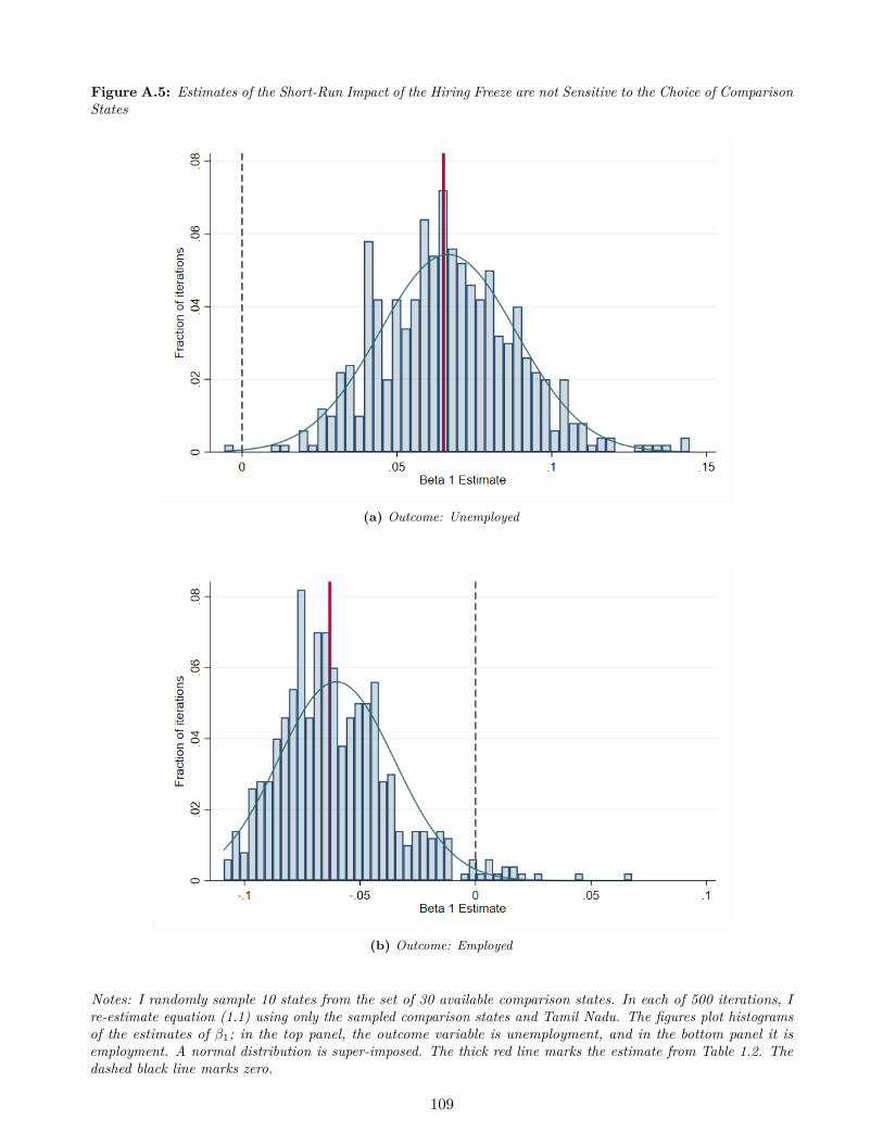
Figure A.5: Estimates of the Short-Run Impact of the Hiring Freeze are not Sensitive to the Choice of ComparisonStates

(a) Outcome: Unemployed

(b) Outcome: Employed

Notes: I randomly sample 10 states from the set of 30 available comparison states. In each of 500 iterations, Ire-estimate equation (1.1) using only the sampled comparison states and Tamil Nadu. The figures plot histogramsof the estimates of β1; in the top panel, the outcome variable is unemployment, and in the bottom panel it isemployment. A normal distribution is super-imposed. The thick red line marks the estimate from Table 1.2. Thedashed black line marks zero.

109

Figure A.6: Comparison of the GDP Growth Rate in Tamil Nadu and the Rest of India

Notes: Data sourced from the website of Niti Aayog. For this time period, the government calculatesthree different series: the 1993-1994 series, the 1999-2000 series, and the 2004-2005 series. In somecases these series overlap, in which case I average the estimates of the growth rates across the series.

110

Figure A.7: Assessing the Fit of the IRT Model

Data: Administrative data from the Tamil Nadu Public Service Commission, 2013/09 examNotes: The figure presents estimates of the average score residual conditional on estimated the estimatedability parameter. If the model is correctly specified, then the average residual should be zero across thedistribution. The dashed lines at -2 and 1 demarcate the boundary of the region where the model has abetter fit.

111

Figure A.8: Most candidates drop out after their first attempts

Data: Administrative data from the Tamil Nadu Public Service CommissionNotes: The figure presents re-application rates over time. The sample is restricted to male collegegraduates were between the ages of 20 to 22 in the year in which they are likely to have made theirfirst attempt. The year of the first attempt is inferred by restricting the sample to individuals who didnot make an attempt in any prior year. The y-axis plots the fraction of applicants in the cohort whoapplied to any exam that was notified in the given year.

112

Table A.1: Sample Size in Tamil Nadu Cohorts by Education Level, National Sample Survey

Age in 2001 College Graduates Ineligible Sample

17 122 489

18 125 539

19 134 468

20 140 402

21 115 349

22 122 591

23 89 350

24 52 275

25 48 160

26 40 155

27 49 266

28 47 417

29 26 179

30 29 202

Notes: Dataset combines all rounds of the National Sample Survey conducted between 1994 and 2010that included a module on employment. This includes the 50th, 55th, 60th, 61st, 62nd, 64th, and 66throunds. I impose the same sample restrictions that I use in the main analysis in Section 1.3, namely:1) men; 2) between the ages of 21 and 27 at the time of the survey; 3) between the ages of 17 to 30 in2001. Sample further restricted to Tamil Nadu. Ineligible sample refers to individuals with less than a10th standard education.

113

Table A.2: Coverage Rate of 95% Confidence Intervals for Main Specification

Parameter

Inference Method β1 β2

Stata Clustered SE 0.856 0.784

Wild Bootstrap 0.928 0.93

Notes: Table reports the results of simulations that test the coverage rate of different inference methodsfor the data and main specification used in Section 1.3. In each of 500 iterations, the outcome variableis changed to a new draw of a Bernoulii random variable that is i.i.d. across observations with a meanof 0.5. The coverage rate measures the fraction of confidence intervals that contain zero.

114

Table A.3: Tamil Nadu vs. the Rest of India Before the Hiring Freeze

(1) (2) (3)

Unemployment Employment Out of Labor Force

Tamil Nadu -0.002 0.038 -0.036

(0.036) (0.044) (0.038)

Mean, rest of India 0.213 0.453 0.334

Observations 5,087 5,087 5,087

Notes: Sample restricted to: 1) men; 2) who are college graduates; 3) between the ages of 21 to 27 atthe time of the survey; 4) who were less than 30 years of age in 2001; and 5) whose outcomes weremeasured before 2001. Standard errors clustered at the year x NSS primary sampling unit level. ∗p < 0.1, ∗∗ p < 0.05, ∗∗∗ p < 0.01

Table A.4: College Completion Rates Across Cohorts by Sex

(1) (2)

TN × Age 17-21 in 2001, Post-freeze (β1) 0.012 0.023∗∗

[-0.007, 0.030] [0.006, 0.038]

TN × Age 22-24 in 2001, Post-freeze (β2) 0.022 0.018

[-0.020, 0.061] [-0.008, 0.044]

Sample Men Women

Mean, reference group in TN 0.072 0.064

Observations 167,722 163,784

Notes: 95% confidence intervals in brackets, computed via wild bootstrap with 999 replications, clusteredby state x cohort level. ∗ p < 0.1, ∗∗ p < 0.05, ∗∗∗ p < 0.01

115

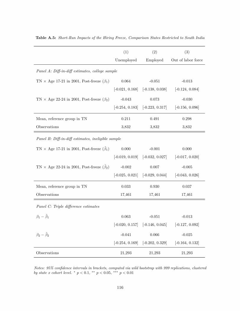
Table A.5: Short-Run Impacts of the Hiring Freeze, Comparison States Restricted to South India

(1) (2) (3)

Unemployed Employed Out of labor force

Panel A: Diff-in-diff estimates, college sample

TN × Age 17-21 in 2001, Post-freeze (β1) 0.064 -0.051 -0.013

[-0.021, 0.168] [-0.138, 0.038] [-0.124, 0.084]

TN × Age 22-24 in 2001, Post-freeze (β2) -0.043 0.073 -0.030

[-0.254, 0.183] [-0.223, 0.317] [-0.156, 0.096]

Mean, reference group in TN 0.211 0.491 0.298

Observations 3,832 3,832 3,832

Panel B: Diff-in-diff estimates, ineligible sample

TN × Age 17-21 in 2001, Post-freeze (β1) 0.000 -0.001 0.000

[-0.019, 0.019] [-0.032, 0.027] [-0.017, 0.020]

TN × Age 22-24 in 2001, Post-freeze (β2) -0.002 0.007 -0.005

[-0.025, 0.021] [-0.029, 0.044] [-0.043, 0.026]

Mean, reference group in TN 0.033 0.930 0.037

Observations 17,461 17,461 17,461

Panel C: Triple difference estimates

β1 − β1 0.063 -0.051 -0.013

[-0.020, 0.157] [-0.146, 0.045] [-0.127, 0.092]

β2 − β2 -0.041 0.066 -0.025

[-0.254, 0.169] [-0.202, 0.329] [-0.164, 0.132]

Observations 21,293 21,293 21,293

Notes: 95% confidence intervals in brackets, computed via wild bootstrap with 999 replications, clusteredby state x cohort level. ∗ p < 0.1, ∗∗ p < 0.05, ∗∗∗ p < 0.01

116

Table A.6: Short-Run Impacts of the Hiring Freeze, Comparison States Restricted to Large States

(1) (2) (3)

Unemployed Employed Out of labor force

Panel A: Diff-in-diff estimates, college sample

TN × Age 17-21 in 2001, Post-freeze (β1) 0.072∗∗ -0.075∗∗ 0.003

[0.017, 0.134] [-0.139, -0.014] [-0.081, 0.075]

TN × Age 22-24 in 2001, Post-freeze (β2) -0.023 0.059 -0.036

[-0.183, 0.109] [-0.084, 0.249] [-0.151, 0.081]

Mean, reference group in TN 0.211 0.491 0.298

Observations 15,417 15,417 15,417

Panel B: Diff-in-diff estimates, ineligible sample

TN × Age 17-21 in 2001, Post-freeze (β1) 0.072∗∗ -0.075∗∗ 0.003

[0.015, 0.129] [-0.138, -0.013] [-0.081, 0.074]

TN × Age 22-24 in 2001, Post-freeze (β2) -0.023 0.059 -0.036

[-0.200, 0.089] [-0.081, 0.238] [-0.156, 0.083]

Mean, reference group in TN 0.211 0.491 0.298

Observations 15,417 15,417 15,417

Panel C: Triple difference estimates

β1 − β1 0.073∗∗ -0.080∗∗ 0.008

[0.017, 0.136] [-0.156, -0.006] [-0.082, 0.081]

β2 − β2 -0.019 0.052 -0.032

[-0.176, 0.106] [-0.091, 0.234] [-0.147, 0.102]

Observations 87,865 87,865 87,865

Notes: 95% confidence intervals in brackets, computed via wild bootstrap with 999 replications, clusteredby state x cohort level. ∗ p < 0.1, ∗∗ p < 0.05, ∗∗∗ p < 0.01

117

Table A.7: Short-Run Impacts of the Hiring Freeze, Dropping Caste and Religion Controls

(1) (2) (3)

Unemployed Employed Out of labor force

Panel A: Diff-in-diff estimates, college sample

TN × Age 17-21 in 2001, Post-freeze (β1) 0.060∗∗ -0.057∗ -0.003

[0.004, 0.122] [-0.125, 0.008] [-0.088, 0.072]

TN × Age 22-24 in 2001, Post-freeze (β2) -0.028 0.064 -0.035

[-0.188, 0.088] [-0.084, 0.253] [-0.158, 0.084]

Mean, reference group in TN 0.211 0.491 0.298

Observations 19,303 19,303 19,303

Panel B: Diff-in-diff estimates, ineligible sample

TN × Age 17-21 in 2001, Post-freeze (β1) -0.002 0.005 -0.004

[-0.022, 0.018] [-0.026, 0.036] [-0.027, 0.022]

TN × Age 22-24 in 2001, Post-freeze (β2) -0.004 0.007 -0.003

[-0.041, 0.025] [-0.022, 0.038] [-0.045, 0.036]

Mean, reference group in TN 0.033 0.930 0.037

Observations 90,300 90,300 90,300

Panel C: Triple difference estimates

β1 − β1 0.062∗∗ -0.063 0.001

[0.001, 0.130] [-0.144, 0.028] [-0.084, 0.077]

β2 − β2 -0.024 0.057 -0.033

[-0.202, 0.093] [-0.110, 0.234] [-0.149, 0.107]

Observations 109,603 109,603 109,603

Notes: 95% confidence intervals in brackets, computed via wild bootstrap with 999 replications, clusteredby state x cohort level. ∗ p < 0.1, ∗∗ p < 0.05, ∗∗∗ p < 0.01

118

Table A.8: Short-Run Impacts of the Hiring Freeze on Wages

(1) (2)

Log Weekly earnings Log Average daily wage

TN × Age 17-21 in 2001, Post-freeze (β1) 0.249∗ 0.234∗

[-0.052, 0.599] [-0.063, 0.535]

TN × Age 22-24 in 2001, Post-freeze (β2) 0.613 0.613

[-0.415, 1.181] [-0.446, 1.134]

Mean, reference group in TN 6.291 4.398

Observations 4,818 4,818

Notes: 95% confidence intervals in brackets, computed via wild bootstrap with 999 replications, clusteredby state x cohort level. ∗ p < 0.1, ∗∗ p < 0.05, ∗∗∗ p < 0.01

119

Table A.9: Candidates with no prior experience with the exam have more positively biased beliefsabout exam performance

(1) (2)

Bias Bias

No prior experience 10.180∗∗ 14.911∗∗∗

(3.241) (3.408)

Has taken practice test in prior 8 months 0.945

(3.735)

Any nuclear family in government job 6.162

(14.978)

Any family in government job -0.640

(15.097)

Age 0.621

(0.494)

Average bias, candidates with prior experience 29.1 28.8

Library fixed effects Yes Yes

R2 0.037 0.103

Observations 88 85

Data Source: Survey data from Pune, Maharashtra.Notes: Bias is the difference between a candidate’s predicted score on a practice test and their actualscore. Positive values correspond to over-estimates. “No prior experience" is an indicator for whetherthe candidate reported appearing for a Maharashtra state or Union Public Service Commission exam inthe past 4 years. Specification includes fixed effects for the library in which the candidate was surveyed.Heteroskedasticity-robust standard errors in parentheses. ∗ p < 0.1, ∗∗ p < 0.05, ∗∗∗ p < 0.01

120

A.2 Estimating the Direct Demand Effect

Summary. In this section I assess the size of the effect that the hiring freeze may have had

arising just from the government’s reduced expenditure in the labor market. I term this effect

the demand effect. I estimate that this effect is small, and an order of magnitude smaller than

the shifts in labor market equilibrium that we observe.

Estimation Strategy.

1. How many vacancies were lost as a result of the hiring freeze?

Because the hiring freeze order exempted teachers and police, I assume all losses

were incurred in TNPSC. Estimating the loss in vacancies in TNPSC requires making

assumptions about the data generating process. I assume that, in the absence of the

freeze, vacancies in a given year are generated according to log(vacancy)t = µ + εt,

where E[εt] = 0. This assumption is roughly consistent with the observed variation in

vacancies in Figure 1.1.

I then estimate a regression of the form log(vacancy)t = α + βfreezet + εt, where

freezet = 1 for 2001 ≥ t ≥ 2005. This model implies that loss in the number of

vacancies per year can be estimated as exp(α)− exp(α+ β)) = 2422. Over the 5 years

of the hiring freeze, the estimated loss in vacancies is: 12110.

2. How many vacancies were lost by each cohort?

The overall loss in vacancies is distributed across cohorts. Using TNPSC administrative

data from 2012-2016, in Figure A.9 I plot the fraction of all available posts that accrue

to each cohort.

121

Figure A.9: Fraction of vacancies accruing to each cohort

We see that no cohort captures more than 8.2% of the available vacancies over 5 years.

Because my analysis focuses on male college graduates, we would also want to know

what share of that 8.2% is captured by them. I find that it’s about 60%. I thus estimate

the loss in vacancies to individual cohorts of male college graduates to be at most:

12, 110× 0.082× 0.6 = 595

3. How does the loss in vacancies compare to the size of the labor force in each cohort?

The 2011 Census indicates that were 484,027 male college graduates between the ages of

30-34. This is the age category that is closest to the group on which I focus my analysis

(i.e. recent college graduates in 2001 would be ≈ 21). This tells us that there were

about 484,027 / 5 = 96,805 male college graduates in each individual cohort.

Thus, the reduction in vacancies means that about

595/96, 805 = 0.006

or 0.6% of the most affected cohorts were delayed in getting or did not get a government

job. Note, this is an upper bound, assuming a cohort lost 5 years worth of vacancies.

122

Among the cohorts that were expected to graduate from college during the hiring freeze

(the focus of the analysis), cohorts lost between 1 to 5 years of vacancies, so the average

affect across this group is on the order of 0.3%.

4. What is the average loss in income for each vacancy?

The estimate of the public sector wage premium in Finan et al. (2017) is 71.2 log points

(Table 1, Column 3). Thus the earnings effect should be about

71.2× 0.006 = 0.43 log points

which is also about 0.43%.

123

A.3 Measurement Error in Age in the CMIE

Summary. Age is a critical variable in the analysis in Section 1.4, since it defines which

individuals belong to which cohort. In this appendix, I first present evidence that there

is substantial measurement error in this variable after September 2016. I then discuss the

imputation procedure that I use to adjust for this error.

Evidence of measurement error. In each wave of the survey, CMIE captures the age

of each household member. This allows me to track how the age of each individual in the

sample evolves over the course of the panel. Since birthdays are roughly uniformly distributed,

and since CMIE conducts three survey waves per year, then roughly one-third of the sample

should complete a birthday between each wave.

To check whether this is the case, I compute, for the sample collected in each month,

the average difference in age for each respondent from the previous wave. These results are

presented in Figure A.10 below. The red line marks 1/3, which is where the average should lie

if measurement error is on average close to zero. It appears this is the case until September

2016. In October and November of 2016, age increments too slowly; thereafter, the age

increments too fast. I’ll refer to the period from January 2014 until September 2016 as the

“Good Period," since the measurement error appears to be zero on average in this time frame.

124

Figure A.10: Average change in age between waves

Characterizing measurement error during the Good Period. For our purposes, even

if measurement error is zero on average across the whole sample, we may still be concerned

about measurement error at the individual level. In particular, we might worry that: 1) the

size of the measurement error is still substantial for individuals; 2) measurement error is

correlated with age; and 3) errors are serially correlated. I present evidence that suggests that

none of these concerns apply.

First, given that age is measured in whole numbers, if individual age is correctly measured,

then we should see that about 2/3 of the sample has the same age across waves, and 1/3 of

the sample increments by 1. In Figure A.11 below, I confirm that this is the case. Only about

1% of observations due not fit into this expected pattern.

125

Figure A.11: Average change in age between waves

Second, I test whether some positive errors in some age groups cancel out negative errors

for other age groups. This does not appear to be the case either. To illustrate, the figure

below plots a candidate’s age in a given wave on the X-axis (Aget), and the average change in

age between subsequent waves on the Y-axis (i.e. E[Aget+1 −Aget]). We see that people of

all age groups seem to be aging at the correct speed.

126

Figure A.12: Average change in age between waves

Lastly, to test for serial correlation in the errors, I correlate the difference in ages between

two successive waves (Aget+1 − Aget) with their lagged equivalents (Aget − Aget−1). The

strong negative correlation we see in Figure A.13 is consistent with mean reversion, which is

what one would expect if the errors were serially uncorrelated.

127

Figure A.13: Average change in age between waves

Imputation. One possible solution to the measurement error problem is to restrict the

analysis the Good Period, i.e. observations collected before October 2016. The advantage of

this approach is that it imposes minimal assumptions on the structure of the measurement

error. However, the lack of assumptions imposes heavy costs: 1) restricting the sample in this

way would result in a loss in 54% of the available observations; and 2) it misses an opportunity

to reduce measurement error at the individual level by exploiting the panel structure of the

data.

An alternative approach—and the one I use in the paper—is to find, for each individual, a

sequence of ages that increments correctly according to calendar time and fits the data best.

To fit the data, we have to have some notion of the structure of the measurement error. Based

on the evidence in the previous section, I assume that, for each individual, the measurement

error is zero on average. I can therefore compute the best fitting age series by minimizing

quadratic loss.

Formally: I suppose that in each wave of the survey, an individual’s true age is given by

128

a vector ai = (ai1, ai2, . . . , aiT ). Due to measurement error, in each wave we only observe

ait = ait + εit. The evidence presented above suggests that E[εit] = 0 in the Good Period. If

this assumption holds, then the true age minimizes a quadratic loss function. Thus, within

the Good Period, we can calculated an imputed age series ai as follows:

ai = arg minai

1T

T∑t=1

(ait − ait)2 s.t. ∀t, ai,t+1 − ai,t = 1/3 (A.1)

I implement this algorithm by computing, for each individual, many different age streams. I

take each observed age and then add a perturbation ∆ ∈ {−11/12,−10/12, . . . , 10/12, 11/12}.

I then compute the calendar-consistent age stream using that age in the observed month as a

starting point. In other words, given T data points for an individual, I compute 23T plausible

age streams. For each of these potential age streams, I then choose the one that minimizes

quadratic loss.

Once I have imputed age, I can extrapolate into the Bad Period by adding 1/3 to the last

imputed age for each additional wave, i.e. if I observe T observations in the Good Period,

then the imputed ages in the bad period will be ait = (1/3)(t − T ) + aiT . I drop from the

analysis any individuals that were not surveyed during the Good Period.

129

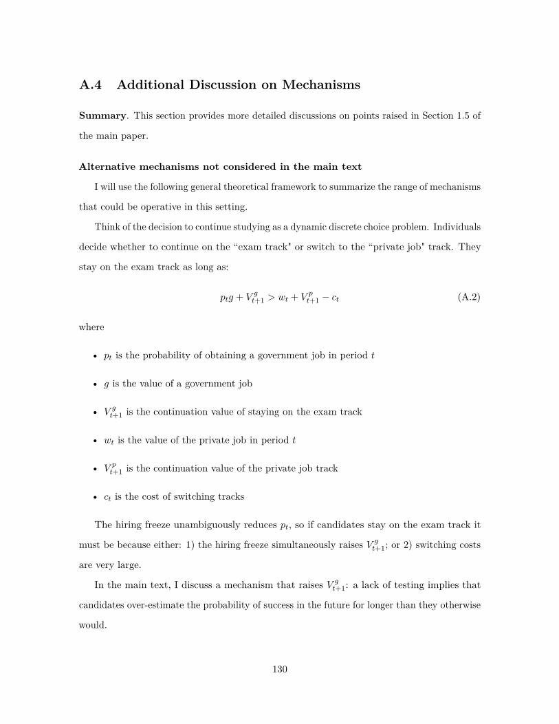
A.4 Additional Discussion on Mechanisms

Summary. This section provides more detailed discussions on points raised in Section 1.5 of

the main paper.

Alternative mechanisms not considered in the main text

I will use the following general theoretical framework to summarize the range of mechanisms

that could be operative in this setting.

Think of the decision to continue studying as a dynamic discrete choice problem. Individuals

decide whether to continue on the “exam track" or switch to the “private job" track. They

stay on the exam track as long as:

ptg + V gt+1 > wt + V p

t+1 − ct (A.2)

where

• pt is the probability of obtaining a government job in period t

• g is the value of a government job

• V gt+1 is the continuation value of staying on the exam track

• wt is the value of the private job in period t

• V pt+1 is the continuation value of the private job track

• ct is the cost of switching tracks

The hiring freeze unambiguously reduces pt, so if candidates stay on the exam track it

must be because either: 1) the hiring freeze simultaneously raises V gt+1; or 2) switching costs

are very large.

In the main text, I discuss a mechanism that raises V gt+1: a lack of testing implies that

candidates over-estimate the probability of success in the future for longer than they otherwise

would.

130

However, it is possible that there are other reasons why V gt+1 would increase. One class

of explanations relates to beliefs about future vacancy availability. For example, candidates

may have thought that the government would compensate for the hiring freeze by increasing

vacancy availability in the future. Alternatively, candidates may believe that if enough of

them stayed on the exam track, then the government would feel pressure to provide more

vacancies at the end of the freeze and/or end the hiring freeze sooner.

If switching costs are large, it is likely not because searching for a private sector job

is expected to take years (in fact, for many candidates, the outside option is likely to be

self-employment). Instead, it seems more likely that these costs are psychological or social.

Candidates may have a hard time giving up on their dreams, or “admitting defeat" to their

friends and family.

Why the convexity of the returns to exam preparation matters

This section provides a formal model of the proposition that candidates will have an

incentive to study during the hiring freeze if the returns to exam preparation are convex.

Let us examine a situation in which two identical candidates (indexed by A and B) need

to make a decision about whether to study during the hiring freeze. Both candidates know

that the hiring freeze will last t1 years and that the time between the end of the hiring freeze

and the resumption of exams will last t2 years.

Test scores are a function of the time spent preparing for the exam, plus an error term,

i.e. Ti = h(si) + εi, where si is the total time spent preparing by candidate i. The cost per

unit of time spent studying is c. The value of the government job is g.

Candidates are not able to coordinate their decisions with each other. By assumption, both

candidates find it valuable to study at least after the vacancies are announced. In that case

both candidates will study for si = t2 years, and have the same average score. The winner will

be determined by who obtains the larger shock to their score. Write F (x) = Pr(εB − εA ≤ x).

This implies that for candidate A the payoff to both studying after the vacancies are announced

is F (0)g − ct2.

Depending on the returns to studying, candidates may have an incentive to “deviate" and

131

study during the hiring freeze as well. It’s worth deviating as long as

(F (h(t1 + t2)− h(t2))

)g − c(t1 + t2) > F (0)g − ct2 (A.3)

which is equivalent toP (t1)− P (0)

t1> c/g (A.4)

where P (x) ≡ F (h(x+ t2)−h(t2)). Note that P captures the marginal returns to study effort.

The more convex is P , the larger the term on the left hand side will be.

132

Appendix B

Supplementary Materials to

Chapter 2

B.1 Theory Appendix

This section presents proofs of the propositions from the main text.

Lemma 1. Gt, Pt, and Ut are strictly decreasing in t.

Proof. We’ll start with Gt. Since Gt > max{Ut, Pt} for all t by assumption, it is an absorbing

state. Therefore Gt is just a finite geometric sum for T − t+ 1 periods. Thus

Gt = u(w′)1− βT−(t−1)

1− β (B.1)

which is clearly decreasing in t.

Next, I will verify the lemma for both P and U simultaneously, working backwards from

period T . Since PT = u(w) and UT = u(b), we can write

PT−1 = PT + βmax{PT , UT }

UT−1 = UT + β [pGT + (1− p) max{PT , UT }]

133

or, equivalently,

PT − PT−1 = −βmax{PT , UT } < 0

UT − UT−1 = −β [pGT + (1− p) max{PT , UT }] < 0

Now assume the induction hypothesis, i.e. Pt − Pt−1 < 0 and Ut − Ut−1 < 0 for some t.

First we want to show that

Pt−1 − Pt−2 < 0

which is true iff

max{Pt, Ut} −max{Pt−1, Ut−1} < 0

There are four cases. Note that Ut − Ut−1 < 0 by assumption and

Pt − Pt−1 < 0 =⇒ Pt −max{Pt−1, Ut−1} < 0

Therefore the only remaining case is Ut − Pt−1. This case occurs when Pt−1 > Ut−1. By the

induction hypothesis we also know that Ut−1 > Ut. Putting these inequalities together we get

Ut − Pt−1 < 0.

Next we want to show the similar case for U , i.e.

Ut−1 − Ut−2 < 0

This expression holds iff

βp(Gt −Gt−1) + β(1− p) (max{Ut, Pt} −max{Ut−1, Pt−1}) < 0

This is clearly true since: 1) we established that Gt−Gt−1 < 0 since Gt is decreasing, and

2) we just showed that max{Ut, Pt} −max{Ut−1, Pt−1} < 0.

Proposition 3. Someone who starts unemployed will eventually take private sector work

if not employed by the government, i.e. Pt > Ut for some t. Furthermore, taking private

employment is an absorbing state, i.e. Pt > Ut =⇒ Pt+s > Ut+s for all s.

Proof. If someone starts unemployed, then U0 > P0. Since UT < PT by construction, Ut

134

must cross Pt at some point t∗. Furthermore, since both Ut and Pt are strictly decreasing (by

Lemma 1), they must cross at a single point. Therefore after accepting private employment,

the agent will never choose to remain unemployed.

Proposition 4. When b < w < w′, the optimal dropout age is given by

t∗ =

0 if u(w)− u(b) ≥ β(1− βT )

1− β p[u(w′)− u(w)]

T − 1ln β ln

[1− (1− β)[u(w)− u(b)]

βp[u(w′)− u(w)]

]otherwise

(B.2)

Proof. Since there is a single crossing point between Ut and Pt, the optimal stopping point is

given by the t at which Ut = Pt.

Since P and G are both absorbing states, we can write their value functions as

Gt = u(w′)1− β(T−(t−1))

1− β (B.3)

Pt = u(w)1− β(T−(t−1))

1− β (B.4)

Setting Pt equal to Ut at t∗ yields:

u(w) + βPt∗+1 = u(b) + βpGt∗+1 + β(1− p)Pt∗+1 (B.5)

Solving for t∗ by substituting in the formulas for Gt and Pt gives us:

t∗ = T − 1ln β ln

[1− (1− β)[u(w)− u(b)]

βp[u(w′)− u(w)]

](B.6)

Given the assumption that b < w < w′, the second term is positive, so t∗ is always strictly

less than T . However, it is possible that t∗ will fall less than zero, which is outside the domain.

Solving for when t∗ ≤ 0 yields the condition u(w)− u(b) ≥ β(1−βT )1−β p[u(w′)− u(w)].

135

B.2 Additional Figures and Tables

Figure B.1: A Map of the Peth Area, Pune

Notes: The Peth Area is marked by the shaded region. The boundary marks the edges of the 411030pin code, which define the boundaries of the sampled area.

136

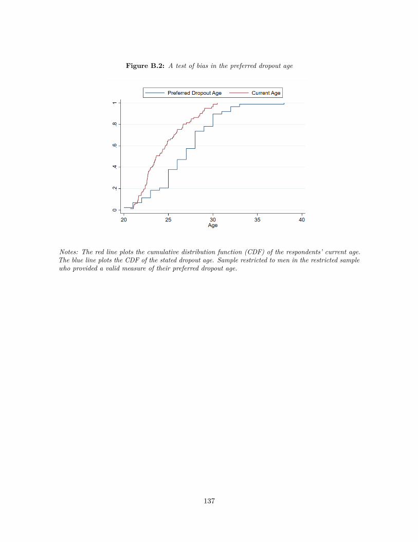
Figure B.2: A test of bias in the preferred dropout age

Notes: The red line plots the cumulative distribution function (CDF) of the respondents’ current age.The blue line plots the CDF of the stated dropout age. Sample restricted to men in the restricted samplewho provided a valid measure of their preferred dropout age.

137

Figure B.3: Age of retirement for male college graduates in Maharashtra

Notes: Figure is based on data from the CMIE Consumer Households Pyramids Survey. I use the 2019Wave 1 round. The figure plots a non-parametric estimate of the fraction of male college graduates inMaharashtra that are retired conditional on their age. The red line marks the age of retirement used inthe estimation of the model.

138

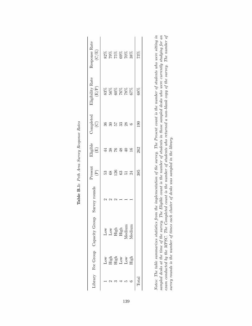
Tab

leB.1:Pe

thAreaSu

rvey

Respon

seRa

tes

Library

FeeGroup

Cap

acity

Group

Survey

roun

dsPr

esent

(P)

Eligible

(E)

Com

pleted

(C)

Eligibility

Rate

(E/P

)Respo

nseRate

(C/E

)

1Lo

wLo

w2

5344

3683

%82

%2

High

Low

268

3830

56%

79%

3High

High

212

676

5760

%75%

4Lo

wHigh

163

4833

76%

69%

5Lo

wMed

ium

151

4028

78%

70%

6High

Med

ium

124

166

67%

38%

Total

385

262

190

68%

73%

Notes:The

tablesummarizes

statistic

sfro

mtheim

plem

entatio

nof

thesurvey.The

Presentc

ount

isthenu

mberof

stud

ents

whowe

resitting

insampled

desksat

thetim

eof

thesurvey.The

Eligible

coun

tisthenu

mberof

stud

ents

inthosesampled

deskswh

owe

recurren

tlystud

ying

foran

exam

cond

uctedby

theMPSC

.The

Com

pleted

coun

tis

thenu

mberof

stud

ents

whoreturned

ano

n-blan

kcopy

ofthesurvey.The

numberof

survey

roun

dsis

thenu

mberof

times

each

clusterof

deskswa

ssampled

inthelibrary.

139

Appendix C

Supplementary Materials to

Chapter 3

C.1 Additional Figures and Tables

Figure C.1: Marriage rates for men and women are correlated within districts

Notes: The figure plots the fraction of men and women who were ever-married between the ages of20-24 for each district in Tamil Nadu. Data are sourced from the 2011 Census.

140

Table C.1: How competitive are TNPSC exams?

Appeared for

Recruitment Group Multiple choice exam Main exam Interview Selected

2013/14 2 498,471 10,003 2,225 1,129

2013/17 1 70,547 2,782 163 79

2014/01 2A 242,629 – – 1,241

2015/07 2 478,266 5,742 2,141 1,078

2015/09 1 101,649 2,520 150 72

2015/17 2A 654,316 – – 2,142

Overall 2,268,990 5,828

Notes: For each recruitment, we summarize the number of applicants that participated in each stage ofthe exam. Group 1 corresponds to the most prestigious posts, followed by Group 2 and finally Group2A.

141